Scheduling Parallel Iterative Applications on Volatile Resources

Henry Casanova, Fanny Dufosse, Yves Robert and Frederic VivienEcole Normale Superieure de Lyon and University of Hawai‘i at Manoa

October 2010

LIP Research Report RR-2008-31

Abstract

In this paper we study the execution of iterative applications on volatile processorssuch as those found on desktop grids. We develop master-worker scheduling schemes thatattempt to achieve good trade-offs between worker speed and worker availability. A keyfeature of our approach is that we consider a communication model where the bandwidthcapacity of the master for sending application data to workers is limited. This limitationmakes the scheduling problem more difficult both in a theoretical sense and a practicalsense. Furthermore, we consider that a processor can be in one of three states: available,down, or temporarily preempted by its owner. This preempted state also makes the designof scheduling algorithms more difficult. In practical settings, e.g., desktop grids, masterbandwidth is limited and processors are temporarily reclaimed. Consequently, addressing theaforementioned difficulties is necessary for successfully deploying master-worker applicationson volatile platforms.

Our first contribution is to determine the complexity of the scheduling problem in itsoff-line version, i.e., when processor availability behaviors are known in advance. Even withthis knowledge, the problem is NP-hard, and cannot be approximated within a factor 8/7.Our second contribution is a closed-form formula for the expectation of the time neededby a worker to complete a set of tasks. This formula relies on a Markovian assumptionfor the temporal availability of processors, and is at the heart of some heuristics that aimat favoring “reliable” processors in a sensible manner. Our third contribution is a set ofheuristics, which we evaluate in simulation. Our results provide insightful guidance toselecting the best strategy as a function of processor state availability versus average taskduration.

1 Introduction

We study the problem of efficiently executing parallel applications on platforms that comprisevolatile resources. More specifically we focus on iterative applications implemented using themaster-worker paradigm. The master coordinates the computation of each iteration as the exe-cution of a fixed number of independent tasks. A synchronization of all tasks occurs at the endof each iteration. This scheme applies to a broad spectrum of scientific computations including,but not limited to, mesh based solvers (e.g., elliptic PDE solvers), signal processing applica-tions (e.g., recursive convolution), and image processing algorithms (e.g., stencil algorithms).We study such applications when they are executed on networked processors whose availability

1

inria

-005

2478

4, v

ersi

on 1

- 8

Oct

201

0

evolves over time, meaning that each processor alternates between being available for executinga task and being unavailable.

Solutions for executing master-worker applications, and in particular applications imple-mented with the Message Passing Interface (MPI), on failure-prone platforms have been devel-oped (e.g., [1, 2, 3, 4]). In these works, the focus is on tolerating failures caused by softwareor hardware faults. For instance, a software fault will cause the processor to stall, but com-putations may be restarted from scratch or be resumed from a saved state after rebooting. Ahardware failure may keep the processor down for a long period of time, until the failed compo-nent is repaired or replaced. In both cases, fault-tolerant mechanisms are implemented in theaforementioned solutions to make faults transparent to the application execution.

In addition to failures, processor volatility can also be due to temporary interruptions. Suchinterruptions are common in volunteer computing platforms [5] and desktop grids [6]. In theseplatforms processors are contributed by resource owners that can reclaim them at any time,without notice, and for arbitrary durations. A task running on a reclaimed processor is simplysuspended. At a later date, when the processor is released by its owner, the task can be resumedwithout any wasted computation. In fact, fault-tolerant MPI solutions were proposed in thespecific context of desktop grids [4], which is also the context of this work. While mechanismsfor executing master-worker applications on volatile platforms are available, our focus is onscheduling algorithms for deciding which processors should run which tasks and when.

At a given time a (volatile) processor can be in one of three states: UP (available), DOWN(crashed due to a software or hardware fault), or RECLAIMED (temporarily preempted byowner). Accounting for the RECLAIMED state, which arises in desktop grid platforms, com-plexifies scheduling decisions. More specifically, since before going to the DOWN state a proces-sor may alternate between the UP and RECLAIMED states, the time needed by the processorto compute a given workload to completion is difficult to predict. A way to make such pre-diction tractable is to assume that state transitions obey a Markov process. The Markov (i.e.,memoryless) assumption is popular because it enables analytical derivations. In fact, recentwork on desktop grid scheduling has made use of this assumption [7]. Unfortunately, the mem-oryless assumption is known to not hold in practice. Several authors have reported that thedurations of availability intervals in production desktop grids are not sampled from exponen-tial distributions [8, 9, 10]. There is no true consensus regarding what is a “good” model foravailability intervals defined by the elapsed time between processor failures, let alone regardinga model for the durations of recoverable interruptions. Note that some authors have attemptedto model processor availabilities using (non-memoryless) semi-Markov processes [11]. Facedwith the lack of a good model for transitions between the UP , DOWN , and RECLAIMEDstates, and not knowing whether such a model would be tractable or not, for now we opt for theMarkovian model. The goal of this work is to provide algorithmic foundations for schedulingiterative master-worker applications on processors that can fail or be temporarily reclaimed.The 3-state Markovian model allows us to achieve this goal, and the insight from our resultsshould provide guidance for dealing with more complex, and hopefully more realistic, stochasticmodels of processor availabilities.

A unique aspect of this work is that we account for network bandwidth constraints forcommunication between the master and the workers. More specifically, we bound the totaloutgoing communication bandwidth of the master while ensuring that each communicationuses a reasonably large fraction of this bandwidth. The master is thus able to communicatesimultaneously with only a limited number of workers, sending them either the applicationprogram or input data for tasks. This assumption, which corresponds to the bounded multi-port model [12], applies to concurrent data transfers implemented with multi-threading. Onealternative is to simply not consider these constraints. However, in this case, a scheduling

2

inria

-005

2478

4, v

ersi

on 1

- 8

Oct

201

0

strategy could enroll a large (and vastly suboptimal) number of processors to which it would senddata concurrently each at very low bandwidth. Another alternative is to disallow concurrentdata transfers from the master to the workers. However, in this case, the bandwidth capacityof the master may not be fully exploited, especially for workers executing on distant processors.We conclude that considering the above bandwidth constraints is necessary for applicationsthat do not have an extremely low communication-to-computation ratio. It turns out that theaddition of these constraints makes the problem dramatically more difficult at the theoreticallevel, and thus complicates the design of practical scheduling strategies.

The specific scheduling problem under consideration is to maximize the number of appli-cation iterations that are successfully completed before a deadline. Informally, during eachiteration, we have to identify the “best” processors among those that are available (e.g., thefastest, the likeliest to remain available, etc.). In addition, since processors can become availableagain after being unavailable for some time, it may be beneficial to change the set of enrolledprocessors even if all enrolled processors are available. We thus have to decide whether to releaseenrolled processors, to decide which ones should be released, and to decide which ones shouldbe enrolled instead. Such changes come at a price: the application program file need be sent tonewly enrolled processors, which consumes some (potentially precious) fraction of the master’sbandwidth.

Our contributions are the following. First, we assess the complexity of the problem in itsoff-line version, i.e., when processor availability behaviors are known in advance. Even with thisknowledge, the problem is NP-hard, and cannot be approximated within a factor 8/7. Next,relying on the Markov assumption for processor availability, we provide a closed-form formulafor the expectation of the time needed by a worker to complete a set of tasks. This formula isat the heart of several heuristics that aim at giving priority to “reliable” resources rather thanto “fast” ones. In a nutshell, when the task size is very small in comparison to the expectedduration of an interval between two consecutive processor state changes, “classical” heuristicsbased upon the estimated completion time of a task perform reasonably well. But when thetask size is no longer negligible with respect to the expected duration of such an interval, itis mandatory to account for processor reliability, and only those heuristics building upon suchknowledge are shown to achieve good performance. Altogether, we design a set of heuristics,which we thoroughly evaluate in simulation. The results provide insights for selecting the beststrategy as a function of processor state availability versus task duration.

This paper is organized as follows. Section 2 discusses related work. Section 3 describesthe application and platform models. Complexity results for the off-line study are given in Sec-tion 4; these results do not rely on any assumption regarding stochastic distribution of resourceavailability. In Section 5, we describe our 3-state Markovian model of processor availability,and we show how to compute the expected time for a processor to complete a given workload.Heuristics for the on-line problem are described in Section 6, some of which use the result inSection 5 for more informed resource selection. An experimental evaluation of the heuristics ispresented in Section 7. Section 8 concludes with a summary of our findings and perspectiveson future work.

2 Related work

There is a large literature on scheduling master-worker applications, or applications that consistof a sequence of iterations where each iteration can be executed in master-worker fashion [13,14, 15]. In this work we focus on executions on volatile resources, such as desktop resources.The volatility of desktop or other resources is well documented and characterizations havebeen proposed [8, 9, 10]. Several authors have studied the master-worker (or “bag-of-tasks”)

3

inria

-005

2478

4, v

ersi

on 1

- 8

Oct

201

0

scheduling problem in the face of such volatility in the context of desktop grid computing, eitherat an Internet-wide scale or with an Enterprise [16, 17, 18, 19, 7, 20, 21, 22]. Most of theseworks propose simple greedy scheduling algorithms that rely on mechanisms to pick processorsaccording to some criteria. These processor selection criteria include static ones (e.g., processorclock-rates or benchmark results), simple ones based on past host behavior [16, 18, 20], andmore sophisticated ones based on statistical analysis of past host availability [21, 22, 19, 7].In a global setting, the work in [17] includes time-zone as a criterion for processor selection.These criteria are used to rank processors, but also to exclude them from consideration [16, 18].The work in [7] is particularly related to our own in that it uses a Markov model of processoravailability (but not accounting for preemption).

Most of these works also advocate for task replication as a way to cope with volatile resources.Expectedly, injecting task replicas is sensible toward the end of application execution. Giventhe number of possible variants of scheduling algorithms, in [20] the authors propose a methodto automatically instantiate the parameters that together define the behavior of a schedulingalgorithm. Works published in this area are of a pragmatic nature, and few theoretical resultshave been sought or obtained (one exception is the work in [23]).

A key difference between our work and all the above is that we seek to develop schedulingalgorithms that explicitly manage for the master’s bandwidth. Limited master bandwidth isa known issue for desktop grid computing [24, 25, 26] and must therefore be addressed eventhough it complexifies the scheduling problem. To the best of our knowledge no previous workhas made such an attempt.

3 Problem Definition

In this section, we detail our application and platform models, describe the scheduling model,and provide a precise statement of the scheduling problem.

3.1 Application Model

We target an iterative application in which iterations entail the execution of a fixed number mof same-size independent tasks. Each iteration is executed in a master-worker fashion, with asynchronization of all tasks at the end of the iteration. A processor is assigned one or moretasks during an iteration. Each task needs some input data, of constant size Vdata in bytes. Thisdata depends on the task and the iteration, and is received from the master. Such applicationsallow for a natural overlap of computation and communication: computing for the current taskcan occur while data for the next task (of the same iteration) is being received. Before it canstart computing, a processor needs to receive the application program from the master, whichis of size Vprog in bytes. This program is the same for all tasks and iterations.

3.2 Platform Model

We consider a platform that consists of p processors, P1, . . . , Pp, encompassing with this termcompute nodes that contain multiple physical processor cores. Each processor is volatile, mean-ing that its availability for computing application tasks varies over time. More precisely, aprocessor can be in one of three states: UP (available for computation), RECLAIMED (tem-porarily reclaimed by its owner), or DOWN (crashed and to be rebooted). We assume thatthe master, which implements the scheduling algorithm that decides which processor computeswhich tasks and when, executes on a host that is always UP (otherwise a simple redundancymechanism such as primary back-up [27] can be used to ensure reliability of the master). We

4

inria

-005

2478

4, v

ersi

on 1

- 8

Oct

201

0

also assume that the master is aware of the states of the processors, e.g., via a simple heart-beatmechanism [28]. The availabilities of processors evolve independently. For a processor all statetransitions are allowed, with the following implications:

• When a UP or RECLAIMED processor becomes DOWN , it loses the application program,all the data for its assigned tasks, and all partially computed results. When it laterbecomes UP it has to acquire the program again before executing tasks;• When a UP processor becomes RECLAIMED , its activities are suspended. However,

when it becomes UP again it can simply resume task computations and data transfers.

We discretize time so that the execution occurs over a sequence of discrete time slots. Weassume that task computations and data transfers all require an integer number of time slots,and that processor state changes occur at time-slot boundaries. We leave the time slot durationunspecified. Indeed, the time slot duration that achieves a good approximation of continuoustime varies for different applications and platforms.

The temporal availability of Pq is described by a vector Sq whose component Sq[t] ∈ {u, r, d}represents its state at time-slot t. Here u corresponds to the UP state, r to the RECLAIMEDstate, and d to the DOWN state. Note that vector Sq is unknown before executing the appli-cation.

Processor Pq requires wq time-slots of availability (i.e., UP state) to compute a task. If allwq values are identical, then the platform is homogeneous. We model communications betweenthe master and the workers using the bounded multi-port communication model [12]. In thismodel, the master can initiate multiple concurrent communications, each to a different worker.Each communication is allotted a bandwidth fraction of the master’s network card, and the sumof all fractions cannot exceed the total capacity of the card. This model is enabled by popularmulti-threaded communication libraries [29]. We consider that the master can communicate upto bandwidth BW (we use the term “bandwidth” loosely to mean maximum data transfer rate).Communication to each worker is performed at some fixed bandwidth bw. This bandwidth canbe enforced in software or can correspond to same-capacity communication paths from themaster’s processor to each other processor. We define ncom = BW/bw as the maximum numberof workers to which the master can send data simultaneously (i.e., the maximum number ofsimultaneous communications). For simplicity, we assume ncom to be an integer. Let nprog bethe number of processors receiving the application program at time t, and ndata be the numberof processors receiving the input data of a task at time t. Given that the bandwidth of themaster must not be exceeded, we have

nprog + ndata ≤ ncom = BW/bw.

Let Pq be a processor engaged in communication at time t, for receiving either the programor some data. In both cases, it does this with bandwidth bw. Hence the time for a worker toreceive the program is Tprog = Vprog/bw, and the time to receive the data is Tdata = Vdata/bw.

3.3 Scheduling Model

Let config(t) denote the set of processors enrolled for computing the m application tasks in aniteration, or configuration, at time t. Enrolled processors work independently, and execute theirtasks sequentially. While a processor could conceivably execute two tasks in parallel (providedthere is enough available memory), this would only delay the completion time of the first task,thereby increasing the risk of not completing it due to volatile availability. The scheduler assignstasks to processors and may choose a new configuration at each time-slot t. Let Pq be a newlyenrolled processor at time t, i.e., Pq ∈ config(t+ 1) \ config(t). Pq needs to receive the programunless it already received a copy of it and has not been in the DOWN state since. In all cases, Pq

5

inria

-005

2478

4, v

ersi

on 1

- 8

Oct

201

0

needs to receive data for a task before computing it. This holds true even if Pq had been enrolledat some previous time-slot t′ < t but has been un-enrolled since: we assume any received datais discarded when a processor is un-enrolled. In other words, any input data communication isresumed from scratch, even if it had previously completed.

If a processor becomes DOWN at time t, the scheduler may simply use the remaining UPprocessors in config(t) to complete the iteration, or enroll a new processor. Even if all processorsin config(t) are in the UP state, the scheduler may decide to change the configuration. Thiscan be useful if a more desirable (e.g., faster, more available) but un-enrolled processor has justreturned to the UP state. Removing an UP processor from config(t) has a cost: partial resultsof task computations, partial task data being received, and previously received task data are alllost. Note, however, that results obtained for previously completed tasks are not lost becausealready sent back to the master. Due to the possibility of a processor leaving the configuration(either due to becoming DOWN or due to a decision of the scheduler), the scheduler enforcesthat task data is received for at most one task beyond the one currently being computed. Inother terms, the processor does not accumulate task data beyond that for the next task. This issensible so as to allow some overlap of computation and communication while avoiding wastingbandwidth for data transfers that would be increasingly likely to be redone from scratch.

3.4 Problem Statement

The scheduling problem we address in this work is that of maximizing the number of success-fully completed application iterations before a deadline. Given the discretization of time, theobjective of the scheduling problem is then to maximize the number of successfully completediterations within some integral number of time slots, N . In the off-line case (see Section 4), if anefficient algorithm can be found to solve this problem, then, using a binary search, an efficientalgorithm can be designed to solve the problem of executing a given number of iterations in theminimum amount of time.

4 Off-line complexity

In this section, we study the off-line complexity of the problem. This means that we assume apriori knowledge of all processor states. In other words, the value of Sq[j] is known in advance,for 1 ≤ q ≤ p and 1 ≤ j ≤ N . The problem turns out to be difficult: even minimizingthe time to complete the first iteration with same-speed processors is NP-complete. We alsoidentify a polynomial instance with ncom = +∞, which highlights the impact of communicationcontention.

For the off-line study, we can simplify the model and have only two processor states, UP(also denoted by u) and RECLAIMED (also denoted by r). Indeed, suppose that processor Pq isDOWN for the first time at time-slot t: Sq[t] = d. We can replace Pq by two 2-state processorsPq′ and Pq′′ such that: 1) for all j < t, Sq′ [j] = Sq[j] and Sq′′ [j] = r, 2) Sq′ [t] = Sq′′ [t] = r, and3) for all j > t, Sq′ [j] = r and Sq′′ [j] = Sq[i]. In this way, we remove a DOWN state and adda two-state processor. If we do this modification for each DOWN state, we obtain an instancewith only UP or RECLAIMED processors. In the worst case, the total number of processors ismultiplied by N , which does not affect the problem’s complexity (polynomial versus NP-hard).Let Off-Line denote the problem of minimizing the time to complete the first iteration, withsame-speed processors:

Theorem 1. Problem Off-Line is NP-hard.

Proof. Consider the associated decision problem: given a number m of tasks, of computingcost w and communication cost Tdata, a program of communication cost Tprog, and a platform

6

inria

-005

2478

4, v

ersi

on 1

- 8

Oct

201

0

of p processors, with availability vectors Sq, a bound ncom on the number of simultaneouscommunications, and a time limit N , does there exist a schedule that executes one iteration intime less than N? The problem is obviously in NP: given a set of tasks, a platform, a time limitand a schedule (of communications and computations), we can check the schedule and computeits completion time with polynomial complexity.

C6C5C4C3C2C1

x1

x1

x2

x2

x3

x3

x4

x4

Figure 1: Proof of NP-completeness of Off-Line.

The proof follows from a reduction from 3SAT. Let I1 be an instance of 3SAT : given a setU = {x1, ..., xn} of variables and a collection {C1, ..., Cm} of clauses, does there exist a truthassignment of U? We suppose that each variable is present in at least one clause.

We construct the following instance I2 of the Off-Line problem with m tasks and p = 2nprocessors: ncom = 1, Tprog = m, Tdata = 0, wi = w = 1, N = m(n + 1) and ∀i ∈ [1, n],∀j ∈[1,m], 1) if xi ∈ Cj then S2i−1[j] = u else S2i−1[j] = r, 2) if xi ∈ Cj then S2i[j] = u elseS2i[j] = r, 3) S2i[mi+ j] = S2i−1[mi+ j] = u and 4) ∀k ∈ [1, n], i 6= k, S2k−1[mi+ j] = S2k[mi+j] = r. The size of I2 is polynomial in the size of I1. Figure 1 illustrates this construction forI1 = (x1∨x3∨x4)∧ (x1∨ x2∨ x3)∧ (x2∨x3∨ x4)∧ (x1∨x2∨x4)∧ (x1∨ x2∨ x4)∧ (x2∨x3∨x4).

Suppose that I1 has a solution A with, for all j ∈ [1, n], xj = A[j]. For any i ∈ [1,m], thereexists at least one true literal of A in Ci. We pick one arbitrarily. Let xj be the associatedvariable. Then during time-slot i, if A[j] = 1, processor P2i−1 will download (a fraction of)the program, while if A[j] = 0, processor P2i will download it. During this time-slot, no otherprocessor communicates with the master. Then, for all ∀i ∈ [1, n]:

• if A[j] = 1, between mi + 1 and m(i + 1), P2i−1 completes the reception of the programand then executes as many tasks as possible, P2i stays idle• if A[j] = 0, then P2i−1 is idle and P2i completes downloading its copy of the program and

computes as many tasks as possible.

For all i ∈ [1, 2n], let Li be the number of communication time-slots for processor Pi betweentime-slots 1 and m. By the choice of the processor receiving the program at any time-slott ∈ [1,m], if A[i] = 0, then L2i−1 = 0, else L2i = 0. Let, for all i ∈ [1, n], p(i) = 2i−A[i]. Then,for all i ∈ [1, n], between time mi+1 and m(i+1), Pp(i) is available and Pp(i)+2A[i]−1 is idle. Pp(i)

completes receiving its program at the latest at time mi+ Tprog − Lp(i) = m(i+ 1)− Lp(i) andcan execute Lp(i) tasks before being reclaimed. Overall, the processors execute X =

∑ni=1 Lp(i)

tasks. For any j ∈ [1,m], by construction there is exactly one processor downloading theprogram during time-slot j. Consequently, X = m, and thus I2 has a solution.

Suppose now that I2 has a solution. As ncom = 1, for all i ∈ [1, n], processors P2i−1 and P2i

receive the program during at m time slots before time m. After time m, processors P2i−1 andP2i are only available between time mi + 1 and m(i + 1). Then, at time N , the sum S of thetime-slots spent in receiving the program on processors P2i−1 and P2i is S ≤ 2m. This meansthat at most one of these processors can execute tasks before time N . Among P2i−1 and P2i, letp(i) be the processor computing at least one task. If neither P2i−1 nor P2i computes any task, letp(i) = 2i. Let A be an array of size n such that if p(i) = 2i− 1, then A[i] = 1 else A[i] = 0. Wewill prove that all clauses of I1 are satisfied with this assignment. Without loss of generality weassume that no communication is made to a processor that does not execute any task. Suppose

7

inria

-005

2478

4, v

ersi

on 1

- 8

Oct

201

0

that for i ∈ [1,m], a processor Pj with j = p(k) receives a part of the program during time-sloti. Then, by definition of the function p, either A[k] = 1 and xk ∈ Ci, or A[k] = 0 and xk ∈ Ci.This means that assignment A satisfies clause Ci. Let X be the number of true clauses withassignment A. For all i ∈ [1, 2n], we define Li as the number of communication time-slotsfor processor Pi between times 1 and m. Then, X ≥

∑nj=1 Lp(i). In addition, processor Pp(i)

completes the reception of the program at the latest at time m(i+ 1)−Li, and then computesat most Li tasks before being reclaimed at time m(i + 1). Overall, the processors compute mtasks. Then,

∑nj=1 Lp(i) ≥ m, and X ≥ m. Consequently, all clauses are satisfied by A, i.e., I1

has a solution, which concludes the proof.

Proposition 1. Problem Off-Line cannot be approximated within 87 − ε for all ε > 0.

Proof. MAXIMUM 3-SATISFIABILITY cannot be approximated within 87 − ε for all ε >

0 [30]. By construction of the proof of Theorem 1, problem Off-Line cannot be approximatedwith the same value.

Now we show that the difficulty of problem Off-Line is due to the bound ncom: if we relaxthis bound, the problem becomes polynomial.

Proposition 2. Off-Line is polynomial when ncom = +∞, even with different-speed proces-sors.

Proof. We send the program to processors as soon as possible, at the beginning of the execution.Then, task by task, we greedily assign the next task to the processor that can terminate itsexecution the soonest; this is the classical MCT (Minimum Completion Time) strategy, whosecomplexity is m× p.

To show that this strategy is optimal, let S1 be an optimal schedule, and let S2 the MCTschedule. Let T1 and T2 be the associated completion times. We aim at proving that T2 = T1.We first modify the schedule S1 as follows. Suppose that processor Pq begins a computationor a communication at time t, and that it is available but idle during time-slot t − 1. Then,we can shift forward the operation and execute it at time t− 1 without breaking any rules andwithout increasing the completion time of the current iteration. We repeat this modification asmany times as possible, and finally obtain a schedule S′1 with completion time T ′1 = T1. Assumenow that Pq executes i tasks under schedule S′1 and j under S2. The first min{i, j} tasks areexecuted at the same time by S′1 and by S2. Suppose that T2 > T1. Consider S2 right beforethe allocation of the first task whose completion time is t > T1. At this time, at least oneprocessor Pq0 has strictly fewer tasks in S2 than in S′1. We can thus allocate a task to Pq0 withcompletion time t ≤ T1. The MCT schedule should have chosen the latter allocation, and weobtain a contradiction. The MCT schedule S2 is thus optimal.

The MCT algorithm is not optimal if ncom < +∞. Consider an instance with Tprog =Tdata = 2, two tasks (m = 2) and two identical processors (p = 2, wq = w = 2). Suppose thatncom = 1, and that S1 = [u, u, u, u, u, u, r, r, r] and S2 = [r, u, u, u, u, u, u, u, u]. The optimalschedule computes both tasks in time 9 one waits for one time-slot and then sends the programand data to P2. However, MCT executes the first task on P1, and is thus not optimal.

5 Computing the expectation of a workload

In this section, we first introduce a Markov model for processor availability, and then show howto compute the expected execution time of a processor to complete a given workload.

8

inria

-005

2478

4, v

ersi

on 1

- 8

Oct

201

0

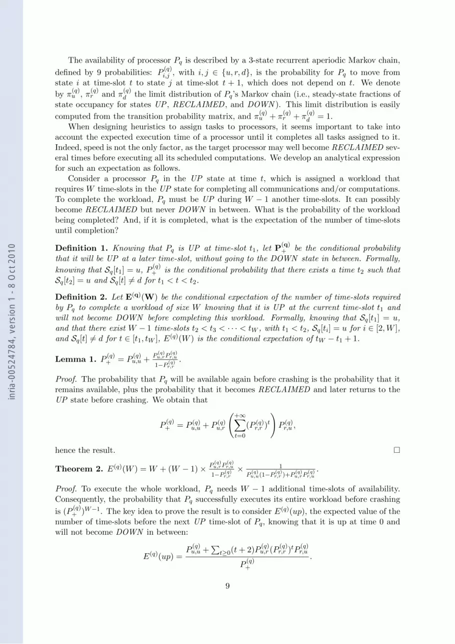
The availability of processor Pq is described by a 3-state recurrent aperiodic Markov chain,

defined by 9 probabilities: P(q)i,j , with i, j ∈ {u, r, d}, is the probability for Pq to move from

state i at time-slot t to state j at time-slot t + 1, which does not depend on t. We denote

by π(q)u , π

(q)r and π

(q)d the limit distribution of Pq’s Markov chain (i.e., steady-state fractions of

state occupancy for states UP , RECLAIMED , and DOWN ). This limit distribution is easily

computed from the transition probability matrix, and π(q)u + π

(q)r + π

(q)d = 1.

When designing heuristics to assign tasks to processors, it seems important to take intoaccount the expected execution time of a processor until it completes all tasks assigned to it.Indeed, speed is not the only factor, as the target processor may well become RECLAIMED sev-eral times before executing all its scheduled computations. We develop an analytical expressionfor such an expectation as follows.

Consider a processor Pq in the UP state at time t, which is assigned a workload thatrequires W time-slots in the UP state for completing all communications and/or computations.To complete the workload, Pq must be UP during W − 1 another time-slots. It can possiblybecome RECLAIMED but never DOWN in between. What is the probability of the workloadbeing completed? And, if it is completed, what is the expectation of the number of time-slotsuntil completion?

Definition 1. Knowing that Pq is UP at time-slot t1, let P(q)+ be the conditional probability

that it will be UP at a later time-slot, without going to the DOWN state in between. Formally,

knowing that Sq[t1] = u, P(q)+ is the conditional probability that there exists a time t2 such that

Sq[t2] = u and Sq[t] 6= d for t1 < t < t2.

Definition 2. Let E(q)(W) be the conditional expectation of the number of time-slots requiredby Pq to complete a workload of size W knowing that it is UP at the current time-slot t1 andwill not become DOWN before completing this workload. Formally, knowing that Sq[t1] = u,and that there exist W − 1 time-slots t2 < t3 < · · · < tW , with t1 < t2, Sq[ti] = u for i ∈ [2,W ],and Sq[t] 6= d for t ∈ [t1, tW ], E(q)(W ) is the conditional expectation of tW − t1 + 1.

Lemma 1. P(q)+ = P

(q)u,u +

P(q)u,rP

(q)r,u

1−P (q)r,r

.

Proof. The probability that Pq will be available again before crashing is the probability that itremains available, plus the probability that it becomes RECLAIMED and later returns to theUP state before crashing. We obtain that

P(q)+ = P (q)

u,u + P (q)u,r

(+∞∑t=0

(P (q)r,r )t

)P (q)r,u ,

hence the result.

Theorem 2. E(q)(W ) = W + (W − 1)× P(q)u,rP

(q)r,u

1−P (q)r,r

× 1

P(q)u,u(1−P

(q)r,r )+P

(q)u,rP

(q)r,u

.

Proof. To execute the whole workload, Pq needs W − 1 additional time-slots of availability.Consequently, the probability that Pq successfully executes its entire workload before crashing

is (P(q)+ )W−1. The key idea to prove the result is to consider E(q)(up), the expected value of the

number of time-slots before the next UP time-slot of Pq, knowing that it is up at time 0 andwill not become DOWN in between:

E(q)(up) =P

(q)u,u +

∑t≥0(t+ 2)P

(q)u,r (P

(q)r,r )tP

(q)r,u

P(q)+

.

9

inria

-005

2478

4, v

ersi

on 1

- 8

Oct

201

0

To compute E(q)(up), we study the value of

A =∑

t≥0(t+ 2)P(q)u,r (P

(q)r,r )tP

(q)r,u

=P

(q)u,rP

(q)r,u

P(q)r,r

∑t≥0(t+ 2)(P

(q)r,r )t+1 =

P(q)u,rP

(q)r,u

P(q)r,r

g′(P(q)r,r )

with g(x) =∑

t≥0 xt+2 = x2

1−x . Differentiating, we obtain g′(x) = x(2−x)(1−x)2 and

A =P

(q)u,rP

(q)r,u

P(q)r,r

× P(q)r,r (2− P (q)

r,r )

(1− P (q)r,r )2

.

Letting z =P

(q)u,rP

(q)r,u

P(q)u,u(1−P

(q)r,r )

, we derive

E(q)(up) =1 + z

(2−P (q)r,r )

(1−P (q)r,r )

1 + z= 1 +

z

(1− P (q)r,r )(1 + z)

We then conclude by remarking that:E(q)(W ) = 1 + (W − 1)× E(q)(up).

6 On-line heuristics

6.1 Rationale

In this section, we propose heuristics to address the on-line version of the problem. Conceptually,we can envision three main classes of heuristics:Passive heuristics that conservatively keep current processors active as long as possible: the

current configuration is changed only when one of the enrolled processors becomes DOWN .Dynamic heuristics that may change configuration on the fly, while preserving ongoing work.

More precisely, if a processor is engaged in a computation, it finishes it; if it is engagedin a communication, it finishes it together with the corresponding computation. Butotherwise, tasks can be freely reassigned among processors, whether already enrolled ornot. Intuitively, the idea is to benefit from, say, a fast and reliable resource that has justbecome UP , while not risking losing part of the work already completed for the currentiteration.

Proactive heuristics that would allow for the possibility of aggressively terminating ongoingtasks, at the risk for an iteration to never complete.

In our model, the dynamic strategy is the most appealing. Since tasks are executed oneby one and independently on each processor, using a passive approach by which all m tasksare assigned once and for all without possible reassignment does not make sense. A proactivestrategy would have little impact on the time to complete the iteration unless the last tasksare assigned to slow processors. In this case, these tasks should be terminated and assigned tofaster processors, which could have significant benefit when m is small. A simpler, and popular,solution is to use only dynamic strategies but to replicate these last tasks on one or more hostsin the UP state, canceling all remaining replicas when one of them completes. Task replicationmay seem wasteful, but it is a commonly used technique in desktop grid environments in whichresources are plentiful and often free of charge. While never detrimental to execution time, taskreplication is more beneficial when m is small.

In all the heuristics described hereafter, a task is replicated whenever there are more pro-cessors in the UP state than there are remaining tasks to execute. We limit the number of

10

inria

-005

2478

4, v

ersi

on 1

- 8

Oct

201

0

additional replicas of a task to two, which has been used in previous work [16] and works wellin our experiments (better performance than with only one additional replica, not significantlyworse performance than with more additional replicas). For simplicity, we describe all ourheuristics assuming no task replication, but it is to be understood that there are up to 3m tasks(instead of m) distributed by the master during each iteration; the m original tasks are givenpriority over replicas, which are scheduled only when room permits.

All heuristics assign tasks to processors (that must be in the UP state) one-by-one, untilm tasks are assigned. More precisely, at time slot t, there are enrolled processors that arecurrently active, either receiving some message, or computing a task, or both. Let m′ be thenumber of tasks whose communication or computation has already begun at time t. Sinceongoing activities are never terminated, there remain m−m′ tasks to assign to processors. Theobjective of the heuristics is to decide which processors should be used for these tasks.

The dynamic heuristics below fall into two classes, random and greedy. Most of theseheuristics rely on the assumption that processor availability is due to a Markov process, asdiscussed in Section 5.

6.2 Random heuristics

The heuristics described in this section use randomness to select, among the processors thatare in the UP state, which one will execute the next task. The simplest one, Random, assignsthe next task to a processor picked randomly using a uniform probability distribution. Goingbeyond Random, it is possible to assign a weight to processor Pq, in a view to giving largerweight to more “reliable” processors. Processors are picked with a probability equal to theirnormalized weights. We propose four ways of defining these weights:

1. Long time UP : the weight of Pq is P(q)u,u, the probability that Pq remains UP , hence

favoring to processors that stay UP for a long time.

2. Likely to work more: the weight of Pq is P(q)+ , the probability that Pq will be UP

another time slot before crashing (see Section 5), hence favoring processors with highprobability of becoming UP again before crashing.

3. Often UP : the weight of Pq is π(q)u , the steady-state fraction of time that Pq is UP , hence

favoring processors that are UP more often.

4. Rarely DOWN : the weight of Pq is (1−π(q)d ), hence favoring processors that are DOWNless often.

We call the corresponding heuristics Random1, Random2, Random3, and Random4. Foreach of these four heuristics Pq’s weight can be divided by wq, attempting to account forprocessing speed as well as reliability. We thus obtain four additional variants, designed by thesuffix w.

6.3 Greedy heuristics

We propose three general heuristics, each of which can be enhanced to account for networkcontention.

6.3.1 MCT (Minimum Completion Time)

Assigning a task to the processor that can complete it the soonest is the optimal policy in theoffline case without network contention (Proposition 2). We apply MCT here as follows. Foreach processor Pq we compute Delay(q), the delay before Pq finishes its current activities, andafter which it could be enrolled for one of the m − m′ remaining tasks to be scheduled. Inaddition to processors finishing ongoing work, other processors could need to receive all or part

11

inria

-005

2478

4, v

ersi

on 1

- 8

Oct

201

0

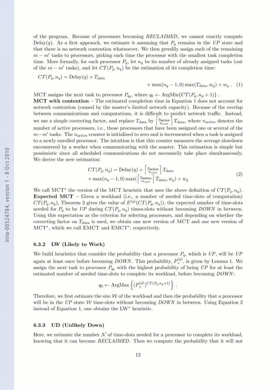
of the program. Because of processors becoming RECLAIMED , we cannot exactly computeDelay(q). As a first appraoch, we estimate it assuming that Pq remains in the UP state andthat there is no network contention whatsoever. We then greedily assign each of the remainingm−m′ tasks to processors, picking each time the processor with the smallest task completiontime. More formally, for each processor Pq, let nq be its number of already assigned tasks (outof the m−m′ tasks), and let CT (Pq, nq) be the estimation of its completion time:

CT (Pq, nq) = Delay(q) + Tdata

+ max(nq − 1, 0) max(Tdata, wq) + wq . (1)

MCT assigns the next task to processor Pq0 , where q0 ← ArgMin{CT (Pq, nq + 1)} .MCT with contention – The estimated completion time in Equation 1 does not account fornetwork contention (caused by the master’s limited network capacity). Because of the overlapbetween communications and computations, it is difficult to predict network traffic. Instead,

we use a simple correcting factor, and replace Tdata by⌈nactivencom

⌉Tdata, where nactive denotes the

number of active processors, i.e., those processors that have been assigned one or several of them−m′ tasks. The nactive counter is initialized to zero and is incremented when a task is assignedto a newly enrolled processor. The intuition is that this counter measures the average slowdownencountered by a worker when communicating with the master. This estimation is simple butpessimistic since all scheduled communications do not necessarily take place simultaneously.We derive the new estimation:

CT (Pq, nq) = Delay(q) +⌈nactivencom

⌉Tdata

+ max(nq − 1, 0) max(⌈nactivencom

⌉Tdata, wq) + wq

(2)

We call MCT∗ the version of the MCT heuristic that uses the above definition of CT (Pq, nq).Expected MCT – Given a workload (i.e., a number of needed time-slots of computation)CT (Pq, nq), Theorem 2 gives the value of E(q)(CT (Pq, nq)), the expected number of time-slotsneeded for Pq to be UP during CT (Pq, nq) times-slots without becoming DOWN in between.Using this expectation as the criterion for selecting processors, and depending on whether thecorrecting factor on Tdata is used, we obtain one new version of MCT and one new version ofMCT∗, which we call EMCT and EMCT∗, respectively.

6.3.2 LW (Likely to Work)

We build heuristics that consider the probability that a processor Pq, which is UP , will be UP

again at least once before becoming DOWN . This probability, P(q)+ , is given by Lemma 1. We

assign the next task to processor Pq0 with the highest probability of being UP for at least theestimated number of needed time-slots to complete its workload, before becoming DOWN :

q0 ← ArgMax{

(P(q)+ )CT (Pq ,nq+1)

}.

Therefore, we first estimate the sizeW of the workload and then the probability that a processorwill be in the UP state W time-slots without becoming DOWN in between. Using Equation 2instead of Equation 1, one obtains the LW∗ heuristic.

6.3.3 UD (Unlikely Down)

Here, we estimate the number N of time-slots needed for a processor to complete its workload,knowing that it can become RECLAIMED . Then we compute the probability that it will not

12

inria

-005

2478

4, v

ersi

on 1

- 8

Oct

201

0

become DOWN for N time-slots. Given that Pq starts in the UP state, the probability that itdoes not go to the DOWN state during k time-slots is:

P(q)UD(k) =

[1 1

].

[P

(q)u,u P

(q)u,r

P(q)r,u P

(q)r,r

]k−1.

[10

].

We approximate this expression by forgetting the state of Pq after the first transition:

P(q)UD(k) = (1− P (q)

u,d)

1−P

(q)u,dπ

(q)u + P

(q)r,d π

(q)r

π(q)u + π

(q)r

k−2

.

We use this value with k = E(q)(CT (Pq, nq +1)). UD assigns the next task to the processor Pq0

that maximizes the probability of not becoming DOWN before the estimated number of time-slots needed for it to complete its workload, counting the time-slots spent in the RECLAIMEDstate:

q0 ← ArgMax{P (q)UD(E(q)(CT (Pq, nq + 1)))} .

Using Equation 2 instead of Equation 1, one obtains the UD∗ heuristic.

7 Experiments

We have evaluated the heuristics described in the previous section using a discrete-even simulatorfor the execution of application on volatile resources (The simulator is publicly available at http://navet.ics.hawaii.edu/~casanova/software/cp_simulator.tgz). The simulator takes asinput values for all the parameters listed in Section 3, and it assumes that temporal processoravailability follows a Markov process.

For the simulation experiments, rather than fixing N , the number of time-slots, we insteadfix the number of iterations to 10. The quality of an application execution is then measuredby the time needed to complete 10 iterations, or makespan. This equivalent problem is simplerto instantiate since it does not require choosing meaningful N values, which would depend onthe application and platform characteristics. We have executed all heuristics presented abovefor several problem instances. For each problem instance we compute the degradation from best(dfb) of each heuristic, i.e., the percentage relative difference between the makespan achievedby the heuristic and that achieved by the best heuristic, all for that particular instance. A valueof zero means that the heuristic is best for the instance. We use this metric because makespansvary widely between instances depending on processor availability patterns. We also count howoften, over all instances, each heuristic is the (or tied with the) best one, so that we can reporton numbers of wins for each heuristics.

All our experiments are for p = 20 processors. The Markov chain that characterizes processorPq’s availability is defined as follows. We uniformly pick a random value between 0.90 and 0.99

for each P(q)x,x value (for x = u, r, d). We then set P

(q)x,y to 0.5 × (1 − P

(q)x,x), for x 6= y. An

experimental scenario is defined by the above and by three parameters: n, the number of tasksper iteration, ncom, the constraint on the master’s communication bandwidth, and the wmin

parameter, which is used as follows. For each processor Pq, we pick wq uniformly betweenwmin and 10 × wmin. Tdata is set to wmin, meaning that the fastest possible processor has acomputation-communication ratio of 1. Tprog is set to 5×wmin, meaning that downloading theprogram takes 5 times as much time as downloading the data for a task. We define experimentalscenarios for each of the possible instantiations of (n, ncom, wmin) given the values shown inTable 1. We must emphasize that our goal here is not to instantiate a representative model for

13

inria

-005

2478

4, v

ersi

on 1

- 8

Oct

201

0

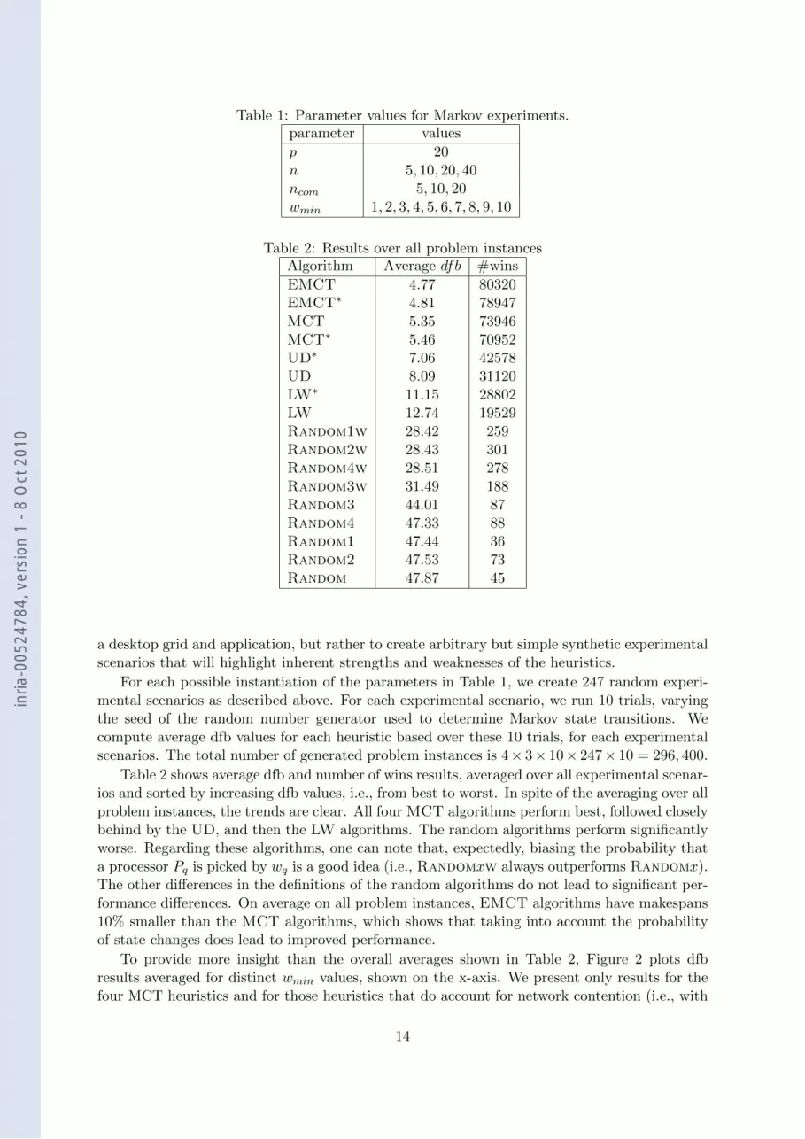
Table 1: Parameter values for Markov experiments.parameter values

p 20n 5, 10, 20, 40ncom 5, 10, 20wmin 1, 2, 3, 4, 5, 6, 7, 8, 9, 10

Table 2: Results over all problem instancesAlgorithm Average dfb #wins

EMCT 4.77 80320EMCT∗ 4.81 78947MCT 5.35 73946MCT∗ 5.46 70952UD∗ 7.06 42578UD 8.09 31120LW∗ 11.15 28802LW 12.74 19529Random1w 28.42 259Random2w 28.43 301Random4w 28.51 278Random3w 31.49 188Random3 44.01 87Random4 47.33 88Random1 47.44 36Random2 47.53 73Random 47.87 45

a desktop grid and application, but rather to create arbitrary but simple synthetic experimentalscenarios that will highlight inherent strengths and weaknesses of the heuristics.

For each possible instantiation of the parameters in Table 1, we create 247 random experi-mental scenarios as described above. For each experimental scenario, we run 10 trials, varyingthe seed of the random number generator used to determine Markov state transitions. Wecompute average dfb values for each heuristic based over these 10 trials, for each experimentalscenarios. The total number of generated problem instances is 4× 3× 10× 247× 10 = 296, 400.

Table 2 shows average dfb and number of wins results, averaged over all experimental scenar-ios and sorted by increasing dfb values, i.e., from best to worst. In spite of the averaging over allproblem instances, the trends are clear. All four MCT algorithms perform best, followed closelybehind by the UD, and then the LW algorithms. The random algorithms perform significantlyworse. Regarding these algorithms, one can note that, expectedly, biasing the probability thata processor Pq is picked by wq is a good idea (i.e., Randomxw always outperforms Randomx).The other differences in the definitions of the random algorithms do not lead to significant per-formance differences. On average on all problem instances, EMCT algorithms have makespans10% smaller than the MCT algorithms, which shows that taking into account the probabilityof state changes does lead to improved performance.

To provide more insight than the overall averages shown in Table 2, Figure 2 plots dfbresults averaged for distinct wmin values, shown on the x-axis. We present only results for thefour MCT heuristics and for those heuristics that do account for network contention (i.e., with

14

inria

-005

2478

4, v

ersi

on 1

- 8

Oct

201

0

Table 3: Results for contention-prone experimentsCommunication times ×5

Algorithm Average dfb

EMCT∗ 3.87MCT∗ 4.10UD∗ 5.23EMCT 6.13UD 6.42MCT 7.70LW∗ 8.76LW 10.11

Communication times ×10

Algorithm Average dfb

UD∗ 2.76UD 3.20EMCT∗ 3.66LW∗ 4.02MCT∗ 4.22LW 4.46EMCT 8.02MCT 15.50

a ∗), and leave out the random heuristics. Note that increasing wmin amounts to scaling theunit time, meaning that availability state transitions occur more often during the execution of atask. In other words, the right hand side of the x-axis in Figure 2 corresponds to more difficultproblem instances. Indeed, the larger wmin, the higher the probability that a task’s processorexperiences a state transition. Therefore, as wmin increases, it becomes increasingly importantto estimate the negative impacts of the DOWN and RECLAIMED states: the most powerfulprocessor may no longer be the best choice if it has a higher probability of going into the statesRECLAIMED or DOWN . The two EMCT algorithms take into account the probability thata processor enters the RECLAIMED state. We see that they overtake the MCT algorithmswhen wmin becomes larger than 3. The UD and LW algorithms also take into account theprobability that a processor goes DOWN . UD heuristics consistently outperform their LWcounterparts. Also, UD (slightly) overtakes EMCT as soon as wmin = 7. We conclude thatwhen the probability of state transitions rises one must use heuristics that explicitly take intoaccount that processors can go in the states RECLAIMED and DOWN .

In our results, we do not see much difference between the original versions of the heuristicsand the versions that that try to account for network contention, i.e., the heuristics thave havea ∗ in their names. Part of the reason may be that, as stated in Section 6.3.1, the correctingfactor used to account for contention is a very coarse approximation. However, our experimentalscenarios correspond to compute-intensive executions, meaning that processors typically spendmuch more time computing than communicating. We ran a set of experiments for n = 20,ncom = 5, and wmin = 1, but with Tdata = 5wmin and Tprog = 25wmin, i.e., with communicationtimes 5 times larger than those in our base set of experimental scenarios. Results averaged over100 such “contention-prone” experimental scenarios (each of which is ran for 10 trials) are shownin the left-hand side of Table 3. The right-hand side shows similar results for communicationthat are 10 times larger than those in our base set of scenarios. These results confirm that, asthe scenario becomes more communication intensive, those algorithms that account for networkcontention outperform their counterparts.

8 Conclusion

In this paper we have studied the problem of scheduling master-worker iterative applications onvolatile platforms in which hosts can experience failures or be temporarily reclaimed by theirowners. A unique aspect of our work is that we model the fact that communication betweenthe master and the workers is subject to a bandwidth constraint, e.g., due to the limitedcapacity of the master’s network card. In this context we have made a theoretical contributionby characterizing the computational complexity of the off-line problem, which turns out to beNP-hard. Interestingly, without any bandwidth constraint, the problem becomes solvable in

15

inria

-005

2478

4, v

ersi

on 1

- 8

Oct

201

0

1 2 3 4 5 6 7 8 9 100

5

10

15

20

25

30

35

40

mct

mct*

emct

emct*

ud*

lw*

Figure 2: Averaged dbf results vs. wmin.

polynomial time. We have then proposed several online scheduling heuristics. By assuming aMarkov model of processor availability, we have been able to derive a closed-form formula forthe expectation of the time needed by a volatile worker to complete a set of tasks. Some ofour heuristics use this expectation for making scheduling decision (namely EMCT, EMCT*,UD, UD*). Some heuristics also use a contention-correcting factor as a way to account for theconstraint on the master’s bandwidth (namely EMCT*, LW*, UD*). The evaluation of ourheuristics in simulation has led to the following conclusions:

• Our failure-aware heuristics deliver better performance than classical heuristics when theprobability that a task is subject to processor state transitions becomes non negligible;• Our contention-correcting factor improves performance on contention-prone platforms,

and does not degrade performance otherwise;• Our EMCT* heuristic delivers overall good performance, leading to a 10% reduction over

the makespans achieved by MCT, the optimal algorithm for the contention-free offlinecase;• EMCT* is outperformed by UD* in scenarios that exhibit from very large state transition

probabilities when compare to task duraction, or a highly contented network.

The next step in this research is to challenge the Markov assumption for processor availabil-ity. As explained in Section 1, processor availability in desktop grid platforms is not Markovian.We see two possible avenues of research. First, we could rely on those stochastic models of pro-cessor availability that are available [8, 9, 10, 11], and evolve our algorithmic techniques, if at allpossible, to account for those models. Second, given that no consensus has emerged regardingthe correct models of processor availability (and that perhaps there is none), we could embarkon a purey empirical study based on availability traces such as those available in the Failure

16

inria

-005

2478

4, v

ersi

on 1

- 8

Oct

201

0

Trace Archive [31].

Acknowledgment: F. Dufosse, Y. Robert and F. Vivien are with the Universite de Lyon. Y.Robert is with the Institut Universitaire de France. F. Vivien is with INRIA. This work wassupported in part by the ANR StochaGrid project.

References

[1] G. E. Fagg and J. Dongarra, “FT-MPI: Fault Tolerant MPI, Supporting Dynamic Appli-cations in a Dynamic World,” in Proc. 7th EuroPVM/MPI. Springer-Verlag, 2000, pp.346–353.

[2] J. R. de Souza, E. Argollo, A. Duarte, D. Rexachs, and E. Luque, “Fault tolerant master-worker over a multi-cluster architecture,” in Proc. of ParCo 2005. NIC Series, Vol. 33,2006, pp. 465–472.

[3] T. Leblanc, R. Anand, E. Gabriel, and J. Subhlok, “VolpexMPI: An MPI Library forExecution of Parallel Applications on Volatile Nodes,” in Proc. of EuroPVM/MPI 2009.Springer-Verlag, 2009, pp. 124–133.

[4] D. Buntinas, C. Coti, T. Herault, P. Lemarinier, L. Pilard, A. Rezmerita, E. Rodriguez,and F. Cappello, “MPICH-V: Toward a Scalable Fault Tolerant MPI for Volatile Nodes,”FGCS, vol. 24, no. 1, pp. 73–84, 2008.

[5] “BOINC: Berkeley Open Infrastructure for Network Computing,” http://boinc.berkeley.edu.

[6] A. Chien, B. Calder, S. Elbert, and K. Bhatia, “Entropia: Architecture and performance ofan enterprise desktop grid system,” J. Par. and Distr. Comp., vol. 63, pp. 597–610, 2003.

[7] E. Byun, S. Choi, M. Baik, J. Gil, C. Park, and C. Hwang, “MJSA: Markov job schedulerbased on availability in desktop grid computing environment,” FGCS, vol. 23, no. 4, pp.616–622, 2007.

[8] D. Nurmi, J. Brevik, and R. Wolski, “Modeling Machine Availability in Enterprise andWide-area Distributed Computing Environments,” in Proc. of Europar, 2005.

[9] R. Wolski, D. Nurmi, and J. Brevik, “An Analysis of Availability Distributions in Condor,”in Proc. of the IPDPS Workshop on Next-Generation Software, 2007.

[10] B. Javadi, D. Kondo, J. Vincent, and D. Anderson, “Mining for Statistical Models ofAvailability in Large-Scale Distributed Systems: An Empirical Study of SETI@home,” inProc. of the 17th MASCOTS, 2009.

[11] X. Ren, S. Lee, R. Eigenmann, and S. Bagchi, “Prediction of Resource Availability inFine-Grained Cycle Sharing Systems Empirical Evaluation,” Journal of Grid Computing,vol. 5, no. 2, pp. 173–195, 2007.

[12] B. Hong and V. K. Prasanna, “Adaptive allocation of independent tasks to maximizethroughput,” IEEE TPDS, vol. 18, no. 10, pp. 1420–1435, 2007.

[13] J. M. Bahi, S. Contassot-Vivier, and R. Couturier, Parallel Iterative Algorithms: FromSequential to Grid Computing. Chapman and Hall/CRC Press, 2007.

17

inria

-005

2478

4, v

ersi

on 1

- 8

Oct

201

0

[14] A. Heddaya and K. Park, “Mapping parallel iterative algorithms onto workstation net-works,” in HPDC’94, 1994, pp. 211 –218.

[15] A. Legrand, H. Renard, Y. Robert, and F. Vivien, “Mapping and load-balancing iterativecomputations on heterogeneous clusters with shared links,” IEEE TPDS, vol. 15, pp. 546–558, 2004.

[16] D. Kondo, A. Chien, and H. Casanova, “Resource Management for Rapid ApplicationTurnaround on Enterprise Desktop Grids,” in Proc. of SC’04, 2004.

[17] D. Zhou and V. Lo, “Wave Scheduler: Scheduling for Faster Turnaround Time in Peer-based Desktop Grid Systems,” in Proc. of the 11th JSSPP Workshop, 2005.

[18] T. Estrada, D. Flores, M. Taufer, P. Teller, A. Kerstens, and D. Anderson, “The Effective-ness of Threshold-Based Scheduling Policies in BOINC Projects,” in Proc. of e-Science’06,2006.

[19] C. Anglano, J. Brevik, M. Canonico, D. Nurmi, and R. Wolski, “Fault-aware schedulingfor Bag-of-Tasks applications on Desktop Grids,” in Proc. of Grid Computing, 2006, pp.56–63.

[20] T. Estrada, O. Fuentes, and . Taufer, “A distributed evolutionary method to design schedul-ing policies for volunteer computing,” SIGMETRICS Perf. Eval. Rev., vol. 36, no. 3, pp.40–49, 2008.

[21] J. Wingstrom and H. Casanova, “Probabilistic Allocation of Tasks on Desktop Grids,” inProc. of PCGrid, 2008.

[22] E. Heien, D. Anderson, and K. Hagihara, “Computing Low Latency Batches with Unreli-able Workers in Volunteer Computing Environments,” Journal of Grid Computing, vol. 7,no. 4, pp. 501–518, 2009.

[23] N. Fujimoto and K. Hagihara, “Near-Optimal Dynamic Task Scheduling of IndependentCoarse-Grained Tasks onto a Computational Grid,” in Proc. of ICPP, 2003.

[24] C. Moretti, T. Faltemier, D. Thain, and P. Flynn, “Challenges in Executing Data IntensiveBiometric Workloads on a Desktop Grid,” in Proc. of PCGrid, 2007.

[25] T. Toyoma, Y. Yamada, and K. Konishi, “A Resource Management System for Data-Intensive Applications in Desktop Grid Environments,” in Proc. of PDCS, 2006.

[26] H. He, G. Fedak, B. Tang, and F. Cappello, “BLAST Application with Data-Aware DesktopGrid Middleware,” in Proc. of CCGrid, 2009, pp. 284–291.

[27] R. Guerraoui and A. Schiper, “Software-Based Replication for Fault Tolerance,” IEEEComputer, vol. 30, pp. 68–74, 1997.

[28] P. Stelling, C. DeMatteis, I. Foster, C. Kesselman, C. Lee, and G. von Laszewski, “A faultdetection service for wide area distributed computations,” Cluster Computing, vol. 2, no. 2,pp. 117–128, 1999.

[29] W. Gropp, “MPICH2: A New Start for MPI Implementations,” in PVM/MPI, 2002, p. 7.

[30] J. Hastad, “Some optimal inapproximability results,” in STOC ’97. ACM, 1997, pp. 1–10.

18

inria

-005

2478

4, v

ersi

on 1

- 8

Oct

201

0

[31] D. Kondo, B. Javadi, A. Iosup, and D. Epema, “The Failure Trace Archive: EnablingComparative Analysis of Failures in Diverse Distributed Systems,” in Proc. of CCGrid,2010.

19

inria

-005

2478

4, v

ersi

on 1

- 8

Oct

201

0