arX

iv:c

ond-

mat

/051

1354

v1

14

Nov

200

5

Scaling and Universality of the Complexity of Analog Computation

Yaniv Avizrats a, Joshua Feinberga,b, Shmuel Fishmana

a)Physics Department,Technion, Israel Institute of Technology, Haifa 32000, Israel

b)Physics Department,University of Haifa at Oranim, Tivon 36006, Israel

Abstract

We apply a probabilistic approach to study the computational complexity of ana-

log computers which solve linear programming problems. We analyze numerically

various ensembles of linear programming problems and obtain, for each of these en-

sembles, the probability distribution functions of certain quantities which measure

the computational complexity, known as the convergence rate, the barrier and the

computation time. We find that in the limit of very large problems these proba-

bility distributions are universal scaling functions. In other words, the probability

distribution function for each of these three quantities becomes, in the limit of large

problem size, a function of a single scaling variable, which is a certain composition

of the quantity in question and the size of the system. Moreover, various ensembles

studied seem to lead essentially to the same scaling functions, which depend only on

the variance of the ensemble. These results extend analytical and numerical results

obtained recently for the Gaussian ensemble, and support the conjecture that these

scaling functions are universal.

PACS numbers: 5.45-a, 89.79+c, 89.75.D

1 Introduction

Digital computers are part of our present civilization. There are, however, other devicesthat are capable of computation. These are analog computers, that are ubiquitious com-putational tools. The most relevant examples of analog computers are VLSI devices im-plementing neural networks [1], or neuromorphic systems [2], whose structure is directlymotivated by the workings of the brain. Various processes taking place in living cells canbe considered as analog computation [3] as well.

An analog computer is essentially a physical device that performs computation, evolvingin continuous time and phase space. It is useful to model its evolution in phase space bydynamical systems (DS) [4], the way classical systems such as particles moving in a potential(or electric circuits), are modeled. For example, there are dynamical systems (describedby ordinary differential equations) that are used to solve computational problems [5, 6, 7].This description makes a large set of analytical tools and physical intuition, developed fordynamical systems, applicable to the analysis of analog computers.

In contrast, the evolution of a digital computer is discrete both in its phase space andin time. Consequently, the standard theory of computation and computational complexity[8] deals with computation in discrete time and phase space, and is inadequate for thedescription of analog computers. The analysis of computation by analog devices requiers atheory that is valid in continuous time and phase space.

1

Since the systems in question are physical systems, the computation time is the timerequired for a system to reach the vicinity of an attractor (a stable fixed point in the presentwork) combined with the time required to verify that it indeed reached this vicinity. Thistime is the elapsed time measured by a clock, contrary to standard computation theory,where it is the number of discrete steps.

In the exploration of physical systems, it is sometimes much easier to study statisticalensembles of systems, estimating their typical behavior using statistical methods [9, 10, 11].In [12, 13] a statistical theory was used to calculate the computational complexity of astandard representative problem, namely Linear Programming (LP), as solved by a DS.

A framework for computing with DS that converge exponentially to fixed points wasproposed in [14]. For such systems it is natural to consider the attracting fixed point asthe output. The input can be modeled in various ways. One possible choice is the initialcondition. This is appropriate when the aim of the computation is to decide to whichattractor out of many possible ones the system flows [15]. Here, in [12, 13], as well as in[14], the parameters on which the DS depends (e.g., the parameters appearing in the vectorfield F in (1)) are the input.

The basic entity of the computational model is a dynamical system [4], that may bedefined by a set of Ordinary Differential Equations (ODEs)

dx

dt= F (x), (1)

where x is an n-dimensional vector, and F is an n-dimensional smooth vector field, whichconverges exponentially to a fixed point. Eq. (1) solves a computational problem as follows:Given an instance of the problem, the parameters of the vector field F are set (i.e., theinput is read), and it is started from some pre-determined initial condition. The result ofthe computation is then deduced from the fixed point that the system approaches.

In our model we assume we have a physical implementation of the flow equation (1).Thus, the vector field F need not be computed, and the computation time is determined bythe convergence time to the attractive fixed point. In other words, the time of flow to thevicinity of the attractor is a good measure of complexity, namely the computational effort,for the class of continuous dynamical systems introduced above [14].

In this paper, as in [12, 13], we will study a specific algorithm for the solution of theLP problem [16]. We will consider real-continuous inputs, as the ones found in physicalexperiments, and that are studied in the BSS model [17], as well as integer-valued inputs.For computational models defined on the real numbers, worst case behavior, that is tra-ditionally studied in computer science, can be ill-defined and lead to infinite computationtimes, in particular, for some methods for solving LP [17, 18]. Therefore, we compute thedistribution of computation times for a probabilistic model of LP instances with variousdistributions of the data like in [19, 20]. Ill-defined instances constitute a set of measurezero in our countinuous probability ensembles, and need not be concerned about. In thediscrete probability ensembles, we treat them by appropriate regularization.

The computational complexity of the method presented in [12, 13] and discussed hereis O(n log n), compared to O(n3.5 log n) found for standard interior point methods [21].The basic reason is that for standard methods (such as interior point methods), the majorcomponent of the complexity of each iteration is O(n3) due to matrix decomposition andinversion of the constraint matrix, while here, because of its analog nature, the system just

2

flows according to its equations of motion (which need not be computed).Since we consider the evolution of a vector field, our model is inherently parallel. There-

fore, to make the analog vs. digital comparison entirely fair, we should compare the com-plexity of our method to that of the best parallel algorithm. The latter can reduce theO(n3) time needed for matrix decomposition/inversion to polylogarithmic time (for well-posed problems), at the cost of O(n2.5) processors [22], while our system of equations (1)uses only O(n) variables.

The main result of [12, 13], in which LP problems were drawn from the Gaussiandistribution of the parameters of F (namely, the constraints and cost function in (2)), wasthat the distribution functions of various quantities that characterize the computationalcomplexity, were found to be scaling functions in the limit of LP problems of large size. Inparticular, it was found that these distribution functions depend on the various parametersonly via specific combinations, namely, the scaling variables. Such behavior is analogousto the situation found for the central limit theorem, for critical phenomena [23] and forAnderson localization [24], in spite of the very different nature of these problems. It wasdemonstrated in [12, 13] how for the implementation of the LP problem on a physical device,methods used in theoretical physics enable to describe the distribution of computation timesin a simple and physically transparent form. Based on experience with certain universalityproperties of rectangular and chiral random matrix models [25], it was conjectured in [12,13] that some universality for computational problems should be expected and should beexplored. That is, the scaling properties that were found for the Gaussian distributionsshould hold also for other distributions. In particular, some specific questions were raisedin [12, 13]: Is the Gaussian nature of the ensemble unimportant in analogy with [25]? Arethere universality classes [23] of analog computational problems, and if they exist, what arethey?

Thus, we extend the earlier analysis [12, 13] of the Gaussian distribution to other prob-ability distributions of LP problems, and demonstrate numerically that the distributionfunctions of various quantities that characterize the computational complexity of the ana-log computer which solves LP problems are indeed universal scaling functions, in the limitof large systems. These universal functions depend upon the original probability ensembleof inputs only via the scaling variables, that are proportional to the ones found for theGaussian distribution. For some distributions of LP problems the scaling variables are evenidentical (not just proportional) to the ones found for the Gaussian distribution. For otherdistributions, on the other hand, where some of the parameters defining an LP problemmay vanish at random (the so-called diluted ensembles in Section 4), either the convergenceto universality is much slower, or universality is only approximate.

The distribution of constraints and cost function of the LP problems that are usedin practice is not known. Therefore, the universality of the distribution functions of thecomputation time and other quantities related to computational complexity is of greatimportance. It would imply that it may hold also for the distributions of the LP problemssolved in applications. In this paper we demonstrate numerically that for several probabilitydistributions universality is satisfied, providing support for the conjecture that it holds ingeneral.

This paper is organized as follows: In the next section we briefly review the dynamicalsystem which solves LP problems. In section 3 we summarize the scaling results of [12, 13]for the Gaussian ensemble. In section 4 we present our numerical results for the distribution

3

functions of various quantities that characterize the computational complexity of the analogcomputer for non-Gaussian probability ensembles. In section 5 we demonstrate that thesedistributions are indeed universal scaling functions. Finally, in section 6 we discuss thesignificance of our results and also pose some open problems.

4

2 A dynamical flow for linear programming

Linear programming is a P-complete problem [8], i.e. it is representative of all problemsthat can be solved in polynomial time. The standard form of LP is to find

max{cT x : x ∈ IRn, Ax = b, x ≥ 0} (2)

where c ∈ IRn, b ∈ IRm, A ∈ IRm×n and m ≤ n. The set generated by the constraints in (2)is a polyheder. If a bounded optimal solution exists, it is obtained at one of its vertices.The vector defining this optimal vertex can be decomposed (in an appropriate basis) in theform x = (xN , xB) where xN = 0 is an n − m component vector, while xB = B−1b ≥ 0 isan m component vector, and B is the m × m matrix whose columns are the columns of Awith indices identical to the ones of xB. Similarly, we decompose A = (N,B).

A flow of the form (1) converging to the optimal vertex, introduced by Faybusovich [6]will be studied here. Its vector field F is a projection of the gradient of the cost functioncT x onto the constraint set, relative to a Riemannian metric which enforces the positivityconstraints x ≥ 0 [6]. It is given by

F (x) = [X − XAT (AXAT )−1AX] c , (3)

where X is the diagonal matrix Diag(x1 . . . xn). The nm+n entries of A and c, namely, theparameters of the vector field F , constitute the input; as in other models of computation, weignore the time it takes to “load” the input, since this step does not reflect the complexity ofthe computation being performed, either in analog or digital computation. It was shown in[16] that the flow equations given by (1) and (3) are, in fact, part of a system of Hamiltonianequations of motion of a completely integrable system of a Toda type. Therefore, like theToda system, it is integrable with the formal solution [6]

xi(t) = xi(0) exp

−∆it +m

∑

j=1

αji logxj+n−m(t)

xj+n−m(0)

(4)

(i = 1, . . . , n − m), that describes the time evolution of the n − m independent variablesxN (t), in terms of the variables xB(t). In (4) xi(0) and xj+n−m(0) are components of theinitial condition, xj+n−m(t) are the xB components of the solution, αji = −(B−1N)ji is anm × (n − m) matrix, while

∆i = −ci −m

∑

j=1

cjαji . (5)

For the decomposition x = (xN , xB) used for the optimal vertex ∆i ≥ 0 i = 1, . . . , n − m ,and xN (t) converges to 0, while xB(t) converges to x∗ = B−1b. Note that the analyticalsolution is only a formal one, and does not provide an answer to the LP instance, sincethe ∆i depend on the partition of A, and only relative to a partition corresponding to amaximum vertex are all the ∆i positive.

The second term in the exponent in (4), when it is positive, is a kind of “barrier”: ∆itmust be larger than the barrier before xi can decrease to zero. In the following we ignorethe contribution of the initial condition and denote the value of this term in the infinitetime limit by

βi =m

∑

j=1

αji log x∗j+n−m. (6)

5

Note that although one (or more) of the x∗j+n−m may vanish, in the probabilistic ensemble

studied here, such an event is of measure zero for the continuous probability distributions, aswell as for the regularized discretized ones (see (25)), and therefore should not be considered.In order for x(t) to be close to the maximum vertex we must have xi(t) < ǫ for i =1, . . . , n − m for some small positive ǫ, namely exp(−∆it + βi) < ǫ , for i = 1, . . . , n − m.Therefore we consider

T = maxi

(

βi

∆i+

| log ǫ|∆i

)

, (7)

as the computation time. We denote

∆min = mini

∆i, βmax = maxi

βi . (8)

The ∆i can be arbitrarily small when the inputs are real numbers, but in the probabilisticmodel, “bad” instances, resulting in computation taking arbitrarily long time, are rare asis clear from1 (9).

1Strictly speaking, (9) was derived in [12, 13] for a probabilistic model in which the components of (A, b, c)were independent identically distributed Gaussian random variables. However, one of the main points ofthis paper is that (9) is valid for a broad class of probability distributions of LP problems.

6

3 Probability distributions and scaling

Consider an ensemble of LP problems in which the components of (A, b, c) are independentidentically distributed (i.i.d.) random variables taken from various even distributions, with0 mean and bounded variance. In a probabilistic model of LP instances, ∆min, βmax andT are random variables. Since the expression for ∆i, equation (5), is independent of b, itsdistribution is independent of b. For a given realization of A and c, with a partition of Ainto (N,B) such that ∆i ≥ 0, there exists2 a vector b such that the resulting polyheder has abounded optimal solution. Since b in our probabilistic model is independent of A we obtain:P(∆min < ∆|∆min > 0,LP instance has a bounded maximum vertex) = P(∆min < ∆|∆min >0).

In [12, 13], the components of A, b, and c were taken from the Gaussian distribution(see, e.g., Eqs.(12-18) in [12]) with zero mean and variance σ2, that was taken as unity inthe numerical calculations. It was found analytically, in the large (n,m) limit, that theprobability P(∆min < ∆|∆min > 0) ≡ F (n,m)(∆) is of the scaling form

F (n,m)(∆) = 1 − ex2

∆ erfc(x∆) ≡ F(x∆). (9)

with the scaling variable

x∆(n,m) =1√π

(

n

m− 1

)√

m∆

σ. (10)

The scaling function F contains all asymptotic information on ∆. The probability densityfunction derived from F(x∆) is very wide and does not have a finite variance. Also theaverage of 1/x∆ diverges.

The amazing point is that in the limit of large m and n, the probability distributionof ∆min depends on the variables m, n and ∆ only via the scaling variable x∆. For futurereference it is convenient to write x∆ in the form

x∆ = a(g)∆ (n/m)

√m∆ , (11)

with

a(g)∆ (n/m) =

1√π

(

n

m− 1

)

1

σ, (12)

where the superscript refers to the Gaussian distribution. If the limit of infinite m and

n is taken, so that n/m is fixed, a(g)∆ is constant. It was verified numerically that for the

Gaussian ensemble (9) was a good approximation already for m = 20, and n = 40.The existence of scaling functions like (9) for the barrier βmax, that is the maximum of

the βi defined by (6) and for T defined by (7) (assuming that ǫ is not too small so that thefirst term in (7) dominates) was verified numerically for the Gaussian distribution [12, 13].In particular for fixed m/n, we found that

P(1/βmax < 1/β) = F (n,m)1/βmax

(1/β) ≡ F1/β(xβ) (13)

2The existence of b is guaranteed by the fact that the various probability distributions are even. See [12],Lemma 3.1. The latter was proved in [12] under the assumption that the components of (A, b, c) were i.i.d.Gaussian variables, but the proof extends trivially to the class of probability ensembles of the type specifiedabove.

7

andP(1/T < 1/t) = F (n,m)

1/T (1/t) ≡ F1/T (xT ). (14)

The corresponding scaling variables are

xβ = a(g)β (n/m)

m

β(15)

and

xT = a(g)T (n/m)

m log m

t. (16)

Since the distribution functions (13) and (14) are not known analytically, and since n = 2m

was taken in the numerical investigations in [12], we can set arbitrarily a(g)β (2) = a

(g)T (2) = 1.

The scaling functions (9), (13) and (14) imply the asymptotic behavior

1/∆min ∼√

m, βmax ∼ m, t ∼ m log m (17)

with “high probability” [12, 13].

8

4 Non-Gaussian distributions

In this section we present the results of our numerical calculations of the distributionfunctions of ∆min, 1/βmax, and 1/T for various probability distributions of A, b, and c.For this purpose we generated full LP instances (A, b, c) with the probability distributionin question. For each instance the LP problem was solved using the linear programmingsolver of MatLab. Only instances with a bounded optimal solution were kept, and ∆min

was computed relative to the optimal partition and optimality was verified by checking that∆min > 0. Using the sampled instances we obtain an estimate of F (n,m)(∆) = P(∆min <∆|∆min > 0), and of the corresponding cumulative distribution functions of the barrierβmax and the computation time T.

The solution of the LP problem is used here in order to identify the optimal partitionof A into B and N . This enables one to compute ∆min, βmax, and t from (5), (6), (7) and(8), and the distributions

P∆(∆) = P(∆min < ∆|∆min > 0) , (18)

Pβ(1/β) = P(1/βmax < 1/β) (19)

andPT (1/t) = P(1/T < 1/t) (20)

are obtained.It is convenient at first to keep n/m fixed3 and to compute these distributions as func-

tions of the corresponding scaling variables

x′∆ =

√m∆ (21)

x′β = m/β (22)

andx′

T = m log m/t (23)

These are proportional to x∆, xβ and xT defined by (10), (15) and (16). We turn now toexplore in some detail, various distributions.

4.1 The bimodal distribution

In this case, the various elements of A, b and c take only the values +1 or −1 with probability1/2 each, namely,

P (y) =1

2[δ(y − 1) + δ(y + 1)] . (24)

The mean of this distribution is 0, and its variance is 1. One problem associated with thediscrete ensemble (24) is the finite probability to draw a degenerate LP problem. (Notethat such degenerate, ill-defined LP problems, comprize a set of zero measure in continuousensembles such as the Gaussian ensemble.) In order to avoid these degenerate solutions,

3In fact, in all our numerical simulations we kept n/m = 2 fixed.

9

0 0.5 1 1.5 2 2.5 3 3.5 4 4.5 50

0.1

0.2

0.3

0.4

0.5

0.6

0.7

0.8

0.9

1

∆

P∆

m=20m=30m=40

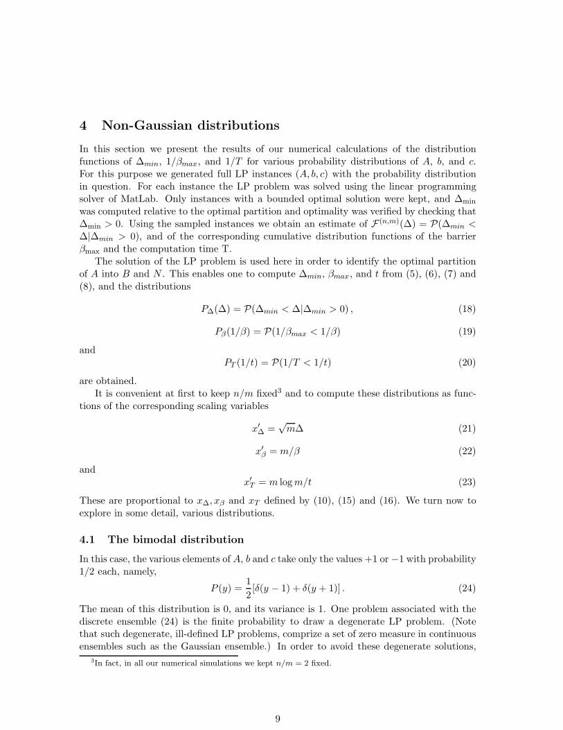
Figure 1: P∆ is plotted as a function of ∆, for the bimodal distribution (for n = 2m).The number of instances used in the simulation is 39732 for the m = 20 case, 46583 for them = 30 case and 47169 for the m = 40 case. The number of converging instances for eachcase is 5000.

we introduce a “regularization” by which each matrix element Aij , chosen at random fromthe ensemble (24), is multiplied by

fij = 1 + [i + 2(j − 1)]ǫ̃ , (25)

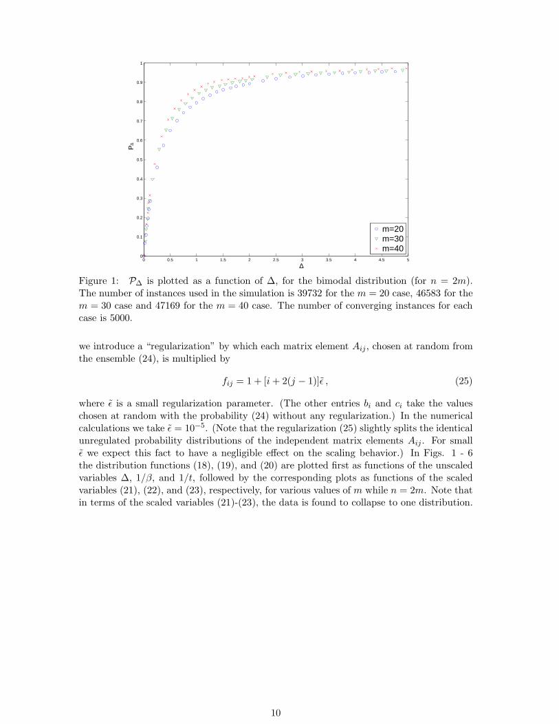
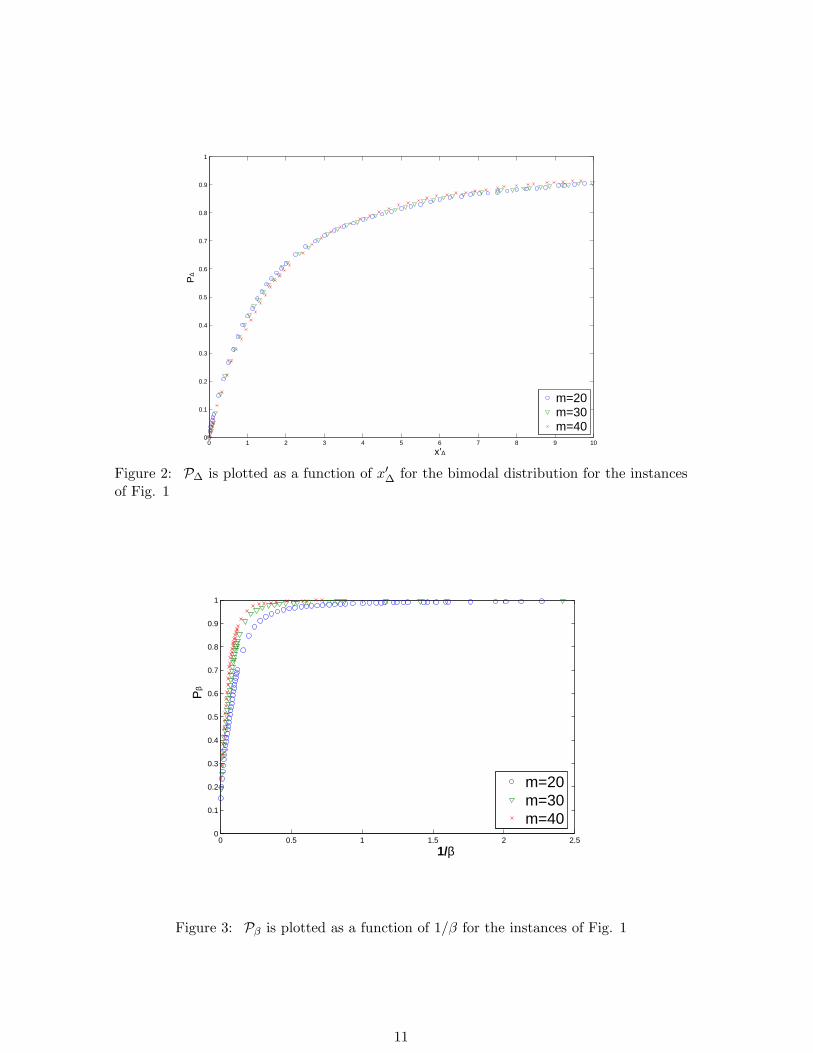
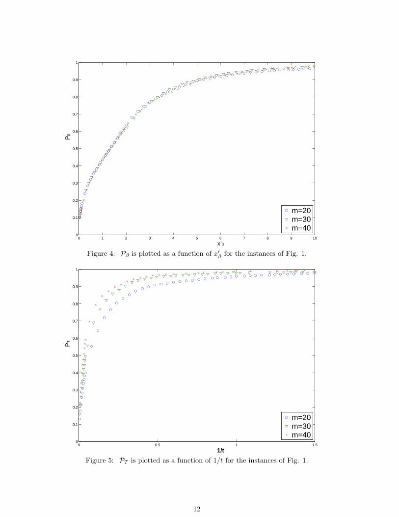
where ǫ̃ is a small regularization parameter. (The other entries bi and ci take the valueschosen at random with the probability (24) without any regularization.) In the numericalcalculations we take ǫ̃ = 10−5. (Note that the regularization (25) slightly splits the identicalunregulated probability distributions of the independent matrix elements Aij . For smallǫ̃ we expect this fact to have a negligible effect on the scaling behavior.) In Figs. 1 - 6the distribution functions (18), (19), and (20) are plotted first as functions of the unscaledvariables ∆, 1/β, and 1/t, followed by the corresponding plots as functions of the scaledvariables (21), (22), and (23), respectively, for various values of m while n = 2m. Note thatin terms of the scaled variables (21)-(23), the data is found to collapse to one distribution.

10

0 1 2 3 4 5 6 7 8 9 100

0.1

0.2

0.3

0.4

0.5

0.6

0.7

0.8

0.9

1

x’∆

P∆

m=20m=30m=40

Figure 2: P∆ is plotted as a function of x′∆ for the bimodal distribution for the instances

of Fig. 1

0 0.5 1 1.5 2 2.50

0.1

0.2

0.3

0.4

0.5

0.6

0.7

0.8

0.9

1

1/β

Pβ

m=20m=30m=40

Figure 3: Pβ is plotted as a function of 1/β for the instances of Fig. 1

11

0 1 2 3 4 5 6 7 8 9 100

0.1

0.2

0.3

0.4

0.5

0.6

0.7

0.8

0.9

1

x’β

Pβ

m=20m=30m=40

Figure 4: Pβ is plotted as a function of x′β for the instances of Fig. 1.

0 0.5 1 1.50

0.1

0.2

0.3

0.4

0.5

0.6

0.7

0.8

0.9

1

1/t

PT

m=20m=30m=40

Figure 5: PT is plotted as a function of 1/t for the instances of Fig. 1.

12

0 2 4 6 8 10 12 14 16 18 200

0.1

0.2

0.3

0.4

0.5

0.6

0.7

0.8

0.9

1

x’T

PT

m=20m=30m=40

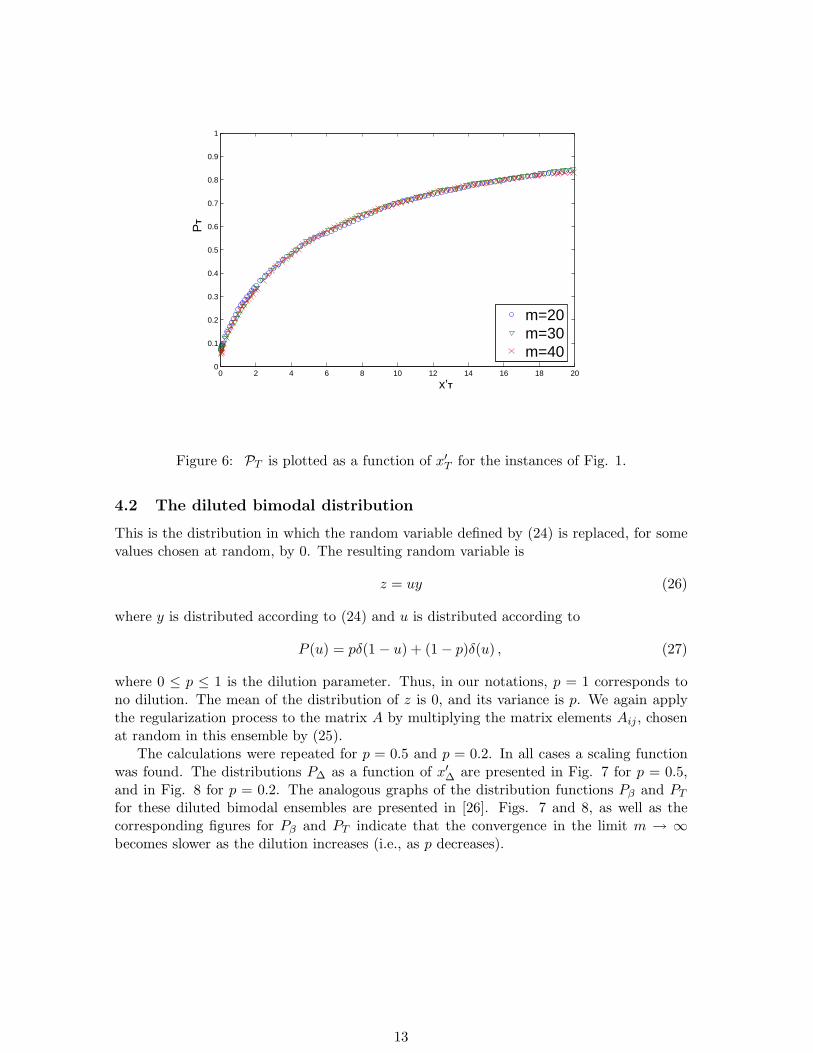
Figure 6: PT is plotted as a function of x′T for the instances of Fig. 1.

4.2 The diluted bimodal distribution

This is the distribution in which the random variable defined by (24) is replaced, for somevalues chosen at random, by 0. The resulting random variable is

z = uy (26)

where y is distributed according to (24) and u is distributed according to

P (u) = pδ(1 − u) + (1 − p)δ(u) , (27)

where 0 ≤ p ≤ 1 is the dilution parameter. Thus, in our notations, p = 1 corresponds tono dilution. The mean of the distribution of z is 0, and its variance is p. We again applythe regularization process to the matrix A by multiplying the matrix elements Aij , chosenat random in this ensemble by (25).

The calculations were repeated for p = 0.5 and p = 0.2. In all cases a scaling functionwas found. The distributions P∆ as a function of x′

∆ are presented in Fig. 7 for p = 0.5,and in Fig. 8 for p = 0.2. The analogous graphs of the distribution functions Pβ and PT

for these diluted bimodal ensembles are presented in [26]. Figs. 7 and 8, as well as thecorresponding figures for Pβ and PT indicate that the convergence in the limit m → ∞becomes slower as the dilution increases (i.e., as p decreases).

13

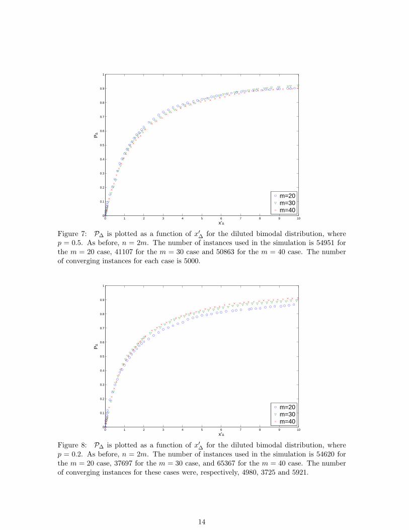
0 1 2 3 4 5 6 7 8 9 100

0.1

0.2

0.3

0.4

0.5

0.6

0.7

0.8

0.9

1

x’∆

P∆

m=20m=30m=40

Figure 7: P∆ is plotted as a function of x′∆ for the diluted bimodal distribution, where

p = 0.5. As before, n = 2m. The number of instances used in the simulation is 54951 forthe m = 20 case, 41107 for the m = 30 case and 50863 for the m = 40 case. The numberof converging instances for each case is 5000.

0 1 2 3 4 5 6 7 8 9 100

0.1

0.2

0.3

0.4

0.5

0.6

0.7

0.8

0.9

1

x’∆

P∆

m=20m=30m=40

Figure 8: P∆ is plotted as a function of x′∆ for the diluted bimodal distribution, where

p = 0.2. As before, n = 2m. The number of instances used in the simulation is 54620 forthe m = 20 case, 37697 for the m = 30 case, and 65367 for the m = 40 case. The numberof converging instances for these cases were, respectively, 4980, 3725 and 5921.

14

0 1 2 3 4 5 6 7 8 9 100

0.1

0.2

0.3

0.4

0.5

0.6

0.7

0.8

0.9

1

x’∆

P∆

m=20m=30m=40

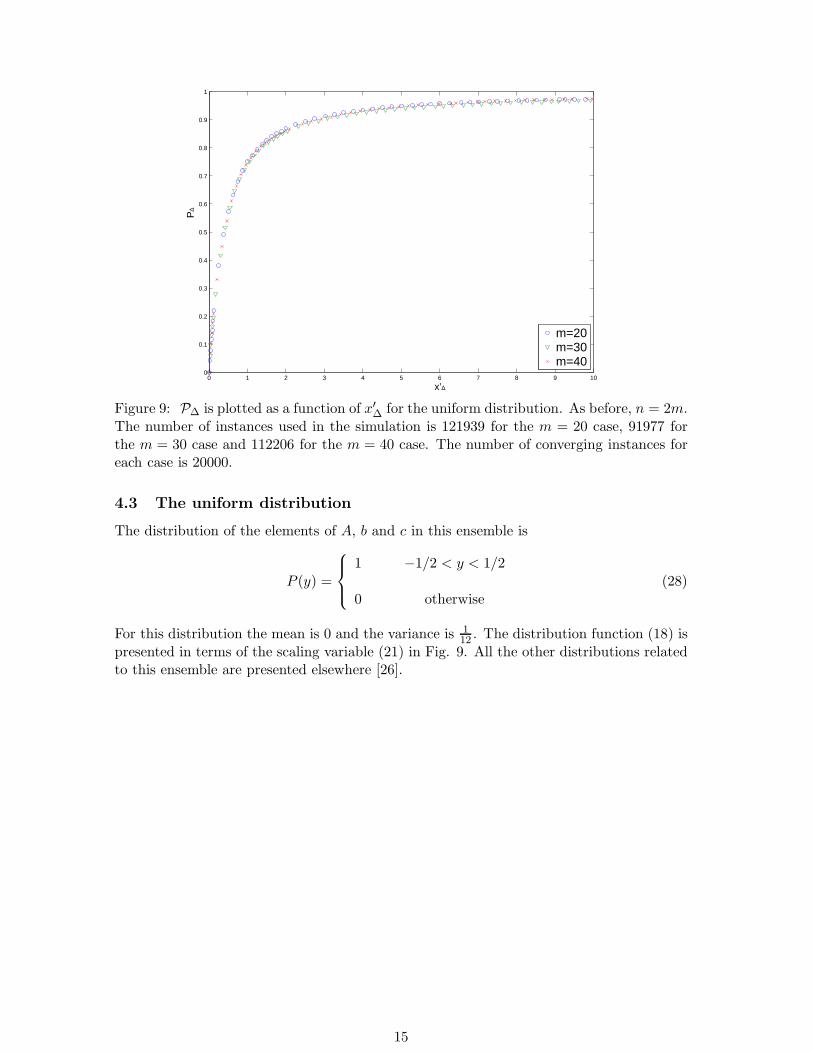
Figure 9: P∆ is plotted as a function of x′∆ for the uniform distribution. As before, n = 2m.

The number of instances used in the simulation is 121939 for the m = 20 case, 91977 forthe m = 30 case and 112206 for the m = 40 case. The number of converging instances foreach case is 20000.

4.3 The uniform distribution

The distribution of the elements of A, b and c in this ensemble is

P (y) =

1 −1/2 < y < 1/2

0 otherwise(28)

For this distribution the mean is 0 and the variance is 112 . The distribution function (18) is

presented in terms of the scaling variable (21) in Fig. 9. All the other distributions relatedto this ensemble are presented elsewhere [26].

15

0 1 2 3 4 5 6 7 8 9 100

0.1

0.2

0.3

0.4

0.5

0.6

0.7

0.8

0.9

1

x∆

P∆

BimodalBimodal p=0.2Bimodal p=0.5UniformGauss (Numerical)Gauss (Analytical)

Figure 10: P∆ as a function of x∆ (for n = 2m and m = 40). The graphs are scaled to fit

the theoretical Gaussian result by appropriate choice of the factors a(µ)∆ .

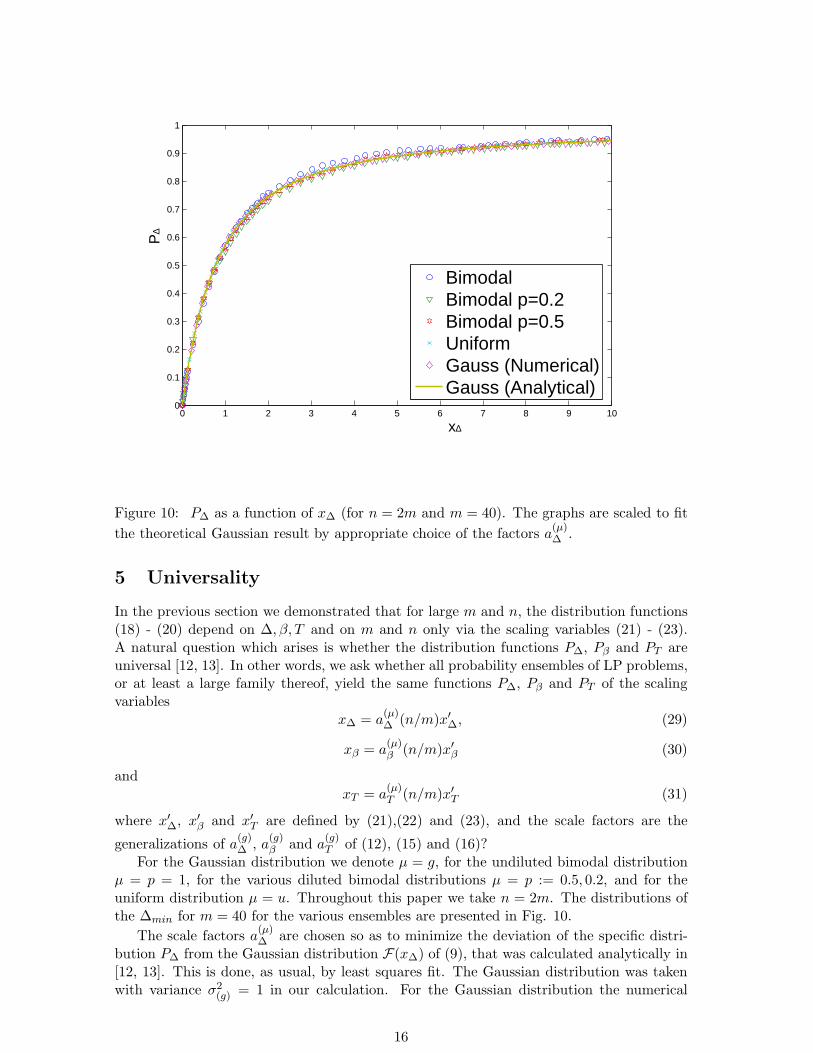
5 Universality

In the previous section we demonstrated that for large m and n, the distribution functions(18) - (20) depend on ∆, β, T and on m and n only via the scaling variables (21) - (23).A natural question which arises is whether the distribution functions P∆, Pβ and PT areuniversal [12, 13]. In other words, we ask whether all probability ensembles of LP problems,or at least a large family thereof, yield the same functions P∆, Pβ and PT of the scalingvariables

x∆ = a(µ)∆ (n/m)x′

∆, (29)

xβ = a(µ)β (n/m)x′

β (30)

andxT = a

(µ)T (n/m)x′

T (31)

where x′∆, x′

β and x′T are defined by (21),(22) and (23), and the scale factors are the

generalizations of a(g)∆ , a

(g)β and a

(g)T of (12), (15) and (16)?

For the Gaussian distribution we denote µ = g, for the undiluted bimodal distributionµ = p = 1, for the various diluted bimodal distributions µ = p := 0.5, 0.2, and for theuniform distribution µ = u. Throughout this paper we take n = 2m. The distributions ofthe ∆min for m = 40 for the various ensembles are presented in Fig. 10.

The scale factors a(µ)∆ are chosen so as to minimize the deviation of the specific distri-

bution P∆ from the Gaussian distribution F(x∆) of (9), that was calculated analytically in[12, 13]. This is done, as usual, by least squares fit. The Gaussian distribution was takenwith variance σ2

(g) = 1 in our calculation. For the Gaussian distribution the numerical

16

results were found to fit the analytical result (9) with a(g)∆ ≃ 0.564 ≃ 1√

π, as expected from

(12) for n = 2m. For the bimodal distribution it was found that a(1)∆ ≃ 0.558 ≃ 0.989√

π. For

the diluted bimodal distributions at p = 0.5 we found a(0.5)∆ ≃ 0.581 ≃ 1.030√

π, and for the

more diluted ensemble at p = 0.2 we found a(0.2)∆ ≃ 0.687 ≃ 1.218√

π. Finally, for the uniform

distribution we obtained a(u)∆ ≃ 1.957 ≃ 3.469√

π≃

√

12.030π . Recall that the variances of these

distributions are σ2(1) = 1, and σ2

(u) = 112 , respectively. Therefore, on the basis of these

numerical results we conjecture that

σ(g)a(g)∆ = σ(1)a

(1)∆ = σ(u)a

(u)∆ , (32)

and that their common value is given by (12), that is equal to 1/√

π for n = 2m.

Our numerical results indicate that the scale factors a(p)∆ of the diluted distributions

deviate from this simple law, and this deviation seems to be more pronounced for higher

dilution (smaller p). For these distributions σ2(p) = p, leading to a

(0.5)∆ σ(0.5) ≃ 0.411 and

a(0.2)∆ σ(0.2) ≃ 0.307, which differ significantly from the more or less common value of this

product for the undiluted distributions, namely 1/√

π ≃ 0.564.From Fig. 10 we see that the distribution functions of the scaling variables x∆ corre-

sponding to the convergence rates ∆ approach a universal function, that is identical to theone that is found analytically for the Gaussian distribution, and is given by (9). For theundiluted distributions also the scale factors were found to agree with (12).

The proportionality of a(µ)∆ to 1/σ(µ) probably results from the fact that if all parameters

ci and Aij in (2) are rescaled by some common factor, also the ∆i, defined by (5), arerescaled by the same factor. For the diluted distributions, the behavior of the scalingfactors is different. Behavior of similar nature is found also for the distribution functionsPβ and PT .

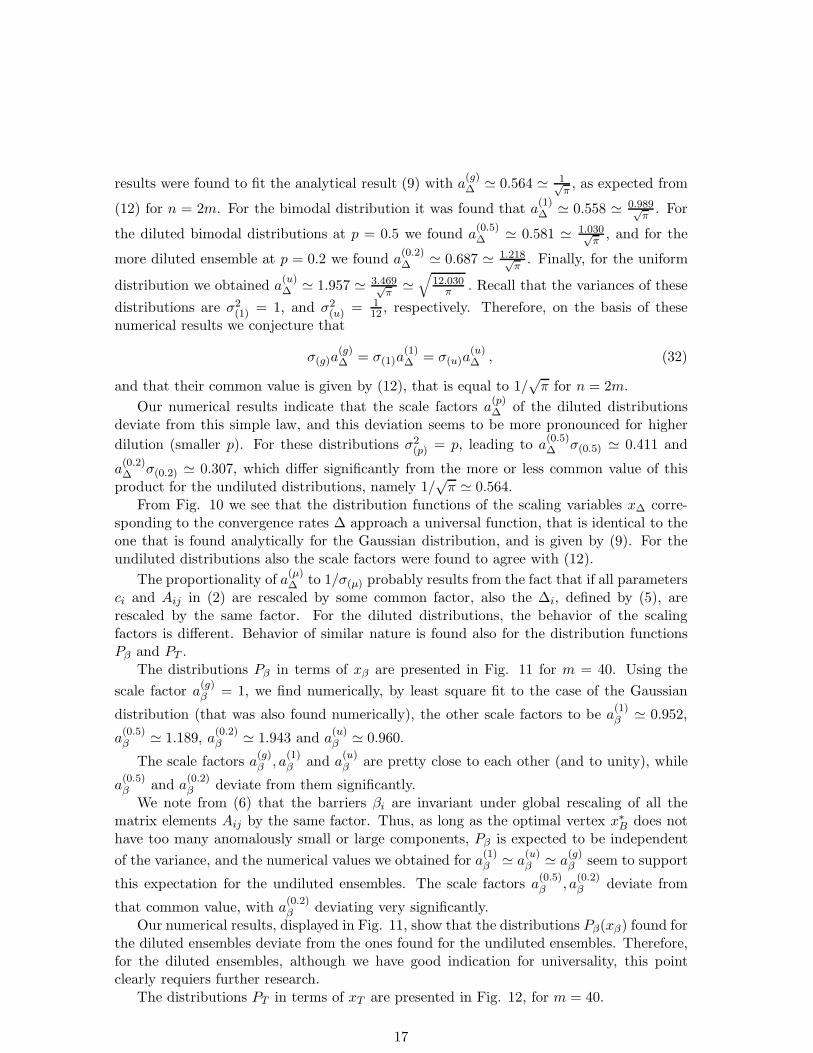
The distributions Pβ in terms of xβ are presented in Fig. 11 for m = 40. Using the

scale factor a(g)β = 1, we find numerically, by least square fit to the case of the Gaussian

distribution (that was also found numerically), the other scale factors to be a(1)β ≃ 0.952,

a(0.5)β ≃ 1.189, a

(0.2)β ≃ 1.943 and a

(u)β ≃ 0.960.

The scale factors a(g)β , a

(1)β and a

(u)β are pretty close to each other (and to unity), while

a(0.5)β and a

(0.2)β deviate from them significantly.

We note from (6) that the barriers βi are invariant under global rescaling of all thematrix elements Aij by the same factor. Thus, as long as the optimal vertex x∗

B does nothave too many anomalously small or large components, Pβ is expected to be independent

of the variance, and the numerical values we obtained for a(1)β ≃ a

(u)β ≃ a

(g)β seem to support

this expectation for the undiluted ensembles. The scale factors a(0.5)β , a

(0.2)β deviate from

that common value, with a(0.2)β deviating very significantly.

Our numerical results, displayed in Fig. 11, show that the distributions Pβ(xβ) found forthe diluted ensembles deviate from the ones found for the undiluted ensembles. Therefore,for the diluted ensembles, although we have good indication for universality, this pointclearly requiers further research.

The distributions PT in terms of xT are presented in Fig. 12, for m = 40.

17

0 1 2 3 4 5 6 7 8 9 100

0.1

0.2

0.3

0.4

0.5

0.6

0.7

0.8

0.9

1

xβ

Pβ

BimodalBimodal p=0.2Bimodal p=0.5UniformGauss (Numerical)

Figure 11: Pβ as a function of xβ for all the distributions checked (for n = 2m and

m = 40), where the scale factors a(µ)β were found by least squares fit to the distribution for

the Gaussian ensemble, which was found numerically as well.

0 1 2 3 4 5 6 7 8 9 100

0.1

0.2

0.3

0.4

0.5

0.6

0.7

0.8

0.9

1

xT

PT

BimodalBimodal p=0.2Bimodal p=0.5UniformGauss (Numerical)

Figure 12: PT as a function of xT for all the distributions checked (for n = 2m and m = 40).

The scale factors a(µ)T were found by least squares fit to the distribution for the Gaussian

ensemble, which was found numerically as well.

18

Using the scale factor a(g)T = 1 we find numerically a

(1)T ≃ 1.008, a

(0.5)T ≃ 1.240, a

(0.2)T ≃

2.088, and a(u)T ≃ 3.399 ≃

√11.553 . From (7) we see that under global rescaling of the

parameters Aij , bi, ci in (2), the scaled variables x′∆ and x′

T are rescaled in the same way.

Thus, since a(g)∆ is proportional to 1/σ, also a

(g)T should satisfy a similar proportionality.

Since for the Gaussian distribution we have taken σ2(g) = 1 and a

(g)T = 1 , our numerical

results, where we find a(u)T ≃

√12 , suggest that for the undiluted ensembles

σ(g)a(g)T = σ(1)a

(1)T = σ(u)a

(u)T , (33)

taking the value unity in our case. For the diluted ensembles we find σ(0.5)a(0.5)T ≃ 0.877 and

σ(0.2)a(0.2)T ≃ 0.933, deviating significantly from unity. For p = 0.2 a significant deviation

of PT from the other distributions is found.

6 Summary and Discussion

In this paper we have presented ample numerical evidence for the fact that the asymptoticdistribution functions P∆, Pβ and PT are scaling functions.

In particular, all the undiluted ensembles of LP problems which we studied, seem tohave the same set of asymptotic distribution functions, when the latter are expressed interms of the scaling variables x∆, xβ and xT . Furthermore, we have found that then the

following combinations of scaling factors, σ(µ)a(µ)∆ , a

(µ)β and σ(µ)a

(µ)T are independent of the

probability distribution. Therefore, in particular, a(µ)∆ should satisfy (12) that was found

for the Gaussian distribution, while a(µ)β and a

(µ)T , as well as corresponding distributions,

are yet to be found analytically.Based the results presented in this paper, as well as the results of [12, 13], we conjecture

the scaling behavior of the various undiluted distribution functions (and the correspondingscaling factors) is universal, i.e., that it is robust and should be valid in a large class ofensembles of LP problems, in which the (A, b, c) data are taken from a distribution withzero mean and finite variance.

We have also studied the effect of dilution, namely, imposing that the parameters Aij , ci

and bi in (2) could vanish with finite probability 1 − p. Specifically, we have studied theeffects of dilution only on the bimodal distribution.

Our findings, depicted in Figs. 7 and 8, as well as the corresponding figures for Pβ

and PT , indicate that the convergence in the limit m → ∞ becomes slower as the dilutionincreases (i.e., as p decreases). More importantly, our numerical results indicate that thediluted distributions may exhibit scaling behavior as well, but with scaling factors which aredifferent from those of the undiluted ensembles which belong in the universality class of theundiluted Gaussian ensemble. Moreover, the corresponding asymptotic scaling distributionfunctions P∆, Pβ and PT of these diluted ensembles deviate sometimes from those of thecorresponding ones of the undiluted Gaussian universality class. This deviation appearsto become more pronounced as dilution increases, and it may be related to the fact thata finite fraction of the admissible LP instances in diluted ensemble may have an optimalvertex x∗

B which has too many anomalously small or large components.

19

Generally speaking, dilution seems to have interesting effects, which are not completelyunderstood, and call for further investigation. Specific questions are motivated by thepresent work. In particular, are the asymptotic scaling distribution functions P∆, Pβ andPT , which we computed numerically, really different from the ones found for the undilutedGaussian ensemble (with possibly scale factors which differ from the Gaussian ones), orthe deviations of these functions, indicated by our numerical results, are merely effects ofthe slower convergence towards asymptotics? If they are different - do they form anotheruniversality class?

Finally, we would like to raise a question which may be of practical importance. Thus,imagine that all LP problems used in practice (or at least, a large fraction thereof) arecollected into an unbiased probability ensemble. How is this distribution of realistic LPproblems related to the ensembles studied in this paper? Does it really relate to a univer-sality class (or classes) of ensembles of LP problems studied here? Does it agree more withthe diluted or the undiluted ensembles? These questions clearly pose important conceptualchallenges for further investigation, and also have practical implications.

20

Acknowledgements: It is a great pleasure to thank our colleagues Asa Ben-Hur andHava Siegelmann for very useful advice and discussions. This research was supported inpart by the Shlomo Kaplansky Academic Chair, by the Technion-Haifa University Collab-oration Fund, by the US-Israel Binational Science Foundation (BSF), by the Israeli ScienceFoundation (ISF), and by the Minerva Center of Nonlinear Physics of Complex Systems.

References

[1] J. Hertz, A. Krogh, and R. Palmer. Introduction to the Theory of Neural Computation.Addison-Wesley, Redwood City, 1991.

[2] C. Mead. Analog VLSI and Neural Systems. Addison-Wesley, 1989.

[3] D. Bray. Nature 376, 307 (1995); A. Ben-Hur and H.T. Siegelmann. Proceedings ofMCU 2001, Lecture Notes in Computer Science 2055, pages 11-24, M. Margensternand Y. Rogozhin (Editors), Springer Verlag, Berlin 2001 (and references therein).

[4] E. Ott, Chaos in Dynamical Systems. Cambridge University Press, Cambridge, Eng-land, 1993.

[5] R. W. Brockett. Linear Algebra and Its Applications 146, 79 (1991); M.S. Branicky.Analog computation with continuous ODEs. In Proceedings of the IEEE Workshop onPhysics and Computation , pages 265–274, Dallas, TX, 1994.

[6] L. Faybusovich. IMA Journal of Mathematical Control and Information 8, 135 (1991).

[7] U. Helmke and J.B. Moore. Optimization and Dynamical Systems. Springer Verlag,London, 1994.

[8] C. Papadimitriou. Computational Complexity. Addison-Wesley, Reading, Mass., 1995.

[9] M.L. Mehta. Random Matrices (2nd ed.). Academic Press, San-Diego, CA, 1991.

[10] T.A. Brody, J. Flores, J.B. French, P.A. Mello, A. Pandey and S.S.M. Wong. Rev.Mod. Phys. 53, 385 (1981).

[11] O. Bohigas, M.-J. Giannoni and C. Schmit. Phys. Rev. Lett. 52, 1 (1984); O. Bohigas.Random Matrix Theories and Chaotic Dynamics. In Chaos and Quantum Physics,Proceedings of the Les-Houches Summer School, Session LII, 1989, M.-J. Giannoni,A. Voros and J. Zinn-Justin, (eds.), North-Holland, Amsterdam, The Netherlands,1991.

[12] A. Ben-Hur, J. Feinberg S. Fishman, and H.T. Siegelmann, J. Complexity 19, 474(2003) (preprint cs.CC/0110056).

[13] A. Ben-Hur, J. Feinberg S. Fishman, and H.T. Siegelmann, Phys. Lett. A 323, 204(2004) (preprint cond-mat/0110655).

[14] H.T. Siegelmann, A. Ben-Hur and S. Fishman, Phys. Rev. Lett. 83, 1463 (1999);A. Ben-Hur, H.T. Siegelmann, and S. Fishman. J. Complexity 18, 51 (2002).

21

[15] H.T. Siegelmann and S. Fishman. Physica 120, 214 (1998).

[16] L. Faybusovich. Physica D53, 217 (1991).

[17] L. Blum, F. Cucker, M. Shub, and S. Smale. Complexity and real Computation.Springer-Verlag, 1999.

[18] S. Smale. Math. Programming 27, 241 (1983); M.J. Todd. Mathematics of OperationsResearch 16, 671 (1991).

[19] S. Smale. Math. Programming 27, 241 (1983).M.J. Todd. Mathematics of Operations Research 16, 671 (1991).

[20] R. Shamir. Management Science 33(3), 301 (1987).

[21] Y. Ye. Interior Point Algorithms: Theory and Analysis. John Wiley and Sons Inc.,1997.

[22] V. Y. Pan and J. Reif, Computers and Mathematics (with Applications) 17, 1481(1989).

[23] K.G. Wilson and J. Kogut, Phys. Rep. 12, 75 (1974).

[24] E. Abrahams, P. W. Anderson, D. C. Licciardelo and T. V. Ramakrishnan, Phys. Rev.Lett. 42 673 (1979).

[25] Some papers that treat random real rectangular matrices, such as the matrices relevantfor this work (which are not necessarily Gaussian ), are: A. Anderson, R. C. Myers andV. Periwal, Phys. Lett.B 254, 89 (1991); Nucl. Phys. B 360, (1991) 463 (Section3); J. Feinberg and A. Zee, J. Stat. Mech. 87, 473 (1997); For earlier work see: G.M.Cicuta, L. Molinari, E. Montaldi and F. Riva, J. Math.Phys. 28, 1716 (1987).

[26] Y. S. Avizrats, J. Feinberg and S. Fishman, Scaling and Universality of the Complexity

of Analog Computation, to appear.

22