scaling and regionalization of flood flows in british columbia, canada

HYDROLOGICAL PROCESSESHydrol. Process. 16, 3245–3263 (2002)Published online 1 October 2002 in Wiley InterScience (www.interscience.wiley.com). DOI: 10.1002/hyp.1100

Scaling and regionalization of flood flows in BritishColumbia, Canada

Brett Eaton, Michael Church* and Darren HamDepartment of Geography, The University of British Columbia, 217-1984 West Mall, Vancouver, British Columbia V6T 1Z2, Canada

Abstract:

A regionalization of flood data in British Columbia reveals a common scaling with drainage area over therange 0Ð5 ð 102 < Ad < 104 km2. This scaling is not a function of flood return period, which implies that simplescaling—consistent with a snowmelt-dominated flow regime—applies to the province. The observed scale relationtakes the form Q / A0Ð75

d , similar to values reported in previous studies. The scaling relation identified was used todefine the regional pattern of hydroclimatic variability for flood flows in British Columbia after discounting the effectof drainage area. The pattern was determined by kriging a scale-independent runoff factor k for the mean annual flood,5 year flood and 20 year flood. The analysis permits quantification of uncertainty of the estimates, which can be usedin conjunction with the mapped k-fields to calculate a mean and range for floods with the identified return period forungauged basins. Owing to the sparsity of data, the precision is relatively poor. The standard error is generally less than75% of the estimate in the southern half of the province, whereas in the northern half it is often between 75 and 100%.Examination of the relative increase in flood magnitude with increasing return period reveals spatially consistent butstatistically insignificant differences. Flood magnitude tends to increase more rapidly in the western regions, where rainevents may contribute to flood generation. The relative increase in flood magnitude with return period is consistentlylower in the eastern mountain ranges, where snowmelt dominates the flood flow regime. Copyright 2002 John Wiley& Sons, Ltd.

KEY WORDS flood flows; regional hydrology; scaling; self-similarity; specific runoff

INTRODUCTION

Water management in British Columbia revolves principally about the surface water resource. Informationabout this resource is derived from flow gauging in streams and water level records of lakes. Thesemeasurements are expensive to make; consequently, they are relatively sparse, and certainly insufficientto provide direct answers to many practical water resource questions. However, the moderately conservativenature of hydrological fields opens the possibility to increase the practical information that can be extractedfrom measurements by regionalization of the extant data.

Traditionally, regionalization has been achieved through a division of the domain of study into compact,evidently homogeneous units. This procedure is constrained by ‘scale domains’—units in space and timewithin which the hydrological processes remain, in some sense, consistent. But in order to examine theregional hydrology, it is necessary first to discount the effect of drainage basin area Ad. Discharge has beenempirically related to drainage area by non-linear relations of the form:

Q D cAbd �1�

Dooge (1986) reminds us of speculative discussions about the non-linearity of Q�Ad) relations as far backas 1850. The first systematic attempt to relate floods of a particular return period to drainage basin area

* Correspondence to: Michael Church, Department of Geography, The University of British Columbia, 217-1984 West Mall, Vancouver,British Columbia V6T 1Z2, Canada. E-mail: [email protected]

Received 18 June 2001Copyright 2002 John Wiley & Sons, Ltd. Accepted 25 February 2002

3246 B. EATON, M. CHURCH AND D. HAM

apparently was that of Fuller (1914), who found, for mean annual flood, b D 0Ð80. Much more recently theUnited Kingdom Flood Study (NERC, 1975) found b D 0Ð77, whilst Mosley and McKerchar (1992) havereplicated Fuller’s result for a sample of New Zealand rivers. In Canada, Ribeiro and Rousselle (1996)obtained a scaling exponent of 0Ð64 for a sample of southern Ontario rivers, whilst Pandey (1998) reported0Ð72 for Ontario streams and 0Ð76 for streams in southern Quebec. Values ranging from 0Ð60 to 1Ð0 havebeen reported in a range of North American studies summarized by Cathcart (2001) (see also Bloschl andSivapalan (1997)). Dooge (1986) observed that most figures are close to the result b D 0Ð75, which one wouldexpect on purely dimensional grounds based on a Froude similarity criterion. However, Bloschl and Sivapalan(1997) and Cathcart (2001) have noted an apparently systematic variation in the exponent from low values(e.g. 0Ð60) for arid systems to high values (approaching 1Ð0) for perhumid systems. That is, scaling appearsto approach linearity with increasing humidity. Other investigators (e.g. Benson, 1962) have found somewhatdifferent correlations when drainage basin gradient is added as an additional variate.

Recent work on scaling of hydrologic variables (Gupta and Waymire, 1990) indicates that—withinhydrologically homogeneous regions—flood runoff moments scale with drainage area according to log–loglinear relations. So, for example, specific runoff (q, the first moment of specific runoff) scales as:

log�q� D a C b log�Ad� �2a�

or

q D 10aAbd �2b�

where b < 1. The quantity 10a in Equation (2b) is equivalent to the parameter c in Equation (1), and b inEquation (2) is different from b in Equation (1) by a constant value of 1Ð0 (because q D Q/Ad). Their resultsprovide a probabilistic–statistical basis to expect the observed empirical scale relations.

It is clear, then, that in order to investigate the underlying physical behaviour of drainage systems, the scaleeffect must be eliminated in order to isolate the physical effects for study. An exploration of this matter, bya study of scale relations for mean annual flood Qmaf, 5 year return period flood Q5 and the 20 year returnperiod flood Q20 in the province of British Columbia, is the object of this paper.

THE DATA SET

A data set was assembled by examining all Water Survey of Canada (WSC) streamflow records for BritishColumbia. Because temporal variability becomes confounded with spatial variability if records are chosenfrom different periods, a common period of record is required. Furthermore, analysis should be restricted to aperiod of relative hydroclimatological stability in order that flow recurrence intervals can properly be defined.Significant hydrological variability is evident within the period of record in British Columbia, which is drivenby decadal-scale climatic variations in the central North Pacific, referred to as the Pacific decadal oscillation(Mantua et al., 1997). Hydrological stability was examined by the construction of cumulative departure plotsfor a number of long stream gauging records in British Columbia (Figure 1). There are strong trends evidentthroughout the hydrometric record. We wished to adopt a relatively recent period for analysis, both because theresults would seem to be more relevant to the current situation and because the largest number of hydrometricstations has been active in recent time.

There are indications of an overall reduction in flood flows since about the mid 1970s. The reason for it is theoccurrence of warmer winters, which has reduced the magnitude of winter snowpacks, and hence the magnitudeand duration of spring runoff. Drainage basins in which the annual peak flow is usually contributed bysnowmelt runoff—i.e. nearly all of British Columbia except in low elevation coastal areas—have accordinglyexperienced reduced flood flows in recent years; see Moore (1991) and Moore and McKendry (1996). In fact,the change of regime appears to have occurred after 1976, in concert with widespread changes in western

Copyright 2002 John Wiley & Sons, Ltd. Hydrol. Process. 16, 3245–3263 (2002)

SCALING SURFACE RUNOFF 3247

-100

300

200

200

0

-200

700

500

300

100

0

100 0

-300

90

60

0

-200

500

300

10019001900 1930 1960 1990 1930 1960 1990

30

-100

1900 1930 1960 1990 1990 1930 1960 1990

Cowichan River Boundary Creek

Columbia River/Nicholson Stuart River

Cu

m. D

ep.

(%)

Cu

m. D

ep.

(%)

Flo

w(m

3 /s)

Flo

w(m

3 /s)

Figure 1. Mean annual flood sequences and cumulative departures plots for selected long-term hydrometric stations in British Columbia. Thecumulative departure of a record (see Buishand (1982)) is Xi D ∑

�xi � hxi�, in which hxi is the long-term mean value of the signal. Anyportion of the record that exhibits a consistent linear trend is stable. A portion of the record that exhibits no trend (i.e. plots horizontally) isstable with the mean for that period equal to the long-term mean. The shaded region indicates the period selected for analysis. Stuart Riveris regulated by large natural lakes. This does not affect analysis of long-term trends in flows. At Cowichan River an abrupt change fromabove-average (rising graph) to below-average (descending graph) conditions occurs midway through the observing period, illustrating the

difficulty in obtaining homogeneous records from all parts of the province. Stations are located in Figure 2

North American climatic regime (Trenberth, 1990). Accordingly, the flood analysis was restricted to the20 year interval 1976–95.

Four other criteria constrained the choice of records for analysis. First, only stations with unregulatedflows were considered. ‘Regulation’ was defined to include the presence of significant natural lakes in thedrainage basin, as well as human manipulation. Second, only stations with at least 10 years of record in theperiod 1976–95 were included in the analysis, since this is the minimum number of data that is consideredto be sufficient for estimating the 20 year return period flood (Stedinger et al., 1992; see also Ribeiro andRousselle (1996)). Third, a minimum basin size was established. Evidence from Melone (1985), who analysedmaximum observed flows in the Coast Mountains, suggests that, below about 100 km2, spatial scale effectsdo not systematically affect flood runoff, whilst Coulson (1991) specified 25 km2 for the region. Smith (1992)and Cathcart (2001) have identified a similar limit on the order of 50 km2. For this work, the lower limit ondrainage basin size was chosen to be 60 km2, which maximizes the number of stations retained for analysis.Last, the upper limit on basin size was chosen to be 10 000 km2 in order to preserve regional integrity in therecords. However, one record is included from an 11 200 km2 basin in the northeastern mountains of BritishColumbia in order to increase the minimally sparse information in that region.

In total, 147 stations were selected for examination (Figure 2). The sample realized is well distributedwithin the range 60 < Ad < 10 000 km2, representing linear scales between 10 and 100 km. On average, eachstation represents about 7000 km2, although in parts of southern British Columbia the density is as high as one



0 250 km

Cowichan R. Chilliwack R.Squamish R.

Boundary Cr.

Columbia R.

NortheasternPlains

NortheasternMountains

Northern Interior

Stuart R.

Caribooand Monashee

Mountains

NorthernRocky

Mountains

SouthernRocky

MountainsCoast

Mountains Okanagan Kootenayand

ColumbiaMountains

Chilcotinand Cariboo

Plateaux

ExposedCoasts

and Fjords

Gauge locationsHydrologic regionsRivers and lakes

Cascade Mountains

Figure 2. Distribution of sample gauges in British Columbia superimposed on the arbitrary regionalization used for initial analysis of scalerelations. Stations for which records are displayed in Figures 1 and 3 are located (italic type)

in 2500 km2 (corresponding to 50 km spacing). In the north, it is nearer one in 20 000 km2(150 km spacing).In comparison, the World Meteorological Organization norm for hydrometric station density in mountains isone in less than 1000 km2 and the outside guideline is one station in 5000 km2 (WMO, 1981). Furthermore,most of the smallest basins in the study are located in the southern interior regions of the province, whereasa disproportionate number of the largest basins is located in the northern half of the province. There is, then,potential to confound basin scale with regional factors in the streamflow data.

Estimates of the 5 and 20 year floods were made using the extreme value distribution that best fit the rankedannual maximum flood record at each station. Because the record length was nominally 20 years, in mostcases estimates of the 5 and 20 year flood did not involve extrapolation outside the data range. The intent ofusing a frequency distribution to estimate the 5 and 20 year floods was to reduce the sampling scatter in theestimates. The distributions tested included the normal, log-normal, Gumbel, Pearson type III, and log-Pearsontype III distributions, which are the distribution types used by the British Columbia River Forecast Centre.Use of these models assumes that the flood frequency distribution is generated by a homogeneous underlyingprocess. This seems to be appropriate for most of the province, but may be violated along the coast, wherefloods are characteristically produced by both snowmelt and rain-on-snow events in basins of intermediate



size (Church, 1988). The effect that this has on the fit of the theoretical distributions to the data is shownin Figure 3. The records for the rivers illustrated contain two distinct populations of events; one populationincludes events occurring in the autumn and winter (typically between October and February) that are usuallythe result of rain-on-snow events; the other population includes spring and summer events (April to August)that result primarily from snowmelt. Although it is evident that the flood-generating processes in these twodrainage basins are not homogeneous, the test distributions seem to perform adequately.

The fit of each of the distributions was assessed visually using a typical return period versus discharge plot.In most cases the normal, log-normal and log-Pearson distributions were quickly discarded as inappropriate,and the choice was practically limited to the Gumbel and Pearson type III distributions. The Pearson type IIIfit best 88% of the time, and the Gumbel was used for all but two of the remaining stations.

During the flood frequency analysis, it was noted that, for certain stations, the largest flood in the 20 yearrecord was much larger than the estimated 20 year flood. Inclusion of these extreme events has a substantialeffect on the estimates for the 5 and 20 year floods. This problem can be dealt with using ‘probabilityweighted moments’ (Kumar et al., 1994), but we chose instead to proceed empirically. In all cases wherean event of exceptionally large magnitude seemed to have been included in the record, the flood frequencyanalysis was subsequently repeated, excluding the extreme event. Such outliers were identified in the recordsof 58 stations; the apparent return period for these outliers ranged from 45 to >200 years, with a mean of72 years. According to Chow (1964), the probability of exceeding a flood of return period t within n yearsis 1 � �1 � �1/t��n. Assuming that all floods with return periods greater than 40 to 50 years were identifiedas outliers, we would expect between 33 and 40% of the gauge records to be affected. This calculation isconsistent with our findings, since outliers were identified in 39% of the station records. The removal ofthese outliers from the data set resulted in a reduction of between 5 and 34% in the 20 year flood estimate;the mean reduction was 17%. Because of the influence that these outliers have on estimates of the 20 yearflood, and given that the associated return periods for these outliers average nearly 75 years, it was decidedto exclude them from the hydrologic records used for this analysis. The resulting flood estimates are assumedto represent estimates of the values that would be realized by a long record during a period of no net climatechange.

2500

2000

1500

1000

500

01 2 5 10 20 1 2 5 10 20

500

400

300

200

100

0

Return Period (yrs)

a) b)

Mea

n A

nn

ual

Max

imu

m D

aily

Dis

char

ge

(m3 /

s)

Figure 3. Flood frequency distributions for two stations with mixed flood-generating processes. Open symbols identify spring and summerevents primarily associated with snowmelt, and solid symbols identify fall and winter events primarily associated with rain-on-snow events.Fitted distributions are the Gumbel distribution, indicated with a dashed line, and the Pearson type III distribution, with a solid line.(a) Squamish River near Brackendale (WSC stn. 08GA022); (b) Chilliwack River at Vedder Crossing (WSC stn. 08MH001). Stations are

located in Figure 2



STRATEGY FOR ANALYSIS

Since drainage basin size is clearly the dominant determinant of streamflow magnitude within any reasonablydefined region, a meaningful regionalization consists of defining hydrological variability not associated withdrainage-basin scale. Scale effects may be incorporated into regional analyses either by making drainage areaan independent variable or by performing an adjustment of the data to account for it.

The relation Q�Ad� is known, from analyses conducted over many years at the provincial Water ManagementBranch, to vary within the province (Coulson, 1991). This is the consequence of large variations in the principalcontrolling factors: climate and physiography. To facilitate the identification of scale relations and to studytheir regional consistency, an initial regionalization was arbitrarily imposed that divided the province intoten regions based on expected hydroclimatic uniformity. Figure 2 shows the regions. They were defined usingjudgement based on knowledge of physiography and climate, thus introducing implicit information about thefactors that control regional hydrology in the province. However, this does not control the final results. Thedata were inspected for subregional homogeneity and a few stations were reassigned to a different region,which entailed making minor adjustments to the regional boundaries.

Subregional variability was also noted that could not be eliminated by reassignment. Separate populationsof drainage basins can be identified in the Okanagan–Thompson Plateau region, depending upon whether ornot the station includes significant upland drainage. Similarly distinct populations of high and low elevationdrainage basins are identified in the Kootenay Mountains. Such variations are apparent only in regions withinwhich there are a number of relatively small gauged basins (<100 km2); larger basins average out this sortof variability. On the coast, exposure is evidently important and determined the occurrence of the ‘exposedcoast’ region. In all, five of the ten regions were further subdivided, giving a total of 16 different populations.

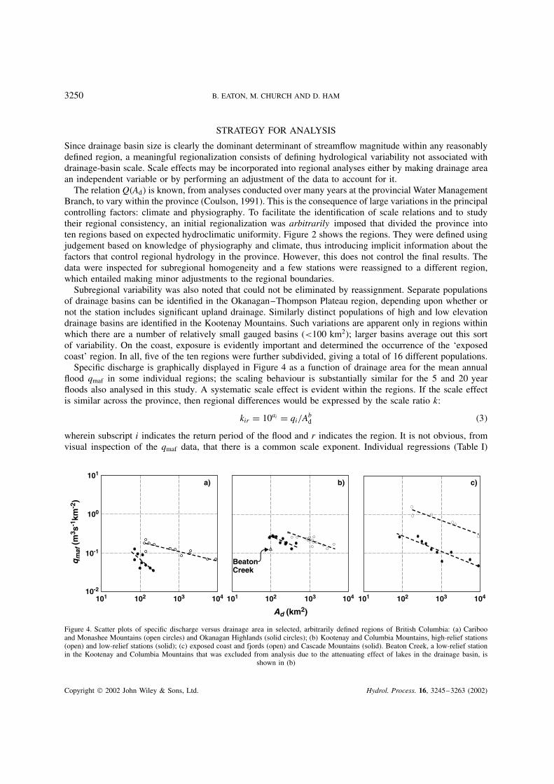
Specific discharge is graphically displayed in Figure 4 as a function of drainage area for the mean annualflood qmaf in some individual regions; the scaling behaviour is substantially similar for the 5 and 20 yearfloods also analysed in this study. A systematic scale effect is evident within the regions. If the scale effectis similar across the province, then regional differences would be expressed by the scale ratio k:

kir D 10ai D qi/Abd �3�

wherein subscript i indicates the return period of the flood and r indicates the region. It is not obvious, fromvisual inspection of the qmaf data, that there is a common scale exponent. Individual regressions (Table I)

101

100

10-1

10-2

101 102 103 104 101 102 103 104 101 102 103 104

Ad (km2)

qm

af (

m3 s

-1km

-2)

a) b) c)

BeatonCreek

Figure 4. Scatter plots of specific discharge versus drainage area in selected, arbitrarily defined regions of British Columbia: (a) Caribooand Monashee Mountains (open circles) and Okanagan Highlands (solid circles); (b) Kootenay and Columbia Mountains, high-relief stations(open) and low-relief stations (solid); (c) exposed coast and fjords (open) and Cascade Mountains (solid). Beaton Creek, a low-relief stationin the Kootenay and Columbia Mountains that was excluded from analysis due to the attenuating effect of lakes in the drainage basin, is

shown in (b)



Table I. Regional scale relations for mean annual flood (log10 data)a

Region n Intercept Slope R2 hlog Adri hlog qmafri kmafr

coef. t stat. coef. t stat. (m3 s�1)

1.1 Exposed Coast and fjords 6 0Ð960 4Ð87 �0Ð370 �5Ð73 0Ð86 2Ð99 �0Ð146 4Ð051.2 E Vancouver Isl. and W Coast Mtns 18 0Ð722 4Ð93 �0Ð364 �6Ð75 0Ð72 2Ð67 �0Ð250 2Ð651.3 Eastern Coast Mountains 7 0Ð364 2Ð46 �0Ð341 �6Ð01 0Ð85 2Ð59 �0Ð517 1Ð362 Cascade Mountains 10 0Ð212 1Ð12 �0Ð391 �6Ð10 0Ð80 2Ð91 �0Ð925 0Ð6443.1 Okanagan Highlands 9 0Ð533 0Ð90 �0Ð850 �2Ð97 0Ð49 2Ð06 �1Ð22 0Ð1993.2 Okanagan & adjacent valleys 2 2Ð02 �2Ð10 0Ð0264.1 Chilcotin & Cariboo plateaux: uplands 7 �0Ð463 �2Ð80 �0Ð324 �5Ð14 0Ð81 2Ð57 �1Ð30 0Ð2254.2 Chilcotin & Cariboo plateaux: Fraser Basin 3 3Ð23 �1Ð87 0Ð0885 Cariboo & Monashee Mountains 11 �0Ð034 �0Ð27 �0Ð236 �5Ð36 0Ð76 2Ð82 �0Ð930 0Ð6146.1 Kootenay & Columbia Mtns: high relief 15 0Ð396 2Ð12 �0Ð356 �5Ð83 0Ð70 3Ð04 �0Ð685 1Ð206.2 Kootenay & Columbia Mtns: low relief 10 0Ð238 1Ð07 �0Ð406 �4Ð18 0Ð65 2Ð28 �0Ð687 0Ð7717.1 Southern Rocky Mountains 16 �0Ð474 �4Ð13 �0Ð164 �4Ð39 0Ð55 2Ð99 �0Ð964 0Ð6157.2 Northern Rocky Mountains 10 �0Ð400 �2Ð59 �0Ð112 �2Ð17 0Ð29 2Ð92 �0Ð728 1Ð028 Northeastern Mountains 5 3Ð58 �1Ð12 0Ð6109 Northeastern Plains 4 3Ð40 �1Ð25 0Ð40410 Northern Interior 14 �0Ð680 �3Ð38 �0Ð108 �1Ð73b 0Ð13 3Ð17 �1Ð02 0Ð596

a No regressions were performed for regions with �5 data points. h. . .i indicates a mean value. In logarithmic units, log kmafr Dhlog qmafri � bhlog Adri. kmafr reported in original units. Student’s t statistics test the hypothesis that the coefficient is not different fromunity.b Not significant at ˛ D 0Ð05.

reveal substantial variation. But each region is represented by only a small sample of stations, so there is aconsiderable chance that the scale exponent in individual regions is biased by the particular set of availablestations.

Some additional factors increase the possibility of regional bias. Within individual regions, the choiceof basins for gauging is sometimes biased by the purpose of the gauging program. For example, in theOkanagan region, most of the stations are located in small drainage basins selected because of downstreamcontrol for provision of irrigation water. In the north, all gauged basins are large, the consequence of selectionto investigate the potential for hydropower or for regional water resource inventory. In the southern RockyMountains, a significant subset of the gauges was established to facilitate studies of potential water qualityimpacts of coal mining. In some regions, several of the gauged stations are on a single river system. Forexample, Similkameen River and its principal tributaries contribute seven of ten records in the CascadeMountains. This may create artificially good scale relations that, nevertheless, are not the best regionalestimates.

Covariance analysis shows that there is, nevertheless, a common scale effect (discussed below). A scalecollapse can, therefore, be achieved and the scale-free data analysed further to demonstrate the regional effectsof the primary physiographic and climatological controls of runoff. We may, then, suppose that scale effectsdo not strongly depend on the primary controls of runoff. This is convenient because, in the same way that aregional scale relation has a scale ratio kir , defined by Equation (3), each station may be supposed to possessa scale ratio, given by:

kij D 10aij D qij/Abdj �4�

where the subscript j indicates the station. kij incorporates both the variation of the regional scale relationfrom the common scale, and the variation of the individual station from its regional relation (Figure 5: inset).That is, each station may be collapsed to a scale-free relation independently of the others in its set. kij carriesthe information about the effect of primary controls on the runoff in the individual drainage basin and it (or,



101

101

100

10-1

10-2

102 103101100

102 103 104

101

10-2

10-1

100

qi

Ad

qmaf =1.0Ad-0.2507

adjusted qmaf values

regional data centroid

qm

af a

dju

sted

by

k maf

r (m

3 s-1

km-2

)

qi = A

db

station j

kij

Ad (km2)

Figure 5. Massed plot of the reduced data for mean annual flood and the common scaling relation. The diagram also shows the regionalmeans, the departures of which constitute the values of kmafr for each region. The value kmafr for each region is thus seen to be the ratioof runoff given by the common scale relation to the mean runoff for that region. The inset diagram illustrates the principle of the scale

reduction

equivalently, the un-transformed parameter aij) is the appropriate quantity for further analysis. This frees usfrom dependence upon the original, arbitrary regionalization, which has served merely to investigate the scalerelation for runoff. The finally adjusted data are scale free (i.e. do not depend upon the drainage areas of theobserving stations) and free of arbitrary categorization. kij is an estimate of the unit-area or specific runoffassociated with each gauge. The individual kij values generally resemble their regional mean, but they alsopreserve information about intra-regional variations. The following analysis examines the spatial variations ofkij, thereby replacing the initial regionalization with a smooth surface representing continuous hydrologicalgradations.

There are some practical statistical issues associated with the analysis. First, we investigated the scaleexponent b using ordinary forward regression, since we suppose that drainage areas are known with highprecision in comparison with the return-period flows derived from relatively short records (see Mark andChurch (1977) on the issue of functional relations and regression). Second, the analyses were conductedin logarithmic space. The back-transformed scale relations represent median regional response (as opposedto mean response; see Miller (1984)). This is tantamount to de-emphasizing the significance of occasional



unusually large values (such as an individual drainage basin with anomalously large runoff, or an anomalouslylarge estimate of mean annual flood). Hence, no transform adjustments were performed. Finally, because thenumber of data associated with each region is small, no tests of distribution assumptions (e.g. of the residualsfrom regression) have been performed.

The balance of the paper displays the results of our analyses. These lead to a method to synthesize flowsfor a drainage basin of some specified size at any place in the province.

SCALE RELATIONS

Mean annual flood

We consider mean annual flood first because this analysis has many precedents in the literature (althoughthey have not generally been represented as scale relations). Before the analysis of covariance, inspectionof the regional plots led to the deletion of five stations as obviously anomalous within their region. Theanomalous stations were examined on 1 : 250 000 scale maps, and explanations for their anomalous characterwere sought. Most often, previously undetected lakes or significant wetlands were present in the basin. As anexample of the judgement applied in identifying anomalous streams, Beaton Creek, a low-relief basin in theKootenay and Columbia Mountains region, is shown in Figure 4b with the rest of the data from that region.

Table II reports the analysis of covariance for 133 stations that satisfied the selection criteria for regionalhomogeneity; 14 stations were excluded from the analysis, since they were located in regions having fewerthan six stations (see Table I). In the analysis, a dummy variable was used to represent the effect of individualregions, yielding estimates of kmafr . The effect of basin scale was accounted for by including the drainagebasin area in the model. Thus, for an analysis of n regions, n dummy variables are generated, giving n C 1dependent variables. The coefficients for the dummy variables represent kmafr , and the coefficient for drainagearea represents the scaling exponent in Equation (2). The regions account for 78Ð5% of the variability, andthe common regression (log�Ad� in Table II) accounts for an additional 12Ð3% of the variability. The latter

Table II. Analysis of covariance (ANCOVA)

Source Sum of squares Degrees offreedom

Meansquare

F-ratio P

Dependent variable D log�qmaf�Region 14Ð448 11 1Ð313 92Ð955 0Ð000log�Ad� 2Ð256 1 2Ð256 159Ð649 0Ð000

Error 1Ð696 120 0Ð014Total 18Ð400

n D 133, R D 0Ð950, R2 D 0Ð903

Dependent variable D log�q5�Region 15Ð03 11 1Ð366 101Ð546 0Ð000log(Ad� 2Ð326 1 2Ð326 172Ð854 0Ð000

Error 1Ð615 120 0Ð013Total 18Ð971

n D 133, R D 0Ð955, R2 D 0Ð911

Dependent variable D log�q20�Region 15Ð973 11 1Ð452 104Ð225 0Ð000log�Ad� 2Ð336 1 2Ð336 167Ð694 0Ð000

Error 1Ð672 120 0Ð014Total 19Ð981

n D 133, R D 0Ð956, R2 D 0Ð913



result is significant and indicates a common scale effect; this permits collapse of all the data onto a singlescale relation.

It is useful to examine this relation in order to appreciate the residual variance not associated with drainagebasin area. The regional values kmafr are applied to reduce the data of each region to scaled values qmafj/kmafr ,which are then plotted against Adj (Figure 5). The common scale relation has the expression (obtained byregression):

log�qmafj/kmafr� D �0Ð2507 log�Adj� �5�

for which R2 D 0Ð641 and the 95% confidence interval about the coefficient (which is the exponent in theback-transformed relation) is š0Ð0342. The relation when transformed back from log units is given by:

qmafj/kmafr D 1Ð0A�0Ð2507dj �6a�

or

Qmafj/kmafr D 1Ð0A0Ð7493dj �6b�

This result is consistent with results reported in prior studies, in that the exponent for the Qmaf�Adi� relationis not statistically different from the value of 0Ð75 suggested by Dooge (1986).

Substantial variation in the scaled data remains unaccounted for. The residuals are normally distributed(Figure 6a), but they vary systematically with the value of Qmaf (Figure 6b). There is a tendency for largerthan average discharges to be underestimated and vice versa. The regional regressions summarized in Table Ireflect the same tendency, since most of them have b < �0Ð25, implying an aggregate deviation of the within-region scaling from the common scaling. This may be attributable to spatial hydrological gradients within theregions. There is known to be a continuous gradient of climate across the province, and there may also bean elevation effect whereby higher (and smaller) basins receive more precipitation than lower, larger basins.These effects may be exaggerated by the spatial distribution of large and small basins in our data set. Theeffect remains a source of local bias in the scale collapse, but we have not pursued it for lack of additionalinformation.

101 102 103 104 105 0%-0.400

-0.200

0.000

0.200

0.400

100% 200%

Area

a) b)

log(Qmafj/kmafr) /<log(Qmafj/kmafr)>

Res

idu

al {

log

(Qo

bs.

)-lo

g(Q

est.)}

Figure 6. Residual plots for mean annual flood: (a) residuals plotted against area; (b) residuals plotted against the regionally collapsed,normalized discharge (Qmaf/kmafr)



5 and 20 year return period floods

Using the estimates of the 5 and 20 year floods, analysis of covariance was performed, as discussedabove for the mean annual flood, with similar results (Table II). The common scale relations are given inEquations (7) and (8):

q5j/k5r D 1Ð0A�0Ð2545dj �7�

q20j/k20r D 1Ð0A�0Ð2551dj �8�

The exponents in the common scale relations for the mean annual flood, the 5 year flood and the 20 yearflood are not significantly different from each other or from the expected value of 0Ð75 proposed by Dooge(1986). These results confirm that simple scaling applies in British Columbia, as previously speculated.

Once we have the scaling exponent, the n values of kir can be replaced by values of kij, and then used inthe kriging procedure described below to develop a predictive system for flood magnitude in a drainage basinof any size within the limits 60 to 104 km2 at any location in the province.

REGIONAL MAPS OF FLOOD MAGNITUDE

Individual stations can be related to the common scale equation, as shown in Figure 5. The calculationof a set of kij values adjusts all data to represent unit-area runoff, independent of scale effects. Maps ofthese data present the variability of streamflow due to non-scale factors. We present maps of specific runofffor the mean annual flood, 5 year flood and 20 year flood. These maps were created by kriging individualvalues of the untransformed parameter aij (because it meets homogeneity requirements for the procedure)then transforming the resultant surface to kij. The results are not bound by the original, arbitrarily definedregions: the information is expressed as a smoothly varying hydrologic field reflecting intra-regional as wellas inter-regional hydrologic variability. We referred the scaled flow data to the gauge points for mapping(rather than to the basin centroid), since the flows remain a property of the gauge point.

Kriging (see Davis (1986)) takes advantage of the local correlation to estimate a non-regular trend surfaceoptimally fitted through all the data by finding a best set of weights to estimate the surface at unsampledpoints. This procedure permits an estimate to be made of the local standard error. The particular surface thatis developed is, of course, an artifact of the data. The ‘true’ regional surface could be predicted only if thegauging system truly samples the regional variation of hydrological quantities. The British Columbia gaugingsystem certainly does not achieve that.

We performed our analysis using the kriging function of the Arc/Info GIS, which offers six kriging choices.Model performance was assessed by (1) examining the fit of the kriging algorithms to the semivariogram,and (2) comparing kriged values at the data locations with the data themselves. We found that the exponential(root-mean-square error (RMSE): 0Ð048) and universal (RMSE: 0Ð048) kriging models best fitted the data(Figure 7), suggesting that they might represent optimal kriging methods. We know that there is large-scalestructure in the runoff fields, and we therefore chose to use the universal kriging method, for which we obtaineda zero nugget. Because the data are irregularly distributed, we defined our computing window on the basisof 12 included data points, within the constraint of a 250 km maximum radius indicated by the variogram.Kriged estimates of the aij were produced on a 10 km ð 10 km lattice covering the entire province, leadingto about 104 runoff estimates. Maps were produced by back-transforming the lattice values to yield the kij,and converting the lattices to polygon coverages representing 1000 range classes. These were then classifiedinto seven range classes for presentation. The maps reflect both the original gauge data and the decisionstaken in the kriging process.

The maps presented in Figures 8, 9 and 10 permit runoff estimates to be made for any point in the provincefor the mean annual flood, 5 year flood and 20 year flood respectively. For example, given a drainage basin



00

0.3

0.2

0.1

200 400

Distance (km)600 800

sem

ivar

ian

ce

ACTUAL

EXPONENTIAL

Figure 7. Semivariogram and fitted exponential kriging function for the mean annual flood. A fit to the semivariogram is not possible usingthe universal kriging algorithm, which detects and adjusts for systematic trends in the data. (The drift is modelled by a linear function and

the final surface is estimated by a combination of the kriged residuals and the linear drift)

with area Adj the discharges for these three return periods can be calculated by:

Qmafj D kmafjA0Ð7493dj �9a�

Q5j D k5jA0Ð7455dj �9b�

Q20j D k20jA0Ð7449dj �9c�

in which the coefficient kmafj, k5j or k20j is extracted from the appropriate map (or, more precisely, from thecomputed lattice file of the map) for an arbitrary point in the province. Error estimates may be attached tothe runoff estimates by substituting in Equation (9) upper and lower bound estimates for the value of kj. Thestandard error map produced by the kriging model (SEai) can be manipulated to give upper and lower boundsfor the kj estimates. Because of the transformation applied to the aj surface, the standard error associatedwith the kj surface is asymmetrical. In Figure 11, we present a map for one standard error above the mean(i.e. the larger error), expressed as a proportion of the mean, for Qmaf. The quantity actually mapped is givenin Equation (10a); the equation for the lower bound is given in Equation (10b).

SEkmaf�upper� D 10SEamaf � 1 �10a�

SEkmaf�lower� D 1 � 10�SEamaf �10b�

REGIONAL PATTERNS OF RUNOFF

Figures 8, 9 and 10 represent the scale-free regional hydrology of mean annual flood, 5 year flood and 20 yearflood respectively. The major pattern of flows is well known to follow the structural–topographic grain of the



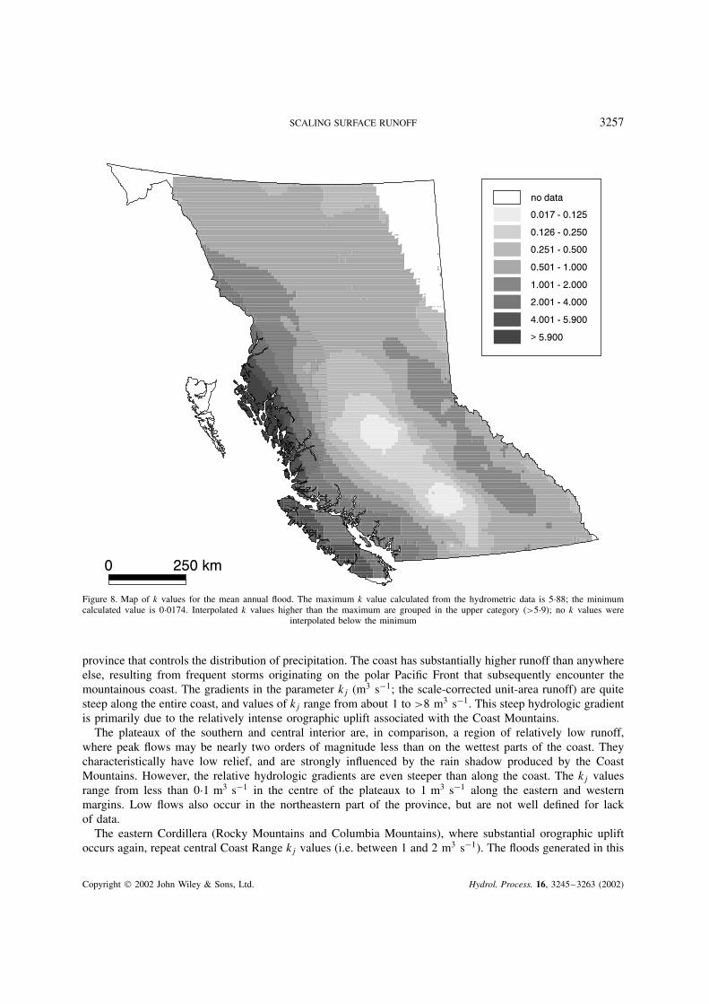
Figure 8. Map of k values for the mean annual flood. The maximum k value calculated from the hydrometric data is 5Ð88; the minimumcalculated value is 0Ð0174. Interpolated k values higher than the maximum are grouped in the upper category (>5Ð9); no k values were

interpolated below the minimum

province that controls the distribution of precipitation. The coast has substantially higher runoff than anywhereelse, resulting from frequent storms originating on the polar Pacific Front that subsequently encounter themountainous coast. The gradients in the parameter kj (m3 s�1; the scale-corrected unit-area runoff) are quitesteep along the entire coast, and values of kj range from about 1 to >8 m3 s�1. This steep hydrologic gradientis primarily due to the relatively intense orographic uplift associated with the Coast Mountains.

The plateaux of the southern and central interior are, in comparison, a region of relatively low runoff,where peak flows may be nearly two orders of magnitude less than on the wettest parts of the coast. Theycharacteristically have low relief, and are strongly influenced by the rain shadow produced by the CoastMountains. However, the relative hydrologic gradients are even steeper than along the coast. The kj valuesrange from less than 0Ð1 m3 s�1 in the centre of the plateaux to 1 m3 s�1 along the eastern and westernmargins. Low flows also occur in the northeastern part of the province, but are not well defined for lackof data.

The eastern Cordillera (Rocky Mountains and Columbia Mountains), where substantial orographic upliftoccurs again, repeat central Coast Range kj values (i.e. between 1 and 2 m3 s�1). The floods generated in this



no data

0.036 - 0.125

0.126 - 0.250

0.251 - 0.500

0.501 - 1.000

1.001 - 2.000

2.001 - 4.000

4.001 - 7.400

> 7.400

0 250 km

Figure 9. Map of k values for the 5 year flood. The maximum k value calculated from the hydrometric data is 7Ð36; the minimum calculatedvalue is 0Ð0364. Interpolated k values higher than the maximum are grouped in the upper category (>7Ð4); no k values were interpolated

below the minimum

part of British Columbia are more strictly limited in their variability (ultimately, by the energy available forsnowmelt) than are rainstorm-generated floods. The hydrologic gradients reflect the influence of the relativelyhigh (and wet) Columbia Mountains, but are much less strong here.

Figure 11 presents a measure of the precision of kriged estimates, as a percentage of the mean. In thesouthern part of the province the precision is generally within 75% of the mean value, falling to between25 and 50% in close proximity to the actual data points. Owing to the scattered data in the northern halfof the province (which leads to the pox-like map pattern there), precision is often between 75 and 100%of the mean value. Where there are no data—in the northeastern corner of the province and along thecoast north of Vancouver Island—the precision falls rapidly, with standard errors (above the mean) reachingseveral hundred percent. The kriging procedure is not informed by knowledge of the general climatic andphysiographic gradients in British Columbia, with which the kriged k values exhibit a close correspondence.It is possible, therefore, that the actual precision is greater than that indicated in Figure 11.

An additional question of interest is relative increase in discharge with return periods. AsEquations (9a)–(9c) show, the scale relations for floods of different magnitudes are nearly identical. However,



0 250 km

no data

0.063 - 0.125

0.126 - 0.250

0.251 - 0.500

0.501 - 1.000

1.001 - 2.000

2.001 - 4.000

4.001 - 8.800

> 8.800

Figure 10. Map of k values for the 20 year flood. The maximum k value calculated from the hydrometric data is 8Ð79; the minimumcalculated value is 0Ð0631. Interpolated k values higher than the maximum are grouped in the upper category (>8Ð8); no k values were

interpolated below the minimum

when we examined the ratio k20j/kmafj region by region, we found that this ratio was not constant (Figure 12).Though all but four of the regions are not significantly different from the grand mean, and most are notdifferent from each other, there is a systematic pattern present in the data. The lowest ratios are associatedwith the eastern Cordillera (regions 5 to 8) and the northern interior (region 10). In these areas, snowmelt isthe dominant flood-generating mechanism, and rain-on-snow events producing large floods are relatively lesscommon than on the coast. The highest ratios occur along the coast and in the southern interior (regions 1 to4), where rain events play a more prominent role in generating flooding. The northeastern plains (region 9)exhibit anomalously high k20j/kmafj ratios, which may be an artifact of the small number of data (n D 4) andthe particular sequence of floods between 1976 and 1995.

DISCUSSION AND CONCLUSIONS

In this report, empirical scaling analyses have been presented for mean annual flood, 5 year flood and 20 yearflood in British Columbia, based upon the epoch 1976–95, which represents a more or less hydrologically



0 250 km

no data

0.000 - 0.250

0.251 - 0.500

0.501 - 0750

0.751 - 1.000

1.001 - 1.500

1.500 - 2.000

2.001 - 4.000

4.001 - 8.000

Figure 11. Map of one standard error above the mean for estimates of kmaf. Values plotted are specified in Equation (10a), and expressedas a proportion of the estimate. Owing to the transformation applied to generate kmaf from the kriged amaf, the error below the mean is

smaller; i.e. the confidence interval is asymmetric about the mean

homogeneous period. Analysis was restricted to stations with natural flow regime and no significant regulation,which should represent the runoff regime well. For other epochs, regional patterns are likely to be similar,but the absolute data may change. For example, floods in the province are known to have been systematicallylarger in the preceding epoch 1950–76.

The k-factor, as defined in this paper, represents the effect of physical controls of runoff at the regional scaleof order 101 to 102 km. Within this range, there is no ‘natural scale’ evident in plots of runoff versus area,so that self-similar scaling represents a viable means to reduce data derived from variable drainage areas to acomparable basis. Interpolation of a k-factor from an appropriately detailed map gives the apparent unit-arearunoff as resolved at the regional scale for any point in the province. Multiplication by the appropriate basinscale factor Ab

d recovers an estimate for any selected drainage-basin area.It appears that the scale exponent b does not vary systematically with flood return period. It is statistically

similar for the mean annual flood and for the 5 and 20 year floods. This is consistent with simple scaling ofhydrologic variables, which has been associated with snowmelt-dominated flood sequences (Gupta and Dawdy,1995). The scaling exponent recovered for mean annual flood in this study, 0Ð75, is consistent with most values



K20

(i)/

Km

af(i

)

1.00

1.40

1.80

2.20

2.60

1.1

Exp

ose

d C

oas

t &

Fjo

rds

1.2

E V

anco

uve

r Is

l. &

W C

oas

t M

tns

1.3

Eas

tern

Co

ast

Mo

un

tain

s

2 C

asca

de

Mo

un

tain

s

3.1

Oka

nag

an H

igh

lan

ds

3.2

Oka

nag

an &

ad

jace

nt

valle

ys (

n/a

)

4.1

Ch

ilco

tin

& C

arib

oo

pla

teau

x U

pla

nd

s

4.2

Ch

ilco

tin

& C

arib

oo

pla

teau

x F

rase

r B

asin

5 C

arib

oo

& M

on

ash

ee m

ou

nta

ins

6.1

Ko

ote

nay

& C

olu

mb

ia m

tns:

hig

h r

elie

f

6.2

Ko

ote

nay

& C

olu

mb

ia m

tns:

low

rel

ief

7.1

So

uth

ern

Ro

cky

Mo

un

tain

s

7.2

No

rth

ern

Ro

cky

Mo

un

tain

s

8 N

ort

hea

ster

n M

ou

nta

ins

9 N

ort

hea

ster

n P

lain

s

10 N

ort

her

n In

teri

or

Figure 12. Regional variation of the ratio k20�j�/kmaf�j�. The mean and range (from the 5th to 95th percentiles) of the ratio based on datafrom the individual hydrometric stations in each region are presented, except for the region 3Ð2, where n D 2. The grand mean (solid line)

and range (dashed line) are overlaid for comparison

reported from prior studies, and is coincident with the scaling expected based on hydraulic similarity (Dooge,1986). Though this scaling is entirely empirical, the consistent results imply that some sort of dimensionlessscaling parameter may be represented by these empirical results. Given the empirical evidence for variationin the scaling exponent with hydroclimatic regime, it is likely that the dominant flood production mechanismin the region conditions the result. Snowmelt may generate runoff from a consistent proportion of a drainagebasin for an extended period of time, leading, perhaps, to consistency with area in flood behaviour. Resultspresented here probably become biased for areas much less than about 100 km2, although the scale plots(like Figure 4) remain consistent for Ad as low as 60 km2. Areas near 100 km2 represent both the lower limitof well-represented drainage basins in the study and the lower observed limit of consistent scale effects ofthe type assumed in the analysis. The sources of hydrological variability that could be analysed using thek-factors are those regional hydroclimatic and physiographic factors that exhibit significant variation over therange 102 –104 km2. More local topographic controls of hydrological variability remain as potential sources ofresidual variance within the data. Amongst these, relief and aspect may be important. There are consistentlydetectable elevation effects within the data of some of the initial regions and effects indicated in the analysisof the model residuals (Figure 6b) that should be examined systematically. Their presence suggests that thescale separation between ‘topographic’ and ‘regional’ effects remains imperfect. It bears emphasis, as well,that we have examined only the first moment of flood flows in this study. Analysis of higher moments hasclarified some aspects of residual variability in prior studies (e.g. Ribeiro and Rousselle, 1996).

Owing to the relative scarcity of data, the present results do not have great precision. Precision is limitedby the relatively small number of estimates of flows provided by the period of observation, yet it is difficultto expand the temporal window because of the non-stationarity of climate. The small number (less than ten,



say) and limited range in basin size of observing stations in some regions also risks a biased apparent regionalbehaviour. This almost certainly is the outcome in some regions. This analysis represents, then, only a firstapproximation. Before proceeding to systematic physical analysis of the k-factors, it would be worth makinga more searching analysis of hydroclimatological trends in an attempt to lengthen the observing window.It would also be worth making a closer examination of the data archive in an attempt to rescue additionalstation records. Some stations with modest regulated storage, and some seasonally regulated stations, mayyield acceptable flood records. Nonetheless, the analyses of covariance are consistently significant, and thecomparison of the three analyses is consistent with hydrological expectation for the controls of flood flows.The overall patterns presented here are undoubtedly correct.

The spatial resolution of this analysis, on the order of 100 km, is consistent with that required forrepresentation of hydrological effects in contemporary global climate models, but it is scarcely sufficientfor mesoscale modelling and is totally inadequate for the solution of local problems, which are apt to bedominated by topographic and even site-scale effects. Consequently, it would not serve well for detailedwater resources analysis at practical scales. Perhaps the most obvious conclusion of this study is that theregional hydrometric network remains grossly inadequate to support rational analysis and planning of thesurface water resource in a time of increasing pressure of use and substantial uncertainty about the magnitudeof future supplies.

The major result in this paper is to demonstrate the existence of a systematic scale effect on surface runoff atthe supra-regional scale. The result has implicitly been demonstrated many times before by the presentation ofempirical scale relations for flood flows. However, the implication, that this is a systematic effect of the runoffintegration area that must be taken into account before regional analysis may be undertaken, has not—to thewriters’ knowledge—been widely appreciated. Nor have such results been widely applied to the problem ofscaling hydrological observations for consistent representation in regional models of climate and hydrology.Much work remains to explore the variety of regional scaling behaviour, to understand the limits of the scalerange of regional response, and to determine the data and analytical requirements to achieve a prescribedlevel of precision in the scaling specification. Then the concept might be applied as a useful tool for regionalhydrological analysis.

ACKNOWLEDGEMENTS

This project was encouraged by S. Chatwin (then at British Columbia Ministry of Forests). Partial supportfor its execution was received from the British Columbia Ministry of Forests and from the (then) Ministryof Environment, Lands and Parks. Significant contributions to analysis were made by Anthony Cheong andKristie Trainor. R. D. Moore and G. Bloschl provided valuable comments to improve the paper.

REFERENCES

Benson M. 1962. Evaluation of methods for evaluating the occurrence of floods. United States Geological Survey, Water Supply Paper1550-A.

Bloschl G, Sivapalan M. 1997. Process controls on regional flood frequency: coefficients of variation and basin scale. Water ResourcesResearch 33: 2967–2980.

Buishand TA. 1982. Some methods for testing the homogeneity of rainfall records. Journal of Hydrology 58: 11–27.Cathcart J. 2001. The effects of scale and storm severity on the linearity of watershed response revealed through the regional L-moment

analysis of annual peak flows. Ph.D. thesis, University of British Columbia.Chow VT. 1964. Handbook of Applied Hydrology . McGraw-Hill: Toronto.Church M. 1988. Flood in cold climates. In Flood Geomorphology , Baker VR, Kochel RC, Patton PC (eds). John Wiley: New York;

205–229.Coulson CH. 1991. Manual of Operational Hydrology in British Columbia, 2nd edn. British Columbia Ministry of Environment, Water

Management Division: Victoria; 234 pp.Davis JC. 1986. Statistics and Data Analysis in Geology , 2nd edn. John Wiley and Sons: New York; 646 pp.Dooge JCI. 1986. Looking for hydrologic laws. Water Resources Research 22: 46S–58S.



Fuller WE. 1914. Flood flows. American Society of Civil Engineers, Transactions 77: 564–617.Gupta VK, Dawdy DR. 1995. Physical interpretations of regional variations in the scaling exponents of flood quantiles. Hydrological

Processes 9: 347–361.Gupta VK, Waymire E. 1990. Multiscaling properties of spatial rainfall and river flow distributions. Journal of Geophysical Research 96(D3):

1999–2009.Kumar P, Guttorp P, Foufoula-Georgiou E. 1994. A probability weighted moment test to assess simple scaling. Stochastic Hydrology and

Hydraulics 8: 173–183.Mantua NJ, Hare SR, Zhang Y, Wallace JM, Francis C. 1997. A Pacific interdecadal climate oscillation with impacts on salmon production.

Bulletin of the American Meteorological Society 78(6): 1069–1079.Mark DM, Church M. 1977. On the misuse of regression in Earth science. Mathematical Geology 9: 63–75.Melone AM. 1985. Flood producing mechanisms in coastal British Columbia. Canadian Water Resources Journal 10(3): 46–64.Miller DM. 1984. Reducing transformation bias in curve fitting. The American Statistician 38: 124–126.Moore RD. 1991. Hydrology and water supply in the Fraser basin. In Water in Sustainable Development: Exploring our Common Future

in the Fraser River Basin, Dorcey AHJ, Griggs JR (eds). The University of British Columbia, Westwater Research Centre: Vancouver;21–40.

Moore RD, McKendry IK. 1996. Spring snowpack anomaly patterns and winter climatic variability, British Columbia, Canada. WaterResources Research 32: 623–632.

Mosley MP, McKerchar AI. 1992. Streamflow. In Handbook of Hydrology , Maidment DR (ed.). McGraw-Hill: New York; 8.1–8.39.NERC (Natural Environment Research Council (UK)). 1975. Flood Studies Report . HMSO: London.Pandey GR. 1998. Assessment of scaling behaviour of regional floods. Journal of Hydrologic Engineering 3: 169–173.Ribeiro J, Rousselle J. 1996. Robust simple scaling analysis of flood peaks series. Canadian Journal of Civil Engineering 23: 1139–1145.Smith JA. 1992. Representation of basin scale in flood peak distributions. Water Resources Research 28: 2993–2999.Stedinger JR, Vogel RM, Foufoula-Georgiou E. 1992. Frequency analysis of extreme events. In Handbook of Hydrology , Maidment DR

(ed.). McGraw-Hill: New York; 18.1–18.66.Trenberth KE. 1990. Recent observed interdecadal climate changes in the Northern Hemisphere. Bulletin of the American Meteorological

Society 71: 988–993.WMO. 1981. Guide to Hydrological Practices, vol. 1. World Meteorological Organization: Geneva.


scaling and regionalization of flood flows in british columbia, canada

Documents