satellite orbits
TRANSCRIPT

Montenbruck - Gill Satellite Orbits

Physics and Astronomy http://www.springende/phys/
Springer Berlin Heidelberg New York Barcelona Hong Kong London Milan Paris Singapore Tokyo

Oliver Montenbruck Eberhard Gill
Satellite Orbits
Models, Methods, and Applications
With 97 Figures Including io Color Figures, 47 Tables, and CD-ROM
Springer

Dr. Oliver Montenbruck Dr. Eberhard Gill Deutsches Zentrum fiir Luft- und Raumfahrt (DLR) e.V.
Oberpfaffenhofen Postfach mó 82230 WeBling, Germany e-mail: [email protected] [email protected]
Cover picture: Designed for a mission time of two years; on duty for eight years. Built by Dornier SatelLitensysteme GmbH, the German X-ray satellite Rosat is an ongoing success story. © DSS
Library of Congress Cataloging-in-Publication Data. Montenbruck, Oliver, 1961-. Satellite orbits : mod-els, methods, and applications/Oliver Montenbruck, Eberhard GiLl. p.cm. Includes bibliographical ref-erences and index. ISBN354067280X (alk. paper) 1. artificial satellites-Orbits. L Eberhard, Gill, 1961- II. Title. TL io80.M66 2000 629.4'113-dc21 00-038815
Corrected 2nd Printing 2001
1st Edition 2000
ISBN 3-540-67280-X Springer-Verlag Berlin Heidelberg New York
This work is subject to copyright. All rights are reserved, whether the whole or part of the material is concerned, specifically the rights of translation, reprinting, reuse of illustrations, recitation, broad-casting, reproduction on microfilm or in any other way, and storage in data banks. Duplication of this publication or parts thereof is permitted only under the provisions of the German Copyright Law of September 9, 1965, in its current version, and permission for use must always be obtained from Springer-Verlag. Violations are liable for prosecution under the German Copyright Law.
Springer-Verlag Berlin Heidelberg New York a member of BertelsmannSpringer Science+Business Media GmbH
http://www.springer.de
© Springer-Verlag Berlin Heidelberg 2000
Printed in Germany
The use of general descriptive names, registered names, trademarks, etc. in this publication does not imply, even in the absence of a specific statement, that such names are exempt from the relevant pro-tective laws and regulations and therefore free for general use.
Please note: Before using the programs in this book, please consult the technical manuals provided by the manufacturer of the computer - and of any additional plug-in boards - to be used. The authors and the publisher accept no legal responsibility for any damage caused by improper use of the instructionA, and programs contained herein. Although these programs have been tested with extreme care, we can offer no formal guarantee that they will function correctly. The programs on the enclosed CD-ROM are under copyright protection and may not be reproduced without written permission by Springer-Verlag. One copy of the programs may be made as a back-up, but all further copies violate copyright law.
Typesetting: camera-ready copy from the authors Cover design: Erich Kirchner, Heidelberg
Printed on acid-free paper SPIN: 10855805 55/3141/ba - 5 4 3 2 1 0

Preface
Satellite Orbits — Models, Methods, and Applications has been written as a compre-hensive textbook that guides the reader through the theory and practice of satellite orbit prediction and determination. Starting from the basic principles of orbital mechanics, it covers elaborate force models as well as precise methods of satellite tracking and their mathematical treatment. A multitude of numerical algorithms used in present-day satellite trajectory computation is described in detail, with proper focus on numerical integration and parameter estimation. The wide range of levels provided renders the book suitable for an advanced undergraduate or gradu-ate course on spaceflight mechanics, up to a professional reference in navigation, geodesy and space science. Furtheimore, we hope that it is considered useful by the increasing number of satellite engineers and operators trying to obtain a deeper understanding of flight dynamics.
The idea for this book emerged when we realized that documentation on the methods, models and tools of orbit determination was either spread over numerous technical and scientific publications, or hidden in software descriptions that are not, in general, accessible to a wider community. Having worked for many years in the field of spaceflight dynamics and satellite operations, we tried to keep in close touch with questions and problems that arise during daily work, and to stress the practical aspects of orbit determination. Nevertheless, our interest in the underlying physics motivated us to present topics from first principles, and make the book much more than just a cookbook on spacecraft trajectory computation.
With the availability of powerful onground and onboard computefs; as well as increasing demands for precision, the need for analytical perturbation theories has almost been replaced by a purely numerical treatment of the equations of motion. We therefore focus on models and methods that can be applied within a numerical reconstruction of the satellite orbit and its fbrecast. As a consequence, topics like orbit design, long-term orbit evolution and orbital decay are not addressed specifi-cally, although the required fundamentals are provided. Geodesic satellite missions, on the other hand, have reached an unprecedented level of position accuracy with a need for very complex force and measurement models, which could not always be covered in full detail. In any case, references to background information are given, so as to allow the reader easy access to these specific areas.
Each chapter includes exercises at varying levels of complexity, which aim at an additional practice of the presented material, or address supplementary topics of practical interest. Where possible, we have tried to focus on problems that high-

VI Preface
light the underlying physicals models or algorithmic methods, rather than relying
on purely numerical reference examples. In most cases, the exercises include a comprehensive description of the suggested solution, as well as the numerical re-sults. These are either derived directly from equations given in the text, or based on sample computer programs.
This book comes with a CD-ROM that contains the C++ source code of all sample programs and applications, as well as relevant data files. The software is built around a powerful spaceflight dynamics library, which is likewise provided as source code. For the sake of simplicity we have restricted the library to basic mod-els, but emphasized transparent programming and in-code documentation. This, in turn, allows for an immediate understanding of the code, and paves the way for easy software extensions by the user. Free use of the entire software package including the right for modifications is granted for non-commercial purposes. Readers, stu-dents and lecturers are, therefore, encouraged to apply it in further studies, and to develop new applications. We assume that the reader is familiar with computer programming, but even inexperienced readers should be able to use the library func-tions as black boxes. All source code is written in C++, nowadays a widely used programming language and one which is readily available on a variety of different platforms and operating systems.
We would like to thank Springer-Verlag for their cordial cooperation and in-terest during the process of publishing this book. Our thanks are also due to all our friends and colleagues, who, with their ideas and advice, and their help in correct-ing the manuscript and in testing the programs, have played an important role in the successful completion of this book. Real mission data sets for the application programs have kindly been provided by the GPS/MET project and the Flight Dy-namics Analysis Branch of the Goddard Space Flight Center. Numerous agencies and individuals have contributed images for the introduction of this book, which is gratefully acknowledged.
May 2000 Oliver Montenbruck and Eberhard Gill

Contents
1 Around the World in a Hundred Minutes 1 1.1 A Portfolio of Satellite Orbits 1
1.1.1 Low-Earth Orbits 2 1.1.2 Orbits of Remote Sensing Satellites 3 1.1.3 Geostationary Orbits 4 1.1.4 Highly Elliptical Orbits 6 1.1.5 Constellations 7
1.2 Navigating in Space 8 1.2.1 Tracking Systems 8 1.2.2 A Matter of Effort 10
2 Introductory Astrodynatnics 15 2.1 General Properties of the Two-Body Problem 16
2.1.1 Plane Motion and the Law of Areas 16 2.1.2 The Form of the Orbit 17 2.1.3 The Energy Integral 19
2.2 Prediction of Unperturbed Satellite Orbits 22 2.2.1 Kepler's Equation and the Time Dependence of Motion. . 22 2.2.2 Solving Kepler's Equation 23 2.2.3 The Orbit in Space 24 2.2.4 Orbital Elements from Position and Velocity . .... 28 2.2.5 Non-Singular Elements 29
2.3 Ground-Based Satellite Observations 32 2.3.1 Satellite Ground Tracks 32 2.3.2 Satellite Motion in the Local Tangent Coordinate System . 36
2.4 Preliminary Orbit Determination 39 2.4.1 Orbit Determination from Two Position Vectors 40 2.4.2 Orbit Determination from Three Sets of Angles 43
Exercises •47
3 Force Model 53 3.1 Introduction 53 3.2 Geopotential 56
3.2.1 Expansion in Spherical Harmonics 56 3.2.2 Some Special Geopotential Coefficients 59

VIII Contents
3.2.3 Gravity Models 61 3.2.4 Recursions 66 3.2.5 Acceleration 68
3.3 Sun and Moon 69 3.3.1 Perturbing Acceleration 69 3.3.2 Low-Precision Solar and Lunar Coordinates 70 3.3.3 Chebyshev Approximation 73 3.3.4 JPL Ephemerides 75
3.4 Solar Radiation Pressure 77 3.4.1 Eclipse Conditions 80 3.4.2 Shadow Function 81
3.5 Atmospheric Drag 83 3.5.1 The Upper Atmosphere 86 3.5.2 The Harris—Priester Density Model 89 3.5.3 The Jacchia 1971 Density Model 91 3.5.4 A Comparison of Upper Atmosphere Density Models 98 3.5.5 Prediction of Solar and Geomagnetic Indices 102
3.6 Thrust Forces 104 3.7 Precision Modeling 107
3.7.1 Earth Radiation Pressure 107 3.7.2 Earth Tides 108 3.7.3 Relativistic Effects 110 3.7.4 Empirical Forces 112
Exercises 113
4 Numerical Integration 117 4.1 Runge—Kutta Methods 118
4.1.1 Introduction 118 4.1.2 General Runge—Kutta Foimulas 120 4.L3 Stepsize Control 121 4.1.4 Runge—Kutta—Nystrom Methods 123 4.1.5 Continuous Methods 127 4.1.6 Comparison of Runge—Kutta Methods 129
4.2 Multistep Methods 132 4.2.1 Introduction 132 4.2.2 Adams—Bashforth Methods 134 4.2.3 Adams—Moulton and Predictor—Corrector Methods 136 4.2.4 Interpolation 140 4.2.5 Variable Order and Stepsize Methods 141 4.2.6 Stoenner and Cowell Methods 143 4.2.7 Gauss—Jackson or Second Sum Methods 145 4.2.8 Comparison of Multistep Methods 146
4.3 Extrapolation Methods 147 4.3.1 The Mid-Point Rule 147

Contents
4.3.2 Extrapolation 148 4.3.3 Comparison of Extrapolation Methods 150
4.4 Comparison 151 Exercises 154
5 Time and Reference Systems 157 5.1 Time 157
5.1.1 Ephemeris Time 160 5.1.2 Atomic Time 161 5.1.3 Relativistic Time Scales 162 5.1.4 Sidereal Time and Universal Time 165
5.2 Celestial and Terrestrial Reference Systems 169 5.3 Precession and Nutation 172
5.3.1 Lunisolar Torques and the Motion of the Earth's Rotation Axis 172 5.3.2 Coordinate Changes due to Precession 174 5.3.3 Nutation 178
5.4 Earth Rotation and Polar Motion 181 5.4.1 Rotation About the Celestial Ephemeris Pole 181 5.4.2 Free Eulerian Precession 182 5.4.3 Observation and Extrapolation of Polar Motion 183 5.4.4 Transformation to the International Reference Pole 185
5.5 Geodetic Datums 185 Exercises 190
6 Satellite Tracking and Observation Models 193 6.1 Tracking Systems 193
6.1.1 Radar Tracking 193 6.1.2 Laser Tracking 202 6.1.3 The Global Positioning System 203
6.2 Tracking Data Models 208 6.2.1 Transmitter and Receiver Motion 208 6.2.2 Angle Measurements 209 6.2.3 Range Measurements 213 6.2.4 Doppler Measurements 215 6.2.5 GPS Measurements 217
6.3 Media Corrections 219 6.3.1 Interaction of Radiation and Atmosphere 219 6.3.2 Tropospheric Refraction 221 6.3.3 Ionospheric Refraction 225
Exercises 229
7 Linearization 233 7.1 Two-Body State Transition Matrix 235
7.1.1 Orbital-Elements Transition Matrix 235

X Contents
7.1.2 Keplerian-to-Cartesian Partial Derivatives 236 7.1.3 Cartesian-to-Keplerian Partial Derivatives 238 7.1.4 The State Transition Matrix and Its Inverse 239
7.2 Variational Equations 240 7.2.1 The Differential Equation of the State Transition Matrix 240 7.2.2 The Differential Equation of the Sensitivity Matrix 241 7.2.3 Form and Solution of the Variational Equations 241 7.2.4 The Inverse of the State Transition Matrix 243
7.3 Partial Derivatives of the Acceleration 244 7.3.1 Geopotential 244 7.3.2 Point-Mass Perturbations 247 7.3.3 Solar Radiation Pressure 248 7.3.4 Drag 248 7.3.5 Thrust 249
7.4 Partials of the Measurements with Respect to the State Vector . 250 7.5 Partials with Respect to Measurement Model Parameters 252 7.6 Difference Quotient Approximations 253 Exercises 255
8 Orbit Determination and Parameter Estimation 257 8.1 Weighted Least-Squares Estimation 258
8.1.1 Linearization and Normal Equations 260 8.1.2 Weighting 262 8.1.3 Statistical Interpretation 263 8.1.4 Consider Parameters 265 8.1.5 Estimation with A Priori Information 266
8.2 Numerical Solution of Least-Squares Problems 268 8.2.1 QR Factorization 268 8.2.2 Householder Transformations 270 8.2.3 Givens Rotations 272 8.2.4 Singular Value Decomposition 274
8.3 Kalman Filtering 276 8.3.1 Recursive Formulation of Least-Squares Estimation 277 8.3.2 Sequential Estimation 280 8.3.3 Extended Kalman Filter 282 8.3.4 Factorization Methods 283 8.3.5 Process Noise 284
8.4 Comparison of Batch and Sequential Estimation 286 Exercises 289
9 Applications 293 9.1 Orbit Determination Error Analysis 293
9.1.1 A Linearized Orbit Model 294 9.1.2 Consider Covariance Analysis 297

Contents XI
9.1.3 The GEODA Program 299 9.1.4 Case Studies 300
9.2 Real-Time Orbit Determination 303 9.2.1 Model and Filter Design 303 9.2.2 The RTOD Program 306 9.2.3 Case Studies 307
9.3 Relay Satellite Orbit Determination 312 9.3.1 Mathematical Models 312 9.3.2 The TDRSOD Program 313 -9.3.3 Case Study 315
Appendix A 319 A.1 Calendrical Calculations 319
A.1.1 Modified Julian Date from the Calendar Date 321 A.1.2 Calendar Date from the Modified Julian Date 322
A.2 GPS Orbit Models 324 A.2.1 Almanac Model 325 A.2.2 Broadcast Ephemeris Model 326
Appendix B 329 B.1 Internet Resources 329 B.2 The Enclosed CD-ROM 330
B.2.1 Contents 330 B.2.2 System Requirements 331 B.2.3 Executing the Programs 331 B.2.4 Compilation and Linking 332 B.2.5 Index of Library Functions 335
List of Symbols 339
References 347
Index 361


1, Around the World in a Hundred Minutes
Even though the first man-made spacecraft was only launched in 1957, satellite orbits had already been studied two centuries before this. Starting from Newton's formulation of the law of gravity, scientists sought continuously to develop and refine analytical theories describing the motion of the Earth's only natural satellite, the Moon. Today, several thousand man-made satellites orbit the Earth, together with countless pieces of space debris (Fig. 1.1). Much as celestial mechanics studied the laws of motion of solar system bodies, the branch of astrodynamics is concerned with the mathematical and physical description of artificial satellite orbits, as well as their control. Here, the tenn orbit refers to a trajectory that is essentially periodic in nature, and does not consider the special case of objects leaving the realm of the Earth towards interplanetary space.
Fig. 1.1. A snapshot of orbiting satellites and known pieces of space debris resem-bles a swarm of mosquitoes dancing around a bulb. Most objects stay in low-Earth orbits with altitudes typically less than 1500 km. Aside from that, many satellites populate the geostationary ring at a height of 36 000 km. The cloud of satellites in the northern hemisphere mainly comprises navigation and science satellites (photo courtesy ESA/ESOC)
1.1 A Portfolio of Satellite Orbits
Aside from the eternal dream of mankind to overcome the two-dimensional surface of the Earth, there are a number of other compelling reasons to launch a satellite into orbit (Fig. 1.2). Satellites are the only-means of obtaining in-situ measurements of the upper atmosphere or the Earth's magnetosphere. Astronomical telescopes in orbit provide an uncorrupted, diffraction-limited view of the sky at all regions of the electromagnetic spectrum. By the very nature of things, one has to leave the

2 1. Around the World in a Hundred Minutes
Earth to collect large-scale images of its continents, oceans, and atmosphere. Like-wise, satellites are able to communicate with a large number of places on Earth simultaneously, thus forming the basis for worldwide telephone and data networks as well as TV transmissions. Finally, constellations of navigation satellites nowa-days provide the means for precision localization and aircraft navigation around the world.
Fig. 1.2. An album of ESA's space missions: manned and microgravity (Space station, Spacelab, Eureca), Earth observation (ERS, Meteosat, Envisat), telecommunications (Olympus, ECS, DRS) and science (Hipparcos, ISO). Photo credit ESA
1.1.1 Low-Earth Orbits
The applications just mentioned and the technical (and commercial) constraints of existing launch vehicles have led to certain commonalities among the orbits of present satellites. The great majority of satellites are launched into near-circular or-bits with altitudes of 300-1500 km. Below that level, a satellite's orbit would rapidly decay due to the resistance of the Earth's atmosphere, thus restricting extremely low-altitude orbits to short-term ballistic missions or powered trajectories. Higher altitudes, on the other hand, are neither required nor desirable for many missions. A space observatory (like the Hubble Space Telescope or the XMM X-ray satellite) already has an unobstructed view at 600 km altitude, where the atmospheric distor-tion and absorption is wholly negligible. Remote sensing satellites benefit from a higher spatial resolution at lower altitudes and, last but not least, a higher altitude requires more powerful launchers.
Among the low-Earth satellites there is a wide range of orbital inclinations. The inclination describes the angle between the orbital plane and the equator, which is often determined by the geographical latitude of the launch site. Making use of the

1.1 A Portfolio of Satellite Orbits 3
Earth's rotation, one achieves the highest orbital velocity by launching a satellite in an easterly direction. The orbital plane, which is spanned by the instantaneous inertial position and velocity vector, thus exhibits an inclination that is equal to the geographical latitude at separation of the spacecraft from the launcher. Any change in inclination — to either higher or lower values — requires a different launch direction, with an associated loss in performance.
1.1.2 Orbits of Remote Sensing Satellites
Irrespective of the launch site restrictions, however, there is a pronounced inter-est in injecting spacecraft into highly inclined polar orbits, to obtain a maximum coverage of the Earth's surface. Remote sensing satellites are designed to collect high-resolution images of the Earth in a variety of spectral bands (Kramer 1996). These comprise both optical frequencies (visible and infrared) as well as radio frequencies (radar) that provide an unobstructed view independent of clouds and weather phenomena. Resolutions presently provided by civil satellites and sensors (SPOT, Landsat, MOMS-2P) are in the order of 5-10m for panchromatic images and 10-30m for multispectral sensors. Synthetic aperture radar (SAR) images, ob-tained by e.g. the European ERS satellite from an altitude of 750 km, achieve a resolution of roughly 20 m.
Fig. 1.3. The ERS-1 remote sensing satellite as seen by an artist (left; courtesy ESA) and imaged in orbit by the French Spot-4 satellite on May 6, 1998 over the Tenere Desert of Niger from 41 km altitude (right; photo credit CNES)
Besides the global or near-global coverage, there are other requirements that affect the selection of remote sensing orbits. The ground track should be repetitive but free from gaps, to ensure that each point on Earth can be imaged again and again. Clearly the orbits should be circular, to achieve a constant spacecraft altitude when taking repeated images of the same area. Furtheimore, identical illumination

4 1. Around the World in a Hundred Minutes
conditions are a prerequisite for comparative studies and analysis of images from different areas. Fortunately these requirements may simultaneously be met by a specific set of orbits, known as sun-synchronous repeat orbits.
Here use is made of the fact that the Earth's oblateness causes a secular pre-cession of the orbital plane. For orbital inclinations of 97°-102° and associated altitudes of 500-1500 km, the nodal line of the orbital plane on the equator is shifted by almost 10 per day in a clockwise direction. This value matches the ap-parent mean motion of the Sun along the equator, and results in a (near-)constant alignment of the orbital plane and the projected direction of the Sun. Accordingly, the mean local time when the satellite crosses the equator is the same for each or-bit (typically 10:00 a.m. at the ascending node), giving optimum and reproducible illumination conditions for image data takes.
By making a proper choice of the orbital altitude, one may further achieve an orbital period in resonance with the Earth's rotation. At 900 km, for example, the satellite performs exactly 14 orbits per day, after which period the ground track is repeated again and again. To avoid inherent gaps in the ground coverage, a rational ratio is preferable, however, as is e.g. the case for the orbit of the ERS satellites. They performs a total of 43 orbits in a period of 3 days, which results in a ground track separation of about 1000 kin at the equator. In order to maintain the orbital characteristics of a remote sensing satellite, regular adjustments of its semi-major axis are required, which compensate the perturbations due to atmospheric drag.
1.1.3 Geostationary Orbits
The idea of geosynchronous telecommunication satellites was addressed by Arthur C. Clarke in his 1945 article on Extra-Terrestrial Relays (Clarke 1945), i.e. more than a decade before the first satellite, Sputnik 1, was launched. Even earlier, K. E. Tsiolkovsky (1918) and H. Noordung (1929) had pointed out that a satellite placed at an altitude of 35 800 km above the equator would have an orbital period matching the period of the Earth's rotation. The two writers may not have anticipated the future significance of their ideas.
Starting with the first geostationary satellite Syncom 2, launched in 1963, and the transmission of the 1964 Olympic games in Tokyo via Syncom 3, geostationary satellites quickly foimed the basis for a commercial utilization of space. Today some 300 active satellites are flying in a geosynchronous orbit, serving as a platform for all kinds of telecommunications activities. The exceptional characteristics of the geostationary belt and the associated space limitations have resulted in international regulations governing the assignment of individual longitude slots to interested countries and agencies. The assigned windows usually cover a range of ±0.1 0 in longitude, which the satellite should not violate, to avoid signal interference (or even physical contact) with neighboring spacecraft. To do so, regular station keeping maneuvers are required, typically once a week, to counteract the perturbations of the Sun, Earth, and Moon, which would otherwise drive the satellite out of its assigned slot (Soop 1983, 1994).
1.1 A Portfolio of Satellite Orbits 5
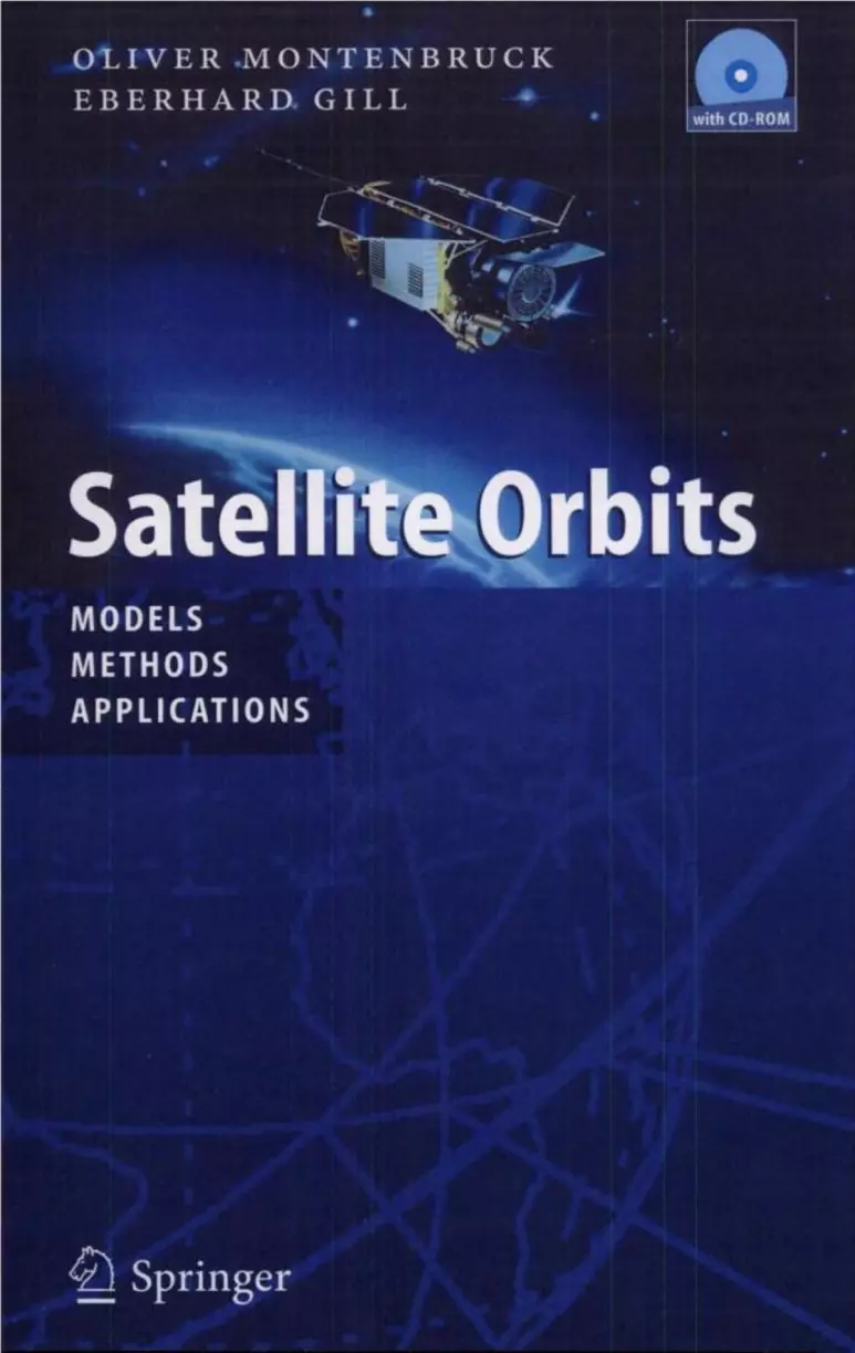
Fig. 1.4. Orbital positions of geostationary satellites controlled by the European telecommunications organization Eutelsat (photo courtesy Eutelsat)
Increasing communication needs could only partly be fulfilled by more and more powerful satellites, which has resulted in a need to co-position (or colocate) multiple satellites in a single control window. At present, a total of 7 ASTRA satellites are actively controlled in a box of ±0.1 0 x ±0.1 0 size in longitude and latitude at 19.2° East, giving the owners of a single antenna the opportunity to receive an ever-increasing number of TV and radio programs.
Aside from telecommunications, the geostationary orbit is also of interest for weather satellites like Goes and Meteosat. A single satellite can provide an almost hemispherical coverage of the Earth at low resolution, thus making it particularly useful for the study of global weather phenomena. Finally, geostationary satel-lites are of growing importance as a complement to traditional satellite navigation systems. The European EGNOS system, for example, makes use of an auxiliary navigation payload onboard the Inmarsat III satellites to provide users with real-time corrections to the existing GPS system, which increase the available navigation accuracy and reliability to the level required for precision aircraft landing.
A more specialized application of geostationary satellites is given by the United States' Tracking and Data Relay Satellite System (TDRSS). It offers the possibility of continuous communication with the Space Shuttle and satellites in low-Earth orbit. Furthermore, it can provide tracking data with full orbital coverage, which would not be possible with conventional ground stations, due to their limited visi-bility.

6 1. Around the World in a Hundred Minutes
1.1.4 Highly Elliptical Orbits
When a satellite is brought into geostationary orbit, it is first injected into an eccen-tric transfer orbit, which is later circularized by a -suitable apogee boost maneuver. Here, the highly elliptic trajectory mainly serves as an intermediate orbit. There are a couple of other applications, however, that intentionally select an eccentric orbit for a spacecraft.
Fig. 1.5. Since 1965 Molniya satellites have provided telephone communications and television within the USSR as well as to western states. Photo by Karl D. Dodenhoff, USAF Museum
Among these, the Russian Molniya and Tundra satellites (Fig. 1.5) are most common. Considering the fact that geostationary satellites provide unfavorable visibility for users in polar regions (e.g. Siberia), an alternative concept of telecom-munications satellites was devised in the former Soviet Union. It is based on syn-chronous 12-hour orbits of 1000 x 40000 km altitude that are inclined at an angle of 63.4° to the equator. The apocenter, i.e. the point farthest away from the Earth, is located above the northern hemisphere, thus providing visibility of the satellite from high latitudes for most of its orbit. Contact is lost for only a few hours, while the satellite passes rapidly through its pericenter, before it becomes visible again to the user. This gap is overcome by additional satellites in a similar, but rotated orbit. Despite the larger number of satellites required, the concept provides a well-suited and cost-effective solution for the communication needs of polar countries.
The second application of elliptic orbits is primarily of scientific interest. In order to explore the magnetosphere of the Earth and the solar-terrestrial interaction, spacecraft orbits that cover a large range of geocentric distances up to 15 or 20
1.1 A Portfolio of Satellite Orbits 7
Earth radii are useful. Examples of related missions are the joint US/European ISEE-1 satellite, with an apocenter height of 140 000 km, or ESA's Cluster mission with four satellites flying in highly eccentric orbits in a tetrahedron formation (Schoenmaekers 1991).
1.1.5 Constellations
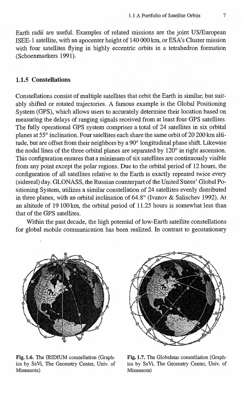
Constellations consist of multiple satellites that orbit the Earth in similar, but suit-ably shifted or rotated trajectories. A famous example is the Global Positioning System (GPS), which allows users to accurately determine their location based on measuring the delays of ranging signals received from at least four GPS satellites. The fully operational GPS system comprises a total of 24 satellites in six orbital planes at 55° inclination. Four satellites each share the same orbit of 20 200 km alti-tude, but are offset from their neighbors by a 90° longitudinal phase shift. Likewise the nodal lines of the three orbital planes are separated by 1200 in right ascension. This configuration ensures that a minimum of six satellites are continuously visible from any point except the polar regions. Due to the orbital period of 12 hours, the configuration of all satellites relative to the Earth is exactly repeated twice every (sidereal) day. GLONASS, the Russian counterpart of the United States' Global Po-sitioning System, utilizes a similar constellation of 24 satellites evenly distributed in three planes, with an orbital inclination of 64.8° (Ivanov & Salischev 1992). At an altitude of 19 100 km, the orbital period of 11.25 hours is somewhat less than that of the GPS satellites.
Within the past decade, the high potential of low-Earth satellite constellations for global mobile communication has been realized. In contrast to geostationary
Fig. 1.6. The IRIDIUM constellation (Graph- Fig. 1.7. The Globalstar constellation (Graph- ics by SaVi, The Geometry Center, Univ. of ics by SaVi, The Geometry Center, Univ. of Minnesota) Minnesota)

8 1. Around the World in a Hundred Minutes
satellites, which require bulky user antennas, communication with low-Earth satel-lites can be established from a hand-held phone, due to the much shorter signal paths. At least one satellite is always visible from any location. Making use of intersatellite links, telephone calls can then be routed around the world to other mobile-phone users or to a suitable ground network terminal. Following IRIDIUM, a 66 satellite constellation at an altitude of 700 km, which was put into operation in 1999 (Fig. 1.6, Pizzicaroli 1998), a couple of other constellations have been designed and partly implemented. These include Globalstar with 48 satellites at 1 414 km altitude (Fig. 1.7), ICO with 10 satellites at 10 400 km, ORBCOMM (Evans & Maclay 1998) and Teledesic with 288 satellites at 1 350 km (Matossian 1998). Constellations require regular orbital control maneuvers to avoid a change in the relative configuration and alignment of satellites.
1.2 Navigating in Space
Irrespective of the level of autonomy that may be achieved with present-day satel-lites, any spacecraft would rapidly become useless if one were unable to locate it and communicate with it. Furthermore, many of the spacecraft described earlier necessitate an active control of their orbit in accordance with specific mission re-quirements. Navigation is therefore an essential part of spacecraft operations. It comprises the planning, determination, prediction, and correction of a satellite's trajectory in line with the established mission goals.
1.2.1 Tracking Systems
A variety of tracking systems may be used to obtain measurements related to the instantaneous position of a satellite or its rate of change. Most of these systems are based on radio signals transmitted to or from a ground antenna (Fig. 1.8). Com-mon radio tracking systems are able to perform angle measurements by locating the direction of a radio signal transmitted by a satellite. The resolution of these measure-ments depends on the angular diameter of the antenna cone, which is determined by the ratio of the carrier wavelength to the antenna diameter. Given a frequency of 2 GHz as applied in common antenna systems, a diameter of 15 m is required to achieve a beam width of 0.5°. Distance and velocity information can be obtained by measuring the turn-around delay or Doppler-shift of a radio signal sent to the spacecraft and returned via a transponder. Representative ranging systems achieve an accuracy between 2 m and 20 m, depending on the frequency band used and the type of ranging signal applied. Doppler measurements can provide the range rate of an Earth-orbiting satellite with an accuracy of typically 1 mm/s. In the absence of an active transmitter or transponder onboard the spacecraft, sufficiently powerful radar may also be applied for spacecraft tracking. Its use, however, is mainly restricted to emergency cases or space surveillance tasks (Pensa & Sridharan 1997).
For low-Earth satellites, a purely ground-based tracking suffers from the lim-ited station contacts that constrain the available tracking measurements to a small

1.2 Navigating in Space 9
Fig. 1.8. The ground station complex at Redu, Belgium, provides telemetry, tracking, and telecom-mand operations for low-Earth and geostationary satellites (courtesy ESA)
fraction of the orbit. To overcome this restriction, geostationary satellites like the United Sates' Tracking and Data Relay Satellite (TDRS) can be used to track a user satellite via a relay transponder. Going even further, GPS ranging signals of-fer the opportunity to obtain position measurements onboard a satellite completely independently of a ground station.
Aside from radiometric tracking, optical sensors may likewise be used to lo-cate a satellite, as illustrated both by the early days' Baker—Nunn cameras (Henize 1957) and today's high-precision satellite laser ranging systems (Fig. 1.9). Imaging telescopes are well suited for detecting unknown spacecraft and space debris up to geostationary distances, which makes them a vital part of the United States' space surveillance network. Instead of photographic films employed in foimer Baker—Nunn cameras, the Ground-Based Electro-Optical Deep Space Surveillance (GEODSS) telescopes are equipped with electronic sensors that allow online im-age processing and removal of background stars. Other applications of optical tele-scopes include the monitoring of colocated geostationary satellites, which are not controlled in a coordinated way by a single control center. Besides being completely passive, telescopic images can provide the plane-of-sky position of geostationary satellites to much better accuracies (typically 1" 200 m) than angle measure-ments of common tracking antennas.

10 1. Around the World in a Hundred Minutes
Fig. 1.9. Satellite laser ranging facility of the Natural Environ-ment Research Council (photo: D. Calvert)
Satellite laser ranging (SLR) systems provide highly accurate distance mea-surements by determining the turn-around light time of laser pulses transmitted to a satellite and returned by a retro-reflector. Depending on the distance and the resulting strength of the returned signal, accuracies of several centimeters may be achieved. Satellite laser ranging is mainly used for scientific and geodetic missions that require an ultimate precision. In combination with dedicated satellites like Starlet and Lageos (Rubincam 1981, Smith & Dunn 1980), satellite laser ranging has contributed significantly to the study of the Earth's gravitational field. Other applications of SLR include independent calibrations of radar tracking systems like GPS or PRARE (Zhu et al. 1997).
1.2.2 A Matter of Effort
A discussion on spacecraft navigation sooner or later ends up with a question on the achieved accuracy. As illustrated in Fig. 1.10, widely varying levels of accuracy apply for the knowledge of a satellite's orbit, depending on the particular goals of a space project. In accord with these requirements, widely varying tracking systems are employed in present space projects.

Mission operations,, scheduling; _ antenna . pointing (ROSAT)
Satellite Tracking and Navigation
Attitude control
s (BIRD)
Colocation and 'constellation: - keeping (ASTRA
Relay. atilie. , - bratkirig . (TDRS
Remote sensing ..
•(ERS- 1 ).
Hi resolution ,gravity . field recovery . (GRACE) -
Satellite:Laser . Ranging -
(Herstrnonceaux
1.2 Navigating in Space 11
Fig. 1.10. Representative tracking and orbit determination accuracies employed in current spac missions (pictures courtesy DLR, DSS, NASA, SES)

12 1. Around the World in a Hundred Minutes
An upper threshold to the permissible position uncertainty is generally given by the need for safe communication with the spacecraft from the ground. Considering, for example, an orbital altitude of 800 km and the 0.3° (0.005 rad) half-beam width of a 15 m S-band antenna, the spacecraft trajectory must be predicted to within an accuracy of 4 km to permit accurate antenna pointing throughout an entire sta-tion pass. A similar level of accuracy is required for many scheduling functions. Spacecraft-specific events like shadows, station contacts, or payload activation are commonly considered in the operations timeline with a one-second resolution. Con-sidering an orbital velocity of 3-7 km/s, the spacecraft position must be known to within several kilometers in order to predict an orbit-related event with the de-sired accuracy. An angle tracking system locating the direction of the downlink signal is generally sufficient to meet these types of basic operational requirements. Aside from a transmitter, which is employed anyway for ground communication, no specific onboard equipment is required for this type of tracking.
Quite a different accuracy can be achieved by ground-based or space-based range and Doppler measurements. Their use is typically considered for missions requiring active orbital control. Colocated geostationary satellites, for example, may experience intentional proximities down to the level of several kilometers. Accordingly, the position knowledge and the associated tracking accuracy must at least be one order of magnitude better. Similar considerations hold for remote sens-ing satellites. In order to enable a reliable geocoding of images with a resolution of up to 10m, a consistent orbit determination accuracy is mandatory. Considering the visibility restrictions of common ground stations for low-Earth orbits, space-based tracking systems like TDRSS, GPS, or DORIS are often preferred to achieve the specific mission requirements. While ground-based tracking requires a conventional transponder, the use of the other systems necessitates specialized onboard equip-ment like steerable antennas (TDRSS) or a Doppler measurement unit (DORIS). Utilization of GPS, in contrast, offers position accuracies of 100m (navigation so-lution) to 25 m (with dynamical filtering) even for simple C/A code receivers. GPS tracking is therefore considered to be the sole source of orbit information for more and more spacecraft.
Leaving the field of traditional spacecraft operations, one enters the domain of scientific satellite missions with even more stringent accuracy requirements. Among these, geodetic satellite missions like Starlet and Lageos have long been the most challenging. Using satellite laser ranging systems, their orbits have been tracked with an accuracy in the centimeter to decimeter region, thus allowing a consistent improvement in trajectory models and Earth orientation parameters. For other Earth exploration missions like TOPEX (Bath et al. 1989, 1998), ERS, or JERS, the use of satellite altimeters has been a driving factor for the refinement of orbital models and tracking techniques. Besides selected laser ranging campaigns, these missions are mainly supported by space-based radio tracking systems like TDRSS, GPS, DORIS, and PRARE. Their use has enabled the achievement of or-bital accuracies in the decimeter region, with focus on the exact restitution of the radial component. In the case of GPS usage, the differential processing of space-

1.2 Navigating in Space 13
based and concurrent ground-based pseudorange and carrier phase measurements provides for the required increase in precision over the Standard Positioning Ser-vice. The GPS satellite orbits themselves are determined with position accuracies of several centimeters, using GPS measurements collected by a global network of geodetic reference stations (Springer et al. 1999).
Looking at the future, a new era will be opened by the upcoming GRACE mission (Davis et al. 1999). Making use of a KJKa-band intersatellite link that provides dual one-way range measurements, changes in the distance of the two spacecraft can be established with an accuracy of about 0.01 mm. In combination with supplementary onboard accelerometers, this will for the first time allow the detection of short-term variations in the cumulative gravity field of the solid Earth, the oceans and the atmosphere.

2. Introductory Astrodynamics
Even though elaborate models have been developed to compute the motion of artificial Earth satellites to the high level of accuracy required for many applications today, the main features of their orbits may still be described by a reasonably simple approximation. This is due to the fact that the force resulting from the Earth's central mass outniles all other forces acting on the satellite by several orders of magnitude, in much the same way as the attraction of the Sun governs the motion of the planets. The laws of planetary motion, which were found empirically by Kepler about 400 years ago, may, therefore, equally well be applied to a satellite's orbit around the Earth.
In the sequel, the basic laws of orbital motion are derived from first principles. For this purpose, a satellite is considered whose mass is negligible compared to the Earth's mass M. Assuming the Earth to be spherically symmetric, the acceleration
of the satellite is given by Newton's law of gravity:
GM = r (2.1)
r 3
Here the fraction in (2.1) denotes a unit vector pointing from the satellite to the center of the Earth, which forms the origin of the coordinate system. The magnitude of the acceleration is proportional to the inverse square of the satellite's distance r from the Earth's center.
By measuring the mutual attraction of two bodies of known mass, the gravi-tational constant G can directly be determined from torsion balance experiments. Due to the small size of the gravitational force, these measurements are extremely difficult, however, and G is presently only known with limited accuracy:
G = (6.67259 ± 0.00085)- 10 -11 m3kg-1 S-2
(2.2)
(Cohen & Taylor 1987). Independent of the measurement of G itself, the gravita-tional coefficient GM, i.e. the product of the gravitational constant and the Earth's mass, has been determined with considerable precision from the analysis of laser distance measurements of artificial Earth satellites:
GM e = 398 600.4405 ± 0.001 km 3 s-2
(2.3)
(Ries et al. 1989). The corresponding value of the Earth's mass is given by
Me = 5.974.1024 kg . (2.4)

Fig. 2.1. The central force does not alter the plane of the satel-lite's orbit
16 2. Introductory Astrodynamics
2.1 General Properties of the Two-Body Problem
The study of the motion of a satellite in the spherically symmetric 1/r 2 force field of a central mass is usually referred to as Kepler's problem, or as two-body problem. It was first solved in the second half of the 17th century by Isaac Newton, who was thus able to prove the validity of Kepler's laws of planetary motion.
2.1.1 Plane Motion and the Law of Areas
The fact that the force exerted on the satellite always points to the Earth's center in the two-body problem has the immediate consequence that the orbit is confined to a fixed plane for all times. The satellite cannot leave the orbital plane, since the force is always anti-parallel to the position vector and, therefore, does not give rise to any acceleration perpendicular to the plane.
(D Earth
For a mathematical description of this fact, one forms the cross product of (2.1) with the position vector r:
GMED rxr = (r x r)
r3
0
The right-hand side in this equation is equal to zero since the cross product of a vector with itself vanishes. The left-hand side may further be written as
rxF=rxi;+i-xi-=—d
(2.6) dt
Since the time derivative of rxi- equals zero, the quantity itself must be a constant, i.e.
rxi-=h= const . (2.7)
Geometrically, the cross product of two vectors is a vector at right angles to both of them. Therefore, the position vector r as well as the velocity vector i- are always perpendicular to h, or – in other words – the orbit is confined to a plane. The vector h is the angular momentum per unit mass or the specific angular momentum. It is
(2.5)

2.1 General Properties of the Two-Body Problem 17
related to the angular momentum vector 1 by 1 mh, where m is the mass of the satellite.
Equation (2.7), furthermore, implies Kepler's second law or the law of areas. Considering the satellite's motion as linear over a small time step At, then
1 1 AA = —Ir x rAtI = —IhlAt
2 2 (2.8)
is just the area swept by the radius vector during the time At (see Fig. 2.1). The absolute value h = 1111 is therefore known as areal velocity and since h and h
remain constant, the radius vector sweeps over equal areas in equal time intervals (Kepler's second law).
2.1.2 The Form of the Orbit
Some other properties of the orbit may be found by multiplying both sides of the equation of motion (2.1) with the vector h:
GM@ x h (h x r)
r3 GMED
r3 ((r x i.) x r)
GME9 . (r (r • r) — r (r • i-))
r 3
(2.9)
Now, since
d r
dt r)
one finds that
1 —r — —2 r
1 —Tr (r (r • r) — r (r • i.))
(2.10)
(2.11)
(2.12)
d h —GM@—
dt (—
r r
)
Integrating both sides with respect to time yields
h x = —GM @ (—r) — A
where —A means an additive constant of integration that is determined by the initial position and velocity. A is called the Runge—Lenz or Laplace vector (Goldstein 1980, Battin 1987). Note that the negative sign of A is just a matter of convention, which facilitates the geometrical interpretation.
The vector h x r is part of the orbital plane since it is perpendicular to the angular momentum vector, and the same is true for the unit position vector r/r.
18 2. Introductory Astrodynamics
Therefore, A lies in the orbital plane, too. Some further properties may be revealed by multiplying the last equation with r, which results in
(h x i-) • r —GM er — A • r . (2.13)
Introducing y, the true anomaly, as the angle between A and the position vector r, one arrives at
h2 = GMer + Ar cos y (2.14)
where the identity
(a x b) • c — (c x b) • a (2.15)
has been used to simplify the left-hand side of (2.13). One may now define two (positive) auxiliary quantities
h2 A p e (2.16)
GM G
to finally obtain the conic section equation
r (2.17) 1 e cos y
This equation relates the satellite's distance r to the angle between its position vector and the reference direction given by A, and thus defines the satellite's path in the orbital plane. It may further be seen that the distance varies between a minimum value of
rmin
1
(2.18)
(2.19)
1
for y -,.. 0, and
rmax =
+ e
a maximum value of
P for 0 < e < 1 — e — {oo for 1 < e .
The corresponding points of the orbit are known as perigee and apogee and their connection is the line of apsides. The mean value of the minimum and the maximum distance is the semi-major axis a, which is found to be
1 h2 a = — (rmin rm..) = (2.20)
2 1 _e2 GMED (1 — e)
for an orbit with a finite apogee distance. The constant e is called eccentricity, since it is a measure of the orbit's deviation from a circle (which corresponds to e = 0). The parameter p, which denotes the distance of the satellite from the Earth's center at right angles to perigee and apogee, is called semi-latus rectum (see Fig. 2.2).
Equation (2.17) is known as the equation of a conic section in polar coordinates. It is an extension of Kepler's first law, stating that planetary orbits are ellipses. In

Ellipse (e=0.5)
=
Parabola (e=1.0) Hyperbola (e=1.5)
2.1 General Properties of the Two-Body Problem 19
Fig. 2.2. Conic sections with eccentricities e = 0.5, e = 1.0, and e = 1.5 with the same semi-latus rectum p
general, three distinct types of curves may be obtained from intersecting a plane with a cone. They are known as ellipses, parabolas, and hyperbolas, and have eccen-tricities smaller than, equal to, and larger than one, respectively. In the following, the discussion is confined to the elliptic motion of Earth-orbiting satellites in contrast to deep space probes, which leave the Earth's gravity field on hyperbolic orbits. A general discussion of the geometry of conic sections may be found in Montenbruck (1989) together with formulas for calculating parabolic or hyperbolic orbits.
2.1.3 The Energy Integral
Last but not least, another interesting law of Keplerian motion may be derived, which relates the satellite's velocity to the distance from the center of the Earth. For this purpose one fauns the square of both sides of (2.12) and obtains
r • A (h x ) 2 = (G M e9 ) 2 2GMe A2
(GM)2 (1 + 2e cos y + e2)
= (GM e ) 2 (2(1 + e cos v) —(1 — e 2))
(2.21)
Since the vectors h and i- are perpendicular, the value of the left-hand side is equal to h2 y2 , using y = ii-1 to denote the satellite's velocity. Substituting the value 1/a = G M @ (1 — e2)/ h2 of the reciprocal semi-major axis, and making use of the conic section equation, finally yields the equation
2 1 v2 Gme
r a (2.22)

30
25
Iner
t ial V
eloc
ity [
km/s
i
10 o
5
0 4 8 12 16 20 24 28 32 36 40
Satellite Altitude [1000 km]
20 2. Introductory Astrodynamics
which is called the vis-viva law. It is equivalent to the energy law, which states that the sum of the kinetic energy
Ekin —1
m v2 2
and the potential energy
Gm Me Epot =
is constant during motion:
1 Gm M ED 1 Gm Me Etot = — m v
2
2 a
(2.23)
(2.24)
(2.25)
As may be seen from this expression, the total energy depends only on the reciprocal semi-major axis, not on the eccentricity of the orbit. The energy of an elliptic satellite orbit which is always bound to the Earth, is negative, since the semi-major axis is a positive quantity. Parabolic (1/a 0) and hyperbolic (1/a <O) orbits, on the other hand, have a zero or positive energy, which allows a satellite to reach an infinite distance from the Earth.
Fig. 2.3. Velocity and orbital pe-riod for circular Earth satellite orbits
For a satellite on a circular orbit (r = a) the vis-viva law yields a velocity of
GM vcirc
a (2.26)
which evaluates to 7.71 km/s for a low-Earth orbit at an altitude of 320 km, and corresponds to an orbital period
27 a Tcirc = = 2m (2.27)

2.1 General Properties of the Two-Body Problem 21
of 91 minutes (Fig. 2.3). For a satellite at a distance of 42 164 km from the center of the Earth (i.e. at an altitude of 35 786 km) the velocity is only 3.07 km/s, and the time of revolution amounts to 231 56m . Since this is just the period of the Earth's rotation, a satellite at this height appears stationary with respect to the Earth, if it is placed above the equator and orbits the Earth in an easterly direction. Due to this fact, geostationary orbits are of special interest for e.g. telecommunications satellites, which may provide a continuous transmission from one continent to another.
v=3.07 km/s
Fig. 2.4. An application of the vis-viva law: the velocity requirement for orbital transfer from a circular low-Earth orbit to geosta-tionary orbit Geostationary orbit
For an eccentric orbit the satellite's velocity varies between a maximum of
(2.28)
at perigee and a minimum of
v apo\IGME9 /1—e
a I 1 e (2.29)
at apogee according to the vis-viva law. Considering, for example, an orbit with its perigee at an altitude of 320 km and its apogee at an altitude of 35786 km (a = 24430 km, e = 0.726), these velocities amount to 10.13 km/s and 1.61 krrils, respectively. As may be concluded from these figures, a velocity increment of 2.42 km/s is required to transfer a satellite on a low-Earth orbit onto an elliptic orbit with its apogee near the geostationary orbit. An additional 1.46 km/s is, furthermore, required in the apogee to circularize the orbit by raising the perigee to the same altitude (Fig. 2.4).

22 2. Introductory Astrodynamics
2.2 Prediction of Unperturbed Satellite Orbits
2.2.1 Kepler's Equation and the Time Dependence of Motion
So far the discussion of Keplerian orbits has mainly been concerned with the geo-metrical form of a satellite's orbit in space. From the law of gravity it has been concluded that the motion may not follow an arbitrary curve in space, but is con-fined to an ellipse or another conic section. However, no information on the time dependence of the motion has yet been derived, i.e. the orbital position at a specific time is still unknown.
Fig. 2.5. The definition of the ec-centric anomaly E
Apogee a ae e x Perigee
For this purpose an auxiliary variable E, which is called the eccentric anomaly, is defined via the equations
= r cos y =: a (cos E — e)
r sin v a — e2 sin E
or equivalently
r = a(1 — e cos E)
(2.30)
(2.31)
The geometrical meaning of E is illustrated by Fig. 2.5. Using the coordinates î and 9, which denote the satellite's position in the orbital
plane with respect the center of the Earth, one may express the areal velocity h=lhl as a function of E:
h =
= a (cos(E) — e) a-11— e2 cos(E)É
a-V1 —e2 sin(E) • a sin(E)È
= a2-11 — e2 t(1 — e cos(E)) .
This equation may further be simplified using
(2.32)
h = 1GMea(1 — e2) (2.33)

2.2 Prediction of Unperturbed Satellite Orbits 23
to give the following differential equation for-the eccentric anomaly:
(1 — e cos E)È = n
Here the mean motion
(2.34)
G
(2.35) n a3
has been introduced to simplify the notation. Integrating with respect to time finally yields Kepler's Equation
E(t) — e sin E(t) = n(t — tp) , (2.36)
where tp denotes the time of perigee passage at which the eccentric anomaly van-ishes. The right hand side
M = n(t — t p) (2.37)
is called the mean anomaly. It changes by 3600 during one revolution but — in contrast to the true and eccentric anomalies — increases uniformly with time. Instead of specifying the time of perigee passage to describe the orbit, it is customary to introduce the value Mo of the mean anomaly at some reference epoch to. The mean anomaly at an arbitrary instant of time may then be found from
M = Mo n(t — to)
(2.38)
The orbital period, i.e. the time during which the mean anomaly changes by 27r or 360°, is proportional to the inverse of the mean motion n and is given by
T = = 27r
(2.39)
This relation is essentially Kepler's third law, which states that the second power of the orbital period is proportional to the third power of the semi-major axis. The same result that was earlier derived for circular orbits from the vis-viva law (see (2.27)) is therefore valid for periodic orbits of arbitrary eccentricity.
2.2.2 Solving Kepler's Equation
Kepler's equation relates the time t to the coordinates is and 9 in the orbital plane via the eccentric anomaly. In order to obtain the position of the satellite at time t one has to know the time of perigee passage and the semi-major axis to calculate the mean anomaly One may then find the value of E that fulfils (2.36) and finally obtain î and 9 from (2.30).
Kepler's equation can, however, be solved by iterative methods only. A common way is to start with an approximation of
E0 = M or E0 = 7r (2.40)
24 2. Introductory Astrodynamics
and employ Newton's method to calculate successive refinements Ei until the result changes by less than a specified amount from one iteration to the next. Defining an auxiliary function
f(E) = E — e sin E — M , (2.41)
the solution of Kepler's equation is equivalent to finding the root of f (E) for a given value of M. Applying Newton's method for this purpose, an approximate root Ei of f may be improved by computing
f (Ei) Ei — e sin Ei — M Ei+1 = Ei = Ei (2.42)
(Ei) 1 — e cos Ei Note that this expression has to be evaluated with E in radians (1 rad = 18077r) and not in degrees, to avoid erroneous results.
The starting value E0 M recommended above is well suited for small ec-centricities, since E only differs from M by a term of order e. For highly eccentric orbits (e.g. e > 0.8) the iteration should be started from E0 = TC to avoid any convergence problems during the iteration.
A more general discussion of starting values and iteration procedures for solv-ing Kepler's equation can be found in the literature (see Smith 1979, Danby & Burkardt 1983, Taff & Brennan 1989, and references therein). Great efforts have been made to develop methods that require a minimum of iterations and may safely be applied for all values of e and M. Since the critical case of eccentricities close to unity is rarely encountered in the practical computation of periodic Earth satellite orbits, the discussion is somewhat academic, however. Unless one has to solve Ke-pler's equation exceedingly often or in a real-time application, there is little need to look for methods converging faster than Newton's method.
2.2.3 The Orbit in Space
So far the satellite's motion has been discussed in its natural orbital-plane reference system, which allows the most simple description. More general expressions can be obtained by introducing the unit vector P = A/IA I, which points towards the perigee (cf. (2.12)) and the perpendicular unit vector Q, corresponding to a true anomaly of v = 90°. Using these vectors one may express the three-dimensional position by
r = P + Q
= r cosy P r sin y Q (2.43)
a(cosE — e) P a-11 — e2 sin E Q and the velocity by
=
,/GMea ( sin E P -11 — e2 cos E Q) ,
(2.44)
since cIÉ = ,/GMED alr according to (2.34).
2.2 Prediction of Unperturbed Satellite Orbits 25
+y
+x (Equinox Y) a
Fig. 2.6. The equatorial coordinate system
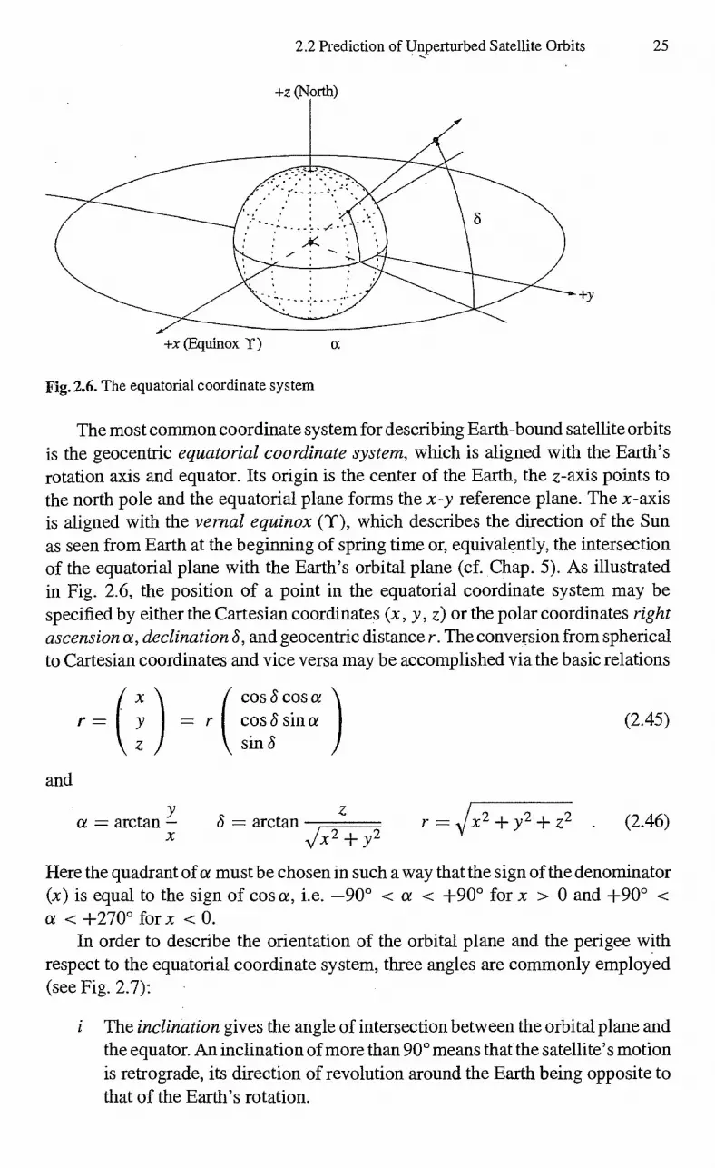
The most common coordinate system for describing Earth-bound satellite orbits is the geocentric equatorial coordinate system, which is aligned with the Earth's rotation axis and equator. Its origin is the center of the Earth, the z-axis points to the north pole and the equatorial plane forms the x-y reference plane. The x-axis is aligned with the vernal equinox (Y), which describes the direction of the Sun as seen from Earth at the beginning of spring time or, equivalently, the intersection of the equatorial plane with the Earth's orbital plane (cf. Chap. 5). As illustrated in Fig. 2.6, the position of a point in the equatorial coordinate system may be specified by either the Cartesian coordinates (x, y, z) or the polar coordinates right
ascension a, declination 8, and geocentric distance r. The conversion from spherical to Cartesian coordinates and vice versa may be accomplished via the basic relations
x cos 8 cos a
r = ( y = r cos 8 sin a sin 8
(2.45)
and
= arctan — 8 = arctan r .1x2 + y2 + z2 (2.46) + y2
Here the quadrant of a must be chosen in such a way that the sign of the denominator (x) is equal to the sign of cos a, i.e. —90° <a < +900 for x > 0 and +90° < a <+2700 for x <O.
In order to describe the orientation of the orbital plane and the perigee with respect to the equatorial coordinate system, three angles are commonly employed (see Fig. 2.7):
The inclination gives the angle of intersection between the orbital plane and the equator. An inclination of more than 90° means that the satellite's motion is retrograde, its direction of revolution around the Earth being opposite to that of the Earth's rotation.

Fig. 2.7. The orbital elements i , Q, and co of a satellite
26 2. Introductory Astrodynamics
S2 The right ascension of the ascending node indicates the angle between the vernal equinox and the point on the orbit at which the satellite crosses the equator from south to north.
co The argument of perigee is the angle between the direction of the ascending node and the direction of the perigee.
The satellite's position in space may be expressed as a function of these angles by a sequence of three elementary transformations. In the orbital plane system, which is defined by the unit vectors P, Q and W = hlh, the coordinates are given by
a, 9, 2) = (r cos v , r sin y, 0) . (2.47)
In a coordinate system that is rotated around W by an angle of —co (i.e. with an x'-axis pointing to the ascending node), the coordinates are
(x', y', z') = (r cos(v + co), r sin(v + co), 0) (2.48)
and the corresponding transformation is written as
(cos(v + co) r sin(v + co) J = Rz (—co
0
cos v ) sin v 0
(2.49)
In order to express the satellite's position in equatorial coordinates, two further rotations are required. First, a rotation around the x'-axis by an angle —i is used to obtain equatorial coordinates counted from the line of nodes. A final rotation

2.2 Prediction of Unperturbed Satellite Orbits 27
around the new z"-axis by —0 then yields the equatorial coordinates counted from the direction of the equinoxl :
x ). ( cos v y = R(—Q)R x (—i)R z (—co) r sin. v
0
Evaluating this expression one finds
x cos u cos Q — sin u cos i sin Q Y = r cos u sin Q + sin u cos i cos Q
sin u sin i
(2.50)
(2.51)
with u = (argument of latitude) as the angle between r and the line of nodes. Similar considerations lead to the coordinate representation of the vectors P and Q that correspond to points at unit distance with a true anomaly of 0° and 900 :
and
+ cos co cos Q — sin co cos i sin Q P = + cos co sin Q + sin co cos i cos Q
+ sin co sin i
— sin co cos Q — cos co cos i sin Q — sin co sin S2 + cos co cos i cos Q + cos co sin i
(2.52)
(2.53)
The third vector W may finally be expressed as
+ sin i sin S2 \ W — sin i cos Q (2.54)
+ cos i
It is noted that P, Q, and W are just the column vectors of the matrix
(P, Q, W) = R z (— Q)R x (—i)R z (—co) (2.55)
which is especially useful when coordinates have to be transformed between the equatorial and the orbital-plane coordinate system. The three vectors are usually referred to as Gaussian vectors.
I The elementary matrices
1 0 0 ) R x (0) = (0 +cos0 +sin0
0 —sin0 ±cosq5
(-1-coscp 0 —sin/ +cos0 +sin0 0) R y 05) = 0 1 0 R z (0)= —sin0 +cos0 0
+sin0 0 +cos0 0 0 1
are employed to describe rotations around the x, y and z-axes. The signs are chosen in such a way that a positive angle 4) corresponds to a positive (counterclockwise) rotation of the reference axes as viewed from the positive end of the rotation axis towards the origin (Goldstein 1980, Mueller 1969).
Next, the vis-viva law yields the semi-major axis
GM@
v2 )_1
a = (2.60)
n = a3
,IGM0 (2.61)
28 2. Introductory Astrodynamics
2.2.4 Orbital Elements from Position and Velocity
As has been shown, a total of six independent parameters are required to describe the motion of a satellite around the Earth. Two of these orbital elements (a and e) describe the form of the orbit, one element (M) defines the position along the orbit and the three others (S2, i, and co) finally define the orientation of the orbit in space. Given these six elements, it is always possible to uniquely calculate the position and velocity vector.
Vice versa there is exactly one set of orbital elements that corresponds to given initial values of r and y, and one may ask how to find these elements. Part of the answer is already evident from the solution of the two-body problem presented above. First of all the areal velocity vector
(y i — zSi ) h =r xi.= zi—_x
x .S1 — y _X (2.56)
and its modulus h can be obtained from the position and velocity. Then, from the representation of h or W = hl h as a function of i and Q in (2.54), it follows that
( sin i sin Q) ( +17,1h \ (+W„ ) sin i cos S2 = —h y l h = —W,, (2.57) cos i +hz / h 1 +Wz
Hence the inclination and the right ascension of the ascending node are given by
( ) S2
rWx,
i= arctan = arctan (2.58) WZ y )
The areal velocity can further be used to derive the semi-laths rectum
h2 P = GMED
(2.59)
and consequently the mean motion
2In evaluating expressions of the form a = arctan(y/x) the quadrant of a must be chosen in such a way that the sign of the denominator (x) is equal to the sign of cos a, i.e. —90° < a < +900 for x > 0 and +90° < a < +270° for x < 0.
2.2 Prediction of Unperturbed Satellite Orbits 29
For elliptic orbits a will always be positive. The eccentricity e follows from
e = 1
(2.62) a
Considering (2.31) and the identity
= a (cos(E) — e) • a sin(E)È
e2 sin(E) • cc ,,/1 — e2 cos(E)t -
= a-9 nesm(E)
(2.63)
1 — r I a
The eccentric anomaly may now be used to obtain the mean anomaly from Kepler's equation
M (t) = E (t) — e sin E (t) (in radians) (2.65)
with t being the epoch of r and r. In order to find the remaining orbital element co, one has to determine the
argument of latitude u first. Solving (2.51) for cos u and sin u yields
u = arctan z/ sin i
= arctan (2.66) x cos S2 y sin S2) —x Wy YWx)
Furthermore, the true anomaly is given by
y = arctan (. ■,/1 — e2 sin E)
(2.67) cos E — e
taking proper care of the correct quadrant (cf. (2.30)). The result may finally be used to obtain the argument of perigee from
(2.68)
2.2.5 Non-Singular Elements
In many applications, satellite orbits are chosen to be near-circular, to provide a constant distance from the surface of the Earth or a constant relative velocity. Typ-ical examples are low-altitude remote sensing satellites or geostationary satellites, which are furtheimore required to orbit the Earth in a near-equatorial plane.
While there is no inherent difficulty in calculating position and velocity from known orbital elements with e and i close to zero, the reverse task may cause prac-tical and numerical problems. These problems are due to singularities arising from the definition of some of the classical orbital elements. The argument of perigee,
one may solve for e sin(E) and e cos(E) to find the eccentric anomaly from
E = arctan (r- I (a2 n))
(2.64)
30 2. Introductory Astrodynamics
for example, is not a meaningful orbital element for small eccentricities, since the perigee itself is not well defined for an almost circular orbit Small changes of the orbit may change the perigee location by a large amount, and small numerical er-rors may lead to enhanced errors in the computation of co since the equation for E becomes almost singular in this case. Similar considerations apply to small incli-nations where the line of nodes is no longer well defined and where the equations for a become singular. Several attempts have therefore been made to substitute other parameters for the classical Keplerian elements. These elements are usually referred to as non-singular, regular or equinoctial elements (see e.g. Broucke & Cefola 1972).
A possible set of regular elements that may be used for both low eccentricities and inclinations is defined by3
a h = e sin(S2 ± co) p = sin(i/2) sin S2 (2.69)
1= S2 +co+ M k=ecos(S2 +co) q= sin(i /2) cos S?.
Geometrically, k and h closely approximate the projection of the Runge—Lenz vector A into the equatorial plane for orbits of small inclination, and are likewise used to define the eccentricity and the direction of perigee Similarly p and —q give the approximate projection of the orbital-plane nomial vector W onto the equator, if one neglects the factor 1/2, which has been introduced to allow use of these elements for high inclinations, and to avoid a singularity at i = 90°. The mean longitude 1, which is defined as the sum of the right ascension of the ascending node, the argument of perigee and the mean anomaly, may further be interpreted as the approximate right ascension of the satellite for near-circular orbits of small inclination.
An alternative set of non-singular elements defined by
a h = esin(S2 ± co) p = ta.n(i /2) sin S2
1= S2 ± co+ M k =ecos(S2 co) q = tan(i/2) cos
is due to Broucke & Cefola (1972). While (2.69) is preferable, due to the sim-plified structure of the associated partial derivatives of the position and velocity vector (Dow 1975), the second set (2.70) is more convenient when working with perturbational equations (see Battin 1987).
Adopting the convention of equinoctial elements by Broucke & Cefola (1972), the satellite position and velocity vector may be expressed as
r = Xi f + Yig = + (2.71)
in analogy with (2.43) and (2.44). The orthogonal unit vectors
(2.70)
—2p
3 For consistency with the notation commonly employed in the literature, the symbols h and p are used to denote non-singular elements throughout this section. They should not be confused with the areal velocity and the semi-latus used elsewhere.
(1 — p2 ±q2) 1 f cos(co-FS2)P — sin(co+S2) Q = ±p2±q2 2pq (2.72)
and
1 2pq
1 rp2 +,72 1 +P2— q 2q
(2.73) g = sin(co+ S2) P cos(w+ S2) Q =
2.2 Prediction of Unperturbed Satellite Orbits 31
span the orbital plane like the Gaussian vectors, but are rotated by an angle of Q +co with respect to P and O. For small inclinations, f and g almost coincide with the
x- and y-axis of the equatorial coordinate system, respectively. After proper rearrangement of (2.43) and (2.44), the Cartesian coordinates with
respect to f and g, and the corresponding time derivatives, can be expressed as
X1 = a ((1—h 2 18) cos(F) hk,8 sin(F) — k)
= a ( (l — k 2 16) sin(F) hk,8 cos(F) — h)
a2 n cos(F) — (1 — h 2P) sin(F))
1.71 = -a2n
(—h1cP sin(F) (1 —k 2,8) cos(F))
making use of the auxiliary quantity
(2.74)
1
(2.75) 1+ ,V1—h 2 —k 2
(Cefola 1972). The eccentric longitude
F=E-F-co-FS2 (2.76)
replaces the eccentric anomaly when working with non-singular elements, and is found by solving a modified version of Kepler's equation given by
F—ksin(F) h cos(F) =l=M-F-w-F-S2
(2.77)
Finally, the radius r is expressed as
r =a (1 k cos(F) — hsin(F))
(2.78)
in terms of the equinoctial elements. The equinoctial elements defining the orientation of the orbital plane are related
to the orbital plane normal vector W = (r x x r I by
-1-Wx — W Y q (2.79) P = = 1+W 1+ W
which may be used to detennine the vectors f and g corresponding to a given position and velocity. Projection of the Runge—Lenz vector
A = x (r x — G M e —r (2.80)

Fig. 2.8. The ground projection of a satellite orbit
32 2. Introductory Astrodynamics
onto these reference vectors then yields the eccentricity components
k=
A -f h Ag
=
GM® GM®
Inserting the in-plane coordinates
(2.81)
Xi r • f
r•g (2.82)
into (2.74), and solving for the sine and cosine of F, furtheimore yields the expres-sions
cos(F) = k + (1 —k2P)Xi — hicfiYi
a/1 —h 2 —k 2
sin(F) = h+ (1 —h 2,8)Yi — hkf3X1
(2.83)
a-11—h 2 —k2
for determining the eccentric longitude, from which the mean longitude 1 can be obtained via Kepler's equation (2.77).
2.3 Ground-Based Satellite Observations
2.3.1 Satellite Ground Tracks
At each instant of time, the intersection of the orbital plane of a satellite with the surface of the Earth yields a great circle, which depends only on the inclination of the orbital plane and the position of the ascending node (Fig. 2.8). This great circle intersects the Earth's equator at an angle that is equal to the inclination i of the orbital plane, and covers geographical latitudes between a minimum of ço = —i and a maximum of ço = i. The geographical latitude ço of the satellite and its ground
-10° -20 -30" -40°
-50°
2.3 Ground-Based Satellite Observations 33
projection is equal to its declination 8, both of which denote the angle between the geocentric radius vector and the equatorial plane4 . The geographical longitude
on the other hand, denotes the angle between the Greenwich meridian and the meridian through the point. It is counted positively towards the east, and differs from the right ascension a by the right ascension 0 (t) of the Greenwich meridian at time t:
= a (t) . (2.84)
Denoting by d the time in days5 since 12h on 1 January 2000, the angle 0 (t) is given by
e = 280.4606° ± 360.9856473° d , (2.85)
where small secular changes have been neglected. & increases by 3600 during one revolution of the Earth, which lasts approximately 23h56ine•e• somewhat less than one day. Since 0 (t) is a measure of the time between subsequent meridian crossings of a star for an observer on Earth, it is also known as sidereal time or Greenwich Hour Angle.
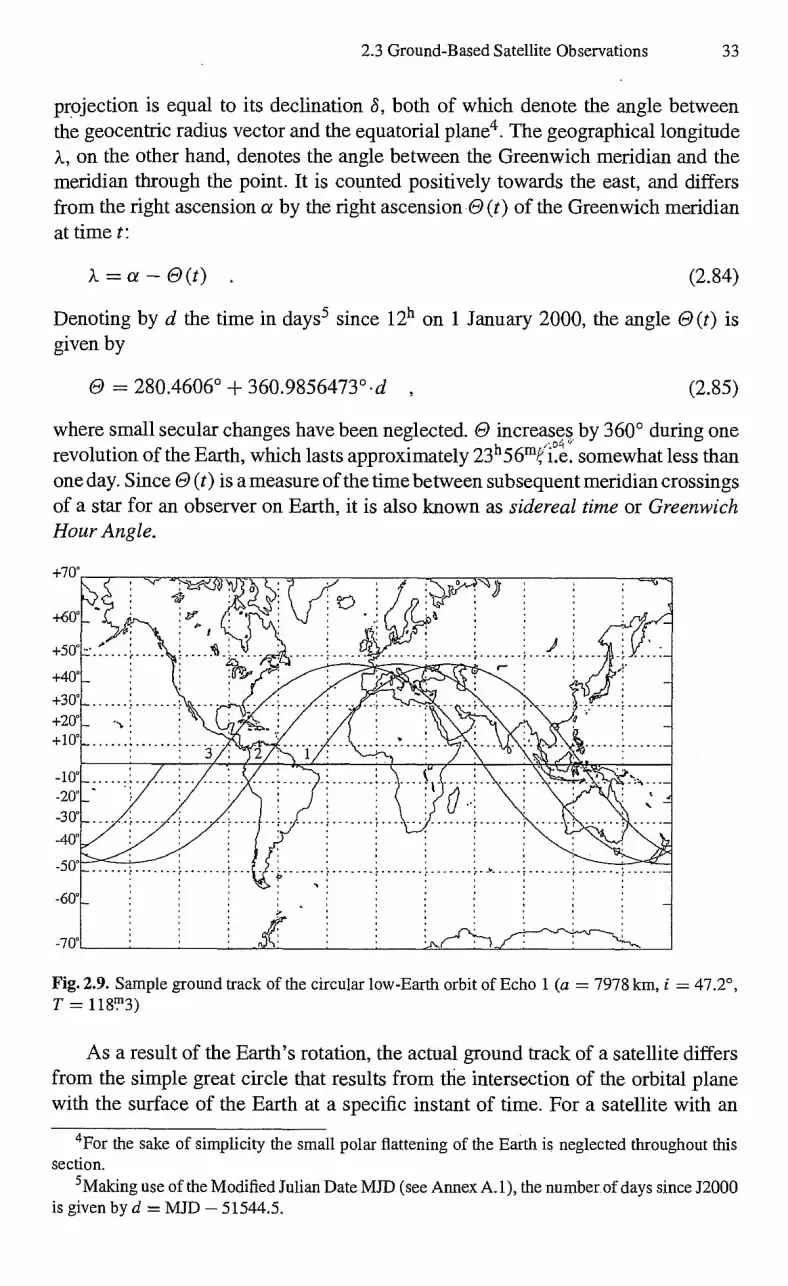
Fig. 2.9. Sample ground track of the circular low-Earth orbit of Echo 1 (a = 7978 km, i = 47.2°, T = 118T3)
As a result of the Earth's rotation, the actual ground track of a satellite differs from the simple great circle that results from the intersection of the orbital plane with the surface of the Earth at a specific instant of time. For a satellite with an
4 For the sake of simplicity the small polar flattening of the Earth is neglected throughout this section.
5 Malcing use of the Modified Julian Date MID (see Annex A.1), the number of days since J2000 is given by d = MJD — 51544.5.
-10° -20° -30"
-40°
-50"
-60°
34 2. Introductory Astrodynamics
orbital period T, the geographic longitude Xç2 = Q — e at which the satellite crosses the equator, is shifted by
= -6-T = —0.2507°/min- T (2.86)
from one revolution to the next. This westwards shift of ground tracks from subse-quent orbits is clearly visible in the projection of three sample orbits of Echo 1 that is illustrated in Fig. 2.9 (Bohrmann 1963). After its launch in August 1960, Echo 1 orbited the Earth once every two hours at a nearly constant altitude of 1300 km and an inclination of i = 47.2°. The corresponding ground tracks cover South America and Australia in the southern hemisphere, as well as North America, Europe and parts of Asia in the northern hemisphere. While the general direction of motion is from west to east (left to right in Fig. 2.9), the ground track is subject to a superposed westwards shift of almost 30° per orbit as a consequence of the Earth's rotation.
The ground track of Echo 1 is typical of all near-circular low-altitude Earth or-bits, which differ only in the inclination and the resulting coverage of high northern and southern latitudes. In the case of eccentric orbits, the resulting ground track pattern may be quite different, however, for a geostationary transfer orbit and a Molniya orbit, as illustrated in Figs. 2.10 and 2.11.
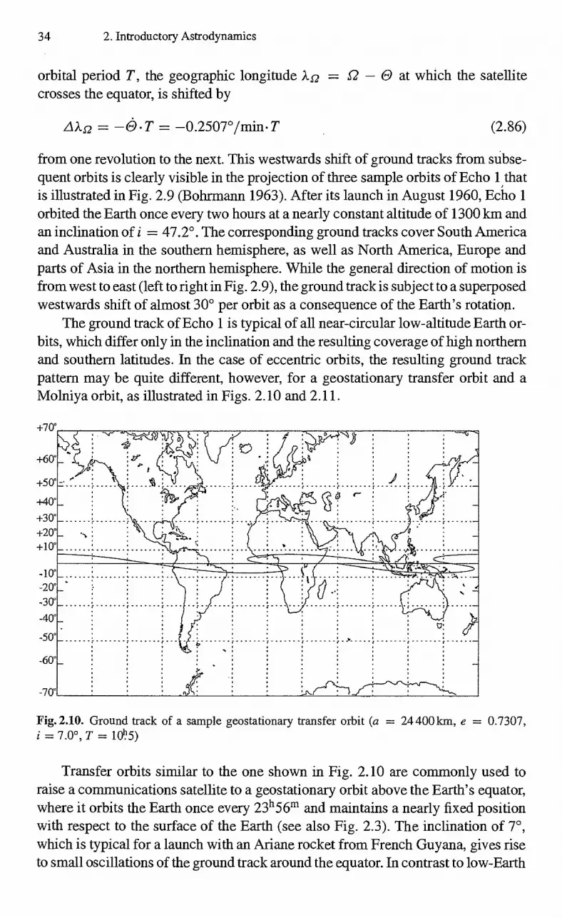
Fig. 2.10. Ground track of a sample geostationary transfer orbit (a = 24 400km, e = 0.7307, = 7.0°, T = 10P5)
Transfer orbits similar to the one shown in Fig. 2.10 are commonly used to raise a communications satellite to a geostationary orbit above the Earth's equator, where it orbits the Earth once every 23h56m and maintains a nearly fixed position with respect to the surface of the Earth (see also Fig. 2.3). The inclination of 7°, which is typical for a launch with an Ariane rocket from French Guyana, gives rise to small oscillations of the ground track around the equator. In contrast to low-Earth
2.3 Ground-Based Satellite Observations 35
orbits, however, the ground track exhibits an S-shaped pattern, which is due to the small angular speed of the satellite at high altitudes. Near apogee, at a distance of roughly 42 000 km, the satellite's inertial velocity amounts to 1 6 km/s, which corresponds to an angular velocity of only 190°/d. As a consequence, the satellite falls back behind the Earth's rotation and appears • to move in a westward direction opposite to the general direction of motion.
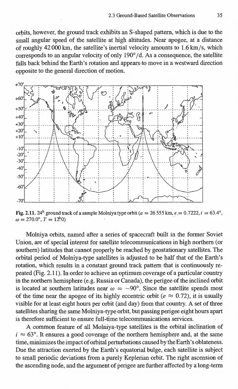
Fig. 2.11. 24h ground track of a sample Molniya type orbit (a = 26 555 km, = 0.7222, i = 63.4°, e.o = 270.0°, T = 120)
Molniya orbits, named after a series of spacecraft built in the former Soviet Union, are of special interest for satellite telecommunications in high northern (or southern) latitudes that cannot properly be reached by geostationary satellites. The orbital period of Molniya-type satellites is adjusted to be half that of the Earth's rotation, which results in a constant ground track pattern that is continuously re-peated (Fig. 2.11). In order to achieve an optimum coverage of a particular country in the northern hemisphere (e.g. Russia or Canada), the perigee of the inclined orbit is located at southern latitudes near co = —90°. Since the satellite spends most of the time near the apogee of its highly eccentric orbit (e 0.72), it is usually visible for at least eight hours per orbit (and day) from that country. A set of three satellites sharing the same Molniya-type orbit, but passing perigee eight hours apart is therefore sufficient to ensure full-time telecommunications services.
A common feature of all Molniya-type satellites is the orbital inclination of i 63°. It ensures a good coverage of the northern hemisphere and, at the same time, minimizes the impact of orbital perturbations caused by the Earth's oblateness. Due the attraction exerted by the Earth's equatorial bulge, each satellite is subject to small periodic deviations from a purely Keplerian orbit. The right ascension of the ascending node, and the argument of perigee are further affected by a long-term

...............
.................
36 2. Introductory Astrodynamics
change that amounts to
2 AS2 = —0.584° (—
Re) cos(i)
and
(2.87)
2 Zko = +0.292° (—
Re ) (5 cos2 (i) — 1) (2.88)
per orbit (see e.g. Bohrmann 1963, Escobal 1965). Here Re stands for the equatorial Earth radius of 6378 km, while p = a(1— e2 ) is the orbital parameter or semi-latus rectum. As can be seen from these equations, the secular drift of the perigee vanishes for an inclination of i = 63.4°, which is also known as the critical inclination. By choosing this particular value for the orbital inclination of the Molniya satellites, it can easily be assured that the perigee and apogee remain at the desired position even without active correction maneuvers.
Fig. 2.12. Satellite motion in the local tangent coordinate system. Only the part of the orbit which is marked by a bold line, and the corresponding ground track, are visible from the given station
2.3.2 Satellite Motion in the Local Tangent Coordinate System
A natural coordinate system for describing the motion of a satellite with respect to an observer or ground station is the topocentric or local tangent coordinate system. For a given point on Earth, it is aligned with the local horizontal plane, i.e. with the plane that is tangential to the surface of the Earth at that point. Commonly, three orthogonal unit vectors eE, eN and ez pointing in the east, north and zenith direction, are employed to define the reference axes of the local tangent coordinate system for a given station. As illustrated in Fig. 2.12, the vectors eN and eE are aligned with the meridian and the parallel of latitude passing through the station,

2.3 Ground-Based Satellite Observations 37
while ez is perpendicular to the horizontal plane in the direction away from the center of the Earth.
In order to express a satellite's position in the local tangent coordinate system, a three-step transformation is required. Denoting the geocentric equatorial coordi-nates by r, a rotation by the Greenwich hour angle 0 around the z-axis yields the position
ref = Rz (e)r (2.89)
in an Earth-fixed coordinate system that is aligned with the equatorial plane and the Greenwich meridian. The corresponding coordinates of a ground station at longitude X and latitude ço are given by
( cos q) cos q)
X) R = R e cos sin X (2.90)
sin ço
and the difference
Sef = ref — R
(2.91)
then yields the topocentric station-satellite vector in Earth-fixed, equatorial coor-dinates. The east, north and zenith unit vectors in the same coordinate system are given by
(— sin X) — sin q) cos X cos q) cos X eE = ± cos X eN = — sin ço sin X ez = cos q) sin X (2.92)
0 cos q) sin q)
Defining the orthogonal transformation matrix
E = (eE eN ez) T , (2.93)
the satellite's local tangent coordinates may finally be written as
( sE S = sN) = E (Rz (e)r — R) .
sz (2.94)
Here sE, si\T and sz are the projection of the station-satellite vector onto the east, north and zenith unit vectors.
For the description of antenna pointing directions the Cartesian coordinates are commonly supplemented by the azimuth and elevation angles
sgr )
The azimuth A gives the angle between the projection of the station-satellite vector on the horizontal plane and the north direction. It is counted positively from the north
A = arctan (—sN
SE ) E = arctan (
Sz (2.95)
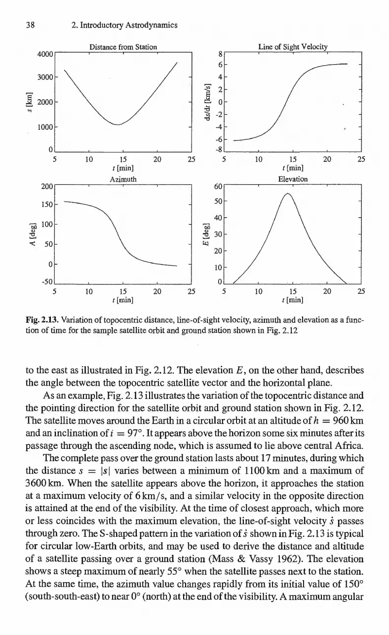
Distance from Station Line of Sight Velocity
10 20 25
5 15 t [min]
25 20 10
4000
3000
2000
1000
O 5 20 25
Fig. 2.13. Variation of topocentric distance, line-of-sight velocity, azimuth and elevation as a func-tion of time for the sample satellite orbit and ground station shown in Fig. 2.12
200
150
7,3 100 -o '‹ 50
0
-50
38 2. Introductory Astrodynamics
to the east as illustrated in Fig. 2.12. The elevation E, on the other hand, describes the angle between the topocentric satellite vector and the horizontal plane.
As an example, Fig. 2.13 illustrates the variation of the topocentric distance and the pointing direction for the satellite orbit and ground station shown in Fig. 2.12. The satellite moves around the Earth in a circular orbit at an altitude of h = 960 km and an inclination of i = 97°. It appears above the horizon some six minutes after its passage through the ascending node, which is assumed to lie above central Africa.
The complete pass over the ground station lasts about 17 minutes, during which the distance s = is I varies between a minimum of 1100 km and a maximum of 3600 km When the satellite appears above the horizon, it approaches the station at a maximum velocity of 6 km/s, and a similar velocity in the opposite direction is attained at the end of the visibility. At the time of closest approach, which more or less coincides with the maximum elevation, the line-of-sight velocity passes through zero. The S-shaped pattern in the variation of shown in Fig. 2.13 is typical for circular low-Earth orbits, and may be used to derive the distance and altitude of a satellite passing over a ground station (Mass & Vassy 1962). The elevation shows a steep maximum of nearly 55° when the satellite passes next to the station. At the same time, the azimuth value changes rapidly from its initial value of 150° (south-south-east) to near 0° (north) at the end of the visibility. A maximum angular

2.4 Preliminary Orbit Determination 39
velocity of A 0.5°/s is required to follow the spacecraft with a ground station antenna, in this particular case.
2.4 Preliminary Orbit Determination
Ground-based satellite observations like angle, distance or velocity measurements depend directly on the satellite's motion with respect to the center of the Earth. They may therefore be used to deduce the orbital elements of a satellite, if its orbit is not known from other sources. Situations in which a satellite orbit must be determined from a small set of available measurements without additional information are likely to occur during tracking of foreign spacecraft, in the case of unforeseen launcher injection errors, or after detection of pieces of space debris from former satellites and rocket upper stages.
At least six independent measurements are required to uniquely determine an orbit if no further assumptions on the form or size of the orbit are made. Deriving the six orbital elements from this minimum set of observations is commonly referred to as preliminary orbit determination, since techniques like the least-squares method (cf. Chap. 8) can later be employed to further refine the orbit determination as more and more observations become available.
Based on the formulation of the unperturbed two-body problem, a variety of different analytical orbit determination methods has been developed. They are gen-erally divided into Laplacian and Gaussian type methods, referring to the two scientists that devised the prototypes of these methods in the late 18 th and early 19th centuries for orbit determination of solar system bodies. Laplacian orbit deter-mination methods are generally designed to derive the inertial position and velocity at an instant of time in the middle of the observation interval, which can then be converted- to orbital elements according to Sect. 2.2.4. Laplacian type orbit determi-nations can be formulated for various combinations of measurements, but may not be well suited for longer tracking arcs if the velocity information has to be obtained from interpolation of positional measurements. Gaussian orbit determination, on the other hand, was originally designed to find the orbital elements from three sets of widely spaced direction measurements. In the case of satellite measurements, it may also be applied to finding the orbit from two position vectors, which is useful if both range and angle measurements are available.
The choice of the most suitable preliminary orbit determination method de-pends strongly on the type and distribution of available measurements, and is still an ongoing discussion, even though most methods for satellite orbit determination were devised in the early days of spaceflight. In View of the great variety of pos-sible approaches to the solution of the preliminary orbit determination problem, the following presentation has intentionally been restricted to a brief account of a simple Gaussian type algorithm.

40 2. Introductory Astrodynamics
2.4.1 Orbit Determination from Two Position Vectors
In favorable cases a satellite may allow simultaneous distance and angle mea-surements yielding directly the satellite's three-dimensional position relative to the ground station. Accounting for the known station location, these measurements can be converted to the position with respect to the center of the Earth. Only two of these position vectors (corresponding to six independent measurements) are then required to determine all six orbital elements in a unique way. The method described in the following comes from Gauss, and provides an efficient and robust way of solving the orbit determination problem for two given position vectors. Further methods like the Lambert-Euler method, the p-iteration and the use of f and g
series are discussed in Escobal (1965) and Bate et al. (1971).
The Ratio of Sector to Triangle
As shown by Gauss, the problem of determining an orbit from two position vectors and a time interval is closely related to the problem of finding the ratio of the sector and the triangle formed by the orbit and the radius vectors.
Let T a and Tb denote the satellite's geocentric position at times ta and th. The area A of the triangle defined by the vectors T a and Tb (Fig. 2.14) depends on the length of the sides ra and rb, and the included angle vh —Va , which is assumed to be less than 1800 in what follows:
1 A = —
2rarb • sin(vh — va) • (2.96)
Here va and vh are the values of the true anomaly at the times under consideration.
Fig. 2.14. Areas of sectors and triangles
The area S of the sector that is bounded by T a and Tb and the arc of the orbit between them, is proportional to the difference between the times ta and th according to Kepler's second law (2.8):
S -1--VGMe -la (1 — e2) (tb — ta) • (2.97) 2
Here a and e denote the semi-major axis and the eccentricity of the orbit that joins the given points. Substituting the semi-latus rectum p = a(1 — e2 ) yields the expression
- 7.1 — ra rb • sin(vb va)
(2.98) 7
2.4 Preliminary Orbit Determination 41
for the ratio n between the two areas, where, for simplicity, the normalized time interval r is defined by
r = N/GM ED • (tb ta) (2.99)
If the semi-latus rectum is replaced by known quantities using the equations for the two-body problem, one finds that it is no longer possible to express n as a solvable algebraic equation. Instead one obtains a system of two equations
2g sin(2g)
(2.100)
772 = m
1+ sin (g/2) with the (positive) auxiliary variables
t 2
,3 N/2(rarb T a rb) (2.101)
ra 1 1 =
2,/2(rarb r a • r b ) 2 from which n can be determined together with the value g that equals half the difference of the eccentric anomalies at times th and ta . Eliminating g yields the transcendental equation
n = i. + . w (—,-,- — / Tr ir
m ) , (2.102)
m
where the function W is defined by 2g — sin(2g)
' W (w) g = 2 sin-1 -1 -- -w (2.103)
sin 3 (g)
2 W(W) (2.104) —
3 ± —
3.5w +
3.5.7w + ..
(Bucerius 1950, Escobal 1965). The argument w is always positive and smaller than one for elliptic orbits. To determine n iteratively, one may use the secant procedure
rii — qi-1
for finding the root of ni m
f (x) = 1 — x (2.106) x x
Appropriate starting values
111 = rio ± 0.1 and 712 = rio (2.107)
may be computed from Hansen's approximation (Bucerius 1950, Battin 1987)
= sin 3 (g)
1
171 =
Or
= rui f(m) f (7- i) — f
(2.105)
12 10 44 m =
1 + 9 1 + 5 /6 •
(2.108)

e cos(y a ) = plra — 1
e cos(vb) = p I rb — 1
when solving for e cos(v). Taking into account that
(2.11 1)
cos(vb) = cos(va ) cos(vb — va ) — sin(va ) sin(vb — va )
= cos(va ) (rb. ea )
sin(v a) (—ro)
rb ri,
on e ob tains the two equations
42 2. Introductory Astrodynamics
Orbital Elements from Two Positions
The orbit of a satellite that passes through the points ra and Tb is always restricted to the plane determined by these two points and the center of the Earth. In order to derive the inclination i of this plane with respect to the equator, as well as the right ascension of the ascending node, one first obtains the orthogonal unit vectors Ca and eo, which both lie in the orbital plane:
T a (2.109)
Iral TO
eo = where ro = rb— (rb • ea)ea (2.110) Irol
Ca is aligned with ra , ro and eo are perpendicular to it. If one now fowls the cross product of ea and eo, the result obtained is the Gaussian vector W = ea X Co, which is perpendicular to the orbital plane, and is likewise nounalized to unit length. Equation (2.58) then yields the right ascension of the node and the orbital inclination. Furthermore, the argument of latitude ua may now be determined from
In order to determine the remaining orbital elements, one requires the ratio sector to triangle, which was derived in the previous subsection. One is then able to express the semi-latus rectum
2.(A 77) 2
ua = arctan Za
— XaWy YaWx)
P = (2.112)
(2.114)
(2.115)
= p/ra — 1
= (p/ ra — 1) ( rb • ea)
(plrb —1)1 (:2-) rb
e cos(v a )
e sin(va )
in terms of the interval r and the area 1 1
= —2
ra rb sin(vb — va ) = —2 ra ro (2.113)
of the triangle defined by the vectors ra and rb. The eccentricity of the orbit follows from the conic section equation (2.17) that
leads to
(2.116)

2.4 Preliminary Orbit Determination 43
which may themselves be solved for the eccentricity and the true anomaly at time ta . The argument of perigee now follows from the difference between the argument of latitude and the true anomaly:
CO = lia Va • (2.117)
From the semi-latus rectum and the eccentricity, one furthermore obtains the semi-major axis
a = 1 — e 2
(2.118)
Finally, the sixth element is the mean anomaly Ma, which is obtained from Kepler's equation
Ma = Ea e sjn Ea (radians) . (2.119)
Here the eccentric anomaly Ea follows from the equations
cos v e cos Ea =
1 e • cos v a
— e2 sin va sin Ea =
1 e • cos V a (2.120)
Or
(-V 1 — e 2 sin va Ea = arctan
cos va e (2.121)
2.4.2 Orbit Determination from Three Sets of Angles
In order to obtain the three-dimensional satellite position at a specific instant of time, simultaneous angle and distance measurements are required. Distance mea-surements, however, require special onboard equipment like a retro-reflector or transponder, in order to determine the round-trip time of a signal from the ground to the satellite and back. In general, they are less easily available than passive angle measurements, which can be obtained by optical observations or the localization of arbitrary radio signals transmitted from a satellite. Orbit determination from ex-clusive angle measurements is therefore of special interest for applications like the identification of unknown spacecraft.
As was shown by Gauss in his analysis of minor planet orbit determination, the problem of finding an orbit from angle observations can be reduced to that of finding an orbit from two position vectors by accounting for various geometrical and dynamical relations between the observations. Each set of angle measurements (for example azimuth and elevation) defines a unit vector, which describes the direction from the station to the satellite at the instant of the observation. The distance is unknown, however, and has to be derived during the process of determining the orbit. In order to obtain all six orbital elements in an unambiguous manner, three sets of observations (i.e. six angle measurements) must be available. From these values, and the known station location, the satellite position at the time of each

44 2. Introductory Astrodynanilcs
observation can be derived in an iterative way. Knowing the position vectors, the orbital elements may finally be computed as illustrated in the previous section.
Let el, e2 and e3 denote the unit vectors that describe the direction of observa-tion at the measurement times t1 <t2 < t3, and let R1, R2 and R3 be the equatorial coordinates of the ground station, from which the corresponding measurements have been obtained. Note that the observations may be obtained from different sta-tions, and that all vectors have to be converted to a common, space-fixed coordinate system, which is in general aligned with the equator. The Earth—satellite—station triangle then yields the fundamental relation
ri = Ri + piei (i = 1, 2, 3) (2.122)
between the given quantities and the unknown station—satellite distances pi and Earth—satellite position vectors ri.
Since the satellite's orbit lies in a plane with the center of the Earth for unper-turbed Keplerian motion, it is possible to express the second position vector by an appropriate linear combination of the other two:
r9 = niri + n3r3 . (2.123)
The factors ni. and n3 depend on the relative position of r 1, r2 and r3, and are positive, provided that the entire arc of the orbit is less than 180°. By inserting (2.123) into (2.122), the unknown position vectors can be eliminated, yielding
p2e2 — n3p3e3 = n1R1 — R2 ± n3R3 (2.124)
after suitable rearrangement. Following Bucerius (1950) one introduces the auxil-iary vectors
= e2 x e3 d2 = e3 x e d3 = e1 x e2 (2.125)
to solve this vectorial equation for pi, p2 and p3. By definition d1 is perpendicular to e2 and e3, d2 is perpendicular to e3 and el, and d3 is perpendicular to el and e2. Consequently, the dot product ei • d only differs from zero for i = j. Multiplying (2.124) by d1, d2 and d3 therefore yields the equations
(2.126)
D = ei • (e2 x e3) = e2 • (e3 x ei) = e1. d1 = e2 d2
= e3 • (el x e2) = e3 • d3
—niPi (el • d1) = R2+ n3R3) • di
P2(e2 • r12) = — R2 +n3R3) - d2
— n3P3(e3 • d3) = (niRi — R2 +n3R3) • d3 .
These expressions may further be simplified using the abbreviations
and
(2.127)
Dii = di Ri , (2.128)

Or
11'2 x r3I Ai (2.131)
In 1 x r21 Z13 123= = --
ri x r3 I ZA2 Vi X r31 Z12
which finally gives the three equations
2.4 Preliminary Orbit Determination 45
P1 =
P2=
P3 =
1 — —(niDii —
n i D 1
—(ni D21 — D22 D
1 — —(n 1 D31 —
n3D
Di2 + n3D13)
± n3 D23)
D32 + n3D33)
(2.129)
The distances P1' p2 and p3 can therefore be expressed in terms of ni and n3, as well as the vectors ei and R.
By introducing equation (2.123) for the orbital plane, the number of unknowns has thus been reduced from three (p1,2,3) to two (n1,3). Furthermore, the newly introduced coefficients are of particular interest, since they can be closely approx-imated by expressions involving the time intervals between the observations. For this purpose the equation of the orbital plane is again considered. Forming the cross product of both sides of (2.123) with r3 and ri, one obtains the expressions
(r2 x r3) = ni • (ri x r3)
(ri x r2) = 12 3 . (ri x r3) (2.130)
ni and 12 3 can therefore be interpreted as ratios of the triangle areas fowled by ri, r2, and r3 (see Fig. 2.15).
Fig. 2.15. Sector and triangle areas for three satellite positions
46 2. Introductory Astrodynarnics
For small arcs of the orbit in particular, the areas of the triangles differ only slightly from the corresponding sector areas Si = qi ik, which are themselves proportional to these time intervals:
272 t3 — t2 t3 — t2 272 t2 — t1 t2 — t1 ni .---- n3 = . (2.132)
771 t3 — t1 t3 — t1 273 t3 — ti t3 — ti
Approximate values for n 1 and n3 are therefore known, which provides a way to determine first approximations for the geocentric distances (pi).
These coarse initial values may then be improved by an iterative method. As outlined in the previous subsection, an orbit is unambiguously determined if one knows the geocentric position of a satellite at two given times. The same applies to the orbital elements and the sector—triangle ratio. If, on the other hand, one knows the value of the sector—triangle ratio for a set of three observed positions, the position vectors with respect to the station and the center of the Earth may be calculated. A simple iteration scheme may therefore be applied to determine an orbit from three sets of angle measurements. To start with, ni = (t3 — t2)/(t3 — ti) and n3 =
(t2 — ti)/(t3 — ti) are used as initial approximations for the ratios of the triangle areas. Improved values of both quantities are then obtained by calculating the station—satellite distances pi from (2.129), the geocentric position vectors ri from (2.122), the sector—triangle ratios Ili for each pair of geocentric position vectors, and finally the corresponding triangle ratios from (2.132). These steps may be repeated until the various quantities change only negligibly from one iteration to the next.
The iteration described here is due to Bucerius (1950) and provides the easi-est way of solving the given orbit determination problem on the basis of Gauss's method. More refined algorithms may be used to improve the convergence, and extend the range of applicability. For a description and valuation of these methods the reader is referred to Escobal (1965).
Exercises 47
Exercises
Exercise 2.1 (Orbit raising using Hohmann transfer) Compute the total ve-locity increment required for a Hohmann transfer between two circular orbits of radius ri = a and r2 = a+ Aa. The Hohmann transfer makes use of a first velocity increment vi to change the orbit into an ellipse with perigee radius ri and apogee radius r2. At apogee, a second maneuver tAy2 is performed, which circularizes the transfer orbit again at a radius of r2. Expand your result, assuming Lia << a and demonstrate that, to first order, the required velocity increment is equal to the difference of the orbital velocities. Check the expressions for the case of an orbit raising maneuver changing the altitude of a remote sensing satellite from 750 km to 775 km.
Solution: From the vis -viva law (2.22), orbital velocities of
and v2=
are obtained for the initial and final circular orbits. The transfer ellipse has a semi-major axis at = • (ri + r2), yielding a perigee and apogee velocity of
V =
( 2 2 ) GM@ r2 G Me)
ri ri r2 at ri
and
li Va = GMe ( 2
T2 ri + T2
GMe ri at r2
respectively. In total, a velocity increment of
zAy = + tAv2 = (Vp V1) ± ( V2 Va)
is required to perform the orbit raising. Substituting y = , the linear expansion in Lia yields at
as
2
a + Lia/2 as well
1 Aa v2 v (1 — ,
Accordingly,
1 Aa 3 Aa vp v (1+ -zt —a ) --) .
4 a
1 Aa Avi Av2 = --v— =V1 V2 2 a
for small altitude raising maneuvers of circular orbits. Note, however, that both ma-neuvers increase the instantaneous velocity of the satellite, but effectively decrease the mean orbital velocity.

48 2 Introductory Astrodynamics
For the given sample case, the following results are obtained from the rigorous equations:
vi = 7.478 lcm/s v = 7.484 lcm/s V2 = 7.465 lcm/s va =-- 7.458 km/s v2 — vi = 13.08 m/s zAv = 13.08 m/s
Both values for the velocity difference agree well with each other and with the approximate value of ZA v 13.11 m/s.
Exercise 2.2 (Kepler's equation) Solve Kepler's equation for an eccentricity of e = 0.72 and a mean anomaly of M = 4° (the typical values of an Ariane geosta-tionary transfer orbit at spacecraft separation). Compare the number of iterations and the total number of trigonometric function evaluations required by Newton's method with the simple fixed-point iteration
E0 = M E1+1 =-- M + e sin(Ei) .
Which method performs better for M = 50°?
Solution: In the first case, Newton's iteration converges within three steps, whereas a total of sixty steps are required for the fixed-point iteration. In terms of trigono-metric function evaluations, Newton's method outperforms the fixed-point iteration by a factor of ten:
Newton's iteration i E LE n trig
Fixed-point iteration i E LIE n trig
1 0.24807037959 4.88 • 10-3 2 1 0.12003783118 1.23 • 10-1 1 2 0.24319412989 6.93-10-6 4 2 0.15603300183 8.72-10-2 2 3 0.24318719638 1.38 • 10-11 6 3 0.18170162689 6.15-10-2 3
20 0.24304481906 1.42 • 10-4 20 21 0.24308769931 9.95 • 10-5 21 22 0.24311766554 6.95 • 10-5 22
58 0.24318719620 1.73-10-10 58 59 0.24318719625 1.21 • 10-1° 59 60 0.24318719629 8.47•10-11 60
Further away from pericenter, however, the fixed-point iteration may well be applied even for large eccentricities. Despite the larger number of iterations, the computa- tional effort may even be smaller than that of Newton's method, as illustrated by
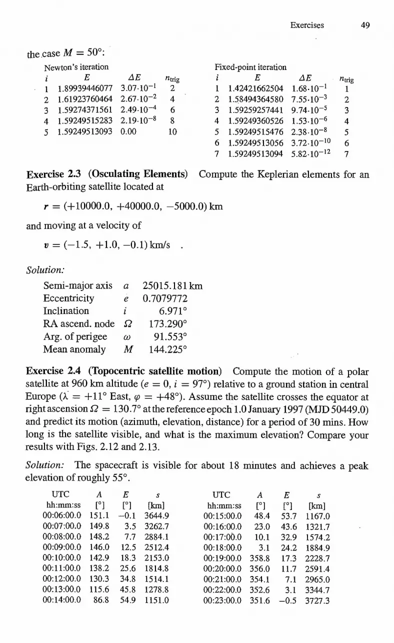
the .case M = 500 : Newton's iteration
dE n trig
Fixed-point iteration
Exercises
dE
49
n trig
1 1.89939446077 3.07 • 10-1 2 1 1.42421662504 1.68-10 -1 1 2 1.61923760464 2.67-10-2 4 2 1.58494364580 7.55 • 10-3 2 3 1.59274371561 2.49 • 10-4 6 3 1.59259257441 9.74 • 10-5 3 4 1.59249515283 2.19-10-8 8 4 1.59249360526 1.53-10-6 4 5 1.59249513093 0.00 10 5 1.59249515476 2.38-10-8 5
6 1.59249513056 3.72 • 10-1 ° 6 7 1.59249513094 5.82-10-12 7
Exercise 2.3 (Osculating Elements) Compute the Keplerian elements for an Earth-orbiting satellite located at
r = (+10000.0, +40000.0, -5000.0) km
and moving at a velocity of
= (-1.5, +1.0, -0.1) km/s .
Solution:
Semi-major axis Eccentricity Inclination RA ascend. node Arg. of perigee Mean anomaly
a 25015.181km 0.7079772
6.971° S2 173.290°
91.553° M 144.225°
Exercise 2.4 (Topocentric satellite motion) Compute the motion of a polar satellite at 960 km altitude (e = 0, i = 97°) relative to a ground station in central Europe (A: = +11° East, go = +48°). Assume the satellite crosses the equator at right ascension Q = 130.7° at the reference epoch 1.0 January 1997 (MJD 50449.0) and predict its motion (azimuth, elevation, distance) for a period of 30 mins How long is the satellite visible, and what is the maximum elevation? Compare your results with Figs. 2.12 and 2.13.
Solution: The spacecraft is visible for about 18 minutes and achieves a peak elevation of roughly 55°.
UTC A E s UTC A E hh:mm:ss [°] [0 ] [km] hh:mm:ss [°] [0 ] [km]
00:06:00.0 151.1 -0.1 3644.9 00:15:00.0 48.4 53.7 1167.0 00:07:00.0 149.8 3.5 3262.7 00:16:00.0 23.0 43.6 1321.7 00:08:00.0 148.2 7.7 2884.1 00:17:00.0 10.1 32.9 1574.2 00:09:00.0 146.0 12.5 2512.4 00:18:00.0 3.1 24.2 1884.9 00:10:00.0 142.9 18.3 2153.0 00:19:00.0 358.8 17.3 2228.7 00:11:00.0 138.2 25.6 1814.8 00:20:00.0 356.0 11.7 2591.4 00:12:00.0 130.3 34.8 1514.1 00:21:00.0 354.1 7.1 2965.0 00:13:00.0 115.6 45.8 1278.8 00:22:00.0 352.6 3.1 3344.7 00:14:00.0 86.8 54.9 1151.0 00:23:00.0 351.6 -0.5 3727.3
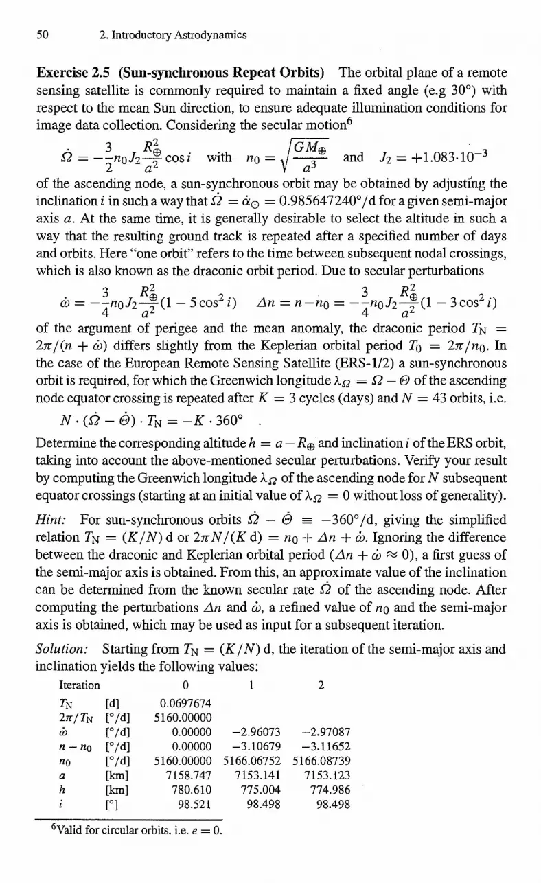
50 2. Introductory Astrodynamics
Exercise 2.5 (Sun-synchronous Repeat Orbits) The orbital plane of a remote sensing satellite is commonly required to maintain a fixed angle (e.g 30 0) with respect to the mean Sun direction, to ensure adequate illumination conditions for image data collection. Considering the secular motion6
3 G --n0J2--"-- cos i with no = and J2 = +1.08340— 2
3 a2 a3
of the ascending node, a sun-synchronous orbit may be obtained by adjusting the inclination i in such a way that s'2 = el 0 = 0.985647240°/d for a given semi-major axis a. At the same time, it is generally desirable to select the altitude in such a way that the resulting ground track is repeated after a specified number of days and orbits. Here "one orbit" refers to the time between subsequent nodal crossings, which is also known as the draconic orbit period. Due to secular perturbations
3 Ri 3 = — —no .12- (1 — 5 cos2 i) An = n —no = (1 — 3 cos 2 i)
4 a2 C/2 of the argument of perigee and the mean anomaly, the draconic period TN = 2n-/ (n + ci)) differs slightly from the Keplerian orbital period To = 27r/no. In the case of the European Remote Sensing Satellite (ERS-1/2) a sun-synchronous orbit is required, for which the Greenwich longitude kg = Q — 0 of the ascending node equator crossing is repeated after K = 3 cycles (days) and N = 43 orbits, i.e.
N • (.f . — 6) . TN = — K 360° .
Determine the corresponding altitude h = a — Re and inclination i of the ERS orbit, taking into account the above-mentioned secular perturbations. Verify your result by computing the Greenwich longitude Xs? of the ascending node for N subsequent equator crossings (starting at an initial value of Xs2 = 0 without loss of generality).
Hint: For sun-synchronous orbits Ô — —360°/d, giving the simplified relation TN = (KIN) d or 271- NI(K d) = no + An + ci). Ignoring the difference between the draconic and Keplerian orbital period (An + c't) 0), a first guess of the semi-major axis is obtained. From this, an approximate value of the inclination can be determined from the known secular rate Q of the ascending node. After computing the perturbations An and ci), a refined value of no and the semi-major axis is obtained, which may be used as input for a subsequent iteration.
Solution: Starting from TN = (K I N) d, the iteration of the semi-major axis and inclination yields the following values:
Iteration 0 1 2
TN [d] 0.0697674 2n-/ [° /d] 5160.00000 (;) [°/d] 0.00000 —2.96073 —2.97087 n — n [°/d] 0.00000 —3.10679 —3.11652 no [°/d] 5160.00000 5166.06752 5166.08739 a [1(1111 7158.747 7153.141 7153.123 h [km] 780.610 775.004 774.986
[O ] 98.521 98.498 98.498
6 Valid for circular orbits. i.e. e 0.

Exercises 51
Convergence is achieved within 2-3 steps, giving the final solution h = 774.99 l -and i = 98.50° for the parameters of the ERS orbit.
Consecutive ground tracks are shifted by in.Q = 360° K I N = -25.12° at the equator. As required, the ground track is closed after 3 days and 43 orbits:
Day 1 ÀS2
Day 2 Xs2
Day 3 Xs2
0 0.000 15 -16.74° 30 -33.49° 1 -25.12° 16 -41.86° 31 -58.60° 2 -50.23° 17 -66.98° 32 -83.72° 3 -75.35° 18 -92.09° 33 -108.84°
10 108.84° 25 92.09° 40 75.35° 11 83.72° 26 66.98° 41 50.23° 12 58.60° 27 41.86° 42 25.12° 13 33.49° 28 16.74° 43 0.00° 14 8.37° 29 -8.37° 44 -25.12°
Exercise 2.6 (Initial Orbit Determination) An Indian ground station collects two sets of range and angle measurements of a satellite:
Date UTC Azim. Elev. Range [km] 1999/04/02 00:30:00.0 132.67° 32.44° 16945.450 1999/04/02 03:00:00.0 123.08° 50.06° 37350.340
Given the Greenwich coordinates
X +1344.143 km , Y +6068.6011cm , Z +1429.311 lcm
of the station, find the inertial position vector of the spacecraft at both times, and use the result to derive the Keplerian elements of the orbit.
Solution: • The observed distances and pointing angles correspond to the following positions with respect to the Earth equator and vernal equinox:
Date UTC x [km] y [km] z [km] 1999/04/02 00:30:00.0 +11959.978 -16289.478 -5963.827 1999/04/02 03:00:00.0 +39863.390 -13730.547 -4862.350
Taking into account the flight time of 2.5 hours between both points, a highly eccentric orbit with elements
Semi-major axis a 28196.776km Eccentricity e 0.7679436 Inclination i 20.315° RA ascend. node S2 359.145° Arg. of perigee co 179.425° Mean anomaly M 29.236°
is obtained, where the value of the mean anomaly applies for the epoch of the first observation.


3.. Force Model
3.1 Introduction
In the framework of Newtonian physics the motion of a satellite under the influence of a force F is described by the differential equation
= F(t,r,v)Im , (3.1)
where r and y are the position and the velocity of the satellite in a non-rotating geocentric coordinate system, and m denotes the satellite's mass. As shown in the previous chapter, one obtains elliptic satellite orbits with fixed orbital planes for the special case of a radially symmetric force
GM63, F m r2 er (3.2)
which decreases with the second power of the distance. Here er denotes the nor-malized position vector of the satellite pointing in radial direction. This simple inverse-square law describes the gravitational attraction of a point-like mass, and can also be shown to be true for extended bodies, provided that they are built up of concentric shells of constant density. Since this is a basic model for the structure of the Earth, Keplerian orbits provide a reasonable first approximation of satellite motion.
Due to its daily rotation, the Earth is not, however, a perfect sphere, but has the fowl of an oblate spheroid with an equatorial diameter that exceeds the polar diameter by about 20 km. The resulting equatorial bulge exerts a force that pulls the satellite back to the equatorial plane whenever it is above or below this plane and thus tries to align the orbital plane with the equator. As may be expected from the small flattening of the Earth, this perturbation is about three orders of magnitude smaller than the central attraction but it may nevertheless be easily detected. Due to its angular momentum the orbit behaves like a gyroscope, and reacts with a precessional motion of the orbital plane, and a shift of the line of nodes by several degrees per day. Aside from this secular perturbation of the orbital plane, the asphericity of the Earth gives rise to a variety of further perturbations that affect all orbital elements, and are most pronounced for satellites at low altitudes.
A different behavior is observed for the perturbations that arise from the grav- itational attraction of the Sun and the Moon. In order to describe the motion of a satellite with respect to the center of the Earth, one has to consider the lunar and

54 3. Force Model
solar forces on both the Earth and the satellite. Their difference increases almost linearly with the satellite's distance from the Earth and yields a perturbation of the geocentric orbit that is comparable in size to that of the Earth's equatorial bulge for geostationary orbits. The resulting acceleration points away from the Earth whenever the satellite is aligned with the Earth and the Sun or Moon, and is di-rected towards the Earth when the satellite is approximately at right angles to the Earth—Sun/Moon line. Similar forces as for the Moon and the Sun arise from the gravitational attraction of the planets. However, their amplitude is much smaller than the lunisolar perturbations; the dominant planetary contributions stem from the planets Venus and Jupiter.
Satellites with altitudes of several hundred kilometers above ground are subject to an additional, velocity-dependent force that is caused by the resistance of the Earth's atmosphere. Since the atmospheric density decreases exponentially with increasing height, drag affects mainly the low-Earth satellites, and is strongest during the perigee of an orbit. It reduces the orbit's kinetic energy and angular momentum, and leads to a slow decrease of the semi-major axis and the eccentricity. For uncontrolled satellites, the loss of altitude and the circularisation of the orbit pose severe limits on the satellite's lifetime Drag has little or no effect on the orbital plane since its main component is always anti-parallel to the velocity vector.
While the acceleration due to gravitational forces is independent of the satel-lite's mass and area, this is not true for drag and other surface forces. Among these, the solar radiation pressure is most notable, especially for communications satel-lites with large solar panels. The radiation pressure arises when photons impinge on the satellite surface, and are subsequently absorbed or reflected, transferring the photons' impulse to the satellite. In contrast to drag, the solar radiation pressure does not vary with altitude. Its main effect is a slight change of the eccentricity and of the longitude of perigee.
The effect of various perturbations as a function of geocentric satellite distance is illustrated in Fig. 3.1. For the calculation of the influence of atmospheric drag on circular low-Earth satellite orbits, exospheric temperatures between 500 K and 2000 K (cf. Sect. 3.5) have been assumed. The area-to-mass ratio used in the com-putation of non-gravitational forces is 0.01 m2/kg. For specially designed geodetic satellites like LAGEOS, the corresponding value may be smaller by one to two or-ders of magnitude. The perturbations due to various geopotential coefficients 41,m
and the lunisolar attraction have been calculated from rule-of-thumb foimulas by Milani et al. (1987). For the purpose of comparison it is mentioned that a constant radial acceleration of 10 -11 km/s2 changes the semi-major axis of a geostationary satellite by approximately 1 m.
Aside from the aforementioned forces, various minor perturbations are consid-ered in Fig. 3.1 which produce accelerations in the order of 10-15-10-12 lun/s2 . The most notable are due to the radiation pressure, resulting from the sunlight reflected by the Earth (albedo), as well as relativistic effects and the solid Earth tides.

55 3.1 Introduction
0
Lageos GPS "1 DRS
GM
10-
Acc
eler
atio
n [k
m/s2
]
10-10
1,%11111111ilift.- -w"IIIIIIIIIM111111111.11111111111ftft-
J2,0 MOOn
Sun
-111111%1Dynàmic Radiation Solid Tide Pressure
Solar
64 1 I I I I I I 1 i
7.8 9.6 11.8 14.5 17.9 21.9 27.0 33.1 40.7
Distance from the center of the Earth [1000 km] 50.0
Fig. 3.1. Order of magnitude of various perturbations of a satellite orbit. See text for further expla-nations.

56 3. Force Model
3.2 Geopotential
In the introductory chapter on unperturbed Keplerian motion, it was assumed that the total mass of the Earth is concentrated in the center of the coordinate system, and the gravitational law (2.1)
GM r =
r3 can therefore be used to calculate the acceleration felt by a satellite at r. For the following discussion of a more realistic model, it is convenient to use an equivalent representation involving the gradient of the corresponding gravity potential U
1 r = VU with U = GMe —
r . (3.3)
This expression for the potential may easily be generalized to an arbitrary mass distribution by summing up the contributions created by individual mass elements dm = p (s) d3 s according to
U = Gf p (s) d3 s (3.4)
IT —s i
Here p (s) means the density at some point s inside the Earth, and ir — si is the satellite's distance from this place (Fig. 3.2).
Fig. 3.2. The contribution of a small mass element to the geopotential
3.2.1 Expansion in Spherical Harmonics
In order to evaluate the integral in the above equation, the inverse of the distance may be expanded in a series of Legendre polynomials. For r > s, which holds for all points r outside a circumscribing sphere, one has
1 " (s ) n 13, (cos y) with cos y = r s (3.5)
1
Ir — si r s n=
Here
13,(u) = 1 dn (u 2 — 1) n 2'n! dun
is the Legendre polynomial of degree n, and y is the angle between r and s.
(3.6)
3.2 Geopotential 57
By introducing the longitude A (counted positively towards the East) and the geocentric latitude of the point r according to
x = r cos 0 cos
y = r cos 0 sin X
(3.7)
z = r sin ,
as well as the corresponding quantities A.' and Of for s (cf. Fig. 3.2), one can make use of the addition theorem of Legendre polynomials, which states that
(n — m)! . Pn (cos Y) = (2— 80m)
(n+m)!Pnm(sln 0) Pnm (sin 0') cos(m (X — A')). (3.8)
Here Pnm , which is called the associated Legendre polynomial of degree n and order m, is defined as
dm PnnAu) = (1 — u 2)m12 P(u)
dum • (3.9)
Explicit formulas for selected low-order Legendre polynomials may be found in Table 3.1.
Table 3.1. Low-order Legendre polynomials
n m Pnm (u) Pnm (sin g» 00 1 1
u sin 0 1..1
1..1
(1 _ u2)112 cos 0
0 ,--1 C
N1
11,1„2 —1) 2 k'1".
1(3 sin2 0 _ 1)
cv 3u(1 — u2) 1 /2 3 cos 0 sin0 3(1 — u2) 3 cos2 0
One is now able to write the Earth's gravity potential in the form
oo n G MED RI U = — Pnm (sin 0)(Cnn, cos(mX) + Snm sin(m)0),
r rn n=0 m=0
with coefficients
(3.10)
M=0
2-80 (n—m)! f sn 1
M '
e, (n +m)! —
RI
Pnm (sin 0) cos(mX C nm = ) p (s) d3 s
2-80m (n—m)! f sn
Me, (n +m)! /--i-1
Pnm(sin. 0 1) sin(mXI)p(s) d3 Snm = s
which describe the dependence on the Earth's internal mass distribution. Geopo- tential coefficients with m =0 are called zonal coefficients, since they describe the
(3.11)

(2 - 80m) (2n -1-1)(n — m)! Pnm = (3.16) Pnm (n +m)!
58 3. Force Model
part of the potential that does not depend on the longitude. All Sno vanish due to their definition, and the notation
Jn = — CnO (3.12)
is commonly used for the remaining zonal ternis. The other geopotential coefficients are known as tes serai and sectorial coefficients for (m <n) and (m = n), respectively.
A close look at (3.10) reveals that a change of Ro affects the geopotential coefficients Cnm and Snm . Therefore, care must be taken to apply matching values of GM, Ro , as well as Cnni and Snm , when computing the satellite's acceleration.
Since the geopotential coefficients Cm', and Snm cover a range of ten or more orders of magnitude, even for a small model, the nomialized coefficients enm and :9-nm are usually given, which are defined as
'-'Snnmm I -1 (2 —80m )(n2+n+171 1) ; —m)!I CSn'imm I
(3.13)
The nomialized coefficients are much more unifomi in magnitude than the unnor-malized coefficients, and their size is given approximately by the empirical Kaula rule (Kaula 1966) as
n m Snm
(3.14) n2
Making use of the nomialized geopotential coefficients, the acceleration due to the Earth's gravity potential may be rewritten as (Milani et al. 1987)
GME, °° n - =V = Pnm(Sin 0)(C- nm COs(mA.) + S nnz sin(mX)) rn
n=0 m=0
where the nomialized associated Legendre functions are given as
(3.15)
In contrast to the unnomialized functions Pnnz, the Pnni exhibit a less pronounced variation with n and m, according to their normalization relations.
Note: The reader should be aware that a slightly different definition of the associ-ated Legendre polynomials is frequently used, which involves an additional factor (-1)m. Both definitions are distinguished by the notation P,T = (-1)m Pnrn fl Abramowitz & Stegun (1965), but often the two notations are mixed up in the literature. For applications in geodesy and related fields it is important to use the definition given here (i.e. the one without the factor (-1)m) in order to be consistent with published geopotential coefficients.
3.2 Geopotential 59
3.2.2 Some Special Geopotential Coefficients
Even though the definition of the geopotential coefficients Cnni and Sn,n is rather complicated at first sight, one may nevertheless derive some simple results if only low-degree and order coefficients are considered, or if one uses an approximate model for the terrestrial density variation.
First of all, it is easy to show that C00 is always equal to 1, since the integral
f so — Poo (sin 0') cos(0)p(s) d3 s = p(s) d3 s = MED (3.17) 143,
yields just the total mass of the Earth. The first term in the expansion of the Earth's potential is therefore just the two-body potential U =GMED Ir. Furthermore, one recognizes from (3.11) that all terms Sno vanish, since sin(mX 1 ) in the integrand is equal to zero for m = O.
As mentioned in the introductory section of this chapter, the potential of a spherical body that is built up from concentric shells of constant density is the same as that of a point-like mass, and it is now possible to prove this statement with the help of (3.11). If the density p depends only on s, but not on 41 and X', then all
Snm = K fS
n
— Pnni (Sin 41) sin(mA, 1)p(s)d 3s R E9n
Rea +7r/2 2r
0 —7r/2 0 RG) +7r/2 27r
= K f sn+2
P(s)ds • R f Prun (sin g5 1 ) cos(e)dck'
. f sin(mX1)dX' ,m,"
O - —7r/2 0
2 - 30,7, (n - m)!
with K = M (n m)!
Kf f fsn R ,p(s)P„,, (sin c/i) sin(m4s 2 cos(0') dc/l ds
(3.18)
vanish, since f sin(mXI)dX' = 0 for all m and the same proof applies to Cnm = for n, m O. For m= 0 the integral f cos(m4dX1 does not vanish, but
+z/2 1
f PnO(Sin 0 1 ) COS(41)dq51 = f Pn (u)du = 0
-7r/2 -1
for all n > O. Therefore all C„,, and Snn, vanish, with the exception of Coo, and the potential reduces to that of a point-like mass, as long as the density does not vary with longitude and latitude.
A similar consideration shows that the expansion of the potential contains only zonal terms (Co), if one considers the more general case of a mass distribution that is symmetric with respect to the axis of rotation. For an oblate rotational ellipsoid

60 3. Force Model
J = —3/2C20 is the largest geopotential coefficient aside from Coo, and its value is approximately given by
w2 R2/ 2
GM / R
where the flattening f measures the difference between the polar and the equatorial diameter in units of the equatorial diameter, while M, R and w are the mass, radius and rotational velocity of the body, respectively. The relation follows from the condition that the sum of the gravitational potential and the centrifugal potential must be constant on the surface of a fluid body, and is derived in standard textbooks on geodesy (e.g. Bomford 1980, Torge 1991). Using appropriate values
f GMED R ® we
= = = =
1/298.257 398 600.4405 km3 s-2
6378.137 km 0.7292115-10-4 rad
(3.20)
for the Earth, one finds that J =0.001621 . The Earth is not an ideal rotational ellipsoid, however, which gives rise to
additional tesseral and sectorial geopotential coefficients. Approximate values of the Earth's low-order potential coefficients can be found in Table 3.2.
Table 3.2. Geopotential coefficients up to degree and order three
Cnm m0 1 3
+1.00 0.00 0.00
N —1.08-10-3 0.00 +1.57-10-6
+2.53-10-6 +2.18-10-6 +3.11-10-7 1.02•10-7
n m=0 1 2 3
0 ,--1
N cn
ll 0.00 0.00 0.00 0.00 0.00 —9.03.10-7 0.00 +2.68-10-7 —2.12.10-7 1.9840-7
Aside from the coefficients Sno, which are zero by definition, there are five other coefficients that vanish as a consequence of a special choice of the coordinate system. By choosing the center of mass
1 = f s p (s) d3 s (3.21)
i To be precise, equation (3.19) in a slightly extended fowl is used in geodesy to define the flattening f of a suitable reference ellipsoid, since J2 is easier to determine than the mean figure of the Earth (see e.g. Kaula 1966).
(3.19)

C io=1
s sin 01 p (s) d3 s = Ms Rs j f p d3 s=—
Re Me Re
3.2 Geopotential 61
as the origin of the coordinate system, one may always observe that the three coefficients
(3.22)
of degree one are equal to zero. Similarly C21 and 521, vanish as long as the z-axis is aligned with the Earth's main axis of inertia.
3.2.3 Gravity Models
Because the internal mass distribution of the Earth is not known, the geopotential coefficients cannot be calculated from the defining equation (3.11), but have to be determined indirectly. Three principal types of measurements and observations are currently used to improve Earth gravity models
• Satellite Tracking: From the very beginning of spaceflight, ground-based ob-servations of artificial satellites allowed scientists to determine the Earth's gravity field through the perturbations seen in the satellite orbits. The first ob-servations mainly used Baker–Nunn wide angle telescopes, which provided pictures of the satellites' orbital tracks. Subsequently, it turned out that radio-metric Doppler tracking led to models superior to those based on optical data. The development of satellite laser ranging (SLR) systems around 1965, and their continuous refinement up to a precision of better than 1 cm, significantly improved the knowledge of the gravity field. In the beginning of the 1990s, the French DORIS system with a Doppler precision of 0.4 mm/s, as well as the German PRARE system with a range noise of 7 cm, provided further advanced tracking systems with a high potential for satellite geodesy. Latest enhancements in the gravity field recovery from satellite tracking are due to the inclusion of satellite-to-satellite (SST) tracking Especially the GPS track-ing of satellites, starting with the TOPEX/POSEIDON spacecraft in 1992, may significantly improve the gravity models due to its nearly continuous, high-precision and three-dimensional information. The global coverage of the Earth's surface with satellite tracks allows the retrieval of global infor-mation on the long-wavelength gravity field of the Earth.
• Swface Gravimetry: Static spring gravimeters measure the local gravita-tional acceleration with an accuracy of 10 -3 mGal (Torge 1991) (1 mGal = 10-5 m/s2 ), and thus provide precise local and regional (short-wavelength) information on the gravity field. Relative gravimetry measures the gravity differences from point to point by sensing the inertial reaction of a test mass
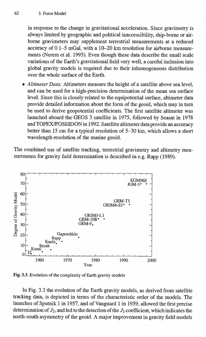
62 3. Force Model
in response to the change in gravitational acceleration. Since gravimetry is always limited by geographic and political inaccessibility, ship-borne or air-borne gravimeters may supplement terrestrial measurements at a reduced accuracy of 0.1-5 mGal, with a 10-20 km resolution for airborne measure-ments (Nerem et al. 1995). Even though these data describe the small scale variations of the Earth's gravitational field very well, a careful inclusion into global gravity models is required due to their inhomogeneous distribution over the whole surface of the Earth.
• Altimeter Data: Altimeters measure the height of a satellite above sea level, and can be used for a high-precision determination of the mean sea surface level. Since this is closely related to the equipotential surface, altimeter data provide detailed information about the form of the geoid, which may in turn be used to derive geopotential coefficients. The first satellite altimeter was launched aboard the GEOS 3 satellite in 1975, followed by Seasat in 1978 and TOPEX/POSEIDON in 1992. Satellite altimeter data provide an accuracy better than 15 cm for a typical resolution of 5-30 km, which allows a short wavelength resolution of the marine geoid.
The combined use of satellite tracking, terrestrial gravimetry and altimetry mea-surements for gravity field determination is described in e.g. Rapp (1989).
61. 40
80
70
7.1 60 o
50
10
Gaposchkin Rapp •
Kaula. • Itzsak
Kozai . O - J2. •
1, 11 1
EGM96S - JGM-3• • —
GEM-T3 GRIM4-S2• •
GRIM3-L1 GEM-10B • • - GEM-9.
1960
1970
1980
1990
2000 Year
Fig. 3.3. Evolution of the complexity of Earth gravity models
In Fig. 3.3 the evolution of the Earth gravity models, as derived from satellite tracking data, is depicted in terms of the characteristic order of the models. The launches of Sputnik 1 in 1957, and of Vanguard 1 in 1959, allowed the first precise deteimination of J2, and led to the detection of the J3 coefficient, which indicates the north-south asymmetry of the geoid. A major improvement in gravity field models

3.2 Geopotential 63
was achieved in 1966 by Anderle, using radiometric Doppler data instead of the camera data, that had been previously applied (Nerem et al. 1995). Between 1966 and 1977, the leading models were those derived by Gaposchkin and colleagues at the Smithonian Astrophysical Observatory (SAO).
As a reaction to the military classification of Doppler-based gravity models, NASA's Goddard Space Flight Center (GSFC) started in 1972 to develop a series of models GEM 1—GEM 10 (Goddard Earth Model) of degree 12-22. Here the odd-numbered models are exclusively based on satellite observations, the correspond-ing even-numbered models have been derived using additional surface gravimetry data. While the satellite tracking data determine the long-wavelength components of the gravity field of degree n, according to a spatial resolution of 2n- Re / (2n) or — 20000 km/ n, the altimeter and surface gravimetry data allow a much higher resolution at shorter wavelength. An example is the GEM 10C model of degree and order 180, while at the same time the GEM 10B model of degree and order 36 was developed using a less dense grid of surface gravimetry and altimetry data (Lerch et al. 1981). The models GEM-Tl (Marsh et al. 1988) and GEM-T2 (Marsh et al. 1990), both complete to order and degree 36, were entirely based on satellite tracking data from 17 and 31 satellites, respectively. In addition to a small augmen-tation of satellite tracking data, the GEM-T3 model (Lerch et al. 1994) also applied altimeter data from GEOS 3, Seasat and Geosat, and was complete to degree and order 50.
The oceanographic mission TOPEX/POSEIDON (TIP), with its challenging requirement on the radial orbit accuracy of 13 cm, led to a cooperation between NASA's GSFC, the University of Texas Center for Space Research (CSR) and the Centre National d'Études Spatiales (CNES) for gravity field determination. As a result, the final prelaunch TIP gravity model JGM-1 (Joint Gravity Model) of order and degree 70 was issued in 1994 (Nerem et al.). It reiterated the GEM-T3 gravity model solution by processing all of the data with improved models and constants. Its successor JGM-2 (Nerem et al. 1994) was a first postlaunch TIP model, which included a six-month set of TIP SLR and DORIS data. A further improvement in accuracy was obtained with JGM-3 (Tapley et al. 1996), which comprised new TIP SLR, DORIS, as well as for the first time GPS tracking data of TIP. In addition, new LAGEOS 1, LAGEOS 2 and Stella laser tracking, as well as DORIS tracking of the SPOT 2 satellite, were included. A subset of the JGM-3 model (Tapley et al. 1996) is reproduced in Table 3.3.
Although JGM-3 is a very elaborate global gravity model for precision orbit determination, new models are continuously being developed. This is demonstrated by a collaboration of NASA's Goddard Space Flight Center (GSFC), the National Imagery and Mapping Agency (NIMA) and the Ohio State University (OSU), that published the EGM96S (Earth Gravity Model) of degree and order 70, and the EGM96 model of degree and order 360 (Lemoine et al. 1998). The inclusion of tracking data from 40 satellites, with more continuous data from GPS and TDRSS satellite-to-satellite tracking, contributes to a further improvement of the gravity field model.

64 3. Force Model
Table 3.3. JGM-3 nounalized gravitational coefficients up to degree and order 20, in units of 10-6 (GMe = 398 600.44151cm3 s-2 , Re = 6378.136301cm) (Tapley et al. 1996)
n m E'n,m Er 1,m n m Cn,m :S;n,m n m ST'n,m
2 0 -484.165368 0.000000 2 1 -0.000187 0.001195 2 2 2.439261 -1.400266
3 0 0.957171 0.000000 3 1 2.030137 0.248131 3 2 0.904706 -0.618923 3 3 0.721145 1.414204
4 0 0.539777 0.000000 4 1 -0.536244 -0.473772 4 2 0.350670 0.662571 4 3 0.990869-0.200987 4 4-0.188481 0.308848
5 0 0.068659 0.000000 5 1 -0.062727 -0.094195 5 2 0.652459 -0.323334 5 3 -0.451837 -0.214954 5 4 -0.295123 0.049741 5 5 0.174832 -0.669393
6 0 -0.149672 0.000000 6 1 -0.076104 0.026900 6 2 0.048328 -0.373816 6 3 0.057021 0.008890 6 4 -0.086228 -0.471405 6 5 -0.267112 -0.536410 6 6 0.009502 -0.237262
7 0 0.090723 0.000000 7 1 0.280287 0.094777 7 2 0.329760 0.093194 7 3 0.250502 -0.217320 7 4 -0.275541 -0.124142 7 5 0.001644 0.018075 7 6 -0.358843 0.151778 7 7 0.001380 0.024129
8 0 0.049118 0.000000 8 1 0.023334 0.058499 8 2 0.080071 0.065519 8 3 -0.019252 -0.086286 8 4 -0.244358 0.069857 8 5 -0.025498 0.089090 8 6 -0.065859 0.308921 8 7 0.067263 0.074813 8 8 -0.123971 0.120441
9 0 0.027385 0.000000 9 1 0.142230 0.021910 9 2 0.022621 -0.032175 9 3 -0.161064 -0.074546 9 4 -0.008202 0.020068 9 5 -0.016325 -0.054272 9 6 0.062833 0.222677 9 7 -0.118159 -0.096899 9 8 0.187984 -0.003015 9 9 -0.047725 0.096586
10 0 0.054130 0.000000 10 1 0.083759 -0.131554 10 2 -0.093558 -0.051416 10 3 -0.007197 -0.154180 10 4 -0.084335 -0.078485 10 5 -0.049520 -0.050293 10 6 -0.037419-0.079464 10 7 0.008208-0.003149 10 8 0.040468-0.091917 10 9 0.125403-0.037737 10 10 0.100382-0.023809
11 0 -0.050161 0.000000 11 1 0.016107-0.027892 11 2 0.018430-0.098452 11 3 -0.030561-0.148803 11 4 -0.040024 -0.063596 11 5 0.037436 0.049828 11 6 -0.001461 0.034173 11 7 0.004706 -0.089777 11 8 -0.006141 0.024572 11 9 -0.031456 0.042041 11 10 -0.052129 -0.018302 11 11 0.046227 -0.069593
12 0 0.036383 0.000000 12 1 -0.054192 -0.042012 12 2 0.013986 0.031048 12 3 0.038979 0.024577 12 4-0.068420 0.002954 12 5 0.031107 0.007639 12 6 0.003324 0.039369 12 7 -0.018603 0.035571 12 8 -0.025703 0.016667 12 9 0.041793 0.025325 12 10 -0.006169 0.030986 12 11 0.011321 -0.006344 12 12 -0.002349 -0.010959
13 0 0.039946 0.000000 13 1 -0.052967 0.039877 13 2 0.056039 -0.062699 13 3 -0.021817 0.098209 13 4 -0.001471 -0.012614 13 5 0.058253 0.065846 13 6 -0.035312 -0.006058 13 7 0.002706 -0.007711 13 8 -0.009887 -0.009729 13 9 0.024754 0.045359 13 10 0.040892 -0.037099 13 11 -0.044739 -0.004833 13 12 -0.031410 0.088106 13 13 -0.061211 0.068409

3.2 Geopotential 65
Table 3.3. (continued)
n ni S;11,in n 172 Cn,m 3n,m n ni Cn,m 'gn,nz
.14 0 -0.021804 0.000000 14 1 -0.019024 0.027472 14 2 -0.036979 -0.002989 14 3 0.036809 0.020313 14 4 0.001712-0.020688 14 5 0.029900-0.016858 14 6-0.019401 0.002413 14 7 0.036851-0.004222 14 8 -0.034867 -0.014888 14 9 0.032377 0.028698 14 10 0.038839 -0.001466 14 11 0.015357 -0.039039 14 12 0.008505-0.030922 14 13 0.032167 0.045200 14 14 -0.051783 -0.005014
15 0 0.003166 0.000000 15 1 0.012019 0.008173 15 2 -0.021746 -0.031733 15 3 0.052403 0.015160 15 4-0.042163 0.007827 15 5 0.013451 0.008982 15 6 0.033463 -0.037753 15 7 0.059913 0.006056 15 8 -0.031990 0.022271 15 9 0.013027 0.037876 15 10 0.010311 0.014956 15 11 -0.000952 0.018716 15 12 -0.032729 0.015720 15 13 -0.028289 -0.004294 15 14 0.005305 -0.024443 15 15 -0.019228 -0.004704
16 0 -0.005430 0.000000 16 1 0.027534 0.033708 16 2 -0.022395 0.026207 16 3 -0.035101 -0.023242 16 4 0.041219 0.046057 16 5 -0.013495 -0.001679 16 6 0.014321 -0.034445 16 7 -0.007813 -0.008510 16 8 -0.021538 0.005248 16 9 -0.022777 -0.038924 16 10 -0.012129 0.012065 16 11 0.019266 -0.002975 16 12 0.019698 0.006915 16 13 0.013837 0.000994 16 14 -0.019126 -0.038862 16 15 -0.014461 -0.032699 16 16 -0.037529 0.003591
17 0 0.018108 0.000000 17 1 -0.026389 -0.029853 17 2 -0.017379 0.009197 17 3 0.007423 0.008195 17 4 0.007520 0.023382 17 5 -0.017058 0.005353 17 6 -0.013467 -0.028275 17 7 0.024011 -0.005884 17 8 0.037625 0.003761 17 9 0.003291 -0.028586 17 10 -0.004304 0.018038 17 11 -0.015726 0.011021 17 12 0.028689 0.020744 17 13 0.016603 0.020305 17 14 -0.014061 0.011376 17 15 0.005332 0.005387 17 16 -0.030061 0.003724 17 17 -0.034064 -0.019733
18 0 0.007269 0.000000 18 1 0.004210-0.039076 18 2 0.012828 0.013586 18 3 -0.003760 -0.003109 18 4 0.053092 0.001460 18 5 0.007314 0.024650 18 6 0,013378 -0.015661 18 7 0.006529 0.006280 18 8 0.031066 0.002470 18 9 -0.019183 0.036144 18 10 0.005566 -0.004595 18 11 -0.007643 0.002117 18 12 -0.029603 -0.016193 18 13 -0.006380 -0.034980 18 14 -0.008003 -0.013078 18 15 -0.040536 -0.020249 18 16 0.010671 0.006965 18 17 0.003600 0.004510 18 18 0.002621 -0.010810
19 0 -0.003519 0.000000 19 1 -0.006968 0.000158 19 2 0.031435-0.004330 19 3 -0.009900 -0.000988 19 4 0.015827 -0.005662 19 5 0.012058 0.027204 19 6 -0.002385 0.017952 19 7 0.007368 -0.008665 19 8 0.031052-0.010463 19 9 0.003031 0.006452 19 10 -0.033378 -0.007090 19 11 0.016081 0.011000 19 12 -0.002989 0.009310 19 13 -0.007447 -0.028398 19 14 -0.004529 -0.013114 19 15 -0.017839 -0.014106 19 16 -0.021421 -0.006958 19 17 0.029106 -0.015153 19 18 0.034714 -0.009439 19 19 -0.002371 0.004780
20 0 0.018790 0.000000 20 1 0.008348 0.006245 20 2 0.020030 0.0148 85 20 3 -0.005935 0.035571 20 4 0.005457 -0.022410 20 5 -0.011452 -0.006935 20 6 0.011565 -0.000423 20 7 -0.020302 -0.000130 20 8 0.004922 0.004067 20 9 0.018044 -0.005865 20 10 -0.032549 -0.005760 20 11 0.014563 -0.018930 20 12 -0.006409 0.018154 20 13 0.027324 0.007033 20 14 0.011894-0.014472 20 15 -0.025833 -0.000766 20 16 -0.012064 0.000330 20 17 0.004435 -0.013703 20 18 0.014917 -0.000984 20 19-0.002963 0.010960 20 20 0.004045 -0.012347

66 3. Force Model
3.2.4 Recursions
In the computation of the Earth's gravity potential at a given point, several recur-rence relations for the evaluation of Legendre polynomials can be used. Starting with Poo = 1, all polynomials Pmn, up to the desired degree and order are first calculated from
Pinin(u) = (2m - 1)(1 — u 2) 1/2 Pm—i,m—i , (3.23)
where u and (1 — ti 2 ) 112 stand for sin and cos ¢), respectively. With these results the remaining values may be obtained from
(u) = (2m -1- Ou Pmni (u) (3.24)
and from the recursion
PP(u) = 1
n — m((2n — Pn—i,m(u) — +m — 1) Pn-2,m(14 )) (3.25)
for n > m +1. The above relations for the Legendre polynomials may, according to Cunning-
ham (1970), be favorably combined with the addition theorems
cos((m + 1) ).) = cos(mX) cos(h) — sin(mX) sin(h) (3.26)
sin((m 1)h) = sin(mh) cos(h) cos(mh) sin(h)
for the angular functions of the longitude-dependent terms into a single recursion. This allows an efficient computation of the geopotential and the resulting acceler-ation as a function of the Cartesian coordinates (x, y, z) of the satellite. Defining
Rn+1
Vnm = ( .33.1 ) • Pnm (sin q5) • cos m)
= ( R ) n+1
7 . Pnm (sin 0) - sin mX
the gravity potential may be written as
Wnin
(3.27)
(CnmVnm SnmWnm) (3.28)
The VI1171 and Wnm satisfy the recurrence relations
VMM (2m — 1) y Re
r 2 Vm-1,m-1
r2 Wm-1,m-1
(3.29)
WM111 (2m — 1) x Re y RG
In-1 ' in— W 1 + Vm-1,-1 I 2 r-
m

3.2 Geopotential 67
and
(2n -1 Z RED (n+m-1) Vnm
r2 Vn-1,m
r2 Vn-2,m n—m
(2n zR ED (n-l-m-1 Wnm n—m r2 Wn-1,m n—m r2 Wn —2,m
(3.30)
which follow immediately from the above relations for the Legendre polynomials and the trigonometric functions. The second set of equations holds for n = m +1, too, if Vm-1,m and Wm-i,,n are set to zero. Furthermore,
Voo = —r
and W00 = 0
(3.31)
are known. In order to calculate all Vnm and W„, (0 <m < n < nmax), one first obtains
the zonal terms Vo by using (3.30) with m=0. The corresponding values Wno are all identical to zero. Now, (3.29) yields the first tesseral terms VIA and W11 from V00, which allows all Vn (1 < n < nmax ) to be determined. Thus the recursions are used according to the following scheme:
Voo, Woo Eqn. (3.29) 4, Eqn. (3.30)
Wio Vii, Wll
4,
V20, W20 V21, W21 V22, W22
4,
Vn(), Wn0 Vn i, Wnl Vn2, Wn2 Vnn, Wnn
Finally it should be noted that many other recursion formulas exist for the calcu-lation of Legendre polynomials, and may be looked up in standard text books or mathematical tables (Abramowitz & Stegun 1965). Not all of these are, however, equally well suited for the numerical computation, especially if high-order polyno-mials are required (cf. Lundberg 1985). The recursions presented here are stable, which means that small numerical errors in the computation of low-order terms .do not lead to meaningless results for high orders. As was shown by Deufihard (1976), recurrence relations for P„,n that keep either order (m) or degree (n) constant are more stable than others. This is the case for (3.25) and applies equally well to the formulas for Vn„, and Wri ,n . As a rule of thumb, one can expect to loose 2-3, 4-5, and 5-6 digits when evaluating these functions up to orders 15, 50, and 100, respectively.

68 3. Force Model
3.2.5 Acceleration
The acceleration which is equal to the gradient of U, may be directly calculated from the Vn,n and VIT„„, as
= X nm 7 nm nm (3.32)
n,m n,m
with the partial accelerations
(m>0)
GM {— CnOVn+1,1 }
GM 1
4 2
(n—m+2)!
(n—m)! (+CnmVn+1,m-1 + SnmWn+1,m-1)/
inm (m=0)
{( — CninVn+1,m+1 — SnmWn+1,m+1)
Ynm (m=o) GM {— CnOWn+1,1 Rt,
(m>0) GM 1 f ( — Cnin Wn+1,m+1 + Snm • Vn+1,m+1) 2
(3.33)
(n—m+2)! ( CiunWn+1,m-1 SnmVn+1,m-1)/
(n—m)!
inm GM
R2 { (n—m+1) - ( — CnmVn+1,m SnmWn+1,m)) •
The derivation of these equations is given in Cunningham (1970), together with similar relations for the second-order partial derivatives of the potential. It is noted that the Vvi, and Kt, terms are required up to degree and order n+1 if the partial accelerations due to geopotential coefficients up to Cnn and Snn are to be calculated.
The formulas given so far yield the acceleration r = 53, i) in an Earth-fixed coordinate system as a function of the Earth-fixed position vector r = (x, y, z). Some coordinate transformations are therefore required to obtain the acceleration in an inertial or Newtonian coordinate system which is consistent with the equation of motion (3.1). Using indices ef and sf to distinguish Earth-fixed from space-fixed coordinates, one has
ref = U(t) • rsf and isf = UT (t) ief 7 (3.34)
where U(t) is a time-dependent matrix that describes the Earth's rotation. The rigorous computation of U(t), furthermore, has to account for the long and short-term perturbations of the Earth's axis, known as precession and nutation, that are described in detail in Chap. 5.

3.3 Sun and Moon 69
3.3 Sun and Moon
3.3.1 Perturbing Acceleration
According to Newton's law of gravity, the acceleration of a satellite by a point mass M is given by
= GM. s — r
(3.35) Is — ri
where r and s are the geocentric coordinates of the satellite and of M, respectively. Some care is required, however, before this expression can be used for describing the satellite's motion with respect to the center of the Earth. The value of in (3.35) refers to an inertial or Newtonian coordinate system in which the Earth is not at rest, but is itself subject to an acceleration
r= GM is i 3
due to M. Both values have to be subtracted to obtain the second derivative
(3.36)
= GM s — r s
Is — ri 3 Is13 (3.37)
of the satellite's Earth-centered position vector. Since both the Sun and the Moon are much further away from the Earth than
most of the satellites, one may derive a simple approximation from (3.37) which gives an insight into the structure of the acceleration in an Earth-centered reference frame, and is often used for analytical perturbation theories. For this purpose the denominator of (3.35) is expanded as
1 1 3/2 1 —
3 a -1-311 (eser)) Is — rI 3 = s2±r2 — 2sr(es er) s s
with the unit vectors
(3.38)
(3.39) e, = — and er= -s
pointing in the direction of s and r. This yields the approximate relation
GMr ( er +3es(eser))
s3
which reduces to 2GM
r 53
for er = ±es , and to
GM r F
(3.40)
(3.41)
(3.42)

70 3. Force Model
Acceleration Inertial Frame
Satellite Orbit
Perturbing Mass
Acceleration Earth-Centered Frame
Fig. 3.4. Tidal forces due to the gravitational attraction of a distant point-like mass
for eres =0. Therefore the satellite experiences an acceleration away from the Earth whenever it is collinear with the Earth and the perturbing body, but is attracted towards the Earth whenever it is perpendicular to this line (cf. Fig. 3.4).
One may further see from (3.40) that the acceleration increases linearly with the satellite's distance r from the center of the Earth, while it decreases with the third power of the distance of the perturbing body.
3.3.2 Low-Precision Solar and Lunar Coordinates
Since the forces exerted by the Sun and the Moon are much smaller than the central attraction of the Earth, it is not necessary to know their coordinates to the highest precision when calculating the perturbing acceleration acting on a satellite. For many purposes it is even sufficient to use simple equations for the solar and lunar coordinates that are accurate to about 0.1-1% and follow from more advanced analytical theories for the motion of the Sun and the Moon (see e.g. van Flandern & Pulkkinen 1979, Montenbruck 1989, Montenbruck & Pfleger 2000 for further references).
Geocentric solar coordinates can easily be obtained from the assumption of an unperturbed motion of the Earth around the Sun. Appropriate mean orbital elements, which approximate the Sun's elliptic orbit with respect to the Earth and the ecliptic for some decades around the year 2000, are given by
a = 149 600 000 km = 0.016709
?0000 ± co = 282?9400
= 357?5256 35999?049 T
where
T = (JD — 2451545.0)/36525.0
3.3 Sun and Moon 71
is the number of Julian centuries since 1.5 January 2000 (J2000), and JD is the Julian Date (cf. Annex A.1). The position coordinates may be found from these elements using the equations for Keplerian orbits that were derived in the previous chapter. Due to the small eccentricity and inclination, the use of some simple series expansions is, however, recommended to speed up the calculation without loss of accuracy. This results in the expressions
X0 = ± co M 6892" sin M 72" sin 2M re = (149.619 — 2.499 cos M — 0.021 cos 2M) 106 km
for the Sun's ecliptic longitude A,0 and distance re , whereas the* ecliptic latitude /30 vanishes within an accuracy of 1' (cf. Montenbruck 1989).
These values may be converted to Cartesian coordinates referring to the equator by applying an appropriate rotation
/ re cos A.0 cos fie ro = 1?,(— s) ro sin A.e cos Po (3.44)
\ re sin fie
where
s = 23?43929111
(3.45)
is the obliquity of the ecliptic, i.e. the inclination of the ecliptic relative to the Earth's equator. Since 130 = 0, the expression for re may further be simplified to give
re cos A.e r = ro sin Xe cos 8 (3.46)
re sin A.0 sin s
To be precise, the longitude A.e , the latitude fie , and the position vector r e in (3.44) refer to the mean equinox and ecliptic of J2000 (EME2000). Precession, which is a result of perturbing forces of the Sun, Moon and planets, gives rise to a slow motion of both the ecliptic and the equinox. While the ecliptic changes its ori-entation by less than 1' per century, the motion of the equinox is more pronounced, however, and amounts to 5030" per century. Referred to the mean equinox of 1950, for example, the Sun's longitude is smaller than the above value by about 2515". In order to refer the coordinates to . the equinox of some epoch Teqx (measured in centuries since the epoch 2000), one has to add a correction of
1 ?3972 Teq,,
to the value of A.e given above. The ecliptic latitude need not be changed since it varies by less than one arcminute within a full century.
Series expansions similar to those for the Sun exist for the lunar coordinates as well. Due to the strong solar and terrestrial perturbations, a larger number of terms are, however, needed to describe the lunar motion in terms of the mean arguments of the lunar and solar orbit. The following relations allow the computation of lunar
(3.43)
72 3. Force Model
longitude and latitude with a typical accuracy of several arcminutes and about 500 km in the lunar distance. The calculation of the perturbations is based on five fundamental arguments: the mean longitude Lo of the Moon, the Moon's mean anomaly 1, the Sun's mean anomaly 1', the mean angular distance of the Moon from the ascending node F, and the difference D between the mean longitudes of the Sun and the Moon. The longitude of the ascending node Q is not explicitly employed. It is obtained from the difference Q = Lo — F.
218?31617 + 481267?88088 T — 1?3972 T 134?96292 + 477198?86753 • T 35752543+ 3599904944. T (3.47) 93?27283 + 483202?01873 • T 297?85027 + 445267?11135 • T
Using these values the Moon's longitude with respect to the equinox and ecliptic of the year 2000 may be expressed as
A.m = L0+22640" sin(/) + 769" sin(21) —4586" • sin(/ —2D) + 2370" • sin(2D) —668" sin(r) — 412" - sin(2F) —212" • sin(21 —2D) — 206" • sin(/ +/' —2D) (3.48) +192" • sin(/ +2D) — 165" sin(/' — 2D) +148" • sin(/ —l') — 125" • sin(D) —110" sin(/ —55" sin(2F — 2D) .
Here, the first two terms describe the motion in an ellipse of eccentricity e = 0.055, whereas the remaining terms denote the various perturbations. The lunar latitude is given by
Pm = 18520" sin(F+X—Lo+412" • sin 2F+541" - sin 1') —526" • sin(F — 2D) + 44" - sin(/ + F —2D) —31" - sin(—/+F —2D) — 25" - sin(-21+ F) (3.49) —23" sin(r+F —2D) + 21" • sin(—l+ F) +11" sin(-1' + F —2D) ,
where the leading teim is due to the inclination of the Moon's orbit relative to the ecliptic, which amounts to approximately 5.1 0 . Finally the Moon's distance from the center of the Earth is
rm = ( 385 000 — 20 905 cos(l) —3699 cos(2D —l) —2956 cos(2D) — 570 cos(21) + 246 cos(21 —2D)
(3.50) —205 cos(/' —2D) — 171 cos(/-1-2D) —152 cos(/+r— 2D) ) km ,
where terms smaller than 150 km have been neglected. The spherical ecliptic coordinates may again be converted to equatorial Carte-
sian coordinates using the transformation
rm cos Xm cos Pm rm sin A.m cos tim J (3.51)
\ rm sin fim
1,0 = 1 =
= F = D =
rm = R( -8)

3.3 Sun and Moon 73
A .change of the reference system from EME2000 to the equator and equinox of some epoch Teqx is further accounted for in the same way as for the Sun's coordinates.
3.3.3 Chebyshev Approximation
The above description of the solar and lunar motion is well suited for deriving analytical expressions of the perturbations exerted on a satellite by these bodies, or for low accuracy requirements. If, however, one requires accurate numerical values of the solar and lunar coordinates very frequently, approximations by Chebyshev polynomials may be more adequate. These polynomials are defined as
T(r) = cos(n-arccos r) (3.52)
for I r I < 1, and may recursively be computed by
To (r) = 1
(r) = r
T1(r) = 2r Tn(r) (r) for n> 1 .
The property which makes these polynomials so well suited for the approximation of functions is their behaviour within the interval [-1, +1]. As can be seen from Fig. 3.5, the absolute value of each polynomial Tn (r) is always less than or equal to one for —1 < < 1. Therefore, given an approximation
n-1
f (t) ai Ti(r)
(3.54) i=o
(3.53)
1
Fig. 3.5. The Chebyshev polynomials T1 to T5
74 3. Force Model
of some function f (t) over a finite time interval [t1, t2] that is mapped to [-1, +1] by the transformation
(3.55)
one may easily judge the contribution of each individual term to the total accuracy of the approximation. If, for example, one would like to neglect the final teina an _iTn _i, then one would produce an error that varies uniformly between t1 and t2, and never exceeds the absolute value of an_i. If, on the other hand, one had chosen a Taylor series approximation
n-1
f (t)
r i=0
of equal order, the error of neglecting bn_i rn -1 would be negligible in the middle of the approximation interval, but most pronounced at the beginning and the end. Furthermore, the coefficients bi are generally found to be much larger than ai , so that a higher number of terms would be needed for a similar degree of approximation.
The way in which the coefficients for the approximation of a function f may be calculated depends on the fowl in which this function is available. If f is known analytically, then one may use the relation
2 sio n-1
ai = f TiK) i = 0, . . . , n — 1 (3.56) k=0
(see Press et al. 1992), to construct an approximation of order n —1 from n values of f at predefined times t that correspond to the n roots
__ 2
t r
1
t2 tl
= cos (71- 2k + 1)
2n (3.57)
of T. This algorithm is not, however, feasible for the approximation of a function that is only known at a number of evenly spaced times. In this case one has to use standard least-squares fit techniques to obtain the desired coefficients for the approximation of f. In the case of JPL's Development Ephemerides, a least-squares fit is used to obtain the n coefficients (ao, . . . , an_i) from equally spaced positions generated by the numerical integration (Newhall 1989). By using a constrained least-squares adjustment it is, furthermore, assured that continuous position and velocity values are obtained from the Chebyshev approximations at the interval boundaries.
In order to evaluate a given Chebyshev approximation it is not necessary to calculate the Chebyshev polynomials explicitly. An algorithm due to Clenshaw is recommended instead, which minimizes the total number of multiplications re-quired. To start with, fn and in+ i are set equal to zero. Subsequently the values
= 2r fi — fi+2 ai for i = n-1, n — 2, . . . , 1 (3.58)

3.3 Sun and Moon 75
are computed using the normalized time r. The approximate value of f is then given by
• f (t) = rft — f2 ao (3.59)
For some applications, e.g. for the computation of the spacecraft velocity from the Chebyshev approximation of the spacecraft position, the derivative of a given Chebyshev approximation is required. To this end, one may obtain the coefficients of the approximation
n-2 d 2 f (t)
l a; Ti (r) (3.60)
t . i=0
of the time derivative of f from the set of coefficients (ao, al, . . . , an_i) approxi-mating f (t) itself, using the recurrence relation
ao
= a' 2 . + 2(i + 1)ai+1 = n —2, ... , 1) t+
a;12 (3.61)
with an = an' _ 1 = 0. The same method would yield Chebyshev approximations of the higher order derivatives of f (t) if required.
3.3.4 JPL Ephemerides
The Jet Propulsion Laboratory (JPL) provides a series of solar system ephemer-ides in the form of Chebyshev approximations. The Development Ephemerides (DE) are _publicly available and have emerged as a standard for high-precision planetary and lunar coordinates (Seidelmann 1992). Currently the DE200 (Standish 1982, 1990) and DE405 (Standish 1998) ephemerides are most widely used for general applications. They cover a total of roughly 600 years from 1600 to 2170. An extended version of DE405 is, furthermore, available for historical purposes. It is known as DE406 and covers the time span —3000 to +3000.
While the B1950 reference system has been employed in ephemerides with series numbers of less than 200 (e.g. DE118), the DE200 series uses the dynamical equator and equinox of J2000 (EME2000) as reference system. In the recent DE400 series all data are referred to the International Celestial Reference Frame (ICRF, cf. Sect. 5.2), which is realized through a catalog of radio sources. The difference between the dynamical J2000 reference frame and the ICRF is at a level of 0'.'01, and determined with an accuracy of 0'.'003 (Standish et al. 1995).
All ephemerides are based on a rigorous numerical integration of the respec-tive equations of motion (Newhall et al. 1983, Seidelmann 1992). In addition to the point-mass interactions among the Moon, the planets and the Sun, the perturbations from selected asteroids are considered, as well as relativistic post-Newtonian cor-rections to the equations of motion. Furthermore, the lunisolar torques on the figure

76 3. Force Model
Table 3.4. Number of Chebyshev coefficients (n) per coordinate, number of sub-intervals (k), and sub-interval size (At) in days, used in DE200 and DE405. EMB denotes the Earth-Moon-Barycenter.
# Body DE200
n k At DE405
n k At
1 Mercury 12 4 8 14 4 8 2 Venus 12 1 32 10 2 16 3 EMB 15 2 16 13 2 16 4 Mars 10 1 32 11 1 32 5 Jupiter 9 1 32 8 1 32 6 Saturn 8 1 32 7 1 32 7 Uranus 8 1 32 6 1 32 8 Neptune 6 1 32 6 1 32 9 Pluto 6 1 32 6 1 32
10 Moon 12 8 4 13 8 4 11 Sun 15 1 32 11 2 16
12 Nutation 10 4 8 10 4 8 13 Libration 10 4 8
of the Earth, and the Earth's and Sun's torques on the figure of the Moon, are taken into account. The observational database for the development of DE405 comprises mainly optical transit measurements of the Sun and the planets since 1911, radar ranging to Mercury and Venus since 1964, tracking of deep space probes, planetary orbiters and landers since 1971, and lunar laser ranging since 1970.
In addition to planetary and lunar coordinates, nutation angles and lunar li-bration angles are available with some of the ephemerides. In order to obtain a compact representation of the ephemeris data, the discrete positions are replaced by Chebyshev approximations, which allow a direct interpolation of the position and velocity of each body. The complete ephemeris is blocked into data records, where each record covers a fixed time interval of typically 32 days, and contains coefficients for the Chebyshev polynomial approximation of the positions of eleven solar system bodies. As shown in Table 3.4, the order and the time covered by each polynomial has been chosen in accordance with the period of revolution of the individual bodies. An evaluation of the polynomials yields Cartesian coordinates x, y, z in km for the planets, the Earth-Moon barycenter and the Sun with respect to the barycenter of the solar system, while lunar positions are given with respect to the center of the Earth.
While the lunar coordinates rm of the JPL ephemerides are already given in the desired form for perturbation calculations (i.e. with respect to the Earth's center), the geocentric position of the Sun re is not directly available from the ephemeris but may be computed as
1 r® = — rEmg rm (3.62)
1 -I- p,*
from the position vector of the Sun's center with respect to the solar barycenter the position of the Earth-Moon barycenter TEMB and the geocentric lunar coordi-
3.4 Solar Radiation Pressure 77
nates TM. Here p,* 81.3 denotes the ratio of the Earth's and the Moon's masses. For compatibility with the generation of the ephemeris, the value of /,/,* used in the transformation should be retrieved from the DE file.
3.4 Solar Radiation Pressure
A satellite that is exposed to solar radiation experiences a small force that arises from the absorption or reflection of photons. In contrast to the gravitational perturbations discussed up to now, the acceleration due to the solar radiation depends on the satellite's mass and surface area.
The size of the solar radiation pressure is determined by the solar flux
AE 0 = (3.63)
A A t
i.e. by the energy AE that passes through an area A in a time interval At. A single photon of energy E, carries an impulse
E, Pv =
where c is the velocity of light. Accordingly, the total impulse of an absorbing body that is illuminated by the Sun changes by
= —AAt Ap = AE
(3.65)
during the time At. This means that the satellite experiences a force
Ap 0 (3.66)
At c
that is proportional to the cross-section A or, equivalently, a pressure
0 P = —
c (3.67)
In a distance of 1 AU from the Sun — i.e. in the vicinity of the Earth — the solar flux amounts to
0 1 367 Wm-2 (3.68)
(McCarthy 1996), and the solar radiation pressure is, therefore, given by
P0 4.56-10-6 Nm-2 (3.69)
if one assumes that the satellite's surface A absorbs all photons and is perpendicular to the incoming radiation.
The more general case of a satellite surface with an arbitrary orientation is illustrated in Fig. 3.6 for the cases of complete absorption (reflectivity s = 0) and complete specular reflection (reflectivity s = 1). In contrast to specular reflection,
(3.64)

78 3. Force Model
s = 0 E = 1
Fig. 3.6. The force due to solar radiation pressure for absorbing (E = 0) and reflecting (s = 1) surface elements
the diffuse reflection of light is neglected in the sequel. The normal vector n gives the orientation of the surface A. It is inclined at an angle 9 to the vector e® which points into the direction of the Sun.
For an absorbing surface, it follows from the consideration given above that the force Fabs is equal to
Fabs = — Po COS(0)Ae® (3.70)
where cos(0)A is the cross-section of the bundle of light that illuminates A. For a reflecting surface, the force is not, in general, directed away from the Sun, since no impulse is transferred in the direction parallel to the surface. Due to the reflected light rays, the impulse transferred in the direction of n is twice as large, however, as in the case of pure absorption, and the resulting force is, therefore, given by
F refl = —2P® cos(0)A cos(0)n . (3.71)
Both formulas may be combined for a body that reflects a fraction 8 of the incoming radiation tAE, while it absorbs the remaining energy (1 —6).%1E:
F = —Po cos(0)A [(1—s)eo ± 2s cos(0)n] . (3.72)
For typical materials used in the construction of satellites, the reflectivity s lies in the range from 0.2 to 0.9 (see Table 3.5).
Table 3.5. Reflectivity, absorption and radiation pressure coefficient of selected satellite components (cf. van der Ha & Modi 1977)
Material s 1—c CRÇ-,-,1-Es
Solar panel 0.21 0.79 1.21 High-gain antenna 0.30 0.70 1.30 Aluminum coated mylar solar sail 0.88 0.12 1.88

3.4 Solar Radiation Pressure 79
Due to the eccentricity of the Earth's orbit, the distance between an Earth-orbiting satellite and the Sun varies between 147.106 km and 152.106 km during the course of a year. This results in an annual variation of the solar radiation pressure by about ±3.3%, since the solar flux decreases with the square of the distance from the Sun. Accounting for this dependence, one finally obtains the following expression for the acceleration of a satellite due to the solar radiation pressure:
1AU2 A = — PG c s(0) [(1—e)e® + 2e cos(0)n] .
m
Here m means the satellite's mass and cos 0 may be calculated from
(3.73)
cos 6) = nT e , (3.74)
since both n and e® are unit vectors. For many applications (e.g. satellites with large solar arrays) it suffices, how-
ever, to assume that the surface normal n points in the direction of the Sun. In this case (3.73) may further be simplified, yielding
A re = — P0CR — --3-AU` ,
m re
where the radiation pressure coefficient CR stands for
(3.75)
CR =1+e . (3.76)
Equation (3.75) is commonly used in orbit determination programs with the option of estimating CR as a free parameter. Orbital perturbations due to the solar radiation pressure may thus be accounted for with high precision, even if no details of the satellites structure, orientation and reflectivity are known.
For high-precision applications, which are required for geodetic space mis-sions, the simple model of Equation (3.75) no longer suffices. In this case the complex satellite structure, as well as the various surface properties, have to be treated. To avoid an excessive computational effort during orbit determination, a complex micro model may be established prior to the mission, which is used to adjust parameters of a simplified macro model, applied during routine spacecraft operations (Marshall et al. 1991). To this end, a finite element method is applied to model the complex spacecraft shape and orientation, the optical and thermal prop-erties of the surfaces, and the impinging radiation. The definition of a simplified macro satellite model may then consist of a "box-wings" satellite shape, with six flat plates as the satellite body, and four fiat plates for the front and back of the two connected solar arrays. The adjustable parameters of the macro model consist of the area and specular and diffuse reflectivities of the individual plates; the individual vector accelerations are finally summed to compute the total acceleration on the satellite's center-of-mass.

80 3. Force Model
3.4.1 Eclipse Conditions
So far, the size of the solar radiation pressure has been derived under the assumption of full illumination by the Sun. For most Earth-orbiting satellites, however, partial or total eclipses occur when the satellite passes the night side of the Earth. Apart from occultations of the Sun by the Earth, the Moon may also cast a shadow on the satellite, even though these events occur less frequently and in a "random" fashion. Although the computation of eclipse conditions is generally applied for the Earth as occulting body, the following models are generic and may well be adapted to other cases.
Neglecting the atmosphere or oblateness of the occulting body, eclipse con-ditions may be derived from a conical shadow model as illustrated in Fig. 3.7. Let
So = r® — rB (3.77)
and
S = r — TB (3.78)
denote the coordinates of the Sun and the spacecraft with respect to the occulting body at TB. The fundamental plane, which is perpendicular to the shadow axis and passes through the satellite, then intersects the shadow axis at a distance
■ SO = (—S T son1
IS01 (3.79)

3.4 Solar Radiation Pressure 81
from the center of the occulting body in anti-Sun direction. Accordingly,
/ = 1/s2 sg (3.80)
is the distance of the spacecraft from the shadow axis. Making use of the solar radius Ro and the body radius RB, the generating
angles of the shadow cones are given by
sin fi = (Re + RB)/s® sin f2 = (Ro — RB)/so .
Here and in the sequel, the index i denotes quantities related to the shadow cone of the penumbra, whereas the index 2 refers to the cone of the umbra. When the occulting body is the Earth, the half cone angle of the umbra is 0.264° and 0.269° for the penumbra. This yields the distances
ci = so + RB/ sin fi C2 = SO - R13/ sin f2
(measured in anti-Sun direction) of the fundamental plane from the vertices Vi and V2 of the shadow cones, as well as the radii
12 = C2 tan f2
of the shadow cones in the fundamental plane. Regarding the sign of 12, it is noted that 12 is negative between the occulting body and the vertex of the umbra! cone (total eclipse region). Behind the vertex V2 (C2 > 0, 12 > 0), with a geocentric distance of 1.384 106 km for the Earth, the apparent diameter of the occulting body is less than that of the Sun, implying an annular eclipse if the spacecraft is inside the umbra! cone.
3.4.2 Shadow Function
The orbital perturbations resulting from shadow transits may be treated by gener-alizing (3.73) according to
1AU2 A = —yPo c s(19) [(1 s)e 0 + 26 cos(9)n] (3 .84)
r` 0
where y is the shadow function, such that
= 0 if the satellite is in umbra
y = 1 if the satellite is in sunlight
0 < y < 1 if the satellite is in penumbra.
(3.81)
(3.82)
/1 = q tanfi (3.83)
The degree of the Sun's occultation by a body like the Earth or the Moon is computed from the angular separation and diameters of the respective bodies. Due to the small

82 3. Force Model
Fig. 3.8. Occultation of the Sun by a spher-ical body.
apparent diameter of the Sun, it is sufficient to model the occultation by overlapping circular disks. Let
Re a = arcsin
(3.85)
ira—ri
be the apparent radius of the occulted body (i.e. the Sun),
B. R b arcsin (3.86)
be the apparent radius of the occulting body, and
—s T (ro — r) c = arccos (3.87)
sire — ri
be the apparent separation of the centers of both bodies (cf. Fig. 3.8). Then the area of the occulted segment of the apparent solar disk is
(3.88) A .--- AcFcr Acpc/
provided that
la — bl < c < a + b .
The occulted area may be expressed as
A = 2(ABc — AEcE) 2(AAcp — AAcE)
(3.89)
(3.90)
Using the notation AE = x, EC = y, and L.CAE = a, the individual areas are given by
AACD = -laa2
(3.91) AACE = -2xy
with similar relations for the other area sections. Finally we end up with
A = a2 • arccos(x/a) b 2 • arccos((c — x)/b) — c • y (3.92)

3.5 Atmospheric Drag 83
where
e2 a2 b2
X = and y = A/a2 — x2 . (3.93) • 2c
The remaining fraction of Sun light is thus given by
A v = 1 ' (3.94) ira2
If the condition (3.89) is not satisfied, no occultation takes place (a + b < c) or the occultation is total (c < b — a implying that a < b) or partial but maximum (c < a — b implying that a > b). It is noted that shadow transits violate the as-sumption of continuous high-order derivatives of the force function, which is made by all common algorithms for the numerical integration of the equation of motion. Especially if the penumbra regime is not sampled by the integration algorithm due to a large stepsize, an apparent discontinuity is noted, leading to numerical inte-gration errors. In some cases, the error when entering the shadow is opposite to the error when exiting the shadow, but an error cancellation will not inevitably occur. Hence, for long-term orbit prediction, the integration step size should not be in resonance with the shadow entry period (i.e. the time interval between shadow en-tries in subsequent orbits) to avoid an accumulation of numerical integration errors (Lundberg 1996).
3.5 Atmospheric Drag
Atmospheric forces represent the largest non-gravitational perturbations acting on low altitude satellites. However, accurate modeling of aerodynamic forces is diffi-cult from three points of view. Firstly, the physical properties of the atmosphere, in this case especially the density of the upper atmosphere, are not known very accu-rately. Secondly, the modeling of these forces requires detailed knowledge of the interaction of neutral gas, as well as charged particles, with the different spacecraft surfaces. Thirdly, the varying attitude of non-spherical satellites with respect to the atmospheric particle flux has to be taken into account.
The dominant atmospheric force acting on low altitude satellites, called drag, is directed opposite to the velocity of the satellite motion with respect to the atmo-spheric flux, hence decelerating the satellite. Minor contributions to atmospheric forces are the lift force and binormal forces, acting perpendicular to this relative velocity. In most cases they can safely be neglected. The dependence of the drag force on the velocity of the object relative to the atmosphere I), can be derived in a simple way. Consider a small mass element Am of an atmosphere column that hits the satellite's cross-sectional area A in some time interval At
Am = p A I), At , (3.95)

0 5 30 10 15 20 Object length [in]
25
250
100
84 3. Force Model
where p is the atmospheric density at the location of the satellite. The impulse dp exerted on the satellite is then given by
= dm = p A V r2 , (3.96)
which is related to the resulting force F by F = Ap 1 At . The satellite acceleration due to drag can therefore be written as
= CD — p tr4 e, (3.97) 2 m r
where m is the spacecraft mass. The drag coefficient CD is a dimensionless quantity that describes the interaction of the atmosphere with the satellite's surface material. Typical values of CD range from 1.5-3.0, and are commonly estimated as free parameters in orbit determination programs. The direction of the drag acceleration is always (anti-)parallel to the relative velocity vector as indicated by the *unit vector e v = vrIvr. Here the factor of has been introduced to preserve a consistent notation in all branches of aerodynamics, sincelp Av 2 At is the increase in pressure when low-speed air is stopped.
The drag coefficient CD depends on the interaction of the atmospheric con-stituents with the satellite surface. In the free molecular flow regime, where the satellites usually move, the particles re-emitted from the satellite do not interfere with the incident molecules, i.e. the mean free path X is much greater than the typi-cal satellite dimension 1. This regime can be characterized by a so-called Knudsen number K = A/i > 10. At lower altitudes X decreases, and a situation with K < 0.1 may occur which is then called the hypersonic continuum flow. In this regime, which is entered in most cases only near the end of low-Earth satellite lifetimes, the CD coefficient is reduced from about 2.3 to about 1.0, since the re-emitted molecules partially shield the satellite from the incident flow. In Fig. 3.9 the Knudsen numbers depending on the satellite dimension and altitude are shown.
Fig. 3.9. Knudsen numbers depending on satellite dimension and altitude
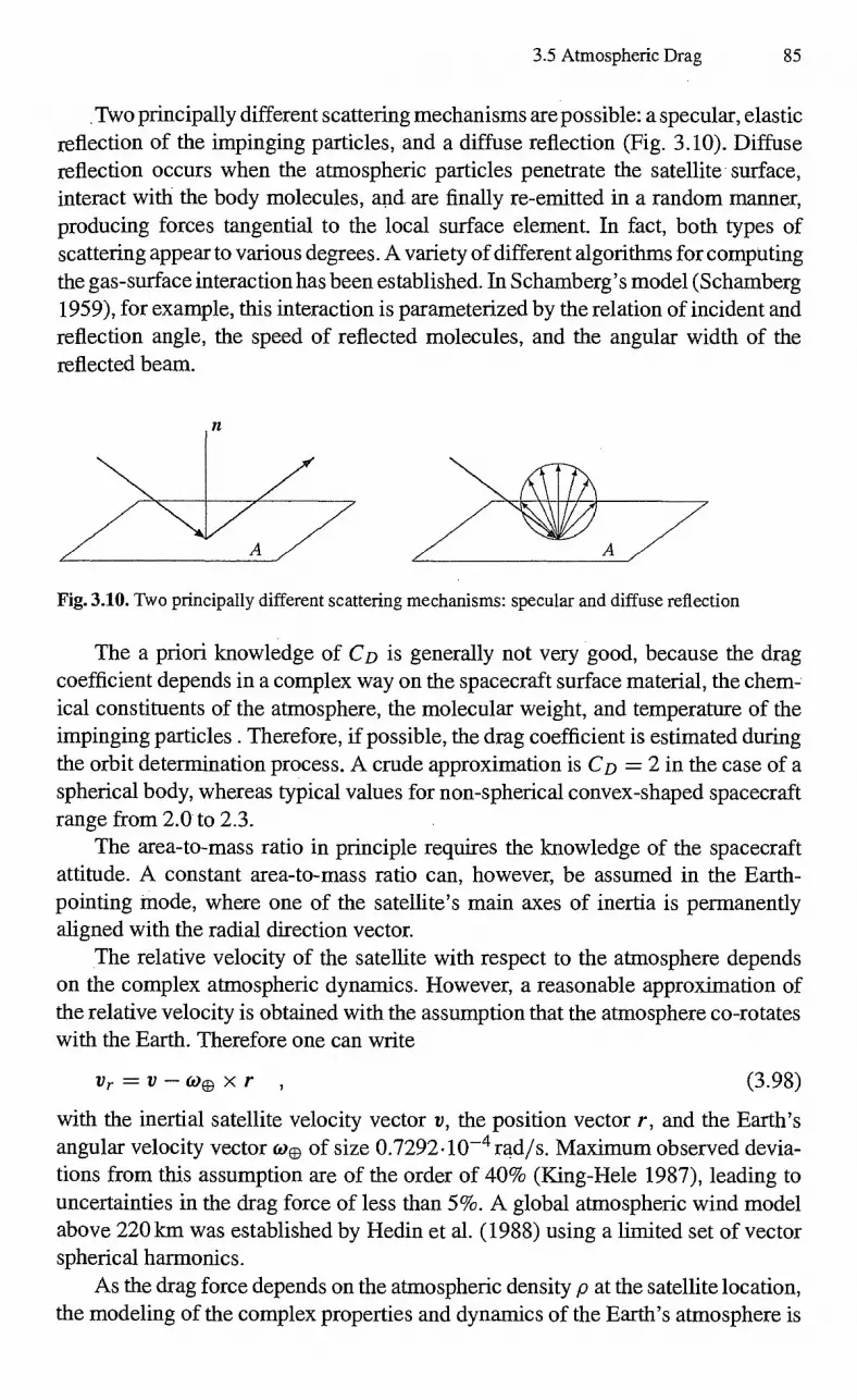
3.5 Atmospheric Drag 85
. Two principally different scattering mechanisms are possible: a specular, elastic reflection of the impinging particles, and a diffuse reflection (Fig. 3.10). Diffuse reflection occurs when the atmospheric particles penetrate the satellite • surface, interact with the body molecules, and are finally re-emitted in a random manner, producing forces tangential to the local surface element. In fact, both types of scattering appear to various degrees. A variety of different algorithms for computing the gas-surface interaction has been established. In Schamberg's model (Schamberg 1959), for example, this interaction is parameterized by the relation of incident and reflection angle, the speed of reflected molecules, and the angular width of the reflected beam.
Fig. 3.10. Two principally different scattering mechanisms: specular and diffuse reflection
The a priori knowledge of CD is generally not very good, because the drag coefficient depends in a complex way on the spacecraft surface material, the chem-ical constituents of the atmosphere, the molecular weight, and temperature of the impinging particles . Therefore, if possible, the drag coefficient is estimated during the orbit determination process. A crude approximation is CD = 2 in the case of a spherical body, whereas typical values for non-spherical convex-shaped spacecraft range from 2.0 to 2.3.
The area-to-mass ratio in principle requires the knowledge of the spacecraft attitude. A constant area-to-mass ratio can, however, be assumed in the Earth-pointing mode, where one of the satellite's main axes of inertia is permanently aligned with the radial direction vector.
The relative velocity of the satellite with respect to the atmosphere depends on the complex atmospheric dynamics. However, a reasonable approximation of the relative velocity is obtained with the assumption that the atmosphere co-rotates with the Earth. Therefore one can write
V r = V — We X r , (3.98)
with the inertial satellite velocity vector y, the position vector r, and the Earth's angular velocity vector coe of size 0.7292 .10-4 rad/s. Maximum observed devia-tions from this assumption are of the order of 40% (King-Hele 1987), leading to uncertainties in the drag force of less than 5%. A global atmospheric wind model above 220 km was established by Hedin et al. (1988) using a limited set of vector spherical harmonics.
As the drag force depends on the atmospheric density p at the satellite location, the modeling of the complex properties and dynamics of the Earth's atmosphere is

Part
icle
den
sity
log
ion
[N/c
m3]
86 3. Force Model
a challenging task of modern precision orbit determination. A variety of more or less complicated atmospheric models have been established recently, with typical density differences for different models of about 20% at a lower altitude of 300 km, even increasing at higher altitudes. It is remarkable that the accuracy of empirical drag models has not significantly improved during the past two decades (see e.g. Marcos et al. 1989).
3.5.1 The Upper Atmosphere
The density of the upper atmosphere depends in a complex way on a variety of different parameters. The most evident dependency, however, is its decrease with increasing altitude. A very rough estimate of this dependency is expressed in the strongly simplified formula
= Poe—h/Ho (3.99)
where po is the atmospheric density at some reference height, and Ho is the density scale height, which is 7.9 km at mean sea level and increases with geodetic height. According to the theory of thermodynamics, the hydrostatic equation together with the gas law can be used to derive HO as
RI Ho=
jig (3.100)
Here, R, denotes the universal gas constant, T the absolute temperature, g = GM/r2 the Earth's gravitational acceleration, and p, the molecular weight of the atmospheric constituents. From (3.100) it is seen that the partial densities of the different gas constituents decrease at different rates. Therefore, the distribution
Fig. 3.11. Number density of atmospheric constituents at Tco = 1000 K
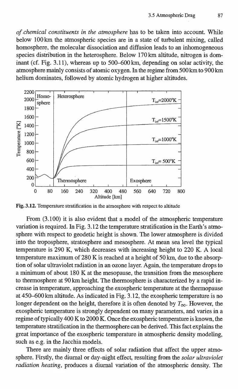
Heterosphere
Exosphere
3.5 Atmospheric Drag 87
of .chemical constituents in the atmosphere has to be taken into account. While below 100 km the atmospheric species are in a state of turbulent mixing, called homosphere, the molecular dissociation and diffusion leads to an inhomogeneous species distribution in the heterosphere. Below 170 km altitude, nitrogen is dom-inant (cf. Fig. 3.11), whereas up to 500-600 km, depending on solar activity, the atmosphere mainly consists of atomic oxygen. In the regime from 500 km to 900 km helium dominates, followed by atomic hydrogen at higher altitudes.
Tem
pera
ture
[°K
]
2200 2000
1800
1600
1400
1200
1000
800
600
400
200 0
0 80 160 240 320 400 480 560 640 720 800 Altitude [km]
Fig. 3.12. Temperature stratification in the atmosphere with respect to altitude
From (3.100) it is also evident that a model of the atmospheric temperature variation is required. In Fig. 3.12 the temperature stratification in the Earth's atmo-sphere with respect to geodetic height is shown. The lower atmosphere is divided into the troposphere, stratosphere and mesosphere. At mean sea level the typical temperature is 290 K, which decreases with increasing height to 220 K. A local temperature maximum of 280 K is reached at a height of 50 km, due to the absorp-tion of solar ultraviolet radiation in an ozone layer. Again, the temperature drops to a minimum of about 180 K at the mesopause, the transition from the mesosphere to thermosphere at 90 km height. The thermosphere is characterized by a rapid in-crease in temperature, approaching the exospheric temperature at the thermopause at 450-600 km altitude. As indicated in Fig. 3.12, the exospheric temperature is no longer dependent on the height, therefore it is often denoted by T. However, the exospheric temperature is strongly dependent on many parameters, and varies in a regime of typically 400 K to 2000 K. Once the exospheric temperature is known, the temperature stratification in the thermosphere can be derived. This fact explains the great importance of the exospheric temperature in atmospheric density modeling, such as e.g. in the Jacchia models.
There are mainly three effects of solar radiation that affect the upper atmo-sphere. Firstly, the diurnal or day-night effect, resulting from the solar ultraviolet radiation heating, produces a diurnal variation of the atmospheric density. The

88 3. Force Model
maximum density occurs two hours after local noon, approximately at the latitude of the sub-solar point, while a minimum density is found three hours past midnight near the same latitude but in the opposite hemisphere. This density variation is therefore dependent on the geographical latitude. The second effect results from the extreme ultraviolet radiation of the Sun, varying on different time scales. Be-sides a short-term 27-day period, related to the rotation period of the Sun, the Sun's activity is characterized by the 11-year Sun spot cycle. It has been discovered that variations in the solar decimeter flux are related to the extreme ultraviolet radiation from the Sun. Therefore, the 10.7 cm radiation index denoted by F103 is intro-duced, which accounts for extreme ultraviolet radiation effects. F10.7 is measured in units of 10-22w/m2/s = 4 10 Jansky (Jy). Since 1947, measurements of this flux line have been recorded by the National Research Council in Ottawa on a daily basis, and from 1991 on by a radio telescope in Penticton, British Columbia. These values appear in printed form as "Solar-Geophysical Data prompt reports" as well as electronically, published by the National Geophysical Data Center (NGDC) in Boulder, Colorado Finally, the third effect results from the corpuscular solar wind, which is responsible for short-term fluctuations in the atmospheric density.
Table 3.6. Relation of geomagnetic ap to Kp values (Mayaud 1980)
rz,, 0 2 3 4 5 6 7 8 12 15 18 22 27 32
Oo 0+ 1— lo 1+ 2— 2o 2+ 3— 30 3+ 4— 40 4+
s'.4. ca.
k ,
Ci '''
39 48 56 67 80 94 111 132 154 179 207 236 300 400 5— 50 5+ 6— 6o 6+ 7— 70 7+ 8— 8o 8+ 9— 90
Geomagnetic storms affecting the thermosphere have been observed for many years. They increase the temperature, as well as the total density, associated with chemical composition changes on a timescale of one or two days. Although a large number of satellite acceleration measurements are available (Berger at al. 1988) the basic physical processes are not yet known precisely. It is, however, evident that the interaction of the solar wind and the Earth's magnetic field plays a major role in perturbations of the geomagnetic field. The "three-hourly planetary geomagnetic index" K p is used as a global measure of a three-hour variation in the Earth's magnetic field. It is obtained from K -indices that are measured at 12 observatories situated at locations ranging from 48° to 63° geomagnetic latitude. The K-indices, integers in the range 0 to 9, correspond to variations in the horizontal component of the geomagnetic field with respect to a quiet day, as measured by magnetometers. These variations amount up to 400 nT, compared to the Earth's magnetic field of about 30 000 nT. In some cases geomagnetic data are given as ap values, the "three-hourly planetary amplitude index", which is related to K p as given in Table 3.6. Note that K p is a one-digit number, subdivided into units of 1/3.
A collation of minimum, typical and maximum numbers of the daily F10.7 index, the É10.7, averaged over 90 days, and the geomagnetic K p index, is given in Table 3.7. The short- and long-term evolution of solar flux values and prediction algorithms are discussed in Sect. 3.5.5.

3.5 Atmospheric Drag 89
Table 3.7. Solar flux values and geomagnetic indices
F10.7 P10.7 K p
Minimum • 70 70 Oo Typical 200 155 40 Maximum 330 240 80
A lag of 6.7 hours in the response of temperature changes to geomagnetic storms, indicated by K p values from 6 to 9, has been observed. Along with the solar flux values, geomagnetic data are also available in the above-mentioned "Solar -Geophysical Data prompt reports".
Semi-annual variations in the atmospheric density show a strong height depen-dence and periodic variations throughout the year. However, these variations seem not to be connected with the solar activity, and the geophysical mechanisms behind these variations are not well understood.
At lower altitudes of 90-120 km, latitudinal density fluctuations have been observed in the thermosphere related to seasonal variations. The amplitude of these variations attains a maximum at about 110 km height, and is assumed to decrease rapidly with increasing height.
Seasonal-latitudinal variations of the helium density in the upper atmosphere have been observed, resulting from helium migration towards the winter pole. No major height-dependency seems to exist.
Additionally, there are a number of further atmospheric processes that affect the density, as e.g. variations in the hydrogen density and pressure waves in the atmosphere. However, as accurate modeling of global atmospheric properties is lacking, these smaller effects are neglected in most cases.
3.5.2 The Harris—Priester Density Model
Although the dynamics of the upper atmosphere shows a significant temporal and spatial variation, there exist relatively simple atmospheric models that already allow for a reasonable atmospheric density computation. Thus, prior to a description of elaborate and complex models, we consider the algorithm of Harris—Priester (Harris & Priester 1962, see also Long et al. 1989), which is still widely used as a standard atmosphere and may be adequate for many applications.
The Harris—Priester model is based on the properties of the upper atmosphere as determined from the solution of the heat conduction equation under quasi-hydrostatic conditions. While neglecting the explicit dependence of semi-annual and seasonal latitude variations, it has been extended to consider the diurnal den-sity bulge. As the atmospheric heating due to the solar radiation leads to a gradual increase of the atmospheric density, the apex of this bulge is delayed by approxi-mately 2 hours, equivalent to a location 30° to the east of the subsolar point (Long et al. 1989). The antapex and apex density Pm (h) and pm (h) at a given altitude h is computed through the exponential interpolation between tabulated minimum and
90 3. Force Model
maximum density values pm (hi) and pm (hi) according to
hi — h Pm (h) = (hi ) exp ( )
hi —h PM(h) = pm (hi) exp (
Hm
(h i <h h 1 +1) (3.101)
where h is the height above the Earth's reference ellipsoid. The corresponding scale heights are given as
Hm (h) = InCom (hi+1) Pin(hi)) .
hi+1 H m (h) =
ln(pm(hi+01 Pm (hi))
hi —
(3.102)
The diurnal density variation from the apex to the antapex due to the solar radiation is accomplished through a cosine variation according to
p(h) = Pm (h) (pm(h) — p ni (h)) cos (-2) (3.103)
where W is the angle between the satellite position vector and the apex of the diurnal bulge. In practice, the latitudinal density variations are roughly taken into account by the declination-dependent angle W and by the exponent n, which has a numerical value of 2 for low-inclination orbits, and 6 for polar orbits. Using trigonometric calculus and the definition of W we derive
= 1 ± COS = (1 e r e 12) cos' 2 ) 2 2 2 )
(3.104)
with the unit satellite position vector er . The unit vector eb to the apex of the diurnal bulge is given as
( cos (S 0 o cos(ao + 2 eb = = cos (So sin(ao + Xi) (3.105)
sin So
with the Sun's right ascension ao , declination (So and the lag angle in longitude X1ç-z-,-' 30°
In Table 3.8 the minimum and maximum density values are given for an altitude regime of 100 km to 1000 km and mean solar activity. In addition to its computa-tional simplicity, the benefit of the Harris—Priester density model is that it can easily be tailored or extended to other altitude regimes or to other solar flux conditions. A multi-parametric comparison with the Jacchia 1971 model shows a mean deviation in density of about 40% for mean solar flux conditions, which increases to 60% for maximum solar activity. Since considerably higher deviations have been observed for minimum solar flux conditions, the tabular coefficients should be modified suit-ably for low solar activity phases.

3.5 Atmospheric Drag 91
Table 3.8. Harris-Priester atmospheric density coefficients valid for mean solar activity (Long et al. 1989)
h [km]
pm
[g/km3 ] Pm
[g/km3 1 h
[km] pm
[g/km3 ] PM
[g/lan3 ]
100 497400.0 497400.0 420 1.558 5.684 120 24900.0 24900.0 440 1.091 4.355 130 8377.0 8710.0 460 0.7701 3.362 140 3899.0 4059.0 480 0.5474 2.612 150 2122.0 2215.0 500 0.3916 2.042 160 1263.0 1344.0 520 0.2819 1.605 170 800.8 875.8 540 0.2042 1.267 180 528.3 601.0 560 0.1488 1.005 190 361.7 429.7 580 0.1092 0.7997 200 255.7 316.2 600 0.08070 0.6390 210 183.9 239.6 620 0.06012 0.5123 220 134.1 185.3 640 0.04519 0.4121 230 99.49 145.5 660 0.03430 0.3325 240 74.88 115.7 680 0.02632 0.2691 250 57.09 93.08 700 0.02043 0.2185 260 44.03 75.55 720 0.01607 0.1779 270 34.30 61.82 740 0.01281 0.1452 280 26.97 50.95 760 0.01036 0.1190 290 21.39 42.26 780 0.008496 0.09776 300 17.08 35.26 800 0.007069 0.08059 320 10.99 25.11 840 0.004680 0.05741 340 7.214 18.19 880 0.003200 0.04210 360 4.824 13.37 920 0.002210 0.03130 380 3.274 9.955 960 0.001560 0.02360 400 2.249 7.492 1000 0.001150 0.01810
3.5.3 The Jacchia 1971 Density Model
A number of different atmospheric density models have been published since 1965 by L. G. Jacchia (1965, 1970, 1971, 1977) and Jacchia & Slowey (1981). The first model, called J65, was solely based upon the primary parameters geodetic height and temperature, with the latter determining the atmospheric conditions. When further density-related data became available from the analysis of satellite acceler-ations due to drag, an improved atmospheric model was established (Jacchia 1971). The J71 model includes density variations as a function of time, and covers the al-titude interval from 90 km to 2500 km. It was adopted by the COS PAR (Committee on Space Research) working group as the International Reference Atmosphere in 1972, for heights ranging from 110 km to 2000 km (see CIRA 1972).
In 1977 Jacchia published the atmospheric model J77 (Jacchia 1977), which was based upon measurements of the acceleration of satellites, and additionally upon analyses of mass spectrometer data. The J77 model was revised once more in 1981 (Jacchia et al. 1981).

92 3. Force Model
All Jacchia models employ the exospheric temperature Too as a basic parameter for the computation of the atmospheric density. The models are based upon the assumption that the chemical constituents of the atmosphere are in a state of mixing below heights of 100 km. The density for altitudes from 90 to 100 km is computed by integration of the barometric equation. At higher altitudes the atmosphere is assumed to be in diffusion equilibrium, where the constituents N9, 02, 0, Ar, He and H2 are taken into account. These two assumptions cause the Jacchia Models to be static in nature. Therefore, temperature and density predictions will be poor when dynamical variations with time scales shorter than those typical for diffusion are present in the atmosphere. The densities from 100 km upwards are computed by integration of the differential equations for diffusion.
The J71 model offers a reasonable description of the atmospheric density at moderate computational expense, and is therefore widely used in the fields of orbit determination and prediction. The computation of atmospheric densities in the J71 model is perfouned in three steps:
1. The exospheric temperature Too is computed from data on solar activity and from the geomagnetic index, in combination with a model of the diurnal variations in the atmosphere.
2. Once Too is known, a temperature profile is assumed, which is input for the integration of the barometric or diffusion equation (whichever is applicable). It is this integration in particular that turns out to be time-consuming. As an alternative, use is made of the coefficients of a bi-polynomial fit for the computation of the standard density values.
3. Time-dependent corrections are applied to the density, which account for various observed density variations.
Exospheric Temperature
In the J71 model, the minimum global exospheric temperature without solar ra-diation or geomagnetic activity is assumed to be Tc = 379.0°. The exospheric temperature with the effect of solar radiation included is given by
Tc = 379.0° ± 3.24°F10.7 1.3° (F10.7 — (3.106)
(Jacchia 1971), where F10.7 is the actual solar flux at 10.7 cm, and F107 the average solar flux (both measured in Solar Flux Units of 10-22 W/(m2Hz)) at this wave-length. In this model the actual flux is taken to be the average over the day before the date under consideration. The mean flux .24-).0.7 is found by taking an average over three solar rotations of 27 days. The last tem.). in (3.106) thus represents daily variations around the mean global exospheric temperature.
The actual exospheric temperature is a function of local time or, in other words, depends on the local hour angle of the Sun with respect to the satellite. It also depends, however, on the declination of the Sun and the geographic latitude of the

1 = —
2 (q) + (So)
1 = —2 — 8o) •
(3.108)
3.5 Atmospheric Drag 93
satellite. The actual exospheric temperature T1 with the diurnal variations included can be computed from
= T [1 + 0.3 (sin2-2 101 (cos2.2ini_ sin2.2101) cos3.0 (1))] , (3.107) 2 / /
(Jacchia 1971) with the angles t (- 180° <t < +1800), e, 77 given by
H — 37.0° + 6.0° sin(H ± 43.0°)
In these equations 8® denotes the Sun's declination, ço the geographic latitude and H the local hour angle of the Sun with respect to the satellite. The additional terms in (3.108) which modify the hour angle H, account for asymmetric effects in the temperature variation relative to the position of the Sun. The difference between the geographic and the geocentric latitude is always less than 12' and can therefore be neglected. The local hour angle H is simply given by
H = CYSAT — a® , (3.109)
where asAT and a® are the right ascension of the satellite and of the Sun respectively. Jacchia's original representation (3.107) can further be amended by
= ]2.1.. (1 — cos 0))
1.1
1.1 = (1 + COS a))
(3.110)
to avoid the noun of the angles. Geomagnetic activities axe taken into account by using the three-hourly plan-
etary geomagnetic index Kp for a time 6.7 hours earlier than the time under con-sideration (Jacchia 1971). The resulting change in exospheric temperature can be written as
AT0,1,/, = 28.0°Kp 0.030eKP (Z > 350 km)
TooL = 14.0°Kp 0.020 eKP (Z < 350 km)
for high and low altitude (Z) respectively. In order to retain continuity of the tem-perature correction at 350km, Jacchia introduced a transition function f
f = —1
(tanh(0.04(Z — 350 km)) + 1) . (3.112) 2
The temperature correction due to geomagnetic activity can then be written as
(3.113)

94 3. Force Model
It should be noted that in the J71 model, geomagnetic perturbations affect the den-sity in a twofold hybrid manner. Firstly, the temperature perturbations are directly reflected in the density and, secondly, an additional geomagnetic density correction term is added.
Finally, the full expression for the exospheric temperature, with solar and ge-omagnetic teims included, becomes
Too = Ti ± A Too , (3.114)
which, together with the height Z, determines the standard density values.
Standard Density Computation
The standard Jacchia 1971 model is based upon an empirical temperature profile which starts from a fixed value To = 183 K at 90 km. The temperature increases with altitude in a transition region until it reaches Too asymptotically (Jacchia 1965). The standard density is obtained by integration of the barometric differential equation below 100 km and of the diffusion differential equation above this height. The molecular weights, and the fraction by volume of the atmospheric species nitrogen (N2), oxygen (02), argon (Ar), and helium (He) at sea level, are input parameters to the model.
The Fortran source code provided in CIRA (1972) uses a Newton—Cotes five-point quadrature formula for the numerical integration of the individual constituent number densities. The advantage of this approach is that only few input data are necessary in order to get the full information content of the Jacchia model. The inherent drawback, however, is the computational effort, because each time a density is calculated, the equations must be integrated. It is estimated that more than 90% of the processing time is consumed by the computation of the standard density in this method. A graphical presentation of the J71 standard density as a function of altitude and exospheric temperature is given in Figure 3.13.
Considerable savings in processing time may be obtained by interpolating the standard density from precomputed tabular values or corresponding polynomials A sophisticated bi-polynomial representation
5 4 .. (
1000
Z )
I ICM
i
( 1000 K j Too V
i.o 1,-o
of the standard density p (in [kg/m3]) as a function of height and exospheric tem-perature was developed by Gill (1996). It achieves a representative accuracy of 7% with coefficients cii given in Tables 3.9 and 3.10. The approximation is applicable within the altitude range 90-2500 km and the temperature range 500-1900 K, which is divided into 4 x 2 subintervals. In order to ensure continuous density values and first-order derivatives at the sub-interval boundaries, the polynomial coefficients were obtained from a constrained least-squares fit that is described in detail in Gill (1996).
log p(Z, Too ) = (3.115)

3.5 Atmospheric Drag 95
Fig. 3.13. Logarithm of the standard density in the J71 model as a function of temperature and altitude
Density Corrections
In addition to the computation of the standard density, several density corrections have to be applied to account for various observed density variations. Below 350 km there is an additional geomagnetic term
log pGm = (0.012Kp + 1.2.10-5 e l<" P) (1 f) (3.116)
as part of the hybrid Jacchia geomagnetic algorithm. The semi-annual density variation in the thermosphere and the lower exosphere
is only considered by temperature corrections in the Jacchia 1965 model. Large discrepancies with this model were found, however, when actual data of the drag force on satellites became available. This forced Jacchia to the assumption that those density variations are not primarily caused by variations in temperature. Hence, an empirical relationship
log psA = f (Z) g(t) (3.117)
for the density correction was assumed, where g(t) represents the temporal varia-tion, and f (Z) is the amplitude of the density variation at a given altitude. A b'est fit to the available data was found with the functions
,. f (Z) = (5.876 10 (z ikm 2331
— )7 + 0.06328 e (-0.002868 Z/Icm))
g(t) = 0.02835+ (3.118)
(0.3817+0.17829 sin(27rrsA +4.137)) x sin(47rtsA +4.259) .

96 3. Force Model
Table 3.9. Coefficients cif of Jacchia 1971 standard density polynomials in temperature (index j) and height (index i) below 500 km
901cm < Z < 1801cm 500K < Too <850K
0 1 2 3 4
0 1 2 3 4 5
-0.3520856402 +0.1129210404 -0.1527475.105
+0.9302042-105 -0.2734394.106
+0.3149696-106
+0.3912622.10 1 +0.1198158, 104
-0.3558481.105 +0.3646554.106
-0.1576097.107 +0.2487723.107
-0.8649259.102 +0.8633794-103
+0.1899243• 105 -0.3290364.106
+0.1685831• 107 -0.2899124.107
+0.1504119.103 -0.3577091.104
+0.2508241•10 -0.1209631.105
-0.4282943.106 +0.1111904.107
-0.7109428.102 +0.1970558.104 -0.1968253.105
+0.8438137• 105 -0.1345593.106
+0.3294095.104
901cm < Z < 1801crn 850K < Too <1900K
i 0 1 2 3 4
0 -0.5335412402 +0.2900557402 -0.2046439.102 +0.7977149 .10 1 -0.1335853-10 1 1 +0.1977533-104 -0.7091478.103 +0.4398538-103 -0.1568720 •103 +0.2615466402 2 -0.2993620-105 +0.5187286-104 -0.1989795.104 +0.3643166 -103 -0.5700669402 3 +0.2112068-106 -0.4483029404 -0.1349971.105 +0.9510012 •104 -0.1653725.104 4 -0.7209722-106 -0.7684101.105 +0.1256236.106 -0.6805699 • 105 +0.1181257.105 5 +0.9625966.106 +0.2123127.106 -0.2622793.106 +0.1337130 .106 -0.2329995.105
180 km < Z < 500 km 500K.< Too <850K
i 0 1 2 3 4
0 +0.2311910.102 +0.1355298.103 -0.8424310.103 +0.1287331.104 -0.6181209.103 1 -0.1057776404 +0.6087973.103 +0.8690566.104 -0.1715922405 +0.9052671.104 2 +0.1177230405 -0.3164132.105 -0.1076323.104 +0.6302629.105 -0.4312459.105 3 -0.5827663405 +0.2188167.106 -0.2422912.106 +0.2461286.105 +0.6044096.105 4 +0.1254589.106 -0.5434710.106 +0.8123016.106 -0.4490438.106 +0.5007458.105 5 -0.9452922-105 +0.4408026.106 -0.7379410.106 +0.5095273.106 -0.1154192.106
1801an < Z < 5001an 850K < Too < 1900K
0 1 2 3 4
0 +0.4041761402 -0.1305719.103 +0.1466809403 -0.7120296.102 +0.1269605.102 1 -0.8127720-103 +0.2273565.104 -0.2577261.104 +0.1259045 • 104 -0.2254978.103 2 +0.5130043.104 -0.1501308405 +0.1717142.105 -0.8441698.104 +0.1518796.104 3 -0.1600170.105 +0.4770469.105 -0.5473492.105 +0.2699668.105 -0.4870306.104 4 +0.2384718-105 -0.7199064.105 +0.8284653.105 -0.4098358.105 +0.7411926.104 5 -0.1363104-105 +0.4153499 • 105 -0.4793581.105 +0.2377854•05 -0.4310233.104
Here the time-dependent parameter is
+ sin(2n- + 6.035)) 1 .65- I 2 2 2
with (t - 36204)
= 365.2422
rsA = 0 +0.09544 (3.119)
(3.120)
In equation (3.120), t is the time expressed in Modified Julian Days (MJD JD -2400000.5). Hence, 0 is the number of tropical years since January 1, 1958. The maximum semi-annual density correction is A log pm" IsA 0.21.

500 km < Z < 1000km 500K < Too <850K
0 1 2 3 4
o -0.1815722.10 +0.9792972.104 -0.1831374.105 +0.1385255 • 105 -0.3451234-104 1 +0.9851221.104 -0.5397525.105 +0.9993169.105 -0.7259456 • 105 +0.1622553.105 2 -0.1822932-105 +0.1002430.106 -0.1784481.106 +0.1145178 .106 -0.1641934-105 3 +0.1298113-10 5 -0.7113430.105 +0.1106375.106 -0.3825777 •105 -0.1666915-105 4 -0.1533510.104 +0.7815537.104 +0.7037562.104 -0.4674636 .105 +0.3516949-105 5 -0.1263680.10 +0.7265792-104 -0.2092909.105 +0.2936094 • 105 -0.1491676-105
500 km < Z < 1000km 850K < Too < 1900 K
0 1 2 3 4
o -0.4021335-102 -0.1326983.10 3 +0.3778864 • 103 -0.2808660.103 +0.6513531.102 1 +0.4255789.103 +0.3528126.103 -0.2077888.104 +0.1726543-104 -0.4191477-103 2 -0.1821662.104 +0.7905357.103 +0.3934271.104 -0.3969334-104 +0.1027991.104 3 +0.3070231 • 10 -0.2941540.10 -0.3276639.104 +0.4420217.104 -0.1230778.104 4 -0.2196848.104 +0.2585118.104 +0.1382776.104 -0.2533006-104 +0.7451387-103 5 +0.5494959 • 103 -0.6604225.10 3 -0.3328077.10 3 +0.6335703.103 -0.1879812-10 3
1000km < Z < 2500km 500K < Too <850K
0 1 2 3 4
O +0.3548698 -103 -0.2508685.10 +0.6252742 • 10 -0.6755376.104 +0.2675763.104 1 -0.5370852 • 103 +0.4182586 • 10 -0.1151114.10 5 +0.1338915.10 5 -0.5610580.104 2 -0.2349586 .102 -0.8941841.10 3 +0.4417927 • 104 -0.6732817.104 +0.3312608 • 104 3 +0.3407073 -10 3 -0.1531588.10 +0.2179045.10 -0.8841341.103 -0.1369769-103 4 -0.1698471 .103 +0.8985697.1 0 -0.1704797.10 +0.1363098.10 -0.3812417.103 5 +0.2497973 -102 -0.1389618.103 +0.2820058 • 103 -0.2472862.103 +0.7896439.102
1000krn < Z < 2500 Ian 850K < Too < 1900K
0 1 2 3 4
O +0.1281061.102 -0.3389179.10 3 +0.6861935 • 103 -0.4667627.10 3 +0.1029662-103 1 +0.2024251-103 +0.1668302-103 -0.1147876.10 +0.9918940 • 103 -0.2430215.103 2 -0.5750743.10 3 +0.8259823.103 +0.2329832.103 -0.6503359.10 3 +0.1997989.10 3 3 +0.5106207.103 -0.1032012.10 +0.4851874.103 +0.8214097.102 -0.6527048.102 4 -0.1898953.103 +0.4347501.103 -0.2986011.103 +0.5423180.102 +0.5039459 • 10' 5 +0.2569577.102 -0.6282710.102 +0.4971077.102 -0.1404385.102 +0.8450500 • 10°
3.5 Atmospheric Drag 97
Table 3.10. Coefficients cif of Jacchia 1971 standard density polynomials in temperature (index j) and height (index i) above 500 km
So far, the model gives a constant density over the globe at 90 km. This contra-dicts observations of density variations below 120 km, which indicate a seasonal-latitudinal density dependence with a maximum amplitude at Z 110 km In tel ins of the latitude, ço, and the deviation from the reference height, AZ90 = Z - 90 km, the deviation in density can be written as
A log PSL = 0.014A Z90e(-0.00 1 3Az30) sin(27ro + 1.72) s i n3 w
I sin ço I . (3.121)
In a computer application sin ço/ I sin 'pi should be replaced by SIGN(sin2 ço, ço).

98 3. Force Model
A strong increase of the helium concentration above the winter pole has been found from mass-spectrometer data, as well as from satellite drag data. This phe-nomenon is accounted for in the Jacchia 1971 model by an empirical seasonal-latitudinal correction
A log //He = 0.65 80 / 3 7 7 9 \
13Z ) 0.35355) (3.122)
to the helium number density He (in [1/m3]), where E is the obliquity of the eclip-tic. The maximum helium density contribution to the standard density is given by A log pAleax 0.88. It is straightforward to compute this correction from the inte-gration of the diffusion equation, which yields the number density of the individual species. However, a standard density computation from tabular data now requires additional table values for the helium number density as a function of altitude and of exospheric temperature.
Therefore, a polynomial approximation, similar to the one for the standard density, is also made for the helium density. To this end the helium density correction is written as
(iolognue _ 1) APHe = 101°g n He m He
(3.123) A„
with the helium number density
1=0 j=0
the helium molecular weight mile = 4.0026, and the number of Avogadro A. Coefficients hi./ for a smooth and continuous approximation of the helium number density as derived by Gill (1996) are collated in Table 3.11.
3.5.4 A Comparison of Upper Atmosphere Density Models
Only after the advent of the space age, with the launch of the Sputnik satellite in 1957, could information on the physical properties of the upper atmosphere above 150 km be deduced. In particular, atmospheric densities can be derived from the evolution and decay of the satellite orbits, assuming a given drag coefficient. This method was primarily used for the density model development up to the mid seven-ties. Its inherent drawback is, however, that only integrated drag effects over several orbit revolutions may be resolved from orbit determination, and thus the method is restricted to a limited spatial and temporal resolution. Its benefit, on the other hand, is that density models derived from these observations can consistently be applied to other space missions, being free from any further instrument calibration.
Rapid developments in satellite and ground system instrumentation consider-ably improved the knowledge of detailed atmospheric properties in the seventies. The use of spacecraft accelerometers directly monitored the non-inertial forces act-ing on the satellite. Mass spectrometers were integrated into the satellite hardware
log nHe(Z, Too) 5 4
( Z '(T )
j 1K (3.124)

3.5 Atmospheric Drag 99
Table 3.11. Coefficients hij of Jacchia 1971 logarithmic helium number density polynomials in temperature (index j) and height (index i)
90 km <Z < 5001cm
ifi 0 1 2 3 4
+1.831549 • 10+°1 +5.887556.1 003 —4.813257.10-06 +1.701738 • 1 009 —2.128374.10 -13 —7.374008.10-02 —1.251077.10—°4 +1.039269 • 1 007 —3.679280.10 — " +4.555258 • 10-15 -L4.384164.10-04 +8.657027 • 1 007 —7.216946.10-1 0 +2.481534 • 10-13 —2.859074.10-17 —1.411195.10-06 —2.483834.1(09 +2.004107.10-12 —6.244985.10-16 +5.561004.10-20 +2.153639.1 009 +3.421944.10-12 —2.628961.10 -15 +7.085655.10 -19 —3.279804.10 -23 —1.255139.10 -12 —1.827253.10-15 +1.321581.10-18 —2.887398.10 -22 —7.827178.10 -27
500km < Z < 1000Icm
i fj 0 1 2 3 4
+1.627089.10+°1 —1.786816.10-02 +3.079079 • 1 005 —2.043431.10-08 +4.643419.10 -12 —1.958297.10 -02 +1.386126 • 1 004 —2.532463.1(07 +1.714183.10 -1° —3.934230.10 -14 +2.514251.1(05 —3.806339.1 007 +7.692376.10-1° —5.394766.10-13 +1.260304.10 -16
cn —2.983314.10-08 +5.855851.10-1 0 —1.210663.10-12 +8.561632.10-16 —2.009030.10 -19
+1.802028.10 — " —4.382878.10-13 +9.201530.10-16 —6.543935.10-19 +1.540220.10 -22 —4.243067.10 -15 +1.268830.10-16 —2.695807.10-19 +1.925469.10-22 —4.542329.10 -26
1000km < Z < 2500km
iti 0 1 2 3 4
cD
(NI
•zt.. tr
)
+1.873346.10+° 1 +2.285683-10-02 —6.860776.1(05 +5.379623-10-08 —1.327559.10-11 —2.362530.10 -02 —6.907613.1(05 +2.251680.1(07 —1.795937.10 -1° +4.463659.10 -14 +1.893899.1 005 +1.145960 • 1 007 —3.183259.10-1° +2.461076.10-13 —6.040423.10 -17 —1.132198.10-08 —7.438326.10-11 +2.040288.10 -13 —1.573191.10 -16 +3.857032.10-20 +3.465014.10 -12 +2.308943 • 10-14 —6.320466.10 -17 +4.871419.10-2° —1.194139.10-23 —4.156710.10 -16 —2.791930.10-18 +7.632792.10-21 —5.881112.10-24 +1.441455.10 -27
that produced in-situ measurements of the chemical composition and temperature at upper atmospheric altitudes. Incoherent radar scattering techniques from ground-based antennas provided measurements of atmospheric electron and ion properties that could be related to the neutral atmospheric density and composition. More recent atmospheric models, such as the J77 model, or the series of MSIS (Mass Spectrometer and Incoherent Scatter) models, make extensive use of those data. The spatial and temporal resolution of these models is therefore high, at the cost of increased complexity and CPU time.
Apart from the well-known and frequently applied J71 model, a variety of other density models of the upper atmosphere exists. These range from very simple, easy to implement algorithms to elaborate theories, which either require much CPU time, or refer to a large number of numerical coefficients. A brief summary of the various models is given in this section, and a comparison is made in teints of computation time and of relative density difference with respect to the original J71 model provided in CIRA (1972).
The Jacchia—Roberts model of the atmosphere (Roberts 1971) was originally derived from J70. Later on it was modified according to J71 (Long et al. 1989). Roberts' method is based upon analytical solutions of the barometric and diffusion

100 3. Force Model
Table 3.12. Comparison of density models. Relative CPU time performance, mean, and maximum difference in density relative to J71
Model CPU Pmean dPmax Jacchia 71 1.00 - Jacchia-Roberts 0.22 0.01 0.03 Jacchia-Lineberry 0.43 0.13 0.35 Jacchia-Gill 0.11 0.02 0.08 Jacchia 77 10.69 0.13 0.35 Jacchia-Lafontaine 0.86 0.13 0.36 MSIS 77 0.06 0.18 0.53 MSIS 86 0.32 0.21 1.45 TD88 0.01 0.91 7.49 DTM 0.03 0.40 1.22
differential equations, which are obtained by integration of partial fractions. The original Jacchia temperature profile (exospheric temperature computed as in J70) is used between 90 and 125 km. Above 125 km a different temperature profile is assumed, which results in a diffusion equation that can be integrated analytically. Hence, Roberts' results match Jacchia's exactly between 90 and 125 km, and are in close agreement above 125 km The mean relative difference in density and the maximum relative differences with respect to J71 are 1% and 3% respectively. According to Long et al. (1989) the maximum density difference amounts to 6.7%. This demonstrates the close agreement between both models. The CPU performance is better by a factor of almost five compared to J71, as can be seen from Table 3.12. The advantage of the Roberts model is that numerical integration is avoided, and storage of a large number of coefficients is also unnecessary. At the same time the computational speed is good.
The Jacchia-Lineberry model (Mueller 1982) assumes that the logarithm of the density can be computed as a truncated Laurent series in temperature and altitude. The altitude is split into nine intervals at most, and the necessary number of coef-ficients in this model is about a hundred. However, the seasonal-latitudinal helium variation is not included. Density differences between the Jacchia-Lineberry model and J71 are typically 13%, and the gain in computational speed is moderate.
The model ofJacchia-Gill (Gill 1996), as described above, uses a bi-polynomial approximation of the Jacchia 1971 standard density model. It is based upon poly-nomials of elth order in temperature and of 5th degree in altitude. The temperature interval from 500 to 1900 K and the altitude interval from 90 to 2500 km are divided into eight sections, each with its own bi-polynomial fit. A continuous transition be-tween the several height intervals is ensured by the use of a constrained least-squares fit. The helium number density is obtained in a similar way. The total number of coefficients required in the Jacchia-Gill model is 330. Typical differences with J71 are 2% and the maximum deviation is 8%. The computing time is reduced by a factor of nine.
In 1977 Jacchia published an updated atmosphere model, J77, which was re-vised once more in 1981 (Jacchia et al. 1981). These models are based upon mea-

3.5 Atmospheric Drag 101
surements of satellite acceleration and, additionally, upon analyses of mass spec-trometer data. Similar to the older Jacchia models a physical description of the upper atmosphere with regard to satellite drag is attempted by the integration of the barometric and diffusion equations. However, a greater complexity is introduced through a species-dependent pseudo-temperature in order to account for the fact that the density of different constituents peaks at different hours of the day. Further-more, the mean solar flux is replaced by a weighted mean value which is centered around the epoch. Finally, the time at which the Kp index is required is corrected for the geomagnetic latitude of the satellite position. These extensions make the model significantly more complex. This is of course directly reflected in the CPU time, which is ten times higher than for the J71 model. Yet, the J77 model does not significantly improve the accuracy of density modeling for satellite orbit prediction and determination.
Modifications of the temperature profile at low altitudes in the J77 model, as compared to the J70 and J71 models, caused Roberts' approach to be no longer applicable. This situation was resolved by de Lafontaine & Hughes (1983). They modified Jacchia's temperature profile below 125 km and extended Roberts' expo-nential temperature profile above 125 km in order to obtain an analytical version of the J77 model. Their approach is more general than Roberts' method and it is not restricted to the J77 model, but can also be applied to the J70 and J71 models. The computational efficiency is considerably better than that of the original J77 foimulation and, in contrast to Roberts' method, continuity of the first derivative of the density is guaranteed for all exospheric temperatures. The mean and maximum deviations relative to the J71 density are 13% and 36% respectively.
A different class of models was published in papers by A. E. Hedin. These models are entirely based upon in-situ data from satellites and sounding rockets, as well as incoherent scatter measurements. The first model was published in 1977 by Hedin et al. and is known as MSIS-77 (Mass Spectrometer and Incoherent Scatter). When more data became available, this model was upgraded yielding MSIS-83 (Hedin 1983) and MSIS-86 (Hedin 1987) models. The latter model was adopted as the CIRA 1986 reference atmosphere. MSIS-86 is based on a complex function, which has to be evaluated to compute the density, as well as other atmospheric quantities. More than 850 coefficients have to be provided, which, in turn, allows a detailed modeling of the complex atmospheric properties.
Barlier et al. (1978) published the thermospheric density model, DTM, which is based upon total density data derived from satellite drag observations. An expan-sion in terms of spherical harmonics is performed for the exospheric temperature and for the density of the main atmospheric constituents helium, atomic oxygen, and nitrogen comprising up to terdiumal and semi-annual terms. The total density depends in a simple analytical foini upon the altitude and is obtained from the integration of the diffusion equation with an empirical temperature profile. About 150 parameters are required for the evaluation of the model, which requires ex-tremely little computer time. However, very high density differences of typically 40% relative to the J71 model are found. The maximum difference lies at 122%.

102 3. Force Model
The simple atmospheric model TD88 was derived by Sehnal & Posprgilovd (1988) mainly by fitting an analytical series of exponential functions in height and of trigonometric functions in time to the density values from the DTM model. The resulting model requires only 40 parameters and is according to Sehnal applicable for altitudes between 150 and 750 km. Compared to the performance of J71 a run-time gain of a factor of a hundred is obtained. The density differences, however, seem to be unacceptably high, lying on the average at 91%. In Table 3.12' the maximum density deviation of 749% with respect to J71 was due to an evaluation at 130 km altitude, which is just outside the validity interval of the model given by Sehnal.
There have been a number of publications which analyze and compare the per-formance of different density models (e.g. Gaposchkin & Coster 1990, Marcos et al. 1989). The conclusion is that the models have statistical accuracies of about 15% and that there has been no significant improvement in density models over the last two decades. The profit achieved by the application of complex atmosphere models in the field of satellite orbit determination and prediction is therefore question-able. It appears fully justified to select density models with a moderate complexity only, which essentially minimize the computational effort and coefficient storage requirements.
3.5.5 Prediction of Solar and Geomagnetic Indices
Low-Earth satellite orbits are severely affected by atmospheric drag, which strongly varies with the solar flux and geomagnetic activity. While the measured solar and geomagnetic activity indices can be applied in orbit determination, orbit forecasts have to rely on predictions of these parameters. Short-term to mid-term predictions are required for spacecraft operations, especially for ground station scheduling and maneuver planning of low-Earth satellites. In particular, remote sensing missions require the control of orbit equator crossings within specified equatorial longitude bands, which are maintained by orbit raising or lowering maneuvers. Hence, the orbit maneuver schedule depends on the evolution of the semi-major axis within pe-riods of typically some weeks, while the semi-major axis evolution itself is governed by the evolution of the solar and geomagnetic flux in that time frame. Long-tenri predictions of the solar and geomagnetic flux, on the other hand, are important for mission planning and analysis. The knowledge of the profile and magnitude of the next solar cycle, for example, is crucial for the logistic planning of the assembly of the International Space Station. Furthermore, mission planning requires long-term forecasts for estimates of the expected satellite lifetime.
It is therefore adequate to distinguish three different time scales for solar and geomagnetic index forecast, namely
1. Short-terri predictions (days) 2. Mid-term predictions (months) 3. Long-term forecasts (years)

‘\,
3.5 Atmospheric Drag 103
200
150
;IF poo
50 1998
1999 Year
Fig. 3.14. Short-term variation of solar flux values due to solar rotation
each of which may apply mathematical methods or physical models or a combina-tion thereof as forecast algorithms.
Short-term predictions have to account for the 27-day periodicity of the solar activity that results from the synodic solar rotation with this period (Fig. 3.14). The periodic variation in the F10.7 index may be forecasted using a regression algorithm (Nostrand 1984) that compares the long-ten.'" trend from three solar rotations with a recent trend from the past three days. Supposing that the two trends are directed opposite, the prediction follows the recent trend with a later regression towards the long-term trend. This method assures that the predicted values evolve smoothly from the observed values and it leads to a particularly good prediction accuracy for the first 7-10 days (Frauenholz & Shapiro 1991).
Mathematical methods are in general applied to mid-term predictions. The linear-regression technique of McNish & Lincoln (1949) makes use of the relation between the solar flux F10.7 values and the sunspot numbers to compute a mean solar cycle. This approach considerably improves the database, since F10.7 data are available only from 1947 onwards, whereas the first sunspot numbers date back to 1749. Departures of the current cycle from the mean cycle are then based on the assumption that they are related to deviations of the previous cycle from the mean cycle (Mugellesi & Kerridge 1991). This method provides monthly smoothed F103
values and can correspondingly be applied to geomagnetic index predictions. The drawback of this method is that the prediction accuracy deteriorates with increasing forecast periods and that no understanding of the involved physical mechanisms is achieved.
The long-term evolution of solar flux values is governed by the 11-year solar cycle as depicted in Fig. 3.15. Among various prediction methods, the precursor models have shown the best performance. Here, it is assumed that the solar cycle actually starts in the declining phase of the previous cycle, where the next cycle

104
300
250
3. Force Model
Cycles 20 21 22 23
Ç 2
150
2 100
50 —
0 1960 1970 1980 1990
Year
Fig. 3.15. Monthly averages of the solar flux for solar cycles 20-23. Predicted average values and +2a uncertainties in the predicted average are due to Schatten (1999).
manifests itself in the occurrence of coronal holes and the strength of the polar magnetic field of the Sun. According to the solar dynamo model, the Sun's polodial magnetic field at solar minimum is transformed by differential rotation to a toroidal field that gives rise to phenomena such as sunspot numbers and solar activity for the next cycle (Schatten et al. 1978, Schatten & Pesnell 1993). Although the model allows a physical connection between the Sun's polar magnetic field, and coronal holes, as well as solar and geomagnetic activity, a drawback of this method is that the Sun's polar magnetic field is difficult to measure and that the assumed physical model might be oversimplified.
3.6 Thrust Forces
Aside from the natural forces discussed so far, the motion of a spacecraft may also be affected by the action of an onboard thruster system. Thrusters are frequently applied for orbit control, attitude control, or a combination of both, and exhibit a variety of performance levels (cf. Table 3.13) and burn durations. In view of a significant impact on the spacecraft orbit, thrust forces must be taken into account in the trajectory prediction using an adequate mathematical model. In turn, thruster and maneuver parameters may be calibrated by adjusting them along with other parameters in an orbit determination.
While attitude thrusters are ideally burned in pairs to produce a pure momentum-free torque, changes in the shape and orientation of the orbit are accomplished by thrusters acting primarily in the along-track and cross-track directions. In the case of orbital maneuvers the overall thruster activity is generally confined to a finite time interval, ranging from seconds or minutes for ground track control of remote sensing satellites to several hours for inclination control of geostationary satellites
2000
2010

3.6 Thrust Forces 105
Table 3.13. Representative values of the thrust level, the ejection velocity, the specific impulse (hp ve/9.81 m/s2), and the mass flow rate for various thrust systems
Propulsion system F Ve ithi
Solid propellant boost motor 40 kN 3000 m/s 300 s 1.3 kg/s Liquid propellant boost motor 400 N 3500 mJs 350 s 130 g/s Station keeping thruster 10 N 3500 m/s 350 s 3 g/s Ion thruster 20 mN 25 km/s 2500 s 0.8 mg/s
with ionic propulsion. Whereas maneuvers may conveniently be treated as instan-taneous velocity increments
= v(Ç) Av(t m ) (3.125)
occurring at the impulsive maneuver time tm whenever the thrust duration is small as compared to the orbital period, an adequate thrust model is required for extended maneuvers. This is particularly true for orbital transfers with large boost maneuvers that are applied e.g. in the positioning of geostationary satellites (see Fig. 2.4). Here, a substantial amount of propellant is consumed during a single maneuver, which results in a continuous change of the spacecraft mass along the burn.
Despite the variety of spacecraft propulsion systems, a simple, constant thrust model is often sufficient to describe the motion of a spacecraft during thrust arcs. The model described in the sequel is applicable to most types of extended orbit maneuvers ranging from high-thrust orbital transfer maneuvers to low-thrust orbit corrections. To ensure compatibility with commonly employed impulsive maneuver models, a formulation in terms of velocity increments is chosen. -
Under the action of a propulsion system which ejects a mass Idm I = Irhidt of propellant per time interval dt at a velocity ve , a spacecraft of mass m experiences a thrust '
F = lth IVe (3.126)
which results in an acceleration F Intl
a = — = —V e (3.127)
Upon integration over the burn time At, the total velocity increment is given by
to-FAt m(to-I-At) 1
Av = f a(t)dt = —v e f --dm = —ve m(to -I- At) )
MO to MO
Or
(3.128)
Av F = -- In (1 I7i11/1 3 ) Intl \ mo I
assuming a constant mass-flow rate Intl.
(3.129)

or IhI 1
a(t) EtAv . mILt mo
(3.133) m(t)
— ln (1
106 3. Force Model
Making use of the total velocity increment Av, the acceleration may be ex-pressed as
3.130)
which approaches the limiting value
a(t) (3.131)
in the case of negligible mass flow (IrhizAt <<mo). The one-dimensional motion considered so far may be generalized by intro-
ducing a time-dependent set of orthogonal unit vectors el, e2 and e3 with constant projected thrust vector components F1, F2 and F3. The resulting acceleration vector is given by
1 7F1 a(t) = —E F2
m
\
(3.132)
IhI 1 a(t) =
m(t) 21'1 v
— ln 1 mo
Here
(zAvi 4 .11(0= A v2 (3.134)
.6,1)3
is the vector of velocity increments in the chosen thrust reference frame, while the rotation matrix
E(t)= (el, e2, e3) (3.135)
performs the transfonnation into the inertial reference frame used to describe the spacecraft motion.
In most cases the spacecraft maintains a constant orientation during the thrust phase, either with respect to the orbital frame or the inertial reference system. In the orbital frame the unit vectors el and e3 are aligned with the radial direction and the angular momentum vector , e2 completes the right-handed system and is parallel to the velocity vector for circular orbits:
el Id
e2 e3 x (3.136)
r x v e3
Ir x vi
3.7 Precision Modeling 107
The. orbital frame is a co-moving frame, which is particularly suited to separate in-plane thrust components, which change the size and shape of the orbit, and out-of-plane components, which affect the orbit's spatial orientation.
The inertial thrust direction model is e.g. applicable to spin-stabilized space-craft. Here, the inertially fixed spacecraft attitude results in a constant thrust direc-tion vector and the transformation matrix E = I is simply the identity matrix.
It should be noted that for a numerical treatment of accelerations due to thrust, both instantaneous and extended maneuvers lead to discontinuities in the equations of motion. Thus, a proper maneuver treatment requires the restart of the numerical integration algorithm at the beginning and end of each thrust phase.
3.7 Precision Modeling
For a wide range of applications, the accelerations described so far are fully suf-ficient for a precise description of the satellite orbit. However, there are missions with challenging accuracy requirements, such as in satellite geodesy, which have to account for even more and smaller perturbations. A prominent example is the US/French TOPEX/POSEIDON mission, which requests a radial position error of less than 10 cm. Such high-precision modeling needs to account for additional perturbations like the radiation pressure of the Earth, tidal forces that modify the Earth's gravity field, as well as general relativistic deviations to the Newtonian equations of motion. Finally empirical accelerations may be introduced to account for effects that cannot suitably be described by physical models.
3.7.1 Earth Radiation Pressure
In addition to the direct solar radiation pressure, the radiation emitted by the Earth leads to a small pressure on the satellite. Two components are distinguished: the shortwave optical radiation and the longwave infrared radiation. In both cases the ac-celeration on the satellite decreases slightly with increasing altitude. This is caused by the inverse square law of the emitted radiation pressure, which is partially com-pensated for by an increase of the illuminating surface section of the Earth with altitude. The amplitude of the typical albedo acceleration for low-Earth satellites is 10% to 35% of the acceleration due to direct solar radiation pressure (Knocke et al. 1988).
The optical albedo radiation is produced by reflection and scattering of incident solar radiation on the Earth's surface. This reflection is described by the albedo factor a, defined as the fraction of the shortwave radiation reflected from the Earth to space to the incident shortwave solar radiation. The average global albedo value is a 0.34, equivalent to a radiation of 459 W/m2 of the Earth surface elements. The optical albedo radiation has essentially the same spectral distribution as the direct solar radiation pressure. It is emitted only by the daylight side of the Earth and may vary significantly due to different surface characteristics and cloud coverage.

108 3. Force Model
In contrast to the optical radiation, the infrared radiation is a near isotropic re-emission of the direct solar radiation absorbed by the Earth and its atmosphere. The average emissivity E is approximately 0.68. Its contribution to the flux is, however, reduced by a factor of 4 due to the ratio of the irradiated Earth cross-section r to the total radiating Earth surface 47 4. Hence, the effective radiation of Earth surface elements due to infrared emission is 0.17 45 or 230 W/m2 .
The acceleration of the spacecraft due to Earth radiation is summed up from j (j = 1, .. . , N) individual terms, corresponding to different Earth area elements d A
CR via./ cos + —1
ei)
P0 —A
cos 65 2 dAi
ej 4 m •
(3.137) s
j=1 7tr
where the vi denote the Earth element shadow functions and Of and (PI are the angles of the Earth surface or satellite surface normals to the incident radiation. The unit vector ei points from the Earth surface element to the satellite, while the distance is rj. The albedo and emissivity may be expressed using a second-degree zonal spherical harmonic model (Knocke et al. 1988). Typically about 20 Earth surface elements are considered.
3.7.2 Earth Tides
The gravitation of the Sun and the Moon exerts a direct force on Earth satellites, as discussed in Sect. 3.3. In addition, those forces are also acting on the body of the Earth and thus lead to a time-varying deformation of the Earth. The small periodic deformations of the solid body of the Earth are called solid Earth tides, while the oceans respond in a different way to lunisolar tidal perturbations, known as ocean tides. As a consequence, the Earth's gravity field is no longer static in nature, but exhibits small periodic variations, which also affect the motion of satellites.
In a co-rotating frame, the gravitational field of the Sun or the Moon of mass M implies a potential U at a point P on the Earth's surface, which is given by
GM 1 (3.138) U =
Is—RI + n2d2 i
where R and s are the geocentric coordinates of P and of the tide generating body, respectively. Furthermore, n is the mean motion of the body about an axis through the system's center of mass and d is the distance of P to this axis. Since s» R for the Sun and the Moon, the denominator of (3.138) is expanded as
1 1 1R2 3R2 —
( R 1 — cos y — --- COS
2 y) (3.139)
I s — RI 2s 2 s2 where y is the angle between s and R. The distance d may furthermore be expressed as
d2 R2c0s20 2d,R cos cos(A).)
dc2 R2cos20 — 2d,R cos y , (3.140)
=

3.7 Precision Modeling 109
where c/c. = Ms/ (M MED ) is the geocentric distance of the center of mass of the system, 0 is the geocentric latitude and AX is the difference of the East longitudes of P and the perturbing body. With the above relations and n2s3 = G(M Me), the potential may thus be written as (Bertotti & Farinella 1990)
U =
GM! 1+
1 M ) GM R 2 (3 cos2 y 1)
n2R2 cos- 0 . (3.141)
s 2 M MED 2s3 2
While the first term is constant, the third term describes the rotational potential about an axis through the Earth's center and perpendicular to the orbital plane. It adds a small permanent equatorial bulge to the Earth, similar to the one produced by the rotation of the Earth, but of a much smaller size, since n2 <<
The second term in (3.141) is called the tidal potential U2. It is a second-order zonal harmonic that deforms the equipotential to a prolate, axisymmetric ellipsoid, aligned along the direction to the Moon or to the Sun. Its amplitude is proportional to GM/s 3 and thus the lunar tides are about twice as strong as the solar tides. The dominant periodicity of the tidal acceleration is nearly semi-diurnal according to the dependence of U2 on cos2 y , which itself is a function of cos 2X.
The tidal potential essentially leads to an elastic deformation of the Earth. This may mathematically be described by a linear relation of the tidal potential U2 and the resulting perturbed gravity potential UT, the ratio of both potentials being the Love number ic c 0.3. A completely stiff body would therefore have a vanishing Love number. As the tidal potential is a second-order harmonic, the perturbed gravity potential falls off with 1/ r 3 and can finally be expressed as
1 GMR1
UT = 2
K s3r3—
(3 cos2 y — 1) (3.142)
The Earth is, however, only elastic to first order. Deviations from an elastic tidal response are due to the rate-dependent behavior of terrestrial fluids, like the Earth's inner core and the oceans, as well as friction, i.e. energy dissipation in matter. The latter causes phase lags of the tidal bulge with respect to the position of the Sun and the Moon. The tidal-induced gravity potential contains many different periods, as the angle y depends on the position of the Sun and the Moon with respect to the rotating Earth. Moreover, the potential varies with 1/s 3 and accordingly the variation in the eccentricity of the Sun's and Moon's orbit leads to monthly and annual periods.
The perturbations of satellite orbits from the lunisolar solid Earth tides are derived by an expansion of the tidal-induced gravity potential using spherical har-monics in a similar way as for the static gravity field of the Earth. For practical purposes, the time-dependent corrections to the unnounalized geopotential coeffi-cients can be computed according to
I ACnm1=4kn ( GM )
A
( Re V +111(n+2)(n—m)! 3 pn. (sin 0) jcos(mX)
AS nm G.11/1e s (n+m)!3 sin(mX)

110 3. Force Model
(Sanchez 1974) for the Sun and the Moon respectively, where kn are the Love numbers of degree n, çb is the Earth-fixed latitude and the Earth-fixed longitude of the disturbing body. As the acceleration due to solid Earth tides falls off at least with 1/r 4 , a careful evaluation of an adequate force model is required especially for low altitude missions, depending on the accuracy requirements.
Ocean tides also play an important role in satellite geodesy, although their am-plitudes are about one order of magnitude smaller than that of solid Earth tides. Their contributions can be expressed by an ocean tide potential, which is expanded in terms of spherical harmonics and mapped to time-varying geopotential coeffi-cients
C, m 1 47r G Rip ?, 1+1c1„
12AS nin GM 2n-I-1
(Cs1-2m+ Cs—nnz )COS Os ± (S-sf-nni+ Ss—nm ) sin O
(Ss+nm+ Ss—mn )cos Os — (C,n+ Cs—nm )sin O
(Eanes et al. 1983) where pu, is the density of seawater, knI are the load deformation coefficients and Cs±n,„ and Ss±nn, are the ocean tide coefficients in meters for the tide constituent s. Moreover, Os is the weighted sum of the six Doodson variables. Doodson variables denote fundamental arguments of the Sun's and Moon's orbit, being closely related to the arguments of the nutation series. An alternative rep-resentation of ocean tide harmonics may be found in Schwiderski (1983). For a rigorous computation of the solid Earth and ocean tides, the Love numbers may no longer be treated as constant values, leading to a dual-step approach in the evalu-ation of the geopotential coefficient corrections. The practical computation of the solid Earth and ocean tides is therefore a complex task, which is described in detail in Seidelmann (1992) and McCarthy (1996).
3.7.3 Relativistic Effects
A rigorous treatment of the satellite's motion should be formulated in accordance with the theory of general relativity. While the special theory of relativity considers a fiat four-dimensional space-time, this is no longer true in the vicinity of the Earth. Instead, the Earth's mass MED with the potential U = G1141 r and the Earth's angular momentum vector / 0 with the potential V = G12(1 x r)/r3 lead to a curvature of the four-dimensional space-time Making use of the standard coordinates xi.' = (ct , x', x2 , x 3) the post-Newtonian space-time can be described using the invariant element
ds2=_c2d.r 2
=giLvdxlidx v
2U U2 0 9 Vi (1— ---+
2 )(dx — 4—dx °dx i ( 2U 1+ dx c2 c4 2 if C3
(3.143)

3.7 Precision Modeling 111
between two events (Soffel 1989). Here, Einstein's summation convention is ap-plied, which states that summation is assumed, when a literal index is repeated in a term, both as a subscript and a superscript. The Greek indices run from 0. . . 3 and the Roman indices from 1 . . .3. The time r is the proper time that would be measured by an atomic clock comoving with the satellite, while the coordinate time t may be associated with an atomic clock located at the geocenter. In (3.143) the so-called gravito-electric contributions stem from the curvature of space-time due to the Earth's mass, which is (GM6B)/(c2 REB ) 7 - 10-10 at the Earth's surface. The gravito-magnetic contributions, on the other hand, stem from a dragging of space-time due to the rotation of the Earth with a magnitude of (G L ED) / (c3 4.10-16 .
According to the theory of general relativity, the motion of a satellite can be expressed using the geodesic equation (Weinberg 1972)
d2x dxv dxOE dr2 r
' dr ch bt =0 (3.144)
where the Christoffel symbols V are obtained from derivatives of the space-time metric gp,v
1 ag„vgŒP 1,1;' =
cr 2 axa axv
agvcr)
axa (3.145)
Here ei can be computed as elements of the matrix inverse of gap,. Based on the given metric in the vicinity of the Earth, the geodesic equation
may be expanded to first order in the relativistic terms U/c2 and .V/c3 . This pro-cedure leads to the Newtonian equation of motion with additional post-Newtonian correction terms. Following McCarthy (1996), the coordinate time t is associated with the Terrestrial Time TT (see Sect. 5.1) and dropping the gravito-magnetic contributions leads to the post-Newtonian correction of the acceleration
GM ED ( GM ED v 2 r 2 C r c 2 -
v - cz
where er and e v denote the unit positon and velocity vector. For a circular orbit GIV E) / r = y2 and the velocity is perpendicular to the radius vector. Accordingly the relativistic correction of the acceleration
GM ED e (3 .1) 2 ) 2 r e2
(3.147)
is equal to the product of the Newtonian acceleration and a factor of 3v 2/c2 which is roughly 3-10-10 for a typical satellite velocity.
As a rough rule, the size of general relativistic effects is given by the Schwarz-schild radius of the Earth (2G/14)/c 2 1 cm. Any application in satellite geodesy that approaches this level of accuracy must carefully consider the effects of general relativity. The relativistic effects due to the mass of the Sun on the orbit of an Earth
r = (3.146)
GM ° r GM0 AU 3 n c2 AU —
0.1mm (3.148)
112 3. Force Model
satellite show up as post-Newtonian corrections to the third-body (tidal) forces of the Sun and lead to a relativistic satellite distance variation of
where n is the mean motion of the satellite.
3.7.4 Empirical Forces
Despite the tremendous improvements of force models applied within orbit deter-mination, further progress is getting more and more difficult. This is, in general, caused by the growing complexity and computational load of these models. In par-ticular, the imperfect non-conservative force models impose major limitations to a high-precision force modeling of Earth observing platforms. Even the most detailed models for the satellite's surface forces are limited by uncertainties in the knowledge of the time-varying orientation, material properties, and surface temperatures.
Based on a highly precise force model, small unmodeled forces may be ac-counted for using the concept of empirical accelerations. Much of this mismodel-ing occurs at a frequency of one-cycle-per-orbital-revolution (1CPR). Accordingly, constant and 1CPR empirical accelerations
r = E (ao - - al sin v a2 cos v) (3.149)
are employed to accommodate the effect. Here, ao is a constant acceleration bias, while al and a2 are the 1CPR coefficients and y is the true anomaly. The direction of the empirical acceleration is commonly specified in the local orbital frame, with principal axes in the radial, cross-track, and along-track direction, which is transformed into the inertial system by the matrix E. In order to provide an optimum compensation of unmodelled forces, the empirical acceleration coefficients have to be adjusted along with other parameters in an orbit determination.
Empirical accelerations have successfully been employed to mitigate the effects of force model errors and spacecraft momentum unloads of GPS satellites (Colombo 1989, Bertiger et al. 1994) as well as for TOPEX/POSEIDON (Tapley et al. 1994). While this technique is especially well suited for an a posteriori high-precision orbit restitution, care must be taken to apply the empirical acceleration parameters for orbit prediction purposes, since this may lead to a substantial degradation of the position accuracy.

5.0 4.5 4.0
7 3.5 —a; 3.0
2.0 u 1 5
1.0 0.5 0.0
02 4 6 8 10 12 14 16 18 20 22 Degree
Exercises 113
Exercises
Exercise 3.1 (Gravity Field) The processor time required to compute the satel-lite acceleration due to the Earth's gravity field is to be determined as a function of the model's order using the Cunningham algorithm and a maximum order of 20. Compare the observed times with the assumption of a quadratic increase of the workload with the order of the gravity field.
Solution: In a sample test run the CPU times have been determined for 10 000 evaluations of the gravity field at a given order and are marked in Fig. 3.16. As can be seen the CPU times may be modelled by a parabola that intersects the abscissa at a value of about 0.3 s, which reflects a computational overhead for function calls, initialization, and other computations performed independently of the actual Cunningham recursions. As a consequence, the evaluation of a 10x10 gravity field takes only 3 times longer than that of a 4 x 4 field. This is about two time less than would be expected for a purely quadratic increase.
Fig. 3.16. Sample CPU times for 10 000 evaluations of the gravity field
Exercise 3.2 (Moon ephemerides) The Moon ephemeris is to be computed and evaluated. To this end the geocentric Cartesian position coordinates of the Moon are to be computed from 2006/03/14 00:00 to 2006/03/18 00:00 (Terrestrial Time) in steps of one day. A comparison of low-precision analytic lunar coordinates is to be made with positions as derived from the Chebyshev coefficients of JPL's DE405. A listing of the 39 Chebyshev coefficients (13 per coordinate) is given below, which covers the DE405 subinterval size of 4 days.
a, [km] ay [km] . az [km] 0 —0.383089044877.10+06 —0.379891721705 —0.178496690739.10+ 05 1 0.218158411755.10+°5 —0.143611643157-10+ 06 —0.788257550332- 10+°5 2 0.179067292901.10+°5 0.187126702787-10+04 0.880684692614.10+03 3 —0.836928063412.10+02 0.112734362473.10+°4 0.618395886330.10 +°3 4 —0.628266733052.10+02 0.932891213817-10+0° 0.103331218595.10+01 5 —0.459274434235.10+°° —0.191932684131.10+ °1 —0.104949867328- 10+ °1 6 0.491167202820.10-01 —0.266517663332-10 —m —0.150337371963.10-01
114 3. Force Model
7 0.770804039288-10-m 0.104558913449-10-02 0.569056416308-10-m 8 —0.125935992206-10-m —0.359077689124-10 -04 —0.186297523287-1(04 9 0.500271026611-10-4)5 —0.123405162037 -1(0 4 —0.680012420654-10 -05
10 0.107044869186-1 005 0.180479239596-10 -06 0.902057208454-10 -°7 11 0.172472464344-10-08 0.525522632334-10 -07 0.287891446432-1(0 7 12 —0.269667589577-10-08 0.543313967009-10 -09 0.319822827700-10 -09
Solution: The Cartesian position coordinates of the Moon using the analytic équa-tions are given as
Date 11 x [km] Y [km] z [km] 2006/03/14 00:00:00.0 —387105.185 106264.577 61207.474 2006/03/15 00:00:00.0 —403080.629 33917.735 21704.832 2006/03/16 00:00:00.0 —401102.631 —39906.188 —18757.478 2006/03/17 00:00:00.0 —381055.373 —111853.486 —58337.911 2006/03/18 00:00:00.0 —343564.315 —178551.672 —95178.733
In comparison, the position coordinates as derived from the Chebyshev coefficients of the Development Ephemeris DE405 are
Date IT x [km] Y [km] z [km] 2006/03/14 00:00:00.0 —386976.783 106369.219 61240.442 2006/03/15 oo:oo:oo.o —403002.331 34008.826 21741.255 2006/03/16 oo:oo:oo.o —401058.650 —39859.480 —18729.305 2006/03/17 oo:oo:oo.o —381019.563 —111859.423 —58322.341 2006/03/18 oo:oo:oo.o —343513.403 —178603.217 —95176.374
The position differences in the above interval amount to 169 km at maximum, consistent with the relative accuracy of the analytic theory of 10-3
Exercise 3.3 (Accelerations) The selection of an appropriate force model for a specific satellite orbit requires an assessment of the various perturbations acting on the satellite. To first order the analytical acceleration equations may be evaluated and the altitude regimes determined, where certain perturbations exceed others.
Determine the altitudes where the acceleration from the Earth's dominant zonal gravity term J20 and sectorial term J22 equals the acceleration due to the Moon and Sun. In addition, determine the altitude, where the non-conservative accelerations due to atmospheric drag and solar radiation pressure balance (CR = 1.3, CD = 2.3).
Hint: Make use of the following simplified relations
GM Dn @ ajmn = (n + 1) 2
r rn
as 1m 2G M
r s 3
A aSRP = r P
1 A GM @ aDRG = —
2 m CDp
a
that are derived from (3.15), (3.41), (3.75), and (3.97), respectively.

Exercises 115
Solution: The geocentric distance, where the lunar and solar acceleration balances that of the Earth's gravity field, is
+3 n +1 GM0 r' 3 s CL+ . OV 2 GM nm
The density p, where the solar radiation pressure is balanced by the atmospheric drag, is given as
CR a p =2- P0
CD GMED
The associated altitude may be determined from the difference of the two accel-erations using a conventional root-finding algorithm. The following relations are obtained:
aDRG for h 7521cm > asRp < _ aJ22 _.> am for h < 8750 km ai22
_ > ao for h < 112981cm
al20 _ _
> am for h < 35983 km ano _ _
>ao for h < 431171cm . _ _
Note that the dependence of the various acceleration sources on the altitude is depicted in Fig. 3.1.
Exercise 3.4 (Orbit Perturbations) The orbit perturbations due to the non-spherical gravity field of the Earth, the third-body forces of the Sun and the Moon, as well as the solar radiation pressure and the atmospheric drag are to be evaluated. To this end, the equations of motion of the satellite are to be numerically integrated for a reference (truth) orbit that takes into account all relevant perturbations and is based on a gravity model of the Earth complete to order and degree 20. To compute the orbit perturbations, the satellite position using a restricted force model with individual perturbations switched off is computed and the difference with respect to the reference trajectory is derived.
The orbit perturbations are to be computed for a remote sensing satellite of area 5 m2 and mass 1000 kg with the initial orbital elements at epoch 1999/03/01 00:00:00.0 UTC of
Semi-major axis a 7178 0 km Eccentricity e 0.001 Inclination i 98.57° RA ascend. node Q 0.0° Arg. of perigee co 0.0° Mean anomaly M 0.0°
for a propagation period of one revolution as well as for a one-day period. The considered perturbations are to describe the position errors arising, when the Earth's

116 3. Force Model
gravity model is restricted to J20, J22, J, J10,10 and when Sun, Moon, solar radiation pressure and drag are neglected, respectively.
In addition, the orbital perturbations are to be computed for a geostationary satellite of area 10m2 and mass 1000 kg with initial orbital elements
Semi-major axis a 42166 0 km Eccentricity e 0.0004 Inclination j 0.02°
RA ascend. node Q 0.0° Arg. of perigee co 0.0°
Mean anomaly M 0.0°
for propagation periods of one and two days. Both satellites are supposed to have a solar radiation pressure coefficients of 1.3 and a drag coefficient of 2.3.
Solution: The equations of motion are numerically integrated over the specified time intervals, both with the reference force model and the restricted models. The resulting position differences exhibit both a steady increase and periodic varia-tions. Below, the maximum position differences within the propagation interval are tabulated.
Restricted force model Remote sensing Geostationary 1 rev 1 day 1 day 2 days
[rill {111] [rill [nil J20 595 5034 669 2533 J22 231 3104 1 2 ./44 154 1997 0 0 J10,10 22 457 0 0 Sun 3 34 3142 4833 Moon 6 66 5078 5432 Radiation pressure 1 14 415 830 Atmospheric drag 1 105 0 0
It should be noted that the position differences for a restricted gravity field model in the above table describe the position errors arising from a neglect of the respective higher-order terms.
4. Numerical Integration
The high accuracy that is nowadays required in the computation of satellite orbits can only be achieved by using numerical methods for the solution of the equation of motion (cf. Gendt & Sorokin 1978). A variety of methods has been developed for the numerical integration of ordinary differential equations and many of them have successfully been applied in the field of celestial mechanics. Since each method has its own inherent advantages and drawbacks, it is in general not possible to simply select one method as best suited for the prediction of satellite motion.
The present chapter describes the basic principles and properties of the most important integration methods and assesses their usefulness for orbit computation purposes:
o Runge—Kutta methods that are particularly easy to use and may be applied to a wide range of different problems,
• multistep methods that provide a high efficiency but require a storage of past data points, and
o extrapolation methods that are famous for their high accuracy.
Special attention is also given to methods for the direct integration of second-order equations of motion. These methods may be preferable in those cases where the forces acting on a satellite do not depend on its velocity.
The discussion of numerical integration methods is by no means exhaustive, however, and the reader who wants to study the matter in more detail should con-sult one of the various textbooks published on this subject, e.g. Lambert (1973), Shampine & Gordon (1975), Stoer & Bulirsch (1983) or Hairer et al. (1987). For further reading the reviews of integration methods by Gupta et al. (1985) and by Kinoshita & Nakai (1989) are recommended.
To start with, it is assumed that the differential equations to be solved are n-dimensional first-order equations of the form
= f (t Y .i7 , f E ,
(4.1)
where dotted symbols denote derivatives with respect to time t. This form can always be obtained from the second-order differential equation
= a(t,r,r) (4.2)

14
12
10
8
6
4
2
o 0
1
3
4
5
6
7 t/h
118 4. Numerical Integration
for the acceleration of a satellite by combining position r and velocity r into the 6-dimensional state vector
'Y =(*)
(4.3)
which satisfies
= f (t, y) = a(t , (4.4)
4.1 Runge—Kutta Methods
4.1.1 Introduction
Starting from initial values yo = y (to) at time to one may calculate a simple approximation of y at some later time to -I- h from a first-order Taylor expansion
y(to h) yo h Y o = Yo + hf (to, Yo) (4.5)
which is known as a Euler step. The geometrical interpretation of this equation is to start with (to, yo) and to proceed with a time-step of size h along the tangent to the graph of y. Performing a series of subsequent Euler steps (see Fig. 4.1) one obtains approximate values n i of the solution at distinct times ti = to ih (1=1, 2, .).
Fig. 4.1. Approximate solu-tion of a differential equa-tion ji = f (t, y) using Euler steps of size h
Obviously the stepsize has to be very small if one wants to follow the solution curve over several steps and it seems worthwhile to look for better approximations. Using the general notation
y(to + h) y 0 + h • 45 = y(t0+ h) (4.6)
for the approximate solution n (to + h), it is evident that 45, the increment func- tion, should closely approximate the slope of the secant through (to, y o) and (to -I-

4.1 Runge—Kutta Methods 119
h, y (to -I- h)) which may deviate considerably from the slope f of the tangent used in the Euler step.
To overcome this deficiency, the mathematicians Carl Runge and Wilhelm Kutta develèped improved expressions around the end of the 19th century, which are based on the slopes at various points within the integration step. In the classical RK4 Runge—Kutta method, the increment function 0 is calculated as the weighted mean
1 RIC4 = —
6 (k1 2k2 2k3 k4)
of four slopes
k1 = f (to, yo) k2 = f (to + yo + hk112)
k3 = f (to + h /2, yo + hk212)
k4 = f (to + h, yo + hk3)
(4.7)
(4.8)
This formula is designed to approximate the exact solution up to terms of order h4 , provided that y (t) is sufficiently smooth and differentiable, and the RK4 method is therefore called a 4th-order method. Its local truncation error
eRK4 = (to h) — y(to + h)1 < const • h 5 (4.9)
is bound by a term of order h 5 . The accuracy of the RK4 method is comparable to that of a 4th-order Taylor
polynomial
h2 (2) h3 (3) h4 (4) Yo + hi'o + + —3 , Yo + Yo
where the superscripts in brackets indicate the order of derivatives with respect to time. However, the Runge—Kutta method avoids the calculation of the derivatives
:Y0 =f (to, yo)
(2) d a Yo Yo = J°
8 t0
(3)_ d (2) 8Y(2)
yo Y o = " 0 81-0
(4) d (2) 8 y (3)
Yo Y o = ° 8 t0
8 :Y0 a f(to, yo) +
f (to, Yo)
Yo 8t0 8Y0 ;0
(2)
aY0 :Yo
aY0 (3)
+ aY0Yo
ay()
(4.11)
which may be pretty cumbersome and replaces them by evaluations of the function f. This makes Runge—Kutta methods an easy to use standard technique for the numerical solution of ordinary differential equations.
(4.10)

120 4. Numerical Integration
4.1.2 General Runge—Kutta Formulas
The RK4 method presented so far is the prototype of Runge—Kutta formulas all of which share the same common structure'. In an s-stage RK formula, s function evaluations
k 1 = (to+ Yo) i- 1
ki = if i) (i =2 ...$) (4.12)
.i=I
are used to form the increment function
0 = biki
which yields an approximation
y(to ± h) = yo ILO .
Each method is fully described by the coefficients
(4.13)
an a3 1 a32
as 1 a52 • •
b1 b2 b5--1 bs
Cl
C2
C3
cs
(4.14)
which are chosen in such a way that the order p of the local truncation error is as high as possible. Usually the coefficients are determined such that they obey the relations
i-1
= 1 , Ci -= 0 , c • • (i > 1) . (4.15)
For the RK4 method described above the number s of function evaluations is just equal to the order p of the local truncation error, but this is not generally the case. Butcher (1964, 1965, 1985) has shown that at least one additional evaluation is required for methods of order 5 and 6, that two additional evaluations are required for order 7 and three for order 8 and upwards. These rules are known as Butcher barriers. Only few methods of higher order are currently known, since the derivation
1 To be precise, only explicit Runge—Kutta methods are considered here. See e.g. Hairer et al. (1987) for a discussion of implicit methods which require the solution of a nonlinear system of equations to obtain the increment function. An overview of explicit methods is provided in the review of Enright et al. (1995)

4.1 Runge—Kutta Methods 121
of appropriate coefficients becomes increasingly difficult. The tenth-order method of Hairer (1978) requires a total of 17 function evaluations per step.
Since the coefficients are not uniquely determined by the condition of maximum order, one May find various Runge—Kutta methods with an equal number of stages. Furtheimore it is possible to construct methods of neighboring order that are based on the saine set of function evaluations. These methods are known as embedded Runge—Kutta methods and allow an easy estimation of the local truncation error which is a prerequisite for an efficient stepsize control during the integration. An embedded method of s stages yields two independent approximations
TI N + = yo +h biki i=1
W0+0 = Yo±h Liki i=1
of orders p and p +1 with local truncation errors
(4.16)
e = ly(to+h)— n(to < c hp-FI (4.17)
= ly(to+h) — i(to h) êhP
Now, since ê is smaller than e by the order of h (which we assume to be a small quantity), one has
e = — — vl
(4.18)
which means that one is able to get an estimate of the local truncation error of the pth-order formula from the difference of the two solutions. While this would also be possible with arbitrary methods of neighboring order, using an embedded method has the advantage of requiring only s instead of 2s-1 function evaluations.
As an example Table 4.1 lists the coefficients of the embedded RK8(7)-13M method2 of Prince & Dormand (1981) which can be recommended as a general purpose method for a wide range of applications. A Fortran implementation (DO-PRI8) of this method is described in Hairer et al. (1987). Even though methods up to an order of 10 have been developed by some authors (Curtis 1975, Hairer 1978) they have not become widely accepted due to the lack of an embedded lower-order formula for stepsize control. Except for very high accuracies there seems to be no advantage of using them instead of DOPRI8 (Hairer et al. 1987).
4.1.3 Stepsize Control
During the numerical integration of a differential equation the stepsize should be chosen in such a way that each step contributes uniformly to the total integration
2The notation RKp(q)s is used for a method of order p with an embedded qth-order method for stepsize control and a total of s stages.

am Jo
slu
otog
j oo
p •
rt, a
m,
uopat
8alu
i rep
tioun
im --
i7
8(7)-13 Runge—
Kutta
method fo
r first-order diff erential equations
c, av cr
•
co 0
1
18 18
1 1 1
12 48 16
1 1 0
3 00
32 32
5 5 75 75 0
16 16 64 64
3 3 3 3 0 0
80 16 20
59 29443841 0 0
77736538 28693883 23124283
614563906 692538347 1125000000 1800000000 400
93 16016141 61564180 22789713 545815736 180193667 0 0
946692911 158732637 633445777 2771057229 1043307555 200
5490023248 39632708 433636366 421739975 100302831 790204164 800635310 0 0
9719169821 573591083 683701615 26162923001 723423059 839813087 3783071287
13 246121993 0 0
37695042795 309121744 12992083 6005943493 393006217 123872331
1340847787 15268766246 1061227803 490766935 2108947869 1396673457 1001029789 20
1201146811 1028468 189 8478235783 1311729495 10304129995 48777925059 15336726248 45442868181 3065993473 0 0
1299019798 846180014 508512852 1432422823 1701304382 3047939560 1032824649 3398467696 597172653
185892177 3185094517 477755414 703635378 5731566787 5232866602 4093664535 3692137247 65686358 1 0 0
718116043 667107341 1098053517 230739211 1027545527 850066563 808688257 1805957418 487910083
1 403863854
0 0 5068492393 411421997 652783627 11173962825 13158990841 3936647629 160528059 248638103
0 491063109 434740067 543043805 914296604 925320556 6184727034 1978049680 685178525 1413531060
L, 14005451 0 0 0 0
59238493 181606767 561292985 1041891430 760417239 118820643 528747749 1
4 335480064 1068277825 758867731 797845732 1371343529 1151165299 751138087 2220607170
13451932 0 0 0 0
808719846 1757004468 656045339 3867574721 465885868 53011238 2
455176623 976000145 5645159321 265891186 1518517206 322736535 667516719 45
4.1 Runge—Kutta Methods 123
error. While obviously a single step should not be too large, it should not be too short either, since this might increase the total number of steps, round-off errors, and the computational effort considerably. A common technique of stepsize control for Runge—Kutta methods is based on the error estimate available with embedded methods. It tries to limit the local truncation error e, an estimate of which can be computed in each step.
Suppose that a single integration step has been performed with a given stepsize h yielding an estimate
(4.19)
for the local truncation error of the lower-order formula. If this value is larger than a tolerance E, the step has to be repeated with a smaller stepsize h*. Knowing that e(h) is proportional to hP+ 1 for the method of order p, the local truncation error will then be equal to
e(h*) e(h) (h*—h
y +1 —
111 .12—h
* y+1 (4.20)
for the new stepsize. Requiring this to be smaller than E and solving for h* yields the maximum allowed stepsize
h P+1 h
Iii — iii
(4.21)
for repeating the step. In practice about 0.9 times this maximum value is commonly used for safety reasons to avoid another unsuccessful step. If the step was successful one may use h* for the next step. In order to avoid rapid oscillations of the stepsize, h should not, however, be changed by more than a factor of 2 to 5 from one step to the next.
While this kind of stepsize control is well capable of adapting the current stepsize to the behavior of the differential equation, it does not relieve the user from supplying an initial guess of the starting step size. As long as one is concerned with a special type of problem, some test calculations and a bit of experience will certainly help to find a reasonable value. For the integration of a satellite orbit one may e.g. start with h equal to 1/100 of the time of revolution, integrate over several orbits and monitor the stepsize calculated by the stepsize control. The obtained value may then be used as starting stepsize for similar calculations. Aside from this approach some methods have been devised to calculate an initial stepsize guess from several evaluations of the function f (Watts 1983, Gladwell et al. 1987).
4.1.4 Runge—Kutta—Nystriim Methods
Many problems in physics and especially the motion of artificial satellites and celestial bodies may be described by a second-order differential equation
= (4.22)
for the acceleration F as a function of time t, position r and velocity y =
124 4. Numerical Integration
If one rewrites this second-order equation as a system of first-order equations, applies a standard Runge—Kutta method and keeps in mind the relation ci = one arrives at
r (to h) = r 0 + hvo + h2
v(to + h) = vo + h
bik
with
(4.23)
= ci h , ro + ci hvo + h2 aiiej ) (4.24)
and coefficients
= aikaki bi =
b1 a1 (4.25)
Runge—Kutta—Nystrom methods differ from standard Runge—Kutta methods by using (4.23) and (4.24) in combination with coefficients that are especially adapted to the direct integration of second-order differential equations and do not necessarily obey equation (4.25). Several methods of this type have been developed by Fehlberg (1975), the highest of which is of order 7 and requires a total of 13 stages.
The advantages of Runge—Kutta—Nystrom formulas over standard Runge-Kutta methods are most pronounced if the acceleration
= a(t , r) (4.26)
does not depend on the velocity of the body. In this case special Runge—Kutta-Nystrom methods may be derived that usually need a smaller number of stages to provide a given order of the local truncation error. An embedded 6(4)th-order method may be realized e.g. using 6 function evaluations (Donnand & Prince 1987), only, instead of 7 evaluations required by the Butcher barriers for standard Runge—Kutta methods.
Runge—Kutta—Nystrom methods of order p + 1 (p) which allow for an easy stepsize control and are well suited for high accuracy requirements have been developed by Donnand & Prince (1978), Filippi & Grdf (1986) and Dounand et al. (1987). They are described by the equations
i -1
ki = a ( to + cih , ro + cihvo + h j=0
r (to ± = ro + hvo h
biki e = 0 (hP+1 ) 1,0
(to + h) = ro + hvo +h2 k ê = O(h) i=0
(to + h) = vo + h -ki i.o
(4.27)

4.1 Runge—Kutta Methods 125
and coefficients
Co =0
c1 a10
a20 a21 C2
cs =1 a50 a51 a_1 =0
(4.28)
bo = aso b1 = as .. = b5 =A.
10 =b0 1 1=b1 Ls—i=0 bs =o Lo Li • • •
The formulas for and i) yield an approximation of position and velocity at to +h of order p + 1 while r gives an estimate of the local truncation error
e — ri = ks I (4.29)
of the embedded pth-order formulas. This may then be used to control the stepsize using the same strategy that led to (4.21) for the classical Runge—Kutta methods:
h* = 13+1.1 h — 13+1 h (4.30) e(h) V Xh 2 lk5-1 —k 5 i
The coefficient Ls = A > 0 is a free parameter which is not determined by the order conditions. It does not affect the solution r and y, since it only appears in the stepsize control formula. By changing the value of A one may influence the estimation of the truncation error and adjust the value of e required to obtain a certain stepsize and error. Recommended values are usually given together with the other coefficients of the methods.
The s'pecial conditions c s = 1 and bi = asi for i =0, . , s —1 which are part of the design of these methods result in a saving of one evaluation of the function a per step. This is due to the fact that the final function evaluation
s-1
ks = a (to + cs h , ro+ cs hvo as k) (4.31) i=o
in the step from to to to + h is just the same as the first evaluation
ko = a (to + h , (to + h) )
= a (to + h , + hvo + h s-1
biki ) i.0
(4.32)
of the next step starting at to + h. It is, therefore, common to speak of s-stage methods, even though an individual step actually requires s + 1 function values. As an example, the coefficients of the seventh-order method of Dounand & Prince (1978) are listed in Table 4.2. A Fortran subroutine that implements this method may be found in Hairer et al. (1987).
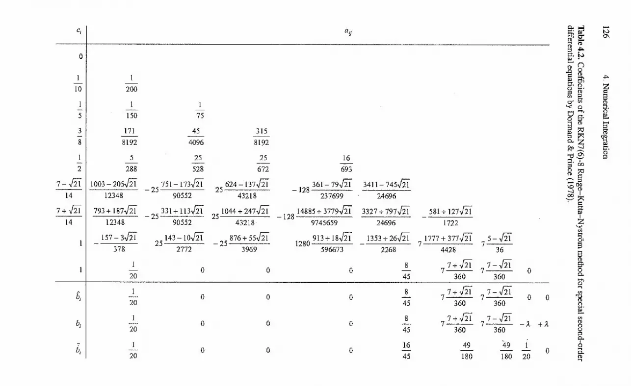
C7N
uopu
Bal
ui F
opau
mN
au Eit Zi c. cr -, (7; 0 • .I , • i...) r4) •
On 1 R
200 ô" ri,. 6, • a i 1 ...., 0
150 75 Ci _,'"-h
171 45 315 § ,`-°
8192 4096 E 2 8192
ci
0
1
10
1
3
73'
1
-2-
7— Î
14
7+ T 14
1 8 7 + -/-2-1- 7- — : (0): 0 0 0 7 '7 0 20 45 360 360
,-, 1 8 7 + I-if 7- —Hi cl,o o 0 7 7 0 0
CD 20 45 360 360 ....). ....
1 8 7+Z 7-5- cl) 0 0 0 7 7 A. + 1 CD o
20 45 360 360 0
91' 1 16 49 49 1 o 0 0 0 0 a 20 45 180 180 20 0 -,
Ro ----1 5 25 25 16
288 528 672 693 co ,--.
1003-205Ï 25
751-173Z 25
624-137Î
128 361-79121 3411-745J21 --) ?
12348 90552 43218 237699 24696 ,..9 •
793+ 187a-
25 331+1131121
25 1044 + 247-51 12814885+377921 3327 + 797,/21 581+ 127Z FS
12348 90552 43218 9745659 24696 1722
157 — 3.51 25 1431021 25
876 +555-
1280 913+185i 1353+26/Ï 1777 + 377Z 7
5— 5- 7
4 g
378 2772 3969 596673 2268 4428 36
b.
b.

4.1 Runge—Kutta Methods 127
4.1.5 Continuous Methods
In the discussion of stepsize control for Runge—Kutta methods no notice was taken of the fact that the solution of a differential equation is often required at prede-fined output points. This does not cause major problems as long as the difference between two subsequent points is considerably larger than the stepsize proposed by the stepsize control. If, however, the stepsize has to be truncated very often to reach predefined output points, the use of a Runge—Kutta method turns to be very ineffective. Considering the case of satellite orbits the problem of dense output may, for example, arise from ephemeris printout requirements or from the need for a smooth graphical representation of the orbit. Dense satellite position points are furtheimore required for an iterative search for special events like shadow entries of a satellite.
The straightforward way to cope with this problem is to calculate the solution of the differential equation at widely spaced time steps and to interpolate it to the desired dense output points by means of an appropriate polynomial. A major disadvantage of this method is, however, that the results of subsequent Runge—Kutta integration steps have to be stored for interpolation similar to common multistep methods.
Within the last decades several authors (e.g. Horn 1981, 1983, Shampine 1985, Doiniand & Prince 1986, 1987, Sharp & Verner 1998) have, therefore, been con-cerned with the design of interpolation foimulas for Runge—Kutta methods that preserve the character of a single-step method. The idea of these famiulas is to use the function values ki (which have already been calculated to obtain the in-crement function ÇA) and a few additional evaluations to construct an interpolating polynomial valid between y (to) and y (to -I- h).
As an example of an interpolant, one of the first continuous methods, which has been proposed by Horn (1981, 1983), is described in what follows. It is based on the embedded 6-stage Runge—Kutta—Fehlberg method RKF4(5)
= f (to cih, y o h ) (i = 1 . . . 6)
= y0 +h i= 1
5
TIN h) = yo h biki i=1
which is defined by the coefficients of Table 4.3. In addition to k1 . . . k6, the method of Horn requires the value
1 1 2 k7 = f (to h, yo + h —k5 —k6))
6 6 3
(4.33)
(4.34)
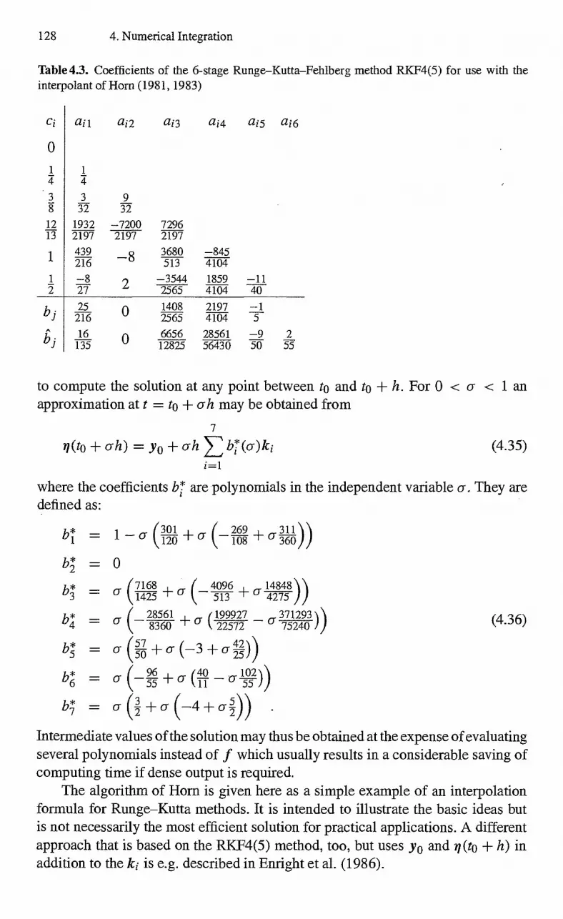
Ci
0
1 zt• 3 "g.
1
1
b
Li
128 4. Numerical Integration
Table 4.3. Coefficients of the 6-stage Runge—Kutta—Fehlberg method RKF4(5) for use with the interpolant of Horn (1981, 1983)
ai
3 32-
1932
ai2
9 32
-7200
ai3
7296
ai4
-845
ai5
-11
a1 6
2197
439
2197
—8
2
2197
3680 216
-8 27
513
-3544 4104
1859 2565 4104 40
25 0
0
1408 2197 -1 5
-9 50
2 55
216
16
2565
6656
4104
28561 135 12825 56430
to compute the solution at any point between to and to ± h. For 0 < cr < 1 an approximation at t = to ± ah may be obtained from
7
n(to ± h) = yo + ah bl'(a)ki (4.35)
where the coefficients b;' are polynomials in the independent variable a. They are defined as:
(_43. ,w) )
- 0
7168 496 0.14287458)) - a (1425
03 ± 4
b4 28561 „ (199927 „ 371293 \) (4.36
2, ) ( 8360 ' k 22572 75240
b; —
40 102 \) =
=
Intennediate values of the solution may thus be obtained at the expense of evaluating several polynomials instead of f which usually results in a considerable saving of computing time if dense output is required.
The algorithm of Horn is given here as a simple example of an interpolation foiniula for Runge—Kutta methods. It is intended to illustrate the basic ideas but is not necessarily the most efficient solution for practical applications. A different approach that is based on the RKF4(5) method, too, but uses yo and n(to ± h) in addition to the ki is e.g. described in Enright et al. (1986).

4.1 Runge—Kutta Methods 129
Up to some time ago interpolants were only available for several methods of in-•
termediate order. Recently, however, a 7th-order interpolant based on an embedded 8(6)th-order/12-stage Runge—Kutta pair has been announced by Dormand & Prince (1989). This interpolation formula requires four function evaluations in addition to those of the basic method.
Dense output formulas have also been developed for several Runge—Kutta-Nystrom methods. A 6th-order interpolant is, for example, available for the RKN6(4) pair of Dormand & Prince (1987) and the authors are concerned with the search for an interpolant for their 12(10)th-order pair (see Brankin et al. 1989).
4.1.6 Comparison of Runge—Kutta Methods
For the assessment of different numerical integration methods several sets of test problems have been developed by Hull et al. (1972) which greatly facilitate the comparison of performance data obtained by different authors. From the various test problems proposed by Hull et al. the plane two-body problem is frequently used by many authors and describes the main aspects of satellite motion very well. Even though it is not possible to cover all aspects that might affect the choice of an integration method by such a simple example, one can get a first idea of the performance of the Runge—Kutta methods discussed so far. For further discussion the reader is referred to Sect. 4.4.
The differential equation of the two-body problem is given by
571 = .Y3
512 = Y4
513 = —Y1/ (Y? Y) 3/2
.574 = — Y2/(Y? +Y )312
(4.37)
which results from writing 1 —r/r 3 as a first-order equation with r = (Yip y2) and y = (y3, y4). Initial values for t =0 that describe an orbit with semi-major axis a =1 and eccentricity e starting at pericenter are given by
571(0) = 1 — e
5/2(0) = 0
573(0) = 0
514(0) = ,N/(1 + e)I(1 — e)
(4.38)
Since the velocity variations in an eccentric orbit are a crucial test for the capability of a numerical integration method to change its stepsize, Hull et al. (1972) defined the distinct test problems Dito D5 with eccentricities ranging from e = 0.1 to e = 0.9 in steps of 0.2. The stop time is defined as t=20 in all cases, corresponding
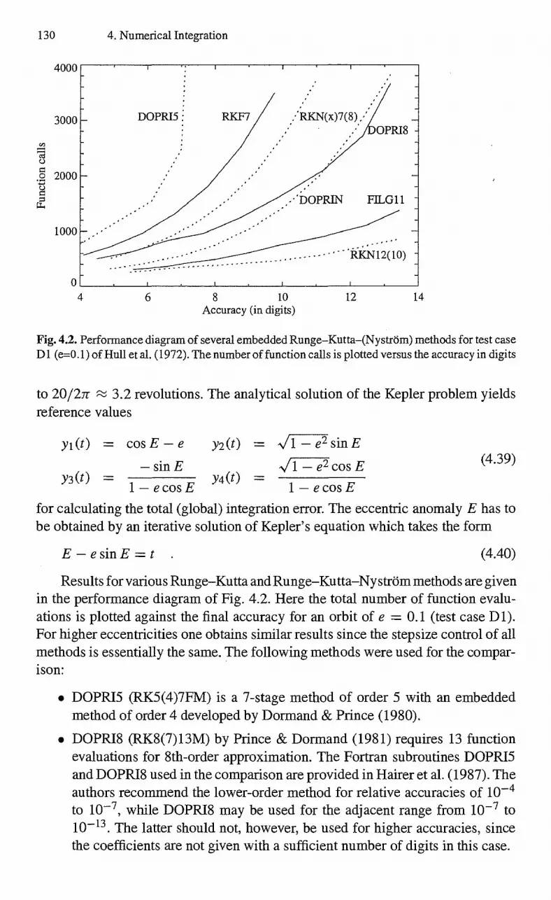
130
4000
3000
74—
0 2000
1000
o
4. Numerical Integration
4
6
8
10
12
14 Accuracy (in digits)
Fig. 4.2. Performance diagram of several embedded Runge—Kutta—(Nystrom) methods for test case DI (e=0.1) of Hull et al. (1972). The number of function calls is plotted versus the accuracy in digits
to 20/27r 3.2 revolutions. The analytical solution of the Kepler problem yields reference values
y1(t) = cos E - e y2(t) 1 - e2 sin E
- sin E - e2 cos E Y4 (t) = 1 - e cos E 1 - e cos E
for calculating the total (global) integration error. The eccentric anomaly E has to be obtained by an iterative solution of Kepler's equation which takes the form
E - e sin E = t . (4.40)
Results for various Runge-Kutta and Runge-Kutta-Nystrom methods are given in the performance diagram of Fig. 4.2. Here the total number of function evalu-ations is plotted against the final accuracy for an orbit of e = 0.1 (test case D1). For higher eccentricities one obtains similar results since the stepsize control of all methods is essentially the same. The following methods were used for the compar-ison:
• DOPRI5 (RK5(4)7FM) is a 7-stage method of order 5 with an embedded method of order 4 developed by Dormand & Prince (1980).
• DOPRI8 (RK8(7)13M) by Prince & Dormand (1981) requires 13 function evaluations for 8th-order approximation. The Fortran subroutines DOPRI5 and DOPRI8 used in the comparison are provided in Hairer et al. (1987). The authors recommend the lower-order method for relative accuracies of 10-4 to 10-7 , while DOPRI8 may be used for the adjacent range from 10-7 to 10-13 . The latter should not, however, be used for higher accuracies, since the coefficients are not given with a sufficient number of digits in this case.
(4.39) y3(t)
4.1 Runge—Kutta Methods 131
• RKF7 - a famous method developed by Fehlberg (1968) - is similar to DOPRI8 but uses the 7th-order method for integration, while the 8th-order method is only used for error estimation. A total of 13 function evaluations are required per step.
• DOPRIN (RKN7(6)9) is an embedded Runge-Kutta-Nystrom method of order 7(6), which - in contrast to the aforementioned methods - is used for the direct integration of special second-order differential equations of type y" = f (t, y). The Fortran implementation is taken from Hirer et al. (1987).
• RKN(.5c)7(8) is a 13-stage Runge-Kutta-Nystrom method of order 7 devel-oped by Fehlberg (1975) which - in contrast to the other Nystrom methods considered here - may also be used for second-order differential equations depending on i-. An implementation is described in Schastok et al. (1989).
• 1-1LG11 is based on the 11(10)th-order/17 stages RKN coefficient set K17M by Filippi & Grdf (1986) and has been implemented similar to DOPRIN.
• RKN12(10)17M is a 12(10)th-order/17-stage Nystrom method recently de-veloped by Dormand et al. (1987). Implementations of this code are de-scribed in Brankin et al. (1987, 1989). The authors' RKNINT program, which combines the RKN12(10) method with the RKN6(4) Runge-Kutta-NystrOm triple (Dormand & Prince 1987), has been used for the present comparison. It allows the user to choose between a high-precision solution obtained with the 12th-order formulas and dense output at a somewhat lower precision. The code is also available under the name DO2LAF in the well known NAG library.
The comparison of the various methods clearly shows that high-order methods are required to achieve accuracies of better than 10 -8 . Forcing a low-order code like DOPRI5. to produce a highly accurate solution by using small stepsizes results in excessive computing times. A comparison of RKF7 and DOPRI8 - both of which are embedded methods of order 7 and 8 - clearly shows the superiority of the approach of Dormand and Prince to optimize the higher-order method for calculating the solution and only use the low-order method for stepsize control. The excellent performance of the methods developed by Dormand and Prince is also seen in a comparison of DOPRI8 or DOPRIN with Fehlberg's Nystrom method RK.N(5c)7(8). Methods like DOPRI8 or DOPRIN can be recommended for a wide range of accuracies, but high-order codes like FILG11 or RKN12(10) are certainly more efficient even for moderate accuracy requirements. Where applicable, the special Runge-Kutta-Nystrom methods are preferable to standard Runge-Kutta methods of similar order.
The stepsize control of all codes performs well up to high eccentricities since all methods considered are embedded methods. Even though this is not essential for near-circular orbits, it facilitates the use of Runge-Kutta methods, since even a bad initial stepsize can easily be corrected to the optimum stepsize during the integration. All examples were calculated with a starting step size of h= 0.1.
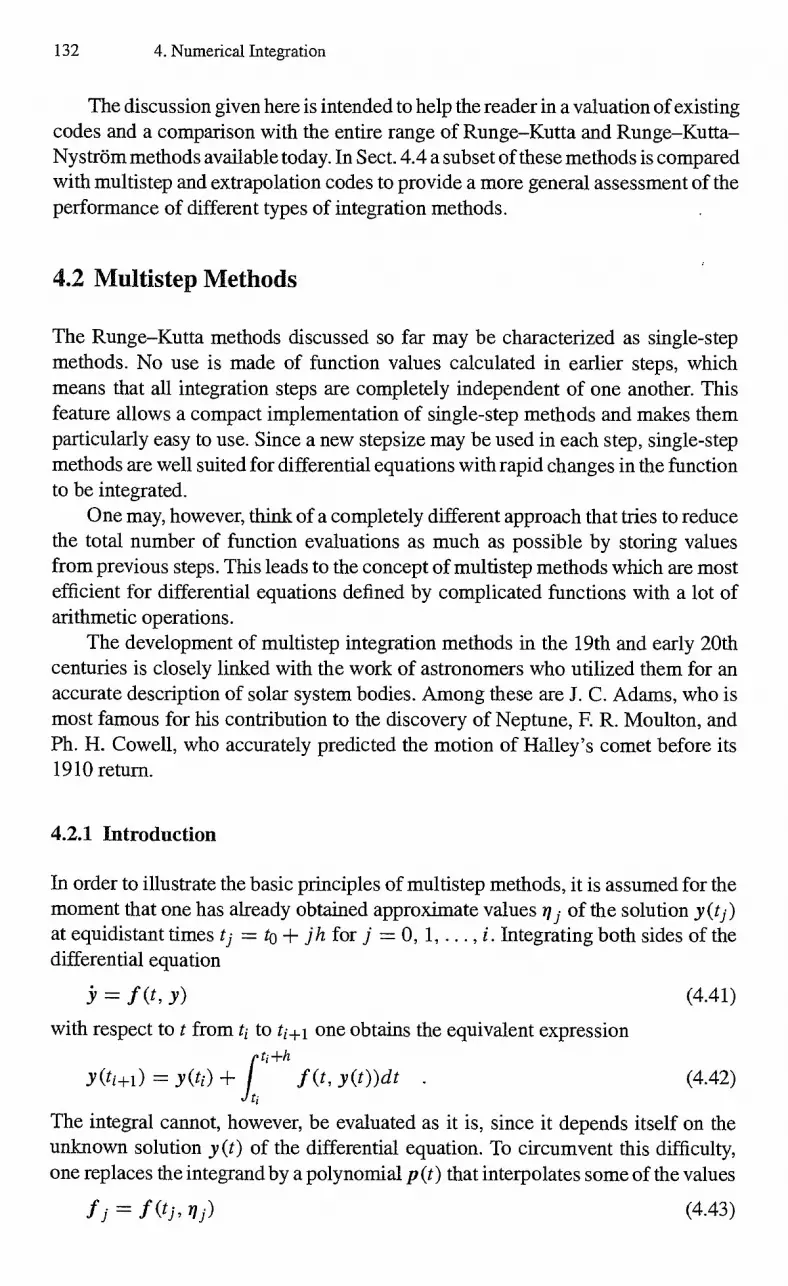
132 4. Numerical Integration
The discussion given here is intended to help the reader in a valuation of existing codes and a comparison with the entire range of Runge—Kutta and Runge—Kutta-Nystrom methods available today. In Sect. 4.4 a subset of these methods is compared with multistep and extrapolation codes to provide a more general assessment of the performance of different types of integration methods.
4.2 Multistep Methods
The Runge—Kutta methods discussed so far may be characterized as single-step methods. No use is made of function values calculated in earlier steps, which means that all integration steps are completely independent of one another. This feature allows a compact implementation of single-step methods and makes them particularly easy to use. Since a new stepsize may be used in each step, single-step methods are well suited for differential equations with rapid changes in the function to be integrated.
One may, however, think of a completely different approach that tries to reduce the total number of function evaluations as much as possible by storing values from previous steps. This leads to the concept of multistep methods which are most efficient for differential equations defined by complicated functions with a lot of arithmetic operations.
The development of multistep integration methods in the 19th and early 20th centuries is closely linked with the work of astronomers who utilized them for an accurate description of solar system bodies. Among these are J. C. Adams, who is most famous for his contribution to the discovery of Neptune, F. R. Moulton, and Ph. H. Cowell, who accurately predicted the motion of Halley's comet before its 1910 return.
4.2.1 Introduction
In order to illustrate the basic principles of multistep methods, it is assumed for the moment that one has already obtained approximate values ?i f of the solution y (ti ) at equidistant times t1 to jh for j = 0, 1, .. . , i. Integrating both sides of the differential equation
= f (t, 31 ) (4.41)
with respect to t from ti to ti+1 one obtains the equivalent expression ti+h
y (ti +i) = y(ti) f f (t , y(t))dt . (4.42)
The integral cannot, however, be evaluated as it is, since it depends itself on the unknown solution y (t) of the differential equation. To circumvent this difficulty, one replaces the integrand by a polynomial p(t) that interpolates some of the values
f = f (ti , ni ) (4.43)
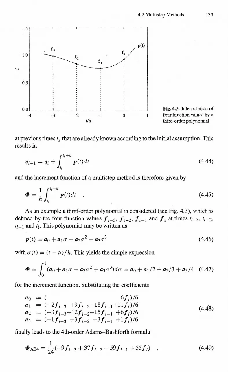
Fig. 4.3. Interpolation of four function values by a third-order polynomial
1.5
1 .0
0.5
00 -4 -3 -2 -1
O
1 t/h
4.2 Multistep Methods 133
at previous times ti that are already known according to the initial assumption. This results in
= + f
ti+h
p(t)dt (4.44)
and the increment function of a multistep method is therefore given by
1 f ti±h = — p(t)dt . (4.45)
h ti
As an example a third-order polynomial is considered (see Fig. 4.3), which is defined by the four function values f i -3' f i -2' f and f. at times ti_3, 4-2, ti_i and t1 . This polynomial may be written as
p(t) = ao aia a2a2 a3a3 (4.46)
with cr(t) = (t — ti)/ h. This yields the simple expression
= f
(ao aia a2cr 2 a3a3)da = ao ai/2 a2/3 a3/4 (4.47) 0
for the increment function. Substituting the coefficients
ao = ( 6f i)/6 ai = (-2fi_3 +9f i-2-18f i_i+11f i ) /6 a2 = (-3f i_3+12, fi_2-15 f -F6fi)/6 a3 = (-1f 3 +3f 2 +1 f i )
finally leads to the 4th-order Adams—Bashforth formula
(4.48)
AB4 = —24
(-9 f i-3 + 37 fi-2 — 59f ± 55 f i)
(4.49)

134 4. Numerical Integration
which may be used to calculate the approximate solution
(4.50)
of the differential equation at ti+1 = t + h. Repeated application of the Adams-Bashforth formula then yields the solution of the differential equation for subse-quent times ti +j h.
In order to start the integration scheme the first four values f 0, f 1 , 12 and f 3 or, equivalently, no , 17 1, 172 and 11 3 are required. They may, for example, be obtained from to and 11 0 using three steps of a fourth or higher-order Runge—Kutta method with sufficient accuracy.
4.2.2 Adams—Bashforth Methods
The simple procedure described in the introductory section may easily be extended to derive general multistep methods of arbitrary order.
For this purpose one makes use of Newton's founula for a polynomial prni of order m —1 that interpolates m points
(ti_„1±1 , fi —m+1) (ti, i)
with equidistant nodes ti. This polynomial is given by the compact expression
p(t) = + h)
m-1
)V i fi , (4.51) 1-=-0
where the binomial coefficient stands for (—cr) (—a)( —c- — 1) . . . — j 1)
j!
if j > 0 and is equal to 1 for j O. The backward differences of f i are recursively defined by
yo u = f
Vfi — fi — fi-1 v n f vn—i f _ —1f
and may be computed from the given function values as outlined in Fig. 4.4. Using this notation the increment function of the mth-order Adams—Bashforth
multistep method may now be written as
(PABm = —1 ff±
m-1 h prn
i (t)dt = yiVi f (4.54) h Li
j=0
with stepsize independent coefficients
yi (-1)i f 1 ( a ) do- (4.55)
(4.52)
(4.53)

4.2 Multistep Methods 135
. f i-4 . . .
fi -3 --> V 1 fi_3 . •
fi-2 --> V 1 fi_2 -->
f
▪
f
f
▪
f -->
V2 f_2
v2 f i_
v2 f i
----> V 3 f
---> V3 f
▪
v4 f i
Fig. 4.4. Backward difference table for polynomial interpolation
Numerical values of yo. )18 are given in Table 4.4. They may be obtained from a simple recurrence relation (see e.g. Hairer et al. 1987):
yi 1 (4.56)
Table 4.4. Coefficients of Adams—Bashforth methods in backwards difference notation
0 1 2 3 4 5 6 7 8
yi 1 It ?1 i 311, 1 6108807 i57225870 31067180170
The local truncation error of the Adams—Bashforth method decreases with the order m and may be estimated by comparing two methods of order m and m +1:
eABm = 1Y (ti h) — 11ABInl 1 11ABm+1 hlABmI = hlYinV m fi I • (4-57)
Since Vm f 1 hm is an approximation of the m-th derivative of f, the truncation error may also be expressed as
eABm hm+1 I yn, fri) I = hm±l lym y7n+1) I (4.58)
which shows that the order of the Adams—Bashforth method is equal to the number (m) of nodes (ti_m±i • • - ti).
Substituting the definition of backwards differences into (4.54), the increment function may also be written in terms of the function values f
(PAM = tim 1 fi-m+1 + + fl,nmfj =
flrnj f i_m ±; (4.59)
j=1
This formulation of the increment function, which has already been used in our introductory example, avoids the computation of the backwards differences and is therefore more convenient and efficient as long as methods of fixed order are
136 4. Numerical Integration
Table 4.5. Coefficients of Adams—Bashforth methods up to order m = 8.
j 1 2 3 4 5 6 7 8
pi; 1 _1 3
P2j 2 2
5 —16 23 P3 j
—9 37 —59 55 P4i 24 5 24 -51.
251 —1274 2616 —2774 1901 P5 :I 720 720 720 720 720
a —475 2877 —7298 9982 —7923 4277 P6I 1440 1440 1440 1440 1440 1440
R 19087 —134472 407139 —688256 705549 —447288 198721 fr'7 / 60480 60480 60480 60480 60480 60480 60480
—36799 295767 —1041723 2102243 —2664477 2183877 —1152169 434241 138/ 120960 120960 120960 120960 120960 120960 120960 120960
considered. There are, however, several applications where (4.54) is preferable, since the use of backwards differences allows a straightforward estimation of the local truncation error and an easy change of the order from one step to the next.
The new coefficients /3„,i — which are no longer independent of the order m — may be obtained from the yi 's using the relation
m-1
Pmi = (-1)m-f Y1( . 1 )
l=m—i
for j = 1, . , m (Grigorieff 1977). Explicit values are given in Table 4.5.
(4.60)
4.2.3 Adams—Moulton and Predictor—Corrector Methods
In the mth-order Adams—Bashforth method the polynomial p(t) is defined by m function values up to and including f i at time ti. The integration is, however, performed over the subsequent interval ti ti+1 where the approximation cannot be expected to be very good.
Another type of multistep method — known as the Adams—Moulton method — therefore uses the polynomial p im+ 1 (t) which interpolates m function values at time steps ti_m+2 and ti±i :
pm (t ) = pm (ti + ah) =
j=0
(-1)i ( —a 4- 1 ) vii +1 (4.61)
Upon integration this yields the Adams—Moulton formula
1 f ti+h
Amm — mi+1 (t)dt = h ti
m-1
j=0
YI i f (4.62)

E * ( 1
m - j )
trz-1
l=m—j
(4.67)
4.2 Multistep Methods 137
with coefficients
(4.63) 0
that are given in Table 4.6. Further values may be calculated from the recurrence relation
(4.64)
Table 4.6. Coefficients of Adams—Moulton methods in backwards difference notation
j 0 1 2 3 4 5 6 7 8 , 1 -1 =1 —1 —19 —3 —863 —275 —33953 Yi _I 2 12 24 720 160 60480 24192 3628800
The order of the Adams-Moulton method is equal to m and is, therefore, the same as that of an Adams-Bashforth method involving m grid points for the in-terpolating polynomial. The local truncation error of the Adams-Moulton method, which is given by
e m hm+ 1 I ym* Yi (m+1) , (4.65)
is smaller, however, than that of an Adams-Bashforth method of equal order, since the error constant I ym* I is smaller than I )6, I.
As with the Adams-Bashforth methods, the backwards differences may be substituted to yield a formulation that depends on f only:
(P AMm Pm* 1 f i—m+2 4- • Pm* m f i+i = Pm* f i+l— m±j (4.66)
j=1
The coefficients fim* si (see Table 4.7) of the mth-order method may be obtained from the y7 using the relation
for j = 1, . , m (Grigorieff 1977). Since the increment function of the Adams-Moulton method depends on
f i+i = f (ti+i, i+1)
(4.68)
it is not possible to calculate an explicit solution at ti ± i from
ni+1 = + hoAmm (4.69)

138 4. Numerical Integration
Table 4.7. Coefficients of Adams—Moulton methods up to order m = 8.
j 1 2 3 4 5 6 7
1 1 P2 j
—1 8 5 /33/ 12 12 12
1 —5 19 9 P4j -2-zi 24 271. 5
—19 106 —264 646 251 135i 720 720 720 720 720
27 —173 482 —798 1427 475 P6i 1440- 1440 1440- 1440 1440 1440
—863 6312 —20211 37504 —46461 65112 19087 137i 60480 60480 60480 60480 60480 60480 60480
1375 —11351 41499 —88547 123133 —121797 139849 36799 138j 120960 120960 120960 120960 120960 120960 120960 120960
The Adams—Moulton formula is therefore called an "implicit" method and some iterative procedure is required to solve for y i±i
To avoid this difficulty, an Adams—Bashforth method of order m is usually combined with an Adams—Moulton method of order m or m 1 in a so-called predictor—corrector or PECE-algorithm which consists of four steps:
1. In the first step — the Predictor step — an initial estimate of the solution at ti is calculated from the Adams—Bashforth formula
= ii +htPAB • (4.70)
2. The result is used in the Evaluation step to find the corresponding function value
f 1+ 1 f (t1+1 ' 71 i+1)
(4.71)
3. In the third step — called the Corrector — the Adams—Moulton formula is applied to find an improved value
= +hoAm(f+1) - (4.72)
4. The final Evaluation step yields the updated function value
f i±i = f (ti+i, (4.73)
which may then be used for the start of the next integration step.
In principle the third and fourth step would have to be repeated until convergence is achieved to find the exact solution of the Adams—Moulton formula, but since each such iteration costs another function evaluation, this would not be worth the effort. A single corrector step is enough to assure that the order of the combined Adams—Bashforth—Moulton method is equal to that of the implicit method, even though the local truncation error is slightly larger (cf. Grigorieff 1977).

4.2 Multistep Methods 139
The justification for using the somewhat complicated predictor—corrector al-gorithm, lies in the stability of multistep methods at large stepsizes. Due to the truncation at a fixed order and a limited computing accuracy, the individual steps of the numerical integration are always affected by small local errors. An analysis of the way in which these errors are propagated from one step to the next shows that the errors may grow exponentially for large stepsizes. In order to avoid this unfa-vorable behavior and to guarantee stability, the stepsize may not exceed a certain limit that depends on the method and the differential equation to be solved.
Low-order methods are generally more stable even for large stepsizes. Due to their modest accuracy, small steps have to be used anyway and stability is often not a serious problem. When using high-order multistep methods, however, stability can pose stringent limits on the allowed stepsize. Even steps that yield a sufficiently small truncation error may then be too large since the propagation of local errors could result in an unbounded growth of the global integration error.
The implicit Adams—Moulton methods behave much better in this respect than the explicit Adams—Bashforth methods and even the approximate solution of the Adams—Moulton formula in the PECE algorithm improves the stability consider-ably. This is the main reason why it is generally recommended to use one additional function evaluation for the corrector step. Another advantage is that the local trun-cation error can be reduced by using the corrector. The doubled expense for a single integration step can at least partially be compensated for by larger stepsizes.
o 5
10
15
20
Fig. 4.5. A plot of the global integration error versus time t for an orbit of e = 0.1 reveals the effect of instability of high-order Adams—Bashforth methods •
To illustrate the practical meaning of stability, the two-body problem (D1) has been integrated.with both a 6th-order and an 8th-order Adams—Bashforth method (AB6, AB 8) at a stepsize of h = 0.04 (see Fig. 4.5). Since the local truncation error decreases with higher order, one might expect more precise results for the
140 4. Numerical Integration
AB 8 method, but the growth of the global integration error clearly shows the onset of instability. When combined with a corrector, the resulting Adams—Bashforth-Moulton method (ABM8) is stable, however, even at twice the stepsize.
As a compromise between a cheap predictor-only method and a more stable PECE method, a PECE* algorithm (cf. Long et al. 1989) may be useful for the treat-ment of perturbed satellite orbits. Here E* stands for a pseudo-evaluate step, which means that some simplifications are made in the final evaluation step. According to (4.4) the evaluation of f involves the computation of the acceleration
GM@ a(t, r, r p(t,r,r) , (4.74)
r3
where the dominant first term arises from the central gravity field of the Earth and p means the sum of all perturbations. Since the perturbations are much smaller than the central force, one makes a small error only if one does not recompute them after the corrector step. In a pseudo-evaluate step only the dominant term of the total acceleration is therefore updated with the coordinates obtained in the corrector step, while the perturbations are taken from the predictor step:
ED r p(t, rP , i.P) . a* (t , r,
GM i-) = (4.75)
r 3
Since the computation of the perturbations is much more time-consuming than that of the central acceleration term, the PECE* method increases the stability at almost no additional cost.
Irrespective of the use of a stabilizing corrector step one should not arbitrarily increase the order of a multistep method in an attempt to increase the stepsize and the accuracy. For the requirements of typical orbit computations orders in the range from 8 to 12 can usually be recommended.
4.2.4 Interpolation
The multistep methods of Adams' type may be extended in a straightforward manner to provide a solution at intemiediate output points. For this purpose it is assumed that a PECE step of size h has been used to advance from ti to ti and that one is interested in the approximate solution at some time t ah, where 0 <o < 1. From a total of m+1 points
(ti—m+i, f . • . (te, f i) , f4i)
one may construct the interpolating polynomial
P (ti + oh) = j=0
(-1)i ( —(7 + 1 ) V f* (4.76)
that was already used in the implicit Adams—Moulton folinula of the corrector step. Here the * denotes that f4 1 is a predictor value while all other f result from the
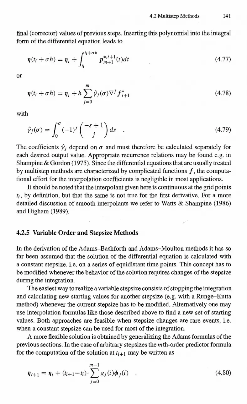
Or
fti
*,i+1 n(ti ah) p.+1 Wdt n+ah
(4.77)
4.2 Multistep Methods 141
final (corrector) values of previous steps. Inserting this polynomial into the integral form of the differential equation leads to
n(ti -I- ah) = j , + h Pi(a)Vi .174-1 (4.78) 1=0
with a
Pi(a) fo ( —s ± 1 ) ds (4.79)
The coefficients p; depend on a and must therefore be calculated separately for each desired output value. Appropriate recurrence relations may be found e.g. in Shampine & Gordon (1975). Since the differential equations that are usually treated by multistep methods are characterized by complicated functions f, the computa-tional effort for the interpolation coefficients is negligible in most applications.
It should be noted that the interpolant given here is continuous at the grid points ti, by definition, but that the same is not true for the first derivative. For a more detailed discussion of smooth interpolants we refer to Watts & Shampine (1986) and Higham (1989).
4.2.5 Variable Order and Stepsize Methods
In the derivation of the Adams—Bashforth and Adams—Moulton methods it has so far been assumed that the solution of the differential equation is calculated with a constant stepsize, i.e. on a series of equidistant time points. This concept has to be modified whenever the behavior of the solution requires changes of the stepsize during the integration.
The easiest way to realize a variable stepsize consists of stopping the integration and calculating new starting values for another stepsize (e.g. with a Runge—Kutta method) whenever the current stepsize has to be modified. Alternatively one may use interpolation foiniulas like those described above to find a new set of starting values. Both approaches are feasible when stepsize changes are rare events, i.e. when a constant stepsize can be used for most of the integration.
A more flexible solution is obtained by generalizing the Adams foimulas of the previous sections. In the case of arbitrary stepsizes the mth-order predictor foimula for the computation of the solution at 4+ I may be written as
m — 1
ni+ 1 =-- n i +(ti+1—ti). . (4.80) j=0

142 4. Numerical Integration
Here the factors
1 4+1 t — dt = — ti 1=I0 ti±i - ti_i
correspond to the coefficients yi of the fixed stepsize formula, while the
j-1
= I 1(ti± i - f[4, , 1=0
(4.81)
(4.82)
replace the backward differences Vi f. (see e. g. Hairer et al. 1987). The expressions f[ti, . . ,ti_i] are known as divided differences and result from the use of Newton's formula for a general interpolation polynomial. They are recursively defined by
= fi
f f
- ti_i f[4, ti -11 - ti-21
ti -
(4.83)
For constant stepsize h
1 f [ti , , ti_ i] = —7V f . (4.84)
'
The coefficients MO and obi (i) as well as those of a corresponding corrector fonnula may be calculated from recurrence relations which are essential for an efficient implementation of variable order methods (see e.g. Shampine & Gordon 1975).
For the selection of order and stepsize the error for the order currently in use is estimated as well as the expected error for adjacent orders. At the same time a new stepsize is calculated based on the current error estimate and the current order. Evaluating this information a new order or stepsize can be chosen. Since changes in the stepsize require an increased effort for the computation of the coefficients 8,1(i) the stepsize is changed only if the recommended stepsize is larger or smaller than the present one by a factor of at least two.
A great advantage of variable order and stepsize methods is the fact that they do not require a starting procedure. Starting from order one and a very small initial stepsize, both order and stepsize may be increased up to an optimum value within a few steps. This makes variable order and stepsize codes particularly easy to use. Among the various implementations the following are mentioned:
• DVDQ — developed at the Jet Propulsion Laboratory by Krogh (1969, 1974) — is one of the earliest variable order and stepsize multistep codes. DVDQ has, for example, been used for the numerical integration of the solar system ephemeris DE102 (Newhall et al., 1983).
4.2 Multistep Methods 143
• DE/DEABM is one of the most popular methods of its kind. The code and its theoretical background are explained in detail in the textbook of Shampine & Gordon (1975). The original code DE has since been improved to meet the needs of program libraries (Shampine & Watts 1979) and is available under the name DEABM now. Further amendments of the interpolation routines are reported in Watts & Shampine (1986).
• VOAS is a variable order and stepsize multistep code by Sedgwick (1973). Aside from a different implementation its characteristics and performance are similar to DE/DEABM.
• The predictor—corrector method of Hall & Watts — implemented as DO2CJF in the NAG Fortran library — provides interpolation for dense output similar to DE/DEABM.
4.2.6 Stoermer and Cowell Methods
In the discussion of Runge—Kutta methods, Nystrom methods have been introduced that are especially designed for the direct integration of second-order differential equations. Corresponding multistep methods that are known as Stoenner and Cow-ell methods may be derived by an extension of the concept of Adams methods. For this purpose the differential equation
= a(t, r) (4.85)
is integrated twice to font' the equivalent integral equation
ti t
r(ti + h) = ri + i f f r, r(r))d-rdt (4.86)
Using partial integration the double integral can be replaced by a single integral:
ti-Fh t ti-ph t tid-h
f 1 f a (- c r (-c))dr dt = t • f a( - r(z))dr f t a(t, r(t))dt
ti+h
f (tid-h—t)a(t, r (t))dt ti
= h2 f (1—s) (ti +sh, r(ti+sh))ds
0

144 4. Numerical Integration
Table 4.8. Coefficients of Stoermer and Cowell methods in backwards difference notation. See e.g. Schubart & Stumpff (1966) for higher-order coefficients.
0 1 2 3 4 5 6 7 8
• 1 0 1 77-7 T z . 1
1-7.- i L.
19 3 -4-5
863 275 33953 240 12096 4032 518400
* '^-,
C.<:) 1 - 1 -i ii 0 —1 —1 —221 —19 —9829 — 240 240 60480 6048 3628800
By adding r (ti + h) and r (ti — h) one can eliminate the velocity i-i, which results in
r(ti+h) — 2r (ti) r (ti —h) 1
= h2 f (1 —s)[a(ti +sh, r(ti +sh)) a(ti—sh, r(ti —sh))]ds (4.87)
O
As in the derivation of the Adams—Bashforth foiniulas one may now use a polyno-mial through m points
(4—m±i, ai—m+i), • • • , (ti, ai)
to approximate a and to evaluate the integral. This yields the Stoenner foi nula m-1
ri+1 = 2r — ri_1+ h2 8iViai (4.88) i=o
with coefficients given by
Si = f (1 — s)[(7 5 ) + (lids (4.89) J J
0 They are easily obtained from the coefficients yi* of the implicit Adams method (see Table 4.6) via the relation
8i = (1 — Dy7 . (4.90)
Numerical values for j < 8 are given in Table 4.8. The use of the Stoeinier foiniula requires the knowledge of two position vec-
tors r11, . . . , ri and m accelerations ai_m+i, , ai. These initial values may be obtained from a special starting procedure (see e.g. Schubart & Stumpff 1966) or a Runge—Kutta method.
The explicit Stoenner method may be supplemented by the implicit Cowell method
m -1
r = 2r — ri_1+ h
e Via 1+1 (4.91)
j=0
as corrector. The coefficients are given in Table 4.8 up to order 8. Further values follow from the simple relation
8.7 = 8i — 8.1_1 . (4.92)

4.2 Multistep Methods 145
4.2.7 Gauss—Jackson or Second Sum Methods
The Gauss—Jackson or second sum methods (Jackson 1924, Merson 1974) are slightly modified versions of the Stoerrner—Cowell methods for second-order dif-ferential equations and probably the most recommendable fixed-stepsize multistep methods for orbit computations. The explicit Stoeuner formula is replaced by the equation
m+1
ri+i =
(5j vj-2a1 (4.93)
i=o
and the modified Cowell formula is given by
m-1-1
ri+i = (4.94) i=o
Velocities at each step may be obtained from similar equations that follow from the Adams—Bashforth—Moulton formulas:
= h (4.95) j=0
and
vi+i = * vj-1 (4.96)
j=0
The coefficients yi , 31, (5j and Sy are listed in Tables 4.4, 4.6 and 4.8. The expressions for ri±i and vi+ i involve the use of first and second sums
(V-1 , V-2), which are generalizations of the backwards differences introduced earlier. They are implicitly defined by the recursions
ai = v —i ai _ v-2ai v-2ai_
in close analogy with definition (4.53). By applying the backward difference oper-ator V twice to the explicit second sum formula (4.93) for r+1, one obtains
m- 1
ri+i — 2r i ri _ SiViai (4.98) j=0
which is just equation (4.88) of the Stoeiffler method. In a similar manner one may prove the validity of the implict second sum formulas as well as the first sum formulas for the prediction of v.
Despite the apparent equivalence of the Bashforth—Moulton and Stoemier-Cowell formulas and the first and second sum formulas, the latter are generally preferred in practical computations. According to Henrici (1962) and Herrick (1971,
(4.97)

(4.99) j-2a0 v
2 v — h2
j=1
146 4. Numerical Integration
1972) the sum formulas are less influenced by round-off errors that result from the finite computing accuracy. This is especially important in long-term integrations where round-off errors are the main source of error, since the local truncation error can always be limited by choosing a high-order method and/or a small stepsize.
In order to use the summed version of the Stoeimer—Cowell formulas one has to determine initial values of the first and second sums in addition to the initial set of backward differences. For starting the calculation it is assumed that one knows the position and velocity (r1, v1) of the satellite for a given set of m equidistant times tj= to + jh (j = —m +1, ..., 0). These data can always be obtained from the initial values (to, ro, vo) by a backwards integration with a high-order Runge-Kutta method or an extrapolation method. From position and velocity one is able to calculate the accelerations (21 and the backward differences Vao Vm —l ao. The desired values of the first and second sums can now be determined by solving the implicit Adams—Moulton and Cowell foimulas for V —l ao and V-2a0:
As an alternative to using a single-step method for obtaining the initial set of accelerations and backward differences one may use a special starting calcula-tion. It involves an iterative refinement of a crude approximation of the satellite's coordinates and the corresponding difference table that may be based e.g. on the assumption of an unperturbed Keplerian orbit. For a detailed description of this method the reader is referred to Herrick (1971, 1972).
4.2.8 Comparison of Multistep Methods
The relative performance of some of the multistep methods described so far is com-pared in Fig. 4-.6. The test set covers a 6th-order Adams—Bashforth method (AB6), two Adams—Bashforth—Moulton methods of order 8 and 12 (ABM8, ABM12) and the variable order, variable stepsize code DE (Shampine & Gordon 1975), all of which may be used for integrating general first-order differential equations. In ad-dition two high-order Stoenner and Stoeimer—Cowell methods (S14, SC14) for the integration of second-order differential equations are included.
When considering fixed-order multistep methods the user must be careful to select a method of appropriate order for a given accuracy requirement. While low-order methods may be inefficient for high accuracies, the higher-order methods are subject to instability at low accuracies (i.e. at large stepsizes). As an example, the ABM 12 method can only be used to integrate problem D1 with accuracies of better than 9 digits, whereas the ABM8 method becomes inefficient at just the same accuracy. These problems may be avoided, however, by using a variable order and stepsize method like DE, since the automatic order selection avoids an unstable behavior and, simultaneously, guarantees a high efficiency.

AB6 • DE"
ABM8 ABM12 ---------- ------- --".- SC14 —
--------------------- S14
Func
tion
calls
4.3 Extrapolation Methods 147
4000
3000
4 6 8 10 12 14 Accuracy (in digits)
Fig. 4.6. Performance diagram of several multistep methods for test case D1 (e=0.1) of Hull et al. (1972). The number of function calls is plotted versus the relative accuracy in digits.
While the use of a corrector is essential for all but the lowest-order Adams methods, the same is not true for the Stoenner(—Cowell) methods, which are con-siderably more stable. Predictor methods of the Stoei nier type have therefore been preferred by several authors (see e.g. Schubart & Stumpff (1966), Herrick (1971, 1972)) for applications in celestial mechanics, especially for long-tenn integrations of the solar system. Due to their high stability, Stoenner(—Cowell) methods may be used up to very high orders which makes them the most efficient methods of the test set.
4.3 Extrapolation Methods
The extrapolation method is a powerful single-step method that extends the idea of Richardson extrapolation (i.e. extrapolation to zero stepsize) to the numeri-cal solution of ordinary differential equations. It is often called Bulirsch—Stoer or Gragg—Bulirsch—Stoer method in honor of the pioneering work of Gragg (1965) and Bulirsch & Stoer (1966). A general review of extrapolation methods may be found in Deuflhard (1985).
4.3.1 The Mid-Point Rule
In order to find the solution of a first-order differential equation at some time to+H from given initial values (to, yo), the interval [to, to -I- H] is first subdivided into n (micro-)steps of size h = HIn. A simple Euler step is then used to find an approximation u1 at to +h, while further values ui are obtained from the so-called mid-point rule:
2000
1000
ui = Yo +hf (to, Yo) ui.+1 = -I-2h f (to-Pih, ui)
(4.100) (i = 1, , n — 1) .
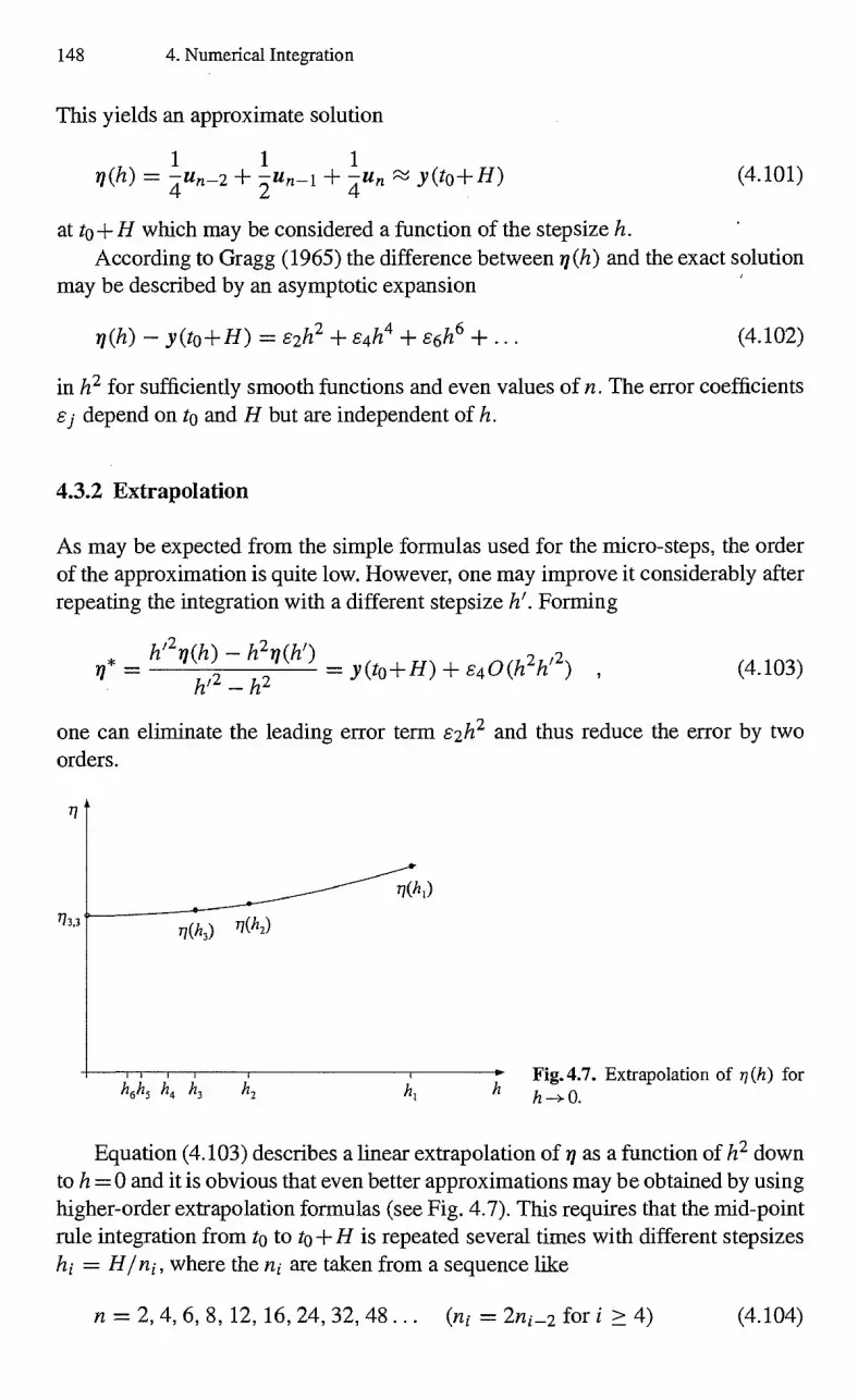
= (to+ 11) + 64 0 (12 2h12 ) h/2 h2
h/2 71(h) — h 2 71(17/ ) (4.103)
148 4. Numerical Integration
This yields an approximate solution
1 1 1 71(h) = —
411
n_2 + —
2 un_i + —
4U
n y (to+ H) (4.101)
at to+ H which may be considered a function of the stepsize h. According to Gragg (1965) the difference between n(h) and the exact solution
may be described by an asymptotic expansion
71(h) (to +H) = E2h2 84h4 s6h6 (4.102)
in h2 for sufficiently smooth functions and even values of n. The error coefficients si depend on to and H but are independent of h.
4.3.2 Extrapolation
As may be expected from the simple formulas used for the micro-steps, the order of the approximation is quite low. However, one may improve it considerably after repeating the integration with a different stepsize h". Forming
one can eliminate the leading error term s2h 2 and thus reduce the error by two orders.
Fig.4.7. Extrapolation of n(h) for 0.
Equation (4.103) describes a linear extrapolation of 71 as a function of h2 down to h =0 and it is obvious that even better approximations may be obtained by using higher-order extrapolation formulas (see Fig. 4.7). This requires that the mid-point rule integration from to to to + H is repeated several times with different step sizes hi = Hlni, where the ni are taken from a sequence like
n = 2, 4, 6, 8, 12, 16, 24, 32, 48 ... (ni = 2ni_2 for i ?4) (4.104)

4.3 Extrapolation Methods 149
which is called the Bulirsch sequence. The extrapolation is then performed accord-ing to the following scheme:
n(hi)
1 1 OD
q(h3)
Vh4)
1105)
=
=
=
=
=
111 , 1
77 -.2,1
77 .3,1
7/ -.4,1
ll -5,1
\ —>
\ —>
\ —>
\ —>
172,2
173,2
174,2
q5 , 2
\ —>
\ —>
\ —>
17 3 , 3
17 4, 3
17 5 , 3
\ —>
\ —>
174 , 4
17 5 , 4
\ —> n
(4.105)
When using polynomial extrapolation3 each entry of the table is a simple linear combination
i n — nid — ni,i+i =
, _ = (ni ni i)2 _ 1 (4.106)
of the entries to the left and upper left of it. From the asymptotic expansion of the error and 62j = 0 (H) one obtains the
following estimate:
= ly(to+H)—n id i = s21 0(12f. i+i) = 0 (H2i+ 1 ) .(4.107)
This means that each value Il i; in column j of the extrapolation table provides an approximation comparable to that of a Runge—Kutta method of order 2f. Since the number of columns may be quite high (e.g. 7-10), the extrapolation method exceeds any known Runge—Kutta method with respect to the attainable order and is therefore often considered the best method for very high accuracy requirements.
The stepsize control of the extrapolation method may be based on the same consideration that led to (4.21) for embedded Runge—Kutta methods. For a given size of the extrapolation table one can estimate the truncation error from the dif-ference of two neighboring values 1 .;, ;_ 1 and n and calculate a new stepsize from
H* = 0.9H • 2j-
(4.108)
where 0.9 is a safety factor that avoids an overoptimistic stepsize estimate and s is the required tolerance. Simultaneously one may check whether the order of the
3 Bulirsch & Stoer (1966) proposed an extrapolation involving rational functions, but polynomials are at least equally well suited (see e.g. Hairer et al. (1987)).

150 4. Numerical Integration
extrapolation table should be changed to decrease the total integration effort. For details of the stepsize control used in practical implementations of the extrapolation method the reader is referred to Hussels (1973), Deuflhard (1983) and flairer et al. (1987).
4000
3000 DIFSY1
rFt' z 0 2000
1000
0 4 6
8 10 Accuracy (in digits)
12 14
Fig. 4.8. Performance diagram of several extrapolation methods for test case DI (e=0.1) of Hull et al. (1972). The number of function calls is plotted versus the relative accuracy in digits. Note the jump in the graph for DIFSY1 that is caused by the stepsize and order control
4.3.3 Comparison of Extrapolation Methods
Implementations of the extrapolation method have been published by various au-thors. They differ mainly in the choice of polynomial or rational extrapolation, the set of micro-stepsizes and the stepsize and order control:
• DIFSY1, DIFSY2: Extrapolation methods using rational instead of polyno-mial extrapolation (Bulirsch & Stoer 1966). The initial stepsize control has been improved by Hussels (1973). DIFSY2 has been developed by Hussels (1973) for special second-order differential equations j) = f (t, y) that do not depend on first-order derivatives. For this purpose the mid-point rule is replaced by the lowest-order Stoermer formula (y +1 = 2y — y i _ i h2 f i ). Compared to DIFSY1, computing times may be reduced considerably by using DIFSY2 whenever appropriate.
• DIFEX1, DIFEX2: Extrapolation codes for first and second-order differential equations with a new kind of order and stepsize control developed by Deu-flhard (1983). The Bulirsch sequence (4.104) is replaced by the harmonic sequence (n = 2, 4, 6, 8, 10, 12, 14, .. .).

4.4 Comparison 151
. • ODEX1, ODEX2: Implementations of the extrapolation method described in Hairer et al. (1987). ODEX2 — like DIFSY2 — is intended for use with second-order differential equations.
As with the Runge—Kutta methods (see Fig. 4.2), test problem D1 of Hull et. al. (1972) is used to compare the performance of some of these extrapolation codes (Fig. 4.8). The high order of the extrapolation methods is evident from the fact that even a small increase in the number of function evaluations leads to a considerable increase of the number of accurate digits. Within the set of first-order methods (DIFSY1, DIFEX1, ODEX1) performance differences of about 20% are observed in agreement with Hairer et al. (1987). The use of DIFEX2 and ODEX2 which have been developed for the direct integration of second-order differential equations in-creases the efficiency by about 30-50%. Concerning the order and stepsize control, the ODEX codes are notable for the smooth relation between function evaluations and accuracy in the performance diagram.
Since the effective order of extrapolation codes can be quite high, the integra-tion is usually performed with large stepsizes. This may be pretty inefficient, if dense output is required. The situation is similar to that of high-order Runge—Kutta methods with the difference that an extrapolation method may be considered as a variable order method. If the maximum stepsize is limited by the requested out-put points, codes like DIFEX1 and ODEX therefore try to reduce the order as far as possible using only one column of the extrapolation table, if necessary. Even though the costs per integration step are reduced to a minimum in this way, the total integration effort may still be quite high. As a possible solution to this problem Shampine et al. (1982) have constructed a low-order interpolating Runge—Kutta formula based on the function evaluations that are required for the first entries of the extrapolation table. An interpolation algorithm that preserves the high order of extrapolation codes has only recently been developed by Hairer & Ostelinann (1990) for first-order differential equations, but has not yet been tested for use in high-precision ephemeris calculations.
4.4 Comparison
In the preceding sections the basic concepts and features of Runge—Kutta, multistep, and extrapolation methods for the integration of ordinary differential equations have been discussed. Regarding the class of Runge—Kutta methods, it has been shown that only high-order methods are reasonable candidates for the accuracy requirements of orbit computations. FILG11 and RKN12(10) were identified as the most efficient methods, but if the acceleration involves velocity dependent terms, DOPRI8 will serve best. Among the extrapolation codes ODEX2 is most promising, being about 40% faster than the corresponding codes for first-order differential equations. As expected, an excellent performance is also found for all multistep methods.
The sample calculations presented so far have been restricted to near-circular orbits, however, and in order to extend the discussion to more general orbits, highly

Func
tion
calls
4000
2000
6000
8000
0
152 4. Numerical Integration
eccentric orbits (e = 0 .9 ; test case D5 of Hull et al. (1972)) have been considered, too. In addition to DOPRI8, FILG11, and ODEX2 the variable order, variable stepsize multistep code DE/DEABM is used for this comparison.
As before, the valuation of the different integration methods is based on a perfor-mance diagram showing the relation between the number of function evaluations and the achieved accuracy. This approach avoids the measurement of machine-dependent computing times but some comments may be helpful to illustrate its validity.
The total computing effort of a numerical integration method depends not only on the number of function evaluations but also on the extent of additional arithmetic operations that are required inside the integration routine. In the case of the two-body problem the total computing time is, for example, about 30-60% higher than expected from the number of function evaluations alone, if one uses a Runge—Kutta or Extrapolation method. For variable-order and stepsize multistep methods which require a lot of work to calculate new coefficients at each step, this computational overhead is even higher and may well be in the order of 200%. The situation changes, however, if one considers a realistic force model that is appropriate for the prediction of satellite orbits. While the additional perturbations do not affect the number of function evaluations, they increase the total computing time considerably and make the integration overhead more or less negligible. As an example we found values between 5% (single-step methods) and 20% (variable-order and stepsize multistep methods) for a satellite force model including a 3 x 3 geopotential, lunisolar gravitational attraction, and solar radiation pressure.
The number of function evaluations that are required to achieve a given accuracy is, therefore, an appropriate performance measure for our purposes and we may now
4
6
8 10
12
14 Accuracy (in digits)
Fig. 4.9. Performance diagram of several single- and multistep methods for test cases DI (e=0.1, lower set of curves) and D5 (e=0.9, upper set of curves) of Hull et al. (1972). The number of function calls is plotted versus the relative accuracy in digits.

4.4 Comparison 153
turn to Fig. 4.9 which presents the results for the various integration methods under consideration. First of all it is evident that the total integration effort for a highly eccentric orbit is larger by a factor of about 3-4 than that for a near-circular orbit. Since this factor is almost the same for all methods, it can be concluded that the stepsize control of all codes works well even for Orbits of high eccentricity. While the good performance of the multistep methods at low eccentricities is beyond doubt, it is noteworthy that DE is well suited for very high eccentricities, too. This clearly indicates the usefulness of variable-order and stepsize multistep methods for application to general types of orbits. A regularization of the equations of motion (see e.g. Long et al. 1989), which is essential for an efficient use of simple fixed-stepsize multistep methods at high eccentricities, can thus be avoided completely.
A comparison of single-step methods with multistep methods indicates that both classes of integration methods have become almost competitive by now. While the 8th-order code DOPRI8 needs still 2-2.5 times the computing effort required by DE, one may note that the 11th-order Nystrom method FILG11 is even more efficient than the multistep method for both low and high eccentricities. An excellent performance is also found for the ODEX2 code, which shows that all types of single-step methods are well worth considering for applications in the field of orbital mechanics.
This result is somewhat in contrast to the common opinion that the use of a mul-tistep method is an indispensable prerequisite for an efficient numerical integration of satellite orbits due to the small number of function evaluations required. While there is strong support for this point of view in earlier reviews (Moore 1974, Fox 1984) one should keep in mind that the technique of Runge—Kutta integration has been improved considerably within the past two decades and that new high-order methods like FILG11 are much more efficient than their predecessors. Fox (1984), for example, recommends the Gauss—Jackson method (without corrector step) for near-circular orbits, since he finds it superior to the 8th-order Runge—Kutta method DOPRI8 by a factor of about 3. This result is in close agreement with our com-parison of DOPRI8 and the multistep method DE/DEABM and Fox's conclusions can be supported as long as methods for general first or second-order differential equations are considered. If the equation of motion does not contain any veloc-ity dependent term, however, then high-order Runge—Kutta—Nystrom codes like FILG11 or RKN12(10) may be used which are even faster than multistep methods like DE or VOAS.
The good performance of Runge—Kutta and extrapolation methods exhibited in the sample calculations should not, however, obscure the fact that the efficiency of these method deteriorates considerably when the distance between subsequent out-put points becomes smaller than the natural stepsize. This situation might change with the development of interpolants for high-order Runge—Kutta methods, but up to now single-step methods can only be recommended, if less than 50 to 100 output points per revolution are required. Multistep methods are still, therefore, prefer-able for the generation of equidistant ephemerides at small time intervals. With the availability of variable-order and stepsize codes these methods are no longer

154 4. Numerical Integration
restricted to near-circular orbits, but may also be used for high eccentricities with-out any precautions. Due to this increased flexibility, variable-order and stepsize multistep methods are ideal candidates for use in general satellite orbit prediction and determination systems. Nevertheless, fixed stepsize codes that have been fa-vored in software packages like GTDS (Long et al. 1989), GEODYN (Martin et al. 1976), UTOPIA (Schutz & Tapley, 1980), and PEPSOC (Soop 1983) are useful for an efficient treatment of near-circular orbits like those of geodetic or geostationary satellites.
Exercises
Exercise 4.1 (4th-Order Runge—Kutta Method) Apply the 4th-order Runge-Kutta method (cf. Sect. 4.1.1) to integrate the normalized two-body problem from to = 0 to t = 20 for an eccentricity of e = 0.1 (test problem D1, cf. Sect. 4.1.6). Determine the resulting accuracy of the state vector at the end point using n = {50, 100, 250, 500, 750, 1000, 1500, 2000} steps and count the corresponding number of function evaluations.
Solution: Reference values obtained with thEE 8-byte floating point arithmetics (double precision) are given below:
nfne Accuracy Digits 200 1.953.10-1 0.71 400 6.663.10-3 2.18
1000 9.051-10-5 4.04 2000 4.012-10-6 5.40 3000 6.847.10-7 6.16 4000 1.996.10-7 6.70 6000 3.608.10-8 7.44 8000 1.089.10-8 7.96
Exercise 4.2 (4th-Order Gauss—Jackson Method) Implement the 4th-order Gauss—Jackson method (cf. Sect. 4.2.7) and integrate the second-order differen-tial equation F = —r/r 3 of the normalized two-body problem from to = 0 to t = 20 for an eccentricity of e = 0.1 (Test problem D1, cf. Sect. 4.1.6). De-termine the resulting accuracy of the state vector at the end point using n = {100, 300, 600, 1000, 1500, 2000, 3000, 4000} steps and count the correspond-ing number of function evaluations.
Hint: Apply the 4th-order Runge—Kutta method to compute position and velocity at times to — h, to — 2h and to — 3h from the intial values ro and vo. The correspond- ing accelerations ao, , a_3 can then be used to foam the backwards differences

0.20 0.20
- 0.15 0.15
- 0.10
r.t)
0.05
20 0.001,
o
0.05 -
0.00 20 00 5 10 15
Time (t) 0.5 1.0 1.5
Distance (r)
Exercises 155
Vqao, , V3 a0 and to initialize the sums
V -2a0
_1 vOao _1 V l ao — — V2ao
2 19
12 24 720 a° u,3
—NPao — — 40
V ao 12 240 V ° 1 1 2
at the starting point to.
Solution: Reference values obtained with IEEE 8-byte floating-point arithmetics (double precision) are given below:
nfnc Accuracy Digits 116 2.456.10—°3 2.61 316 3.363-10-06 5.47 616 7.705-10-08 7.11
1016 4.539-10—°9 8.34 1516 5.174.10-10 9.29 2016 1.166.10-10 9.93 3016 1.499.10-11 10.82 4016 3.577.10-12 11.45
Exercise 4.3 (Stepsize Control for Eccentric Orbits) Integrate the nontialized two-body problem with eccentricity e = 0.9 from to = 0 to t = 20 (test problem D5, cf. Sect. 4.1.6) using the DE multistep method of Shampine & Gordon (1975) and monitor the step size variation as a function of time and distance.
Solution: Using double-precision arithmetics and a value of Sabs = 10-8 for the error control parameter of the DE method, the results shown in Fig. 4.10 are obtained. -
Fig. 4.10. Stepsize variation of DE multistep method during integration of normalized two-body problem with eccentricity e =-- 0.9.

156 4. Numerical Integration
Following an infinitesimal initial step, the order and stepsize of the DE multistep method are continuously increased, until a typical order of ten is achieved. During the integration small steps are chosen close to pericenter, where the orbital position changes rapidly. Near apocenter, in contrast, the slow motion allows for much larger steps. It may be observed that the stepsize varies roughly as the square of the distance from the center, and is thus almost proportional to the inverse of the central acceleration. In total the stepsize varies by two orders of magnitude during one orbit.

5. Time and Reference Systems
The physical and numerical models presented so far have tacitly assumed the avail-ability of a unique time and reference system for the equation of motion. In practice, however, one faces a multitude of historically grown concepts and definitions, which are employed along with each other. Whereas the definition of both time and the fundamental reference systems has traditionally been based on the rotational and translational motion of the Earth, one has now advanced to ideally unifona atomic time scales and an ideally non-rotating quasar-tied celestial reference frame. Nev-ertheless, a thorough understanding of the Earth's motion and rotation remains essential for a rigorous description of satellite orbits and even more the accurate modeling of ground based measurements.
5.1 Time
Despite the apparent familiarity and its use in everyday life, time has remained an issue that requires careful attention in the description of astronomical, physical, and geodetic phemomena. In accordance with the advance of physical theories, obser-vational Methods, and measuring devices, the underlying concepts and definitions have undergone continued revisions and refinements up to the present date.
Time is traditionally measured in days of 86 400 seconds duration, where the length of the solar day is determined from subsequent meridian transits of the Sun. Because of the orbital motion of the Earth around the Sun, the Sun's right ascension changes by approximately one degree per day and the solar day is thus about 4 minutes longer than the period of the Earth's rotation. The latter time interval, which is also known as a sidereal day, amounts to 231 56m4 1 (solar time) and is equal to time between successive meridian passages of the vernal equinox.
In view of the eccentricity of the Earth's orbit and the resulting seasonal varia-tions of the Sun's apparent motion, the real Sun is pot, however, well suited for time reckoning purposes. Instead it had to be replaced by the concept of a mean Sun, that moves unifolinly in right ascension at a rate determined from observations and analytical ephemerides. Based on a conventional expression for the right ascension of the mean Sun that was derived from Newcomb's Tables of the Motion of the Earth, the Greenwich Mean Time GMT or Universal Time UT was established in 1925 as an international time scale for astronomical and civil purposes.

158 5. Time and Reference Systems
When imperfections in the UT time scale became apparent that are due to irregularities and secular variations in the Earth's rotation, it was decided to establish a new time scale in 1960 that was based exclusively on the orbital motion of solar system bodies. This time scale, known as Ephemeris Time ET, defined time as the independent argument of planetary and lunar ephemerides. Based on this definition ET could be determined by comparing observed positions of the Sun, the planets, or the Earth's Moon with tabulated data predicted from analytical or numerical theories of motion. Ephemeris Time is thus the prototype of a dynamical time scale, which considers time as a continuously and unifolinly passing physical quantity in the dynamical theories of motion.
With the advent of atomic clocks Atomic Time was introduced as a new tim-ing system that was more easily accessible by laboratory standards and free from deficiencies of dynamical models. More recently a set of time scales has been defined that accounts for the effects of general relativity in the framework of a four-dimensional space-time
Today the following time scales are of prime relevance in the precision modeling of Earth orbiting satellites:
• Terrestrial Time (IT), a conceptually unifoun time scale that would be mea-sured by an ideal clock on the surface of the geoid. TT is measured in days of 86 400 SI' seconds and is used as the independent argument of geocentric ephemerides.
• International Atomic Time (TAI), which provides the practical realization of a uniform time scale based on atomic clocks and agrees with TT except for a constant offset of 32.184 s and the imperfections of existing clocks.
• GPS Time, which like TAI is an atomic time scale but differs in the chosen offset and the choice of atomic clocks used in its realization.
• Greenwich Mean Sidereal Time (GMST), the Greenwich hour angle of the vernal equinox.
• Universal Time (UT]), today's realization of a mean solar time, which is derived from GMST by a conventional relation.
• Coordinated Universal Time (UTC), which is tied to the International Atomic Time TAI by an offset of integer seconds that is regularly updated to keep UTC in close agreement with UT1.
For a description of planetary and lunar motion as well as solar system events within a general relativistic context, the above time scales are further supplemented by Geocentric and Barycentric Coordinate Time (TCG and TCB) as well as Dynamical Barycentric Time (TDB).
The mutual relation of the above time scales and their historical evolution is outlined in Fig. 5.1. Here distinction is made between dynamical time scales that serve as independent argument in the equations of motion, atomic time scales that provide the practical realization of a unifoun clock, and the non-uniform solar time scales that are tied to the motion of the Sun and the rotation of the Earth.
1 Système International (cf. Goodman & Bell 1986)

5.1 Time 159
Dynamical Time Atomic Time Mean Solar Time
Universal Time UT
(Greenwich Mean Time GMT) Solar day defined as time
between two meridian transits of the fictitious mean Sun
Universal Time UT1
1mplicitely defined by the adopted right ascension of the
mean Sun and the observed Greenwich Sidereal Time
Ephemeris Time ET
Time argument of Newcomb's Tables of the motion of the Earth; second defined
by duration of the tropical century. (ET-UT on Jan. 1, 1900)
Terrestrial Dynamical Time TDT Independent variable of geocentric
ephemerides; lday = 86400 SI seconds. ET-TDT=TAI+32.184s
Barycentric Dynamical Time TDB Independent variable of barycentric
solar system ephemerides; rate and unit of length adjusted
to retain only periodic terms (-2ms) in TDB-TDT time difference.
Terrestrial Time TT Independent variable of geocentric
ephemerides; Id =86400 SI seconds of a clock on the geoid; renames TDT.
TT=TAI+32.184s Geocentric Coordinate Time TCG Relativistic time coordinate of the 4-dimensional geocentric frame.
TCG = TT + 2.2s/cy .(year-1977.0) Barycentric Coordinate Time TCB
Relativistic time coordinate of the 4-dimensional barycentric frame.
TCB = TDB + 46.7s/cy .(year-1977.0)
International Atomic Time TAI
SI second defined by hyperfine radiation of cesium-133 atoms.
ET=TA1+32.184s (TA1-UT on Jan 1, 1958)
GPS Time Atomic time scale of the
Global Positioning System GPS=TAI(GPS)-19s
(GPS=UTC on Jan 6, 1980)
Coordinated Universal Time UTC
Common civil time; differs from TAI by an integer number of leap seconds to follow UT1
within 0.9s
Universal Time UT 1
Conventional relation between UT1(Oh) and GMST (FK5 equinox)
Fig. 5.1. Evolution of conventional time scales
1925
1960
1967
1972
1976
1980
1984
1992

160 5. Time and Reference Systems
5.1.1 Ephemeris Time
Ephemeris Time was adopted in 19602 to cope with irregularities in the Earth's rotation that had been found to affect the flow of mean solar time. Even though its definition is based on Newtonian physics and has meanwhile been replaced by TT, TCG, and TCB within a relativistic framework, Ephemeris Time still represents the prototype of a dynamical time scale and provides a useful link to historical planetary observations.
The definition of Ephemeris Time is based on Newcomb's analytical theory of the Earth's motion around the Sun (Newcomb 1898). In his analytical solution of the equations of motion, Newcomb expressed the relative motion of the Earth-Moon barycenter and the Sun by a set of secularly perturbed Keplerian elements and superimposed periodic perturbations. Based on his theory and an adjustment to obervations, he derived the expression
L o = 279°41'48'.'04 + 129 602 768 1.1 13 • T 1 1.'089 • T2 (5.1)
for the geometric mean longitude of the Sun with respect to the Earth-Moon barycenter. Here L 0 refers to the mean equinox of date while T measures time from noon 1900 January 0 (JD 2 415 020.0) GMT in Julian centuries of 36525 days.
While a day was originally meant to represent a mean solar day in Newcomb's computations, the above relation was later adopted as a conventional expression in the definition of Ephemeris Time. To this end, the instant at which the geometric mean longitude of the Sun had a value of 279°41'48 1.'04 near the beginning of the calendar year AD 1900 was defined as 1900 January 0, 12h Ephemeris Time (ET). The rate of change dL oldT at this epoch is given by the linear tenu in (5.1), which corresponds to an orbital period of
360 • 3600" P = 36525 86400s = 31 556 925.9747 s . (5.2)
129 602 768n3 Accordingly, the ephemeris second was defined as the fraction 1/31556925.9747 of the tropical year at 1900 January 0.5 ET, where a tropical year specifies the time during which the Sun's mean longitude, as referred to the mean equinox of date, increases by 360°.
Even though Ephemeris Time provides a conceptually smooth and unifoiiii time scale it is more difficult to measure than mean solar time that is closely related to the Earth's rotation. In practice Ephemeris Time has to be determined by com-paring observations of the Sun, Moon or planets with precomputed ephemerides. Among these bodies the Moon exhibits the fastest orbital motion and has therefore formed the basis for the actual implementation of Ephemeris Time. Soon, however, Ephemeris Time became superseded by the use of atomic time scales, which pro-vided a much better short-term availability together with an excellent long-term stability.
2A preliminary definition of Ephemeris Time was actually devised about ten years earlier (see Seidelmann 1992), but was refined and revised in subsequent resolutions.

5.1 Time 161
5.1.2 Atomic Time
Atomic (or molecular) clocks are based on the periodic oscillation of a microwave signal that is in resonance with a low-energy state transition of a specific atom or molecule. While the first clock built at the National Bureau of Standards in 1948 used an ammonia (NH3) absorption line to control the frequency generation (For-man 1985), today's atomic clocks are generally based on cesium ( 133 Cs), hydrogen ( 1 H), or rubidium (87Rb) (McCoubrey 1996). Among these types, cesium clocks provide the best long-temi stability and are therefore used as primary standards in the practical realization of atomic time scales.
The principle of a cesium-beam atomic clock is illustrated in Fig. 5.2. A beam of cesium-133 atoms leaves an oven through a thin hole and enters the inhomogenous field of a Stern—Gerlach magnet. It then passes through a microwave resonator and a second magnet before it is finally collected by a detector (cf. Vessot 1974).
dH/dz
Cesium Oven Magnet
Microwave Resonator
9 192 631 770 Hz
dH/dz
F=3 _
F=4
Magnet Detector
F=3
F=4
Fig. 5.2. Schematic view of a cesium-beam atomic clock
Depending on the nucleus and outer electron spins, the cesium atoms exhibit a total angular momentum of either F = 3 or F = 4. Both states are separated by a small energy of about 0.04 meV and are almost equally populated in thermal equilibrium. Atoms in the F =3 state experience an acceleration along the gradient of an external magnetic fi eld, while atoms in the F = 4 state are deflected into the opposite direction. The first Stern—Gerlach magnet thus acts as a state selector, which allows only atoms in the F = 3 state to enter the subsequent microwave resonator. Here the beam passes through an electromagnetic field with a nominal frequency of 9 192 631 770 Hz, which corresponds to the energy difference between the two states. Accordingly, atoms in the F = 3 state may absorb a microwave photon and change the electron spin from anti-parallel to parallel orientation with respect to the spin of the nucleus. Upon leaving the resonator, the atoms pass a second Stern—Gerlach magnet (analyzer) that separates the F = 3 and F = 4 states and allows only the latter (i.e. those with modifed electron spin) to enter the detector. A maximum signal is thus obtained, if the microwave radiation frequency is properly centered to the hyperfine transition. The detector signal can, therefore, be used to adjust the resonator frequency to a fraction of the natural linewidth and obtain a highly stable frequency reference. Upon continued subdivision, lower frequencies of equal stability are obtained that ultimately provide the desired clock signal.
Due to the sharpness of the absorption line, the resonance frequency can be matched with great precision and is thus ideally suited as an accurate time reference.

162 5. Time and Reference Systems
Typical accuracies achieved with present cesium clocks range from 10-12 to 10-14 (Guinot 1989) with prospects for stabilities down to 10-16 (Wolf & Petit 1995).
This may be compared to a stability of the Earth's rotation of about 10-8 (0.3 s/year) and an accuracy of ephemeris time determination in the range of 10-10 (0.05 s in 10 years). •
In comparison with Ephemeris Time as derived from lunar observations, the ce-sium resonance frequency was determined as 9 192 631 770 ± 20 Hz by Markowitz (1958). The numerical value was finally adopted in 1967 to independently define one second in the Système International (SI) as the duration of exactly 9 192 631 770 periods of the radiation corresponding to the transition between the two hyperfine levels of the ground state of the cesium-133 atom.
At the French Bureau International de l'Heure BIH atomic clocks were used as early as 1955 in addition to traditional astronomical time keeping procedures. In 1972, the BIH atomic time scale was adopted as a world-wide standard time under the name International Atomic Time TAI. The unit of time of TAI is defined as the SI second and the origin has arbitrarily been chosen such that TAI closely matches Universal Time on 1958 January 1.0, yielding the relation
ET = TAI + 32.184 s . (5.3)
Today TAI is established at the French Bureau International des Poids et Mesures BIPM using an elaborate stability algorithm and clock readings from a large number of atomic clocks (Guinot 1989).
In addition to TAI, the atomic time scale established by the Global Positioning Satellite (GPS) system has become of great significance in the past decade due to the common availability of GPS receivers. Besides serving the direct needs of geodetic and navigational measurements, GPS provides high-precision timing signals with a near-instantaneous and worldwide availability. GPS time is realized by an independent set of atomic clocks and is maintained to follow the United States Naval Observatory (US NO) atomic clock time with an accuracy of 1 /Is, which itself differs from TAI by less than 5 tis. The origin of GPS time was arbitrarily chosen to coincide with UTC on 1980 January 6.0 UTC, i.e. GPS time differs from TAI by a constant offset of
GPS = TAI — 19 s (5.4)
aside from the aforementioned clock offsets on the micro-second level.
5.1.3 Relativistic Time Scales
While time is an absolute quantity in the context of Newtonian physics, which does not depend on the location and the motion of a clock, the same is no longer true in a general relativistic framework. Instead, different proper times apply for each clock, that are related to each other by a four-dimensional space-time transformation. This transformation requires knowledge of the space-time metric, which itself depends

5.1 Time 163
on the location and motion of the gravitating masses. Within the solar system, a first-order post-Newtonian approximation is generally adequate for a treatment of relativistic effects in view of moderate velocities and gravitational potentials (Soffel & Brumberg 1991).
In the vicinity of the Earth, it is possible to choose a rotation-free system of four-dimensional space-time coordinates (x° = ct, x = (x 1 , x2 , x3)) in such a way that the invariant space-time distance between two events is given by
2U 2U ds2 = _c2d .r.2 = _1 — —) (dx0 (
± 1 ± —) (dx)2 (5.5) c2 c2
to lowest order. Here c denotes the speed of light, T. is the proper time (as opposed to coordinate time t) and U is the sum of the Earth's gravitational potential and the tidal potential generated by external bodies. Eqn. (5.5) implies that the rate of a clock at rest on the surface of the Earth differs from the rate of coordinate time by a factor of
dt
2U v 2 GM v 2 1
c2 c2 R@c2 1 — 740-1° (5.6)
2c2
where y we Re cos go is the clock's speed in the non-rotating frame for a given latitude (p. Likewise, clocks at different altitudes will have different proper times and experience a rate difference in long-term comparisons.
The conceptual difference between proper time and coordinate time has led the International Astronomical Union (TAU) to adopt two different time scales for use since 1992, which are named as Terrestrial Time 11:1"(faunerly Terrestrial Dynamical Time TDT)3 and Geocentric Coordinate Time TCG. Terrestrial Time has as its unit the SI second as measured on the geoid and provides a smooth continuation of Ephemeris Time, i.e.
TT = TDT = ET = TAI + 32.184 s . (5.7)
Geocentric Coordinate Time TCG in contrast represents the time coordinate of a four-dimensional reference system and differs from TT by a constant scale factor 1 — LG with
LG = 6 . 9692903.10_ 10 (5.8)
(Wolf & Petit 1995). By convention TCG agress with TT on 1977 January 1.0, yielding the relation
TCG = TT + LG (JD —2443144.5) 86400 s . (5.9)
Around the epoch J2000, the difference TCG—TT amount to roughly 0.5 s.
3 The word dynamical was originally used to emphasize its nature as the argument of dynamical theories of motion in contrast to atomic time scales governed by the laws of quantum mechanics. It was eventually dropped in 1992, since for practical purposes Terrestrial Time is actually derived from the atomic TAI time scale.

164 5. Time and Reference Systems
Supplementary to TCG, the Barycentric Coordinate Time TCB has been intro-duced to describe the motion of solar-system objects in a non-rotating relativistic frame centered at the solar-system barycenter. Both time scales are defined to match each other on 1977 January 1.0 TAI but exhibit a rate difference
d(TCB — TCG) GM® vi ? P® 1.5-10-8 (5.10)
dTCG ac2 2c2 2 ac2
that depends on the gravitational potential of the Sun at the mean Earth-Sun distance a = 1 AU and the Earth's orbital velocity ye . Due to the eccentricity of the Earth's orbit and the associated variations of the heliocentric distance and velocity, the rigorous transformation involves additional periodic terms and is given by
TCB TCG Lc • (JD — 2443144.5) • 86400 s P (5.11)
with
Lc = 1 .4808268457.10_ 8 (5.12)
(McCarthy 1996) and
P +0!0016568-sin(35999?37T 357?5) +0!0000224•sin(32964?5T + 246°) +0!0000138- sin(71998?7T + 355°) +0!0000048 • sin(3034?9T + 25°) +0!0000047 • sin(34777?3T + 230°)
T = (JD — 2451545.0)/36525
(Seidelmann & Fukushima 1992). The leading periodic tenu is of 1.7 ms amplitude and varies with the sine of the Earth's mean anomaly. All other terms are about two orders of magnitude smaller. In view of the significant rate difference between TCB and TCG/TT the accumulated TCB—TT time difference amounts to roughly 11 s around the epoch J2000 (cf. Fig. 5.3).
TCB supersedes a time scale known as Barycentric Dynamical Time TDB, which was introduced by the TAU in 1976 and defined to differ from IDT (now TT) by periodic tenus, only. Accordingly TDB and TCB are related by
TCB = TDB + LB • (JD — 2443144.5) • 86400 s , (5.14)
where the scale difference
LB = Lc LG = 1.5505197487-10 -8
(5.15)
(McCarthy 1996) synchronizes the average rate of Barycentric Dynamical Time with that of Terrestrial (Dynamical) Time. While the definition of TDB appeared to be useful at first sight in view of the small amplitude of the TDB-TT time difference it has a subtle implication for models of solar system dynamics. While the post-Newtonian equations hold irrespective of the use of TCB or TDB time, the TDB
(5.13)
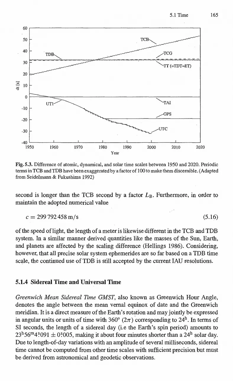
5.1 Time 165
60
50 —
40 —
30 —
20
10-
0
-10 —
-20 —
-30 —
-40 1950
TT (=TDT=ET)
TAI
UTC
1960 1970 1980 1990 2000 2010 2020 Year
TCB
TDB ,v.TCG
Fig. 5.3. Difference of atomic, dynamical, and solar time scales between 1950 and 2020. Periodic terms in TCB and TDB have been exaggerated by a factor of 100 to make them discernible. (Adapted from Seidelmann & Fukushima 1992)
second is longer than the TCB second by a factor LB. Furthermore, in order to maintain the adopted numerical value
c = 299 792 458 m/s (5.16)
of the speed of light, the length of a meter is likewise different in the TCB and TDB system. In a similar manner derived quantities like the masses of the Sun, Earth, and planets are affected by the scaling difference (Hellings 1986). Considering, however, that all precise solar system ephemerides are so far based on a TDB time scale, the continued use of TDB is still accepted by the current TAU resolutions.
5.1.4 Sidereal Time and Universal Time
Greenwich Mean Sidereal Time GMST, also known as Greenwich Hour Angle, denotes the angle between the mean vernal equinox of date and the Greenwich meridian. It is a direct measure of the Earth's rotation and may jointly be expressed in angular units or units of time with 360° (27) 'corresponding to 2411 . In terms of SI seconds, the length of a sidereal day (i.e the Earth's spin period) amounts to 23h56m4091 ± 0O05, making it about four minutes shorter than a 24h solar day. Due to length-of-day variations with an amplitude of several milliseconds, sidereal time cannot be computed from other time scales with sufficient precision but must be derived from astronomical and geodetic observations.

166 5. Time and Reference Systems
BULLETIN B 135 03 May 1999
Contents described in the Explanatory Supplement, mailed with Bulletin B133
1 - EARTH ORIENTATION PARAMETERS (IERS evaluation). The values in this section are samplings of section 2 given at five-day intervals.
Date MJD
UT1R -UTC
UT1R-TAI dPsi dEpsilon 1999
0.001" 0.001" (Oh UTC)
Final Bulletin B values.
MAR 2 51239 MAR 7 51244 MAR 12 51249 MAR 17 51254 MAR 22 51259
MAR 27 51264 APR 1 51269
.06888 .24160 .651265
.06436 .24260 .646766
.05871 .24135 .641753
.05110 .23914 .636039
.04643 .24049 .629993
.03623 .24148 .623165
.02603 .24102 .616594
-31.348735 -31.353234 -31.358247 -31.363961 -31.370007
-31.376835 -31.383407
-45.4 -5.7 -46.6 -5.6 -45.8 -5.9 -44.7 -6.2 -45.3 -6.4
-44.2 -7.0 -44.1 -7.1
Preliminary extension, to be updated weekly in Bulletin A and monthly in Bulletin B.
APR 6 51274 .01733 .23957 .609575 -31.390425
-45.1
-7.2 APR 11 51279 .01051 .24108 .602247 -31.397753 -43.6 -7.0 APR 16 51284 .00731 .24620 .595119 -31.404881 -44.6 -7.4
JUN 10 51339 -.04182 .28130 JUN 15 51344 -.04460 .28498 JUN 20 51349 -.04711 .28882 JUN 25 51354 -.04935 .29281 JUN 30 51359 -.05133 .29693
.519993 -31.480007
.514725 -31.485275
.509953 -31.490048
.505676 -31.494324
.501881 -31.498119
-45.1 -7.3 -46.4
-8.1 -45.4
-7.4 -47.9 -7.4
-47.4 -7.7
Note. In UT1R, the effects of zonal tides with periods shorter than 35 days are removed; UT1-UT1R ( smaller than 0.0025s in absolute value ) should be added after quadratic interpolation of UT1R.Section 2 of this Bulletin gives the daily interpolation of x, y, UT1, duration of day, dPsi, and dEpsilon.
2 - SMOOTHED VALUES OF X, Y, UT1, D, DPSI, DEPSILON (IERS EVALUATION) at one-day intervals. For smoothing characteristics, see Table2 in the explanatory supplement. The reference system is described in the 1997 IERS Annual Report.
1999 MJD (0 h UTC)
UT1-UTC UT1-UT1R D ms ms
dPsi dEpsilon 0.001" 0.001"
MAR 1 51238 .06996 .24157 .652011 -.154 .960 -45.4 -5.7 MAR 2 51239 .06888 .24160 .651078 -.187 .944 -45.4 -5.7 MAR 3 51240 .06806 .24156 .650161 -.277 .930 -45.7 -5.7 MAR 4 51241 .06740 .24173 .649232 -.391 .990 -46.0 -5.7 MAR 5 51242 .06657 .24214 .648193 -.490 1.053 -46.3 -5.6
APR 26 51294 -.00689 .25211 .580721 -.475 1.379 -42.7 -6.9 APR 27 51295 -.00808 .25277 .579283 -.552 1.425 -42.0 -6.8 APR 28 51296 -.00831 .25398 .577792 -.641 1.475 -42.4 -6.8 APR 29 51297 -.00846 .25501 .576290 -.705 1.469 -42.8 -6.8 APR 30 51298 -.00871 .25641 .574839 -.713 1.405 -42.9 -6.9
Fig. 5.4. Sample set of Earth Orientation Parameters as provided by the Bulletin B of the WRS International Earth Rotation Service
5.1 Time 167
Universal Time UT] is the presently adopted realization of a mean solar time scale with the purpose of achieving a constant average length of the solar day of 24 hours. As a result, the length of one second of Universal Time is not constant, because the actual mean length of a day depends on the rotation of the Earth and the apparent motion of the Sun (i.e. the length of the year). Similar to sidereal time, it is not possible to determine Universal Time by a direct conversion from e.g. atomic time, because the rotation of the Earth cannot be predicted accurately. Every change in the Earth's rotation alters the length of the day, and must therefore be taken into account in UT 1. Universal Time is therefore defined as a function of sidereal time, which directly reflects the rotation of the Earth. For any particular day, O h UT1 is defined as the instant at which Greenwich Mean Sidereal Time has the value
GMST(OhUT1) = 24110 54841 8640184 812866 • To + 0 093104 To2 — 0 0000062 To3
(5.17)
(Aoki et al. 1982). In this expression the time argument
JD(OhUT1) — 2451545 To = (5.18)
36525
denotes the number of Julian centuries of Universal Time that have elapsed since 2000 Jan. 1.5 UT1 at the beginning of the day. For an arbitrary time of the day, the expression may be generalized to obtain the relation
GMST = 241105484l
-I- 8640184 812866 To ± 1.002737909350795 UT1
+ 0 093104 T 2 — W0000062 T 3 ,
where the time argument
Jll(UT1) — 2451545 36525
(5.19)
(5.20)
specifies the time in Julian centuries of Universal Time elapsed since 2000 Jan. 1.5 UT1.
The difference between Universal Time and Terrestrial Time or International Atomic Time can only be determined retrospectively. At the end of the 20th century zAT = TT — UT1 amounts to roughly 65s and increases by about 0.5 to 1.0 seconds per year (cf. Fig. 5.3). In addition to the secular variation, which is caused by tidal friction in the Earth-Moon system, UT1 is subject to periodic variations on the 1 ms level that are caused by tidal perturbations of the polar moment of inertia (see McCarthy (1996) and references therein). By convention, zonal tide terms with periods between 5 and 35 days are removed from UT1 to obtain the regularized Universal Time UT1R. Values of the UT1R—TAI time difference are published on a monthly basis in Bulletin B of the International Earth Rotation Service (MRS) (cf. Fig. 5.4), while the adopted expression for UT1-UT1R is given in McCarthy (1996). Aside from reconstructed, post-facto values of the Earth orientation parameters, the
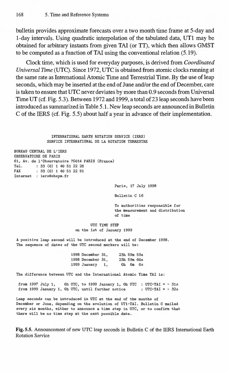
168 5. Time and Reference Systems
bulletin provides approximate forecasts over a two month time frame at 5-day and 1-day intervals. Using quadratic interpolation of the tabulated data, UT1 may be obtained for arbitrary instants from given TAI (or T1"), which then allows GMST to be computed as a function of TAI using the conventional relation (5.19).
Clock time, which is used for everyday purposes, is derived from Coordinated Universal Time (UTC). Since 1972, UTC is obtained from atomic clocks running at the same rate as International Atomic Time and Terrestrial Time. By the use of leap seconds, which may be inserted at the end of June and/or the end of December, care is taken to ensure that UTC never deviates by more than 0.9 seconds from Universal Time UT (cf. Fig. 5.3). Between 1972 and 1999, a total of 23 leap seconds have been introduced as summarized in Table 5.1. New leap seconds are announced in Bulletin C of the 1ERS (cf. Fig. 5.5) about half a year in advance of their implementation.
INTERNATIONAL EARTH ROTATION SERVICE (IERS) SERVICE INTERNATIONAL DE LA ROTATION TERRESTRE
BUREAU CENTRAL DE L'IERS OBSERVATOIRE DE PARIS 61, Av. de l'Observatoire 75014 PARIS (France) Tel. : 33 (0) 1 40 51 22 26 FAX 33 (0) 1 40 51 22 91 Internet : [email protected]
Paris, 17 July 1998
Bulletin C 16
To authorities responsible for the measurement and distribution of time
UTC TIME STEP on the 1st of January 1999
A positive leap second will be introduced at the end of December 1998. The sequence of dates of the UTC second markers will be:
1998 December 31, 23h 59m 59s 1998 December 31, 23h 59m 60s 1999 January 1, Oh Om Os
The difference between UTC and the International Atomic Time TAI is:
from 1997 July 1, Oh UTC, to 1999 January 1, Oh UTC : UTC-TAI = - 31s from 1999 January 1, Oh UTC, until further notice : UTC-TAI = - 32s
Leap seconds can be introduced in UTC at the end of the months of December or June, depending on the evolution of UT1-TAI. Bulletin C mailed every six months, either to announce a time step in UTC, or to confirm that there will be no time step at the next possible date.
Fig. 5.5. Announcement of new UTC leap seconds in Bulletin C of the I E.RS International Earth Rotation Service
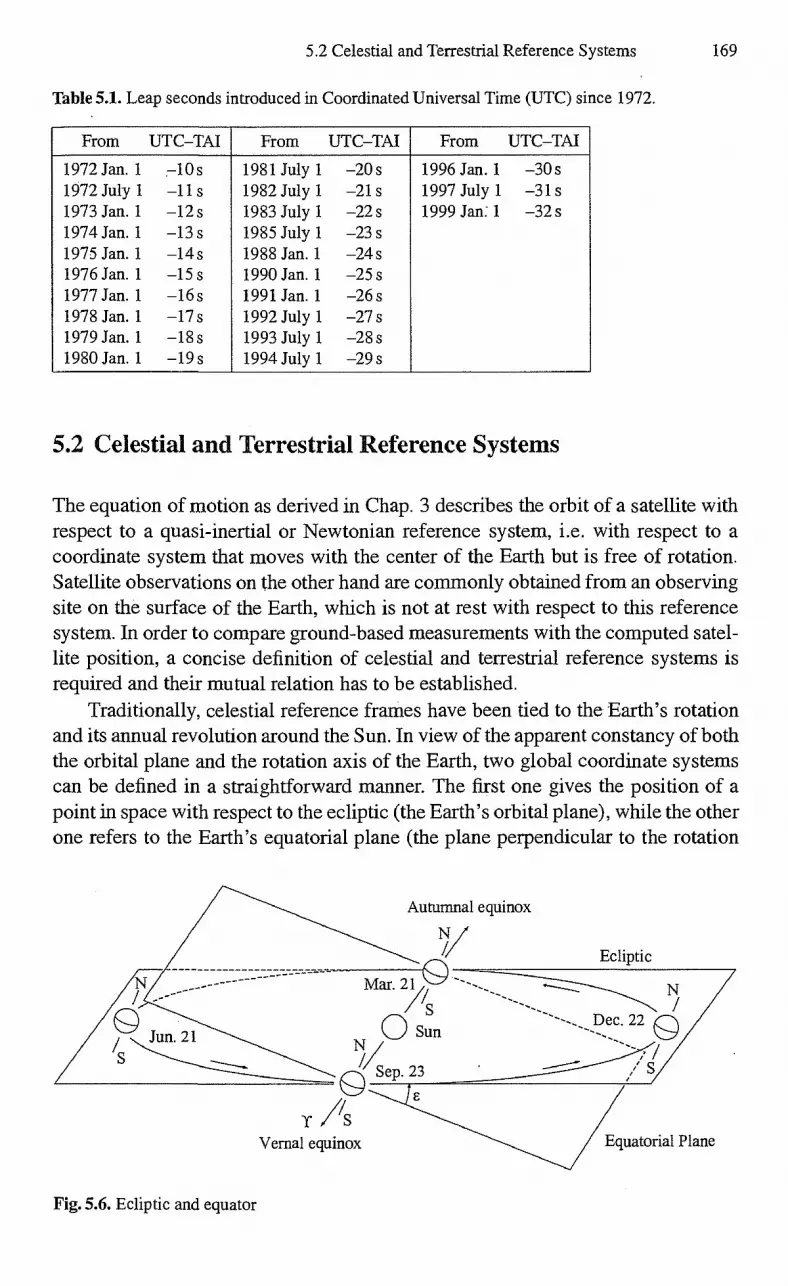
Autumnal equinox 1\111
Mar. 2
Sun Ni1
ol Sep. 23
y S Vernal equinox Equatorial Plane
5.2 Celestial and Terrestrial Reference Systems 169
Table 5.1. Leap seconds introduced in Coordinated Universal Time (UTC) since 1972.
From UTC—TAI From UTC—TAI From UTC—TAI
1972 Jan. 1 —10 s 1981 July 1 —20s 1996 Jan. 1 —30s 1972 July 1 —11 s 1982 July 1 —21 s 1997 July 1 —31s 1973 Jan. 1 —12s 1983 July 1 —22s 1999 Jan: 1 —32s 1974 Jan. 1 —13s 1985 July 1 —23s 1975 Jan. 1 —14s 1988 Jan. 1 —24s 1976 Jan. 1 —15s 1990 Jan. 1 —25s 1977 Jan. 1 —16s 1991 Jan. 1 —26s 1978 Jan. 1 —17s 1992 July 1 —27s 1979 Jan. 1 —18s 1993 July 1 —28s 1980 Jan. 1 —19s 1994 July 1 —29s
5.2 Celestial and Terrestrial Reference Systems
The equation of motion as derived in Chap. 3 describes the orbit of a satellite with respect to a quasi-inertial or Newtonian reference system, i.e. with respect to a coordinate system that moves with the center of the Earth but is free of rotation. Satellite observations on the other hand are commonly obtained from an observing site on the surface of the Earth, which is not at rest with respect to this reference system. In order to compare ground-based measurements with the computed satel-lite position, a concise definition of celestial and terrestrial reference systems is required and their mutual relation has to be established.
Traditionally, celestial reference frames have been tied to the Earth's rotation and its annual revolution around the Sun. In view of the apparent constancy of both the orbital plane and the rotation axis of the Earth, two global coordinate systems can be defined in a straightforward manner. The first one gives the position of a point in space with respect to the ecliptic (the Earth's orbital plane), while the other one refers to the Earth's equatorial plane (the plane perpendicular to the rotation
Fig. 5.6. Ecliptic and equator
170 5. Time and Reference Systems
axis). These planes are inclined at an angle 8 23.5° and the line of intersection is a common axis of both coordinate systems (cf. Fig. 5.6). The x '-axis is defined as being the direction of the vernal equinox or First Point of Aries, designated by T. It is perpendicular to both the North Celestial Pole (the z-axis) and the north pole of the ecliptic (the Z-axis). According to their definition the equatorial coordinates r and the ecliptic coordinates r' of a given point are related by a rotation
= Rx (s)r , (5.21)
where the precise value of the obliquity e is given in (5.42). The choice between ecliptic and equatorial coordinates is mainly a question of vividness and conve-nience. Planetary orbits, for example, are inclined at small angles to the Earth's orbital plane and are therefore commonly described in ecliptic coordinates. Equa-torial coordinates, on the other hand, are closely related to geographical coordinates and provide a natural link to an Earth-fixed reference system.
While the orbital plane of a body around a central mass is fixed in space as long as the attractive force is parallel to the radius vector, this condition does not hold for the Earth due to the presence of other solar system planets. This results in a small secular variation of the orbital plane which is known as planetary precession. At the same time the Earth's axis of rotation is perturbed by the torque exerted on the equatorial bulge by the Sun and Moon. This torque tries to align the equator with the ecliptic and results in a gyroscopic motion of the Earth's rotation axis around the pole of the ecliptic with a period of about 26 000 years. As a result of this lunisolar precession the vernal equinox recedes slowly on the ecliptic, whereas the obliquity of the ecliptic remains essentially constant. In addition to precession some minor periodic perturbations of the Earth's rotation axis may be observed that are known as nutation and reflect variations of the solar and lunar torques on time scales larger than a month. In view of the time-dependent orientation of equator and ecliptic a standard reference frame is usually based on the mean equator, ecliptic, and equinox of some fixed epoch, which is currently selected as the beginning of the year 2000. Access to the Earth Mean Equator and Equinox of J2000 (EME2000) is provided by the FK5 star catalog (Fricke et al. 1988), which provides precise positions and proper motions of some 1 500 stars for the epoch J2000 as referred to the given reference frame
In view of conceptual difficulties related to the dynamical definition of the ecliptic and equinox (see e.g. Kinoshita & Aoki 1983), it was decided by the TAU in 1991 to establish a new International Celestial Reference System (ICRS) 4 and adopt it for use from 1998 onwards (Feissel & Mignard 1998). The origin of the ICRS is defined as the solar-system barycenter within a relativistic framework and its axes are fixed with respect to distant extragalactic radio objects. These are supposed to have no proper motion, thus ensuring that the ICRS exhibits no net rotation. For a smooth transition to the new system, the ICRS axes are chosen in
4 Here, the term Reference System means the set of basic concepts and models used to define at any instant the orientation of the reference axes. A Reference Frame, in contrast, means a specific realization in accordance with the concepts.
5.2 Celestial and Terrestrial Reference Systems 171
such. a way as to be consistent with the previous FK5 system to within the accuracy of the latter. The fundamental plane of the ICRS is closely aligned with the mean Earth equator at J2000 and the origin of right ascension is defined by an adopted right ascension of the quasar 3C273.
The practical realization of the ICRS is designated the International Celestial Reference Frame (ICRF) and is jointly maintained by the I FRS and the TAU Working Group on Reference Frames (cf. Arias et al. 1995). It is mainly based on high-precision observations of extragalactic radio sources using Very Long Baseline Interferometry (VLBI) and may be accessed through a catalog providing source coordinates of 608 objects (cf. McCarthy 1996). Links to existing optical catalogs are provided by radio stars (Seidelmann 1998), while the ICRS and planetary frame tie is provided by VLBI observations of planetary spacecraft as well as lunar laser ranging (LLR) (Folkner et al. 1994, Standish 1998).
Complementary to the ICRS, the International Terrestrial Reference System (ITRS) provides the conceptual definition of an Earth-fixed reference system (Mc-Carthy 1996). Its origin is located at the Earth's center of mass (including oceans and atmosphere) and its unit of length is the SI meter (consistent with the TCG time coordinate). The orientation of the IERS Reference Pole (IRP) and Meridian (IRM) are consistent with the previously adopted BIH system at epoch 1984.0 and the former Conventional International Origin (CIO) (cf. Sect. 5.4.3). The time evo-lution of the ITRS is such that it exhibits no net rotation with respect to the Earth's crust. Realizations of the ITRS are given by the International Terrestrial Refer-ence Frame (ITRF) that provides estimated coordinates and velocities of selected observing stations under authority of the TF,RS. Observational techniques used in their determination include satellite laser ranging (SLR), lunar laser ranging (LLR), Global Positioning System (GPS), and VLBI measurements. New versions of the ITRF are published annually and exhibit global differences at the centimeter level.
The transformation between the International Celestial Reference System and the International Terrestrial Reference System is accomplished by conventional models for
• precession (Lieske et al. 1977), describing the secular change in the orienta-tion of the Earth's rotation axis and the equinox,
• nutation (Seidelmann 1982), describing the periodic and short-tenn variation of the equator and the vernal equinox, and
• Sidereal Time in relation to UT1 (Aoki et al. 1982), describing the Earth's rotation about its axis.
These models are supplemented by the II-RS Earth Observation Parameters (EOP), comprising
• observations of the UT 1-TAT difference and • measured coordinates of the rotation axis relative to the I I-RS Reference Pole
(1ERS 1998). The resulting transfonnation may be expressed as
rims = H(t) (t) N (t) P (t) ricRs (5.22)

172 5. Time and Reference Systems
where the rotation matrices P, N, 0, and IT describe the coordinate changes due to precession, nutation, Earth rotation, and polar motion, respectively. A detailed account of the underlying concepts of these transfoimations and the adopted nu-merical expressions is presented in the subsequent sections.
5.3 Precession and Nutation
5.3.1 Lunisolar Torques and the Motion of the Earth's Rotation Axis
In order to describe the precession of the Earth's rotation axis, the Earth is considered as a rotationally symmetric gyroscope with an angular momentum / that changes with time under the influence of an external torque D according to
dl dt D
Even though the direction of the angular momentum may, in general, differ from the symmetry axis of a gyroscope and the instantaneous axis of rotation, one may neglect these differences in the discussion of precession and nutation and assume that 1 is parallel to the unit vector ez that defines the Earth's axis (cf. Fig. 5.7). Then
= Cakoz (5.24)
where
7.29 10-5 rad/s (5.25)
is the angular velocity of the Earth's rotation and C is the moment of inertia. For a spherical body of homogeneous density with mass Me and radius Re the moment of inertia is given by
2 I = —Me R2 (5.26)
5 8 for an arbitrary axis of rotation. Due to the Earth's flattening and its internal structure the actual moments of inertia are given by slightly differing values
A = 0.329Me R1 and C = 0.330MED R1 (5.27)
for a rotation around an axis in the equatorial plane and a rotation around the polar axis, respectively. It may be noted that these quantities are related to the C20 geopotential coefficient by
C — A = —C20MED R1 . (5.28)
The torque D due to a point mass m (i.e. the Sun or Moon) at a geocentric position r is given by
(5.23)
D = (r x (5.29)

5.3 Precession and Nutation 173
Fig. 5.7. Motion of the Earth's axis under the influence of solar and lunar torques
if designates the acceleration of m by the gravitational force of the Earth. Ne-glecting higher-order zonal teuns in the expansion of the geopotential, r is obtained as
GM ED 3 GMeR 2 C20
[ (5z 2 —r 2)r — 2(zr 2)ez r = r3 2
(5.30)
for a rotationally symmetric Earth (cf. Sect. 3.2), where z =rez is the distance of m from the equatorial plane. All terms of the acceleration that are parallel to the radius vector affect the Earth's center of mass, only, and the resulting torque is given by the simple expression
3z(r x ez) (5.31) D = Gm(C — A) r5
The Sun moves around the Earth in a near-circular orbit that is inclined at an angle E with respect to the equator and the resulting torque vanishes whenever the Sun crosses the equator (z = 0). Introducing the unit vector ex in the direction of the vernal equinox (cf. Fig. 5.7), the torque of the Sun at right angles to the line of

174 5. Time and Reference Systems
nodes is found to be
D0 = GM0 (C — A)3 sin e cos s
ex (5.32) r(3)
irrespective of whether the Sun is above or below the equatorial plane. This results in a mean solar torque
Do = GM0(C — A) 3 sin E cos E
e x (5.33) 2r2)
in the direction of the vernal equinox during the course of a year, whereas the mean component in the direction perpendicular to ex vanishes. Making use of Kepler's third law, the last expression may further be written as
3 Do = —
2 (C — A) sin 6' COS s 71 20 ex (5.34)
where no is the mean motion of the Sun in its orbit around the Earth. Similar considerations hold for the Moon, with the exception that the inclination
of the lunar orbit with respect to Earth's equator is not fixed, but varies between 18° and 28° during a period of about 18 years. Since this period is small compared to the time scale of precession, one may, however, assume that the Moon moves in the ecliptic just like the Sun. This yields a total mean torque of
Mm = -3 (C — A) sin e cos e (n 2 + e 0 x, m (5.35)
2 e which changes neither the Earth's total angular momentum nor the obliquity s but forces 1 to move around the pole of the ecliptic at an angular velocity
3 C — A —
nLMA4/ Me prec — . = cos(E) (5.36)
sin(E)1/1 2 C co0
of one revolution in 26 000 years.
5.3.2 Coordinate Changes due to Precession
The combined effects of precession on the orientation of the ecliptic and the equator are illustrated in Fig. 5.8, where the motion of both planes is described with respect to the mean equator and ecliptic of the reference epoch J2000 (2000 January 1.5).
Due to lunisolar precession the intersection of the mean equator of epoch t and the mean ecliptic of J2000 lags behind the vernal equinox T2000 of J2000 by an angle
5038 1.'8 • T — 1 1.1 1 • T2 (5.37)
that increases almost linearly with time, while the inclination of the mean equator with respect to the ecliptic of J2000 is nearly constant:
= 23°26'21" + 0' /05 • T 2 . (5.38)

5.3 Precession and Nutation 175
Fig. 5.8. The effects of precession on the ecliptic, equator, and vernal equinox
Here
T = (JD — 2451545.0)/36525.0 (5.39)
is measured in Julian centuries Terrestrial Time5 since J2000 TT. While the gravitational pull of the Sun and Moon changes the direction of the
Earth's axis and the equatorial plane, it does not affect the orientation of the ecliptic. Long-term changes of the mean orbit of the Earth around the Sun do, however, arise from the influence of the planets, which results in a corresponding motion of the ecliptic. With respect to the ecliptic of J2000 the ecliptic at another epoch is inclined at an angle of
= 47 1:0029 • T — 0 1:03302 • T 2 + 0 1:000060 - T3 , (5.40)
where the line of intersection is described by the angle
H = 174?876383889 — 869'8089• T 0'03536- T2 (5.41)
These values follow from a theory of the secular changes of the Earth's orbital elements and have been derived by Lieske et al. (1977) following earlier calculations by Newcomb.
5Following a recommendation of the IERS (McCarthy 1996), the expressions for precession and nutation are to be evaluated in terms of Terrestrial Time, instead of Barycentric Dynamical Time.

176 5. Time and Reference Systems
As a result of planetary precession the obliquity of the ecliptic is slightly de-creasing and amounts to
= 23?43929111 — 46/.18150 T — 0/100059 T2 + 01001813 T3 . (5.42)
The combined precession in longitude
p = A — 17 = 5029'.10966 • T 1 1.'11113 - T 2 — 0000006T3 (5.43)
is somewhat smaller, therefore, than the lunisolar precession 1r alone. The orientation of the mean equator and equinox of epoch T with respect to
the equator and equinox of J2000 is defined by the three angles
= 2306 1.'2181 T 0 1.130188 T2 + 0 1./017998 T3
= 2004n109 T — 0 1.'42665 T2 — 0M41833 T3
(5.44)
z = + 0'179280 T 2 + 0/.1000205 T3
that follow from the fundamental quantities 7r, 17, p, and s. According to Fig. 5.8 the transfolination from coordinates ricRF (referred to
the mean equator and equinox of J2000) to coordinates referred to the mean equator and equinox of some other epoch ("mean-of-date") may now be written as
rmod = P rICRF (5.45)
where the matrix P is the product of three consecutive rotations:
P = R(-90 ° — z) R,(0) R z (90° — (5.46)
Evaluating the matrix product, one obtains the following expression for P = (pif):
Pli = — sin z sin + cos Z cos 29' cos
P21 -= + COS Z sin + sin cos 0 cos
P31 = + sin 0 cos
P12 = — sin z cos — cOs cos 0- sin
P22 = + cos Z COS — Sm Z cos 29- sin
P32 = — sin 0 sin
P13 = — COS z sin .0
P23 = — sin sin 0-
P33 = + COS 1.7 .
(5.47)
Since P is a rotation matrix, its inverse P -1 is equal to the transpose PT :
p-1 = pT (5.48)

5.3 Precession and Nutation 177
The precession transfonnation between arbitrary epochs T1 and T2 is thus obtained from
r2 = P (T2) PT (TO r • (5.49)
Here P(T) denotes the rotation from the mean equator and equinox of J2000 to the mean equator and equinox of epoch T.
Alternatively, the generalized expressions
, t) = (+2306'12181 + 1"39656 T — 0'.'000139 T 2) t
+(+0'.'30188 — 0 11000344 T) t 2 0'1017998 t 3
z(T, t) = (+2306'12181 + 139656 T — 0'.'000139 T 2) t
+ (+1 1.'09468 + 0 11000066 T) t 2 011018203 t 3
7,(T, t) = (+2004'13109 — 0'85330 T — 0'1000217 T 2) t
+ (-0 1.42665 — 0 11000217 T) t 2 — 0'1041833 t 3
(Lieske et al.1977, Lieske 1979) with
T = Ti = (JD1(TT) — 2451545.0)/36525.0 t = T2 —T1 = (M2(TT) — iDi(TT))/36525.0
can be used to compute the transfoimation matrix
P(T2, T1) = R( —z(T, t))R y (i(T , t))R z (- - (T, t))
directly from the mean equator and equinox of epoch Ti to the mean equator and equinox of epoch T2.
The 3rd-order polynomials6 for the precession angles given in (5.50) obey the identities
z(T t, —t) = t, —t) = —z(T, (5.53)
0- (T + t, —t) = t) .
Accordingly,
P(Ti, T2) = R( —z(T +t, —0)R y (-1-0(T -Ft, —t))R z (— VT -Ft, —t))
= R z (T , R y (— (T R z (z(T , t)) (5.54)
PT (T2,
yields the rigorous inverse of P (T2, TO . On the other hand, the transitivity relation
P(T3, T1) = P(T3, T2)P(T2, (5.55)
is not maintained exactly by the generalized precession angles. It is therefore better in practical applications of expression (5.50) to avoid the sequential use of preces-sion matrices. Otherwise, errors typically of the order of 10-11 rad, or 10-6", will arise for epochs lying within one century from the reference epoch J2000.
(5.50)
(5.51)
(5.52)
6The coefficient .10 3 782taT is originally given as —0.000345 in Lieske (1977) and has been replaced by the proper value —0.000344 in Lieske (1979).

178 5. Time and Reference Systems
5.3.3 Nutation
Aside from the secular precessional motion the orientation of the Earth's rotation axis is affected by small periodic perturbations that are known as nutation. They are due to the monthly and annual variations of the lunar and solar torque that have been averaged in the treatment of precession. The main contribution to nutation arises from the varying orientation of the lunar orbit with respect to the Earth's equator as expressed by the longitude of the Moon's ascending node Q. It induces a periodic shift
A * —17 /.1200 • sin(Q) (5.56)
of the vernal equinox and a change
As +9 11203 • cos(Q) (5.57)
of the obliquity of the ecliptic during the 18.6-year nodal period of the Moon. As a result the true celestial pole performs an elliptic motion around the mean position as affected by the lunisolar precession.
The currently adopted IAU 1980 nutation series is based on theories of Ki-noshita (1977) and Wahr (1981). It expresses the nutation angles
106
A W =
As
i=1 106
i=1
(AW)i sin(0i)
(A s) i • cos(0i)
(5.58)
by a total of 106 terms, which are summarized in Table 5.2 (Seidelmann 1982). Each term describes a periodic function of the mean elements of the lunar and solar orbit with argument
= P1,il + py,it + PF,iF + p D,i D ps2,i (5.59)
and integer coefficients pF,i, PD,i, and p, . The other parameters are the Moon's mean anomaly (1), the Sun's mean anomaly (1 1), the mean distance of the Moon from the ascending node (F), the difference between the mean longitudes of the Sun and the Moon (D), and the mean longitude of the ascending node of the lunar orbit (Q). Numerical values for use with the IAU 1980 theory of nutation are originally given as
1 = 134°57'46 1.1733 + 477198°52'02 1.1633 T + 31 n10 T 2 + 0''064T3
= 357°31'39 1.'804 + 35999°03'01 /.1224 T — 0 /./577 T 2 — 0 1./012 T 3
F = 93°16'1e877 + 483202°01'03/. 1 137 T — 13"257T2 +0'011 T 3
(5.60)
D =297°51'011.'307 + 445267°06'41/.1 328 T — 6/./891 T 2 + 0/.1019 T3
= 125°02'40 /280 — 1934°08'10 1.1539 T 7/./455 T 2 + 0 1.1008 T3

5.3 Precession and Nutation
179
Table 5.2. The IAU 1980 nutation theory
PI pl, PP pp ps2 AW [0.00011 As [0.00011 i pr pp pp- PD ps2 AW As i
0 0 0 0 1 —171996-1742 T +92025+8.9 T 1 1 0 2 2 2
Il
54 0 0 0 0 • 2 2062 +0.2 T —895+0.5 T 2 1 0 0 0 0 55
—2 0 2 0 1 46 —24 3 2 0 2 —2 2 56 2 0-2 0 0 11 0 4 0 0 0 2 1 57
—20202 —3 1 5 0 0 2 2 1 58 1—i 0-1 0 —3 0 6 1 0 2-2 1 59 0-2 2-2 1 —2 1 7 0 0 0-2 1 60 2 0-2 0 1 1 0 8 1-1 0 0 0 61 0 0 2-2 2 —13187 —1.6 T 5736-3.1 T 9 2 0 2 0 1 62 0 1 0 0 0 1426 —3.4 T 54-0.1 T 10 0 1 0-2 0 63 0 1 2-2 2 —517 +1.2 T 224-0.6 T 11 1 0-2 0 0 64 0-1 2-2 2 217 —0.5 T —95+0.3 T 12 0 0 0 1 0 65 0 0 2-2 1 129 +0.1 T —70 13 1 1 0 0 0 66 2 0 0-2 0 48 1 14 1 0 2 0 0 67 0 0 2-2 0 —22 0 15 1-1 2 0 2 68 0 2 0 0 0 17 —0.1 T 0 16 —1 —1 2 2 2 69 0 1 0 0 1 —15 9 17 —2 0 0 0 1 70 0 2 2-2 2 —16 +0.1 T 7 18 3 0 2 0 2 71 0-1 0 0 1 —12 6 19 0-1 2 2 2 72
—20021 —6 3 20 1 1 2 0 2 73 0-1 2-2 1 —5 3 21 —1 0 2-2 1 74 2 0 0-2 1 4 —2 22 2 0 0 0 1 75 0 1 2-2 1 4 —2 23 1 0 0 0 2 76 1 0 0-1 0 —4 0 24 3 0 0 0 0 77 2 1 0-2 0 1 0 25 0 0 2 1 2 78 0 0-2 2 1 1 0 26 —1 0 0 0 2 79 0 1-2 2 0 —1 0 27 1 0 0-4 0 80 0 1 0 0 2 1 0 28 —2 0 2 2 . 2 81
—10011 1 0 29-1 024 2 82 0 1 2-2 0 —1 0 30 2 0 0-4 0 83 0 0 2 0 2 —2274 —0.2 T 977-0.5 T 31 1 1 2 —2 2 84 1 0 0 0 0 712 +0.1 T —7 32 1022 1 85 0 0 2 0 1 —386 —0.4 T 200 33 —2 0 2 4 2 86 1 0 2 0 2 —301 129-0.1 T 34 —1 0 4 0 2 87 1 0 0-2 0 —158 —1 35 1-1 0-2 0 88
—1 0 2 0 2 123 —53 36 2 0 2-2 1 89 0 0 0 2 0 63 —2 37 2 0 2 2 2 90 1 0 0 0 1 63 +0.1 T —33 38 1 0 0 2 1 91
—1 0 0 0 1 —58 —0.1 T 32 39 0 0 4-2 2 92 —1 0 2 2 2 —59 26 40 3 0 2-2 2 93
1 0 2 0 1 —51 27 41 1 0 2-2 0 94 0 0 2 2 2 —38 16 42 0 1 2 0 1 95 2 0 0 0 0 29 —1 43 —1-1 0 2 1 96 1 0 2-2 2 29 —12 44 0 0-2 0 1 97 2 0 2 0 2 —31 13 45 0 0 2-1 2 98 0 0 2 0 0 26 —1 46 0 1 0 2 0 - 99
—1 0 2 0 1 21 —10 47 1 0 —2 —2 0 100 —1 0 0 2 1 16 —8 48 0-1 2 0 1 101
1 0 0-2 1 —13 7 49 1 1 0-2 1 102 —10221 —10 5 50 1 0 —2 2 0 103
1 1 0 —2 0 —7 0 51 2 0 0 2 0 104 0 1 2 0 2 7 —3 52 0 0 2 4 2 105 0 —1 2 0 2 —7 3 53 0 1 0 1 0 106

True equator Mean equator
Ecliptic
180 5. Time and Reference Systems
Fig. 5.9. The shift in the posi-tions of the equator, the eclip-tic and the vernal equinox, caused by nutation
in Seidelmann (1982), while slightly modified expressions recommended by the I ERS are given in McCarthy (1996).
Following Fig. 5.9, the transformation from mean-of-date coordinates (referred to the mean equator and equinox) to true-of-date coordinates (referred to the true equator and equinox) may be written as
rtod = N(T)r mod, (5.61)
with
N(T) = R(—s— 4s) R(—Aifr) R(s) . (5.62)
The elements of the transformation matrix N = (nu) in equatorial coordinates are given by
cos(W)
Cos (e l) • sin(AW)
sin(e) • sin(A W)
nu =
n21 =
n3i =
nil =
n22 =
n32 =
— cos(e) • sin(AW)
Cos(s) • cos(6 1) • cos(LW) sin(s) • sin(e)
cos(s) • sin(e) • cos(AW) — sin(s) • cos(e)
(5.63)
n = — sin(s) • sin(AW)
n23 = sin(s) cos(e) • cos(W) — cos(s) • sin(e)
n33 = sin(8) • sin(e) - cos(AW) cos(s) cos(e) ,
where e and s' = s+ A6 are the mean and true obliquity of the ecliptic at time T = (JD(TT) — 2451545.0)/36525.
From VLBI and LLR observations, the TAU 1980 theory of nutation is known to be in error on the level of several milli-arcseconds and an improved nutation the-ory (IERS 1996) due to T. Herring has been made available in McCarthy (1996). Nevertheless, the TAU 1980 series is retained as official standard in the I FRS con-ventions and the existing deficiencies are compensated for by observed values of the celestial pole offsets SAip . and SAE. Improved nutation angles are obtained by adding these corrections to the TAU 1980 values:
Alfr = A *IAU1980 SA* As = A 8IAU1980 As •
(5.64)

5.4 Earth Rotation and Polar Motion 181
The corresponding correction to the nutation matrix is obtained from
( +8A-tfr cos s 1 —SAE (5.65)
+8.Alk sins +SAE 1 NuU1980
1 —8.Aik cos s —8.%Aik sin s
(McCarthy 1996). Post-facto determinations and short-term predictions of the ce-lestial pole offsets are published on a monthly basis in Bulletin B of the !FRS (cf. Fig. 5.4).
5.4 Earth Rotation and Polar Motion
5.4.1 Rotation About the Celestial Ephemeris Pole
The IAU precession and nutation theories yield the instantaneous orientation of the Earth's rotation axis, or, more precisely, the orientation of the Celestial Ephemeris Pole (CEP)7 with respect to the International Celestial Reference System. The ro-tation about the CEP axis itself is described by the Greenwich Mean Sidereal Time (GMST) that measures the angle between the mean vernal equinox and the Green-wich Meridian (cf. Sect. 5.1.4). Given the UT1—UTC or UT1—TAI time difference as monitored and published by the I ERS, the Greenwich Mean Sidereal Time at any instant can be computed from the conventional relation (5.19).
Similar to GMST, the Greenwich Apparent Sidereal Time (GAST) measures the hour angle of the true equinox. Both values differ by the nutation in right ascension
GAST — GMST = Li,1r cos E , (5.66)
which is also known as the equation of the equinoxes 8 . Given the apparent sidereal time, the matrix
e (t) = R z (GAST) (5.67)
yields the transformation between the true-of-date coordinate system (as defined by the adopted precession—nutation theory) and a system aligned with the Earth equator and Greenwich meridian.
7The Celestial Ephemeris Pole differs slightly from the instantaneous rotation axis which was used in the earlier nutation theory of Woolard (1953). The adoption of the CEP is related to the fact that the rotation axis performs a predictable daily motion around the CEP under the action of Sun and Moon and is not, therefore, a proper reference pole for theoretical and observational reasons. On the Earth's surface the difference between both poles amounts to approximately 0.6 m. For à. detailed discussion the reader is referred to Seidehnann (1982) Groten (1984), and Capitaine et al. (1985).
81f milliarcsecond accuracy is required in the equation of the equinoxes, two additional terms +0'.'002649 sin S2 — 0'.'000013 cos S2 with S2 denoting the longitude of the Moon's ascending node should be added to the right-hand side of (5.66). These terms represent a second-order correction resulting from a coupling between precession in longitude and nutation in obliquity in a kinematical definition of apparent sidereal time (cf. Capitaine & Gontier 1993, McCarthy 1996).
182 5. Time and Reference Systems
The common z-axis of both systems points to the Celestial Ephemeris Pole, which is not, however, fixed with respect to the surface of the Earth, but performs a periodic motion around its mean position from which it differs by at most 10m. This motion is known as polar motion and can be understood by considering a rotationally symmetric gyroscope, in which the rotation axis moves around the axis of figure in the absence of external torques.
5.4.2 Free Eulerian Precession
In a body-fixed coordinate system (e i, e2, e3) that is aligned with the principal axes of inertia the angular momentum 1' of a symmetric gyroscope is given by
A 0 0 ) 0 A 0 , (5.68)
0 0 C
where co is the instantaneous rotation axis and where A and C are the moments of inertia for a rotation around the el- or e2-axis and the e3-axis, respectively. Without external torques the angular momentum / is constant in an inertial reference system, but since 1' refers to a rotating system it obeys the relation
dl dl' + x = 0 (5.69)
dt dt
Upon insertion this yields Euler's equations
dcoi A + (C — A) co2w3 = 0
dt do2,
A c
(C — A) coico3 = 0 dt
C dc°3
=0 dt
(5.70)
for the motion of co with respect to the body-fixed coordinate system in the special-ized case of a symmetric gyroscope. While the third equation implies a constant component of co around the symmetry axis e3, the solution of the first two equations is given by
W1 = a cos (C — A
A (03t +
(02 = a sin ( C — A A
co3t + (5.71)
The instantaneous rotation vector therefore describes a circle around the e3-axis, where the radius a and phase b are fixed by the initial conditions. The period
27r- A P = (5.72)
£03 C — A
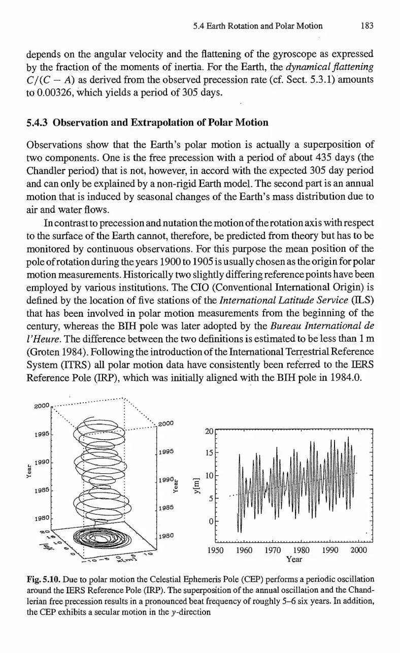
20
0
1950 1960 1970 1980 1990 2000 Year
5.4 Earth Rotation and Polar Motion 183
depends on the angular velocity and the flattening of the gyroscope as expressed by the fraction of the moments of inertia. For the Earth, the dynamical flattening
C l(C — A) as derived from the observed precession rate (cf. Sect. 5.3.1) amounts to 0.00326, which yields a period of 305 days.
5.4.3 Observation and Extrapolation of Polar Motion
Observations show that the Earth's polar motion is actually a superposition of two components. One is the free precession with a period of about 435 days (the Chandler period) that is not, however, in accord with the expected 305 day period and can only be explained by a non-rigid Earth model. The second part is an annual motion that is induced by seasonal changes of the Earth's mass distribution due to air and water flows.
In contrast to precession and nutation the motion of the rotation axis with respect to the surface of the Earth cannot, therefore, be predicted from theory but has to be monitored by continuous observations. For this purpose the mean position of the pole of rotation during the years 1900 to 1905 is usually chosen as the origin for polar motion measurements. Historically two slightly differing reference points have been employed by various institutions. The CIO (Conventional International Origin) is defined by the location of five stations of the International Latitude Service (ILS) that has been involved in polar motion measurements from the beginning of the century, whereas the BIH pole was later adopted by the Bureau International de
l'Heure. The difference between the two definitions is estimated to be less than 1 m (Groten 1984). Following the introduction of the International Terrestrial Reference System (FIRS) all polar motion data have consistently been referred to the 1ERS Reference Pole (TRIP), which was initially aligned with the BIH pole in 1984.0.
Fig. 5.10. Due to polar motion the Celestial Ephemeris Pole (CEP) performs a periodic oscillation around the IERS Reference Pole (IRP). The superposition of the annual oscillation and the Chand-lerian free precession results in a pronounced beat frequency of roughly 5-6 six years. In addition, the CEP exhibits a secular motion in the y-direction

cu 0.8
-a, 0.6 G a)
0.4
r4 0.2
0.0
1.0
300 600
184 5. Time and Reference Systems
Examples of polar motion observations are given in Fig. 5.10 which shows the coordinates xp and yp of the Celestial Ephemeris Pole with respect to the 1ERS Reference Pole as a function of time The x and y-axes are aligned with the !FRS
Reference Meridian (Greenwich meridian) and the 90°-West meridian. A displace-ment of 0 1./ 1 corresponds to 3 m on the surface of the Earth. Since 1900 the mean position of the pole has shifted by about 10 m due to small changes in the Earth's mass distribution (cf. Fig. 5.10). As a result of this motion, which is known as' polar wander, the observed oscillation of the rotation axis is no longer symmetric with respect to the adopted CIO/BIH-pole. The superposition of the annual oscillation and the free precession is evident from the frequency spectrum of polar motion shown in Fig. 5.11. Both contributions are of near-equal magnitude and almost cancel each other with a beat period of 5 to 6 years (cf. Fig. 5.10). Current values of the pole coordinates are published on a monthly basis in Bulletin B (cf. Fig. 5.4) of the International Earth Rotation Service with a resolution of one and five days, respectively. From these data intermediate values for any time may be obtained by quadratic interpolation with sufficient accuracy.
Fig. 5.11. The polar motion fre-quency spectrum for the xp coordi-nate (continuous line) and the yp co-ordinate (dashed line) clearly shows the annual and the Chandlerian pe-riod
Even though polar motion cannot rigorously be predicted, an extrapolation over a certain interval is nevertheless possible from previous data. For this purpose the motion of the pole may be modeled as a superposition of a linear motion (polar wander), an oscillation with a period of 365.25 days (annual term), and an oscillation with a period of 435 days (Chandler term). Appropriate coefficients that provide an extrapolation of tabulated polar motion data with an accuracy of about 0'.'01 over one month are published twice per week in MRS Bulletin A issued jointly by the I ERS and US National Earth Orientation Service (NEOS). Similar predictions are also provided by the US National Imagery and Mapping Agency (NIMA) as part of the GPS precise ephemeris generation process (NIIVIA 1999).
For a prediction over longer time scales a more flexible model has been proposed by Chao (1985). The two components of polar motion are represented by time-
5.5 Geodetic Datums 185
dependent functions
xp = ax bxt cax cos(2211 I Pax + 40ax) ccx cos(2711 Pcx Ocx) (5.73)
yp = ay + by t cay sin(27r tIPay Oay) cc), sin(221- t I Pcy Ocy)
with a total of 16 free parameters ax , . . . , Ocy that are obtained from a least-squares fit to six years of past polar motion data. By allowing for different annual and Chandlerian periods Pa and Pc as well as different phases Oa and (joc in the x- and y-component of polar motion some additional degrees of freedom are introduced in this model that improve the prediction in times of notable period changes (e.g. starting in 1977). Within a one-year prediction interval an accuracy of 0'.'025 can thus be achieved.
5.4.4 Transformation to the International Reference Pole
Based on the previous discussion, the transformation from true-of-date coordinates (as defined by the theory of precession and nutation) to the International Terrestrial Reference System may be expressed as
riTRF = H(t) e (t) rtod • (5.74)
Here 0 (cf. (5.67)) describes the Earth's rotation about the CEP axis, while
/ 1 0 +xp R(-x) R( --yp)
0 1 —yp (5.75) \—xp+yp 1
accounts for polar motion and describes the subsequent transition to the Interna-tional Reference Pole and Meridian. In view of the small angles involved (On 1.5 Arad), second order terms can safely be neglected in the expansion of the trigonometric functions and the linearized form of H is fully adequate for all ap-plications.
5.5 Geodetic Datums
Besides the International Terrestrial Reference System and its annually updated realizations ITRFyy, a variety of other global geodetic datums are in widespread use. Common to all systems is the goal of establishing a global coordinate system that originates at the Earth's center of mass and is closely aligned with the Greenwich meridian and the adopted pole.
The World Geodetic System 1972 (WGS72) and 1984 (WGS84) have been established by the United States Department of Defense (DoD) and the Defence Mapping Agency9 (DMA) for use with the TRANSIT and GPS satellite navigation systems. WG584, in its initial realization, was itself based on reference station
9Now: National Imagery and Mapping Agency (1\111VIA)
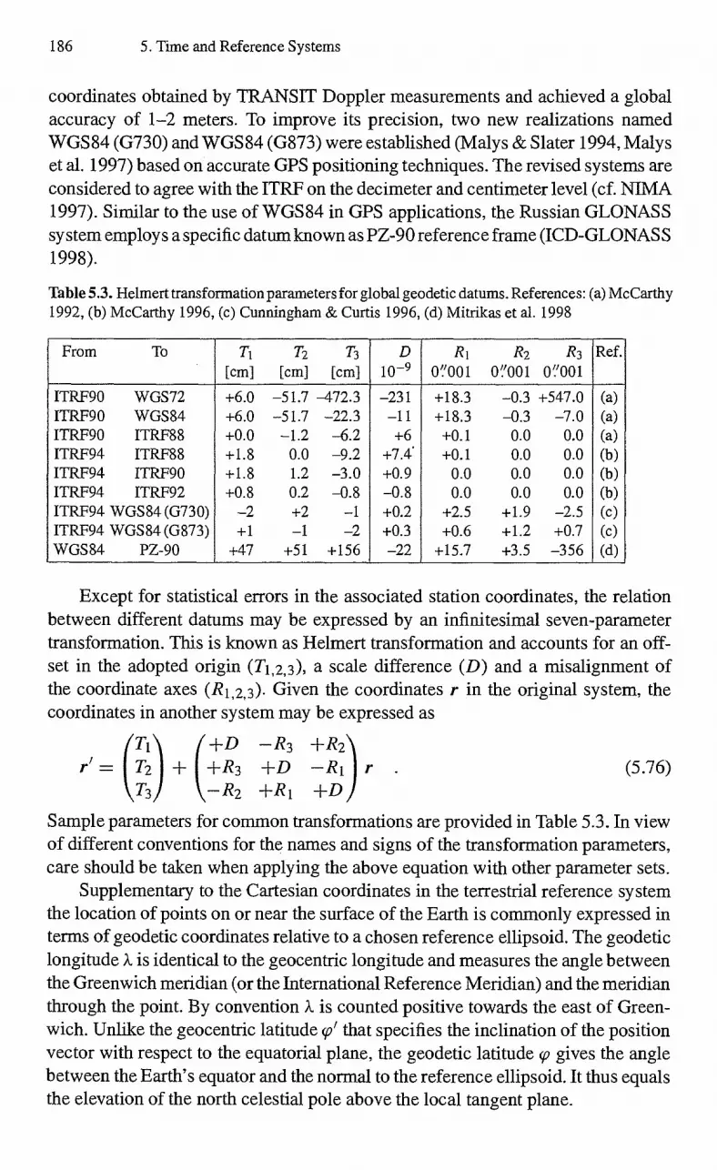
186 5. Time and Reference Systems
coordinates obtained by TRANSIT Doppler measurements and achieved a global accuracy of 1-2 meters. To improve its precision, two new realizations named WGS84 (G730) and WGS84 (G873) were established (Malys & Slater 1994, Malys et al. 1997) based on accurate GPS positioning techniques. The revised systems are considered to agree with the ITRF on the decimeter and centimeter level (cf. NTMA 1997). Similar to the use of WGS84 in GPS applications, the Russian GLONASS system employs a specific datum known as PZ-90 reference frame (ICD-GLONASS 1998).
Table 5.3. Helmert transformation parameters for global geodetic datums References: (a) McCarthy 1992, (b) McCarthy 1996, (c) Cunningham & Curtis 1996, (d) Mitrikas et al. 1998
From To Ti [cm]
T2
[cm] T3
[cm] D
10 -9 R1
0'.'001 R2
0 1.'001 R3
0001 Ref.
ITRF90 WGS72 +6.0 -51.7 -472.3 -231 +18.3 -0.3 +547.0 (a) ITRF90 WGS84 +6.0 -51.7 -22.3 -11 +18.3 -0.3 -7.0 (a) ITRF90 ITRF88 +0.0 -1.2 -6.2 +6 +0.1 0.0 0.0 (a) 1TRF94 ITRF88 +1.8 0.0 -9.2 +7.4. +0.1 0.0 0.0 (b) 1TRF94 ITRF90 +1.8 1.2 -3.0 +0.9 0.0 0.0 0.0 (b) 1TRF94 ITRF92 +0.8 0.2 -0.8 -0.8 0.0 0.0 0.0 (b) 1TRF94 WGS84 (G730) -2 +2 -1 +0.2 +2.5 +1.9 -2.5 (c) 1TRF94 WGS84 (G873) +1 -1 -2 +0.3 +0.6 +1.2 +0.7 (c) WGS 84 PZ-90 +47 +51 +156 -22 +15.7 +3.5 -356 (d)
Except for statistical errors in the associated station coordinates, the relation between different datums may be expressed by an infinitesimal seven-parameter transformation. This is known as Helmert transformation and accounts for an off-set in the adopted origin (T1,2,3), a scale difference (D) and a misalignment of the coordinate axes (R1,2, 3 ). Given the coordinates r in the original system, the coordinates in another system may be expressed as
/7'1\ ■ +D -R3 +R2\ r'= T2 + +R3 +D -R1 r (5.76)
\T3/ \-R2 +RI +DJ Sample parameters for common transformations are provided in Table 5.3. In view of different conventions for the names and signs of the transformation parameters, care should be taken when applying the above equation with other parameter sets.
Supplementary to the Cartesian coordinates in the terrestrial reference system the location of points on or near the surface of the Earth is commonly expressed in terms of geodetic coordinates relative to a chosen reference ellipsoid. The geodetic longitude X is identical to the geocentric longitude and measures the angle between the Greenwich meridian (or the International Reference Meridian) and the meridian through the point. By convention X is counted positive towards the east of Green-wich. Unlike the geocentric latitude yl that specifies the inclination of the position vector with respect to the equatorial plane, the geodetic latitude ço gives the angle between the Earth's equator and the normal to the reference ellipsoid. It thus equals the elevation of the north celestial pole above the local tangent plane.

5.5 Geodetic Datums 187
North pole +z
Fig. 5.12. Geocentric and geodetic latitude
The reference ellipsoid is rotationally symmetric and any plane through the symmetry axis intersects the ellipsoid in an ellipse of flattening f which is defined by the relative difference of the equatorial radius and the polar radius:
f = Re — Rpole (5.77)
Re
All points on the Greenwich meridian therefore obey the relation
Z2
= R2 X 2 +
(1 - D2 e 7
(5.78)
which may also be written in the differenced form as
dz - —dx = —(1 — f )2 X Z •
(5.79)
On the other hand
dz 1 = dx tan q)
according to the definition of q), and by equating both expressions
z = x (1 — f) 2 tan q) .
(5.80)
one obtains
(5.81)
Inserting this relation into the equation of the ellipse and solving for x finally leads to
1 cos ço x = Re , = Re
+ (1—f) 2 tan2 q) 1 f (2— f) sin2 q)
(1 — f) 2 tan ço (1 — f) 2 sin ço z = Re
V , = Re 1 + (1— f) 2 tan2 ço -11 — f (2 — f) sin2 q)
(5.82)

188 5. Time and Reference Systems
This relation between Cartesian and geodetic coordinates may easily be generalized for arbitrary points yielding
I (N h) cos ço cos A.\ r = (N + h) cos q) sin X (5.83)
\ ((1 — f) 2N + h) sin q))
where
N
Re (5.84)
1 f (2 — f) sin2 ço
is an auxiliary quantity that is illustrated in Fig. 5.12 and where h is the height above the reference ellipsoid.
While the computation of Cartesian coordinates from given geodetic coordi-nates is fairly simple, the inverse transformation is slightly more involved. Besides direct methods that involve the solution of a quartic equation (Borkowski 1989, Bowring 1985) there are several iterative methods, which usually converge rapidly. The method described here utilizes the quantity
Az = z — (N + h) sin q) =-- N e2 sin q) (5.85)
where
e = 1 — (1 — f)2 (5.86)
stands for the eccentricity of the reference ellipsoid. Initially Az is set to e2z, which is a good approximation for all points that are reasonably close to the surface of the Earth. Improved values are then calculated from
z + Az sin g) =
ibc2 + y2 ± (z Az)2
Re (5.87)
— e2 sin2
Az = N e2 sin ço ,
until the iteration converges. The geodetic longitude and latitude and the height above the reference ellipsoid may then be calculated from
= arctan ( 2)-)
z + Az ) = arctan
+ y2
(5.88)
h Atx2 + y2 + Az)2 N

5.5 Geodetic Datums 189
Table 5.4. Common reference ellipsoids
Datum Re 1/f Reference
GEM-10B 6378 138 m 298.257 McCarthy 1992 . GEM-T3 6378 137m 298.257 McCarthy 1992 WGS72 6378 135 m 298.26 McCarthy 1992 WGS84 6378 137 m 298.257223563 NIMA 1997 ITRF (GRS-80) 6378 137m 298.257222101 McCarthy 1996, Moritz 1980 PZ-90 6378 136m 298.257839303 ICD-GLONASS 1998
which follows immediately from Fig. 5.12. It is noted that the above relations are singular for points on the z-axis, which is likewise the case for many direct methods (see e.g. Seidelmann 1992).
Since the difference between the Earth's equatorial and polar radii is less than 22 km, the flattening f • 1/298.257 is a very small quantity and the difference between geodetic and geocentric latitudes amounts to twelve arcrninutes at most. To a first approximation
ço = f sin(2V) , (5.89)
which shows that the difference between ço and qi reaches its maximum for inter-mediate latitudes but vanishes at the poles and the equator. Numerical values of the inverse flattening for various datums and reference ellipsoid are presented in Table 5.4.

190
5. Time and Reference Systems
Exercises
Exercise 5.1 (ICRS to ITRS Transformation) Compute the transformation from the International Celestial Reference System (or the mean equator and equinox of J2000) to the International Terrestrial Reference System (or the reference - pole and Greenwich meridian) for the epoch 1999 March 4, Oh UTC.
Hint: Obtain Terrestrial Time (TT) and Universal Time 1 (UT 1) as well as pole coordinates at the time of interest from the respective IERS bulletins (cf. Figs. 5.4 and 5.5). Employ the TAU 1976 precession theory and the IAU 1980 nutation theory to compute the instantaneous orientation of the Celestial Ephemeris Pole (neglecting any corrections to the nutation angles). In computing the Earth rotation transformation account for the conventional relation between UT1 and GMST as well as the first-order teim of the equation of the equinoxes.
Solution: The IERS Bulletins B (No. 135) and C (No. 16) provide the following Earth orientation parameters and derived quantities:
UTC - TAI = -32 TT - UTC = +64184
UT1 - UTC = +0 649232 xP = +0 1.106740
Yp = +0 1.'24713
Using the above assumptions, the following step-by-step transformation matrices for precession (P), nutation (N), Earth rotation (0), and polar motion (17) are obtained:
( +0.99999998 +0.00018581 +0.00008074 \ P -0.00018581 +0.99999998 -0.00000001
- 0.00008074 -0.00000001 +1.00000000 /
( +1.00000000 +0.00004484 +0.00001944 N = -0.00004484 +1.00000000 +0.00003207
- 0.00001944 -0.00003207 +1.00000000
( -0.94730417 +0.32033547 +0.00000000'\ 0 -0.32033547 -0.94730417 +0.00000000
+0.00000000 +0.00000000 +1.00000000 j
( +1.00000000 +0.00000000 +0.00000033 H +0.00000000 +1.00000000 -0.00000117
- 0.00000033 +0.00000117 +1.00000000
Multiplication then yields the matrix
( -0.94737803 +0.32011696 -0.00008431 UM = 110NP= -0.32011696 -0.94737803 -0.00006363
-0.00010024 -0.00003330 +0.99999999
that describes the full ICRS to ITRS transformation.

Exercises 191
Exercise 5.2 (Velocity in the Earth-fixed Frame) The GPS precise ephemerides of the National Imagery and Mapping Agency (NIMA) provide the state vectors of the GPS satellites in an Earth-fixed reference system (presently WGS84 (G873)). This frame is considered as rotating, which implies that the rotation of the axes must be considered in the transformation of the velocity vector, i.e.
rwGs = UWIa (t) rICRS TTICRS
WGS 1 VWGS = Uk,Vra (t ) V ICRS rICRS
dt
Given the state vector
(5.90)
r WGS = ( 19440.953805, 16881.609273, —6777.115092) km
VWGS = ( —0.8111827456, —0.2573799137, —3.0689508125) km/s
of satellite PRN 15 at epoch 1999 March 4, Oh GPS time, compute the position and velocity vector in the International Celestial Reference System (mean equator and equinox of J2000). Check your result by showing that the corresponding orbital elements describe a near-circular orbit with a twelve-hour period (a 26560 km) and an inclination of about 56°.
Hint: The WGS84 (G873) frame is identical to the International Terrestrial Refer-ence Frame within an accuracy of a few centimeters. In computing the derivative of the ICRS to ITRS transfoimation, the precession, nutation and polar motion matrix may be considered as constant, i.e.
dir r icRs (f) " ITRS " H de
N P dt dt
Furthemiore, the time derivative of the Earth rotation matrix is given by
(5.91)
0 +1 0 ( —1 0 0 ) e(t ) 0 0 0
de (t) dt
= COED
where
(5.92)
d (GAST) 27t coe = 1.002737909350795 = 7.2921158553-10 -5 s -1
dt 86400s
(cf. (5.19)) is the Earth's angular velocity. MRS Earth orientation parameters for the date of interest are provided in the previous exercise.
Solution: The GPS—UTC time difference amounts to 13s, which results in the ICRS-ITRS transformation matrix
( U = —0.94707414 —0.32101491 —0.00010024
+0.32101491 —0.94707414 —0.00003330
—0.00008425 —0.00006371 +0.99999999

192 5. Time and Reference Systems
and in its derivative
VICRS
—0.23408779 —0.69061744 +0.69061743 —0.23408779 +0.00000089 —0.00000005
= U T rWGS
= (-23830.593, —9747.074,
= U T VwGs + Û T rWGS
—0.00004561 +0.00006167 +0.00000000
—6779.829) km
• 10 -4/s U = (
Then
rICRS
(+1.561964, —1.754346, —3.068851) km/s
is the state vector in the inertial celestial reference system. The associated osculating orbital elements of the GPS satellite are obtained as
Semiinajor axis a 26561.013 km Eccentricity e 0.0070606 Inclination i 56.338° RA ascend. node Q 12.146° Arg. of perigee w 87.617° Mean anomaly M 109.435°
which matches the specified orbital characteristics of the GPS space segment.
Exercise 5.3 (Geodetic coordinates) The Cartesian coordinates of the NIMA GPS receiver at Diego Garcia are given by
rWGS84(G873) = (+1917032.190, +6029782.349, —801376.113) m
at epoch 1997.0 (Cunningham & Curtis 1996). Compute the corresponding geodetic coordinates using the WGS84 reference ellipsoid.
Solution:
East longitude X = +72.36312094° Latitude ço = —7.26654999° Height h = —63.667m .

6. Satellite Tracking and Observation Models
6.1 Tracking Systems
Orbit determination of an artificial satellite requires as input measurements that are related to the satellite's position or velocity. These data are collected by a satellite tracking system that measures the properties of electromagnetic wave propagation between the transmitter and the receiver. The transmitter as well as the receiver may either be a ground station or a satellite.
6.1.1 Radar Tracking
Since the early times of spaceflight radar techniques have been utilized to gather information on the position and velocity of artificial satellites. Restricting to a simple configuration with one ground station and one satellite:
1. the pointing angles in the topocentric system of the ground station are ob-tained by measuring the direction of the maximum signal amplitude of the spacecraft;
2. the slant range or distance from the satellite to the station is computed from the round-trip light time of a radar signal emitted from the ground station antenna to the satellite and radiated back to the station;
3. the range rate or line-of-sight velocity of the spacecraft relative to the ground station can be derived from the Doppler shift of a radar wave emitted from the ground station, transponded by the satellite, and received again at the ground station.
In many cases range and range rate measurements are two-way measurements with a ground station serving as transmitter and receiver. This is related to the fact that only few satellites are equipped with high-precision time and frequency standards to perform one-way range (high-precision transmit time required) or one-way Doppler (high-precision transmit frequency required) measurements. In case of ground-based two-way measurements the transmit time and frequency as well as the reception time and frequency are determined very accurately using the high-precision ground station equipment. In the sequel a variety of different radar tracking systems and principles is addressed in more detail.

0
-40 -0 06 -0.03 0.00 0.03 0.06
Offset angle [deg]
194 6. Satellite Tracking and Observation Models
Angle Measurements
To determine the direction towards a radio signal emitted by the satellite, the ground antenna has to automatically follow the satellite beacon (autotrack mode). This may be achieved using the conical scan method, where the antenna feed perfonns a slight rotation in such a way that the cone always covers the direction to the satellite. The amplitude modulation of the received signal leads to an error signal that can be used to steer the antenna.
Fig. 6.1. Antenna beams of a monopulse autotrack system (left) and associated sum and difference signals (right)
The monopulse technique derives antenna-angle offsets by the extraction of two signals from the satellite beacon: the difference signal A and the sum signal .E, which are illustrated in Fig. 6.1 (see Hartl 1977). There are two different methods to obtain these signals:
• a feed network attached to the radiator system measures the incident direction of the satellite signals. By differencing and summation of the individual feed outputs the difference and sum signals are derived. This technique is hardware-intensive, since it requires several feed units.
• a single feed such as a corrugated horn is applied. The incoming satellite signal generates low and high-oscillation modes. High modes are excited on the horn aperture by the asymmetry of the received wavefront caused by the antenna pointing error and extracted by a mode coupler. These error signals are similar to signals obtained with differencing techniques.
The sum signal is essentially applied as a reference for the error signal. The ampli-tude of the difference signal is proportional to the amplitude of the antenna-angle offset, while the phase of the difference signal corresponds to the direction of the offset. The error signal together with the sum signal is fed to a tracking unit to provide azimuth and elevation error outputs. The difference signal is, in contrast to the sum signal, extremely sensitive to the antenna angle offset (cf. Fig. 6.1) and may therefore be used to precisely measure the antenna angle offset and to control the antenna motion.

15.0 / 2.2-2.3 / 2.3 GHz
13.8 / 2.0-2.1 / 2.1 GHz
e TDRSS
13.4-14.1 GHz
14.6-15.2 GHz
6.1 Tracking Systems 195
a S-band ranging
b S-band Doppler
c PRARE
d DORIS
Fig. 6.2. Methods of radar range and range rate tracking

Transmitted PN code Transmitted tone
196 6. Satellite Tracking and Observation Models
The angle measurement errors depend essentially on the beamwidth of the ground station antenna. The beamwidth itself depends linearly on the carrier fre-quency of the satellite signal and the inverse of the antenna diameter. For an an-tenna of 15 m diameter the 3 dB beamwidth amounts to 0.6° at 2 000 MHz (S-band). Nevertheless, a resolution of about 50" can be achieved in combination with a monopulse tracking system. At Ku-band (14 000 MHz) an accuracy of 10" (0.05 mrad) may be obtained with an antenna of 10 m diameter that is commonly used for the control of geostationary communications satellites. Depending on the altitude, the position of a spacecraft can be obtained with accuracies between 100 m and 5000 m using typical angle tracking systems.
In general, angle measurements are severely affected by systematic errors that are due to calibration deficiencies, thennoelastic distortions, and wind or snow loads. Within an orbit determination the systematic angle errors may partially be absorbed by the estimation of angle measurement biases, although the error sources lead, in general, to varying angle errors.
Ranging
The classical two-way radar ranging employs a ranging signal that is radiated from the ground station to the satellite. A satellite transponder is required to receive the signal and to transmit it back to the ground station (see Fig. 6.2a). The ground station receives the transponded ranging signal from the satellite and determines the signal travel time r. This is expressed as an equivalent range value p = 1/2-cr, which is equal to the average of the uplink and downlink distance.
Fig. 6.3. Principle of distance measurements using tone ranging (left) and code ranging (right)
There are basically two different techniques to generate ranging signals. Com-mon tone-ranging systems modulate the carrier signal with a sine wave of frequency fo 100 kHz, which is known as major tone. Upon reception, the ranging demod-ulator locks onto the incoming tone and determines its phase with respect to the outgoing tone (Fig. 6.3). The phase shift AO is directly proportional to the turn-around signal travel time
M' = 27rfo
(6.1)
6.1 Tracking Systems 197
and can be measured with a resolution of about (To = 10-2 cyc = 27 .10-2 rad. As a result, the two-way range is obtained with a typical accuracy of ap =10-2c1 (2 fo ) = 15 m. Because the phase shift can only be measured in the interval [0, 27], the range measurements suffer from an indetermination or ambiguity of
2f (6.2)
0
which amounts to 1500 m in the given example. To overcome this difficulty, the ranging signal is supplemented by a series of sub-harmonic minor tones, which are derived from the major tone and coherently modulated on the carrier. A representa-tive sequence of major and minor tones is given by the frequencies fo = 100 kHz, fi = 20 kHz, f2 = 4 kHz, f3 = 800 Hz, fe, = 160 Hz, f5 = 32 Hz, and f6 = 8 Hz (Zarrouati 1987). Here, the turn-around time can uniquely be measured up to a value of 1/8 s as determined by the lowermost minor-tone frequency. This results in an overall range ambiguity of a = c/ (2f6) = 18 750 km that can readily be accepted in practice.
In contrast to harmonic signals, the code-ranging system applies a pseudo-noise (PN) code that is continuously modulated onto the carrier (Fig. 6.3). The PN code consists of a random-like sequence of bits (or chips) that each take a value of zero or one. It is repeated again and again after a predefined number of bits, which is known as code length. Upon reception of the ranging signal the turn-around light time is obtained by correlating the incoming signal with a replica of the uplink code. The ranging accuracy is thus determined by the code rate (or, equivalently, the chip length), whereas the range ambiguity is given by the code length. The advantage of a code-ranging system lies in the simple acquisition of PN signals and the continuous frequency spectrum that allows sharing of the ranging signal with telecommand signals. On the other hand the acquisition time for weak signals is higher than that of tone-ranging systems and the achieved measurement accuracy may be worse, unless a pre-steering Doppler shift is used to reduce the loop bandwidth of the system (Gaudenzi et al. 1990).
PRARE
PRARE (Precise Range and Range Rate Equipment) is a spaceborne tracking sys-tem that provides high-precision two-way range and range rate measurements (Hard . 1984). The PRARE system was developed by the Institut fiir Navigation (INS) of the University of Stuttgart and has been operated since 1995 aboard the European remote sensing satellite ERS-2.
The measurements are based on the signal travel time of an X-band ranging signal transmitted from the satellite, transponded by a PRARE ground-based user station, and received again by the satellite. Here the two-way signal travel time is measured, from which range data are derived (Fig. 6.2c). The Doppler shift of the X-band carrier frequency is, furthermore, measured to derive precise range rate data.

198 6. Satellite Tracking and Observation Models
The space-based PRARE unit has dimensions 40x21x18 cm and a power con-sumption of 30 W in operational mode. Two crossed dipole antennas transmit continuous ranging signals to the ground segment in the S-band (2248 MHz) and X-band (8489 MHz) as well as station-relevant information, such as visibility pre-diction. The ranging signals are pseudo-noise (PN) codes, modulated on the carriers with a rate of 10 MChips/s in X-band and 1 MChip/s in S-band. With a hardware resolution of 1/1000 an effective range resolution of c 10-7s 10-3 3 cm is'given, while the Doppler hardware resolution is 1/1000 of the wavelength within one sec-ond, thus c/ (8.5.109Hz) 10-3 /s 0.04 mm/s. The overall accuracy (r. m. s.) is about 6 cm for range and 0.4 mm/s for range rate at a 1 s integration time (Bedrich et al. 1997). Four independent correlators and four Doppler counters allow a simul-taneous data collection from up to four stations in a code multiplexing mode.
The user-station network currently comprises a worldwide net of about 30 small transportable and automated ground stations, equipped with 60 cm diameter antennas. Since the user stations measure the downlink signal travel time both in S-band and X-band, the ionospheric path delay (TEC) along the signal path may be derived and subsequently corrected within the orbit determination. The received X-band signal is then coherently transposed to 7225 MHz, modulated with the regenerated PN code, and uplinked together with the dual frequency time delay, meteorological data at the ground site and housekeeping data.
The PRARE control segment comprises a command station, a master station, as well as a calibration station. While the command station performs the monitoring of the space system and commanding, the master station serves as central reception station, receiving the measured tracking data, time difference data from the user stations, and meteorological data from the global network. The data are processed, time-tagged to the UTC time scale, archived and disseminated to the users. The calibration station uses a laser tracking system to determine the hardware biases of the PRARE system.
TDRSS
NASA's Tracking and Data Relay Satellite System (TDRSS) is a constellation of six geosynchronous satellites and a ground system which provides tracking and communications support for low-Earth orbiting space vehicles. The first TDRS starting operated in 1983 and since then spacecraft like the Extreme Ultra-Violet Explorer (EUVE), the Compton Gamma Ray Observatory (CGRO), the Earth Radi-ation Budget Satellite (ERBS), Landsat-4, TOPEX/Poseidon, and the Space Shuttle have been tracked by TDRSS.
The space segment consists of geostationary satellites at longitudes of 41° West (TDE), 171° viz. 174° West (TDW) and, to close a gap in coverage over the Indian Ocean (zone of exclusion), 275° West (LUZ) (STDN 1998). Each TDRS can relay voice, television, and digital signals between a ground station and a user satellite. In the altitude regime from 1200 km to 3000 km the primary satellites TDE and TDW are sufficient to ensure continuous communication, while an 85% coverage

6.1 Tracking Systems 199
can be achieved for altitudes of 200 km (STDN 1998). The TDRS provides links to the user spacecraft through two steerable single-access (SA) antennas with 4.9 m diameter in the Ku-band and S-band. In addition a multiple-access (MA) S-band array may receive data from up to 20 satellites simultaneously and transmit to one satellite at a time. The communication to the ground is achieved using a 2 m Ku-band space-to-ground link (SGL) antenna.
The ground segment comprises the White Sands Ground Terminal (WSGT) in New Mexico, operating three 18 m antennas for Ku-band communication and one 6 m S-band antenna, as well as a second TDRSS ground terminal (STGT). The WS GT/STGT performs the tracking, telemetry, and telecorrunand operations for TDRSS and collects the user spacecraft data. Through the NASA ground terminal (GT) the communication with the Network Control Center (NCC) at the Goddard Space Flight Center (GSFC) is established, which manages the space network through system scheduling and TDRSS monitoring.
A TDRS allows relayed two-way range and range rate tracking of user satel-lites and, for user spacecraft equipped with an ultra-stable frequency reference, also precise relayed one-way range rate measurements. In case of two-way mea-surements, the signals are transmitted (14.6-15.25 GHz) (SN 1995) from the White Sands station to the TDRS, where they are coherently forwarded (2.1064 GHz MA, 2.0258-2.1179 GHz SA, 13.775 GHz SA) to the user spacecraft (Fig. 6.2e). The signals are transponded by the user satellite and transmitted (2.2875 GHz MA, 2.200-2.300 GHz SA, 15.0034 GHz SA) back to the TDRS, where they are relayed (13.4-14.05 GHz) to the receiving antenna at White Sands (Long et al. 1989). In the same way as the TDRS tracks a user satellite, each TDRS may also track ground-based TDRSS transponders, which are located at four different sites and are part of the Bilateration Ranging Transponder System (BRTS).
The overall quality of TDRS-relayed range and range rate data is similar to ground-based tracking. In the case of TOPEX/Poseidon the relayed two-way range and range rate residuals show a standard deviation of 2 m and 0.5 mm/s (Marshall et al. 1996). The operational TDRSS orbit determination is based on relayed two-way range data from the BRTS. Due to a limited observation geometry, unmodeled iono-spheric perturbations, and measurement biases, the operational TDRS trajectories are limited to 30-40 m (1u) total position accuracies (Cox & Oza 1994). When '1DRS tracking of TOPEX/Poseidon is applied together with a highly precise a priori ephemeris of TOPEXJPoseidon, the TDRS ephemerides may be determined with a total position accuracy of 1-3 m ( 1 ) (Rowlands et al. 1997).
Doppler Tracking
The Doppler tracking of satellites is based on the frequency shift
fr 1 – vr elc UrIc2 ± v2, I (2 c2 ) — = (6.3) ft 1– v t elc -FUt /c2 v?:1(2c2 )
of radio waves (Soffel 1989), which depends on the relative motion between the transmitter and receiver. Here ft and fr are the transmitted and received signal

200 6. Satellite Tracking and Observation Models
frequencies, v t and V,. are the velocities of the transmitter and the receiver, e is the unit vector in the direction of the signal propagation, and Ut and Ur are the Newtonian potentials at the transmitter and the receiver. The c2-terms in (6.3) result from the general and special theory of relativity.
The frequency shift cannot, however, be measured instantaneously. The Doppler shift is measured instead by counting accumulated cycles of zero-crossings between the received frequency fr and a reference frequency fref over a count time tcf. The measurement is also referred to as integrated Doppler measurement and must be clearly distinguished from the instantaneous Doppler shift.
Table 6.1. Transponder turn-around ratios (CCSDS 1998)
Band fe [MHz] fr [MHz] T1,2
S/S 2025 — 2120 2200 — 2300 240/221 X/X 7145 — 7235 8400 — 8500 880/749 SIX 2025 — 2110 8450 — 8500 900/221 XIS 7190 — 7235 2200 — 2290 240/765
Consider a two-way Doppler measurement, where a radar signal is emitted from a ground station with frequency fe and is received at the satellite with a certain Doppler shift (Fig. 6.2b). To avoid interference of the received and transmitted signals at the satellite, a satellite transponder coherently multiplies the received frequency by the transponder turn-around ratio T1,2 before the transmission to the ground station. Within the transponder a phase locked loop (PLL) assures that the precise fidelity of the received signal is transmitted by the satellite. The transponder ratios are standardized and depend on the frequency bands involved (Table 6.1). The carrier signal is then received at the same ground station (two-way) with about twice the Doppler shift of the uplink or at a separate station (three-way). The Doppler measurement provides the number of accumulated cycle counts
N = f
(fr fref) dt (6.4) t i
in the interval [t1, t2]. Under the assumption of a constant reference frequency over the count interval this can also be expressed as
N = f
t2
frdt — fref(t2 — t1) • t i
(6.5)
The same number of accumulated cycles N is present in the interval [t1 — t1, t2 — T2], where ri and r2 are the signal travel times for signals received at the station at the start ti and end t2 of the count interval. Let T1,2 fe. be the reception frequency for zero Doppler, then
—r2 t2
frdt = T1,2 fedt . (6.6) —ri
t2
6.1 Tracking Systems 201
Assuming a constant transmission frequency over the count-time interval, the num-ber of counts is given by
N = T1,2 feRt2 — --C2) (t1 r1)] fref(t2 ti) • (6.7)
Provided that the reference frequency fi ef at the ground station is set to T1,2 fe the Doppler count may finally be expressed as
N = T1,2fe(ri — r2) • (6.8)
As the two-way Doppler counts themself are abstract measurements, a conversion is usually applied to average range rate measurements according to
1 cN P = (6.9)
2 T1,2 fetc
Here t, = t2 — t1 denotes the duration of the count interval and the negative sign relates a positive Doppler frequency shift (approach) to a negative range rate. The measurement may then be modeled as the difference of the two-way range at the a delta range over the count time
1 cer2 — P2 — P1 p = (6.10) 2 t, t,
Here pi = 1/2c -ci is the two-way range, i.e. one half of the light path of a signal being transmitted at t1 — r1 from the station and received again at the station at time t1. Likewise p2 is the two-way range value for a ground reception time t2.
Existing Doppler tracking systems usually derive the reference frequency from the transmitted carrier frequency. Furthermore, the electronic implementation must assure that the frequency being counted exhibits no zero-crossings. A known fr-requency bias is therefore added to the received signal prior to" subtracting the reference frequency from it. Basically two different realizations of cycle counters are available. The first method counts the number of cycles of the reference fre-quency N required to accumulate a fixed number of cycles of the Doppler-plus-bias cycle counter. The count time t, is not fixed for this measurement technique. The cycle counter is reset after each measurement. Therefore, this method is called a destructive Doppler measurement. The second approach accumulates the Dop-pler-plus-bias count over a pre-defined number of reference frequency cycles, or equivalently, a fixed count time tc . The Doppler-plus-bias counter is not reset after each measurement, therefore this method is referred to as a non-destructive Doppler measurement. As the counter is not reset an accumulated phase variation over time is recorded and the non-destructive Doppler measurement may be referred to as a biased range measurement.
The noise of two-way Doppler data is often expressed by the phase noise av with typical values of 0.1 rad. This may be converted to the range rate noise according to (Segura 1998)
(Tv af3 = (6.11)
27'1,2 fetc
For S-band signals (2 GHz) and a count time of 1 s a representative accuracy of about 1 mm/s is achieved.

202 6. Satellite Tracking and Observation Models
DORIS
DORIS (Doppler Orbitography and Radiopositioning Integrated by Satellite) is a precise Doppler tracking system developed by CNES (Centre National d'Études Spatiales), GRGS (Groupe de Recherche en Géodésie Spatiale), and the IGN (Insti-tut Géographique National). The first DORIS receiver was implemented on SPOT2 in 1990, followed by receivers on TOPEX/Poseidon, SPOT3, SPOT4, and a planned utilization for ENVISAT, Jason, and SPOT5.
DORIS is a one-way Doppler tracking system, where the frequency shift of a radio signal transmitted from a ground beacon is measured onboard the satellite (Fig. 6.2d). To this end, the satellite receiver applies an ultrastable oscillator (USO), i.e. a temperature-controlled crystal oscillator with an Allen variance of 5 -10-13 over the count time of 10 s, which results in a Doppler noise value of 0 3 mm/s for the precision measurements (Laudet et al. 1995). As DORIS is a single-channel, dual-frequency receiver, only signals from one ground station at a time are supported.
The DORIS ground segment comprises about 50 uniformly distributed small ground stations that provide a geographical coverage of better than 80% for the TOPEX/Poseidon mission. Each of the automated ground stations consists of a beacon that transmits two ultrastable frequencies: 2036.25 MHz for precise Doppler tracking and 401.25 MHz for ionospheric Doppler correction. The latter frequency is also used for auxiliary data transmission, such as meteorological data at the ground site that are required for tropospheric corrections.
The DORIS control center is situated at Toulouse, France, where the daily schedule of the beacon contacts is computed. The command transmission and telemetry reception is performed using two master beacons at Toulouse and Kourou. In addition, the master beacon also provides the long-term frequency stability, as it is linked to a cesium atomic clock. To cope with deviations of the ground-based beacons and the satellite USO, biases are solved for each individual pass, and the satellite frequency is thus linked to the frequency of the master beacon. The track-ing data collected at the satellite are stored in the receiver's telemetry memory and dumped twice a day to the ground, where time-tagging, preprocessing, and orbit determination are performed.
6.1.2 Laser Tracking
Satellite laser ranging (SLR) is a technique for precisely measuring the range be-tween a laser station and a satellite that is equipped with retroreflectors. SLR was demonstrated as early as 1964 and since then a continuous extension of laser track-ing networks has been achieved together with a steady improvement of the measure-ment accuracy. Nowadays more than 40 laser stations track satellites like GFZ-1, Lageos I, TOPEX/Poseidon, ERS-2, as well as the GPS-35 and GPS-36 satellites with a precision in the range of one centimeter.
Modern laser transmitters use a solid-state pulsed laser that applies neodymium as a lasing impurity in a lattice of yttrium aluminum garnet (Nd:YAG) (Degnan & Pavlis 1994). This allows the generation of green laser light with a wavelength of

6.1 Tracking Systems 203
532 rim and ultra-short pulses of 30-200 ps width that are repeated at a rate of 5— 10 Hz. When a laser pulse is transmitted by the telescope (Fig. 1.9), a discriminator starts a time interval counter for initialization of a range measurement. The laser pulse then propagates through the atmosphere until it is reflected by a retroreflector array onboard a satellite. When the pulse is received at the telescope, a high-speed photodetector stops the time interval counter with a time granularity of less than 20 ps, equivalent to a one-way range precision of better than 3 mm. The half difference of the counter stop and start time multiplied by the velocity of light hence gives an unambiguous average one-way range. The measurement is time-tagged with an accuracy of better than a microsecond, when a rubidium or cesium atomic clock is applied that is regularly synchronized by a GPS time receiver.
The precision of modern SLR systems is usually given as the root-mean-square of the single-shot accuracy over a single pass and is in the order of 5-50 mm. To further reduce the data scatter, normal points are formed at the laser stations by averaging individual range measurements over a two-minute data interval. This reduces the RMS values by a factor of 4-5 (Husson 1997) and thus leads to a normal point RMS of 1-12 mm. Systematic errors in the station hardware, such as non-linearities in the tracking electronics, lead to biases that limit the absolute SLR accuracy to +1 cm (Marshall et al. 1995).
Due to the high accuracy of SLR data, geodetic applications in the fields of crustal dynamics, gravity field determination, and Earth rotation parameter esti-mation are the major applications of SLR. In addition, the development of precise satellite force models, and the calibration of other tracking devices significantly benefit from SLR (Zhu et al. 1997).
It is noted that laser tracking (other than radar tracking) does not allow auto-tracking of satellites, but depends on the availability of high-precision a priori orbit elements for antenna pointing. Furthermore, the use of SLR for regular tracking is restricted due to its dependence on the weather at the laser stations and to the dense operations schedule of the ground segment.
6.1.3 The Global Positioning System
NAVSTAR GPS (NAVigation System with Time and Ranging Global Positioning System) is a satellite-based radio navigation, positioning, and time-transfer system. It was initiated in 1973 and achieved its full operational capability in 1995. GPS consists of three major segments: the space segment, the control segment, and the user segment.
The GPS space segment comprises 24 satellites deployed in six evenly spaced planes (A to F) with 55 0 inclination, and with four satellites per plane (Fig. 6.4). The GPS satellites move in near-circular orbits with an altitude of about 20 200 km and a period of 12 sidereal hours. The space segment provides a global and continuous coverage with at least four simultaneously visible satellites. A ground-based user will observe the same satellite constellation once per day but four minutes earlier each day due to the difference between the sidereal and solar day.

204 6. Satellite Tracking and Observation Models
Fig. 6.4. GPS Space Segment Constellation
The GPS control segment consists of five monitor stations, a master control sta-tion, and three ground control stations. The unmanned monitor stations are located at Colorado Springs, Hawaii, Kwajalein, Diego Garcia, and Ascension Island. They are equipped with a GPS receiver and a cesium atomic clock to perform continuous one-way pseudorange measurements to all GPS satellites in view as well as weather data measurements for tropospheric corrections. The coordinating master control station at the Schriever Air Force Base, Colorado Springs, Colorado, is responsible for the GPS satellite control and system operations. It collects the tracking data from the monitor stations and computes the satellite ephemerides and clock parameters that are transferred to the ground control stations for daily command upload. The ground control stations operate in the S-band and are collocated with the monitor stations at Ascension, Diego Garcia, and Kwajalein.
GPS provides two levels of service to the user segment. A Standard Positioning Service (SPS) provides position and timing information to any user on a contin-uous worldwide basis. The Precise Positioning Service (PPS) provides position, velocity, and timing information to authorized U.S. and allied military, federal gov-ernment, and civil users who can satisfy specific U.S. requirements. The specified 50th percentile SPS and PPS accuracies are compiled in Table 6.2, and are based on instantaneous GPS measurement sets for the computation of the position and velocity in the presence of typical random and systematic errors.
The GPS satellites transmit microwave carrier signals at the Li frequency (1575.42 MHz) and the L2 frequency (1227.60 MHz). The second frequency allows

6.1 Tracking Systems 205
Table 6.2. SPS and PPS 50th percentile accuracies for instantaneous measurements (NRC 1995)
Specification SPS PPS
Position horizontal 40m 8 m vertical 47m 9m spherical 76m 16m
Velocity any axis - 0.07 in/s
Time GPS 95 ns 17 ns UTC 115ns 68ns
measurement of the ionospheric signal delay using PPS-capable receivers. Three binary codes are modulated on the Li or L2 carrier or both:
1. The Coarse Acquisition (C/A) code is a short pseudorandom noise (PRN) code of 1023 bits or 1 ms duration at a 1.023 Mbps bit rate (Spilker 1978). The C/A code modulates the Li carrier and is the basis for the civil SPS. Since each satellite has a specific and different C/A code PRN, GPS satellites may uniquely be identified by their PRN number.
2. The Precise (P) code is a PRN code with about 6-10 12 bits, equivalent to a period of exactly one week and a bit rate of 10.23 Mbps. The P code modulates both the Li and L2 carrier phases and is the basis for the military PPS. When the Anti-Spoofing (AS) mode is active, the P code is encrypted into the Y code and requires a classified AS module with cryptographic keys.
3. The navigation data are transmitted in a 50 bit/s stream, added to the C/A and P(Y) codes on the Li frequency and, depending on the satellite mode, also on the L2 P(Y) code. Each message word consists of 30 bits with 10 words in one subframe. Each frame consists of 5 subframes and a superframe consists of 25 frames. Thus the navigation message comprises 37 500 bits and is re-peated every 12.5 minutes (Spilker 1994). The navigation message contains low-accuracy (almanac parameters) and high-accuracy (broadcast ephemeris) GPS satellite orbit data as well as clock corrections, and other system param-eters (see Annex A.2).
An overview of the GPS signal characteristics is given in Table 6.3, where the frequency and wavelength for the PRN-codes refers to their chip length.
Table 6.3. GPS satellite signal characteristics (Spilker 1978)
Signal Type f Frequency [MHz] Wavelength [cm]
Satellite Clock fo 10.23 2931 Carrier Signal Li 154 fo 1575.42 19.05
L2 120 fo 1227.60 24.45 PRN-Codes P fo 10.23 2931
C/A 0.1 fo 1.023 29310

206 6. Satellite Tracking and Observation Models
The GPS-based positioning relies essentially on the measurement of biased one-way range data, called pseudoranges (Fig. 6.2f). To perform pseudorange mea-surements, the GPS receiver produces replicas of the C/A or P(Y) code for a specific GPS satellite and shifts the code in time until the cross-correlation of the satellite and the receiver codes achieves a maximum. The measured code phase 0 (4.) cor-responds to a reception time t,. at the receiver clock while the signal transmission time t, is provided via the PRN code. Hence the difference of the transmission and reception time readings multiplied by the velocity of light c yields a range value of
PO (tr) = C(tr tt) . (6.12)
This is actually called apseudorange (Hofmann-Wellenhof et al. 1997) since tr and t, are obtained by different clocks. Denoting GPS system time by a superscript GPS and offsets of the receiver and transmitter clocks from GPS time by the symbols Str and 84 the pseudorange is obtained as
po r) = c ((trGPS +80 _ (ttGPs +80)
(6.13)
Using 4 tGPS = trGPS tGPS and 8 t = 8.r _ r 84 it can be seen that the pseudorange
1)0(0 = C (LO )S 8t) (6.14)
is larger than the actual signal path by a distance c8t, which depends on the relative offset of the two clocks. Since the individual clock errors exhibit independent variations with time, the difference between the pseudorange and the actual range is also a time-varying quantity.
Due to the C/A code length of about 1 ms the C/A code pseudoranges are ambiguous at about 300 km, while the P(Y) code pseudoranges are unambiguous. As the code phases are determined with a typical accuracy of 0.1 rad (lo- ) or about 0.01591 cycles, the noise figures for code phases are 0.01591 - 293 m 5 m for C/A code pseudoranges and 0.5 m for P code pseudoranges.
Highly precise GPS carrier phase measurements or phase pseudoranges apply the carrier phase instead of the code phase 0 and thus require no information modulated on the carrier. Here the phase of the GPS satellite signal received by the user at GPS system time t is given as
Or(t) = ft (t — \t0P5) ft8tt (6.15)
where ft is the emitted frequency and ft At GPs denotes the phase retardation due to the signal propagation from the transmitter to the receiver. At the receiver a reference signal with phase
ref (t) = fref t fref 8 tr (6.16)
is generated using the receivers reference frequency fref. . The phase difference
(t) ref (t) = N AO (6.17)

6.1 Tracking Systems 207
which is also called the beat phase, may then be expressed by an integer number of cycles N and the actual measurement value AO, known as the instantaneous fractional beat phase. Provided that the reference frequency equals the transmitted frequency, insertion of (6.15) and (6.16) into equation (6.17) gives, the observation equation
po(t) = cAt GPs ± AN c8t (6.18)
where po = — X,A0 is the range equivalent of the measured phase difference. The integer number of carrier cycles N is unknown, hence carrier phase measurements are ambiguous with one wavelength A of about 20 cm. During a continuous signal lock of a GPS satellite by the receiver, the integer ambiguity N remains constant for that satellite. The ambiguity resolution may be achieved with different techniques (Hofmann-Wellenhof et al. 1997). It has, however, to be kept in mind that ambiguity resolution may require a high computational effort or may even fail under certain conditions. When the signal lock is lost, the integer ambiguity after re-establishing the lock is changed, which is known as cycle slip. Considering that carrier phases are determined with an accuracy of at least 0.1 rad or about 0.01591 cycles, the noise figures for carrier phases are less than 3 mm and 4 mm for L2 and Li signals, respectively.
GPS users with moderate or low-positioning requirements may directly apply the receiver's navigation solution or position fixes, i.e. the receiver coordinates (x, y, z) in the Earth-centered, Earth-fixed reference frame WGS-84. Position fixes are not raw GPS measurements, but are derived from code pseudoranges that may have been smoothed by carrier phases within the receiver for data noise reduction. The derivation of position fixes is based on the geometric method of triangulation, where three range measurements to three locations of known position uniquely determine the receiver's coordinates. For GPS applications, pseudoranges to at least four GPS satellites simultaneously have to be available to determine, in addition to the position, the receiver's instantaneous clock offset with respect to GPS system time.
As the inherent SPS performance leads to a positioning accuracy of about 10 m (Parkinson 1994), an intentional degradation has been implemented, called Selec-tive Availability (SA). SA consists of a manipulation of the navigation message orbit data (c process) as well as the intentional degradation of the satellite clock frequency (8 process), also known as clock dither. The clock dither leads to oscil-lations in the C/A code and P code pseudoranges of 23 m (la) with a period of 2-5 min (van Graas & Braasch 1994), while the c process leads to a slow varia-tion of the satellite positions with an amplitude of 50-150 m (Hofmann-Wellenhof et al. 1997) and a period of the order of hours. As a result, the achievable SPS position accuracy in the presence of SA amounts to roughly 100 meters and only authorized users are able to correct for these errors. In support of commercial GPS applications SA has been deactivated, however, on 1 May 2000 by decision of the US government. Since then every user of a single-frequency GPS receiver is able to achieve a position accuracy of 10 m.

208 6. Satellite Tracking and Observation Models
The GPS makes use of two dedicated representations of the GPS satellite or-bits, which are known as almanac and (broadcast) ephemeris (see Annex A.2). Both parameter sets are transmitted as part of the GPS navigation message and enable a user receiver to compute positions of the GPS satellites with different levels of accuracy. Almanac data are mainly used to determine the constellation of visible satellites above the horizon, to select the best satellites for navigation and to de-termine approximate Doppler shifts for improved signal acquisition. The receiver has to demodulate the entire navigation data superframe within 12.5 minutes to completely retrieve all almanac data. The almanac accuracy is about 900 m within a one-day interval from the transmission of the almanac and degrades to 1200 m and 3600 m respectively within a one-week and two-week interval (Spilker 1994). Almanac updates are performed at least once in six days. The ephemeris parame-ters, on the other hand, provide a much more accurate description of the spacecraft trajectory that is essential for the computation of precise user position fixes. The broadcast ephemerides are accurate to 5-10 m in the absence of SA and 5-100 m (Hofmann-Wellenhof et al. 1997) if SA is active. Broadcast ephemeris updates are performed approximately every hour and are valid through a period of four hours. In accordance with the envisaged usage, the low-accuracy almanac parameters are always provided for the full constellation of active satellites, whereas each satellite only transmits ephemeris parameters for itself.
In addition to the raw GPS measurement types, a variety of combinations of raw measurement types can be applied to facilitate the data analysis. These derived measurement types are, in general, constructed by computing the difference of raw GPS measurements referring to the same measurement epoch. Taking single carrier phase differences that involve two receivers and a single GPS satellite, it can e.g. be shown that the satellite clock error cancels. Likewise, double carrier phase differences are computed from single carrier phase differences to two GPS satellites. Both GPS satellite and user clock errors are cancelled for this data type. Vice-versa, the combination of raw measurement types allows the isolation of specific error contributions. As an example, multipath effects that are caused by reflecting surfaces in the vicinity of the GPS antenna can be evaluated by forming the difference of ionosphere-corrected code and carrier pseudoranges.
6.2 Tracking Data Models
6.2.1 Transmitter and Receiver Motion
Satellite tracking methods involve the propagation of a signal over a finite time span. The signal originates from a transmitter at a certain time t and is recorded at the receiver at a later time t r > t. Thus, a rigorous observation model has to account for the motion of the transmitter and the receiver during the signal travel time r .
The signal travel time r ranges from 5 ms for low-Earth orbiting (LEO) satellites up to 100 ms for geostationary satellites (GEO). Thus, the computation of the

6.2 Tracking Data Models 209
satellite position at the time of signal transmission r (t — r) can be performed either by an interpolation of adjacent position values or by a Taylor expansion
1 f, (6.19)
2
where r and Y are the inertial satellite velocity and acceleration, respectively. With a satellite velocity of 3 km/s for GEO's and 7 5 km/s for LEO's the linear term in (6.19) is about 400m for GEO's and 100 m for LEO's, while the second-order term is about 2 mm. When using numerical integration methods for the trajectory prediction the satellite position at signal transmission may be obtained from interpolation of subsequent integration steps. Preferrably, however, an integration method should be used that directly supports dense output generation (cf. Chap. 4).
The motion of a ground station in an inertial reference system is dominated by the Earth rotation with a velocity of 460 m/s at the equator. When the motion of the ground station is modeled in the inertial International Celestial Reference System (ICRS, see Sect. 5.2), the position RITRS of the station in the International Terrestrial Reference System (ITRS) has to be transformed using the matrices for precession (P), nutation (N), Earth rotation (0) and polar motion (II) according to
RicRs = PT (t) (t) eT(t) fir(t) RITRS • (6.20)
In addition, the precise computation of the ground station position requires mod-eling site displacements due to tidal perturbations and plate motion. Due to the differential lunisolar acceleration, the solid Earth tides cause a maximum radial site displacement of 25 mm with a daily period. Horizontal displacements are less than one millimeter, and are in general neglected. The ocean tides deform the Earth's crust and hence each ground station undergoes a displacement that reaches a few centimeters near the coast and less than one centimeter for continental stations (Mc-Carthy 1996). The pole tides are caused by the contribution of the polar motion in the centrifugal potential due to the Earth rotation. They lead to a tidal response with a maximum radial displacement of 25 mm and a maximum horizontal displacement of 7 mm (McCarthy 1996). Similar amplitudes are found for atmospheric loading, i.e. temporal variations in the geographic distribution of atmospheric masses that deform the Earth's surface (Manabe et al. 1991). For geodetic applications, the relative motion of stations on different tectonic plates with rates of 5 cm per year or larger may be accounted for using a plate motion model (DeMets et al. 1994).
6.2.2 Angle Measurements
Light Time and Aberration
Angle measurements are modeled using the vector d = r — R from the ground station to the satellite. Due to the finite velocity of light, the geometric relative

position do = r(t) — R(t) at the time t of signal reception is different, however, from the true signal path. This is given by the vector
d = r (t —r) — R(t) (6.21)
that links the ground station position R(t) at the reception time to the satellite position r (t —r) at the transmission time (cf. Fig. 6.5). The signal travel time r may thus be computed from the implicit light-time equation
cr = Ir(t —r) — R(t) (6.22)
Starting from an initial value of r (°) = 0 the light time is consecutively determined using the fixed-paint iteration
= vc Ir(t —r (i) ) — R(t)I (6.23)
The iteration may be continued until successive values of r agree to better than a certain threshold, such as 10-7 s for general data types. Given a light time of 0.01 s for a low-Earth orbiting satellite, the light-time correction for angle measurements is in the order of 7 1' . Here, the correction refers to the difference between the true signal path (d) and the geometric relative position (do).
Fig. 6.5. The motion of the satellite during sig- Fig. 6.6. The effect of aberration nal travel time for the downlink
The solution of the light-time equation yields the true signal path in the inertial system which is different, however, from the apparent direction to the spacecraft for a moving ground station. This effect is known as aberration and may be under-stood by considering the relative motion of the incoming signal and the observer (Fig. 6.6). Neglecting a rigorous formulation within the theory of special relativity, the observed direction is given by the vector
d' = d , (6.24)
where V is the inertial velocity of the ground station relative to the geocenter. Thus the apparent position
d' =d+TV=r (t --r) — R(t) TV (t) r (t -r) — R(t — r) (6.25)
matches the geometric position at time t — r to first order. The aberration is about 0.6" for low-Earth satellites and 0.3" for geostationary satellites. It can be neglected in most cases in view of the limited resolution of common radar tracking systems.

6.2 Tracking Data Models 211
Local Tangential Coordinates
For a station with geodetic coordinates (X, cp, h) the three unit vectors
(— sin X) — sin ço cos X cos ço cos X eE = 4- cos X eN = — sin go sin X ez = cos sin X (6.26)
0 cos y) sin 'p
that point to the east, north, and zenith direction provide a natural and convenient frame for describing a satellite's motion with respect to an antenna (cf. Fig. 6.7). According to their definition, eE and eN span the tangential plane to the reference ellipsoid, while ez points to the geodetic zenith. Aside from small deviations of the geoid from the adopted reference ellipsoid, the tangential coordinate system is aligned with the horizon and the zenith as defined by the local direction of the plumb line.
North
Fig. 6.7. Orientation of local horizontal co-ordinate systems South
The satellite coordinates in the local tangential coordinate system may be ob-tained by projecting the station-satellite vector ref — R ef in the Earth-fixed system onto the axes eE, eN, and ez:
sE S = sN)
( = E (ref — Ref) (6.27-)
sz
Here
— sin X ± cos X 0 E =
eETT) ( — sin cos X — sin sin X q) 4- cos g) (6.28)
ezT ± cos yo cos X ± cos cio sin X ± sin
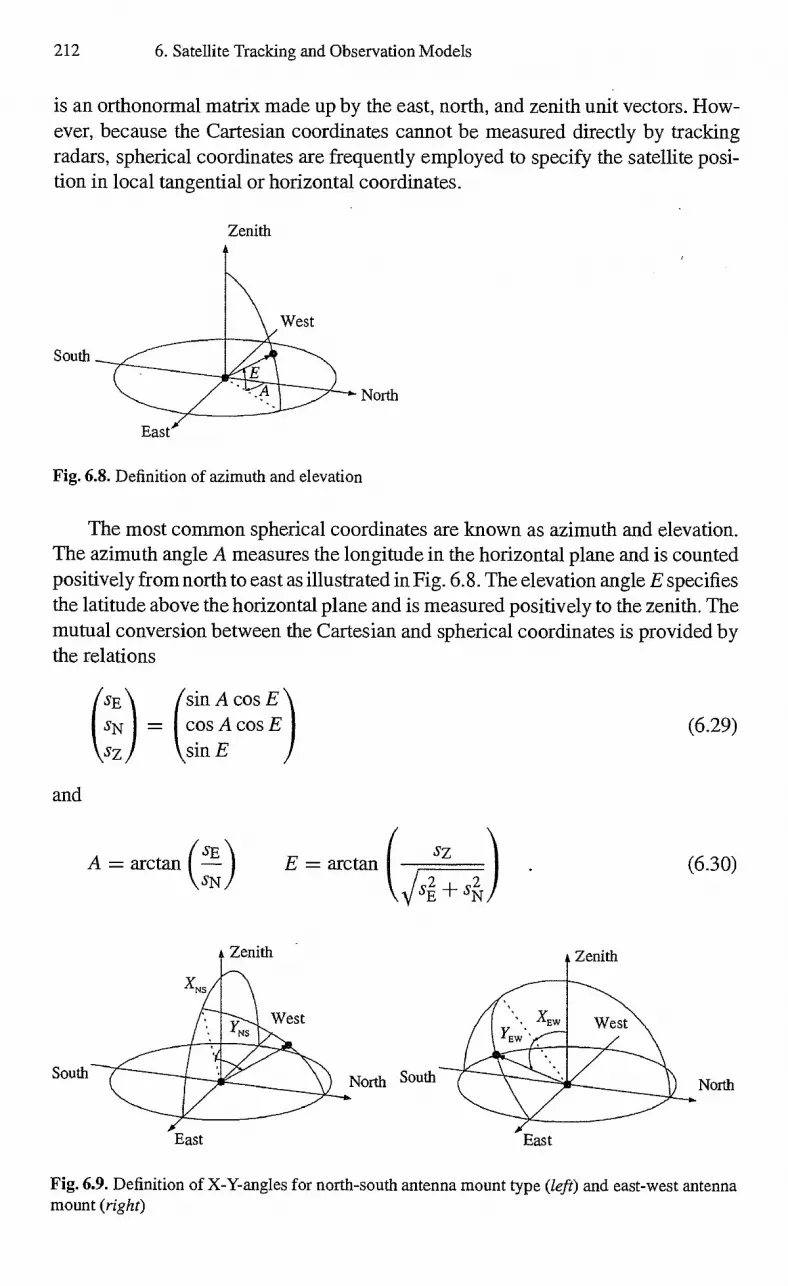
212 6. Satellite Tracking and Observation Models
is an orthonoimal matrix made up by the east, north, and zenith unit vectors. How-ever, because the Cartesian coordinates cannot be measured directly by tracking radars, spherical coordinates are frequently employed to specify the satellite posi-tion in local tangential or horizontal coordinates.
Zenith
South
North
Fig. 6.8. Definition of azimuth and elevation
The most common spherical coordinates are known as azimuth and elevation. The azimuth angle A measures the longitude in the horizontal plane and is counted positively from north to east as illustrated in Fig. 6.8. The elevation angle E specifies the latitude above the horizontal plane and is measured positively to the zenith. The mutual conversion between the Cartesian and spherical coordinates is provided by the relations
and
(SE (sin A cos E)
SN cos A cos E
sz sin E (6.29)
A = arctan — ( sE sN
E = arctan
SZ (6.30)
ii/ C.2 ,2
South North
East East
Fig. 6.9. Definition of X-Y-angles for north-south antenna mount type (left) and east-west antenna mount (right)

and
XNs = arctan (— SE ) Sz
YNS = arctan (6.31)
6.2 Tracking Data Models 213
Alternatively X-Y-angles are sometimes used that differ from azimuth and elevation by the choice of a reference plane at right angles to the horizon (cf. Fig. 6.9):
Both X- and Y-angles are less than 90° (7/2) by magnitude for all points above the horizon.
XEW = arctan —sSzN
YEW = arctan SE )
(.1sA -I- si (6.32)
6.23 Range Measurements
Round-trip Light Time
Two-way radar and laser ranging comprises the signal uplink from the ground station to the satellite and the downlink from the satellite to the ground station. When a two-way range measurements has been recorded at the ground station at time t, the signal has been received and transmitted back by the satellite at t — rd, where rd is the downlink light travel time. The transmission time of the signal at the ground station is thus given by t td tu, where ru is the uplink light travel time.
Therefore, the modeling of range measurements requires the iterative solutions of two light-time equations for the downlink and the uplink path (cf. Fig. 6.10). The algorithm for the downlink light-time computation was described in (6.22) and (6.23) as part of the angle measurement modeling. For the uplink the light time is given by the implicit equation
Cru I r (t — rd) — R (t — rd I
(6.33)
A fixed-point iteration for the uplink with
= 1/c • ir (t — td) — R (t — d — (6.34)
is perfouned until successive values of ru agree to better than a certain threshold, e.g. 10-7 s. It requires one iteration step less than for the downlink, since an initial value of riP) = rd can be applied. In addition, the light-time correction to the uplink is a factor of about 20-30 smaller than for the downlink, due to the ratio of the inertial ground station velocity and the inertial velocity of the satellite.
The two-way range measurement p is then modeled from the average of the uplink and downlink range pu and pd, according to
1 1 P = i(Pu Pd) = —
2c (ru TO • (6.35)
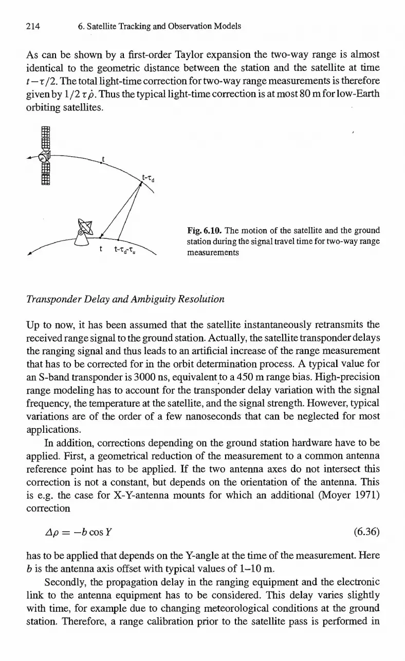
214 6. Satellite Tracking and Observation Models
As can be shown by a first-order Taylor expansion the two-way range is almost identical to the geometric distance between the station and the satellite at time t —r /2. The total light-time correction for two-way range measurements is therefore given by 1/2 r /5. Thus the typical light-time correction is at most 80 m for low-Earth orbiting satellites.
Fig. 6.10. The motion of the satellite and the ground station during the signal travel time for two-way range measurements
Transponder Delay and Ambiguity Resolution
Up to now, it has been assumed that the satellite instantaneously retransmits the received range signal to the ground station. Actually, the satellite transponder delays the ranging signal and thus leads to an artificial increase of the range measurement that has to be corrected for in the orbit determination process. A typical value for an S-band transponder is 3000 ns, equivalent to a 450 m range bias. High-precision range modeling has to account for the transponder delay variation with the signal frequency, the temperature at the satellite, and the signal strength. However, typical variations are of the order of a few nanoseconds that can be neglected for most applications.
In addition, corrections depending on the ground station hardware have to be applied. First, a geometrical reduction of the measurement to a common antenna reference point has to be applied. If the two antenna axes do not intersect this correction is not a constant, but depends on the orientation of the antenna. This is e.g. the case for X-Y-antenna mounts for which an additional (Moyer 1971) correction
zip = —b cos Y (6.36)
has to be applied that depends on the Y-angle at the time of the measurement. Here b is the antenna axis offset with typical values of 1-10 m.
Secondly, the propagation delay in the ranging equipment and the electronic link to the antenna equipment has to be considered. This delay varies slightly with time, for example due to changing meteorological conditions at the ground station. Therefore, a range calibration prior to the satellite pass is performed in
6.2 Tracking Data Models 215
a so-called closed-loop configuration. Typical range calibration values are in the order of several thousand nanoseconds.
Depending on the ranging method, the collected range value is ambiguous by a certain value a. For a tone ranging system with a lowest frequency of 8 Hz the respective one-way ambiguity is 18 750 km. Other ranging systems may even provide range data with a varying ambiguity. The ambiguity resolution requires a priori knowledge of the satellite position to compute the expected range p with an accuracy of better than the ambiguity value. The integer ambiguity n is then computed from minimizing the expression lp — nat.
Since the satellite reception and transmission antennas are not located at the center of mass of the satellite, a corresponding correction has to be applied for high-precision range modeling. An adequate knowledge of the instantaneous attitude is necessary to compute the inertial antenna location with respect to the satellite's center of mass.
Multiple Ranging Links
The principle of two-way ranging may be generalized to arbitrary links with space-borne as well as ground-based transmitters and receivers. An example is the four-way ranging of the geostationary satellite Meteosat, where ranging signals are broadcast from the Primary Ground Station (PGS) at Fucino, Italy, to the satel-lite. The satellite retransmits the signals to a land-based transponder (LBT), an unattended ground station near Kourou, French Guiana, that transponds the signals via the satellite back to the PGS for reception and range measurement recording (EUMETS AT 1999) .
Another example is described in Chap. 6.1 and illustrated in Fig. 6.2, where TDRS four-way ranging measurements are initiated by sending a ranging signal to one of the geostationary relay satellites. From here it is forwarded to the user spacecraft, retransmitted and linked back to the ground station after passing the relay satellite a second time
In each particular ranging configuration the light-time equations for the indi-vidual signal paths is formulated and solved along the principles described before. The case of TDRS four-way ranging is furthermore addressed in (9.23).
6.2.4 Doppler Measurements
Two -Way Range Rate
Two-way Doppler measurements are obtained from the integration of Doppler counts over a count-time interval tc . The measured range rate may be modeled as the difference of the two-way ranges at the end and at the beginning of the count-time interval. Thus a total of four light-time iterations is required for the modeling

tc tc
, (r2 — r1) (P2 — Pi) p = c (6.38)
216 6. Satellite Tracking and Observation Models
of a single average range rate measurement (cf. Fig. 6.11). When the Doppler mea-surement time tag t refers to the end of the count interval t2, the associated carrier signal was transponded by the satellite at t2 — r2u and transmitted by the ground station at time t2 — r2u — r2d . Similarly, the signal at count interval start ti = t2 — tc
was transponded at the satellite at time ti — ri u and broadcast from the ground station at time ti — t1u rid. Thus the average range rate measurement may be modeled as
C ( t2u r2d) (Tlu ± rid)=
1. (P2u + P2d) — (Plu + Pid) , (6.37) p(t) = 2 2 tc tc
where the pi = Cti denote the individual one-way ranges involved. For three-way Doppler measurements, where the signal is transmitted from a ground station, transponded by the satellite, and received at a different ground station, the model is accordingly applicable.
Fig. 6.11. The motion of the satellite and the ground station during signal travel time for two-way Doppler measurements
One - Way Range Rate
The model for one-way Doppler measurements is easily derived from the two-way range rate model. Here the carrier signal is transmitted from the ground to the satellite (DORIS) or from satellite to the ground. Considering a measurement with time tag t that refers to the end of the count interval t2, the signal transmission time is t2 — r2. The beginning of the count interval is then ti = t2 — t, and the associated transmission time is ti — ri. Hence, the one-way range rate model is
It is noted that in contrast to two-way Doppler measurements, one-way Doppler measurements require precise frequency standards both at the transmitter and at the receiver. Nonetheless, the frequency difference of the transmitter and the receiver should be estimated as part of the orbit determination.

6.2 Tracking Data Models 217
Rotational Doppler Bias
A spinning spacecraft exhibits a modulation of the two-way Doppler shift due to the rotational motion of the spacecraft antenna onto the direction vector from the satellite to the ground station. Following Kallemeyn & Vaughan (1996) the average range rate during the count interval is changed by
- 1 =
—J t
d • co sin a sin(cot)dt . (6.39) tc t--tc
Here d is the distance of the spin axis to the electric antenna center, co is the satellite's angular velocity, and a is the angle between the spin axis and the direction to the ground station. In addition to the periodic Doppler modulation, a rotational Doppler bias is also present for circular polarized signals. To understand the principle of this bias, a satellite antenna is considered which rotates in a right-hand sense about the positive z-axis of the antenna zenith. As the antenna emits a right-hand circular polarized wave along the positive z-axis the transmission frequency is increased by the spin rate of the antenna. If the antenna emits a left-hand circular polarized signal along the positive z-axis, the transmitted frequency is decreased by the spin rate of the satellite. Spinning satellites cause such frequency shifts both at the reception and at the transmission of the signal. According to Marini (1970) this frequency shift introduces a bias
_ Act) SR ± ST/ T1,2 A 16 = (6.40)
27r 2 to the range rate measurements, where 2k. is the signal wavelength, T1,2 is the transponder turn-around ratio and SR and ST denote the signs of the frequency shift on reception and transmission, respectively. Considering a satellite spinning at two revolutions per second and a satellite antenna with the same polarization for transmission and reception (i.e. ST = sR), the rotational Doppler bias is 28 cm/s in the S-b and.
6.2.5 GPS Measurements
Pseudoranges
Following (6.13), pseudoranges may be modeled as
Po = (rd4-3tr —6 4)
(6.41)
Here rd is the signal travel time from the GPS satellite to the user satellite, which is obtained from the iterative solution of the light-time equation.
The offset 8tr (t) of the user satellite clock from GPS system time is commonly estimated within the orbit determination program based on a second-order Taylor expansion
1.. Str (to ± At) Str (to) + 3.t r (to) At — St r (to) Lit
2 (6.42)
218 6. Satellite Tracking and Observation Models
around a reference epoch to, where the receiver clock bias 3tr(t0), the clock drift r , and the clock drift rate cii r are included in the estimated parameter set.
The offset 64(0 of the GPS satellite clock from GPS system time may be derived from the transmitted broadcast ephemeris parameters according to
34(0 = apo afi(t — tc) af2(t — 0 2
(6.43)
where tc denotes the satellite clock reference epoch and afo, a fi, and af2 are the clock bias, frequency bias, and frequency drift, respectively.
In addition to the dependency of the signal travel time and the GPS and user clock errors, the pseudorange measurement is affected by ionospheric perturbations, multipath effects, the offset of the GPS antenna phase center from the satellite center of mass, as well as the Selective Availability (SA).
Integrated Carrier Phases
According to (6.18) the integrated carrier phase measurement may be modeled as
pi, = ctd-1- XN atr — att (6.44)
To resolve the integer ambiguity N, different techniques may be applied, as dis-cussed in Hofmann-Wellenhof et al. (1997).
A rigorous formulation of the measurement process has to account for the general theory of relativity, which implies that two clocks at different altitudes (a transmitter at geocentric distance rt and a receiver at geocentric distance rr ) run at different rates in the gravity field of the Earth. As a consequence, the relativistic light travel time r is given as (Gibson 1983)
3GM ( 1 1)
c
2 2 td —r r V r — rtvt (6.45)
2c2 rt.
where rr , v r , and rt , v t are the position and velocity vectors of the receiver and transmitter. The term in brackets is constant for circular orbits and introduces a time bias, while the velocity-dependent terms are linearly dependent on the eccentricity and vary with the sine of the eccentric anomaly. It is noted that the time-varying relativistic effects of the GPS satellite have already been mapped to the broadcast parameters arc), api, and af2 at a level of better than 9 ns within a one-hour interval (van Dierendonck et al. 1978). Therefore, a precise treatment of the relativistic GPS effects based on (6.45) requires the removal of the relativistic contributions from
ap, and af2 making use of the equations given in van Dierendonck et al. (1978).
Integrated carrier phase measurements are affected by ionospheric perturba-tions and Selective Availability (SA). Multipath effects are much smaller than for pseudoranges, since the carrier wavelength is smaller than the code wavelength.
6.3 Media Corrections 219
Navigation Solution
The navigation solutions (x, y, z) provided by the GPS receiver are not mea-surements in a rigorous sense, since they are actually derived from raw pseudor-ange measurements. Nevertheless, navigation solutions may in practice be applied as pseudo-measurements for satellite orbit determination (Carter et al. 1995, Gill 1997). The need for processing navigation solutions within an orbit determination software, instead of using the solutions itself, may arise for various reasons. Most notably the use of a dynamic model allows the smoothing of SA-effects, the detec-tion of outliers, and the bridging of gaps without GPS measurements. Furthermore a dynamic filtering of the position solution can be used to obtain reliable velocity infoimation. This is important, because the receiver-provided velocity solutions exhibit typical errors of 1 m's, which prevents their use in orbit predictions. An inherent advantage of using navigation solutions instead of pseudoranges is their simple measurement modeling. As the user satellite orbit may be integrated in a mean-of-date reference system, the measurement modeling just requires the trans-formation from the mean-of-date system to the WGS84 coordinate system, where the navigation solution vector is given by
r\yQ = ri N rmod • (6.46)
Thus, any knowledge of the GPS satellite ephemerides is avoided as well as the need for light-time iterations. This renders the use of navigation solutions especially interesting for spacebome applications.
6.3 Media Corrections
6.3.1 Interaction of Radiation and Atmosphere
Electromagnetic signals that are transmitted from a spacecraft traverse the Earth's atmosphere before they are received by a ground station. As the signals propa-gate, the electromagnetic radiation interacts with the electrons, ions, atoms, and molecules constituting the Earth's plasma environment and atmosphere to a var-ious extent. As a consequence, the signals undergo a change of direction, known as refractive bending, and a change of the velocity of propagation. In addition, the atmosphere affects the signal polarization and field strength.
The velocity of propagation and the wavelength of electromagnetic waves de-pend on the refractive index n of the surrounding medium. Given the vacuum wavelength X and speed of light c, the corresponding values X, and c, in a medium of refractive index n are related by the expression
X n = — = —
Cn X n (6.47)
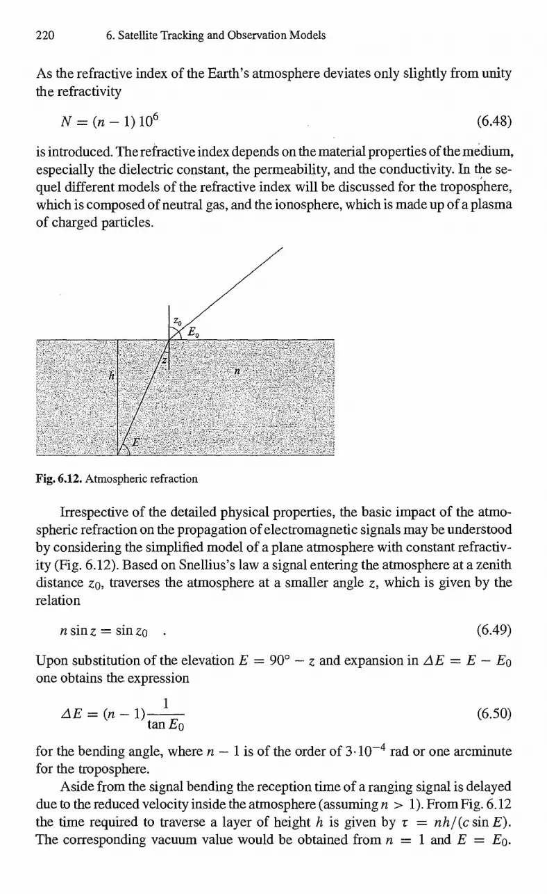
220 6. Satellite Tracking and Observation Models
As the refractive index of the Earth's atmosphere deviates only slightly from unity the refractivity
N = (n — 1)10 6 (6.48)
is introduced. The refractive index depends on the material properties of the medium, especially the dielectric constant, the peimeability, and the conductivity. In the se-quel different models of the refractive index will be discussed for the troposphere, which is composed of neutral gas, and the ionosphere, which is made up of a plasma of charged particles.
Fig. 6.12. Atmospheric refraction
Irrespective of the detailed physical properties, the basic impact of the atmo-spheric refraction on the propagation of electromagnetic signals may be understood by considering the simplified model of a plane atmosphere with constant refractiv-ity (Fig. 6.12). Based on Snellius's law a signal entering the atmosphere at a zenith distance zo, traverses the atmosphere at a smaller angle z, which is given by the relation
n sin z = sin zo . (6.49)
Upon substitution of the elevation E = 90° — z and expansion in ZAE = E — Eo one obtains the expression
tan Eo
for the bending angle, where n — 1 is of the order of 3-10-4 rad or one arcminute for the troposphere.
Aside from the signal bending the reception time of a ranging signal is delayed due to the reduced velocity inside the atmosphere (assuming n > 1). From Fig. 6.12 the time required to traverse a layer of height h is given by t = nhl (c sin E). The corresponding vacuum value would be obtained from n = 1 and E = Eo.
1 ZAE = (n 1) (6.50)
6.3 Media Corrections 221
Neglecting the small bending angle, the difference between the two values may be expressed as a range difference
Ap 1
h(n —1) (6.51) sin E0
The measured range value is thus larger than the one that would be obtained in the absence of an atmosphere.
For the modeling of ionospheric refraction it is necessary to distinguish between the refractive index ni- of a single electromagnetic wave (e.g. the carrier phase) and the refractive index ng, of wave groups (e.g. ranging signals). This is due to the fact that the refractive index depends on the frequency f of the respective waves in a dispersive medium like a plasma of charged particples. For a signal composed of different harmonic frequencies the resulting wave group propagates at the group velocity cg, = cing, where
d n ph
df
is the group refractive index. The resulting group velocity is always smaller than the vacuum speed of light c. In contrast to this the phase velocity cph = c2 /cgr is larger than c for dispersive media. For non-dispersive media like the troposphere both refractive indices are equal as are the group and phase velocity c, = c In < c.
6.3.2 Tropospheric Refraction
The troposphere, composed almost totally of neutral gas, is the lower atmosphere extending-from sea surface level to approximately 42 km. The extension of the different troposphere layers depends essentially on the temperature and the ver-tical temperature gradient. The troposphere is a non-dispersive medium for radio waves, hence the refractive index does not depend on the radiation frequency. The propagation of electromagnetic waves through the troposphere is mainly affected by the temperature T, the atmospheric pressure p, and the partial pressure of water vapor e. An empirical expression for radio frequencies below 300 GHz relates these parameters to the dry component
=77.624V p[hPa]/ TM] (6.53)
and the wet component
12.92 e[hPa]
N2 = 371900 e[hPa]
(6.54)
(T[K]) 2 T[K]
of the refractivity N = N1+ N2 (Goad & Goodman 1974). Since the tropospheric refractivity is positive, the tropospheric refractive index is always greater than one. Following GroBkopf (1970) the partial pressure of water vapor, which is required
ngr = nph+ f (6.52)

222 6. Satellite Tracking and Observation Models
in the above equations, can be expressed as a function of the relative humidity of the air fh (0 < fh < 1) and the temperature Tc:
( 17.15 e[hPa] = 6.10 fh exp
Tcrq (6.55)
The above expression for the radio refractive index is accurate to better than 1%. At sea surface level the refractivity for radio waves is about 320-380, whereas it is 282 for optical frequencies (A = 0.69 ,um) and standard atmospheric conditions (Jeske 1988). The tropospheric refractivity decreases with increasing altitude and approaches zero at the upper tropospheric boundary.
As shown above, the tropospheric refraction is composed of the refraction due to dry air and a contribution due to water vapor, which is denoted as wet term. Dry air contributions are dominant and can be modeled reasonably well. The contribution from water vapor amounts to about 10% and can be modeled only poorly due to the high temporal, horizontal, and altitude variations. In principle, two different approaches can be adopted to determine the wet troposphere refraction
• Modeling of the wet refraction contribution The water vapor contributions may be modeled using theoretical considera-tions and observation data obtained from radio probes launched with sound-ing rockets. However, as continuous observation data are not available, the models have a limited validity and, moreover, imply a considerable expense and effort.
• Measurement of the water vapor
Water-vapor measurements may be collected either from an infrared hydro- meter or a water-vapor radiometer. Both techniques suffer from technical problems of calibrating the amount of wet water due to clouds or rain. Fur- thermore, considerable expenses are implied in the case of the radiometer.
A variety of refraction correction models for spacecraft tracking data has been established in the past, ranging from simple exponential formulas to sophisticated and numerically expensive algorithms that account for the light-path curvature in the atmosphere by applying ray-tracing methods. In Table 6.4 the refraction corrections for radar range and elevation data are given, as derived from the elaborate Hopfield-Goad model for representative meteorological conditions.
Table 6.4. Tropospheric refraction for p = 938 hPa, T = 286 K, and fi, = 0.73
E(°) 1 3 5 7 10 15 20 30 40 50 70 90
AE(") 1358 836 589 449 328 222 166 106 73 52 23 0 Ap(m) 58 34 23 17 13 9 7 5 4 3 2 2
As shown above a simple model for the tropospheric refraction of radar range and elevation measurements is given by
1 Z1E = N 10_6
tan E [rad] (6.56)

6.3 Media Corrections 223
and
Ap = N 10 -6 h 1 (6.57) sin E
where h denotes the effective scale height of the troposphere. The scale height is about 7.5 km at sea level and may be computed from the Hopfield two-quartic model
1 1 N2 h = -hd - - — (hd - hw) 5 5 N
(6.58)
(Hopfield 1969). Here the first term denotes the contribution from dry air and the second term gives the wet contributions. The top of the dry troposphere may be computed from hd = 148.98(T - 4.12) m (Black 1978), while the top of the wet troposphere is h w = 12 km.
The above model yields an error of less than 10% for elevations above 5°. This renders the model attractive for many applications, in particular if no meteorological parameters are available that justify the use of more elaborate models. It should be noted, however, that errors up to 100% may arise at elevations of 1 0 .
A general and accurate tropospheric refraction model is the Hopfield model, modified by Goad to use, the Saastamoinen zenith range correction (Goad & Good-man 1974). It is applicable both to radar data as well as to optical observations. In the Hopfield model, the dry troposphere height hl is determined from
5.0 0.002277 h1[m]
P {hPal
h2 is given
- 1255 0.05
by
e[hPa] .
(6.59)
(6.60)
Ni • 10-6
while the wet troposphere height
, 5.0 0.002277 h2[In-1 N2 • 10-6
+ _T [IC]
The tropospheric range correction for the Hopfield model is given by a ninth-order polynomial
Ap = (6.61)
where the constant
170.2649 F78.88281 [173.3 + 1/X' 2 1 - L173.3 - 1/X'2 [ 77.624 j L173.3 - 1/X'2
is approximately one for radio frequencies. The dimensionless signal wavelength = X/(1,um) and thus the term 1/X'2 can be set to zero for radio frequencies. The
distance to the top of the dry (j = 1) and wet (j = 2) troposphere is
r1 = (Re + 111)2 - (Re cos E)2 - Re sin E . (6.63)

224 6. Satellite Tracking and Observation Models
The coefficients of the polynomial are defined as = 1
a2 j = 4c/1
a31 = 64c/ 4h1 J
a4j = 4a1 (s4 3121)
a51 = a4: 122b 6b J
a61 = 4a i b + 3h1)
a71 = (62 + 4h1) J J
a81 = 4a •b3. J
a91 = b4.
with
b = 2h i R ee
The tropospheric correction of average range rate data is obtained from the correc-tion of range data (Schmid & Lynn 1978). Hence, the range rate correction depends on the elevation angle as well as the elevation rate.
The tropospheric correction of the elevation angles according to the Hopfield model is
—sin E a =
hJ
—cOS2 E
N • f3i •r i.+1 J
106 1/1 i=i (/ + 1) i=l
.AE = C E 4 cos E
where the constant CE [ 170.2649 [ 78.8828-
CE = (6.65) 173.3 — 1/M2 _ L 77.624
is approximately one for radio frequencies and p is the range to the satellite. The elevation correction coefficients are computed from
= 1 = 3a1
2 = 3(ai bi) 2 = ai(ai +6bi)
= 3b i(a+ bi)
= 3a 1 b
= b3. .
For optical frequencies the above equations can be applied as well, when only the dry temi is considered (N2 = 0). The azimuth measurements are not affected by refraction.
181j
182j
183j
I84j
I85j
I86j
,87j
(6.64)

F region E region
active Sun, day —
active Sun, nigh
quiet Sun, day ' - - .................. 7
quiet Sun, night _
102 —
10 1
107
106
0
0
10
6.3 Media Corrections 225
6.3.3 Ionospheric Refraction
From about 50 km up to a height of 1000 km the ionosphere plays the major role for propagating electromagnetic waves. The abundance of ions and free electrons, resulting primarily from the absorption of solar ultraviolet radiation, is the cause of the ionospheric refraction. Due to small mass ratio of the electron and ion mass, free electrons play a more important role than ions. The electron density at 50 km altitude is about 108 electrons/m 3 and increases with height due to the increasing intensity of the solar radiation. A maximum electron density of 10 12 electrons/m 3 near sunspot maxima can be found at about 300 km, decreasing towards higher altitudes due to the decreasing atmospheric density. Both photochemistry and transport processes contribute to the structure of the ionosphere, which is shown in Fig. 6.13. The electron density profile primarily depends on the altitude, the sunspot activity as well as day and night variations. Several regions can be identified that are designated as D region (60-90 km), E region (105-160 km) and F region (160-1000 km). More detailed models distinguish further the Fl region (160-180 km) and the F2 region (200-1000 km). The D and Fl regions vanish at night, while the E region becomes considerably weaker and the F2 region shows a reduced marking.
80 100 120 150 200 300 500 750 1000 1500 2000 Height [km]
Fig. 6.13. Electron density profiles at mid-latitudes based on the International Reference Ionosphere ERI 1995 (Bilitza et al. 1993, 1995)
It is extremely difficult to construct global ionospheric models that accurately predict the electron density. Neglecting the perturbations due to ions, the contribu-tion of the Earth's magnetic field, and absorption effects, the ionospheric refractive indices are (Jeske 1988)
fl ph = f 2
and gr 2 f 2 (6.66)
Ele
ctro
n de
nsity
[cm
-31
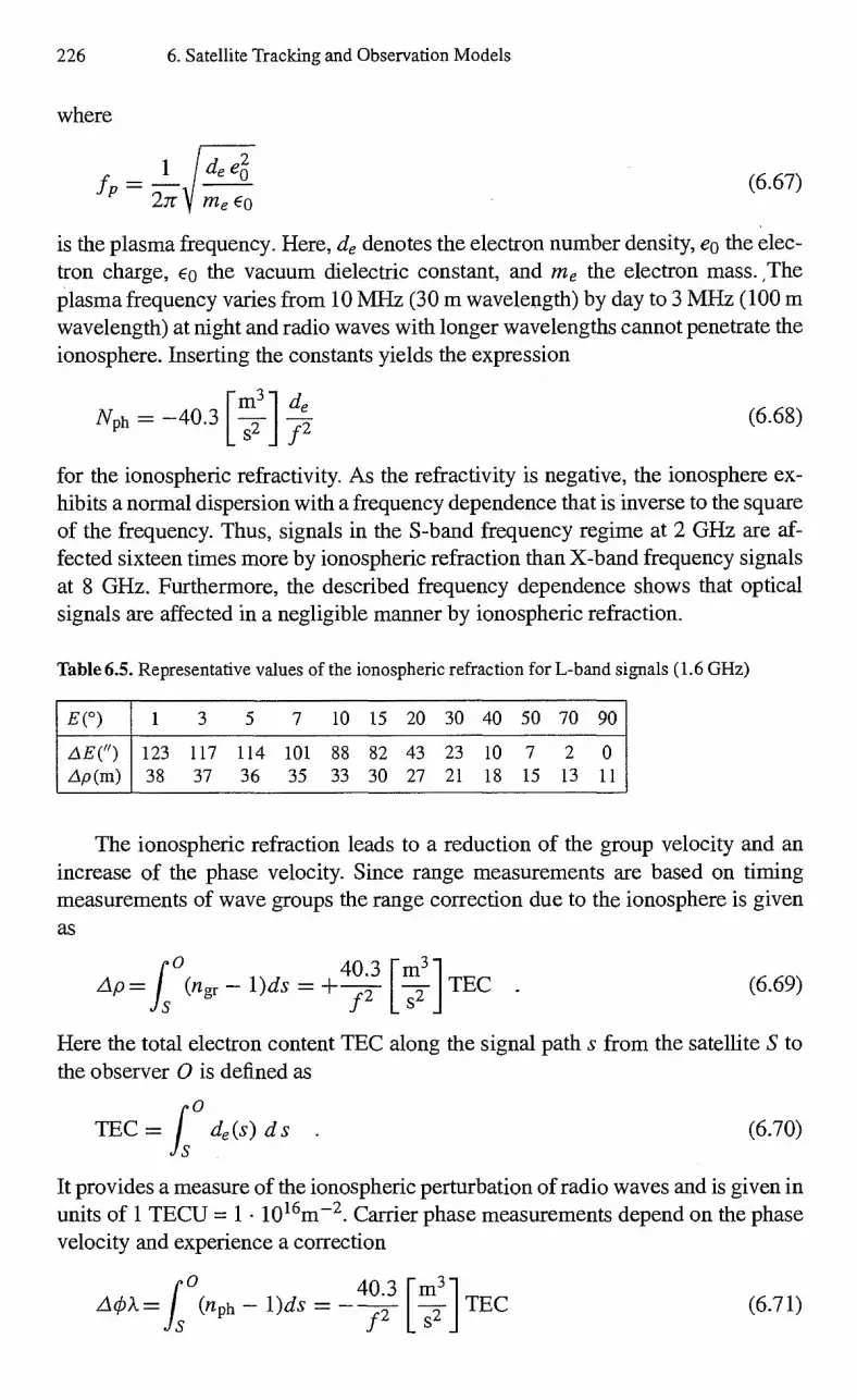
226 6. Satellite Tracking and Observation Models
where
1 de eg fP 27r V me E0
(6.67)
is the plasma frequency. Here, d, denotes the electron number density, e0 the elec-tron charge, co the vacuum dielectric constant, and me the electron mass. The plasma frequency varies from 10 MHz (30 m wavelength) by day to 3 MHz (100 m wavelength) at night and radio waves with longer wavelengths cannot penetrate the ionosphere. Inserting the constants yields the expression
Nph = —40.3 —m31 de s2 f2
(6.68)
for the ionospheric refractivity. As the refractivity is negative, the ionosphere ex-hibits a normal dispersion with a frequency dependence that is inverse to the square of the frequency. Thus, signals in the S-band frequency regime at 2 GHz are af-fected sixteen times more by ionospheric refraction than X-b and frequency signals at 8 GHz. Furthermore, the described frequency dependence shows that optical signals are affected in a negligible manner by ionospheric refraction.
Table 6.5. Representative values of the ionospheric refraction for L-b and signals (1.6 GHz)
E(') 1 3 5 7 10 15 20 30 40 50 70 90
AE(") 123 117 114 101 88 82 43 23 10 7 2 0 Ap(m) 38 37 36 35 33 30 27 21 18 15 13 11
The ionospheric refraction leads to a reduction of the group velocity and an increase of the phase velocity. Since range measurements are based on timing measurements of wave groups the range correction due to the ionosphere is given as
40.3 [m3 ] 1 = f (ngr 1)ds = +— -- .
f2 s2 (6.69)
Here the total electron content TEC along the signal path s from the satellite S to the observer 0 is defined as
TEC = f de (s) d s (6.70)
It provides a measure of the ionospheric perturbation of radio waves and is given in units of 1 TECU = 1 • 10 16m-2 . Carrier phase measurements depend on the phase velocity and experience a correction
40.3 [m3 AO. = f (nph — 1)ds = —1 TEC (6.71) f 2 s2

6.3 Media Corrections 227
Fig. 6.14. Variation of the TEC with the time of the year and local time for a mid-latitude station based on the IR1 1995 model
which is opposite in sign to the range correction. Thus the measured radar range is increased when affected by the ionosphere, while the values of integrated carrier phase measurements are reduced.
Typical ionospheric effects on radar range and elevation data are listed in Table 6.5 for a transmission frequency of the GPS Li carrier at 1.6 GHz. The variation of the total electron content in a zenith column for a mid-latitude station with local time and the date of the year is shown in Fig. 6.14.
As global ionospheric models do not, in general, provide the required modeling accuracy, _the measurement of the total electron content is an adequate approach for determining the ionospheric refraction. Before the advent of the NAVSTAR GPS system, the Faraday rotation of linear polarized signals emitted from the user satellite or geostationary satellites was applied to determine the electron content along the signal path (Llewellyn et al. 1976). This technique, however, requires knowledge of the transmission characteristics of the satellite antenna as well as the satellite attitude. Another approach was to determine the change in the total electron content from building the Differenced Range Versus Integrated Doppler (DRVID). Since range measurements are determined by the group velocity and integrated Doppler counts by the phase velocity, both data types are affected in the same order but different sign (Radomski & Doll 1995). This technique has mainly been applied to correct the ionospheric and interplanetary plasma effects of deep-space probes.
As the ionospheric refraction depends on the signal frequency, the measurement of the signal delay or the signal frequency shift in two frequency bands allows the determination of the TEC value and the ionospheric measurement correction. This technique is applied for the DORIS system (2036 MHz and 401 MHz), the PRARE system (2248 MHz and 8489 MHz) as well as for NAVSTAR GPS (1575 MHz and 1228 MHz). The determination of ionospheric electron-density profiles from the

228 6. Satellite Tracking and Observation Models
GPS Meteorology (GPS/MET) experiment aboard the MicroLab I satellite has been demonstrated by Hajj and Romans (1998). A GPS receiver for l'EC determination may be collocated with a conventional single-frequency tracking system to provide the ionospheric refraction correction by interpolation of the TEC values along the directions to the GPS satellites at the direction to the user satellite. Alternatively, GPS-derived TEC observables from a worldwide network may be applied to derive global TEC infoimation models, which enable ionospheric corrections for any user satellite (Feltens et al. 1997). Considering the GPS system, where pseudorange measurements pi at the Li frequency fi and pseudoranges p2 at the L2 frequency f2 are available, the ionosphere-free pseudorange p can be derived from (6.69) as
P2 — (fl if2) 2 Pl P = —1.545,92 -I- 2.545pi . (6.72)
When precision accuracy requirements force the application of ionospheric cor-rections but measurements of the total electron content are not available, software models have to be applied that predict ionospheric properties either restricted to a dedicated ground station (local model) or worldwide (global model). In this case, models like the Penn state model (Nisbet 1974) that directly simulate the photo-chemical ionospheric reactions and processes are available as well as the empirical worldwide Bent model (Llewellyn et al. 1973). A recent development is the param-eterized ionospheric model (PIM), which provides a near-real-time specification of the global ionosphere from near-real-time satellite and ground-based data (Daniell et al. 1995).

Exercises 229
Exercises
Exercise 6.1 (Light-Time Iteration) Solve the light-time equation for two-way range measurements of a polar satellite at 960 km altitude (e = 0, i = 970 „Q = 130.70 ) and a ground station in central Europe (X = +11 0 East, yo = +48°). The downleg (satellite to station) and upleg (station to satellite) light-time corrections are to be computed at 6 min, 15 mm, and 24 min past the passage of the ascending node, which is assumed to take place at 1997/01/01 011 UTC. The orbit propagation is to be based on Keplerian motion, neglecting precession and similar corrections in the reference system transformations.
Solution: The times of the light-time evaluation are close to the pass beginning, culmination, and end of the pass. To reach an accuracy level of 1 mm, the downleg light-time iteration has to consider two iterations (I-1, I-2), while the upleg light-time iteration may already be stopped after the first iteration:
UTC Distance Down I-1 Down I-2 Up I-1 Range hh:mm:ss Ern] [111] [min] Ern] [nil
00:06:00.0 3644878.6 75.8 1.6 1.8 3644956.2 00:15:00.0 1167049.9 —6.4 0.0 0.5 1167044.0 00:24:00.0 4110978.7 —87.0 1.8 —0.7 4110891.0
Since the range and the amplitude of the range rate is largest at the beginning and end of the satellite pass, the range correction in the downleg is most pronounced near the rising and setting. As the light-time correction varies in proportion to the range rate, the correction vanishes near culmination (cf. Fig. 2.13) and changes its sign. The light-time corrections in the second iteration of the upleg (note the different units) are always positive due to their dependence on the rate of the relative velocity. The light-time correction in the upleg is small as compared to the downleg, since the inertial motion of the ground station due to the Earth rotation is smaller than the relative velocity of the satellite with respect to the station.
Exercise 6.2 (Range Rate Modeling) Compute the average two-way range rate measurements for the scenario described in Exercise 6.1. Assume a Doppler count interval t, of 1 s and show that the average range rate measurement can be approxi-mated by the instantaneous Doppler value at the middle of the count-time interval. The average and the instantaneous range rates as well as their differences are to be computed in steps of 3 min
Hint: The modeling of the average range rate measurement is described by (6.37.), while the instantaneous range rate follows from
do(t) = —44 do
Here, do = r (t) — R(t) denotes the geometric distance of the satellite and the station at time t.
(6.73)

230 6. Satellite Tracking and Observation Models
Solution: In the limiting case of an infinite speed of light the average range rate can be approximated by the expression
(t) -1
(do (t) - do (t - te)) , (6.74) tc
which follows from (6.37) by substitution of the geometric distance do for the two-way range p. The right-hand side may further be expanded into a Taylor series around the center of the interval [t - tc , t], giving
1 -tc
(do(t) do(t - te)) = do(t te/2) + 0(tc.2 'fi) . (6.75)
Combining both approximations then shows the near-identity
kt) do(t - te /2) (6.76)
of the measured average two-way range rate at time t and the instantaneous range rate at the mid of the count interval. Applied to the example, the following numerical results are obtained:
UTC hh:mm:ss
?)(t) [mis]
c./o(t - tc /2) [mis] [mis]
00:06:00.0 -6385.694 -6385.554 -0.140 00:09:00.0 -6113.312 -6113.161 -0.151 00:12:00.0 -4575.872 -4575.720 -0.153 00:15:00.0 1488.564 1488.732 -0.168 00:18:00.0 5500.474 5500.635 -0.161 00:21:00.0 6286.690 6286.839 -0.149 00:24:00.0 6392.679 6392.813 -0.134
Here, the Taylor expansion over the count interval contributes an error of less than 9 mm/s to the overall approximation. The leading wan resulting from the neglect of the light-time correction is given by - ( t(5 2 + pi(5)1c. In the present example this term is responsible for the dominant errors of 10-20 cm/s. With a range rate measurement accuracy of 1 mrn/s it is obvious that both effects have to be modeled rigorously and that the instantaneous Doppler computation is inadequate for a precise range rate modeling.
Exercise 6.3 (User Clock Error from GPS Pseudorange) The user clock error of the GPS Rogue receiver at Goldstone is to be determined from pseudoranges of the PRN 1 UPS satellite. The PRN 1 position and clock errors at 1998/02/19 are taken from a precise ephemeris of the International UPS Service (JUS)
GPS hhannEss
xwGS YWGS
[In] ZWGS St
[As] 08:00:00.0 -15504.291797 -21530.763883 -1271.498273 40.018233 08:15:00.0 -15284.290679 -21684.703684 1573.435406 40.097295 08:30:00.0 -14871.711829 -21600.510259 4391.350089 40.028697 08:45:00.0 -14242.843546 -21306.712708 7133.948741 40.154941 09:00:00.0 -13380.818523 -20837.175663 9754.366309 40.193626 09:15:00.0 -12276.418004 -20229.688085 12207.953668 40.039288 09:30:00.0 -10928.585710 -19524.421024 14453.015617 40.012677 09:45:00.0 -9344.633744 -18762.314034 16451.492281 39.883106 10:00:00.0 -7540.134384 -17983.451817 18169.574686 40.181357

Exercises 231
10:15:00.0 —5538.503062 —17225.491970 19578.246580 40.328261 • 10:30:00.0 —3370.289205 —16522.202377 20653.745961 40.039533 10:45:00.0 —1072.201838 —15902.162018 21377.940941 40.052642 11:00:00.0 1314.093678 —15387.672739 21738.615794 40.025493
To circumvent the effect of Selective Availability, the pseudoranges of PRN 1 are evaluated only at epochs where precise SP3 position and GPS clock errors are available. The pseudoranges on 1998/02/19 comprise the P code pseudoranges at the L2 frequency (P2) and the C/A code pseudoranges at the Li frequency (C1):
GPS hh:mm:ss
P2 [m]
Cl [m]
08:30:00.0 21096577.475 21096579.501 09:00:00.0 20519964.850 20519966.875 09:30:00.0 20282706.954 20282709.233 10:00:00.0 20375838.496 20375840.613 10:30:00.0 20751678.769 20751680.997 11:00:00.0 21340055.129 21340057.362
The user clock error is to be determined from ionosphere-free pseudoranges derived from a suitable combination of P2 and Cl. The signal travel time is to be determined from a rigorous iteration of the light-time equation that makes use of interpolated GPS positions. The WGS-84 coordinates of the receiver at Goldstone are
X = —2353.614128 km, Y = —4641.385447 km, Z = +3676.976501 km .
Hint: The light-time iteration is usually performed in an inertial system with the station position vector R and the satellite position vector r. When U denotes the transformation from the inertial to the Earth-fixed WGS84 system, the signal path is given by
dwos(t) = U (t) (R(t) — r(t — r)) ,
where r denotes the signal travel time Making use of the approximation
U(t) R z (we r)U (t — r)
the inertial position of the GPS satellite may be substituted by the corresponding Earth-fixed position
rWGS (t — r) = U(t — r)r(t — r)
This yields the light-time equation
cr = dwGs(t) = IRz(wer)rwGs(t — — RWGS (6.77)
in the Earth-fixed reference frame, which is best suited for use with common tabular or analytical ephemerides of GPS satellites.

232 6. Satellite Tracking and Observation Models
Solution: The residual of the ionosphere-free pseudorange yields the user clock bias, converted to meters, of the Goldstone GPS receiver at the time of the measure-ment. Over a time interval of 2.5 h the clock drift can be neglected and the mean value of the residuals gives a clock bias of 17674.77 m. In particular the following pseudorange residuals and their deviations from the mean (Delta) are found:
GPS ClockError Delta hh:mm:ss [m]
08:30:00.0 17674.52 -0.25 09:00:00.0 17676.14 1.37 09:30:00.0 17675.59 0.82 10:00:00.0 17674.45 -0.33 10:30:00.0 17673.53 -1.25 11:00:00.0 17674.41 -0.36
A maximum variation of the pseudorange residuals of less than 3 mis found in fair accord with the accuracy of the ionosphere-free pseudoranges.
Exercise 6.4 (Tropospheric Refraction) Compute the daily variation of the elevation of a geostationary satellite (a = 42 164 km, e = 0.00296, i = 0.05°, S2 = 150.7°) for the ground station given in Exercise 6.1. Assume an epoch of 1997/01/01 Oh UTC and compute the elevation at intervals of 3 h. Compare the variation in elevation with the amplitude of the tropospheric refraction correction, as derived from (6.50) for a partial pressure of dry air of 1024 hPa, and a relative humidity of 0.7. Consider two cases with temperatures Ti and T2 of 283 K and 303 K, respectively.
Solution: The elevation is E0 = 23.363° at the epoch and varies over a day with an amplitude of about 0.06°. The maximum elevation occurs 6 h past the epoch and the minimum elevation is reached at 18 h. The daily variation of the elevation E from E0 together with the elevation refraction corrections ET' and \ET2 are obtained as
UTC hh:mm:ss
E - E0 [deg]
ET [deg]
ET2 [deg]
00:00:00.0 0.000 0.051 0.043 03:00:00.0 0.021 0.051 0.042 06:00:00.0 0.031 0.051 0.042 09:00:00.0 0.024 0.051 0.042 12:00:00.0 0.004 0.051 0.043 15:00:00.0 -0.017 0.051 0.043 18:00:00.0 -0.027 0.051 0.043 21:00:00.0 -0.020 0.051 0.043 24:00:00.0 -0.001 0.051 0.043
For the particular case considered, the refraction correction is of the order of the daily elevation variation but stays essentially constant for given meteorological conditions. The assumed temperature difference of 20 K changes the observed elevation by about 0.008° which may be compared to the 0.060° change resulting from the orbital inclination. At the distance of a geostationary satellite 0.001° corresponds to an along-track or cross-track position variation of about 700 m.
7. Linearization
The trajectory and measurement model developed so far provides a concise and detailed description of a satellite's motion with respect to an Earth-bound observer. Besides the state variables that define the initial conditions, these models depend on a variety of parameters that either affect the dynamical motion or the measurement process. Due to the complexity of the applied models it is hardly possible to solve directly for any of these parameters from a given set of observations. It is therefore customary to linearize the relation between the observables and the independent parameters to obtain simplified expressions that can be handled more easily. Within a statistical orbit determination one can then determine those state and model pa- t rameters that provide the best representation of a large set of measurements using a differential correction and parameter estimation algorithm.
A rigorous linearization of the trajectory and measurement model requires a large number of partial derivatives, which may be divided into four different categories:
• The State Transition Matrix
The state vector y (to) = (rT (t0), V T (tO)) T at some specified epoch to deter-mines the form of the orbit and its orientation in space. Any change of these initial values results in a change of position and velocity at a later epoch t
which is described by the state transition matrix
ay(t) (t,
to) (7.1)
y (to)J 66
e The Sensitivity Matrix
Aside from the initial state the orbit is also a function of various parameters pi (i =1, ..., np ) that determine the different forces acting on the satellite. This dependence is described by the sensitivity matrix, i.e. by the partial derivatives
(4(0) = S (t) (7.2)
)6.n
with respect to the force model parameters. Depending on the application in mind, the parameter vector p may e.g. contain the drag and radiation pressure coefficients (CD, CR), the thrust level of a maneuver or the size of certain gravity model coefficients.

234 7. Linearization
• Partials of the measurements with respect to the state vector The linearized dependence of a measurement z (t) on the state vector y (t) = (r T (t) , V T (t)) T of the satellite at the time of the measurement is described by the partial derivatives
Y( 1"))1x6
(7.3)
It may be noted that the partials 8z/0 v(t) with respect to the instanta-neous velocity vanish for all types of range and angle observations (z = p, A, E, X, Y) if one neglects the light time and aberration correction and considers only geometrical values.
• Partials with respect to measurement model parameters Last but not least the predicted observations depend on certain measurement model parameters qi (i = 1, .. . , n) like bias values due to an insufficient calibration of the zero point for angle readings or the transponder and ground station delay for range measurements. More elaborate measurement models may take care of further effects like antenna axis displacement and misalign-ment or ground station coordinate offsets that may be estimated during an orbit determination. The corresponding partial derivatives are given by an n -dimensional vector
( a z) \q (7.4)
Combining these partial derivatives yields the dependence of an individual mea-surement z on the initial state vector y (to), the vector p of force model parameters and the vector q of measurement model parameters:
0z 8z 0z
y(to) Bp aq) ix(6+,,,+no (7.5)
az ((B.Yaz(t)) ((t,
to) s(t)) . aq
Given the models presented earlier, the analytical computation of the individual derivatives is tedious and cumbersome work, which provides little additional in-sight into the underlying concepts. Nevertheless, it forms an essential part of the overall orbit determination process, and may have a notable impact on the achiev-able performance and speed of convergence. The required relations are therefore derived and presented here in an adequate level of detail. Impatient readers may, however, skip to Chap. 8 on first reading and content themselves with the fact that any desired partial derivative could, in principle, be obtained from a numerical difference quotient approximation.
7.1 Two-Body State Transition Matrix 235
7.1 Two-Body State Transition Matrix
In the simplified case of unperturbed Keplerian orbits the state transition matrix and its inverse can be expressed as an analytical function of the Cartesian coordinates and the orbital elements. To this end, the state vector transition matrix is commonly factorized into the product of the more simple orbital elements transition matrix and the partial derivatives of the state vector with respect to the elements, both of which are derived in the sequel.
7.1.1 Orbital-Elements Transition Matrix
The orbital-elements transition matrix is given by
ce(t, tO) = ( aU(t) 0e(t0)/6x6
(7.6)
where
a = (a, e, j, £2, co, M) T (7.7)
denotes the vector of orbital elements. For an unperturbed orbit the orbital elements at time t are the same as those at time to with the exception of the mean anomaly that changes by
M(t) — M(to) = n (t — to) . (7.8)
Here, the mean motion
n = (7.9)
is a function of the semi-major axis a. The orbital elements transition matrix may therefore be written as
tkce(t, to) =
1 0 0 0 0 0
0 1 0 0 0 0
0 0 1 0 0 0
0 0 0 1 0 0 (7.10)
0 0 0 0 1 0 DM(t)0 o o 0 1
a (to) where the only non-vanishing off-diagonal element is given by the teini
am(t) 3 n = (t — to) (7.11) 0a(to) 2 a
that describes the effect of small changes in the semi-major axis at time to on the mean anomaly M(t) at time t.
236 7. Linearization
7.1.2 Keplerian-to-Cartesian Partial Derivatives
According to the results of Chap. 2 the position r and velocity y of an unperturbed satellite in the central field of the Earth is given by
r = 2P+9Q y = P Q , (7.12)
where the Gaussian vectors P and Q are functions of the orbital elements i, and co that define the orientation of the orbit in space, while the coordinates î and 9 inside the orbital plane are a function of the semi-major axis a, the eccentricity e and the mean anomaly M. The partial derivatives of r and r with respect to an orbital element a may therefore be expressed as
ar afc a9 ay p a9 n - = Q (7.13) B a B a B a B a Ba A ± Ba '
for a = a, e, M and as
Br ,ap ,aQ ay • ap ,,aQ — = x— +y y = x + y (7.14) B a Ba Ba B a Ba Ba
for a = S2, co, i. The partial derivatives of the in-plane coordinates with respect to a, e and M
follow from the basic equations
= a (cos E — e) X = • G MEDa sin E
• GM0a V
/1 —e2 cos E
(7.15)
= a-il—e2 sin E
with
r = a (1 — e cos E) (7.16)
Since the eccentric anomaly E, which is implicitly defined by Kepler's equation
E — e sin E = M (7.17)
as a function of e and M, does not depend on the semi-major axis a, one obtains immediately
— = cos E — e = (7.18) Ba a
For the derivatives with respect to e and M one has to consider the dependence of E on both quantities, which is expressed by the total differential
dE — e cos E dE — de sin E = dM
of Kepler's equation. The partial derivatives of E are therefore given by
BE sin E a sin E
(7.19)
(7.20) - =
Be 1 e cos E
7.1 Two-Body State Transition Matrix 237
and 8 E 1 a = — (7.21)
am 1— e cos E r Using these results it follows that
—a.i = a — sin E aE — 1 = —a 92
(7.22) 8e 0 e J r (1— e 2)
and a.i a E .5sc — = a (— sin E) —a ill , 7, (7.23) am
The remaining derivatives are obtained in a completely analogous way yielding
_( a .92 ) —1 \ / î
0(1,9)T a r (1— e 2) n
a(a, e, M)T = 9 \ —a r (1— e 2) ) n i
for the dependence of the in-plane position on a, e and M, while the velocity partials are given by
. . p (1 , .9) 7- (a, e, M)T =
2a .is, (a) 2 (2 () ± l _e e2 (9 ) 2)
—n (—r
x
a)3 2 (7.25) ,.. x
2a
9 n (a) 2 ( .22 92
V1— e2"r r a (1— e2) n y
) —(—
r
a 3 - 2
(Broucke 1970, Long et al. 1989). The representation of these partial derivatives as a function of .5e, 2, 9 and 9 is convenient from the computational point of view, but one may equally well replace these quantities by the basic definitions given above. In this case one obtains the derivatives as a function of a, e and E, where E has to be obtained by solving Kepler's equation for the given value of the mean anomaly M.
In order to complete the computation of partial derivatives of the state vector with respect to the various orbital elements we may now turn to the derivatives of the Gaussian vectors with respect to i „f2 and co. Since changes in these angles correspond to rotations around the line of nodes vector n = (cos S2, sin Q, 0) T , the unit vector ez = (0, 0, 1) T and the vector W=Px Q at right angles to the orbital plane, respectively, the partial derivatives of P and Q are given by
(7.24)
OP 0 Q = n x P n x Q ai ai
OP 0 Q = ez x P ez x Q as2 as2
aP Q = W x P
a —0,„ . W x Q aw
(7.26)

—2 — na Jl_ e2 na2 e
—(1 — e 2) na2 e
1
(7.31)
na2 ../ 1 — e2 sin i — cot i
238 7. Linearization
Evaluating the cross products finally yields O P 8 Q
= sin(w) W = cos(co) W ai ai a P
±PPxY a 2 = +QQ: a S2 — a S2 0 0 O P a Q
+ Q — P , aw aw where Px , Pi,, Qx and Q3, are the x- and y-components of P and Q, respectively. The same result may also be obtained by direct differentiation of the definition of P and Q given in Chap. 2.
(7.27)
7.1.3 Cartesian-to-Keplerian Partial Derivatives
The partial derivatives of the orbital elements a with respect to the state vector y = (r T, V T ) T may be obtained by computing the partial derivatives of the state vector with respect to the orbital elements and inverting the resulting 6 x 6-matrix using appropriate numerical methods:
(aY)6x6 = (8a)6x6 (7.28)
aa y
More favorably, however, the inverse is obtained from the analytical relationship
p(ce, 01) +(aV) T — (ar)T ar av V a) Vol)
where P is an anti-symmetric 6 x 6 matrix made up of the Poisson parentheses
p oti) Cai) . (0011T (aaj (acyi\ T
ar av ar ) av In total, only five independent matrix elements
P(a,M) = —P(M,a)
P (e, co) = — P (w, e)
P (e, M) = —P (M, e)
P (i, S2) = — P (S2, =
na2 A/1 —e 2 exist, while all other Poisson parentheses vanish. For further details and a proof of these relations the reader is referred to Broucke (1970).
(7.29)
(7.30)
P (i, co) = — P (o), i) =

—1 0 6x6 with j ( 0 +1 ) o T Jo _ j (7.33)
7.1 Two-Body State Transition Matrix 239
7.1.4 The State Transition Matrix and Its Inverse
Making use of the results obtained so far, the state transition matrix can be parti-tioned into the product
4p(t,to)= ( a Y (t) * Oa (t, to). /0y(to)
80/ (t) 801 (t0) (7.32)
of the orbital elements transition matrix and the state vector partials with respect to the orbital elements. In evaluating this expression, care must be taken that the partial derivatives of the state vector with respect to the orbital elements need to be evalu-ated at two different epochs, namely to (right-hand matrix) and t (left-hand matrix). As a consequence, only a small number of terms is common to the computation of both expressions (e.g. the derivatives of the Gaussian vectors with respect to the orientation elements). This problem may partly be overcome by improved formu-lations for the direct computation of the state transition matrix as given in Sconzo (1963), Goodyear (1965), and Shepperd (1985). Furthermore, it is noted that the use of orbital elements in the above factorization introduces an artificial singular-ity at zero eccentricity and inclination into the resulting expressions. To avoid this singularity, one may apply equivalent, but less common expressions for equinoctial elements (see Sect. 2.2.5) and the associated partial derivatives (Broucke & Cefola 1972, Dow 1975).
In computing the inverse of the state transition matrix, one benefits considerably from the fact that 0 is a symplectic matrix for Keplerian orbits. As shown in more detail in Sect. 7.2.4, 0 obeys the relation
-1
(Wintner 1941, Battin 1987) Making use of the identity J2 = —1, the inverse of a symplectic matrix 0 is given by
o -1 joT (7.34)
in much the same way as the inverse of a symmetric matrix is equal to its transpose. Upon splitting the transition matrix
(t, tO) = r
vr
Or
( °I-t) VI)
(7.35)
into its position and velocity related blocks, the result finally takes the form
rTv
= ' vv vT r +0 rTr (7.36)
The inverse of the state transition matrix is thus obtained by simple rearrangement of its elements without a need to refer to general numerical matrix-inversion methods.

obeys the first-order differential equation
d v(t) —dt .Y(t) = f (t, y) =
a(t,r,v))
then
a d y(t) =
a f (t, y(t)) a f (t , y (t)) 8y(t)
Y (to) dt 8 y (to) Y 8y (to)
The state transition matrix
(t, to) = By (to)
may therefore be obtained from
d
—dt °(t ' Aa) = a f (t y(t))
0 (t , to) 8y(t)
8y(t)
(7.38)
(7.39)
(7.40)
(7.41)
or
240 7. Linearization
7.2 Variational Equations
Even though the state transition matrix of the two-body problem is a reasonable approximation of the actual transition matrix, it is sometimes desirable to take into account at least the major perturbations in the computation of I (t, to). As with the treatment of the perturbed satellite motion, one may not, however, obtain an analytical solution anymore in this case, but has to solve a special set of aiffer-ential equations – the variational equations – by numerical methods. Aside from the increased accuracy that may be obtained by accounting for perturbations, the concept of the variational equations offers the advantage that it is not limited to the computation of the state transition matrix, but may also be extended to the treatment of partial derivatives with respect to force model parameters.
7.2.1 The Differential Equation of the State Transition Matrix
The differential equation, which describes the change of the state transition matrix with time, follows from the equation of motion of the satellite. If the state vector
y (t) = (r (t)
v(t) (7.37)
03x3 13x3 8a (r, v, 8a (r, y , t)
\ . (t, to)
(7.42)
8r(t) 8v(t) 16x6
and the initial value 0 (to, to) = 16x6

, (7.45) 03x 6
03x6
tar(t)\ ap
ay(t)
\ Bp /
. (7.46)
aa\ ap )
(7.47)
(7.48)
7.2 Variational Equations 241
7.2.2 The Differential Equation of the Sensitivity Matrix
The differential equation of the sensitivity matrix that gives the partial derivatives of the state vector with respect to the force model parameter vector may be obtained in a completely analogous way, yielding
d a y(t) a f(t, y(t), p) 0y(t) a f(t, y(t), p) (7.43)
dt 0p a y (t) 0 p a p or
d
Tt S(t)6x n p
( 03x3 13x3 03xn p
aa(t, r, y, p) aa(t, r, y, p) • S(t)+ aa(t, r, y, p
8T (t) 8v(t)
)
6x6 0 P 6xn p
Since the state vector at to does not depend on any force model parameter, the initial value of the sensitivity matrix is given by S(to) = 0.
7.2.3 Form and Solution of the Variational Equations
By combining the differential equations for the state transition matrix and the sen-sitivity matrix one obtains the following form of the variational equations
(7.44)
d =
dt (
03x3 1-3x3
aa aa )
ar av 6x6
which is adequate for use with numerical integration methods for the solution of first-order initial value problems. An alternate representation, which is suitable for methods that allow the direct integration of second-order differential equations, may be obtained by decomposing 0 and S into
ar(t) r sr
a (r (to), y (to)) av(t)
\a(r(to), v(t0))/ \Svi
Since (by changing the order of differentiation) d
dt(Or, Sr) = (0v, Sv) ,
the variational equations may then be written as
(L, STr) = PjLir (0 r Sr) ± PéLiv ( r , r) (03x 6
0 S

242 7. Linearization
If the acceleration does not depend on the velocity, the actiay terni vanishes, which means that the right-hand side of the second-order variational equations does not depend on , anymore. This fact may be useful since it allows the use of very efficient numerical integration methods for solution of the variational equations (e.g. Runge—Kutta—Nystrom or Stoenner—Cowell methods).
Independent of the preferred foini of the variational equations it is important to note that the variational equations have to be integrated simultaneously with the state vector. Otherwise the position and velocity of the satellite, which are required to evaluate the acceleration partials in the right-hand side of the variational equations, would be unknown. The combined integration of the state vector y, the state transition matrix 0 and the sensitivity matrix S therefore requires the solution of (7 +np) six-dimensional first-order differential equations or, equivalently, the same number of three-dimensional second-order differential equations. It should be emphasized, however, that the total effort is usually much less than (7 +n)-times the effort for integrating the differential equation of the orbit alone. The reason for this property lies in the fact that the highest amount of work during the numerical integration is generally spent in the evaluation of the variational equations and not in the integration routine. The total integration effort is therefore proportional to the work required for the computation of the partial derivatives of the acceleration. By computing these derivatives along with the acceleration itself one can make use of common sub-expressions, which reduces the computing effort considerably.
Since accuracy requirements for the partial derivatives are generally more re-laxed than that for the trajectory itself, it is common to apply a simplified force model in the solution of the variational equations. While purely Keplerian state transition matrices may cause slow convergence of iterated differential correction methods for orbit determination, the incorporation of the lowest-order zonal gravity field perturbation (C2,0) already provides an acceptable minimum model (see e.g. Ballani 1988),
As pointed out by various authors, considerable care must be taken, however, to use consistent models in the simultaneous integration of the state vector and variational equations. This is dramatically shown by the analytical solution of the combined equations for an equatorial orbiter and a second-order zonal gravity field given by Rice (1967). While a purely Keplerian formulation yields a transition matrix in fair agreement with the solution of the perturbed problem, a completely erroneous solution is obtained after a few orbits upon combining an unperturbed gravity field in the differential equation of the transition matrix with a second-order gravity field in the state equations! The problem is further confirmed by numerical studies of more elaborate force models (May 1980), giving clear indication for the need of a consistent modeling. From a practical point of view, one may thus choose to either perfoini a rigorous integration of the variational equations using the same sophisticated model as required for the state equations or to treat the variational equations as a separate problem. In the latter case, the state equations are once integrated individually with the full model and once along with the variational equations using a simplified force model (e.g. up to C2, 0). Even though the trajectory

7.2 Variational Equations 243
of the simplified model diverges notably from the true orbit, the resulting state transition matrix will nevertheless be found to closely match the actual value.
7.2.4 The Inverse of the State Transition Matrix
Aside from the state transition matrix itself, a variety of applications requires the inverse matrix oP (t, to) to map a state vector change at time t back to the initial epoch to. While numerical methods are generally available and well suited to per-forming the inversion, the special properties of the transition matrix offer various alternatives. In the case that the inverse state matrix is of primary interest, one may e.g. solve the adjoint matrix differential equation
to) = (t to) • (—V ) (7.49) dt a y
(Curkendall 1974), which follows from (7.41) and the identity d (00 -1 )Idt = 0 (Battin 1987). Like the variational equations described before, this equation is integrated along with the state vector using the initial conditions P = 1.
Another approach can be applied whenever the acceleration does not depend on the velocity and, at the same time, exhibits a symmetric gradient G = In this case, the partial derivatives
F = af =(
01 '
ay °) 6X6 obey the relation
JF = —F T J with J ( 0 +1
0 ) 6x6
(7.50)
(7.51)
As a consequence, the state transition matrix can be shown to be a symplectic matrix, which is characterized by the relation
T TO = (7.52)
Following Battin (1987) the time derivative of (P T JO vanishes under the given conditions, while the relation at epoch to (i.e. (1) = 1) is a trivial identity. The sig-nificance of this property lies in the ease of determining the inverse of a symplectic matrix. Making use of the identity J2 = —1, the inverse is given by
(7.53)
in much the same way as the inverse of a symmetric matrix is equal to its transpose. The state transition matrix is, in particular, syMplectic for all types of gravita-tional forces due to the symmetry of the gravity gradient. Its inverse can then be found from (7.36) by simple rearrangement of the matrix elements. Care should be taken, however, that the symplectic property is evidently violated in the presence of aerodynamic drag, in which case reference to numerical matrix inversion methods should be made.

244 7. Linearization
7.3 Partial Derivatives of the Acceleration
The variational equations depend on the partial derivatives of the acceleration with respect to the state and model parameters, which are discussed in more detail in the present section.
7.3.1 Geopotential
The most important contribution to the variational equations for the state transition matrix arises from the central term
= G MED
r (7.54) r3
of the Earth's gravitational attraction. Using the general relation
arn
8(x2 + y2 + z2r/2 = n rrz-2 rT
ar ar
it follows that
= —GM ED —a (r —1 ) Dr Dr \ r 1
(7.55)
(7.56)
Here the factor rrT in the second tei in is a dyadic product, which yields a 3x3-matrix and should not be confused with the dot product rT r. Evaluating the individual components of a iv ar yields
ai — = Dr
which shows that the gravity gradient is symmetric with respect to the main diagonal and that the sum of the diagonal elements vanishes.
Both properties follow from the fact that the gravitational attraction may be written as the gradient
— . anT
(7.58) ar
of a potential U, which is given by
U = GM1
ED —r
(7.59)
for the simplified case of a point mass Me in the center of the Earth. The partial derivatives of r with respect to r are just the second partial deriva-
tives of U, which are clearly symmetric, since the order of differentiation with respect to the components of r may be interchanged, i.e.
GM / 3x2 — r2 3yx 3zx
3xy 3y2 r2
3zy
3x z 3yz
3z2 — r2 (7.57) r5
ai; au a 2 u — = = _ ax axay ay ax ay etc. (7.60)
7.3 Partial Derivatives of the Acceleration 245
Since this symmetry is independent of the particular form of U, it is not only valid for the central term of the Earth's potential but also for all higher order harmonics. By considering the Laplacian
02u 02u 02 u A U = (7.61)
ax2
which reduces to
1 82 AU (r) (r U (r)) = 0 (r > 0) (7.62)
r a r 2
in the case of the radially symmetric 1/ r-potential, one may easily verify that the sum of the diagonal elements of ai/ar vanishes for the attraction of a point like body. For an extended body like the Earth the gravitational potential may be represented by a superposition
U =Gf p (s) d3 s
(7.63)
of the hr-potentials arising from all mass elements dm = p (s) d3 s and the Lapla-cian is therefore zero, too, for all points outside the surface of the body.
The symmetry property of the matrix a iz la r of partial derivatives of the Earth's attraction with respect to the position and the condition of a vanishing sum of the diagonal elements reduces the number of independent components that have to be considered in the computation from nine to five. In an Earth-fixed frame these components may conveniently be obtained from
ay2 a z2
ainm (7.64) 0r
(cf. (3.33)) using expressions for the Willis of degree n and order m derived by Cunningham (1970):
ainm (m=0) GM =
e) 1 f (+CnOVn+2,2)
(n+2)! 1 (+Gil () Vn+2,0) ax R1 . 2 1 n!
(m=1) GM 1 f =
R 4 1 (-f-Cn 1 Vn+2,3 + SnlWn+2,3) I (n +1)!
+ (n — 1)!
( 3 Cn1 17n+2,1 — Sn1 Wn-1-2,1) }
G Me) 1 {
R3 4 ,
--f - CnmVn-1-2,m-1-2 4- SnmWn+2,m-1-2) e
+2 ( CnmVn+2,m — SnmWn-1-2,m) (n — m)!
(n — m + 4)! +
(n—m)! (+Cnm Vn+2,m-2 + SnmWn-I-2,m-2)1
(m> 1)
(n — m +2)!
(7.65)
GMED (n+1) -
R 3
GMED fn—m+1
R1 1 2
(n—m+3)!
2 (n —m)!
GMED
R 3 ED
GM@ 1 n—m-F1
4 1 2
a-nm
az
246
7. Linearization
aïnm (m.0)
ay GM® 1
4 2
GMED 1
4 4
(n+1)!
(n-1)!
(+CnOWn+2,2)
(f- Cn 1 Wn+2,3 SnlVn+2,3)
CniWn+2,1 SnlVn+2,1)1
(m=1)
(7.66)
GM® 1 I ( , --f- UnmWn+2,m-1-2 — SnmVn+2,m-1-2) R 3 4 ED
(n—m +4)! + (
(n—m)! C nmWn+2,m-2 + SnmWn-I-2,m-2)}
(+CnO Vn+2, 1 )
(+CnmVn+2,m+1 SnmWn-1-2,m+1)
( CnmVn-1-2,m-1 — SnmWn-1-2,m-01
(4- CnO Wn -1-2,1
(+Cnm Wn+2,m+1 — SnmVn+2,m-1-1)
(n—m+3)!
2(n—m)! (+CnmWn-1-2,m-1 — SnmVn-1-2,m-1) I
GM@ { (n—m+2)! (+CnmVn+2,m SnmWn-I-2,m)}
R 3 (n—m)!
Here Vnm and Wnm , which follow from the recurrence relations (3.29) and (3.30), are the same quantities that are used in the computation of the acceleration. If the partial derivatives of the acceleration due to geopotential coefficients up to Cnn and Snn have to be calculated then Vw, and Ww, are required up to degree and order n + 2.
For a non-rotating Earth the expressions derived so far would directly represent the desired partial derivatives. Due the Earth's rotation some additional transfor-mations are, however, required, since the components of r and r in (7.65)... (7.69) refer to a coordinate system that is aligned with the instantaneous rotation axis of the Earth and the direction of the meridian of Greenwich. Using indices "si" and "ef' to distinguish between space-fixed and Earth-fixed coordinates the desired partial derivatives in the space-fixed reference system are given by
= U-1 (0 • (Li) • U(t) , sf ef
inm
az
(7.67)
(7.68)
(7.69)
(7.70)
7.3 Partial Derivatives of the Acceleration 247
where U describes the time-dependent transfounation to Earth-fixed coordinates according to
ref = U(t) r sf and isf = U-1 (t) (7.71)
The temi (a ar)ef may be computed by evaluating (7.65)... (7.69) with (x, y, z) replaced by the Earth-fixed coordinates (Xef, Yef, Zef). It should further be empha-sized that both (a iz ar)sf and (a i; a r)ef are partial derivatives of the acceleration in inertial coordinate systems which are rotated against each other by a given rotation U. The acceleration in a rotating coordinate system would be different by Coriolis and centrifugal ternis.
Since the acceleration due to the Earth's attraction does not depend on the satellite's velocity, the partial derivatives with respect to the position are all that is required to compute the contribution of the geopotential to the variational equations for the state transition matrix. In the case of the sensitivity matrix some further partials may, however, be of interest. Neglecting the influence of Earth rotation parameters on the acceleration the only model parameters of interest are the product GM ED of the gravitational constant and the Earth's mass as well as the gravity model coefficients Cmn and Simi . Since GM@ is a multiplicative factor in the computation of the Earth's acceleration, the corresponding partials are simply given by
a 1 . . (7.72)
The corresponding expressions for the x and y-components may easily be derived from (3.33).
Even though the partials with respect to GM, Cnm and Snm may therefore be computed at almost no additional cost from known quantities, they are not considered in most orbit determination programs. This is due to the fact that the estimation of these force model parameters is not possible for individual satellites but requires the simultaneous consideration of a large set of observations from different types of satellite orbits. An estimation of GM, Cnm and S„„, is therefore only foreseen in specialized programs for geodetic applications (see e.g. McCarthy et al. 1993).
7.3.2 Point-Mass Perturbations
According to (3.37) the perturbations of the Sun and the Moon in an Earth-centred reference frame are given by
— s = —GM .
(r s
Ir — si3 + —
is 13 (7.74)
a Gme, Glue, The derivatives with respect to the geopotential coefficients follow in a similar manner from the fundamental relations for the acceleration yielding e.g.
ai ai GMED = (n m-I-1) ( — Vn-Fi,m , — Wn+1,m)
R2 (7.73)
Cnni Stun
248 7. Linearization
Only the direct gravitational attraction depends on the satellite coordinates and the partial derivatives of the acceleration with respect to r are therefore given by
ar GM ( si3 13x3 3(r s) (r s)T Ir — sl 5
(7.75)
in analogy with (7.56). The derivatives with respect to the solar or lunar mass M may easily be computed from
1 aGm (7.76)
but are again only required in special applications.
7.3.3 Solar Radiation Pressure
For the most common solar radiation pressure model (3.75) the resulting accelera-tion varies with the satellite position in the same way as the gravitational attraction of the Sun. The corresponding partial derivatives are therefore given by
ar PeCr 7-7-1 AU 2 1 A 1
Ir — sl 3 3x3 3(r s) (r s)T
Ir — sl 5 (7.77)
Here r and s are the geocentric coordinates of the satellite and the Sun, respectively. Due to the large distance of the Sun this contribution to the variational equations
is quite small and may therefore safely be neglected in most applications. What is more important, however, is the partial derivative
ai 1.. A r 0 2 —r = — Pe — --AU (7.78)
Cr Cr m r(3)
which is required to compute the influence of variations in the radiation pressure coefficient on the satellite trajectory. This allows the estimation of Cr during an orbit determination, which cannot usually be predicted accurately enough from material constants and the satellite geometry.
73.4 Drag
Starting from the basic expression
1 A = --2
CD -
m
p VVr with vr = v coe x r
(7.79)
for the acceleration due to atmospheric drag (cf. Sect. 3.5) one easily obtains the derivative with respect to the drag coefficient as
1 A — p V r V r acp 2m (7.80)
7.3 Partial Derivatives of the Acceleration 249
Furthermore, the dependence on the spacecraft velocity is described by the partial derivatives
— = — — CD A - p
( VrVT r ± Vr1)
ay 2 m
1 Vr
(7.81) ai
The partial derivatives with respect to position involve .a direct term describing the atmospheric density variation as well as a minor contribution resulting from the changing atmospheric wind velocity:
— — CD - VrVr — - - CD - p r + vr 1 Or
1 A Op 1 A (
vr
v r v T ay r i
in Or 2 m
) = ar
ai
Introducing the cross-product matrix
X (w) —wz wy
0 ±wx 0
(7.83)
to rewrite the cross-product teun coED x r as X (coe) r, one finally obtains the rep-resentation
OP 1 A Op OP — = CD- VrVr — — X( 6)e) • (7.84) or 2 m Or ay
Here Op/Or describes the dependence of the atmospheric density on the spacecraft location. Except for simplistic models like that of Harris—Priester, the complexity of representative atmospheric density models renders the analytical computation of the density gradient extremely cumbersome. Numerical differentiation therefore provides a meaningful alternative, but care must still be taken to avoid singular-ities caused by a non-smooth or non-differentiable representations of the density functions. -
7.3.5 Thrust
The thrust model developed in Sect. 3.6 represents the acceleration as a function of the total velocity increment .%1 v along a set of coordinate axes defined by the transformation matrix E. Considering the boost start and stop times as well as the mass profile as known quantities, the acceleration depends in a linear way on the ZAv components that may be calibrated within an orbit determination. The corresponding derivatives are easily obtained as
Oa Iiiil 1 m(t)
—141 mo
(7.85)
throughout the thrust phase and zero otherwise. In case of an inertial reference frame (E =1) the acceleration is independent of the actual spacecraft position and velocity. A more complicated situation is encountered for the co-moving, orbital
(7.82)
250 7. Linearization
frame, where the reference axes are aligned with the instantaneous radius vector, angular momentum vector and orbital plane. Partial derivatives of the unit vectors with respect to position and velocity may then be obtained from the basic relation
a f(x) iv a 1( f + f = 1 (7.86)
Ox if(x)i f ax ax f f f 2 j ax
where 1 — f f T is a rank-2 matrix spanning the plane perpendicular to f. Further-more the notation of the cross-product matrix (7.83) is used to conveniently express partial derivatives of cross-products:
O(f (x)x g(x)) = X (f)
a g(x) X(g)
a f (x) (7.87)
Ox ax ax Making use of these relations, the partial derivatives of the unit vectors
E(t) = (el, e2, e3) (7.88)
in radial, along-track and cross-track direction with respect to the spacecraft position are given by
ael =. —
1 (1 — eie 1T )
Or r 0 e2 aei
8 e3
= X(e3)—ar
— X(ei) —ar Or ae31 — =. (1— e34) (—X(v)) ar ir x vi
Likewise
(7.89)
_ae2 0e3 = _X(ei) ay ay
a e31 — = (1— e34) (+X(r)) ay ir x vi
are the partial derivatives with respect to the satellite velocity vector.
(7.90)
7.4 Partials of the Measurements with Respect to the State Vector
In the computation of partial derivatives that describe the dependence of a mea-surement on the instantaneous position and velocity of the satellite one may — to first order — neglect all light-time effects and consider the geometrical measurement equations, only. Both angle and distance measurements may then be expressed as functions of the topocentric local tangent coordinates s, which are related to the

7.4 Partials of the Measurements with Respect to the State Vector 251
Earth-centered, space-fixed satellite position r and the Earth-fixed station coordi-nates R by -
s(t) = E (U (t)r (t) — R) . (7.91)
Here U is again the matrix describing the transfolination from space-fixed to Earth-fixed coordinates, while
E = (eETT) — sin
+ cos 'p cos a. + cos ço sin + sin p— sin cio cos — sin ço sin -I- cos cp
+ cos 0 (7.92)
is the orthonormal matrix made up by the east, north and zenith unit vectors. The desired partials of a range or angle measurement z may then be expressed as
a z az — u . (7.93)
ar as Neglecting light-time corrections and propagation effects the partial derivative of a range measurement with respect to the instantaneous position vector is therefore given by
ap as sT =- = 7EU (7.94)
0r 0r
with s = Isl, while the partials with respect to velocity vanish completely. In a similar manner one obtains the partial derivatives
81:3 s §T
EU (7.95) ar = s2
and
=sT —EU s
of the instantaneous and geometric range rate from the relation
. . p =. s =. —
(7.96)
(7.97)
Using the basic expressions for azimuth and elevation one may furthermore verify that
0 ) EU (7.98) aA SN — SE
and
— SNSZ — SESZ a E si EU . (7.99)
Or 2.i 2 2 2.1 2 2 S 2 S SE SN S SE
ar= ,2 2 ,2 2 ,..3 E oE 1.3 N
a YNS — SE SN
( S2-152 + S2 (7.101) =.
ar E Z
\ 4+ 4 EU
s2 — Sz SN
5 2-14 +
and
sN2 sz2 sN2 sz2 0 EU Sz +SN
(7.102) a XEW
a r
252 7. Linearization
The appropriate partials for X and Y-angles are given by
a XNS Sz —SE
ar =.
sE2 s sz2 EU (7.100)
and
as well as
—SzSE 1s +SNSE
.2 s2 a YEW N Z EU . ar sN2 sz2 s2 .isN2 sz2 s2
(7.103)
As with the range measurements, the geometric angles do not depend on the velocity and the corresponding partials are equal to zero.
7.5 Partials with Respect to Measurement Model Parameters
The precise prediction of an observation for a given satellite position involves various measurement model parameters like station coordinates, transponder delay, antenna axis displacement and others. In order to assess the influence of small errors in these parameters or to estimate their values in an orbit determination, one requires the corresponding partial derivatives of the measurements with respect to the model parameters. Since many parameters are of interest only in specialized applications, the following discussion is restricted to station coordinates and simple bias values, which are the most commonly considered measurement model parameters.
The partial derivatives with respect to the station coordinates, which are e.g. required for geodetic purposes, follow from (7.91) and (7.93). They are closely related to the measurement partials with respect to the satellite state vector and may easily be derived from the expressions given in the previous section. Since
az az --asE = --az uT aR ar (7.104)
it is simply necessary to replace EU in any partial az/ a r by —E to obtain the corresponding value of 8z/8 R.

7.6 Difference Quotient Approximations 253
For measurement biases q = z — z*, defined as the difference between the actual measurement z (affected by the bias) and the corrected (bias-free) value z*, the corresponding partial derivatives
az (7.105)
are equal to +1 (if qi = qz is the bias value related to the measurement z) or 0 (if qi is the bias value of some other measurement type).
7.6 Difference Quotient Approximations
Due to the complex structure of the partial derivatives described in this chapter the computer implementation of the corresponding formulas is quite laborious and error prone. Since a finite accuracy of the derivates is sufficient for many applica-tions it may therefore appear preferable to replace the rigorous computation by a simple difference quotient approximation. This technique is mainly applied to the computation of the state transition and sensitivity matrix and is illustrated here for the partial derivative a y(t)/a Cr of the state vector with respect to the radiation pressure coefficient.
For a given initial state yo and the nominal coefficient C r, 0 the equation of mo-tion is first integrated from to to t to obtain the reference state vector y (t, yo, Cr,0)- In parallel a varied trajectory is computed with Co replaced by Co+ ACr and the desired partial derivative is then obtained from the first-order difference quotient
Cr , 0
Y(t, yo, Cr,o ACr) — .Y(t, yo, Cr,o)
Cr (7.106)
Since the reference trajectory is usually available from the treatment of the nominal orbit, the partial derivatives can be computed at the expense of an additional integra-tion of the equation of motion with slightly varied initial conditions or parameters. The same concept may be applied to obtain the partial derivatives with respect to other force model parameters as well as the initial conditions. If multiple partials are required, the reference trajectory need only be computed once, yielding a total of 7 +np trajectory integrations for the computation of the state vector, the state transition matrix and the sensitivity matrix.
Despite the obvious algorithmic simplicity, it must be emphasized, however, that the difference quotient approximation should only be used deliberately. One major drawback of the approach lies in the difficulty of choosing a proper value of the parameter increment AG, which is important to minimize the overall error of the approximation. If s is the relative global accuracy of the numerical integration, the total error of the partial derivative is approximately given by
Dy(t) 1 .%1 AC r acr 2 JtCr
(7.107)

254 7. Linearization
Here the first term. describes the discretization error which is proportional to the increment A Cr and the second-order Taylor coefficient in the expansion of y(Cr). The second teun results from the numerical integration errors s I y I of both the reference trajectory and the varied trajectory. Unless special provision is taken, the individual integration errors are uncorrelated and therefore additive as expressed by the leading factor of two. AG must thus be sufficiently small to avoid the linearization error described by the first tem.', but must be large enough to ensure a small contribution from the integration error at the same time Since it is difficult to find a general solution to these conflicting requirements, a reasonable value of the variation A Cr must usually be found by experiment for a particular application. This is even more a problem for the computation of the state transition matrix, which exhibits secularly growing components. Accordingly, the optimal choice of the variations LAyi depends on the overall time interval considered.
The simple procedure outlined above may be replaced by more sophisticated approaches to reduce either of the individual error terms. First, a symmetric differ-ence quotient
0y(t) y(t, yo, Cr,0 4Cr12) — y(t, yo,Cr,o— ACr/2) (7.108) a Cr cr, 0 A Cr
can be used to obtain an approximation of the derivative which is correct up to second order in AC r . Event though the discretization error can thus be reduced significantly, a separate reference trajectory is now required for each parameter. The computational workload is thus approximately doubled, yielding a total of 1 + 2(6+ np) trajectory integrations to be carried out.
The contribution of the numerical integration error may effectively be avoided by ensuring that the integration of the reference trajectory and the varied trajectory are performed with exactly the same integration steps (Hairer et al. 1987). Aside from choosing independent integrations with a fixed-stepsize method, one may also combine the individual problems into a single, 6- (7+n) dimensional vector and integrate all trajectories simultaneously with appropriate setting of the initial conditions and force model parameters. While each of the individual state vectors still suffers from an integration error of approximately s I y I, the respective errors become highly correlated. As as result, their impact on the difference quotient is significantly reduced.
Similar results may further be achieved by integrating the variational equations as described earlier (cf. Sect. 7.2.3) but computing the relevant partial derivatives of the acceleration at each time steps from a numerical difference quotient. This approach provides great flexibility, since it also allows a joint use of analytical and numerical derivatives. As an example, one may wish to rigorously compute the gravity gradient from the analytical expressions described above, but refer to a difference quotient approximation for the atmospheric density gradient due to the non-availability of an appropriate analytical formulation.
Aside from the aforementioned accuracy problems, it has to be emphasized that the computation of the state transition and sensitivity matrices using difference

Exercises 255
quotient approximations is generally computationally less efficient than the rigorous treatment of the variational equations. This is due to the fact that the total effort for the numerical solution of the variational equations is governed by the evaluation of the partial derivatives of the acceleration with respect to position, velocity and force model parameters. Due to common sub-expressions that are also required for the computation of the acceleration itself, the expense for the additional solution of the variational equations is notably smaller than that of the corresponding varied trajectories. As a rule of thumb, one may expect a 2-3 times increased performance when using variational equations instead of numerical differences.
The rigorous computation of the state transition and sensitivity matrix is there-fore clearly preferable to the difference quotient approximation as regards precision and efficiency. Nevertheless the partial derivatives are rarely required with full pre-cision and one may still for a method that yields a reasonable approximation at moderate costs. The best way to accomplish this is to neglect small perturbations in the computation of the variational equations. Good results may e.g. be obtained by restricting the partials a a/a r of the acceleration with respect to the satellite position to terms involving the low-order geopotential coefficients (Ballani 1988). In this case the computational effort for the evaluation of the variational equations and the integration of the transition and sensitivity matrix may be reduced consid-erably at the expense of a moderate loss in accuracy. Since the choice of the force model considered in the variational equations is essentially free, the method may individually be adapted to the accuracy and run-time requirements of a particular application. For further discussion and relevant caveats the reader is again referred to Sect. 7.2.3.
Exercises
Exercise 7.1 (State Transition Matrix) Compute the state transition matrix for a near-circular orbit with osculating elements a = R ED +650 km, e = 0.001, i = 51 0 and Q = co = M = 00 at the initial epoch J2000 over a time interval of one day, considering (a) Keplerian motion, (b) Earth oblateness and (c) a full 10 x 10 gravity model. Evaluate the accuracy of approximations (a) and (b) in comparison with the rigorous solution (c).
Hint: Choose a modified time scale r = NIG MED ' a3 t in the representation of the state transition matrices to obtain a unifoiin scaling of the position and velocity teuns. The accuracy of a simplified transition matrix P can be assessed via the noun of the matrix
11/1 ( ) = 1 — (7.109)
It describes how well a state error A y at time t can be corrected by an appropriate - —1
change Ay() = 0 dy of the epoch state vector in a differential correction process. Ideally, all elements of M are zero if P matches the rigorous transition matrix 0.

256 7. Linearization
Matrix elements up to 0.1 can generally be tolerated, implying that each step of a differential correction process yields a 10% reduction of the residuals. Values of 1.0 or larger in contrast imply that the correction of the epoch state computed with the approximate transition matrix is completely in error and ultimately results in divergence of the correction process.
Solution: The integration of the variational equations for the full gravity model yields the following state transition matrix at t = 86400 s after normalization of the velocity components:
7-279.76389 -0.61436 -0.77128 -1.97749 -176.76882 -218.58094\ 5.44482 0.46365 0.46751 0.67732 2.85186 4.76225
-20.31820 0.40525 0.58659 0.64261 -12.32589 -16.24931 9.26340 0.69774 0.76639 1.06876 5.85008 7.23464
-176.39686 0.19895 -0.98557 -1.26867 -111.02555 -137.36300 \-216.94806 -0.92156 -0.14293 -1.46183 -136.56202 -168.92823/
A similar result is obtained for the reduced force model accounting only for the second-order zonal gravity coefficient:
(-279.73142 -0.61300 -0.76831 -1.97488 -176.73944 -218.54595\ 4.94588 0.46436 0.46459 0.67371 2.53764 4.37347
-20.94583 0.40252 0.58628 0.63834 -12.72045 -16.73746 10.08752 0.69945 0.76835 1.07427 6.37036 7.87800
-176.42392 0.20077 -0.98205 -1.26529 -111.03517 -137.37942 \ -216.90555 -0.91896 -0.13879 -1.45733 -136.52976 -168.88617/
Finally the analytical solution of the Keplerian state transition matrix is given by:
Kep
(-279.15804 15.74647 19.44527
-28.38266 -174.82513
\ -215.89105
-0.68758 -0.84909 -2.08471
0.37945 0.58939 0.75689
0.58939 0.63001 0.93468
0.55643 0.68713 0.78578 0.13049 -1.06908 -1.37290
-1.06908 -0.32400 -1.69539
-176.75552 9.33762
12.75888 -17.96557
-110.35739 -136.16070
-218.27488\ 12.75888 14.76158
-22.18563 -136.16070 -168.24110/
Significant relative errors may here be observed in the third and fourth lines, which even exhibit an erroneous sign in the major elements. Upon evaluating the above ma-trix functional for J2 and -4i Kep one obtains maximum elements m = maxi, (M1 ) of 0.18 and 1.01, respectively. This quantifies that the accuracy of the h transi-tion matrix is just about acceptable over the concerned time frame, whereas the Keplerian approximation is clearly inadequate. Defining a threshold of m = 0.1, the Keplerian state transition matrix is applicable for slightly more than two hours, whereas the h model is valid for almost 18 hours.

8. Orbit Determination and Parameter Estimation
The equation of motion and the measurement model provide the basic framework for describing the motion of a satellite with respect to a ground station. Given an initial position and velocity vector and various model parameters the satellite's position and the expected observations can be computed at arbitrary times. Even though an orbit prediction may require lengthy and time-consuming computations in case of high accuracy requirements, it does not pose any algorithmic difficulties, as outlined in the previous chapters. The situation becomes more involved, however, if one tries to solve the inverse problem, namely the determination of orbital elements and model parameters from a given set of observations of the satellite.
Depending on the application, it is customary to distinguish between prelim-
inary orbit determination used for the direct computation of six orbital elements from six observations with no a priori knowledge of the spacecraft orbit and orbit estimation (or differential correction) used for the improvement of a priori orbital elements from a large set of tracking data. The need for a distinction between both approaches arises essentially from two reasons. First of all the, complex mathe-matical foi inulation of orbit prediction and measurement modeling does not allow a direct inversion except for the simplified case of Keplerian orbits and a coarse measurement model. Second, the measurements employed for an orbit determina-tion cannot be expected to be exact quantities due to inevitable measurement (and model) errors. Some means for smoothing out these errors by considering a larger amount of tracking data than required for an initial orbit determination are therefore necessary for a reliable reconstruction of a satellite orbit from actual measurements.
While preliminary orbit determination is of great importance for solar system bodies like comets and minor planets immediately following their detection, its significance for satellite orbits is limited by regular tracking campaigns for most satellites and orbital-element databases of reasonable accuracy. Nevertheless, a preliminary orbit determination may still, for example, be required in the case of launcher injection errors or for the identification of an uncatalogued spacecraft. Most methods for preliminary orbit determination are based on Gauss' algorithm (cf. Chap. 2) for computing orbital elements from two position vectors (i.e. from two sets of range and angle measurements) or three direction vectors (i.e from three sets of angle measurements). A comprehensive discussion of these and other analytical methods is given in Escobal (1965).
In addition to the above methods a numerical root-finding technique — the homotopy continuation method (Allgower & Georg 1990) — has, furthermore, suc-

258 8. Orbit Determination and Parameter Estimation
cessfully been applied to the preliminary orbit determination problem. It avoids the restrictions of analytical methods as regards the required tracking data types by solving a system of six non-linear equations that relates six arbitrary observa-tions to the unknown orbital elements. In contrast to other root-finding methods the homotopy method may even be used with a bad initial guess of the orbital ele-ments and is able to cope with multiple solutions. The method is e.g. employed at the Goddard Space Flight Center to support preliminary orbit determination using tracking data from both the Tracking and Data Relay Satellite System (TDRSS) and from traditional ground-based tracking stations (Kirschner et al. 1990).
In view of their importance for practical applications of satellite orbit deter-mination, the remaining part of the chapter is devoted to the discussion of batch and sequential estimation techniques that may be used for the improvement of a priori orbit information from an arbitrary set of tracking data (Fallon 1978, Tapley 1973, Tapley 1989). While the classical batch or least-squares estimator improves an epoch state estimate by processing a whole set of observations in each run, the sequential estimator or filter processes one measurement at a time and yields subsequent estimates of the state vector at the time of each measurement.
Both batch and sequential estimators are powerful estimation methods that have successfully been applied to various types of orbit determination problems in the past. While the method of weighted least-squares dates back to the end of the 18 th century, where it was developed for the improvement of minor planet orbits by Gauss, the Kalman filter was introduced some thirty years ago, only. Nevertheless, it was immediately recognized as a fast and efficient method that is particularly suited for on-board and real-time applications and provides a unique way of considering process noise (Leondes 1970). As an example filters have extensively been applied in the Apollo program (Baffin & Levine 1970, Battin 1987) and for interplane-tary navigation (Moyer 1971, Curkendall 1974, Campbell et al. 1983). The batch least-squares method, on the other hand, is traditionally used in many programs for operational and scientific orbit determination (e.g. GTDS (Long et al. 1989), GEODYN (McCarthy et al. 1993), UTOPIA (Schutz & Tapley 1980), PEPSOC (Soop 1983)), where execution time and memory considerations do not pose severe restrictions on the ground-based and off-line operation of such programs.
8.1 Weighted Least-Squares Estimation
The basic idea of least-squares estimation as applied to orbit determination is to find the trajectory and the model parameters for which the square of the difference between the modeled observations and the actual measurements becomes as small as possible, or, in other words, a trajectory which best fits the observations in a least-squares of the residuals sense (cf. Fig. 8.1). In actuality, since different measurements have different units and reliability, a weighting factor is applied to each residual and it is the square of the weighted residuals which is minimized. In
8.1 Weighted Least-Squares Estimation 259
order to arrive at a mathematical formulation of this principle let
f r (t) v (t)
(t) (8.1)
q /
denote a time-dependent, m-dimensional vector comprising the satellite's position r and velocity y as well as the free parameters p and q that affect the force and measurement model. No distinction need then be made between trajectory and parameter estimation, which can both be treated in a unified way. The time-evolution of x may always be described by an ordinary differential equation of the form
f (t, x)
and an initial value
X0 = x (to)
at epoch to. Furthermore, let
zi
(8.2)
(8.3)
(8.4) \ Zn /
denote an n-dimensional vector of measurements taken at times t1 , , tn . The observations are described by
zi (ti ) = gi(ti, x(ti)) E = hi(ti, .r0) Ei (8.5)
or briefly
z h(x0) + c (8.6)
Here gi denotes the model value of the ith observation as a function of time ti and the instantaneous state x (ti), whereas hi denotes the same value as a function of the state xo at the reference epoch to. The quantities ei account for the difference between actual and modeled observations due to measurement errors, which are usually assumed to be randomly distributed with zero mean value.
The least-squares orbit determination problem may now be defined as finding lsq the state xo , that minimizes the loss function
J(x0) = PT P= (z — h (x 0)) T (Z h (X 0)) (8.7)
(i.e. the squared sum of the residuals pi) for a given set of measurements z. It is noted that the given formulation of the loss function requires all measurements to be of equal type and quality. This assumption simplifies the subsequent presentation but will later be dropped to arrive at a completely general formulation (Sect. 8.1.2). In order to avoid a non-unique determination of x, it is further assumed that the number of observations n is at least equal to the number of unknowns m.

260 8. Orbit Determination and Parameter Estimation
Estimated Trajectory
Reference Trajectory
Xoref
Fig. 8.1. Least-squares orbit determination: the parameters of a reference trajectory are corrected to find the trajectory which best fits the observations in a least-squares of the residuals sense.
8.1.1 Linearization and Normal Equations
The practical solution of the least-squares orbit determination problem is compli-cated by the fact that h is a highly non-linear function of the unknown vector x0, which makes it difficult or impossible to locate the minimum of the loss function without additional infoimation. As mentioned above, an approximate value xr of the actual epoch state is, however, often known, which may be used to simplify the least-squares problem considerably.
Linearizing all quantities around a reference state xroef , which is initially given by x0aPr , the residual vector is approximately given by
p = z — h(xo)
z — h(xre) ,ah (xo —xr) (8.8) 0x0
= Az — HAx° .
Here
Zlx° = X0 — X roef
(8.9)
denotes the difference between x0 and the reference state, while
Az = z — h(x)
(8.10)
denotes the difference between the actual observations and the observations pre-dicted from the reference trajectory. Furthermore, the Jacobian
ah(x 0) axo xo =re
gives the partial derivatives of the modeled observations with respect to the state vector at the reference epoch to. Using the above abbreviations, eqn. (8.8) provides a prediction of the measurement residual after applying a correction Ax° to the reference state and recomputing the modeled observations h.
H = (8.11)

8.1 Weighted Least-Squares Estimation 261
The orbit determination problem is now reduced to the linear least-squares problem of finding tAx ir such that
J (4x0) = (Az — H Axo) T (AZ — H LAX()) 7 (8.12)
i.e., the predicted loss function after applying a correction Lx o becomes a minimum. If the Jacobian has full rank m, i.e. if the columns of H are linearly independent, this minimum is uniquely determined by the condition that the partial derivatives of .1 with respect to tAxo vanish:
aoz— Hzixo)T(ZAz — Hziro) a ,6xo
Using the relation aaT b T ab , T aa = a — — (8.14)
ac ac ac to compute the derivatives of p T p, the general solution of the linear least-squares problem may be written as
Zair = (H T H) -1 (H T .6z) (8.15)
after a proper rearrangement. The matrix HT H is an m-dimensional symmetric square matrix, which is also known as the normal equations matrix. Since H was assumed to have full rank, the inverse of HT H exists, even though it need not actually be computed. Instead, ilx iosq may be obtained by solving the m -dimensional normal equations
(HT H x H z ) (8.16)
using standard techniques for positive definite linear systems of equations (e.g. Cholesky's algorithm).
Due to the non-linearity of h, the simplified loss function differs slightly from the rigorous one and the value of xir= xrcl?f ziodosq (cf. Fig. 8.1) determined so far is not yet the exact solution of the orbit determination problem. It may, however, be further improved by substituting it for the reference value xroef and repeating the same procedure. Based on this idea the non-linear problem can be solved by an iteration
=0 (8.13) zix 0=Axoisq
x '= _h
, )- 1 H T h (x 0 o 0 7 (8.17)
which is started from xg = x aoPr and continued until the relative change of the loss function is smaller than a prescribed tolerance for successive approximations. The Jacobian
h•
a (x0) H = (8.18)
axo xo=x-
should be updated in each iteration to ensure an optimum convergence, but may also be replaced by the constant value H ° . Even though the number of iterations increases in this case, the total computational effort can often be reduced, due to the high amount of work that is otherwise required for the integration of the state transition matrix.

262 8. Orbit Determination and Parameter Estimation
8.1.2 Weighting
The algorithm developed so far suffers from the fact that all observations are treated equally, even though the observation vector z is generally composed of different measurement types. The accuracy of each measurement type may, however, easily be accounted for by weighting all observations with the inverse of the mean mea-surement error i.e. by replacing the residuals pi with the normalized residuals
1 1 = — Pi = — (Zi hi(x0)) •
Oj Cri (8.19)
Here ai should consider the total expected error in the measurement due to both random noise and systematic errors (e.g. refraction). As a result the basic least-squares equation
,Axolsq = (fIT fir 1. (fiT sj) (8.20)
remains essentially unchanged, except that H and Az are replaced by the modified values
il = SH and Ai = SzAz . (8.21)
Here S is a square diagonal matrix
S = an—i) (8.22)
which divides the ith row of a matrix or vector by o-i upon multiplication from the left.
Alternatively the solution of the weighted least-squares problem may be written as
Axiosq = (H T WH) -1 (H T WAz)
(8.23)
using the weighting matrix
W = S2 = diag(o-172, arT2) (8.24)
Both representations are equally well suited to handling uncorrelated measurement errors, which are fully described by the corresponding values cri. The weighting matrix may, however, also be used for correlated measurement errors, in which case W becomes a non-diagonal matrix.
8.1 Weighted Least-Squares Estimation 263
8.1.3 Statistical Interpretation
According to the definition of the weighted least-squares orbit determination prob- hq lem xo is the state that minimizes the weighted squared sum of the residuals. In
the absence of measurement and modeling errors it is obvious that x iosq is equal to the actual state, for which all residuals vanish. As soon as the observations are affected by measurement errors, the question arises, however, in which way these errors influence the least-squares solution.
For this purpose let xo and c denote the actual state and the measurement errors. The observation vector is then given by
z = h(x0) (8.25)
which may be linearized to obtain
Az = H (x 0 — xroef) , (8.26)
where xroef is a reference state sufficiently close to xo. The solution of the corre-sponding least-squares problem is given by
x lsq xref (17T wHy l (HT wAz) o o (8.27) = xo ± (HT wil) ' (H T ive) 7
which shows that x losq differs from the actual state in the presence of measurement errors.
Some further results may be derived by neglecting any systematic errors and considering c as a random quantity. The statistical properties of the measurement errors can then be described by the expected values' of c and EE T . These are assumed as
E(E) = 0 (8.28)
and
E(ce T = diag(o-2 a2 ) n (8.29)
which means that the expected value of each component of c is zero, that all com- ponents are uncorrelated (E(eici) = 0 for j A j) and that the standard deviation
of the i th component is i/E,(c7) = cri. An immediate consequence of the first assumption is that the expected value
of the least-squares solution, which is also a random variable due to its dependence on c, is equal to the actual state:
- 1sq E(x) = Xo + (HT WH) -1 (HT WE(E)) = xo (8.30)
1 The expected value or mean value of a random variable x is defined by E(x) = i = f sp(s)ds, where p(s)ds is the probability that the value of x lies in the interval [s, s dsi. Furthermore, the variance Cov(x) = o-2 = E((x — i) 2) of x is defined as expected value of the squared deviation from the mean value. The square root a- of the variance denotes the standard deviation of x. For two random variables the quantity Cov(x, y) = E((x — 37)(y — 53)) is called the covariance of x and y.

0.40
2 3 4
0.30
pé 0-, 0.20
0.10
0.00 -4 -3 -2 -1 0 1
(xo'sq-x0)/o.
Fig. 8.2. Probability distribu-tion of the least-squares or-bit determination solution in the case of normally dis-tributed measurement errors. The shaded area covers 67% of all cases.
264 8. Orbit Determination and Parameter Estimation
The second important result concerns the covariance of the least-squares solution, i.e. the quantity
Cov(x 1r, x 1r) = E((x ir — xo)(x ir — xo) T ) (8.31)
lsq that describes the mean squared deviation of xo from the actual state. Inserting
the expression for xiosq yields
T (H w H)-1 T (H w)E(E. E.T )(w H)(H T w H)-1 COV(X iosq , X 1r) = (8.32)
which may further be simplified, provided that the weighting matrix has been choosen in accord with the measurement standard deviation. Then
W = diag(a 1-2 , .. . , an-2) (8.33)
is the inverse of E (cc T ) and the covariance matrix is given by
Cov(xlsq x lSq (HT WH)- 1
0 ' 0 (8.34)
which is just the inverse of the normal equations matrix. The diagonal elements of the covariance matrix yield the standard deviation
CY (X Ok ) COV(Xok , Xok ) lsq lsq lsq (8.35)
of the components of x iosq , while the off-diagonal terms are a measure of the corre-lation between errors of individual components.
Even though it is obvious that the expected value and the covariance of xiosq define an interval that most likely contains the actual state xo, some care is required to use these data for a valuation of the orbit determination accuracy. A rigorous in-
lsq terpretation has to account for the fact that both É and xo are considered as random variables. The expected value and the covariance therefore describe the distribu-
lsq tion of values xo that would be obtained in a random experiment of repeated orbit determinations for the same trajectory but with randomly generated measurement

8.1 Weighted Least-Squares Estimation 265
errors. If the measurement errors exhibit a normal distribution, it can be shown that there is a 67% probability that x ir as derived from the actual measurements deviates from xo by less than la and a 99.7% probability that the deviation is less than 3a (cf. Fig. 8.2). In the case of systematic errors ir there will further be an additional offset of
lsq 3x0 (11
w (H T w) (8.36)
Concerning the use and interpretation of the covariance matrix, it is furthermore important to emphasize that its correct computation relies on the a priori knowledge of the measurement standard deviation o- (c), which enters the weighting matrix W. Aside from that, the covariance depends only on the partial derivatives H and therefore on the type and distribution of measurements. The actual measurement errors, in contrast, do not affect the computation of the covariance matrix. It is therefore obvious that the covariance is not an a-posteriori measure of the tracking data quality and accuracy. This can only be derived from an analysis of the final distribution of the measurement residuals and by solving for systematic errors.
8.1.4 Consider Parameters
While the covariance matrix clearly provides a measure of the achievable orbit determination accuracy, it is often found to be too optimistic in the presence of systematic force and measurement model errors. This is particularly true if a large number of redundant measurements is processed, since the computed covariance is inversely proportional to the number of measurements within a given data arc. The impact of systematic errors, on the other hand, does not depend on the num-ber of data and eventually limits the attainable orbit determination accuracy. It is, therefore, worthwhile to consider the effect of unmodeled, systematic errors in the covariance computation. With proper assumptions on the expected size of these errors, the resulting consider covariance matrix then provides realistic estimates of the achievable orbit determination accuracy.
For the mathematical treatment of systematic errors in the covariance compu-tation, the observation vector
z = h(xo, (8.37)
is expressed as a function of the estimation parameters x0, the consider parameters c and the measurement noise E. The vector c comprises those force and measurement model parameters that are supposed to be uncertain but are not adjusted as part of the least-squares estimation. Without loss of generality, the consider parameters are assumed to be small quantities with an expected value of zero. The above expression for the observation vector may then be linearized around a reference state xroef to obtain the differential relation
Az = Hx (xo — x rf oe ) + Hcc + E , (8.38)

266 8. Orbit Determination and Parameter Estimation
where H , and H c denote the partial derivatives of the modeled measurements h with respect to x0 and c, respectively. The resulting least-squares solution
1Sq X0
= 0 ± (HT w Hx y 1 Hi; W ("lee (8.39)
differs from the true values of the estimation parameters by an offset that depends on both the consider parameters c and the measurement noise E.
In the sequel, the consider parameters are assumed to be random quantities with zero mean and covariance C that are uncorrelated with the measurement noise (E(cc ) = 0). The expected value
E(x) = xo ± (HT WHx ) -1 W (H eE(c) E(E)) = xo (8.40)
of the least-squares solution is then again identical to the true state. The consider covariance matrix P c , however, is larger than the noise-only covariance
P (HTWHx) -1 (8.41)
which is also designated as formal or computed covariance. It is given by
pC (p 7-71;
= P (P W )(H cE (P Hr W ) 7' ,
11 W)(HcCHc E(Ec T ))(PHTW) T (8.42)
where the weighting matrix W has again been taken as the inverse of the measure-ment covariance.
While both the consider parameters c and the measurement noise c are assumed to be random quantities in the above formulation, their interpretation is different and should be carefully distinguished. Data noise affects the individual measure-ments processed in a single orbit determination. By adopting a large number of measurements, the impact of the data noise is effectively averaged out and the un-certainty of the estimated parameters is decreased. Consider parameters, in contrast, are assumed to be constant throughout a single orbit determination but affected by a given uncertainty. This is mapped into a corresponding uncertainty of the estimated parameters and expressed by the respective contribution to the consider covariance. As may be expected, the additive term in (8.42) does not decrease with increasing data rate, but is essentially constant for a given data arc and tracking configuration. The consider covariance calculus is therefore well suited to assessing the impact of systematic errors in the orbit determination process. Typical examples of consider parameters are measurement biases, station location errors or uncertainties in the drag and radiation pressure model.
8.1.5 Estimation with A Priori Information
Aside from the approximate state xoapr that is required to start the least-squares orbit determination, some information on the accuracy of this value is often available. In

8.1 Weighted Least-Squares Estimation 267
order to incorporate the a priori covariance P7r into the least-squares estimation an alternative representation of the loss function
= PT- so = (Az — H Zixo) T (AZ — H AXO) (8.43)
is first considered, which again assumes normalized observations. Using
Ax losq = (H T H) -1 (HT Az) (8.44)
the loss function may also be written as
j(xo) = (LAX° — ZAX iosq) T (HT H)C6X0 — x losq ) ±(zAz T zAz _ _lsqT
0 H- H Axolsq) (8.45)
lsq, T lsq (X0 — X 0 ) ro (xo — x 0 ) const ,
which is a quadratic form of xo — 4 1 defined by the inverse covariance matrix P0-1 = HT H of xo — x iosq . The loss-function minimum and the covariance matrix therefore provide the same information for the least-squares estimation that is oth-erwise contained in the measurement vector dz and the partial derivative matrix H.
As a consequence, an a priori estimate XaoPr = x rod ± Axoapr of the state xo can
be considered using a modified loss function
aPrT apr T J = (xo — X 0 )ii(X0— x o )+ p p (8.46)
r _ Here A = (P ) 1 , which is also known as information matrix, is used to penalize
any deviations from x0apr by an appropriate contribution to the loss function. Since A denotes the inverse of the covariance matrix, it is always required to be
positive semi-definite. It can therefore be factored into a product A = S T S, which is useful for locating the minimum of the combined loss function. By writing J as
J = (Axo — tAx aoPr) T ACZAX0 — Zir oaPr )
+(Az — H Axo) T (zAz — H Axo) (8.47)
((
szirr) S) ,6x0) ((StAzxxoaPr)
)
(HS ) Ax0)
it may be seen that the information matrix can be treated like additional observations and the minimum is therefore obtained as
—1 S zix ir S) T S) S) T Ax7)
VT-1 VH) ! ) Az )
which simplifies to
Axiosq = (A ± H T H) -1 (Alir aoPr HT ZAZ) (8.49)
(8.48)
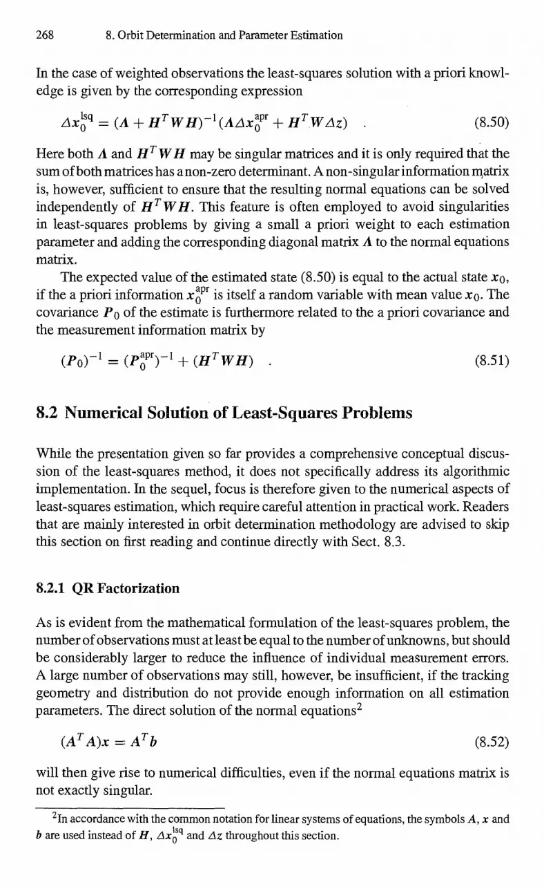
268 8. Orbit Determination and Parameter Estimation
In the case of weighted observations the least-squares solution with a priori knowl-edge is given by the corresponding expression
Axolsq = (A ± H T WHY' (AZAX aoPr HT WAz) (8.50)
Here both A and H T WH may be singular matrices and it is only required that the sum of both matrices has a non-zero determinant A non-singular information matrix is, however, sufficient to ensure that the resulting normal equations can be solved independently of H T WH. This feature is often employed to avoid singularities in least-squares problems by giving a small a priori weight to each estimation parameter and adding the corresponding diagonal matrix A to the normal equations matrix.
The expected value of the estimated state (8.50) is equal to the actual state xo, if the a priori information xaoPr is itself a random variable with mean value xo. The covariance Po of the estimate is furthermore related to the a priori covariance and the measurement information matrix by
(Po- = (Pr) -1 + (H T wH) (8.51)
8.2 Numerical Solution of Least-Squares Problems
While the presentation given so far provides a comprehensive conceptual discus-sion of the least-squares method, it does not specifically address its algorithmic implementation. In the sequel, focus is therefore given to the numerical aspects of least-squares estimation, which require careful attention in practical work. Readers that are mainly interested in orbit determination methodology are advised to skip this section on first reading and continue directly with Sect. 8.3.
8.2.1 QR Factorization
As is evident from the mathematical formulation of the least-squares problem, the number of observations must at least be equal to the number of unknowns, but should be considerably larger to reduce the influence of individual measurement errors. A large number of observations may still, however, be insufficient, if the tracking geometry and distribution do not provide enough information on all estimation parameters. The direct solution of the normal equations 2
(A T A)x = A T b (8.52)
will then give rise to numerical difficulties, even if the normal equations matrix is not exactly singular.
2 1n accordance with the common notation for linear systems of equations, the symbols A, x and b are used instead of H Axolsq and Az throughout this section.

8.2 Numerical Solution of Least-Squares Problems 269
In the case of near-singularity, the solution of the normal equations becomes ex-tremely sensitive to small errors in the normal equation matrix, which are inevitable when forming the product A T A with a limited machine accuracy. Considering, for example, the simple matrix
/1 1\ A= 8 0
\0 8
it may easily be seen that the computed value
A T A = 1 ± 82 1 ) (32<rriach)
1 1 + 82
of
( 1 1
1 1 \ )
(8.53)
(8.54)
becomes singular, if 3 is smaller than the square root of the machine accuracy Emach
(cf. Golub & Reinsch 1970). A different treatment of the least-squares problem is possible, however, that
avoids the normal equations and yields the same accuracy with single-precision computer arithmetic that otherwise requires a double-precision arithmetic. It is based on a QR factorization
An xm = Qnxn (
Rrnxin
0 (n—m)x (8.55)
of A into an orthonormal matrix Q and an upper triangular matrix R. Since Q T Q = Q = 1, the loss function may be written as
J = (b — Ax) T (b — Ax)
QTb QT A x )T (QT b QT A x )
= = ((dr) (R0)) T ((él1 . ( 0?))
(d — Rx) T (d — Rx) r ,
where Q T b has been partitioned into two vectors d and r of dimension m and n—m, respectively. This expression shows that rT r is the minimum of the loss function, which is reached for
Rx = d . (8.57)
If A has rank m, the same is also true for R and the linear system of equations -
/Ru R1,2 ' • • R1,m-1 R1,m \ X1 \ I dl \
0 R2,1 • - • R2,m-1 R2,m X2 d2
• • =-7 • (8.58) 0 0 - • - Rm-1,m Xm-1 dm-1
\ 0 0 0 Rin , m xm dm
(8.56)

270 8. Orbit Determination and Parameter Estimation
has a unique solution. No further decomposition of R is required because of its upper triangular structure. The components of x can be obtained directly from the back-substitution
xn, = dm 1 Rm ,,„
xi (di — i = m — 1, . ,1 , (8.59)
j=i+1
because all components Rij with j > j vanish. The normal equations are not re-quired anymore when using the orthogonal transformation and the corresponding numerical problems can therefore be avoided completely.
The same method of orthogonal transformations may also be applied to weighted observations, if A and b are replaced by
A' = diag(a—- • - an-1 ) A and b' = diag(a1' • • •' —1 a-1 ) b . (8.60)
Following (8.47), an a priori information matrix X can further be considered by an appropriate extension
SxaPr) A" = s
A'/) and
b„ ( (8.61)
where S denotes a square root of A (cf. (8.47)). S can easily be computed for diagonal matrices, but a Cholesky factorization or similar operation is required to obtain a representation of the form A = ST S for an arbitrary information matrix (see e.g. Schwarz 1988, Press et. al. 1992).
Finally, the QR decomposition may be employed to facilitate the computation of the covariance matrix by writing
Cov(x, x) = (A T A) -1 = (R T R) -1 = (R-1 )(R -1 ) T . (8.62)
Since R is an upper triangular matrix, the same holds for its inverse R-1 , which may conveniently be obtained by solving RR -1 = 1 with the back-substitution algorithm described above (cf. Lawson & Hanson 1974).
8.2.2 Householder Transformations
The most efficient method for performing the QR factorization is due to House-holder (1958). It involves a total of m orthonormal transformations (cf. Fig. 8.3), which subsequently annihilate the sub-diagonal elements of A yielding
.0 2U = Q T A (R0)
(8.63)
(U. ni U 2U 1) b = Q T b _ (dr)

8.2 Numerical Solution of Least-Squares Problems 271
(X X X \
0 X X
= 0 X X
0 X X
0 X X/
X X X
0 x x U2U1A = 0 0 x
0 0 x 0 0 x
(x x x\ 0 x x
U3U2U1A = 0 0 x 000
0 0 0/
Fig. 8.3. Triangularization of a 5 x 3 matrix by a sequence of Householder Transformations
An individual Householder transformation is defined as
U = (1 — 2ww T ) = U T (8.64)
where ww T denotes the outer product of a unit vector w and its transpose. The orthonormality of U follows from the fact that
u T u ==. U2 = 1 — 4ww T ± 4w w T ww T = 1 (8.65)
for w T w = I w 1 2 = 1, which also means that U is its own inverse. Since vectors at right angles to w are not affected by U, while w is mapped into —w, it may seen that U corresponds to a reflection at a hyperplane perpendicular to w (cf. Fig. 8.4).
Hyperplane I w
h
he
Fig. 8.4. Householder Transformation
By a proper choice of w, a vector h of length h can be mapped into a multiple he of the unit vector e = (1, 0, , 0) T , which is zero except for the first component. For this purpose w must be a unit vector in the direction of the difference vector hlh — e and is therefore given by
hlh—e hlh— e W
=(8.66)
jhlh — el ,/2(1 — hi/h)

272 8. Orbit Determination and Parameter Estimation
Using the same expression with h replaced by the first column vector of A, one obtains the first transformation matrix U1 = 1 — 2w 1w f that eliminates all sub-diagonal elements in the first column of A. The same principle may then be applied to determine the transformations U2, . . . , Un that convert the remaining columns and yield the desired upper triangular matrix R.
For further details on the algorithm and an efficient computer implementation of Householder transfoimations in least-squares problems the reader is referred to standard text books like Golub & van Loan (1989) or Schwarz (1988).
8.2.3 Givens Rotations
A second type of orthonormal transformations that may be used to perform a QR factorization is known as Givens rotations (Givens 1958). A single n-dimensional transformation matrix
1
U i k
+c +5
—s +c
(8.67)
is an identity matrix except for the elements
( U11 Uik) ( H-
+c +s) (± cos 0 ± sin 0 Uki Ukk —S C — sin q5 + cos 0) '
which define a rotation by an angle 0 in the (ik)-plane. Since Uliyik =-- 1, the matrix is in fact orthonormal and therefore does not change the Euclidean norm of a vector.
When applied to an n xm matrix A = (A11) from the left, U ik affects only lines i and k, while the remaining lines are unchanged. The new elements of A' — U ik A are given by
== +c Aii + s • Aki (./ =-7 1, • • • , in) Alki = —s • Aii c Akj
If c and s are chosen as Ai i )
+4 (Aki
(8.70)
(8.68)
(8.69)
then
= A' 0 .
(8.71)
8.2 Numerical Solution of Least-Squares Problems 273
/ .X X X \ x x \ / X X X \ / X X X \
X X X 0 X X 0 X X 0 X X
X X X U2,1 U i U3 2 -4 X>: X X -;3 0 X X 0 0 X -4
•X X X X X X X X X X X X
• \ : : :j
U4,1
/ X X X \ / x x x \ 0 x X 0 X X 0 X X
0 0 X U4,2 -4- 0 0 X
U 3
-44 0 0 X -4- 0 X X 0 0 X 000
: / y :j y :j
Fig. 8.5. Row-wise triangularization of an n x 3 matrix by a sequence of Givens rotations
In other words, the element A'ki vanishes. While the Householder transformation which eliminates all sub-diagonal el-
ements in a column of A, a Givens rotation reduces only one element to zero at a time This gives the freedom to process one row after another as indicated in Fig. 8.5. The complete transformation is then given by
(UnUn-1 ...U3UDA
Q T A = (Ro )
(8.72)
(UnUn-1 ...U3U2)b ---= QT b = (dr) .
Here
U1 i,max(i —1,m) • • U1,2U1,1 (8.73)
denotes the sequence of rotations required to eliminate the sub-diagonal elements in the ith row of A.
The advantage of a row-by-row transformation is that the QR factorization can already be computed with parts of the design matrix A and the vector b. Denoting the ith row of A by aT and the ith element of b by bi, the measurement equations
a• x =bi i =1, n (8.74)
can be processed one-by-one with the sequential accumulation algorithm This is illustrated in Fig. 8.6.
A sequence of in Givens rotations for each measurement transforms the given upper triangular system of linear equations Rx = d and a single data equation aT x = b into the upper triangular system 12/ x = d' and the scalar b". Assuming that the sum of the residuals squared before the triangularization was jr 1 2 , its value after processing of the new measurement equation is given by
I r i I 2 i r 12 ± (b)2 (8.75)

=-7
4di
d2 d3
R3 , 3
a3
X -7-- X =
/RÇ 1 2 3 \ ' 2
0 o' \ 0 0 0' /
(
R1,1 R2,2 R2,3 0 R2,2 R2,3 00 00
274 8. Orbit Determination and Parameter Estimation
R1,1 R1,2 R1,3
0 R2,2 R2,3 0 0 R3,3
a2 a3
Fig. 8.6. Accumulation of a data equation by Givens rotations. For each step, boxes indicate the values affected by the transformation that annihilates the leading non-zero element of the data equation.
With start values of R = 0 and b = 0 the algorithm can be applied to process all data equations recursively.
The only quantities which have to be stored during the sequential accumulation of all measurement equations are the upper triangular m xm matrix R, the vector d, and the Euclidean noun of the residual vector In . The overall storage requirements are therefore considerably smaller than for Householder factorization of an n x m design matrix A.
8.2.4 Singular Value Decomposition
Aside from the QR decomposition discussed so far, a singular value decomposition may be used to analyze a given least-squares problem and solve it in a numerically stable manner. The method is well suited to detecting and overcoming a possible singularity or near singularity of the least-squares equations and is therefore recom-mended for all ill-conditioned problems despite an increased computational effort as compared to other techniques (Lawson 1971).
The singular value decomposition of the n x m partial derivative matrix A is denoted by
A =-- UDV T (8.76)
where
D diag(di, , din ) (8.77)
is a diagonal m x m matrix. U and V are orthonormal matrices of dimension nx m and m x m, which means that both UT U and V T V are equal to the in dimensional identity matrix.
The quantities dl > d2. > dm > 0 are known as singular values. There are exactly k positive singular values for a matrix of rank k < m, whereas the remaining m — k values dk +i, . .. , dm are zero. Since
A T A = V D2 V T = Vdiag(d?, , 42 )V T , (8.78)
8.2 Numerical Solution of Least-Squares Problems 275
each column vector v i of V is an eigenvector of the normal equations matrix and the singular value di is the non-negative square root of the associated eigenvalue Xi =
In view 6f the effort required for an eigenvalue analysis it is not surprising that the computation of the singular value decomposition is also much more involved than that of a simple QR factorization. By a sequence of Householder transforma-tions, which are alternately applied from the left and right, A is first converted into a bi-diagonal matrix, in which all elements are zero except those in the diagonal and immediately above it. Next an iterative sequence of orthogonal transformations is applied, which retains the bi-diagonal form but tends to eliminate the elements in the upper diagonal and finally converges to a diagonal matrix containing the sin-gular values. For a detailed discussion of the algorithm, which is beyond the scope of this presentation, the reader is referred to Golub & Reinsch (1970) or Golub & van Loan (1989). Useful computer implementations are furthermore described in Lawson & Hanson (1974) or Press et al. (1992).
In order to illustrate the application of singular value decomposition to least-squares problems, the loss function
J = (b — Ax) T (b — Ax) (8.79)
is considered. Making use of the singular value decomposition of A and of the definitions
s = V T x t = U T b (8.80)
the condition
(A T A)x = A T b (8.81)
for the loss function minimum can be replaced by the equivalent expression
D2 s = Dt . (8.82)
For non-singular normal equations the inverse of D exists and the solution of the least-squares problem is then given by s = I:I—I t or
m uTb
i1 d1
vi (8.83)
Here u i and vi are used to denote the column vectors of U and V, respectively. If the rank of A is less than m, however, only the first k components of s can
be determined from (8.82) according to
t1 /d1
tkldk o (8.84)
0
x = V D -1 U T b
276 8. Orbit Determination and Parameter Estimation
The remaining components are arbitrary, but can be fixed by the additional require-ment of choosing x in such a way that the norm 1x1 = T X is as small as possible. Since x Tx = s T s, this requirement is equivalent to setting si = 0 for all i > k. The solution of the degenerate least-squares problem is therefore given by
k T U. b
x => , (8.85) di
which is the same as (8.83), except that all terms corresponding to zero singular values are discarded.
The same principle may also be applied in the case that A has full rank but is nevertheless near-singular as indicated by a high ratio di /dm of the largest and smallest singular value. This ratio, which is also known as the condition number of the normal equations matrix, gives a general indication of the quality with which the solution is defined by the given measurements. Since the singular values appear in the denominator of (8.83), it is evident that x is particularly sensitive to changes in the measurement vector b for small di. In order to avoid a deterioration of the solution it may therefore be preferable to neglect contributions associated with small singular values. A useful solution (Lawson 1971) of the least-squares problem may then be obtained by replacing all singular values below a given limit dmin by zero and proceeding as in the case of degenerate normal equations. As a result the loss function is slightly higher than the exact minimum. This is preferable, however, to a solution that is far off the correct value due to the strong influence of measurement errors.
As a general means for avoiding singularities one may employ a fixed limit dmin /di = a for truncating the singular values, where a is a predefined value some orders of magnitude above the machine accuracy Emach. Improved results for a particular least-squares problem may furthermore be obtained from an analysis of the sequence of singular values as well as the associated solution and loss function value. Considering
d1 d2 • • • dm
u T b 141) UT b 1 x = v1+ : v2+...+ m vm (8.86)
d1 a2 dm
J(x) = bT b _ (u T b)2 _ (4 b)2 _ . .
one may then select a value for di-nin , which reduces the loss function to an acceptable value but does not give rise to a large value of x.
8.3 Kalman Filtering
The least-squares or batch estimation method yields an estimate of the epoch state vector by processing the complete set of observations in each iteration. Therefore,

8.3 Kalman Filtering 277
it requires that all measurements to be considered in an orbit determination are available before the a priori information can be improved. This makes least-squares estimation less convenient for real-time or near-real-time applications that call for a quasi-Continuous update of the state information with each observation. In addition, the least-squares method requires the estimate of the epoch state vector to fit the entire data span, which makes it suceptible to dynamical model errors and the assumption of constant measurement biases. An alternative estimation method which copes with these problems, is known as sequential estimation or Kalman filter referring to the pioneering work of Kalman (1960) and Kalman & Bucy (1961).
8.3.1 Recursive Formulation of Least-Squares Estimation
Despite evident differences between least-squares estimation and the Kalman filter, both methods can be related to each other by a variety of intermediate formulations. In order to derive the filter equations from the least-squares method, one may con-sider a situation in which the whole set of observations is partitioned into statistically independent batches or subsets and ask how the estimated epoch state changes by including successive batches into the estimation.
Upon processing a single batch of measurements z, an a priori estimate xo— = ref X 0 ± Ax 0— and its covariance Po— are assumed to be available either from the pro-
cessing of previous data batches or from initial information. As usual, all quantities are linearized about a common reference state xroef . Based on the solution (8.50) of the general least-squares problem, the measurements and the a priori estimate can now be combined into an improved estimate
,Axt, = P (1- ((.1) (7) -1 ,Ax (7, ± H T W Az) (8.87)
Here, the a-posteriori covariance matrix
(-1)8-) = ((P)_1 ± (H T W H)) 1 (8.88)
represents the increased knowledge of xo resulting from both the a priori informa-tion and the latest data batch.
In order to relate the new estimate to the previous estimate x 0— , one substi- tutes the a priori information matrix by the difference
up0-1 up-01-)-1 (HTwH) (8.89)
of the a-posteriori information matrix and the measurement information matrix. This yields the basic expression
Axt, = Lx ± Pt, HT W (Liz — Htlx0— ) (8.90)
for a recursive formulation of least-squares estimation. The matrix
K = PHTW (8.91)
278 8. Orbit Determination and Parameter Estimation
maps the residuals
p = Az — HAx o— = z — h(xr) — HAx o— (8.92)
into an appropriate correction of the estimate x o— and is known as Kalman gain. The vector p represents residuals with respect to reference values defined by the estimate xo— . It is computed from the measurements z, the reference-model observations h (x roef ) and a linear correction H (x — x roef ) that accounts for the difference between xo— and the reference state.
A recursive formulation of the orbit determination problem as given above has already been suggested by Swerling (1959) but could not gain widespread acceptance. For practical applications (8.90) suffers from the fact that the direct computation of the covariance matrix .138- from (8.88) requires the inversion of an m x m-matrix in each step with m denoting the dimension of the estimation vector xo. To remove this deficiency the product K = PHT W can be replaced by the equivalent expression
K p o— HT ( w - 1 Hp o— HT) 1 (8.93)
Even though this expression seems to be more involved at first sight, it turns out to be more efficient, if the size of each data set is small compared to the dimension m. In particular, this is the case when each batch consists of a single observation only. The matrix is then reduced to a scalar quantity and the inverse is obtained by a simple division.
The validity of substitution (8.93) follows from the relation
HT HTw H p H T ____=. HT H T wH p H T
H T 4 (1 4 —1 H P HT ) = (p-1 ± HT w p H T
(p-1 ± H T w H)-1 H T w = p H T (ur-1 ffv H P H T ) -1 , (8.94)
which is based on a matrix inversion lemma attributed to A. S. Householder see Bierman 1977). Considering, furthemiore, the identities
= 13 8 (P8- ) -1 = 1) 8- ((PD -1 + HT W H ) = P ± (Pt, H T W)H P (7, = K H 13 (7, ,
(8.95)
the Kalman gain K may also be employed to compute the updated covariance matrix
= (1 — K H)P (1, (8.96)
without the need to invert the normal equations matrix.

8.3 Kalman Filtering 279
Recursive Estimation Algorithm
Combining the results obtained so far, the recursive least-squares estimation al-gorithm proceeds in the following way. Given the a priori and reference state xg, the associated covariance P2, and the measurement batches zi (I = 1, , N) recursive estimates x6 of the epoch state xo as well as the associated covariance matrices P6 are computed for each batch (I =1, N) via the steps Kalman-gain computation, epoch state vector update and epoch covariance update
K1 H poi—i HD-1
I-1 X = X0 KI - 111(4) — H1(4' — Ax)) 1
6 (1— ICI-111) 13 01-1
(8.97)
While the above expressions are general enough to handle an arbitrary number of measurements per batch, the Kalman-gain computation is optimized for processing only a small number of measurements per step. Thus each batch will usually com-prise a vector of measurement taken at a common epoch with possible correlations or a single, scalar observation. Uncorrelated measurements can always be processed one at a time3 , in which case the vector zi is replaced by the scalar measurement zi , the weighting matrix W1 is replaced by the scalar weighting factor wi = and the Kalman gain matrix K1 becomes a vector IQ with the same dimension (m) as the state vector x0. Similarly, the Jacobian H1 = 8Z1 /8x0 reduces to a 1 x m matrix (i.e. a row vector), which means that products of the foini HPHT or Hx are scalar quantities, too. The resulting set of equations may then be written as
p (0,12 ± Hi p io—i HT ) -1
x io-1 ki(zi — hi (4) — H — xg))
(8.98)
= (1— kiHi) Pio-1
In the expression for the covariance update care should be taken that kiHi denotes the dyadic product of the Kalman gain (a column vector) and the measurement partials (a row vector). Unlike the dot product that results in a scalar value, the dyadic product yields an m x m matrix.
Independent of the subdivision of the measurement vector into individual batches the state estimate and covariance obtained after processing the last ob-servation is identical to the one that would have been obtained in the first iteration of the standard least-squares method. The recursive formulation may be used, how-ever, to obtain state estimates and covariances after each measurement without the need to collect all observations before inverting the normal equations.
3 Appropriate transformations for the treatment of vector observations with correlated measure-ment errors are discussed in Andrews (1968).

280 8. Orbit Determination and Parameter Estimation
8.3.2 Sequential Estimation
Even though the recursive least-squares estimation allows an on-line monitoring of the way in which each observation improves the epoch state estimate, the method cannot readily be used to obtain estimates of the state vector at the measurement times. This requires a propagation of both the state vector and its covariance between the times of successive observations and yields the classical sequential estimation or Kalman filter algorithm
In the sequel it is assumed that a single data set zi contains only observations taken at the same time ti . As an example a batch of measurements may consist of a pair of azimuth/elevation values that have been obtained simultaneously from the antenna or it may consist of a single range measurement taken independently. Starting from the state and covariance at a previous epoch ti_i the measurement vector zi can then be used to obtain an improved state vector at the measurement epoch ti together with the associated covariance. For that purpose let
ref ref X i = X (ti ; X (to) = X \ 0 = X (ti X (4-1) X ef i ) (8.99)
denote the state vector that is obtained by propagating the epoch reference state xoref from to to ti or, alternatively, by propagating xr. d from ti_i to ti . Furthermore, / —1 let
aX r. ef (Pi = 0(t, ti-1) = ref = (ti, t0) 0 (ti-1, t0) -1 (8.100)
A,
denote the state transition matrix from epoch ti _i to epoch ti, which follows from the solution of the appropriate variational equations.
Using these quantities, the state vector 4- (obtained from data up to and including time t1 _1) may be employed to predict an a priori state vector
X: X ref (xi /-1 / —1 (8.101)
at epoch ti . The corresponding a priori covariance at that epoch follows from
=
E (0i(xt 1 ))(xt —E(xt i )) T OT)
-13- 1 4'T
where P+— is the covariance of x . t Since the observations zi have not yet been /1 taken into account, the information contained in x ï and PT is exactly the same as that in x and P» except for the epoch to which these values refer.
In order to incorporate the new measurements and update the a priori informa-tion, the residual vector pi is expressed as a function of quantities referring to ti
instead of to:
(8.102)
pi = zi — hi(xroef ) — i(x (7, — xroef)
= zi — g(x) — Gi(xT — xrief ) . (8.103)

8.3 Kalman Filtering 281
Here hi, which models the observations at time ti in terms of the state at epoch to, has been replaced by the equivalent function
gi (ti, x(4)) = hi(ti,x(to))
(8.104)
which models the observations in terms of the state vector at the measurement time (cf. (8.5)). Accordingly, the Jacobian H i has been factored into
azi
Hi azi axiref
axroef = axef axroef Gig) (ti, to) (8.105)
to obtain the desired expression for the residual vector. Similarly, the Kalman gain is formulated as
Ki = PT GT (Wï l GiPÏGT) -1 , (8.106)
which maps the residuals into a state vector correction at the measurement epoch ti.
Linearized Kalman Filter
Combining the results obtained so far, the sequential estimation algorithm or Kalman filter proceeds by computing estimates xt of the state vector at the measurement times ti (i = 1, .. . , n) as well as the associated covariance matrices Pt via se-quential time and measurement update steps (Fig. 8.7).
The time update phase starts with the integration of the equation of motion and the variational equations from ti_i to ti in order to obtain the reference state xii-ef and the transition matrix Oi . Using these quantities the previous
Estimated Trajectory
Reference Trajectory
xoref po
Fig. 8.7. The linearized Kalman filter (LKF) refers all measurements and state corrections to a common reference trajectory. Initially, when the covariance is still small, the filter output closely matches the observations (shaded circles). Later on, the filter approaches the true trajectory and becomes less sensitive to new data. Due to the increasing difference between the reference state and the estimated trajectory the filter output may become erroneous in case of non-linearities.

282 8. Orbit Determination and Parameter Estimation
estimate xt and the associated covariance matrix Pt may then be propagated / —1 —1 to the time ti of the most recent measurement:
x7 ref — x i ± ip i (x+ _ X1
ref \ — 1 i — )
P7 P t (PT •
(8.107)
The subsequent measurement update phase comprises the computation of the Kalman gain as well the state and covariance update:
K =Pï GT (Wï l Gi PT GT) -1
= x7 Ki (zi g ) Gi (xi xr.e f ))
(8.108)
Pt = (1— K iGi ) Pï
The filter starts with x0+ = xroef and Po+ = Proef .
8.3.3 Extended Kalman Filter
The sequential processing of a given set of measurements corresponds essentially to a single iteration of the least-squares estimation method. For a successful appli-cation of the basic Kalman filter the deviations between the reference state and the estimated state must therefore be small enough to neglect any non-linearities in the system dynamics and the measurement modeling. In order to avoid this restriction and make full use of the advantages of sequential estimation for orbit determina-tion purposes the Extended Kalman Filter has been developed (Fig. 8.8). It may be derived from the basic Kalman filter by resetting the reference state x 1 to the estimate x» 1 at the start of each step.
The time update phase of the extended filter thus comprises the propagation of the previous estimate xt from ti_i to ti and the simultaneous solution of the
Estimated Trajectory
x1 f, PI-
xoref, po
Fig. 8.8. The extended Kalman filter (EKF) makes use of the latest estimate to propagate the state vector and the state transition matrix. This makes the EKF less sensitive to non-linearities than the linearized Kalman filter.

8.3 Kalman Filtering 283
variational equations for the state transition matrix. As a result one obtains the predicted state vector xï and the associated covariance matrix PI:
P7
= x (ti x(ti-1) = 41 1)
= 4̀ i Pt 4)T (8.109)
The measurement update phase remains the same as for the basic Kalman filter, except for the simplified state update equation:
Ki = P i— GT (W i-1 GiPi— GT) -1
xt = x i— ± Ki (zi — gi (x i— )) (8.110)
P» = (1— KiGi) P
The filter starts with xo = x 0aPr and Po = PoaPr . Due to the regular update of the reference state non-linearities are reduced to a minimum and within a few steps the filter may arrive at a solution that would otherwise require multiple iterations.
Some price has to be paid, however, for the improved perfoiniance of the extended Kalman filter that results from an increased computational effort for the state and covariance propagation. When using the same reference orbit for the processing of all measurements in the basic Kalman filter, only one initial value problem has to be solved by numerical integration. The reference state and state transition matrix at the time of a particular measurement can then be obtained by interpolation independent of the stepsize control employed for the integration. In case of the extended filter a separate initial value problem has to be solved for each measurement to be processed, and the required restart of the integration method may then result in a considerable increase in computing time. Typically, low-order-single-step integration methods like the 4th-order Runge—Kutta scheme are therefore employed in real-time orbit deteimination programs based on extended Kalman filters.
8.3.4 Factorization Methods
As with the batch least-squares method the perfoimance of a Kalman filter may deteriorate considerably under certain conditions unless special care is taken to reduce the impact of numerical errors in the computation. The problem is more serious, however, in case of the Kalman filter, since it must often be implemented in single precision arithmetic to speed up the computation in real-time or on-board applications.
A simple, but efficient method of coping with these difficulties consists of using the Joseph algorithm (Bucy & Joseph 1968) for the update of the covariance matrix. Since the covariance Pi becomes smaller and smaller as new observations are processed, round-off errors in the update foimulas
= (1— KiGi)P i— (8.111)
284 8. Orbit Determination and Parameter Estimation
may ultimately result in a matrix with small negative or zero eigenvalues, which does not represent the true covariance matrix anymore and leads to a failure of the filtering algorithm. Rewriting the update foimula as
Pt = (1— KiGi)P7
(1— K iGi )P1 — Pt GT KT PI- GT. KT (8.112)
= ( 1 — KiGi) PT (1— KiGi)T G T K T and making use of Ki = Pt GT W one may, however, obtain an alternative update formula
Pt = (1— K i Gi) P (1— KiGi) T KiW KT , (8.113)
which ensures that t is always positive definite irrespective of errors in Ki or 1 — KiGi. With minor modifications the stabilized update, which has here been derived for the extended Kalman filter, may equally well be applied to other forms of recursive and sequential estimators.
Further methods, which are more closely related to techniques employed for a numerical stable solution of the least-squares problem, make use of an appropriate factorization of the covariance matrix (or information matrix). By updating the factorization instead of the covariance matrix an annihilation of near-equal numbers is avoided and the filter becomes less sensitive to round-off errors. Single precision arithmetic may then be used to obtain an accuracy that would otherwise require twice the word length.
The square root factorization method due to Potter and Andrews (see Battin 1987, Bierman 1977) utilizes a factorization of the foul'
= SS T (8.114)
and replaces the update foimula- for Pi by an update formula for its square root Si. An equally stable but computationally more efficient method is the UDU T -Filter developed by Biennan (1977), which makes use of a factorization into an upper triangular matrix U and a diagonal matrix D.
Further details and reviews of various types of square root filters and factor-ization methods for sequential estimation are given in Kaminsky et al. (1971) and Bierman (1977). As regards the computer performance and resource requirements, factorization methods have been shown to be fully compatible with simple for-mulations of the Kalman filter provided that they are coded in an optimal way (cf. Bielinan 1977, Campbell et al. 1983). For practical applications the use of advanced Kalman filter implementations is considerably facilitated by appropriate software libraries (see e.g. Bieinian & Bieiman 1984, Branyon et al. 1988).
8.3.5 Process Noise
A phenomenon that is likely to occur in the practical application of a Kalman filter is the filter's divergence from the actual solution after processing a certain amount
8.3 Kalman Filtering 285
of .data. Initially, the state uncertainty and the corresponding covariance matrix is sufficiently high to allow an appropriate correction of the state vector with each new observation. As more and more measurements are processed, however, both the covariance Matrix and the Kalman gain approach zero, which may ultimately inhibit further improvements of the state vector. Any errors that arise from small non-linearities, round-off errors or simplifications of the force and measurement model will then be propagated without further correction by subsequent measurements and result in an erroneous and diverging state estimate.
A possible way of coping with this problem consists of adding a small noise teiin to the covariance matrix in each step that inhibits the matrix from getting smaller and smaller. The method arises from the concept of process noise, which affects the system dynamics in much the same way as the measurement noise affects the observations. The differential equation describing the evolution of the state vector is supplemented by a teiin u(t) to represent stochastic modeling errors inherent in the description of the dynamical system:
= f (t , x) u(t) . (8.115)
As an approximation of the actual modeling errors, u(t) is assumed to be a random variable with mean value
E(u(t)) = 0 (8.116)
and covariance
E(u(t)u(t I)) = Q(t)8(t — t') (8.117)
The covariance may be time-dependent, but no time correlation is assumed to exist as expressed by the Dirac delta function 8 (t — t'). Frequently, the latter property is expressed by the teim white noise in contrast to colored noise which exhibits a correlation in time.
Since the expected value of the process noise is zero, it does not affect the orbit on the average. The state estimate may therefore be propagated as usual by solving the equation of motion without consideration of the noise teiiii. The covariance propagation formula is modified, however, to account for an increased state uncertainty due to the presence of process noise. Since each time interval [t, t--1-dt] within ti_i and ti gives rise to a contribution Q(t)dt to the covariance at time t, the predicted covariance at ti is given by
(1) (ti, 1 0 T (ti, ti_i) f (ti, t)Q(t)O T (te, t)dt , (8.118)
tu
where the integral can be obtained analytically for simple dynamical systems (Brown & Hwang 1996). Alternatively, the matrix differential equation
dP (t) fa f\ /apT
dt ) (t) P (t) Q(t) x (8.119)

286 8. Orbit Determination and Parameter Estimation
with initial conditions P(ti_i ) = P 1 is integrated along with the state vector in the continuous discrete Kalman filter to obtain continuous covariance information between the measurement updates (see. e.g. Halain et al. 1998).
If Q does not depend on t and if the interval between subsequent measurements is small enough to neglect deviations of the state transition matrix from unity, the covariance propagation may further be simplified yielding .
' = ck(ti, i ck T (ti, t1 _1) Q (ti — t 1 _1) (8.120)
The Q-matrix thus contributes to an increase of the covariance in each step and can be used to balance the subsequent decrease due to the processing of a measurement.
Taking into account process noise gives the filter a fading memory characteris-tics, which means that past observations have a gradually decreasing effect on the state estimate. By increasing the Q-matrix, both the covariance and the Kalman gain increase, thus making the filter more sensitive to new observations. A small value of the Q-matrix is necessary, on the other hand, to avoid large state corrections in the event of erroneous observations. In practical applications the Q-matrix may be deteimined by simulations in order to find a proper balance between process and measurement noise and ensure an optimum filter perfoimance.
An alternative approach has been developed by Wright (1981), which builds a covariance based on physical models of error contributions such as drag, grav-ity, and propulsion system perfoimance as well as measurement characteristics. This technique is particularly robust and overcomes problems encountered in the traditional modeling of process noise.
8.4 Comparison of Batch and Sequential Estimation
As has been pointed out in the introduction, the common estimation techniques employed for orbit determination purposes are closely related to each other and a smooth transition is possible from the batch least-squares method to the various foul's of Kalman filter. Each type of estimator has inherent advantages and disad-vantages and a trade-off is usually required to select the most suitable estimation method for a particular application:
Measurement processing and state correction: The classic batch least-squares method computes the epoch state estimate after processing the full set of ob-servations. If improved epoch state estimates are required after each measure-ment, a foimulation involving Givens rotations or the recursive least-squares method may be used. The Kalman filter in contrast processes a single scalar or vector measurement at a time and yields sequential state estimates at the measurement times.
• Treatment of non-linearities: Due to the non-linear relation between the epoch state vector and the modeled measurements, multiple iterations are required in the least-squares method to compute a state estimate that actually mini-mizes the loss function. Using the extended Kalman filter these iterations may
8.4 Comparison of Batch and Sequential Estimation 287
in general be avoided, since the reference solution is changed with each ob-servation. Problems are more likely, however, in the case of large deviations between the a priori state and the actual state as well as poor management of the covariance.
• Computer implementation: When using a Kalman filter for orbit determi-nation there is no need for storing measurements from previous time steps. Storage requirements are therefore smaller than for the least-squares method, in which various data have to be stored for subsequent iterations.
• Numerical stability: Both filters and least-squares estimators may be sub-ject to numerical problems in the case of bad observability as indicated by an ill-conditioned noinial equations matrix or covariance matrix. Numeri-cally stable algorithms employing different types of matrix factorizations are available, however, for both estimation techniques. The increase in comput-ing effort and storage requirement is generally negligible and the stabilized algorithms can therefore be recommended for most applications.
• Divergence: A divergence of the least-squares solution from one iteration to the next may occur in rare instances of bad observability, a bad initial state estimate and high non-linearities. All of these could also cause a Kalman filter to diverge. In addition divergence of the state estimate from the true solution is likely to occur in a Kalman filter, when the covariance becomes small and the filter gets insensitive to new observations. Process noise may be incorporated into the filter to avoid divergence but heuristic assumptions and simulations are often required to determine the appropriate noise model for a particular situation, unless a physical description of the process noise density matrix is available.
• Process noise: A unique feature of Kalman filters as compared to the least-squares method is the incorporation of process noise into the estimation pro-cess. Aside from being required to avoid filter divergence problems, it may be employed to get more realistic covariance predictions in the presence of unmodeled accelerations. Furthermore, it may be used to reduce the influ-ence of past observations on the state estimate as compared to more recent observations.
• Influence of bad data points: The batch estimator and the recursive least-squares method process all data points using a common reference trajectory. This facilitates the handling of bad data points, which may be recognized by residuals that are considerably larger than the average value. In general the least-squares technique is therefore more robust and easier to handle than the Kalman filter. The latter requires a careful balancing between a priori covariance, measurement weighting and process noise to allow a rejection of bad data points. For example, a Q-matrix, which is too large, will allow larger measurement errors to be accepted. One which is too small may allow good measurements to be rejected.

288 8. Orbit Determination and Parameter Estimation
Traditional applications in which Kalman filters are preferred to batch least-squares techniques include the on-board navigation of manned or unmanned spacecraft requiring a real-time state estimate (Battin & Levine 1970). Filtering techniques are, furthermore, used in the field of interplanetary orbit determination and navigation. By incorporating appropriate process noise, unmodeled statistical accelerations due to attitude thruster activities or radiation pressure modeling simplifications may be accounted for, which provides more realistic estimates of the injection error near the target planet (Campbell et al. 1983).
The batch least-squares method on the other hand is commonly employed for off-line orbit determination of Earth-bound satellites (Long et al. 1989, Soop 1983) and for the estimation of geodetic parameters from satellite orbits (McCarthy et al. 1993). A comparison indicating a good agreement of orbit determination results from precision batch least-squares and sequential estimation programs (GTDS, RTOD/E) for satellites tracked by the Tracking Data and Relay Satellite System (TDRSS) has recently been established by a study conducted on behalf of the God-dard Space Flight Center (Oza et al. 1992) Similar conclusions have been obtained by Halain et al. (1998) for single and multi-station tracking of geostationary satel-lites.

Exercises 289
Exercises
Exercise 8.1 (Givens Rotations) The following sequence of measurements zi of a physical quantity z(t) has been collected at non-equidistant times ti :
i 0 1 2 3 4 5 6 ti 0.04 0.32 0.51 0.73 1.03 1.42 1.60 zi 2.63 1.18 1.16 1.54 2.65 5.41 7.67
From a graphical representation of the measurements a quadratic relation between z and t may be suspected. Employ a least-squares estimation with Givens rotations to adjust a second-order polynomial
z(t) = co + ci -t + c2.t 2 (8.121)
to the data points (adopted from Schwarz 1988).
Solution: Inserting the measurement zi and times ti into (8.121) yields an overde-termined linear system of equations Ax = b with
A =
(1.0 1.0 1.0 1.0 1 .0 1.0
\1.0
0.04 0.32 0.51 0.73 1.03 1.42 1.60
0.0016\ 0.1024
0.2601 0.5329 1.0609 2.0164 2.5600/
co) x = (ci
c2 b =
12.63\ 1.18 1.16 1.54 2.65 5.41
\7.67/
Upon processing each individual data equation using Givens rotations, the following values for the square-root information matrix R and the transformed measurement vector d are obtained:
Ro = .
R1 =
R2 =
R3 =
R6 =
(+1.0000 +0.0000 +0.0000
(+1.4142 +0.0000 +0.0000
(+1.7321 +0.0000 +0.0000
(+2.0000 +0.0000 +0.0000
(+2.6458 +0.0000 +0.0000
+0.0400 +0.0000 +0.0000
+0.2546 +0.1980 +0.0000
+0.5023 +0.3344 +0.0000
+0.8000 +0.5070 +0.0000
+2.1355 +1.4050 +0.0000
+0.0016 +0.0000 +0.0000
+0.0735 +0.0713 +0.0000
+0.2102 +0.1791 +0.0432
+0.4485 +0.3860 +0.1093
+2.4697 +2.3719 +0.6179
+2.6300 ( +0.0000
+0.0000 )
+2.6941 dl = -1.0253
( +0.0000
+2.8694 d2 = -1.0973
+0.4660
()
(+3.2550) d3 = -0.7997
+0.8806
+8.4059 d6 = +4.9335
+3.4646)
Using backsubstitution, one finally obtains the solution: ( co +2.749198 ci) = d6 = (-5.954657 c2 +5.607247

290 8. Orbit Determination and Parameter Estimation
Exercise 8.2 (Least-Squares Orbit Determination) The Bangalore ground sta-tion, located in India at R = (+1344.0, +6069.0, 1429.0) km, has collected six sets of range and angle tracking data of a telecommunications satellite in geosta-tionary transfer orbit:
Date UTC A [°] E p [km] 1995/03/30 00:20:00.0 196.280 49.179 6606.330 1995/03/30 00:40:00.0 148.760 55.273 11459.583 1995/03/30 01:00:00.0 133.129 53.164 15939.297 1995/03/30 01:20:00.0 126.894 52.313 19747.028 1995/03/30 01:40:00.0 124.077 52.575 22978.426 1995/03/30 02:00:00.0 122.943 53.574 25728.145
According to the launcher agency, the nominal position and velocity with respect to the Earth equator and equinox are given by
r (to) = (-6335.0, -3728.0, -579.0)km v (to) = (+2.1680, -9.2630, -1.0795) km/s
at the time to = 1995/03/30 00:00 UTC of injection. Determine the achieved injec-tion state from the above observations using a batch least-squares fit. How many iterations are required and how accurate is your result, assuming that the standard deviation of the measurements amounts to o-A = 0.01 0 - cos(E), (TE = 0.01° and a = 10m?
Hint: The above observations match a Keplerian orbit with epoch state vector
r (to) = (-6345 .0 , -3723.0, -580.0)1cm v(to) = (+2.1690, -9.2660, -1.0790)1cm/s
neglecting precession, nutation, UT1-UTC, light time and refraction. The same model is recommended for the orbit determination process.
Solution: The following residuals are obtained in the first and second iteration:
1st Iteration 2nd Iteration Date UTC A [°] E [O] p [m] A [°] E [3 ] p [m]
1995/03/30 00:20:00.0 0.100 -0.002 5479.1 0.001 0.002 -4.5 1995/03/30 00:40:00.0 0.063 0.044 14250.5 -0.001 0.001 0.8 1995/03/30 01:00:00.0 0.055 0.063 28320.9 -0.001 0.001 10.0 1995/03/30 01:20:00.0 0.065 0.081 45272.4 -0.001 0.000 24.7 1995/03/30 01:40:00.0 0.083 0.100 64708.7 -0.001 0.000 43.7 1995/03/30 02:00:00.0 0.108 0.120 86542.9 -0.000 0.000 66.1
Thereafter, all residuals vanish to the given number of digits. Likewise, the a priori state vector is corrected to the final value within two iterations:
Parameter A priori A1 A2 Final x [m] -6335000.0 -9946.9 -53.1 -6345000.0 276.9 Y -3728000.0 5188.3 -188.3 -3723000.0 737.0 z [m] -579000.0 -1124.8 124.8 -580000.0 829.8
[m/s] 2168.0000 0.8918 0.1082 2169.0000 0.6520 [m/s] -9263.0000 -3.0983 0.0983 -9266.0000 0.5226 [m/s] -1079.5000 0.3216 0.1784 -1079.0000 0.3695
The standard deviation of the achieved estimate amounts to roughly 1 km in position and 1 m/s in velocity.
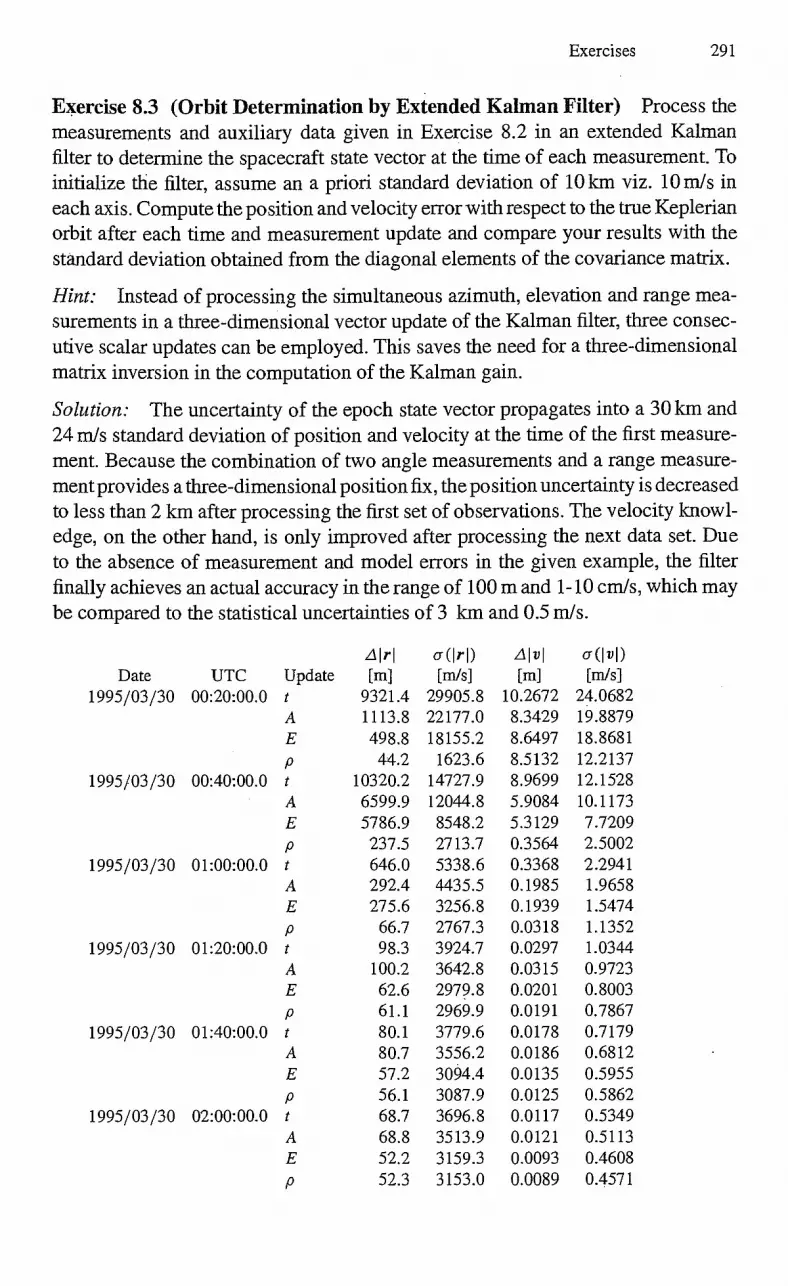
Exercises 291
Exercise 8.3 (Orbit Determination by Extended Kalman Filter) Process the measurements and auxiliary data given in Exercise 8.2 in an extended Kalman filter to determine the spacecraft state vector at the time of each measurement. To initialize the filter, assume an a priori standard deviation of 10 km viz. 10 m/s in each axis. Compute the position and velocity error with respect to the true Keplerian orbit after each time and measurement update and compare your results with the standard deviation obtained from the diagonal elements of the covariance matrix.
Hint: Instead of processing the simultaneous azimuth, elevation and range mea-surements in a three-dimensional vector update of the Kalman filter, three consec-utive scalar updates can be employed. This saves the need for a three-dimensional matrix inversion in the computation of the Kalman gain.
Solution: The uncertainty of the epoch state vector propagates into a 30 km and 24 m/s standard deviation of position and velocity at the time of the first measure-ment. Because the combination of two angle measurements and a range measure-ment provides a three-dimensional position fix, the position uncertainty is decreased to less than 2 km after processing the first set of observations. The velocity knowl-edge, on the other hand, is only improved after processing the next data set. Due to the absence of measurement and model errors in the given example, the filter finally achieves an actual accuracy in the range of 100m and 1-10 cm/s, which may be compared to the statistical uncertainties of 3 km and 0.5 m/s.
Date UTC Update Alrl [m]
a(Id ) [mis]
Alvl [m]
0- (1 13 1) [mis]
1995/03/30 00:20:00.0 t 9321.4 29905.8 10.2672 24.0682 A 1113.8 22177.0 8.3429 19.8879
498,8 18155.2 8.6497 18.8681 44.2 1623.6 8.5132 12.2137
1995/03/30 00:40:00.0 t 10320.2 14727.9 8.9699 12.1528 A 6599.9 12044.8 5.9084 10.1173
5786.9 8548.2 5.3129 7.7209 237.5 2713.7 0.3564 2.5002
1995/03/30 01:00:00.0 t 646.0 5338.6 0.3368 2.2941 A 292.4 4435.5 0.1985 1.9658
275.6 3256.8 0.1939 1.5474 66.7 2767.3 0.0318 1.1352
1995/03/30 01:20:00.0 t 98.3 3924.7 0.0297 1.0344 A 100.2 3642.8 0.0315 0.9723
62.6 2979.8 0.0201 0.8003 61.1 2969.9 0.0191 0.7867
1995/03/30 01:40:00.0 t 80.1 3779.6 0.0178 0.7179 A 80.7 3556.2 0.0186 0.6812
57.2 3094.4 0.0135 0.5955 56.1 3087.9 0.0125 0.5862
1995/03/30 02:00:00.0 t 68.7 3696.8 0.0117 0.5349 A 68.8 3513.9 0.0121 0.5113
52.2 3159.3 0.0093 0.4608 52.3 3153.0 0.0089 0.4571

9. Applications
The presentation of statistical estimation methods given in the previous chapter forms the final building block in the derivation of fundamental models and methods for satellite orbit prediction and determination. Focus is now given to the practical aspects by discussing selected applications, each of which emphasizes certain key elements:
• an Orbit Determination Error Analysis illustrates the use of consider covari-ance studies in the design of tracking systems for geostationary communica-tions satellites,
• a section on Real-Time Orbit Determination discusses the design and ap-plication of a dynamical Kalman filter for autonomous orbit determination based on on-board navigation measurements and, finally,
• concepts of satellite-satellite tracking and multi-satellite orbit adjustment are demonstrated in the section on Relay Satellite Orbit Determination.
Each section comprises a dedicated computer program, which deepens the under-standing of the interaction of numerical trajectory models, measurement processing, and estimation methods in related software systems. Upon performing realistic case studies and processing real-life data, the reader should be able to collect hands-on experience and gain a better understanding of the underlying models and methods.
9.1 Orbit Determination Error Analysis
In the mission design of geostationary satellite projects, certain requirements on the orbit determination accuracy are commonly imposed to ensure safe and fuel-optimal spacecraft control. Each satellite must be maintained within given limits of the sub-satellite longitude and latitude that have been assigned by international agreement. A minimum position knowledge is required e.g. to avoid violations of the specified deadband and to avoid proximities with other satellites. A consider covariance analysis is helpful to answer the following questions:
• Can a given knowledge of the orbital elements be achieved with the planned tracking configuration?
• What is the impact of the systematic errors in the station location or the ranging calibration onto the resulting orbit determination accuracy?
• How quickly, and to what accuracy can the orbit be recovered after a maneuver and how does the maneuver calibration uncertainty affect the evolution of the predicted spacecraft orbit?

+1
1-i (Equinox Y) Equator
294 9. Applications
While answers to the above questions might also be obtained from a Monte-Carlo simulation, a large number of cases would be required to obtain the desired statistical information. Using the type of orbit determination error analysis described below, results can generally be obtained much faster and with less computational effort.
Fig. 9.1. Motion of a satellite in the vicinity of a geostationary point
9.1.1 A Linearized Orbit Model
As their name implies, geostationary satellites maintain an essentially fixed position with respect to the surface of the Earth. This is made possible by inserting the spacecraft into a circular, equatorial orbit at an altitude of roughly 36 000 km Here its mean motion matches the Earth's rotation rate of one revolution per 23 1i56m and the spacecraft thus remains fixed with respect to the surface of the Earth. While an ideal geostationary motion is prevented by the perturbations of the Earth's aspherical gravity field, the lunisolar gravity and the solar radiation pressure, it is common practice to actively control a satellite in a box of 100-150 km width around a nominal geostationary longitude.
Due to its special nature the actual motion of a (near-)geostationary satellite may conveniently be described in a co-rotating equatorial reference frame, which is centered at the ideal geostationary position (Fig. 9.1). The coordinates r = (x, y, z) T in this frame are related to the inertial coordinates (as referred to the true equator and equinox) by the relation
r = Rz (G1 + X0) "i; — (ao, 0, 0) T . (9.1)
Here À0 and a() = 42 164 0 km denote the geographic longitude and the radius of the geostationary reference point.
The transformation into the rotating reference frame gives rise to Coriolis terms and centripetal accelerations, which may, however, be simplified by linearization around the circular reference orbit. The resulting equations of motion
— 2n5) — 3n2x = ax j+2n = ay (9.2)
n2z = az

9.1 Orbit Determination Error Analysis 295
relate the coordinates x (radial direction), y (along-track direction), and z (cross-track direction) to the perturbing accelerations (ax , ay , az ) and are known as Hill's equations or Clohessy—Wiltshire equations (Clohessy & Wiltshire 1960). The quan-tity n denotes the mean motion of the reference orbit and is equal to the Earth's rotation rate when considering the motion near a geostationary point.
In the simplifying case of unperturbed, Keplerian motion the equations can be integrated in closed form (cf. Vallado 1997). For given initial conditions Yo = (xo, yo, zo, .0) 7' the position at time t after the initial epoch is given by
x(t) = —(3x0+40/n)cos(nt) + (io/n)sin(nt) + (4x0+2k)/n)
At) = -F(6xo+4570/n)sin(nt) + (2.io/n)cos(nt) —(6x0+3.Yo/n) (nt) + (yo—Zio/n) (9.3)
z(t) = (zo)cos(nt) + (io/n)sin(nt) .
As may already be recognized from the Clohessy—Wiltshire equations, the mo-tion along the z-axis (i.e. in north-south direction) is a harmonic oscillation that is completely decoupled from the motion in the x-y-plane. The motion within the equatorial plane is more complex and comprises a constant offset from the geo-stationary reference point, a linear drift in the along-track direction (y-axis) and a superimposed oscillation. The latter results in an ellipse which is twice as large in the along-track direction as in the radial direction. The constant offset
Aa =4x0 40/n (9.4)
in radial direction corresponds to a difference between the actual semi-major axis and the geostationary radius. It is responsible for the observed drift of
aAn = --3
nAa = —(6nx0 3.5 10) 2 (9.5)
in the +y-direction (see (9.3)). The above equations may be supplemented by the corresponding expressions
for the velocity vector and rearranged to obtain a linear relation
y(t) = Yo (9.6)
between the instantaneous state vector y and the epoch state vector y o . The state transition matrix clo, which maps the initial state to the state at time t, does not depend on the actual orbit and involves time-dependent terms only. It is given by the expression
4 — 3c 0 0 sIn 2(1 — c)/n 0 6(s — nt) 1 0 2(c — 1)/n 4s In — 3t 0
0 0 c 0 0 s / n 3ns 0 0 c 2s 0
6n(c — 1) 0 0 —2s 4c — 3 0 0 0 —ns 0 0
, (9.7) of) (t) =

296 9. Applications
where s and c denote the sine and cosine of phase angle nt, respectively. Within the linearized orbit model, the motion of a (near-)geostationary satellite may conve-niently be described in terms of the epoch state vector using elementary linear and harmonic functions of time. Even more, the partial derivatives with respect to the initial values are obtained at no extra cost along with the prediction of the trajectory itself.
Based on the description of the spacecraft orbit in the geostationary reference frame, one may compute the modeled observations (azimuth A, elevation E, and range p) using suitably adapted relations for the topocentric position of the satellite. For a station at longitude X = X0 + AX, latitude yo and Greenwich coordinates R, the spacecraft position s measured in the local east, north, and zenith direction is given by
s = so + Er
with
(9.8)
so = E ((ao, 0, 0) T —
and f — sin AX
R(X0)R)
+ cos AX 0
(9.9)
E = — sin (p cos AX — sin (p sin AX + cos (p )
(9.10) + cos (p cos AX + cos go sin AX + sin go
Here AX is the ground station longitude relative to the direction of geostationary point, which is offset from the Greenwich meridian by the angle Xo. Azimuth, elevation, and range as well as the associated partial derivatives with respect to the spacecraft position in the geostationary frame are then obtained using relations presented earlier (cf. Chaps. 6 & 7).
Due to the near-constant observation geometry, the partial derivatives can be evaluated at the nominal geostationary point (i.e. r = 0) without sacrificing accu-racy. As a consequence the partial derivatives
a (A, E, p) a (A, E, p)
ayo
ar - a (A, E, p) = E 4'1...3,1_6 (9.11)
r.o °Y0 8 s
may be factored into the product of a term that depends only on the station geom-etry and a second term that depends only on the measurement time with respect to initial epoch. This factorization unveils a fundamental degeneracy of the geo-stationary orbit determination problem, which is discussed in more detail in Soop (1983, 1994). Each component of the spacecraft position vector (9.3) and the state transition matrix (9.7) exhibits a time dependence, which is fully described by the superposition
f (t) = fo + fit + f cos(nt) Is sin(nt) (9.12)
of a sinusoidal and a linear motion with corresponding parameters f. Based on the above assumption of a constant observation geometry, the variation of the mea- surements with time is a linear combination of state transition matrix elements.

20 5 10 15
337.90
337.85
70 337.80 -8 g 337.75 ,E
't-1 337.70
337.65
337.60
0
47.80
47.75
47.70 70 -8 z
47.65 .52
47.60
47.55
47.50
9.1 Orbit Determination Error Analysis 297
Therefore, the general time dependence of each measurement type is also fully described by a four-parameter model comprising e.g. a sine and cosine amplitude, a drift and an offset. This is illustrated by a sample set of azimuth and elevation measurements shown in Fig. 9.2.
Time [h]
Fig. 9.2. Sample azimuth and elevation measurements of a geostationary satellite.
Evidently, it is impossible to uniquely determine six orbital elements or state vector components from a single set of measurements that depends on four param-eters only, irrespective of the length of the data arc. To cope with this problem, it is mandatory to combine different measurement types (e.g. range and angles) or to use more than one tracking station (e.g. dual station ranging) in the orbit determination of geostationary satellites. Even though the degeneracy described above is strictly valid only for the linearized orbit model, the conclusions are likewise applicable to the practice. Both perturbations and non-linearities in the true orbit model are gen-erally insufficient to allow a well-conditioned adjustment of all orbital parameters from a single measurement type.
9.1.2 Consider Covariance Analysis
The orbit and measurement model derived in the previous section provides the basis for a consider covariance analysis of geostationary satellite orbit determination. In accordance with common practice, range and angle tracking from up to two ground stations is discussed in the sequel. Among the possible set of consider parameters, focus is given to measurement biases, i.e. systematic offsets of the range and angle measurements from their true values. Besides having a major impact on the achievable orbit determination accuracy, these parameters are easily treated in the error analysis due to the simple structure of the associated partial derivatives. They are thus well suited to illustrating and understanding the concepts behind more sophisticated consider covariance studies.
298 9. Applications
In total, the problem formulation comprises up to twelve parameters, including the epoch state vector yo as well as the biases A A i , A Ei , Api and A A2, AE2, 402
of the range and angle measurements from the first and second ground stations. The whole set may be partitioned into a vector x of estimation parameters and a vector c of consider parameters. As an example one might study tracking from a single station, in which the estimation parameter vector x r = (y1; , AA , L E) comprises the epoch state vector and the azimuth and elevation biases of the tracking station, whereas the range bias Ap is the only consider parameter vector.
Partial derivatives Hy0 = azlay o of the measurements with respect to the epoch state vector are computed as outlined in the previous section. Biases constitute additive terms in the respective measurement equation, which e.g. takes the form
z = h p (y o , t) Ap (9.13)
for a range measurement. The partial derivatives HA = 8z/8 A with respect to a bias parameter are thus equal to one if the station and type of the bias matches that of the respective measurement (e.g. aA i /aAA i = 1) but zero otherwise (e.g. 0A1/8Api = 0, 8A2/8AA I = 0).
For an assumed tracking schedule, as defined by the time and type of each measurement as well as the applied ground station, one can thus form the partial derivatives
H = H) (9.14)
of the full measurement vector z with respect to the selected estimation vector x and the consider parameters c. Using these, the noise-only covariance and the consider covariance as defined in (8.41) and (8.42) can be computed for given values of the measurements weights o-i and the consider parameter covariance C = Cov(c, c). In the practical implementation a QR decomposition is preferred, however, which is based on a sequential processing of the partial derivatives using Givens rotations (Fig. 8.6). Subject to proper ordering of the various parameters (estimation param-eters first, consider parameters last), the transformation yields an upper triangular matrix
xx Rxc Q T (diag(a.-1 ) • H) = R = (R (9.15) 0 Rcc
which, as a sub-block, contains the upper triangular square-root information matrix R x, of the estimation parameters. Together with the rectangular sub-block R,, it may be used to form both the noise-only covariance
P = Rx—x1 R x—I (9.16)
and the consider covariance
P c = P (Rx—x1Rxc)C(Rx—xi Rxc.)T (9.17)
In view of its shape, the required inversion of Rxx may again be performed by the back-substitution algorithm for triangular matrices.
0 0 0 0 0 1 0 0 0 o o lo o o
ayO — n -Fn 0 0 0
1
(9.21) 0 1 0 0 0 0 1 0 0 0 0 1
9.1 Orbit Determination Error Analysis 299
For further analysis it is useful to compute the variance of the semi-major a axis from the state vector covariance. Making use of (9.4) the partial derivatives of a with respect to the epoch state vector are given by
8a/8y 0 = (4, 0, 0, 0, 2/n, 0) . S (9.18)
This, finally, yields the desired variance
Cov(a, a). (0a/8y0) Cov(yo , y o)(aalayo) T , (9.19)
as a function of the 6 x 6 covariance matrix of the state vector components. In contrast to other orbital elements, errors in the semi-major axis affect the mean motion and thus give rise to secularly increasing errors in the predicted spacecraft orbit. Based on Kepler's third law, a semi-major axis error Aa results in an along-track position offset of 37r La per day for a geostationary satellite. The semi-major axis variance is thus particularly important to assess the accuracy with which an orbit can be propagated based on the estimated epoch state vector.
In a similar fashion, pre- and post-multiplication with the state transition matrix yields the covariance
Cov(y(t), Y(t)) = (t)Cov(y o , Yo)'P T (t) (9.20)
of the state vector at an arbitrary epoch t. Concerning the interpretation of the velocity covariance, care has to be taken of the fact that the results refer to the rotating reference system used to describe the geostationary satellite motion. In order to obtain the covariance of the inertial velocity vector i) in the radial, along-track and cross-track direction, the above results have to be properly mapped using the differential relation
between the state vector in the inertial system and the rotating system, which is a direct consequence of (9.1).
9.1.3 The GEODA Program
The algorithms discussed so far are implemented in the GEODA program for orbit determination error analysis of geostationary satellites. The user may choose a combination of range and angle tracking data from up to two stations at a specified data rate. In addition to the measurement standard deviation, the standard deviation of a systematic bias may be specified for each data type. Depending on the choice of the user, biases are either treated as estimation parameters or consider parameters.
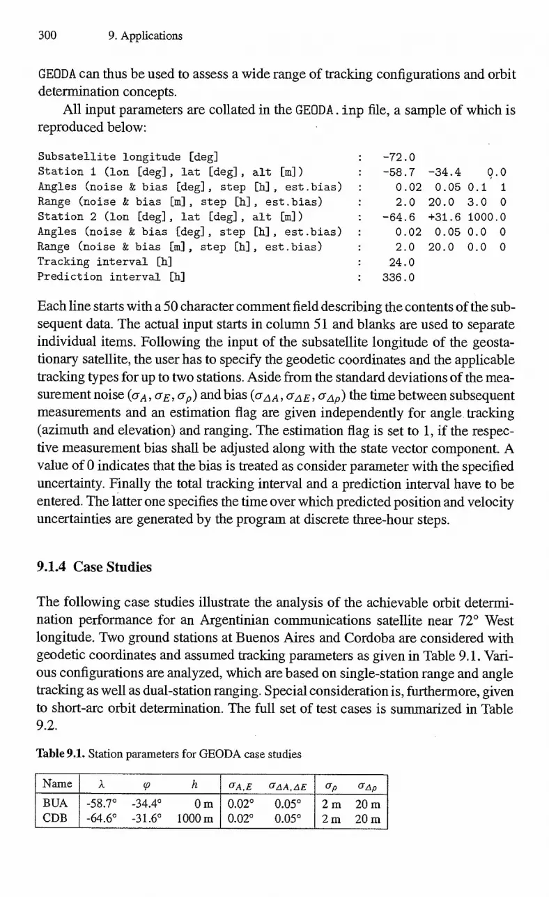
300 9. Applications
GEODA can thus be used to assess a wide range of tracking configurations and orbit determination concepts.
All input parameters are collated in the GEODA inp file, a sample of which is reproduced below:
Subsatellite longitude [deg] -72.0 Station 1 (ion [deg] , lat [deg] , alt [tu]) -58.7 -34.4 o . o Angles (noise & bias [deg] , step [h], est bias) 0.02 0.05 0.1 1 Range (noise & bias [tu], step [h] , est bias) 2.0 20.0 3.0 0 Station 2 (ion [deg] , lat [deg] , alt [tu]) -64.6 +31.6 1000.0 Angles (noise & bias [deg] , step [L], est.bias) 0.02 0.05 0.0 0 Range (noise & bias [tu], step [h] est.bias) 2.0 20.0 0.0 0 Tracking interval [h] 24.0 Prediction interval [h] 336.0
Each line starts with a 50 character comment field describing the contents of the sub-sequent data. The actual input starts in column 51 and blanks are used to separate individual items. Following the input of the subsatellite longitude of the geosta-tionary satellite, the user has to specify the geodetic coordinates and the applicable tracking types for up to two stations. Aside from the standard deviations of the mea-surement noise (c -A, cri, cri,) and bias (aziA,o -AE,0 -zip ) the time between subsequent measurements and an estimation flag are given independently for angle tracking (azimuth and elevation) and ranging. The estimation flag is set to 1, if the respec-tive measurement bias shall be adjusted along with the state vector component. A value of 0 indicates that the bias is treated as consider parameter with the specified uncertainty. Finally the total tracking interval and a prediction interval have to be entered. The latter one specifies the time over which predicted position and velocity uncertainties are generated by the program at discrete three-hour steps.
9.1.4 Case Studies
The following case studies illustrate the analysis of the achievable orbit determi-nation performance for an Argentinian communications satellite near 72° West longitude. Two ground stations at Buenos Aires and Cordoba are considered with geodetic coordinates and assumed tracking parameters as given in Table 9.1. Vari-ous configurations are analyzed, which are based on single-station range and angle tracking as well as dual-station ranging. Special consideration is, furthermore, given to short-arc orbit determination. The full set of test cases is summarized in Table 9.2.
Table 9.1. Station parameters for GEODA case studies
Mune À V h a A , E OELIA,dE up azIp
BUN. CaB
-58.7° -64.6°
-34.4° -31.6°
0 rn 1000m
0.02° 0.02°
0.05° 0.05°
2 rn 2m
20 rn 20m

9.1 Orbit Determination Error Analysis 301
Table 9.2. Tracking configuration for individual GEODA study cases
Case Description
Al
A2 A3
One -day of angle measurements (1/6') and ranging (1/3 h) from BUA station; bias parameters considered Same as Al, but azimuth & elevation biases estimated Same as A2, but for CDB station
B1 B2
One day ranging (1/3h ) from BUA and CDB stations; range biases considered Same as Bl, but CDB range bias estimated
Cl
C2
12 hours angle measurements (1/6') and ranging (1/30) from BUA station; angle biases estimated, range bias considered 6 hours ranging (1/30') from BUA and CDB stations; range biases considered
Table 9.3. Epoch state vector accuracies for individual GEODA study cases
Case Type Grx
[m] [111] Em] [mis] (Ty
[mis] [mis] [m]
Al Noise 104.0 347.0 1073.9 0.0215 0.0076 0.0785 7.8 Consider 170.5 4463.3 1088.4 0.3234 0.0093 0.0792 123.6
A2 Noise 104.1 368.9 1073.9 0.0234 0.0076 0.0785 8.5 Consider 104.1 716.6 1073.9 0.0505 0.0076 0.0785 8.5
A3 Noise 99.5 863.7 1087.4 0.0616 0.0072 0.0795 14.6 Consider 99.5 1363.0 1087.4 0.0985 0.0072 0.0795 14.6
Bl Noise 1.9 76.7 6.9 0.0056 0.0001 0.0006 1.8 Consider 52.5 2207.8 7.0 0.1607 0.0019 0.0010 52.3
B2 Noise 7.4 262.3 6.9 0.0191 0.0003 0.0006 7.4 Consider 7.4 668.0 6.9 0.0487 0.0003 0.0006 7.4
Cl Noise 168.8 2208.8 1553.1 0.1579 0.0115 0.2233 65.7 Consider 168.8 2292.7 1553.1 0.1641 0.0115 0.2233 65.7
C2 Noise 13.4 519.0 31.0 0.0379 0.0005 0.0021 13.5 Consider 58.7 2199.6 31.3 0.1605 0.0022 0.0021 57.2
The use of single-station range and angle measurements (cases Al to A3) allows the orbit to be determined with an accuracy of roughly 100 m in radial direction (x) as well as 1 km in along-track (y) and nomial (z) direction. A comparison of cases Al and A2 (Table 9.3) shows that the estimation of angle biases is essential to reduce the impact of systematic measurement errors on the resulting orbit. The range bias cannot, however, be estimated together with the angle biases in a single station configuration, since the resulting least squares equations would be close to singular. It mainly affects the accuracy by which the along-track position and the radial velocity component can be determined. As may be recognized from cases A2 and A3, use of the Buenos Aires station promises better orbit determination results than that of Cordoba despite an equal tracking performance. This fact may be attributed to a more favorable tracking geometry of the Buenos Aires station caused by the larger longitude and latitude offset with respect to the sub-satellite point.

1400
302 9. Applications
1200 cross-track
7 1000
o 800
o *E8 600— o a.
along-track
400
200 radial
o 0
2 4 6 8 10 12 14 Time [d]
Fig. 9.3. Evolution of the predicted position accuracy for single station range and angle tracking (Case A2)
The evolution of the radial, along-track, cross-track and total position accuracy for case A2 is illustrated in Fig. 9.3. The individual errors exhibit little to no orbital periodicity due to the continuous coverage of the tracking arc. While the uncertainty in the radial and normal component remains essentially constant, the tangential component varies in a quadratic way as a consequence of the semi-major axis error.
Dual-station ranging (cases B1 and B2) allows for a notable improvement of the radial and cross-track position vector component as well as the tangential and cross-track velocity over the single-station scenario. The along-track position and the radial velocity, however, remain sensitive to the range bias and are 1-2 orders of magnitude less accurate than the other components. The estimation of one range bias (Case B2) is possible in the dual-station configuration and recommended to minimize the impact of systematic errors on the solution.
While one or two-day tracking is generally considered as a standard for the determination of a geostationary satellite orbit, shorter data arcs may be desirable e.g. after maneuvers or in contingency situations. As shown by cases Cl and C2 a reasonable accuracy can already be achieved with half a day of single-station range and angle measurements or even six hours of dual-station ranging. In the latter case care should be taken, not to a estimate any bias at all, since the resulting nolinal equations would be ill-conditioned and result in a large founal covariance. For even shorter data arcs, it is difficult to separate the periodic and linear part in the daily variation of each measurement, which severely reduces the overall condition of the estimation problem.

9.2 Real-Time Orbit Determination 303
9.2 Real-Time Orbit Determination
The increasing number of GPS receivers for spaceborne applications has revitalized the interest in real-time and on-board orbit determination to increase the space-craft autonomy and reduce the required amount of ground operations. Aside from high-precision applications that require a direct processing of raw code and phase measurements, the orbit determination can be based on the navigation solution gen-erated by most of the GPS receivers. In general position values are provided with a spherical la accuracy of about 100m (cf. Table 6.2), whereas velocity is only' accurate to 1 m/s in representative spacebome receivers. Using a Kalman filter and an appropriate dynamical model, the inherent measurement noise may be reduced considerably and much more accurate state vectors be obtained.
The filtering of the SPS (Standard Positioning Service) data provides various benefits for on-board navigation. These are mainly related to the fact that the result-ing trajectory is constrained by the dynamical laws of motion, whereas subsequent GPS position solutions are essentially uncorrelated. As such, the adjusted orbit infonnation is less sensitive to the intentional deterioration of the GPS measure-ments (Selective Availability) than the navigation solution itself. In addition, the dynamical modeling allows a smooth interpolation of the trajectory, a bridging of data gaps and a detection of erroneous measurements. Finally, the Kalman filter provides precise velocity infonnation as part of the estimated state vector, which results from the accumulation of position knowledge over extended data arcs.
9.2.1 Model and Filter Design
For on-board applications, computer resources are generally much more constrained than for ground operations due to limitations of processor speed and memory. A careful selection of dynamical models, reference systems, integration methods, and estimation methods is therefore required in the design of onboard navigation systems.
Force Model: The UPS navigation data to be processed in the present application have been collected as part of the UPS/MET experiment (Hajj et al. 1995) on-board the MicroLab-1 satellite. The spacecraft was launched in 1995 and orbits the Earth at an altitude of roughly 740 km At this altitude, the acceleration is dominated by the gravity field of the Earth including higher-order tenias in the spherical harmonics expansion. Lunisolar gravity on the other hand provides only minor perturbations for satellites in low-Earth orbits as does the solar radiation pressure for satellites with representative area-to-mass ratios (cf. Fig. 3.1). From the Harris—Priester density tables (Table 3.8) it may further be concluded that atmospheric drag does not impose major perturbationi s n the relevant altitude range. To illustrate these considerations,
Considering a typical low-Earth orbit a position knowledge of 100m represents the same relative accuracy as a velocity knowledge of 0.1 m/s.
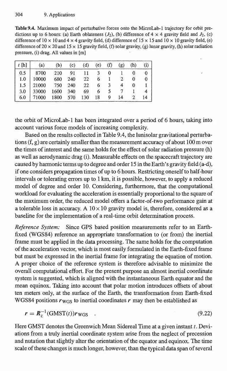
304 9. Applications
Table 9.4. Maximum impact of perturbative forces onto the MicroLab-1 trajectory for orbit pre-dictions up to 6 hours: (a) Earth oblateness (J2), (b) difference of 4 x 4 gravity field and h, (c) difference of 10 x 10 and 4 x 4 gravity field, (d) difference of 15 x 15 and 10 x 10 gravity field, (e) difference of 20 x 20 and 15 x 15 gravity field, (f) solar gravity, (g) lunar gravity, (h) solar radiation pressure, (i) drag. All values in [m]
t [h] (a) (b) (c) (d) (e) (f) (g) (h) (i)
In c. I
n c::! o
c:3 --4 .--; cr) .0
8700 210 91 11 3 0 1 0 0 10000 680 240 22 6 1 2 0 0 21000 750 240 22 6 3 4 0 1 33000 1600 340 69 6 5 7 1 4 71000 1800 570 130 18 9 14 2 14
the orbit of MicroLab-1 has been integrated over a period of 6 hours, taking into account various force models of increasing complexity.
Based on the results collected in Table 9.4, the lunisolar gravitational perturba-tions (f, g) are certainly smaller than the measurement accuracy of about 100 m over the times of interest and the same holds for the effect of solar radiation pressure (h) as well as aerodynamic drag (i). Measurable effects on the spacecraft trajectory are caused by harmonic terms up to degree and order 15 in the Earth's gravity field (a-d), if one considers propagation times of up to 6 hours. Restricting oneself to half-hour intervals or tolerating errors up to 1 km, it is possible, however, to apply a reduced model of degree and order 10. Considering, furthermore, that the computational workload for evaluating the acceleration is essentially proportional to the square of the maximum order, the reduced model offers a factor-of-two performance gain at a tolerable loss in accuracy. A 10 x 10 gravity model is, therefore, considered as a baseline for the implementation of a real-time orbit determination process.
Reference System: Since GPS based position measurements refer to an Earth-fixed (WGS84) reference an appropriate transformation to (or from) the inertial frame must be applied in the data processing. The same holds for the computation of the acceleration vector, which is most easily formulated in the Earth-fixed frame but must be expressed in the inertial frame for integrating the equation of motion. A proper choice of the reference system is therefore advisable to minimize the overall computational effort. For the present purpose an almost inertial coordinate system is suggested, which is aligned with the instantaneous Earth equator and the mean equinox. Taking into account that polar motion introduces offsets of about ten meters only, at the surface of the Earth, the transformation from Earth-fixed WGS84 positions rwGs to inertial coordinates r may then be established as
r = RT1 (GMST (t))rwGs • (9.22)
Here GMST denotes the Greenwich Mean Sidereal Time at a given instant t. Devi-ations from a truly inertial coordinate system arise from the neglect of precession and nutation that slightly alter the orientation of the equator and equinox. The time scale of these changes is much longer, however, than the typical data span of several

9.2 Real-Time Orbit Determination 305
revolutions required for a reliable orbit adjustment. As such, the associated changes of the reference system have no practical impact on the performance of the orbit determination process.
Estimation and Integration: Before discussing the choice of a suitable numerical integration method for the equation of motion, a brief consideration of the overall estimation concept is required. While a least-squares method would ensure a high degree of robustness in the handling of non-linearities or the rejection of erroneous measurements, it would necessitate an on-board storage of a large measurement batch to allow multiple iterations. A Kalman filter is therefore preferable, which processes each measurement exactly once as soon as it is collected. In this case, however, an extended Kalman filter must be selected to cope with the non-linearity of the orbit determination problem. The associated change of the reference trajec-tory in each update step does, however, imply a frequent restart of the numerical integration. Even for a data rate of only one value per five minutes, a high-order in-tegration method would be forced to work at a non-optimal stepsize. Considering in addition the complexity and storage requirements of elaborate single-step methods, low-order Runge—Kutta methods turn out to be best suited for the envisaged usage. Furthermore, no stepsize control is required for near-circular orbits. In the sequel the well-known 4th-order Runge—Kutta method will be applied, which provides a particularly simple set of coefficients. As a baseline, a 30 s step size is adequate to integrate the orbit to the desired accuracy.
State Transition Matrix: Another issue that has to be addressed in the design of the orbit determination process concerns the modeling of the state transition matrix between consecutive steps. While a rigorous integration of the variational equations would ensure full consistency between the trajectory model and the asso-ciated partial derivatives, it is generally too cumbersome to be applied in real-time systems. Simple Taylor expansions may, on the other hand, cause problems if the time between consecutive data points covers a notable fraction of the orbit. As a compromise, a Keplerian founulation of the state transition matrix is therefore applied in the RTOD program.
Process Noise: Last but not least, a suitable process noise model has to be consid-ered in the design of the extended Kalman filter. For the present purpose a simple model is adequate, since measurements are provided at almost equidistant time steps throughout the whole data arc. It is therefore sufficient to add a constant process-noise matrix Q = diag(wiios , Wv2e) to the predicted covariance in each time update step. Position and velocity variances as given by the diagonal elements of Q are selected in accordance with the expected trajectory modeling errors arising in the propagation from one measurement to the next. All off-diagonal elements of Q are set to zero. Suitable values of wpos and wvei are best found by experiment and de-pend on the data interval, the assumed measurement accuracy, and the accuracy of the dynamical model. In the present application nominal process-noise parameters of 0.5 m and 05 minis are applied for a five-minute data interval, which helps to avoid a filter divergence without sacrificing the achievable accuracy.

306 9. Applications
9.2.2 The RTOD Program
The RTOD program processes a sequence of GPS navigation data and auxiliary information provided in the RTOD . dat file. Aside from a single header line that may be skipped on reading, the file contains one record per time with a structure as described in Table 9.5. Following the date and GPS time tag, the position and velocity vector in the WGS84 system as determined by the GPS receiver are given in the initial columns To evaluate the filter performance, the actual spacecraft position and velocity in the rotating, Earth-fixed system is furthermore provided as determined from a least-squares orbit determination with an elaborate force model. Both position and velocity measurements from the first data record are used to derive the inertial state vector of the spacecraft, which is required to initialize the filter and to start the trajectory integration. Subsequent measurement updates make use of the position measurements only, which provide a much better relative accuracy than the velocity data.
Table 9.5. Structure of the RTOD data file
Cols. Description
1— 10 Date (yyyy/mm/dd) 13— 24 GPS time (hh:mm:ss.sss) 28— 37 Measured position x (WGS84 system, in [m]) 39— 48 Measured position y (WGS84 system, in [m]) 50— 59 Measured position z (WGS84 system, in Ern]) 63— 72 Measured velocity •i (WGS84 system, in [mis]) 74— 83 Measured velocity .):, (WGS84 system, in [mis]) 85— 94 Measured velocity (WGS84 system, in [mis]) 98-107 True position x (WGS84 system, in [m])
109-118 True position y (WGS84 system, in Em]) 120-129 True position z (WGS84 system, in [m]) 133-142 True velocity •i (WGS84 system, in [mis]) 144-153 True velocity 57 (WGS84 system, in [mis]) 155-164 True velocity i (WGS84 system, in [mis])
A supplementary setup file RTOD . inp is used to control and modify the filter performance. The individual parameters comprise the gravity-field order and the step size applied in the numerical trajectory integration as well as the measure-ment standard deviation, the a priori statevector uncertainty and two state-noise parameters for controlling the addition of process noise. An edit (or culling) level is, furthermore, specified, to allow the rejection of bad measurements. It serves as a threshold for the identification of outliers and is specified in units of the mea-surement standard deviation o- . Assuming a Gaussian error distribution, more than 99% of all measurements should exhibit errors of less than 3o- . Measurements, for which the ratio of the residual and the standard deviation exceeds an edit level of about three should therefore be considered as erroneous data points and discarded.
Each line of the input file provides a single parameter following a 30-character comment. Representative parameter values are given in the subsequent listing:

9.2 Real-Time Orbit Determination 307
Gravity model order (<=20) . 10 Integration step size [s] -
. 30 Measurement Sigma [ni] - . 100 A priori sigma position [m] : 1000 A priori sigma velocity [mis]: 10 State noise position [ni] . 0.5 State noise velocity [mis] •
. 0.0005 Edit level (sigma) 3.0
The output of the RTOD program comprises a copy of the setup parameters and a table of filter outputs at each step. The table is made up of 13 blank separated columns, giving the time t since epoch (Col. 1, in [s]), the filtered Earth-fixed position r (Col. 2-4, in [nil) and the measurement and solution errors. The latter parameters comprise the difference IrGps — rref I between the measured position and the reference orbit (Col. 5), the standard deviation o-, of the estimated position (Col. 6) and the error Ir — rref I of the estimated position (Col. 7). Corresponding quantities are provided for the errors of the velocity (Col. 8-10) and the semi-major axis (Col. 11-13). For information, measurements rejected by the filter are marked by an asterisk immediately following the measurement error.
9.2.3 Case Studies
The following case studies are based on a 24-hour data arc of GPS measurements collected by a TurboStar receiver as part of the GPS/MET experiment on October 1, 1996. The measurements are sampled at a rate of one point per five minutes, yielding an average of 20 measurements per orbit. The data noise as derived from the root-mean-square deviation from the reference trajectory amounts to roughly 110 m in position and 2.5 m/s in velocity.
Table 9.6. Filter parameters for selected case studies
Parameter Case A Case B Case C
Gravity model order n 10 10 4 Integration step size dt [s] 30 60 30 Measurement standard deviation axyz [1111 100 100 100 A priori std. dey, position Crpos [In] 1000 1000 1000 A priori std. dev , velocity avei [nus] 10 10 10 State noise position Wpos Ern] 0.5 0.0 10.0 State noise velocity wvel [rnis] 0.0005 0.0000 0.0100 Edit level 3.0 3.0 3.0
To start with, the nominal filter performance is illustrated in case A (cf. Table 9.6). The equation of motion is integrated in 30 s steps and includes perturbations due to the harmonic gravity field of the Earth up to degree and order 10. The a priori standard deviation of the initial state taken from the first data point is assumed to be 1 km and 10 m/s, respectively, for the position and velocity coordinates. While this is about a factor of 10 worse than the actual measurement standard deviation, the

308 9. Applications
adopted values ensure that the filter starts properly, even if the initial measurement is affected by larger than average errors.
300
250 -
200 -
150 -
• •
100 -
50 -
2 3 4 5 6 7 8 9 10 11 12 13 14 15 16 17 18 19 20 21 22 23 24 Time [h]
Fig. 9.4. Nominal filter performance for GPS/MET orbit determination (case A): error of the esti- mated position (bold line), standard deviation of the estimate (narrow line) and GPS measurement errors (dots).
Results of the corresponding RTOD run are summarized in Fig. 9.4, which shows the measurement residuals, the error of the estimated position and the standard deviation computed by the filter. The filter takes about three hours (two revolutions) before it converges to a steady-state behavior. During the initial phase the filter is affected by pronounced errors of two consecutive measurements that amount to 250m and 500 m, respectively. The latter value exceeds the 3a (.300 m) data editing criterion, which results in a rejection of the corresponding measurement and an associated increase in the propagated position covariance. During the steady-state phase the filter approaches a constant position standard deviation of roughly 50m. This equilibrium value results from a balance between the information gain due to the processing of new measurements and the covariance increase caused by the addition of process noise in the state update phase. The deviation between the estimated position and the reference trajectory is generally less than the computed standard deviation and amounts to 25 m on average (r.m.s.) after the initial two hours. Thus, the filtered positions are more accurate than the measured positions by a factor of four to five, which clearly illustrates the advantage of a dynamical orbit determination over the purely kinematic GPS position solutions. The benefit is even more pronounced for the velocity determined by the filter, which is approximately 100 times more accurate (2.5 cm/s r.m.s.) than the velocity values provided by the
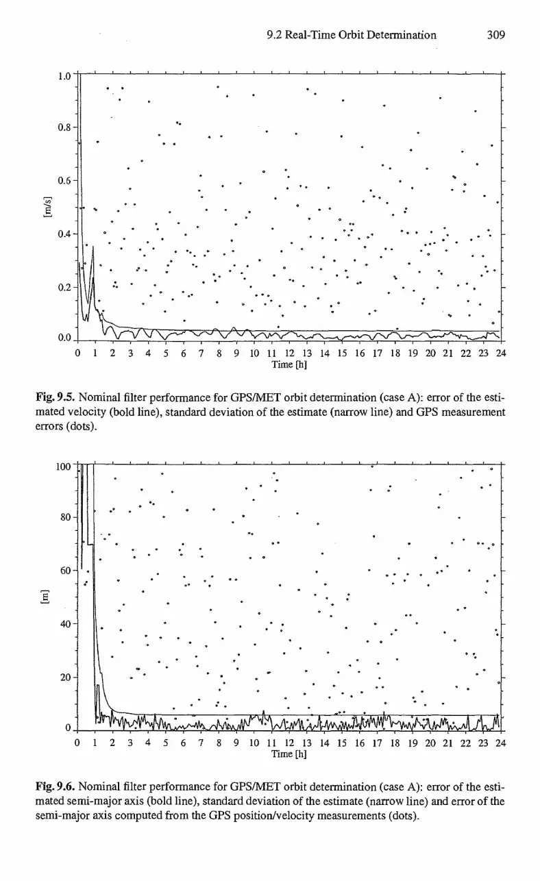
0.6
:17 0.4
• • •
0.2 - * • • e* • •
1.0
•
0.8 - • • •
•
•
00
0 0 • • 0 • 0 • 0 •
• •
•
•
• • • •
• •
• •
0 0
0 1 2 3 4 5 6 7 8 9 10 11 12 13 14 15 16 17 18 19 20 21 22 23 24 Time [h]
"v7M11
80 -
60
40
• •
0 •
• op
• • •
• * • • • 0
•
•
•
• 0
• •
y
*
9.2 Real-Time Orbit Determination 309
Fig. 9.5. Nominal filter performance for GPS/MET orbit determination (case A): error of the esti-mated velocity (bold line), standard deviation of the estimate (narrow line) and GPS measurement errors (dots).
0 2 3 4 5 6 7 8 9 10 11 12 13 14 15 16 17 18 19 20 21 22 23 24 Time [h]
Fig. 9.6. Nominal filter performance for GPS/MET orbit determination (case A): error of the esti-mated semi-major axis (bold line), standard deviation of the estimate (narrow line) and error of the semi-major axis computed from the GPS position/velocity measurements (dots).

310 9. Applications
300
250 -
200 -
-
0 1 2 3 4 5 6 7 8 9 10 11 12 13 14 15 16 17 18 19 20 21 22 23 24 Time [h]
Fig. 9.7. Filter divergence due to numerical integration errors in the absence of process noise (case B): error of the estimated position (bold line), standard deviation of the estimate (narrow line) and measurement errors (dots).
0 1 2 3 4 5 6 7 8 9 10 11 12 13 14. 15 16 17 18 19 20 21 22 23 24 Time [h]
Fig. 9.8. Compensation of low-order gravity model errors by increased process noise (case C): error of the estimated position (bold line), standard deviation of the estimate (narrow line) and measurement errors (dots).

100
80 -
60 -
40 -
20 -
9.2 Real-Time Orbit Determination 311
0 1 2 4 5 6 7 8 9 10 11 12 13 14 15 16 17 18 19 20 21 22 23 24 Time [h]
Fig. 9.9. Compensation of low order gravity model errors by increased process noise (case C): error of the estimated semi-major axis (bold line), standard deviation of the estimate (narrow line) and error of the semi-major axis computed from the position/velocity measurements (dots).
GPS receiver itself (Fig. 9.5). The semi-major axis derived from the estimated state vector is accurate to about 3 m r.m.s. (cf. Fig. 9.6).
An example of moderate filter divergence is given by case B, in which slight propagation errors have been introduced by selecting a larger than nominal inte-gration step size. At the same time, no process noise is added, which makes the filter continuously less receptive to new measurements. For up to seven hours (4-5 revolutions) the filter output closely matches that of case A. Thereafter, however, the position error starts to increase past the formal standard deviation and the so-lution differs from the true position by up to 100m (Fig. 9.7). Case B obviously lacks a sufficient amount of process noise to compensate the inherent model errors, whereas both factors are properly balanced in case A.
An extreme case of model error compensation is, furthermore, presented in case C, where the degree and order of the gravity field have been reduced from ten to four. At the same time the process noise has been increased by a factor of 20 over case A, which results in a steady-state position uncertainty of about 100m. While the root-mean-square position and velocity errors are approximately doubled during the steady-state phase in comparison to case A, the filtered solution and its variance become sensitive to erroneous data and data gaps (Fig. 9.8). More importantly one may note a ten-fold increase of the semi-major axis error and standard deviation in comparison to case A (Figs. 9.6 and 9.9). As a rule of thumb, the observed peak error of La = 50m would result in a 500m along-track error after one - orbit or about 7 km after one day.
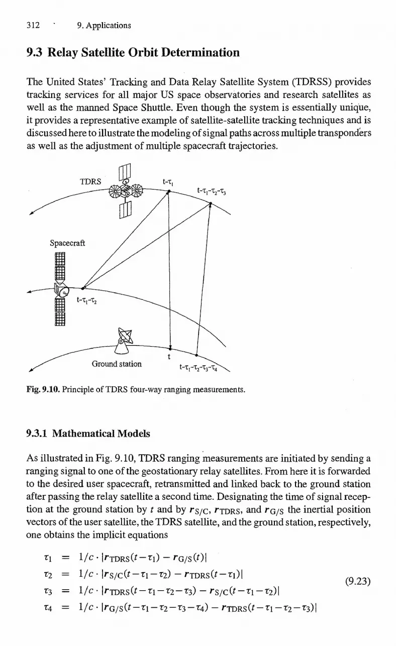
312 ' 9. Applications
9.3 Relay Satellite Orbit Determination
The United States' Tracking and Data Relay Satellite System (TDRSS) provides tracking services for all major US space observatories and research satellites as well as the manned Space Shuttle. Even though the system is essentially unique, it provides a representative example of satellite-satellite tracking techniques and is discussed here to illustrate the modeling of signal paths across multiple transponders as well as the adjustment of multiple spacecraft trajectories.
Fig. 9.10. Principle of TDRS four-way ranging measurements.
9.3.1 Mathematical Models
As illustrated in Fig. 9.10, TDRS ranging measurements are initiated by sending a ranging signal to one of the geostationary relay satellites. From here it is forwarded to the desired user spacecraft, retransmitted and linked back to the ground station after passing the relay satellite a second time. Designating the time of signal recep-tion at the ground station by t and by rs/c, rTDRs, and rG/s the inertial position vectors of the user satellite, the TDRS satellite, and the ground station, respectively, one obtains the implicit equations
ri = 1/c I rTDRS (t r1) rGis
1'2 =- 1/c irsic(t — — 1-2) — rTDRS (t —1-1)1
1-3 = 1 /c • I rTDRS(t — r1 — t2 — r3) — rs/c(t — r1 — r2)1
r4 1/c • lrG/s (t — — T3 — r4) rTDRS (t "r2 r3)
(9.23)

9.3 Relay Satellite Orbit Determination 313
for the individual light times. Starting from initial values of zero, the light times are consecutively determined from these relations using a simple fixed-point iteration. The resulting values then yield the modeled four-way range
P = —2 • (ri r2 + r3 + ) • (9.24)
Neglecting the relative motion of the station and the two satellites, the 4-way range is equal to the sum of the distances from the ground station to the relay satellite and from the relay satellite to the user satellite.
The measurement noise and the systematic errors of the TDRS ranging system are generally less than 10m, which implies that the motion of the user spacecraft, the relay satellite, and the ground station must be modeled to a similar level of accuracy. Since most of the user satellites tracked by the TDRS system orbit the Earth at altitudes of several hundreds of kilometers, the force model must as a minimum, comprise the harmonic gravity field of the Earth as well as the acceleration due to atmospheric drag. The geostationary relay satellite, on the other hand, is notably affected by lunisolar gravitational perturbations and solar radiation pressure. In order to avoid different models for the various satellites concerned, a common model comprising all of the above-mentioned perturbations should be considered. A gravity field model up to degree and order 20 is recommended to describe the motion of user satellites at altitudes of 500-1000 km with the desired accuracy.
For a compatible modeling of the ground station position, polar motion and true sidereal time must be considered to describe the Earth's rotation. In addition, nutation and precession need to be accounted in the transformation to a common inertial reference frame (e.g. the mean equator and equinox of J2000). For an adequate modeling of the Greenwich hour angle, knowledge of Universal Time UT1 is required to better than 0.01 s.
In accordance with Sect. 7.2.3, the variational equations for the state transition matrix may be based on a simplified force model comprising only the second-order zonal harmonics in the gravity field. Along with the state transition matrix, the sensitivity matrix describing the state vector partials with respect to the drag and solar radiation pressure coefficients is integrated to allow an adjustment of these parameters within the orbit determination.
9.3.2 The TDRSOD Program
The TDRSOD program performs a least-squares orbit determination using TDRS four-way range measurements. Based on an appropriate set of measurements the orbital parameters of a single user spacecraft and up to two relay satellites can be adjusted simultaneously. Tracking data are provided in the TDRSOD dat file, which contains one record per time with a structure as described in Table 9.7. A single header line serves to label each column and is skipped upon reading. Following the epoch of the measurement the ground station and spacecraft identification numbers as well as the four-way relay range are given in each line.
314 9. Applications
Table 9.7. Structure of the TDRSOD tracking data file
Cols. Description
1-10 Date (yyyy/mm/dd) 13-24 UTC time (hh:mm:ss.sss) of signal reception 26-30 Station number 32-34 'MRS identification number (ID) 36 16 Range measurement (in [m]) corrected for refraction
A supplementary setup file TDRSOD . inp provides a priori state vectors and spacecraft-related parameters for the user and TDRS satellites as well as relevant auxiliary information. The individual parameters comprise the total number (< 2) and IDs of the TDRS satellites, the total number (< 2) and IDs of the employed ground stations, the desired number of iterations, the UT1 -UTC and UTC-TAI time differences, as well as the current pole coordinates, all of which are given at the beginning of the input file. Following the initial epoch, the state vectors of the user spacecraft and the specified number of TDRS satellites are provided together with the associated a priori standard deviations. The spacecraft-related information is complemented by the specification of each satellite's mass, area, drag coefficient, and radiation pressure coefficient, as well as the related a priori uncertainties of the latter parameters. The file closes with a section providing the coordinates of the specified number of ground stations.
Each line provides a single parameter starting at column 26. The initial char-acters are ignored on input and serve to describe the meaning of the respective quantities. Representative parameter values are given in the subsequent listing:
TDRS 2 4 5 Stations 2 161 162 Iterations 4 UT1-UTC, UTC-TAI [s] +0.49 -32.00 x-pole,y-pole ["] -0.00651 +0.36588 Epoch (UTC) 1999/09/01 00:00:00.000 x UARS [m] 1476200.0 1000.0 y UARS [m] 5996200.0 1000.0 z UARS [m] -3209000.0 1000.0 vx UARS [m/s] -3854.0000 1.0 vy UARS [m/s] 3778.5000 1.0 vz UARS [m/s] 5302.2000 1.0 in [kg] , A [m- 2] 5968.3 27.22 CD, sigma(CD) 2.3 1.0 CR, sigma(CR) 1.3 0.1 x TDRS-4 [m] •
. +20174293.6 1.0 y TDRS-4 [m] •
. -37024903.8 1.0 z TDRS-4 [m] -982925.2 1.0 vx TDRS-4 [m/s] +2696.9634 0.001 vy TDRS-4 [m/s] +1471.5074 0.001 vz TDRS-4 [m/s] -100.5261 0.001 in [kg], A [m- 2] 1668.9 40.0 CD, sigma(CD) 2.3 0.001

CR, sigma(CR)
9.3 Relay Satellite Orbit Determination 315
1.3915 0.001 x * TDRS-5 [m] -40783913.5 100.0 y TDRS-5 [m] 10622599.3 100.0 z TDRS-5 Em] 992633.1 100.0 vx TDRS-5 [m/s] -774.3896 0.1 vy TDRS-5 [m/s] -2976.0955 0.1 vz TDRS-5 [m/s] 18.8994 0.1 m [kg], A [m- 2] 1718.4 40.0 CD, sigma(CD) 2.3 0.1 CR, sigma(CR) 1.4062 0.1 Sta WHSK/161 (xyz) Ern] -1539385.74 -5160953.12 +3408202.16 Sta WH2K/162 (xyz) [m] -1539390.43 -5160968.83 +3408176.45
The TDRSOD program uses the DE multistep method to integrate the state vector as well as the state transition and sensitivity matrix for each individual satellite from specified initial conditions. Considering the widely different orbital periods of the low-Earth user satellite and the geostationary relay satellites, the respective trajectories are integrated independently of each other using the most appropri-ate integration stepsize for each orbit. Interpolation over multiple steps is used to interpolate the solution during the light time iteration.
The least-squares adjustment is performed over the specified number of itera-tions, during each of which the observation residuals and the computed parameter corrections are output. No data editing or convergence check is performed to main-tain a simple overall program structure. A priori standard deviations are expected for all estimation parameters, which should be selected in accordance with the expected uncertainty of the respective state vector component or force model parameter.
9.3.3 Case Study
In the subsequent application TDRS range measurements of NASA's Upper Atmo-sphere Research Satellite (UARS) are processed, which were collected on Septem-ber 1, 1999. The data set comprises 14 batches of 10-15 minutes duration each, which are evenly distributed over the entire day. Out of these, three batches have been obtained via the TDRS-4 satellite, located at 41.0' West longitude, while the remaining Measurements were performed with TORS-5 at 174.3° West longitude. All data have previously been corrected for refraction.
Orbits of the two TORS satellites have independently been derived from ground-based tracking and serve as a priori information for the UARS orbit determination. The corresponding state vectors, as referred to the Earth's mean equator and equinox (EME2000), are collated in Table 9.8 together with relevant spacecraft parameters. In addition, Table 9.9 provides the coordinates of the WHSK and WH2K antennas of the White Sands ground station complex, which were employed in the four-way ranging measurements via TDRS-4 and TDRS-5, respectively.
For a proper performance of the least-squares orbit determination, a priori standard deviations need to be specified for the state vector components as well as the drag and solar radiation pressure coefficients. In the absence of actual a

316 9. Applications
Table 9.8. A priori orbit and spacecraft parameters of UARS, 1DRS-4, and TDRS-5 for the epoch 1999/09/01 00:00 UTC
UARS 1 DRS-4 '1 DRS-5
x [m] +1476200.0 +20174293.6 +40783913.5 y [m] +5996200.0 -37024903.8 +10622599.3 z [m] -3209000.0 -982925.2 +992633.1 ± [mis] -3854.0000 +2696.9634 -774.3896 57 [rn/s] +3778.5000 +1471.5074 -2976.0955 i [m/s] +5302.2000 -100.5261 +18.8994
m [kg] 5968.3 1668.9 1718.4 A [m2] 27.22 40.0 40.0 CD 2.3 2.3 2.3 CR 1.3 1.3915 1.4062
Table 9.9. White Sands antenna locations
Station No. x [m] Y [m] z [m]
WHSK WH2K
161 162
-1539385.74 -1539390.43
-5160953.12 -5160968.83
+3408202.16 +3408176.45
priori statistics, appropriate values may be obtained from a consideration of the orbital characteristics, the tracking geometry, and the data distribution. In the case of the user satellite, which is tracked over roughly 15 revolutions with a sufficient coverage during each orbit, one may expect a reliable determination of its orbital elements from the given measurements. In accord with the given number of digits, an uncertainty of 1 km and 1 m/s in each axis is therefore assumed for the initial position and velocity of the UARS satellite. Neither of these values puts a stringent constraint on the resulting least-squares solution, as does the assumed standard deviation of 1.0 for the drag coefficient. For the solar radiation pressure coefficient, on the other hand, the a priori standard deviation is set to 0.1, in accordance with the uncertainty in the knowledge of relevant material properties.
For the Tracking and Data Relay Satellites, which orbit the Earth at geosta-tionary altitude, drag does not impose any orbit perturbations and thus cannot be calibrated during the orbit determination. An a priori standard deviation of 0.1 for the respective CD coefficients therefore merely serves to avoid a singularity of the resulting normal equations. In fact, the a priori value (2.3) will not be changed at all within the least-squares adjustment. Concerning the other parameters, it is recalled that 'IDRS-4 tracking data are only available for a limited number of data arcs, while TDRS-5 tracking essentially covers the whole day. In view of the even sam-pling of the IDRS-5 orbit, the four-way range measurements performed via this satellite can therefore be employed to improve its orbit along with that of the user satellite. This is accomplished by assuming a priori standard deviations of 100m and 0.1 m/s for position and velocity as well as 0.1 for the CR coefficient. These figures take care of the fact that the 'IDRS-5 orbit has already been determined with good accuracy from independent tracking data and, at the same time, avoid
15
1 0- A A
-5 7
5 ^
-15 -
0 1 2 3 4 5 6 7 8 9 10 11 12 13 14 15 16 17 18 19 20 21 22 23 24 Time [h]
9.3 Relay Satellite Orbit Determination 317
unrealistic parameter corrections in case of potential correlations between orbital parameters of the user satellite and the 'IDRS satellite. Finally, a priori standard deviations of 1 m (position), 1 mm/s (velocity), and 0.001 (CD, CR) are adopted for the TDRS-4 satellite, which essentially constrains its orbit to the given a priori trajectory. Due to the inadequate coverage of thiS satellite's 24-hour orbital period with tracking data, it would not be possible to independently determine or improve its trajectory from the given UARS ranging measurements.
Table 9.10. Adjusted orbit and spacecraft parameters of UARS, TDRS-4 and TDRS-5 for epoch 1999/09/01 00:00 UTC
UARS TDRS-4 I DRS-5
x [m] +1476163.0+ 12.9 +20174293.6+ 1.0 +40783910.4+ 13.5 y [m] +5996245.6+ 11.5 —37024903.8+ 1.0 +10622602.5+ 43.5 z [m] —3208799.5+ 17.2 —982925.2+ 1.0 +992611.7+ 55.1 .i [m/s] —3854.0030+0.0071 +2696.9636+0.0003 —774.3906+0.0031 5/ [rn/s] +3778.3897+0.0163 +1471.5076+0.0004 —2976.0954+0.0007
+5302.2419+0.0136 i [mis] —100.5264+0.0010 +18.8998+0.0050
CD 2.6125+0.1632 2.3000+0.0010 2.3000+0.1000 CR 1.3002+0.1000 1.3915+0.0010 1.4538+0.0366
Fig. 9.11. Residuals of IDRS four-way ranging measurements of the UARS satellite collected on Sept. 1, 1999. Triangles indicate measurements taken via TDRS-4, while diamonds refer to the TDRS-5 relay satellite.
Representative values for the adjusted orbital parameters are given in Ta-ble 9.10, while the corresponding residuals are shown in Fig. 9.11. In total, the a priori state vector of the user spacecraft is corrected by about 200 m and 0.1 mis, with formal uncertainties being a factor 5 to 10 smaller. The initial state vectors of

318 9. Applications
the 1DRS satellites remain essentially unchanged, except for the z-component of the TDRS-5 satellite that is modified by 25 m. As expected, the drag coefficients of the geostationary relay satellites are completely unaffected, while the user satellite's solar radiation pressure coefficient is virtually the same as before the adjustment. On the other hand, the drag coefficient of the user satellite and the solar radiation pressure coefficient of TDRS-5 can be adjusted with good confidence and improved significantly over the default a priori values.
The residuals obtained during the final iteration exhibit an overall measurement and modeling accuracy of 5-10m. Obviously, the distribution of residuals does not comply with the assumption of random noise but indicates the presence of system-atic errors. In the absence of independent tracking data for either the user satellite or the TDRS satellites, it is not, however, possible to uniquely attribute these errors to either an incomplete modeling of perturbative forces, an incomplete account of media corrections in the preprocessing, or systematic errors in the measurement process.
Appendix A
A.1 Calendrical Calculations
The civilian calendar which measures time in terms of years, months, and days provides a convenient and well-established time scale for our daily life. It is not, however, well suited to finding the time difference between two dates or advancing a date by a certain time increment. To cope with this difficulty, a continuous day count is often used in astronomical computations, which is known as the Julian Date. It is attributed to Joseph Justus Scaliger, who introduced a "Julian Period" of 7 980 Julian years for chronological purposes (see Derwshowitz & Reingold 1997, Moyer 1981).
The Julian Date (JD) is the number of days since noon January 1, 4 713 BC including the fraction of day. It thus provides a continuous time scale which, for all practical purposes, is always positive. Counting starts at noon for historical reasons, to avoid a change of date in the middle of astronomical observations. Presently, the Julian Day numbers are already quite large (well over two millions) and it is also desirable to start counting at midnight. Therefore, a Modified Julian Date (MJD) is defined as: 1-1‘qW.6- W (.1
MJD = JD — 2 400 000.5 (A.1)
A table of Modified Julian Dates for the beginning of each month between 1975 and 2020 is given in Table A.1.
Interconversion to civil calendar date and time is often done by tables, however, there also exist a number of numerical algorithms. The method described here is based upon Meeus (1978, 1991) and requires several points to be considered:
• Civil time is expressed in year (Y), month (M), and day (D). Both D and Julian Day may include fraction of days:
o The years BC are counted astronomically in all folinulas. E.g. 1 BC would be the year Y = 0 and 10 BC corresponds to the year Y = —9.
• The Julian Day begins at 12h o'clock midday. • The Julian calendar is used until 4th October 1582 AD, which corresponds
to JD < 2 299 160.5. The average length of the year in the Julian calendar was taken as 365.25 days which implied one extra day every fourth year. The true length of the mean solar year, however, is about eleven minutes less. By

320 Appendix A
Table A.1. Modified Julian Date at day 0.0 of each month. To obtain the MID of a given date, add the day and fractions of day to the tabulated value for the respective month and year. Example: MJD(2000 Jan. 1, 12h) = 51543 + 1.5 = 51544.5.
Year Jan Feb Mar Apr May Jun Jul Aug Sep Oct Nov Dec
1975 42412 42443 42471 42502 42532 42563 42593 42624 42655 42685 42716 42746 1976 42777 42808 42837 42868 42898 42929 42959 42990 43021 43051 43082 43112 1977 43143 43174 43202 43233 43263 43294 43324 43355 43386 43416 43447 43477 1978 43508 43539 43567 43598 43628 43659 43689 43720 43751 43781 43812 43842 1979 43873 43904 43932 43963 43993 44024 44054 44085 44116 44146 44177 44207 1980 44238 44269 44298 44329 44359 44390 44420 44451 44482 44512 44543 44573 1981 44604 44635 44663 44694 44724 44755 44785 44816 44847 44877 44908 44938 1982 44969 45000 45028 45059 45089 45120 45150 45181 45212 45242 45273 45303 1983 45334 45365 45393 45424 45454 45485 45515 45546 45577 45607 45638 45668 1984 45699 45730 45759 45790 45820 45851 45881 45912 45943 45973 46004 46034 1985 46065 46096 46124 46155 46185 46216 46246 46277 46308 46338 46369 46399 1986 46430 46461 46489 46520 46550 46581 46611 46642 46673 46703 46734 46764 1987 46795 46826 46854 46885 46915 46946 46976 47007 47038 47068 47099 47129 1988 47160 47191 47220 47251 47281 47312 47342 47373 47404 47434 47465 47495 1989 47526 47557 47585 47616 47646 47677 47707 47738 47769 47799 47830 47860 1990 47891 47922 47950 47981 48011 48042 48072 48103 48134 48164 48195 48225 1991 48256 48287 48315 48346 48376 48407 48437 48468 48499 48529 48560 48590 1992 48621 48652 48681 48712 48742 48773 48803 48834 48865 48895 48926 48956 1993 48987 49018 49046 49077 49107 49138 49168 49199 49230 49260 49291 49321 1994 49352 49383 49411 49442 49472 49503 49533 49564 49595 49625 49656 49686 1995 49717 49748 49776 49807 49837 49868 49898 49929 49960 49990 50021 50051 1996 50082 50113 50142 50173 50203 50234 50264 50295 50326 50356 50387 50417 1997 50448 50479 50507 50538 50568 50599 50629 50660 50691 50721 50752 50782 1998 50813 50844 50872 50903 50933 50964 50994 51025 51056 51086 51117 51147 1999 51178 51209 51237 51268 51298 51329 51359 51390 51421 51451 51482 51512 2000 51543 51574 51603 51634 51664 51695 51725 51756 51787 51817 51848 51878 2001 51909 51940 51968 51999 52029 52060 52090 52121 52152 52182 52213 52243 2002 52274 52305 52333 52364 52394 52425 52455 52486 52517 52547 52578 52608 2003 52639 52670 52698 52729 52759 52790 52820 52851 52882 52912 52943 52973 2004 53004 53035 53064 53095 53125 53156 53186 53217 53248 53278 53309 53339 2005 53370 53401 53429 53460 53490 53521 53551 53582 53613 53643 53674 53704 2006 53735 53766 53794 53825 53855 53886 53916 53947 53978 54008 54039 54069 2007 54100 54131 54159 54190 54220 54251 54281 54312 54343 54373 54404 54434 2008 54465 54496 54525 54556 54586 54617 54647 54678 54709 54739 54770 54800 2009 54831 54862 54890 54921 54951 54982 55012 55043 55074 55104 55135 55165 2010 55196 55227 55255 55286 55316 55347 55377 55408 55439 55469 55500 55530 2011 55561 55592 55620 55651 55681 55712 55742 55773 55804 55834 55865 55895 2012 55926 55957 55986 56017 56047 56078 56108 56139 56170 56200 56231 56261 2013 56292 56323 56351 56382 56412 56443 56473 56504 56535 56565 56596 56626 2014 56657 56688 56716 56747 56777 56808 56838 56869 56900 56930 56961 56991 2015 57022 57053 57081 57112 57142 57173 57203 57234 57265 57295 57326 57356 2016 57387 57418 57447 57478 57508 57539 57569 57600 57631 57661 57692 57722 2017 57753 57784 57812 57843 57873 57904 57934 57965 57996 58026 58057 58087 2018 58118 58149 58177 58208 58238 58269 58299 58330 58361 58391 58422 58452 2019 58483 58514 58542 58573 58603 58634 58664 58695 58726 58756 58787 58817 2020 58848 58879 58908 58939 58969 59000 59030 59061 59092 59122 59153 59183
and
Y — 1 if M < 2
I. Y= I Y otherwise (A.3)
A.1 Calendrical Calculations 321
1582 AD the error in the Julian calendar, which was introduced in 45 BC, had accumulated to more than ten days. This led to the calendar reform under Pope Gregory XIII.
4, The Gregorian calendar is used from 15 th October 1582 AD onwards corre-sponding to JD > 2 299 160.5. The average length of the year in this calendar is 365.2425 days which deviates by less than half a minute from the mean solar year of 365.2422 days. In practice this is accomplished by inserting one extra day every fourth year, but omitting this three times per four hundred years. By convention, every year whose number can be divided by four is a leap year except when it is also divisible by one hundred. However, those years where the year number is divisible by four hundred are again leap years. In leap years the intercalary day 29th February is inserted.
The function entier(x) or, briefly, [x] will be used extensively in the subsequent algorithms. It is defined as the smallest integer which is smaller than or equal to x, i.e.
[x] < x < [x]+1 . (A.2)
For positive numbers [x] is equal to the integral part int(x) of x. For negative (non-integer) numbers, however, it is the integral part of x minus one. Negative arguments have been carefully avoided in the expressions given below. The entier(x) function can therefore also be written as int(x) for all permitted dates.
A.1.1 Modified Julian Date from the Calendar Date
The handling of leap years in the computation of the Modified Julian Date is facil-itated by letting the year run from March 1 until the end of February. To this end Y and M are replaced by the quantities
m = I M + 12 if M < 2
1 M otherwise (A.4)
The number of days since March 1 at the beginning of a month M can then be expressed as [30.6(m +1)] — 122 as illustrated in Table A.2.
Leap days in the Julian and Gregorian Calendar are taken into account by the auxiliary quantity
{ B = —2 + [(Y + 4716)/4] — 1179 until 4 Oct. 1582
(A.5) +[Y/400] — [Y/100] + [Y/4] from 10 Oct. 1582 .
The Modified Julian Date including the fraction of day, is then given by:
MJD = 365y — 679004 + B [30.6001(m +1)] + D (A.6)

322 Appendix A
Table A.2. Annual day count
Month Mar Apr May Jun Jul Aug Sep Oct Nov Dec Jan Feb
M Days [30.6(m +1)] — 122
3 31 0
4 30 31
5 31 61
6 30 92
7 31 122
8 31 153
9 30 184
10 31
214
11 30
245
12 31
275
1 31
306
2
337
Here, the multiplication factor of m + 1 is taken as 30.6001 rather than 30.6 in order to avoid numerical errors in case of limited floating-point accuracy.
Some simplifications are possible, if only a limited time interval is considered. E.g. B can be replaced by a fixed value of —15 + [Y/4] between 1 March 1900 and 28 February 2100, because the year 2000 is a regular leap year,
A.1.2 Calendar Date from the Modified Julian Date
The computation of the calendar date from the Modified Julian Date requires a number of intermediate steps. First, the integer Julian Day (i.e. the Julian Date at noon) is determined:
a = [MJD] + 2400001 . (A.7)
At the same time the fraction of day, q, is given by the decimal part of the Modified Julian Date:
q = MJD — [MID] . (A.8)
Two auxiliary quantities b and c are defined as
and
b = 10 if a < 2299161 (Julian calendar) (A.9) [(a — 1867216.25)/36524.25] otherwise (Gregorian calendar)
la + 1524 if a < 2299161 (Julian calendar) (A.10) C =
a + b — [b / 4] + 1525 otherwise (Gregorian calendar) .
The next step is to calculate the auxiliary quantities
d = [(c —121.1)/365.25] , (A.11)
and
e . [365.25d] (A.12)
f = [(c — e) / 30 .6001 ] . (A.13)
Finally, the calendar date is obtained from the following three steps: the day of the month (D) is given by
D = c — e — [30.6001f] 4- q , (A.14)

A.1 Calendrical Calculations 323
the month of the year (M) follows from
M = f — 1 — 12[f/14]
(A.15)
and the year (Y) in astronomical reckoning is determined by
Y = d — 4715 — [(7+M)/10] . (A.16)
It is again possible to simplify the computation somewhat if only a limited time interval is considered. E.g. the computation of the auxiliary quantities a, b, and c can be focussed into c = [(JD + 0.5)] + 1537 if only the interval March 1900 until 2100 is taken into account.

324 Appendix A
A.2 GPS Orbit Models
The Global Positioning System (UPS) makes use of two dedicated representations of the GPS satellite orbits, which are known as almanac and (broadcast) ephemeris'. Both parameter sets are transmitted as part of the GPS navigation message and en-able a UPS receiver to compute positions of the UPS satellites with different levels of accuracy. Almanac data are mainly used to deteimine the constellation of visible satellites above the horizon, to select the best satellites for navigation, and to deter-mine approximate Doppler shifts for improved signal acquisition. The ephemeris parameters, on the other hand, provide a much more accurate description of the spacecraft trajectory that is essential for the computation of precise user-position fixes. In accord with the envisaged usage, the low-accuracy almanac parameters are always provided for the full constellation of active satellites, whereas each satellite transmits ephemeris parameters for itself, only.
Conceptionally, both the almanac and the ephemeris model are based on a Ke-plerian elements representation of the orbit with a suitably chosen set of correction tenus modeling any deviation from an unperturbed ellipse. This enables a particu-larly compact parameter set at the price of a moderate computational burden. For further details the reader is referred to the respective Navstar UPS Interface Control Document (ICD-GPS-200 1997) as well as van Dierendonck et al. (1978). The latter reference addresses the rational behind the design of the UPS navigation message and the recommended computational algorithms.
Table A.3. Conventional values of specific constants employed in GPS almanac and ephemeris models (ICD-GPS-200, 1997)
Parameter Value Description
G Me 398600.5-1 m3 /s2 WGS84 Gravitational coefficient coe 7.2921151467-10-5 s-1 WGS84 Earth rotation rate 7t 3.1415926535898
By convention a specific set of constants based on the (old) WGS84 system is to be applied in both the almanac and ephemeris models that is reproduced in Table A.3. Readers should be aware that the latest refinement of WGS84- constants (NEVIA 1997) has not resulted in an update of the above standard.
Times are referred to the UPS system time, which differs from TAI by a constant offset of 19s and matched UTC when it was introduced in January 1980. The standard epoch 6.0 January 1980 UPS Time (JD(GPS) 2 444 244.5) serves as origin for the UPS specific week count. A UPS week starts on Sunday 0.00 UPS Time and the first week, starting at the standard epoch, is assigned the week count 0.
The terminology "broadcast ephemeris" (see Hofmann-Wellenhoff et al. 1997) is used to ex-plicitly distinguish the orbit information transmitted as part of the GPS navigation messsage from high-precision GPS ephemerides distributed in tabular form by e.g. the IGS and NIMA.

A.2 GPS Orbit Models 325
Accordingly, the week number for arbitrary dates is given by
JD(GPS) — 2444244.5 1 WN =
7 j (A.17)
where brackets denote the entier function introduced in (A.2). Vice versa, GPS week WN starts at Julian Date
JD(GPS) 2 444 244.5 + 7 -WN . (A.18)
Within a UPS week, times are typically specified in seconds past the start of week, yielding a count of at most 604 800 s.
A.2.1 Almanac Model
Aside from the reference epoch, the almanac message of each satellite comprises a total of seven orbit-related parameters (Table A.4). These resemble the classical Keplerian elements but differ in various GPS-specific details. Instead of the semi-major axis, its square root is given in the almanac to simplify computation of the mean motion. The inclination is specified relative to a reference value of iref = 540 , which is about one degree smaller than the nominal inclination of the GPS constellation. All angular elements are given in units of semi-circles equivalent to rc radians or 180°. Special care is required in the interpretation of Q0 which must not be confused with the inertial right ascension. S2 of the ascending node as used with classical Keplerian elements. To be precise, Q0 defines the orientation of the orbital plane at the almanac reference epoch, but referred to the Greenwich meridian at the start of the respective UPS week. The parameter is thus related to the right ascension of the ascending node 2 and the Greenwich Sidereal Time e by the expression
00 = Q (ta) e (to) (A.19)
where to denotes the start of the UPS week and ta is the almanac reference epoch (as defined by the WN0a and toa counts). Due to the Earth's oblateness the inertial right ascension of the ascending node experiences a secular change of S2 —0.04°/d, which is also specified as part of the almanac message. This allows the instantaneous Greenwich longitude kQ of the ascending node to be computed from
?Q(t) = S2(t) - e(t)
S2 (ta) (t — ta) — e (t0) — (as (t tO)
= 00 + (t ta) WED (t tO)
for arbitrary times t. After solving Kepler's equation
(A.20)
GM@ E — esin(E) M Mo + (t — ta)
a3 (A.21)
326 Appendix A
Table A.4. GPS almanac parameters
Parameter Description Units
WN0a
toe
Almanac reference epoch (part 1): GPS week number (mod 256) Almanac reference epoch (part 2): fraction of current GPS week
[s]
e
81
S20
,6
co
Mo
Square root of semi-major axis Eccentricity Inclination offset from reference value of iref = 0.3 semi-circles Longitude of the ascending node at the weekly epoch Rate of change of the right ascension of the
ascending node Argument of perigee Mean anomaly at reference epoch
[,/in]
[semi-circles]
[semi-circles]
[semi-circles/si
[semi-circles] [semi-circles]
ao at
Spacecraft clock offset from GPS time Clock frequency offset
[s] [s/si
for the eccentric anomaly at the time of interest, the position of the UPS satellite in the Earth-fixed WGS84 system can be computed from the common expressions
a (cos E — e) \
TwGS84 = Rz ( — )*.f2)Rx ( — iref — 3i)Rz ( — CO) a/1 —e2 sin E 0
/
(A.22)
of the two-body problem (cf. Chap. 2). An alternative, but mathematically equiva-lent computational scheme is specified in ICD-UPS-200 (1997) for use within UPS receivers. It takes care of the UPS specific data representation and should be used instead of the generalized foimulation introduced above whenever full consistency with the ICD is desired.
A.2.2 Broadcast Ephemeris Model
The model associated with the GPS ephemeris parameters is essentially similar to the almanac model introduced above, but provides for a better representation of the UPS orbits by additional secular and periodic perturbations. For reference, the full parameters set is reproduced in Table A.5.
The ephemeris model first applies a correction An to the computed mean mo-tion. Accordingly, Kepler's equation for the eccentric anomaly is solved with a value
(11 GMED + An) (t — te) M = MO + a3 (A.23)

A.2 GPS Orbit Models 327
Table A.5. GPS broadcast ephemeris parameters
Parameter Description Units
WNoe
toe
Ephemeris reference epoch (part 1): GPS week number (mod 1024) Ephemeris reference epoch (part 2): fraction of current GPS week
[s]
Id Lin
e
io dildt S20
Q
w Mo Crc , Crs
Cuc , Cu.,
Cic , Cis
Square root of semi-major axis Correction to mean motion Eccentricity Inclination at reference epoch Rate of change of inclination Longitude of the ascending node at the weekly epoch Rate of change of the right ascension of the ascending node Argument of perigee Mean anomaly at reference epoch Amplitude of (co)sine harmonic correction term to the orbital radius Amplitude of (co)sine harmonic correction term to the argument of latitude Amplitude of (co)sine harmonic correction term to the inclination
k/Fri] [semi-circles/s]
[semi-circles] [semi-circles/s] [semi-circles]
[semi-circles/s]
[semi-circles] [semi-circles] [m]
[rad]
[rad]
a10 a f I a12
Spacecraft clock offset from GPS time Clock frequency offset Clock frequency drift
[s] [s/si [s/s2 ]
of the mean anomaly. Here te is the ephemeris reference epoch as defined by the counters WNoe and toe. Based on the perifocal coordinates
=- a (cos E — e)
= aA/1— e2 sin E
one obtains the (uncorrected) argument of latitude
= w arctan(9/2) (A.25)
from which the periodic corrections
(A.26)
to the argument of latitude (u), the radius (r), and the inclination (i) can be computed. Making use of the appropriately corrected elements
= a (1— e cos E) 3r
F 3 u (A.27)
jo + di Idt (t — te ) + 6i
S20 + (t te) We(t tO)
(A.24)
Sr = Crs sin(21-1) Cr, cos(2ü) Su = C„, sin(2ü) Citc cos(2ù) Si = Cis sin(2i,i) C1c cos(2a)

328 Appendix A
one finally obtains the desired position
(r cos u rWGS84 = R( -))R( -i) r sin u
(A.28)
0
Again, a slightly different, but mathematically equivalent foimulation is specified in ICD-GPS-200 (1997). It should be applied whenever full consistency with the ICD is desired.
Satellite Orbits odels, Methodi_r and Aripticatioris - Netscape '
":•;•.• Edit
: "dürtabrit . Dorle-
Commurgc0504
'Reload me
, Bp•qtriark LoCaticier file:///Cl/Sat/S at html
W24 ;-FTight ; ' .. L) . 4aratiori
Earth Gravity Field
International Geoid Service (IGeS) IGeS Files Repository - GEM-T3 IGeS Files Repository- JGM-3 IGeS Files Repository- EGM96 Goddard Earth Gravity Models (GSFC) EGIvI96 1998 (NSSDC) EGM96 (360.360) Public Web Page (NIMA)
Atmospheric Density
Atmospheric Models (NSSDC) US Standard Atmosphere 1976 (NSSDC) COSPAR International Reference Atmosphere: 1986 (0 km to 120 km) COSPAR International Reference Atmosphere: 1986 (Thermosphere) MSIS Model 1986 MSIS-E Model 1990 MSIS-E Model 1990 (online)
Ionosphere
vi
• Introduction • Table of Contents
• Satelrites and Missions • Tracking Systems • Global Navigation Satellite
Systems • Space Physics Models • Solar System
Ephemerides • Earth Orientation
Parameters • Geodetic Reference
Systems • Astrodynamics Standards • Numerical Methods and
SAN
Appendix B
B.1 Internet Resources
A wealth of data as well as software that could not be provided within this book or the enclosed CD-ROM is available via the Internet and the World Wide Web. We have, therefore, compiled a set of useful URL resources with a focus on data that require frequent updates. All addresses may conveniently be accessed via the hyperlink file SAT. html given on the CD. Links are ordered by topics and accompanied by brief textual descriptions (cf. Fig. B.1). It is emphasized, however, that the given list is in no way comprehensive and that server names and files are subject to changes without further notice.
Fig. B.1. Useful internet links provided in SSAT . html

330 Appendix B
B.2 The Enclosed CD-ROM
B.2.1 Contents
The enclosed CD-ROM provides a comprehensive library of C++ modules as well as programs to solve the exercises given at the end of each chapter. A summary of the individual directories and files is given in the subsequent table. The CD drive name (here E:) may, however, vary depending on the particular PC configuration.
Directory Description E: \ Sat \ Source \ Source codes of library modules (header and implementation
files) GNILiomanip . h SAT_Const . h, SAT_DE . h, SAT_DE. cpp,
SAT_Filter .h, SAT_Filter cpp, SAT_Force .h, SAT_Force . cpp,
SAT_Kepler. . h, SAT_Kepler. cpp, SAT_Ref Sys .h, SAT_Ref Sys . cpp,
SAT_Time . h, SAT_Time . cpp, SAT_VecMat . h, SAT_VecMat . cpp
Source codes for solutions to exercises Exercise_2_1.cpp,...,Exercise_2_6.cpp, Exercise_3_1.cpp,...,Exercise_3_4.cpp, Exercise_4_1.cpp,...,Exercise_4_3.cpp,
Exercise_5_1.cpp,...,Exercise_5_3.cpp, Exercise_6_1.cpp,...,Exercise_6_4.cpp,
Exercise_7_1.cpp,
Exercise_8_1.cpp,...,Exercise_8_3 cpp
Application programs GEODA. cpp, RTOD. cpp, TDRSOD. cpp
\ InOut \ Output of exercise programs Exercise_2_1.out,...,Exercise_8_3.out
Input data for application programs GEODA_A1 .inp, GEODA_C2. tap, RTOD_A. tap, RTOD_C.inp, RTOD.dat, TDRSOD. tap, TDRSOD .dat
Output of application programs GEODA_Al . out, ..., GEODA_C2. out, RTOD_A. out, ..., RTOD_C . out TDRSOD. out
\W1n32 \ Executable programs (Windows 32-bit Version) GEODA. exe, RTOD. exe, TDRSOD. exe
\ Linux \ Executable programs (Linux Version) GEODA, RTOD, TDRSOD
Unix archives of input/output files, executable programs (Linux only) and source code (incl. makefile) satio .tar, satexe . tar, satsrc . tar
The SAT_Lib library comprises elementary operators, functions, and classes, which are common to the various exercises but may also be applied by the reader to develop

B.2 The Enclosed CD-ROM 331
his/her own applications. In total the library comprises nine modules, each covering a specific and well defined scope:
SAT_Const.h Mathematical and astronomical constants SAT_DE . h Numerical integration of differential equations SAT_Filter . h Kalman filtering and least-squares estimation SAT_Force .h Satellite force model SAT_Kepler . h Keplerian orbit computation SAT_Ref Sys . h Reference system transfolinations SAT_Time . h Calendrical computations SAT_VecMat 3D . h Vector and matrix arithmetics
Making use of the header files SAT_* . h, the required modules can be included into the application programs in an easy way. The associated implementations are provided in the corresponding files SAT_* . cpp , which can be compiled separately and linked in the foi ni of object or library files. Excluded from this is the SAT_Const module, which requires no implementation part and consists of a header file only.
B.2.2 System Requirements
For a painless application of the programs we recommend the installation on a personal computer with the following characteristics:
• Intel Pentium processor 133 MHz or equivalent, • 32 MB memory, • 100 MB free hard disk space, • CD drive, • Windows 95/98/NT or SuSE Linux 7.2 operating system, • Microsoft Visual C++ 6.0 or GNU C++ 2.95.
B.2.3 Executing the Programs
The CD-ROM contains pre-compiled versions of the application programs de-scribed in Chap. 9. To run these programs on a PC with the Windows operating system, the files in the E : \ Sat \Win32 folder on the CD-ROM should be copied to an appropriate folder (e.g., C: \Sat \Exe) on the hard disk. The input data files from the folder E: \ Sat \ InOut should then be copied to the same folder. After the command interpreter has been started (by switching to DOS mode or running command exe under Windows 95, cmd . exe under Windows NT) and switching to the chosen program folder, the individual programs may be run as in the following example:
C:\Sat\Exe>TDRSOD TDRSOD.inp TDRSOD.dat TDRS Orbit Determination
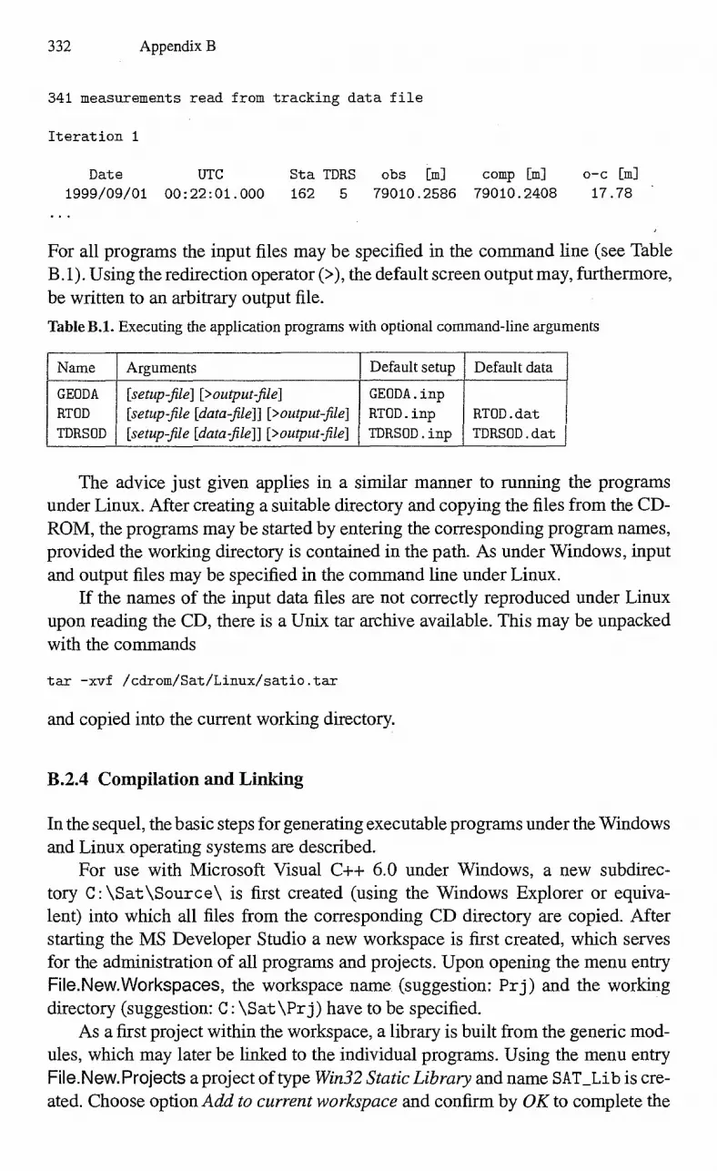
332 Appendix B
341 measurements read from tracking data file
Iteration 1
Date UTC
Sta TDRS obs [m] comp [m] o-c [m]
1999/09/01 00:22:01.000 162 5 79010.2586 79010.2408 17.78
For all programs the input files may be specified in the command line (see Table B.1). Using the redirection operator (>), the default screen output may, furthennore, be written to an arbitrary output file. Table B.1. Executing the application programs with optional command-line arguments
Name Arguments Default setup Default data
GEODA
RTOD
TDRSOD
[setup-file] [>output-file] [setup-file [data-file]] [>output-file]
[setup-file [data-file]] [>output-file]
GEODA . inp
RTOD. inp
TDRSOD . inp
RTOD .dat
TDRSOD . dat
The advice just given applies in a similar manner to running the programs under Linux. After creating a suitable directory and copying the files from the CD-ROM, the programs may be started by entering the corresponding program names, provided the working directory is contained in the path. As under Windows, input and output files may be specified in the command line under Linux.
If the names of the input data files are not correctly reproduced under Linux upon reading the CD, there is a Unix tar archive available. This may be unpacked with the commands
tar -xvf /cdrom/Sat/Linux/satio.tar
and copied into the current working directory.
B.2.4 Compilation and Linking
In the sequel, the basic steps for generating executable programs under the Windows and Linux operating systems are described.
For use with Microsoft Visual C++ 6.0 under Windows, a new subdirec-tory C: \ Sat \ Source \ is first created (using the Windows Explorer or equiva-lent) into which all files from the corresponding CD directory are copied. After starting the MS Developer Studio a new workspace is first created, which serves for the administration of all programs and projects. Upon opening the menu entry File.New.Workspaces, the workspace name (suggestion: Prj) and the working directory (suggestion: C: \ Sat \ Pr j ) have to be specified.
As a first project within the workspace, a library is built from the generic mod-ules, which may later be linked to the individual programs. Using the menu entry File.New.Projects a project of type Win32 Static Library and name SAT_Lib is cre-ated. Choose option Add to current workspace and conflua by OK to complete the
B.2 The Enclosed CD-ROM 333
allocation of this project. Subsequently the source files of the library modules are added to the project SAT_Lib by calling the menu Project.Add To Project.Files... and selecting all files within the C: \Sat \Source\ folder, which adhere to the naming scheme SAT_* . cpp. Optionaly, the header files (* . h) may also be incorpo-rated. This is not, however, mandatory, since the compiler automatically searches the source directory for header files. Now, the library can be completed by selecting the Build.Build menu. To this end, the development environment compiles all source texts and then links the resulting object files into a static library SAT_Lib . lib.
The Exercises Exerc s e_2_1 to Exerc is e_8_3 and the application programs (GEODA, RTOD, TDRSOD) are treated as independent projects within the Sat \Prj
workspace. In the sequel this is illustrated for the RTOD program. Within the menu File.New.Projects a project of type Win32 Console Application is selected and the project name RTOD is entered into the appropriate field. As in the case of the SAT_Lib project choose the option Add to current workspace and conflua with the OK button to generate the project sceleton. Now add the RTOD . cpp file from the C: \Sat \Sour ce folder to the project using the Project.Add To Project.Files... menu. Then activate Project.Dependencies... and mark the option SAT_Lib for the current project, to inform the builder that this library is required for linking the RTOD program The executable module RTOD . exe is finally built by selecting Build.Build and can subsequently be started from the DOS command window. For further hints we refer to the comprehensive documentation of the Microsoft C++ compilers and the Developer Studio environment.
Using Linux and the GNU C++ compiler, a set of minor modifications of the source codes are required. Unfortunately, the current version .2.95 of the GNU C++ compiler does not support all iostream-manipulators of the C++ standard library. This affects all programs and modules that make use of the left, right, fixed, scientific, showpos, and noshowpos manipulators. As a substitute the definitions
#include <iomanip> #include <iostream> namespace X °stream& left (ostream& o){o.setf(ios::left ,ios::adjustfield);return o; } ; °stream& right(ostream& o){o.setf(ios::right,ios::adjustfield);return o; } ; °stream& fixed(ostream& o){o.setf(ios::fixed,ios::floatfield); return o; } ; °stream& scientific(ostream& o)
{ o.setf(ios::scientific,ios::floatfield); return o; } ; °stream& showpos (ostream& o){o.setf(los::showpos); return o; } ; °stream& noshowpos(ostream& o){o.unsetf(ios;:showpos); return o; } ;
are provided in the GNU_iomanip . h file, which may be included into all relevant source files by the statements
#ifdef // GNU C++ adaptations #include "GNU_iomanip.h" #endif

334 Appendix B
Another incompatibility concerns the determination of the machine accuracy by <limits> module of the standard library, which is not currently implemented for GNU C++. This affects the module SAT_DE cpp as well as SAT_Kepler. . cpp, which should be modified as indicated below: •
#ifdef __GNUC__ // GNU C++ adaptation #include <float.h> #else // Standard C++ version #include <limits> #endif
#ifdef __GNUC__ // GNU C++ adaptation const double umach = DBL_EPSILON; #else // Standard C++ version const double umach = numeric_limits<double>::epsilon(); #endif
For compilation and linking of the individual programs, it is advisable to combine all modules SAT_* in a library libSAT . a using the shell commands:
> g++ -c SAT*.cpp # Compilation of library modules > ar rc libSAT.a SAT*.o # Generation of library from object files
Assuming that all relevant files are contained in the same directory, the main pro-grams can subsequently be built by the commands
Exercise_2_1.cpp -o Exercise_2_1 -1SAT -L. Exercise_2_2.cpp -o Exercise_2_2 -1SAT -L.
TDRSOD.cpp -o TDRSOD -1SAT -L.
For ease of use, a make file is provided as part of the satsrc . tar archive, which perfoinis all steps in a single run.

B.2 The Enclosed CD-ROM 335
B.2.5 Index of Library Functions
The following compilation summarizes all identifiers of public types, constants, functions, and classes provided by the individual modules.
<< Output operator for dates, vectors, and matrices Access to vector and matrix components Assignment of vectors and matrices Addition of vectors and matrices
+= Vector addition Subtraction of vectors and matrices Unary minus (vector, matrix)
-= Vector subtraction Multiplication (scalar, vector, matrix) Division by a scalar
abs err Public element of DE class specifying the absolute accuracy requirement
AccelDrag Acceleration due to atmospheric drag AccelHarmonic Acceleration due to harmonic gravity field of central body AccelMain Total acceleration of an Earth-orbiting satellite AccelPointMass Acceleration due to point-mass perturbation AccelSolrad Acceleration due to solar radiation pressure Accumulate Method of class LSQ for accumulation of data equations Arcs Arcseconds per radian AU Astronomical unit [m] AzEl Azimuth, elevation and, optionally, partials from local tangen-
tial coordinates [m] CalDat Calendar date and time c_light Velocity of light [mis] Col Column vector of a matrix Coy Method of class EKF returning the current covariance Coy Method of class LSQ for covariance computation Cross Cross product of 3-dimensional vectors Date Auxiliary class for output of dates Data Method of class LSQ returning the transfouned right-hand side
of the data equations DE Class for numerical solution of differential equations DE_BADACC Enumerator of type DE_STATE (Flag for too stringent accuracy
requirements) DE_DONE Enumerator of type DE_STATE (Flag for successful integration
step) Define Method of DE class defining the differential equation DEf unct Function prototype for differential equations Deg 180°/7
336
Appendix B
DE_INIT DE_INVPARAM Density_HP DE_NUMSTEPS
DE_STATE DE_STIFF Diag Diag
Dot Dyadic EccAnom EclMatrix EKF Elements Elements EgnEquinox f_Earth FindEta GAST Geodetic GHAMatrix GM_Earth GM_Moon GM_Sun GMST GPS_TAI GPS_UTC Gray GravModel Id IERS Illumination mit
mit mit
Integ Intrp Inv InvUpper LSQ
Enumerator of type DE_STATE (Integrator restart) Enumerator of type DE_STATE (invalid input parameters) Atmospheric density based on Harris—Priester model Enumerator of type DE_STATE (Permitted number of steps ex-ceeded) Enumeration type for status codes of class DE inegrator Enumerator of type DE_STATE (Suspect of stiff problem) Diagonal matrix from vector of diagonal elements Method of Matrix class returning the vector of diagonal ele-ments Dot product of two vectors Dyadic vector product Eccentric anomaly for elliptic orbits Transfounation matrix from equator to ecliptic Extended Kalman filter class Orbital elements from position and velocity Orbital elements from two positions Equation of the equinoxes [rad] Flattening of the Earth Sector—triangle ratio Greenwich Apparent Sidereal Time Class for handling geodetic coordinates Earth rotation matrix Product of gravitational constant x mass of Earth [m3/s2] Product of gravitational constant x lunar mass [m3/s2 ] Product of gravitational constant x solar mass [m31s2] Greenwich Mean Sidereal Time Method of IERS returning GPS—TAI time difference [s] Method of IERS returning GPS—UTC time difference [s] Earth gravity model Data structure for gravity model parameters Identity matrix Class for handling of Earth rotation parameters Fractional illumination of a spacecraft near the Earth Method of DE class for initialization of a new initial value prob-lem Method of class EKF for initialization of a Kalman filter Method of class LSQ for initialization of a least-squares problem (with or without a priori infounation) Method of class DE for performing an integration step Method of class DE for interpolation of solution Inversion of general square matrix Inversion of upper triangular matrix Least-squares estimation class

B.2 The Enclosed CD-ROM 337
Transformation from Greenwich coordinates to local tangential coordinates Method of class geodetic returning the transformation to local tangential coordinates Matrix class Mean obliquity of the ecliptic Method of class EKF performing the measurement update of Kalman filter parameters Modified Julian Date Modified Julian Date at epoch J2000 Low-precision lunar coordinates Euclidean norm of a vector Nutation matrix Earth rotation rate [rad/s] Public element of DE class controlling integration past the spec-ified output point
27r Polar motion matrix Method of class Geodetic computing Cartesian from geodetic coordinates Precession matrix Solar radiation pressure at 1 AU [N/m2] Earth radius [m] Lunar radius [m] Solar radius [m] Matrix describing elementary x-axis rotation Matrix describing elementary y-axis rotation Matrix describing elementary z-axis rotation 7/180° Public element of DE class specifying the relative accuracy re-quirement Class for 4th-order Runge—Kutta integration Function prototype for differential equations Row vector of a matrix Method of class IERS for initialization of Earth orientation pa-rameters Method of Matrix class for assignment of a column vector. Method of Matrix class for assignment of a row vector Method of Vector class returning the number of vector ele-ments Method of Matrix class returning the first dimension (number of rows)
LTCMatrix
LTC_Matrix
Matrix MeanObliquity Mea sUpdate
Mjd MJD_J2000 Moon Norm NutMatrix omega_Earth PermitTOUT
Pi pi2 PoleMatrix Position
PrecMatrix P_Sol R_Earth R_Moon R_Sun R_x R_y R_z Rad relerr
RK4 RK4funct Row Set
SetCol SetRow size
sizel

Appendix B
Method of Matrix class returning the second dimension (num-ber of columns) Method of Vector class for extraction of a sub-vector Method of Matrix class for extraction of a sub-matrix Method of class LSQ for solution of a least-squares problem by backsubstitution Method of Vector class returning the square-roots of all vector elements Method of class LSQ returning the square-root information ma-trix Method of class EKF returning the current state vector Position and velocity from Keplerian elements Public element of DE class specifying the current integrator status Partial derivatives of state vector w.r.t. Keplerian elements Method of class EKF returning the current standard deviation Method of class LSQ for computing the standard deviation of the solution Method of RK4 class performing a single integration step Low-precision solar coordinates Method of class EKF returning the current time Method of class EKF performing the time update of Kalman filter parameters Epoch J2000 (in Julian centuries since J2000) Matrix transposition Method of IERS class returning TT—TM time difference [s] Method of IERS class returning TT—UTC time difference [s] State vector propagation and transition matrix for Keplerian orbits Method of IERS returning UTC—TAI time difference [s] Method of MRS returning UT1—UTC time difference [s] Three-dimensional vector from polar coordinates Vector class Matrix of class IERS returning the x-coordinate of the Earth's pole [rad] Matrix of class IERS returning the y-coordinate of the Earth's pole [rad]
338
size2
slice slice Solve
Sqrt
SRIM
State State State
StatePartials StdDev StdDev
Step Sun Time TimeUpdate
T_J2000 Transp TT_TAI TT_UTC TwoBody
UTC_TAI UTl_UTC VecPolar Vector x_pole
y_pole
List of Symbols
A Runge—Lenz vector A Cross-section (surface area) A Avogadro number A Moment of inertia with respect to the x-/y-axes A Azimuth
Moment of inertia with respect to the z-axis CD Drag coefficient CR Radiation pressure coefficient Cnm Potential coefficient D Torque vector D Diagonal matrix Do Solar torque vector
Mean solar torque vector D Mean elongation of the Moon from the Sun
Earth-fixed to local-tangent transfounation matrix Expectation value Eccentric anomaly Elevation Energy
ET Ephemeris Time Force vector Mean distance of the Moon from the ascending node of its orbit
F10.7 Index measuring solar UV radiation at 10.7 cm G Jacobian matrix (partial derivatives of measurement vector
with respect to the state vector) G Gravitational constant GMST Greenwich Mean Sidereal Time H Jacobian matrix (partial derivatives of measurement vector
with respect to the epoch state) Ho Atmospheric density scale height H Sun-satellite hour angle H Macro step size
Moment of inertia Loss function
340 List of Symbols
n Zonal potential coefficient of degree n Julian Date Kalman gain Knudsen number
Kp Three-hourly planetary geomagnetic index L0 Mean longitude of the Moon
Mean anomaly Mass
Mo Mean anomaly at reference epoch MID Modified Julian Date
Nutation matrix N. Particles per unit volume
Auxiliary quantity for transformation of geodetic coordinates Accumulated Doppler counts Integer cycle ambiguity Gaussian vector (in direction of perigee) Precession matrix Covariance matrix Period
Pn Legendre polynomial of degree n Pnm Associated Legendre polynomial of degree n and order m P0 Solar radiation pressure at 1 AU
Gaussian vector (perpendicular to perigee) Orthonormal matrix Process-noise covariance matrix Upper triangular matrix Station position vector
Ry , Rz Matrices describing rotations around the x, y, z-axes liZ Universal gas constant
Radius of a celestial body Upper triangular matrix
R 0 Equatorial radius of the Earth Sensitivity matrix Square root of the weighting matrix
SA Square root of the information matrix Area of sector bounded by two position vectors
Snm Potential coefficient Time in Julian centuries since J2000 Absolute temperature
T1,2 Satellite transponder turn-around ratio Teqx Epoch of reference equinox in Julian centuries since J2000 Tn Chebyshev polynomial of order n To9 Exospheric temperature TM International Atomic Time

List of Symbols 341
TCB Barycentric Coordinate Time TCG Geocentric Coordinate Time '11JB Barycentric Dynamic Time 1DT Terrestrial Dynamic Time TT Terrestrial Time
Transformation matrix (inertial to Earth-fixed) Orthonounal matrix
U Elementary Householder transfolination matrix U ik Elementary Givens rotation matrix
Potential U2 Potential due to tides UT Potential of tide-induced gravity UT Universal Time UTC Coordinated Universal Time V Orthonoillial matrix Vnm Potential function
Gaussian vector perpendicular to the orbital plane Weighting matrix
Wnm Potential function XEW, YEW XJY-angles using antenna with East/West mount XNS, YNS X/Y-angles using antenna with North/South mount
Height Height of inflection point
a Acceleration vector a Semi-major axis a Ambiguity a Albedo of the Earth ai Coefficient of Chebyshev expansion
Runge—Kutta(—Nystrom) coefficients a Three-hourly planetary amplitude index
Chebyshev coefficient for derivative of a function Ecliptic latitude
bi Runge—Kutta(—Nystrom) coefficients Aerial velocity or specific angular momentum vector Velocity of light ( c = 299 792 458 m/s) Element of Givens rotation matrix
ci Runge—Kutta coefficients di Singular value
Unit vector Orbital eccentricity Local truncation error Eccentricity of reference ellipsoid Vector function

342 List of Symbols
Orbital-plane unit vector Flattening of the Earth (f P•e, 1/298.257) Frequency Modeled measurement vector Orbital-plane unit vector Gravitational acceleration
g (i) Coefficient of variable stepsize multistep method h Aerial velocity (specific angular momentum) vector h Modeled measurement vector h Equinoctial element (eccentricity vector component) h Altitude (height above reference ellipsoid) h Step size
Orbital inclination ki Function values for use in Runge—Kutta methods
Equinoctial element (eccentricity vector component) 1 Angular momentum vector 1 Mean longitude 1 Typical satellite dimension 1 Mean anomaly of the Moon 1 Ecliptic longitude
Mean anomaly of the Sun Satellite mass Surface normal unit vector Mean motion Particle number density Elements of nutation matrix Polynomial approximation of vector-valued function Force model parameter vector Semi-latus rectum Equinoctial element (inclination vector component) Order of numerical integration method Precession in longitude
Pif Elements of precession matrix Pv Impulse of a photon
Measurement model parameter vector Equinoctial element (inclination vector component)
go
Fraction by volume of atmospheric constituents Geocentric satellite position vector Geocentric satellite velocity vector Geocentric satellite acceleration vector
ro
Geocentric position vector of the Sun Geocentric satellite distance Position vector Satellite position in local tangent coordinates

List of Symbols 343
Tide constituent Time
to Reference epoch Process noise
ui Mid-point rule approximation in extrapolation method Argument of latitude Geocentric satellite velocity vector Geocentric satellite velocity Householder transformation vector
x, y, z Geocentric satellite coordinates Y', j Geocentric satellite acceleration
X, 0 Satellite coordinates with respect to the orbital plane xp , yp Pole coordinates X0 Reference epoch state x 0 Least-squares estimate of reference epoch state y State vector Yo State vector (initial value)
Measurement vector Auxiliary angle in description of precession Height in km Measurement
zx Height of inflection point in km
Area of triangle formed by two position vectors AE Transfered photon energy AT Ephemeris Time — Universal Time difference AT00 Exospheric temperature correction Am Mass element .6p Transfered photon impulse At Time interval .6X0 Reference state correction Az Measurement residuals relative to reference orbit As Nutation in ecliptic latitude
Nutation in ecliptic longitude Earth rotation matrix Greenwich sidereal time
A Infoimation matrix A Auxiliary angle in description of-precession H Polar motion transfoimation matrix 17 Auxiliary angle for description of precession O GPS code phase
Increment function O State transition matrix O Solar radiation flux

344 List of Symbols
tif Geocentric angle between satellite and apex of density bulge Right ascension (or longitude) of the ascending node
a Orbital elements vector a Right ascension ai Thelma' diffusion coefficient 0/0 Right ascension of the Sun
Ecliptic latitude Pnif Adams—Bashforth coefficient An* j Adams—Moulton coefficient y Angle yj Adams—Bashforth coefficient
Adams—Moulton coefficient 8 Declination 8 Dirac delta function
Coefficient of Stoeimer method St Coefficient of Cowell method
8rzm Kronecker symbol (S rim = 101 I for f nn ;int n 1)
Measurement noise vector Emissivity of the Earth Reflectivity Mean obliquity of the ecliptic Coefficient of reflectivity True obliquity of the ecliptic
E • Error coefficient of mid-point rule approximation Auxiliary angle in description of precession Numerical approximation of initial value problem Ratio of sector to triangle
O Angle between incoming radiation and surface normal Os Angle of the weighted sum of Doodson variables
Auxiliary angle in description of precession ic Love number K rz Ocean-load deformation coefficient
Geocentric longitude (positive towards the East) Mean free path length Error constant of Runge—Kutta—NystrOm method Wavelength Ecliptic longitude Ratio of the Earth's and the Moon's mass CO 81.3) True anomaly
y Shadow function 7r 3.1415926...
Angle between ecliptic of epoch and fixed reference ecliptic Residual vector

List of Symbols 345
Density Range (topocentric distance)
po GPS code pseudorange GPS carrier pseudorange Range rate (topocentric velocity) Average range rate Fraction of integration step size Measurement weight Phase noise
crp- Range rate noise Time within unit interval Signal travel time Rotation angle Geocentric latitude GPS carrier phase
(i) Backward difference of variable stepsize multistep method ço Geodetic/geographic latitude
Geocentric latitude Lunisolar precession
coEe Angular velocity vector of the Earth Argument of perigee (or perihelion) Angular velocity Inclination of mean equator with respect to reference ecliptic
Vfl Backwards difference of order n On xm Null matrix of dimension n x m
xn n-dimensional identity matrix Earth
O Sun 0 Degree a - b Dot product of two vectors a T b Dot product of two vectors A T Transposed matrix A -1 Inverse matrix A — T Inverse of transposed matrix
The elementary rotation matrices are defined as
( 1 0 0 ) ±cos0 0 —sin0 ±cos4) -Fsin4) 0)
R1 () = 0 +cos4) -Fsin4) R y (4)) = 0 1 0 1 R()=z = —sin l) +coal) 0 0 —sin 0 +cos0 +sit* 0 +cos0 0 0 1


References
Abramowitz M., Stegun I. A.; Handbook of Mathematical Functions; Dover, New York (1965). Allgower E. L., Georg K.; Numerical Continuation Methods; SCM13; Springer Verlag, New York
(1990). Andrews A.; A Square Root Formulation of the Kalman Covariance Equations; AIAA Journal 6,
No. 6, 1165-1166 (1968). Aoki S., Guinot B., Kaplan G. H., Kinoshita H., McCarthy D. D., Seidelman P. K.; The New
Definition of Universal Time; Astronomy and Astrophysics 105, 359-361(1982). Arias E. E, Charlot P., Feissel M., Lestrade J.-E; The extragalactic reference system of the Interna-
tional Earth Rotation Service, ICRS; Astronomy and Astrophysics 303, 604-608 (1995). Ballani L.; Partielle Ableitungen und Variationsgleichungen zur Modellie rung von Satellitenbahnen
und Parameterbestimmung; Vermessungstechnik, 36. Jg., Heft 6, 192-194 (1988a). Ballani L.; Numerische Untersuchungen zur Bestimmung von Parametem des Erdkdrpers und von
Satellitenbahnen; Vermessungstechnik, 36. Jg., Heft 7, 220-223 (1988b). Barlier F., Berger C., FalM J. L., Kockarts G., Thuillier G.; A thermospheric model based on satellite
drag data; Ann. Geophys., 34, 9-24 (1978). Bate R. R., Mueller D. D., White J. E.; Fundamentals of Astrodynamics; Dover Publications, Inc.,
New York (1971). Battin R. H.; An Introduction to the Mathematics and Methods of Astrodynamics; AIAA Education
Series; American Institute of Aeronautics and Astronautics, New York (1987). Battin R. H., Levine G. M.; Application of Kalman Filtering Techniques to the Apollo Program;
Chap. 14 in Leondes C. T. (ed.); Theory and applications of Kalman filtering; NATO Advisory Group for Aerospace Res. Develop., AGARDograph 139 (1970).
Bedrich S., Flechtner F., FOrste Ch., Reigber Ch., Teubel A.; PRARE System Petformance; Proc. 3rd ERS Scientific Symposium (ESA SP-414), Florence, Italy (1997).
Berger C., Barlier E, Ill M.; Diurnal Variations of the Response of the Equatorial Thermosphere to Geomagnetic Activity; Physica Scripta, 37, 427-431(1988).
Bertiger W. I., Bar-Sever Y. E., Christensen E. J., Davis E. S., Guinn J. R., Haines B. J., Ibanez-Meier R. W., Jee J. R., Lichten S. M., Melbourne W. G., Muellerschoen R. J., Munson T. N., Vigue Y., Wu S. C., Yunck T. P., Schutz B. E., Abusali P. A. M., Rim H. J., Watkins M. M., Willis P.; GPS Precise Tracking of TOPEX/POSEIDON: Results and Implications; J. Geophys. Res., TOPEX/POSEIDON Special Issue, 99, No. C12, 24449,-24465 (1994).
Bertotti B., Farinella P.; Physics of the Earth and the Solar System; Kluwer Academic Publishers, Dordrecht (1990).
Bhat R. S., Frauenholz R. B., Canelli P. E.; TOPEX/Poseidon Orbit Maintenance Maneuver Design; AAS 89-408, 645-670 (1989).
Bhat R. S., Frauenholz R. B., Canelli P. E.; TOPEX/Poseidon Orbit Maintenance for the Firsi Five Years; AAS 98-379, 953 (1998).
Bierman G. J.; Factorization Methods for Discrete Sequential Estimation; Academic Press; New York (1977).
Bierman G. J.; Bierman K. H.; Estimation Subroutine Library User Guide; 1-EA Report No. 81584, Factorized Estimation Applications Inc., Sherman Oaks, California (1984).
Bilitza D., Rawer K., Bossy L., Gulyaeva T.; International Reference Ionosphere -past, present, and friture: I. electron density; Adv. Space. Res. 1313, 3 (1993).

348 References
Bilitza D., Koblinsky C., Beckley B., Zia S., Williamson R.; Using IRI for the Computation of Ionospheric Corrections for Altimeter Data Analysis; Adv. Space. Res. 15/2, 113-119 (1995).
Black H. D.; An Easily Implemented Algorithm for the Tropospheric Range Correction; Journal of Geophysical Research, 83 No. B4, 1825-1828 (1978).
B6hnhardt H., Ruder H., Schneider M.; Modelle des Strahlungsdrucksfi,ir die Theorie der Satelliten-bahnen; Deutsche Geod5tische Kommission bei der Bayerischen Akademie der Wissenschafteri, Reihe A, Heft 93; Miinchen (1981).
Bohrmann A ; Bahnen kiinstlicher Satelliten; Bibliographicshes Institut, Mannheim (1963). Bomford G.; Geodesy; Clarendon Press, Oxford; 4th ed. (1980). Borkowski K. M.; Accurate Algorithms to Transform Geocentric to Geodetic Coordinates; Bulletin
Geodetique 63, 50-56 (1989). Bowring B. R.; The accuracy of geodetic latitude and height equations; Survey Review 28,202-206
(1985). Brankin R. W., Dormand J. R., Gladwell I., Prince P. J., Seward W. L.; A Runge—Kutta—Nystrom
Code; Num. Anal. Rep. 136, University of Manchester (1987). Branldn R. W., Gladwell I., Dormand J. R., Prince P. J., Seward W. L.; Algorithm 670 —A Runge-
Kutta—Nystrom Code; ACM Transactions on Mathematical Software, 15/1, 31-40 (1989). Branyon S. A., Knowles H. B., Hess G. K. jr.; Kalman Filters in Generic ADA Packages; 6th
National Conference on Ada Technology - Washington 1988, U.S. Dept. Commerce, Springfield VA, 365-376 (1988).
Broucke R. A.; On the Matrizant of the Two-Body Problem; Astronomy and Astrophysics 6, 173-182 (1970).
Broucke R. A., Cefola P. J.; On the equinoctial orbit elements; Celestial Mechanics 5, 303-310 (1972).
Brown R. G., Hwang P. Y. C.; Introduction to Random Signals and Applied Kalman Filtering with Matlab Exercises and Solutions; John Wiley & Sons, 3rd ed. (1996)
Bucerius H.; Bahnbestimmung ais Randwertproblem; Astronornische Nachrichten 278, 193-216 (1950).
Bucy R. S., Joseph P. D.; Filtering for Stochastic Processes with Applications to Guidance; Wiley, New York (1968).
Bulirsch R., Stoer J.; Numerical treatment of ordinary differential equations by extrapolation meth-ods; Num. Math. 8, 1-13 (1966).
Butcher J. C.; On Runge—Kutta processes of high order, J. Austral. Math. Soc., IV/2, 179-194 (1964).
Butcher J. C.; On the attainable order of Runge—Kutta methods; Math. of Comp., 19, 408-417 (1965).
Butcher J. C.; The non-existence of ten stage eighth order explicit Runge—Kutta methods; BIT, 25, 521-540 (1985).
Campbell J. K., Synnott S. P., Bierman G. J.; Voyager Orbit Determination at Jupiter; IEEE Trans-actions on Automatic Control, AC-28, 256-268 (1983).
Capitaine N., Williams J. G., Seidelmann P. K.; Clarifications concerning the definition and deter- mination of the celestial ephemeris pole; Astronomy and Astrophysics 146, 381-383 (1985).
Capitaine N., Gontier A.-M.; Accurate procedure for deriving UT I at a submilliarcsecond accuracy from Greenwich Sidereal Time or from the stellar angle; Astronomy and Astrophysics 275, 645— 650 (1993).
Carter S. S., Cefola P. J., Proulx R. J.; The Determination of Precision Mean Element Sets from GPS Receiver on-Board Navigation Solutions; AAS 95-371; Advances in the Astronautical Sciences 90, Astrodynamics, pp. 1203 (1995).
CCSDS; Radio Frequency and Modulation Systems - Part I - Earth Stations and Spacecraft; CCSDS 401.0-B Blue Book (1998).
Cefola P. J.; Equinoctial Orbit Elements - Application to Artificial Satellite Orbits; AIAA/AAS Astrodynamics Conference, Palo Alto, California, Sep. 11-12, 1972; A1AA 72-937, (1972).

References 349
Cicci D. A., Tapley B. D.; Optimal Solution of Unobservable Orbit Determination Problems; Ce-lestial Mechanics 44, 339-363 (1988).
CIRA; COSPAR International Reference Atmosphere 1972; Compiled by COSPAR Working Group IV, Akadernie-Verlag, Berlin (1972).
CIRA; COSPAR International Reference Atmosphere: 1986 Part I: Thermosphere Models; Advances in Space Research, 8 (1986).
Chao B. F.; Predictability of the Earth's Polar Motion; Bull. Géod. 59, 81-93 (1985). Clarke A. C.; Extra-Terrestrial Relays; Wireless World, October 1945, pp. 305-308 (1945). Clohessy W. H., Wiltshire R. S.; Terminal Guidance system for Satellite Rendezvous; Journal of
Aerospace Science 270, 653 (1960). Cohen E. R., Taylor B. N.; The 1986 CODA TA Recommended Values Of the Fundamental Physical
Constants; Journal of Research of the National Bureau of Standards 92, No. 2,85-95 (1987). Colombo O. L.; The Dynamics of Global Positioning System Orbits and the Determination of P recise
Ephemerides; Journal of Geophysical Research 94, No. B7,9167-9182 (1989). Cox C., Oza D.; Tracking and Data Relay Satellite (TDRS) Orbit Determination: Operations Con-
cepts for Using Global Positioning System (GPS) Tracking and Alternative Approaches; 553- FDD-94/036/ROUDO, Goddard Space Flight Center, Mission Operations and Data Systems Di-rectorate (1994).
Cunningham L. E.; On the Computation of the Spherical Harmonic Terms needed during the Numer-ical Integration of the Orbital Motion of an Artificial Satellite; Celestial Mechanics 2, 207-216 (1970).
Cunningham J., Curtis V.; WGS84 Coordinate Validation and Improvement for the NIMA and Air Force GPS Tracking Stations; NSWCDD/TR-96/201; Naval Surface Warfare Center, Dahlgren Division; Dahlgren, Virginia (1996).
Curkendall D. W., Leondes C. T.; Sequential Filter Design for Precision Orbit Determination and Physical Constant Determination; Celestial Mechanics 8, 481-494 (1974).
Curtis L. E.; High order explicit Runge—Kutta formulae, their uses, and limitations; J. Inst. Maths Applics 16, 35-55 (1975).
Danby J. M. A., Burkardt T. M.; The Solution of Kepler's Equation I; Celestial Mechanics, 31, 95-107 (1983).
Daniell R. E., Brown L. D., Anderson D. N., Fox M. W., Doherty P. H., Decker D. T., Sojka J. J., Schunk R. W.; Parametrized Ionospheric Model: A global ionospheric Parametrization based on First Principles Models Radio Science 30, 1499-1510 (1995).
Davis E., Dunn C. E., Stanton R. H., Thomas J. B.; The GRACE Mission: Meeting the Technical Challenge; 50th International Astronautical Congress, 4-8 Oct. 1999, Amsterdam; (1999).
Degnan J. J., Pavlis E. C.; Laser Ranging to GPS Satellites with Centimeter Accuracy; GPS World September 1994,62-70 (1994).
DeMets C., Gordon R. G., Argus D. F., Stein S.; Effect of recent revisions to the geomagnetic reversal time scale on estimates of current plate motions; Geophys. Res. Let. 21, 2191-2194 (1994).
Dershowitz N., Reingold E. M.; Calendrical Calculations; Cambridge University Press, New York (1997). •
Deuflhard P.; On Algorithms for the Summation of Certain Special Functions; Computing 17,37-48 (1976).
Deuflhard P.; Order and Stepsize Control in Extrapolation Methods; Numerische Mathematik 41, 399-422 (1983).
Deuflhard P.; Recent progress in extrapolation methods for ordinary differential equations; SIAM Review 27, 505-535 (1985).
van Dierendonck A. J., Russell S. S., Kopitzke E. R., Birnbaum M.; The GPS Navigation Message; Navigation 25, No. 2, p. 147-165 (1978).
Dormand J. R., Prince P. J.; New Runge—Kutta algorithms for numerical simulation in dynamical astronomy; Cel. Mech. 18, 223-232 (1978).
Dormand J. R., Prince P. J.; A family of embedded Runge—Kutta forrrzulae; J. Comp. Appl. Math. 6, No.1,19-26 (1980).

350 References
Dormand J. R., Prince R J.; Runge—Kutta triples; Comput. Math. Appl., 12A, 1007-1017 (1986). Dormand J. R., Prince P. J.; Runge—Kutta—Nystrdm triples; Comput. Math. Appl., 13, 937-949
(1987). Dormand J. R., Prince P. J.; Practical Runge—Kutta Processes; SIAM J. Sci. Stat. Comput., 5,
977-989 (1989). Dormand J. R., El-Mikkawy M. E. A., Prince P. J.; High Order Embedded Runge—Kutta—Nystrom
Formulae; IMA J. Numer. Anal. 7, 423-430 (1987). Dow J. M.; Non-singular Partial Derivatives for Synchronous Orbits; ESOC OAD Working Paper
No. 22; European Space Operations Centre, Orbit and Attitude Division; Darmstadt (1975). Eanes R. J., Schutz B., Tapley B.; Earth and Ocean Tide Effects on Lageos and Starlette; in Proceed-
ings of the Ninth International Symposium on Earth Tides, Kuo J. T. (ed), E. Sckweizerbart'sche Verlagsbuchhandlung, Stuttgart (1983).
Edenhofer P., Glesner D., Stein V.; Ausbreitungsfehler elektromagnetischer Wellen bei der Bahn- 'vermessung von Erdsatelliten; DFVLR Forschungsbericht 73-56; Oberpfaffenhofen (1973).
Enright W. H., Jackson K. R., NOrsett S. P., Thomsen P. G.; Interpolants for Runge—Kutta Formulas; ACM Transactions on Mathematical Software, 12, No. 3,193-218 (1986).
Enright W. H., Higham D. J., Owren B., Sharp P. W.; A Survey of the Explicit Runge—Kutta Method; Technical Report 291/94, Dept. Computer Science, University of Toronto; revised version; April (1995).
Escobal P. R.; Methods of Orbit Determination; John Wiley & Sons, Inc., New York (1965). Reprint: Krieger Publishing Company, Malabar, Florida (1976).
EUMETSAT; The Meteosat System; EUM TD 05 Rev. 3, May 1999 (1999). Evans M. J., Maclay T. D.; Mission Design of the ORBCOMM Constellation; in: van der Ha J. C.
(ed.), Mission Design & Implementation of Satellite Constellations, 103-112; Kluwer Academic Publishers (1998).
Fallon L. III; Recursive Least-Squares Estimators and Kalman Filters; Chap. 13.5 in Wertz J. R. (ed.); Spacecraft Attitude Determination and Control; D. Reidel Publishing Company (1978).
Fehlberg E.; Classical fifth-, sixth-, seventh-, and eighth-order Run ge—Kutta formulas with stepsize control; Technical Report NASA TR R-287 (1968).
Fehlberg E.; Klassische Runge—Kutta—Nystr5m-Formeln mit Schrittweiten-Kontrolle fir Differen-tialgleichungen ï f (t , x, i); Computing 14, 371-387 (1975).
Feltens J., Dow J. M., Martfn-Mur T. J., Garcia Martinez C., Martfnez-Fadrique F., Piriz R.; Using GPS for Ionospheric Corrections of ESA Tracking Data; 12th International Symposium on Space Flight Dynamics, &F1) 97/17 ESA SP-403,121-125, Darmstadt (1997).
Feissel M., Mignard F.; The adoption of ICRS on I January 1998: meaning and consequences; Astronomy and Astrophysics 331, L33—L36 (1998).
Filippi S., Grdf J.; New Runge—Kutta—Nystrom formula-pairs of order 8(7), 9(8), 10(9) and 11( 10) for differential equations of the form y" f (x , y); Journal of Computational and Applied Mathematics, 14, 361-370 (1986).
van Flandern T. C., Pulkkinen K.F.; Low precision formulae for planetary positions; Astrophysical Journal Supplement Series 41, 391 (1979).
Follcner W. M., Charlot P., Finger M. H., Williams J. G., Sovers O. J., Newhall X. X., Standish E. M. jr.; Determination of the extragalactic-planetary frame tie from joint analysis of radio interferometric and lunar ranging measurements; Astronomy and Astrophysics 287, 279-289 (1994).
Forman P.; Atomichron: The Atomic Clock from Concept to Commercial Product; Proc. IEEE, Vol. 73, No. 7,1181 (1985).
Fox K; Numerical Integration of the Equations of Motion of Celestial Mechanics; Celestial Me-chanics 33, 127-142 (1984).
Frauenholz R. B., Shapiro B. E.; The role of predicted solar activity in TOPEX/POSEIDON orbit maintenance maneuver design; AAS/AIAA Astrodynamics Specialist Conference, AAS 91-515, Durango, Colorado (1991).
References 351
Fricke W., Schwan H., Lederle T., Bastian U., Bien R., Burkhardt G., du Mont B., Hering, R., Jdhrling R., JahreiB H., Reiser S., Schwerdtfeger H.-M., Walter H. G. Fifth filndamental catalogue (F K5). Part I. The Basic Fundamental Stars; Verafentlichungen Astronomisches Rechen-Institut Heidelberg Nr. 32; Verlag G. Braun, Karlsruhe (1988).
Gaposchkin E M., Coster A. J.; Evaluation of Thermospheric Models and the Precipitation Index for Satellite Drag; Adv. Space Res., 10, 3303-3309 (1990).
Gaudenzi De R., Lijphart E. E., Vassallo E.; The New ESA Multi-Purpose Tracking System; ESA Journal 14, 23-40 (1990).
Gelb A. (ed.); Applied Optimal Estimation; The MIT Press; Massachusetts Institute of Technology; Cambridge, Massachusetts (1974).
Gendt G., Sorokin N. A.; Probleme bei der numerischen Integration von Satellitenbahnen mit ho her Genauigkeit; Vermessungstechnik, 26. Jg., Heft 9,291-295 (1978).
Gerstl M.; Vergleich von Algorithmen zur Summation von Kugelfteichenfunktionen; in M. Schneider, Die Arbeiten des SEB 78 Satellitengeoddsie der TU Milnchen 1977,81-88 (1978).
Gibson R.; A Derivation of Relativistic Effects in Satellite Tracking; 1R 83-55, Naval Surface Weapons Center, Dahlgren Virginia (1983).
Gill E.; Smooth Bi-Polynomial Interpolation of Jacchia 1971 Atmospheric Densities For Effi cient Satellite Drag Computation; DLR-GSOC IB 96-1; German Aerospace Center (DLR) (1996).
Gill E.; Orbit Determination of the MIR Space Stationfrom GPS Navigation Data; 12th International Symposium on Space Flight Dynamics, SFD 97/17 ESA SP-403,79-84, Darmstadt (1997).
Gill P. E., Murray W., Wright M. H.; Numerical Linear Algebra and Optimization; Addison-Wesley Publ. Co., California (1990).
Givens J. W.; Computation of plane unitary rotations transforming a general matrix to triangular form; SIAM J. Appl. Math. 6, 26-50 (1958).
Gladwell I., Shampine L. F., Brankin R.W.; Automatic selection of the initial step size for an ODE solver; Journal of Computational and Applied Mathematics, 18, 175-192 (1987).
Goad C.C., Goodman L.; A Modified Hopfield Tropospheric Refraction Correction Model; Fall Annual Meeting, Americal Geophysical Union, San Fransisco, CA, Dec. 12-17, (1974).
Goldstein H.; Classical Mechanics; Addison-Wesley, Reading Mass., 2nd ed. (1980). Golub G. H., Reinsch C.; Singular Value Decomposition and Least Squares Solution; Handbook
Series Linear Algebra; Numer. Math., 14,403-420 (1970). Golub G. H., van Loan Ch.; Matrix Computations; 2nd edition; The Johns Hopkins University Press,
Baltimore (1989). Goodman D. T., Bell R. J. (eds.); The International System of Units (SI); U. S. Department of
Commerce (1986). Goodyear W. H.; Completely general closed-form solution for coordinates and partial derivatives
of the two-body problem; Astronomical Journal 70, 189-192(1965). Erratum: AJ 70, 446 (1965). Gragg W. B.; On extrapolation algorithms for ordinary initial value problems; SIAM J. Num. Anal.,
ser. B, 2, 384-403 (1965). van Graas F., Braasch M. S.; Selective Availability; in: Gldbal Positioning System: Theory and Appli-
cations; Eds.: Parkinson B. W., Spilker J. J., American Institute of Aeronautics and Astronautics, Washington (1994).
Green R. M.; Spherical Astronomy; Cambridge University Press; Cambridge (1985). Grigorieff R. D.; Numerik gewanlicher Differentialgleichungen 2; Teubner Verlag, Stuttgart (1977). GroBkopf J.; Wellenausbreitung 1+II; Hochschultaschenbuch BI 141/141a; Bibliographisches In-
stitut, Mannheim (1970). Groten E.; The motion of the Earth; in Landolt-B6rnstein, Numerical Data and Functional Rela-
tionships in Science and Technology, New Series, Group V, 2a, Springer Verlag, Berlin (1984). Guinot B.; Atomic Time; in Kovalevsky J., Mueller I. I., Kolaczek B. (eds.); Reference Frames in
Astronomy and Geophysics; Astronomy and Space Science Library Vol. 154,379-415; Kluwer Academic Publishers (1989).
Gupta G. K., Sacks-Davis R., Tischer R E.; A Review of Recent Developments in Solving ODEs; Computing Surveys 17, 5 (1985).

352 References
van der Ha J. C., Moth V. J.; Analytical Evaluation of Solar Radiation Induced Perturbations of Space Structures; The Journal of the Astronautical Sciences, XXV, No.4, 283-306 (1977).
Hairer E.; A Runge—Kutta Method of Order 10; J. Inst. Maths Applics, 21, 47-59 (1978). Hairer E., Norsett S. P., Wanner G.; Solving Ordinary Differential Equations I; Springer-Verlag,
Berlin-Heidelberg-New York (1987). Hairer E., Ostermann A.; Dense output for extrapolation methods; Numer. Math. 58, 419-439
(1990). Hajj G. A., Kursinski E. R., Bertiger W, Leroy, Romans L., Schofield J. T.; Sensing the atmosphere..
from a low-earth orbiter tracking GPS: early results and lessons from the GPS/MET experiment; Proceedings of the ION GPS-95, Institute of Navigation, Palm Springs, Calif, U.S.A., 12-15, Sept., pp. 1167-1174(1995).
Hajj G. A., Romans L. J.; Ionospheric Electron Density Profiles obtained from the Global Positioning System: Results from the GPS/MET experiment; Radio Science 33, 175-190 (1998).
Halain J. P., Welter T., Francken P., Krier G., Wauthier R, Rochus P.; Performance of Least Squares and Kalman Filter Algorithms for Orbit Determination using Single- and Multi-Station Tracking of Geostationary Satellites; AAS 98-368; Advances in the Astronautical Sciences 100, Spaceflight Dynamics, pp. 835 (1998).
Harris I., Priester W.; Time-Dependent Structure of the Upper Atmosphere; NASA TN D-1443; Goddard Space Flight Center, Maryland (1962).
Hartl Ph.; Fernwirktechnik der Raumfahrt; Springer Verlag, Berlin, Heidelberg, New York (1977). Hartl Ph.; The Precise Range and Range Rate Equipment (PRARE) and its Possible Support to
the Radar Altimeter Measurements For ERS-1; Proceedings of a Workshop on ERS-1 Radar Altimeter Data Products, Frascati, Italy, ESA SP-221 (1984).
Hedin A. E.; A Revised Thermospheric Model based on Mass Spectrometer and Incoherent Scatter Data - MSIS-83; Journal of Geophysical Research, 88 10170-10 188 (1983).
Hedin A. E.; MSIS-86 Thermospheric Model; Journal of Geophysical Research, 92 4649-4662 (1987).
Hedin A. E., Salah J. E., Evans J. V., Reber C. A., Newton G. P.; Spencer N. W., Kayser D. C., Alcayde D., Bauer P., Cogger L., McLure J. P.; A Global Thennospheric Model based on Mass Spectrometer and Incoherent Scatter Data, MSIS 1, N2 Density and Temperature; Journal of Geophysical Research, 82 2139-2147 (1977).
Hedin A. E., Spencer N. W., Killeen T. L.; Empirical Global Model of Upper Thermosphere Winds Based on Atmosphere and Dynamics Explorer Satellite Data; Journal of Geophysical Research, 93 No. A9, 9959-9978 (1988).
Hellings R. W.; Relativistic Effects in Astronomical Timing Measurements; Astronomical Journal 91, No. 3, 650-659 (1986); Erratum in Astronomical Journal 92, No. 6, 1446 (1986).
Henize K. G.; The Baker—Nunn Satellite Tracking Camera; Sky and Telescope 16, 108-111(1957). Henrici P.; Discrete Variable Methods in Ordinary Differential Equations; Wiley, New York (1962).
Herrick S.; Astrodynamics I & II; Van Nostrand Reinhold, London (1971, 1972). Higham D. J.; Defect estimation in Adams PECE Codes; SIAM J. Sci. Stat. Comput. 10, 964-976
(1989). Hofmann-Wellenhof B., Lichtenegger H., Collins J.; Global Positioning System Theory and Appli-
cations; Springer-Verlag Wien New York 4th ed. (1997). Hopfield H. S.; Two-Quartic Tropospheric Refraction Profile for Correcting Satellite Data; Journal
of Geopysical Research 74, 4487 /1/99 (1969). Horn M. K.; Scaled Runge—Kutta Algorithms for Handling Dense Output; DFVLR-1-1:1 81-13;
Deutsche Forschungs- und Versuchsanstalt fiir Luft- und Raurnfahrt, Oberpfaffenhofen (1981). Horn M. K.; Fourth- andfifth-order, scaled Runge—Kutta algorithms for treating dense output; SIAM
J. Numer. Anal., 20/3, 558-568 (1983). Householder A. S.; Unitary triangularization of a nonsymmetric matrix; J. Assoc. Comp. Mach. 5,
339-342 (1958). Hull T. E., Enright W. H., Fellen B. M., Sedgwick A. E.; Comparing numerical methods for ordinary
differential equations; SIAM J. Numer. Anal. 9, 603-637 (1972).

References 353
Hussels H.-G.; Schrittweitensteuerung bei der Integration gewdhnlicher Differentialgleichungen mit Extrapolationsverfahren; Diplomarbeit, Köln (1973).
Husson V.; Global SLR Performance Evaluation; AlliedSignal Technical Services Corporation, NASA SLR Program, Lanham Maryland (1997).
ICD-GLONASS; Global Navigation Satellite System GLONASS Interface Control Document; Co-ordination Scientific Information Center; Moscow (1998).
ICD-GPS -200; Navstar GPS Space Segment / Navigation User Interfaces; Revison C; 25 Sept. 1997; Arinc Research Corp., El Segundo (1997).
TFRS; Explanatory Supplement to IERS Bulletins A and B; International Earth Rotation Service; Paris (1998).
Ivanov N., Salischev V.; The GLONASS System —An Overview; The Journal of Navigation 45, No. 2, 175-182 (1992).
Jacchia L. G.; Static Diffusion Models of the Upper Atmosphere with Empirical Temperature Profiles; Smithsonian Contr. Astrophys. 8, No. 9, 215-257 (1965).
Jacchia L. G.; New Static Models of the Thermosphere and Exosphere with Empirical Temperature Profiles; SAO Special Report 313, Cambridge (1970).
Jacchia L. G.; Revised Static Models of the Thermosphere and Exosphere with Empirical Temper-ature Profiles; SAO Special Report 332, Cambridge (1971).
Jacchia L. G.; Thermospheric Temperature, Density, and Composition: New Models; SAO Special Report 375, Cambridge (1977).
Jacchia L. G., Slowey J. W.; Analysis of Data for the Development of Density and Composition Models of the Upper Atmosphere; Air Force Geophsyics Laboratory, AFGL-TR-81-0230, Ma. (1981).
Jackson J.; Monthly Notices of the Royal Astronomical Society 84, 602 (1924). Jazwinski A. H.; Stochastic Processes and Filtering Theory; Academic Press, New York (1970). Jeske H.; Chap. 7.2/7.3; in Landolt-B6rnstein, Numerical Data and Functional Relationships in
Science and Technology, New Series, Group V, 4b; Springer Verlag, Berlin (1988). Kallemeyn P., Vaughan R.; Observing Doppler to Verify Attitude Behaviour; .TPL Interoffice Mem-
orandum TOM 312.3-96-028 (1996). Kalman R. E.; A New Approach to Linear Filtering and Prediction Problems; J. Basic Eng. 82,
35-45 (1960). Kalman R. E., Bucy R. S.; New Results in Linear Filtering and Prediction Theory; J. Basic Eng.
83D, 95-108 (1961). Kaminski P. G., Bryson A. E., Schmidt S. F.; Discrete square root filtering: a survey of current
techniques; IEEE Trans. Automatic Control AC-16, No. 6, 727-736 (1971). Kaula W. M.; Theory of Satellite Geodesy; Blaisdell Publishing Company, Waltham, Massachusetts
(1966). Knocke P.C., Ries J.C., Tapley B.D.; Earth Radiation Pressure Effects on Satellites; Proceedings of
the AIAAJAAS Astrodynamics Conference, 88-4292-CP, pp. 577-587 (1988). King-Hele D.; Satellite orbits in an atmosphere; Blackie and. Son Ltd.; London (1987). Kinoshita H.; Theory of the Rotation of the Rigid Earth; Celestial Mechanics 15, 277 (1977). Kinoshita H., Aoki S.; The Definition of the Ecliptic; Celestial Mechanics 31, 329-338 (1983). Kinoshita H., Nakai H.; Numerical Integration Methods in Dynamical Astronomy; Celestial Me-
chanics 45, 231-244 (1989). Kirschner S. M., Beni A. C., Broaddus S. R., Doll C. E.; Spacecraft preliminary orbit determination
using tracking measurements obtained from the tracking and data relay satellite system (TDRSS) and the ground spaceflight tracking data network (GSTDN); Space Dynamics Conference, CNES Toulouse, Nov. 89 (1990).
Kramer H. J.; Observation of the Earth and Its Environment — Survey of Missions and Sensors; Springer Verlag, 3rd ed. (1996).
Krogh F. T.; VODQ/SVDQ/DVDQ - Variable Order Integrators for the Numerical Solution of Ordi-nary Differential Equations; JPL Technical Utilization Document CP-2308, NPO-11643 (1969).

354 References
Krogh F. T.; Changing Stepsize in the Integration of Differential Equations Using Modified Differ- ences; in Lecture Notes in Mathematics 362, 22-71, Springer Verlag, New York (1974).
Kumar M.; World Geodetic System 1984: A Reference Frame for Global Mapping, Charting and Geodetic Applications; Surveying and Land Information Systems 53/1, 53-56 (1993).
Lafontaine de J., Hughes P.; An Analytic Version of Jacchia's 1977 Model Atmosphere; Celestial Mechanics, 29, 3-26 (1983).
Lambert J. D.; Computational Methods in Ordinary Differential Equations; John Wiley and Sons, London (1973).
Lanyi G.; Tropospheric Propagation Delay Effects in Radio Interferometric Measurements; EOS Transactions, American Geophys. Union 64, pp. 210 (1983).
Laudet P., Deleuze M., Guitart A., Piuzzi A., Valorge C.; Precise Orbit Determination with DORIS; Carrou J. P. (ed.), Spaceflight Dynamics; Cépaduès-Éditions (1995).
Lawson C. L.; Applications of Singular Value Analysis; in Rice J. R., Mathematical Software; Academic Press (1971).
Lawson C. L., Hanson R. J.; Solving Least Squares Problems; Prentice Hall, Englewood Cliffs, New Jersey (1974).
Lemoine F. G., Kenyon S. C., Factor J. K., Trimmer R. G., Pavlis N. K., Chinn D. S., Cox C. M., Kiosk° S. M., Luthcke S. B., Torrence M. H., Wang Y. M., Williamson R. G., Pavlis E. C., Rapp R.. H., Olson T. R.; The Development of the Joint NASA GSFC and NIMA Geopotential Model EGM96; NASA/GSFC, NASA/IF- 1998-206891 (1998).
Leondes C. T. (ed.); Theory and applications of Kalman filtering; NATO Advisory Group for Aerospace Res. Develop., AGARDograph 139 (1970),
Lerch F. J., Putney B. H., Wagner C. A., Klosko S. M.; Goddard Earth Models for Oceanographic Applications (GEM 10B and 10C); Marine Geodesy 5, No. 2,145-187 (1981).
Lerch F. J., Nerem R. S., Putney B. H., Felsentreger T. L., Sanchez B. V., Klosko S. M.,Patel G. B., Williamson R. G., Chinn D. S., Chan J. C., Rachlin K. E., Chandler N. L., McCarthy J. J., Marshall J. A., Lutchke S. B., Pavlis D. W., Robbins J. W., Kapoor S., Pavlis E. C.; Geopotential Models from Satellite Tracking, Altimeter, and Surface Gravity Data: GEM-T3 and GEM-T3S; Journal of Geophysical Research 99, 2815-2839 (1994).
Llewellyn S. K.; Documentation and Description of the Bent Ionospheric Model; Atlantic Science Corporation AD-772 733 (1973).
Llewellyn S. K., Nesterczuk G., Bent R. B.; Evaluation of the Faraday Rotation Technique for Use in Real Time Ionospheric Modeling; Atlantic Science Corporation NAS5-22353 (1976).
Lieske J. H.; Precession Matrix based on TAU ( 1976) System of Astronomical Constants; Astronomy and Astrophysics 73, 282 (1979).
Lieske J. H., Lederle T., Fricke W., Morando B.; Expressions for the Precession Quantities Based upon the IAU (1976) System of Astronomical Constants; Astronomy and Astrophysics 58, 1 (1977).
Long A. C., Cappellari J. O., Velez C. E., Fuchs A. J.; Mathematical Theory of the Goddard Trajectory Determination System; Goddard Space Flight Center; FDD/552-891001; Greenbelt, Maryland (1989).
Lundberg J. B.; Computational errors and their control in the determination of satellite orbits; Center for Space Research, Univ. of Texas at Austin, CSR-85-3 (1985).
Lundberg J. B.; Mitigation of Satellite Orbit Errors Resulting from the Numerical Integration Across Shadow Boundaries; Proceedings of the AAS/AIAA Astrodynamics Conference 1996, Halifax, AAS 96-408, pp. 1701-1719 (1996).
Malys S., Slater J.; Maintenance and Enhancement of the World Geodetic System 1984; Proc. ION GPS-94, Sept. 1994, Salt Lake City, Utah; The Institute of Navigation (1994).
Malys S., Slater J., Smith R., Kunz L., Kenyon S.; Status of the World Geodetic System 1984; Proc. ION GPS-97; Sept. 1997, Kansas City, Missouri; The Institute of Navigation (1997).
Manabe S. T., Sato T., Sakai S., Yokoyama K.; Atmospheric Loading Effects on VLBI Observations; in: Proceedings of the AGU Chapman Conference on Geodetic VLBI: Monitoring Global Change, NOAA Tech. Rep. NOS 137 NGS 49,111-122 (1991).
References 355
Marcos F. A., Killeen T. L., Burns A. G., Roble R. G.; Evaluation of new atmospheric drag modeling techniques; AAS 89-419 (1989).
Marini J. W.; The Effect of Satellite Spin on Two-Way Doppler Range-Rate Measurements; IEEE Trans. Aerospace and Electronic Systems 7,316-320 (1970).
Marini J. W.; Correction of satellite tracking data for an arbitrary tropospheric profile; Radio Science 7,223-231 (1972).
Markowitz W., Hall R. G., Essen L., Perry J. V. L.; Frequency of Cesium in Terms of Ephemeris Time; Physical Review Letters 1,105 (1958).
Marsh J. G., Lerch F. J., Putney B. H., Christodoulidis D. C., Smith D. E., Felsentreger T. L., Sanchez B. V., Klosko S. M., Pavlis E. C., Martin T. V., Robbins J. W., Williamson R. G., Colombo O. L., Rowlands D. D., Eddy W. F., Chandler N. L., Rachlin K. E., Patel G. B., Bhati S., Chinn D. S.; A New Gravitational Model for the Earth from Satellite Tracking Data: GEM-Tl; Journal of Geophysical Research 93, 6169-6215 (1988).
Marsh J. G. et al.; The GEM-T2 Gravitational Model; Journal of Geophysical Research 95, 22043— 22070 (1990), Correction: Journal of Geophysical Research 96, 16651 (1991).
Marshall J. A., Antreasian P. G., Rosborough G. W., Putney B. H.; Modeling Radiation Forces Acting on Satellites for Precision Orbit Determination; AAS/AIAA Astrodynamics Specialist Conference, Durango Co., AAS 91-357 (1991).
Marshall J. A., Klosko S. M., Reis J. C.; Dynamics of SLR Tracked Satellites; Rev. Geophys. 33 Suppl. (1995).
Marshall J. A., Lerch F. J., Luthcke S.B., Williamson R.G., Chan J.C.; An Assessment of TDRSS for Precision Orbit Determination; The Journal of the Astronautical Sciences, 44, No.1,115-127 (1996).
Mass J., Vassy E.; Doppler Effect of Artificial Satellites; Advances in Space Science and Technology 4, 1-38 (1962)
Matossian M. G.; A TELEDESIC Space Infrastructure Overview; in: van der Ha J. C. (ed.), Mission Design & Implementation of Satellite Constellations, 153-156; Kluwer Academic Publishers (1998).
May J. A.; A Study of the Effects of State Transition Matrix Approximations; Proceedings of a Symposium held at Greenbelt, MD, Oct. 17-18,1979; NASA CP 21123, NASA/GSFC, (1980).
Mayaud R N.; Derivation, Meaning, and Use of Geomagnetic Indices; American Geophysical Union, Geophysical Monograph 22, Washington D.C. (1980).
McCarthy D. D.; IERS Standards (1992); IERS Technical Note 13; Central Bureau of IERS - Observatoire de Paris; Paris (1992).
McCarthy D. D.; IERS Conventions (1996); IERS Technical Note' 21; Central Bureau of MRS - Observatoire de Paris; Paris (1996).
McCarthy J. J., Rowton S., Moore D., Pavlis D., Luthcke .S. B., Tsaoussi L.; GEODYN II Systems Description; NASA Goddard Space Flight Center, Greenbelt Maryland (1993).
McCoubrey A. O.; History of Atomic Frequency Standards: A Trip Through 20th Century Physics; Proceedings of the 1996 TREE International Frequency Symposium, pp. 1225-1241 (1996).
McNish A. G., Lincoln J. V.; Prediction of Sunspot Numbers; Trans. Am. Geophys. Union 30, 673-685 (1949).
Merson R. H.; RAE Technical Report 74184, Royal Airforce Establishment (1974). Meeus J.; Astronomical Formulae for Calculators; Volksterrenwacht Urania, Belgium (1978). Meeus J.; Astronomical Algorithms; Willmann-B ell, Inc.; Richmond, Virginia (1991). Milani A., Nobili A. M., Farinella P.; Non-gravitational perturbations and satellite geodesy; Adam
Miser, Bristol (1987). Misra R N., Abbot R. I., Gaposchldn E. M.; Transformation Between WGS-84 and PZ-90; Proc.
ION GPS-96,307-314; 17-20 Sept. 1996, Kansas City, Missouri; The Institute of Navigation (1996).
Mitrikas V., Revnivykh S., Bykhanov E., WGS84/PZ90 Transformation Parameters Determination Based on Laser and Ephemeris Long-Term GLONASS Orbital Data Processing; ION GPS-98, September 15-18,1998, Nashville; pp. 1625 (1998).
356 References
Montenbruck O.; Practical Ephemeris Calculations; Springer Verlag, Heidelberg (1989). Montenbruck O., Pfleger T.; Astronomy on the Personal Computer; Springer Verlag, Heidelberg;
4th edition (2000). Moore H.; Comparison of Numerical Integration Techniques for Orbital Applications; in Bettis D.
G., Proceedings of the Conference on the Numerical Solution of Ordinary Differential Equations, 19/20 Oct. 1972, Texas; Lecture Notes in Mathematics 362, p.149, Springer Verlag (1974).
Moritz H.; Geodetic Reference System 1980; Bulletin Geodesique 54/3, 395-405 (1980). Moyer T. D.; Mathematical Formulation of the Double Precision Orbit Determination prograrn
(DPODP); IPL Technical Report 32-1527 (1971); Moyer G.; The Origin of the Julian Day System; Sky and Telescope 61, 311-313 (1981). Mueller A. C.; Jacchia—Lineberry Upper Atmosphere Density Model; Johnson Space Center Internal
Note No. 82-FM-52, JSC-18507 (1981). Mueller I. I.; Spherical and Practical Astronomy as Applied to Geodesy; F. Ungar Publ. Co., New
York (1969). Mueller I. I.; Transformations between Celestial and Terrestrial Reference Frames; in Kovalevsky
J. et al. (ed.), Reference Frames in Astronomy and Geophysics, 287-294; Kluwer Academic Publishers, Dordrecht (1989).
Mugellesi R., Kerridge D. J.; Prediction of Solar and Geomagnetic Activity for Low-Flying Space-craft; ESA Journal 15, 123-134 (1991).
Nagel E., Reigber Ch.; Verwendung der Atmosphdrenmodelle CIRA 65 und CIRA 72 in der Bahnbes-timmung geodeitischer Satelliten; Forschungsbericht W 73-11; Inst. Astron. Physik. Geoddsie TU Miinchen, Bundesministerium fiir Forschung und Technologie (1973).
Nerem R. S., Lerch F. J., Marshall J. A., Pavlis E. C., Putney B. H., Tapley B. D., Eanes R. J., Ries J. C., Schutz B. E., Shum C. K., Watkins M. M., Klosko S. M., Chan J. C., Luthcke S. B., Patel G. B., Pavlis N. K., Williamson R. G., Rapp R. H., Biancle R., Nouel F.; Gravity Model Development for TOPEX/POSEIDON: Joint Gravity Models 1 and 2; Journal of Geophysical Research 99, 24421-24447 (1994).
Nerem R. S., Jekeli C., Kaula W. M.; Gravity Field Detennination and Characteristics: Retrospective and Prospective; Journal of Geophysical Research 100, 15053-15074 (1995).
Newcomb S.; Tables of the motion of the Earth on its Axis and around the Sun; Astronomical Papers of the American Ephemeris Vol. VI/1,1-170, Washington (1898).
Newhall X. X.; Numerical representation of planetary ephemerides; Celestial Mechanics 45, 305- 310 (1989).
Newhall X. X., Standish E. M., Williams J. G.; DE102: a Numerically Integrated Ephemeris of the Moon and Planets Spanning Fourty-four Centuries; Astron. Astroph. 125, 150-167 (1983).
NIMA; Department of Defense World Geodetic System 1984 — Its Definition and Relationships with Local Geodetic Systems; NIMA TR 8350.2,3rd ed., 4 July 1997; National Imagery and Mapping Agency; Bethesda, Maryland (1997).
NIMA; Earth Orientation Parameter Prediction Description; http://164.214.2.59/GanAG/sathtml/eoppdoc.html Revision May 1999; (1999).
Nisbet J. S.; On the Construction and Use of a Simple Ionospheric Model; Radio Science 6, 437-464 (1974).
Noordung H.; Das Problem der Befahrung des Weltraums - Der Raketenmotor; Richard Carl Schmidt & Co., Berlin W62 (1929).
Nostrand P. M.; Forecast Verification of the 10.7 Centimeter Solar Flux and the A p Daily Geomag-netic Activity Indices; Report No. AD-A152959, Department of the Air Force, Air Force Institute of Technology, Ohio (1984).
NRC; The Global Positioning System: A Shared National Asset; National Academy Press, Wash-ington, D.C. (1995).
Oza D. H., Jones T. L., Hodjatzadeh M., Samii M. V., Doll C. E., Hart R. C., Mistretta G. D.; Evalu-ation of TDRSS- User Orbit Determination Accuracy Using Batch Least-Squares and Sequential

References 357
.Methods; 3rd International Symposium on Spacecraft Flight Dynamics, Darmstadt Sep/Oct. 1991; (1992), .
Parkinson B. W.; GPS Error Analysis; in: Global Positioning System: Theory and Applications; Eds.: Parkinson B. W., Spilker J. J., American Institute of Aeronautics and Astronautics, Washington (1994).
Pensa A. F., Sridharan R.; Monitoring Objects in Space with the U.S. Space Surveillance Network; International Workshop on Mission Design and Implementation of Satellite Constellations; Astro-dynamics Committee of the International Astronautical Federation; Toulouse, November 17-19 (1997).
Pizzicaroli J. C.; Launching and Building the IRIDIUM Constellation; in: van der Ha J. C. (ed.), Mission Design & Implementation of Satellite Constellations, 113-121; Kluwer Academic Pub-lishers (1998).
Press W. H., Flannery B. P., Teukolsky S. A., Vetterling W. T.; Numerical Recipes in C - The Art of Scientific Computing; Cambridge University Press; Cambridge; 2nd ed. (1992).
Prince P. J., Dormand J. R.; High order embedded Runge—Kutta formulae; J. Comp. Appl. Math. 7, 67-75 (1981).
Radomski M. S., Doll C. E.; Differenced Range Versus Integrated Doppler (DRVID) Ionospheric Analysis of Metric Tracking in the Tracking and Data Relay Satellite System (TDRSS); NASA Con-ference Publication 3299, Flight Mechanics/Estimation Theory Symposium, Greenbelt (1995).
Raol J. R., Sinha N. K.; On the Orbit Determination Problem; IEEE Transactions on Aerospace and Electronic Systems AES-21 No. 3,274-290 (1985).
Rapp R. H.; Combination of Satellite, Altimetric and Terrestrial Gravity Data; in Sanso F., Rummel R.; Theory of Satellite Geodesy and Gravity Field Determination; Springer Lecture Notes in Earth Sciences 25; Springer Verlag, Berlin (1989).
Reigber Ch.; Clberblick über Stand und Entwicklung von Erdschweremodellen zur preizisen Bahnbes-timmung bei geodynamischen Anwendungen; in Schneider M., Satellitengeodlisie — Ergebnisse aus dem gleichnamigen Sonderforschungsbereich der Technischen Universitat München; VCH Verlagsgesellschaft, Weinheim (1990).
Rice D. R.; An Investigation into the Effects of Using Simplified Force Models in the Computation of State Transistion Matrices; AIAA Paper 67-123; AIAA 5th Aerospace Sciences Meeting, New York, Jan. 23-26 (1967).
Ries J. C„ Eanes R. J., Huang C., Schutz B. E., Shum C. K., Tapley B. D., Watkins M. M., Yuan D. N.; Determination of the Gravitational Coefficient of the Earth from Near-Earth satellites; Geophysical Research Letters 16, No. 4,271-274 (1989).
Roberts C. E.; Densities Based Upon Jacchia's 1970 Models; Celestial Mechanics 4, 368-377 (1971).
Rowlands D. D., Luthcke S. B., Marshall J. A., Cox C. M., Williamson R. G., Rowton S. C.; Space Shuttle Precision Orbit Determination in Support of SLA-1 Using TDRSS and GPS Tracking Data; The Journal of the Astronautical Sciences 45 (1997).
Rubincam D. P.; On the Secular Decrease in the Semimajor Axis of LAGEOS 's Orbit; Celestial Mechanics, 361 (1981).
Sanchez B. V.; Rotational Dynamics of Mathematical Models of the Nonrigid Earth; AMRL 1066; Department of Aerospace Engineering and Engineering Mechanics, The University of Texas at Austin (1974).
Schamberg R.; A new analytic representation of surface interaction for hyperthermal free molecule flow; Rep. RM-2313, Rand Corp., Santa Monica (1959).
Schastok J., Gleixner H., Soffel M., Ruder H., Schneider M.; The Ephemeris Program GLE2000 Comp. Phys. Commun. 54, 167-170 (1989).
Schatten K. H., Scherrer P. H., Svalgaard L., Wilcox J. M.; Using Dynamo Theory to predict the Sunspot Number during Solar Cycle 21; Geophysical Research Letters 5, 411-414 (1978).
Schatten K. H., Pesnell W. D.; An Early Solar Dynamo Prediction: Cycle23 - Cycle 22; Geophysical Research Letters 20, 2275-2278 (1993).

358 References
Schatten K. H.; Predicted Solar Data as of January 1, 1999; http: //envnet . gsf c .nasa. gov/Models/Schatten_Predicitions_01 -99 .htm1; (1999).
Schmid P. E., Lynn J. J.; Satellite Doppler-Data Processing using a Microcomputer; IEEE Trans-actions on Geoscience Electronics, GE-16, No. 4,340-349 (1978).
Schoenmaekers J.; Cluster: Fuel-optimum Spacecraft Formation Control; 3rd International Sym-posium on Spacecraft Flight Dynamics, 30 Sep. -4 Oct. 1991, Darmstadt; ESA SP-326 (1991).
Schubart J., Stumpff P.; On an n-body program of high accuracy for the computation of ephemerides of minor planets and comets; Ver6ffentlichungen des Astronomischen Rechen-Instituts Heider-berg Nr. 18 (1966).
Schutz B. E., Tapley B. D.; UTOPIA: University of Texas Orbit Processor; Department of Aerospace Engineering and Engineering Mechanics, University of Texas at Austin, '1`It 80-1 (1980).
Schwarz H. R.; Numerische Mathematik; B. G. Teubner, Stuttgart (1988). Schwiderski E.; Atlas of Ocean Tidal Charts and Maps, Part I: The Semidiumal Principal Lunar
Tide M2; Marine Geodesy 6, 219-256 (1983). Sconzo P.; Explicit Expressions for the 36 Terms of a Jacobian Matrix used in Orbit Computations;
Mem. della Soc. Astr. Ital.; (1963). Sedgwick A. E.; An effective variable order variable step Adams method; Ph. D. Thesis, Tech. Rep.
No. 53, Departement of Computer Science, University of Toronto (1973). Seeber G.; Satellitengeodasie; Walter de Gruyter, Berlin (1989). Segura R.; Analysis of Rosetta RSI Ground Station Requirements; TOS/ONN/981103/RS; ESA,
ESOC, Darmstadt (1998). Seidelmann P. K.; 1980 IAU Theory of Nutation: The Final Report of the IAU Working Group on
Nutation; Celestial Mechanics 27,79-106 (1982). Seidelmann P K (ed.); Explanatory Supplement to the Astronomical Almanac; University Science
Books, Mill Valley, California (1992). Seidelmann P. K.; The International Celestial Reference System; AAS/AIAA Spaceflight Mechanics
Meeting, 9-11 Feb. 1998, Monterey CA; (1998). Seidelmann P. K., Fukushima T.; Why new time scales?; Astronomy and Astrophysics 265, 833-838
(1992). Sehnal L.; Thermospheric Total Density Model TD; Bull. Astron. Inst. Czechosl. 39, 120-127
(1988). Sehnal L.; Comparison of the Thermosphere Total Density Model TD 88 with CIRA 86; Adv. Space
Res. 10 No. 6, pp.(6)27-(6)31 (1990). Sehnal L., Pospailovd L.; Thennospheric Model TD88; Astronomical Institute, Czechoslovak
Academy of Sciences, Observatory Oncli-ejov, Prepr. No. 67 (1988). Shampine L. F.; Interpolation for Runge-Kutta methods; SIAM J. Numer. Anal., 22, 1014-1027
(1985). Shampine L. F., Gordon M. K.; Computer Solution of Ordinary Differential Equations; Freeman
and Comp., San Francisco (1975). Shampine L. F., Watts, H. A.; DEPAC - Design of a user oriented package of ODE solvers; SAND79-
2374, Sandia Laboratories (1979). Shampine L. F., Baca L. S., Bauer H.-J.; Output in Extrapolation Codes; Tech. Rep. 196 SFB 123,
Univ. Heidelberg (1982). Sharp P. W., Verner J. H.; Generation of high-order interpolants for explicit Runge-Kutta pairs;
ACM Transactions on Mathematical Software 24, No. 1,13-29 (1998). Shepperd S. W.; Universal Keplerian State Transition Matrix; Celestial Mechanics 35, 129-144
(1985). Smith G. R.; A Simple Efficient Starting Value for the Iterative Solution of Kepler's Equation;
Celestial Mechanics 19, 163 (1979). Smith D. E., Dunn P.; Long term evolution of the LAGEOS orbit; Geophysical Research Letters 7,
437 1 /10 (1980). SN; Space Network Users' Guide; 530-SNUG, NASA Goddard Space Flight Center, Rev. 7 (1995).

References 359
Soffel M. H.; Relativity in Astrometry, Celestial Mechanics and Geodesy; Springer Verlag, Heidel-berg (1989).
Soffel M. H., Brumberg V. A.; Relativistic Reference Frames Including Time Scales; Celestial Mechanics and Dynamical Astronomy 52, 355-373 (1991).
Soop E. M.; Introduction to geostationary orbits; ESA SP-1053 (1983). Soop E. M.; Handbook of Geostationary Orbits; Kluwer Academic Publishers Dordrecht, Boston,
London (1994). Spilker J. J.; GPS Signal Structure and Performance Characteristics; Navigation 25 121-146(1978).
Spilker J. J.; GPS Navigation Data; in: Global Positioning System: Theory and Applications; Eds.: Parkinson B. W., Spilker J. J., American Institute of Aeronautics and Astronautics, Washington (1994).
Springer T. A., Beutler G., Rothacher M.; Improving the orbit estimates of GPS satellites; Journal of Geodesy 73, 147-157 (1999).
Standish E. M.; Orientation of the JPL Ephemerides, DE 200/LE 200, to the Dynamical Equinox of J2000; Astronomy and Astrophysics 114, 297-302 (1982).
Standish E. M.; User's Guide to the JPL Lunar and Planetary Ephemeris Export Package; Jet Propulsion Laboratory (1985).
Standish E. M.; The Observational Basis for JPL's DE200, the Planetary Ephemeris of the Astro-nomical Almanac; Astron. Astroph. 233, 252-271(1990).
Standish E. M.; JPL Planetary and Lunar Ephemerides, DE405/I F,405; JPL Interoffice Memoran-dum IOM 312.F-98-048, Aug. 26 (1998).
Standish E. M., Newhall X. X., Williams J. G., Folkner W. F.; JPL Planetary and Lunar Ephemerides, DE403/LE403; JPL IOM 314.10-127 (1995)
S'IDN; STDN Operations Concept; 451-0CD-STDN, NASA Goddard Space Flight Center, Rev. 5 (1998).
Stein V.; Modelle der ionosphiirischen Elektronendichteverteilung zur Korrektur von Ausbreitungs- fehlern elektromagnetischer Wellen; DFVLR-Mitt. 82-03, Oberpfaffenhofen (1982).
Stoer J., Bulirsch R.; Introduction to Numerical Analysis; Springer Verlag; 2nd ed. (1983). Swerling P.; A Proposed Stagewise Differential Correction Procedure for Satellite Tracking and
Prediction; The Journal of the Astronautical Sciences 6, (1959). Taff L. G.; Celestial Mechanics: A Computational Guide for the Practitioner; John Wiley & Sons;
(1985). Taff L. G.,-Brennan T. A.; On Solving Kepler's Equation; Celestial Mechanics and Dynamical
Astronomy 46, 163-176 (1989). Tapley B. D.; Statistical Orbit Determination Theory; in Tapley B. D:, Szebehely V. (eds.), Recent
Advances in Dynamical Astronomy; D. Reidel Publ. Co., Dordrecht-Holland (1973). Tapley B. D.; Fundamentals of Orbit Determination; in Saps° F., Rummel R.; Theory of Satellite
Geodesy and Gravity Field Determination; Springer Lecture Notes in Earth Sciences 25,235-260; Springer Verlag, Berlin (1989).
Tapley B. D., Ries J. C., Davis G. W., Eanes R. J., Schutz B. g., Shum C. K., Watkins M. M.; Precision Orbit Determination for TOPEX/POSEIDON; J. Geophys. Res., TOPEX/POSEIDON Special Issue, 99, No. C12, 24 383-24404 (1994).
Tapley B. D., Watkins M. M., Ries J. C., Davis G. W., Eanes R. J., Poole S. R., Rim H. J., Schutz B. E., Shum C. K., Nerem R. S., Lerch E J., Marshall J. A., Klosko S. M., Pavlis N. K., Williamson R. G.; The Joint Gravity Model 3; Journal of Geophysical Research 101, 28029-28049 (1996).
Torge W.; Geodesy; W. de Gruyter, Berlin, New York, 2nd ed. (1991). Tsiolkovsky K. E.; Outside the Earth (1918); engl. transl. in: The Call of the Cosmos, Moscow
(1960). Vallado D. A.; Fundamentals of Astrodynamics and Applications; McGraw-Hill; New York (1997). Vessot R. F. C.; Lectures on frequency stability and clocks; in Bertotti B., ed.; Experimental Gravi-
tation, 111-162; Academic Press, New York (1974). Wahr J. M.; The Forced Nutations of an Elliptical, Rotating, Elastic, and Oceanless Earth; Geophys.
J. R. Astr. Soc. 64, 705 (1981).
360 References
Watts H. A.; Starting step size for an ODE solver; Journal of Computational and Applied Mathe-matics, 9, 177-191 (1983).
Watts H. A., Shampine L. F.; Smoother interpolants for Adams codes; SIAM J. Sci. Stat. Comput. 7, 334-345 (1986).
Weinberg S.; Gravitation and Cosmology; Wiley, New York - (1972). Wintner A.; The Analytical Foundations of Celestial Mechanics; Princeton University Press (1941). Wolf P., Petit G.; Relativistic clock theory for clock syntonization and the realization of geocentric
coordinate times; Astronomy and Astrophysics 304, 653-661 (1995). Woolard E. W.; Theory of the Rotation of the Earth Around its Center of Mass; Astronomical Papers
for the American Ephemeris XV/1; Washington (1953). Wright J. R.; Sequential Orbit Determination with Auto-Correlated Gravity Modeling Errors; Jour-
nal of Guidance and Control 4, 304 (1981). Zarrouati O.; Trajectoires Spatiales; CNES, Cepadues Editions (1987). Zhu S. Y., Reigber C., Kang Z.; Apropos laser tracking to GPS satellites; Journal of Geodesy 71
423-431 (1997).

Index
A priori —covariance 268,280 —information 266,277 —information matrix 270 —standard deviation 307,314 —state 279,287,306 —weight 268 Aberration 210,234 Absorption 77 —line 161 Acceleration 15 —due to drag 84 —due to Earth radiation 108 —due to gravity 68 —due to Moon 69 —due to point mass 69 —due to solar radiation pressure 79 —due to Sun 69 —due to thrust 105 —empirical 112 —partials 244 —post-Newtonian formulation 111 Accuracy —of angle measurements 196 —of range measurements 197-199 —of range rate data 198,199 Adams—Bashforth method 133 Adams—Moulton method 136 Aerodynamic drag 83,243 —partials 248 Albedo 107 Allen variance 202 Almanac 208,324,325 Altimeter 62 Ambiguity 197,215 —resolution 207,215,218 Ammonium 161 Amplitude modulation 194 Angle measurement 193,194,196,209 Angular momentum 16,54 —of orbit 53 —of the Earth 172 —relativistic effects 110
Anomaly —eccentric 22,29 —mean 23,43 —true 18,29,43 Antapex 90 Antenna —aperture 194 —beamwidth 196 —feed 194 —mount 212 Anti-Spoofing 205 Aperture 194 Apex 90 Apogee 18,47 Apollo 258 Area-to-mass ratio 85 Areal velocity 17,28 Argument —of latitude 27,29,43 —of perigee 26,29
— secular change 35 Ariane 34,48 Ascending nodè 26,28,42 —secular change 35,50 Atmosphere 87 —drag 83 — hypersonic flow 84 —wind model 85 Atmospheric drag 243 Atomic clock 161 Atomic Time 158,161 Attitude models 106 Autotrack mode 194 Azimuth 37,194,212 —partials 251
Back-substitution 270 Backward differences 134,142 Baker—Nunn camera 61 Barycenter —Earth-Moon system 76,160 — solar system 76,164 Barycentric Coordinate Time 164
362 Index
Barycentric Dynamical Time 164 Batch estimation 276 Beamwidth of the antenna 196 Bias 298 —estimation 196 BIH 162,183 —system 171 BIPM 162 Broadcast ephemeris 208,326 BRTS 199 Bulirsch sequence 149 Bureau International —de l'Heure 162,183 —des Poids et Mesures 162 Butcher barriers 120
C/A code 205 Calendar 319 —date from Modified Julian Date 322 —Gregorian 321 —Julian 319 Carrier phase 206 Celestial Ephemeris Pole 181 Center for Space Research 63 Centre National d'Études Spatiales 63 CEP 181 Cesium 161 CGRO 198 Chandler period 183 Chebyshev —approximation of lunisolar position 75 —Clenshaw algorithm 74 —polynomial approximation 73 Cholesky factorization 261,270 CIO 171,183 Clock —dither 207 —error 206,217 Clohessy—Wiltshire equations 295 CNES 63,202 Coarse Acquisition 205 Code-ranging system 197 Coefficients —of Adams—Bashforth method 134,136 —of Adams—Moulton method 137 —of geopotential 172,233,246 Conic section 18 Conical scan 194 Consider —covariance 266 — covariance analysis 297 —parameters 265 Conventional International Origin 171,183
Convergence 48,242 Coordinate system —equatorial 25 —local tangent 36 —orbital plane 27 Coordinate time 163 Coordinated Universal Time 158 Coordinates —Cartesian 25 —geodetic 186 —polar 25 —spherical 25 Coriolis forces 294 Corrector step 138,140 Correlation 264 Covariance 263 —a priori 268 —consider 266 —matrix 264 Cross-section area 77,83 Cunningham algorithm 66,68 Cycle slip 207
Day —sidereal 157 —solar 157 DE 75 Declination 25 Degeneracy 296 Dense output 127,131,151,153 Density —atmospheric 54 —comparison of models 98 —exponential interpolation 89 —Harris—Priester model 89,303 —Helium polynomial coefficients 99 —Jacchia models 91 —Jacchia polynomial coefficients 96,97 —scale height 86 Development Ephemerides 75 Dielectric constant 220 Difference quotient 253 Differential equation 117,129,141,240 —of sensitivity matrix 241 —of state transition matrix 240 — second order 123,143,151,241 Diffuse reflection 85 Distance 45 —Earth-Sun 79 —geocentric 25 —measurement 196 —zenith 220 Dither of GPS clocks 207

Index 3
Divergence 287 Divided differences 142 Doodson variables 110 Doppler —count 200,215 —effect 199 —measurement 200,215
—bias 217 —destructive 201 —one-way 202,216 —two-way 215
—tracking 63,199 DORIS tracking system 61,63,202 Drag 83,243 —atmospheric 54 —coefficient 84,315 —partials 248 DRVID 227
Earth — asphericity 53 —atmospheric drag 54 —axis 25 —center 25 —density structure 53 —emissivity 108 —equator 25 —flattening 189 —gravity potential 56,57,163 —main axes of inertia 61 —mass 15 —oblateness 35 —plasma 219 —plate motion 209 —polar motion 183 —radiation pressure 107 —rotation 33,53,158 —rotation rate 294 —spin period 165 —tides 108,209 Earth Orientation Parameters 171 Eccentric anomaly 22,29 Eccentricity 18,29,42 — of Earth orbit 157 Echo-1 34 Eclipse 80 Ecliptic 169 —coordinates 72 — obliquity 71,176 Eigenvalue 275 Elastic reflection 85 Electron density 227 Elevation 38,194,212
— partials 251 Ellipse 19,295 Ellipsoid, oblate rotational 59 EME2000 170,315 Empirical accelerations 112 Encryption 205 Energy law 20 ENVISAT 202 Ephemeris — GPS satellite 324,326 — planetary and lunar 158 Ephemeris Time 158,160 Equation
Clohessy-Wiltshire 295 — Euler's 182 — Hill's 295 — Kepler's 23,326 — of light time 210,213 —of motion 53,117,153,257
— regularization 153 — of relativistic motion 111 — variational 241 Equator 25,169 Equatorial — coordinates 72 —plane 25 Equinoctial elements 30 Equinox 25,27,170 — true 181 ERBS 198 ERS 50,197,202 ET 158,160 Euler —equations 182
step 118 EUVE 198 Exospheric temperature 92 Expected value 263 Extrapolation methods 147
Bulirsch sequence 149 — comparison 150 — stepsize control 149
Faraday rotation 227 Feed 194 Fixed-point iteration 48,313 FK5 catalog 170 Flattening 60,189 —dynamical 183 Force — binomial 83 — lift 83 — radially symmetric 53

364 Index
—velocity-dependent 54 Four-way ranging 215 Free molecular flow 84 Fundamental plane 80
GAST 181 Gauss C. R 43,258 Gauss—Jackson method 145,154 Gaussian orbit determination 39 Gaussian vectors 27,31 General relativity 110,162,218 Geocentric Coordinate Time 163 GEODA 299,332 Geodetic —coordinates 186,192 — datums 185 GEODYN 154,258 Geoid 62 Geomagnetic —activity 92 —index 88 — index prediction 102 — storms 88 Geopotential 56 —coefficients 58,68,172,233,246 —partials 244 GEOS 62,63 Geosat 63 Geostationary — orbit 21 — radius 294 —satellite 29,154,294 GFZ 202 Givens rotations 272,289 GLONASS 186 GMST 165 GMT 157 Goddard Space Flight Center 63,199 GPS 171,203,204,303,324 — E process 207 —almanac 324,325 —broadcast ephemeris 324,326 — clock dither 207 — empirical forces 112 —multipath 208 —navigation data 205,303 —position fix 207 — signal frequencies 204 —tracking of satellites 61 — week 324 GPS Time 158,162,324 GPS/MET 303 Gravimetry 61
Gravitational constant 15 Gravity — coefficients 57 — gradient 243,244 — JGM-3 coefficients 64 — models 61 — normalized coefficients 58 — potential 56
— recurrence relation 66 Great circle 32 Greenwich — Apparent Sidereal Time 181 —Hour Angle 33,158,165 —Mean Sidereal Time 158,165 —Mean Time 157 — meridian 33,186 GRGS 202 Ground track 32 — shift 51 GSFC 63 GTDS 154,258 Gyroscope 53,172,182
Harmonic oscillation 295 Helmert transformation 186 Heterosphere 87 Hill's equations 295 Hohmann transfer 47 Homosphere 87 Homotopy continuation method 257 Horizontal plane 37 Hour angle 33 Householder transformation 270 Humidity 222 Hydrogen 161 Hyperbola 19 Hypersonic continuum flow 84
IAU 163 ICRS 170 IEEE 154,155 IERS 167 —Bulletin A 184 —Bulletin B 166,184 —Bulletin C 168 —Reference Pole 171,183 IGN 202 ILS 183 Impulse, specific 105 Inclination 25,28,42 —of mean equator 174 Increment function 118,133 Information matrix 267,268,270

Index 365
International — Astronomical Union 163 — Atomic Time 158,162 — Celestial Reference System 170 — Earth Rotation Service 167 — Latitude Service 183 — Terrestrial Reference System 171 Internet 329 Interpolant 129 Interpolation — in multistep methods 140 — Newton's formula 134,142 — polynomial 132,140 Inverse — of covariance matrix 267 — of symplectic matrix 239,243 Ionosphere 225 — path delay 198 — refraction 226 'IRS 171
J2000 163 Jacobian 260 Jason 202 JPL Ephemerides 75 Julian Date 319 Jupiter 54
Kalman filter 258,276,303 — continuous discrete 286 — extended 282 — factorization 283 — linearized 281 — process noise 284 Kalman gain 278 Kaula rule 58 Kepler J. 15 Kepler's equation 23,32,48,326 — iterative solution 23 Kepler's laws
first 18 — second 17 — third 23,174 Kepler's problem 16,130 Knudsen number 84
L1/2 frequency 204 LAGEOS 54,63,202 Landsat 198 Laplace vector 17 Laplacian orbit determination 39 Laser 202 — ranging 61,202 Latitude
— geocentric 186 —geodetic 186
• — geograpical 32 Law — energy 20 — Keplèr's first 18 — Kepler's second 17 — Kepler's third 23,174 — of areas 17 — of gravity 15 —vis-viva 20,47 Leap seconds 169 Least-squares estimation 258 Legendre polynomials 56,66 —addition theorem 57 —associated polynomials 57,58 Light time 208,234,313 — equation 210,213,215 Line of nodes 26,30 Linearization 233,260 Linux 332 LLR 171 Local tangential system 211 Local truncation error 119,135,146 Longitude —geocentric 186 — geodetic 186 —geograpical 33 — mean 30 Loss function 259 — with a priori information 267 Love number 109 Lunar laser ranging 76,171
Major tone 196, Maneuver 47,104,105 Mass . —flow rate 105 — point-like 53 —relativistic effects 110 Matrix —consider covariance 266 —covariance 264 —Earth rotation 181 —elementary rotation 27 —information 267,268 —Jacobian 260 —normal equations 261 —nutation 180 —orthonormal 269 —polar motion 185 —precession 176 —sensitivity 233
366 Index
—state transition 233 —symplectic 239 — upper triangular 269 —weighting 262 Mean anomaly 23,43 Mean longitude 30 Mean motion 23,28 Mean Sun 157 Mean value 263 Measurement — accuracy 196-199,201,202 —model 257 — update 282 —vector 259 Mercury 76 Mesosphere 87 Meteorological data 202 Meteosat 215 Metric 162 Micro-step 148 MicroLab-1 303 Microwave signal 161 Mid-point rule 147 Mode coupler 194 Modified Julian Date 33,319 —from calendar date 321 Molniya 35 Moment of inertia 172,183 Monopulse 194 Moon —libration 76 —low precision coordinates 70 —mean torque 174 —orbit perturbations due to the 53 Multipath effects 208,218 Multistep methods 132 —comparison 146 —Gauss—Jackson method 145 —interpolation 140 —second sum method 145 —Stoermer—Cowell 143 — variable order and stepsize 141
NAG 131,143 NASA 63 National Bureau of Standards 161 Navigation solution 207 Newcomb S. 157,160 Newton L 16 Newton's law 15 Newton's method 24,48 NIMA 63 Non-singular elements 30
Normal distribution 265 Normal equations 260 Normal points 203 North pole 25,170 Numerical integration 74,83,107,117,209,
241,253,305 —comparison of methods 151 Nutation 76,170,171,178 —angles 178 —TAU 1980 theory 179 —in longitude 181
Oblateness 35 Obliquity of the ecliptic 71 Occulation 80 Ocean tide 209 One-way measurements 193,199 Orbit —form 17 —geostationary 21 —geostationary transfer 34,48 — Molniya 34 —near-circular 29,154 —near-equatorial 29 —sun-synchronous 50 Orbit determination —batch estimation 258 —from three sets of angles 43 —from two position vectors 40 —preliminary 39,51,257 —real-time 283,303 —sequential estimation 258 Orbital elements 28 —classical 29 —from position & velocity 28 —from two positions 42 —non-singular 30 —osculating 49 —transition matrix 235 Orbital period 20,23 Orbital plane 17,25,32 Osculating elements 49
P code 205 Parabola 19 Partial derivatives 30,233,260 —difference quotient 253 —of acceleration 244 —of Keplerian elements 236 —of measurements 250,252 —w.r.t. Keplerian elements 238 PECE method 138 Penumbra 81

Index 367
PEPSOC 154,258 Perigee 18,47 —argument of 26 Photon, impillse of 77 Plane —ecliptic 169 —equatorial 25,169 —horizontal 37 —orbital 17,25,32 Plasma frequency 226 Plate motion 209 PN code 197,198 Point-mass —acceleration 69 —partials 247 Poisson parentheses 238 Polar motion 183,209 Polarization of signal 217,219 Pole —Bill 183 —celestial 181 —CIO 183 —IERS reference 183 —of the ecliptic 174 —true celestial 178 Polynomial interpolation 132 Position fix 207 Post-Newtonian approximation 163 PPS 204 PRARE tracking system 61,197 Precession 71,170-172 —free Eulerian 182 —in longitude 176 —lunisolar 174 —planetary 176 Precise GPS Code 205 Precise Positioning Service 204 Predictor—Corrector method 138 Probability distribution 264 Process noise 284,305 Proper time 163 Pseudorange 206,217 PZ-90 186
QR factorization 269,298 Quadrant 25,28,29 Quasar 171
Radius vector 17 Random variable 263 Range measurement 193,196 —4-way 313 —calibration 214
Range rate measurement 193,201,216 Recurrence relation —Adams—Bashforth coefficients 135 —Adams—Moulton coefficients 137 —divided differences 142 —geopotential 246 Recursive estimation 277 Reflection 77 —diffuse 85 —elastic 85 —specular 85 Reflectivity 77,78 Refraction 220 Regular elements 30 Regularization 153 Relativity 162 —effects of Sun 111 — planetary motion 75 —satellite motion 110 Remote sensing 29,47,50 Residuals 259,318 Resonance 161 Retro-reflector 43 Retrograde 25 Richardson extrapolation 147 Right ascension 25 —of ascending node 26,28,42 —Sun 157 RK4 method 119,154 - Rotation matrix 27 RTOD 306,332 Rubidium 161 Run ge—Kutta Methods 118 —continuous 127 —embedded 12 1 —explicit 120 —performance 129 —RK4 119,283,305 —stepsize control 121 Runge—Kutta—Nystrom methods 123 Runge—Lenz vector 17,30
SA 207,218 Satellite —area-to-mass ratio 85 —attitude 106 —box-wing shape 79 —geodetic 54,154 —geostationary 29,154,198,294 —GPS 191 —mass 77,84,105 —propulsion systems 105 — remote sensing 29,47,50
368 Index
— signal travel time 208 — surface area 77 — telecommunications 21 — tracking 61,193 — transponder 196,200,214 Satellite laser ranging 10,61,171,202 Satellite-satellite tracking 61,312 Scale height 86 Scaliger J. J. 319 Schwarzschild radius 111 Seasat 62,63 Secant 118 Second — Ephemeris 160 — SI 158,162 Second sum method 145 Sector—triangle ratio 40 Sectorial gravity coefficients 58 Selective Availability 207,218,303 Semi-latus rectum 18,28,42 Semi-major axis 18,28 — variance 299 Sensitivity matrix 233 — differential equation 241 Sequential estimation 280 Shadow — cone angle 81 — conical model 80 — transits 83 — vertex 81 Shuttle 198 SI second 158,162 Sidereal Time 33,165,171 — apparent 181 Signal travel time 208 Singular value decomposition 274 Singularity 29,276 SLR 10,61,171,202 Solar — cycle 103 — flux 77,103 — flux prediction 102 — radiation pressure 54,77 — radiation pressure coefficient 78,315 Solid Earth tide 209 Space shuttle 198 Space-Time 162 Specific impulse 105 Specular reflection 85 Speed of light 165 Spherical harmonics 56 Spheroid 53 SPOT 63,202
SPS 204 Sputnik 62,98 SST 61 Stability 287 —of atomic clocks 162 —of Earth rotation 162 —of multistep methods 139 Standard deviation 263 Standard Positioning Service 204 State transition matrix 233 — differential equation 240 — for orbital elements 235 —inverse 239,243 — linearized orbit model 295 —two-body problem 239 State vector 118,233,240 Statistics 263 Stella 63 Stepsize control 121,131,149,155 Stern—Gerlach magnet 161 Stoermer—Cowell methods 143 Stratosphere 87 Sun —dynamo model 104 —fraction of light 83 —low precision coordinates 70 —mean 157 —orbit perturbations due to 53 —radio flux 88 —relativistic effects 111 —rotation period 88 —spot cycle 88 —torque 174 Sunspot numbers 103 Symplectic matrix 239,243 Système International 158
TAI 158,162 Taylor expansion 118 TCB 164 TCG 163,171 'DB 164 TDRSOD 313,332 1DRSS 63,198,312 DT 163
'LEE 198 Telecommand 197 Temperature, exospheric 54,92 Terrestrial Dynamical Time 163 Terrestrial Time 158,163 Tesseral gravity coefficients 58 Third-body forces 108 Three-way Doppler 200

Index 369
Thrust 105 —force 104 — partials 249 —performance 105 Thruster activity 104 Tidal —force 70 —friction 167 —station displacement 209 Tide 209 Time 157 —coordinate 163 — 1T 167 —proper 163 Time update 281 Tone-ranging system 196 TOPEX/POSEIDON 61,107,112,198,199,202 Topocentric 37 Total electron content 226 Tracking unit 194 Transfer ellipse 47 TRANSIT 186 Transponder 43,196,200,214,234,312 Tropical year 160 Troposphere 87,221 —refraction 222 True anomaly 18,29,43 TT 158,163 Two-body problem 16,129 —state transition matrix 239 Two-way measurements 193
UARS 315 Ultrastable oscillator 202 Umbra 81 United States Naval Observatory 162 Universal Time 157 —UTI 158,167 —UTIR 167 —UTC 158,168
USNO 162 UT 157 UT1 167 UTC 158,168 UTOPIA 154,258
Vanguard 62 Variance 263 Variational equations 241 Velocity —areal 17,28 —at apogee 47 —at perigee 47 —transformation 191 —two-body problem 24 Velocity increment 105 Venus 54,76 Vernal equinox 25,170 Very Long Baseline Interferometry 171 Vis-viva law 20,47 VLBI 171
Water vapor pressure 221 Weighting 262 WGS84 185,304,324 White Sands 199 Wind model 85 Windows 331 World Geodetic System 185
X-angle 213 — partials 252
Y code 205 Y-angle 213 — partials 252
Zenith distance 220 Zonal gravity coefficients 58 Zone of exclusion 198

