HAL Id: tel-03267693https://tel.archives-ouvertes.fr/tel-03267693

Submitted on 22 Jun 2021

HAL is a multi-disciplinary open accessarchive for the deposit and dissemination of sci-entific research documents, whether they are pub-lished or not. The documents may come fromteaching and research institutions in France orabroad, or from public or private research centers.

L’archive ouverte pluridisciplinaire HAL, estdestinée au dépôt et à la diffusion de documentsscientifiques de niveau recherche, publiés ou non,émanant des établissements d’enseignement et derecherche français ou étrangers, des laboratoirespublics ou privés.

Projective and complex billiards, periodic orbits andPfaffian systems

Corentin Fierobe

To cite this version:Corentin Fierobe. Projective and complex billiards, periodic orbits and Pfaffian systems. DynamicalSystems [math.DS]. Université de Lyon, 2021. English. NNT : 2021LYSEN014. tel-03267693

Numéro National de Thèse : 2021LYSEN014

THÈSE de DOCTORAT DE L'UNIVERSITÉ DE LYONopérée par

l'École Normale Supérieure de Lyon

École Doctorale No512Informatique et Mathématiques de Lyon

Discipline : Mathématiques

Soutenue publiquement le 25/05/2021, parCorentin FIEROBE

Billards projectifs et complexes, orbites

périodiques et systèmes Pfaens

Devant le jury composé de :

Stolovitch, Laurent Directeur de recherche Université Côte d'Azur Rapporteur

Tabachnikov, Sergei ProfessorPennsylvannia State

UniversityRapporteur

Mazzucchelli, Marco Chargé de rechercheÉcole Normale Supérieure

de LyonExaminateur

Paris-Romaskevich, Olga Chargée de rechercheInstitut de Mathématiques

de MarseilleExaminatrice

Radnovi¢, Milena Associate professor The University of Sydney Examinatrice

Sorrentino, Alfonso ProfessorUniversita degli Studi di

Roma Tor VergataExaminateur

Zeghib, Abdelghani Directeur de rechercheÉcole Normale Supérieure

de LyonExaminateur

Glutsyuk, Alexey Chargé de rechercheÉcole Normale Supérieure

de LyonDirecteur de

thèse

École Normale Supérieure de LyonUnité de Mathématiques Pures et Appliquées

THÈSE DE DOCTORAT

Billards projectifs et complexes, orbites

périodiques et systèmes Pfaens

réalisée par

Corentin Fierobe

dirigée par

Alexey Glutsyuk

Remerciements

Je tiens à remercier très sincèrement mon directeur de thèse, Alexey Glutsyuk, qui s'est beau-coup investi dans mon travail et qui m'a beaucoup soutenu. J'ai appris beaucoup grâce à toi,en mathématiques mais aussi sur la recherche. Tes compétences, ton ouverture d'esprit et tagentillesse m'ont permis de faire mûrir mes réexions en toute liberté. Un grand merci dem'avoir permis de participer à de nombreux séminaires et conférences ; visiter Moscou, NizhnyiNovgorod et Novosibirsk furent des expériences inoubliables.

J'aimerais aussi remercier tous les membres du jury de cette thèse pour leur expertise précieuse,Marco Mazzucchelli, Olga Paris-Romaskevich, Milena Radnovi¢, Alfonso Sorrentino, LaurentStolovitch, Sergei Tabachnikov, Abdelghani Zeghib. Un merci appuyé à Laurent Stolovitch etSergei Tabachnikov d'avoir accepté d'être rapporteurs. Merci aussi pour vos remarques et vosconseils.

Je remercie également Alfonso Sorrentino avec qui j'ai pu faire un peu de maths, mais aussiobserver les débuts de la crise sanitaire depuis les régions glacées de Sibérie. Merci aussi à LiorShalom et Sergyi Maksymenko d'avoir rendu le voyage plus sympathique encore.

Merci aux doctorants de l'UMPA et de l'ICJ, merci Simon Allais pour nos discussions stim-ulantes, merci Valentine Roos pour ton aide dans l'élaboration du cours de calcul diérentielpour économiste, merci Matthieu Joseph pour ton aide dans le déroulement du TD d'analysecomplexe. Merci Mélanie Théillière, Anatole Ertul, Gauthier Clerc, Mete Demircigil, GabrieleSbaiz, pour votre aide dans l'organisation du séminaire des doctorants deux années de suite.Merci Mendes Oulamara pour nos discussions au sujet de la thèse.

Je voudrais aussi remercier tous les membres de l'UMPA pour leur soutien inconditionnel.Un grand merci à Magalie Le Borgne, Virginia Goncalves et Laure Savetier pour leur aideprécieuse et leur écoute. Merci notamment de m'avoir laissé libre de partir en mission sansprendre l'avion. Merci aussi à Micaël Calvas pour ses conseils en informatique.

Un grand merci à ma future femme, Anastasia. Mes premières pensées vont naturellement verstoi, pour ton soutien, ton écoute et ta présence. Merci à toute ma famille pour leur aide et leursoutien, à mes frères, Stéphane, Victor, Hippolyte et Achille, mes parents Florence et Thierry,mes grand-parents Jacqueline, Pierre, Claudie et Edgar, ainsi qu'à Élise, Eugénie, Balthazar,Lisiane, Aurore, Julie et au reste de ma famille. Ñïàñèáî Àëèíå è âñåì ÷ëåíàì åå ñåìüè,

Ìèòå, Îëüãå, Êèðèëëó, Êñåíèè, Àðòóðó. Merci Romy, Pesto, Opia, Ai, Nida, Mao, Muse,Blue.

Merci !

1

Contents

Introduction en français 4

Résultats obtenus dans cette thèse . . . . . . . . . . . . . . . . . . . . . . . . . 8

Introduction in English 14

Results obtained in this thesis . . . . . . . . . . . . . . . . . . . . . . . . . . . . 17

1 Complex and projective billiards 23

1.1 Projective billiards . . . . . . . . . . . . . . . . . . . . . . . . . . . . . . . . . . 24

1.1.1 Harmonic quadruple of lines . . . . . . . . . . . . . . . . . . . . . . . . . 24

1.1.2 Line-framed hypersurfaces and projective reection law . . . . . . . . . . 27

1.1.3 Projective orbits and projective billiard map . . . . . . . . . . . . . . . . 28

1.1.4 Projective billiards induced by a metric . . . . . . . . . . . . . . . . . . . 29

1.2 Complex billiards . . . . . . . . . . . . . . . . . . . . . . . . . . . . . . . . . . . 30

1.2.1 Complex reection law . . . . . . . . . . . . . . . . . . . . . . . . . . . . 30

1.2.2 Complex orbits . . . . . . . . . . . . . . . . . . . . . . . . . . . . . . . . 31

1.3 Proof by complexication: circumcenters of triangular orbits . . . . . . . . . . . 32

1.3.1 Complex triangular obits on an ellipse . . . . . . . . . . . . . . . . . . . 33

1.3.2 Circumcircles and circumcenters of complex orbits . . . . . . . . . . . . . 34

1.3.3 Proof of Theorem 1.22 . . . . . . . . . . . . . . . . . . . . . . . . . . . . 37

2 On the existence of caustics 39

2.1 General properties of quadrics . . . . . . . . . . . . . . . . . . . . . . . . . . . . 39

2.1.1 Polarity with respect to a quadratic form . . . . . . . . . . . . . . . . . . 41

2.1.2 Pencil of quadrics . . . . . . . . . . . . . . . . . . . . . . . . . . . . . . . 42

2.1.3 Theorems of Poncelet and Cayley . . . . . . . . . . . . . . . . . . . . . . 43

2.2 Complex caustics of complexied conics . . . . . . . . . . . . . . . . . . . . . . . 44

2.2.1 Confocal conics are complex caustics . . . . . . . . . . . . . . . . . . . . 45

2.2.2 Number of complex confocal n-caustics . . . . . . . . . . . . . . . . . . . 46

2.2.3 Complex Joachimsthal invariant . . . . . . . . . . . . . . . . . . . . . . . 53

2.3 Caustics of quadrics endowed with a structure of projective billiard . . . . . . . 57

2.4 On Berger property Only quadrics have caustics . . . . . . . . . . . . . . . . . . 60

2

2.4.1 Berger's key argument for projective billiards . . . . . . . . . . . . . . . 61

2.4.2 Distributions of permitted hyperplanes . . . . . . . . . . . . . . . . . . . 63

2.4.3 Caustics of billiards in pseudo-Euclidean spaces . . . . . . . . . . . . . . 64

3 Billiards with open subsets of periodic orbits 67

3.1 Examples of k-reective projective billiards . . . . . . . . . . . . . . . . . . . . . 68

3.1.1 3-reectivity of the right-spherical billiard . . . . . . . . . . . . . . . . . 71

3.1.2 4-reectivity of the centrally-projective quadrilateral . . . . . . . . . . . 72

3.1.3 2m-reectivity of centrally-projective regular 2m-sided polygons . . . . . 74

3.1.4 2n-reectivity of centrally-projective n-sided polygons . . . . . . . . . . . 75

3.2 Billiards and Pfaan systems . . . . . . . . . . . . . . . . . . . . . . . . . . . . 77

3.2.1 Classical Birkho's distribution . . . . . . . . . . . . . . . . . . . . . . . 77

3.2.2 Prolongations of Pfaan systems . . . . . . . . . . . . . . . . . . . . . . 80

3.2.3 r-jets approximation of integral manifolds . . . . . . . . . . . . . . . . . 82

3.2.4 From smooth to analytic k-reective classical billiards . . . . . . . . . . . 84

3.2.5 From smooth to analytic k-reective projective billiards . . . . . . . . . . 85

3.3 Triangular orbits of projective billiards . . . . . . . . . . . . . . . . . . . . . . . 88

3.3.1 Complex projective billiards . . . . . . . . . . . . . . . . . . . . . . . . . 89

3.3.2 3-reective projective billiards supported by lines . . . . . . . . . . . . . 90

3.3.3 Space of 3-periodic orbits attached to a curve . . . . . . . . . . . . . . . 91

3.3.4 Proof of Theorem 3.51 for analytic planar billiards . . . . . . . . . . . . . 96

3.3.5 Proof of Theorem 3.51: planar case . . . . . . . . . . . . . . . . . . . . . 102

3.3.6 Proof of Theorem 3.51: multidimensional case . . . . . . . . . . . . . . . 103

3

Introduction en français

Un billard peut être décrit comme un système dynamique modélisant le comportement d'unobjet sans volume ni masse, par exemple une particule inniment petite ou un grain de lumière,qui évolue sans frottements dans un milieu homogène délimité par une paroi rééchissante.Comme l'ont très bien résumé Valerii V. Kozlov et Dmitrii V. Treshchëv [37], l'étude desbillards qui [a commencé] avec les travaux de D. Birkho, a été un sujet de recherche populairecombinant diérents éléments de théorie ergodique, théorie de Morse, théorie KAM, etc. Lesbillards sont d'autant plus remarquables qu'ils apparaissent naturellement dans un grand nombrede problèmes de mécanique et de physique (systèmes vibrant à impacts, diraction des ondescourtes, etc.). 1 La thèse ci-présente s'inscrit dans ce champ de recherche et tente d'apporterdes réponses partielles à de grandes questions qui la traversent.

Le mouvement d'une particule dans un billard est régi par deux contraintes: 1) elle se déplace enligne droite à l'intérieur du milieu et 2) se rééchit sur la paroi selon la loi d'optique géométriqueangle d'incidence = angle de réexion. Le modèle mathématique le plus courant pour décrireles assertions 1) et 2) est celui d'une variété Riemannienne complète : le déplacement en lignesdroites est celui qui suit les géodésiques, et la mesure des angles est donnée par la métrique.On peut donc par exemple étudier des billards dans le plan, dans l'espace, sur un hyperboloïdeou sur une sphère, ce dernier cas pouvant s'avérer utile par exemple dans une simulation où lacourbure de la terre n'est plus négligeable. Il existe cependant d'autres modèles de billards queces billards dits classiques : évoquons les billards extérieurs, les billards laires, les billards dansles pavages ou les billards pseudo-Euclidiens. Dans cette thèse, une attention particulière seraportée aux billards dits projectifs ainsi qu'aux billards complexes. Ces deux derniers modèlesgénéralisent les billards classiques et peuvent permettre de démontrer certains résultats liés àla théorie classique du billard, ce dont une partie de cette thèse va s'attacher à montrer.

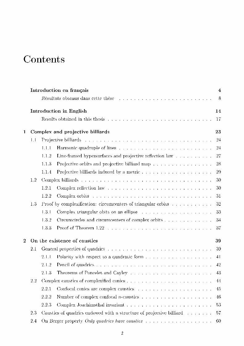
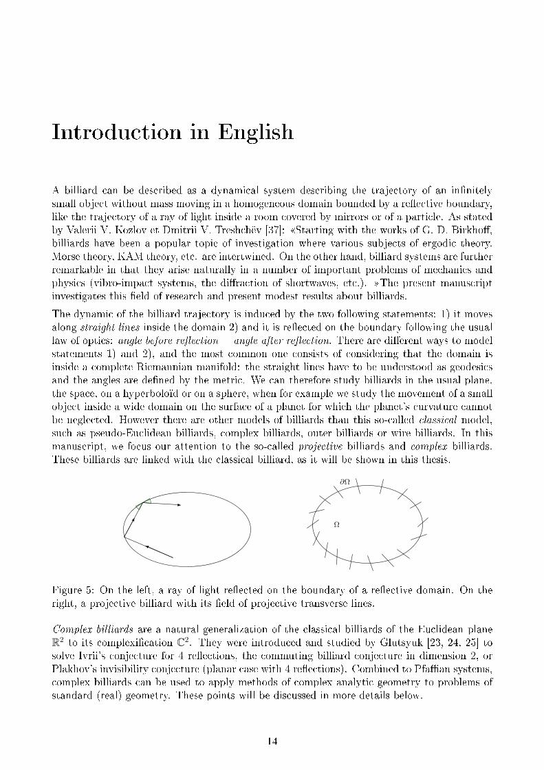
∂Ω

Ω

Figure 1: À gauche, un rayon lumineux se rééchissant sur le bord d'un domaine selon la loid'optique géométrique. À droite, un billard projectif et son champ de droites transverses.

Les billards complexes sont une extension naturelle des billards classiques au plan Euclidiencomplexié, c'est-à-dire à C2. Ils ont été introduits et étudiés par Glutsyuk [23, 24, 25] pour

1Íà÷èíàÿ ñ ðàáîò Äæ. Áèðêãîôà, áèëëèàðäû ÿâëÿþòñÿ ïîïóëÿðíîé òåìîé èññëåäîâàíèÿ, ãäå åñòåñòâåí-íûì îáðàçîì ïåðåïëåòàþòñÿ ðàçëè÷íûå ñþæåòû èç ýðãîäè÷åñêèé òåîðèè, òåîðèè Ìîðñà, ÊÀÌ-òåîðèè èò.ä. Ñ äðóãîé ñòîðîíû, áèëëèàðäíûå ñèñòåìû çàìå÷àòåëüíû åùå è òåì, ÷òî åñòåñòâåííî âîçíèêàþò â ðÿäåâàæíûõ çàäà÷ ìåõàíèêè è ôèçèêè (âèáðîóäàðíûå ñèñòåìû, äèôðàêöèÿ êîðîòêèõ âîëí è äð.).

4

résoudre la conjecture de Ivrii à quatre réexions, la conjecture des billards commutants endimension 2, ou encore la conjecture d'invisibilité de Plakhov (cas planaire à 4 réexions).Souvent combinés à la théorie des sytèmes Pfaens, ils permettent notamment d'appliquerdes méthodes d'analyse complexe à la résolution de problèmes réels. Nous reviendrons plus endétails sur ces questions.

Introduits par Tabachnikov qui les a étudiés en détails [58, 60], les billards projectifs généralisentles billards classiques. Un billard projectif est un domaine borné d'un espace euclidien dont lebord est traversé par un champ de droites transverses, dites droites projectives. Une particule àl'intérieur du domaine se déplace le long de droites. Elle est rééchie sur le bord de sorte que ladroite incidente, la droite rééchie, la droite projective en le point d'impact, et la droite obtenuepar intersection de l'hyperplan contenant ces trois premières droites avec l'hyperplan tangent àla surface forment une famille harmonique. Lorsque la droite projective est perpendiculaire aubord, cette condition impose à la réexion de suivre la loi d'optique géométrique. Ceci reste vraiquand la droite projective est perpendiculaire à la surface pour une métrique pseudo-Euclidienneou encore une métrique projectivement équivalente à la métrique Euclidienne (c'est à dire dontles géodésiques sont supportées par des droites). Ainsi les billards projectifs englobent diérentstypes de billards.

Dans le modèle du billard classique à l'intérieur d'un domaine Ω borné de frontière ∂Ω lisse,la dynamique d'une particule évoluant à l'intérieur de Ω se décrit à l'aide de deux objets. Lepremier est l'espace des phases, c'est à dire l'ensemble des morceaux de trajectoires entre deuxrebonds. Il peut notamment être codé par un couple (p, v), où p est un point du bord ∂Ω et vet un vecteur unitaire dirigé vers l'intérieur de Ω et représentant la direction de la trajectoire.Dans le plan, on peut aussi remplacer v par une mesure θ ∈ [0, π] de l'angle qu'il forme avec latangente Tp∂Ω. Dépendant de ces deux paramètres, l'espace des phases est ainsi de dimension2 pour les billards du plan, et de façon générale de dimension 2(d− 1) pour les billards dans unespace de dimension d. Le deuxième objet modélisant la dynamique du billard est l'applicationde billard, une application qui, étant donné un couple (p, v) de l'espace des phases codantla trajectoire d'une particule émise du point p avec une direction v, renvoie le couple (q, w)de l'espace des phases où q ∈ ∂Ω est le prochain point d'impact de la particule et w est levecteur unitaire dirigeant la trajectoire après réexion. Ces deux objets, espace des phases etapplication de billard, peuvent aussi être dénis pour d'autres types de billards.

Conjecture de Ivrii

L'un des enjeux de la théorie des billards est l'étude des trajectoires périodiques, c'est-à-dire destrajectoires qui se répètent après un nombre ni de réexions. Ivrii [33] a montré en 1980 quel'étude des orbites périodiques de billards a une application dans un problème célèbre, qui a étérésumé par Kac [35] en une question : peut-on entendre la forme d'un tambour ? 2 Il s'agit decomprendre si la donnée des valeurs propres du problème de Dirichlet dans un domaine bornéΩ ⊂ Rd permet de retrouver Ω. Les valeurs propres du problème de Dirichlet sont les réels λpour lesquels le système

∆u+ λu = 0u|∂Ω = 0

(1)

possède des solutions non-triviales. Elles peuvent être interprétées physiquement comme lesdiérents modes de vibration d'une forme Ω donnée, ce qui explique la question de Kac. Laréponse à cette question s'est avérée être négative et des exemples de domaines de formes

2Can one hear the shape of a drum , titre de l'article cité, [35].

5

distinctes ont été donnés pour lesquels les problèmes de Dirichlet (1) correspondants ont lesmêmes valeurs propres. Néanmoins se pose toujours la question de pouvoir retrouver desinformations sur Ω à partir des valeurs propres du problème de Dirichlet. Weyl [64] a montréque l'on peut entendre le volume3 de Ω, au sens ou la connaissance du spectre de Dirichletpermet de retrouver ce volume. En eet, les valeurs propres du problème de Dirichlet peuventêtre énumérées par une famille (λn)n de sorte que 0 ≤ λ1 ≤ λ2 ≤ . . . ≤ λn ≤ . . . avec λn → +∞.On note N(λ) le nombre de valeurs propres inférieures ou égales à λ. Alors Weyl a prouvé queN(λ) ∼ (2π)−dvdvol(Ω)λd/2, où vd est le volume de la boule unité de Rd. Il a aussi conjecturéle second terme de ce développement asymptotique :

N(λ) = (2π)−dvdvol(Ω)λd/2 − 1

4(2π)d−1area(∂Ω)λ(d−1)/2 + o(λ(d−1)/2). (2)

Cette formule reste une conjecture dans sa généralité malgré de nombreuses avancées dont unenotable est due à Ivrii [33], qui a prouvé que (2) est vériée sous réserve que le billard constituépar Ω a peu d'orbites périodiques. Plus précisément, la condition imposée est que l'ensembledes paramètres correspondant aux orbites périodiques dans l'espace des phases du billard soitde mesure nulle. Cela a donné lieu à une célèbre conjecture portant son nom :

Conjecture de Ivrii. Étant donné un domaine d'un espace Euclidien dont le bord est su-isamment lisse, l'ensemble de ses orbites périodiques est de mesure nulle.

Cette conjecture, qui tient toujours, relève d'une grande complexité malgré sa simplicité ap-parente. Si elle est vériée, elle impliquerait notamment qu'un billard ne possède pas d'ouvertd'orbites périodiques, c'est à dire que son espace des phases ne contient pas d'ouvert contenantuniquement des paramètres (p, v) associés à des orbites périodiques d'une période donnée k.On ne sait pas encore si un tel billard, dit k-rééchissant, existe ou non. Son existence auraitla conséquence amusante suivante: elle permettrait de construire une salle dont les murs sontrecouverts de miroirs et de sorte qu'il existe un endroit de la salle où un observateur regar-dant devant lui peut toujours voir son image de dos, même s'il se déplace un peu et/ou tournelégèrement sur lui-même.

La conjecture de Ivrii a été abordée dans de nombreux articles. Elle a d'abord été prouvéede façon générique par Petkov et Stojanov [45] : l'ensemble des domaines de Rd de bord C∞ayant pour tout k ≥ 2 un nombre ni d'orbites périodiques de période k contient un ensemblerésiduel, c'est-à-dire une intersection dénombrable d'ouverts denses. Une autre réponse partielleà la conjecture a été donnée par Vasiliev [62] qui l'a prouvée pour un domaine convexe de bordanalytique. Notons aussi qu'il est possible de restreindre la conjecture à l'ensemble des orbitespériodiques d'une période donnée arbitraire, et que l'ensemble de ces conjectures restreintes estéquivalent à la conjecture globale. Dans cet idée, Rychlik [52], puis Stojanov [53] ont démontréque l'ensemble des orbites de période 3, ou triangulaires, est de mesure nulle dans un billarddu plan de frontière de classe C3, et Vorobets [63] a étendu ce résultat aux billards en toutedimension. Un peu plus tard, Wojtkowski [66], puis Baryshnikov et Zharnitsky [1] ont donné denouvelles preuves de ce résultat. Plus récemment, Glutsyuk et Kudryashov [27] ont démontréla conjecture pour les orbites périodiques de période 4 dans des billards planaires de classe C4.En toute généralité dans le cas Euclidien, la conjecture de Ivrii tient toujours pour un nombrequelconque de réexions, même pour des classes de billards de frontière très lisse (par exempleanalytique par morceaux).

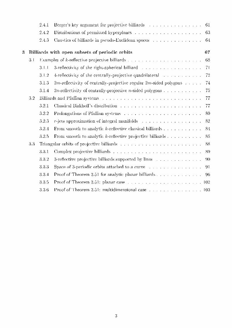
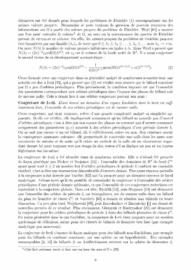
La conjecture de Ivrii s'énonce de façon analogue pour des billards non-Euclidiens, par exemplepour les billards en courbure constante, sur une sphère ou un hyperboloïde. Des exemplesremarquables [3, 10] de billards 2- ou 3-rééchissants existent sur la sphère de dimension 2,

3The rst pertinent result is that one can hear the area of Ω , [35]

6

Figure 2: Un exemple de billard 3-rééchissant sur la sphère proposé par Barychnikov. Letriangle extérieur représente le bord du billard, le triangle intérieur en pointillé est une orbite.On peut bouger arbitrairement deux points de l'orbite sans changer son caractère périodique.

liés d'une certaine façon à l'existence de points joints par une innité de géodésiques distincteset contredisant la conjecture de Ivrii sur la sphère, voir la Figure 2. Les articles cités [3, 10]donnent une classication des billards sur la sphère unité S2 ayant un ouvert d'orbites de période3 ainsi que la non-existence de tels billards sur l'hyperboloïde H2.

Malgré tous ces résultats, la conjecture de Ivrii reste encore ouverte. Il semble d'ailleurs que lesspécialistes sont partagé.e.s entre celleux qui pensent qu'elle est vraie, et celleux qui pensentqu'elle est fausse et qui recherchent des contre-exemples.

Billards intégrables

Un autre enjeu de la théorie des billards est l'étude des billards dits intégrables. Un billard Ωdu plan est dit globalement intégrable si son espace des phases est feuilleté de façon lisse parune famille de courbes fermées invariantes par l'application de billard. On dit aussi que Ω estlocalement intégrable si seul un voisinage du bord, correspondant à la courbe θ = 0 dansl'espace des phases, admet un tel feuilletage. Cette propriété se manifeste par l'existence decaustiques correspondant à ces courbes invariantes et qui se dénissent de façon indépendanteen toute dimension : une caustique d'un billard Ω est une hypersurface Γ ⊂ Ω telle que toutedroite tangente à Γ et intersectant la frontière ∂Ω en un point p est rééchie en une droitetangente à Γ après réexion en p sur le bord de Ω.

Un exemple de billard globalement intégrable est le disque, puisque tout cercle concentriqueinclus dans le disque est une caustique du disque. L'ellipse est un exemple de billard localementintégrable, puisque toute trajectoire de billard qui ne passe pas entre les foyers reste tangente àune même ellipse homofocale, qui dès lors est une caustique de l'ellipse initiale. La question aété posée par Birkho et Poritsky de savoir si ce sont les seuls exemples de billards intégrableset cela a donné lieu à la célèbre conjecture de Birkho, ou Birkho-Poritsky comme cela a étérappelé dans [36].

Conjecture de Birkho-Poritsky. Les seuls billards localement intégrables sont les ellipses.

Certaines avancées majeures ont été réalisées sur cette conjecture. Citons le théorème de Bialy[7] énonçant que si l'espace des phases d'un billard est feuilleté par des courbes fermées continuesinvariantes et non-homotopes à un point, alors ∂Ω est un cercle. Cela implique que le seul

7

billard globalement intégrable est le disque. Ce résultat nécessite néanmoins l'hypothèse que lefeuilletage est global et ne permet pas de conclure que la conjecture est vraie en toute généralité.Une version algébrique de la conjecture de Birkho-Poritsky a été démontrée conjointementpar Bialy, Glutsyuk et Mironov [8, 9, 29, 30] pour les billards sur le plan et sur les autreshypersurfaces de courbure constante. Kaloshin et Sorrentino [36] ont prouvé la version localede la conjecture, démontrant que toute déformation intégrable d'une ellipse est une ellipse. Endimension supérieure, l'étude des billards ayant des caustiques a été conclue par Berger [6]qui a montré que si un billard de Rd, avec d ≥ 3, admet une caustique, alors ce dernier estune quadrique et sa caustique est une quadrique homofocale. Ainsi en dimension au moins3, il sut juste d'une seule caustique, et non plus un feuilletage, pour que la conjecture deBirkho-Poritsky soit vériée.

Résultats obtenus dans cette thèse

Cette thèse présente diérents résultats sur les billards complexes et projectifs, applicables pourcertains à la théorie des billards classiques. Elle se divise en trois chapitres : le Chapitre 1présente en détails les modèles des billards projectifs et complexes. Le Chapitre 2 étudie lanotion de caustique dans ces deux modèles de billard. Le Chapitre 3 porte son attention surl'analogue de la conjecture de Ivrii appliquée aux billards projectifs.

Détails du Chapitre 1

Ce chapitre présente les deux classes de billards étudiées tout au long de cette thèse, les billardscomplexes et les billards projectifs. Nous exposons brièvement quelques aspects de ces billardspour rendre compréhensible les résumés des chapitres suivants. Plus de détails seront donnésdans le Chapitre 1 lui-même.

Un billard projectif est un domaine borné Ω de Rd dont le bord est lisse et muni d'un champde droites transverses. Ce champ de droites induit en chaque point p ∈ ∂Ω du bord unetransformation de l'ensemble des droites orientées passant par p, qui permet de considérer lesorbites du billard: une droite orientée `0 intersectant Ω en p est rééchie en une droite orientée`1 par la transformation décrite précédemment. Si `1 intersecte le bord en un autre point, cetteconstruction peut être répétée, et ainsi de suite.

Un billard complexe est une courbe complexe γ de CP2 sur laquelle on dénit une loi deréexion de droites complexes qui l'intersecte. Cette construction est réalisée en considérant lacomplexication de la métrique Euclidienne dx2 +dy2 à C2. Étant donnée une droite complexeL ⊂ C2 dite non-isotrope, on peut dénir une symétrie de droites complexes par rapport à L :cette symétrie est l'unique involution ane non triviale qui xe les points de L et préserve laforme quadratique complexiée dénie précédemment. Deux droites complexes `, `′ intersectantγ en un point p sont dites symétriques (pour cette loi de réexion complexe) si la symétrie dedroites complexes par rapport à la tangente Tpγ envoie l'une sur l'autre. Pour les autres droitesL, dites isotropes, on utilise un passage à la limite.

Détails du Chapitre 2

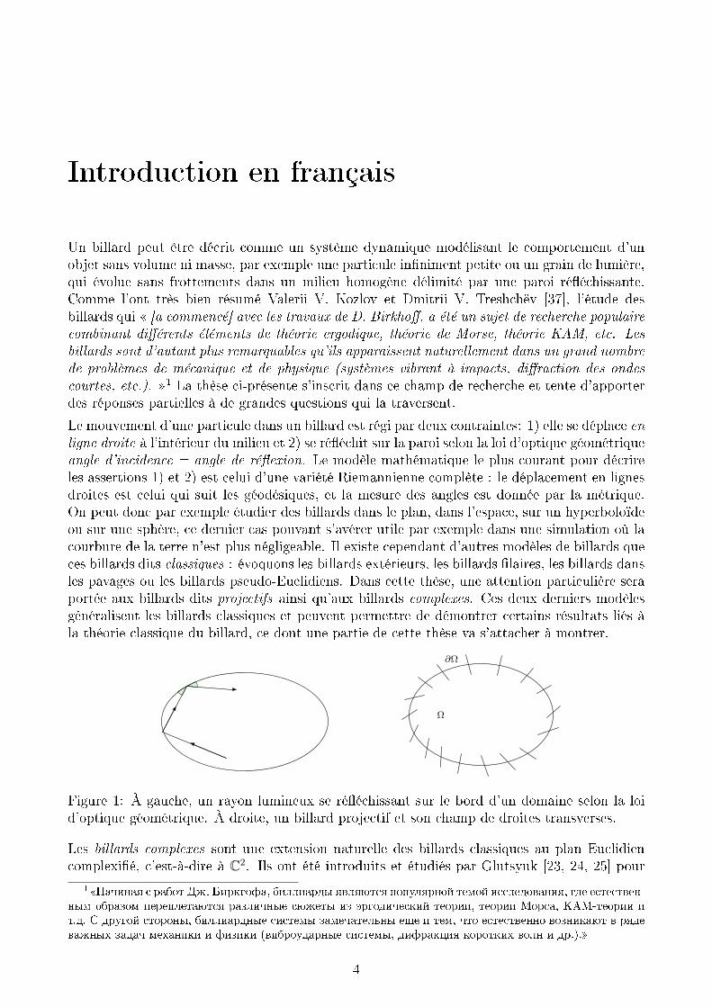
Ce chapitre propose l'étude de propriétés relatives aux caustiques des billards projectifs etcomplexes. La Section 2.1 présente un premier résultat publié [19] sur les caustiques ditescomplexes d'une ellipse ou d'une hyperbole. On dira qu'une conique C ′ ⊂ CP2 est une caustique

8

C0

Ce

Ci

C0

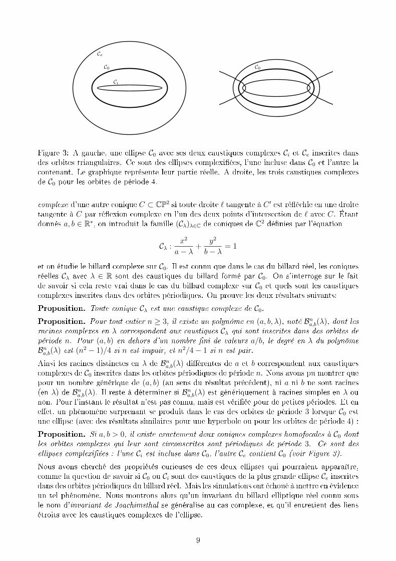
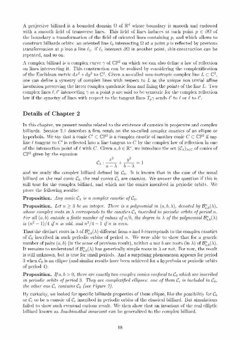
Figure 3: A gauche, une ellipse C0 avec ses deux caustiques complexes Ci et Ce inscrites dansdes orbites triangulaires. Ce sont des ellipses complexiées, l'une incluse dans C0 et l'autre lacontenant. Le graphique représente leur partie réelle. A droite, les trois caustiques complexesde C0 pour les orbites de période 4.

complexe d'une autre conique C ⊂ CP2 si toute droite ` tangente à C ′ est rééchie en une droitetangente à C par réexion complexe en l'un des deux points d'intersection de ` avec C. Étantdonnés a, b ∈ R∗, on introduit la famille (Cλ)λ∈C de coniques de C2 dénies par l'équation

Cλ :x2

a− λ+

y2

b− λ= 1

et on étudie le billard complexe sur C0. Il est connu que dans le cas du billard réel, les coniquesréelles Cλ avec λ ∈ R sont des caustiques du billard formé par C0. On s'interroge sur le faitde savoir si cela reste vrai dans le cas du billard complexe sur C0 et quels sont les caustiquescomplexes inscrites dans des orbites périodiques. On prouve les deux résultats suivants:

Proposition. Toute conique Cλ est une caustique complexe de C0.

Proposition. Pour tout entier n ≥ 3, il existe un polynôme en (a, b, λ), noté Bna,b(λ), dont lesracines complexes en λ correspondent aux caustiques Cλ qui sont inscrites dans des orbites depériode n. Pour (a, b) en dehors d'un nombre ni de valeurs a/b, le degré en λ du polynômeBna,b(λ) est (n2 − 1)/4 si n est impair, et n2/4− 1 si n est pair.

Ainsi les racines distinctes en λ de Bna,b(λ) diérentes de a et b correspondent aux caustiquescomplexes de C0 inscrites dans les orbites périodiques de période n. Nous avons pu montrer quepour un nombre générique de (a, b) (au sens du résultat précédent), ni a ni b ne sont racines(en λ) de Bna,b(λ). Il reste à déterminer si Bna,b(λ) est génériquement à racines simples en λ ounon. Pour l'instant le résultat n'est pas connu, mais est vériée pour de petites périodes. Et eneet, un phénomène surprenant se produit dans le cas des orbites de période 3 lorsque C0 estune ellipse (avec des résultats similaires pour une hyperbole ou pour les orbites de période 4) :

Proposition. Si a, b > 0, il existe exactement deux coniques complexes homofocales à C0 dontles orbites complexes qui leur sont circonscrites sont périodiques de période 3. Ce sont desellipses complexiées : l'une Ci est incluse dans C0, l'autre Ce contient C0 (voir Figure 3).

Nous avons cherché des propriétés curieuses de ces deux ellipses qui pourraient apparaître,comme la question de savoir si C0 ou Ci sont des caustiques de la plus grande ellipse Ce inscritesdans des orbites périodiques du billard réel. Mais les simulations ont échoué à mettre en évidenceun tel phénomène. Nous montrons alors qu'un invariant du billard elliptique réel connu sousle nom d'invariant de Joachimsthal se généralise au cas complexe, et qu'il entretient des liensétroits avec les caustiques complexes de l'ellipse.

9

Cette thèse propose ensuite une étude sur l'existence de caustiques dans les billards projec-tifs. Notons d'abord que de nombreux résultats ont été obtenus par Tabachnikov [58, 60] surl'existence de formes d'aire dans l'espace des phases qui sont invariantes par l'application debillard projectif, et sur les propriétés d'intégrabilités qui en découlent. Citons par exemple [60]Corollaire F : si l'application de billard dans un cercle muni d'une structure de billard projectifa une forme d'aire invariante lisse au voisinage du bord, alors le billard est intégrable. Notonsaussi qu'une nouvelle preuve de l'intégrabilité du billard elliptique dans le plan Euclidien, surl'hyperboloïde ou sur la sphère a été donnée par des considérations sur les billards projectifs(voir Corollaire G de [60]).

Dans la Section 2.3, nous considérons le cas des caustiques pour des quadriques munies d'unestructure de billard projectif. Précisons que dans le terme quadriques sont aussi comprises lesconiques. Nous montrons le résultat suivant qui découle d'une construction proposée dans [13]pour généraliser le théorème de Poncelet, mais qui ne mentionne pas les billards projectifs :

Proposition. Soit Q1 et Q2 deux coniques ou quadriques distinctes. On peut munir un ouvertdense de Q1 d'une structure de billard projectif de sorte que Q2 est une caustique pour le billardprojectif induit sur Q1.

Étant données deux quadriquesQ1 etQ2 distinctes, on peut alors considérer le faisceau F∗(Q1, Q2)de quadriques qui contient Q1 et Q2 et est déni ainsi par dualité : l'ensemble des quadriquesduales des quadriques de F∗(Q1, Q2) est une droite qui contient les quadriques duales de Q1 etQ2 (dans l'espace des quadriques). On peut le voir comme une généralisation des faisceaux dequadriques homofocales. On prouve alors:

Proposition. Les quadriques de F∗(Q1, Q2) sont des caustiques de Q1 pour la structure debillard projectif induite par Q2 sur Q1. Toute quadrique de F∗(Q1, Q2) induit la même structureprojective sur Q1 que celle induite par Q2.

En dimension au moins 3, l'étude des billards classiques possédant des caustiques a été concluepar Berger [6] qui a énoncé un résultat dont les hypothèses sont beaucoup plus faibles quedans la conjecture de Birkho-Poritsky: Berger a montré que s'il existe des hypersurfaces S,U , V de Rd, avec d ≥ 3, ayant des secondes formes fondamentales non-dégénérées et telles qu'ilexiste un ouvert de droites tangentes à U et intersectant S qui sont rééchies sur S en desdroites tangentes à V , alors S est un morceau de quadrique, et U, V sont des morceaux d'uneseule et même quadrique homofocale. Ainsi la conjecture de Birkho-Poritsky est vériée dèsl'existence d'au moins une caustique.

Dans la Section 2.4, nous prouvons qu'un argument clé de la preuve de Berger peut se généraliserau cas des billards projectifs de Rd, avec toujours d ≥ 3, et nous l'avons appliqué pour généraliserle résultat de Berger aux billards pseudo-Euclidiens convexes:

Proposition. Soit Ω ⊂ Rd, d ≥ 3, un billard pseudo-Euclidien strictement convexe qui admetune caustique Γ. Alors ∂Ω est un ellipsoïde et Γ est un morceau de quadrique homofocale pourla métrique pseudo-Euclidienne.

L'argument de Berger que nous généralisons repose sur l'idée suivante. Soit S ⊂ Rd unehypersurface, et U, V comme dans l'énoncé de Berger cité plus haut. Toute droite ` de l'ouvertde droites tangentes à U , intersectant S en p et rééchie en une droite `′ tangente à V , est telleque l'hyperplan tangent à U contenant ` et l'hyperplan tangent à V contenant `′ intersectentTpS en un même hyperplan H de TpS. Un tel hyperplan H ⊂ TpS est dit autorisé, et l'argumentde Berger est que pour p xé il y a au plus d−1 hyperplans autorisés. Nous montrons que dansle cas projectif, l'argument est encore valable génériquement (un sens plus précis sera donné àce mot) :

Proposition. Génériquement en un point de réexion d'un billard projectif en dimension ≥ 3,le nombre d'hyperplans autorisés est au plus d− 1.

10

Nous pensons que ce résultat, valable pour tout billard projectif, n'est pas applicable unique-ment pour caractériser les billards pseudo-Euclidiens ayant des caustiques, mais peut-être encorepour d'autres billards. Peut-être permettrait-il au moins d'armer que si un billard projectifadmet une caustique, alors cette caustique est une quadrique. Comme ce résultat semble délicatà démontrer, une première avancée pourrait consister à le prouver pour une classe assez généralede billards projectifs, ceux ayant un champ dit exact de droites projectives et qui contient laclasse des billards pseudo-Euclidiens, voir [58].

Détails du Chapitre 3

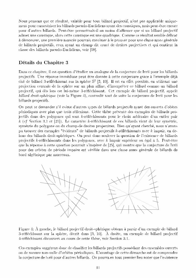
Dans ce chapitre, il est question d'étudier un analogue de la conjecture de Ivrii pour les billardsprojectifs. Une réponse immédiate peut être donnée à cette conjecture grâce à l'exemple déjàcité de billard 3-rééchissant sur la sphère S2 [3, 10]. Il est en eet possible, en utilisant uneprojection centrale de la sphère sur un plan ane, d'interpréter ce billard comme un billardprojectif, qui dès lors est lui-même 3-rééchissant. Cet exemple de billard projectif, appelébillard droit-sphérique (voir la Figure 4), contredit tout de suite la conjecture de Ivrii pour lesbillards projectifs.

On peut se demander s'il existe d'autres types de billards projectifs ayant des ouverts d'obitespériodiques avec plus que trois réexions. Cette thèse présente des exemples de billards pro-jectifs dans des polygones qui sont k-rééchissants pour le choix arbitraire d'un entier pairk (cf Section 3.1 et [21]). Le caractère k-rééchissant de ces billards vient de leur symétrie,symétrie du polygone ou du champ de droites projectives. Bien qu'ayant cherché, nous n'avonspu trouver des exemples "évidents" de billards projectifs k-rééchissants avec k impair, en de-hors des billards droit-sphériques. On peut donc soulever la question de l'existence de billardsprojectifs k-rééchissants dans les polygones, avec k impair supérieur ou égal à 5. Peut-êtreque la réponse à cette question pourrait s'inspirer de [25], qui montre que la conjecture de Ivriipour des orbites de période impaire est vériée dans une classe assez générale de billards debord algébrique par morceaux.

Figure 4: À gauche, le billard projectif droit-sphérique obtenu à partir d'un exemple de billard3-rééchissant sur la sphère, décrit dans [3, 10]. À droite, un exemple de billard projectif4-rééchissant découvert au cours de cette thèse, voir Section 3.1.

Ces exemples suggèrent donc de classier les billards projectifs possédant des ensembles ouvertsou de mesure non-nulle d'orbites périodiques. L'avantage de cette démarche est de comprendrela conjecture de Ivrii pour d'autres billards. On pourra en tout premier lieu noter que l'existence

11

d'un billard projectif k-rééchissant fournit de nombreux exemples de billards projectifs ayantun ensemble de mesure non-nulle d'orbites k-périodiques par la construction suivante : étantdonné un billard projectif k-rééchissant ayant un ouvert U d'orbites périodiques, tout billardqui coïncide avec le précédent sur un ensemble de Cantor de mesure non-nulle inclus dans Upossède un ensemble de mesure non-nulle d'orbites k-périodiques. Ainsi quand un billard k-rééchissant existe, on pourra classier uniquement les billards k-rééchissants pour comprendreles obstructions à la conjecture de Ivrii. Cette thèse s'intéresse notamment au cas particulierdes billards projectifs ayant des ensembles ouverts ou de mesure non-nulle d'orbites de période3. Elle prouve la classication suivante de ces billards en Section 3.3:

Théorème. 1) Les seuls billards projectifs 3-rééchissants de R2 de bord C∞ par morceauxsont les billards droit-sphériques.2) Si d ≥ 3, il n'y a pas de billards projectifs dans Rd de bord C∞ par morceaux possédant unensemble de mesure non-nulle d'orbites 3-périodiques.

La preuve de ce théorème est très largement inspirée de [23, 27] et se décompose en deux étapes:il est d'abord question de traiter le résultat pour une version complexe des billards projectifs3-rééchissants de bord analytique par morceaux, puis de l'élargir aux bords C∞ en utilisantles systèmes Pfaens. Cette dernière étape est l'objet de la Section 3.2, dans laquelle sontintroduits et étudiés des systèmes Pfaens relatifs aux billards projectifs et Euclidiens.

L'utilité des systèmes Pfaens vient d'une idée de Barychnikov et Zharnitsky [1, 2] d'associerun billard classique k-rééchissant à une surface intégrale d'une certaine distribution, appeléedistribution de Birkho : pour les billards dans le plan, la distribution de Birkho est la distri-bution qui associe à un polygone non-dégénéré à k côtés le produit cartésien de ses bissectricesextérieures (c'est-à-dire les droites qui coupent en deux les deux angles extérieurs opposés for-més par les droites supportant deux côtés consécutifs du polygone). Elle vérie que si unesurface intégrale de dimension 2 de cette distribution est telle que la projection sur chaquesommet est une courbe lisse, alors ces courbes lisses forment des morceaux du bord d'un mêmebillard k-rééchissant. En eet, tout point de la surface intégrale est un polygone dont lesbissectrices extérieures sont tangentes aux bords du billard, par dénition de la distribution, etdonc est une orbite de période k. Un système Pfaen est alors un objet qui résume la donnéed'une distribution, de la dimension de ses variétés intégrales recherchées, et de conditions ditesde transversalité, sur lequel peuvent être eectuées certaines opérations de prolongement dansle but de trouver des surfaces intégrales. L'idée de Barychnikov et Zharnitsky a été reprise dans[27], où est conjecturé (Conjecture 5) l'énoncé suivant:

Conjecture de Kudryashov. Soient k ≥ 3 et d ≥ 2 deux entiers. Il existe un entier r ≥ 2,dépendant uniquement de k et d, tel que l'existence dans Rd d'un billard de bord Cr par morceauxpossédant un ensemble de mesure non-nulle d'orbites k-périodiques entraine l'existence d'unbillard analytique par morceaux qui est k-rééchissant.

Cette conjecture peut être résumée en disant que si la conjecture de Ivrii est fausse pour les bil-lards de bord Cr par morceaux, alors il existe un billard analytique par morceaux k-rééchissant.Certains arguments présentés dans [27] et dispersés dans l'article permettent de prouver uncas plus simple de cette conjecture en prenant r =∞, mais ce résultat n'est malheureusementpas énoncé dans l'article. Comme il mérite d'être explicitement formulé, nous en donnons unepreuve en Section 3.2, et dont l'essentiel des arguments provient de [27].

Théorème. La conjecture de Kudryashov est valable pour r =∞.

Nous prouvons de plus que si un billard k-rééchissant de bord C∞ par morceaux existe, alorspour tout entier r ≥ 1 son bord peut être approché par des r-jets de billards k-rééchissantsde bord analytique par morceaux. Nous élargissons alors aussi au cas des billards projectifs la

12

preuve de la conjecture de Kudryashov avec r = ∞ (cf Section 3.2), en prouvant le résultatsuivant:

Théorème. S'il existe un billard projectif de bord C∞ par morceaux (avec un champ dedroites transverses C∞ par morceaux) possédant un ensemble de mesure non-nulle d'orbitesk-périodiques, alors il existe un billard projectif analytique k-rééchissant.

Ainsi ces arguments peuvent fournir des outils intéressants pour la résolution éventuelle de laconjecture de Ivrii : se ramener aux cas des billards k-rééchissants de bord analytique parmorceaux ou bien étudier ces mêmes billards dans un cadre projectif. Généraliser peut parfoispermettre de simplier.

Perspectives de recherche

Pour récapituler, le travail accompli pendant cette thèse a permis de mieux comprendre lesbillards projectifs ayant des ensembles de mesure non nulle d'orbites périodiques, de les classi-er lorsqu'il s'agit en particulier des orbites triangulaires, de mettre en évidence des caustiquesdites complexes du billard sur une conique complexiée, de proposer des structures projec-tives sur des coniques et quadriques de sorte que ces dernières admettent des caustiques, etd'étendre un résultat de Berger pour les caustiques de billards projectifs en dimension aumoins 3 qui s'applique à la classication des billards pseudo-Euclidiens ayant des caustiques.Mais l'étude réalisée dans cette thèse n'est pas terminée et soulève peut-être plus de questionsqu'elle n'apporte de réponses...

Le problème des billards projectifs admettant des caustiques en dimension d ≥ 3 n'est quetrès partiellement résolu : certes un argument clé de Berger a pu être étendu à cette classe debillards, mais aucun résultat général similaire à celui de Berger n'a pu être prouvé, à part pourle cas très particulier des espaces pseudo-Euclidiens. Il serait intéressant de le généraliser à uneclasse plus vaste de billards projectifs, par exemples aux billards projectifs ayant un champ ditexact de droites transverses [58]. Peut-on avancer une conjecture ? Peut-être que les seulescaustiques possibles d'un billard projectif en dimension d ≥ 3 sont les quadriques. Je seraistrès curieux de connaître le résultat.

La conjecture de Ivrii est un problème majeur de théorie des billards. Sans chercher à en donnerune réponse dénitive, il pourrait être intéressant d'étudier des classes simples de billardsprojectifs k-rééchissants. On pourrait par exemple essayer de savoir s'il existe des billardsprojectifs k-rééchissants dans des polygones avec k ≥ 5 impair. Notre recherche n'a en eetpas permis d'en trouver. On peut plus généralement se demander si les exemples de billards k-rééchissants que nous présentons en Section 3.1 sont les seuls billards projectifs k-rééchissantsdans des polygones. Enn il serait à envisager de comprendre si les arguments de classicationdes billards projectifs 3-rééchissants avancés par [23, 27] et repris dans le chapitre 3 peuventêtre synthétisés et généralisés à un nombre général de réexions.

13

Introduction in English

A billiard can be described as a dynamical system describing the trajectory of an innitelysmall object without mass moving in a homogeneous domain bounded by a reective boundary,like the trajectory of a ray of light inside a room covered by mirrors or of a particle. As statedby Valerii V. Kozlov et Dmitrii V. Treshchëv [37]: Starting with the works of G. D. Birkho,billiards have been a popular topic of investigation where various subjects of ergodic theory,Morse theory, KAM theory, etc. are intertwined. On the other hand, billiard systems are furtherremarkable in that they arise naturally in a number of important problems of mechanics andphysics (vibro-impact systems, the diraction of shortwaves, etc.). The present manuscriptinvestigates this eld of research and present modest results about billiards.

The dynamic of the billiard trajectory is induced by the two following statements: 1) it movesalong straight lines inside the domain 2) and it is reected on the boundary following the usuallaw of optics: angle before reection = angle after reection. There are dierent ways to modelstatements 1) and 2), and the most common one consists of considering that the domain isinside a complete Riemannian manifold: the straight lines have to be understood as geodesicsand the angles are dened by the metric. We can therefore study billiards in the usual plane,the space, on a hyperboloïd or on a sphere, when for example we study the movement of a smallobject inside a wide domain on the surface of a planet for which the planet's curvature cannotbe neglected. However there are other models of billiards than this so-called classical model,such as pseudo-Euclidean billiards, complex billiards, outer billiards or wire billiards. In thismanuscript, we focus our attention to the so-called projective billiards and complex billiards.These billiards are linked with the classical billiard, as it will be shown in this thesis.

∂Ω

Ω

Figure 5: On the left, a ray of light reected on the boundary of a reective domain. On theright, a projective billiard with its eld of projective transverse lines.

Complex billiards are a natural generalization of the classical billiards of the Euclidean planeR2 to its complexication C2. They were introduced and studied by Glutsyuk [23, 24, 25] tosolve Ivrii's conjecture for 4 reections, the commuting billiard conjecture in dimension 2, orPlakhov's invisibility conjecture (planar case with 4 reections). Combined to Pfaan systems,complex billiards can be used to apply methods of complex analytic geometry to problems ofstandard (real) geometry. These points will be discussed in more details below.

14

Projective billiards were introduced by Tabachnikov [60, 58] as a generalization of classical bil-liards of the Euclidean space. A projective billiard is a bounded domain of a Euclidean spacewhose boundary is endowed with a eld of transverse lines, called projective lines. A trajectoryis then reected at a point on the boundary by a specic law of reection depending on theprojective line at the point of impact. When the latter projective line is orthogonal to theboundary, the reection of the trajectory is the same as the usual law of optics. This state-ment is still valid for other billiards, like billiards in pseudo-Euclidean manifolds or in metricsprojectively equivalent to the Euclidean one (which are metrics whose geodesics are supportedby lines). Therefore, the model of projective billiards contain other models of billiards.

In the classical model of billiard inside a domain Ω bounded by a smooth boundary, the dierenttrajectories can be mathematically described by two objects. The rst one is the phase spacewhich is dened as the set of oriented geodesics between two points of reection. It can bedescribed as the set of pairs (p, v) where p is a point of the boundary ∂Ω and v is a unitvector with origin at p, pointing inside Ω and representing the direction of the correspondinggeodesic. In dimension 2, v can be replaced by the angle θ ∈ [0, π] it makes with the tangentline Tp∂Ω. The dimension of the phase space is 2 for billiards in the plane, and 2(d − 1) forbilliards in a space of dimension d. The second object describing a billiard is the billiard map:it is a map associating to an element (p, v) of the phase space representing a trajectory movingfrom p in the direction given by v the element (q, v) where q is the next point of impact of thetrajectory and w is the directing vector of the trajectory after reection. Both objects havesimilar denitions for other billiard types.

Ivrii's conjecture

One of the main issues of billiard theory is the study of periodic orbits, which are trajectoriesrepeating themselves after a nite number of reections. Ivrii [33] showed in 1980 that thestudy of periodic orbits has an application in a famous problem which was summarized by Kac[35] in one question: Can one hear the shape of a drum ? The problem is about to understandif the eigenvalues of the Laplacien with Dirichlet initial condtions in a bounded domain Ω ⊂ Rd

determine completely the shape of Ω. These eigenvalues are dened as the real numbers λ ∈ Rfor which the system

∆u+ λu = 0u|∂Ω = 0

(3)

has non-trivial solutions u. They can be interpreted physically as dierent vibration modes of ashape given by Ω. Kac's question was answered negatively since examples of distinct shapes weregiven in which the corresponding Dirichlet problems (3) have the same eigenvalues. Howeverthe question of recovering data about Ω from these eigenvalues is still investigated. Weyl [64]showed that we can hear the volume4 of Ω, meaning that we can recover the volume of Ω fromDirichlet eigenvalues. Indeed, the eigenvalues of Dirichlet problem can be enumerated into asequence (λn)n of real numbers such that 0 ≤ λ1 ≤ λ2 ≤ . . . ≤ λn ≤ . . . and λn → +∞.If we denote by N(λ) the number of eigenvalues less or equal to λ, then Weyl showed thatN(λ) ∼ (2π)−dvdvol(Ω)λd/2, where vd denotes the volume of the unit Euclidean sphere in Rd.He also conjectured the second asymptotic term

N(λ) = (2π)−dvdvol(Ω)λd/2 − 1

4(2π)d−1area(∂Ω)λ(d−1)/2 + o(λ(d−1)/2). (4)

4The rst pertinent result is that one can hear the area of Ω , [35]

15

This conjecture is not proven yet although many results exist and conrm Weyl's conjecture.One of them is a result due to Ivrii [33] who proved that (4) is satised under the assumptionthat the billiard inside Ω has a few periodic orbits, meaning that the set of parameters in thephase space corresponding to periodic orbits has zero measure in Ω. A famous conjecture wasstated following this result:

Ivrii's conjecture. Given a bounded domain in the Euclidean space with suciently smoothboundary, its set of periodic orbits has zero measure.

This conjecture still holds and is more dicult than it was expected at the beginning. Particularcases of billiards with a set of positive measure of periodic orbits are given by the so-called k-reective billiards: billiards having open subsets of periodic orbits of period k, more preciselyhaving open subsets in its phase space of parameters (p, v) corresponding to periodic orbits.The existence of a k-reective billiard is still unknown, but could lead to a rather curiousconstruction: a room whose walls are covered by mirrors and such that there is a place in theroom where any observer can still see himself from behind, even by moving or turning a littleround.

There is still no denitive answer to Ivrii's conjecture, even for k-reective billiards with anyinteger k. Many partial results however already exist. Petkov and Stojanov [45] proved it forgeneric billiards: the set of all domains in Rd with C∞-smooth boundary having a nite numberof periodic orbits of period k for all k contains a residual set (a countable intersection of opendense subsets). Another answer was given by Vasiliev [62] who proved the conjecture for aconvex domain with analytic boundary. Rychlik [52] and then Stojanov [53] proved that theset of periodic orbits of period 3 has zero measure in any billiard of the Euclidean plane withC3-smooth boundary. Vorobets [63] extended this result to billiards in any dimension. Later,Wojtkowski [66], and then Baryshnikov and Zharnitsky [1] gave new proofs of this result. Morerecently, Glutsyuk and Kudryashov [27] proved the conjecture for periodic orbits of period 4in planar billiards with C4-smooth boundary. Thus in the Euclidean case, Ivrii's conjectureremains unproved for any period and any regularity of the boundary (even for billiards withpiecewise-analytic boundary).

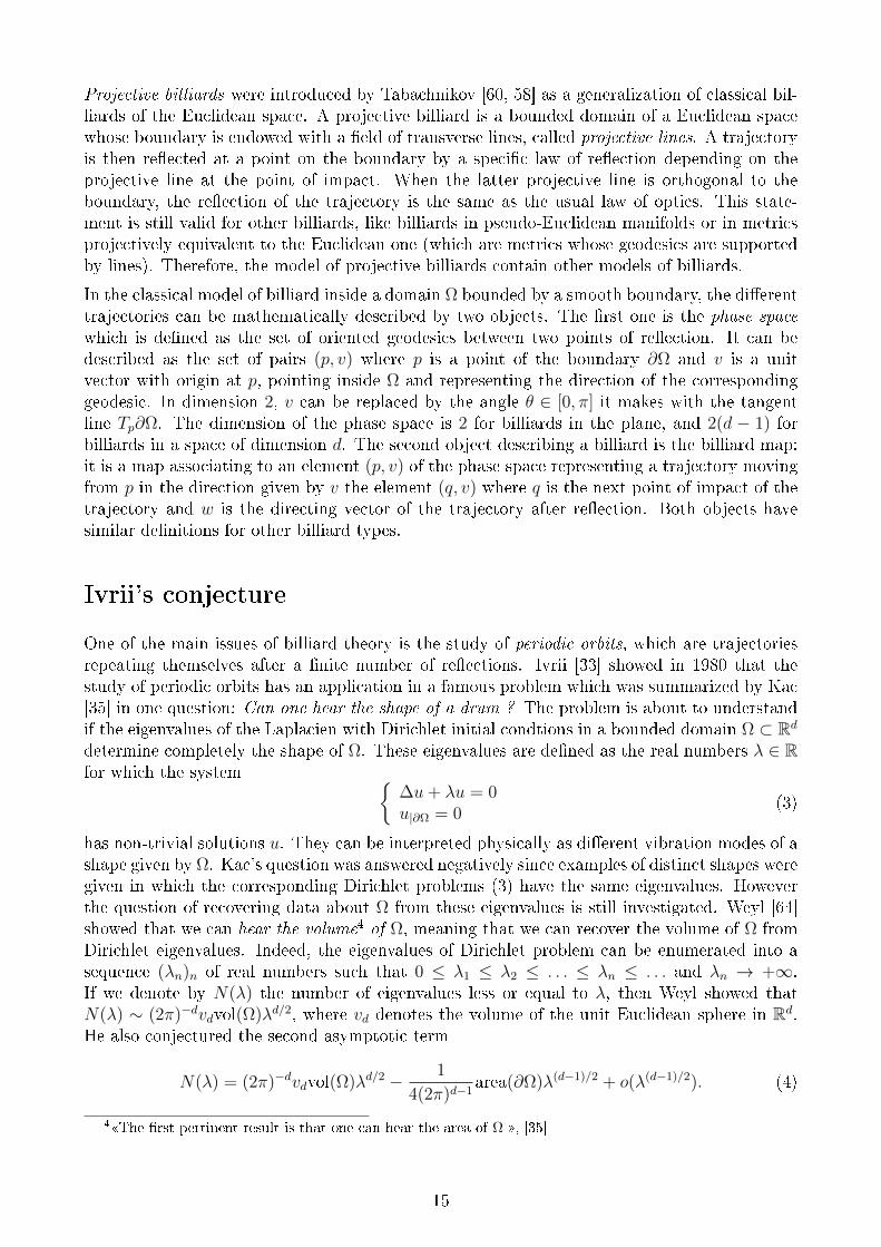
Figure 6: An example of 3-reective billiard on the sphere presented by Barychnikov. Theouter triangle is boundary of the billiard, the interior triangle in dotted lines is an orbit. Twovertices of the orbit can be moved arbitrarily without changing its periodicity.

Ivrii's conjecture can be stated analogously for non-Euclidean billiards, such as billiards inmanifolds of constant curvature, on a sphere or on a hyperboloïd. Remarkable examples of 2-and 3-reective billiards can be given on the 2-dimensional sphere S2 [3, 10], which are linked

16

with the existence of points joined by an innite number of geodesics, see Figure 6. The citedarticles give a classication of billiards on the unit sphere S2 having a set of non-zero measureof periodic orbit of period 3. They also prove that Ivrii's conjecture for 3-periodic orbits is alsotrue for billiards on the hyperboloïd.

Integrable billiards

An other important issue of billiard theory is the study of the so-called integrable billiards. Abilliard Ω of the plane is said to be globally integrable if its phase space is foliated by smoothclosed curves invariant by the billiard map. Ω is said to be locally integrable if such a foliationexists only in neighborhood of the curve θ = 0 in the phase space. This property is stronglylinked with the existence of caustics corresponding to these invariant curves, and which can bedened independantly in all dimensions: a caustic of a billiard Ω is a hypersurface Γ ⊂ Ω suchthat any line tangent to Γ and intersecting the boundary ∂Ω at p is reected into a line tangentto Γ after reection at p on ∂Ω.

An example of globally integrable billiard is the disk, since any concentric circle inside the diskis a caustic of the corresponding billiard. An ellipse is an example of a locally integrable billiard,since any billiard trajectory which do not passes between the foci of the ellipse remains tangentto a smaller confocal ellipse. Birkho and Poritsky asked if these examples are the only suchexamples of locally integrable billiard, and this question is now cited as a famous conjecture,as it is recalled in [36].

Birkho-Poritsky conjecture. If a billiard is locally integrable, then it is an ellipse.

Major results were discovered about this conjecture. Bialy [7] proved that if the phase spaceof the billiard Ω is foliated by not null-homotopic continuous invariant closed curves, then ∂Ωis a circle. Notice that this result requires the foliation to be global and implies that the onlyglobally integrable billiard is the circle. An algebraic proof of Birkho-Poritsky conjecture forplanar billiards and billiards on surfaces of constant curvature was found by Bialy, Glutsyukand Mironov [8, 9, 29, 30]. Kaloshin and Sorrentino [36] showed that any integrable deformationof an ellipse is an ellipse. In greater dimension, the study of billiards having caustics was endedearlier by Berger [6] who proved that if a billiard Ω in Rd, with d ≥ 3, has a caustic, then ∂Ωis a quadric and its caustic is a confocal quadric. The assumptions of this result are weaker,and they do not require the existence of a foliation.

Results obtained in this thesis

This manuscript pesents dierent results about complex and projective billiards which someof them can also be applied to classical billiards. It is structured in three chapters: Chapter1 exposes in details both models of complex and projective billiards. Chapter 2 study theexistence of caustics for dierent billiards of both types. Chapter 3 is focused on the analogueof Ivrii's conjecture for projective billiards.

Details of Chapter 1

This chapter presents two types of billiards studied all along this manuscript: the complex andprojective billiards. We present here briey the denitions of these billiards to understand theoverviews of each chapter.

17

A projective billiard is a bounded domain Ω of Rd whose boundary is smooth and endowedwith a smooth eld of transverse lines. This eld of lines induces at each point p ∈ ∂Ω ofthe boundary a transformation of the eld of oriented lines containing p, and which allows toconstruct billiards orbits: an oriented line `0 intersecting Ω at a point p is reected by previoustransformation at p into a line `1. If `1 intersect ∂Ω in another point, this construction can berepeated, and so on.

A complex billiard is a complex curve γ of CP2 on which we can also dene a law of reectionon lines intersecting it. This construction can be realised by considering the complexicationof the Euclidean metric dx2 + dy2 to C2. Given a so-called non-isotropic complex line L ⊂ C2,one can dene a symetry of complex lines with respect to L as the unique non-trivial aneinvolution preserving the latter complex quadratic form and xing the points of the line L. Twocomplex lines `, `′ intersecting γ at a point p are said to be symetric for the complex reectionlaw if the symetry of lines with respect to the tangent lines Tpγ sends `′ to ` or ` to `′.

Details of Chapter 2

In this chapter, we present results related to the existence of caustics in projective and complexbilliards. Section 2.1 describes a rst result on the so-called complex caustics of an ellipse orhyperbola. We say that a conic C ′ ⊂ CP2 is a complex caustic of another conic C ⊂ CP2 if anyline ` tangent to C ′ is reected into a line tangent to C by the complex law of reection in oneof the intersection point of ` with C. Given a, b ∈ R∗, we introduce the set (Cλ)λ∈C of conics ofCP2 given by the equation

Cλ :x2

a− λ+

y2

b− λ= 1

and we study the complex billiard dened by C0. It is known that in the case of the usualbilliard on the real conic C0, the real conics Cλ are caustics. We answer the question if this isstill true for the complex billiard, and which are the conics inscribed in periodic orbits. Weprove the following results:

Proposition. Any conic Cλ is a complex caustic of C0.

Proposition. Let n ≥ 3 be an integer. There is a polynomial in (a, b, λ), denoted by Bna,b(λ),whose complex roots in λ corresponds to the caustics Cλ inscribed in periodic orbits of period n.For all (a, b) outside a nite number of values of a/b, the degree in λ of the polynomial Bna,b(λ)is (n2 − 1)/4 if n is odd, and n2/4− 1 if n is even.

Thus the distinct roots in λ of Bna,b(λ) dierent from a and b corresponds to the complex causticsof C0 inscribed in such periodic orbits of period n. We were able to show that for a genericnumber of pairs (a, b) (in the sense of previous result), neither a nor b are roots (in λ) of Bna,b(λ).It remains to understand if Bna,b(λ) has generically simple roots in λ or not. For now, the resultis still unknown, but is true for small periods. And a surprising phenomenon appears for period3 when C0 is an ellipse (and similar results have been achieved for a hyperbola or periodic orbitsof period 4):

Proposition. If a, b > 0, there are exactly two complex conics confocal to C0 which are inscribedin periodic orbits of period 3. They are complexied ellipses: one of them Ci is included in C0,the other one Ce contains C0 (see Figure 7).

By curiosity, we looked for specic billiards properties of these ellipse, like the possibility for C0

or Ci to be a caustic of Ce inscribed in periodic orbits of the classical billiard. But simulationsfailed to show such eventual curious result. We then show that an invariant of the real ellipticbilliard known as Joachimsthal invariant can be generalized to the complex billiard.

18

C0

Ce

Ci

C0

Figure 7: On the left, an ellipse C0 with its two caustics Ci and Ce inscribed in triangular orbits.These are two complexied ellipses, one of them is included in C0 and the other one contains it.The graphic represents their real parts. On the right, the complex caustics of C0 for periodicorbits of period 4.

This thesis then presents a result related to the existence of caustics in projective billiards.Let us rst note that numerous results were obtained by Tabachnikov [58, 60] on the existenceof area forms of the phase space invariant by the projective billiard map, and on their conse-quences about the integrability of the billiard. For example Corollary F of [60] states that if theprojective billiard inside a circle has an invariant area form smooth up to the boundary, thenthe billiard is integrable. Note also that a new proof of the integrability of the elliptic billiardin the Euclidean plane, on the sphere or on a hyperboloid was given using considerations aboutprojective billiards (see Corollary G of [60]).

In Section 2.3, we investigate the existence of caustics for quadrics endowed with a structureof projective billiard. Let us precise that in the following results the term quadric contains theconics. We show the following result which is a consequence of a construction contained in [13]to generalize Poncelet theorem, but the latter does not mention the projective billiards:

Proposition. Let Q1 and Q2 be two distinct conics or quadrics. There is an open dense subsetof Q1 which can be endowed with a structure of projective billiard such that Q2 is caustic of thecorresponding projective billiard on Q1.

Given two distinct quadricsQ1 andQ2, we can consider the pencil of quadrics F∗(Q1, Q2), whichcontains Q1 and Q2 and is dened by duality: the dual quadrics of the quadrics contained inF∗(Q1, Q2) is a line containing the dual quadrics of Q1 and Q2 (in the space of quadrics). Wecan interpret F∗(Q1, Q2) as a generalization of the notion of pencil of confocal quadrics. Thenwe prove:

Proposition. The quadrics of F∗(Q1, Q2) are caustics of Q1 for the structure of projectivebilliard induced by Q2 on Q1. Any quadric of F∗(Q1, Q2) induces the same projective structureon Q1 as the one induced by Q2.

In dimension greater than 2, the study of billiards having caustics has been ended by Berger[6]. He stated a result whose assumptions are weaker than Birkho-Poritsky conjecture: Bergershowed that if there are hypersurfaces S, U , V of Rd, with d ≥ 3, having non-degenerate secondfundamental forms and such that there is an open subset of lines tangent to U and intersectingS which are reected by S in lines tangent to V , then S is a piece of quadric, and U, V arepieces of one and the same confocal quadric.

We prove at Section 2.4 that a key argument of Berger's proof can be generalized to projectivebilliards of Rd, d ≥ 3, and we apply it to generalize Berger's result to pseudo-Euclidean billiards:

19

Theorem. Let Ω ⊂ Rd, d ≥ 3, be a strictly convex pseudo-Euclidean billiard having a causticΓ. Then ∂Ω is an ellipsoid and Γ is a piece of quadric which is confocal for the pseudo-Euclideanmetric.

The argument of Berger we generalize can be described as follows. Let S ⊂ Rd be a hypersurfaceand U, V be as in the previous mentionned result of Berger. Any line ` of the open subsetof lines tangent to U , intersecting S at p and reected in a line `′ tangent to V , is suchthat the hyperplane tangent to U containing ` and the hyperplane tangent to V containing`′ intersect TpS in the same hyperplane H of TpS. Such hyperplane H ⊂ TpS is said to bepermitted. Berger's key argument states that for a xed p there are at most d−1 such permittedhyperplanes. We show that in the case of projective billiards, this argument is still satisedgenerically (a more precise meaning to this word will be given later):

Proposition. Generically at a point of reection of a projective billiard in dimension d ≥ 3,the number of permitted hyperplanes is at most d− 1.

We think that this result is applicable not only to pseudo-Euclidean billiards. Maybe it couldbe used at least to show that if a projective billiard has a caustic, then this caustic is a quadric.A rst step would consist for example in proving it for a wider class of projective biliardscontaining pseudo-Euclidean billiards, and called projective billiards with exact transverse lineelds, see [58].

Details of Chapter 3

We study in this chapter the analogue of Ivrii's conjecture for projective billiards. A rstanswer can be given thanks to the above mentionned example of 3-reective billiard on the unitsphere S2 [3, 10]. Indeed, a central projection from the sphere onto an ane plane projectssuch 3-reective billiard into a 3-reective projective billiard of the plane. This example ofprojective billiard, called right-spherical billiard (see Figure 8), immediately contradicts Ivrii'sconjecture for projective billiards.

We can ask if there are other examples of projective billiards having open subsets of periodicorbits with more than 3 reections. This thesis presents examples of projective billiards insidepolygons which are k-reective for any choice of an arbitrary even integer k (cf Section 3.1and [21]). Their k-reectivity comes from the particular symmetry of the polygons and of theirprojective elds of lines. We were unable to nd other examples of k-reective billiards withan odd k. We can ask the question wether there exist or not k-reective billiards in polygonswith an odd k ≥ 5. Maybe the answer to this question could use a similar argument to [25],which prove Ivrii's conjecture for periodic orbits of odd periods inside billiards with piecewisealgebraic boundary.

These examples suggest to classify the projective billiards having open subsets or subsets of non-zero measure of periodic orbits. The benet of this method is to understand Ivrii's conjecture inother geometries. We can rst note that the existence of a k-reective projective billiard givesnumerous examples of projective billiards having a subset of non-zero measure of k-periodicorbits by the following construction: given a k-reective projective billiard having an opensubset U of k-periodic orbits, any billiard which coincide with the rst one on a Cantor set ofpositive measure included in U has a subset of non-zero measure of k-periodic orbits. Thereforewe can focus on classifying k-reective projective billiards only, as soon as a k-reective billiardalready exists. This manuscript gives a classication of billiards having open subsets of periodicorbits (in dimension 2) and subset of non-zero measure of periodic orbits (in dimension d ≥ 3):

Proposition. 1) The only 3-reective projective billiard of R2 with piecewise C∞-smoothboundary is the right-spherical billiard.

20

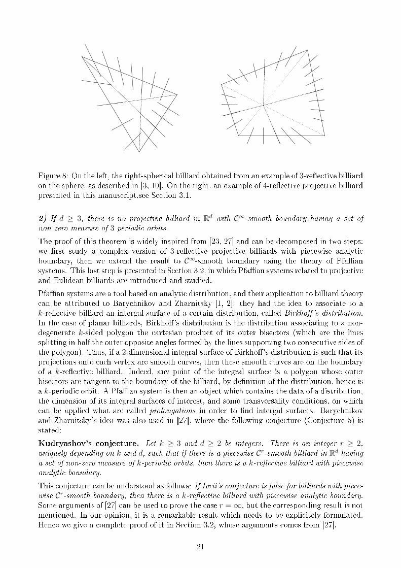
Figure 8: On the left, the right-spherical billiard obtained from an example of 3-reective billiardon the sphere, as described in [3, 10]. On the right, an example of 4-reective projective billiardpresented in this manuscript,see Section 3.1.

2) If d ≥ 3, there is no projective billiard in Rd with C∞-smooth boundary having a set ofnon-zero measure of 3-periodic orbits.

The proof of this theorem is widely inspired from [23, 27] and can be decomposed in two steps:we rst study a complex version of 3-reective projective billiards with piecewise analyticboundary, then we extend the result to C∞-smooth boundary using the theory of Pfaansystems. This last step is presented in Section 3.2, in which Pfaan systems related to projectiveand Eulidean billiards are introduced and studied.

Pfaan systems are a tool based on analytic distribution, and their application to billiard theorycan be attributed to Barychnikov and Zharnitsky [1, 2]: they had the idea to associate to ak-reective billiard an intergal surface of a certain distribution, called Birkho's distribution.In the case of planar billiards, Birkho's distribution is the distribution associating to a non-degenerate k-sided polygon the cartesian product of its outer bisectors (which are the linessplitting in half the outer opposite angles formed by the lines supporting two consecutive sides ofthe polygon). Thus, if a 2-dimensional integral surface of Birkho's distribution is such that itsprojections onto each vertex are smooth curves, then these smooth curves are on the boundaryof a k-reective billiard. Indeed, any point of the integral surface is a polygon whose outerbisectors are tangent to the boundary of the billiard, by denition of the distribution, hence isa k-periodic orbit. A Pfaan system is then an object which contains the data of a distribution,the dimension of its integral surfaces of interest, and some transversality conditions, on whichcan be applied what are called prolongations in order to nd intergal surfaces. Barychnikovand Zharnitsky's idea was also used in [27], where the following conjecture (Conjecture 5) isstated:

Kudryashov's conjecture. Let k ≥ 3 and d ≥ 2 be integers. There is an integer r ≥ 2,uniquely depending on k and d, such that if there is a piecewise Cr-smooth billiard in Rd havinga set of non-zero measure of k-periodic orbits, then there is a k-reective billiard with piecewiseanalytic boundary.

This conjecture can be understood as follows: If Ivrii's conjecture is false for billiards with piece-wise Cr-smooth boundary, then there is a k-reective billiard with piecewise analytic boundary.Some arguments of [27] can be used to prove the case r =∞, but the corresponding result is notmentioned. In our opinion, it is a remarkable result which needs to be explicitely formulated.Hence we give a complete proof of it in Section 3.2, whose arguments comes from [27].

21

Theorem. Kudryashov's conjecture holds for r =∞.

We also prove that if a k-reective billiard with piecewise C∞-smooth boundary exists, thenfor any integer r ≥ 1 its boundary can be approwimated by r-jets of k-reective billiards withpiecewise analytic boundary. We further extend this proof to the class of projective billiards(cf Section 3.2):

Theorem. If there is a piecewise C∞-smooth projective billiard (with a piecewise C∞-smootheld of transverse lines) having a subset of non-zero measure of periodic orbits, then there is apiecewise analytic k-reective projective billiard.

These arguments can give interesting tools towards the possible resolution of Ivrii's conjecture,like for example studying the more simple case of k-reective billiards with piecewise analyticboundary, or studying these billiards in the class of projective billiards. Generalizations couldmaybe lead to simplications.

Perspectives

To conclude, the main results obtained during this thesis helped to better understand projectivebilliards with sets of non-zero measure of periodic orbits, to classify them in the particularcase of 3-periodic orbits, to expose so-called complex caustics of the elliptic billiard, to showthe existence of projective billiard structures on conics and quadrics so that the latter admitcaustics, and to generalize a result of Berger to projective billiards in dimension at least 3,which was applied to classify pseudo-Euclidean billiards having caustics. Nevertheless, thestudy realised during this thesis is not over and raises maybe more questions than it givesanswers...

The problem of projective billiards having caustics in dimension d ≥ 3 has only partial answers:a key argument of Berger was succesfuly generalized to projective billiards, but the result ofBerger was itself generalized only to a small class of projective billiards (the pseudo-Euclideanones). It could be interesting to nd a more general class of billiards in which this result can beproven to be true, for example the so-called projective billiards with exact transverse line elds[58]. We can maybe state a conjecture: possibly, if a projective billiard in dimension d ≥ 3 hasa caustic then this caustic is a quadric. I am very curious about the answer.

Ivrii's conjecture is also a major problem of billiard theory. We do not pretend to give an answer,but it could be interesting to study "simple" classes of k-reective projective billiards. We cantry fro example to answer the question if there are k-reective projective billiards with an oddk ≥ 5 inside polygons. We were unable to nd examples of such billiards. More generally, wecan investigate the question if the examples of k-reective billiards presented in Section 3.1 arethe only k-reective projective billiards inside polygons. We can nally try to understand ifthe arguments given in [23, 27] and also studied in Chapter 3 to classify 3-reective projectivebilliards can be generalized to a nite number of reections.

22

Chapter 1

Complex and projective billiards

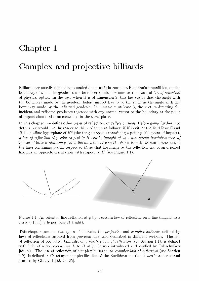
Billiards are usually dened as bounded domains Ω in complete Riemannian manifolds, on theboundary of which the geodesics can be reected into new ones by the classical law of reectionof physical optics. In the case when Ω is of dimension 2, this law states that the angle withthe boundary made by the geodesic before impact has to be the same as the angle with theboundary made by the reected geodesic. In dimension at least 3, the vectors directing theincident and reected geodesics together with any normal vector to the boundary at the pointof impact should also be contained in the same plane.

In this chapter, we dene other types of reection, or reection laws. Before going further intodetails, we would like the reader to think of them as follows: if K is either the eld R or C andH is an ane hyperplane of Kd (the tangent space) containing a point p (the point of impact),a law of reection at p with respect to H can be thought of as a non-trivial involutive map ofthe set of lines containing p xing the lines included in H. When K = R, we can further orientthe lines containing p with respect to H, so that the image by the reection law of an orientedline has an opposite orientation with respect to H (see Figure 1.1).

p

γ

Figure 1.1: An oriented line reected at p by a certain law of reection on a line tangent to acurve γ (left)/a hyperplane H (right).

This chapter presents two types of billiards, the projective and complex billiards, dened bylaws of reections inspired from previous idea, and described in dierent sections. The lawof reection of projective billiards, or projective law of reection (see Section 1.1), is denedwith help of a transverse line L to H at p. It was introduced and studied by Tabachnikov[58, 60]. The law of reection of complex billiards, or complex law of reection (see Section1.2), is dened in C2 using a complexication of the Euclidean metric. It was introduced andstudied by Glutsyuk [23, 24, 25].

23

1.1 Projective billiards

In this section, we dene the usual model of projective billiard in Rd as it is presented in[58, 60]. This model of billiard generalizes the usual model of Euclidean billiard, but also ofpseudo-Euclidean billiards and of billiards in metrics projectively equivalent to the Euclideanone (metrics in Rd whose geodesics are contained in lines).

A projective billiard in Rd is a hypersurface S or a collection of hypersurfaces endowed witha eld of transverse lines to S, called eld of projective lines. For example, if Rd is endowedwith a metric or a eld of non-degenerate quadratic forms, we can dene a eld of lines on ahypersurface S ⊂ Rd as follows: for p ∈ S, dene the line L(p) to be the line containing p andorthogonal to TpS with respect to the metric or quadratic form. It is however possible thatline L(p) is not transverse to S at p if the restriction to TpS of the eld of quadratic forms isdegenerate. Otherwise, S has the structure of a projective billiard induced by the metric or theeld of quadratic forms.

A reection law, called projective reection law, can be dened on a hypersurface S endowedwith a eld of transverse lines L: given an oriented line of Rd intersecting S at a certain point p,we dene the reected line `′ to be a line containing p and satisfying a condition of harmonicitywith L(p) (see Denition 3.54). In the case when the projective lines L(p) at p is orthogonal toTpS, the reected line `′ coincides with the line reected by the usual law of reection (whichpreserves the angles of reection in the Euclidean case).

We rst recall some properties about harmonic quadruples of lines in Subsection 1.1.1, then weapply it to dene projective billiards in Subsection 1.1.2, and we nally introduce the projectivebilliard map in Subsection 1.1.3.

1.1.1 Harmonic quadruple of lines

In this section, K is the eld R or C. We recall some properties of the cross-ratio and harmonicquadruple of points in P1(K). They can be extended to quadruple of lines containing the samepoint, and this will lead to the denition of projective reection law. Most of the results onharmonic quadruples of points are very basic, and we refer the reader for example to [5] formore details.

Let d ≥ 1 be an integer. We denote by Pd(K) the d-dimensional projective space, which is theset of equivalence classes in Kd+1 r 0 for the relation ∼, dened for all x, y ∈ Kd+1 r 0 byx ∼ y if and only if there is λ ∈ K r 0 such that y = λx. For x = (x0, . . . , xd) ∈ Kd+1 r 0,write (x0 : . . . : xd) ∈ Pd(K) the equivalence class of x for this relation.

Cross-ratio. The cross-ratio of four distinct points p1, p2, p3, p4 of P1(K) is a well-known quan-tity which can be dened in many dierent ways. Here we adopt the denition of [5] Vol. IChap. 6. based on the sharp 3-reectivity of the projective line's group of transformations:

Denition 1.1. The cross-ratio of four distinct points p1, p2, p3, p4 of P1(K) is the image h(p4)of the only projective transformation h of P1(K) satisfying h(p1) =∞, h(p2) = 0 and h(p3) = 1,where ∞ = (1 : 0) and x stands for (x : 1) given any x ∈ K.

The cross-ratio of four distinct points is invariant under projective transformations of P1(K)([5] Sec. 6.1.4.). We say that the quadruple (p1, p2, p3, p4) is harmonic if the cross-ratio ofthe corresponding points is −1. If we permute p1 with p2, or p3 with p4, or even (p1, p2) with(p3, p4), then the corresponding quadruple of points is still harmonic ([5] Prop. 6.3.1.).

24

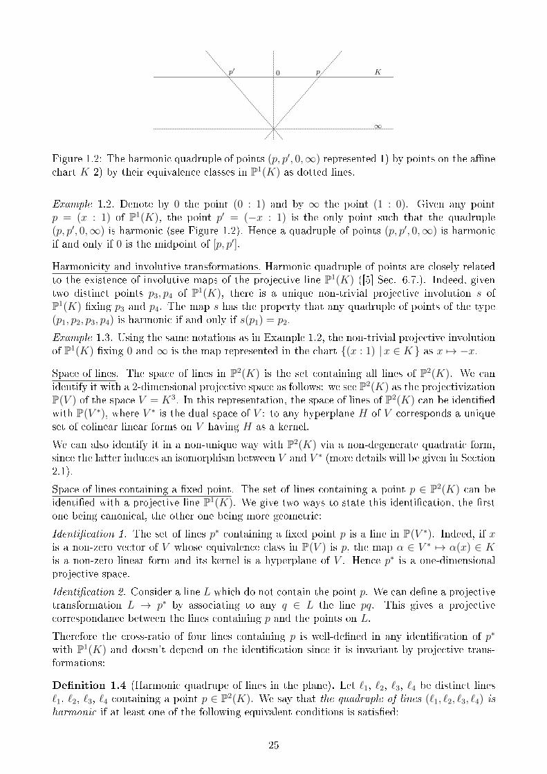
0 K

∞

pp′

Figure 1.2: The harmonic quadruple of points (p, p′, 0,∞) represented 1) by points on the anechart K 2) by their equivalence classes in P1(K) as dotted lines.

Example 1.2. Denote by 0 the point (0 : 1) and by ∞ the point (1 : 0). Given any pointp = (x : 1) of P1(K), the point p′ = (−x : 1) is the only point such that the quadruple(p, p′, 0,∞) is harmonic (see Figure 1.2). Hence a quadruple of points (p, p′, 0,∞) is harmonicif and only if 0 is the midpoint of [p, p′].

Harmonicity and involutive transformations. Harmonic quadruple of points are closely relatedto the existence of involutive maps of the projective line P1(K) ([5] Sec. 6.7.). Indeed, giventwo distinct points p3, p4 of P1(K), there is a unique non-trivial projective involution s ofP1(K) xing p3 and p4. The map s has the property that any quadruple of points of the type(p1, p2, p3, p4) is harmonic if and only if s(p1) = p2.

Example 1.3. Using the same notations as in Example 1.2, the non-trivial projective involutionof P1(K) xing 0 and ∞ is the map represented in the chart (x : 1) |x ∈ K as x 7→ −x.

Space of lines. The space of lines in P2(K) is the set containing all lines of P2(K). We canidentify it with a 2-dimensional projective space as follows: we see P2(K) as the projectivizationP(V ) of the space V = K3. In this representation, the space of lines of P2(K) can be identiedwith P(V ∗), where V ∗ is the dual space of V : to any hyperplane H of V corresponds a uniqueset of colinear linear forms on V having H as a kernel.

We can also identify it in a non-unique way with P2(K) via a non-degenerate quadratic form,since the latter induces an isomorphism between V and V ∗ (more details will be given in Section2.1).

Space of lines containing a xed point. The set of lines containing a point p ∈ P2(K) can beidentied with a projective line P1(K). We give two ways to state this identication, the rstone being canonical, the other one being more geometric:

Identication 1. The set of lines p∗ containing a xed point p is a line in P(V ∗). Indeed, if xis a non-zero vector of V whose equivalence class in P(V ) is p, the map α ∈ V ∗ 7→ α(x) ∈ Kis a non-zero linear form and its kernel is a hyperplane of V . Hence p∗ is a one-dimensionalprojective space.

Identication 2. Consider a line L which do not contain the point p. We can dene a projectivetransformation L → p∗ by associating to any q ∈ L the line pq. This gives a projectivecorrespondance between the lines containing p and the points on L.

Therefore the cross-ratio of four lines containing p is well-dened in any identication of p∗

with P1(K) and doesn't depend on the identication since it is invariant by projective trans-formations:

Denition 1.4 (Harmonic quadrupe of lines in the plane). Let `1, `2, `3, `4 be distinct lines`1, `2, `3, `4 containing a point p ∈ P2(K). We say that the quadruple of lines (`1, `2, `3, `4) isharmonic if at least one of the following equivalent conditions is satised:

25

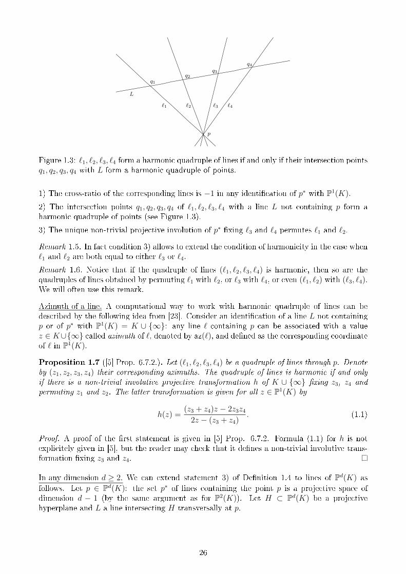
p

q1q2

q3

q4

`1 `2 `3 `4

L

Figure 1.3: `1, `2, `3, `4 form a harmonic quadruple of lines if and only if their intersection pointsq1, q2, q3, q4 with L form a harmonic quadruple of points.

1) The cross-ratio of the corresponding lines is −1 in any identication of p∗ with P1(K).

2) The intersection points q1, q2, q3, q4 of `1, `2, `3, `4 with a line L not containing p form aharmonic quadruple of points (see Figure 1.3).

3) The unique non-trivial projective involution of p∗ xing `3 and `4 permutes `1 and `2.

Remark 1.5. In fact condition 3) allows to extend the condition of harmonicity in the case when`1 and `2 are both equal to either `3 or `4.

Remark 1.6. Notice that if the quadruple of lines (`1, `2, `3, `4) is harmonic, then so are thequadruples of lines obtained by permuting `1 with `2, or `3 with `4, or even (`1, `2) with (`3, `4).We will often use this remark.

Azimuth of a line. A computational way to work with harmonic quadruple of lines can bedescribed by the following idea from [23]. Consider an identication of a line L not containingp or of p∗ with P1(K) = K ∪ ∞: any line ` containing p can be associated with a valuez ∈ K∪∞ called azimuth of `, denoted by az(`), and dened as the corresponding coordinateof ` in P1(K).

Proposition 1.7 ([5] Prop. 6.7.2.). Let (`1, `2, `3, `4) be a quadruple of lines through p. Denoteby (z1, z2, z3, z4) their corresponding azimuths. The quadruple of lines is harmonic if and onlyif there is a non-trivial involutive projective transformation h of K ∪ ∞ xing z3, z4 andpermuting z1 and z2. The latter transformation is given for all z ∈ P1(K) by

h(z) =(z3 + z4)z − 2z3z4

2z − (z3 + z4). (1.1)

Proof. A proof of the rst statement is given in [5] Prop. 6.7.2. Formula (1.1) for h is notexplicitely given in [5], but the reader may check that it denes a non-trivial involutive trans-formation xing z3 and z4.

In any dimension d ≥ 2. We can extend statement 3) of Denition 1.4 to lines of Pd(K) asfollows. Let p ∈ Pd(K): the set p∗ of lines containing the point p is a projective space ofdimension d − 1 (by the same argument as for P2(K)). Let H ⊂ Pd(K) be a projectivehyperplane and L a line intersecting H transversally at p.

26

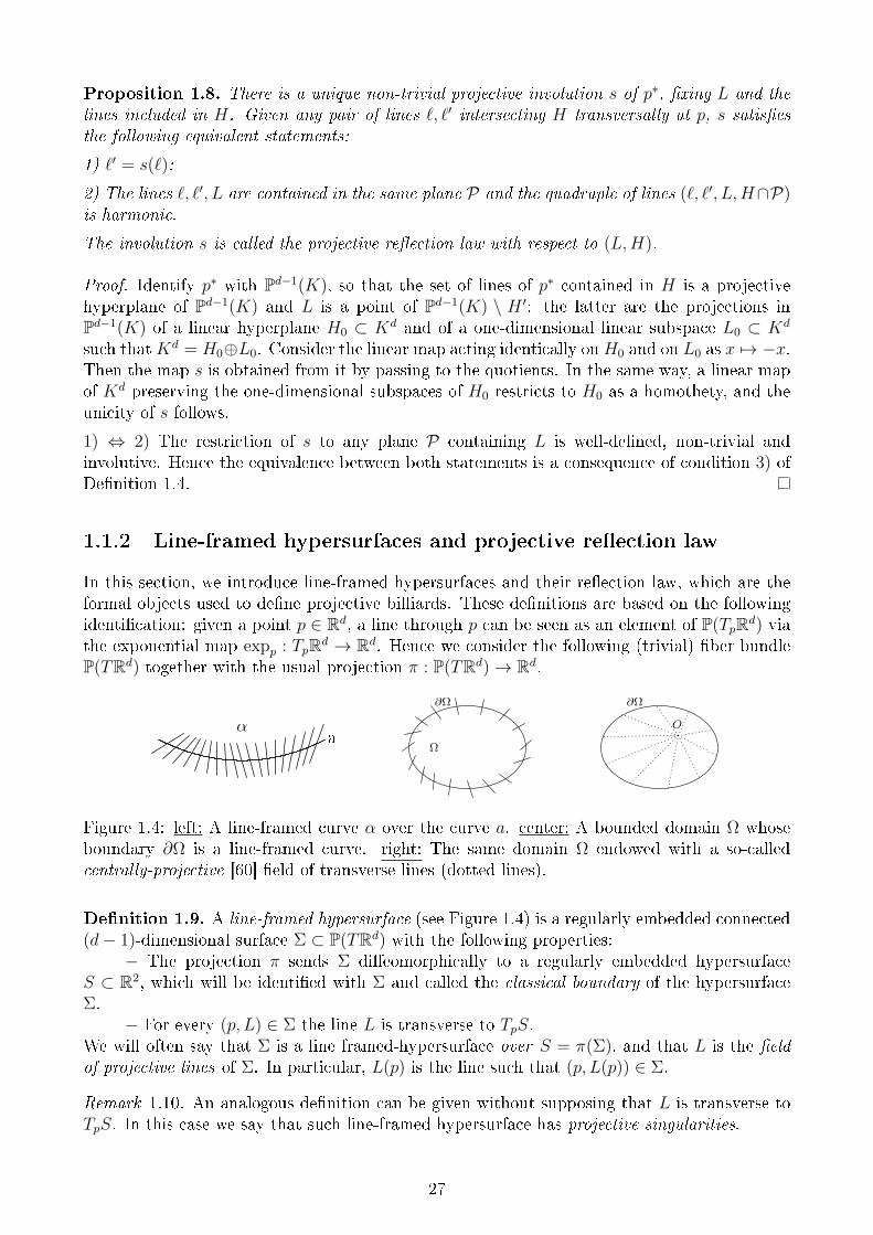
Proposition 1.8. There is a unique non-trivial projective involution s of p∗, xing L and thelines included in H. Given any pair of lines `, `′ intersecting H transversally at p, s satisesthe following equivalent statements:

1) `′ = s(`);

2) The lines `, `′, L are contained in the same plane P and the quadruple of lines (`, `′, L,H∩P)is harmonic.

The involution s is called the projective reection law with respect to (L,H).

Proof. Identify p∗ with Pd−1(K), so that the set of lines of p∗ contained in H is a projectivehyperplane of Pd−1(K) and L is a point of Pd−1(K) \ H ′: the latter are the projections inPd−1(K) of a linear hyperplane H0 ⊂ Kd and of a one-dimensional linear subspace L0 ⊂ Kd

such thatKd = H0⊕L0. Consider the linear map acting identically onH0 and on L0 as x 7→ −x.Then the map s is obtained from it by passing to the quotients. In the same way, a linear mapof Kd preserving the one-dimensional subspaces of H0 restricts to H0 as a homothety, and theunicity of s follows.

1) ⇔ 2) The restriction of s to any plane P containing L is well-dened, non-trivial andinvolutive. Hence the equivalence between both statements is a consequence of condition 3) ofDenition 1.4.

1.1.2 Line-framed hypersurfaces and projective reection law

In this section, we introduce line-framed hypersurfaces and their reection law, which are theformal objects used to dene projective billiards. These denitions are based on the followingidentication: given a point p ∈ Rd, a line through p can be seen as an element of P(TpRd) viathe exponential map expp : TpRd → Rd. Hence we consider the following (trivial) ber bundleP(TRd) together with the usual projection π : P(TRd)→ Rd.

aα

∂Ω

Ω

∂Ω

O

Figure 1.4: left: A line-framed curve α over the curve a. center: A bounded domain Ω whoseboundary ∂Ω is a line-framed curve. right: The same domain Ω endowed with a so-calledcentrally-projective [60] eld of transverse lines (dotted lines).

Denition 1.9. A line-framed hypersurface (see Figure 1.4) is a regularly embedded connected(d− 1)-dimensional surface Σ ⊂ P(TRd) with the following properties:

− The projection π sends Σ dieomorphically to a regularly embedded hypersurfaceS ⊂ R2, which will be identied with Σ and called the classical boundary of the hypersurfaceΣ.

− For every (p, L) ∈ Σ the line L is transverse to TpS.We will often say that Σ is a line framed-hypersurface over S = π(Σ), and that L is the eldof projective lines of Σ. In particular, L(p) is the line such that (p, L(p)) ∈ Σ.

Remark 1.10. An analogous denition can be given without supposing that L is transverse toTpS. In this case we say that such line-framed hypersurface has projective singularities.

27

Remark 1.11. Line-framed hypersurface can also be dened on P(TPd(R)) with analogue state-ments as in Denition 1.9.

Let Σ be a line-framed hypersurface over an hypersurface S ⊂ Rd. The projective reectionlaw on Σ can be dened as follows:

Denition 1.12. Let p ∈ S and `, `′ be oriented lines intersecting S at p. We say that `′ isobtained from ` by the projective reection law on Σ at p if

− the lines `, `′, L(p) are contained in a plane P− the quadruple of lines `, `′, L(p), TpS ∩ P is harmonic in P ;− the orientations of ` and `′ with respect to TpS are opposite.

Using previous statements, projective billiards can be dened as follows:

Denition 1.13. A projective billiard is a domain Ω whose boundary S = ∂Ω is the classicalboundary of a C1-smooth line-framed hypersurface Σ together with the corresponding projectivereection law on Σ. See Figure 1.4.

1.1.3 Projective orbits and projective billiard map

One can study the orbits of the projective reection law inside bounded domain Ω whoseboundary S = ∂Ω is the classical boundary of a C1-smooth line-framed hypersurface Σ.

Denition 1.14. A projective orbit, or simply an orbit, of the projective billiard Ω is a sequenceof points p1, . . . , pk ∈ ∂Ω such that for each j = 1, . . . , k − 1

− pj 6= pj+1, the line pjpj+1 is oriented from pj to pj+1;− the interior of each segment pjpj+1 is included in Ω ;− for j > 1, the lines pj−1pj and pjpj+1 are transverse to S at pj;− for j > 1, the line pjpj+1 is obtained from pj−1pj by the projective reection law at pj.

The orbit is said to be k-periodic if (p1, . . . , pk, p1, p2) is an orbit.

Let (p1, p2, p3) be a projective orbit of Σ such that the line p2p3 is transverse to S at p3. Thereis an open subset U(p1,p2) of S×S containing (p1, p2) such that for all (q1, q2) ∈ U(p1,p2), q1 6= q2,the line q1q2 is transverse to S at q2 and is reected into a line intersecting S transversaly ata point q3 by the projective law of reection at q2. We can dene on U(p1,p2) the projectivebilliard map using above description as the map B : U(p1,p2) → S × S satisfying

B(q1, q2) = (q2, q3). (1.2)

Proposition 1.15. Let r ≥ 2 be an integer. If Σ is Cr-smooth (respectively analytic) then B isa Cr−1-smooth (respectively an analytic) map of rank 2(d− 1).

Proof. We rst show that B is of class Cr−1 (resp. analytic). Indeed, notice that there isa Cr−1-smooth (resp. an analytic map) dened on the restriction of the set P(TRd)|S whichassociate to (p, `), where p ∈ S and ` is a line containing p, the element (p, `′) where `′ is theline containing p and obtained by the projective reection law at p dened by Σ. In fact therestriction of such map on each ber p × P(TRd) is a projective transformation dependingCr−1-smoothly (resp. analyticaly) on p.

We conclude on the regularity by proving the following result: consider a line ` intersecting aCr-smooth (resp. an analytic) hypersurface S transversaly at a point p; then if another line`′ is close to `, then `′ intersects S at a point q close to p and that the map `′ 7→ q is of

28

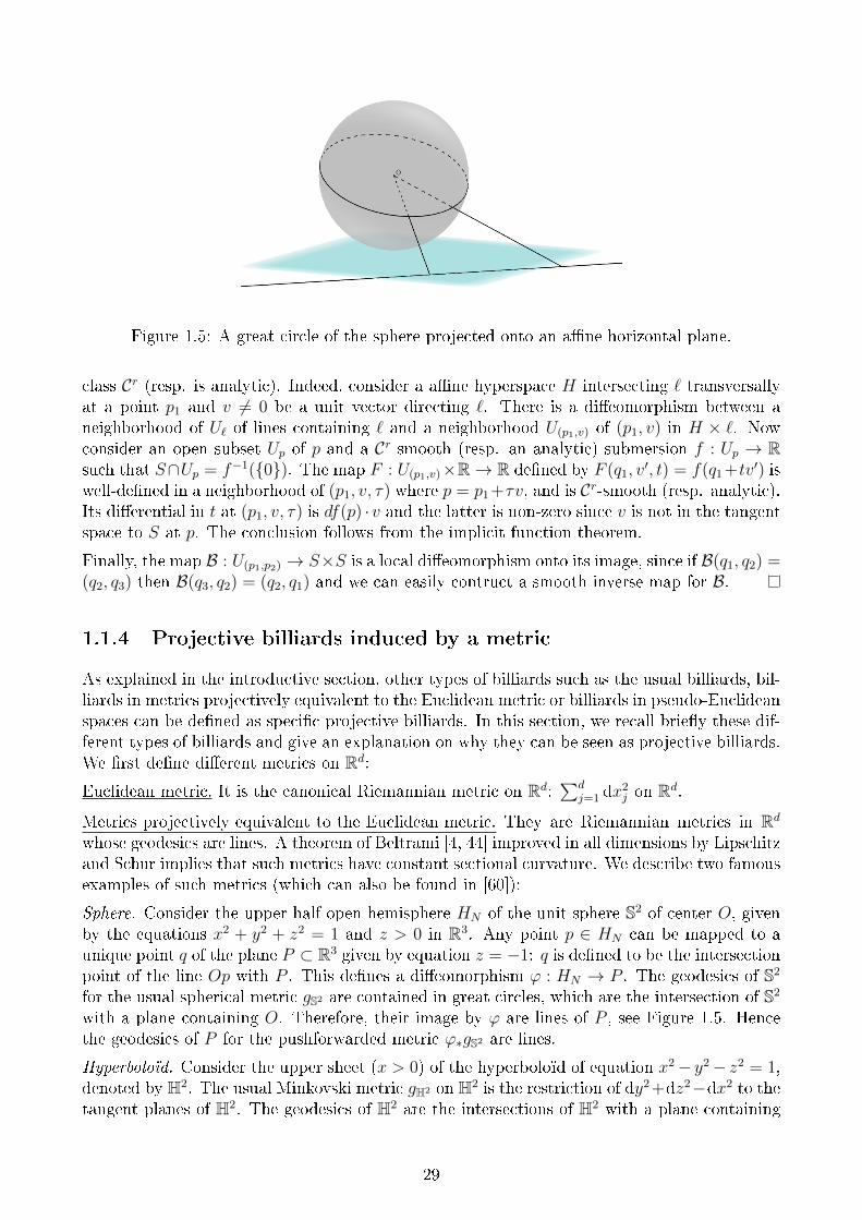
Figure 1.5: A great circle of the sphere projected onto an ane horizontal plane.

class Cr (resp. is analytic). Indeed, consider a ane hyperspace H intersecting ` transversallyat a point p1 and v 6= 0 be a unit vector directing `. There is a dieomorphism between aneighborhood of U` of lines containing ` and a neighborhood U(p1,v) of (p1, v) in H × `. Nowconsider an open subset Up of p and a Cr-smooth (resp. an analytic) submersion f : Up → Rsuch that S∩Up = f−1(0). The map F : U(p1,v)×R→ R dened by F (q1, v

′, t) = f(q1 +tv′) iswell-dened in a neighborhood of (p1, v, τ) where p = p1 +τv, and is Cr-smooth (resp. analytic).Its dierential in t at (p1, v, τ) is df(p) ·v and the latter is non-zero since v is not in the tangentspace to S at p. The conclusion follows from the implicit function theorem.

Finally, the map B : U(p1,p2) → S×S is a local dieomorphism onto its image, since if B(q1, q2) =(q2, q3) then B(q3, q2) = (q2, q1) and we can easily contruct a smooth inverse map for B.

1.1.4 Projective billiards induced by a metric

As explained in the introductive section, other types of billiards such as the usual billiards, bil-liards in metrics projectively equivalent to the Euclidean metric or billiards in pseudo-Euclideanspaces can be dened as specic projective billiards. In this section, we recall briey these dif-ferent types of billiards and give an explanation on why they can be seen as projective billiards.We rst dene dierent metrics on Rd:

Euclidean metric. It is the canonical Riemannian metric on Rd:∑d

j=1 dx2j on Rd.

Metrics projectively equivalent to the Euclidean metric. They are Riemannian metrics in Rd

whose geodesics are lines. A theorem of Beltrami [4, 44] improved in all dimensions by Lipschitzand Schur implies that such metrics have constant sectional curvature. We describe two famousexamples of such metrics (which can also be found in [60]):

Sphere. Consider the upper half open hemisphere HN of the unit sphere S2 of center O, givenby the equations x2 + y2 + z2 = 1 and z > 0 in R3. Any point p ∈ HN can be mapped to aunique point q of the plane P ⊂ R3 given by equation z = −1: q is dened to be the intersectionpoint of the line Op with P . This denes a dieomorphism ϕ : HN → P . The geodesics of S2

for the usual spherical metric gS2 are contained in great circles, which are the intersection of S2

with a plane containing O. Therefore, their image by ϕ are lines of P , see Figure 1.5. Hencethe geodesics of P for the pushforwarded metric ϕ∗gS2 are lines.

Hyperboloïd. Consider the upper sheet (x > 0) of the hyperboloïd of equation x2− y2− z2 = 1,denoted by H2. The usual Minkovski metric gH2 on H2 is the restriction of dy2 +dz2−dx2 to thetangent planes of H2. The geodesics of H2 are the intersections of H2 with a plane containing

29

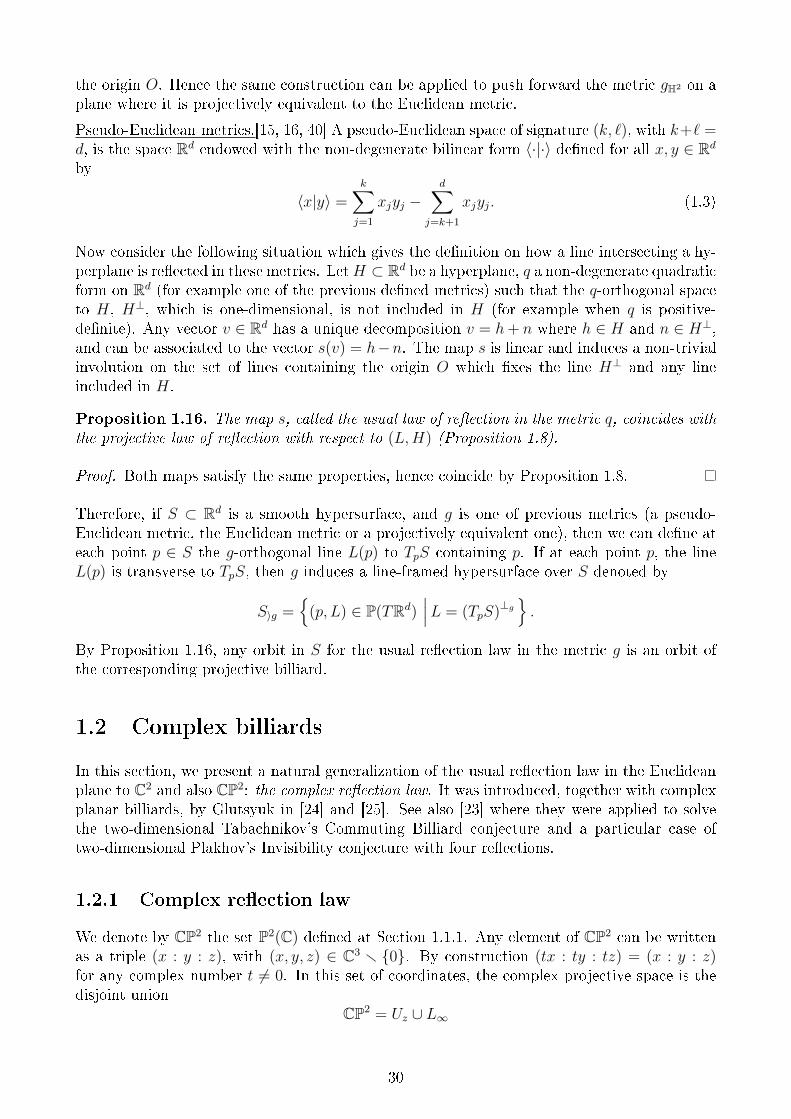
the origin O. Hence the same construction can be applied to push forward the metric gH2 on aplane where it is projectively equivalent to the Euclidean metric.

Pseudo-Euclidean metrics.[15, 16, 40] A pseudo-Euclidean space of signature (k, `), with k+` =d, is the space Rd endowed with the non-degenerate bilinear form 〈·|·〉 dened for all x, y ∈ Rd

by

〈x|y〉 =k∑j=1

xjyj −d∑

j=k+1

xjyj. (1.3)

Now consider the following situation which gives the denition on how a line intersecting a hy-perplane is reected in these metrics. LetH ⊂ Rd be a hyperplane, q a non-degenerate quadraticform on Rd (for example one of the previous dened metrics) such that the q-orthogonal spaceto H, H⊥, which is one-dimensional, is not included in H (for example when q is positive-denite). Any vector v ∈ Rd has a unique decomposition v = h+ n where h ∈ H and n ∈ H⊥,and can be associated to the vector s(v) = h−n. The map s is linear and induces a non-trivialinvolution on the set of lines containing the origin O which xes the line H⊥ and any lineincluded in H.

Proposition 1.16. The map s, called the usual law of reection in the metric q, coincides withthe projective law of reection with respect to (L,H) (Proposition 1.8).

Proof. Both maps satisfy the same properties, hence coincide by Proposition 1.8.

Therefore, if S ⊂ Rd is a smooth hypersurface, and g is one of previous metrics (a pseudo-Euclidean metric, the Euclidean metric or a projectively equivalent one), then we can dene ateach point p ∈ S the g-orthogonal line L(p) to TpS containing p. If at each point p, the lineL(p) is transverse to TpS, then g induces a line-framed hypersurface over S denoted by

S〉g =

(p, L) ∈ P(TRd)∣∣∣L = (TpS)⊥g

.

By Proposition 1.16, any orbit in S for the usual reection law in the metric g is an orbit ofthe corresponding projective billiard.

1.2 Complex billiards

In this section, we present a natural generalization of the usual reection law in the Euclideanplane to C2 and also CP2: the complex reection law. It was introduced, together with complexplanar billiards, by Glutsyuk in [24] and [25]. See also [23] where they were applied to solvethe two-dimensional Tabachnikov's Commuting Billiard conjecture and a particular case oftwo-dimensional Plakhov's Invisibility conjecture with four reections.

1.2.1 Complex reection law

We denote by CP2 the set P2(C) dened at Section 1.1.1. Any element of CP2 can be writtenas a triple (x : y : z), with (x, y, z) ∈ C3 r 0. By construction (tx : ty : tz) = (x : y : z)for any complex number t 6= 0. In this set of coordinates, the complex projective space is thedisjoint union

CP2 = Uz ∪ L∞

30

of the so-called standard open subset Uz = (x : y : 1) | (x, y) ∈ C2 and the line L∞ =(x : y : 0) | (x, y) ∈ C2 r 0 called line at innity. The map (x, y) ∈ C2 7→ (x : y : 1) ∈ Uzis an analytic chart mapping C2 to Uz. Hence we can consider the pushforward of the non-degenerate quadratic form q = dx2 + dy2 dened on TCP2

|Uz := TUz.

Denition 1.17. A line of CP2 is said to be isotropic if it contains either the point I = (1 : i : 0)or the point J = (1 : −i : 0), and non-isotropic if not. Notice that the line at innity is isotropic.

In the case of a non-isotropic line L ⊂ CP2, we can dene a complex q-isometric involution ofthe space Uz ' C2 xing the points of L. This involution can be constructed by consideringthe projective transformations preserving L and its q-orthogonal lines. This involution inducesa symmetry on lines of Uz, and can be extended to all lines of CP2 by sending L∞ to L∞. Inthe case of an isotropic line, this contruction fails since q-orthogonal lines to L are its parallellines.

Denition 1.18 ([24], denition 2.1). The symmetry with respect to a line L 6= L∞ is denedas follows:

− Case 1: L is non-isotropic. The symmetry acting on C2 is the unique non-trivialcomplex q-isometric involution xing the points of the line L. It induces the same symmetryacting on lines.

− Case 2: L is isotropic. We dene the symmetry of lines through a point p ∈ L∩Uz: twolines ` and `′ which contain p are called symmetric if there are sequences (Ln)n, (`n)n, (`′n)nof lines through points pn so that Ln is non-isotropic, `n and `′n are symmetric with respect toLn, `n → `, `′n → `′, Ln → L and pn → p.

We recall now lemma 2.3 [24] which gives an idea of this notion of symmetry in the case of anisotropic line through a nite point.

Lemma 1.19 ([24], lemma 2.3). If L is an isotropic line through a point p ∈ Uz and `, `′ aretwo lines which contain x, then ` and `′ are symmetric with respect to L if and only if either` = L, or `′ = L.

1.2.2 Complex orbits

Let γ ⊂ CP2 be a complex curve of CP2 (that is smooth at each point).

Denition 1.20 ([24]). A non-degenerate orbit on γ is a nite sequence (p1, . . . , pk) ∈ γk

such that− pj 6= pj+1 for each j ∈ 1, . . . , k − 1;− Tpjγ is not isotropic for each j ∈ 1, . . . , k;− the lines pj−1pj and pjpj+1 are symmetric with respect to the tangent line Tpjγ for each

j ∈ 2, . . . , k − 1.The side of an orbit is one of the lines pjpj+1. A non-degenerate k-periodic orbit is a non-degenerate orbit (p1, . . . , pk) ∈ γk such that (p1, . . . , pk, p1, p2) is a non-degenerate orbit.

By opposition we can dene degenerate orbits as follows:

Denition 1.21 ([24]). A degenerate orbit (resp. a degenerate k-periodic orbit) on γ is a setof points (p1, . . . , pk) ∈ γk which is the limit of non-degenerate orbits (resp. non-degeneratek-periodic orbits) and is not a non-degenerate orbit (resp. non-degenerate k-periodic orbits).

We can also dene the side of a degenerate orbit as the limit of the sides of non-degenerateorbits converging to it. In the case when pj = pj+1, we can naturally dene the side pjpj+1 asthe tangent line Tpjγ.

31

1.3 Proof by complexication: circumcenters of triangular

orbits

In this section, we present a published result [18] on the circumcenters of triangular orbits inan elliptic billiard, which is of great interest for us since its proof uses complex billiards to solvea problem of real geometry. More precisely, we are interested in the usual billiard inside anellipse and its 3-periodic or triangular orbits. We show that the set of all circumcenters to theseorbits is an ellipse. The proof of this result is based on the complexication of the problem andon the use of the complex reection law introduced at Section 1.2.

Theorem 1.22. The set C of the circumcenters of all triangular orbits of the billiard withinan ellipse is also an ellipse.

Remark 1.23. Theorem 1.22 is obvious in the particular case where the ellipse is a circle, becausethen the set of circumcenters is reduced to a single point. Thus, we will assume that the ellipseis not a circle.

There are many other results similar to theorem 1.22. Dan Reznik discovered experimentallythe same result for the incenters of triangular orbits, see the video [48] and the github page [49]written with Jair Koiller. Romaskevich (see [50]) conrmed these observations by proving themand her proof widely inspired ours. Tabachnikov and Schwartz, in [54], proved that the loci ofthe centers of mass (and of an other particular point) of a 1-parameter family of Poncelet n-gonsin an ellipse is an ellipse homothetic to the previous one. They also mention that a similarresult was proved by Zaslawski, Kosov and Muzafarov for the orthocenters ([67], reference from[54]). And Garcia (see [51]) uses explicit calculations to prove that the loci of circumcenters,incenters and orthocenters of triangular orbits are ellipses, and describes them precisely. Hisproof of the result about circumcenters was found simultaneously and independantly to us.

Before going into details, we give here a brief summary of the proof, which is inspired by [50],and in which we use the same complex methods. We consider a projective complexied versionof C, denoted by C, which turns out to be an algebraic curve as a consequence of Remmert propermapping theorem and Chow's theorem, see [31] p. 34. Then we show that the intersection ofthe complex curve C with the foci line of the boundary ellipse E is reduced to two points, eachone of them corresponding to a single triangular orbit. Further algebraic arguments on theintersection type of C with the foci line of E allow to conclude that it is a conic, using Bezouttheorem. It's then possible to check that C is an ellipse since its real part is bounded.

As explained, one considers the projective complex Zariski closure of the ellipse E and a com-plexied version C of C. In order to dene C and to prove the rst statement concerning theintersection with the foci line, we study an extension of the reection law and of the triangularorbits to complex domain, as in [50], and we use some of the results contained in the latterarticle such as Proposition 1.33.

Section 1.3.1 is devoted to the complex reection law and to complex orbits in a complexiedellipse: Subsection 1.3.1.1 recalls some results about complexied conics; we further denewhat is a triangular complex orbit in Subsection 1.3.1.2; then, in Section 1.3.2 we intro-duce the denition and we study properties of complex circumscribed circles to such orbits:Proposition 1.41 is the main result of this section. Finally, Section 1.3.3 is devoted to theproof of Theorem 1.22, using previous results.

32

1.3.1 Complex triangular obits on an ellipse

In this section, we recall some results about complexied conics and we study results abouttriangular orbits of the complexied ellipse E .

1.3.1.1 Preliminary results on complexied conics

We dene a complexied conic as the algebraic closure of a real conic in R2: an ellipse, ahyperbola or a parabola. We recall that an ellipse cuts the line at innity in two distinct pointswith strictly complex coordinates, a hyperbola in two distinct points with real coordinates, anda parabola is tangent to the line at innity. The following results on conics are well-known andcan be found in [5, 41].

Proposition 1.24 ([5] subsection 17.4.2.1). A conic is a circle if and only if some of the pointsI or J belong to it. Furthermore, if a conic is a circle, then both I and J belong to it.

In fact, a circle has two isotropic tangent lines intersecting at its center (see the followingpropositions).

Proposition 1.25 ([5] subsection 17.4.3.1). A focus f of a conic lies in the intersection of twoisotropic tangent lines to the conic.

Proposition 1.26 ([41], p. 179). Two complexied confocal ellipses have the same tangentisotropic lines, which are four isotropic lines taken with multiplicities: one pair intersecting ata focus, and the other one - at the other focus.

This brings us to the following redenition of the foci:

Denition 1.27 ([5] subsection 17.4.3.2). The complex foci of an ellipse are the intersectionpoints of its isotropic tangent lines.

Remark 1.28. The complex projective closure of a real ellipse has four complex foci, includingtwo real ones.

Corollary 1.29. A conic has at most four dinstinct nite isotropic tangent lines, each two ofthem intersecting either at a focus, or at an isotropic point at innity.

1.3.1.2 Triangular orbits

Let E ⊂ CP2 be a complexied ellipse which is not a circle.

Denition 1.30. A non-degenerate triangular orbit is a non-degenerate 3-periodic orbit (seeDenition 1.20).

Remark 1.31. The vertices of a non-degenerate orbit are not collinear since a line intersects theellipse in at most two points.

Remark 1.32. As explained in [25], the reection with respect to a non-isotropic line permutesthe isotropic directions I and J . This argument implies that a non-degenerate triangular orbithas no isotropic side.

Proposition 1.33 ([50], lemma 3.4). A degenerate triangular orbit of E has an isotropic sideA which is tangent to E, and two coinciding non-isotropic sides B.

33

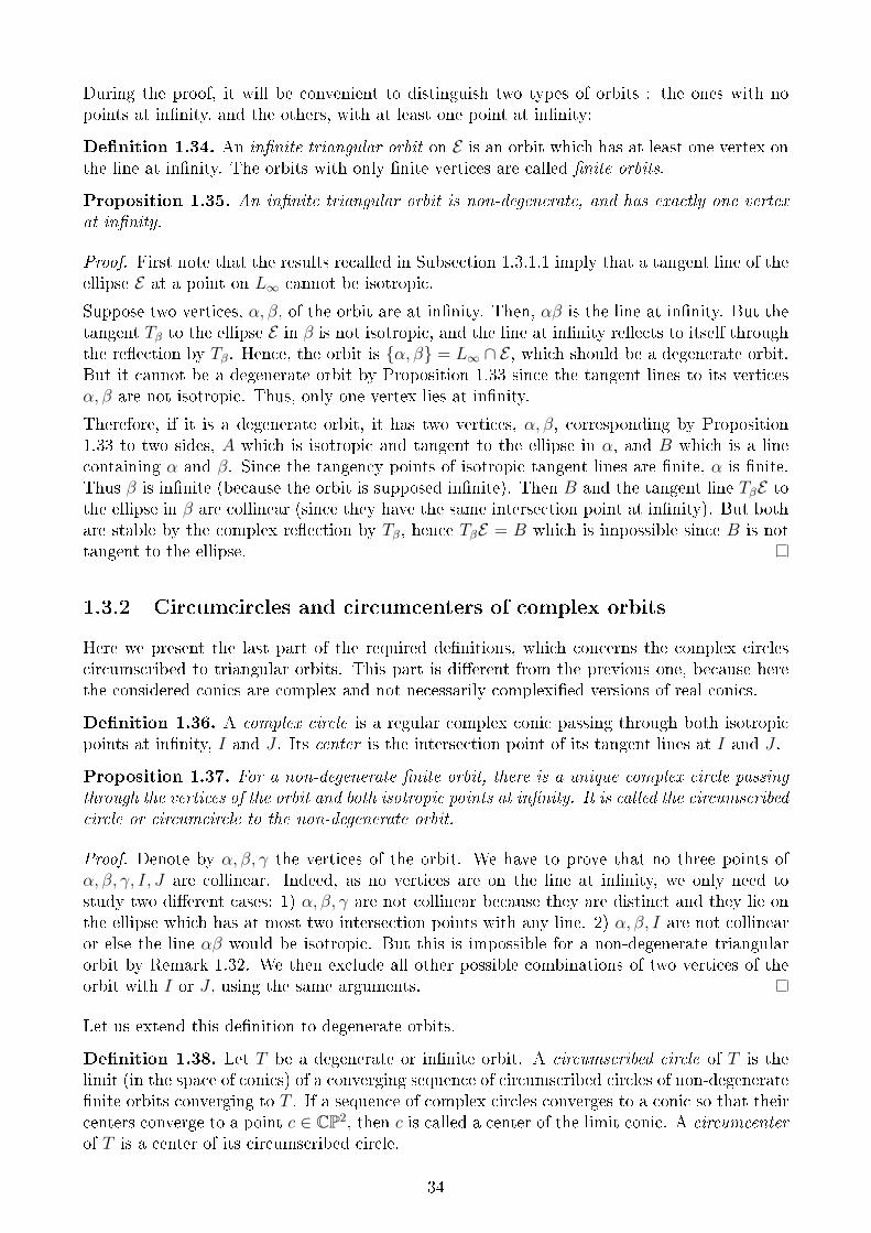
During the proof, it will be convenient to distinguish two types of orbits : the ones with nopoints at innity, and the others, with at least one point at innity:

Denition 1.34. An innite triangular orbit on E is an orbit which has at least one vertex onthe line at innity. The orbits with only nite vertices are called nite orbits.

Proposition 1.35. An innite triangular orbit is non-degenerate, and has exactly one vertexat innity.

Proof. First note that the results recalled in Subsection 1.3.1.1 imply that a tangent line of theellipse E at a point on L∞ cannot be isotropic.

Suppose two vertices, α, β, of the orbit are at innity. Then, αβ is the line at innity. But thetangent Tβ to the ellipse E in β is not isotropic, and the line at innity reects to itself throughthe reection by Tβ. Hence, the orbit is α, β = L∞ ∩ E , which should be a degenerate orbit.But it cannot be a degenerate orbit by Proposition 1.33 since the tangent lines to its verticesα, β are not isotropic. Thus, only one vertex lies at innity.

Therefore, if it is a degenerate orbit, it has two vertices, α, β, corresponding by Proposition1.33 to two sides, A which is isotropic and tangent to the ellipse in α, and B which is a linecontaining α and β. Since the tangency points of isotropic tangent lines are nite, α is nite.Thus β is innite (because the orbit is supposed innite). Then B and the tangent line TβE tothe ellipse in β are collinear (since they have the same intersection point at innity). But bothare stable by the complex reection by Tβ, hence TβE = B which is impossible since B is nottangent to the ellipse.

1.3.2 Circumcircles and circumcenters of complex orbits

Here we present the last part of the required denitions, which concerns the complex circlescircumscribed to triangular orbits. This part is dierent from the previous one, because herethe considered conics are complex and not necessarily complexied versions of real conics.

Denition 1.36. A complex circle is a regular complex conic passing through both isotropicpoints at innity, I and J . Its center is the intersection point of its tangent lines at I and J .

Proposition 1.37. For a non-degenerate nite orbit, there is a unique complex circle passingthrough the vertices of the orbit and both isotropic points at innity. It is called the circumscribedcircle or circumcircle to the non-degenerate orbit.

Proof. Denote by α, β, γ the vertices of the orbit. We have to prove that no three points ofα, β, γ, I, J are collinear. Indeed, as no vertices are on the line at innity, we only need tostudy two dierent cases: 1) α, β, γ are not collinear because they are distinct and they lie onthe ellipse which has at most two intersection points with any line. 2) α, β, I are not collinearor else the line αβ would be isotropic. But this is impossible for a non-degenerate triangularorbit by Remark 1.32. We then exclude all other possible combinations of two vertices of theorbit with I or J , using the same arguments.

Let us extend this denition to degenerate orbits.

Denition 1.38. Let T be a degenerate or innite orbit. A circumscribed circle of T is thelimit (in the space of conics) of a converging sequence of circumscribed circles of non-degeneratenite orbits converging to T . If a sequence of complex circles converges to a conic so that theircenters converge to a point c ∈ CP2, then c is called a center of the limit conic. A circumcenterof T is a center of its circumscribed circle.

34

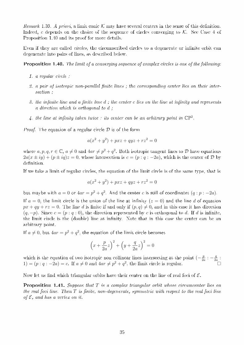
Remark 1.39. A priori, a limit conic K may have several centers in the sense of this denition.Indeed, c depends on the choice of the sequence of circles converging to K. See Case 4 ofProposition 1.40 and its proof for more details.

Even if they are called circles, the circumscribed circles to a degenerate or innite orbit candegenerate into pairs of lines, as described below.

Proposition 1.40. The limit of a converging sequence of complex circles is one of the following:

1. a regular circle ;

2. a pair of isotropic non-parallel nite lines ; the corresponding center lies on their inter-section ;

3. the innite line and a nite line d ; the center c lies on the line at innity and representsa direction which is orthogonal to d ;

4. the line at innity taken twice : its center can be an arbitrary point in CP2.

Proof. The equation of a regular circle D is of the form

a(x2 + y2) + pxz + qyz + rz2 = 0

where a, p, q, r ∈ C, a 6= 0 and 4ar 6= p2 + q2. Both isotropic tangent lines to D have equations2a(x± iy) + (p± iq)z = 0, whose intersection is c = (p : q : −2a), which is the center of D bydenition.

If we take a limit of regular circles, the equation of the limit circle is of the same type, that is

a(x2 + y2) + pxz + qyz + rz2 = 0

but maybe with a = 0 or 4ar = p2 + q2. And the center c is still of coordinates (q : p : −2a).

If a = 0, the limit circle is the union of the line at innity (z = 0) and the line d of equationpx + qy + rz = 0. The line d is nite if and only if (p, q) 6= 0, and in this case it has direction(q,−p). Since c = (p : q : 0), the direction represented by c is orthogonal to d. If d is innite,the limit circle is the (double) line at innity. Note that in this case the center can be anarbitrary point.

If a 6= 0, but 4ar = p2 + q2, the equation of the limit circle becomes(x+

p

2az)2

+(y +

q

2az)2

= 0

which is the equation of two isotropic non collinear lines intersecting at the point (− p2a

: − q2a

:1) = (p : q : −2a) = c. If a 6= 0 and 4ar 6= p2 + q2, the limit circle is regular.

Now let us nd which triangular orbits have their center on the line of real foci of E .

Proposition 1.41. Suppose that T is a complex triangular orbit whose circumcenter lies onthe real foci line. Then T is nite, non-degenerate, symmetric with respect to the real foci lineof E, and has a vertex on it.

35

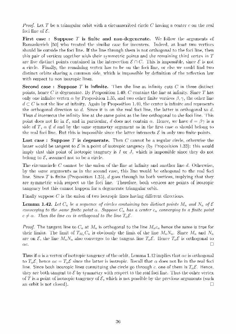
Proof. Let T be a triangular orbit with a circumscribed circle C having a center c on the realfoci line of E .First case : Suppose T is nite and non-degenerate. We follow the arguments ofRomaskevich [50] who treated the similar case for incenters. Indeed, at least two verticesshould lie outside the foci line. If the line through them is not orthogonal to the foci line, thenthis pair of vertices together with their symmetric points and the remaining third vertex in Tare ve distinct points contained in the intersection E ∩ C. This is impossible, since E is nota circle. Finally, the remaining vertex has to be on the foci line, or else we could nd twodistinct orbits sharing a common side, which is impossible by denition of the reection lawwith respect to non-isotropic lines.

Second case : Suppose T is innite. Then the line at innity cuts C in three distinctpoints, hence C is degenerate. By Proposition 1.40, C contains the line at innity. Since T hasonly one innite vertex α by Proposition 1.35, and two other nite vertices β, γ, the other lined ⊂ C is not the line at innity. Again by Proposition 1.40, the center is innite and representsthe orthogonal direction to d. Since it is on the real foci line, the latter is orthogonal to d.Thus d intersects the innity line at the same point as the line orthogonal to the foci line. Thispoint does not lie in E , and in particular, d does not contain α. Hence, we have d = βγ is aside of T , α /∈ d and by the same symmetry argument as in the rst case α should belong tothe real foci line. But this is impossible since the latter intersects E in only two nite points.

Last case : Suppose T is degenerate. Then C cannot be a regular circle, otherwise thelatter would be tangent to E in a point of isotropic tangency (by Proposition 1.33): this wouldimply that this point of isotropic tangency is I or J , which is impossible since they do notbelong to E , assumed not to be a circle.

The circumcircle C cannot be the union of the line at innity and another line d. Otherwise,by the same arguments as in the second case, this line would be othogonal to the real fociline. Since T is nite (Proposition 1.35), d goes through its both vertices, implying that theyare symmetric with respect to the foci line. Therefore, both vertices are points of isotropictangency but this cannot happen for a degenerate triangular orbit.

Finally suppose C is the union of two isotropic lines having dierent directions.

Lemma 1.42. Let Cn be a sequence of circles containing two distinct points Mn and Nn of Econverging to the same nite point α. Suppose Cn has a center cn converging to a nite pointc 6= α. Then the line cα is orthogonal to the line TαE.

Proof. The tangent line to Cn at Mn is orthogonal to the line Mncn hence the same is true fortheir limits. The limit of TMnCn is obviously the limit of the line MnNn. Since Mn and Nn

are on E , the line MnNn also converges to the tangent line TαE . Hence TαE is orthogonal toαc.

Thus if α is a vertex of isotropic tangency of the orbit, Lemma 1.42 implies that αc is orthogonalto TαE , hence αc = TαE since the latter is isotropic. Recall that α does not lie in the real fociline. Since both isotropic lines constituing the circle go through c, one of them is TαE . Hence,they are both tangent to E by symmetry with respect to the real foci line. Thus the other vertexof T is a point of isotropic tangency of E , which is not possible by the previous arguments (suchan orbit is not closed).

36

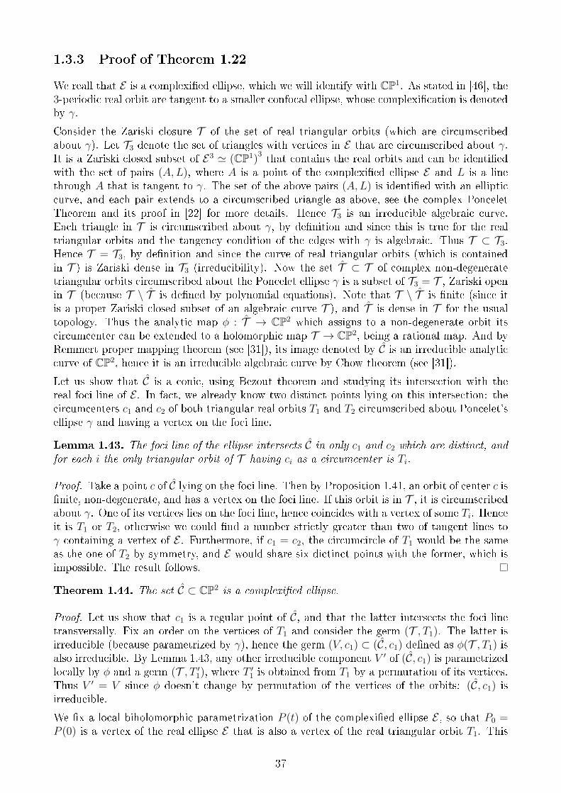
1.3.3 Proof of Theorem 1.22

We reall that E is a complexied ellipse, which we will identify with CP1. As stated in [46], the3-periodic real orbit are tangent to a smaller confocal ellipse, whose complexication is denotedby γ.

Consider the Zariski closure T of the set of real triangular orbits (which are circumscribedabout γ). Let T3 denote the set of triangles with vertices in E that are circumscribed about γ.It is a Zariski closed subset of E3 ' (CP1)

3 that contains the real orbits and can be identiedwith the set of pairs (A,L), where A is a point of the complexied ellipse E and L is a linethrough A that is tangent to γ. The set of the above pairs (A,L) is identied with an ellipticcurve, and each pair extends to a circumscribed triangle as above, see the complex PonceletTheorem and its proof in [22] for more details. Hence T3 is an irreducible algebraic curve.Each triangle in T is circumscribed about γ, by denition and since this is true for the realtriangular orbits and the tangency condition of the edges with γ is algebraic. Thus T ⊂ T3.Hence T = T3, by denition and since the curve of real triangular orbits (which is containedin T ) is Zariski dense in T3 (irreducibility). Now the set T ⊂ T of complex non-degeneratetriangular orbits circumscribed about the Poncelet ellipse γ is a subset of T3 = T , Zariski openin T (because T \ T is dened by polynomial equations). Note that T \ T is nite (since itis a proper Zariski closed subset of an algebraic curve T ), and T is dense in T for the usualtopology. Thus the analytic map φ : T → CP2 which assigns to a non-degenerate orbit itscircumcenter can be extended to a holomorphic map T → CP2, being a rational map. And byRemmert proper mapping theorem (see [31]), its image denoted by C is an irreducible analyticcurve of CP2, hence it is an irreducible algebraic curve by Chow theorem (see [31]).

Let us show that C is a conic, using Bezout theorem and studying its intersection with thereal foci line of E . In fact, we already know two distinct points lying on this intersection: thecircumcenters c1 and c2 of both triangular real orbits T1 and T2 circumscribed about Poncelet'sellipse γ and having a vertex on the foci line.

Lemma 1.43. The foci line of the ellipse intersects C in only c1 and c2 which are distinct, andfor each i the only triangular orbit of T having ci as a circumcenter is Ti.

Proof. Take a point c of C lying on the foci line. Then by Proposition 1.41, an orbit of center c isnite, non-degenerate, and has a vertex on the foci line. If this orbit is in T , it is circumscribedabout γ. One of its vertices lies on the foci line, hence coincides with a vertex of some Ti. Henceit is T1 or T2, otherwise we could nd a number strictly greater than two of tangent lines toγ containing a vertex of E . Furthermore, if c1 = c2, the circumcircle of T1 would be the sameas the one of T2 by symmetry, and E would share six dictinct points with the former, which isimpossible. The result follows.

Theorem 1.44. The set C ⊂ CP2 is a complexied ellipse.

Proof. Let us show that c1 is a regular point of C, and that the latter intersects the foci linetransversally. Fix an order on the vertices of T1 and consider the germ (T , T1). The latter isirreducible (because parametrized by γ), hence the germ (V, c1) ⊂ (C, c1) dened as φ(T , T1) isalso irreducible. By Lemma 1.43, any other irreducible component V ′ of (C, c1) is parametrizedlocally by φ and a germ (T , T ′1), where T ′1 is obtained from T1 by a permutation of its vertices.Thus V ′ = V since φ doesn't change by permutation of the vertices of the orbits: (C, c1) isirreducible.

We x a local biholomorphic parametrization P (t) of the complexied ellipse E , so that P0 =P (0) is a vertex of the real ellipse E that is also a vertex of the real triangular orbit T1. This

37

gives local parametrizations of the orbits T (P ) whose rst vertex is P and of their circumcentersc(t) = φ(T (P (t))). We restrict P to the curve P (t) parametrizing the real points of E . We cansuppose that P (t) and P (−t) are symmetric with respect to F . Write r(t) = |P (t)c(t)| for theradius of the circumscribed circle to T (t). Thus we have c(0) = φ(T1) = c1, and we need toshow that c′(0) 6= 0 and that c′(0) has not the same direction as the line of real foci of E .First, we have r(t) = r(−t) by symmetry, and r is smooth around 0 since P (0) 6= c(0). Thus,r′(0) = 0. This implies that the vector c′(0)−P ′(0) is orthogonal to the line c(0)P (0), which isthe real foci line by denition. But P ′(0) is already orthogonal to the foci line (being a vectortangent to E at its vertex P0), hence the same hold for c′(0). It's then enough to show thatc′(0) 6= 0.

Suppose the contrary, i.e. c′(0) = 0. We use again r′(0) = 0. If we denote by Q(t) one of theother vertices of T (t) and Q0 = Q(0), then since also r(t) = |Q(t)c(t)|, the equality r′(0) = 0gives that the line Q0c1 is orthogonal to TQ0E . It means that the circumscribed circle D to T1

has the same tangent line in Q0 as E . Since this is also true in P0 and in the third point ofT1 (same proof), we get that E and D have three common points with the same tangent lines,which means that E is a circle. But this case was excluded at the beginning (remark 1.23).

Hence c′(0) 6= 0 and c′(0) is orthogonal to the line of real foci. The proof is the same for c2.Hence by Bezout theorem, C is a complexied conic. Since its real part is bounded, it is acomplexied ellipse.

38

Chapter 2

On the existence of caustics

This chapter is devoted to the study of caustics in complex billiards and projective billiards.

In the classical model of billiard, a caustic of a billiard Ω is a hypersurface C inside Ω suchthat any oriented line tangent to C and intersecting ∂Ω transversally is reected on ∂Ω into aline tangent to C. This implies that any iterated reections of a line tangent to C will producetangent lines to C.Caustics of projective billiards can be dened similarly:

Denition 2.1. Let Σ ⊂ P(TRd) be a line-framed hypersurface over a hypersurface S ⊂ Rd. Acaustic of Σ is a hypersurface Γ ⊂ Rd such that any line ` ⊂ Rd tangent to Γ and interecting Stransversally at a point p, is reected into a line tangent to Γ by the projective law of reectionat p.

Caustics of complex billiards (or complex caustics) are dicult to dene in the general casesince there is no possible orientation of lines. For our purpose to work on conics such denitionis more simple, since any line of CP2 is either tangent to a xed conic or intersects it in exactlytwo distinct points. Therefore, complex caustics can be dened as follows in this specic case:let C,C ′ ⊂ CP2 be two distinct conics. We say that C ′ is a complex caustic of C if for any line` tangent to C ′ and p a point of intersection of the line with C, the line reected from ` by thecomplex law of reection at p on C is also tangent to C ′.

This chapter is structured as follows. Basic results about conics and quadrics are rst recalledat Section 2.1. Then we present results about complex caustics of the billiard on a complexiedellipse or hyperbola at Section 2.2. It is followed by Section 2.3 which explains that given acertain pencil of conics or quadrics and any xed conic or quadric Q of this pencil, Q can beendowed with a structure of projective billiard such that any element of the pencil is a causticfor Q. Finally, an argument of Berger [6] will be generalized to projective billiards at Section2.4, and applied in the case of pseudo-Euclidean billiards to show that if a pseudo-Euclideanbilliard has a caustic, then it is itself a quadric.

2.1 General properties of quadrics

In this section we describe general properties on conics which we are going to use all alongChapter 2. They are very classic and can be found in [5], Vol. II, Chap. 13 to 17.

Let K be the eld R or C, d ≥ 1 an integer and π : Kd+1r0 → Pd(K) the natural projection.

39

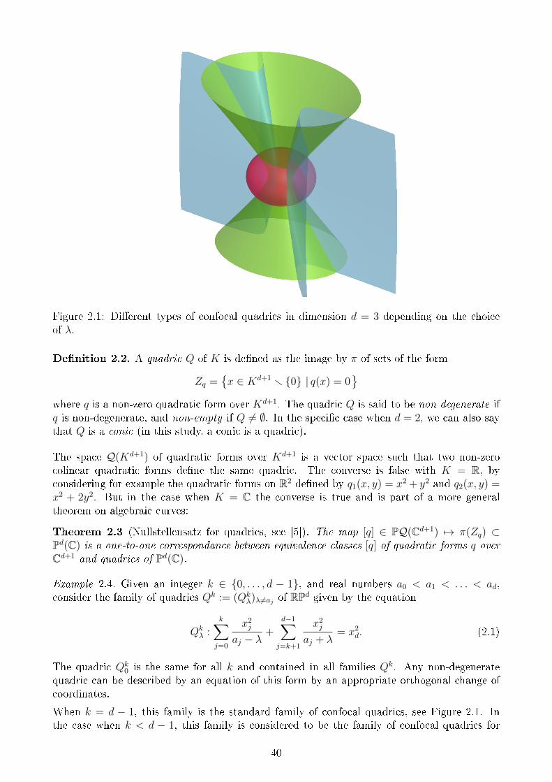
Figure 2.1: Dierent types of confocal quadrics in dimension d = 3 depending on the choiceof λ.

Denition 2.2. A quadric Q of K is dened as the image by π of sets of the form

Zq =x ∈ Kd+1 r 0 | q(x) = 0

where q is a non-zero quadratic form over Kd+1. The quadric Q is said to be non-degenerate ifq is non-degenerate, and non-empty if Q 6= ∅. In the specic case when d = 2, we can also saythat Q is a conic (in this study, a conic is a quadric).

The space Q(Kd+1) of quadratic forms over Kd+1 is a vector space such that two non-zerocolinear quadratic forms dene the same quadric. The converse is false with K = R, byconsidering for example the quadratic forms on R2 dened by q1(x, y) = x2 + y2 and q2(x, y) =x2 + 2y2. But in the case when K = C the converse is true and is part of a more generaltheorem on algebraic curves:

Theorem 2.3 (Nullstellensatz for quadrics, see [5]). The map [q] ∈ PQ(Cd+1) 7→ π(Zq) ⊂Pd(C) is a one-to-one correspondance between equivalence classes [q] of quadratic forms q overCd+1 and quadrics of Pd(C).

Example 2.4. Given an integer k ∈ 0, . . . , d − 1, and real numbers a0 < a1 < . . . < ad,consider the family of quadrics Qk := (Qk

λ)λ 6=aj of RPd given by the equation

Qkλ :

k∑j=0

x2j

aj − λ+

d−1∑j=k+1

x2j

aj + λ= x2

d. (2.1)

The quadric Qk0 is the same for all k and contained in all families Qk. Any non-degenerate

quadric can be described by an equation of this form by an appropriate orthogonal change ofcoordinates.

When k = d − 1, this family is the standard family of confocal quadrics, see Figure 2.1. Inthe case when k < d − 1, this family is considered to be the family of confocal quadrics for

40

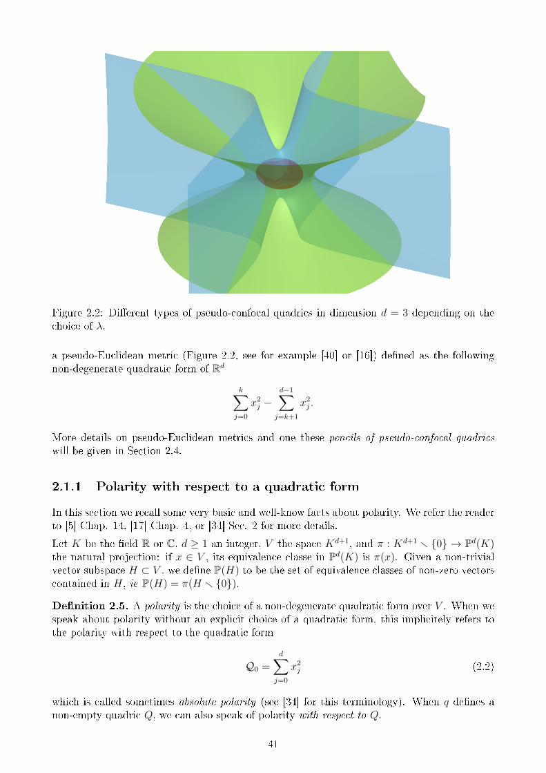
Figure 2.2: Dierent types of pseudo-confocal quadrics in dimension d = 3 depending on thechoice of λ.

a pseudo-Euclidean metric (Figure 2.2, see for example [40] or [16]) dened as the followingnon-degenerate quadratic form of Rd

k∑j=0

x2j −

d−1∑j=k+1

x2j .

More details on pseudo-Euclidean metrics and one these pencils of pseudo-confocal quadricswill be given in Section 2.4.

2.1.1 Polarity with respect to a quadratic form

In this section we recall some very basic and well-know facts about polarity. We refer the readerto [5] Chap. 14, [17] Chap. 4, or [34] Sec. 2 for more details.

Let K be the eld R or C, d ≥ 1 an integer, V the space Kd+1, and π : Kd+1 r 0 → Pd(K)the natural projection: if x ∈ V , its equivalence classe in Pd(K) is π(x). Given a non-trivialvector subspace H ⊂ V , we dene P(H) to be the set of equivalence classes of non-zero vectorscontained in H, ie P(H) = π(H r 0).

Denition 2.5. A polarity is the choice of a non-degenerate quadratic form over V . When wespeak about polarity without an explicit choice of a quadratic form, this implicitely refers tothe polarity with respect to the quadratic form

Q0 =d∑j=0

x2j (2.2)

which is called sometimes absolute polarity (see [34] for this terminology). When q denes anon-empty quadric Q, we can also speak of polarity with respect to Q.

41

This choice of quadratic form has concrete geometric consequences, described in what follows.

An isomorphism. Given a non-degenerate quadratic form q over V , one can consider the iso-morphism from V to its dual space V ∗ dened by

x ∈ V 7→ q(x, ·) ∈ V ∗.

It induces a projective isomorphism Iq : P(V )→ P(V ∗) which only depends on the equivalenceclass of q in PQ(V ).

A bijection between points and projective hyperplanes. The projective hyperplanes of P(V ) canbe identied with P(V ∗), by associating to any non-zero linear form α on V its kernel kerα ⊂ V .Therefore the map Iq induces an explicit realization of this identication via the map

π(x) ∈ P(V ) 7→ P(ker q(x, ·)) ⊂ P(V ).

More generally, we can dene a bijective correspondance between k-dimensional and (d−1−k)-dimensional projective subspaces of P(V ) via the map

P(W ) 7→ P(W⊥q)

where W⊥q denes the q-orthogonal vector subspace of W in V .

Denition 2.6. Given a projective space H = P(W ) ⊂ P(V ), we call polar space of H withrespect to q the projective space P(W⊥q). The polar space of a point with respect to q is aprojective hyperplane. The polar space of a hyperplane is a point, also called pole with respectto q of this hyperplane.

Dual hypersurfaces/curves. Let Γ be a C1-smooth hypersurface of P(V ). The projective hyper-plane containing p and tangent to Γ is a projective space TpΓ = P(W ), and we can consider itspole with respect to q: the latter is the point up = π(x) such that x is q-orthogonal to W . Thecollection of all up when p describes Γ is called dual of Γ with respect to q and denoted by Γ∗.

Dual quadric. Let q1 be another non-degenerate quadratic form. There is a (d + 1) × (d + 1)invertible matrix M with coecients in K such that for all x, y ∈ V , q1(x, y) = q(Mx, y).We dene the dual of q1 with respect to q as the quadratic form q1

∗ over V satisfying for allx, y ∈ V the equality q1

∗(x, y) = q(M−1x, y). It is well-known that the dual with respect to qof a quadric Q1 dened by the quadratic form q1 is a quadric dened by the dual q1

∗ of q1 withrespect to q, see for example [34]:

Proposition 2.7. The dual of a non-empty non-degenerate quadric Q1 dened by the quadraticform q1 is the quadric dened by the quadratic form q1

∗.

2.1.2 Pencil of quadrics

We recall that Q(Kd+1) is the set of quadratic forms over Kd+1. In this subsection we willabusively write quadrics for quadratic forms.

Denition 2.8 (see [5], Ch. 14.1). A pencil of quadrics is a line in PQ(Kd+1). It can beequivalently dened as a set of quadratic forms of the type

F(q1, q2) :=λq1 + µq2

∣∣ (λ, µ) ∈ K2 r 0

where q1, q2 are quadratic forms with distinct equivalence classes in PQ(Kd+1) (non-colinear).We say that the pencil F(q1, q2) is non-degenerate if it contains at least one non-degeneratequadratic form.

42

Since the map (λ, µ) 7→ det(λq1 + µq2) is a homogeneous polynomial of degree at most d + 1over K, a pencil of quadrics contains either only degenerate quadratic forms, or a nite numberless than d+ 1 of degenerate quadratic forms.

Let us consider the absolute polarity, that is the polarity with respect to the quadratic formQ0 =

∑j x

2j (see Subsection 2.1.1). Given a non-degenerate quadratic form q, we can dene its

dual q∗.

Denition 2.9. The dual pencil of quadrics associated to a non-degenerate pencil of quadricsF(q1, q2), is the set F(q1, q2)∗ of duals q∗ of non-degenerate quadratic forms q contained inF(q1, q2) :

F(q1, q2)∗ = q∗ | q ∈ F(q1, q2), q is non-degenerate = (λq1 + µq2)∗ | det(λq1 + µq2) 6= 0 .

The pencil of (q1, q2)-confocal quadrics is the set F(q1∗, q2

∗)∗ which contains q1 and q2.

Remark 2.10. The pencil of (q1, q2)-confocal quadrics F(q1∗, q2

∗)∗ contains q1 and q2 by involu-tivity of polarity operations.

Example 2.11. Consider two confocal conics C and D of RP2 dened by the quadratic formsqC(x, y, z) = x2

a+ y2

b− z2 and qD(x, y, z) = x2

a−λ + y2

b−λ − z2 with a, b, λ ∈ R, λ /∈ a, b. ByProposition 2.7, their dual conics are dened by their dual quadratic forms qC∗ = ax2 +by2−z2

and qD∗ = (a−λ)x2 + (b−λ)y2− z2. Hence qD∗ belong to the pencil of quadrics F(qC∗, qD

∗) =F(qC

∗, qEucl) where qEucl is the degenerate quadratic form qEucl(x, y) = x2 + y2.

More generally, confocal conics or quadrics (for the usual meaning) can be dened as quadricsof a pencil of the form F(q1

∗, q2∗)∗, which contains the quadratic form dening the Euclidean

metric after an eventual change of coordinates (see [34]). This explains our terminology.

2.1.3 Theorems of Poncelet and Cayley

The theorems of Poncelet and Cayley are remarkable results on conics and many dierentversions of these theorems exists, see for example [5], Section 16.6, but also [13, 17, 14, 32], and[46] for the original statement. Here we present the version of [22, 32] since we consider conicsof CP2.

Let C,D be two conics in CP2. We say that C,D are in general position if their intersectionconsists of four distinct points. The statements of Poncelet's and Cayley's theorems are aboutpolygons inscribed in C and circumscribed about D: an n-sided polygon is an ordered setP = (p1, . . . , pn) of distinct points of CP2 called the vertices of P . An n-sided polygon P issaid to be inscribed in C if pj ∈ C for all j and circumscribed about D if for all j, the twotangent lines to D containing pj are pj−1pj and pjpj+1 (where the indices j − 1 and j + 1 areseen modulo n).

Theorem 2.12 (Poncelet, [32] p. 3). Let C,D be two conics of CP2 in general position.Suppose that there is an n-sided polygon inscribed in C and circumscribed about D. Then forany point p ∈ C there is an n-sided polygon inscribed in C and circumscribed about D havingp as a vertex.

The natural question which arises is about the existence of such n-sided polygons. The answeris given by Cayley's theorem.

43

Theorem 2.13 (Cayley, [32] p. 4). Let C,D be two conics of CP2 in general position. LetQC, QD be two quadratic forms dening respectively C and D. Consider an analytic branch oft 7→

√det(tQC +QD) dened in a neighborhood of 0 and denote its analytic expansion at 0 by√

det(tQC +QD) = A0 + A1t+ A2t2 . . .

Then there is an n-sided polygon inscribed in C and circumscribed about D if and only if∣∣∣∣∣∣∣A2 . . . Am+1...

. . ....

Am+1 . . . A2m

∣∣∣∣∣∣∣ = 0, when n is odd, with m =n− 1

2,

or ∣∣∣∣∣∣∣A3 . . . Am+1...

. . ....

Am+1 . . . A2m−1

∣∣∣∣∣∣∣ = 0 when n is even, with m =n

2.

2.2 Complex caustics of complexied conics

We present in this section what can be considered as a complexied version of the result statingthat given a conic C of the Euclidean plane, any confocal conic C ′ to C is a caustic of the billiardon C. The results presented in this section can also be found in [19].

Denition 2.14. Let C ⊂ CP2 be a conic. Given another conic C ′ ⊂ CP2, we say that C ′

is a complex caustic of C if any line tangent to C ′ and intersecting C at a certain point p isreected into a line tangent to C ′ by the complex reection law at p.

Let C,C ′ be conics such that C ′ a complex caustic of C. Suppose we have n distinct pointsp1, . . . , pn on C. Denition 2.14 implies that the following statements are equivalent:

− (p1, . . . , pn) is a piece of non-degenerate orbit of C (see Denition 1.20) such that pjpj+1

is tangent to C ′ for a certain j < n− 1;− for each j ∈ 2, . . . , n − 1, the tangent lines to C ′ containing pj are exactly the lines

pj−1pj and pjpj+1.

In the case of n-periodic orbits, if C ′ is a caustic of C, the n-periodic orbits of C are thesame as the n-sided polygons circumscribed about C ′. Hence Poncelet's theorem (see theorem2.12) implies that if an orbit circumscribed about some caustic C ′ is n-periodic, then all orbitscircumscribed about C ′ are n-periodic:

Proposition 2.15. Let C,C ′ be conics in general position such that C ′ is a complex causticof C. Suppose that there is an n-periodic orbit of C circumscribed about C ′ (as an n-sidedpolygon). Then any billiard orbit of C circumscribed about C ′ is n-periodic.

This induces the following denition:

Denition 2.16. Given two conics C,C ′ in general position, we say that C ′ is an n-caustic ofC if C ′ is a caustic of C about which an n-periodic orbit of C is circumscribed.

44

2.2.1 Confocal conics are complex caustics

In the following we show that given the complexication C of a real conic, its confocal conicsare caustics. Suppose that we are given a set of coordinates (x : y : z) on CP2 such that C isdened by the following equation in the ane chart Uz = z = 1

C :x2

a+y2

b= 1 (2.3)

where x, y ∈ C and a, b ∈ R∗. The confocal conics Cλ to C are given by the following family ofequations depending on a λ ∈ C dierent from a or b:

Cλ :x2

a− λ+

y2

b− λ= 1. (2.4)

Remark 2.17. In the case of the real elliptic billiard, that is when a, b are positive and we studythe usual billiard inside the ellipse C, it is well-known (see [59] Chapt. 4) that the real conicsgiven by Equation (2.4) with 0 < λ < a and λ 6= b are caustics in the usual meaning. Let F1, F2

be the two foci of the ellipse C. Given an orbit of the elliptic billiard, we distinguish betweenthree disjoint situations:1) If the orbit has an edge containing a focus, then all its edges alternatively contain one ofboth foci.2) If the orbit has an edge intersecting the interior of the segment F1F2, then all its edgesintersect the interior of F1F2 and remain tangent to the same hyperbola Cλ with b < λ < a.3) If the orbit has an edge which does not intersect F1F2, then all its edges do not intersectF1F2 and remain tangent to the same smaller confocal ellipse Cλ with 0 < λ < b.

Proposition 2.18. For any λ ∈ Cr a, b, the confocal conic Cλ is a complex caustic of C.

Proof. First notice that given p ∈ C, the tangent line to C at p is not the line at innity denedby L∞ = z = 0. Therefore the complex reection law induces a projective transformation onthe set of lines containing p, hence on the projective line p∗ ' CP1 dened as the polar spaceof p, and its action on p∗ is denoted by q 7→ q′.

For λ 6= a, b, the absolute dual conic C∗λ of Cλ is given by the equation (a−λ)x2 + (b−λ)y2 = 1and thus is also dened for λ = a or b (as a degenerate conic). Hence we can consider the set

V =

(p, q, λ) ∈ C × CP2 × C | q ∈ p∗ ∩ C∗λ

which is an algebraic subset of CP2 × C since it is given by polynomial equations. Let V0 bethe algebraic subset of V containing the elements (p, q, λ) ∈ V such that (p, q′, λ) ∈ V .If λ is a real number, denote by CRλ the points of Cλ with real coordinates which can be consideredas the conic of RP2 dened by Equation (2.4). If p is a point on CR and λ is a real numberdierent from a or b, we know that the line of RP2 containing p and tangent to CRλ is reectedinto a line tangent to CRλ by the usual reection law at p (see Remark 2.17). Hence the sameholds for the complexication of these objects since the same equations are satised.

Hence the map s : C × CP2 × C → C × C dened by (p, q, λ) 7→ (p, λ) is such that s(V0)contains CR× (Rr a, b). Now since C can be identied with CP1, C ×CP2×C and C ×C areprojective spaces, and therefore s(V0) is an algebraic subset of C × C. From the identicationCR ' RP1 we get that CR × (Rr a, b) is Zariski-dense. Hence s(V0) = C × C: this meansthat if (p, λ) ∈ C × C with λ 6= a or b, there is a q ∈ p∗ ∩ C∗λ for which (p, q, λ) ∈ V0, andby construction we have exactly p∗ ∩ C∗λ = q, q′. Therefore both lines tangent to Cλ andcontaining p are reected into each other by the complex reection law at p.

45

2.2.2 Number of complex confocal n-caustics

Given an integer n ≥ 2, and a real conic C, we would like to study the n-caustics of thecomplex billiard C. Caustics of n-periodic orbits of the real elliptic billiard are such that theircomplexications are n-caustics of the corresponding complex billiard by denition. We willshow that other complex n-caustics can appear.

In the case when n = 3 and C is an ellipse, it is well-known that the usual 3-periodic orbitsof C are all circumscribed about exactly one smaller confocal ellipse γ3. Therefore, the com-plexication of γ3 is a 3-caustic of C. We can ask if it is the only 3-caustic confocal to thecomplexication of C. The answer is no, since there is another complexied ellipse confocal toC which is a 3-caustic as it will be shown in this subsection. Interestingly, this caustic is biggerthan C.Remark 2.19. In the case of the real elliptic billiard, we can associate to a caustic of a periodicorbit an invariant quantity called rotation number which is an integer. It can be dened asfollows (see [59] Chapt. 6). Parametrize the ellipse C by S1 = R/Z. For a periodic orbit givenby parameters (x1, . . . , xn) ∈ (S1)

n, consider t1, . . . , tn ∈ (0, 1) such that for each k modulo n,the class of tk in R/Z is xk+1 − xk. Since the orbit is closed, the quantity ρ = t1 + . . . + tn isan integer called rotation number of the orbit. Now since this quantity depends continuouslyon the orbit, it is the same for all periodic orbits circumscribed about the same caustic. As aconsequence, periodic orbits with dierent rotation numbers are circumscribed about distinctcaustics. Birkho's theorem (see [59] Chapt. 6 or [37] Chapt. II) states, for all n ≥ 2 andρ ≤ b(n − 1)/2c coprime with n, the existence of n-periodic orbits, hence the existence ofcaustics with rotation number ρ in the elliptic case.

Remark 2.20. If a complex n-caustic Cλ of C is inscribed in a periodic orbit with all its verticeshaving real coordinates then λ is a real number comprised between 0 and a (see Remark 2.17).Hence if λ is a complex number outside [0, a] corresponding to an n-caustic Cλ, then the periodicorbits circumscribed about Cλ have at least one point with a strictly complex coordinate. Theycorresponds to either complexied bigger confocal ellipses (case λ ∈ R−), or to what will becalled strictly complex confocal conics (case λ ∈ Cr] −∞, a]). As it will be shown, the casen = 4 provides examples of 4-caustics of each of the above described types.

2.2.2.1 Counting n-caustics using Cayley's determinant

Let C be the conic given by Equation (2.3), and Cλ the family of its confocal conics givenby Equation (2.3). Fix an integer n ≥ 3: we study the number Na,b(n) of confocal complexn-caustics of C.As stated in Proposition 2.18, each Cλ is a caustic of C (with λ 6= a, b). For λ 6= 0, Cλ and Care in general position, hence we can study the complex numbers λ for which Cλ is an n-causticof C.In this subsection we prove the following results:

Proposition 2.21. Let n ≥ 3. There is a polynomial Bna,b(λ) such that λ /∈ a, b is a root ofBna,b(λ) if and only if Cλ is an n-caustic of C.The degree of Bna,b satises

degBna,b ≤

n2−14

if n is oddn2

4− 1 if n is even.

If Bna,b has only simple roots distinct from a and b then Na,b(n) = degBna,b.

46

Proposition 2.22. There exist r1, . . . , rp ∈ R such that for all (a, b) with a/b /∈ r1, . . . , rp,we have

degBna,b =

n2−1

4if n is odd,

n2

4− 1 if n is even.

Proposition 2.23. There exist r′1, . . . , r′q ∈ R such that for all (a, b) with a/b /∈ r′1, . . . , r′q, a

and b are not roots of Bna,b.

Remark 2.24. We show in Proposition 2.25 that p ≥ 1 by studying the case of the circle, moreprecisely that 1 belongs to the collection of r1, . . . , rp.

Proof of Proposition 2.21. Suppose rst that n = 2m+1 is odd and x a λ 6= a, b. As explained,Cλ is an n-caustic if and only if on can nd an n-sided polygon inscribed in C and circumscribedabout C. Hence we apply Cayley's theorem (see Theorem 2.13): there is such a polygon if andonly if the determinant

An(λ) =

∣∣∣∣∣∣∣A2(λ) . . . Am+1(λ)

.... . .

...Am+1(λ) . . . A2m(λ)

∣∣∣∣∣∣∣vanishes, where the Ak(λ) are the coecients in the analytic expansion of

f : t→√

det(tQ0 +Qλ)

where Q0 and Qλ are quadratic forms respectively associated to C and to Cλ. The quadraticform Qλ = (a − λ)−1x2 + (b − λ)−1y2 − z2 denes Cλ in CP2. Replacing λ by 0, we get Q0.Therefore

tQ0 +Qλ =

(t

a+

1

a− λ

)x2 +

(t

b+

1

b− λ

)y2 − (t+ 1)z2

hence

det(tQ0 +Qλ) = −(t

a+

1

a− λ

)(t

b+

1

b− λ

)(t+ 1)

which we factorize in

det(tQ0 +Qλ) = − 1

(a− λ)(b− λ)

(a− λa

t+ 1

)(b− λb

t+ 1

)(t+ 1).

Dene the map g : t 7→√(

a−λat+ 1

) (b−λbt+ 1

)(t+ 1) and write its Taylor expansion as

g(t) =∞∑k=0

Bk(λ)t.k

Since

f(t) =ig(t)√

(a− λ)(b− λ)

we have

Ak(λ) =iBk(λ)√

(a− λ)(b− λ).

This shows thatAn(λ) is a function of λ which vanishes at λ 6= a, b if and only if the determinant

Bn(λ) =

∣∣∣∣∣∣∣B2(λ) . . . Bm+1(λ)

.... . .

...Bm+1(λ) . . . B2m(λ)

∣∣∣∣∣∣∣47

also vanishes. Let us compute the Bk's. Write√t+ 1 = c0 + c1t+ c2t

2 + . . . where

ck =1

k!

(1

2

)(1

2− 1

). . .

(1

2− k + 1

)=

(−1)k+1

4k(2k − 1)

(2k

k

). (2.5)

Therefore for any β we have√βt+ 1 = c0 + c1βt+ c2β

2t2 + . . . Hence Bk(λ) is given by

Bk(λ) =∑

u+v+w=k

cucvcwaubv

(a− λ)u(b− λ)v. (2.6)

Therefore each Bk is a polynomial in λ of degree at least k. Hence Bn(λ) = Bna,b(λ) is apolynomial in λ verifying: for any λ 6= a, b, Bna,b(λ) = 0 if and only if An(λ) = 0, which is trueif and only if there exists an n-sided polygon inscribed in C and circumscribed about Cλ. Thesame proof also works when n is even.

It remains to give an upper bound on degBna,b(λ). Suppose rst that n = 2m + 1 is odd. Forany permutation σ of 1, . . . ,m we have

degm∏j=1

Bσ(j)+j =m∑j=1

degBσ(j)+j ≤m∑j=1

(σ(j) + j) = m(m+ 1)

and since Bna,b(λ) is a sum of ±∏m

j=1Bσ(j)+j over all σ, we have degBna,b(λ) ≤ m(m+ 1) = n2−14

.If n = 2m is even, Cayley's determinant gives Bna,b(λ) = det(Bi+j+1)1≤i,j≤m−1. Hence for anypermutation σ of 1, . . . ,m we have

degm−1∏j=1

Bσ(j)+j+1 = m2 − 1

and the same argument leads to degBna,b ≤ m2 − 1 = n2

4− 1.

Proof of Proposition 2.22. Suppose n = 2m+ 1 is odd. By Equation (2.6), Bk is of degree ≤ kand the coecient in front of λk is

d(Bk) = (−1)k∑u+v=k

cucvaubv

=1

4k

∑u+v=k

1

aubv(2u− 1)(2v − 1)

(2u

u

)(2v

v

). (2.7)

Fix a permutation σ of 1, . . . ,m. We have

degm∏j=1

Bσ(j)+j =m∑j=1

degBσ(j)+j ≤m∑j=1

(σ(j) + j) = m(m+ 1)

and the coecient in front of λm(m+1) is∏m

j=1 d(Bσ(j)+j). Since Bna,b(λ) is a sum of±∏m

j=1Bσ(j)+j

over all σ, we have that degBna,b(λ) ≤ m(m+ 1), and the coecient in front of λm(m+1) is

dn(a, b) =

∣∣∣∣∣∣∣d(B2) . . . d(Bm+1)

.... . .

...d(Bm+1) . . . d(B2m)

∣∣∣∣∣∣∣ .Let us show that dn(a, b) 6= 0 except for specic (a, b) as described in Proposition 2.22. Noterst that each d(Bk) is a homogeneous polynomial in (a−1, b−1) of degree k, and by Equation(2.7) the coecient in front of a−k is

− 1

4k(2k − 1)

(2k

k

)= − 2

4kCatk−1

48

where Catk = 1k+1

(2kk

)is the k-th Catalan number.

Now by m-linearity of the determinant, dn(a, b) is also a homogeneous polynomial in (a−1, b−1),and we apply the same procedure as before: for any permutation σ of 1, . . . ,m, we have

degm∏j=1

d(Bσ(j)+j) =m∑j=1

deg d(Bσ(j)+j) =m∑j=1

(σ(j) + j) = m(m+ 1)

and the coecient in front of a−k ism∏j=1

−2

4j+σ(j)Catj+σ(j)−1 =

(−1)m

2m(2m+1)

m∏j=1

Catj+σ(j)−1.

Since dn(a, b) is a sum of ±∏m

j=1 d(Bσ(j)+j) over all σ, we have that deg dn(a, b) ≤ m(m + 1),and the coecient in front of a−m(m+1) is

(−1)m

2m(2m+1)detHm

where Hm is the Hankel matrix of the sequence (Catk+1)k dened as

Hm =

Cat1 Cat2 · · · CatmCat2 Cat3...

. . ....

Catm · · · Cat2m−1

.

One can show that detHm = 1, see for example [38] Theorem 33, or [39] Formula (1.2) for thecase when n is odd and Formula (1.3) for the case when n is even. Hence dn(a, b) is a non-zerohomogeneous polynomial in (a−1, b−1) and therefore there exists a nite collection of numbersr1, . . . , rp ∈ R such that for all a, b > 0, we have dn(a, b) = 0 if and only if a/b ∈ r1, . . . , rp.

Proof of Proposition 2.23. Suppose n = 2m+ 1 is odd. By Equation (2.6), for k ≥ 2,

Bk

(−a2

)=∑

v+w=k

cvcwb2v

(b2 − a2)v =1

b2k

∑v+w=k

cvcwb2w(b2 − a2)v =

1

b2kPk(a, b) (2.8)

where Pk(a, b) is a homogeneous polynomial in (a, b) of degree 2k. The coecient in front ofa2k is

(−1)kck = − 1

4k(2k − 1)

(2k

k

)= −Catk−1

22k−1.

As in the proof of Proposition 2.22, for any permutation σ of 1, . . . ,m,m∏j=1

Bσ(j)+j(−a2) =m∏j=1

1

b2(σ(j)+j)Pσ(j)+j(a, b) =

Qσ(a, b)

b2m(m+1)

where Qσ(a, b) is a homogeneous polynomial of degree

m∑j=1

degPj+σ(j) =m∑j=1

2(σ(j) + j) = 2m(m+ 1)

whose coecient in front of a2m(m+1) ism∏j=1

(−Catj+σ(j)−1

22(j+σ(j))−1

)=

(−1)m

2m(2m+1)

m∏j=1

Catj+σ(j)−1.

49

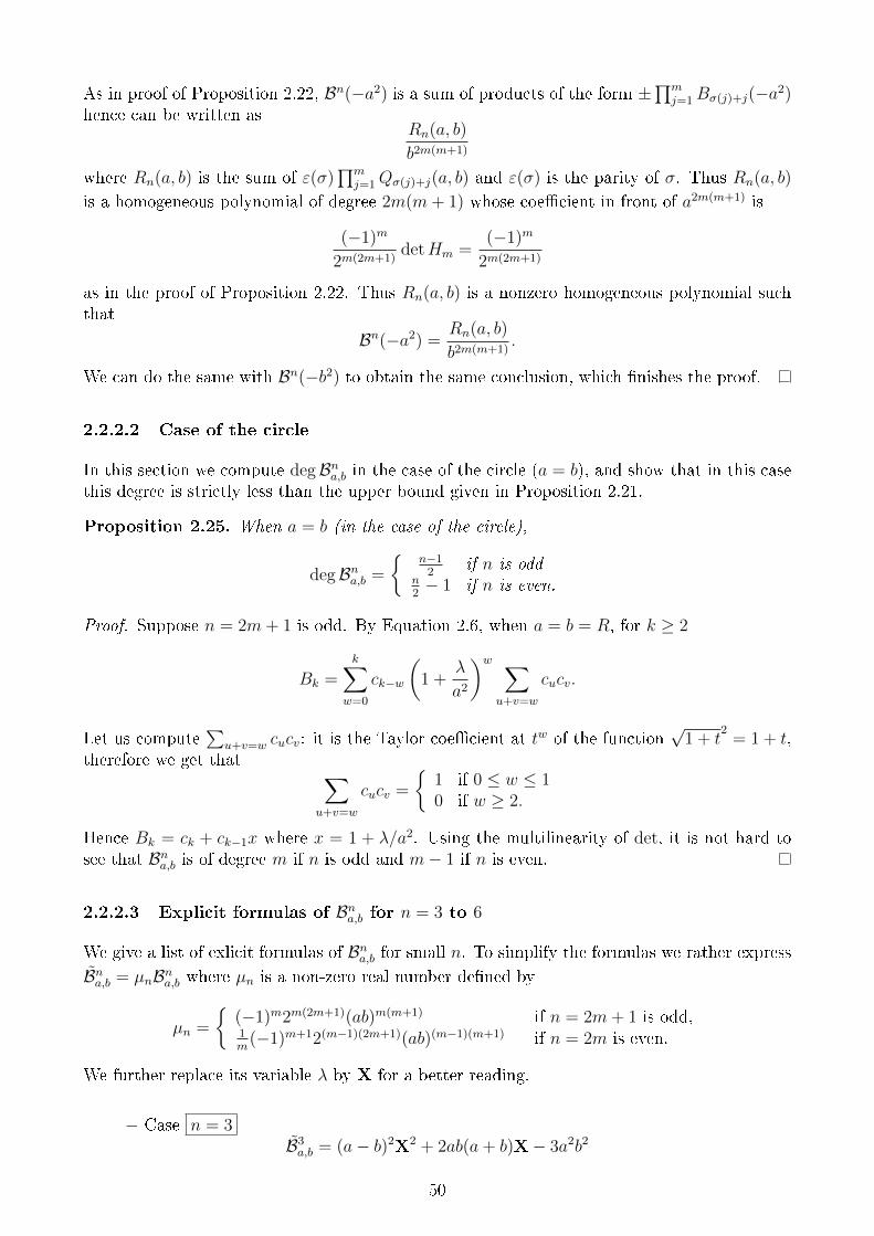
As in proof of Proposition 2.22, Bn(−a2) is a sum of products of the form ±∏m

j=1Bσ(j)+j(−a2)hence can be written as

Rn(a, b)

b2m(m+1)

where Rn(a, b) is the sum of ε(σ)∏m

j=1Qσ(j)+j(a, b) and ε(σ) is the parity of σ. Thus Rn(a, b)

is a homogeneous polynomial of degree 2m(m+ 1) whose coecient in front of a2m(m+1) is

(−1)m

2m(2m+1)detHm =

(−1)m

2m(2m+1)

as in the proof of Proposition 2.22. Thus Rn(a, b) is a nonzero homogeneous polynomial suchthat

Bn(−a2) =Rn(a, b)

b2m(m+1).

We can do the same with Bn(−b2) to obtain the same conclusion, which nishes the proof.

2.2.2.2 Case of the circle

In this section we compute degBna,b in the case of the circle (a = b), and show that in this casethis degree is strictly less than the upper bound given in Proposition 2.21.

Proposition 2.25. When a = b (in the case of the circle),

degBna,b =

n−1

2if n is odd

n2− 1 if n is even.

Proof. Suppose n = 2m+ 1 is odd. By Equation 2.6, when a = b = R, for k ≥ 2

Bk =k∑

w=0

ck−w

(1 +

λ

a2

)w ∑u+v=w

cucv.

Let us compute∑

u+v=w cucv: it is the Taylor coecient at tw of the function√

1 + t2

= 1 + t,therefore we get that ∑

u+v=w

cucv =

1 if 0 ≤ w ≤ 10 if w ≥ 2.

Hence Bk = ck + ck−1x where x = 1 + λ/a2. Using the multilinearity of det, it is not hard tosee that Bna,b is of degree m if n is odd and m− 1 if n is even.

2.2.2.3 Explicit formulas of Bna,b for n = 3 to 6

We give a list of exlicit formulas of Bna,b for small n. To simplify the formulas we rather expressBna,b = µnBna,b where µn is a non-zero real number dened by

µn =

(−1)m2m(2m+1)(ab)m(m+1) if n = 2m+ 1 is odd,1m

(−1)m+12(m−1)(2m+1)(ab)(m−1)(m+1) if n = 2m is even.

We further replace its variable λ by X for a better reading.

− Case n = 3B3a,b = (a− b)2X2 + 2ab(a+ b)X− 3a2b2

50

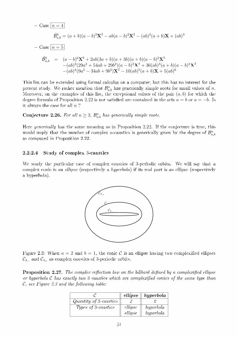
− Case n = 4

B4a,b = (a+ b)(a− b)2X3 − ab(a− b)2X2 − (ab)2(a+ b)X + (ab)3

− Case n = 5

B5a,b = (a− b)6X6 + 2ab(3a+ b)(a+ 3b)(a+ b)(a− b)2X5

−(ab)2(29a2 + 54ab+ 29b2)(a− b)2X4 + 36(ab)3(a+ b)(a− b)2X3

−(ab)4(9a2 − 34ab+ 9b2)X2 − 10(ab)5(a+ b)X + 5(ab)6

This list can be extended using formal calculus on a computer, but this has no interest for thepresent study. We rather mention that Bna,b has generically simple roots for small values of n.Moreover, on the examples of this list, the exceptional values of the pair (a, b) for which thedegree formula of Proposition 2.22 is not satised are contained in the sets a = b or a = −b. Isit always the case for all n ?

Conjecture 2.26. For all n ≥ 3, Bna,b has generically simple roots.

Here generically has the same meaning as in Proposition 2.22. If the conjecture is true, thiswould imply that the number of complex n-caustics is generically given by the degree of Bna,bas computed in Proposition 2.22.

2.2.2.4 Study of complex 3-caustics

We study the particular case of complex caustics of 3-periodic orbits. We will say that acomplex conic is an ellipse (respectively a hyperbola) if its real part is an ellipse (respectivelya hyperbola).

C

Cλ+

Cλ−

Figure 2.3: When a = 2 and b = 1, the conic C is an ellipse having two complexied ellipsesCλ− and Cλ+ as complex caustics of 3-periodic orbits.

Proposition 2.27. The complex reection law on the billiard dened by a complexied ellipseor hyperbola C has exactly two 3-caustics which are complexied conics of the same type thanC, see Figure 2.3 and the following table:

C ellipse hyperbolaQuantity of 3-caustics 2 2Types of 3-caustics ellipse hyperbola

ellipse hyperbola

51

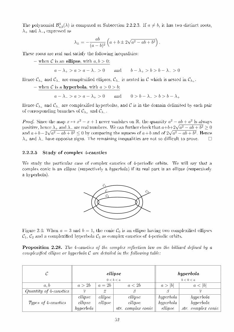
The polynomial B3a,b(λ) is computed at Subsection 2.2.2.3. If a 6= b, it has two distinct roots,

λ+ and λ−, expressed as

λ± = − ab

(a− b)2

(a+ b± 2

√a2 − ab+ b2

).

These roots are real and satisfy the following inequalities:

− when C is an ellipse, with a, b > 0:

a− λ+ > a > a− λ− > 0 and b− λ+ > b > b− λ− > 0

Hence Cλ+ and Cλ− are complexied ellipses, Cλ− is nested in C which is nested in Cλ+ .− when C is a hyperbola, with a > 0 > b:

a− λ− > a > a− λ+ > 0 and 0 > b− λ− > b > b− λ+

Hence Cλ+ and Cλ− are complexied hyperbolas, and C is in the domain delimited by each pairof corresponding branches of Cλ+ and Cλ− .

Proof. Since the map x 7→ x2 − x+ 1 never vanishes on R, the quantity a2 − ab+ a2 is alwayspositive, hence λ+ and λ− are real numbers. We can further check that a+b+2

√a2 − ab+ b2 ≥ 0

and a+b−2√a2 − ab+ b2 ≤ 0 by comparing the squares of a+b and of 2

√a2 − ab+ b2. Hence

λ+ and λ− have opposite signs. The remaining inequalities are not so dicult to prove.

2.2.2.5 Study of complex 4-caustics

We study the particular case of complex caustics of 4-periodic orbits. We will say that acomplex conic is an ellipse (respectively a hyperbola) if its real part is an ellipse (respectivelya hyperbola).

CC2

C1

C3

Figure 2.4: When a = 3 and b = 1, the conic C0 is an ellipse having two complexied ellipsesC1, C2 and a complexied hyperbola C3 as complex caustics of 4-periodic orbits.

Proposition 2.28. The 4-caustics of the complex reection law on the billiard dened by acomplexied ellipse or hyperbola C are detailed in the following table:

C ellipse hyperbola0 < b < a b < 0 < a

a, b a > 2b a = 2b a < 2b a > |b| a < |b|Quantity of 4-caustics 3 2 3 3 3

ellipse ellipse ellipse hyperbola hyperbolaTypes of 4-caustics ellipse ellipse ellipse hyperbola hyperbola

hyperbola str. complex conic ellipse str. complex conic

52

The polynomial B4a,b(λ) is computed in Subsection 2.2.2.3. If a 6= b and a 6= −b, it has three

distinct roots, expressed as

λ1 =ab

b− aλ2 =

ab

a+ bλ3 =

ab

a− b.

These roots satisfy the following inequalities:

− when C is an ellipse, with a > b > 0:

a− λ1 > a > a− λ2 > 0 and b− λ1 > b > b− λ2 > 0

b− λ3 < 0 and a− λ3

> 0 if a > 2b= 0 if a = 2b< 0 if a < 2b

Hence Cλ1 and Cλ2 are always complexied ellipses, Cλ2 is nested in C which is nested in Cλ1 .The conic Cλ3 is an hyperbola if a > 2b, not dened if a = 2b and a complex conic if a < 2b.

− when C is a hyperbola, with a > 0 > b:

Case |b| < a

0 < a− λ1 < a < a− λ3 < a− λ2 and b− λ1 < b < b− λ3 < 0 < b− λ2

Hence Cλ1 is a hyperbola, Cλ2 an ellipse, Cλ3 a hyperbola. The branches of C are in the domainbounded by the corresponding branches of Cλ1 and Cλ3 .

Case |b| > a

a− λ2 < 0 < a− λ1 < a < a− λ3 and b− λ2 < b− λ1 < b < b− λ3 < 0

Hence Cλ1 is a hyperbola, Cλ2 a complex conic, Cλ3 a hyperbola. The branches of C are in thedomain bounded by the corresponding branches of Cλ1 and Cλ3 .

2.2.3 Complex Joachimsthal invariant

The rst proof of Proposition 2.18 which we were able to obtain was dierent from the one wegive in Subsection 2.2.1. It used a complex version of the so-called Joachimsthal invariant, awell-known quantity in the theory of billiards on conics. This complex invariant is described inthe present subsection.

The context of this subsection is as follows. We consider the conic C of R2 given by equation(2.3):

C :x2

a+y2

b= 1

where a, b 6= 0 and x, y ∈ R. Its complexication is given by the same equation with x, y ∈ C.In [59] Chapter 4, Theorem 4.4 shows that for a set of points and directions dened as successivebilliard reections on the real ellipse C with a, b > 0, there is an invariant quantity. Known asJoachimsthal invariant, it is dened by

xvxa

+yvyb

53

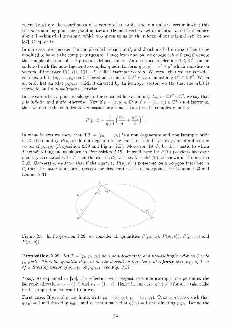
where (x, y) are the coordinates of a vertex of an orbit, and v a unitary vector having thisvertex as starting point and pointing toward the next vertex. Let us mention another referenceabout Joachimsthal invariant, which was given to us by the referee of our original article: see[37], Chapter IV.

In our case, we consider the complexied version of C, and Joachimsthal invariant has to bemodied to handle the complex structure. Hence from now on, we choose a, b 6= 0 and C denotethe complexication of the previous dened conic. As described in Section 1.2, C2 can beendowed with the non-degenerate complex quadratic form q(x, y) = x2 + y2 which vanishes onvectors of the space C(1, i) ∪C(1,−i), called isotropic vectors. We recall that we can considercomplex orbits (p1, . . . , pk) on C viewed as a conic of CP2 via an embedding C2 ⊂ CP2. Whenan orbit has an edge pjpj+1 which is directed by an isotropic vector, we say that the orbit isisotropic, and non-isotropic otherwise.

In the case when a point p belongs to the so-called line at innity L∞ := CP2 rC2, we say thatp is innite, and nite otherwise. Now if p = (x, y) ∈ C2 and v = (vx, vy) ∈ C2 is not isotropic,then we dene the complex Joachimsthal invariant at (p, v) as the complex quantity

P (p, v) =1

q(v)

(xvxa

+yvyb

)2

.

In what follows we show that if T = (p0, . . . , pk) is a non-degenerate and non-isotropic orbiton C, the quantity P (pj, v) do not depend on the choice of a nite vertex pj or of a directingvector of pj−1pj (Proposition 2.29 and Figure 2.5). Moreover, let Cλ be the caustic to whichT remains tangent, as shown in Proposition 2.18. If we denote by P (T ) previous invariantquantity associated with T then the caustic Cλ satises λ = abP (T ), as shown in Proposition2.32. Conversely, we show that if the quantity P (pj, v) is preserved on a polygon inscribed inC, then the latter is an orbit (except for degenerate cases of polygons), see Lemma 2.33 andLemma 2.34.

C

p0

p1

p2

v0

v′1v1

v′2

Figure 2.5: In Proposition 2.29, we consider all quantities P (p0, v0), P (p1, v′1), P (p1, v1) and

P (p2, v′2).

Proposition 2.29. Let T = (p0, p1, p2) be a non-degenerate and non-isotropic orbit on C withp0 nite. Then the quantity P (pj, v) do not depend on the choice of a nite vertex pj of T orof a directing vector of pj−1pj or pjpj+1 (see Fig. 2.5).

Proof. As explained in [25], the reection with respect to a non-isotropic line permutes theisotropic directions vI = (1, i) and vJ = (1,−i). Hence in our case, q(v) 6= 0 for all v taken likein the proposition we want to prove.

First case: If p0 and p1 are nite, write p0 = (x0, y0), p1 = (x1, y1). Take v0 a vector such thatq(v0) = 1 and directing p0p1, and v1 vector such that q(v1) = 1 and directing p1p2. Dene the

54

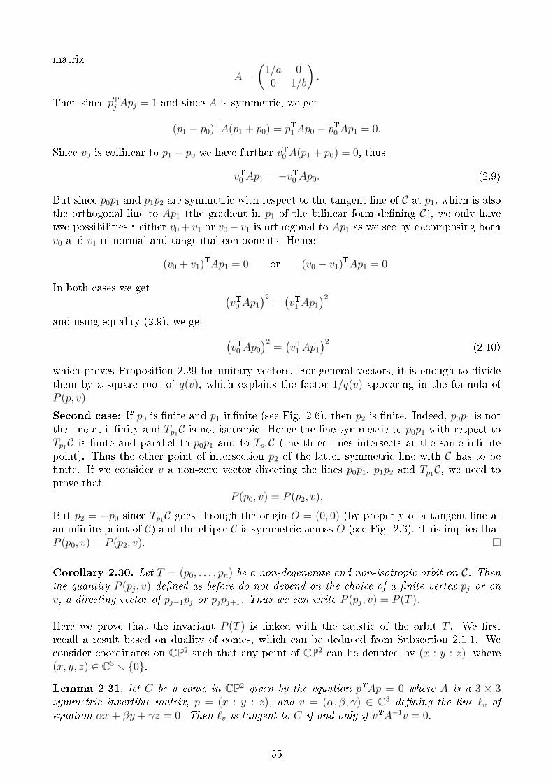
matrix

A =

(1/a 00 1/b

).

Then since pTj Apj = 1 and since A is symmetric, we get

(p1 − p0)TA(p1 + p0) = pT1Ap0 − pT0Ap1 = 0.

Since v0 is collinear to p1 − p0 we have further vT0 A(p1 + p0) = 0, thus

vT0 Ap1 = −vT0 Ap0. (2.9)

But since p0p1 and p1p2 are symmetric with respect to the tangent line of C at p1, which is alsothe orthogonal line to Ap1 (the gradient in p1 of the bilinear form dening C), we only havetwo possibilities : either v0 + v1 or v0− v1 is orthogonal to Ap1 as we see by decomposing bothv0 and v1 in normal and tangential components. Hence

(v0 + v1)TAp1 = 0 or (v0 − v1)TAp1 = 0.

In both cases we get (vT0 Ap1

)2=(vT1 Ap1

)2

and using equality (2.9), we get (vT0 Ap0

)2=(vT1 Ap1

)2(2.10)

which proves Proposition 2.29 for unitary vectors. For general vectors, it is enough to dividethem by a square root of q(v), which explains the factor 1/q(v) appearing in the formula ofP (p, v).

Second case: If p0 is nite and p1 innite (see Fig. 2.6), then p2 is nite. Indeed, p0p1 is notthe line at innity and Tp1C is not isotropic. Hence the line symmetric to p0p1 with respect toTp1C is nite and parallel to p0p1 and to Tp1C (the three lines intersects at the same innitepoint). Thus the other point of intersection p2 of the latter symmetric line with C has to benite. If we consider v a non-zero vector directing the lines p0p1, p1p2 and Tp1C, we need toprove that

P (p0, v) = P (p2, v).

But p2 = −p0 since Tp1C goes through the origin O = (0, 0) (by property of a tangent line atan innite point of C) and the ellipse C is symmetric across O (see Fig. 2.6). This implies thatP (p0, v) = P (p2, v).

Corollary 2.30. Let T = (p0, . . . , pn) be a non-degenerate and non-isotropic orbit on C. Thenthe quantity P (pj, v) dened as before do not depend on the choice of a nite vertex pj or onv, a directing vector of pj−1pj or pjpj+1. Thus we can write P (pj, v) = P (T ).

Here we prove that the invariant P (T ) is linked with the caustic of the orbit T . We rstrecall a result based on duality of conics, which can be deduced from Subsection 2.1.1. Weconsider coordinates on CP2 such that any point of CP2 can be denoted by (x : y : z), where(x, y, z) ∈ C3 r 0.

Lemma 2.31. let C be a conic in CP2 given by the equation pTAp = 0 where A is a 3 × 3symmetric invertible matrix, p = (x : y : z), and v = (α, β, γ) ∈ C3 dening the line `v ofequation αx+ βy + γz = 0. Then `v is tangent to C if and only if vTA−1v = 0.

55

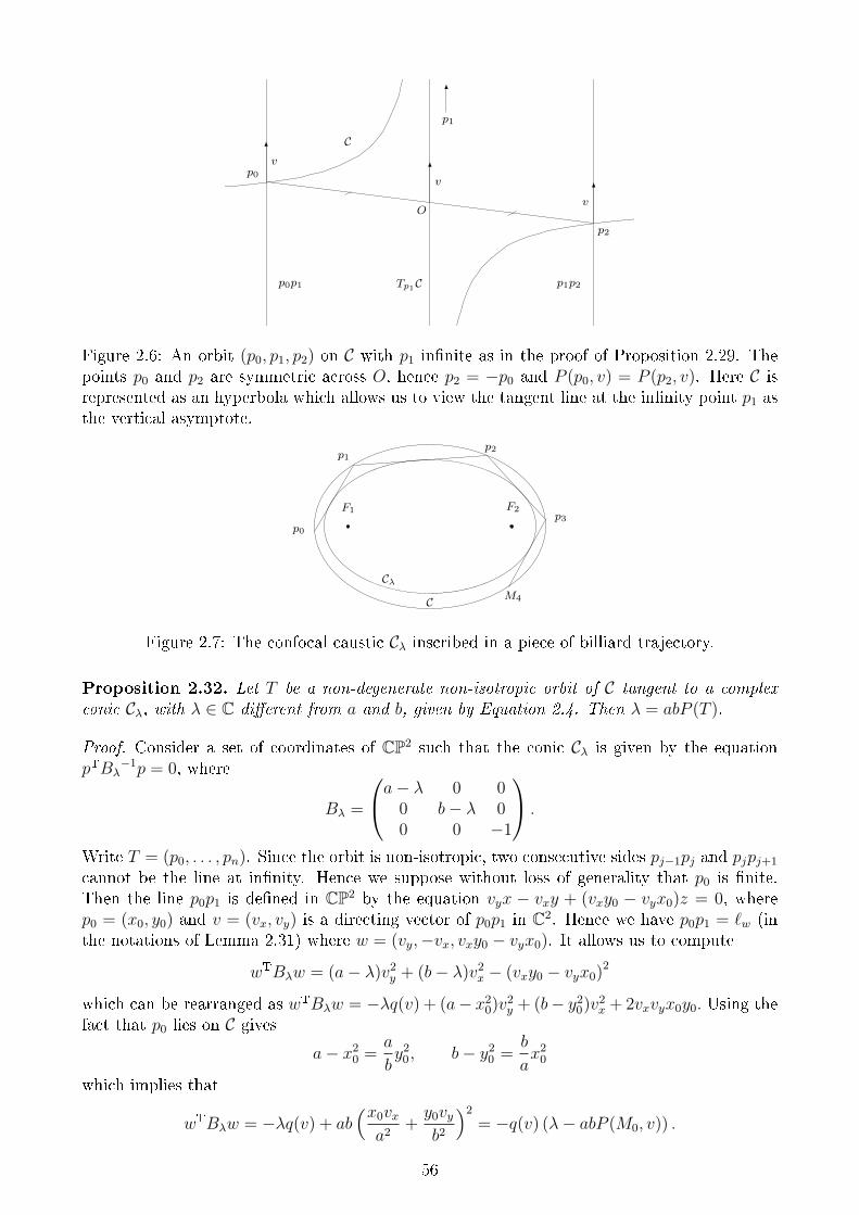
p0

p1

p2

O

Cv

v

v

p0p1 p1p2Tp1C

Figure 2.6: An orbit (p0, p1, p2) on C with p1 innite as in the proof of Proposition 2.29. Thepoints p0 and p2 are symmetric across O, hence p2 = −p0 and P (p0, v) = P (p2, v). Here C isrepresented as an hyperbola which allows us to view the tangent line at the innity point p1 asthe vertical asymptote.

F1 F2

p1p2

p3p0

M4

Cλ

C

Figure 2.7: The confocal caustic Cλ inscribed in a piece of billiard trajectory.

Proposition 2.32. Let T be a non-degenerate non-isotropic orbit of C tangent to a complexconic Cλ, with λ ∈ C dierent from a and b, given by Equation 2.4. Then λ = abP (T ).

Proof. Consider a set of coordinates of CP2 such that the conic Cλ is given by the equationpTBλ

−1p = 0, where

Bλ =

a− λ 0 00 b− λ 00 0 −1

.

Write T = (p0, . . . , pn). Since the orbit is non-isotropic, two consecutive sides pj−1pj and pjpj+1

cannot be the line at innity. Hence we suppose without loss of generality that p0 is nite.Then the line p0p1 is dened in CP2 by the equation vyx − vxy + (vxy0 − vyx0)z = 0, wherep0 = (x0, y0) and v = (vx, vy) is a directing vector of p0p1 in C2. Hence we have p0p1 = `w (inthe notations of Lemma 2.31) where w = (vy,−vx, vxy0 − vyx0). It allows us to compute

wTBλw = (a− λ)v2y + (b− λ)v2

x − (vxy0 − vyx0)2

which can be rearranged as wTBλw = −λq(v) + (a− x20)v2

y + (b− y20)v2

x + 2vxvyx0y0. Using thefact that p0 lies on C gives

a− x20 =

a

by2

0, b− y20 =

b

ax2

0

which implies that

wTBλw = −λq(v) + ab(x0vxa2

+y0vyb2

)2

= −q(v) (λ− abP (M0, v)) .

56

Since p0p1 is tangent to Cλ, wTBλw = 0 and we get the result.

In what follows, we show that the invariant property implies a billiard reection property.

Lemma 2.33. Let p be a nite point on C such that the line TpC is non-isotropic. Let `1, `2

two lines containing p and directed by non-isitropic vectors v1, v2. If

P (p, v1) = P (p, v2) (2.11)

then one of the following cases holds:1) `1 = `2;2) `1 and `2 are symmetric with respect to TpC.

Proof. We can suppose q(v1) = q(v2) = 1. By Equality (2.11), we have vT1 Ap = ±vT2 Ap hence(v2 ± v1)TAp = 0. Thus we get that v1 + v2 or v2 − v1 is orthogonal to Ap which is orthogonalto the tangent line of C at p. Hence v1 + v2 or v1 − v2 is tangent to C at p. This implies thatone of these vectors is xed by the complex reection with respect to TpC.This means that the components of the vj's along the direction of TpC⊥ are the same or haveopposite signs. Since the vj's are unit vectors, their components along the direction of TpC arealso the same or have opposite signs. Hence we have only three possibilities: a) v1 and v2 aresymmetric with respect to TMC, b) v1 and v2 are symmetric with respect to TMC⊥, c) v2 = ±v1.All these cases imply the result.

Lemma 2.34. Suppose that C is not a circle (ie a 6= b). Let p0, p1, p2 be points on C such thatp0, p2 are nite and p1 innite. Let vj be a vector directing the line p1pj, j = 0, 2. If

P (p0, v0) = P (p2, v2) (2.12)

then one of the following cases holds:1) p0 = p2;2) p0p1 and p1p2 are symmetric with respect to Tp1C.

Proof. Since the three lines p0p1, p1p2 and Tp1C contain the same innite point p1, they areparallel, and therefore directed by the same vector v = v0 = v2. The vector v cannot beisotropic, since an ellipse having an isotropic tangent line at a innite point is a circle (itis recalled at Section 1.3 or it can be shown independantly by computations). Suppose thatq(v) = 1. As before, Equation (2.12) implies that p2 − p1 is either colinear or orthogonal to v.Both cases gives the result.

2.3 Caustics of quadrics endowed with a structure of pro-

jective billiard

In this section, we use an idea found in [13] Sec. III: it appeared to us as a construction ofa eld of projective lines on a quadric using another quadric, also projective billiards are notmentioned in the corresponding paper. We rst describe how to construct such eld, and thenwe study its properties related to caustics. All the results taken separately are well-known,the only interest of our work is to gather them and to interpret them as results on projectivebilliards.

Let Q1, Q2 be two non-empty and non-degenerate distinct quadrics. Consider a point p ∈ Q1

such that Q2 is not tangent to Q1 at p. Let u be the pole of TpQ1 with respect to Q2 (seeDenition 2.6). Since Q2 is not tangent to Q1 at p, we have u 6= p and we can dene the line

LQ2(p) = pu.

57

Lemma 2.35. The line LQ2(p) is tangent to Q1 at p if and only if TpQ1 is tangent to Q2.

Proof. LQ2(p) is tangent to Q1 at p if and only if u ∈ TpQ1 and the proof follows from thedenition of polar spaces as projections of specic orthogonal spaces, see Section 2.1.

The set of points p ∈ Q1 such that LQ2(p) is dened corresponds to the set of such p for whichQ2 is not tangent to Q1 at p. Since Q1 6= Q2, it is a dense open subset of Q1. By Lemma 2.35,the set U of points p ∈ U such that LQ2(p) is transverse to Q1 is also open and dense in Q1

(the complementary set of a strict algebraic subset).

Denition 2.36. We denote by Q1〉Q2the line-framed hypersurface over U dened by

Q1〉Q2= (p, LQ2(p)) | p ∈ U .

If q2 is a quadratic form dening Q2, we can also write Q1〉q2 .

Proposition 2.37. The quadric Q2 is a caustic of the line-framed hypersurface Q1〉Q2over Q1.

Proof. Let p ∈ Q1 r Q2 such that TpQ1 is not tangent to Q2. Let u be the pole of TpQ1 withrespect to Q2. Note that the line LQ2(p) = pu is not tangent to Q2, since otherwise we wouldhave pu ⊂ TpQ1 by a polarity argument and contradicting Lemma 2.35.

Let ` be a line tangent to Q2 and intersecting Q1 at p transversally. Since LQ2(p) is not tangentto Q2, the lines ` and LQ2(p) are distinct: one can consider the unique 2-dimensional planeP containing both lines ` and LQ2(p). The plane P intersect Q2 transversally: otherwise ifP is tangent to Q2 one get that ` ⊂ TpQ1 by a polarity argument, which contradicts thetransversality of ` with Q1. Therefore the intersection C := Q2 ∩ P is a non-degenerate non-empty conic of P .

Let `′ ⊂ P be the other tangent line to C in P containing p (since such a tangent line ` alreadyexists, there are exactly two distinct such tangent lines). To conclude the proof, we show thatthe lines `, `′, pu and TpQ1∩P form a harmonic set of lines. Denote by T the line TpQ1∩P andby z, z′ the respective tangency points of ` and `′. Now consider the polarity in the plane Pwith respect to the conic C: the polar line p∗ to p contains z and z′, hence p∗ = zz′. Then sinceu is the pole in P of T = TpQ1 ∩ P , we have that u ∈ zz′. Now consider the map s from p∗ top∗ such that the image s(x) of a point x ∈ p∗ is the pole of the line px. By construction, s xesthe points z and z′, and permutes u with the intersection point of T with p∗. Therefore thesefour points are harmonic, and so are the lines `, `′, pu and T which concludes the proof.

Let q1, q2 be non-degenerate quadratic forms dening Q1 and Q2. We can consider their re-spective dual quadratic forms q1

∗ and q2∗, together with the non-degenerate pencil of quadrics

F(q1∗, q2

∗). Notice that q1 and q2 belongs to the corresponding dual pencil of quadric F(q1∗, q2

∗)∗

which we called pencil of (q1, q2)-confocal quadrics (see Section 2.1). We prove in fact that allquadratic forms of F(q1

∗, q2∗)∗ dene the same eld of projective lines over Q1:

Proposition 2.38. Let q3 ∈ F(q1∗, q2

∗)∗ not colinear to q1. Then Q1〉q3 = Q1〉q2.

Corollary 2.39. Any quadric Q 6= Q1 dened by a quadratic form q ∈ F(q1∗, q2

∗)∗ is a causticof Q1〉q2.

Proof of Proposition 2.38. Fix p ∈ Q1 and q3 ∈ F(q1∗, q2

∗)∗. We want to show that the pole u3

of TpQ1 with respect to q3 and the pole u2 of TpQ1 with respect to q2 are on the same line.

58

By assumption, one can nd λ, µ ∈ R such that

q3∗ = λq1

∗ + µq2∗ (2.13)

and µ 6= 0. Denote by [x] the equivalence class in RPd of an element x ∈ Rd+1. For j = 1, 2, 3,choose an xj ∈ Rd+1 r 0 such that the dual of TpQ1 with respect to qj is [xj]: we have byconstruction p = [x1], u2 = [x2] and u3 = [x3]. Further denote by Mj the (d + 1) × (d + 1)invertible matrix such that for all x, y ∈ Rd+1 we can write qj(x, y) = Q0(Mjx, y), where Q0 isthe quadratic form

∑k x

2k. Equation 2.13 can be rewritten as M3

−1 = λM1−1 + µM2

−1.

Let V ⊂ Rd+1 be the hyperplane such that TpQ1 = P(V ). For j = 1, 2, 3, the vector xj isqj-orthogonal to V , hence Mjxj is Q0-orthogonal to V . In particular, we can nd non-zeroν2, ν3 ∈ R such that M1x1 = ν2M2x2 and M3x3 = ν3M1x1. Hence

x3 = ν3M3−1M1x1 = ν3

(λx1 + µM2

−1M1x1

)= ν3 (λx1 + µν2x2) (2.14)

It follows from this equation that u3 is on the line containing p = [x1] and u2 = [x2].

Let qd be a degenerate quadratic form over Rd+1 of rank d. The kernel ker qd of qd has dimension1 and is generated by a non-zero vector xd. Thus given a hyperplane V0 of Rd+1 transverseto ker qd, the restriction of the form qd to V0 is non-degenerate. Consider the ane subspaceV = xd +V0 ⊂ Rd+1. Its tautological projection P(V ) is an ane chart identied with V0 ' Rd

by x ∈ V0 7→ [xd + x] ∈ P(V ), where [y] denotes the equivalence class of y in RPd. Hence wedeal with qd as a non-degenerate quadratic form on P(V ) ' V0. We can dene its dual qd∗ withrespect to the restriction of Q0 to V0 (the latter is dened as a quadratic form on V0 ' P(V )).

In what follows, we take V0 ⊂ Rd+1 to be the Q0-orthogonal hyperplane to ker qd, whereQ0 =

∑j x

2j (see Equation 2.2).

Proposition 2.40. Let qd be a degenerate quadratic form over Rd+1 of rank d contained in thepencil of quadrics F(q1

∗, q2∗)∗. Let V0 be the Q0-orthogonal hyperplane to ker qd and V ⊂ Rd+1

an ane space parallel to V0. Then given p ∈ Q1 ∩ P(V ), the intersections TpQ1 ∩ P(V ) andLQ2(p) ∩ P(V ) are qd∗-orthogonal.

Proof. Let p ∈ Q1 ∩ P(V ) and u be the pole of TpQ1 with respect to q2. We want to show thatthe line pu and the hyperplane TpQ1 are qd∗-orthogonal when intersected with P(V ). Writep = [X1] and u = [X2].

We rst nd the qd∗-orthogonal line to TpQ1 through p in P(V ). Let T0 ⊂ V0 be the hyperplanesuch that TpQ1 = [x+ λxd] |x ∈ T0, λ ∈ R. Let y ∈ V0 be such that y is qd∗-orthogonal toT0. Let fd : V0 → V0 be the invertible linear map such that qd(x, x′) = Q0(fd(x), x′) for allx, x′ ∈ V0, and f1 : Rd+1 → Rd+1 be the invertible linear map dened for all x, x′ ∈ Rd+1 byq1(x, x′) = Q0(f1(x), x′). By construction, for all x ∈ T0 we have

0 = qd∗(y, x) = Q0(fd

−1(y), x)

Writing f1(X1) = πV0f1(X1) + λxd, where πV0f1(X1) ∈ V0 , λ ∈ R, we have for the same x ∈ T0

Q0(πV0f1(X1), x) = Q0(f1(X1), x) = q1(X1, x) = 0

since V0 and ker qd areQ0-orthogonal. We deduce that fd−1(y) and πV0f1(X1) are colinear, hence

y and fd(πV0f1(X1)) are colinear. Hence the qd∗-orthogonal space to T0 is Rfd(πV0f1(X1)).

Now let us show that fd(πV0f1(X1)) ∈ V0 considered as a point in P(V ) (after the aboveidentication V ' V0 ' P(V )) lies in the line pu. This will conclude the proof. Let f2 : Rd+1 →

59

Rd+1 be the invertible linear map dened for all x, x′ ∈ Rd+1 by q2(x, x′) = Q0(f2(x), x′).The deinition of pole and tangent line to Q1 allows us to write [f1(X1)] = [f2(X2)], henceu = [X2] = [f2

−1 f1(X1)]. And since qd ∈ F(q1∗, q2

∗), we can write α2f2−1 = fd + α1f1

−1

where α1, α2 ∈ R∗ and fd has been extended to the whole space Rd+1 by fd(xd) = 0. Therefore,u = [f2

−1 f1(X1)] = [fd(f1(X1)) + α1X1]. This shows that fd(f1(X1)) = fd(πV0f1(X1)) ∈pu.

We apply the previous result to families of (pseudo-)confocal quadrics as it was described inSection 2.1. Fix an integer k ∈ 0, . . . , d − 1, real numbers a0 < a1 < . . . < ad and considerthe family of quadrics Qk := (Qk

λ)λ 6=aj of RPd given by the equation

Qkλ :

k∑j=0

x2j

aj − λ+

d−1∑j=k+1

x2j

aj + λ= x2

d. (2.15)

We think of this family as a family of confocal quadratics for a certain pseudo-Euclidean metric(an Euclidean metric when k = d− 1) which is the degenerate quadratic form of Rd+1 denedby

qkd(x) =k∑j=0

x2j −

d−1∑j=k+1

x2j .

The restriction of qkd to the ane chart xd = 1 ' Rd is a non-degenerate quadratic form onRd. Note that given a non-degenerate quadratic form q1 dening a non-degenerate quadric ofQk, the quadrics of Qk are dened by the pencil F(q1

∗, qkd)∗. By Propositions 2.37 and 2.38, all

quadrics Qkλ with λ 6= 0 dene the same eld of projective lines Lk(p) on Q := Qk

0 for whichthey are caustics.

Proposition 2.41. The line Lk(p) of the eld of projective lines dened on Q := Qk0 by its

confocal quadrics is qkd-orthogonal to TpQ in the ane chart xd = 1 ' Rd.

Proof. This is a direct consequence of Proposition 2.40: by denition, the quadratic formsdening each Qk

λ form a pencil of quadrics containing qkd . Moreover, the Q0-orthogonal spaceto ker qkd is the vector space V0 = xd = 0. The restriction to V0 of qkd is non-degenerate andits dual qkd

∗with respect to the restriction Q0|V0 is q

kd itself.

2.4 On Berger property Only quadrics have caustics

In this section, we are interested in projective billiards in dimension d ≥ 3 having caustics.We try to study a generalization to projective billiards of a fundamental result discovered byBerger in [6] and which can be stated as follows:

Theorem 2.42 (Berger, [6]). Let d ≥ 3 and S, U , V be open subsets of C2-smooth hypersurfacesin Rd with non-degenerate second fundamental forms. Suppose that there is an open subset oflines tangent to U and intersecting S transversally which are reected into lines tangent to V .Then S is a piece of quadric and U, V are pieces of one and the same quadric confocal to S.

Glutsyuk [28] extended Berger's result to space forms of non-zero constant curvature, that isto the Euclidean unit sphere Sd and the hyperbolic space Hd with d ≥ 3. In the correspondingpaper [28], this result is also used to prove the Commuting Billiards Conjecture in dimensiond ≥ 3. This conjecture was stated by Tabachnikov, see [56, 59], and was also proved byGlutsyuk in dimension 2, see [23]. We can now call it Commuting Billiards Theorem, and the

60

latter can be stated as follows: consider two nested billiards of Rd (respectively R2) with C2-smooth (respectively piecewise C4-smooth) strictly convex boundaries. Each one of their billiardmaps acts on the set of oriented lines intersecting them. If these maps commute then thebilliards are confocal ellipsoids (respectively ellipses).

This section is structured as follows. We rst extend in Subsection 2.4.1 a key argument ofBerger's proof to projective billiards. In Subsection 2.4.2, we dene a distribution of hyperplanesrelated to cones of lines tangent to possible caustics. In Subsection 2.4.3, we apply results foundin the two rst subsections to show that if a convex pseudo-Euclidean billiard has a caustic,then it is a quadric and its caustic is a confocal quadric for the pseudo-Euclidean metric.

2.4.1 Berger's key argument for projective billiards

We rst extend a result based on an observation made by Berger [6] in the case of usual billiards.This observation can be stated as follows for projective billiards: consider hypersurfaces S, U, Vof Rd and a line-framed hypersurface Σ over S. Suppose that there is an open subset of lines `tangent to U and intersecting S which are reected into lines `′ tangent to V by the projectivelaw of reection on Σ. If we consider three non-colinear points A ∈ U , B ∈ S, C ∈ V such thatthe above property is satised with ` = AB and `′ = BC, then by symmetry the intersectionH = TAU ∩ TBS coincides with TCV ∩ TBS.This observation leads to a result of niteness on such hyperplanes H of TBS which we are goingto detail below. Let Σ be a line-framed hypersurface over a hypersurface S ⊂ Rd, (B,L) ∈ Σand ξ ∈ TBS a non-zero vector.

Denition 2.43. Let H be a hyperplane of TBS. H is said to be permitted by ξ if ξ /∈ Hand for any C1-smooth germ of curve (B(t), L(t)) ∈ Σ with B(0) = B and L(0) = L, and anyC1-smooth germ of curve ξ(t) ∈ TB(t)S with ξ(0) = ξ, there exist germs of C1-smooth curvesA(t), C(t) in Rd such that

− A := A(0), B, C := C(0) are not colinear and the vector ξ belongs to the plane ABC;− A′(0) belongs to the hyperplane containing the line AB and H;− C ′(0) belongs to the hyperplane containing the line CB and H;− A(t)B(t) is reected into B(t)C(t) by the projective reection law on Σ at B(t).

Denition 2.44. If ` is a line intersecting S transversally at B, we will say that a hyperplaneH ⊂ TBS is permitted by ` if it is permitted by a non-zero vector ξ in the intersection of theplane containing L and ` with TBS.

The main result of this section is the following proposition:

Proposition 2.45. Suppose S has non-degenerate second fundamental form at B. Then thereis a closed subset F of TBS such that TBS\F is dense in TBS and such that for all ξ ∈ TBS\F ,the number of hyperplanes H ⊂ TBS permitted by ξ is at most d− 1.

Remark 2.46. In the proof we show that F is the nite union of strict vector subspaces of TBS.

Proof of Proposition 2.45. The proof is computational and we wonder if one can nd a moregeometrical one. We apply the same formulas as in [6], and use a result of linear algebra toconclude. We endow Rd with its usual Riemannian metric: we denote by x · y the canonicalscalar product on Rd.

Let H be a hyperplane of TBS permitted by a certain ξ ∈ TBS, and let η ∈ TBS be anorthogonal vector to H of norm 1. Choose an orthonormal basis (u1, . . . , ud−1) of eigenvectors

61

of S's second fundamental form at B, and denote by k1, . . . , kd−1 the corresponding eigenvalues.Choose αi such that ξ = cos(αi)ui + sin(αi)vi, where vi is a vector of length 1 orthogonal to ui,and write `i = cos(αi) ∈ [−1, 1]. Note that ξ =

∑d−1k=1 `kuk.

Fix an i ∈ 1, . . . , d − 1. Let A(t), (B(t), L(t)), C(t) be as in Denition 2.43 and verifyingB′(0) = ui. Let n(t) be a smooth family of normal vectors to S at B(t) of length 1, and ν(t) asmooth family of vectors directing L(t) and such that ν(t) · n(t) = 1.

Dene ui(t) = B′(t) for all t, extend vi into a vector eld vi(t) along B(t) by parallel transport,and set ξ(t) = cos(αi)ui(t) + sin(αi)vi(t). In the following, given any curve γ(t), we will writeγ′ for γ′(0).

1)We rst express in a matrix form the fact that A′(0) belongs to the hyperplane PA containingthe line AB and H, and that C ′(0) belongs to the hyperplane PC containing the line AC andH.

Here we adapt the computations of [6] to the projective case. Let e(t) = E1(t)ν(t) + E2(t)ξ(t)and e(t) = E1(t)ν(t)− E2(t)ξ(t) be two unit vectors directing the oriented lines A(t)B(t) andB(t)C(t), with E1(t), E2(t) ∈ R, and having the same orientation with respect to TBS. Onecan write

A(t) = B(t) + a(t)e(t) and C(t) = B(t) + c(t)e(t) (2.16)

where a(t), c(t) > 0. Normal vectors to PA and PC can be respectively dened by

nA = (η · e)n− (n · e)η = (E1(η · ν) + E2(η · ξ))n− E1η,

nC = (η · e)n− (n · e)η = (E1(η · ν)− E2(η · ξ))n− E1η.

If we denote by ′ the derivative taken in 0, we get

A′ · nA = 0 and C ′ · nC = 0. (2.17)

Now since e is parallel to PA we have e · nA = 0, hence by combining Equations (2.16) and(2.17) we get

0 = A′ · nA = ui · nA + a(e′ · nA) (2.18)

Yet, as recalled in [6] we have n′ = kiui, u′i = −kin, v′i = 0, hence ξ′ = −ki`in. Thereforereplacing e′ by its expression in Equation (2.18) gives

0 = A′ · nA = −E1(η · ui) + a ((E2E′1 − E1E

′2 − ki`iE2

2 + E1E2(n · ν ′))(η · ξ)+(E2

1(n · ν ′)− ki`iE1E2)(η · ν)− E21(η · ν ′)) (2.19)

and the same with C by changing E2 in −E2 and a in c:

0 = C ′ · nC = −E1(η · ui) + c ((E ′2E1 − E ′1E2 − ki`iE22 − E1E2(n · ν ′))(η · ξ)

+(E21(n · ν ′) + ki`iE1E2)(η · ν)− E2

1(η · ν ′)) (2.20)

If we substitute Equations (2.19) and (2.20) in A′·nAa

+ C′·nCc

= 0 we get(1a

+ 1c

)E1(η · ui) = 2E2

1(n · ν ′)(η · ν)− 2E21(η · ν ′)− 2ki`iE

22(η · ξ)

= −2E21(η ·Ni)− 2ki`iE

22(η · ξ) (2.21)

where Ni = ν ′ − (n · ν ′)ν. The vector Ni lies in TBS since we can check that (Ni · n) = 0. Now(n(t) · ν(t)) = 1 for all t, hence (n · ν ′) = −(n′ · ν) = −ki(ui · ν), and Ni can be expressed asNi = dν · ui + ki(ui · ν)ν. Ni only depends on the 2-jet of Σ at (B,L).

Let us rewrite Equation (2.21) in a matrix form. Denote by− α the quantity −(a−1 + c−1)/2E1;

62

− Vξ the vector given by Vξ = (E2/E1)2∑d−1i=1 ki`iui;

− M the matrix of Md−1 (R) whose lines are given by the coordinates of Ni in theorthonormal basis (u1, . . . , ud−1).

Then Equation (2.21), together with the assumption that ξ /∈ H, can be rewritten asMη + (ξ · η)Vξ = αηη /∈ ξ⊥ (2.22)

where η and ξ are considered as vectors of Rd−1 with coordinates given by their coordinates inthe basis (u1, . . . , ud−1).

2) For xed α and ξ, we now study the space of solutions η of Equation (2.22).

Given an endomorphism f of Rk, we call eigenspace of f any subspace of Rk of the formker(f − βid) for a certain β, and denote by Im f the set of all f(x) where x ∈ Rk.

Lemma 2.47. Let β1, . . . , βs be the real eigenvalues of M . If Vξ doesn't belong to any of thesets Im (M − βiId−1), then the eigenspaces of the endomorphism fM,ξ of Rd−1 dened by

fM,ξ : x 7→Mx+ (ξ · x)Vξ

are either of dimension at most 1 or contain only orthogonal vectors to ξ.

Proof. Let α be an eigenvalue of fM,ξ. Consider an eigenvector x of fM,ξ associated to α: itsatises

(M − αId−1)x = −(ξ · x)Vξ.

If α 6= βk for all k, then M − αId−1 is invertible. Hence x ∈ R(M − αId−1)−1Vξ and thereforethe eigenspace of fM,ξ associated to α is of dimension at most 1. Now if α = βk for a certain k,since Vξ /∈ Im (M −βkId−1) we necessarily have (ξ ·x) = 0 and the eigenspace of fM,ξ associatedto α contains only orthogonal vectors to ξ.

We can now nish the proof of Proposition 2.45. The second fundamental form of S at B isnon-degenerate, hence none of the ki equals 0. Hence the set F of vectors ξ ∈ Rd−1 =

∑d−1i=1 `iui

such that Vξ belongs to ∪iIm (M − βiId−1) is the nite union of strict vector subspaces of TBS,and it depends neither on E1 nor on E2; it depends only on M .

Thus if we suppose that ξ /∈ F , Lemma 2.47 implies that there are one-dimensional vectorsubspaces G1, . . . , Gs of TBS, s ≤ d − 1, contained in the eigenspaces of fM,ξ such that anysolution η of Equation (2.22) is contained in some Gi. Hence any hyperplane H permitted byξ is an orthogonal space in TBS to one of the Gi, which ends the proof of the result.

2.4.2 Distributions of permitted hyperplanes

Let Σ be a line-framed hypersurface over a hypersurface S ⊂ Rd, and B ∈ S such that S has anon-degenerate second fundamental form at B. In this section, we dene d− 1 distributions ofhyperplanes based on Proposition 2.45. We use the same notations as in the statement of thisproposition.

Let ξ ∈ TBS be a vector outside F and H ⊂ TBS be a hyperplane permitted by ξ. As a con-sequence of Lemma 2.47 together with the implicit function theorem, there are neighborhoodsUH of H in the Grassmanian and Uξ of ξ in TBS, and an analytic map H : Uξ → UH such thatfor any hyperplane H ′ ∈ UH , H ′ is permitted by a vector ξ′ ∈ Uξ if and only if H ′ = H(ξ′).The same can be done with hyperplanes permitted by a line `.

63

In the case when the number of hyperplanes of TBS permitted by ` is exactly d − 1, we havedened, in a neighborhood of `, d − 1 analytic elds of hyperplanes H1, . . . , Hd−1 in TBS,depending on `. For each one of them, dene Hk(`) the ane hyperplane of Rd containingHk(`) and `. The latter can be considered as a hypersurface of the set of lines LB ' RPd−1

containing B, and it contains `. We denote by hk(`) = T`Hk(`) ⊂ T`LB its tangent space at `.

Denition 2.48. The d− 1 elds of hyperplanes h1, . . . , hd−1 dene distributions on an opensubset of LB ' RPd−1 containing ` and called the permitted distributions of Σ at B.

Proposition 2.49. Suppose that the number of hyperplanes of TBS permitted by ` is exactlyd− 1, so that the d− 1 permitted distributions of Σ at B are well-dened. Further suppose thatΣ′ is a line-framed hypersurface over a hypersurface S ′ ⊂ Rd containing B. If S and S ′ havethe same 2-jet at B and the elds of projective lines of Σ and Σ′ have the same 1-jet at B, thenthe d − 1 permitted distributions at B of Σ′ are well-dened and coincide with the permitteddistributions of Σ at B.

Proof. This is a direct consequence of Equation (2.22), which only depends on the 1-jet of thenormal vector eld n to S at B and on the 1-jet at B of a normalized directing vector eld νof the projective eld of lines of Σ.

In the following proposition, we suppose that Σ has d − 1 permitted distributions at B,h1, . . . , hd−1, well-dened in a neighborhood of a line ` intersecting S at B.

Proposition 2.50. Let U, V ⊂ Rd be hypersurfaces with non-degenerate second fondamentalforms, with ` tangent to U . Suppose that there is an open subset Ω, containing `, of linestangent to U and intersecting S which are reected into lines tangent to V by the projective lawof reection on Σ. Then for any line `′ in Ω containing B and tangent to U at a point A, thehyperplane H = TAU ∩TBS is permitted by `′. The corresponding hyperplanes on TLB coincidewith one of the d− 1 permitted distributions of Σ at B, say hj. The set of lines containing Band tangent to U is an integral surface of hj.

Proof. It is easy to check that H satises all requirements of Denition 2.43 since the pairU, V is a caustic of S. Hence H is a hyperplane of TBS permitted by `′. The correspondinghyperplane h(`′) ⊂ T`′LB coincides with one of the d − 1 permitted distributions hj(`′) bydenition. The rest of the result follows from the denition of the distribution hj.

2.4.3 Caustics of billiards in pseudo-Euclidean spaces

In this section, we are interested specically in billiards of pseudo-Euclidean spaces of dimensiond ≥ 3 having caustics. We adopt the denition of pseudo-Euclidean spaces used in [15, 40]:the pseudo-Euclidean space Ek,l of signature (k, l), k, l ∈ N, with k + l = d, is the space Rd

endowed with the non-degenerate symetric bilinear form 〈·|·〉 dened for x, y ∈ Rd by

〈x|y〉 =k∑j=1

xjyj −d∑

j=k+1

xjyj. (2.23)

We will denote by qkd the quadratic form associated to 〈·|·〉. A line ` ⊂ Ek,l directed by anon-zero vector v is said to be

− space-like if 〈v|v〉 > 0;− time-like if 〈v|v〉 < 0;− light-like if 〈v|v〉 = 0.

64

Denote the usual scalar product on Rd by (x · y) for all x, y ∈ Rd. An ane ellipsoid is a setcontaining at least two points which is of the form

E =x ∈ Rd | (Ax · x) + (B · x) + C = 0

where A ∈ Md (R) is a positive-denite symmetric matrix, B ∈ Rd is a vector, and C ∈ R.As noticed in [15, 40], since A is positive-denite there is a linear change of coordinates in Rd

preserving the pseudo-Euclidean metric (2.23), in which (Ax · x) takes the form

(Ax · x) =d∑j=1

x2j

aj

where a1, . . . , ad > 0. Therefore, by an appropriate choice of a new origin, the ellipsoid E isgiven by an equation of the form

d∑j=1

x2j

a′j= 1 (2.24)

where a′1, . . . , a′d > 0. Notice that the form of the pseudo-Euclidean metric (2.23) is left un-

changed in this set of coordinates. A pseudo-confocal quadric to E is a quadric Qλ which canbe expressed in this new set of coordinates by an equation of the form

Qλ :k∑j=1

x2j

a′j − λ+

d∑j=k+1

x2j

a′j + λ= 1. (2.25)

where λ ∈ R. See Figure 2.2 for a 3-dimensional representation.

Let us recall results from [15, 40] which can be applied to a general quadric, not only anellipsoid:

Theorem 2.51 (pseudo-Euclidean version of Chasles theorem; see [40] Theorem 4.8 and [15]Theorem 2.3). A space- or time-like line ` intersecting E is tangent to d − 1 pseudo-confocalquadrics. The tangent hyperplanes at the tangency points with ` are pairwise orthogonal.

Theorem 2.52 (pseudo-Euclidean version of Jacobi-Chasles theorem; see [40] Theorem 4.9).A space- or time-like billiard trajectory in E remains tangent to d− 1 xed quadrics Qλ.

We deduce the following result:

Theorem 2.53. Let S, U, V ⊂ Rd be open subsets of hypersurfaces with non-degenerate secondfundamental forms, and S being convex. Suppose that there is an open subset of the set of linesintersecting S and tangent to U which are reected into lines tangent to V by pseudo-Euclideanreection on S. Then S is a piece of quadric; U, V are pieces of one and the same quadricpseudo-confocal to S.

Proof. We rst begin by proving the following

Lemma 2.54. Consider the set K of lines tangent to U and intersecting S transversally. Thenthe set of lines of K which are not light-like is an open dense subset of K.

Proof. Denote byK0 this set. It is clearly open, and it remains to show that it is dense. Supposethe contrary, then there is a light-like line ` ∈ K contained in an open subset Ω ⊂ K \ K0

of K. Let x ∈ U be the point of tangency of ` with U . All lines tangent to U at x andsuciently close to ` are contained in Ω, hence the pseudo-Euclidean metric 〈v|v〉 vanishes onan open subset of TxU , hence on TxU . This implies that TxU is contained in its orthogonalspace, contradiction.

65

We can now prove Theorem 2.53. Consider the line-framed hypersurface Σ = S〉qkd over Sdened by the pseudo-Euclidean metric qkd (see Subsection 1.1.4). Consider a line ` of K whichis not light-like and intersecting S at a point B transversally. Using the same notations as inProposition 2.45, we can suppose that any non-zero vector ξ of the intersection of TBS withthe plane containing ` and the pseudo-Euclidean normal line to S at B is not in F .

Now consider an ane ellipsoid E tangent to S at B, with the same principal directions. Inparticular, S and E have the same 2-jet at B, and therefore their eld of normal lines withrespect to the pseudo-Euclidean metric have the same 1-jet at B. Let E ′ = E〉qkd be the line-framed hypersurface over E induced by the pseudo-Euclidean metric qkd : let us show that E ′ hasd − 1 permitted distribution at B which are integrable. By Proposition 2.49, Σ will have thesame permitted distributions at B.

Indeed, by Theorem 2.51, one can nd d− 1 pseudo-confocal quadrics Q1, . . . , Qd−1 tangent to`, and such that the hyperplanes containing ` and tangent to each Qj are pairwise orthogonal.By Theorem 2.52, each Qj is a caustic of E ′, and by Proposition 2.50, the intersection of thelatter hyperplanes with TBE are pairwise distinct and permitted by `. Therefore E ′ has d − 1permitted distributions h1, . . . , hd−1 dened on a neighborhood of ` in LB which are inducedby the latter hyperplanes. Moreover, the distributions h1, . . . , hd−1 are integrable: the integralmanifold of hj is the set of lines tangent to one quadric among Q1, . . . , Qd−1. Therefore theunion of all lines contained in the integral manifold of hj is a piece of quadratic cone (a conedened by a quadratic form).

Yet, the set of lines containing B and tangent to U and V is also an integral manifold of one ofthe permitted distributions hj of Σ at B, by Proposition 2.49 and Proposition 2.50. Hence Uand V are tangent to one of previously dened quadratic cones at points dening curves of Uand V . The same operation can be applied by taking dierent points B in a small open subsetof S. Now by an argument of [6] working on the duals of U and V , this implies that U and Vare pieces of one and the same quadric Q.

To prove that S is a piece of pseudo-confocal quadric, we use the same argument as Berger inthe pseudo-Euclidean case. For points B′ ∈ Rd close to B, consider the quadratic cone CB′tangent to Q and containing B′. We can dene a hyperplane HB′ ⊂ Rd containing B′ as theonly hyperplane through B′ close to TBS such that CB′ is symmetric by the pseudo-Euclideanorthogonal symmetry with respect to HB′ . The induced hyperplane distribution is integrableand its integral surfaces are quadrics pseudo-confocal to Q by Theorem 2.52. Hence S is a pieceof quadric pseudo-confocal to Q.

66

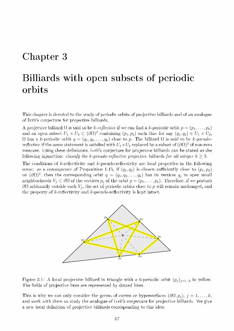
Chapter 3

Billiards with open subsets of periodic

orbits

This chapter is devoted to the study of periodic orbits of projective billiards and of an analogueof Ivrii's conjecture for projective billiards.

A projective billiard Ω is said to be k-reective if we can nd a k-periodic orbit p = (p1, . . . , pk)and an open subset U1 × U2 ⊂ (∂Ω)2 containing (p1, p2) such that for any (q1, q2) ∈ U1 × U2,Ω has a k-periodic orbit q = (q1, q2, . . . , qk) close to p. The billiard Ω is said to be k-pseudo-reective if the same statement is satised with U1×U2 replaced by a subset of (∂Ω)2 of non-zeromeasure. Using these denitions, Ivrii's conjecture for projective billiards can be stated as thefollowing injunction: classify the k-pseudo-reective projective billiards for all integer k ≥ 3.

The conditions of k-reectivity and k-pseudo-reectivity are local properties in the followingsense: as a consequence of Proposition 1.15, if (q1, q2) is chosen suciently close to (p1, p2)on (∂Ω)2, then the corresponding orbit q = (q1, q2, . . . , qk) has its vertices qj in open smallneighborhoods Vj ⊂ ∂Ω of the vertices pj of the orbit p = (p1, . . . , pk). Therefore, if we perturb∂Ω arbitrarily outside each Vj, the set of periodic orbits close to p will remain unchanged, andthe property of k-reectivity and k-pseudo-reectivity is kept intact.

p1

p2

p3

p4

p5

p6

Figure 3.1: A local projective billiard in triangle with a 6-periodic orbit (pj)j=1...6 in yellow.The elds of projective lines are represented by dotted lines.

This is why we can only consider the germs of curves or hypersurfaces (∂Ω, pj), j = 1, . . . , k,and work with them to study the analogue of Ivrii's conjecture for projective billiards. We givea new local denition of projective billiards corresponding to this idea:

67

Denition 3.1. A local projective billiard B is a collection of line-framed hypersurfaces α1, . . . , αk ⊂P(TRd) over hypersurfaces a1, . . . , ak of Rd called classical boundaries of B. It is said to berespectively Cr-smooth (with r = 1, 2, . . . ,∞) or analytic if all αj are Cr-smooth or are analytic.

An orbit of B is a (nite or innite) sequence of points (pj)j=−s...t, with integers s ≤ t eventuallyinnite, such that for each j (seen modulo k)

− pj ∈ ajmod k, pj 6= pj+1 and the line pjpj+1 is oriented from pj to pj+1;− the line pjpj+1 is transverse to both aj and aj+1;− the line pjpj+1 is obtained from pj−1pj by the projective reection law of αjmod k at pj.

If k′ is a multiple of k, an orbit (pj)j is said to be k′-periodic if s = 1, t = k′ and (p1, . . . , pk′ , p1, p2)is an orbit.

A local classical billiard (or simply local billiard) is a local projective billiard whose line-framedhypersurfaces are induced by the Euclidean metric, i.e. the lines of the projective elds of linesare orthogonal to the tangent hyperplanes (see Subsection 1.1.4).

A local projective billiard B is said to be k-reective (respectively k-pseudo-reective) if thereis a non-empty open subset (respectively a subset of non-zero measure) U1×U2 ⊂ a1× a2 suchthat to any pair (p1, p2) ∈ U1 × U2 corresponds a k-periodic orbit of B. The k-reective set ofB is the set of pairs (p1, p2) contained in open subsets U1 × U2 ⊂ a1 × a2 satisfying previousproperty.

Remark 3.2. If an analytic local projective billiard is k-pseudo-reective, then it is k-reective.This result is an easy corollary of the Uniqueness Theorem for analytic extension.

Remark 3.3. We will sometimes consider that the αj are line-framed hypersurfaces of P(TRPd)(see Remark 1.11).

This chapter is structured as follows: dierent examples of k-reective projective billiards insidepolygons are given at Section 3.1. Section 3.2 introduces Pfaan systems and applies them tothe study of Ivrii's conjecture. A classication of the 3-reective and 3-pseudo-reective localprojective billiards is given at Section 3.3.

3.1 Examples of k-reective projective billiards

In this section, we construct dierent types of local projective billiards in the plane which arek-reective for all integer k being either 3 or an even integer. The constructed examples areprojective billiards whose classical boundaries are lines, hence can be considered as projectivebilliards inside polygons. All the results presented here are gathered in a preprint [21].

Remark 3.4. I apologize in advance for this remark which is not related directly to mathematicalconsiderations. I remember the results of this section as a very pleasant moment of my thesis.In this remark I just describe a funny anecdote taking place in a train from Nizhnyi Novgorodto Novosibirsk and related to the discovery of the present results. I found some of the latter'sproofs during this two days long journey, while the train was moving in the middle of beautifulempty frozen steppes. When the redaction was over, I tried to put the preprint online. But wiwas only available for short periods of time at dierent train stops situated midway betweenNizhnyi Novgorod and Novosibirsk, so that I had to be quite dexterous and try again manytimes to achieve the upload. This journey appeared to me as a great moment of creativity,which probably would have been dierent if I decided to take the airplane instead of the trainin order to join Novosibirsk from Nizhnyi Novgorod.

68

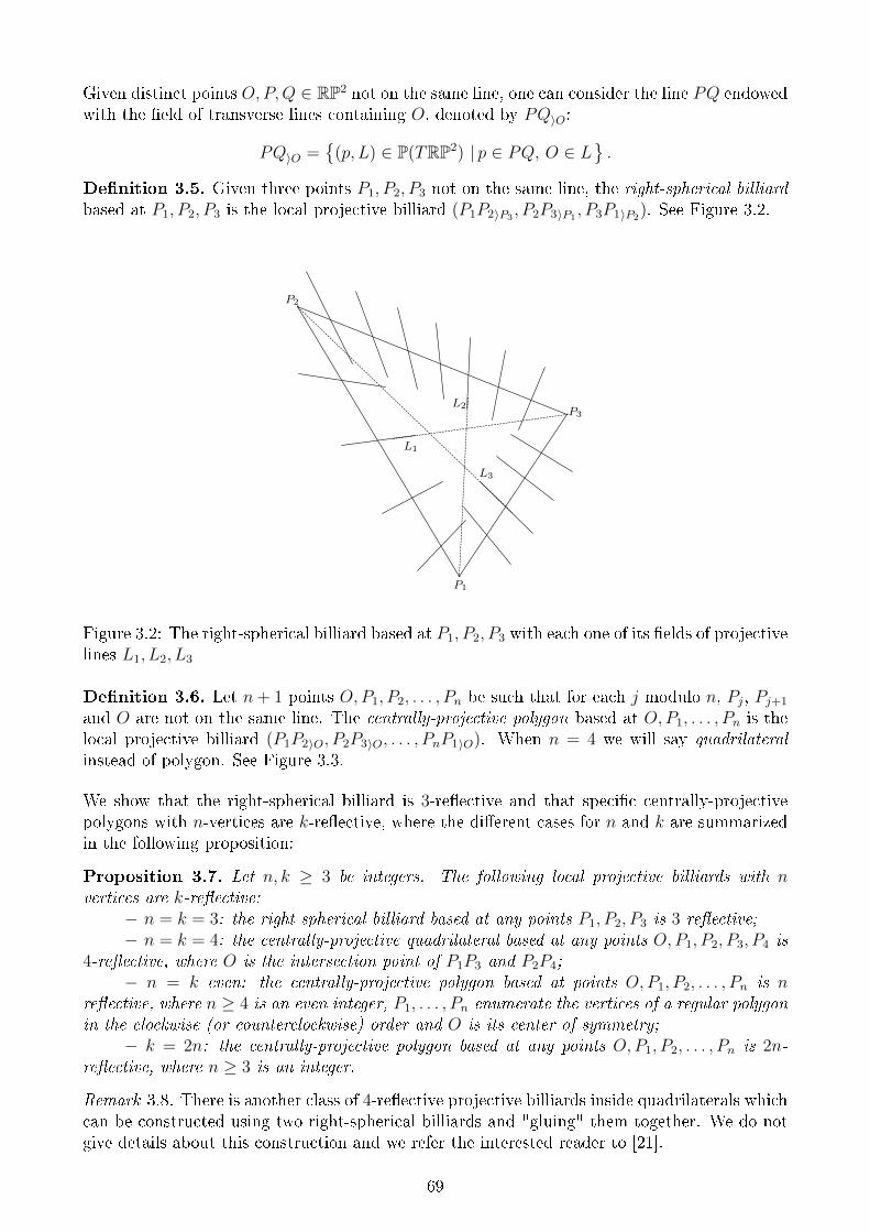
Given distinct points O,P,Q ∈ RP2 not on the same line, one can consider the line PQ endowedwith the eld of transverse lines containing O, denoted by PQ〉O:

PQ〉O =

(p, L) ∈ P(TRP2) | p ∈ PQ, O ∈ L.

Denition 3.5. Given three points P1, P2, P3 not on the same line, the right-spherical billiardbased at P1, P2, P3 is the local projective billiard (P1P2〉P3

, P2P3〉P1, P3P1〉P2

). See Figure 3.2.

P3

P1

P2

L3

L1

L2

Figure 3.2: The right-spherical billiard based at P1, P2, P3 with each one of its elds of projectivelines L1, L2, L3

Denition 3.6. Let n+ 1 points O,P1, P2, . . . , Pn be such that for each j modulo n, Pj, Pj+1

and O are not on the same line. The centrally-projective polygon based at O,P1, . . . , Pn is thelocal projective billiard (P1P2〉O, P2P3〉O, . . . , PnP1〉O). When n = 4 we will say quadrilateralinstead of polygon. See Figure 3.3.

We show that the right-spherical billiard is 3-reective and that specic centrally-projectivepolygons with n-vertices are k-reective, where the dierent cases for n and k are summarizedin the following proposition:

Proposition 3.7. Let n, k ≥ 3 be integers. The following local projective billiards with nvertices are k-reective:

− n = k = 3: the right-spherical billiard based at any points P1, P2, P3 is 3-reective;− n = k = 4: the centrally-projective quadrilateral based at any points O,P1, P2, P3, P4 is

4-reective, where O is the intersection point of P1P3 and P2P4;− n = k even: the centrally-projective polygon based at points O,P1, P2, . . . , Pn is n

reective, where n ≥ 4 is an even integer, P1, . . . , Pn enumerate the vertices of a regular polygonin the clockwise (or counterclockwise) order and O is its center of symmetry;

− k = 2n: the centrally-projective polygon based at any points O,P1, P2, . . . , Pn is 2n-reective, where n ≥ 3 is an integer.

Remark 3.8. There is another class of 4-reective projective billiards inside quadrilaterals whichcan be constructed using two right-spherical billiards and "gluing" them together. We do notgive details about this construction and we refer the interested reader to [21].

69

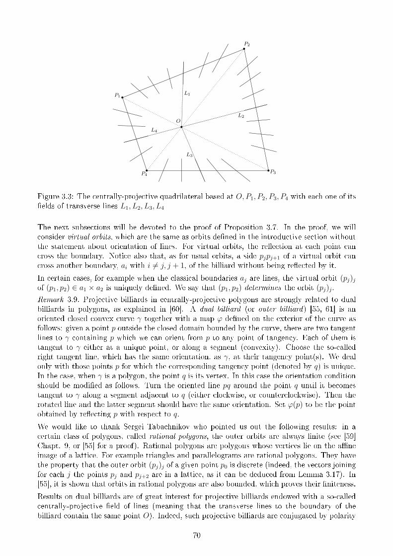
P4

P1

P2

P3

O

L4

L1

L2

L3

Figure 3.3: The centrally-projective quadrilateral based at O,P1, P2, P3, P4 with each one of itselds of transverse lines L1, L2, L3, L4

The next subsections will be devoted to the proof of Proposition 3.7. In the proof, we willconsider virtual orbits, which are the same as orbits dened in the introductive section withoutthe statement about orientation of lines. For virtual orbits, the reection at each point cancross the boundary. Notice also that, as for usual orbits, a side pjpj+1 of a virtual orbit cancross another boundary, ai with i 6= j, j + 1, of the billiard without being reected by it.

In certain cases, for example when the classical boundaries aj are lines, the virtual orbit (pj)jof (p1, p2) ∈ a1 × a2 is uniquely dened. We say that (p1, p2) determines the orbit (pj)j.

Remark 3.9. Projective billiards in centrally-projective polygons are strongly related to dualbilliards in polygons, as explained in [60]. A dual billiard (or outer billiard) [55, 61] is anoriented closed convex curve γ together with a map ϕ dened on the exterior of the curve asfollows: given a point p outside the closed domain bounded by the curve, there are two tangentlines to γ containing p which we can orient from p to any point of tangency. Each of them istangent to γ either at a unique point, or along a segment (convexity). Choose the so-calledright tangent line, which has the same orientation, as γ, at their tangency point(s). We dealonly with those points p for which the corresponding tangency point (denoted by q) is unique.In the case, when γ is a polygon, the point q is its vertex. In this case the orientation conditionshould be modied as follows. Turn the oriented line pq around the point q until it becomestangent to γ along a segment adjacent to q (either clockwise, or counterclockwise). Then therotated line and the latter segment should have the same orientation. Set ϕ(p) to be the pointobtained by reecting p with respect to q.

We would like to thank Sergei Tabachnikov who pointed us out the following results: in acertain class of polygons, called rational polygons, the outer orbits are always nite (see [59]Chapt. 9, or [55] for a proof). Rational polygons are polygons whose vertices lie on the aneimage of a lattice. For example triangles and parallelograms are rational polygons. They havethe property that the outer orbit (pj)j of a given point p0 is discrete (indeed, the vectors joiningfor each j the points pj and pj+2 are in a lattice, as it can be deduced from Lemma 3.17). In[55], it is shown that orbits in rational polygons are also bounded, which proves their niteness.

Results on dual billiards are of great interest for projective billiards endowed with a so-calledcentrally-projective eld of lines (meaning that the transverse lines to the boundary of thebilliard contain the same point O). Indeed, such projective billiards are conjugated by polarity

70

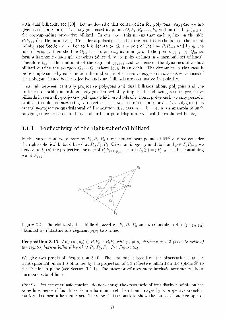
with dual billiards, see [60]. Let us describe this construction for polygons: suppose we aregiven a centrally-projective polygon based at points O,P1, P2, . . . , Pn and an orbit (pj)j∈Z ofthe corresponding projective billiard. In our case, this means that each pj lies on the sidePjPj+1 (see Denition 3.1). Consider a polarity such that the point O is the pole of the line atinnity (see Section 2.1). For each k denote by Qk the pole of the line PkPk+1 and by qk thepole of pkpk+1: then the line Opk has its pole ωk at innity, and the points qk−1, qk, Qk, ωkform a harmonic quadruple of points (since they are poles of lines in a harmonic set of lines).Therefore Qk is the midpoint of the segment qkqk+1 and we recover the dynamics of a dualbilliard outside the polygon Q1 · · ·Qn where (qk)k is an orbit. The dynamics in this case ismore simple since by construction the midpoints of successive edges are consecutive vertices ofthe polygon. Hence both projective and dual billiards are conjugated by polarity.

This link between centrally-projective polygons and dual billiards about polygons and theniteness of orbits in rational polygons immediately implies the following result: projectivebilliards in centrally-projective polygons which are duals of rational polygons have only periodicorbits. It could be interesting to describe this new class of centrally-projective polygons (thecentrally-projective quadrilateral of Proposition 3.7, case n = k = 4, is an example of suchpolygon, since its associated dual billiard is a parallelogram, as it will be explained below).

3.1.1 3-reectivity of the right-spherical billiard

In this subsection, we denote by P1, P2, P3 three non-colinear points of RP2 and we considerthe right-spherical billiard based at P1, P2, P3. Given an integer j modulo 3 and p ∈ PjPj+1, wedenote by Lj(p) the projective line at p of PjPj+1〉Pj+2

, that is Lj(p) = pPj+2, the line containingp and Pj+2.

P2

P1

P3

p1

p2

p3

L1

L2

L3

Figure 3.4: The right-spherical billiard based at P1, P2, P3 and a triangular orbit (p1, p2, p3)obtained by reecting any segment p1p2 two times

Proposition 3.10. Any (p1, p2) ∈ P1P2 × P2P3 with p1 6= p2 determines a 3-periodic orbit ofthe right-spherical billiard based at P1, P2, P3. See Figure 3.4.

We give two proofs of Proposition 3.10. The rst one is based on the observation that theright-spherical billiard is obtained by the projection of a 3-reective billiard on the sphere S2 tothe Euclidean plane (see Section 1.1.4). The other proof uses more intrinsic arguments aboutharmonic sets of lines.

Proof 1. Projective transformations do not change the cross-ratio of four distinct points on thesame line, hence if four lines form a harmonic set then their images by a projective transfor-mation also form a harmonic set. Therefore it is enough to show that at least one example of

71

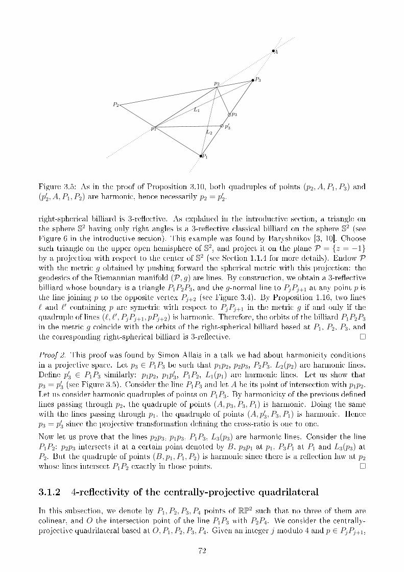
P2

P1

P3

p1

p2

p3L1

L2

A

p′3

Figure 3.5: As in the proof of Proposition 3.10, both quadruples of points (p2, A, P1, P3) and(p′2, A, P1, P2) are harmonic, hence necessarily p2 = p′2.

right-spherical billiard is 3-reective. As explained in the introductive section, a triangle onthe sphere S2 having only right angles is a 3-reective classical billiard on the sphere S2 (seeFigure 6 in the introductive section). This example was found by Baryshnikov [3, 10]. Choosesuch triangle on the upper open hemisphere of S2, and project it on the plane P = z = −1by a projection with respect to the center of S2 (see Section 1.1.4 for more details). Endow Pwith the metric g obtained by pushing forward the spherical metric with this projection: thegeodesics of the Riemannian manifold (P , g) are lines. By construction, we obtain a 3-reectivebilliard whose boundary is a triangle P1P2P3, and the g-normal line to PjPj+1 at any point p isthe line joining p to the opposite vertex Pj+2 (see Figure 3.4). By Proposition 1.16, two lines` and `′ containing p are symetric with respect to PjPj+1 in the metric g if and only if thequadruple of lines (`, `′, PjPj+1, pPj+2) is harmonic. Therefore, the orbits of the billiard P1P2P3

in the metric g coincide with the orbits of the right-spherical billiard based at P1, P2, P3, andthe corresponding right-spherical billiard is 3-reective.

Proof 2. This proof was found by Simon Allais in a talk we had about harmonicity conditionsin a projective space. Let p3 ∈ P1P3 be such that p1p2, p2p3, P2P3, L2(p2) are harmonic lines.Dene p′3 ∈ P1P3 similarly: p1p2, p1p

′3, P1P2, L1(p1) are harmonic lines. Let us show that

p3 = p′3 (see Figure 3.5). Consider the line P1P3 and let A be its point of intersection with p1p2.Let us consider harmonic quadruples of points on P1P3. By harmonicity of the previous denedlines passing through p2, the quadruple of points (A, p3, P3, P1) is harmonic. Doing the samewith the lines passing through p1, the quadruple of points (A, p′3, P3, P1) is harmonic. Hencep3 = p′3 since the projective transformation dening the cross-ratio is one to one.

Now let us prove that the lines p2p3, p1p3, P1P3, L3(p3) are harmonic lines. Consider the lineP1P2: p2p3 intersects it at a certain point denoted by B, p3p1 at p1, P3P1 at P1 and L3(p3) atP2. But the quadruple of points (B, p1, P1, P2) is harmonic since there is a reection law at p2

whose lines intersect P1P2 exactly in those points.

3.1.2 4-reectivity of the centrally-projective quadrilateral

In this subsection, we denote by P1, P2, P3, P4 points of RP2 such that no three of them arecolinear, and O the intersection point of the line P1P3 with P2P4. We consider the centrally-projective quadrilateral based at O,P1, P2, P3, P4. Given an integer j modulo 4 and p ∈ PjPj+1,

72

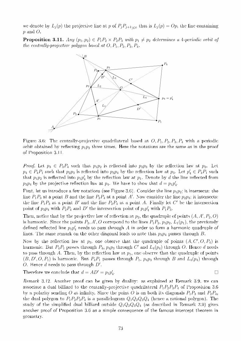
we denote by Lj(p) the projective line at p of PjPj+1〉O, that is Lj(p) = Op, the line containingp and O.

Proposition 3.11. Any (p1, p2) ∈ P1P2 × P2P3 with p1 6= p2 determines a 4-periodic orbit ofthe centrally-projective polygon based at O,P1, P2, P3, P4.

P2

P3

P4

P1

O

p1

p2

p3

A

B

p4 = p′4

C′

D′

A′

B′

L2

L3

L1

L4

Figure 3.6: The centrally-projective quadrilateral based at O,P1, P2, P3, P4 with a periodicorbit obtained by reecting p1p2 three times. Here the notations are the same as in the proofof Proposition 3.11.

Proof. Let p3 ∈ P3P4 such that p1p2 is reected into p2p3 by the reection law at p2. Letp4 ∈ P4P1 such that p2p3 is reected into p3p4 by the reection law at p3. Let p′4 ∈ P4P1 suchthat p1p2 is reected into p1p

′4 by the reection law at p1. Denote by d the line reected from

p3p4 by the projective reection law at p4. We have to show that d = p1p′4.

First, let us introduce a few notations (see Figure 3.6). Consider the line p1p2; it intersects: theline P1P3 at a point B and the line P2P4 at a point A′. Now consider the line p2p3; it intersects:the line P1P3 at a point B′ and the line P2P4 at a point A. Finally let C ′ be the intersectionpoint of p3p4 with P2P4 and D′ the intersection point of p1p

′4 with P1P3.

Then, notice that by the projective law of reection at p2, the quadruple of points (A,A′, P2, O)is harmonic. Since the points P2, A

′, O correpond to the lines P1P2, p1p2, L1(p1), the previouslydened reected line p1p

′4 needs to pass through A in order to form a harmonic quadruple of

lines. The same remark on the other diagonal leads to note that p3p4 passes through B.

Now by the reection law at p3, one observe that the quadruple of points (A,C ′, O, P4) isharmonic. But P4P1 passes through P4, p4p3 through C ′ and L4(p4) through O. Hence d needsto pass through A. Then, by the reection law at p1, one observe that the quadruple of points(B,D′, O, P1) is harmonic. But P4P1 passes through P1, p4p3 through B and L4(p4) throughO. Hence d needs to pass through D′.

Therefore we conclude that d = AD′ = p1p′4.

Remark 3.12. Another proof can be given by duality: as explained at Remark 3.9, we canassociate a dual billiard to the centrally-projective quadrilateral P1P2P3P4 of Proposition 3.6by a polarity sending O at innity. Since the point O is on both its diagonals P1P3 and P2P4,the dual polygon to P1P2P3P4 is a parallelogram Q1Q2Q3Q4 (hence a rational polygon). Thestudy of the simplied dual billiard outside Q1Q2Q3Q4 (as described in Remark 3.9) givesanother proof of Proposition 3.6 as a simple consequence of the famous intercept theorem ingeometry.

73

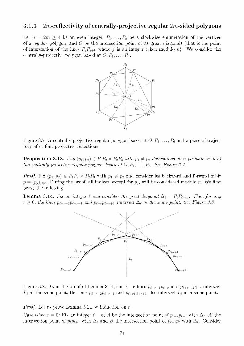
3.1.3 2m-reectivity of centrally-projective regular 2m-sided polygons

Let n = 2m ≥ 4 be an even integer, P1, . . . , Pn be a clockwise enumeration of the verticesof a regular polygon, and O be the intersection point of its great diagonals (that is the pointof intersection of the lines PjPj+k where j is an integer taken modulo n). We consider thecentrally-projective polygon based at O,P1, . . . , Pn.

P2

P3

P4

P1

P6

P5

Op1

p2p3

p4

p5p6

L2 L3

L4

L5L6

L1

Figure 3.7: A centrally-projective regular polygon based at O,P1, . . . , P6 and a piece of trajec-tory after four projective reections.

Proposition 3.13. Any (p1, p2) ∈ P1P2 × P2P3 with p1 6= p2 determines an n-periodic orbit ofthe centrally-projective regular polygon based at O,P1, . . . , Pn. See Figure 3.7.

Proof. Fix (p1, p2) ∈ P1P2 × P2P3 with p1 6= p2 and consider its backward and forward orbitp = (pj)j∈Z. During the proof, all indices, except for pj, will be considered modulo n. We rstprove the following

Lemma 3.14. Fix an integer ` and consider the great diagonal ∆` = P`P`+m. Then for anyr ≥ 0, the lines p`−r−2p`−r−1 and p`+rp`+r+1 intersect ∆` at the same point. See Figure 3.8.

P`P`−r

P`−r−1

P`−r−2

P`+r

P`+r+1

P`+r+2

p`−r−1

p`−r

p`−r−2

p`+r−1

p`+r+1

p`+r

L`

Figure 3.8: As in the proof of Lemma 3.14, since the lines p`−r−1p`−r and p`+r−1p`+r intersectL` at the same point, the lines p`−r−2p`−r−1 and p`+rp`+r+1 also intersect L` at a same point.

Proof. Let us prove Lemma 3.14 by induction on r.

Case when r = 0: Fix an integer `. Let A be the intersection point of p`−2p`−1 with ∆`, A′ theintersection point of p`p`+1 with ∆` and B the intersection point of p`−1p` with ∆`. Consider

74

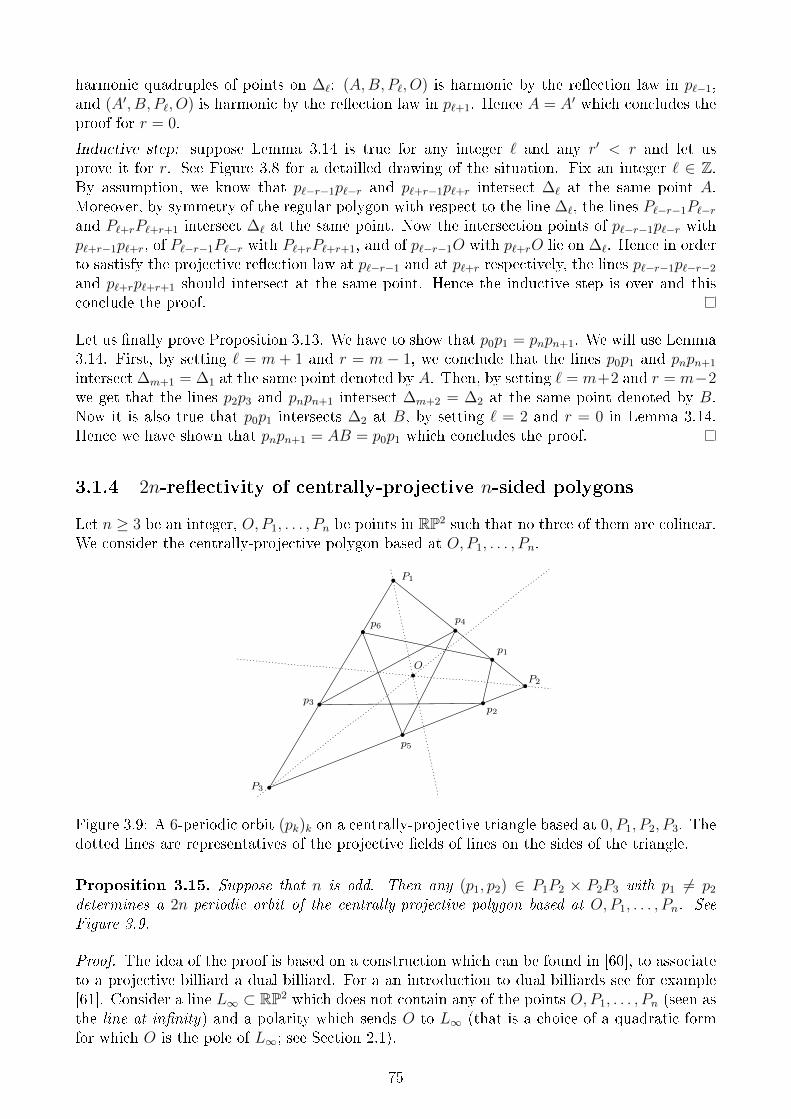
harmonic quadruples of points on ∆`: (A,B, P`, O) is harmonic by the reection law in p`−1,and (A′, B, P`, O) is harmonic by the reection law in p`+1. Hence A = A′ which concludes theproof for r = 0.

Inductive step: suppose Lemma 3.14 is true for any integer ` and any r′ < r and let usprove it for r. See Figure 3.8 for a detailled drawing of the situation. Fix an integer ` ∈ Z.By assumption, we know that p`−r−1p`−r and p`+r−1p`+r intersect ∆` at the same point A.Moreover, by symmetry of the regular polygon with respect to the line ∆`, the lines P`−r−1P`−rand P`+rP`+r+1 intersect ∆` at the same point. Now the intersection points of p`−r−1p`−r withp`+r−1p`+r, of P`−r−1P`−r with P`+rP`+r+1, and of p`−r−1O with p`+rO lie on ∆`. Hence in orderto sastisfy the projective reection law at p`−r−1 and at p`+r respectively, the lines p`−r−1p`−r−2

and p`+rp`+r+1 should intersect at the same point. Hence the inductive step is over and thisconclude the proof.

Let us nally prove Proposition 3.13. We have to show that p0p1 = pnpn+1. We will use Lemma3.14. First, by setting ` = m + 1 and r = m − 1, we conclude that the lines p0p1 and pnpn+1

intersect ∆m+1 = ∆1 at the same point denoted by A. Then, by setting ` = m+2 and r = m−2we get that the lines p2p3 and pnpn+1 intersect ∆m+2 = ∆2 at the same point denoted by B.Now it is also true that p0p1 intersects ∆2 at B, by setting ` = 2 and r = 0 in Lemma 3.14.Hence we have shown that pnpn+1 = AB = p0p1 which concludes the proof.

3.1.4 2n-reectivity of centrally-projective n-sided polygons

Let n ≥ 3 be an integer, O,P1, . . . , Pn be points in RP2 such that no three of them are colinear.We consider the centrally-projective polygon based at O,P1, . . . , Pn.

P1

P3

P2

p5

p6

p1

O

p2p3

p4

Figure 3.9: A 6-periodic orbit (pk)k on a centrally-projective triangle based at 0, P1, P2, P3. Thedotted lines are representatives of the projective elds of lines on the sides of the triangle.

Proposition 3.15. Suppose that n is odd. Then any (p1, p2) ∈ P1P2 × P2P3 with p1 6= p2

determines a 2n-periodic orbit of the centrally-projective polygon based at O,P1, . . . , Pn. SeeFigure 3.9.

Proof. The idea of the proof is based on a construction which can be found in [60], to associateto a projective billiard a dual billiard. For a an introduction to dual billiards see for example[61]. Consider a line L∞ ⊂ RP2 which does not contain any of the points O,P1, . . . , Pn (seen asthe line at innity) and a polarity which sends O to L∞ (that is a choice of a quadratic formfor which O is the pole of L∞; see Section 2.1).

75

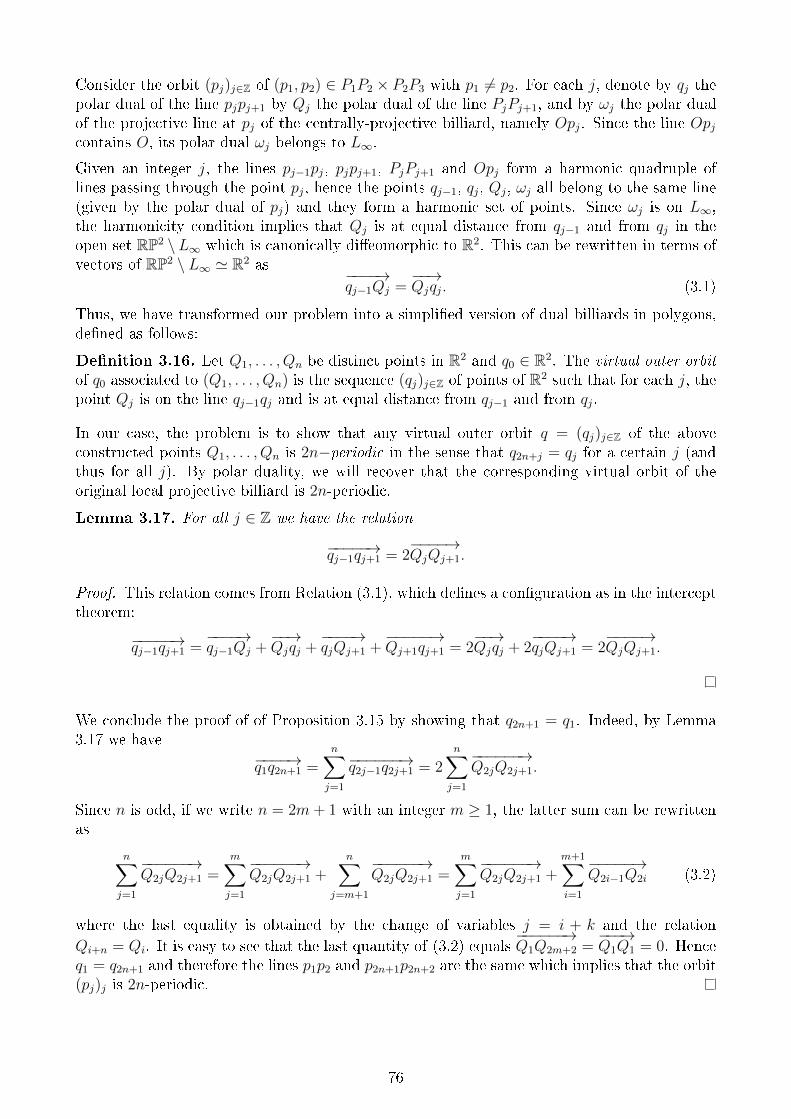
Consider the orbit (pj)j∈Z of (p1, p2) ∈ P1P2 × P2P3 with p1 6= p2. For each j, denote by qj thepolar dual of the line pjpj+1 by Qj the polar dual of the line PjPj+1, and by ωj the polar dualof the projective line at pj of the centrally-projective billiard, namely Opj. Since the line Opjcontains O, its polar dual ωj belongs to L∞.

Given an integer j, the lines pj−1pj, pjpj+1, PjPj+1 and Opj form a harmonic quadruple oflines passing through the point pj, hence the points qj−1, qj, Qj, ωj all belong to the same line(given by the polar dual of pj) and they form a harmonic set of points. Since ωj is on L∞,the harmonicity condition implies that Qj is at equal distance from qj−1 and from qj in theopen set RP2 \L∞ which is canonically dieomorphic to R2. This can be rewritten in terms ofvectors of RP2 \ L∞ ' R2 as

−−−−→qj−1Qj =

−−→Qjqj. (3.1)

Thus, we have transformed our problem into a simplied version of dual billiards in polygons,dened as follows:

Denition 3.16. Let Q1, . . . , Qn be distinct points in R2 and q0 ∈ R2. The virtual outer orbitof q0 associated to (Q1, . . . , Qn) is the sequence (qj)j∈Z of points of R2 such that for each j, thepoint Qj is on the line qj−1qj and is at equal distance from qj−1 and from qj.

In our case, the problem is to show that any virtual outer orbit q = (qj)j∈Z of the aboveconstructed points Q1, . . . , Qn is 2n−periodic in the sense that q2n+j = qj for a certain j (andthus for all j). By polar duality, we will recover that the corresponding virtual orbit of theoriginal local projective billiard is 2n-periodic.

Lemma 3.17. For all j ∈ Z we have the relation

−−−−−→qj−1qj+1 = 2−−−−→QjQj+1.

Proof. This relation comes from Relation (3.1), which denes a conguration as in the intercepttheorem:

−−−−−→qj−1qj+1 =−−−−→qj−1Qj +

−−→Qjqj +

−−−−→qjQj+1 +

−−−−−→Qj+1qj+1 = 2

−−→Qjqj + 2

−−−−→qjQj+1 = 2

−−−−→QjQj+1.

We conclude the proof of of Proposition 3.15 by showing that q2n+1 = q1. Indeed, by Lemma3.17 we have

−−−−→q1q2n+1 =n∑j=1

−−−−−−→q2j−1q2j+1 = 2n∑j=1

−−−−−−→Q2jQ2j+1.

Since n is odd, if we write n = 2m+ 1 with an integer m ≥ 1, the latter sum can be rewrittenas

n∑j=1

−−−−−−→Q2jQ2j+1 =

m∑j=1

−−−−−−→Q2jQ2j+1 +

n∑j=m+1

−−−−−−→Q2jQ2j+1 =

m∑j=1

−−−−−−→Q2jQ2j+1 +

m+1∑i=1

−−−−−→Q2i−1Q2i (3.2)

where the last equality is obtained by the change of variables j = i + k and the relationQi+n = Qi. It is easy to see that the last quantity of (3.2) equals

−−−−−−→Q1Q2m+2 =

−−−→Q1Q1 = 0. Hence

q1 = q2n+1 and therefore the lines p1p2 and p2n+1p2n+2 are the same which implies that the orbit(pj)j is 2n-periodic.

76

3.2 Billiards and Pfaan systems

In this section we present a strong link between k-reective (eventually projective) billiardsand integral surfaces of a certain distribution called Birkho's distribution. The idea wasdevelopped in [1], and interesting arguments are given in [27] from which this section of themanuscript is inspired. Some of the results presented in this section are gathered in a preprint[20].

3.2.1 Classical Birkho's distribution

Let M be a smooth or analytic manifold and k be a non-zero positive integer. We denote byGrk (TM) the ber bundle over M made by k-dimensional vector subspaces of TM , and byπ : Grk (TM)→M its natural projection.

Denition 3.18. A k-dimensional distribution on M is a smooth (or analytic) section D :M → Grk (TM). An `-dimensional integral manifold (or surface) of D is a smooth (or analytic)submanifold S ⊂M of dimension ` such that for all p ∈ S

TpS ⊂ D(p). (3.3)

An `-dimensional pseudo-integral manifold (or surface) of D is a smooth (or analytic) subman-ifold S ⊂ M of dimension ` such that (3.3) holds only for p in a subset V ⊂ S of non-zeroLebesgue measure, called integral set.

Remark 3.19. A connected analytic pseudo-integral manifold of an analytic distribution is anintegralble manifold. This result is implied by the Uniqueness Theorem for analytic extension.

Now let us dene the usual version of Birkho's distribution. We set M = (Rd)k. Considerthe open dense subset U ⊂ M of k-tuples p = (p1, . . . , pk) such that for each j = 2, . . . , k − 1the points pj−1, pj, pj+1 do not lie on the same line of Rd. For each j (modulo k), consider theinterior bisector Lj(p) ⊂ Rd of the oriented angle between the vectors −−−→pjpj−1 and −−−→pjpj+1 anddenote by Hj(p) ⊂ Rd its orthogonal hyperplane (with respect to the Euclidean metric of Rd).The hyperplanes Hj(p) have the following simple property related to billiards which is simplydue to the denition of the reection law on the billiard.

Lemma 3.20. Let Ω be a (classical) billiard in Rd and p be a sequence of points (p1, . . . , pk) onthe boundary ∂Ω such that p ∈ U . Then p is a k-periodic orbit if and only if Tpj∂Ω = Hj(p).

Then we can identify TpU with ⊕kj=1TpjRd, and consider the projections πjM → Rd sending pto pj. We can consider the

Denition 3.21. The k(d−1)-dimensionnal analytic distribution on U ⊂ (Rd)k dened for allp ∈ U by

D(p) = ⊕kj=1Hj(p)

is called Birkho's distribution. We further say that an integral (respectively pseudo-integral)manifold S of D is non-trivial if the restriction of each πj to S has rank d − 1 for all p ∈ S(respectively p ∈ V ).

Notice that if the restrictions of πj to S have rank d−1 at p, then there is a small neighborhoodW of p such that the πj(V ) are submanifolds of Rd of the same regularity than S. Birkho'sdistribution has then the following property which is related to the latter remark and to Lemma3.20:

77

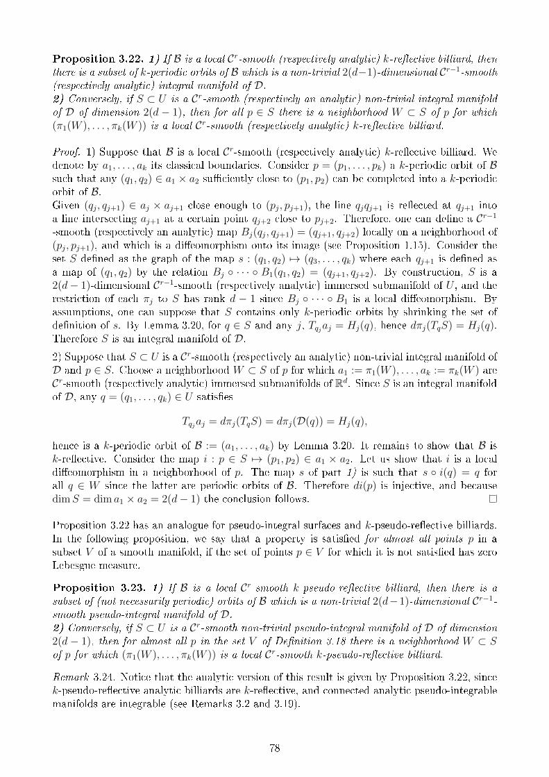
Proposition 3.22. 1) If B is a local Cr-smooth (respectively analytic) k-reective billiard, thenthere is a subset of k-periodic orbits of B which is a non-trivial 2(d−1)-dimensional Cr−1-smooth(respectively analytic) integral manifold of D.2) Conversely, if S ⊂ U is a Cr-smooth (respectively an analytic) non-trivial integral manifoldof D of dimension 2(d − 1), then for all p ∈ S there is a neighborhood W ⊂ S of p for which(π1(W ), . . . , πk(W )) is a local Cr-smooth (respectively analytic) k-reective billiard.

Proof. 1) Suppose that B is a local Cr-smooth (respectively analytic) k-reective billiard. Wedenote by a1, . . . , ak its classical boundaries. Consider p = (p1, . . . , pk) a k-periodic orbit of Bsuch that any (q1, q2) ∈ a1 × a2 suciently close to (p1, p2) can be completed into a k-periodicorbit of B.Given (qj, qj+1) ∈ aj × aj+1 close enough to (pj, pj+1), the line qjqj+1 is reected at qj+1 intoa line intersecting aj+1 at a certain point qj+2 close to pj+2. Therefore, one can dene a Cr−1

-smooth (respectively an analytic) map Bj(qj, qj+1) = (qj+1, qj+2) locally on a neighborhood of(pj, pj+1), and which is a dieomorphism onto its image (see Proposition 1.15). Consider theset S dened as the graph of the map s : (q1, q2) 7→ (q3, . . . , qk) where each qj+1 is dened asa map of (q1, q2) by the relation Bj · · · B1(q1, q2) = (qj+1, qj+2). By construction, S is a2(d− 1)-dimensional Cr−1-smooth (respectively analytic) immersed submanifold of U , and therestriction of each πj to S has rank d − 1 since Bj · · · B1 is a local dieomorphism. Byassumptions, one can suppose that S contains only k-periodic orbits by shrinking the set ofdenition of s. By Lemma 3.20, for q ∈ S and any j, Tqjaj = Hj(q), hence dπj(TqS) = Hj(q).Therefore S is an integral manifold of D.2) Suppose that S ⊂ U is a Cr-smooth (respectively an analytic) non-trivial integral manifold ofD and p ∈ S. Choose a neighborhood W ⊂ S of p for which a1 := π1(W ), . . . , ak := πk(W ) areCr-smooth (respectively analytic) immersed submanifolds of Rd. Since S is an integral manifoldof D, any q = (q1, . . . , qk) ∈ U satises

Tqjaj = dπj(TqS) = dπj(D(q)) = Hj(q),

hence is a k-periodic orbit of B := (a1, . . . , ak) by Lemma 3.20. It remains to show that B isk-reective. Consider the map i : p ∈ S 7→ (p1, p2) ∈ a1 × a2. Let us show that i is a localdieomorphism in a neighborhood of p. The map s of part 1) is such that s i(q) = q forall q ∈ W since the latter are periodic orbits of B. Therefore di(p) is injective, and becausedimS = dim a1 × a2 = 2(d− 1) the conclusion follows.

Proposition 3.22 has an analogue for pseudo-integral surfaces and k-pseudo-reective billiards.In the following proposition, we say that a property is satised for almost all points p in asubset V of a smooth manifold, if the set of points p ∈ V for which it is not satised has zeroLebesgue measure.

Proposition 3.23. 1) If B is a local Cr-smooth k-pseudo-reective billiard, then there is asubset of (not necessarily periodic) orbits of B which is a non-trivial 2(d−1)-dimensional Cr−1-smooth pseudo-integral manifold of D.2) Conversely, if S ⊂ U is a Cr-smooth non-trivial pseudo-integral manifold of D of dimension2(d − 1), then for almost all p in the set V of Denition 3.18 there is a neighborhood W ⊂ Sof p for which (π1(W ), . . . , πk(W )) is a local Cr-smooth k-pseudo-reective billiard.

Remark 3.24. Notice that the analytic version of this result is given by Proposition 3.22, sincek-pseudo-reective analytic billiards are k-reective, and connected analytic pseudo-integrablemanifolds are integrable (see Remarks 3.2 and 3.19).

78

Proof. The proof is analogous to the proof of Proposition 3.22, except that we will work withso-called Lebesgue points. Let us rst recall dentions and results about them.

Denition 3.25. Let V ⊂ Rd be a Lebesgue measurable set. A point x ∈ V is said to be aLebesgue point of V if one has

limr→0

λ(V ∩B(x, r))

λ(B(x, r))= 1

where λ is the Lebesgue measure of Rd and B(x, r) is the Euclidean ball of radius r > 0 centeredat x.

This denition naturally extends to subset V of smooth dierentiable manifolds. We observethe following

Theorem 3.26 (Lebesgue density theorem). Let V be a Lebesgue measurable set of a smoothdierentiable manifold. Then almost all points of V are Lebesgue poins of V .

Lemma 3.27 (see [27]). Let U ⊂ M be an open subset of a dierentiable manifold M andf, g : U → N be Cr-smooth maps from U to a dierentiable manifold N . If V is a subset of Uon which f = g and p is a Lebesgue point of V , then the 1-jets of f and g at p coincide.

Proof. Choosing a convenient set of coordinates, one can suppose that U ⊂M = Rd, N = Rk,p = 0 and also that g = 0, by substituing f−g to f . Consider the map P : Rd \0 → ∂B(0, 1)dened by P (x) = x/‖x‖ where ‖ · ‖ is the Euclidean metric. We rst prove that for r > 0Wr := P (V ∩ B(0, r) \ 0) is dense in ∂B(0, 1). Indeed, otherwise there would exist a non-empty open subset U of ∂B(0, 1) included in ∂B(0, 1) \Wr. The cone U ′ := P−1(U) is open ansatises for all 0 < ρ ≤ r that

− λ(U ′ ∩B(0, ρ)) = ρdλ(U ′ ∩B(0, 1)), since U ′ ∩B(0, ρ) is obtained from U ′ ∩B(0, 1) bythe dilatation x 7→ ρx;

− U ′ ∩B(0, ρ) ⊂ B(0, ρ) \ V , because U and Wr have empty intersection.Hence for 0 < ρ ≤ r

λ(V ∩B(0, ρ))

λ(B(0, ρ))= 1− λ(B(0, ρ) \ V )

λ(B(0, ρ))≤ 1− λ(U ′ ∩B(0, ρ))

λ(B(0, ρ))= 1− λ(U ′ ∩B(0, 1))

λ(B(0, 1))< 1

and the latter bound doesn't depend on ρ, which is impossible since p = 0 is a Lebesgue point ofV . Hence for v ∈ ∂B(0, 1), one can nd a sequence of vn ∈ V such that vn → 0 and P (vn)→ v.This implies that df(0) · v = lim f(vn)/‖vn‖ = 0.

Now we can prove Proposition 3.23:

1) Suppose that B is a local Cr-smooth k-pseudo-reective billiard. We denote by a1, . . . , ak itsclassical boundaries and by V ′ ⊂ a1 × a2 a subset of non-zero measure of points (q1, q2) whichcan be completed into a k-periodic orbit of B.Consider p = (p1, . . . , pk) a k-periodic orbit of B such that (p1, p2) ∈ a1×a2 is a Lebesgue pointof V ′. The corresponding manifold S dened in Proposition 3.22 as the graph of a map s doesnot only contain k-periodic orbits anymore. However by Lemma 3.20, all q = (q1, q2) ∈ V ′ lyingin an open subset W ′ containing p on which s is dened is such that s(q) is k-periodic. Thensince (p1, p2) ∈ W ′ ∩ V ′ is a Lebesgue point of V ′, W ′ ∩ V ′ has non-zero measure in W ′. Hencethe subset s(W ′ ∩ V ′) ⊂ S has non-zero measure in S and contains only k-periodic orbits.

2) Suppose that S ⊂ U is a Cr-smooth non-trivial pseudo-integral manifold of D, V the setof points p ∈ S for which TpS ⊂ D(p) and p ∈ V a Lebesgue point. Choose a neighborhoodW ⊂ S of p for which a1 := π1(W ), . . . , ak := πk(W ) are Cr-smooth immersed submanifolds ofRd. As in the proof of Proposition 3.22, any q ∈ W ∩V is a k-periodic orbit of B := (a1, . . . , ak).

79

Consider the map i : p ∈ S 7→ (p1, p2) ∈ a1 × a2. The map s of part 1) is such that s i(q) = qfor all q ∈ W ∩ V since the latter are periodic orbits of B. Therefore by Lemma 3.27, sincep is a Lebesgue point of V we can write ds(p1, p2) di(p) = Id and the conclusion follows asbefore.

3.2.2 Prolongations of Pfaan systems

Let M be an analytic manifold, D be an analytic distribution on M , and k ∈ 1, . . . , dimD.We denote by Grk (TM) the ber bundle over M made by k-dimensional vector subspaces ofTM , with its natural projection π : Grk (TM)→M .

One can dene a natural analytic distribution K on Grk (TM), called contact distribution, anddened for all (x,E) ∈ Grk (TM) by K(x,E) = dπ−1(E). In this subsection we introducePfaan systems and their prolongations, as a way to link integral manifolds of D and integralmanifolds of K contained in some submanifolds of (x,E) ∈ Grk (TM).

Denition 3.28 ([27], denition 21). Given a family of analytic distributions (Di)i on M , wecall the data P = (M,D, k; (Di)i) a Pfaan system with transversality conditions.

− A k-plane E ∈ Grk (TM) is said to be integral if for any 1-form ω vanishing on D, dωvanishes on E.

− An integral manifold (or surface) of P is an integral manifold of D of dimension k suchthat, for all i, its tangent subspaces either are transverse to Di, or intersect it by zero.

− An pseudo-integral manifold (or surface) of P is a pseudo-integral manifold of D ofdimension k such that, for x lying in its integral set V (see Denition 3.18) and for all i, TxSis either transverse to Di, or intersects it by zero.

It follows immediately that the tangent planes to an integral manifold S are integral. Noticealso that if S is a pseudo-integral manifold and V is its integral set, then, due to Lemma 3.27,TxS is integral for any Lebesgue point x of V .

In the following P = (M,D, k; (Di)i) denote a Pfaan system with transversality conditions.As described in [27], subsection 2.3, the set Mk of integral k-planes of M is an analytic subsethence a stratied manifold: it is a locally nite and at most countable disjoint union of smoothanalytically constructible subsets (see [43], section IV.8).

Denition 3.29 ([27], denition 23). Let M ′ be a stratum of Mk, K′ the restriction of thecontact distribution K to M ′, and D′i the pull-back of Di on M ′ for each i. The Pfaan systemP ′ = (M ′,K′, k; (D′i)i, ker dπ) is called a rst Cartan prolongation of P .

If S ⊂ M is a Cr-smooth submanifold of M of dimension k, one can consider the subsetS(1) ⊂ Grk (TM) dened by

S(1) = (x, TxS) |x ∈ S . (3.4)

It is Cr−1-smooth submanifold of Grk (TM), of dimension dimS and transverse to π. We callit the rst lift of S.

Proposition 3.30 ([27], subsection 2.3, [11], chapter VI). The lift S(1) of an integral surfaceS of P contains an open dense subset such that each its connected component S ′ lies in somestratum M ′ of Mk, and such that S ′ is an integral surface of the rst Cartan prolongationP ′ = (M ′,K′, k; (D′i)i, ker dπ).

80

Proof. As explained, the tangent planes of an integral manifolds are integral, hence S(1) iscontained in the set Mk of integral k-planes of D. Now let S ′ be a connected component of S(1)

contained in a stratum M ′ of Mk. For all p = (x, TxS) ∈ S ′ we have dπ(TpS(1)) = TxS, hence

TpS(1) ⊂ K(p) and therefore TpS ′ ⊂ K′(p). Moreover, the equality dπ(TpS

(1)) = TxS impliesthat dπ is injective on TpS

(1) hence on TpS′, and the transversality condition with ker dπ is

satised. One can easily check that he other transversality conditions are satised.

The converse result is also true, but only locally:

Proposition 3.31. Let M ′ be a stratum of Mk and S ′ be an integral manifold of the Pfaansystem P ′ = (M ′,K′, k; (D′i)i, ker dπ) such that the intersection TS ′ ∩ ker dπ is 0. Then forany p ∈ S ′ there is an open subset U ⊂ S ′ containing p and such that S := π(U) is an integralsurface of P such that S(1) = S ′.

Proof. Since TS ′ ∩ ker dπ = 0 are transverse, there is a small neighborhood U of p suchthat S := π(U) is a k-dimensionnal manifold with Tπ(q)S = dπ(TqS

′) for any q ∈ U . Henceif q = (x,E) ∈ U , then Tπ(q)S = E, because S ′ is an integral manifold of the distribution K′.Therefore TxS is an integral plane of D, and thus S is an integral manifold of D. One cananalogously check that S saties transversality conditions Di.

The same constructions work also for pseudo-integral manifolds of P :

Proposition 3.32 ([27], subsection 2.3). Let S ⊂ M be a pseudo-intergral surface of P, andV be its integral set. Suppose p = (x, TxS) ∈ S(1) is such that x is a Lebesgue point of V . Thenreplacing p by a Lebesgue point in V arbitrarily close to p (now denoted by p) one can achievethat there is a stratum M ′ of Mk and a smooth submanifold S ′ in an open subset of M ′, suchthat:

− S ′ contains p and is tangent to S(1) at p;− S ′ is a pseudo-integral surface of the Cartan prolongation P ′ = (M ′,K′, k; (D′i)i, ker dπ).

Proof. Denote by V ⊂ S(1) the set of points p = (x, TxS) ∈ S(1) such that x ∈ V : π maps theLebesgue points of V to the Lebesgue points of V . Denote by L(V ) the set of Lebesgue pointsof V . As explained, any Lebesgue point p ∈ L(V ) of V belongs to Mk (since TxS is an integralplane, where p = (x, TxS)).

Fix p ∈ L(V ): p is also a Lebesgue point of L(V ) which is a simple consequence of Lebesguedensity theorem (Theorem 3.26). In particular, any small neighborhood of p in L(V ) has non-zero measure in S(1). Hence one can choose a stratum M ′ of Mk containing points arbitrarilyclose to p such thatM ′∩L(V ) has non-zero Lebesgue measure in S(1) and the latter intersection(considered as a subset in S(1)) has Lebesgue points arbitrarily close to p. From now on, p willbe one of the latter Lebesgue points.

On a small neighborhood W of p in Grk (TM), one can dene a smooth map s : W → M ′

such that s(q) = q for q ∈ W ∩M ′ (take for example the orthogonal projection onto M ′ in aset of coordinates). For q ∈ L(V ) ∩M ′, we have s(q) = q = i(q) where i : S(1) → Grk (TM)is the natural embedding of S(1). By Lemma 3.27, ds(p) = di(p) hence ds(p) is injective, andtherefore one can suppose that S ′ := s(S(1) ∩W ) is an `-dimensional submanifold of M ′ (byshrinking W if necessary). It is tangent to S(1) since TpS ′ = Im ds(p) = Im di(p) = TpS

(1).

Let us show that S ′ is a pseudo-integral manifold of the Cartan prolongation P ′ = (M ′,K′,k; (D′i)i, ker dπ). Write V ′ = L(V ) ∩W , the Lebesgue points of V contained in W . Previousargument shows that V ′ ⊂ S ′ and that for all q ∈ V ′, TqS ′ = TqS

(1), hence dπ(TqS′) = Tπ(q)S

81

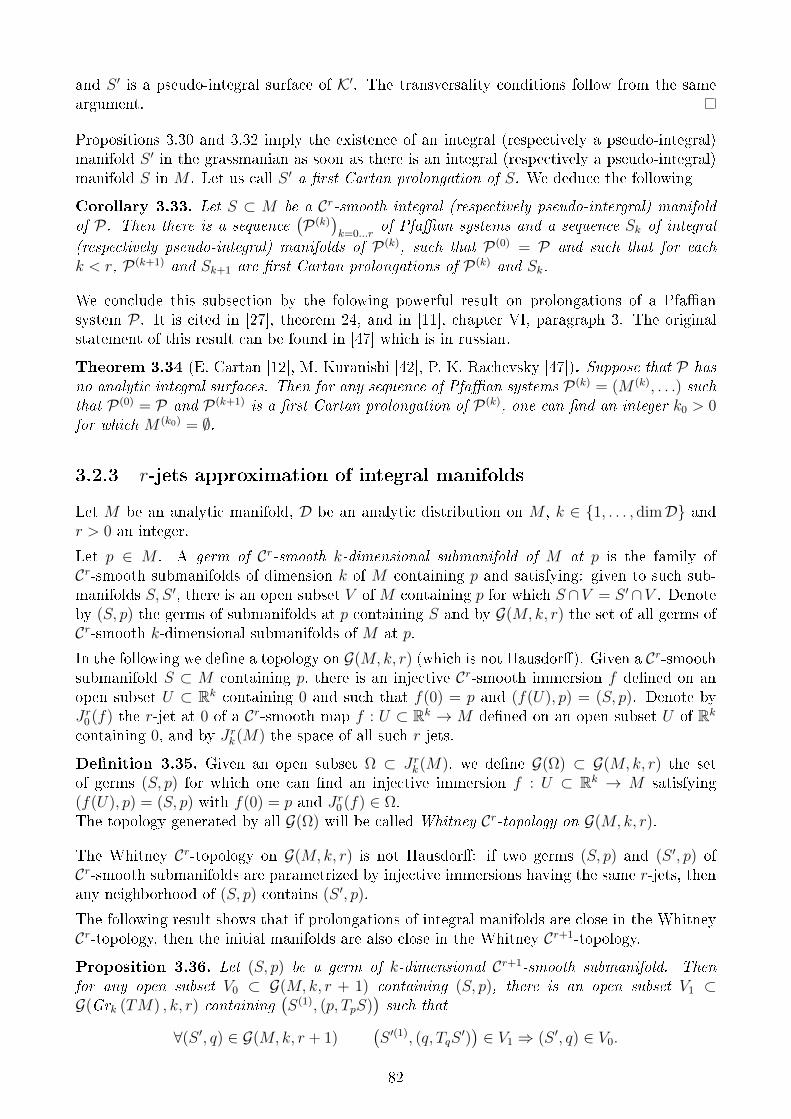
and S ′ is a pseudo-integral surface of K′. The transversality conditions follow from the sameargument.

Propositions 3.30 and 3.32 imply the existence of an integral (respectively a pseudo-integral)manifold S ′ in the grassmanian as soon as there is an integral (respectively a pseudo-integral)manifold S in M . Let us call S ′ a rst Cartan prolongation of S. We deduce the following

Corollary 3.33. Let S ⊂ M be a Cr-smooth integral (respectively pseudo-intergral) manifoldof P. Then there is a sequence

(P(k)

)k=0...r

of Pfaan systems and a sequence Sk of integral(respectively pseudo-integral) manifolds of P(k), such that P(0) = P and such that for eachk < r, P(k+1) and Sk+1 are rst Cartan prolongations of P(k) and Sk.

We conclude this subsection by the folowing powerful result on prolongations of a Pfaansystem P . It is cited in [27], theorem 24, and in [11], chapter VI, paragraph 3. The originalstatement of this result can be found in [47] which is in russian.

Theorem 3.34 (E. Cartan [12], M. Kuranishi [42], P. K. Rachevsky [47]). Suppose that P hasno analytic integral surfaces. Then for any sequence of Pfaan systems P(k) = (M (k), . . .) suchthat P(0) = P and P(k+1) is a rst Cartan prolongation of P(k), one can nd an integer k0 > 0for which M (k0) = ∅.

3.2.3 r-jets approximation of integral manifolds

Let M be an analytic manifold, D be an analytic distribution on M , k ∈ 1, . . . , dimD andr > 0 an integer.

Let p ∈ M . A germ of Cr-smooth k-dimensional submanifold of M at p is the family ofCr-smooth submanifolds of dimension k of M containing p and satisfying: given to such sub-manifolds S, S ′, there is an open subset V of M containing p for which S ∩V = S ′∩V . Denoteby (S, p) the germs of submanifolds at p containing S and by G(M,k, r) the set of all germs ofCr-smooth k-dimensional submanifolds of M at p.

In the following we dene a topology on G(M,k, r) (which is not Hausdor). Given a Cr-smoothsubmanifold S ⊂ M containing p, there is an injective Cr-smooth immersion f dened on anopen subset U ⊂ Rk containing 0 and such that f(0) = p and (f(U), p) = (S, p). Denote byJr0 (f) the r-jet at 0 of a Cr-smooth map f : U ⊂ Rk → M dened on an open subset U of Rk

containing 0, and by Jrk(M) the space of all such r-jets.

Denition 3.35. Given an open subset Ω ⊂ Jrk(M), we dene G(Ω) ⊂ G(M,k, r) the setof germs (S, p) for which one can nd an injective immersion f : U ⊂ Rk → M satisfying(f(U), p) = (S, p) with f(0) = p and Jr0 (f) ∈ Ω.The topology generated by all G(Ω) will be called Whitney Cr-topology on G(M,k, r).

The Whitney Cr-topology on G(M,k, r) is not Hausdor: if two germs (S, p) and (S ′, p) ofCr-smooth submanifolds are parametrized by injective immersions having the same r-jets, thenany neighborhood of (S, p) contains (S ′, p).

The following result shows that if prolongations of integral manifolds are close in the WhitneyCr-topology, then the initial manifolds are also close in the Whitney Cr+1-topology.

Proposition 3.36. Let (S, p) be a germ of k-dimensional Cr+1-smooth submanifold. Thenfor any open subset V0 ⊂ G(M,k, r + 1) containing (S, p), there is an open subset V1 ⊂G(Grk (TM) , k, r) containing

(S(1), (p, TpS)

)such that

∀(S ′, q) ∈ G(M,k, r + 1)(S ′(1), (q, TqS

′))∈ V1 ⇒ (S ′, q) ∈ V0.

82

Proof. Given a Cr+1-smooth injective immersion f : U →M dened on an open subset U ⊂ Rk,one can dened its rst lift to be the Cr-smooth injective immersion

f (1) : U → Grk(TRd

)dened for all x ∈ U by f (1)(x) = (x, Im df(x)). Notice that if S is a submanifold of Mparametrized by f , then the rst lift S(1) of S is parametrized by f (1). Therefore, by anappropriate choice of coordinates, we just have to show the following

Lemma 3.37. Let f : U ⊂ Rk → Rd be a Cr+1-smooth injective immersion dened on an opensubset U ⊂ Rk containing 0. Then for any neighborhood V0 ⊂ Jr+1

k (Rd) containing Jr+10 (f),

there is a neighborhood V1 ⊂ Jrk(Grk(TRd

)) containing Jr0 (f (1)) at 0, and verifying the following

property:for any Cr+1-smooth injective immersion g dened on an open subset U ′ ⊂ Rk containing 0, ifJr0 (g(1)) ∈ V1, then there is a smooth dieomorphism ϕ : W ⊂ Rk → W ′ ⊂ U , sending 0 to 0and for which Jr+1

0 (g ϕ) ∈ V0.

Proof of Lemma 3.37. Replacing f and g by ψ f ψ′ and by ψ g ψ′ for xed Cr+1-smoothdieomorphisms ψ : Rd → Rd and ψ′ : W ⊂ Rk → W ′ ⊂ U with ψ′(0) = 0, we can proveLemma 3.37 when f is of the form f : x ∈ U 7→ (x, f0(x)), where f0 : U → Rd−k is a Cr+1-smooth map.Since π g(1) = g, we can choose a rst neighborhood V1 of f (1) such that if Jr0 (g(1)) ∈ V1, thenone can nd a C∞-smooth dieomorphism ϕ : W ⊂ Rk → W ′ ⊂ U , sending 0 on 0, such thatg ϕ is of the form x ∈ W 7→ (x, g0(x)), where g0 : W → Rd−k is a Cr+1-smooth map. Noticethat Im d(g ϕ) = Im dg, hence Im dg is generated by the vectors (ei, ∂ig0), i = 1 . . . k, whereB = (e1, . . . , ed) is the canonical basis of Rd and ∂i is the i-th partial derivative. Similarly Im dfis generated by the vectors (ei, ∂if0), i = 1 . . . k.The canonical basis B denes a set of coordinates in Grk

(TRd

)in which the coordinates of

Im df are the coordinates of (∂1f0, . . . , ∂kf0) in (ed−k, . . . , ed), and the coordinates of Im dg arethe coordinates of (∂1g0, . . . , ∂kg0) in (ed−k, . . . , ed). Therefore, saying that the r-jet of Im dgat 0 is close to the r-jet of Im df at 0 means that the same holds for the r-jets at 0 of thepartial derivatives (∂1g0, . . . , ∂kg0) and (∂1f0, . . . , ∂kf0). And with the additionnal assumptionthat g(0) is close to f(0), this means that the (r + 1)-jets of f and g ϕ at 0 are close.

This concludes the proof of Proposition 3.36.

Given a Pfaan system P = (M,D, k; (Di)i), a C∞-smooth integral manifold S of P andp ∈ S, the following result establishes the existence of germs of analytic integral manifolds ofP arbitrarily close to (S, p) in the Whitney Cr-topology.

Proposition 3.38. Let S ⊂ M be a C∞-smooth integral manifold of a Pfaan system P =(M,D, k; (Di)i), p ∈ S and a positive integer r. Then for any open subset V ⊂ G(M,k, r)containing (S, p) one can nd an analytic integral manifold Sa ⊂ M of P and pa ∈ Sa suchthat (Sa, pa) ∈ V .

Proof. We rst prove Proposition 3.38 for r = 0. We need to show that for any open subsetV ⊂ M containing p, one can nd an analytic integral manifold S ′ of P intersecting V . Theset V contains the C∞-smooth integral manifold S ∩ V of P . Hence, one can nd a sequence ofprolongations P(r) = (M (r), . . .) of the Pfaan system P = (M,D, k; (Di)i) such that M (r) 6= ∅for all r (Corollary 3.33). Therefore, Theorem 3.34 implies the existence of an analytic integralsurface of P in V , which concludes the proof in the case when r = 0.We conclude the proof by induction. Let r > 0 and V ⊂ G(M,k, r) be an open subset

83

containing (S, p). By Proposition 3.36, there is an open subset V1 ⊂ G(Grk (TM) , k, r − 1)

containing(S(1), (p, TpS)

)such that for all (S, q) ∈ G(M,k, r) satisfying

(S(1), (q, TqS)

)∈ V1

then (S, q) ∈ V0. Hence given a prolongation P ′ = (M ′,K′, k; (D′i)i, ker dπ) of P on a stratumM ′ containing a prolongation S ′ of S, the germs of V1 contained in G(M ′, k, r − 1) dene anopen set V ′1 of G(M ′, k, r − 1) containing (S ′, (p, TpS)). By shrinking V ′1 if necessary, one canfurther suppose that if (S, q) ∈ V ′1 , then T S ∩ ker dπ is 0. By induction, one can nd ananalytic integral manifold S ′a of P ′ and a point qa ∈ Sa such that (S ′a, qa) ∈ V ′1 . The conclusionfollows immediately from Proposition 3.31.

3.2.4 From smooth to analytic k-reective classical billiards

In this subsection, we show that the existence of a k-pseudo-reective C∞-smooth classicalbilliard implies the existence of a k-reective analytic classical billiard. We also prove thatk-reective C∞-smooth classical billiards can be approximated by r-jets of k-reective analyticbilliards (a more precise meaning will be given).

To establish these results, we translate Propositions 3.22 and 3.23 in terms of Pfaan systemswith transversality conditions. Let D be the classical Birkho's distribution dened on thesubset U of M = (Rd)k constituted by all p = (p1, . . . , pk) such that pj−1, pj, pj+1 do not lie onthe same line for each j modulo k (see Denition 3.21). Denote by π1, . . . , πk : M → Rd themaps given by πj(p) = pj for each j. Given a 2(d− 1)-dimensional vector space E ⊂ D(p), wehave rk dπ|E ≤ d− 1 by construction of Birkho's distribution. We consider the following

Lemma 3.39. A 2(d − 1)-dimensional vector space E ⊂ D(p) is transverse to ker dπj if andonly if rk dπj|E = d− 1.

Proof. By Grassmann's formula, we get dim(ker dπj|D + E) = rk dπj|E + dimD − rk dπj|D.Hence ker dπj|D + E = D if and only if rk dπj|E + dimD = rk dπj|D = d− 1.

Lemma 3.39 implies that in Propositions 3.22 and 3.23 we can replace the terms non-trivial2(d−1)-dimensional integral (respectively pseudo-integral) manifolds of Birkho's distributionD by integral (respectively pseudo-integral) manifolds of the Pfaan system with transversalityconditions given by P = (U,D, 2(d− 1); ker dπ1, . . . , ker dπk).

Theorem 3.40. Suppose that one can nd a local C∞-smooth k-pseudo-reective classical bil-liard (a1, . . . , ak). Then given open subsets V1, . . . , Vk of Rd containing respectively a1, . . . , ak,one can nd a local analytic k-reective classical billiard (b1, . . . , bk) such that bj ⊂ Vj for all j.

Proof. By proposition 3.23 and Lemma 3.39, one can nd a C∞-smooth pseudo-integral man-ifold S of the above dened Pfaan system P , which is contained in V := V1 × . . . × Vk. Inparticular, S is a C∞-smooth pseudo-integral manifold of the Pfaan system P|V := (V,D, 2(d−1); ker dπ1, . . . , ker dπk). Now by Corollary 3.33 and the theorem of Cartan-Kuranishi-Rachevsky(Theorem 3.34), P|V posseses an analytic integral manifold. The conclusion follows from Propo-sition 3.22 and Lemma 3.39.

In the following, we name by k-reective set of a local k-reective billiard (a1, . . . , ak) the set ofits k-periodic orbits p = (p1, p2, . . . , pk) for which there is an open subset U ⊂ a1×a2 containing(p1, p2) and whose elements (q1, q2) ∈ U can be completed into a k-periodic orbit close to p.

84

Theorem 3.41. Suppose that one can nd a local C∞-smooth k-reective classical billiard(a1, . . . , ak). Then given any integer r > 0, any orbit p = (p1, . . . , pk) ∈ a1 × . . . × ak in itsk-reective set, and any neighborhoods V1, . . . , Vk ⊂ G(Rd, d − 1, r) containing respectively thegerms of hypersurfaces (a1, p1), . . . , (ak, pk), one can nd a local analytic k-reective classicalbilliard (b1, . . . , bk) and an orbit q = (q1, . . . , qk) in its k-reective set such that (bj, qj) ∈ Vj forall j.

Remark 3.42. It might be possible that Theorem 3.41 remains valid for a k-pseudo-reectivebilliard (a1, . . . , ak). The answer to this problem can possibly be found using the results of thismanuscript.

Proof. Choose p and V1, . . . , Vd as in the statement of Theorem 3.41. By Proposition 3.22and Lemma 3.39, one can nd a C∞-smooth integral manifold S of the above dened Pfaansystem P such that (πj(S), πj(p)) ∈ Vj for each j. Let an open set W ⊂ G((Rd)k, 2(d −1), r) containing the germ (S, p) be such that any germ (S ′, q) ∈ W transverse to all ker dπjsatises (πj(S

′), πj(q)) ∈ Vj. By Proposition 3.38, the Pfaan system P := ((Rd)k,D, 2(d −1);D1, . . . ,Dk) posseses an analytic integral manifold Sa for which one can nd pa ∈ Sa verifying(Sa, pa) ∈ W . The conclusion follows from Proposition 3.22.

3.2.5 From smooth to analytic k-reective projective billiards

In this subsection, we extend the classical Birkho's distribution and its links with the k-reective classical billiards to projective billiards. In the case of projective billiards, the naturalspace on which the distribution is dened has to be replaced to take into account each eld ofprojective transverse lines.

3.2.5.1 Projective Birkho distribution

Consider the space P(TRd), which can be identied as the set of (p, L) such that p ∈ Rd is apoint and L ⊂ Rd is a line containing p, together with the natural projection Π : P(TRd) →Rd. Consider the manifold M = P(TRd)k and the constructible subset U ⊂ M of elements(p1, L1, . . . pk, Lk), such that for each j (modulo k), (pj, Lj) ∈ P(TRd), pj−1, pj, pj+1 do not lieon the same line, Lj belongs to the plane pj−1pjpj+1 and doesn't coincide with the lines pj−1pjand pj+1pj. Note that when d = 2, U is an open dense subset of M .

We dene for each j the maps projj : M → P(TRd) and πj : M → Rd by

projj(p1, L1, . . . pk, Lk) = (pj, Lj) and πj(p1, L1, . . . pk, Lk) = pj.

In what follows, we introduce the analogue of Birkho's exterior bissectors for elements inU . If P = (p1, L1, . . . pk, Lk) ∈ U , one can dene for each j (modulo k) the line Tj(P ) ⊂ Rd

containing pj and such that the four lines pj−1pj, pj+1pj, Lj Tj(P ) are in the same plane andform a harmonic set of lines. This induces an analytic map U → P(TRd)k which associates toa P ∈ U the element (p1, T1(P ), . . . , pk, Tk(P )).

The analogue of Lemma 3.20 is given by the following

Lemma 3.43. Let B = (α1, . . . , αk) be a local projective billiard in P(RRd) with classicalboundaries a1, . . . , ak and P = (p1, L1, . . . , pk, Lk) ∈ U such that (pj, Lj) ∈ αj for all j. Thenp = (p1, . . . , pk) is a k-periodic orbit of B if and only if Tj(P ) ⊂ Tpjaj for all j.

85

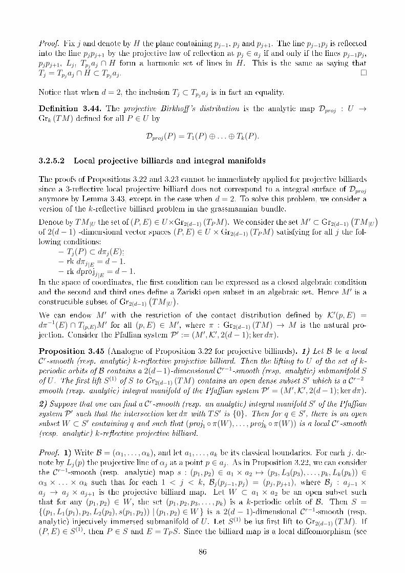
Proof. Fix j and denote by H the plane containing pj−1, pj and pj+1. The line pj−1pj is reectedinto the line pjpj+1 by the projective law of reection at pj ∈ aj if and only if the lines pj−1pj,pjpj+1, Lj, Tpjaj ∩ H form a harmonic set of lines in H. This is the same as saying thatTj = Tpjaj ∩H ⊂ Tpjaj.

Notice that when d = 2, the inclusion Tj ⊂ Tpjaj is in fact an equality.

Denition 3.44. The projective Birkho's distribution is the analytic map Dproj : U →Grk (TM) dened for all P ∈ U by

Dproj(P ) = T1(P )⊕ . . .⊕ Tk(P ).

3.2.5.2 Local projective billiards and integral manifolds

The proofs of Propositions 3.22 and 3.23 cannot be immediately applied for projective billiardssince a 3-reective local projective billiard does not correspond to a integral surface of Dprojanymore by Lemma 3.43, except in the case when d = 2. To solve this problem, we consider aversion of the k-reective billiard problem in the grassmannian bundle.

Denote by TM |U the set of (P,E) ∈ U×Gr2(d−1) (TPM). We consider the setM ′ ⊂ Gr2(d−1)

(TM |U

)of 2(d− 1) -dimensional vector spaces (P,E) ∈ U ×Gr2(d−1) (TPM) satisfying for all j the fol-lowing conditions:

− Tj(P ) ⊂ dπj(E);− rk dπj |E = d− 1.− rk dprojj |E = d− 1.

In the space of coordinates, the rst condition can be expressed as a closed algebraic conditionand the second and third ones dene a Zariski open subset in an algebraic set. Hence M ′ is aconstructible subset of Gr2(d−1)

(TM |U

).

We can endow M ′ with the restriction of the contact distribution dened by K′(p, E) =dπ−1(E) ∩ T(p,E)M

′ for all (p, E) ∈ M ′, where π : Gr2(d−1) (TM) → M is the natural pro-jection. Consider the Pfaan system P ′ := (M ′,K′, 2(d− 1); ker dπ).

Proposition 3.45 (Analogue of Proposition 3.22 for projective billiards). 1) Let B be a localCr-smooth (resp. analytic) k-reective projective billiard. Then the lifting to U of the set of k-periodic orbits of B contains a 2(d−1)-dimensional Cr−1-smooth (resp. analytic) submanifold Sof U . The rst lift S(1) of S to Gr2(d−1) (TM) contains an open dense subset S ′ which is a Cr−2-smooth (resp. analytic) integral manifold of the Pfaan system P ′ = (M ′,K′, 2(d− 1); ker dπ).

2) Suppose that one can nd a Cr-smooth (resp. an analytic) integral manifold S ′ of the Pfaansystem P ′ such that the intersection ker dπ with TS ′ is 0. Then for q ∈ S ′, there is an opensubset W ⊂ S ′ containing q and such that (proj1 π(W ), . . . , projk π(W )) is a local Cr-smooth(resp. analytic) k-reective projective billiard.

Proof. 1) Write B = (α1, . . . , αk), and let a1, . . . , ak be its classical boundaries. For each j, de-note by Lj(p) the projective line of αj at a point p ∈ aj. As in Proposition 3.22, we can considerthe Cr−1-smooth (resp. analytic) map s : (p1, p2) ∈ a1 × a2 7→ (p3, L3(p3), . . . , pk, Lk(pk)) ∈α3 × . . . × αk such that for each 1 < j < k, Bj(pj−1, pj) = (pj, pj+1), where Bj : aj−1 ×aj → aj × aj+1 is the projective billiard map. Let W ⊂ a1 × a2 be an open subset suchthat for any (p1, p2) ∈ W , the set (p1, p2, p3, . . . , pk) is a k-periodic orbit of B. Then S =(p1, L1(p1), p2, L2(p2), s(p1, p2)) | (p1, p2) ∈ W is a 2(d − 1)-dimensional Cr−1-smooth (resp.analytic) injectively immersed submanifold of U . Let S(1) be its rst lift to Gr2(d−1) (TM). If(P,E) ∈ S(1), then P ∈ S and E = TPS. Since the billiard map is a local dieomorphism (see

86

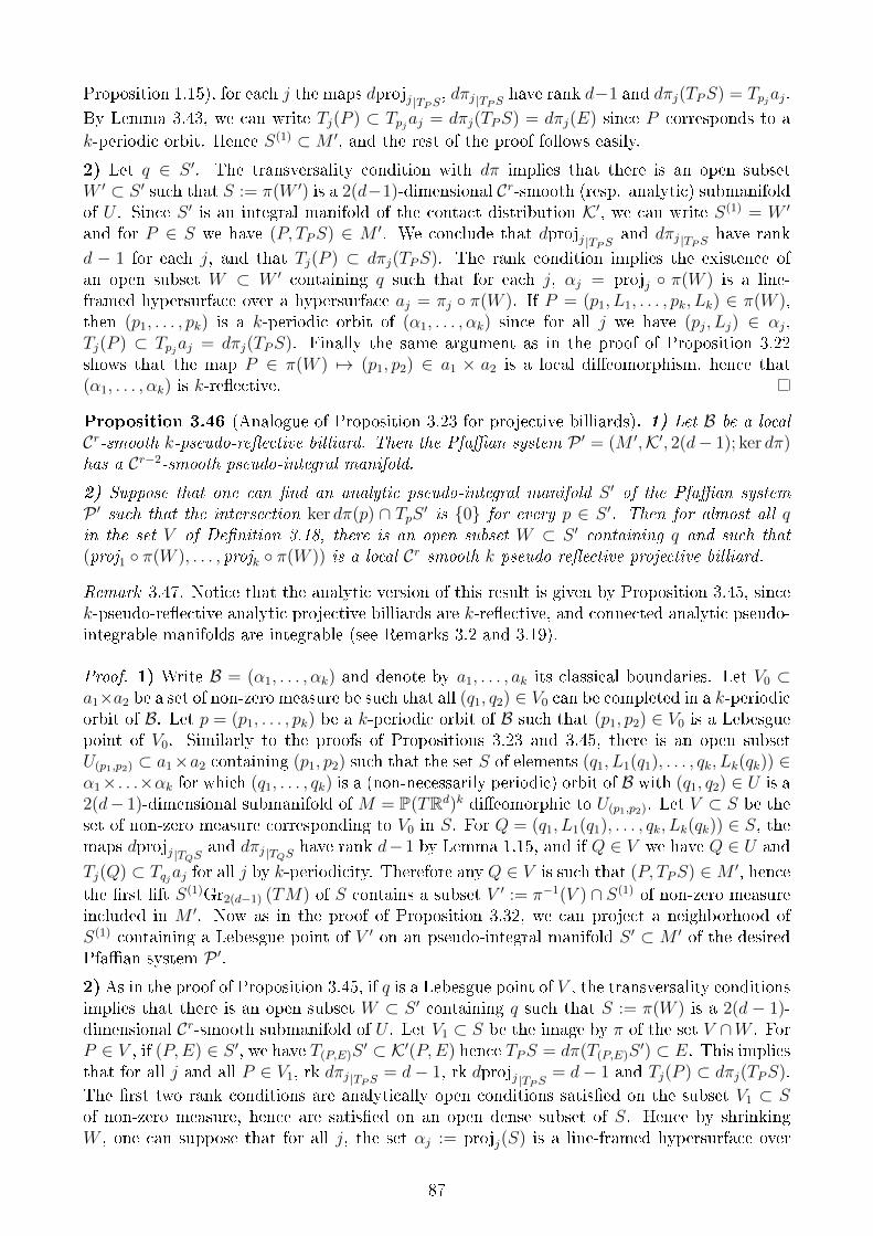
Proposition 1.15), for each j the maps dprojj |TPS, dπj |TPS have rank d−1 and dπj(TPS) = Tpjaj.

By Lemma 3.43, we can write Tj(P ) ⊂ Tpjaj = dπj(TPS) = dπj(E) since P corresponds to ak-periodic orbit. Hence S(1) ⊂M ′, and the rest of the proof follows easily.

2) Let q ∈ S ′. The transversality condition with dπ implies that there is an open subsetW ′ ⊂ S ′ such that S := π(W ′) is a 2(d−1)-dimensional Cr-smooth (resp. analytic) submanifoldof U . Since S ′ is an integral manifold of the contact distribution K′, we can write S(1) = W ′

and for P ∈ S we have (P, TPS) ∈ M ′. We conclude that dprojj |TPS and dπj |TPS have rank

d − 1 for each j, and that Tj(P ) ⊂ dπj(TPS). The rank condition implies the existence ofan open subset W ⊂ W ′ containing q such that for each j, αj = projj π(W ) is a line-framed hypersurface over a hypersurface aj = πj π(W ). If P = (p1, L1, . . . , pk, Lk) ∈ π(W ),then (p1, . . . , pk) is a k-periodic orbit of (α1, . . . , αk) since for all j we have (pj, Lj) ∈ αj,Tj(P ) ⊂ Tpjaj = dπj(TPS). Finally the same argument as in the proof of Proposition 3.22shows that the map P ∈ π(W ) 7→ (p1, p2) ∈ a1 × a2 is a local dieomorphism, hence that(α1, . . . , αk) is k-reective.

Proposition 3.46 (Analogue of Proposition 3.23 for projective billiards). 1) Let B be a localCr-smooth k-pseudo-reective billiard. Then the Pfaan system P ′ = (M ′,K′, 2(d− 1); ker dπ)has a Cr−2-smooth pseudo-integral manifold.

2) Suppose that one can nd an analytic pseudo-integral manifold S ′ of the Pfaan systemP ′ such that the intersection ker dπ(p) ∩ TpS ′ is 0 for every p ∈ S ′. Then for almost all qin the set V of Denition 3.18, there is an open subset W ⊂ S ′ containing q and such that(proj1 π(W ), . . . , projk π(W )) is a local Cr-smooth k-pseudo-reective projective billiard.

Remark 3.47. Notice that the analytic version of this result is given by Proposition 3.45, sincek-pseudo-reective analytic projective billiards are k-reective, and connected analytic pseudo-integrable manifolds are integrable (see Remarks 3.2 and 3.19).

Proof. 1) Write B = (α1, . . . , αk) and denote by a1, . . . , ak its classical boundaries. Let V0 ⊂a1×a2 be a set of non-zero measure be such that all (q1, q2) ∈ V0 can be completed in a k-periodicorbit of B. Let p = (p1, . . . , pk) be a k-periodic orbit of B such that (p1, p2) ∈ V0 is a Lebesguepoint of V0. Similarly to the proofs of Propositions 3.23 and 3.45, there is an open subsetU(p1,p2) ⊂ a1×a2 containing (p1, p2) such that the set S of elements (q1, L1(q1), . . . , qk, Lk(qk)) ∈α1× . . .×αk for which (q1, . . . , qk) is a (non-necessarily periodic) orbit of B with (q1, q2) ∈ U is a2(d− 1)-dimensional submanifold of M = P(TRd)k dieomorphic to U(p1,p2). Let V ⊂ S be theset of non-zero measure corresponding to V0 in S. For Q = (q1, L1(q1), . . . , qk, Lk(qk)) ∈ S, themaps dprojj |TQS and dπj |TQS have rank d− 1 by Lemma 1.15, and if Q ∈ V we have Q ∈ U and

Tj(Q) ⊂ Tqjaj for all j by k-periodicity. Therefore any Q ∈ V is such that (P, TPS) ∈M ′, hencethe rst lift S(1)Gr2(d−1) (TM) of S contains a subset V ′ := π−1(V ) ∩ S(1) of non-zero measureincluded in M ′. Now as in the proof of Proposition 3.32, we can project a neighborhood ofS(1) containing a Lebesgue point of V ′ on an pseudo-integral manifold S ′ ⊂ M ′ of the desiredPfaan system P ′.2) As in the proof of Proposition 3.45, if q is a Lebesgue point of V , the transversality conditionsimplies that there is an open subset W ⊂ S ′ containing q such that S := π(W ) is a 2(d − 1)-dimensional Cr-smooth submanifold of U . Let V1 ⊂ S be the image by π of the set V ∩W . ForP ∈ V , if (P,E) ∈ S ′, we have T(P,E)S

′ ⊂ K′(P,E) hence TPS = dπ(T(P,E)S′) ⊂ E. This implies

that for all j and all P ∈ V1, rk dπj |TPS = d− 1, rk dprojj |TPS = d− 1 and Tj(P ) ⊂ dπj(TPS).The rst two rank conditions are analytically open conditions satised on the subset V1 ⊂ Sof non-zero measure, hence are satised on an open dense subset of S. Hence by shrinkingW , one can suppose that for all j, the set αj := projj(S) is a line-framed hypersurface over

87

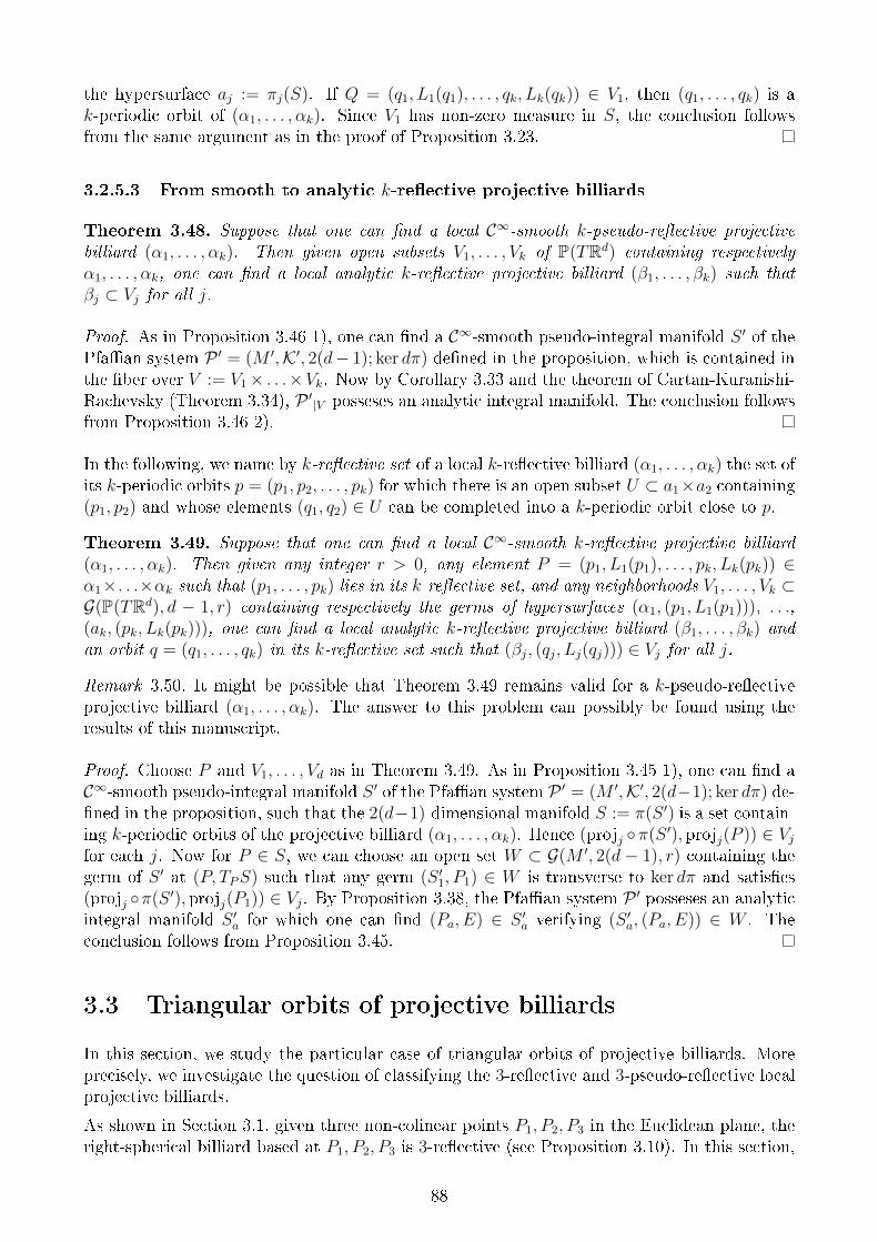
the hypersurface aj := πj(S). If Q = (q1, L1(q1), . . . , qk, Lk(qk)) ∈ V1, then (q1, . . . , qk) is ak-periodic orbit of (α1, . . . , αk). Since V1 has non-zero measure in S, the conclusion followsfrom the same argument as in the proof of Proposition 3.23.

3.2.5.3 From smooth to analytic k-reective projective billiards

Theorem 3.48. Suppose that one can nd a local C∞-smooth k-pseudo-reective projectivebilliard (α1, . . . , αk). Then given open subsets V1, . . . , Vk of P(TRd) containing respectivelyα1, . . . , αk, one can nd a local analytic k-reective projective billiard (β1, . . . , βk) such thatβj ⊂ Vj for all j.

Proof. As in Proposition 3.46 1), one can nd a C∞-smooth pseudo-integral manifold S ′ of thePfaan system P ′ = (M ′,K′, 2(d− 1); ker dπ) dened in the proposition, which is contained inthe ber over V := V1× . . .×Vk. Now by Corollary 3.33 and the theorem of Cartan-Kuranishi-Rachevsky (Theorem 3.34), P ′|V posseses an analytic integral manifold. The conclusion followsfrom Proposition 3.46 2).

In the following, we name by k-reective set of a local k-reective billiard (α1, . . . , αk) the set ofits k-periodic orbits p = (p1, p2, . . . , pk) for which there is an open subset U ⊂ a1×a2 containing(p1, p2) and whose elements (q1, q2) ∈ U can be completed into a k-periodic orbit close to p.

Theorem 3.49. Suppose that one can nd a local C∞-smooth k-reective projective billiard(α1, . . . , αk). Then given any integer r > 0, any element P = (p1, L1(p1), . . . , pk, Lk(pk)) ∈α1×. . .×αk such that (p1, . . . , pk) lies in its k-reective set, and any neighborhoods V1, . . . , Vk ⊂G(P(TRd), d − 1, r) containing respectively the germs of hypersurfaces (α1, (p1, L1(p1))), . . .,(ak, (pk, Lk(pk))), one can nd a local analytic k-reective projective billiard (β1, . . . , βk) andan orbit q = (q1, . . . , qk) in its k-reective set such that (βj, (qj, Lj(qj))) ∈ Vj for all j.

Remark 3.50. It might be possible that Theorem 3.49 remains valid for a k-pseudo-reectiveprojective billiard (α1, . . . , αk). The answer to this problem can possibly be found using theresults of this manuscript.

Proof. Choose P and V1, . . . , Vd as in Theorem 3.49. As in Proposition 3.45 1), one can nd aC∞-smooth pseudo-integral manifold S ′ of the Pfaan system P ′ = (M ′,K′, 2(d−1); ker dπ) de-ned in the proposition, such that the 2(d−1)-dimensional manifold S := π(S ′) is a set contain-ing k-periodic orbits of the projective billiard (α1, . . . , αk). Hence (projj π(S ′), projj(P )) ∈ Vjfor each j. Now for P ∈ S, we can choose an open set W ⊂ G(M ′, 2(d − 1), r) containing thegerm of S ′ at (P, TPS) such that any germ (S ′1, P1) ∈ W is transverse to ker dπ and satises(projj π(S ′), projj(P1)) ∈ Vj. By Proposition 3.38, the Pfaan system P ′ posseses an analyticintegral manifold S ′a for which one can nd (Pa, E) ∈ S ′a verifying (S ′a, (Pa, E)) ∈ W . Theconclusion follows from Proposition 3.45.

3.3 Triangular orbits of projective billiards

In this section, we study the particular case of triangular orbits of projective billiards. Moreprecisely, we investigate the question of classifying the 3-reective and 3-pseudo-reective localprojective billiards.

As shown in Section 3.1, given three non-colinear points P1, P2, P3 in the Euclidean plane, theright-spherical billiard based at P1, P2, P3 is 3-reective (see Proposition 3.10). In this section,

88

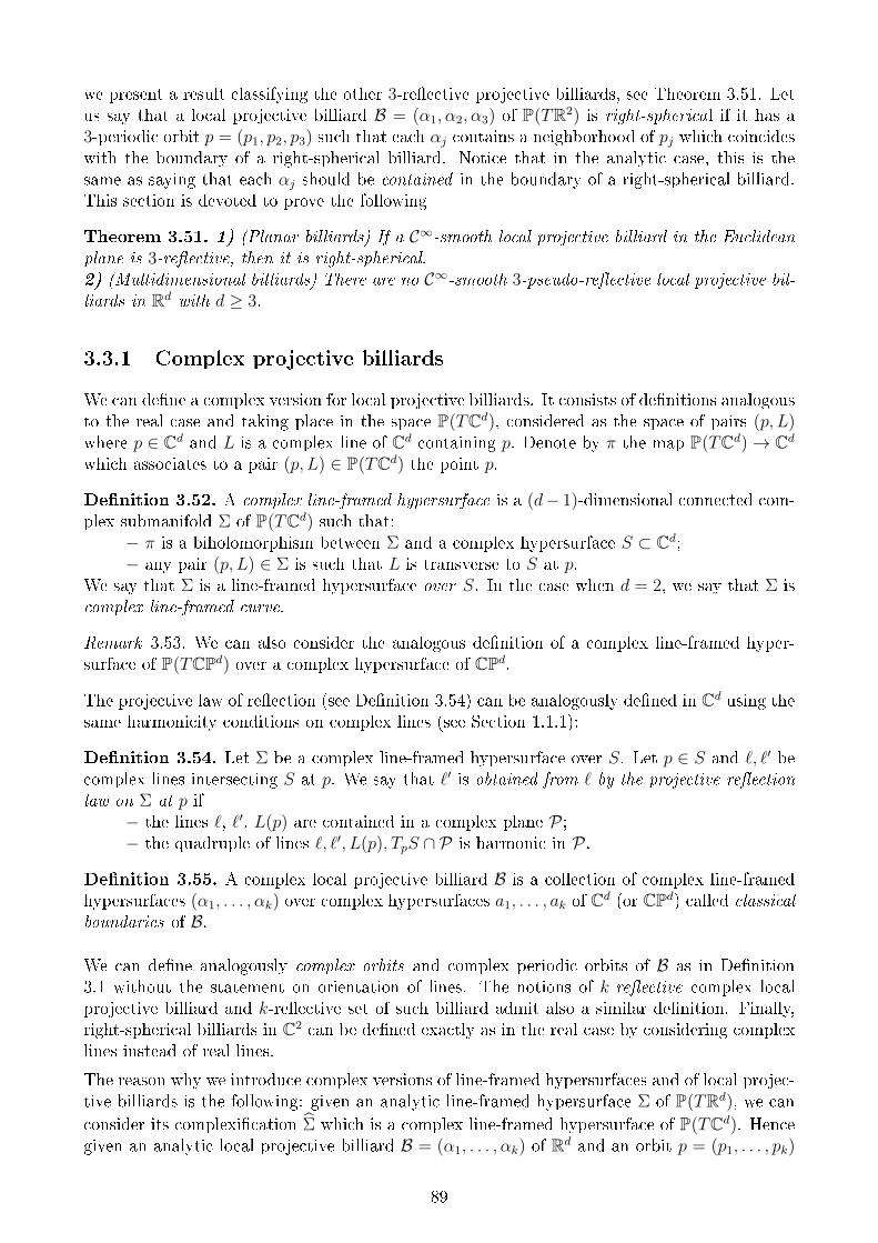
we present a result classifying the other 3-reective projective billiards, see Theorem 3.51. Letus say that a local projective billiard B = (α1, α2, α3) of P(TR2) is right-spherical if it has a3-periodic orbit p = (p1, p2, p3) such that each αj contains a neighborhood of pj which coincideswith the boundary of a right-spherical billiard. Notice that in the analytic case, this is thesame as saying that each αj should be contained in the boundary of a right-spherical billiard.This section is devoted to prove the following

Theorem 3.51. 1) (Planar billiards) If a C∞-smooth local projective billiard in the Euclideanplane is 3-reective, then it is right-spherical.2) (Multidimensional billiards) There are no C∞-smooth 3-pseudo-reective local projective bil-liards in Rd with d ≥ 3.

3.3.1 Complex projective billiards

We can dene a complex version for local projective billiards. It consists of denitions analogousto the real case and taking place in the space P(TCd), considered as the space of pairs (p, L)where p ∈ Cd and L is a complex line of Cd containing p. Denote by π the map P(TCd)→ Cd

which associates to a pair (p, L) ∈ P(TCd) the point p.

Denition 3.52. A complex line-framed hypersurface is a (d− 1)-dimensional connected com-plex submanifold Σ of P(TCd) such that:

− π is a biholomorphism between Σ and a complex hypersurface S ⊂ Cd;− any pair (p, L) ∈ Σ is such that L is transverse to S at p.

We say that Σ is a line-framed hypersurface over S. In the case when d = 2, we say that Σ iscomplex line-framed curve.

Remark 3.53. We can also consider the analogous denition of a complex line-framed hyper-surface of P(TCPd) over a complex hypersurface of CPd.

The projective law of reection (see Denition 3.54) can be analogously dened in Cd using thesame harmonicity conditions on complex lines (see Section 1.1.1):

Denition 3.54. Let Σ be a complex line-framed hypersurface over S. Let p ∈ S and `, `′ becomplex lines intersecting S at p. We say that `′ is obtained from ` by the projective reectionlaw on Σ at p if

− the lines `, `′, L(p) are contained in a complex plane P ;− the quadruple of lines `, `′, L(p), TpS ∩ P is harmonic in P .

Denition 3.55. A complex local projective billiard B is a collection of complex line-framedhypersurfaces (α1, . . . , αk) over complex hypersurfaces a1, . . . , ak of Cd (or CPd) called classicalboundaries of B.

We can dene analogously complex orbits and complex periodic orbits of B as in Denition3.1 without the statement on orientation of lines. The notions of k-reective complex localprojective billiard and k-reective set of such billiard admit also a similar denition. Finally,right-spherical billiards in C2 can be dened exactly as in the real case by considering complexlines instead of real lines.

The reason why we introduce complex versions of line-framed hypersurfaces and of local projec-tive billiards is the following: given an analytic line-framed hypersurface Σ of P(TRd), we canconsider its complexication Σ which is a complex line-framed hypersurface of P(TCd). Hencegiven an analytic local projective billiard B = (α1, . . . , αk) of Rd and an orbit p = (p1, . . . , pk)

89

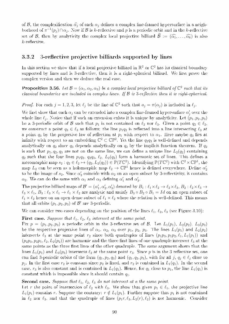
of B, the complexication αj of each αj denes a complex line-framed hypersurface in a neigh-borhood of π−1(pj)∩αj. Now if B is k-reective and p is a periodic orbit and in the k-reectiveset of B, then by analyticity the complex local projective billiard B := (α1, . . . , αk) is alsok-reective.

3.3.2 3-reective projective billiards supported by lines

In this section we show that if a local projective billiard in R2 or C2 has its classical boundarysupported by lines and is 3-reective, then it is a right-spherical billiard. We rst prove thecomplex version and then we deduce the real case.

Proposition 3.56. Let B = (α1, α2, α3) be a complex local projective billiard of C2 such that itsclassical boundaries are included in complex lines. If B is 3-reective then it is right-spherical.

Proof. For each j = 1, 2, 3, let `j be the line of C2 such that aj = π(αj) is included in `j.

We rst show that each αj can be extended into a complex line-framed hypersurface α′j over thewhole line `j. Notice that if such an extension exists it is unique by analyticity. Let (p1, p2, p3)be a 3-periodic orbit of B such that p1 is not contained on `2 nor `3. Given a point q2 ∈ `2,we construct a point q3 ∈ `3 as follows: the line p1q2 is reected into a line intersecting `3 ata point q3 by the projective law of reection at p1 with respect to α1. Here maybe q3 lies atinnity with respect to an embedding C2 ⊂ CP2. Yet the line q2q3 is well-dened and dependsanalytically on q2 since q3 depends analytically on q2 by the implicit function theorem. If q2

is such that p1, q2, q3 are not on the same line, we can dene a unique line L2(q2) containingq2 such that the four lines p1q2, q2q3, `2, L2(q2) form a harmonic set of lines. This denes ameromorphic map s2 : q2 ∈ `2 7→ (q2, L2(q2)) ∈ P(TC2). Identifying P(TC2) with C2×CP1, themap L2 can be seen as a holomorphic map `2 → CP1 hence is dened everywhere. Dene α′2to be the image of s2. Since α′2 coincide with α2 on an open subset by 3-reectivity, it containsα2. We can do the same with α1 and α3 dening α′1 and α′3.

The projective billiard maps of B′ = (α′1, α′2, α

′3) denoted by B1 : `1×`2 → `2×`3, B2 : `2×`3 →

`3 × `1, B3 : `3 × `1 → `1 × `2 are analytic and satisfy B3 B2 B1 = Id on an open subset of`1× `2 hence on an open dense subset of `1× `2 where the relation is well-dened. This meansthat all orbits (p1, p2, p3) of B′ are 3-periodic.

We can consider two cases depending on the position of the lines `1, `2, `3 (see Figure 3.10):

First case. Suppose that `1, `2, `3 intersect at the same point.Fix p = (p1, p2, p3) a periodic orbit in the 3-reective set of B. Let L1(p1), L2(p2), L3(p3)be the respective projective lines of α1, α2, α3 over p1, p2, p3. The lines L1(p1) and L2(p2)intersects `3 at the same point r2 since both quadruples of lines (p1p3, p1p2, `1, L1(p1)) and(p2p3, p2p1, `2, L2(p2)) are harmonic and the three rst lines of one quadruple intersect `3 at thesame points as the three rst lines of the other quadruple. The same argument shows that thelines L1(p1) and L3(p3) intersects `2 at the same point r3. Since p is in the 3-reective set, onecan nd 3-periodic orbits of the form (q1, p2, q3) and (q1, q2, p3), with for all j, qj ∈ `j close topj. In the rst case r2 is constant since p2 is xed, and r2 is contained in L1(q1). In the secondcase, r3 is also constant and is contained in L1(q1). Hence, for q1 close to p1, the line L1(q1) isconstant which is impossible since it should contain q1.

Second case. Suppose that `1, `2, `3 do not intersect at a the same point.Let r the point of intersection of `2 with `3. We show that given p1 ∈ `1, the projective lineL1(p1) contains r. Suppose the contrary: r /∈ L1(p1). Further suppose that p1 is not containedin `2 nor `3, and that the quadruple of lines (p1r, `3, L2(r), `2) is not harmonic. Consider

90

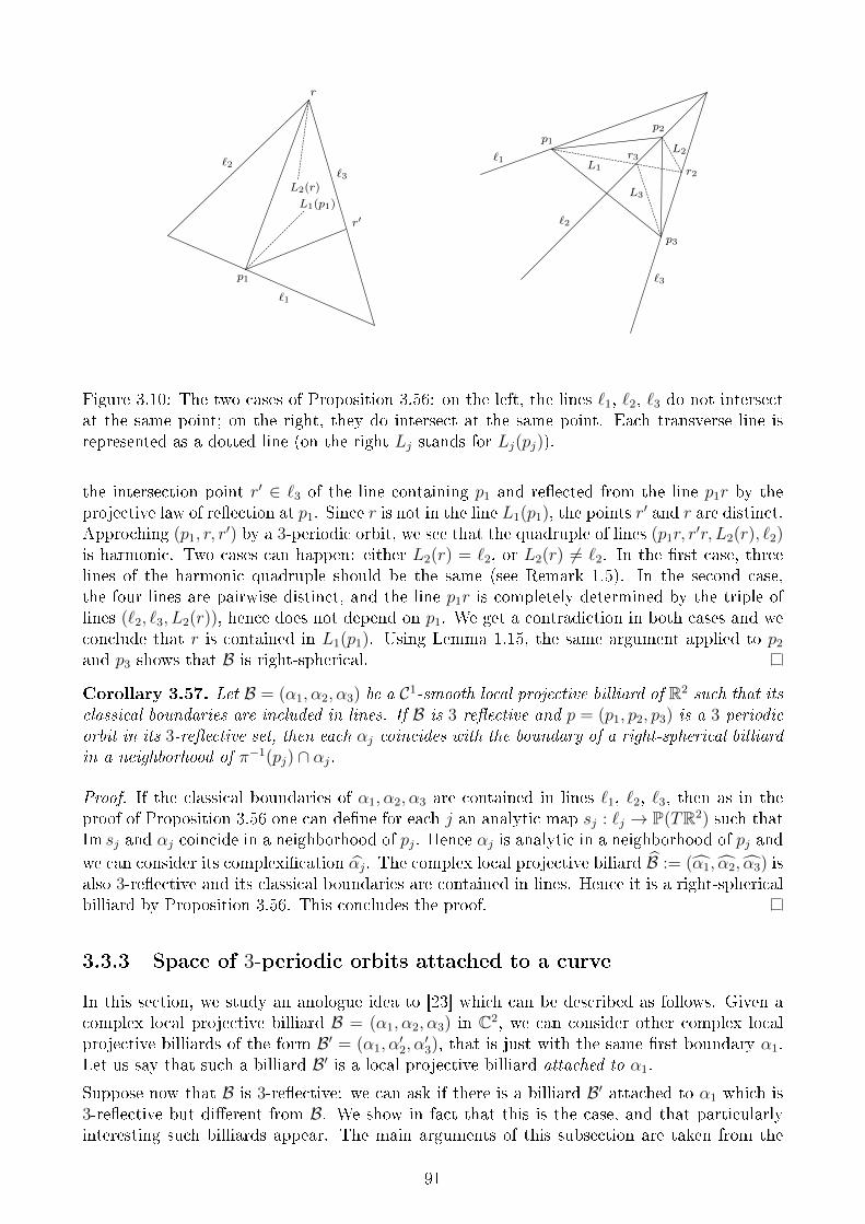
r

p1

r′L1(p1)

L2(r)

`2`3

`1

`1

`2

`3

p1p2

p3

r2

L2

L1

r3

L3

Figure 3.10: The two cases of Proposition 3.56: on the left, the lines `1, `2, `3 do not intersectat the same point; on the right, they do intersect at the same point. Each transverse line isrepresented as a dotted line (on the right Lj stands for Lj(pj)).

the intersection point r′ ∈ `3 of the line containing p1 and reected from the line p1r by theprojective law of reection at p1. Since r is not in the line L1(p1), the points r′ and r are distinct.Approching (p1, r, r

′) by a 3-periodic orbit, we see that the quadruple of lines (p1r, r′r, L2(r), `2)

is harmonic. Two cases can happen: either L2(r) = `2, or L2(r) 6= `2. In the rst case, threelines of the harmonic quadruple should be the same (see Remark 1.5). In the second case,the four lines are pairwise distinct, and the line p1r is completely determined by the triple oflines (`2, `3, L2(r)), hence does not depend on p1. We get a contradiction in both cases and weconclude that r is contained in L1(p1). Using Lemma 1.15, the same argument applied to p2

and p3 shows that B is right-spherical.

Corollary 3.57. Let B = (α1, α2, α3) be a C1-smooth local projective billiard of R2 such that itsclassical boundaries are included in lines. If B is 3-reective and p = (p1, p2, p3) is a 3-periodicorbit in its 3-reective set, then each αj coincides with the boundary of a right-spherical billiardin a neighborhood of π−1(pj) ∩ αj.

Proof. If the classical boundaries of α1, α2, α3 are contained in lines `1, `2, `3, then as in theproof of Proposition 3.56 one can dene for each j an analytic map sj : `j → P(TR2) such thatIm sj and αj coincide in a neighborhood of pj. Hence αj is analytic in a neighborhood of pj andwe can consider its complexication αj. The complex local projective biliard B := (α1, α2, α3) isalso 3-reective and its classical boundaries are contained in lines. Hence it is a right-sphericalbilliard by Proposition 3.56. This concludes the proof.

3.3.3 Space of 3-periodic orbits attached to a curve

In this section, we study an anologue idea to [23] which can be described as follows. Given acomplex local projective billiard B = (α1, α2, α3) in C2, we can consider other complex localprojective billiards of the form B′ = (α1, α

′2, α

′3), that is just with the same rst boundary α1.

Let us say that such a billiard B′ is a local projective billiard attached to α1.

Suppose now that B is 3-reective: we can ask if there is a billiard B′ attached to α1 which is3-reective but dierent from B. We show in fact that this is the case, and that particularlyinteresting such billiards appear. The main arguments of this subsection are taken from the

91

theory of analytic distribution and of an analogue of Birkho's distribution in the complexprojective case.

3.3.3.1 Singular analytic distributions

We recall some denitions and properties of singular analytic distributions, which can be foundin [23].

Denition 3.58 ([23], Lemma 2.27). Let W be a complex manifold, Σ ⊂ W a nowhere denseclosed subset, k ∈ 0, . . . , n and D an analytic eld of k-dimensional planes dened on W \Σ.We say that D is a singular analytic distribution of dimension k and singular set Sing(D) = Σif D extends analytically to no points in Σ and if for all x ∈ W , one can nd holomorphic1-forms α1,..., αp dened on a neighborhood U of x and such that for all y ∈ U \ Σ,

D(y) =

p⋂i=1

kerαi(y).

Singular analytic distributions can be restricted to analytic subsets:

Proposition 3.59 ([23], Denition 2.32). Let W be a complex manifold, M an irreducibleanalytic subset of W and D a singular analytic distibution on W with M * Sing(D). Thenthere exists an open dense subset M o

reg of point x ∈Mreg for which

D|M(x) := D(x) ∩ TxM

has minimal dimension. We say that D|M is a singular analytic distribution on M of singularset Sing(D) := M \M o

reg.

Remark 3.60. When M is not irreducible anymore, we still can restrict D to M by looking atits restriction to each of the irreducible components of M .

As in the smooth case, we can look for integral surfaces dened by the following

Denition 3.61 ([23], Denition 2.34). Let D be a k-dimensional analytic distribution on anirreducible analytic subset M and ` ∈ 0, . . . , k. An integral `-surface of D is a submanifoldS ⊂ M \ Sing(D) of dimension ` such that for all x ∈ S, we have the inclusion TxS ⊂ D(x).The analytic distribution D is said to be integrable if each x ∈M \ Sing(D) is contained in anintegral k-surface. (In this case the k-dimensional integral surfaces form a holomorphic foliationof the manifold M \ Sing(D), by Frobenius theorem.)

We can nally introduce the following lemma, which will be used in a key result (Corollary3.69). We recall here that the analytic closure of a subset A of a complex manifold W , is thesmallest analytic subset of W containing A. We denote it by A

an.

Lemma 3.62 ([23], Lemma 2.38). Let D be a k-dimensional singular analytic distribution onan analytic subset N and S be a k-dimensional integral surface of D. Then the restriction ofD to S

anis an integrable analytic distribution of dimension k.

The proof is the same as in [23]:

92

Proof. Write M = San. First, let us prove that D|M is k-dimensional. Consider the subset

A :=x ∈M \ Sing(D|M) | D(x) ⊂ TxM

.

It contains S \ Sing(D|M), hence its closure, which is an analytic subset of M , contains S. Bydenition, A

an= M which implies that D|M is k-dimensional.

Now let us show that D|M is integrable. The argument is similar: dene the subset B of thosex ∈ M \ Sing(D|M) such that the Frobenius integrability condition is satised. B containsS \ Sing(D|M) and its closure is an analytic subset of M containing S, hence it is the wholeM . Thus Frobenius theorem can be applied on the manifold M \ Sing(D|M), which implies theresult.

3.3.3.2 Birkho's distribution and the 3-reective billiard problem

In this section we dene an analogue of Birkho's distribution in the case of complex localprojective billiards attached to a xed line-framed curve α. We give an analogue of Proposition3.22 for such billiards at Proposition 3.64.

We rst dene the space of the distribution. Let L be the ber bundle

L = P(TCP2) ×CP2

P(TCP2)

that is the set of triples (p, L, T ) where p ∈ CP2 and L, T are lines in TpCP2. Consider thespace α × L × L of triples P = (P1, P2, P3) where P1 = (p1, L1) ∈ α, P2 = (p2, L2, T2) ∈ L,P3 = (p3, L3, T3) ∈ L.Consider the subspace M0

α of 3-periodic billiard orbits having one reection in α, that is theset of elements P ∈ α×L×L such that the points p1, p2, p3 do not lie on the same line and thequadruples of lines (p1p2, p1p3, L1, Tp1α), (p2p3, p2p1, L2, T2), (p3p1, p3p2, L3, T3) form harmonicsets of distinct lines. Denote by Mα the analytic closure of M0

α.

We use the same notations for the dierent projections as in Section 3.2:− proj1 : α × L2 → α, proj2, proj3 : α × L2 → P(TCP2) dened for all P ∈ α × L2 and

all integers j = 1, 2, 3 by projj(P ) = (pj, Lj);− π1, π2, π3 : α × L2 → CP2 dened for all P ∈ α × L2 and all integer j = 1, 2, 3 by

πj(P ) = pj.

Denition 3.63. We call Birkho's distribution attached to α the restriction Dα to Mα of theanalytic distribution D dened for all P ∈ α× L2 by

D(P ) = dπ2−1(T2) ∩ dπ3

−1(T3).

Proposition 3.64 (Analogue of Proposition 3.22 for Dα). Let P ∈M0α such that one can nd a

2-dimensional integral analytic surface S of Dα containing P . Suppose that for each j = 1, 2, 3the restrictions of projj and πj to S have rank 1. Then there exists a neighborhood U of P inS such that the complex local projective billiard (α, proj2(U), proj3(U)) is 3-reective.

Proof. Let U ⊂ S be an open subset such that α2 := proj2(U) and α3 := proj3(U) are complexline-framed curves over the complex curves a2 := π2(U) and a3 := π3(U). Since S is an integralsurface of D, for Q = (q1, L1, q2, L2, T2, q3, L3, T3) ∈ U we can write Tq2a2 = dπ2(TQS) ⊂ T2,hence Tq2a2 = T2 and it follows that the quadruple of lines (q2q1, q2q3, L2, Tq2a2) is harmonic,and a similar argument can be applied to the lines through q3. Hence (q1, q2, q3) is a 3-periodicorbit of B := (α, α2, α3).

93

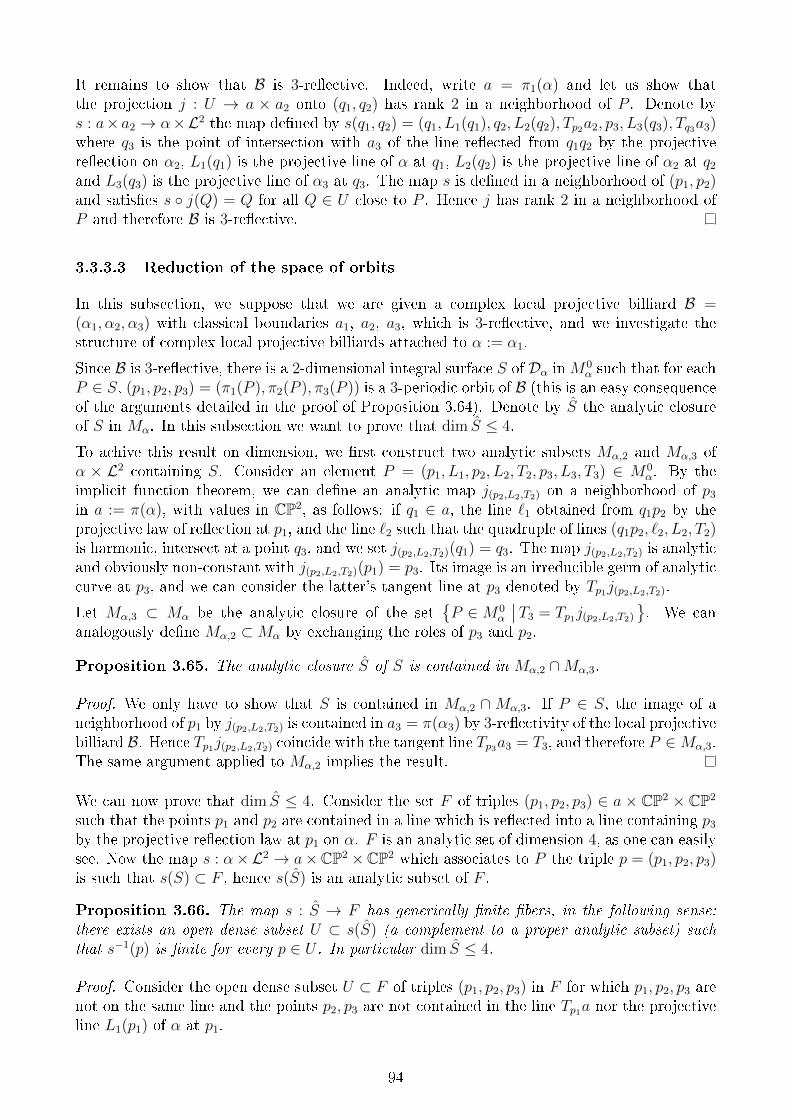
It remains to show that B is 3-reective. Indeed, write a = π1(α) and let us show thatthe projection j : U → a × a2 onto (q1, q2) has rank 2 in a neighborhood of P . Denote bys : a× a2 → α×L2 the map dened by s(q1, q2) = (q1, L1(q1), q2, L2(q2), Tp2a2, p3, L3(q3), Tq3a3)where q3 is the point of intersection with a3 of the line reected from q1q2 by the projectivereection on α2, L1(q1) is the projective line of α at q1, L2(q2) is the projective line of α2 at q2

and L3(q3) is the projective line of α3 at q3. The map s is dened in a neighborhood of (p1, p2)and satises s j(Q) = Q for all Q ∈ U close to P . Hence j has rank 2 in a neighborhood ofP and therefore B is 3-reective.

3.3.3.3 Reduction of the space of orbits

In this subsection, we suppose that we are given a complex local projective billiard B =(α1, α2, α3) with classical boundaries a1, a2, a3, which is 3-reective, and we investigate thestructure of complex local projective billiards attached to α := α1.

Since B is 3-reective, there is a 2-dimensional integral surface S of Dα inM0α such that for each

P ∈ S, (p1, p2, p3) = (π1(P ), π2(P ), π3(P )) is a 3-periodic orbit of B (this is an easy consequenceof the arguments detailed in the proof of Proposition 3.64). Denote by S the analytic closureof S in Mα. In this subsection we want to prove that dim S ≤ 4.

To achive this result on dimension, we rst construct two analytic subsets Mα,2 and Mα,3 ofα × L2 containing S. Consider an element P = (p1, L1, p2, L2, T2, p3, L3, T3) ∈ M0

α. By theimplicit function theorem, we can dene an analytic map j(p2,L2,T2) on a neighborhood of p3

in a := π(α), with values in CP2, as follows: if q1 ∈ a, the line `1 obtained from q1p2 by theprojective law of reection at p1, and the line `2 such that the quadruple of lines (q1p2, `2, L2, T2)is harmonic, intersect at a point q3, and we set j(p2,L2,T2)(q1) = q3. The map j(p2,L2,T2) is analyticand obviously non-constant with j(p2,L2,T2)(p1) = p3. Its image is an irreducible germ of analyticcurve at p3, and we can consider the latter's tangent line at p3 denoted by Tp1j(p2,L2,T2).

Let Mα,3 ⊂ Mα be the analytic closure of the setP ∈M0

α

∣∣T3 = Tp1j(p2,L2,T2)

. We can

analogously dene Mα,2 ⊂Mα by exchanging the roles of p3 and p2.

Proposition 3.65. The analytic closure S of S is contained in Mα,2 ∩Mα,3.

Proof. We only have to show that S is contained in Mα,2 ∩Mα,3. If P ∈ S, the image of aneighborhood of p1 by j(p2,L2,T2) is contained in a3 = π(α3) by 3-reectivity of the local projectivebilliard B. Hence Tp1j(p2,L2,T2) coincide with the tangent line Tp3a3 = T3, and therefore P ∈Mα,3.The same argument applied to Mα,2 implies the result.

We can now prove that dim S ≤ 4. Consider the set F of triples (p1, p2, p3) ∈ a × CP2 × CP2

such that the points p1 and p2 are contained in a line which is reected into a line containing p3

by the projective reection law at p1 on α. F is an analytic set of dimension 4, as one can easilysee. Now the map s : α×L2 → a×CP2 ×CP2 which associates to P the triple p = (p1, p2, p3)is such that s(S) ⊂ F , hence s(S) is an analytic subset of F .

Proposition 3.66. The map s : S → F has generically nite bers, in the following sense:there exists an open dense subset U ⊂ s(S) (a complement to a proper analytic subset) suchthat s−1(p) is nite for every p ∈ U . In particular dim S ≤ 4.

Proof. Consider the open dense subset U ⊂ F of triples (p1, p2, p3) in F for which p1, p2, p3 arenot on the same line and the points p2, p3 are not contained in the line Tp1a nor the projectiveline L1(p1) of α at p1.

94

Consider p = (p1, p2, p3) ∈ U and suppose that the ber s−1(p) is not nite. By construction,s−1(p) is an analytic subset contained in (p1, L1(p1))×p2×P(Tp2CP2)2×p3×P(Tp3CP2)2,hence it is algebraic by Chow's theorem (see [31]). Since s−1 is not nite, at least one of theprojection from s−1(p) to L2, T2, L3 or T3 is innite. Without loss of generality we supposethat the projection to T2 is innite: the image of such projection is an innite analytic subsetin P(Tp2CP2) ' CP1, hence is the whole CP1 by Chow's theorem.

Therefore we can consider an element P = (p1, L1, p2, L2, T2, p3, L3, T3) ∈ s−1(p) for which T2

is dierent from the lines p1p2 and p2p3 with usual identication. By the same argument, wecan consider another element P ′ ∈ s−1(p) of the form P ′ = (p1, L1, p2, L

′2, L2, p3, L

′3, T

′3), that is

the projection on T2 of P ′ gives previous L2. Since P and P ′ are in Mα, the quadruple of lines(p1p2, p2p3, L2, T2) and (p1p2, p2p3, L

′2, L2) are harmonic, hence L′2 = T2.

Since P ∈ Mα,3, T3 is dened by the relation T3 = Tp1j(p2,L2,T2). Applying the same argumentto P ′ we get T ′3 = Tp1j(p2,T2,L2). Now, permuting L2 and T2 doesn't change the projectivereection law at p2, and j(p2,L2,T2) = j(p2,T2,L2), therefore T3 = T ′3. The harmonicity conditionsat p3 implies that L3 = L′3.

Thus we just proved that P = (p1, L1, p2, L2, T2, p3, L3, T3) and P ′ = (p1, L1, p2, T2, L2, p3, L3, T3).But if we consider now that P, P ′ ∈Mα,2, by the same arguments we get that T2 = Tp1j(p1,L3,T3) =L2. This contradicts the harmonicity condition of the quadruple of lines (p1p2, p1p3, L2, T2).Hence s−1(p) is nite.

Given a point p1 ∈ a = π(α1), we denote by Sp1 the set π1−1(p1)∩ S. It is algebraic by Chow's

theorem.

Lemma 3.67. Suppose dim S ≥ 3. Then for all p1 lying outside a discrete subset of a we haveeither π2(Sp1) = CP2 or π3(Sp1) = CP2.

Proof. For j = 2, 3 and any p1 ∈ a, the set πj(Sp1) ⊂ CP2 is algebraic by Chow's theorem andcontains the classical boundary aj = π(αj), hence it has dimension at least 1. Now since themap π1 : S → a is surjective, for p1 lying outside a discrete subset a∗ of a the algebraic set Sp1has dimension at least 2. And exactly as in the proof of Proposition 3.66, the restriction of sto Sp1 has generically nite bers. Hence if p1 /∈ a∗ we have dim s(Sp1) ≥ 2.

Suppose that π2(Sp1) has dimension 1. Hence for all points p2 in an open and dense subsetof π2(Sp1), the ber over p2 of the projection s(Sp1) → π2(Sp1) sending (p1, p2, p3) to p2 hasdimension 1. By denition of F , this ber over a xed point p2 is contained in the set of triples(p1, p2, p3) for which p3 is in a line ` determined by p1 and p2: ` is obtained from the line p1p2 bythe projective law of reection on α at p1. Hence the ber over p2 contains all triples (p1, p2, p3)where p3 ∈ `. Therefore π3(Sp1) contains all lines ` obtained by the projective law of reectionfrom a line p1p2 where p2 ∈ π2(Sp1).

If a2 is not contained in a line, there are innitely many such lines ` and we get π3(Sp1) = CP2.If a2 is contained in a line, we get the same result by choosing p1 outside this line.

3.3.3.4 Integrability of Birkho's distribution on S

In this subsection, we suppose that we are given a complex local projective billiard B =(α1, α2, α3) with classical boundaries a1, a2, a3, which is 3-reective. We consider the re-striction to S of Birkho's distribution attached to α1, denoted by DS. We rst compute thedimension of DS and then we show that it is integrable.

Proposition 3.68. The singular analytic distribution DS is 2-dimensional.

95

Proof. We rst have dimDS ≥ dimS = 2 since TPS ⊂ DS(P ) for P ∈ S. By Proposition 3.66,2 ≤ dim S ≤ 4 and so is dimDS. We consider two cases: dim S = 3 and dim S = 4. In bothcases, we consider a regular point P = (p1, L1, p2, L2, T2, p3, L3, T3) of S such that dimDS(P )

is minimal. We can further suppose that P ∈M0α since S ∩M0

α is an open dense subset of S.

Case when dim S = 3. We have to nd one vector u ∈ TP S which is not in DS(P ). By Lemma3.67 we can suppose that p1 satises without loss generality π2(Sp1) = CP2. Hence there is apath u(t) ∈ S such that u(0) = P and π2 u(t) is contained in the the line p1p2 with non-zeroderivative at 0. The vector u′(0) of TP S is such that dπ2 · u′(0) is a non-zero vector directedalong the line p1p2. Hence dπ2 · u′(0) /∈ T2 since T2 6= p1p2 because P ∈M0

α. We conclude thatu′(0) /∈ DS(P ).

Case when dim S = 4. Let us nd two linearly independent vectors u, v ∈ TP S such thatDS(P ) and the plane spanned by (u, v) intersect by 0. We can suppose that p1 is such thatSp1 = 3, and as in the proof of Proposition 3.66 that s(Sp1) = F ∩(p1 × (CP2)2). Let u(t) ∈ Sbe a path such that u(0) = P , π2 u(t) belongs to the line p1p2 with non-zero derivative at 0and π3 u(t) is contant equal to p3. Now exchange the role of p2 and p3 and dene similarly apath v(t) such that v(0) = P , π3 v(t) ∈ p1p3 with non-zero derivative at 0 and π2 v(t) = p2.

Then u′(0) and v′(0) are linearly independant since dπ2 · u′(0) 6= 0 and dπ3 · v′(0) 6= 0 whiledπ3 · u′(0) = 0 and dπ2 · v′(0) = 0. Moreover, if there are λ, µ ∈ C such that λu′(0) + µv′(0) ∈DS(P ), then λdπ2 · u′(0) = dπ2(λu′(0) + µv′(0)) ∈ T2 by the denition of DS. Thus λ = 0 sincep1p2 6= T2. Similarly µ = 0 and this concludes the proof.

As a consequence of Proposition 3.68 and Lemma 3.62, we can state the following

Corollary 3.69. The singular analytic distribution DS is integrable.

3.3.4 Proof of Theorem 3.51 for analytic planar billiards

In this section, we prove the following result:

Proposition 3.70. Let B be a complex local projective billiard of C2. If B is 3-reective, thenits classical boundaries are contained in lines.

We deduce a proof of Theorem 3.51 in the case of complex local projective billiards from thisresult and from Proposition 3.56:

Theorem 3.71 (Complex version of Theorem 3.51 case 1.). Let B be a complex local projectivebilliard of C2 or an analytic local projective billiard of R2. If B is 3-reective, then it is right-spherical.

Proof. By complexication, we can suppose that B is a complex local projective billiard of C2

which is 3-reective. By Proposition 3.70 the classical boundaries of B are contained in lines.This implies that B is right-spherical by Proposition 3.56.

The idea of the proof is as follows: let B = (α1, α2, α3) be a complex local projective billiardwith classical boundaries denoted by a1, a2, a3 and suppose that B is 3-reective. If one ofthe classical boundaries, say a1, is not contained in a line, then we consider the complex localprojective billiards attached to α1 (as dened at the beginning of Section 3.3.3). We show thatthe existence of B implies the existence of a complex local projective billiard attached to α1

having what we call a one-parameter family of at orbits dened below (Denition 3.72). Wenally show that if such a billiard has this property, then a1 is contained in a line.

96

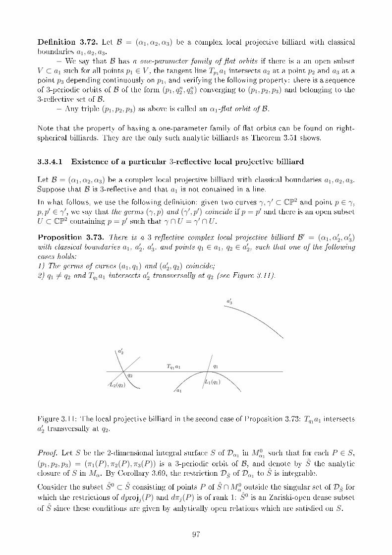
Denition 3.72. Let B = (α1, α2, α3) be a complex local projective billiard with classicalboundaries a1, a2, a3.

− We say that B has a one-parameter family of at orbits if there is a an open subsetV ⊂ a1 such for all points p1 ∈ V , the tangent line Tp1a1 intersects a2 at a point p2 and a3 at apoint p3 depending continuously on p1, and verifying the following property: there is a sequenceof 3-periodic orbits of B of the form (p1, q

n2 , q

n3 ) converging to (p1, p2, p3) and belonging to the

3-reective set of B.− Any triple (p1, p2, p3) as above is called an α1-at orbit of B.

Note that the property of having a one-parameter family of at orbits can be found on right-spherical billiards. They are the only such analytic billiards as Theorem 3.51 shows.

3.3.4.1 Existence of a particular 3-reective local projective billiard

Let B = (α1, α2, α3) be a complex local projective billiard with classical boundaries a1, a2, a3.Suppose that B is 3-reective and that a1 is not contained in a line.

In what follows, we use the following denition: given two curves γ, γ′ ⊂ CP2 and point p ∈ γ,p, p′ ∈ γ′, we say that the germs (γ, p) and (γ′, p′) coincide if p = p′ and there is an open subsetU ⊂ CP2 containing p = p′ such that γ ∩ U = γ′ ∩ U .

Proposition 3.73. There is a 3-reective complex local projective billiard B′ = (α1, α′2, α

′3)

with classical boundaries a1, a′2, a′3, and points q1 ∈ a1, q2 ∈ a′2, such that one of the following

cases holds:1) The germs of curves (a1, q1) and (a′2, q2) coincide;2) q1 6= q2 and Tq1a1 intersects a′2 transversally at q2 (see Figure 3.11).

a1

a′2

q1

q2

Tq1a1

a′3

L2(q2)L1(q1)

Figure 3.11: The local projective billiard in the second case of Proposition 3.73: Tq1a1 intersectsa′2 transversally at q2.

Proof. Let S be the 2-dimensional integral surface S of Dα1 in M0α1

such that for each P ∈ S,(p1, p2, p3) = (π1(P ), π2(P ), π3(P )) is a 3-periodic orbit of B, and denote by S the analyticclosure of S in Mα. By Corollary 3.69, the restriction DS of Dα1 to S is integrable.

Consider the subset S0 ⊂ S consisting of points P of S ∩M0α outside the singular set of DS for

which the restrictions of dprojj(P ) and dπj(P ) is of rank 1: S0 is an Zariski-open dense subset

of S since these conditions are given by anlytically open relations which are satised on S.

97

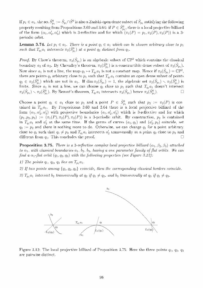
If p1 ∈ a1, the set S0p1

:= Sp1∩S0 is also a Zariski-open dense subset of Sp1 satisfying the following

property resulting from Propositions 3.69 and 3.64: if P ∈ S0p1, there is a local projective billiard

of the form (α1, α′2, α

′3) which is 3-reective and for which (π1(P ) = p1, π2(P ), π3(P )) is a 3-

periodic orbit.

Lemma 3.74. Let p1 ∈ a1. There is a point q1 ∈ a1 which can be chosen arbitrary close to p1

such that Tq1a1 intersects π2(S0p1

) at a point q2 distinct from q1.

Proof. By Chow's theorem, π2(Sp1) is an algebraic subset of CP2 which contains the classicalboundary a2 of α2. By Chevalley's theorem, π2(S0

p1) is a constructible dense subset of π2(Sp1).

Now since a1 is not a line, the map q1 7→ Tq1a1 is not a constant map. Hence if π2(Sp1) = CP2,there are points q1 arbitrary close to p1 such that Tq1a1 contains an open dense subset of pointsq2 ∈ π2(S0

p1) which are not in a1. If dim π2(Sp1) = 1, the algebraic set π2(Sp1) r π2(S0

p1) is

nite. Since a1 is not a line, we can choose q1 close to p1 such that Tq1a1 doesn't intersectπ2(Sp1) r π2(S0

p1). By Bezout's theorem, Tq1a1 intersects π2(Sp1) hence π2(S0

p1).

Choose a point q1 ∈ a1 close to p1 and a point P ∈ S0p1

such that p2 := π2(P ) is con-tained in Tq1a1. By Propositions 3.69 and 3.64 there is a local projective billiard of theform (α1, α

′2, α

′3) with projective boundaries (a1, a

′2, a′3) which is 3-reective and for which

(p1, p2, p3) := (π1(P ), π2(P ), π3(P )) is a 3-periodic orbit. By construction, p2 is containedin Tq1a1 and a′2 at the same time. If the germs of curves (a1, q1) and (a′2, p2) coincide, setq2 := p2 and there is nothing more to do. Otherwise, we can change q1 for a point arbitraryclose to q1 such that q1 6= p2 and Tq1a1 intersects a′2 transversally at a point q2 close to p2 anddierent from q1. This concludes the proof.

Proposition 3.75. There is a 3-reective complex local projective billiard (α1, β2, β3) attachedto α1, with classical boundaries a1, b2, b3, having a one-parameter family of at orbits. We cannd a α1-at orbit (q1, q2, q3) with the following properties (see Figure 3.12):

1) The points q1, q2, q3 lies on Tp1a1.

2) If two points among q1, q2, q3 coincide, then the corresponding classical borders coincide.

3) Tp1a1 intersect b2 transversally at q2 if q1 6= q2, and b3 transversally at q3 if q1 6= q3.

a1

b2

q1

q2

Tq1a1

b3

L2(q2)L1(q1)

q3

L3(q3)

Figure 3.12: The local projective billiard of Proposition 3.75. Here the three points q1, q2, q3

are pairwise distinct.

98

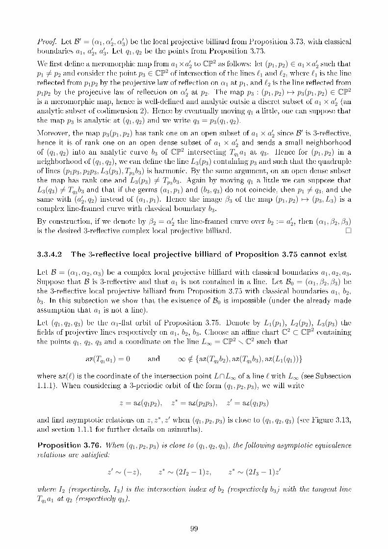
Proof. Let B′ = (α1, α′2, α

′3) be the local projective billiard from Proposition 3.73, with classical

boundaries a1, a′2, a′3. Let q1, q2 be the points from Proposition 3.73.

We rst dene a meromorphic map from a1×a′2 to CP2 as follows: let (p1, p2) ∈ a1×a′2 such thatp1 6= p2 and consider the point p3 ∈ CP2 of intersection of the lines `1 and `2, where `1 is the linereected from p1p2 by the projective law of reection on α1 at p1, and `2 is the line reected fromp1p2 by the projective law of reection on α′2 at p2. The map p3 : (p1, p2) 7→ p3(p1, p2) ∈ CP2

is a meromorphic map, hence is well-dened and analytic outsie a discret subset of a1 × a′2 (ananalytic subset of codimension 2). Hence by eventually moving q1 a little, one can suppose thatthe map p3 is analytic at (q1, q2) and we write q3 = p3(q1, q2).

Moreover, the map p3(p1, p2) has rank one on an open subset of a1 × a′2 since B′ is 3-reective,hence it is of rank one on an open dense subset of a1 × a′2 and sends a small neighborhoodof (q1, q2) into an analytic curve b3 of CP2 intersecting Tq1a1 at q3. Hence for (p1, p2) in aneighborhood of (q1, q2), we can dene the line L3(p3) containing p3 and such that the quadrupleof lines (p1p3, p2p3, L3(p3), Tp3b3) is harmonic. By the same argument, on an open dense subsetthe map has rank one and L3(p3) 6= Tp3b3. Again by moving q1 a little we can suppose thatL3(q3) 6= Tq3b3 and that if the germs (a1, p1) and (b3, q3) do not coincide, then p1 6= q3, and thesame with (a′2, q2) instead of (a1, p1). Hence the image β3 of the map (p1, p2) 7→ (p3, L3) is acomplex line-framed curve with classical boundary b3.

By construction, if we denote by β2 = α′2 the line-framed curve over b2 := a′2, then (α1, β2, β3)is the desired 3-reective complex local projective billiard.

3.3.4.2 The 3-reective local projective billiard of Proposition 3.75 cannot exist

Let B = (α1, α2, α3) be a complex local projective billiard with classical boundaries a1, a2, a3.Suppose that B is 3-reective and that a1 is not contained in a line. Let B0 = (α1, β2, β3) bethe 3-reective local projective billiard from Proposition 3.75 with classical boundaries a1, b2,b3. In this subsection we show that the existence of B0 is impossible (under the already madeassumption that a1 is not a line).

Let (q1, q2, q3) be the α1-at orbit of Proposition 3.75. Denote by L1(p1), L2(p2), L3(p3) theelds of projective lines respectively on a1, b2, b3. Choose an ane chart C2 ⊂ CP2 containingthe points q1, q2, q3 and a coordinate on the line L∞ = CP2 rC2 such that

az(Tq1a1) = 0 and ∞ /∈ az(Tq2b2), az(Tq3b3), az(L1(q1))

where az(`) is the coordinate of the intersection point L∩L∞ of a line ` with L∞ (see Subsection1.1.1). When considering a 3-periodic orbit of the form (q1, p2, p3), we will write

z = az(q1p2), z∗ = az(p2p3), z′ = az(q1p3)

and nd asymptotic relations on z, z∗, z′ when (q1, p2, p3) is close to (q1, q2, q3) (see Figure 3.13,and section 1.1.1 for further details on azimuths).

Proposition 3.76. When (q1, p2, p3) is close to (q1, q2, q3), the following asymptotic equivalencerelations are satised:

z′ ∼ (−z), z∗ ∼ (2I2 − 1)z, z∗ ∼ (2I3 − 1)z′

where I2 (respectively, I3) is the intersection index of b2 (respectively b3) with the tangent lineTq1a1 at q2 (respectively q3).

99

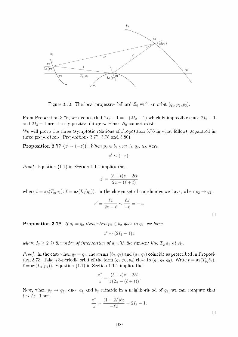
a1

b2

q1q2 Tq1a1

b3

q3

p2z

p3

z∗ z′

L2(p2)

L3(p3)

L1(q1)

Figure 3.13: The local projective billiard B0 with an orbit (q1, p2, p3).

From Proposition 3.76, we deduce that 2I3 − 1 = −(2I2 − 1) which is impossible since 2I2 − 1and 2I3 − 1 are strictly positive integers. Hence B0 cannot exist.

We will prove the three asymptotic relations of Proposition 3.76 in what follows, separated inthree propositions (Propositions 3.77, 3.78 and 3.80).

Proposition 3.77 (z′ ∼ (−z)). When p2 ∈ b2 goes to q2, we have

z′ ∼ (−z).

Proof. Equation (1.1) in Section 1.1.1 implies that

z′ =(`+ t)z − 2`t

2z − (`+ t)

where t = az(Tq1a1), ` = az(L1(q1)). In the chosen set of coordinates we have, when p2 → q2,

z′ =`z

2z − `∼ `z

−`= −z.

Proposition 3.78. If q1 = q2 then when p2 ∈ b2 goes to q2, we have

z∗ ∼ (2I2 − 1)z

where I2 ≥ 2 is the index of intersection of a with the tangent line Tq1a1 at A1.

Proof. In the case when q2 = q1, the germs (b2, q2) and (a1, q1) coincide as prescribed in Proposi-tion 3.75. Take a 3-periodic orbit of the form (q1, p2, p3) close to (q1, q2, q3). Write t = az(Tp2b2),` = az(L2(p2)). Equation (1.1) in Section 1.1.1 implies that

z∗

z=

(`+ t)z − 2`t

z(2z − (`+ t)).

Now, when p2 → q2, since a1 and b2 coincide in a neighborhood of q2, we can compute thatt ∼ Iz. Thus

z∗

z∼ (1− 2I)`z

−`z= 2I2 − 1.

100

Lemma 3.79. If q2 = q3, then the germs (a1, q1), (b2, q2) and (b3, q3) coincide.

Proof. Suppose that the three germs do not coincide and that q2 = q3: as prescribed in Propo-sition 3.75 we should have (b3, q3) = (b2, q2) but q1 6= q2 with Tp1a1 intersecting b2 transversallyat q2 by Proposition 3.75. Consider a 3-periodic orbit of the form (q1, p2, p3) close to (q1, q2, q3).Then write t = az(Tp2b2) and ` = az(L2(p2)). Remark 1.6 and Equation (1.1) in Section 1.1.1imply that

` =(z + z∗)t− 2zz∗

2t− (z + z∗).

Now, when p2 → q2, we have z → 0 and t→ t0 where t0 := az(Tq2b2) /∈ 0,∞ by transversalityof b2 with Tq1a1 at q2 and by choice of coordinates. But we also have z∗ → t0 because p2p3 →Tq2b2 since p2,p3 are distinct points of the same irreducible germ of curve b2 = b3 converging tothe same point q2 = q3. Hence, when p2 → q2,

`→ t20t0

= t0

which means that L2(q2) = Tq2b2. But this is not the case by Proposition 3.75, contradiction.

Proposition 3.80. Suppose that q2 6= q1. Then when p2 ∈ b2 goes to q2, we have

z∗ ∼ z

which allows to extend the formula of Proposition 3.78 by setting I2 = 1 in this case (transverseintersection).

Proof. First, let us prove the following lemma, which gives the form of the projective eld oflines locally around q2:

Lemma 3.81. Suppose that q2 6= q1. Then when p2 ∈ b2 is close to q2, there is a p1 ∈ a1 closeto q1 for which L2(p2) is tangent to a1 at p1.

Proof. Proposition 3.75 implies that Tq1a1 intersects b2 transversally at q2. By the implicitfunction theorem, there is an analytic map which associates to any p1 close to q1 a point p2 ∈ b2

close to q2 which is contained in Tp1a1. Since a1 is not a line, this map is not constant, henceis open and thus parametrizes (maybe non-bijectively) the germ of b2 at q2. We choose p1 inthe neighborhood of q1, and denote by p2 the corresponding point on b2 obtained via the aboveparametrization.

We can suppose that that Tp1a1 is transverse to b2 at p2 and that p2 /∈ b3 (possible by Lemma3.79). Consider a 3-periodic orbit of the form (p1, p

′2, p′3) such that p′2 converges to p2. The line

p1p′2 converges to Tp1a1 and by the projective reection law at p1 we get that the line p1p

′3 also

converges to Tp1a1, hence the limit p3 of p′3 lies on Tp1a1. We also have that p3 6= p1 (Lemma3.79). Hence p2p3 = Tp1a = p1p2: Tp1a1 is invariant by the projective reection law of β2 at p2.Since the latter tangent line is transverse to b2, we have Tp1a1 = L2(p2), and this concludes theproof.

We now conclude the proof of Proposition 3.80. As in Lemma 3.81, when p2 ∈ b2 is close to q1,L2(q2) is tangent to a1 at a point p1 close to q1. Write t = az(Tp2b2), ` = az(L2(p2)). We have,by Equation (1.1) in Section 1.1.1,

z∗ =(`+ t)z − 2`t

2z − (`+ t). (3.5)

101

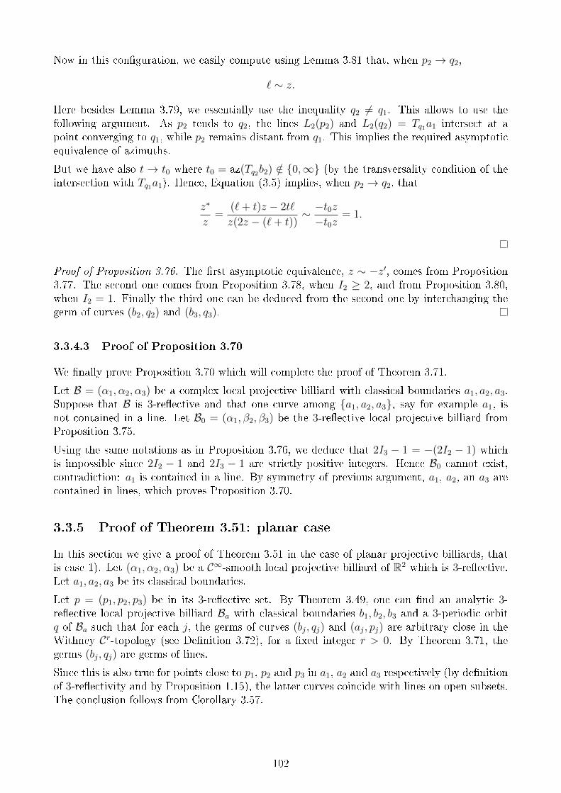
Now in this conguration, we easily compute using Lemma 3.81 that, when p2 → q2,

` ∼ z.

Here besides Lemma 3.79, we essentially use the inequality q2 6= q1. This allows to use thefollowing argument. As p2 tends to q2, the lines L2(p2) and L2(q2) = Tq1a1 intersect at apoint converging to q1, while p2 remains distant from q1. This implies the required asymptoticequivalence of azimuths.

But we have also t→ t0 where t0 = az(Tq2b2) /∈ 0,∞ (by the transversality condition of theintersection with Tq1a1). Hence, Equation (3.5) implies, when p2 → q2, that

z∗

z=

(`+ t)z − 2t`

z(2z − (`+ t))∼ −t0z−t0z

= 1.

Proof of Proposition 3.76. The rst asymptotic equivalence, z ∼ −z′, comes from Proposition3.77. The second one comes from Proposition 3.78, when I2 ≥ 2, and from Proposition 3.80,when I2 = 1. Finally the third one can be deduced from the second one by interchanging thegerm of curves (b2, q2) and (b3, q3).

3.3.4.3 Proof of Proposition 3.70

We nally prove Proposition 3.70 which will complete the proof of Theorem 3.71.

Let B = (α1, α2, α3) be a complex local projective billiard with classical boundaries a1, a2, a3.Suppose that B is 3-reective and that one curve among a1, a2, a3, say for example a1, isnot contained in a line. Let B0 = (α1, β2, β3) be the 3-reective local projective billiard fromProposition 3.75.

Using the same notations as in Proposition 3.76, we deduce that 2I3 − 1 = −(2I2 − 1) whichis impossible since 2I2 − 1 and 2I3 − 1 are strictly positive integers. Hence B0 cannot exist,contradiction: a1 is contained in a line. By symmetry of previous argument, a1, a2, an a3 arecontained in lines, which proves Proposition 3.70.

3.3.5 Proof of Theorem 3.51: planar case

In this section we give a proof of Theorem 3.51 in the case of planar projective billiards, thatis case 1). Let (α1, α2, α3) be a C∞-smooth local projective billiard of R2 which is 3-reective.Let a1, a2, a3 be its classical boundaries.

Let p = (p1, p2, p3) be in its 3-reective set. By Theorem 3.49, one can nd an analytic 3-reective local projective billiard Ba with classical boundaries b1, b2, b3 and a 3-periodic orbitq of Ba such that for each j, the germs of curves (bj, qj) and (aj, pj) are arbitrary close in theWithney Cr-topology (see Denition 3.72), for a xed integer r > 0. By Theorem 3.71, thegerms (bj, qj) are germs of lines.

Since this is also true for points close to p1, p2 and p3 in a1, a2 and a3 respectively (by denitionof 3-reectivity and by Proposition 1.15), the latter curves coincide with lines on open subsets.The conclusion follows from Corollary 3.57.

102

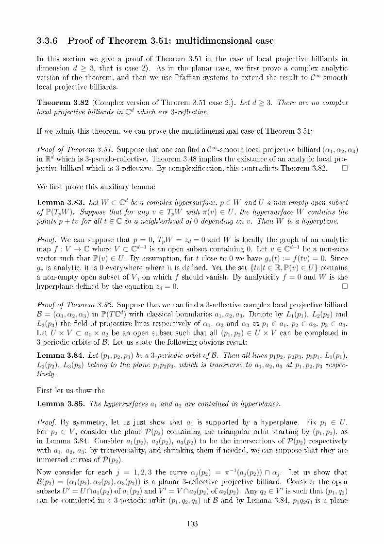
3.3.6 Proof of Theorem 3.51: multidimensional case

In this section we give a proof of Theorem 3.51 in the case of local projective billiards indimension d ≥ 3, that is case 2). As in the planar case, we rst prove a complex analyticversion of the theorem, and then we use Pfaan systems to extend the result to C∞-smoothlocal projective billiards.

Theorem 3.82 (Complex version of Theorem 3.51 case 2.). Let d ≥ 3. There are no complexlocal projective billiards in Cd which are 3-reective.

If we admit this theorem, we can prove the multidimensional case of Theorem 3.51:

Proof of Theorem 3.51. Suppose that one can nd a C∞-smooth local projective billiard (α1, α2, α3)in Rd which is 3-pseudo-reective. Theorem 3.48 implies the existence of an analytic local pro-jective billiard which is 3-reective. By complexication, this contradicts Theorem 3.82.

We rst prove this auxiliary lemma:

Lemma 3.83. Let W ⊂ Cd be a complex hypersurface, p ∈ W and U a non-empty open subsetof P(TpW ). Suppose that for any v ∈ TpW with π(v) ∈ U , the hypersurface W contains thepoints p+ tv for all t ∈ C in a neighborhood of 0 depending on v. Then W is a hyperplane.

Proof. We can suppose that p = 0, TpW = zd = 0 and W is locally the graph of an analyticmap f : V → C where V ⊂ Cd−1 is an open subset containing 0. Let v ∈ Cd−1 be a non-zerovector such that P(v) ∈ U . By assumption, for t close to 0 we have gv(t) := f(tv) = 0. Sincegv is analytic, it is 0 everywhere where it is dened. Yet the set tv|t ∈ R,P(v) ∈ U containsa non-empty open subset of V , on which f should vanish. By analyticity f = 0 and W is thehyperplane dened by the equation zd = 0.

Proof of Theorem 3.82. Suppose that we can nd a 3-reective complex local projective billiardB = (α1, α2, α3) in P(TCd) with classical boundaries a1, a2, a3. Denote by L1(p1), L2(p2) andL3(p3) the eld of projective lines respectively of α1, α2 and α3 at p1 ∈ a1, p2 ∈ a2, p3 ∈ a3.Let U × V ⊂ a1 × a2 be an open subset such that all (p1, p2) ∈ U × V can be completed in3-periodic orbits of B. Let us state the following obvious result:

Lemma 3.84. Let (p1, p2, p3) be a 3-periodic orbit of B. Then all lines p1p2, p2p3, p3p1, L1(p1),L2(p2), L3(p3) belong to the plane p1p2p3, which is transverse to a1, a2, a3 at p1, p2, p3 respec-tively.

First let us show the

Lemma 3.85. The hypersurfaces a1 and a2 are contained in hyperplanes.

Proof. By symmetry, let us just show that a1 is supported by a hyperplane. Fix p1 ∈ U .For p2 ∈ V , consider the plane P(p2) containing the triangular orbit starting by (p1, p2), asin Lemma 3.84. Consider a1(p2), a2(p2), a3(p2) to be the intersections of P(p2) respectivelywith a1, a2, a3: by transversality, and shrinking them if needed, we can suppose that they areimmersed curves of P(p2).

Now consider for each j = 1, 2, 3 the curve αj(p2) = π−1(aj(p2)) ∩ αj. Let us show thatB(p2) = (α1(p2), α2(p2), α3(p2)) is a planar 3-reective projective billiard. Consider the opensubsets U ′ = U∩a1(p2) of a1(p2) and V ′ = V ∩a2(p2) of a2(p2). Any q2 ∈ V ′ is such that (p1, q2)can be completed in a 3-periodic orbit (p1, q2, q3) of B and by Lemma 3.84, p1q2q3 is a plane

103

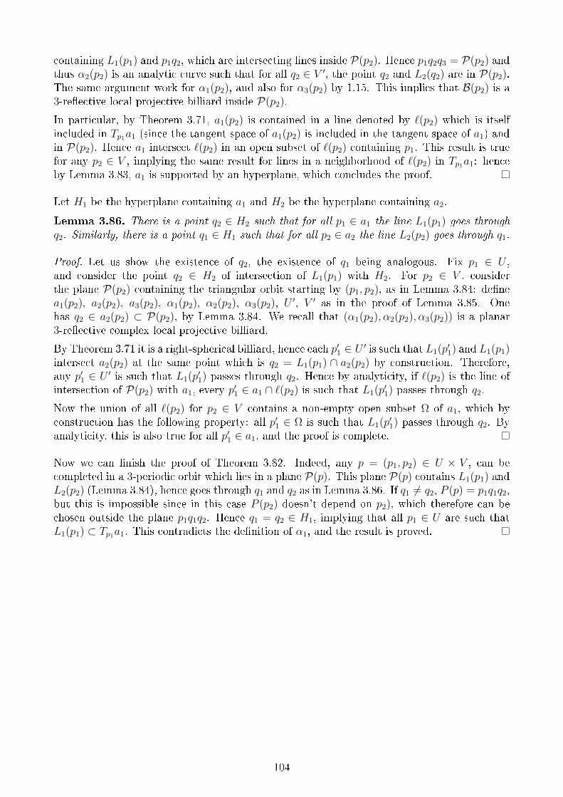
containing L1(p1) and p1q2, which are intersecting lines inside P(p2). Hence p1q2q3 = P(p2) andthus α2(p2) is an analytic curve such that for all q2 ∈ V ′, the point q2 and L2(q2) are in P(p2).The same argument work for α1(p2), and also for α3(p2) by 1.15. This implies that B(p2) is a3-reective local projective billiard inside P(p2).

In particular, by Theorem 3.71, a1(p2) is contained in a line denoted by `(p2) which is itselfincluded in Tp1a1 (since the tangent space of a1(p2) is included in the tangent space of a1) andin P(p2). Hence a1 intersect `(p2) in an open subset of `(p2) containing p1. This result is truefor any p2 ∈ V , implying the same result for lines in a neighborhood of `(p2) in Tp1a1: henceby Lemma 3.83, a1 is supported by an hyperplane, which concludes the proof.

Let H1 be the hyperplane containing a1 and H2 be the hyperplane containing a2.

Lemma 3.86. There is a point q2 ∈ H2 such that for all p1 ∈ a1 the line L1(p1) goes throughq2. Similarly, there is a point q1 ∈ H1 such that for all p2 ∈ a2 the line L2(p2) goes through q1.

Proof. Let us show the existence of q2, the existence of q1 being analogous. Fix p1 ∈ U ,and consider the point q2 ∈ H2 of intersection of L1(p1) with H2. For p2 ∈ V , considerthe plane P(p2) containing the triangular orbit starting by (p1, p2), as in Lemma 3.84: denea1(p2), a2(p2), a3(p2), α1(p2), α2(p2), α3(p2), U ′, V ′ as in the proof of Lemma 3.85. Onehas q2 ∈ a2(p2) ⊂ P(p2), by Lemma 3.84. We recall that (α1(p2), α2(p2), α3(p2)) is a planar3-reective complex local projective billiard.

By Theorem 3.71 it is a right-spherical billiard, hence each p′1 ∈ U ′ is such that L1(p′1) and L1(p1)intersect a2(p2) at the same point which is q2 = L1(p1) ∩ a2(p2) by construction. Therefore,any p′1 ∈ U ′ is such that L1(p′1) passes through q2. Hence by analyticity, if `(p2) is the line ofintersection of P(p2) with a1, every p′1 ∈ a1 ∩ `(p2) is such that L1(p′1) passes through q2.

Now the union of all `(p2) for p2 ∈ V contains a non-empty open subset Ω of a1, which byconstruction has the following property: all p′1 ∈ Ω is such that L1(p′1) passes through q2. Byanalyticity, this is also true for all p′1 ∈ a1, and the proof is complete.

Now we can nish the proof of Theorem 3.82. Indeed, any p = (p1, p2) ∈ U × V , can becompleted in a 3-periodic orbit which lies in a plane P(p). This plane P(p) contains L1(p1) andL2(p2) (Lemma 3.84), hence goes through q1 and q2 as in Lemma 3.86. If q1 6= q2, P (p) = p1q1q2,but this is impossible since in this case P (p2) doesn't depend on p2), which therefore can bechosen outside the plane p1q1q2. Hence q1 = q2 ∈ H1, implying that all p1 ∈ U are such thatL1(p1) ⊂ Tp1a1. This contradicts the denition of α1, and the result is proved.

104

Bibliography

[1] Y.M. Baryshnikov, V. Zharnitsky, Billiards and nonholonomic distributions, J. Math. Sci.128 (2005), 27062710.

[2] Y.M. Baryshnikov, V. Zharnitsky, Sub-Riemannian geometry and periodic orbits in clas-sical billiards, Math. Res. Lett. 13 (2006), no. 4, 587598.

[3] Y.M. Baryshnikov, Spherical billiards with periodic orbits, preprint.

[4] Beltrami, E. Risoluzione del problema: Riportare i punti di una supercie sopra un pianoin modo che le linee geodetiche vengano rappresentate da linee rette. Annali di Matematicapura ed applicata 7, 185204 (1865).

[5] M. Berger, Geometry, Volumes I and II, Springer-Verlag, 1987.

[6] M. Berger, Seules les quadriques admettent des caustiques, Bull. Soc. math. France 123(1995), 107116.

[7] M. Bialy, Convex billiards and a theorem by E. Hopf, Math. Z. 214, No. 1 (1993), 14715.

[8] M. Bialy, A. E. Mironov, Angular billiard and algebraic Birkho conjecture, Adv. Math.313 (2017), 102126.

[9] M. Bialy, A. E. Mironov, Algebraic Birkho conjecture for billiards on Sphere and Hyper-bolic plane, J. Geom. Phys. 115 (2017), 150156.

[10] V. Blumen, K. Kim, J. Nance, V. Zharnitsky, Three-Period Orbits in Billiards on theSurfaces of Constant Curvature, International Mathematics Research Notices (2012),10.1093/imrn/rnr228.

[11] R. L. Bryant, S. S. Chern, R. B. Gardner, H. L. Goldschmidt, P. A. Griths, ExteriorDierential Systems, Springer Science and Business Media, 2013.

[12] E. Cartan, Les systèmes diérentiels extérieurs et leurs applications géométriques, Paris,1945.

[13] S.J. Chang, B. Crespi, K.J. Shi, Elliptical billiard systems and the full Poncelet's theoremin n dimensions, Journal of Mathematical Physics 34, 2242 (1993).

[14] V. Dragovi¢, M. Radnovi¢, Bicentennial of the Great Poncelet Theorem (1813-2013): Cur-rent Advances, Bulletin of the American Mathematical Society 51 (2013), No. 3, 373445.

[15] V. Dragovi¢, M. Radnovi¢, Ellipsoidal billiards in pseudo-Euclidean spaces and relativisticquadrics, Advances in Mathematics 231 (2012), 11731201.

[16] A.K. Adabrah, V. Dragovi¢, M. Radnovi¢, Periodic billiards within conics in the Minkowskiplane and Akhiezer polynomials, Regul. Chaotic Dyn. 24 (2019), 464501.

105

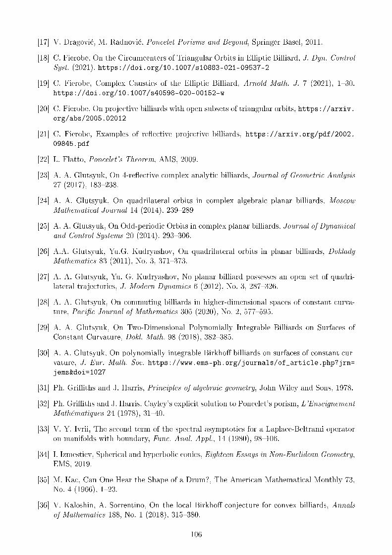
[17] V. Dragovi¢, M. Radnovi¢, Poncelet Porisms and Beyond, Springer Basel, 2011.

[18] C. Fierobe, On the Circumcenters of Triangular Orbits in Elliptic Billiard, J. Dyn. ControlSyst. (2021). https://doi.org/10.1007/s10883-021-09537-2

[19] C. Fierobe, Complex Caustics of the Elliptic Billiard, Arnold Math. J. 7 (2021), 130.https://doi.org/10.1007/s40598-020-00152-w

[20] C. Fierobe, On projective billiards with open subsets of triangular orbits, https://arxiv.org/abs/2005.02012

[21] C. Fierobe, Examples of reective projective billiards, https://arxiv.org/pdf/2002.09845.pdf

[22] L. Flatto, Poncelet's Theorem, AMS, 2009.

[23] A. A. Glutsyuk, On 4-reective complex analytic billiards, Journal of Geometric Analysis27 (2017), 183238.

[24] A. A. Glutsyuk, On quadrilateral orbits in complex algebraic planar billiards, MoscowMathematical Journal 14 (2014), 239289

[25] A. A. Glutsyuk, On Odd-periodic Orbits in complex planar billiards, Journal of Dynamicaland Control Systems 20 (2014), 293306.

[26] A.A. Glutsyuk, Yu.G. Kudryashov, On quadrilateral orbits in planar billiards, DokladyMathematics 83 (2011), No. 3, 371373.

[27] A. A. Glutsyuk, Yu. G. Kudryashov, No planar billiard possesses an open set of quadri-lateral trajectories, J. Modern Dynamics 6 (2012), No. 3, 287326.

[28] A. A. Glutsyuk, On commuting billiards in higher-dimensional spaces of constant curva-ture, Pacic Journal of Mathematics 305 (2020), No. 2, 577595.

[29] A. A. Glutsyuk, On Two-Dimensional Polynomially Integrable Billiards on Surfaces ofConstant Curvature, Dokl. Math. 98 (2018), 382385.

[30] A. A. Glutsyuk, On polynomially integrable Birkho billiards on surfaces of constant cur-vature, J. Eur. Math. Soc. https://www.ems-ph.org/journals/of_article.php?jrn=jems&doi=1027

[31] Ph. Griths and J. Harris, Principles of algebraic geometry, John Wiley and Sons, 1978.

[32] Ph. Griths and J. Harris, Cayley's explicit solution to Poncelet's porism, L'EnseignementMathématiques 24 (1978), 3140.

[33] V. Y. Ivrii, The second term of the spectral asymptotics for a Laplace-Beltrami operatoron manifolds with boundary, Func. Anal. Appl., 14 (1980), 98106.

[34] I. Izmestiev, Spherical and hyperbolic conics, Eighteen Essays in Non-Euclidean Geometry,EMS, 2019.

[35] M. Kac, Can One Hear the Shape of a Drum?, The American Mathematical Monthly 73,No. 4 (1966), 123.

[36] V. Kaloshin, A. Sorrentino, On the local Birkho conjecture for convex billiards, Annalsof Mathematics 188, No. 1 (2018), 315380.

106

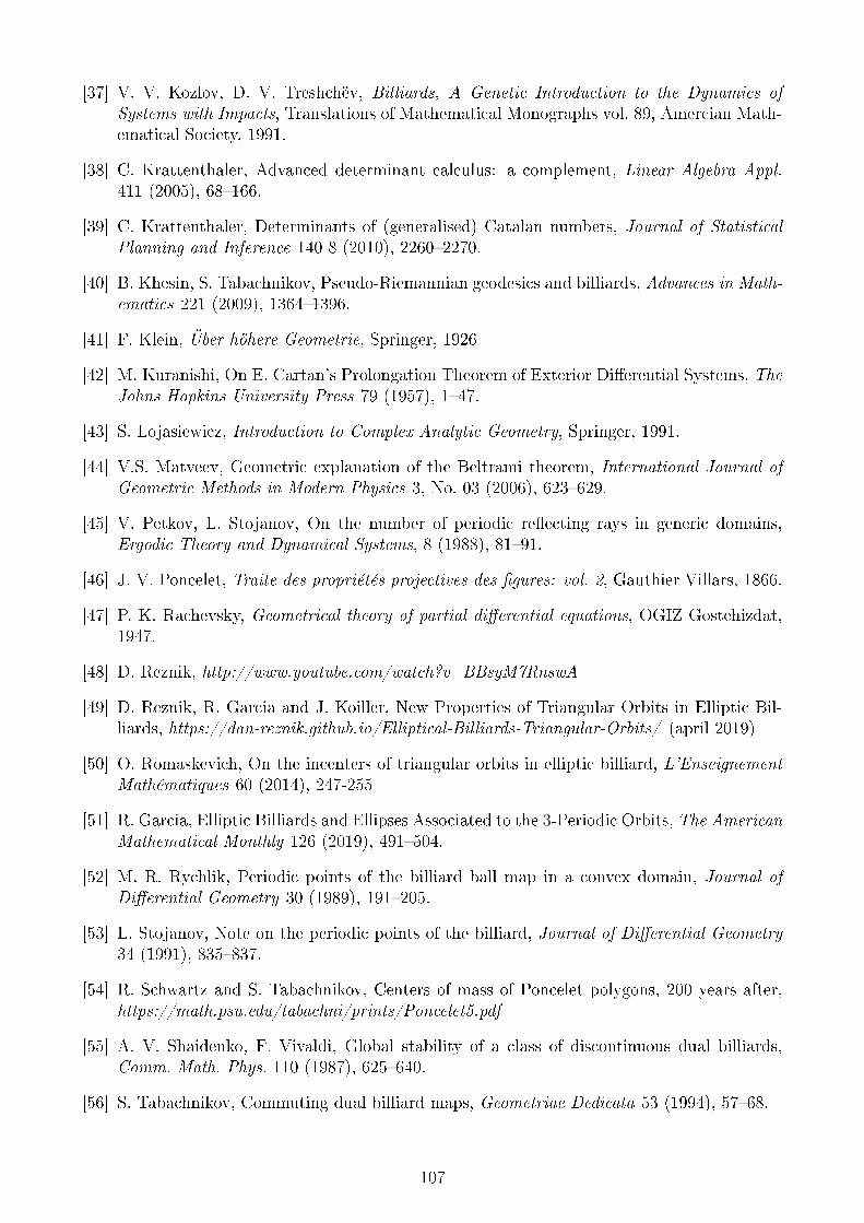
[37] V. V. Kozlov, D. V. Treshchëv, Billiards, A Genetic Introduction to the Dynamics ofSystems with Impacts, Translations of Mathematical Monographs vol. 89, Amercian Math-ematical Society, 1991.

[38] C. Krattenthaler, Advanced determinant calculus: a complement, Linear Algebra Appl.411 (2005), 68166.

[39] C. Krattenthaler, Determinants of (generalised) Catalan numbers, Journal of StatisticalPlanning and Inference 140 8 (2010), 22602270.

[40] B. Khesin, S. Tabachnikov, Pseudo-Riemannian geodesics and billiards, Advances in Math-ematics 221 (2009), 13641396.

[41] F. Klein, Über höhere Geometrie, Springer, 1926

[42] M. Kuranishi, On E. Cartan's Prolongation Theorem of Exterior Dierential Systems, TheJohns Hopkins University Press 79 (1957), 147.

[43] S. Lojasiewicz, Introduction to Complex Analytic Geometry, Springer, 1991.

[44] V.S. Matveev, Geometric explanation of the Beltrami theorem, International Journal ofGeometric Methods in Modern Physics 3, No. 03 (2006), 623629.

[45] V. Petkov, L. Stojanov, On the number of periodic reecting rays in generic domains,Ergodic Theory and Dynamical Systems, 8 (1988), 8191.

[46] J. V. Poncelet, Traite des propriétés projectives des gures: vol. 2, Gauthier Villars, 1866.

[47] P. K. Rachevsky, Geometrical theory of partial dierential equations, OGIZ Gostehizdat,1947.

[48] D. Reznik, http://www.youtube.com/watch?v=BBsyM7RnswA

[49] D. Reznik, R. Garcia and J. Koiller, New Properties of Triangular Orbits in Elliptic Bil-liards, https://dan-reznik.github.io/Elliptical-Billiards-Triangular-Orbits/ (april 2019)

[50] O. Romaskevich, On the incenters of triangular orbits in elliptic billiard, L'EnseignementMathématiques 60 (2014), 247-255

[51] R. Garcia, Elliptic Billiards and Ellipses Associated to the 3-Periodic Orbits, The AmericanMathematical Monthly 126 (2019), 491504.

[52] M. R. Rychlik, Periodic points of the billiard ball map in a convex domain, Journal ofDierential Geometry 30 (1989), 191205.

[53] L. Stojanov, Note on the periodic points of the billiard, Journal of Dierential Geometry34 (1991), 835837.

[54] R. Schwartz and S. Tabachnikov, Centers of mass of Poncelet polygons, 200 years after,https://math.psu.edu/tabachni/prints/Poncelet5.pdf

[55] A. V. Shaidenko, F. Vivaldi, Global stability of a class of discontinuous dual billiards,Comm. Math. Phys. 110 (1987), 625640.

[56] S. Tabachnikov, Commuting dual billiard maps, Geometriae Dedicata 53 (1994), 5768.

107

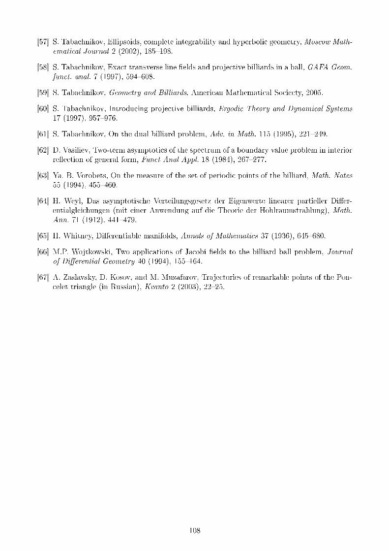
[57] S. Tabachnikov, Ellipsoids, complete integrability and hyperbolic geometry, Moscow Math-ematical Journal 2 (2002), 185198.

[58] S. Tabachnikov, Exact transverse line elds and projective billiards in a ball, GAFA Geom.funct. anal. 7 (1997), 594608.

[59] S. Tabachnikov, Geometry and Billiards, American Mathematical Sociecty, 2005.

[60] S. Tabachnikov, Introducing projective billiards, Ergodic Theory and Dynamical Systems17 (1997), 957976.

[61] S. Tabachnikov, On the dual billiard problem, Adv. in Math. 115 (1995), 221249.

[62] D. Vasiliev, Two-term asymptotics of the spectrum of a boundary value problem in interiorreection of general form, Funct Anal Appl. 18 (1984), 267277.

[63] Ya. B. Vorobets, On the measure of the set of periodic points of the billiard, Math. Notes55 (1994), 455460.

[64] H. Weyl, Das asymptotische Verteilungsgesetz der Eigenwerte linearer partieller Dier-entialgleichungen (mit einer Anwendung auf die Theorie der Hohlraumstrahlung), Math.Ann. 71 (1912), 441479.

[65] H. Whitney, Dierentiable manifolds, Annals of Mathematics 37 (1936), 645680.

[66] M.P. Wojtkowski, Two applications of Jacobi elds to the billiard ball problem, Journalof Dierential Geometry 40 (1994), 155164.

[67] A. Zaslavsky, D. Kosov, and M. Muzafarov, Trajectories of remarkable points of the Pon-celet triangle (in Russian), Kvanto 2 (2003), 2225.

108