arX

iv:h

ep-t

h/02

1023

9v3

31

Oct

200

2

Preprint typeset in JHEP style. - HYPER VERSION SWAT-356

S-duality of the Leigh-Strassler Deformation

via Matrix Models

Nick Dorey, Timothy J. Hollowood and S. Prem Kumar

Department of Physics, University of Wales Swansea, Swansea, SA2 8PP, UK

E-mail: t.hollowood@swan.ac.uk, n.dorey@swan.ac.uk

s.p.kumar@swan.ac.uk

Abstract: We investigate an exactly marginal N = 1 supersymmetric deforma-

tion of SU(N) N = 4 supersymmetric Yang-Mills theory discovered by Leigh and

Strassler. We use a matrix model to compute the exact superpotential for a fur-

ther massive deformation of the U(N) Leigh-Strassler theory. We then show how

the exact superpotential and eigenvalue spectrum for the SU(N) theory follows by a

process of integrating-in. We find that different vacua are related by an action of the

SL(2, Z) modular group on the bare couplings of the theory extending the action of

electric-magnetic duality away from the N = 4 theory. We perform non-trivial tests

of the matrix model results against semiclassical field theory analysis. We also show

that there are interesting points in parameter space where condensates can diverge

and vacua disappear. Based on the matrix model results, we propose an exact elliptic

superpotential to describe the theory compactified on a circle of finite radius.

1. Introduction

It has been known for some time that the N = 4 supersymmetric Yang-Mills the-

ory in four dimensions possesses exactly marginal deformations. Leigh and Strassler

[1] identified two N = 1 SUSY-preserving exactly marginal directions other than

the N = 4 gauge coupling itself, giving rise to a three (complex) dimensional

renormalization-group-fixed manifold of N = 1 superconformal theories (SCFTs)

of which the N = 4 fixed line is a subset. Given that strong and weak coupling on

the N = 4 fixed line are related by the action of SL(2, Z) on τ , the gauge coupling

of the N = 4 theory, it is then natural to ask whether this duality extends in some

non-trivial way over the entire N = 1 fixed manifold.

In this article we answer this question for a particular Leigh-Strassler defor-

mation of the N = 4 theory: the so-called “q-deformation” [2] 1 . By studying a

mass deformation of this Leigh-Strassler SCFT using a recently proposed connection

between N = 1 theories and matrix models [6–8], we demonstrate that Montonen-

Olive electric-magnetic duality, extended to the full SL(2, Z) modular group, extends

non-trivially to this space of N = 1 superconformal theories accompanied by a well-

defined action on the marginal parameters. Not only will we uncover the duality

group action in these theories, but we will also provide rather powerful checks on

the applicability of the matrix model approach towards solving these N = 1 SUSY

theories. (Recent checks of the matrix model proposal for other N = 1 models have

been performed in [3–5]). In particular we will test the superpotential and eigenvalue

spectrum obtained from the matrix model against classical field theory results and

find nontrivial agreement between the two. Furthermore, rather remarkably the ma-

trix model results for the vacuum expectation values of the effective superpotential

can be used to directly infer an exact, dynamical quantum superpotential for the

mass deformation of the Leigh-Strassler SCFT compactified on R3 ×S1. This super-

potential written in terms of the effective fields of the 3-dimensional theory encodes

the entire vacuum structure of the four-dimensional theory and satisfies extremely

non-trivial checks to be discussed below. It turns out to be a natural deformation of

the elliptic superpotential of [9] for the mass-deformed N = 4, or N = 1∗, theory.

Relevant deformations of SCFTs can tell us a great deal about the CFTs them-

selves; in particular, as is well-known in the context of N = 4 SUSY Yang-Mills and

the so-called N = 2 elliptic quiver models [8–11,14], the duality properties of the par-

ent theories are inherited by the perturbed theories and manifest themselves as mod-

ular properties of various exactly calculable observables in the perturbed theories.

In fact, what happens in these known examples is that the holomorphic observables

1One such deformation has been analysed recently using matrix models in [3].

1

in one vacuum get mapped into the corresponding observables in a different vacuum

(realized in a different phase) under the action of SL(2, Z) with well-defined modular

weights. The holomorphic quantities in question can often be computed exactly and

reflect the duality symmetries of the parent theory in this simple fashion.

The lesson to be drawn from this limited set of examples is that the consequences

of dualities in these SCFTs are readily visible and more importantly, are readily

calculable for certain relevant deformations of these SCFTs. With this in mind,

rather than focusing on the SCFT itself we investigate a special mass perturbation

of the Leigh-Strassler fixed points. This theory is the SU(N) gauge theory with

N = 1 SUSY and three adjoint-valued chiral multiplets Φ+, Φ− and Φ; the same

matter content as the N = 4 theory, but with the following classical superpotential2

Wcl = Tr(

iλΦ[Φ+, Φ−]β + MΦ+Φ− + µΦ2)

, (1.1)

where we have defined the q-commutator

[Φ+, Φ−]β ≡ Φ+Φ−eiβ/2 − Φ−Φ+e−iβ/2 (1.2)

and where λ and β are complex bare couplings. We also introduce the complex bare

gauge coupling of this theory τ ≡ 4πi/g2Y M + θ/2π. This superpotential represents a

deformation away from the N = 4 point which is at λ = 1, β = 0 and M = µ = 0.

It is worth noting that there are alternative relevant deformations we could have

considered involving the operators Tr Φ+2 and Tr Φ−2. These are equivalent to (1.1)

as a deformation of the N = 4 theory, i.e. when β = 0, but differ once the Leigh-

Strassler marginal deformation is present. In particular, the resulting theories differ

in the IR. However, as they only differ by strictly relevant operators they both flow

to the same fixed point in the UV: namely the Leigh-Strassler SCFT. The reason for

choosing to study the specific relevant deformation (1.1) is simply that the resulting

matrix model turns out to be exactly soluble [6, 7, 15].

Aside from masses for the chiral multiplets Φ± and Φ, our theory also involves

two trilinear deformations, O1 = Tr Φ[Φ+, Φ−] and O2 = Tr Φ{Φ+, Φ−}. Both the

operators O1 and O2 are of course, marginal by power counting but only one of

them, or more precisely, only one linear combination of these operators is an exactly

marginal deformation of the N = 4 theory. Adding O1 to the N = 4 Lagrangian only

changes the coefficient in front of the N = 4 superpotential, but it is an irrelevant

operator even at one-loop at the N = 4 fixed point [16]. The operator O1 is actually

a descendant and not a chiral primary field in the N = 4 theory, hence its dimensions

2We choose a normalization in which the kinetic terms of the chiral multiplets do not have

factors of 1/g2

Y M in front. In the following, hatted quantities refer to SU(N) to distinguish them

from U(N).

2

are not protected.3 The second operator O2 on the other hand is known to be exactly

marginal at one-loop at the N = 4 point [16]. More generally, away from the N = 4

line one should expect, for fixed gY M , a particular linear combination of O1 and O2

to be exactly marginal. We have parametrized this particular linear combination via

two complex numbers λ and β. In principle, λ should be determined as a function

of β and gY M on the fixed manifold. Fortunately the specifics of this will not be

important for us. Note that in the SU(2) theory the operator O2 vanishes identically

and the above superpotential does not yield a marginal deformation. We will assume

that N > 2 throughout this paper.

The theory with masses for all the fields, as in Eq. (1.1), has a number of vacua,

many of which are massive. The canonical examples are the Higgs and confining

vacua which will play an important role in our discussion. The confining vacua

correspond to the trivial classical solution of the F -term conditions with Φ = Φ± = 0

and preserves the full SU(N) gauge symmetry classically. At low energies the only

classically massless fields comprise of the N = 1 gauge multiplet which confines and

generates a mass gap. There is also a Higgs vacuum where at the classical level the

gauge symmetry is completely broken. In addition, there are other massive vacua

which are visible classically as solutions that leave a non-abelian gauge subgroup

unbroken. Their classification is similar to that of the N = 1∗ theory [9, 10, 18].

What is interesting about the Leigh-Strassler deformation is that we shall find other

vacua which are not present in the N = 1∗ theory itself. In tandem with this, for

special values of the deformation parameter β, such that eiβ is a root of unity, vacua

can disappear as a result of the condensates diverging.

In this paper, we compute the values of the condensates 〈Tr Φk〉 and the effec-

tive superpotential in all the massive vacua of the SU(N) theory and we find that

Montonen-Olive duality indeed relates the holomorphic condensates in different vacua

with a special action on the couplings that we discuss below. This explicit compu-

tation is made possible by the recent proposal of Dijkgraaf and Vafa [6] wherein the

effective superpotential of the gauge theory is computed by the genus zero free energy

of a holomorphic three-matrix integral [7]. The matrix model however, computes the

superpotentials for the U(N) gauge theory. One of our important conclusions is that

the SU(N) superpotential differs non-trivially from its U(N) counterpart. (See also

the work of [5] where a similar issue is discussed). We show however that the former

can be unambiguously extracted from the latter by a process of “integrating in” of

additional fields present in the U(N) gauge theory. This difference turns out to be

crucial as it is the SU(N) results that clearly exhibit Montonen-Olive duality while

3In the context of the AdS/CFT correspondence it is expected that these operators will get mass

dimensions ∼ (g2

Y MN)1/4 [17] in the strongly coupled N = 4 theory in the large-N limit.

3

the U(N) results do not. For the SU(N) theory we find in a generic (p, k) massive

vacuum (up to inconsequential vacuum-independent additive constants)

WSU(N)eff =

pNµM2

2λ2 sin β·θ′1(pβ/2|τ)

θ1(pβ/2|τ). (1.3)

with

τ =pτR + k

q; τR ≡ τ −

iN

πln λ ; p · q = N ; k = 0, 1, . . . , q − 1 . (1.4)

The main consequence of this result is that the values of the effective superpo-

tential (and indeed all the eigenvalues of Φ) in different massive vacua of the theory

with deformation parameter β are mapped into one another by the action of the

SL(2, Z) transformations on the couplings:

τR −→aτR + b

cτR + d; β −→

β

cτR + d; λ2 sin β →

λ2 sin β

cτR + d, (1.5)

ad − bc = 1; a, b, c, d ∈ Z. In particular, duality of the underlying SCFT is actually

realized via modular transformations on a particular combination of the bare cou-

plings τR rather than the gauge coupling τ . In addition, SL(2, Z) permutes vacua of

a theory with deformation parameter β provided β transforms with modular weight

−1 as above along with a specific action on λ deduced from above.

The vacuum structure and modular transformations described above can also

be understood via an exact elliptic superpotential for the theory compactified on

R3 ×S1. The superpotential is a function of N chiral superfields Xa (a = 1, 2, . . . N ,∑N

a=1 Xa = 0) which parameterize the Coulomb branch of the compactified the-

ory. These are a complex combination of the Wilson lines and dual photons of the

compactified theory. The superpotential

WR3×S1 =M2µ

2λ2 sin β

(ω1

π

)

∑

a6=b

(ζ(Xa − Xb + βω1/π) − ζ(Xa − Xb − βω1/π)) (1.6)

reproduces the vacua described in Eqs. (1.3) and (1.4), taking the value (1.3) de-

scribed above. Here, ζ(z) is the Weierstrass-ζ function for the torus with half-periods

ω1 = iπ and ω2 = iπτR, i.e. with complex structure τR. This superpotential also

predicts new SL(2, Z)-invariant vacua, not present in the N = 1∗ theory, whose

existence is confirmed by the classical analysis of the four-dimensional field theory.

We also remark that the properties of β under modular transformations are

similar to those of individual gauge couplings in elliptic quiver theories [14, 19]. In

addition, at non-zero β the matrix model solution naturally involves a torus with

4

two marked points with β parameterizing the separation. These suggest a deeper

connection between the Leigh-Strassler and quiver SCFTs.

The layout of this paper is as follows: in Section 2 we show how one can relate the

superpotentials for the U(N) and SU(N) theories by a process of integrating-in the

trace part of the fields. This is very important because the matrix model approach

yields the superpotential in the U(N) theory, whereas, we are primarily interested

in the SU(N) theory. In Section 3, following Dijkgraaf and Vafa, we show how a

matrix model can be used to find the superpotential in the confining vacua of the

U(N) theory and therefore by implication in SU(N) theory. In particular, we find the

spectrum of eigenvalues of the adjoint-valued field Φ from which all the holomorphic

condensates can be calculated. Section 4 is devoted to an analysis of the vacuum

structure of the mass deformed Leigh-Strassler theory from the point-of-view of the

tree-level superpotential. In particular, this leads to expressions for the classical

limit of the condensates in each of the massive vacua. In addition, for the case of

gauge group SU(3) we find new vacua that are not present in the N = 1∗ theory.

We also show how some of the massive vacua can disappear when the coupling β

takes particular values. In Section 5, we return to the matrix model and consider

multi-cut solutions that describe all the massive vacua. We then go on to how the

structure of vacua can be used to deduce the action of the SL(2, Z) duality group on

the Leigh-Strassler theory itself. The final Section briefly reports on how the results

from the matrix model can be used to deduce the exact elliptic superpotential (1.6)

for the theory compactified on a circle to three dimensions, generalizing the one for

the N = 1∗ theory constructed in [9].

2. Relation between the U(N) and SU(N) theories

As we have explained one of our aims is to compute the quantum superpotential and

a certain set of holomorphic observables in the massive vacua of the mass deformed

SU(N) Leigh-Strassler SCFT with N = 1 SUSY. For this purpose, we would like to

employ matrix model techniques that have been proposed recently by Dijkgraaf and

Vafa [6]. However, already there is a subtlety. A direct application of the matrix

model approach will solve the U(N) theory since the DV proposal relates the effective

superpotentials for U(N) N = 1 gauge theories to the planar diagram expansion of

corresponding matrix models. So the first question that we must address is how are

the SU(N) results related to those of the U(N) gauge theory? We will now show that

there is a very specific relation between the effective superpotential of the SU(N)

theory with classical superpotential Eq. (1.1), and the effective superpotential of the

U(N) theory with the same classical superpotential. This relation will eventually

5

allow us to extract the SU(N) results from the matrix model for the U(N) gauge

theory.

2.1 The U(N) gauge theory

The Leigh-Strassler theory with SU(N) gauge group differs non-trivially from its

U(N) counterpart. The U(N) theory contains additional neutral chiral multiplets

that couple to the chiral superfields transforming in the adjoint representation of

the SU(N) ⊂ U(N). These interactions can modify the superpotential and other

holomorphic observables of the SU(N) ⊂ U(N) theory. The way this happens is

clearly seen from the point-of-view of the U(N) theory. Let us begin by considering

the U(N) version of the theory, namely, the N = 1 SUSY gauge theory with tree

level superpotential

WU(N)cl = Tr

(

iλΦ[Φ+, Φ−]β + MΦ+Φ− + µΦ2)

, (2.1)

where Φ± and Φ are the fields in the adjoint of U(N). Now the fields Φ± and Φ can

be naturally split into their traceless and trace parts:

Φ ≡ Φ + a ; Φ± ≡ Φ± + a± ; Tr Φ ≡ 0 ; Tr Φ± ≡ 0 . (2.2)

Here, Φ± and Φ are traceless and so transform in the adjoint representation of

SU(N) ⊂ U(N) while a± = Tr Φ±/N and a = Tr Φ/N are neutral. Rewritten in

terms of these variables the tree level superpotential (2.1) for the U(N) theory is

WU(N)cl = N

(

M − 2λa sin β2

)

a+a− + Nµa2 + WSU(N)cl (a, a±) (2.3)

where

WSU(N)cl (a, a±) =Tr

(

iλΦ[Φ+, Φ−]β +(

M − 2λa sin β2

)

Φ+Φ− + µΦ2

−2λ sin β2a−ΦΦ+ − 2λ sin β

2a+ΦΦ−

)

.(2.4)

The main point here is that the neutral trace fields a and a± have the effect

of modifying the couplings of the SU(N) fields. For example, the mass M has been

renormalized to M−2λa sin β2. In addition, there are new bilinears in Φ± and Φ whose

couplings4 depend on a, a±. (Notice that when β = 0, that is for the N = 1∗ theory,

these modifications disappear and there is no real difference between SU(N) and

4Strictly speaking, of course, these “couplings” are actually chiral superfields. But from the

point of view the SU(N) sub-sector of the U(N) theory, these neutral chiral superfields do appear

like couplings that have been elevated to chiral superfields otherwise known as “spurions”.

6

U(N).) In fact, we show below that because of the symmetries of the theory the VEVs

of a+ and a− are forced to be zero self-consistently in the full theory. Thus the only

effect of the neutral fields is to modify the mass term M → M ′ ≡ M−2aλ sin β2. One

might then suspect that answers for pure SU(N) theory of Eq. (1.1) may be obtained

by simply rescaling the U(N) results by appropriate powers of M ′ = M − 2aλ sin β2.

We will now see that this is almost correct.

First of all, the fields a, a± are blind to all gauge interactions while Φ, Φ± ex-

perience only SU(N) gauge interactions, the remaining U(1) gauge multiplet being

decoupled from everything else. Hence in a vacuum where the SU(N) fields are

rendered massive and the gauge interactions generate an effective superpotential for

that sector of the theory, we may readily write the effective superpotential for the

U(N) gauge theory as

WU(N)eff = N

(

M − 2λa sin β2

)

a+a− + Nµa2 + WSU(N)eff (a, a±) . (2.5)

Note that the chiral fields a, a± appear as parameters or couplings for the SU(N)

sub-sector, however they are actually dynamical variables in the full theory and

their values must be determined by extremizing the full effective superpotential.

This procedure can actually be implemented formally by first noting that the SU(N)

sub-sector, from Eq. (2.4), has certain abelian symmetries. Let us define for the

sake of convenience M ′ ≡ M − 2λa sin β2. It is then sufficient to consider the fol-

lowing discrete symmetries: (i) (Φ±, a±) → −(Φ±, a±); (ii) (Φ+, Φ, a+, M ′, µ) →

(−iΦ+, iΦ,−ia+, iM ′,−µ); and (iii) (Φ−, Φ, a−, M ′, µ) → (−iΦ−, iΦ,−ia−, iM ′,−µ).

The only possible form for the SU(N) effective superpotential, consistent with these

symmetries, analytic in the parameters and which has mass dimension three, is

WSU(N)eff = µM ′2 F (a+a−/µM ′) , (2.6)

for some unknown function F . Plugging this back into Eq. (2.5) for the effective U(N)

superpotential, and imposing the F -term conditions by extremizing with respect

a, a±, the only solution that generates a nontrivial effective superpotential is the one

where

〈a±〉 = 0 ; andNMµ

2λ sin β2

〈a〉 = WU(N)eff . (2.7)

This tells us that in a vacuum of the U(N) gauge theory, the trace of the adjoint

scalar Φ must be related to the value of the effective superpotential of the U(N)

theory in that vacuum, precisely according to the above equation. This already

constitutes a non-trivial prediction for the Dijkgraaf-Vafa approach for solving the

U(N) gauge theory, one that our results from the matrix model must satisfy.

7

2.2 The relation between the U(N) and SU(N) superpotentials

The symmetry arguments above also imply that the effective superpotential of the

SU(N) theory with a classical action as in Eq. (1.1) must be

WSU(N)eff = µM2 F (0) . (2.8)

But we can easily determine the unknown function F in terms of the U(N) super-

potential using Eqs. (2.5), (2.6) and (2.7) and we find:

WSU(N)eff =

WU(N)eff

1 − 4λ2 sin2 β/2NµM2 W

U(N)eff

. (2.9)

Anticipating the matrix model results of the following section, we will write this in

a slightly different way that may turn out to be more illuminating:

WSU(N)eff =

M2

M ′2(〈a〉)

[

−WU(N)eff +

NµM2

4λ2 sin2 β2

]

−NµM2

4λ2 sin2 β2

. (2.10)

In this form, it is apparent that the effective superpotentials of the U(N) and SU(N)

gauge theories are indeed related by the replacement M ′(〈a〉) → M after subtracting

off certain additive constants. This form of the relation will turn out to be quite

suggestive and useful when we discuss the matrix model results. Importantly, this

simple relation tells us how to extract the SU(N) answer from the U(N) result which

the matrix model naturally computes.

3. The U(N) theory from the matrix model

According to the Dijkgraaf-Vafa proposal [6], in any given vacuum, the effective su-

perpotential of the U(N) N = 1 gauge theory with classical superpotential Eq. (1.1)

is computed in terms of the planar diagram expansion of the three-matrix model

partition function expanded around that vacuum

Z =

∫

[dΦ+] [dΦ−] [dΦ] exp−g−1s Tr

(

iλΦ[Φ+, Φ−]β + MΦ+Φ− + µΦ2)

. (3.1)

We use the same notation for the matrix fields and the associated superfields in the

U(N) theory. In the matrix model, unlike the field theory, one takes Φ+ = (Φ−)†

with the fluctuations of Φ around the saddle point to be Hermitian. This matrix

model has been actually solved in a different context [15] in the large-N limit. First

one integrates out Φ± and performs a field rescaling Φ → Φ/λ to get

Z = λ−N2

∫

[dΦ]exp−g−1

s µ TrΦ2/λ2

|det(M1 ⊗ 1 − ie−iβ/2Φ ⊗ 1 + ieiβ/21 ⊗ Φ)|. (3.2)

8

Now we can follow [15] to obtain the saddle-point equation in the large-N limit. For

completeness we will now follow the steps required.

Let {φi} denote the eigenvalues of the matrix Φ. Changing the integration

variables in the matrix integral by going to the eigenvalue basis introduces a Jacobian:

the famous Van der Monde determinant which leads to a repulsive force between

the eigenvalues. The second step is a variable change that will eventually yield a

simplified form for the saddle-point equation:

φi = −Meδi +M

2 sin β2

. (3.3)

In terms of these variables the classical potential for the matrix model eigenvalues

takes the following form

µ

λ2Tr Φ2 =

∑

i

V (δi) +µNM2

4λ2 sin2 β2

, (3.4)

where we have defined

V (δ) ≡µM2

λ2

(

e2δ −eδ

sin β2

)

. (3.5)

In addition to this classical potential, the eigenvalues δi also experience pairwise

effective interactions induced both by the Van der Monde determinant and the de-

terminant resulting from integrating out Φ± in Eq. (3.2). The eigenvalues δi are

naturally defined on the complex-z plane with the identification z ≃ z + 2πi, i.e. a

cylinder.

3.1 Solving the large-N matrix model for the confining vacuum

In the large-N limit, the eigenvalues form a continuum and condense onto cuts in

the complex plane. On can think of these cuts as arising from a quantum smearing-

out of the classical eigenvalues of Φ. For the confining vacuum all the classical

eigenvalues are degenerate, since Φ ∝ 1, and so we expect a solution in the matrix

model involving a single cut. Multi-cut solutions will be discussed later. The extent

of the cut and the matrix model density of eigenvalues ρ(δ) can be determined from

the saddle-point equation in terms of the parameters of the classical potential and

the ’t Hooft coupling of the matrix model S = gsN . The saddle-point equation is

most conveniently formulated after defining the resolvent function:

ω(z) = 12

∫ b

a

dδρ(δ)

tanh z−δ2

, δ ∈ [a, b] ,

∫ b

a

ρ(δ) dδ = 1 . (3.6)

9

π

-i π

a-i β/2 b-i β/2

b+iβ/2a+i

i

β

z

/2

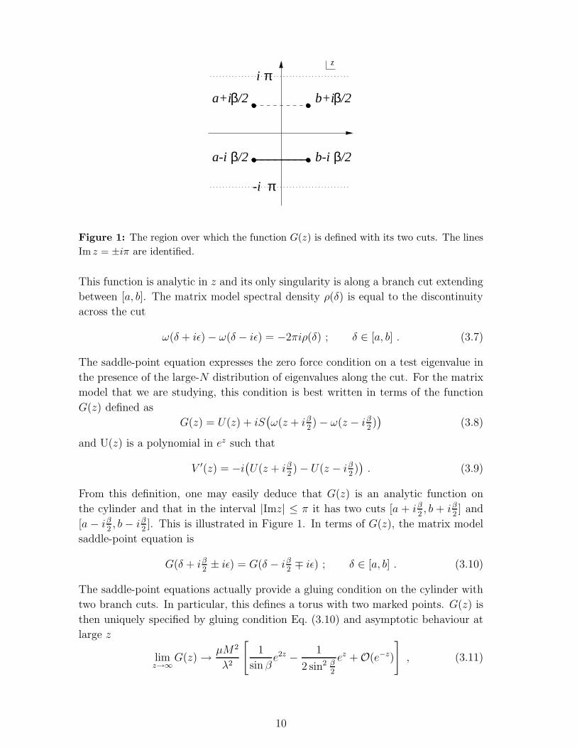
Figure 1: The region over which the function G(z) is defined with its two cuts. The lines

Im z = ±iπ are identified.

This function is analytic in z and its only singularity is along a branch cut extending

between [a, b]. The matrix model spectral density ρ(δ) is equal to the discontinuity

across the cut

ω(δ + iǫ) − ω(δ − iǫ) = −2πiρ(δ) ; δ ∈ [a, b] . (3.7)

The saddle-point equation expresses the zero force condition on a test eigenvalue in

the presence of the large-N distribution of eigenvalues along the cut. For the matrix

model that we are studying, this condition is best written in terms of the function

G(z) defined as

G(z) = U(z) + iS(

ω(z + iβ2) − ω(z − iβ

2))

(3.8)

and U(z) is a polynomial in ez such that

V ′(z) = −i(

U(z + iβ2) − U(z − iβ

2))

. (3.9)

From this definition, one may easily deduce that G(z) is an analytic function on

the cylinder and that in the interval |Imz| ≤ π it has two cuts [a + iβ2, b + iβ

2] and

[a − iβ2, b − iβ

2]. This is illustrated in Figure 1. In terms of G(z), the matrix model

saddle-point equation is

G(δ + iβ2± iǫ) = G(δ − iβ

2∓ iǫ) ; δ ∈ [a, b] . (3.10)

The saddle-point equations actually provide a gluing condition on the cylinder with

two branch cuts. In particular, this defines a torus with two marked points. G(z) is

then uniquely specified by gluing condition Eq. (3.10) and asymptotic behaviour at

large z

limz→∞

G(z) →µM2

λ2

[

1

sin βe2z −

1

2 sin2 β2

ez + O(e−z)

]

, (3.11)

10

A

CA’

CB

CA

CA’

CB

C

l

ab

cd

a

i

k

i

02w

w

-w2

2

1

z u

j l

cb d

kj

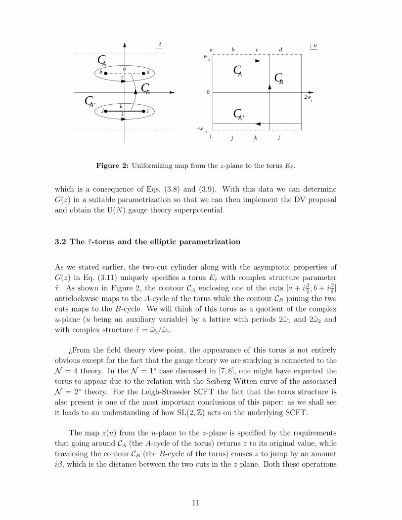
Figure 2: Uniformizing map from the z-plane to the torus Eτ .

which is a consequence of Eqs. (3.8) and (3.9). With this data we can determine

G(z) in a suitable parametrization so that we can then implement the DV proposal

and obtain the U(N) gauge theory superpotential.

3.2 The τ-torus and the elliptic parametrization

As we stated earlier, the two-cut cylinder along with the asymptotic properties of

G(z) in Eq. (3.11) uniquely specifies a torus Eτ with complex structure parameter

τ . As shown in Figure 2, the contour CA enclosing one of the cuts [a + iβ2, b + iβ

2]

anticlockwise maps to the A-cycle of the torus while the contour CB joining the two

cuts maps to the B-cycle. We will think of this torus as a quotient of the complex

u-plane (u being an auxiliary variable) by a lattice with periods 2ω1 and 2ω2 and

with complex structure τ = ω2/ω1.

¿From the field theory view-point, the appearance of this torus is not entirely

obvious except for the fact that the gauge theory we are studying is connected to the

N = 4 theory. In the N = 1∗ case discussed in [7, 8], one might have expected the

torus to appear due to the relation with the Seiberg-Witten curve of the associated

N = 2∗ theory. For the Leigh-Strassler SCFT the fact that the torus structure is

also present is one of the most important conclusions of this paper: as we shall see

it leads to an understanding of how SL(2, Z) acts on the underlying SCFT.

The map z(u) from the u-plane to the z-plane is specified by the requirements

that going around CA (the A-cycle of the torus) returns z to its original value, while

traversing the contour CB (the B-cycle of the torus) causes z to jump by an amount

iβ, which is the distance between the two cuts in the z-plane. Both these operations

11

leave G unchanged which is therefore an elliptic function on the u-plane. Thus

A − cycle : z(u + 2ω1) = z(u) ; G(z(u + 2ω1)) = G(z(u)) , (3.12a)

B − cycle : z(u + 2ω2) = z(u) + iβ ; G(z(u + 2ω2)) = G(z(u)) . (3.12b)

This determines the following unique map z(u) from the u-plane to the two-cut

cylinder:

exp z(u) =1

2 tan β2

·θ′1(0|τ)θ1(πu/2ω1 − β/4|τ)

θ′1(β/2|τ)θ1(πu/2ω1 + β/4|τ)(3.13)

The fact that G(z(u)) is an elliptic function on the u-plane along with its asymptotic

behaviour at large z (3.11) (corresponding to a pole in the u-plane) leads uniquely

to

G(z(u)) =µM2ω2

1 cos β2

4π2λ2 sin3 β2

·θ1(β/2|τ)2

θ′1(β/2|τ)2

[

℘(u + ω1β/2π) − ℘(ω1β/π)]

. (3.14)

Here, ℘(u) is the Weierstrass function, an elliptic function defined on Eτ , and θ1(u|τ)

is the Jacobi theta function of the first kind (see [20] and Appendix A for more

details). As expected, G(z(u)) is an elliptic function of u with a second order pole in

the u-plane; z(u) on the other hand is only quasi-elliptic. For a different choice of the

deformation potential the asymptotic behaviour of G(z) will change and G(z(u)) will

end up being an elliptic function of a different order, but significantly z(u) will remain

unchanged. There are two special points on the torus Eτ at u = ±βω1/2π which map

to the points z = ∓∞. Having determined G(z) in the elliptic parametrization we

can now implement the DV proposal to compute the superpotential in the confining

vacuum of the U(N) gauge theory.

3.3 Superpotential of the U(N) theory via Dijkgraaf-Vafa

According the Dijkgraaf-Vafa proposal, the gluino condensate of the gauge theory

gets identified with the ’t Hooft coupling S of the matrix model. From Eqs. (3.6)

and (3.8), the integral of G(z) around one of its cuts, say CA, is equal to −2πS, so we

can directly compute the gluino condensate of the U(N) gauge theory in the elliptic

parametrization:

ΠA = 2πiS = −i

∫

A

G(z(u))dz(u)

dudu . (3.15)

The second ingredient required to determine the QFT superpotential is the variation

in the genus zero free energy of the matrix model in transporting a test eigenvalue

from infinity to the endpoint of the cut. This is obtained by integrating the force

on a test eigenvalue from infinity to the endpoint of the cut and can be expressed

12

as ΠB = −i∫

BG(z)dz. There is a slight subtlety here as there is a “zero-point” en-

ergy associated with additive constants in the matrix model potential. First note that

there is a multiplicative factor of λ−N2

in the partition function (3.2) and an additive

constant in the classical scalar potential (3.4). Both these appear as S-dependent con-

tributions to the matrix model genus zero free energy defined as F0/g2s = N2F0/S

2,

so that

∂F0

∂S= ΠB − 2S ln λ +

µM2

4λ2 sin2 β2

; ΠB = −i

∫

B

G(z(u))dz(u)

dudu . (3.16)

The effective superpotential of the mass deformation of the U(N) Leigh-Strassler

theory in its confining vacuum is obtained by extremizing the following expression

with respect to S:

WU(N)eff = N

∂F0

∂S− 2πiτS;

∂

∂SW

U(N)eff = 0 . (3.17)

where τ is the bare coupling of the theory. The S-independent constant in Eq. (3.16)

appears as a vacuum-independent additive constant in the superpotential. On the

other hand, the term linear in S in Eq. (3.16) actually has the effect of renormalizing

the bare coupling τ so that

τ −→ τR = τ −iN

πln λ . (3.18)

Both ΠA and ΠB are easy to evaluate in our elliptic parametrization:

ΠA =dh(τ )

dτ; ΠB = τ

dh(τ )

dτ− h(τ ) , (3.19)

where

h(τ ) =µM2 cos β

2

4λ2 sin3 β2

·θ1(β/2|τ)

θ′1(β/2|τ). (3.20)

It follows straightforwardly that

∂

∂SW

U(N)eff = 0 =⇒ τ =

τR

N(3.21)

so that

WU(N)eff = −Nh(τR/N) +

NµM2

4λ2 sin2 β2

. (3.22)

Finally we have, therefore, the quantum superpotential of the U(N) gauge theory in

its confining vacuum,

WU(N)eff = −

NµM2 cos β2

4λ2 sin3 β2

·θ1(β/2|τR/N)

θ′1(β/2|τR/N)+

NµM2

4λ2 sin2 β2

, (3.23)

13

with τR defined in (3.18). This result satisfies the first obvious check: in the β → 0

limit with λ = 1 it reproduces the superpotential of the N = 1∗ theory. The

superpotential in the other N−1 confining vacua are obtained by repeated T -dualities

τR → τR+1. Note that the T -dualities in question naturally act on τR rather than the

bare coupling τ . Similarly the result for the superpotential has a modular parameter

τR/N and so we expect that any modular properties we uncover should naturally be

a consequence of the modular group acting on τR the “renormalized” coupling.

3.4 Eigenvalues of Φ in the U(N) theory and a test

One of the main results of our earlier work [7] in the context of N = 1∗ theory

was that the map z(u) from the u-plane to the z-plane, when evaluated along the

A-cycle of the τ -torus (which maps to the upper cut on the z-plane), precisely yields

the eigenvalues of the adjoint scalar Φ of the gauge theory in its confining vacuum,

distributed uniformly along this cycle.5 We were able to prove this assertion for a

class of deformations of the N = 4 theory involving masses for two of the adjoint

chiral superfields and arbitrary polynomials in the third adjoint field Φ. We will

not pursue this generalized analysis in the present case, but we will present strong

evidence that the same relation with the field theory eigenvalues holds under the

Leigh-Strassler deformation.

For the Leigh-Strassler theory, we first recall that the δi are valued in the z-plane

and these are in turn related to the eigenvalues of the Φ matrix through Eq. (3.3).

Taking into account the fact that the function G(z) is defined in Eq. (3.8) in terms

of the resolvent functions ω(z ± iβ2) where the positions of the cuts of the latter

have been displaced by ±iβ2, we conjecture that the function −M exp (z(u) − iβ

2)/λ

evaluated along the A-cycle gives the eigenvalues of Φ in the U(N) theory:

φ(x) =M

2λ sin β2

[

− cos β2

θ′1(0|τR/N)

θ′1(β/2|τR/N)

θ3(πx − β/4|τR/N)

θ3(πx + β/4|τR/N)+ 1

]

; x ∈ [−12, 1

2] .

(3.24)

Note that the factor λ takes into account the field rescaling prior to Eq. (3.3) and we

also incorporate the additive shift of M/(2λ sin β2) involved in the variable change in

Eq. (3.3). This is of course a continuous distribution of eigenvalues appropriate for

the U(N) theory in the large-N limit. But the finite N answer is obtained by simply

replacing the continuous index x by a discrete index. For this to be legitimate, it

is essential that the field theory eigenvalues be uniformly distributed in the interval

5In contrast the matrix model eigenvalues are not distributed uniformly along this cycle signalling

the crucial difference between the spectral densities of the two systems. Nevertheless, the matrix

model provides a means to extract the field theory distributions in a simple way.

14

x ∈ [−12, 1

2] as we have indeed pointed out earlier. The difference between finite-N

and large-N manifests itself in gauge-invariant observables as vacuum-independent

operator mixing ambiguities that vanish in the large-N limit [7].

Our results for the eigenvalues in the confining vacuum of the U(N) theory

satisfy several checks. Firstly in the classical limit τR → i∞, using the properties of

the Jacobi theta functions (see Appendix A), Eq. (3.24) vanishes as expected, since

the confining vacuum should correspond to the trivial classical solution. Secondly,

in the β → 0 limit with λ = 1 the eigenvalues of N = 1∗ theory in its confining

vacuum reproduce the expressions in [7,21]. Two further nontrivial tests involve the

computation of 〈Tr Φ〉 and 〈Tr Φ2〉 in the U(N) theory using the eigenvalues above.

With a large-N distribution, the trace reduces to an integral and we find

⟨

Tr Φ⟩

= N

∫ 1/2

−1/2

dxφ(x) =2λ sin β

2

µMW

U(N)eff , (3.25a)

⟨

Tr Φ2⟩

= N

∫ 1/2

−1/2

dxφ2(x) =1

µW

U(N)eff , (3.25b)

where WU(N)eff is the expression obtained in Eq. (3.23). We show how to compute the

associated integrals explicitly in Appendix B. The first (3.25a) demonstrates that the

trace of Φ calculated using the matrix model results satisfies precisely the relation

Eq. (2.7) predicted on general grounds from field theory. The second integral is also

exactly in accord with field theory expectations since from our general arguments in

Section 2, we have WU(N)eff ∝ µ and therefore differentiating with respect to µ gives

〈Tr Φ2〉 = WU(N)eff /µ precisely (3.25b).

In summary, the eigenvalues of the adjoint scalar Φ in the confining vacuum of

the mass deformed U(N) Leigh-Strassler theory at large N are given by Eq. (3.24).

The eigenvalues of the U(N) theory at finite N are obtained by substituting the

continuous index x with an appropriate discrete index.

3.5 The SU(N) superpotential

We argued in Section 2 that the superpotentials of the U(N) and SU(N) theories

differ non-trivially, but are nevertheless simply related by Eq. (2.10). The main point

there was that the U(N) theory allows a non-zero 〈Tr Φ〉 ≡ N〈a〉 6= 0 to develop in

the confining vacuum of the quantum theory. This leads to what is effectively a

renormalization of the mass parameter M → M ′ = M − 2〈a〉λ sin β2. According

to the result of our field theory analysis of Section 2, the SU(N) superpotential

may be recovered by a rescaling of the U(N) result by M2/M ′2, after subtracting

15

off a vacuum independent constant. It is quite interesting to note that precisely the

same vacuum independent constant makes an appearance in the U(N) superpotential

(3.23) computed in the Dijkgraaf-Vafa approach.

Using our results for the U(N) superpotential from the previous section and

Eq. (2.10), we thus find that in the confining vacuum the SU(N) theory develops the

superpotential,

WSU(N)eff =

NµM2

2λ2 sin β·θ′1(β/2|τR/N)

θ1(β/2|τR/N)−

NµM2

4λ2 sin β2

, (3.26)

where the renormalized coupling is defined in (3.18). This expression for the SU(N)

superpotential has the correct β → 0 limit in that it reproduces the N = 1∗ super-

potential exactly.

3.6 SU(N) eigenvalues and condensates

The eigenvalues φi of the adjoint scalar Φ in the confining vacuum of the SU(N)

theory are related to the U(N) eigenvalues by a simple extension of our arguments

in Section 2 as

φ(x) =M

M ′

(

φ(x) −M

2λ sin β2

)

+M

2λ sin β2

. (3.27)

This can be understood simply as a rescaling of the U(N) spectrum of eigenvalues

by M/M ′(〈a〉) after subtracting out a constant and is in line with the arguments of

Section 2 for extracting the SU(N) superpotential.

Evaluating this explicitly yields

φ(x) =M

2λ

[

−θ′1(0|τR/N)

θ1(β/2|τR/N)

θ3(πx − β/4|τR/N)

θ3(πx + β/4|τR/N)+

1

sin β2

]

; x ∈ [−12, 1

2] .

(3.28)

We show in Appendix B that with these eigenvalues 〈Tr Φ〉 = 0 and 〈Tr Φ2〉 =

WSU(N)eff /µ. Once again we remark that with a continuous label x these are really the

eigenvalues of the large-N gauge theory but finite-N results are obtained by simply

replacing x with a discrete index.

Now that we have the complete distribution of eigenvalues of Φ in the confining

vacuum of the SU(N) theory, every condensate of the form 〈Tr Φk〉 is automatically

computed via the integrals

⟨

Tr Φk⟩

= N

∫ 1/2

−1/2

dx φk(x) . (3.29)

16

We will not undertake the exercise of computing these but, if desired, they can be

computed following the methods in Appendix B.

3.7 Summary

In this section we have computed the value of the effective superpotential and the

spectrum of eigenvalues of Φ in the confining vacuum of the SU(N) theory. We

did this by obtaining the U(N) superpotential via a matrix model and subsequently

extracting the SU(N) results by a process of integrating-in6 discussed in Section 2.

The results of the computation have satisfied several general field theory checks. In

addition, the emergence of a quasi-modular function (θ′1/θ1) as the superpotential

of the SU(N) theory is strongly suggestive of Montonen-Olive duality being realized

in this theory. (In contrast, the U(N) superpotential being basically the reciprocal

of the SU(N) result, transforms in a complicated way under the modular group.)

In order to establish electric-magnetic duality we need to be able to compute the

corresponding quantities in other massive vacua of the theory (most notably the

Higgs vacuum which should be S-dual to the confining phase). We will address this

in Sections 4 and 5 which will be devoted to understanding the classical and quantum

vacuum structure respectively.

4. Vacuum structure of deformed SU(N) Leigh-Strassler the-

ory

In this section we exhibit the classical vacuum structure of the SU(N) theory. Im-

portantly these classical configurations will serve as the starting point for analysing

other saddle points of the matrix model and thence obtaining the effective quantum

superpotential in all the massive vacua. Interestingly the classical solutions (the

eigenvalues) for the Higgs vacuum that we find here will be shown to be related by

S-duality to the quantum eigenvalue spectrum of the confining vacuum that we have

already obtained in the previous section.

The vacuum structure of the mass deformed SU(N) Leigh-Strassler theory turns

out to be subtly different from that of the N = 1∗ theory: there are new vacua and

6We remark that one might have expected to obtain the SU(N) superpotential and eigenvalues

directly from the matrix model by imposing a constraint on the matrices via a Lagrange multiplier.

However this turns out not to work in any simple way, the primary reason being, as pointed out in [7],

that the matrix model eigenvalue spectrum is completely different from the field theory spectrum

and tracelessness of the latter translates into a rather complicated constraint on the former.

17

old vacua can disappear. In order to describe the vacuum structure, we start with

the tree-level superpotential (1.1). At the classical level vacua are determined by

solving the F - and D-flatness conditions modulo gauge transformations. As usual,

if one is interested in holomorphic information it is sufficient to solve the F -flatness

conditions modulo complex gauge transformations. These conditions follow from

extremizing the tree-level superpotential (1.1):7

P [Φ+, Φ−]β = −i2µ

λΦ , P [Φ, Φ+] = −i

M

λΦ+ , P [Φ−, Φ] = −i

M

λΦ− . (4.1)

In the above, P is the projector onto the traceless part which must be imposed

since we are dealing with the SU(N), rather than the U(N), theory. Complex gauge

transformation can be used to diagonalize Φ.

In the limit β = 0, the theory becomes the basic N = 1∗ theory and the condi-

tions (4.1) reduce to the Lie algebra of SU(2). Let us briefly recall the solutions in

that case. Each solution is associated to a representation of SU(2) of dimension N

where Φ and Φ± are, up to a trivial re-scaling, J3 and J±, respectively. Each repre-

sentation of SU(2) of dimension N is associated to a partition N → n1 + · · · + nq,

where each integer ni is the dimension of each irreducible component. In general the

unbroken gauge group has abelian factors and the phase is Coulomb, or massless.

The massive vacua are associated to the the equi-partitions N = q · p for which the

unbroken gauge group is SU(q). In such a vacuum, the low energy description is pure

N = 1 with gauge group SU(q) which has q inequivalent quantum vacua. Hence,

there are∑

q|N q vacua with a mass gap (the sum being over the positive integer

divisors of N).

Now we consider the case when β 6= 0. Each of the vacua of the N = 1∗ theory

remains a vacuum of the deformed theory, at least for generic values of β. These

deformed solutions have the following form. Firstly, the block form of the solutions

associated to the partition N → n1 + · · · + nq is preserved. Let us concentrate on

one of the blocks of dimension n. For β = 0, Φ and Φ± are equal to J3 and J±, up

to trivial re-scaling, of the irreducible SU(2) representation of dimension n:

β = 0 : Φ = −M

λJ3 ; Φ± =

2µM

λJ± . (4.2)

When β 6= 0, the non-zero elements of Φ± have the same pattern as J± (so only

the elements just above and below the diagonal, respectively are non-zero) but the

numerical values are changed. The elements of diagonal matrix Φ in the block in

7Note that the F -term equations are rather similar to the “q-deformed” SU(2) algebra. They

are similar to, but not the same as the equations encountered in [2]. The authors of [2] considered

a slightly different mass deformation and a U(N) gauge group.

18

question are found to be

φj =M

2λ

( 1

sin β2

−n

sin nβ2

e−iβ(n+1−2j)/2)

, j = 1, . . . , n . (4.3)

Notice that when β → 0, Φ, in this block, becomes equal to −(M/λ)J3 as expected.

For generic β, these deformed vacua are massive/massless according to their type

when β = 0. However, for specific values of β vacua can migrate off to infinity in field

space and hence cease to be genuine vacua of the field theory. This occurs when the

eigenvalues of Φ diverge. It is easy to see that this will occur in a block of dimension

n when the deformation parameter

β =2πk

n, k ∈ Z . (4.4)

In one of the N/p massive vacua with unbroken SU(N/p) symmetry the eigen-

values of Φ are given by (4.3) with n = p and where each eigenvalue has degeneracy

N/p. From this spectrum, we can calculate the classical values for the condensates;

for instance, for the quadratic condensate:

〈Tr Φ2〉 =M2N

4λ2 sin2 β2

(

ptan β

2

tan pβ2

− 1)

. (4.5)

Notice that this condensate diverges when β = 2πk/p, k ∈ Z in accord with (4.4).

4.1 New classical branches

As well as the original massive vacua, there are also new vacua which are not present

when β = 0. We illustrate this is in the simplest case where the gauge group is

SU(3). In this case there is a new vacuum, more precisely a moduli space of vacua,

in which Φ and Φ± are all, up to complex gauge transformations, diagonal:

Φ =M

2λ sin β2

diag(

x1, x2, x3

)

,

Φ+ =

√

µM/2

λ sin β2

ρ diag(

(1 − x1)−1, (1 − x2)

−1, (1 − x3)−1)

,

Φ− =

√

µM/2

λ sin β2

ξ diag(

(1 − x1)−1, (1 − x2)

−1, (1 − x3)−1)

.

(4.6)

Here, ρ and ξ are two complex moduli of the solution and xi, i = 1, 2, 3 are the three

distinct roots of the cubic

x3 − 3x + 2 − ρξ = 0 . (4.7)

19

Note that the tracelessness of Φ and Φ± is guaranteed by the form of the cubic (4.7).

Clearly these solutions diverge to infinity when β → 0. However, the moduli space

of the solutions also has additional branches which occur whenever

eiβ/2xi − e−iβ/2xj = 2i sin β2

. (4.8)

In this case, an off-diagonal component of either of (Φ±)ij can become non-zero. The

quadratic condensate in this space of vacua is

SU(3) : 〈Tr Φ2〉 =3M2

2λ2 sin2 β2

. (4.9)

Clearly this diverges when β = 0. We will see that these new vacua are important

for checking a conjecture that we make later.

5. Electric-magnetic duality in the Leigh-Strassler Deforma-

tion

The question we now address is what becomes of the S-duality of the N = 4 theory

under the Leigh-Strassler deformation? Specifically we are considering a deformation

of the N = 4 Lagrangian of the form;

L = LN=4 +

∫

d2θ ∆W (5.1)

where the deforming superpotential can be written as

∆W = i(

λ cos β2− 1)

O1 − λ sin β2O2 + M Tr Φ+Φ− + µ Tr Φ2 (5.2)

where, as in Section 1, O1 = Tr Φ[Φ+, Φ−] and O2 = Tr Φ{Φ+, Φ−}. At the N = 4

point, the operators appearing in the deforming superpotential transform under S-

duality in a definite way. Adding these operators to the superpotential therefore

breaks modular invariance. However, as is standard when dealing with broken sym-

metries, we should be able to restore invariance by allowing the corresponding cou-

plings to transform in an appropriate way. This strategy was implemented in detail

for the N = 1∗ case β = 0 in [13]. We will now review this briefly and extend this

discussion to the marginal deformation.

Using the conventions described in [13],8 the superspace measure d2θ has holo-

morphic modular weight −2. Hence for modular invariance of the Lagrangian, the

8See the final paragraph of Section 3 of this reference.

20

superpotential must have weight +2. In the N = 4 theory, the mass operators

Tr Φ+Φ− and Tr Φ2 are both part of the multiplet of chiral primary operators which

transform as second rank symmetric traceless tensors under the SO(6) R-symmetry.

Their modular weights can be deduced via the AdS/CFT correspondence by com-

parison with the dual fields in IIB supergravity [12]. In fact they have holomorphic

modular weight +2 and the Lagrangian will be invariant if we assign the mass pa-

rameters M and µ weight zero. Although there is no explicit breaking of modular

invariance, it is important to remember that the theory has various vacuum states

in which these mass operators acquire expectation values, thereby ‘spontaneously’

breaking S-duality. In other words, modular transformations map the observables

in one vacuum to those in another. Indeed, this property is manifest in the exact

results of [11, 13].

Similar arguments should apply to the Leigh-Strassler theory at least near the

N = 4 point where the modular properties of the deforming operators are known.

If we set λ = 1 and work to linear order in β, the deformation only contains the

cubic operator O2. This operator is also part of an N = 4 chiral primary multiplet

consisting, in this case, of third rank symmetric traceless tensors of SO(6). In the

conventions of [13] it has modular weight +3. To restore invariance under S-duality

we should therefore assign the parameter β holomorphic modular weight −1. In Sec-

tion 5.2, we will find the appropriate generalization of this transformation property

throughout the parameter space, by using the matrix model to find the exact super-

potential in each of the massive vacua. In Section 5.1 we see what can be deduced

by looking at the Higgs and confining vacua alone.

5.1 A first look at S-duality

Let us concentrate on the Higgs and confining vacua. In the N = 1∗ limit, it is

well known that each observable in the Higgs vacuum is simply related by S-duality,

τ → −1/τ , to the corresponding observable in the confining vacuum. This is an

explicit realization of the Montonen-Olive electric-magnetic duality of the N = 4

theory. The question is whether a similar duality persists under the Leigh-Strassler

deformation.

If S-duality is realized in this theory it should exchange the Higgs and confining

vacua. Since we already have the eigenvalues in the confining vacuum of the SU(N)

theory a simple and powerful test emerges: use S-duality to deduce the eigenvalues

in the Higgs vacuum and then take the classical limit and compare with the spectrum

(4.3) (n = N) deduced from the F -flatness conditions. In the next section, we shall

use the matrix model to solve for the superpotential in each of the massive vacua

21

and this uncovers the action of the whole of the modular group.

The eigenvalues of Φ in the confining vacuum are given in (3.28). (Recall that

the eigenvalues in this vacuum have the property that they vanish in the classical

limit.) The first thing to notice is that the modular parameter of the elliptic function

parametrizing the eigenvalue spectrum is τR/N with τR = τ − (iN/π) ln λ, where τ

is the gauge coupling. Hence S-duality, if realized, must act on the renormalized

coupling τR as τR → −1/τR rather than τ itself. Under this action, the modular

parameter of the elliptic functions changes as τR/N → −1/(τRN). But now we want

to take the classical limit τR → i∞ and this can be done easily after performing a

modular transformation −1/(τRN) → τRN on the (quasi-)elliptic functions. Using

the modular transformation properties of the theta functions (see Appendix A) we

find

φ(x) −→ −τRNM

2λ sin NτRβ2

e−iNτRβx +M

2λ sin β2

; x ∈ [−12, 1

2] . (5.3)

Apart form the additive constant, this coincides precisely with the expression Eq. (4.3)

(n = N) for the eigenvalues in the Higgs vacuum of the deformed SU(N) Leigh-

Strassler theory with β replaced by τRβ. Equivalently, the Higgs and confining

vacua of the theory with deformation parameter β are simply exchanged under the

combined operation τR → −1/τR and β → β/τR

The overall factor of τR in the above expression is expected because the eigen-

values have modular weight one. The fact that the additive constants are different

is to be expected: even in the context of N = 1∗ theory the matrix model approach

only yields results that are S-duality covariant up to a vacuum independent shift [7].

This additive shift will be discussed in more detail in the next section. We should

also point out that after S-duality on the spectrum of eigenvalues in the confining

vacuum we have taken a classical limit above. In this limit, the exact transformation

properties of the couplings λ, β are not visible. These will become clear in the next

section.

The results of this simple analysis are that there is indeed a form of S-duality

that relates the Higgs and confining vacua of the theory with deformation parameter

β. In particular this duality acts on the bare couplings of the Leigh-Strassler theory

as

τR −→ −1/τR , β −→ β/τR . (5.4)

This is consistent with β having modular weight -1 as expected. Recall that the

bare theory has 3 couplings τ , λ and β with one non-trivial relation, so that (5.4)

determines the action of S-duality on the bare theory up to the unknown relation.

In the next section we expand the discussion of duality to include the whole of the

modular group SL(2, Z) and deduce the action on all three of the bare couplings.

22

5.2 Multi-cut solutions of the matrix model and SL(2, Z)

Now that we have described the structure of massive vacua of the Leigh-Strassler

deformed theory, we can return to the matrix model and ask whether we can solve

for the exact superpotential and condensates in each of these vacua. This will turn

out to be very important because it will prove that there is an action of electric-

magnetic duality on the Leigh-Strassler deformation of the N = 4 theory. In fact

this extends to the action of the full SL(2, Z) modular group.

The way to use the matrix model to solve for the theory in an arbitrary massive

vacuum is described for the N = 1∗ theory in [8]. One finds that the same techniques

can be used in the deformed matrix model described in Section 3. In order to describe

the massive vacua with unbroken SU(N/p) symmetry, one needs a multi-cut solution

of the matrix model. Of course the matrix model computes the superpotential in the

U(N) theory and we then use (2.9) to deduce it in the SU(N) theory.

We start with the observation that the classical eigenvalues in the massive vacua

with unbroken SU(N/p) are given by (4.3) with n = p, each with degeneracy N/p.

The only thing that will be important for us will be the range of the phases of

these classical eigenvalues. The classical eigenvalues of the U(N) gauge theory also

have exactly the same phases in the corresponding massive vacua. As we have seen

explicitly in the case of the confining vacuum, the eigenvalues of the field theory are

essentially proportional to exp[z]. This directs us to consider a p-cut solution of the

matrix model with the cuts in the z-plane situated at[

a + iβ(p + 1 − 2j)/2, b + iβ(p + 1 − 2j)/2] ; j = 1, . . . , p (5.5)

where these positions are dictated precisely by the phases of the classical eigenvalues.

The classical eigenvalues are clustered in groups of N/p at each of these points, but

the pairwise effective interactions induced in the matrix model will cause each cluster

to spread out into a cut.

Following [8], we then make an ansatz where the cuts have the same length and

the same filling fractions. It can then be shown that G(z) defined in (3.8) again

only has two cuts, as in the confining vacuum, but where the cuts are shifted to

±[a + iβp/2, b + iβp/2]. This modifies the map z(u) in (3.13) by a shift β → pβ:

exp z(u) =1

2 tan pβ2

·θ′1(0|τ)θ1(πu/2ω1 − pβ/4|τ)

θ′1(pβ/2|τ)θ1(πu/2ω1 + pβ/4|τ). (5.6)

Similarly

G(z(u)) =µM2ω2

1 cos pβ2

4π2λ2 sin3 pβ2

·θ1(pβ/2|τ)2

θ′1(pβ/2|τ)2

[

℘(u + ω1pβ/2π) − ℘(ω1pβ/π)]

. (5.7)

23

When the Dijkgraaf-Vafa recipe is followed one finds that for each cut there is

an associated filling fraction of eigenvalues Nj/N which translates to an effective ’t

Hooft coupling Sj = gsNj with∑

Sj = S. For the massive vacua we note that the

filling fractions in each of the p cuts are the same and equal to N/p = q

2πiSj =dh(τ )

dτ; j = 1, . . . , p , (5.8)

where h(τ ) is the same function that we encountered in (3.20) with β → pβ:

h(τ ) =µM2 cos pβ

2

4λ2 sin3 pβ2

·θ1(pβ/2|τ)

θ′1(pβ/2|τ). (5.9)

In addition one also needs the variation in the genus zero free energy upon trans-

porting an eigenvalue from any given cut to infinity. After minor modifications this

is also given by the same expressions that were encountered in the one-cut solution

for the confining vacuum:

p∑

j=1

∂F0

∂Sj

= τdh(τ)

dτ− h(τ) − 2 lnλ

p∑

j=1

Sj + pµM2

4λ2 sin2 β2

. (5.10)

Then the superpotential for the U(N) theory at any of its massive vacua is

WU(N)eff =

N

p

p∑

j=1

∂F0

∂Sj− 2πiτ

p∑

j=1

Sj . (5.11)

Extremizing with respect to τ gives

τ =p2

NτR (5.12)

and therefore we find that the value of the quantum effective superpotential for the

U(N) theory is

WU(N)eff = −

NµM2 cos pβ2

4pλ2 sin3 pβ2

·θ1(pβ/2|p2τR/N)

θ′1(pβ/2|p2τR/N)+

NµM2

4λ2 sin2 β2

. (5.13)

In all of the above we should remember that p is a divisor of N .

The result for SU(N) follows by the application of Eq. (2.9):

WSU(N)eff =

pNµM2

2λ2 sin β·θ′1(pβ/2|p2τR/N)

θ1(pβ/2|p2τR/N)−

NµM2

4λ2 sin2 β2

. (5.14)

This gives the result in only one of q = N/p vacua of this type. The results in the

remaining vacua follow by the replacement

τR −→ τR + k/p ; k = 0, 1, . . . q − 1 . (5.15)

24

The Higgs vacuum corresponds to p = N whilst the confining vacuum considered

previously has p = 1 and k = 0.

One interesting and immediate check on the form of the superpotential follows

from the fact that it is manifestly divergent when the deformation parameter takes

the special values

β =2πk

p, k ∈ Z . (5.16)

But this matches precisely the values of β in Eq. (4.4) for which the classical eigen-

values of Φ for the massive vacua diverge (since they consist of q blocks of size n = p).

Another check follows by taking the classical limit of the superpotential (5.14). Using

(A.3c), one finds

WSU(N)eff

τR→i∞−→ 〈Tr Φ2〉 =

NµM2

4λ2 sin2 β2

(

ptan β

2

tan pβ2

− 1)

, (5.17)

which matches the values of µ〈Tr Φ2〉 obtained in (4.5) from the F -flatness condition

precisely.

Now that we have the superpotential in each of the massive vacua, we can now

investigate how the full SL(2, Z) duality group acts on the theory. In the N =

1∗ theory described in [7, 8], we established that the matrix model yields a result

for the superpotential which is only duality covariant when shifted by a vacuum

independent constant. This kind of additive ambiguity is ubiquitous in this subject:

see [7,9]. Naturally, the same kind of ambiguity will be present in the Leigh-Strassler

deformation where we claim that the appropriate definition of a duality covariant

superpotential is

WSU(N)eff = W

SU(N)eff + C(τR, β, λ) , (5.18)

where the vacuum-independent constant is given by either of the expressions

C(τR, β, λ) =NµM2

4λ2 sin2 β2

−NµM2

2λ2 sin β·θ′1(β/2|τR)

θ1(β/2|τR)+

N(N − 1)µM2β

12λ2 sin βE2(τR)

=NµM2

4λ2 sin2 β2

−NµM2ω1

πλ2 sin β

(

ζ(ω1β/π) −Nβ

πζ(ω1)

)

.

(5.19)

Here, the Weierstrass ζ-function is defined relative to a torus with periods ω1 and

ω2 and τR = ω2/ω1 and E2(τR) is the 2nd Eisenstein series (see the Appendix of [7]

for definitions and references). One property that the C has is that it reduces to the

correct form needed in the N = 1∗ theory in the limit β → 0.

25

Our claim is that the duality-covariant definition of the superpotential in the

each of the massive vacua labelled by (p, k), p · q = N and k = 0, . . . , q, is then

WSU(N)eff =

NµM2

2λ2 sin β

(

pθ′1(pβ/2|τ)

θ1(pβ/2|τ)−

θ′1(β/2|τR)

θ1(β/2|τR)+

β

6(N − 1)E2(τR)

)

, (5.20)

where

τ = (pτR + k)/q . (5.21)

Using the modular properties of the theta functions and the 2nd Eisenstein series,

(A.2a) and (A.5), one can easily show, for example, that

Weff(β/τR,−1/τR, λ)∣

∣

∣

Conf= τR

sin β

sin(β/τR)· Weff(β, τR, λ)

∣

∣

∣

Higgs. (5.22)

Notice that the coupling β transforms with unit weight under the modular group.

Note also the rather unconventional transformation of the superpotential itself: this

we will have to cure by an appropriate definition of the transformation of the coupling

λ.

A consideration of the other massive vacua show that they all lie on a single

orbit of the SL(2, Z) duality group. For the element

σ =

(

a b

c d

)

∈ SL(2, Z) , (5.23)

which relates two vacua A = σ(B), we have9

Weff

(

βcτR+d

, aτR+bcτR+d

, λ)

∣

∣

∣

A= (cτR + d)

sin β

sin[β/(cτR + d)]· Weff(β, τR, λ)

∣

∣

∣

B. (5.24)

From this we can deduce the action of σ ∈ SL(2, Z) on the bare couplings of the

theory; clearly

σ(τR) =aτR + b

cτR + d, σ(β) =

β

cτR + d, (5.25)

confirming that β transforms with modular weight -1. However, we can say more: in

order that the superpotential transforms with a definite modular weight, so that it is

consistent with the group action, we can deduce the transformation of the coupling

λ. Recall, that on the marginal surface of the Leigh-Strassler deformation λ is a

function—albeit unknown—of the other two couplings and so must transform. In

addition, since in the limit β → 0, the superpotential transforms with modular

weight 2, we expect this to be preserved for β 6= 0. This requires the combination

λ2 sin β that appears as an overall factor in the superpotential must transform with

unit modular weight:

σ(λ2 sin β) =λ2 sin β

cτR + d. (5.26)

9The actual action of σ on a vacuum with labels (p, k) is not difficult to elucidate.

26

6. An exact elliptic superpotential

Another method that has been used to calculate the exact values of the superpotential

in all the vacua of the N = 1∗ theory is to compactify it on a circle of finite radius [9].

The effective superpotential is then a function of the dual photons and Wilson lines

of the abelian subgroup U(1)N−1 ⊂ SU(N). These comprise N − 1 complex scalar

fields Xa, a = . . . , N (with∑N

a=1 Xa = 0) which naturally live on a torus of complex

structure τ because of the periodicity of each dual photon and Wilson line. The

superpotential describing the N = 1∗ deformation is therefore constrained to be an

elliptic function of the complex scalars Xa. In [9] the exact answer was found to be

WR3×S1 ∼

∑

a6=b

℘(Xa − Xb) , (6.1)

where ℘(z) is the Weierstrass function defined on a torus with half periods ω1,2

with τ = ω2/ω1. What is particularly useful about this superpotential is that it

is independent of the compactification radius, and therefore, yields results that are

valid in the four-dimensional limit, and it encodes all the vacua of the N = 1∗ theory:

both massive and massless.

The question is whether there is an elliptic superpotential that describes the

Leigh-Strassler deformation? Similar arguments to those used in [9] suggest that

there should be, but are not powerful enough to determine the exact answer. How-

ever, there is an obvious candidate for appropriate marginal deformation of (6.1),

which turns out to be correct. Specifically, we can replace the Weierstrass function

℘(z), by its unique deformation in the space of even elliptic functions.10 In particular,

the Weierstrass function has one double pole at the origin and we can consider the

elliptic function of order two obtained by splitting the double pole into two single

poles. Remarkably, a superpotential of precisely this form reproduces our results

from the matrix model for the superpotential in each of the massive vacua. This

superpotential can be written as,

WR3×S1 =M2µ

2λ2 sin β

(ω1

π

)

∑

a6=b

(ζ(Xa − Xb + βω1/π) − ζ(Xa − Xb − βω1/π)) . (6.2)

The Weierstrass-zeta function ζ(u) can be defined via ℘(u) = −ζ ′(u) where ℘(u) is

the Weierstrass function for the torus with complex structure τR. Then in the limit

β = 0 this reproduces (6.1). What is remarkable is that the massive vacua of the

N = 1∗ theory for which the Xa lie on sub-lattices are also critical points of (6.2)

since this only relies on the fact that the two-body interaction is an even elliptic

10The function must be even to respect the Weyl group of SU(N)

27

function. For instance, for the p · q = N massive vacuum with k = 0 we have

Xa ∈{2ω1r

p+

2ω2s

q, r = 0, . . . , p − 1 , s = 0, . . . , q − 1

}

. (6.3)

Furthermore, the values of the superpotential are precisely given by (5.20).

A very strong check on the form of the superpotential we have conjectured in

(6.2) is possible because of the existence of new vacua which are not present in

the limit β = 0. For example, it is easy to show that Xa = 0, ∀a, is a critical

point. Actually this is an SL(2, Z)-invariant vacuum. Now we can take the classical

limit, τ → i∞, after having shifted by minus the vacuum-independent shift (5.19),

and compare with the analysis of the vacuum structure in Section 4. In the case

of SU(3), the classical limit of the superpotential WR3×S1 − C in the vacuum with

Xa = 0 precisely equals the value calculated from the new vacuum solution of the

F -flatness conditions (4.9). We expect this to generalize to SU(N), however, the

analysis remains to be done.

The properties and construction of this elliptic superpotential will be described

in a separate publication; however, we mention the fact that for N = 1∗, the el-

liptic superpotential is, more or less, the (complexified) Hamiltonian of the elliptic

Calogero-Moser integrable system which described N particles interacting though

pair-wise forces proportion to ℘(Xa − Xb). The intriguing question is whether this

system can be deformed

℘(Xa − Xb) → ζ(Xa − Xb + βω1/π) − ζ(Xa − Xb − βω1/π) (6.4)

whilst preserving integrability.

Finally we comment on a remarkable correspondence between our results for

the Leigh-Strassler deformation and the exact superpotential of a certain relevant

deformation of the A1-quiver theory studied in [14]. Specifically this is the theory of

an SU(N)× SU(N) gauge multiplet with gauge couplings g1 and g2, with two chiral

multiplets A and B in the (N, N) representation and two chiral multiplets A and

B in the (N , N). The theory also contains two chiral multiplets Φ1 and Φ2 in the

(adj, 0) and (0, adj) representations respectively with classical superpotential

W = Tr{

(g1Φ1 + M/2)(AA + BB) + (g2Φ2 + M/2)(AA + BB)}

. (6.5)

This theory actually has N = 2 supersymmetry but we further deform it by adding

the operator,

µTr(

Φ21 − Φ2

2

)

. (6.6)

to the classical superpotential which preserves N = 1 supersymmetry. This theory

is a relevant deformation of the N = 2 superconformal theory obtained by setting

28

µ = M = 0. The exact vacuum structure and superpotential was determined in [14].

The theory has N∑

d|N d massive vacua. Remarkably, in∑

d|N d of these vacua, we

find exactly the same value of the superpotential as in each of the massive vacua of the

SU(N) Leigh-Strassler theory studied in this paper. Specifically, this agreement holds

if we identify the parameter β of the Leigh-Strassler deformation and the complexified

coupling of one of the SU(N) factors in the quiver theory τ1 = 4πi/g21 + θ1/2π (or

z = 2iπτ1 to use the notation of [14]) :

z =Nω1β

π. (6.7)

In the brane set-up for the quiver model z is the relative separation of the two NS5-

branes. We also identify the parameters M and µ of the quiver superpotential with

parameters of the same name in the deformed Leigh-Strassler superpotential (1.1).

This connection suggests that there should be an RG flow from the superconfor-

mal A1-quiver to the Leigh-Strassler fixed line. At least in one special case, such a

flow is known to exist. In [23], Klebanov and Witten considered the quiver theory

in the case of equal gauge couplings g1 = g2 and zero masses for the bi-fundamental

multiplets, M = 0. In this case one can integrate out the adjoint chiral fields Φ1

and Φ2 and induce a marginal quartic superpotential for the bi-fundamentals which

corresponds to D3-branes placed at a resolved conifold singularity. Moving onto the

Higgs branch where SU(N) × SU(N) is broken to the diagonal SU(N), we find an

effective theory of three chiral superfields transforming in the adjoint of the unbroken

SU(N) which coincides with N = 4 SUSY Yang-Mills. Repeating this exercise with

unequal gauge couplings g1 6= g2, we find that the Leigh-Strassler marginal defor-

mation as well as other irrelevant operators are induced. However, it is not obvious

whether this flow is related to the exact agreement we have found above.

Acknowledgements: TJH would like to thank Frank Ferrari for discussions.

The authors would also like to thank Robbert Dijkgraaf and Cumrun Vafa for valu-

able discussions. We thank Robbert Dijkgraaf for his comments and observations

on a preliminary version of this article. SPK acknowledges support from a PPARC

Advanced Fellowship.

Appendix A: Some properties of elliptic functions

The (quasi-)elliptic functions that we need, ℘(z), ζ(z) and θi(z|τ), are all stan-

dard and their definitions and properties can be found in [20]. In our conventions,

29

the basic torus has periods 2ω1 and 2ω2 with complex structure τ = ω2/ω1. We also

define q = exp(iπτ). Below we list some properties of these functions that will be

useful.

An important relation between the Weierstrass and Jacobi theta functions is

ζ(u) −ζ(ω1)

ω1

u =π

2ω1

θ′1(πu/(2ω1)|τ)

θ1(πu/(2ω1)|τ). (A.1)

The Jacobi theta functions have the following modular properties that will be useful

θ1(x|τ) = i(−iτ)−12 exp(−ix2/πτ)θ1(x/τ | − 1/τ) , (A.2a)

θ3(x|τ) = (−iτ)−12 exp(−ix2/πτ)θ3(x/τ | − 1/τ) . (A.2b)

In order to take the classical limit, we will need the expansion

θ1(x|τ) = 2∞∑

n=0

(−1)nq(n+1/2)2 sin(2n + 1)x , (A.3a)

θ3(x|τ) = 1 + 2∞∑

n=0

(−1)nqn2

cos 2nx , (A.3b)

θ′1(x|τ)

θ1(x|τ)= cotx + 4

∞∑

n=1

q2n

1 − q2nsin 2nx . (A.3c)

We also need the 2nd Eisenstein series [22]

E2(τ) = 1 − 24∑

n=1

σ1(n)q2n , (A.4)

where σ1(n) is a sum over each positive integral divisor of n. It has the following

non-trivial modular transformation

E2(−1/τ) = τ 2E2(τ) +6τ

πi. (A.5)

Appendix B: Calculating condensates

In this appendix we show how the integrals of the type (3.25a) and (3.25b) can

be computed to yield the condensates in the U(N) and SU(N) gauge theories. Let us

first consider the function f(x) in terms of which the eigenvalues have been defined

f(x) =θ4(πx − β/4|τ)

θ4(πx + β/4|τ)≡

θ3(πx − π/2 − β/4|τ)

θ3(πx − π/2 + β/4|τ); x ∈ [0, 1] . (B.1)

30

Clearly, the eigenvalues can be written either in terms of θ3 or θ4 since the only

difference is in the range of the argument x. We also define the function g(x)

g(x) =θ1(πx − β/4|τ)

θ1(πx + β/4|τ). (B.2)

The functions f and g have some nice properties

g(x + 1) = g(x) ; g(x + τ /2) = e−iβ/2f(x) ; g(x − τ /2) = eiβ/2f(x) , (B.3)

which follow from standard identities. Note also that the function g(x) has a simple

pole in its fundamental period at x = 1−β/4π. Now it is a simple matter to convince

oneself that because of the periodicity properties of g(x) the contour integral around

this pole and hence the residue there can also be written as

Res g(x)∣

∣

∣

x=−β/4π= −2i sin β

2

∫ 1

0

f(x) dx . (B.4)

Thus we see that∫ 1

0

f(x) dx =1

sin β2

θ1(β/2|τ)

θ′1(0|τ). (B.5)

From this key result it follows using Eq. (3.24)

⟨

Tr Φ⟩

= N

∫ 1

0

dxφ(x) =NM

2λ sin β2

[

−1

tan β2

θ1(β/2|τ)

θ′1(β/2|τ)+ 1

]

=2λ sin β

2

MµW

U(N)eff .

(B.6)

(Note that because φ(x) is a periodic function under x → x + 1 the actual limits

of integration can always be changed from (−1/2, 1/2) to (0, 1).) Similarly it also

follows that in the SU(N) theory

⟨

Tr Φ⟩

= N

∫ 1

0

φ(x) dx = 0 . (B.7)

To compute the quadratic condensates we need the integrals∫ 1

0f 2(x)dx. These

can also be calculated using the same trick as above and we find that

∫ 1

0

f 2(x) dx = −1

2i sin βRes g2(x)

∣

∣

∣

x=−β/4π=

2θ′1(β/2|τ)θ1(β/2|τ)

sin β θ′1(0|τ)2. (B.8)

Using the results Eqs. (B.5) and (B.8) we can readily compute the quadratic

condensates. For the U(N) theory we find

⟨

Tr Φ2⟩

= N

∫ 1

0

φ2(x) dx = −NM2

2λ2 sin β·θ1(β/2|τ)

θ′1(β/2|τ)+

NM2

4λ2 sin2 β2

=1

µW

U(N)eff . (B.9)

31

For the SU(N) theory we find similarly

⟨

Tr Φ2⟩

= N

∫ 1

0

φ2(x) dx =NM2

2λ2 sin β·θ′1(β/2|τ)

θ1(β/2|τ)−

NM2

4λ2 sin2 β2

=1

µW

SU(N)eff (B.10)

Similarly higher condensates could be computed explicitly if required and will in

general depend on the residue of gn(x) at the pole x = −β/4π

References

[1] R. G. Leigh and M. J. Strassler, Nucl. Phys. B 447, 95 (1995)

[arXiv:hep-th/9503121].

[2] D. Berenstein, V. Jejjala and R. G. Leigh, Nucl. Phys. B 589, 196 (2000)

[arXiv:hep-th/0005087].

[3] D. Berenstein, “Quantum moduli spaces from matrix models,”

[arXiv:hep-th/0210183].

[4] H. Fuji and Y. Ookouchi, [arXiv:hep-th/0210148].

[5] F. Ferrari, “On exact superpotentials in confining vacua,” [arXiv:hep-th/0210135].

[6] R. Dijkgraaf and C. Vafa, “A perturbative window into non-perturbative physics,”

arXiv:hep-th/0208048; “On geometry and matrix models”, arXiv:hep-th/0207106;

“Matrix models, topological strings, and supersymmetric gauge theories”,

arXiv:hep-th/0206255

[7] N. Dorey, T. J. Hollowood, S. Prem Kumar and A. Sinkovics, “Exact superpotentials

from matrix models,” arXiv:hep-th/0209089.

[8] N. Dorey, T. J. Hollowood, S. P. Kumar and A. Sinkovics, “Massive vacua of N = 1*

theory and S-duality from matrix models,” arXiv:hep-th/0209099.

[9] N. Dorey, JHEP 9907, 021 (1999) [arXiv:hep-th/9906011].

[10] C. Vafa and E. Witten, Nucl. Phys. B 431, 3 (1994) [arXiv:hep-th/9408074].

[11] N. Dorey and S. P. Kumar, JHEP 0002, 006 (2000) [arXiv:hep-th/0001103].

[12] K. A. Intriligator, Nucl. Phys. B 551 (1999) 575 [arXiv:hep-th/9811047].

[13] O. Aharony, N. Dorey and S. P. Kumar, JHEP 0006 (2000) 026

[arXiv:hep-th/0006008].

[14] N. Dorey, T. J. Hollowood and S. Prem Kumar, Nucl. Phys. B 624, 95 (2002)

[arXiv:hep-th/0108221],

T. J. Hollowood and S. P. Kumar, “World sheet instantons via the Myers effect and

N = 1* quiver superpotentials,” arXiv:hep-th/0206051.

32

[15] I. K. Kostov, Nucl. Phys. B 575, 513 (2000) [arXiv:hep-th/9911023].

[16] O. Aharony and S. S. Razamat, JHEP 0205, 029 (2002) [arXiv:hep-th/0204045].

[17] E. Witten, Adv. Theor. Math. Phys. 2, 253 (1998) [arXiv:hep-th/9802150].

[18] J. Polchinski and M. J. Strassler, “The string dual of a confining four-dimensional

gauge theory,” [arXiv:hep-th/0003136].

[19] S. Katz, P. Mayr and C. Vafa, Adv. Theor. Math. Phys. 1, 53 (1998)

[arXiv:hep-th/9706110]; A. E. Lawrence, N. Nekrasov and C. Vafa, Nucl. Phys.

B 533, 199 (1998) [arXiv:hep-th/9803015].

[20] E. T. Whittaker, G. N. Watson, A course of Modern Analysis, 4th edn., Cambridge

University Press, 1927.

[21] N. Dorey and A. Sinkovics, JHEP 0207, 032 (2002) [arXiv:hep-th/0205151].

[22] N. Koblitz, “Introduction to Elliptic Curves and Modular Forms”. Springer-Verlag,

2nd Edition 1993.

[23] I. R. Klebanov and E. Witten, Nucl. Phys. B 536 (1998) 199

[arXiv:hep-th/9807080].

33