rtdaq - real-time data acquisition software version 1.4
TRANSCRIPT
RTDAQ Real-Time Data
Acquisition Software Version 1.4
Revision: 03/2020 Copyright © 2008 – 2020 Campbell ScientificCSL I.D - 791

Limited Guarantee The following warranties are in effect for ninety (90) days from the date of shipment of the original purchase. These warranties are not extended by the installation of upgrades or patches offered free of charge.
Campbell Scientific warrants that the installation media on which the software is recorded and the documentation provided with it are free from physical defects in materials and workmanship under normal use. The warranty does not cover any installation media that has been damaged, lost, or abused. You are urged to make a backup copy (as set forth above) to protect your investment. Damaged or lost media is the sole responsibility of the licensee and will not be replaced by Campbell Scientific.
Campbell Scientific warrants that the software itself will perform substantially in accordance with the specifications set forth in the instruction manual when properly installed and used in a manner consistent with the published recommendations, including recommended system requirements. Campbell Scientific does not warrant that the software will meet licensee’s requirements for use, or that the software or documentation are error free, or that the operation of the software will be uninterrupted.
Campbell Scientific will either replace or correct any software that does not perform substantially according to the specifications set forth in the instruction manual with a corrected copy of the software or corrective code. In the case of significant error in the installation media or documentation, Campbell Scientific will correct errors without charge by providing new media, addenda, or substitute pages. If Campbell Scientific is unable to replace defective media or documentation, or if it is unable to provide corrected software or corrected documentation within a reasonable time, it will either replace the software with a functionally similar program or refund the purchase price paid for the software.
All warranties of merchantability and fitness for a particular purpose are disclaimed and excluded. Campbell Scientific shall not in any case be liable for special, incidental, consequential, indirect, or other similar damages even if Campbell Scientific has been advised of the possibility of such damages. Campbell Scientific is not responsible for any costs incurred as a result of lost profits or revenue, loss of use of the software, loss of data, cost of re-creating lost data, the cost of any substitute program, telecommunication access costs, claims by any party other than licensee, or for other similar costs.
This warranty does not cover any software that has been altered or changed in any way by anyone other than Campbell Scientific. Campbell Scientific is not responsible for problems caused by computer hardware, computer operating systems, or the use of Campbell Scientific’s software with non-Campbell Scientific software.
Licensee’s sole and exclusive remedy is set forth in this limited warranty. Campbell Scientific’s aggregate liability arising from or relating to this agreement or the software or documentation (regardless of the form of action; e.g., contract, tort, computer malpractice, fraud and/or otherwise) is limited to the purchase price paid by the licensee.


Licence for Use
The software is protected by both United States copyright law and
international copyright treaty provisions. You may copy it onto a
computer to be used and you may make archival copies of the software for
the sole purpose of backing up Campbell Scientific Ltd. software and
protecting your investment from loss. All copyright notices and labelling
must be left intact.
The software may be used by any number of people, and may be freely
moved from one computer location to another so long as there is no
possibility of it being used at one location while it's being used at another.
Under the terms of this licence, the software cannot be used by two
different people in two different places at the same time.
Campbell Scientific Ltd,
80 Hathern Road,
Shepshed, Loughborough, LE12 9GX, UK
Tel: +44 (0) 1509 601141
Fax: +44 (0) 1509 270924Email: [email protected]
http://www.campbellsci.co.uk

i
Table of Contents PDF viewers: These page numbers refer to the printed version of this document. Use the PDF reader bookmarks tab for links to specific sections.
Preface — What’s New in RTDAQ? ............................... xi
1. Introduction............................................................. 1-11.1 RTDAQ Overview ........................................................................... 1-2
1.1.1 Main Screen .............................................................................. 1-2 1.1.2 Clock/Program and the EZSetup Wizard .................................. 1-3 1.1.3 Monitor Data ............................................................................. 1-3
1.1.3.1 Real-time Monitors ......................................................... 1-3 1.1.4 Collect Data .............................................................................. 1-6 1.1.5 Field Calibration and the Calibration Wizard ........................... 1-7 1.1.6 RTMC Development, Run-time and Pro Development ............ 1-7 1.1.7 View Pro ................................................................................... 1-8 1.1.8 Split ........................................................................................... 1-9 1.1.9 CardConvert .............................................................................. 1-9 1.1.10 Short Cut ................................................................................... 1-9 1.1.11 CRBasic Editor ....................................................................... 1-10 1.1.12 CR5000/CR9000X Program Generators ................................. 1-10
1.2 Getting Help for RTDAQ Applications ......................................... 1-11 1.3 Windows Conventions ................................................................... 1-11
2. System Requirements ............................................ 2-12.1 Hardware and Software .................................................................... 2-1
3. Installation, Operation, and Backup Procedures . 3-13.1 Installation ........................................................................................ 3-1 3.2 RTDAQ Operations and Backup Procedures ................................... 3-2
3.2.1 RTDAQ Directory Structure and File Descriptions .................. 3-2 3.2.1.1 Program Directory .......................................................... 3-2 3.2.1.2 Working Directories ....................................................... 3-2
3.2.2 Backing up the Network Map and Data Files ........................... 3-3 3.2.2.1 Performing a Backup ...................................................... 3-4 3.2.2.2 Restoring the Network from a Backup File .................... 3-4
3.2.3 Loss of Computer Power ........................................................... 3-4
4. The RTDAQ Main Screen........................................ 4-14.1 Overview .......................................................................................... 4-1
4.1.1 Program Startup and Main Screen Functionality ...................... 4-1 4.1.2 Datalogger Connectivity, Help and Program Exit ..................... 4-3
4.2 EZSetup Wizard ............................................................................... 4-3 4.2.1 Add Datalogger ......................................................................... 4-3 4.2.2 Communication Setup ............................................................... 4-4 4.2.3 Datalogger Settings ................................................................... 4-4
4.2.3.1 Max Time Online ........................................................... 4-5 4.2.4 Summary, Communications Test, and Clock Set ...................... 4-5 4.2.5 Send Program ............................................................................ 4-5
Table of Contents
ii
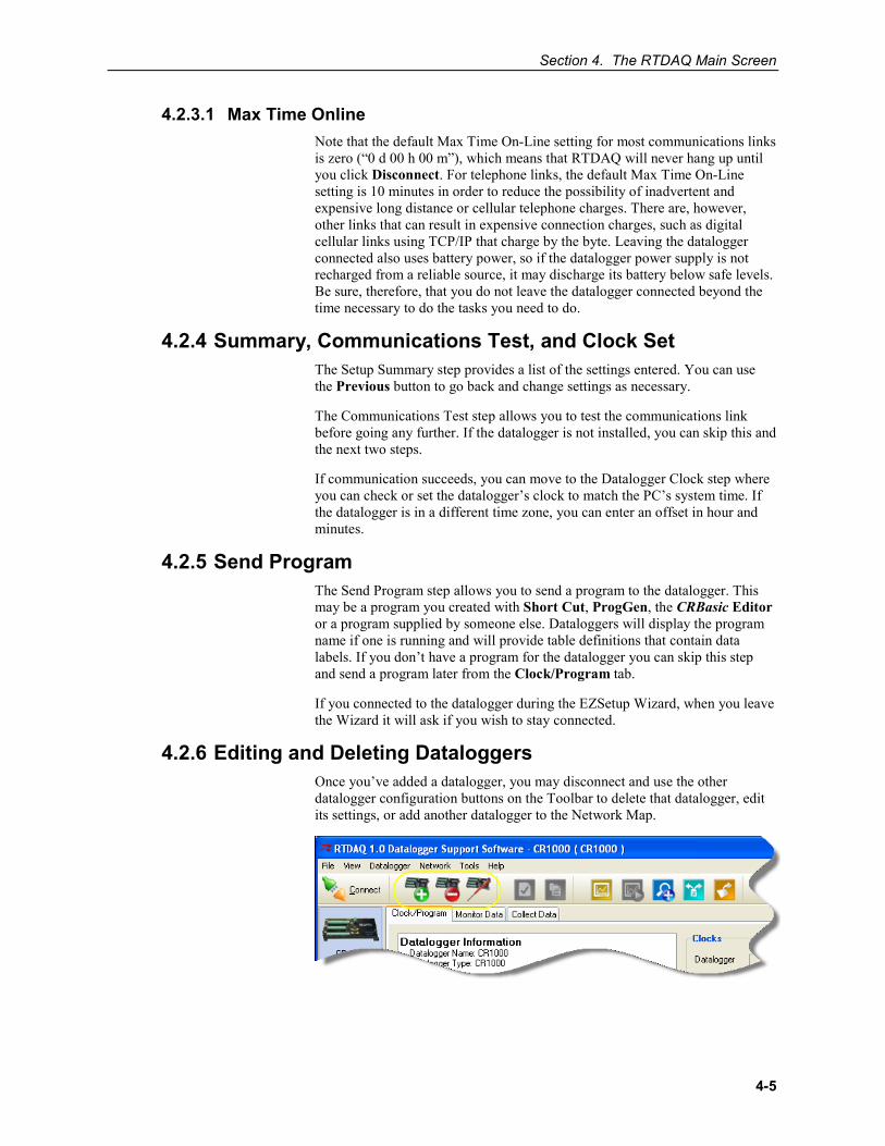
4.2.6 Editing and Deleting Dataloggers ............................................. 4-5 4.3 Clock/Program Tab .......................................................................... 4-6
4.3.1 Basic Operation ......................................................................... 4-6 4.4 Monitor Data Tab ............................................................................. 4-7
4.4.1 Field Monitor ............................................................................ 4-7 4.4.2 Editing Variable Values ............................................................ 4-7 4.4.3 Specialized Real-time Monitor Screens .................................... 4-8
4.5 Collect Data Tab .............................................................................. 4-8 4.6 Pull-down Menus ............................................................................. 4-9
4.6.1 File Menu .................................................................................. 4-9 4.6.1.1 Saving and Loading Configurations ............................... 4-9 4.6.1.2 Exit ................................................................................. 4-9
4.6.2 View Menu................................................................................ 4-9 4.6.3 Datalogger Menu..................................................................... 4-10
4.6.3.1 Connect/Disconnect ...................................................... 4-10 4.6.3.2 Update Table Definitions ............................................. 4-10 4.6.3.3 Status Table .................................................................. 4-10
4.6.3.3.1 Summary Tab .................................................... 4-11 4.6.3.3.2 Table Fill Times ................................................ 4-11 4.6.3.3.3 Status Table Tab ................................................ 4-12
4.6.3.4 File Control................................................................... 4-12 4.6.3.4.1 Datalogger Devices ............................................ 4-13 4.6.3.4.2 Run Options ....................................................... 4-13 4.6.3.4.3 Working with Files and Directories ................... 4-13 4.6.3.4.4 Right-Click Menu Options ................................ 4-16
4.6.3.5 Calibration Wizard ....................................................... 4-17 4.6.3.6 Terminal Emulator........................................................ 4-17
4.6.4 Network Menu ........................................................................ 4-18 4.6.4.1 Add/Delete/Edit/Rename Datalogger ........................... 4-18 4.6.4.2 Backup/Restore Network .............................................. 4-18 4.6.4.3 Computer’s Global PakBus Address ............................ 4-19
4.6.5 Tools Menu ............................................................................. 4-19 4.6.5.1 Auxiliary Applications ................................................. 4-19 4.6.5.2 Options ......................................................................... 4-20 4.6.5.3 LogTool ........................................................................ 4-20 4.6.5.4 PakBus Graph ............................................................... 4-22
4.6.5.4.1 Selecting the PakBus Network to View ............. 4-22 4.6.5.4.2 Dynamic and Static Links .................................. 4-22 4.6.5.4.3 Viewing/Changing Settings in a PakBus
Datalogger ...................................................... 4-23 4.6.5.4.4 Right-Click Functionality .................................. 4-23 4.6.5.4.5 Discovering Probable Routes between
Devices ........................................................... 4-23 4.7 The RTDAQ Toolbar ..................................................................... 4-24
5. Program Creation and Editing ............................... 5-15.1 CRBasic Editor................................................................................. 5-1
5.1.1 Overview ................................................................................... 5-1 5.1.2 Inserting Instructions................................................................. 5-2
5.1.2.1 Parameter Dialogue Box .................................................5-2 5.1.2.2 Right-Click Functionality ............................................... 5-4
5.1.3 Toolbar ...................................................................................... 5-5 5.1.3.1 Compile .......................................................................... 5-7 5.1.3.2 Compile, Save, and Send ................................................ 5-7 5.1.3.3 Conditional Compile and Save ..................................... 5-11
Table of Contents
iii
5.1.3.4 Templates ..................................................................... 5-11 5.1.3.5 Program Navigation using BookMarks and GoTo ....... 5-12 5.1.3.6 CRBasic Editor File Menu ........................................... 5-12 5.1.3.7 CRBasic Editor Edit Menu ........................................... 5-12
5.1.3.7.1 Other Options .................................................... 5-13 5.1.3.8 CRBasic Editor View Menu ......................................... 5-13
5.1.3.8.1 Editor Preferences.............................................. 5-13 5.1.3.8.2 Instruction Panel Preferences ............................ 5-15 5.1.3.8.3 Other Options .................................................... 5-15
5.1.3.9 CRBasic Editor Tools Menu......................................... 5-16 5.1.3.9.1 Edit Instruction Categories ................................ 5-16 5.1.3.9.2 Constant Customization ..................................... 5-17 5.1.3.9.3 Other Options .................................................... 5-19
5.1.3.10 Available Help Information .......................................... 5-20 5.1.4 CRBasic Programming ........................................................... 5-20
5.1.4.1 Programming Sequence ................................................ 5-20 5.1.4.2 Program Declarations ................................................... 5-21 5.1.4.3 Mathematical Expressions ............................................ 5-22 5.1.4.4 Measurement and Output Processing Instructions........ 5-22 5.1.4.5 Line Continuation ......................................................... 5-22 5.1.4.6 Inserting Comments Into Program ............................... 5-23 5.1.4.7 Example Program ......................................................... 5-23 5.1.4.8 Data Tables ................................................................... 5-24 5.1.4.9 The Scan — Measurement Timing and Processing ...... 5-26 5.1.4.10 Numerical Entries ......................................................... 5-27 5.1.4.11 Logical Expression Evaluation ..................................... 5-27
5.1.4.11.1 What is True? .................................................... 5-27 5.1.4.11.2 Expression Evaluation ....................................... 5-28 5.1.4.11.3 Numeric Results of Expression Evaluation ....... 5-28
5.1.4.12 Flags ............................................................................. 5-28 5.1.4.13 Parameter Types ........................................................... 5-28
5.1.4.13.1 Expressions in Parameters ................................. 5-29 5.1.4.13.2 Arrays of Multipliers and Offsets for Sensor
Calibration ...................................................... 5-29 5.1.4.14 Program Access to Data Tables .................................... 5-30
5.2 Short Cut ........................................................................................ 5-31 5.2.1 Overview ................................................................................. 5-31 5.2.2 Creating a Program Using Short Cut....................................... 5-32
5.2.2.1 Step 1 – Create a New File or Open Existing File ........ 5-32 5.2.2.2 Step 2 – Select Datalogger ........................................... 5-32 5.2.2.3 Step 3 – Choose Sensors to Monitor ............................ 5-35 5.2.2.4 Step 4 – Set up Output Tables ...................................... 5-43 5.2.2.5 Step 5 – Set up Advanced Outputs ............................... 5-45 5.2.2.6 Step 6 – Select Outputs ................................................. 5-47 5.2.2.7 Step 7 – Generate the Program in the Format
Required by the Datalogger ...................................... 5-49 5.2.3 Short Cut Settings ................................................................... 5-50
5.2.3.1 Program Security .......................................................... 5-50 5.2.3.2 Datalogger ID ............................................................... 5-50 5.2.3.3 Power-up Settings ......................................................... 5-51 5.2.3.4 Select CR200 Compiler ................................................ 5-51 5.2.3.5 Sensor Support ............................................................. 5-51 5.2.3.6 Integration/First Notch Frequency (fN1) ....................... 5-52 5.2.3.7 Font............................................................................... 5-52 5.2.3.8 Set Working Directory ................................................. 5-52 5.2.3.9 Enable Creation of Custom Sensor Files ...................... 5-52
Table of Contents
iv
5.2.4 Editing Programs Created by Short Cut .................................. 5-52 5.2.5 New Sensor Files .................................................................... 5-53 5.2.6 Custom Sensor Files................................................................ 5-53
5.3 Program Creation with the RTDAQ Program Generator ............... 5-53 5.3.1 Basic Operation ....................................................................... 5-53 5.3.2 Program Startup ...................................................................... 5-54 5.3.3 Using the CR5000 or CR9000X Program Generator .............. 5-55 5.3.4 Supporting Functionality ......................................................... 5-56
5.3.4.1 File | New ..................................................................... 5-56 5.3.4.2 File | Open… ................................................................ 5-56 5.3.4.3 File | Save As ................................................................ 5-57 5.3.4.4 File | Edit Generator Program ....................................... 5-57 5.3.4.5 File | Open Wire Diagram ............................................ 5-57 5.3.4.6 File | <Previously opened programs> ........................... 5-57 5.3.4.7 File | Exit ...................................................................... 5-58 5.3.4.8 Edit | Colour Options .....................................................5-58 5.3.4.9 Edit | CR9000X Generator Options, Edit | CR5000
Generator Options ..................................................... 5-59 5.3.4.10 Help | Program Generator ............................................. 5-59 5.3.4.11 Help | About ................................................................. 5-59
5.3.5 Using Save and Send............................................................... 5-59 5.3.5.1 Download ..................................................................... 5-60 5.3.5.2 Run Options .................................................................. 5-61 5.3.5.3 Datalogger Response .................................................... 5-61
6. View Pro .................................................................. 6-16.1 Overview .......................................................................................... 6-1 6.2 The Toolbar ...................................................................................... 6-1 6.3 Opening a File .................................................................................. 6-3
6.3.1 Opening a Data File .................................................................. 6-4 6.3.2 Opening Other Types of Files ................................................... 6-4 6.3.3 Opening a File in Hexadecimal Format .................................... 6-4
6.4 Viewing a LoggerNet Database Table ............................................. 6-4 6.4.1 Selecting a Database ................................................................. 6-4 6.4.2 Selecting a Table ....................................................................... 6-7
6.5 Importing a CSV File ....................................................................... 6-7 6.6 Data View ........................................................................................ 6-9
6.6.1 Column Size ............................................................................ 6-10 6.6.2 Header Information ................................................................. 6-10 6.6.3 Row Shading ........................................................................... 6-10 6.6.4 Locking the TimeStamp Column ............................................ 6-10 6.6.5 File Information ...................................................................... 6-10 6.6.6 Background Colour .................................................................6-11 6.6.7 Font ......................................................................................... 6-11 6.6.8 Window Arrangement ............................................................. 6-11
6.7 Graphs ............................................................................................ 6-11 6.7.1 Line Graph .............................................................................. 6-12
6.7.1.1 Selecting Data to be Graphed ....................................... 6-13 6.7.1.2 Graph Width ................................................................. 6-14 6.7.1.3 Scrolling ....................................................................... 6-14 6.7.1.4 Graph Cursor ................................................................ 6-14 6.7.1.5 Line Graph Toolbar ...................................................... 6-15
6.7.2 Histogram ................................................................................ 6-17 6.7.2.1 Selecting Data to be Viewed ........................................ 6-18 6.7.2.2 Options ......................................................................... 6-19
Table of Contents
v
6.7.2.3 Histogram Toolbar........................................................ 6-19 6.7.3 XY Plot ................................................................................... 6-20
6.7.3.1 Selecting Data to be Plotted.......................................... 6-20 6.7.3.2 XY Plot Toolbar ........................................................... 6-21
6.7.4 Rainflow Histogram ................................................................ 6-21 6.7.4.1 Selecting Data to be View ............................................ 6-22 6.7.4.2 Options ......................................................................... 6-24 6.7.4.3 Rainflow Histogram Toolbar ........................................ 6-24
6.7.5 FFT.......................................................................................... 6-25 6.7.5.1 Selecting Data to be Graphed ....................................... 6-25 6.7.5.2 Options ......................................................................... 6-27 6.7.5.3 FFT Toolbar ................................................................. 6-27
6.8 Right-click-Menus.......................................................................... 6-28 6.8.1 Data View ............................................................................... 6-28 6.8.2 Graphs ..................................................................................... 6-30 6.8.3 Traces ...................................................................................... 6-30
6.9 Printing Options ............................................................................. 6-30 6.9.1 Print Setup ............................................................................... 6-30 6.9.2 Printing Text ........................................................................... 6-30 6.9.3 Printing Graphs ....................................................................... 6-31
6.10 View Pro Online Help .................................................................... 6-31 6.11 Assigning Data Files to View ......................................................... 6-31
7. Monitoring Data in Real-time ................................. 7-17.1 Using the Monitor Data Screen ........................................................ 7-1
7.1.1 Connect to Target Datalogger ................................................... 7-1 7.1.2 Selecting Items for Display in the Monitor Data Screen ........... 7-2 7.1.3 Using the Start/Stop Button ...................................................... 7-3 7.1.4 Customizing the Display of Data in the Monitor Data Screen .. 7-4 7.1.5 Setting the Monitor Data Screen Options ................................. 7-4
7.1.5.1 Display Tab .................................................................... 7-5 7.1.5.2 Alarms Tab ..................................................................... 7-6 7.1.5.3 Setup Tab ........................................................................ 7-7
7.1.6 Specialized Real-time Monitoring Screens ............................... 7-7 7.2 Ports and Flags ................................................................................. 7-8 7.3 Table Monitor .................................................................................. 7-9
7.3.1 Using the Table Monitor ........................................................... 7-9 7.3.2 Displaying Tables on the Table Monitor ................................. 7-11
7.3.2.1 Start and Stop ............................................................... 7-11 7.3.2.2 Reset Table ................................................................... 7-12 7.3.2.3 Fields and Values ......................................................... 7-12 7.3.2.4 Save | Load Configurations .......................................... 7-13 7.3.2.5 Saving Displayed Data to a File ................................... 7-13
7.3.3 Moving and Resizing the Table Monitor Window .................. 7-14 7.4 Real Time Graph ............................................................................ 7-14
7.4.1 Using Graph Window ............................................................. 7-14 7.4.2 Adding Items for Display on the Graph .................................. 7-16 7.4.3 Moving and Resizing the Graph Window ............................... 7-16 7.4.4 Basic Graph Operation ............................................................ 7-16 7.4.5 Zooming and Scaling the Graph Window ............................... 7-18 7.4.6 Data Retrieval Methods used by the Graph Screen ................. 7-19 7.4.7 Drawing Methods used by the Graph Screen .......................... 7-20 7.4.8 Graph Window Display and Print Options ............................. 7-21 7.4.9 Setting the Options for the Graph Screen ................................ 7-22
7.4.9.1 Scaling the Axes ........................................................... 7-22
Table of Contents
vi
7.4.9.2 Data Display Options ................................................... 7-23 7.4.9.3 Visual Display Options ................................................. 7-25 7.4.9.4 Customizing the Traces on the Display ........................ 7-26
7.4.9.4.1 Individual Trace Options ................................... 7-26 7.4.9.4.2 Using Marks on the Graph ................................. 7-27
7.4.9.5 Using Saved Configurations ......................................... 7-28 7.4.10 Accepting or Abandoning Changes to the Graph Options ...... 7-29
7.5 Fast Graph ...................................................................................... 7-29 7.5.1 Using the Fast Graph............................................................... 7-29 7.5.2 Similarity between the Real Time Graph and the Fast
Graph ................................................................................... 7-30 7.6 XY Plot .......................................................................................... 7-30
7.6.1 Using the XY Plot ................................................................... 7-30 7.6.2 Setting up the XY Plot for Display ......................................... 7-32
7.6.2.1 Setting Values for Display ............................................ 7-32 7.6.2.2 Number of Points per Field .......................................... 7-34 7.6.2.3 Right-Click Functionality ............................................. 7-35
7.6.3 Using the Control Buttons ....................................................... 7-36 7.6.4 Using the Graphical Display Area of the XY Plot .................. 7-40 7.6.5 Zooming with the XY Plot ...................................................... 7-41 7.6.6 Using the Special Options of the XY Plot ............................... 7-42
7.6.6.1 Scaling Tab ................................................................... 7-43 7.6.6.2 Data Display Tab .......................................................... 7-44 7.6.6.3 Visual Display Tab ....................................................... 7-45 7.6.6.4 Trace Tab ...................................................................... 7-45 7.6.6.5 Save Tab ....................................................................... 7-47
7.6.7 Applying Changes to the XY Plot Screen ............................... 7-48 7.7 Histogram Monitoring .................................................................... 7-48
7.7.1 Histogram Overview ............................................................... 7-48 7.7.2 Displaying Histograms ............................................................ 7-49
7.8 Fast Fourier Transform Spectra ...................................................... 7-50 7.8.1 Brief Overview of Fourier Analysis ........................................ 7-50 7.8.2 FFT vs. FFTSample ................................................................ 7-51 7.8.3 Opening FFT Viewer Windows .............................................. 7-51
7.9 Configuration of FFT and Histogram Windows ............................ 7-52 7.9.1 Moving and Resizing the FFT/Histo Window ........................ 7-53 7.9.2 Displaying FFT Spectra or Histograms ................................... 7-53 7.9.3 Using the Buttons .................................................................... 7-54 7.9.4 3D View .................................................................................. 7-55 7.9.5 X-Axis Mode .......................................................................... 7-577.9.6 Zooming in on the Spectrum or Histogram ............................. 7-58 7.9.7 Save and Print Options ............................................................ 7-58 7.9.8 Setting the Options for the FFT/Histogram Screen ................. 7-60
7.9.8.1 Scaling the Axes ........................................................... 7-60 7.9.8.2 Data Display Options ................................................... 7-61 7.9.8.3 Visual Display Options ................................................. 7-62 7.9.8.4 Individual Trace Options .............................................. 7-63
7.9.8.4.1 Display Tab ....................................................... 7-63 7.9.8.4.2 Marks Tab .......................................................... 7-63
7.9.8.5 Using Saved Configurations ......................................... 7-64 7.9.9 Accepting or Abandoning Changes to the FFT/Histogram
Options ................................................................................ 7-65 7.10 Rainflow Histogram Monitoring .................................................... 7-66
7.10.1 Rainflow Histogram Overview ............................................... 7-66 7.10.2 Opening Rainflow Histograms ................................................ 7-66 7.10.3 Movement and Resizing of the Rainflow Window ................. 7-68
Table of Contents
vii
7.10.4 Selecting Tables and Bins For Display ................................... 7-68 7.10.5 Using the Buttons and Controls .............................................. 7-69 7.10.6 X-Axis Mode .......................................................................... 7-72 7.10.7 Zooming in on the Histogram ................................................. 7-72 7.10.8 Save and Print Options ............................................................ 7-73 7.10.9 Setting the Options for the Rainflow Screen ........................... 7-75
7.10.9.1 Scaling the Axes ........................................................... 7-75 7.10.9.2 Visual Display Options ................................................. 7-76 7.10.9.3 Trace Options ............................................................... 7-77 7.10.9.4 Using Saved Configurations ......................................... 7-78
7.10.10 Accepting or Abandoning Changes to the Rainflow Options ................................................................................ 7-79
7.11 Saving and Loading Configurations ............................................... 7-80 7.11.1 Saving and Loading Configuration Files for Real-Time
Data Screens ........................................................................ 7-80 7.11.2 Using Configurations in the Field Monitor ............................. 7-81 7.11.3 Using Configurations in the Table Monitors ........................... 7-82 7.11.4 Saving and Loading Global Configuration Files ..................... 7-82
8. Real-Time Monitoring and Control Software ........ 8-18.1 Development Mode ......................................................................... 8-1
8.1.1 The RTMC Workspace ............................................................. 8-3 8.1.2 Single Datalogger RTMC Projects ............................................ 8-3 8.1.3 Display Components ................................................................. 8-3 8.1.4 Functions Available from the RTMC Menus ............................ 8-5
8.1.4.1 File Menu ....................................................................... 8-5 8.1.4.2 Edit Menu ....................................................................... 8-5 8.1.4.3 View Menu ..................................................................... 8-6 8.1.4.4 Project Menu .................................................................. 8-7 8.1.4.5 Screen Menu ................................................................... 8-7 8.1.4.6 Component Menu ........................................................... 8-7 8.1.4.7 Window Menu ................................................................ 8-9 8.1.4.8 Help Menu ...................................................................... 8-9
8.1.5 Expressions ............................................................................... 8-9 8.1.5.1 Operators ...................................................................... 8-11 8.1.5.2 Order of Precedence ..................................................... 8-12 8.1.5.3 Predefined Constants .................................................... 8-12 8.1.5.4 Predefined Time Constants ........................................... 8-12 8.1.5.5 Functions ...................................................................... 8-13 8.1.5.6 Logical Functions ......................................................... 8-14 8.1.5.7 String Functions ........................................................... 8-15 8.1.5.8 Conversion Functions ................................................... 8-16 8.1.5.9 Time Functions ............................................................. 8-16 8.1.5.10 Start Option Functions .................................................. 8-16 8.1.5.11 Functions with State ..................................................... 8-17
8.2 RTMC Run-time ........................................................................... 8-18
9. Calibration and Zeroing ......................................... 9-19.1 Calibration Essentials ....................................................................... 9-1
9.1.1 Definition of Calibration ........................................................... 9-1 9.1.2 Basic Calibration Process .......................................................... 9-1
9.2 Writing Calibration Programs with the CRBasic Editor .................. 9-2 9.2.1 The FieldCal Instruction ........................................................... 9-2 9.2.2 Calibration File Details ............................................................. 9-3
Table of Contents
viii
9.3 Five Kinds of Calibration ................................................................. 9-3 9.3.1 Zeroing ...................................................................................... 9-3 9.3.2 Offset Calibration ...................................................................... 9-4 9.3.3 Two-Point Multiplier and Offset Calibration ............................ 9-4 9.3.4 Two-Point Multiplier Only Calibration ..................................... 9-5 9.3.5 Zero Basis Point Calibration ..................................................... 9-5
9.4 Performing a Manual Calibration ..................................................... 9-6 9.4.1 How to Use the Mode Variable for Calibration Status and
Control ................................................................................... 9-6 9.4.2 Using the Mode Variable for Manual Single-Point
Calibration ............................................................................. 9-7 9.4.3 Using the Mode Variable for Manual Two-Point Calibration ... 9-7
9.5 Generating Calibration Programs ..................................................... 9-8 9.6 Using the Calibration Wizard with Running Programs .................... 9-8
9.6.1 Calibration Wizard Basic Operation ......................................... 9-9 9.6.2 Using the Wizard to Perform Two-Point Multiplier and
Offset Calibrations ................................................................. 9-9 9.6.3 Using the Wizard to Perform Zeroing Calibrations ................ 9-13 9.6.4 Using the Wizard to Perform Offset Calibrations ................... 9-15
9.7 Strain and Shunt Calibration .......................................................... 9-16
10. Utilities .................................................................. 10-110.1 CardConvert ................................................................................... 10-1
10.1.1 Input/Output File Settings ....................................................... 10-1 10.1.2 Destination File Options ......................................................... 10-2
10.1.2.1 File Format ................................................................... 10-2 10.1.2.2 File Processing ............................................................. 10-3 10.1.2.3 File Naming .................................................................. 10-4 10.1.2.4 TOA5/TOB1 Format .................................................... 10-4
10.1.3 Converting the File.................................................................. 10-5 10.1.4 Repairing/Converting Corrupted Files .................................... 10-5 10.1.5 Viewing a Converted File ....................................................... 10-6 10.1.6 Running CardConvert from a Command Line ........................ 10-6
10.2 Device Configuration Utility .......................................................... 10-7 10.2.1 Overview ................................................................................. 10-7 10.2.2 Main DevConfig Screen .......................................................... 10-8 10.2.3 Downloading an Operating System......................................... 10-9 10.2.4 Terminal Tab ......................................................................... 10-12 10.2.5 The Unknown Device Type .................................................. 10-12 10.2.6 Off-line Mode ....................................................................... 10-13 10.2.7 Backing Up and Restoring a Datalogger ............................... 10-13 10.2.8 Data Recovery ....................................................................... 10-15
10.3 Split ............................................................................................. 10-16 10.3.1 Functional Overview ............................................................. 10-17 10.3.2 Getting Started ...................................................................... 10-17 10.3.3 Split Parameter File Entries .................................................. 10-24
10.3.3.1 Input Files ................................................................... 10-24 10.3.3.1.1 File Info ........................................................... 10-25 10.3.3.1.2 File Offset/Options .......................................... 10-26 10.3.3.1.3 Start Condition ................................................. 10-29 10.3.3.1.4 Stop Condition ................................................. 10-32 10.3.3.1.5 Copy ................................................................ 10-35 10.3.3.1.6 Select ............................................................... 10-37 10.3.3.1.7 Ranges ............................................................. 10-37 10.3.3.1.8 Variables .......................................................... 10-38
Table of Contents
ix
10.3.3.1.9 Numerical Limitations ..................................... 10-38 10.3.3.1.10 Mathematical Functions, Details, and
Examples ...................................................... 10-39 10.3.3.1.11 Time Series Functions, Details, and
Examples ...................................................... 10-41 10.3.3.1.12 Special Functions, Details, and Examples ....... 10-46 10.3.3.1.13 Split Functions Example .................................. 10-50 10.3.3.1.14 Summary of Select Line Syntax Rules ............ 10-53 10.3.3.1.15 Time Synchronization ...................................... 10-53
10.3.3.2 Output Files ................................................................ 10-56 10.3.3.2.1 Description of Output Option Commands ....... 10-57 10.3.3.2.2 Report Headings .............................................. 10-62 10.3.3.2.3 Column Headings ............................................ 10-62
10.3.4 Help Option ........................................................................... 10-62 10.3.5 Editing Commands ................................................................ 10-62 10.3.6 Running Split From a Command Line .................................. 10-62
10.3.6.1 Splitr Command Line Switches .................................. 10-63 10.3.6.1.1 Closing the Splitr.exe Program After
Execution (/R or /Q Switch) ......................... 10-63 10.3.6.1.2 Running Splitr in a Hidden or Minimized
State (/H Switch) .......................................... 10-63 10.3.6.1.3 Running Multiple Copies of Splitr (/M
Switch) ......................................................... 10-63 10.3.6.2 Using Splitr.exe in Batch Files ................................... 10-64 10.3.6.3 Processing Alternate Files .......................................... 10-64
10.3.6.3.1 Input/Output File Command Line Switches for Processing Alternate Files ...................... 10-64
10.3.6.4 Processing Multiple Parameter Files with One Command Line ....................................................... 10-68
10.3.7 Log Files ............................................................................... 10-68 10.4 Log Files and the LogTool Application ....................................... 10-68
10.4.1 Event Logging ....................................................................... 10-68 10.4.1.1 Log Categories ........................................................... 10-68 10.4.1.2 Log File Message Formats ......................................... 10-69
10.4.1.2.1 General File Format Information ..................... 10-69 10.4.1.2.2 Transaction Log Format .................................. 10-70 10.4.1.2.3 Communications Status Log Format ............... 10-86 10.4.1.2.4 Object State Log Format .................................. 10-88
10.4.2 CQR Log (RF Link) .............................................................. 10-89 10.5 SDM-CAN Helper Software ........................................................ 10-89
Appendices
A. Campbell Scientific File Formats .......................... A-1A.1 PC File Data Formats ...................................................................... A-1
A.1.1 TOA5 ....................................................................................... A-1 A.1.2 TOB1 ....................................................................................... A-2
A.2 Datalogger Data Formats ................................................................ A-3 A.2.1 TOB2 or TOB3 ........................................................................ A-3
A.3 Binary Data Value Types ................................................................ A-5 A.3.1 FP2 (2 Byte Low Resolution Format) ...................................... A-5 A.3.2 FP4 (4 Byte High Resolution Format) ..................................... A-5 A.3.3 IEEE4 ....................................................................................... A-5 A.3.4 IEEE8 ....................................................................................... A-5
Table of Contents
x
A.4 Converting Binary File Formats ...................................................... A-6 A.4.1 Split .......................................................................................... A-6 A.4.2 View Pro .................................................................................. A-6 A.4.3 CardConvert ............................................................................. A-6
B. Importing Files into Excel ..................................... B-1B.1 Table-Based Data File Import (TOA5) ............................................ B-1
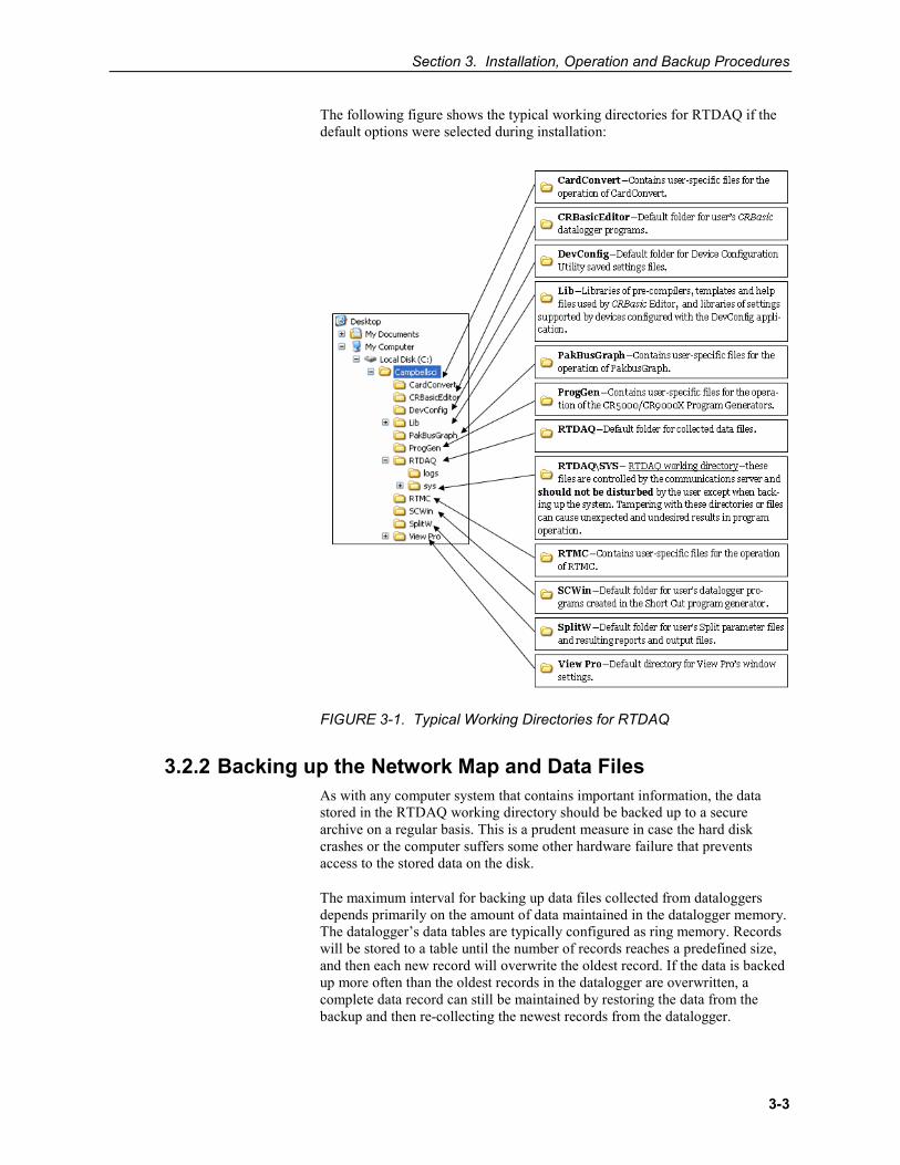
Figure 3-1. Typical Working Directories for RTDAQ ....................................... 3-3
Tables 5-1. Formats for Output Data ................................................................ 5-26 5-2. Formats for Entering Numbers in CRBasic.................................... 5-27 5-3. Synonyms for True and False ......................................................... 5-27 5-4. Rules for Names ............................................................................. 5-29 9-1. The FieldCal Instruction “Family” ................................................... 9-2 10-1. Comma Separated, Field Formatted, Printable ASCII, and
Table Oriented ASCII Input File Format Types ....................... 10-24 10-2. Example of Event Driven Test Data Set....................................... 10-34 10-3. Processed Data File Using Option C ............................................ 10-34 10-4. Input File Entries to Process the First Data Point for each Test ... 10-3510-5. Effects of Out of Range Values for Given Output Options .......... 10-37 10-6. Split Operators and Math Functions ............................................. 10-39 10-7. Time Series Functions .................................................................. 10-41 10-8. Split SPECIAL FUNCTIONS ...................................................... 10-46 10-9. Definition of Blank or Bad Data for each Data File Format ........ 10-59 10-10. Transaction Log Messages ........................................................... 10-70 10-11. Communication Status Log Messages ......................................... 10-87

xi
Preface — What's New in RTDAQ? RTDAQ 1.4 adds support for the new GRANITE Data Logger Modules.
Beginning with RTDAQ 1.3, Windows XP and Windows Vista are no longer supported.
NOTE

1-1
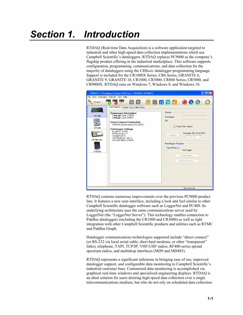
Section 1. Introduction RTDAQ (Real-time Data Acquisition) is a software application targeted to industrial and other high-speed data collection implementations which use Campbell Scientific’s dataloggers. RTDAQ replaces PC9000 as the company’s flagship product offering in the industrial marketplace. This software supports configuration, programming, communications, and data collection for the majority of dataloggers using the CRBasic datalogger programming language. Support is included for the CR1000X Series, CR6 Series, GRANITE 6, GRANITE 9, GRANITE 10, CR1000, CR3000, CR800 Series, CR5000, and CR9000X. RTDAQ runs on Windows 7, Windows 8, and Windows 10.
RTDAQ contains numerous improvements over the previous PC9000 product line. It features a new user-interface, including a look and feel similar to other Campbell Scientific datalogger software such as LoggerNet and PC400. Its underlying architecture uses the same communications server used by LoggerNet (the “LoggerNet Server”). This technology enables connection to PakBus dataloggers (including the CR1000 and CR3000) as well as tight integration with other Campbell Scientific products and utilities such as RTMC and PakBus Graph.
Datalogger communications technologies supported include “direct connect” (or RS-232 via local serial cable, short haul modems, or other “transparent” links), telephone, TAPI, TCP/IP, VHF/UHF radios, RF400-series spread spectrum radios, and multidrop interfaces (MD9 and MD485).
RTDAQ represents a significant milestone in bringing ease of use, improved datalogger support, and configurable data monitoring to Campbell Scientific’s industrial customer base. Customized data monitoring is accomplished via graphical real-time windows and specialized engineering displays. RTDAQ is an ideal solution for users desiring high-speed data collection over a single telecommunications medium, but who do not rely on scheduled data collection.
Section 1. Introduction
1-2
1.1 RTDAQ Overview 1.1.1 Main Screen
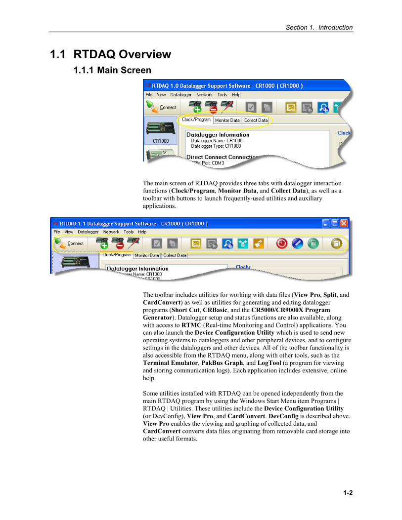
The main screen of RTDAQ provides three tabs with datalogger interaction functions (Clock/Program, Monitor Data, and Collect Data), as well as a toolbar with buttons to launch frequently-used utilities and auxiliary applications.
The toolbar includes utilities for working with data files (View Pro, Split, and CardConvert) as well as utilities for generating and editing datalogger programs (Short Cut, CRBasic, and the CR5000/CR9000X Program Generator). Datalogger setup and status functions are also available, along with access to RTMC (Real-time Monitoring and Control) applications. You can also launch the Device Configuration Utility which is used to send new operating systems to dataloggers and other peripheral devices, and to configure settings in the dataloggers and other devices. All of the toolbar functionality is also accessible from the RTDAQ menu, along with other tools, such as the Terminal Emulator, PakBus Graph, and LogTool (a program for viewing and storing communication logs). Each application includes extensive, online help.
Some utilities installed with RTDAQ can be opened independently from the main RTDAQ program by using the Windows Start Menu item Programs | RTDAQ | Utilities. These utilities include the Device Configuration Utility (or DevConfig), View Pro, and CardConvert. DevConfig is described above. View Pro enables the viewing and graphing of collected data, and CardConvert converts data files originating from removable card storage into other useful formats.
Section 1. Introduction
1-3
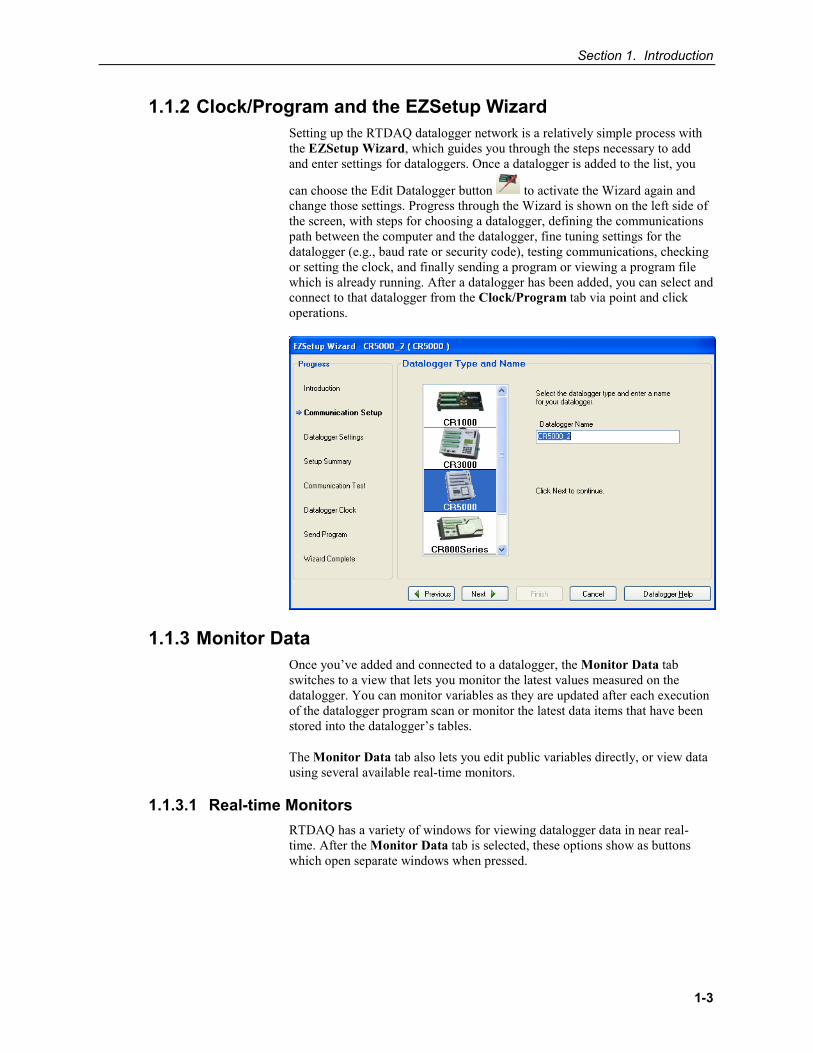
1.1.2 Clock/Program and the EZSetup Wizard Setting up the RTDAQ datalogger network is a relatively simple process with the EZSetup Wizard, which guides you through the steps necessary to add and enter settings for dataloggers. Once a datalogger is added to the list, you
can choose the Edit Datalogger button to activate the Wizard again and change those settings. Progress through the Wizard is shown on the left side of the screen, with steps for choosing a datalogger, defining the communications path between the computer and the datalogger, fine tuning settings for the datalogger (e.g., baud rate or security code), testing communications, checking or setting the clock, and finally sending a program or viewing a program file which is already running. After a datalogger has been added, you can select and connect to that datalogger from the Clock/Program tab via point and click operations.
1.1.3 Monitor Data Once you’ve added and connected to a datalogger, the Monitor Data tab switches to a view that lets you monitor the latest values measured on the datalogger. You can monitor variables as they are updated after each execution of the datalogger program scan or monitor the latest data items that have been stored into the datalogger’s tables.
The Monitor Data tab also lets you edit public variables directly, or view data using several available real-time monitors.
1.1.3.1 Real-time Monitors RTDAQ has a variety of windows for viewing datalogger data in near real-time. After the Monitor Data tab is selected, these options show as buttons which open separate windows when pressed.
Section 1. Introduction
1-4
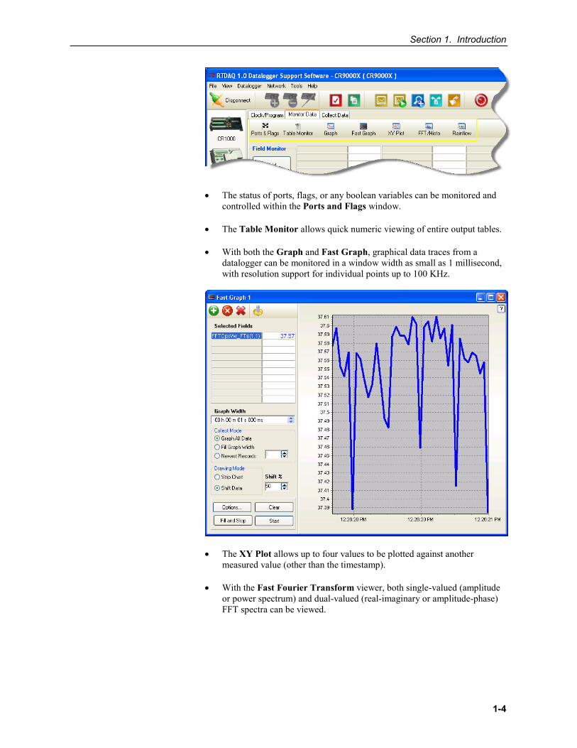
• The status of ports, flags, or any boolean variables can be monitored andcontrolled within the Ports and Flags window.
• The Table Monitor allows quick numeric viewing of entire output tables.
• With both the Graph and Fast Graph, graphical data traces from adatalogger can be monitored in a window width as small as 1 millisecond,with resolution support for individual points up to 100 KHz.
• The XY Plot allows up to four values to be plotted against anothermeasured value (other than the timestamp).
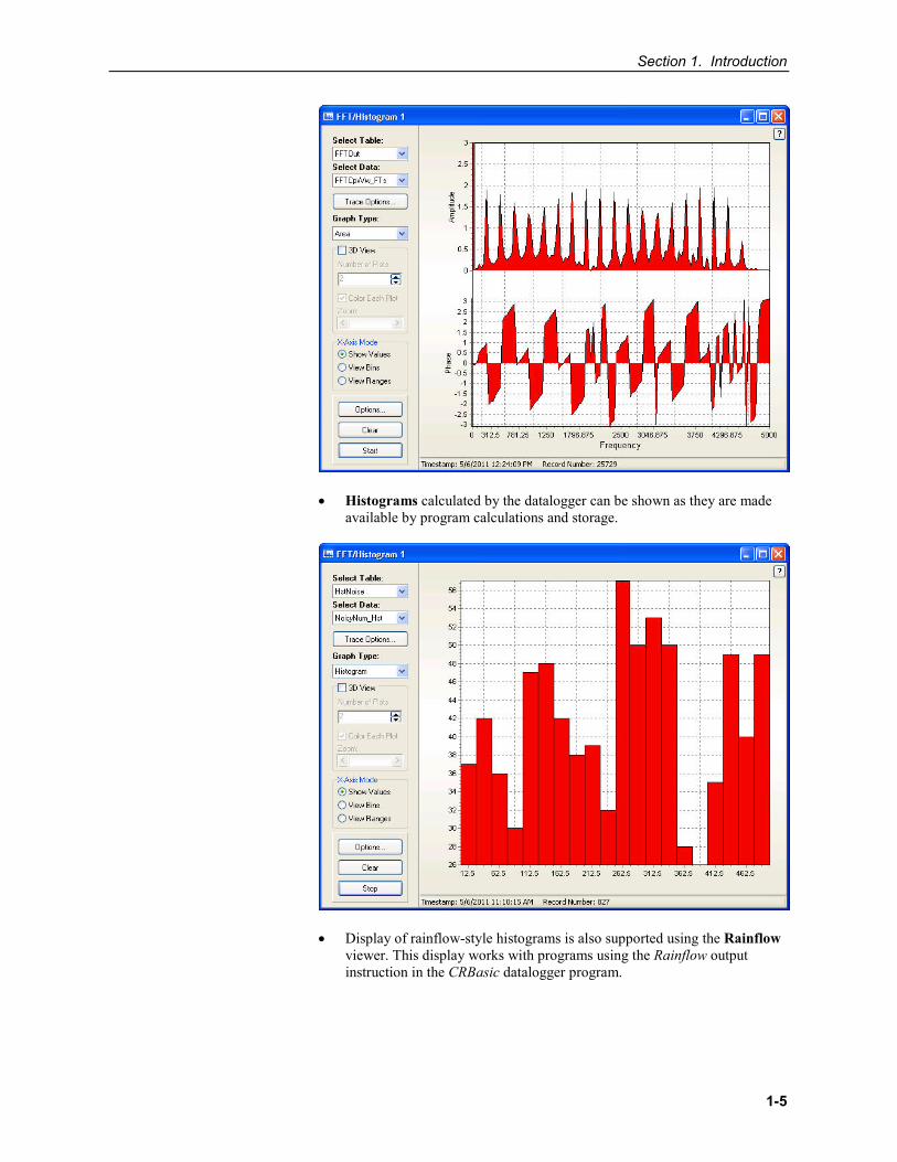
• With the Fast Fourier Transform viewer, both single-valued (amplitudeor power spectrum) and dual-valued (real-imaginary or amplitude-phase)FFT spectra can be viewed.
Section 1. Introduction
1-5
• Histograms calculated by the datalogger can be shown as they are madeavailable by program calculations and storage.
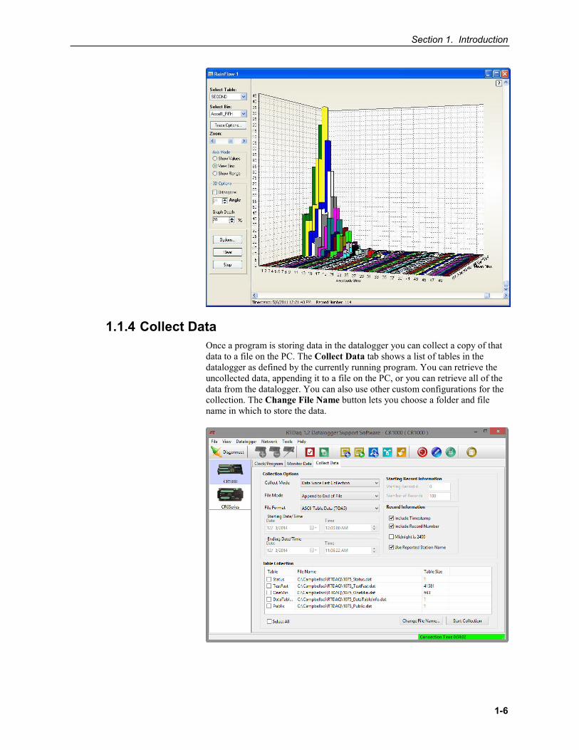
• Display of rainflow-style histograms is also supported using the Rainflowviewer. This display works with programs using the Rainflow outputinstruction in the CRBasic datalogger program.
Section 1. Introduction
1-6
1.1.4 Collect Data Once a program is storing data in the datalogger you can collect a copy of that data to a file on the PC. The Collect Data tab shows a list of tables in the datalogger as defined by the currently running program. You can retrieve the uncollected data, appending it to a file on the PC, or you can retrieve all of the data from the datalogger. You can also use other custom configurations for the collection. The Change File Name button lets you choose a folder and file name in which to store the data.
Section 1. Introduction
1-7
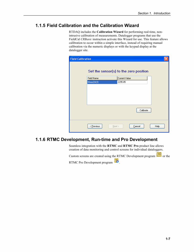
1.1.5 Field Calibration and the Calibration Wizard RTDAQ includes the Calibration Wizard for performing real-time, non-intrusive calibration of measurements. Datalogger programs that use the FieldCal CRBasic instruction activate this Wizard for use. This feature allows calibration to occur within a simple interface, instead of requiring manual calibration via the numeric displays or with the keypad display at the datalogger site.
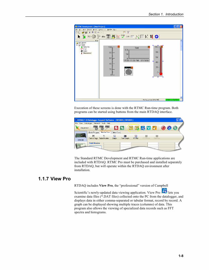
1.1.6 RTMC Development, Run-time and Pro Development Seamless integration with the RTMC and RTMC Pro product line allows creation of data monitoring and control screens for individual dataloggers.
Custom screens are created using the RTMC Development program or the
RTMC Pro Development program .
Section 1. Introduction
1-8
Execution of these screens is done with the RTMC Run-time program. Both programs can be started using buttons from the main RTDAQ interface.
The Standard RTMC Development and RTMC Run-time applications are included with RTDAQ. RTMC Pro must be purchased and installed separately from RTDAQ, but will operate within the RTDAQ environment after installation.
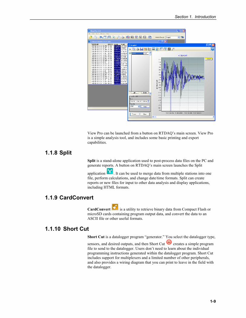
1.1.7 View Pro RTDAQ includes View Pro, the “professional” version of Campbell
Scientific’s newly-updated data viewing application. View Pro lets you examine data files (*.DAT files) collected onto the PC from the datalogger, and displays data in either comma-separated or tabular format, record by record. A graph can be displayed showing multiple traces (columns) of data. This program also allows the viewing of specialized data records such as FFT spectra and histograms.
Section 1. Introduction
1-9
View Pro can be launched from a button on RTDAQ’s main screen. View Pro is a simple analysis tool, and includes some basic printing and export capabilities.
1.1.8 Split Split is a stand-alone application used to post-process data files on the PC and generate reports. A button on RTDAQ’s main screen launches the Split
application . It can be used to merge data from multiple stations into one file, perform calculations, and change date/time formats. Split can create reports or new files for input to other data analysis and display applications, including HTML formats.
1.1.9 CardConvert
CardConvert is a utility to retrieve binary data from Compact Flash or microSD cards containing program output data, and convert the data to an ASCII file or other useful formats.
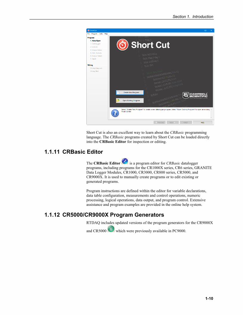
1.1.10 Short Cut Short Cut is a datalogger program “generator.” You select the datalogger type,
sensors, and desired outputs, and then Short Cut creates a simple program file to send to the datalogger. Users don’t need to learn about the individual programming instructions generated within the datalogger program. Short Cut includes support for multiplexers and a limited number of other peripherals, and also provides a wiring diagram that you can print to leave in the field with the datalogger.
Section 1. Introduction
1-10
Short Cut is also an excellent way to learn about the CRBasic programming language. The CRBasic programs created by Short Cut can be loaded directly into the CRBasic Editor for inspection or editing.
1.1.11 CRBasic Editor
The CRBasic Editor is a program editor for CRBasic datalogger programs, including programs for the CR1000X series, CR6 series, GRANITE Data Logger Modules, CR1000, CR3000, CR800 series, CR5000, and CR9000X. It is used to manually create programs or to edit existing or generated programs.
Program instructions are defined within the editor for variable declarations, data table configuration, measurements and control operations, numeric processing, logical operations, data output, and program control. Extensive assistance and program examples are provided in the online help system.
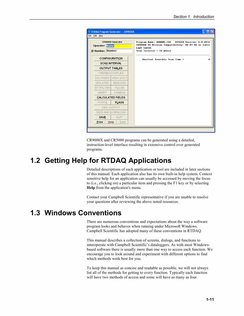
1.1.12 CR5000/CR9000X Program Generators RTDAQ includes updated versions of the program generators for the CR9000X
and CR5000 which were previously available in PC9000.
Section 1. Introduction
1-11
CR9000X and CR5000 programs can be generated using a detailed, instruction-level interface resulting in extensive control over generated programs.
1.2 Getting Help for RTDAQ Applications Detailed descriptions of each application or tool are included in later sections of this manual. Each application also has its own built-in help system. Context sensitive help for an application can usually be accessed by moving the focus to (i.e., clicking on) a particular item and pressing the F1 key or by selecting Help from the application's menu.
Contact your Campbell Scientific representative if you are unable to resolve your questions after reviewing the above noted resources.
1.3 Windows Conventions There are numerous conventions and expectations about the way a software program looks and behaves when running under Microsoft Windows. Campbell Scientific has adopted many of these conventions in RTDAQ.
This manual describes a collection of screens, dialogs, and functions to interoperate with Campbell Scientific’s dataloggers. As with most Windows-based software there is usually more than one way to access each function. We encourage you to look around and experiment with different options to find which methods work best for you.
To keep this manual as concise and readable as possible, we will not always list all of the methods for getting to every function. Typically each function will have two methods of access and some will have as many as four.
Section 1. Introduction
1-12
The most common methods for accessing functionality are:
Menus – Text menus are displayed at the top of most windows. Menu items are accessed either by a left mouse click, or using a hot key combination (e.g., Alt+F opens the File menu). When the menu is opened, you can click on an item to select it, or use arrow keys to highlight it and press the Enter key, or just type the underlined letter.
By convention, menu items that bring up dialogue boxes or new windows requiring interaction will be followed by an ellipsis (…). Other items execute functions directly or can be switched on or off. Some menu items show a check mark if a function is enabled and no check mark if disabled.
Items with Program Focus – On each screen one button, text area, or other control is selected at a time to “have the focus.” The “Focus” is usually indicated when the item is surrounded by a dotted line or is bolded. Pressing the tab key can move the focus from item to item. Typing text changes a selected text edit box that has the focus. Pressing the space bar toggles a selected check box. A selected button can also be activated by pressing the Enter key.
Buttons – Buttons are an easy way to access a function. They are normally used for the functions that need to be called frequently or are very important. Clicking a button executes that function or brings up another window. Button functions can also be accessed from the keyboard using the tab key to move among items on a screen and pressing the Enter key to execute the button function. Most text-based buttons have a hot-key.
Right-Click Menus – Some areas have pop-up menus that bring up frequently used tasks or provide shortcuts. Just right-click on an area and if a context menu appears, left-click the menu item you want.
Hot Keys or Keyboard Shortcuts – Many of the menus and buttons can be accessed using Hot Keys. An underlined letter identifies the hot key for a button or function. To get to a menu or execute a function on a button hold down the Alt key and type the underlined letter in the menu name or the button text. The hot key letters may not appear until after you’ve pressed the Alt key.
Pop-Up Hints – Hints are available for many of the on-screen controls. Let the mouse pointer hover over a control, text box or other screen feature and the hint will appear automatically and remain visible for a few seconds. These hints will often explain the purpose of a control or a suggested action. For text boxes where some of the text is hidden, the full text will appear in the hint.
2-1
Section 2. System Requirements 2.1 Hardware and Software
RTDAQ is an integrated application of 32-bit programs designed to run on Intel-based computers running Microsoft Windows operating systems. Recommended platforms for running RTDAQ include Windows 7, Windows 8, and Windows 10.
RTDAQ also requires that TCP/IP support be installed on the PC.
3-1
Section 3. Installation, Operation, and Backup Procedures
You must have administrator rights on your computer to install Campbell Scientific software. After the software is installed, administrator rights are not required by the user to run the software.
3.1 Installation If you are installing RTDAQ from a download, run the executable file, RTDAQ_version.exe, to begin the installation.
If you are installing from a CD, place the installation disk in your computer’s CD-ROM drive. If autorun is enabled for the drive, the RTDAQ installation will start automatically. If the installation does not start automatically, use the Browse button to access the CD-ROM drive and select the autorun.exe file from the disk.
The first screen displayed by the installation is a Welcome screen. Click Next to proceed to the licensing agreement. After reading the licensing agreement, select the “I Accept…” option and press Next to proceed to the User Information screen. At the bottom of the User Information screen is a field for entering the CD key for the software. The CD key is found on the back of the CD case in which RTDAQ is shipped or in your user account on our website, www.campbellsci.eu. After entering the CD key, select Next and continue through the remaining screens, following the on-screen prompts to complete the installation.
Items are added to your computer’s Start menu under All apps | Campbell Scientific that start RTDAQ and some other selected utilities. At the end of installation, you also have the option to add a desktop shortcut to RTDAQ.
By default, the installation copies the RTDAQ program files to the C:\Program Files\CampbellSci\RTDAQ directory. In addition to placing files in the Program Files directory of your computer, the installation also creates working directories for the RTDAQ server and the individual RTDAQ applications under C:\CampbellSci. Section 3.2.1, RTDAQ Directory Structure and File Descriptions (p. 3-2), provides more detail on the directories that are created.
If you are installing the trial version of RTDAQ, you will have 30 days to use this fully functional trial version. Each time you run RTDAQ, you will be advised as to how many days are remaining on your trial version. At the end of the 30 days, the trial version of RTDAQ will no longer function.
If you choose to purchase RTDAQ, you will need to uninstall the trial version, run the install program, and input the CD Key. This can be done either before or after the 30-day trial period has expired.
NOTE
Section 3. Installation, Operation and Backup Procedures
3-2
Note that the trial version will install applications in the C:\Program Files\Campbellsci\Demo directory. When the purchased version of RTDAQ is installed, the applications will each be installed in their own directory under C:\Program Files\Campbellsci.
3.2 RTDAQ Operations and Backup Procedures This section describes some of the concepts and procedures recommended for routine operation and security of the RTDAQ software. Since the occurrence of operational issues cannot be fully eliminated on most computer systems, the following guidelines and procedures are provided to help minimize possible problems that may occur.
3.2.1 RTDAQ Directory Structure and File Descriptions 3.2.1.1 Program Directory
As described earlier in the installation procedures, the files for program execution are stored in the C:\Program Files\Campbellsci\ directory. This includes the executables, DLLs, and most of the application help files. This directory does not need to be included in back up efforts. RTDAQ and its applications rely on registry entries to run correctly; therefore, any restoration of the program should be done by reinstalling the software from the original CD.
3.2.1.2 Working Directories In this version of RTDAQ, each major application keeps its own working directory. The working directory holds the user files created by the application, as well as configuration and initialization (*.INI) files.
This scheme was implemented because Campbell Scientific uses the underlying tools and many of the applications (the communications server, library files, datalogger program editors, etc.) in a number of different products. By providing a common working directory for each major application, you should see consistent file organization as you move from one product to another.
Section 3. Installation, Operation and Backup Procedures
3-3
The following figure shows the typical working directories for RTDAQ if the default options were selected during installation:
FIGURE 3-1. Typical Working Directories for RTDAQ
3.2.2 Backing up the Network Map and Data Files As with any computer system that contains important information, the data stored in the RTDAQ working directory should be backed up to a secure archive on a regular basis. This is a prudent measure in case the hard disk crashes or the computer suffers some other hardware failure that prevents access to the stored data on the disk.
The maximum interval for backing up data files collected from dataloggers depends primarily on the amount of data maintained in the datalogger memory. The datalogger’s data tables are typically configured as ring memory. Records will be stored to a table until the number of records reaches a predefined size, and then each new record will overwrite the oldest record. If the data is backed up more often than the oldest records in the datalogger are overwritten, a complete data record can still be maintained by restoring the data from the backup and then re-collecting the newest records from the datalogger.
Section 3. Installation, Operation and Backup Procedures
3-4
3.2.2.1 Performing a Backup RTDAQ provides a simple way to back up the network map, the RTDAQ data cache, and the initialization files for the main application. The network map will restore all settings and data collection pointers for the dataloggers and other devices in the network. The data cache is the binary database which contains the collected data from the datalogger. Initialization files store settings such as window size and position, configuration of the data display, etc.
The *.INI files backed up in the RTDAQ backup procedure are those found in the C:\Campbellsci\RTDAQ\sys\inifiles folder only. Other *.INI files such as those for Short Cut, CardConvert, Split and the CRBasic Editor are not a part of the backup.
From RTDAQ’s menu, choose Network | Backup/Restore Network, and then press Backup.
The backup file is named RTDAQ.bkp and is stored in the C:\CampbellSci\RTDAQ directory (if you installed RTDAQ using the default directory structure). You can, however, provide a different file name if desired.
3.2.2.2 Restoring the Network from a Backup File To restore a network from a backup file, choose Network | Backup/Restore Network. Select the *.bkp file that contains the network configuration you want to restore, and press Restore. Note that this process DOES NOT append to the existing network — the existing network will be overwritten when the restore is performed.
3.2.3 Loss of Computer Power The RTDAQ communications server writes to several files in the \SYS directory during normal operations. The most critical files are the data cache table files and the network configuration files. The data cache files contain all of the data that has been collected from the dataloggers by the RTDAQ server. These files are kept open (or active) as long as data is being stored to the file.
The configuration files contain information about each device in the datalogger network, including device settings, and other parameters. These files are written to frequently to make sure that they reflect the current state and configuration of each device. The configuration files are only opened as needed.
If computer system power is lost while the RTDAQ server is writing data to the active files, the files can become corrupted, making the files inaccessible to the server. While loss of power won’t always cause a file problem, having files backed up as described above will allow you to recover more effectively if a problem occurs. If a file does get corrupted, all of the server’s working files need to be restored from a backup file to maintain synchronization with the server state.
NOTE
4-1
Section 4. The RTDAQ Main Screen This section provides an overview of RTDAQ, including a detailed description of the communications tabs, pull-down menus, and toolbar. An overview of RTDAQ’s troubleshooting tools is also provided.
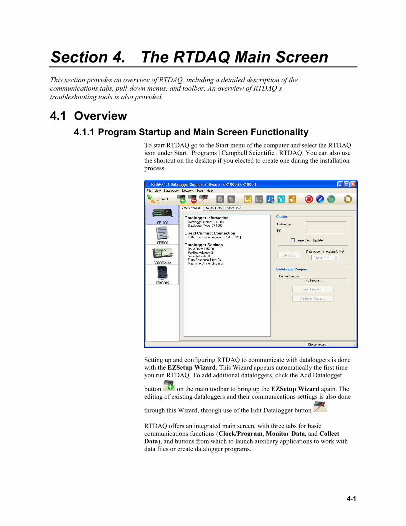
4.1 Overview 4.1.1 Program Startup and Main Screen Functionality
To start RTDAQ go to the Start menu of the computer and select the RTDAQ icon under Start | Programs | Campbell Scientific | RTDAQ. You can also use the shortcut on the desktop if you elected to create one during the installation process.
Setting up and configuring RTDAQ to communicate with dataloggers is done with the EZSetup Wizard. This Wizard appears automatically the first time you run RTDAQ. To add additional dataloggers, click the Add Datalogger
button on the main toolbar to bring up the EZSetup Wizard again. The editing of existing dataloggers and their communications settings is also done
through this Wizard, through use of the Edit Datalogger button .
RTDAQ offers an integrated main screen, with three tabs for basic communications functions (Clock/Program, Monitor Data, and Collect Data), and buttons from which to launch auxiliary applications to work with data files or create datalogger programs.
Section 4. The RTDAQ Main Screen
4-2
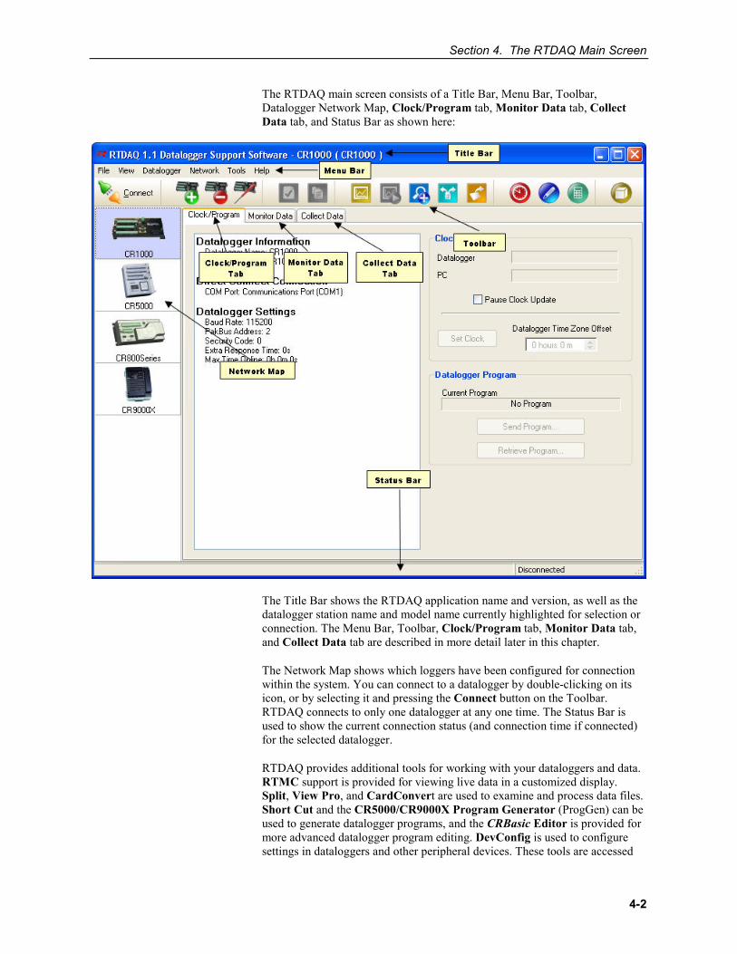
The RTDAQ main screen consists of a Title Bar, Menu Bar, Toolbar, Datalogger Network Map, Clock/Program tab, Monitor Data tab, Collect Data tab, and Status Bar as shown here:
The Title Bar shows the RTDAQ application name and version, as well as the datalogger station name and model name currently highlighted for selection or connection. The Menu Bar, Toolbar, Clock/Program tab, Monitor Data tab, and Collect Data tab are described in more detail later in this chapter.
The Network Map shows which loggers have been configured for connection within the system. You can connect to a datalogger by double-clicking on its icon, or by selecting it and pressing the Connect button on the Toolbar. RTDAQ connects to only one datalogger at any one time. The Status Bar is used to show the current connection status (and connection time if connected) for the selected datalogger.
RTDAQ provides additional tools for working with your dataloggers and data. RTMC support is provided for viewing live data in a customized display. Split, View Pro, and CardConvert are used to examine and process data files. Short Cut and the CR5000/CR9000X Program Generator (ProgGen) can be used to generate datalogger programs, and the CRBasic Editor is provided for more advanced datalogger program editing. DevConfig is used to configure settings in dataloggers and other peripheral devices. These tools are accessed
Section 4. The RTDAQ Main Screen
4-3
via the buttons on the main screen or the pull-down menu selections under the Tools menu. More information about these tools is provided later in this manual.
4.1.2 Datalogger Connectivity, Help and Program Exit RTDAQ supports the CR1000X series, CR6 series, GRANITE Data Logger Modules, CR800 series, CR1000, CR3000, CR5000, and CR9000X.
RTDAQ supports one medium of communications for any given datalogger. These media include direct connect via serial communications (or RS-232) via local serial cable, short haul modems, other “transparent” links, telephone, TAPI, TCP/IP, VHF/UHF radios, RF400-series spread spectrum radios, and multidrop interfaces (MD9 and MD485).
RTDAQ does not support parallel port communications, RF95T modems, or multiple media (such as phone-to-RF). RTDAQ is designed to use PakBus dataloggers and other PakBus devices in their default configurations; they are not supported as PakBus routers.
In order to be easy to use, RTDAQ relies on user-attended communications. It does not provide for automated scheduled data collection or automated clock checks. It does not support remote connections from other PCs.
Help for each application is available from the Help menu item, or by moving the focus to a control (by clicking on or tabbing to a control) and pressing F1.
To exit RTDAQ, either click the [X] in the upper right hand corner of the main screen, or select Exit under the File menu.
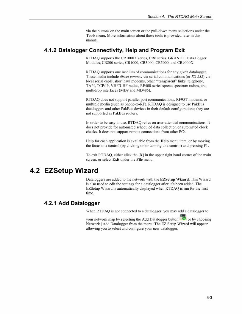
4.2 EZSetup Wizard Dataloggers are added to the network with the EZSetup Wizard. This Wizard is also used to edit the settings for a datalogger after it’s been added. The EZSetup Wizard is automatically displayed when RTDAQ is run for the first time.
4.2.1 Add Datalogger When RTDAQ is not connected to a datalogger, you may add a datalogger to
your network map by selecting the Add Datalogger button or by choosing Network | Add Datalogger from the menu. The EZ Setup Wizard will appear allowing you to select and configure your new datalogger.
Section 4. The RTDAQ Main Screen
4-4
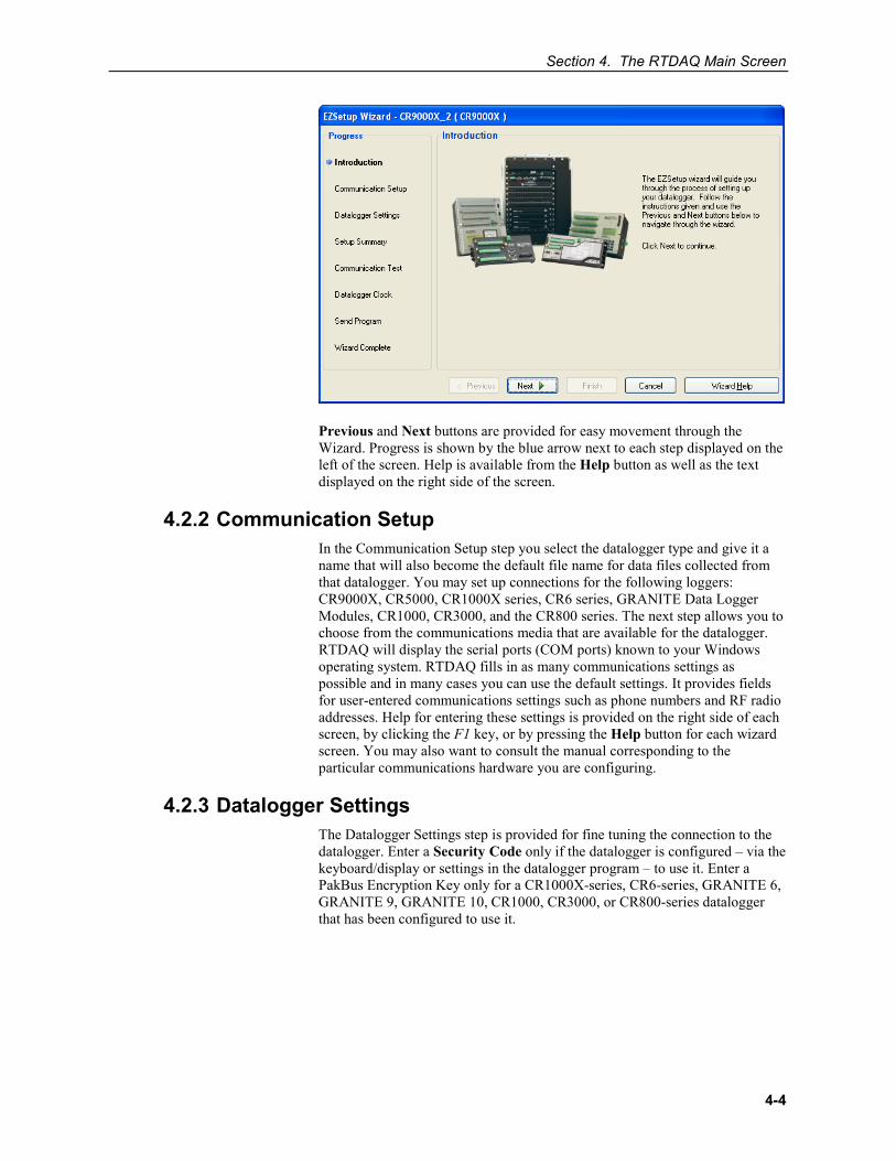
Previous and Next buttons are provided for easy movement through the Wizard. Progress is shown by the blue arrow next to each step displayed on the left of the screen. Help is available from the Help button as well as the text displayed on the right side of the screen.
4.2.2 Communication Setup In the Communication Setup step you select the datalogger type and give it a name that will also become the default file name for data files collected from that datalogger. You may set up connections for the following loggers: CR9000X, CR5000, CR1000X series, CR6 series, GRANITE Data Logger Modules, CR1000, CR3000, and the CR800 series. The next step allows you to choose from the communications media that are available for the datalogger. RTDAQ will display the serial ports (COM ports) known to your Windows operating system. RTDAQ fills in as many communications settings as possible and in many cases you can use the default settings. It provides fields for user-entered communications settings such as phone numbers and RF radio addresses. Help for entering these settings is provided on the right side of each screen, by clicking the F1 key, or by pressing the Help button for each wizard screen. You may also want to consult the manual corresponding to the particular communications hardware you are configuring.
4.2.3 Datalogger Settings The Datalogger Settings step is provided for fine tuning the connection to the datalogger. Enter a Security Code only if the datalogger is configured – via the keyboard/display or settings in the datalogger program – to use it. Enter a PakBus Encryption Key only for a CR1000X-series, CR6-series, GRANITE 6, GRANITE 9, GRANITE 10, CR1000, CR3000, or CR800-series datalogger that has been configured to use it.
Section 4. The RTDAQ Main Screen
4-5
4.2.3.1 Max Time Online Note that the default Max Time On-Line setting for most communications links is zero (“0 d 00 h 00 m”), which means that RTDAQ will never hang up until you click Disconnect. For telephone links, the default Max Time On-Line setting is 10 minutes in order to reduce the possibility of inadvertent and expensive long distance or cellular telephone charges. There are, however, other links that can result in expensive connection charges, such as digital cellular links using TCP/IP that charge by the byte. Leaving the datalogger connected also uses battery power, so if the datalogger power supply is not recharged from a reliable source, it may discharge its battery below safe levels. Be sure, therefore, that you do not leave the datalogger connected beyond the time necessary to do the tasks you need to do.
4.2.4 Summary, Communications Test, and Clock Set The Setup Summary step provides a list of the settings entered. You can use the Previous button to go back and change settings as necessary.
The Communications Test step allows you to test the communications link before going any further. If the datalogger is not installed, you can skip this and the next two steps.
If communication succeeds, you can move to the Datalogger Clock step where you can check or set the datalogger’s clock to match the PC’s system time. If the datalogger is in a different time zone, you can enter an offset in hour and minutes.
4.2.5 Send Program The Send Program step allows you to send a program to the datalogger. This may be a program you created with Short Cut, ProgGen, the CRBasic Editor or a program supplied by someone else. Dataloggers will display the program name if one is running and will provide table definitions that contain data labels. If you don’t have a program for the datalogger you can skip this step and send a program later from the Clock/Program tab.
If you connected to the datalogger during the EZSetup Wizard, when you leave the Wizard it will ask if you wish to stay connected.
4.2.6 Editing and Deleting Dataloggers Once you’ve added a datalogger, you may disconnect and use the other datalogger configuration buttons on the Toolbar to delete that datalogger, edit its settings, or add another datalogger to the Network Map.
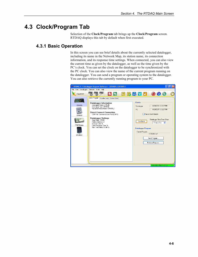
Section 4. The RTDAQ Main Screen
4-6
4.3 Clock/Program Tab Selection of the Clock/Program tab brings up the Clock/Program screen. RTDAQ displays this tab by default when first executed.
4.3.1 Basic Operation In this screen you can see brief details about the currently selected datalogger, including its name in the Network Map, its station name, its connection information, and its response time settings. When connected, you can also view the current time as given by the datalogger, as well as the time given by the PC’s clock. You can set the clock on the datalogger to be synchronized with the PC clock. You can also view the name of the current program running on the datalogger. You can send a program or operating system to the datalogger. You can also retrieve the currently running program to your PC.
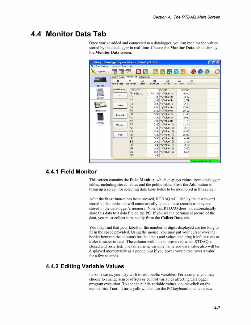
Section 4. The RTDAQ Main Screen
4-7
4.4 Monitor Data Tab Once you’ve added and connected to a datalogger, you can monitor the values stored by the datalogger in real-time. Choose the Monitor Data tab to display the Monitor Data screen.
4.4.1 Field Monitor This screen contains the Field Monitor, which displays values from datalogger tables, including stored tables and the public table. Press the Add button to bring up a screen for selecting data table fields to be monitored in this screen.
After the Start button has been pressed, RTDAQ will display the last record stored to that table and will automatically update these records as they are stored in the datalogger’s memory. Note that RTDAQ does not automatically store this data to a data file on the PC. If you want a permanent record of the data, you must collect it manually from the Collect Data tab.
You may find that your labels or the number of digits displayed are too long to fit in the space provided. Using the mouse, you may put your cursor over the border between the columns for the labels and values and drag it left or right to make it easier to read. The column width is not preserved when RTDAQ is closed and restarted. The table name, variable name and data value also will be displayed momentarily as a popup hint if you hover your cursor over a value for a few seconds.
4.4.2 Editing Variable Values In some cases, you may wish to edit public variables. For example, you may choose to change sensor offsets or control variables affecting datalogger program execution. To change public variable values, double-click on the number itself until it turns yellow, then use the PC keyboard to enter a new
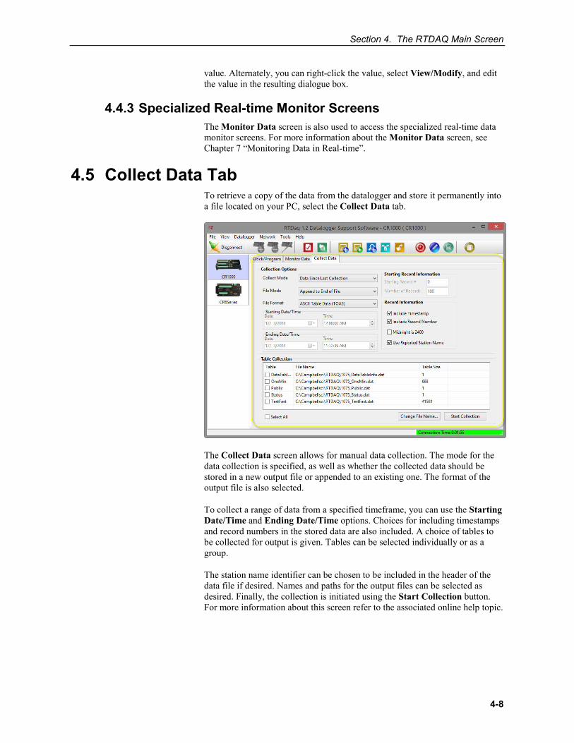
Section 4. The RTDAQ Main Screen
4-8
value. Alternately, you can right-click the value, select View/Modify, and edit the value in the resulting dialogue box.
4.4.3 Specialized Real-time Monitor Screens The Monitor Data screen is also used to access the specialized real-time data monitor screens. For more information about the Monitor Data screen, see Chapter 7 “Monitoring Data in Real-time”.
4.5 Collect Data Tab To retrieve a copy of the data from the datalogger and store it permanently into a file located on your PC, select the Collect Data tab.
The Collect Data screen allows for manual data collection. The mode for the data collection is specified, as well as whether the collected data should be stored in a new output file or appended to an existing one. The format of the output file is also selected.
To collect a range of data from a specified timeframe, you can use the Starting Date/Time and Ending Date/Time options. Choices for including timestamps and record numbers in the stored data are also included. A choice of tables to be collected for output is given. Tables can be selected individually or as a group.
The station name identifier can be chosen to be included in the header of the data file if desired. Names and paths for the output files can be selected as desired. Finally, the collection is initiated using the Start Collection button. For more information about this screen refer to the associated online help topic.
Section 4. The RTDAQ Main Screen
4-9
4.6 Pull-down Menus Access to almost all of the buttons and tabs on RTDAQ’s screens is also available via pull-down menus. Many of these functions are described in detail in other sections of this manual.
The File menu is used to save and retrieve global setting configurations and close the RTDAQ program. The View menu allows selection of languages other than English. The Datalogger menu is used for datalogger control functions, connections, and wizards. The Network menu is used for adding, editing and deleting loggers, and performing backups of the network map. The Tools menu is used for accessing supplementary programs such as the ones shown on the Toolbar. The Help menu is used for accessing the RTDAQ online help system.
4.6.1 File Menu 4.6.1.1 Saving and Loading Configurations
For information on how to use these functions, refer to Section 7.11.4, Saving and Loading Global Configuration Files (p. 7-82).
4.6.1.2 Exit The Exit item is used to close all real-time windows, disconnect from the connected datalogger, and close RTDAQ.
4.6.2 View Menu RTDAQ can display the user interface component text (for buttons, dialogue boxes, and other user interface elements) in a language other than English if a separate language package has been installed. If a language package is installed on your machine, the View menu will have a Languages entry and you will see the installed language as an item in the submenu. When a new language is chosen, RTDAQ will immediately reflect that change. Opened clients will not reflect the change until they are closed and reopened.
Applications that support alternate languages are Short Cut, CRBasic Editor, View Pro, CardConvert, PakBus Graph, LogTool, and the Device Configuration Utility.
Available language packages are provided by Campbell Scientific's international representatives or on the CSI web site. They are not included in the standard RTDAQ installation.
NOTE
Section 4. The RTDAQ Main Screen
4-10
4.6.3 Datalogger Menu 4.6.3.1 Connect/Disconnect
This option provides the same function as the Connect/Disconnect button on the main toolbar (see Section 4.7, The RTDAQ Toolbar (p. 4-24)).
4.6.3.2 Update Table Definitions When a CRBasic datalogger is configured for the first time or when a new program is sent, RTDAQ queries the datalogger for its table definitions. Whenever a new program is loaded into the datalogger, the table definitions will automatically be sent to RTDAQ. When using the real-time screens to view data, RTDAQ requires the latest table definitions in order to work properly. To avoid unnecessary data throughput on a datalogger, this information is not sent to RTDAQ with every configuration change, but only when deemed necessary, such as when a program changes.
If you find the table definitions in RTDAQ to be mismatched with the datalogger program, you can update those definitions manually. To update the table definitions for a datalogger manually, connect to that datalogger and select Update Table Definitions from the Datalogger menu.
4.6.3.3 Status Table CRBasic dataloggers include a default data table called the Status Table, which displays key values about the condition of the datalogger. The Datalogger | Status Table menu item opens a window to display that information. Records from the datalogger’s status table are generated on demand. Each datalogger has its own list of status fields, but they typically include such information as the hardware operating system version, the name of running program, battery voltage, and various error counters including watch dog and low battery conditions. Detailed information on the status table for each datalogger can be found in the operator’s manual for that particular datalogger.
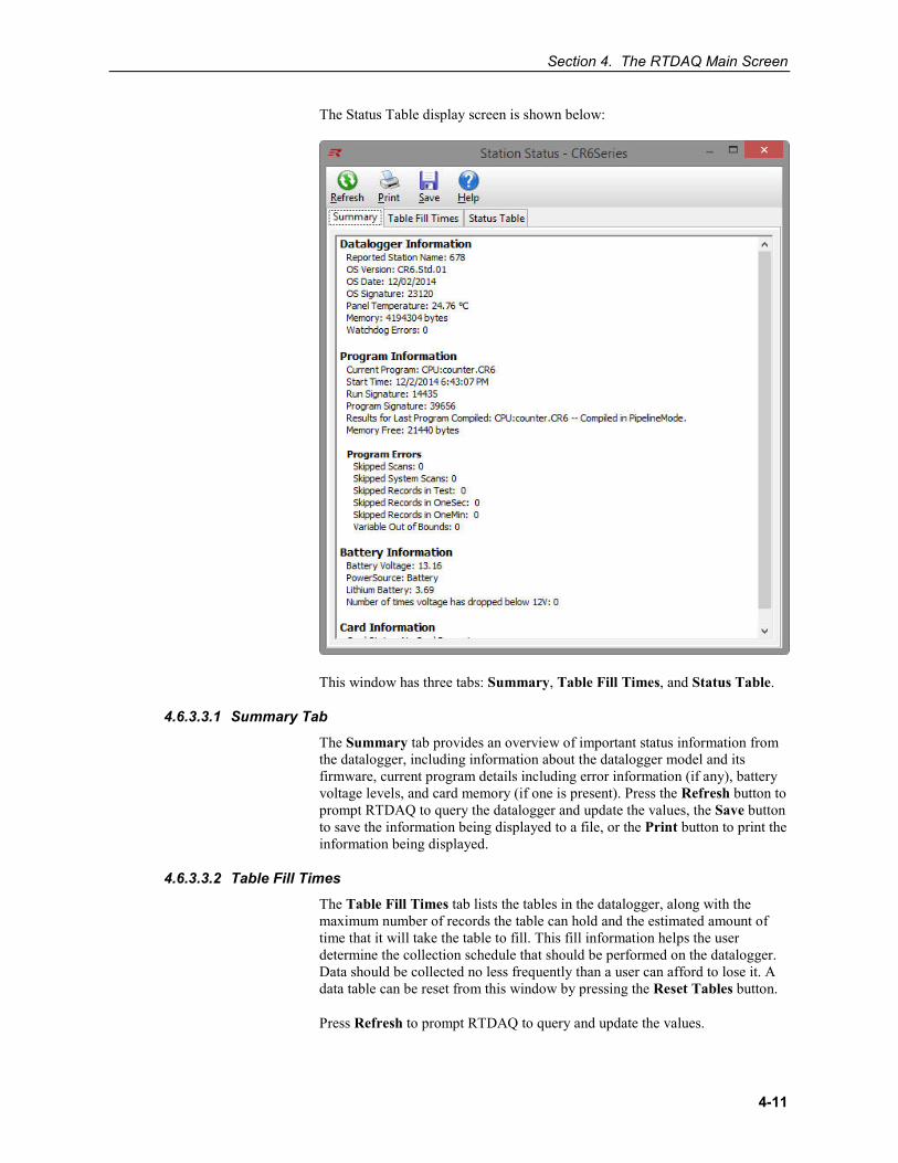
Section 4. The RTDAQ Main Screen
4-11
The Status Table display screen is shown below:
This window has three tabs: Summary, Table Fill Times, and Status Table.
4.6.3.3.1 Summary Tab
The Summary tab provides an overview of important status information from the datalogger, including information about the datalogger model and its firmware, current program details including error information (if any), battery voltage levels, and card memory (if one is present). Press the Refresh button to prompt RTDAQ to query the datalogger and update the values, the Save button to save the information being displayed to a file, or the Print button to print the information being displayed.
4.6.3.3.2 Table Fill Times
The Table Fill Times tab lists the tables in the datalogger, along with the maximum number of records the table can hold and the estimated amount of time that it will take the table to fill. This fill information helps the user determine the collection schedule that should be performed on the datalogger. Data should be collected no less frequently than a user can afford to lose it. A data table can be reset from this window by pressing the Reset Tables button.
Press Refresh to prompt RTDAQ to query and update the values.
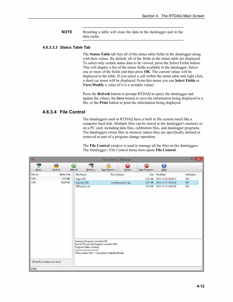
Section 4. The RTDAQ Main Screen
4-12
Resetting a table will erase the data in the datalogger and in the data cache.
4.6.3.3.3 Status Table Tab
The Status Table tab lists all of the status table fields in the datalogger along with their values. By default, all of the fields in the status table are displayed. To select only certain status data to be viewed, press the Select Fields button. This will display a list of the status fields available in the datalogger. Select one or more of the fields and then press OK. The current values will be displayed in the table. If you select a cell within the status table and right click, a short cut menu will be displayed. From this menu you can Select Fields or View/Modify a value (if it is a writable value).
Press the Refresh button to prompt RTDAQ to query the datalogger and update the values, the Save button to save the information being displayed to a file, or the Print button to print the information being displayed.
4.6.3.4 File Control The dataloggers used in RTDAQ have a built in file system much like a computer hard disk. Multiple files can be stored in the datalogger's memory or on a PC card, including data files, calibration files, and datalogger programs. The dataloggers retain files in memory unless they are specifically deleted or removed as part of a program change operation.
The File Control window is used to manage all the files on the dataloggers. The Datalogger | File Control menu item opens File Control.
NOTE
Section 4. The RTDAQ Main Screen
4-13
4.6.3.4.1 Datalogger Devices
Each datalogger will have a device designated as the CPU drive. If an add-in card is installed on the datalogger, you will also see the CRD storage device. The File Control window displays a list of files stored on each of its devices such as the CPU, PC card, or user-specified drive. The window on the left lists all of the data storage devices available for the selected datalogger (CPU, CRD, USB, CS9, or USR). Selecting a device shows a list in the right pane of the screen displaying the files stored on that device.
The USR drive is a user-created drive in the CR1000X-series, CR6-series, GRANITE 6, GRANITE 9, GRANITE 10, CR800, CR1000, and CR3000 dataloggers. It can be set up by assigning a value to the datalogger's UsrDriveSize setting. This drive must be set to at least 8192 bytes, in 512 byte increments. If the value entered is not a multiple of 512 bytes, the size will be rounded up. The size may also be rounded up to the account for a certain amount of overhead that is required for the drive to operate.
For GRANITE Data Logger Modules, an SC115 is specified as CS9 and USB refers to the integrated USB Host. For all other data loggers, USB refers to the SC115.
4.6.3.4.2 Run Options
The Run Options for a program file indicate whether it is set to running, power up, or both (running, power up). The currently executing program is indicated by the running attribute. The file size is also displayed for each file, as well as the last time the file was modified and whether or not the file is Read Only or Read/Write. Note that the Size and Modified date are not available for the CR9000X and CR5000 dataloggers.
4.6.3.4.3 Working with Files and Directories
There are several options for working with the files and directories on the datalogger.
Send is used to transfer files from the computer to the datalogger. Clicking the Send button brings up a standard file selection dialogue box. A new file can be chosen and sent to the highlighted device. Datalogger programs, data files, and other ASCII files can be sent to the datalogger.
If you select the Set Run Options on Send check box in the File Control screen, you will have the opportunity to set the Run On Power-up and/or Run Now options as the file is being transferred from the PC’s file system to the selected device (see the Run Options section below).
Format is used to format the selected device. Just like formatting a disk on a computer, all of the files on the device are deleted and the device is initialized.
Refresh will update the list of files for the selected device.
NOTE
NOTE
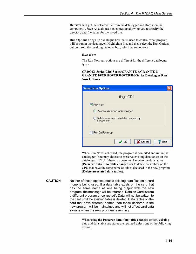
Section 4. The RTDAQ Main Screen
4-14
Retrieve will get the selected file from the datalogger and store it on the computer. A Save As dialogue box comes up allowing you to specify the directory and file name for the saved file.
Run Options brings up a dialogue box that is used to control what program will be run in the datalogger. Highlight a file, and then select the Run Options button. From the resulting dialogue box, select the run options.
Run Now
The Run Now run options are different for the different datalogger types.
CR1000X-Series/CR6-Series/GRANITE 6/GRANITE 9/ GRANITE 10/CR1000/CR3000/CR800-Series Datalogger Run Now Options
When Run Now is checked, the program is compiled and run in the datalogger. You may choose to preserve existing data tables on the datalogger’s CPU if there has been no change to the data tables (Preserve data if no table changed) or to delete data tables on the CPU that have the same name as tables declared in the new program (Delete associated data tables).
Neither of these options affects existing data files on a card if one is being used. If a data table exists on the card that has the same name as one being output with the new program, the message will be returned “Data on Card is from a different program or corrupted”. Data will not be written to the card until the existing table is deleted. Data tables on the card that have different names than those declared in the new program will be maintained and will not affect card data storage when the new program is running.
When using the Preserve data if no table changed option, existing data and data table structures are retained unless one of the following occurs:
CAUTION
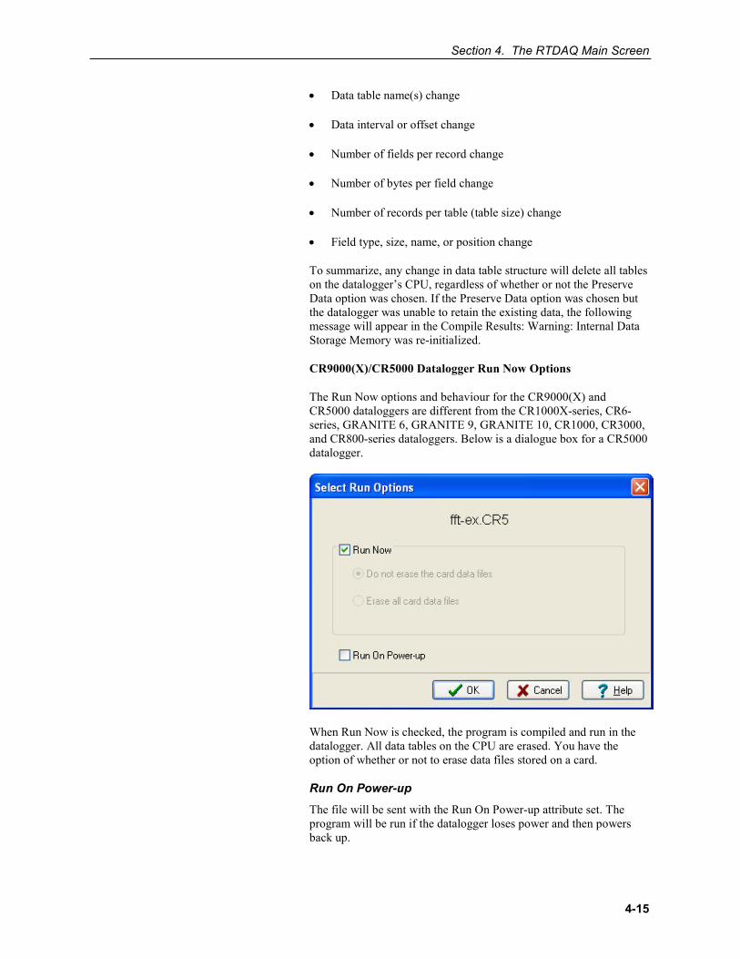
Section 4. The RTDAQ Main Screen
4-15
• Data table name(s) change
• Data interval or offset change
• Number of fields per record change
• Number of bytes per field change
• Number of records per table (table size) change
• Field type, size, name, or position change
To summarize, any change in data table structure will delete all tables on the datalogger’s CPU, regardless of whether or not the Preserve Data option was chosen. If the Preserve Data option was chosen but the datalogger was unable to retain the existing data, the following message will appear in the Compile Results: Warning: Internal Data Storage Memory was re-initialized.
CR9000(X)/CR5000 Datalogger Run Now Options
The Run Now options and behaviour for the CR9000(X) and CR5000 dataloggers are different from the CR1000X-series, CR6-series, GRANITE 6, GRANITE 9, GRANITE 10, CR1000, CR3000, and CR800-series dataloggers. Below is a dialogue box for a CR5000 datalogger.
When Run Now is checked, the program is compiled and run in the datalogger. All data tables on the CPU are erased. You have the option of whether or not to erase data files stored on a card.
Run On Power-up
The file will be sent with the Run On Power-up attribute set. The program will be run if the datalogger loses power and then powers back up.
Section 4. The RTDAQ Main Screen
4-16
Run Always
Run Now and Run On Power-up can both be selected. This sets the program’s file attribute in the datalogger as Run Always. The program will be compiled and run immediately and it will also be the program that runs if the datalogger is powered down and powered back up.
Pressing Run Options to restart a stopped program in the CR1000X-series, CR6-series, GRANITE 6, GRANITE 9, GRANITE 10, CR1000, CR3000, or CR800-series datalogger displays a different dialogue box. From the dialogue box you choose Restart Program to begin running the selected program immediately. You can also select an option button to determine whether or not the data tables previously created by the program are erased or retained. Note that you cannot change the Run on Power-up option when restarting a program.
CR1000X-series, CR6-series, GRANITE 6, GRANITE 9, GRANITE 10, CR1000, CR3000, and CR800-series dataloggers — A program marked as “Run on power up” can be disabled when power is first applied to the datalogger by pressing and holding the DEL key.
Delete - Highlight a file and press the Delete button to remove the file from the datalogger's memory. A running program may not be deleted.
Stop Program halts execution of the currently running datalogger program.
Select the option to stop the program and retain the data files, or to stop the program and delete data files. The option to retain or delete data files includes those in internal datalogger memory and those on a card written by the CardOut instruction. In most cases, data written to a card using the TableFile instruction will not be erased. However, when writing data to the card using the TableFile instruction with option 64, the file currently in use will be erased while other files will be maintained.
If you select the option to Delete Data, you also have the option of whether or not to clear the Run On Power-up option for the file. Select the check box to clear the Run On Power-up option. Clear the check box to leave the Run On Power-up option of the file unchanged.
If a CR1000X-series, CR6-series, GRANITE 6, GRANITE 9, GRANITE 10, CR1000, CR3000, or CR800-series program has been stopped, use the Run Options to restart it. If data files were not deleted when the program was stopped, you will once again be able to choose whether to retain or erase the data files. Instead of restarting the stopped program, you can choose a new program file to run by selecting a different file in the File Name field before pressing Run Options.
4.6.3.4.4 Right-Click Menu Options
When a file name is selected, pressing the right mouse button displays a menu with the Retrieve File, Delete File, Rename File, View File (retrieves the file and opens it in the CRBasic Editor), Run Options, and Stop Program options.
NOTE
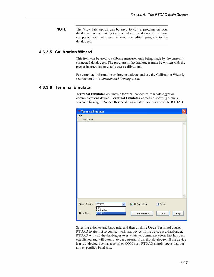
Section 4. The RTDAQ Main Screen
4-17
The View File option can be used to edit a program on your datalogger. After making the desired edits and saving it to your computer, you will need to send the edited program to the datalogger.
4.6.3.5 Calibration Wizard This item can be used to calibrate measurements being made by the currently connected datalogger. The program in the datalogger must be written with the proper instructions to enable these calibrations.
For complete information on how to activate and use the Calibration Wizard, see Section 9, Calibration and Zeroing (p. 9-1).
4.6.3.6 Terminal Emulator Terminal Emulator emulates a terminal connected to a datalogger or communications device. Terminal Emulator comes up showing a blank screen. Clicking on Select Device shows a list of devices known to RTDAQ.
Selecting a device and baud rate, and then clicking Open Terminal causes RTDAQ to attempt to connect with that device. If the device is a datalogger, RTDAQ will call the datalogger over whatever communications link has been established and will attempt to get a prompt from that datalogger. If the device is a root device, such as a serial or COM port, RTDAQ simply opens that port at the specified baud rate.
NOTE
Section 4. The RTDAQ Main Screen
4-18
Terminal Emulator has several uses. If you open a COM port, you can use it to set up devices that present their own menus, such as RF400 radios or NL100s. See the manuals for those devices to obtain information on how to navigate the menus and what settings to choose.
Another potential use is to communicate with smart devices attached to the datalogger. Some dataloggers allow a “pass-through” mode whereby you can communicate through them to an attached SDI-12 sensor to set its address or other parameters. See the manuals for the datalogger and sensor for the relevant commands.
Troubleshooting communications devices is another use for Terminal Emulator. When calling for support on these devices, a customer support engineer may ask you to use this method to manually dial through phone or RF modems, for example.
You can close a connection to start another one by clicking the Close Terminal button. You can close the Terminal Emulator itself by clicking the [X] button in the upper right corner of the screen.
4.6.4 Network Menu 4.6.4.1 Add/Delete/Edit/Rename Datalogger
The Add Datalogger, Delete Datalogger, and Edit Datalogger Setup options perform the same functions as the buttons on the main toolbar. The Rename Datalogger item can be used to change the name of a datalogger.
4.6.4.2 Backup/Restore Network This function can be used to save a copy of the network map to a file, and then to restore the network if necessary. The settings for all the devices in the network will be saved.
A default is given for the directory and file name to be used for the backup or restore. This can be changed by typing over the default directory and/or file name or selecting the button to the right of the field containing the file name and browsing to the desired directory and file name.
To backup the current network map, select the file name to which the backup will be stored, and then press the Backup button. The network map will be saved to the chosen file, and a message will appear indicating that the network has been backed up.
To regenerate the network map from a backup file, select the name of the backup file to restore from the dialogue box, and then press the Restore button. Note that this backup will replace the existing network (it does not add to the existing network).
The backup/restore option will be disabled if you are currently connected to a datalogger. You must disconnect from the datalogger before performing a backup or restoring the network.
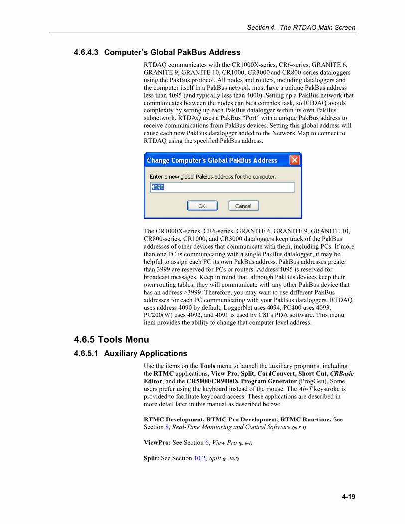
Section 4. The RTDAQ Main Screen
4-19
4.6.4.3 Computer’s Global PakBus Address RTDAQ communicates with the CR1000X-series, CR6-series, GRANITE 6, GRANITE 9, GRANITE 10, CR1000, CR3000 and CR800-series dataloggers using the PakBus protocol. All nodes and routers, including dataloggers and the computer itself in a PakBus network must have a unique PakBus address less than 4095 (and typically less than 4000). Setting up a PakBus network that communicates between the nodes can be a complex task, so RTDAQ avoids complexity by setting up each PakBus datalogger within its own PakBus subnetwork. RTDAQ uses a PakBus “Port” with a unique PakBus address to receive communications from PakBus devices. Setting this global address will cause each new PakBus datalogger added to the Network Map to connect to RTDAQ using the specified PakBus address.
The CR1000X-series, CR6-series, GRANITE 6, GRANITE 9, GRANITE 10, CR800-series, CR1000, and CR3000 dataloggers keep track of the PakBus addresses of other devices that communicate with them, including PCs. If more than one PC is communicating with a single PakBus datalogger, it may be helpful to assign each PC its own PakBus address. PakBus addresses greater than 3999 are reserved for PCs or routers. Address 4095 is reserved for broadcast messages. Keep in mind that, although PakBus devices keep their own routing tables, they will communicate with any other PakBus device that has an address >3999. Therefore, you may want to use different PakBus addresses for each PC communicating with your PakBus dataloggers. RTDAQ uses address 4090 by default, LoggerNet uses 4094, PC400 uses 4093, PC200(W) uses 4092, and 4091 is used by CSI’s PDA software. This menu item provides the ability to change that computer level address.
4.6.5 Tools Menu 4.6.5.1 Auxiliary Applications
Use the items on the Tools menu to launch the auxiliary programs, including the RTMC applications, View Pro, Split, CardConvert, Short Cut, CRBasic Editor, and the CR5000/CR9000X Program Generator (ProgGen). Some users prefer using the keyboard instead of the mouse. The Alt-T keystroke is provided to facilitate keyboard access. These applications are described in more detail later in this manual as described below:
RTMC Development, RTMC Pro Development, RTMC Run-time: See Section 8, Real-Time Monitoring and Control Software (p. 8-1)
ViewPro: See Section 6, View Pro (p. 6-1)
Split: See Section 10.2, Split (p. 10-7)
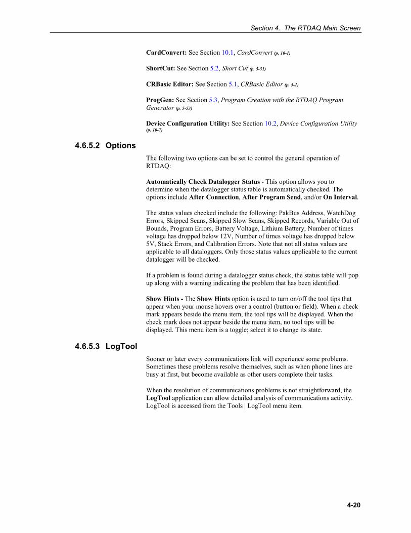
Section 4. The RTDAQ Main Screen
4-20
CardConvert: See Section 10.1, CardConvert (p. 10-1)
ShortCut: See Section 5.2, Short Cut (p. 5-31)
CRBasic Editor: See Section 5.1, CRBasic Editor (p. 5-1)
ProgGen: See Section 5.3, Program Creation with the RTDAQ Program Generator (p. 5-53)
Device Configuration Utility: See Section 10.2, Device Configuration Utility (p. 10-7)
4.6.5.2 Options The following two options can be set to control the general operation of RTDAQ:
Automatically Check Datalogger Status - This option allows you to determine when the datalogger status table is automatically checked. The options include After Connection, After Program Send, and/or On Interval.
The status values checked include the following: PakBus Address, WatchDog Errors, Skipped Scans, Skipped Slow Scans, Skipped Records, Variable Out of Bounds, Program Errors, Battery Voltage, Lithium Battery, Number of times voltage has dropped below 12V, Number of times voltage has dropped below 5V, Stack Errors, and Calibration Errors. Note that not all status values are applicable to all dataloggers. Only those status values applicable to the current datalogger will be checked.
If a problem is found during a datalogger status check, the status table will pop up along with a warning indicating the problem that has been identified.
Show Hints - The Show Hints option is used to turn on/off the tool tips that appear when your mouse hovers over a control (button or field). When a check mark appears beside the menu item, the tool tips will be displayed. When the check mark does not appear beside the menu item, no tool tips will be displayed. This menu item is a toggle; select it to change its state.
4.6.5.3 LogTool Sooner or later every communications link will experience some problems. Sometimes these problems resolve themselves, such as when phone lines are busy at first, but become available as other users complete their tasks.
When the resolution of communications problems is not straightforward, the LogTool application can allow detailed analysis of communications activity. LogTool is accessed from the Tools | LogTool menu item.
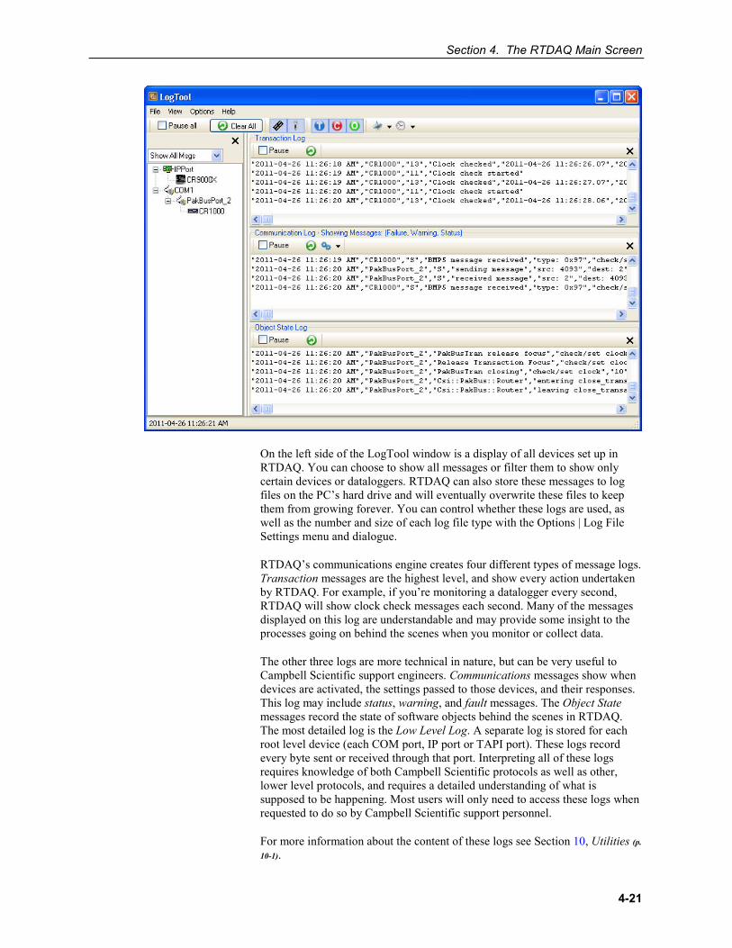
Section 4. The RTDAQ Main Screen
4-21
On the left side of the LogTool window is a display of all devices set up in RTDAQ. You can choose to show all messages or filter them to show only certain devices or dataloggers. RTDAQ can also store these messages to log files on the PC’s hard drive and will eventually overwrite these files to keep them from growing forever. You can control whether these logs are used, as well as the number and size of each log file type with the Options | Log File Settings menu and dialogue.
RTDAQ’s communications engine creates four different types of message logs. Transaction messages are the highest level, and show every action undertaken by RTDAQ. For example, if you’re monitoring a datalogger every second, RTDAQ will show clock check messages each second. Many of the messages displayed on this log are understandable and may provide some insight to the processes going on behind the scenes when you monitor or collect data.
The other three logs are more technical in nature, but can be very useful to Campbell Scientific support engineers. Communications messages show when devices are activated, the settings passed to those devices, and their responses. This log may include status, warning, and fault messages. The Object State messages record the state of software objects behind the scenes in RTDAQ. The most detailed log is the Low Level Log. A separate log is stored for each root level device (each COM port, IP port or TAPI port). These logs record every byte sent or received through that port. Interpreting all of these logs requires knowledge of both Campbell Scientific protocols as well as other, lower level protocols, and requires a detailed understanding of what is supposed to be happening. Most users will only need to access these logs when requested to do so by Campbell Scientific support personnel.
For more information about the content of these logs see Section 10, Utilities (p. 10-1).
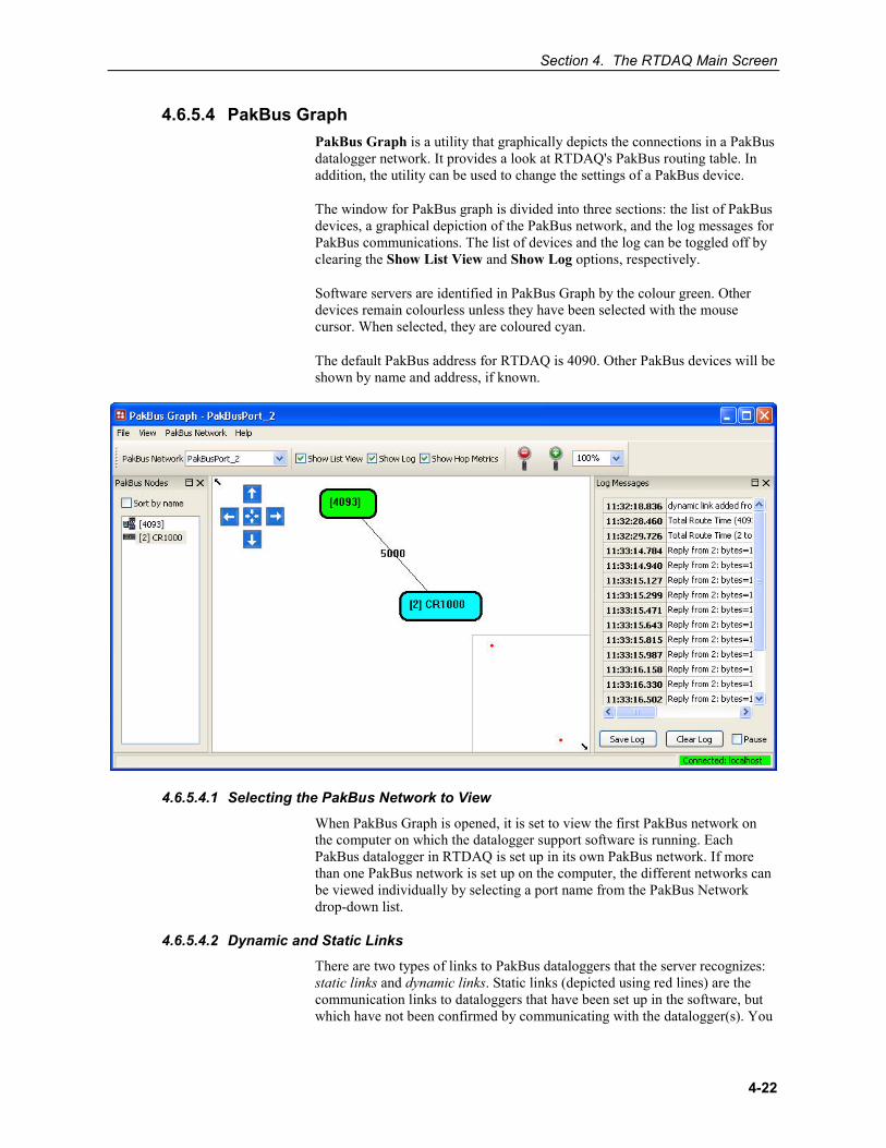
Section 4. The RTDAQ Main Screen
4-22
4.6.5.4 PakBus Graph PakBus Graph is a utility that graphically depicts the connections in a PakBus datalogger network. It provides a look at RTDAQ's PakBus routing table. In addition, the utility can be used to change the settings of a PakBus device.
The window for PakBus graph is divided into three sections: the list of PakBus devices, a graphical depiction of the PakBus network, and the log messages for PakBus communications. The list of devices and the log can be toggled off by clearing the Show List View and Show Log options, respectively.
Software servers are identified in PakBus Graph by the colour green. Other devices remain colourless unless they have been selected with the mouse cursor. When selected, they are coloured cyan.
The default PakBus address for RTDAQ is 4090. Other PakBus devices will be shown by name and address, if known.
4.6.5.4.1 Selecting the PakBus Network to View
When PakBus Graph is opened, it is set to view the first PakBus network on the computer on which the datalogger support software is running. Each PakBus datalogger in RTDAQ is set up in its own PakBus network. If more than one PakBus network is set up on the computer, the different networks can be viewed individually by selecting a port name from the PakBus Network drop-down list.
4.6.5.4.2 Dynamic and Static Links
There are two types of links to PakBus dataloggers that the server recognizes: static links and dynamic links. Static links (depicted using red lines) are the communication links to dataloggers that have been set up in the software, but which have not been confirmed by communicating with the datalogger(s). You
Section 4. The RTDAQ Main Screen
4-23
will see these dataloggers listed in the software's network map. Dynamic links (black lines) are communication links to dataloggers that have been confirmed.
4.6.5.4.3 Viewing/Changing Settings in a PakBus Datalogger
If you right-click a device in PakBus graph, you will be presented with a context menu. From this menu, select Edit Settings to display a list of the PakBus settings for the datalogger. Some of these settings are read-only, but other settings can be changed. Click within the cell for a setting, enter a new value, and then press Enter to make a change. If the change is accepted, the cell will appear green. If the change was denied (which likely means the setting is read-only), the cell will appear red.
4.6.5.4.4 Right-Click Functionality
There are several options available from the context menu that is displayed when you right-click a device (not all devices will have all settings):
Edit Settings - This option shows the PakBus settings of a device (see above).
Ping Node - This option will send a packet to the selected device to determine if it is reachable in the PakBus network. The results of the ping will be displayed in the Log Messages. Each ping message will include the size of the packet sent, and the time of response from the pinged device. The last message recorded will include summary information from the ping.
Verify Routing Table – This option will request the routing table from a PakBus device.
Reset Node - This option will reset the routing table in a PakBus device.
Change PakBus Address (server only) - By default, the PakBus address of the software server is 4090 (RTDAQ). This option lets you change this default.
Search for Neighbors (server only) - When this option is selected, the software server will broadcast a Hello Request every 5 seconds to search for PakBus neighbors with which it can communicate. During this time, the PakBus port is kept on-line.
Broadcast Reset (server only) - This option will reset the routing table in the selected PakBus device, as well as any neighbors of the selected device that are acting as routers.
Unlock Position – This option will unlock a device that has been locked into position in PakBus Graph by dragging it to a new position on the screen. All devices can be unlocked by selecting View | Unlock All Positions from the menu.
4.6.5.4.5 Discovering Probable Routes between Devices
You can view the probable route that communication will take between two PakBus devices by sequentially clicking on the two devices in Pakbus Graph. The probable communication route will be highlighted in cyan. If the Show Hop Metrics check box is selected, the graph will include the time, in milliseconds, that communication takes between the two devices. The results are also displayed in the Log Messages portion of the window.
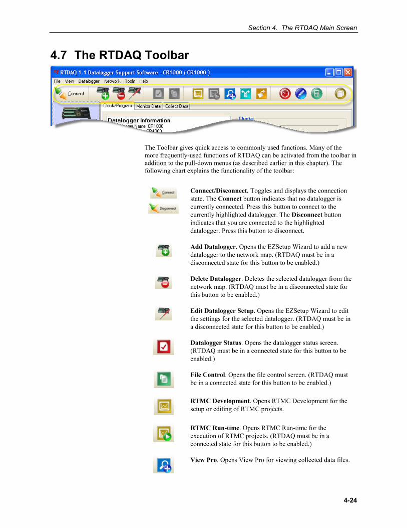
Section 4. The RTDAQ Main Screen
4-24
4.7 The RTDAQ Toolbar
The Toolbar gives quick access to commonly used functions. Many of the more frequently-used functions of RTDAQ can be activated from the toolbar in addition to the pull-down menus (as described earlier in this chapter). The following chart explains the functionality of the toolbar:
Connect/Disconnect. Toggles and displays the connection state. The Connect button indicates that no datalogger is currently connected. Press this button to connect to the currently highlighted datalogger. The Disconnect button indicates that you are connected to the highlighted datalogger. Press this button to disconnect.
Add Datalogger. Opens the EZSetup Wizard to add a new datalogger to the network map. (RTDAQ must be in a disconnected state for this button to be enabled.)
Delete Datalogger. Deletes the selected datalogger from the network map. (RTDAQ must be in a disconnected state for this button to be enabled.)
Edit Datalogger Setup. Opens the EZSetup Wizard to edit the settings for the selected datalogger. (RTDAQ must be in a disconnected state for this button to be enabled.)
Datalogger Status. Opens the datalogger status screen. (RTDAQ must be in a connected state for this button to be enabled.)
File Control. Opens the file control screen. (RTDAQ must be in a connected state for this button to be enabled.)
RTMC Development. Opens RTMC Development for the setup or editing of RTMC projects.
RTMC Run-time. Opens RTMC Run-time for the execution of RTMC projects. (RTDAQ must be in a connected state for this button to be enabled.)
View Pro. Opens View Pro for viewing collected data files.
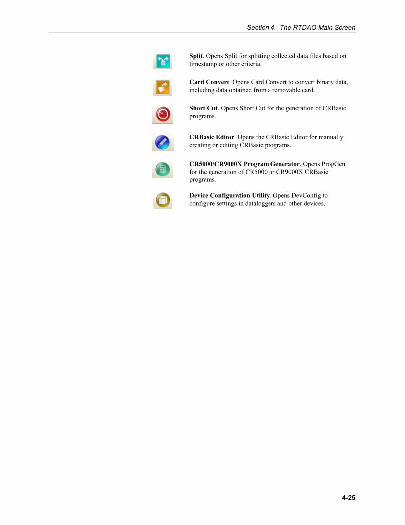
Section 4. The RTDAQ Main Screen
4-25
Split. Opens Split for splitting collected data files based on timestamp or other criteria.
Card Convert. Opens Card Convert to convert binary data, including data obtained from a removable card.
Short Cut. Opens Short Cut for the generation of CRBasic programs.
CRBasic Editor. Opens the CRBasic Editor for manually creating or editing CRBasic programs.
CR5000/CR9000X Program Generator. Opens ProgGen for the generation of CR5000 or CR9000X CRBasic programs.
Device Configuration Utility. Opens DevConfig to configure settings in dataloggers and other devices.
5-1
Section 5. Program Creation and Editing
The CRBasic Editor is a programming tool which can be used with the CR1000X-series, CR6-series, GRANITE 6, GRANITE 9, GRANITE 10, CR1000, CR3000, CR800-series, CR5000, and CR9000X dataloggers. It is intended for use by experienced datalogger programmers who need more flexibility and control over the datalogger operation than what can be achieved using program generators such as SCWIN or the CR5000/CR9000X Program Generator (ProgGen). This programming language is similar in syntax, program flow, and logic to the Structured BASIC programming language.
SCWIN and the CR5000/CR9000X Program Generator are also discussed in this chapter.
5.1 CRBasic Editor 5.1.1 Overview
Although RTDAQ does not support the CR300-series, CR200-series, or CR9000 dataloggers, the CRBasic application included with RTDAQ is the same one included for use with LoggerNet and other Campbell Scientific support software. Because of this, the documentation included here contains references to these dataloggers. For most RTDAQ implementations, these references can be ignored.
As shown below, the CRBasic Editor's main window is divided into three parts: the Program Entry Window, the Instruction Panel, and the Message area. The Instruction Panel on the right side is a list that comprises the instructions for a particular datalogger in the CRBasic language. Instructions can be selected from this list or entered directly into the Program Entry Window on the left. The Message area at the bottom becomes visible after a program is compiled and shows results of the compile and any errors detected.
NOTE
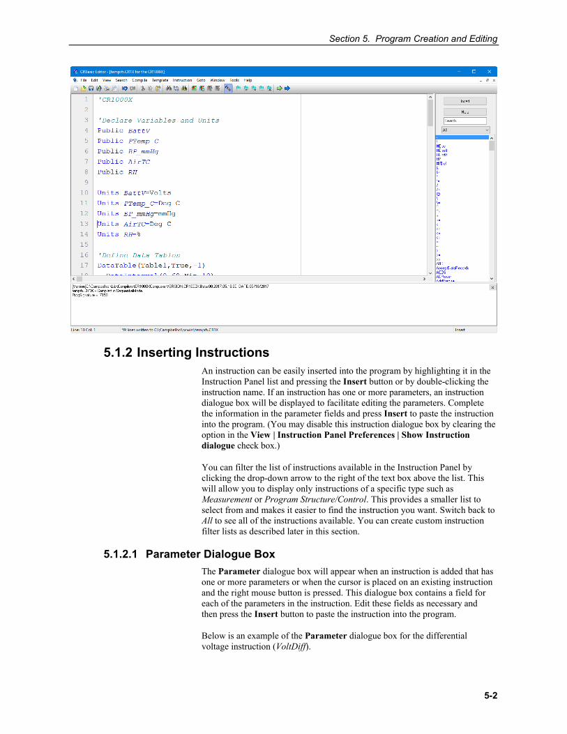
Section 5. Program Creation and Editing
5-2
5.1.2 Inserting Instructions An instruction can be easily inserted into the program by highlighting it in the Instruction Panel list and pressing the Insert button or by double-clicking the instruction name. If an instruction has one or more parameters, an instruction dialogue box will be displayed to facilitate editing the parameters. Complete the information in the parameter fields and press Insert to paste the instruction into the program. (You may disable this instruction dialogue box by clearing the option in the View | Instruction Panel Preferences | Show Instruction dialogue check box.)
You can filter the list of instructions available in the Instruction Panel by clicking the drop-down arrow to the right of the text box above the list. This will allow you to display only instructions of a specific type such as Measurement or Program Structure/Control. This provides a smaller list to select from and makes it easier to find the instruction you want. Switch back to All to see all of the instructions available. You can create custom instruction filter lists as described later in this section.
5.1.2.1 Parameter Dialogue Box The Parameter dialogue box will appear when an instruction is added that has one or more parameters or when the cursor is placed on an existing instruction and the right mouse button is pressed. This dialogue box contains a field for each of the parameters in the instruction. Edit these fields as necessary and then press the Insert button to paste the instruction into the program.
Below is an example of the Parameter dialogue box for the differential voltage instruction (VoltDiff).
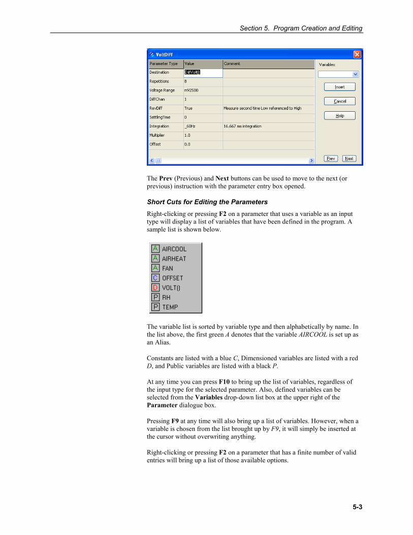
Section 5. Program Creation and Editing
5-3
The Prev (Previous) and Next buttons can be used to move to the next (or previous) instruction with the parameter entry box opened.
Short Cuts for Editing the Parameters
Right-clicking or pressing F2 on a parameter that uses a variable as an input type will display a list of variables that have been defined in the program. A sample list is shown below.
The variable list is sorted by variable type and then alphabetically by name. In the list above, the first green A denotes that the variable AIRCOOL is set up as an Alias.
Constants are listed with a blue C, Dimensioned variables are listed with a red D, and Public variables are listed with a black P.
At any time you can press F10 to bring up the list of variables, regardless of the input type for the selected parameter. Also, defined variables can be selected from the Variables drop-down list box at the upper right of the Parameter dialogue box.
Pressing F9 at any time will also bring up a list of variables. However, when a variable is chosen from the list brought up by F9, it will simply be inserted at the cursor without overwriting anything.
Right-clicking or pressing F2 on a parameter that has a finite number of valid entries will bring up a list of those available options.
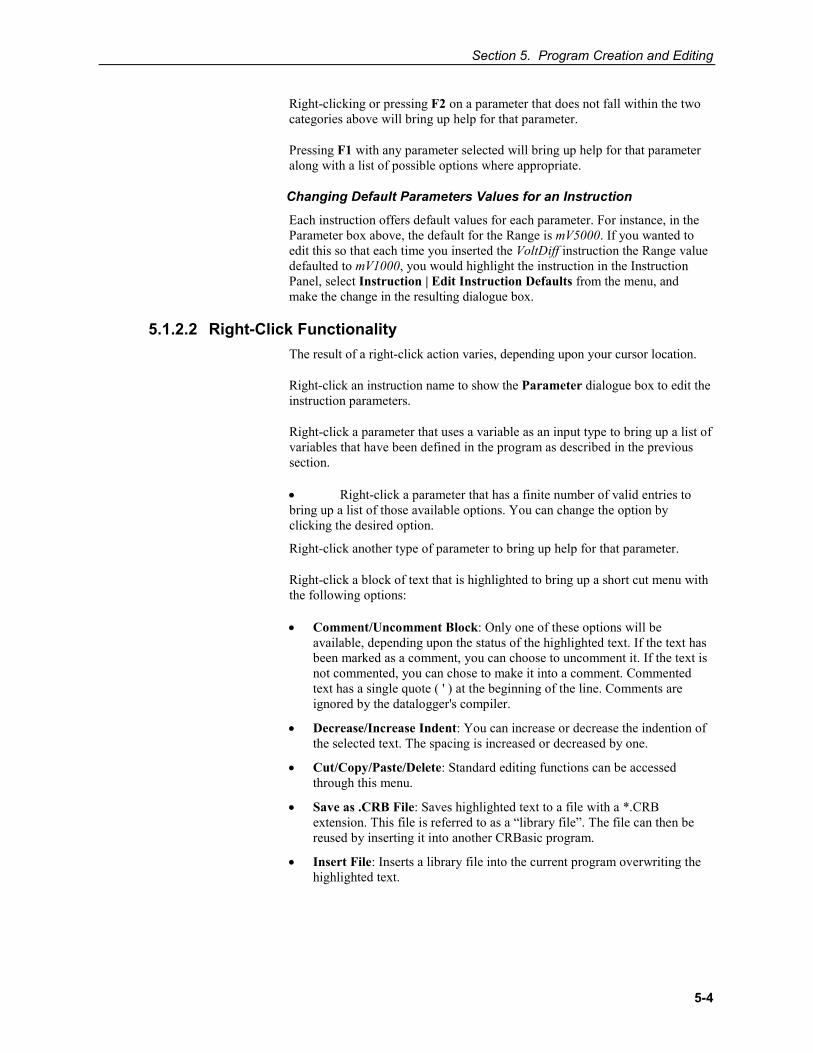
Section 5. Program Creation and Editing
5-4
Right-clicking or pressing F2 on a parameter that does not fall within the two categories above will bring up help for that parameter.
Pressing F1 with any parameter selected will bring up help for that parameter along with a list of possible options where appropriate.
Changing Default Parameters Values for an Instruction
Each instruction offers default values for each parameter. For instance, in the Parameter box above, the default for the Range is mV5000. If you wanted to edit this so that each time you inserted the VoltDiff instruction the Range value defaulted to mV1000, you would highlight the instruction in the Instruction Panel, select Instruction | Edit Instruction Defaults from the menu, and make the change in the resulting dialogue box.
5.1.2.2 Right-Click Functionality The result of a right-click action varies, depending upon your cursor location.
Right-click an instruction name to show the Parameter dialogue box to edit the instruction parameters.
Right-click a parameter that uses a variable as an input type to bring up a list of variables that have been defined in the program as described in the previous section.
• Right-click a parameter that has a finite number of valid entries tobring up a list of those available options. You can change the option byclicking the desired option.
Right-click another type of parameter to bring up help for that parameter.
Right-click a block of text that is highlighted to bring up a short cut menu with the following options:
• Comment/Uncomment Block: Only one of these options will beavailable, depending upon the status of the highlighted text. If the text hasbeen marked as a comment, you can choose to uncomment it. If the text isnot commented, you can chose to make it into a comment. Commentedtext has a single quote ( ' ) at the beginning of the line. Comments areignored by the datalogger's compiler.
• Decrease/Increase Indent: You can increase or decrease the indention ofthe selected text. The spacing is increased or decreased by one.
• Cut/Copy/Paste/Delete: Standard editing functions can be accessedthrough this menu.
• Save as .CRB File: Saves highlighted text to a file with a *.CRBextension. This file is referred to as a “library file”. The file can then bereused by inserting it into another CRBasic program.
• Insert File: Inserts a library file into the current program overwriting thehighlighted text.
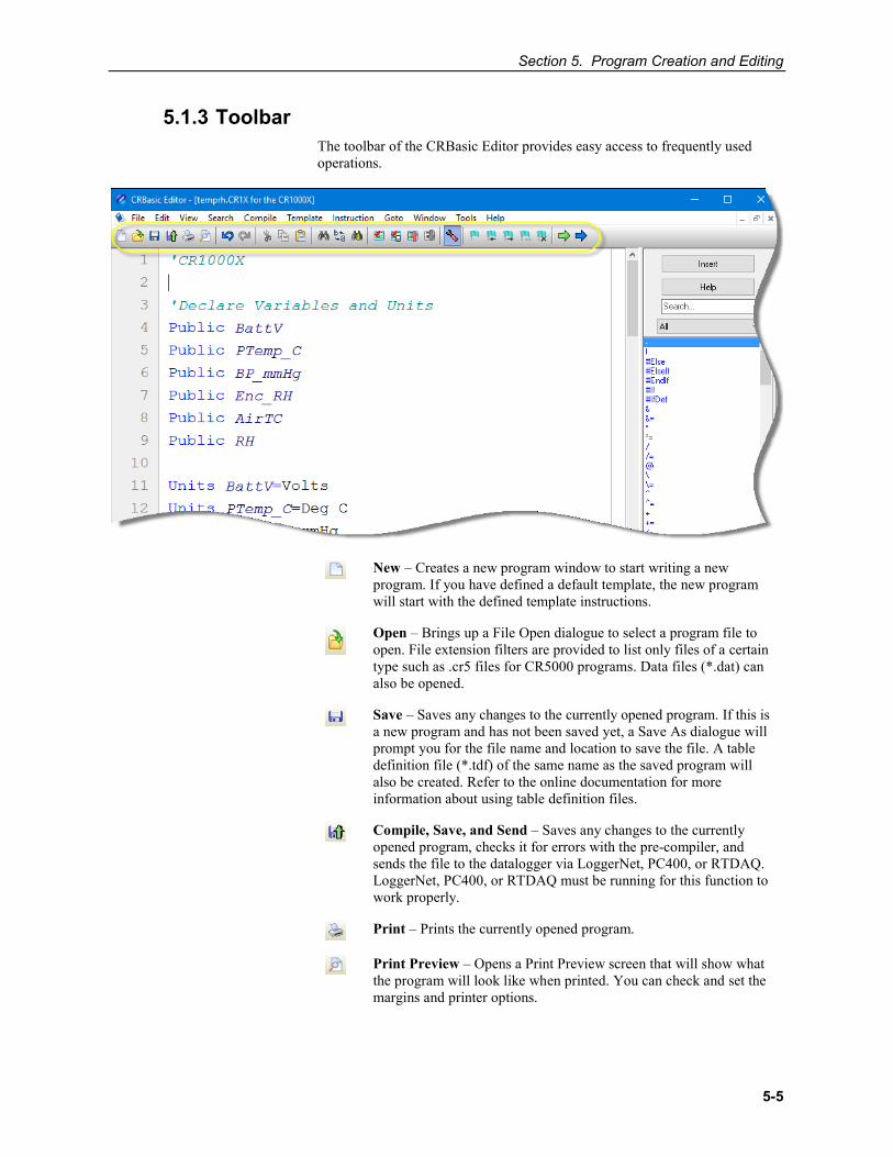
Section 5. Program Creation and Editing
5-5
5.1.3 Toolbar The toolbar of the CRBasic Editor provides easy access to frequently used operations.
New – Creates a new program window to start writing a new program. If you have defined a default template, the new program will start with the defined template instructions.
Open – Brings up a File Open dialogue to select a program file to open. File extension filters are provided to list only files of a certain type such as .cr5 files for CR5000 programs. Data files (*.dat) can also be opened.
Save – Saves any changes to the currently opened program. If this is a new program and has not been saved yet, a Save As dialogue will prompt you for the file name and location to save the file. A table definition file (*.tdf) of the same name as the saved program will also be created. Refer to the online documentation for more information about using table definition files.
Compile, Save, and Send – Saves any changes to the currently opened program, checks it for errors with the pre-compiler, and sends the file to the datalogger via LoggerNet, PC400, or RTDAQ. LoggerNet, PC400, or RTDAQ must be running for this function to work properly.
Print – Prints the currently opened program.
Print Preview – Opens a Print Preview screen that will show what the program will look like when printed. You can check and set the margins and printer options.
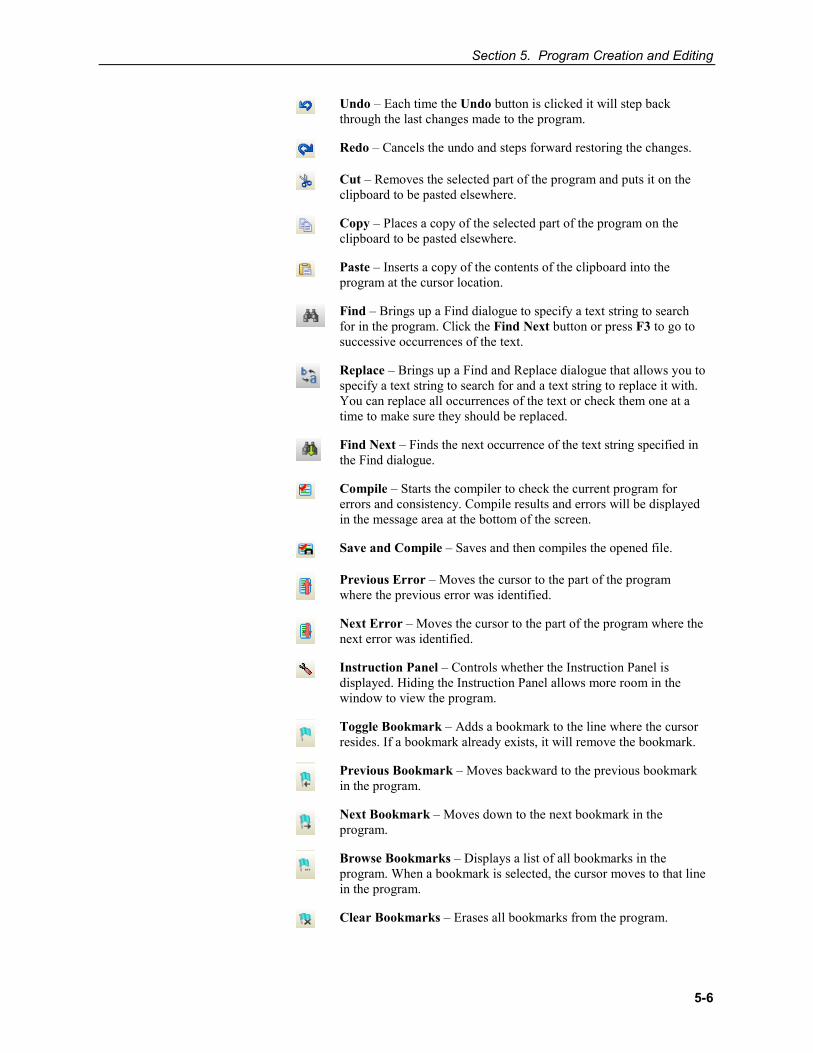
Section 5. Program Creation and Editing
5-6
Undo – Each time the Undo button is clicked it will step back through the last changes made to the program.
Redo – Cancels the undo and steps forward restoring the changes.
Cut – Removes the selected part of the program and puts it on the clipboard to be pasted elsewhere.
Copy – Places a copy of the selected part of the program on the clipboard to be pasted elsewhere.
Paste – Inserts a copy of the contents of the clipboard into the program at the cursor location.
Find – Brings up a Find dialogue to specify a text string to search for in the program. Click the Find Next button or press F3 to go to successive occurrences of the text.
Replace – Brings up a Find and Replace dialogue that allows you to specify a text string to search for and a text string to replace it with. You can replace all occurrences of the text or check them one at a time to make sure they should be replaced.
Find Next – Finds the next occurrence of the text string specified in the Find dialogue.
Compile – Starts the compiler to check the current program for errors and consistency. Compile results and errors will be displayed in the message area at the bottom of the screen.
Save and Compile – Saves and then compiles the opened file.
Previous Error – Moves the cursor to the part of the program where the previous error was identified.
Next Error – Moves the cursor to the part of the program where the next error was identified.
Instruction Panel – Controls whether the Instruction Panel is displayed. Hiding the Instruction Panel allows more room in the window to view the program.
Toggle Bookmark – Adds a bookmark to the line where the cursor resides. If a bookmark already exists, it will remove the bookmark.
Previous Bookmark – Moves backward to the previous bookmark in the program.
Next Bookmark – Moves down to the next bookmark in the program.
Browse Bookmarks – Displays a list of all bookmarks in the program. When a bookmark is selected, the cursor moves to that line in the program.
Clear Bookmarks – Erases all bookmarks from the program.
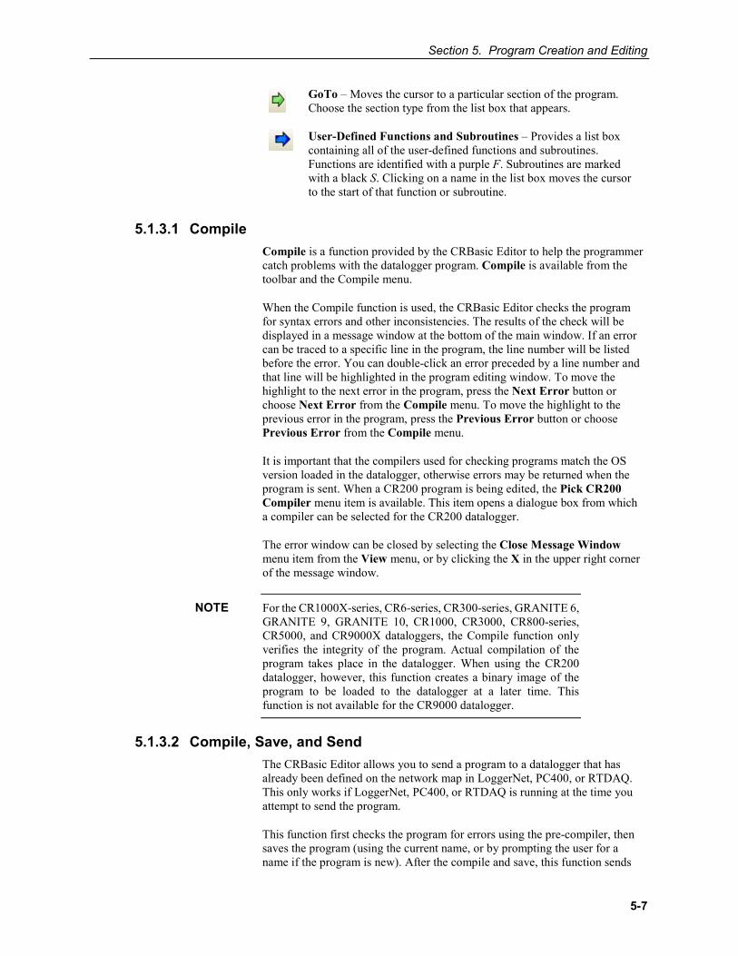
Section 5. Program Creation and Editing
5-7
GoTo – Moves the cursor to a particular section of the program. Choose the section type from the list box that appears.
User-Defined Functions and Subroutines – Provides a list box containing all of the user-defined functions and subroutines. Functions are identified with a purple F. Subroutines are marked with a black S. Clicking on a name in the list box moves the cursor to the start of that function or subroutine.
5.1.3.1 Compile Compile is a function provided by the CRBasic Editor to help the programmer catch problems with the datalogger program. Compile is available from the toolbar and the Compile menu.
When the Compile function is used, the CRBasic Editor checks the program for syntax errors and other inconsistencies. The results of the check will be displayed in a message window at the bottom of the main window. If an error can be traced to a specific line in the program, the line number will be listed before the error. You can double-click an error preceded by a line number and that line will be highlighted in the program editing window. To move the highlight to the next error in the program, press the Next Error button or choose Next Error from the Compile menu. To move the highlight to the previous error in the program, press the Previous Error button or choose Previous Error from the Compile menu.
It is important that the compilers used for checking programs match the OS version loaded in the datalogger, otherwise errors may be returned when the program is sent. When a CR200 program is being edited, the Pick CR200 Compiler menu item is available. This item opens a dialogue box from which a compiler can be selected for the CR200 datalogger.
The error window can be closed by selecting the Close Message Window menu item from the View menu, or by clicking the X in the upper right corner of the message window.
For the CR1000X-series, CR6-series, CR300-series, GRANITE 6, GRANITE 9, GRANITE 10, CR1000, CR3000, CR800-series, CR5000, and CR9000X dataloggers, the Compile function only verifies the integrity of the program. Actual compilation of the program takes place in the datalogger. When using the CR200 datalogger, however, this function creates a binary image of the program to be loaded to the datalogger at a later time. This function is not available for the CR9000 datalogger.
5.1.3.2 Compile, Save, and Send The CRBasic Editor allows you to send a program to a datalogger that has already been defined on the network map in LoggerNet, PC400, or RTDAQ. This only works if LoggerNet, PC400, or RTDAQ is running at the time you attempt to send the program.
This function first checks the program for errors using the pre-compiler, then saves the program (using the current name, or by prompting the user for a name if the program is new). After the compile and save, this function sends
NOTE
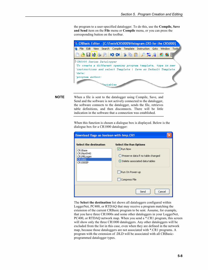
Section 5. Program Creation and Editing
5-8
the program to a user-specified datalogger. To do this, use the Compile, Save and Send item on the File menu or Compile menu, or you can press the corresponding button on the toolbar.
When a file is sent to the datalogger using Compile, Save, and Send and the software is not actively connected to the datalogger, the software connects to the datalogger, sends the file, retrieves table definitions, and then disconnects. There will be little indication in the software that a connection was established.
When this function is chosen a dialogue box is displayed. Below is the dialogue box for a CR1000 datalogger:
The Select the destination list shows all dataloggers configured within LoggerNet, PC400, or RTDAQ that may receive a program matching the extension of the current CRBasic program to be sent. Assume, for example, that you have three CR1000s and some other dataloggers in your LoggerNet, PC400, or RTDAQ network map. When you send a *.CR1 program, this screen will show only the three CR1000 dataloggers. Any other dataloggers will be excluded from the list in this case, even when they are defined in the network map, because those dataloggers are not associated with *.CR1 programs. A program with the extension of .DLD will be associated with all CRBasic-programmed datalogger types.
NOTE
Section 5. Program Creation and Editing
5-9
Select the datalogger to send the file to, and then select the Run Options.
Run Now The Run Now run options are different for the different datalogger types.
CR1000X-Series/CR6-Series/CR300-Series/GRANITE 6/ GRANITE 9/GRANITE 10/CR1000/CR3000/CR800-Series Run Now Options
When Run Now is checked, the file will be sent with the Run Now attribute set. With this attribute, the program is compiled and run in the datalogger. You may choose to preserve existing data tables on the datalogger's CPU if there has been no change to the data tables (Preserve data if no table changed) or to delete data tables on the CPU that have the same name as tables declared in the new program (Delete associated data tables).
Neither of these options affects existing data files on a card if one is being used. If a data table exists on the card that has the same name as one being output with the new program, the message will be returned "Data on Card is from a different program or corrupted". Data will not be written to the card until the existing table is deleted. Data tables on the card that have different names than those declared in the new program will be maintained and will not affect card data storage when the new program is running.
When using the Preserve data if no table changed option, existing data and data table structures are retained unless one of the following occurs:
• Data table name(s) change
• Data interval or offset change
• Number of fields per record change
• Number of bytes per field change
• Number of records per table (table size) change
• Field type, size, name, or position change
To summarize, any change in data table structure will delete all tables on the datalogger's CPU, regardless of whether or not the Preserve Data option was chosen. If the Preserve Data option was chosen but the datalogger was unable to retain the existing data, the following message will appear in the Compile Results: Warning: Internal Data Storage Memory was re-initialized.
CAUTION
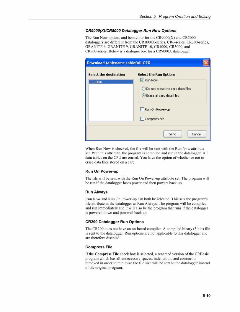
Section 5. Program Creation and Editing
5-10
CR9000(X)/CR5000 Datalogger Run Now Options
The Run Now options and behaviour for the CR9000(X) and CR5000 dataloggers are different from the CR1000X-series, CR6-series, CR300-series, GRANITE 6, GRANITE 9, GRANITE 10, CR1000, CR3000, and CR800-series. Below is a dialogue box for a CR9000X datalogger.
When Run Now is checked, the file will be sent with the Run Now attribute set. With this attribute, the program is compiled and run in the datalogger. All data tables on the CPU are erased. You have the option of whether or not to erase data files stored on a card.
Run On Power-up The file will be sent with the Run On Power-up attribute set. The program will be run if the datalogger loses power and then powers back up.
Run Always Run Now and Run On Power-up can both be selected. This sets the program's file attribute in the datalogger as Run Always. The program will be compiled and run immediately and it will also be the program that runs if the datalogger is powered down and powered back up.
CR200 Datalogger Run Options The CR200 does not have an on-board compiler. A compiled binary (*.bin) file is sent to the datalogger. Run options are not applicable to this datalogger and are therefore disabled.
Compress File If the Compress File check box is selected, a renamed version of the CRBasic program which has all unnecessary spaces, indentation, and comments removed in order to minimize the file size will be sent to the datalogger instead of the original program.
Section 5. Program Creation and Editing
5-11
Sending the Program To send the file and perform the associated functions you have selected in the screen, press the Send button. If LoggerNet, PC400, or RTDAQ is not running, an error message will appear indicating that there is no communications server currently running. If LoggerNet, PC400, or RTDAQ is running and the program compiles properly on the hardware, you will receive a message indicating that the program is now running on the datalogger. If something goes wrong when sending the program, a message will appear indicating the error conditions. This may be a hardware-level compile error or another failure as reported to the software by the datalogger’s program load and run process.
Press Cancel if you do not wish to send the program to the datalogger.
When sending a program with the Compile, Save, and Send feature to a CR9000X datalogger while you are connected to the datalogger, you may get a disconnect message or similar notification. This is unique to the CR9000X datalogger and does not indicate any problem with the sending of the program. You can simply reconnect to the datalogger and continue your work.
5.1.3.3 Conditional Compile and Save The Conditional Compile and Save option is used to generate a new CRBasic program from code that uses conditional compile syntax (#If/Else/ElseIf statements) or constant customization. (See conditional compilation in the CRBasic Editor’s online help for more information on conditional compile syntax. See Section 5.1.3.9.2, Constant Customization (p. 5-17), for more information on constant customization.)
When a program is compiled that uses conditional syntax, any conditional compilation statements that do not evaluate as true are removed from the program and the program is compiled. When a program is compiled that uses constant customization, the constant values selected in the Tools | Customize Constants menu item are used when compiling the new program. In either instance, you are prompted to save the file under a user-specified name or the file will be saved under the name of the original program with _CC# appended. The # is a number that increments to create a unique filename. For instance, if the program name is myprogram.cr1, the first time it is compiled the default name will be myprogram_CC1.cr1. If myprogram_CC1.cr1 exists, the program will be named myprogram_CC2.cr1.
5.1.3.4 Templates The use of templates can be a powerful way to quickly create a set of similar datalogger programs. All or part of a program can be saved so that it can be used when creating new programs. These files are called templates. The Template menu provides access to create and use templates.
Save as Template – Saves the comments and instructions in the active file as a template. To save part of a program as a template, copy the selected part to a new program file and then Save as Template.
Save as Default Template – Saves the comments and instructions in the active file as a template that will be used each time File | New is selected for that type of datalogger.
NOTE
Section 5. Program Creation and Editing
5-12
Delete – When selected, a list of all dataloggers is displayed. Select a datalogger to open a dialogue box containing a list of saved templates. A template can then be highlighted and deleted from disk.
(Datalogger Types) – When a datalogger type is selected, a list of all templates is displayed.
Template files are associated with a specific datalogger type. For example, templates for a CR5000 cannot be used for CR9000X programming and vice versa. Each datalogger has its own set of instructions that may be different than the other.
5.1.3.5 Program Navigation using BookMarks and GoTo Bookmarks are lines of code in the program that the user marks, which can be quickly navigated to using the Next, Previous, and Browse Bookmark functions. Buttons for the bookmark function are available on the toolbar or in the GoTo | Bookmarks menu. Selecting the Toggle Bookmark option will add a bookmark to a line. Selecting it a second time will remove the bookmark. When a line is bookmarked, the entire line will be highlighted with a colour (the colour can be changed using the View | Editor Preferences menu item). You can then navigate from bookmark to bookmark by selecting Previous or Next. All bookmarks can be removed from the program by selecting Clear Bookmarks. Bookmarks are persistent when you close a program (i.e., they are saved and will exist the next time the program is opened).
All programs have certain common instructions, such as the declaration of variables, data table definitions, the BeginProg/EndProg statements and Scan/NextScan. The Goto function is used to move the cursor to the next occurrence of a common instruction in the program (GoTo | Navigation or choose the GoTo button from the toolbar). In addition, you can move to a particular line number in the program by selecting GoTo | Go To Line.
5.1.3.6 CRBasic Editor File Menu Many of the functions available from the CRBasic Editor Toolbar are found in this menu. They have been discussed previously. Other options include:
Open as Read-Only – Opens a copy of a program file in read-only view. In this mode, the file cannot be edited. However, you can copy text from a read-only file into another file. Read-only allows the same program to be opened twice – once in regular view and once in read-only view. This allows the user to examine multiple areas of a very large program at the same time.
Save and Encrypt – Encrypts the active file. Encrypted files can be compiled in the datalogger but cannot be read by a user. (Refer to FileEncrypt in the CRBasic Editor’s online help for dataloggers that support file encryption.)
5.1.3.7 CRBasic Editor Edit Menu This menu item allows you to edit and manipulate the text currently being displayed in the Editor. Standard text editing functions such as Cut, Copy, Paste, Delete, Select All, Undo and Redo are found in this menu.
NOTE
Section 5. Program Creation and Editing
5-13
5.1.3.7.1 Other Options
Create Compressed File – Creates a new file with a _str extension. All user comments and line spacing in the program are removed from the file. Removing comments and spaces can significantly reduce the file size in larger programs.
Rebuild Indentation – Reworks the indentation of loops, If/Then/Else statements and other logic nesting, and removes blank lines based on the Vertical Spacing rules (Options | Editor Preferences, Vertical Spacing tab).
Save As CRB – Saves highlighted text to a file with a *.CRB extension. This file is referred to as a library file. The file can then be reused by inserting it into another CRBasic program.
Insert File – Inserts a library file (*.CRB) into the current program at the location of the cursor.
5.1.3.8 CRBasic Editor View Menu This menu item allows you to specify the files used in the CRBasic Editor and customize its look and syntax highlighting.
5.1.3.8.1 Editor Preferences
This option sets up the appearance options for the text instructions and the behaviour of pop-up hints.
The Editor tab allows the user to toggle on or off the pop-up hints for parameters in instructions, set the amount of time the cursor must hover over the instruction before the pop-up hint appears, and the background colour of the pop-up hint. This is also used to choose whether CRBasic automatic instruction indenting indents using tabs or spaces, and set the number of spaces if that option is chosen. Other options relating to the use of the tab key, capitalization, name checking, and line numbers are also available. Press the Help button for more information.
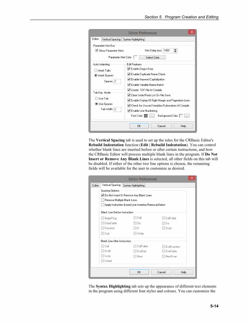
Section 5. Program Creation and Editing
5-14
The Vertical Spacing tab is used to set up the rules for the CRBasic Editor's Rebuild Indentation function (Edit | Rebuild Indentation). You can control whether blank lines are inserted before or after certain instructions, and how the CRBasic Editor will process multiple blank lines in the program. If Do Not Insert or Remove Any Blank Lines is selected, all other fields on this tab will be disabled. If either of the other two line options is chosen, the remaining fields will be available for the user to customize as desired.
The Syntax Highlighting tab sets up the appearance of different text elements in the program using different font styles and colours. You can customize the
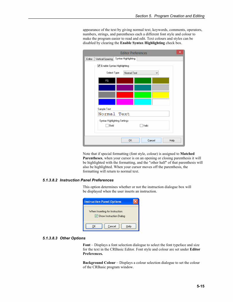
Section 5. Program Creation and Editing
5-15
appearance of the text by giving normal text, keywords, comments, operators, numbers, strings, and parentheses each a different font style and colour to make the program easier to read and edit. Text colours and styles can be disabled by clearing the Enable Syntax Highlighting check box.
Note that if special formatting (font style, colour) is assigned to Matched Parentheses, when your cursor is on an opening or closing parenthesis it will be highlighted with the formatting, and the "other half" of that parenthesis will also be highlighted. When your cursor moves off the parenthesis, the formatting will return to normal text.
5.1.3.8.2 Instruction Panel Preferences
This option determines whether or not the instruction dialogue box will be displayed when the user inserts an instruction.
5.1.3.8.3 Other Options
Font – Displays a font selection dialogue to select the font typeface and size for the text in the CRBasic Editor. Font style and colour are set under Editor Preferences.
Background Colour – Displays a colour selection dialogue to set the colour of the CRBasic program window.
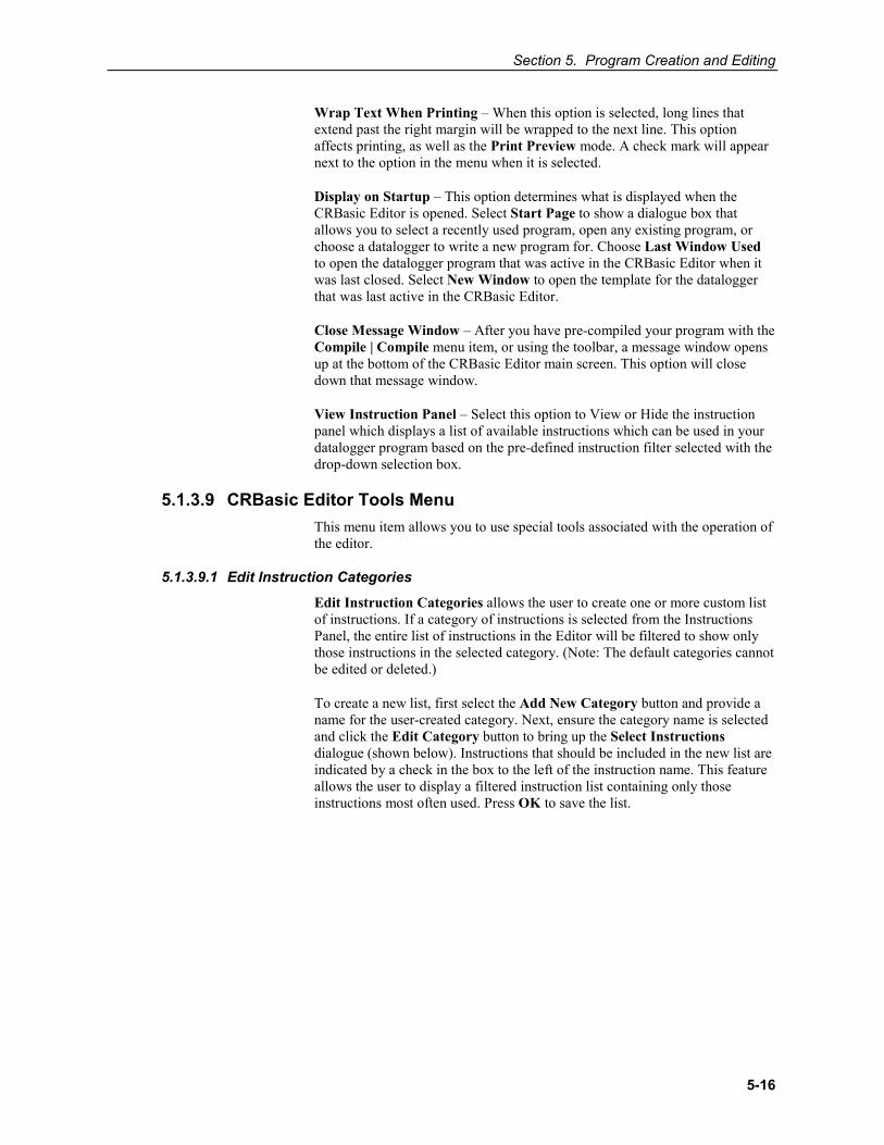
Section 5. Program Creation and Editing
5-16
Wrap Text When Printing – When this option is selected, long lines that extend past the right margin will be wrapped to the next line. This option affects printing, as well as the Print Preview mode. A check mark will appear next to the option in the menu when it is selected.
Display on Startup – This option determines what is displayed when the CRBasic Editor is opened. Select Start Page to show a dialogue box that allows you to select a recently used program, open any existing program, or choose a datalogger to write a new program for. Choose Last Window Used to open the datalogger program that was active in the CRBasic Editor when it was last closed. Select New Window to open the template for the datalogger that was last active in the CRBasic Editor.
Close Message Window – After you have pre-compiled your program with the Compile | Compile menu item, or using the toolbar, a message window opens up at the bottom of the CRBasic Editor main screen. This option will close down that message window.
View Instruction Panel – Select this option to View or Hide the instruction panel which displays a list of available instructions which can be used in your datalogger program based on the pre-defined instruction filter selected with the drop-down selection box.
5.1.3.9 CRBasic Editor Tools Menu This menu item allows you to use special tools associated with the operation of the editor.
5.1.3.9.1 Edit Instruction Categories
Edit Instruction Categories allows the user to create one or more custom list of instructions. If a category of instructions is selected from the Instructions Panel, the entire list of instructions in the Editor will be filtered to show only those instructions in the selected category. (Note: The default categories cannot be edited or deleted.)
To create a new list, first select the Add New Category button and provide a name for the user-created category. Next, ensure the category name is selected and click the Edit Category button to bring up the Select Instructions dialogue (shown below). Instructions that should be included in the new list are indicated by a check in the box to the left of the instruction name. This feature allows the user to display a filtered instruction list containing only those instructions most often used. Press OK to save the list.
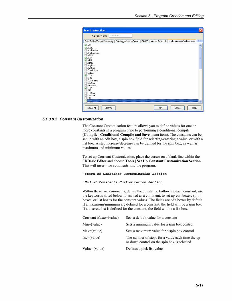
Section 5. Program Creation and Editing
5-17
5.1.3.9.2 Constant Customization
The Constant Customization feature allows you to define values for one or more constants in a program prior to performing a conditional compile (Compile | Conditional Compile and Save menu item). The constants can be set up with an edit box, a spin box field for selecting/entering a value, or with a list box. A step increase/decrease can be defined for the spin box, as well as maximum and minimum values.
To set up Constant Customization, place the cursor on a blank line within the CRBasic Editor and choose Tools | Set Up Constant Customization Section. This will insert two comments into the program:
'Start of Constants Customization Section
'End of Constants Customization Section
Within these two comments, define the constants. Following each constant, use the keywords noted below formatted as a comment, to set up edit boxes, spin boxes, or list boxes for the constant values. The fields are edit boxes by default. If a maximum/minimum are defined for a constant, the field will be a spin box. If a discrete list is defined for the constant, the field will be a list box.
Constant Name=(value) Sets a default value for a constant
Min=(value) Sets a minimum value for a spin box control
Max=(value) Sets a maximum value for a spin box control
Inc=(value) The number of steps for a value each time the up or down control on the spin box is selected
Value=(value) Defines a pick list value
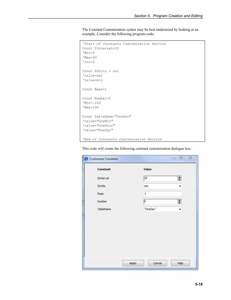
Section 5. Program Creation and Editing
5-18
The Constant Customization syntax may be best understood by looking at an example. Consider the following program code:
'Start of Constants Customization Section Const SInterval=10 'Min=5 'Max=60 'Inc=5
Const SUnits = sec 'value=sec 'value=min
Const Reps=1
Const Number=0 'Min=-100 'Max=100
Const TableName="OneSec" 'value="OneMin" 'value="OneHour" 'value="OneDay"
'End of Constants Customization Section
This code will create the following constant customization dialogue box:
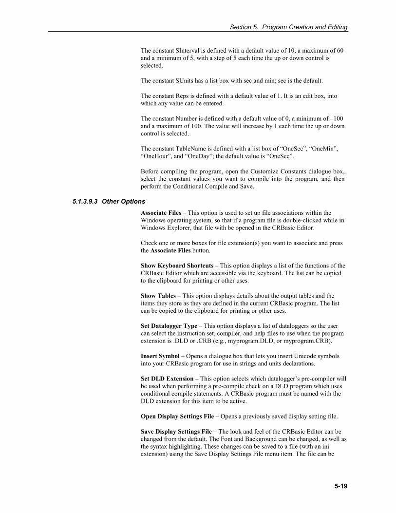
Section 5. Program Creation and Editing
5-19
The constant SInterval is defined with a default value of 10, a maximum of 60 and a minimum of 5, with a step of 5 each time the up or down control is selected.
The constant SUnits has a list box with sec and min; sec is the default.
The constant Reps is defined with a default value of 1. It is an edit box, into which any value can be entered.
The constant Number is defined with a default value of 0, a minimum of –100 and a maximum of 100. The value will increase by 1 each time the up or down control is selected.
The constant TableName is defined with a list box of “OneSec”, “OneMin”, “OneHour”, and “OneDay”; the default value is “OneSec”.
Before compiling the program, open the Customize Constants dialogue box, select the constant values you want to compile into the program, and then perform the Conditional Compile and Save.
5.1.3.9.3 Other Options
Associate Files – This option is used to set up file associations within the Windows operating system, so that if a program file is double-clicked while in Windows Explorer, that file with be opened in the CRBasic Editor.
Check one or more boxes for file extension(s) you want to associate and press the Associate Files button.
Show Keyboard Shortcuts – This option displays a list of the functions of the CRBasic Editor which are accessible via the keyboard. The list can be copied to the clipboard for printing or other uses.
Show Tables – This option displays details about the output tables and the items they store as they are defined in the current CRBasic program. The list can be copied to the clipboard for printing or other uses.
Set Datalogger Type – This option displays a list of dataloggers so the user can select the instruction set, compiler, and help files to use when the program extension is .DLD or .CRB (e.g., myprogram.DLD, or myprogram.CRB).
Insert Symbol – Opens a dialogue box that lets you insert Unicode symbols into your CRBasic program for use in strings and units declarations.
Set DLD Extension – This option selects which datalogger’s pre-compiler will be used when performing a pre-compile check on a DLD program which uses conditional compile statements. A CRBasic program must be named with the DLD extension for this item to be active.
Open Display Settings File – Opens a previously saved display setting file.
Save Display Settings File – The look and feel of the CRBasic Editor can be changed from the default. The Font and Background can be changed, as well as the syntax highlighting. These changes can be saved to a file (with an ini extension) using the Save Display Settings File menu item. The file can be
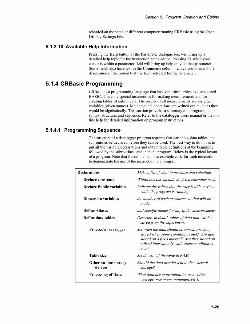
Section 5. Program Creation and Editing
5-20
reloaded on the same or different computer running CRBasic using the Open Display Settings File.
5.1.3.10 Available Help Information Pressing the Help button of the Parameter dialogue box will bring up a detailed help topic for the instruction being edited. Pressing F1 when your cursor is within a parameter field will bring up help only on that parameter. Some fields also have text in the Comments column, which provides a short description of the option that has been selected for the parameter.
5.1.4 CRBasic Programming CRBasic is a programming language that has some similarities to a structured BASIC. There are special instructions for making measurements and for creating tables of output data. The results of all measurements are assigned variables (given names). Mathematical operations are written out much as they would be algebraically. This section provides a summary of a program, its syntax, structure, and sequence. Refer to the datalogger users manual or the on-line help for detailed information on program instructions.
5.1.4.1 Programming Sequence The structure of a datalogger program requires that variables, data tables, and subroutines be declared before they can be used. The best way to do this is to put all the variable declarations and output table definitions at the beginning, followed by the subroutines, and then the program. Below is the typical layout of a program. Note that the online help has example code for each instruction to demonstrate the use of the instruction in a program.
Declarations Make a list of what to measure and calculate.
Declare constants Within this list, include the fixed constants used,
Declare Public variables Indicate the values that the user is able to view while the program is running,
Dimension variables the number of each measurement that will be made,
Define Aliases and specific names for any of the measurements.
Define data tables Describe, in detail, tables of data that will be saved from the experiment.
Process/store trigger Set when the data should be stored. Are they stored when some condition is met? Are data stored on a fixed interval? Are they stored on a fixed interval only while some condition is met?
Table size Set the size of the table in RAM.
Other on-line storage devices
Should the data also be sent to the external storage?
Processing of Data What data are to be output (current value, average, maximum, minimum, etc.).
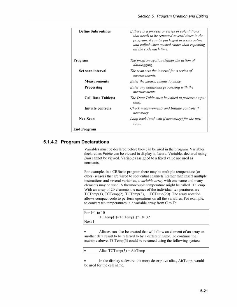
Section 5. Program Creation and Editing
5-21
Define Subroutines If there is a process or series of calculations that needs to be repeated several times in the program, it can be packaged in a subroutine and called when needed rather than repeating all the code each time.
Program The program section defines the action of
datalogging. Set scan interval The scan sets the interval for a series of
measurements. Measurements Enter the measurements to make. Processing Enter any additional processing with the
measurements. Call Data Table(s) The Data Table must be called to process output
data. Initiate controls Check measurements and Initiate controls if
necessary. NextScan Loop back (and wait if necessary) for the next
scan. End Program
5.1.4.2 Program Declarations Variables must be declared before they can be used in the program. Variables declared as Public can be viewed in display software. Variables declared using Dim cannot be viewed. Variables assigned to a fixed value are used as constants.
For example, in a CRBasic program there may be multiple temperature (or other) sensors that are wired to sequential channels. Rather than insert multiple instructions and several variables, a variable array with one name and many elements may be used. A thermocouple temperature might be called TCTemp. With an array of 20 elements the names of the individual temperatures are TCTemp(1), TCTemp(2), TCTemp(3), ... TCTemp(20). The array notation allows compact code to perform operations on all the variables. For example, to convert ten temperatures in a variable array from C to F:
For I=1 to 10 TCTemp(I)=TCTemp(I)*1.8+32 Next I
• Aliases can also be created that will allow an element of an array or another data result to be referred to by a different name. To continue the example above, TCTemp(3) could be renamed using the following syntax:
• Alias TCTemp(3) = AirTemp
• In the display software, the more descriptive alias, AirTemp, would be used for the cell name.
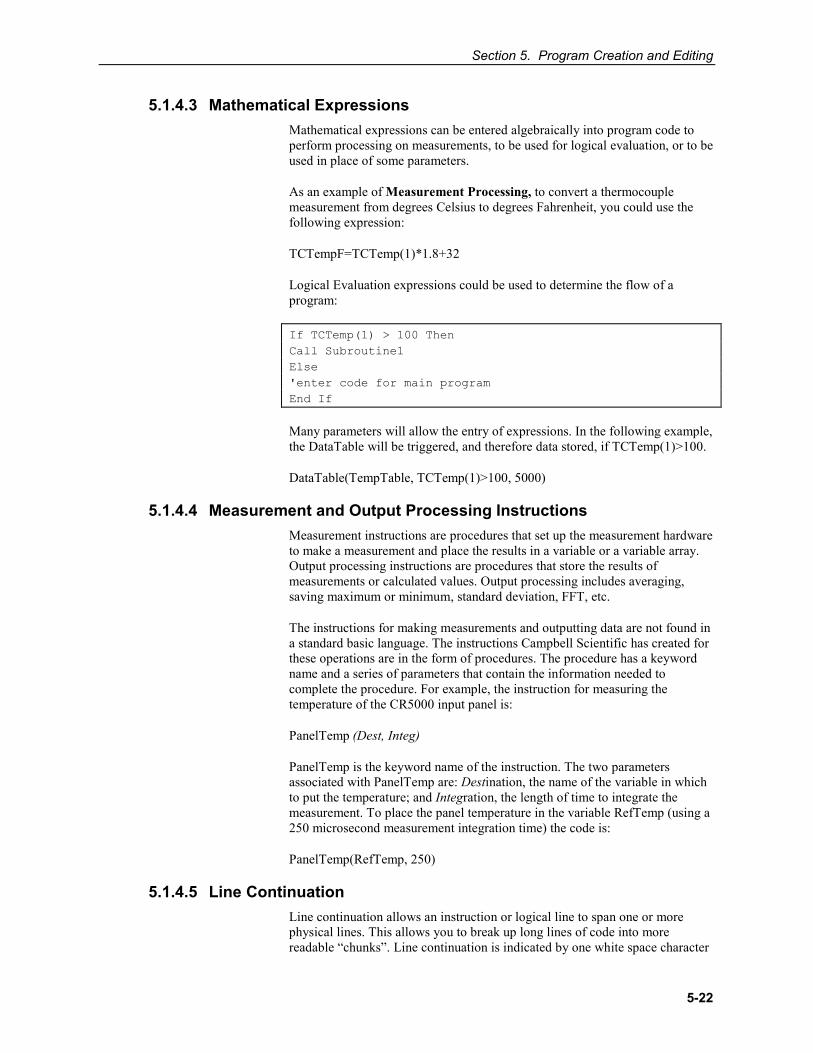
Section 5. Program Creation and Editing
5-22
5.1.4.3 Mathematical Expressions Mathematical expressions can be entered algebraically into program code to perform processing on measurements, to be used for logical evaluation, or to be used in place of some parameters.
As an example of Measurement Processing, to convert a thermocouple measurement from degrees Celsius to degrees Fahrenheit, you could use the following expression:
TCTempF=TCTemp(1)*1.8+32
Logical Evaluation expressions could be used to determine the flow of a program:
If TCTemp(1) > 100 Then Call Subroutine1 Else 'enter code for main program End If
Many parameters will allow the entry of expressions. In the following example, the DataTable will be triggered, and therefore data stored, if TCTemp(1)>100.
DataTable(TempTable, TCTemp(1)>100, 5000)
5.1.4.4 Measurement and Output Processing Instructions Measurement instructions are procedures that set up the measurement hardware to make a measurement and place the results in a variable or a variable array. Output processing instructions are procedures that store the results of measurements or calculated values. Output processing includes averaging, saving maximum or minimum, standard deviation, FFT, etc.
The instructions for making measurements and outputting data are not found in a standard basic language. The instructions Campbell Scientific has created for these operations are in the form of procedures. The procedure has a keyword name and a series of parameters that contain the information needed to complete the procedure. For example, the instruction for measuring the temperature of the CR5000 input panel is:
PanelTemp (Dest, Integ)
PanelTemp is the keyword name of the instruction. The two parameters associated with PanelTemp are: Destination, the name of the variable in which to put the temperature; and Integration, the length of time to integrate the measurement. To place the panel temperature in the variable RefTemp (using a 250 microsecond measurement integration time) the code is:
PanelTemp(RefTemp, 250)
5.1.4.5 Line Continuation Line continuation allows an instruction or logical line to span one or more physical lines. This allows you to break up long lines of code into more readable “chunks”. Line continuation is indicated by one white space character
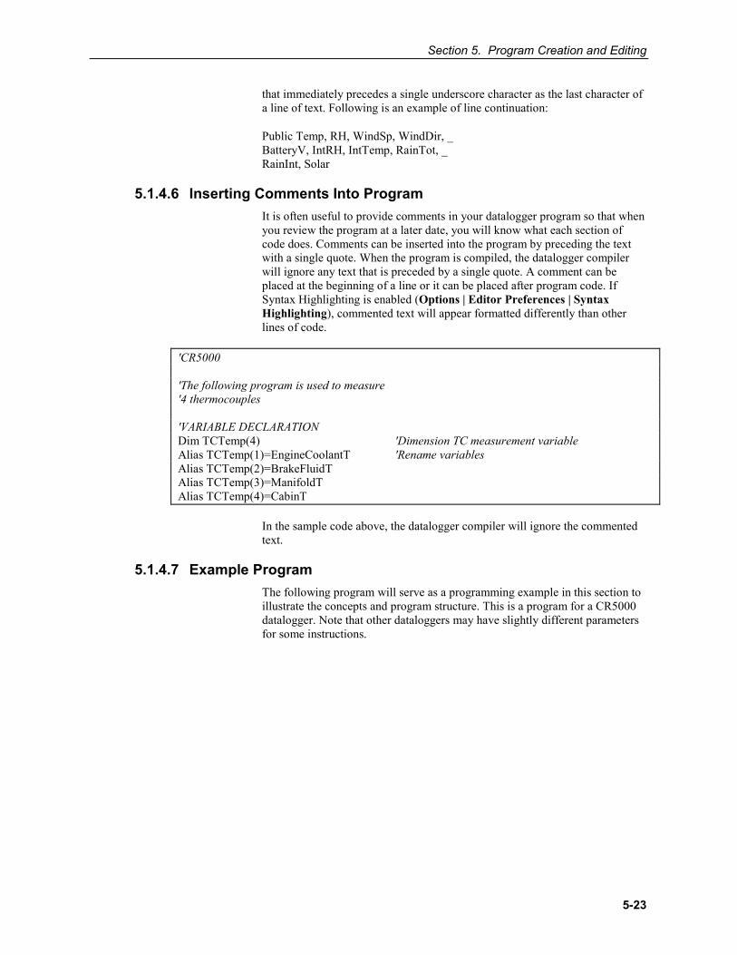
Section 5. Program Creation and Editing
5-23
that immediately precedes a single underscore character as the last character of a line of text. Following is an example of line continuation:
Public Temp, RH, WindSp, WindDir, _ BatteryV, IntRH, IntTemp, RainTot, _ RainInt, Solar
5.1.4.6 Inserting Comments Into Program It is often useful to provide comments in your datalogger program so that when you review the program at a later date, you will know what each section of code does. Comments can be inserted into the program by preceding the text with a single quote. When the program is compiled, the datalogger compiler will ignore any text that is preceded by a single quote. A comment can be placed at the beginning of a line or it can be placed after program code. If Syntax Highlighting is enabled (Options | Editor Preferences | Syntax Highlighting), commented text will appear formatted differently than other lines of code.
'CR5000 'The following program is used to measure '4 thermocouples 'VARIABLE DECLARATION Dim TCTemp(4) 'Dimension TC measurement variable Alias TCTemp(1)=EngineCoolantT 'Rename variables Alias TCTemp(2)=BrakeFluidT Alias TCTemp(3)=ManifoldT Alias TCTemp(4)=CabinT
In the sample code above, the datalogger compiler will ignore the commented text.
5.1.4.7 Example Program The following program will serve as a programming example in this section to illustrate the concepts and program structure. This is a program for a CR5000 datalogger. Note that other dataloggers may have slightly different parameters for some instructions.
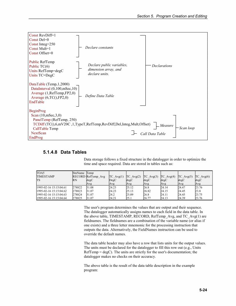
Section 5. Program Creation and Editing
5-24
Const RevDiff=1 Const Del=0 Const Integ=250 Const Mult=1 Const Offset=0 Public RefTemp Public TC(6) Units RefTemp=degC Units TC=DegC DataTable (Temp,1,2000) DataInterval (0,100,mSec,10) Average (1,RefTemp,FP2,0) Average (6,TC(),FP2,0) EndTable BeginProg Scan (10,mSec,3,0) PanelTemp (RefTemp, 250) TCDiff (TC(),6,mV20C ,1,TypeT,RefTemp,RevDiff,Del,Integ,Mult,Offset) CallTable Temp NextScan EndProg
5.1.4.8 Data Tables Data storage follows a fixed structure in the datalogger in order to optimize the time and space required. Data are stored in tables such as:
TOA5 StnName Temp TIMESTAMP RECORD RefTemp_Avg TC_Avg(1) TC_Avg(2) TC_Avg(3) TC_Avg(4) TC_Avg(5) TC_Avg(6) TS RN degC DegC degC degC degC degC degC Avg Avg Avg Avg Avg Avg Avg 1995-02-16 15:15:04.61 278822 31.08 24.23 25.12 26.8 24.14 24.47 23.76 1995-02-16 15:15:04.62 278823 31.07 24.23 25.13 26.82 24.15 24.45 23.8 1995-02-16 15:15:04.63 278824 31.07 24.2 25.09 26.8 24.11 24.45 23.75 1995-02-16 15:15:04.64 278825 31.07 24.21 25.1 26.77 24.13 24.39 23.76
The user's program determines the values that are output and their sequence. The datalogger automatically assigns names to each field in the data table. In the above table, TIMESTAMP, RECORD, RefTemp_Avg, and TC_Avg(1) are fieldnames. The fieldnames are a combination of the variable name (or alias if one exists) and a three letter mnemonic for the processing instruction that outputs the data. Alternatively, the FieldNames instruction can be used to override the default names.
The data table header may also have a row that lists units for the output values. The units must be declared for the datalogger to fill this row out (e.g., Units RefTemp = degC). The units are strictly for the user's documentation; the datalogger makes no checks on their accuracy.
The above table is the result of the data table description in the example program:
Declare public variables, dimension array, and declare units.
Declare constants
Define Data Table
Declarations
Scan loop Measure
Call Data Table
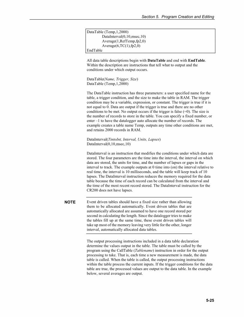
Section 5. Program Creation and Editing
5-25
DataTable (Temp,1,2000) DataInterval(0,10,msec,10) Average(1,RefTemp,fp2,0) Average(6,TC(1),fp2,0) EndTable
All data table descriptions begin with DataTable and end with EndTable. Within the description are instructions that tell what to output and the conditions under which output occurs.
DataTable(Name, Trigger, Size) DataTable (Temp,1,2000)
The DataTable instruction has three parameters: a user specified name for the table, a trigger condition, and the size to make the table in RAM. The trigger condition may be a variable, expression, or constant. The trigger is true if it is not equal to 0. Data are output if the trigger is true and there are no other conditions to be met. No output occurs if the trigger is false (=0). The size is the number of records to store in the table. You can specify a fixed number, or enter –1 to have the datalogger auto allocate the number of records. The example creates a table name Temp, outputs any time other conditions are met, and retains 2000 records in RAM.
DataInterval(TintoInt, Interval, Units, Lapses) DataInterval(0,10,msec,10)
DataInterval is an instruction that modifies the conditions under which data are stored. The four parameters are the time into the interval, the interval on which data are stored, the units for time, and the number of lapses or gaps in the interval to track. The example outputs at 0 time into (on) the interval relative to real time, the interval is 10 milliseconds, and the table will keep track of 10 lapses. The DataInterval instruction reduces the memory required for the data table because the time of each record can be calculated from the interval and the time of the most recent record stored. The DataInterval instruction for the CR200 does not have lapses.
Event driven tables should have a fixed size rather than allowing them to be allocated automatically. Event driven tables that are automatically allocated are assumed to have one record stored per second in calculating the length. Since the datalogger tries to make the tables fill up at the same time, these event driven tables will take up most of the memory leaving very little for the other, longer interval, automatically allocated data tables.
The output processing instructions included in a data table declaration determine the values output in the table. The table must be called by the program using the CallTable (Tablename) instruction in order for the output processing to take. That is, each time a new measurement is made, the data table is called. When the table is called, the output processing instructions within the table process the current inputs. If the trigger conditions for the data table are true, the processed values are output to the data table. In the example below, several averages are output.
NOTE
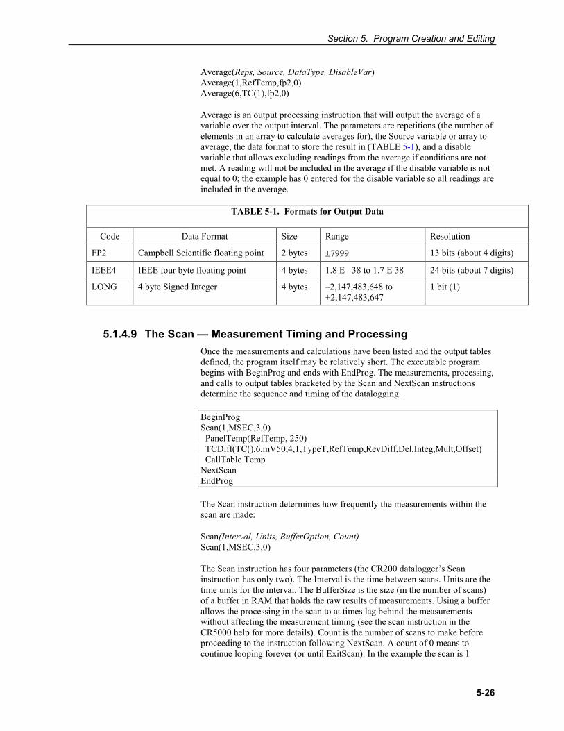
Section 5. Program Creation and Editing
5-26
Average(Reps, Source, DataType, DisableVar) Average(1,RefTemp,fp2,0) Average(6,TC(1),fp2,0)
Average is an output processing instruction that will output the average of a variable over the output interval. The parameters are repetitions (the number of elements in an array to calculate averages for), the Source variable or array to average, the data format to store the result in (TABLE 5-1), and a disable variable that allows excluding readings from the average if conditions are not met. A reading will not be included in the average if the disable variable is not equal to 0; the example has 0 entered for the disable variable so all readings are included in the average.
TABLE 5-1. Formats for Output Data
Code Data Format Size Range Resolution
FP2 Campbell Scientific floating point 2 bytes ±7999 13 bits (about 4 digits)
IEEE4 IEEE four byte floating point 4 bytes 1.8 E –38 to 1.7 E 38 24 bits (about 7 digits)
LONG 4 byte Signed Integer 4 bytes –2,147,483,648 to+2,147,483,647
1 bit (1)
5.1.4.9 The Scan — Measurement Timing and Processing Once the measurements and calculations have been listed and the output tables defined, the program itself may be relatively short. The executable program begins with BeginProg and ends with EndProg. The measurements, processing, and calls to output tables bracketed by the Scan and NextScan instructions determine the sequence and timing of the datalogging.
BeginProg Scan(1,MSEC,3,0) PanelTemp(RefTemp, 250) TCDiff(TC(),6,mV50,4,1,TypeT,RefTemp,RevDiff,Del,Integ,Mult,Offset) CallTable Temp NextScan EndProg
The Scan instruction determines how frequently the measurements within the scan are made:
Scan(Interval, Units, BufferOption, Count) Scan(1,MSEC,3,0)
The Scan instruction has four parameters (the CR200 datalogger’s Scan instruction has only two). The Interval is the time between scans. Units are the time units for the interval. The BufferSize is the size (in the number of scans) of a buffer in RAM that holds the raw results of measurements. Using a buffer allows the processing in the scan to at times lag behind the measurements without affecting the measurement timing (see the scan instruction in the CR5000 help for more details). Count is the number of scans to make before proceeding to the instruction following NextScan. A count of 0 means to continue looping forever (or until ExitScan). In the example the scan is 1
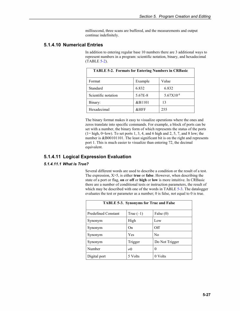
Section 5. Program Creation and Editing
5-27
millisecond, three scans are buffered, and the measurements and output continue indefinitely.
5.1.4.10 Numerical Entries In addition to entering regular base 10 numbers there are 3 additional ways to represent numbers in a program: scientific notation, binary, and hexadecimal (TABLE 5-2).
TABLE 5-2. Formats for Entering Numbers in CRBasic
Format Example Value
Standard 6.832 6.832
Scientific notation 5.67E-8 5.67X10⁻⁸
Binary: &B1101 13
Hexadecimal &HFF 255 The binary format makes it easy to visualize operations where the ones and zeros translate into specific commands. For example, a block of ports can be set with a number, the binary form of which represents the status of the ports (1= high, 0=low). To set ports 1, 3, 4, and 6 high and 2, 5, 7, and 8 low; the number is &B00101101. The least significant bit is on the right and represents port 1. This is much easier to visualize than entering 72, the decimal equivalent.
5.1.4.11 Logical Expression Evaluation 5.1.4.11.1 What is True?
Several different words are used to describe a condition or the result of a test. The expression, X>5, is either true or false. However, when describing the state of a port or flag, on or off or high or low is more intuitive. In CRBasic there are a number of conditional tests or instruction parameters, the result of which may be described with one of the words in TABLE 5-3. The datalogger evaluates the test or parameter as a number; 0 is false, not equal to 0 is true.
TABLE 5-3. Synonyms for True and False
Predefined Constant True (–1) False (0)
Synonym High Low
Synonym On Off
Synonym Yes No
Synonym Trigger Do Not Trigger
Number ≠0 0
Digital port 5 Volts 0 Volts

Section 5. Program Creation and Editing
5-28
5.1.4.11.2 Expression Evaluation
Conditional tests require the datalogger to evaluate an expression and take one path if the expression is true and another if the expression is false. For example: If X>=5 then Y=0 will set the variable Y to 0 if X is greater than or equal to 5.
The datalogger will also evaluate multiple expressions linked with and or or. For example: If X>=5 and Z=2 then Y=0 will set Y=0 only if both X>=5 and Z=2 are true. If X>=5 or Z=2 then Y=0 will set Y=0 if either X>=5 or Z=2 is true (see And and Or in the help). A condition can include multiple and and or links.
5.1.4.11.3 Numeric Results of Expression Evaluation
5.1.4.12 Flags
The datalogger’s expression evaluator evaluates an expression and returns a number. A conditional statement uses the number to decide which way to branch. The conditional statement is false if the number is 0 and true if the number is not 0. For example: If 6 then Y=0, is always true, Y will be set to 0 any time the conditional statement is executed. If 0 then Y=0 is always false, Y will never be set to 0 by this conditional statement.
The expression evaluator evaluates the expression, X>=5, and returns –1, if the expression is true, and 0, if the expression is false. W=(X>Y) will set W equal to –1 if X>Y or will set W equal to 0 if X<=Y.
The datalogger uses –1 rather than some other non-zero number because the and and or operators are the same for logical statements and binary bitwise comparisons. The number –1 is expressed in binary with all bits equal to 1, the number 0 has all bits equal to 0. When –1 is anded with any other number the result is the other number, ensuring that if the other number is non-zero (true), the result will be non-zero.
Any variable can be used as a flag as far as logical tests in CRBasic are concerned. If the value of the variable is non-zero the flag is high. If the value of the variable is 0 the flag is low. LoggerNet, PC400, or RTDAQ looks for the variable array with the name Flag when the option to display flag status is selected from the Connect Screen. If a Flag array is found, as many elements of that array which can fit will be displayed in the Port and Flags dialogue box.
5.1.4.13 Parameter Types Instruction parameters allow different types of inputs. These types are listed below and specifically identified in the description of the parameter in the following sections or in CRBasic help.
Constant Variable Variable or Array Constant, Variable, or Expression
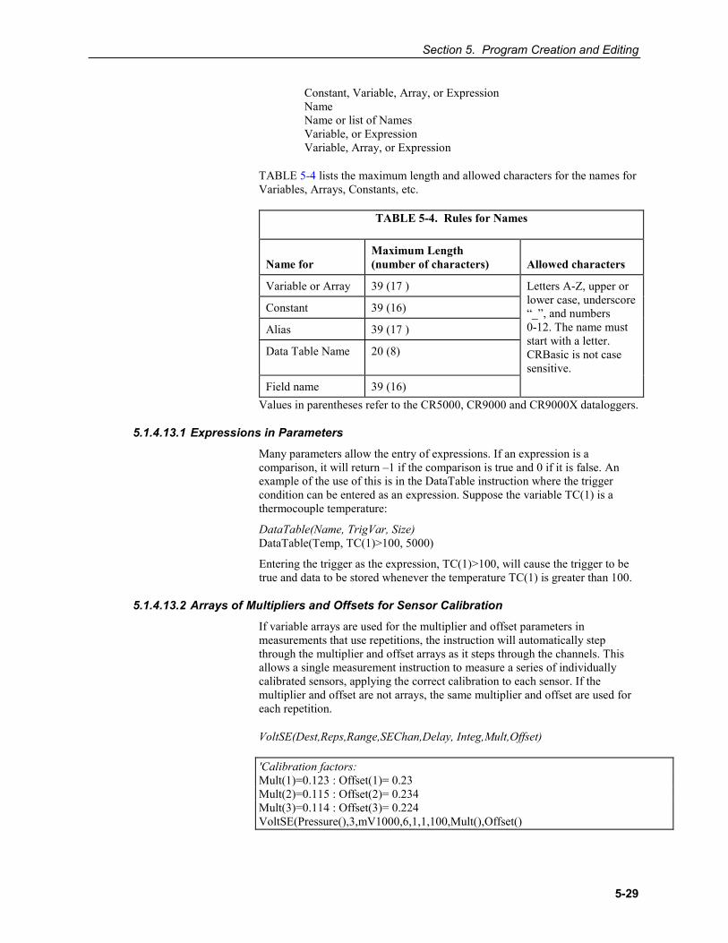
Section 5. Program Creation and Editing
5-29
Constant, Variable, Array, or Expression Name Name or list of Names Variable, or Expression Variable, Array, or Expression
TABLE 5-4 lists the maximum length and allowed characters for the names for Variables, Arrays, Constants, etc.
TABLE 5-4. Rules for Names
Name for
Maximum Length (number of characters)
Allowed characters
Variable or Array 39 (17 ) Letters A-Z, upper or lower case, underscore “_”, and numbers 0-12. The name must start with a letter. CRBasic is not case sensitive.
Constant 39 (16)
Alias 39 (17 )
Data Table Name 20 (8)
Field name 39 (16) Values in parentheses refer to the CR5000, CR9000 and CR9000X dataloggers.
5.1.4.13.1 Expressions in Parameters
Many parameters allow the entry of expressions. If an expression is a comparison, it will return –1 if the comparison is true and 0 if it is false. An example of the use of this is in the DataTable instruction where the trigger condition can be entered as an expression. Suppose the variable TC(1) is a thermocouple temperature:
DataTable(Name, TrigVar, Size) DataTable(Temp, TC(1)>100, 5000)
Entering the trigger as the expression, TC(1)>100, will cause the trigger to be true and data to be stored whenever the temperature TC(1) is greater than 100.
5.1.4.13.2 Arrays of Multipliers and Offsets for Sensor Calibration
If variable arrays are used for the multiplier and offset parameters in measurements that use repetitions, the instruction will automatically step through the multiplier and offset arrays as it steps through the channels. This allows a single measurement instruction to measure a series of individually calibrated sensors, applying the correct calibration to each sensor. If the multiplier and offset are not arrays, the same multiplier and offset are used for each repetition.
VoltSE(Dest,Reps,Range,SEChan,Delay, Integ,Mult,Offset)
'Calibration factors: Mult(1)=0.123 : Offset(1)= 0.23 Mult(2)=0.115 : Offset(2)= 0.234 Mult(3)=0.114 : Offset(3)= 0.224 VoltSE(Pressure(),3,mV1000,6,1,1,100,Mult(),Offset()
Section 5. Program Creation and Editing
5-30
Note that one exception to this is when the Multiplier or Offset points to an index into the array, then the instruction will not advance to the next Multiplier or Offset but use the same for each repetition. For instance in the above example, if Mult(2) and Offset(2) were used, the instruction would use 0.115 and 0.234 for the Multiplier and Offset, respectively, for each repetition. To force the instruction to advance through the Multiplier and Offset arrays while still specifying an index into the array, use the syntax Mult(2)() and Offset(2)().
5.1.4.14 Program Access to Data Tables Data stored in a table can be accessed from within the program. The format used is:
Tablename.Fieldname(fieldname index,records back)
Where Tablename is the name of the table in which the desired value is stored. Fieldname is the name of the field in the table. The fieldname is always an array even if it consists of only one variable; the fieldname index must always be specified. Records back is the number of records back in the data table from the current time (1 is the most recent record stored, 2 is the record stored prior to the most recent). For example, the expression:
Tdiff=Temp.TC_Avg(1,1)–Temp.TC_Avg(1,101)
could be used in the example program to calculate the change in the 10 ms average temperature of the first thermocouple between the most recent average and the one that occurred a second (100 x 10 ms) earlier.
In addition to accessing the data actually output in a table, there are some pseudo fields related to the data table that can be retrieved:
Tablename.record(1,n) = the record number of the record output n records ago.
Tablename.output(1,1) = 1 if data were output to the table the last time the table was called, = 0 if data were not output.
Tablename.timestamp(m,n) = element m of the timestamp output n records ago where:
timestamp(1,n) = microseconds since 1990 timestamp(2,n) = microseconds into the current year timestamp(3,n) = microseconds into the current month timestamp(4,n) = microseconds into the current day timestamp(5,n) = microseconds into the current hour timestamp(6,n) = microseconds into the current minute timestamp(7,n) = microseconds into the current second
Tablename.eventend(1,1) is only valid for a data table using the DataEvent instruction, Tablename.eventend(1,1) = 1 if the last record of an event occurred the last time the table was called, = 0 if the data table did not store a record or if it is in the middle of an event.
TableName.EventCount = the number of data storage events that have occurred in an event driven DataTable.
TableName.Tablefull = 1 to indicate a fill and stop table is full or a ring-mode table has begun overwriting its oldest data, = 0 if the data table is not full/begun overwriting oldest data.
Section 5. Program Creation and Editing
5-31
TableName.TableSize = the size allocation, in number of records, of the selected DataTable.
The values of Tablename.output(1,1) and Tablename.eventend (1,1) are only updated when the tables are called.
5.2 Short Cut Although RTDAQ does not support the older “mixed-array” group of Campbell Scientific dataloggers (such as the CR10X, CR23X, and CR510), the Short Cut application included with RTDAQ is the same one included for use with LoggerNet and other Campbell Scientific support software. Because of this, the documentation included here contains references to mixed-array dataloggers. For most RTDAQ implementations these references can be ignored.
5.2.1 Overview The Short Cut program generator creates programs for Campbell Scientific dataloggers in seven easy-to-follow steps. Using a wizard-like interface, you create a new or open an existing program, select the datalogger, choose which sensors you wish to measure, select the measurement interval and the frequency of data stored in datalogger memory, specify advanced output options (that is, to store data based on a flag or the value of a measurement), specify what processing to perform on raw measurements for final storage, and finally generate the program. Short Cut also generates a wiring diagram for connecting your sensors to the datalogger.
Short Cut was designed to help the beginning datalogger programmer create datalogger programs quickly and easily. Short Cut effectively insulates the user from having to know the nuances of datalogger programming and the Edlog versus CRBasic programming languages. It supports the most commonly sold sensors from Campbell Scientific, as well as generic measurements (such as differential voltage, bridge, and pulse), commonly used calculation and control functions (such as heat index calculation, alarm conditions, and simple controls), and multiplexer analogue channel expansion devices.
Short Cut cannot be used to edit existing Edlog, CRBasic, or Short Cut for DOS programs. Program editing and more complex datalogger programming functions should be accomplished using our Edlog or CRBasic Editor programming tools.
Short Cut was designed with extensive built-in help. Help can be accessed at any time by pressing the F1 key. There are also Help buttons on most screens. You can also open the Help by selecting Short Cut Help from Short Cut’s Help menu. Help for each sensor can be accessed by searching the Help Index or pressing the Help button from the sensor form.
After generating the program, you can send it to the datalogger from the Results tab of Short Cut’s Finish screen or from LoggerNet’s Connect Screen or from PC400, PC200W, or RTDAQ’s Clock/Program tab.
NOTE
NOTE
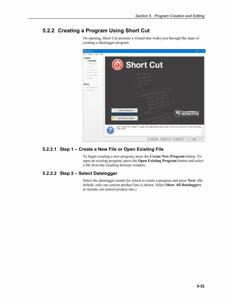
Section 5. Program Creation and Editing
5-32
5.2.2 Creating a Program Using Short Cut On opening, Short Cut presents a wizard that walks you through the steps of creating a datalogger program.
5.2.2.1 Step 1 – Create a New File or Open Existing File To begin creating a new program, press the Create New Program button. To open an existing program, press the Open Existing Program button and select a file from the resulting browser window.
5.2.2.2 Step 2 – Select Datalogger Select the datalogger model for which to create a program and press Next. (By default, only our current product line is shown. Select Show All Dataloggers to include our retired product line.)
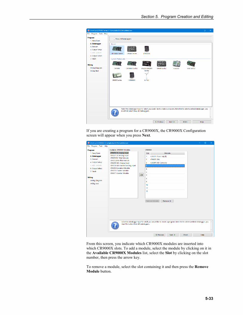
Section 5. Program Creation and Editing
5-33
If you are creating a program for a CR9000X, the CR9000X Configuration screen will appear when you press Next.
From this screen, you indicate which CR9000X modules are inserted into which CR9000X slots. To add a module, select the module by clicking on it in the Available CR9000X Modules list, select the Slot by clicking on the slot number, then press the arrow key.
To remove a module, select the slot containing it and then press the Remove Module button.
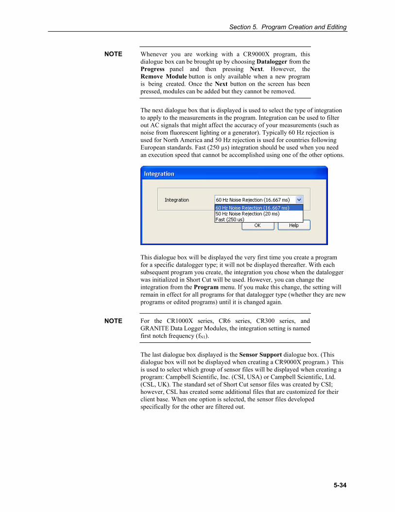
Section 5. Program Creation and Editing
5-34
Whenever you are working with a CR9000X program, this dialogue box can be brought up by choosing Datalogger from the Progress panel and then pressing Next. However, the Remove Module button is only available when a new program is being created. Once the Next button on the screen has been pressed, modules can be added but they cannot be removed.
The next dialogue box that is displayed is used to select the type of integration to apply to the measurements in the program. Integration can be used to filter out AC signals that might affect the accuracy of your measurements (such as noise from fluorescent lighting or a generator). Typically 60 Hz rejection is used for North America and 50 Hz rejection is used for countries following European standards. Fast (250 µs) integration should be used when you need an execution speed that cannot be accomplished using one of the other options.
This dialogue box will be displayed the very first time you create a program for a specific datalogger type; it will not be displayed thereafter. With each subsequent program you create, the integration you chose when the datalogger was initialized in Short Cut will be used. However, you can change the integration from the Program menu. If you make this change, the setting will remain in effect for all programs for that datalogger type (whether they are new programs or edited programs) until it is changed again.
For the CR1000X series, CR6 series, CR300 series, and GRANITE Data Logger Modules, the integration setting is named first notch frequency (fN1).
The last dialogue box displayed is the Sensor Support dialogue box. (This dialogue box will not be displayed when creating a CR9000X program.) This is used to select which group of sensor files will be displayed when creating a program: Campbell Scientific, Inc. (CSI, USA) or Campbell Scientific, Ltd. (CSL, UK). The standard set of Short Cut sensor files was created by CSI; however, CSL has created some additional files that are customized for their client base. When one option is selected, the sensor files developed specifically for the other are filtered out.
NOTE
NOTE
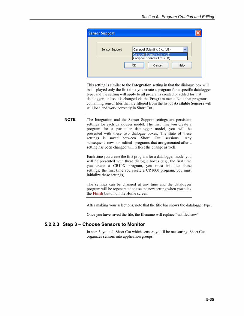
Section 5. Program Creation and Editing
5-35
This setting is similar to the Integration setting in that the dialogue box will be displayed only the first time you create a program for a specific datalogger type, and the setting will apply to all programs created or edited for that datalogger, unless it is changed via the Program menu. Note that programs containing sensor files that are filtered from the list of Available Sensors will still load and work correctly in Short Cut.
The Integration and the Sensor Support settings are persistent settings for each datalogger model. The first time you create a program for a particular datalogger model, you will be presented with these two dialogue boxes. The state of these settings is saved between Short Cut sessions. Any subsequent new or edited programs that are generated after a setting has been changed will reflect the change as well.
Each time you create the first program for a datalogger model you will be presented with these dialogue boxes (e.g., the first time you create a CR10X program, you must initialize these settings; the first time you create a CR1000 program, you must initialize these settings).
The settings can be changed at any time and the datalogger program will be regenerated to use the new setting when you click the Finish button on the Home screen.
After making your selections, note that the title bar shows the datalogger type.
Once you have saved the file, the filename will replace “untitled.scw”.
5.2.2.3 Step 3 – Choose Sensors to Monitor In step 3, you tell Short Cut which sensors you’ll be measuring. Short Cut organizes sensors into application groups:
NOTE
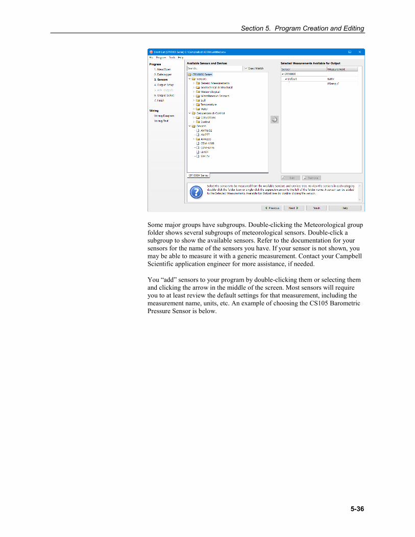
Section 5. Program Creation and Editing
5-36
Some major groups have subgroups. Double-clicking the Meteorological group folder shows several subgroups of meteorological sensors. Double-click a subgroup to show the available sensors. Refer to the documentation for your sensors for the name of the sensors you have. If your sensor is not shown, you may be able to measure it with a generic measurement. Contact your Campbell Scientific application engineer for more assistance, if needed.
You “add” sensors to your program by double-clicking them or selecting them and clicking the arrow in the middle of the screen. Most sensors will require you to at least review the default settings for that measurement, including the measurement name, units, etc. An example of choosing the CS105 Barometric Pressure Sensor is below.
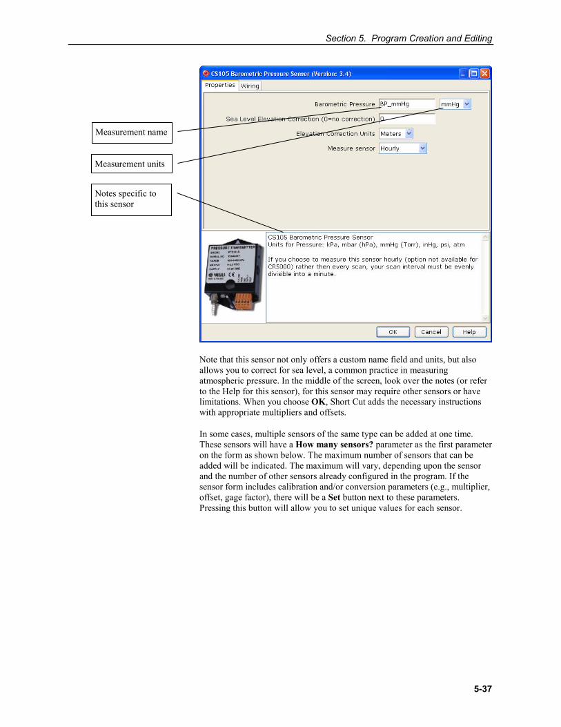
Section 5. Program Creation and Editing
5-37
Note that this sensor not only offers a custom name field and units, but also allows you to correct for sea level, a common practice in measuring atmospheric pressure. In the middle of the screen, look over the notes (or refer to the Help for this sensor), for this sensor may require other sensors or have limitations. When you choose OK, Short Cut adds the necessary instructions with appropriate multipliers and offsets.
In some cases, multiple sensors of the same type can be added at one time. These sensors will have a How many sensors? parameter as the first parameter on the form as shown below. The maximum number of sensors that can be added will be indicated. The maximum will vary, depending upon the sensor and the number of other sensors already configured in the program. If the sensor form includes calibration and/or conversion parameters (e.g., multiplier, offset, gage factor), there will be a Set button next to these parameters. Pressing this button will allow you to set unique values for each sensor.
Measurement name
Measurement units
Notes specific to this sensor
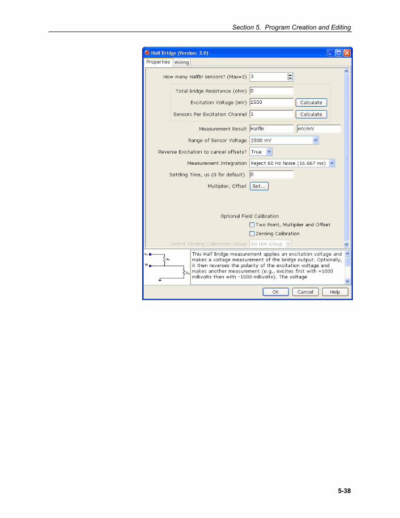
Section 5. Program Creation and Editing
5-38
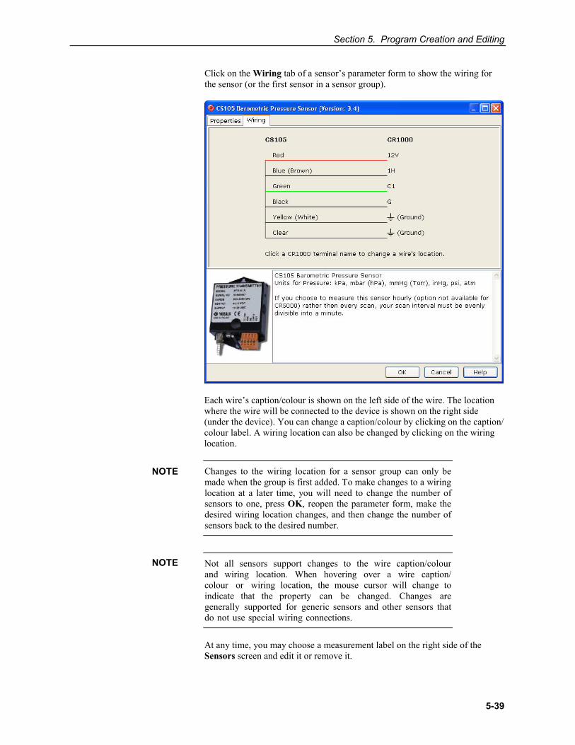
Section 5. Program Creation and Editing
5-39
Click on the Wiring tab of a sensor’s parameter form to show the wiring for the sensor (or the first sensor in a sensor group).
Each wire’s caption/colour is shown on the left side of the wire. The location where the wire will be connected to the device is shown on the right side (under the device). You can change a caption/colour by clicking on the caption/colour label. A wiring location can also be changed by clicking on the wiring location.
Changes to the wiring location for a sensor group can only be made when the group is first added. To make changes to a wiring location at a later time, you will need to change the number of sensors to one, press OK, reopen the parameter form, make the desired wiring location changes, and then change the number of sensors back to the desired number.
Not all sensors support changes to the wire caption/colour and wiring location. When hovering over a wire caption/colour or wiring location, the mouse cursor will change to indicate that the property can be changed. Changes are generally supported for generic sensors and other sensors that do not use special wiring connections.
At any time, you may choose a measurement label on the right side of the Sensors screen and edit it or remove it.
NOTE
NOTE
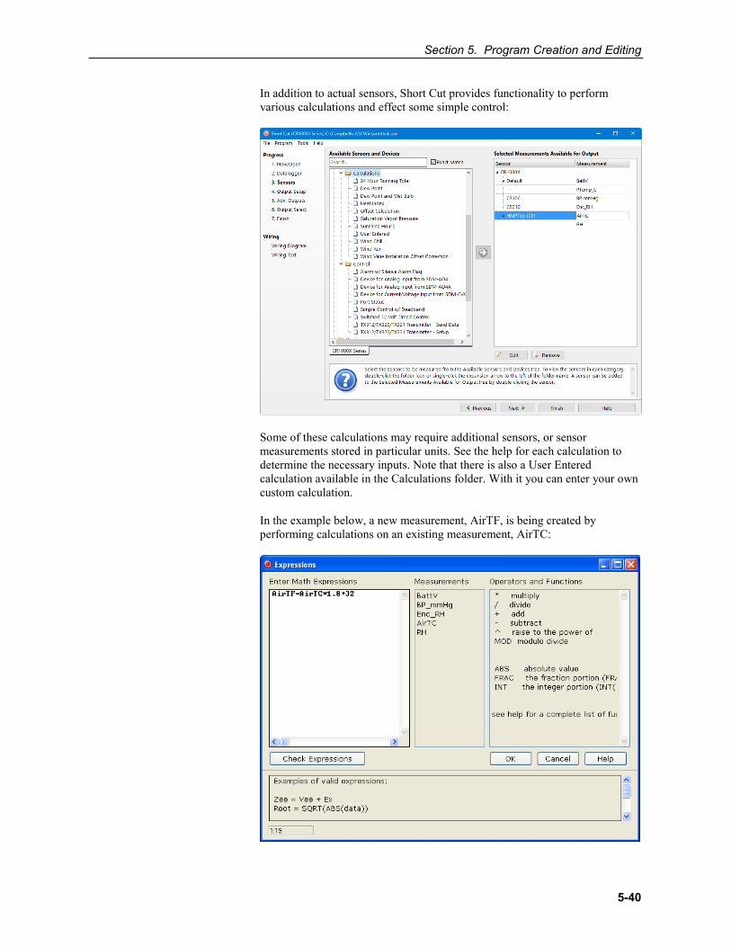
Section 5. Program Creation and Editing
5-40
In addition to actual sensors, Short Cut provides functionality to perform various calculations and effect some simple control:
Some of these calculations may require additional sensors, or sensor measurements stored in particular units. See the help for each calculation to determine the necessary inputs. Note that there is also a User Entered calculation available in the Calculations folder. With it you can enter your own custom calculation.
In the example below, a new measurement, AirTF, is being created by performing calculations on an existing measurement, AirTC:
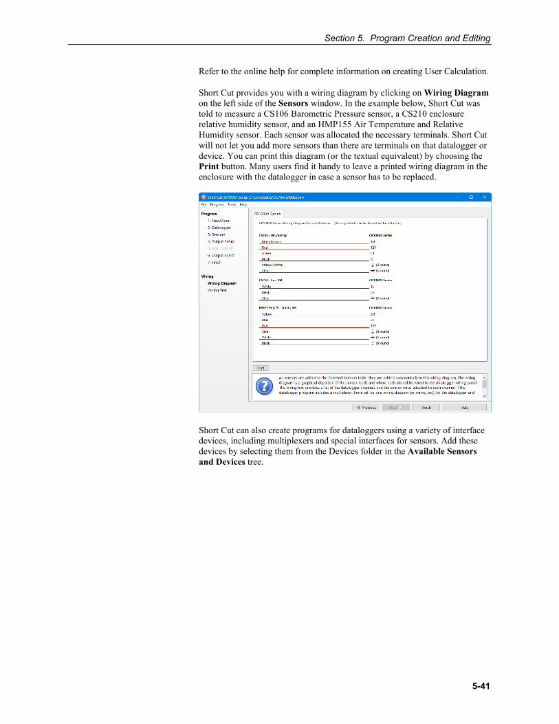
Section 5. Program Creation and Editing
5-41
Refer to the online help for complete information on creating User Calculation.
Short Cut provides you with a wiring diagram by clicking on Wiring Diagram on the left side of the Sensors window. In the example below, Short Cut was told to measure a CS106 Barometric Pressure sensor, a CS210 enclosure relative humidity sensor, and an HMP155 Air Temperature and Relative Humidity sensor. Each sensor was allocated the necessary terminals. Short Cut will not let you add more sensors than there are terminals on that datalogger or device. You can print this diagram (or the textual equivalent) by choosing the Print button. Many users find it handy to leave a printed wiring diagram in the enclosure with the datalogger in case a sensor has to be replaced.
Short Cut can also create programs for dataloggers using a variety of interface devices, including multiplexers and special interfaces for sensors. Add these devices by selecting them from the Devices folder in the Available Sensors and Devices tree.
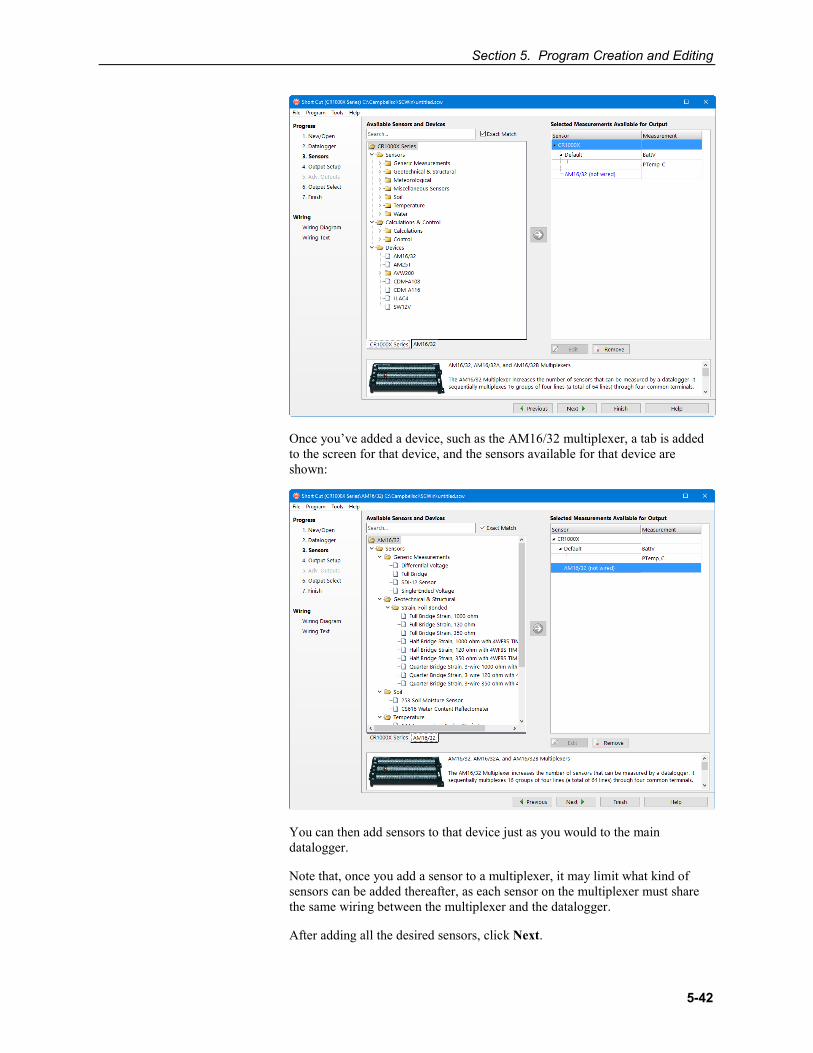
Section 5. Program Creation and Editing
5-42
Once you’ve added a device, such as the AM16/32 multiplexer, a tab is added to the screen for that device, and the sensors available for that device are shown:
You can then add sensors to that device just as you would to the main datalogger.
Note that, once you add a sensor to a multiplexer, it may limit what kind of sensors can be added thereafter, as each sensor on the multiplexer must share the same wiring between the multiplexer and the datalogger.
After adding all the desired sensors, click Next.

Section 5. Program Creation and Editing
5-43
5.2.2.4 Step 4 – Set up Output Tables The fourth step in creating a program is to set up the output tables for the sensor measurements you have selected. The output tables must be completed or no data will be stored in the datalogger's memory.
In the How often should the datalogger measure its sensor(s)? field, specify how often the datalogger will execute the instructions in its program. This is known as the measurement or scan interval.
When choosing a scan interval, remember that faster scan intervals will use more power. For most applications, a 10 to 60 second scan interval is sufficient. If faster scan intervals are required for your application, make sure there is sufficient time for the execution of all instructions in the program (refer to the section in the datalogger manual on Execution Intervals for additional information).
By default, data is sent to memory based on time. Data can also be sent to memory based on one or more of the following conditions: time, the state of a flag, or the value of a measurement. This is set up from the Advanced Outputs screen. To use the Advanced Outputs screen, select the Advanced Outputs (all tables) check box at the lower left of the Output Setup screen. The Data Output Storage Interval field will be removed from the Output Setup screen (and moved to the Advanced Outputs screen). After completing the fields on the Output Setup screen and pressing Next, Short Cut will advance to the Advanced Outputs screen.
Two tables are defined by default. Additional tables can be added by pressing the Add Table button. Short Cut limits the number of output tables to 10. An output table can be removed by clicking on the table to make it the active table and pressing the Delete Table button.
NOTE
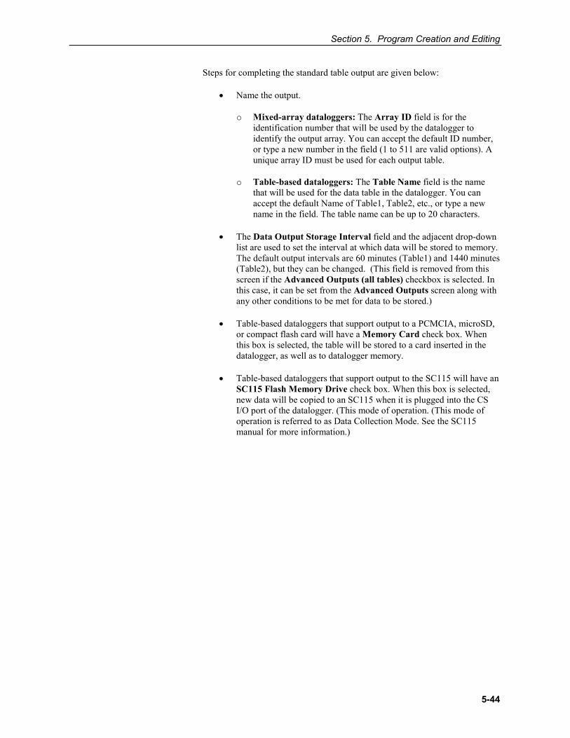
Section 5. Program Creation and Editing
5-44
Steps for completing the standard table output are given below:
• Name the output.
o Mixed-array dataloggers: The Array ID field is for the identification number that will be used by the datalogger to identify the output array. You can accept the default ID number, or type a new number in the field (1 to 511 are valid options). A unique array ID must be used for each output table.
o Table-based dataloggers: The Table Name field is the name that will be used for the data table in the datalogger. You can accept the default Name of Table1, Table2, etc., or type a new name in the field. The table name can be up to 20 characters.
• The Data Output Storage Interval field and the adjacent drop-down list are used to set the interval at which data will be stored to memory. The default output intervals are 60 minutes (Table1) and 1440 minutes (Table2), but they can be changed. (This field is removed from this screen if the Advanced Outputs (all tables) checkbox is selected. In this case, it can be set from the Advanced Outputs screen along with any other conditions to be met for data to be stored.)
• Table-based dataloggers that support output to a PCMCIA, microSD, or compact flash card will have a Memory Card check box. When this box is selected, the table will be stored to a card inserted in the datalogger, as well as to datalogger memory.
• Table-based dataloggers that support output to the SC115 will have an SC115 Flash Memory Drive check box. When this box is selected, new data will be copied to an SC115 when it is plugged into the CS I/O port of the datalogger. (This mode of operation. (This mode of operation is referred to as Data Collection Mode. See the SC115 manual for more information.)
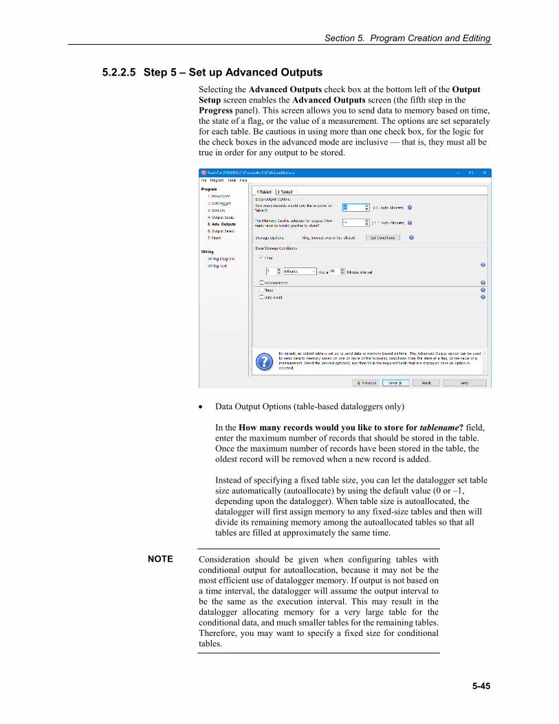
Section 5. Program Creation and Editing
5-45
5.2.2.5 Step 5 – Set up Advanced Outputs Selecting the Advanced Outputs check box at the bottom left of the Output Setup screen enables the Advanced Outputs screen (the fifth step in the Progress panel). This screen allows you to send data to memory based on time, the state of a flag, or the value of a measurement. The options are set separately for each table. Be cautious in using more than one check box, for the logic for the check boxes in the advanced mode are inclusive — that is, they must all be true in order for any output to be stored.
• Data Output Options (table-based dataloggers only) In the How many records would you like to store for tablename? field, enter the maximum number of records that should be stored in the table. Once the maximum number of records have been stored in the table, the oldest record will be removed when a new record is added. Instead of specifying a fixed table size, you can let the datalogger set table size automatically (autoallocate) by using the default value (0 or –1, depending upon the datalogger). When table size is autoallocated, the datalogger will first assign memory to any fixed-size tables and then will divide its remaining memory among the autoallocated tables so that all tables are filled at approximately the same time.
Consideration should be given when configuring tables with conditional output for autoallocation, because it may not be the most efficient use of datalogger memory. If output is not based on a time interval, the datalogger will assume the output interval to be the same as the execution interval. This may result in the datalogger allocating memory for a very large table for the conditional data, and much smaller tables for the remaining tables. Therefore, you may want to specify a fixed size for conditional tables.
NOTE
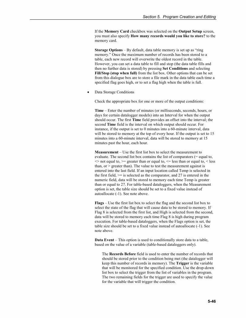
Section 5. Program Creation and Editing
5-46
If the Memory Card checkbox was selected on the Output Setup screen, you must also specify How many records would you like to store? to the memory card.
Storage Options – By default, data table memory is set up as “ring memory.” Once the maximum number of records has been stored to a table, each new record will overwrite the oldest record in the table. However, you can set a data table to fill and stop (the data table fills and then no further data is stored) by pressing Set Conditions and selecting Fill/Stop (stop when full) from the list box. Other options that can be set from this dialogue box are to store a file mark in the data table each time a specified flag goes high, or to set a flag high when the table is full.
• Data Storage Conditions
Check the appropriate box for one or more of the output conditions:
Time – Enter the number of minutes (or milliseconds, seconds, hours, ordays for certain datalogger models) into an Interval for when the outputshould occur. The first Time field provides an offset into the interval; thesecond Time field is the interval on which output should occur. Forinstance, if the output is set to 0 minutes into a 60-minute interval, datawill be stored to memory at the top of every hour. If the output is set to 15minutes into a 60-minute interval, data will be stored to memory at 15minutes past the hour, each hour.
Measurement – Use the first list box to select the measurement toevaluate. The second list box contains the list of comparators (= equal to,<> not equal to, >= greater than or equal to, <= less than or equal to, < lessthan, or > greater than). The value to test the measurement against isentered into the last field. If an input location called Temp is selected inthe first field, >= is selected as the comparator, and 27 is entered in thenumeric field, data will be stored to memory each time Temp is greaterthan or equal to 27. For table-based dataloggers, when the Measurementoption is set, the table size should be set to a fixed value instead ofautoallocate (-1). See note above.
Flags – Use the first list box to select the flag and the second list box toselect the state of the flag that will cause data to be stored to memory. IfFlag 8 is selected from the first list, and High is selected from the second,data will be stored to memory each time Flag 8 is high during programexecution. For table-based dataloggers, when the Flags option is set, thetable size should be set to a fixed value instead of autoallocate (-1). Seenote above.
Data Event – This option is used to conditionally store data to a table,based on the value of a variable (table-based dataloggers only).
The Records Before field is used to enter the number of records that should be stored prior to the condition being met (the datalogger will keep this number of records in memory). The Trigger is the variable that will be monitored for the specified condition. Use the drop-down list box to select the trigger from the list of variables in the program. The two remaining fields for the trigger are used to specify the value for the variable that will trigger the condition.
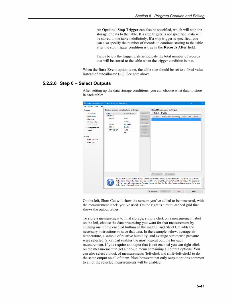
Section 5. Program Creation and Editing
5-47
An Optional Stop Trigger can also be specified, which will stop the storage of data to the table. If a stop trigger is not specified, data will be stored to the table indefinitely. If a stop trigger is specified, you can also specify the number of records to continue storing to the table after the stop trigger condition is true in the Records After field.
Fields below the trigger criteria indicate the total number of records that will be stored to the table when the trigger condition is met.
When the Data Event option is set, the table size should be set to a fixed value instead of autoallocate (–1). See note above.
5.2.2.6 Step 6 – Select Outputs After setting up the data storage conditions, you can choose what data to store in each table:
On the left, Short Cut will show the sensors you’ve added to be measured, with the measurement labels you’ve used. On the right is a multi-tabbed grid that shows the output tables.
To store a measurement to final storage, simply click on a measurement label on the left, choose the data processing you want for that measurement by clicking one of the enabled buttons in the middle, and Short Cut adds the necessary instructions to save that data. In the example below, average air temperature, a sample of relative humidity, and average barometric pressure were selected. Short Cut enables the most logical outputs for each measurement. If you require an output that is not enabled you can right-click on the measurement to get a pop-up menu containing all output options. You can also select a block of measurements (left-click and shift+left-click) to do the same output on all of them. Note however that only output options common to all of the selected measurements will be enabled.
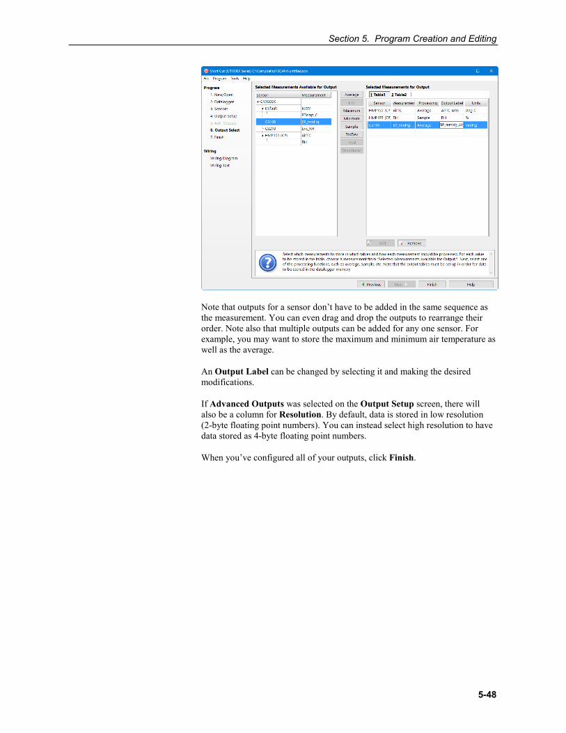
Section 5. Program Creation and Editing
5-48
Note that outputs for a sensor don’t have to be added in the same sequence as the measurement. You can even drag and drop the outputs to rearrange their order. Note also that multiple outputs can be added for any one sensor. For example, you may want to store the maximum and minimum air temperature as well as the average.
An Output Label can be changed by selecting it and making the desired modifications.
If Advanced Outputs was selected on the Output Setup screen, there will also be a column for Resolution. By default, data is stored in low resolution (2-byte floating point numbers). You can instead select high resolution to have data stored as 4-byte floating point numbers.
When you’ve configured all of your outputs, click Finish.
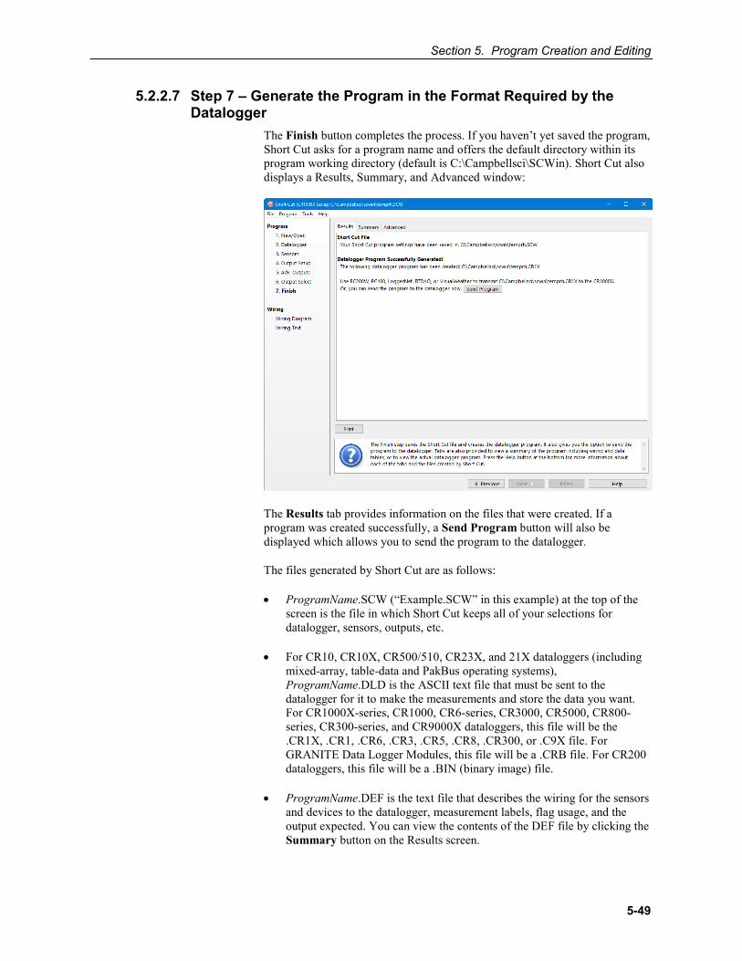
Section 5. Program Creation and Editing
5-49
5.2.2.7 Step 7 – Generate the Program in the Format Required by the Datalogger
The Finish button completes the process. If you haven’t yet saved the program, Short Cut asks for a program name and offers the default directory within its program working directory (default is C:\Campbellsci\SCWin). Short Cut also displays a Results, Summary, and Advanced window:
The Results tab provides information on the files that were created. If a program was created successfully, a Send Program button will also be displayed which allows you to send the program to the datalogger.
The files generated by Short Cut are as follows:
• ProgramName.SCW (“Example.SCW” in this example) at the top of the screen is the file in which Short Cut keeps all of your selections for datalogger, sensors, outputs, etc.
• For CR10, CR10X, CR500/510, CR23X, and 21X dataloggers (including mixed-array, table-data and PakBus operating systems), ProgramName.DLD is the ASCII text file that must be sent to the datalogger for it to make the measurements and store the data you want. For CR1000X-series, CR1000, CR6-series, CR3000, CR5000, CR800-series, CR300-series, and CR9000X dataloggers, this file will be the .CR1X, .CR1, .CR6, .CR3, .CR5, .CR8, .CR300, or .C9X file. For GRANITE Data Logger Modules, this file will be a .CRB file. For CR200 dataloggers, this file will be a .BIN (binary image) file.
• ProgramName.DEF is the text file that describes the wiring for the sensors and devices to the datalogger, measurement labels, flag usage, and the output expected. You can view the contents of the DEF file by clicking the Summary button on the Results screen.
Section 5. Program Creation and Editing
5-50
• For mixed-array dataloggers, ProgramName.FSL is a text file containing output labels (created for mixed-array dataloggers only). This file can be used by Split or View or other software to provide column headers for the data file.
The Summary tab displays the information in the DEF file as described above.
The Advanced tab (for CRBasic dataloggers) displays the CRBasic program that was generated. It includes a CRBasic Editor button which opens the program for editing in the CRBasic Editor. Note that any changes made to the generated program in the CRBasic Editor will not be reflected in Short Cut or future programs generated by Short Cut.
Note that, while Short Cut can generate a program file for the datalogger, you must use datalogger communication software to transmit that program to the datalogger. (This is true even when pressing the Send Program button from Short Cut’s Finish screen. Short Cut relies on the datalogger communication software to transmit the program.)
5.2.3 Short Cut Settings The Program and Tools menus on the Short Cut menu offer several settings that may prove useful.
5.2.3.1 Program Security Some dataloggers allow you to set security by entering one or more numbers into their security fields. You can allow different levels of access (e.g.; only allow data retrieval, or also allow monitoring of values, or also allow sending a new program or setting the clock) by entering multiple levels.
Datalogger security is not meant to be extremely tight. Rather, it is designed to prevent honest people from making mistakes.
Notwithstanding its intention, one mistake you can make is to set security and then forget the values. If you send a program with security set, you will then need to add that security setting to LoggerNet's Setup Screen or RTDAQ or PC400’s EZSetup Wizard for that datalogger. If you don’t, you may find that you can no longer communicate with the datalogger. Should this happen and you forget the security code and have lost the Short Cut program file, you may have to visit the datalogger site and cycle power on the datalogger to be able to communicate with it. Most dataloggers that offer security will communicate over their CS I/O port directly with a keyboard/display or PC in the first few seconds of powering up. See the datalogger manual for a full description of the security features.
5.2.3.2 Datalogger ID Mixed-array dataloggers keep a memory location available for a datalogger ID value. This is typically an integer that you can read from within the program and store into final storage to keep track of the identity of the datalogger that created the data. Valid Datalogger IDs are 1 through 12 and 14 through 254. Use the Datalogger ID instruction in Short Cut (found under Miscellaneous Sensors) to use the ID in the datalogger program.
Section 5. Program Creation and Editing
5-51
5.2.3.3 Power-up Settings Some dataloggers offer the option to retain interim measurements or calculations or the states of flags or ports when they power-up from a low battery or loss of power condition. This may be useful when calculations are used to control devices. You may, for example, want to ensure that pumps or controls are off when a datalogger powers up so as to make the control decision based on a fresh measurement. See the datalogger manual for a full description of this feature.
5.2.3.4 Select CR200 Compiler Use this setting to select the directory and executable name that will be used to pre-compile the CR200/205 program to check for errors.
Most Campbell Scientific dataloggers are sent an ASCII program file, which they then compile into machine code. The CR200/205 does not have enough memory and processing capability to do this compilation, so it’s necessary to compile the program file into the binary version used by the datalogger itself. This compilation is done by Short Cut to check for errors in the program before sending it. It’s done again by LoggerNet, RTDAQ, PC400, or PC200W when sending the program to the datalogger. Compilation is performed using a special executable that mimics the functions and capability in the datalogger’s operating system. Therefore, the compiler executable must match the datalogger’s operating system or the datalogger may fail to run the compiled binary (*.BIN) program. LoggerNet, RTDAQ, PC400, PC200W, and Short Cut are installed with precompilers for all of the released versions of the CR200/205 operating systems. If, at some time in the future, you acquire a newer CR200/205, or choose to install a later operating system, you must make sure you also have the compiler executable that matches. These compiler executables are typically installed in a library directory. By default, this directory would be installed as:
C:\Campbellsci\Lib\CR200Compilers
If you receive an operating system update, you should copy the compiler associated with it to this directory. If, for some reason, you put the compiler in a different directory, this menu item provides a way to choose that compiler executable.
5.2.3.5 Sensor Support The Sensor Support option is used to select which group of sensor files will be displayed when creating a program: Campbell Scientific, Inc., (CSI) or Campbell Scientific, Ltd. (CSL). The standard set of Short Cut sensor files was created by CSI; however, CSL has created some additional files that are customized for their client base. When one option is selected, the sensor files developed specifically for the other are filtered out.
This dialogue box is displayed the very first time you create a program for a specific datalogger type; it will not be displayed thereafter. With each subsequent program you create, the group of sensor files that you chose when the datalogger was initialized in Short Cut will be used. However, you can change this setting at any time. If you make a change, the setting will remain in effect for all programs for that datalogger type (whether they are new programs or edited programs) until it is changed again.
Section 5. Program Creation and Editing
5-52
5.2.3.6 Integration/First Notch Frequency (fN1) Some dataloggers have parameters available in their measurement instructions to provide integration for rejection of noise due to AC electrical signals. These parameters will be used by Short Cut if possible, but the frequency of this noise varies. In most of North America, the AC frequency is 60 Hz. However, in many countries the frequency is 50 Hz. If you know the frequency of this AC noise, you can select one or the other frequency. Fast (250 µs) integration should be used when you need an execution speed that cannot be accomplished using one of the other options. This setting remains in effect for other programs generated by Short Cut until you change it.
For the CR1000X series, CR6 series, CR300 series, and GRANITE Data Logger Modules, the integration setting is named first notch frequency (fN1).
5.2.3.7 Font This setting is accessed from the Options menu item of the Tools menu. Use this setting to change the appearance of the font used by Short Cut. Most windows other than the wiring descriptions (which require a non-proportional font to make sure wiring diagrams are aligned) will use this font.
5.2.3.8 Set Working Directory This setting is accessed from the Options menu item of the Tools menu. This setting changes the directory that Short Cut offers as a default for your programs. Upon installation, the default is set to C:\CampbellSci\SCWIN.
5.2.3.9 Enable Creation of Custom Sensor Files This setting is accessed from the Options menu item of the Tools menu. It allows the user to create custom sensor files as described in Section 5.2.6, Custom Sensor Files (p. 5-53).
5.2.4 Editing Programs Created by Short Cut Short Cut is very flexible and has many features. It does not, however, support all of the functionality in Campbell Scientific dataloggers. Some users will need to develop programs with capabilities beyond that offered by Short Cut, but will want to take advantage of the library of instructions and settings known to a program generator in order to get a head start.
For Edlog dataloggers, the easiest method is to Document the DLD file from within Edlog (discussed later in this section). Short Cut creates a .DLD file to send to the datalogger that includes input location and final storage labels. Documenting a .DLD file causes Edlog to use the same labels and to show you the individual instructions being used to carry out the program. You can then add and delete instructions from within Edlog to add functionality to the program. Short Cut cannot import the files created by Edlog, however. Short Cut reads only its own SCW-formatted files.
For CRBasic dataloggers, you can use the CRBasic Editor to open the .CR# files directly. Again, Short Cut will not be able to open the files you’ve edited with the CRBasic Editor, since they are not an SCW file.
NOTE
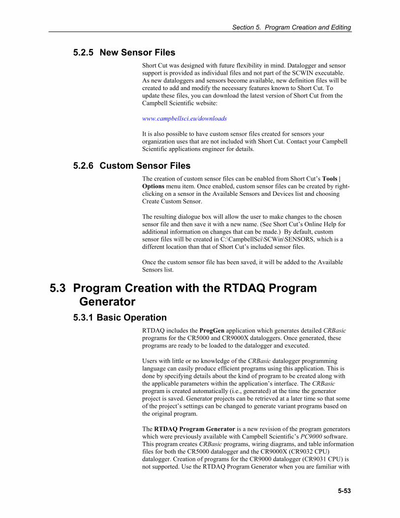
Section 5. Program Creation and Editing
5-53
5.2.5 New Sensor Files Short Cut was designed with future flexibility in mind. Datalogger and sensor support is provided as individual files and not part of the SCWIN executable. As new dataloggers and sensors become available, new definition files will be created to add and modify the necessary features known to Short Cut. To update these files, you can download the latest version of Short Cut from the Campbell Scientific website:
www.campbellsci.eu/downloads
It is also possible to have custom sensor files created for sensors your organization uses that are not included with Short Cut. Contact your Campbell Scientific applications engineer for details.
5.2.6 Custom Sensor Files The creation of custom sensor files can be enabled from Short Cut’s Tools | Options menu item. Once enabled, custom sensor files can be created by right-clicking on a sensor in the Available Sensors and Devices list and choosing Create Custom Sensor.
The resulting dialogue box will allow the user to make changes to the chosen sensor file and then save it with a new name. (See Short Cut’s Online Help for additional information on changes that can be made.) By default, custom sensor files will be created in C:\CampbellSci\SCWin\SENSORS, which is a different location than that of Short Cut’s included sensor files.
Once the custom sensor file has been saved, it will be added to the Available Sensors list.
5.3 Program Creation with the RTDAQ Program Generator
5.3.1 Basic Operation RTDAQ includes the ProgGen application which generates detailed CRBasic programs for the CR5000 and CR9000X dataloggers. Once generated, these programs are ready to be loaded to the datalogger and executed.
Users with little or no knowledge of the CRBasic datalogger programming language can easily produce efficient programs using this application. This is done by specifying details about the kind of program to be created along with the applicable parameters within the application’s interface. The CRBasic program is created automatically (i.e., generated) at the time the generator project is saved. Generator projects can be retrieved at a later time so that some of the project’s settings can be changed to generate variant programs based on the original program.
The RTDAQ Program Generator is a new revision of the program generators which were previously available with Campbell Scientific’s PC9000 software. This program creates CRBasic programs, wiring diagrams, and table information files for both the CR5000 datalogger and the CR9000X (CR9032 CPU) datalogger. Creation of programs for the CR9000 datalogger (CR9031 CPU) is not supported. Use the RTDAQ Program Generator when you are familiar with
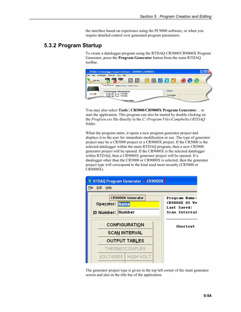
Section 5. Program Creation and Editing
5-54
the interface based on experience using the PC9000 software, or when you require detailed control over generated program parameters.
5.3.2 Program Startup To create a datalogger program using the RTDAQ CR5000/CR9000X Program Generator, press the Program Generator button from the main RTDAQ toolbar.
You may also select Tools | CR5000/CR9000X Program Generator… to start the application. This program can also be started by double-clicking on the ProgGen.exe file directly in the C:\Program Files\Campbellsci\RTDAQ folder.
When the program starts, it opens a new program generator project and displays it to the user for immediate modification or use. The type of generator project may be a CR5000 project or a CR9000X project. If the CR5000 is the selected datalogger within the main RTDAQ program, then a new CR5000 generator project will be opened. If the CR9000X is the selected datalogger within RTDAQ, then a CR9000X generator project will be opened. If a datalogger other than the CR5000 or CR9000X is selected, then the generator project type will correspond to the kind used most recently (CR5000 or CR9000X).
The generator project type is given in the top left corner of the main generator screen and also in the title bar of the application.
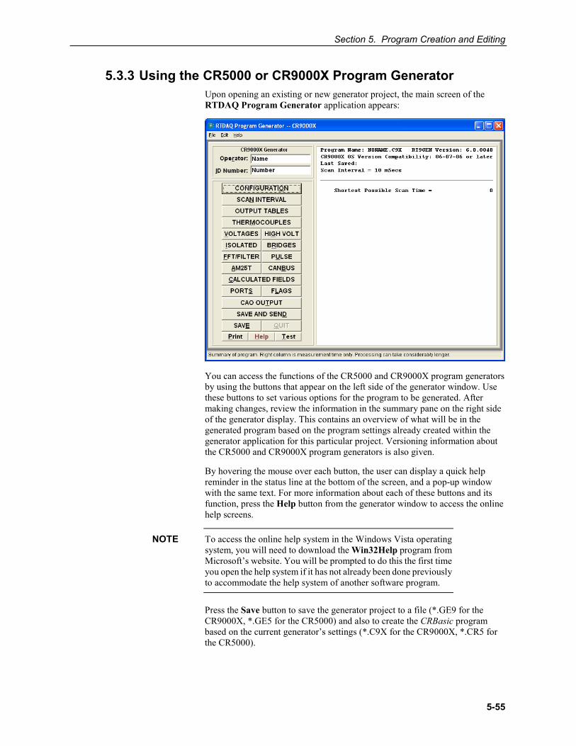
Section 5. Program Creation and Editing
5-55
5.3.3 Using the CR5000 or CR9000X Program Generator Upon opening an existing or new generator project, the main screen of the RTDAQ Program Generator application appears:
You can access the functions of the CR5000 and CR9000X program generators by using the buttons that appear on the left side of the generator window. Use these buttons to set various options for the program to be generated. After making changes, review the information in the summary pane on the right side of the generator display. This contains an overview of what will be in the generated program based on the program settings already created within the generator application for this particular project. Versioning information about the CR5000 and CR9000X program generators is also given.
By hovering the mouse over each button, the user can display a quick help reminder in the status line at the bottom of the screen, and a pop-up window with the same text. For more information about each of these buttons and its function, press the Help button from the generator window to access the online help screens.
To access the online help system in the Windows Vista operating system, you will need to download the Win32Help program from Microsoft’s website. You will be prompted to do this the first time you open the help system if it has not already been done previously to accommodate the help system of another software program.
Press the Save button to save the generator project to a file (*.GE9 for the CR9000X, *.GE5 for the CR5000) and also to create the CRBasic program based on the current generator’s settings (*.C9X for the CR9000X, *.CR5 for the CR5000).
NOTE
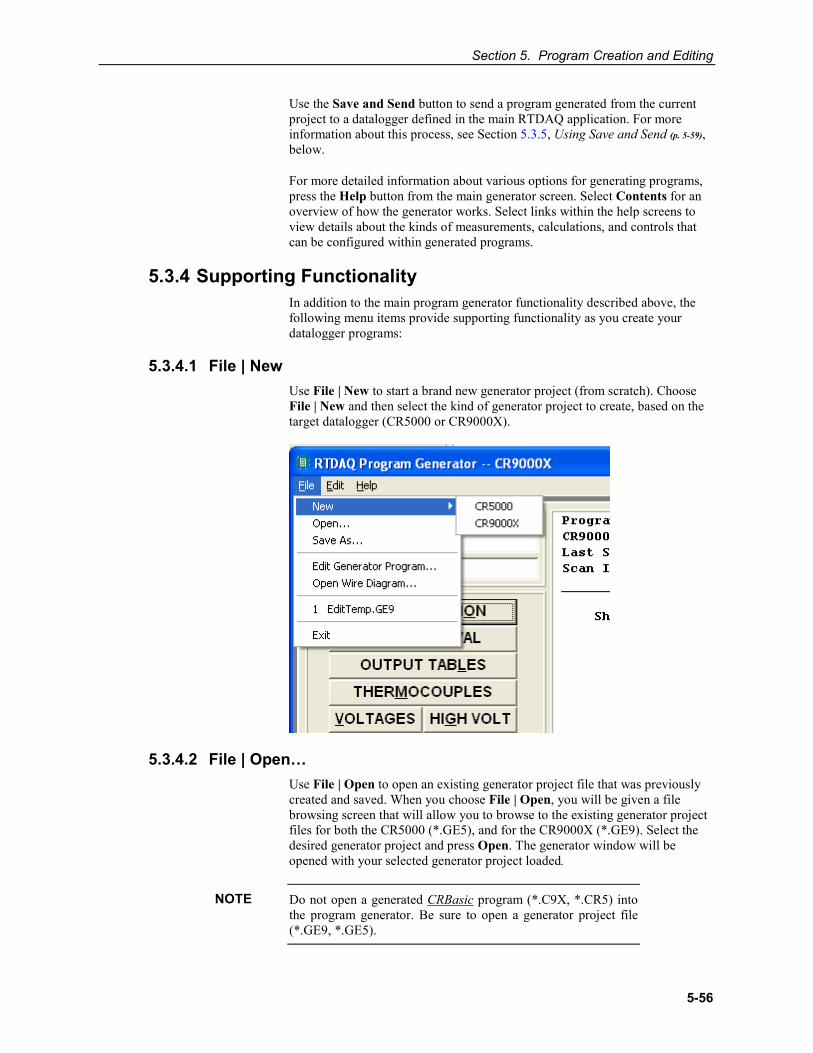
Section 5. Program Creation and Editing
5-56
Use the Save and Send button to send a program generated from the current project to a datalogger defined in the main RTDAQ application. For more information about this process, see Section 5.3.5, Using Save and Send (p. 5-59), below.
For more detailed information about various options for generating programs, press the Help button from the main generator screen. Select Contents for an overview of how the generator works. Select links within the help screens to view details about the kinds of measurements, calculations, and controls that can be configured within generated programs.
5.3.4 Supporting Functionality In addition to the main program generator functionality described above, the following menu items provide supporting functionality as you create your datalogger programs:
5.3.4.1 File | New Use File | New to start a brand new generator project (from scratch). Choose File | New and then select the kind of generator project to create, based on the target datalogger (CR5000 or CR9000X).
5.3.4.2 File | Open… Use File | Open to open an existing generator project file that was previously created and saved. When you choose File | Open, you will be given a file browsing screen that will allow you to browse to the existing generator project files for both the CR5000 (*.GE5), and for the CR9000X (*.GE9). Select the desired generator project and press Open. The generator window will be opened with your selected generator project loaded.
Do not open a generated CRBasic program (*.C9X, *.CR5) into the program generator. Be sure to open a generator project file (*.GE9, *.GE5).
NOTE
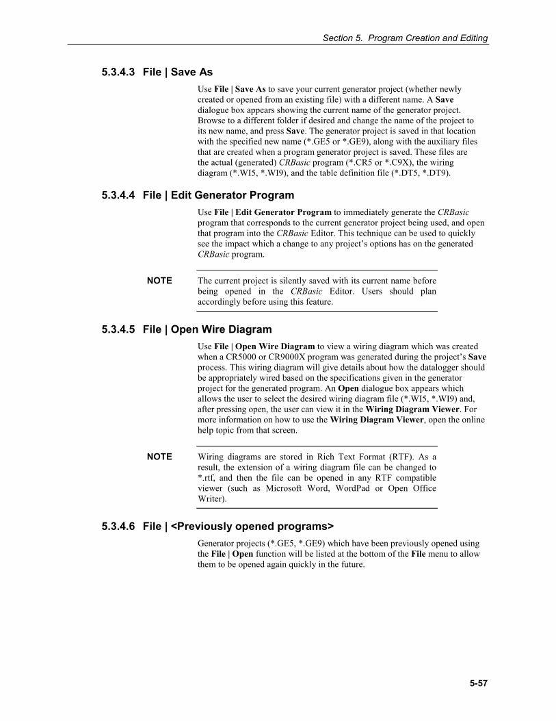
Section 5. Program Creation and Editing
5-57
5.3.4.3 File | Save As Use File | Save As to save your current generator project (whether newly created or opened from an existing file) with a different name. A Save dialogue box appears showing the current name of the generator project. Browse to a different folder if desired and change the name of the project to its new name, and press Save. The generator project is saved in that location with the specified new name (*.GE5 or *.GE9), along with the auxiliary files that are created when a program generator project is saved. These files are the actual (generated) CRBasic program (*.CR5 or *.C9X), the wiring diagram (*.WI5, *.WI9), and the table definition file (*.DT5, *.DT9).
5.3.4.4 File | Edit Generator Program Use File | Edit Generator Program to immediately generate the CRBasic program that corresponds to the current generator project being used, and open that program into the CRBasic Editor. This technique can be used to quickly see the impact which a change to any project’s options has on the generated CRBasic program.
The current project is silently saved with its current name before being opened in the CRBasic Editor. Users should plan accordingly before using this feature.
5.3.4.5 File | Open Wire Diagram Use File | Open Wire Diagram to view a wiring diagram which was created when a CR5000 or CR9000X program was generated during the project’s Save process. This wiring diagram will give details about how the datalogger should be appropriately wired based on the specifications given in the generator project for the generated program. An Open dialogue box appears which allows the user to select the desired wiring diagram file (*.WI5, *.WI9) and, after pressing open, the user can view it in the Wiring Diagram Viewer. For more information on how to use the Wiring Diagram Viewer, open the online help topic from that screen.
Wiring diagrams are stored in Rich Text Format (RTF). As a result, the extension of a wiring diagram file can be changed to *.rtf, and then the file can be opened in any RTF compatible viewer (such as Microsoft Word, WordPad or Open Office Writer).
5.3.4.6 File | <Previously opened programs> Generator projects (*.GE5, *.GE9) which have been previously opened using the File | Open function will be listed at the bottom of the File menu to allow them to be opened again quickly in the future.
NOTE
NOTE
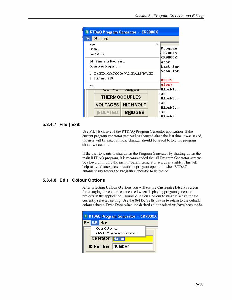
Section 5. Program Creation and Editing
5-58
5.3.4.7 File | Exit Use File | Exit to end the RTDAQ Program Generator application. If the current program generator project has changed since the last time it was saved, the user will be asked if those changes should be saved before the program shutdown occurs.
If the user to wants to shut down the Program Generator by shutting down the main RTDAQ program, it is recommended that all Program Generator screens be closed until only the main Program Generator screen is visible. This will help to avoid unexpected results in program operation when RTDAQ automatically forces the Program Generator to be closed.
5.3.4.8 Edit | Colour Options After selecting Colour Options you will see the Customize Display screen for changing the colour scheme used when displaying program generator projects in the application. Double-click on a colour to make it active for the currently selected setting. Use the Set Defaults button to return to the default colour scheme. Press Done when the desired colour selections have been made.
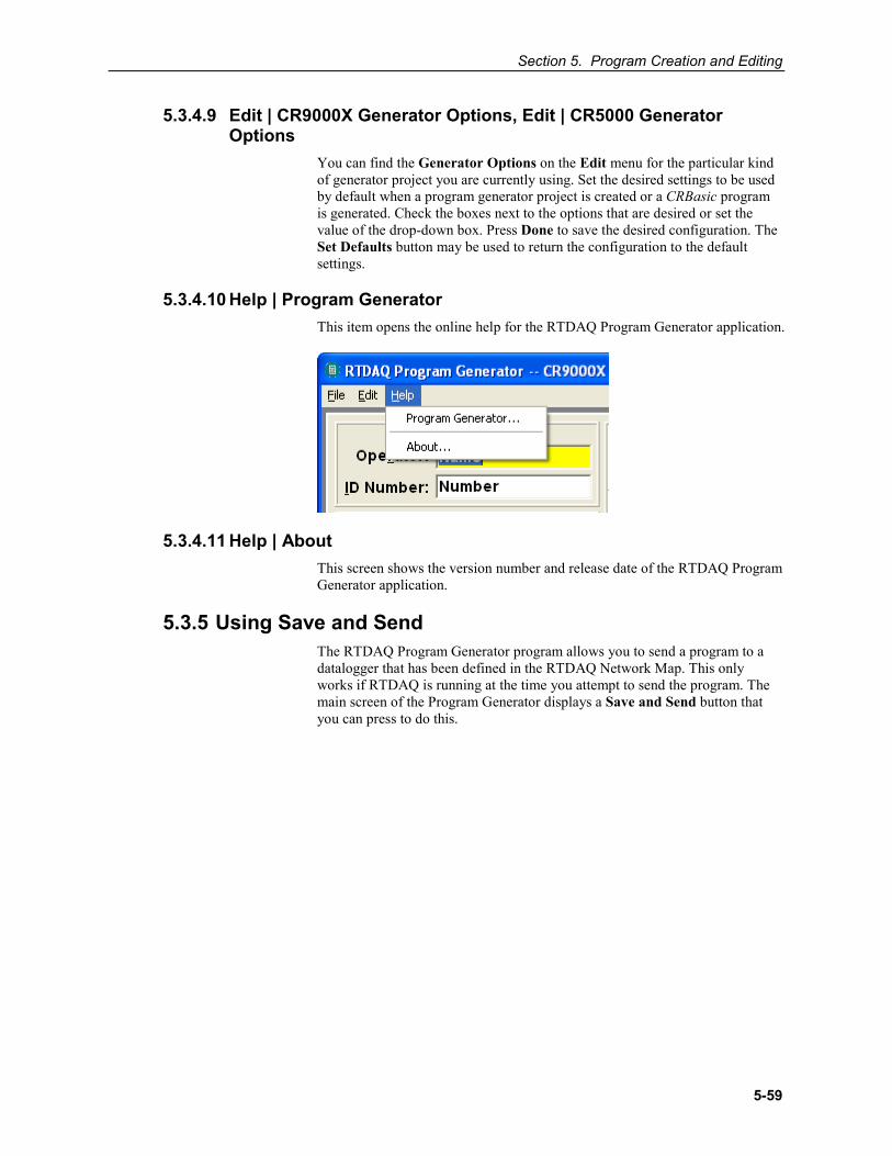
Section 5. Program Creation and Editing
5-59
5.3.4.9 Edit | CR9000X Generator Options, Edit | CR5000 Generator Options
You can find the Generator Options on the Edit menu for the particular kind of generator project you are currently using. Set the desired settings to be used by default when a program generator project is created or a CRBasic program is generated. Check the boxes next to the options that are desired or set the value of the drop-down box. Press Done to save the desired configuration. The Set Defaults button may be used to return the configuration to the default settings.
5.3.4.10 Help | Program Generator This item opens the online help for the RTDAQ Program Generator application.
5.3.4.11 Help | About This screen shows the version number and release date of the RTDAQ Program Generator application.
5.3.5 Using Save and Send The RTDAQ Program Generator program allows you to send a program to a datalogger that has been defined in the RTDAQ Network Map. This only works if RTDAQ is running at the time you attempt to send the program. The main screen of the Program Generator displays a Save and Send button that you can press to do this.
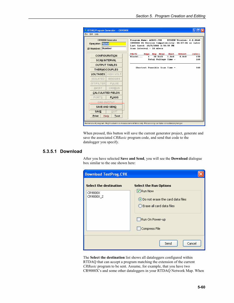
Section 5. Program Creation and Editing
5-60
5.3.5.1 Download
When pressed, this button will save the current generator project, generate and save the associated CRBasic program code, and send that code to the datalogger you specify.
After you have selected Save and Send, you will see the Download dialogue box similar to the one shown here:
The Select the destination list shows all dataloggers configured within RTDAQ that can accept a program matching the extension of the current CRBasic program to be sent. Assume, for example, that you have two CR9000X’s and some other dataloggers in your RTDAQ Network Map. When
Section 5. Program Creation and Editing
5-61
you send a CR9000X program, this screen will show only the two CR9000X dataloggers. Any CR3000, CR1000, or CR5000 dataloggers will be excluded from the list, even when they are defined in the network map, because those dataloggers are not associated with CR9000X programs.
5.3.5.2 Run Options You may check the Run Now check box to run the program immediately after it has been sent to the datalogger. You can choose whether or not to erase card data files by selecting the appropriate option button. If you want the program to start the next time the datalogger is powered up, check the corresponding check box.
Checking the Compress File check box will send a renamed version of the CRBasic program to the datalogger which has all unnecessary spaces, indentation, and comments removed in order to minimize the file size.
5.3.5.3 Datalogger Response To send the file and perform the associated functions as you have selected in the screen, press the Send button. If RTDAQ is not running an error message will appear indicating that there is no communications server currently running. If RTDAQ is running and the program compiles properly on the hardware, you will receive a message indicating that the program is now running on the datalogger. If something goes wrong when sending the program, a message will appear indicating the error conditions. This may be a hardware-level compile error or another failure as reported to the software by the datalogger’s “program load and run” process.
Press Cancel if you do not wish to send the program to the datalogger.
6-1
Section 6. View Pro Although RTDAQ does not support the older “mixed-array” group of Campbell Scientific dataloggers (such as the CR10X, CR23X, and CR510), the Short Cut application included with RTDAQ is the same one included for use with LoggerNet and other Campbell Scientific support software. Because of this, the documentation included here contains references to mixed-array dataloggers. For most RTDAQ implementations these references can be ignored.
6.1 Overview The View Pro button on the RTDAQ toolbar brings up View Pro. This program can be used to open data files (*.DAT) or other CSI file types (*.DLD, *.CSI, *.FSL, *.LOG, *.CR1, *.CR3, etc.). View Pro can easily handle files up to 2 Gigabytes in size. View Pro can also be used to view data from a LoggerNet database table created with LNDB.
Once a data file or database table is opened, data can be printed or graphed in several different graph types including Line Graphs, Histograms, XY Plots, FFTs (Fast Fourier Transforms), or Rainflow Histograms as appropriate for the data type. (Note that these graphical windows are only available for *.DAT files and database tables. Other file types are viewable only as text.)
Since View Pro is primarily a file viewing utility, a file cannot be edited or saved using this program.
View Pro can also be run as a stand-alone program by using the Windows Start Menu and selecting All apps | Campbell Scientific | View Pro or by using Windows Explorer and double-clicking on the ViewPro.exe file in the C:\Program Files\CampbellSci\View Pro folder. A desktop shortcut can be created by right-clicking on this file in Windows Explorer and choosing Create Shortcut.
View Pro is closed by selecting File | Exit from the menu or pressing the red X in the upper right-hand corner. When View Pro is closed, all open graphs and data files will also be closed.
6.2 The Toolbar Many of View Pro’s features can be accessed from the toolbar. The main View Pro toolbar includes the following icons:
Open. Brings up a dialogue box from which you can choose a data file to open.
NOTE
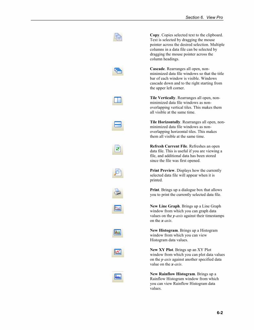
Section 6. View Pro
6-2
Copy. Copies selected text to the clipboard. Text is selected by dragging the mouse pointer across the desired selection. Multiple columns in a data file can be selected by dragging the mouse pointer across the column headings.
Cascade. Rearranges all open, non-minimized data file windows so that the title bar of each window is visible. Windows cascade down and to the right starting from the upper left corner.
Tile Vertically. Rearranges all open, non-minimized data file windows as non-overlapping vertical tiles. This makes them all visible at the same time.
Tile Horizontally. Rearranges all open, non-minimized data file windows as non-overlapping horizontal tiles. This makes them all visible at the same time.
Refresh Current File. Refreshes an open data file. This is useful if you are viewing a file, and additional data has been stored since the file was first opened.
Print Preview. Displays how the currently selected data file will appear when it is printed.
Print. Brings up a dialogue box that allows you to print the currently selected data file.
New Line Graph. Brings up a Line Graph window from which you can graph data values on the y-axis against their timestamps on the x-axis.
New Histogram. Brings up a Histogram window from which you can view Histogram data values.
New XY Plot. Brings up an XY Plot window from which you can plot data values on the y-axis against another specified data value on the x-axis.
New Rainflow Histogram. Brings up a Rainflow Histogram window from which you can view Rainflow Histogram data values.
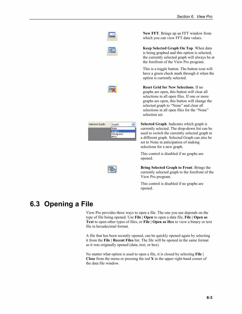
Section 6. View Pro
6-3
New FFT. Brings up an FFT window from which you can view FFT data values.
Keep Selected Graph On Top. When data is being graphed and this option is selected, the currently selected graph will always be at the forefront of the View Pro program.
This is a toggle button. The button icon will have a green check mark through it when the option is currently selected.
Reset Grid for New Selections. If no graphs are open, this button will clear all selections in all open files. If one or more graphs are open, this button will change the selected graph to “None” and clear all selections in all open files for the “None” selection set.
Selected Graph. Indicates which graph is currently selected. The drop-down list can be used to switch the currently selected graph to a different graph. Selected Graph can also be set to None in anticipation of making selections for a new graph.
This control is disabled if no graphs are opened.
Bring Selected Graph to Front. Brings the currently selected graph to the forefront of the View Pro program.
This control is disabled if no graphs are opened.
6.3 Opening a File View Pro provides three ways to open a file. The one you use depends on the type of file being opened. Use File | Open to open a data file, File | Open as Text to open other types of files, or File | Open as Hex to view a binary or text file in hexadecimal format.
A file that has been recently opened, can be quickly opened again by selecting it from the File | Recent Files list. The file will be opened in the same format as it was originally opened (data, text, or hex).
No matter what option is used to open a file, it is closed by selecting File | Close from the menu or pressing the red X in the upper right-hand corner of the data file window.
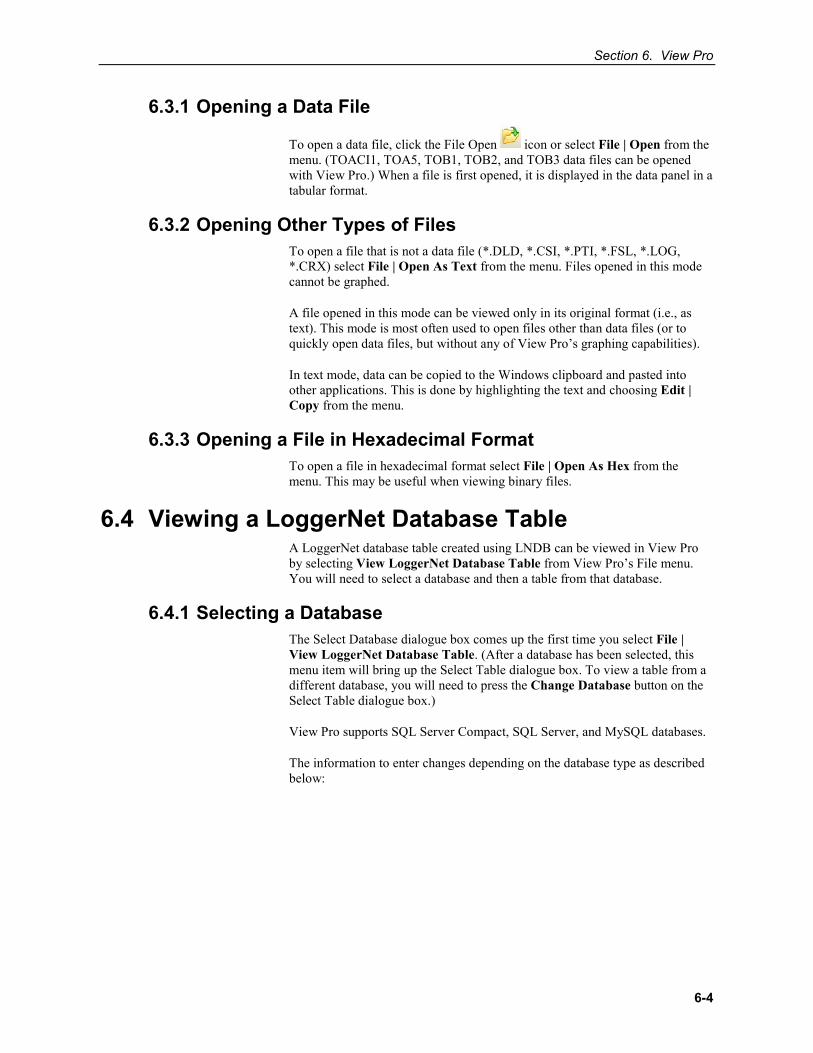
Section 6. View Pro
6-4
6.3.1 Opening a Data File
To open a data file, click the File Open icon or select File | Open from the menu. (TOACI1, TOA5, TOB1, TOB2, and TOB3 data files can be opened with View Pro.) When a file is first opened, it is displayed in the data panel in a tabular format.
6.3.2 Opening Other Types of Files To open a file that is not a data file (*.DLD, *.CSI, *.PTI, *.FSL, *.LOG, *.CRX) select File | Open As Text from the menu. Files opened in this mode cannot be graphed.
A file opened in this mode can be viewed only in its original format (i.e., as text). This mode is most often used to open files other than data files (or to quickly open data files, but without any of View Pro’s graphing capabilities).
In text mode, data can be copied to the Windows clipboard and pasted into other applications. This is done by highlighting the text and choosing Edit | Copy from the menu.
6.3.3 Opening a File in Hexadecimal Format To open a file in hexadecimal format select File | Open As Hex from the menu. This may be useful when viewing binary files.
6.4 Viewing a LoggerNet Database Table A LoggerNet database table created using LNDB can be viewed in View Pro by selecting View LoggerNet Database Table from View Pro’s File menu. You will need to select a database and then a table from that database.
6.4.1 Selecting a Database The Select Database dialogue box comes up the first time you select File | View LoggerNet Database Table. (After a database has been selected, this menu item will bring up the Select Table dialogue box. To view a table from a different database, you will need to press the Change Database button on the Select Table dialogue box.)
View Pro supports SQL Server Compact, SQL Server, and MySQL databases.
The information to enter changes depending on the database type as described below:
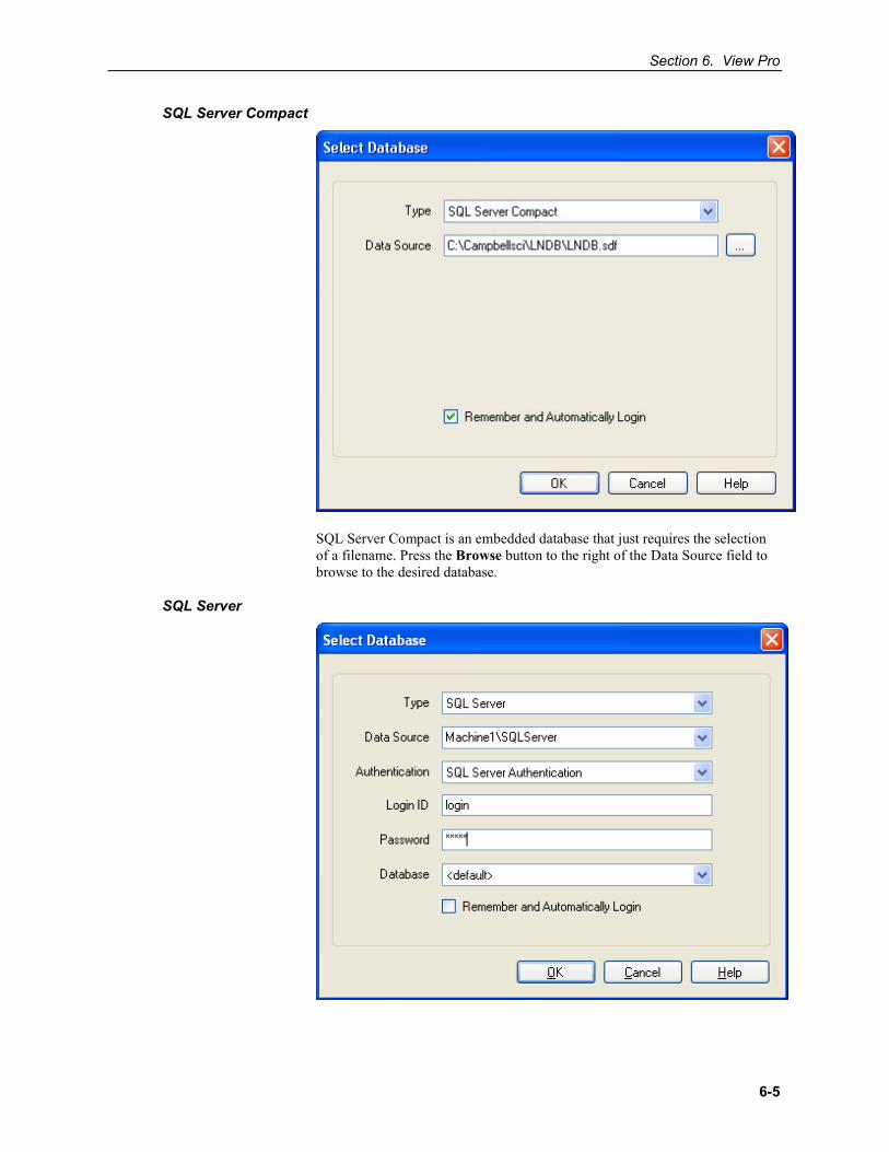
Section 6. View Pro
6-5
SQL Server Compact
SQL Server Compact is an embedded database that just requires the selection of a filename. Press the Browse button to the right of the Data Source field to browse to the desired database.
SQL Server
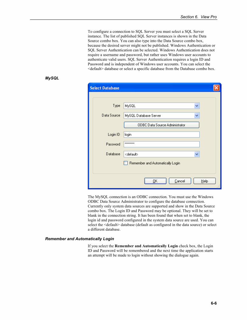
Section 6. View Pro
6-6
To configure a connection to SQL Server you must select a SQL Server instance. The list of published SQL Server instances is shown in the Data Source combo box. You can also type into the Data Source combo box, because the desired server might not be published. Windows Authentication or SQL Server Authentication can be selected. Windows Authentication does not require a username and password, but rather uses Windows user accounts to authenticate valid users. SQL Server Authentication requires a login ID and Password and is independent of Windows user accounts. You can select the <default> database or select a specific database from the Database combo box.
MySQL
The MySQL connection is an ODBC connection. You must use the Windows ODBC Data Source Administrator to configure the database connection. Currently only system data sources are supported and show in the Data Source combo box. The Login ID and Password may be optional. They will be set to blank in the connection string. It has been found that when set to blank, the login id and password configured in the system data source are used. You can select the <default> database (default as configured in the data source) or select a different database.
Remember and Automatically Login
If you select the Remember and Automatically Login check box, the Login ID and Password will be remembered and the next time the application starts an attempt will be made to login without showing the dialogue again.
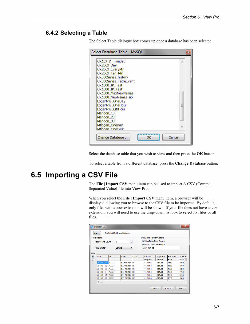
Section 6. View Pro
6-7
6.4.2 Selecting a Table The Select Table dialogue box comes up once a database has been selected.
Select the database table that you wish to view and then press the OK button.
To select a table from a different database, press the Change Database button.
6.5 Importing a CSV File The File | Import CSV menu item can be used to import A CSV (Comma Separated Value) file into View Pro.
When you select the File | Import CSV menu item, a browser will be displayed allowing you to browse to the CSV file to be imported. By default, only files with a .csv extension will be shown. If your file does not have a .csv extension, you will need to use the drop-down list box to select .txt files or all files.
Section 6. View Pro
6-8
File
The name of the file to be imported. Press the File button to bring up a browser to select the desired file.
Header Line Count
CSV files may have multiple header lines or no header line. Use the Header Line Count field to designate how many header lines your file contains before the data begins.
File Delimiter
Although CSV files are by definition comma delimited, other file delimiters (tab or space) can be selected in the File Delimiter drop-down list box.
Date/Time Format Options
When importing a CSV file, View Pro will attempt to derive a timestamp from data in the first column, if common timestamp delimiters exist in the data. If View Pro is able to derive the timestamp, the Has Date/Time Column check box will be checked and the derived timestamp format will be displayed in the Derived Date/Time Format field using the codes shown below. Any errors in the derived format can be corrected in this field.
If the first column contains a timestamp, but does not have the common timestamp delimiters that allow View Pro to determine that it is a timestamp, you can manually check the Has Date/Time Column check box and then input the appropriate codes in the Derived Date/Time Format field to designate the format of the timestamp.
If the first column of data does not contain a timestamp, leave the Has Date/Time Column check box unchecked. You will still be able to import the file into View Pro and view the data. However, you will not be able to graph the data.
Date and Time Format Codes
yy = Year last 2 digits yyyy = Year as 4 digits m = Month number no-leading 0 mm = Month number as 2 digits mmm = Month using short form (Jan) mmmm = Month using long form (January) d = Day number no-leading 0 dd = Day number as 2 digits ddd = Day using short day names (Sun) dddd = Day using long day names (Sunday) h = Hour with no leading 0's hh = Hour as 2 digits n = Minute with no leading 0's nn = Minute as 2 digits s = Seconds with no leading 0's ss = Seconds as 2 digits z = Milli-seconds with no leading 0's zzz = Milli-seconds as 3 digits
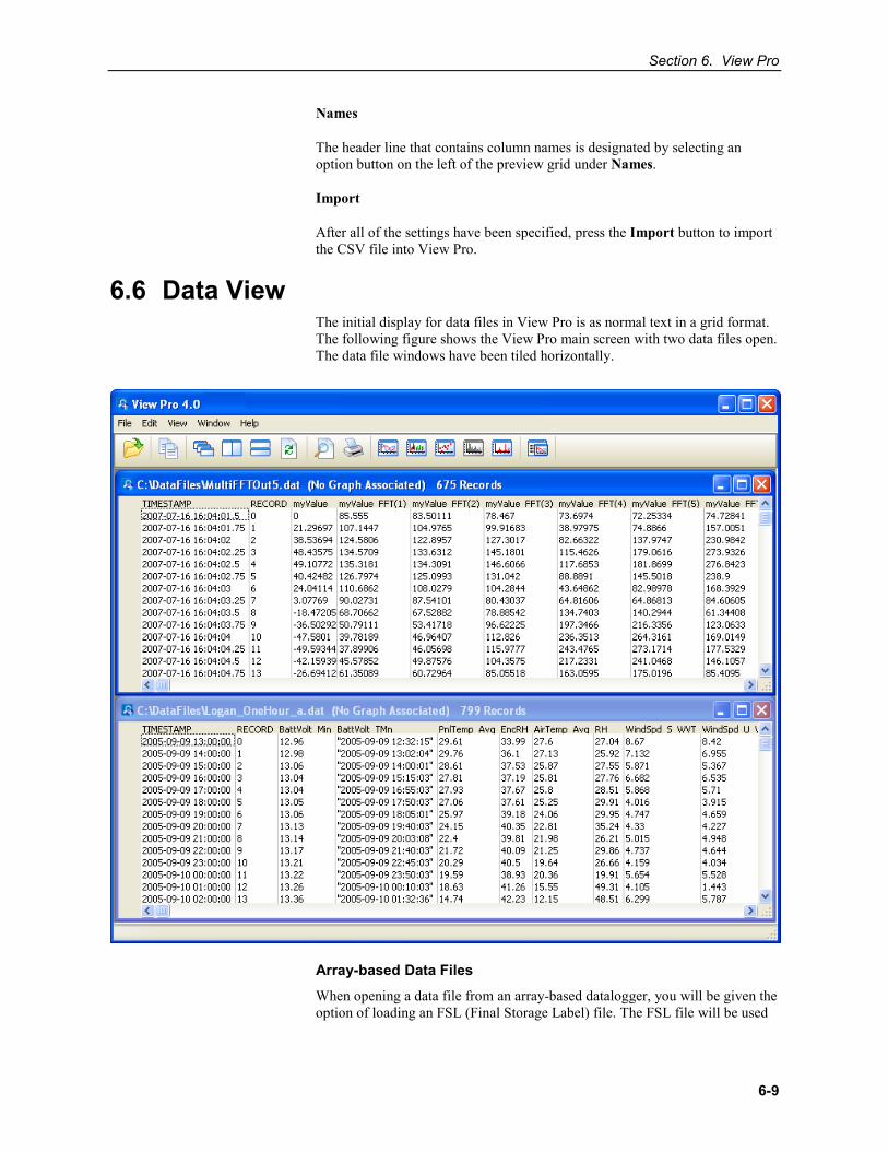
Section 6. View Pro
6-9
Names
The header line that contains column names is designated by selecting an option button on the left of the preview grid under Names.
Import
After all of the settings have been specified, press the Import button to import the CSV file into View Pro.
6.6 Data View The initial display for data files in View Pro is as normal text in a grid format. The following figure shows the View Pro main screen with two data files open. The data file windows have been tiled horizontally.
Array-based Data Files When opening a data file from an array-based datalogger, you will be given the option of loading an FSL (Final Storage Label) file. The FSL file will be used
Section 6. View Pro
6-10
to provide column headings. (The *.FSL file is created when a datalogger program is compiled in Edlog or ShortCut.)
If a data file is opened that contains multiple arrays, the entire data file will be opened in one window. In addition, each array will be opened in a separate window. The window containing the entire data file is for viewing only. Data must be graphed from the individual array windows.
Array-based data files do not contain timestamps. If an FSL file is associated with the data file, View Pro will try to extract timestamps from the appropriate columns. You can select Array Definitions from View Pro’s View menu to specify how the timestamps are created. Note that if no timestamps are used, data cannot be graphed.
6.6.1 Column Size When a data file is opened, the columns are autosized to fit the data. Column sizes can be changed by dragging a column divider bar to the desired location. If column sizes have been changed, they can be returned to the default sizes by selecting View | Autosize Columns from the menu.
6.6.2 Header Information By default, only column names are shown for each column in the data file. Selecting View | Show Full Header will show full header information for each column in the data file, including units and field names, if available in the *.DAT file.
This is a toggle menu item. There will be a check mark next to the item, when it is active. Deactivate it by selecting it again.
6.6.3 Row Shading Selecting View | Row Shading will shade every other row in the data file.
This is a toggle menu item. There will be a check mark next to the item, when it is active. Deactivate it by selecting it again.
6.6.4 Locking the TimeStamp Column Selecting View | Lock TimeStamp Column will lock the timestamp column on the left of the data file so that it remains visible as you scroll through the columns in the data file.
This is a toggle menu item. There will be a check mark next to the item, when it is active. Deactivate it by selecting it again.
6.6.5 File Information Selecting View | View File Information from the menu will display information on the currently selected data file including file name and file format, and information about the datalogger and program that generated the data file such as station name, table name, datalogger model, datalogger OS version, program name, and program signature.
Section 6. View Pro
6-11
6.6.6 Background Colour
6.6.7 Font
The background colour used for the currently selected data panel can be changed by selecting View | Background Colour from the menu.
The font used for the data panel can be changed with the font selection dialogue box. Select View | Font from the menu to change the font used for the printer and data panel. Normal font options such as colour, bold, underline and italic are also available.
6.6.8 Window Arrangement
6.7 Graphs
When multiple data files are opened, they are arranged so that the title bar of each window is visible and they cascade down and to the right starting from the upper left corner. Pressing the Cascade button or choosing Window | Cascade from the View Pro menu will return the data windows to this default arrangement at any time.
Windows can be tiled horizontally as non-overlapping horizontal tiles by pressing the Tile Horizontally button or choosing Window | Tile Horizontally from the menu. They can be tiled vertically as non-overlapping vertical tiles by pressing the Tile Vertically button or choosing Window | Tile Vertically from the menu.
A data window can be moved manually by clicking on the title bar and dragging it to the desired location.
The data view window can be kept in front of any opened graphs by selecting View | Keep Data on Top from the menu.
Once a data file is opened, data values can be displayed in several different graphical forms including a Line Graph, Histogram, XY Plot, Rainflow Histogram, or FFT. Each of these are launched from a button on the View Pro toolbar. Graph buttons are enabled only if the graph type is appropriate for the opened data file. For instance, if there is no data appropriate for an FFT, the FFT button will be disabled on the View Pro toolbar. Multiple instances of each type of graph can be launched.
Graphing Data from Multiple Data Files
Data from multiple data files can be displayed in a single graph. This is done by opening multiple data files and selecting data to be graphed as described for each graph type below. This may be useful when comparing data from multiple datalogger stations.
Options
Each type of graph has several different options that can be set by the user. Options that apply to the entire graph are generally set from a dialogue box that is opened by pressing the Options button at the lower-left of the graph window, by pressing the Graph Options button on the toolbar, or by right-clicking
Section 6. View Pro
6-12
on the graph and choosing Options. Note that the XY Plot does not have an Options button, so the Options dialogue box is opened by pressing the Graph Options button on the toolbar or right-clicking on the graph.
Options that apply to individual traces are set by selecting the trace in the list of data values being graphed, and then pressing the Edit button located below that list. The XY Plot does not have user-configurable trace options.
For information on graph options refer to the online help. Help for a graph can be accessed by pressing the ? button in the upper-right corner of the graph.
Zoom Feature
You can zoom in on a particular area of a graph by holding the left mouse button and dragging the mouse cursor from top-left to bottom-right over the area to be zoomed. Dragging the mouse cursor from bottom-right to top-left will undo the zoom. This can also be accomplished by pressing the Undo Zoom button on the toolbar.
For a Rainflow Histogram or for a Histogram or FFT in 3D View, you can also zoom in and out by using the Page Down and Page Up buttons on your keyboard.
Rotation
For a Rainflow Histogram or for a Histogram or FFT in 3D View, you can rotate the graph by using the scroll bars at the bottom and right of the graph.
Keeping Graph on Top
The currently selected graph can be kept in front of the data view window by selecting View | Keep Graph on Top from the menu or pressing this button
on the main View Pro toolbar.
6.7.1 Line Graph From the Line Graph screen, you can graph data values on the y-axis against their timestamps on the x-axis.
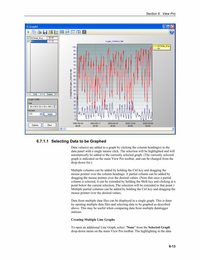
Section 6. View Pro
6-13
6.7.1.1 Selecting Data to be Graphed Data value(s) are added to a graph by clicking the column heading(s) in the data panel with a single mouse click. The selection will be highlighted and will automatically be added to the currently selected graph. (The currently selected graph is indicated on the main View Pro toolbar, and can be changed from the drop-down list.)
Multiple columns can be added by holding the Ctrl key and dragging the mouse pointer over the column headings. A partial column can be added by dragging the mouse pointer over the desired values. (Note that once a partial column is selected, it can be extended by holding the Shift key and clicking at a point below the current selection. The selection will be extended to that point.) Multiple partial columns can be added by holding the Ctrl key and dragging the mouse pointer over the desired values.
Data from multiple data files can be displayed in a single graph. This is done by opening multiple data files and selecting data to be graphed as described above. This may be useful when comparing data from multiple datalogger stations.
Creating Multiple Line Graphs
To open an additional Line Graph, select “None” from the Selected Graph drop-down menu on the main View Pro toolbar. The highlighting in the data
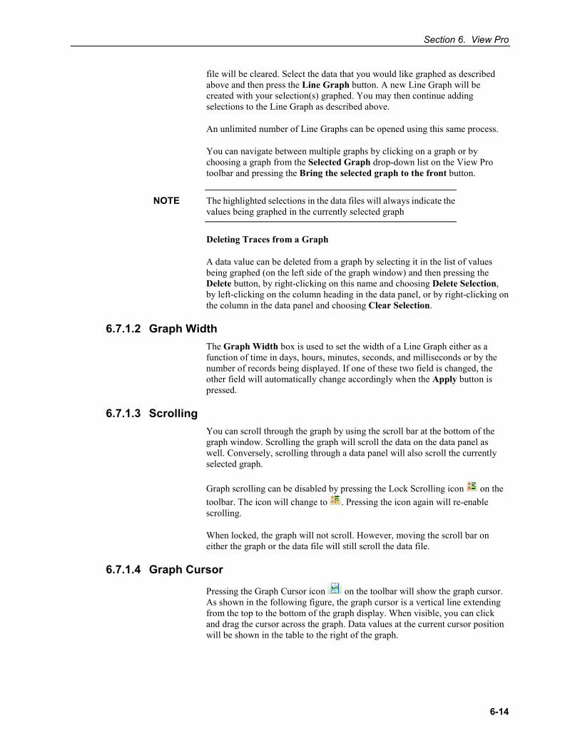
Section 6. View Pro
6-14
file will be cleared. Select the data that you would like graphed as described above and then press the Line Graph button. A new Line Graph will be created with your selection(s) graphed. You may then continue adding selections to the Line Graph as described above.
An unlimited number of Line Graphs can be opened using this same process.
You can navigate between multiple graphs by clicking on a graph or by choosing a graph from the Selected Graph drop-down list on the View Pro toolbar and pressing the Bring the selected graph to the front button.
The highlighted selections in the data files will always indicate the values being graphed in the currently selected graph
Deleting Traces from a Graph
A data value can be deleted from a graph by selecting it in the list of values being graphed (on the left side of the graph window) and then pressing the Delete button, by right-clicking on this name and choosing Delete Selection, by left-clicking on the column heading in the data panel, or by right-clicking on the column in the data panel and choosing Clear Selection.
6.7.1.2 Graph Width The Graph Width box is used to set the width of a Line Graph either as a function of time in days, hours, minutes, seconds, and milliseconds or by the number of records being displayed. If one of these two field is changed, the other field will automatically change accordingly when the Apply button is pressed.
6.7.1.3 Scrolling You can scroll through the graph by using the scroll bar at the bottom of the graph window. Scrolling the graph will scroll the data on the data panel as well. Conversely, scrolling through a data panel will also scroll the currently selected graph.
Graph scrolling can be disabled by pressing the Lock Scrolling icon on the toolbar. The icon will change to . Pressing the icon again will re-enable scrolling.
When locked, the graph will not scroll. However, moving the scroll bar on either the graph or the data file will still scroll the data file.
6.7.1.4 Graph Cursor
Pressing the Graph Cursor icon on the toolbar will show the graph cursor. As shown in the following figure, the graph cursor is a vertical line extending from the top to the bottom of the graph display. When visible, you can click and drag the cursor across the graph. Data values at the current cursor position will be shown in the table to the right of the graph.
NOTE
Section 6. View Pro
6-15
6.7.1.5 Line Graph Toolbar The Line Graph toolbar includes the following icons:
Statistics. Displays statistics for each trace including Average, Standard Deviation, Minimum and Maximum. Note that these statistics are for the data displayed in the graph. They are not statistics for the entire column(s) of data. Note that an asterisk next to a statistics value indicates that the trace contains one or more bad data values (i.e., NAN, INF, etc.).
The Statistics button is disabled when a graph is in a zoomed stated.
Copy to Clipboard. Places the graphic on the Windows clipboard. It can then be pasted into other applications.
Print. Prints the graph. Print options can be set before printing begins.
Export. Allows the graph to be exported in a choice of text or graphical formats.
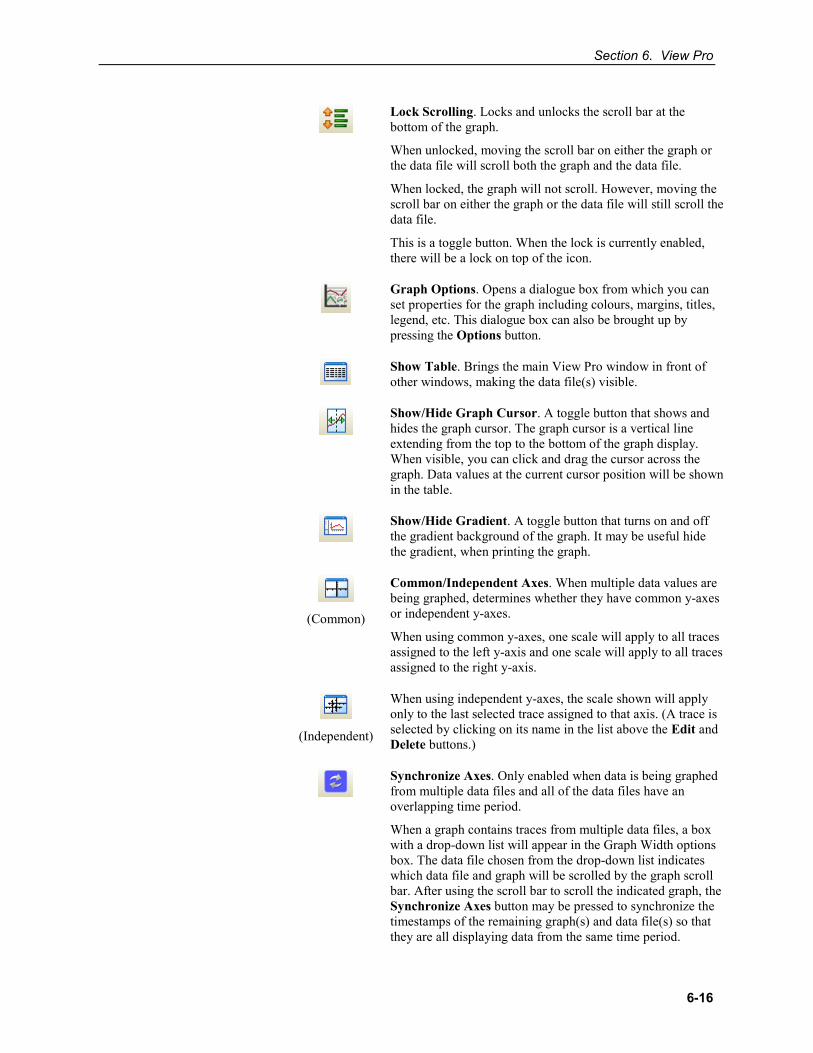
Section 6. View Pro
6-16
(Common)
(Independent)
Lock Scrolling. Locks and unlocks the scroll bar at the bottom of the graph.
When unlocked, moving the scroll bar on either the graph or the data file will scroll both the graph and the data file.
When locked, the graph will not scroll. However, moving the scroll bar on either the graph or the data file will still scroll the data file.
This is a toggle button. When the lock is currently enabled, there will be a lock on top of the icon.
Graph Options. Opens a dialogue box from which you can set properties for the graph including colours, margins, titles, legend, etc. This dialogue box can also be brought up by pressing the Options button.
Show Table. Brings the main View Pro window in front of other windows, making the data file(s) visible.
Show/Hide Graph Cursor. A toggle button that shows and hides the graph cursor. The graph cursor is a vertical line extending from the top to the bottom of the graph display. When visible, you can click and drag the cursor across the graph. Data values at the current cursor position will be shown in the table.
Show/Hide Gradient. A toggle button that turns on and off the gradient background of the graph. It may be useful hide the gradient, when printing the graph.
Common/Independent Axes. When multiple data values are being graphed, determines whether they have common y-axes or independent y-axes.
When using common y-axes, one scale will apply to all traces assigned to the left y-axis and one scale will apply to all traces assigned to the right y-axis.
When using independent y-axes, the scale shown will apply only to the last selected trace assigned to that axis. (A trace is selected by clicking on its name in the list above the Edit and Delete buttons.)
Synchronize Axes. Only enabled when data is being graphed from multiple data files and all of the data files have an overlapping time period.
When a graph contains traces from multiple data files, a box with a drop-down list will appear in the Graph Width options box. The data file chosen from the drop-down list indicates which data file and graph will be scrolled by the graph scroll bar. After using the scroll bar to scroll the indicated graph, the Synchronize Axes button may be pressed to synchronize the timestamps of the remaining graph(s) and data file(s) so that they are all displaying data from the same time period.
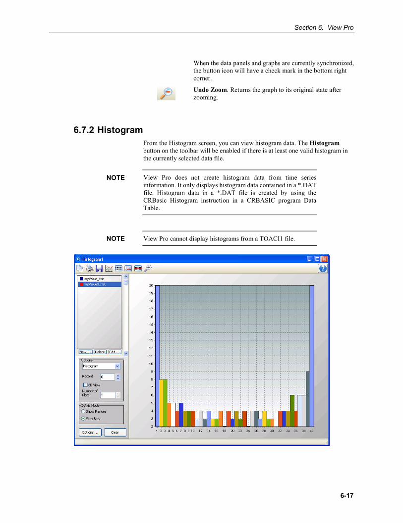
Section 6. View Pro
6-17
When the data panels and graphs are currently synchronized, the button icon will have a check mark in the bottom right corner.
Undo Zoom. Returns the graph to its original state after zooming.
6.7.2 Histogram From the Histogram screen, you can view histogram data. The Histogram button on the toolbar will be enabled if there is at least one valid histogram in the currently selected data file.
View Pro does not create histogram data from time series information. It only displays histogram data contained in a *.DAT file. Histogram data in a *.DAT file is created by using the CRBasic Histogram instruction in a CRBASIC program Data Table.
View Pro cannot display histograms from a TOACI1 file.
NOTE
NOTE
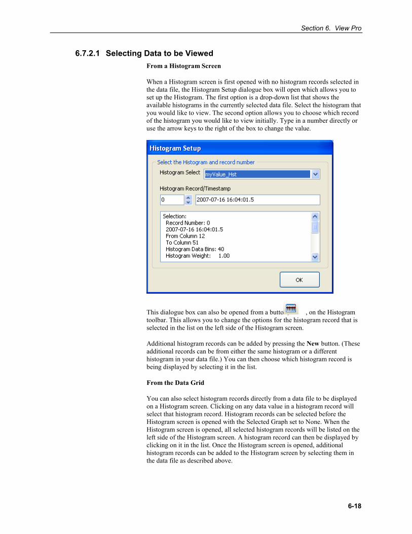
Section 6. View Pro
6-18
6.7.2.1 Selecting Data to be Viewed From a Histogram Screen
When a Histogram screen is first opened with no histogram records selected in the data file, the Histogram Setup dialogue box will open which allows you to set up the Histogram. The first option is a drop-down list that shows the available histograms in the currently selected data file. Select the histogram that you would like to view. The second option allows you to choose which record of the histogram you would like to view initially. Type in a number directly or use the arrow keys to the right of the box to change the value.
This dialogue box can also be opened from a button, , on the Histogram toolbar. This allows you to change the options for the histogram record that is selected in the list on the left side of the Histogram screen.
Additional histogram records can be added by pressing the New button. (These additional records can be from either the same histogram or a different histogram in your data file.) You can then choose which histogram record is being displayed by selecting it in the list.
From the Data Grid
You can also select histogram records directly from a data file to be displayed on a Histogram screen. Clicking on any data value in a histogram record will select that histogram record. Histogram records can be selected before the Histogram screen is opened with the Selected Graph set to None. When the Histogram screen is opened, all selected histogram records will be listed on the left side of the Histogram screen. A histogram record can then be displayed by clicking on it in the list. Once the Histogram screen is opened, additional histogram records can be added to the Histogram screen by selecting them in the data file as described above.

Section 6. View Pro
6-19
All histogram records from the same histogram will have the same default name in the list. They can be distinguished by the coloured boxes next to their names. Each box is the same colour with which that histogram record is highlighted in the data file. It is also the colour with which that histogram record is displayed if the “Use Selection colour” option is chosen in the Selection Properties dialogue box. The colour associated with a histogram record can also be changed from this dialogue box. (The Selection Properties dialogue box is opened by clicking on the histogram record in the list and then pressing the Edit button.)
Deleting Records from a Histogram Display
A Histogram can be deleted from a graph by selecting it in the list of values being graphed (on the left side of the graph window) and then pressing the Delete button, by right-clicking on this name and choosing Delete Selection, or by right-clicking on the record in the data panel and choosing Clear Selection.
6.7.2.2 Options From the main Histogram screen, you can set the Histogram type to Area, Histogram, Line, or Bar. You can use the arrow buttons to the right of Record to scroll through records of the Histogram.
You can also determine whether the Histogram is viewed in 2D or 3D. Selecting the 3D View check box will enable 3D View. Clearing the check box will cause the Histogram to be viewed in 2D. When in 3D View, the Number of Plots field will determine how many records are viewed in the Histogram. In 3D View, scroll bars appear on the bottom and right of the screen which allow the Histogram to be rotated.
You can also determine how the labels on the X-Axis are displayed. Select Show Ranges to have ranges of data values shown on the X-Axis. Select View Bins to have bin numbers shown on the X-Axis.
6.7.2.3 Histogram Toolbar The Histogram toolbar includes the following icons:
Copy to Clipboard. Places the Histogram graphic on the Windows clipboard. It can then be pasted into other applications.
Print. Prints the Histogram. Print options can be set before printing begins.
Export. Allows the Histogram to be exported in a choice of text or graphical formats.
Histogram Options. Opens a dialogue box from which you can set properties for the Histogram including scaling, colours, margins, titles, etc. This dialogue box can also be brought up by pressing the Options button.
NOTE
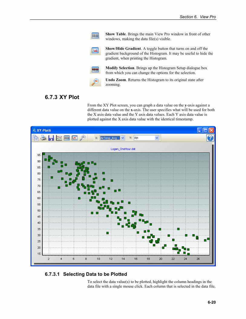
Section 6. View Pro
6-20
Show Table. Brings the main View Pro window in front of other windows, making the data file(s) visible.
Show/Hide Gradient. A toggle button that turns on and off the gradient background of the Histogram. It may be useful to hide the gradient, when printing the Histogram.
Modify Selection. Brings up the Histogram Setup dialogue box from which you can change the options for the selection.
Undo Zoom. Returns the Histogram to its original state after zooming.
6.7.3 XY Plot From the XY Plot screen, you can graph a data value on the y-axis against a different data value on the x-axis. The user specifies what will be used for both the X axis data value and the Y axis data values. Each Y axis data value is plotted against the X axis data value with the identical timestamp.
6.7.3.1 Selecting Data to be Plotted To select the data value(s) to be plotted, highlight the column headings in the data file with a single mouse click. Each column that is selected in the data file,
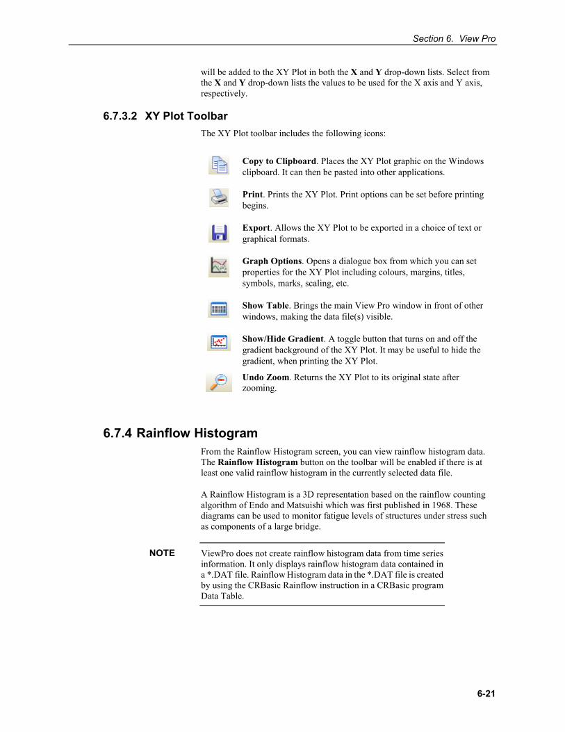
Section 6. View Pro
6-21
will be added to the XY Plot in both the X and Y drop-down lists. Select from the X and Y drop-down lists the values to be used for the X axis and Y axis, respectively.
6.7.3.2 XY Plot Toolbar The XY Plot toolbar includes the following icons:
Copy to Clipboard. Places the XY Plot graphic on the Windows clipboard. It can then be pasted into other applications.
Print. Prints the XY Plot. Print options can be set before printing begins.
Export. Allows the XY Plot to be exported in a choice of text or graphical formats.
Graph Options. Opens a dialogue box from which you can set properties for the XY Plot including colours, margins, titles, symbols, marks, scaling, etc.
Show Table. Brings the main View Pro window in front of other windows, making the data file(s) visible.
Show/Hide Gradient. A toggle button that turns on and off the gradient background of the XY Plot. It may be useful to hide the gradient, when printing the XY Plot.
Undo Zoom. Returns the XY Plot to its original state after zooming.
6.7.4 Rainflow Histogram From the Rainflow Histogram screen, you can view rainflow histogram data. The Rainflow Histogram button on the toolbar will be enabled if there is at least one valid rainflow histogram in the currently selected data file.
A Rainflow Histogram is a 3D representation based on the rainflow counting algorithm of Endo and Matsuishi which was first published in 1968. These diagrams can be used to monitor fatigue levels of structures under stress such as components of a large bridge.
ViewPro does not create rainflow histogram data from time series information. It only displays rainflow histogram data contained in a *.DAT file. Rainflow Histogram data in the *.DAT file is created by using the CRBasic Rainflow instruction in a CRBasic program Data Table.
NOTE
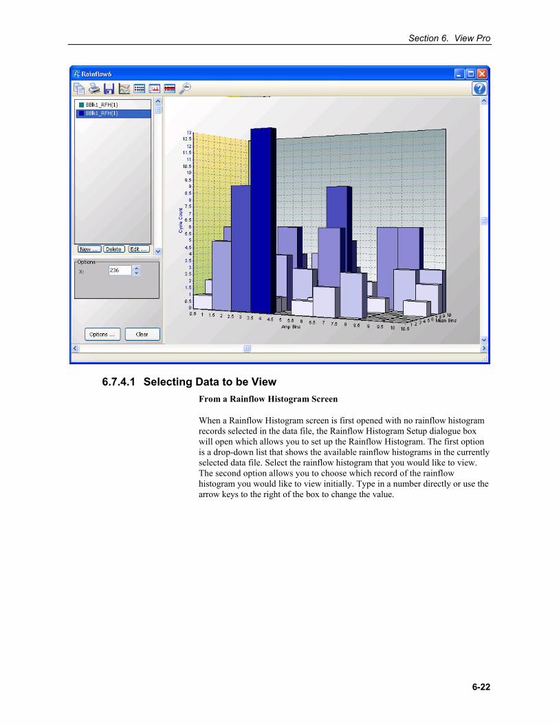
Section 6. View Pro
6-22
6.7.4.1 Selecting Data to be View From a Rainflow Histogram Screen
When a Rainflow Histogram screen is first opened with no rainflow histogram records selected in the data file, the Rainflow Histogram Setup dialogue box will open which allows you to set up the Rainflow Histogram. The first option is a drop-down list that shows the available rainflow histograms in the currently selected data file. Select the rainflow histogram that you would like to view. The second option allows you to choose which record of the rainflow histogram you would like to view initially. Type in a number directly or use the arrow keys to the right of the box to change the value.

Section 6. View Pro
6-23
This dialogue box can also be opened from a button, , on the Rainflow Histogram toolbar. This allows you to change the options for the rainflow histogram record that is selected in the list on the left side of the Rainflow Histogram screen.
Additional rainflow histogram records can be added by pressing the New button. (These additional records can be from either the same rainflow histogram or a different rainflow histogram in your data file.) You can then choose which rainflow histogram record is being displayed by selecting it in the list.
From the Data Grid
You can also select rainflow histogram records directly from a data file to be displayed on a Rainflow Histogram screen. Clicking on any data value in a rainflow histogram record will select that rainflow histogram record. Rainflow histogram records can be selected before the Rainflow Histogram screen is opened with the Selected Graph set to None. When the Rainflow Histogram screen is opened, all selected rainflow histogram records will be listed on the left side of the Rainflow Histogram screen. A rainflow histogram record can then be displayed by clicking on it in the list. Once the Rainflow Histogram screen is opened, additional rainflow histogram records can be added to the Rainflow Histogram screen by selecting them in the data file as described above.
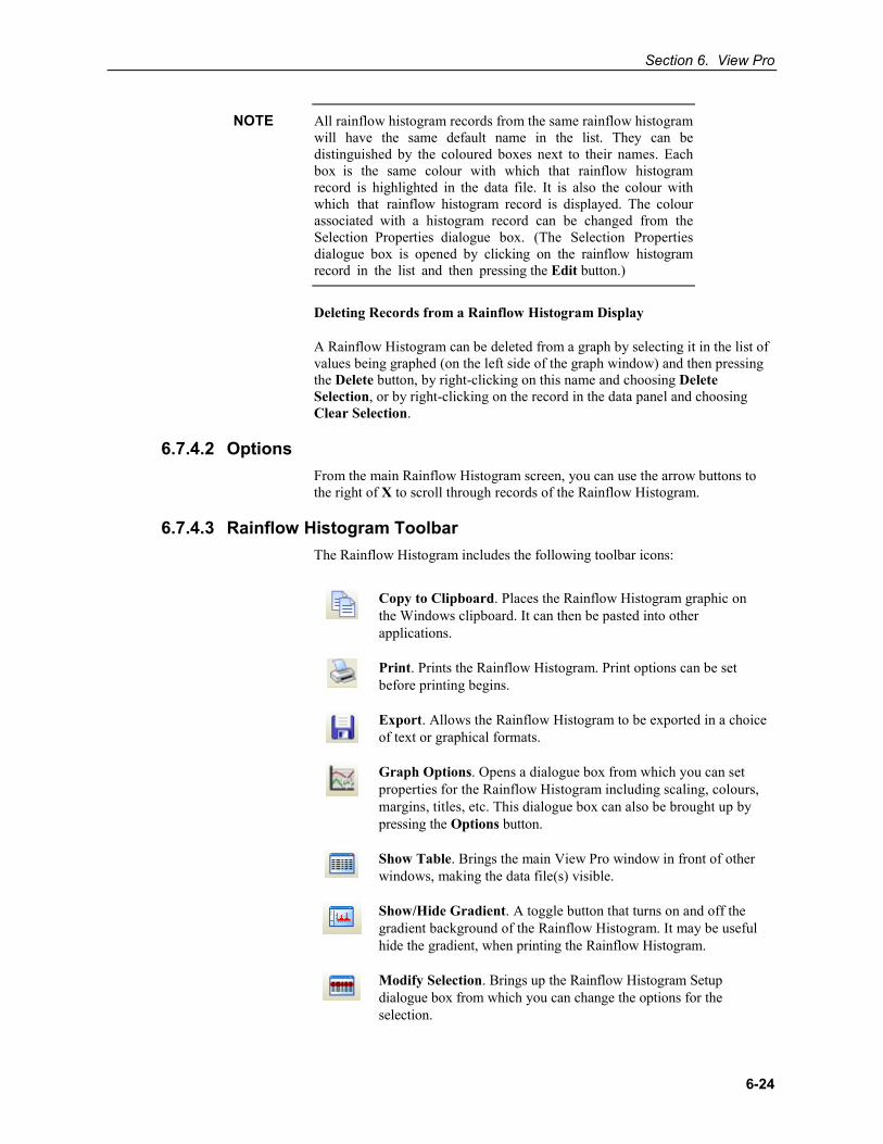
Section 6. View Pro
6-24
All rainflow histogram records from the same rainflow histogram will have the same default name in the list. They can be distinguished by the coloured boxes next to their names. Each box is the same colour with which that rainflow histogram record is highlighted in the data file. It is also the colour with which that rainflow histogram record is displayed. The colour associated with a histogram record can be changed from the Selection Properties dialogue box. (The Selection Properties dialogue box is opened by clicking on the rainflow histogram record in the list and then pressing the Edit button.)
Deleting Records from a Rainflow Histogram Display
A Rainflow Histogram can be deleted from a graph by selecting it in the list of values being graphed (on the left side of the graph window) and then pressing the Delete button, by right-clicking on this name and choosing Delete Selection, or by right-clicking on the record in the data panel and choosing Clear Selection.
6.7.4.2 Options From the main Rainflow Histogram screen, you can use the arrow buttons to the right of X to scroll through records of the Rainflow Histogram.
6.7.4.3 Rainflow Histogram Toolbar The Rainflow Histogram includes the following toolbar icons:
Copy to Clipboard. Places the Rainflow Histogram graphic on the Windows clipboard. It can then be pasted into other applications.
Print. Prints the Rainflow Histogram. Print options can be set before printing begins.
Export. Allows the Rainflow Histogram to be exported in a choice of text or graphical formats.
Graph Options. Opens a dialogue box from which you can set properties for the Rainflow Histogram including scaling, colours, margins, titles, etc. This dialogue box can also be brought up by pressing the Options button.
Show Table. Brings the main View Pro window in front of other windows, making the data file(s) visible.
Show/Hide Gradient. A toggle button that turns on and off the gradient background of the Rainflow Histogram. It may be useful hide the gradient, when printing the Rainflow Histogram.
Modify Selection. Brings up the Rainflow Histogram Setup dialogue box from which you can change the options for the selection.
NOTE
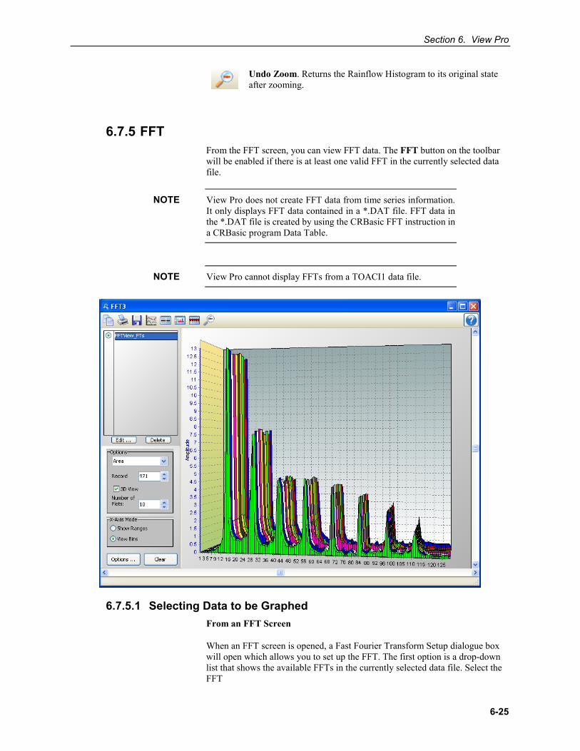
Section 6. View Pro
6-25
Undo Zoom. Returns the Rainflow Histogram to its original state after zooming.
6.7.5 FFT From the FFT screen, you can view FFT data. The FFT button on the toolbar will be enabled if there is at least one valid FFT in the currently selected data file.
View Pro does not create FFT data from time series information. It only displays FFT data contained in a *.DAT file. FFT data in the *.DAT file is created by using the CRBasic FFT instruction in a CRBasic program Data Table.
View Pro cannot display FFTs from a TOACI1 data file.
6.7.5.1 Selecting Data to be Graphed From an FFT Screen
When an FFT screen is opened, a Fast Fourier Transform Setup dialogue box will open which allows you to set up the FFT. The first option is a drop-down list that shows the available FFTs in the currently selected data file. Select the FFT
NOTE
NOTE
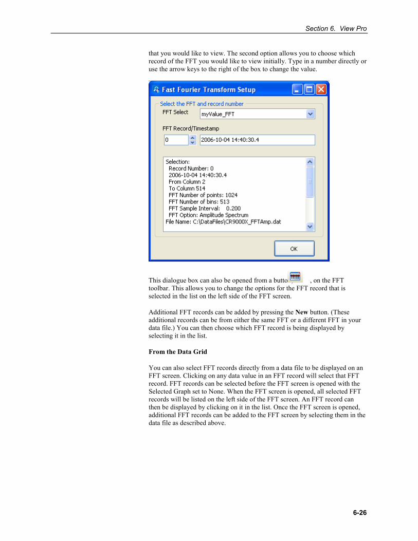
Section 6. View Pro
6-26
that you would like to view. The second option allows you to choose which record of the FFT you would like to view initially. Type in a number directly or use the arrow keys to the right of the box to change the value.
This dialogue box can also be opened from a button, , on the FFT toolbar. This allows you to change the options for the FFT record that is selected in the list on the left side of the FFT screen.
Additional FFT records can be added by pressing the New button. (These additional records can be from either the same FFT or a different FFT in your data file.) You can then choose which FFT record is being displayed by selecting it in the list.
From the Data Grid
You can also select FFT records directly from a data file to be displayed on an FFT screen. Clicking on any data value in an FFT record will select that FFT record. FFT records can be selected before the FFT screen is opened with the Selected Graph set to None. When the FFT screen is opened, all selected FFT records will be listed on the left side of the FFT screen. An FFT record can then be displayed by clicking on it in the list. Once the FFT screen is opened, additional FFT records can be added to the FFT screen by selecting them in the data file as described above.
Section 6. View Pro
6-27
All FFT records from the same FFT will have the same default name in the list. They can be distinguished by the coloured boxes next to their names. Each box is the same colour with which that FFT record is highlighted in the data file. It is also the colour with which that FFT record is displayed if the “Use Selection colour” option is chosen in the Selection Properties dialogue box. The colour associated with an FFT record can also be changed from this dialogue box. (The Selection Properties dialogue box is opened by clicking on the FFT record in the list and then pressing the Edit button.)
Deleting Records from an FFT Display
An FFT can be deleted from a graph by selecting it in the list of values being graphed (on the left side of the graph window) and then pressing the Delete button, by right-clicking on this name and choosing Delete Selection, or by right-clicking on the record in the data panel and choosing Clear Selection.
6.7.5.2 Options From the main FFT screen, you can set the FFT type to Area, Histogram, Line, or Bar. You can use the arrow buttons to the right of Record to scroll through records of the FFT.
You can also determine whether the FFT is viewed in 2D or 3D. Selecting the 3D View check box will enable 3D View. Clearing the check box will cause the FFT to be viewed in 2D. When in 3D View, the Number of Plots field will determine how many records are viewed in the FFT. In 3D View, scroll bars appear on the bottom and right of the screen which allow the FFT to be rotated.
You can also determine how the labels on the X-Axis are displayed. Select Show Ranges to have ranges of data values shown on the X-Axis. Select View Bins to have bin numbers shown on the X-Axis.
6.7.5.3 FFT Toolbar The FFT includes the following toolbar icons:
Copy to Clipboard. Places the FFT graphic on the Windows clipboard. It can then be pasted into other applications.
Print. Prints the FFT. Print options can be set before printing begins.
Export. Allows the FFT to be exported in a choice of text or graphical formats.
FFT Options. Opens a dialogue box from which you can set properties for the FFT including scaling, colours, margins, titles, etc. This dialogue box can also be brought up by pressing the Options button.
NOTE
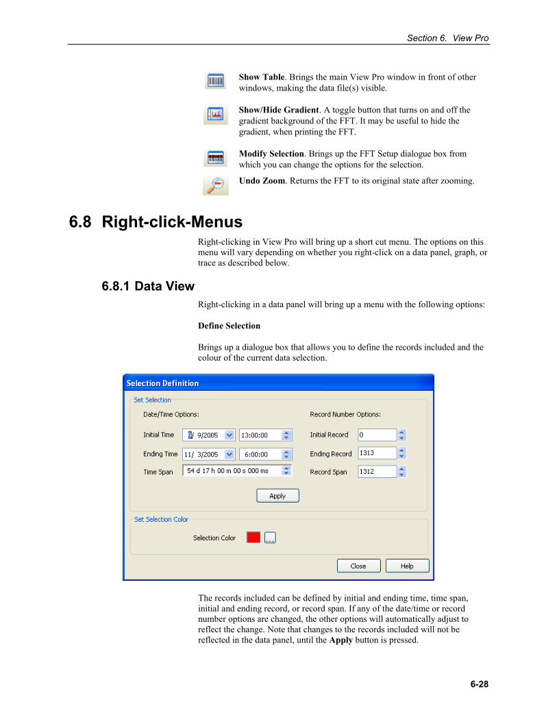
Section 6. View Pro
6-28
Show Table. Brings the main View Pro window in front of other windows, making the data file(s) visible.
Show/Hide Gradient. A toggle button that turns on and off the gradient background of the FFT. It may be useful to hide the gradient, when printing the FFT.
Modify Selection. Brings up the FFT Setup dialogue box from which you can change the options for the selection.
Undo Zoom. Returns the FFT to its original state after zooming.
6.8 Right-click-Menus
6.8.1 Data View
Right-clicking in View Pro will bring up a short cut menu. The options on this menu will vary depending on whether you right-click on a data panel, graph, or trace as described below.
Right-clicking in a data panel will bring up a menu with the following options:
Define Selection
Brings up a dialogue box that allows you to define the records included and the colour of the current data selection.
The records included can be defined by initial and ending time, time span, initial and ending record, or record span. If any of the date/time or record number options are changed, the other options will automatically adjust to reflect the change. Note that changes to the records included will not be reflected in the data panel, until the Apply button is pressed.
Section 6. View Pro
6-29
Copy Selection
Copies selected text to the Windows clipboard.
Add Selections to Graph
Adds the current selections to a graph. Click on or hover over this menu item to see a list of the opened graphs. Choose a graph to add the selections to. Note that this can be used to add selections made when Selected Graph is set to None to a graph. It can also be used to move selections from the currently-selected graph to a different graph.
Clear All Selections
Clears all selections in the currently selected data panel.
Clear Selection
In the currently selected data panel, clears the selection with focus. (This is the selection that has the dashed box around it. Left or right-click on a selection to give it focus.)
Format Columns
This option allows you to format a column in a binary (TOB) or CSIXML file. For a column containing a time, you can choose the date/time format option. For a column containing a floating point number, you can specify the number of decimal places, the number of leading zeroes, and whether the number is to be displayed in scientific notation. See ViewPro’s online help for more information.
Autosize Columns
Returns columns to the default sizes. (This function can also be accomplished by selecting View | Autosize Columns from the menu.)
Add Bookmark
The user can quickly navigate to a bookmarked record by using the Goto Bookmark option. Choosing the Add Bookmark option will add a bookmark to a record. When a record is bookmarked, a numbered circle (beginning at 0) will appear to the left of the record.
A bookmark can also be added to the top visible record by typing Ctrl-Shift-n, where n is the number of the bookmark.
Note that bookmarks are not persistent and will be gone once the data panel or View Pro is closed.
Goto Bookmark
If the data panel contains one or more bookmarks, hovering over the Goto Bookmark menu item will bring up a list of the current bookmarks. Selecting a bookmark from the list will automatically move the data panel to that record.
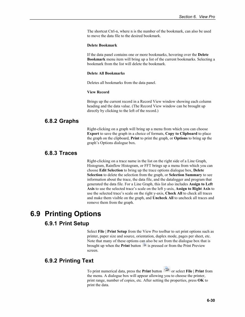
Section 6. View Pro
6-30
6.8.2 Graphs
6.8.3 Traces
The shortcut Ctrl-n, where n is the number of the bookmark, can also be used to move the data file to the desired bookmark.
Delete Bookmark
If the data panel contains one or more bookmarks, hovering over the Delete Bookmark menu item will bring up a list of the current bookmarks. Selecting a bookmark from the list will delete the bookmark.
Delete All Bookmarks
Deletes all bookmarks from the data panel.
View Record
Brings up the current record in a Record View window showing each column heading and the data value. (The Record View window can be brought up directly by clicking to the left of the record.)
Right-clicking on a graph will bring up a menu from which you can choose Export to save the graph in a choice of formats, Copy to Clipboard to place the graph on the clipboard, Print to print the graph, or Options to bring up the graph’s Options dialogue box.
Right-clicking on a trace name in the list on the right side of a Line Graph, Histogram, Rainflow Histogram, or FFT brings up a menu from which you can choose Edit Selection to bring up the trace options dialogue box, Delete Selection to delete the selection from the graph, or Selection Summary to see information about the trace, the data file, and the datalogger and program that generated the data file. For a Line Graph, this list also includes Assign to Left Axis to use the selected trace’s scale on the left y-axis, Assign to Right Axis to use the selected trace’s scale on the right y-axis, Check All to check all traces and make them visible on the graph, and Uncheck All to uncheck all traces and remove them from the graph.
6.9 Printing Options 6.9.1 Print Setup
Select File | Print Setup from the View Pro toolbar to set print options such as printer, paper size and source, orientation, duplex mode, pages per sheet, etc. Note that many of these options can also be set from the dialogue box that is brought up when the Print button is pressed or from the Print Preview screen.
6.9.2 Printing Text To print numerical data, press the Print button or select File | Print from the menu. A dialogue box will appear allowing you to choose the printer, print range, number of copies, etc. After setting the properties, press OK to print the data.
Section 6. View Pro
6-31
To preview your data before printing, press the Print Preview button or select File | Print Preview from the menu. From Print Preview you can browse among the pages that will be printed and change the paper orientation if desired. You can zoom in on a particular area of the previewed page by left-clicking the page. You can zoom out by left-clicking with the Shift button pressed. You can pan across a page by right-clicking and dragging the page. To return to normal view, choose the Page Width or the Full Page icon. Simply press the Print button on the toolbar to print one or more pages. See the online help for details of the Print Preview options.
6.9.3 Printing Graphs With a graph window opened, click the Print button to preview the printed page and set various printing options. Then select the Print button to print the graph. You can also right-click the graph to bring up a menu from which you can select Print.
6.10 View Pro Online Help View Pro has an online help system that can be accessed by choosing Help | View Pro from the toolbar. Once the help file is opened, pressing the Contents tab will open the Table of Contents. Choosing the Index tab will bring up an index. Keywords can be typed in to search for a topic. An in-depth search can be performed by choosing the Search tab and typing in a word.
Help for any of the graphical windows can be accessed by pressing the ? button in the upper right corner of the graph screen or by pressing F1. Help for dialogue boxes can be accessed by pressing the Help button at the bottom of the dialogue box or by pressing F1 with the dialogue box opened.
6.11 Assigning Data Files to View Windows will let you assign the program with which a particular file type will be opened based on that file’s extension. When a file with an assigned extension is double-clicked, it will be opened with the associated program. You may want to associate *.DAT files with the View Pro program for quick opening of data files. This association can be made by selecting Tools | Folder Options | File Types from the Windows Explorer menu.
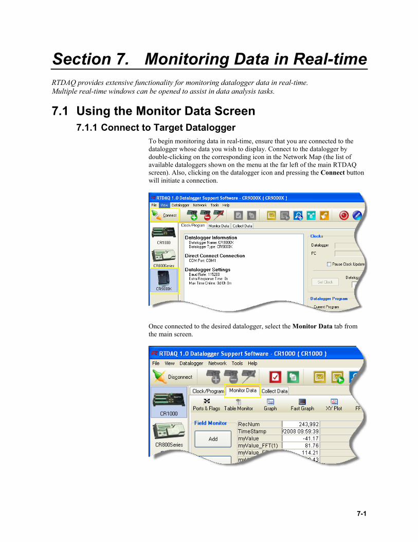
7-1
Section 7. Monitoring Data in Real-time RTDAQ provides extensive functionality for monitoring datalogger data in real-time. Multiple real-time windows can be opened to assist in data analysis tasks.
7.1 Using the Monitor Data Screen 7.1.1 Connect to Target Datalogger
To begin monitoring data in real-time, ensure that you are connected to the datalogger whose data you wish to display. Connect to the datalogger by double-clicking on the corresponding icon in the Network Map (the list of available dataloggers shown on the menu at the far left of the main RTDAQ screen). Also, clicking on the datalogger icon and pressing the Connect button will initiate a connection.
Once connected to the desired datalogger, select the Monitor Data tab from the main screen.
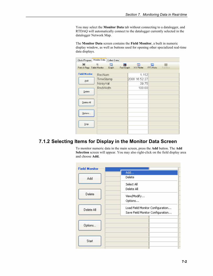
Section 7. Monitoring Data in Real-time
7-2
You may select the Monitor Data tab without connecting to a datalogger, and RTDAQ will automatically connect to the datalogger currently selected in the datalogger Network Map.
The Monitor Data screen contains the Field Monitor, a built in numeric display window, as well as buttons used for opening other specialized real-time data displays.
7.1.2 Selecting Items for Display in the Monitor Data Screen To monitor numeric data in the main screen, press the Add button. The Add Selection screen will appear. You may also right-click on the field display area and choose Add.
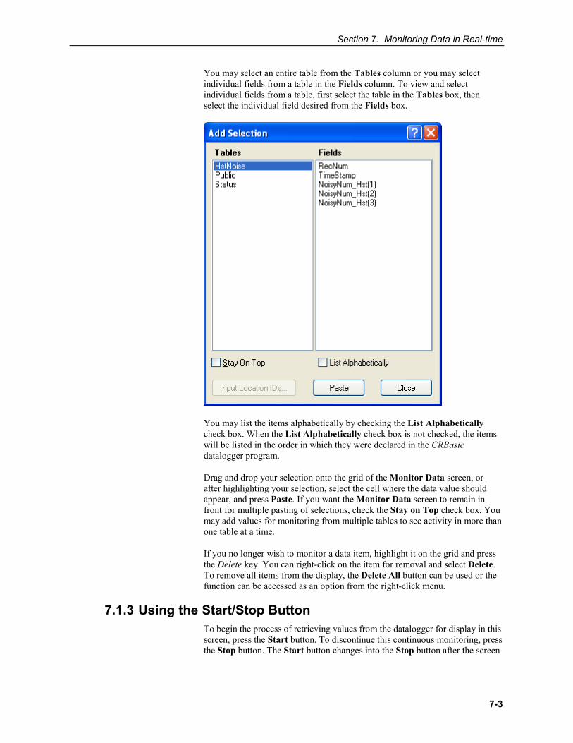
Section 7. Monitoring Data in Real-time
7-3
You may select an entire table from the Tables column or you may select individual fields from a table in the Fields column. To view and select individual fields from a table, first select the table in the Tables box, then select the individual field desired from the Fields box.
You may list the items alphabetically by checking the List Alphabetically check box. When the List Alphabetically check box is not checked, the items will be listed in the order in which they were declared in the CRBasic datalogger program.
Drag and drop your selection onto the grid of the Monitor Data screen, or after highlighting your selection, select the cell where the data value should appear, and press Paste. If you want the Monitor Data screen to remain in front for multiple pasting of selections, check the Stay on Top check box. You may add values for monitoring from multiple tables to see activity in more than one table at a time.
If you no longer wish to monitor a data item, highlight it on the grid and press the Delete key. You can right-click on the item for removal and select Delete. To remove all items from the display, the Delete All button can be used or the function can be accessed as an option from the right-click menu.
7.1.3 Using the Start/Stop Button To begin the process of retrieving values from the datalogger for display in this screen, press the Start button. To discontinue this continuous monitoring, press the Stop button. The Start button changes into the Stop button after the screen
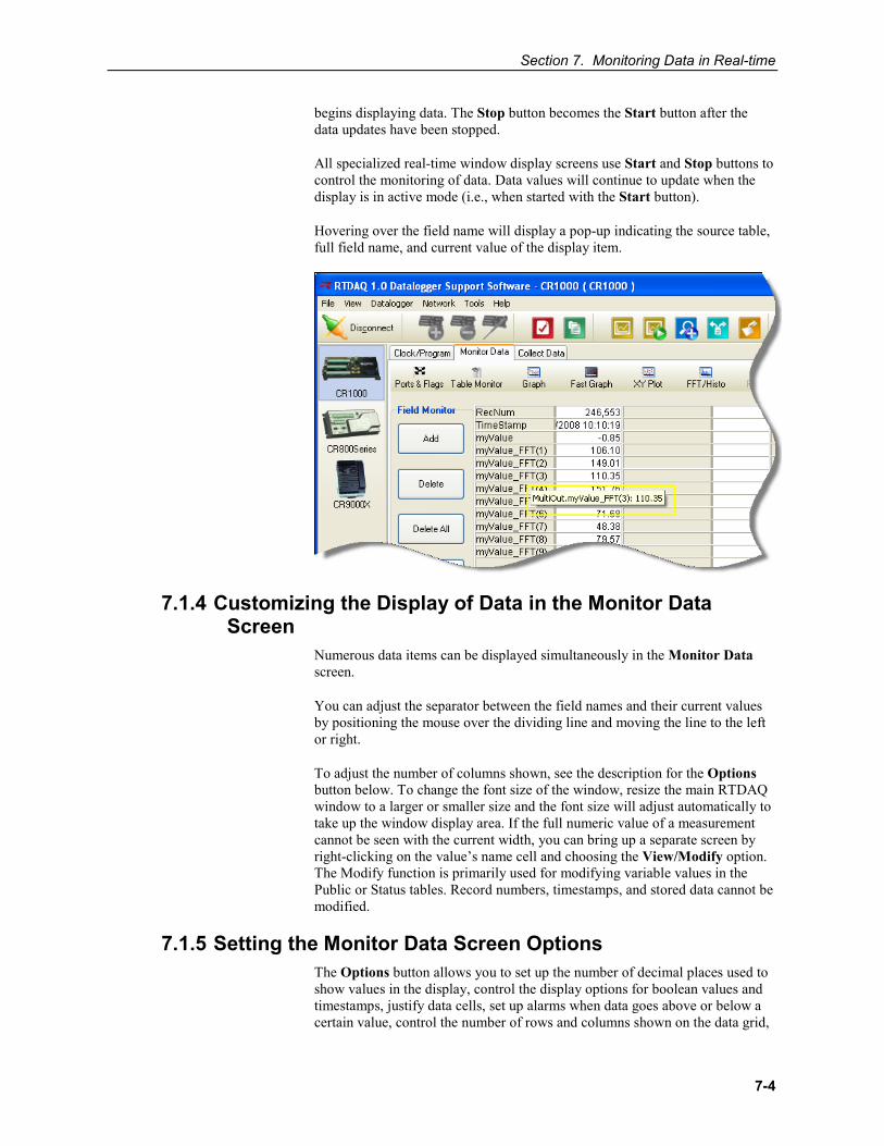
Section 7. Monitoring Data in Real-time
7-4
begins displaying data. The Stop button becomes the Start button after the data updates have been stopped.
All specialized real-time window display screens use Start and Stop buttons to control the monitoring of data. Data values will continue to update when the display is in active mode (i.e., when started with the Start button).
Hovering over the field name will display a pop-up indicating the source table, full field name, and current value of the display item.
7.1.4 Customizing the Display of Data in the Monitor Data Screen
Numerous data items can be displayed simultaneously in the Monitor Data screen.
You can adjust the separator between the field names and their current values by positioning the mouse over the dividing line and moving the line to the left or right.
To adjust the number of columns shown, see the description for the Options button below. To change the font size of the window, resize the main RTDAQ window to a larger or smaller size and the font size will adjust automatically to take up the window display area. If the full numeric value of a measurement cannot be seen with the current width, you can bring up a separate screen by right-clicking on the value’s name cell and choosing the View/Modify option. The Modify function is primarily used for modifying variable values in the Public or Status tables. Record numbers, timestamps, and stored data cannot be modified.
7.1.5 Setting the Monitor Data Screen Options The Options button allows you to set up the number of decimal places used to show values in the display, control the display options for boolean values and timestamps, justify data cells, set up alarms when data goes above or below a certain value, control the number of rows and columns shown on the data grid,
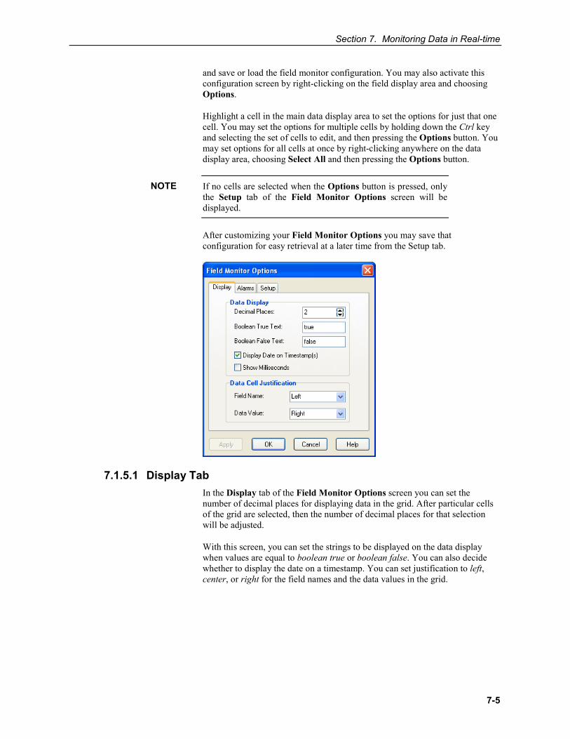
Section 7. Monitoring Data in Real-time
7-5
and save or load the field monitor configuration. You may also activate this configuration screen by right-clicking on the field display area and choosing Options.
Highlight a cell in the main data display area to set the options for just that one cell. You may set the options for multiple cells by holding down the Ctrl key and selecting the set of cells to edit, and then pressing the Options button. You may set options for all cells at once by right-clicking anywhere on the data display area, choosing Select All and then pressing the Options button.
If no cells are selected when the Options button is pressed, only the Setup tab of the Field Monitor Options screen will be displayed.
After customizing your Field Monitor Options you may save that configuration for easy retrieval at a later time from the Setup tab.
7.1.5.1 Display Tab In the Display tab of the Field Monitor Options screen you can set the number of decimal places for displaying data in the grid. After particular cells of the grid are selected, then the number of decimal places for that selection will be adjusted.
With this screen, you can set the strings to be displayed on the data display when values are equal to boolean true or boolean false. You can also decide whether to display the date on a timestamp. You can set justification to left, center, or right for the field names and the data values in the grid.
NOTE
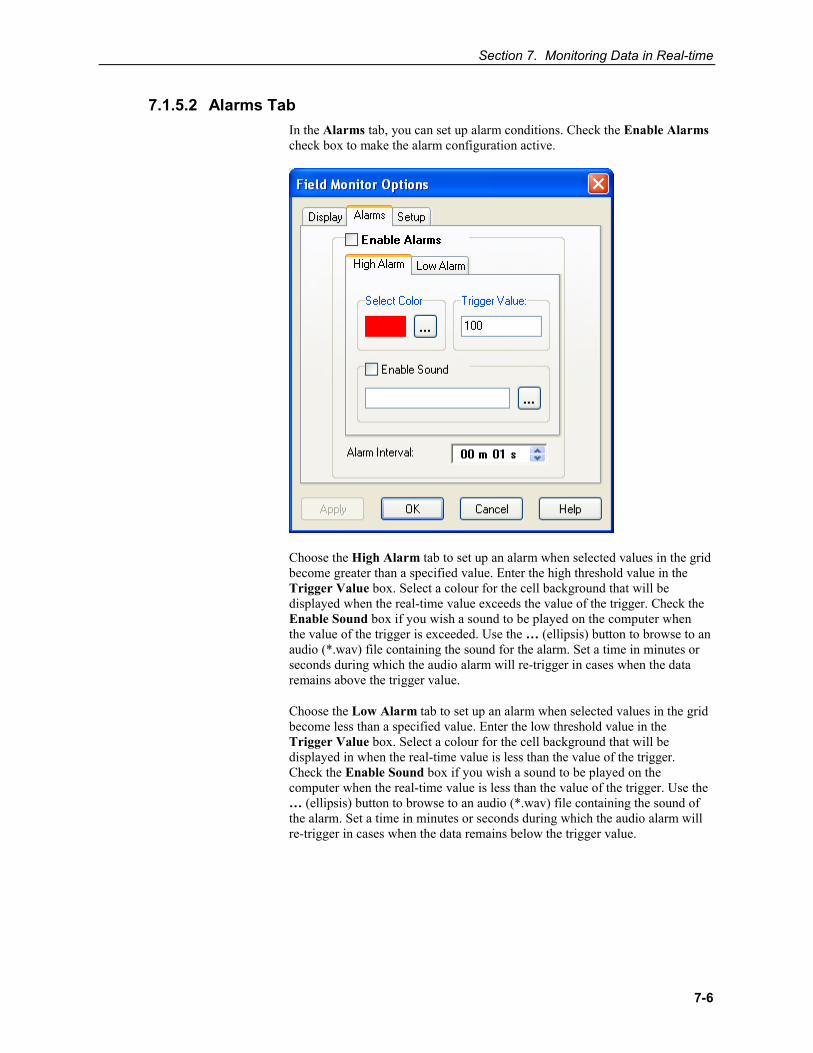
Section 7. Monitoring Data in Real-time
7-6
7.1.5.2 Alarms Tab In the Alarms tab, you can set up alarm conditions. Check the Enable Alarms check box to make the alarm configuration active.
Choose the High Alarm tab to set up an alarm when selected values in the grid become greater than a specified value. Enter the high threshold value in the Trigger Value box. Select a colour for the cell background that will be displayed when the real-time value exceeds the value of the trigger. Check the Enable Sound box if you wish a sound to be played on the computer when the value of the trigger is exceeded. Use the … (ellipsis) button to browse to an audio (*.wav) file containing the sound for the alarm. Set a time in minutes or seconds during which the audio alarm will re-trigger in cases when the data remains above the trigger value.
Choose the Low Alarm tab to set up an alarm when selected values in the grid become less than a specified value. Enter the low threshold value in the Trigger Value box. Select a colour for the cell background that will be displayed in when the real-time value is less than the value of the trigger. Check the Enable Sound box if you wish a sound to be played on the computer when the real-time value is less than the value of the trigger. Use the … (ellipsis) button to browse to an audio (*.wav) file containing the sound of the alarm. Set a time in minutes or seconds during which the audio alarm will re-trigger in cases when the data remains below the trigger value.
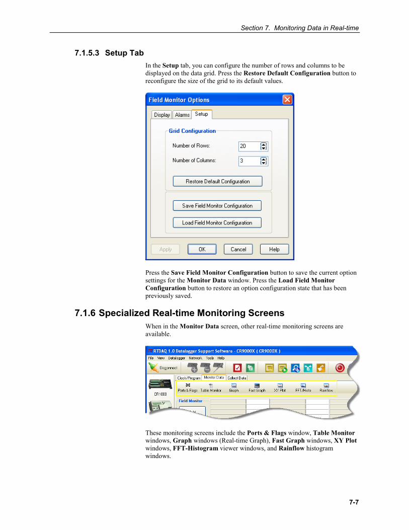
Section 7. Monitoring Data in Real-time
7-7
7.1.5.3 Setup Tab In the Setup tab, you can configure the number of rows and columns to be displayed on the data grid. Press the Restore Default Configuration button to reconfigure the size of the grid to its default values.
Press the Save Field Monitor Configuration button to save the current option settings for the Monitor Data window. Press the Load Field Monitor Configuration button to restore an option configuration state that has been previously saved.
7.1.6 Specialized Real-time Monitoring Screens When in the Monitor Data screen, other real-time monitoring screens are available.
These monitoring screens include the Ports & Flags window, Table Monitor windows, Graph windows (Real-time Graph), Fast Graph windows, XY Plot windows, FFT-Histogram viewer windows, and Rainflow histogram windows.
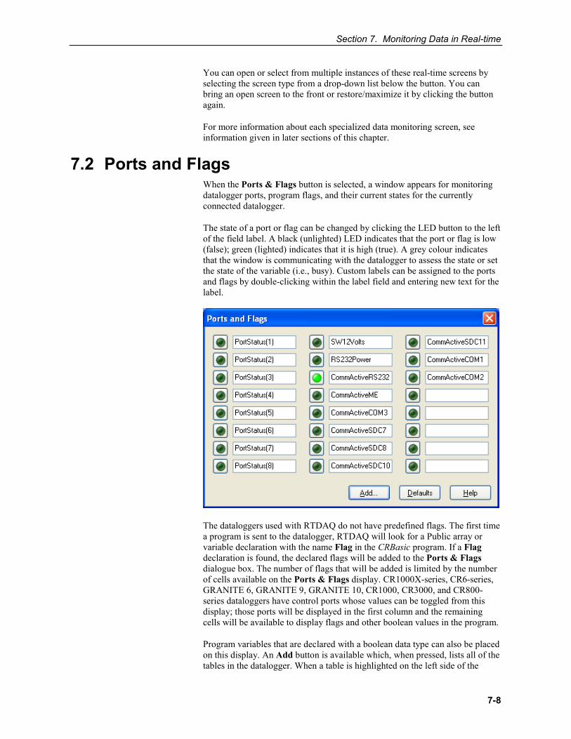
Section 7. Monitoring Data in Real-time
7-8
You can open or select from multiple instances of these real-time screens by selecting the screen type from a drop-down list below the button. You can bring an open screen to the front or restore/maximize it by clicking the button again.
For more information about each specialized data monitoring screen, see information given in later sections of this chapter.
7.2 Ports and Flags When the Ports & Flags button is selected, a window appears for monitoring datalogger ports, program flags, and their current states for the currently connected datalogger.
The state of a port or flag can be changed by clicking the LED button to the left of the field label. A black (unlighted) LED indicates that the port or flag is low (false); green (lighted) indicates that it is high (true). A grey colour indicates that the window is communicating with the datalogger to assess the state or set the state of the variable (i.e., busy). Custom labels can be assigned to the ports and flags by double-clicking within the label field and entering new text for the label.
The dataloggers used with RTDAQ do not have predefined flags. The first time a program is sent to the datalogger, RTDAQ will look for a Public array or variable declaration with the name Flag in the CRBasic program. If a Flag declaration is found, the declared flags will be added to the Ports & Flags dialogue box. The number of flags that will be added is limited by the number of cells available on the Ports & Flags display. CR1000X-series, CR6-series, GRANITE 6, GRANITE 9, GRANITE 10, CR1000, CR3000, and CR800-series dataloggers have control ports whose values can be toggled from this display; those ports will be displayed in the first column and the remaining cells will be available to display flags and other boolean values in the program.
Program variables that are declared with a boolean data type can also be placed on this display. An Add button is available which, when pressed, lists all of the tables in the datalogger. When a table is highlighted on the left side of the
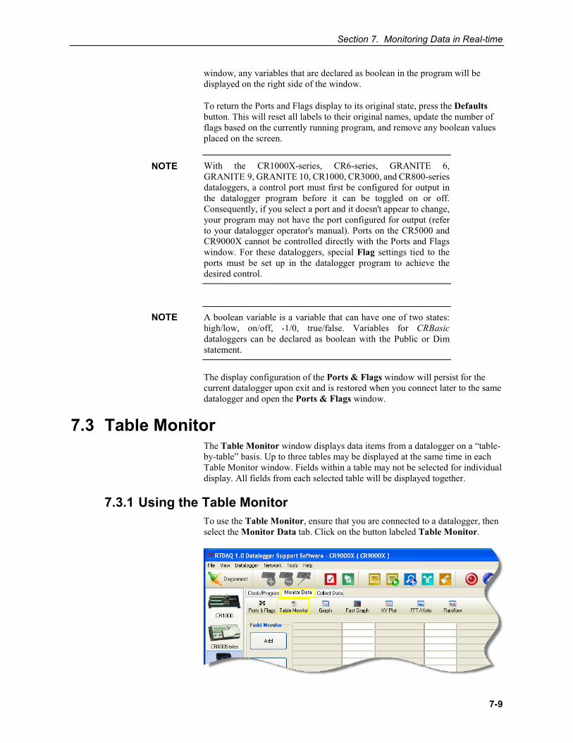
Section 7. Monitoring Data in Real-time
7-9
window, any variables that are declared as boolean in the program will be displayed on the right side of the window.
To return the Ports and Flags display to its original state, press the Defaults button. This will reset all labels to their original names, update the number of flags based on the currently running program, and remove any boolean values placed on the screen.
With the CR1000X-series, CR6-series, GRANITE 6, GRANITE 9, GRANITE 10, CR1000, CR3000, and CR800-series dataloggers, a control port must first be configured for output in the datalogger program before it can be toggled on or off. Consequently, if you select a port and it doesn't appear to change, your program may not have the port configured for output (refer to your datalogger operator's manual). Ports on the CR5000 and CR9000X cannot be controlled directly with the Ports and Flags window. For these dataloggers, special Flag settings tied to the ports must be set up in the datalogger program to achieve the desired control.
A boolean variable is a variable that can have one of two states: high/low, on/off, -1/0, true/false. Variables for CRBasic dataloggers can be declared as boolean with the Public or Dim statement.
The display configuration of the Ports & Flags window will persist for the current datalogger upon exit and is restored when you connect later to the same datalogger and open the Ports & Flags window.
7.3 Table Monitor The Table Monitor window displays data items from a datalogger on a “table-by-table” basis. Up to three tables may be displayed at the same time in each Table Monitor window. Fields within a table may not be selected for individual display. All fields from each selected table will be displayed together.
7.3.1 Using the Table Monitor To use the Table Monitor, ensure that you are connected to a datalogger, then select the Monitor Data tab. Click on the button labeled Table Monitor.
NOTE
NOTE
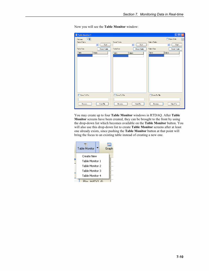
Section 7. Monitoring Data in Real-time
7-10
Now you will see the Table Monitor window:
You may create up to four Table Monitor windows in RTDAQ. After Table Monitor screens have been created, they can be brought to the front by using the drop-down list which becomes available on the Table Monitor button. You will also use this drop-down list to create Table Monitor screens after at least one already exists, since pushing the Table Monitor button at that point will bring the focus to an existing table instead of creating a new one.
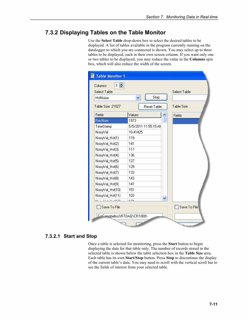
Section 7. Monitoring Data in Real-time
7-11
7.3.2 Displaying Tables on the Table Monitor Use the Select Table drop-down box to select the desired tables to be displayed. A list of tables available in the program currently running on the datalogger to which you are connected is shown. You may select up to three tables to be displayed, each in their own screen column. If you want only one or two tables to be displayed, you may reduce the value in the Columns spin box, which will also reduce the width of the screen.
7.3.2.1 Start and Stop Once a table is selected for monitoring, press the Start button to begin displaying the data for that table only. The number of records stored in the selected table is shown below the table selection box in the Table Size area. Each table has its own Start/Stop button. Press Stop to discontinue the display of the current table’s data. You may need to scroll with the vertical scroll bar to see the fields of interest from your selected table.
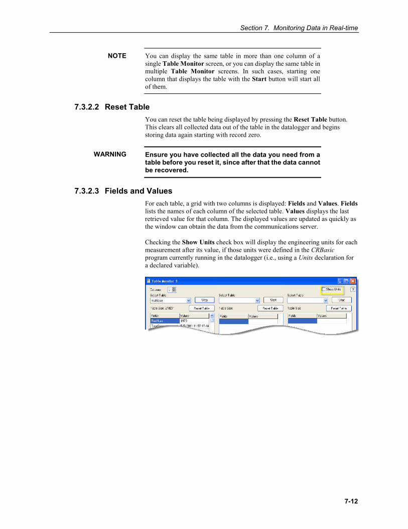
Section 7. Monitoring Data in Real-time
7-12
You can display the same table in more than one column of a single Table Monitor screen, or you can display the same table in multiple Table Monitor screens. In such cases, starting one column that displays the table with the Start button will start all of them.
7.3.2.2 Reset Table You can reset the table being displayed by pressing the Reset Table button. This clears all collected data out of the table in the datalogger and begins storing data again starting with record zero.
Ensure you have collected all the data you need from a table before you reset it, since after that the data cannot be recovered.
7.3.2.3 Fields and Values For each table, a grid with two columns is displayed: Fields and Values. Fields lists the names of each column of the selected table. Values displays the last retrieved value for that column. The displayed values are updated as quickly as the window can obtain the data from the communications server.
Checking the Show Units check box will display the engineering units for each measurement after its value, if those units were defined in the CRBasic program currently running in the datalogger (i.e., using a Units declaration for a declared variable).
NOTE
WARNING
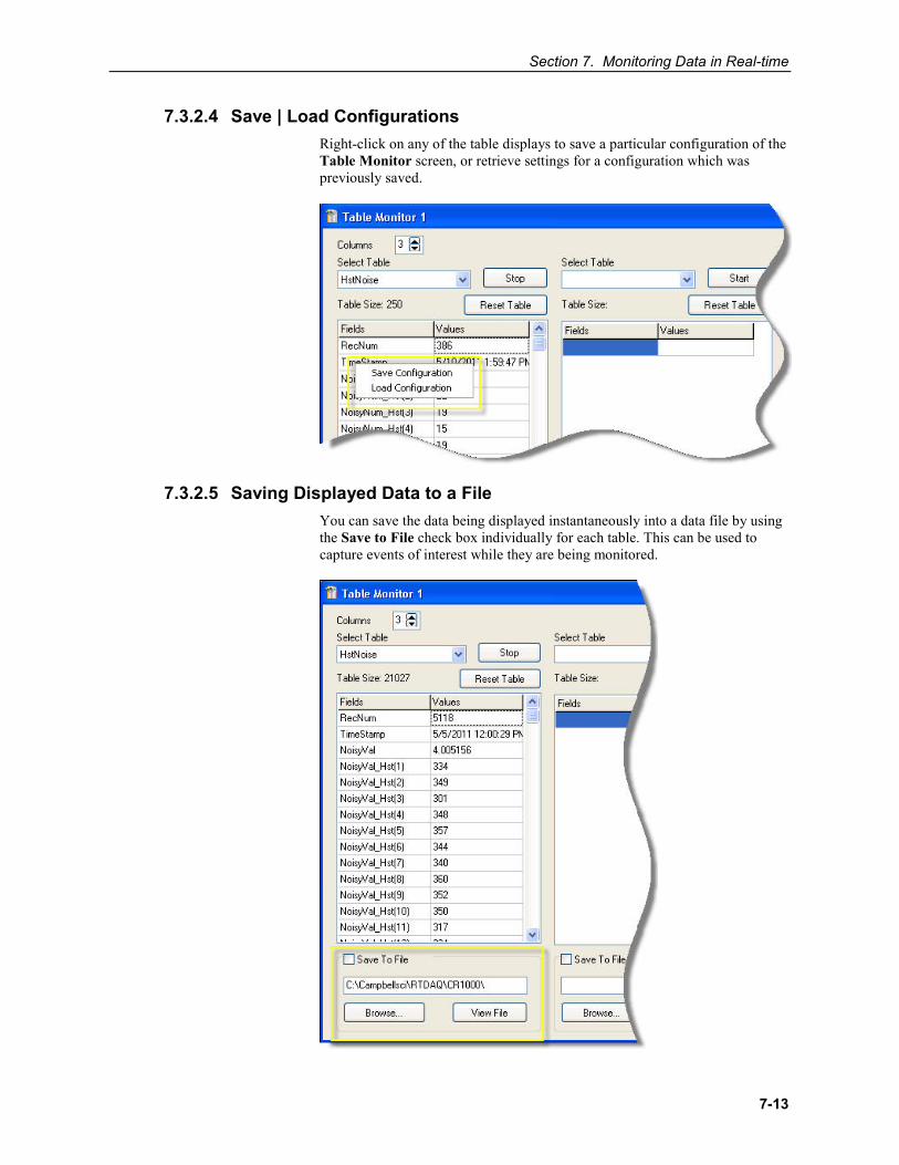
Section 7. Monitoring Data in Real-time
7-13
7.3.2.4 Save | Load Configurations Right-click on any of the table displays to save a particular configuration of the Table Monitor screen, or retrieve settings for a configuration which was previously saved.
7.3.2.5 Saving Displayed Data to a File You can save the data being displayed instantaneously into a data file by using the Save to File check box individually for each table. This can be used to capture events of interest while they are being monitored.
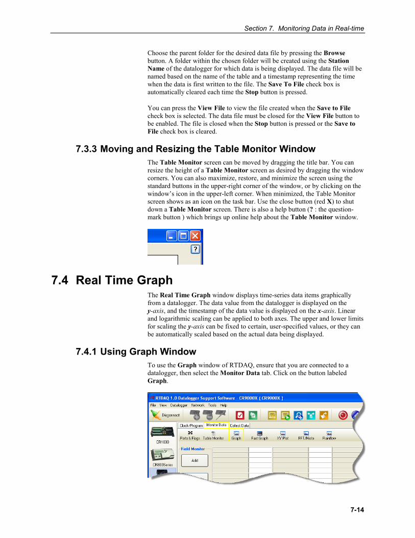
Section 7. Monitoring Data in Real-time
7-14
Choose the parent folder for the desired data file by pressing the Browse button. A folder within the chosen folder will be created using the Station Name of the datalogger for which data is being displayed. The data file will be named based on the name of the table and a timestamp representing the time when the data is first written to the file. The Save To File check box is automatically cleared each time the Stop button is pressed.
You can press the View File to view the file created when the Save to File check box is selected. The data file must be closed for the View File button to be enabled. The file is closed when the Stop button is pressed or the Save to File check box is cleared.
7.3.3 Moving and Resizing the Table Monitor Window The Table Monitor screen can be moved by dragging the title bar. You can resize the height of a Table Monitor screen as desired by dragging the window corners. You can also maximize, restore, and minimize the screen using the standard buttons in the upper-right corner of the window, or by clicking on the window’s icon in the upper-left corner. When minimized, the Table Monitor screen shows as an icon on the task bar. Use the close button (red X) to shut down a Table Monitor screen. There is also a help button (? : the question-mark button ) which brings up online help about the Table Monitor window.
7.4 Real Time Graph The Real Time Graph window displays time-series data items graphically from a datalogger. The data value from the datalogger is displayed on the y-axis, and the timestamp of the data value is displayed on the x-axis. Linear and logarithmic scaling can be applied to both axes. The upper and lower limits for scaling the y-axis can be fixed to certain, user-specified values, or they can be automatically scaled based on the actual data being displayed.
7.4.1 Using Graph Window To use the Graph window of RTDAQ, ensure that you are connected to a datalogger, then select the Monitor Data tab. Click on the button labeled Graph.
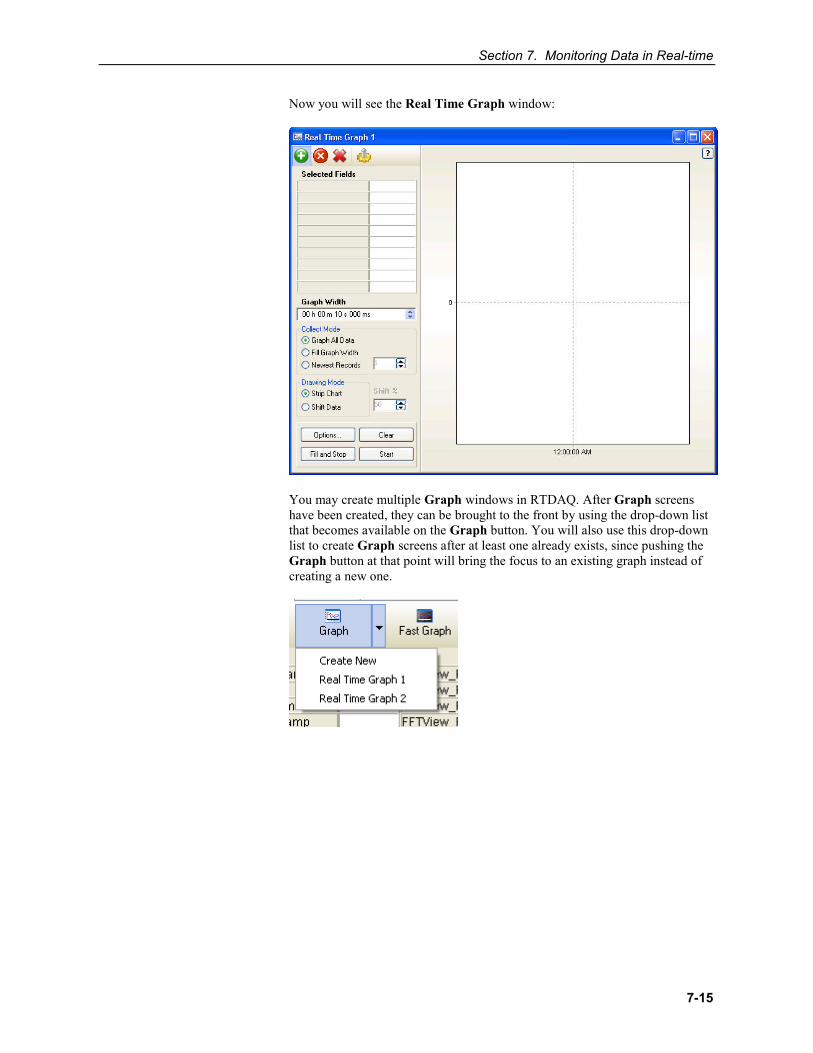
Section 7. Monitoring Data in Real-time
7-15
Now you will see the Real Time Graph window:
You may create multiple Graph windows in RTDAQ. After Graph screens have been created, they can be brought to the front by using the drop-down list that becomes available on the Graph button. You will also use this drop-down list to create Graph screens after at least one already exists, since pushing the Graph button at that point will bring the focus to an existing graph instead of creating a new one.
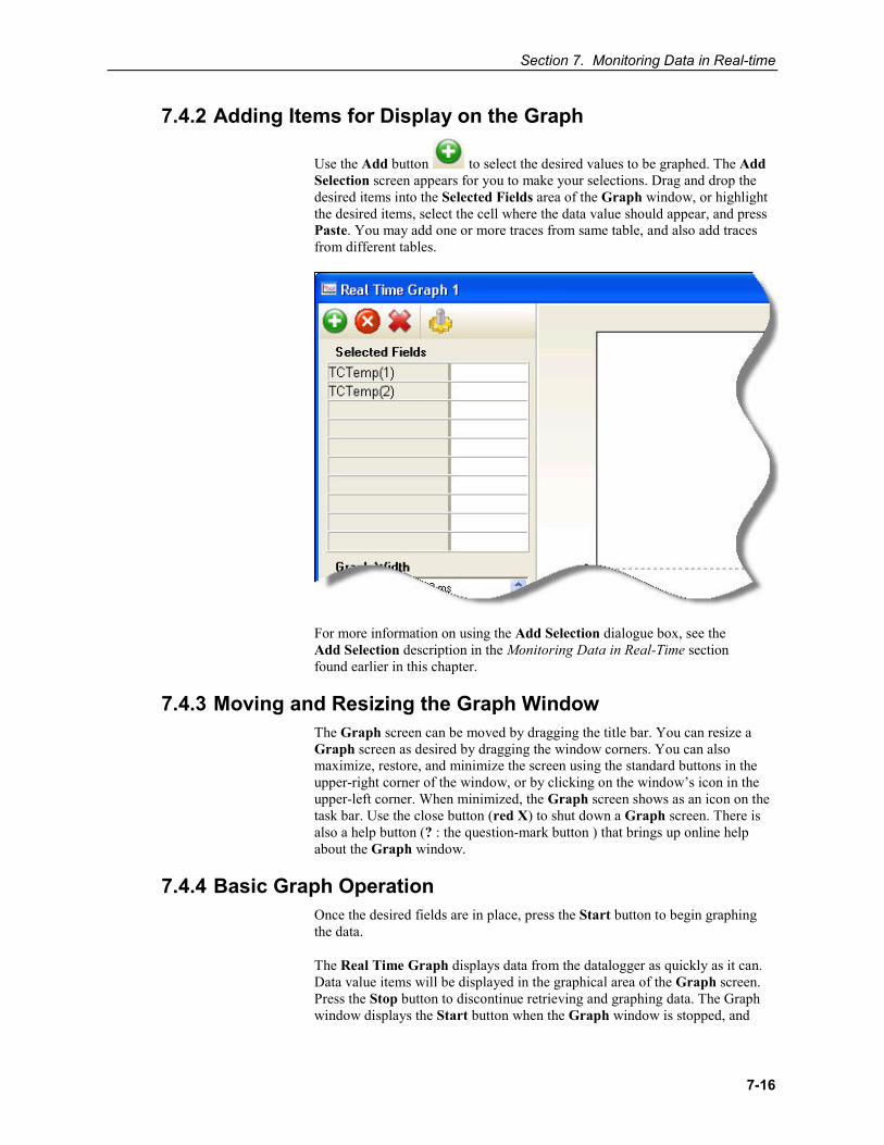
Section 7. Monitoring Data in Real-time
7-16
7.4.2 Adding Items for Display on the Graph
Use the Add button to select the desired values to be graphed. The Add Selection screen appears for you to make your selections. Drag and drop the desired items into the Selected Fields area of the Graph window, or highlight the desired items, select the cell where the data value should appear, and press Paste. You may add one or more traces from same table, and also add traces from different tables.
For more information on using the Add Selection dialogue box, see the Add Selection description in the Monitoring Data in Real-Time section found earlier in this chapter.
7.4.3 Moving and Resizing the Graph Window The Graph screen can be moved by dragging the title bar. You can resize a Graph screen as desired by dragging the window corners. You can also maximize, restore, and minimize the screen using the standard buttons in the upper-right corner of the window, or by clicking on the window’s icon in the upper-left corner. When minimized, the Graph screen shows as an icon on the task bar. Use the close button (red X) to shut down a Graph screen. There is also a help button (? : the question-mark button ) that brings up online help about the Graph window.
7.4.4 Basic Graph Operation Once the desired fields are in place, press the Start button to begin graphing the data.
The Real Time Graph displays data from the datalogger as quickly as it can. Data value items will be displayed in the graphical area of the Graph screen. Press the Stop button to discontinue retrieving and graphing data. The Graph window displays the Start button when the Graph window is stopped, and
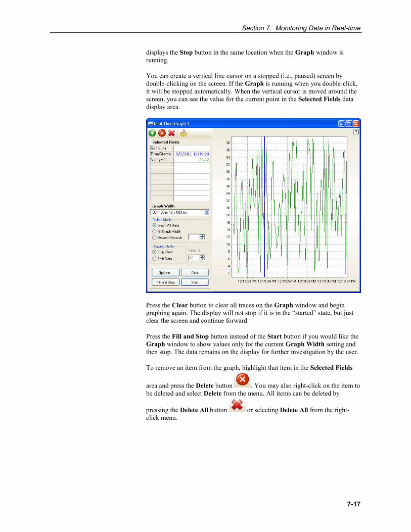
Section 7. Monitoring Data in Real-time
7-17
displays the Stop button in the same location when the Graph window is running.
You can create a vertical line cursor on a stopped (i.e., paused) screen by double-clicking on the screen. If the Graph is running when you double-click, it will be stopped automatically. When the vertical cursor is moved around the screen, you can see the value for the current point in the Selected Fields data display area.
Press the Clear button to clear all traces on the Graph window and begin graphing again. The display will not stop if it is in the “started” state, but just clear the screen and continue forward.
Press the Fill and Stop button instead of the Start button if you would like the Graph window to show values only for the current Graph Width setting and then stop. The data remains on the display for further investigation by the user.
To remove an item from the graph, highlight that item in the Selected Fields
area and press the Delete button . You may also right-click on the item to be deleted and select Delete from the menu. All items can be deleted by
pressing the Delete All button or selecting Delete All from the right-click menu.
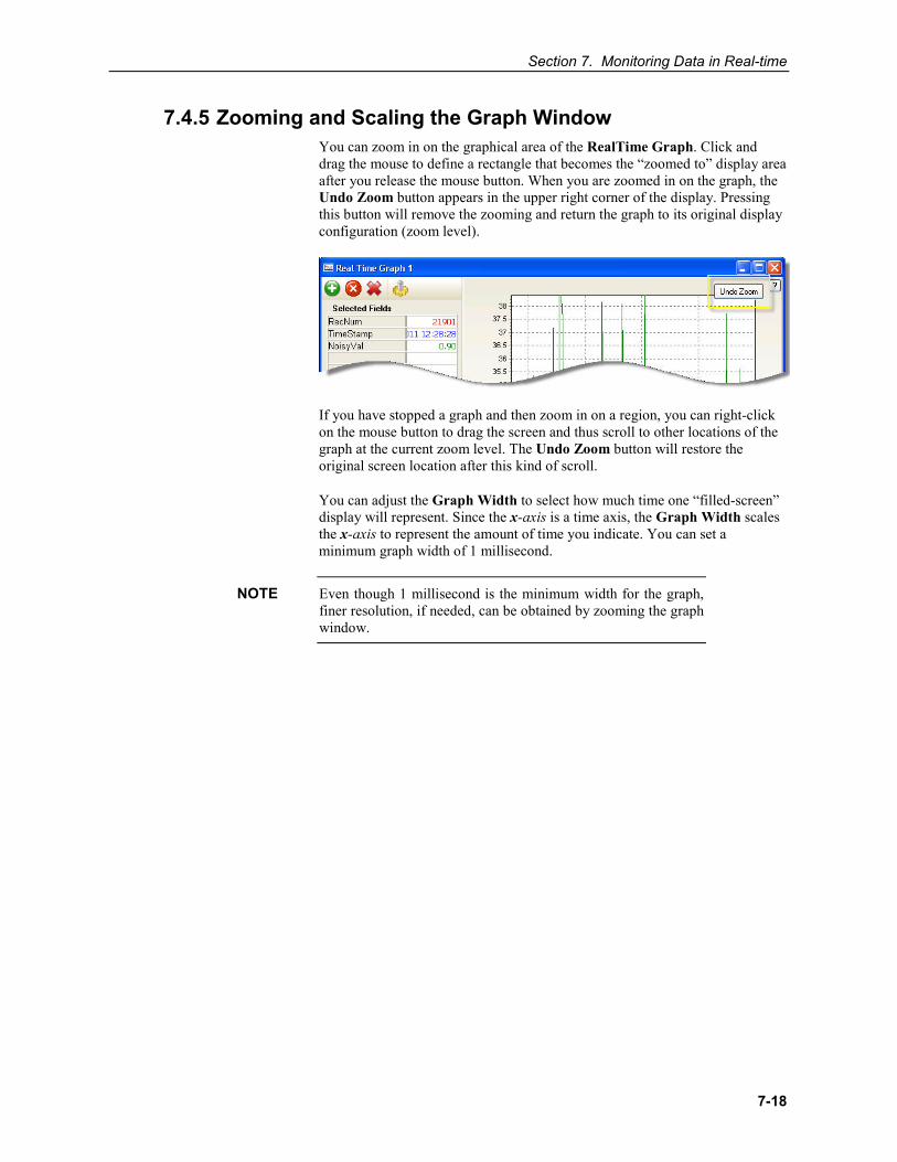
Section 7. Monitoring Data in Real-time
7-18
7.4.5 Zooming and Scaling the Graph Window You can zoom in on the graphical area of the RealTime Graph. Click and drag the mouse to define a rectangle that becomes the “zoomed to” display area after you release the mouse button. When you are zoomed in on the graph, the Undo Zoom button appears in the upper right corner of the display. Pressing this button will remove the zooming and return the graph to its original display configuration (zoom level).
If you have stopped a graph and then zoom in on a region, you can right-click on the mouse button to drag the screen and thus scroll to other locations of the graph at the current zoom level. The Undo Zoom button will restore the original screen location after this kind of scroll.
You can adjust the Graph Width to select how much time one “filled-screen” display will represent. Since the x-axis is a time axis, the Graph Width scales the x-axis to represent the amount of time you indicate. You can set a minimum graph width of 1 millisecond.
Even though 1 millisecond is the minimum width for the graph, finer resolution, if needed, can be obtained by zooming the graph window.
NOTE
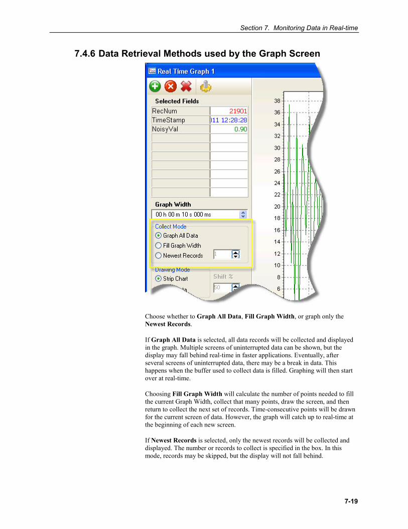
Section 7. Monitoring Data in Real-time
7-19
7.4.6 Data Retrieval Methods used by the Graph Screen
Choose whether to Graph All Data, Fill Graph Width, or graph only the Newest Records.
If Graph All Data is selected, all data records will be collected and displayed in the graph. Multiple screens of uninterrupted data can be shown, but the display may fall behind real-time in faster applications. Eventually, after several screens of uninterrupted data, there may be a break in data. This happens when the buffer used to collect data is filled. Graphing will then start over at real-time.
Choosing Fill Graph Width will calculate the number of points needed to fill the current Graph Width, collect that many points, draw the screen, and then return to collect the next set of records. Time-consecutive points will be drawn for the current screen of data. However, the graph will catch up to real-time at the beginning of each new screen.
If Newest Records is selected, only the newest records will be collected and displayed. The number or records to collect is specified in the box. In this mode, records may be skipped, but the display will not fall behind.
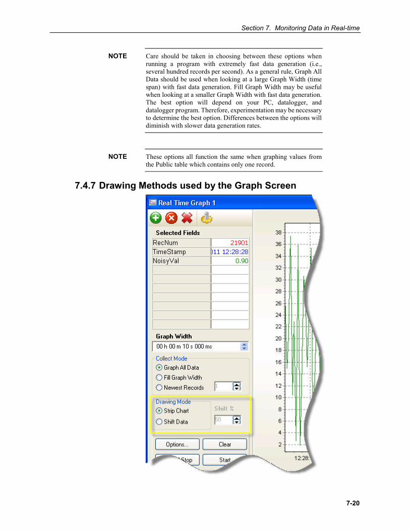
Section 7. Monitoring Data in Real-time
7-20
Care should be taken in choosing between these options when running a program with extremely fast data generation (i.e., several hundred records per second). As a general rule, Graph All Data should be used when looking at a large Graph Width (time span) with fast data generation. Fill Graph Width may be useful when looking at a smaller Graph Width with fast data generation. The best option will depend on your PC, datalogger, and datalogger program. Therefore, experimentation may be necessary to determine the best option. Differences between the options will diminish with slower data generation rates.
These options all function the same when graphing values from the Public table which contains only one record.
7.4.7 Drawing Methods used by the Graph Screen
NOTE
NOTE
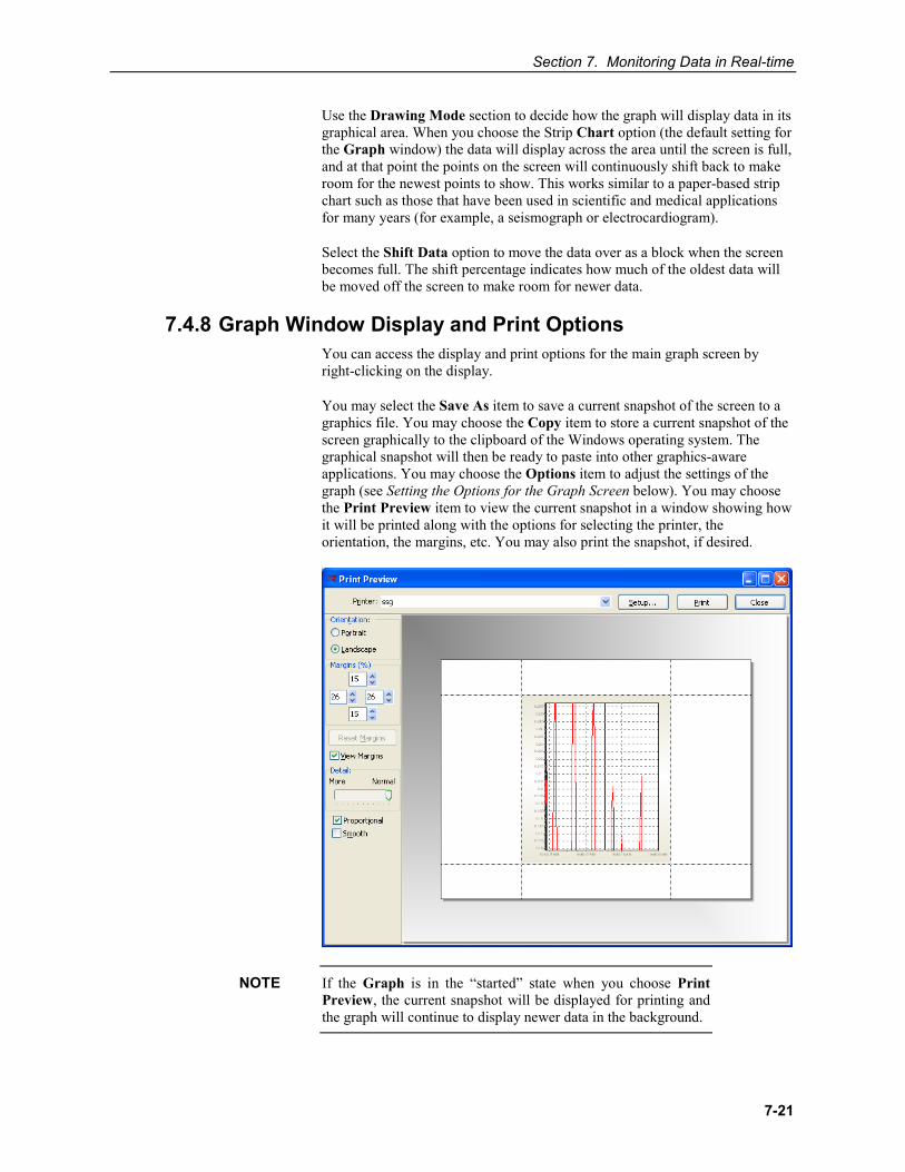
Section 7. Monitoring Data in Real-time
7-21
Use the Drawing Mode section to decide how the graph will display data in its graphical area. When you choose the Strip Chart option (the default setting for the Graph window) the data will display across the area until the screen is full, and at that point the points on the screen will continuously shift back to make room for the newest points to show. This works similar to a paper-based strip chart such as those that have been used in scientific and medical applications for many years (for example, a seismograph or electrocardiogram).
Select the Shift Data option to move the data over as a block when the screen becomes full. The shift percentage indicates how much of the oldest data will be moved off the screen to make room for newer data.
7.4.8 Graph Window Display and Print Options You can access the display and print options for the main graph screen by right-clicking on the display.
You may select the Save As item to save a current snapshot of the screen to a graphics file. You may choose the Copy item to store a current snapshot of the screen graphically to the clipboard of the Windows operating system. The graphical snapshot will then be ready to paste into other graphics-aware applications. You may choose the Options item to adjust the settings of the graph (see Setting the Options for the Graph Screen below). You may choose the Print Preview item to view the current snapshot in a window showing how it will be printed along with the options for selecting the printer, the orientation, the margins, etc. You may also print the snapshot, if desired.
If the Graph is in the “started” state when you choose Print Preview, the current snapshot will be displayed for printing and the graph will continue to display newer data in the background.
NOTE
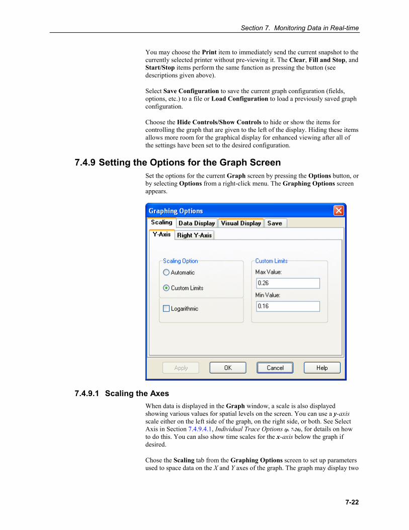
Section 7. Monitoring Data in Real-time
7-22
You may choose the Print item to immediately send the current snapshot to the currently selected printer without pre-viewing it. The Clear, Fill and Stop, and Start/Stop items perform the same function as pressing the button (see descriptions given above).
Select Save Configuration to save the current graph configuration (fields, options, etc.) to a file or Load Configuration to load a previously saved graph configuration.
Choose the Hide Controls/Show Controls to hide or show the items for controlling the graph that are given to the left of the display. Hiding these items allows more room for the graphical display for enhanced viewing after all of the settings have been set to the desired configuration.
7.4.9 Setting the Options for the Graph Screen Set the options for the current Graph screen by pressing the Options button, or by selecting Options from a right-click menu. The Graphing Options screen appears.
7.4.9.1 Scaling the Axes When data is displayed in the Graph window, a scale is also displayed showing various values for spatial levels on the screen. You can use a y-axis scale either on the left side of the graph, on the right side, or both. See Select Axis in Section 7.4.9.4.1, Individual Trace Options (p. 7-26), for details on how to do this. You can also show time scales for the x-axis below the graph if desired.
Chose the Scaling tab from the Graphing Options screen to set up parameters used to space data on the X and Y axes of the graph. The graph may display two
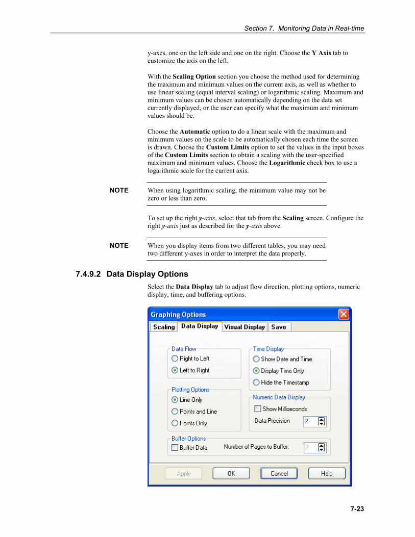
Section 7. Monitoring Data in Real-time
7-23
y-axes, one on the left side and one on the right. Choose the Y Axis tab to customize the axis on the left.
With the Scaling Option section you choose the method used for determining the maximum and minimum values on the current axis, as well as whether to use linear scaling (equal interval scaling) or logarithmic scaling. Maximum and minimum values can be chosen automatically depending on the data set currently displayed, or the user can specify what the maximum and minimum values should be.
Choose the Automatic option to do a linear scale with the maximum and minimum values on the scale to be automatically chosen each time the screen is drawn. Choose the Custom Limits option to set the values in the input boxes of the Custom Limits section to obtain a scaling with the user-specified maximum and minimum values. Choose the Logarithmic check box to use a logarithmic scale for the current axis.
When using logarithmic scaling, the minimum value may not be zero or less than zero.
To set up the right y-axis, select that tab from the Scaling screen. Configure the right y-axis just as described for the y-axis above.
When you display items from two different tables, you may need two different y-axes in order to interpret the data properly.
7.4.9.2 Data Display Options Select the Data Display tab to adjust flow direction, plotting options, numeric display, time, and buffering options.
NOTE
NOTE
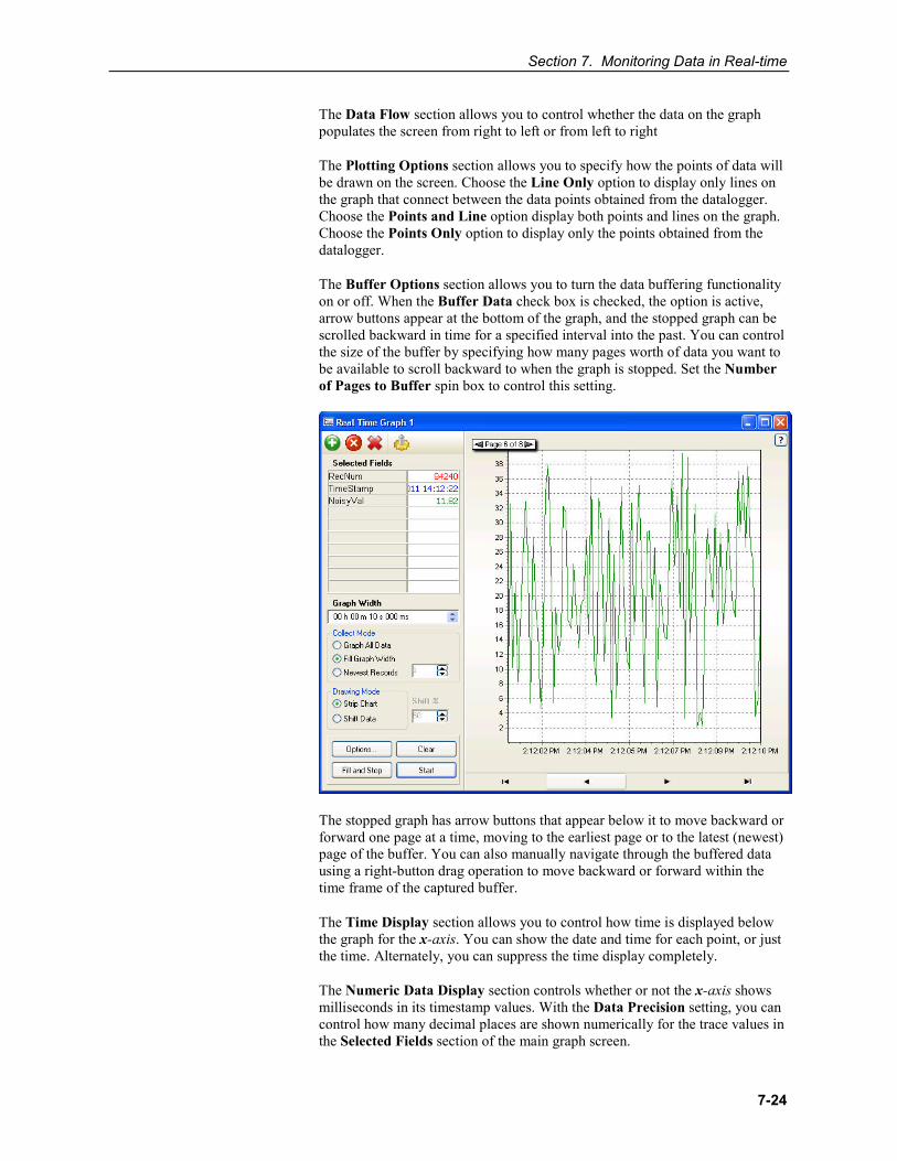
Section 7. Monitoring Data in Real-time
7-24
The Data Flow section allows you to control whether the data on the graph populates the screen from right to left or from left to right
The Plotting Options section allows you to specify how the points of data will be drawn on the screen. Choose the Line Only option to display only lines on the graph that connect between the data points obtained from the datalogger. Choose the Points and Line option display both points and lines on the graph. Choose the Points Only option to display only the points obtained from the datalogger.
The Buffer Options section allows you to turn the data buffering functionality on or off. When the Buffer Data check box is checked, the option is active, arrow buttons appear at the bottom of the graph, and the stopped graph can be scrolled backward in time for a specified interval into the past. You can control the size of the buffer by specifying how many pages worth of data you want to be available to scroll backward to when the graph is stopped. Set the Number of Pages to Buffer spin box to control this setting.
The stopped graph has arrow buttons that appear below it to move backward or forward one page at a time, moving to the earliest page or to the latest (newest) page of the buffer. You can also manually navigate through the buffered data using a right-button drag operation to move backward or forward within the time frame of the captured buffer.
The Time Display section allows you to control how time is displayed below the graph for the x-axis. You can show the date and time for each point, or just the time. Alternately, you can suppress the time display completely.
The Numeric Data Display section controls whether or not the x-axis shows milliseconds in its timestamp values. With the Data Precision setting, you can control how many decimal places are shown numerically for the trace values in the Selected Fields section of the main graph screen.
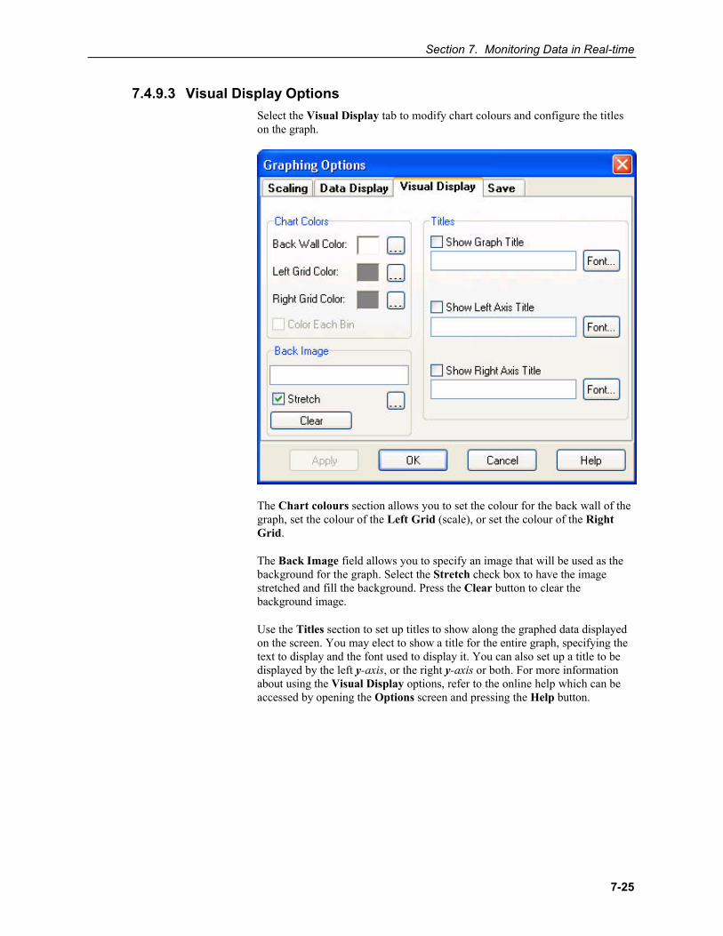
Section 7. Monitoring Data in Real-time
7-25
7.4.9.3 Visual Display Options Select the Visual Display tab to modify chart colours and configure the titles on the graph.
The Chart colours section allows you to set the colour for the back wall of the graph, set the colour of the Left Grid (scale), or set the colour of the Right Grid.
The Back Image field allows you to specify an image that will be used as the background for the graph. Select the Stretch check box to have the image stretched and fill the background. Press the Clear button to clear the background image.
Use the Titles section to set up titles to show along the graphed data displayed on the screen. You may elect to show a title for the entire graph, specifying the text to display and the font used to display it. You can also set up a title to be displayed by the left y-axis, or the right y-axis or both. For more information about using the Visual Display options, refer to the online help which can be accessed by opening the Options screen and pressing the Help button.
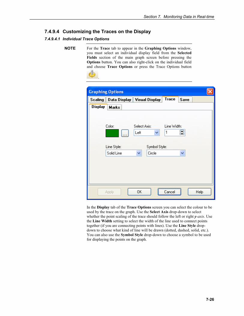
Section 7. Monitoring Data in Real-time
7-26
7.4.9.4 Customizing the Traces on the Display 7.4.9.4.1 Individual Trace Options
For the Trace tab to appear in the Graphing Options window, you must select an individual display field from the Selected Fields section of the main graph screen before pressing the Options button. You can also right-click on the individual field and choose Trace Options or press the Trace Options button
.
In the Display tab of the Trace Options screen you can select the colour to be used by the trace on the graph. Use the Select Axis drop-down to select whether the point scaling of the trace should follow the left or right y-axis. Use the Line Width setting to select the width of the line used to connect points together (if you are connecting points with lines). Use the Line Style drop-down to choose what kind of line will be drawn (dotted, dashed, solid, etc.). You can also use the Symbol Style drop-down to choose a symbol to be used for displaying the points on the graph.
NOTE
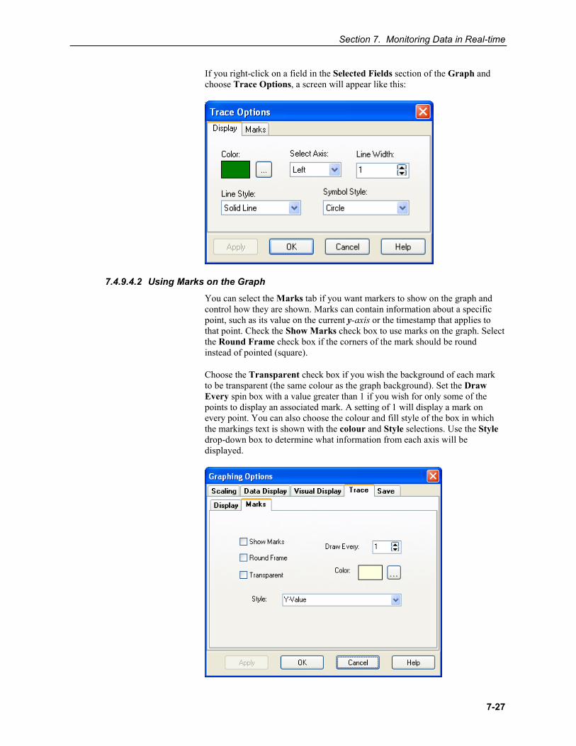
Section 7. Monitoring Data in Real-time
7-27
If you right-click on a field in the Selected Fields section of the Graph and choose Trace Options, a screen will appear like this:
7.4.9.4.2 Using Marks on the Graph
You can select the Marks tab if you want markers to show on the graph and control how they are shown. Marks can contain information about a specific point, such as its value on the current y-axis or the timestamp that applies to that point. Check the Show Marks check box to use marks on the graph. Select the Round Frame check box if the corners of the mark should be round instead of pointed (square).
Choose the Transparent check box if you wish the background of each mark to be transparent (the same colour as the graph background). Set the Draw Every spin box with a value greater than 1 if you wish for only some of the points to display an associated mark. A setting of 1 will display a mark on every point. You can also choose the colour and fill style of the box in which the markings text is shown with the colour and Style selections. Use the Style drop-down box to determine what information from each axis will be displayed.
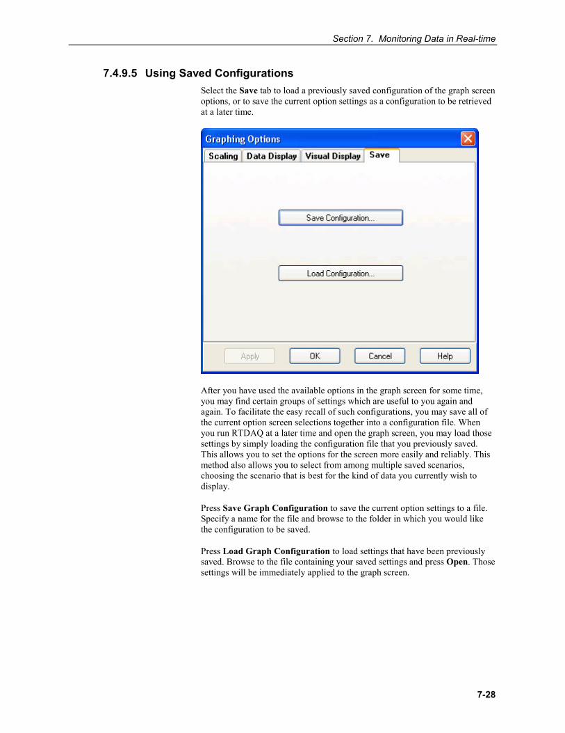
Section 7. Monitoring Data in Real-time
7-28
7.4.9.5 Using Saved Configurations Select the Save tab to load a previously saved configuration of the graph screen options, or to save the current option settings as a configuration to be retrieved at a later time.
After you have used the available options in the graph screen for some time, you may find certain groups of settings which are useful to you again and again. To facilitate the easy recall of such configurations, you may save all of the current option screen selections together into a configuration file. When you run RTDAQ at a later time and open the graph screen, you may load those settings by simply loading the configuration file that you previously saved. This allows you to set the options for the screen more easily and reliably. This method also allows you to select from among multiple saved scenarios, choosing the scenario that is best for the kind of data you currently wish to display.
Press Save Graph Configuration to save the current option settings to a file. Specify a name for the file and browse to the folder in which you would like the configuration to be saved.
Press Load Graph Configuration to load settings that have been previously saved. Browse to the file containing your saved settings and press Open. Those settings will be immediately applied to the graph screen.
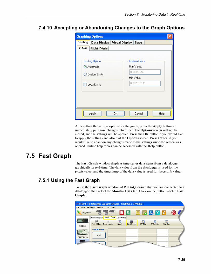
Section 7. Monitoring Data in Real-time
7-29
7.4.10 Accepting or Abandoning Changes to the Graph Options
After setting the various options for the graph, press the Apply button to immediately put those changes into effect. The Options screen will not be closed, and the settings will be applied. Press the OK button if you would like to apply the settings and also exit the Options screen. Press Cancel if you would like to abandon any changes made to the settings since the screen was opened. Online help topics can be accessed with the Help button.
7.5 Fast Graph The Fast Graph window displays time-series data items from a datalogger graphically in real-time. The data value from the datalogger is used for the y-axis value, and the timestamp of the data value is used for the x-axis value.
7.5.1 Using the Fast Graph To use the Fast Graph window of RTDAQ, ensure that you are connected to a datalogger, then select the Monitor Data tab. Click on the button labeled Fast Graph.
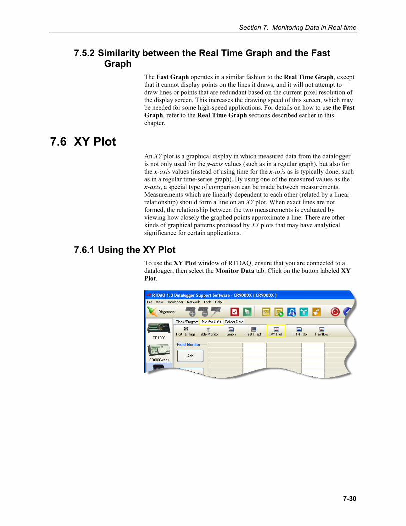
Section 7. Monitoring Data in Real-time
7-30
7.5.2 Similarity between the Real Time Graph and the Fast Graph
The Fast Graph operates in a similar fashion to the Real Time Graph, except that it cannot display points on the lines it draws, and it will not attempt to draw lines or points that are redundant based on the current pixel resolution of the display screen. This increases the drawing speed of this screen, which may be needed for some high-speed applications. For details on how to use the Fast Graph, refer to the Real Time Graph sections described earlier in this chapter.
7.6 XY Plot An XY plot is a graphical display in which measured data from the datalogger is not only used for the y-axis values (such as in a regular graph), but also for the x-axis values (instead of using time for the x-axis as is typically done, such as in a regular time-series graph). By using one of the measured values as the x-axis, a special type of comparison can be made between measurements. Measurements which are linearly dependent to each other (related by a linear relationship) should form a line on an XY plot. When exact lines are not formed, the relationship between the two measurements is evaluated by viewing how closely the graphed points approximate a line. There are other kinds of graphical patterns produced by XY plots that may have analytical significance for certain applications.
7.6.1 Using the XY Plot To use the XY Plot window of RTDAQ, ensure that you are connected to a datalogger, then select the Monitor Data tab. Click on the button labeled XY Plot.
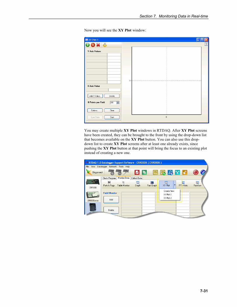
Section 7. Monitoring Data in Real-time
7-31
Now you will see the XY Plot window:
You may create multiple XY Plot windows in RTDAQ. After XY Plot screens have been created, they can be brought to the front by using the drop-down list that becomes available on the XY Plot button. You can also use this drop-down list to create XY Plot screens after at least one already exists, since pushing the XY Plot button at that point will bring the focus to an existing plot instead of creating a new one.
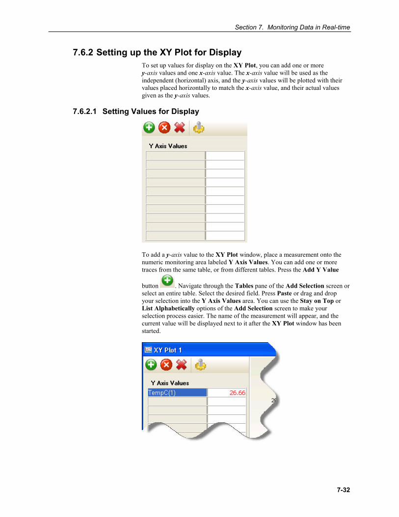
Section 7. Monitoring Data in Real-time
7-32
7.6.2 Setting up the XY Plot for Display To set up values for display on the XY Plot, you can add one or more y-axis values and one x-axis value. The x-axis value will be used as the independent (horizontal) axis, and the y-axis values will be plotted with their values placed horizontally to match the x-axis value, and their actual values given as the y-axis values.
7.6.2.1 Setting Values for Display
To add a y-axis value to the XY Plot window, place a measurement onto the numeric monitoring area labeled Y Axis Values. You can add one or more traces from the same table, or from different tables. Press the Add Y Value
button . Navigate through the Tables pane of the Add Selection screen or select an entire table. Select the desired field. Press Paste or drag and drop your selection into the Y Axis Values area. You can use the Stay on Top or List Alphabetically options of the Add Selection screen to make your selection process easier. The name of the measurement will appear, and the current value will be displayed next to it after the XY Plot window has been started.
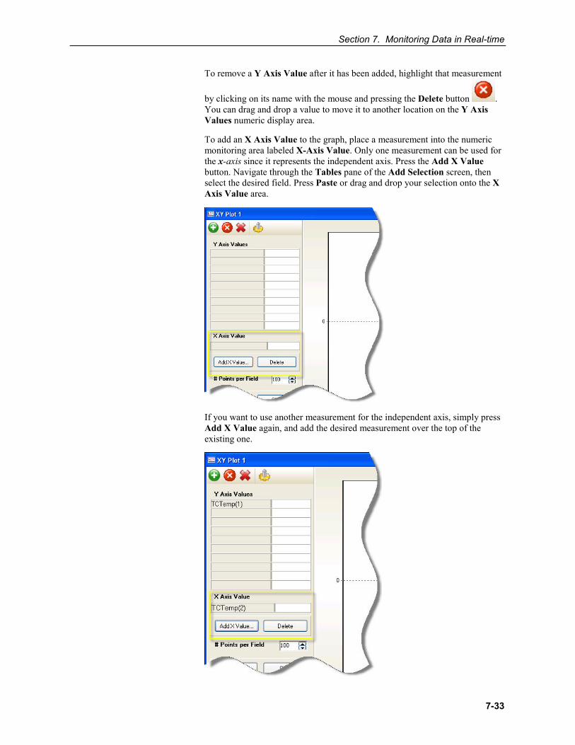
Section 7. Monitoring Data in Real-time
7-33
To remove a Y Axis Value after it has been added, highlight that measurement
by clicking on its name with the mouse and pressing the Delete button . You can drag and drop a value to move it to another location on the Y Axis Values numeric display area.
To add an X Axis Value to the graph, place a measurement into the numeric monitoring area labeled X-Axis Value. Only one measurement can be used for the x-axis since it represents the independent axis. Press the Add X Value button. Navigate through the Tables pane of the Add Selection screen, then select the desired field. Press Paste or drag and drop your selection onto the X Axis Value area.
If you want to use another measurement for the independent axis, simply press Add X Value again, and add the desired measurement over the top of the existing one.
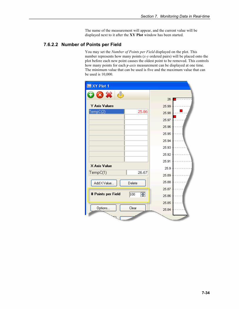
Section 7. Monitoring Data in Real-time
7-34
The name of the measurement will appear, and the current value will be displayed next to it after the XY Plot window has been started.
7.6.2.2 Number of Points per Field You may set the Number of Points per Field displayed on the plot. This number represents how many points (x-y ordered pairs) will be placed onto the plot before each new point causes the oldest point to be removed. This controls how many points for each y-axis measurement can be displayed at one time. The minimum value that can be used is five and the maximum value that can be used is 10,000.
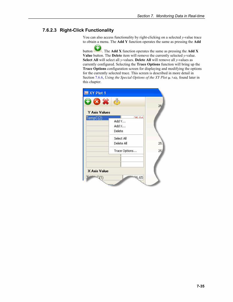
Section 7. Monitoring Data in Real-time
7-35
7.6.2.3 Right-Click Functionality You can also access functionality by right-clicking on a selected y-value trace to obtain a menu. The Add Y function operates the same as pressing the Add
button . The Add X function operates the same as pressing the Add X Value button. The Delete item will remove the currently selected y-value. Select All will select all y-values. Delete All will remove all y-values as currently configured. Selecting the Trace Options function will bring up the Trace Options configuration screen for displaying and modifying the options for the currently selected trace. This screen is described in more detail in Section 7.6.6, Using the Special Options of the XY Plot (p. 7-42), found later in this chapter.
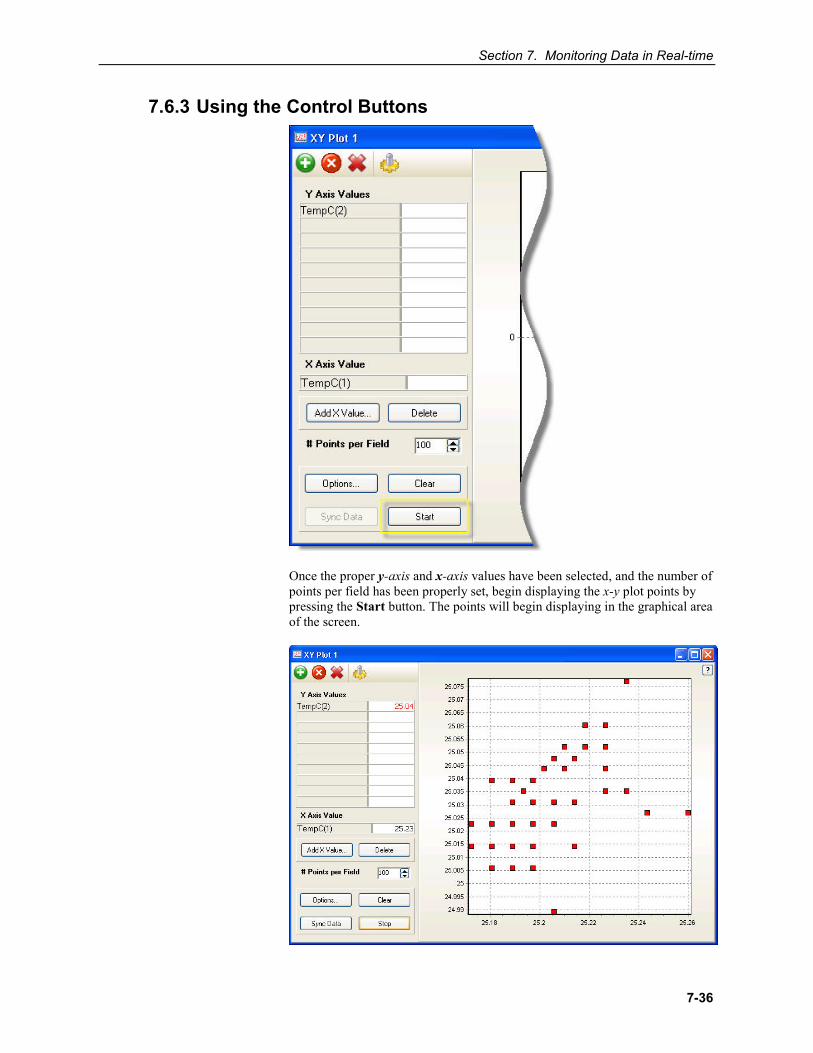
Section 7. Monitoring Data in Real-time
7-36
7.6.3 Using the Control Buttons
Once the proper y-axis and x-axis values have been selected, and the number of points per field has been properly set, begin displaying the x-y plot points by pressing the Start button. The points will begin displaying in the graphical area of the screen.
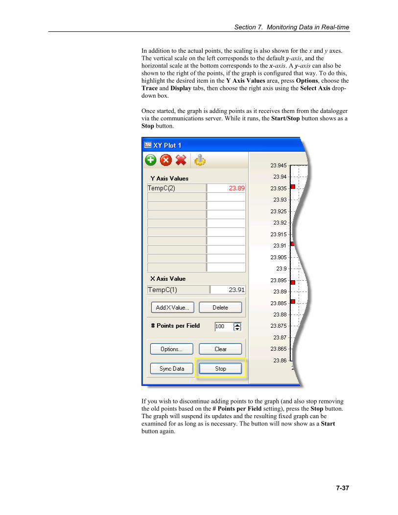
Section 7. Monitoring Data in Real-time
7-37
In addition to the actual points, the scaling is also shown for the x and y axes. The vertical scale on the left corresponds to the default y-axis, and the horizontal scale at the bottom corresponds to the x-axis. A y-axis can also be shown to the right of the points, if the graph is configured that way. To do this, highlight the desired item in the Y Axis Values area, press Options, choose the Trace and Display tabs, then choose the right axis using the Select Axis drop-down box.
Once started, the graph is adding points as it receives them from the datalogger via the communications server. While it runs, the Start/Stop button shows as a Stop button.
If you wish to discontinue adding points to the graph (and also stop removing the old points based on the # Points per Field setting), press the Stop button. The graph will suspend its updates and the resulting fixed graph can be examined for as long as is necessary. The button will now show as a Start button again.
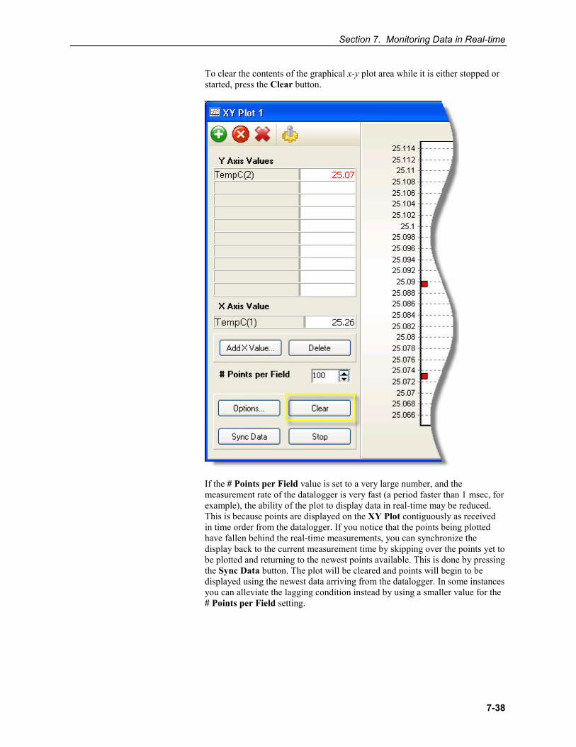
Section 7. Monitoring Data in Real-time
7-38
To clear the contents of the graphical x-y plot area while it is either stopped or started, press the Clear button.
If the # Points per Field value is set to a very large number, and the measurement rate of the datalogger is very fast (a period faster than 1 msec, for example), the ability of the plot to display data in real-time may be reduced. This is because points are displayed on the XY Plot contiguously as received in time order from the datalogger. If you notice that the points being plotted have fallen behind the real-time measurements, you can synchronize the display back to the current measurement time by skipping over the points yet to be plotted and returning to the newest points available. This is done by pressing the Sync Data button. The plot will be cleared and points will begin to be displayed using the newest data arriving from the datalogger. In some instances you can alleviate the lagging condition instead by using a smaller value for the # Points per Field setting.
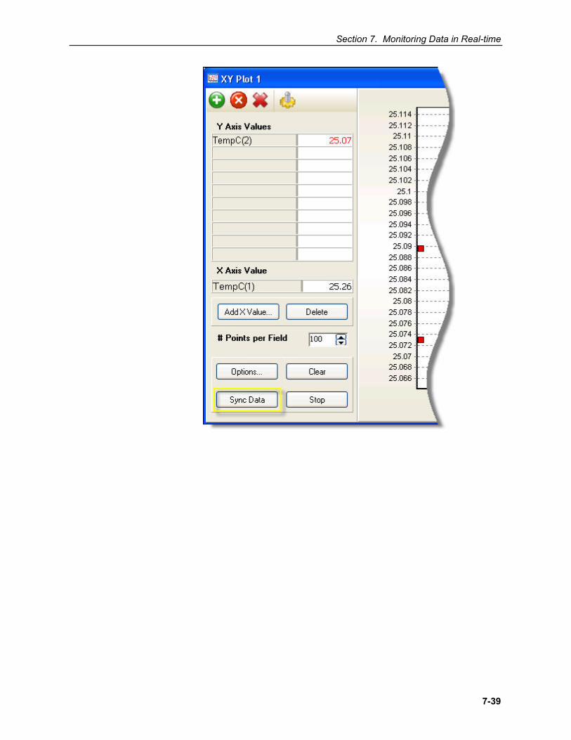
Section 7. Monitoring Data in Real-time
7-39
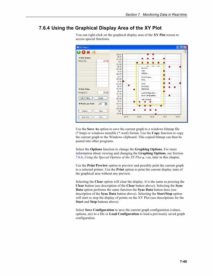
Section 7. Monitoring Data in Real-time
7-40
7.6.4 Using the Graphical Display Area of the XY Plot You can right-click on the graphical display area of the XY Plot screen to access special functions.
Use the Save As option to save the current graph to a windows bitmap file (*.bmp) or windows metafile (*.wmf) format. Use the Copy function to copy the current graph to the Windows clipboard. This copied bitmap can then be pasted into other programs.
Select the Options function to change the Graphing Options. For more information about viewing and changing the Graphing Options, see Section 7.6.6, Using the Special Options of the XY Plot (p. 7-42), later in this chapter.
Use the Print Preview option to preview and possibly print the current graph to a selected printer. Use the Print option to print the current display state of the graphical area without any preview.
Selecting the Clear option will clear the display. It is the same as pressing the Clear button (see description of the Clear button above). Selecting the Sync Data option performs the same function the Sync Data button does (see description of the Sync Data button above). Selecting the Start/Stop option will start or stop the display of points on the XY Plot (see descriptions for the Start and Stop buttons above).
Select Save Configuration to save the current graph configuration (values, options, etc) to a file or Load Configuration to load a previously saved graph configuration.
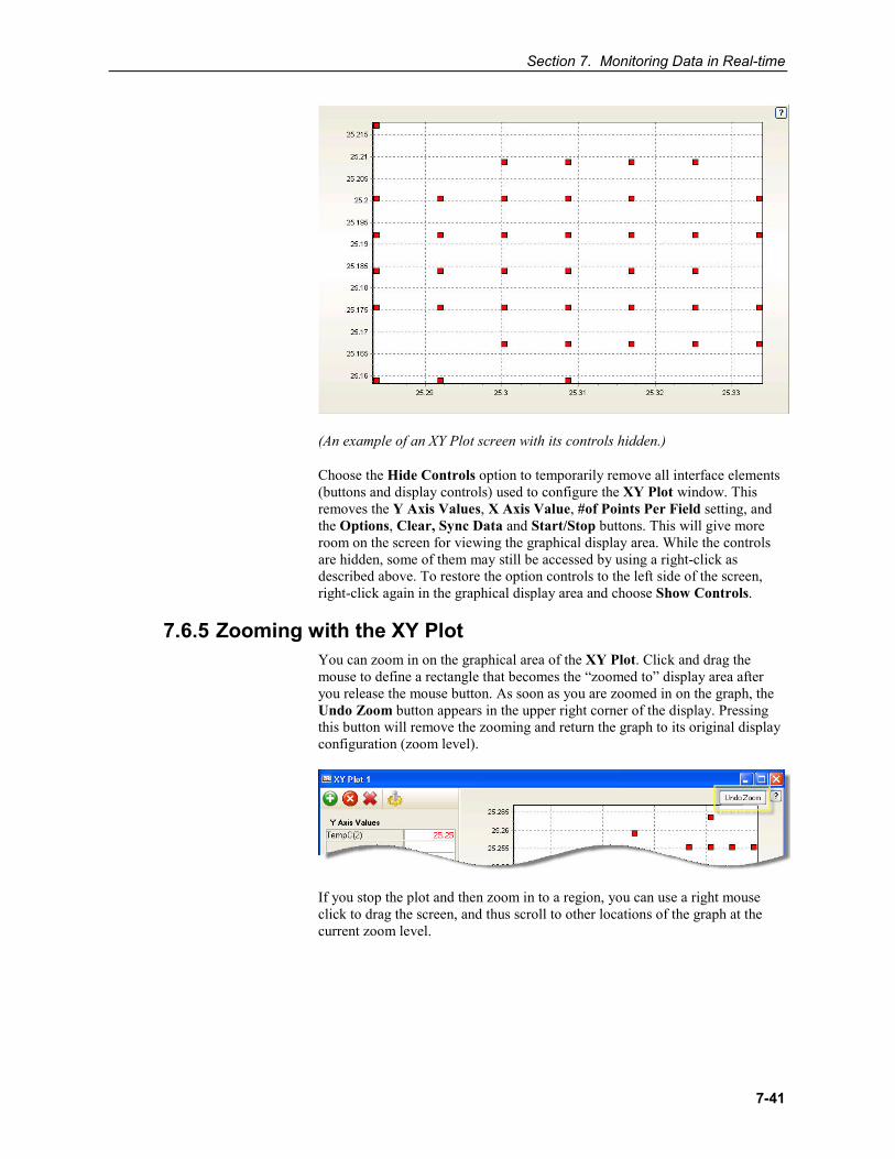
Section 7. Monitoring Data in Real-time
7-41
(An example of an XY Plot screen with its controls hidden.)
Choose the Hide Controls option to temporarily remove all interface elements (buttons and display controls) used to configure the XY Plot window. This removes the Y Axis Values, X Axis Value, #of Points Per Field setting, and the Options, Clear, Sync Data and Start/Stop buttons. This will give more room on the screen for viewing the graphical display area. While the controls are hidden, some of them may still be accessed by using a right-click as described above. To restore the option controls to the left side of the screen, right-click again in the graphical display area and choose Show Controls.
7.6.5 Zooming with the XY Plot You can zoom in on the graphical area of the XY Plot. Click and drag the mouse to define a rectangle that becomes the “zoomed to” display area after you release the mouse button. As soon as you are zoomed in on the graph, the Undo Zoom button appears in the upper right corner of the display. Pressing this button will remove the zooming and return the graph to its original display configuration (zoom level).
If you stop the plot and then zoom in to a region, you can use a right mouse click to drag the screen, and thus scroll to other locations of the graph at the current zoom level.
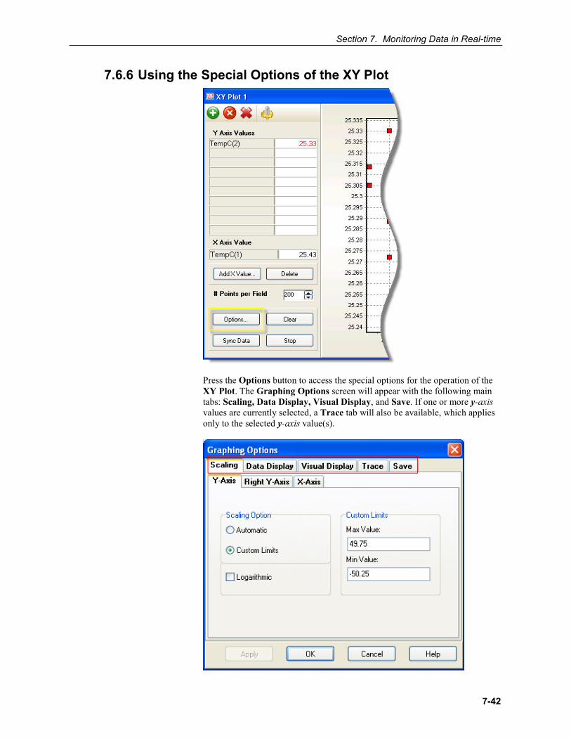
Section 7. Monitoring Data in Real-time
7-42
7.6.6 Using the Special Options of the XY Plot
Press the Options button to access the special options for the operation of the XY Plot. The Graphing Options screen will appear with the following main tabs: Scaling, Data Display, Visual Display, and Save. If one or more y-axis values are currently selected, a Trace tab will also be available, which applies only to the selected y-axis value(s).
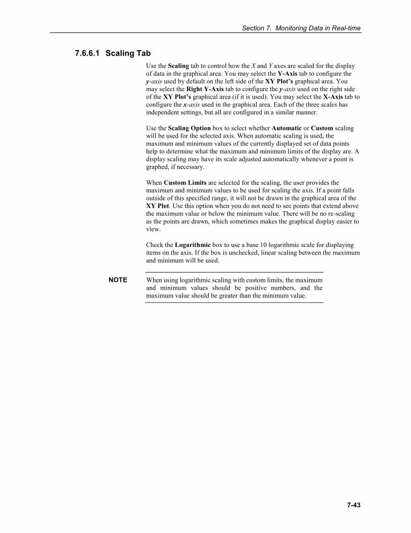
Section 7. Monitoring Data in Real-time
7-43
7.6.6.1 Scaling Tab Use the Scaling tab to control how the X and Y axes are scaled for the display of data in the graphical area. You may select the Y-Axis tab to configure the y-axis used by default on the left side of the XY Plot’s graphical area. You may select the Right Y-Axis tab to configure the y-axis used on the right side of the XY Plot’s graphical area (if it is used). You may select the X-Axis tab to configure the x-axis used in the graphical area. Each of the three scales has independent settings, but all are configured in a similar manner.
Use the Scaling Option box to select whether Automatic or Custom scaling will be used for the selected axis. When automatic scaling is used, the maximum and minimum values of the currently displayed set of data points help to determine what the maximum and minimum limits of the display are. A display scaling may have its scale adjusted automatically whenever a point is graphed, if necessary.
When Custom Limits are selected for the scaling, the user provides the maximum and minimum values to be used for scaling the axis. If a point falls outside of this specified range, it will not be drawn in the graphical area of the XY Plot. Use this option when you do not need to see points that extend above the maximum value or below the minimum value. There will be no re-scaling as the points are drawn, which sometimes makes the graphical display easier to view.
Check the Logarithmic box to use a base 10 logarithmic scale for displaying items on the axis. If the box is unchecked, linear scaling between the maximum and minimum will be used.
When using logarithmic scaling with custom limits, the maximum and minimum values should be positive numbers, and the maximum value should be greater than the minimum value.
NOTE
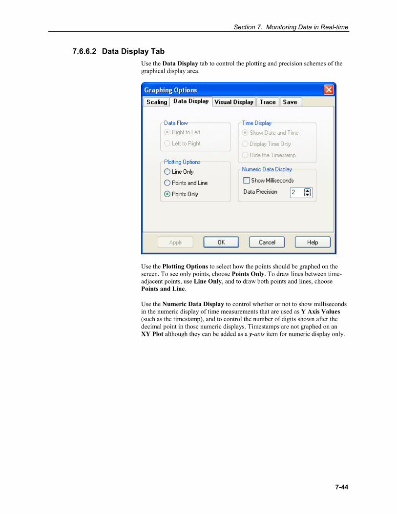
Section 7. Monitoring Data in Real-time
7-44
7.6.6.2 Data Display Tab Use the Data Display tab to control the plotting and precision schemes of the graphical display area.
Use the Plotting Options to select how the points should be graphed on the screen. To see only points, choose Points Only. To draw lines between time-adjacent points, use Line Only, and to draw both points and lines, choose Points and Line.
Use the Numeric Data Display to control whether or not to show milliseconds in the numeric display of time measurements that are used as Y Axis Values (such as the timestamp), and to control the number of digits shown after the decimal point in those numeric displays. Timestamps are not graphed on an XY Plot although they can be added as a y-axis item for numeric display only.
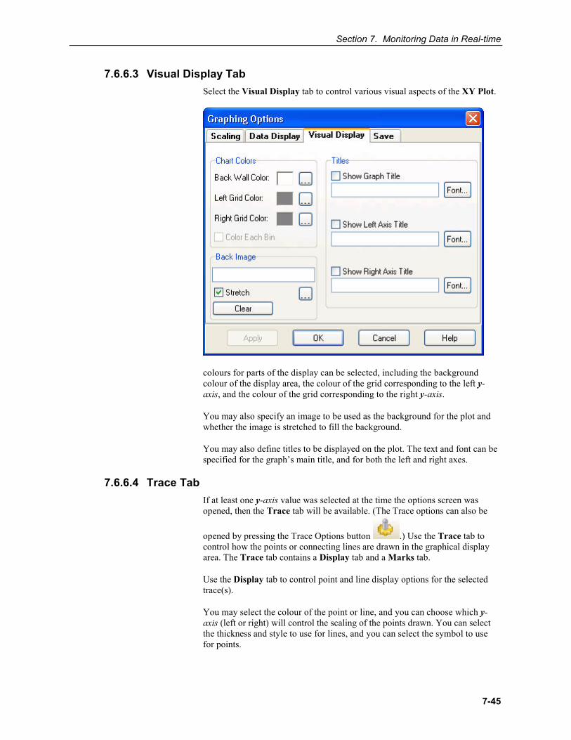
Section 7. Monitoring Data in Real-time
7-45
7.6.6.3 Visual Display Tab Select the Visual Display tab to control various visual aspects of the XY Plot.
7.6.6.4 Trace Tab
colours for parts of the display can be selected, including the background colour of the display area, the colour of the grid corresponding to the left y-axis, and the colour of the grid corresponding to the right y-axis.
You may also specify an image to be used as the background for the plot and whether the image is stretched to fill the background.
You may also define titles to be displayed on the plot. The text and font can be specified for the graph’s main title, and for both the left and right axes.
If at least one y-axis value was selected at the time the options screen was opened, then the Trace tab will be available. (The Trace options can also be
opened by pressing the Trace Options button .) Use the Trace tab to control how the points or connecting lines are drawn in the graphical display area. The Trace tab contains a Display tab and a Marks tab.
Use the Display tab to control point and line display options for the selected trace(s).
You may select the colour of the point or line, and you can choose which y-axis (left or right) will control the scaling of the points drawn. You can select the thickness and style to use for lines, and you can select the symbol to use for points.
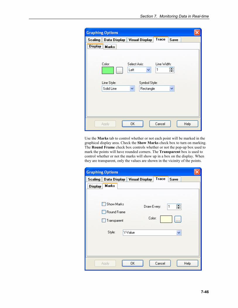
Section 7. Monitoring Data in Real-time
7-46
Use the Marks tab to control whether or not each point will be marked in the graphical display area. Check the Show Marks check box to turn on marking. The Round Frame check box controls whether or not the pop-up box used to mark the points will have rounded corners. The Transparent box is used to control whether or not the marks will show up in a box on the display. When they are transparent, only the values are shown in the vicinity of the points.
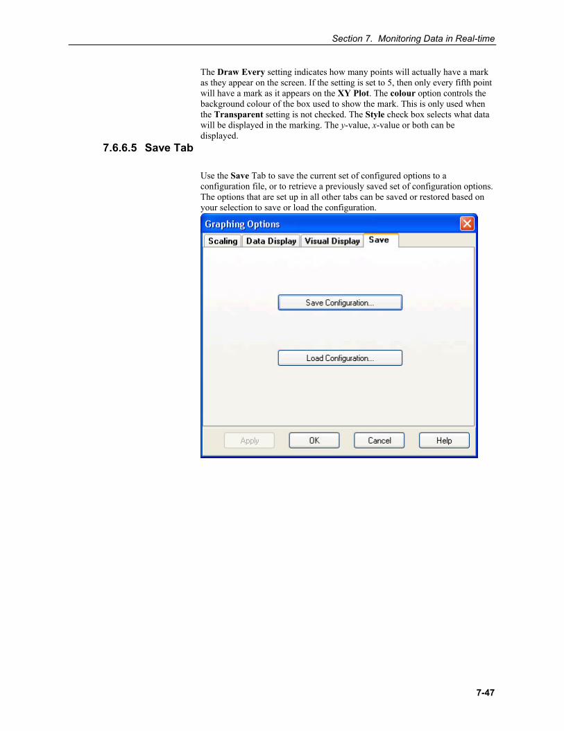
Section 7. Monitoring Data in Real-time
7-47
7.6.6.5 Save Tab
The Draw Every setting indicates how many points will actually have a mark as they appear on the screen. If the setting is set to 5, then only every fifth point will have a mark as it appears on the XY Plot. The colour option controls the background colour of the box used to show the mark. This is only used when the Transparent setting is not checked. The Style check box selects what data will be displayed in the marking. The y-value, x-value or both can be displayed.
Use the Save Tab to save the current set of configured options to a configuration file, or to retrieve a previously saved set of configuration options. The options that are set up in all other tabs can be saved or restored based on your selection to save or load the configuration.
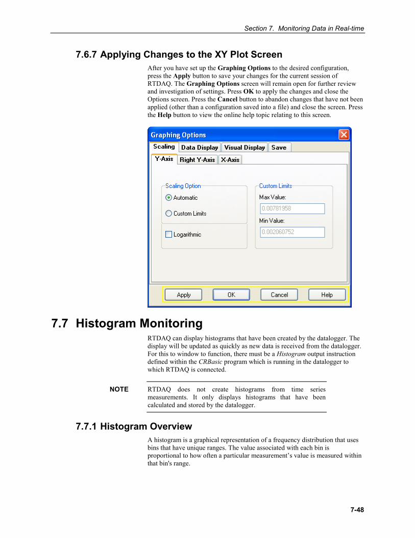
Section 7. Monitoring Data in Real-time
7-48
7.6.7 Applying Changes to the XY Plot Screen After you have set up the Graphing Options to the desired configuration, press the Apply button to save your changes for the current session of RTDAQ. The Graphing Options screen will remain open for further review and investigation of settings. Press OK to apply the changes and close the Options screen. Press the Cancel button to abandon changes that have not been applied (other than a configuration saved into a file) and close the screen. Press the Help button to view the online help topic relating to this screen.
7.7 Histogram Monitoring RTDAQ can display histograms that have been created by the datalogger. The display will be updated as quickly as new data is received from the datalogger. For this to window to function, there must be a Histogram output instruction defined within the CRBasic program which is running in the datalogger to which RTDAQ is connected.
RTDAQ does not create histograms from time series measurements. It only displays histograms that have been calculated and stored by the datalogger.
7.7.1 Histogram Overview A histogram is a graphical representation of a frequency distribution that uses bins that have unique ranges. The value associated with each bin is proportional to how often a particular measurement’s value is measured within that bin's range.
NOTE
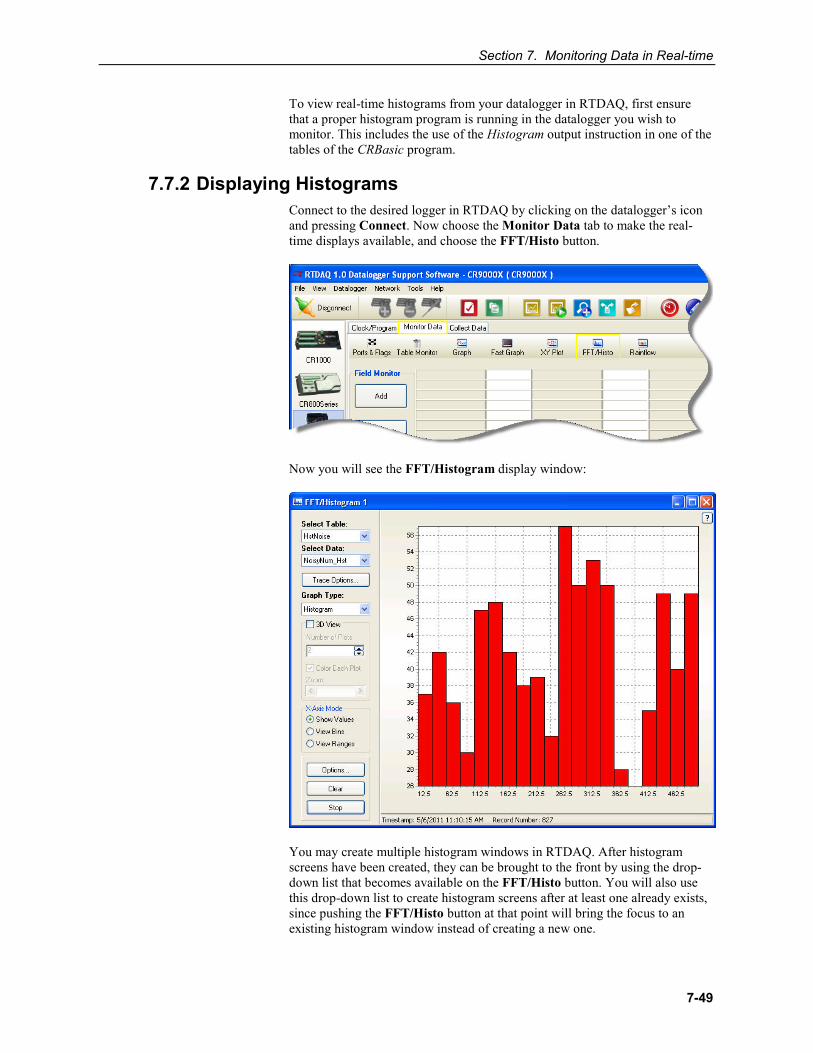
Section 7. Monitoring Data in Real-time
7-49
To view real-time histograms from your datalogger in RTDAQ, first ensure that a proper histogram program is running in the datalogger you wish to monitor. This includes the use of the Histogram output instruction in one of the tables of the CRBasic program.
7.7.2 Displaying Histograms Connect to the desired logger in RTDAQ by clicking on the datalogger’s icon and pressing Connect. Now choose the Monitor Data tab to make the real-time displays available, and choose the FFT/Histo button.
Now you will see the FFT/Histogram display window:
You may create multiple histogram windows in RTDAQ. After histogram screens have been created, they can be brought to the front by using the drop-down list that becomes available on the FFT/Histo button. You will also use this drop-down list to create histogram screens after at least one already exists, since pushing the FFT/Histo button at that point will bring the focus to an existing histogram window instead of creating a new one.
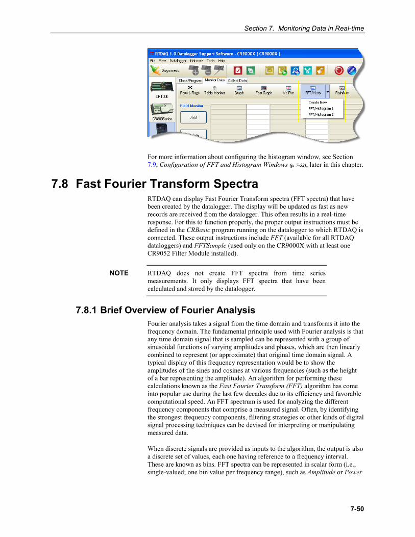
Section 7. Monitoring Data in Real-time
7-50
For more information about configuring the histogram window, see Section 7.9, Configuration of FFT and Histogram Windows (p. 7-52), later in this chapter.
7.8 Fast Fourier Transform Spectra RTDAQ can display Fast Fourier Transform spectra (FFT spectra) that have been created by the datalogger. The display will be updated as fast as new records are received from the datalogger. This often results in a real-time response. For this to function properly, the proper output instructions must be defined in the CRBasic program running on the datalogger to which RTDAQ is connected. These output instructions include FFT (available for all RTDAQ dataloggers) and FFTSample (used only on the CR9000X with at least one CR9052 Filter Module installed).
RTDAQ does not create FFT spectra from time series measurements. It only displays FFT spectra that have been calculated and stored by the datalogger.
7.8.1 Brief Overview of Fourier Analysis Fourier analysis takes a signal from the time domain and transforms it into the frequency domain. The fundamental principle used with Fourier analysis is that any time domain signal that is sampled can be represented with a group of sinusoidal functions of varying amplitudes and phases, which are then linearly combined to represent (or approximate) that original time domain signal. A typical display of this frequency representation would be to show the amplitudes of the sines and cosines at various frequencies (such as the height of a bar representing the amplitude). An algorithm for performing these calculations known as the Fast Fourier Transform (FFT) algorithm has come into popular use during the last few decades due to its efficiency and favorable computational speed. An FFT spectrum is used for analyzing the different frequency components that comprise a measured signal. Often, by identifying the strongest frequency components, filtering strategies or other kinds of digital signal processing techniques can be devised for interpreting or manipulating measured data.
When discrete signals are provided as inputs to the algorithm, the output is also a discrete set of values, each one having reference to a frequency interval. These are known as bins. FFT spectra can be represented in scalar form (i.e., single-valued; one bin value per frequency range), such as Amplitude or Power
NOTE
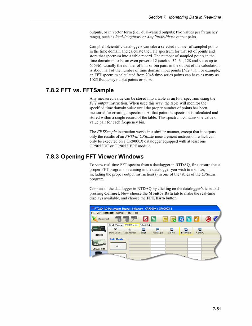
Section 7. Monitoring Data in Real-time
7-51
outputs, or in vector form (i.e., dual-valued outputs; two values per frequency range), such as Real-Imaginary or Amplitude-Phase output pairs.
Campbell Scientific dataloggers can take a selected number of sampled points in the time domain and calculate the FFT spectrum for that set of points and store that spectrum into a table record. The number of sampled points in the time domain must be an even power of 2 (such as 32, 64, 128 and so on up to 65536). Usually the number of bins or bin pairs in the output of the calculation is about half of the number of time domain input points (N/2 +1). For example, an FFT spectrum calculated from 2048 time-series points can have as many as 1025 frequency output points or pairs.
7.8.2 FFT vs. FFTSample Any measured value can be stored into a table as an FFT spectrum using the FFT output instruction. When used this way, the table will monitor the specified time domain value until the proper number of points has been measured for creating a spectrum. At that point the spectrum is calculated and stored within a single record of the table. This spectrum contains one value or value pair for each frequency bin.
The FFTSample instruction works in a similar manner, except that it outputs only the results of an FFTFilt CRBasic measurement instruction, which can only be executed on a CR9000X datalogger equipped with at least one CR9052DC or CR9052IEPE module.
7.8.3 Opening FFT Viewer Windows To view real-time FFT spectra from a datalogger in RTDAQ, first ensure that a proper FFT program is running in the datalogger you wish to monitor, including the proper output instruction(s) in one of the tables of the CRBasic program.
Connect to the datalogger in RTDAQ by clicking on the datalogger’s icon and pressing Connect. Now choose the Monitor Data tab to make the real-time displays available, and choose the FFT/Histo button.
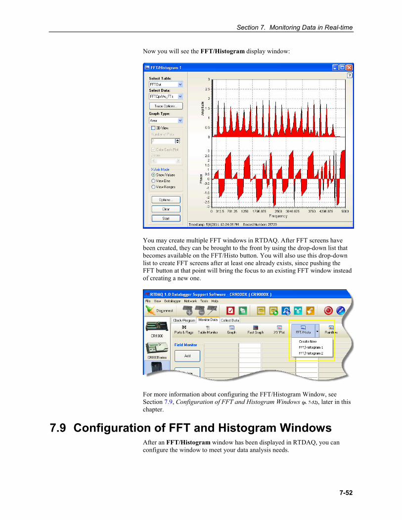
Section 7. Monitoring Data in Real-time
7-52
Now you will see the FFT/Histogram display window:
You may create multiple FFT windows in RTDAQ. After FFT screens have been created, they can be brought to the front by using the drop-down list that becomes available on the FFT/Histo button. You will also use this drop-down list to create FFT screens after at least one already exists, since pushing the FFT button at that point will bring the focus to an existing FFT window instead of creating a new one.
For more information about configuring the FFT/Histogram Window, see Section 7.9, Configuration of FFT and Histogram Windows (p. 7-52), later in this chapter.
7.9 Configuration of FFT and Histogram Windows After an FFT/Histogram window has been displayed in RTDAQ, you can configure the window to meet your data analysis needs.
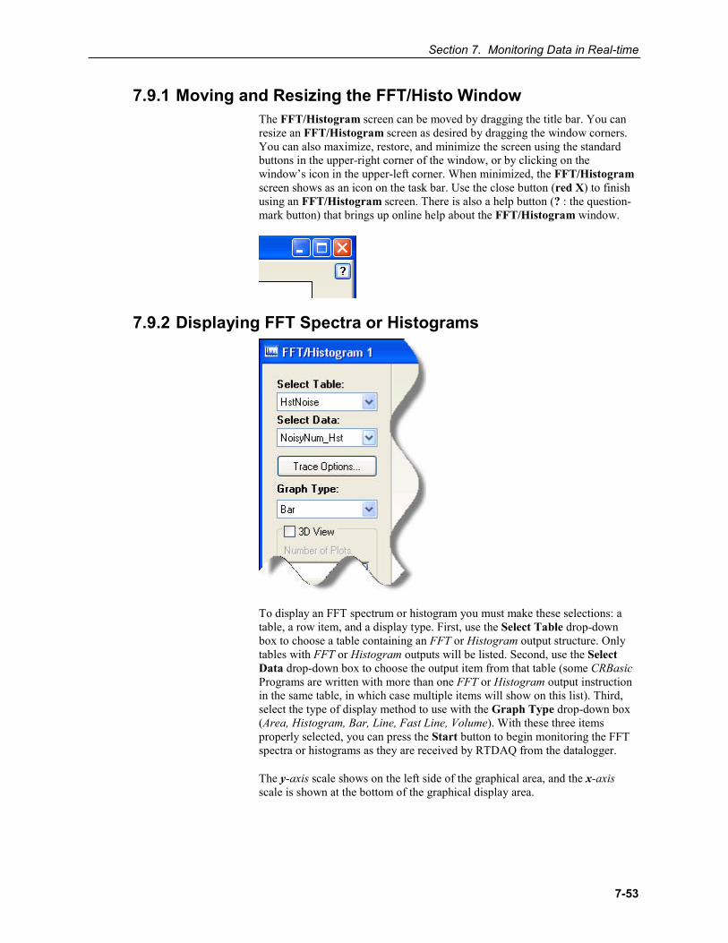
Section 7. Monitoring Data in Real-time
7-53
7.9.1 Moving and Resizing the FFT/Histo Window The FFT/Histogram screen can be moved by dragging the title bar. You can resize an FFT/Histogram screen as desired by dragging the window corners. You can also maximize, restore, and minimize the screen using the standard buttons in the upper-right corner of the window, or by clicking on the window’s icon in the upper-left corner. When minimized, the FFT/Histogram screen shows as an icon on the task bar. Use the close button (red X) to finish using an FFT/Histogram screen. There is also a help button (? : the question-mark button) that brings up online help about the FFT/Histogram window.
7.9.2 Displaying FFT Spectra or Histograms
To display an FFT spectrum or histogram you must make these selections: a table, a row item, and a display type. First, use the Select Table drop-down box to choose a table containing an FFT or Histogram output structure. Only tables with FFT or Histogram outputs will be listed. Second, use the Select Data drop-down box to choose the output item from that table (some CRBasic Programs are written with more than one FFT or Histogram output instruction in the same table, in which case multiple items will show on this list). Third, select the type of display method to use with the Graph Type drop-down box (Area, Histogram, Bar, Line, Fast Line, Volume). With these three items properly selected, you can press the Start button to begin monitoring the FFT spectra or histograms as they are received by RTDAQ from the datalogger.
The y-axis scale shows on the left side of the graphical area, and the x-axis scale is shown at the bottom of the graphical display area.
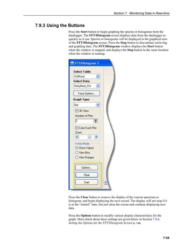
Section 7. Monitoring Data in Real-time
7-54
7.9.3 Using the Buttons Press the Start button to begin graphing the spectra or histograms from the datalogger. The FFT/Histogram screen displays data from the datalogger as quickly as it can. Spectra or histograms will be displayed in the graphical area of the FFT/Histogram screen. Press the Stop button to discontinue retrieving and graphing data. The FFT/Histogram window displays the Start button when the window is stopped, and displays the Stop button in the same location when the window is running.
Press the Clear button to remove the display of the current spectrum or histogram, and begin displaying the next record. The display will not stop if it is in the “started” state, but just clear the screen and continue displaying new data.
Press the Options button to modify various display characteristics for the graph. More detail about these settings are given below in Section 7.9.8, Setting the Options for the FFT/Histogram Screen (p. 7-60).
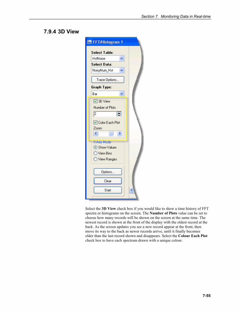
Section 7. Monitoring Data in Real-time
7-55
7.9.4 3D View
Select the 3D View check box if you would like to show a time history of FFT spectra or histograms on the screen. The Number of Plots value can be set to choose how many records will be shown on the screen at the same time. The newest record is shown at the front of the display with the oldest record at the back. As the screen updates you see a new record appear at the front, then move its way to the back as newer records arrive, until it finally becomes older than the last record shown and disappears. Select the Colour Each Plot check box to have each spectrum drawn with a unique colour.
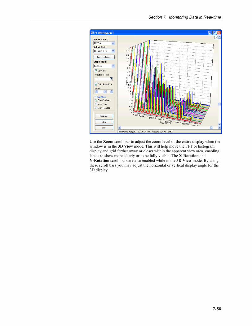
Section 7. Monitoring Data in Real-time
7-56
Use the Zoom scroll bar to adjust the zoom level of the entire display when the window is in the 3D View mode. This will help move the FFT or histogram display and grid farther away or closer within the apparent view area, enabling labels to show more clearly or to be fully visible. The X-Rotation and Y-Rotation scroll bars are also enabled while in the 3D View mode. By using these scroll bars you may adjust the horizontal or vertical display angle for the 3D display.
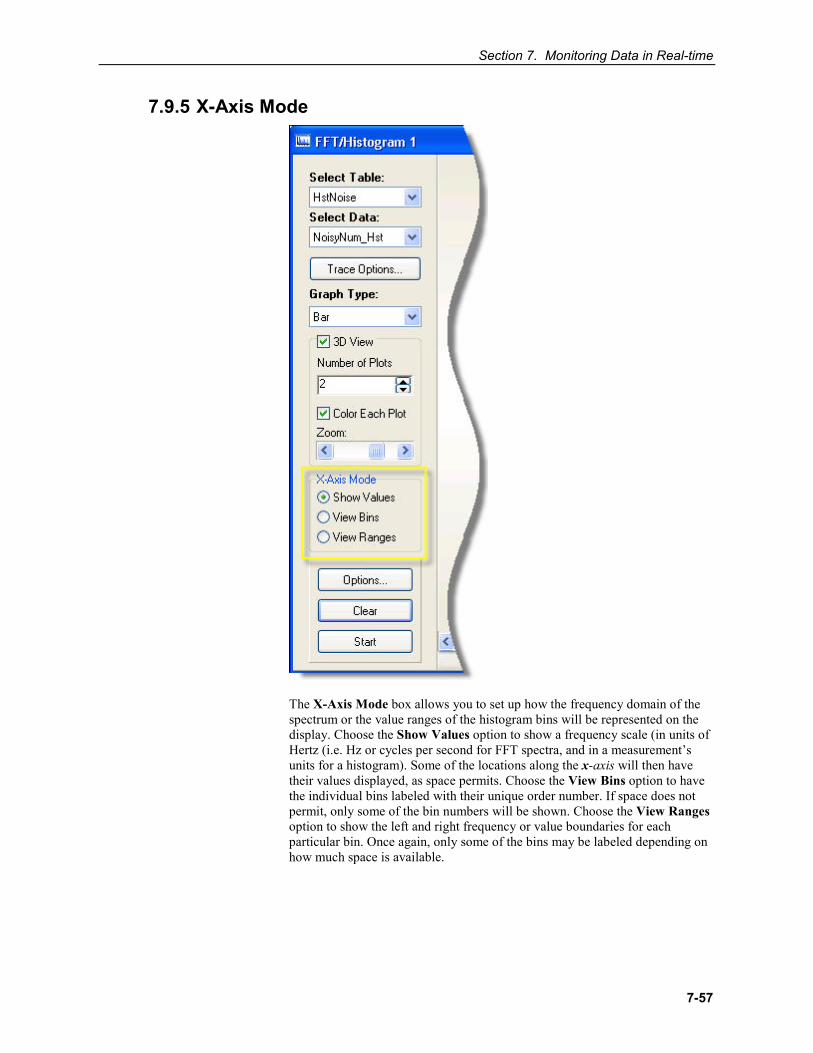
Section 7. Monitoring Data in Real-time
7-57
7.9.5 X-Axis Mode
The X-Axis Mode box allows you to set up how the frequency domain of the spectrum or the value ranges of the histogram bins will be represented on the display. Choose the Show Values option to show a frequency scale (in units of Hertz (i.e. Hz or cycles per second for FFT spectra, and in a measurement’s units for a histogram). Some of the locations along the x-axis will then have their values displayed, as space permits. Choose the View Bins option to have the individual bins labeled with their unique order number. If space does not permit, only some of the bin numbers will be shown. Choose the View Ranges option to show the left and right frequency or value boundaries for each particular bin. Once again, only some of the bins may be labeled depending on how much space is available.
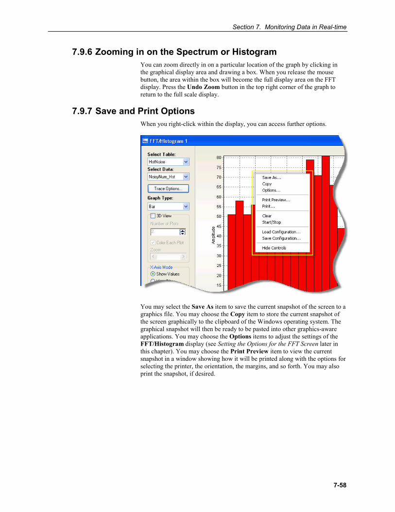
Section 7. Monitoring Data in Real-time
7-58
7.9.6 Zooming in on the Spectrum or Histogram You can zoom directly in on a particular location of the graph by clicking in the graphical display area and drawing a box. When you release the mouse button, the area within the box will become the full display area on the FFT display. Press the Undo Zoom button in the top right corner of the graph to return to the full scale display.
7.9.7 Save and Print Options When you right-click within the display, you can access further options.
You may select the Save As item to save the current snapshot of the screen to a graphics file. You may choose the Copy item to store the current snapshot of the screen graphically to the clipboard of the Windows operating system. The graphical snapshot will then be ready to be pasted into other graphics-aware applications. You may choose the Options items to adjust the settings of the FFT/Histogram display (see Setting the Options for the FFT Screen later in this chapter). You may choose the Print Preview item to view the current snapshot in a window showing how it will be printed along with the options for selecting the printer, the orientation, the margins, and so forth. You may also print the snapshot, if desired.
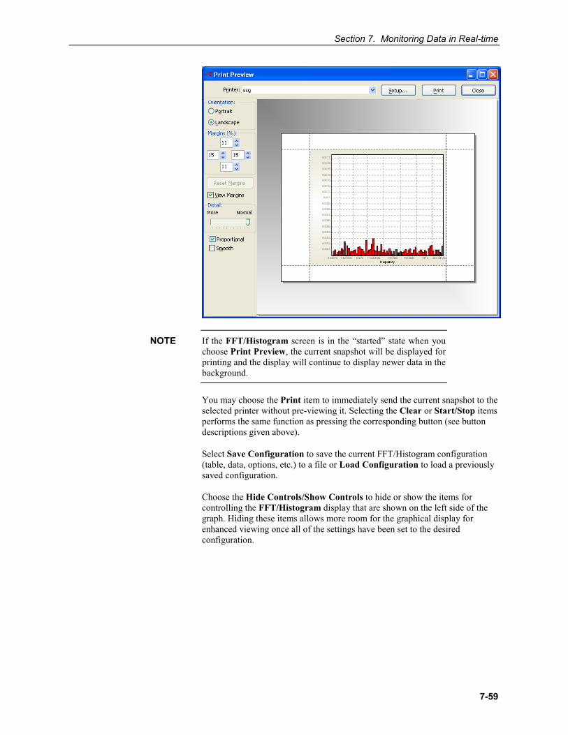
Section 7. Monitoring Data in Real-time
7-59
If the FFT/Histogram screen is in the “started” state when you choose Print Preview, the current snapshot will be displayed for printing and the display will continue to display newer data in the background.
You may choose the Print item to immediately send the current snapshot to the selected printer without pre-viewing it. Selecting the Clear or Start/Stop items performs the same function as pressing the corresponding button (see button descriptions given above).
Select Save Configuration to save the current FFT/Histogram configuration (table, data, options, etc.) to a file or Load Configuration to load a previously saved configuration.
Choose the Hide Controls/Show Controls to hide or show the items for controlling the FFT/Histogram display that are shown on the left side of the graph. Hiding these items allows more room for the graphical display for enhanced viewing once all of the settings have been set to the desired configuration.
NOTE
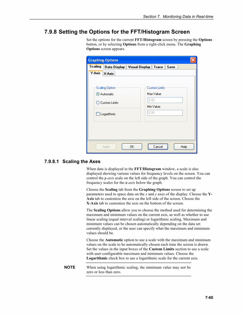
Section 7. Monitoring Data in Real-time
7-60
7.9.8 Setting the Options for the FFT/Histogram Screen Set the options for the current FFT/Histogram screen by pressing the Options button, or by selecting Options from a right-click menu. The Graphing Options screen appears.
7.9.8.1 Scaling the Axes When data is displayed in the FFT/Histogram window, a scale is also displayed showing various values for frequency levels on the screen. You can control the y-axis scale on the left side of the graph. You can control the frequency scales for the x-axis below the graph.
Choose the Scaling tab from the Graphing Options screen to set up parameters used to space data on the x and y axes of the display. Choose the Y-Axis tab to customize the axis on the left side of the screen. Choose the X-Axis tab to customize the axis on the bottom of the screen.
The Scaling Options allow you to choose the method used for determining the maximum and minimum values on the current axis, as well as whether to use linear scaling (equal interval scaling) or logarithmic scaling. Maximum and minimum values can be chosen automatically depending on the data set currently displayed, or the user can specify what the maximum and minimum values should be.
Choose the Automatic option to use a scale with the maximum and minimum values on the scale to be automatically chosen each time the screen is drawn. Set the values in the input boxes of the Custom Limits section to use a scale with user-configurable maximum and minimum values. Choose the Logarithmic check box to use a logarithmic scale for the current axis.
When using logarithmic scaling, the minimum value may not be zero or less than zero.
NOTE
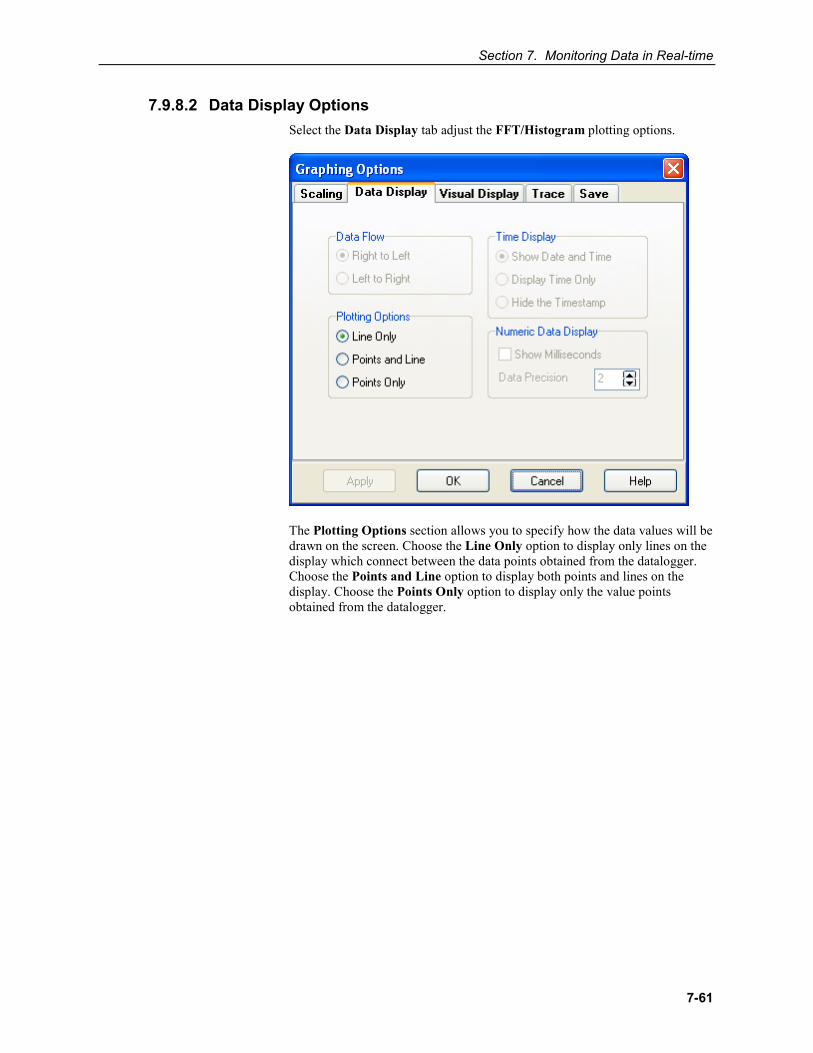
Section 7. Monitoring Data in Real-time
7-61
7.9.8.2 Data Display Options Select the Data Display tab adjust the FFT/Histogram plotting options.
The Plotting Options section allows you to specify how the data values will be drawn on the screen. Choose the Line Only option to display only lines on the display which connect between the data points obtained from the datalogger. Choose the Points and Line option to display both points and lines on the display. Choose the Points Only option to display only the value points obtained from the datalogger.
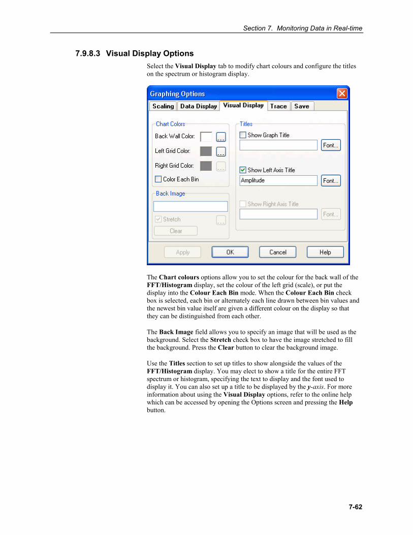
Section 7. Monitoring Data in Real-time
7-62
7.9.8.3 Visual Display Options Select the Visual Display tab to modify chart colours and configure the titles on the spectrum or histogram display.
The Chart colours options allow you to set the colour for the back wall of the FFT/Histogram display, set the colour of the left grid (scale), or put the display into the Colour Each Bin mode. When the Colour Each Bin check box is selected, each bin or alternately each line drawn between bin values and the newest bin value itself are given a different colour on the display so that they can be distinguished from each other.
The Back Image field allows you to specify an image that will be used as the background. Select the Stretch check box to have the image stretched to fill the background. Press the Clear button to clear the background image.
Use the Titles section to set up titles to show alongside the values of the FFT/Histogram display. You may elect to show a title for the entire FFT spectrum or histogram, specifying the text to display and the font used to display it. You can also set up a title to be displayed by the y-axis. For more information about using the Visual Display options, refer to the online help which can be accessed by opening the Options screen and pressing the Help button.
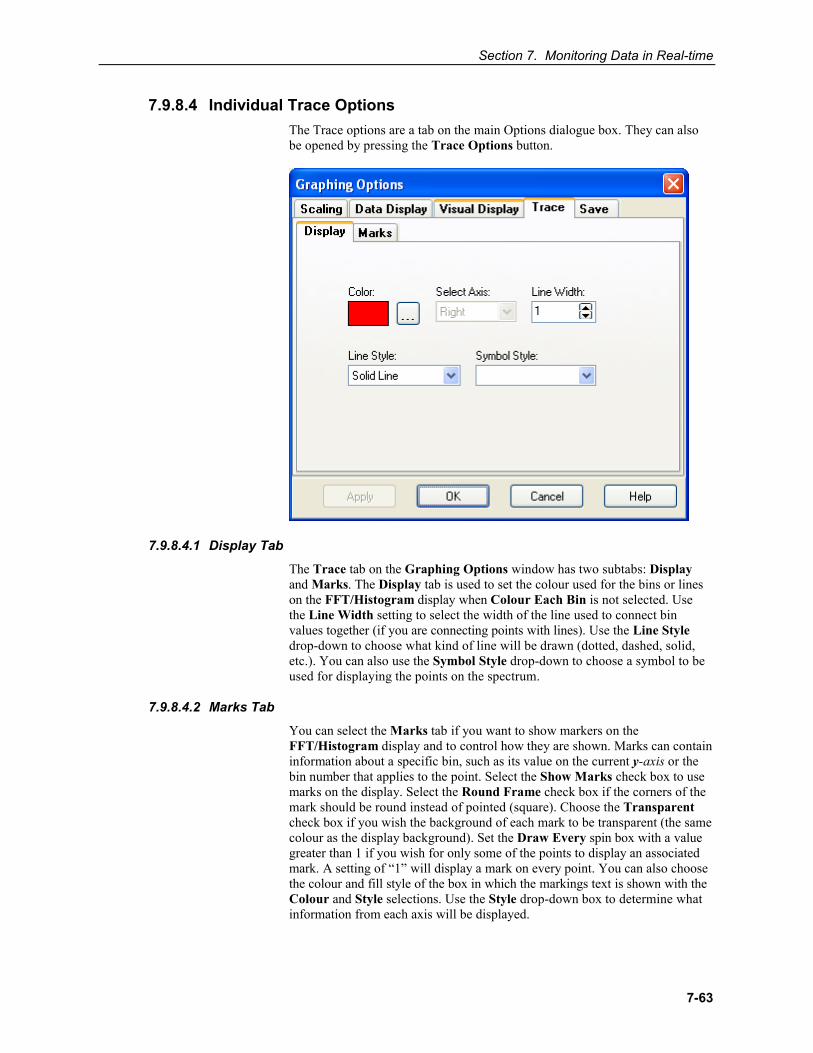
Section 7. Monitoring Data in Real-time
7-63
7.9.8.4 Individual Trace Options The Trace options are a tab on the main Options dialogue box. They can also be opened by pressing the Trace Options button.
7.9.8.4.1 Display Tab
7.9.8.4.2 Marks Tab
The Trace tab on the Graphing Options window has two subtabs: Display and Marks. The Display tab is used to set the colour used for the bins or lines on the FFT/Histogram display when Colour Each Bin is not selected. Use the Line Width setting to select the width of the line used to connect bin values together (if you are connecting points with lines). Use the Line Style drop-down to choose what kind of line will be drawn (dotted, dashed, solid, etc.). You can also use the Symbol Style drop-down to choose a symbol to be used for displaying the points on the spectrum.
You can select the Marks tab if you want to show markers on the FFT/Histogram display and to control how they are shown. Marks can contain information about a specific bin, such as its value on the current y-axis or the bin number that applies to the point. Select the Show Marks check box to use marks on the display. Select the Round Frame check box if the corners of the mark should be round instead of pointed (square). Choose the Transparent check box if you wish the background of each mark to be transparent (the same colour as the display background). Set the Draw Every spin box with a value greater than 1 if you wish for only some of the points to display an associated mark. A setting of “1” will display a mark on every point. You can also choose the colour and fill style of the box in which the markings text is shown with the Colour and Style selections. Use the Style drop-down box to determine what information from each axis will be displayed.
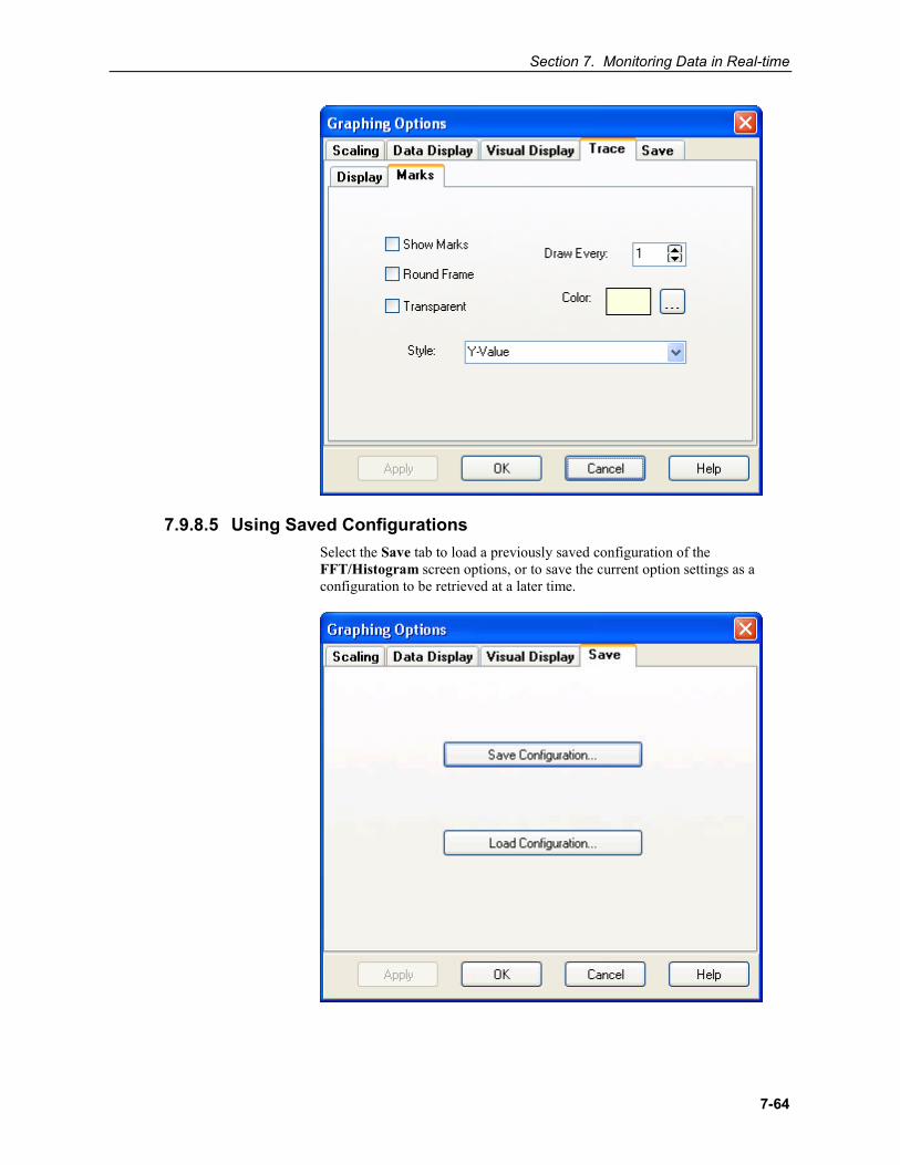
Section 7. Monitoring Data in Real-time
7-64
7.9.8.5 Using Saved Configurations Select the Save tab to load a previously saved configuration of the FFT/Histogram screen options, or to save the current option settings as a configuration to be retrieved at a later time.
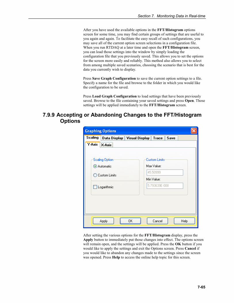
Section 7. Monitoring Data in Real-time
7-65
After you have used the available options in the FFT/Histogram options screen for some time, you may find certain groups of settings that are useful to you again and again. To facilitate the easy recall of such configurations, you may save all of the current option screen selections in a configuration file. When you run RTDAQ at a later time and open the FFT/Histogram screen, you can load those settings into the window by simply loading the configuration file that you previously saved. This allows you to set the options for the screen more easily and reliably. This method also allows you to select from among multiple saved scenarios, choosing the scenario that is best for the data you currently wish to display.
Press Save Graph Configuration to save the current option settings to a file. Specify a name for the file and browse to the folder in which you would like the configuration to be saved.
Press Load Graph Configuration to load settings that have been previously saved. Browse to the file containing your saved settings and press Open. Those settings will be applied immediately to the FFT/Histogram screen.
7.9.9 Accepting or Abandoning Changes to the FFT/Histogram Options
After setting the various options for the FFT/Histogram display, press the Apply button to immediately put those changes into effect. The options screen will remain open, and the settings will be applied. Press the OK button if you would like to apply the settings and exit the Options screen. Press Cancel if you would like to abandon any changes made to the settings since the screen was opened. Press Help to access the online help topic for this screen.
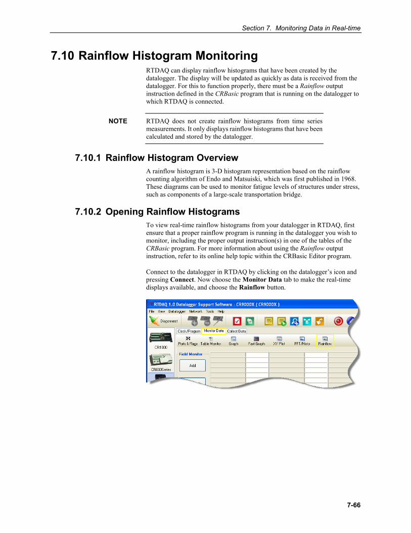
Section 7. Monitoring Data in Real-time
7-66
7.10 Rainflow Histogram Monitoring RTDAQ can display rainflow histograms that have been created by the datalogger. The display will be updated as quickly as data is received from the datalogger. For this to function properly, there must be a Rainflow output instruction defined in the CRBasic program that is running on the datalogger to which RTDAQ is connected.
RTDAQ does not create rainflow histograms from time series measurements. It only displays rainflow histograms that have been calculated and stored by the datalogger.
7.10.1 Rainflow Histogram Overview A rainflow histogram is 3-D histogram representation based on the rainflow counting algorithm of Endo and Matsuiski, which was first published in 1968. These diagrams can be used to monitor fatigue levels of structures under stress, such as components of a large-scale transportation bridge.
7.10.2 Opening Rainflow Histograms To view real-time rainflow histograms from your datalogger in RTDAQ, first ensure that a proper rainflow program is running in the datalogger you wish to monitor, including the proper output instruction(s) in one of the tables of the CRBasic program. For more information about using the Rainflow output instruction, refer to its online help topic within the CRBasic Editor program.
Connect to the datalogger in RTDAQ by clicking on the datalogger’s icon and pressing Connect. Now choose the Monitor Data tab to make the real-time displays available, and choose the Rainflow button.
NOTE
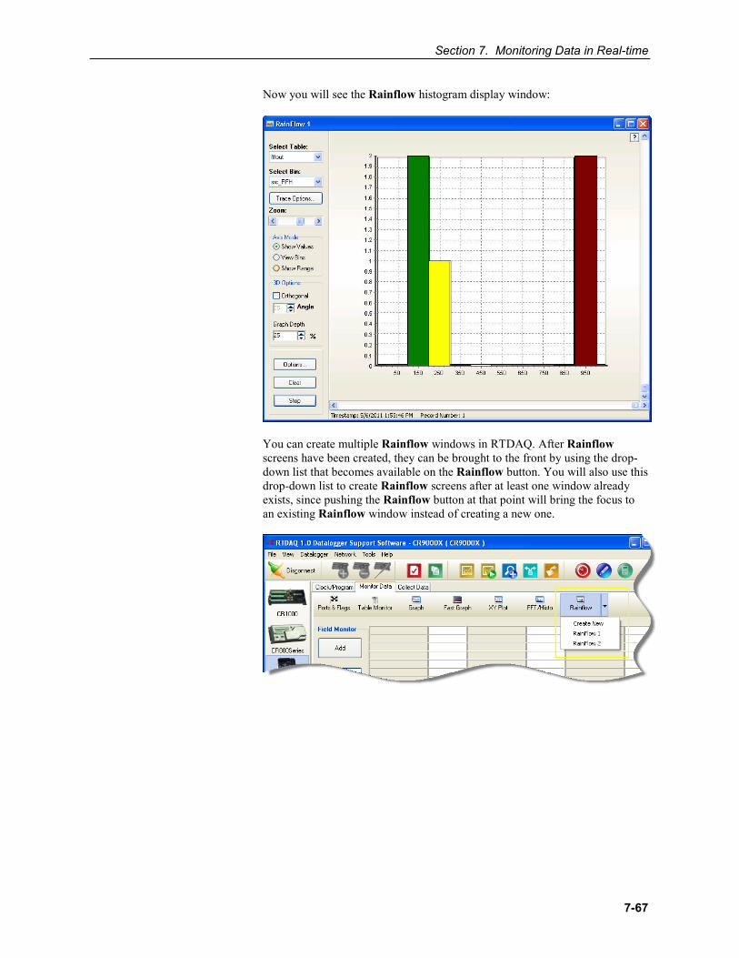
Section 7. Monitoring Data in Real-time
7-67
Now you will see the Rainflow histogram display window:
You can create multiple Rainflow windows in RTDAQ. After Rainflow screens have been created, they can be brought to the front by using the drop-down list that becomes available on the Rainflow button. You will also use this drop-down list to create Rainflow screens after at least one window already exists, since pushing the Rainflow button at that point will bring the focus to an existing Rainflow window instead of creating a new one.
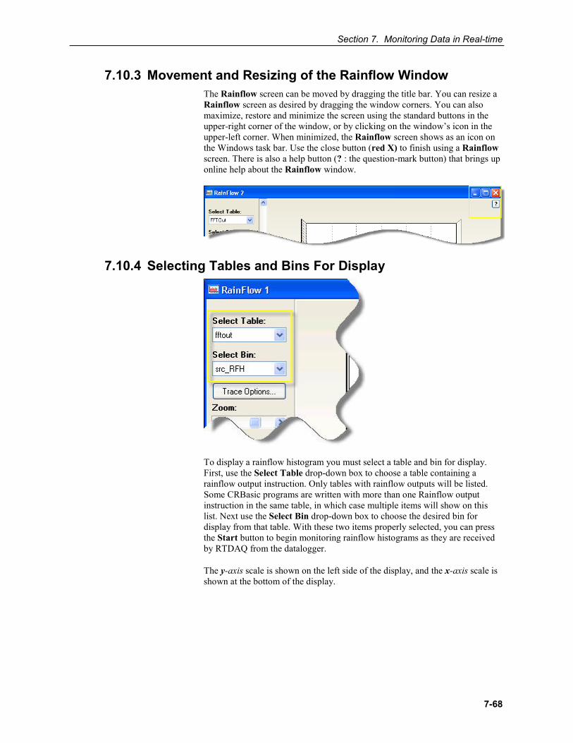
Section 7. Monitoring Data in Real-time
7-68
7.10.3 Movement and Resizing of the Rainflow Window The Rainflow screen can be moved by dragging the title bar. You can resize a Rainflow screen as desired by dragging the window corners. You can also maximize, restore and minimize the screen using the standard buttons in the upper-right corner of the window, or by clicking on the window’s icon in the upper-left corner. When minimized, the Rainflow screen shows as an icon on the Windows task bar. Use the close button (red X) to finish using a Rainflow screen. There is also a help button (? : the question-mark button) that brings up online help about the Rainflow window.
7.10.4 Selecting Tables and Bins For Display
To display a rainflow histogram you must select a table and bin for display. First, use the Select Table drop-down box to choose a table containing a rainflow output instruction. Only tables with rainflow outputs will be listed. Some CRBasic programs are written with more than one Rainflow output instruction in the same table, in which case multiple items will show on this list. Next use the Select Bin drop-down box to choose the desired bin for display from that table. With these two items properly selected, you can press the Start button to begin monitoring rainflow histograms as they are received by RTDAQ from the datalogger.
The y-axis scale is shown on the left side of the display, and the x-axis scale is shown at the bottom of the display.
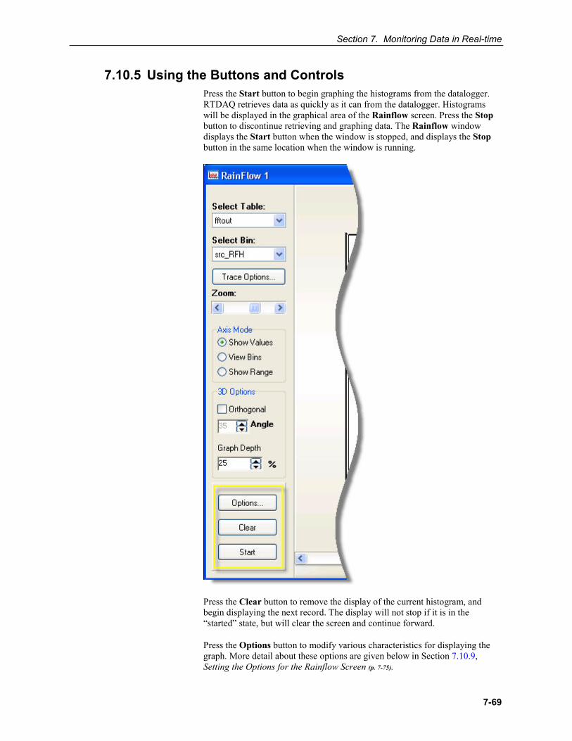
Section 7. Monitoring Data in Real-time
7-69
7.10.5 Using the Buttons and Controls Press the Start button to begin graphing the histograms from the datalogger. RTDAQ retrieves data as quickly as it can from the datalogger. Histograms will be displayed in the graphical area of the Rainflow screen. Press the Stop button to discontinue retrieving and graphing data. The Rainflow window displays the Start button when the window is stopped, and displays the Stop button in the same location when the window is running.
Press the Clear button to remove the display of the current histogram, and begin displaying the next record. The display will not stop if it is in the “started” state, but will clear the screen and continue forward.
Press the Options button to modify various characteristics for displaying the graph. More detail about these options are given below in Section 7.10.9, Setting the Options for the Rainflow Screen (p. 7-75).
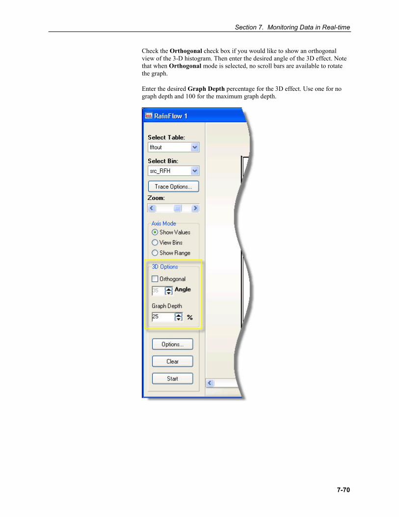
Section 7. Monitoring Data in Real-time
7-70
Check the Orthogonal check box if you would like to show an orthogonal view of the 3-D histogram. Then enter the desired angle of the 3D effect. Note that when Orthogonal mode is selected, no scroll bars are available to rotate the graph.
Enter the desired Graph Depth percentage for the 3D effect. Use one for no graph depth and 100 for the maximum graph depth.
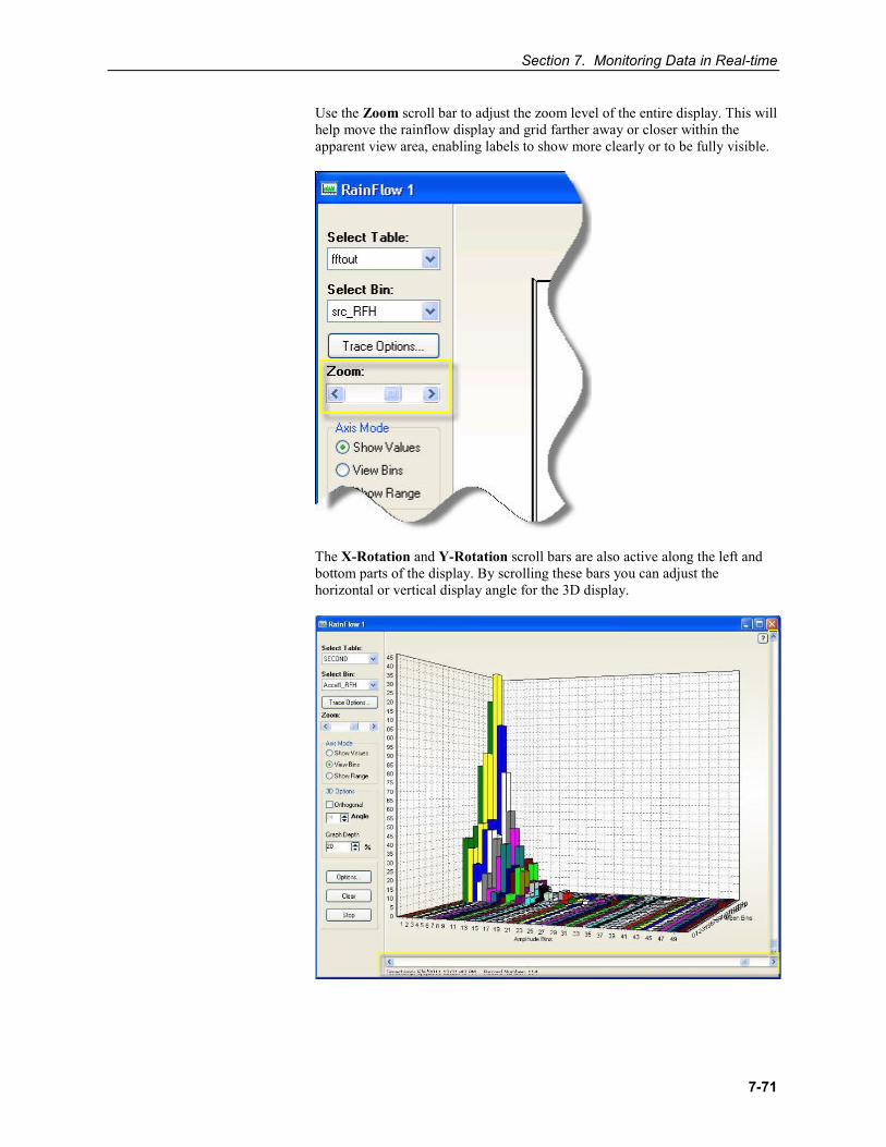
Section 7. Monitoring Data in Real-time
7-71
Use the Zoom scroll bar to adjust the zoom level of the entire display. This will help move the rainflow display and grid farther away or closer within the apparent view area, enabling labels to show more clearly or to be fully visible.
The X-Rotation and Y-Rotation scroll bars are also active along the left and bottom parts of the display. By scrolling these bars you can adjust the horizontal or vertical display angle for the 3D display.
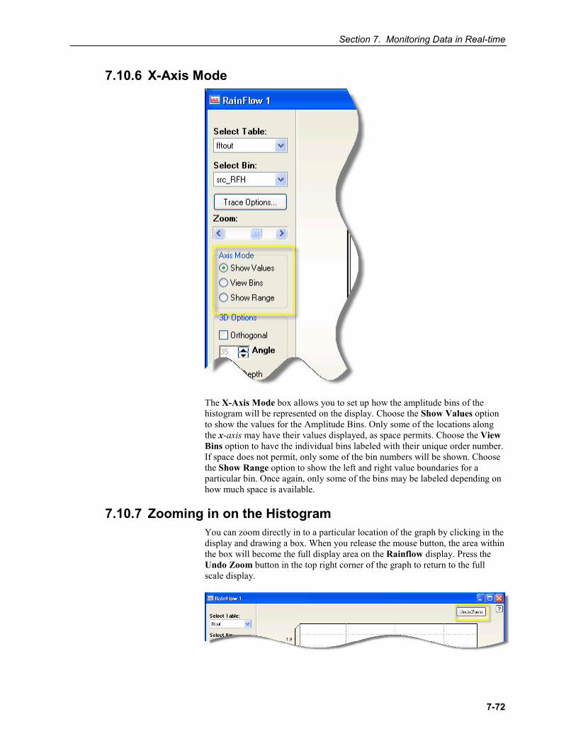
Section 7. Monitoring Data in Real-time
7-72
7.10.6 X-Axis Mode
The X-Axis Mode box allows you to set up how the amplitude bins of the histogram will be represented on the display. Choose the Show Values option to show the values for the Amplitude Bins. Only some of the locations along the x-axis may have their values displayed, as space permits. Choose the View Bins option to have the individual bins labeled with their unique order number. If space does not permit, only some of the bin numbers will be shown. Choose the Show Range option to show the left and right value boundaries for a particular bin. Once again, only some of the bins may be labeled depending on how much space is available.
7.10.7 Zooming in on the Histogram You can zoom directly in to a particular location of the graph by clicking in the display and drawing a box. When you release the mouse button, the area within the box will become the full display area on the Rainflow display. Press the Undo Zoom button in the top right corner of the graph to return to the full scale display.
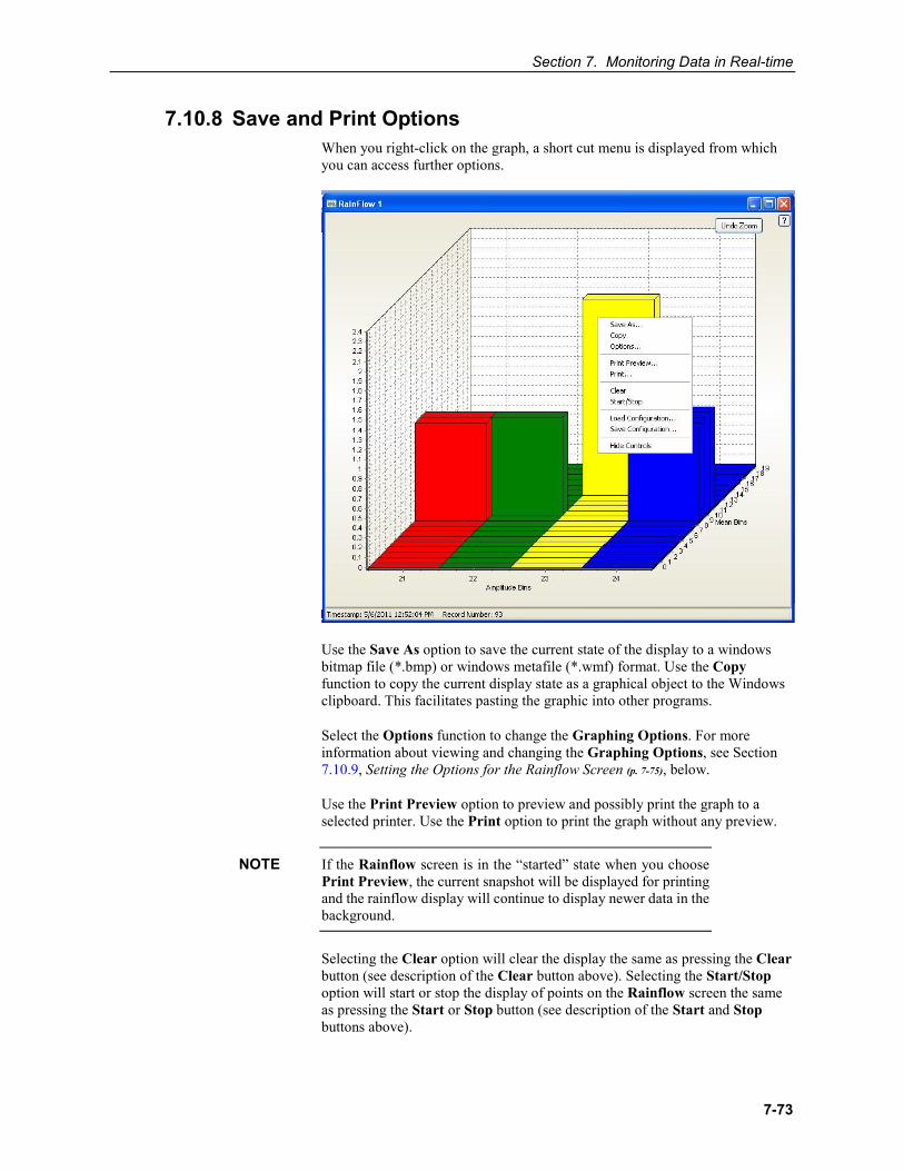
Section 7. Monitoring Data in Real-time
7-73
7.10.8 Save and Print Options When you right-click on the graph, a short cut menu is displayed from which you can access further options.
Use the Save As option to save the current state of the display to a windows bitmap file (*.bmp) or windows metafile (*.wmf) format. Use the Copy function to copy the current display state as a graphical object to the Windows clipboard. This facilitates pasting the graphic into other programs.
Select the Options function to change the Graphing Options. For more information about viewing and changing the Graphing Options, see Section 7.10.9, Setting the Options for the Rainflow Screen (p. 7-75), below.
Use the Print Preview option to preview and possibly print the graph to a selected printer. Use the Print option to print the graph without any preview.
If the Rainflow screen is in the “started” state when you choose Print Preview, the current snapshot will be displayed for printing and the rainflow display will continue to display newer data in the background.
Selecting the Clear option will clear the display the same as pressing the Clear button (see description of the Clear button above). Selecting the Start/Stop option will start or stop the display of points on the Rainflow screen the same as pressing the Start or Stop button (see description of the Start and Stop buttons above).
NOTE
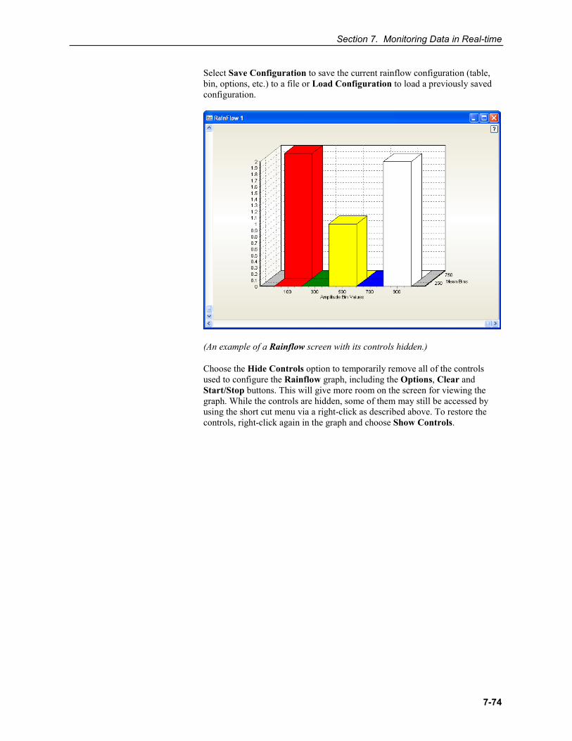
Section 7. Monitoring Data in Real-time
7-74
Select Save Configuration to save the current rainflow configuration (table, bin, options, etc.) to a file or Load Configuration to load a previously saved configuration.
(An example of a Rainflow screen with its controls hidden.)
Choose the Hide Controls option to temporarily remove all of the controls used to configure the Rainflow graph, including the Options, Clear and Start/Stop buttons. This will give more room on the screen for viewing the graph. While the controls are hidden, some of them may still be accessed by using the short cut menu via a right-click as described above. To restore the controls, right-click again in the graph and choose Show Controls.
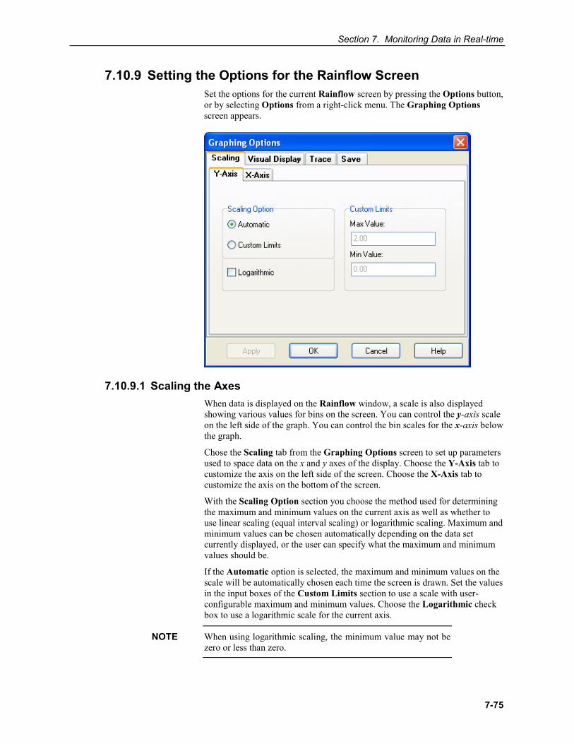
Section 7. Monitoring Data in Real-time
7-75
7.10.9 Setting the Options for the Rainflow Screen Set the options for the current Rainflow screen by pressing the Options button, or by selecting Options from a right-click menu. The Graphing Options screen appears.
7.10.9.1 Scaling the Axes When data is displayed on the Rainflow window, a scale is also displayed showing various values for bins on the screen. You can control the y-axis scale on the left side of the graph. You can control the bin scales for the x-axis below the graph.
Chose the Scaling tab from the Graphing Options screen to set up parameters used to space data on the x and y axes of the display. Choose the Y-Axis tab to customize the axis on the left side of the screen. Choose the X-Axis tab to customize the axis on the bottom of the screen.
With the Scaling Option section you choose the method used for determining the maximum and minimum values on the current axis as well as whether to use linear scaling (equal interval scaling) or logarithmic scaling. Maximum and minimum values can be chosen automatically depending on the data set currently displayed, or the user can specify what the maximum and minimum values should be.
If the Automatic option is selected, the maximum and minimum values on the scale will be automatically chosen each time the screen is drawn. Set the values in the input boxes of the Custom Limits section to use a scale with user-configurable maximum and minimum values. Choose the Logarithmic check box to use a logarithmic scale for the current axis.
When using logarithmic scaling, the minimum value may not be zero or less than zero.
NOTE

Section 7. Monitoring Data in Real-time
7-76
7.10.9.2 Visual Display Options Select the Visual Display tab to modify chart colours and configure the titles on the rainflow histogram display.
The Chart colours section allows you to set the colour for the back wall of the Rainflow display, set the colour of the left grid (scale), or put the display into the Colour Each Bin mode. When the Colour Each Bin check box is selected, each bin is given a different colour on the display so that bins can be distinguished from each other.
The Back Image field allows you to specify an image that will be used as the background. Select the Stretch check box to have the image stretched to fill the background. Press the Clear button to clear the background image.
Use the Titles section to set up titles to show alongside the values shown on your Rainflow display. You may elect to show a title for the entire rainflow histogram, specifying the text to display and the font used to display it. You can also set up a title to be displayed by the y-axis. For more information about using the Visual Display options, refer to the online help that can be accessed by opening the options screen and pressing the Help button.
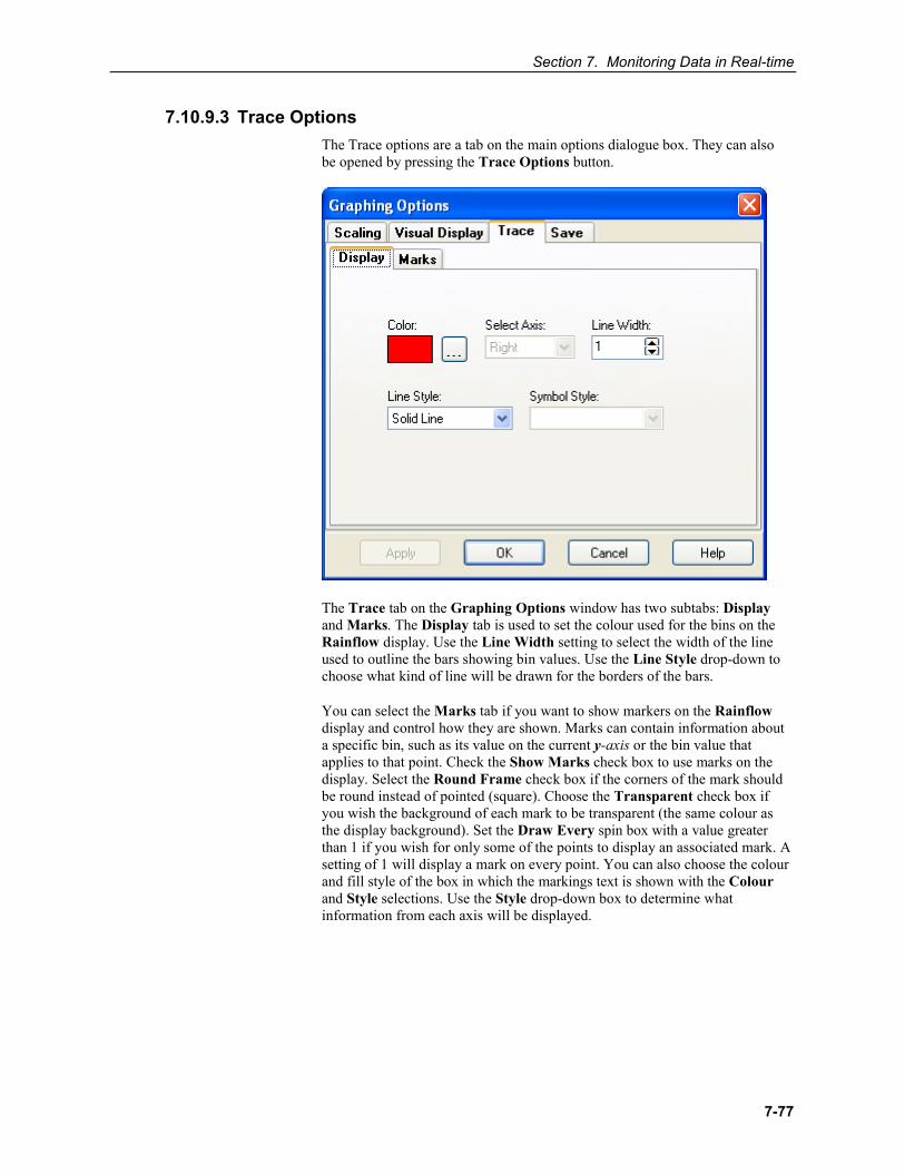
Section 7. Monitoring Data in Real-time
7-77
7.10.9.3 Trace Options The Trace options are a tab on the main options dialogue box. They can also be opened by pressing the Trace Options button.
The Trace tab on the Graphing Options window has two subtabs: Display and Marks. The Display tab is used to set the colour used for the bins on the Rainflow display. Use the Line Width setting to select the width of the line used to outline the bars showing bin values. Use the Line Style drop-down to choose what kind of line will be drawn for the borders of the bars.
You can select the Marks tab if you want to show markers on the Rainflow display and control how they are shown. Marks can contain information about a specific bin, such as its value on the current y-axis or the bin value that applies to that point. Check the Show Marks check box to use marks on the display. Select the Round Frame check box if the corners of the mark should be round instead of pointed (square). Choose the Transparent check box if you wish the background of each mark to be transparent (the same colour as the display background). Set the Draw Every spin box with a value greater than 1 if you wish for only some of the points to display an associated mark. A setting of 1 will display a mark on every point. You can also choose the colour and fill style of the box in which the markings text is shown with the Colour and Style selections. Use the Style drop-down box to determine what information from each axis will be displayed.
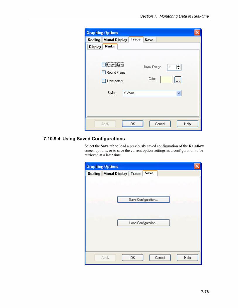
Section 7. Monitoring Data in Real-time
7-78
7.10.9.4 Using Saved Configurations Select the Save tab to load a previously saved configuration of the Rainflow screen options, or to save the current option settings as a configuration to be retrieved at a later time.
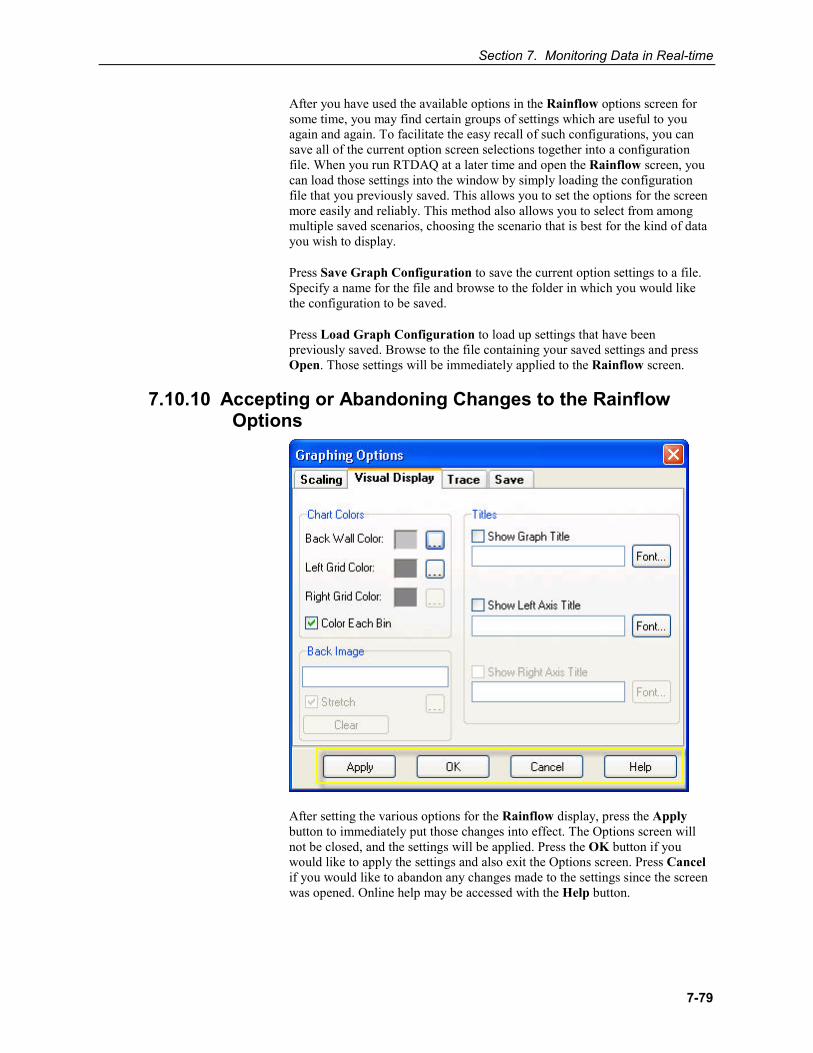
Section 7. Monitoring Data in Real-time
7-79
After you have used the available options in the Rainflow options screen for some time, you may find certain groups of settings which are useful to you again and again. To facilitate the easy recall of such configurations, you can save all of the current option screen selections together into a configuration file. When you run RTDAQ at a later time and open the Rainflow screen, you can load those settings into the window by simply loading the configuration file that you previously saved. This allows you to set the options for the screen more easily and reliably. This method also allows you to select from among multiple saved scenarios, choosing the scenario that is best for the kind of data you wish to display.
Press Save Graph Configuration to save the current option settings to a file. Specify a name for the file and browse to the folder in which you would like the configuration to be saved.
Press Load Graph Configuration to load up settings that have been previously saved. Browse to the file containing your saved settings and press Open. Those settings will be immediately applied to the Rainflow screen.
7.10.10 Accepting or Abandoning Changes to the Rainflow Options
After setting the various options for the Rainflow display, press the Apply button to immediately put those changes into effect. The Options screen will not be closed, and the settings will be applied. Press the OK button if you would like to apply the settings and also exit the Options screen. Press Cancel if you would like to abandon any changes made to the settings since the screen was opened. Online help may be accessed with the Help button.
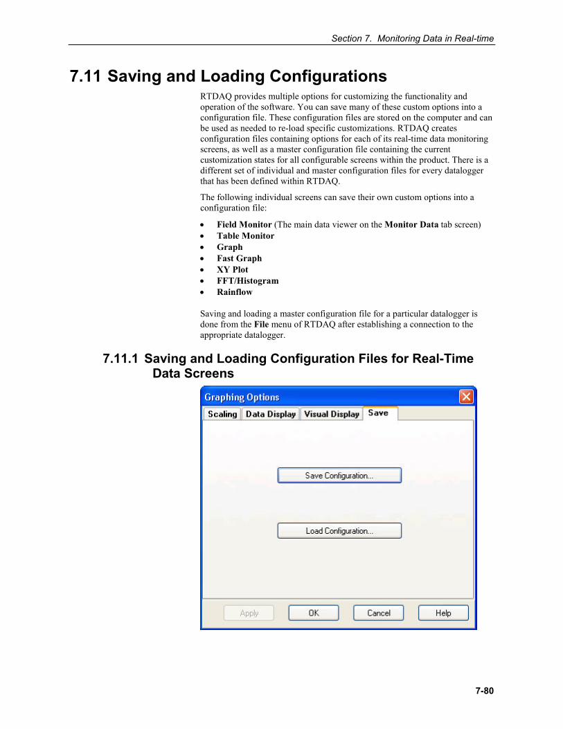
Section 7. Monitoring Data in Real-time
7-80
7.11 Saving and Loading Configurations RTDAQ provides multiple options for customizing the functionality and operation of the software. You can save many of these custom options into a configuration file. These configuration files are stored on the computer and can be used as needed to re-load specific customizations. RTDAQ creates configuration files containing options for each of its real-time data monitoring screens, as well as a master configuration file containing the current customization states for all configurable screens within the product. There is a different set of individual and master configuration files for every datalogger that has been defined within RTDAQ.
The following individual screens can save their own custom options into a configuration file:
• Field Monitor (The main data viewer on the Monitor Data tab screen) • Table Monitor • Graph • Fast Graph • XY Plot • FFT/Histogram • Rainflow
Saving and loading a master configuration file for a particular datalogger is done from the File menu of RTDAQ after establishing a connection to the appropriate datalogger.
7.11.1 Saving and Loading Configuration Files for Real-Time Data Screens
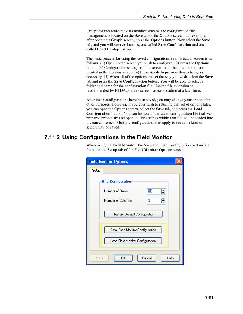
Section 7. Monitoring Data in Real-time
7-81
Except for two real-time data monitor screens, the configuration file management is located on the Save tab of the Options screen. For example, after opening a Graph screen, press the Options button. Now select the Save tab, and you will see two buttons, one called Save Configuration and one called Load Configuration.
The basic process for using the saved configurations in a particular screen is as follows: (1) Open up the screen you wish to configure. (2) Press the Options button. (3) Configure the settings of that screen in all the other tab options located in the Options screen. (4) Press Apply to preview those changes if necessary. (5) When all of the options are set the way you wish, select the Save tab and press the Save Configuration button. You will be able to select a folder and name for the configuration file. Use the file extension as recommended by RTDAQ in this screen for easy loading at a later time.
After those configurations have been saved, you may change your options for other purposes. However, if you ever wish to return to that set of options later, you can open the Options screen, select the Save tab, and press the Load Configuration button. You can browse to the saved configuration file that was prepared previously and open it. The settings within that file will be loaded into the current screen. Multiple configurations that apply to the same kind of screen may be saved.
7.11.2 Using Configurations in the Field Monitor When using the Field Monitor, the Save and Load Configuration buttons are found on the Setup tab of the Field Monitor Options screen.
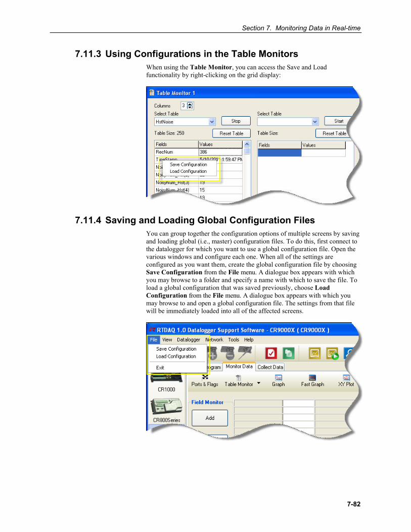
Section 7. Monitoring Data in Real-time
7-82
7.11.3 Using Configurations in the Table Monitors When using the Table Monitor, you can access the Save and Load functionality by right-clicking on the grid display:
7.11.4 Saving and Loading Global Configuration Files You can group together the configuration options of multiple screens by saving and loading global (i.e., master) configuration files. To do this, first connect to the datalogger for which you want to use a global configuration file. Open the various windows and configure each one. When all of the settings are configured as you want them, create the global configuration file by choosing Save Configuration from the File menu. A dialogue box appears with which you may browse to a folder and specify a name with which to save the file. To load a global configuration that was saved previously, choose Load Configuration from the File menu. A dialogue box appears with which you may browse to and open a global configuration file. The settings from that file will be immediately loaded into all of the affected screens.
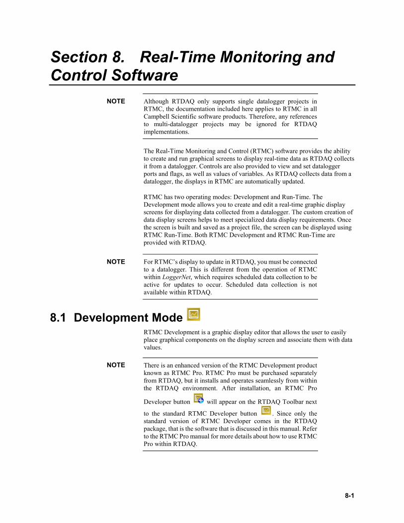
8-1
Section 8. Real-Time Monitoring and Control Software
Although RTDAQ only supports single datalogger projects in RTMC, the documentation included here applies to RTMC in all Campbell Scientific software products. Therefore, any references to multi-datalogger projects may be ignored for RTDAQ implementations.
The Real-Time Monitoring and Control (RTMC) software provides the ability to create and run graphical screens to display real-time data as RTDAQ collects it from a datalogger. Controls are also provided to view and set datalogger ports and flags, as well as values of variables. As RTDAQ collects data from a datalogger, the displays in RTMC are automatically updated.
RTMC has two operating modes: Development and Run-Time. The Development mode allows you to create and edit a real-time graphic display screens for displaying data collected from a datalogger. The custom creation of data display screens helps to meet specialized data display requirements. Once the screen is built and saved as a project file, the screen can be displayed using RTMC Run-Time. Both RTMC Development and RTMC Run-Time are provided with RTDAQ.
For RTMC’s display to update in RTDAQ, you must be connected to a datalogger. This is different from the operation of RTMC within LoggerNet, which requires scheduled data collection to be active for updates to occur. Scheduled data collection is not available within RTDAQ.
8.1 Development Mode RTMC Development is a graphic display editor that allows the user to easily place graphical components on the display screen and associate them with data values.
There is an enhanced version of the RTMC Development product known as RTMC Pro. RTMC Pro must be purchased separately from RTDAQ, but it installs and operates seamlessly from within the RTDAQ environment. After installation, an RTMC Pro
Developer button will appear on the RTDAQ Toolbar next
to the standard RTMC Developer button . Since only the standard version of RTMC Developer comes in the RTDAQ package, that is the software that is discussed in this manual. Refer to the RTMC Pro manual for more details about how to use RTMC Pro within RTDAQ.
NOTE
NOTE
NOTE
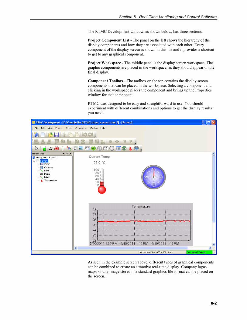
Section 8. Real-Time Monitoring and Control Software
8-2
The RTMC Development window, as shown below, has three sections.
Project Component List - The panel on the left shows the hierarchy of the display components and how they are associated with each other. Every component of the display screen is shown in this list and it provides a shortcut to get to any graphical component.
Project Workspace - The middle panel is the display screen workspace. The graphic components are placed in the workspace, as they should appear on the final display.
Component Toolbox - The toolbox on the top contains the display screen components that can be placed in the workspace. Selecting a component and clicking in the workspace places the component and brings up the Properties window for that component.
RTMC was designed to be easy and straightforward to use. You should experiment with different combinations and options to get the display results you need.
As seen in the example screen above, different types of graphical components can be combined to create an attractive real-time display. Company logos, maps, or any image stored in a standard graphics file format can be placed on the screen.
Section 8. Real-Time Monitoring and Control Software
8-3
Many images have been included with RTMC. The directory in which these files are stored is C:\Campbellsci\Lib\RTMCMediaLib. Custom images can be used as well; these should be placed in the media library directory to make them available for RTMC's use.
8.1.1 The RTMC Workspace The RTMC workspace is a container for holding one or more display screens. As new display screens are added (Project | Add New Screen) they appear as tabs in the project. The size of the workspace (and the resulting run-time window) can be changed by selecting Project | Configure WorkSpace.
8.1.2 Single Datalogger RTMC Projects RTDAQ connects to only one datalogger at any one time. Unlike RTMC in LoggerNet, RTMC projects in RTDAQ may only reference one datalogger per project. When creating a new project, the currently connected datalogger will be used as the station for that project. If no datalogger is connected, the user will be prompted to select one. Only one station can be used for specifying table and column data to be displayed. The project will be saved with data references to only one datalogger.
You may edit projects created with RTMC in LoggerNet that reference multiple dataloggers. In such instances, only the data from the connected datalogger will be updated. All other components relying on data from other dataloggers will show the exclamation point marker indicating that no data is available.
8.1.3 Display Components Display components are the objects that are used to display data. To add a component to the workspace, click an item on the Component Toolbox and then click anywhere in the workspace. The component’s Properties window is automatically displayed when the object is first placed in the work area. The Properties window is used to set colours, scale values, text, etc., and to assign the data value to be displayed by the component.
When a display component is linked to a data value, the value will be updated on the display at the table output rate if RTDAQ is connected to the associated datalogger. If RTDAQ is not connected to a datalogger, the values will not update and an exclamation point will appear in the upper right corner of the component to indicate the incomplete data connection.
After a component's properties have been set, select OK to enable the changes and close the Properties window. Once the link to the data value has been applied, if there is data available from RTDAQ for the component, the value on the display will update.
To make changes in display component settings, the Properties window can be opened by double-clicking the component. If you make changes to a component’s properties but then decide to reject those changes, press the Cancel button to return the properties to the last applied state. If Cancel is selected when a component is first placed in the work area (and OK has not been pressed), the display component will be removed from the screen.
NOTE
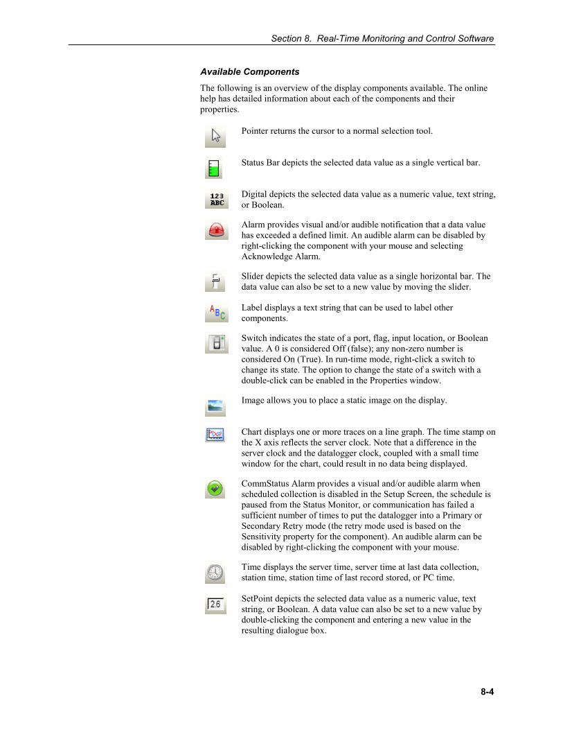
Section 8. Real-Time Monitoring and Control Software
8-4
Available Components
The following is an overview of the display components available. The online help has detailed information about each of the components and their properties.
Pointer returns the cursor to a normal selection tool.
Status Bar depicts the selected data value as a single vertical bar.
Digital depicts the selected data value as a numeric value, text string, or Boolean.
Alarm provides visual and/or audible notification that a data value has exceeded a defined limit. An audible alarm can be disabled by right-clicking the component with your mouse and selecting Acknowledge Alarm.
Slider depicts the selected data value as a single horizontal bar. The data value can also be set to a new value by moving the slider.
Label displays a text string that can be used to label other components.
Switch indicates the state of a port, flag, input location, or Boolean value. A 0 is considered Off (false); any non-zero number is considered On (True). In run-time mode, right-click a switch to change its state. The option to change the state of a switch with a double-click can be enabled in the Properties window.
Image allows you to place a static image on the display.
Chart displays one or more traces on a line graph. The time stamp on the X axis reflects the server clock. Note that a difference in the server clock and the datalogger clock, coupled with a small time window for the chart, could result in no data being displayed.
CommStatus Alarm provides a visual and/or audible alarm when scheduled collection is disabled in the Setup Screen, the schedule is paused from the Status Monitor, or communication has failed a sufficient number of times to put the datalogger into a Primary or Secondary Retry mode (the retry mode used is based on the Sensitivity property for the component). An audible alarm can be disabled by right-clicking the component with your mouse.
Time displays the server time, server time at last data collection, station time, station time of last record stored, or PC time.
SetPoint depicts the selected data value as a numeric value, text string, or Boolean. A data value can also be set to a new value by double-clicking the component and entering a new value in the resulting dialogue box.
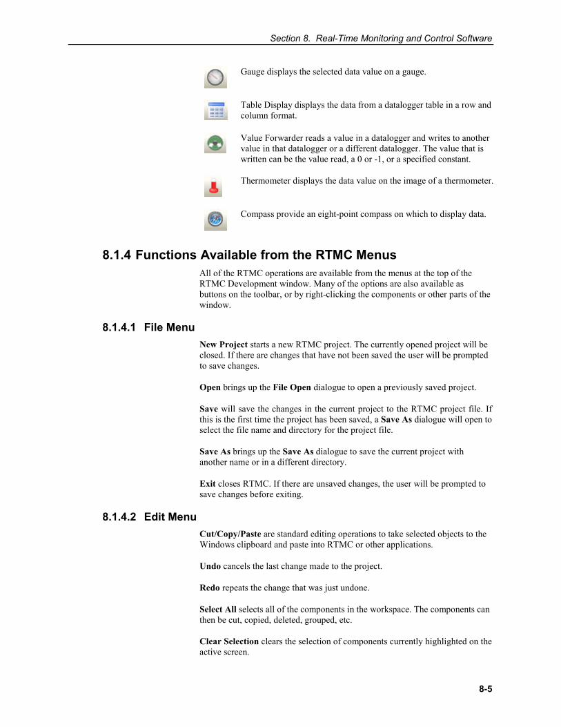
Section 8. Real-Time Monitoring and Control Software
8-5
Gauge displays the selected data value on a gauge.
Table Display displays the data from a datalogger table in a row and column format.
Value Forwarder reads a value in a datalogger and writes to another value in that datalogger or a different datalogger. The value that is written can be the value read, a 0 or -1, or a specified constant.
Thermometer displays the data value on the image of a thermometer.
Compass provide an eight-point compass on which to display data.
8.1.4 Functions Available from the RTMC Menus
8.1.4.1 File Menu
8.1.4.2 Edit Menu
All of the RTMC operations are available from the menus at the top of the RTMC Development window. Many of the options are also available as buttons on the toolbar, or by right-clicking the components or other parts of the window.
New Project starts a new RTMC project. The currently opened project will be closed. If there are changes that have not been saved the user will be prompted to save changes.
Open brings up the File Open dialogue to open a previously saved project.
Save will save the changes in the current project to the RTMC project file. If this is the first time the project has been saved, a Save As dialogue will open to select the file name and directory for the project file.
Save As brings up the Save As dialogue to save the current project with another name or in a different directory.
Exit closes RTMC. If there are unsaved changes, the user will be prompted to save changes before exiting.
Cut/Copy/Paste are standard editing operations to take selected objects to the Windows clipboard and paste into RTMC or other applications.
Undo cancels the last change made to the project.
Redo repeats the change that was just undone.
Select All selects all of the components in the workspace. The components can then be cut, copied, deleted, grouped, etc.
Clear Selection clears the selection of components currently highlighted on the active screen.
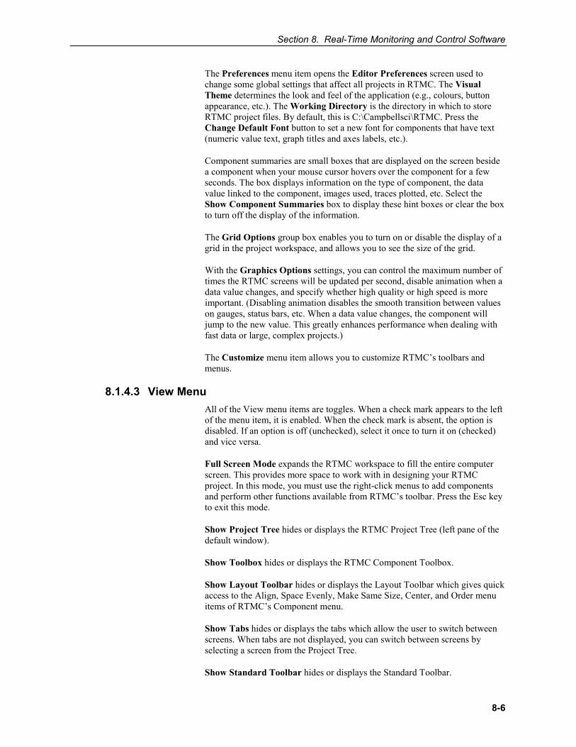
Section 8. Real-Time Monitoring and Control Software
8-6
The Preferences menu item opens the Editor Preferences screen used to change some global settings that affect all projects in RTMC. The Visual Theme determines the look and feel of the application (e.g., colours, button appearance, etc.). The Working Directory is the directory in which to store RTMC project files. By default, this is C:\Campbellsci\RTMC. Press the Change Default Font button to set a new font for components that have text (numeric value text, graph titles and axes labels, etc.).
Component summaries are small boxes that are displayed on the screen beside a component when your mouse cursor hovers over the component for a few seconds. The box displays information on the type of component, the data value linked to the component, images used, traces plotted, etc. Select the Show Component Summaries box to display these hint boxes or clear the box to turn off the display of the information.
The Grid Options group box enables you to turn on or disable the display of a grid in the project workspace, and allows you to see the size of the grid.
With the Graphics Options settings, you can control the maximum number of times the RTMC screens will be updated per second, disable animation when a data value changes, and specify whether high quality or high speed is more important. (Disabling animation disables the smooth transition between values on gauges, status bars, etc. When a data value changes, the component will jump to the new value. This greatly enhances performance when dealing with fast data or large, complex projects.)
The Customize menu item allows you to customize RTMC’s toolbars and menus.
8.1.4.3 View Menu All of the View menu items are toggles. When a check mark appears to the left of the menu item, it is enabled. When the check mark is absent, the option is disabled. If an option is off (unchecked), select it once to turn it on (checked) and vice versa.
Full Screen Mode expands the RTMC workspace to fill the entire computer screen. This provides more space to work with in designing your RTMC project. In this mode, you must use the right-click menus to add components and perform other functions available from RTMC’s toolbar. Press the Esc key to exit this mode.
Show Project Tree hides or displays the RTMC Project Tree (left pane of the default window).
Show Toolbox hides or displays the RTMC Component Toolbox.
Show Layout Toolbar hides or displays the Layout Toolbar which gives quick access to the Align, Space Evenly, Make Same Size, Center, and Order menu items of RTMC’s Component menu.
Show Tabs hides or displays the tabs which allow the user to switch between screens. When tabs are not displayed, you can switch between screens by selecting a screen from the Project Tree.
Show Standard Toolbar hides or displays the Standard Toolbar.
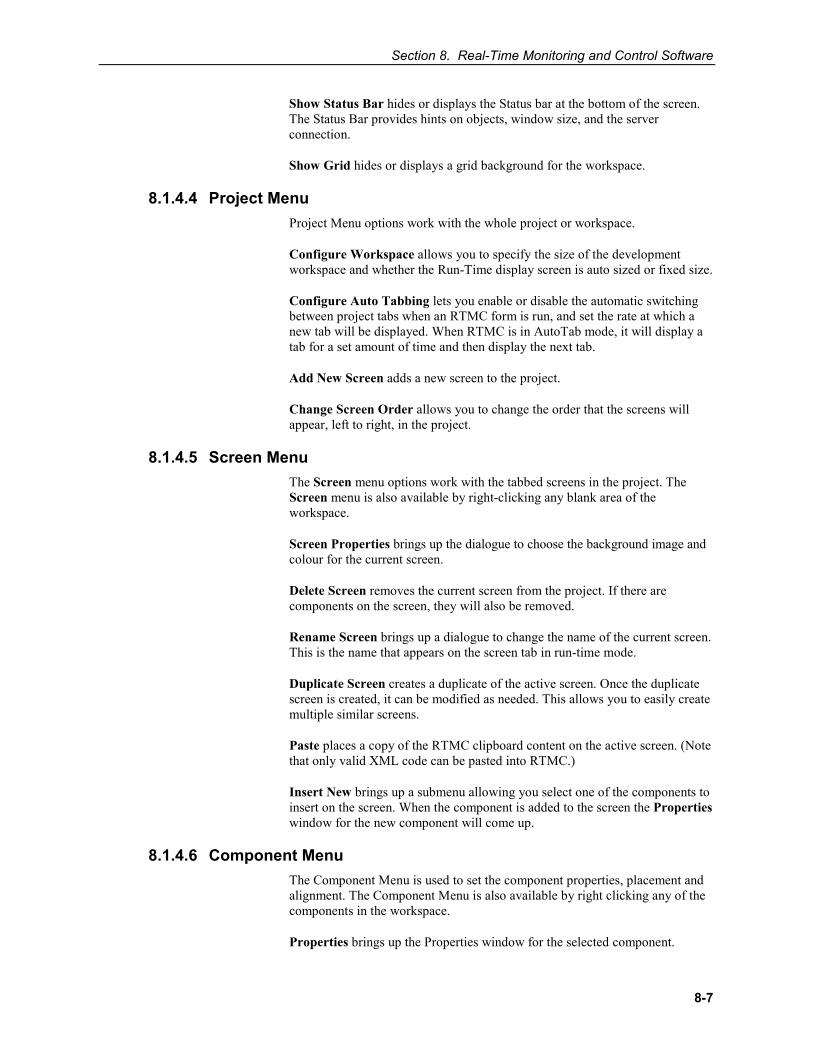
Section 8. Real-Time Monitoring and Control Software
8-7
Show Status Bar hides or displays the Status bar at the bottom of the screen. The Status Bar provides hints on objects, window size, and the server connection.
Show Grid hides or displays a grid background for the workspace.
8.1.4.4 Project Menu Project Menu options work with the whole project or workspace.
Configure Workspace allows you to specify the size of the development workspace and whether the Run-Time display screen is auto sized or fixed size.
Configure Auto Tabbing lets you enable or disable the automatic switching between project tabs when an RTMC form is run, and set the rate at which a new tab will be displayed. When RTMC is in AutoTab mode, it will display a tab for a set amount of time and then display the next tab.
Add New Screen adds a new screen to the project.
Change Screen Order allows you to change the order that the screens will appear, left to right, in the project.
8.1.4.5 Screen Menu The Screen menu options work with the tabbed screens in the project. The Screen menu is also available by right-clicking any blank area of the workspace.
Screen Properties brings up the dialogue to choose the background image and colour for the current screen.
Delete Screen removes the current screen from the project. If there are components on the screen, they will also be removed.
Rename Screen brings up a dialogue to change the name of the current screen. This is the name that appears on the screen tab in run-time mode.
Duplicate Screen creates a duplicate of the active screen. Once the duplicate screen is created, it can be modified as needed. This allows you to easily create multiple similar screens.
Paste places a copy of the RTMC clipboard content on the active screen. (Note that only valid XML code can be pasted into RTMC.)
Insert New brings up a submenu allowing you select one of the components to insert on the screen. When the component is added to the screen the Properties window for the new component will come up.
8.1.4.6 Component Menu The Component Menu is used to set the component properties, placement and alignment. The Component Menu is also available by right clicking any of the components in the workspace.
Properties brings up the Properties window for the selected component.
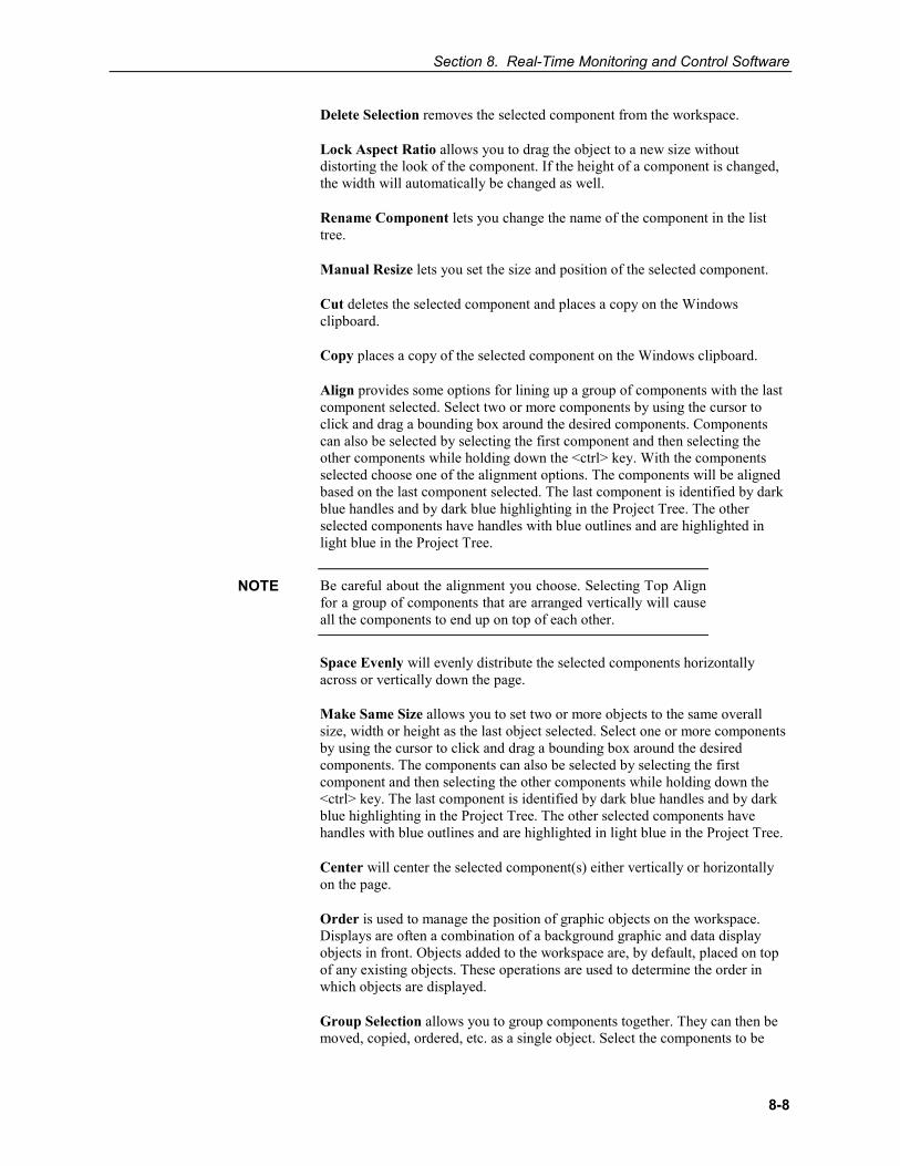
Section 8. Real-Time Monitoring and Control Software
8-8
Delete Selection removes the selected component from the workspace.
Lock Aspect Ratio allows you to drag the object to a new size without distorting the look of the component. If the height of a component is changed, the width will automatically be changed as well.
Rename Component lets you change the name of the component in the list tree.
Manual Resize lets you set the size and position of the selected component.
Cut deletes the selected component and places a copy on the Windows clipboard.
Copy places a copy of the selected component on the Windows clipboard.
Align provides some options for lining up a group of components with the last component selected. Select two or more components by using the cursor to click and drag a bounding box around the desired components. Components can also be selected by selecting the first component and then selecting the other components while holding down the <ctrl> key. With the components selected choose one of the alignment options. The components will be aligned based on the last component selected. The last component is identified by dark blue handles and by dark blue highlighting in the Project Tree. The other selected components have handles with blue outlines and are highlighted in light blue in the Project Tree.
Be careful about the alignment you choose. Selecting Top Align for a group of components that are arranged vertically will cause all the components to end up on top of each other.
Space Evenly will evenly distribute the selected components horizontally across or vertically down the page.
Make Same Size allows you to set two or more objects to the same overall size, width or height as the last object selected. Select one or more components by using the cursor to click and drag a bounding box around the desired components. The components can also be selected by selecting the first component and then selecting the other components while holding down the <ctrl> key. The last component is identified by dark blue handles and by dark blue highlighting in the Project Tree. The other selected components have handles with blue outlines and are highlighted in light blue in the Project Tree.
Center will center the selected component(s) either vertically or horizontally on the page.
Order is used to manage the position of graphic objects on the workspace. Displays are often a combination of a background graphic and data display objects in front. Objects added to the workspace are, by default, placed on top of any existing objects. These operations are used to determine the order in which objects are displayed.
Group Selection allows you to group components together. They can then be moved, copied, ordered, etc. as a single object. Select the components to be
NOTE
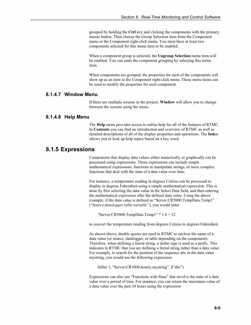
Section 8. Real-Time Monitoring and Control Software
8-9
grouped by holding the Ctrl key and clicking the components with the primary mouse button. Then choose the Group Selection item from the Component menu or the Component right-click menu. You must have at least two components selected for this menu item to be enabled.
When a component group is selected, the Ungroup Selection menu item will be enabled. You can undo the component grouping by selecting this menu item.
When components are grouped, the properties for each of the components will show up as an item in the Component right-click menu. These menu items can be used to modify the properties for each component.
8.1.4.7 Window Menu If there are multiple screens in the project, Window will allow you to change between the screens using the menu.
8.1.4.8 Help Menu The Help menu provides access to online help for all of the features of RTMC. In Contents you can find an introduction and overview of RTMC as well as detailed descriptions of all of the display properties and operations. The Index allows you to look up help topics based on a key word.
8.1.5 Expressions Components that display data values either numerically or graphically can be processed using expressions. These expressions can include simple mathematical expressions, functions to manipulate strings, or more complex functions that deal with the state of a data value over time.
For instance, a temperature reading in degrees Celsius can be processed to display in degrees Fahrenheit using a simple mathematical expression. This is done by first selecting the data value in the Select Data field, and then entering the mathematical expression after the defined data value. Using the above example, if the data value is defined as “Server:CR5000.TempData.Temp1” (“Source:datalogger.table.variable”), you would enter
“Server:CR5000.TempData.Temp1” * 1.8 + 32
to convert the temperature reading from degrees Celsius to degrees Fahrenheit.
As shown above, double quotes are used in RTMC to enclose the name of a data value (or source, datalogger, or table depending on the component). Therefore, when defining a literal string, a dollar sign is used as a prefix. This indicates to RTMC that you are defining a literal string rather than a data value. For example, to search for the position of the sequence abc in the data value mystring, you would use the following expression:
InStr( 1, “Server:CR1000.hourly.mystring”, $”abc”)
Expressions can also use “Functions with State” that involve the state of a data value over a period of time. For instance, you can return the maximum value of a data value over the past 24 hours using the expression:
Section 8. Real-Time Monitoring and Control Software
8-10
MaxRunOverTime(“Server:CR1000.QtrHour.Temp”,Timestamp(“Server:CR1000.QtrHour.Temp”),nsecPerDay)
When RTMC-RT is launched it begins processing with the newest record by default. Therefore, using the above expression, a component will not immediately display the maximum value over the past 24 hours. Rather, it will display the maximum value since RTMC-RT was launched. The 24-hour maximum will only be displayed after it has been running for 24 hours. In order to get a 24 hour maximum immediately, you can use a “Start Option Function” to cause RTMC to begin processing data at an earlier point. For example,
StartRelativeToNewest(nsecPerDay,ordercollected); MaxRunOverTime(“Server:CR1000.QtrHour.Temp”,Timestamp(“Server:CR1000.QtrHour.Temp”),nsecPerDay)
would begin displaying a 24 hour maximum immediately, provided that the data is available in the communications server’s data cache.
Aliases
If a data value is used multiple times in an expression, the expression can be simplified by declaring an alias for the data value at the first of the expression, in the form:
Alias(alias_name, data_value)
For example,
StartAtOffsetFromNewest(5,OrderCollected);IIF(ABS(("Server:CR1000.MyTable.Value"-ValueAtTime("Server:CR1000.MyTable.Value",TimeStamp("Server:CR1000.MyTable.Value"),30*nsecPerSec,0))>10 AND ABS(ValueAtTime("Server:CR1000.MyTable.Value",TimeStamp("Server:CR1000.MyTable.Value"),30*nsecPerSec,0)-ValueAtTime("Server:CR1000.MyTable.Value",TimeStamp("Server:CR1000.MyTable.Value"),60*nsecPerSec,0)))>10,1,0)
can be replaced by:
Alias(X,"Server:CR1000.MyTable.Value");StartAtOffsetFromNewest(5,OrderCollected);IIF((ABS(X-ValueAtTime(X,TimeStamp(X),30*nsecPerSec,0))>10 AND ABS(ValueAtTime(X,TimeStamp(X),30*nsecPerSec,0)-ValueAtTime(X,TimeStamp(X),60*nsecPerSec,0)))>10,1,0)
Synchronizing Variables
The ValueSynch function can be used to synchronize data values coming from multiple data sources so that you can display the results of a calculation on those data values in a single component. The Value Synch function takes the form:
ValueSynch(synchronized_name, data_value)
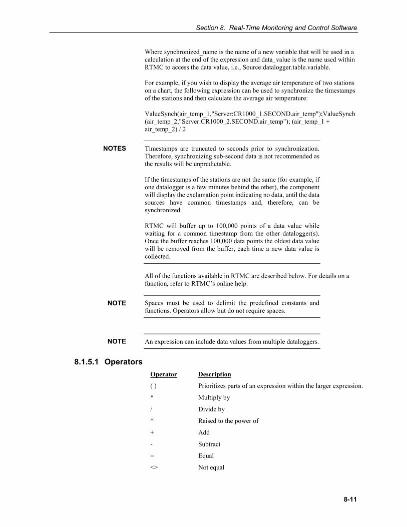
Section 8. Real-Time Monitoring and Control Software
8-11
Where synchronized_name is the name of a new variable that will be used in a calculation at the end of the expression and data_value is the name used within RTMC to access the data value, i.e., Source:datalogger.table.variable.
For example, if you wish to display the average air temperature of two stations on a chart, the following expression can be used to synchronize the timestamps of the stations and then calculate the average air temperature:
ValueSynch(air_temp_1,"Server:CR1000_1.SECOND.air_temp");ValueSynch(air_temp_2,"Server:CR1000_2.SECOND.air_temp"); (air_temp_1 + air_temp_2) / 2
Timestamps are truncated to seconds prior to synchronization. Therefore, synchronizing sub-second data is not recommended as the results will be unpredictable.
If the timestamps of the stations are not the same (for example, if one datalogger is a few minutes behind the other), the component will display the exclamation point indicating no data, until the data sources have common timestamps and, therefore, can be synchronized.
RTMC will buffer up to 100,000 points of a data value while waiting for a common timestamp from the other datalogger(s). Once the buffer reaches 100,000 data points the oldest data value will be removed from the buffer, each time a new data value is collected.
All of the functions available in RTMC are described below. For details on a function, refer to RTMC’s online help.
Spaces must be used to delimit the predefined constants and functions. Operators allow but do not require spaces.
An expression can include data values from multiple dataloggers.
8.1.5.1 Operators Operator Description
( ) Prioritizes parts of an expression within the larger expression.
* Multiply by
/ Divide by
^ Raised to the power of
+ Add
- Subtract
= Equal
<> Not equal
NOTES
NOTE
NOTE
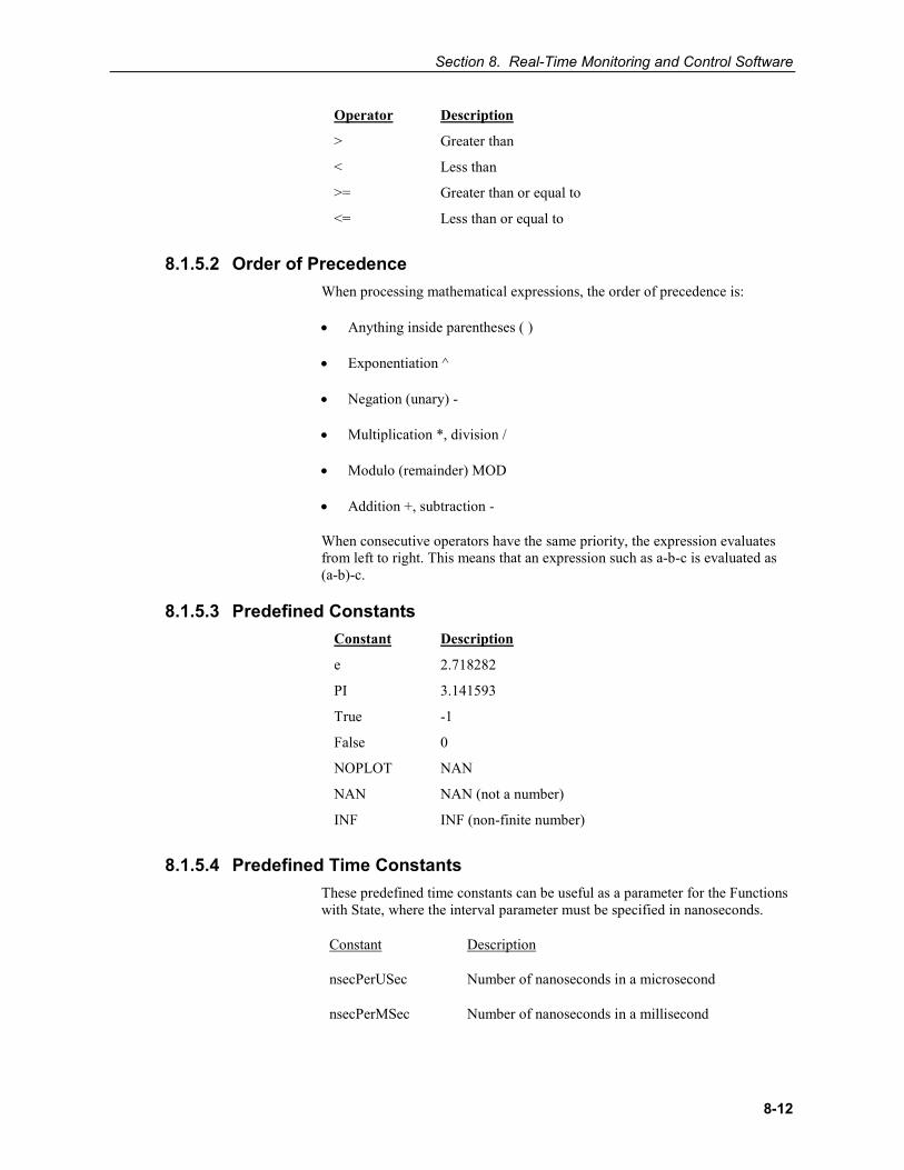
Section 8. Real-Time Monitoring and Control Software
8-12
Operator Description
> Greater than
< Less than
>= Greater than or equal to
<= Less than or equal to
8.1.5.2 Order of Precedence When processing mathematical expressions, the order of precedence is:
• Anything inside parentheses ( )
• Exponentiation ^
• Negation (unary) -
• Multiplication *, division /
• Modulo (remainder) MOD
• Addition +, subtraction -
When consecutive operators have the same priority, the expression evaluates from left to right. This means that an expression such as a-b-c is evaluated as (a-b)-c.
8.1.5.3 Predefined Constants Constant Description
e 2.718282
PI 3.141593
True -1
False 0
NOPLOT NAN
NAN NAN (not a number)
INF INF (non-finite number)
8.1.5.4 Predefined Time Constants These predefined time constants can be useful as a parameter for the Functions with State, where the interval parameter must be specified in nanoseconds.
Constant Description
nsecPerUSec Number of nanoseconds in a microsecond
nsecPerMSec Number of nanoseconds in a millisecond
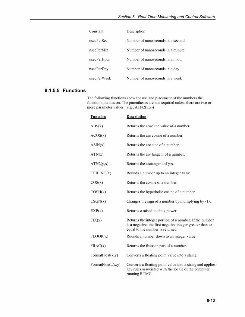
Section 8. Real-Time Monitoring and Control Software
8-13
Constant Description
nsecPerSec Number of nanoseconds in a second
nsecPerMin Number of nanoseconds in a minute
nsecPerHour Number of nanoseconds in an hour
nsecPerDay Number of nanoseconds in a day
nsecPerWeek Number of nanoseconds in a week
8.1.5.5 Functions The following functions show the use and placement of the numbers the function operates on. The parentheses are not required unless there are two or more parameter values. (e.g., ATN2(y,x))
Function Description
ABS(x) Returns the absolute value of a number.
ACOS(x) Returns the arc cosine of a number.
ASIN(x) Returns the arc sine of a number.
ATN(x) Returns the arc tangent of a number.
ATN2(y,x) Returns the arctangent of y/x.
CEILING(x) Rounds a number up to an integer value.
COS(x) Returns the cosine of a number.
COSH(x) Returns the hyperbolic cosine of a number.
CSGN(x) Changes the sign of a number by multiplying by -1.0.
EXP(x) Returns e raised to the x power.
FIX(x) Returns the integer portion of a number. If the number is a negative, the first negative integer greater than or equal to the number is returned.
FLOOR(x) Rounds a number down to an integer value.
FRAC(x) Returns the fraction part of a number.
FormatFloat(x,y) Converts a floating point value into a string.
FormatFloatL(x,y) Converts a floating point value into a string and applies any rules associated with the locale of the computer running RTMC.
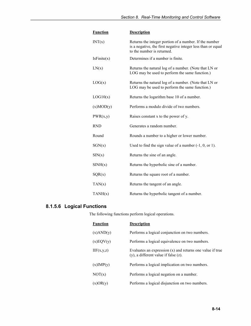
Section 8. Real-Time Monitoring and Control Software
8-14
Function Description
INT(x) Returns the integer portion of a number. If the number is a negative, the first negative integer less than or equal to the number is returned.
IsFinite(x) Determines if a number is finite.
LN(x) Returns the natural log of a number. (Note that LN or LOG may be used to perform the same function.)
LOG(x) Returns the natural log of a number. (Note that LN or LOG may be used to perform the same function.)
LOG10(x) Returns the logarithm base 10 of a number.
(x)MOD(y) Performs a modulo divide of two numbers.
PWR(x,y) Raises constant x to the power of y.
RND Generates a random number.
Round Rounds a number to a higher or lower number.
SGN(x) Used to find the sign value of a number (-1, 0, or 1).
SIN(x) Returns the sine of an angle.
SINH(x) Returns the hyperbolic sine of a number.
SQR(x) Returns the square root of a number.
TAN(x) Returns the tangent of an angle.
TANH(x) Returns the hyperbolic tangent of a number.
8.1.5.6 Logical Functions The following functions perform logical operations.
Function Description
(x)AND(y) Performs a logical conjunction on two numbers.
(x)EQV(y) Performs a logical equivalence on two numbers.
IIF(x,y,z) Evaluates an expression (x) and returns one value if true (y), a different value if false (z).
(x)IMP(y) Performs a logical implication on two numbers.
NOT(x) Performs a logical negation on a number.
(x)OR(y) Performs a logical disjunction on two numbers.
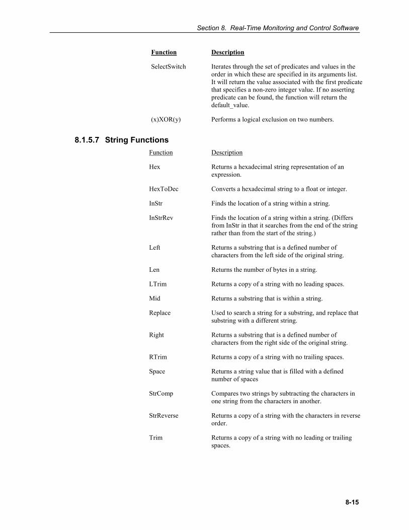
Section 8. Real-Time Monitoring and Control Software
8-15
Function Description
SelectSwitch Iterates through the set of predicates and values in the order in which these are specified in its arguments list. It will return the value associated with the first predicate that specifies a non-zero integer value. If no asserting predicate can be found, the function will return the default_value.
(x)XOR(y) Performs a logical exclusion on two numbers.
8.1.5.7 String Functions Function Description
Hex Returns a hexadecimal string representation of an expression.
HexToDec Converts a hexadecimal string to a float or integer.
InStr Finds the location of a string within a string.
InStrRev Finds the location of a string within a string. (Differs from InStr in that it searches from the end of the string rather than from the start of the string.)
Left Returns a substring that is a defined number of characters from the left side of the original string.
Len Returns the number of bytes in a string.
LTrim Returns a copy of a string with no leading spaces.
Mid Returns a substring that is within a string.
Replace Used to search a string for a substring, and replace that substring with a different string.
Right Returns a substring that is a defined number of characters from the right side of the original string.
RTrim Returns a copy of a string with no trailing spaces.
Space Returns a string value that is filled with a defined number of spaces
StrComp Compares two strings by subtracting the characters in one string from the characters in another.
StrReverse Returns a copy of a string with the characters in reverse order.
Trim Returns a copy of a string with no leading or trailing spaces.
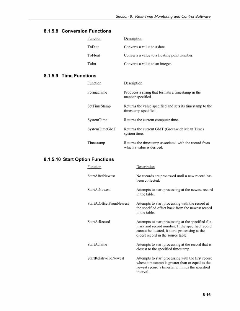
Section 8. Real-Time Monitoring and Control Software
8-16
8.1.5.8 Conversion Functions Function Description
ToDate Converts a value to a date.
ToFloat Converts a value to a floating point number.
ToInt Converts a value to an integer.
8.1.5.9 Time Functions Function Description
FormatTime Produces a string that formats a timestamp in the manner specified.
SetTimeStamp Returns the value specified and sets its timestamp to the timestamp specified.
SystemTime Returns the current computer time.
SystemTimeGMT Returns the current GMT (Greenwich Mean Time) system time.
Timestamp Returns the timestamp associated with the record from which a value is derived.
8.1.5.10 Start Option Functions Function Description
StartAfterNewest No records are processed until a new record has been collected.
StartAtNewest Attempts to start processing at the newest record in the table.
StartAtOffsetFromNewest Attempts to start processing with the record at the specified offset back from the newest record in the table.
StartAtRecord Attempts to start processing at the specified file mark and record number. If the specified record cannot be located, it starts processing at the oldest record in the source table.
StartAtTime Attempts to start processing at the record that is closest to the specified timestamp.
StartRelativeToNewest Attempts to start processing with the first record whose timestamp is greater than or equal to the newest record’s timestamp minus the specified interval.
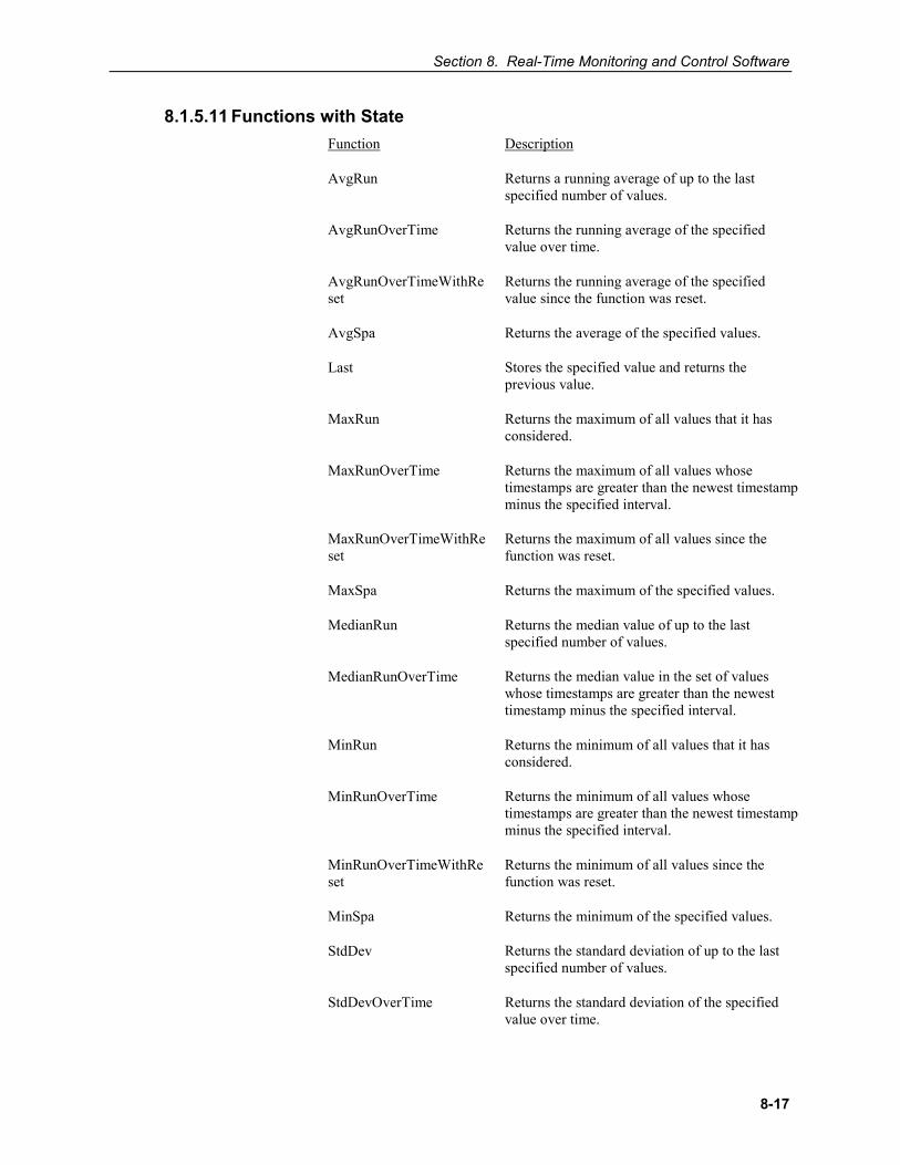
Section 8. Real-Time Monitoring and Control Software
8-17
8.1.5.11 Functions with State Function Description
AvgRun Returns a running average of up to the last specified number of values.
AvgRunOverTime Returns the running average of the specified value over time.
AvgRunOverTimeWithReset
Returns the running average of the specified value since the function was reset.
AvgSpa Returns the average of the specified values.
Last Stores the specified value and returns the previous value.
MaxRun Returns the maximum of all values that it has considered.
MaxRunOverTime Returns the maximum of all values whose timestamps are greater than the newest timestamp minus the specified interval.
MaxRunOverTimeWithReset
Returns the maximum of all values since the function was reset.
MaxSpa Returns the maximum of the specified values.
MedianRun Returns the median value of up to the last specified number of values.
MedianRunOverTime Returns the median value in the set of values whose timestamps are greater than the newest timestamp minus the specified interval.
MinRun Returns the minimum of all values that it has considered.
MinRunOverTime Returns the minimum of all values whose timestamps are greater than the newest timestamp minus the specified interval.
MinRunOverTimeWithReset
Returns the minimum of all values since the function was reset.
MinSpa Returns the minimum of the specified values.
StdDev Returns the standard deviation of up to the last specified number of values.
StdDevOverTime Returns the standard deviation of the specified value over time.
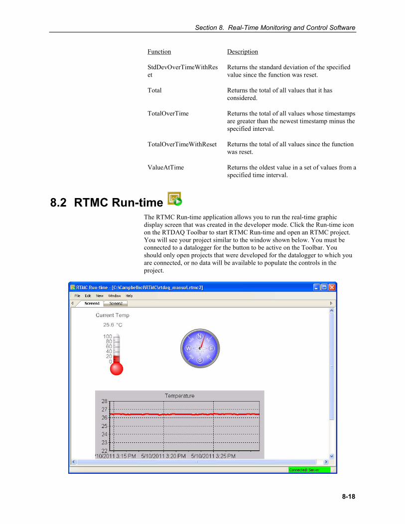
Section 8. Real-Time Monitoring and Control Software
8-18
Function Description
StdDevOverTimeWithReset
Returns the standard deviation of the specified value since the function was reset.
Total Returns the total of all values that it has considered.
TotalOverTime Returns the total of all values whose timestamps are greater than the newest timestamp minus the specified interval.
TotalOverTimeWithReset Returns the total of all values since the function was reset.
ValueAtTime Returns the oldest value in a set of values from a specified time interval.
8.2 RTMC Run-time The RTMC Run-time application allows you to run the real-time graphic display screen that was created in the developer mode. Click the Run-time icon on the RTDAQ Toolbar to start RTMC Run-time and open an RTMC project. You will see your project similar to the window shown below. You must be connected to a datalogger for the button to be active on the Toolbar. You should only open projects that were developed for the datalogger to which you are connected, or no data will be available to populate the controls in the project.
Section 8. Real-Time Monitoring and Control Software
8-19
When the run-time display screen is started, the display components will have a red exclamation point in the upper right corner until data is received from RTDAQ. If data is not displayed, check to see that you are connected to the proper datalogger.
Once a project file has been created and saved, the display screen can be run without starting the RTMC Development application. You may switch to the display of a different project by choosing File | Open and selecting another RTMC project file. In Run-time mode, you can print an image of the RTMC display screen by selecting File | Print Screens.
9-1
Section 9. Calibration and Zeroing 9.1 Calibration Essentials
9.1.1 Definition of Calibration Calibration, in general, refers to actions taken on a measurement system to increase its accuracy. This is usually done by matching the system’s outputs to known, “control” values in order to increase confidence in the measurement of future unknowns.
Campbell Scientific’s approach to calibration uses a datalogger’s measurement and computational capability to calculate the multipliers and/or offsets to be used by a measurement instruction to provide more accurate readings. The process of calibration uses the datalogger to assist the operator in intelligently and automatically setting the multiplier and offset to be used in a measurement instruction in order to obtain more accurate output data.
Calibration is periodically necessary when there has been sensor drift or other variation in sensor outputs. When a calibration scenario is properly in place within the datalogger program, it is quick and easy to use a software Wizard to change the measurement configuration at run-time. This saves time over previously used methods, such as re-writing the CRBasic program or interfering with measurements to obtain calibration constants manually. With this method, changes to multipliers and offsets can be made quickly and automatically without rewriting datalogger programs or interfering with sensor measurements.
9.1.2 Basic Calibration Process When calibrating with a Campbell Scientific datalogger, known and measured values are given as inputs. The outputs of the calibration then become the new values for the multiplier and offset variables in the CRBasic program. If needed, these calculated multipliers and offsets can be permanently stored and automatically reloaded upon program restart (such as when a power-cycle occurs on the datalogger). The datalogger makes use of a calibration file (*.cal) to store these calibration values, and load them as desired. This can be done at datalogger startup, or at other times designated within the datalogger program.
To evaluate calibration histories, a final storage output table can be configured to store the results of calibrations that have been performed, and the date and time at which those calibrations were performed. This data is separate from the calibration file and forms a permanent history of calibration constants used within the program.
Section 9. Calibration and Zeroing
9-2
9.2 Writing Calibration Programs with the CRBasic Editor
9.2.1 The FieldCal Instruction If you wish to make measurements that will be calibrated as discussed above, you should use the FieldCal instruction within the CRBasic program. When the program is running in the datalogger, you can use the RTDAQ Calibration Wizard to perform the actual calibrations (in real-time) on the sensors that were previously designated for calibration. You can also perform a manual calibration against a running program using the RTDAQ Monitor Data screen (see Chapter 7) or from a keyboard display connected directly to the datalogger.
The FieldCal instruction works together with other related CRBasic instructions to complete the calibration task. These instructions are shown in TABLE 9-1.
TABLE 9-1. The FieldCal Instruction “Family”
Instruction Description
FieldCal This is the main calibration instruction. The CRBasic program should contain one FieldCal instruction per measurement requiring calibration. This instruction is placed after the measurement instruction to which it applies.
LoadFieldCal (optional) This instruction loads values into program variables from the calibration file (*.cal), if it exists. It will also indicate whether the attempt to load those values was successful or not by returning a boolean (true/false) result.
SampleFieldCal (optional) This is a table output instruction. It writes the latest calibration values for all calibrated measurements to a data table (separate from the *.cal file).
NewFieldCal (optional) This is a boolean system value indicating when a calibration has succeeded. During one scan cycle after a calibration has occurred this value will be true. Its value is then set to false until another calibration occurs. The value of this variable cannot be set within a CRBasic Program, but only evaluated. The main purpose for this variable is to be used together with the SampleFieldCal instruction to output one table record per calibration to a specified table.
To set up a measurement for calibration in CRBasic, first insert the instruction(s) that make the measurement, using variables for the multiplier and/or offset. Then add a FieldCal instruction after the measurement instruction and refer back to the measurement being calibrated using the variable containing the measured output. Provide the FieldCal instruction with the variables holding the multiplier and the offset of the measured sensor. If you need to retrieve a calibration value into multipliers and offsets upon
Section 9. Calibration and Zeroing
9-3
program start or under other conditions, use the LoadFieldCal instruction. To store calibration values to a data table (in addition to the values stored in the *.cal file), use the SampleFieldCal table output instruction with the NewFieldCal system variable as the trigger.
For more information about how to use these instructions, refer to the FieldCal instruction topic of your datalogger manual, or use the online help topic for FieldCal within the CRBasic Editor.
9.2.2 Calibration File Details It is important to understand the purpose and function of the calibration file created by a CRBasic program when using the FieldCal instruction. The calibration file has the same name as the program that creates and uses it, except that it ends with a .cal extension. For example, myProg.CR1 would generate a calibration file called myProg.CAL. The calibration file is located on the same datalogger storage device as the program that creates it (e.g., CPU, CRD, USR). The calibration file is created when the program runs and doesn’t find an existing calibration file that it can use, and it is updated upon each successful calibration. The calibration file contains information about the latest calibrations performed during program execution and information that the RTDAQ Calibration Wizard needs to step users through the calibration process.
9.3 Five Kinds of Calibration The FieldCal instruction family can perform five basic kinds of calibrations: Zeroing Calibration, Offset Calibration, Two-point Multiplier/Offset Calibration (Linear Fit), Two-point Multiplier Only Calibration, and Zero Basis Point Calibration. These calibration types are described below.
9.3.1 Zeroing Zeroing is the act of placing a sensor into a state where the output condition is known to be zero and changing the measurement’s offset variable so that the sensor output reads as zero. By measuring the output of the sensor in this specialized condition (the zero condition), the offset variable will be changed to ensure that the known zero condition results in a measurement value of zero. Note that this process only changes the offset variable that is shared between the measurement instruction and the FieldCal instruction. The multiplier is unaffected.
A simple example of zeroing would be taking off all items from a scale designed to measure the mass of objects. With nothing on the scale, this is the condition in which the scale should give a “zero” reading for its output. The calibration is triggered and the offset is adjusted to ensure the scale gives a zero reading for that condition.
To perform a zeroing calibration, use an argument of 0 (the number zero) for the calibration type in the FieldCal instruction of your CRBasic program. The Calibration Wizard can be used to calculate and apply the proper offset while the program is running in the datalogger, or code can be configured within the CRBasic program to trigger the zeroing event based on flags or other user-defined conditions that occur while the program runs.
Section 9. Calibration and Zeroing
9-4
The simplest way to set up a program that performs zeroing calibration is to generate it. See Generating Calibration Programs later in this chapter.
9.3.2 Offset Calibration Offset Calibration is the act of placing a sensor into a state where the output condition is known to be a certain value and then changing the measurement’s offset variable so that the sensor output reads as exactly that value. It is similar to a zeroing calibration, except that the known value is a non-zero value. By measuring the output of the sensor in this specialized condition (the known offset condition), the offset variable will be changed to ensure that this condition results in a measurement value that matches it. Note that this process only changes the offset variable that is shared between the measurement instruction and the FieldCal instruction. The multiplier variable is unaffected.
A simple example of offset calibration would be placing an object of known weight (such as 10 lbs.) on a scale designed to measure the mass of objects. With a known weight on the scale, this is the condition in which the scale should give a known reading for its output. First the calibration is triggered, then the user informs the datalogger about the value of the known weight, and finally the offset is adjusted to ensure that the scale gives a properly matched reading for that condition.
To perform an offset calibration, use an argument of 1 (the number one) for the calibration type in the FieldCal instruction of your CRBasic program. The Calibration Wizard can be used to calculate and apply the proper offset while the program is running in the datalogger, or code can be configured within the CRBasic program to trigger the offset event based on flags or other user-defined conditions that occur while the program runs.
9.3.3 Two-Point Multiplier and Offset Calibration Two-point multiplier and offset calibration uses a linear fit technique against two different known value conditions of the sensor’s measurement. The sensor is placed into the first condition, and the known value for that condition is provided to the datalogger program. One or more measurements of that first condition are stored, and then the datalogger informs the user that the second known condition should now be applied to the sensor. The second condition is applied and its known value is then provided to the datalogger. The datalogger then measures the second condition. When the measurement of the second point condition is complete, a linear fit of the two points is calculated. The results are a slope value (m value, or multiplier), and a y-intercept (b value or offset). Thus the simple form y=mx+b is a representation of the linear fit, where m is the new multiplier value used and b is the new offset used.
A simple example of a two-point multiplier and offset calibration would be placing two objects of known weight (such as 5 lbs. and 15 lbs.) on a conventional scale at two different times. With the first known weight on the scale (5 lbs), this is the first condition in which the scale should give a “known” reading for its output. The calibration is triggered, the datalogger is informed of the value of the known weight, and the measurement is read. The datalogger then notifies the user that it is ready to measure the second point. The second known weight is placed on the scale (15 lbs), and this is the second condition in which the scale should give a known reading for its output. The second point of calibration is triggered, the datalogger is informed of the value of the second known weight, and the measurement is read. At this point the
Section 9. Calibration and Zeroing
9-5
new multiplier and offset are calculated by the datalogger and the variables are adjusted accordingly to ensure that the scaling gives a properly matched reading for those two conditions. For future measurements (unknowns), a linear response will be used based on the line defined by those two points.
To perform a two-point multiplier and offset calibration, use an argument of 2 (the number two) for the calibration type in the FieldCal instruction of your CRBasic program. The Calibration Wizard can be used to calculate and apply the two different known conditions while the program is running in the datalogger. The simplest way to set up a program that does two-point multiplier and offset calibration is to generate it. See Generating Calibration Programs later in this chapter.
9.3.4 Two-Point Multiplier Only Calibration Two-point multiplier only calibration uses a linear fit technique against two different known value conditions of the sensor’s measurement, but only the slope value (multiplier) is calculated and changed. The offset is unaffected by this calibration. The sensor is placed into the first condition, and the known value for that condition is provided to the datalogger program. One or more measurements in that first condition occur, and then the datalogger informs the user that the second known condition should be applied to the sensor. When that condition is applied, the second known value is provided to the datalogger, and the datalogger measures the second condition. After completing the measurement of the second point condition, a best fit of the two points is calculated, resulting in a slope value (m value or multiplier) with the offset assumed to be zero. Thus the simple form y=mx is a representation of the fit, where m is the new multiplier value.
To perform a two-point multiplier only calibration, use an argument of 3 (the number three) for the calibration type in the FieldCal instruction of your CRBasic program. The Calibration Wizard can be used to calculate and apply the two different known conditions while the program is running in the datalogger.
9.3.5 Zero Basis Point Calibration The purpose of this calibration type is to simply load the value of certain variables into zero point variables.
This type of calibration would be used when the storing of values into variables needs to be done as the result of a calibration event, when that value capture needs to be triggered from the Calibration Wizard, and when the result needs to be stored into the calibration file.
A common application for this type of calibration would be a measurement in which a zeroing calibration is based not only on the zero offset for a single sensor, but the zero state of multiple sensors. An expression using the loaded variables would be used after the FieldCal instruction in the CRBasic program to ensure that regular measurements return a calibrated value.
To perform a zero basis point calibration, use an argument of 4 (the number four) for the calibration type in the FieldCal instruction of your CRBasic program.
Section 9. Calibration and Zeroing
9-6
The syntax would be:
FieldCal (4,RTS(),3,0,ZeroState(),Mode,0,1,Avg)
Using the instruction shown above, when a calibration is performed the current values of the variable array, RTS, will be loaded into the variable array, ZeroState.
In the Calibration Wizard, choose “Zero” as the type of calibration to perform when doing a Zero Basis Point Calibration.
9.4 Performing a Manual Calibration 9.4.1 How to Use the Mode Variable for Calibration Status and
Control To perform a manual calibration (without use of the RTDAQ Calibration Wizard) on a FieldCal enabled program running in a datalogger, it is necessary to understand the function of the mode variable that is used as an argument of the FieldCal instruction.
In a CRBasic calibration program, a mode variable is declared and associated with a particular FieldCal instruction, thereby associating it with the measurement to be calibrated.
Most values of the mode variable represent the status of the calibration for that affected measurement. A few values of the mode variable are set by the user of the datalogger to instruct the program to proceed with calibrations.
The following values of the mode variable give the status of the calibration:
0 No calibration has been performed since program start
2 Calibration in progress OR first stage of two-point calibration in progress
3 Waiting for second stage of two-point calibration to begin
5 Second stage of two-point calibration in progress
6 Calibration complete
-1 Calibration error
-2 Measurement range error
-3 Error with the value used as the Reps argument in the FieldCal instruction. The following values of the mode variable are used to initiate a calibration process:
1 Start the calibration, OR start the first point of a two point calibration
4 Start the second point of a two point calibration
NOTE
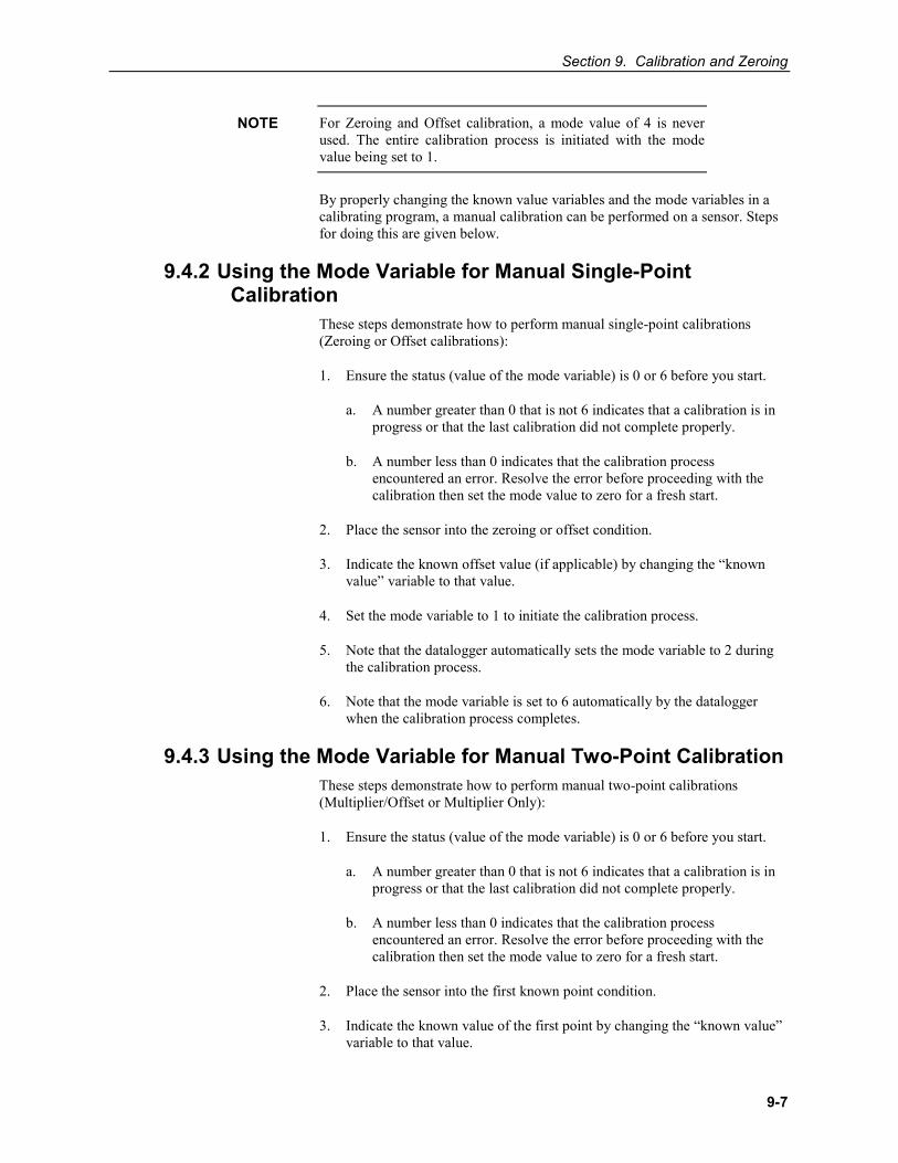
Section 9. Calibration and Zeroing
9-7
For Zeroing and Offset calibration, a mode value of 4 is never used. The entire calibration process is initiated with the mode value being set to 1.
By properly changing the known value variables and the mode variables in a calibrating program, a manual calibration can be performed on a sensor. Steps for doing this are given below.
9.4.2 Using the Mode Variable for Manual Single-Point Calibration
These steps demonstrate how to perform manual single-point calibrations (Zeroing or Offset calibrations):
1. Ensure the status (value of the mode variable) is 0 or 6 before you start.
a. A number greater than 0 that is not 6 indicates that a calibration is in progress or that the last calibration did not complete properly.
b. A number less than 0 indicates that the calibration process encountered an error. Resolve the error before proceeding with the calibration then set the mode value to zero for a fresh start.
2. Place the sensor into the zeroing or offset condition.
3. Indicate the known offset value (if applicable) by changing the “known value” variable to that value.
4. Set the mode variable to 1 to initiate the calibration process.
5. Note that the datalogger automatically sets the mode variable to 2 during the calibration process.
6. Note that the mode variable is set to 6 automatically by the datalogger when the calibration process completes.
9.4.3 Using the Mode Variable for Manual Two-Point Calibration These steps demonstrate how to perform manual two-point calibrations (Multiplier/Offset or Multiplier Only):
1. Ensure the status (value of the mode variable) is 0 or 6 before you start.
a. A number greater than 0 that is not 6 indicates that a calibration is in progress or that the last calibration did not complete properly.
b. A number less than 0 indicates that the calibration process encountered an error. Resolve the error before proceeding with the calibration then set the mode value to zero for a fresh start.
2. Place the sensor into the first known point condition.
3. Indicate the known value of the first point by changing the “known value” variable to that value.
NOTE
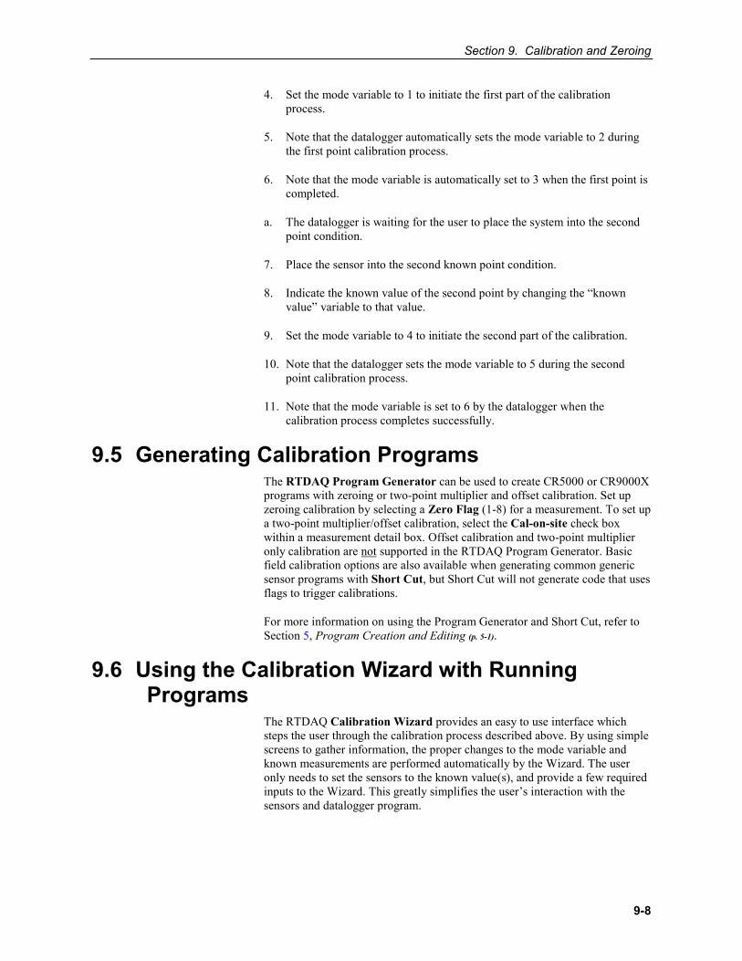
Section 9. Calibration and Zeroing
9-8
4. Set the mode variable to 1 to initiate the first part of the calibration process.
5. Note that the datalogger automatically sets the mode variable to 2 during the first point calibration process.
6. Note that the mode variable is automatically set to 3 when the first point is completed.
a. The datalogger is waiting for the user to place the system into the second point condition.
7. Place the sensor into the second known point condition.
8. Indicate the known value of the second point by changing the “known value” variable to that value.
9. Set the mode variable to 4 to initiate the second part of the calibration.
10. Note that the datalogger sets the mode variable to 5 during the second point calibration process.
11. Note that the mode variable is set to 6 by the datalogger when the calibration process completes successfully.
9.5 Generating Calibration Programs The RTDAQ Program Generator can be used to create CR5000 or CR9000X programs with zeroing or two-point multiplier and offset calibration. Set up zeroing calibration by selecting a Zero Flag (1-8) for a measurement. To set up a two-point multiplier/offset calibration, select the Cal-on-site check box within a measurement detail box. Offset calibration and two-point multiplier only calibration are not supported in the RTDAQ Program Generator. Basic field calibration options are also available when generating common generic sensor programs with Short Cut, but Short Cut will not generate code that uses flags to trigger calibrations.
For more information on using the Program Generator and Short Cut, refer to Section 5, Program Creation and Editing (p. 5-1).
9.6 Using the Calibration Wizard with Running Programs
The RTDAQ Calibration Wizard provides an easy to use interface which steps the user through the calibration process described above. By using simple screens to gather information, the proper changes to the mode variable and known measurements are performed automatically by the Wizard. The user only needs to set the sensors to the known value(s), and provide a few required inputs to the Wizard. This greatly simplifies the user’s interaction with the sensors and datalogger program.
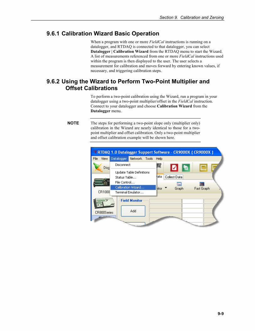
Section 9. Calibration and Zeroing
9-9
9.6.1 Calibration Wizard Basic Operation When a program with one or more FieldCal instructions is running on a datalogger, and RTDAQ is connected to that datalogger, you can select Datalogger | Calibration Wizard from the RTDAQ menu to start the Wizard. A list of measurements referenced from one or more FieldCal instructions used within the program is then displayed to the user. The user selects a measurement for calibration and moves forward by entering known values, if necessary, and triggering calibration steps.
9.6.2 Using the Wizard to Perform Two-Point Multiplier and Offset Calibrations
To perform a two-point calibration using the Wizard, run a program in your datalogger using a two-point multiplier/offset in the FieldCal instruction. Connect to your datalogger and choose Calibration Wizard from the Datalogger menu.
The steps for performing a two-point slope only (multiplier only) calibration in the Wizard are nearly identical to those for a two-point multiplier and offset calibration. Only a two-point multiplier and offset calibration example will be shown here.
NOTE
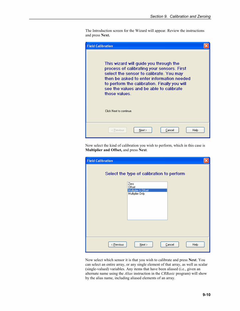
Section 9. Calibration and Zeroing
9-10
The Introduction screen for the Wizard will appear. Review the instructions and press Next.
Now select the kind of calibration you wish to perform, which in this case is Multiplier and Offset, and press Next.
Now select which sensor it is that you wish to calibrate and press Next. You can select an entire array, or any single element of that array, as well as scalar (single-valued) variables. Any items that have been aliased (i.e., given an alternate name using the Alias instruction in the CRBasic program) will show by the alias name, including aliased elements of an array.
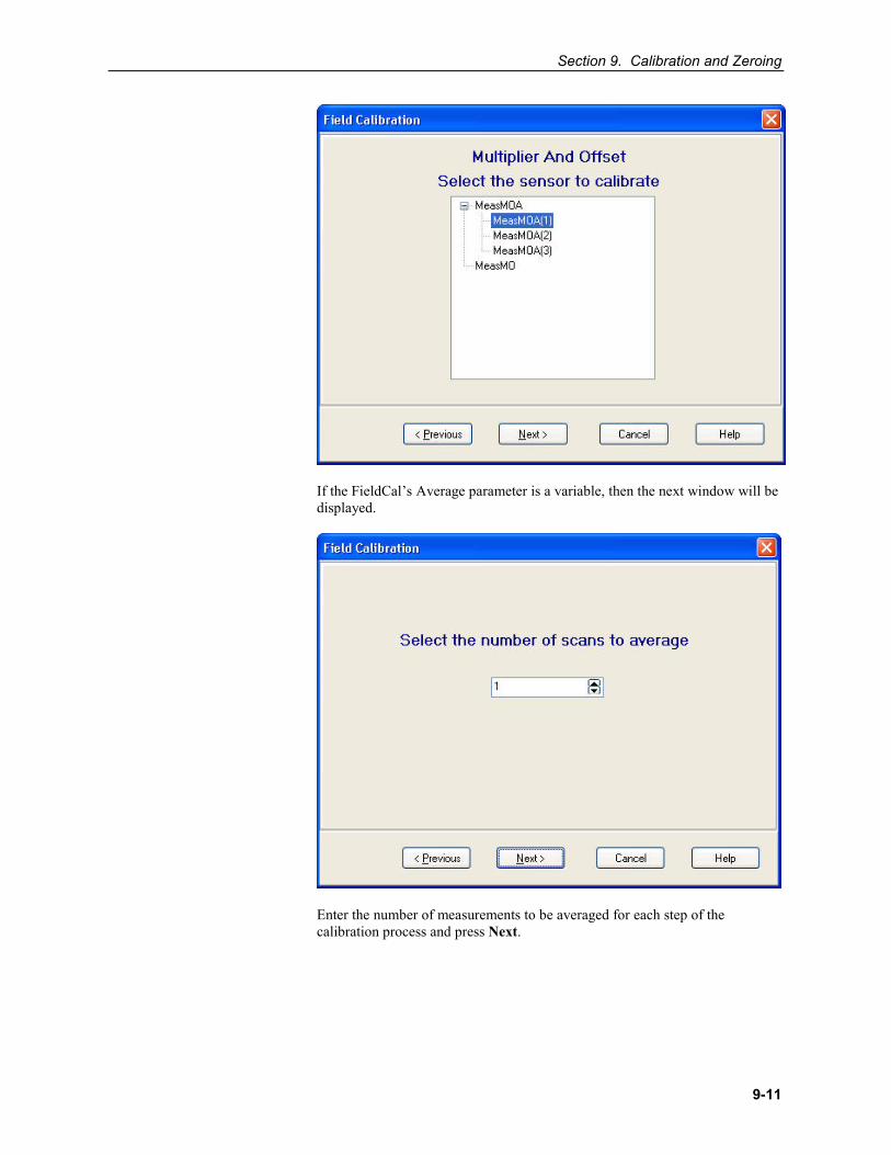
Section 9. Calibration and Zeroing
9-11
If the FieldCal’s Average parameter is a variable, then the next window will be displayed.
Enter the number of measurements to be averaged for each step of the calibration process and press Next.
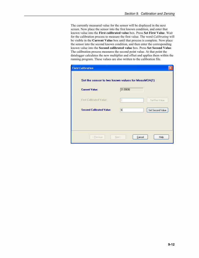
Section 9. Calibration and Zeroing
9-12
The currently measured value for the sensor will be displayed in the next screen. Now place the sensor into the first known condition, and enter that known value into the First calibrated value box. Press Set First Value. Wait for the calibration process to measure the first value. The word Calibrating will be visible in the Current Value box until that process is complete. Now place the sensor into the second known condition, and then enter the corresponding known value into the Second calibrated value box. Press Set Second Value. The calibration process measures the second point value. At that point the datalogger calculates the new multiplier and offset and applies them within the running program. These values are also written to the calibration file.
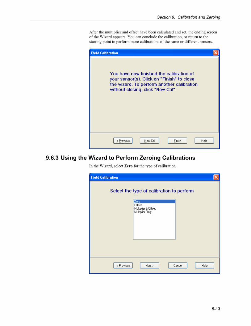
Section 9. Calibration and Zeroing
9-13
After the multiplier and offset have been calculated and set, the ending screen of the Wizard appears. You can conclude the calibration, or return to the starting point to perform more calibrations of the same or different sensors.
9.6.3 Using the Wizard to Perform Zeroing Calibrations In the Wizard, select Zero for the type of calibration.
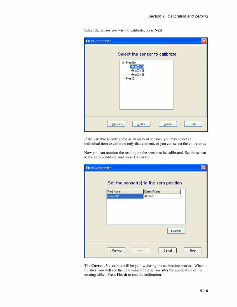
Section 9. Calibration and Zeroing
9-14
Select the sensor you wish to calibrate, press Next.
If the variable is configured as an array of sensors, you may select an individual item to calibrate only that element, or you can select the entire array.
Now you can monitor the reading on the sensor to be calibrated. Set the sensor to the zero condition, and press Calibrate.
The Current Value box will be yellow during the calibration process. When it finishes, you will see the new value of the sensor after the application of the zeroing offset. Press Finish to end the calibration.
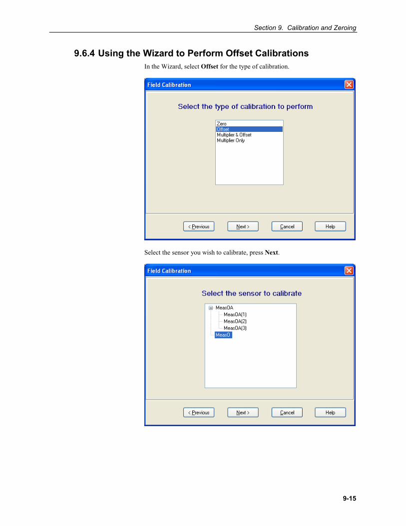
Section 9. Calibration and Zeroing
9-15
9.6.4 Using the Wizard to Perform Offset Calibrations In the Wizard, select Offset for the type of calibration.
Select the sensor you wish to calibrate, press Next.
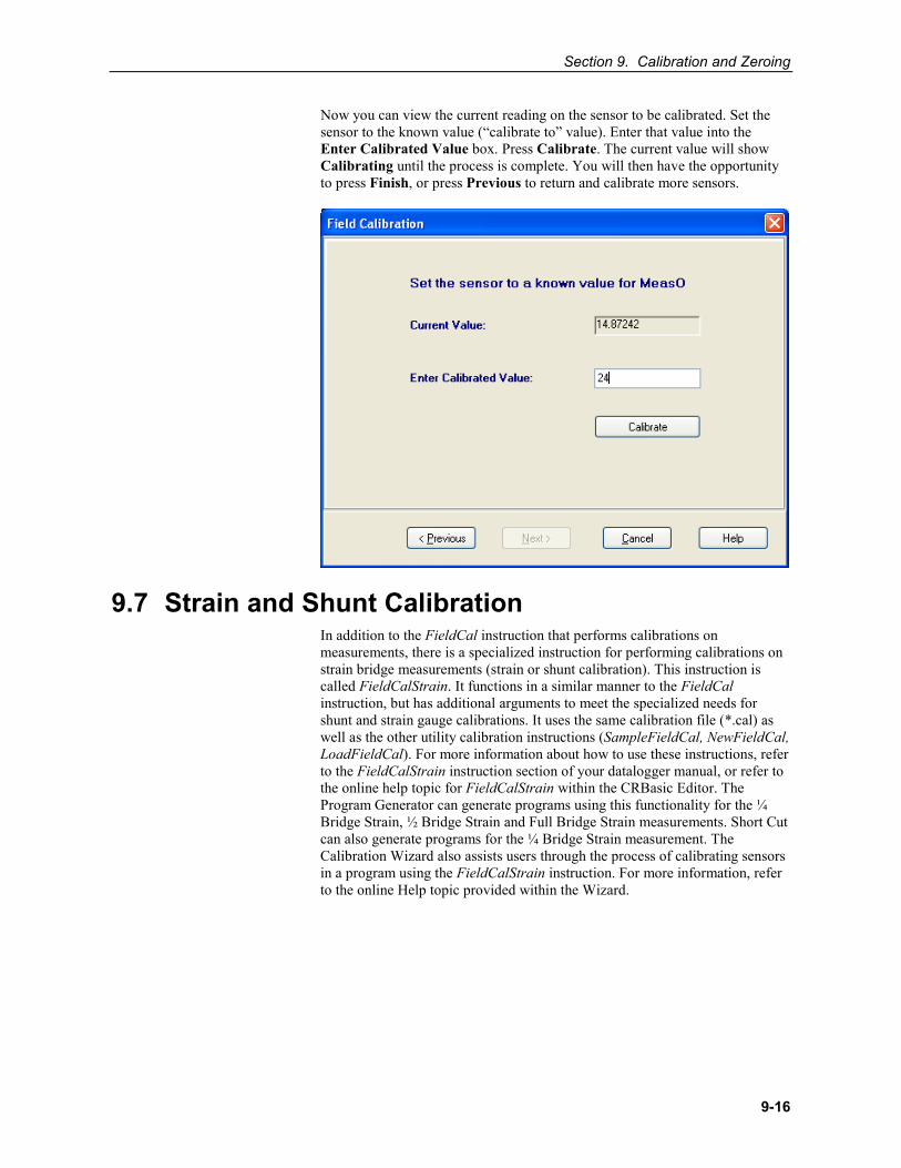
Section 9. Calibration and Zeroing
9-16
Now you can view the current reading on the sensor to be calibrated. Set the sensor to the known value (“calibrate to” value). Enter that value into the Enter Calibrated Value box. Press Calibrate. The current value will show Calibrating until the process is complete. You will then have the opportunity to press Finish, or press Previous to return and calibrate more sensors.
9.7 Strain and Shunt Calibration In addition to the FieldCal instruction that performs calibrations on measurements, there is a specialized instruction for performing calibrations on strain bridge measurements (strain or shunt calibration). This instruction is called FieldCalStrain. It functions in a similar manner to the FieldCal instruction, but has additional arguments to meet the specialized needs for shunt and strain gauge calibrations. It uses the same calibration file (*.cal) as well as the other utility calibration instructions (SampleFieldCal, NewFieldCal, LoadFieldCal). For more information about how to use these instructions, refer to the FieldCalStrain instruction section of your datalogger manual, or refer to the online help topic for FieldCalStrain within the CRBasic Editor. The Program Generator can generate programs using this functionality for the ¼ Bridge Strain, ½ Bridge Strain and Full Bridge Strain measurements. Short Cut can also generate programs for the ¼ Bridge Strain measurement. The Calibration Wizard also assists users through the process of calibrating sensors in a program using the FieldCalStrain instruction. For more information, refer to the online Help topic provided within the Wizard.
10-1
Section 10. Utilities CardConvert is a utility that is used to quickly read and convert binary datalogger data that is retrieved from a compact flash, microSD, or a PCMCIA card. The binary data can also be a file already saved to the user's PC. The binary data is converted to another format (such as TOA5) and saved on the user's PC.
The Device Configuration Utility, or DevConfig, is a utility for setting up datalogger and communication peripherals for use in a datalogger network.
CardConvert and DevConfig can be accessed from the RTDAQ toolbar or by opening the Windows Start menu and selecting Programs | RTDAQ | Utilities | (desired utility).
Split is a tool that works with output data files (*.dat) collected from Campbell Scientific dataloggers. It is used to post-process data from either mixed-array or table-based dataloggers. It is accessed from the RTDAQ Toolbar.
LogTool is used to monitor the logs created by the RTDAQ communications server. This utility is accessible from the Tools | LogTool menu item in RTDAQ, or the actual log files can be opened directly in a simple text editor.
10.1 CardConvert CardConvert is a utility that is used to quickly read and convert binary datalogger data that is retrieved or copied from a compact flash or a PCMCIA card. The converted data is saved on the user's PC.
10.1.1 Input/Output File Settings The file settings are used to specify the directory where the binary data is stored, and the directory in which the converted file(s) should be saved.
Press the Select Card Drive button to bring up dialogue box that helps you browse for the drive assigned to the card reader. Note that you can also select a directory on your hard drive in which binary data files have been copied. When a card drive or directory is selected, any convertible files found with a *.dat extension will be displayed in the Source Filename column in CardConvert.
By default, the converted data files will be saved to the same drive or directory as the source files. To change the destination, press the Change Output Dir button. Once again you will be provided with a dialogue box that helps you to browse for the desired drive or directory. When the drive or directory is selected, the path and the filename that will be used for the converted files will show up in the Destination Filename column.
The default filename for a converted file is comprised of the table name in the datalogger program, along with a prefix that reflects the file format and an extension of either *.dat or a numeric value (e.g., *.000), depending upon whether or not filemarks are processed (see below for information on file formats and filemarks). For instance, the default name for a table called MyData stored in TOA5 format would be TOA5_MyData.dat.
Section 10. Utilities
10-2
The destination directory or filename for a converted file can be changed on an individual file basis. Click on the row for the file that you wish to change. It will be highlighted. Select Options | Change Output File from the CardConvert menu, and browse for or type in a new path and/or filename. You can apply a directory path change to all files by selecting Options | Apply Directory to All.
You do not have to convert all files that are found in the selected directory. Select one or more files for conversion by selecting or clearing the check box beside the individual file name. If a box is checked the file will be converted; if a box is cleared the file will not be converted. To quickly select or clear all check boxes, choose Options | Check All or Clear Check All from the CardConvert menu.
The list of files displayed for a particular drive or directory can be updated by selecting Options | Rebuild File Lists from the menu. Any new files that have been stored since you last selected the drive (or since the last rebuild), will be added to the list.
Tip: Right-click within the file list to display a shortcut menu containing the items on the Options menu.
10.1.2 Destination File Options The Destination File Options determine whether the data will be stored on the PC in ASCII or binary format, how filemarks will be processed, and what should happen when existing files with the same name are found.
10.1.2.1 File Format The File Format is used to specify the format in which the data file should be saved. Select the desired option from the list box:
ASCII Table Data (TOA5) - Data is stored in an ASCII comma separated format. Header information for each of the data values is included, along with field names and units of measure if they are available.
Binary Table Data (TOB1) - Data is stored in a binary format. Though this format saves disk storage space, it may need to be converted before it is usable in some other programs.
Array Compatible CSV - Data is stored in a user-defined comma separated format. This option can be used to produce output files from table data dataloggers that are similar to those created by mixed array dataloggers. When this option is chosen, the Array CSV Options button becomes available, so that you can customize the data string for the CSV file.
Section 10. Utilities
10-3
If an array ID is desired, select the Include Array ID check box and enter a value into the field. The value can range from 1 to 1023. The Array ID will be the first value in the array of data.
Select the appropriate timestamp options for the type of timestamp to write to the file. Each time element will be output as a separate data value in the array and the data values will be separated by a comma. Selecting Year will output the year represented by four digits, YYYY (e.g., 2009). The Day will be represented as a Julian Day. The Hour/Minutes will be represented by four digits (hhmm). When Midnight is 2400 is selected, the timestamp will reflect midnight as the current date with 2400 for the Hour/Minutes. Otherwise, the timestamp will reflect midnight as the next day's date, with the Hours/Minutes as 0000.
The Max and Min Timestamp Options is used to determine the type of timestamp that will be used for Maximum and Minimum outputs that include a timestamp along with the value. You can choose to output No Timestamp, a timestamp that includes Hours/Minutes/Seconds (produces two values, hhmm and seconds), a timestamp that includes Hours/Minutes only, or a timestamp that includes Seconds only.
CSIXML - Data is stored in XML format with Campbell Scientific defined elements and attributes.
The file format is reflected in the default filename by the prefix of either TOA5, TOB1, CSV, or CSIXML added to the table name.
10.1.2.2 File Processing Use Filemarks - CRBasic dataloggers have a FileMark instruction that allows you to store a filemark along with the data. These filemarks are ignored by the LoggerNet or RTDAQ data collection process. However, in CardConvert you can convert the file with the Use Filemarks option selected, and the file will be stored as multiple files, based upon the filemarks. Each file created will be given a numeric suffix prior to the *.dat extension. The first file is stored with a _1 at the end of the root file name (e.g., TOA5_Mytable_1.dat). The number is incremented by one with each new file saved. If a file with the same name is found, the number will be incremented to the next available number.
Use Removemarks - When a compact flash card is removed from a CR1000 or CR3000 datalogger, a special mark is inserted in the last record. The Removemark is similar in nature to the Filemark. In CardConvert, you can split a file into multiple files, separated at the Removemarks, by converting the file with the Use Removemarks option selected. As with the Use Filemarks option, the first file stored uses a _1 at the end of the root file name and the number is incremented by one with each new file saved.
Use Filemarks and Use Removemarks can be selected at the same time, to create a new file from the data table any time either of the marks is encountered.
Use Time - This option is used to store the converted data into files based on the timestamp of the data. When the Use Time check box is selected, the Time Settings button becomes available. This button opens a dialogue box that is used to set a Start Date and Time, along with an Interval, which are used to determine the time frame for the data that goes into each file. Note that the
Section 10. Utilities
10-4
Start Date and Time are not used to specify the actual time and date to begin processing the file; rather, they are used as a reference for the file interval. Processing always starts at the beginning of the file.
When Use Filemarks, Use Removemarks, or Use Time is selected, the Create New Filenames option is disabled. New file names will always be created.
Convert Only New Data – When this option is selected, only data that has been collected since CardConvert’s last conversion of the specified file(s) will be converted. The first time CardConvert is used on a file, all data will be converted. On subsequent conversions, only new data will be converted. However, if CardConvert cannot tell what data is new (i.e. if data on the card has wrapped [ring memory] since the last conversion), all data will be converted. This option can be used with Append to Last File to create a continuous file with no repetition of data.
10.1.2.3 File Naming Time/Date Filenames - When this option is selected, the date and time of the last record of data in the file will be appended to the end of the base file name. The suffix includes a four digit year, a two digit month, a two digit day of month, and a four digit hour/minute. When this option is selected, Use Day of Year becomes available. If this option is selected, the Julian day (day of year) will be used for the suffix instead of the year/month/day/hour/minute suffix.
Create New Filenames - When the Create New Filenames option is selected, CardConvert will add a _01 to the filename, if a file of the same name is found (e.g., TOA5_Mydata_01.dat). If a *_01.dat file is found, the file will be named with a _02 suffix. If the Create New Filenames check box is cleared and a file with the same name is found, you will be offered the option to Overwrite the existing file or Cancel the conversion.
The Create New Filenames option is disabled when the Use Filemarks, Use Removemarks, or Use Time option is enabled.
Append to Last File – When this option is selected, converted data will be appended to the end of the destination file. If the destination file does not exist when a conversion is done, a new file will be created. On subsequent conversions, converted data will be appended to the end of that file. If the header of the new data does not match that of the data in the destination file, an error will be generated. This option is most useful with the Convert Only New Data option to create a continuous file with no repetition of data.
10.1.2.4 TOA5/TOB1 Format These two options are available when the ASCII Table Data (TOA5) or the Binary Table Data (TOB1) output option is selected.
Store Record Number - By default, the record number for each row of data is stored in the data file. This record number can be omitted from the converted file by clearing the Store Record Number check box.
Store Time Stamp - The time stamp can be omitted from the file by clearing the Store Time Stamp check box.
Section 10. Utilities
10-5
10.1.3 Converting the File Once the file and conversion settings are selected, press the Start Conversion button. CardConvert will begin processing the file. When the file is being processed, the estimated number of records and a percentage of the conversion completed will be displayed at the bottom edge of the window. Note that the values reflect an estimate of the amount of data in a table. If the table is set to a fixed size, CardConvert returns a fairly close estimate. However, if the table is set to auto-allocate, CardConvert essentially returns an estimate that reflects the maximum number of records that can be stored based on card size (even if the table is not completely full). Because of this, you may see the progress reported as something less than 100% when the conversion is complete.
If a conversion is in progress and you wish to stop it, press the Cancel Conversion button.
After file conversion is complete, summary information is provided in the field below the file list. The summary provides a listing of the new files that were created, and the total number of records converted for each table (if filemarks are being processed for a table, the number of records returned is the cumulative number of records for all files).
10.1.4 Repairing/Converting Corrupted Files If you attempt to convert a file and receive a message that the input file contained no data, you may want to consider using the Repair File option. You may also want to consider using the Repair File option if you think there is additional data on the card that is not being converted and included in the output file. With either case, it is possible that data on the card has become corrupted. The Repair File option will attempt to scan the card for good frames of data and output that data to a new binary file.
In some instances, data on a card can become corrupted. Corruption can occur if the card is subjected to electrostatic discharge or if it is removed when data is being written to the card (e.g., the card is removed from the CFM100 without pressing the Card Control button to stop data storage to the card). This corruption can be at the beginning of the data file or anywhere within the stored data. Using the standard conversion option, CardConvert will stop if it encounters a corrupted frame of data because it assumes it has come to the end of the data file. If corrupted frames of data are found at the beginning of the file, CardConvert will display a message indicating that no data could be found on the card. If corrupted frames of data are found within the data file, you may get some, but not all, of the data that you expect in the converted file.
CardConvert offers a repair option, which will attempt to scan the card for good frames of data and output that data to a new binary file (the original file is unchanged). To start the repair of a file, highlight the suspected corrupt file in the list of Source Filenames and right-click to display a floating menu. Select the Repair File option from the list. The repair process will create a new TOB3 file (the default name is Repair_existingfilename), which can then be converted to an ASCII file using the standard CardConvert process.
Section 10. Utilities
10-6
When CardConvert comes to what it believes is the end of the data file during the repair process (the end of valid frames), it will stop and display a message. The message prompts the user either to continue searching the file for more good data frames or to stop the repair process. CardConvert displays the last time stamp for data in the repaired file. If you think there should be additional data on the card, you can continue to run the repair process. If it appears that all the data has been stored to the new file, you can stop. The option to continue processing the file allows you to recover all good data on a card with more than one corrupted frame.
Note that CardConvert can repair only TOB2 or TOB3 files. TOB1 files cannot be repaired.
The Repair File option should be used only if a standard conversion cannot be done.
10.1.5 Viewing a Converted File Converted data files can be reviewed using the View Pro file viewing application. View Pro can be launched by pressing the View Files button. If a file is highlighted in the list of files, that file will be displayed when View Pro is opened. Otherwise you can select the file to view from View Pro's File | Open menu.
10.1.6 Running CardConvert from a Command Line In order to run CardConvert from a command line without user interaction, you will first need to create a CCF file that contains the CardConvert settings to be used when running from a command line. To create the CCF file, open CardConvert and select the desired source directory (Select Card Drive), destination directory (Change Output Dir), and Destination File Options. When CardConvert is closed, it will produce a file named “lastrun.ccf” that contains the designated settings. The file will be written to the C:\Campbellsci\CardConvert directory. You should rename this file as it will be overwritten the next time that CardConvert is closed.
When running CardConvert from a command line, you can designate the CCF file using the command line option runfile. For example,
"C:\Program Files\Campbellsci\CardConvert\CardConvert.exe" runfile=”C:\Campbellsci\CardConvert\myfile.ccf”
The above command line will run CardConvert using the settings contained in myfile.ccf.
The path to the CCF file should be specified. It will not default to the CardConvert working directory.
If there are no problems or questions encountered, CardConvert will start, convert the file(s), and then exit with no user interaction. However, if any problems or questions are encountered, CardConvert will display a dialogue box as usual and then wait for a user response. Therefore, this command line option allows some automation of CardConvert but does not allow for completely unattended automation. To minimize the user interaction required, the
NOTE
NOTE
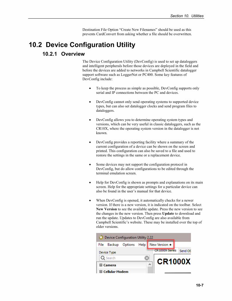
Section 10. Utilities
10-7
Destination File Option “Create New Filenames” should be used as this prevents CardConvert from asking whether a file should be overwritten.
10.2 Device Configuration Utility 10.2.1 Overview
The Device Configuration Utility (DevConfig) is used to set up dataloggers and intelligent peripherals before those devices are deployed in the field and before the devices are added to networks in Campbell Scientific datalogger support software such as LoggerNet or PC400. Some key features of DevConfig include:
• To keep the process as simple as possible, DevConfig supports only serial and IP connections between the PC and devices.
• DevConfig cannot only send operating systems to supported device types, but can also set datalogger clocks and send program files to dataloggers.
• DevConfig allows you to determine operating system types and versions, which can be very useful in classic dataloggers, such as the CR10X, where the operating system version in the datalogger is not known.
• DevConfig provides a reporting facility where a summary of the current configuration of a device can be shown on the screen and printed. This configuration can also be saved to a file and used to restore the settings in the same or a replacement device.
• Some devices may not support the configuration protocol in DevConfig, but do allow configurations to be edited through the terminal emulation screen.
• Help for DevConfig is shown as prompts and explanations on its main screen. Help for the appropriate settings for a particular device can also be found in the user’s manual for that device.
• When DevConfig is opened, it automatically checks for a newer version. If there is a new version, it is indicated on the toolbar. Select New Version to see the available update. Press the new version to see the changes in the new version. Then press Update to download and run the update. Updates to DevConfig are also available from Campbell Scientific’s website. These may be installed over the top of older versions.
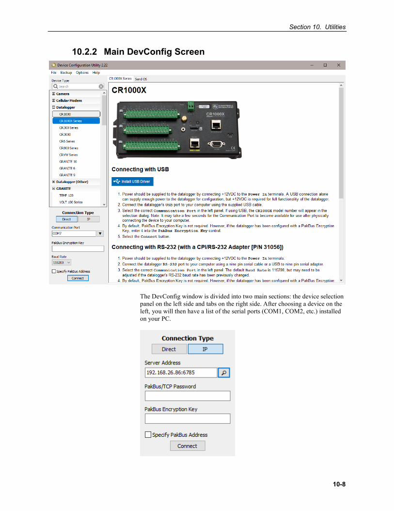
Section 10. Utilities
10-8
10.2.2 Main DevConfig Screen
The DevConfig window is divided into two main sections: the device selection panel on the left side and tabs on the right side. After choosing a device on the left, you will then have a list of the serial ports (COM1, COM2, etc.) installed on your PC.
Section 10. Utilities
10-9
If the device supports IP communication, the IP button will be enabled. In order to communicate via IP, click IP under Connection Type and enter the IP address or domain name for the device in the Server Address field. For some devices, you may be able to click on the Browse button to the right of the Server Address control to bring up a dialogue that searches your local area network for any available devices. If the device has a PakBus/TCP Password, you will need to enter it in the PakBus/TCP Password field.
If the device is using PakBus encryption, you will need to enter the key in the PakBus Encryption Key field.
You’ll be offered a choice of baud rates only if the device supports more than one baud rate in its configuration protocol. The page for each device presents instructions about how to set up the device to communicate with DevConfig. Different device types will offer one or more tabs on the right.
When the user presses the Connect button, the device type, serial port, and baud rate selector controls become disabled and, if DevConfig is able to connect to the device, the button will change from “Connect” to “Disconnect”. The tabs on the right side of the window will be replaced with tabs that represent the various operations that are available for that device in a connected state. These operations can vary from device to device.
10.2.3 Downloading an Operating System Our new data loggers have a Manage OS tab in DevConfig. By default, when connecting to a data logger, DevConfig checks for an updated operating system. If one is found, DevConfig automatically navigates to the Manage OS tab. This tab displays the changes in the new version of the operating system. Press Update to install the new version.
DevConfig can send operating systems from the Send OS tab to all Campbell Scientific devices with flash replaceable operating systems. An example for the CR1000X is shown below:
NOTE
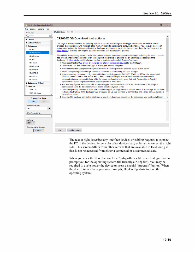
Section 10. Utilities
10-10
The text at right describes any interface devices or cabling required to connect the PC to the device. Screens for other devices vary only in the text on the right side. This screen differs from other screens that are available in DevConfig in that it can be accessed from either a connected or disconnected state.
When you click the Start button, DevConfig offers a file open dialogue box to prompt you for the operating system file (usually a *.obj file). You may be required to cycle power the device or press a special “program” button. When the device issues the appropriate prompts, DevConfig starts to send the operating system:
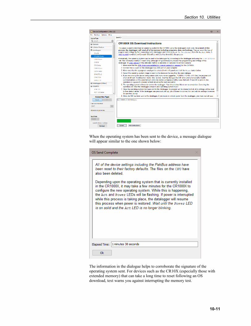
Section 10. Utilities
10-11
When the operating system has been sent to the device, a message dialogue will appear similar to the one shown below:
The information in the dialogue helps to corroborate the signature of the operating system sent. For devices such as the CR10X (especially those with extended memory) that can take a long time to reset following an OS download, text warns you against interrupting the memory test.
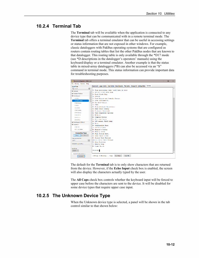
Section 10. Utilities
10-12
10.2.4 Terminal Tab The Terminal tab will be available when the application is connected to any device type that can be communicated with in a remote terminal mode. The Terminal tab offers a terminal emulator that can be useful in accessing settings or status information that are not exposed in other windows. For example, classic dataloggers with PakBus operating systems that are configured as routers contain routing tables that list the other PakBus nodes that are known to that datalogger. This routing table is only available through the *D17 mode (see *D descriptions in the datalogger’s operators’ manuals) using the keyboard/display or a terminal emulator. Another example is that the status table in mixed-array dataloggers (*B) can also be accessed via an “S” command in terminal mode. This status information can provide important data for troubleshooting purposes.
The default for the Terminal tab is to only show characters that are returned from the device. However, if the Echo Input check box is enabled, the screen will also display the characters actually typed by the user.
The All Caps check box controls whether the keyboard input will be forced to upper case before the characters are sent to the device. It will be disabled for some device types that require upper case input.
10.2.5 The Unknown Device Type When the Unknown device type is selected, a panel will be shown in the tab control similar to that shown below:
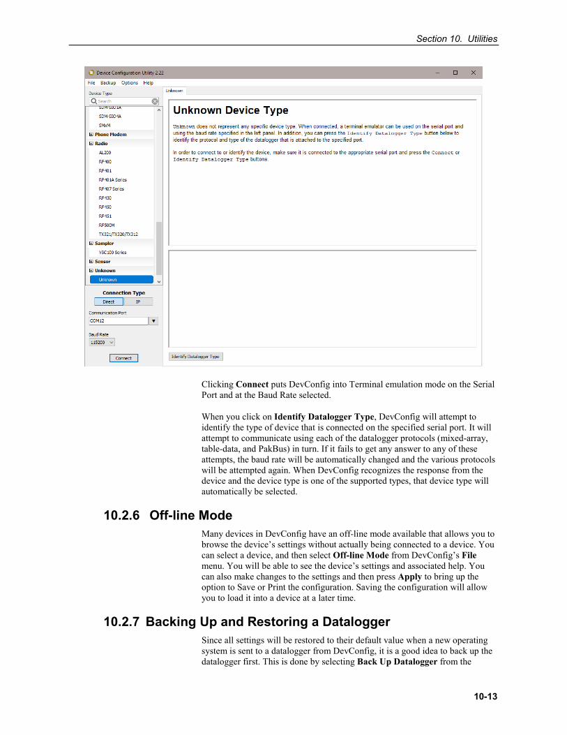
Section 10. Utilities
10-13
Clicking Connect puts DevConfig into Terminal emulation mode on the Serial Port and at the Baud Rate selected.
When you click on Identify Datalogger Type, DevConfig will attempt to identify the type of device that is connected on the specified serial port. It will attempt to communicate using each of the datalogger protocols (mixed-array, table-data, and PakBus) in turn. If it fails to get any answer to any of these attempts, the baud rate will be automatically changed and the various protocols will be attempted again. When DevConfig recognizes the response from the device and the device type is one of the supported types, that device type will automatically be selected.
10.2.6 Off-line Mode Many devices in DevConfig have an off-line mode available that allows you to browse the device’s settings without actually being connected to a device. You can select a device, and then select Off-line Mode from DevConfig’s File menu. You will be able to see the device’s settings and associated help. You can also make changes to the settings and then press Apply to bring up the option to Save or Print the configuration. Saving the configuration will allow you to load it into a device at a later time.
10.2.7 Backing Up and Restoring a Datalogger Since all settings will be restored to their default value when a new operating system is sent to a datalogger from DevConfig, it is a good idea to back up the datalogger first. This is done by selecting Back Up Datalogger from the
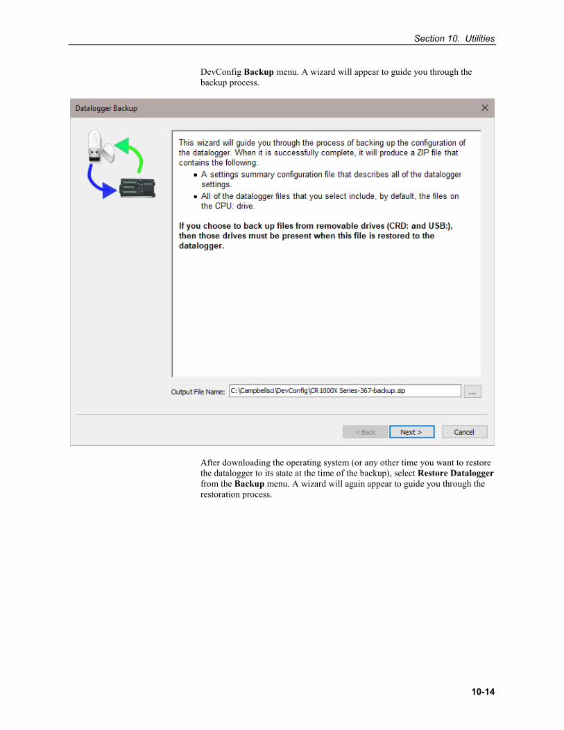
Section 10. Utilities
10-14
DevConfig Backup menu. A wizard will appear to guide you through the backup process.
After downloading the operating system (or any other time you want to restore the datalogger to its state at the time of the backup), select Restore Datalogger from the Backup menu. A wizard will again appear to guide you through the restoration process.
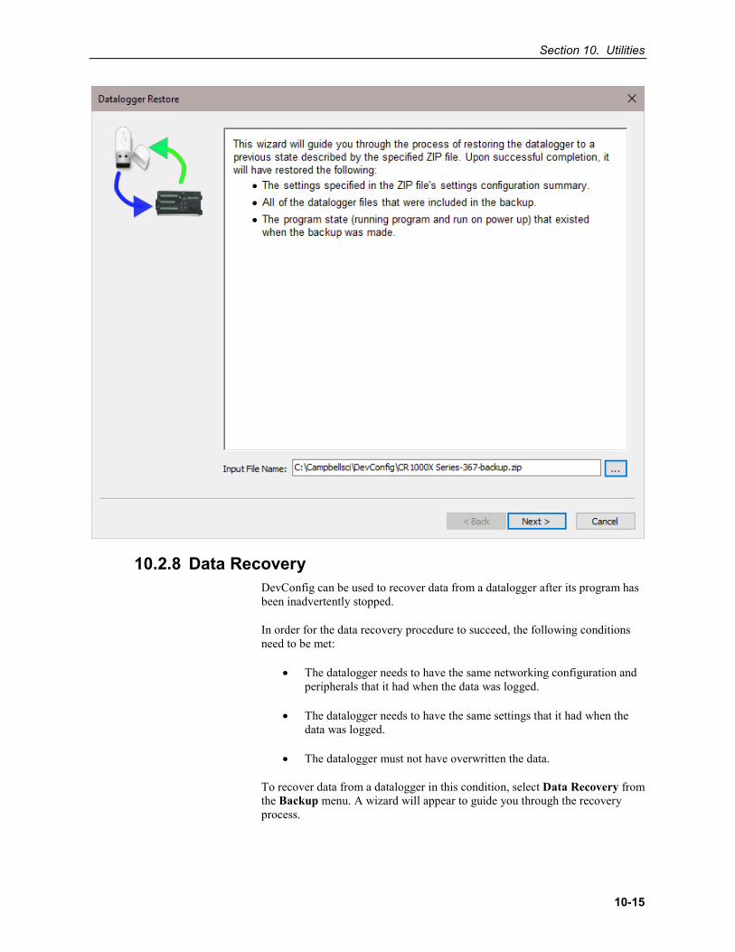
Section 10. Utilities
10-15
10.2.8 Data Recovery DevConfig can be used to recover data from a datalogger after its program has been inadvertently stopped.
In order for the data recovery procedure to succeed, the following conditions need to be met:
• The datalogger needs to have the same networking configuration and peripherals that it had when the data was logged.
• The datalogger needs to have the same settings that it had when the data was logged.
• The datalogger must not have overwritten the data.
To recover data from a datalogger in this condition, select Data Recovery from the Backup menu. A wizard will appear to guide you through the recovery process.
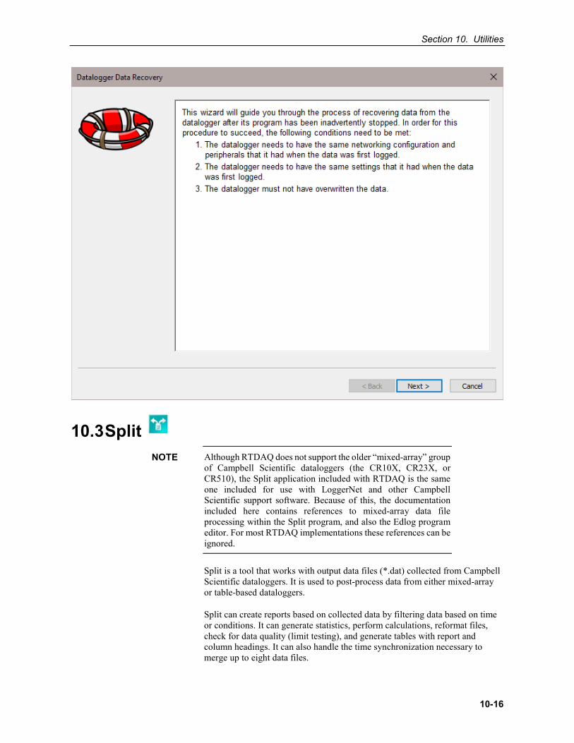
Section 10. Utilities
10-16
10.3 Split Although RTDAQ does not support the older “mixed-array” group of Campbell Scientific dataloggers (the CR10X, CR23X, or CR510), the Split application included with RTDAQ is the same one included for use with LoggerNet and other Campbell Scientific support software. Because of this, the documentation included here contains references to mixed-array data file processing within the Split program, and also the Edlog program editor. For most RTDAQ implementations these references can be ignored.
Split is a tool that works with output data files (*.dat) collected from Campbell Scientific dataloggers. It is used to post-process data from either mixed-array or table-based dataloggers.
Split can create reports based on collected data by filtering data based on time or conditions. It can generate statistics, perform calculations, reformat files, check for data quality (limit testing), and generate tables with report and column headings. It can also handle the time synchronization necessary to merge up to eight data files.
NOTE
Section 10. Utilities
10-17
10.3.1 Functional Overview Split is a tool to analyze data collected from Campbell Scientific dataloggers. Its name comes from its function of splitting out specific data from a larger data file. Originally, Split could only process mixed-array files, and it was used to “split” the different arrays – typically different time intervals – of a file into separate files (e.g., for hourly versus daily data).
In addition to splitting out mixed-array data, Split can filter output data based on time or conditions, calculate statistics and new values, reformat files, or check data quality (limit testing). Split can generate tables with report and column headings, as well as time synchronize and merge up to eight data files.
Input Files (maximum of eight) are read by Split, specific operations are performed on the data, and the results are output to a new Output File or a printer. Split creates a parameter file (filename.PAR) that saves all of your settings such as which data files are read, what operations are performed on the data set, and where the final results will be saved. The parameter file may be saved and used again.
Input Files must be formatted in Printable ASCII, Comma Separated ASCII, Field Formatted ASCII, Final Storage (Binary) Format, Table Oriented ASCII (TOACI1 or TOA5), Table Oriented Binary (TOB), or Raw A/D data (such as the results of a burst measurement).
Split can be used to convert a file of one format to a different format. For example, a Table Oriented ASCII file can be converted to the Comma Separated ASCII format used in mixed-array datalogger data files. This is useful to convert table-based data files to work with applications that were written to work with mixed-array files.
Output files generated by Split can be Field Formatted (default), Comma Separated ASCII, or Printable ASCII. Split can also create reports in ASCII as well as html formats, or send them directly to a printer.
Split lends itself to experimentation. The processed data are displayed on the screen, giving immediate feedback as to the effect of changes or new entries to the parameter file. Split does not modify the original Input File.
10.3.2 Getting Started The most common use of Split is to separate array data collected on a particular interval from a data file containing data output at several different intervals.
In the following example, hourly data are split from a data set that contains 15 minute, hourly and daily data. The data was collected from BirchCreek, a CR10X datalogger. The CR10X was loaded with a program created by Edlog named Birch.dld.
The 15 minute data, array 99, the hourly data, array 60, and the daily data, array 24, are intermixed in the data file.
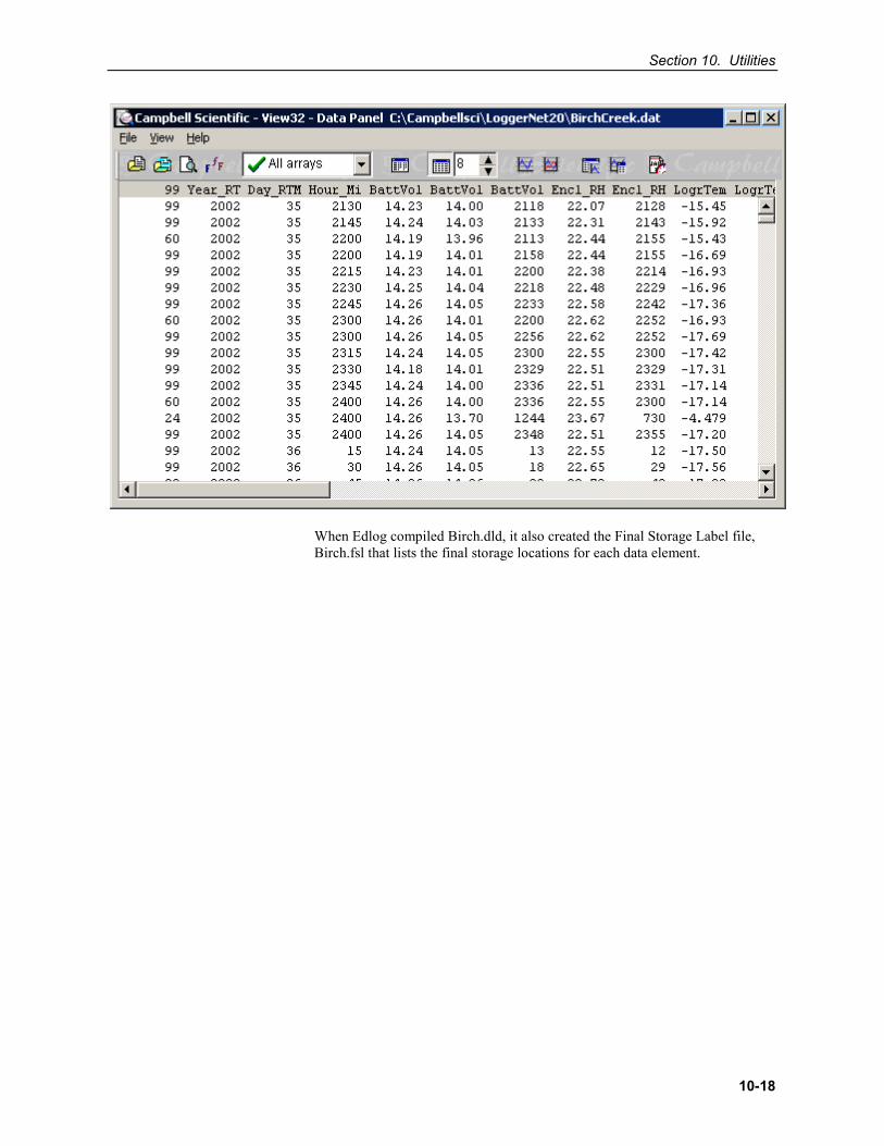
Section 10. Utilities
10-18
When Edlog compiled Birch.dld, it also created the Final Storage Label file, Birch.fsl that lists the final storage locations for each data element.
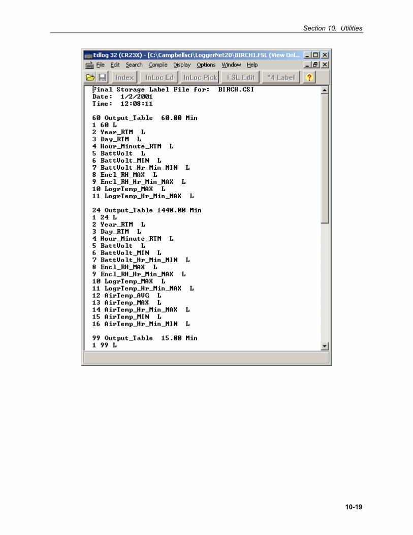
Section 10. Utilities
10-19
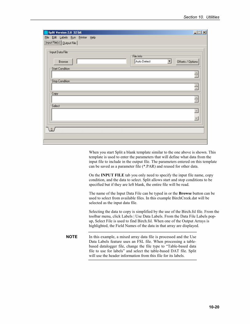
Section 10. Utilities
10-20
When you start Split a blank template similar to the one above is shown. This template is used to enter the parameters that will define what data from the input file to include in the output file. The parameters entered on this template can be saved as a parameter file (*.PAR) and reused for other data.
On the INPUT FILE tab you only need to specify the input file name, copy condition, and the data to select. Split allows start and stop conditions to be specified but if they are left blank, the entire file will be read.
The name of the Input Data File can be typed in or the Browse button can be used to select from available files. In this example BirchCreek.dat will be selected as the input data file.
Selecting the data to copy is simplified by the use of the Birch.fsl file. From the toolbar menu, click Labels | Use Data Labels. From the Data File Labels pop-up, Select File is used to find Birch.fsl. When one of the Output Arrays is highlighted, the Field Names of the data in that array are displayed.
In this example, a mixed array data file is processed and the Use Data Labels feature uses an FSL file. When processing a table-based datalogger file, change the file type to “Table-based data file to use for labels” and select the table-based DAT file. Split will use the header information from this file for its labels.
NOTE
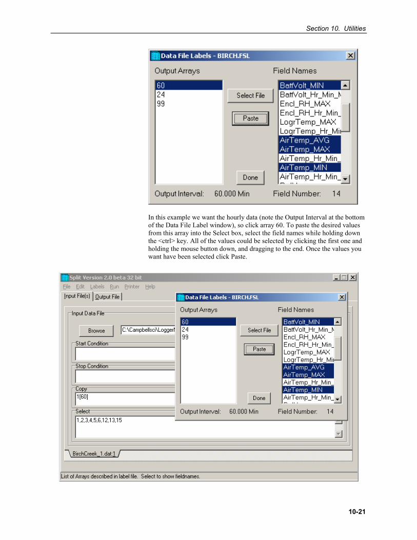
Section 10. Utilities
10-21
In this example we want the hourly data (note the Output Interval at the bottom of the Data File Label window), so click array 60. To paste the desired values from this array into the Select box, select the field names while holding down the <ctrl> key. All of the values could be selected by clicking the first one and holding the mouse button down, and dragging to the end. Once the values you want have been selected click Paste.
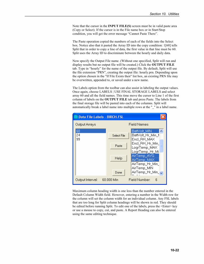
Section 10. Utilities
10-22
Note that the cursor in the INPUT FILE(S) screen must be in valid paste area (Copy or Select). If the cursor is in the File name box or in Start/Stop condition, you will get the error message “Cannot Paste There”.
The Paste operation copied the numbers of each of the fields into the Select box. Notice also that it pasted the Array ID into the copy condition: 1[60] tells Split that in order to copy a line of data, the first value in that line must be 60. Split uses the Array ID to discriminate between the hourly and daily data.
Now specify the Output File name. (Without one specified, Split will run and display results but no output file will be created.) Click the OUTPUT FILE tab. Type in “hourly” for the name of the output file. By default, Split will use the file extension “PRN”, creating the output file: hourly.prn. Depending upon the option chosen in the "If File Exists then" list box, an existing PRN file may be overwritten, appended to, or saved under a new name.
The Labels option from the toolbar can also assist in labeling the output values. Once again, choose LABELS | USE FINAL STORAGE LABELS and select array 60 and all the field names. This time move the cursor to Line 1 of the first column of labels on the OUTPUT FILE tab and press Paste. The labels from the final storage file will be pasted into each of the columns. Split will automatically break a label name into multiple rows at the "_" in a label name.
Maximum column heading width is one less than the number entered in the Default Column Width field. However, entering a number in the Width row for the column will set the column width for an individual column. Any FSL labels that are too long for Split column headings will be shown in red. They should be edited before running Split. To edit one of the labels, press the <Enter> key or use a mouse to copy, cut, and paste. A Report Heading can also be entered using the same editing technique.
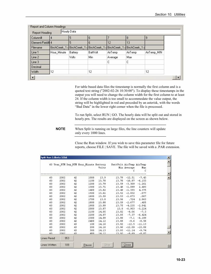
Section 10. Utilities
10-23
For table based data files the timestamp is normally the first column and is a quoted text string ("2002-02-26 10:30:00"). To display these timestamps in the output you will need to change the column width for the first column to at least 24. If the column width is too small to accommodate the value output, the string will be highlighted in red and preceded by an asterisk, with the words “Bad Data” in the lower right corner when the file is processed.
To run Split, select RUN | GO. The hourly data will be split out and stored in hourly.prn. The results are displayed on the screen as shown below.
When Split is running on large files, the line counters will update only every 1000 lines.
Close the Run window. If you wish to save this parameter file for future reports, choose FILE | SAVE. The file will be saved with a .PAR extension.
NOTE
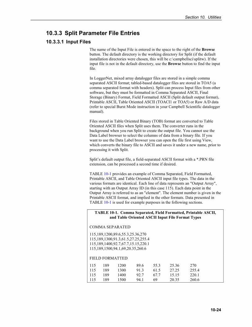
Section 10. Utilities
10-24
10.3.3 Split Parameter File Entries 10.3.3.1 Input Files
The name of the Input File is entered in the space to the right of the Browse button. The default directory is the working directory for Split (if the default installation directories were chosen, this will be c:\campbellsci\splitw). If the input file is not in the default directory, use the Browse button to find the input file.
In LoggerNet, mixed array datalogger files are stored in a simple comma separated ASCII format; tabled-based datalogger files are stored in TOA5 (a comma separated format with headers). Split can process Input files from other software, but they must be formatted in Comma Separated ASCII, Final Storage (Binary) Format, Field Formatted ASCII (Split default output format), Printable ASCII, Table Oriented ASCII (TOACI1 or TOA5) or Raw A/D data (refer to special Burst Mode instruction in your Campbell Scientific datalogger manual).
Files stored in Table Oriented Binary (TOB) format are converted to Table Oriented ASCII files when Split uses them. The converter runs in the background when you run Split to create the output file. You cannot use the Data Label browser to select the columns of data from a binary file. If you want to use the Data Label browser you can open the file first using View, which converts the binary file to ASCII and saves it under a new name, prior to processing it with Split.
Split’s default output file, a field-separated ASCII format with a *.PRN file extension, can be processed a second time if desired.
TABLE 10-1 provides an example of Comma Separated, Field Formatted, Printable ASCII, and Table Oriented ASCII input file types. The data in the various formats are identical. Each line of data represents an "Output Array", starting with an Output Array ID (in this case 115). Each data point in the Output Array is referred to as an "element". The element number is given in the Printable ASCII format, and implied in the other formats. Data presented in TABLE 10-1 is used for example purposes in the following sections.
TABLE 10-1. Comma Separated, Field Formatted, Printable ASCII, and Table Oriented ASCII Input File Format Types
COMMA SEPARATED
115,189,1200,89.6,55.3,25.36,270 115,189,1300,91.3,61.5,27.25,255.4 115,189,1400,92.7,67.7,15.15,220.1 115,189,1500,94.1,69,20.35,260.6
FIELD FORMATTED
115 189 1200 89.6 55.3 25.36 270 115 189 1300 91.3 61.5 27.25 255.4 115 189 1400 92.7 67.7 15.15 220.1 115 189 1500 94.1 69 20.35 260.6
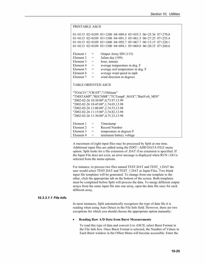
Section 10. Utilities
10-25
PRINTABLE ASCII
01+0115 02+0189 03+1200 04+089.6 05+055.3 06+25.36 07+270.0 01+0115 02+0189 03+1300 04+091.3 05+061.5 06+27.25 07+255.4 01+0115 02+0189 03+1400 04+092.7 05+067.7 06+15.15 07+220.1 01+0115 02+0189 03+1500 04+094.1 05+069.0 06+20.35 07+260.6
Element 1 = Output Array ID# (115) Element 2 = Julian day (189) Element 3 = hour, minute Element 4 = average temperature in deg. F Element 5 = average soil temperature in deg. F Element 6 = average wind speed in mph Element 7 = wind direction in degrees
TABLE ORIENTED ASCII
"TOACI1","CR10T","15Minute" "TMSTAMP","RECNBR","TCTempF_MAX","BattVolt_MIN" "2002-02-26 10:30:00",0,73.97,13.99 "2002-02-26 10:45:00",1,74.03,13.98 "2002-02-26 11:00:00",2,74.53,13.98 "2002-02-26 11:15:00",3,74.82,13.98 "2002-02-26 11:30:00",4,75.23,13.98
Element 1 = Timestamp Element 2 = Record Number Element 3 = temperature in degrees F Element 4 = minimum battery voltage
A maximum of eight input files may be processed by Split at one time. Additional input files are added using the EDIT | ADD DATA FILE menu option. Split looks for a file extension of .DAT if no extension is specified. If the Input File does not exist, an error message is displayed when RUN | GO is selected from the menu options.
For instance, to process two files named TEST.DAT and TEST_1.DAT the user would select TEST.DAT and TEST_1.DAT as Input Files. Two blank input file templates will be generated. To change from one template to the other, click the appropriate tab on the bottom of the screen. Both templates must be completed before Split will process the data. To merge different output arrays from the same input file into one array, open the data file once for each different array.
10.3.3.1.1 File Info
In most instances, Split automatically recognizes the type of data file it is reading when using Auto Detect in the File Info field. However, there are two exceptions for which you should choose the appropriate option manually:
• Reading Raw A/D Data from Burst Measurements
To read this type of data and convert it to ASCII, select Burst Format in the File Info box. Once Burst Format is selected, the Number of Values in Each Burst window in the Offset Menu will become accessible. Enter the
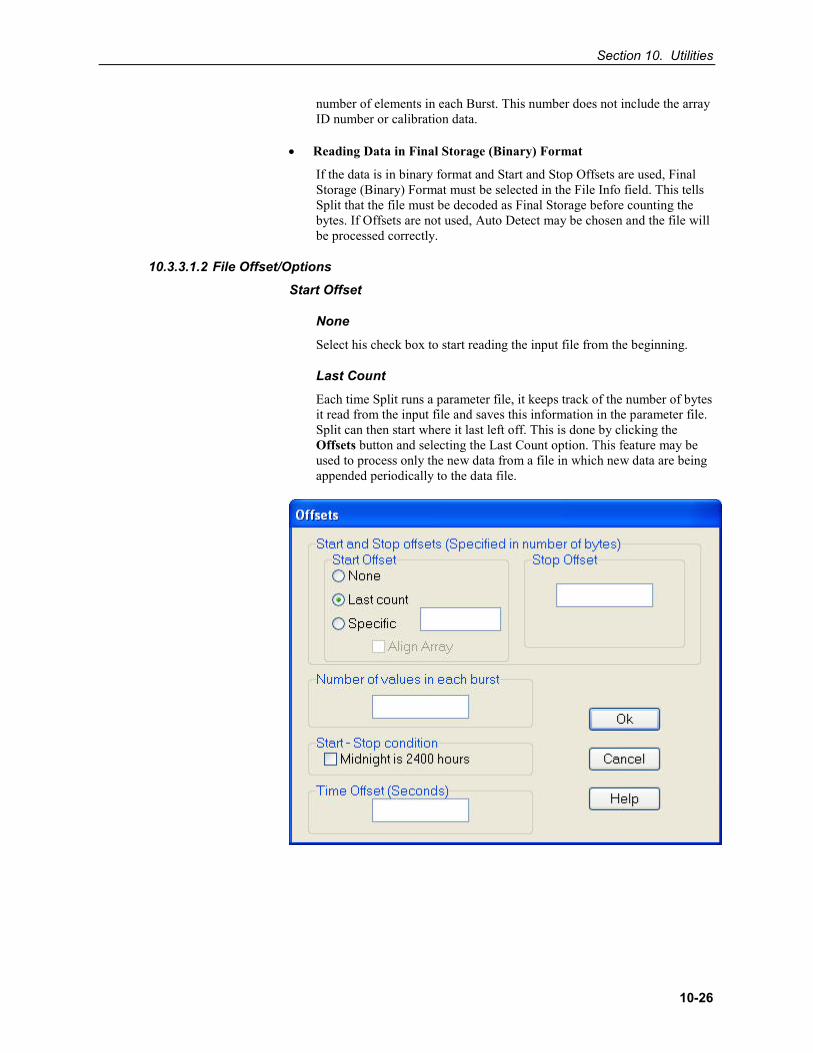
Section 10. Utilities
10-26
number of elements in each Burst. This number does not include the array ID number or calibration data.
• Reading Data in Final Storage (Binary) Format
If the data is in binary format and Start and Stop Offsets are used, Final Storage (Binary) Format must be selected in the File Info field. This tells Split that the file must be decoded as Final Storage before counting the bytes. If Offsets are not used, Auto Detect may be chosen and the file will be processed correctly.
10.3.3.1.2 File Offset/Options
Start Offset
None
Select his check box to start reading the input file from the beginning.
Last Count
Each time Split runs a parameter file, it keeps track of the number of bytes it read from the input file and saves this information in the parameter file. Split can then start where it last left off. This is done by clicking the Offsets button and selecting the Last Count option. This feature may be used to process only the new data from a file in which new data are being appended periodically to the data file.
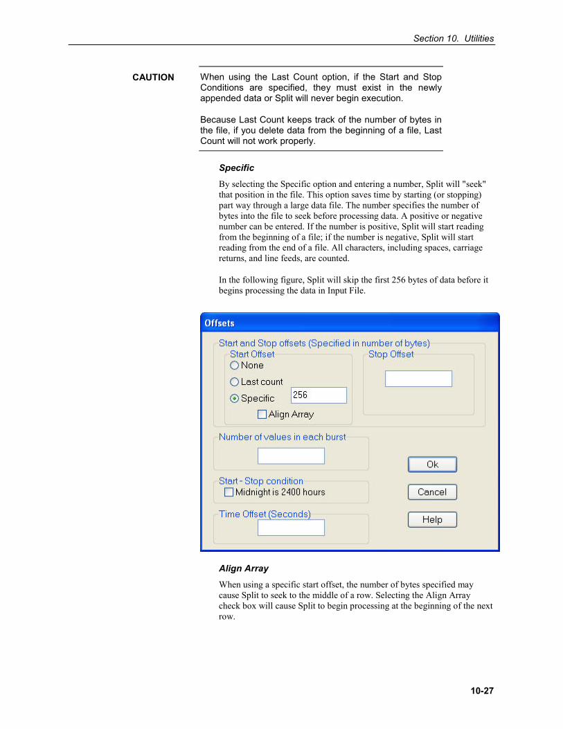
Section 10. Utilities
10-27
When using the Last Count option, if the Start and Stop Conditions are specified, they must exist in the newly appended data or Split will never begin execution.
Because Last Count keeps track of the number of bytes in the file, if you delete data from the beginning of a file, Last Count will not work properly.
Specific
By selecting the Specific option and entering a number, Split will "seek" that position in the file. This option saves time by starting (or stopping) part way through a large data file. The number specifies the number of bytes into the file to seek before processing data. A positive or negative number can be entered. If the number is positive, Split will start reading from the beginning of a file; if the number is negative, Split will start reading from the end of a file. All characters, including spaces, carriage returns, and line feeds, are counted.
In the following figure, Split will skip the first 256 bytes of data before it begins processing the data in Input File.
Align Array
When using a specific start offset, the number of bytes specified may cause Split to seek to the middle of a row. Selecting the Align Array check box will cause Split to begin processing at the beginning of the next row.
CAUTION
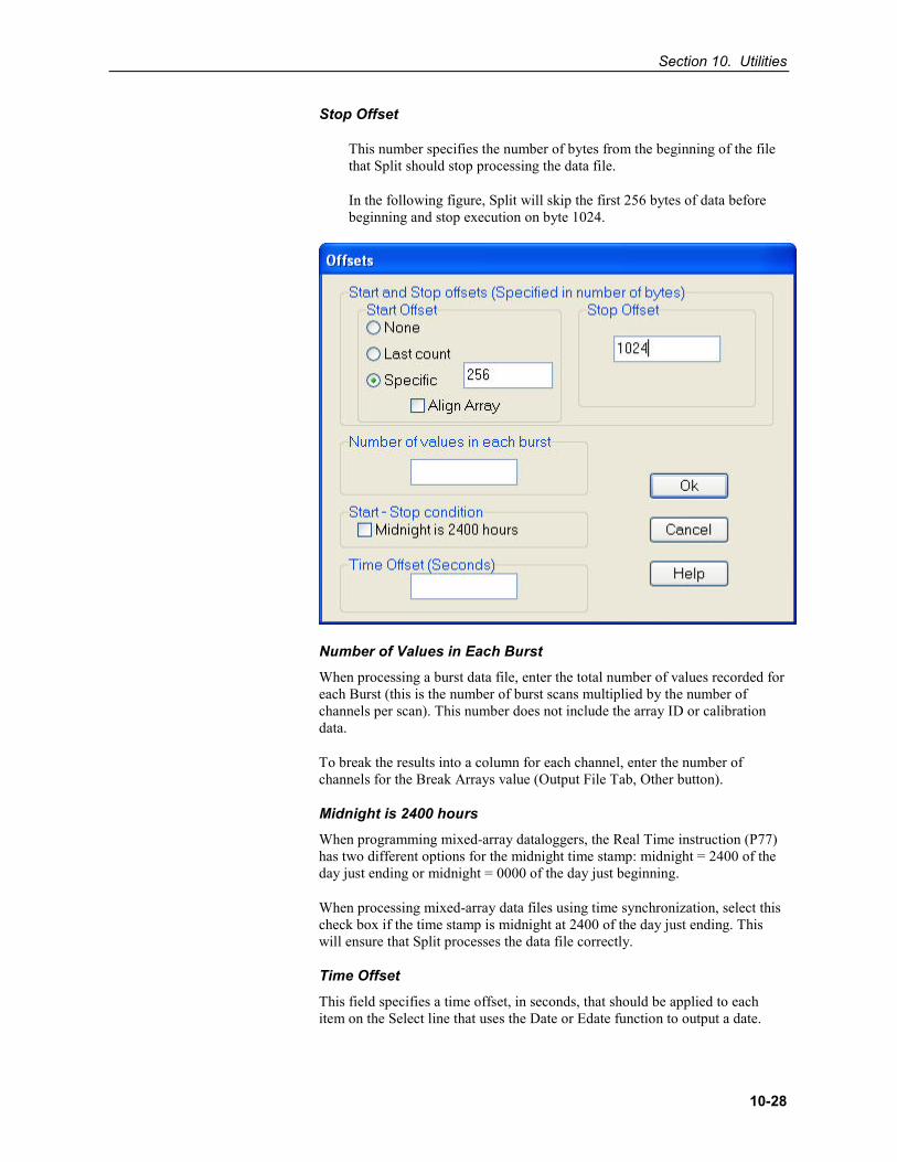
Section 10. Utilities
10-28
Stop Offset
This number specifies the number of bytes from the beginning of the file that Split should stop processing the data file.
In the following figure, Split will skip the first 256 bytes of data before beginning and stop execution on byte 1024.
Number of Values in Each Burst
When processing a burst data file, enter the total number of values recorded for each Burst (this is the number of burst scans multiplied by the number of channels per scan). This number does not include the array ID or calibration data.
To break the results into a column for each channel, enter the number of channels for the Break Arrays value (Output File Tab, Other button).
Midnight is 2400 hours
When programming mixed-array dataloggers, the Real Time instruction (P77) has two different options for the midnight time stamp: midnight = 2400 of the day just ending or midnight = 0000 of the day just beginning.
When processing mixed-array data files using time synchronization, select this check box if the time stamp is midnight at 2400 of the day just ending. This will ensure that Split processes the data file correctly.
Time Offset
This field specifies a time offset, in seconds, that should be applied to each item on the Select line that uses the Date or Edate function to output a date.
Section 10. Utilities
10-29
The offset can be positive or negative. Each input file can have its own offset (or no offset) for its Select line.
For example, with an input timestamp of “2008-10-09 10:25” and an offset of 3600, the timestamp output by Date (“yyyy-mm-dd hh:nn”;1;1;1;1) would be “2008-10-09 11:25”.
This may be useful when adjusting for different time zones.
The offset will not be applied to Date and Edate functions with only two parameters. (The two-parameter mode is backwards compatible with the original Date and Edate functions used in older versions of Split.)
10.3.3.1.3 Start Condition
A starting point may be specified to begin processing data. If the Start Condition field is left blank, Split will start processing data at the beginning of the data file. The starting point can be any element within the array or a combination of elements within an array.
The font for Start Condition, Stop Condition, Copy, and Select can be changed from the Options Menu.
The syntax can be expressed as:
ei[vali]
where ei = the position number of the element within the array
vali = the value of that element.
For example, the data in TABLE 10-1 contains seven elements per Output Array, representing hourly data. Assume that this data file contains one month of hourly data. To start processing data at 1500 hours on the first day, the Start Condition is expressed as 3[1500], where 3 means the third element within the array and 1500 is the value of that third element.
The element must match this start value exactly to trigger the start condition. However, when starting based on time, you can enable the "Start-Stop On/After Time" function to trigger the start of processing when the exact time is found or at the first instance of data after that time has occurred. This option is found on the Output tab, Other button.
NOTE
NOTE
Section 10. Utilities
10-30
Table data files contain the time and date as a single quoted string at the beginning of each data record. Split handles the dates as long as you include a colon separator as a placeholder for each of the fields in the timestamp. 1[Year]:1[Day of Year]:1[Time of Day]:1[Seconds]
See the examples below:
:1[60]:: Day of Year 60
1[2002]:1[60]:1[1250]: Year 2002, Day of Year 60, Time of Day 12:50
::1[1445]:1[30] Time of Day 14:45, Seconds 30
Logical “and” and “or” statements can be used when specifying the Start Condition. A logical “and” statement means that all conditions must be true for the statement to be true. Up to three conditions can be connected with “and” statements. If too many “and” statements are used, an error message will be displayed when you run Split.
The logical “or” statement means that if any of the conditions are true, then the statement is true. Split allows up to six conditions to be connected with “or” statements. Additionally, each “or” statement can contain up to three “and” conditions. As with the “and” statements, if the maximum number of valid statements is exceeded, an error message will be displayed.
These rules for logical statements also apply to the Stop and Copy Conditions.
An example of a simple logical “and” statement follows:
2[189]and3[1200]
Element two (the Julian day) must equal 189, and element three (the time in hours/minutes) must equal 1200.
If the following “and” statement was used:
2[189]and3[1200]and4[92]and5[67]
an error would be returned because the maximum number of allowable “and” statements has been exceeded.
A range can be specified for vali by putting ".." between the lower and upper limit. For example:
2[189]and7[200..275]
In this example two conditions must be satisfied to start processing data. First, the day of year must be 189, and second, element 7 must be between 200 to 275 degrees, inclusive.
NOTE
Section 10. Utilities
10-31
10.3.3.1.3.1 Starting Relative to PC Time
Split has the ability to start relative to the current PC TIME (computer time). This feature allows a .PAR file to be run on new data files without changing the Start Conditions, provided the Input Data File is collected at a fixed interval and Split is run at a fixed interval. For example, the same PAR file could be run every day to display the last 48 hours of data without changing the start conditions. For example, using a table based data file:
Start Condition = 1:1[-1]:1[1200]:1:
In this instance, Split will begin processing data when the date for both files is one less than the current date (1:1[-1]:1[1200]:1:)and the time is 1200 (1:1[-1]:1[1200]:1:).
As an expanded example, assume that LoggerNet is used to append data to an archive file. SplitR is executed using a desktop shortcut. In this case the frequency of data collection and data reduction is the same. Time values in the data file (day, hrmn, sec.) are different each time the data are collected, but by telling Split where to Start reading relative to the PC clock, the Start Conditions do not need to be changed. To accommodate variations in the data collection and reduction frequencies, an interval in minutes or seconds may be specified as shown in the examples below.
2[-0]:3[-60,5] tells Split to start at a timestamp in the data that is between 55 and 65 minutes prior to the current PC time (the closest 5 minute interval of the current day that is less than the PC time minus 60 minutes). If you are processing data stored at the top of the hour and the PC time is 1404, Split calculates 1304 and looks for hour 1300 to start reading.
2[-3]:3[-120,60] tells Split to find the closest 60 minute interval that is less than the PC time minus 3 days and 2 hours. If the PC time is the day of year 159, hour 0017, Split will start reading on data output at 2200 hours on day 155.
2[-3]:3[-120]:4[20,5] tells Split to find the closest 5 second interval that is less than the PC time minus 3 days, 2 hours and 20 seconds. If the PC time is 27 seconds after noon on day 30, Split will begin reading on data output at 1000 hours and 05 seconds on day 27.
Split can also begin processing a file on a particular month and day. Use the syntax :E[Month%Day]::, where E is the element that contains the Julian Day, and Month and Day are either constants or a value related to PC time. For example:
:2[-1%1]:: tells Split to begin processing on the first day of the previous month. :2[-0%15]:: tells Split to begin processing on the fifteenth day of the current month. :2[5%1]:: tells Split to begin processing on May 1.
This function can be used in both the Start and Stop conditions. It provides a simple way to create a monthly report. For additional information, refer also to Section 10.3.3.1.15.2, 10.3.3.1.15.2 Using Time Synchronization While Starting Relative to PC Time (p. 10-55).
Section 10. Utilities
10-32
Split will not start reading if the exact specified starting time cannot be found, unless you enable the "Start-Stop On/After Time" feature. The interval (5 minutes, 60 minutes, and 5 seconds in the examples above) must be evenly divisible into 60 minutes.
• If the start time is a certain number of days prior to the PCtime, the file will be processed beginning at midnight of the dayspecified.
• To specify a start time in minutes from the current PC time,you must also specify a day parameter of [-0]. Otherwise,processing will begin at the first instance in the data file that theminutes parameter equals the current minutes.
10.3.3.1.4 Stop Condition
The Stop Condition specifies when to stop processing data. This feature allows segments of data to be removed from large data files. For instance, if a data file contains one month of data and just one day is desired, the start and stop values allow the user to get just that day’s data.
The Stop Condition is expressed with the same syntax as the Start Condition. If the Stop Condition parameter is left blank, Split will execute until the end of the file. As with the Start Condition, logical "and" and "or" statements can be used when specifying the Stop Condition (Section 10.3.3.1.3, Start Condition (p. 10-29)), as well as stopping based on PC time.
The array or record containing the Stop Condition is not included in the output file. If the stop value is not found, Split will display a dialogue box that gives the option to select a new file and continue processing the data. This feature is useful when data are contained in more than one data file.
The "Start-Stop On/After Time" function can be used with a Stop Condition. This will stop processing of the file when the exact time is found or at the first instance of data after that time has occurred. This option is found on the Output tab, Other button.
The C and F commands alter the meaning of the Stop Condition.
10.3.3.1.4.1 "C" Option: Formatting Event Tests Containing Conditional Output Arrays
The C option is used to combine data from two or more conditional arrays onto one Split output line. A conditional array is one that is only output when a defined event occurs.
Assume that two or more conditional Output Arrays with unique Output Array IDs compose a test period, followed by an unconditional Output Array that defines the end of a test. The unconditional "end of test" Output Array is at the end of each test, but the conditional Output Arrays may or may not be present. The data file is comprised of several of these tests.
CAUTION
NOTE
Section 10. Utilities
10-33
As an example, let's look at a vehicle test application. The start of the test is when the vehicle is turned on, and the end of the test is when the vehicle is turned off. The conditional output arrays could be:
• monitoring the engine temperature and outputting data to a unique array when the temperature exceeds a limit
• outputting data to a unique array when the brakes are applied
• outputting data when engine RPM exceeds a limit
The unconditional array data (the stop condition) would be output to a unique array when the engine is turned off. By processing the data with Split using the C option, the data collected during each test could be merged on to one line, with blanks inserted if a set of data didn't exist (e.g., if the engine temperature never exceeded the defined limit).
• An Input File must be set up for each array ID in the test. The first Input File is configured on the Input File tab that appears when you open Split. Additional Input Files are added by choosing Edit | Add Data File from the Split menu. The same data file will be used as the Input File for each array.
• Type in the array ID in the Copy field of the Input File tab for each array. The array ID is the first element of a data file, so the line should read 1[123], where 123 is the actual array ID you want to process.
• In the Select field, type in the number for each element (data value) you want to be output in the report.
• In the Stop Condition field, type in a "C," followed by the ID of your stop condition array. If your "end of test" array was array ID 200, the Stop Condition field would read: C,1[200]. This should be typed into the Stop Condition fields of each array, including the "end of test" array.
Set up the Output File as you would for any Split process. If you are including column headings, the arrays and elements will appear in the order they are listed on the Input File tabs. That is, the first column will be Input File number 1, element number 1; the next column is Input File number 1, element number 2… Input File number 2, element number 1 follows in the column immediately after the last element of Input File number 1.
Consider TABLE 10-2 below:
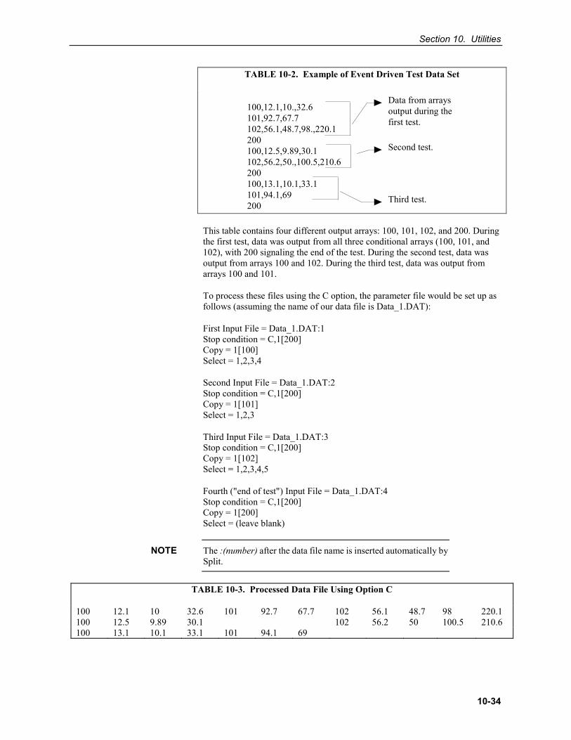
Section 10. Utilities
10-34
TABLE 10-2. Example of Event Driven Test Data Set
This table contains four different output arrays: 100, 101, 102, and 200. During the first test, data was output from all three conditional arrays (100, 101, and 102), with 200 signaling the end of the test. During the second test, data was output from arrays 100 and 102. During the third test, data was output from arrays 100 and 101.
To process these files using the C option, the parameter file would be set up as follows (assuming the name of our data file is Data_1.DAT):
First Input File = Data_1.DAT:1 Stop condition = C,1[200] Copy = 1[100] Select = 1,2,3,4
Second Input File = Data_1.DAT:2 Stop condition = C,1[200] Copy = 1[101] Select = 1,2,3
Third Input File = Data_1.DAT:3 Stop condition = C,1[200] Copy = 1[102] Select = 1,2,3,4,5
Fourth ("end of test") Input File = Data_1.DAT:4 Stop condition = C,1[200] Copy = 1[200] Select = (leave blank)
The :(number) after the data file name is inserted automatically by Split.
TABLE 10-3. Processed Data File Using Option C
100 12.1 10 32.6 101 92.7 67.7 102 56.1 48.7 98 220.1 100 12.5 9.89 30.1 102 56.2 50 100.5 210.6 100 13.1 10.1 33.1 101 94.1 69
100,12.1,10.,32.6101,92.7,67.7102,56.1,48.7,98.,220.1200100,12.5,9.89,30.1102,56.2,50.,100.5,210.6200100,13.1,10.1,33.1101,94.1,69200
Data from arraysoutput during thefirst test.
Second test.
Third test.
NOTE
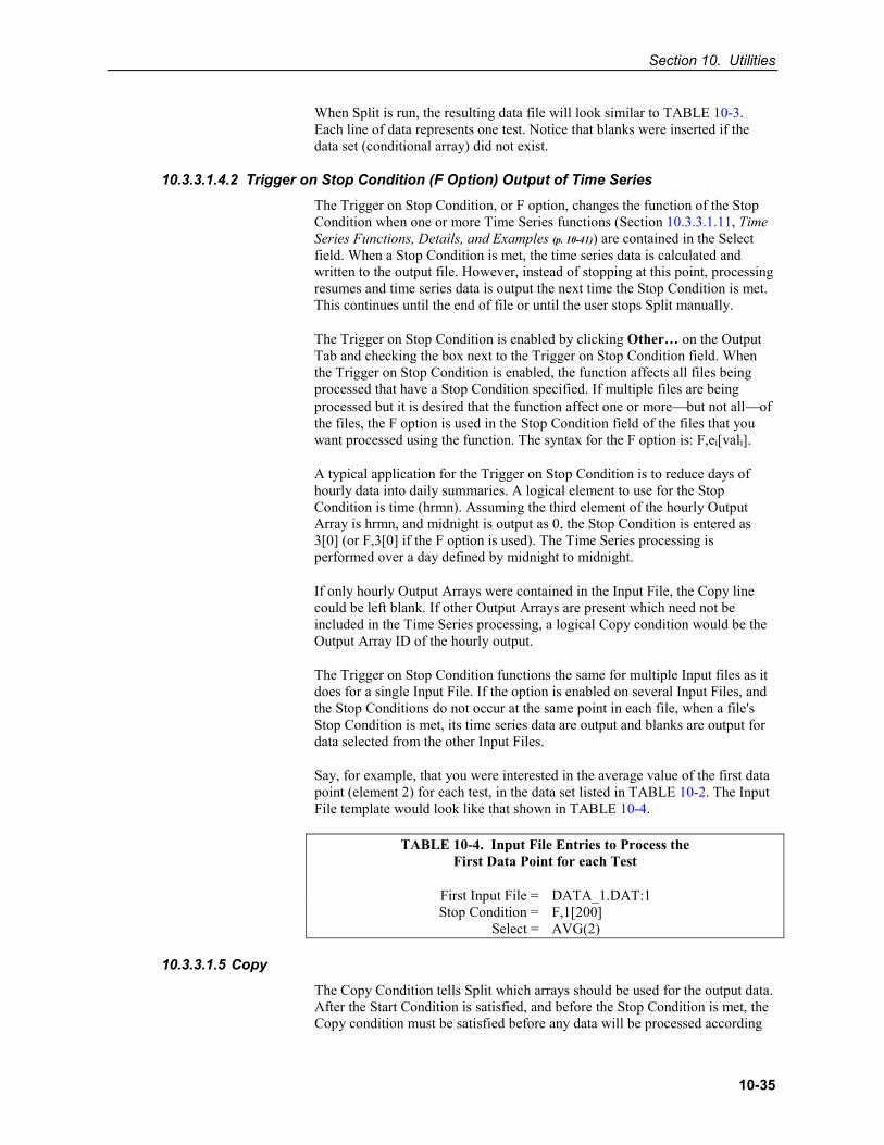
Section 10. Utilities
10-35
When Split is run, the resulting data file will look similar to TABLE 10-3. Each line of data represents one test. Notice that blanks were inserted if the data set (conditional array) did not exist.
10.3.3.1.4.2 Trigger on Stop Condition (F Option) Output of Time Series
The Trigger on Stop Condition, or F option, changes the function of the Stop Condition when one or more Time Series functions (Section 10.3.3.1.11, Time Series Functions, Details, and Examples (p. 10-41)) are contained in the Select field. When a Stop Condition is met, the time series data is calculated and written to the output file. However, instead of stopping at this point, processing resumes and time series data is output the next time the Stop Condition is met. This continues until the end of file or until the user stops Split manually.
The Trigger on Stop Condition is enabled by clicking Other… on the Output Tab and checking the box next to the Trigger on Stop Condition field. When the Trigger on Stop Condition is enabled, the function affects all files being processed that have a Stop Condition specified. If multiple files are being processed but it is desired that the function affect one or morebut not allof the files, the F option is used in the Stop Condition field of the files that you want processed using the function. The syntax for the F option is: F,ei[vali].
A typical application for the Trigger on Stop Condition is to reduce days of hourly data into daily summaries. A logical element to use for the Stop Condition is time (hrmn). Assuming the third element of the hourly Output Array is hrmn, and midnight is output as 0, the Stop Condition is entered as 3[0] (or F,3[0] if the F option is used). The Time Series processing is performed over a day defined by midnight to midnight.
If only hourly Output Arrays were contained in the Input File, the Copy line could be left blank. If other Output Arrays are present which need not be included in the Time Series processing, a logical Copy condition would be the Output Array ID of the hourly output.
The Trigger on Stop Condition functions the same for multiple Input files as it does for a single Input File. If the option is enabled on several Input Files, and the Stop Conditions do not occur at the same point in each file, when a file's Stop Condition is met, its time series data are output and blanks are output for data selected from the other Input Files.
Say, for example, that you were interested in the average value of the first data point (element 2) for each test, in the data set listed in TABLE 10-2. The Input File template would look like that shown in TABLE 10-4.
TABLE 10-4. Input File Entries to Process the First Data Point for each Test
First Input File = DATA_1.DAT:1 Stop Condition = F,1[200] Select = AVG(2)
10.3.3.1.5 Copy
The Copy Condition tells Split which arrays should be used for the output data. After the Start Condition is satisfied, and before the Stop Condition is met, the Copy condition must be satisfied before any data will be processed according
Section 10. Utilities
10-36
to Select line instructions. If the Copy condition is left blank, all arrays are processed between the Start and Stop values. Syntax for the Copy condition is similar to the Start and Stop values mentioned above. Logical "and" and "or" statements (see Section 10.3.3.1.3, Start Condition (p. 10-29)) can be used when specifying the Copy condition.
For example, referring to TABLE 10-1, if only those hours during day 189 when the temperature was above 90 and the soil temperature was below 62 is desired, or, during day 189 when the average wind speed was below 21 while the wind direction was between 255 to 265 is desired, the Copy condition would be:
1[189]and4[90..150]and5[0..61.99]or1[189]and6[0..20.99]and7[255..265]
Only Output Arrays with hours 1300 and 1500, TABLE 10-1, conform to the above Copy conditions.
The Copy Condition is used almost exclusively for mixed-array dataloggers, except when time-syncing two or more data files. See Section 10.3.3.1.15, Time Synchronization (p. 10-53), for additional information.
Time Ranges When specifying a Copy condition, a range of time values can be specified instead of a single time. If the element being tested falls within the range, the Copy condition is satisfied and the data is processed. A range is indicated by entering two periods between the first and last values of the range.
Examples:
Table-based
With an entry of 1:1:1[600..1200]:1 in the Copy condition, Split will only process the data file when the time is between 6:00 a.m. and 12:00 p.m.
(Since the timestamp for table-based dataloggers is all one string, each portion of the timestamp (year, day, hour/minute, seconds) will use the same element number. Colons are used to separate each portion. The format is 1[year]:1[day]:1[hhmm]:1[seconds] (the number 1 was used since, typically, the timestamp is the first element in the data string). In this format, hhmm is the four-digit hour/minute.)
Array-based
With an entry of 1[30] and 2:3:4[600..1200]: in the Copy condition, Split will only process the data file when the time is between 6:00 a.m. and 12:00 p.m.
(This assumes 2 is the year element, 3 is the day element, and 4 is the hour/minute element.)
Time ranges cannot be used with the time-sync function.
NOTE
NOTE
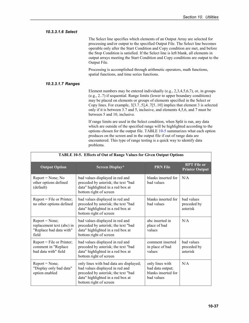
Section 10. Utilities
10-37
10.3.3.1.6 Select
The Select line specifies which elements of an Output Array are selected for processing and/or output to the specified Output File. The Select line becomes operable only after the Start Condition and Copy condition are met, and before the Stop Condition is satisfied. If the Select line is left blank, all elements in output arrays meeting the Start Condition and Copy conditions are output to the Output File.
Processing is accomplished through arithmetic operators, math functions, spatial functions, and time series functions.
10.3.3.1.7 Ranges
Element numbers may be entered individually (e.g., 2,3,4,5,6,7), or, in groups (e.g., 2..7) if sequential. Range limits (lower to upper boundary conditions) may be placed on elements or groups of elements specified in the Select or Copy lines. For example, 3[3.7..5],4..7[5..10] implies that element 3 is selected only if it is between 3.7 and 5, inclusive, and elements 4,5,6, and 7 must be between 5 and 10, inclusive.
If range limits are used in the Select condition, when Split is run, any data which are outside of the specified range will be highlighted according to the options chosen for the output file. TABLE 10-5 summarizes what each option produces on the screen and in the output file if out of range data are encountered. This type of range testing is a quick way to identify data problems.
TABLE 10-5. Effects of Out of Range Values for Given Output Options
Output Option Screen Display* PRN File RPT File or Printer Output
Report = None; No other options defined (default)
bad values displayed in red and preceded by asterisk; the text "bad data" highlighted in a red box at bottom right of screen
blanks inserted for bad values
N/A
Report = File or Printer; no other options defined
bad values displayed in red and preceded by asterisk; the text "bad data" highlighted in a red box at bottom right of screen
blanks inserted for bad values
bad values preceded by asterisk
Report = None; replacement text (abc) in "Replace bad data with" field
bad values displayed in red and preceded by asterisk; the text "bad data" highlighted in a red box at bottom right of screen
abc inserted in place of bad values
N/A
Report = File or Printer; comment in "Replace bad data with" field
bad values displayed in red and preceded by asterisk; the text "bad data" highlighted in a red box at bottom right of screen
comment inserted in place of bad values
bad values preceded by asterisk
Report = None; "Display only bad data" option enabled
only lines with bad data are displayed; bad values displayed in red and preceded by asterisk; the text "bad data" highlighted in a red box at bottom right of screen
only lines with bad data output; blanks inserted for bad values
N/A
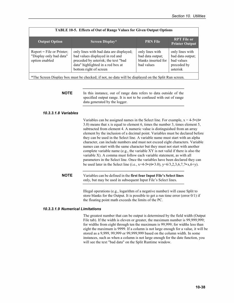
Section 10. Utilities
10-38
TABLE 10-5. Effects of Out of Range Values for Given Output Options
Output Option Screen Display* PRN File RPT File or Printer Output
Report = File or Printer; "Display only bad data" option enabled
only lines with bad data are displayed; bad values displayed in red and preceded by asterisk; the text "bad data" highlighted in a red box at bottom right of screen
only lines with bad data output; blanks inserted for bad values
only lines with bad data output; bad values preceded by asterisk
*The Screen Display box must be checked; if not, no data will be displayed on the Split Run screen.
In this instance, out of range data refers to data outside of the specified output range. It is not to be confused with out of range data generated by the logger.
10.3.3.1.8 Variables
Variables can be assigned names in the Select line. For example, x = 4-5∗(6∗3.0) means that x is equal to element 6, times the number 3, times element 5, subtracted from element 4. A numeric value is distinguished from an array element by the inclusion of a decimal point. Variables must be declared before they can be used in the Select line. A variable name must start with an alpha character, can include numbers and must not exceed eight characters. Variable names can start with the same character but they must not start with another complete variable name (e.g., the variable XY is not valid if there is also the variable X). A comma must follow each variable statement, as with all parameters in the Select line. Once the variables have been declared they can be used later in the Select line (i.e., x=4-5∗(6∗3.0), y=6/3,2,3,6,7,7∗x,6+y).
Variables can be defined in the first four Input File’s Select lines only, but may be used in subsequent Input File’s Select lines.
Illegal operations (e.g., logarithm of a negative number) will cause Split to store blanks for the Output. It is possible to get a run time error (error 0/1) if the floating point math exceeds the limits of the PC.
10.3.3.1.9 Numerical Limitations
The greatest number that can be output is determined by the field width (Output File tab). If the width is eleven or greater, the maximum number is 99,999,999; for widths from eight through ten the maximum is 99,999; for widths less than eight the maximum is 9999. If a column is not large enough for a value, it will be stored as a 9,999, 99,999 or 99,999,999 based on the column width. In some instances, such as when a column is not large enough for the date function, you will see the text "bad data" on the Split Runtime window.
NOTE
NOTE
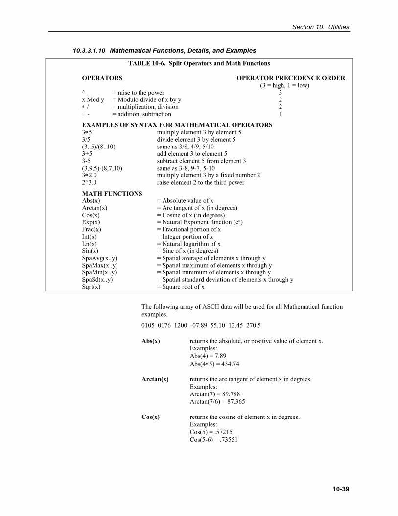
Section 10. Utilities
10-39
10.3.3.1.10 Mathematical Functions, Details, and Examples
TABLE 10-6. Split Operators and Math Functions
OPERATORS OPERATOR PRECEDENCE ORDER (3 = high, 1 = low) ^ = raise to the power 3 x Mod y = Modulo divide of x by y 2 ∗ / = multiplication, division 2 + - = addition, subtraction 1
EXAMPLES OF SYNTAX FOR MATHEMATICAL OPERATORS 3∗5 multiply element 3 by element 5 3/5 divide element 3 by element 5 (3..5)/(8..10) same as 3/8, 4/9, 5/10 3+5 add element 3 to element 5 3-5 subtract element 5 from element 3 (3,9,5)-(8,7,10) same as 3-8, 9-7, 5-10 3∗2.0 multiply element 3 by a fixed number 2 2^3.0 raise element 2 to the third power
MATH FUNCTIONS Abs(x) = Absolute value of x Arctan(x) = Arc tangent of x (in degrees) Cos(x) = Cosine of x (in degrees) Exp(x) = Natural Exponent function (ex) Frac(x) = Fractional portion of x Int(x) = Integer portion of x Ln(x) = Natural logarithm of x Sin(x) = Sine of x (in degrees) SpaAvg(x..y) = Spatial average of elements x through y SpaMax(x..y) = Spatial maximum of elements x through y SpaMin(x..y) = Spatial minimum of elements x through y SpaSd(x..y) = Spatial standard deviation of elements x through y Sqrt(x) = Square root of x
The following array of ASCII data will be used for all Mathematical function examples.
0105 0176 1200 -07.89 55.10 12.45 270.5
Abs(x) returns the absolute, or positive value of element x. Examples:
Abs(4) = 7.89 Abs(4∗5) = 434.74
Arctan(x) returns the arc tangent of element x in degrees. Examples:
Arctan(7) = 89.788 Arctan(7/6) = 87.365
Cos(x) returns the cosine of element x in degrees. Examples:
Cos(5) = .57215 Cos(5-6) = .73551
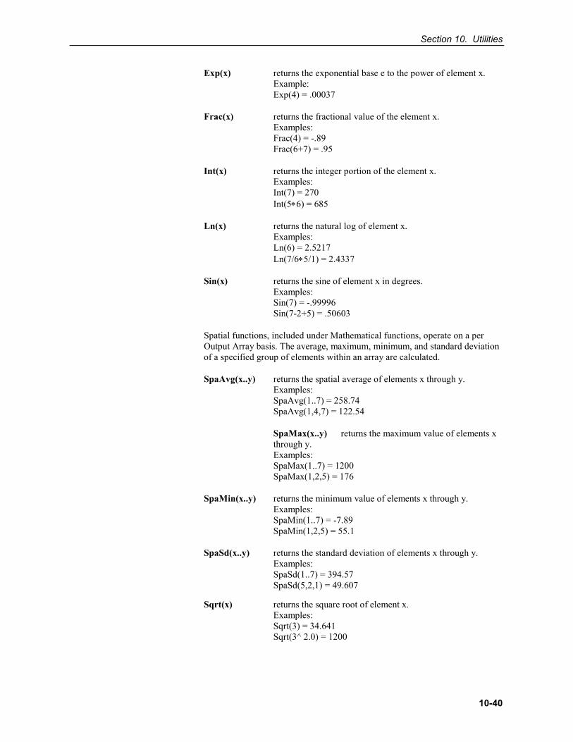
Section 10. Utilities
10-40
Exp(x) returns the exponential base e to the power of element x. Example:
Exp(4) = .00037
Frac(x) returns the fractional value of the element x. Examples:
Frac(4) = -.89 Frac(6+7) = .95
Int(x) returns the integer portion of the element x. Examples:
Int(7) = 270 Int(5∗6) = 685
Ln(x) returns the natural log of element x. Examples:
Ln(6) = 2.5217 Ln(7/6∗5/1) = 2.4337
Sin(x) returns the sine of element x in degrees. Examples:
Sin(7) = -.99996 Sin(7-2+5) = .50603
Spatial functions, included under Mathematical functions, operate on a per Output Array basis. The average, maximum, minimum, and standard deviation of a specified group of elements within an array are calculated.
SpaAvg(x..y) returns the spatial average of elements x through y. Examples:
SpaAvg(1..7) = 258.74 SpaAvg(1,4,7) = 122.54
SpaMax(x..y) returns the maximum value of elements x through y. Examples:
SpaMax(1..7) = 1200 SpaMax(1,2,5) = 176
SpaMin(x..y) returns the minimum value of elements x through y. Examples:
SpaMin(1..7) = -7.89 SpaMin(1,2,5) = 55.1
SpaSd(x..y) returns the standard deviation of elements x through y. Examples:
SpaSd(1..7) = 394.57 SpaSd(5,2,1) = 49.607
Sqrt(x) returns the square root of element x. Examples:
Sqrt(3) = 34.641 Sqrt(3^ 2.0) = 1200
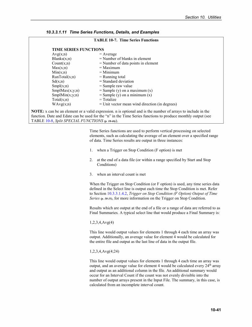
Section 10. Utilities
10-41
10.3.3.1.11 Time Series Functions, Details, and Examples
TABLE 10-7. Time Series Functions
TIME SERIES FUNCTIONS Avg(x;n) = Average Blanks(x;n) = Number of blanks in element Count(x;n) = Number of data points in element Max(x;n) = Maximum Min(x;n) = Minimum RunTotal(x;n) = Running total Sd(x;n) = Standard deviation Smpl(x;n) = Sample raw value SmplMax(x;y;n) = Sample (y) on a maximum (x) SmplMin(x;y;n) = Sample (y) on a minimum (x) Total(x;n) = Totalize WAvg(x;n) = Unit vector mean wind direction (in degrees)
NOTE: x can be an element or a valid expression. n is optional and is the number of arrays to include in the function. Date and Edate can be used for the “n” in the Time Series functions to produce monthly output (see TABLE 10-8, Split SPECIAL FUNCTIONS (p. 10-46)).
Time Series functions are used to perform vertical processing on selected elements, such as calculating the average of an element over a specified range of data. Time Series results are output in three instances:
1. when a Trigger on Stop Condition (F option) is met
2. at the end of a data file (or within a range specified by Start and Stop Conditions)
3. when an interval count is met
When the Trigger on Stop Condition (or F option) is used, any time series data defined in the Select line is output each time the Stop Condition is met. Refer to Section 10.3.3.1.4.2, Trigger on Stop Condition (F Option) Output of Time Series (p. 10-35), for more information on the Trigger on Stop Condition.
Results which are output at the end of a file or a range of data are referred to as Final Summaries. A typical select line that would produce a Final Summary is:
1,2,3,4,Avg(4)
This line would output values for elements 1 through 4 each time an array was output. Additionally, an average value for element 4 would be calculated for the entire file and output as the last line of data in the output file.
1,2,3,4,Avg(4;24)
This line would output values for elements 1 through 4 each time an array was output, and an average value for element 4 would be calculated every 24th array and output as an additional column in the file. An additional summary would occur for an Interval Count if the count was not evenly divisible into the number of output arrays present in the Input File. The summary, in this case, is calculated from an incomplete interval count.
Section 10. Utilities
10-42
The date( ) function can be used for the interval in a time series function to produce monthly output. Refer to the Monthly summary example in Section 10.3.3.1.12, Special Functions, Details, and Examples (p. 10-46).
When Date and Edate are used within other functions they must be used with the older format Date(doy;y) and Edate(doy;y) instead of using the extended date functions. For example AVG(1;Date(2;2002.0)). The decimal is needed to indicate a fixed number. Numbers without the decimal are interpreted as element IDs.
The interval count in a Time Series Function is optional and does not require a decimal point. To determine the interval, Split counts the number of arrays which meet the specified conditions (Stop, Start, and Copy). If the time synchronize function is enabled, the Time Series functions remain synchronized to the starting time even if a complete array is missing from the input data. When elements are missing, the Time Series calculations are based on the actual number of elements found.
Semicolons are used in Time Series functions to separate the elements or expressions from the count which determines the interval. SmplMax and SmplMin require two elements separated by a semicolon. The first is checked for a maximum or minimum, while the second is sampled on the maximum or minimum.
The following set of weather data from Mt. Logan in northern Utah gives a total of seven elements each hour. This Field Formatted output, with title and column headers, was generated by Split. These data are used in the following examples of Time Series functions.
NOTE
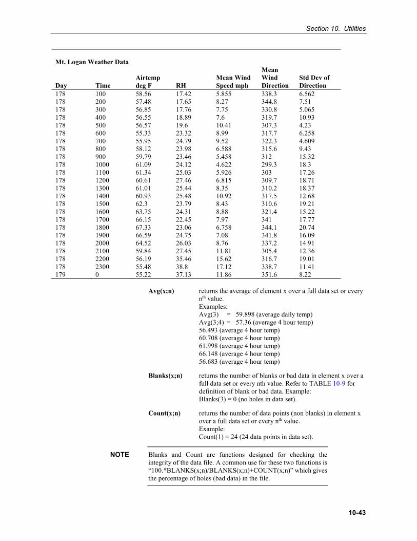
Section 10. Utilities
10-43
Mt. Logan Weather Data Day
Time
Airtemp deg F
RH
Mean Wind Speed mph
Mean Wind Direction
Std Dev of Direction
178 100 58.56 17.42 5.855 338.3 6.562 178 200 57.48 17.65 8.27 344.8 7.51 178 300 56.85 17.76 7.75 330.8 5.065 178 400 56.55 18.89 7.6 319.7 10.93 178 500 56.57 19.6 10.41 307.3 4.23 178 600 55.33 23.32 8.99 317.7 6.258 178 700 55.95 24.79 9.52 322.3 4.609 178 800 58.12 23.98 6.588 315.6 9.43 178 900 59.79 23.46 5.458 312 15.32 178 1000 61.09 24.12 4.622 299.3 18.3 178 1100 61.34 25.03 5.926 303 17.26 178 1200 60.61 27.46 6.815 309.7 18.71 178 1300 61.01 25.44 8.35 310.2 18.37 178 1400 60.93 25.48 10.92 317.5 12.68 178 1500 62.3 23.79 8.43 310.6 19.21 178 1600 63.75 24.31 8.88 321.4 15.22 178 1700 66.15 22.45 7.97 341 17.77 178 1800 67.33 23.06 6.758 344.1 20.74 178 1900 66.59 24.75 7.08 341.8 16.09 178 2000 64.52 26.03 8.76 337.2 14.91 178 2100 59.84 27.45 11.81 305.4 12.36 178 2200 56.19 35.46 15.62 316.7 19.01 178 2300 55.48 38.8 17.12 338.7 11.41 179 0 55.22 37.13 11.86 351.6 8.22
Avg(x;n) returns the average of element x over a full data set or every
nth value. Examples:
Avg(3) = 59.898 (average daily temp) Avg(3;4) = 57.36 (average 4 hour temp) 56.493 (average 4 hour temp) 60.708 (average 4 hour temp) 61.998 (average 4 hour temp) 66.148 (average 4 hour temp) 56.683 (average 4 hour temp)
Blanks(x;n) returns the number of blanks or bad data in element x over a full data set or every nth value. Refer to TABLE 10-9 for definition of blank or bad data. Example:
Blanks(3) = 0 (no holes in data set).
Count(x;n) returns the number of data points (non blanks) in element x over a full data set or every nth value. Example:
Count(1) = 24 (24 data points in data set).
Blanks and Count are functions designed for checking the integrity of the data file. A common use for these two functions is “100.*BLANKS(x;n)/BLANKS(x;n)+COUNT(x;n)” which gives the percentage of holes (bad data) in the file.
NOTE
Section 10. Utilities
10-44
Max(x;n) returns the maximum value of element x over a full data set or every nth value.
Examples: Max(5) = 17.12 (max WS for day) Max(5;12) = 10.41 (max WS for 12 hours) 17.12 (max WS for 12 hours)
Min(x;n) returns the minimum value of element x over a full data set or every nth value.
Examples: Min(7) = 4.23 (min std. dev. of WS for day) Min(3;8) = 55.33 (min temp for 8 hours) 59.79 (min temp for 8 hours) 55.22 (min temp for 8 hours)
RunTotal(x;n) returns a running total of element x for every line in the data set. If an nth value is specified, a running total will be output every nth value.
Example: RunTotal(5) = 5.85 14.12 21.87 29.47 39.88 48.87 : : : 166.76 182.38 199.50 211.36 211.36
Running total of hourly average wind speed provides up-to-the-hour wind run for that day. Because an nth value was not specified, the Final Summary output, which is daily wind, is the same as the "total" output.
Sd(x;n) returns the standard deviation of element x over a full data set or every nth value.
Examples: Sd(3) = 3.6593 (std. dev. temp for day) Sd(3;8) = 1.011 (Sd temp for 8 hours) 1.1182 (Sd temp for 8 hours) 4.965 (Sd temp for 8 hours)
Smpl(x;n) returns a sample of element x every nth value. Examples: Smpl(4;8) = 23.98 (RH every 8 hours) 24.31 (RH every 8 hours) 37.13 (RH every 8 hours)
Section 10. Utilities
10-45
SmplMax(x;y;n) looks for a maximum value in element x and samples
element y when the maximum is found. If an nth value is specified then it outputs the sample on a maximum every nth value, otherwise it outputs the sample on a maximum at the end of file.
Examples: SmplMax(5;(3)) = 55.48 (on max wind speed sample
temperature) SmplMax(5;(3,6);8) = 56.57 307.3 60.93 317.5 55.48 338.7 (on max wind speed sample temperature and wind direction
every 8 hours)
SmplMin(x;y;n) looks for a minimum value in element x and samples element y when the minimum is found. If an nth value is specified then it outputs the sample on a minimum every nth value, otherwise it outputs the sample on a minimum at the end of file. Examples:
SmplMin(3;5) = 11.86 (on min temp sample wind speed) SmplMin(3; (5,6);8) = 8.99 317.7 5.458 312 11.86 351.6 (on min temperature sample wind speed and wind direction
every 8 hours)
Total(x;n) returns the total of element x over a data set or every nth value.
Examples: Total(5) = 211.36 (daily wind run)
WAvg(x;n) Returns the unit vector mean wind direction in degrees of element x (wind direction in degrees) over a full data set or every nth value.
Example: WAvg(6) = 323.14 (mean wind direction for the day) WAvg(6;4) = 333.41 (mean wind direction for 4 hours) 315.73 (mean wind direction for 4 hours) 306 (mean wind direction for 4 hours) 314.92 (mean wind direction for 4 hours) 341.03 (mean wind direction for 4 hours) 328.09 (mean wind direction for 4 hours)
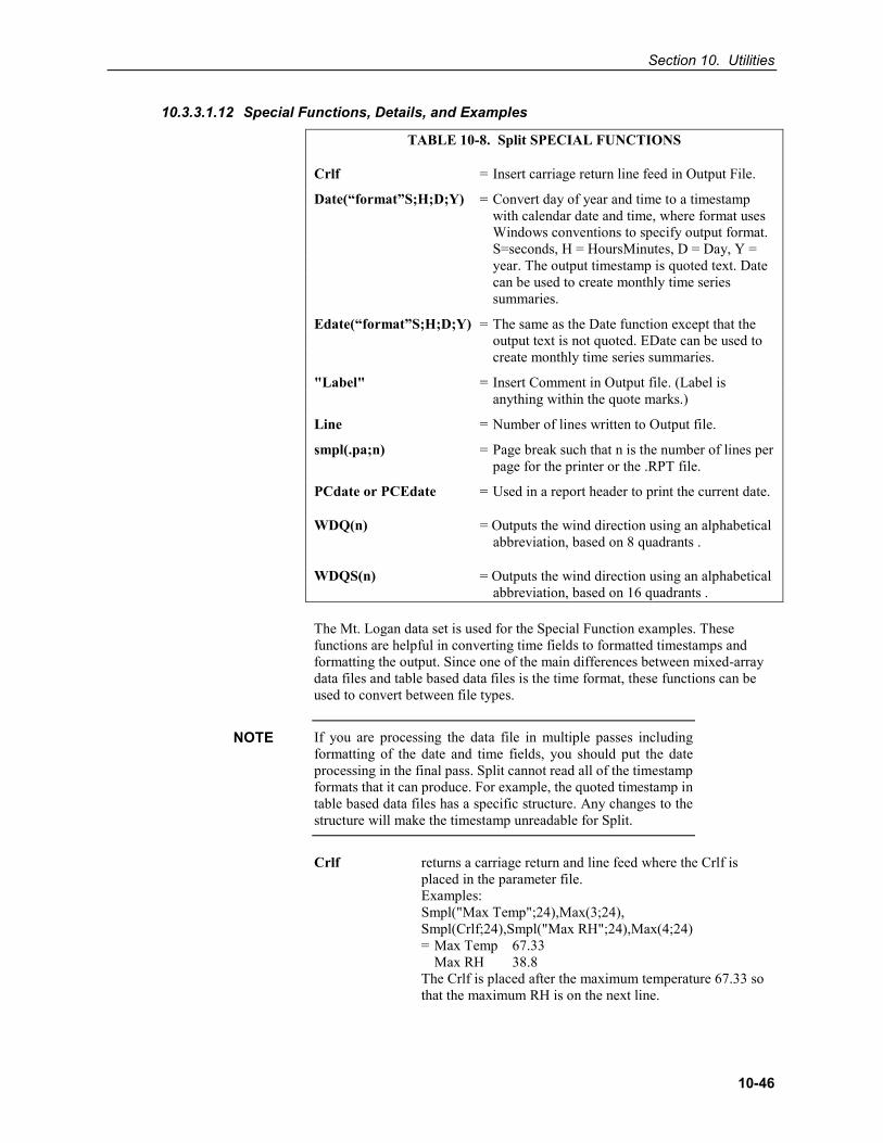
Section 10. Utilities
10-46
10.3.3.1.12 Special Functions, Details, and Examples
TABLE 10-8. Split SPECIAL FUNCTIONS
Crlf = Insert carriage return line feed in Output File.
Date(“format”S;H;D;Y) = Convert day of year and time to a timestamp with calendar date and time, where format uses Windows conventions to specify output format. S=seconds, H = HoursMinutes, D = Day, Y = year. The output timestamp is quoted text. Date can be used to create monthly time series summaries.
Edate(“format”S;H;D;Y) = The same as the Date function except that the output text is not quoted. EDate can be used to create monthly time series summaries.
"Label" = Insert Comment in Output file. (Label is anything within the quote marks.)
Line = Number of lines written to Output file.
smpl(.pa;n) = Page break such that n is the number of lines per page for the printer or the .RPT file.
PCdate or PCEdate = Used in a report header to print the current date.
WDQ(n) = Outputs the wind direction using an alphabetical abbreviation, based on 8 quadrants .
WDQS(n) = Outputs the wind direction using an alphabetical abbreviation, based on 16 quadrants .
The Mt. Logan data set is used for the Special Function examples. These functions are helpful in converting time fields to formatted timestamps and formatting the output. Since one of the main differences between mixed-array data files and table based data files is the time format, these functions can be used to convert between file types.
If you are processing the data file in multiple passes including formatting of the date and time fields, you should put the date processing in the final pass. Split cannot read all of the timestamp formats that it can produce. For example, the quoted timestamp in table based data files has a specific structure. Any changes to the structure will make the timestamp unreadable for Split.
Crlf returns a carriage return and line feed where the Crlf is placed in the parameter file. Examples:
Smpl("Max Temp";24),Max(3;24), Smpl(Crlf;24),Smpl("Max RH";24),Max(4;24) = Max Temp 67.33 Max RH 38.8 The Crlf is placed after the maximum temperature 67.33 so
that the maximum RH is on the next line.
NOTE
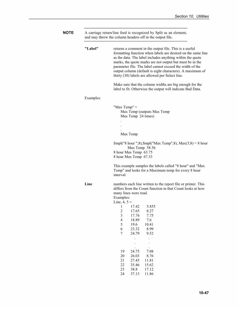
Section 10. Utilities
10-47
A carriage return/line feed is recognized by Split as an element, and may throw the column headers off in the output file.
"Label" returns a comment in the output file. This is a useful formatting function when labels are desired on the same line as the data. The label includes anything within the quote marks, the quote marks are not output but must be in the parameter file. The label cannot exceed the width of the output column (default is eight characters). A maximum of thirty (30) labels are allowed per Select line.
Make sure that the column widths are big enough for the label to fit. Otherwise the output will indicate Bad Data.
Examples:
"Max Temp" = Max Temp (outputs Max Temp Max Temp 24 times) . . . Max Temp
Smpl("8 hour ";8),Smpl("Max Temp";8), Max(3;8) = 8 hour Max Temp 58.56
8 hour Max Temp 63.75 8 hour Max Temp 67.33
This example samples the labels called "8 hour" and "Max Temp" and looks for a Maximum temp for every 8 hour interval.
Line numbers each line written to the report file or printer. This differs from the Count function in that Count looks at how many lines were read.
Examples: Line, 4, 5 = 1 17.42 5.855 2 17.65 8.27 3 17.76 7.75 4 18.89 7.6 5 19.6 10.41 6 23.32 8.99 7 24.79 9.52 . . . . . . 19 24.75 7.08 20 26.03 8.76 21 27.45 11.81 22 35.46 15.62 23 38.8 17.12 24 37.13 11.86
NOTE
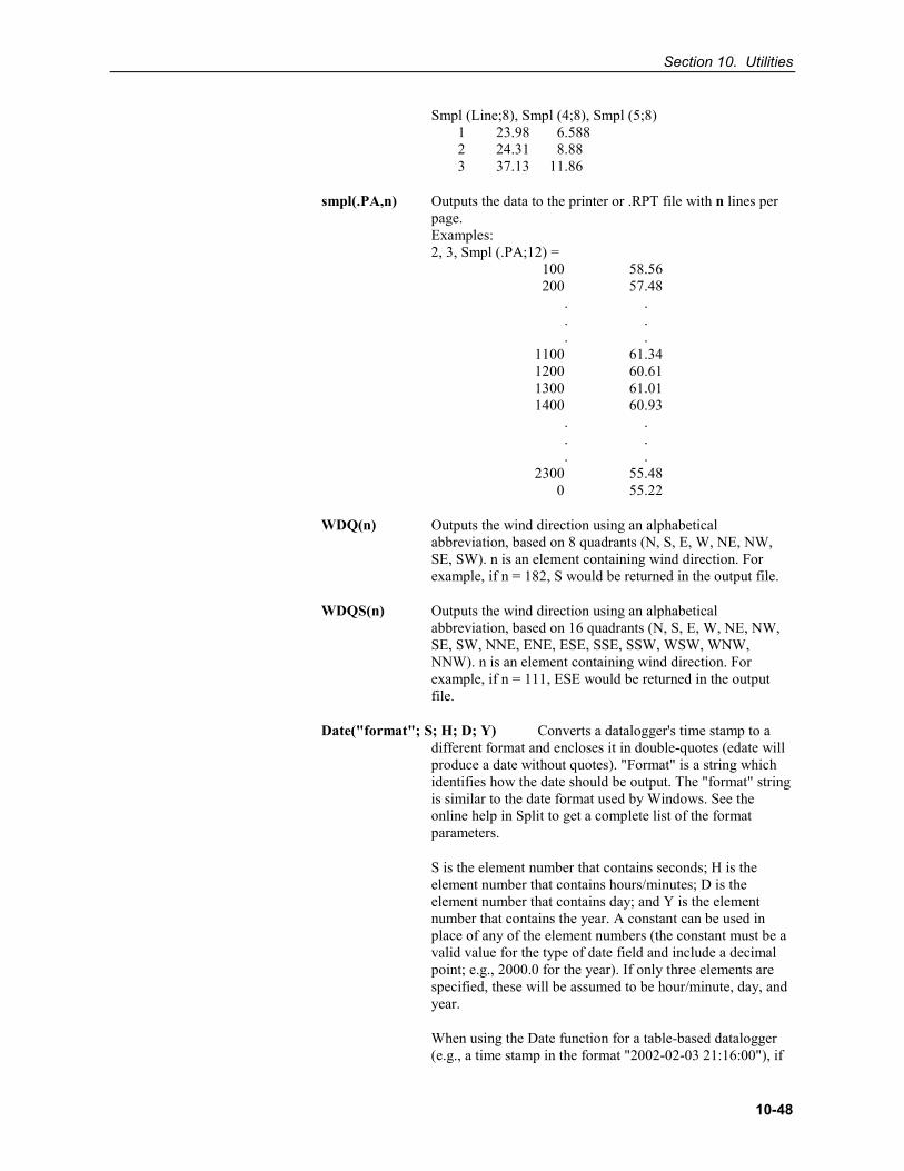
Section 10. Utilities
10-48
Smpl (Line;8), Smpl (4;8), Smpl (5;8) 1 23.98 6.588 2 24.31 8.88 3 37.13 11.86
smpl(.PA,n) Outputs the data to the printer or .RPT file with n lines per page. Examples:
2, 3, Smpl (.PA;12) = 100 58.56 200 57.48 . . . . . . 1100 61.34 1200 60.61 1300 61.01 1400 60.93 . . . . . .
2300 55.48 0 55.22
WDQ(n) Outputs the wind direction using an alphabetical abbreviation, based on 8 quadrants (N, S, E, W, NE, NW, SE, SW). n is an element containing wind direction. For example, if n = 182, S would be returned in the output file.
WDQS(n) Outputs the wind direction using an alphabetical abbreviation, based on 16 quadrants (N, S, E, W, NE, NW, SE, SW, NNE, ENE, ESE, SSE, SSW, WSW, WNW, NNW). n is an element containing wind direction. For example, if n = 111, ESE would be returned in the output file.
Date("format"; S; H; D; Y) Converts a datalogger's time stamp to a different format and encloses it in double-quotes (edate will produce a date without quotes). "Format" is a string which identifies how the date should be output. The "format" string is similar to the date format used by Windows. See the online help in Split to get a complete list of the format parameters.
S is the element number that contains seconds; H is the element number that contains hours/minutes; D is the element number that contains day; and Y is the element number that contains the year. A constant can be used in place of any of the element numbers (the constant must be a valid value for the type of date field and include a decimal point; e.g., 2000.0 for the year). If only three elements are specified, these will be assumed to be hour/minute, day, and year.
When using the Date function for a table-based datalogger (e.g., a time stamp in the format "2002-02-03 21:16:00"), if
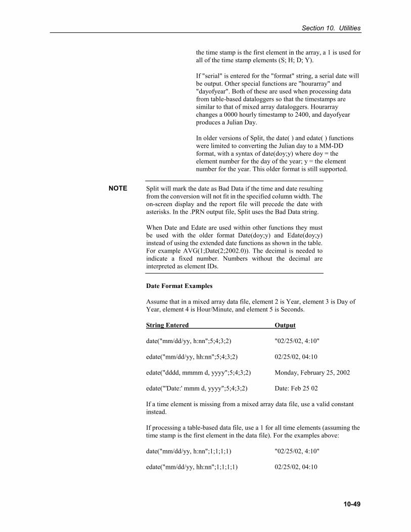
Section 10. Utilities
10-49
the time stamp is the first element in the array, a 1 is used for all of the time stamp elements (S; H; D; Y).
If "serial" is entered for the "format" string, a serial date will be output. Other special functions are "hourarray" and "dayofyear". Both of these are used when processing data from table-based dataloggers so that the timestamps are similar to that of mixed array dataloggers. Hourarray changes a 0000 hourly timestamp to 2400, and dayofyear produces a Julian Day.
In older versions of Split, the date( ) and edate( ) functions were limited to converting the Julian day to a MM-DD format, with a syntax of date(doy;y) where doy = the element number for the day of the year; y = the element number for the year. This older format is still supported.
Split will mark the date as Bad Data if the time and date resulting from the conversion will not fit in the specified column width. The on-screen display and the report file will precede the date with asterisks. In the .PRN output file, Split uses the Bad Data string.
When Date and Edate are used within other functions they must be used with the older format Date(doy;y) and Edate(doy;y) instead of using the extended date functions as shown in the table. For example AVG(1;Date(2;2002.0)). The decimal is needed to indicate a fixed number. Numbers without the decimal are interpreted as element IDs.
Date Format Examples
Assume that in a mixed array data file, element 2 is Year, element 3 is Day of Year, element 4 is Hour/Minute, and element 5 is Seconds.
String Entered Output
date("mm/dd/yy, h:nn";5;4;3;2) "02/25/02, 4:10"
edate("mm/dd/yy, hh:nn";5;4;3;2) 02/25/02, 04:10
edate("dddd, mmmm d, yyyy";5;4;3;2) Monday, February 25, 2002
edate("'Date:' mmm d, yyyy";5;4;3;2) Date: Feb 25 02
If a time element is missing from a mixed array data file, use a valid constant instead.
If processing a table-based data file, use a 1 for all time elements (assuming the time stamp is the first element in the data file). For the examples above:
date("mm/dd/yy, h:nn";1;1;1;1) "02/25/02, 4:10"
edate("mm/dd/yy, hh:nn";1;1;1;1) 02/25/02, 04:10
NOTE
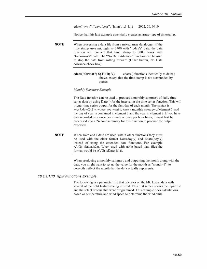
Section 10. Utilities
10-50
edate(“yyyy”, “dayofyear”, “hhnn”;1;1;1;1) 2002, 56, 0410
Notice that this last example essentially creates an array-type of timestamp.
When processing a data file from a mixed array datalogger, if the time stamp uses midnight as 2400 with "today's" date, the date function will convert that time stamp to 0000 hours with "tomorrow's" date. The “No Date Advance” function can be used to stop the date from rolling forward (Other button, No Date Advance check box).
edate("format"; S; H; D; Y) edate( ) functions identically to date( ) above, except that the time stamp is not surrounded by quotes.
Monthly Summary Example
The Date function can be used to produce a monthly summary of daily time series data by using Date( ) for the interval in the time series function. This will trigger time series output for the first day of each month. The syntax is avg(7;date(3;2)), where you want to take a monthly average of element 7, and the day of year is contained in element 3 and the year in element 2. If you have data recorded on a once per minute or once per hour basis, it must first be processed into a 24 hour summary for this function to produce the output expected.
When Date and Edate are used within other functions they must be used with the older format Date(doy;y) and Edate(doy;y) instead of using the extended date functions. For example AVG(1;Date(3;2)). When used with table based data files the format would be AVG(1;Date(1;1)).
When producing a monthly summary and outputting the month along with the data, you might want to set up the value for the month as "month -1", to correctly reflect the month that the data actually represents.
10.3.3.1.13 Split Functions Example
The following is a parameter file that operates on the Mt. Logan data with several of the Split features being utilized. This first screen shows the input file and the select criteria that were programmed. This example does calculations based on temperature and wind speed to determine the wind chill.
NOTE
NOTE
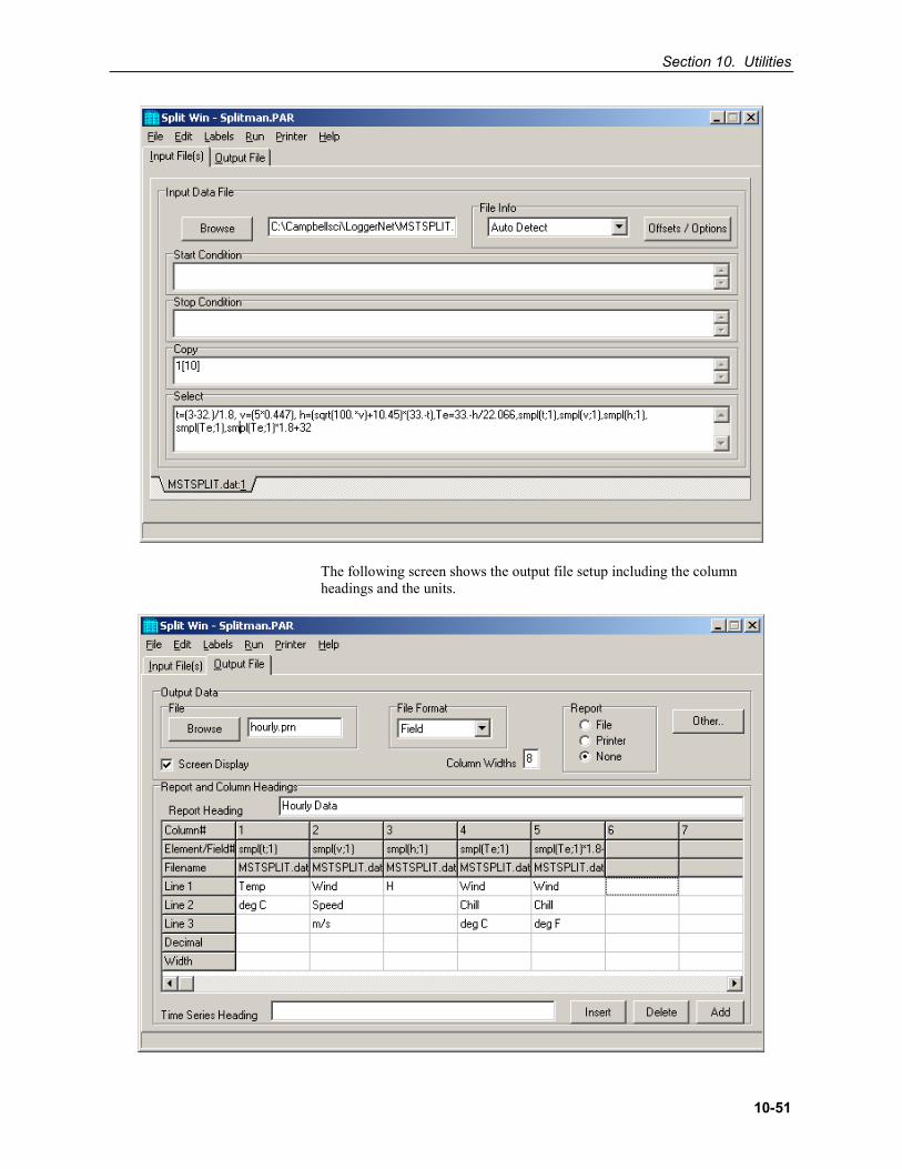
Section 10. Utilities
10-51
The following screen shows the output file setup including the column headings and the units.
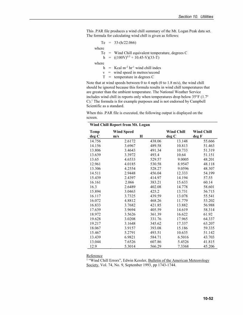
Section 10. Utilities
10-52
This .PAR file produces a wind chill summary of the Mt. Logan Peak data set. The formula for calculating wind chill is given as follows:
Te = 33-(h/22.066) where
Te = Wind Chill equivalent temperature, degrees C h = ((100V)0.5 + 10.45-V)(33-T)
where h = Kcal m-2 hr-1 wind chill index v = wind speed in metres/second T = temperature in degrees C
Note that at wind speeds between 0 to 4 mph (0 to 1.8 m/s), the wind chill should be ignored because this formula results in wind chill temperatures that are greater than the ambient temperature. The National Weather Service includes wind chill in reports only when temperatures drop below 35°F (1.7°C).1 The formula is for example purposes and is not endorsed by Campbell Scientific as a standard.
When this .PAR file is executed, the following output is displayed on the screen.
Wind Chill Report from Mt. Logan
Temp deg C
Wind Speed m/s H
Wind Chill deg C
Wind Chill deg F
14.756 2.6172 438.06 13.148 55.666 14.156 3.6967 489.58 10.813 51.463 13.806 3.4643 491.34 10.733 51.319 13.639 3.3972 493.4 10.64 51.151 13.65 4.6533 529.57 9.0005 48.201 12.961 4.0185 530.58 8.9547 48.118 13.306 4.2554 528.27 9.0596 48.307 14.511 2.9448 456.04 12.333 54.199 15.439 2.4397 414.97 14.194 57.55 16.161 2.066 383.21 15.633 60.14 16.3 2.6489 402.08 14.778 58.601 15.894 3.0463 425.2 13.731 56.715 16.117 3.7325 439.59 13.078 55.541 16.072 4.8812 468.26 11.779 53.202 16.833 3.7682 421.85 13.882 56.988 17.639 3.9694 405.59 14.619 58.314 18.972 3.5626 361.39 16.622 61.92 19.628 3.0208 331.76 17.965 64.337 19.217 3.1648 345.62 17.337 63.207 18.067 3.9157 393.08 15.186 59.335 15.467 5.2791 493.51 10.635 51.142 13.439 6.9821 584.71 6.5016 43.703 13.044 7.6526 607.86 5.4526 41.815 12.9 5.3014 566.29 7.3368 45.206
Reference 1 “Wind Chill Errors”, Edwin Kessler, Bulletin of the American Meteorology Society, Vol. 74, No. 9, September 1993, pp 1743-1744.
Section 10. Utilities
10-53
10.3.3.1.14 Summary of Select Line Syntax Rules
• A fixed numeric value must include a decimal point "." or be in scientific notation. There are some exceptions to this as noted below.
• Scientific notation has the format "mantissa E power of ten” (e.g., 3E5 = 3 x 10⁵).
• Element numbers are entered without a decimal point.
• Commas separate Select line parameters (e.g., 2,3,(3+4)/3.2,6).
• Two decimal points are used to select consecutive elements between starting and ending elements (e.g., 3..6, refers to the elements 3,4,5, and 6).
• A set is a group of two or more elements and/or expressions separated by commas and enclosed by parentheses. No member of a set can include parentheses. Therefore, a set cannot include a set or a function as one of its members. For example: VALID EXPRESSION INVALID EXPRESSION Arctan (2/3) Arctan ((2/3)) Arctan (2/3, 3/4, 4/5) Arctan ((2/3, 3/4), 4/5) Arctan (COS(2)) Arctan (COS(2), COS(3))
• A single expression can operate on a set of elements. For example, the expression (3..6,8)/2.0 is the same as 3/2.0, 4/2.0, 5/2.0, 6/2.0, 8/2.0; (3..6)/(2..5) is the same as 3/2, 4/3, 5/4, 6/5.
• The element or expression that is the argument of a math or Time Series function, must be enclosed in parentheses. A range of elements can be specified, resulting in as many outputs as elements (e.g., Avg(3..5,7) will output 4 averages).
• Square brackets are used to enclose an allowable range for a value (e.g., 3[3.6..12] ) to indicate that the allowable range for element 3 is from 3.6 to 12. Whole numbers within brackets do not require a decimal point. TABLE 10-5 explains how values outside the specified range are treated.
• The interval in a Time Series function is optional and does not require a decimal point.
• Semicolons are used in Time Series functions to separate the elements or expressions from the number that determines the interval. Sample on maximum and sample on minimum require two elements or expressions also separated by a semicolon.
10.3.3.1.15 Time Synchronization
The time synchronize function is useful when data is missing from a file or if several files of data need to be merged together. The files are synchronized according to time; any missing data in the file (or files) will be replaced with blank data.
This function synchronizes according to day, hrmn (hour-minute), and/or seconds. The syntax used to identify the time elements for array data is:
ei[day]:ei[hrmn]:ei[seconds]
Section 10. Utilities
10-54
Referring to TABLE 10-1, to identify the day of year for a mixed-array data file, type:
2[189]::
for hrmn type:
:3[1200]:
and seconds are expressed as:
::4[5]
A single colon is assumed to be between day and hrmn (e.g., 2[189]: means day, :3[1200] means hours, and 2[189]:3[1200] means day and hour-minute). When the time synchronize function is used, a time interval must be specified in the Copy line of the first data file. For example, 4[60] in the Copy line will create a synchronized file containing the data from the input files that occurred every 60 minutes. If no time interval is specified in the Copy line then the time specified in the Start Condition becomes simply a starting time with no time synchronization.
Typically, the starting time specified must actually be found in the input file before the Start Condition is satisfied (e.g., if the input file starts at 1100 hrs and 1000 hrs is entered for the starting time, with no day specified, Split will skip over arrays until it reaches 1000 hrs the next day). However, the Start-Stop On/After Time function can be enabled (Output tab, Other button) to trigger the start of processing when the exact time is found or at the first instance of data after that time has occurred.
Table-based dataloggers
Because the time stamp for a table-based datalogger is all one string, and therefore read by Split as one element, the syntax is somewhat different. All elements in the time stamp are specified by a 1 (if the time stamp is the first item in each row of data).
The 1s in the string identify the position of the time stamp in the line of data. Each colon represents a portion of the time stamp. The format is 1[year]:1[day]:1[hour/minute]:1[seconds]. The colons in the time stamp must be present or the function will not work correctly.
Time synchronization can only be done for data from a single year. It will not work over a year boundary.
Time elements can be identified without specifying a starting time (e.g., 2:3). If you are working with only one file, Split will begin processing that file at the first record in the file. If any gap in the data is found, blank data (or the "Replace Bad Data With" text) and a carriage return line feed will be inserted for each line of missing data. Note that Split will also detect a gap in data if, for instance, you specify a start time of 2[92]:3 (start at Julian day 92) and your hour/minute for day 92 starts at 9:30 a.m. The time between the start of the day (0000) and 9:30 a.m. will be considered missing data. Blanks (or the "Replace bad data with" text) and a carriage return line feed will be inserted at the beginning of the PRN file for each "missed" output interval.
NOTE
Section 10. Utilities
10-55
If you are working with two or more files, once Split starts processing the files (based on the time of the first record of the first file), if no data exists for the other file(s), blank data will be inserted.
If multiple input files are given specific starting times, Split starts the output at the earliest specified starting time. In a PRN file, Blanks or the comment entered in the “Replace bad data with” field are inserted for values from other input files until their starting times are reached. In a RPT file only blanks are used.
When using time synchronization with a mixed array data file, with a midnight time stamp of 2400, you will need to select the Other button, “Midnight at 2400 hours” checkbox.
10.3.3.1.15.1 Time Synchronization and the Copy Condition
To use the time synchronize function, time element(s) must be specified in the Start Condition. The user must also specify a time interval in the Copy condition. For instance, if the original data had 15 minute outputs and you only want hourly outputs, then an interval of 60 minutes must be specified following the element number. This is entered as (assuming hrmn is element number 3) “3[60]”. If time synchronization is specified in the Start Condition, Split looks for the interval in a time element in the Copy condition. Only one time interval is specified. This interval is the unit of time to synchronize each file.
The interval can be given tolerance limits by following the interval with a comma and the tolerance. For example, if 3 is the hrmn element, and the time interval is 60 minutes +/-2 minutes, the syntax is 3[60,2].
Table based data files need to use the same time format as described in Section 10.3.3.1.3, Start Condition (p. 10-29). You can specify the interval for time synchronization on table files as ::1[60]: which will give you an output interval of 60 minutes.
If the time synchronize function is enabled and data are missing at one or more of the time intervals specified, then a blank (or the comment entered in the “Replace bad data with” field) is output to the Output File. See TABLE 10-5.
10.3.3.1.15.2 Using Time Synchronization While Starting Relative to PC Time
Split tries to time-sync files to the top of the hour when starting relative to PC time. If you are synchronizing files where the data output interval is not at the top of the hour, you will need to specify an interval in the Copy Condition that represents a window of time in which Split should look for the hour/minute. For instance, if your data is output 50 minutes into a 60 minute interval (and therefore, your time stamps are 50, 150, 250, 350...2350) your Start Condition and Copy Conditions for the first file might look like the following:
Start Condition 2[-1]:3[50]:
Copy Condition 1[106]and3[60,10]
Where:
NOTE
Section 10. Utilities
10-56
element 1 is the array ID element 2 is the Julian day element 3 is the hour/minute
The Start Condition directs Split to begin processing data when the time is one day prior to the current PC time and when the hour/minute value is equal to 50. The 1[106] in the Copy Condition specifies the array from which the data should be copied. The 3[60,10] indicates that the interval for the time stamp is 60 minutes and designates a 10 minute time window on each side of the top of the hour in which Split should look for the hour/minute data (10 minutes before the hour, 10 minutes after the hour).
The second file's Copy Condition should include only the array from which to copy the data. No interval is necessary.
10.3.3.2 Output Files To create an Output File, click the OUTPUT FILE tab. The file is created on the default drive or directory unless the file name is preceded with an alternative drive or directory. Use the Browse button to change directories.
Split will assign this file an extension of .PRN if an extension is not specified by the user. Whenever an Output file name is entered, regardless of extension, an Output file is created only when the RUN | GO menu option is selected.
If the file name you have selected already exists, you can use the "If File Exists Then" drop-down list box to determine what action Split will take. By default, each time a PAR file is run the existing output files (PRN, RPT, and HTM) are overwritten (Overwrite option). When Append is selected, the PRN file will not be overwritten -- the new data will be added to the end of the existing file. However, the RPT and HTM files will be overwritten. If Create New is selected, Split will create all new files using the original file name and appending an _0, _1, and so on to each subsequent run.
In Append mode, if an HTM or RPT file is needed with all the data, you will need to run the PRN created by Split through the program a second time. If the Output File name is left blank, Split does not write data to an Output File on disk; rather, it will display the processed values on the screen if the Screen Display box is checked. If Screen Display is not enabled, no data will be displayed on the Split RUN screen.
The Output file name cannot be the same as the Input file name. Split will display an error message if this condition occurs.
Several output options may be specified to alter the default output to the file. Some are located on the main OUTPUT FILE screen and some are made available by pressing the Other button.
CAUTION
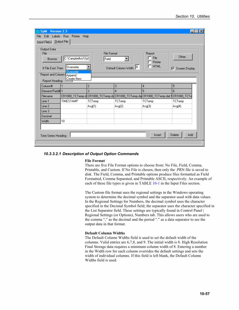
Section 10. Utilities
10-57
10.3.3.2.1 Description of Output Option Commands
File Format There are five File Format options to choose from: No File, Field, Comma, Printable, and Custom. If No File is chosen, then only the .PRN file is saved to disk. The Field, Comma, and Printable options produce files formatted as Field Formatted, Comma Separated, and Printable ASCII, respectively. An example of each of these file types is given in TABLE 10-1 in the Input Files section.
The Custom file format uses the regional settings in the Windows operating system to determine the decimal symbol and the separator used with data values. In the Regional Settings for Numbers, the decimal symbol uses the character specified in the Decimal Symbol field; the separator uses the character specified in the List Separator field. These settings are typically found in Control Panel | Regional Settings (or Options), Numbers tab. This allows users who are used to the comma “,” as the decimal and the period “.” as a data separator to see the output data in that format.
Default Column Widths The Default Column Widths field is used to set the default width of the columns. Valid entries are 6,7,8, and 9. The initial width is 8. High Resolution Final Storage data requires a minimum column width of 8. Entering a number in the Width row for each column overrides the default settings and sets the width of individual columns. If this field is left blank, the Default Column Widths field is used.
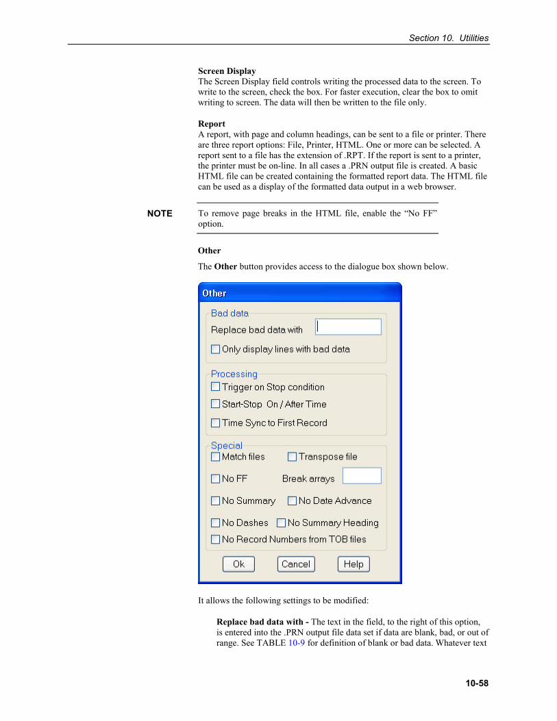
Section 10. Utilities
10-58
Screen Display The Screen Display field controls writing the processed data to the screen. To write to the screen, check the box. For faster execution, clear the box to omit writing to screen. The data will then be written to the file only.
Report A report, with page and column headings, can be sent to a file or printer. There are three report options: File, Printer, HTML. One or more can be selected. A report sent to a file has the extension of .RPT. If the report is sent to a printer, the printer must be on-line. In all cases a .PRN output file is created. A basic HTML file can be created containing the formatted report data. The HTML file can be used as a display of the formatted data output in a web browser.
To remove page breaks in the HTML file, enable the “No FF” option.
Other
The Other button provides access to the dialogue box shown below.
It allows the following settings to be modified:
Replace bad data with - The text in the field, to the right of this option, is entered into the .PRN output file data set if data are blank, bad, or out of range. See TABLE 10-9 for definition of blank or bad data. Whatever text
NOTE
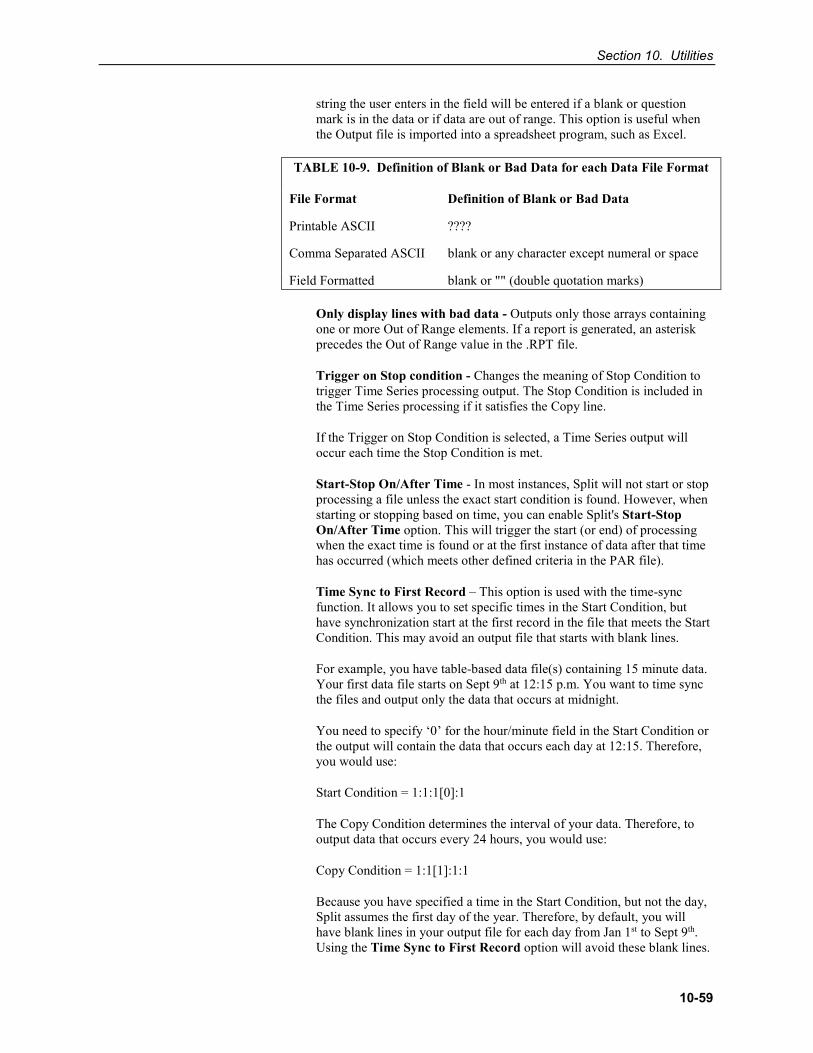
Section 10. Utilities
10-59
string the user enters in the field will be entered if a blank or question mark is in the data or if data are out of range. This option is useful when the Output file is imported into a spreadsheet program, such as Excel.
TABLE 10-9. Definition of Blank or Bad Data for each Data File Format
File Format Definition of Blank or Bad Data
Printable ASCII ????
Comma Separated ASCII blank or any character except numeral or space
Field Formatted blank or "" (double quotation marks)
Only display lines with bad data - Outputs only those arrays containing one or more Out of Range elements. If a report is generated, an asterisk precedes the Out of Range value in the .RPT file.
Trigger on Stop condition - Changes the meaning of Stop Condition to trigger Time Series processing output. The Stop Condition is included in the Time Series processing if it satisfies the Copy line.
If the Trigger on Stop Condition is selected, a Time Series output will occur each time the Stop Condition is met.
Start-Stop On/After Time - In most instances, Split will not start or stop processing a file unless the exact start condition is found. However, when starting or stopping based on time, you can enable Split's Start-Stop On/After Time option. This will trigger the start (or end) of processing when the exact time is found or at the first instance of data after that time has occurred (which meets other defined criteria in the PAR file).
Time Sync to First Record – This option is used with the time-sync function. It allows you to set specific times in the Start Condition, but have synchronization start at the first record in the file that meets the Start Condition. This may avoid an output file that starts with blank lines.
For example, you have table-based data file(s) containing 15 minute data. Your first data file starts on Sept 9th at 12:15 p.m. You want to time sync the files and output only the data that occurs at midnight.
You need to specify ‘0’ for the hour/minute field in the Start Condition or the output will contain the data that occurs each day at 12:15. Therefore, you would use:
Start Condition = 1:1:1[0]:1
The Copy Condition determines the interval of your data. Therefore, to output data that occurs every 24 hours, you would use:
Copy Condition = 1:1[1]:1:1
Because you have specified a time in the Start Condition, but not the day, Split assumes the first day of the year. Therefore, by default, you will have blank lines in your output file for each day from Jan 1st to Sept 9th. Using the Time Sync to First Record option will avoid these blank lines.
Section 10. Utilities
10-60
Match files - This option compares two files of the same data. If good data exists in one and not the other (question marks), then Split will fill the OUTPUT file with the good data. This is used to get a more complete record from an error ridden file (e.g., one recorded at freezing temperatures by reading a tape twice and running both files through Split).
For the Match files option to produce a correct Output File, the differences between the two Input Files can only be question marks. Both files must have the same Start Condition or the beginning of both files must be the same.
Transpose file - Transposes the rows and columns of the input file. Only one Input File can be transposed at a time and no Select options can be specified. A maximum of 26 arrays are transposed per pass of Split.
To transpose a file containing more than 26 arrays, several passes are required. Change the Output file name and Start Condition for each pass. Split may then be used to merge the multiple files.
No FF – Suppresses form feeds and page breaks in RPT and HTML files. When this option is selected, a header appears on the first page only. This option is used for printing reports on continuous feed paper or for displaying HTM files in a browser.
Break arrays - This option breaks up the Output Array into new arrays that are #+1 elements in each new array. Split automatically assigns an array ID number equal to the first element in the first array. Only one Input File may be specified. Start, Stop, and Copy Conditions may be specified, but the Select line must be left blank.
The Break Arrays function works only for mixed array data. It is typically used when processing data from burst measurements.
No Summary - When producing reports that include time series processing based on an interval, sometimes that interval will not divide evenly into the number of lines in the data file that is being processed. For example, you may be processing one-minute data on a five-minute interval, and the data file has 103 lines; thus, there are 3 lines of data "left over" at the end of the report. By default, the summary (average, total, maximum, etc., depending upon which time series function is being used) of the left over values is printed at the bottom of the report following the Time Series Heading. Enable the No Summary check box to omit the summary of the left over values and the Time Series Heading from the report.
No Date Advance - When processing a data file from a mixed array datalogger, if the time stamp uses midnight as 2400 with "today's" date, the date function will convert that time stamp to 0000 hours with "tomorrow's" date. (This is because the algorithm used by the date function is based on Windows' time format, and it does not support a 2400 time stamp.) For example:
CAUTION
NOTE
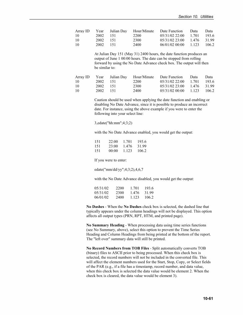
Section 10. Utilities
10-61
Array ID Year Julian Day Hour/Minute Date Function Data Data 10 2002 151 2200 05/31/02 22:00 1.701 193.6 10 2002 151 2300 05/31/02 23:00 1.476 31.99 10 2002 151 2400 06/01/02 00:00 1.123 106.2
At Julian Day 151 (May 31) 2400 hours, the date function produces an output of June 1 00:00 hours. The date can be stopped from rolling forward by using the No Date Advance check box. The output will then be similar to:
Array ID Year Julian Day Hour/Minute Date Function Data Data 10 2002 151 2200 05/31/02 22:00 1.701 193.6 10 2002 151 2300 05/31/02 23:00 1.476 31.99 10 2002 151 2400 05/31/02 00:00 1.123 106.2
Caution should be used when applying the date function and enabling or disabling No Date Advance, since it is possible to produce an incorrect date. For instance, using the above example if you were to enter the following into your select line:
3,edate("hh:mm";4;3;2)
with the No Date Advance enabled, you would get the output:
151 22:00 1.701 193.6 151 23:00 1.476 31.99 151 00:00 1.123 106.2
If you were to enter:
edate("mm/dd/yy";4;3;2),4,6,7
with the No Date Advance disabled, you would get the output:
05/31/02 2200 1.701 193.6 05/31/02 2300 1.476 31.99 06/01/02 2400 1.123 106.2
No Dashes - When the No Dashes check box is selected, the dashed line that typically appears under the column headings will not be displayed. This option affects all output types (PRN, RPT, HTM, and printed page).
No Summary Heading - When processing data using time series functions (see No Summary, above), select this option to prevent the Time Series Heading and Column Headings from being printed at the bottom of the report. The "left over" summary data will still be printed.
No Record Numbers from TOB Files - Split automatically converts TOB (binary) files to ASCII prior to being processed. When this check box is selected, the record numbers will not be included in the converted file. This will affect the element numbers used for the Start, Stop, Copy, or Select fields of the PAR (e.g., if a file has a timestamp, record number, and data value, when this check box is selected the data value would be element 2. When the check box is cleared, the data value would be element 3).
Section 10. Utilities
10-62
10.3.3.2.2 Report Headings
A report is output to a printer or file with the extension .RPT. Headings are not included in the standard output to disk (.PRN or user named extension output file). However, a report can be labeled with a header by entering text into the Report Heading field. A report heading can have several lines, but it is limited to a total of 253 characters including backslashes and carriage returns. “\” characters break the report heading into multiple lines.
When Time Series functions are used in the Select field without an interval, they appear as a final summary at the end of the report. They can be labeled by entering a title into the Time Series Heading field at the bottom of the Output File page. Time Series interval summaries cannot be assigned individual titles directly, but you can use special functions such as "Label" and "Crlf" to create column headings and special formatting.
“PCDATE” within the Report Heading inserts the computer's current date (Month-Day-Year). For the European format (Day-Month-Year), enter “PCEDATE”.
10.3.3.2.3 Column Headings
Up to three lines per column can be entered as column headings. These headings are limited to a length of one less than the Output field width.
Column headings associated with Time Series outputs are repeated for Final Summaries if a title for the Final Summary is requested on the headings for report line.
The number of digits to report to the right of the decimal point is entered in the Decimal field and can be set independently for each column. The value output will be rounded to the specified number of digits. Leave this field blank if you do not want to round the data to a specific number of digits.
Column headings can be entered using Split’s Data Labels Function (Labels | Use Data Labels).
10.3.4 Help Option On-line Help is available from any location in Split. Simply select the area of Split in question and press <F1>. Split also offers a brief on-the-fly Help. Place the cursor on the area of Split in question; after a moment a brief description is displayed in the hint line of the Split window (bottom left).
10.3.5 Editing Commands Split supports the Windows Cut, Copy, and Paste commands. Text from any field in Split or other Windows applications can be Cut, Copied, or Pasted.
10.3.6 Running Split From a Command Line Existing parameter files can be executed using Splitr.exe which is a "run-time" version of the Split Report Generator. When Splitr.exe is run, the file is processed as if the user chose Run | Go from the Split menu. Splitr.exe can be executed by the Task Master, from a batch file, or from a Windows command line prompt or shortcut.
Section 10. Utilities
10-63
10.3.6.1 Splitr Command Line Switches Splitr has four switches that can be used to control how the executable is run.
10.3.6.1.1 Closing the Splitr.exe Program After Execution (/R or /Q Switch)
Typically when Split is run, after the file is processed the user must close the Screen Display window. When Splitr.exe is run from a command line, the user must also close the Screen Display window unless the /R switch is used.
The syntax for this switch is:
SPLITR LOGAN/R
where LOGAN is the parameter file name.
The /R switch should follow immediately after the parameter file name with no space between the two. If a space is used, the following message will be displayed "There was a problem opening the input file. File could not be found or may be in use."
The /Q switch is similar in function and syntax to /R. However, if Split encounters an error when processing the file, no message box is displayed that requires user response (the exceptions are a disk space error or an internal error with the Split executable). This option should be used with caution, since there will be no indication of a problem if a file cannot be processed.
10.3.6.1.2 Running Splitr in a Hidden or Minimized State (/H Switch)
Splitr can be run in a minimized state, so that the Screen Display window does not interrupt other processes on the computer. The syntax for running Splitr minimized is:
SPLITR /H LOGAN
where LOGAN is the parameter file name.
The /H switch must be positioned after SPLITR but before the parameter file name, and a space is required between the executable name and the switch.
10.3.6.1.3 Running Multiple Copies of Splitr (/M Switch)
Multiple copies of Splitr can be run at one time by using the /M switch. This switch must appear immediately after Splitr. For instance, a batch file containing the lines:
SPLITR /M Logan/R SPLITR /M Sinks/R
will open two copies of Splitr and process the two files simultaneously.
When using the /M switch in a batch file, the behaviour may depend on your Windows version. In some cases, the files will be processed simultaneously, while in other cases, the files will be processed sequentially. It may be possible to change this behaviour using the Windows "start" command.
NOTE
Section 10. Utilities
10-64
10.3.6.2 Using Splitr.exe in Batch Files Batch files containing one or more Splitr command lines can be useful for automating data processing. Batch files can be executed manually or by setting them up in the Task Master.
Batch files process each command in succession, without waiting for execution of a command to be completed before proceeding to the next unless they are configured to do so. If multiple parameter files are being processed using Splitr in a batch file, there are no conflicts because only one copy of Splitr can be active at any one time (unless the /M switch is used. However, if other commands are used along with Splitr (such as opening the file in a spreadsheet, copying it to an archive directory, or appending it to an existing file) these commands might be executed before Splitr finishes processing data.
The Windows Start /w (wait) command can be added to a batch file command line to delay execution of the next command until the first command has finished. The Start command has different arguments depending upon the operating system you are using. Refer to your computer’s on-line help for information on this command.
10.3.6.3 Processing Alternate Files Splitr allows the user to select different input and/or output files for an existing parameter file by entering them on the command line after the parameter file name. For example:
“Splitr LOGAN.PAR/R TEST.DAT TEST.PRN”
Replaces the Input and Output file names in LOGAN.PAR, with TEST.DAT and TEST.PRN, respectively.
A space must be used to separate command line parameters. Splitr uses as many entries as exist on the command line. However, the command line has a limit to the number of characters it can accommodate—this limit is operating system dependent. The parameters must be in the following sequence: Input file name, Output file name, Start Condition, Stop Condition, Copy Condition, and Select.
If a parameter is to be left as it is in the parameter file, then space comma space ( , ) may be entered in the command line. For instance, if the parameter file LOGAN.PAR contained TEST1.DAT as an input file name, the following command line would leave the input file TEST1.DAT and change the output file to TEST.PRN.
“SPLITR LOGAN/R , TEST.PRN”
10.3.6.3.1 Input/Output File Command Line Switches for Processing Alternate Files
The one caveat of using the command line to specify an alternate input and/or output file name is that Split’s default options will be used with the alternate file. For instance, by default, output files are written with field-formatted columns. If the original PAR file specified a comma-separated output, that option would be ignored and the and defaults would be used.
Command line switches can be used to control these options for the output and input files. The switch is added immediately after the input or output file name.
Section 10. Utilities
10-65
In most instances, full path names to the Splitr executable and the input and output file names must be used. In addition, if long file names are used in the path, you may need to surround the path and file name by double quotes.
Output File Options
These switches are entered after the output file name; e.g., Splitr Test.par/r Input.dat Output.prn/P
/P Sends the output to a printer. This is the same as checking the Printer box for the Report type on the Output File tab.
/R Creates a formatted RPT file. This is the same as checking the File box for the Report type on the Output File tab.
/W Creates a simple HTML file. This is the same as checking the HTML box for the Report type on the Output File tab.
/A Appends the output to the end of an existing file. This is the same as selecting Append for the If File Exists option on the Output File tab.
/L Creates a new output file with a different name if a file exists. This is the same as selecting Create New for the If File Exists option on the Output File tab.
/O Turns the screen display off when Split is processing the PAR file. This is the same as clearing the Screen Display check box on the Output File tab.
/6..9 Sets the default width for all the columns in the report. This is the same as entering a value in the Default Column Width field on the Output File tab.
/[text] Sets the text that will be used in the place of bad data. This is the same as the text string used in the Replace Bad Data field that is found under the Other button of the Output File tab.
/M Compares two input files and creates an output file with a complete data set comprised of both files. This is the same at the Match Files option that is found under the Other button of the Output File tab. The two input file names are separated with a comma but no spaces. Example: Splitr Test.par/r Input1.dat,Input2.dat Output.prn/M
/S Writes the output file without a form feed command after each page. This is the same as the No FF (form feed) option that is found under the Other button of the Output File tab.
/G Outputs only the data marked as “bad” to the file. This is the same as the Only Display Lines with Bad Data check box that is found under the Other button of the Output File tab.
/0 Outputs the data in comma separated format. This is the same as choosing the Comma option for the File Format.
NOTE
Section 10. Utilities
10-66
/1 Outputs the data in printable ASCII format. This is the same as choosing the Printable option for the File Format.
/2 Outputs the data using the Regional Settings of your Windows operating system for the decimal indicator and data value separator. This is the same as choosing the Custom option for the File Format (this is the default option for the File Format field).
/F Conditionally outputs the data using the Trigger On Stop Condition. This is the same as choosing the Trigger On Stop Condition option that is found under the Other button of the Output File tab. A stop condition must also be specified. The example below does not specify a start or copy condition. These two fields are indicated by the “space-comma-space” entries. Select line entries are also shown in this example. Example: Test.par/r input1.dat Output.prn/F , 4[1450] , smpl(1..6),avg(7)
/T Transposes the rows and columns of a file. This is the same as choosing the Transpose File option that is found under the Other button of the Output File tab.
/D Enables the No Date Advance function, which keeps the date for midnight from rolling to the next day. This is the same as choosing the No Date Advance check box that is found under the Other button of the Output File tab.
/N Suppresses the summary information when processing time series data. This is the same as choosing the No Summary check box that is found under the Other button of the Output File tab.
/H Removes the dashed lines from the heading of the RPT file. This is the same as choosing the No Dashes check box that is found under the Other button of the Output File tab.
/U Removes the record number from TOB files that are processed with Split. This is the same as choosing the No Record Numbers from TOB Files check box that is found under the Other button of the Output File tab.
/E Begins processing the file, or stops processing the file, on or after the Start or Stop condition when starting or stopping based on time (the default is to start only if the exact start condition is found). This is the same as choosing the Start -Stop On/After Time option that is found under the Other button of the Output File tab. Example: Splitr test.par input1.dat Output.prn/E 4[1450]: 4[1456]: (where 1450 and 1456 are the start and stop times, respectively. Colons are required to indicate a time value.)
/I Suppresses the time series heading and column heading information when processing time series data. This is the same as choosing the No
Section 10. Utilities
10-67
Summary Heading check box that is found under the Other button of the Output File tab.
/Bnnn Breaks a long array into multiple lines, where nnn is the number of values to place on each line. This is the same as choosing the Break Arrays check box that is found under the Other button of the Output File tab.
Input File Options
These switches are entered after the input file name; e.g., Splitr Test.par/r Input.dat/L Output.prn
/nnn Begins processing nnn bytes into the file. If /nnn..mmm is used, then processing begins at nnn bytes into the file and stops at mmm bytes into the file. This is the same as setting a specific Start and Stop offset, which is found under the Offsets/Options button of the Input File tab.
/L Begins processing the file at the byte value where processing last stopped. If /L..mmm is used, then processing begins where it left off and stops at mmm bytes into the file. This is the same as enabling Last Count, which is found under the Offsets/Options button of the Input File tab.
/Bnnn Specifies the file type as Burst data. nnn indicates the size of the arrays. This is the same as selecting Burst Format for the File Info field on the Input File tab.
/F Specifies the file type as Final Storage (binary) data. This is the same as selecting Final Storage Format for the File Info field on the Input File tab.
/M Changes the value for midnight to 2400 instead of 0000. This is the same as selecting Midnight is 2400 Hours check box found under the Offsets/Options button of the Input File tab.
Batch File Example
"c:\Program Files\campbellsci\LoggerNet\splitr.exe" c:\Campbellsci\SplitW\switch-test.par input1a.dat Output.prn/E/H/W 4[1200]: , , 1..6
where PAR file: switch-test.par Input file: input1a.dat Output file: output.prn Other outputs: Output.HTML Start condition: on or after 1200 Stop condition: end of file Copy condition: none Elements: 1 through 6
Section 10. Utilities
10-68
10.3.6.4 Processing Multiple Parameter Files with One Command Line More than one .PAR file can be executed with a single Splitr command line. Each .PAR file and its associated parameters are separated from the next .PAR file by a semicolon with one space on each side ( ; ). For example:
“SPLITR LOGAN/R TEST.DAT TEST.PRN ; SINKS/R TEST1.DAT TEST2.DAT 1[189]”
executes the LOGAN.PAR file on TEST.DAT and outputs the results to TEST.PRN, then executes the SINKS.PAR file on TEST1.DAT and outputs the results to TEST2.DAT. Execution of SINKS.PAR starts when the first element in TEST1.DAT is 189.
10.3.7 Log Files Split maintains a log file each time Splitr is run. The main purpose of this log file is to enable users running Splitr in command line mode to identify what happened with each execution of Splitr. The file is named splitr.log and is written to the Sys directory of the Split working directory. (By default, this is C:\Campbellsci\Splitw\sys.) The file will grow to approximately 4-5K in size and then be renamed to splitr.bak. (Any previous splitr.bak file will be overwritten. Therefore, only two log files will be retained.)
If a second instance of Splitr is started when one is already running, another log file, splitrunning.log, will be written. This file simply identifies the time that the second instance of Splitr was started and that Splitr was already running.
10.4 Log Files and the LogTool Application 10.4.1 Event Logging
As RTDAQ performs its work, it can create records of various kinds of events and store them in ASCII log files. These logs can be very useful for troubleshooting problems and monitoring the operation of the datalogger network. You can monitor these logs using a built-in tool, called LogTool, accessible from the Tools | LogTool menu item, or open these log files in a simple text editor.
Most users will not need to understand these logs, but if you request technical assistance, a Campbell Scientific application engineer may ask you to send them one or more of the logs.
10.4.1.1 Log Categories The RTDAQ server stores events in four different kinds of logs as follows:
Transaction Status (TranX.log) — This log file documents the state of the various transactions that occur between the RTDAQ communications server and devices in the datalogger network. This is the most readable of the logs and contains event messages that are meaningful to most users. Examples of these events are:
• Datalogger clock check/set
• Datalogger program downloads
Section 10. Utilities
10-69
• Data collection
The format and type of records in this log are strictly defined to make it possible for a software program to parse the log records.
Communications Status (CommsX.log) — This log file documents the quality of communications in the datalogger network.
Object State (StateX.log) — This log file documents the state of an object. This is primarily for troubleshooting by software developers and the messages are relatively unstructured in form.
Low Level I/O (IOXSerial Port_1.log) — A low level log file is associated with each root device in the datalogger network to record incoming and outgoing communications. While the entire network can be monitored from a single messaging session of the transaction, communications status, or object state logs, monitoring of the low-level log is performed on a session with the root device for that log.
You can monitor the logs with a special application called LogTool, accessed from the Tools | LogTool menu item in RTDAQ. To store these logs to disk choose the Log File Settings item from the Options menu of the LogTool application, and choose the desired logs by selecting To Disk check box. The number of log files RTDAQ will save can be changed by entering a new value into the File Count field. The size of the log files can also be changed by entering a new value into the File Size field. By default, RTDAQ stores five historical files of each type of log, each file 1.4 MB in size. After five files have been created, the oldest log file is deleted as a new one is begun. RTDAQ stores the most recent log records in a file that has a $ character in the place of the version number or “X” in the above file names. When this file grows to the point that it will exceed the threshold set by the File Size setting for that log (default 1.4 MB in RTDAQ), the server renames the log file by replacing the dollar sign with a new version number. At the same time that the server rolls over to a new log file, the File Count parameter for that log will also be evaluated. If there are more saved files for that log than are allowed by the File Count parameter (default is five files in RTDAQ), the server will delete the oldest of these files until the count is less than or equal to the File Count.
10.4.1.2 Log File Message Formats 10.4.1.2.1 General File Format Information
The communications status, transaction, and object state logs all share the same basic file format. Each record in a log file ends with a carriage return and line feed. A single record will consist of two or more fields where each field is surrounded by quotation marks and separated by commas.
The two fields that will be present in all records are:
Timestamp - The server time when the record was generated. It will have the following format:
YYYY-MM-DD HH:MM:SS.mmm
where "YYYY" is the 4-digit year, "MM" is the month number, "DD" is the day of the month, "HH" is the hour in the day (24 hour format), "MM" is the
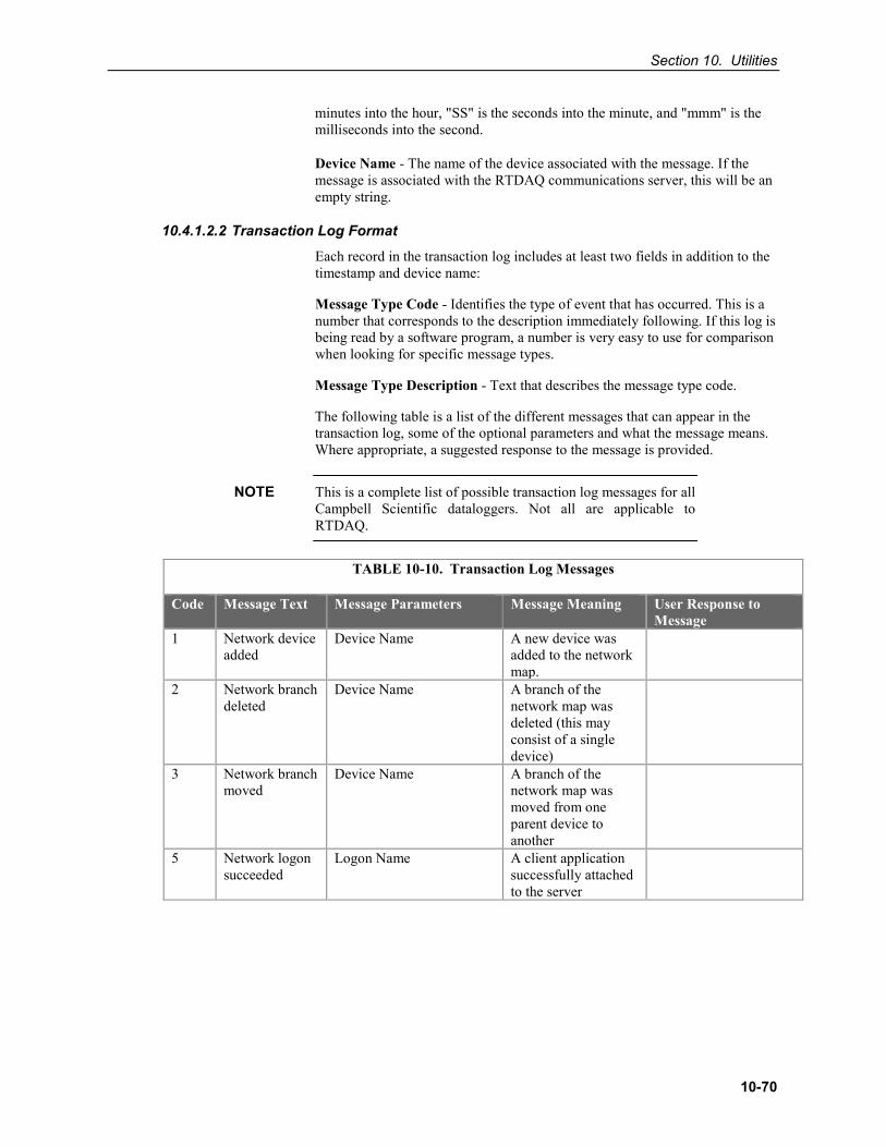
Section 10. Utilities
10-70
minutes into the hour, "SS" is the seconds into the minute, and "mmm" is the milliseconds into the second.
Device Name - The name of the device associated with the message. If the message is associated with the RTDAQ communications server, this will be an empty string.
10.4.1.2.2 Transaction Log Format
Each record in the transaction log includes at least two fields in addition to the timestamp and device name:
Message Type Code - Identifies the type of event that has occurred. This is a number that corresponds to the description immediately following. If this log is being read by a software program, a number is very easy to use for comparison when looking for specific message types.
Message Type Description - Text that describes the message type code.
The following table is a list of the different messages that can appear in the transaction log, some of the optional parameters and what the message means. Where appropriate, a suggested response to the message is provided.
This is a complete list of possible transaction log messages for all Campbell Scientific dataloggers. Not all are applicable to RTDAQ.
TABLE 10-10. Transaction Log Messages
Code Message Text Message Parameters Message Meaning User Response to Message
1 Network device added
Device Name A new device was added to the network map.
2 Network branch deleted
Device Name A branch of the network map was deleted (this may consist of a single device)
3 Network branch moved
Device Name A branch of the network map was moved from one parent device to another
5 Network logon succeeded
Logon Name A client application successfully attached to the server
NOTE
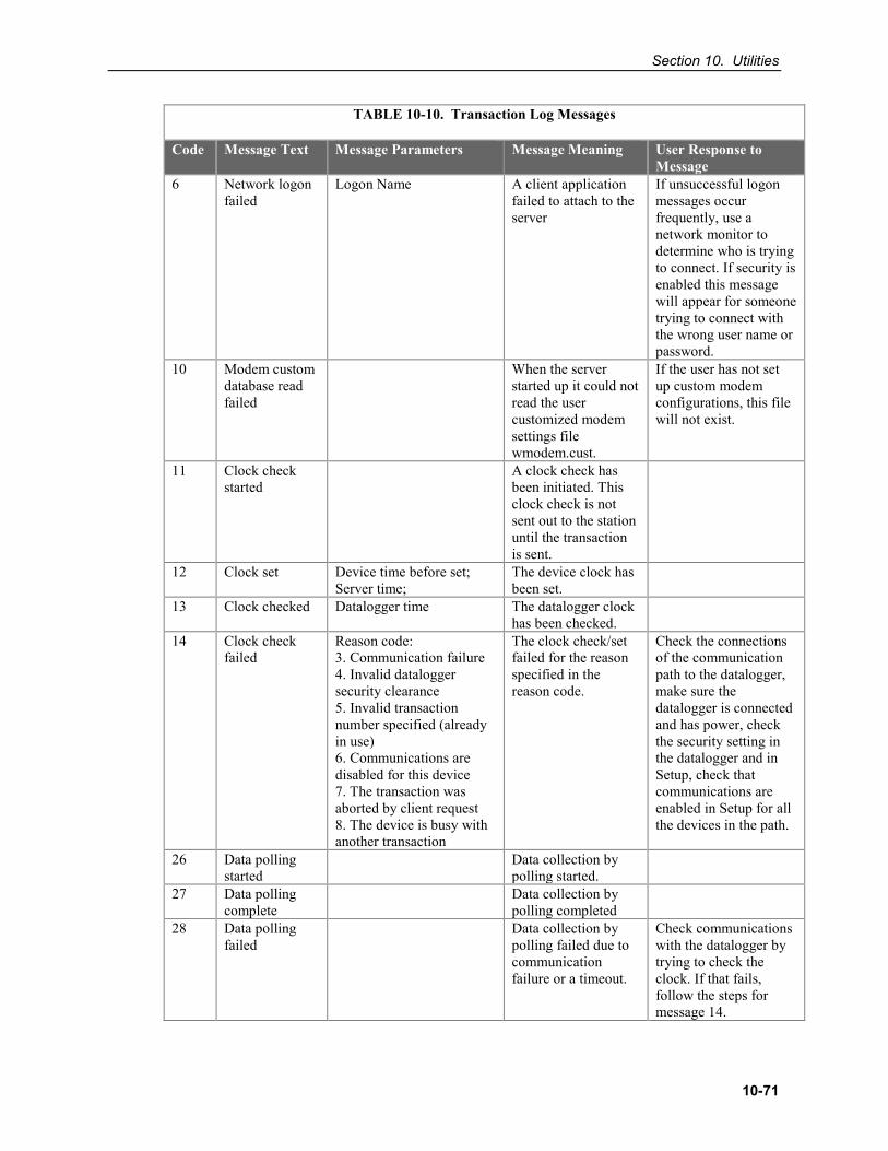
Section 10. Utilities
10-71
TABLE 10-10. Transaction Log Messages
Code Message Text Message Parameters Message Meaning User Response to Message
6 Network logon failed
Logon Name A client application failed to attach to the server
If unsuccessful logon messages occur frequently, use a network monitor to determine who is trying to connect. If security is enabled this message will appear for someone trying to connect with the wrong user name or password.
10 Modem custom database read failed
When the server started up it could not read the user customized modem settings file wmodem.cust.
If the user has not set up custom modem configurations, this file will not exist.
11 Clock check started
A clock check has been initiated. This clock check is not sent out to the station until the transaction is sent.
12 Clock set Device time before set; Server time;
The device clock has been set.
13 Clock checked Datalogger time The datalogger clock has been checked.
14 Clock check failed
Reason code: 3. Communication failure 4. Invalid datalogger security clearance 5. Invalid transaction number specified (already in use) 6. Communications are disabled for this device 7. The transaction was aborted by client request 8. The device is busy with another transaction
The clock check/set failed for the reason specified in the reason code.
Check the connections of the communication path to the datalogger, make sure the datalogger is connected and has power, check the security setting in the datalogger and in Setup, check that communications are enabled in Setup for all the devices in the path.
26 Data polling started
Data collection by polling started.
27 Data polling complete
Data collection by polling completed
28 Data polling failed
Data collection by polling failed due to communication failure or a timeout.
Check communications with the datalogger by trying to check the clock. If that fails, follow the steps for message 14.
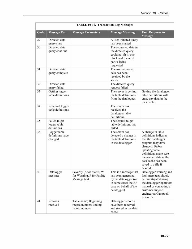
Section 10. Utilities
10-72
TABLE 10-10. Transaction Log Messages
Code Message Text Message Parameters Message Meaning User Response to Message
29 Directed data query start
A user initiated query has been started.
30 Directed data query continue
The requested data in the directed query could not fit in one block and the next part is being requested.
31 Directed data query complete
The user requested data has been received by the server.
32 Directed data query failed
The directed query request failed.
33 Getting logger table definitions
The server is getting the table definitions from the datalogger.
Getting the datalogger table definitions will erase any data in the data cache.
34 Received logger table definitions
The server has received the datalogger table definitions.
35 Failed to get logger table definitions
The request to get table definitions has failed.
36 Logger table definitions have changed
The server has detected a change in the table definitions in the datalogger.
A change in table definitions indicates that the datalogger program may have changed. Before updating table definitions make sure the needed data in the data cache has been saved to a file if desired.
40 Datalogger message
Severity (S for Status, W for Warning, F for Fault); Message text.
This is a message that has been generated by the datalogger (or in some cases the RF base on behalf of the datalogger).
Datalogger warning and fault messages should be investigated using the datalogger operators manual or contacting a customer support engineer at Campbell Scientific.
41 Records received
Table name; Beginning record number; Ending record number
Datalogger records have been received and stored in the data cache.
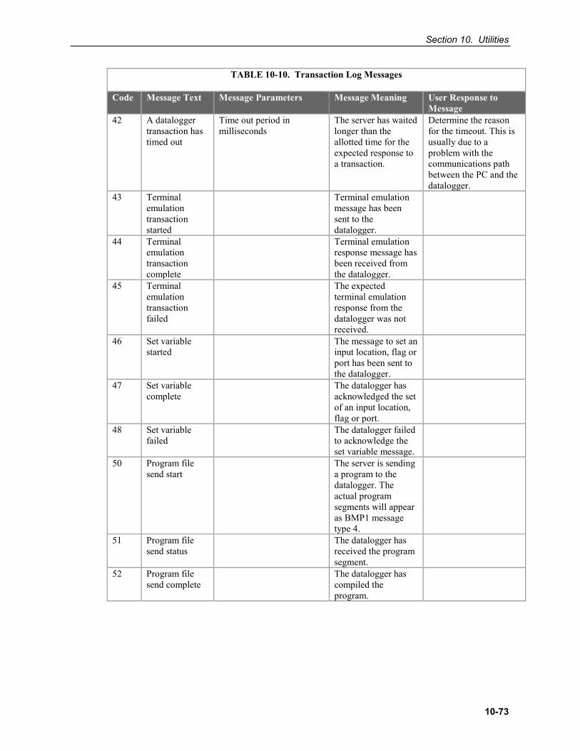
Section 10. Utilities
10-73
TABLE 10-10. Transaction Log Messages
Code Message Text Message Parameters Message Meaning User Response to Message
42 A datalogger transaction has timed out
Time out period in milliseconds
The server has waited longer than the allotted time for the expected response to a transaction.
Determine the reason for the timeout. This is usually due to a problem with the communications path between the PC and the datalogger.
43 Terminal emulation transaction started
Terminal emulation message has been sent to the datalogger.
44 Terminal emulation transaction complete
Terminal emulation response message has been received from the datalogger.
45 Terminal emulation transaction failed
The expected terminal emulation response from the datalogger was not received.
46 Set variable started
The message to set an input location, flag or port has been sent to the datalogger.
47 Set variable complete
The datalogger has acknowledged the set of an input location, flag or port.
48 Set variable failed
The datalogger failed to acknowledge the set variable message.
50 Program file send start
The server is sending a program to the datalogger. The actual program segments will appear as BMP1 message type 4.
51 Program file send status
The datalogger has received the program segment.
52 Program file send complete
The datalogger has compiled the program.
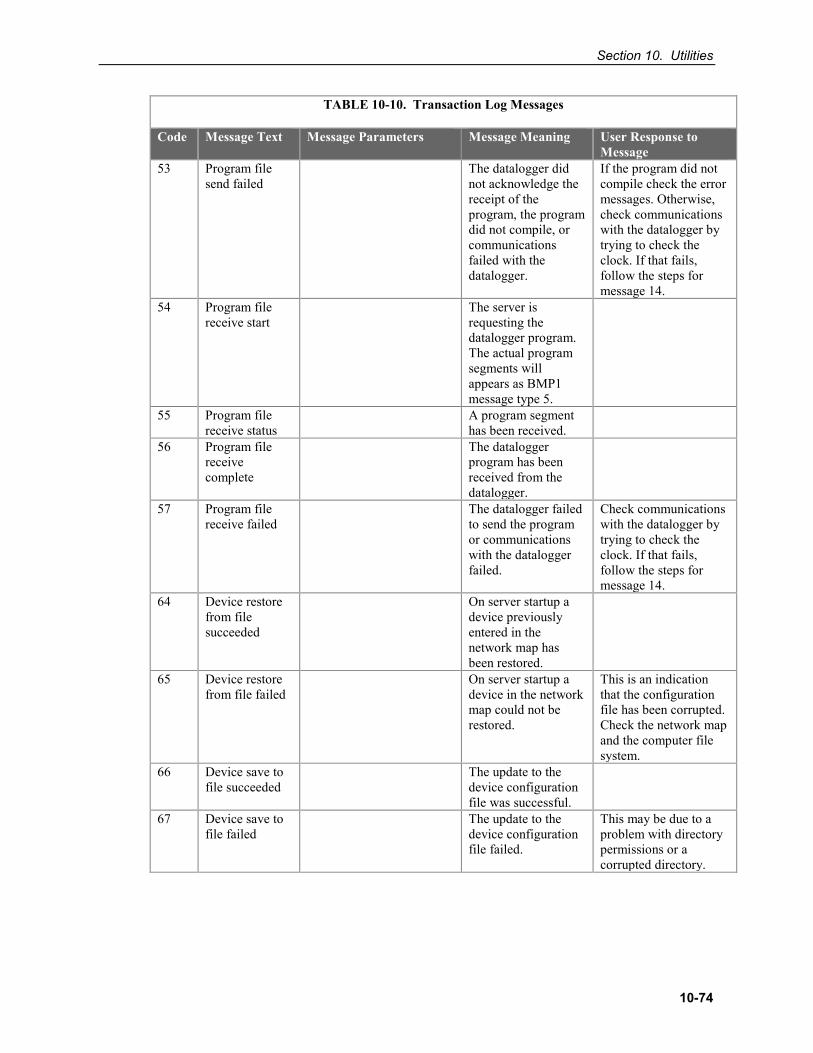
Section 10. Utilities
10-74
TABLE 10-10. Transaction Log Messages
Code Message Text Message Parameters Message Meaning User Response to Message
53 Program file send failed
The datalogger did not acknowledge the receipt of the program, the program did not compile, or communications failed with the datalogger.
If the program did not compile check the error messages. Otherwise, check communications with the datalogger by trying to check the clock. If that fails, follow the steps for message 14.
54 Program file receive start
The server is requesting the datalogger program. The actual program segments will appears as BMP1 message type 5.
55 Program file receive status
A program segment has been received.
56 Program file receive complete
The datalogger program has been received from the datalogger.
57 Program file receive failed
The datalogger failed to send the program or communications with the datalogger failed.
Check communications with the datalogger by trying to check the clock. If that fails, follow the steps for message 14.
64 Device restore from file succeeded
On server startup a device previously entered in the network map has been restored.
65 Device restore from file failed
On server startup a device in the network map could not be restored.
This is an indication that the configuration file has been corrupted. Check the network map and the computer file system.
66 Device save to file succeeded
The update to the device configuration file was successful.
67 Device save to file failed
The update to the device configuration file failed.
This may be due to a problem with directory permissions or a corrupted directory.
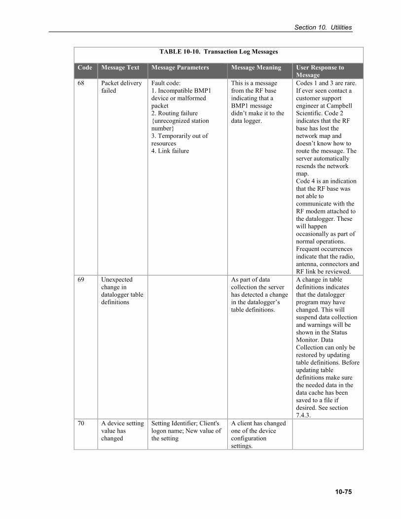
Section 10. Utilities
10-75
TABLE 10-10. Transaction Log Messages
Code Message Text Message Parameters Message Meaning User Response to Message
68 Packet delivery failed
Fault code: 1. Incompatible BMP1 device or malformed packet 2. Routing failure {unrecognized station number} 3. Temporarily out of resources 4. Link failure
This is a message from the RF base indicating that a BMP1 message didn’t make it to the data logger.
Codes 1 and 3 are rare. If ever seen contact a customer support engineer at Campbell Scientific. Code 2 indicates that the RF base has lost the network map and doesn’t know how to route the message. The server automatically resends the network map. Code 4 is an indication that the RF base was not able to communicate with the RF modem attached to the datalogger. These will happen occasionally as part of normal operations. Frequent occurrences indicate that the radio, antenna, connectors and RF link be reviewed.
69 Unexpected change in datalogger table definitions
As part of data collection the server has detected a change in the datalogger’s table definitions.
A change in table definitions indicates that the datalogger program may have changed. This will suspend data collection and warnings will be shown in the Status Monitor. Data Collection can only be restored by updating table definitions. Before updating table definitions make sure the needed data in the data cache has been saved to a file if desired. See section 7.4.3.
70 A device setting value has changed
Setting Identifier; Client's logon name; New value of the setting
A client has changed one of the device configuration settings.
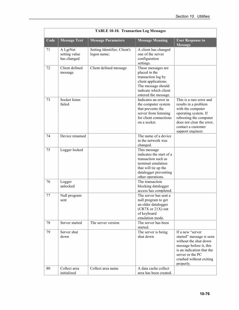
Section 10. Utilities
10-76
TABLE 10-10. Transaction Log Messages
Code Message Text Message Parameters Message Meaning User Response to Message
71 A LgrNet setting value has changed
Setting Identifier; Client's logon name;
A client has changed one of the server configuration settings.
72 Client defined message
Client defined message These messages are placed in the transaction log by client applications. The message should indicate which client entered the message.
73 Socket listen failed
Indicates an error in the computer system that prevents the server from listening for client connections on a socket.
This is a rare error and results in a problem with the computer operating system. If rebooting the computer does not clear the error, contact a customer support engineer.
74 Device renamed The name of a device in the network was changed.
75 Logger locked This message indicates the start of a transaction such as terminal emulation that will tie up the datalogger preventing other operations.
76 Logger unlocked
The transaction blocking datalogger access has completed.
77 Null program sent
The server has sent a null program to get an older datalogger (CR7X or 21X) out of keyboard emulation mode.
78 Server started The server version The server has been started.
79 Server shut down
The server is being shut down
If a new “server started” message is seen without the shut down message before it, this is an indication that the server or the PC crashed without exiting properly.
80 Collect area initialized
Collect area name A data cache collect area has been created.
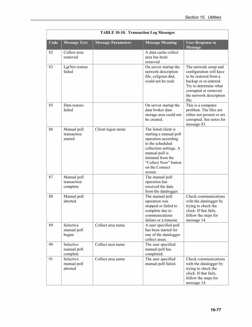
Section 10. Utilities
10-77
TABLE 10-10. Transaction Log Messages
Code Message Text Message Parameters Message Meaning User Response to Message
82 Collect area removed
A data cache collect area has been removed
83 LgrNet restore failed
On server startup the network description file, csilgrnet.dnd, could not be read.
The network setup and configuration will have to be restored from a backup or re-entered. Try to determine what corrupted or removed the network description file.
85 Data restore failed
On server startup the data broker data storage area could not be created.
This is a computer problem. The files are either not present or are corrupted. See notes for message 83.
86 Manual poll transaction started
Client logon name The listed client is starting a manual poll operation according to the scheduled collection settings. A manual poll is initiated from the “Collect Now” button on the Connect screen.
87 Manual poll transaction complete
The manual poll operation has received the data from the datalogger.
88 Manual poll aborted
The manual poll operation was stopped or failed to complete due to communications failure or a timeout.
Check communications with the datalogger by trying to check the clock. If that fails, follow the steps for message 14.
89 Selective manual poll begun
Collect area name A user specified poll has been started for one of the datalogger collect areas.
90 Selective manual poll complete
Collect area name The user specified manual poll has completed.
91 Selective manual poll aborted
Collect area name The user specified manual poll failed.
Check communications with the datalogger by trying to check the clock. If that fails, follow the steps for message 14.
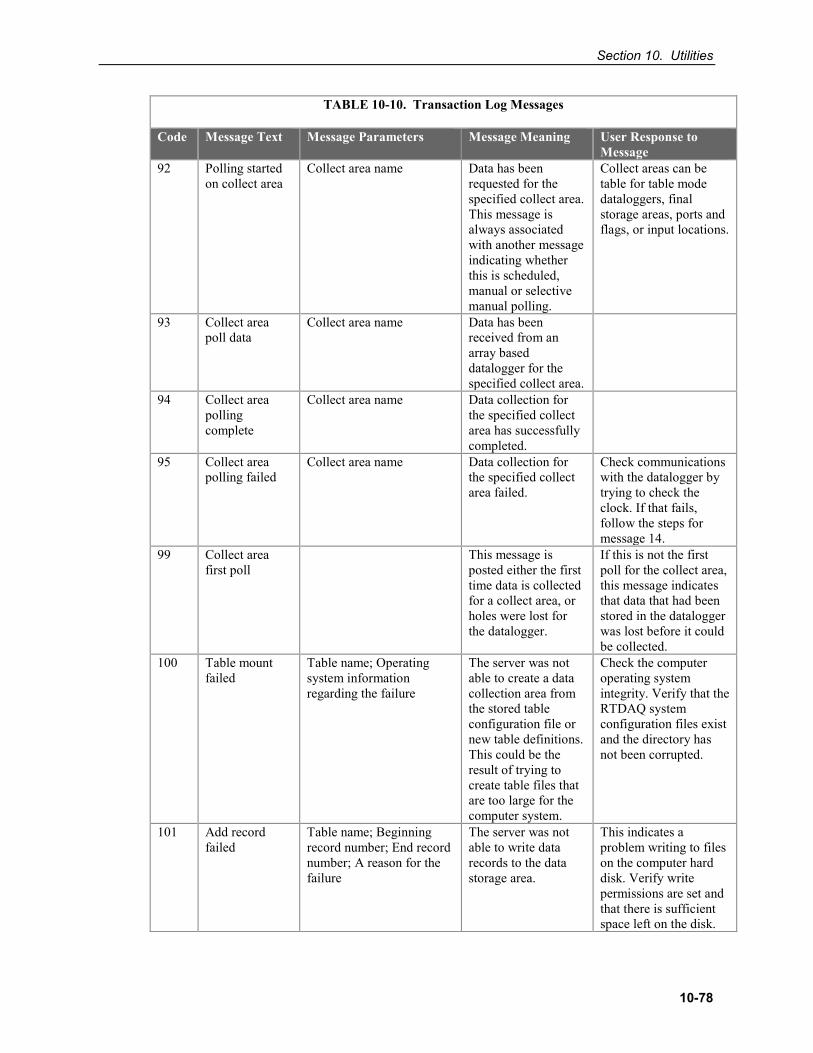
Section 10. Utilities
10-78
TABLE 10-10. Transaction Log Messages
Code Message Text Message Parameters Message Meaning User Response to Message
92 Polling started on collect area
Collect area name Data has been requested for the specified collect area. This message is always associated with another message indicating whether this is scheduled, manual or selective manual polling.
Collect areas can be table for table mode dataloggers, final storage areas, ports and flags, or input locations.
93 Collect area poll data
Collect area name Data has been received from an array based datalogger for the specified collect area.
94 Collect area polling complete
Collect area name Data collection for the specified collect area has successfully completed.
95 Collect area polling failed
Collect area name Data collection for the specified collect area failed.
Check communications with the datalogger by trying to check the clock. If that fails, follow the steps for message 14.
99 Collect area first poll
This message is posted either the first time data is collected for a collect area, or holes were lost for the datalogger.
If this is not the first poll for the collect area, this message indicates that data that had been stored in the datalogger was lost before it could be collected.
100 Table mount failed
Table name; Operating system information regarding the failure
The server was not able to create a data collection area from the stored table configuration file or new table definitions. This could be the result of trying to create table files that are too large for the computer system.
Check the computer operating system integrity. Verify that the RTDAQ system configuration files exist and the directory has not been corrupted.
101 Add record failed
Table name; Beginning record number; End record number; A reason for the failure
The server was not able to write data records to the data storage area.
This indicates a problem writing to files on the computer hard disk. Verify write permissions are set and that there is sufficient space left on the disk.
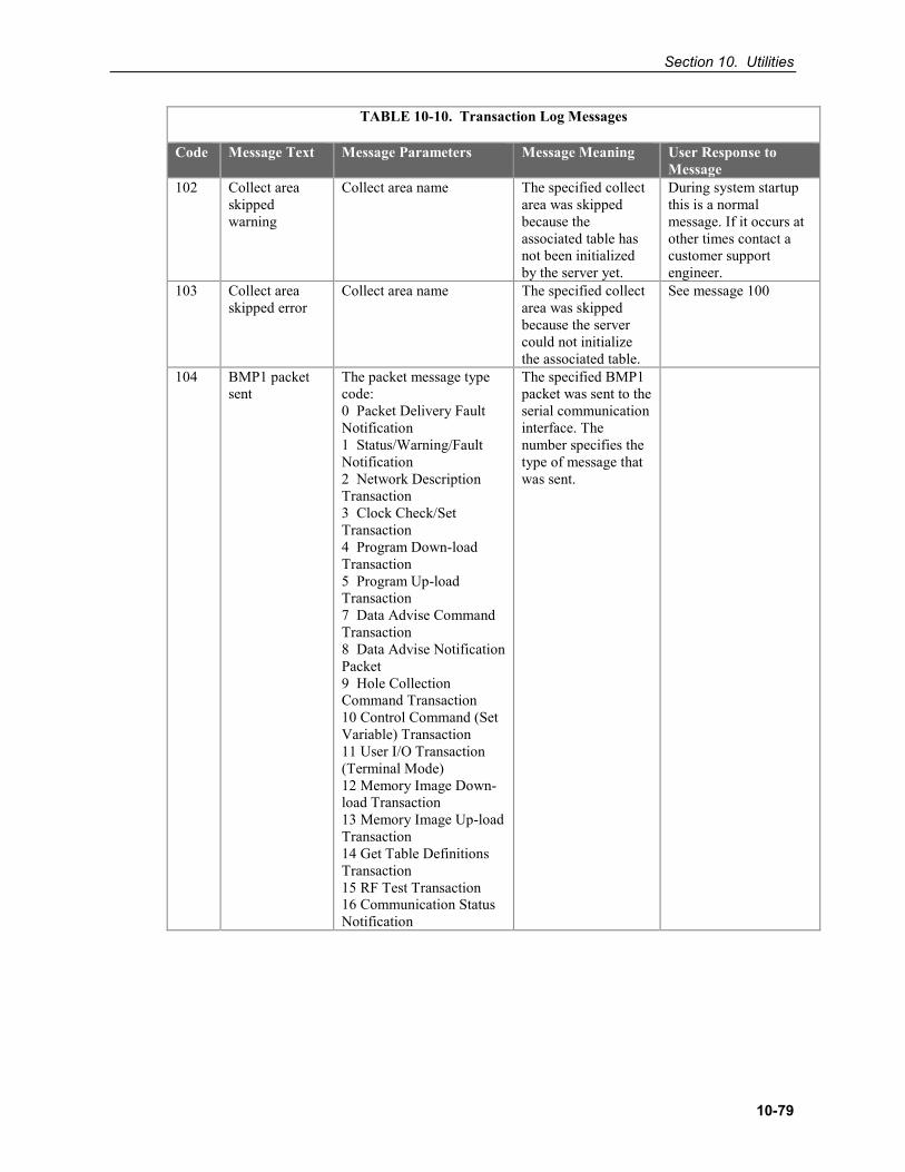
Section 10. Utilities
10-79
TABLE 10-10. Transaction Log Messages
Code Message Text Message Parameters Message Meaning User Response to Message
102 Collect area skipped warning
Collect area name The specified collect area was skipped because the associated table has not been initialized by the server yet.
During system startup this is a normal message. If it occurs at other times contact a customer support engineer.
103 Collect area skipped error
Collect area name The specified collect area was skipped because the server could not initialize the associated table.
See message 100
104 BMP1 packet sent
The packet message type code: 0 Packet Delivery Fault Notification 1 Status/Warning/Fault Notification 2 Network Description Transaction 3 Clock Check/Set Transaction 4 Program Down-load Transaction 5 Program Up-load Transaction 7 Data Advise Command Transaction 8 Data Advise Notification Packet 9 Hole Collection Command Transaction 10 Control Command (Set Variable) Transaction 11 User I/O Transaction (Terminal Mode) 12 Memory Image Down-load Transaction 13 Memory Image Up-load Transaction 14 Get Table Definitions Transaction 15 RF Test Transaction 16 Communication Status Notification
The specified BMP1 packet was sent to the serial communication interface. The number specifies the type of message that was sent.
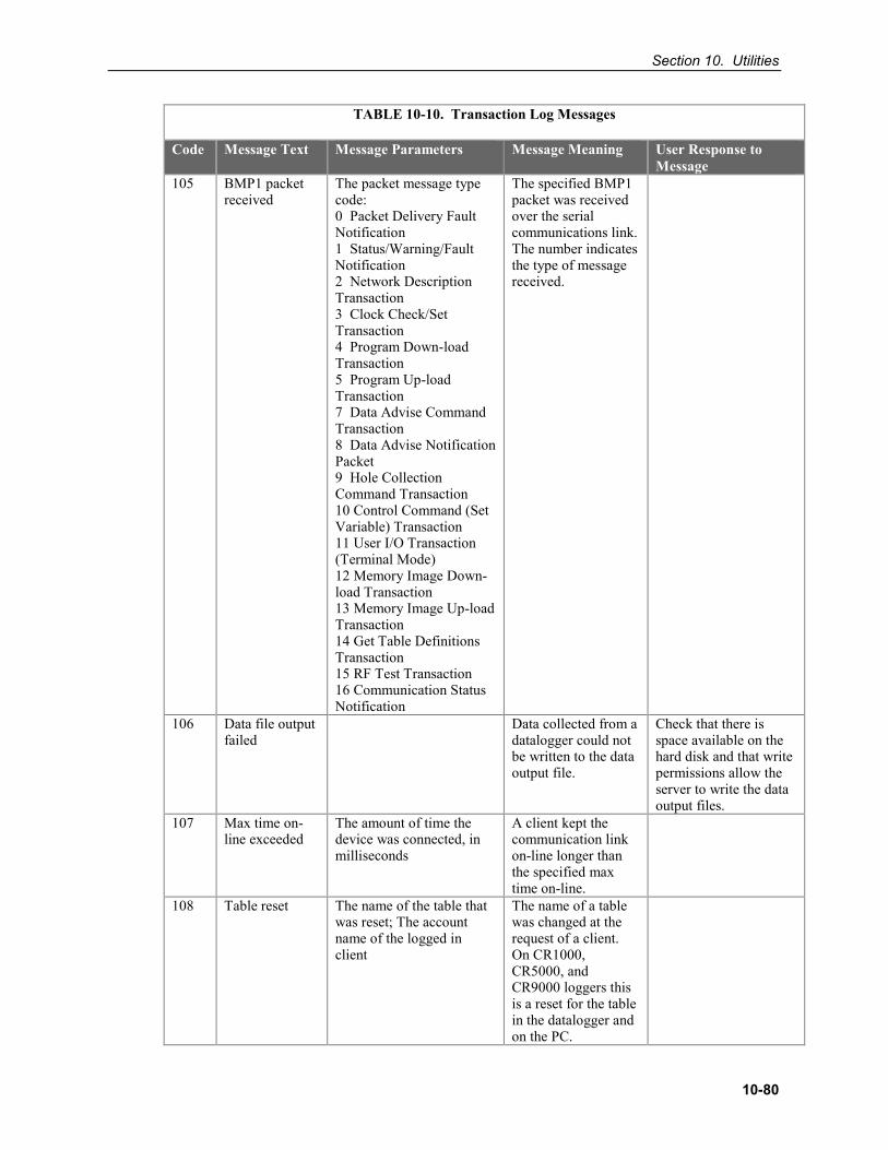
Section 10. Utilities
10-80
TABLE 10-10. Transaction Log Messages
Code Message Text Message Parameters Message Meaning User Response to Message
105 BMP1 packet received
The packet message type code: 0 Packet Delivery Fault Notification 1 Status/Warning/Fault Notification 2 Network Description Transaction 3 Clock Check/Set Transaction 4 Program Down-load Transaction 5 Program Up-load Transaction 7 Data Advise Command Transaction 8 Data Advise Notification Packet 9 Hole Collection Command Transaction 10 Control Command (Set Variable) Transaction 11 User I/O Transaction (Terminal Mode) 12 Memory Image Down-load Transaction 13 Memory Image Up-load Transaction 14 Get Table Definitions Transaction 15 RF Test Transaction 16 Communication Status Notification
The specified BMP1 packet was received over the serial communications link. The number indicates the type of message received.
106 Data file output failed
Data collected from a datalogger could not be written to the data output file.
Check that there is space available on the hard disk and that write permissions allow the server to write the data output files.
107 Max time on-line exceeded
The amount of time the device was connected, in milliseconds
A client kept the communication link on-line longer than the specified max time on-line.
108 Table reset The name of the table that was reset; The account name of the logged in client
The name of a table was changed at the request of a client. On CR1000, CR5000, and CR9000 loggers this is a reset for the table in the datalogger and on the PC.
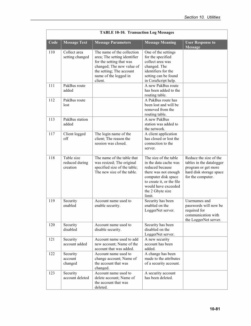
Section 10. Utilities
10-81
TABLE 10-10. Transaction Log Messages
Code Message Text Message Parameters Message Meaning User Response to Message
110 Collect area setting changed
The name of the collection area; The setting identifier for the setting that was changed; The new value of the setting; The account name of the logged in client.
One of the settings for the specified collect area was changed. The identifiers for the setting can be found in CoraScript help.
111 PakBus route added
A new PakBus route has been added to the routing table.
112 PakBus route lost
A PakBus route has been lost and will be removed from the routing table.
113 PakBus station added
A new PakBus station was added to the network.
117 Client logged off
The login name of the client; The reason the session was closed.
A client application has closed or lost the connection to the server.
118 Table size reduced during creation
The name of the table that was resized; The original specified size of the table; The new size of the table.
The size of the table in the data cache was reduced because there was not enough computer disk space to create it, or the file would have exceeded the 2 Gbyte size limit.
Reduce the size of the tables in the datalogger program or get more hard disk storage space for the computer.
119 Security enabled
Account name used to enable security.
Security has been enabled on the LoggerNet server.
Usernames and passwords will now be required for communication with the LoggerNet server.
120 Security disabled
Account name used to disable security.
Security has been disabled on the LoggerNet server.
121 Security account added
Account name used to add new account; Name of the account that was added.
A new security account has been added.
122 Security account changed
Account name used to change account; Name of the account that was changed.
A change has been made to the attributes of a security account.
123 Security account deleted
Account name used to delete account; Name of the account that was deleted.
A security account has been deleted.
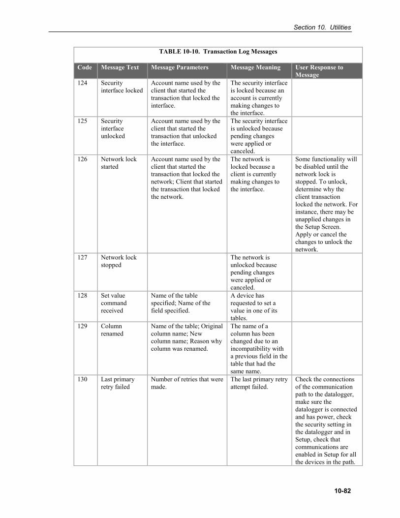
Section 10. Utilities
10-82
TABLE 10-10. Transaction Log Messages
Code Message Text Message Parameters Message Meaning User Response to Message
124 Security interface locked
Account name used by the client that started the transaction that locked the interface.
The security interface is locked because an account is currently making changes to the interface.
125 Security interface unlocked
Account name used by the client that started the transaction that unlocked the interface.
The security interface is unlocked because pending changes were applied or canceled.
126 Network lock started
Account name used by the client that started the transaction that locked the network; Client that started the transaction that locked the network.
The network is locked because a client is currently making changes to the interface.
Some functionality will be disabled until the network lock is stopped. To unlock, determine why the client transaction locked the network. For instance, there may be unapplied changes in the Setup Screen. Apply or cancel the changes to unlock the network.
127 Network lock stopped
The network is unlocked because pending changes were applied or canceled.
128 Set value command received
Name of the table specified; Name of the field specified.
A device has requested to set a value in one of its tables.
129 Column renamed
Name of the table; Original column name; New column name; Reason why column was renamed.
The name of a column has been changed due to an incompatibility with a previous field in the table that had the same name.
130 Last primary retry failed
Number of retries that were made.
The last primary retry attempt failed.
Check the connections of the communication path to the datalogger, make sure the datalogger is connected and has power, check the security setting in the datalogger and in Setup, check that communications are enabled in Setup for all the devices in the path.
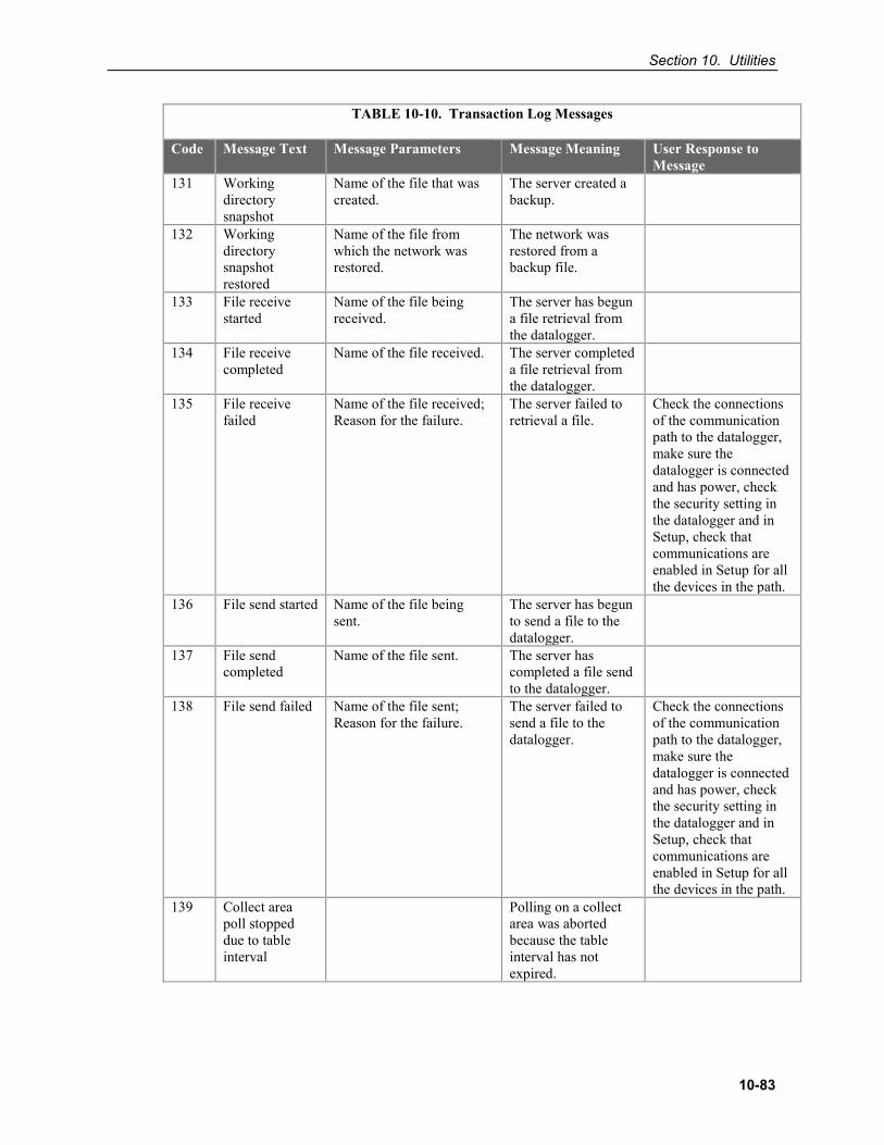
Section 10. Utilities
10-83
TABLE 10-10. Transaction Log Messages
Code Message Text Message Parameters Message Meaning User Response to Message
131 Working directory snapshot
Name of the file that was created.
The server created a backup.
132 Working directory snapshot restored
Name of the file from which the network was restored.
The network was restored from a backup file.
133 File receive started
Name of the file being received.
The server has begun a file retrieval from the datalogger.
134 File receive completed
Name of the file received. The server completed a file retrieval from the datalogger.
135 File receive failed
Name of the file received; Reason for the failure.
The server failed to retrieval a file.
Check the connections of the communication path to the datalogger, make sure the datalogger is connected and has power, check the security setting in the datalogger and in Setup, check that communications are enabled in Setup for all the devices in the path.
136 File send started Name of the file being sent.
The server has begun to send a file to the datalogger.
137 File send completed
Name of the file sent. The server has completed a file send to the datalogger.
138 File send failed Name of the file sent; Reason for the failure.
The server failed to send a file to the datalogger.
Check the connections of the communication path to the datalogger, make sure the datalogger is connected and has power, check the security setting in the datalogger and in Setup, check that communications are enabled in Setup for all the devices in the path.
139 Collect area poll stopped due to table interval
Polling on a collect area was aborted because the table interval has not expired.
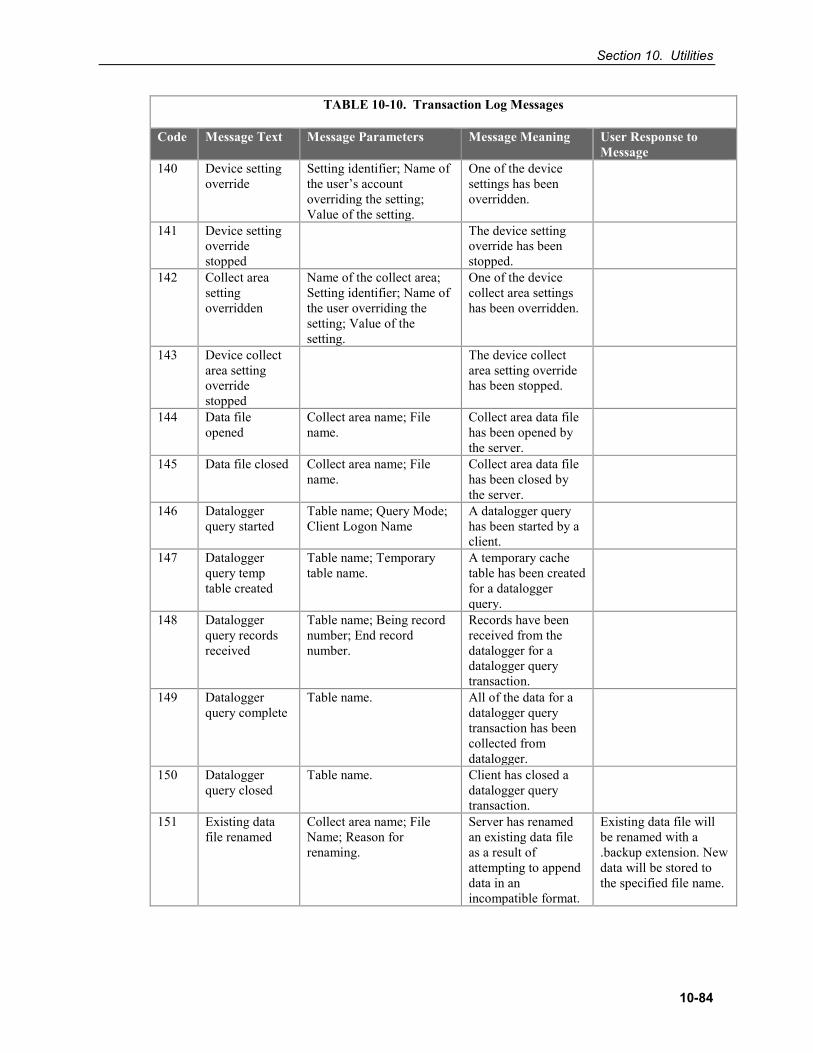
Section 10. Utilities
10-84
TABLE 10-10. Transaction Log Messages
Code Message Text Message Parameters Message Meaning User Response to Message
140 Device setting override
Setting identifier; Name of the user’s account overriding the setting; Value of the setting.
One of the device settings has been overridden.
141 Device setting override stopped
The device setting override has been stopped.
142 Collect area setting overridden
Name of the collect area; Setting identifier; Name of the user overriding the setting; Value of the setting.
One of the device collect area settings has been overridden.
143 Device collect area setting override stopped
The device collect area setting override has been stopped.
144 Data file opened
Collect area name; File name.
Collect area data file has been opened by the server.
145 Data file closed Collect area name; File name.
Collect area data file has been closed by the server.
146 Datalogger query started
Table name; Query Mode; Client Logon Name
A datalogger query has been started by a client.
147 Datalogger query temp table created
Table name; Temporary table name.
A temporary cache table has been created for a datalogger query.
148 Datalogger query records received
Table name; Being record number; End record number.
Records have been received from the datalogger for a datalogger query transaction.
149 Datalogger query complete
Table name. All of the data for a datalogger query transaction has been collected from datalogger.
150 Datalogger query closed
Table name. Client has closed a datalogger query transaction.
151 Existing data file renamed
Collect area name; File Name; Reason for renaming.
Server has renamed an existing data file as a result of attempting to append data in an incompatible format.
Existing data file will be renamed with a .backup extension. New data will be stored to the specified file name.
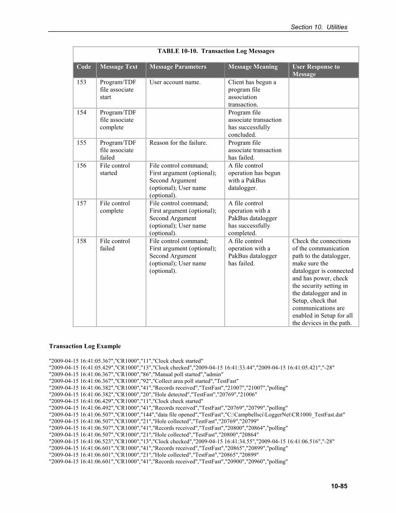
Section 10. Utilities
10-85
TABLE 10-10. Transaction Log Messages
Code Message Text Message Parameters Message Meaning User Response to Message
153 Program/TDF file associate start
User account name. Client has begun a program file association transaction.
154 Program/TDF file associate complete
Program file associate transaction has successfully concluded.
155 Program/TDF file associate failed
Reason for the failure. Program file associate transaction has failed.
156 File control started
File control command; First argument (optional); Second Argument (optional); User name (optional).
A file control operation has begun with a PakBus datalogger.
157 File control complete
File control command; First argument (optional); Second Argument (optional); User name (optional).
A file control operation with a PakBus datalogger has successfully completed.
158 File control failed
File control command; First argument (optional); Second Argument (optional); User name (optional).
A file control operation with a PakBus datalogger has failed.
Check the connections of the communication path to the datalogger, make sure the datalogger is connected and has power, check the security setting in the datalogger and in Setup, check that communications are enabled in Setup for all the devices in the path.
Transaction Log Example
"2009-04-15 16:41:05.367","CR1000","11","Clock check started" "2009-04-15 16:41:05.429","CR1000","13","Clock checked","2009-04-15 16:41:33.44","2009-04-15 16:41:05.421","-28" "2009-04-15 16:41:06.367","CR1000","86","Manual poll started","admin" "2009-04-15 16:41:06.367","CR1000","92","Collect area poll started","TestFast" "2009-04-15 16:41:06.382","CR1000","41","Records received","TestFast","21007","21007","polling" "2009-04-15 16:41:06.382","CR1000","20","Hole detected","TestFast","20769","21006" "2009-04-15 16:41:06.429","CR1000","11","Clock check started" "2009-04-15 16:41:06.492","CR1000","41","Records received","TestFast","20769","20799","polling" "2009-04-15 16:41:06.507","CR1000","144","data file opened","TestFast","C:\Campbellsci\LoggerNet\CR1000_TestFast.dat" "2009-04-15 16:41:06.507","CR1000","21","Hole collected","TestFast","20769","20799" "2009-04-15 16:41:06.507","CR1000","41","Records received","TestFast","20800","20864","polling" "2009-04-15 16:41:06.507","CR1000","21","Hole collected","TestFast","20800","20864" "2009-04-15 16:41:06.523","CR1000","13","Clock checked","2009-04-15 16:41:34.55","2009-04-15 16:41:06.516","-28" "2009-04-15 16:41:06.601","CR1000","41","Records received","TestFast","20865","20899","polling" "2009-04-15 16:41:06.601","CR1000","21","Hole collected","TestFast","20865","20899" "2009-04-15 16:41:06.601","CR1000","41","Records received","TestFast","20900","20960","polling"
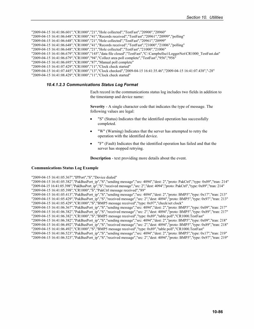
Section 10. Utilities
10-86
"2009-04-15 16:41:06.601","CR1000","21","Hole collected","TestFast","20900","20960" "2009-04-15 16:41:06.648","CR1000","41","Records received","TestFast","20961","20999","polling" "2009-04-15 16:41:06.648","CR1000","21","Hole collected","TestFast","20961","20999" "2009-04-15 16:41:06.648","CR1000","41","Records received","TestFast","21000","21006","polling" "2009-04-15 16:41:06.648","CR1000","21","Hole collected","TestFast","21000","21006" "2009-04-15 16:41:06.679","CR1000","145","data file closed","TestFast","C:\Campbellsci\LoggerNet\CR1000_TestFast.dat" "2009-04-15 16:41:06.679","CR1000","94","Collect area poll complete","TestFast","956","956" "2009-04-15 16:41:06.695","CR1000","87","Manual poll complete" "2009-04-15 16:41:07.429","CR1000","11","Clock check started" "2009-04-15 16:41:07.445","CR1000","13","Clock checked","2009-04-15 16:41:35.46","2009-04-15 16:41:07.438","-28" "2009-04-15 16:41:08.429","CR1000","11","Clock check started"
10.4.1.2.3 Communications Status Log Format
Each record in the communications status log includes two fields in addition to the timestamp and device name:
Severity - A single character code that indicates the type of message. The following values are legal:
• "S" (Status) Indicates that the identified operation has successfullycompleted.
• "W" (Warning) Indicates that the server has attempted to retry theoperation with the identified device.
• "F" (Fault) Indicates that the identified operation has failed and that theserver has stopped retrying.
Description - text providing more details about the event.
Communications Status Log Example
"2009-04-15 16:41:05.367","IPPort","S","Device dialed" "2009-04-15 16:41:05.382","PakBusPort_ip","S","sending message","src: 4094","dest: 2","proto: PakCtrl","type: 0x09","tran: 214" "2009-04-15 16:41:05.398","PakBusPort_ip","S","received message","src: 2","dest: 4094","proto: PakCtrl","type: 0x89","tran: 214" "2009-04-15 16:41:05.398","CR1000","S","PakCtrl message received","89" "2009-04-15 16:41:05.413","PakBusPort_ip","S","sending message","src: 4094","dest: 2","proto: BMP5","type: 0x17","tran: 213" "2009-04-15 16:41:05.429","PakBusPort_ip","S","received message","src: 2","dest: 4094","proto: BMP5","type: 0x97","tran: 213" "2009-04-15 16:41:05.429","CR1000","S","BMP5 message received","type: 0x97","check/set clock" "2009-04-15 16:41:06.367","PakBusPort_ip","S","sending message","src: 4094","dest: 2","proto: BMP5","type: 0x09","tran: 217" "2009-04-15 16:41:06.382","PakBusPort_ip","S","received message","src: 2","dest: 4094","proto: BMP5","type: 0x89","tran: 217" "2009-04-15 16:41:06.382","CR1000","S","BMP5 message received","type: 0x89","table poll","CR1000.TestFast" "2009-04-15 16:41:06.382","PakBusPort_ip","S","sending message","src: 4094","dest: 2","proto: BMP5","type: 0x09","tran: 218" "2009-04-15 16:41:06.492","PakBusPort_ip","S","received message","src: 2","dest: 4094","proto: BMP5","type: 0x89","tran: 218" "2009-04-15 16:41:06.492","CR1000","S","BMP5 message received","type: 0x89","table poll","CR1000.TestFast" "2009-04-15 16:41:06.523","PakBusPort_ip","S","sending message","src: 4094","dest: 2","proto: BMP5","type: 0x17","tran: 219" "2009-04-15 16:41:06.523","PakBusPort_ip","S","received message","src: 2","dest: 4094","proto: BMP5","type: 0x97","tran: 219"
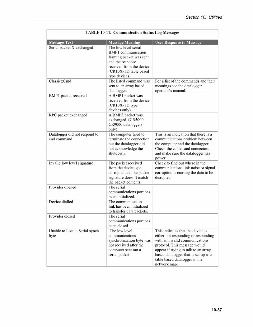
Section 10. Utilities
10-87
TABLE 10-11. Communication Status Log Messages
Message Text Message Meaning User Response to Message Serial packet X exchanged The low level serial
BMP1 communication framing packet was sent and the response received from the device. (CR10X-TD table based type devices)
Classic;;Cmd The listed command was sent to an array based datalogger.
For a list of the commands and their meanings see the datalogger operator’s manual.
BMP1 packet received A BMP1 packet was received from the device. (CR10X-TD type devices only)
RPC packet exchanged A BMP3 packet was exchanged. (CR5000, CR9000 dataloggers only)
Datalogger did not respond to end command
The computer tried to terminate the connection but the datalogger did not acknowledge the shutdown.
This is an indication that there is a communications problem between the computer and the datalogger. Check the cables and connectors and make sure the datalogger has power.
Invalid low level signature The packet received from the device got corrupted and the packet signature doesn’t match the packet contents.
Check to find out where in the communications link noise or signal corruption is causing the data to be disrupted.
Provider opened The serial communications port has been initialized.
Device dialled The communications link has been initialized to transfer data packets.
Provider closed The serial communications port has been closed.
Unable to Locate Serial synch byte
The low level communications synchronization byte was not received after the computer sent out a serial packet.
This indicates that the device is either not responding or responding with an invalid communications protocol. This message would appear if trying to talk to an array based datalogger that is set up as a table based datalogger in the network map.
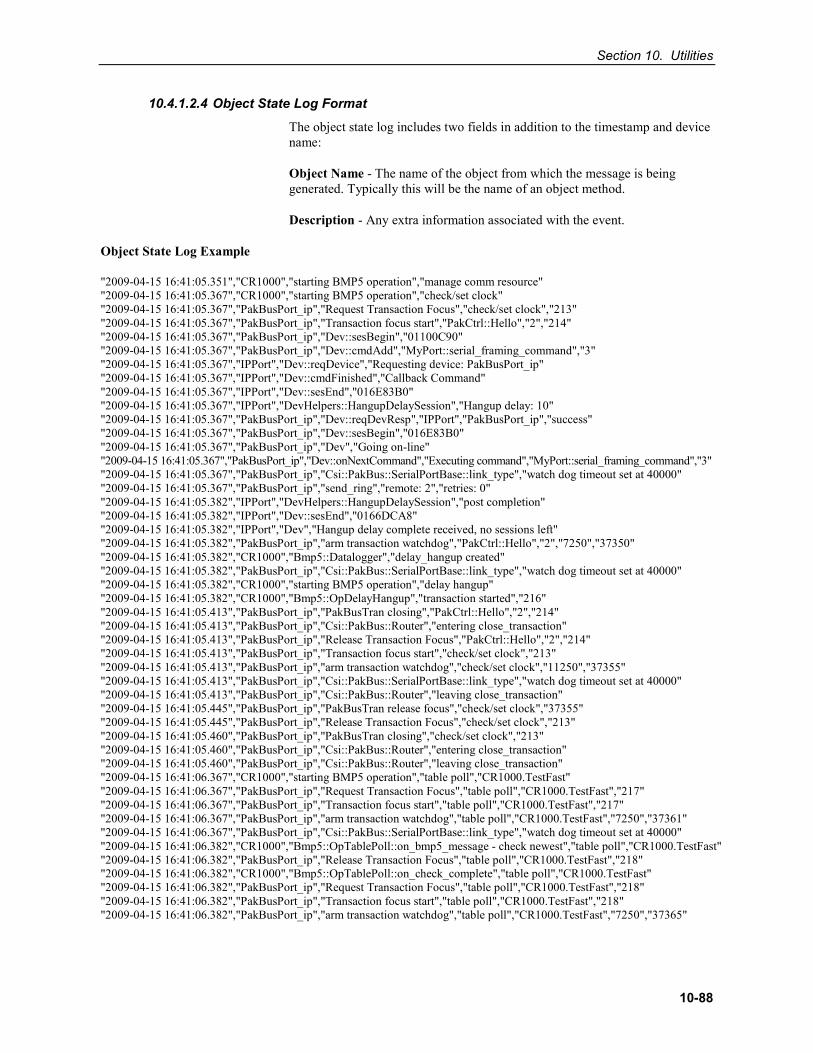
Section 10. Utilities
10-88
10.4.1.2.4 Object State Log Format
The object state log includes two fields in addition to the timestamp and device name:
Object Name - The name of the object from which the message is being generated. Typically this will be the name of an object method.
Description - Any extra information associated with the event.
Object State Log Example
"2009-04-15 16:41:05.351","CR1000","starting BMP5 operation","manage comm resource" "2009-04-15 16:41:05.367","CR1000","starting BMP5 operation","check/set clock" "2009-04-15 16:41:05.367","PakBusPort_ip","Request Transaction Focus","check/set clock","213" "2009-04-15 16:41:05.367","PakBusPort_ip","Transaction focus start","PakCtrl::Hello","2","214" "2009-04-15 16:41:05.367","PakBusPort_ip","Dev::sesBegin","01100C90" "2009-04-15 16:41:05.367","PakBusPort_ip","Dev::cmdAdd","MyPort::serial_framing_command","3" "2009-04-15 16:41:05.367","IPPort","Dev::reqDevice","Requesting device: PakBusPort_ip" "2009-04-15 16:41:05.367","IPPort","Dev::cmdFinished","Callback Command" "2009-04-15 16:41:05.367","IPPort","Dev::sesEnd","016E83B0" "2009-04-15 16:41:05.367","IPPort","DevHelpers::HangupDelaySession","Hangup delay: 10" "2009-04-15 16:41:05.367","PakBusPort_ip","Dev::reqDevResp","IPPort","PakBusPort_ip","success" "2009-04-15 16:41:05.367","PakBusPort_ip","Dev::sesBegin","016E83B0" "2009-04-15 16:41:05.367","PakBusPort_ip","Dev","Going on-line" "2009-04-15 16:41:05.367","PakBusPort_ip","Dev::onNextCommand","Executing command","MyPort::serial_framing_command","3" "2009-04-15 16:41:05.367","PakBusPort_ip","Csi::PakBus::SerialPortBase::link_type","watch dog timeout set at 40000" "2009-04-15 16:41:05.367","PakBusPort_ip","send_ring","remote: 2","retries: 0" "2009-04-15 16:41:05.382","IPPort","DevHelpers::HangupDelaySession","post completion" "2009-04-15 16:41:05.382","IPPort","Dev::sesEnd","0166DCA8" "2009-04-15 16:41:05.382","IPPort","Dev","Hangup delay complete received, no sessions left" "2009-04-15 16:41:05.382","PakBusPort_ip","arm transaction watchdog","PakCtrl::Hello","2","7250","37350" "2009-04-15 16:41:05.382","CR1000","Bmp5::Datalogger","delay_hangup created" "2009-04-15 16:41:05.382","PakBusPort_ip","Csi::PakBus::SerialPortBase::link_type","watch dog timeout set at 40000" "2009-04-15 16:41:05.382","CR1000","starting BMP5 operation","delay hangup" "2009-04-15 16:41:05.382","CR1000","Bmp5::OpDelayHangup","transaction started","216" "2009-04-15 16:41:05.413","PakBusPort_ip","PakBusTran closing","PakCtrl::Hello","2","214" "2009-04-15 16:41:05.413","PakBusPort_ip","Csi::PakBus::Router","entering close_transaction" "2009-04-15 16:41:05.413","PakBusPort_ip","Release Transaction Focus","PakCtrl::Hello","2","214" "2009-04-15 16:41:05.413","PakBusPort_ip","Transaction focus start","check/set clock","213" "2009-04-15 16:41:05.413","PakBusPort_ip","arm transaction watchdog","check/set clock","11250","37355" "2009-04-15 16:41:05.413","PakBusPort_ip","Csi::PakBus::SerialPortBase::link_type","watch dog timeout set at 40000" "2009-04-15 16:41:05.413","PakBusPort_ip","Csi::PakBus::Router","leaving close_transaction" "2009-04-15 16:41:05.445","PakBusPort_ip","PakBusTran release focus","check/set clock","37355" "2009-04-15 16:41:05.445","PakBusPort_ip","Release Transaction Focus","check/set clock","213" "2009-04-15 16:41:05.460","PakBusPort_ip","PakBusTran closing","check/set clock","213" "2009-04-15 16:41:05.460","PakBusPort_ip","Csi::PakBus::Router","entering close_transaction" "2009-04-15 16:41:05.460","PakBusPort_ip","Csi::PakBus::Router","leaving close_transaction" "2009-04-15 16:41:06.367","CR1000","starting BMP5 operation","table poll","CR1000.TestFast" "2009-04-15 16:41:06.367","PakBusPort_ip","Request Transaction Focus","table poll","CR1000.TestFast","217" "2009-04-15 16:41:06.367","PakBusPort_ip","Transaction focus start","table poll","CR1000.TestFast","217" "2009-04-15 16:41:06.367","PakBusPort_ip","arm transaction watchdog","table poll","CR1000.TestFast","7250","37361" "2009-04-15 16:41:06.367","PakBusPort_ip","Csi::PakBus::SerialPortBase::link_type","watch dog timeout set at 40000" "2009-04-15 16:41:06.382","CR1000","Bmp5::OpTablePoll::on_bmp5_message - check newest","table poll","CR1000.TestFast" "2009-04-15 16:41:06.382","PakBusPort_ip","Release Transaction Focus","table poll","CR1000.TestFast","218" "2009-04-15 16:41:06.382","CR1000","Bmp5::OpTablePoll::on_check_complete","table poll","CR1000.TestFast" "2009-04-15 16:41:06.382","PakBusPort_ip","Request Transaction Focus","table poll","CR1000.TestFast","218" "2009-04-15 16:41:06.382","PakBusPort_ip","Transaction focus start","table poll","CR1000.TestFast","218" "2009-04-15 16:41:06.382","PakBusPort_ip","arm transaction watchdog","table poll","CR1000.TestFast","7250","37365"
Section 10. Utilities
10-89
10.4.2 CQR Log (RF Link) The CQR log contains information about the quality of communication each time an RFBase is dialled. (Note that information on an RFBase-TD link is not contained in the CQR log). The CQR log is written to the <working directory>\Logs directory. By default, this is C:\Campbellsci\RTDAQ\Logs.
Each time an RF link is shutdown, an entry will be written to the CQR Log. The first line in each entry is the timestamp and the name of the datalogger being communicated with. The remaining lines are the RF Link Quality Accumulators (RLQA) for each modem in the link. The RLQA are representative of the active period of the link. The line for each modem will contain three numbers:
xxxx yyyy zzzz
where
xxxx = Number of communication failures yyyy = Noise Level Indicator zzzz = Noise Level Indicator
A communication failure occurs when a signature of a block of data does not match its original signature. These blocks are subsequently retransmitted. The noise level indicators should be 102 (±70) at 3.0K baud rate or 124 (±70) at 2.4K baud.
Example CQR log entry
"10/14/2010 12:10:35",CR10XTD 0002 0128 0055 0000 0129 0063
The first line is the timestamp and name of the datalogger being communicated with. The next line is the RLQA for the EOL (End of Link) modem. This is the remote modem connected to the datalogger. The last line is the RLQA for the SOL (Start of Link) modem. This is the base modem. (This entry is for a link that contains no repeaters. A link with repeaters would show an additional line for each repeater between the EOL line and the SOL line.) The 0002 indicates that two interruptions occurred on the EOL modem while the link was active. All noise level indicators are within acceptable bounds in this example.
10.5 SDM-CAN Helper Software Registered users of the RTDAQ software may install, at no cost, an add-on product called "SDM-CAN Helper". The installation program for SDM-CAN Helper is available from www.campbellsci.eu/downloads. SDM-CAN Helper will only be installed if a valid installation of RTDAQ is detected on your computer.
SDM-CAN Helper assists customers who are using Campbell Scientific’s SDM-CAN Datalogger-to-CANbus Interface with our dataloggers and RTDAQ software. This add-on program is for users who are doing automotive monitoring and testing, or other Controller-Area Network (CAN) applications.
Section 10. Utilities
10-90
The SDM-CAN allows readings from a vehicle network to be transferred to a datalogger. This software helps those users move through the process of defining their vehicle network messaging within a datalogger program, so that the datalogger can read and store those values. SDM-CAN Helper will significantly reduce the amount of technical support required to operate this kind of a measurement system.
There are two main parts to SDM-CAN Helper:
1. A utility program called "DBC2PCK" converts industry standard ".DBC"files to a picklist format, which is usable by Campbell Scientific software. The.DBC file contains critical information about the data that can be digitallycaptured from the CAN network of a vehicle.
2. An RTMC Project contains multiple screens that walk the user through theprocess of configuring the SDM-CAN interface; connecting the SDM-CAN totheir datalogger; sending an appropriate program to the datalogger; and settingup the configuration to read values from the CAN network and get theminserted into the datalogger's storage.
For more information about the SDM-CAN Helper, please refer to the Campbell Scientific website (www.campbellsci.eu).
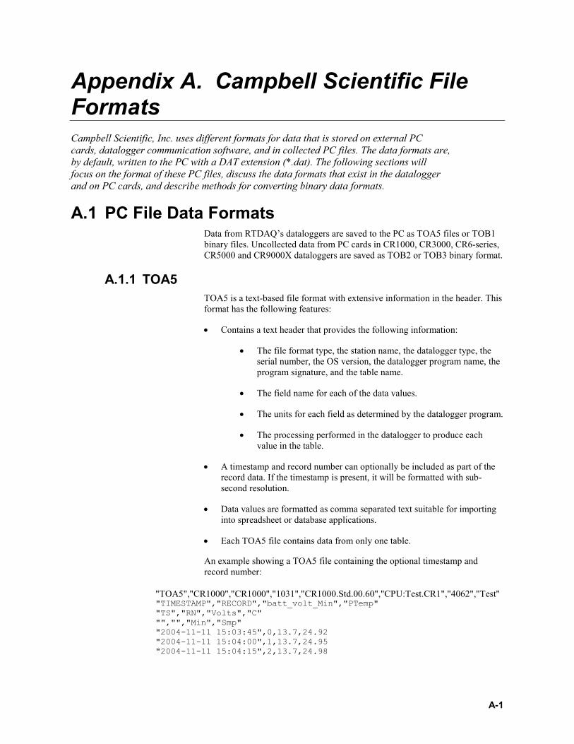
A-1
Appendix A. Campbell Scientific File Formats Campbell Scientific, Inc. uses different formats for data that is stored on external PC cards, datalogger communication software, and in collected PC files. The data formats are, by default, written to the PC with a DAT extension (*.dat). The following sections will focus on the format of these PC files, discuss the data formats that exist in the datalogger and on PC cards, and describe methods for converting binary data formats.
A.1 PC File Data Formats Data from RTDAQ’s dataloggers are saved to the PC as TOA5 files or TOB1 binary files. Uncollected data from PC cards in CR1000, CR3000, CR6-series, CR5000 and CR9000X dataloggers are saved as TOB2 or TOB3 binary format.
A.1.1 TOA5 TOA5 is a text-based file format with extensive information in the header. This format has the following features:
• Contains a text header that provides the following information:
• The file format type, the station name, the datalogger type, the serial number, the OS version, the datalogger program name, the program signature, and the table name.
• The field name for each of the data values.
• The units for each field as determined by the datalogger program.
• The processing performed in the datalogger to produce each value in the table.
• A timestamp and record number can optionally be included as part of the record data. If the timestamp is present, it will be formatted with sub-second resolution.
• Data values are formatted as comma separated text suitable for importing into spreadsheet or database applications.
• Each TOA5 file contains data from only one table.
An example showing a TOA5 file containing the optional timestamp and record number:
"TOA5","CR1000","CR1000","1031","CR1000.Std.00.60","CPU:Test.CR1","4062","Test" "TIMESTAMP","RECORD","batt_volt_Min","PTemp" "TS","RN","Volts","C" "","","Min","Smp" "2004-11-11 15:03:45",0,13.7,24.92 "2004-11-11 15:04:00",1,13.7,24.95 "2004-11-11 15:04:15",2,13.7,24.98
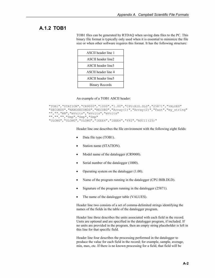
Appendix A. Campbell Scientific File Formats
A-2
A.1.2 TOB1 TOB1 files can be generated by RTDAQ when saving data files to the PC. This binary file format is typically only used when it is essential to minimize the file size or when other software requires this format. It has the following structure:
ASCII header line 1
ASCII header line2
ASCII header line3
ASCII header line 4
ASCII header line5
Binary Records
An example of a TOB1 ASCII header:
"TOB1","STATION","CR9000","1000","1.00","CPU:BIG.DLD","25871","VALUES" "SECONDS","NANOSECONDS","RECORD","Array(1)","Array(2)","Fast","my_string" "","","RN","mVolts","mVolts","mVolts" "","","","Smp","Smp","Smp" "ULONG","ULONG","ULONG","IEEE4","IEEE4","FP2","ASCII(25)"
Header line one describes the file environment with the following eight fields:
• Data file type (TOB1).
• Station name (STATION).
• Model name of the datalogger (CR9000).
• Serial number of the datalogger (1000).
• Operating system on the datalogger (1.00).
• Name of the program running in the datalogger (CPU:BIB.DLD).
• Signature of the program running in the datalogger (25871).
• The name of the datalogger table (VALUES).
Header line two consists of a set of comma-delimited strings identifying the names of the fields in the table of the datalogger program.
Header line three describes the units associated with each field in the record. Units are optional and are specified in the datalogger program, if included. If no units are provided in the program, then an empty string placeholder is left in this line for that specific field.
Header line four describes the processing performed in the datalogger to produce the value for each field in the record; for example, sample, average, min, max, etc. If there is no known processing for a field, that field will be
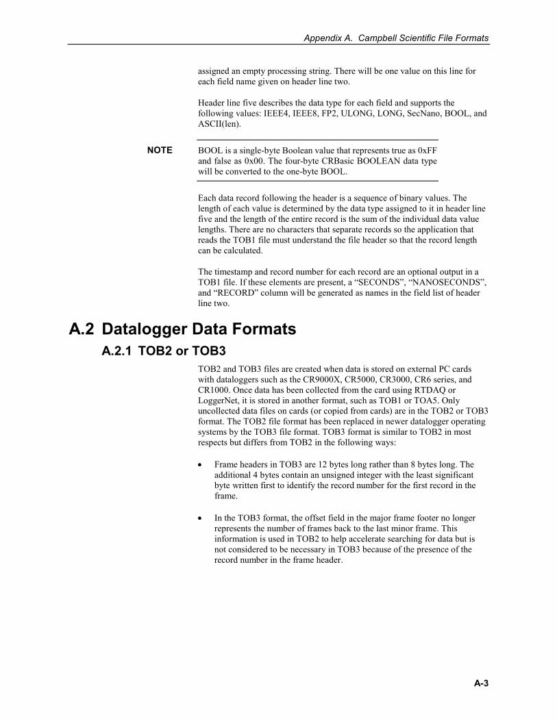
Appendix A. Campbell Scientific File Formats
A-3
assigned an empty processing string. There will be one value on this line for each field name given on header line two.
Header line five describes the data type for each field and supports the following values: IEEE4, IEEE8, FP2, ULONG, LONG, SecNano, BOOL, and ASCII(len).
BOOL is a single-byte Boolean value that represents true as 0xFF and false as 0x00. The four-byte CRBasic BOOLEAN data type will be converted to the one-byte BOOL.
Each data record following the header is a sequence of binary values. The length of each value is determined by the data type assigned to it in header line five and the length of the entire record is the sum of the individual data value lengths. There are no characters that separate records so the application that reads the TOB1 file must understand the file header so that the record length can be calculated.
The timestamp and record number for each record are an optional output in a TOB1 file. If these elements are present, a “SECONDS”, “NANOSECONDS”, and “RECORD” column will be generated as names in the field list of header line two.
A.2 Datalogger Data Formats A.2.1 TOB2 or TOB3
TOB2 and TOB3 files are created when data is stored on external PC cards with dataloggers such as the CR9000X, CR5000, CR3000, CR6 series, and CR1000. Once data has been collected from the card using RTDAQ or LoggerNet, it is stored in another format, such as TOB1 or TOA5. Only uncollected data files on cards (or copied from cards) are in the TOB2 or TOB3 format. The TOB2 file format has been replaced in newer datalogger operating systems by the TOB3 file format. TOB3 format is similar to TOB2 in most respects but differs from TOB2 in the following ways:
• Frame headers in TOB3 are 12 bytes long rather than 8 bytes long. The additional 4 bytes contain an unsigned integer with the least significant byte written first to identify the record number for the first record in the frame.
• In the TOB3 format, the offset field in the major frame footer no longer represents the number of frames back to the last minor frame. This information is used in TOB2 to help accelerate searching for data but is not considered to be necessary in TOB3 because of the presence of the record number in the frame header.
NOTE
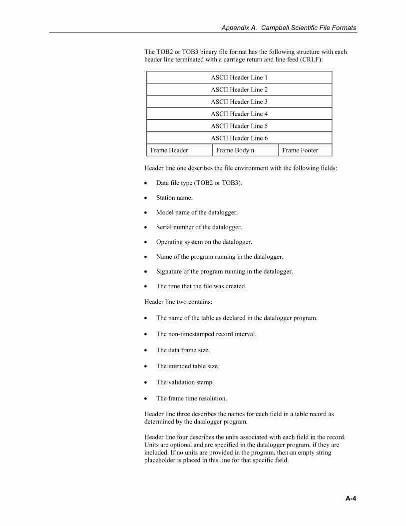
Appendix A. Campbell Scientific File Formats
A-4
The TOB2 or TOB3 binary file format has the following structure with each header line terminated with a carriage return and line feed (CRLF):
ASCII Header Line 1
ASCII Header Line 2
ASCII Header Line 3
ASCII Header Line 4
ASCII Header Line 5
ASCII Header Line 6
Frame Header Frame Body n Frame Footer Header line one describes the file environment with the following fields:
• Data file type (TOB2 or TOB3).
• Station name.
• Model name of the datalogger.
• Serial number of the datalogger.
• Operating system on the datalogger.
• Name of the program running in the datalogger.
• Signature of the program running in the datalogger.
• The time that the file was created.
Header line two contains:
• The name of the table as declared in the datalogger program.
• The non-timestamped record interval.
• The data frame size.
• The intended table size.
• The validation stamp.
• The frame time resolution.
Header line three describes the names for each field in a table record as determined by the datalogger program.
Header line four describes the units associated with each field in the record. Units are optional and are specified in the datalogger program, if they are included. If no units are provided in the program, then an empty string placeholder is placed in this line for that specific field.
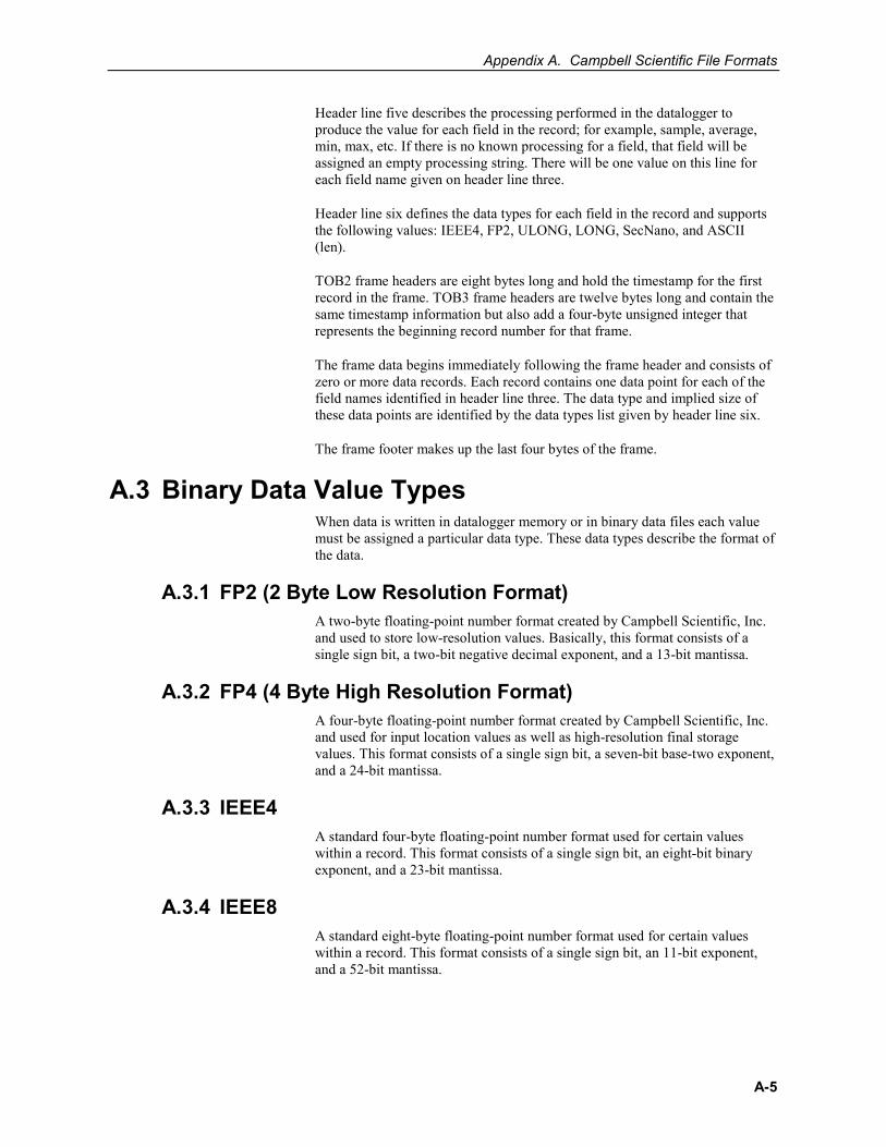
Appendix A. Campbell Scientific File Formats
A-5
Header line five describes the processing performed in the datalogger to produce the value for each field in the record; for example, sample, average, min, max, etc. If there is no known processing for a field, that field will be assigned an empty processing string. There will be one value on this line for each field name given on header line three.
Header line six defines the data types for each field in the record and supports the following values: IEEE4, FP2, ULONG, LONG, SecNano, and ASCII (len).
TOB2 frame headers are eight bytes long and hold the timestamp for the first record in the frame. TOB3 frame headers are twelve bytes long and contain the same timestamp information but also add a four-byte unsigned integer that represents the beginning record number for that frame.
The frame data begins immediately following the frame header and consists of zero or more data records. Each record contains one data point for each of the field names identified in header line three. The data type and implied size of these data points are identified by the data types list given by header line six.
The frame footer makes up the last four bytes of the frame.
A.3 Binary Data Value Types When data is written in datalogger memory or in binary data files each value must be assigned a particular data type. These data types describe the format of the data.
A.3.1 FP2 (2 Byte Low Resolution Format) A two-byte floating-point number format created by Campbell Scientific, Inc. and used to store low-resolution values. Basically, this format consists of a single sign bit, a two-bit negative decimal exponent, and a 13-bit mantissa.
A.3.2 FP4 (4 Byte High Resolution Format) A four-byte floating-point number format created by Campbell Scientific, Inc. and used for input location values as well as high-resolution final storage values. This format consists of a single sign bit, a seven-bit base-two exponent, and a 24-bit mantissa.
A.3.3 IEEE4 A standard four-byte floating-point number format used for certain values within a record. This format consists of a single sign bit, an eight-bit binary exponent, and a 23-bit mantissa.
A.3.4 IEEE8 A standard eight-byte floating-point number format used for certain values within a record. This format consists of a single sign bit, an 11-bit exponent, and a 52-bit mantissa.
Appendix A. Campbell Scientific File Formats
A-6
A.4 Converting Binary File Formats Campbell Scientific dataloggers not only use the previously mentioned binary file formats but users may also choose to use and access these binary formats on the PC. Binary files may be output as data files to the PC by RTDAQ to save hard disk space or to accommodate a user who is only interested in using binary files in an application. In addition, PC cards that are written by the datalogger will contain binary files that can be accessed directly by the PC.
Binary files cannot be interpreted through mere visual inspection. Therefore, binary file processing tools are available to read and convert these binary data files to ASCII text. These conversion tools are Split and CardConvert. Refer to earlier sections of this manual for complete information on Split and CardConvert.
A.4.1 Split Split has the capability of reading TOB1, TOB2, and TOB3 files and displaying data from those files in ASCII format. The output parameters are user specified and Split generates a file containing the converted ASCII format values.
A.4.2 View Pro View Pro converts TOB1, TOB2 and TOB3 data files and generates a new TOA5 file. Once the TOA5 file is generated, View Pro can display the converted data. In that sense, View Pro is a software tool that combines the conversion of binary files to TOA5 with the ability to view the data once the file has been converted.
A.4.3 CardConvert The CardConvert program can convert TOB1, TOB2, and TOB3 files to TOA5 file format or can convert TOA5 files to TOB1 file format.
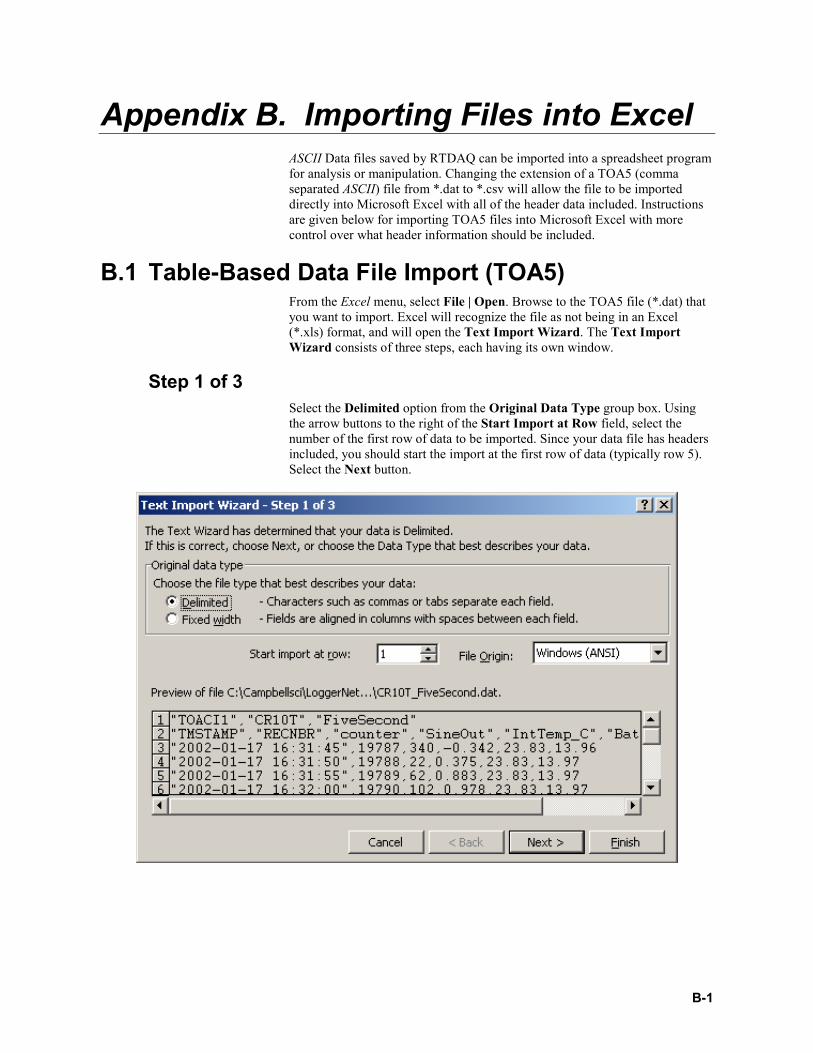
B-1
Appendix B. Importing Files into Excel ASCII Data files saved by RTDAQ can be imported into a spreadsheet program for analysis or manipulation. Changing the extension of a TOA5 (comma separated ASCII) file from *.dat to *.csv will allow the file to be imported directly into Microsoft Excel with all of the header data included. Instructions are given below for importing TOA5 files into Microsoft Excel with more control over what header information should be included.
B.1 Table-Based Data File Import (TOA5) From the Excel menu, select File | Open. Browse to the TOA5 file (*.dat) that you want to import. Excel will recognize the file as not being in an Excel (*.xls) format, and will open the Text Import Wizard. The Text Import Wizard consists of three steps, each having its own window.
Step 1 of 3 Select the Delimited option from the Original Data Type group box. Using the arrow buttons to the right of the Start Import at Row field, select the number of the first row of data to be imported. Since your data file has headers included, you should start the import at the first row of data (typically row 5). Select the Next button.
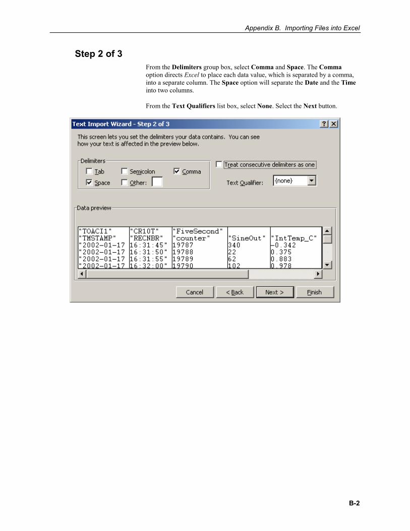
Appendix B. Importing Files into Excel
B-2
Step 2 of 3 From the Delimiters group box, select Comma and Space. The Comma option directs Excel to place each data value, which is separated by a comma, into a separate column. The Space option will separate the Date and the Time into two columns.
From the Text Qualifiers list box, select None. Select the Next button.
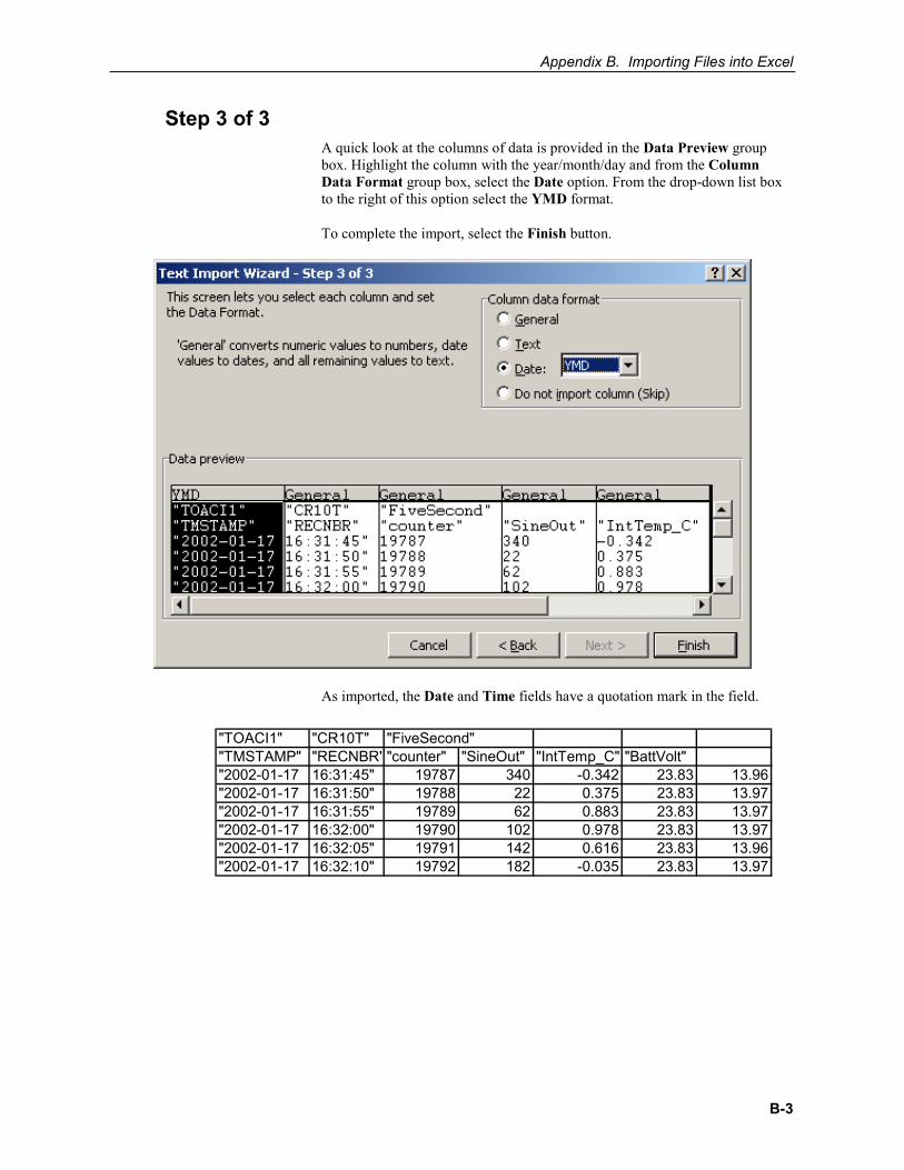
Appendix B. Importing Files into Excel
B-3
Step 3 of 3 A quick look at the columns of data is provided in the Data Preview group box. Highlight the column with the year/month/day and from the Column Data Format group box, select the Date option. From the drop-down list box to the right of this option select the YMD format.
To complete the import, select the Finish button.
As imported, the Date and Time fields have a quotation mark in the field.
"TOACI1" "CR10T" "FiveSecond""TMSTAMP" "RECNBR" "counter" "SineOut" "IntTemp_C" "BattVolt""2002-01-17 16:31:45" 19787 340 -0.342 23.83 13.96"2002-01-17 16:31:50" 19788 22 0.375 23.83 13.97"2002-01-17 16:31:55" 19789 62 0.883 23.83 13.97"2002-01-17 16:32:00" 19790 102 0.978 23.83 13.97"2002-01-17 16:32:05" 19791 142 0.616 23.83 13.96"2002-01-17 16:32:10" 19792 182 -0.035 23.83 13.97
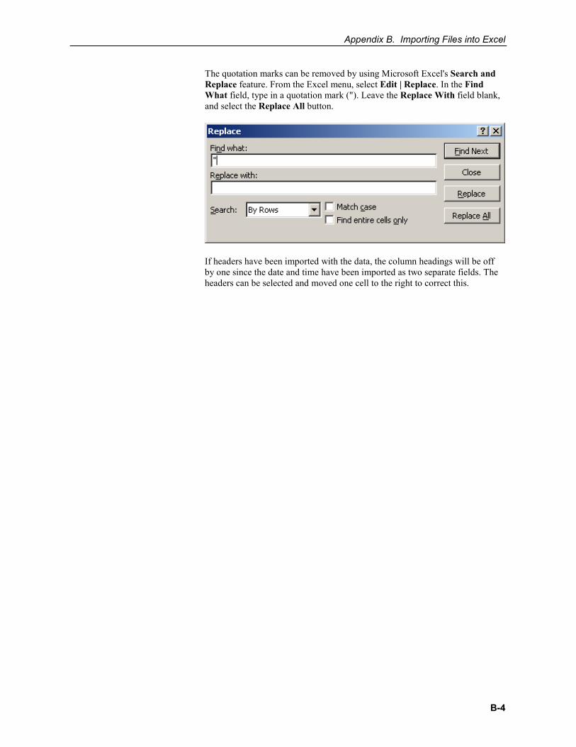
Appendix B. Importing Files into Excel
B-4
The quotation marks can be removed by using Microsoft Excel's Search and Replace feature. From the Excel menu, select Edit | Replace. In the Find What field, type in a quotation mark ("). Leave the Replace With field blank, and select the Replace All button.
If headers have been imported with the data, the column headings will be off by one since the date and time have been imported as two separate fields. The headers can be selected and moved one cell to the right to correct this.

AustraliaLocation:Phone:Email:Website:
Garbutt, QLD Australia61.7.4401.7700info@campbellsci.com.auwww.campbellsci.com.au
BrazilLocation:Phone:Email:Website:
São Paulo, SP Brazil11.3732.3399vendas@campbellsci.com.brwww.campbellsci.com.br
CanadaLocation:Phone:Email:Website:
Edmonton, AB [email protected]
ChinaLocation:Phone:Email:Website:
Beijing, P. R. China86.10.6561.0080info@campbellsci.com.cnwww.campbellsci.com.cn
Costa RicaLocation:Phone:Email:Website:
San Pedro, Costa [email protected]
FranceLocation:Phone:Email:Website:
Vincennes, [email protected]
GermanyLocation:Phone:Email:Website:
Bremen, [email protected]
IndiaLocation:Phone:Email:Website:
NewDelhi, DL [email protected]
South AfricaLocation:Phone:Email:Website:
Stellenbosch, South [email protected]
SpainLocation:Phone:Email:Website:
Barcelona, [email protected]
ThailandLocation:Phone:Email:Website:
Bangkok, [email protected]
UKLocation:Phone:Email:Website:
Shepshed, Loughborough, [email protected]
USALocation:Phone:Email:Website:
Logan, UT [email protected]