role of specific humidity anomalies in caribbean sst response to enso
TRANSCRIPT

Instructions for use
Title Role of Specific Humidity Anomalies in Caribbean SSTResponse to ENSO
Author(s) CHIKAMOTO, Yoshimitsu; TANIMOTO, Youichi
Citation Journal of the Meteorological Society of Japan, 83(6): 959-975
Issue Date 2005-12-26
Doc URL http://hdl.handle.net/2115/14528
Right
Type article
AdditionalInformation
Hokkaido University Collection of Scholarly and Academic Papers : HUSCAP

Role of specific humidity anomalies in
Caribbean SST response to ENSO
Yoshimitsu Chikamoto
Graduate School of Environmental Earth Science, Hokkaido University, Sapporo, Japan
Youichi Tanimoto
Faculty of Environmental Earth Science, Hokkaido University, Sapporo, Japan
(Received 6 April 2005; revised 25 July 2005; final 19 August 2005)
Yoshimitsu Chikamoto, Graduate School of Environmental Earth Science, Hokkaido
University, N10W5, Kita-ku, Sapporo, 060-0810, Japan.
E-mail: [email protected]

ABSTRACT
Remote influences of El Nino-Southern Oscillation (ENSO) on tropical Atlantic sea
surface temperature (SST) are examined using reanalysis and in-situ observational datasets.
During both the warm and cold events of ENSO, latent heat flux anomalies are the major
mechanism for SST anomalies over the Caribbean Sea. Results from a linear decomposition
of the latent heat flux anomalies indicate that the anomalous air-sea difference in specific
humidity (∆q′) is the dominant term in January, one month after the ENSO’s mature phase.
Since anomalies of SST and saturation specific humidity at the sea surface are still small in
January, ∆q′ is due mostly to changes in specific humidity in the lower atmosphere. Changes
in surface air humidity and temperature and their relationship to temperature variability in
the upper troposphere during ENSO warm events are discussed.
(i)

1. Introduction
Sea surface temperature anomalies (SSTAs) in the northern tropical Atlantic (NTA)
play an important role in pan-Atlantic climate variabilities because SSTA distribution
in this region changes the meridional location of the Atlantic inter-tropical convergence
zone (e.g., the review of Xie and Carton 2004). On interannual and decadal timescales,
several mechanisms are involved in the tropical Atlantic SST variability: Atlantic Nino
(Zebiak 1993; Sutton et al. 2000; Okumura and Xie 2004) and pan-Atlantic decadal oscillation
(Xie and Tanimoto 1998; Rajagopalan et al. 1998; Tanimoto and Xie 1999; Tourre et al. 1999;
Okumura et al. 2001). In addition to these mechanisms seen in the tropical Atlantic, remote
influences of El Nino-Southern Oscillation (ENSO) are shown by previous observational
studies. While ENSO warm (cold) events tend to be mature in boreal winters, positive
(negative) SSTAs in the NTA region are formed in the boreal spring-summer season, a
few months later, after the mature phase of the events in the tropical Pacific (Curtis and
Hastenrath 1995; Klein et al. 1999). The ENSO index explains 20-30% of the total SST
variance in the boreal spring-summer season over the NTA region (Enfield and Mayer 1997;
Liu et al. 2004).
Observational studies showed that these boreal spring SSTAs in the NTA region are
mainly formed by the preceding surface latent heat flux variabilities as a remote response
to ENSO (Curtis and Hastenrath 1995; Klein et al. 1999). During the mature phase
of the ENSO warm (cold) events, the sea level pressure anomalies tend to be positive
(negative) over the equatorial Atlantic and negative (positive) over the subtropical North
Atlantic (Giannini et al. 2000; Wang 2002), which reduce (enhance) the meridional pressure
gradient and weaken (strengthen) the climatological northeasterly trades. These weakened
1

(strengthened) northeasterly trades in boreal winter reduce (enhance) latent heat release
from the ocean surface and lead to warm (cold) SSTAs in the boreal spring. These anomalous
surface winds and associated latent heat release over the NTA region are reproduced by the
remote response to tropical Pacific SST variabilities in the atmospheric general circulation
model (AGCM) experiments coupled with the slab ocean mixed layer model (Lau and
Nath 2001; Alexander and Scott 2002). Huang et al. (2002), using the locally coupled
atmosphere-ocean GCM only in the Atlantic sector, suggested that initial changes in the
boreal winter surface wind in the NTA region during the mature phase of the ENSO events
maintain SSTAs via wind-evaporation-SST feedback (Xie and Philander 1994).
In contrast, Saravanan and Chang (2000) showed that not only anomalous surface wind
but also anomalous air-sea temperature differences are crucial in determining the surface
heat flux anomalies in the NTA region during the mature phase of the ENSO events. They
conducted two AGCM experiments: one forced by the prescribed SSTAs in the entire
tropical ocean and the other by those only in the tropical Atlantic. From difference fields
of these two experiments, they estimated each of the contributions from the anomalous
surface wind speed (W ′) and the anomalous air-sea temperature difference (∆T ′) to the
surface turbulent heat flux anomalies (F ′est; sum of latent and sensible heat flux anomalies)
by linearizing the aerodynamic bulk formula as follows:
F ′est = cW ′∆T + cW∆T ′, (1)
where c is a constant coefficient evaluated from the climatological means of the surface
turbulent heat flux, wind speed (W ), and air-sea temperature difference (∆T ). In their
model, regressed anomalies of the first and second terms on the right-hand side onto the
Nino3 index showed comparable contributions to surface turbulent heat flux anomalies in
2

the NTA region after the mature phase of the ENSO events.
Chiang and Sobel (2002) proposed a mechanism of the tropical tropospheric response
to the ENSO events (hereafter TT-mechanism) applying the strict quasi-equilibrium (SQE)
concept (Emanuel et al. 1994). Under the SQE, the equivalent potential temperature in
the boundary layer is related to the thermal structure in the free atmosphere so that
the convective available potential energy (CAPE) is conserved over the deep convective
region. In fact, Brown and Bretherton (1997) indicated that the tropospheric temperature
is positively correlated with the boundary layer equivalent potential temperature over active
convecting regions of the tropical oceans on a month and longer timescales. Since tropical
atmosphere can not maintain zonal gradients in temperature and pressure under the weak
Coriolis force, the large-scale dynamics induce zonally uniform temperature anomalies over
most of the tropical belt (Charney 1963; Wallace 1992; Sobel et al. 2002). Therefore,
tropospheric warming associated with the ENSO warm events is found over the most of
tropical oceans (Yulaeva and Wallace 1994; Sobel et al. 2002; Chiang and Sobel 2002),
thereby increasing potential temperature in the boundary layer. These increases of temperature
and humidity affect underlying SSTAs via changes in turbulent heat fluxes. Chiang and
Sobel (2002) suggest that the TT-mechanism operates over the NTA region.
Over the NTA region, turbulent heat flux anomalies are mainly contributed from latent
heat flux anomalies rather than sensible heat flux anomalies (Curtis and Hastenrath 1995;
Alexander and Scott 2002). Therefore, the direct estimation by air-sea differences in specific
humidity (∆q), instead of temperature (Eq. (1)), provides a better estimation on the
linearized components of turbulent heat flux anomalies. This is represented as
F ′est = cW ′∆q + cW∆q′. (2)
3

In this study, we examined the temporal sequence of components in Eq. (2) in the NTA
region after the mature phase of the ENSO events, using monthly mean datasets, both from
assimilated reanalysis data and in-situ marine meteorological observations. In Section 3, we
will show that the second term on the right-hand side of Eq. (2) is much more significant than
the first term in a particular month when SSTAs over the Caribbean Sea are still incoherent.
In the subsequent sections, we will see that the coherent structure of the anomalous air-sea
difference in specific humidity should be induced by changes in the lower atmosphere.
Due to the zonal asymmetry in mean SST and its effect on the deep convection, a
response of anomalous diabatic heating by ENSO and associated changes in the Walker
circulation are not always symmetric between the ENSO warm and cold events. In fact,
spatial patterns of rainfall anomalies over the tropical Pacific do not represent symmetric
responses to ENSO’s extreme phases (Hoerling et al. 1997, 2001; Deweaver and Nigam 2002).
Hence, we will treat the warm and cold phases of the ENSO events separately.
The rest of this paper is organized as follows. Section 2 describes the datasets and defines
the ENSO warm and cold events from the Nino3 index. In Section 3, we calculate each of
the contributions of wind speed anomalies and anomalous air-sea differences in specific
humidity to the total amount of the latent heat flux anomalies. In Section 4, we consider
the asymmetric responses of the linearized components of the latent heat flux anomaly
to the ENSO events, and discuss the formation of these anomalous air-sea differences in
specific humidity based on TT-mechanism during the ENSO warm events. The results are
summarized in Section 5.
2. Datasets
To capture month-to-month variations in the troposphere over the tropical Atlantic ocean
4

after the mature phase of the ENSO events, the monthly latent heat flux from the ocean
surface (upward positive), surface net heat flux, precipitation rate, and specific humidity
at 2-m height are taken from the National Centers for Environmental Prediction-National
Center for Atmospheric Research (NCEP-NCAR) reanalysis (Kalnay et al. 1996) approximately
on a 1.875˚ x 1.875˚ Gaussian grid. The surface net heat flux consists of the latent, sensible,
shortwave, and longwave heat fluxes taken from this dataset. Monthly surface fields of wind
velocity, its speed, and pressure are obtained from the NCEP-NCAR reanalysis data on a
2.5˚ x 2.5˚ grid. Monthly horizontal wind and specific humidity fields at eight pressure
levels of this dataset are also used. The monthly SST data are obtained from the global
sea ice and SST (GISST) on a 1˚ x 1˚ grid (Folland and Parker 1995). From the linearly
interpolated SST and surface pressure, a monthly saturation specific humidity at the ocean
surface is calculated on a 2.5˚ x 2.5˚ grid. We calculate air-sea differences in specific
humidity on a 2.5˚ x 2.5˚ grid between the ocean surface and 2-m height using spherical
harmonic interpolation.
The surface latent heat fluxes of the reanalysis data are less reliable than other elements
in the free atmosphere due to insufficient treatments of the planetary boundary layer.
Therefore, we employ the 2˚ x 2˚ monthly dataset of surface latent heat fluxes based on
individual marine meteorological reports archived in the Comprehensive Ocean-Atmosphere
Data Set (COADS; Woodruff et al. 1987). Although this non-assimilated data may suffer
sampling errors in the region of few marine reports, ship tracks to the Panama Canal
provide a sufficient number of observations in the Caribbean Sea. However, this dataset
contains some missing values over the southern tropical Atlantic and the central equatorial
Atlantic since satellite observations and spatial interpolation were not used. Details of the
calculation procedure are described in Tanimoto and Xie (2002) and Tanimoto et al. (2003).
5

We calculate the monthly climatological means based on a 52-year period (1948-1999) for
NCEP-NCAR reanalysis and GISST datasets, and on a 46-year period (1950-1995) for
COADS. The monthly anomalies are defined as departures from the climatological mean
values.
In Section 4, we will calculate a moisture budget to examine the formation of the air-sea
difference in specific humidity. In reanalysis datasets, however, the moisture budget is not
always conserved due to four-dimensional data assimilation (Trenberth and Guillemot 1995;
Mo and Higgins 1996; Trenberth and Guillemot 1998). For this reason, we will use two
datasets to conduct an accurate estimation of the moisture budget. One is the NCEP-Department
of Energy Reanalysis 2 (NCEP2; Kanamitsu et al. 2002) dataset that is a modified version
of NCEP-NCAR reanalysis. The other is the precipitation obtained from the Climate
Prediction Center’s Merged Analysis of Precipitation (CMAP; Xie and Arkin 1997) dataset
on a 2.5˚ x 2.5˚ grid. Both NCEP2 and CMAP datasets are available from January
1979 to December 1999. A monthly moisture flux is calculated from monthly variables of
horizontal winds and specific humidity on pressure levels in the NCEP2 dataset. A transient
component of monthly moisture flux (q′V′) calculated from 4 times daily of those variables
was negligible over the Caribbean Sea.
To represent the magnitude of the ENSO warm and cold events in the eastern tropical
Pacific, we use time series of SSTAs in the Nino3 region (5˚S-5˚N, 90˚-150˚W) based on
GISST. This time series averaged from November through January in the following year
is defined as the Nino3 index (Fig. 1). In the present study, we refer these three monthsFig. 1
as the mature phase of the ENSO events. We extract eight higher and lower events based
on this index. The eight warm and cold events are listed in Table 1. When we use theTable 1
Nino3 index based on Reynolds Reconstructed SST (Smith et al. 1996) instead of GISST,
6

the 1986/87 and 1987/88 events (the 1964/65 and 1967/68 events) are selected as the 9th
and 8th warmest events (the 8th and 9th cold events), respectively. Including the 1986/87
warm event and the 1964/65 cold event as the additional events to our composite does not
affect our results of the analyses.
3. The formation of SSTAs in the NTA region
To represent the temporal evolution of the ENSO-related SSTAs in the NTA region, we
made three monthly composite maps from December to February during the ENSO warm
events (Figs. 2a, 2b, and 2c). In December, no coherent structure of SSTAs appears inFig. 2
this region, while the tropical Pacific SSTAs are already mature (Fig. 2a). In the following
January, when matured SSTAs in the tropical Pacific gradually decrease, positive SSTA
regions higher than 0.2 C emerge in the southwestern parts of the Caribbean Sea and
equatorial eastern Atlantic (Fig. 2b). Furthermore, in February, the former positive SSTA
region expands to the entire Caribbean Sea, and the latter extends its area to 20˚N along
the west coast of Africa (Fig. 2c). These results indicate that SSTAs in the NTA region
during the ENSO warm events begin to be formed in the January-February period. These
SSTAs over the Caribbean Sea reach a local maximum in boreal summer, as shown later
(Fig. 4d). In addition to these positive SSTAs, a significant negative SSTA region is observed
in the Gulf of Mexico and off the east coast of North America during February (Fig. 2c).
Figures 2d-f and 2g-i show the same composite maps of SSTA tendencies and surface
latent heat flux anomalies, respectively. SSTA tendency in a given month is defined as the
difference between the SSTA in the subsequent month and that in the previous month. In
December, this tendency (Fig. 2d) is incoherent and inconsistent with the latent heat flux
anomalies (Fig. 2g). In the following January, it becomes coherent in three portions of the
7

NTA region: the Caribbean Sea, off the west coast of Africa, and the extratropical region
over the Gulf of Mexico and off the east coast of North America (Fig. 2e). Among these
regions, the coherent structures of positive SSTA tendencies in the Caribbean Sea (Figs.
2e and 2f) collocate with the zonal elongated region of the anomalous latent heat flux of
−15 W m−2 appearing in the January-February period (Figs. 2h and 2i), while sensible heat
flux anomaly is less than −5 W m−2 in this region (not shown). As shown in the previous
studies introduced in Section 1, these latent heat flux anomalies, which explain most of the
turbulent heat flux anomalies, contribute in forming positive SSTAs over the NTA region
in this period.
Given that SSTA tendencies of 0.2 C/2-month are only due to surface latent heat flux
anomalies of −15 W m−2 in the Caribbean region, we obtain an equivalent mixed layer
depth of 100-m, comparable to an observed isothermal layer in the northern Caribbean
Sea in January (Kara et al. 2003)1. This means that surface heat flux anomaly mainly
contributes to the SSTA formation on that region. SSTA tendencies off the west coast of
Africa in January, on the other hand, are about 0.5 C/2-month, while negative latent heat
flux anomalies are less than 7.5 W m−2 around the same region. In this case, an equivalent
mixed layer corresponds to 20-m depth. The observed isothermal layer off the west coast of
Africa is deeper than this equivalent mixed layer depth, implying that SSTA in this region is
controlled by coastal upwelling induced by local alongshore winds (Carton and Zhou 1997).
In the Gulf of Mexico and off the east coast of North America during January, the local
maximum in SSTA tendencies of −1.0 C/2-month and positive latent heat flux anomalies
of 15 W m−2 correspond to the equivalent mixed layer depth of 20-m. This underestimation
1Kara et al. (2003) provided monthly climatologies of isothermal layer depth that is defined as the depth
where water temperature has changed by an absolute temperature difference of 0.8 C from the surface layer.
8

of equivalent mixed layer depth suggests that the other components of net surface heat flux
anomalies or ocean dynamic processes contribute to the negative SSTA formation in the
Gulf of Mexico and the east coast of North America. Alexander and Scott (2002) suggested
that the sensible heat flux anomalies, in addition to the latent heat flux anomalies, are
important in cooling ocean along the coast of North America.
Over the negative latent heat flux anomalies in the Caribbean region, we found a coherent
pattern of anomalous surface southerly and southwesterly winds in January (Fig. 2h). Given
that these surface winds weaken by 0.5 m s−1 in northeasterly climatological trade winds,
the contribution of wind speed anomalies to latent heat flux anomalies is about 9.3 W m−2
under the climatological air-sea difference in specific humidity. However, negative latent
heat flux anomalies of −15 W m−2 over the Caribbean region imply that changes in the
air-sea difference in specific humidity are also involved in latent heat flux anomalies. Each
contribution from changes in wind speed and air-sea difference in specific humidity to the
latent heat flux anomaly will be estimated later.
During the ENSO cold events, coherent SSTAs over the Caribbean region appear in
December, one month earlier than the warm events, extending its area northeastward with
latitude (Fig. 3a). These negative SSTAs over the Caribbean region tend to be local maximaFig. 3
in the following January (Fig. 3b) and further extends its area to the west coast of Africa
in the subsequent February (Fig. 3c). Despite differences in initial months in the SSTA
formation between the ENSO warm and cold events, the spatial structures of SSTAs over
the Caribbean region and off the west coast of Africa in February show similar patterns
with opposite polarity of the ENSO warm events (Figs. 2c and 3c). In the Gulf of Mexico
and off the east coast of North America, however, SSTAs are incoherent from December
through to the following February during the ENSO cold events.
9

Monthly composite maps of SSTA tendencies and latent heat flux anomalies during the
ENSO cold events are shown in Figs. 3d-i. As in the warm events, SSTA tendencies during
the cold events are mostly explained by latent heat flux anomalies over the Caribbean Sea in
the December-January period, while coherent SSTA tendencies in the other regions require
other SSTA formation processes (Figs. 3d, 3e, 3g, and 3h). The anomalous surface winds
during the cold events are insufficient in explaining the latent heat flux anomalies over the
Caribbean region, indicating anomalous air-sea differences in specific humidity involved in
latent heat flux anomalies.
The latent heat flux anomaly can be decomposed into three linearized components as in
Tanimoto et al. (2003):
F ′lh = ρceLe{W ′∆q + W∆q′ + (W ′∆q′ − W ′∆q′)} (3)
where Flh is the latent heat flux, W is the scalar wind speed, ∆q is the air-sea difference in
specific humidity, ρ is the atmospheric density, ce is the bulk coefficient, Le is the latent heat
of vaporization for water, and the overbar and prime indicate the time mean and deviation,
respectively. The bulk coefficients are assumed to be constant in NCEP-NCAR reanalysis
and to be dependent on scalar wind speed and static stability in COADS. However, when
we linearize the surface heat flux anomalies, we ignore the dependence of the coefficients on
those variables. On the right-hand side of (3), the first two terms represent contributions
of the wind speed anomaly (W ′) and the anomalous air-sea difference in specific humidity
(∆q′) to the total amount of latent heat flux anomalies, respectively. As we will show later,
the last term becomes negligible.
Figures 4a-c and 4e-g show the time evolutions of individual contributions (W ′∆q, W∆q′)
to latent heat flux anomalies during the ENSO warm and cold events. Note that the verticalFig. 4
10

axes of heat flux anomalies are reversed for easier comparison with SSTAs. As shown in Figs.
2 and 3, SSTAs over the Caribbean Sea are formed in February, and show a local maximum in
boreal summer during the both phases of ENSO (solid lines in Figs. 4d and 4h). A correlation
analysis shows that the Nino3 index is positively correlated with monthly SSTAs in the
Caribbean Sea from February to July. These positive correlations indicate that the ENSO
variability explains 20-30% of the total variance in each of months, consistent with previous
results (Enfield and Mayer 1997; Liu et al. 2004). During both phases of these events, the
total amount of latent heat flux anomalies averaged over the Caribbean Sea (dashed lines
in Figs. 4c and 4g) is well represented by the sum of W ′∆q and W∆q′ components. These
latent heat flux anomalies contribute to the most of the net surface heating anomaly that is
a 90-degree out of phase with the SSTAs from boreal winter through summer (Figs. 4d and
4h). For the latent heat flux anomalies during the warm events, the contribution of ∆q′ in
January, which is three times larger than that of W ′, accounts for 64% of the total latent
heat flux anomaly of 18 W m−2 (Figs. 4a-c) . These two linearized components tend to
be comparable from February through to May, and counteracting to each other from June
through August (Figs. 4a and 4b). This counteracting effect induces negative SST tendency
during the boreal summer. During the cold events, the contributions of ∆q′ are important
in representing local maxima in latent heat flux anomalies in the December-January period
(Fig. 4f), while contributions of W ′ are considerably larger from December through to the
following April (Fig. 4e). From May through July, the contributions of W ′ are counteracting
those of ∆q′. These results indicate that ∆q′ in January specifically plays an important role
in forming latent heat flux anomalies over the Caribbean Sea during both phases of the
ENSO events. Note that the contribution of ∆q′ is well captured during the ENSO warm
events rather than the cold events. This asymmetry between the warm and cold events will
11

be examined in the next section.
January composite maps of the linearized components of latent heat flux anomalies
during the ENSO warm events were constructed in Figs. 5a and 5b. The sum of the twoFig. 5
linearized components (Fig. 5c) shows a zonally elongated pattern of negative (positive)
anomalies extended from the Caribbean Sea off to the west coast of Africa (over the
Gulf of Mexico and off the east coast of North America). These coherent anomalies are
quantitatively and qualitatively consistent with the anomalous pattern of total latent heat
flux anomalies (Fig. 2h). In the Caribbean Sea, the contribution of ∆q′ is 20 W m−2 near
the center of action, while the contribution of W ′ is only 5 W m−2 in the same region.
These results show that ∆q′ is the major contributor to latent heat flux anomalies over the
Caribbean Sea in a particular month after the mature phase of the ENSO warm events.
Based on the in-situ observational data obtained from COADS, the contributions of ∆q′
(Fig. 5e) are larger than those of W ′ (Fig. 5d) in the Caribbean Sea. The sum of these
linearized components explains the most variance of the latent heat flux anomalies over the
NTA region (not shown), although there are many noisy values as well as some missing
values due to insufficient measurements in the central equatorial Atlantic.
During the ENSO cold events, January composite maps of individual contributions to
latent heat flux anomalies based on both datasets show robust structures as in the warm
events (Fig. 6). These composite maps show that about half of the latent heat flux anomaliesFig. 6
over the Caribbean Sea and the Gulf of Mexico can be explained by ∆q′.
For the formation of SSTAs over the NTA region associated with the ENSO events,
previous studies indicated the importance of W ′ to induce changes in latent heat flux (e.g.,
Curtis and Hastenrath 1995; Enfield and Mayer 1997; Lau and Nath 2001). However,
our observational results showed that the contributions of ∆q′ are necessary in forming
12

substantial latent heat flux anomalies. These results are consistent with the estimation from
the anomalous air-sea difference in “temperature” in the AGCM experiments by Saravanan
and Chang (2000).
4. Discussion
a. Asymmetric latent heat flux anomalies to the ENSO activity
To see whether the surface meteorological variables in the Caribbean Sea linearly respond
to the ENSO events, we made January scatter plots of W ′ and ∆q′ onto the Nino3 index
(Figs. 7a and 7b). For the total number (51 years) of scatters, ∆q′ is correlated with the indexFig. 7
(correlation coefficient, r=−0.49), while W ′ is less correlated (r=−0.24). The regressed ∆q′
and W ′ onto the Nino3 index are −0.16 g kg−1 and −0.17 m s−1 over the Caribbean Sea,
inducing −5.6 W m−2 and −3.0 W m−2 of latent heat flux anomalies, respectively. As
shown with the composite analysis in Section 3, correlation analysis also shows that ∆q′
rather than W ′ contributes to form latent heat flux anomalies over the Caribbean Sea.
When we examine the correlation of ∆q′ during positive and negative values of the
Nino3 index separately, we find the asymmetric response of ∆q′ over the Caribbean Sea to
the ENSO events (Fig. 7b). During years with the positive values of the Nino3 index (23
years), 15 scatters of ∆q′ (65% of all positive index years) are in the lower-right quadrant,
and tend to be linear with the index. Similarly, six closed scatters among eight warm events
are plotted in the lower-right quadrant. During years with the negative values (28 years),
on the other hand, 15 years (56% of all negative index years) are plotted over the upper-left
quadrant. However, since only two closed scatters among the eight cold events are plotted in
this quadrant, the linear relation of scatters onto the index is not so apparent. As a result,
13

∆q′ is strongly correlated with the positive Nino3 index (r=−0.66) rather than the negative
(r=−0.30). The correlation coefficients of W ′ are less significant regardless of the sign of
the index, being −0.18 and −0.33 during positive and negative Nino3 index, respectively
(Fig. 7a).
In January during the positive Nino3 index, ∆q′ over the Caribbean Sea is not correlated
with SSTA (r=0.14, not shown), but strongly correlated with a specific humidity anomaly
at 2-m height (q′a) (r=−0.67, not shown). Scatter plots of q′a onto the Nino3 index (Fig.
7c) show strong correlation (r=0.71) regardless of the sign of the index. Specifically, during
the positive Nino3 index, 21 scatters among 23 years are in the upper-right quadrant, and
tend to be much more linear with the index. By contrast, scatters during the negative
Nino3 index are both in the upper- and lower-left quadrants, and do not show the linear
relation with the index. As a result, a correlation coefficient of q′a during the positive index
is much significant (r=0.79). These asymmetric responses between the positive and the
negative Nino3 indices may reflect asymmetry in the Nino3 SSTA; the dominant ENSO
events exceeding the Nino3 SSTA of 2.0 C exist during the warm events but not during the
cold events (Figs. 1 and 7). Since the changes in q′a are most pronounced during the positive
Nino3 index, we will examine how q′a is formed over the Caribbean region during the warm
events.
b. Changes in surface air humidity and temperature and their relationship to
temperature variability in the upper troposphere during ENSO warm events
To see the horizontal structures of q′a and ∆q′, we construct composite maps of these
variables in January during the ENSO warm events (Fig. 8). A tongue-like structure ofFig. 8
positive q′a and the same structure but with opposite polarity of ∆q′ extend northeastward
14

from the Caribbean Sea, indicating that q′a explains most of ∆q′ on that region. By contrast,
these two variables show the same polarity over the equatorial Pacific because positive q′a
is induced by warm SSTAs (Kleeman et al. 2001). These different characteristics between
the Atlantic and Pacific oceans imply that the positive q′a over the Caribbean region, under
small SSTAs (Fig. 2b), should be formed by atmospheric processes induced by the ENSO
forcing.
Figure 9 shows the January composite map of temperature anomaly at 400 hPa during
the ENSO warm events. Associated with the tongue-like structure of positive q′a over theFig. 9
Caribbean region (Fig. 8a), positive temperature anomalies at 400 hPa also appear over this
region extending from the eastern tropical Pacific (Fig. 9). Tropospheric mean temperature
anomalies estimated from the microwave sounding unit also show the same structure over
the tropics (Yulaeva and Wallace 1994; Chiang and Sobel 2002). Over the Caribbean Sea,
temperature anomalies at 400 hPa show significant positive correlations with q′a and surface
air temperature anomalies in January (r=0.74 and 0.75, respectively). These results imply
that the temperature anomaly in the free atmosphere is closely related to the boundary
layer equivalent potential temperature anomaly, which is consistent with the SQE concept
(Emanuel et al. 1994; Brown and Bretherton 1997) that requires conservation of the CAPE
in the troposphere.
Figure 10 shows the time evolutions of surface air temperature anomaly and SSTA
(thick solid and dashed lines, respectively) over the Caribbean Sea during the ENSO warm
events. The air temperature anomalies lead the SSTAs until May except for February inFig. 10
COADS, and show largest difference from SSTAs in January. The q′a also exhibits the
similar behavior to the surface air temperature anomaly (Fig. 4b) because a surface relative
humidity generally remains constant in the tropics. Associated with these largest ∆T ′ and
15

∆q′, air temperature anomalies at 400 hPa (thin solid line in Fig. 10) also reach a maximum
in January, implying that temperature warming in the free atmosphere is closely related to
the surface temperature and humidity anomalies. As results, these changes in ∆q′ of 0.3
g kg−1 and ∆T ′ of 0.3 C induce latent heat flux anomaly of 11 W m−2 and sensible heat
flux anomaly of 4 W m−2, respectively, under the January climatological wind speed over
the Caribbean Sea.
c. Moisture balance over the Caribbean Sea
Associated with the humidity variation in the boundary layer, we expect changes in
the hydrological processes. To see the changes, we diagnose a vertical integrated moisture
budget equation as follows:
E ′est =
1
g
∫ Ps
300
∇ · (qV)′dp + P ′, (4)
where Ps is the pressure surface, V is the horizontal component of the velocity vector,
P is the precipitation, and E is the evaporation from the ocean surface. As a result,
Eq. (4) indicates that a change in evaporation is diagnostically determined by changes in
atmospheric hydrological processes: the moisture flux anomaly divergence and the precipitation
anomaly. This diagnostic equation does not necessary mean that the terms on the right-hand
side are always independent of each other.
When we use the precipitation anomaly of CMAP (P ′CMAP) and the moisture flux
anomaly divergence of NCEP2 (∇ · (qV)′), E ′est is in good agreement with the evaporation
of NCEP2 (E ′) in January during the ENSO warm events (Fig. 11a). Due to the smallFig. 11
precipitation anomaly during that time, the negative anomaly of the moisture flux divergence
nearly balances the suppressed evaporation, which is consistent with the positive q′a over the
Caribbean region (Fig. 8a). Using the precipitation based on NCEP2 instead of CMAP, this
16

anomalous moisture flux convergence still contributes to the suppressed surface evaporation
(Fig. 11b), and can be mainly explained by the contribution of anomalous wind convergence
(−∇ · (qV)′ ≈ −q∇ · V′), as described below. Over the Caribbean region, the anomalous
moisture transport is represented by the product of anomalous wind and climatological
specific humidity (∇·(qV)′ ≈ ∇·(qV′)) because the ratio of the anomaly to the climatology
in winds is greater than that in specific humidity (V′/V ∼ 10−1 and q′/q ∼ 10−2). In
addition, the anomalous wind advection is relatively small (i.e., ∇ · (qV′) ≈ q∇ · V′)
because the climatological specific humidity is almost uniform around the Caribbean Sea.
During the ENSO warm events, surface northwesterly from the Gulf of Mexico and southerly
from the South America that may be induced by the ENSO forcing tend to converge
over the Caribbean region (Fig. 2h). These results suggest that the suppressed surface
evaporation balances the anomalous moisture flux convergence induced by surface wind
anomaly convergence.
5. Summary
We showed, during the ENSO events, that latent heat flux anomalies in January are
the major contributors in forming SSTAs over the Caribbean Sea (Figs. 2 and 3). Over
this region, the calculation of linearized components of latent heat flux anomalies indicated
that an anomalous air-sea difference in specific humidity (∆q′), rather than a wind speed
anomaly (W ′), plays an important role in generating substantial latent heat flux anomalies
after the mature phases of the ENSO events. Specifically, the contribution of ∆q′ during
the ENSO warm events accounts for 64% of total latent heat flux anomaly in January over
the Caribbean region (Fig. 4).
As mentioned in Section 1, many observational and modeling studies have indicated that
17

W ′ is necessary to the substantial latent heat flux anomalies for forming SSTAs over the
NTA regions during the ENSO events. On the other hand, model experiments conducted by
Saravanan and Chang (2000) suggested the relative importance of ∆T ′ in generating latent
heat flux anomalies. Our composite and correlation analyses for the observational datasets
indicated that, in addition to the W ′, the ∆q′ plays an important role in generating latent
heat flux anomalies over the Caribbean region particularly during the ENSO warm events.
The correlation analysis showed that the ∆q′ over the Caribbean Sea, compared to the
W ′, is significantly correlated with the Nino3 index (Fig. 7). Specifically, the scatter plots
of ∆q′ showed the strong negative correlation with the positive Nino3 index (Fig. 7b). The
January composite maps during the ENSO warm events indicated that the negative ∆q′ over
the Caribbean Sea is collocated with the positive q′a (Fig. 8). Since SSTA over this region
is small (Fig. 2b), this positive q′a should be formed by atmospheric processes. Associated
with this positive q′a over the Caribbean region, positive temperature anomalies at 400 hPa
appear over this region extending from eastern tropical Pacific (Fig. 9), which is consistent
with the TT-mechanism (Chiang and Sobel 2002). Our diagnosis of a moisture budget
equation indicated that the suppressed evaporation nearly balances the anomalous moisture
flux convergence (Fig. 11a).
Acknowledgments. The authors are grateful to Profs. M. Ikeda, K. Yamazaki, A. Kubokawa,
and M. Watanabe for their stimulating discussions. The manuscript benefitted from the
constructive comments by Prof. S.-P. Xie and anonymous reviewers. The NCEP and
NCEP2 datasets were provided by the NOAA-CIRES Climate Diagnostics Center, Boulder,
Colorado, USA, from their website (at http://www.cdc.noaa.gov/). This work was partly
supported by Grand-In-Aid for Scientific Research defrayed by the Ministry of Education,
18

Culture, Sports, Science and Technology of Japan (15540416) and by Category 7 of the
MEXT RR 2002 Project for Sustainable Coexistence of Human, Nature and the Earth.
19

REFERENCES
Alexander, M. A., and J. D. Scott, 2002: The influence of ENSO on air-sea interaction in
the Atlantic. Geophys. Res. Lett., 29, 46, doi:10.1029/2001GL014347.
Brown, R. G., and C. S. Bretherton, 1997: A test of the strict quasi-equilibrium theory on
long time and space scales. J. Atmos. Sci., 54, 624–638.
Carton, J. A., and Z. Zhou, 1997: Annual cycle of sea surface temperature in the tropical
Atlantic Ocean. J. Geophys. Res., 102, 27813–27824.
Charney, J. G., 1963: A note on large-scale motions in the tropics. J. Atmos. Sci., 20,
607–609.
Chiang, J. C. H., and A. H. Sobel, 2002: Tropical tropospheric temperature variations
caused by ENSO and their influence on the remote tropical climate. J. Climate, 15,
2616–2631.
Curtis, S., and S. Hastenrath, 1995: Forcing of anomalous sea surface temperature evolution
in the tropical Atlantic during Pacific warm events. J. Geophys. Res., 100, 15835–15847.
Deweaver, E., and S. Nigam, 2002: Linearity in ENSO’s atmospheric response. J. Climate,
15, 2446–2461.
Emanuel, K. A., J. D. Neelin, and C. S. Bretherton, 1994: On large-scale circulations in
convecting atmospheres. Quart. J. Roy. Meteor. Soc., 120, 1111–1143.
Enfield, D. B., and D. A. Mayer, 1997: Tropical Atlantic sea surface temperature variability
and its relation to El Nino-Southern Oscillation. J. Geophys. Res., 102, 929–945.
Folland, C. K., and D. E. Parker, 1995: Correction of instrumental biases in historical sea
surface temperature data. Quart. J. Roy. Meteor. Soc., 121, 319–367.
20

Giannini, A., Y. Kushnir, and M. A. Cane, 2000: Interannual variability of Caribbean
rainfall, ENSO, and the Atlantic ocean. J. Climate, 13, 297–311.
Hoerling, M. P., A. Kumar, and M. Zhong, 1997: El Nino, La Nina, and the nonlinearity of
their teleconnections. J. Climate, 10, 1769–1786.
——, ——, and T. Xu, 2001: Robustness of the nonlinear climate response to ENSO’s
extreme phases. J. Climate, 15, 1277–1293.
Huang, B., P. S. Schopf, and Z. Pan, 2002: The ENSO effect on the tropical Atlantic
variability: a regionally coupled model study. Geophys. Res. Lett., 29, 2039,
doi:10.1029/2002GL014872.
Kalnay, E., M. Kanamitsu, R. Kistler, W. Collins, D. Deaven, L. Gandin, M. Iredell, S. Saha,
G. White, J. Wollen, Y. Zhu, M. Chelliah, W. Ebisuzaki, W. Higgins, J. Janowiak, K. C.
Mo, C. Ropelewski, J. Wang, A. Leetmaa, R. Reynolds, R. Jenne, and D. Joseph, 1996:
The NCEP/NCAR 40-year reanalysis project. Bull. Amer. Meteor. Soc., 77, 437–471.
Kanamitsu, M., W. Ebisuzaki, J. Woollen, S.-K. Yang, J. J. Hnilo, M. Fiorino, and G. L.
Potter, 2002: NCEP-DOE AMIP-II reanalysis (R-2). Bull. Amer. Meteor. Soc., 83,
1631–1643.
Kara, A. B., P. A. Rochford, and H. E. Hurlburt, 2003: Mixed layer depth variability over
the global ocean. J. Geophys. Res., 108, doi:10.1029/2000JC000736.
Kleeman, R., G. Wang, and S. Jewson, 2001: Surface flux response to interannual tropical
Pacific sea surface temperature variability in AMIP models. Clim. Dyn., 17, 627–641.
Klein, S. A., B. J. Soden, and N. C. Lau, 1999: Remote sea surface temperature variations
during ENSO: evidence for a tropical atmospheric bridge. J. Climate, 12, 917–932.
Lau, N. C., and M. J. Nath, 2001: Impact of ENSO on SST variability in the North Pacific
21

and North Atlantic: seasonal dependence and role of extratropical air-sea coupling. J.
Climate, 14, 2846–2866.
Liu, Z., Q. Zhang, and L. Wu, 2004: Remote impact on tropical Atlantic climate variability:
statistical assessment and dynamic assessment. J. Climate, 17, 1529–1549.
Mo, K. C., and R. W. Higgins, 1996: Large-scale atmospheric moisture transport as
evaluated in the NCEP/NCAR and the NASA/DAO reanalyses. J. Climate, 9,
1531–1545.
Okumura, Y., and S. P. Xie, 2004: Interaction of the Atlantic equatorial cold tongue and
African monsoon. J. Climate, 17, 3588–3601.
——, ——, A. Numaguti, and Y. Tanimoto, 2001: Tropical Atlantic air-sea interaction and
its influence on the NAO. Geophys. Res. Lett., 28, 1507–1510.
Rajagopalan, B., Y. Kushnir, and Y. Tourre, 1998: Observed decadal midlatitude and
tropical Atlantic climate variability. Geophys. Res. Lett., 25, 3967–3970.
Saravanan, R., and P. Chang, 2000: Interaction between tropical Atlantic variability and El
Nino-Southern oscillation. J. Climate, 13, 2177–2194.
Smith, T. M., R. W. Reynolds, R. E. Livezey, and D. C. Stokes, 1996: Reconstruction of
historical sea surface temperatures using empirical orthogonal functions. J. Climate, 9,
1403–1420.
Sobel, A. H., I. M. Held, and C. S. Bretherton, 2002: The ENSO signal in tropical
tropospheric temperature. J. Climate, 15, 2702–2706.
Sutton, R. T., S. P. Jewson, and D. P. Rowell, 2000: The elements of climate variability in
the tropical Atlantic region. J. Climate, 15, 3261–3284.
22

Tanimoto, Y., and S. P. Xie, 1999: Ocean-atmosphere variability over the pan-Atlantic
basin. J. Meteor. Soc. Japan, 77, 31–46.
——, and ——, 2002: Inter-hemisphere decadal variations in SST, surface wind, heat flux
and cloud cover over the Atlantic ocean. J. Meteor. Soc. Japan, 80, 1199–1219.
——, H. Nakamura, T. Kagimoto, and S. Yamane, 2003: An active role of extratropical
sea surface temperature anomalies in determining anomalous turbulent heat flux. J.
Geophys. Res., 108, 3304, doi:10.1029/2002JC001750.
Tourre, Y., B. Rajagopalan, and Y. Kushnir, 1999: Dominant patterns of climate variability
in the Atlantic ocean region during the last 136 years. J. Climate, 12, 2285–2299.
Trenberth, K. E., and C. J. Guillemot, 1995: Evaluation of the global atmospheric moisture
budget as seen from analyses. J. Climate, 8, 2255–2272.
——, and ——, 1998: Evaluation of the atmospheric moisture and hydrological cycle in the
NCEP/NCAR reanalyses. Clim. Dyn., 14, 213–231.
Wallace, J. M., 1992: Effect of deep convection on the regulation of tropical sea surface
temperature. Nature, 357, 230–231.
Wang, C., 2002: Atlantic climate variability and its associated atmospheric circulation cells.
J. Climate, 15, 1516–1536.
Woodruff, S. D., R. J. Slutz, R. L. Jenne, and P. M. Steurer, 1987: A comprehensive
ocean-atmosphere data set. Bull. Amer. Meteor. Soc., 68, 1239–1250.
Xie, P., and P. A. Arkin, 1997: Global precipitation: a 17-year monthly analysis based
on gauge observations, satellite estimates, and numerical model outputs. Bull. Amer.
Meteor. Soc., 78, 2539–2558.
Xie, S. P., and J. A. Carton, 2004: Tropical Atlantic variability: patterns, mechanisms, and
23

impacts. Earth Climate: Ocean-atmosphere interaction and climate variability, 147,
121–142, Geophysical Monograph, AGU, Washington D. C.
——, and S. G. H. Philander, 1994: A coupled ocean-atmosphere model of relevance to the
ITCZ in the eastern Pacific. Tellus, 46A, 340–350.
——, and Y. Tanimoto, 1998: A pan-Atlantic decadal climate oscillation. Geophys. Res.
Lett., 25, 2185–2188.
Yulaeva, E., and J. M. Wallace, 1994: The signature of ENSO in global temperature and
precipitation fields derived from the microwave sounding unit. J. Climate, 7, 1719–1736.
Zebiak, S. E., 1993: Air-sea interaction in the equatorial Atlantic region. J. Climate, 6,
1567–1586.
24

Captions of Figures
Fig. 1. Nino3 index (unit: C) averaged from November to January in the following
year. White (black) bars denote the eight ENSO warm (cold) events.
Fig. 2. Monthly composite maps of SSTAs (left panels), SSTA tendencies (center
panels), latent heat flux anomalies (contours in right panels), and surface wind anomalies
(arrows in right panels) in December (top), January (middle), and February (bottom) during
the ENSO warm events. Contour intervals are 0.2 C in the left panels, 0.1 C/2-month in
the center panels, and 7.5 W m−2 (positive anomalies indicate heat loss from the ocean) in
the right panels. Zero contours are omitted. The reference vector at the upper right corner
indicates 2 m s−1. An SSTA tendency in a given month is defined by the difference between
the SSTA in the subsequent month and that in the previous one. These variables are based
on NCEP-NCAR reanalysis and GISST.
Fig. 3. Same as in Fig. 2, but for ENSO cold events.
Fig. 4. Composites of (a,e) contributions from W ′, (b,f) contributions of ∆q′, (c,g) the
sum of these contributions (bars) to the total amount of latent heat flux anomalies (dashed
lines), and (d,h) the net heat flux anomalies (bars) averaged over the Caribbean Sea (the
rectangular region: 10 - 20˚N and 80 - 60˚W) during the ENSO warm (left panels) and cold
(right panels) events based on NCEP-NCAR reanalysis and GISST. The total amount of
latent heat flux anomalies (dashed lines) and SSTA (solid line; right axis) are superimposed
on (d) and (h). White (black) bars denote negative (positive) anomalies. Units in left (right)
axis are W m−2 ( C).
Fig. 5. January composite maps of (a,d) contributions from wind speed anomaly (W ′),
(b,e) contributions of anomalous air-sea difference in specific humidity (∆q′), and (c,f)
25

the sum of these contributions during the ENSO warm events. Left (right) panels are
derived from NCEP-NCAR reanalysis and GISST datasets (COADS). Contour intervals are
5 W m−2 (upper and middle panels) and 7.5 W m−2 (bottom panels). Zero contours are
omitted.
Fig. 6. Same as in Fig. 5, but for ENSO cold events.
Fig. 7. January scatter plots of (a) the wind speed anomaly (m s−1), (b) the anomalous
air-sea difference in specific humidity (g kg−1), and (c) the specific humidity anomaly at 2-m
(g kg−1) over the Caribbean Sea onto the Nino3 index (x-axis; C). Solid circles indicate the
eight warm and cold events. Values at the center above the panels indicate the correlation
coefficients calculated from all scatter plots. Values at the left (right) corner above the
panels indicate the correlation coefficients calculated from scatter plots only during negative
(positive) phase of the Nino3 index. A correlation coefficient of 0.44 is statistically significant
at 95% level under 20 degrees of freedom.
Fig. 8. January composite maps of (a) q′a and (b) ∆q′ during the ENSO warm events.
Contour intervals are 0.2 g kg−1. Zero contours are omitted.
Fig. 9. January composite map of temperature anomaly at 400 hPa based on NCEP-NCAR
reanalysis during the ENSO warm events. Contour intervals are 0.5 C. Zero contours are
omitted.
Fig. 10. Composites of air temperature anomaly at 2-m (thick solid line; C) and
SSTA (dashed line; C) over the Caribbean Sea derived from (a) NCEP-NCAR reanalysis
and GISST and (b) COADS during the ENSO warm events. Thin solid line plotted with
each panels is the air temperature anomalies at 400 hPa in NCEP-NCAR reanalysis divided
by 2.
26

Fig. 11. January moisture budget in the Caribbean Sea during the warm events using
precipitation based on (a) CMAP and (b) NCEP2. All other variables are based on NCEP2.
In these datasets, we take 5 years for the composite during the ENSO warm events.
27

Caption of Table
Table 1. Years of ENSO warm and cold events.
28

Fig. 1. Nino3 index (unit: C) averaged from November to January in the followingyear. White (black) bars denote the eight ENSO warm (cold) events.
(I)
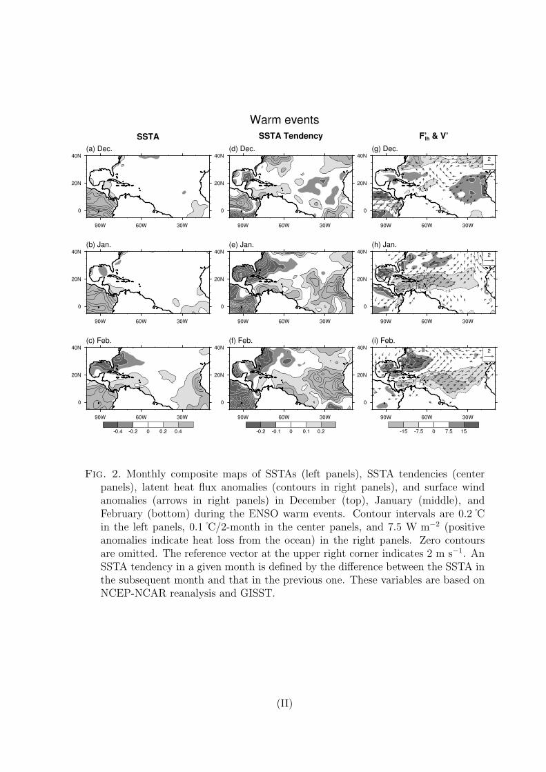
Fig. 2. Monthly composite maps of SSTAs (left panels), SSTA tendencies (centerpanels), latent heat flux anomalies (contours in right panels), and surface windanomalies (arrows in right panels) in December (top), January (middle), andFebruary (bottom) during the ENSO warm events. Contour intervals are 0.2 Cin the left panels, 0.1 C/2-month in the center panels, and 7.5 W m−2 (positiveanomalies indicate heat loss from the ocean) in the right panels. Zero contoursare omitted. The reference vector at the upper right corner indicates 2 m s−1. AnSSTA tendency in a given month is defined by the difference between the SSTA inthe subsequent month and that in the previous one. These variables are based onNCEP-NCAR reanalysis and GISST.
(II)

Fig. 3. Same as in Fig. 2, but for ENSO cold events.
(III)

Fig. 4. Composites of (a,e) contributions from W ′, (b,f) contributions of ∆q′, (c,g) thesum of these contributions (bars) to the total amount of latent heat flux anomalies(dashed lines), and (d,h) the net heat flux anomalies (bars) averaged over theCaribbean Sea (the rectangular region: 10 - 20˚N and 80 - 60˚W) during theENSO warm (left panels) and cold (right panels) events based on NCEP-NCARreanalysis and GISST. The total amount of latent heat flux anomalies (dashedlines) and SSTA (solid line; right axis) are superimposed on (d) and (h). White(black) bars denote negative (positive) anomalies. Units in left (right) axis areW m−2 ( C). (IV)

Fig. 5. January composite maps of (a,d) contributions from wind speed anomaly (W ′),(b,e) contributions of anomalous air-sea difference in specific humidity (∆q′), and(c,f) the sum of these contributions during the ENSO warm events. Left (right)panels are derived from NCEP-NCAR reanalysis and GISST datasets (COADS).Contour intervals are 5 W m−2 (upper and middle panels) and 7.5 W m−2 (bottompanels). Zero contours are omitted.
(V)

Fig. 6. Same as in Fig. 5, but for ENSO cold events.
(VI)

Fig. 7. January scatter plots of (a) the wind speed anomaly (m s−1), (b) theanomalous air-sea difference in specific humidity (g kg−1), and (c) the specifichumidity anomaly at 2-m (g kg−1) over the Caribbean Sea onto the Nino3 index(x-axis; C). Solid circles indicate the eight warm and cold events. Values atthe center above the panels indicate the correlation coefficients calculated fromall scatter plots. Values at the left (right) corner above the panels indicate thecorrelation coefficients calculated from scatter plots only during negative (positive)phase of the Nino3 index. A correlation coefficient of 0.44 is statistically significantat 95% level under 20 degrees of freedom.
(VII)

Fig. 8. January composite maps of (a) q′a and (b) ∆q′ during the ENSO warm events.Contour intervals are 0.2 g kg−1. Zero contours are omitted.
(VIII)

Fig. 9. January composite map of temperature anomaly at 400 hPa based onNCEP-NCAR reanalysis during the ENSO warm events. Contour intervals are0.5 C. Zero contours are omitted.
(IX)

Fig. 10. Composites of air temperature anomaly at 2-m (thick solid line; C) andSSTA (dashed line; C) over the Caribbean Sea derived from (a) NCEP-NCARreanalysis and GISST and (b) COADS during the ENSO warm events. Thinsolid line plotted with each panels is the air temperature anomalies at 400 hPa inNCEP-NCAR reanalysis divided by 2.
(X)

Fig. 11. January moisture budget in the Caribbean Sea during the warm events usingprecipitation based on (a) CMAP and (b) NCEP2. All other variables are basedon NCEP2. In these datasets, we take 5 years for the composite during the ENSOwarm events.
(XI)

Table 1. Years of ENSO warm and cold events.
Warm events Cold events
1957/58 1949/50
1965/66 1955/56
1972/73 1967/68
1982/83 1970/71
1987/88 1973/74
1991/92 1975/76
1994/95 1984/85
1997/98 1988/89
(XII)