rocket and missiles
TRANSCRIPT
— mI
I
^H
H
Rocket Propulsion and Spaceflight Dynamicsis designed to be a complete and integrated
text on the basis of spaceflight,
incorporating rocket propulsion, trajectory
analysis, orbital mechanics andinterplanetary flights. It is introduced by ageneral discussion on astronautics, on the
basicconcepts in astronomy andgeophysics,and on the mechanics of particles, bodies
and fluids.
Derived from the authors' experience in
presenting a series of postgraduate coursesat the Department of Aerospace
Engineering of Delft University of
Technology, this text is unique in co-
ordinating established data from diverse
sources and in providing a thoroughworking knowledge of astronautics. It is
ideally suited both as a handbook for those
working in the field, and as a textbook for
self-study and for graduate courses.
The authors, although aiming at uniform
notation and presentation, have not only
provided a text with sufficient flexibility to
enable it to be used with other texts andsource material, but which will also assist
the reader in gaining an overall
understanding of the field, whilst clarifying
the frequently confused nomenclature.
Thistextwill prove invaluable to institutions
in aerospace research, development andoperations, to all concerned with
contributory components and systems, andas a textbook for senior undergraduateand graduate level courses.
Rocket Propulsionand Spaceflight Dynamics
J.W Cornelisse estec, Noordwijk
H. F. R. SCnOyer Delft University of Technology
K. F. Wakker Delft University of Technology
Jt
PitmanLONDON • SAN FRANCISCO • MELBOURNE
ACCESSION 1 No.
1 --155472
C
'Xi$- uI { QGQ
~~\
G/S
HcnWwl
PITMAN PUBLISHING LIMITED39 Parker Street, London WC2B 5PB
FEARON-PITMAN PUBLISHERS INC.
6 Davis Drive, Belmont, California 94002, USA
Associated Companies
Copp Clark Ltd, Toronto
Pitman Publishing New Zealand Ltd, Wellington
Pitman Publishing Pty Ltd, Melbourne
First published 1979
British Library Cataloguing in Publication Data
Cornelisse, J. W.Rocket propulsion and spaceflight dynamics.
1. Astrodynamics 2. Space vehicles-Propulsion
systems
1. TitleJI. Schoyer, H F R III. Wakker, K F
62>4Trl TL1050 78-40059
[SBN 0-273-01141-3
© J. W. Cornelisse, H. F. R. Schoyer and K. F. Wakker, 1979
All rights reserved. No part of this publication may be reproduced,
stored in a retrieval system, or transmitted in any form or by any
means, electronic, mechanical, photocopying, recording and/or otherwise
without the prior written permission of the publishers.
o
Printed in Northern Ireland at the Universities Press (Belfast) Ltd.
Contents
Preface xii
Symbols xvi
1 The Range of Astronautics 1
1.1 Some historical remarks 1
1.2 The rocket motor 3
1.3 Rocket trajectories and performance 3
1.4 Satellite orbits and interplanetary trajectories 4
66
6
7
7
8
9
9
10
11
12
13
13
14
15
15
16
17
17
18
18
19
19
19
21
22
23
2 1lasic Concepts in Astronomy and Geophysics
2.1 The universe
2.2 The solar system
2.2.1 The Sun
2.2.2 The planets
2.2.3 Asteroids, comets and meteoroids
2.3 Reference frames and coordinate systems
2.3.1 Position on the Earth's surface
2.3.2 The celestial sphere
2.3.3 The ecliptic
2.3.4 Geocentric reference frames
2.3.5 Heliocentric reference frames
2.3.6 Motion of the vernal equinox
2.3.7 The velocity vector
2.4 Time and calendar
2.4.1 Sidereal time
2.4.2 Solar time
2.4.3 Mean solar time
2.4.4 Standard time
2.4.5 Ephemeris time and atomic time
2.4.6 The year
2.4.7 The Julian date
2.5 The Earth
2.5.1 The shape of the Earth
2.6 The Earth's atmosphere
2.6.1 The troposphere, stratosphere and mesosphere
2.6.2 The ionosphere, thermosphere and exosphere
vi Contents
3 Mechanics of Particles, Bodies and Fluids 25
3.1 Newton's first law 25
3.2 Newton's second law 27
3.3 Non-inertial frames 28
3.3.1 Rotation 28
3.3.2 Newton's laws 30
3.4 Dynamics of particle systems 32
3.4.1 Systems of discrete particles 33
3.4.2 Bodies 36
3.4.3 Rigid bodies 37
3.4.4 Solidification principle 40
3.5 Gravitation 41
3.6 Motion of a particle in an inverse-square field 44
3.6.1 Constants of motion 45
3.6.2 Trajectory geometry 47
3.6.3 Classification and characteristics of conic sections 50
3.7 Mechanics of fluids 54
3.7.1 Conservation of mass 54
3.7.2 Conservation of linear momentum 56
3.7.3 Conservation of energy 58
3.7.4 Conservation of angular momentum 61
References 62
4 The Equations of Motion of Rigid Rockets 634.1 Reference frames 64
4.1.1 The relative orientation of the various reference frames 65
4.2 The dynamical equations 69
4.2.1 The apparent forces 70
4.2.2 The apparent moments 72
4.2.3 The inertial moment 74
4.2.4 The external forces 74
4.2.5 The external moments 76
4.2.6 The equations of motion 77
4.3 The kinematical equations 79
4.3.1 The position of the rocket 81
4.3.2 The orientation of the rocket 82
4.3.3 The velocity components in the vehicle-centered hori-
zontal reference frame 83
5 The Chemical Rocket Motor 85
5.1 The ideal rocket motor 86
5.1.1 The exhaust velocity 87
5.1.2 Nozzle geometry 90
5.1.3 Mass flow and exit pressure 93
5.1.4 The exit surface 96
Contents vii
5.1.5 Maximum thrust 98
5.2 Real rocket motors 99
5.2.1 The effect of ambient pressure on the nozzle flow 102
5.2.2 Other nozzle designs 106
5.2.3 Thrust misalignment 107
5.2.4 Thrust vector control 108
5.2.5 Thrust magnitude control 110
References 111
6 Characteristic Coefficients and Parameters of the Rocket Motor 1136.1 Some notes on rocket testing 113
6.2 Total and specific impulse 114
6.3 The volumetric specific impulse 115
6.4 The thrust coefficient 116
6.5 The characteristic velocity 118
6.6 The effective exhaust velocity 120
6.7 Characteristic length and residence time 120
References 122
7 Thermochemistry of the Rocket Motor 123
7.1 Concepts of chemical thermodynamics 123
7.1.1 General definitions 123
7.1.2 Chemical equilibrium 130
7.2 Combustion in the rocket motor 136
7.2.1 The composition in the combustion chamber and the
adiabatic flame temperature 137
7.3 Expansion through the nozzle 138
7.3.1 Constant properties flow 139
7.3.2 Frozen flow 140
7.3.3 Equilibrium flow 144
7.3.4 The modified Bray approximation 145
References 148
8 Heat Transfer in Rocket Motors 151
8.1 The energy equation 151
8.2 Heat transfer processes 152
8.2.1 Conductive heat transfer 152
8.2.2 Radiative heat transfer 152
8.2.3 Radiating gases 155
8.2.4 Convective heat transfer 156
8.3 Heat transfer in the rocket motor 160
8.3.1 Gas-side heat transfer 160
8.3.2 Heat transfer in the wall 162
8.3.3 Coolant-side heat transfer 164
8.3.4 Radiation cooling 166
References 168
viii Contents
9 The Solid-Propellant Rocket Motor 169
9.1 Solid propellants 170
9.1.1 Double-Base propellants 170
9.1.2 Composite propellants 171
9.1.3 The burning rate 174
9.1.4 Combustion models 177
9.2 Internal ballistics 180
9.2.1 Equilibrium chamber pressure 180
9.2.2 The flow in a cylindrical grain 185
9.2.3 The flow between the grain end and the nozzle 191
9.3 Propellant grains 194
9.3.1 Definitions 196
9.3.2 Cylindrical grains 197
9.3.3 Three-dimensional grains 202
9.4 Burning rate augmentation 203
9.4.1 Erosive burning 203
9.4.2 Pressure-induced burning rate changes 204
9.4.3 Acceleration-induced burning rate augmentation 205
References 206
10 The Liquid-Propellant Rocket Motor 208
10.1 Liquid propellants 209
10.2 Propellant tanks 211
10.3 The propellant feed system 213
10.3.1 Pumps 213
10.3.2 Turbines 221
10.3.3 The injector 224
10.4 The thrust chamber 226
10.4.1 Aspects of oscillatory combustion 227
10.4.2 The shape of the combustion chamber 227
10.4.3 The chamber volume 227
10.5 Cooling of liquid engines 228
10.5.1 Active cooling systems 229
10.5.2 Passive cooling systems 231
References 232
11 Two-Dimensional Rocket Motion in Vacuum 23411.1 The equations of motion 234
11.2 Rocket motion in free space 237
11.2.1 Tsiolkovsky's equation 238
11.2.2 Rocket parameters 239
11.2.3 The burnout range 242
11.3 Rocket motion in a homogeneous gravitational field 246
11.3.1 Vertical flight 247
Contents ix
11.3.2 Constant pitch angle 25011.3.3 Gravity turns 255
References 261
12 The Multi-Stage Rocket 26212.1 Nomenclature of the multi-stage rocket 26212.2 The ideal velocity of the multi-stage rocket 26512.3 Vertical ascent in a homogeneous gravitational field and in
vacuum 272
12.3.1 The burnout velocity 273
12.3.2 The culmination altitude 27412.3.3 Vertical ascent of a two-stage rocket 276
12.4 Parallel staging 280
References 281
282
283
286
287
288
293295
298
304
306
306
308
310
315
14 Rocket Motion in the Atmosphere 31714.1 The equations of motion 317
14.1.1 Aerodynamic forces, moments and coefficients 318
14.2 The magnitude of the aerodynamic coefficients 321
14.2.1 The normal force and pitching moment coefficients 321
14.2.2 The drag coefficient 323
14.3 Some aspects of aerodynamic stability 325
14.3.1 Static longitudinal stability 325
14.3.2 Dynamic longitudinal stability 326
14.3.3 Some aspects of non-linear instability 329
14.4 Other atmospheric effects 331
References 334
15 The Many-Body Problem 33615.1 The general N-body problem 336
15.1.1 Integrals of motion 337
13 1 ballistic Missile Trajectories
13.1 The boost phase
13.2 The ballistic phase
13.2.1 The orientation of the trajectory plane
13.2.2 Trajectory geometry
13.2.3 A graphical technique
13.2.4 Optimal flights
13.2.5 Time of flight
13.3 The re-entry phase
13.4 The position of the impact point
13.4.1 Spherical Earth
13.4.2 Oblate Earth
13.4.3 Influence coefficients
References
x Contents
15.1.2 The Virial theorem 340
15.2 The circular restricted three-body problem 342
15.2.1 Jacobi's integral 344
15.2.2 Surfaces of zero velocity 346
15.2.3 Stability of motion near the libration points 350
15.2.4 Applications to spaceflight 353
15.3 Relative motion in the N-body problem 354
15.3.1 Satellite orbit perturbations by a third body 357
15.3.2 Sphere of influence 358
References 360
16 The Two-Body Problem 362
16.1 Equations of motion 362
16.2 General characteristics of motion 363
16.2.1 The circular orbit 366
16.2.2 The elliptic orbit 368
16.2.3 The parabolic orbit 369
16.2.4 The hyperbolic orbit 369
16.3 Relations between position and time 370
16.3.1 The elliptic orbit 371
16.3.2 The parabolic orbit 373
16.3.3 The hyperbolic orbit 373
16.4 Expansions in elliptic motion 375
16.5 Orbital elements 377
16.6 Relations between orbital elements and position and velocity 379
16.6.1 Rectangular coordinates from orbital elements 380
16.6.2 Orbital elements from rectangular coordinates 381
16.6.3 Orbital elements from spherical coordinates 382
16.7 / and g series 383
16.8 Relativistic effects 385
References 387
17 The Launching of a Satellite 389
17.1 Launch vehicle ascent trajectories 389
17.2 The injection of a satellite 390
17.2.1 General aspects of satellite injection 391
17.2.2 Dependence of orbital parameters on in-plane injec-
tion parameters 392
17.3 Launch vehicle performances 395
17.4 Orbit deviations due to injection errors 401
17.4.1 Small injection errors 402
References 405
18 Perturbed Satellite Orbits 407
18.1 Special and general perturbations 409
Contents xi
18.2 Cowell's method 41018.3 Encke's method 41118.4 Method of variation of orbital elements 413
18.4.1 Lagrange's planetary equations 41418.4.2 Modification of the sixth Lagrange equation 42018.4.3 Other forms of the planetary equations 422
18.5 A simple general perturbations approach 42518.6 First-order effects of the asphericity of the Earth 427References 434
19 Interplanetary Missions 43619.1 Basic concepts 43719.2 Two-dimensional interplanetary trajectories 439
19.2.1 Hohmann trajectories 44019.2.2 Launch opportunities 44419.2.3 Fast interplanetary trajectories 446
19.3 Three-dimensional interplanetary trajectories 44919.4 The launch of interplanetary spacecraft 45319.5 Trajectory about the target planet 455References 460
20 Low-Thrust Trajectories 46220.1 Equations of motion 46320.2 Constant radial thrust acceleration 46520.3 Constant tangential thrust 468
20.3.1 Characteristics of the motion 46920.3.2 Linearization of the equations of motion 47220.3.3 Performance analysis 474
References 479
Tables 480T.l Physical constants 480T.2 Selected astronomical constants 480T.3 Planetary orbital elements 482T.4 Planetary orbits and physical elements 483T.5 Satellite orbits and physical elements 484
Appendices 485
Appendix 1 Gauss' Theorem 485
Appendix 2 Reynolds' Transport Theorem 486
Appendix 3 The First Law of Thermodynamics 489
Index 491
Preface
In scarcely two decades astronautics has outgrown its infancy and has
become increasingly important in daily life. Many countries have their ownspace programs, cooperate in international projects, and are members of
international space organizations. Many thousands of people make their
living in the fields of space technology, space research and space applica-
tions; most of them are required to have a thorough knowledge of the
physical and mathematical backgrounds to astronautics. The aim of this
book is to meet the demand for this knowledge in three basic, and highly
related areas of astronautics: rocket propulsion, rocket trajectory analysis
and flight mechanics of satellites and interplanetary spacecraft.
Up to now, it is the chemical rocket motor that has provided the thrust for
large launch vehicles that carry Earth satellites, interplanetary spacecraft or
other payloads. This chemical rocket motor, which derives its power from
chemical reactions, is the only well developed, reliable and extensively
flight-proven motor that can provide the large thrust necessary to lift the
heavy vehicles from the Earth's surface. Therefore, a basic understanding of
its principles and limitations is mandatory for anyone working in astronau-
tics.
As the main purpose of the launch vehicle is delivering a payload at a
prescribed position with a specified velocity, the success of the mission is
highly dependent on the ability to predict accurately the vehicle's trajectory,
which is determined by the thrust and Earth's gravitation and is influenced
by the atmosphere. On successful completion of the launch vehicle's flight,
the main mission will start and a satellite is injected into an Earth orbit, or a
space vehicle will set course to one or various bodies of our solar system.
Earth satellites are launched with a variety of objectives: pure scientific
satellites, which help to unravel the enigma of the universe, or will give a
better understanding of the geometrical, climatological or electromagnetic
picture of the Earth, but also commercial communications satellites, which
provide relatively cheap high-capacity space links for maritime, aeronautical
and public use.
Interplanetary spacecraft have greatly extended our horizons. They have
mapped the towering mountains and battered plains of Mars and the spinning
clouds of Venus; they have opened the possibility for exciting discoveries
on Mercury, Jupiter and beyond. All this will eventually lead to a better
insight into the history, nature and destiny of our solar system in general,
and our own planet, the Earth, in particular. It will be clear that for all these
Preface xiii
missions, careful trajectory selection is crucial as small errors may seriously
degrade the value of the mission.
This book introduces the reader to all these astronautical topics and
illustrates their intense interrelationship. The text is based on a series of
postgraduate courses given by the authors at the Department of Aerospace
Engineering of Delft University of Technology (DUT). Until now, there
was, to the authors' knowledge, no single text available which combinedthese highly related topics in astronautics; so someone with a knowledge of
one part of astronautics had to refer to several sources to familiarize himself
with other areas. Books on orbital mechanics mostly seem to forget that the
satellite has to be injected by a launch vehicle. Texts on rocket propulsion
sometimes seem to consider rocket propulsion as a goal in itself, and not as
a tool for launching satellites or for reaching 'heavenly bodies', as Walter
Hohmann wrote in 1925. The trajectory of the launch vehicle often seems to
be a step-child, either of rocket propulsion or of orbital mechanics. Astudent in rocket trajectory analysis had to refer to various articles or to
texts on military exterior ballistics or to flight handbooks to grasp the
subject. Moreover, the nomenclature in the various sources is not uniform,
and equations describing the same phenomenon are often presented in slightly
different forms, hampering a clear understanding and correct use. In the
present text, the authors have aimed at a uniform notation and presentation,
though they have not pursued this to extremes. For example, in mechanics it
is customary to denote the angular momentum by the symbol B, while the
symbol H is used in celestial mechanics. To facilitate communication with
other texts, these conventions are adopted here too; such rare cases are,
however, clearly stated in the text. The mathematical derivations are given
with many intermediate steps, to make them clear and readily understanda-
ble. Clarity of derivation and formulation is favored above the addition of
more subjects, and as far as possible the physical nature of what is happen-
ing is emphasized, since an expression or formula is merely a shorthand for a
physical phenomenon.Throughout the book, SI units (Systeme International) are used. This
system of units has for a long time been accepted by the scientific world, and
its consistency and ease of use also promoted its rapid adoption in technol-
ogy during the last decade. Both NASA and ESA already use the SI units in
their publications, but to the authors' knowledge this is the first comprehen-
sive text on space technology to use solely SI units in a rigorous manner,
which enhances its value as a teaching text.
The book is written for those engineers and scientists who, for various
reasons, have more than a passing interest in astronautics and/or related
areas, and for students in the aerospace sciences. The experienced worker in
the field will find an easily accessible corridor to related areas, while the
student is introduced to a field of related topics in a logical and rigorous
way. We hope that this book may also be of much value to ballisticians and
to those who use rockets and missiles, such as military people and
xiv Preface
experimenters using sounding rockets or satellites for their investigations.
Often, this last category of people needs to know the limitations dictated by
the rocket, the trajectory or the orbit, and this book may elucidate these
restrictions.
The book, which contains twenty chapters, consists of four major parts. The
first three chapters introduce the reader to astronautics, astronomy and
geophysics, and cover the basic concepts of the mechanics and physics
needed for an understanding of the remainder. Readers who are familiar
with these notions may forego these chapters and turn to the following
parts; the first three chapters then merely serve as a reference source.
In Chapter 4 a rigorous derivation of the equations of motion of a
rocket vehicle is given.
Chapters 5 to 10 deal with rocket propulsion. The basic theory of the
ideal (chemical) rocket motor is given, and linked with the real rocket
motor. The combustion process in the rocket motor is discussed on the basis
of chemical (equilibrium) reactions. As, in general, very high temperatures
will occur in some parts of the rocket motor, relevant aspects of heat transfer
are also covered, while finally the solid and liquid propellant motors are
discussed extensively.
Chapters 11 to 14 deal with the trajectory and performances of the rocket
vehicle. These chapters comprise rocket motion in a vacuum, the theory of
multi-stage rockets, trajectories of intercontinental ballistic missiles and the
influence of the atmosphere on the trajectory of a rocket vehicle.
In the concluding six chapters, satellite orbits and interplanetary flights
are treated. These chapters start with some topics of classical celestial
mechanics. Then, the theory of Keplerian orbits is presented, and the
problems of the launching and injection of satellites are discussed and
explained with the help of performance diagrams for expendable launch
vehicles and the Space Shuttle. Methods for computing perturbed satellite
orbits are treated in some detail, and the analysis of interplanetary trajec-
tories is discussed. The last chapter deals with low-thrust trajectories of
spacecraft with, for example, an electric rocket motor or a solar sail.
Tables are included, giving physical and astronomical constants and data
on our solar system. Much care has been taken to make this set of data
consistent. The book concludes with an Appendix on some often used
concepts, such as Gauss' theorem, Reynolds' transport theorem and the
first law of thermodynamics, thus facilitating the reader to check on these
topics.
The authors have done everything to keep errors to a minimum, but of
course, it is possible that some errors still occur; we will appreciate being
informed of these.
The authors are indebted to many people who have contributed in various
ways; not least by giving advice and providing necessary data and informa-
tion. Though it is not possible to name them all, a few should be mentioned
Preface xv
here. The authors wish to express their sincere thanks to Prof. H. Witten-
berg, Dean of the Department of Aerospace Engineering of DUT and to
Prof. J. A. van Ghesel Grothe, Managing Director of the same department,
for their encouragement to write the present work and their permission to
the authors to devote part of their time to its preparation. Professor H.Wolff of Technion, Israel Institute of Technology, Haifa, read the complete
first version of the manuscript and gave many highly useful comments, based
on his vast industrial and teaching experience. Mr. R. S. de Boer of the
National Defense Organization (T.N.O.), Dr. F. P. Israel of Leiden Univer-
sity and Mr. B. A. C. Ambrosius of DUT gave comments which proved
highly valuable. Mr. D. M. van Paassen of DUT prepared all the artwork,
and certainly should be mentioned here for his excellent contribution. Themanuscript was typed by Mrs. C. G. van Niel-Wilderink and Miss M. M.Derwort, who succeeded in patiently transforming the handwritten version
with all its changes into a readable and printable manuscript. The authors
are also much indebted to Dr. Th. van Holten of DUT, who betted that the
text would never be completed and who lost! This wager and his sarcasm
were at least a great stimulus. Finally, we wish to thank our families, whoaccepted that so much time had to be sacrificed for the preparation of this
book. If it proves to be valuable to the reader, and contributes to the
enthusiasm for astronautics, this time was not spent in vain.
J. W. Cornelisse
H. F. R. Schoyer
K. F. WakkerDelft, The Netherlands
August 1978
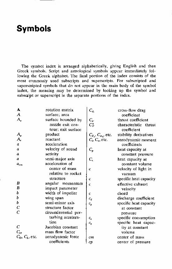
Symbols
The symbol index is arranged alphabetically, giving English and then
Greek symbols. Script and astrological symbols appear immediately fol-
lowing the Greek alphabet. The final portion of the index consists of the
most commonly used subscripts and superscripts. For subscripted and
superscripted symbols that do not appear in the main body of the symbol
index, the meaning may be determined by looking up the symbol and
subscript or superscript in the separate portions of the index.
A rotation matrix Q cross-flow drag
A surface; area coefficient
Ae surface bounded by cF thrust coefficient
nozzle exit con- c°F characteristic thrust
tour; exit surface coefficient
\ product Wv> ^*v ® stability derivatives
Ar reactant ^h^ni etC. aerodynamic momenta acceleration coefficients
a velocity of sound cP heat capacity at
a activity constant pressure
a semi-major axis cv heat capacity at
"'cm acceleration of constant volumecenter of mass c velocity of light in
relative to rocket vacuumstructure c specific heat capacity
B angular momentum c effective exhaustB impact parameter velocity
b width of impeller c chordb wing span cd discharge coefficient
b semi-minor axis CP
specific heat capacity
C structure factor at constant
C circumferential per- pressure
turbing accelera- cs specific consumptiontion cv specific heat capac-
c Jacobian constant ity at constant
cD mass flow factor volume
("Di (^l> etc. aerodynamic force cm center of masscoefficients cp center of pressure
Symbols xvii
c* characteristic H enthalpy
exhaust velocity AH heat change at con-
D drag stant pressure;
D diameter; outer heat of reaction
diameter H hour angle
D distance H.T.A. Hohmann transfer
D.A. direct ascent ascent
Db ballistic linear range Hepumphead
d rocket base diameter AH) standard heat of
E matrix of unit formation
vectors F1g Greenwich hour
E internal energy angle at Oh U.T.
AE heat change at h specific enthalpy
constant volume h Planck's constant
E eccentric anomaly h altitudea
.
e unit vector K convective heat
e specific internal transfer coefficient
energy I inertia tensor
e (numerical) eccen- I total impulse
tricity •*spspecific impulse
F force; thrust h volumetric specific
F Gibbs free energy impulse
F augmented function I polar moment of
F focus inertia
F hyperbolic anomaly -*xx» -*yy -*zzmoments of inertia
Fs total external force ^xy» ^yzJ e*C - products of inertia
applied to system i inclination
S J linear momentum
F rocket motor J throat to port area
vacuum thrust ratio
f fugacity J coefficient of zonal
G universal gravita- harmonics, tes-
tional constant seral harmonics
g force per unit mass; and sectorial har-
(gravitational) monics
field strength K klemmung
go standard surface K drag parameter
gravity Kn equilibrium constant
go reference gravita- (on basis of
tional acceleration number of mols)
H angular momentum kp
equilibrium constant
of system of (on basis of partial
point masses pressure)
H angular momentum Kpf
equilibrium constant
per unit mass of formation
xviii Symbols
k Boltzmann's N normal force
constant N pump's number of
k thermal conductivity revolutions per
*. injection velocity second; rotational
parameter speed
K spectral absorption N perturbing accelera-
coefficient of a gas tion normal to
L lift velocity vector
L length N number of
L gas layer thickness revolutions
L mean longitude NPSE net positive suction
L Lagrange libration energy
point Nu Nusselt numberJ-'eq equivalent beam NA Avogadro's number
length K pump specific speedL* rocket motor Nss suction specific
characteristic speed
length N' yawing momentV, M', N' aerodynamic n unit normal
moments n concentration or
k perimeter of cross- number of molssection of perfor- n dimensionless accel-
mation in propel- eration
lant grain n (mean) angularM moment of a force motionM total mass of a sys- n dimensionless radius
tem (of particles); of planet orbit
mass of a body; np neutral point
mass of a satel- O origin of reference
lite or spacecraft frameM mean anomaly P powerMa Mach number Pr Prandtl numberMc structural mass Pi power delivered to
Me empty (final) rocket pumpmass Pu useful power
MF moment due to P pressure
thrust (misalign- P semi-latus rectumment) P,4,r angular velocity
Mp (useful) propellant components
mass Pa (undisturbed) at-
Mu payload mass mospheric pres-M' pitching moment sure
m mass of particles or Pi partial pressure of
point mass species i
m mass flow; flux of Po front-end stagnation
matter pressure
Symbols xix
heat propellant; burn-
volumetric flow rate ing rate
Q energy flux; heat re position vector for
flux center of mass
q dimensionless semi- flow
latus rectum re erosive burning rate
4 dynamic pressure f dimensionless
R position vector; distance
radius vector S mass-system
R Earth radius; planet S inertial reference
radius; local frame
radius of Standard s entropy
Ellipsoid s (closed) surface
R gas constant s reference area; roc-
R perturbing or dis- ket cross-sectional
turbing potential base area
Re Reynolds number s radial perturbing ac-
R disturbing function celeration
Re ballistic cross-range St Stanton numberinfluence coeffi- sR outer wall of the
cient rocket
&RC cross-range error s, reference area
capture radius sw projected wing area
RD ballistic down-range s structure ratio
influence coeffi- s distance
cient As distance covered by
Ai?D down-range error: rocket
down-range cor- T torque
rection T tangential force
Re mean equatorial T tangential perturb-
Earth radius ing acceleration
RPEarth polar radius T temperature
Rs .iradius of sphere of T time of flight
influence or activ- T orbital period
ity sphere Tb bulk temperature
Ro universal gas Tf
fluid film tempera-
constant ture
Ro mean Earth radius T, flame temperature
r radius vector; posi- Trrecovery tempera-
tion vector (rela- ture
tive to center of T* syn synodic period
mass of rocket) T. exospheric tempera-
r recovery factor ture
r velocity of burning r auto-ignition tem-
surface with re- perature
spect to solid t time
xx Symbols
tb burning-time W normal perturbing
tc coast-time acceleration
*ftime of flight w propellant grain web
f dimensionless time thickness
U identity matrix -^a> ^a> ^a aerodynamic forces
u potential function; x,y,z axes of a reference
potential; poten- frametial energy per a absorptance
unit mass a angle of attack;
u ideal velocity ratio angle of incidence
u argument of latitude a nozzle divergence
u, v, w linear velocity angle
components a turbine nozzle angle
"cm velocity of center of a right ascension
mass relative to a general orbital
rocket structure elementV velocity vector a asymptotic deflec-
AV velocity increment tion angle
of a rocket a correction factor
yc local circular vel- «x monochromatic ab-
ocity sorptivity of a gas
'char launch vehicle char- layer
acteristic velocity P specific thrust
* char mission characteris- P blade angle
tic velocity P sideslip angle
^ ' char launch site and r Vandenkerckhovelaunch azimuth function
velocity penalty r velocity factor
Ve exhaust velocity r time factor
ve mean exhaust y ratio of specific
velocity heats
v' esc local escape velocity y flight path angle
Vi propellant injection y dimensionless
velocity distance
Via ideal velocity of 8 declination
N-stage rocket 8 thickness
AVid ideal velocity 8 thrust (misalign-
increment) ment) anglevL limiting value of Ve 8 kick angle
Vi volumetric loading e structural efficiency
fraction e (hemispherical)
V„ hyperbolic excess emittance
velocity e obliquity of the
w gravitational force ecliptic
w work e flattening of the
Symbols xxi
Earth P reflectance
e downwash angle P mass density; air
etottotal structural density
efficiency Pi ratio of injection
eA monochromatic radius and re-
emissivity of a gas entry radius
layer PP average propellant
1? efficiency density
e angular coordinate X dimensionless burn-
e angular displace- ing surface
ment X ballistic angular
e pitch angle range
e true anomaly (J Stefan-Boltzmann
A0 heliocentric transfer constant
angle T transmittance
K thermal diffusivity T Thoma parameter
A mass ratio T time of (last) peri-
A geographic center passage
longitude T* residence time
A payload ratio <D geocentric latitude
A wavelength <D' geodetic or geo-
A nozzle reduction graphic latitude
factor<P
propellant ratio
A celestial longitude<P
bank angle
P<attraction parame-
<Pangular coordinate
ter; gravitation<P
celestial latitude
parameter<Ptot
total propellant ratio
P<dynamic viscosity * angular coordinate
^ dimensionless mass * flight path azimuth;
M-mass flow parameter down-range head-
V stoichiometric ing
coefficient * yaw angle
V Lagrange multiplier<A
pressure parameter
£ extent of reaction ^0 thrust-to-weight
£ quality factor ratio
£*U coordinate axes ft angular or rotational
it sensitivity coefficient velocity
for burning pro- ft right ascension of
pellant ascending node
P position vector (with ft longitude of ascend-
respect to center ing node
of mass) (O angular velocity
P position vector for (O argument of peri-
(unperturbed) re- center
ference orbit<»e
angular velocity of
xxii Symbols
the Earth about its / fluid film
axis / friction
CO longitude of peri- / flame
center / impact
% total energy (per G Greenwich
unit mass) g rotating geocentric
£k kinetic energy reference frame
£p potential energy g gas
M (mean) molecular g propellant grain-end
weight H Hohmanny (material) volume i interference
yrp volume available to i body i
store propellants i sub-rocket
V vernal equinox; first i injection
point of Aries i impact£L autumnal equinox; in inertial
Libra I launch (site)
max maximum
Subscripts o point of application of
a force
a aerodynamic P pressure
a apocenter P product
abs absolute P propellant
as outgoing asymptote P propellant port area
B body P pericenter
b burnout P planet
c (rocket) chamber par parking orbit
c condensed phase r reactant
c Coriolis r radiative
c circular (orbit) r vehicle reference frame
c critical rel relative
c culmination s constant entropy
c spacecraft s stagnation
cm center of mass s Suncr critical s satellite
D drag t throat; sonic
d directional t target planet
d disturbing body th theoretical
dr dragging tot total
e exit of nozzle V vehicle-centered horizontal
e after the reaction reference frame
e re-entry W fin
e Earth w wallesc escape x,y,z component in x-, y-,
exp experimental and z-direction
Symbols xxiii
initial
reference temperature
before the reaction
propellant grain front-end
in the parking orbit about
the Earth
1 at the start of the inter-
planetary heliocentric leg
2 on arrival at the target
planet in the interplane-
tary heliocentric leg
3 at pericenter of the hyper-
bolic trajectory about the
target planet
4 at leaving the sphere of in-
fluence of swingby planet
A at a wavelength
Superscripts
' small perturbation°
at standard reference state—
mean value; average

1 The Range of Astronautics
More than a thousand satellites have been launched since 1957, and many
of these still encircle the Earth. They comprise communications, navigation,
and Earth survey satellites, satellites for scientific and technical purposes,
military satellites, etc. All were put into a more or less elliptical orbit by
large rockets. To modern man, astronautics is an accepted part of human
society. A manned flight to the Moon is not regarded as anything peculiar
anymore, and an unmanned flight to Jupiter hardly affects 'the man in the
street'. On the other hand, one notices the great interest in the findings and
achievements of astronautics, completely in agreement with the historical
development of our society and the inquisitive nature of mankind.
1.1 Some historical remarks
Astronautics belongs to the youngest endeavors of men. Like the desire to
master the art of flying, the need to visit and survey the planets seems
deeply rooted in our minds. For long there haved existed tales about humans
flying to the Moon, Sun or stars. The large market for science-fiction novels
illustrates the natural human interest in space travel.
In ancient times, astronomical events, especially the solar and lunar
eclipses, puzzled and frightened people as they were not understood. One
tried to explain the lunar eclipse for instance, by imagining that an evil black wolf
swallowed theMoon. Fortunately, there was always a hunterwho killed the wolf,
opened its stomach, and the Moon came out, not hurt at all. This in fact, may be
the origin of the well-known tale of Little Red Ridinghood.
In the ancient, agricultural world, a calendar was of utmost importance,
and astronomy, which had to provide this instrument of time-keeping
started to develop in Mesopotamia as is assumed by archeologists. The first
primitive calendars usually were based on the phases of the Moon. Soon, the
astronomers could predict the eclipses and they got some insight into the
motion of Moon, Sun and stars.
When people started sailing the seas, their only means of navigation at
night were the stars and this again promoted the interest in astronomy.
Around the middle of the seventeenth century the first science-fiction novels
about travels to the Moon appeared, but certainly Jules Verne's De la Terre
a la Lune (From the Earth to the Moon) from 1865 belongs to the most
inspiring ones.
The rocket, as a small weapon, was well developed at this time. We are
2 Rocket Propulsion & Spaceflight Dynamics
told of Asian armies, armed with rocket-weapons when Europeans still used
the bow. However, the theory of rocket flight was still lacking. It was the
Russian teacher Tsiolkovsky, who in 1903 published in the Moscow Techni-cal Review an article with the title Study of Space by Jet-Propelled Devices,
in which he derived the equation, relating the velocity of a rocket to its
exhaust velocity and mass ratio, and which presently is known as Tsiol-
kovsky's equation. His work, however, did not become generally known,and in 1923, Oberth, in his Ph.D. thesis, independently arrived at a similar
result.
Especially in Germany, in Russia where Tsiolkovsky continued his
studies, and in the United States, there were at that time people trying to
promote space flight. These people, like Oberth, Hohmann, Goddard andothers, foresaw that space travel might soon become a reality, and theydevoted much time, energy and money, to what most other people regardedas a foolish and dangerous hobby. Much work of those days has become the
classical foundation of modern astronautics.
The German rearmament after 1933 gave a strong impetus to the de-
velopment of the rocket-weapon, and the final outcome was the notoriousV-2. After World War II, the large scale development of rockets continued,
especially in the United States and Russia, which culminated in the success-
ful launch of the first 'artificial moon', the Sputnik, on October 4, 1957 byRussia. The United States accomplished their first successful launch of a
satellite on January 31, 1958 with Explorer 1. On May 25, 1961, President
Kennedy told the American congress that 'this nation should commit itself to
achieving the goal, before the decade is out, of landing a man on the Moonand returning him safely to Earth'. This was the offical start of the famousApollo project, which reached a climax in Neil Armstrong and EdwinAldrin setting foot on the Moon on July 20, 1969.
Meanwhile, many applications for civil and military use of space werefound, and many satellites had been launched. Both Russia and the UnitedStates had orbited animals and men, and spacecraft were sent out to exploreour solar system, and to survey and map the planets. Nowadays, scientific
and technical research is carried out in space laboratories and the day whenthe manufacturing of special products in space will be a normal procedure,may not be far off.
In the foreseeable future, reusable rocket vehicles, like the Space Shuttle,
will provide an efficient means of manned space flight both for civil andmilitary purposes.
The missile has become a very sophisticated weapon. Large warheads canbe targeted with extremely high precision at intercontinental distances. If
one compares this with the V-2, which carried a warhead of about 1000 kgat a range of about 300 km, this development is both frightening anddramatic. The highly increased reliability and accuracy of the rocket vehicle
are mainly due to the improvements in rocket engine technology and the
miniaturization of the electronic guidance and control systems.
The Range of Astronautics 3
Now that more and more countries have their own space program, and
companies operate their own telecommunications satellites, one may say
that space technology has grown mature.
1.2 The rocket motor
The basic principle of the rocket is simple: matter, the propellant, is
accelerated, resulting in a reaction force, the thrust. As the rocket contains
all the propellant itself, it is independent of its environment and, hence, can
operate in empty space.
If chemical energy, contained within the propellants is used to produce
gases of a high temperature and pressure, one speaks of a chemical rocket
motor.
If the high pressure and temperature of the propulsive gas are caused by a
nuclear reactor, one speaks of a nuclear rocket engine. Electric rocket
motors may electrically heat a propulsive gas, but the electric energy can
also be used to create a strong electromagnetic field to accelerate electrically
charged particles. The energy may stem for instance from a nuclear power
source or from the Sun.
The chemical rocket motors can be subdivided into liquid, solid and
hybrid motors. The liquid motor uses liquid propellants, usually a fuel and
an oxidizer stored in separate tanks. The solid motor uses a solid propellant
which combines fuel and oxidizer. The reaction and gasification take place at
the propellant's surface. The hybrid motor combines a solid and a liquid
propellant; the solid usually is the fuel. At the present time, liquid and solid
rockets are the most used types. Both can deliver high thrusts during a
relatively short period. The nuclear rocket is still in its experimental stage.
Applications are especially seen for deep space missions. There are various
types of electric engines, but all have in common that they deliver a low
thrust and have long operation times. Therefore, the electric rocket motor is
especially suited for low-thrust trajectories in interplanetary space, for
stationkeeping of satellites, etc. Some electric motors have flown already.
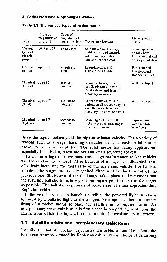
Table 1.1 lists the various types of rocket motors mentioned, and their
characteristics. In this book, we will devote our attention to the solid and
liquid rocket motors. Of course, much of the general theory of the chemical
rocket motor can be applied to the nuclear motor, some types of electric
engines and the cold gas jets.
1.3 Rocket trajectories and performance
Tsiolkovsky's equation shows that the velocity increment of a single-stage
rocket, which is an important performance parameter, depends on the
exhaust velocity and the mass ratio, i.e. the ratio of take-off mass and
burnout mass. Both have to be as high as possible. At the present time, for
Earth-based launch vehicles, only chemical rockets can be used, and of
4 Rocket Propulsion & Spaceflight Dynamics
Table 1.1 The various types of rocket motor
Type
Order of
magnitude of
thrust (N)
Order of
magnitude of
operation time Typical applications
Developmentstatus
Various 10"6 to 102
types of
electric
propulsion
up to years Satellite stationkeeping,
stabilization and control,
interplanetary flights,
satellite orbit transfer
Some types havealready flown.
Experimental anddevelopment stage
Nuclear
reactor
up to 105 minutes to
hours
Interplanetary, andEarth-Moon flights
Experimental.
Developmentstopped in 1973
Chemical(Liquid)
up to 107seconds to
minutes
Launch vehicles, missiles,
stabilization and control,
Earth-Moon and inter-
planetary missions
Well developed
Chemical(Solid)
up to 107 seconds to
minutes
Launch vehicles, missiles,
various small rocket weapons,sounding rockets, inter-
planetary missions, boosters
Well developed
Chemical(Hybrid)
up to 105seconds to
minutesSounding rockets, small
rocket weapons, final stages
of launch vehicles
Experimental.
Some modelshave flown
those the liquid rockets yield the highest exhaust velocity. For a variety of
reasons such as storage, handling characteristics and costs, solid motorsprove to be very useful too. The solid motor has many applications,
especially for missiles, boost motors and small sounding rockets.
To obtain a high effective mass ratio, high-performance rocket vehicles
use the multi-stage concept. After burnout of a stage, it is discarded, thus
effectively increasing the mass ratio of the remaining vehicle. For ballistic
missiles, the stages are usually ignited directly after the burnout of the
previous one. Shut-down of the final stage takes place at the moment that
the resulting ballistic trajectory yields an impact point as near to the target
as possible. The ballistic trajectories of rockets are, at a first approximation,
Keplerian orbits.
If the vehicle is used to launch a satellite, the powered flight usually is
followed by a ballistic flight to the apogee. Near apogee, there is anotherfiring of a rocket motor to place the satellite in its required orbit. Aninterplanetary spacecraft is usually first placed into a parking orbit about the
Earth, from which it is injected into its required interplanetary trajectory.
1.4 Satellite orbits and interplanetary trajectories
Just like the ballistic rocket trajectories the orbits of satellites about the
Earth can be approximated by Keplerian orbits. The existence of disturbing
The Range of Astronautics 5
forces means that this approximation does not hold if one considers the orbit
for a longer period of time. It turns out that the major perturbations are due
to the non-central force field of the Earth, the atmosphere, the attraction by
Moon and Sun, and the solar radiation pressure. Which of the perturbing
forces dominates, depends on the altitude of the orbit and the mass and
dimensions of the satellite.
In many cases, the orbit perturbations observed can be used to obtain
quantitative information about the specific perturbing forces. For instance,
one can in this way obtain information on the atmospheric density at high
altitudes, and determine the shape of the Earth, etc. One can also deliber-
ately use these perturbations to obtain certain desired orbital changes.
The trajectories of interplanetary spacecraft can be approximated by
heliocentric and planetocentric Keplerian orbits.
The position and velocity of interplanetary spacecraft during their flight
are measured, and corrective midcourse manoeuvres can be executed if
necessary. As it may take a long time for the spacecraft to reach its target
(for a Jovian journey a year or more, and for a journey to Saturn a few
years), the reliability of the complete spacecraft is of utmost importance, as
a premature breakdown of one component may wreck the whole mission.
Especially on these long-duration flights, electric propulsion, with its long
operation times, can considerably reduce the time of flight, or facilitate
flights which are beyond the capability of the launch vehicle.
Another technique that enables flights to regions for which the present
launch vehicles have insufficient power, is the swingby technique. Here, the
gravitational field of a planet accelerates the spacecraft and deflects its
trajectory into the required direction for the encounter with a target planet.
2 Basic Concepts in Astronomyand Geophysics
2.1 The universe
According to our present view, 10 to 20 billion years ago there was nothing
but an exploding, enormously hot and dense Primeval Fireball that con-
tained all the matter and energy of the present universe. In this rapidly
expanding and cooling gas of elementary particles, such as protons, neutronsand electrons, particles gradually combined and nearly all matter took the
form of hydrogen atoms. In later stages clumps of gas were formed.Looking at the universe now, we get a picture of a nearly complete
emptiness; the mean mass density is extremely low, corresponding to that of
a few hydrogen atoms per ten cubic meters. We observe that matter in the
universe is mainly concentrated in objects with extremely large dimensionsand of complex structure: the galaxies. Billions of these galaxies are as-
sumed to be present in the universe. The mean distance between them is of
the order of 10 18to 1020 km. To express those large distances we usually
take the light year as the unit of length. The light year is defined as the
distance traversed by light in vacuum during one year, which corresponds to
about 9.46xl0 12 km.Our Sun belongs to one of those galaxies, named the Milky Way. This
Milky Way, which comprises about 100 billion stars, has the appearance of a
large, relatively flat structure with spiral arms and a diameter of about100,000 light years. Our Sun is located at a distance of about 30,000 light
years from the center of this galaxy and is moving with a velocity of roughly250 km/s about this center, completing one revolution in about 250 million
years. The galaxy nearest to the Milky Way is the Great Magellanic Cloudat a distance of about 160,000 light years from the Sun. Light emitted bystars in this galaxy takes 160,000 years to reach us. Consequently, all ourobservations of those distant objects are related to conditions in thosegalaxies of many thousands or even millions of years ago.
In the neighborhood of our Sun there is about one star per thousand cubiclight years, and a quantity of interstellar gas and dust with a mass densityequal to that of 2 to 3 hydrogen atoms per cubic centimeter.
2.2 The solar system
The volume of space very close to the Sun, up to a distance of about 1 light
year, is called the solar system. It is in this tiny part of the universe that our
Basic Concepts in Astronomy and Geophysics 7
space travel will take place in the foreseeable future. In this solar system the
planets and a great many other bodies move in orbits about the Sun.
2.2.1 The Sun
The Sun comprises 99.86% of all matter in the solar system. Its energy flux
equals roughly 4x 1026 W. At Earth-distance from the Sun, the solar power
density is still about 1400 W/m2. The energy emitted by the Sun is generated
by nuclear reactions which take place in the interior of the Sun. There, at a
temperature of about 107 K and a pressure of about 1010 MPa, hydrogen is
converted into helium whereby large amounts of energy are released. The
visible light of the Sun is emitted from the photosphere, a relatively thin layer
with a temperature of about 6000 K. This photosphere forms the visible
surface or disk of the Sun. Its radius is about 7 x 10⁵ km. The outermost
region of the Sun is called the corona. This corona, which is visible from
Earth during solar eclipses, extends up to many photospheric radii. The
corona continuously emits matter, mainly in the form of protons and
electrons. At crossing the Earth's orbit, this solar wind has a velocity of
300-500 km/s and contains about 10 protons per cubic centimeter.
Some temporary phenomena on the Sun, like sunspots and solar flares, are
associated with an 11 -year solar activity cycle. As a result of large solar
flares occurring at a solar activity maximum, high-energy solar particles and
a strongly enhanced UV- and X-ray radiation are emitted. When this
radiation interacts with the Earth's atmosphere, it may cause auroral effects,
disturbances of the geomagnetic field and radio-interference. The solar
activity thus is strongly related to many physical conditions on Earth.
2.2.2 The planets
The main bodies orbiting about the Sun are the nine planets: Mercury,
Venus, Earth, Mars, Jupiter, Saturn, Uranus, Neptune and Pluto, in order of
increasing distance from the Sun. Unlike the Sun, these bodies hardly emit
radiation in the visible part of the spectrum; the only reason that they are
visible is because of their reflection of solar light. The first six planets
mentioned were already known in ancient times. Uranus was discovered
accidentally in 1781 by Herschel who was making a routine telescopic
survey of the sky. From irregularities in the orbit of Uranus, it soon became
clear that still another planet had to be present. Using the perturbation
theory of celestial mechanics (Chapter 18), Adams and Leverrier, indepen-
dently of each other, predicted the mass and position of this eighth planet.
From the data of Leverrier, Neptune was discovered in 1846 by Galle.
Following the discovery of Neptune, it was observed that small discrepancies
still existed between the predicted and observed position of Uranus and
Neptune. Again the probable position of a ninth planet was calculated, in
8 Rocket Propulsion & Spaceflight Dynamics
this case by Lowell. In 1930 Tombaugh identified Pluto on a photographic
plate made from the region of the sky where Pluto was predicted.
In Table T.4, some relevant data on the planets are given. We note that
the planets Mercury, Venus, Earth, Mars and Pluto are relatively small as
compared to the giant planets Jupiter, Saturn and, to a lesser extent, also as
compared to Uranus and Neptune. Compared to the Sun, even the largest
planet is small: the Jovian diameter is about one tenth of the solar disk
diameter. All planets, except Mercury and probably Pluto, are surrounded
by an appreciable gaseous atmosphere. Mercury and Venus are closer to the
Sun than the Earth and are named the inner planets. Their surface tempera-
tures are higher. The lighted side of Mercury is assumed to have a surface
temperature of about 620 K. The planet Uranus, on the other hand, receives
very little solar energy so that its surface temperature may be as low as 80 Kand substances like methane, ammonia and carbon dioxide could be present
as liquid or solid. The low mean density of Saturn is remarkable; this density
is less than that of water. This may indicate the presence of a large
abundance of hydrogen and helium.
All planets move in nearly circular orbits about the Sun. The orbits of
Mercury and Pluto are the most elliptic; the minimum distance of Pluto
from the Sun is even less than the distance between Neptune and the Sun.
The orbital planes of the planets are nearly coincident. Again Mercury andPluto are exceptions; their orbital planes are inclined about 7° and 17°,
respectively, to the orbital plane of the Earth. All planets orbit in the samedirection about the Sun: counter-clockwise as viewed from the north. Their
mean distance from the Sun ranges from about 58 x 106 km for Mercury to
about 59 x 108 km for Pluto; the period needed to complete one revolution
thereby varies from 88 days for Mercury to about 246 years for Pluto. Toexpress the distances in the solar system we commonly use the Astronomical
Unit (AU) which is about the mean distance of the Earth from the Sun(Table T.2).
Each planet, except Mercury, Venus and perhaps Pluto, is accompaniedby one or more natural satellites or moons. The Earth has one natural
satellite, the Moon. Mars has two, and Jupiter even fourteen known satel-
lites (Table T.5). Six of the 34 known satellites are about as large as, or
larger than our Moon. One of the Jovian satellites, Ganymede, is evenlarger than the planet Mercury. It is known that some of the larger moons of
Jupiter and Saturn possess atmospheres. Saturn is the only planet which has
a ring-system consisting of billions of pieces of matter orbiting around the
planet.
2.2.3 Asteroids, comets and meteoroids
Between the orbits of Mars and Jupiter there exists a belt in which millions
of smaller bodies, called asteroids, orbit about the Sun. The largest asteroid,
Ceres, which was discovered in 1801, measures about 750 km in diameter.
Basic Concepts in Astronomy and Geophysics 9
Thousands have been identified and only a few hundred are over 25 kmacross; most of the asteroids are very small. Besides the asteroids in the belt,
there are asteroids which periodically pass the Earth quite closely.
Comets are mostly rather small objects, composed of frozen gases and
solid particles, coming from the outerpart of the solar system where they are
assumed to have been produced as a by-product in the formation of the
solar system. Owing to the attraction of the nearest stars, some comets are
directed into the inner part of the solar system. When a comet moves in
closer to the Sun, it warms up and the nucleus releases gases and dust
particles forming a large cloud around the nucleus: the coma. Some of the
constituents are expelled more or less radially from the Sun by the solar
wind and the radiation pressure of solar light to form the characteristic
cometary tail. These tails can become as long as 108 km.
Meteoroids are too small to be observed in their orbit about the Sun.
Their presence becomes known only when they enter the Earth's atmos-
phere, where they are heated by friction until they melt or vaporize. The
luminous phenomenon created this way is called a meteor. Rarely does such
a meteoroid survive its entry into the atmosphere and impact on the Earth's
surface. The material left is called a meteorite. Though the vast majority of
meteoroids are no larger than gravel, occasionally very large meteorites
have struck the Earth, producing meteor craters. The largest known meteor-
ites have masses of about 50 tons. Sometimes, a great number of meteoroids
are found to have the same orbit, they constitute a meteoroid stream. It is
thought that such streams of meteoroids are the debris remaining from the
breakup of a cometary nucleus. When the Earth is passing through a
meteoroid stream a large number of meteors are seen for some days:
a meteor shower.
2.3 Reference frames and coordinate systems
A large part of this book deals with the computation of the trajectories of
rockets, satellites and interplanetary spacecraft. We describe the motion of
these vehicles in terms of a time-varying position vector and its time
derivatives. This requires, of course, a reference frame with respect to which
position, velocity and acceleration are measured.
2.3.1 Position on the Earth's surface
To denote a position relative to the Earth, one usually takes a reference
frame which is based on the Earth's axis of rotation. The points where this
axis crosses the Earth's surface are called the north pole and the south pole.
For simplicity, we will assume temporarily that the shape of the Earth is
exactly spherical. Then, the great circle on the Earth's surface halfway
between the poles is the Earth's equator. The great circles passing through
the poles are called meridians; they intersect the equator at right angles. By
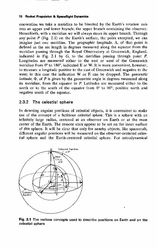
10 Rocket Propulsion & Spaceflight Dynamics
convention we take a meridian to be bisected by the Earth's rotation axis
into an upper and lower branch; the upper branch containing the observer.
Henceforth, with a meridian we will always mean its upper branch. Through
any' point P (Fig. 2.1) on the Earth's surface, the poles excepted, we can
imagine just one meridian. The geographic longitude, A, of that point is
defined as the arc length in degrees measured along the equator from the
meridian passing through the Royal Observatory at Greenwich, England,
indicated in Fig. 2.1 by G, to the meridian passing through point P.
Longitudes are measured either to the east or west of the Greenwich
meridian from 0° to 180°, indicated E or W. It is more convenient, however,
to measure a longitude positive to the east of Greenwich and negative to the
west; in this case the indication W or E can be dropped. The geocentric
latitude, <$, of P is given by the geocentric angle in degrees measured along
its meridian, from the equator to P. Latitudes are measured either to the
north or to the south of the equator from 0° to 90°; positive north and
negative south of the equator.
2.3.2 The celestial sphere
In denoting angular positions of celestial objects, it is convenient to makeuse of the concept of a fictitious celestial sphere. This is a sphere with an
infinitely large radius, centered at an observer on Earth or at the mass
center of the Earth. The remote stars appear to be set on the inner surface
of this sphere. It will be clear that only for nearby objects, like spacecraft,
different angular positions will be measured on the observer-centered celes-
tial sphere and the Earth-centered celestial sphere. For astrodynamical
Celestial Meridian
ofP
Fig. 2.1 The various concepts used to describe positions on Earth and on thecelestial sphere
Basic Concepts in Astronomy and Geophysics 11
purposes we will use the latter type. The celestial poles are defined as the
points where the Earth's rotation axis intersects the celestial sphere; the
north celestial pole corresponds to the Earth's north pole. This celestial
north pole presently lies very near to a moderately bright star, a Ursae
Minoris, called the pole star or Polaris. The intersection of the Earth's
equatorial plane with the celestial sphere is the celestial equator. Great
circles passing through the celestial poles are called hour circles. Again, weconsider an hour circle to be limited to its upper branch.
When the meridian of an observer on Earth is projected onto the celestial
sphere, we speak of the observer's celestial meridian. This celestial meridian,
of course, passes through the celestial poles and through a point directly
above the observer: his zenith. Owing to the Earth's rotation, the observer's
celestial meridian continuously sweeps around the celestial sphere. To put it
another way, the observer watches the celestial sphere rotating about the
Earth's spin axis in a westward direction; celestial objects thereby passing
the observer's stationary celestial meridian. This is the so-called diumal
motion.
2.3.3 The ecliptic
If the Sun is observed from the Earth, it is found to possess a second motion
in addition to the diurnal motion. The Sun moves eastward among the stars
at a rate of about 1° per day, returning to its original position on the celestial
sphere in one year. The path of the Sun over the celestial sphere is called
the ecliptic. It is important to realize that seen from the Sun, the ecliptic is
nothing but the intersection of the plane of the Earth's orbit about the Sunwith the celestial sphere. The ecliptic plane is inclined to the equatorial
plane at an angle e referred to as the obliquity of the ecliptic. At the present
time e = 23°27'. The axis of the ecliptic, being the line through the center of
the celestial sphere perpendicular to the ecliptic, intersects the celestial
sphere in the ecliptic poles. The angular distance between the celestial north
pole and the ecliptic north pole equals the angle e. Great circles through the
ecliptic poles are called circles of celestial longitude. As we did with meri-
dians and hour circles, we will only consider the upper branch of these great
circles. The intersecting line of the equatorial plane and the ecliptic plane
plays a fundamental role in the definition of reference frames. This line is
called the equinox line because when, for an observer on Earth, the Suncrosses this line, day and night have equal length. This is the case at 21
March and 23 September each year. These crossing points are called the
vernal equinox and the autumnal equinox, respectively. They are also
referred to as First Point of Aries T and Libra £k, respectively. Their
position is known relative to the stars. It should be recognized that the
designation vernal and autumnal equinox is somewhat misleading, since for
an observer in the southern hemisphere autumn starts when the Sun crosses
the vernal equinox.
12 Rocket Propulsion & Spaceflight Dynamics
2.3.4 Geocentric reference frames
For describing the motion of small rockets with respect to the Earth's
surface, usually a geocentric rotating reference frame is used. In this frame,
the Z-axis is directed along the Earth's spin axis towards the north pole and
the X-axis is in the Earth's equatorial plane, crossing the upper branch of
the Greenwich meridian. The Y-axis lies in the equatorial plane oriented
such as to make the reference frame right-handed. In spherical coordinates,
position can be expressed by the length of the geocentric radius vector, r,
and the geocentric latitude, <I>, and geographic longitude, A.
For the trajectories of intercontinental ballistic missiles (ICBM), launch
vehicles and Earth satellites, usually a non-rotating reference frame with
origin at the Earth's center of mass is chosen. Its positive Z-axis coincides
with the rotation axis of the Earth and points at the north pole; the positive
X-axis lies in the equatorial plane and points towards the vernal equinox.
The Y-axis completes a right-handed Cartesian frame of reference. This
frame is called the geocentric non-rotating equatorial reference frame (Fig.
2.1). As this reference frame is not rotating with respect to the celestial
sphere, the position of stars in this frame will remain fixed rather than
changing rapidly as in the geocentric rotating frame mentioned before. The
geocentric angle in degrees measured along the hour circle through a
celestial object, indicated by S in Fig. 2.1, from the celestial equator to that
object is called the declination, 8, of that object. It is measured from 0° to
90°; positive when north of the equator, negative when south of it. Declina-
tion in this reference frame is analogous to geocentric latitude on the surface
of the Earth. The geocentric angle in degrees measured along the celestial
equator, from the point T to the foot of the hour circle through S is called
the right ascension, a, of the object. Right ascension is measured from 0° to
360° from the point T eastward. The declination, right ascension and
distance from the Earth's center describe the position of a vehicle in
spherical coordinates.
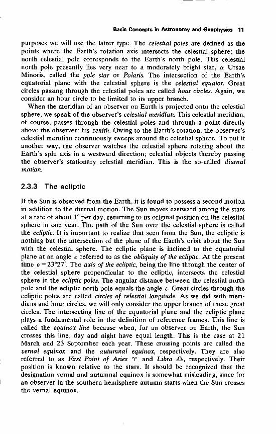
For a discussion of planetary motion and other phenomena in the solar
system, it is often more convenient to use the ecliptic plane as the funda-
mental plane for a reference frame. Then, we speak of a geocentric non-
rotating ecliptic reference frame (Fig. 2.2), in which the XY-plane coincides
with the ecliptic plane. The X-axis points to the vernal equinox. The Z-axis
is along the axis of the ecliptic and points to the ecliptic north pole. TheY-axis is normal to the X- and Z-axis such that the frame is right-handed.
The angular position of the celestial object S in Fig. 2.2, can be specified by
two quantities, the celestial longitude, A, and the celestial latitude, <p. Thecelestial latitude is defined as the geocentric angular distance in degrees
measured along the circle of celestial longitude passing through the object
from the ecliptic to that object. It is taken positive for objects north and
negative for objects south of the ecliptic. The celestial longitude is defined as
the angular distance in degrees measured along the ecliptic from the point
Basic Concepts in Astronomy and Geophysics 13
Fig. 2.2 The geocentric equatorial and ecliptic systems of coordinates
T to the foot of the circle of celestial longitude through that object. This
angle is measured from 0° to 360° eastward along the ecliptic.
2.3.5 Heliocentric reference frames
For describing planetary positions, or the motion of interplanetary space-
craft, the Sun is more convenient as origin of a reference frame. In most cases
the ecliptic plane is taken as the XY-plane in a heliocentric reference frame.
Since the celestial sphere was considered to have an infinite radius, every
point in the solar system can be regarded as being the center of this celestial
sphere. Consequently, parallel lines through the Sun and through the Earth
will intersect the celestial sphere at a common point. Thus, the point T can
serve as the directional reference for the X-axis in a heliocentric reference
frame too. In the heliocentric non-rotating ecliptic frame, a position can be
described by a heliocentric radius, r, and by the heliocentric longitude and
latitude, defined analogously to celestial longitude and latitude in the
geocentric ecliptic frame.
Besides the reference frames mentioned, in astrodynamics still other
reference frames are in use. Discussions on these other frames, used for
specific applications, are beyond the scope of this introductory chapter.
2.3.6 Motion of the vernal equinox
Up to now, we have tacitly assumed that the point T, being fundamental to
the non-rotating reference frames, is fixed between the stars on the celestial
sphere. In fact, however, this is not the case. Firstly, the mass distribution of
the Earth is not spherically symmetrical. As a consequence, the gravitational
attraction of Sun and Moon causes precession and nutation of the Earth's
rotation axis; i.e. the orientation of the equatorial plane varies. Secondly,
the mutual attractions between the Earth and the other planets result in
variations in the orientation of the ecliptic plane. Finally, the stars are only
at a finite distance, showing some of their own motion on the celestial
sphere. Because of these effects, the point T moves on the celestial sphere
at a rate of about 0.8' a year, while the obliquity decreases with about 0.5" a
14 Rocket Propulsion & Spaceflight Dynamics
year. The First Point of Aries, as its name suggests, was some 2000 years
ago located in the constellation of Aries, the Ram. More recently, it has
been in Pisces, the Fish, and presently it is moving into the constellation of
Aquarius, the Water Carrier. In order to avoid inaccuracies in calculations,
we have to specify which orientations of the equatorial plane and the ecliptic
plane, and so the location of the point T , are taken for the reference frame.
Usually, the mean vernal equinox and equator (or ecliptic) of a reference
epoch are selected, whereby mean refers to the fact that the relatively
short-period nutation motion is filtered out. In astrodynamics, two choices
for the reference epoch are commonly used: the beginning of the year 1950
and the date for which the computations are performed. We then speak of
the mean equinox of 1950 reference frame and the mean equinox of date
reference frame.
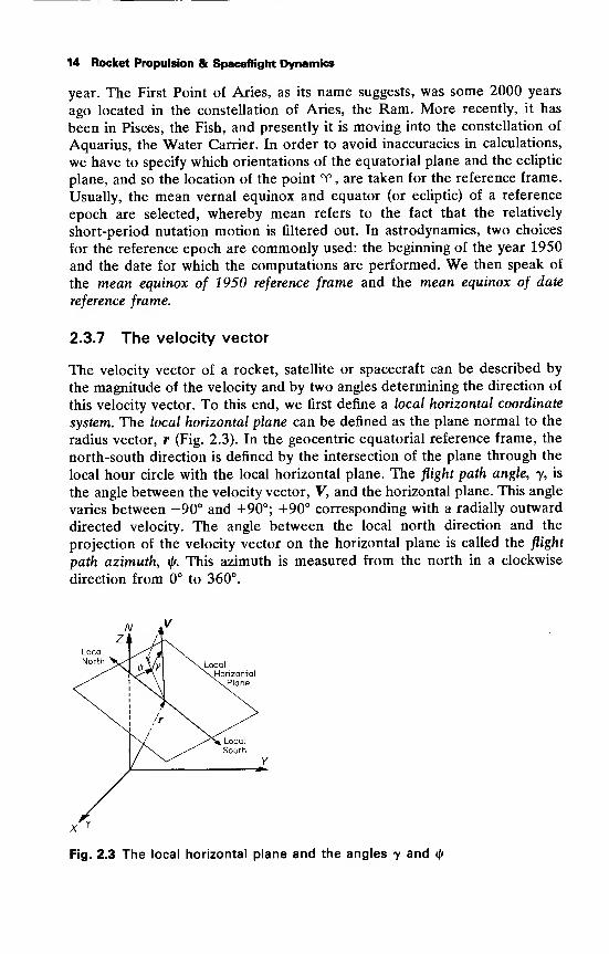
2.3.7 The velocity vector
The velocity vector of a rocket, satellite or spacecraft can be described by
the magnitude of the velocity and by two angles determining the direction of
this velocity vector. To this end, we first define a local horizontal coordinate
system. The local horizontal plane can be defined as the plane normal to the
radius vector, r (Fig. 2.3). In the geocentric equatorial reference frame, the
north-south direction is defined by the intersection of the plane through the
local hour circle with the local horizontal plane. The flight path angle, y, is
the angle between the velocity vector, V, and the horizontal plane. This angle
varies between -90° and +90°; +90° corresponding with a radially outward
directed velocity. The angle between the local north direction and the
projection of the velocity vector on the horizontal plane is called the flight
path azimuth, ij/. This azimuth is measured from the north in a clockwise
direction from 0° to 360°.
LocaNorth Local
Horizontal
Plane
Fig. 2.3 The local horizontal plane and the angles y and i/r
Basic Concepts in Astronomy and Geophysics 15
2.4 Time and calendar
Man has long held a belief that there is a 'uniform time'. This concept of
uniformity, however, turns out to lack meaning. We have no master stand-
ard of which we are sure that it runs uniformly. All we really need is that
our chronometric variable, if inserted into our physical laws, furnishes
reproducible predictions that are in agreement with our observations. In
effect, we take a suitable repetitive physical phenomenon and define succes-
sive periods of repetition to be equal in length. Nowadays, it is felt that the
time provided by a cesium clock should correlate to the highest accuracy
with our physical laws, and we take by definition that this time progresses
uniformly. We call this Atomic Time (A.T.). Though in this way we can
define a unit of time, for the fitting of time in our conventional scale we are
committed to astronomical observations, which historically form the basis
for time reckoning systems.
In astronomy, the measurement of time intervals is based on the rotation
of the Earth. The observer's time is defined as the angular distance covered
by a reference object on the celestial sphere after its last crossing of the
upper branch of the observer's celestial meridian. The time interval between
two successive crossings is called a day. Though the actual length of a day
will, in general, depend on the reference object chosen, each type of day is
divided into 24 equal parts, called hours. These hours again are subdivided
into 60 minutes and each minute into 60 seconds.
The hour angle, H, of an object is defined as the angular distance in
degrees measured along the celestial equator from the observer's meridian
to the foot of the object's hour circle. Because for an observer on Earth, the
apparent motion of celestial objects on the celestial sphere is in a westward
direction, the hour angle is measured positive to the west so that the hour
angle increases with time. For a celestial object S, this hour angle is
indicated in Fig. 2.1. As an increment in the hour angle of 360° corresponds
to a time increment of exactly one day, time can be defined as the hour
angle of the reference object. As reference object a particular star can be
selected, e.g. Antares. When Antares crosses the observer's meridian we can
speak ofh m s Antares-time. Instead of selecting a particular star, it turns
out to be more convenient to use the vernal equinox or the Sun as reference
object, resulting in sidereal time or solar time, respectively. As the hour
angle of a given point on the celestial sphere differs at a certain epoch for
observers with a different geographical longitude, both types of time are
local and we speak of local sidereal time and local solar time.
2.4.1 Sidereal time
The sidereal day is defined as the interval between two successive passages
of the vernal equinox across the observer's meridian. From the definitions of
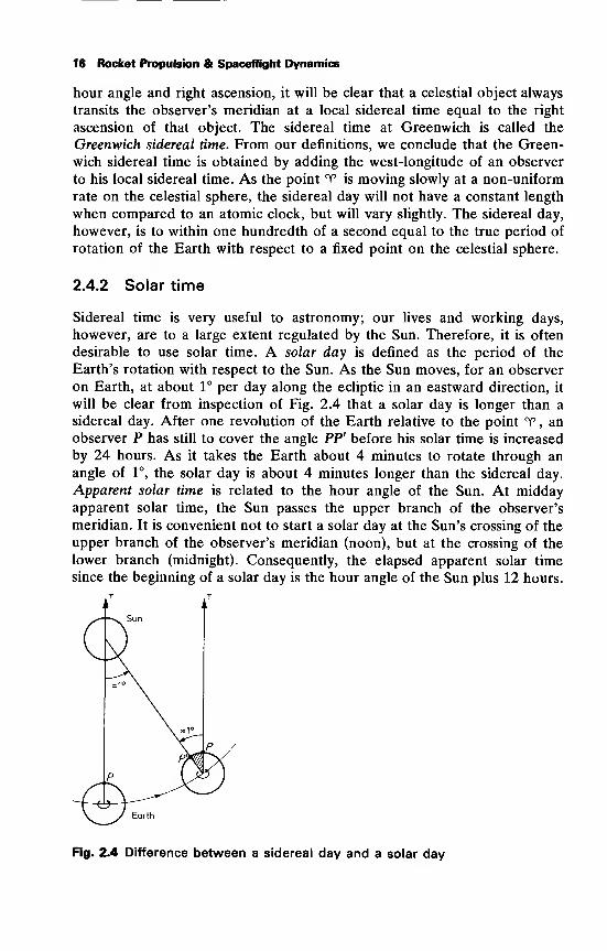
16 Rocket Propulsion & Spaceflight Dynamics
hour angle and right ascension, it will be clear that a celestial object always
transits the observer's meridian at a local sidereal time equal to the right
ascension of that object. The sidereal time at Greenwich is called the
Greenwich sidereal time. From our definitions, we conclude that the Green-
wich sidereal time is obtained by adding the west-longitude of an observer
to his local sidereal time. As the point T is moving slowly at a non-uniform
rate on the celestial sphere, the sidereal day will not have a constant length
when compared to an atomic clock, but will vary slightly. The sidereal day,
however, is to within one hundredth of a second equal to the true period of
rotation of the Earth with respect to a fixed point on the celestial sphere.
2.4.2 Solar time
Sidereal time is very useful to astronomy; our lives and working days,
however, are to a large extent regulated by the Sun. Therefore, it is often
desirable to use solar time. A solar day is defined as the period of the
Earth's rotation with respect to the Sun. As the Sun moves, for an observer
on Earth, at about 1° per day along the ecliptic in an eastward direction, it
will be clear from inspection of Fig. 2.4 that a solar day is longer than a
sidereal day. After one revolution of the Earth relative to the point T , an
observer P has still to cover the angle PP' before his solar time is increased
by 24 hours. As it takes the Earth about 4 minutes to rotate through an
angle of 1°, the solar day is about 4 minutes longer than the sidereal day.
Apparent solar time is related to the hour angle of the Sun. At middayapparent solar time, the Sun passes the upper branch of the observer's
meridian. It is convenient not to start a solar day at the Sun's crossing of the
upper branch of the observer's meridian (noon), but at the crossing of the
lower branch (midnight). Consequently, the elapsed apparent solar time
since the beginning of a solar day is the hour angle of the Sun plus 12 hours.
Fig. 2.4 Difference between a sidereal day and a solar day
Basic Concepts in Astronomy and Geophysics 17
On September 23, the Sun passes through the autumnal equinox. The vernal
equinox then passes the meridian of an observer for whom it is midnight. Atthat moment, local apparent solar time and local sidereal time are equal for
the observer mentioned. With each succeeding day from then, sidereal time
gains some minutes on solar time, until just one year later the difference
between them is 24 hours.
2.4.3 Mean solar time
Owing to the ellipticity of the Earth's orbit about the Sun, and the fact that
the equatorial plane and the ecliptic plane do not coincide, the apparent
motion of the Sun on the celestial sphere is not 'uniform'. For that reason
the solar day has not a constant length. Therefore, the concept of a fictitious
mean Sun has been introduced, which is assumed to move at a uniform rate
eastward along the celestial equator, with a sidereal motion equal to the
mean sidereal motion of the true Sun at January 0.5 (i.e. December 31, 12
hours E.T.*), 1900. This period is the so-called tropical year of January 0.5,
1900, to be discussed in Section 2.4.6. A mean solar day, or civil day, is the
interval between two successive crossings of the mean Sun through the
observer's meridian, and mean solar time is defined as the hour angle of the
mean Sun plus 12 hours. The maximum difference between both kinds of
solar time can be as much as 17 minutes. In astrodynamics, we often use a
standardized mean solar time: the Greenwich mean solar time or Universal
Time (U.T.).
2.4.4 Standard time
For civil life, in 1884 an international agreement was reached to establish a
system of 25 time zones around the world. All but two cover a longitude interval
of 15°. The Greenwich zone, Zone 0, has bounding meridians 7.5°W and 7.5°E.
All other zones are numbered from the Greenwich zone; positively to the west.
The Standard Time or Zone Time (Z.T.) of any place on Earth is given by the
mean solar time of the meridian through the center of the Zone of that place. Theconvention is made that the Zone from 172.5°W to 180°W is Zone 12, while the
zone from 172.5°E to 180°E is Zone - 12. The meridian separating these two
zones is the International Date Line. Going eastward from Greenwich one finds
the time at the Date Line to be 12 hours later than the time at Greenwich; going
westward one finds a time 12 hours earlier than at Greenwich. Consequently, a
crossing of the Date Line results in a discontinuityof 24 hours.We thereforeomit
one day from our calendar when crossing the Date Line in a westward direction
and count a day twicewhen crossing it in the opposite direction. For geographical
and political reasons, the actual Date Line and the zone boundaries deviate from
the strict classification given above.
* See Section 2.4.5
18 Rocket Propulsion & Spaceflight Dynamics
2.4.5 Ephemeris time and atomic time
Because of irregularities in the Earth's rotation rate, even the mean solar
day varies slightly as compared to A.T. over the years. For very precise
determinations of time therefore a new kind of time was introduced in 1950:
Ephemeris Time (E.T.). This is the time which is consistent with the laws of
dynamics, and causes the position of celestial bodies, as predicted from the
dynamical equations of motion, to agree with observation. The fundamental
unit of E.T. is the ephemeris second which is 1/31,556,925.9747 tropical
year of 1900, January at Greenwich mean noon, and is chosen such that it
equals the length of a mean solar second at that epoch. In 1975 U.T. and
E.T. differed by about 45 seconds owing to changes in the Earth's rotation
rate since January 0, 1900.
We have seen that, formally, two definitions of uniform time are in use. In
astronomy, E.T. was devised from the laws of dynamics; in physics, A.T.
was introduced. The big advantage of A.T. is that it can be measured in a
laboratory environment, in contrast to E.T. The epoch at which A.T. starts
is usually set at 1958, January 1, hours U.T. The atomic second is nowdefined so that the frequency corresponding to a certain resonance of the
cesium atom is 9, 192, 631, 770 cycles per second. This numerical value is such
that the A.T. second is equal to the observationally determined value of the
E.T. second over the period 1956 to 1965. At 1958, January 1, A.T. and
E.T. differed by about 32 seconds and assuming that A.T. and E.T. run at
an equal rate, presently the difference is still about 32 seconds.
In January 1972, the atomic second was adopted for all timing, replacing
the ephemeris second.
2.4.6 The year
In addition to the day as a unit of time, we are accustomed in civil life to
other natural units: the year, the month and the week. Here we will discuss
only the year. The year is defined as the orbital period of the Earth in its
motion about the Sun. Various types of years can be distinguished. The most
important are the tropical year, the Julian year and the civil calendar year.
The tropical year is defined as the time interval between two successive
passages of the Sun through the vernal equinox. It equals about 365.2422
mean solar days.
In the Julian calendar, every year counts 365 mean solar days, except
those years divisible by four: the leap years, which have 366 mean solar
days. So, the average length of the Julian year is 365.25 mean solar days.
To approximate the tropical year more closely, the Gregorian calendar
was introduced. The difference between the both calendars being that in the
Gregorian calendar those century years not divisible by 400 are ordinary
years. Today, the Gregorian calendar is the civil calendar in use over most
of the globe. The average length of a Gregorian year is 365.2425 mean solar
Basic Concepts in Astronomy and Geophysics 19
days, which is so close to the tropical year that the error in using the
Gregorian calendar is only three days in 10,000 years.
2.4.7 The Julian date
Finally, the concept of Julian Date (J.D.) has to be mentioned. This is a
system of Julian day numbers which involves a continuing count of meansolar days rather than years, and so provides a simpler way of determining
the interval of time between two dates than use of the conventional
calendar. The epoch at which the Julian Date was exactly zero was set at
4713 B.C., January 1, Greenwich noon, on the Julian calendar. This epochis close to the one that in medieval times was believed to have marked the
creation of the Earth. As an example: the Julian Date for 1975 August 1,18hours U.T. is 2, 442, 626.25. In order to avoid those large numbers for
indicating dates in our times, it is convenient to express epochs in Modified
Julian Dates (M.J.D.), which are related to Julian Dates by:
MJ.D. = J.D. -2,400,000.5.
It should be recognized that while a Julian Date starts at Greenwich meannoon, a Modified Julian Date starts at Greenwich midnight.
2.5 The Earth
Our planet Earth can, in a first approximation, be considered a sphere with
a radius of 6371km. As its mass equals about 5.98xl024kg, its mean
density amounts to 5520 kg/m3. Because the mean density of the material
near the Earth's surface is about 2700 kg/m3, the interior of the Earth must
be much denser. The outermost layer of the Earth, the crust, extends to a
depth of about 35 km beneath the continents, but only to about 5 km under
the ocean floors. Beneath the crust there is the mantle which extends downto a depth of about 3000 km. From a depth of 3000 km to about 5000 km,we speak of the outer-core, consisting of liquid material. The innermost part
of the Earth, the inner-core, is probably solid and extremely hot.
The Earth rotates about its polar axis at a rate of about 0.25'/s. The force
acting on a body on the Earth's surface, the gravity force, is the resultant of
the gravitational force (Section 3.5) and the centrifugal force caused by the
Earth's rotation. We can regard this resultant force as being derived fromthe so-called geopotential. The gravity force per unit of mass varies from
9.78 m/s2 at the Earth's equator to 9.83 m/s2at the poles.
2.5.1 The shape of the Earth
If the Earth had no rigidity at all, its surface should be an equipotential
surface with a constant value of the geopotential. But the Earth has a certain
amount of rigidity, and its surface shows an irregular shape. The oceans,
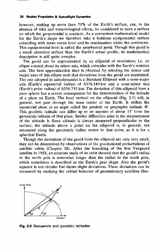
20 Rocket Propulsion & Spaceflight Dynamics
however, making up more than 70% of the Earth's surface, can, in the
absence of tidal and meteorological effects, be considered to have a surface
on which the geopotential is constant. As a convenient mathematical model
for the Earth's shape we therefore take a fictitious equipotential surface
coinciding with mean ocean level and its continuation under the continents.
This equipotential level is called the geophysical geoid. Though this geoid is
a much smoother surface than the Earth's actual profile, its mathematical
description is still quite complex.
The geoid can be approximated by an ellipsoid of revolution; i.e. an
ellipse rotated about its minor axis, which coincides with the Earth's rotation
axis. The best approximation then is obtained by selecting the minor and
major axes of this ellipse such that deviations from the geoid are minimized.
The one adopted in astrodynamics is a Standard Ellipsoid with a semi-major
axis (Earth's equatorial radius) of 6378.140 km and a semi-minor axis
(Earth's polar radius) of 6356.755 km. The deviation of this ellipsoid from a
pure sphere has a severe consequence for the determination of the latitude
of a place on Earth. The local vertical on the ellipsoid (Fig. 2.5) will, in
general, not pass through the mass center of the Earth. It strikes the
equatorial plane at an angle called the geodetic or geographic latitude, <!>'.
This geodetic latitude can differ up to an amount of about 11' from the
geocentric latitude of that place. Similar difficulties arise in the measurement
of the altitude h. Since altitude is always measured perpendicular to the
surface, the altitude above a point on the ellipsoid is, in general, not
measured along the geocentric radius vector to that point, as it is for a
spherical Earth.
Though the deviations of the geoid from the ellipsoid are only very small,
they can be determined by observations of the gravitational perturbations of
satellite orbits (Chapter 18). After the launching of the first Vanguard
satellite in 1958, an accurate study of its orbit showed that the geoid's radius
to the north pole is somewhat longer than the radius to the south pole,
which sometimes is described as the Earth's pear shape. Also the geoid's
equator is not circular but shows slight deviations. These deviations can be
measured by studying the orbital behavior of geostationary satellites (Sec-
Equator
Fig. 2.5 Geocentric and geodetic latitudes
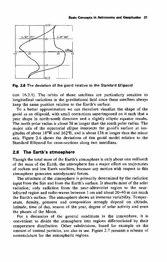
Basic Concepts in Astronomy and Geophysics 21
A=90°, n§°*s^
/.o V-2
90/V-
l&-A=0°, 180°
, A/?(m]
20
£5-
90S
Fig. 2.6 The deviation of the geoid relative to the Standard Ellipsoid
tion 16.2.1). The orbits of those satellites are particularly sensitive to
longitudinal variations in the gravitational field since these satellites always
keep the same position relative to the Earth's surface.
To a better approximation we can therefore visualize the shape of the
geoid as an ellipsoid, with small corrections superimposed on it such that a
pear shape in north-south direction and a slightly elliptic equator results.
The north polar radius is about 38 m longer than the south polar radius. The
major axis of the equatorial ellipse intersects the geoid's surface at lon-
gitudes of about 18°W and 162°E, and is about 138 m longer than the minor
axis. Figure 2.6 shows the deviations of this geoid model relative to the
Standard Ellipsoid for cross-sections along two meridians.
2.6 The Earth's atmosphere
Though the total mass of the Earth's atmosphere is only about one millionth
of the mass of the Earth, the atmosphere has a major effect on trajectories
of rockets and low Earth satellites, because any motion with respect to this
atmosphere generates aerodynamic forces.
The structure of the atmosphere is primarily determined by the radiation
input from the Sun and from the Earth's surface. It absorbs most of the solar
radiation; only radiation from the near-ultraviolet region to the near-
infrared region and radio-waves between 1 cm and about 20-40 m can reach
the Earth's surface. The atmosphere shows an immense variability. Temper-
ature, density, pressure and composition strongly depend on altitude,
latitude, time of day, season of the year, degree of solar activity and even
the phases of the Moon.For a discussion of the general conditions in the atmosphere, it is
convenient to divide the atmosphere into regions differentiated by their
temperature distribution. Other subdivisions, based for example on the
amount of ionized particles, are also in use. Figure 2.7 presents a scheme of
nomenclature for the atmospheric regions.
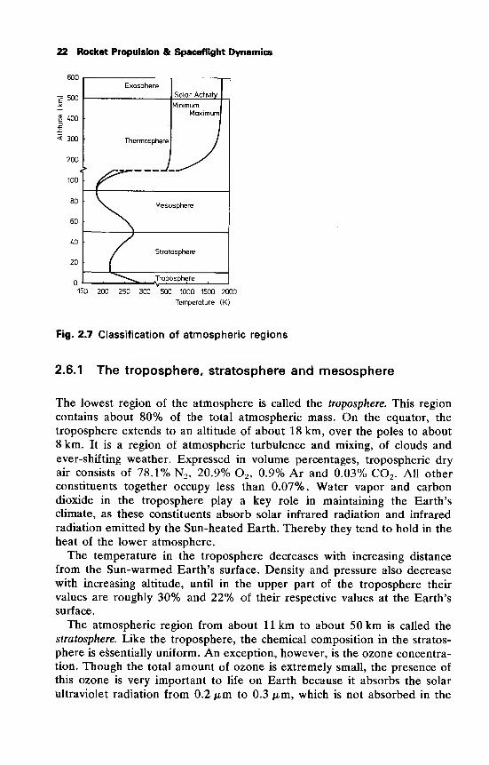
22 Rocket Propulsion & Spaceflight Dynamics
Exosphere
-£ 500 Solar Activity
Minimum
-S 400
< 300 Thermosphere
Maximum
200
J_^y100 i^80 \. Mesosphere
60 N.
40 y/ Stratosphere
20j
"****>>«- Tropospherei , ,—^_,—\ i i 1 1
150 200 250 300 500 1000 1500 2000
Temperature (K)
Fig. 2.7 Classification of atmospheric regions
2.6.1 The troposphere, stratosphere and mesosphere
The lowest region of the atmosphere is called the troposphere. This region
contains about 80% of the total atmospheric mass. On the equator, the
troposphere extends to an altitude of about 18 km, over the poles to about
8 km. It is a region of atmospheric turbulence and mixing, of clouds and
ever-shifting weather. Expressed in volume percentages, tropospheric dry
air consists of 78.1% N2 , 20.9% 2 , 0.9% Ar and 0.03% C02 . All other
constituents together occupy less than 0.07%. Water vapor and carbon
dioxide in the troposphere play a key role in maintaining the Earth's
climate, as these constituents absorb solar infrared radiation and infrared
radiation emitted by the Sun-heated Earth. Thereby they tend to hold in the
heat of the lower atmosphere.
The temperature in the troposphere decreases with increasing distance
from the Sun-warmed Earth's surface. Density and pressure also decrease
with increasing altitude, until in the upper part of the troposphere their
values are roughly 30% and 22% of their respective values at the Earth's
surface.
The atmospheric region from about 11km to about 50 km is called the
stratosphere. Like the troposphere, the chemical composition in the stratos-
phere is essentially uniform. An exception, however, is the ozone concentra-
tion. Though the total amount of ozone is extremely small, the presence of
this ozone is very important to life on Earth because it absorbs the solar
ultraviolet radiation from 0.2 jam to 0.3 jam, which is not absorbed in the
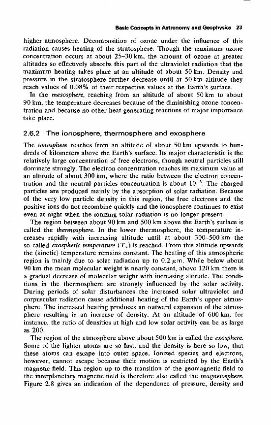
Basic Concepts in Astronomy and Geophysics 23
higher atmosphere. Decomposition of ozone under the influence of this
radiation causes heating of the stratosphere. Though the maximum ozone
concentration occurs at about 25-30 km, the amount of ozone at greater
altitudes so effectively absorbs this part of the ultraviolet radiation that the
maximum heating takes place at an altitude of about 50 km. Density and
pressure in the stratosphere further decrease until at 50 km altitude they
reach values of 0.08% of their respective values at the Earth's surface.
In the mesosphere, reaching from an altitude of about 50 km to about
90 km, the temperature decreases because of the diminishing ozone concen-
tration and because no other heat generating reactions of major importance
take place.
2.6.2 The ionosphere, thermosphere and exosphere
The ionosphere reaches from an altitude of about 50 km upwards to hun-
dreds of kilometers above the Earth's surface. Its major characteristic is the
relatively large concentration of free electrons, though neutral particles still
dominate strongly. The electron concentration reaches its maximum value at
an altitude of about 300 km, where the ratio between the electron concen-
tration and the neutral particles concentration is about 10~3. The charged
particles are produced mainly by the absorption of solar radiation. Because
of the very low particle density in this region, the free electrons and the
positive ions do not recombine quickly and the ionosphere continues to exist
even at night when the ionizing solar radiation is no longer present.
The region between about 90 km and 500 km above the Earth's surface is
called the thermosphere. In the lower thermosphere, the temperature in-
creases rapidly with increasing altitude until at about 300-500 km the
so-called exospheric temperature (TJ) is reached. From this altitude upwards
the (kinetic) temperature remains constant. The heating of this atmospheric
region is mainly due to solar radiation up to 0.2 /xm. While below about
90 km the mean molecular weight is nearly constant, above 120 km there is
a gradual decrease of molecular weight with increasing altitude. The condi-
tions in the thermosphere are strongly influenced by the solar activity.
During periods of solar disturbances the increased solar ultraviolet and
corpuscular radiation cause additional heating of the Earth's upper atmos-
phere. The increased heating produces an outward expansion of the atmos-
phere resulting in an increase of density. At an altitude of 600 km, for
instance, the ratio of densities at high and low solar activity can be as large
as 200.
The region of the atmosphere above about 500 km is called the exosphere.
Some of the lighter atoms are so fast, and the density is here so low, that
these atoms can escape into outer space. Ionized species and electrons,
however, cannot escape because their motion is restricted by the Earth's
magnetic field. This region up to the transition of the geomagnetic field to
the interplanetary magnetic field is therefore also called the magnetosphere.
Figure 2.8 gives an indication of the dependence of pressure, density and
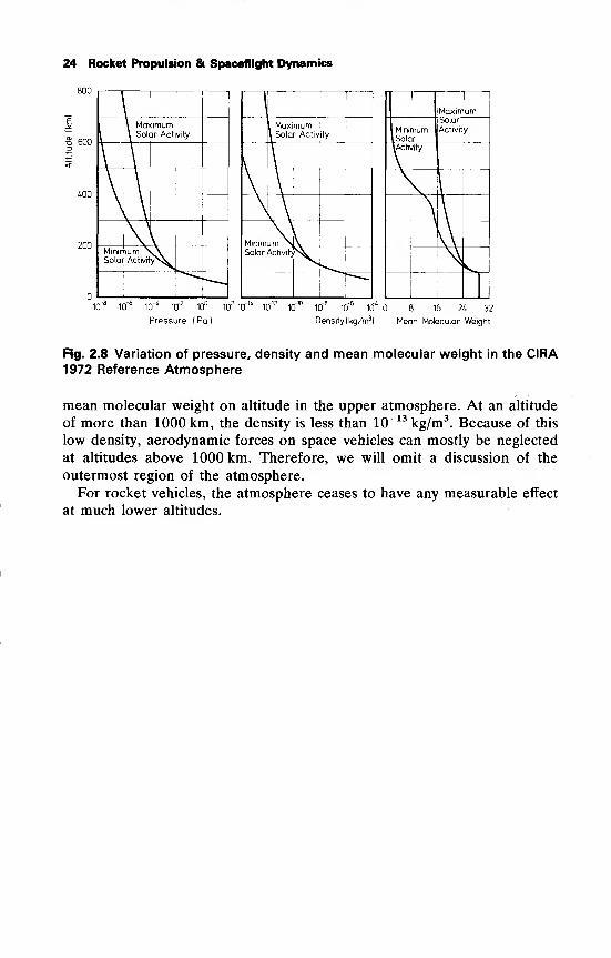
24 Rocket Propulsion & Spaceflight Dynamics
•S 600
400
200
\ Maximum|
\ Solar Activity
MininSola
num N
Activitr\
^ 1
i
i Maximum\ Solar Activ ty
\
Minimum^Solar Activity^\
Maximum
Mini
ISola~\Acti\
numr
Solar'
Activity
(ity
1
)
10~8 10"6
10~4
10~2
10° 102 10"" 10"'
210~'° 10"
810"
610"' 8 16 24 32
Pressure (Pa) Density (kg/m3 ) Mean Molecular Weight
Fig. 2.8 Variation of pressure, density and mean molecular weight in the CIRA1972 Reference Atmosphere
mean molecular weight on altitude in the upper atmosphere. At an altitude
of more than 1000 km, the density is less than 10-13
kg/m3. Because of this
low density, aerodynamic forces on space vehicles can mostly be neglected
at altitudes above 1000 km. Therefore, we will omit a discussion of the
outermost region of the atmosphere.
For rocket vehicles, the atmosphere ceases to have any measurable effect
at much lower altitudes.
3 Mechanics of Particles, Bodiesand Fluids
Up to the present the velocities encountered in astronautics are relatively
small as compared to the velocity of light, and so classical or Newtonianmechanics will suffice our purpose. Newtonian mechanics is based on the
three laws of Newton, Galileo's principle of relativity and the three classical
conservation laws: conservation of mass, linear momentum and energy.
Moreover, the assumption is made that forces behave as vectors and can berepresented mathematically as such. We will now state Newton's laws for
particles, where a particle is defined as a constant mass concentrated at a
point.
1
.
Every particle continues in its state of uniform motion in a straight line
(or rest), unless compelled to change that state by forces acting upon it.
2. The time rate of change of linear momentum of a particle is propor-
tional to the force acting upon that particle and is collinear with and in the
direction of that force.
3. The mutual forces of two particles acting upon each other are equal in
magnitude and opposite in direction (action = reaction).
3.1 Newton's first law
In analyzing the first law, we must realize that it is a statement about
motion, which is a relative concept. If we speak about motion of an object,
we have to specify a frame of reference relative to which the object is
moving.
In the first law no reference frame is specified. We know from experi-
ence that we cannot just choose any reference frame, i.e. there are special
reference frames wherein the first law is valid. We can in fact turn the first
law around and make the following statement:
There exist certain reference frames with respect to which the motion of a
particle, free of all external forces, is uniform (motion in a straight line with
constant speed, including zero).
Those frames are called inertial frames. The first law then becomes in fact
the definition of an inertial frame of reference.
It is a direct consequence of this definition that if such a frame exists, a
whole class of inertial frames can be found. To show this, let us suppose that
the frame S is an inertial frame. If another frame S' translates uniformly,
26 Rocket Propulsion & Spaceflight Dynamics
with velocity V, (i.e. V is constant), with respect to S and if the time in S'
differs by only a constant from the time in S, then S' is an inertial frame too.
We will now proceed to prove this statement, known as Galileo's principle of
relativity.
The transformation of space and time coordinates from S to S' is given by
the following relations:
r' = r-Vt-R,(311)
t'=t+T.
This transformation of coordinates is called the Galilean transformation.
Herein, r and r' are the position vectors of a particle P with respect to the
origins of S and S', respectively. R is a constant vector defining the position
of S' relative to S at time t = 0; t and t' are respectively the times in S and
S', while T, finally, is the constant time difference between S and S'. If noforces are acting on the particle P, then according to the first law the velocity
of the particle relative to S is a constant
r
dt'
The velocity of the particle relative to S' is defined as
r dfUsing Eqs. (3.1-1) we find
aVdf = aV = drr
dtdt' dt dtr
Since both Vr and V are constant, we conclude that V'r is a constant too.
According to the definition of inertial frames, S' and thus any frame whichtranslates uniformly with respect to S is an inertial frame.
As we will see later on, this is not true for reference frames which rotate,
whether or not uniformly, relative to an inertial frame. Any such rotational
motion will produce apparent accelerations. We therefore have to conclude
that Newtonian mechanics requires an absolute reference for rotational
motion. Translational motion on the other hand is relative in that anarbitrary uniform translation may be superimposed. Experience has provedthat for all motions we can find a frame that behaves as an inertial one, at
least within our measuring accuracy. To describe the motion of the planets
in our solar system, the heliocentric frame that is not rotating relative to the
fixed stars can be considered as an inertial frame. Likewise, as for experi-
ments within a laboratory on Earth a frame fixed to the laboratory can beviewed as an inertial one. We therefore define an inertial frame to be one in
which, experimentally, the first law holds within our desired accuracy.
Mechanics of Particles, Bodies and Fluids 27
3.2 Newton's second law
The second law, like the first law, deals with motion and again fromexperience it is found that the second law holds only with respect to inertial
frames. The second law can be expressed as
F=jt
(mV). (3.2-1)
Here mV is the linear momentum of a particle with mass m and velocity V.
The mass in this law is the so-called inertial mass, in contrast with the
gravitational mass which will appear in Newton's law of gravitation later on.
Newton, however, tacitly assumed the equivalence of inertial and gravita-
tional mass. Experiments by Eotvos et al. [1] in the beginning of this century,
and more recently by Roll et al. [2] and Braginsky and Panov [3] haveestablished the constancy of the ratio of inertial to gravitational mass within
1 part in 10 11or better. In Einstein's general theory of relativity the
equivalence between inertial and gravitational mass is a consequence of the
principle of equivalence [4, 5].
We have seen that from the Galilean principle of relativity and from the
first law it followed that systems translating uniformly relative to an inertial
system are inertial systems themselves. We can only use this statement if the
second law is invariant under the Galilean transformation. This invariance
exists indeed if mass and force are invariant and if, moreover, the mass of
the particle is a constant, as will be shown. Consider therefore again the
systems S and S' as described before. If F is the force on the particle P in S,
and F' is the force on P in S', then since the force is invariant, F=F'. It
follows from Eqs. (3.1-1) that the time rate of change of linear momentumof the particle in the two reference systems is related by
d_/ M__d_dt \
mdt)~dt' ™'S+V
d /'drVv dm '
dt' \ dt') dt''
Applying Newton's second law in both systems, we obtain:
c ^ d / dr\In system 5 : F=— \m— ,
dr\ dt)
„, „, d / ,dr'\ ¥ dm'In system S' :F' =— m'— )+V-
dr\ dt') dt''
We see that the second law is invariant only if the mass of the particle is a
constant.
It was for that reason that we stated the laws of motion for particles with
constant mass.
The third law, finally, is clear in itself. However, we have to add the
requirement that the action and reaction forces are collinear. This collinear-
ity is essential for the conservation of mechanical angular momentum of an
28 Rocket Propulsion & Spaceflight Dynamics
isolated system. It is true for all Newtonian gravitational and mechanical
interaction forces but does not apply to certain forces between moving
electrically charged particles. This, however, will not concern us in this
book.
3.3 Non-inertial frames
We have seen that the first and second of Newton's laws are valid only in
inertial frames. This does not mean that studying the motion of an object in
a non-inertial frame prohibits us from using Newton's laws. We will have to
modify these laws in such a way that they are applicable in non-inertial
frames too. In this section we will derive the laws for the said modification.
Suppose S is an inertial frame and S' is a non-inertial one. We know by
now that if S' is non-inertial it is moving with respect to S with a velocity
which is not uniformly translational. According to Chasles' theorem [6], the
most general motion of S' with respect to S consists of a translational
motion and a rotational motion. By a translational motion of S' is meantthat in the infinitesimal time interval At every point fixed with respect to S'
undergoes a displacement Ar relative to S, where Ar is the same for all
points of S'. The translational velocity is defined as
Vs.= lim^. (3.3-1)
The system S' is in pure rotational motion relative to S if every point fixed
with respect to S' undergoes an angular displacement A0 in the time interval
At, where Ad is measured about a line fixed in S: the axis of rotation. Wenow define a vector A6 with magnitude A0 and directed along this axis of
rotation with a sense according to the right-hand rule. The angular velocity
O of S' is then defined as
Aftfl=lim=^. (3.3-2)
Af^O At
3.3.1 Rotation
In order to concentrate a moment on rotation, suppose the origin of system
S' coincides with the origin of S. Suppose S' is in pure rotational motionrelative to S about an axis through the origins of both systems. If P is a
point fixed in S', with position vector r with respect to the origin of S', then
the point P describes in the time interval Ar part of a circle (Fig. 3.1) with
radius r sin <p and lying in a plane perpendicular to the axis of rotation. Here<p is the angle between the vector r and the axis of rotation. Neglecting
second order terms, the point P undergoes a displacement Ar perpendicular
to r and the axis of rotation and with magnitude Ar= r sin <p Ad. So Ar is
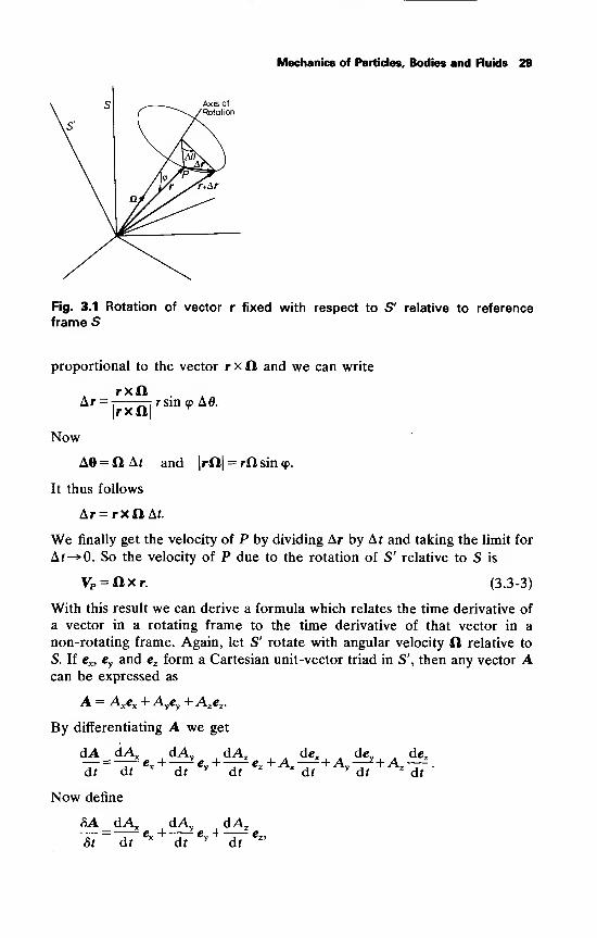
Mechanics of Particles, Bodies and Fluids 29
Fig. 3.1 Rotation of vector r fixed with respect to S' relative to reference
frame S
proportional to the vector r x 11 and we can write
rxflar = ;
— rsin <p A0.rxft
Now
A6 = ft Af and |rft| = rft sin <p.
It thus follows
Ar=rxftAf.
We finally get the velocity of P by dividing Ar by Ar and taking the limit for
Af—»0. So the velocity of P due to the rotation of S' relative to S is
VP = ftxr. (3.3-3)
With this result we can derive a formula which relates the time derivative of
a vector in a rotating frame to the time derivative of that vector in a
non-rotating frame. Again, let S' rotate with angular velocity ft relative to
S. If ex , eyand ez form a Cartesian unit-vector triad in S', then any vector A
can be expressed as
By differentiating A we get
dA = dA^ dA,
dt &t€x
dt
Now define
8A dA
c„+-dA,
dt«.+A,
dt+ A,
dey
dt+ A,
dez
~dt
8t
dAv dAz
dt dty dt
30 Rocket Propulsion & Spaceflight Dynamics
5Athen —— is the time rate of change of the vector A as viewed by an observer
8t
in the rotating system S'. For, only the components of A can change for
such an observer since the unit vectors ex , eyand ez are fixed for him. For an
dexobserver in the inertial system S, —— is the velocity of the point with position
vector ex due to the rotation il. According to Eq. (3.3-3) this velocity is
Hxex . Likewise:
dev ~ de7 ^'—- = llxev and —- = flxez .
dty
dt
So the rate of change of A for an observer in the inertial system is
^ =^+ttxA. (3.3-4)dt 8t
Though we have assumed that S is an inertial frame, it is important to
note that nowhere have we actually used this fact. Therefore Eq. (3.3-4)
generally holds for two systems rotating relative to each other. If, for
example, a system S' is rotating with respect to a system S" with angular
velocity fts < as viewed from S", then for any vector A
8A\ = /8A\ +a (33 _5)8t) s . \8tJ s .
Likewise
(*V(*V*** (33-6)
where ils » is the rotation rate of S" as viewed by an observer in S'. AsHs
»=—£lS ', both expressions are alike.
3.3.2 Newton's laws
We will now turn to the problem how to modify Newton's laws such that
they are valid in non-inertial frames. Let S' be a system which translates and
rotates relative to S (Fig. 3.2). If R is the position vector of the origin of S'
with respect to the origin of S and r and p the position vectors of a particle
P with mass m relative to the origins of S and S', respectively, then
r = R + p. (3.3-7)
By differentiating Eq. (3.3-7) we obtain the absolute velocity of P
V- =£=£+£ (3-3-8)dt dt dt
All derivatives in Eq. (3.3-8) are rates of change as viewed from the inertial
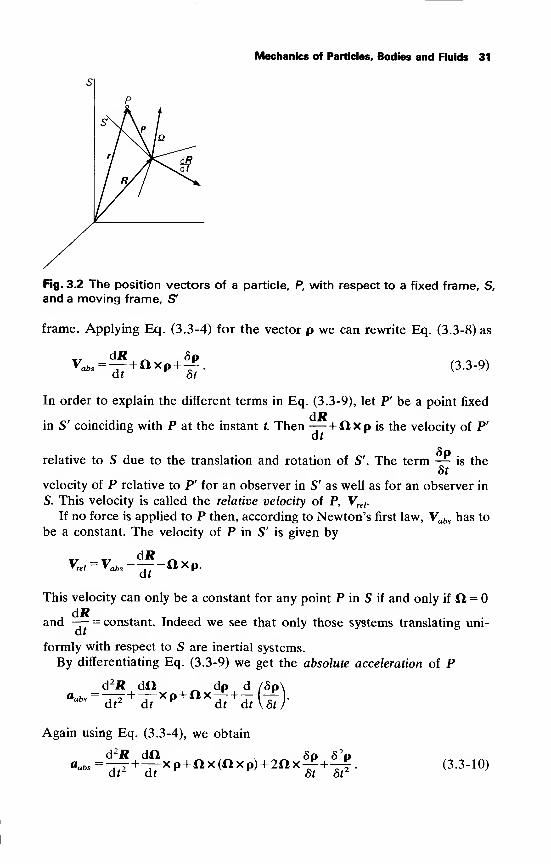
Mechanics of Particles, Bodies and Fluids 31
Fig. 3.2 The position vectors of a particle, P, with respect to a fixed frame, S,
and a moving frame, S'
frame. Applying Eq. (3.3-4) for the vector p we can rewrite Eq. (3.3-8) as
(3.3-9)dR „ So
In order to explain the different terms in Eq. (3.3-9), let P' be a point fixed
dJRin S' coinciding with P at the instant t. Then— + flxp is the velocity of P'
dt
89lrelative to S due to the translation and rotation of S'. The term — is the8t
velocity of P relative to P' for an observer in S' as well as for an observer in
S. This velocity is called the relative velocity of P, Vrel .
If no force is applied to P then, according to Newton's first law, Vabs has to
be a constant. The velocity of P in S' is given by
Vrei= Vabs
-— -ftxp.at
This velocity can only be a constant for any point P in S if and only if ft =dJJ
and —— = constant. Indeed we see that only those systems translating uni-
formly with respect to S are inertial systems.
By differentiating Eq. (3.3-9) we get the absolute acceleration of P
d2R dXl dp d /Sp=rr2"+ ^r~ x P +^ x j
+—dt2 dt dt dt\8t
Again using Eq. (3.3-4), we obtain
d2R dH Sp S2p= -TT + ~r~ xp+flx(ftxp) + 2ftx-£-+
dt2 dt 8t 8t'(3.3-10)
acceleration, ac . The term -^, finally, is the acceleration of P as viewed by
32 Rocket Propulsion & Spaceflight Dynamics
The sum of the first three terms of the right-hand side of Eq. (3.3-10)
represents the acceleration of the fixed point P' for an observer in S. This is
d2Rcalled the dragging acceleration, adr. The term —3 is the absolute accelera-
tion of the origin of S' . The term ft x (ft x p) is due to the rotation of S' and
dftrepresents a centripetal acceleration. The term —— Xp, often called the
at
tangential acceleration is due to the rate of change of rotational velocity.
The sum of the last two terms in Eq. (3.3-10) is the acceleration of P
relative to P' for an observer in S. The term 2ft x— is called the Coriolis8t
8t
an observer in S' and is called the relative acceleration, arel .
So, in general, we can write
<*abs = «dr + «c + ttrel-
If F is the actual force applied to the particle P, then according to Newton's
second law
F = maabs= madr + mac + marel .
We now define two apparent forces: a dragging force
Fdr = ~madr,(3.3-11)
and a Coriolis force
Fc = -mac . (3.3-12)
Thus we can write the second law in the form
Ftot= F+Fdr +Fc
= mareU (3.3-13)
According to Eq. (3.3-13), we can apply Newton's second law in non-
inertial frames if for the total force acting on the particle we take the sum of
the external force and the two apparent forces.
3.4 Dynamics of particle systems
With the laws and formulae stated and derived in the previous sections, the
motion of a single particle under influence of a known force can be
calculated in a fairly straightforward way. By applying Newton's second law,
a second-order vector differential equation is obtained. This vector equation
can be split into 3 scalar second-order differential equations for motion in
physical space. These differential equations, together with appropriate initial
conditions, have to be solved, either analytically or numerically. In this wayone gets velocity and position as a function of time. In Section 3.6 we will
consider the motion of a particle in a gravitational force field, as this analysis
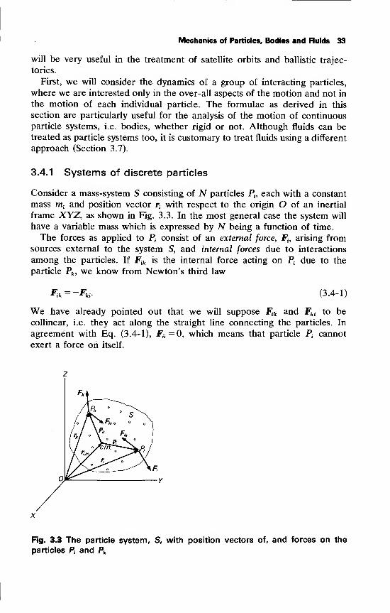
Mechanics of Particles, Bodies and Fluids 33
will be very useful in the treatment of satellite orbits and ballistic trajec-
tories.
First, we will consider the dynamics of a group of interacting particles,
where we are interested only in the over-all aspects of the motion and not in
the motion of each individual particle. The formulae as derived in this
section are particularly useful for the analysis of the motion of continuous
particle systems, i.e. bodies, whether rigid or not. Although fluids can betreated as particle systems too, it is customary to treat fluids using a different
approach (Section 3.7).
3.4.1 Systems of discrete particles
Consider a mass-system S consisting of N particles Pt ,each with a constant
mass m; and position vector rtwith respect to the origin O of an inertial
frame XYZ, as shown in Fig. 3.3. In the most general case the system will
have a variable mass which is expressed by N being a function of time.
The forces as applied to Ptconsist of an external force, F
t ,arising from
sources external to the system S, and internal forces due to interactions
among the particles. If Fik is the internal force acting on Ptdue to the
particle Pk , we know from Newton's third law
Fik - ~fki . (3.4-1)
We have already pointed out that we will suppose Fik and Fki to be
collinear, i.e. they act along the straight line connecting the particles. In
agreement with Eq. (3.4-1), Fu = 0, which means that particle Ptcannot
exert a force on itself.
Fig. 3.3 The particle system, S, with position vectors of, and forces on the
particles P, and Pk
34 Rocket Propulsion & Spaceflight Dynamics
The linear momentum of Ptrelative to XYZ is
Ji = mi^- (3 -4"2)
Applying Newton's second law on Pf ,we get
NdJ.
Fi+I F*=-j;- (3-4-3)
Now summing Eq. (3.4-3) over all N particles which form the system S at
time t, we obtain
N N N N J r
!'.+ ! I*.-I=. (3-4-4)i = l i = l fc = l i = l ut
N"
Now let X Fi=Fs'- the total external force applied to the system S at time t.
i = \
From Eq. (3.4-1) we see that
N N
i=i ^=1
So Eq. (3.4-4) can be written in the form
N dl N d2r
This equation is known as the translational equation of system S.
For an invariable system, i.e. a system where no particles enter or leave
the system, the translational equation can be written in a simpler and morefamiliar form. In that case, summation and differentiation can be inter-
changed, leading to
Nwhere M is the total (constant) mass of the system, given by M = £ w
f ,and
i = l
rcm is the position vector of the center of mass of the system, defined as
1N
rcm = M ^ miTi ' (3.4-6)
The translational equation can be written as
Fs = M^f. (3.4-7)
This equation states that the motion of the center of mass of the system is
the same as if the entire mass of the system were concentrated at the center
Mechanics of Particles, Bodies and Fluids 35
of mass and were driven by an external force equal to the forces external to
the system.
The equation of rotational motion of the system S can be obtained byvectorial multiplication of Eq. (3.4-3) with r
f:
N jjriXF^ £ r
ixFik
= rix-j. (3.4-8)
k = l &t
Now, the moment of Ffwith respect to O is defined as
Mi= r
ixF
i ,
and the angular momentum of P; is
Bi= r
ixJ
i= m
ir
ix-^. (3.4-9)
Then, the right-hand side of Eq. (3.4-8) can be written as
dJt
d . ,. dBt
r'xdTd7
(r<x/
')=ir
Equation (3.4-8) can thus be written as
M,+ £ ri xFik =—
K
(3.4-10)fc=i M
By summing Eq. (3.4-10) over all particles N, we obtain
N N N N J|»
XM; +X I rixFik =lt -f. (3.4-11)
i = l i = l k = l i = l Qt
NNow Y. Mi =Ms : the total moment about O due to the external forces on
the system S. Because of Eq. (3.4-1) and the collinearity of the internal
forces
N N
Z Z r,xFlk= 0,
i=l k=l
as can be seen by taking the terms in pairs together
rixFik + rk xFki
= (ri-rk)xFik
= rik xFik= 0.
Finally, the rotational equation for the system is found to be
*s= If=!>*># (3-4-12)
Again, for an invariable system this equation can be written in a morefamiliar form by defining the total angular momentum relative to O as
B= Z^ XSi=i dr
36 Rocket Propulsion & Spaceflight Dynamics
and as summation and differentiation can be interchanged, we get for such a
system
Ms =^. (3.4-13)at
3.4.2 Bodies
After having derived the equations of motion for mass systems consisting of
a finite number of discrete particles we now can quite easily give the
equations for continuous mass systems, i.e. for bodies. They can be thought
of as consisting of an infinite number of particles with an infinitesimal mass.
In that case the summation signs in Eqs. (3.4-5) and (3.4-12) must be
replaced by integration signs, thus leading to:
f d2r
Fs =\ —2dM, (3.4-14)
Jm dr
Ms = frx^dM. (3.4-15)
Jm Q*
Although there appears only one integral sign in Eqs. (3.4-14) and (3.4-15),
one has to note that the integrals are in fact triple integrals for a
three-dimensional system. For dM can be written as pdV where p is the
mass density and df a volume element. This volume integral will be
indicated by JM.
The Equations (3.4-14) and (3.4-15) can be written in a form more suited
for our applications. If rcm is the location of the center of mass of the system
defined by
fdAf=f rdM, (3.4-16)
and p is the position vector of a point P of the system with respect to the
center of mass, then
r = rcm +p. (3.4-17)
For the absolute acceleration of P, we obtain by using Eq. (3.3-10)
dVd^dil n x )+20x «e+ «jB (34. 18)dt
2dt
2dr St 8t
2
where il is the rotational velocity of the system relative to XYZ. Substitu-
d2r
tion of this expression for —-5 into the translational equation, Eq. (3.4-14),
and taking into account that $M P d-M = 0, leads to
Fs =M^+2nx(MfdM + £|?dM. (3.4-19)
Mechanics of Particles, Bodies and Fluids 37
This equation is the general translational equation for an arbitrary body with
variable mass.
The rotational equation as given in Eq. (3.4-15) can be simplified by
taking the center of mass of the system, instead of a fixed point in inertial
space, as reference point for calculating the external moment and angular
momentum. If r and p are the location vectors of the point of application
of the total external force with respect to O and the center of mass,
respectively, then
Ms = r xFs = (rcm +p )xFs .
The total moment due to the external force relative to the center of mass is
Mcm = p xFs =Ms -rcm xFs .
By substituting the expressions for Ms and Fs into the above equation and
using Eq. (3.4-17) we obtain, as rcm is independent of the three dummyvariables of the integration,
Mcm =f pX^-fdM. (3.4-20)
Thus with Eq. (3.4-18) the rotational equation finally becomes:
^m=[ px(—xpjdM+f px{ftx(ftxp)}dM+
+2J
px(nx^)dM+J P x|^dM. (3.4-21)
This is the general equation of rotational motion for an arbitrary flexible
body with variable mass.
3.4.3 Rigid bodies
So 8 2p
For a rigid body: "r~ = -rT = and the translational equation takes theSt St
familiar form
Fs =M^^. (3.4-22)
For a rigid body the total angular momentum of the body relative to the
center of mass is, according to Eq. (3.3-9)
Bcm =\ px(ftxpjdM. (3.4-23)Jm
We then find
Mcm=^ =| P x (^ x
p)dM+
fpx{Ox(ftxp)}dM. (3.4-24)
38 Rocket Propulsion & Spaceflight Dynamics
Evaluating the quadruple vector product of the second integral on the
right-hand side of Eq. (3.4-24) and using Eq. (3.4-23), we obtain
Mcm =J
p x (^xp^ dM+ftx Bcm . (3.4-25)
Let us now take a reference system xyz, fixed to the body and with origin Ocoinciding with the center of mass of that body. If the unit vectors in this
reference frame are ex, ey and ez , and if x, y, z are the coordinates of point Pin this frame, then
p = xex + yey+ zez ,
(3.4-26a)
and
Cl = pex + qey+ rez , (3.4-26b)
where p, q, r are the components of II in this frame.
We now can evaluate Eq. (3.4-23) as
Bcm = [ex{(y2 + z
2)p
~ xyq- xzr} +
+ ey {
-yxp +(x 2 + z2)q- yzr}+ (3.4-27)
+ ez { -zxp - zyq+ (x2 + y
2)r}]dM.
We now define:
4. =f
(y2 + z
2)dM, Iyy= \(x 2 + z
2)dM,Jm Jm
hz = \(x
2 + y2) dM, Ixy = Iyx = [
- xy dM, (3.4-28)
Jm Jm
= hy=
I
- yz dM, Ixz = Izx = -JM JM
These are the nine components of the inertia tensor I; Ixx , Iyy
and Izz are
called the moments of inertia, and Ixy , Iyz , Ixz , etc., are called the products ofinertia. Hence, we may write
Bcm = exBx + eyB
y+ ezBz ,
(3.4-29)
Mechanics of Particles, Bodies and Fluids 39
where
Bx =Ixxp + Ixyq + Ixz r,
By= Ixyp + I
yyq + Iyz r, (3.4-30)
Bz = Ixzp + Iyzq + Izz r.
Thus, Eq. (3.4-23) can also be written as
Bcm =\ px(axp)dM = I-n. (3.4-31)JM
This last equation is nothing but a formalization of Eq. (3.4-30) and it shows
us that the dot product of the tensor I with the vector 11 again is a vector.
dilGeneralizing this result, and replacing H by —— , we can evaluate the first
at
integral of Eq. (3.4-24), and obtain
Mcm =l~+ilxBcm . (3.4-32)
If one resolves Mcm in Eq. (3.4-32) into its components Mx , My , Mz , one can
write the vector equation for rotational motion as three scalar equations:
Mx = Ixx -£+Ixy -£+Ixz—+qBz- rB
y ,
My= Iyx^+ I
yy^+ Iyzft
+ rBx-PBz ,
(3.4-33)
w r dp , do T dr „ „^ = 4,-^+^-77+^-7-+ pBy~qBx .
It can be proved that it is always possible to find a coordinate system with
its origin coinciding with the center of mass of the body such that the
products of inertia are zero simultaneously [7]. The three coordinate axes
for this case are known as the principal axes and the corresponding momentsof inertia are called the principal moments of inertia. In that case the Eqs.
(3.4-33) reduce to
dp
atMx = Ixx— +(Izz -Iyy
)qr,
My= I
yy^+(Ixx -Izz )pr,
(3.4-34)
dr
atMz = IZZ— + (I
yy~ Ixx )pq-
40 Rocket Propulsion & Spaceflight Dynamics
These equations are known as Euler's equations of motion. They are widely
used in solving for the rotational motion of a rigid body.
We have seen that by writing the rotational equations in terms of the
components along the body axes, the equations simplify considerably. It is
sometimes convenient to do the same with the equation for translational
motion, especially when the forces are most easily specified in the body axis
system. This very often is the case for a thrusting space vehicle flying
through the atmosphere. If V is the velocity of the center of mass relative to
the inertial system, the translational equation for a rigid body can be written
as
dV /8V \F* =Mur MU-+0 * v)-
(3 -4-35)
If Fx , Fyand Fz are the body-axis components of Fs , and u, v and w are the
components of the vector V along the body axes, then according to Eq.
(3.4-35)
Fx = M(—+wq-vr\
Fy= M^+ur-wpY (3.4-36)
_ ,,/dw \Fz
= M\— +vp-uq\.
Note, that if we solve the complete equations of motion for p, q, r and u, v
and w, a transformation of these components to a fixed coordinate system is
required in order to find position and orientation of the body.
3.4.4 Solidification principle
We now return to the general equations of motion for an arbitrary bodywith variable mass as given in Eqs. (3.4-19) and (3.4-21). Defining the
following apparent forces and moments
Coriolis force
Fc= -2ftxf ^dM, (3.4-37)
Relative force
Frel= -\ ^dM, (3.4-38)
Jm ot
Coriolis moment
Mc= -2f P x(ftx|?^dM, (3.4-39)
Mechanics of Particles, Bodies and Fluids 41
Relative moment
Mre/= -|M
pX^dM. (3.4-40)
the equations of motion can be written as
F's=Fs + Fc + Frel=M^, (3.4-41)
M^ =Mcm +Mc +Mrei=J
P x (-^ x p)dM+
+[
px{ftx(ilxp)}dM (3.4-42)Jm
These equations have the same form as the equations for a rigid body. Wenow will end this section by stating the following important principle knownas the Principle of Solidification:
In general, equations of translational and rotational motion of an arbitrary
variable mass system at time t can be written as the translational and
rotational equations for a rigid body with mass M equal to the mass of the
system at time t, while in addition to the true external forces and moments,
two apparent forces and two apparent moments are applied: the Coriolis
and relative forces and moments, respectively.
3.5 Gravitation
Since gravitational forces belong to the most important forces in the
dynamics of space vehicles, we will devote a separate section to this subject.
In the case of gravitational forces, in classical mechanics we again use one
of the greatest discoveries of Newton: his law of gravitation. Briefly the story
of his discovery amounts to the following: for many years the Danish
astronomer Tycho Brahe (1546-1601) had collected accurate records of the
planetary motions. In 1600 Johannes Kepler (1571-1630) joined him as an
assistant and began to study the data of Mars from which he derived his
three laws:
1 The orbit of each planet lies in a fixed plane containing the Sun and is
an ellipse with the Sun at one focus.
2. The line joining the Sun and the planet sweeps out equal areas in equal
times.
3. The squares of the planetary periods are proportional to the cubes of
the semi-major axes of their respective orbits.
Since the distances of the planets to the Sun are very large compared to the
dimensions of the planets and the Sun, Newton considered these celestial
bodies as particles and formulated his law of gravitation as:
42 Rocket Propulsion & Spaceflight Dynamics
Any two particles attract each other with a force which is proportional to the
product of their masses and inversely proportional to the square of the
distance between them and acts along the line joining the particles.
Or, in a formula
F12 = G-^r12 . (3.5-1)'12
In this equation F12 is the force that particle 2 with mass m2 exerts on
particle 1 with mass m x . The vector r12 , with magnitude r12 , is the position
vector of particle 2 with respect to particle 1 . G, finally, is a proportionality
factor and is known as the universal gravitational constant. (Tables T.l and
T.2).
Compared to the dimensions of the solar system, the planets may be
regarded as particles; but is this still allowed in calculating the force that a
planet exerts on an object near that planet, for example on the planet's
surface? Since the planets can be approximated by spheres, one could
answer this question by calculating the force that a sphere exerts on a
particle with mass m 1 outside that sphere. This can be accomplished in the
following way: consider the sphere as a collection of an infinite number of
particles with mass dm and position vector r relative to the particle. Theforce between the particle and an infinitesimal particle of the sphere is
MmdF = G r— r.
r
The total force between particle and sphere could be obtained by integration
of the equation for dF over the sphere. We will follow a different method,
but we first have to explain the important notions of conservative fields and
potentials.
If we have a particle P with mass m then the force, g, exerted by P on a
particle with unit mass is given by
mg=~—r, (3.5-2)r
where r is the position vector of the unit mass relative to P. We can conceive
this force as a force that is exerted remotely by P on the unit mass. We can
also follow another way of thought. By putting the particle P in the space,
the space around P is changed. Where before no force on the unit mass wasobserved, now a definite force is measured. We say around P there exists a
gravitational field which manifests itself by the fact that on a unit mass in the
space around P a force is observed. The field strength of the field is defined
as the force on the unit mass and thus equals g. So the gravitational field is a
vector field.
A force field is said to be conservative if, and only if, the line integral
Ia g * dr is a function of the end points only, which implies that jg • dr = 0.
Mechanics of Particles, Bodies and Fluids 43
The line integral represents the work done by the field as the unit massmoves from A to B. Since the work is only a function of the endpoints, the
integrand must be an exact differential. Thus
gdr = -dU. (3.5-3)
It is convenient to choose the minus sign. The scalar quantity U is called the
potential energy per unit mass, or briefly potential. From Eq. (3.5-3), we see
that the work done by the field is W= UA — UB , or the decrease in potential
energy is equal to the work done on the particle by the force field. Since the
potential U, defined in Eq. (3.5-3), except for a constant, is a function of
position only, we can write in Cartesian coordinates
du bu du ,„ e „dU =— dx +— dy+— dz. (3.5-4)3jc dy dz
If x, y and z and gx , gy and gz are the components of r and g, respectively,
then
g* dr = gx dx + gy dy + g2 dz. (3.5-5)
Combining Eqs. (3.5-3) to (3.5-5) leads to
gxdx*
8ydy'
gz ~dz'
or briefly
g=-VLT. (3.5-6)
Or in words: For a conservative force field there exists a scalar function U,
the potential, such that the field strength, g, equals minus the gradient of U.
The converse is not always true especially in case of a time-varying field.
Now returning to the gravitational field
gdr=- — P -dr=- -r dr=Gm(---) (3.5-7)Ja Ja r Ja t Vb rA/
This shows the line integral to be a function of the endpoints only and thus
the gravitational field is a conservative one. From Eqs. (3.5-3) and (3.5-7) it
follows:
U=-—+C. (3.5-8)r
It is common use to choose C = 0. The potential energy is then always
negative and approaches zero as r approaches infinity.
We will now return to the original problem of finding the gravitational
force between a sphere and a particle. Suppose that a closed surface S
44 Rocket Propulsion & Spaceflight Dynamics
encloses a volume T containing a particle of mass m. Then by Gauss'
Theorem (Appendix 1),
[ V-gdr= [g-ndS. (3.5-9)
In spherical coordinates, the divergence of a vector A is given by [8]:
v . A=^i (r2A)+
i A (AeSin0)+_i_^.r2dr r sin dd r sin 6 d®
GmAccording to Eq. (3.5-2), gr
= 5-, ge = g<j> = 0, and thus
_ GdmV • g= r .5
r23r
For the volume element d¥ we can write d<F=r2 drdfl, where dO is
the element of solid angle, Equation (3.5-9) then becomes
[gndS=-[ G— drdn=-47rGm.
If we have a number of particles within S with a total mass M then
[gndS=-4irGM, (3.5-10)
where g is the field strength due to all particles within 5. Now suppose there
is a sphere with mass M inside S, then Eq. (3.5-10) will still hold. Now let S
be a spherical surface concentric with the sphere and with a radius r. If the
density of the sphere is a function of the distance to the center only then by
symmetry g is everywhere directed normal (inward) to S and has the same
magnitude everywhere on S. The surface integral in Eq. (3.5-10) takes the
value -4irr2g. From Eq. (3.5-10) it then follows that g =—— and
r
g=-^r. (3.5-11)r
We conclude that the gravitational field of a sphere, with the above
mentioned symmetry of mass distribution, is outside that sphere the same as
if all mass were concentrated at the sphere's center.
3.6 Motion of a particle in an inverse-square field
We will now consider the motion of a particle in an inverse-square gravita-
tional field, such as that due to another particle or a sphere of mass M. Wewill suppose that the field is inertial, i.e. a reference frame fixed with respect
to the field is an inertial frame.
Mechanics of Particles, Bodies and Fluids 45
The field strength is given by*
g=-^er, (3.6-1)
where ix = GM and is called the attraction or gravitation parameter of the
mass M and er is the unit vector in radial direction from the center of M.The equation of motion of a particle with mass m then is given by Newton's
second law:
d2r
or
d 2r ix
d?=-? r- <3 -6 -2)
It will be shown in Section 16.1 that this so-called one-body problem is a
good approximation for the motion of rockets and satellites.
3.6.1 Constants of motion
First, we will derive two constants of motion for this case. By multiplying
Eq. (3.6-2) vectorially with r, we obtain
d2r nrx—r = 0, or
dt2
d / dr\ n
So,
rX-=rxV=fl= constant. (3.6-3)at
We see that H is the angular momentum per unit mass of the particle. As is
customary in celestial mechanics, we will use the symbol H here to denote
angular momentum, instead of B we used before. Since the instantaneous
plane of motion is defined as the plane through r and V, we also conclude
from Eq. (3.6-3) that the trajectory of the particle lies in a plane defined by
r and V at the initial time, t . Introducing in this plane the polar coordinates
r and <p, the tangential velocity is given by
V, =A (3.6-4)at
If 7 is the flight path angle defined in Section 2.3.7 then also
Vv = V cos y. (3.6-5)
The magnitude of H is
H = rV cos y = r
V
v = r2 ^. (3.6-6)at
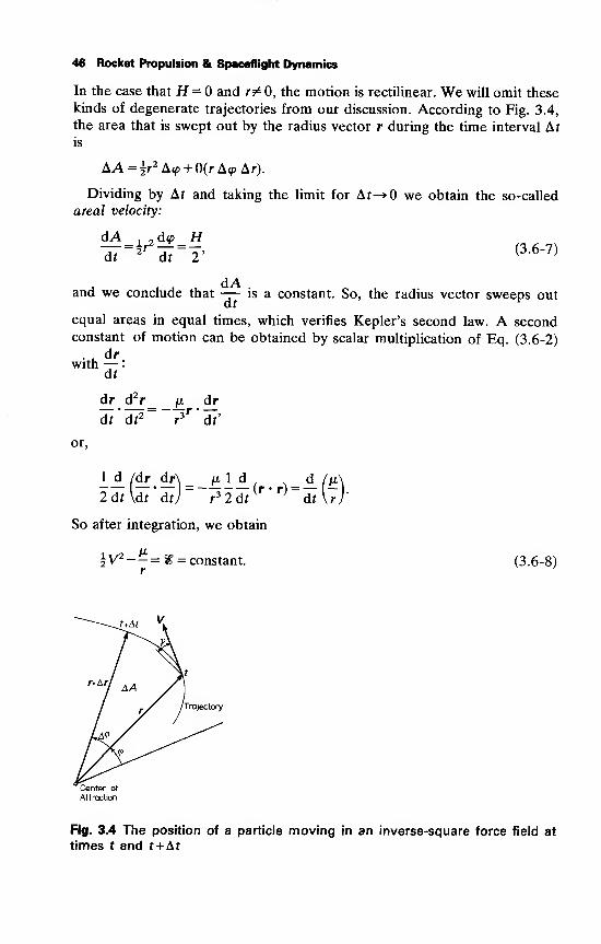
46 Rocket Propulsion & Spaceflight Dynamics
In the case that H = and r^O, the motion is rectilinear. We will omit these
kinds of degenerate trajectories from our discussion. According to Fig. 3.4,
the area that is swept out by the radius vector r during the time interval Afis
AA=|r2A<p + 0(rA<pAr).
Dividing by Af and taking the limit for Af-»0 we obtain the so-called
areal velocity:
dA , _d<p HIf-^ii-r (3 -6"7)
dAand we conclude that — is a constant. So, the radius vector sweeps out
equal areas in equal times, which verifies Kepler's second law. A secondconstant of motion can be obtained by scalar multiplication of Eq. (3.6-2)
with —
:
dr
— .— - -Jt dr
df'df2~~7r'd?
or,
2 dtW ' dt)~ r3 2dt
{r ' r)~dt\r)'
So after integration, we obtain
\V1--=% = constant. (3.6-8)
Fig. 3.4 The position of a particle moving in an inverse-square force field at
times t and f+Af
Mechanics of Particles, Bodies and Fluids 47
V2
Equation (3.6-8) is the law of conservation of energy, since— is the kinetic
energy per unit mass and, as derived in the foregoing section, — is the
potential energy per unit mass.
3.6.2 Trajectory geometry
As the motion takes place in a plane, the vector equation (3.6-2) can be
written as two scalar second-order differential equations. We therefore use a
reference system with the origin in the attraction center and with three
mutually perpendicular axes: the r, <p and z-axis. The r-axis joins the
particle with the attraction center, the <p-axis lies in the plane of motion,
positive in the direction of the tangential velocity. The z-axis, finally, is
normal to the plane of motion and is positive in the direction of the angular
momentum. Owing to the tangential velocity of the particle this reference
system is rotating with angular velocity
We can write
r=re„ (3.6-9)
By differentiating Eq. (3.6-9) and using Eq. (3.3-4), we obtain
dr dr ^ dr dcp
By differentiating again
d2r d2
r /drd<p d2<p\ dr ^ dcp _
dr2
dr2
\dr dr dr2/
vdt dr *
or
cPr
dr2-B-<£)>[>$<%hSubstitution of Eqs. (3.6-9) and (3.6-10) into Eq. (3.6-2) leads to
cfr '^ 2
dr2
d2<p
| 2drd<p
dt2
dr dr
Equation (3.6-12) can be integrated directly after multiplication by r. The
result is then r2— = constant. This was already found, since according todr
r^2+2 i'^f_0. (3.6-12)
48 Rocket Propulsion & Spaceflight Dynamics
2 d(PEq. (3.6-6), r — is the absolute value of the angular momentum, which is a
constant of motion.
Equation (3.6-11) can be used to determine the shape of the trajectory,
i.e. r as a function of <p. In order to solve Eq. (3.6-11) for r as a function of
<p we replace t by <p using the relation
d d<p d— = -tt~ • (3.6-13dt dt d<p
v '
With the use of Eq. (3.6-6) we can write
d H d
5T7v (3 -6" 14)
In order to avoid mathematical difficulties it is useful to substitute
1r = - (3.6-15)
u
Then
T/ dr 2 d /1\ du
and
d2r rr2 2 d
2u
d7= "HMV- (3 -6 - 17)
Substitution of these relations into Eq. (3.6-11) and dividing the resulting
equation by H2u2leads to the second-order linear differential equation
d2u ix
dV2+U =
Hi+u =iT2- (3.6-18)
The general solution of this equation is
w = -^5+Ccos((p-a>), (3.6-19)
where C and &> are integration constants which have to be determined fromthe initial conditions. Let the initial conditions at t = t be given by:
V(t ) = V , y(t ) = y , r(t ) = r and <p(f ) = <p -
Since the energy % is a constant of motion we can write
v n * v2n
Mechanics of Particles, Bodies and Fluids 49
By using Eq. (3.6-16) and Eq. (3.6-6) we find
V2=V2r +Vl = H2 (^+H2
u2
,
and the energy equation can be written as
H2 r/du\ 2 .I
Substitution of Eq. (3.6-19) in this expression results in
2 r ..2-
?MS]from which equation we obtain C as
c vhH?' (3 '6_20)
We have chosen the positive root for C since any possible sign change can
be handled by the choice of &>. Substitution of Eq. (3.6-20) into Eq. (3.6-19)
gives
«=|i[l + (^Ip^T)co.<,-«)].
The constant o> can be determined from the above equation together with
Eq. (3.6-16) at t=t . However, since the reference line from where <p is
measured can be chosen arbitrarily we make the substitution 6 = <p-(o. Theorbit equation then becomes
r =H2
[? . (3.6-21)
1+ J^+Ucosd(V^T)We see that r is minimal when = 0, so 6 is measured from a line drawnfrom the center of attraction to the closest point of the trajectory, the
pericenter. The point farthest away is called the apocenter. Also the terms
periapsis and apoapsis are used.
The angle is called true anomaly, while the angle &>, determining the
polar angle of the pericenter, is known as the argument of pericenter. Theequation of the orbit is the representation in polar coordinates of a so-called
conic section as we will prove now. In general, a conic section is the locus of
rpoints with a constant ratio — (Fig. 3.5), where r is the distance to a given
point F, the focus, and d is the distance to a given line /, the directrix. Theconstant ratio is called the (numerical) eccentricity of the conic and is
denoted by e. From Fig. 3.5 we see that d = d + r cos 6 and since
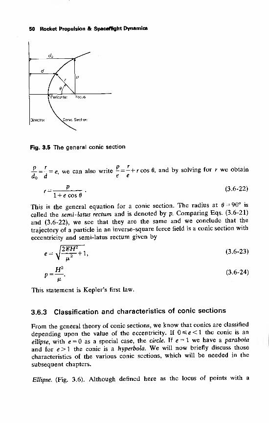
50 Rocket Propulsion & Spaceflight Dynamics
do?
d
P
rPericenter Focus
Directrix \Conic Section
Fig. 3.5 The general conic section
-£. =-= e we can also write - = -+rcos 0, and by solving for r we obtain
d d'
e e
r =1 + e cos
(3.6-22)
This is the general equation for a conic section. The radius at = 90° is
called the semi-latus rectum and is denoted by p. Comparing Eqs. (3.6-21)
and (3.6-22), we see that they are the same and we conclude that the
trajectory of a particle in an inverse-square force field is a conic section with
eccentricity and semi-latus rectum given by
/2£H2,— +1,
P =FT
(3.6-23)
(3.6-24)
This statement is Kepler's first law.
3.6.3 Classification and characteristics of conic sections
From the general theory of conic sections, we know that conies are classified
depending upon the value of the eccentricity. If 0^e<l the conic is an
ellipse, with e = as a special case, the circle. If e = 1 we have a parabola
and for e > 1 the conic is a hyperbola. We will now briefly discuss those
characteristics of the various conic sections, which will be needed in the
subsequent chapters.
Ellipse. (Fig. 3.6). Although defined here as the locus of points with a
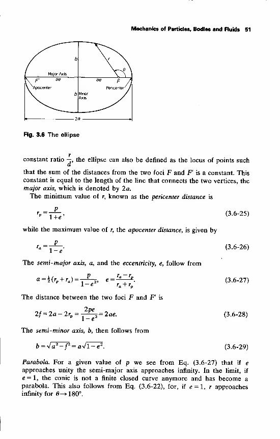
Mechanics of Particles, Bodies and Fluids 51
Fig. 3.6 The ellipse
constant ratio — , the ellipse can also be denned as the locus of points such
that the sum of the distances from the two foci F and F is a constant. This
constant is equal to the length of the line that connects the two vertices, the
major axis, which is denoted by 2 a.
The minimum value of r, known as the pericenter distance is
r„ =1+e'
while the maximum value of r, the apocenter distance, is given by
Pr„ =
\-e
The semi-major axis, a, and the eccentricity, e, follow from
a=\{rp + ra )
=l-e<
e =ra -rpr„ + rn
The distance between the two foci F and F is
2pe2f=2a-2rp
= 2ae.1-e2
The semi-minor axis, b, then follows from
b = 41F=f=a4I:rf.
(3.6-25)
(3.6-26)
(3.6-27)
(3.6-28)
(3.6-29)
Parabola. For a given value of p we see from Eq. (3.6-27) that if e
approaches unity the semi-major axis approaches infinity. In the limit, if
e = l, the conic is not a finite closed curve anymore and has become a
parabola. This also follows from Eq. (3.6-22), for, if e = 1, r approachesinfinity for 0-»18O°.
52 Rocket Propulsion & Spaceflight Dynamics
The pericenter distance is related to the semi-latus rectum by Eq. (3.6-
25), which for e = 1 yields
rv =\V . (3.6-30)
So, we can write the equation for a parabola as
2r£—
.
(3.6-31)r =1 + cos 6
Hyperbola. If e> 1, the denominator on the right-hand side of Eq. (3.6-22)
1changes sign for cos = -. The result of this is that the hyperbola has two
branches with asymptotes making an angle a = arcoss I -Jwith the line
joining the two vertices. This line is the major axis. In order to use the same
equations for all conies, the value of the semi-major axis is taken negative
for a hyperbola. So, the Eqs. (3.6-25) to (3.6-27) remain valid for a
hyperbola, while the distance between the two foci is given by
2/= -2a + 2rp = -7^5 = -2ae. (3.6-32)p 1-e
The semi-minor axis is imaginary for a hyperbola.
Returning to the orbit of the particle we can calculate the semi-major axis
of the trajectory with Eqs. (3.6-23), (3.6-24) and (3.6-27) resulting in
a= ~2%- (3 -6 '33)
The semi-major axis thus is only dependent on the total energy per unit
mass of the particle, i.e. only a function of V and r . The energy equation
(3.6-8) can now be written in the following form:
V2=J?L-±-) (3.6-34)-(H)This is known as the vis-viva integral.
We can conclude directly from Eq. (3.6-33) that the trajectory is an
ellipse if % < 0, a parabola if\% = and a hyperbola if % > 0, which of course
follows from Eq. (3.6-23) too. Expressed in the initial conditions V and r
this means that if
if
V < J— the trajectory is an ellipse,
V = J— the trajectory is a parabola,
Mechanics of Particles, Bodies and Fluids 53
and if
V > \j— the trajectory is a hyperbola.> r
So, increasing the speed will gradually change a closed conic into an open
one. The minimum speed that is required to escape permanently from the
gravitational field is called the escape velocity and is
V. = ^£. (3-6-35)
A special case of an elliptic orbit occurs for e = 0. For such a circular orbit
we find from Eq. (3.6-23)
2£H2, n—5-+ 1 = 0,
Expressing % and H in r , V and y we obtain
A(:T--VoVoCOS 7o)
2 +l = 0.
This equation can also be written as
• 2 , 2/1 r0M)\ nsm 70 + cos 70 1
11=0 -
As both terms in this equation are pure squares, a requirement for a circular
orbit is y = and Vq.= -J—. For the so-called circular velocity we
obtain
V=J^. (3.6-36)*From Eqs. (3.6-35) and (3.6-36) follows the relation between circular and
escape velocity
Vesc= V2Vc . (3.6-37)
Finally, we will derive Kepler's third law for elliptic orbits. The period, T,
of the orbit is found by dividing the area of the ellipse by the areal velocity
_ vab _ 2na2 Vl-e 2
=dA~ H '
df
From Eqs. (3.6-24) and (3.6-27) we see that
H = VTIp = Vjuta(l-e2),
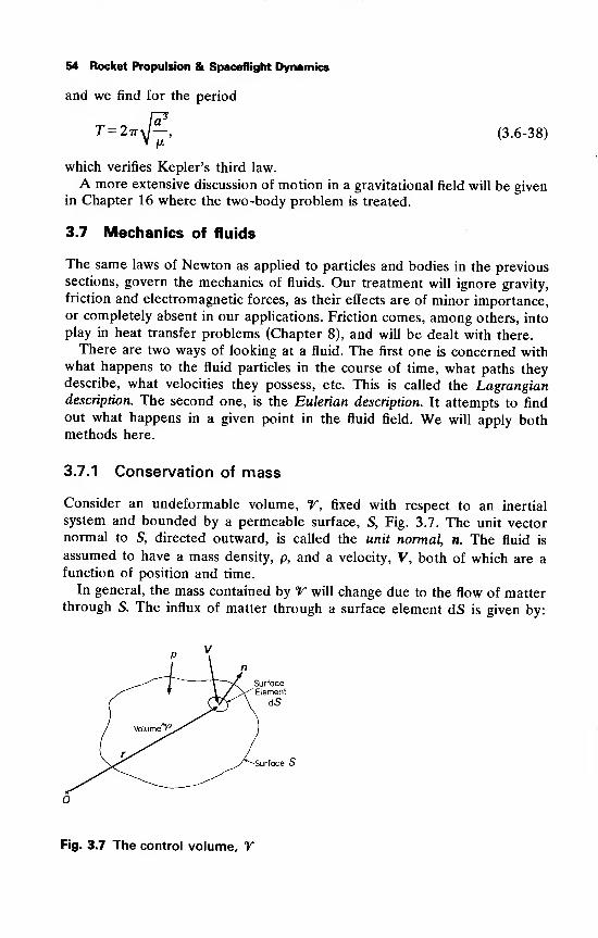
54 Rocket Propulsion & Spaceflight Dynamics
and we find for the period
T-2*M.€ (3.6-38)
which verifies Kepler's third law.
A more extensive discussion of motion in a gravitational field will be givenin Chapter 16 where the two-body problem is treated.
3.7 Mechanics of fluids
The same laws of Newton as applied to particles and bodies in the previoussections, govern the mechanics of fluids. Our treatment will ignore gravity,
friction and electromagnetic forces, as their effects are of minor importance,or completely absent in our applications. Friction comes, among others, into
play in heat transfer problems (Chapter 8), and will be dealt with there.
There are two ways of looking at a fluid. The first one is concerned withwhat happens to the fluid particles in the course of time, what paths theydescribe, what velocities they possess, etc. This is called the Lagrangiandescription. The second one, is the Eulerian description. It attempts to find
out what happens in a given point in the fluid field. We will apply bothmethods here.
3.7.1 Conservation of mass
Consider an undeformable volume, T, fixed with respect to an inertial
system and bounded by a permeable surface, S, Fig. 3.7. The unit vectornormal to S, directed outward, is called the unit normal, n. The fluid is
assumed to have a mass density, p, and a velocity, V, both of which are afunction of position and time.
In general, the mass contained by T will change due to the flow of matterthrough S. The influx of matter through a surface element dS is given by:
Surface S
Fig. 3.7 The control volume, V
Mechanics of Particles, Bodies and Fluids 55
-pV • n dS. The minus sign occurs because n is positive in the outward
direction. By integration over the entire surface we find the total flux of
matter, m, through S:
m = -\ pV-ndS,
which must equal the time rate of change of the mass contained by V, i.e.
^pdr = -| pV-ndS. (3.7-1)
Equation (3.7-1) is called the conservation of mass equation and states that
the time rate of change of mass contained by a volume of fixed shape is
equal to the flux of matter through the boundaries of that volume as long as
no mass is created spontaneously.
It is practical to derive some other forms of Eq. (3.7-1). According to
Gauss' Theorem as given in Appendix 1, the right-hand side of Eq.
(3.7-1) can be transformed into a volume integral
J
pV • n dS = [ (V • pV) dr.
As °V is assumed constant, the order of differentiation and integration can be
interchanged. So Eq. (3.7-1) can be written as
}y 8t }y(V • pV) dT,
or
I [a7+v ' (pV)
]
dr =- (3 -7 "2)
As Eq. (3.7-2) must hold for any volume, the integrand must be zero,
d
ft
+ V-(pV) = 0. (3.7-3)
Equation (3.7-3) is known as the law of conservation of mass, or the equation
of continuity.
The reader himself can derive the special forms of Eq. (3.7-3) such as for
steady-state flow, I — = 0)> or f°r incompressible media (p = constant).
A pure one-dimensional form of Eq. (3.7-3) is
^+^=0. (3.7-4)dt dx
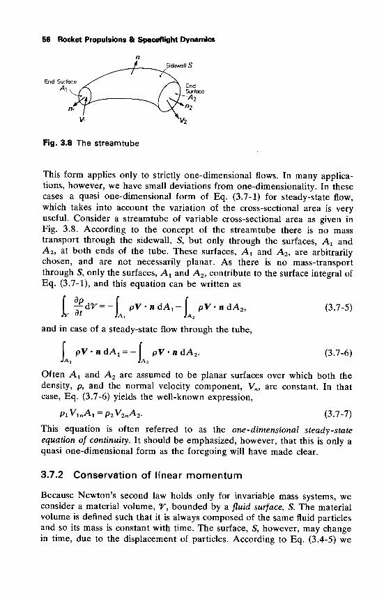
56 Rocket Propulsions & Spaceflight Dynamics
-t-Sidewall S
End Surface
A\
ty
Fig. 3.8 The streamtube
This form applies only to strictly one-dimensional flows. In many applica-
tions, however, we have small deviations from one-dimensionality. In these
cases a quasi one-dimensional form of Eq. (3.7-1) for steady-state flow,
which takes into account the variation of the cross-sectional area is very
useful. Consider a streamtube of variable cross-sectional area as given in
Fig. 3.8. According to the concept of the streamtube there is no masstransport through the sidewall, S, but only through the surfaces, A x andA2 , at both ends of the tube. These surfaces, A x and A2 , are arbitrarily
chosen, and are not necessarily planar. As there is no mass-transport
through S, only the surfaces, A 1 and A2 , contribute to the surface integral of
Eq. (3.7-1), and this equation can be written as
^V = -[ pV-ndAi-J PV-ndA2 , (3.7-5)
and in case of a steady-state flow through the tube,
|
pV-ndA^-) pV-ndA2 . (3.7-6)
Often A x and A2 are assumed to be planar surfaces over which both the
density, p, and the normal velocity component, Vn , are constant. In that
case, Eq. (3.7-6) yields the well-known expression,
PiVlnA 1 = p2V2„A2 . (3.7-7)
This equation is often referred to as the one-dimensional steady-state
equation of continuity. It should be emphasized, however, that this is only a
quasi one-dimensional form as the foregoing will have made clear.
3.7.2 Conservation of linear momentum
Because Newton's second law holds only for invariable mass systems, weconsider a material volume, T, bounded by a fluid surface, S. The material
volume is defined such that it is always composed of the same fluid particles
and so its mass is constant with time. The surface, S, however, may changein time, due to the displacement of particles. According to Eq. (3.4-5) we
Mechanics of Particles, Bodies and Fluids 57
have
dN
F= 7ll, miv
i- (3.7-8)ut
i = l
In passing from a system of discrete particles to a fluid, considered as a
continuum, the sum in Eq. (3.7-8) changes into the integral
1=[ VdM.
Since we neglect gravity, viscosity and electromagnetic effects, the external
force, F, in Eq. (3.7-8) consists only of pressure forces on the fluid surface,
S,
F=-\ pndS.
The minus sign occurs, because the pressure force is opposite to the unit
normal on S. Application of Newton's second law to the material volume, T,
containing fluid of density p gives
4-IpVdV = -
f pn dS. (3.7-9)at Jr Js
The total derivative in this equation is, as we will show, dependent on the
path. Therefore, consider a scalar or vector quantity in the fluid field, which
is a function of position and time, in general. Using Cartesian coordinates,
A = A(t, x, y, z), and the total derivative is given by
dAdA dAdx dAdy dAdzdt dt dx dt dy dt dz dt'
It is clear that this derivative is dependent on the path, given by
x = x(t), y = y(0, z = z(t).
As we follow the particles with the material volume, T, we take a special
path such that
dx dy dz
dt dt dt
where u, v and w are the components of the fluid velocity, V. This special
total derivative is called the material time derivative or substantial derivative.
It is denoted by
D d d d d— =—+w—+u—+w—
,
(3.7-10)\Jt dt dx dy dz
and it is easily seen that this is equivalent to
-5- = A+y.V. (3.7-11)Dt dt
58 Rocket Propulsion & Spaceflight Dynamics
Returning now to Eq. (3.7-9), we note that we consider a material volume,
Y, and so for the total derivative, the substantial derivative has to be taken.
With the help of the Reynolds'1
transport theorem, (Appendix 2), Eq.
(3.7-9) can be written as
Using Gauss' theorem we can transform the surface integral into a volumeintegral and obtain
L \di{pv) +
p
v(v*v) + (v * v)(pv) + Vp
}
dr
=
°-
As this must hold for any volume, Y, it follows that
^(pV) + pV(V-V)+(V-V)(pV)+Vp = 0. (3.7-12)at
Multiplication of the continuity equation, Eq. (3.7-3), by V and subtracting
this form from Eq. (3.7-12) leads to the Euler equation, or the equation of
conservation of linear momentum,
dV 1— + (V • V)V +- Vp = 0. (3.7-13)at p
3.7.3 Conservation of energy
The third relation to be derived, is the energy balance for a flowing fluid.
For an adiabatic system, the first law of thermodynamics (Appendix 3)
states: SE + 8W=0. The 8 indicates that we deal with small increments,
during a time interval, 8t. The work, 8W, done by the material volume, Y,
Fig. 3.7, neglecting terms of order 8 2 and higher, equals: 8W=p8T, where
8T is the change in the volume, Y, during the time interval, 8t. For the
material volume, Y, moving along with the fluid, the change in an elemen-
tary volume element, AY, bounded by a surface element, dS', equals
8dY = dS'n-V8t,
and as n • V on neighboring elements cancel, the total amount of work, 8W,amounts to
8W=I
pn-VdS8t, (3.7-14a)
where S is the outer surface of the control volume, Y.
In the first law of thermodynamics, E stands for the total internal energy
of a system. A flowing fluid not only possesses a specific internal energy, e,
Mechanics of Particles, Bodies and Fluids 59
but also a specific kinetic energy, |V • V. Thus the energy contained by Y is
E=[
p(e +|V-V)dr,
and the change in the energy content during the time interval, dt, is
8E =Dt L
p(c + 2y * y)dr dt (3.7-14b)
Combining the Eqs. (3.7-14a) and (3.7- 14b) yields:
—f
p{e +\V-V)dY+[ pn>VdS = 0.
With the help of Gauss' theorem and Reynolds' transport theorem, this
equation is easily transformed into
or, with the same reasoning as before
^p(e+|V- V)}+V-{(e + ±V- V)(pV)} + V-(pV) = 0. (3.7-15)at
This is the expression for the conservation of energy. However, simpler
expressions can be obtained. Multiplying the continuity equation, Eq. (3.7-3)
by e + zV - V and subtracting the result from Eq. (3.7-15) gives
PT. (e + 2y ' y) + (Py ' V)(e + |V • V) +V • (pV) = 0. (3.7-16)dt
Now
V.(pV) = ^V.(pV) +p(V-WAp \p/
By using the equation of conservation of mass, Eq. (3.7-3), we find
T-(pV) =-^+ p(VV)(4Pot \p)
and the energy equation becomes
±(e + PHy. V) + y. V ( e +P +ly.yyi d-E=
, (3.7-17)dt\ p / \ p I p dt
With the concept of enthalpy, h, defined as (Appendix 3),
fe = c+-, (3.7-18)
60 Rocket Propulsion & Spaceflight Dynamics
Eq. (3.7-17) can be written as
^-(h+±V -V) +V -V(fi+±V 'V)--^=0. (3.7-19)at p at
For ideal gases Eq. (3.7-19) can be simplified. Scalar multiplication of Eq.
(3.7-13) by V leads to
^(iv.v)+v.V(|v.v)+iv-Vp = o.dt p
Subtracting this equation from Eq. (3.7-19) and substituting the perfect gas
law
P = pRT,
and
h = h + cpT,
gives
_L
RT
As
y-1
we find
{^+ V.T(cpT)}-ig+VVp} = 0.
H~)}—{'"FF)Hwhich, after integration yields
T=Cip(y-l)ly (3.7-20a)
Or, using the perfect gas law,
p = c2p\ (3.7-20b)
T=c3p^\ (3.7-20c)
where c x , c2 and c3 are constants. These famous results, known as the Poisson
relations, are usually derived for a static system in thermodynamics. Fromthe derivation given here, it follows that this law also holds for movinggases.
It should be kept in mind that the simple forms Eq. (3.7-20) of the energy
equation hold only if
1. There is no dissipation of energy and no heat is added to or withdrawn
from the system. Therefore the process must be isentropic.
Mechanics of Particles, Bodies and Fluids 61
2. The gases must satisfy the perfect gas law, and cpmust be independent
of the temperature.
Even in cases where these assumptions are questionable, we will often use
the relations Eq. (3.7-20) instead of the more complicated form of Eq.
(3.7-19), because in practice the differences may be very small.
3.7.4 Conservation of angular momentum
Although not an independent equation, we will derive the equation for
conservation of angular momentum, because it will be used in Chapter 10.
From Section 3.4, we know that for an invariable system of particles the rate
of change of angular momentum with respect to an inertially fixed reference
point, O, is equal to the moment due to the external forces. The angular
momentum, B, of the fluid contained by the material volume, Y, with
respect to O is, Fig. (3.7),
B= [ rXVpdY, (3.7-21)
where r is the position vector of an element, dY, with respect to O. The
moment, Ms , due to external forces on the material volume, V, follows from
Ms = -| rXnpdS, (3.7-22)
and, according to Eq. (3.4-13),
— \rxVpdY=-\ rXnpdS. (3.7-23)T)t J°ir Js
By using the Reynolds' transport theorem, (Appendix 2), Eq. (3.7-23) can
be transformed into
f-(rX PV)dY+\ {(rXpV)(V-V) + (V-V)(rX PV)}dr
= -[ rXnpdS. (3.7-24)
Transformation of the second volume integral into a surface integral, with
the help of Gauss' theorem, leads to
[ -(rX PV)dr+[ {(pV-n)(rXV) + rXnp}dS = 0. (3.7-25)
For many applications, such as turbines and pumps, Eq. (3.7-25) proves to
be very useful.
Application of Gauss' theorem to the surface integral in Eq. (3.7-24)
leads to the partial differential equation for the conservation of angular
62 Rocket Propulsion & Spaceflight Dynamics
momentum
-(rXpV) + (rXV)(V-pV) + (pV-V)(rxV)-Vxrp = 0. (3.7-26)ot
We have discussed those aspects of dynamics needed in the following
chapters. Many interesting aspects of dynamics that we will not encounter
have purposely been omitted.
References
1 Eotvos, R. V., Pekar, D. and Fekete, E. (1922), Beitrage zum Gesetze
der Proportionalitat von Tragheit und Gravitat, Ann. d. Physik, 68,
11-66.
2 Roll, P. G., Krotkov, R. and Dicke, R. H. (1964), The equivalence of
inertial and passive gravitational mass, Ann. Phys., 26, 442-517.
3 Braginsky, V. B. and Panov, V. I. (1971), Verification of the equivalence
of inertial and gravitational mass, Zh. Eksp. Teor. Fiz., 61, 873-879 (in
Russian).
4 Einstein, A. and Grossmann, M. (1913), Entwerf einer verallgemeiner-
ten Relativitatstheorie und einer Theorie der Gravitation, Zeit. Math.
Phys., 62, 225-261.
5 M0ller, C. (1952), The Theory of Relativity, Clarendon Press, Oxford, p.
220.
6 Corben, H. C. and Stehle, P. (1965), Classical Mechanics, John Wiley,
New York, p. 139.
7 Slater, J. C. and Frank, N. H. (1933), Introduction to Theoretical Physics,
McGraw-Hill, New York, p. 96.
8 Chambers, L. G. (1969), A Course in Vector Analysis, Chapman andHall, London, p. 100.
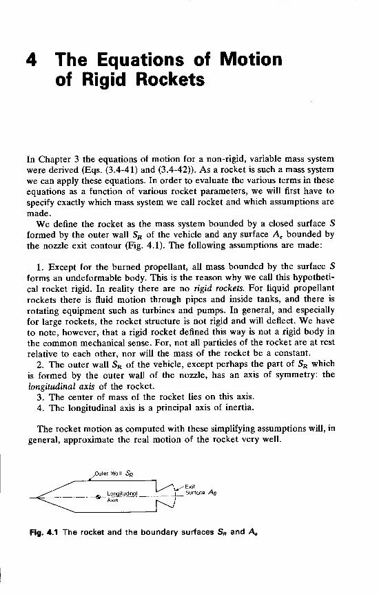
4 The Equations of Motionof Rigid Rockets
In Chapter 3 the equations of motion for a non-rigid, variable mass system
were derived (Eqs. (3.4-41) and (3.4-42)). As a rocket is such a mass system
we can apply these equations. In order to evaluate the various terms in these
equations as a function of various rocket parameters, we will first have to
specify exactly which mass system we call rocket and which assumptions are
made.
We define the rocket as the mass system bounded by a closed surface S
formed by the outer wall SR of the vehicle and any surface Ae bounded by
the nozzle exit contour (Fig. 4.1). The following assumptions are made:
1. Except for the burned propellant, all mass bounded by the surface S
forms an undeformable body. This is the reason why we call this hypotheti-
cal rocket rigid. In reality there are no rigid rockets. For liquid propellant
rockets there is fluid motion through pipes and inside tanks, and there is
rotating equipment such as turbines and pumps. In general, and especially
for large rockets, the rocket structure is not rigid and will deflect. We have
to note, however, that a rigid rocket defined this way is not a rigid body in
the common mechanical sense. For, not all particles of the rocket are at rest
relative to each other, nor will the mass of the rocket be a constant.
2. The outer wall SR of the vehicle, except perhaps the part of SR which
is formed by the outer wall of the nozzle, has an axis of symmetry: the
longitudinal axis of the rocket.
3. The center of mass of the rocket lies on this axis.
4. The longitudinal axis is a principal axis of inertia.
The rocket motion as computed with these simplifying assumptions will, in
general, approximate the real motion of the rocket very well.
Outer Wall SR
L^^/ExitLongjtudina] __ .___. J Surface AeAxis
r-'
Fig. 4.1 The rocket and the boundary surfaces SR and Ag
64 Rocket Propulsion & Spaceflight Dynamics
Despite these assumptions, the equations of motion remain rather compli-
cated. This is due to a number of terms which cannot be determined withoutagain making a lot of assumptions. These terms, however, are very small
relative to the other terms, and have no or hardly any influence on the
motion. When we encounter such small terms we will mention it and neglect
them further without an attempt to rigorously prove that this is permissible.
In most cases, such a proof is impossible, but it is experience that tells us
what terms can be neglected.
4.1 Reference frames
In order to derive the equations of motion of a rocket and to describe
position and orientation of the rocket, we will need various reference
frames. The choice of some of these reference frames depends on the
mission of the rocket. As most rocket vehicles move in the neighborhood of
the Earth, we will use reference frames which are Earth-bound in some way.
To simplify the mathematical treatment, matrices will be used. As we will
have to transform from one coordinate frame to another one, which we will
do by means of matrices, the matrix consisting of the unit vectors along the
axes of the reference frame is given for each reference frame.
Inertial reference frame (XYZ). In Section 3.4, the equations of motion for
an arbitrary mass system are given relative to an inertial frame. In order to
apply these equations to a rocket vehicle, we will have to specify an inertial
frame. For rocket motion in the neighborhood of the Earth, the non-rotating geocentric equatorial reference frame as described in Section 2.3.4
can be used as an inertial frame. If ex, eY and ez are the unit vectors along
the axes of this frame, we define a 3x1 matrix with these unit vectors as
elements
BE=|eY |. (4.1-1)
-ez .
Rotating geocentric reference frame (XgY
gZ
g ). This reference frame, which is
also described in Section 2.3.4, is a convenient reference frame to specify
the position of the rocket relative to the Earth's surface. For short-duration,
high-thrust rocket motion, the acceleration due to the rotation of this
reference frame can often be neglected, and the reference frame can then beregarded as an inertial frame. We define the matrix E„ as
£}E
g= KJ, (4.1-2)
where again the elements are the unit vectors along the axes.
The Equations of Motion of Rigid Rockets 65
Vehicle-centered horizontal reference frame (XVYVZV ). This reference frame
is used to describe the orientation of the rocket and its velocity vector
relative to the Earth's surface. At any moment, the origin of this reference
system coincides with the center of mass of the vehicle. The orientation of
the reference frame is such that it constitutes a local horizontal system as
described in Section 2.3.7. The X„Y„-plane is taken to be the local horizon-
tal plane. The X„-axis is along the north-south direction, positive to the
north. The Y„-axis is along the east-west direction, positive to the east. TheZ„-axis is along the radius vector from the center of the Earth and is
positive downwards. With e^, eY„ and e^ being the unit vectors along the
axes, the matrix E„ is defined as
E„ = |eYv |. (4.1-3)
Vehicle reference frame (xyz). The center of mass of the vehicle is the origin
of this frame. The x-axis lies along the longitudinal axis of the rocket and is
positive forwards. The y- and z-axis lie along the other two principal axes of
inertia of the vehicle such that the frame is right-handed. If ex , eyand ez are
the unit vectors along the axes of the vehicle reference frame, the matrix E r
is defined as
E r = Ul- (4-1-4)-HThe vehicle reference frame is particularly useful to denote the aerodynamic
forces and moments, and the apparent forces and moments.
4.1.1 The relative orientation of the various reference frames
Non-rotating geocentric equatorial frame/Rotating geocentric frame (Fig.
4.2). The rotating geocentric frame which is fixed to the Earth rotates with
angular velocity o>e about the Z-axis of the non-rotating geocentric equator-
ial reference frame. Thus, the relative orientation of these reference frames
is determined by the angle between the X- and the Xg-axis. According to
Section 2.4, this is the Greenwich hour angle of the vernal equinox: HG . If
at t = t both reference frames coincide (zero Greenwich sidereal time), the
angle HG at any time is given by
HG = a>e (t-t ). (4.1-5)
The following relation between the unit vectors in both systems holds:
Eg= A
gE, (4.1-6)
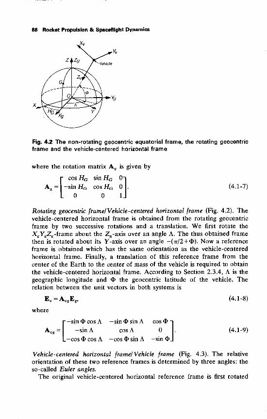
66 Rocket Propulsion & Spaceflight Dynamics
Fig. 4.2 The non-rotating geocentric equatorial frame, the rotating geocentric
frame and the vehicle-centered horizontal frame
where the rotation matrix Ag
is given by
[cos HG sin HG On
-sin HG cos HG I
.
lj
(4.1-7)
Rotating geocentric frame/ Vehicle-centered horizontal frame (Fig. 4.2). The
vehicle-centered horizontal frame is obtained from the rotating geocentric
frame by two successive rotations and a translation. We first rotate the
XgY
gZ
g-frame about the Z
g-axis over an angle A. The thus obtained frame
then is rotated about its Y-axis over an angle -(tt/2 + <!>). Now a reference
frame is obtained which has the same orientation as the vehicle-centered
horizontal frame. Finally, a translation of this reference frame from the
center of the Earth to the center of mass of the vehicle is required to obtain
the vehicle-centered horizontal frame. According to Section 2.3.4, A is the
geographic longitude and $ the geocentric latitude of the vehicle. The
relation between the unit vectors in both systems is
Eu — A^glLg,
where
A =—sin <I> cos A —sin 4> sin A cos <£
-
-sin A cos A.—cos <I> cos A -cos <J> sin A -sin 4>_
(4.1-8)
(4.1-9)
Vehicle-centered horizontal frame/ Vehicle frame (Fig. 4.3). The relative
orientation of these two reference frames is determined by three angles: the
so-called Euler angles.
The original vehicle-centered horizontal reference frame is first rotated
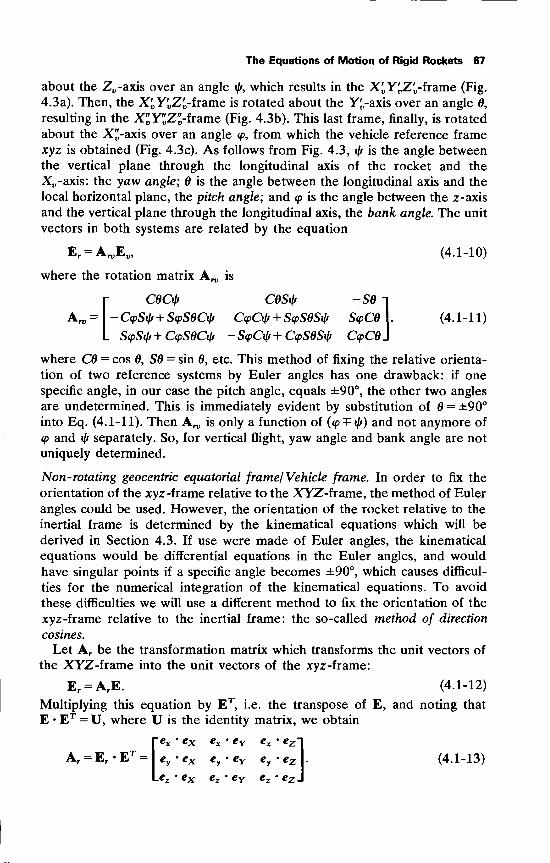
The Equations of Motion of Rigid Rockets 67
about the Z„-axis over an angle \\i, which results in the X'v Y^Z^-frame (Fig.
4.3a). Then, the X^Y^Z^-frame is rotated about the Y(,-axis over an angle 6,
resulting in the X"Y"Z"-frame (Fig. 4.3b). This last frame, finally, is rotated
about the X"-axis over an angle <p, from which the vehicle reference frame
xyz is obtained (Fig. 4.3c). As follows from Fig. 4.3, iff is the angle betweenthe vertical plane through the longitudinal axis of the rocket and the
X -axis: the yaw angle; 6 is the angle between the longitudinal axis and the
local horizontal plane, the pitch angle; and <p is the angle between the z-axis
and the vertical plane through the longitudinal axis, the bank angle. The unit
vectors in both systems are related by the equation
E r= AroE„, (4.1-10)
where the rotation matrix A^ is
[ceai* cesip -se-i
- c<pS\\f + s<psecif/ c<pG(f + S(psesi(f s<pce . (4. 1- 1 1)
ScpS^ + C(psect(f -S(pCif/+ CcpSdSiif c<pce J
where CO = cos 6, SO = sin 6, etc. This method of fixing the relative orienta-
tion of two reference systems by Euler angles has one drawback: if one
specific angle, in our case the pitch angle, equals ±90°, the other two angles
are undetermined. This is immediately evident by substitution of = ±90°
into Eq. (4.1-11). Then Aro is only a function of (<p =F j/r) and not anymore of
<p and if/ separately. So, for vertical flight, yaw angle and bank angle are not
uniquely determined.
Non-rotating geocentric equatorial frame/ Vehicle frame. In order to fix the
orientation of the xyz-frame relative to the XYZ-frame, the method of Euler
angles could be used. However, the orientation of the rocket relative to the
inertial frame is determined by the kinematical equations which will be
derived in Section 4.3. If use were made of Euler angles, the kinematical
equations would be differential equations in the Euler angles, and would
have singular points if a specific angle becomes ±90°, which causes difficul-
ties for the numerical integration of the kinematical equations. To avoid
these difficulties we will use a different method to fix the orientation of the
xyz-frame relative to the inertial frame: the so-called method of direction
cosines.
Let Ar be the transformation matrix which transforms the unit vectors of
the XYZ-frame into the unit vectors of the xyz -frame:
E r= ArE. (4.1-12)
Multiplying this equation by ET, i.e. the transpose of E, and noting that
E • ET = U, where U is the identity matrix, we obtain
ey-ex e
y-eY e
y-ez \. (4.1-13)
ex ex - eY «x
ex ey
• eY ey
ex ez • eY ez
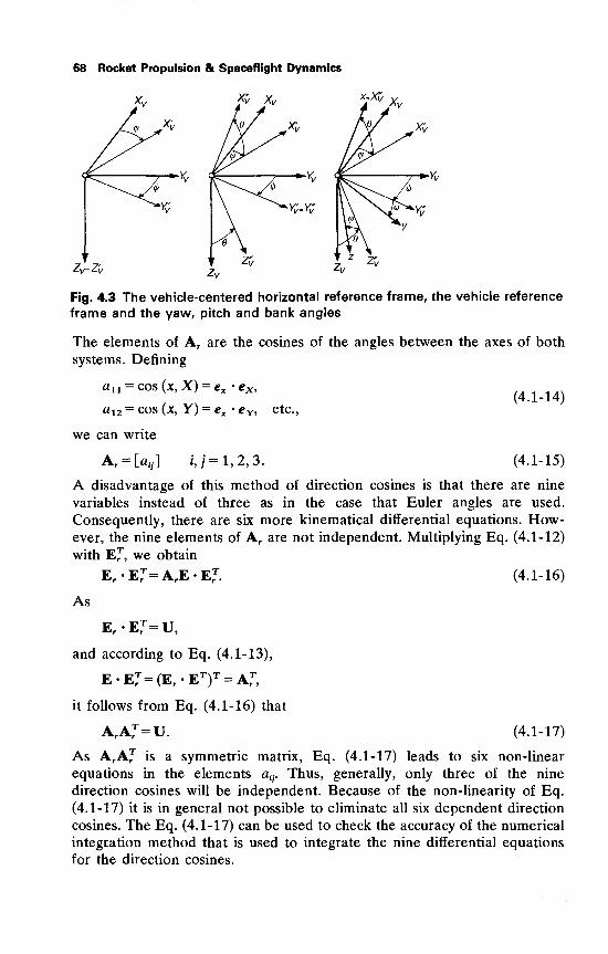
68 Rocket Propulsion & Spaceflight Dynamics
Xv K Xv x-Xv
Fig. 4.3 The vehicle-centered horizontal reference frame, the vehicle reference
frame and the yaw, pitch and bank angles
The elements of A r are the cosines of the angles between the axes of both
systems. Defining
(4.1-14)au = cos(x, X) = ex 'ex,
a 12 = cos (x, Y) = ex • eY, etc.,
we can write
A r= [a
iy ] i, j = 1,2, 3. (4.1-15)
A disadvantage of this method of direction cosines is that there are nine
variables instead of three as in the case that Euler angles are used.
Consequently, there are six more kinematical differential equations. How-ever, the nine elements of Ar are not independent. Multiplying Eq. (4.1-12)
with E^, we obtain
E r -E r
r=A rE-E
r
T. (4.1-16)
As
Er• E r
= U,
and according to Eq. (4.1-13),
E-E^=(Er-ET )
T = A^,
it follows from Eq. (4.1-16) that
A rA^=U. (4.1-17)
As Ar\J is a symmetric matrix, Eq. (4.1-17) leads to six non-linear
equations in the elements af/
. Thus, generally, only three of the nine
direction cosines will be independent. Because of the non-linearity of Eq.
(4.1-17) it is in general not possible to eliminate all six dependent direction
cosines. The Eq. (4.1-17) can be used to check the accuracy of the numerical
integration method that is used to integrate the nine differential equations
for the direction cosines.
The Equations of Motion of Rigid Rockets 69
From Eq. (4.1-17) it follows that the transpose of the matrix A r is also its
inverse. So the matrix is orthogonal. As all rotation matrices in rectangular
Cartesian coordinate systems have direction cosines as elements, all rotation
matrices derived in this section are orthogonal.
The transformation Ar can, of course, also be obtained by successively
applying the transformations Ag, A„g
and Ar„,
Ar= AroA„g
Ag
. (4.1-18)
It is important to note that in all cases where the transformation matrix is
derived by applying successive rotations to the reference frame, the order of
the rotations is not to be changed. This is a consequence of the fact that
matrix multiplication is not commutative.
4.2 The dynamical equations
If Vcm is the velocity of the center of mass of the rocket relative to the
inertial frame, and 11 is the angular velocity of the rocket relative to the
inertial frame, then, according to Section 3.4.4, the equations of motion for
a rocket can be written as
M21sn = F+F+Fnh (4.2-1)at
fr x
(^fx') dM+ [
rX{ilx(ftXr)}dM=Mcm +Mc +Mre„ (4.2-2)
where r is the position vector of a mass element dM relative to the center of
mass of the rocket. The terms at the right-hand side of these equations are
external and apparent forces, and moments, respectively. According to
Section 3.4.4, the apparent forces and moments can be expressed as volume
integrals over the total mass system:
Fc= -2axf ^dM, (4.2-3a)
Frel= -\ ^dM, (4.2-3b)
Jm ot
Mc= -l\ rx(ftx|)dM, (4.2-3c)
MreI= -£rx|lrdM. (4.2-3d)
The factors 8r/8t and 82r/8t
2in these relations represent relative velocity
and acceleration of combustion products with respect to the center of mass
of the rocket. If V and a are velocity and acceleration of the combustion
70 Rocket Propulsion & Spaceflight Dynamics
products relative to the rigid rocket structure, the following relations hold:
8r— =V-«cm, (4.2-4a)
-^2 = a-acm , (4.2-4b)
where ucm and acm are velocity and acceleration of the center of massrelative to the rocket structure. As we deal here with flowing gases i.e.
combustion products, we note that the derivative S/8t is the material
derivative D/Df used in fluid mechanics (Section 3.7.2). We will, however,continue using d/St to make it evident that it is a derivative in a rotating
system. We can now use Eq. (A2-7) of Appendix 2 relating the derivative
of the integrand to the derivative of the integral. This equation can bewritten as
— dM =- PdM+ P(pV-n)dAe , (4.2-5)m ot bt JM Jj^
for any vector P. Here p is the density of the fluid and n is the outward unit
normal on Ae . Instead of the integral over the total controi surface S of oursystem. We can now use Eq. (A2-7) of Appendix 2 relating the derivative
is only a mass transport through this part of the control surface.
4.2.1 The apparent forces
The Coriolis force. Using Eq. (4.2-5) this force can be written as
Fc = -2nxj|| rdM+j r(pV-it)dAel. (4.2-6)
From the definition of the center of mass
rdM=0. (4.2-7)JM
Introducing the mass flow, m, defined as
dM* = -£. (4.2-8)
it follows from the principle of conservation of mass that m is the total massflow through the surface Ae ,
lm=\ (pV-n) dAc . (4.2-9)
We now define a center of mass flow by its position vector re
r e =-\ r(pV-n)dAe . (4.2-10)
The Equations of Motion of Rigid Rockets 71
By using Eqs. (4.2-7) and (4.2-10), the expression for the Coriolis force
simplifies to
Fc= -2mftxr e . (4.2-11)
The relative force. Again using Eq. (4.2-5), the relative force can be written
as
8f —
rel8t f 17 dM"f ^(pV'»)dAe . (4.2-12)
Jm ot Ja. bt
The first integral on the right-hand side of this equation also appears in the
expression for the Coriolis force. Comparing Eq. (4.2-3a) with Eq. (4.2-11)
leads to
f^dM=mr, (4.2-13)
Jm °t
Substituting Eq. (4.2-4a) into the second integral of Eq. (4.2-12), and using
the expression for the mass flow, Eq. (4.2-9), leads to
f |^ (pV • w) dAc=
fV(pV • n) dAe
- m u cm . (4.2-14)
The integral on the right-hand side of this expression is the flux of linear
momentum through the surface Ac . This flux can be_written as the product
of the mass flow, m, and a mean exhaust velocity, Ve , defined by
Ve=—
f V(pV • n) dAc . (4.2-15)
Substitution of Eqs. (4.2-13) to (4.2-15) into Eq. (4.2-12) leads to
Frel= -| (mr.) - m(Vc
- «cm ). (4.2-16)
In general, the relative velocity of the center of mass and of the center of
mass flow will be very small compared to the mean exhaust velocity, which
for most chemical rockets lies between 2000 m/s and 5000 m/s. In addition,
the time rate of change of mass flow will be so small that also the term
re dm/df is negligible compared to mVe . We then may write as a good
approximation
FrcJ= -mVe,
(4.2-17)
and we conclude that the relative force has the same magnitude, but is in the
opposite direction to the flux of linear momentum through the exit surface
A..
72 Rocket Propulsion & Spaceflight Dynamics
4.2.2 The apparent moments
The Coriolis moment. We may write
| {r x(nx r)} =2rx(nx|) +rx(fx r)+nx(|x r ). (4.2-18)
Substituting this result into Eq. (4.2-3c), we obtain for the Coriolis moment
MHJI (' x(" x'»-'*(fS-"*(!H dM. (4.2-19)
By the use of Eq. (4.2-5), which relates the integral of the time rate of
change to the time rate of change of that integral, one finds:
M =IL rx(nxr)dM+
Lrx (f xr
)
dM
-[ {rX(ftx r)}(pV-n)dAc -ftXI
rX^dM. (4.2-20)Ja, Jm °t
With Eq. (3.4-31), we find
Mc = -|(I.ll) +I~-£ {rX(ilXr)}(pV-/i)dAc
-ilxf
r x|^dM. (4.2-21)Jm ot
For a point on the surface Ac , we can write
r = re +v. (4.2-22)
Then, according to Eq. (4.2-10),
J
v(pV • n) dAe = (4.2-23)
Substitution of the Eqs. (4.2-9), (4.2-22) and (4.2-23) into Eq. (4.2-21)
leads to
8tft-mrc x(HXre)-
I
vx (ftXv)(pV • n) dAe
-ftxfrX^dM. (4.2-24)
Jm ot
This is the complete expression for the Coriolis moment. However, as the
dimensions of the nozzle exit are small as compared to the longitudinal
dimensions of the rocket, i.e. |i>|« |re |, the integral over Ac in Eq. (4.2-24)
can be neglected. The volume integral in Eq. (4.2-24) represents the angular
momentum of the rocket due to relative motion with respect to the center of
mass. It is easily seen that only the moving gases contribute to this angular
The Equations of Motion of Rigid Rockets 73
momentum. As the total mass of combustion products within the rocket is
very small, while by good approximation the mean gas flow in the rocket is
parallel to the longitudinal axis, this angular momentum is negligible. Wethen, finally, find for the Coriolis moment
51Mc = -— .ft-mrc x(ftxr c ). (4.2-25)
Relative moment. Using Eq. (4.2-5), the relative moment can be written as
Mre/ = --j^rX-^dM-j rXyt
(pV>n)dAe . (4.2-26)
Substitution of Eq. (4.2-4a) into Eq. (4.2-26) and using the definition of re
(Eq. (4.2-10)) leads to
Mrel= --\ rX-^dM-J rXV(pV-n)dAe + mre Xiicm . (4.2-27)
On the surface Ae the velocity, V, can be written as
V = Ve + n. (4.2-28)
Then according to Eqs. (4.2-9) and (4.2-15),
fi)(pV • it) dAe = 0. (4.2-29)
By substitution of Eq. (4.2-22) and Eq. (4.2-28) into Eq. (4.2-27) and using
Eqs. (4.2-9), (4.2-23) and (4.2-29), we obtain
Mrel= --\ rX-^dM-l (vXr,)(PV-n)6Ae -mre X(Ve -ucm ).
By the same reasoning as before, we neglect the term containing the volume
integral in this expression. Furthermore |i>|« \re \, while also f| as well as the
relative velocity, ucm , of the center of mass will be small relative to the meanexhaust velocity. Therefore, the relative moment can very well be approxi-
mated by
Mrel= -mre xVe . (4.2-30)
Now, we have derived expressions for the apparent forces and moments in
terms of the rocket parameters m, Ve, re and I and the angular velocity of
the rocket ft. Mass flow, mean exhaust velocity and center of mass flow are
determined by the internal ballistics of the rocket motor (Chapter 5). Theposition of the center of mass and the components of the inertia tensor can
be determined if the mass distribution is known at anytime. The angular
velocity ft, finally, is an independent variable in the equations of motion.
74 Rocket Propulsion & Spaceflight Dynamics
4.2.3 The inertial moment
The terms on the left-hand side of the equations of motion (Eqs. (4.2-1) and
(4.2-2)) are inertial terms. The inertial force in Eq. (4.2-1) needs no further
explanation; the inertial moment, however, requires some elaboration.
Using Eq. (3.3-4), we can write for the inertial moment
Min =\M [ft
{rX(aXr)}~ft
{rX(aXr)] + rX {^ Xr)dM (4,2 '31)
By use of Eq. (4.2-5), we get
Mm=T-| rX(ftx r)dM+| {r X (ft X r)}(pV • n) dAeat JM K-J- f
rX(ftXr)dM-[ {rX(ftx r)}(pV • n) dAc°t JM jAe
+L
rx (f xr)dM (4 -2-32)
In the same way as for Eq. (3.4-31), one finally finds
^^l - a)-i,^
a)+1-f' (4 -2-33)
or
Min =£(I.ft)-^.ft. (4.2-34)at ot
4.2.4 The external forces
The most important external forces acting on a rocket in free flight can be
divided into gravitational forces, pressure forces and frictional forces. If the
rocket is not in free flight, i.e. during launch or during staging, there are also
other external forces. In general, these phases of the flight are relatively
short. They will not be discussed here.
Gravitational forces. These forces are due to the presence of celestial bodies
which yield a gravitational field of strength g at the location of the rocket.
The gravitational force acting on the rocket is
W=Mg. (4.2-35)
As rockets are used in the close vicinity of the Earth, the contribution of
other celestial bodies to the total field strength g can be neglected. In most
cases, it will also be possible to consider the gravitational field of the Earth
as a central field following the inverse-square law (Section 18.6). Then, the
field strength is only a function of the position vector Rcm of the center of
The Equations of Motion of Rigid Rockets 75
mass of the vehicle relative to the center of the Earth
g = —£rRcm, (4.2-36)
where ju, is the gravitation parameter of the Earth.
Pressure forces. If dS is an element of the control surface S, and p is the
external pressure at dS, then the external pressure force on dS is
dFp= -pn dS,
where n is the outward unit normal on dS. The total external pressure force
on the rocket then is
Fp= -[pndS. (4.2-37)
For every closed surface S, we have
[ndS=0,
and the pressure force can be written too as
*; = -[ (p-p>tdS, (4.2-38)Js
where pa is any constant pressure. It will be convenient to take for pa the
undisturbed atmospheric pressure at the position of the rocket. The surface
S consists of the surface SR and the exit surface Ae . So, the integral in Eq.
(4.2-38) can be split into two integrals
FP= -\ (p-pa)ndS-{ (p-pa)ndAe . (4.2-39)
If the rocket is not moving with respect to the surrounding atmosphere, the
pressure everywhere on SR will equal pa and the first integral of Eq. (4.2-39)
will vanish. So the first term of the pressure force is exclusively due to the
motion of the rocket relative to the surrounding atmosphere. It is called the
aerodynamic pressure force. If the rocket is thrusting, the pressure p on Ae
will generally differ from the atmospheric pressure. Thus, the second term of
the pressure force is due to motor operation and is called the pressure thrust.
Frictional forces. The resultant friction force Ff
is also only due to motion of
the rocket relative to the surrounding air and the frictional force is an
aerodynamic force too.
The total aerodynamic force, Fa is the sum of the aerodynamic pressure
force and the frictional force,
*« = -[ (p-pa)ndS+Ff . (4.2-40)
76 Rocket Propulsion & Spaceflight Dynamics
A more extensive discussion on aerodynamic forces and moments is given in
Chapter 14.
The total external force, finally, is the sum of the aerodynamic force, the
gravitational force and the pressure thrust:
Fs =Fa + W-\ (p-pa)ndAe . (4.2-41)
4.2.5 The external moments
Just like the total external force, the total external moment is due to
gravitation, pressure and friction.
Gravitational moment. Because of the dependence of the gravitational field
strength on position, the center of gravity does, in general, not coincide with
the center of mass of the rocket. Therefore, gravitational forces will cause a
moment about the center of mass of the rocket. However, the dimensions of
rockets are very small compared to the distance from the attraction center
and consequently the distance between the center of mass and the center of
gravity will be negligible. Consequently, the moment due to gravitational
forces is small compared to the other moments and can be neglected.
Pressure moment. The moment of the pressure force on the surface element
dSis
dMp =rxdFp ,
and the total moment due to pressure forces is
Mp= -[ prXndS. (4.2-42)
For any closed surface S, we have
rXndS=0,
and the total moment due to pressure can be written as
Mp= - f (p
-pa )r X ii dS, (4.2-43)
1
or, again splitting the integral into two parts,
= -f (p-pJrXndS- f (p-pa)rx n dAe . (4.2-44)
The first term is due to the motion of the rocket relative to the surrounding
air and we call it the aerodynamic pressure moment. The second integral is
The Equations of Motion of Rigid Rockets 77
due to the pressure thrust.
The total aerodynamic moment is
Ma=Mf-\ (p-pa)rXndS, (4.2-45)
where Mf
is the frictional moment.
The total external moment, finally, is given by
Mcm =Ma -\ (p-pa)rXndAe (4.2-46)
4.2.6 The equations of motion
We have derived expressions for the apparent and external forces and
moments, as well as for the inertial moment. Substituting these expressions
into Eqs. (4.2-1) and (4.2-2) leads to
dV- = _2mftxrc -mVe-
f(p - pa)n dAe + W+
F
a ,(4.2-47)M-
— (I-ft) = -mre x(flxrc)-mre xVc -j (p-pa)rXndAe +Ma
(4.2-48)
We now define
F=-mVc -f (p-pa)ndAe . (4.2-49)
The force F is exclusively due to the motor operation of the rocket. During
a static test, where the aerodynamic force and Coriolis force are absent, it is,
apart from the weight W and the reaction forces of the test stand, the only
'force acting on the rocket'. It is therefore called the thrust. The first term,
due to transport of linear momentum through Ae , is called the impulse
thrust. The second term represents the already defined pressure thrust.
If the thrust is not acting along a line through the center of mass, a
moment will result
MF = -mre xVe -\ (p-p>Xn dAc . (4.2-50)
If this moment is generated deliberately, e.g. for changing the orientation of
the rocket, we speak of thrust vector control (Section 5.2.4.). For rockets that
do not use thrust vector control, it is endeavoured to let the thrust act along
a line through the center of mass. Owing to construction inaccuracies,
however, this cannot be realized exactly. In that case, we speak of thrust
misalignment and the resulting moment is the thrust misalignment moment.
As the impulse thrust is much larger than the pressure thrust, the moment
78 Rocket Propulsion & Spaceflight Dynamics
due to the thrust can be approximated very well by
MF=re xF. (4.2-51)
As the velocity of the center of mass flow due to the rotation of the rocket
is very small as compared to the mean exhaust velocity, i.e. |ft Xrc |« Ve , the
Coriolis force can be neglected with respect to the thrust. The Coriolis
moment, however, will in general be of the same order of magnitude as the
aerodynamic moment and the thrust misalignment moment. Therefore, the
Coriolis moment cannot be neglected. Note that the Coriolis momentconsists of two terms. The term -mre x(ilxre ) is due to the exhaust jet
and, as we will see in Chapter 14, is a damping moment. It is therefore often
called the jet damping moment. Most authors only take this jet dampingmoment into account neglecting the term -ft • 81/8t of the Coriolis moment.This is certainly not permissible since the term can decrease the damping bysome 30%.
Finally, we can write the equations of motion as
dVM~^ = F+W+Fa , (4.2-52)at
-(I.ft) = -mrc x(ftXre) + rcxF+Ma , (4.2-53)
where, according to Eq. (4.2-49) and Eq. (4.2-15), the thrust F is given by
*=-[ {V(pV-n) + (p-p>}dAc . (4.2-54)
In Chapter 5 the thrust will be determined explicitly in terms of rocket
motor parameters.
Now, we will dissolve the two vector equations of motion into six scalar
equations. As the thrust, the aerodynamic forces and moments, the inertia
tensor and the vector re are most easily expressed -in the vehicle reference
frame, the vector equations are usually resolved along the axes of this
frame. As this frame is rotating with angular velocity ft relative to the
inertial frame, we have
^ =^+ftxVcm , (4.2-55)
and
d 51 dft-(I-ft) =— -ft +I— +ftx(I-ft). (4.2-56)
We resolve the vectors occurring in Eqs. (4.2-52) and (4.2-53) in the
following way:
The Equations of Motion of Rigid Rockets 79
Vcm =[w,u,w]Er, (4.2-57a)
ft = [p,<j,r]Er, (4.2-57b)
F=[Fx,Fy,F2]Er, (4.2-57c)
Fa =[Xa,Ya,Za]En (4.2-57d)
Ma =[L',M',JV]Er,(4.2-57e)
re =[xc,ye,zc]Er, (4.2-57f)
g = [gx,gy,gz]En (4.2-57g)
We have to note that Fyand Fz are small compared to Fx , and that yc and ze
are small compared to xe, because these terms are a consequence of
asymmetry, which will be restricted to a minimum. We will therefore neglect
terms of second-order in these quantities.
Substitution of Eqs. (4.2-55) to (4.2-57) into Eqs. (4.2-52) and (4.2-53)
leads to
M^=M(vr-wq) + Fx + Mgx +Xa ,(4.2-58a)
at
dvM— = M(wp - ur) + Fy+ Mg
y+ Ya ,
(4.2-58b)
M— = M(uq-vp) + Fz +Mgz + Za ,(4.2-58c)
at
Ixxj?= ~P^f + ^(Jyy " J-> + ™xe (yeq + zer) + V, (4.2-58d)
Iyy M= ~
q^t+ Pr(lzz~U ~ mx2e ~ XeFz + ZeFx +M'' (4-2-58e)
J" 77= ~r^f+pq(Ixx - I
yy )~ mrx 2
e + xeFy- yeFx + N'. (4.2-58f)
dt dt
These are the dynamical equations of motion
-//-
4.3 The kinematical equations
In the dynamical equations, the thrust, the gravitational field strength and
the aerodynamic forces and moments are dependent on the position and
orientation of the rocket. We will therefore need equations which relate
position and orientation of the rocket to the translational and rotational
velocity. These are the kinematical equations.
80 Rocket Propulsion & Spaceflight Dynamics
According to Eq. (4.1-12), the orientation of the rocket is determinedcompletely by the rotation matrix Ar. Differentiating Eq. (4.1-12) gives
dE r dAr „ A dE-t- = -7-E +Ar
—-.
dt dt dt(4.3-1)
As the matrix E has the unit vectors along the axes of the inertial system as
elements
dE
dt= 0.
The vehicle reference system is rotating with velocity ft relative to the
inertial system, so
dE r 8E r ^ „—=—+ftxEr.
dt St
The elements of E r, which are the unit vectors in the vehicle reference
frame, are constants in the vehicle reference frame. This implies that
8E r
8t= 0.
Using these relations, Eq. (4.3-1) simplifies to
dAnxEr=^-r
E,dt
which, after scalar multiplication with ET,yields
—-r=(ftxEr -Er.
dt
According to Eq. (4.1-12),
ET = EjAr.
Substitution of Eq. (4.3-3) into Eq. (4.3-2) leads to
dA—r=(ftxEr)-E r
TAr.
dt
(4.3-2)
(4.3-3)
(4.3-4)
By using Eq. (4.2-57b), we obtain
ftxEr = (pex + qey+ rez )
and
(ft x E r )• E^=
|pez -rex \' [«, «, ez ]
=
[ex~i rrey-qez ~i
ey\=
\
?e*~ re* '
ez \ Vqex -peA
[rey -qez ~i r r
Pez ~rex \'[ex ey ez]=\ -r
qex -pey J L q -pP
0J
(4.3-5)
The Equations of Motion of Rigid Rockets 81
Substitution of Eq. (4.3-5) into Eq. (4.3-4) finally yields
r -q-
Ar. (4.3-6)
[u r
-r
q -p
dA,P
d'
" 0.
Writing out this matrix equation gives nine first-order differential equations
in the elements of Ar, which are the direction cosines between the vehicle
reference system and the inertial reference system.
Finally, we will have to derive the differential equations for the position of
the rocket. If X, Y and Z are the coordinates of the center of mass of the
rocket in the inertial system, we can write
Rcm = [X,Y,Z]E (4.3-7)
By differentiating Eq. (4.3-7) and using Eq. (4.2-57a), we obtain
"df =Vcm= Tt[x
'y
'Z]E = [M
'
u'w]Er- (4 '3 '8)
Substitution of Eq. (4.1-12) into Eq. (4.3-8) leads to
-£[X,Y,Z] = [M,t>,w]Ar. (4.3-9)at
These differential equations relate the position of the rocket to its velocity
components u, v and w and the direction cosines atj
.
So far, we have derived a set of 18 differential equations: the dynamicalequations, Eqs. (4.2-58), and the kinematical equations, Eqs. (4.3-6) andEq. (4.3-9). Together with appropriate initial conditions, these equations
can be integrated simultaneously yielding the velocity components u, v andw, the angular velocity components p, q and r, the direction cosines a
tjand
the coordinates X, Y and Z. The accuracy of the integration method usedmay be checked with the help of Eq. (4.1-17).
4.3.1 The position of the rocket
When the coordinates of the center of mass of the rocket in the inertial
frame are known, the position of the rocket relative to the rotating geocen-
tric frame can be determined. If Xg, Ygand Z
gare the coordinates of the
center of mass in the rotating geocentric frame, we can write
[Xg , Yg, Zg]Eg
= [X, Y, Z]E. (4.3-10)
By using Eq. (4.1-6), it follows that
[Xg, Yg, Zg ]= [X, Y, Z]AJ. (4.3-11)
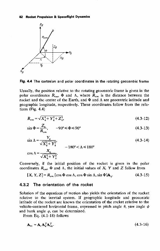
82 Rocket Propulsion & Spaceflight Dynamics
Fig. 4.4 The cartesian and polar coordinates in the rotating geocentric frame
Usually, the position relative to the rotating geocentric frame is given in the
polar coordinates Rcm , <J> and A, where Rcm is the distance between the
rocket and the center of the Earth, and <$ and A are geocentric latitude and
geographic longitude, respectively. These coordinates follow from the rela-
tions (Fig. 4.4)
Rcm — vX,, + y„ + z„,
sin 4> =—*-
R,-90° «=<!>*£ 90°
(4.3-12)
(4.3-13)
sin A =
cos A =Vx!+y!'
(4.3-14)
-180°<A^180°
Conversely, if the initial position of the rocket is given in the polar
coordinates Rcm, <1> and A, the initial values of X, Y and Z follow from
[X, Y, Z] = Rcm [cos <I> cos A, cos <I> sin A, sin &]A>g
.
4.3.2 The orientation of the rocket
(4.3-15)
Solution of the equations of motion also yields the orientation of the rocket
relative to the inertial system. If geographic longitude and geocentric
latitude of the rocket are known the orientation of the rocket relative to the
vehicle-centered horizontal frame, expressed in pitch angle 6, yaw angle if/
and bank angle <p, can be determined.
From Eq. (4.1-18) follows
™n>. ^r-^g^ug • (4.3-16)
The Equations of Motion of Rigid Rockets 83
Solution of the equations of motion yields Arand the coordinates X, Y and
Z, from which, with Eqs. (4.3-10), (4.3-13), (4.3-14) and (4.1-9), the matrix
Awg can be determined. According to Eqs. (4.1-5) and (4.1-7), the matrix Ag
is only a function of the time t. The right-hand side of Eq. (4.3-16) then is
completely known.
Let ctibe the elements of the matrix Aro . Then, from Eq. (4.1-11) we find
for the pitch angle
sin0 = -c13 , -9O°^0^9O° (4.3-17)
and, if |c13|^ 1, for the yaw and bank angle
sin^ = -^-, cos«A = -^-, (4.3-18)cos cos
sin if =-^_ cos <p = -^-. (4.3-19)COS0 COS0
If |c13 |
= 1, which is the case in vertical flight, the yaw and bank angle are
undetermined, which we mentioned already in Section 4.1.
Conversely, the initial value of the matrix Ar can be determined from the
initial values of pitch, yaw and bank angle and geographic longitude andgeocentric latitude with Eq. (4.1-17).
4.3.3 The velocity components in the vehicle-centered horizon-tal reference frame
Sometimes, it may be convenient to describe the translational velocity of the
rocket by its magnitude Vcm , the flight path angle, y, and the flight path
azimuth, «/r (Section 2.3.7). The velocity Vcm can then be written as
Vcm = Vcm [cos y cos if/, cos y sin ip, -sin y]E„. (4.3-20)
According to Eqs. (4.2-57a) and (4.1-10), we may also write
Vcm = [M,t),w]AroE„. (4.3-21)
Thus the magnitude of the velocity, flight path angle and flight path azimuth
can be determined from
Vcm [cos 7 cos \\t, cos y sin «/r, -sin 7] = [u, v, wJA^ (4.3-22)
where the matrix Am is determined by Eq. (4.3-16). Equation (4.3-22) mayalso be used to compute the initial values of u, v and w if the initial values
of Vcm , y and if/ are known.
The angular velocity of the rocket, finally, may be expressed in terms %of
pitch rate, yaw rate and bank rate, being the time rates of change of the
corresponding angles. These rates can be determined by differentiating Eq.
(4.3-16), resulting in
dA)!, _ d
A
r T T dAg at I 4 at"_Ajs
dr dtA
sA»8+A'
dtA^+A^s dr
A^+A.^A^+A.A^^. (4.3-23)
84 Rocket Propulsion & Spaceflight Dynamics
From this equation, expressions for dd/dt, diff/dt and d(p/dt may be derived.
These expressions, however, will be quite complex. This is a consequence of
the fact that the rates mentioned are not components of the angular velocity
ft. We have to note that ft is the angular velocity relative to the inertial
system, while pitch, yaw and bank rate are measured relative to the
vehicle-centered horizontal reference frame, which is rotating itself. The last
two terms on the right-hand side of Eq. (4.3-23) are due to this rotation.
The first of these is due to the rotation of the rotating geocentric frame
relative to the inertial frame, while the last one is a result of the rotation of
the vehicle-centered horizontal reference frame relative to the rotating
geocentric reference frame. The sum of these last two terms therefore is of
the order Vcm cos y/Rcm . If |ft|» Vcm cos y/JRcm , the last two terms of Eq.
(4.3-23) may be neglected. This is the case for flight in the atmosphere
where the angular velocity is mainly due to small oscillations of the rocket
about the center of mass, or to a certain steering program. In that case Eq.
(4.3-23) can be written as
[0r
-r
q -p
dA„, |" ^
P Arc ,(4.3-24)
&q ~p 0J
where use has been made of Eqs. (4.3-6) and (4.3-16). Solving these
equations for the rates of pitch, yaw and bank angle yields
dd .... _ _.— = q cos (p-r sin <p, (4.3-25)
at
^ sin^cos^M)
dt cos cos 6
— = p + q sin <p tan 6 + r cos <p tan 0. (4.3-27)dt
We have derived the complete equations of motion for a rocket vehicle in
free flight. In general, these equations cannot be solved analytically. Only in
some very special cases (vacuum, homogeneous gravitational field) an
analytical solution can be obtained. These cases will be treated in Chapter
11.
5 The Chemical Rocket Motor
The rocket motor is used to propel vehicles under conditions where other
types of propulsion systems cannot operate, are inadequate or inefficient.
All rocket motors are based on the same principle: mass is accelerated and
expelled. The forces necessary to accomplish this, create, according to
Newton's third law, reaction forces which thrust the rocket vehicle. While
this is also true for the jet engine, the main difference between the rocket
motor and the jet engine is that the first takes along its propellants, while the
second only takes along fuel, but consumes oxygen from the surrounding
atmosphere. Note that fuel and oxidizer together are called propellants.
In the combustion chamber of the chemical rocket a reaction takes place
between fuel and oxidizer (combustion). The main combustion products are
gases which are heated by the chemical energy released. As these hot gases
are contained in a relatively small volume (the combustion chamber), the
thermal expansion of the gases results in a high pressure. These pressurized
gases are expanded and accelerated by a nozzle, resulting in a reaction force
on the rocket vehicle. In a nuclear rocket motor, a gas may be heated by a
nuclear reactor instead of by a combustion process. For this type of motor
the same theory applies as for the chemical motor as far as the flow through
the nozzle is concerned. This type of rocket motor is still experimental.
For the chemical rocket motor, the gas temperature in the combustion
chamber lies somewhere between 2000 and 3500 K. As this temperature is
higher than the melting point of most metals, care must be taken to prevent
failure. Measures may be: cooling, insulation, heat sinks or the use of special
materials, such as graphite or ceramics for certain parts. The operation time
of the chemical rocket motor is very short as compared to other propulsive
systems: a few milliseconds up to a few hundred seconds.
In principle, every combination of chemicals which gives gases of high
temperature as reaction products is suitable for rocket propulsion. However,
if the combustion products are very aggressive, such as e.g. hydrogen-
fluoride, they may pose serious problems.
Also the propellants themselves may cause such serious problems, so that
their use is not practicable (03).
Depending on the state of aggregation of the stored propellants, one
distinguishes: liquid propellants, solid propellants and hybrid propellants, and
one speaks of liquid-, solid-, or hybrid-propellant rockets.
In the liquid-propellant rocket, the propellants are stored in separate fuel
and oxidizer tanks. In some cases monopropellants such as hydrogen
86 Rocket Propulsion & Spaceflight Dynamics
peroxide or hydrazine are used. Such propellants can break up in high-
temperature gases. Turbine-driven pumps feed the propellants into the
combustion chamber. Some of the energy of the gases in the combustion
chamber may be used to drive the turbines, but also systems employing a
separate gas -generator to drive the turbines are used. In the modern,
high-pressure rocket motors (pressures up to 40MPa) a pre-combustion
may take place. Here all fuel is injected into a pre-combustion chamber to
react with part of the oxidizer. The high-pressure pre-combustion products
drive the turbines and then enter the main combustion chamber, where the
main combustion takes place with the remaining oxidizer. For simple
liquid-propellant rockets, pumps and turbines may be avoided by pressuriz-
ing the propellant tanks.
In the solid-propellant rocket, all propellant is stored in the combustion
chamber itself. The propellant burns at its surface. Much attention is to bepaid to the shape of the propellant grain, as this shape determines the thrust
history of the solid-propellant rocket. The solid propellant may either be a
propellant which combines fuel and oxidizer in one molecule (double-base),
or a mixture of fuel and oxidizer (composite).
In the hybrid rocket engine, one of the propellants (fuel in general), is a
solid, while the other is a liquid (oxidizer). In general, the oxidizer is stored
in a pressure vessel and pressure fed into the combustion chamber. At the
fuel surface a reaction with the oxidizer takes place, producing high-
temperature and -pressure combustion products.
5.1 The ideal rocket motor
To apply the simple theory of fluid mechanics, as given in Section 3.7, to the
rocket motor, we will make the following assumptions:
1. The combustion and flow are steady; i.e. there are no variations in
time.
2. Details of the combustion process are ignored. For our purpose we will
assume here that the combustion fully takes place in a (small) region of the
chamber, the combustion zone.
3. At the entrance of the nozzle we assume uniform chamber conditions;
i.e. pressure, density and temperature are constant.
4. The velocity at the nozzle entrance is negligible. In a certain way this
defines the nozzle entrance. 4
5. Except for shocks, the flow is isentropic; i.e. friction and heat transfer
are not taken into account.
6. The combustion products are ideal gases with constant specific heats.
7. On surfaces normal to the streamlines the flow variables are assumedconstant. These surfaces will be called surfaces of constant properties.
The most important parameter for rocket performances is the thrust, F,
which, according to Eq. (4.2-54), equals
The Chemical Rocket Motor 87
F=-\ {(PV'n)V+(p-pa)n}dAe . (5.1-1)
The density, p, the velocity, V, and the pressure, p, have to be known on the
exit surface, Ae, to evaluate the integral in Eq. (5.1-1). The ambient
pressure is indicated by pa . The outward unit normal on Ae is n. According
to Eq. (4.2-9), the mass flow through the exit surface is
m = pV* ii dAe . (5.1-2)
Until now, the exit surface, Ae , has not been specified. We will assume Ae to
be a surface of constant properties. Then density and velocity are constant
on Ae , and the flow velocity is normal to Ac, and Eq. (5.1-2) becomes
m = PeVeAe,(5.1-3)
and the thrust, F, can be written as
F=-[m-^ +(p.-p«)]J
ndAe . (5.1-4)
The integral at the right-hand side of Eq. (5.1-4) can be calculated if the
shape of the exit surface is known.
In the following sections, we will discuss the various terms contributing to
the thrust, such as exit or exhaust velocity, Vc, mass flow through the nozzle,
m, and exit pressure, pe .
5.1.1 The exhaust velocity
As the flow is assumed steady and isentropic, we may apply the energy
equation, Eq. (3.7-19), to the flow of the gases after combustion has taken
place:
V-V(h +|V-V) = 0. (5.1-5)
Integration along a streamline leads to
h+\V-V = constant. (5.1-6)
As we assumed uniform chamber conditions, and since all streamlines
originate in the chamber, this means that Eq. (5.1-6) holds for the whole
flow field. Using the fact that
h = cpT, (5.1-7)
we can write Eq. (5.1-6) as
cpT+iV • V = cpTc +\VC
• Vc = cpTtot
= htot . (5.1-8)
The chamber conditions are indicated with the index c, while htot and Ttot
denote the total enthalpy and total temperature, respectively. The index tot,
88 Rocket Propulsion & Spaceflight Dynamics
in general, refers to the total or stagnation conditions, i.e. the conditions that
result if the flow were brought to rest (V = 0) by an isentropic process. Thetotal, or stagnation temperature, Ttot, follows from Eq. (5.1-8), while the
total pressure, ptot, and the total density, ptot, are related to Tm by the
Poisson relations, Eqs. (3.7-20).
In the chamber we assumed a negligible velocity, and we may write
approximately,
Tc = Ttot . (5.1-9)
In that case Eq. (5.1-8) simplifies to
cpT+±V'V=cpTc . (5.1-10)
In those cases where the chamber velocity, Vc, is not negligible one still
could apply the following results: instead of using the chamber conditions
one would have to use the total or stagnation conditions. With
cp=-^-R, (5.1-11)7-1
we find for the velocity, V,
V=yj-^RTC[1-T/Tc ]. (5.1-12)
We now have a relation between the gas velocity, V, the temperature, T,
and the combustion chamber temperature, Tc .
As we assumed an isentropic flow, we may use the Poisson relations, Eqs.
(3.7-20),
T/Tc = (^-j , (5.1-13)
and find
V= yp^RTc[l-(p/pcYy-1Vyl (5.1-14)
The exhaust velocity, Ve, is obtained by substituting the exit pressure, pe, for
p in Eq. (5.1-14)
v-->S^FsrT- <5 - i -i5)
It will be shown in the Chapters 11 and 12 that the rocket performances are
strongly dependent on Ve . For high rocket performance, high values of the
exhaust velocity, Ve, are needed. From Eq. (5.1-15) it is clear that Ve
increases with decreasing pressure ratio pjpc . Figure 5.1 shows the depen-
dence of the dimensionless exhaust velocity, VJ\RTC , on the pressure ratio,
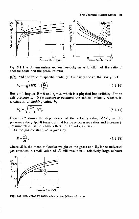
The Chemical Rocket Motor 89
Ii2>
2>2.5
° 2
V=1.15v1.20X1.25X\1.30X^
35
^ 3
2 5
%/%=500/ 400
//300///200V//,100
100 200 300 400
Pressure Ratio prjPp
1.1 1.2 1.3
Ratio of Specific Heats y
Fig. 5.1 The dimensionless exhaust velocity as a function of the ratio of
specific heats and the pressure ratio
pjpe, and the ratio of specific heats, y. It is easily shown that for y—> 1,
i2RTAn© (5.1-16)
But 7=1 implies R = and cp= cv which is a physical impossibility. For an
exit pressure pe — {expansion to vacuum) the exhaust velocity reaches its
maximum, or limiting value, VL ,
Vr =- r1^ RT, (5.1-17)
Figure 5.2 shows the dependence of the velocity ratio, VJVL , on the
pressure ratio pjpe . It turns out that for large pressure ratios and increase in
pressure ratio has only little effect on the velocity ratio.
As the gas constant, R, is given by
R = Ro
M ' (5.1-18)
where M is the mean molecular weight of the gases and R is the universal
gas constant, a small value of M will result in a relatively large exhaust
10 100 1000
Pressure Ratio Pc/Pe
Fig. 5.2 The velocity ratio versus the pressure ratio
90 Rocket Propulsion & Spaceflight Dynamics
velocity. This is one of the reasons for the use of hydrogen as a rocket
propellant. From Eq. (5.1-15) it is clear that a large value of the combustion
chamber temperature, Tc, and a high pressure ratio, pc/pe, also lead to high
exhaust velocities. The exit pressure, pe , depends strongly on the nozzle
geometry, which will be discussed in the next section.
5.1.2 Nozzle geometry
As we will need the concept of Mach number and the velocity of sound, wewill make some brief remarks on these important quantities. The velocity of
sound is defined as the propagation speed of a small pressure disturbance in
the fluid. It can be shown [1] that for isentropic changes of state the velocity
of sound, a, is equal to
-M- (5.1-19)
where the index s indicates at constant entropy. For a perfect gas this means
a = VyRT = Jy£. (5.1-20)V p
The Mach number, Ma , is defined as the ratio of flow speed, V, and velocity
of sound, a,
Ma = Via. (5.1-21)
A Mach number unity means that the velocity of the flow equals the velocity
of sound (sonic flow). A Mach number larger than one (supersonic flow)
means that the fluid velocity is larger than the speed at which a small
pressure disturbance propagates in the fluid. In that case, effects down-
stream cannot propagate upstream. Therefore, a disturbance in the super-
sonic part of the nozzle flow will not influence the chamber conditions. Thechamber conditions therefore are independent of the conditions at the
nozzle exit and, consequently, independent of the atmosphere.
In Section 5.1.1 we argued that the kinetic energy in the combustion
chamber was negligible as compared to the enthalpy, and therefore the total
temperature, Ttot, could be set equal to the combustion chamber tempera-
ture, Tc . By using the Poisson relations, Eqs. (3.7-20), the definitions of the
speed of sound and the Mach number, Eq. (5.1-20) and Eq. (5.1-21), we can
write the steady-state energy equation, Eq. (5.1-10), as
-={l+1~M^ yny
\ (5.1-22)
o ( y-\ x1^-"
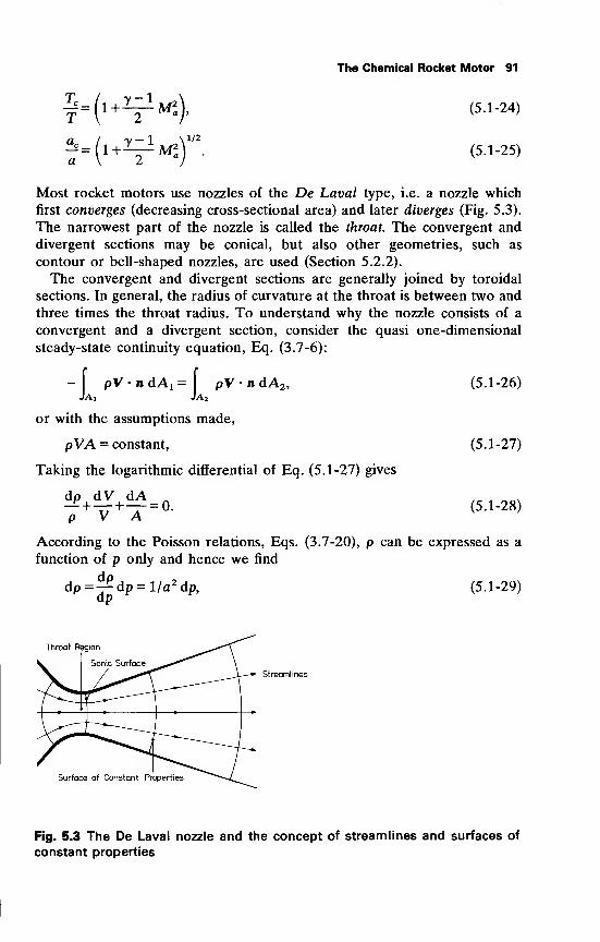
The Chemical Rocket Motor 91
(5.1-24)
(5.1-25)
Most rocket motors use nozzles of the De Laval type, i.e. a nozzle which
first converges (decreasing cross-sectional area) and later diverges (Fig. 5.3).
The narrowest part of the nozzle is called the throat. The convergent and
divergent sections may be conical, but also other geometries, such as
contour or bell-shaped nozzles, are used (Section 5.2.2).
The convergent and divergent sections are generally joined by toroidal
sections. In general, the radius of curvature at the throat is between two and
three times the throat radius. To understand why the nozzle consists of a
convergent and a divergent section, consider the quasi one-dimensional
steady-state continuity equation, Eq. (3.7-6):
I
pV-n dAj =[ pV-n dA2 ,
Jai Ja2
or with the assumptions made,
pVA = constant,
Taking the logarithmic differential of Eq. (5.1-27) gives
dp dV dA n
p V A
(5.1-26)
(5.1-27)
(5.1-28)
According to the Poisson relations, Eqs. (3.7-20), p can be expressed as a
function of p only and hence we find
dp •,
dp =— dp = 1/a dp,dp
(5.1-29)
Throat Region
Sonic Surface
Streamlines
Surface of Constant Properties
Fig. 5.3 The De Laval nozzle and the concept of streamlines and surfaces of
constant properties
92 Rocket Propulsion & Spaceflight Dynamics
where use is made of Eq. (5.1-19), as the Poisson relations hold for an
isentropic change of state.
Substitution of Eq. (5.1-29) into Eq. (5.1-28) yields
——+--= —-. (5.1-30)\_&p dV__dAa2p V~ A
The steady-state energy equation, Eq. (5.1-10), can also be written as
-J—P + iy* = constant. (5.1-31)y-lp
Taking the differentials and rewriting the result with the help of the Poisson
relations, Eqs. (3.7-20), yields
d^+VdV = 0. (5.1-32)P
Substituting Eq. (5.1-32) into Eq. (5.1-30) and using the definition of the
Mach number, we finally get
U-^T—T- (5 - 1 "33)
This is a relation between the velocity increment of the fluid, the local Machnumber, Ma , and the change of the area of a surface of constant properties.
For subsonic flow (Ma < 1) we see that an increase in fluid velocity requires
a decreasing surface area. For supersonic flow (Ma > 1) the opposite is the
case. For sonic flow, i.e. Ma= 1 we find that dA = must hold as we must
require dV, the velocity increment, to remain finite. So we see that, to
accelerate the fluid, the surface area, A, has to decrease in the subsonic
section, and A has to increase in the supersonic part of the nozzle. Sonic
conditions are reached when A is a minimum. On the other hand, it will be
clear that dA = does not imply that we have sonic flow. If Ma ^ 1, this only
means that dV = 0. The sonic surface, i.e. the surface of constant properties
where Ma = 1 , lies in the neighborhood of the throat.
From Eq. (5.1-22) it follows that the Mach number increases with increas-
ing pressure ratios, pjp. Hence, if the pressure ratio exceeds a certain critical
ratio, the flow becomes sonic. This pressure ratio is called the critical pressure
ratio. Accordingly, one also has the critical density ratio and the critical
temperature ratio. They are indicated by the subscript cr. Inserting Ma = 1 in
the Eqs. (5.1-22) through (5.1-24) yields
^Jp)cr=\^Y-) ,(5.1-34a)
(Pc/P)c, = (-^-) ,(5.1-34b)
(Tc/T) cr= (^-). (5.1-34c)
The Chemical Rocket Motor 93
As it is the pressure ratio that determines whether or not the critical
conditions are reached, this is the most important relationship.
5.1.3 Mass flow and exit pressure
In Section 5.1 we have made some brief remarks about the mass flow. Wewill now consider the steady-state mass flow through the nozzle in more
detail. According to Eq. (5.1-27), we have
m = pVA = constant. (5.1-35)
Substituting of Eq. (5.1-14) into Eq. (5.1-35), and using the Poisson
relations, Eqs. (3.7-20), in the form
-'•©"•• (5.1-36)
gives
This equation is often referred to as De Saint Venanfs Equation. It relates
the mass flow per unit area to the chamber conditions and the pressure ratio
p/pc . Figure 5.4 shows the dimensionless mass flow per unit area as a
function of the pressure ratio. In general, the pressure ratio will have a value
somewhere between zero and unity. It is easily seen from Eq. (5.1-37) that
for a pressure ratio equal to one, the mass flow per unit area is zero. This is
clear, because if there is no pressure difference between the chamber and a
point downstream, there cannot be a steady flow and thus m = 0. Thesecond zero of Eq. (5.1-37) occurs for p/pc = 0.
In this case we have expanded to vacuum. As the mass flow itself is a
constant for steady flow, this means that the surface area has to be infinitely
large. On the sonic surface, where A attains its minimum value, we find the
maximum mass flow per unit area. The pressure ratio at which this occurs is
found by differentiation of Eq. (5.1-37) with respect to (plpc ) and setting the
result equal to zero:
(5.1-38)Pc W+l/
This agrees with the critical pressure ratio for which the flow becomes sonic,
Eq. (5.1-34a). We knew this already to occur on the sonic surface.
An explicit relation between the mass flow, m, and the area of the sonic
surface, A„ can be found by substitution of Eq. (5.1-38) into Eq. (5.1-37)
and setting A = At. We then find
m = T-^=At,
(5.1-39)VRT,
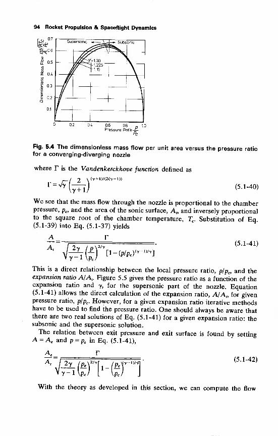
94 Rocket Propulsion & Spaceflight Dynamics
Hsk06
I 0.5
(U
R 0.3
.§ 0.2
0.1
Supersonic '« \ — j—• Subsonic
/XC^r=t3°-1.225
•1.15
0.2 0M 0.6 0.8 _ 1.0
Pressure Ratio -£-
Pc
Fig. 5.4 The dimensionless mass flow per unit area versus the pressure ratiofor a converging-diverging nozzle
where T is the Vandenkerckhove function defined as
r—l 9 \ (t+D/(2(y-D)
(5.1-40)
We see that the mass flow through the nozzle is proportional to the chamberpressure, pc , and the area of the sonic surface, A
t,and inversely proportional
to the square root of the chamber temperature, Tc . Substitution of Eq(5.1-39) into Eq. (5.1-37) yields
AA
' JSiT(5.1-41)
H-(p/PcYy- l),y
]
This is a direct relationship between the local pressure ratio, p/pc, and theexpansion ratio A/A
t .Figure 5.5 gives the pressure ratio as a function of the
expansion ratio and y, for the supersonic part of the nozzle. Equation(5.1-41) allows the direct calculation of the expansion ratio, A/A
t,for given
pressure ratio, p/pc . However, for a given expansion ratio iterative methodshave to be used to find the pressure ratio. One should always be aware thatthere are two real solutions of Eq. (5.1-41) for a given expansion ratio: thesubsonic and the supersonic solution.
The relation between exit pressure and exit surface is found by settingA = Ae and p = pe in Eq. (5.1-41),
JMTFWl(5.1-42)
With the theory as developed in this section, we can compute the flow
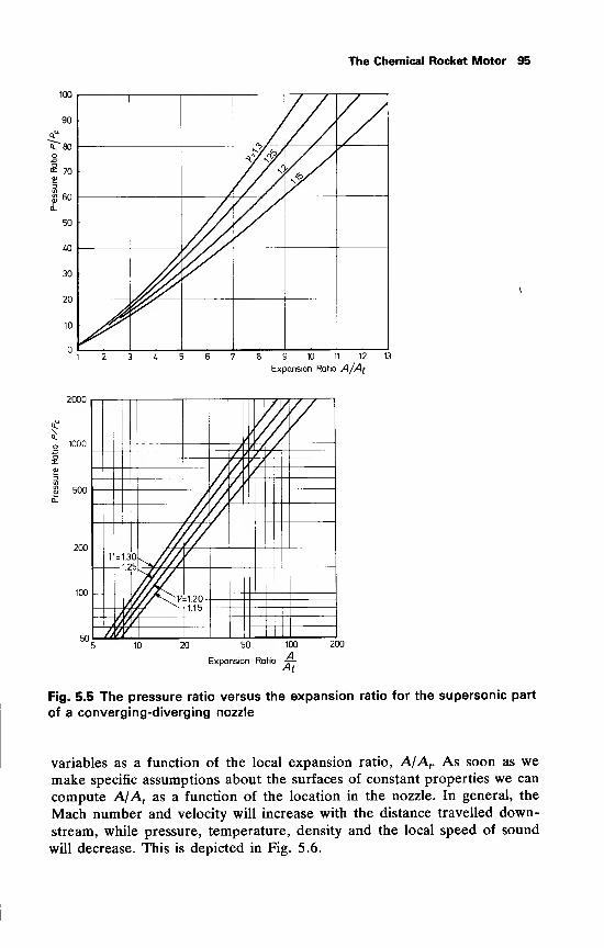
The Chemical Rocket Motor 95
90
oT80o
<* 70Si
g 60
0-
// y
50
30
20
10
n
2000
500
200
100
50
9 10 11 12 13
Expansion Ratio A/At
' / j
V 3C
2\
'. ///y
•
20 50
Expansion Ratio
100
AAt
200
Fig. 5.5 The pressure ratio versus the expansion ratio for the supersonic part
of a converging-diverging nozzle
variables as a function of the local expansion ratio, A/At. As soon as we
make specific assumptions about the surfaces of constant properties we can
compute A/A, as a function of the location in the nozzle. In general, the
Mach number and velocity will increase with the distance travelled down-
stream, while pressure, temperature, density and the local speed of sound
will decrease. This is depicted in Fig. 5.6.
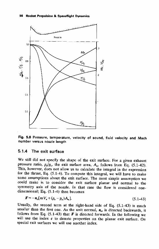
96 Rocket Propulsion & Spaceflight Dynamics
Fig. 5.6 Pressure, temperature, velocity of sound, fluid velocity and Machnumber versus nozzle length
5.1.4 The exit surface
We still did not specify the shape of the exit surface. For a given exhaustpressure ratio, pjpc , the exit surface area, Ac , follows from Eq. (5.1-42).This, however, does not allow us to calculate the integral in the expressionfor the thrust, Eq. (5.1-4). To compute this integral, we will have to makesome assumptions about the exit surface. The most simple assumption wecould make is to consider the exit surface planar and normal to thesymmetry axis of the nozzle. In that case the flow is considered one-dimensional; Eq. (5.1-4) then becomes
F=-ne[mVe + (pe -pa)Ael (5.1-43)
Usually, the second term at the right-hand side of Eq. (5.1-43) is muchsmaller than the first one. As the unit normal, ne, is directed backwards, it
follows from Eq. (5.1-43) that F is directed forwards. In the following wewill use the index e to denote properties on the planar exit surface. Onspecial exit surfaces we will use another index.
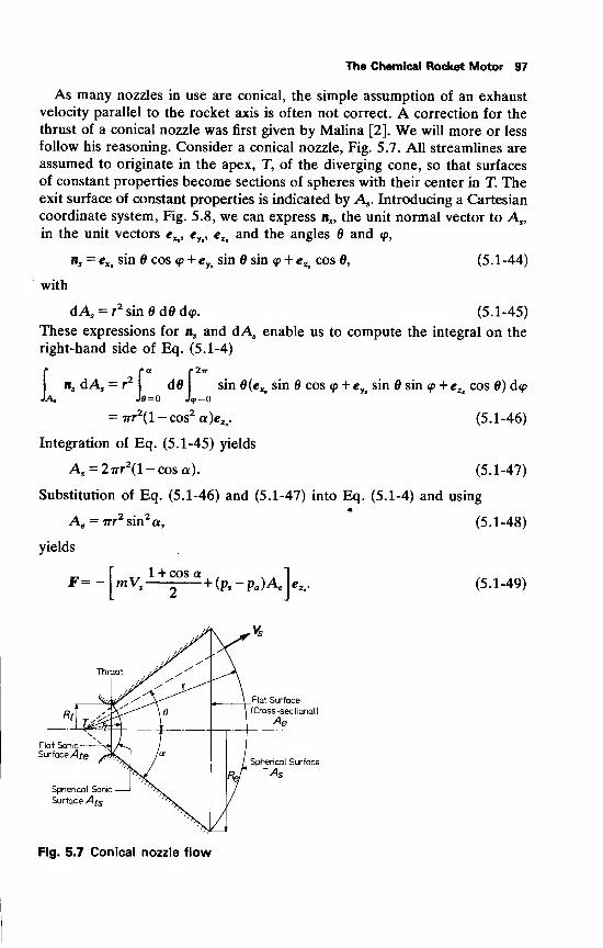
The Chemical Rocket Motor 97
As many nozzles in use are conical, the simple assumption of an exhaust
velocity parallel to the rocket axis is often not correct. A correction for the
thrust of a conical nozzle was first given by Malina [2]. We will more or less
follow his reasoning. Consider a conical nozzle, Fig. 5.7. All streamlines are
assumed to originate in the apex, T, of the diverging cone, so that surfaces
of constant properties become sections of spheres with their center in T. Theexit surface of constant properties is indicated by As . Introducing a Cartesian
coordinate system, Fig. 5.8, we can express ns , the unit normal vector to As,
in the unit vectors ev eyi , eZs
and the angles and <p,
ns= eXi sin cos <p + e
yisin sin <p + eZs cos 0, (5.1-44)
with
dAs= r
2sin dd d<p. (5.1-45)
These expressions for ns and dAs enable us to compute the integral on the
right-hand side of Eq. (5.1-4)
)•
fa |*2ir
ns dAs = r2 d0 sin 0(eXt sin cos <p + e
ytsin 6 sin <p + eZt cos 6) d<p
a, Je=o J<p=o
= 7rr2(l-cos2
a)c2j . (5.1-46)
Integration of Eq. (5.1-45) yields
As= 27rr
2(l-cosa). (5.1-47)
Substitution of Eq. (5.1-46) and (5.1-47) into Eq. (5.1-4) and using
Ae = irr2sin
2a,
*
(5.1-48)
yields
_, . „ 1 + cosa . . 1F=-\mVs +(ps-pa)Ae l (5.1-49)
Throat
Flat SonicSurface Afe
Spherical Sonic
Surface .^5
Flat Surface
(Cross -sectional)
Spherical Surface
As
Fig. 5.7 Conical nozzle flow
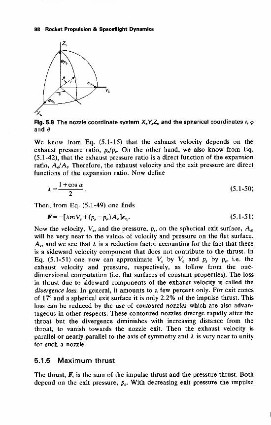
98 Rocket Propulsion & Spaceflight Dynamics
Fig. 5.8 The nozzle coordinate system XSYSZS and the spherical coordinates r, <p
and 6
We know from Eq. (5.1-15) that the exhaust velocity depends on the
exhaust pressure ratio, pe/pc . On the other hand, we also know from Eq.
(5.1-42), that the exhaust pressure ratio is a direct function of the expansion
ratio, AJAt. Therefore, the exhaust velocity and the exit pressure are direct
functions of the expansion ratio. Now define
A =1 + cos a
(5.1-50)
Then, from Eq. (5.1-49) one finds
F=-[AmVs+ (ps -pa)AJeZs
. (5.1-51)
Now the velocity, Vs , and the pressure, ps , on the spherical exit surface, As ,
will be very near to the values of velocity and pressure on the flat surface,
Ae , and we see that A is a reduction factor accounting for the fact that there
is a sideward velocity component that does not contribute to the thrust. In
Eq. (5.1-51) one now can approximate Vs by Ve and ps by pe , i.e. the
exhaust velocity and pressure, respectively, as follow from the one-
dimensional computation (i.e. flat surfaces of constant properties). The loss
in thrust due to sideward components of the exhaust velocity is called the
divergence loss. In general, it amounts to a few percent only. For exit cones
of 17° and a spherical exit surface it is only 2.2% of the impulse thrust. This
loss can be reduced by the use of contoured nozzles which are also advan-
tageous in other respects. These contoured nozzles diverge rapidly after the
throat but the divergence diminishes with increasing distance from the
throat, to vanish towards the nozzle exit. Then the exhaust velocity is
parallel or nearly parallel to the axis of symmetry and A is very near to unity
for such a nozzle.
5.1.5 Maximum thrust
The thrust, F, is the sum of the impulse thrust and the pressure thrust. Both
depend on the exit pressure, pe . With decreasing exit pressure the impulse
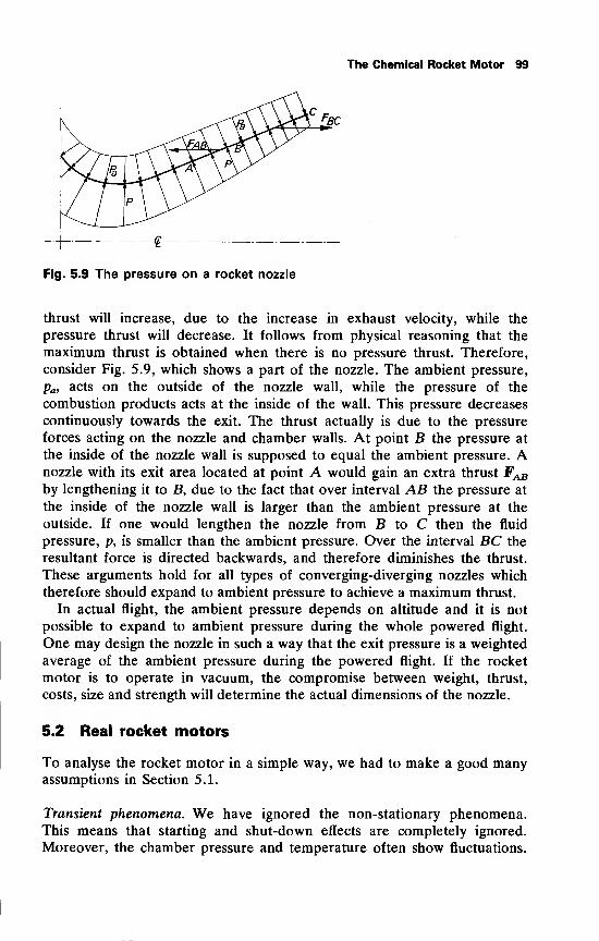
The Chemical Rocket Motor 99
Fig. 5.9 The pressure on a rocket nozzle
thrust will increase, due to the increase in exhaust velocity, while the
pressure thrust will decrease. It follows from physical reasoning that the
maximum thrust is obtained when there is no pressure thrust. Therefore,
consider Fig. 5.9, which shows a part of the nozzle. The ambient pressure,
pa , acts on the outside of the nozzle wall, while the pressure of the
combustion products acts at the inside of the wall. This pressure decreases
continuously towards the exit. The thrust actually is due to the pressure
forces acting on the nozzle and chamber walls. At point B the pressure at
the inside of the nozzle wall is supposed to equal the ambient pressure. Anozzle with its exit area located at point A would gain an extra thrust FABby lengthening it to B, due to the fact that over interval AB the pressure at
the inside of the nozzle wall is larger than the ambient pressure at the
outside. If one would lengthen the nozzle from B to C then the fluid
pressure, p, is smaller than the ambient pressure. Over the interval BC the
resultant force is directed backwards, and therefore diminishes the thrust.
These arguments hold for all types of converging-diverging nozzles which
therefore should expand to ambient pressure to achieve a maximum thrust.
In actual flight, the ambient pressure depends on altitude and it is not
possible to expand to ambient pressure during the whole powered flight.
One may design the nozzle in such a way that the exit pressure is a weighted
average of the ambient pressure during the powered flight. If the rocket
motor is to operate in vacuum, the compromise between weight, thrust,
costs, size and strength will determine the actual dimensions of the nozzle.
5.2 Real rocket motors
To analyse the rocket motor in a simple way, we had to make a good manyassumptions in Section 5.1.
Transient phenomena. We have ignored the non-stationary phenomena.This means that starting and shut-down effects are completely ignored.
Moreover, the chamber pressure and temperature often show fluctuations.
100 Rocket Propulsion & Spaceflight Dynamics
In many cases, these fluctuations are small and do not influence the overall
rocket performances. If this is not the case, special analysis of oscillatory
combustion is necessary [3,4]. In some cases a coupling between the
unsteady combustion process, the vehicle structure and the propellant feed
lines may take place. This effect is known as POGO instability [5]. It is
especially known to occur in liquid-propellant rocket motors. In solid-
propellant test motors, pressure fluctuations up to 30% of the mean chamber
pressure have been measured [6]. Non-stationary effects therefore, can be
very important. However, one mostly aims at a smooth thrust-time history,
even if the thrust varies with time. Then, the non-stationary effects are so
small that they can be ignored.
Uniform, localized combustion. The combustion was assumed to take place
in the combustion zone. This, however, is not fully the case. Chemical
reactions and recombinations take place in the nozzle itself. We will deal
partly with these effects in Chapter 7. In general, however, the approxima-
tion that all combustion takes place in a small region, turns out to give
results with an error of less than 5%.At the nozzle entrance uniform chamber conditions were assumed. In
general, this is not the case. Analysis of the effects of non-uniform chamber
conditions shows that the thrust may change a little (in the order of a few
percent) depending on the shape of the throat [7] as compared to idealized
theory.
Isentropic flow. The assumption that the flow is isentropic, is clearly an
idealization. Heat transfer is a serious problem in the design of rocket
motors. However, except for small motors, it is more a problem of cooling
than a problem of performance loss. Apart from this we have boundary
layer effects. Both heat transfer and boundary layers are strongly dependent
on the nozzle shape and size. These losses usually are of the order of 2% to
3% of the thrust.
Ideal gas combustion products. The assumption that the combustion pro-
ducts are ideal gases and have constant specific heats is certainly an over-
simplification. In many cases, solid particles are present in the flow (two-
phase flow). Because of their drag, these particles are exhausted too, but
usually, there is a velocity difference between the particles and the gas. Theparticles may impinge on the nozzle walls, leading to erosion of, or the
formation of a deposit on, the nozzle wall. To improve the rocket perfor-
mances, one should try to avoid impingement as much as possible. This
would result in nozzles with a very long throat and flaring out towards the
exit. This, however, leads to higher divergence losses and heat transfer
creates more problems too [8]. The presence of solid particles in the
combustion products may be due to incomplete combustion, but in manycases they are due to metal additives. In solid-propellant rockets and in
high-performance liquid-propellant rockets, metal additives are used to
The Chemical Rocket Motor 101
increase the combustion temperature. The presence of solid particles in the
exhaust flow will also increases the molecular weight of the combustion
products, hence, the performance gain will be a little less than one might
expect from the raised combustion temperature alone.
Other effects. The specific heats not being constant may change the rocket
performances, as compared to idealized theory. We will deal with this in
Chapter 7.
Even if we forego viscous effects, such as boundary layers, surfaces of
constant properties, as defined in Section 5.1, can only exist in very special
cases (e.g. purely one-dimensional flow, rotationally-symmetrical flow). The
concept, however, is useful to account for three-dimensional effects. More
accurate analyses of the nozzle flow will account for heat transfer and
viscous effects [9] and chemical reactions [10]. Often, however, approximate
methods [11] or the method of characteristics [1] are used for the computa-
tion of the nozzle flow.
Quality factors. To compare the actual performances with the ideal perfor-
mances, the following quality factors are often used
& = §*, (5.2-1)
which is the ratio of actual thrust, or the thrust as determined by an
experiment, to the theoretical thrust. In general, £F has values between 0.92
and 0.96. The ratio of actual exhaust velocity to theoretical exhaust
velocity,
«,-£• <5 -2-2>
In general, £v nas values somewhere between 0.85 and 0.98, but much lower
values are possible. The ratio of the actual mass flow, as determined by an
experiment, and the theoretical mass flow.
£m =^. (5.2-3)mth
Values for £m range between 0.98 and 1.15. That the correction factor for
the propellant mass flow can become larger than unity is a result of:
1. Recombination, as a result of which the molecular weight of the gases
can increase during expansion.
2. Heat transfer to the nozzle walls; as the temperature is lowered owing
to heat transfer, the density is increased.
3. Other influences such as incomplete combustion, solid particles in the
exhaust products and the change of the specific heats as a result of
temperature drop and recombination.
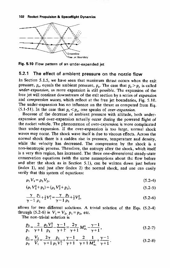
102 Rocket Propulsion & Spaceflight Dynamics
Streamline
Free Jet Boundary
Fig. 5.10 Flow pattern of an under-expanded jet
5.2.1 The effect of ambient pressure on the nozzle flow
In Section 5.1.5, we have seen that maximum thrust occurs when the exit
pressure, pe, equals the ambient pressure, pa . The case that pe > pa is called
under-expansion, as more expansion is still possible. The expansion of thefree jet will continue downstream of the exit section by a series of expansionand compression waves, which reflect at the free jet boundaries, Fig. 5.10.
The under-expansion has no influence on the thrust as computed from Eq.(5.1-51). In the case that pe <pa, one speaks of over-expansion.
Because of the decrease of ambient pressure with altitude, both under-expansion and over-expansion actually occur during the powered flight of
the rocket vehicle. The phenomenon of over-expansion is more complicatedthan under-expansion. If the over-expansion is too large, normal shockwaves may occur. The shock wave itself is due to viscous effects. Across the
normal shock there is a sudden rise in pressure, temperature and density,
while the velocity has decreased. The compression by the shock is a
non-isentropic process. Therefore, the entropy after the shock, which itself
is a very thin region, has increased. The three one-dimensional steady-state
conservation equations (with the same assumptions about the flow before
and after the shock as in Section 5.1), can be written down just before
(index 1), and just after (index 2) the normal shock, and one can easily
verify that this system of equations:
PiV1 = p2V2 , (5.2-4)
(PiV? + p1 )= (p2 V| + p2), (5.2-5)
y Pi, iT,2 _ y P2^+Iy2 = _J_i- + iVi (5 2 .6)7-1 Pi 7-1 P2
allows for two different solutions. A trivial solution of the Eqs. (5.2-4)
through (5.2-6) is V^ V2 , Pi = p2 , etc.
The non-trivial solution is
P_1 = _J_P_1 v\_yz i = ^y_ M2 _lzl (52 _7)Pi 7+1 Pi 7+1' 7 + 1 * 7 + 1' }
Pl _V2 _ 27 Pl y-l_ 2 1 IZip2 V1 7 + 1 PiV? 7 + 1 y+l< 7 + 1' K
'
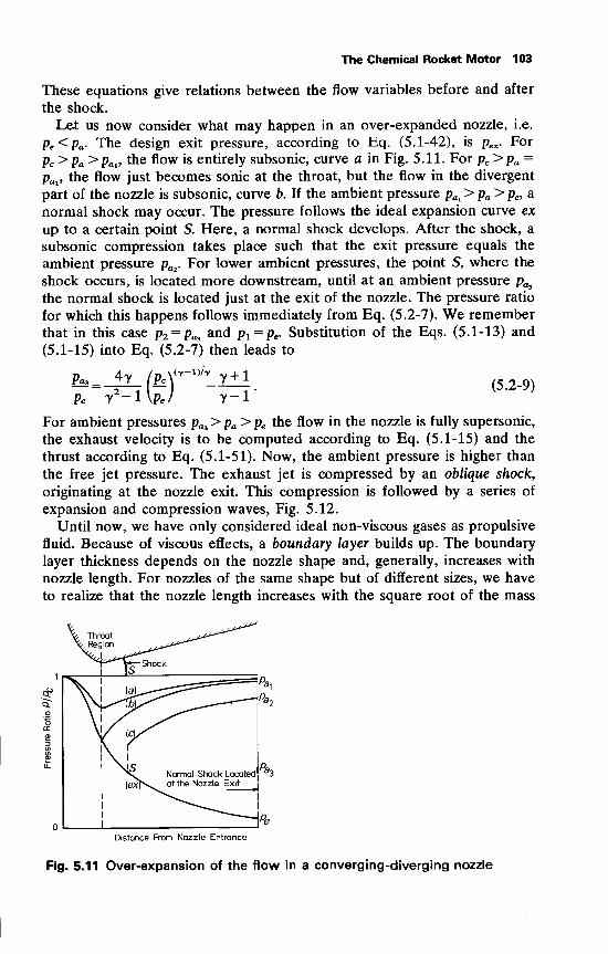
The Chemical Rocket Motor 103
These equations give relations between the flow variables before and after
the shock.
Let us now consider what may happen in an over-expanded nozzle, i.e.
Pe < Pa- The design exit pressure, according to Eq. (5.1-42), is pex . For
Pc> Pa> Pax , the flow is entirely subsonic, curve a in Fig. 5.11. For pc >pa~
pai , the flow just becomes sonic at the throat, but the flow in the divergent
part of the nozzle is subsonic, curve b. If the ambient pressure pai >pa > pe, a
normal shock may occur. The pressure follows the ideal expansion curve ex
up to a certain point S. Here, a normal shock develops. After the shock, a
subsonic compression takes place such that the exit pressure equals the
ambient pressure p^. For lower ambient pressures, the point S, where the
shock occurs, is located more downstream, until at an ambient pressure pa3the normal shock is located just at the exit of the nozzle. The pressure ratio
for which this happens follows immediately from Eq. (5.2-7). We remember
that in this case p2 = Pa3and Pi = pe . Substitution of the Eqs. (5.1-13) and
(5.1-15) into Eq. (5.2-7) then leads to
Pa3 = 4T (PcX
Pe y2-l\Pe)
(-y-D/T y + 1
r-i(5.2-9)
For ambient pressures pa3>pa >pe the flow in the nozzle is fully supersonic,
the exhaust velocity is to be computed according to Eq. (5.1-15) and the
thrust according to Eq. (5.1-51). Now, the ambient pressure is higher than
the free jet pressure. The exhaust jet is compressed by an oblique shock,
originating at the nozzle exit. This compression is followed by a series of
expansion and compression waves, Fig. 5.12.
Until now, we have only considered ideal non-viscous gases as propulsive
fluid. Because of viscous effects, a boundary layer builds up. The boundary
layer thickness depends on the nozzle shape and, generally, increases with
nozzle length. For nozzles of the same shape but of different sizes, we have
to realize that the nozzle length increases with the square root of the mass
Fig.
Distance From Nozzle Entrance
5.11 Over-expansion of the flow in a converging-diverging nozzle
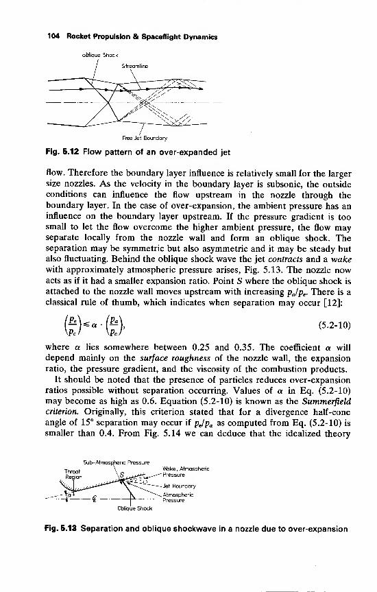
104 Rocket Propulsion & Spaceflight Dynamics
oblique Shock
Streamline
Free Jet Boundary
Fig. 5.12 Flow pattern of an over-expanded jet
flow. Therefore the boundary layer influence is relatively small for the larger
size nozzles. As the velocity in the boundary layer is subsonic, the outside
conditions can influence the flow upstream in the nozzle through the
boundary layer. In the case of over-expansion, the ambient pressure has aninfluence on the boundary layer upstream. If the pressure gradient is too
small to let the flow overcome the higher ambient pressure, the flow mayseparate locally from the nozzle wall and form an oblique shock. Theseparation may be symmetric but also asymmetric and it may be steady but
also fluctuating. Behind the oblique shock wave the jet contracts and a wakewith approximately atmospheric pressure arises, Fig. 5.13. The nozzle nowacts as if it had a smaller expansion ratio. Point S where the oblique shock is
attached to the nozzle wall moves upstream with increasing pjpe . There is a
classical rule of thumb, which indicates when separation may occur [12]:
ftH-ft)-(5.2-10)
where a lies somewhere between 0.25 and 0.35. The coefficient a will
depend mainly on the surface roughness of the nozzle wall, the expansion
ratio, the pressure gradient, and the viscosity of the combustion products.
It should be noted that the presence of particles reduces over-expansion
ratios possible without separation occurring. Values of a in Eq. (5.2-10)
may become as high as 0.6. Equation (5.2-10) is known as the Summerfieldcriterion. Originally, this criterion stated that for a divergence half-cone
angle of 15° separation may occur if pjpa as computed from Eq. (5.2-10) is
smaller than 0.4. From Fig. 5.14 we can deduce that the idealized theory
Sub-Atmospheric Pressure
Th i \ _ \Afake, Atmospheric
Pressure
^ -Jet Boundary
Oblique Shock
Fig. 5.13 Separation and oblique Shockwave in a nozzle due to over-expansion
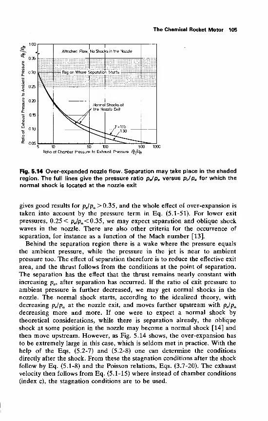
The Chemical Rocket Motor 105
1.00
0.055 10 50 100 500 1000
Ratio of Chamber Pressure to Exhaust Pressure /fc/Pe
Fig. 5.14 Over-expanded nozzle flow. Separation may take place in the shaded
region. The full lines give the pressure ratio pjpa versus pc/pe for which the
normal shock is located at the nozzle exit
gives good results for pjpa > 0.35, and the whole effect of over-expansion is
taken into account by the pressure term in Eq. (5.1-51). For lower exit
pressures, 0.25 < pelpa< 0.35, we may expect separation and oblique shock
waves in the nozzle. There are also other criteria for the occurrence of
separation, for instance as a function of the Mach number [13].
Behind the separation region there is a wake where the pressure equals
the ambient pressure, while the pressure in the jet is near to ambient
pressure too. The effect of separation therefore is to reduce the effective exit
area, and the thrust follows from the conditions at the point of separation.
The separation has the effect that the thrust remains nearly constant with
increasing pa, after separation has occurred. If the ratio of exit pressure to
ambient pressure is further decreased, we may get normal shocks in the
nozzle. The normal shock starts, according to the idealized theory, with
decreasing pjpa at the nozzle exit, and moves further upstream with pjpadecreasing more and more. If one were to expect a normal shock by
theoretical considerations, while there is separation already, the oblique
shock at some position in the nozzle may become a normal shock [14] and
then move upstream. However, as Fig. 5.14 shows, the over-expansion has
to be extremely large in this case, which is seldom met in practice. With the
help of the Eqs. (5.2-7) and (5.2-8) one can determine the conditions
directly after the shock. From these the stagnation conditions after the shock
follow by Eq. (5.1-8) and the Poisson relations, Eqs. (3.7-20). The exhaust
velocity then follows from Eq. (5.1-15) where instead of chamber conditions
(index c), the stagnation conditions are to be used.
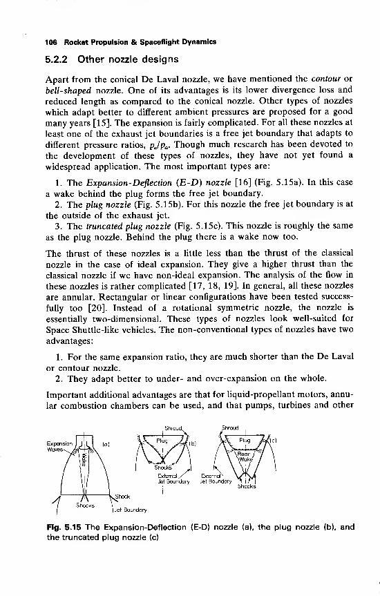
106 Rocket Propulsion & Spaceflight Dynamics
5.2.2 Other nozzle designs
Apart from the conical De Laval nozzle, we have mentioned the contour or
bell-shaped nozzle. One of its advantages is its lower divergence loss and
reduced length as compared to the conical nozzle. Other types of nozzles
which adapt better to different ambient pressures are proposed for a good
many years [15]. The expansion is fairly complicated. For all these nozzles at
least one of the exhaust jet boundaries is a free jet boundary that adapts to
different pressure ratios, pe/pa . Though much research has been devoted to
the development of these types of nozzles, they have not yet found a
widespread application. The most important types are:
1. The Expansion-Deflection (E-D) nozzle [16] (Fig. 5.15a). In this case
a wake behind the plug forms the free jet boundary.
2. The plug nozzle (Fig. 5.15b). For this nozzle the free jet boundary is at
the outside of the exhaust jet.
3. The truncated plug nozzle (Fig. 5.15c). This nozzle is roughly the same
as the plug nozzle. Behind the plug there is a wake now too.
The thrust of these nozzles is a little less than the thrust of the classical
nozzle in the case of ideal expansion. They give a higher thrust than the
classical nozzle if we have non-ideal expansion. The analysis of the flow in
these nozzles is rather complicated [17, 18, 19]. In general, all these nozzles
are annular. Rectangular or linear configurations have been tested success-
fully too [20]. Instead of a rotational symmetric nozzle, the nozzle is
essentially two-dimensional. These types of nozzles look well-suited for
Space Shuttle-like vehicles. The non-conventional types of nozzles have two
advantages:
1. For the same expansion ratio, they are much shorter than the De Laval
or contour nozzle.
2. They adapt better to under- and over-expansion on the whole.
Important additional advantages are that for liquid-propellant motors, annu-
lar combustion chambers can be used, and that pumps, turbines and other
Shroud. Shroud
External/ External
Jet Boundary Jet BoundaryShocks
Fig. 5.15 The Expansion-Deflection (E-D) nozzle (a), the plug nozzle (b), and
the truncated plug nozzle (c)
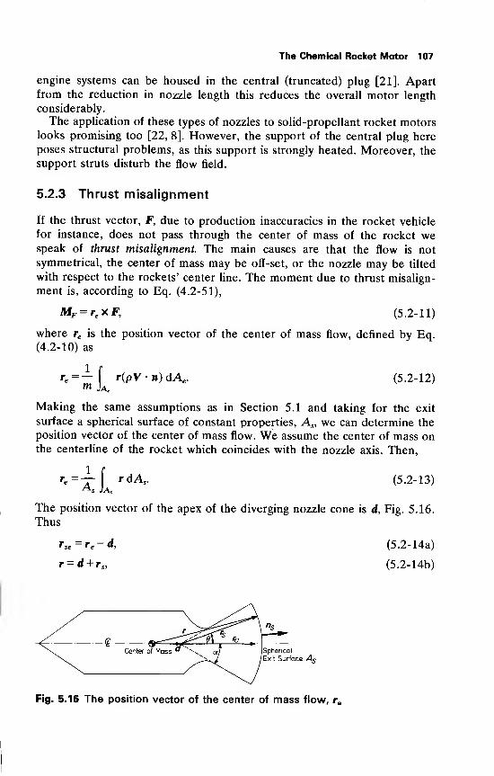
The Chemical Rocket Motor 107
engine systems can be housed in the central (truncated) plug [21]. Apartfrom the reduction in nozzle length this reduces the overall motor length
considerably.
The application of these types of nozzles to solid-propellant rocket motorslooks promising too [22, 8]. However, the support of the central plug here
poses structural problems, as this support is strongly heated. Moreover, the
support struts disturb the flow field.
5.2.3 Thrust misalignment
If the thrust vector, F, due to production inaccuracies in the rocket vehicle
for instance, does not pass through the center of mass of the rocket wespeak of thrust misalignment. The main causes are that the flow is not
symmetrical, the center of mass may be off-set, or the nozzle may be tilted
with respect to the rockets' center line. The moment due to thrust misalign-
ment is, according to Eq. (4.2-51),
MF = re xF, (5.2-11)
where re is the position vector of the center of mass flow, defined by Eq.(4.2-10) as
re =—[ r(PV-n)dAe . (5.2-12)
Making the same assumptions as in Section 5.1 and taking for the exit
surface a spherical surface of constant properties, As , we can determine the
position vector of the center of mass flow. We assume the center of mass onthe centerline of the rocket which coincides with the nozzle axis. Then,
re =-7-\ rdAs . (5.2-13)As Jas
The position vector of the apex of the diverging nozzle cone is d, Fig. 5.16.
Thus
rse = re -d, (5.2-14a)
r = d + r s , (5.2-14b)
Spherical
Exit Surface As
Fig. 5.16 The position vector of the center of mass flow, re
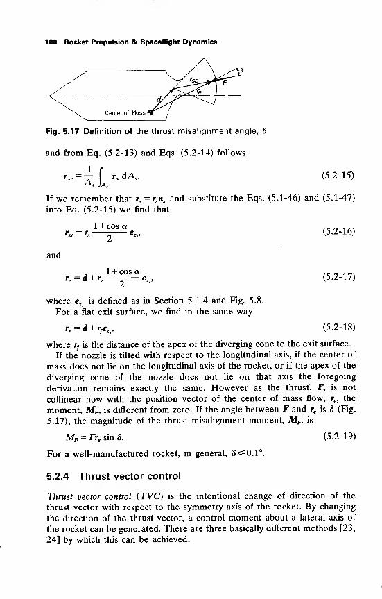
108 Rocket Propulsion & Spaceflight Dynamics
Fig. 5.17 Definition of the thrust misalignment angle, 8
and from Eq. (5.2-13) and Eqs. (5.2-14) follows
rse =4-f '.dA,. (5.2-15)
If we remember that rs = rs tis and substitute the Eqs. (5.1-46) and (5.1-47)
into Eq. (5.2-15) we find that
1 + cos a ,c 1,*
rse = rs eZs ,(5.2-16)
and
1 + cos a K01flre = d + rs e
Zs,(5.2-17)
where eZs
is defined as in Section 5.1.4 and Fig. 5.8.
For a flat exit surface, we find in the same way
re = d + rfeZs ,(5.2-18)
where rf
is the distance of the apex of the diverging cone to the exit surface.
If the nozzle is tilted with respect to the longitudinal axis, if the center of
mass does not lie on the longitudinal axis of the rocket, or if the apex of the
diverging cone of the nozzle does not lie on that axis the foregoing
derivation remains exactly the same. However as the thrust, F, is not
collinear now with the position vector of the center of mass flow, rc, the
moment, MF, is different from zero. If the angle between F and re is 8 (Fig.
5.17), the magnitude of the thrust misalignment moment, MF, is
MF = Fre sin 8. (5.2-19)
For a well-manufactured rocket, in general, 8=^0.1°.
5.2.4 Thrust vector control
Thrust vector control {TVC) is the intentional change of direction of the
thrust vector with respect to the symmetry axis of the rocket. By changing
the direction of the thrust vector, a control moment about a lateral axis of
the rocket can be generated. There are three basically different methods [23,
24] by which this can be achieved.
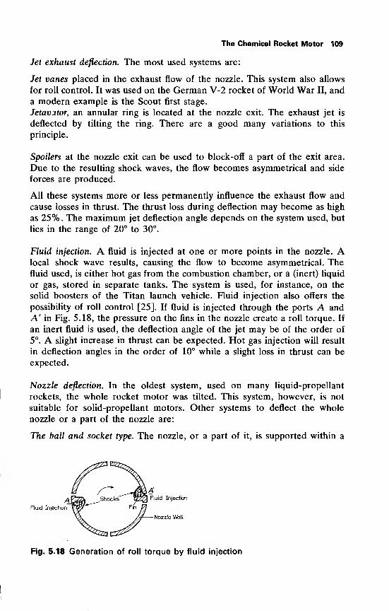
The Chemical Rocket Motor 109
Jet exhaust deflection. The most used systems are:
Jet vanes placed in the exhaust flow of the nozzle. This system also allows
for roll control. It was used on the German V-2 rocket of World War II, and
a modern example is the Scout first stage.
Jetavztor, an annular ring is located at the nozzle exit. The exhaust jet is
deflected by tilting the ring. There are a good many variations to this
principle.
Spoilers at the nozzle exit can be used to block-off a part of the exit area.
Due to the resulting shock waves, the flow becomes asymmetrical and side
forces are produced.
All these systems more or less permanently influence the exhaust flow and
cause losses in thrust. The thrust loss during deflection may become as high
as 25%. The maximum jet deflection angle depends on the system used, but
lies in the range of 20° to 30°.
Fluid injection. A fluid is injected at one or more points in the nozzle. Alocal shock wave results, causing the flow to become asymmetrical. Thefluid used, is either hot gas from the combustion chamber, or a (inert) liquid
or gas, stored in separate tanks. The system is used, for instance, on the
solid boosters of the Titan launch vehicle. Fluid injection also offers the
possibility of roll control [25]. If fluid is injected through the ports A and
A' in Fig. 5.18, the pressure on the fins in the nozzle create a roll torque. If
an inert fluid is used, the deflection angle of the jet may be of the order of
5°. A slight increase in thrust can be expected. Hot gas injection will result
in deflection angles in the order of 10° while a slight loss in thrust can be
expected.
Nozzle deflection. In the oldest system, used on many liquid-propellant
rockets, the whole rocket motor was tilted. This system, however, is not
suitable for solid-propellant motors. Other systems to deflect the whole
nozzle or a part of the nozzle are:
The ball and socket type. The nozzle, or a part of it, is supported within a
AFluid Injection
Fig. 5.18 Generation of roll torque by fluid injection
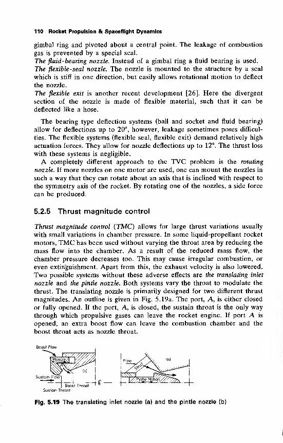
110 Rocket Propulsion & Spaceflight Dynamics
gimbal ring and pivoted about a central point. The leakage of combustion
gas is prevented by a special seal.
The fluid-bearing nozzle. Instead of a gimbal ring a fluid bearing is used.
The flexible-seal nozzle. The nozzle is mounted to the structure by a seal
which is stiff in one direction, but easily allows rotational motion to deflect
the nozzle.
The flexible exit is another recent development [26]. Here the divergent
section of the nozzle is made of flexible material, such that it can be
deflected like a hose.
The bearing type deflection systems (ball and socket and fluid bearing)
allow for deflections up to 20°, however, leakage sometimes poses difficul-
ties. The flexible systems (flexible seal, flexible exit) demand relatively high
actuation forces. They allow for nozzle deflections up to 12°. The thrust loss
with these systems is negligible.
A completely different approach to the TVC problem is the rotating
nozzle. If more nozzles on one motor are used, one can mount the nozzles in
such a way that they can rotate about an axis that is inclined with respect to
the symmetry axis of the rocket. By rotating one of the nozzles, a side force
can be produced.
5.2.5 Thrust magnitude control
Thrust magnitude control (TMC) allows for large thrust variations usually
with small variations in chamber pressure. In some liquid-propellant rocket
motors, TMC has been used without varying the throat area by reducing the
mass flow into the chamber. As a result of the reduced mass flow, the
chamber pressure decreases too. This may cause irregular combustion, or
even extinguishment. Apart from this, the exhaust velocity is also lowered.
Two possible systems without these adverse effects are the translating inlet
nozzle and the pintle nozzle. Both systems vary the throat to modulate the
thrust. The translating nozzle is primarily designed for two different thrust
magnitudes. An outline is given in Fig. 5.19a. The port, A, is either closed
or fully opened. If the port, A, is closed, the sustain throat is the only waythrough which propulsive gases can leave the rocket engine. If port A is
opened, an extra boost flow can leave the combustion chamber and the
boost throat acts as nozzle throat.
Boost Flow
Boost Throat
Sustain Throat
Fig. 5.19 The translating inlet nozzle (a) and the pintle nozzle (b)
The Chemical Rocket Motor 11
The pintle nozzle employs a center body that can move in an axial
direction, thereby continuously varying the throat area, Fig. 5.19b. Thecentral body which holds the movable pintle is mounted on struts on the
nozzle inlet. It is, of course, possible to combine TVC and TMC to obtain
real thrust vector control, i.e. both magnitude and direction of the thrust can
be varied.
Another TMC device that should be mentioned in this section is the
extendable exit cone. If during powered flight under-expansion losses becomeunacceptably large, one can increase the thrust by lengthening the exit cone.
This may be done by moving aft an extension to the divergent part of the
nozzle. This concept was planned for the Space Shuttle Main Engine, SSME,but has been abandoned to keep the mechanism simple.
References
1 Liepmann, H. W. and Roshko, A. (1957), Elements of Gasdynamics,
John Wiley, New York.
2 Malina, F. (1940), Characteristics of the rocket motor unit based on the
theory of perfect gases, J. Franklin Institute, 230, 433-454.
3 Harrje, D. T. and Reardon, F. H. (1972), Liquid Propellant Rocket
Combustion Instability, NASA SP-194, Washington.
4 Culick, F. E. C. (1968), A review of calculations for unsteady burning
of a solid propellant, AIAA J., 6, 2241-2255.
5 Rubin, S. (1972), Analysis of POGO- Stability, paper presented at the
23rd IAF Congress, Vienna.
6 Schoyer, H. F. R. (1971), Report on Low Frequency Oscillatory Com-bustion Experiments, Daniel and Florence Guggenheim Jet Propulsion
Center, California Institute of Technology, Pasadena.
7 Norton, D. J. and White, R. E. (1973), Striated nozzle flow with small
radius of curvature ratio throats, J. Spacecraft, 10, 747-750.
8 Williams, F. A., Barrere, M. and Huang, N. C. (1969), FundamentalAspects of Solid Propellant Rockets, AGARDograph #116, Technivi-
sion Services, Slough.
9 Benison, G. J. and Rubin, E. L. (1971), A time-dependent analysis for
quasi-one-dimensional, viscous, heat conducting, compressible laval
nozzle flows, J. Eng. Math., 5, 39-49.
10 Scaccia, C. and Kennedy, L. A. (1974), Calculating two-dimensional
chemically reacting flows, AIAA J., 12, 1268-1272.
11 Kliegel, J. R. and Quan, V. (1968), Convergent-divergent nozzle flows,
AIAA J., 6, 1728-1734.
12 Bloomer, H. E., Antl, R. J. and Renas, P. E. (1961), Experimental
Study of Effects of Geometric Variables on Performance of Conical
Rocket-engine Exhaust Nozzles, NASA TN D-846, Washington.
13 Arens, M. and Spiegler, E. (1963), Shock-induced boundary layer
separation in over-expanded conical exhaust nozzles, AIAA J., 1,
578-581.
112 Rocket Propulsion & Spaceflight Dynamics
14 Nave, L. H. and Coffey, G. A. (1973), Sea Level Sideloads in High-Area-Ratio Rocket Engines, AIAA Paper 73-1284, New York.
15 Rao, G. V. R. (1961), Recent developments in rocket nozzle configura-
tions, A.R.S. J., 31, 1488-1494.
16 Rao, G. V. R. (1960), The E-D nozzle, Astronautics, 5, September28-29, 50.
17 Hopkins, D. F. and Hill, D. E. (1968), Transonic flow in unconven-
tional nozzles, AIAA J., 6, 838-842.
18 Migdal, D. (1972), Supersonic annular nozzles, J. Spacecraft, 9, 3-6.
19 Sule, W. P. and Mueller, T. J. (1973), Annular truncated plug nozzle
flowfield and base pressure characteristics, J. Spacecraft, 10, 689-695.
20 Fuller, P. N. (1973), Linear Rocket Engine Design-Fabrication-Testing,
AIAA Paper 73-1179, New York.
21 Lamont, E. A. (1973), The Aerospike Engine System for the Space
Tug—A Status Report, AIAA Paper 73-1245, New York.
22 Casci, C, Gismond, E. and Angelino, G. (1968), An experimental
study on the application of plug nozzles to solid-propellant rockets—2,
Spaceflight, 10, 33-36.
23 Ellis, R. A. (1972), Continuing Evaluation of Nozzle Design andAnalysis Techniques, AIAA Paper 72-1190, New York.
24 Burgess, B. (1972), Recent advances in thrust vector control for tactical
missiles (supplementary paper), Aeronautical J., 77, 429-433.
25 Zeierman, I. and Manheimer-Timnat, Y. (1973), Full control of solid
propellant rockets by secondary injection, /. Spacecraft, 10, 161-162.
26 Cauza, J. H. and Mockenhaupt, J. D. (1973), The Integrated Omni-Vector Cone (INOVEC)™ Thrust Vector Control System, AIAA Paper
73-1204, New York.
6 Characteristic Coefficients andParameters of the RocketMotor
It is possible to define some quantities which are characteristic for the rocket
motor or its components. They are useful for outline information about the
rocket motor, but they also allow comparison, in certain respects, of rocket
engines of different sizes. Some other, dimensionless quantities, are useful to
compare theoretical and experimental results. For a better understanding of
how the latter quantities can be used to interpret test results, we will first
briefly discuss the testing of rockets.
6.1 Some notes on rocket testing
The most important performance parameter of the rocket motor is the
thrust. To measure the thrust, the rocket motor is fired on a test stand. As therocket performances are dependent on the burning-time, tb , the chamberpressure, pc, and chamber temperature, Tc , these quantities are measuredtoo. If heat transfer, deformation, etc., are important factors, it is obviousthat many more variables have to be measured. We will concern ourselves, in
this section, only with those quantities, that determine the rocket perfor-mances directly.
The rocket motor may be placed either in a horizontal, vertical or inclined
position. If the rocket is in a pure horizontal position and the thrust is
directed along the axis of symmetry, the weight of the rocket motor can be' measured by the vertical support. In this position, the main components ofweight and thrust are orthogonal. If the rocket is in a vertical position, theweight vector is in the same (or opposite) direction as the thrust vector, anda combination of thrust and weight is measured. This may pose difficulties
for solid-propellant rockets, as it is not possible to determine exactly their
mass flow at any instant. For a liquid-propellant rocket this information is
easily obtained by measuring the mass flow from the propellant tanks.
Although horizontal testing may be easier, for large rocket motors therocket structure may not be suited very well for testing in such a position, orthe liquids injected in the combustion chambers of liquid-propellant rocketsmay stay there while not yet burned, due to the ignition time lag. This maylead to an explosion. One can avoid this risk by putting the rocket motor in avertical position. It is clear that, especially for very large rockets, this leads
to more complicated structures of the teststand.
By measuring the forces on the rocket in three orthogonal directions, at
least at two different points for each direction, one can determine the forces
114 Rocket Propulsion & Spaceflight Dynamics
and moments on the rocket in all directions. This yields information about
thrust misalignment and is also important in the case of thrust vector
control.
Static rocket testing is a specialized technique and we will not discuss the
various ways of measuring the important parameters. We will assume that it
is possible to measure all these quantities more or less accurately. If a rocket
engine does not meet its specifications, it is necessary to determine the cause
of this shortcoming. It is here that the quantities to be discussed in this
chapter turn out to be convenient, because they yield specific information.
6.2 Total and specific impulse
A rocket motor, which during a time interval, tb, exerts a thrust, F(t),
delivers a total impulse, I,
1=fV(r)dt (6.2-1)
Jo
The propellant mass which was needed for this is Mp, and hence, the impulse
per unit weight of the propellant, the specific impulse, Isp, is
[V(f)df fV(f)df
L„ = K~. = ~Jr , (6.2-2a)Mpgo 1"Jo
gom(0dr
where g is the standard surface gravity. Another often used definition of
specific impulse, is the ratio of the impulse delivered during an infinitesimal
time interval, 8t, F8t, and the propellant weight consumed during that time
interval, mg 8t,
Isp = F/(mg ).(6.2-2b)
This quantity is also referred to as the specific thrust, as it is the thrust per
propellant weight flow rate. Both definitions are more or less equivalent,
and are identical if F and m are constant.
The specific impulse shows how much impulse can be obtained from a unit
weight of propellant, and as one tries to keep weights as low as possible in
rocket technology, it is evident that a high specific impulse is desirable. The
specific impulse may also be interpreted as the time during which a propel-
lant can deliver a force which equals the propellants' initial weight. As the
specific impulse is expressed in seconds, it has the same numerical value, in
both English and SI units. The specific impulse depends on both the
propellant and the motor configuration. This can be seen from Eq. (5.1-51)
with Vs= Ve , and ps
= pe ,
F=AmVc +(pe -pa)Ae . (6.2-3)
Characteristic Coefficients and Parameters of the Rocket Motor 115
According to Chapter 5, the reduction factor, A, depends on the nozzle
shape, while the exhaust velocity, Ve, and the exhaust pressure, pe, dependon the expansion ratio, AJAt,
and chamber pressure, pc . Using the second
definition, Eq. (6.2-2b), of the specific impulse, and assuming ideal expan-
sion, i.e. pe = pa , we find, taking A = 1,
mVe VeIsp = - =-
:
6.2-4)mgo go
Then, the specific impulse equals the ratio of the exhaust velocity and the
standard surface gravity. The specific impulse attains its maximum value in
the case that we expand to vacuum, i.e. pe = pa = 0. We then find
IsPmax=—
• (6.2-5)go
This value is a true propellant characteristic, as it is not dependent onpressure or expansion ratio. The direct measurement of the vacuum specific
impulse is difficult, however; therefore one always should indicate the
pressure ratio pc/pe and the ambient pressure if one lists values of the
specific impulse. For solid propellants, Isp attains values roughly between200 s and 300 s. Modern liquid propellants exhibit higher values, somewherebetween 250 s and 460 s. The values of Isp for hybrid propellant combina-
tions are, in general, a little higher than those for solids.
The specific consumption is defined as the ratio of propellant weight
consumed and the total impulse delivered. Therefore, it is the inverse of the
specific impulse:
'"I'F(t)dt
6.3 The volumetric specific impulse
The volumetric specific impulse, Is, is a measure for the influence of different
propellants on the performance of a vehicle of fixed dimensions. It is defined
as
4 = PpLp, (6.3-1)
where pp stands for the average density of the propellants.
In Chapters 11 and 12 it will be shown that AVid , i.e. the velocity
increment of a rocket vehicle in absence of drag and gravitational forces,
Aw T , /Me +Mp\AVid = Ispgo In^
e
Mp
j,(6.3-2)
is a very important performance parameter. In Eq. (6.3-2) Mp is the total
116 Rocket Propulsion & Spaceflight Dynamics
propellant mass, and Me is the empty (final) mass of the vehicle. Then
Mp= PpVp, (6.3-3)
where Vp is the volume available to store propellants. This volume is thought
of as a fixed quantity, as we consider a rocket of fixed dimensions, and study
the propellant influence on rocket performance. Now, if Mp/Me «l, we
approximate the logarithm in Eq. (6.3-2) and find
AVid= IspgoPp-f. (6.3-4)
This equation shows that for a rocket of fixed dimensions and Mp/Me « 1,
the ideal velocity increment, AVid , depends on the volumetric specific
impulse, Js . These small ratios of propellant mass over final mass are
encountered in JATO (Jet Assisted Take-Off) rockets and small rocket
weapons. The ratioMJMe « 1 is one extreme, the other extreme isMJMe » 1.
Then ln(H
—
-\ is not very sensitive anymore to changes in MJMe .
Therefore, for very large ratios of propellant mass and final mass the specific
impulse, Isp is the prime factor that determines the performance parameter,
AVid . In many practical cases, Mp/Me lies somewhere between these ex-
tremes. Then, both effects are noticeable. Thus, both the volumetric specific
impulse and the specific impulse determine the performance. The case mayas well be reversed: if a specified ideal velocity increment, AVid , is required,
which propellant combination yields the smallest vehicle possible? Solid
propellants, which are much denser, exhibit higher volumetric specific
impulses than liquid propellants. This is one of the reasons that solid
propellants, in spite of their lower specific impulse, as compared to liquid
propellants, find so much use.
6.4 The thrust coefficient
If the diverging part of the nozzle did not contribute to the thrust, and if
there were no flow in the combustion chamber, the thrust delivered by the
rocket motor in vacuum, F , would be (Fig. 6.1),
F = pcAt. (6.4-1)
As the divergent section of the nozzle does contribute to the thrust, and as
there is a flow in the combustion chamber, the thrust, F, differs from F . Thethrust coefficient is defined as the ratio of actual thrust and the thrust as
defined by Eq. (6.4-1):
CF = -^-. (6.4-2)
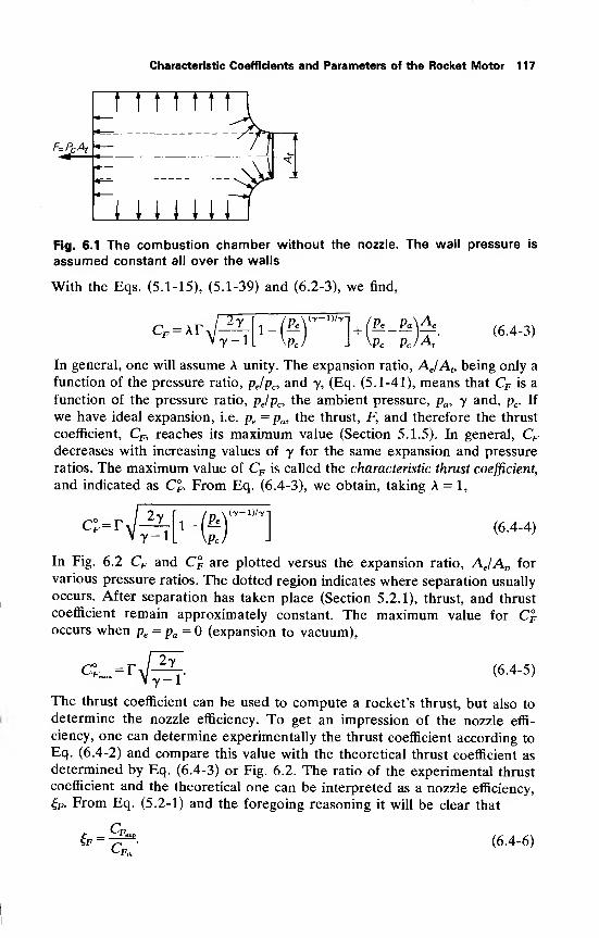
F-PpAt
Characteristic Coefficients and Parameters of the Rocket Motor 117
t t t t ttt
miniFig. 6.1 The combustion chamber without the nozzle. The wall pressure is
assumed constant all over the walls
With the Eqs. (5.1-15), (5.1-39) and (6.2-3), we find,
Ar / 2y 1-/ Pe
yy-ivy-+ (*-.Ei\^i
7-1 \pj \ \Pc PcJA(6.4-3)
In general, one will assume A unity. The expansion ratio, AJAt,being only a
function of the pressure ratio, pe/pc , and y, (Eq. (5.1-41), means that CF is a
function of the pressure ratio, pjpc, the ambient pressure, pa , y and, pc . If
we have ideal expansion, i.e. pe= pa , the thrust, F, and therefore the thrust
coefficient, CF, reaches its maximum value (Section 5.1.5). In general, CFdecreases with increasing values of y for the same expansion and pressure
ratios. The maximum value of CF is called the characteristic thrust coefficient,
and indicated as CF. From Eq. (6.4-3), we obtain, taking A = 1,
Cl=TY-1L \Pc/
(t-D/t-
(6.4-4)7 - i L \Pc
In Fig. 6.2 CF and CF are plotted versus the expansion ratio, AJAt,
for
various pressure ratios. The dotted region indicates where separation usually
occurs. After separation has taken place (Section 5.2.1), thrust, and thrust
coefficient remain approximately constant. The maximum value for CFoccurs when pe = pa = (expansion to vacuum),
C° =-VS (6.4-5)
The thrust coefficient can be used to compute a rocket's thrust, but also to
determine the nozzle efficiency. To get an impression of the nozzle effi-
ciency, one can determine experimentally the thrust coefficient according to
Eq. (6.4-2) and compare this value with the theoretical thrust coefficient as
determined by Eq. (6.4-3) or Fig. 6.2. The ratio of the experimental thrust
coefficient and the theoretical one can be interpreted as a nozzle efficiency,
£F. From Eq. (5.2-1) and the foregoing reasoning it will be clear that
CF(6.4-6)
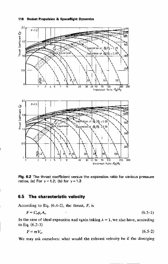
118 Rocket Propulsion & Spaceflight Dynamics
20 30 LQ 50 70 100 200 300
Expansion Ratio AgjAf
20 30 /.0 50 70 100 200 300
Expansion Ratio Ae/Af
Fig. 6.2 The thrust coefficient versus the expansion ratio for various pressure
ratios, (a) For 7 = 1.2; (b) for y = 1.3
6.5 The characteristic velocity
According to Eq. (6.4-2), the thrust, F, is
F=CFpcA t. (6.5-1)
In the case of ideal expansion and again taking A = 1, we also have, according
to Eq. (6.2-3)
F=mVe . (6.5-2)
We may ask ourselves: what would the exhaust velocity be if the diverging
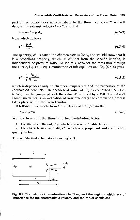
Characteristic Coefficients and Parameters of the Rocket Motor 119
part of the nozzle does not contribute to the thrust, i.e. CF=1? We will
denote this exhaust velocity by c*, and find
F=mc* = pcAt,
from which follows
_* _ PcAm
(6.5-3)
(6.5-4)
The quantity, c*, is called the characteristic velocity, and we will show that it
is a propellant property, which, as distinct from the specific impulse, is
independent of pressure ratio. To see this, consider the mass flow through
the nozzle, Eq. (5.1-39). Combination of this equation and Eq. (6.5-4) gives
= 1 JR^cc = — (6.5-5)
which is dependent only on chamber temperature and the properties of the
combustion products. The theoretical value of c*, as computed from Eq.
(6.5-5), can be compared with the value determined by a test. The ratio of
those two values is an indication of how efficiently the combustion process
takes place within the rocket motor.
It follows immediately from Eq. (6.4-2) and Eq. (6.5-4) that
F=CFc*m.We now have split the thrust into two contributing factors:
(6.5-6)
1. The thrust coefficient, CF, which is a nozzle quality factor.
2. The characteristic velocity, c*, which is a propellant and combustion
quality factor.
This is indicated schematically in Fig. 6.3.
L
AcL^-i {
A t
% H
If-c*
*Isp
%
Fig. 6.3 The cylindrical combustion chamber, and the regions which are of
importance for the characteristic velocity and the thrust coefficient
120 Rocket Propulsion & Spaceflight Dynamics
Directly related to the characteristic velocity is the mass flow factor, CD ,
defined as
YYl
CD =— =l/c*. (6.5-7)PcA,
The mass flow factor, CD , can be computed theoretically from Eq. (6.5-5) byusing the fact that CD = 1/c*, and determined experimentally according to
Eq. (6.5-7). Comparing the experimental and theoretical values leads to
t-=^-& (6-5-8)^Dth
c exp
where use is made of Eq. (5.2-3).
6.6 The effective exhaust velocity
Because Eq. (6.2-3) for the thrust of a rocket engine is not very convenient
for analytical calculations, a simpler form, that avoids the pressure terms, is
often used. One introduces the effective exhaust velocity, c, defined as
c=-Ffm. (6.6-1)
From Eqs. (5.1-39) and (6.2-3) we can derive
c-V.rtf. (6.6-2)
By use of the characteristic velocity, c*, we may also write
vA---Yrc*- (6-6-3)\pc pJAt
Combination of the Eqs. (6.5-6) and (6.6-1) yields
c = CpC* (6.6-4)
From Eqs. (6.6-2) and (6.6-3) it is clear that the effective exhaust velocity is
dependent on the atmospheric pressure and thus will not be constant during
a rocket's ascent. However, the exhaust velocity, Ve , is about constant andthe contribution of the pressure thrust to the total thrust is small. Therefore,
it is admissible in analytical approximations, to assume a constant effective
exhaust velocity c. In that case, we find from the equation for the specific
impulse, Eq. (6.2-2b),
!„=—
.
(6.6-5)go
6.7 Characteristic length and residence time
Consider a cylindrical combustion chamber with length, L, and cross-
sectional area, Ac (Fig. 6.3). The volume of the converging part of the
c =
Characteristic Coefficients and Parameters of the Rocket Motor 121
nozzle is thought of as negligible as compared to the chamber volume, Vc . In
foregoing sections, we assumed the kinetic energy of the gas in the chamber
small as compared to the total enthalpy. Let us now consider the gas velocity
in the chamber. The steady-state continuity equation states for the mass flow
m = pcVcAc=
PtVtA, (6-7 - 1 )
Assuming a constant velocity in the chamber, the residence time, t*, that is
the average time a particle will stay in the combustion chamber, follows
from
T* = _L = J^£- (6.7-2)vc vca:
where L stands for the length of the chamber and Tc for the chamber
volume. Multiplication of the right-hand side of Eq. (6.7-2) with pjpc and
using the fact that the chamber mass flow equals the mass flow through the
throat, Eq. (5.1-39) then leads to
rr lT ' =*-^—-— (6.7-3)
The ratio of chamber volume to throat area is called the characteristic
length, L*, of a rocket motor and is defined, even in the case that the rocket
motor is not cylindrical, as,
L* = ^. (6.7-4)
The characteristic length, L*, is an important parameter in combustion
analysis [1], and it also plays an important role in certain types of combus-
tion instability analysis [2] which, however, is beyond the scope of this book.
It should be emphasized that L* is a constant for a liquid-propellant motor,
but increases with time for solid- and hybrid-propellant motors because,
owing to the propellant consumption, the chamber volume increases. It will
be clear that if one wants to have a good utilization of the propellants, the
whole combustion should take place within the combustion chamber. There-
fore, the residence time, t*, should at least equal the time needed for
vaporization and complete reaction of the propellants. For solid propellants,
where the combustion [3, 4] is different from the combustion of liquid
propellants [5], the residence time is usually large enough. By use of Eq.
(6.5-5) we get a relation between residence time, characteristic velocity and
characteristic length,
L*c*r* = =-?-. (6.7-5)
RTr
122 Rocket Propulsion & Spaceflight Dynamics
References
1 Barrere, M, Jaumotte, A., Fraeijs de Veubeke, B. and Vandenkerck-hove, J., (1960), Rocket Propulsion, Elsevier, Amsterdam, p. 398-403.
2 Strand, L. D. (1968), Summary of a Study of the Low-pressure Combustion
of Solid Propellants, Techn. Rpt. 32-1242, Jet Propulsion Laboratory,
California Institute of Technology, Pasadena.
3 Dadieu, A., Damm, R. and Schmidt, E.W. (1968), Raketentreibstoffe,
Springer, Vienna, p. 160-164.
4 Price, E. W. and Culick, F. E. C. (1969), Combustion of Solid RocketPropellants, AIAA professional study series, New York.
5 Harrje, D. T. (ed.) (1972), Liquid Propellant Rocket Combustion Instability,
NASA SP-194, Washington, p. 74-100.
7 Thermochemistry of the
Rocket Motor
In Chapter 5 we discussed methods to determine thrust and exhaust velocity
from the chamber conditions, i.e. the chamber temperature, Tc, the mean
molecular weight of the combustion products, it, and the ratio of specific
heats, 7. These quantities were supposed to be known. However, in general,
we only know the propellant combination used, and we have to determine
the composition and temperature of the combustion products in the
chamber at a prescribed chamber pressure.
Moreover, we assumed the ratio of specific heats and the composition of
the combustion products constant during the expansion through the nozzle.
In real rocket motors, there will be deviations from this idealized situation
due to dissociation and recombination, variation of specific heats with temper-
ature, condensation, incomplete reactions, and ionization. Generally, the first
two effects dominate.
Because of dissociation and recombination, the molecular weight of the
combustion products, as well as the ratio of specific heats, is not constant.
Moreover, dissociation and recombination are attended with large heat
absorptions or releases.
Even if no reactions take place in the nozzle, 7 will vary during expan-
sion, as the specific heats depend on the temperature.
Because of condensation, which involves heat releases, the density of the
combustion products increases. Other effects of two-phase flow have been
discussed in Section 5.2.
In general, the residence time of the species in the combustion chamber is
rather short, usually less than a few milliseconds. The time required for the
formation of a chemical substance may be much larger, and such a substance
may be formed only in small quantities or not at all.
Ionization becomes an important factor at temperatures in the order of
5000 K. As in chemical rockets the temperature does not exceed 4000 K,
ionization is of minor importance and is not treated in this chapter.
7.1 Concepts of chemical thermodynamics
7.1.1 General definitions
Molar quantities. In chemistry and physics, it is convenient to base the
extensive quantities, such as enthalpy, entropy, etc., on a basic amount of
matter. The basic amount of matter to be used as unit is the mol (mole in
124 Rocket Propulsion & Spaceflight Dynamics
older notations). One mol of matter contains the same number of particles
(molecules, atoms, etc.) as there are atoms in exactly 12 g of the isotope12C.
(In older definitions hydrogen and oxygen have been used as a reference
substance). This number is called Avogadro's number, NA , Table T.l. Themolecular weight, M, of a substance is defined as the mass of one mol of that
substance. It follows from this definition that the molecular weight of the
isotope12C is 12 g/mol. Extensive quantities, based on the mol (kmol)
instead of the gram (kg) are called molar quantities.
Instead of expressing the amount of chemicals considered in mols, we mayas well express them in mols per unit volume. In that case we speak of
concentration.
Compounds. A molecule of a compound consists of one or more atoms of
one or more elements, i.e. H as well as NH4C104 are regarded as com-pounds.
The reaction equation. Consider a system initially containing the substances
Ar. We observe that other substances Ap are formed and express this by the
reaction equation
£nrAr -*£npAp ; r=l,2, ••,!* and p = R + 1, R + 2, • • , P.
r p
(7.1-1)
The substances Ar are called the reactants, and Ap
the products. Thecoefficients n
yindicate the concentration or number of mols of A
y, where
/=1, 2, •••, P. An example may clarify this. Consider the reaction
2H2 + 2 —» 2H20. Here H2 and 2 are the reactants, H2 is the product, and
2, 1, and 2, respectively, are the concentrations or the number of mols of
reactants and products. The equation expressing the formation of products
from the reactants is called the forward reaction. Another reaction is usually
going on simultaneously: the back reaction
2>A*-I"PA
P , (7.1-2)r P
describing the conversion of products into reactants. The Eqs. (7.1-1) and(7.1-2) can be combined to give
£ttrAr **Z VV (7.1-3)r P
Chemical equilibrium. If the concentrations of products and reactants re-
main constant, the two reactions (forward and back) are in equilibrium with
each other. We define the state of chemical equilibrium as the state in whichthere is no spontaneous tendency of the system to change its internal
composition, either by diffusion or by chemical reactions.
Thermochemistry of the Rocket Motor 125
Stoichiometric coefficients. If it is conceivable that all reactants in Eq.
(7.1-3) disappear to form products, nrand n
pare called stoichiometric
coefficients, which will be indicated as vrand v
p. In the equation
2H2 + 2«±2H20,
the stoichiometric coefficients are 2, 1 and 2. However, we could write as
well
H2 + |02?±H20.
In this case, the stoichiometric coefficients are 1, \ and 1. We thus note that
the important thing about the stoichiometric coefficients is their ratio, and
not their magnitude. A mixture, such that the concentrations of the various
species are proportional to the respective stoichiometric coefficients, is called
a stoichiometric mixture.
Consider a system initially containing nio mols of At. These substances, Ah
react with each other to form products, Ay, according to the stoichiometric
equation
XvA^Z^A,; i = h--,R; / = R + 1,---,P. (7.1-4)
> i
The numbers of mols of the substances Afand A, actually present are
indicated by ntand nh respectively. If no chemical equilibrium is reached
yet, the reaction
£ nA *± Z niAh
i i
will proceed to the right according to Eq. (7.1-4) in such a way that
*a=-4a=d6 (7.i-5)V V
and £ is called the extent of reaction.
In this case we assumed that the reaction was progressing to the right,
thus dnt<0. If the reaction progresses to the left and the substances Ay are
disappearing, dny<0. The Eq. (7.1-5) states that the change in concentra-
tion or number of mols of chemical substances during a reaction is propor-
tional to their respective stoichiometric coefficients.
Heat of reaction. The first law of thermodynamics (Appendix 3) for
systems involving only compression and expansion work, and thus applicable
to the rocket motor, states:
dO = d£+pdT, (7.1-6)
i.e. the heat input dQ into the system balances the increase dE of internal
energy and the work, p dV, performed on the surroundings. The enthalpy,
126 Rocket Propulsion & Spaceflight Dynamics
H, is defined as
H = E + pV, (7.1-7)
and the first law can also be written as
dQ = dH-Vdp. (7.1-8)
Now, consider a chemical reaction taking place at constant pressure and at
a specified temperature. The index o indicates the state before the reaction,
the index e the state after the reaction. The heat put into the system during
the reaction is denoted by Q. According to Eq. (7.1-8), we find
Q = He -H = AH. (7.1-9)
Here AH is called the heat change at constant pressure, or commonly the
heat of reaction.
The reaction is called endothermal if Q>0, and exothermal if Q<0. Acombustion process, in general, generates heat and thus is exothermal.
If one considers reactions taking place at constant volume and a specified
temperature, the heat Q put into the system during the reaction, according
to Eq. (7.1-6) is
Q = Ee -E = AE, (7.1-10)
where AE is called the heat change at constant volume.
There is a direct relationship between the changes in enthalpy andinternal energy. Consider a reaction at constant pressure. The volumes of
the system before and after the reaction are indicated by T and Te,
respectively. It then immediately follows from Eq. (7.1-7) that
AH = AE + p(re -V ), (7.1-11)
For reactions involving only liquids or solids, the term p(Ve—V ), in
general, is negligible small as compared to AE. For reactions involving gases
too, this is not the case. The ideal gas law states
pV=nR T, (7.1-12)
where n is the number of gaseous mols in the total volume V. A reaction,
taking place at constant pressure and constant temperature, involving ideal
gases thus yields
p{Ve -Vo) = (ne - no)R T=AnR T,
or, with Eq. (7.1-11),
AH = AE + AnR T. (7.1-13)
The amount of propellants that enter the combustion chamber of a rocket
motor during the time interval At is mAt. After combustion has taken place,
the volume of this amount of matter has increased considerably, as, in
general, liquids or solids are converted into gases. The pressure in the
Thermochemistry of the Rocket Motor 127
combustion chamber has remained the same, all the time. Therefore, the
combustion in a rocket motor essentially is a constant pressure reaction. In
the following, we therefore will restrict ourselves to constant pressure
reactions.
Hess' law. A direct consequence of the first law of thermodynamics, and Hand E being state variables, is that the heat change is the same whether the
reaction takes place in one or in several steps. This is known as Hess' law,
or the law of constant heat summation.
Kirchhoff's equation. The heat of reaction depends on the temperature at
which the reaction takes place. For a constant pressure reaction, we have
AH(T) = He(T)-H (T), (7.1-14)
where the enthalpies are evaluated at the temperature T. Differentiating
both sides with respect to temperature leads to
[dT/p \dTjp {dT);
and as (dH/dT)p= Cp, we have
iw)r c>-- c^c" (71 ' 15)
This result is known as Kirchhoff's equation. Integration leads to
)•
j-2
ACpdT. (7.1-16a)
In those cases where it is admissible to assume ACPconstant, this equation
simplifies to
AH(T2)-AH(T1)= ACP
(T2-T1).(7.1-16b)
In general, the heats of reaction at different temperatures are related by
AH(T2)= AH(T1) + [H(T2)-H(T1)]e -[H(T2)-H(T1)] . (7.1-16c)
For constant volume reactions, identical results hold if one replaces H by Eand C
pby Cv , as the reader can verify himself.
Standard heat of formation. The heats of reaction can be calculated theoreti-
cally, or be determined by experiments. It would be convenient, of course,
to have these heats of reaction in tabular form. It is, however, not possible
to list all possible heats of reactions for a certain substance, as it may be
formed in infinitely many different ways. Besides, the heats of reaction
depend on the state of aggregation of the products and reactants, the
temperature and the number of mols involved. As a result of Hess' law,
however, it suffices to list the heat of reaction for the formation of one mol
128 Rocket Propulsion & Spaceflight Dynamics
of a substance from its elements, at a certain reference temperature, whilewe take the elements and the products in a standard reference state. This heatof reaction is called the standard heat of formation, and is denoted by AH°.The standard reference state for a solid or a liquid is its most stable state at
a certain specified temperature and a pressure of 0.101325 MPa(l atm). Forgases, it is convenient and customary to take the standard reference state as
the (hypothetical) ideal gas condition at a certain specified temperature andat a pressure of 0.101325 MPa (1 atm). To indicate that a thermodynamicquantity corresponds to the standard reference state, the superscript °
is
used; so we write H°, E°, etc. One finds the heats of formation listed in
thermochemical tables [1, 2, 3]. From its definition, it follows that AH°f=
for all elements. The reference temperature at which AH°f
is listed, is mostlyOK or 298.15 K. It should be mentioned that, while the above definitions
are the most common ones, some tables use other definitions.
Just like potential functions, H and E are fully determined, except for aconstant. Often, this constant is taken zero for the elements, either at K orat 298.15 K. For a particular substance, the values of the absolute enthalpy,
H°, may differ from table to table, depending on the reference temperatureand the assigned value of the numerical constant. In general, the tables also
list the sensible enthalpy, H°(T)-H°(0). These values will be the same for
all tables.
From the definition of the standard heat of formation and Eq. (7.1-14) it
immediately follows that
AH°(T) = X [nAH?(DL-X[nAH?(T)L, (7.1-17)
where n indicates the number of mols considered and the indices e and oindicate the final and initial state respectively.
If the heats of formation are given at a reference temperature Tu whilethe heat of reaction is evaluated at a temperature T2 , and the reactants
initially had the temperature T3 , one finds
AH°(T2) = S^[AH?(rx ) + (H°(T2) - H°(0)) - (H ^) - H°(0))]e
- XnJAH^) + (H°(T3) - H°(0)) - (H^TJ - H°(0))l,
(7.1-18a)
where the equation is written in sensible enthalpies. In the case that oneuses absolute enthalpies, Eq. (7.1-18a) can be written as
AH (T2) = He(T2)-H°(T3). (7.1-18b)
If all heat is used to heat up the products, i.e. AH°(T2) = 0, then T2 is called
the adiabatic flame temperature or combustion temperature.
A few examples may illustrate how the above derived equations can beused to compute the heat of reaction, or the adiabatic flame temperature.First consider the formation of water from its elements at 500 K. We want
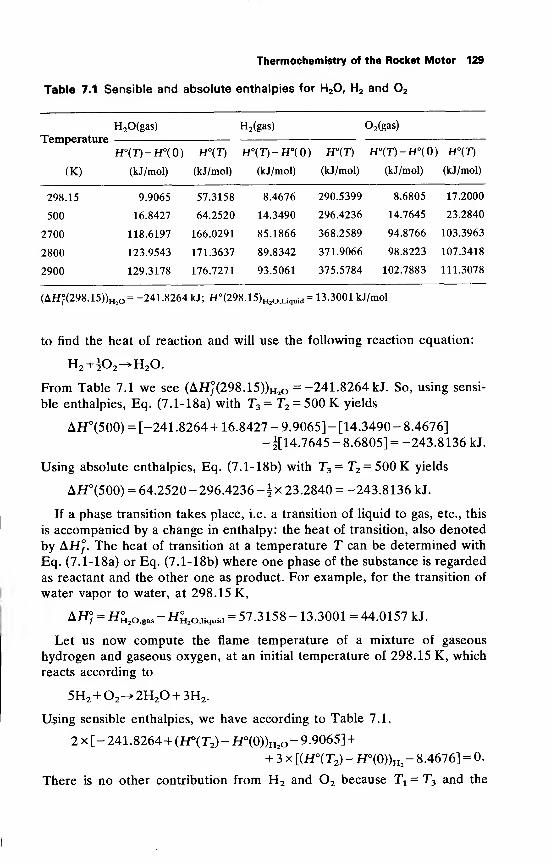
Thermochemistry of the Rocket Motor 129
Table 7.1 Sensible and absolute enthalpies for H 20, H 2 and 2
TemperatureH20(gas)
H°(T)-H°(0) H°(T)
H2(gas) 2(gas)
H°(T)-ff°(0) H°(T) H°(T)-H°(0) H°{T)
(K) (kJ/mol) (kJ/mol) (kJ/mol) (kJ/mol) (kJ/mol) (kJ/mol)
298.15 9.9065 57.3158 8.4676 290.5399 8.6805 17.2000
500 16.8427 64.2520 14.3490 296.4236 14.7645 23.2840
2700 118.6197 166.0291 85.1866 368.2589 94.8766 103.3963
2800 123.9543 171.3637 89.8342 371.9066 98.8223 107.3418
2900 129.3178 176.7271 93.5061 375.5784 102.7883 111.3078
(AH?(298.15))„2o= -241.8264 kJ; H°(298.15)H20iLiquid = 13.3001 kJ/mol
to find the heat of reaction and will use the following reaction equation:
H2 +|02^H20.
From Table 7.1 we see (AH;(298.15))H2o = -241.8264 kJ. So, using sensi-
ble enthalpies, Eq. (7.1-18a) with T3= T2 = 500K yields
AH°(500) = [-241.8264 + 16.8427 - 9.9065] - [14.3490 - 8.4676]
-§[14.7645 - 8.6805] = -243.8136 kJ.
Using absolute enthalpies, Eq. (7.1-18b) with T3= T2 = 500K yields
AH°(500) = 64.2520 - 296.4236 - \ x 23.2840 = -243.8136 kJ.
If a phase transition takes place, i.e. a transition of liquid to gas, etc., this
is accompanied by a change in enthalpy: the heat of transition, also denoted
by AH°f
. The heat of transition at a temperature T can be determined with
Eq. (7.1-18a) or Eq. (7.1-18b) where one phase of the substance is regarded
as reactant and the other one as product. For example, for the transition of
water vapor to water, at 298.15 K,
AH? = H£20 ,gas-H^20 ,liquid= 57.3158-13.3001 = 44.0157 kJ.
Let us now compute the flame temperature of a mixture of gaseous
hydrogen and gaseous oxygen, at an initial temperature of 298.15 K, which
reacts according to
5H2 + 2->2H2 + 3H2 .
Using sensible enthalpies, we have according to Table 7.1,
2x[-241.8264 + (H°(T2)-H°(0))H2o-9.9065] +
+ 3 x [(H°(T2)-H°(0))h2- 8.4676] = 0.
There is no other contribution from H2 and 2 because Tx= T3 and the
130 Rocket Propulsion & Spaceflight Dynamics
heat of formation for the elements equals zero. So, we are left with
2 x [H°(T2) - H°(0)]H2o + 3 x [H°(T2) - H°(0)]H2 = 528.8686 kJ.
By interpolation in Table 7.1 we find for the combustion temperature,
T2 = 2853 K. Using absolute enthalpies we have
2 x (H°(T2))h2o + 3 x (H°(T2))h2= 5 x 290.5399+17.200 = 1469.6995 kJ,
and by interpolation we find T2 = 2852 K.
At these elevated temperatures, however, another phenomenon takes
place: dissociation. Compounds will partially break up into electrically-
neutral fractions called radicals. Water, for instance, may break up accord-
ing to the reaction
H2 -» M!H2 + n2H2 + n3 2 + n4H + nsO + n6OH.
The last three species in this equation are the radicals mentioned. As dissocia-
tion is a highly endothermal process, the flame temperature may drop muchbelow the value as computed by the above method. In rocket motors, the
combustion temperatures are so high that the effects of dissociation cannot
be ignored and we will deal with this in the next section. The opposite of
dissociation is recombination. This phenomenon is important, for determin-
ing the performance of a rocket motor, as it may take place in the nozzle.
Thermodynamic properties of radicals are, like those for compounds, listed
in thermochemical tables.
7.1.2 Chemical equilibrium
The state of chemical equilibrium is defined in Section 7.1.1. In this section
we will discuss thermodynamic relationships for chemical equilibrium reac-
tions.
The second law of thermodynamics states for a change between state 1
and state 2:
S2-S^^^. (7.1-19)
As for an isolated system dQ = 0, the entropy, S, will increase until it has
reached its maximum value for that system. In the state of equilibrium,
where no irreversible processes take place
5 = 5^. (7.1-20)
Combining the first and second law of thermodynamics for a system at
constant temperature yields
S2-S 1 ^y[ (dH-Vdp). (7.1-21)
Thermochemistry of the Rocket Motor 131
If the pressure is also kept constant, we find
Now the Gibbs free energy, F, (also often denoted by G and often called the
free enthalpy) is defined as
F=H-TS, (7.1-22)
and we may also write
In the state of equilibrium the free energy reaches its minimum value
F=Fmin . The state of equilibrium for a system at constant pressure and
temperature thus can be characterized by
(dJ0p.T = d(H - TS)P)T = 0. (7.1-23)
As we will consider equilibrium reactions at constant pressure and tempera-
ture, this is the criterion to be used.
Consider the equilibrium reaction
Z "A ** Z "*Ak-
i k
Denoting the molar free energy of the species i by Ft,we have
F=£niF
i ,(7.1-24)
i
The reader is warned that this molar free energy is to be evaluated at the
partial pressure, ph of the species i. Now, if we consider the change in free
energy of one mol of a substance, we have for a reversible process at
constant temperature,
dF = dH-TdS = rdp.
It is customary to relate the free energy to the free energy in the standard
state, i.e. at a reference pressure, p , of 0.101325 MPa. Thus
F-F° = rVdp. (7.1-25a)
For solids and liquids, the volume of one mol usually is very small, and is
hardly sensitive to changes in pressure. Therefore, one can approximate the
free energy change for solids and liquids by
F(p, T)-F°(T) = 0, (7.1-25b)
or
(dF)T = 0. (7.1-25c)
132 Rocket Propulsion & Spaceflight Dynamics
For ideal gases, this is not the case, there we find
F-F°= P^ dp = R T In (p/Po ). (7.1-26)
As we will often deal with the pressure ratio p/p , we will use the notation
P = p/p , and if we specifically denote a species i, we indicate the ratio of
partial pressure and reference pressure as
Pi = PilPo-
Hence, in Eq. (7.1-24), the molar free energy, Fh stands for
F^FtCD + RoTlnPi. (7.1-27)
Now, the condition for chemical equilibrium was, Eq. (7.1-23)
(dF)p>T = X[n;dFi + F
t dnJp>T = 0. (7.1-28)i
As F°i(T) is a function of the temperature only, we find that
(ifHdF) =RoTl(^dp) .
\i /P,T i\Pi i,,r
According to Dalton's law,
P = Zft» (7.1-29)i
and if we consider a mixture of ideal gases we have
piV=n
iR T, (7.1-30)
for the species i, and
pr=XM* T, (7.1-31)i
for the whole mixture. So
(7.1-32)Pi = P
Wj X rii'
Hence,
l(^dp) =^(ldPi )=0. (7.1-33)
^Pi I p,T P \ i /p,T
Inserting the result that Q]* ntdFj)pT = into Eq. (7.1-28), the condition for
chemical equilibrium, leads to
Z(Fidn
i )p,T = 0. (7.1-34)i
Now, according to Eq. (7.1-5) we have for the products, k,
dnk =+vk d£, (7.1-35a)
Thermochemistry of the Rocket Motor 133
and for the reactants, ;*,
dni=-v
id& (7.1-35b)
where vk and vsdenote the stoichiometric coefficients of the reaction. So the
condition for chemical equilibrium at constant pressure and temperature is,
using Eq. (7.1-27) for the molar free energy,
I vkF°k- 1 VfF> = - RolfI vk In Pk - 1 v, In pX (7.1-36)
or
InFl-lvf] =~RoT\n l±—\ . (7.1-37)
The equilibrium constant, Kp, is defined as
Kp= - . (7.1-38)
UPJ>
i
As the standard free energy, F?, and the stoichiometric coefficients, vt,are
independent of the pressure at which the reaction takes place, it follows that
Kp
is only a function of the temperature, T, and not of the pressure, p. If avt
instead of vtwere taken as stoichiometric coefficients, the equilibrium
constant, Kp, would be raised to the power a.
As for the heat of formation, we have only to know the Kp
for the
formation of one mol of compound from its elements either in their standard
reference state or from atomic gases at 0.101325 MPa. This equilibrium
constant is indicated as Kpf
and called the equilibrium constant of formation.
The Xp/
's are listed in thermodynamic reference tables [1,2,3]. In general,
values for log10 Kpfare listed as this is advantageous for numerical work. The
different definitions of Kpf
will lead to different numerical values. Therefore,
one should always check the definitions in the tables used. The numerical
values of Kpf
are determined from the change in free energy, Eq. (7.1-37).
The change in free energy can be obtained from spectroscopic data [4] or
statistical calculations [5]. The equilibrium constant for a specific reaction
can be obtained by a suitable combination of the Kpf
's.
In practice, one often prefers to use the number of mols considered, nh or
the mol fractions, nfiji^ instead of the partial pressures. Using the relationsi
Pi= niplN, where p = T,Pi, and N = Yd
ni,one may write for the equilibrium
i i
constant
KD= -£) x^—7 . (7.1-39)d) IK
134 Rocket Propulsion & Spaceflight Dynamics
The equilibrium constant, Kn , in terms of the number of mols considered, is
defined as
IK'Kn =^. (7.1-40)
j
It was found that Kp
is only a function of the temperature, T, at which the
reaction takes place. However, only in those cases that Ydvj= Jd
vk , ai k
pressure independent reaction, this holds for Kn too, as is easily seen fromthe Eqs. (7.1-39) and (7.1-40).
Large values of Kp indicate that the reaction is accompanied by a
significant decrease in the free energy and the forward reaction is favored
Values of Kp < 1 indicate that the back reaction is favored. If one deals with
more reactions taking place simultaneously, as is usually the case, the
relative magnitudes of the Kpf
's are an indication of which of the species will
dominate. The reaction with the largest Kpf
will yield the dominating
species.
Differentiating In Kpwith respect to the temperature yields
(d In Kp\ 1 a /AF°\ 1 pAF° AF°1
\ dT )P R dT\ T ) R T[ dT T \ P
' (7.1-41)
From Eq. (7.1-23) follows for an equilibrium reaction at constant tempera-
ture
With Eq. (7.1-22) we then find
-AS°,(d AF°\
and so
In KA AH°(7.1-42)
Id In Kp\ _ AH°
\ dT )P ~
R
T2 '
where AH°, AF° and AS° stand for the changes in standard enthalpy, freeenergy and entropy as a result of the reaction. This equation, due to van'tHoff, is known as the van't Hoff reaction isobar. For exothermal reactions:AH° < and In K
p will decrease with increasing temperature. Integration ofEq. (7.1-42) yields
In
Thermochemistry of the Rocket Motor 135
For small temperature intervals over which AH° may be assumed constant,
Eq. (7.1-43) can be approximated by
'"(tSi)-fNU]Equilibrium reactions involving non-ideal gases, liquids and solids. In the
rocket motor condensed (mostly solid) particles may be present. Examples
of substances that may be present as condensed phases are carbon (C) or
aluminum oxide, (A12 3). Exact integration of the term, Ydp, in Eq.
(7. 1-25 a) for non-ideal gases, liquids or solids, would lead to complicated
expressions. Lewis [6] therefore introduced the concept of fugacity, f, which
has the dimension of a pressure. For our purpose it is sufficient to note that
the fugacity is defined by the relation
ln ^=^f P2rd
P' (7 - 1 "44)h Ko 1 JPl
where the temperature, T, is constant. So for non-ideal gases, liquids, or
solids, one has
F-Fl + RoT In /;//*. (7.1-45)
Here f° is the fugacity in the standard state. For the gaseous phases the
fugacity in the standard state equals the standard reference pressure, i.e.
f°= p = 0.101325 MPa. For the liquid and solid phases the fugacity of the
standard state, in general, will have a different value, usually
f< 0.101325 MPa [7]. The ratio fjf* is called the activity, at. The fugacities
can be thought of as 'corrected' or 'active' pressures [8]. For an ideal gas
/i=
Pi, while for other gases
lim fjpi = 1 and f = p .
The fugacity can be used for the treatment of condensed phases. Consider
two phases of the same substance being in equilibrium with each other. Weassume one phase to be gaseous. The work involved in the quasi-steady,
isothermal and isobaric process of evaporization, condensation or sublima-
tion, follows from
(dW)Tp = TdS-dE = pdY.
or
d(E + pT-TS)p>T = dF=0.
Therefore, the free energy of both phases is the same. If we replace the
pressure ratio, Ph in Eq. (7.1-37) by the activity, at ,we conclude, as the free
energy is the same in both phases, that
avc<=a
v*, (7.1-46)
136 Rocket Propulsion & Spaceflight Dynamics
where the index c indicates the condensed phase and g the gas phase. In
many cases vc = vgand thus ac
= ag .
We mentioned already that the free energy for liquids and solids is
approximately independent of pressure, i.e. F=F°. With the concept of
activity, Eq. (7.1-30) becomes
F;- F° = R T In ^ = 0.
Thus, the activity of the condensed phases is unity, and therefore thefugacity equals the fugacity in the standard state. If one now considers thereaction
^graphite ' ^-'2 *— ^"^-'2>
the equilibrium constant, involving the condensed graphite phase, becomes
v — _£_co2 _ ^co2
^o2 "c fo2
where tacitly is assumed that both 2 and C02 behave like ideal gases.
To determine, whether or not condensed phases will be present, one first
assumes that no condensation has taken plac^. If the calculated partial
pressure exceeds the vapor pressure, condensation must have taken place.
7.2 Combustion in the rocket motor
In order to determine either the performance of a rocket motor for a given
propellant combination and mass flow, or the geometry of such a motor for
a given chamber pressure, exit pressure, mass flow and mixture ratio, we will
assume that the composition of the combustion products is according to
chemical equilibrium. The theory, presented in Section 7.1.2, enables us to
determine the composition and the adiabatic flame temperature.
In principle, one would have to consider the formation of all possible
species. However, some of these species will have such low Kpfs that the
presence of these species can be ignored. For instance, in a H2-0
2 rocket
motor the amount of H2 2 present, will be negligible. In addition, we will
make the following assumptions:
1. The chamber conditions are uniform.
2. Steady-state operation.
3. In the combustion chamber, the kinetic energy of the combustionproducts is negligible.
4. In the nozzle, there exist surfaces of constant properties.
5. Condensed particles have the same velocity and temperature as the
surrounding gaseous species.
6. There are no heat losses.
Actually, one might account for heat losses by assuming enthalpy losses.
Thermochemistry of the Rocket Motor 137
In practice, the assumption that we have an equilibrium composition in
the chamber means that the reaction times are small as compared to the
residence time in the chamber. This may not always be the case; for
instance, if one has a motor with a small characteristic length, L*.
For a fuel rich mixture, containing carbon- and oxygen-compounds, the
theory may predict the formation of solid carbon according to the reaction
2CO«±C + C02 .
As the rate of formation of carbon is rather slow, less carbon may actually be
present than predicted by equilibrium considerations.
One of the combustion products of hydrazine motors is ammonia. Now,NH3 will dissociate according to the reaction
2NH3s±N2 + 3H2 .
The dissociation rate of ammonia being small, an excess of ammonia may bepresent over that predicted by equilibrium calculations. Whether or not the
theory of equilibrium reactions is applicable to certain products depends onthe reaction rates of the species under consideration and the chambergeometry. Unfortunately, there does not exist, at the present time, a set of
standard reaction rates, analogous to the sets of thermodynamic properties
of species, and the rate constants have to be compiled from various sources.
For the flow through the nozzle we have to include the kinetic energy of
the gases and we will have to make specific assumptions concerning the
behavior of the combustion products.
7.2.1 The composition in the combustion chamber and theadiabatic flame temperature
To compute the adiabatic flame temperature and the composition of the
combustion products, the following equations are available. From the knownmixture ratio of the propellants we can write down the equations for the
conservation of elements. If e elements are involved, this yields e equations.
If there are c compounds under consideration, there are c — e independent
equations for the equilibrium constants of formation. Finally, there is the
energy equation, Eq. (7.1-18a) or Eq. (7.1-18b) with AH°(T) = 0. So, wehave c + 1 equations for the number of mols, n x
- • • ,nc , and the adiabatic
flame temperature, 7}. In general, these equations cannot be solved analyti-
cally, and one must resort to numerical techniques [9, 10, 11, 12].
As an example, we will give the equations for a rocket motor using H2
and 2 as propellants. The combustion products will be: H2 , H, OH, H20,O and 2 . The reaction equation can be written as
mH2 + 2^ n 1H2 + n2ii+n3OU + n4H20+ nsO+ n6 2 .
138 Rocket Propulsion & Spaceflight Dynamics
The equations for the conservation of elements are
2m = 2n x + n2 + n3 + 2n4 ,
2 = n3 + n4+n5 + 2n6 .
We assume the chamber pressure being known. Then it is convenient to
write the equilibrium constants of formation in terms of the chamber
pressure, pc , and the number of mols n 1?• • • , n6 , N, where
N= t ^i = l
may be regarded as an additional unknown. The equilibrium constants of
formation for this system are
H + 0*OH; **"=*-(£),n2 n5 \PJ
2H±*H2 ;K
2 {f}
20*02 ;^-Sfg).
where Pc= pjp , the ratio of chamber pressure to reference pressure.
Finally, we have the energy equation
mH°(Tr )H2 +HD(Tr )02 = n 1H°(T/)Ha + n2H°(Tf )H + n3H°(Tf )oli +
+ n4H°erf )U20+n5H (Tf)
+n6H°(Tf)02 .
Here, Tr is the temperature at which the respective propellants, H2 and 2 ,
enter the combustion chamber, and 7} is the adiabatic flame temperature,
which is to be determined. So, now we have the complete set of equations
for the composition and the adiabatic flame temperature. These equations
have to be solved numerically.
7.3 Expansion through the nozzle
The thrust of a rocket motor is, according to Eq. (6.2-3), given by
F=\mVe + (pe -pa)Ae .(7.3-1)
The mass flow, m, equals the rate of propellant flowing into the combustion
chamber, while A depends on the nozzle shape.
For a given rocket motor, the area of the exit surface, Ae , in combination
Thermochemistry of the Rocket Motor 139
with the chamber pressure, pc, determines the exhaust velocity, Ve , and the
exhaust pressure, pe . If one, on the other hand, wants to design a nozzle for
a given chamber pressure, pressure ratio and mass flow, the area of the exit
surface and the exhaust velocity follow from the chamber pressure, pressure
ratio, and mass flow. In both cases, the ambient pressure, pa , is an indepen-
dent variable that will not interfere with the nozzle flow as long as no shock
waves occur. It is convenient to take the pressure, and not the area of a
surface of constant properties, as an independent variable, as the pressure
appears in the equations for the equilibrium constants and the entropy
equation. Therefore, we will determine the local velocity and the local area
of a surface of constant properties as a function of the local pressure.
In general, the composition of the combustion products will change during
the expansion through the nozzle. For an exact determination of how the
composition changes, the integration of the differential equations for the
chemical kinetics and hydrodynamics is necessary. This is beyond the scope
of this book. We can, however, distinguish between two extreme cases:
1. There is no effective change in composition during the expansion
through the nozzle.
2. The composition at any location in the nozzle is according to chemical
equilibrium.
In the first extreme case, one assumes the residence time in the tio^ie to be
very short, as compared to the time needed to change the composition
effectively. Moreover, if we assume that the heat capacity of the mixture of
combustion products is constant too, we can use the theory as developed in
Chapter 5. We call this the constant properties flow. If we do assume a
constant composition throughout the nozzle, but take into account the
variation of the heat capacities with temperature, we speak of a frozen flow.
In the second extreme case, one assumes the reaction rates to be infinite,
so that the composition changes immediately to the one dictated by equilib-
rium conditions. In this case we speak of equilibrium flow.
7.3.1 Constant properties flow
This is the most simple approach. The composition and heat capacities,
which remain constant during the expansion through the nozzle, are knownfrom the chamber conditions. The mean molecular weight, M, of the
combustion products, follows from
•* = I(Mk)/lnk, (7-3-2)k / k
where nfc/£w
fcand Mk stand for the mol fraction and the molecular weight,
k
140 Rocket Propulsion & Spaceflight Dynamics
respectively, of the combustion products Ak . The mean molar heat capacity
at constant pressure, Cp , follows from
Cp= £(nkC )A>k , (7-3-3)
k Ikand the gas constant, R, of the mixture from
R = RJM. (7.3-4)
The ratio of specific heats, y, is determined by
7 = 77%-- (7.3-5)
We assumed no heat losses in the combustion chamber, therefore, the
adiabatic flame temperature equals the temperature of the gases in the
combustion chamber, i.e. 7} = Tc .
Now that pc , Tc , R and y are known, the equations in the Sections 5.1.1
and 5.1.3 allow the direct computation of the velocity, V, the local expan-
sion ratio, A/At,and the ratio mlA for a given local pressure, p. If this
pressure is taken as the exit pressure, pe, one finds the exhaust velocity, Ve ,
with Eq. (5.1-15), the expansion ratio, AJAt,by Eq. (5.1-42) and the ratio
m/Ae with Eq. (5.1-37).
7.3.2 Frozen flow
The main difference of this model with the one above, is that the heat
capacities of the various substances are a function of the local temperature.
Therefore, the simple equations, as derived in the Sections 5.1.1 and 5.1.3
cannot be applied anymore. The expansion process through the nozzle is
assumed adiabatic and reversible, i.e. the entropy remains constant. This
means that all heat transfer and frictional effects are neglected. For the
amount of matter considered, the entropy at any position in the nozzle thus
equals the entropy in the combustion chamber, or at the nozzle entrance. In
Eq. (7.1-27) we showed that
F,-F?=-RoTlnPj. (7.3-6)
With the definition of free energy, Eq. (7.1-22), and as H(T) = H°(T), wefind
S°(T)-Si(T) = R \nP
i. (7.3-7)
As condensed phases do not contribute to the total pressure, the entropy is
found from
S(T) = Zng(so
g(T)-.R In
(p^J-))+ X n s S°s(T), (7.3-8)
Thermochemistry of the Rocket Motor 141
Here, the index g denotes the gaseous species and the index s the condensed
species. For a given pressure, the temperature is determined from this last
equation.
In Section 3.7 we derived the energy equation; for stationary flows
V-V(h+|V-V) = 0. (7.3-9)
Using the same arguments as in Section 5.1.1 we have
h(T)+$V'V=h(Tc ), (7.3-10)
i.e. the sum of the enthalpy and kinetic energy per unit mass of the
combustion products is constant and equals the enthalpy per unit mass in the
combustion chamber. In this chapter, we use the molar enthalpy and Eq.
(7.3-10) becomes
Y nrH%Tr )= ^H^TJ = SXh^CO +IXM^V2
. (7.3-11)
r k k k
Here, Tr is the temperature at which the propellant, Ar,enters the combus-
tion chamber. Tc is the temperature of the combustion products in the
combustion chamber. If there are no heat losses Tc = Tf, the adiabatic flame
temperature. T and V stand for the temperature and velocity, respectively,
of the combustion products, Ak in the nozzle, while nk stands for the
number of mols considered, of the combustion products. The (numerical)
solution of Eq. (7.3-11) yields the velocity, V, as for a given pressure, p, Eq.
(7.3-8) yields the temperature, T. If p = pe, one finds the exit temperature,
Te . The exhaust velocity, Ve , follows from Eq. (7.3-11):
V =2(£n^(T
r)-XnfcH£(Tc)]
k
1/2
(7.3-12)
The area of the surface of constant properties per unit mass flow, Aim, is
determined from the continuity equation, Eq. (5.1-35). For the nozzle wehave
m = pVA, (7.3-13)
where m is known. Because the combustion products in the nozzle may
contain condensed particles, we write
Xn^g +XM^P =
g (7.3-14)y
As the condensed particles do not contribute to the pressure, the volume, V,
142 Rocket Propulsion & Spaceflight Dynamics
considered, follows from
R TLng
r =-Y~- (7-3-15)
From the Eqs. (7.3-13) to (7.3-15) follows
Am
*o*2X(7.3-16)
\ K S /
Now that temperature and velocity at a position in the nozzle are known,the area of the surface of constant properties follows from Eq. (7.3-16). If
no condensed phases are present, Eq. (7.3-16) reduces to
-=^r> <7 -3 - 17>m MVp
where M is the mean molecular weight of the combustion products as given
by Eq. (7.3-2).
The calculations for the frozen flow require the numerical solution of
equations. The constant properties flow can be determined analytically. In
cases that a frozen flow performance calculation is available, while a
neighboring solution is required, the following simple computational schemecan be applied. First, the average heat capacity ratio, y, for which both the
frozen flow and the constant properties flow yield the same results for a
given pressure ratio, pjp, is determined with the help of the Poisson
relations, Eq. (3.7-20), from which follows
In (pjp)KVcV)(7.3-18)
In (pjp) - In (TJTY
where TJT is the temperature ratio, as determined by the frozen flow
calculations. As y is only slowly varying with temperature, especially at
lower temperatures, a constant properties analysis, using y as determined by
Eq. (7.3-18) will yield accurate results for nearby pressure ratios, as com-pared to the frozen flow analysis.
There is no direct way to determine the expansion ratio AJAt. One can,
for instance, approximate the throat conditions by those that follow from the
constant properties flow. These can be used as initial values to determine the
throat as the location where Ma = 1 by an iterative procedure [9],
In general, one will compute the ratio A/m for various pressures, lying
between chamber and exit pressures. These data can be used to determine a
minimum of A/m. This method also immediately yields pt [13].
Thermochemistry of the Rocket Motor 143
The throat conditions are determined by A/m being a minimum, i.e.
A/AIUo. (7.3-19)dp \MVpJ
For the frozen flow, M is constant, and the requirement comes down to
^(^rdvxr(73 „20)
dp\ VdTj p
where use is made of V= V{T(p)}. As the flow is assumed isentropic, we
also have,
TdS=CpdT-Ydp = 0, (7.3-21)
which gives
\dp)s
r I^RqT(7.3-22)
k k
From Eq. (7.3-11) it follows that
*X= * (7.3-23)
k
Combination of the Eqs. (7.3-20) to (7.3-23) yields
__!i_ +4 ± i = o. (7.3-24)
JXq* v lnkMk
The simultaneous solution of the Eqs. (7.3-8), (7.3-12) and (7.3-24) yields
pt,T
tand V
t. The ratio AJm is found from
A = _R£TL (7.3-25)m MV
tpt
The throat conditions, being determined by one method or another, yield,
in combination with the values of A/m, the local expansion ratio
— =^L. (7.3-26a)A
t AJm
The expansion ratio, AJAt,is found by setting A = Ae
A£= AJm (7.3-26b)A, AJm
144 Rocket Propulsion & Spaceflight dynamics
An advantage of this last method is that the throat conditions can bedetermined beforehand, while some of the other methods require computa-tion of Aim before the throat conditions can be determined.
7.3.3 Equilibrium flow
In this case we assume infinitely fast reaction rates, so that the compositionof the combustion products is a function of chemical equilibrium at anylocation in the nozzle. Thus, not only the heat capacities, but also the
composition, are dependent on the location in the nozzle. Again, we assumean isentropic flow through the nozzle.
To determine the velocity, temperature and composition for a given
pressure ratio, the following equations have to be solved:
1. The equations for the conservation of elements. If e different elementsare involved, there are e equations.
2. The equations for the equilibrium constants of formation. If c com-pounds are involved, there are c — e equations.
3. The entropy equation
S(Tc ) = ^ng(si(T)-R \n(p^\\+lnsSos{T), (7.3-27)
g
which equates the total entropy in the chamber to the total entropy at somelocation in the nozzle for the amount of matter considered.
4. The energy equation from which the velocity, V, follows:
V=2[lnrH°r(Tr)-lnkH°k(T)
I«Ait
1/2
(7.3-28)
The exhaust velocity, Ve, exit temperature, Te , and the composition at the
nozzle exit, are found by setting p = pe . The area of a surface of constant
properties is found by Eq. (7.3-17). The average heat capacity ratio, y, is
found by Eq. (7.3-18), with TJT now as determined by the equilibrium flow
calculations.
To determine the throat conditions, we can use the same iterative proce-
dures as were indicated to compute the throat conditions for the frozen flow.
We can also use the simple condition of Aim being at a minimum. As the
composition now varies according to chemical equilibrium, one also has to
determine the differential quotients dnjdp from algebraic equations. Theseequations are found by differentiating the e equations for the conservation
of elements and the c — e equations for the Kpf's with the respect to pressure.
One should be aware that Kpf(T) = K
pf{T(p)} if the local pressure, p, instead
Thermochemistry of the Rocket Motor 145
of the location in the nozzle is taken as an independent variable. By Eq.
(7.1-42) one then finds a relation betweeen dnk/dT and AH°k
. The solution
of the equations in the unknowns nk, dnjdp, T and V yields the throat
conditions [14].
We have discussed three methods that yield results, which are more or
less in agreement with experimental results. The equilibrium flow method,
accounting for many variations, requires much computer time. As it is based
on the assumption that the composition varies according to chemical equilib-
rium, there is no guarantee that its results are a better approximation of
reality than the frozen flow. The frozen flow requires less computing time,
but assumes a constant composition throughout the nozzle. In fact, the real
composition will lie somewhere between the results as computed by the
frozen flow and equilibrium flow method. There is a fourth method, how-ever, that combines both methods mentioned previously, which we will
discuss below.
7.3.4 The modified Bray approximation
In a classical article, Bray [15] studied the effects of recombination in the
nozzles of hypersonic windtunnels. He showed that, by good approximation,
the flow in the nozzle can be divided into three regions: equilibrium flow,
transition region, and frozen flow. The transition region, in general, is very
small and may be approximated by an infinitely small region, the Brayfreezing point. The various reactions taking place in the nozzle will yield
freezing points at different locations. In general, however, there is onedominating reaction with respect to energy release, and this is the one that
determines the Bray freezing point for the rocket motor [13].
Reaction rates increase with temperature, while the recombination rates
increase with pressure. It is these recombinations that yield the high
energy release. For moderate chamber pressures (—5.5 MPa) it is possible to
avoid the exact determination of the Bray freezing point, which requires
knowledge of the reaction rates, but to assume the freezing point location
at the throat. The justification is that temperatures and pressures before the
throat remain relatively high, while they rapidly drop after the throat. Thereverse is the case for the fluid velocity. Experience shows this approxima-tion to be very good [13].
For this modified Bray approximation an equilibrium flow calculation is
performed from the chamber to the throat. It is followed by a frozen flow
calculation from the throat to the exit. The throat conditions are determinedaccording to equilibrium flow calculation.
The Figs. 7.1 to 7.3 show the results of performance computations for a
H2-02 rocket motor (based on LH2 and LOX).As recombination is accompanied by energy release, the calculations for
the equilibrium flow yield higher specific impulses than for the frozen flow.
The dependence of the maximum specific impulse on the mixture ratio and
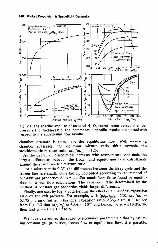
146 Rocket Propulsion & Spaceflight Dynamics
450
JUoo
rE 350o8.
jn 300
Ideal ExpaEquilibrium
Mixture Ra
ision, pe =
Flow
tio mH
irr,
0.101325 MPa
O2=0.25
450
0.15 0.20 0.25 0.30 0.35
Mixture Ratio mH2 //r?o 2
10 20
J* Chamber Pressure fyMPa)
«
^
E
Wfe=210
110
£-1? 35
dia.10
10
c~ -18c01
Ejj
o
7 Frozen Flow
Ideal Expansion
Q, = 0.101325 MPa
10 15 20
Chamber Pressure G,(MPa)
0,05 0.10 0.15 0.20 0.25 0.30
Mixture Ratio m^/'^C^0.35
Fig. 7.1 The specific impulse of an ideal H2-02 rocket motor versus chamber
pressure and mixture ratio. The increments in specific impulse are plotted with
respect to the equilibrium flow results
chamber pressure is shown for the equilibrium flow. With increasing
chamber pressures, the optimum mixture ratio shifts towards the
stoichiometric mixture ratio, muJm02 = 0.125.
As the degree of dissociation increases with temperature, one finds the
largest differences between the frozen and equilibrium flow calculations
around the stoichiometric mixture ratio.
For a mixture ratio 0.25, the differences between the Bray cycle and the
frozen flow are small, while the Isp computed according to the method of
constant gas properties does not differ much from those found by equilib-
rium or frozen flow calculations. The expansion ratio determined by the
method of constant gas properties yields larger differences.
Finally, one can, by Fig. 7.3, determine the effect of a non-ideal expansion
ratio on the exit pressure. For example, with (pcy<pe )
^
ideaX= 110, muJm02 =
0.175 and an offset from the ideal expansion ratio, A(Ae/A f)= 10" 1
, we see
from Fig. 7.3 that A(pe/pc)/A(Ae/At )= 10"3 and hence, for pc = 11 MPa, we
then find pe = -1.1 x 10~3 MPa.
We have determined the rocket performance parameters either by assum-
ing constant gas properties, frozen flow or equilibrium flow. It is possible,
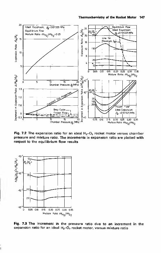
Thermochemistry of the Rocket Motor 147
20
^r 15
Ideal Exp
Equiiibriur
Mixture Re
ansion, p =
n Flow
itio m^ In
0.101325 MPa
7o2= 0.25
S
*- 2^
CO
«q; 20
o
o 1Ren
,u
co<2 12
Equilibrium Row
Pc/Pe
210
/ . Ideal Expansion
\/£ =0.101325 MRa
Jne for
Maximum /« ,
i
110 *^L\\
\
35 V
10\V
0.05 0.10
10 15 20
Chamber Pressure O(MPa)
5-10"
0.15 0.20 0.25 0.30 0.35
Mixture Ratio m^lmn72
Pc/Pe
10
35
110
210v^'Frozeri Flow
/ Ideal Expansion
pe =0.101325 MPa
10 15 20 "Chamber Pressure & (MPa) '-'
0.05 0.10 0.15 0.20 025 0.30 0.35
Mixture Ratio m^im^
Fig. 7.2 The expansion ratio for an ideal H2-02 rocket motor versus chamberpressure and mixture ratio. The increments in expansion ratio are plotted with
respect to the equilibrium flow results
-10"
^
10
Pc/Pe
35
110
210
^0.05 0.10 0.15 0.20 0.25 0.30 0.35
Mixture Ratio '"ho/'^O?
Fig. 7.3 The increment in the pressure ratio due to an increment in theexpansion ratio for an ideal H2-02 rocket motor, versus mixture ratio
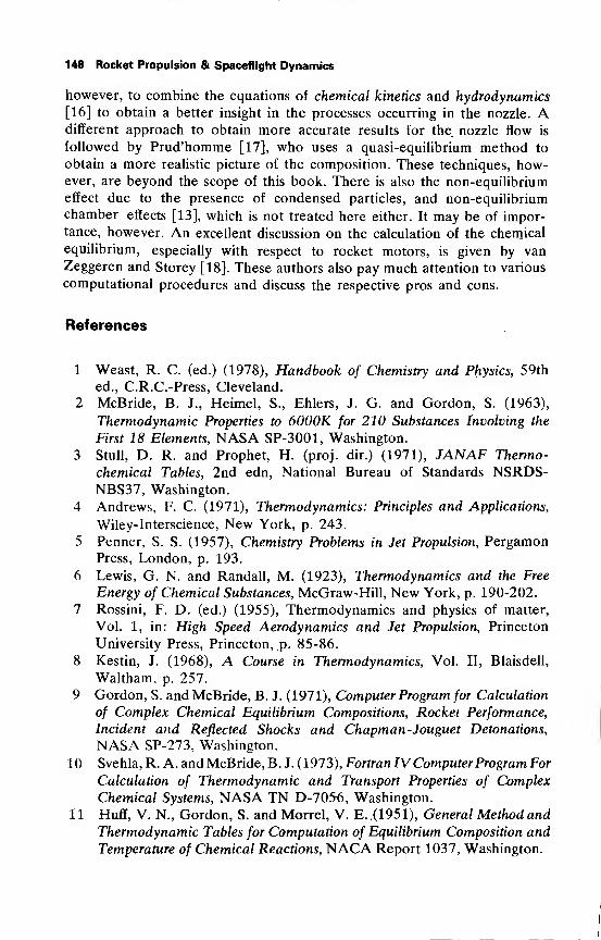
148 Rocket Propulsion & Spaceflight Dynamics
however, to combine the equations of chemical kinetics and hydrodynamics
[16] to obtain a better insight in the processes occurring in the nozzle. Adifferent approach to obtain more accurate results for the. nozzle flow is
followed by Prud'homme [17], who uses a quasi-equilibrium method to
obtain a more realistic picture of the composition. These techniques, how-ever, are beyond the scope of this book. There is also the non-equilibrium
effect due to the presence of condensed particles, and non-equilibrium
chamber effects [13], which is not treated here either. It may be of impor-tance, however. An excellent discussion on the calculation of the chemical
equilibrium, especially with respect to rocket motors, is given by vanZeggeren and Storey [18]. These authors also pay much attention to various
computational procedures and discuss the respective pros and cons.
References
1 Weast, R. C. (ed.) (1978), Handbook of Chemistry and Physics, 59th
ed., C.R.C.-Press, Cleveland,
2 McBride, B. J., Heimel, S., Ehlers, J. G. and Gordon, S. (1963),
Thermodynamic Properties to 6000K for 210 Substances Involving the
First 18 Elements, NASA SP-3001, Washington.
3 Stull, D. R. and Prophet, H. (proj. dir.) (1971), JANAF Thermo-
chemical Tables, 2nd edn, National Bureau of Standards NSRDS-NBS37, Washington.
4 Andrews, F. C. (1971), Thermodynamics: Principles and Applications,
Wiley-Interscience, New York, p. 243.
5 Penner, S. S. (1957), Chemistry Problems in Jet Propulsion, PergamonPress, London, p. 193.
6 Lewis, G. N. and Randall, M. (1923), Thermodynamics and the Free
Energy of Chemical Substances, McGraw-Hill, New York, p. 190-202.
7 Rossini, F. D. (ed.) (1955), Thermodynamics and physics of matter,
Vol. 1, in: High Speed Aerodynamics and Jet Propulsion, Princeton
University Press, Princeton, p. 85-86.
8 Kestin, J. (1968), A Course in Thermodynamics, Vol. II, Blaisdell,
Waltham, p. 257.
9 Gordon, S. and McBride, B. J. (1971), Computer Program for Calculation
of Complex Chemical Equilibrium Compositions, Rocket Performance,
Incident and Reflected Shocks and Chapman-Jouguet Detonations,
NASA SP-273, Washington.
10 Svehla, R. A. and McBride, B. J. (1973), Fortran IVComputerProgram ForCalculation of Thermodynamic and Transport Properties of Complex
Chemical Systems, NASA TN D-7056, Washington.
11 Huff, V. N., Gordon, S. and Morrel, V. E. (1951), General Method and
Thermodynamic Tables for Computation of Equilibrium Composition and
Temperature of Chemical Reactions, NACA Report 1037, Washington.
Thermochemistry of the Rocket Motor 149
12 Barrere, M., Jaumotte, A., Fraeijs de Veubeke, B. and Vandenkerck-
hove, J. (1960), Rocket Propulsion, Elsevier, Amsterdam, p. 140-153.
13 Glassman, I. and Sawyer, R. F. (1970), The Performance of Chemical
Propellants, AGARDograph 121, Technivision Services, Slough.
14 Schoyer, H. F. R. (1976), The Determination of the Throat Conditions
for Equilibrium and Frozen Flows in Rocket Motor Nozzles, Rpt. VTH-209, Delft University of Technology, Dpt. of Aerospace Engineering,
Delft.
15 Bray, K. N. C. (1959), Atomic recombination in a hypersonic wind-
tunnel nozzle, J. Fluid Mech., 6, 1-32.
16 Bitther, D. A. and Scullin, V. J. (1972), General Chemical Kinetics
Computer Program for Static and Flow Reactions, with Application to
Combustion and Shock-Tube Kinetics, NASA TN D-6586, Washington.
17 Prud'homme, R. (1974), Methode de Quasi-Equilibre pour VEtude des
Ecoulements Relaxes, paper presented at the 43rd P.E.P.-AGARDspecialist meeting, Liege.
18 Van Zeggeren, F. and Storey, S. H. (1970), The Computation of Chemi-
cal Equilibria, Cambridge University Press, Cambridge.
8 Heat Transfer in Rocket Motors
Heat transfer is important in astronautics. For instance, the temperature of
satellites and spacecraft has to be kept within certain limits to ensure a good
operation. During the atmospheric flight of rockets and space vehicles,
aerodynamic heating is important. To avoid damage to the structure or the
payload one often has to take special precautions, such as the installment of
heat shields. Another field of astronautics where heat transfer is very
important is rocket motor technology. The high-temperature combustion
products could raise the temperature of the engine structure in many cases
to levels that exceed the melting point of the metals used, if no special
precautions were taken. This often makes an active cooling system impera-
tive. The heat absorbed by the coolant can be used to drive the turbines or
to heat the pressurization gas in the propellant tanks. Evidently, a good
knowledge of the amount of heat transfer in the rocket motor is a necessity
for a successful design of the rocket motor.
In this chapter, we will restrict ourselves to the discussion of the most
important aspects of heat transfer in the rocket motor, and leave out
aerodynamic heating and thermal control of satellites and spacecraft. It is
beyond the scope of this book to give an extensive treatment on heat
transfer, and the reader is referred to the existing standard works [1, 2, 3].
8.1 The energy equation
In Section 3.7, we have derived the energy equation, assuming that there
was no heat transfer. In this section, we will derive the energy equation for
solids, including heat transfer. It is not practical to derive the full energy
equation for fluids. The contribution of viscous effects to the equation for
the conservation of energy for fluids is of the same order as heat transfer. If
one includes these viscous effects in the energy equation, they must also be
accounted for in the momentum equation, which leads to the Navier-Stokes
equation. No general solutions are known to this equation; there are only
exact solutions known for some special cases and there exist many approxi-
mate solutions. Heat transfer problems in fluids will be treated by means of
the theory of convective heat transfer. The solutions to this last type of heat
transfer problems are partly based on approximate solutions of the conser-
vation equations, and partly on experimental results. Therefore, we will
derive the energy equation which in principle allows for heat transfer effects
in solids. We will not account for viscous or elastic forces. Therefore, the
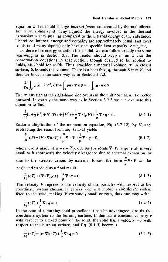
Heat Transfer in Rocket Motors 151
equation will not hold if large internal forces are created by thermal effects.
For most solids (and many liquids) the energy involved in the thermal
expansion is very small as compared to the internal energy of the substance.
Therefore, internal energy and enthalpy are approximately equal, and mostsolids (and many liquids) only have one specific heat capacity, c = c
p^ cv .
To derive the energy equation for a solid, we can follow exactly the samereasoning as in Section 3.7. The reader should keep in mind that the
conservation equations in that section, though derived to be applied to
fluids, also hold for solids. Thus, consider a material volume, V. A closed
surface, S, bounds this volume. There is a heat flux, q, through S into V, andthus we find, in the same way as in Section 3.7.3,
jj-fp(c+|V2)dr+
j
pn-VdS=-|
q-ndS.
The minus sign at the right-hand side occurs as the unit normal, n, is directed
outward. In exactly the same way as in Section 3.7.3 we can evaluate this
equation to find,
-(e +|V2) + V-V(c +|V2
) +iv-(pV)+-V-q = 0. (8.1-1)at p p
Scalar multiplication of the momentum equation, Eq. (3.7-12), by V, andsubtracting the result from Eq. (8.1-1) yields
^-(cT) + (V -V)(cT)+-V • V+-V q = 0, (8.1-2)dt p p
where use is made of h = e = J£ c dT. As for solids V* V, in general, is very
small as it represents the velocity divergence due to thermal expansion, or
due to the stresses caused by external forces, the term —V • V can beP
neglected to yield as a final result
£(c!O + (V-V)(cT)+-V.« = 0. (8-1-3)at p
The velocity V represents the velocity of the particles with respect to the
coordinate system chosen. In general one will choose a coordinate system
fixed to the solid, making V extremely small or zero, thus one may write
f (cT)+-V-q = 0. (8.1-4)at p
In the case of a burning solid propellant it can be advantageous to fix the
coordinate system to the burning surface. If this has a constant velocity r
with respect to a fixed point of the solid, the solid has a velocity -r with
respect to the burning surface, and Eq. (8.1-3) becomes
^(cT)-(r.V)(cD+-V.<| = 0. (8.1-5)dt p
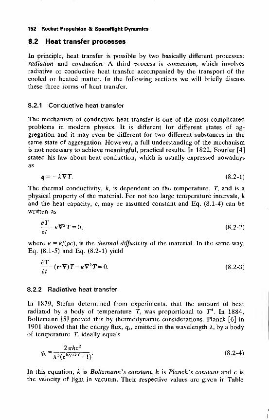
152 Rocket Propulsion & Spaceflight Dynamics
8.2 Heat transfer processes
In principle, heat transfer is possible by two basically different processes:
radiation and conduction. A third process is convection, which involves
radiative or conductive heat transfer accompanied by the transport of the
cooled or heated matter. In the following sections we will briefly discuss
these three forms of heat transfer.
8.2.1 Conductive heat transfer
The mechanism of conductive heat transfer is one of the most complicated
problems in modern physics. It is different for different states of ag-
gregation and it may even be different for two different substances in the
same state of aggregation. However, a full understanding of the mechanismis not necessary to achieve meaningful, practical results. In 1822, Fourier [4]
stated his law about heat conduction, which is usually expressed nowadays
as
q=-kVT. (8.2-1)
The thermal conductivity, k, is dependent on the temperature, T, and is a
physical property of the material. For not too large temperature intervals, k
and the heat capacity, c, may be assumed constant and Eq. (8.1-4) can be
written as
kV2T=0, (8.2-2)dt
where k = k/(pc), is the thermal diffusivity of the material. In the same way,
Eq. (8.1-5) and Eq. (8.2-1) yield
flT(i-V)T-kV2T=0. (8.2-3)
dt
8.2.2 Radiative heat transfer
In 1879, Stefan determined from experiments, that the amount of heat
radiated by a body of temperature T, was proportional to T4. In 1884,
Boltzmann [5] proved this by thermodynamic considerations. Planck [6] in
1901 showed that the energy flux, qA , emitted in the wavelength A, by a bodyof temperature T, ideally equals
lirhc'
A 5(e
HcMkT-l)'
^ = lS /,hc/xkT. , v (8.2-4)
In this equation, k is Boltzmann' s constant, h is Planck's constant and c is
the velocity of light in vacuum. Their respective values are given in Table
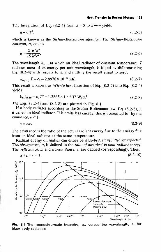
Heat Transfer in Rocket Motors 153
T.l. Integration of Eq. (8.2-4) from A =0 to A—>°° yields
q = aT4,
(8.2-5)
which is known as the Stefan-Boltzmann equation. The Stefan-Boltzmann
constant, a, equals
2 7r5k4
ar =15 hV (8.2-6)
The wavelength kqmat
at which an ideal radiator of constant temperature Tradiates most of its energy per unit wavelength, is found by differentiating
Eq. (8.2-4) with respect to A, and putting the result equal to zero,
A<*>-T = ex = 2-8978 x 10-3 mK. (8.2-7)
This result is known as Wien's law. Insertion of Eq. (8.2-7) into Eq. (8.2-4)
yields
(qJmax = c2T5 = 1.2865 x 1(T 5 T5 W/m3. (8.2-8)
The Eqs. (8.2-4) and (8.2-8) are plotted in Fig. 8.1.
If a body radiates according to the Stefan-Boltzmann law, Eq. (8.2-5), it
is called an ideal radiator. If it emits less energy, this is accounted for by theemittance, e < 1
eo~rp4
(8.2-9)
The emittance is the ratio of the actual radiant energy flux to the energy flux
from an ideal radiator at the same temperature.
Radiant energy on matter can either be absorbed, transmitted or reflected.
The absorptance, a, is defined as the ratio of absorbed to total radiant energy.
The reflectance, p, and transmittance, t, are defined correspondingly. Thus,
a+p + r=l. (8.2-10)
4.10 6.1010"
'
Wavelength X (m)
Fig. 8.1 The monochromatic intensity, qx , versus the wavelength. A, for
black-body radiation
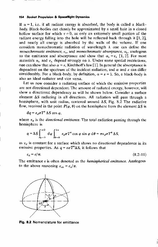
154 Rocket Propulsion & Spaceflight Dynamics
If a = 1, i.e. if all radiant energy is absorbed, the body is called a black-
body. Black-bodies can closely be approximated by a small hole in a closed
hollow surface for which t = 0, as only an extremely small portion of the
radiant energy falling into the hole will be reflected back through it [1,2],
and nearly all energy is absorbed by the walls of the volume. If one
considers monochromatic radiation of wavelength A one can define the
monochromatic emittance, eK , and monochromatic absorptance, ax , analogous
to the emittance and absorptance and show that ax = ek [1, 2]. For most
materials ax and eA depend strongly on A. Under some special restrictions,
one can show that also a = e, Kirchhoff's law [1]. In general the absorptance is
dependent on the spectrum of the incident radiation, and a and e can differ
considerably. For a black-body, by definition, a = e = 1. So, a black-body is
also an ideal radiator and vice versa.
Let us now consider a radiating surface of which the emissive properties
are not directional dependent. The amount of radiated energy, however, will
show a directional dependency as will be shown below. Consider a surface
element AS radiating in all directions. All radiation will pass through a
hemisphere, with unit radius, centered around AS, Fig. 8.2 The radiative
flow, received in the point P(q>, 0) on the hemisphere from the element AS is
dq = BdO-T4 AS cos <p,
where ed is the directional emittance. The total radiation passing through the
hemisphere is
)•
tt/2 r 2-n-
d<p SdO-T4cos <p sin <p d0 = TTEdO-T
4AS,
<p=o Je=o
as ed is constant for a surface which shows no directional dependence in its
emissive properties. As q = ao-T'AS, it follows that
ed = e/7r. (8.2-11)
The emittance e is often denoted as the hemispherical emittance. Analogous
to the above reasoning edk = eJtt.
Fig. 8.2 Nomenclature for emittance
Heat Transfer in Rocket Motors 155
8.2.3 Radiating gases
While liquids and solids usually have a uniform radiation spectrum, gases
often emit in narrow wavebands, which are characteristic for the gases underconsideration. At high pressures, these bands tend to broaden.
As far as radiative heat transfer is concerned, the hot combustion pro-
ducts in the rocket motor can often be regarded as a radiating black-body of
temperature Tc . By the walls, an amount of heat per unit area, awa-T^, is
absorbed, while ew<rTl is emitted. So, the total heat flux into the chamberwalls equals
q = awaTt - ewaTl . (8.2-12)
In those cases that the combustion products hardly contain solid particles,
such as soot or metal oxides, the assumption of black-body radiation fromthe combustion products may not be correct, and Eq. (8.2-12) will predict
wall temperatures which are too high.
Emission and absorption in gases involve the interaction of gas molecules.
Let us therefore consider a narrow beam of monochromatic radiation in a
volume filled with a gas. We assume that the amount of emission (absorp-
tion) is proportional to the number of molecules within the beam. For an
ideal gas the number of molecules per unit volume is proportional to the
pressure, p. The energy flux -dqx , absorbed in a layer of gas of thickness,
dL, is proportional to the total flux qx
-dqx = qx kxpdL,
leading to
(<?a)o-(<?Jz. =a-e-k*L )(qx ) (8.2-13)
where (qx ) stands for the flux at zero distance, and (qx )L for the flux at a
distance L. The constant, kx , is the spectral absorption coefficient of the gas,
and pL is called the optical density. In many cases the quantity - kxpL is so
small that, using the definition of absorptance, Eq (8.2-13) can be approxi-
mated by
ock = ex = kxPL. (8.2-14)
The monochromatic emittance (absorptance) of a layer of gas of unit length is
called the monochromatic emissivity, ex ,(absorptivity, ax ,) and
ax = ex = kxp. (8.2-15)
Now again consider a closed volume filled with radiating gas. From a layer
of gas with thickness L, a surface element dS will receive an amountof radiative energy
dqx = arT4kKpL dS.
156 Rocket Propulsion & Spaceflight Dynamics
With the approximations made, the total amount of monochromatic radia-
tive energy from all the gas in the volume, can be expressed as
qK = (rT*kkpLeqS = <TTiKLeqS, (8.2-16)
where Leq stands for an 'equivalent beam length'.
On the other hand, the monochromatic radiation received by the wall
from a volume element dV of the gas is
d^^^drdOo-T4,
where dft is the solid angle under which the wall is seen by the volume
element. Thus,
T47TO-T4 = 4eA r<rT
4. (8.2-17)e
Equating the Eqs. (8.2-16) and (8.2-17) yields an expression for the equiva-
lent beam length, Leq
4rs
Leq=— (8.2-18)
In those cases that the combustion products cannot be regarded as a
radiating black-body, the heat flux to the chamber walls can be calculated
with Eq. (8.2-16) where Leq follows from Eq. (8.2-18). If the reflectance
(p = 1 — a) of the chamber walls is taken into account, the problem becomesmore complex. According to Ziebland [7], the effective monochromatic gas
emittance, eAg , follows from
-1 =1 +-^- (8.2-19)
Here eA = exL, e^ is the monochromatic emittance of an infinitely thick layer
of gas, while the absorptance, a, of the grey wall may be assumed to be
independent of the wavelength.
8.2.4 Convective heat transfer
If heat transfer is due to the transport of heat containing matter, one speaks
of convection. This phenomenon takes place in fluids. In Section 8.1, wementioned already that the complete solution of the fluid dynamic equa-
tions, including heat transfer and viscosity, is not possible. Prandtl has
shown that approximate solutions can be found for specific regions in the
fluid, the boundary layers. These are thin regions between the wall and the
main flow, in which temperature and velocity differ considerably from the
main flow values. Solution of the boundary layer equations is of a very
specialized character and falls beyond the scope of this book. We restrict
ourselves to give results, which partially stem from theoretical considera-
tions and partially from experiments.
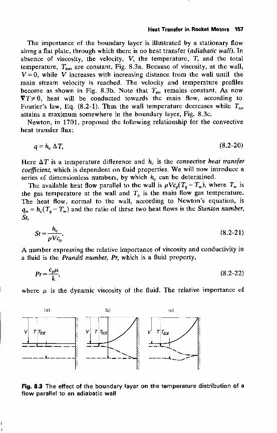
Heat Transfer in Rocket Motors 157
The importance of the boundary layer is illustrated by a stationary flow
along a flat plate, through which there is no heat transfer (adiabatic wall). In
absence of viscosity, the velocity, V, the temperature, T, and the total
temperature, Ttot, are constant, Fig. 8.3a. Because of viscosity, at the wall,
V = 0, while V increases with increasing distance from the wall until the
main stream velocity is reached. The velocity and temperature profiles
become as shown in Fig. 8.3b. Note that Ttot remains constant. As now
V7V0, heat will be conducted towards the main flow, according to
Fourier's law, Eq. (8.2-1). Thus the wall temperature decreases while Ttot
attains a maximum somewhere in the boundary layer, Fig. 8.3c.
Newton, in 1701, proposed the following relationship for the convective
heat transfer flux:
q = hc AT, (8.2-20)
Here AT is a temperature difference and hc is the convective heat transfer
coefficient, which is dependent on fluid properties. We will now introduce a
series of dimensionless numbers, by which hc can be determined.
The available heat flow parallel to the wall is pVcp(T
g-Tw ), where Tw is
the gas temperature at the wall and Tg
is the main flow gas temperature.
The heat flow, normal to the wall, according to Newton's equation, is
qw = hc(Ts - Tw ) and the ratio of these two heat flows is the Stanton number,
St,
St =K
pVcP
(8.2-21)
A number expressing the relative importance of viscosity and conductivity in
a fluid is the Prandtl number, Pr, which is a fluid property,
k'
(8.2-22)
where fx is the dynamic viscosity of the fluid. The relative importance of
(b) (c)
V T Ttot
.
Fig. 8.3 The effect of the boundary layer on the temperature distribution of a
flow parallel to an adiabatic wall
158 Rocket Propulsion & Spaceflight Dynamics
inertial forces with respect to viscous forces is given by the Reynolds number,
Re,
Re =^, (8.2-23)
where L is a suitable chosen reference length. Comparing the relative
importance of convective and conductive heat transfer yields the Nusselt
number, Nu,
Nu =^ = St.Re.Pr (8.2-24)k
For flows through a pipe, there exist experimental relationships of the form
St — St(Re, Pr) or Nu = Nu(Re, Pr) by which hc can be determined, for
instance,
St=aRea1,5 Pr2/3, (8.2-25a)
Nu = aRe%5 Prm, (8.2-25b)
where a is a coefficient. The Reynolds number, ReD , is based on the pipe
diameter. For the divergent part of the nozzle, better correlations are
obtained by expressions of the form,
St = BRex Pr~213
, (8.2-26a)
Nu = B Re bx+1
Pr 1 '3. (8.2-26b)
Here, B and b are constants, and the Reynolds number, Rex, is based on the
distance x from the throat.
To determine Re, Pr, Nu or St, the values of k, cp ,
/u, and p of the fluid
have to be known. These quantities depend, among others, on the tempera-
ture, which is not constant over the boundary layer. It is customary to
evaluate these quantities at a reference temperature, the film temperature,
Tf
. This Tfmay be taken as the average of the wall temperature, Tw , and the
free stream temperature, T,
T = T+TW (8.2-27)
Though the wall temperature is not known a priori, but has to be deter-
mined, it should not exceed certain limits, determined for instance bystrength and stiffness considerations. As convective heat transfer calcula-
tions are of an iterative type, it is convenient to assume for Tw the maximumallowable wall temperature as a first guess.
A more refined determination of Tfincludes the recovery temperature, Tr,
which is the stagnation temperature at the adiabatic wall. As we have seen,
this temperature is lower than the main flow stagnation temperature. This is
Heat Transfer in Rocket Motors 159
expressed by the recovery factor, r,
r = (Tr -T)/(Ttot -T). (8-2-28 )
For a laminar boundary layer:
r = J¥r~, (8.2-29)
and for a turbulent boundary layer:
r = PrV3 .(8.2-30)
For rocket motors, r usually lies between 0.86 and 0.93.
According to Ziebland [7], Tf
is given by
T, = 0.5Tw + 0.28T+ 0.22Tr. (8.2-31)
With the determined value of 7}, Re, Pr and Nu follow, and hc can be
computed from the Nusselt number.
Finally, the convective heat transfer flux, q, normal to the wall follows
from
q=hc(T-Tw ). (8.2-32)
To determine the values of cp, n and k for a mixture of gases, such as the
combustion products, the following expressions can be used. In Chapter 7
we have shown for a mixture of gases
c J^ nicpi = ^£ (8.2-33)
PLYliMi M
In the same way the conductivity, k, and dynamic viscosity, n, follow from:
k=^i, (8.2-34)
J^£i (8.2-35)
Pi
The temperature dependence of CPi
is given in the thermodynamic tables
mentioned in Chapter 7. Hirschfelder [8] gives the temperature dependence
of /u,j. However, a simple, rough approximation, such as
v(Ti)/v(T2) = frJT2 ,(8.2-36)
often will suffice.
There is a direct relationship between the thermal conductivity, viscosity
and heat capacity of gases, due to Eucken [9],
k^KH-SW,, (8.2-37)
160 Rocket Propulsion & Spaceflight Dynamics
which yields for the Prandtl number of a single gas,
Pr = -^-z. (8.2-38)97-5
8.3 Heat transfer in the rocket motor
In the liquid motor, the nozzle and chamber walls are exposed to hot
combustion products. Usually these walls are provided with ducts through
which propellant flows to keep material temperatures within acceptable
limits. This method is known as active cooling (Section 10.5.1). In the solid
motor, the propellant usually insulates the chamber walls from the hot
combustion products, (Section 9.3), but the nozzle is exposed to the hot
combustion products. As active cooling is not possible, one has to select
special materials, such as graphite, ceramics or refractory metals for the hot
parts. Moreover, radiation cooling and heat sinks, consisting of a piece of
material with a high heat capacity, are often used (passive cooling).
Concerning heat transfer in the rocket motor, we will distinguish betweenthe following regions: heat transfer from the combustion products to the
wall (the gas-side heat transfer), heat transfer in the wall, heat transfer fromthe wall to the coolant (liquid or coolant-side heat transfer) and the radiative
heat transfer of hot walls into space, usually called radiation cooling. Anexact analysis of the spatial and time-dependent distribution of temperature
and heat fluxes is very complex. As most rocket engines are about axial-
symmetric, it is customary for a first analysis to consider the rocket motor as
consisting of many annular elements for which the axial heat transfer is
negligible. This may be done because the change in radial heat flux does not
vary strongly in the axial direction. The distribution of temperatures andheat fluxes thus obtained is a first approximation of the real distribution.
8.3.1 Gas-side heat transfer
In the combustion chamber and nozzle, both convection and radiation
contribute to heat transfer. If the emissivity, e, of the combustion products is
not well known, the radiative heat transfer can be estimated with Eq.(8.2-12). The convective heat transfer is found by the method outlined in
Section 8.2.4. For the chamber and nozzle throat region, the convective heattransfer is predicted fairly well if the constant a in Eq. (8.2-25) is takena = 0.023 and the local diameter is taken as the characteristic length. Thethroat region extends to about one throat diameter downstream of thethroat and the result holds for a throat with a radius of curvature equal to,
or larger than the throat diameter. In sharp throats the heat transfer will behigher. From about one throat diameter downstream of the throat, the heattransfer can be calculated with Eq. (8.2-25) with a = 0.025 to 0.028, and the
characteristic length is the distance from the throat.
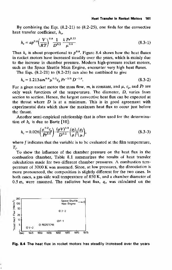
Heat Transfer in Rocket Motors 161
By combining the Eqs. (8.2-21) to (8.2-25), one finds for the convective
heat transfer coefficient, hc,
/ V\ os1 /cPr
-33
K = ap°i£) ^-^rr- (8.3-D
Thus hc is about proportional to p° 8. Figure 8.4 shows how the heat fluxes
in rocket motors have increased steadily over the years, which is mainly due
to the increase in chamber pressure. Modern high-pressure rocket motors,
such as the Space Shuttle Main Engine, encounter very high heat fluxes.
The Eqs. (8.2-21) to (8.2-25) can also be combined to give
hc= 1.213am°-y2
cP Pr2'3 D"18
. (8.3-2)
For a given rocket motor the mass flow, m, is constant, and n, cp , and Pr are
only weak functions of the temperature. The diameter, D, varies from
section to section. Hence, the largest convective heat flux can be expected at
the throat where D is at a minimum. This is in good agreement with
experimental data which show the maximum heat flux to occur just before
the throat.
Another semi-empirical relationship that is often used for the determina-
tion of hc is due to Bartz [10]:
^oW^)^lflllHl (8-3-3)mmm
where / indicates that the variable is to be evaluated at the film temperature,
To show the influence of the chamber pressure on the heat flux in the
combustion chamber, Table 8.1 summarizes the results of heat transfer
calculations made for two different chamber pressures. A combustion tem-
perature of 3000 K was assumed. Since, at low pressures, the dissociation is
more pronounced, the composition is slightly different for the two cases. In
both cases, a gas-side wall temperature of 850 K, and a chamber diameter of
0.5 m, were assumed. The radiative heat flux, qn was calculated on the
_200
*E 100
Z 50
1940 1945 1950 1955 1960 1965 1970 1975
Fig. 8.4 The heat flux in rocket motors has steadily increased over the years
Space Shuttle ^gMain Engine
0J-2
0F-1
OV-2© REDSTONE
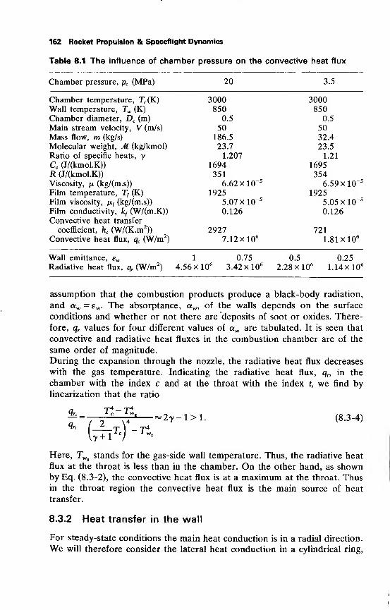
162 Rocket Propulsion & Spaceflight Dynamics
Table 8.1 The influence of chamber pressure on the convective heat flux
Chamber pressure, pc (MPa) 20 3.5
Chamber temperature, TC (K)
Wall temperature, Tw (K)
Chamber diameter, Dc (m)
Main stream velocity, V(m/s)Mass flow, m (kg/s)
Molecular weight, M (kg/kmol)
Ratio of specific heats, yCv (J/(kmol.K))
R (J/(kmol.K))
Viscosity, ju, (kg/(m.s))
Film temperature, 7} (K)
Film viscosity, ju.f(kg/(m.s))
Film conductivity, kf(W/(m.K))
Convective heat transfer
coefficient, hc (W/(K.m2))
Convective heat flux, qc (W/m2)
Wall emittance, ew 1 0.75 0.5 0.25
Radiative heat flux, qr (W/m2) 4.56 x 10
63.42 x 10
62.28 x 10
6 1.14xl06
assumption that the combustion products produce a black-body radiation,
and aw = ew . The absorptance, aw , of the walls depends on the surface
conditions and whether or not there are deposits of soot or oxides. There-
fore, qr values for four different values of aw are tabulated. It is seen that
convective and radiative heat fluxes in the combustion chamber are of the
same order of magnitude.
During the expansion through the nozzle, the radiative heat flux decreases
with the gas temperature. Indicating the radiative heat flux, q„ in the
chamber with the index c and at the throat with the index t, we find bylinearization that the ratio
^- ^^ -~2y-l>l. (8.3-4)
3000 3000850 850
0.5 0.5
50 50186.5 32.4
23.7 23.5
1.207 1.21
1694 1695351 354
6.62 xl0~5 6.59x101925 1925
5.07 xlO-5 5.05x10
0.126 0.126
2927 7217.12X106 1.81x10
""tri^-it,
Here, TWg stands for the gas-side wall temperature. Thus, the radiative heat
flux at the throat is less than in the chamber. On the other hand, as shownby Eq. (8.3-2), the convective heat flux is at a maximum at the throat. Thusin the throat region the convective heat flux is the main source of heat
transfer.
8.3.2 Heat transfer in the wall
For steady-state conditions the main heat conduction is in a radial direction.
We will therefore consider the lateral heat conduction in a cylindrical ring,
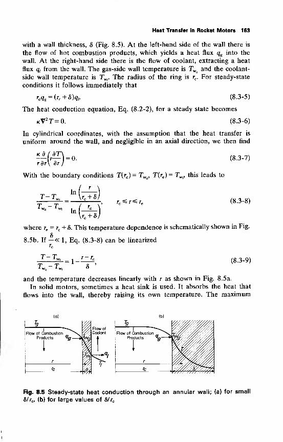
Heat Transfer in Rocket Motors 163
with a wall thickness, 8 (Fig. 8.5). At the left-hand side of the wall there is
the flow of hot combustion products, which yields a heat flux qg into the
wall. At the right-hand side there is the flow of coolant, extracting a heat
flux qtfrom the wall. The gas-side wall temperature is TWg and the coolant-
side wall temperature is TW( . The radius of the ring is rc . For steady-state
conditions it follows immediately that
rc <?g = (rc + «)<?,. (8 -3 "5 )
The heat conduction equation, Eq. (8.2-2), for a steady state becomes
kV2T=0. (8.3-6)
In cylindrical coordinates, with the assumption that the heat transfer is
uniform around the wall, and negligible in an axial direction, we then find
rdr\ drj
With the boundary conditions T(rc)= TWg , T{re)=TWl, this leads to
"fed . .
'
(8.3-7)
T-TT-T
In\rc + 8)
(8.3-8)
where re= rc + 8. This temperature dependence is schematically shown in Fig.
8.5b. If —« 1, Eq. (8.3-8) can be linearized
T-TWl r-rc
TL — TL 8(8.3-9)
and the temperature decreases linearly with r as shown in Fig. 8.5a.
In solid motors, sometimes a heat sink is used. It absorbs the heat that
flows into the wall, thereby raising its own temperature. The maximum
(b)
i
Tg
IbillllllP
1 ' ^\Flow of Combustion ^>^
Products "n *
i
'
i r
i
illl^1 '
Fig. 8.5 Steady-state heat conduction through an annular wall; (a) for smal
8/rc, (b) for large values of 8/rc
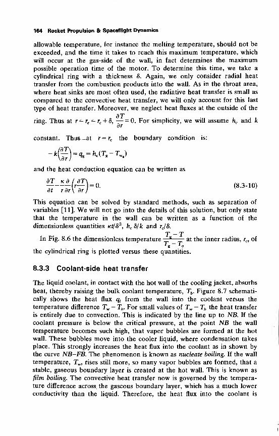
164 Rocket Propulsion & Spaceflight Dynamics
allowable temperature, for instance the melting temperature, should not be
exceeded, and the time it takes to reach this maximum temperature, which
will occur at the gas-side of the wall, in fact determines the maximumpossible operation time of the motor. To determine this time, we take a
cylindrical ring with a thickness 8. Again, we only consider radial heat
transfer from the combustion products into the wall. As in the throat area,
where heat sinks are most often used, the radiative heat transfer is small as
compared to the convective heat transfer, we will only account for this last
type of heat transfer. Moreover, we neglect heat fluxes at the outside of the
ring. Thus at r= re = rc + 8, — = 0. For simplicity, we will assume hc and kdr
constant. Thus—at r= rc the boundary condition is:
and the heat conduction equation can be written as
"LMf^W (8.3-10)dt rdr\ drj
This equation can be solved by standard methods, such as separation of
variables [11]. We will not go into the details of this solution, but only state
that the temperature in the wall can be written as a function of the
dimensionless quantities Kt/82
, hc 8/k and rc/8.
T -TIn Fig. 8.6 the dimensionless temperature — s—— at the inner radius, rc, of
the cylindrical ring is plotted versus these quantities.
8.3.3 Coolant-side heat transfer
The liquid coolant, in contact with the hot wall of the cooling jacket, absorbs
heat, thereby raising the bulk coolant temperature, Tb . Figure 8.7 schemati-
cally shows the heat flux qxfrom the wall into the coolant versus the
temperature difference Tw - Tb . For small values of Tw - Tb the heat transfer
is entirely due to convection. This is indicated by the line up to NB. If the
coolant pressure is below the critical pressure, at the point NB the wall
temperature becomes such high, that vapor bubbles are formed at the hot
wall. These bubbles move into the cooler liquid, where condensation takes
place. This strongly increases the heat flux into the coolant as in shown by
the curve NB-FB. The phenomenon is known as nucleate boiling. If the wall
temperature, Tw , rises still more, so many vapor bubbles are formed, that a
stable, gaseous boundary layer is created at the hot wall. This is known as
film boiling. The convective heat transfer now is governed by the tempera-
ture difference across the gaseous boundary layer, which has a much lower
conductivity than the liquid. Therefore, the heat flux into the coolant is
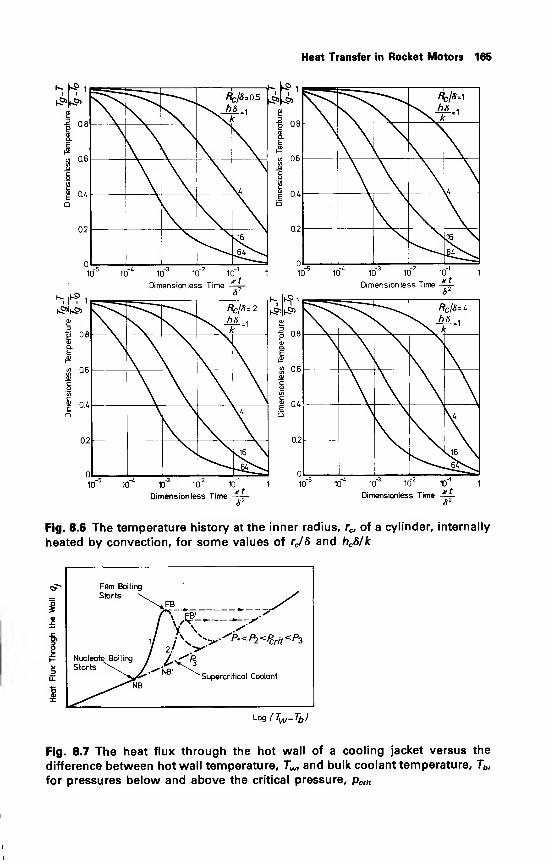
Heat Transfer in Rocket Motors 165
i
-s 0.8
0.6
§ 0.4
0.2
i i
0.8
« 0.6
0.4
0.2
Rc/S=o.st
5
\
V(
sJ6
10* 10° 10'
Dimensionless Time
10'
xt
Dimensionless Timext
/?C/<5=2\ hS ,
X k '
x^
V
sj6 \
0.8
0.6
0.4
0.2
a>
"5 0.8
IS 0.6
ff 0.4
0.2
L/,
.16 \
10 10 10
Dimensionless Time
10'
xt
Rcj8-.U\ hs=1
Xy /r
V
^16 N^
10 10 10
Dimensionless Time
10'
xtS 2
Fig. 8.6 The temperature history at the inner radius, rc, of a cylinder, internally
heated by convection, for some values of rc/8 and hcS/k
Film Boiling
Starts \ s\^FB /r\ fb' ^ — ^'1 \s\———T-^
1/}\^^P^P2<Pcrit<P2
/ 2/ >"'Nucleate Boiling .
Starts \^ J1 .£<%
Supercritical Coolant
^^-^m
Log (Tw-Tb)
Fig. 8.7 The heat flux through the hot wall of a cooling jacket versus the
difference between hot wall temperature, Tw, and bulk coolant temperature, Tb,
for pressures below and above the critical pressure, pcrit
166 Rocket Propulsion & Spaceflight Dynamics
strongly reduced and the wall temperature will rise to a much higher value,
often so high that structural failure may result. Nucleate boiling is a very
effective way of cooling. The point FB where film boiling, which we want to
avoid, starts is difficult to predict and has to be determined experimentally.
When the pressure is increased, but still remains lower than the critical
pressure, nucleate boiling will start at higher wall temperatures (point NB'),
while the maximum heat flux that can be attained (point FB') is apt to be
somewhat less.
For supercritical pressures (line for p3), the liquid will, upon reaching the
critical pressure, transform into gas without evaporation. If the pressure is
near to the critical pressure (i.e. p/pcrit < ~ 3) still large changes in density,
and hence in flow velocities may take place. This has to be analysed
carefully to ascertain that pressure drops do not become too large.
To determine the fluid heat transfer, use can be made of the Sieder-Tate
[7] equation, which allows for the large temperature difference, Tw - Tb , by
the factor hi/fxj014
,
St = 0.027 Ren02 Pr067 (—) . (8.3-11)
All variables are evaluated at the bulk temperature, Tb , of the coolant
except fiw , which is evaluated at the wall temperature, Tw .
For supercritical hydrogen, helium and nitrogen, Taylor [12] recommendsthe use of
(rp x [1.59/(x/D)-0.57]
y) , (8.3-12)
where again, with the exception of Tw, all physical properties are evaluated
at the bulk temperature, Tb . The equation allows for entrance effects by the
factor x/D. Here x stands for the distance from the entrance of the duct, Dis the equivalent duct diameter, D = y/4A/ir and A is the cross-sectional
area of the duct.
8.3.4 Radiation cooling
For rocket motors, radiation cooling is especially important for extremely
hot parts, such as the nozzle extension skirt, and sometimes the combustionchamber, if no active cooling system is used. This is often the case with
satellite and spacecraft rocket engines, and with many solid motors. If the
motor radiates into empty space (the atmosphere during atmospheric flight
can often be regarded as 'empty space' in so far as radiation is concerned) the
heat flow dq radiated by a surface element dS with temperature Tw andemittance e, equals
6q = <reT4w dS. (8.3-13)
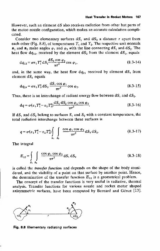
Heat Transfer in Rocket Motors 167
However, such an element dS also receives radiation from other hot parts of
the motor-nozzle configuration, which makes an accurate calculation compli-
cated.
Consider two elementary surfaces dS1 and dS2 a distance r apart from
each other (Fig. 8.8), of temperatures Tx and T2 . The respective unit normals
n x and n2 make angles <p x and <p2 with the line connecting dS x and dS2 . The
heat flow dq12 , received by the element dS2 from the element dSu equals
dq, ^ dSgCOSjp, (Q<11A\= <T£ 1 TidS1~ cos <p x ,
(5.3-14)
and, in the same way, the heat flow dq21 received by element dS x from
element dS2 equals
dq2 i= o-e2T\dS2 2— cos cp2 . (8.3-15)
ITT
Thus, there is an interchange of radiant energy flow between dSx and dS2 .
a ( T* rr^, dS1 dS2 cos <p 1 cos(p2 (aimdq = o-(e 177-e2 7^) 2. (8.3-16)
TTT
If dSx and dS2 belong to surfaces Sx and S2 with a constant temperature, the
total radiation interchange between these surfaces is
,-o(.,T}-.2r3j(
COS
^r
C
2
OS ^ dSldS2 . (8.3-17)
The integral
E12 =J J
c"^»^ dS,dS, (8.3-18)
S t Sj
is called the transfer function and depends on the shape of the body consi-
dered, and the visibility of a point on that surface by another point. Hence,
the determination of the transfer function E12 is a geometrical problem.
The concept of the transfer functions is very useful in radiative, thermal
analysis. Transfer functions for various nozzle and rocket motor shaped
axisymmetric surfaces, have been computed by Bernard and Genot [13].
Fig. 8.8 Elementary radiating surfaces
168 Rocket Propulsion & Spaceflight Dynamics
Using these transfer functions, radiative heat transfer calculations are
strongly simplified.
In this chapter, we had to limit ourselves to a general discussion of heat
transfer in rocket engines. Without going into detail we mentioned somemethods that can be applied quickly to get an estimate of heat fluxes andtemperatures, or methods that give some insight in the processes going on.
A more detailed discussion of heat transfer in the rocket motor is given byZiebland [7].
References
1 Eckert, E. R. G. and Drake Jr., R. M. (1973), Analysis of Heat andMass Transfer, McGraw-Hill, New York.
2 Kreith, F. (1969), Principles of Heat Transfer, Int. Textbook Co., fifth
printing, Scranton.
3 Gebhart, B. (1961), Heat Transfer, McGraw-Hill, New York.
4 Fourier, J. (1878), The Analytical Theory of Heat, Cambridge Univer-sity Press, (English translation by A. Freeman).
5 Boltzmann, L. (1884), Ableitung des Stefan'schen Gesetzes, Ann. d.
Physik, Ser. 2, 22, 291-294.
6 Planck, M. (1901), Ueber das Gesetz der Energieverteilung im Nor-malspectrum, Ann. d. Physik, Ser. 4, no. 3, 553-563.
7 Ziebland, H. and Parkinson, R. C. (1971), Heat Transfer in RocketEngines, AGARDograph 148, NATO, Neuilly-sur-Seine.
8 Hirschfelder, J. O., Bird, R. B. and Curtiss, C. F. (1954), MolecularTheory of Gases and Liquids, John Wiley, New York, p. 533.
9 Eucken, A. (1913), Ueber das Warmeleitvermogen, die spezifische
Warme und die innere Reibung der Gase, Physik. Zeitschr., 14, 324-332.
10 Bartz, D. R. (1957), A simple equation for rapid estimation of rocket
nozzle convective heat transfer coefficients, Jet Propulsion, 27, 49-51.11 Schoyer, H. F. R. (1977) The Determination of Temperature Histories
in a Cylindrical Ring, Heated by Convection, Rpt. LR-253, Delft
University of Technology, Dpt. of Aerospace Engineering, Delft.
12 Taylor, M. F. (1968), Correlation of Local Heat-Transfer Coefficients for
Single-Phase Turbulent Flow of Hydrogen in Tubes with Temperature
Ratio's to 23, NASA TN D-4332, Washington.
13 Bernard, J. J. and Genot, J. (1975), Radiation Cooling of Thrust
Nozzles, AGARDograph 184, NATO, Neuilly-sur-Seine.
9 The Solid-PropellantRocket Motor
In discussing the general characteristics of the solid-propellant rocket motor,or solid rocket, it will prove useful to compare it with its liquid counterpart.
Advantages of the solid rocket are:
1. Long storage life even for high-performance rockets; this makes the
type well suited for military purposes.
2. The propellants are harmless in human contact, this in contrast to
many liquid propellants.
3. No active cooling system is needed, nor a propellant feed system; this
leaves out complicated parts, such as pumps, turbines, etc, and makes lowcost production possible.
4. Solid rockets are immediately ready for firing and have, due to their
small number of components, a high reliability.
Many of the advantages are off-set, more or less, by disadvantages:
1. Relatively low Isp for the solid propellants. This is partly compensated
by a high Is .
2. Some solid propellants become brittle below certain temperatures andthen are liable to crack. These cracks may cause such high chamber pres-
sures after ignition that an explosion results.
3. Thrust modulation, and thrust vector control are more difficult for the
solid motor.
4. Extinguishment and re-ignition, though possible, are difficult.
5. Careful nozzle construction design is required as there is no active
cooling system. The situation is often aggravated by the presence of solid
particles in the combustion products; in most cases metal oxides that maycause serious nozzle erosion, or that may form deposits on the nozzle.
Combustion instability is a major problem in solid rocketry. It occurs
frequently in newly developed rocket motors [1]. Prevention is still difficult
and curing often weight consuming.
Solid rockets find widespread military and civil applications as: tactical
weapons, sounding rockets, boosters for launch vehicles, including man-rated vehicles, such as the Space Shuttle, strategical weapons (ICBM),spacecraft launch vehicles and motors for stage separation.
170 Rocket Propulsion & Spaceflight Dynamics
9.1 Solid propellants
The solid propellant family basically consists of two entirely different types:
the homogeneous or colloidal propellant and the composite propellant. There
is a mixed form too, where ingredients of the first type are used in the
second one. These are called Composite Modified Double-Base (CMDB).
9.1.1 Double-Base propellants
The most important homogeneous propellant is the Double-Base (DB) propel-
lant. It was invented in 1888 by Nobel and has since been used as a
gunpowder. It mainly consists of nitrocellulose (NC), a better name of which is
cellulose -nitrate (CN) and nitroglycerine (NG), a better name of which is
glyceroltrinitrate (GN). The first is a solid material, prone to detonation. It
plasticizes with the highly explosive, liquid NG to a relatively stable solid
propellant. When the propellant plasticizes the two ingredients form a gel
and the propellant gets a homogeneous structure. Both NG and NC com-
bine oxidizer and fuel in one molecule. DB propellants decompose com-pletely into gases and therefore are smokeless. For military purposes this can
be of importance. Often, besides stabilizers to prevent self-ignition, sub-
stances are added to the mixture, either to improve the mechanical proper-
ties, or to influence the burning characteristics. If these additives, such as
Table 9.1 Properties of some double-base propellants
Propellant Composition
(% by weight)
M y(kg/kmol)
Tc
(K)
AHH
NC 55,2; NG 32,7;
Triacetin 8.1; 2-Nitro-
diphenyl amine 1; Lead
salicylate 1.5; L-26 1.5
24.56 1.23 2485
ATNNC 40; NG 48.4;
Triacetin 6.4; 2-Nitro-diphenyl
amine 1; Lead beta-resorcyclate 2;
Lead salicylate 2; Carbolac I 0.2
26.10 1.22 2822
NC 54.5; NG 23.1; Triacetin 18.1;
AFU Ethyl Centralite 0.6; 2-Nitro- 21.55 1.26 1693
Diphenyl amine 0.3; Lead
stearate 3.4
NC 51.22; NG 43; Diethylphtalate
JPN 3.25; Ethyl Centralite 1; K2S04 26.4 1.215 3125
(Ballistite) 1.25; Carbon Black 0.2, wax 0.08
The Solid-Propellant Rocket Motor 171
carbon black, or aluminum powder do not form gaseous combustion pro-
ducts, the DB propellant may produce smoke. Table 9.1 gives the composi-tion of some DB propellants, some thermochemical properties and someperformance properties such as Fsp and c*. Here Psp indicates Isp at ideal
expansion. The volumetric specific impulse is found from pp and Psp . Theburning rate versus the chamber pressure and the burning rate sensitivity for
the initial temperature, are given in the last columns.
In some cases, the NG in DB propellants are replaced by other con-
stituents such as di-or tri-nitrodiethyleneglycol.
Nitroglycerine has an excess of oxygen while NC is deficient in oxygen.
The mixture ratio yielding the highest Isp is about stoichiometric, i.e. the
ratio of NG mass to NC mass should be about 8.6. Presently it is not
possible to obtain a propellant gel with good mechanical properties at NGmass fractions exceeding 0.5.
9.1.2 Composite propellants
These usually are a mixture of an anorganic salt, serving as an oxidizer, andan organic fuel or binder, plastic or rubber in most cases. The following
qualities are important for selecting an oxidizer: high heat of formation, high
amount of available oxygen, high density, not or slightly hygroscopic andsmooth burning characteristics over a wide pressure range. Most propellants
nowadays use NH4C104 , ammonium perchlorate or AP, while sometimes
r=ap n
r c* Pp Pressure Range (p in MPa) *K(s) (m/s) (kg/m3
)(MPa) (mm/s)
a n
(K- 1
)
2.76- 4.83 39.77 0.7
4.83- 5.21 8.74 0.2 1.26 xlO"3
225 1402 1601 5.21- 7.58 21.67 -0.35 0.81X10"3
pc= 7 MPa 7.58- 8.62 39.64 -0.65 1.53 xlO-3
pe = 0.1MPa 8.62-10
10 -25
5.98
1.40
0.23
0.86
at 293 K at 293 K
3.10- 7.58 7.01 0.49 5.04 xlO"3
235 1453 1602 7.58-13.10 116.42 0.07 2.34 X10~3
pc= 7 MPa 13.10-16.89 4.31 0.59 4.32 xlO"3
pe = 0.1MPa at 293 K at 293 K
3.79- 6.21 4 0.24
196 1225 1514 6.21- 9.65 112.87 -0.4 2.16 xlO"3
pc = 7 MPa 9.65-17.24 6.35 0.56 6.66 xlO"3
pe = 0.1 MPa at 293 K
250 1523 1620 8.9 0.69 12.26 xlO"3
172 Rocket Propulsion & Spaceflight Dynamics
Table 9.2 Properties of some composite propellants
Propellant
Composition
(% by weight)
M, y(kg/kmol) (K) (s)
JPL 540A PU 20; AP 80.
Propellant
proposed
for Space
Shuttle
Boosters
PBAN 12.5; Al 16; Epoxy
Curative 1.5; Ferric Oxide
0.1; AP 69.9.
25
27.8
PU24.1; Al 15;
ANP-2639AF Carbon Black 0.5; Copper-
Chromite 0.4; AP 60.
Arcite 373
AP 58.9; Al 21; PVC 8.62;
Dioctyl Adipate 10.79; XB820.17; X23-74 0.17;
British Detergent 0.25.
24.7
29.06
1.2 2600 231
pc= 6 MPa
pe= 0.1MPa
1.18 3480 260
pc= 7 MPa
Pe = 0.1MPA
254
1.18 2703 pc = 7MPa
pe= 0.1MPa
242
pc= 7 MPa
1.18 3370 Ae/A r= 9
266
pc = 7 MPaAJA
t= 9.8
(theoretical)
CDT (80)
NC 26; NG 27.2; AP 19.5;
Al 18.9; 2-Nitro diphenyl
amine 1; Triacetin 6.4;
Magnesium Oxide 1.
30.18 1.168 4000 263
H-3515
AP 35; Pentaeritritol-
trinitrate 35; NC 14.25;
Al 15; Ethylcentralite
0.75.
3450 255
TRX-H609AP70; Al 16;PBAA 11.05;
ERL-2795 2.94. 25.97 1.21 3040 245
Flexadyne
RDS-509(Rocketdyne)
CTPB 12; AP 82;
Al 4; Additive 2.
27.16 1.20 3176
Pc
Pe
248= 7 MPa= 0.1 MPa
Flexadyne
RDS-556(Rocketdyne)
CTPB 15; AP69;Al 14; Additive 2.
26.92 1.20 3246
Pc
Pe
252= 7 MPa= 0.1 MPa
Al aluminum
AP ammonium perchlorate
NC nitrocellulose
NG nitroglycerin
The Solid-Propellant Rocket Motor 173
r = a.p"
c* pp Pressure Range (p in MPa) irK(m/s) (kg/m3
) (MPa) (mm/s) (Kr 1
)
a n
0.1 - 0.45 5.13 0.679
1434 1660 0.45- 1.65 4.13 0.406
1.65- 5.5 4.6 0.189
1583 1772 5- 7 7.35 0.33 8.3xl0~4
at 294 K
1.38-4.14 4.5 0.3135 2.8x 10- 3 ;255 K<Tf<289 K
1480 1669 4.14-8.96 5.61 0.159 1.9x 10"3 ;289 K< T;<316 K
at 289 K
1523 1772 3.45- 4.83 6.74 0.176
4.83-13.1 5.64 0.295 19.8 xlO"4
at 294 K at294K;K=300p = 7 MPa
1635 1745 4.14-20.68 6.99 0.48 8.46 x 10"3at 7 MPa
at 294 K 8.1 x 10"3at 10.5 MPa
1772 4.14-13.79 2.87 0.68 12.4 x 10~3
at 294 K
1517 1760 2.07-13.79 4.92 0.297 19.8 x 10~4
at 294 K
1518 1758 8.25 0.39 2.11 xlO"3
1544 1747 2.76- 6.85 10.79 0.65 2.48 x 10~3
6.85-20.68 18.86 0.36 2.10 x 10~3.
CTPB carboxyl terminated polybutadiene
PBAA polybutadiene-acrylic acid polymer
PBAN polybutadiene-acrylic acid-acrylonitrile terpolymer
PU polyurethane
PVC polyvinyl chloride
174 Rocket Propulsion & Spaceflight Dynamics
NH4N03 , ammonium nitrate, and KC104 ,potassium perchlorate are used.
Other possible oxidizers which have been proposed for instance are
N02C104 , nitronium perchlorate [2], and N2H5C104 , hydrazine perchlorate
[3] while also organic oxidizers are considered. Nevertheless, AP at the
present time is the most commonly used oxidizer for composite propellants.
The choice of the fuel is mainly determined by mechanical properties,
such as strength, elasticity and thermal properties at low and high environ-
mental temperatures, a high energy content and good aging and burning
characteristics. An essential feature of the binder is an initial liquid state of
its components (prepolymers), as this facilitates the mixing of oxidizer and
fuel. The mixing is followed by a curing process during which the binder
becomes a solid. By adding powdered metals, such as Al, aluminum, to the
propellant the flame temperature, and thus Isp , can be increased considera-
bly. Table 9.2 lists compositions and characteristics of some typical compo-site propellants. Like Table 9.1, this table gives the propellant composition,
some thermochemical properties, the burning rate behavior and the temper-
ature sensitivity.
Composite modified double-base propellants contain NC, NG, an anor-
ganic salt, such as AP and a powdered metal, such as Al, and in some cases
a polymer. In general, these propellants have high flame temperatures; their
burning rates are very sensitive to pressure. They are not used in large
quantity as yet.
9.1.3 The burning rate
Solid propellant burns normal to its surface. The (average) burning rate, r, is
defined as the regression of the burning surface per unit time. For a given
propellant, the burning rate is mainly dependent on the pressure, p, and the
initial temperature, Th of the propellant. One determines r(p) by measure-
ments in a Crawford bomb or strand burner (Fig. 9.1). In this vessel, in which
the pressure can be adjusted, a strand of propellant is burnt. Often a gas,
mostly N2 , which does not influence the propellant burning, ventilates the
vessel. The propellant strand is inhibited such that burning will only take
place in the longitudinal direction. Two electrical wires are fixed to the
strand at a mutual distance L. The melting of those two wires will start and
stop, respectively, a chronometer. From the time measured and the distance,
L, the average burning rate is determined. By repeating this procedure at
different pressures and temperatures Th one obtains r(p, Tt ). It should be
emphasized here that the relationship obtained this way only holds for
stationary conditions. As the burning rate is also strongly dependent on
non-stationary effects, this relationship cannot be applied to non-steady
situations.
It turns out that the burning rate dependence on pressure can be expres-
sed as
r=a + bp n, (9.1-1)
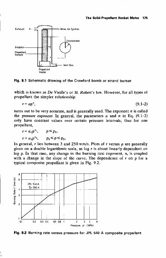
The Solid-Propellant Rocket Motor 175
Exhaust *
Inhibitor
Propellant
Sample
Wires for Ignition
Chronometer
Vent Gas
Fig. 9.1 Schematic drawing of the Crawford bomb or strand burner
which is known as De Vieille's or St. Robert's law. However, for all types of
propellant the simpler relationship
r = ap (9.1-2)
turns out to be very accurate, and is generally used. The exponent n is called
the pressure exponent. In general, the parameters a and n in Eq. (9.1-2)
only have constant values over certain pressure intervals, thus for one
propellant,
r^atf"*, p^Pi,
r=a2pn*, Pi^p^p2 ,
In general, r lies between 3 and 250 mm/s. Plots of r versus p are generally
given on a double logarithmic scale, as log r is about linearly dependent on
log p. In that case, any change in the burning rate exponent, n, is coupled
with a change in the slope of the curve. The dependence of r on p for a
typical composite propellant is given in Fig. 9.2.
JPL 5
7/= 3
40 A
00 K
0.1 0.2 0.3 0.4 0.6 0.8 1 2 3 4 6
Pressure p (MPa)
Fig. 9.2 Burning rate versus pressure for JPL 540 A composite propellant
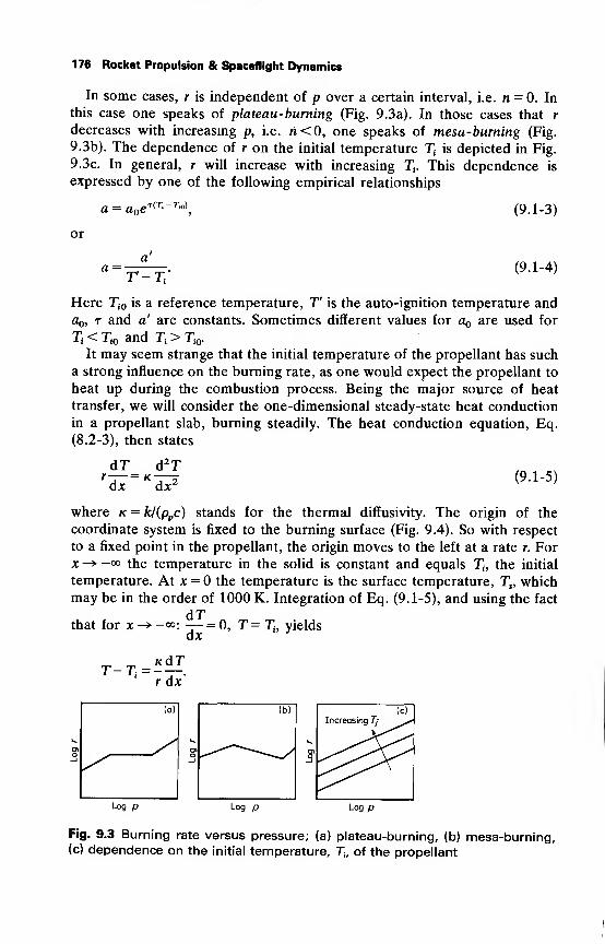
176 Rocket Propulsion & Spaceflight Dynamics
In some cases, r is independent of p over a certain interval, i.e. n = 0. In
this case one speaks of plateau-burning (Fig. 9.3a). In those cases that r
decreases with increasing p, i.e. ri<0, one speaks of mesa-burning (Fig.
9.3b). The dependence of r on the initial temperature Tt
is depicted in Fig.
9.3c. In general, r will increase with increasing Tt. This dependence is
expressed by one of the following empirical relationships
(9.1-3)a = a e TCr.-iVo)
or
T'-Tt
' (9.1-4)
Here Ti0 is a reference temperature, T" is the auto-ignition temperature and
Oq, t and a' are constants. Sometimes different values for a are used for
Ti<Tio andT,>Tio .
It may seem strange that the initial temperature of the propellant has such
a strong influence on the burning rate, as one would expect the propellant to
heat up during the combustion process. Being the major source of heat
transfer, we will consider the one-dimensional steady-state heat conduction
in a propellant slab, burning steadily. The heat conduction equation, Eq.
(8.2-3), then states
dT_ d*T
dx dx 2 (9.1-5)
where k = k/(ppc) stands for the thermal diffusivity. The origin of the
coordinate system is fixed to the burning surface (Fig. 9.4). So with respect
to a fixed point in the propellant, the origin moves to the left at a rate r. Forx—»-°° the temperature in the solid is constant and equals Th the initial
temperature. At x = the temperature is the surface temperature, Ts , whichmay be in the order of 1000 K. Integration of Eq. (9.1-5), and using the fact
dT-7- = 0, T = Ti, yieldsthat for xdx
T-Tt
=-—.r dx
Fig. 9.3 Burning rate versus pressure; (a) plateau-burning, (b) mesa-burning,(c) dependence on the initial temperature, T„ of the propellant
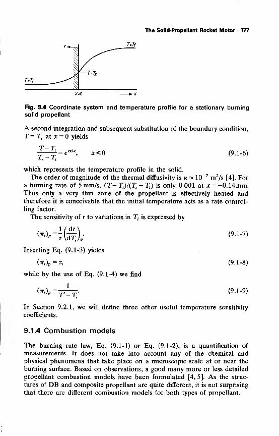
The Solid-Propellant Rocket Motor 177
X=0 X
Fig. 9.4 Coordinate system and temperature profile for a stationary burning
solid propellant
A second integration and subsequent substitution of the boundary condition,
T = Ts at x = yields
T-Tj
T -T= e™'", ;o (9.1-6)
which represents the temperature profile in the solid.
The order of magnitude of the thermal diffusivity is k « 10-7 m2
/s [4]. Fora burning rate of 5mm/s, (r-rj)/(rs -T,) is only 0.001 at x = -0.14mm.Thus only a very thin zone of the propellant is effectively heated andtherefore it is conceivable that the initial temperature acts as a rate control-
ling factor.
The sensitivity of r to variations in 7) is expressed by
(wr ),
Inserting Eq. (9.1-3) yields
while by the use of Eq. (9.1-4) we find
1
to, r-Tt
'
(9.1-7)
(9.1-8)
(9.1-9)
In Section 9.2.1, we will define three other useful temperature sensitivity
coefficients.
9.1.4 Combustion models
The burning rate law, Eq. (9.1-1) or Eq. (9.1-2), is a quantification of
measurements. It does not take into account any of the chemical andphysical phenomena that take place on a microscopic scale at or near the
burning surface. Based on observations, a good many more or less detailed
propellant combustion models have been formulated [4, 5]. As the struc-
tures of DB and composite propellant are quite different, it is not surprising
that there are different combustion models for both types of propellant.
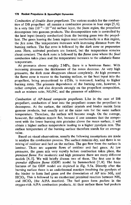
178 Rocket Propulsion & Spaceflight Dynamics
Combustion of Double-Base propellants. The various models for the combus-
tion of DB propellant all assume a combustion process in four steps [5, 6].
In a very thin (10~5 -10~4 m) surface layer, the foam region, the propellant
decomposes into gaseous products. The decomposition rate is controlled by
the heat input (mainly conduction) from the burning gases into the propel-
lant. The gases leaving the foam region react exothermally in a thin region,
the fizz zone. The temperature increases with increasing distance from the
burning surface. The fizz zone is followed by the dark zone or preparation
zone. Here, activated products are formed, but the temperature remains
about constant. The dark zone is followed by the flame zone where the final
combustion takes place and the temperature increases to the adiabatic flame
temperature.
At pressures above roughly 2MPa, there is a luminous flame. With
increasing pressures the thicknesses of the zones decrease. At very high
pressures, the dark zone disappears almost completely. At high pressures
the flame zone is nearer to the burning surface, so the heat input into the
propellant, being proportional to dT/dx, is increased, leading to higher
burning rates. The pressure dependence of the burning rate, however, is
rather complex, and also depends strongly on the propellant composition,
such as mixture ratio, NG/NC, and the presence of additives.
Combustion of AP-based composite propellants. Like in the case of DBpropellant, conduction of heat into the propellant causes the propellant to
decompose. At the surface, the oxidizer crystals and binder matrix form
gaseous products, but usually not at the same rate for the same surface
temperature. Therefore, the surface will become rough. On the average,
however, flat surfaces remain flat, because if one assumes that the compo-
nent with the lower burning rate protudes above the mean surface, it will
obtain a higher surface temperature leading to a higher pyrolysis rate. The
surface temperature of the burning surface therefore stands for an average
value.
Based on visual observations, usually the following assumptions are made
to analyse the combustion process. The surface remains dry, and there is no
mixing of oxidizer and fuel on the surface. The gas flow from the surface is
laminar. There are separate flows of oxidizer and fuel gases. At low
pressures, the gases mix very rapidly before combustion takes place, the
premixed flame. For moderate and high pressures there are many different
models [4, 5]. We will briefly discuss two of them. The first one is the
granular diffusion flame (GDF) model by Summerfield [7,8]. The basic
features of the GDF model are depicted in Fig. 9.5a. Directly after the
burning surface there is an endothermal reaction involving the pyrolysis of
the binder to form fuel gases and the dissociation of AP into NH3 and
HC104 . This is followed by an exothermal premixed reaction between NH3
and HCIO4 (the A/PA reaction). The fuel gases form pockets in the
oxygen-rich A/PA combustion products. At their surface these fuel pockets
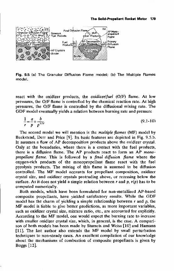
The Solid-Propellant Rocket Motor 179
Granular Diffusion Flqmef
Fig. 9.5 (a) The Granular Diffusion Flame model; (b) The Multiple Flames
model.
react with the oxidizer products, the oxidizer/fuel (O/F) flame. At low
pressures, the O/F flame is controlled by the chemical reaction rate. At high
pressures, the O/F flame is controlled by the diffusional mixing rate. TheGDF model eventually yields a relation between burning rate and pressure
I = -r p p
b_1/3-
(9.1-10)
The second model we will mention is the multiple flames (MF) model by
Beckstead, Derr and Price [9]. Its basic features are depicted in Fig. 9.5.b.
It assumes a flow of AP decomposition products above the oxidizer crystal.
Only at the boundaries, where there is a contact with the fuel products,
there is a diffusion flame. The AP products react to form an AP mono-propellant flame. This is followed by a final diffusion flame where the
oxygen-rich products of the monopropellant flame react with the fuel
pyrolysis products. The mixing of this flame is assumed to be diffusion
controlled. The MF model accounts for propellant composition, oxidizer
crystal size, and oxidizer crystals protruding above, or recessing below the
surface. As it does not yield a simple relation between r and p, r(p) has to be
computed numerically.
Both models, which have been formulated for non-metallized AP-based
composite propellants, have yielded satisfactory results. While the GDFmodel has the charm of yielding a simple relationship between r and p, the
MF model is liable to give better predictions, as more important variables,
such as oxidizer crystal size, mixture ratio, etc., are accounted for explicitly.
According to the MF model, one would expect the burning rate to increase
with smaller oxidizer crystal size, which, in general, is the case. A compari-
son of both models has been made by Stamets and Weiss [10] and Hamann[11]. The last author also extends the MF model by small perturbation
techniques to non-steady cases. An excellent compilation of our knowledge
about the mechanisms of combustion of composite propellants is given by
Boggs [12].
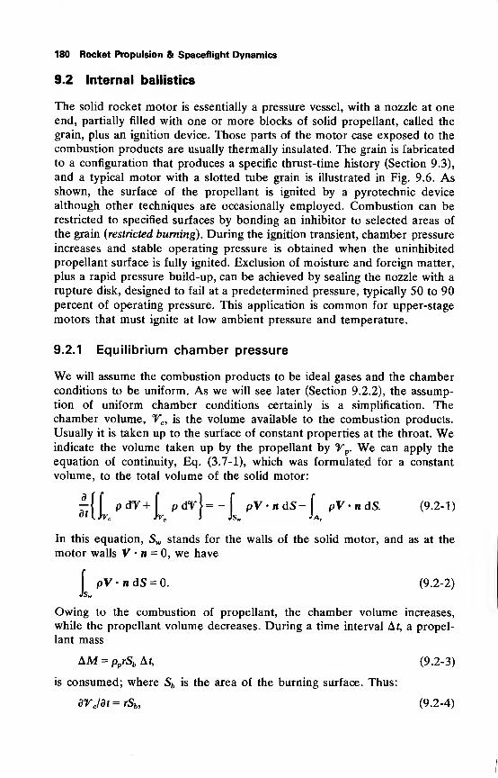
180 Rocket Propulsion & Spaceflight Dynamics
9.2 Internal ballistics
The solid rocket motor is essentially a pressure vessel, with a nozzle at oneend, partially filled with one or more blocks of solid propellant, called the
grain, plus an ignition device. Those parts of the motor case exposed to the
combustion products are usually thermally insulated. The grain is fabricated
to a configuration that produces a specific thrust-time history (Section 9.3),
and a typical motor with a slotted tube grain is illustrated in Fig. 9.6. Asshown, the surface of the propellant is ignited by a pyrotechnic device
although other techniques are occasionally employed. Combustion can be
restricted to specified surfaces by bonding an inhibitor to selected areas of
the grain (restricted burning). During the ignition transient, chamber pressure
increases and stable operating pressure is obtained when the uninhibited
propellant surface is fully ignited. Exclusion of moisture and foreign matter,
plus a rapid pressure build-up, can be achieved by sealing the nozzle with a
rupture disk, designed to fail at a predetermined pressure, typically 50 to 90percent of operating pressure. This application is common for upper-stage
motors that must ignite at low ambient pressure and temperature.
9.2.1 Equilibrium chamber pressure
We will assume the combustion products to be ideal gases and the chamberconditions to be uniform. As we will see later (Section 9.2.2), the assump-
tion of uniform chamber conditions certainly is a simplification. Thechamber volume, Tc , is the volume available to the combustion products.
Usually it is taken up to the surface of constant properties at the throat. Weindicate the volume taken up by the propellant by T
p. We can apply the
equation of continuity, Eq. (3.7-1), which was formulated for a constant
volume, to the total volume of the solid motor:
yl\ pdT+f pdrj=-[ pV-ndS-[ pV-ndS. (9.2-1)
In this equation, Sw stands for the walls of the solid motor, and as at the
motor walls V • n = 0, we have
I
pV-ndS = 0. (9.2-2)Js„
Owing to the combustion of propellant, the chamber volume increases,
while the propellant volume decreases. During a time interval At, a propel-
lant mass
AM = pprSb Af, (9.2-3)
is consumed; where Sb is the area of the burning surface. Thus:
dVJdt=rSb , (9.2-4)
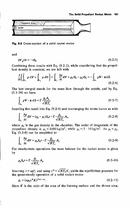
The Solid-Propellant Rocket Motor 181
Fig. 9.6 Cross-section of a solid rocket motor
and
dTpldt= -rSb . (9.2-5)
Combining these results with Eq. (9.2-1), while considering that the propel-
lant density is constant, we are left with
^|£ P<^+£ P dr}
=£ jt
dr+ PcrSb -pprSb = -^ pV • ndS.
(9.2-6)
The last integral stands for the mass flow through the nozzle, and by Eq.
(5.1-39) we have
pV-ndS=T'A,
PcA(9.2-7)
Inserting this result into Eq. (9.2-6) and rearranging the terms leaves us with
(9.2-8)^dT = (pp -pc)Sbr-r-^=A t,
dt VRT,
where pc is the gas density in the chamber. The order of magnitude of the
propellant density is pp = 1600 kg/m3, while pc ~3 — 10kg/m3
. As pc «pp,
Eq. (9.2-8) can be simplified to
I ?,dr =<"s"- rskc
A' (9.2-9)
For steady-state operations the mass balance for the rocket motor is given
by
PPSbr= T
y/RTr
A, (9.2-10)
Inserting r = ap", and using c* = vRTJT, yields the equilibrium pressure for
the quasi-steady operation of a solid rocket motor
pc= (appc*K)^-
n\ (9.2-11)
Here K is the ratio of the area of the burning surface and the throat area,
182 Rocket Propulsion & Spaceflight Dynamics
called thelklemmung\ which means pinching,
K = SJAt. (9.2-12)
We see that for n = 0, pc is proportional with K, while for 0<n<l, pc is
more than proportional with K. For n | 1, the right-hand side of Eq.
(9.2-11) tends to infinity. Logarithmic differentiation of Eq. (9.2-11) leads to
dpc 1 dX— =1 F' 9.2*13
pc 1-n K
which illustrates the same result as discussed above. For most solid motors,
K lies somewhere between 200 and 1000.
In Section 9.1.3 we have defined a temperature sensitivity coefficient (7rr )p
for the propellant. We now can define three more temperature sensitivity
coefficients. They express the pressure change, or the change in the burning
rate with a change in the initial temperature. The first one, defined at a
particular value of the klemmung, K, is
-P )K =1 (^) ,(9.2-14)
pc \dTjK
and expresses the relative variation in chamber pressure, pc , with a change in
the initial temperature, Tt. The second one expresses the relative variation in
burning rate with a change in initial temperature, at a particular value of the
klemmung, K,
M'-~Mh (9 -2-15)
With the Eqs. (9.2-12), (9.2-14), (9.2-15) and (9.1-7), one easily shows that
(^p)k: = (7Tr)jc= ttk = (tjvV1-n
Often {irT)K is denoted as aK. Thus, the sensitivity of combustion pressure to
grain temperature is greater than the sensitivity of the burning rate to the
grain temperature at constant pressure, by the factor 1/(1 — n). Therefore, in
addition to a high T", a desirable propellant should have a low value of n.
The last temperature sensitivity coefficient that is used sometimes is (7r)p/r,
which is the temperature sensitivity coefficient of pressure at a particular
value of pjr [13]
Or),* = -(!£) = T1~MP . (9.2-16)
pc \dTJ Pc/r 1-n
In general irK is given as a propellant variable. For modern composite
propellants, ttk may be about 5 x 10⁻³ K_1
to 5 x 10~4 K' 1. For DB propel-
lants, ttk is generally between 10~2 K~ xto 10
-3 K~ x.
For a stable operation of the motor, the pressure exponent, n, should
The Solid-Propellant Rocket Motor 183
satisfy certain requirements. An indication for this was found already in Eq.
(9.2-13) where dpc tends to infinity for n f 1. Consider the equation for the
conservation of mass for the rocket motor, Eq. (9.2-9). We assume uniform
chamber conditions, and therefore we can write
rc^=p
pSbapnc-T-^=A t
. (9.2-17)dt y/RTc
We will now consider a perturbed steady-state process. A small pressure
perturbation, p'c, will be accompanied by perturbations p'
c and T'c in the
density and chamber temperature, respectively. The steady-state chamber
variables are denoted by pc, pc and Tc . Thus,
Pc = Pc + P'c, Pc = Pc+Pc and TC = TC + TC .
dpcAs —— = 0, we have
dt
PcppSbap
nc = T-^=A t
= m. (9.2-18)
Linearization, and the use of Eq. (9.2-18) yields
Now, if the change of state in the motor is isentropic, i.e. if the compres-
sion or expansion is not accompanied by heat transfer or other irreversible
processes, the Poisson relations, Eq. (3.7-20), will hold
n /n\ xly T In \(t-1)/t
P< -ft)" - H9If the change of state is isothermal, i.e. the temperature remains constant,
we may express this by
Pc a Po and Tc= constant.
It is conceivable that in practice the change of state will be in between
isothermal and isentropic. We will express this by
Pc \PcJ Tc \pj
(S-D/S
Pc
with 8 = 1 for an isothermal change of state and 8 = y for an isentropic one.
Again, linearizing leads to
Si = S ek and IL£zi£i. (9.2-20)Pc Pc Tc 8 pc
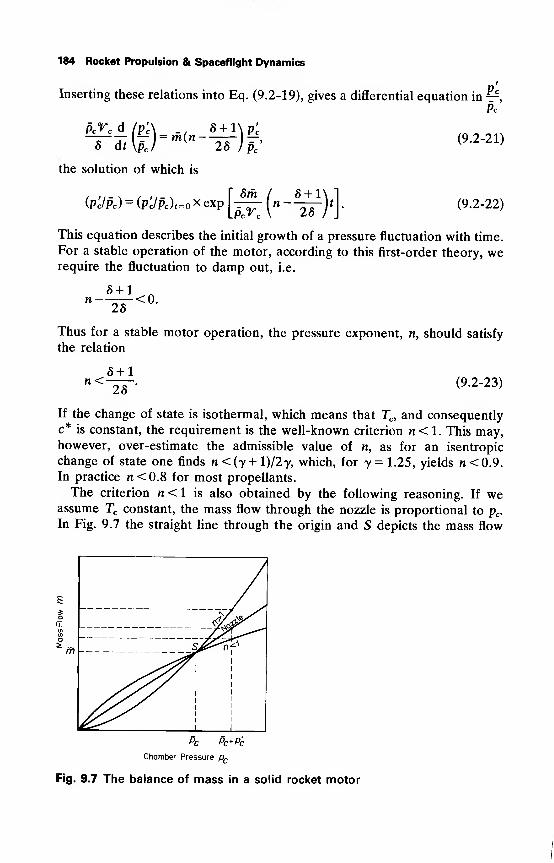
184 Rocket Propulsion & Spaceflight Dynamics
n'Inserting these relations into Eq. (9.2-19), gives a differential equation in ^r,
Pc
Pcrc d (p'c(Pc\ -, 8 + l\p'c8 dt
the solution of which is
(Pc/Pc) = (Pc/Pc) t=o><exp l-z-^- In——ji
(9.2-21)
(9.2-22)
This equation describes the initial growth of a pressure fluctuation with time.
For a stable operation of the motor, according to this first-order theory, werequire the fluctuation to damp out, i.e.
8 + 1 nn—^-<0 -
28
Thus for a stable motor operation, the pressure exponent, n, should satisfy
the relation
n<-8 + 1
28' (9.2-23)
If the change of state is isothermal, which means that Tc , and consequently
c* is constant, the requirement is the well-known criterion n< 1. This may,however, over-estimate the admissible value of n, as for an isentropic
change of state one finds n<(y + l)/2y, which, for y = 1.25, yields n<0.9.In practice n<0.8 for most propellants.
The criterion n<\ is also obtained by the following reasoning. If weassume Tc constant, the mass flow through the nozzle is proportional to pc .
In Fig. 9.7 the straight line through the origin and S depicts the mass flow
m
/j^r'
s^ltf
^HPc Pc+P'c
Chamber Pressure pc
Fig. 9.7 The balance of mass in a solid rocket motor
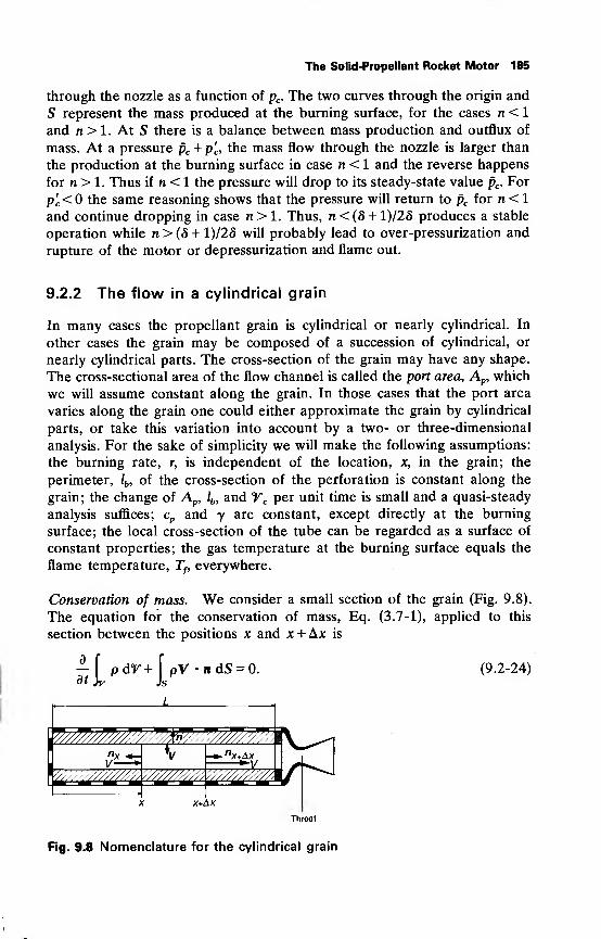
The Solid-Propellant Rocket Motor 185
through the nozzle as a function of pc . The two curves through the origin and
S represent the mass produced at the burning surface, for the cases n < 1
and n > 1. At S there is a balance between mass production and outflux of
mass. At a pressure pc + p'c, the mass flow through the nozzle is larger than
the production at the burning surface in case n < 1 and the reverse happens
for n > 1. Thus if n < 1 the pressure will drop to its steady-state value pc . For
p'c< the same reasoning shows that the pressure will return to pc for n < 1
and continue dropping in case n>l. Thus, n<(8 + l)/28 produces a stable
operation while n>(S + l)/2S will probably lead to over-pressurization and
rupture of the motor or depressurization and flame out.
9.2.2 The flow in a cylindrical grain
In many cases the propellant grain is cylindrical or nearly cylindrical. In
other cases the grain may be composed of a succession of cylindrical, or
nearly cylindrical parts. The cross-section of the grain may have any shape.
The cross-sectional area of the flow channel is called the port area, Ap, which
we will assume constant along the grain. In those cases that the port area
varies along the grain one could either approximate the grain by cylindrical
parts, or take this variation into account by a two- or three-dimensional
analysis. For the sake of simplicity we will make the following assumptions:
the burning rate, r, is independent of the location, x, in the grain; the
perimeter, lb , of the cross-section of the perforation is constant along the
grain; the change of Ap, lb , and Tc per unit time is small and a quasi-steady
analysis suffices; cp and y are constant, except directly at the burning
surface; the local cross-section of the tube can be regarded as a surface of
constant properties; the gas temperature at the burning surface equals the
flame temperature, Tf, everywhere.
Conservation of mass. We consider a small section of the grain (Fig. 9.8).
The equation for the conservation of mass, Eq. (3.7-1), applied to this
section between the positions x and x + Ax is
—fpdT+
I
pV -itdS = 0. (9.2-24)
x+Ax
Throat
Fig. 9.8 Nomenclature for the cylindrical grain
186 Rocket Propulsion & Spaceflight Dynamics
The volume T consists of the volume taken up by the propellant, Yp, and
the volume containing the combustion products, Yc . In the same way as in
Section 9.2.1, we find
dYc/dt=rSb = rlb bx, (9.2-25)
and
dYp/dt = -rSb = -rlb Ax. (9.2-26)
At the walls of the rocket motor V • n = and at the control surface Ax wehave V= - V • nx while at Ax+Ax , we have V= V • nx+Ax . For steady-state,
dp/dt = and hence, in the same way as in Section 9.2.1, we find, as Ax —> 0,
_d_
dxprlb -pp
rlb +—(PV)Ap= 0.
Note that the index p here is used to indicate both port and propellant. Asp « pp , we can write the equation of continuity for a cylindrical channel with
uniform mass addition as
pV=cx, (9.2-27)
with
c = *~. (9.2-28)
The momentum equation, Section 3.7.2, can be written as
|^(pV)dr+[ {(pV-n)V + iip}dS = 0.
Applying this to the section depicted in Fig. 9.8 we find for the steady-state
case
f{pV-n)V+np}dA+ I
{(pV • n)V+np}dA +
+[
{(pV-it)V+np}dSb = 0. (9.2-29)
At the burning surface we have pV • n = -ppr. Using this relation and the
assumption that the control surfaces, Ax , and Ax+Ax, are surfaces of constantproperties, we can evaluate Eq. (9.2-29) to
»x +Ax[(pV2 + p)x+Ax -(pV
2 + p)x]Ap +[ dx<£ (-^L+p)nd/ = 0.
As pp and r are constant and p and p are constant over any cross-sectional
area we have
{(-f +p).-Z-(-f+ p){ .-.-«.
The Solid-Propellant Rocket Motor 187
Now let Ax —> 0, then we find for the momentum equation in a cylindrical
grain
-f (pV2 + p) = 0, (9.2-30)dx
or
pV2 + p = constant.
At the front end of the grain, i.e. at x = 0, the velocity is zero, or practically
zero, and the pressure is the front-end stagnation pressure, p , thus
pV2 + p = p . (9.2-31)
The energy equation, Eq. (3.7-15), can be written in a slightly different
form,
-f
p(e + V2/2) dV = -
[[(pV • n)(e + V2
/2) + pV-n] dS. (9.2-32)
We now apply Eq. (9.2-32) to the cavity enclosed by the burning propellant
and the surfaces of constant properties, Ax and Ax+Ax ,(Fig. 9.8) which
yields,
l1 [p(e + V2
/2)] dV + rlbP (e + V2/2) Ax = [{(pV)(e + V2
/2 + p/p}xat
-{(pV)(c+V2/2 + p/p}x+AJAp- [dx & [(pV-»)(e+V2
/2 + p/p)]d/.
(9.2-33)
At the burning surface, V2« e, the temperature is the flame temperature, Tf,
and
f'
= ef= cvh
t,
dT.
Moreover, we make use of the fact that at the burning surface,
pV-n = -ppr. (9.2-34)
Substituting these relations into Eq. (9.2-33), and letting Ax-»0, this
equation can be evaluated for a steady-state flow, to yield
^ [(pV)(e + V2/2 + p/p)]A
p= rlb [Pp (ef + RTf)
- pef].
(9.2-35)
Use has been made of the ideal gas law and the fact that at the burning
surface the gas temperature equals Tf
. Neglecting p with respect to pp , finally
gives
-T [(PV)(e + V2/2 + pip)] =^(ef
+ RTf).
dx AD
188 Rocket Propulsion & Spaceflight Dynamics
Making use of the concept of enthalpy and Eq. (9.2-27) thus leads to
cx(h +|V 'V-hf )= constant.
As this last equation must also hold for x = 0, the constant at the right-hand
side is zero, which finally yields the energy equation for the flow in the
tubular grain:
h+\V2 =hf
. (9.2-36)
In addition to the Eqs. (9.2-27), (9.2-31) and (9.2-36) we have the perfect
gas law, p = pRT, as a fourth equation to describe the flow in the tubular
grain. As the flow is not isentropic anymore, the Poisson relations, Eq.
(3.7-20), do not hold for the whole field. However, we still can define the
local velocity of sound as
ar.HW- I..P
J9.-v*ji- (9 -2-37)
The local Mach number, Ma , is given by
Ma = Via. (9.2-38)
The momentum equation, Eq. (9.2-31), then can be written as
1 + yMl^polp. (9.2-39)
yR7-1'
By using cp= -, the energy equation transforms into
2Y P, x,2_ 27 Po-+VZ =—'-m (9.2-40)y-lp 7-1
ft)
or
T a2
2=^ =1+J_^M2
5 (9-2_41)
where the index denotes front-end conditions. By the use of the perfect
gas law, Eq. (9.2-39) and Eq. (9.2-41), the ratio pjp can be related to the
local Mach number
a-Jla, 1+yf° , (9 .2 .42)
The local pressure in the grain is found from the three conservation
equations, Eqs. (9.2-27), (9.2-31) and (9.2-36). From Eq. (9.2-27) we have
p = cx/V, and from Eq. (9.2-31), V = (p -p)/(cx). Substitution into the
energy equation, Eq. (9.2-36) leads to
2
2h> ~lh ft)
(1 - p/p°)(p/p°) +ft)
2(1- p/p°>
2'
The Solid-Propellant Rocket Motor 189
which is a quadratic equation in p/p with two different solutions. As for
x = 0, p/po = 1, the solution sought is
"/"°=^[l+ Vi+^2 - i)
(i - 2 ','0
2
)]-(9 -2-43)
Now, according to Eq. (9.2-39)
For brevity, we will write
D = 1 + (y2 - l)(l - 2ft/(-)
2
),(9.2-44)
and as for real solutions of Eq. (9.2-43), Ds^O it follows that
1 1
1 + yM2y + 1'
This inequality immediately yields the important conclusion that for the flow
in a cylindrical grain, with uniform mass addition
Ma *£l, (9.2-45)
and thus, the flow cannot change from subsonic to supersonic.
We will now investigate the occurrence of Ma = 1. By equating the Eqs.
(9.2-39) and (9.2-43) we immediately see that D = in this case. Moreover,
dDas can be seen from Eq. (9.2-44), -r-<0 for x>0. If for x = xu M =1,
dx
then for x = x2 >x 1 : D<0, which would yield complex solutions of Eq.
(9.2-43). The only way to obtain real solutions is increasing the discriminant
D by an increasing pressure p (as Tf
is constant). The location where
Ma = 1 then shifts toward the end of the grain, until Ma = 1 is reached at
x = L; i.e. at the grain end. For Ma = 1 the channel is choked, which is fully
equivalent to the choking of the throat of a supersonic nozzle.
The mass flow at every location in the channel is given by
1+^M2.
pVAp= p ^---a Ap
= p \h£rMaX/ -rrT^TTZT
K
(9-2-46)p a a 'Ki
For Ma = 1, this becomes
(pVA^^po^/Ig^A,, (9.2-47)
which should be compared with the mass flow through the nozzle,
pVA = T-^k (9.2-48)
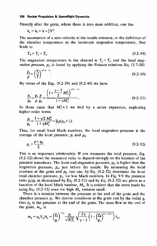
190 Rocket Propulsion & Spaceflight Dynamics
Directly after the grain, where there is zero mass addition, one has
hc = hf= h+kV2
.
The assumption of a zero velocity at the nozzle entrance, or the definition of
the chamber temperature as the isentropic stagnation temperature, thus
leads to
T =Tf=Tc . (9.2-49)
The stagnation temperature in the channel is Ts= T
f, and the local stag-
nation pressure, ps , is found by applying the Poisson relations Eq. (3.7-20)
n /T'xtAt— l)
-=(f)• (9.2-50)
By virtue of the Eqs. (9.2-39) and (9.2-40) we have
P, = £JL = \ i—I—
.
(9.2-51)p p Po l + yM2
a
In those cases that M„« 1 we find by a series expansion, neglecting
higher-order terms
p,_ l + y/2Ml
7—cTwr-~Mpo+l)-
Thus, for small local Mach numbers, the local stagnation pressure is the
average of the local pressure, p, and p ,
Ps= E:y2
. (9.2-52)
This is an important relationship. If one measures the total pressure, Eq.
(9.2-52) shows the measured value to depend strongly on the location of the
pressure transducer. The front-end stagnation pressure, p , is higher than the
stagnation pressure, pc ,just before the nozzle. By measuring the local
pressure at the grain and p , one can, by Eq. (9.2-52) determine the local
total chamber pressure, ps , for low Mach numbers. In Fig. 9.9 the pressure
ratio pjp as determined by Eq. (9.2-51) and by Eq. (9.2-52) are given as a
function of the local Mach number, Ma . It is evident that the error made byusing Eq. (9.2-52) even for high Ma remains small.
There is a relation between the pressure at the end of the grain and the
chamber pressure pc . We denote conditions at the grain end by the index g,
thus pg is the pressure at the end of the grain. The mass flow at the end of
the grain, mg, is
mz = PsW mwi*-
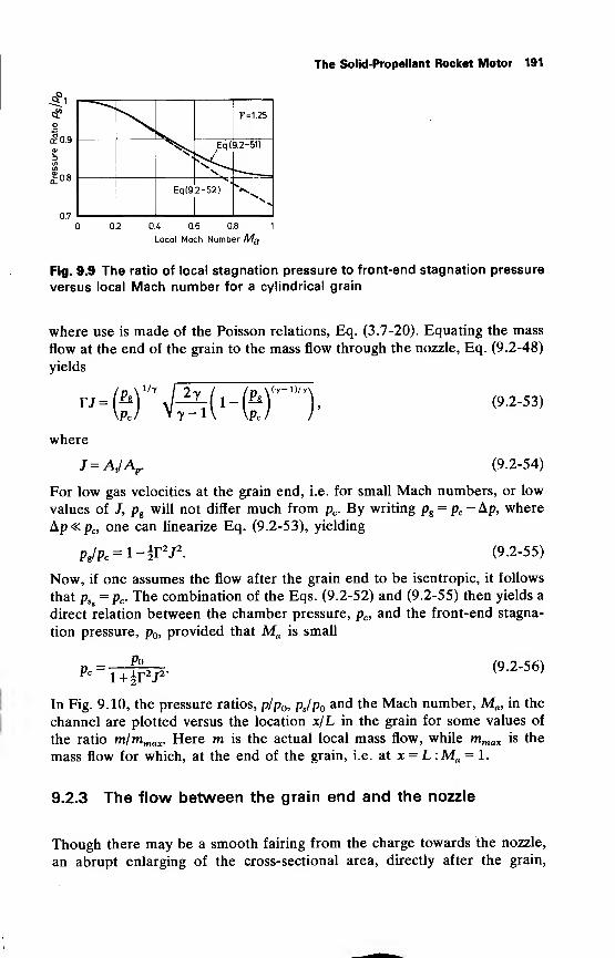
The Solid-Propellant Rocket Motor 191
0.2 OX 0.6 0.8 1
Local Mach Number Mg
Fig. 9.9 The ratio of local stagnation pressure to front-end stagnation pressure
versus local Mach number for a cylindrical grain
where use is made of the Poisson relations, Eq. (3.7-20). Equating the mass
flow at the end of the grain to the mass flow through the nozzle, Eq. (9.2-48)
yields
"-erv3(-er>where
J = AJAP .
(9.2-53)
(9.2-54)
For low gas velocities at the grain end, i.e. for small Mach numbers, or low
values of J, pgwill not differ much from pc . By writing pg
= pc- Ap, where
Ap«pc, one can linearize Eq. (9.2-53), yielding
pg/pc= l-|r2J2 . (9.2-55)
Now, if one assumes the flow after the grain end to be isentropic, it follows
that pSg= pc . The combination of the Eqs. (9.2-52) and (9.2-55) then yields a
direct relation between the chamber pressure, pc, and the front-end stagna-
tion pressure, p ,provided that Ma is small
PoPc 1+ir2/2
' (9.2-56)
In Fig. 9.10, the pressure ratios, p/p , pjp and the Mach number, Ma, in the
channel are plotted versus the location x/L in the grain for some values of
the ratio m/mmax . Here m is the actual local mass flow, while mmax is the
mass flow for which, at the end of the grain, i.e. at x = L :Ma = 1.
9.2.3 The flow between the grain end and the nozzle
Though there may be a smooth fairing from the charge towards the nozzle,
an abrupt enlarging of the cross-sectional area, directly after the grain,
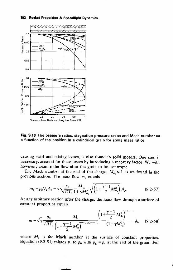
192 Rocket Propulsion & Spaceflight Dynamics
0.2 0J. 0.6 0.8 1
Dimensionless Distance along the Grain x/L
Fig. 9.10 The pressure ratios, stagnation pressure ratios and Mach number asa function of the position in a cylindrical grain for some mass ratios
causing swirl and mixing losses, is also found in solid motors. One can, if
necessary, account for these losses by introducing a recovery factor. We will,
however, assume the flow after the grain to be isentropic.
The Mach number at the end of the charge, Mag =s 1 as we found in the
previous section. The mass flow mgequals
At any arbitrary section after the charge, the mass flow through a surface of
constant properties equals
k y/(7-D/ 1 + J- 1 JVyf2
r Po Ma
y— 1 V
jRTc U +izl Mlt+im -
1)] (i + yMl)-A. (9.2-58)
where Ma is the Mach number at the surface of constant properties.
Equation (9.2-51) relates pc to p with"pgs= pc at the end of the grain. For
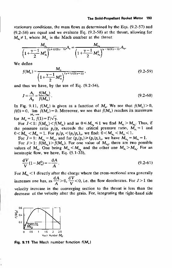
The Solid-Propellant Rocket Motor 193
stationary conditions, the mass flows as determined by the Eqs. (9.2-57) and
(9.2-58) are equal and we evaluate Eq. (9.2-58) at the throat, allowing for
Ma<5* 1, where Ma,
is the Mach number at the throat
AC. A — —^_1 \(t + 1)/(2(7-1))^'
/
,
1+V^) (
M1+^<J
A(7 + l)/(2(7-l))^P'
We define
Wa )= Mn
(i +^«j)(7+l)/(2(7+l)) ' (9.2-59)
(9.2-60)
and thus we have, by the use of Eq. (9.2-54),
At J(MJ
Ap f(MJ'
In Fig. 9.11, /(Ma ) is given as a function of Ma . We see that /(Ma)>0,
f(0)= o, lim /(Ma ) = 0. Moreover, we see that f(Ma ) reaches its maximum
for Ma = l, /(l) = r/V^.
For /<1: f(Mag)<f(MJ and as 0^Mag ^l we find Mat>Mag . Thus, if
the pressure ratio pjpe exceeds the critical pressure ratio, Mai= 1 and
<Mag <Ma,= 1. For pc/pe < {pJpe ) Cr we find: <Mag <Ma< < 1.
For /= 1: Mag=Ma,, and for (pJpe)^(pJPe)cr we have Mflg
=Ma,= 1.
For J>1: /(Mag)>/(Mai ). For one value of Mflg ,
there are two possible
values of Mat. One being Mat
<Ma% and the other one Mat>MUg . For an
isentropic flow, we have, Eq. (5.1-33),
?«-*>--¥• (9.2-61)
For Mflg< 1 directly after the charge where the cross-sectional area generally
increases one has, as -r->0, —— <0, i.e. the flow decelerates. For J> 1 theA V
velocity increase in the converging section to the throat is less than the
decrease of the velocity after the grain. For, integrating the right-hand side
0.6
0.2
0.5 1 1.5 2 2.5
Mach NumberMa
Meg on for
J Mag
Fig. 9.11 The Mach number function f(Ma )
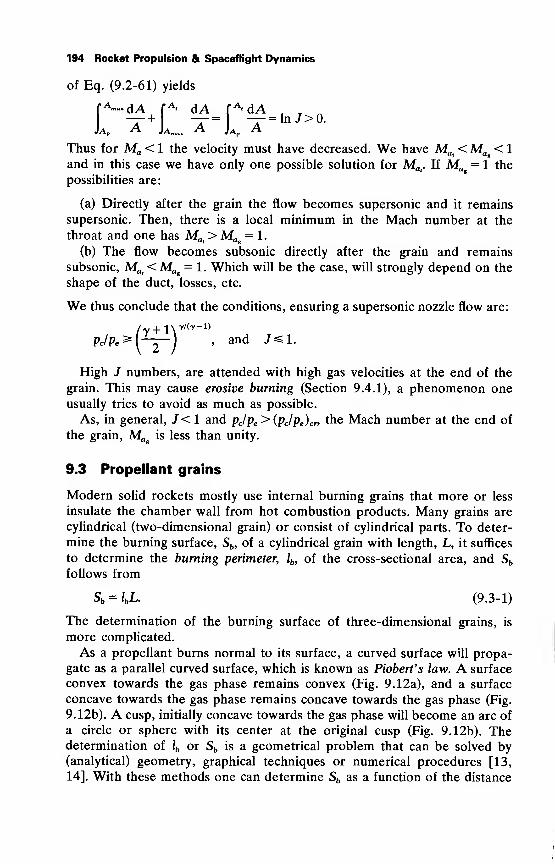
194 Rocket Propulsion & Spaceflight Dynamics
of Eq. (9.2-61) yields
fA— dA p dA_f A'dA
Jap-A jAmax A Jap
-A
Thus for Ma < 1 the velocity must have decreased. We have Mat<Ma < 1
and in this case we have only one possible solution for Ma,. If Mag= 1 the
possibilities are:
(a) Directly after the grain the flow becomes supersonic and it remains
supersonic. Then, there is a local minimum in the Mach number at the
throat and one has Ma >Mn = 1.a, ag
(b) The flow becomes subsonic directly after the grain and remains
subsonic, Mai<Mag
= 1. Which will be the case, will strongly depend on the
shape of the duct, losses, etc.
We thus conclude that the conditions, ensuring a supersonic nozzle flow are:
',y + l\7/(Y-l)(y +1X and J^l.
High J numbers, are attended with high gas velocities at the end of the
grain. This may cause erosive burning (Section 9.4.1), a phenomenon one
usually tries to avoid as much as possible.
As, in general, J<\ and pc/pe > (pJPe)cr> the Mach number at the end of
the grain, Mag is less than unity.
9.3 Propellant grains
Modern solid rockets mostly use internal burning grains that more or less
insulate the chamber wall from hot combustion products. Many grains are
cylindrical (two-dimensional grain) or consist of cylindrical parts. To deter-
mine the burning surface, Sb , of a cylindrical grain with length, L, it suffices
to determine the burning perimeter, lb , of the cross-sectional area, and Sb
follows from
Sb = lbL. (9.3-1)
The determination of the burning surface of three-dimensional grains, is
more complicated.
As a propellant burns normal to its surface, a curved surface will propa-
gate as a parallel curved surface, which is known as Pioberfs law. A surface
convex towards the gas phase remains convex (Fig. 9.12a), and a surface
concave towards the gas phase remains concave towards the gas phase (Fig.
9.12b). A cusp, initially concave towards the gas phase will become an arc of
a circle or sphere with its center at the original cusp (Fig. 9.12b). Thedetermination of lb or Sb is a geometrical problem that can be solved by(analytical) geometry, graphical techniques or numerical procedures [13,
14]. With these methods one can determine Sb as a function of the distance
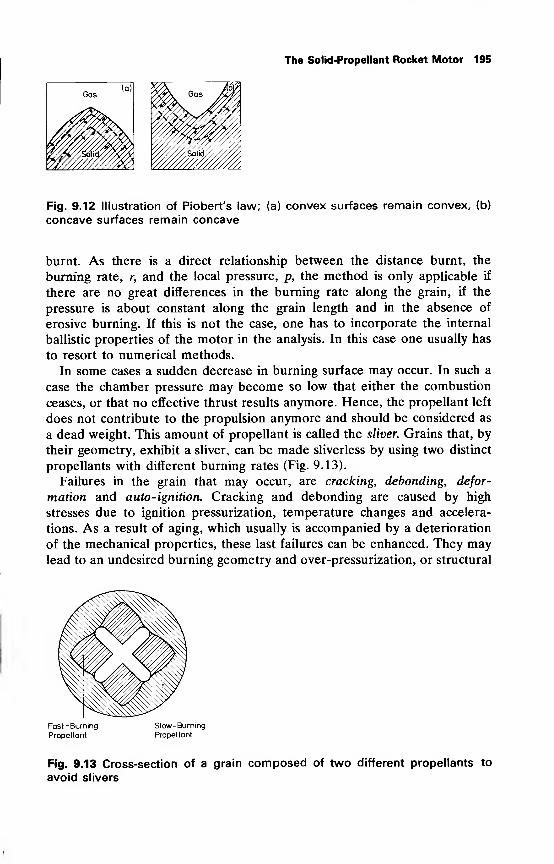
The Solid-Propellant Rocket Motor 195
Fig. 9.12 Illustration of Piobert's law; (a) convex surfaces remain convex, (b)
concave surfaces remain concave
burnt. As there is a direct relationship between the distance burnt, the
burning rate, r, and the local pressure, p, the method is only applicable if
there are no great differences in the burning rate along the grain, if the
pressure is about constant along the grain length and in the absence of
erosive burning. If this is not the case, one has to incorporate the internal
ballistic properties of the motor in the analysis. In this case one usually has
to resort to numerical methods.
In some cases a sudden decrease in burning surface may occur. In such a
case the chamber pressure may become so low that either the combustion
ceases, or that no effective thrust results anymore. Hence, the propellant left
does not contribute to the propulsion anymore and should be considered as
a dead weight. This amount of propellant is called the sliver. Grains that, by
their geometry, exhibit a sliver, can be made sliverless by using two distinct
propellants with different burning rates (Fig. 9.13).
Failures in the grain that may occur, are cracking, debonding, defor-
mation and auto -ignition. Cracking and debonding are caused by high
stresses due to ignition pressurization, temperature changes and accelera-
tions. As a result of aging, which usually is accompanied by a deterioration
of the mechanical properties, these last failures can be enhanced. They maylead to an undesired burning geometry and over-pressurization, or structural
Slow-Burning
Propellant
Fig. 9.13 Cross-section of a grain composed of two different propellants to
avoid slivers
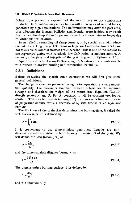
196 Rocket Propulsion & Spaceflight Dynamics
failure from premature exposure of the motor case to hot combustion
products. Deformations may either be a result of creep, or of inertial forces,
generated by high accelerations. The deformations may alter the port area,
thus affecting the internal ballistics significantly. Auto-ignition may result
from a heat build-up in the propellant, caused by internal viscous forces due
to vibrations for instance.
Stress relief, by rounding off sharp corners, or by special slots will reduce
the risk of cracking. Large L/D ratios or large w/D ratios (Section 9.3.1) are
not favorable as internal stresses are concerned. This is one of the reasons to
use segmented grains with relatively low L/D ratios in modern motors. Areview on the structural integrity of the grain is given in Reference [15].
Apart from structural considerations, high L/D ratios are also unfavorable
with respect to erosive burning and combustion instability.
9.3.1 Definitions
Before discussing the specific grain geometries we will first give somegeneral definitions.
The change in chamber pressure during motor operation is a very impor-
tant quantity. The maximum chamber pressure determines the required
strength and therefore the weight of the motor case. Equation (9.2-10)
directly relates pc and Sb . For Sb constant, pc will be constant too, for A,
constant. This is called neutral burning. If Sb increases with time one speaks
of progressive burning, while a decrease of Sb with time is called regressive
burning.
The thickness of the grain that determines the burning-time, is called the
web thickness, w. It is defined by
fJow=\ rdt. (9.3-2)
Jo
It is convenient to use dimensionless quantities. Lengths are non-
dimensionalized by division by half the outer diameter D of the grain. Wewill define the web fraction, w
f,as
and the dimensionless distance burnt, y, as
2 J r dty=-D~-
The dimensionless burning surface, X, is defined by
(9.3-4)
4S,S =5* (9.3-5)
and is a function of y.
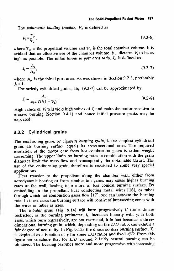
The Solid-Propellant Rocket Motor 197
The volumetric loading fraction, Vb is defined as
Vj=Ie. (9.3-6)
where Tpis the propeilant volume and Vc is the total chamber volume. It is
evident that an effective use of the chamber volume, Tc, dictates V, to be as
high as possible. The initial throat to port area ratio, Ji7is defined as
A (9.3-7)
where Am is the initial port area. As was shown in Section 9.2.3, preferably
Ji<l.For strictly cylindrical grains, Eq. (9.3-7) can be approximated by
J.= ^
. (9.3-8)' 7r/4D2(l-V,)
High values of V, will yield high values of Jtand make the motor sensitive to
erosive burning (Section 9.4.1) and hence initial pressure peaks may be
expected.
9.3.2 Cylindrical grains
The endbuming grain, or cigarette burning grain, is the simplest cylindrical
grain. Its burning surface equals its cross-sectional area. The required
insulation of the motor case from hot combustion gases is rather weight
consuming. The upper limits on burning rates in combination with the grain
diameter limit the mass flow and consequently the obtainable thrust. The
use of the endburning grain therefore is restricted to some very special
applications.
Heat transfer to the propeilant along the chamber wall, either from
aerodynamic heating or from combustion gases, may cause higher burning
rates at the wall, leading to a more or less conical burning surface. By
embedding in the propeilant heat conducting metal wires [16], or tubes
through which hot combustion gases flow [17], one can increase the burning
rate. In these cases the burning surface will consist of intersecting cones with
the wires or tubes as axes.
The tubular grain (Fig. 9.14) will burn progressively if the ends are
restricted, as the burning perimeter, lb, increases linearly with y. If both
ends, which burn regressively, are not restricted, it in fact becomes a three-
dimensional burning grain, which, depending on the L/D ratio, can exhibit a
fair degree of neutrality. In Fig. 9.15a the dimensionless burning surface, £,
is depicted as a function of y for some L/D ratios and fixed d/D. From this
figure we conclude that for L/D around 2 fairly neutral burning can be
obtained. The burning becomes more and more progressive with increasing
198 Rocket Propulsion & Spaceflight Dynamics
Fig. 9.14 The tubular grain
LID. However, for chambers exhibiting a large LID the grain can besegmented, each segment exhibiting an LID that ensures neutral burning.
This method is applied to many segmented motors. Of course, those parts of
the chamber walls exposed to hot combustion gases have to be insulated in
proportion to their time of exposure. Figure 9.15b depicts 2 versus y for
various values of d/D and fixed LID. The curve for d/D = is a limiting
case; it represents a massive cylinder, which is assumed to ignite along its
central axis and both its end surfaces. The neutrality increases with increas-
ing d/D.
Grains that exhibit pure neutral burning are the tubular grain with
restricted ends, burning radially at its inner and outer surface (Fig. 9.16a) andthe rod and shell, also with restricted ends (Fig. 9.16b). The first configura-
tion exposes the chamber walls to the hot combustion products, while in
both the configurations the support is difficult and complicated, and main-
taining the structural integrity until burnout gives rise to serious problems.
27
•2 22.5 -
t 18
13.5
i.5
c//D=0.5 /7D=2.5
2
"
^""v^Oi^"\i
27
.2 22.5
E 18
c 13.5
__£//£ =0.9L/C
,(b)
) = 2
-0.7
0.6
05
—^0 3
^0.2"^01
^
0.25 0.5
Dimensionless Distance Burnt y
0.25 0.5 0.75 1
Dimensionless Distance Burnt y
Fig. 9.15 The dimensionless burning surface of a tubular grain with non-
restricted ends versus the dimensionless distance burnt; (a) for some length
over diameter ratios and (b) for some inner over outer diameter ratios
The Solid-Propellant Rocket Motor 199
(a) (b)
Fig. 9.16 Neutral burning grains, (a) The tubular grain with restricted ends,
burning at its inner and outer surface, (b) The rod and shell configuration
The slotted tube grain, which exhibits a high loading fraction, is depicted in
Fig. 9.17. At its ends, it may either be restricted or not. In most cases at
least one end is restricted and bonded to the front end of the chamber. The
slotted portion of the grain provides regressive burning. The burning pro-
gresses in radial, tangential and longitudinal directions. The number of slots,
N, the slot length, /, and the width of the slots, 2r, are independent variables,
together with the grain length, L, the outer diameter, D, and the inner
diameter d. As the port area in the slotted portion is increased with respect
to that in the tubular section, this provides a way to avoid high gas
velocities. Stone [18] has analysed the geometry of the slotted tube in detail
and gives excellent graphs that can be used in slotted tube grain design [19].
As an example, Fig. 9.17 shows the variation of 2 with y for two specific
slotted tube grains.
4%a4&,
•*3
y.N
|^W\V/5v/W/,1
,2 80
£ _
40
5W5***"":^rr^~
/7=2/7=3
0.15 0.30 0.45
Dimensionless Distance Burnt y
Fig. 9.17 The slotted tube grain; its configuration and an example of its
burning surface versus the dimensionless distance burnt for d/D = 0.16; UD =
8.3; //D = 5.32; 2r/D = 0.06 and N = 2 and W = 3 (Reference [20])
200 Rocket Propulsion & Spaceflight Dynamics
_D _, D
Fig. 9.18 Some multiperforated grains
The grain geometries discussed so far had no sliver. Multiperforated grains,
such as the ones depicted in Fig. 9.18, exhibit slivers. At the end of the
burning, the grain may collapse. If the pressures in the various ports are
different from each other, grain collapse may occur before burnout. It is
easily shown that for a multiperforated grain a sufficient condition for equal
pressures in all ports is that all channels exhibit the same Sb/Apratio.
The star configuration (Fig. 9.19) has been used in many solid motors. It
is a radially burning cylindrical grain. Neutrality can be obtained by the
interaction of the regressive burning star points and the progressive burning
tube. As is obvious from Fig. 9.19b, the star is defined by six independent
variables: N, e, tj, r, w and D. Stone [21] gives an extensive description of
the calculation of the burning surface of the star. A slightly different
approach is followed by Vandenkerckhove [22]. The burning perimeter of the
star can be determined by analysing a section such as depicted in Fig. 9.19b.
There are three different regions or phases: I, II and III. Region I will either
burn regressively, neutrally or progressively, depending on 17, r and e.
Region II will burn progressively, while region III, the sliver, will burnregressively, if it burns at all. In Fig. 9.20, the burning surfaces of twospecific stars are depicted as a function of y.
Sliver
Fig. 9.19 The star configuration and its nomenclature
The Solid-Propellant Rocket Motor 201
0.2 0.3 0A 0.5
Dimensionless Distance Burnt y
Fig. 9.20 The dimensionless burning surface versus the dimensionless dis-
tance burnt for two specific star configurations for 21/D = 0.54; 2r/D = 0.049;
2w/D = 0.46 and L/D=15.2 (Reference [20])
The wagon-wheel (Fig. 9.21a) is another often used grain configuration,
with two more variables than the star: the length and angle, |3, of the spokes.
The wagon-wheel is used if small web fractions are required. Vandenkerck-hove [22] gives an analysis of the wagon-wheel geometry. Next to the
conventional wagon-wheel there is also the dendrite or forked wagon-wheel(Fig. 9.21b). It may exhibit a higher volumetric loading fraction. Theimportant variables can be calculated according to Peretz [23]. The wagon-wheel configuration can exhibit more phases than the star as the number of
phases increases with the number of independent variables. It is possible for
the wagon-wheel that, when the spokes are all burnt, the burning perimeter
decreases discontinuously. Therefore the wagon-wheel is suitable as a boost-
sustain grain.
In those cases that the gas velocities become too high, and erosion is to be
expected, the tapering of the end port of the grain provides means to reduce
the gas velocities and thus the danger of erosive burning.
Fig. 9.21 (a) The wagon-wheel configuration, (b) The dendrite or forked
wagon-wheel
202 Rocket Propulsion & Spaceflight Dynamics
9.3.3 Three-dimensional grains
In the foregoing section we discussed cylindrical grains. Some of them, the
tubular grain with unrestricted ends, and the slotted tube, exhibited three-
dimensional characteristics. There are non-cylindrical grains in use whoseburning characteristics depend strongly on the shape of the outer surface
too. The spherical grains, an example of which is depicted in Fig. 9.22, forman important class. They may be used if aerodynamic drag is not important.
Also, if system requirements dictate limits on the moment of inertia andweight, a spherical motor may be a favorable solution. These motors are
used or have been proposed as apogee-kick motors, final stage motors or
motors for interplanetary spacecraft. They have the potential of a high
volumetric loading fraction. Methods to determine the ballistic properties of
spherical motors are given by Segal [24] and Berti [25]. A simple criterion to
ensure the structural integrity of the spherical grain is discussed by Toda[26].
The conocyl (Fig. 9.23a) is another three-dimensional grain. The namestems from cone-in-cylinder. Both conical burning surfaces burn regres-
sively, while the central perforation burns progressively. In combination
with the chamber envelope the charge can provide neutrality for a range of
LID values up to about 4. Those areas of the chamber that will be exposedto hot combustion gases have to be insulated, in direct proportion to their
time of exposure.
The finocyl, an acronym for fin-in-cylinder (Fig. 9.23b) is used in modernICBM systems. The finocyl can provide long burning-times for relatively low
LID ratios. Instead of the radial slot of the conocyl, the finocyl has axial
slots to provide regressive burning. The ballistics of the finocyl do not differ
much from those of the conocyl, but in some cases fabrication is considered
easier. Other system requirements, however, such as thrust reversal, or
thrust termination ports at the front end of the chamber, require an addedflow channel volume in the forward end, which may make the conocyl a
desirable configuration.
Fig. 9.22 An example of a spherical grain
The Solid-Propellant Rocket Motor 203
(a)
Fig. 9.23 (a) The conocyl design, (b) The finocyl design
Apart from the geometries mentioned, many more configurations exist. Anexcellent survey is given by Billheimer and Wagner [27], while Williams [3]
also gives extensive information on the determination of burning surface,
port area and other ballistic properties. Reference [13] provides excellent
general information on grain geometries, design and verification andanalysis, while reference [15] discusses the structural integrity of solid
propellant grains.
9.4 Burning rate augmentation
In the previous sections, we assumed the actual burning rate in rocket
motors to equal the one measured in a strand burner. This is not always the
case. If high gas velocities, or high mass flow densities, pV, are encountered,
the actual burning rate may substantially exceed the burning rate as meas-ured in the Crawford bomb. This is due to erosive burning. The burning rate
can also be affected by introducing a fluid into the thrust chamber. This is
sometimes done to provide thrust magnitude control. The fluid may either
be inert or may be a high-energy liquid oxidizer which, in combination with
a propellant exhibiting an exponent near unity, produces a wide range of
throttling [28].
Another factor that influences the burning rate is a time dependentpressure. We mentioned already in Section 9.1.3, that burning rate data, as
obtained from strand burner measurements, only hold for constant pressure
processes.
Accelerations, internal stresses in the propellant and specific motor effects
can also affect the propellant combustion. It is current practice, therefore, to
determine r over specified operational pressure and temperature ranges in
small rocket motors, Ballistic Evaluation Motors, or BEM's, too [29].
We will not discuss the above mentioned effects in detail, as this goes
beyond the scope of this book, but restrict ourselves to some general
remarks.
9.4.1 Erosive burning
Most of the work on erosive burning, which is still a field of experimental
and theoretical research, is on a semi-empirical basis. If high gas velocities
204 Rocket Propulsion & Spaceflight Dynamics
s; 12
EE~"
10
65% AP
35 % Polvester
w_
N,
\df6 8 10 12
Pressure p (MPd)
U 6 8 10
Pressure p (MPa)
Fig. 9.24 The dependence of erosion on the velocity and pressure, or density
(Reference [31])
or mass flow densities are met in the propellant grain, there will be a strong
heat transfer into the propellant. In Sections 9.1.3 and 9.1.4, we saw that
heat transfer is a prime rate controlling factor.
Formulae that correlate erosive burning rate data, generally, are of one of
the following forms:
(9.4-1)
or
rh = r+r
er. (9.4-2)
Here rb is the actual burning rate, r stands for the burning rate as obtained
from strand burner data, re is the erosive burning rate, and e is called the
erosion function. Both Lenoir and Robillard [30], and Marklund and Lake
[31] give semi-empirical expressions for the erosive burning rate. These
expressions relate the effect of erosion to the mass flow density pV. If the
chamber temperature, Tc, is about constant, the density is proportional to
the pressure. Figure 9.24 clearly illustrates that the erosion increases with
increasing pressure, or density and velocity. The erosion function, e, is more
widely used than the erosive burning rate. Kreidler [32] gives a relation
between mass flow density and the erosion function. It has been observed
too that the Mach number, Ma , may influence the erosion. For more
information the reader is referred to Williams [3].
9.4.2 Pressure-induced burning rate changes
If the pressure is not constant, but varies with time, the burning rate will be
time dependent too. In general, r(t) will not follow the simple steady-state
burning rate laws, Eq. (9.1-1) or Eq. (9.1-2). From combustion models [7, 9,
11] a theoretical non-stationary burning rate can be determined. A thorough
experimental check, however, is a necessity.
The Solid-Propellant Rocket Motor 205
If one deals with fluctuating pressures, it is, in many cases, customary and
convenient to use, instead of the burning rate, related complex functions [4]:
the admittance, Ab , or the response, Rb, of the propellant. In principle, the
admittance and response functions of propellants, can be deduced from
combustion models. In practice they have to be measured in special devices
such as T- or L* -burners.
For non-oscillatory pressure changes, the GDF model sometimes yields
satisfactory predictions of the burning rate behavior of composite propel-
lants. Von Elbe [33] first derived a simple expression for the burning rate, r,
valid both for composite and double-base propellants, which has been
improved by others [4, 10],
r--P"(l +»^g). (9.4-3)
Here k is the thermal diffusivity of the propellant, n is the pressure exponent
from the steady-state burning rate law, and a is the coefficient in this law. In
many cases Eq. (9.4-3) yields fairly good correlations between pressure and
burning rate.
In case of large negative values of dp/dt, propellant extinction may take
place; the phenomenon is known as dpjdt extinguishment.
The dependence of the combustion on variable pressures is of a highly
complicated character and cannot be given in this chapter. It is mentioned
here, because the reader should be aware that non-stationary problems in
solid-propellant rocketry are not merely a simple extension of the existing
stationary theory.
9.4.3 Acceleration-induced burning rate augmentation
It is a well-known fact that accelerations may influence the burning rate.
These accelerations, as experienced by the propellant, are caused by the
acceleration of the whole vehicle, but can also be spin-induced. For a
specific propellant the burning rate augmentation is dependent on the
magnitude and orientation of the acceleration vector with respect to the
burning surface, and the pressure level [34]. It has also been shown that the
composition of the propellant has much to do with the acceleration-induced
burning rate augmentation [35].
Not only the burning rate itself, but also the burning rate exponent maychange due to acceleration. In general, the accelerations have to be of the
order of about 100 m/s2 before a noticeable deviation from the burning rate
occurs. By how much the rate augmentation is also due to strain induced in
the propellant itself, and to what extent to different flame structures, cannot
be said at the present time. In most cases, propellant strain will also lead to
different burning rates. As no general theories are available, the influence of
the acceleration on the burning rate has to be determined experimentally for
the propellant under consideration.
206 Rocket Propulsion & Spaceflight Dynamics
References
1 Karnesky, A. L. and Colucci, S. E. (1975), Recent occurrences of
combustion instability in solid rocket motors—an overview, J. Spacecraft,
12, 33-38.
2 Shorr, M. and Zaehringer, A. J. (ed.) (1967), Solid Rocket Technology,
John Wiley, New York, p. 50.
3 Williams, F. A., Barrere, M. and Huang, N. C. (1969), Fundamental
Aspects of Solid Propellant Rockets, AGARDograph 116, Technivision
Services, Slough.
4 Price, E. W. and Culick, F. E. C. (1969), Combustion of Solid Rocket
Propellants, AIAA, New York.
5 Dadieu, A., Damm, R. and Schmidt, E. W. (1968), Raketentreibstoffe,
(in German), Springer, Vienna.
6 Barrere, M., Jaumotte, A., Fraeijs de Veubeke, B. and Vandenkerck-
hove, J. (1960), Rocket Propulsion, Elsevier, Amsterdam.
7 Summerfield, M. (ed.) (1960), Solid Propellant Rocket Research,
Academic Press, New York, p. 141-182.
8 Steinz, J. A., Stang, P. L. and Summerfield, M. (1968), The Burning
Mechanism of AP-based Composite Solid Propellants, AIAA Paper
68-658, AIAA, New York.
9 Beckstead, M. W., Derr, R. L. and Price, C. F. (1968), A model of
composite solid propellant combustion based on multiple flames, AIAAJ., 6, 2200-2207.
10 Stamets, L. E. and Weiss, R. R. (1971), Analytical Models of Solid
Propellant Combustion, paper presented at the 22nd I.A.F. Congress,
Brussels.
11 Hamann, R. J. (1974), Three Solid Propellant Combustion Models, AComparison and Some Applications to Non-Steady Cases, MemorandumM-215, Delft University of Technology, Dept. of Aeron. Eng.,
Delft.
12 Boggs, T. L., Zurn, D. E., Strahle, W. C, Handley, J. C. and Milkie, T.
T. (1973), Mechanisms of Combustion, Final Report, NWC TP-5514,
Naval Weapons Center, China Lake.
13 Anon. (1972), Solid Propellant Grain Design and Internal Ballistics,
NASA SP-8076, Washington.
14 Peterson, E. G., Nielsen, C. C, Johnson, W. C, Cook, K. S. and
Barron, J. G. (1968), Generalized Coordinate Grain Design and Internal
Ballistics Evaluation Program, AIAA Paper 68-490, AIAA, New York.
15 Anon. (1973), Solid Propellant Grain Structural Integrity Analysis,
NASA SP-8073, Washington.
16 Schaefer, J. (1973), Schuboptimierung von Feststoffraketen, Z. Flug-
wiss., 21, 195-202.
17 Caveny, L. H. and Sowyer, T. T. (1967), Solid Propellant Burning Along
a Tube Heated by Combustion Gas Influx, AIAA Paper 67-102, AIAA,New York.
The Solid-Propellant Rocket Motor 207
18 Stone, M. W. (1961), Slotted tube grain design, A.R.S. J., 31, 223-228.
19 Stone, M. W. (I960), The Slotted Tube Grain Design, Rep. S-27, Rohm& Haas Comp., Huntsville.
20 Schoyer, H. F. R. (1968), The Design of a Rocket Motor for the Second
Stage of a Two Stage Sounding Rocket (in Dutch), MemorandumM-131, Delft University of Technology, Dept. of Aeron.
Eng./Royal Naval Institute, Delft/Den Helder.
21 Stone, M. W. (1958), A practical mathematical approach to grain
design, Jet. Prop., 28, 236-244.
22 Vandenkerckhove, J. (1958), Internal-Burning Star and Wagon-Wheel
Designs for Solid-Propellant Grains. Publication of the Universite Libre
de Bruxelles, Institute d'Aeronautique, Brussels.
23 Peretz, A. (1969), A practical mathematical approach to the dendrite
design of solid propellant grains, J. Spacecraft, 6, 944-946.
24 Segal, H. M. (1960), Design method for spherical grains, A.R.S. J., 30,
370-371.
25 Berti, J. W. and Wrubel, J. A. (1962), Calculating burning surface areas
of internal burning spherical propellant charges, A.R.S. J., 32, 1283-
1285.
26 Toda, Y., Nagaoka, T., Ueno, L., Orado, Y. and Kunio, T. (1973),
Failure criterion for a propellant of spherical solid rocket motor, J.
Spacecraft, 10, 807-808.
27 Billheimer, J. S. and Wagner, F. R. (1970), The Morphological Con-
tinuum in Solid Propellant Grain Design, Proceedings of the 19th IAF
Congress, Vol 3, Pergamon Press/PWN-Polish Scientific Publishers,
Oxford, p. 153-188.
28 McDonald, A. J. (1971), On-Off and Acceleration Control of Solid
Rockets, SAE Paper 710767, SAE, New York.
29 Miller, W. H. and Barrington, D. K. (1970), A review of contempory
solid rocket motor performance prediction techniques, J. Spacecraft, 7,
225-237.
30 Lenoir, J. M. and Robbillard, G. (1957), A Mathematical Method to
Predict the Effects of Erosive Burning in Solid Propellant Rockets,
Proceedings of the Sixth Symposium on Combustion, Reinhold, NewYork, p. 663-667.
31 Marklund, T. and Lake, A. (1960), Experimental investigation of
propellant erosion, A.R.S. J., 30, 173-178.
32 Kreidler, J. W. (1964), Erosive Burning; New Experimental Techniques
and Methods of Analysis, AIAA Paper 64-155, AIAA, New York.
33 von Elbe, G. (1966), Solid Propellant Ignition and Response of Combus-
tion to Pressure Transients, AIAA Paper 66-668, AIAA, New York.
34 Northam, G. B. (1972), Effects of Orientation of the Acceleration Vector
on Burning-Rate Augmentation, NASA TN D-6952, Washington.
35 Northam, G. B. (1972), Effects of Propellant Composition Variables on
Acceleration Induced Burning-Rate Augmentation, NASA TN D-6923,
Washington.
10 The Liquid-Propellant RocketMotor
In Chapter 9 we discussed the solid rocket motor and also paid brief
attention to the merits of the liquid motor. In this chapter we will give an
jjoverview of the liquid propulsion system. The liquid motor (Fig. 10.1)
j;|consists of one or more propellant tanks, a feed system, a combustion
fehamber and an expansion nozzle. If monopropellants are used, only oneItank is needed. In other cases, fuel and oxidizer are stored in separate tanks.
^Smaller rockets often use (inert) pressurization gas to force the propellants
into the combustion chamber (pressure fed). The larger engines use pumps,
driven by turbines, to feed the combustion chamber. In modern staged-
combustion motors, precombustion chambers may be used. In this precom-
bustion chamber the fuel and part of the oxidizer react, and the precombus-
tion products drive the turbines before entering the main combustion
chamber, where the remainder of the oxidizer reacts with the precombustion
products (Fig. 10.2a). If the turbines are not driven by precombustion
products, they may then use combustion gases from the main combustion
chamber, tap-off system (Fig. 10.2b), or the cooling fluid from the combustion
chamber or nozzle, topping cycle (Fig. 10.2c), or bleed-off system in which
case the turbine gases are dumped, or a separate gas generator (Fig. 10.2d).
Except for motors with a low combustion temperature, or short burning
times, active cooling by one of the propellants is imperative in most cases. In
absence of an active cooling system, either heat sink, radiation cooling or
other means of cooling are used (Section 10.5).
A regulating system to keep the pressures and mass flows within their
required range is needed, just like a control system for the starting andshut-down sequence of the motor. The starting of the motor usually is
accomplished by means of a separate gas generator or by stored pressure gas
which starts the turbines, whereafter the propellants are injected into the
combustion chamber and subsequently ignited.
In this chapter we will devote our attention to those subjects that
directly determine the performance of the liquid motor, such as propellants,
pumps and turbines, and to typical liquid motor components such as tanks,
injectors and cooling systems. We will avoid going into details, such as
feedline dynamics, valves and seals, or injector performance analysis. Thesesubjects, though of high interest to the rocket engineer are of too specialized
a character and often rely heavily on experiments.
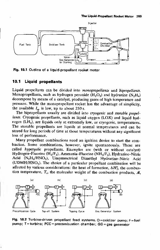
Fuel Tank Oxidizer Tank
The Liquid-Propellant Rocket Motor 209
Injector
Fig. 10.1 Outline of a liquid-propellant rocket motor
10.1 Liquid propellants
Liquid propellants can be divided into monopropellants and bipropellants.
Monopropellants, such as hydrogen peroxide (H2 2) and hydrazine (N2H4)
decompose by means of a catalyst, producing gases of high temperature andpressure. While the monopropellant rocket has the advantage of simplicity,
the available Isp is low, up to about 250 s.
The bipropellants usually are divided into cryogenic and storable propel-
lants. Cryogenic propellants, such as liquid oxygen (LOX) and liquid hyd-rogen (LH2), are liquids only at extremely low, or cryogenic, temperatures.
The storable propellants are liquids at normal temperatures and can bestored for long periods of time at those temperatures without any significant
loss of performance.
Many propellant combinations need an ignition device to start the com-bustion. Some combinations, however, ignite spontaneously. These are
called hypergolic propellants. Examples are (with or without catalyst)
Hydrogen-Fluorine (H2/F2), Ammonia-Fluorine (NH3/F2), Hydrazine-NitricAcid (N2H4/HN03), Unsymmetrical Dimethyl Hydrazine-Nitric Acid(UDMH/HNO3). The choice of a particular propellant combination will beaffected by various considerations: the heat of formation, AH°, the combus-tion temperature, Tc , the molecular weight of the combustion products, M,
(b) <c) (d)
[°3=CfHt mPCC
E==[f3=0t rjD==Gp^f
Precombustion Cycle Tap-off System Topping Cycle Gas Generator System
Fig. 10.2 Turbine-driven propellant feed systems. O =oxidizer pump;F=fuelpump; T = turbine; PCC = precombustion chamber; GG = gas generator
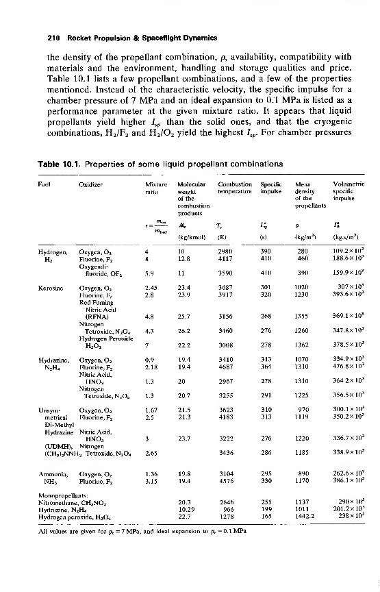
210 Rocket Propulsion & Spaceflight Dynamics
the density of the propellant combination, p, availability, compatibility with
materials and the environment, handling and storage qualities and price.
Table 10.1 lists a few propellant combinations, and a few of the properties
mentioned. Instead of the characteristic velocity, the specific impulse for a
chamber pressure of 7 MPa and an ideal expansion to 0.1 MPa is listed as a
performance parameter at the given mixture ratio. It appears that liquid
propellants yield higher Isp than the solid ones, and that the cryogenic
combinations, H2/F2 and H2/02 yield the highest Isp . For chamber pressures
Table 10.1. Properties of some liquid propellant combinations
Fuel Oxidizer Mixture Molecular Combustion Specific Mean Volumetric
ratio weight
of the
combustion
products
temperature impulse density
of the
propellants
specific
impulse
THoxJic Tc K P 1%
™fuel
(kg/kmol) (K) (s) (kg/m3) (kg.s/m
3)
Hydrogen, Oxygen, 2 4 10 2980 390 280 109.2 xlO3
H2 Fluorine, F2
Oxygendi-
8 12.8 4117 410 460 188.6 X10³
fluoride, OF2 5.9 11 3590 410 390 159.9 xlO3
Kerosine Oxygen, 2 2.45 23.4 3687 301 1020 307 xlO3
Fluorine, F2 2.8 23.9 3917 320 1230 393.6 xlO3
Red Fuming' Nitric Acid(RFNA) 4.8 25.7 3156 268 1355 369.1 xlO3
Nitrogen
Tetroxide, N2 4 4.3 26.2 3460 276 1260 347.8 xlO3
Hydrogen Peroxide
H2 2 7 22.2 3008 278 1362 378.5 xlO3
Hydrazine, Oxygen, 2 0.9 19.4 3410 313 1070 334.9 xlO3
N2H4 Fluorine, F2
Nitric Acid,
2.18 19.4 4687 364 1310 476.8 xlO3
HN03 1.3 20 2967 278 1310 364.2 xlO3
Nitrogen
Tetroxide, N2 4 1.3 20.7 3255 291 1225 356.5 xlO3
Unsym- Oxygen, 2 1.67 21.5 3623 310 970 300.1 xlO3
metrical Fluorine, F2 2.5 21.3 4183 313 1119 350.2 xlO3
Di-Methyl
Hydrazine Nitric Acid,
HNO3 3 23.7 3222 276 1220 336.7 xlO3
(UDMH), Nitrogen
(CH3)2NNH 2 Tetroxide, N2 4 2.65 3436 286 1185 338.9 xlO3
Ammonia, Oxygen, 2 1.36 19.8 3104 295 890 262.6 xlO3
NH3 Fluorine, F2 3.15 19.4 4576 330 1170 386.1 xlO3
Monopropellants:
Nitromethane, CH3N02 20.3 2646 255 1137 290 xlO3
Hydrazine, N2H4 10.29 966 199 1011 201.2X10³
Hydrogen peroxide, H2 2 22.7 1278 165 1442.2 238 xlO3
All values are given for pc= 7 MPa, and ideal expansion to pe = 0.1 MPa
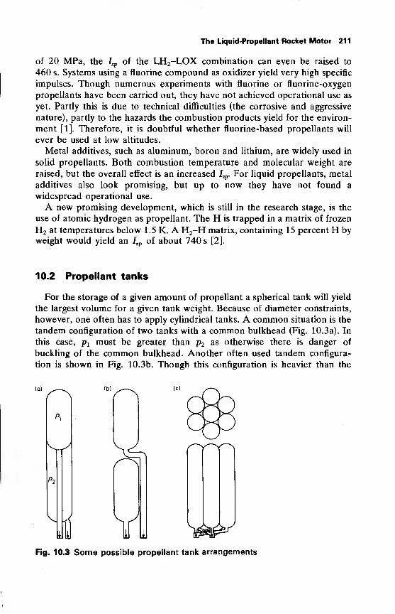
The Liquid-Propellant Rocket Motor 211
of 20 MPa, the Isp of the LH2-LOX combination can even be raised to
460 s. Systems using a fluorine compound as oxidizer yield very high specific
impulses. Though numerous experiments with fluorine or fluorine-oxygen
propellants have been carried out, they have not achieved operational use as
yet. Partly this is due to technical difficulties (the corrosive and aggressive
nature), partly to the hazards the combustion products yield for the environ-
ment [1]. Therefore, it is doubtful whether fluorine-based propellants will
ever be used at low altitudes.
Metal additives, such as aluminum, boron and lithium, are widely used in
solid propellants. Both combustion temperature and molecular weight are
raised, but the overall effect is an increased Isp. For liquid propellants, metal
additives also look promising, but up to now they have not found a
widespread operational use.
A new promising development, which is still in the research stage, is the
use of atomic hydrogen as propellant. The H is trapped in a matrix of frozen
H2 at temperatures below 1.5 K. A H2-H matrix, containing 15 percent H byweight would yield an Isp of about 740 s [2].
10.2 Propellant tanks
For the storage of a given amount of propellant a spherical tank will yield
the largest volume for a given tank weight. Because of diameter constraints,
however, one often has to apply cylindrical tanks. A common situation is the
tandem configuration of two tanks with a common bulkhead (Fig. 10.3a). In
this case, px must be greater than p2 as otherwise there is danger of
buckling of the common bulkhead. Another often used tandem configura-
tion is shown in Fig. 10.3b. Though this configuration is heavier than the
(a) (b) (0
v,.^
V Ayy i HI
Fig. 10.3 Some possible propellant tank arrangements
212 Rocket Propulsion & Spaceflight Dynamics
one with the common bulkhead, it is easier to produce. A multi-tank
arrangement, such as used on the Saturn IB, is depicted in Fig. 10.3c.
In most cases, the walls of the tanks are the outer-walls of the vehicle.
They have to provide the necessary strength to bending moments on the
vehicle and they have to transfer the thrust. Often they are subjected to
aerodynamic heating. A short total tank length is attractive from the
viewpoint of strength and weight. It can be achieved, for instance, by the use
of a common bulkhead, or by careful shaping of the bulkheads [3].
Depending on the feed system, the tank will be submitted to high or
moderate internal pressures. For pressure-fed engines, where the tank
pressure has to overcome the chamber pressure and the pressure loss in
ducts and injector, the tank pressure may be as high as 6 MPa. For
pump-fed systems lower pressures suffice, up to 0.5 MPa. These tank
pressures are necessary to suppress cavitation (Section 10.3.1) in the pumps,
but also to provide the vehicle with the necessary stiffness.
The total tank volume required consists of the volume of the propellant
that is used for propulsion, the propellant volume left in tanks, ducts and
cooling system after shut-down, the boiled-off propellant volume, and the
tank ullage volume, i.e. the tank volume filled with gas.
Because of the vehicle's motion, sloshing of the propellant will occur. This
may have three different, unfavorable effects: it may adversely affect the
vehicle's stability, it causes structural loads, and it will cause a severe mixing
of gas and liquids. To suppress sloshing, baffles are installed in the tank to
dampen the fluid motion. An analysis of slosh loads is given in Reference [4]
and by Woodward [5]. Even if baffles are present, special precautions must
be taken to ensure that most of the gas bubbles are removed from the
propellant before it enters the feedlines [6].
If the rocket coasts, the propellant may, if no special precautions are
taken, not be near the sump, so that no ignition is possible. To ensure
positive propellant expulsion, inflatable diaphragms or a piston between the
ullage and the propellant can be used, which will also suppress sloshing.
Another way to ensure positive expulsion is by means of a capillary barrier.
This device consists of a plate with many orifices located near the sump, and
the fluid surface tension will prevent the gas entering under the plate [6, 7].
A third method to ensure ignition after coasting is the use of small (Vernier)
rockets, which give the vehicle a sufficiently large acceleration to position
the propellant at the sump.
Special provisions have to be taken to minimize the dip in the propellant
surface near the sump when the tank is being emptied. If this dip becomes too
large, gas may enter the feedlines, causing a motor malfunction. This
phenomenon is known as 'vapor pull through' [8].
To pressurize the tank, an inert pressurization gas can be used. In former
days N2 was widely used, nowadays mostly He is used, which, due to its low
molecular weight requires less mass. For LH2 tanks compressed H2 can be
used. As during the expansion from the storage bottles the gas cools,
The Liquid-Propellant Rocket Motor 213
especially for pressure-fed systems, the pressure of the stored gas must be
sufficiently high, often as high as 30 MPa, and heating of the gas by thrust
chamber heat exchangers may be necessary. As during propellant expulsion
the gas in the propellant tanks also cools down, the tanks are often provided
with a heating system too. Tank pressurization can also be achieved by MainTank Injection (MTI). This system, which can be used for hypergolic
propellant combinations, employs the injection of small quantities of fuel
and oxidizer into the main oxidizer and fuel tanks respectively. Only a small
bottle of pressure gas is needed now to overcome the tank pressure.
10.3 The propellant feed system
In order to enter the combustion chamber, the propellant pressure at the
chamber entrance has at least to equal the chamber pressure. This is
achieved either by means of pumps (pump-fed) or by pressurized tanks
(pressure -fed). The tank pressure at the sump consists of the ullage pressure
pu and the hydrostatic pressure ph , which depends on the vehicle accelera-
tion.
For pump-fed systems, the pumps are usually located near the combustion
chamber and the tank pressure has to overcome the pressure losses in the
feedlines. The pressure at the pump entrance has to be sufficiently high to
avoid cavitation.
As for the pressure-fed system all pressure losses and the chamberpressure have to be overcome by a fairly high tank pressure, the tanks
become relatively heavy. Which system is chosen for a particular vehicle will
depend on a performance and cost analysis. For motors having low chamberpressures and short operation times, and for small rockets and upper stages,
the pressure-fed system may prove to be the most suitable one; in other
cases one will usually prefer a pump-fed system.
The feedlines transport the propellants to the thrust chamber or to the
turbopumps. As neither the vehicle nor the feedlines are infinitely stiff, a
closed-loop coupling between the vehicle's longitudinal structural modes,
the feed system and the chamber pressure may result, a phenomenon which
is known as POGO, and which is described lucidly by Rubin [9] and
Rasumoff and Winje [10]. Feedline dynamics and instabilities in liquid
rocket motors are treated by various authors [11, 12, 13]. A general discus-
sion of these instabilities is given by Harrje and Reardon [14].
10.3.1 Pumps
Most liquid-propellant rockets use pumps of the centrifugal type, as these
are light-weight, high-performance, small-volume pumps. The required
power is delivered by one or more turbines. Usually, pumps and turbines are
built together to compact turbopump units.
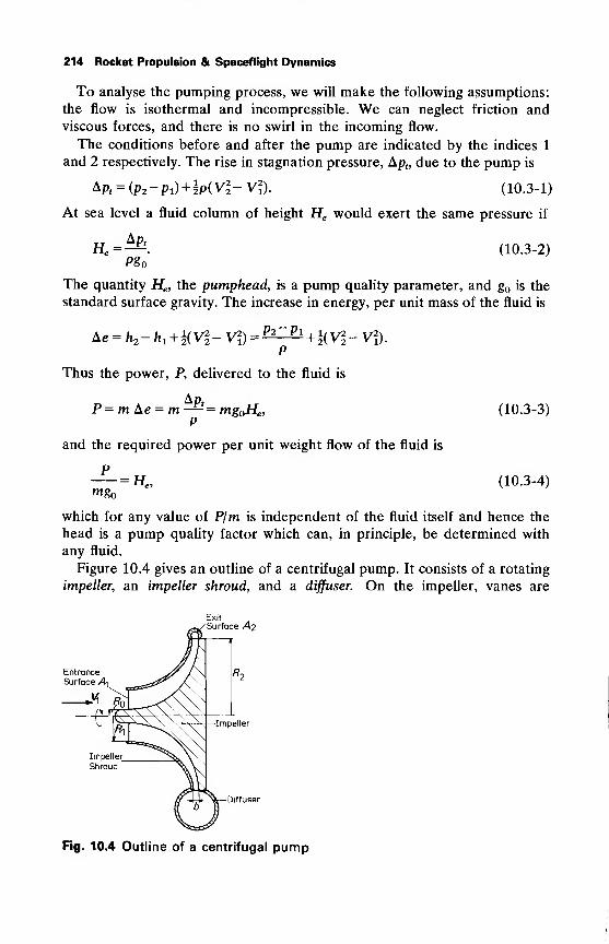
214 Rocket Propulsion & Spaceflight Dynamics
To analyse the pumping process, we will make the following assumptions:
the flow is isothermal and incompressible. We can neglect friction andviscous forces, and there is no swirl in the incoming flow.
The conditions before and after the pump are indicated by the indices 1
and 2 respectively. The rise in stagnation pressure, Ap„ due to the pump is
Ap. = (P2-Pi) + 2P(Vi- V\). (10.3-1)
At sea level a fluid column of height He would exert the same pressure if
Ap,H =PS
(10.3-2)
The quantity He, the pumphead, is a pump quality parameter, and g is the
standard surface gravity. The increase in energy, per unit mass of the fluid is
^e = h2-h 1 + k(V22-V2
1 )=^^ + l(V22 -Vi).
Thus the power, P, delivered to the fluid is
AptP = m Ae = m— = mg He ,
P
and the required power per unit weight flow of the fluid is
P
™go= H„
(10.3-3)
(10.3-4)
which for any value of P/m is independent of the fluid itself and hence the
head is a pump quality factor which can, in principle, be determined with
any fluid.
Figure 10.4 gives an outline of a centrifugal pump. It consists of a rotating
impeller, an impeller shroud, and a diffuser. On the impeller, vanes are
Entrance
Surface A\
M
Exit
Surface A2
Impeller
Diffuser
Fig. 10.4 Outline of a centrifugal pump
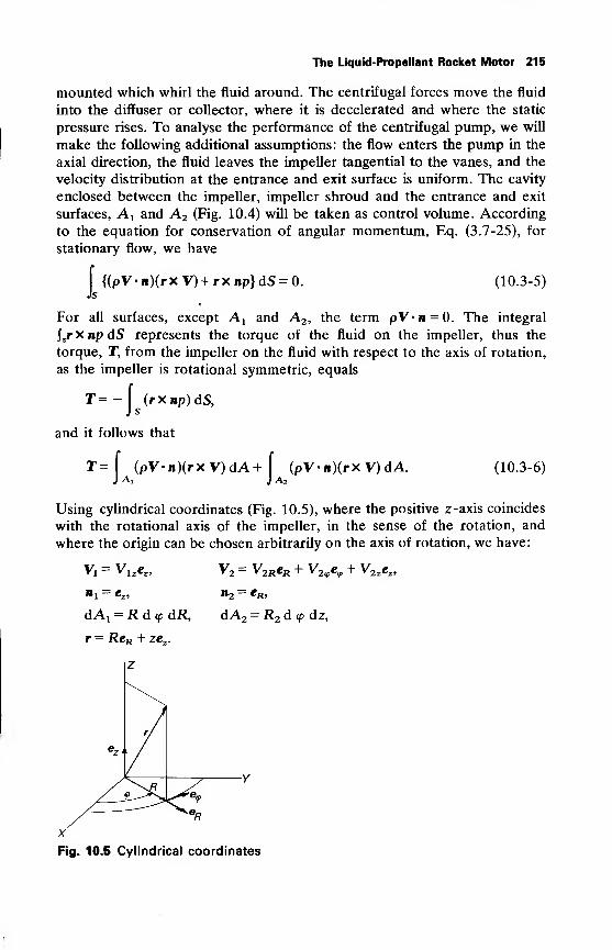
The Liquid-Propellant Rocket Motor 215
mounted which whirl the fluid around. The centrifugal forces move the fluid
into the diffuser or collector, where it is decelerated and where the static
pressure rises. To analyse the performance of the centrifugal pump, we will
make the following additional assumptions: the flow enters the pump in the
axial direction, the fluid leaves the impeller tangential to the vanes, and the
velocity distribution at the entrance and exit surface is uniform. The cavity
enclosed between the impeller, impeller shroud and the entrance and exit
surfaces, A x and A2 (Fig. 10.4) will be taken as control volume. According
to the equation for conservation of angular momentum, Eq. (3.7-25), for
stationary flow, we have
{(pV-n)(rxV) + rxnp}dS = 0. (10.3-5)
For all surfaces, except A x and A2 , the term pV«n = 0. The integral
Jsr x np dS represents the torque of the fluid on the impeller, thus the
torque, T, from the impeller on the fluid with respect to the axis of rotation,
as the impeller is rotational symmetric, equals
T = - (rXnp)dS,
and it follows that
T=\ (pV-n)(rxV)dA+I
(pV-n)(rx V) dA.J A, J A2
(10.3-6)
Using cylindrical coordinates (Fig. 10.5), where the positive z-axis coincides
with the rotational axis of the impeller, in the sense of the rotation, and
where the origin can be chosen arbitrarily on the axis of rotation, we have:
V2 = V2ReR + V2tpe<p + V2zcz ,
n2 = eR>
dA2 = R2 d <p dz,
Fig. 10.5 Cylindrical coordinates
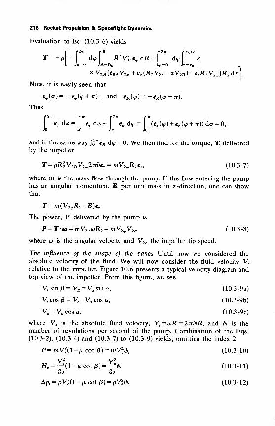
216 Rocket Propulsion & Spaceflight Dynamics
Evaluation of Eq. (10.3-6) yields
- d<p R 2 V2zev dR+\ d<p\ x
x V2R {eRz
V
2<p + ev {R2V22 - zV2R ) -
e
2i?2V2<P}R2 6z1.
Now, it is easily seen that
««>(«p) = -e<p ((p + ir), and eR (<p) = - eR (<p + tt).
Thus
/"2-jr <»ir /«27r /• ir
c<pd<p= e
(pd <p+ e,d<p = (e,(<p) + «,((p + ir))d^ = 0,
Jo Jo Jtt Jo
and in the same way Jo'eR d(p - 0. We then find for the torque, T, delivered
by the impeller
T=pRlV2RV2<p27rbez = mV2<pR2ez , (10.3-7)
where m is the mass flow through the pump. If the flow entering the pumphas an angular momentum, B, per unit mass in z -direction, one can showthat
T=m(V2(pR2 -B)ez
The power, P, delivered by the pump is
P= T-«»= mV2(p(oR2
= mV2(pV2e , (10.3-8)
where a> is the angular velocity and V2e the impeller tip speed.
The influence of the shape of the vanes. Until now we considered the
absolute velocity of the fluid. We will now consider the fluid velocity Vr
relative to the impeller. Figure 10.6 presents a typical velocity diagram andtop view of the impeller. From this figure, we see
Vr sin (3 = VR = Va sin a, (10.3-9a)
Vr cos p = Ve- Va cos a, (10.3-9b)
V<p=Va cosa. (10.3-9c)
where Va is the absolute fluid velocity, Ve = <oR = 2ttNR, and N is the
number of revolutions per second of the pump. Combination of the Eqs.
(10.3-2), (10.3-4) and (10.3-7) to (10.3-9) yields, omitting the index 2
P=mV2e(l-ncotp) = mV2
e i(,, (10.3-10)
V2 V2
Hc=—(1-ju cot |3) =—^, (10.3-11)
go go
Lpt= pV2
e(\ - n cot (S) = pVSfc (10.3-12)
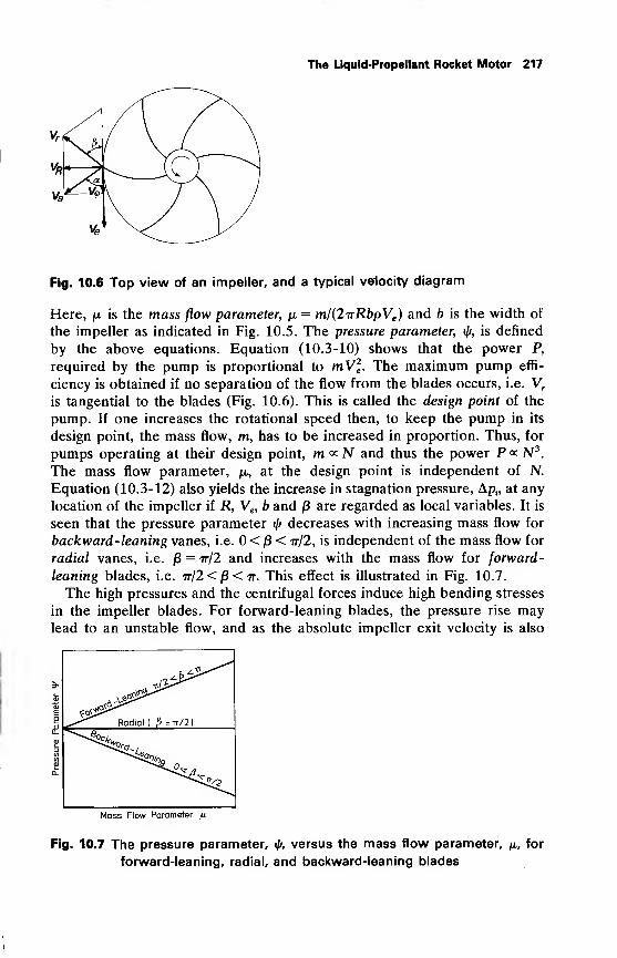
The Liquid-Propellant Rocket Motor 217
Fig. 10.6 Top view of an impeller, and a typical velocity diagram
Here, ju is the mass flow parameter, fx = m/(2TrRbpVe ) and b is the width of
the impeller as indicated in Fig. 10.5. The pressure parameter, if/, is defined
by the above equations. Equation (10.3-10) shows that the power P,
required by the pump is proportional to mW\. The maximum pump effi-
ciency is obtained if no separation of the flow from the blades occurs, i.e. Vr
is tangential to the blades (Fig. 10.6). This is called the design point of the
pump. If one increases the rotational speed then, to keep the pump in its
design point, the mass flow, m, has to be increased in proportion. Thus, for
pumps operating at their design point, m <* N and thus the power P « N3.
The mass flow parameter, p, at the design point is independent of N.
Equation (10.3-12) also yields the increase in stagnation pressure, Ap„ at any
location of the impeller if R, Ve, b and /3 are regarded as local variables. It is
seen that the pressure parameter if/ decreases with increasing mass flow for
backward- leaning vanes, i.e. < j8 < tt/2, is independent of the mass flow for
radial vanes, i.e. |8 = tt/2 and increases with the mass flow for forward-
leaning blades, i.e. 7r/2 < |3 < 7r. This effect is illustrated in Fig. 10.7.
The high pressures and the centrifugal forces induce high bending stresses
in the impeller blades. For forward-leaning blades, the pressure rise maylead to an unstable flow, and as the absolute impeller exit velocity is also
^^ Radial (
/LJ*^—
TT/2)
•^4?
Mass Flow Parameter fi
Fig. 10.7 The pressure parameter, «/», versus the mass flow parameter, /a, for
forward-leaning, radial, and backward-leaning blades
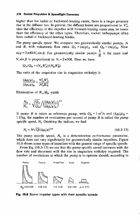
218 Rocket Propulsion & Spaceflight Dynamics
higher than for radial or backward-leaning vanes, there is a larger pressure
rise in the diffuser too. In general, the diffuser losses are proportional to V|,
thus the efficiency of the impeller with forward-leaning vanes may be lower
than the efficiency of the other types. Therefore, rocket turbopumps often
have radial or backward-leaning blades.
The pump specific speed. We compare two geometrically similar pumps, Aand B, with volumetric flow rates QA = (m/p)A and QB = (m/p)B . Now
m/p = 27rRbVr sin j8. For geometrically similar pumps — is the same and
RVr sin /3 is proportional to Ve =2irNR. Thus we have
QJQb = (NaR 3a)/(NbRb).
The ratio of the respective rise in stagnation enthalpy is
(Apt/p)A _ NARA
(Apr/p)B N2
BR 2B
Elimination of RA/RB yields
NB _ Qa //(APt/p)ANA VQB /\(Ap,/p)
)3/4
If pump B is taken as reference pump, with QB = 1 m3/s and (Ap,/p)B =
1 J/kg, the number of revolutions per second of pump B is called the pumpspecific speed, Ns . Omitting the indices, we find
Ns= Ny/QKApJp)3'4 (10.3-13)
The pump specific speed, Ns , is a dimensionless performance parameter,
which does not vary significantly for geometrically similar impellers. Figure
10.8 shows some types of impellers with the general range of specific speeds.
From Eq. (10.3-13) we see that the pump specific speed increases with the
flow rate and decreases with the rise in stagnation enthalpy required. Thenumber of revolutions at which the pump is to operate should, according to
Radial Francis Mixed Flow Axial Propeller
AL=0.03-0.06 0.06-0.12 0.12-0.20 0.20-0.60 up to 0.75
Fig. 10.8 Some impeller types with their specific speeds
The Liquid-Propellant Rocket Motor 219
Eq. (10.3-12) with Ve =2irNR be as high as possible to minimize the pumpdimensions. The angular velocity is limited in most cases either by the
allowable material stresses or by cavitation, which will be discussed later.
Therefore, the maximum allowable rotational speed, N, in combination with
the volumetric flow rate, Q, and the stagnation enthalpy rise will roughly
determine the impeller shape.
Losses can be attributed to the following causes: friction and viscous forces,
leakage, slip, and cavitation. The losses due to friction and viscous effects
arise in the mechanical parts (bearings) and the flow, respectively. After the
flow has become fully turbulent, a further increase in flow velocity through
the pump hardly affects the performance. By means of special mechanical
devices, leakage can be kept to a minimum, but cannot always be avoided. If
the main flow, locally, is not tangential to the blade, one speaks of slip. It
can be kept to a minimum by operating the pump near to its design
conditions.
We have ignored the blade thickness in the performance analysis. Thefinite blade thickness slightly reduces the performance, with respect to the
analysis given above, but is easily accounted for.
Cavitation is the boiling of the liquid at low pressures and the release of
dissolved gas from the liquid. Small gas bubbles grow in the liquid and then
collapse within a few milliseconds. This is accompanied by high temperature
rises, up to ~ 10,000 K, and pressure rises up to ~400MPa. A general
discussion on cavitation is given by Pearsall [15]. Brennen and Acosta [16]
discuss some aspects of cavitation in turbopumps, especially its relation with
the mass flow through the pump, by which it may contribute to the POGOphenomenon. Apart from affecting the mass flow through the pump, the
high pressures and temperatures which may occur locally may cause serious
damage.
Cavitation can be suppressed by ensuring that everywhere in the flow the
static pressure is well above the vapor pressure. This can be achieved by
avoiding high flow velocities, or by using high fluid pressures, or by a
combination of both. The high fluid pressures in the turbopumps are
achieved by high tank pressures, possibly in combination with booster-
pumps. Dissolved gas should be removed from the liquid as much as
possible.
A measure for the occurrence of cavitation is the Net Positive Suction
Energy, NPSE. (In older literature Net Positive Suction Head NPSH.) TheNPSE is defined as
NPSE =^^, (10.3-14)P
where pflis the stagnation pressure at the suction or pump inlet and pv is the
vapor pressure. The NPSE value at which, for the first time cavitation
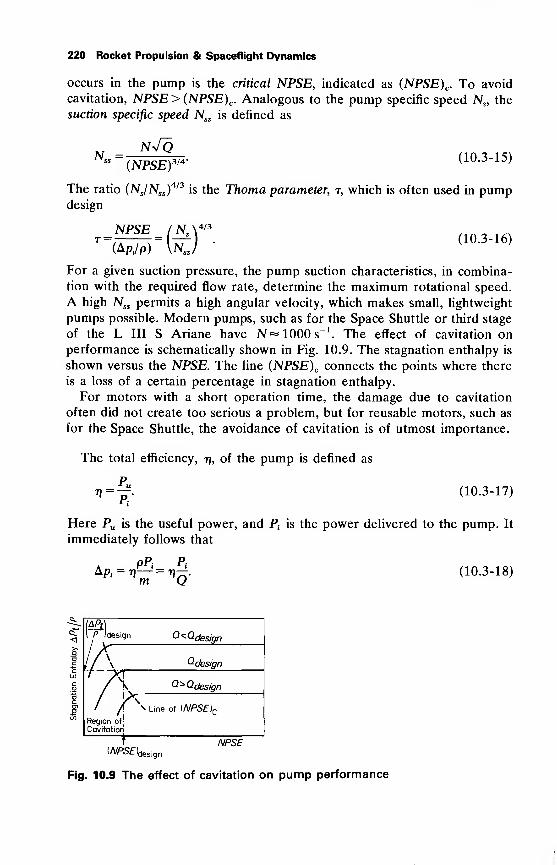
220 Rocket Propulsion & Spaceflight Dynamics
occurs in the pump is the critical NPSE, indicated as (NPSE) C . To avoid
cavitation, NPSE > (NPSE)C . Analogous to the pump specific speed N„ the
suction specific speed Nss is defined as
(NPSE) 2Nss=7^^3T4- (10.3-15)
The ratio (NJNSS )
4/3is the Thoma parameter, t, which is often used in pump
design
m^ /NYT=—
-fa:• (10 -3 - 16)
NPSE IN \4/3
(Ap(/p)
For a given suction pressure, the pump suction characteristics, in combina-
tion with the required flow rate, determine the maximum rotational speed.
A high Nss permits a high angular velocity, which makes small, lightweight
pumps possible. Modern pumps, such as for the Space Shuttle or third stage
of the L III S Ariane have N 8* 1000 s-1
. The effect of cavitation onperformance is schematically shown in Fig. 10.9. The stagnation enthalpy is
shown versus the NPSE. The line (NPSE)C connects the points where there
is a loss of a certain percentage in stagnation enthalpy.
For motors with a short operation time, the damage due to cavitation
often did not create too serious a problem, but for reusable motors, such as
for the Space Shuttle, the avoidance of cavitation is of utmost importance.
The total efficiency, 17, of the pump is defined as
r\=j. (10.3-17)
Here Pu is the useful power, and Pt
is the power delivered to the pump. It
immediately follows that
Ap, = <n^=rA (10.3-18)m Q
design Q^Qc/fdesign
Qck>es/gn
X Q*QdesignA Line of (NPSE)C
NPSEl/V/^design
Fig. 10.9 The effect of cavitation on pump performance
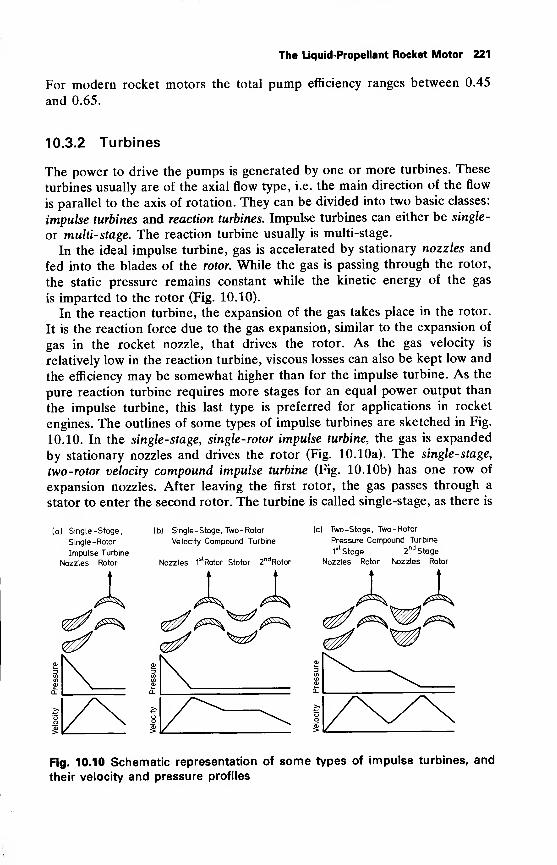
The Liquid-Propellant Rocket Motor 221
For modern rocket motors the total pump efficiency ranges between 0.45
and 0.65.
10.3.2 Turbines
The power to drive the pumps is generated by one or more turbines. These
turbines usually are of the axial flow type, i.e. the main direction of the flow
is parallel to the axis of rotation. They can be divided into two basic classes:
impulse turbines and reaction turbines. Impulse turbines can either be single -
or multi-stage. The reaction turbine usually is multi-stage.
In the ideal impulse turbine, gas is accelerated by stationary nozzles and
fed into the blades of the rotor. While the gas is passing through the rotor,
the static pressure remains constant while the kinetic energy of the gas
is imparted to the rotor (Fig. 10.10).
In the reaction turbine, the expansion of the gas takes place in the rotor.
It is the reaction force due to the gas expansion, similar to the expansion of
gas in the rocket nozzle, that drives the rotor. As the gas velocity is
relatively low in the reaction turbine, viscous losses can also be kept low and
the efficiency may be somewhat higher than for the impulse turbine. As the
pure reaction turbine requires more stages for an equal power output than
the impulse turbine, this last type is preferred for applications in rocket
engines. The outlines of some types of impulse turbines are sketched in Fig.
10.10. In the single-stage, single-rotor impulse turbine, the gas is expanded
by stationary nozzles and drives the rotor (Fig. 10.10a). The single-stage,
two-rotor velocity compound impulse turbine (Fig. 10.10b) has one row of
expansion nozzles. After leaving the first rotor, the gas passes through a
stator to enter the second rotor. The turbine is called single-stage, as there is
(a) Single-Stage,
Single -Rotor
Impulse Turbine
Nozzles Rotor
(b) Single -Stage, Two -Rotor
Velocity Compound Turbine
Nozzles 1s,Rotor Stator 2
ndRotor
(c) Two -Stage, Two -Rotor
Pressure Compound Turbine
1stStage 2
ndStage
Nozzles Rotor Nozzles Rotor
Fig. 10.10 Schematic representation of some types of impulse turbines, and
their velocity and pressure profiles
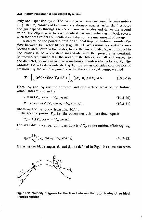
222 Rocket Propulsion & Spaceflight Dynamics
only one expansion cycle. The two- stage pressure compound impulse turbine
(Fig. 10.10c) consists of two rows of stationary nozzles. After the first rotor
the gas expands through the second row of nozzles and drives the secondrotor. The objective is to have identical entrance velocities at both rotors,
such that both rotors are identical and absorb the same amount of energy.
To determine the power output of an ideal impulse turbine, consider the
flow between two rotor blades (Fig. 10.11). We assume a constant cross-
sectional area between the blades, hence the gas velocity, V„ with respect to
the blades is of a constant magnitude and the pressure is constant.
Moreover, we assume that the width of the blades is small with respect to
the diameter, so we can assume a uniform circumferential velocity, Ve . Theabsolute gas velocity is indicated by Va ; the z-axis coincides with the axis of
rotation. By the same arguments as for the centrifugal pump, we find
r-fJ A,
(pVa -n)(rx VJdA+ (PVa-n)(rX Va)dA. (10.3-19)
Here, A x and A2 are the entrance and exit surface areas of the turbine
wheel. Integration yields
T= rm(Vai cos c^- Va2 cos a2), (10.3-20)
P = T-<o=mVe(Vai cos «!- Va2 cos a2), (10.3-21)
where a t and a2 follow from Fig. 10.11.
The specific power, Psp, i.e. the power per unit mass flow, equals
Psp = Ve(Vai cos «! - Va2 cos a2).
The available power per unit mass flow is |Vai , so the turbine efficiency, tjt,
is
2VVT = Trf(Vai cos «! - Va2 cos a2). (10.3-22)
By using the blade angles p x and j82 , as defined in Fig. 10.11, we can write
Fig. 10.11 Velocity diagram for the flow between the rotor blades of an ideal
impulse turbine
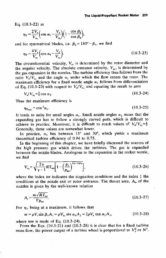
The Liquid-Propellant Rocket Motor 223
Eq. (10.3-22) as
2VJ Ve \( cos/32\,T =— (cos «,--)(!-—),
and for symmetrical blades, i.e. fi2= 180°- /3 l5 we find
^T =^(cosa,-^). (10.3-23)
The circumferential velocity, Ve , is determined by the rotor diameter and
the angular velocity. The absolute entrance velocity, Vai , is determined by
the gas expansion in the nozzles. The turbine efficiency thus follows from the
ratio VJVaiand the angle a x under which the flow enters the rotor. The
maximum efficiency for a fixed nozzle angle a a follows from differentiation
of Eq. (10.3-23) with respect to VJVai and equating the result to zero
VJV^coicn. (10.3-24)
Thus the maximum efficiency is
T)Tm<„ = cos2a 1 . (10.3-25)
It tends to unity for small angles a x . Small nozzle angles a x mean that the
expanding gas has to follow a strongly curved path, which is difficult to
achieve in practice. Moreover, it is difficult to reach values of VJVa ~\.
Generally, these values are somewhat lower.
In practice, a x lies between 15° and 30°, which yields a maximumtheoretical turbine efficiency of 0.94 to 0.75.
In the beginning of this chapter, we have briefly discussed the sources of
the high pressure gas which drives the turbines. The gas is expanded
between the nozzle blades. Analogous to the expansion in the rocket nozzle,
we find
Vai
where the index tot indicates the stagnation conditions and the index 1 the
conditions at the nozzle exit or rotor entrance. The throat area, Ar,
of the
nozzles is given by the well-known relation
At=m^RTtot
. (10.3-27)rptof
For r\T being at a maximum, it follows that
m = pVrsin ftA x
= pVai sin a xA x= 2pVe tan a xAu (10.3-28)
where use is made of Eq. (10.3-24).
From the Eqs. (10.3-21) and (10.3-28) it is clear that for a fixed turbine
mass flow, the power output of a turbine wheel is proportional to V2e or N2
.
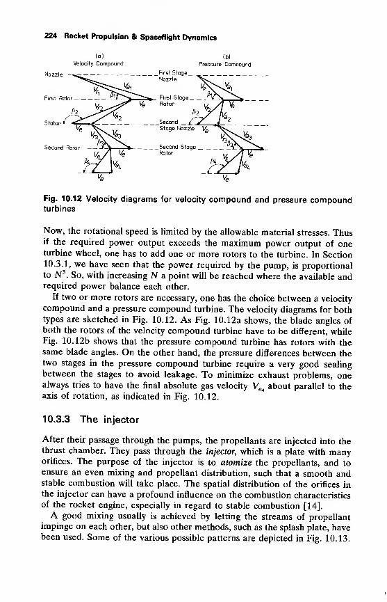
224 Rocket Propulsion & Spaceflight Dynamics
(a) (b)
Velocity Compound Pressure Compound
Nozzle —%^ First Stage_Nozzle
Stator-»—
Fig. 10.12 Velocity diagrams for velocity compound and pressure compoundturbines
Now, the rotational speed is limited by the allowable material stresses. Thusif the required power output exceeds the maximum power output of oneturbine wheel, one has to add one or more rotors to the turbine. In Section
10.3.1, we have seen that the power required by the pump, is proportionalto N3
. So, with increasing N a point will be reached where the available andrequired power balance each other.
If two or more rotors are necessary, one has the choice between a velocity
compound and a pressure compound turbine. The velocity diagrams for bothtypes are sketched in Fig. 10.12. As Fig. 10.12a shows, the blade angles of
both the rotors of the velocity compound turbine have to be different, whileFig. 10.12b shows that the pressure compound turbine has rotors with the
same blade angles. On the other hand, the pressure differences between thetwo stages in the pressure compound turbine require a very good sealing
between the stages to avoid leakage. To minimize exhaust problems, onealways tries to have the final absolute gas velocity V^ about parallel to the
axis of rotation, as indicated in Fig. 10.12.
10.3.3 The injector
After their passage through the pumps, the propellants are injected into thethrust chamber. They pass through the injector, which is a plate with manyorifices. The purpose of the injector is to atomize the propellants, and to
ensure an even mixing and propellant distribution, such that a smooth andstable combustion will take place. The spatial distribution of the orifices in
the injector can have a profound influence on the combustion characteristics
of the rocket engine, especially in regard to stable combustion [14].
A good mixing usually is achieved by letting the streams of propellantimpinge on each other, but also other methods, such as the splash plate, havebeen used. Some of the various possible patterns are depicted in Fig. 10.13.
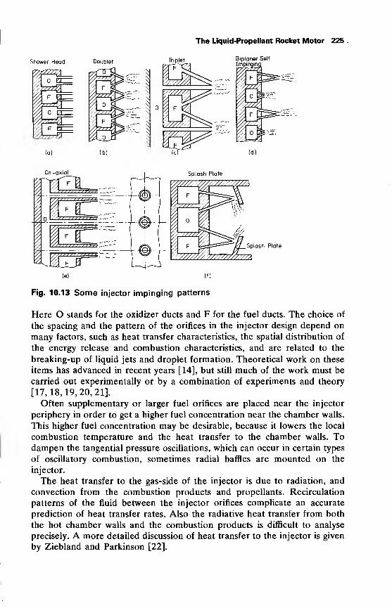
The Liquid-Propellant Rocket Motor 225
Shower Head
Co -axial Splash Plate
Splash Platei^^Fig. 10.13 Some injector impinging patterns
Here O stands for the oxidizer ducts and F for the fuel ducts. The choice of
the spacing and the pattern of the orifices in the injector design depend on
many factors, such as heat transfer characteristics, the spatial distribution of
the energy release and combustion characteristics, and are related to the
breaking-up of liquid jets and droplet formation. Theoretical work on these
items has advanced in recent years [14], but still much of the work must be
carried out experimentally or by a combination of experiments and theory
[17,18,19,20,21].
Often supplementary or larger fuel orifices are placed near the injector
periphery in order to get a higher fuel concentration near the chamber walls.
This higher fuel concentration may be desirable, because it lowers the local
combustion temperature and the heat transfer to the chamber walls. Todampen the tangential pressure oscillations, which can occur in certain types
of oscillatory combustion, sometimes radial baffles are mounted on the
injector.
The heat transfer to the gas-side of the injector is due to radiation, and
convection from the combustion products and propellants. Recirculation
patterns of the fluid between the injector orifices complicate an accurate
prediction of heat transfer rates. Also the radiative heat transfer from both
the hot chamber walls and the combustion products is difficult to analyse
precisely. A more detailed discussion of heat transfer to the injector is given
by Ziebland and Parkinson [22].
226 Rocket Propulsion & Spaceflight Dynamics
The propellant injection velocity, Vh follows from the equation for the
conservation of mass (either for the fuel or the oxidizer),
V,=-^, (10.3-29)pA
where m stands for the fuel or oxidizer mass flow through an orifice, A is
the cross-sectional area of the orifice and p the appropriate density. Because
of viscous forces there is a strong pressure drop, Api5over the injector. This
pressure drop is related to the injection velocity, Vh by the relationship
APi = p/2{^J,
(10.3-30)
where cd is a discharge coefficient which can be determined quite accurately
by means of waterflow tests. Values for cd range from about 0.5 to a little
over 0.9, depending on the shape and length of the orifice.
Upper-stage engines, space engines or motors for landers are often
designed to provide a variable thrust. Since the flow into the chamber
depends on the pressure drop, Apf ,
across the injector orifice, a significant
variation in the flow rate seriously affects the pressurization system and the
injector performance. To avoid this, for variable-thrust rocket motors,
special injectors, such as multi-manifold injectors, variable-area injectors or
aeration injectors may be used. The multi-manifold injectors employ two or
more sets of propellant manifolds, each set connected to its own injector
orifices. By closing propellant manifolds, one can obtain a reduced propel-
lant flow rate at a satisfactory Ap£. The variable-area injector employs a
pintle to vary the injector area, while controlling the pressure drop. Theaeration injector employs fixed area orifices, but it is possible to inject an
inert gas in the propellant manifold, replacing part of the propellants in the
ducts. By changing the amount of gas injected, the propellant flow may be
varied, thus providing throttling capability. It was shown in experiments that
with aeration injection, thrust modulation between 4% and 100% was
possible, while, even in the worst case, losses did not exceed 10%.
Injector design itself is of a fairly complicated and specialized character, a
full discussion of which cannot be given at this place.
10.4 The thrust chamber
After the propellants have entered the combustion chamber, they vaporize,
mix and react. Part of the combustion reaction may already take place in the
liquid state. In some cases one, or both, of the propellants are injected in
gaseous form, which reduces the time necessary to complete the combustion,
j
leading to relatively short motors.
It is possible that a non-uniform mixture ratio exists in the combustion
chamber. It has been observed that regions of identifiable mixture ratios,
The Liquid-Propellant Rocket Motor 227
larger than a typical molecular mixing length (~1 cm), may maintain their
identity throughout the chamber and nozzle. This may result in performance
losses up to 5%.
10.4.1 Aspects of oscillatory combustion
Apart from the POGO phenomenon mentioned already, other types of
combustion instability are encountered in liquid motors. Frequencies rang-
ing from a few Hertz up to 15,000 Hz have been observed, with pressure
amplitudes ranging from 0.1 to 10 times the chamber pressure. Oscillatory
operation of the rocket motor is undesirable, as it causes severe vibrations
(up to 10,000 m/s2) and as it is accompanied by a strong increase in heat
transfer.
Some well-known instabilities are chugging and screaming. Chugging
takes place at low frequencies (less than a few hundred Hertz). It may be
due to an interaction between the propellant flow rate entering the chamber
and the chamber pressure, but also a coupling between the injector structure
and the combustion process has been traced as a cause. Screaming is a high-
frequency acoustic or resonant combustion. Longitudinal, radial and tangen-
tial pressure oscillations have been observed. The energy to drive the
oscillations stems from the propellant combustion.
Combustion instabilities can be eliminated by changing the chamber
geometry, the pattern and size of the injector orifices, or by mounting
baffles. An extensive treatment on oscillatory combustion in liquid motors is
given by Harrje and Reardon [14].
10.4.2 The shape of the combustion chamber
The most commonly used shapes of combustion chambers are spherical,
near spherical and cylindrical. The spherical shape yields the smallest
surface area for a given volume, and thus is attractive from the viewpoint of
cooling and weight. It is also an attractive shape from strength considera-
tions. However, it is more difficult to produce than a cylindrical chamber,
while also its performance is less than that of the cylindrical chamber.
If annular nozzles, such as plug or E-D nozzles, are used, an annular or
toroidal type of chamber is an obvious choice.
10.4.3 The chamber volume
The propellants, after entering the combustion chamber, need some time for
vaporization, mixing and reaction. We will denote this time interval by tc .
The residence time, t*, has to be equal to or larger than rc to ensure a
228 Rocket Propulsion & Spaceflight Dynamics
satisfactory performance. The minimum chamber volume Tc therefore di-
rectly follows from Eq. (6.7-3), with t* = tc ,
Tc = TcA tTy/RTc , (10.4-1)
or with Eq. (5.1-39)
K = Tcm^=Tcm ^p . (10.4-2)Pc Mpc
From this equation, we immediately see that the minimum chamber volumeis proportional to tc , m and Tc and inversely proportional to M and pc . Thecombustion temperature and the molecular weight of the combustion pro-
ducts do not vary strongly with pc . Thus, by increasing the chamber pressure,
pc , one can reduce the required chamber volume and consequently the
weight of the whole system. The weight benefit, however, is partly off-set by
the larger expansion nozzle which is necessary to achieve the same exit
pressure as for an engine with a lower chamber pressure.
10.5 Cooling of liquid engines
In Chapter 8 we discussed some of the most important aspects of heat
transfer in rocket motors. In this section we will discuss some of the most
used cooling techniques for liquid engines.
Cooling is necessary mainly from strength considerations. The strength of
materials decreases with increasing temperatures, but even before the allow-
able stress is reduced to an unacceptable low level, creep may occur. For
reusable engines, the fatigue life, which depends on temperature and stress
levels, will also put an upper limit on the allowable material temperature.
There are no materials available which combine good strength, creep and
fatigue qualities at elevated temperatures, with good manufacturing charac-
teristics and low costs.
Hence, for rocket motors in which temperatures of over 2000 K are
common, the only way to avoid structural parts getting too weak due to high
temperature levels, is cooling. This can be achieved by a great variety of
methods or combinations of these.
The various cooling techniques that are in use in rocket technology have
been discussed by Sutton [23] in 1966, and since, no basically new tech-
niques have been developed. We can distinguish between active and passive
cooling techniques. The active cooling methods use a forced convection heat
transport, as to actively cool the hot spots. Passive cooling systems do not
make use of a special heat transport system but are designed such that
during motor operation they prevent structural parts becoming too hot.
Some of the passive cooling systems do not actually cool, but only reduce
heat fluxes into the structure (insulation cooling). Other methods, such as
radiation cooling and ablative cooling are real cooling methods.
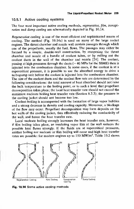
The Liquid-Propellant Rocket Motor 229
10.5.1 Active cooling systems
The four most important active cooling methods, regenerative, film, transpi-
ration and dump cooling are schematically depicted in Fig. 10.14.
Regenerative cooling is one of the most efficient and sophisticated means of
cooling. The method (Fig. 10.14a) is used on many of the large rocket
engines. The thrust chamber and nozzle wall contain passages through which
one of the propellants, usually the fuel, flows. The passages may either be
formed by a simple, double-wall construction, by composing the thrust
chamber and nozzle of a bundle of coolant tubes, or by milling out the
coolant ducts in the wall of the chamber and nozzle [24]. The coolant,
passing at high pressures through the ducts (-40 MPa for the SSME) then is
injected into the combustion chamber. In some cases, if the coolant is at a
supercritical pressure, it is possible to use the absorbed energy to drive a
turbopump unit before the coolant is injected into the combustion chamber.
The size of the coolant ducts and the coolant flow rate are determined by the
following considerations: the total amount of heat absorbed should not raise
the bulk temperature to the boiling point, or to such a level that propellant
decomposition takes place; the local heat transfer rate should not exceed the
maximum nucleate boiling heat transfer rate (Section 8.3.3); the pressure in
the cooling jacket should not become too low.
Coolant boiling is accompanied with the formation of large vapor bubbles
and a strong decrease in density and cooling capacity. Moreover, a blockage
of the flow may occur. Propellant decomposition may form deposits on the
hot walls of the cooling jacket, thus effectively reducing the conductivity of
the wall, and hence the heat transfer rate.
Local nucleate boiling strongly increases the heat transfer rate, however,
if film boiling takes place, an insulating vapor film at the wall reduces the
possible heat fluxes strongly. If the fluids are at supercritical pressures,
neither boiling nor nucleate or film boiling will occur and high heat transfer
rates are possible: for modern engines up to 150 MW/m2. Table 10.2 shows
Regenerative Cooling Film Cooling
Fig. 10.14 Some active cooling methods
Transpiration
Cooling
' Dump Cooling
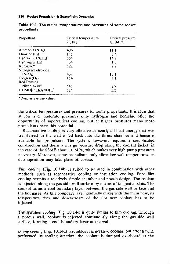
230 Rocket Propulsion & Spaceflight Dynamics
Table 10.2. The critical temperatures and pressures of some rocket
propellants
Propellant Critical temperature Critical pressure
Tcr (K) Per (MPa)
Ammonia (NH3) 406 11.1
Fluorine (F2) 145 5.4
Hydrazine (N2H4) 654 14.7
Hydrogen (H2) 34 1.3
Kerosine* 622 2.2
Nitrogen Tetroxide
(N2 4) 432 10.1
Oxygen (02) 154 5.1
Red FumingNitric Acid* 545 8.9
UDMH[(CH3)2NNH2] 524 5.3
'Denotes average values
the critical temperatures and pressures for some propellants. It is seen that
at low and moderate pressures only hydrogen and kerosine offer the
opportunity of supercritical cooling, but at higher pressures many morepropellants have this potential.
Regenerative cooling is very effective as nearly all heat energy that was
transferred to the wall is fed back into the thrust chamber and hence is
available for propulsion. The system, however, requires a complicated
construction and there is a large pressure drop along the coolant jacket, in
the case of the SSME about 10 MPa, which makes very high pump pressures
necessary. Moreover, some propellants only allow low wall temperatures as
decomposition may take place otherwise.
Film cooling (Fig. 10.14b) is suited to be used in combination with other
methods, such as regenerative cooling or insulation cooling. Pure film
cooling permits a relatively simple chamber and nozzle design. The coolant
is injected along the gas-side wall surface by means of tangential slots. Thecoolant forms a cool boundary layer between the gas-side wall surface and
the hot gases. As this boundary layer gradually mixes with the main flow, its
temperature rises and downstream of the slot new coolant has to be
injected.
Transpiration cooling (Fig. 10.14c) is quite similar to film cooling. Througha porous wall, coolant is injected continuously along the gas-side wall
surface, forming a cool boundary layer at the wall.
Dump cooling (Fig. 10.14d) resembles regenerative cooling, but after having
performed its cooling function, the coolant is dumped overboard at the
The Liquid-Propellant Rocket Motor 231
nozzle exit. Many of the restrictions for regenerative cooling also hold for
dump cooling. The heated, gasified coolant can be accelerated to supersonic
speeds thus providing a small extra thrust. The method is especially suited
for low-pressure engines, using low' molecular weight propellants, but yields
a performance loss as compared to regenerative cooling. On the other hand,
the construction is simpler as compared to regeneratively cooled engines.
10.5.2 Passive cooling systems
Among these systems, the most important ones are: insulation cooling, heat
sink cooling, ablative cooling and radiation cooling.
Insulation cooling. Here liners are used with an extremely low thermal
conductivity, thus reducing the heat flux into the wall. As it is not a real
cooling method by itself, it is mostly used in combination with other cooling
techniques, such as heat sink, radiation or regenerative cooling. A very
special material is pyrolytic graphite. This material has high and low conduc-
tivity directions. While the conductivity parallel to the layer planes is in the
order of 2x 10³ W/(m.K), the conductivity perpendicular to the layer planes
is only 5.75 W/(m.K). This makes it possible to conduct the heat in
preferred directions, and so to avoid the heating of critical parts.
Heat sink cooling is mostly used in solid rockets. The method consists of
applying a piece of solid material with good conductivity and a high specific
heat capacity to certain hot spots. The heat sink absorbs the heat from the
hot gases, thereby raising its own temperature but keeping the wall rela-
tively cool. The method is only suitable for short-duration applications, but
is sometimes used in combination with insulation cooling for small liquid
rocket engines.
Ablative cooling consists of covering the hot gas-side of the engine wall with
a material that decomposes endothermally at high temperatures, while
forming a insulating char layer. It is often used in combination with
radiation and insulation cooling and chosen for upper-stage motors and
reaction control engines for the sake of simplicity [25]. It is also an effective
means to keep the temperature of variable-thrust motors within an accepta-
ble range. Regenerative cooling often poses a problem for variable-thrust
motors, because of the variable chamber pressure and flow rate. Therefore,
ablative cooling offers a simple and efficient way to keep the engine wall
relatively cool.
Radiation cooling is often used for upper-stage engines and reaction control
engines in combination with insulation and ablative cooling. The hot walls
radiate the heat to the surroundings. As the radiative heat flux is propor-
tional to T4, the material temperature must be high to obtain a large
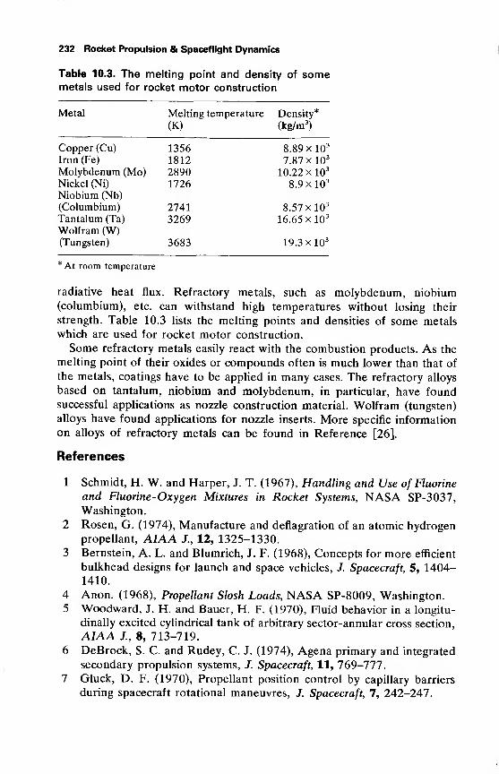
232 Rocket Propulsion & Spaceflight Dynamics
Table 10.3. The melting point and density of somemetals used for rocket motor construction
Metal Melting temperature Density*
(K) (kg/m3)
Copper (Cu) 1356 8.89 xlO3
Iron (Fe) 1812 7.87 xlO3
Molybdenum (Mo) 2890 10.22 xlO3
Nickel (Ni) 1726 8.9 xlO3
Niobium (Nb)
(Columbium) 2741 8.57 xlO3
Tantalum (Ta) 3269 16.65 xlO3
Wolfram (W)(Tungsten) 3683 19.3 xlO3
*At room temperature
radiative heat flux. Refractory metals, such as molybdenum, niobium(columbium), etc. can withstand high temperatures without losing their
strength. Table 10.3 lists the melting points and densities of some metals
which are used for rocket motor construction.
Some refractory metals easily react with the combustion products. As the
melting point of their oxides or compounds often is much lower than that of
the metals, coatings have to be applied in many cases. The refractory alloys
based on tantalum, niobium and molybdenum, in particular, have foundsuccessful applications as nozzle construction material. Wolfram (tungsten)
alloys have found applications for nozzle inserts. More specific information
on alloys of refractory metals can be found in Reference [26].
References
1 Schmidt, H. W. and Harper, J. T. (1967), Handling and Use of Fluorine
and Fluorine-Oxygen Mixtures in Rocket Systems, NASA SP-3037,
Washington.
2 Rosen, G. (1974), Manufacture and deflagration of an atomic hydrogenpropellant, AIAA J., 12, 1325-1330.
3 Bernstein, A. L. and Blumrich, J. F. (1968), Concepts for more efficient
bulkhead designs for launch and space vehicles, J. Spacecraft, 5, 1404-1410.
4 Anon. (1968), Propellant Slosh Loads, NASA SP-8009, Washington.
5 Woodward, J. H. and Bauer, H. F. (1970), Fluid behavior in a longitu-
dinally excited cylindrical tank of arbitrary sector-annular cross section,
AIAA J., 8, 713-719.
6 DeBrock, S. C. and Rudey, C. J. (1974), Agena primary and integrated
secondary propulsion systems, J. Spacecraft, 11, 769-777'.
7 Gluck, D. F. (1970), Propellant position control by capillary barriers
during spacecraft rotational maneuvres, J. Spacecraft, 7, 242-247.
The Liquid-Propellant Rocket Motor 233
8 Easton, C. R. and Catton, I. (1970), Nonlinear free surface effects in
tank draining at low gravity, AIAA J., 8, 2195-2199.
9 Rubin, S. (1972), Analysis of POGO Stability, paper presented at the
23rd IAF-Congress, Vienna.
10 Rasumoff, A. and Winje, R. (1971), The POGO Phenomenon: Its
Causes and Cure, paper presented at the 22nd IAF-Congress, Brussels.
11 Holster, J. L. and Astleford, W. J. (1974), Analytical model for liquid
rocket propellant feedline dynamics, J. Spacecraft, 11, 180-187.12 Astleford, W. J., Holster, J. L., and Gerlach, C. R. (1972), Analysis of
Propellant Feedline Dynamics, NASA CR- 1239 13, Washington.13 Powell, E. A. and Zinn, B. T. (1974), Theoretical investigation of
nonlinear three-dimensional instabilities in liquid rockets with real
nozzles, Acta Astronautica, 1, 1051-1073.14 Harrje, D. T. and Reardon, F. H. (eds) (1972), Liquid Propellant
Rocket Combustion Instability, NASA SP-194, Washington.15 Pearsall, I. S. (1975), Cavitation, Technical File no 14, Engineering,
215, I-VIII.
16 Brennen, C. and Acosta, A. J. (1973), Theoretical quasi-static analysis
of cavitation compliance in turbopumps, J. Spacecraft, 10, 175-180.17 Bracco, F. V. (1973), An experimental-analytical method to study
steady spray combustion, J. Spacecraft, 10, 353-354.
18 Burick, R. J. (1972), Atomization and mixing characteristics of
gas/liquid coaxial injector elements, J. Spacecraft, 9, 326-331.19 Burick, R. J. (1973), Optimum design of space storable gas/liquid
coaxial injectors, J. Spacecraft, 10, 663-670.
20 Wong, J. K. S., Sandri, R. and Newman, J. A. (1974), A new experi-
mental method for the investigation of fuel spray evaporation, AIAAJ., 12, 269-274.
21 George, D. J. (1973), Rocket Injector Hot Firing and Cold Flow SprayFields, AIAA Paper 73-1192, AIAA, New York.
22 Ziebland, H. and Parkinson, R. C. (1971), Heat Transfer in RocketEngines, AGARDograph No. 148, NATO, Neuilly-sur-Seine, p. 77-86.
23 Sutton, G. P., Wagner, W. R. and Seader, J. D. (1966), Advancedcooling techniques for rocket engines, Astronautics and Aeronautics, 4,
no. 1, 60-71.
24 Cook, R. T. and Coffey, G. A. (1973), Space Shuttle Orbiter EngineMain Combustion Chamber Cooling and Life, AIAA Paper 73-1310,AIAA, New York.
25 Park, L. T., Corbin, J. D. and Ernst, R. D. (1973), Titan TranstageSpacecraft Propulsion System, AIAA Paper 73-1210, AIAA, NewYork.
26 Anon. (1970), Recent Advances in Refractory Alloys for Space PowerSystems, NASA SP-245, Washington.
11 Two-dimensional RocketMotion in Vacuum
In Chapter 4 the equations of motion for a rigid rocket were derived. These
equations can only be solved by numerical methods. As, in practice, rocket
motion will be nearly two-dimensional in many cases, and as the assumption
of a pure two-dimensional motion will greatly simplify the treatment of
rocket motion, we will assume in this chapter that the complete trajectory of
the center of mass of the vehicle lies in a single plane. In that case, there are
only three degrees of freedom: two for the position of the center of mass
and one for the orientation of the rocket.
Such a pure two-dimensional motion is, of course, only possible if all
forces acting on the rocket, including the apparent forces, lie in the plane of
motion. Consequently, the resulting moment is perpendicular to that plane.
In practice, pure two-dimensional motion does not occur because of the
presence of forces perpendicular to the instantaneous plane of motion, such
as aerodynamic forces, gravitational forces, or components of the thrust.
The aerodynamic forces may be caused by cross-wind, misalignments or by
the deflection of control surfaces. The gravitational forces may appear if the
instantaneous plane of the trajectory does not coincide with the direction of
the gravitational field. Thrust forces normal to the plane of motion maybe caused either by thrust misalignment or by thrust vector control. For an
uncontrolled rocket, flying in a central or homogeneous gravitational field,
one may assume that no forces are acting normal to the instantaneous plane
of motion, making the nominal trajectory to lie in the nominal plane of
motion. Wind, thrust misalignment, aiming error, launcher deflection, etc.,
cause the real trajectory to deviate from the nominal one. This is called the
dispersion, which can be divided into lateral or out-of-plane dispersion, and
in-plane dispersion. In this chapter we will only discuss nominal trajectories.
11.1 The equations of motion
To describe the motion of the rocket vehicle we need the following refer-
ence frames:
Inertial frame OXYZ. This frame is chosen such that the trajectory of the
center of mass of the vehicle lies in the XZ-plane. So this plane is
determined by the launch direction (initial velocity) and the direction of the
gravitational field. The inertial frame will be specified further where neces-
sary. The unit vectors along the axes of the inertial frame will be denoted by
ex, eY and ez .
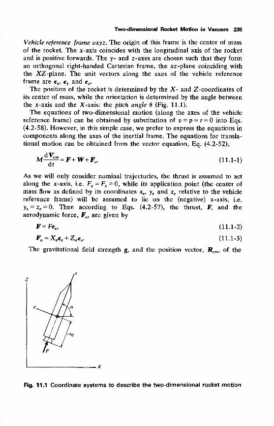
Two-dimensional Rocket Motion in Vacuum 235
Vehicle reference frame oxyz. The origin of this frame is the center of mass
of the rocket. The x-axis coincides with the longitudinal axis of the rocket
and is positive forwards. The y- and z-axes are chosen such that they form
an orthogonal right-handed Cartesian frame, the xz-plane coinciding with
the XZ-plane. The unit vectors along the axes of the vehicle reference
frame are ex, eyand ez .
The position of the rocket is determined by the X- and Z-coordinates of
its center of mass, while the orientation is determined by the angle between
the x-axis and the X-axis: the pitch angle B (Fig. 11.1).
The equations of two-dimensional motion (along the axes of the vehicle
reference frame) can be obtained by substitution of v = p = r = into Eqs.
(4.2-58). However, in this simple case, we prefer to express the equations in
components along the axes of the inertial frame. The equations for transla-
tional motion can be obtained from the vector equation, Eq. (4.2-52),
M^^ = F+W+Fa . (11.1-1)at
As we will only consider nominal trajectories, the thrust is assumed to act
along the x-axis, i.e. Fy= Fz = 0, while its application point (the center of
mass flow as defined by its coordinates xe , ye and ze relative to the vehicle
reference frame) will be assumed to lie on the (negative) x-axis, i.e.
ye = ze = 0. Then according to Eqs. (4.2-57), the thrust, F, and the
aerodynamic force, Fa , are given by
F=Fex , (11.1-2)
Fa = Xaex +Za ez . (11.1-3)
The gravitational field strength g, and the position vector, Rcm , of the
X
Fig. 11.1 Coordinate systems to describe the two-dimensional rocket motion
236 Rocket Propulsion & Spaceflight Dynamics
center of mass are resolved into components along the inertial axes
g = gxex + gZez,(11.1-4)
Rcm =Xex + Zez . (11.1-5)
By substitution of Eqs. (11.1-2) to (11.1-5) into Eq. (11.1-1), and using
the relation between the unit vectors in both reference frames,
EHcos sin B~\
1
-sin cos
exeY
Lez J
we obtain
d2XM
M
dt2
d2Zdt
2
= Fcos 6 +Mgx +Xa cos 0-Za sin 0,
= F sin + Mgz +Xa sin d + Za cos 0.
(11.1-6)
(ll.l-7a)
(ll.l-7b)
The equation for rotational motion is obtained by substitution of p = r
= ze = Fz= into Eq. (4.2-58e)
Jyy47= -q-^- m^ +M'-
dt dt(11.1-8)
Letting Vx and Vz be the velocity components of the center of mass
along the X- and Z-axes respectively, and noting that the pitch rate, q, is
related to the pitch angle, 6, by
4= d$
dt'
the equations of motion can be written as
M
M
dt
dVzdt
= F cos +Mgx +sXa cos — Za sin 0,
= Fsind +Mgz +Xa sin 6 +Za cos 0,
**=Vdt
Vx'
dZdt
= V7
d26_ dd/dlyyy
dt2
dt \ dt;)-m'.
(11.1-9)
(ll.l-10a)
(11.1-lOb)
(ll.l-10c)
(ll.l-10d)
(ll.l-10e)
Two-dimensional Rocket Motion in Vacuum 237
The instantaneous mass of the rocket follows from the differential equation
^=-m. (ll.l-10f)at
According to Section 5.1.4 the thrust can be written as
F=mVe + (pe -pa)Ae . (ll.l-10g)
The equations (11.1-10) are the complete equations for two-dimensional
rocket motion. This system of equations is still rather complicated. Theaerodynamic forces are dependent on velocity and position; the gravitational
components are in general dependent on the position, while the thrust is
dependent on the position owing to the atmospheric pressure term. In
general, analytic solution of these equations is not possible and one must
resort to numerical techniques. We will now make some further simplifica-
tions.
11.2 Rocket motion in free space
In this section we will consider the motion of a rocket in the absence of
gravitational and aerodynamic forces. The equations of motion for this case
are obtained from Eqs. (11.1-10) by setting Xa = Za = M' = gx = gz = 0. Aswe consider flight in vacuum the thrust is given by
F=mVe + peAe,
but we will use the more simple expression (Section 6.6)
F=mc=mg /sp ,(11.2-1)
where c and Isp are effective exhaust velocity and specific impulse respec-
tively, which are assumed to be constant, and g stands for the standard
surface gravity.
From inspection of the equation for rotational motion, Eq. (ll.l-10e)
with M' = 0, it will be clear that if initially d0/df = 0, will remain constant
during the flight. If we have a non-zero initial value of the pitch rate, the
pitch angle will decrease, or increase monotonically. However, the rotational
equation, Eq. (ll.l-10e), is only valid for an uncontrolled rocket. As all
rockets are stabilized and/or controlled during motor operation, a stabilizing
or control moment has to be incorporated in the equation for rotational
motion. For an aerodynamically stabilized, or controlled rocket flying
through the atmosphere, the control moment is part of the total
aerodynamic moment M'. For a mechanically stabilized and controlled
vehicle, control moments are generated by thrust vector control, separate
control rockets, control moment gyros, etc., and an additional term will
appear in the equation for rotational motion. In general, the pitch angle-time
history, pitch-program, of the rocket is specified and control moments will be
238 Rocket Propulsion & Spaceflight Dynamics
generated such that the required pitch-program is obtained. We will, there-
fore, assume in the following that the pitch-program is prescribed. We will
start with the most simple pitch-program: constant pitch angle. If we assumemoreover that the initial velocity of the rocket has the same direction as the
thrust, the problem is purely one-dimensional. The rocket will travel along a
straight line, making an angleOwith the X-axis. The equations of motion
for this case are
(11.2-2a)
(11.2-2b)
,, -. (11.2-2c)at
where V is the velocity of the rocket and s is the distance travelled.
11.2.1 Tsiolkovsky's equation
The equation for the velocity in free space can be integrated directly.
Combining Eqs. (11.2-2a) and (11.2-2c) leads to
(11.2-3)
dVM—
=
drF = mc,
dr '
dM_m,
dV_ c dMdr M dr
"
With the initial conditions
t = 0: V=V,
M=M ,
this equation can be integrated, yielding
AV= V(t\- v = , Mr In-
° -~MW (11 -2 "4)
This is Tsiolkovsky's Equation (1903), also called the equation of Oberth, for
the velocity increment of a rocket in free space. Using the specific impulse
instead of the effective exhaust velocity, this equation can also be written as
AV=g Isp ln^. (11.2-5)
For a given rocket, AV is only a function of the instantaneous mass of the
rocket. In order to determine AV (or V) as a function of time, it is necessary
to know the mass as a function of time. The mass of the rocket follows from
Eq. (11.2-2c)
M=Mn-
Imdr. (11.2-6)
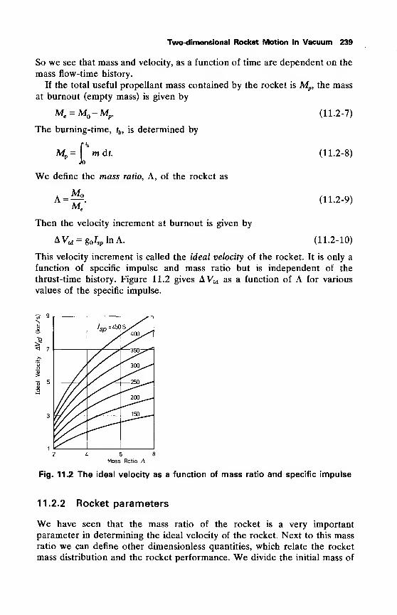
Two-dimensional Rocket Motion in Vacuum 239
So we see that mass and velocity, as a function of time are dependent on the
mass flow-time history.
If the total useful propellant mass contained by the rocket is Mp , the mass
at burnout (empty mass) is given by
Me=M -M
p.
The burning-time, tb , is determined by
Mp= m dt.
Jo
We define the mass ratio, A, of the rocket as
AM°
(11.2-7)
(11.2-8)
(11.2-9)
Then the velocity increment at burnout is given by
AVid= g Isp rnA. (11.2-10)
This velocity increment is called the ideal velocity of the rocket. It is only a
function of specific impulse and mass ratio but is independent of the
thrust-time history. Figure 11.2 gives AVjd as a function of A for various
values of the specific impulse.
S 9
6 8
Mass Ratio A
Fig. 11.2 The ideal velocity as a function of mass ratio and specific impulse
11.2.2 Rocket parameters
We have seen that the mass ratio of the rocket is a very important
parameter in determining the ideal velocity of the rocket. Next to this massratio we can define other dimensionless quantities, which relate the rocket
mass distribution and the rocket performance. We divide the initial mass of
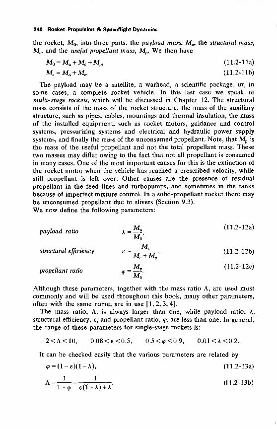
240 Rocket Propulsion & Spaceflight Dynamics
the rocket, M , into three parts: the payload mass, Mu , the structural mass,
Mc, and the useful propellant mass, Mp
. We then have
M = MU +Mc +Mp,(11.2-1 la)
Me = Mu +Mc . (11.2-1 lb)
The payload may be a satellite, a warhead, a scientific package, or, in
some cases, a complete rocket vehicle. In this last case we speak of
multi-stage rockets, which will be discussed in Chapter 12. The structural
mass consists of the mass of the rocket structure, the mass of the auxiliary
structure, such as pipes, cables, mountings and thermal insulation, the mass
of the installed equipment, such as rocket motors, guidance and control
systems, pressurizing systems and electrical and hydraulic power supply
systems, and finally the mass of the unconsumed propellant. Note, that Mp
is
the mass of the useful propellant and not the total propellant mass. These
two masses may differ owing to the fact that not all propellant is consumed
in many cases. One of the most important causes for this is the extinction of
the rocket motor when the vehicle has reached a prescribed velocity, while
still propellant is left over. Other causes are the presence of residual
propellant in the feed lines and turbopumps, and sometimes in the tanks
because of imperfect mixture control. In a solid-propellant rocket there maybe unconsumed propellant due to slivers (Section 9.3).
We now define the following parameters:
payload ratioM^ (11.2-12a)
M '
structural efficiency e = ———
,
(11.2-12b)jvic t~ lyip
• MD (11.2-12c)propellant ratio a, =—E
.MAlthough these parameters, together with the mass ratio A, are used most
commonly and will be used throughout this book, many other parameters,
often with the same name, are in use [1,2,3,4].
The mass ratio, A, is always larger than one, while payload ratio, A,
structural efficiency, e, and propellant ratio, <p, are less than one. In general,
the range of these parameters for single-stage rockets is:
2<A<10, 0.08<e<0.5, 0.5<<p<0.9, 0.01<A<0.2.
It can be checked easily that the various parameters are related by
<p = (l-e)(l-A), (11.2-13a)
A =r~= , f \ur <11.2-13b)1 — <p e(l-A) + A
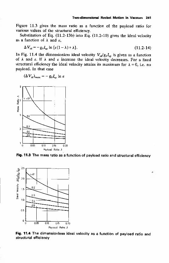
Two-dimensional Rocket Motion in Vacuum 241
Figure 11.3 gives the mass ratio as a function of the payload ratio for
various values of the structural efficiency.
Substitution of Eq. (11.2-13b) into Eq. (11.2-10) gives the ideal velocity
as a function of A and e,
AVw = -g Isp ln{e(l-A) + A}. (11.2-14)
In Fig. 11.4 the dimensionless ideal velocity Vid/g /sp is given as a function
of A and e. If A and e increase the ideal velocity decreases. For a fixed
structural efficiency the ideal velocity attains its maximum for A = 0, i.e. nopayload. In that case
(Avid)max = ~ go4» In e
=1?E = 0l\
\a2
.^03
_ 0.5_
0.05 0.10 0.15 0.20
Fbyload Ratio A
Fig. 11.3 The mass ratio as a function of payload ratio and structural efficiency
2.5
^ 2.0
<1
1.0
\c=0.1
sa2
^03_^__0V
——P-5-.
0.05 0.10 0.15 0.20
Payload Ratio A
Fig. 11.4 The dimensionless ideal velocity as a function of payload ratio andstructural efficiency
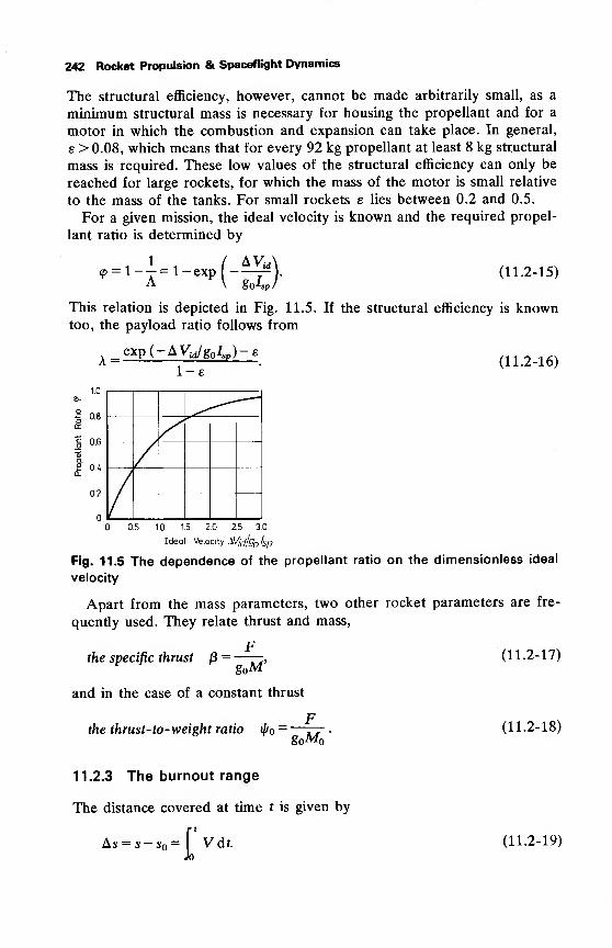
242 Rocket Propulsion & Spaceflight Dynamics
The structural efficiency, however, cannot be made arbitrarily small, as a
minimum structural mass is necessary for housing the propellant and for a
motor in which the combustion and expansion can take place. In general,
e > 0.08, which means that for every 92 kg propellant at least 8 kg structural
mass is required. These low values of the structural efficiency can only be
reached for large rockets, for which the mass of the motor is small relative
to the mass of the tanks. For small rockets e lies between 0.2 and 0.5.
For a given mission, the ideal velocity is known and the required propel-
lant ratio is determined by
<p = l--j-=lA
exp\ golspf
(11.2-15)
This relation is depicted in Fig. 11.5. If the structural efficiency is knowntoo, the payload ratio follows from
(11.2-16)A
1.0
|0.8
1 0.6
(VQ.
e 0.4
0.2
n
_exp(--AVid/g0*sp> — e
1-e
0.5 1.0 1.5 2.0 2.5 3.0
Ideal Velocity SVj^Isp
Fig. 11.6 The dependence of the propellant ratio on the dimensionless ideal
velocity
Apart from the mass parameters, two other rocket parameters are fre-
quently used. They relate thrust and mass,
the specific thrust |8=goM'
and in the case of a constant thrust
(11.2-17)
the thrust- to- weight ratio i^o=g M (11.2-18)
11.2.3 The burnout range
The distance covered at time t is given by
As = s-s = V dt.
Jo
(11.2-19)
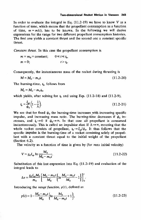
Two-dimensional Rocket Motion in Vacuum 243
In order to evaluate the integral in Eq. (11.2-19) we have to know V as a
function of time, which means that the propellant consumption as a function
of time, m = m(t), has to be known. In the following we will derive
expressions for the range for two different propellant consumption histories.
The first one yields a constant thrust and the second one a constant specific
thrust.
Constant thrust. In this case the propellant consumption is
m = m = constant; ^ t =£ tb ,
m = 0; t>tb .
Consequently, the instantaneous mass of the rocket during thrusting is
M=M -m t. (11.2-20)
The burning-time, tb , follows from
Me =M -m tb,
which yields, after solving for tb and using Eqs. (11.2-18) and (11.2-9),
(11.2-21)
We see that for fixed if/ the burning-time increases with increasing specific
impulse, and increasing mass ratio. The burning-time decreases if i/f in-
creases, and fb-»0 if j/^
-*°°- In that case all propellant is consumedinstantaneously. This is called an impulsive shot. If A—»•<», meaning that the
whole rocket consists of propellant, fb -»Isp/^ . It thus follows that the
specific impulse is the burning-time of a rocket consisting solely of propel-
lant with a constant thrust equal to the initial weight of the propellant
(Section 6.2).
The velocity as a function of time is given by (for zero initial velocity)
V=g Isp lnM°
(11.2-22)M -m t
Substitution of this last expression into Eq. (11.2-19) and evaluation of the
integral leads to
As =go^pMp [M -m t r Mo-mot
_^ 11
'
m [ M \ M J Jo*
Introducing the range function, p(t), defined as
p(() = l_*ti')h_^_+1 l (11.2-23)M I M -m t J
244 Rocket Propulsion & Spaceflight Dynamics
and using Eq. (11.2-18), the range can be written as
*s(t) = ^p*p(t).Wo
The burnout range, i.e. the distance covered at t = tb , then is
Asb= goff
Pb,
where
pb = p(rb)=l--(lnA+l).
(11.2-24)
(11.2-25)
(11.2-26)
Figure 11.6 gives the dimensionless burnout range, hsb/g I?p , as a function of
A and also depicts the range as a function of the instantaneous mass ratio
M /(M -m t).
We see that the burnout range is proportional to the square of the specific
impulse and inversely proportional to the thrust-to-weight ratio. For an
impulsive shot: Asb = (the total velocity increment is given instantane-
ously). If A —> oo the function pb approaches unity and, consequently,
Asb-> g I%/*Po-
After burnout the velocity remains constant and As increases linearly with
time.
The dimensionless acceleration, defined as
1 dV
go df(11.2-27)
equals the specific thrust and is increasing monotonically from ^ to A«/r at
burnout.
<mS-0.7
i? 0.6
a>
§•05tr
o OA
:5ma. 0.3
h-
0.2
0.1
* --y
5
10
5 7 9Mass Ratio A
Fig. 11.6 The dimensionless burnout range in free space
Two-dimensional Rocket Motion in Vacuum 245
Constant specific thrust. In this case
F/3=——=/3 = constant. (11.2-28)
The instantaneous mass of the rocket is obtained by integration of Eq.
(11.2-28), leading to
ln^ = |2t (11.2-29)M Isp
So
M =M exp(-|2r). (11.2-30)
By differentiation of Eq. (11.2-30), the propellant consumption as a function
of time is found to be
mM ft, / p \ nn ,n=—— expl—— M, (11.2-31)
-*sp \ -*sp /
and the burning-time follows from Eq. (11.2-29)
tb =^lnA. (11.2-32)Po
In this case too, the specific impulse can be interpreted as a burning-time,
namely the burning-time of a rocket with mass ratio A = e and a constant
specific thrust of unity. As the acceleration is constant and equal to g j8 ,
velocity and range are given by
V=g pV, (11.2-33)
As = §g pV2
,(11.2-34)
and thus at burnout
Vb = goPoh = g Isp In A, (11.2-35)
Asb = hoPotl = ho& In2A. (1 1.2-36)
Po
It can be verified easily that, in the case of constant specific thrust,
burning-time and burnout range are larger than the corresponding quantities
in the case of constant thrust with the same initial specific thrust. Theburnout velocity, of course, is the same in both cases.
It follows from Eq. (11.2-31) that the mass flow is continuously decreasing
from m at ignition to m /A at burnout. As, for a fixed nozzle geometry, the
chamber pressure is proportional to the mass flow, this pressure will have to
decrease too during powered flight. As the strength of the combustion
246 Rocket Propulsion & Spaceflight Dynamics
chamber is determined by maximum chamber pressure, the combustionchamber will be oversized during the flight. In the case of constant thrust,
the mass flow and so the chamber pressure are constant. From the viewpointof combustion chamber weight this is optimal, and is encountered very muchin practice, in contrast with the case of constant specific thrust. We havetreated the case of constant specific thrust because for a rocket flying
through the atmosphere there is an aerodynamic force, the drag, acting
opposite to the thrust. We can define an effective thrust, equal to the actual
thrust minus the drag. In the case of a constant actual thrust the velocity will
increase and consequently the drag increases too. So the effective thrust is
decreasing. However, the mass of the rocket will decrease too. For prelimi-
nary trajectory calculations the trajectory can be subdivided into portions
along which the ratio of effective thrust and instantaneous weight (the
effective specific thrust) can be assumed constant.
11.3 Rocket motion in a homogeneous gravitational field
In a homogeneous gravitational field the field strength, g, is constant. If weconsider the Earth locally as being flat, the local gravitational field may beconsidered homogeneous. Actually, the Earth is nearly spherical and its
gravitational field can be approximated very well by a central inverse square
field (Section 18.6). However, as long as the altitude and range are small
relative to the mean Earth's radius, the Earth may be considered flat and the
field strength can be approximated very well by a constant. For small
rockets, such as sounding rockets and tactical missiles this approximation
yields good results. For launch vehicles and intercontinental ballistic missiles
(ICfiM's), the powered flight trajectory of the first stages can, in general,
also be calculated by good approximation with the flat Earth assumption.
For the upper stages, however, the velocity will be so large that the flat
Earth approximation will lead to unacceptable deviations from the real
trajectory. However, as most part of this trajectory is a coast phase, the
trajectory can be approximated by a ballistic one and can be determinedanalytically in the case of a spherical Earth (Chapter 13).
If we choose the X-axis of the inertial system to coincide with the flat
Earth surface and the Z-axis vertical, then gx = and gz = - g , where it is
assumed that motion takes place near the surface of the Earth. Then the
equations of translational motion become
dVxM-^=Fcos0, (11.3-la)
dVzM~^f
= F sin e-Mg, (11.3-lb)
dXdJ"=v* (11.3-lc)
Two-dimensional Rocket Motion in Vacuum 247
^= Vz,(11.3-ld)
—— = -m. (11.3-le)dr
As in the foregoing, the thrust is given by
F=mc = mg Isp . (11.3-lf)
We will assume that the pitch program, 6 = d(t), is known.
11.3.1 Vertical flight
If during the whole flight = 90°, and if we have zero initial horizontal
velocity, the trajectory will be a straight line parallel to the Z-axis. In that
case Vz equals the total velocity V, and the equations of motion simplify to
dh dZ— =— =V. (11.3-2b)dt dt
As initial conditions we will choose a zero velocity and altitude at t = 0.
Equation (11.3-2a) can be integrated independently of the mass flow prog-
ram, leading to
[<<>iH-V=g
|4p ln^-fJ. (11.3-3)
We see that, in order to determine V as a function of time, knowledge of
the mass flow history is necessary. Even the burnout velocity in this case is
dependent on the thrust program because the burning-time depends on it.
Again we will assume a constant thrust, in which case the mass flow is given
by
m = m ; 0^t^tb ,
m = 0; t>tb .
For this case, the burning-time is already derived in Section 11.2.3 and is
given by Eq. (11.2-21). Then we find for the velocity as a function of time
V=go[/sp hiM°
-t\; 0^t^tb ,(11.3-4a)
Lv M -m t J
Vb = g Isp [lnA-^(l-£)]; t = tb ,(11.3-4b)
V=g [/sp lnA-f]; t^tb , (11.3-4c)
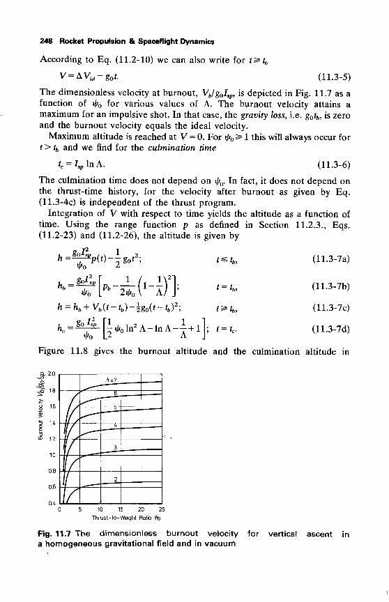
248 Rocket Propulsion & Spaceflight Dynamics
According to Eq. (11.2-10) we can also write for t^tb
V = AVid -g t. (11.3-5)
The dimensionless velocity at burnout, VbJg Isp , is depicted in Fig. 11.7 as a
function of ij/ for various values of A. The burnout velocity attains a
maximum for an impulsive shot. In that case, the gravity loss, i.e. g tb , is zero
and the burnout velocity equals the ideal velocity.
Maximum altitude is reached at V= 0. For i(/ ^ 1 this will always occur for
t> tb and we find for the culmination time
tc = Isp In A. (11.3-6)
The culmination time does not depend on «/f . In fact, it does not depend onthe thrust-time history, for the velocity after burnout as given by Eq.
(11.3-4c) is independent of the thrust program.
Integration of V with respect to time yields the altitude as a function of
time. Using the range function p as defined in Section 11.2.3., Eqs.
(11.2-23) and (11.2-26), the altitude is given by
h= Sop2(r)
1 ,2.
hh =got
h = hb + Vb (t-tb)-^g (t-tb )
2;
t^th
t=th
t^th
h = goH* ln2 A-lnA—+1).-
(11.3-7a)
(11.3-7b)
(11.3-7c)
(11.3-7d)*o 12
T " A
Figure 11.8 gives the burnout altitude and the culmination altitude in
^ 1.8
8 16
$"5 1.4oc
<3 1.2
1.0
0.8
0.6
0.4
A=7
6
4_
3
2
5 10 15 20 25
Thrust -to- Weight Ratio <l>o
Fig. 11.7 The dimensionless burnout velocity for vertical ascent in
a homogeneous gravitational field and in vacuum
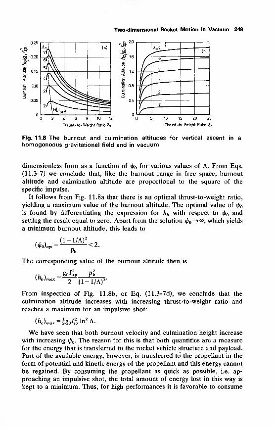
Two-dimensional Rocket Motion in Vacuum 249
0.25
.« 0.20
0.15
"5 0.10
0.05
A=\
7l\(a)
s/jN
^a/jl
2M% t
2 4 6 8 10 12
Thrust -to- Weight Ratio 4>o
^Q. 2.0
JP 1.6
£ 1.2
0.8
OX
/A^ ——
—
(b)
r^—-
-
'
l\
-—^"
(t3
2
/~10 15 20 25
Thrust -to-Weight Ratio ^
Fig. 11.8 The burnout and culmination altitudes for vertical ascent in a
homogeneous gravitational field and in vacuum
dimensionless form as a function of i/f for various values of A. From Eqs.
(11.3-7) we conclude that, like the burnout range in free space, burnout
altitude and culmination altitude are proportional to the square of the
specific impulse.
It follows from Fig. 11.8a that there is an optimal thrust-to-weight ratio,
yielding a maximum value of the burnout altitude. The optimal value of if/
is found by differentiating the expression for hb with respect to i/f and
setting the result equal to zero. Apart from the solution \\i—»<», which yields
a minimum burnout altitude, this leads to
(^o)opr= (1-1/A) 2
Pb
<2.
The corresponding value of the burnout altitude then is
{"bfrnax~ g I
2sp Pb
2 (1-1/A)2
From inspection of Fig. 11.8b, or Eq. (11.3-7d), we conclude that the
culmination altitude increases with increasing thrust-to-weight ratio and
reaches a maximum for an impulsive shot:
(hc)max=hoIsp^
We have seen that both burnout velocity and culmination height increase
with increasing i/f . The reason for this is that both quantities are a measure
for the energy that is transferred to the rocket vehicle structure and payload.
Part of the available energy, however, is transferred to the propellant in the
form of potential and kinetic energy of the propellant and this energy cannot
be regained. By consuming the propellant as quick as possible, i.e. ap-
proaching an impulsive shot, the total amount of energy lost in this way is
kept to a minimum. Thus, for high performances it is favorable to consume
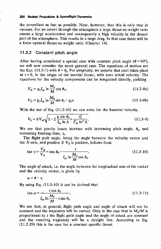
250 Rocket Propulsion & Spaceflight Dynamics
the propellant as fast as possible. Note, however, that this is only true in
vacuum. For an ascent through the atmosphere a large thrust-to-weight ratio
causes a large acceleration and consequently a high velocity in the denser
part of the atmosphere. This results in a large drag. In that case there will bea finite optimal thrust-to-weight ratio (Chapter 14).
11.3.2 Constant pitch angle
After having considered a special case with constant pitch angle (0 = 90°),
we will now consider the more general case. The equations of motion are
the Eqs. (11.3-1) with =O . For simplicity, we assume that start takes place
at t = 0, in the origin of the inertial frame, with zero initial velocity. Theequations for the velocity components can be integrated directly, yielding
MoMMoM
Vx = g Isp In T7 cos O , (11.3-8a)
Vz = g Isp In -^ sin O- g t. (11.3-8b)
With the use of Eq. (11.2-10) we can write for the burnout velocity,
= AVidyitb sin O ,
t
v- Av^ 1- 2±i^+
7!n^A- <1L3 -9>
•sp "» " -» sp
We see that gravity losses increase with increasing pitch angle, O, and
increasing burning-time, tb .
The flight path angle, being the angle between the velocity vector and
the X-axis, and positive if Vz is positive, follows from
tany = -^ = tan0o-j . (11.3-10)
sp ~MCOS °
The angle of attack, i.e. the angle between the longitudinal axis of the rocket
and the velocity vector, is given by
a = - y.
By using Eq. (11.3-10) it can be derived that
t cos O ,„„ „ „„.tana= 2 (11.3-11)
MWe see that, in general, flight path angle and angle of attack will not be
constant and the trajectory will be curved. Only in the case that In MJM is
proportional to t the flight path angle and the angle of attack are constant
and the resulting trajectory will be a straight line. According to Eq.
(11.2-29) this is the case for a constant specific thrust.

Two-dimensional Rocket Motion in Vacuum 251
In the following we will again consider a constant thrust. Then the velocity
components, the flight path angle and the angle of attack follow as a
function of time by substitution of
M=M -m t; 0^t^tb,
M=Me ;t>tb ,
into Eqs. (11.3-8) to (11.3-11). We then find that during powered flight yincreases and the trajectory is curved upwards. By taking the limit for f—»0
of Eq. (11.3-10) it follows that
tan 7o = tan O-
ij/ cos O
(11.3-12)
Consequently, the angle of attack decreases during powered flight. Its initial
value is given by
tan a =cos O
^o -sin O
(11.3-13)
In Fig. 11.9 the angle of attack is given as a function of the instantaneous
mass ratio MJM for ^ t^ tb .
After burnout, y decreases and a increases. Then the trajectory is curved
downwards. Culmination altitude is reached if y = 0, or equivalently if
Vz = 0, leading to
tc = Isp In A sinO . (11.3-14)
Again the culmination time is independent of the thrust program.
4=5
O=5O°
\60°
^^70°
^^80°
85°
90°13 5 7 9
Instantaneous Mass Ratio M jM
Fig. 11.9 The angle of attack for flights with constant pitch angle and constant
thrust in a homogeneous gravitational field and in vacuum
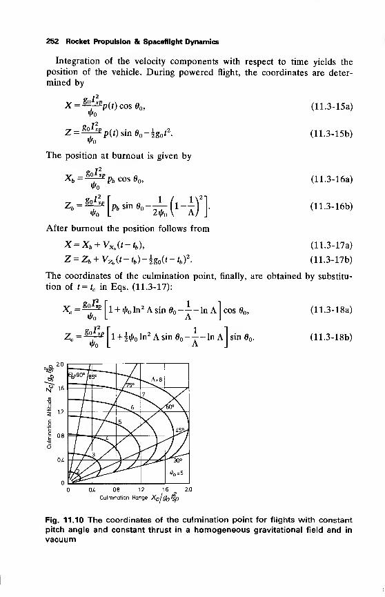
252 Rocket Propulsion & Spaceflight Dynamics
Integration of the velocity components with respect to time yields the
position of the vehicle. During powered flight, the coordinates are deter-
mined by
X =&SEp(t) cos d ,
Z = gol2
*}>0
£ p(t) sin 6 -lg t2
.
The position at burnout is given by
Xb=^pb cos6 ,
— bu*sp
r2
*-*>-*-w.('-mAfter burnout the position follows from
X = Xb + VXb (t-tb ), (11.3-17a)
Z = Zb + VZb (t-tb)-±g (t-tb )
2. (11.3-17b)
The coordinates of the culmination point, finally, are obtained by substitu-
tion of t=tc in Eqs. (11.3-17):
go*?,Xc=g^ fl + «Aoln
2 Asin 0o-T-ln A-
!
cos O ,
«Ao L A J
z = golx[ 1 +
i^o ln
2 A sin o_i_in A l sin 6 .
^o L A J
11.3-15a)
11.3-15b)
11.3-16a)
11.3-16b)
11.3-18a)
11.3-18b)
q 2.0
tf 1-6
I 1-2
0.8
OA
©cf90°t5°
/7S°^A=8
NJ7
WP\
,5
J^y
3 / Uo=5
0.4 0.8 1.6 2.0,2
Culmination Range Xc g lsp
Fig. 11.10 The coordinates of the culmination point for flights with constant
pitch angle and constant thrust in a homogeneous gravitational field and in
vacuum
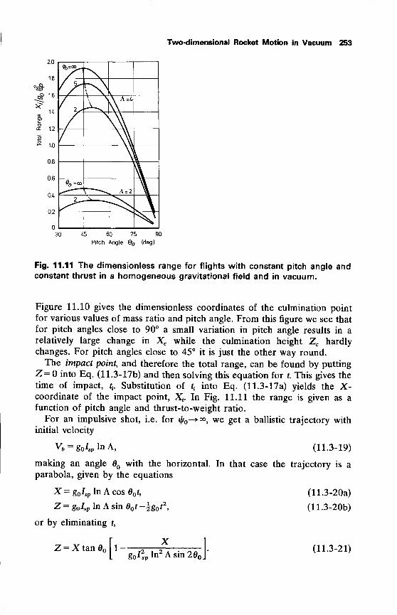
Two-dimensional Rocket Motion in Vacuum 253
2.0
1.8
>?1.4
01
encoo: 1.2
"5
"2 10
0.8
0.6
0A
0.2
&="*-
/ J**"
\ x
2^
\ \ \ A =4.
O =oo
A = 2
2^.
30 l& 60 75 90
Pitch Angle 6 (deg)
Fig. 11.11 The dimensionless range for flights with constant pitch angle andconstant thrust in a homogeneous gravitational field and in vacuum.
Figure 11.10 gives the dimensionless coordinates of the culmination point
for various values of mass ratio and pitch angle. From this figure we see that
for pitch angles close to 90° a small variation in pitch angle results in a
relatively large change in Xc while the culmination height Zc hardly
changes. For pitch angles close to 45° it is just the other way round.
The impact point, and therefore the total range, can be found by putting
Z= into Eq. (11.3- 17b) and then solving this equation for t. This gives the
time of impact, tt. Substitution of t
tinto Eq. (11.3-17a) yields the X-
coordinate of the impact point, X4. In Fig. 11.11 the range is given as a
function of pitch angle and thrust-to-weight ratio.
For an impulsive shot, i.e. for j/^-* 00
, we get a ballistic trajectory with
initial velocity
Vb = g Isp In A, (11.3-19)
making an angleO with the horizontal. In that case the trajectory is a
parabola, given by the equations
X = goJsp lnAcos0o '>
Z = g Isp In A sin 6 t-5g t2
,
or by eliminating t,
Z = X tan n 1 -•[
goIi,ln2 Asin20,d-
(11.3-20a)
(11.3-20b)
(11.3-21)
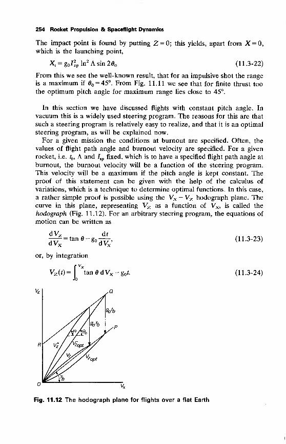
254 Rocket Propulsion & Spaceflight Dynamics
The impact point is found by putting Z = 0; this yields, apart from X = 0,
which is the launching point,
X; = g I* In
2 A sin 20o (11.3-22)
From this we see the well-known result, that for an impulsive shot the range
is a maximum if O = 45°. From Fig. 11.11 we see that for finite thrust too
the optimum pitch angle for maximum range lies close to 45°.
In this section we have discussed flights with constant pitch angle. In
vacuum this is a widely used steering program. The reasons for this are that
such a steering program is relatively easy to realize, and that it is an optimal
steering program, as will be explained now.
For a given mission the conditions at burnout are specified. Often, the
values of flight path angle and burnout velocity are specified. For a given
rocket, i.e. tb , A and Isp fixed, which is to have a specified flight path angle at
burnout, the burnout velocity will be a function of the steering program.
This velocity will be a maximum if the pitch angle is kept constant. Theproof of this statement can be given with the help of the calculus of
variations, which is a technique to determine optimal functions. In this case,
a rather simple proof is possible using the Vx — Vz hodograph plane. Thecurve in this plane, representing Vz as a function of Vx, is called the
hodograph (Fig. 11.12). For an arbitrary steering program, the equations of
motion can be written as
dVy= tan0-go
6t
dvx--" °"dVx
'
or, by integration
Vz (t)
-fJotan0dVx -go *.
(11.3-23)
(11.3-24)
Fig. 11.12 The hodograph plane for flights over a flat Earth
Two-dimensional Rocket Motion in Vacuum 255
Now define
fVxV%=\ tan0dVx,
(11.3-25)Jo
then, according to Eq. (11.3-24),
Vz = V%-g t. (11.3-26)
As
dV*dV,
= tan0, (11.3-27)
the slope of the line V| is just the pitch angle. Because at burnout the flight
path angle is required to be yb the burnout point of the hodograph must lie
on the straight line OP, given by VZb = tan ybVXb . The burnout point of the
curve Vz then has to lie on the line RQ which is parallel to OP and given
by
Vlb= tanybVXb + g fb .
The total length of the curve Vz between t = and t = tb is given by
s=r>Risr dvx=r^ =r^ d ' =g^ ,nA
-
(n -3-28>
We see that s is independent of steering program and thrust-time history.
As Vb = VxJcos yb , the burnout velocity is a maximum, for fixed yb , if VXb is
a maximum. Consequently, for maximum burnout velocity, the burnout
point of Vf has to lie as far as possible to the right on the line RQ. As the
length s of the curve V% is a constant, this is realized if, V% is represented bya straight line in the hodograph plane. Thus, for maximum burnout velocity
the slope of V| and, consequently, the pitch angle has to be a constant. This
result is independent of the thrust program.
11.3.3 Gravity turns
To reduce the aerodynamic forces on a rocket during its flight through the
atmosphere, one will endeavor to keep the angle of attack as small as
possible. For simple aerodynamically stabilized vehicles, this is accomplished
by fixed fins. Vehicles that are mechanically stabilized use more or less
complicated control systems to generate the moments necessary to keep the
angle of attack as small as possible. This is of course not the case for
aerodynamically controlled rockets, during maneuvring. For launch vehicles,
ICBM's and uncontrolled aerodynamically stabilized rockets we can say that
the flight through the atmosphere takes place with zero angle of attack. In
that case there is no lift and the curvature of the trajectory is solely due to
gravity, hence the name gravity turn, or zero-lift trajectory. In this section wewill discuss some gravity turns in vacuum.
256 Rocket Propulsion & Spaceflight Dynamics
As the angle of attack is zero, the flight path angle equals the pitch angle:
6 = y = arctan -f . (11.3-29)
Then the equations of motion become
dVx VxM"df
=F"#' (H.3-30a)
dVz V7M-^f=F^-Mg , (11.3-30b)
where
It is convenient in this case to use the total velocity, V, and the flight path
angle, y, as dependent variables, instead of Vx and Vz. Multiplication of
Eq. (11.3-30a) by Vx, Eq. (11.3-30b) by Vz and summation yields
dV F~di
=M~ goSmy ' (11.3-31)
The differential equation for y is found by multiplication of Eq. (11.3-30a)
by Vz, Eq. (11.3-30b) by Vx, and subsequently subtracting the results:
^=-^cosy. (11.3-32)
The equations for the gravity turn, in general, cannot be solved analytically.
However, some special cases exist which allow for analytical solutions.
These are constant specific thrust and constant pitch rate.
Constant specific thrust, /3 = /3 . In this case the equations of motion become
— =g (/3 -sin 7 ), (11.3-33a)
(11.3-33b)
(11.3-34)
dy
d7~"
cos y"g y
Elimination of t from Eqs. (11.3-33) leads to
dV_V
~ 0o sin 7"
cos y cos ydy.
Integration of this equation yields
Vcos y"l+sinyl^
1-sin yj= constant. (11.3-35)
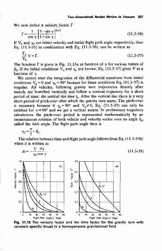
Two-dimensional Rocket Motion in Vacuum 257
We now define a velocity factor, Y
r =1 f l-siny!^2
Ll + sinyJ(11.3-36)
cos y Ll + sin y"
If V and y are initial velocity and initial flight path angle respectively, then
Eq. (11.3-35) in combination with Eq. (11.3-36), can be written as
(11.3-37)^v=r.V
The function T is given in Fig. 11.13a as function of y for various values of
/3 . If the initial conditions V and y are known, Eq. (11.3-37) gives V as a
function of 7.
We cannot start the integration of the differential equations from initial
conditions V = and y = 90° because for these conditions Eq. (11.3-37) is
singular. All vehicles, following gravity turn trajectories directly after
launch, are launched vertically and follow a vertical trajectory for a short
period of time: the vertical rise time tv . After the vertical rise there is a very
short period of pitch-over after which the gravity turn starts. The pitch-over
is necessary because if yo = 90° and Vo ^0, Eq. (11.3-37) can only be
satisfied for y = 90° and we get a vertical ascent. In preliminary trajectory
calculations the pitch-over period is represented mathematically by an
instantaneous rotation of both vehicle and velocity vector over an angle 8,
called the kick angle. The flight path angle then is
The relation between time and flight path angle follows from Eq. (1 1 .3-33b)
when it is written as
V dydf= —
go cos y(11.3-38)
,_ 0.8
~ 0.6
u
0.2
(a)
0.5
(b)
0.4
1E
- 0-3a>
Ei-
No=2
0.2
\A> =2
\3
*.t0.1
\
T^ylO
\M
15 30 (.5 60 75 90
Flight Fath Angle y (deg)
15 30 45 60 75 90
Flight Path Angle y (deg)
Fig. 11.13 The velocity factor and the time factor for the gravity turn with
constant specific thrust in a homogeneous gravitational field
258 Rocket Propulsion & Spaceflight Dynamics
Substitution of V= V(y, y , V ) from Eq. (11.3-37) into Eq. (11.3-38) andchanging to the variable q, denned as
(;4q= tan U 2/'
(11.3-39)
simplifies integration of Eq. (11.3-38), which finally leads to
t~ to=
tr(a2 n [V(flo+ sin y)- Vo(0o + sin y )]. (11.3-40)50VP0 ±)
By introduction of a time factor, V, defined as
P =MSL!! r> (U3 _41)
Eq. (11.3-40) can be written as
^(t-t ) = r-r (n.3-42)
The time factor T' is depicted in Fig. 11.13b as a function of y.
For a rocket with )3 , tb and the initial conditions t , V and y known, the
burnout conditions can be determined as follows. The values of T and T'
follow from Fig. 11.13. Then the time factor at burnout, Tb is determined by
Eq. (11.3-42) and the flight path angle at burnout follows from Fig. 11.13b.
The velocity factor at burnout, rb, is determined with Fig. 11.13a, and Eq.
(11.3-37) finally yields the burnout velocity. If the burnout conditions are
specified, the initial conditions can be found using the described procedure
the other way round.
As, in general, both V and 8 are very small one can start with initial
conditions Vo =0 and yo = 90°. In that case ro/V is undetermined. If,
however, one of the burnout conditions is specified, for example the flight
path angle yb , we can determine the other burnout condition, Vb , in this
case, in the following way: for y = 90°, ro = and as yb is known, T'b is
determined from Fig. 11.13b. From Eq. (11.3-42) the ratio ro/V is deter-
mined and Vb can be calculated with Eq. (11.3-37).
The coordinates X and Z follow from
r V2
X=-\ — dy +X , (11.3-43a)••0'
'o °0
f' V2 siny JZ=- L dy +Z . (11.3-43b)
1 go cos y
Two-dimensional Rocket Motion in Vacuum 259
Again using the variable q defined in Eq. (11.3-39) we can derive
~~^T2— T^—T P* cos r(2j8 + sin 7)- T2
cos 7o(2j3 + sin y )],
(11.3-44a^
-r2(j3 sin 7o + 1 -\ cos
27o)]. (11.3-44b).
As mentioned before, for a flight through the atmosphere, the effective
specific thrust can in some cases very well be approximated by a constant. In
those cases the above discussed method will lead to rapid results.
Miele [5] gives analytical solutions for the gravity turn for constant
specific thrust but uses different end conditions, namely the conditions
V = V2 at 7 = 0. Then V2 is the velocity that the rocket should have if the
flight were continued until the trajectory had become horizontal.
In the case of a constant thrust, the equations for the gravity turn can only
be solved numerically. Here the same difficulty, due to the singularity for
vertical start with zero initial velocity, occurs. Both Seifert [2] and Culler
and Fried [6] eliminate these singularities in an elegant way. Typical plots
for gravity turn trajectories are given by White [7].
Constant pitch rate, q = qQ. Finally we should mention that a simple analyti-
cal solution for the gravity turn is possible in the case of a constant pitch
rate. In that case
d0 dv
dTd?-*' (11 -3 "45)
and the equations of motion become
^=q , (H.3-46)
dV F^- = ^-g„sin 7. (11.3-47)
Differentiation of Eq. (11.3-46) yields
A cos 7 / . dV\ n-j = -^2-(g sin7-^-j = 0. (11.3-48)
d /cos y\ _ cos 7
di\~V
Equation (11.3-48) can only be satisfied either if cos 7 = 0, which means that
we have a vertical ascent with zero pitch rate, or if
dV-jjp go sin 7. (11.3-49)
260 Rocket Propulsion & Spaceflight Dynamics
By combining Eq. (11.3-47) and Eq. (11.3-49) we see that the specific thrust
is determined by
F „ .
—-z = 2smy. (11.3-50)
As according to Eq. (11.3-45)
7 = yo-<*o(<-'o)> (11.3-51)
Eq. (11.3-50) can be integrated, leading to
, M 2 ,In—- =—- (cos y - cosy). (11.3-52)
Thus, at burnout
3o4P ,
cosyb = cosy +-LyE lnA, (11.3-53)
(11.3-54)
which determines yb . The burning-time follows from
t , - To ~ y*
Substitution of Eq. (11.3-51) into Eq. (11.3-49) and integration of the
resulting equation yields the velocity as a function of y:
V= V +-^ (cosy -cos y ). (11.3-55)
By using Eq. (11.3-52) one finds
Vb = ^+k 4plnA, (11.3-56)
or
AVb =iAVid . (11.3-57)
So in this case gravity losses amount to 50% of the ideal velocity. This is a
consequence of the low thrust (/3<2), and the resulting large burning-time.
The trajectory is obtained by integrating
dX— =Vcosy, (11.3-58a)
dZ— =Vsiny. (11.3-58b)
These equations can also be integrated analytically. This will be left to the
reader.
The methods discussed in this chapter can be used for a rough determina-
tion of the trajectory of a launch vehicle or ICBM until burnout of the first

Two-dimensional Rocket Motion in Vacuum 261
stage(s). In most cases such a trajectory is composed of the following
sub-arcs:
1. Vertical rise.
2. Pitch-over maneuver (mathematically represented by kick-angle).
3. Gravity turn to reduce aerodynamic forces in the lower part of the
atmosphere
4. Flight with constant pitch angle to reach a maximum burnout velocity,
or flight with constant pitch rate. However, other pitch programs are used
too.
As all of these vehicles are multi-stage rockets, the next chapter will be
devoted to the theory of the multi-stage rocket.
References
1 Vertregt, M. (1965), Principles of Astronautics, Elsevier, Amsterdam, p.
29.
2 Seifert, H. S. (1959), Space Technology, John Wiley, New York, p.
3-09, 4-10.
3 Williams, M. L. (1957), The calculation of fuel distribution in step-
rockets, J. Brit. Interplanet. Soc, 16, No 4, 211-215.
4 Fraeijs de Veubeke, B. (1958), Performances ballistiques des fusees,
Revue Universelle des Mines, XIV, No. 6, 174-193.
5 Miele, A. (1962), Flight Mechanics I, Addison-Wesley, Reading, p.
345.
6 Culler, G. S. and Fried, B. D. (1957), Universal gravity turn trajec-
tories, J. Appl. Physics, 28, 672-676.
7 White, J. F. (1963), Flight Performance Handbook for Powered Flight
Operations. John Wiley, New York, p. 29A.
12 The Multi-Stage Rocket
During the powered flight of a single-stage rocket, part of its mass has
become 'superfluous'. As the propellant tanks are designed to contain the
gross propellant mass, they will be 'too large' if part of the propellant is
consumed. So an extra, in fact useless mass has to be accelerated by the
rocket engine. Consequently, this superfluous mass absorbs energy, whichotherwise could be utilized for the payload. So it should be advantageous if
this useless mass could be discarded continuously during the flight. How-ever, this is not feasible. We cannot continuously throw away parts of the
propellant tanks. Therefore, a multi-stage rocket contains several propellant
tanks, which are discarded when they are empty. As it is not possible to
discard only a tank, in general a complete propulsion unit, i.e. tanks
together with motor and propellant feed system, is thrown-off. This com-plete unit is called a stage. In this way we do not have the full advantage of
the discarding of the 'useless' mass as more rocket engines and propellant
feed systems will be necessary. Therefore, more stages will only be advan-
tageous for relatively large rockets where the propulsion system mass is
small as compared to the mass of the tanks. In addition to extra rocket
engines and auxiliary equipment, special provisions for separation of the
various stages, and consequently extra mass, will be required.
An additional advantage of this staging is the possibility of thrust-
programming, as well as the possibility of adapting the engines of the
subsequent stages to the altitude where they are fired, thus reducing losses
due to non-ideal expansion.
12.1 Nomenclature of the multi-stage rocket
We distinguish between rocket stages and sub -rockets. A stage (also called
step in older literature) is a complete propulsion unit (motor, propellant feed
system, tanks, propellant) together with control equipment, which is dis-
carded completely when all propellant of that stage is consumed (staging). Asub-rocket is a complete rocket vehicle, consisting of one or more stages
together with the payload and the guidance and control system (astrionics
system).
Figure 12.1 shows a three-stage rocket. In this case we have three stages
and three sub-rockets. The first sub-rocket is the complete rocket vehicle.
The second sub-rocket is the first sub-rocket minus the first stage. The third
sub-rocket, finally, is the second sub-rocket minus the second stage, or,
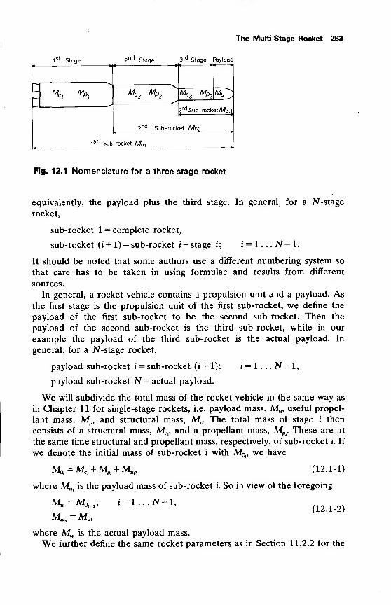
The Multi-Stage Rocket 263
1st Stage 2
nd Stage 3 rd Stage ^yload
- \
^% M
P1MC2 Mp
2MC3 MP2 Mu^3 rd Sub- rocketMoJ
•|St
2nd Sub- rocket M02
Sub-rocket M01
Fig. 12.1 Nomenclature for a three-stage rocket
equivalently, the payload plus the third stage. In general, for a N-stage
rocket,
sub-rocket 1 = complete rocket,
sub-rocket (i + 1) = sub-rocket i — stage i; i = l . . . N-l.
It should be noted that some authors use a different numbering system so
that care has to be taken in using formulae and results from different
sources.
In general, a rocket vehicle contains a propulsion unit and a payload. Asthe first stage is the propulsion unit of the first sub-rocket, we define the
payload of the first sub-rocket to be the second sub-rocket. Then the
payload of the second sub-rocket is the third sub-rocket, while in our
example the payload of the third sub-rocket is the actual payload. In
general, for a N-stage rocket,
payload sub-rocket i = sub-rocket (i + 1); i = 1
payload sub-rocket N = actual payload.
.N-l,
We will subdivide the total mass of the rocket vehicle in the same way as
in Chapter 11 for single-stage rockets, i.e. payload mass, Mu, useful propel-
lant mass, Mp, and structural mass, Mc . The total mass of stage i then
consists of a structural mass, MCj , and a propellant mass, M
Pi. These are at
the same time structural and propellant mass, respectively, of sub-rocket i. If
we denote the initial mass of sub-rocket i with Mq., we have
M0i= M
Ci+M
Pi+M
Ui ,(12.1-1)
where Mu . is the payload mass of sub-rocket i. So in view of the foregoing
M«1
=A^+1 ; i = l... N-l,
M„„ = M„,(12.1-2)
where Mu is the actual payload mass.
We further define the same rocket parameters as in Section 11.2.2 for the
264 Rocket Propulsion & Spaceflight Dynamics
single-stage rocket. For sub-rocket i we have
mass ratio At= ^
, (12.1-3a)
i j Mu . Mapayload ratio *i
=Tr = ^rr1
, (12.1-3b)M0j Mq, '
propellant ratio **=I*~» (12.1-3c)
structural efficiency gi= *
. (12.1-3d)MCi+M
Pi
As we already mentioned in the discussion of rocket parameters of
single-stage rockets, the above defined parameters are the ones most com-monly used, there are, however, other parameters in use. Mass ratio,
payload ratio and propellant ratio are related to sub-rockets only. Thestructural efficiency is related both to sub-rockets and to stages.
Just like for single-stage rockets, here too we have the following relations
between the various rocket parameters
^(l-ejXl-Aj), (12.1-4a)
1 1Ai=
l=~Pi—
TTZ7- (12.1-4b)
The total payload ratio is defined as the ratio of the actual payload massand the total initial mass of the rocket,
Mu MUNk<°<
=T?
=TT- (12.1-5)
Mo Mo,v '
The inverse of this total payload ratio is called the growth factor and is
denoted by G
^ MG=w t12 - 1 -6)
The growth factor is an indication of the increase of the total initial mass as
a result of an increase of payload mass. There is a simple relation betweenthe total payload ratio and the payload ratios of the sub-rockets. Using Eq.(12.1-2) we can write
M^ =MIilM^ M^
Mo, M^M^'-'M^ V-i-0
So, in view of Eqs. (12.1-5) and (12.1-3b), the total payload ratio can bewritten as
Kot = AiA2 . . . AN. (12.1-8)
Furthermore, we define the total propellant ratio as the ratio of total useful
The Multi-Stage Rocket 265
propellant mass, Mp, and initial mass of the rocket
«™ =M =V- (12 - X "9)
Now
and by using Eqs. (12.1-3), we find
^=9iAiA2 ...A,_ 1 . (12.1-10)
Substitution of Eq. (12.1-10) into Eq. (12.1-9) leads to
<Ptot= (pi + <PaAi + . . . + (pNAiA2 . . . AN_ X . (12.1-11)
Finally, we define a total structural efficiency as
= Mc _ £MC .
Stot Mc +Mp lMCi+ZM
Pi
' (12.1-12)
where Mc is the total structural mass of the rocket. As the sum of total
structural and total propellant mass equals the initial mass minus the
payload mass, we may also write, using Eq. (12.1-5),
1 yMCi
l-k tot
L M (12.1-13)
According to Eq. (12.1-3d)
and, using Eq. (12.1-10), we find
Substitution of Eq. (12.1-14) into Eq. (12.1-13) and using Eq. (12.1-4a)
finally gives
1
Btot=i_i t6^ 1 ~ A i) + ea(l - A2)A! + . .
. + eN(l - AN)A XA2 . . . AN_i].1 Atot
(12.1-15)
12.2 The ideal velocity of the multi-stage rocket
According to Eq. (11.2-10), the velocity increment of sub-rocket i during
motor operation in free space is given by
AV^CjlnAj, (12.2-1)
266 Rocket Propulsion & Spaceflight Dynamics
where ct
is the effective exhaust velocity of stage i. If Vbil is the burnoutvelocity of sub-rocket (i-1), the burnout velocity of sub-rocket i is
Vbl= V
bl_ 1+\V
i. (12.2-2)
If the initial velocity of the rocket is zero, the burnout velocity of sub-rocket
N, according to Eqs. (12.2-1) and (12.2-2), is
Vid = VbN = £ A V, = £ ctIn A,. (12.2-3)
i=l i=l
This velocity is called the ideal velocity of the N-stage rocket. By using Eq.
(12.1-4b), we may also write
NVid = - £ c
tIn {A, + e,(l - A,)}. (12.2-4)
Just as for the single-stage rocket, this ideal velocity is an important
measure for the performance of the multi-stage rocket. A second important
performance parameter is the total payload ratio. For a given ideal velocity,
one will endeavor to have a payload ratio as large as possible . This means thatwehave a maximum payload mass for a given initial mass. This, of course, is
equivalent to maximizing the ideal velocity for a given total payload ratio.
From Eq. (12.2-4) we see that the ideal velocity is dependent on the
effective exhaust velocities (i.e. the propellants) and the structural efficien-
cies of the stages, as well as on the payload ratio distribution. In general, weare free to choose this payload ratio distribution such that maximumperformances are obtained. The structural efficiencies and the choice of
propellants, however, are strongly dependent on operational aspects and on
the state of the art of construction techniques. We may assume that in the
design stage e, and c, are known. Maximizing the ideal performances then is
equivalent to maximizing the ideal velocity as a function of the A, 's only, for
a given total payload ratio. So, this comes down to the determination of the
payload ratios such that
NVid (A.) = - J Ci In {A
f+ ei (l - A,)}, (12.2-5)
i = l
is a maximum, with the side condition
A XA2 . . . AN = Atof. (12.2-6)
This is a constrained optimization problem which can be solved by using the
method of Lagrange multipliers [1]. Vertregt [2, 3] was the first to solve the
multi-stage rocket optimization problem this way. We will follow this
approach.
It will prove to be convenient to write the side condition, Eq. (12.2-6), as
X lnAi-lnA
ftrt= 0. (12.2-7)
The Multi-Stage Rocket 267
Now we define an augmented function, F, as
HK) = VM (A,)+ J £ In A, -In AJ. (12.2-8)
The constant v, to be determined later, is called a Lagrange multiplier.
According to the theory of constrained maximization [1], a necessary
condition for Vid to be a maximum, while Eq. (12.2-7) is satisfied, is
dF— = 0; i = l,2,...,N. (12.2-9)
Elaboration of Eq. (12.2-9) yields as necessary conditions:
cix J~
Ei
^-f =- (12.2-10)
Ai + fijCl-Aj) A;
Solution of these equations for \tleads to
Ai=7 ^ -. (12.2-11)(c, - v){\ - e^
The value of the Lagrange multiplier, v, is determined by substitution of Eq.(12.2-11) into the side condition, Eq. (12.2-7), yielding
£ lnT,
^ T m Ato„ (12.2-12)
which is an equation in v only. Thus, the optimal payload ratio distribution
and the corresponding maximum value of the ideal velocity are found by first
solving Eq. (12.2-12) for v. Then this solution is substituted into Eq.(12.2-11), yielding the A
f's. Finally, substitution of the obtained values of the
payload ratios into Eq. (12.2-5) yields the maximum ideal velocity.
In general, Eq. (12.2-12) is a JVth-order algebraic equation in v, whichcannot be solved analytically. As this equation has N roots, it will sometimesbe necessary to check which root yields the maximum value of the ideal
velocity. However, the solution is relatively simple if all stages have the
same effective exhaust velocity. In that case c x= c2 = . . . = cN = c, and Eq.
(12.2-12) leads to
c-v to
\ e 1 e2 ...eN J
Substitution of this expression into Eq. (12.2-11) gives
^[^-..Ki-o-a-^r (12.2-i3)
Substitution of these values of the Aj's into Eq. (12.2-5) yields
(
V
M )m„ - -c ,n [.,., . ..4 +
{^-^t^^TJ}(12.2-14)
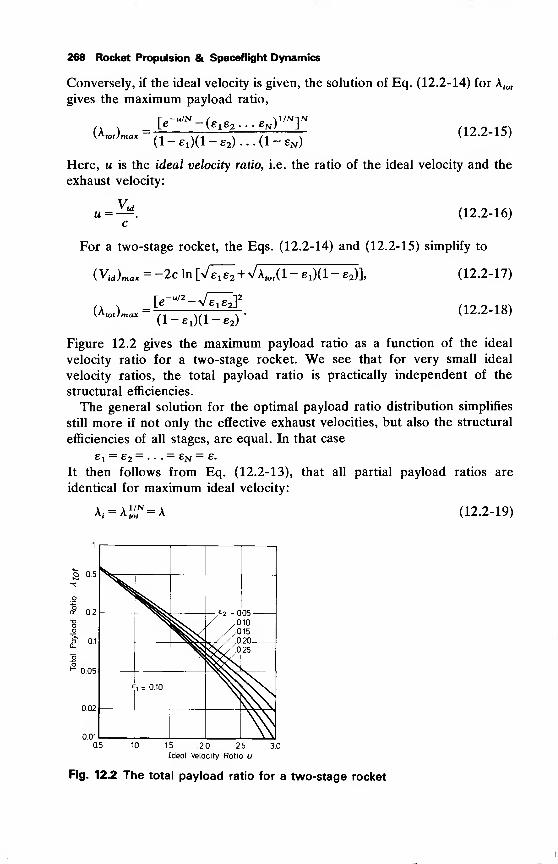
268 Rocket Propulsion & Spaceflight Dynamics
Conversely, if the ideal velocity is given, the solution of Eq. (12.2-14) for At
gives the maximum payload ratio,
[6-"'N -( ei e2 ... eN )
1/Nr\A-tot)max
(l- ei)(l-e2)...(l-eN )
(12.2-15)
Here, u is the ideal velocity ratio, i.e. the ratio of the ideal velocity and the
exhaust velocity:
u = (12.2-16)c
For a two-stage rocket, the Eqs. (12.2-14) and (12.2-15) simplify to
(12.2-17)(
V
id )max = -2c In [V7ie2 + VA(of(l- ei)(l-e2)],
\A-tot)max
[e-^-Ve^]2
(12.2-18)tot,max(l- ei)(l-e2)
Figure 12.2 gives the maximum payload ratio as a function of the ideal
velocity ratio for a two-stage rocket. We see that for very small ideal
velocity ratios, the total payload ratio is practically independent of the
structural efficiencies.
The general solution for the optimal payload ratio distribution simplifies
still more if not only the effective exhaust velocities, but also the structural
efficiencies of all stages, are equal. In that case
e t= e2
=. . . = 6jv = e.
It then follows from Eq. (12.2-13), that all partial payload ratios are
identical for maximum ideal velocity:
Ai= ALf=A (12.2-19)
S 0-5
£ 0.2
0.05
0.02
0.01
05
10
.15
?n/A25
£1 = 0.10
0.5 1.0 1.5 2.0 2.5
Ideal Velocity Ratio u3.0
Fig. 12.2 The total payload ratio for a two-stage rocket
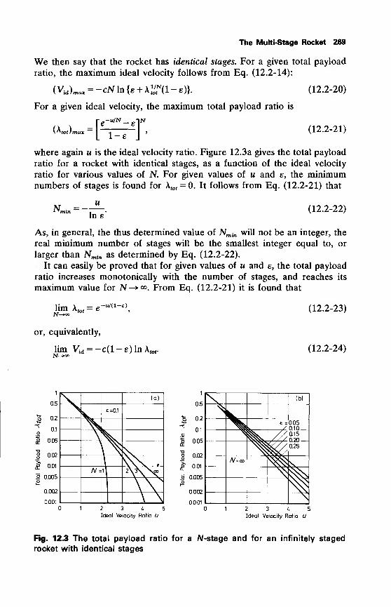
The Multi-Stage Rocket 269
We then say that the rocket has identical stages. For a given total payload
ratio, the maximum ideal velocity follows from Eq. (12.2-14):
(Vid )max = -cN In {e +A^d - e)}. (12.2-20)
For a given ideal velocity, the maximum total payload ratio is
rc-u/N_
e-jN
\"tot)max—
I * I J
L l-e J
(12.2-21)
where again u is the ideal velocity ratio. Figure 12.3a gives the total payload
ratio for a rocket with identical stages, as a function of the ideal velocity
ratio for various values of N. For given values of u and e, the minimumnumbers of stages is found for Xtot
= 0. It follows from Eq. (12.2-21) that
In e(12.2-22)
As, in general, the thus determined value of Nmin will not be an integer, the
real minimum number of stages will be the smallest integer equal to, or
larger than Nmin as determined by Eq. (12.2-22).
It can easily be proved that for given values of u and e, the total payload
ratio increases monotonically with the number of stages, and reaches its
maximum value for N—>°°. From Eq. (12.2-21) it is found that
lim A«=e-^ 1- )
,N—»o°
or, equivalently,
lim Vid = — c(l - e) In At,
N—*»
(12.2-23)
(12.2-24)
£
1
0.5
0.2
0.1
0.05
0.02
0.01
2 0.005
0.002
0.001
(o)
£=0.1
N =1] 2\K >po
1
0.5
o 0.2
1 005
J 0.02
1 0.01
2 0.005
0.002
0.001
(b)
£ - 0.05omQ150200.25
/V=oo
2 3 4 5
Ideal Velocity Ratio U2 3 4 5
Ideal Velocity Ratio U
Fig. 12.3 The total payload ratio for a N-stage and for an infinitely staged
rocket with identical stages
270 Rocket Propulsion & Spaceflight Dynamics
In Fig. 12.3b the total payload ratio is given as a function of the ideal
velocity ratio for the case of infinite staging.
For a rocket with identical stages, the total propellant ratio is, according
to Eq. (12.1-11),
<pto,= <p(l + A + A 2 + ... + A
N- 1) = y^-,p, (12.2-25)
or, by using Eqs. (12.1-4a) and (12.2-19),
<pto,= (l-e)(l-Atot ). (12.2-26)
We see that for a rocket with identical stages the total propellant ratio does
not depend on the number of stages. So, if the total propellant mass is fixed,
it is favorable in this case to distribute it over as many stages as possible.
From Eq. (12.1-15) we find the total structural efficiency to be
etot= e. (12.2-27)
So, again for a rocket with identical stages, the total structural efficiency is
independent of both the number of stages and the total payload ratio and
equals the structural efficiency of the stages.
These results hold only if the structural efficiencies of the stages are
independent of the number of stages. In practice, this is not possible. If, for
a fixed initial gross mass, the number of stages increases, the propellant mass
in each stage will decrease. Consequently, the mass of the tanks in each
stage decreases too. In general, the mass of the motor and the propellant
feed system will decrease too, however, not with the same rate as the
propellant and tank mass. As a result of this, the structural efficiencies of the
stages will increase with increasing number of stages and will approach unity
for infinite staging. Therefore, there will be a finite optimum number of
stages.
The derived results are also strongly dependent on the parameters used
and on the assumptions made. If, instead of the structural efficiency, e, the
structure ratio s, defined as
Si=^, (12.2-28)
is used and if it is assumed that st
is independent of the number of stages,
the results will differ considerably, as will be shown. In this case the relation
between mass ratio, payload ratio and structure ratio is
Ai Mo, Mo,
Consequently, the ideal velocity of a N-stage rocket is
Vid = -£ cln(A, + *). (12.2-30)
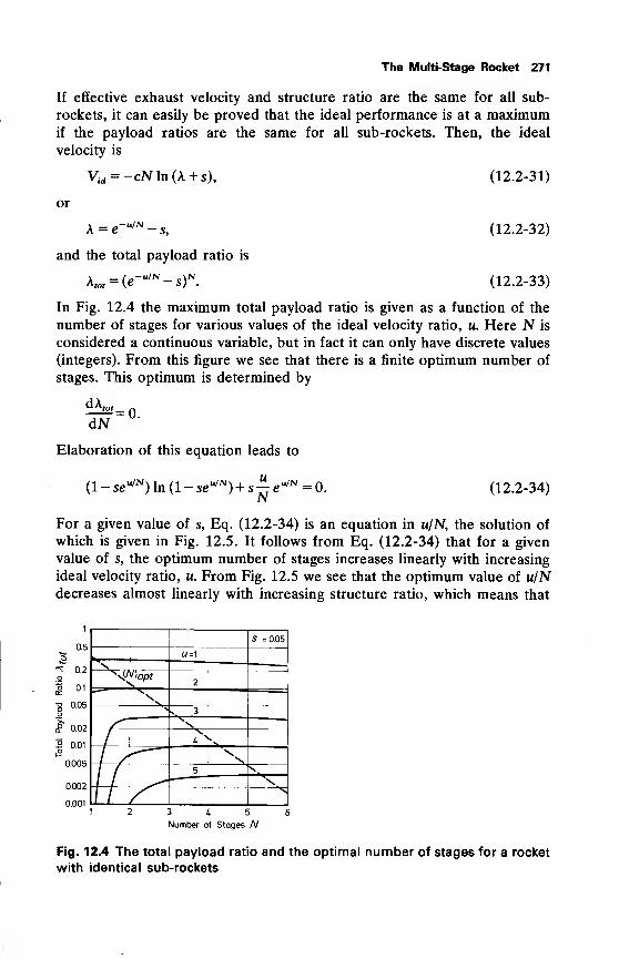
The Multi-Stage Rocket 271
If effective exhaust velocity and structure ratio are the same for all sub-
rockets, it can easily be proved that the ideal performance is at a maximumif the payload ratios are the same for all sub-rockets. Then, the ideal
velocity is
Vid= -cJVln(A + s),
or
_ „-u/NX = e -s,
and the total payload ratio is
AM,= (e-/N -s)N.
(12.2-31)
(12.2-32)
(12.2-33)
In Fig. 12.4 the maximum total payload ratio is given as a function of the
number of stages for various values of the ideal velocity ratio, u. Here N is
considered a continuous variable, but in fact it can only have discrete values
(integers). From this figure we see that there is a finite optimum number of
stages. This optimum is determined by
dA.
dN= 0.
Elaboration of this equation leads to
(l-se u/N)ln(l-se u/N) + s-^e u/N = 0.N (12.2-34)
For a given value of s, Eq. (12.2-34) is an equation in u/N, the solution of
which is given in Fig. 12.5. It follows from Eq. (12.2-34) that for a given
value of s, the optimum number of stages increases linearly with increasing
ideal velocity ratio, u. From Fig. 12.5 we see that the optimum value of u/Ndecreases almost linearly with increasing structure ratio, which means that
1
0.5
.g
^ 0.2o
| 0.1
1 0.05_o
£ 0.02
2 0.01
|2
0.005
0.002
0.00112 3-156Number of Stages N
Fig. 12.4 The total payload ratio and the optimal number of stages for a rocket
with identical sub-rockets
S =0.05
U=1
V ,,——
1
Wopt2
>lv 3/ V
f U "1
'n.
/ /^-
—
/ ^ 5 ^\
/ f *S
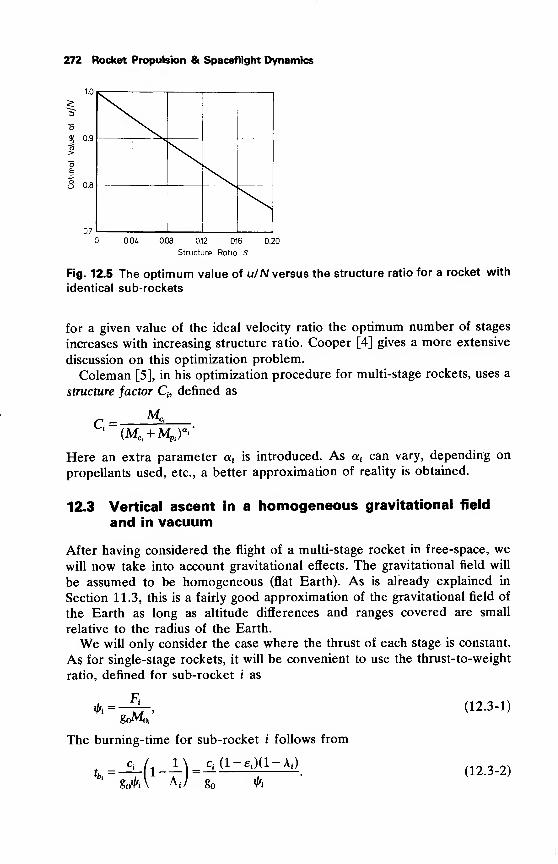
272 Rocket Propulsion & Spaceflight Dynamics
0.08 0.12 0.16
Structure Ratio S
0.20
Fig. 12.5 The optimum value of u/N versus the structure ratio for a rocket with
identical sub-rockets
for a given value of the ideal velocity ratio the optimum number of stages
increases with increasing structure ratio. Cooper [4] gives a more extensive
discussion on this optimization problem.
Coleman [5], in his optimization procedure for multi-stage rockets, uses a
structure factor Q, denned as
Q = Mr.
(MCi+M
PipHere an extra parameter a
{is introduced. As a
tcan vary, depending on
propellants used, etc., a better approximation of reality is obtained.
12.3 Vertical ascent in a homogeneous gravitational field
and in vacuum
After having considered the flight of a multi-stage rocket in free-space, wewill now take into account gravitational effects. The gravitational field will
be assumed to be homogeneous (flat Earth). As is already explained in
Section 11.3, this is a fairly good approximation of the gravitational field of
the Earth as long as altitude differences and ranges covered are small
relative to the radius of the Earth.
We will only consider the case where the thrust of each stage is constant.
As for single-stage rockets, it will be convenient to use the thrust-to-weight
ratio, defined for sub-rocket i as
*.=F
t
goMo*'
The burning-time for sub-rocket i follows from
bi
go'/'A A,/ go *h
(12.3-1)
(12.3-2)
The Multi-Stage Rocket 273
We further define V0i
to be the velocity of sub-rocket i at ignition, taking
place at time ^ and altitude fi^, while Vb . is the burnout velocity of
sub-rocket i, at an altitude hb . at time to. + tb .. We will assume the initial
velocity of the rocket, V = V0l , to be zero.
12.3.1 The burnout velocity
The total velocity increment due to the motor operation of sub-rocket i is
A V, = Vbi- V
0t= c
xIn A, - gotb,
(12.3-3)
If tc . is the time between burnout of sub-rocket i and ignition of sub-rocket
(i + 1), the coast-time, the velocity at ignition of sub-rocket (i + 1) is
Voi+1=V
bi-g fc,
(12.3-4)
From Eqs. (12.3-3) and (12.3-4) we obtain the burnout velocity of the Nth
sub-rocket, the total burnout velocity
Vfc= Vftw =f AV.-&2 <c, (12.3-5)
i = l i=l
We see that the burnout velocity decreases linearly with increasing coast-
time between burnout and ignition of the next stage. Maximum burnout
velocity is obtained if every stage is ignited directly after burnout of the
previous one. For the time being we will assume that this is the case. Theburnout velocity then follows from Eqs. (12.3-5) and (12.3-3):
Vb =fd[c
i\nA
i-g t
bil (12.3-6)i = l
Using Eqs. (12.1-4b) and (12.3-2), we obtain the burnout velocity as a
function of effective exhaust velocity, thrust-to-weight ratio, structural effi-
ciency and payload ratio of the various sub-rockets:
V„ = - £ ci[ln{A
i+ £i(l-A i )} +
(1 £i)£Ai)
].(12.3-7)
As for single-stage rockets, we see that the gravitational losses approach
zero, and consequently the burnout velocity approaches the ideal velocity, if
ifo—> oo, i.e. for impulsive shots. Here too we can ask for the optimal
distribution of the partial payload ratios, such that for given ct,
et , ^ and Atot,
the burnout velocity reaches a maximum value. Again this is a constrained
optimization problem, which can be solved by using Lagrange multipliers.
We define the augmented function F as
F(A.) = Vb (A,) + v\ £ In A, - In AJ
,
Li=i J
and the necessary conditions for maximum burnout velocity with total
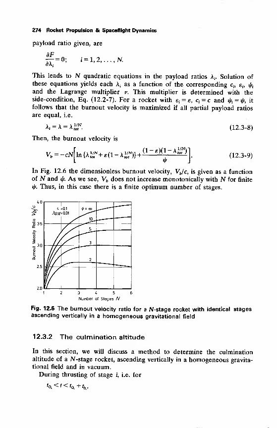
274 Rocket Propulsion & Spaceflight Dynamics
payload ratio given, are
This leads to N quadratic equations in the payload ratios A;. Solution of
these equations yields each A{as a function of the corresponding c=, eh ifo
and the Lagrange multiplier v. This multiplier is determined with the
side-condition, Eq. (12.2-7). For a rocket with e{= e, c
t= c and «& = \\i, it
follows that the burnout velocity is maximized if all partial payload ratios
are equal, i.e.
Ai — A — A tot .
Then, the burnout velocity is
Vb = -cN^ln {k1
tSf+ e(l - A*f)}+
(l-gXl-AffQ
]
(12.3-8)
(12.3-9)
In Fig. 12.6 the dimensionless burnout velocity, VJc, is given as a function
of N and ij/. As we see, Vb does not increase monotonically with N for finite
i/r. Thus, in this case there is a finite optimum number of stages.
A.O
3.5
^ 3.0
2.5
2.0
Mot=0.1
0.01
<[>z. 00
10^
5
3
2
3^5Number of Stages A/
Fig. 12.6 The burnout velocity ratio for a N-stage rocket with identical stagesascending vertically in a homogeneous gravitational field
12.3.2 The culmination altitude
In this section, we will discuss a method to determine the culmination
altitude of a N-stage rocket, ascending vertically in a homogeneous gravita-
tional field and in vacuum.During thrusting of stage i, i.e. for
toi<t<t
0i+t
bi ,
The Multi-Stage Rocket 275
the velocity is
Vi(0=V
ft+ c
iln^-g (r-O, (12.3-10)
where M is the instantaneous mass of sub-rocket i. Thus, the altitude at
burnout of stage i is
K^h^+T' \{t)dt, (12.3-11)
or, by using Eq. (12.3-10)
K = ** + voM +\
S(ci In^- So?) dr, (12.3-12)
where t= f— fo,. Now define
Afc-J^m^-g^dr. (12.3-13)
We then find for constant thrust
'"'-M'-i^^-U'-in (i2 -3 - i4)
At burnout of stage i, time, velocity and altitude are
*=*> + ** (12.3-15a)
Vfc.-V^ + AV,, (12.3-15b)
fch, = ^ + Vo^ + Afe,. (12.3-15c)
After burnout of stage i, this stage is discarded and sub-rocket (i + 1)
remains. This rocket first coasts during a time tCi
. So, at ignition of stage
(i + 1), time, velocity and altitude are
*Q +1=
*oi+ '* + <«, (12.3-16a)
Vo^V^-go^, (12.3-16b)
K +l = K + ybJCi -Jgotl- (12.3-16c)
Now, for given initial conditions of the first sub-rocket, Vbland hbl are
determined with Eqs. (12.3-15). Then V^ and h^ can be determined with
Eqs. (12.3-16) and then V^ and h^ can again be determined, etc. Finally,
VbN and hbN are found this way. This last sub-rocket then coasts during a
time interval tCN until culmination. In some cases, payload and last stage are
separated too after burnout of the last stage. The time tCN is determined with
tCN=— (12.3-17)
So
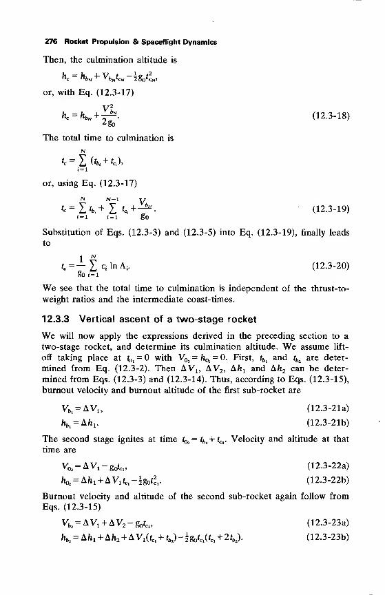
276 Rocket Propulsion & Spaceflight Dynamics
Then, the culmination altitude is
K = hbN+VbstCN -%g ilti,
or, with Eq. (12.3-17)
K = hbN +^. (12.3-18)2go
The total time to culmination is
Ntc= Z (t
bi + tCi ),
i = l
or, using Eq. (12.3-17)
N N-l Y'c=L*bi + I '«+—
•
(12.3-19)i = l < = 1 go
Substitution of Eqs. (12.3-3) and (12.3-5) into Eq. (12.3-19), finally leads
to
1N
'c=-X qlnA,. (12.3-20)g i = !
We see that the total time to culmination is independent of the thrust-to-
weight ratios and the intermediate coast-times.
12.3.3 Vertical ascent of a two-stage rocket
We will now apply the expressions derived in the preceding section to a
two-stage rocket, and determine its culmination altitude. We assume lift-
off taking place at ^ x= with V0l
= hOl= 0. First, tbl and t^ are deter-
mined from Eq. (12.3-2). Then AV1? AV2 , AJij and Ah2 can be deter-
mined from Eqs. (12.3-3) and (12.3-14). Thus, according to Eqs. (12.3-15),
burnout velocity and burnout altitude of the first sub-rocket are
Vbl= AV1 ,
(12.3-21a)
fcbl= Afc!. (12.3-21b)
The second stage ignites at time 1^= tbl -\-
t
Cl . Velocity and altitude at that
time are
V02= AV1
-g0fCl ,
(12.3-22a)
h02= Ah 1 +AV1 rCl -|go^1
. (12.3-22b)
Burnout velocity and altitude of the second sub-rocket again follow from
Eqs. (12.3-15)
Vb2= AV1 +AV2 -g rCl ,
(12.3-23a)
h^A^ +A^ +AV^ + y-lgo^a^y. (12.3-23b)
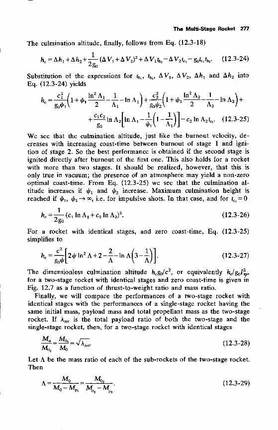
The Multi-Stage Rocket 277
The culmination altitude, finally, follows from Eq. (12.3-18)
fic= Ah 1 + Ah2+^-(AV1
+AV2)2 +AV1 fb2-AV2 fCl
-g fCl fb2 . (12.3-24)
2go
Substitution of the expressions for tbl , t^, AVl5 AV2 , Afix and Aft2 into
Eq. (12.3-24) yields
+^lnA2|mA 1-^l-^]-c2 lnA2 fCl . (12.3-25)
We see that the culmination altitude, just like the burnout velocity, de-
creases with increasing coast-time between burnout of stage 1 and igni-
tion of stage 2. So the best performance is obtained if the second stage is
ignited directly after burnout of the first one. This also holds for a rocket
with more than two stages. It should be realized, however, that this is
only true in vacuum; the presence of an atmosphere may yield a non-zero
optimal coast-time. From Eq. (12.3-25) we see that the culmination al-
titude increases if \\fx and ip2 increase. Maximum culmination height is
reached if iffu ^2 ->°°, i.e. for impulsive shots. In that case, and for fCl=
hc= -i- (d In A! + c2 In A2)
2. (12.3-26)
2 go
For a rocket with identical stages, and zero coast-time, Eq. (12.3-25)
simplifies to
hc =-^-|2 l/fln2 A + 2-^-lnA(3-i\l. (12.3-27)
The dimensionless culmination altitude hcgo/c2
, or equivalently hjg l2sp,
for a two-stage rocket with identical stages and zero coast-time is given in
Fig. 12.7 as a function of thrust-to-weight ratio and mass ratio.
Finally, we will compare the performances of a two-stage rocket with
identical stages with the performances of a single-stage rocket having the
same initial mass, payload mass and total propellant mass as the two-stage
rocket. If \ tot is the total payload ratio of both the two-stage and the
single-stage rocket, then, for a two-stage rocket with identical stages
w^=^- <12 -3 -28)Mo, Mo
Let A be the mass ratio of each of the sub-rockets of the two-stage rocket.
Then
A=xrV=xrV- (12 -3 -29)M -MpiM^-M
P2
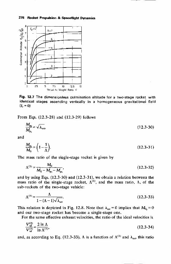
278 Rocket Propulsion & Spaceflight Dynamics
c A = 7
IB25 5 7.5 10 12.5 15
Thrust-to-Weight Ratio <l>
Fig. 12.7 The dimensionless culmination altitude for a two-stage rocket with
identical stages ascending vertically in a homogeneous gravitational field
From Eqs. (12.3-28) and (12.3-29) follows
AL j—
MP1
and
Mo:-H>The mass ratio of the single-stage rocket is given by
MA(1) =
Mo-M^-Mp/
(12.3-30)
(12.3-31)
(12.3-32)
and by using Eqs. (12.3-30) and (12.3-31), we obtain a relation between the
mass ratio of the single-stage rocket, A(1), and the mass ratio, A, of the
sub-rockets of the two-stage vehicle:
A(1)-1-(A-1)VA
;
(12.3-33)
This relation is depicted in Fig. 12.8. Note that Xtot= implies that Mo2
=and our two-stage rocket has become a single-stage one.
For the same effective exhaust velocities, the ratio of the ideal velocities is
Vj? 2 In A(12.3-34)
V2> lnA(1) '
and, as according to Eq. (12.3-33), A is a function of A(1) and A tof, this ratio
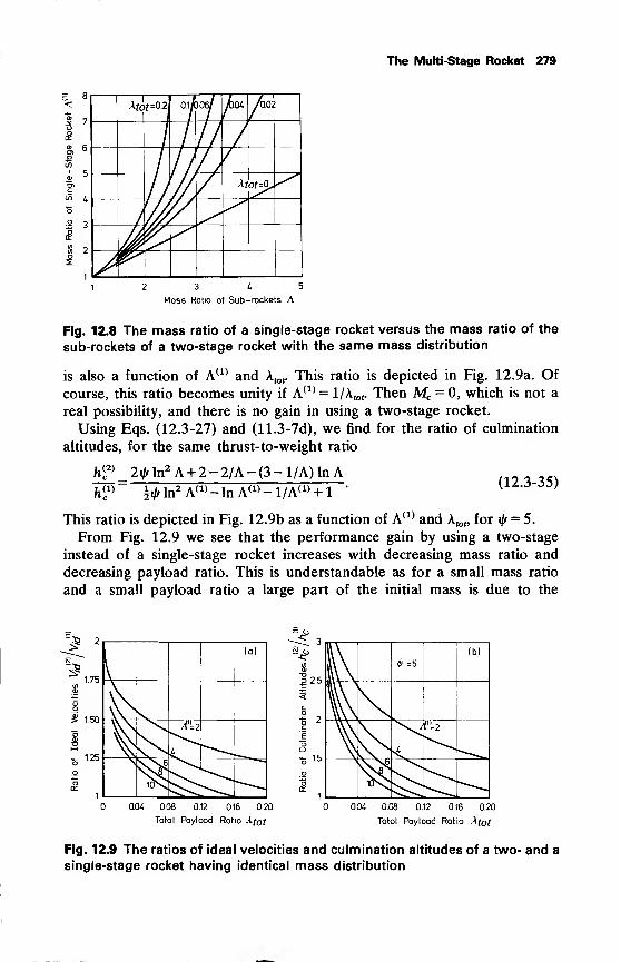
The Multi-Stage Rocket 279
- 8<
2 3
Ate t=0.2\ 0.l/ 306/ AoA—7—
r
/0.02
M ot=Q,
3 4 5
Mass Ratio of Sub -rockets A
Fig. 12.8 The mass ratio of a single-stage rocket versus the mass ratio of the
sub-rockets of a two-stage rocket with the same mass distribution
is also a function of A(1) and km. This ratio is depicted in Fig. 12.9a. Of
course, this ratio becomes unity if A(1) = 1/Atot. Then Mc = 0, which is not a
real possibility, and there is no gain in using a two-stage rocket.
Using Eqs. (12.3-27) and (11.3-7d), we find for the ratio of culmination
altitudes, for the same thrust-to-weight ratio
fi(
c2) _ 2ifr In
2 A + 2 - 2/A - (3 - 1/A) In Aft<1)_
|.Aln2 A(1) -lnA(1) -l/A(1
> + l "
(12.3-35)
This ratio is depicted in Fig. 12.9b as a function of A(1) and A tott for i/r = 5.
From Fig. 12.9 we see that the performance gain by using a two-stage
instead of a single-stage rocket increases with decreasing mass ratio and
decreasing payload ratio. This is understandable as for a small mass ratio
and a small payload ratio a large part of the initial mass is due to the
2T
1.75
2 1.50
,- 1.25
(a)
AUI=2
V\6itNs
0.04 0.08 0.12 0.16 0.20
Total Payload Ratio Af t
2 2.5
=5 2
1.5
4<=5
(b)
f=2
1u\^
0.0£ 0.08 0.12 0.16 0.20
Total Payload Ratio Af t
Fig. 12.9 The ratios of ideal velocities and culmination altitudes of a two- and a
single-stage rocket having identical mass distribution
280 Rocket Propulsion & Spaceflight Dynamics
structure and consequently the useless mass of the single-stage rocket will berelatively large, thus absorbing a relatively large amount of energy. We also
see that the performance improvement is larger if gravitation is taken into
account. This is due to the fact that in that case the useless mass also
represents a certain amount of potential energy in addition to its kinetic
energy. The real performance improvement will be less than calculated here,
owing to the fact that a two-stage rocket with the same payload mass andtotal propellant mass as a single-stage rocket will have a larger structural
mass. This is due to the fact that instead of one, two complete propulsionunits, as well as a mechanism for stage-separation, are required. For verysmall rockets these extra masses are so large as compared to the total mass,that staging hardly improves the performance. For large rockets, the extra
masses are small as compared to the total mass and performance improve-ments of 25% to 80% are possible.
12.4 Parallel staging
Up to now, we have meant by staging the stacking of one stage on top of
another. Parallel staging is defined as staging a vehicle such that the
upper-stage engines are also used during lower stage operation. This is
usually accomplished by arranging the stages alongside one another, hencethe name parallel staging. To distinguish between the two methods of
staging, the first one is often called tandem staging. The main advantage of
parallel staging is the reduction of gravitational losses. As we already
explained, in a gravitational field it is always advantageous to consume the
propellant as fast as possible. Then, the amount of energy that is absorbed
by the propellant as potential energy and cannot be recuperated
anymore, is reduced. By parallel staging, a large propellant consumption is
realized. A disadvantage is that the rocket is likely to be bulky, and for flight
through the atmosphere the drag penalty may be large. This, however, is of
minor importance for large rockets where the drag losses are very small as
compared to gravitational losses (Chapter 14). A second disadvantage of
parallel staging is the reduction in nozzle efficiency of the engines of the first
stage. If these engines are used from the start, their expansion ratio is
limited by the atmospheric pressure at low altitudes. Using tandem staging,
the expansion ratio of the engines of the subsequent stages can be adapted
to the altitude where they are fired.
Often, both methods of staging are applied in one vehicle. For large
launch-vehicles, parallel staging is realized by placing boosters around the
first stage. These boosters are often identified as stage zero. Examples are
the Delta with three, six, or nine solid boosters, the Titan III with two or
four solid boosters, the Space Shuttle with two solid boosters and the
Russian Soyuz launch-vehicle with four boosters using kerosine and LOX as
propellant.
In general, the burning-time of these boosters is shorter than the burning-
time of the first stage. They are jettisoned after burnout.
The Multi-Stage Rocket 281
The analysis of parallel staging is about analogous as for tandem staging
and will not be presented here. Methods of optimal parallel staging are
discussed by White [6, 7] and Barrere [8].
Finally, we have to remark that we discussed optimum staging such that
the take-off mass is minimized. In practice one is perhaps more interested in
minimization of cost than in minimization of take-off mass. A mathematicalprocedure whereby optimum staging for minimum cost may be computed,with minimum mass staging as a special case, is derived by Gray [9].
We have limited ourselves to rectilinear motion in vacuum, but pitching
and drag may have considerable effects on the optimum mass distribution.
Cobb [10] minimizes the gross take-off mass with the constraint that the
total energy, i.e. kinetic and potential energy, imparted to the payload is
fixed. In his paper, pitching is included by assuming an average attitude
angle for each stage. Drag, however, is not included. Adkins [11], finally,
takes both drag and varying attitude into account.
References
1 Leitmann, G. (1962), Optimization Techniques, Academic Press, NewYork, p. 1-31.
2 Vertregt, M. (1955), Calculation of step-rockets, J. Brit. Interplanet.
Soc, 14, 20-25.
3 Vertregt, M. (1956), A method for calculating the mass ratio's of
step-rockets, J. Brit. Interplanet. Soc, 15, 95-97.
4 Cooper, R. S. (1962), Performance of optimized multistage rockets, /.
Aerospace Sciences, 29, 1339-1343.
5 Coleman, J. J. (1961), Optimum stage-weight distribution of multistage
rockets, ARS J., 31, 259-261.
6 White, J. F. (1959), Method for Staging Parallel Boosters for MinimumGross Weight, Space Technology Lab. TM-59-0000-00399, LosAngeles.
7 White, J. F. (1963), Flight Performance Handbook for Powered Flight
Operations, John Wiley, New York, p. 5-80.
8 Barrere, M., Jaumotte, A., Fraeijs de Veubeke, B. and Vanden-kerckhove, J. (1960), Rocket Propulsion, Elsevier, Amsterdam, p. 754.
9 Gray, J. S. and Alexander, R. V. (1965), Cost and weight optimization
for multistage rockets, J. Spacecraft, 2, 80-86.
10 Cobb, E. R. (1961), Optimum staging techniques to maximize payload
total energy, ARS J., 31, 342-344.
11 Adkins, C. N. (1970), Optimization of multistage rockets including
drag, J. Spacecraft, 7, 751-755.
13 Ballistic Missile Trajectories
Ballistic missiles are used for transportation of a payload from one point on
the Earth, the launch site, to another point on the surface of the Earth, the
impact point or target. Long-range ballistic missiles became a practical
reality in World War II with the German V2 and have developed rapidly in
succeeding years.
It is characteristic of these ballistic missiles that during a relatively short
period they are accelerated to a high velocity. Then a re-entry vehicle,
containing the warhead, is released and this vehicle then simply coasts in a
ballistic or free-fall trajectory to the final impact point. The older type
ICBM's (Minuteman-2, Titan-2), carrying only one re-entry vehicle, release
this vehicle after shut-down of the last stage. Modern vehicles (Minuteman-
3, Polaris, Poseidon), carrying so-called multiple independently targetable
re-entry vehicles (MIRV), have a post-boost control system. This system,
which in fact is a low-thrust maneuverable rocket stage, allows for the
accurate successive deployment of the re-entry vehicles against their pre-
selected separate targets. After release of a re-entry vehicle no control can
be exercised anymore and it will be clear that the position of the impact
point is practically uniquely determined by position and velocity at release.
Thus, the burden of establishing a proper ballistic trajectory resulting in
impact at the desired point rests with the guidance and control of the
relatively short powered flight phase. A recent development is the advanced
maneuverable re-entry vehicle (AMARV) now being designed as a payload
for the advanced MX missile and the Trident submarine-launched ballistic
missile (SLBM). This re-entry vehicle, having its own full guidance system,
will be able to maneuver during the terminal phase of the flight to avoid
interception by anti-ballistic missile weapons as well as to eliminate some
error factors, such as booster separation errors, wind shears and atmospheric
behavior, that contribute to target misses.
In this chapter we will discuss the flight of a conventional ballistic missile,
carrying only one re-entry vehicle, from launch until impact, with emphasis
on the ballistic portion of the flight. Vehicles equipped with MIRV'sdistinguish themselves from conventional vehicles by a short low-thrust guided
boost phase after last stage shut-down and the trajectory analysis will be
roughly identical.
Figure 13.1 shows a typical ballistic missile trajectory. It can be divided
into three phases:
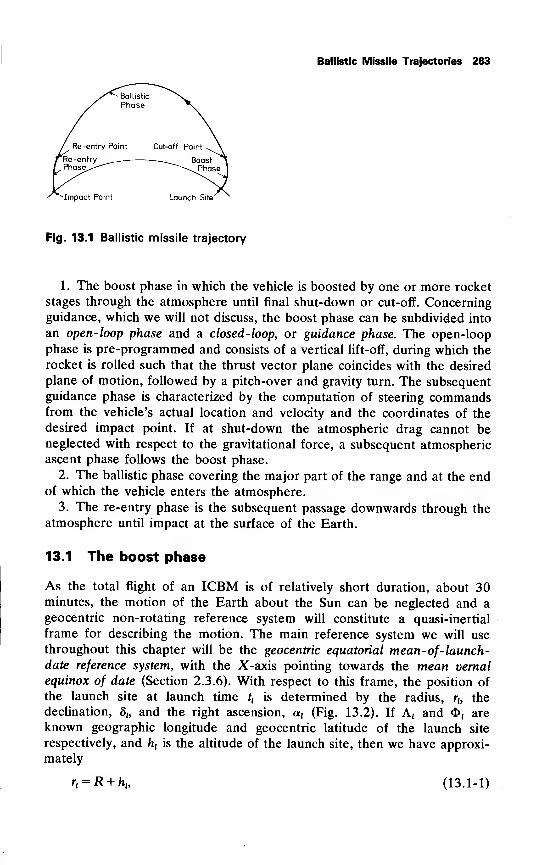
Ballistic Missile Trajectories 283
^Impact Point Launch Site
Fig. 13.1 Ballistic missile trajectory
1. The boost phase in which the vehicle is boosted by one or more rocket
stages through the atmosphere until final shut-down or cut-off. Concerningguidance, which we will not discuss, the boost phase can be subdivided into
an open-loop phase and a closed-loop, or guidance phase. The open-loop
phase is pre-programmed and consists of a vertical lift-off, during which the
rocket is rolled such that the thrust vector plane coincides with the desired
plane of motion, followed by a pitch-over and gravity turn. The subsequent
guidance phase is characterized by the computation of steering commandsfrom the vehicle's actual location and velocity and the coordinates of the
desired impact point. If at shut-down the atmospheric drag cannot beneglected with respect to the gravitational force, a subsequent atmospheric
ascent phase follows the boost phase.
2. The ballistic phase covering the major part of the range and at the endof which the vehicle enters the atmosphere.
3. The re-entry phase is the subsequent passage downwards through the
atmosphere until impact at the surface of the Earth.
13.1 The boost phase
As the total flight of an ICBM is of relatively short duration, about 30minutes, the motion of the Earth about the Sun can be neglected and a
geocentric non-rotating reference system will constitute a quasi-inertial
frame for describing the motion. The main reference system we will use
throughout this chapter will be the geocentric equatorial mean-of-launch-date reference system, with the X-axis pointing towards the mean vernal
equinox of date (Section 2.3.6). With respect to this frame, the position of
the launch site at launch time f, is determined by the radius, rb the
declination, 8h and the right ascension, a, (Fig. 13.2). If A, and 3>, are
known geographic longitude and geocentric latitude of the launch site
respectively, and ht
is the altitude of the launch site, then we have approxi-
mately
r, = R + hb (13.1-1)
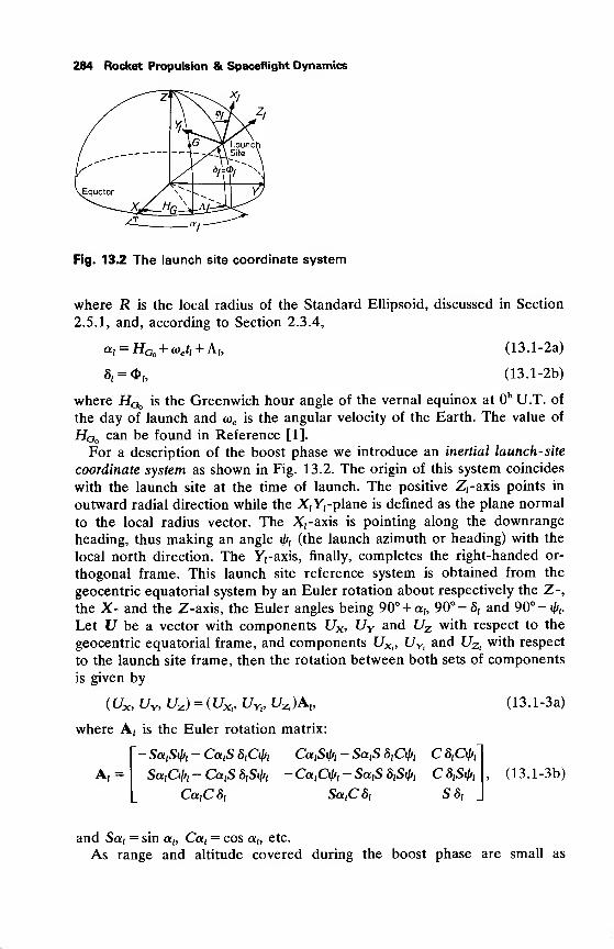
284 Rocket Propulsion & Spaceflight Dynamics
Fig. 13.2 The launch site coordinate system
where jR is the local radius of the Standard Ellipsoid, discussed in Section
2.5.1, and, according to Section 2.3.4,
^i = HGo + o)e tl + Ah
8, = 4>r ,
(13.1-2a)
(13.1-2b)
where HGo is the Greenwich hour angle of the vernal equinox ath U.T. of
the day of launch and cuc is the angular velocity of the Earth. The value of
HGo can be found in Reference [1].
For a description of the boost phase we introduce an inertial launch-site
coordinate system as shown in Fig. 13.2. The origin of this system coincides
with the launch site at the time of launch. The positive Z,-axis points in
outward radial direction while the X,Yrplane is denned as the plane normal
to the local radius vector. The Xraxis is pointing along the downrange
heading, thus making an angle fa (the launch azimuth or heading) with the
local north direction. The Yraxis, finally, completes the right-handed or-
thogonal frame. This launch site reference system is obtained from the
geocentric equatorial system by an Euler rotation about respectively the Z-,
the X- and the Z-axis, the Euler angles being 90° + a„ 90°- 8, and 90°-^.
Let 17 be a vector with components Ux, UY and Uz with respect to the
geocentric equatorial frame, and components UXl , UYl and UZl with respect
to the launch site frame, then the rotation between both sets of components
is given by
(Ux, UY, Uz ) = (UXl , UYl , t/Zl)At ,
where Aj is the Euler rotation matrix:
A,=—SattSfa — Ca t
S SiCfa
SatCfa — CttjS SiSfa
CaiCSi
CcttSfa — SatS 8iCif/i C SiCfa
- CaiCfa - SotiS SiSfa C SiSfa
Sa{C 8i S 8
t
(13.1-3a)
,(13.1-3b)
and Sty = sin ab Cat= cos ab etc.
As range and altitude covered during the boost phase are small as
Ballistic Missile Trajectories 285
compared to the radius of the Earth, the Earth may be considered fiat
during this phase. Neglecting for a moment the rotation of the Earth, the
motion will be two-dimensional and the trajectory will lie in the XXZ
X-plane
of the launch site coordinate system. In Chapters 11 and 12 methods are
discussed to determine two-dimensional powered flight trajectories in a
homogeneous gravitational field, so we can use these theories to determine
the boost phase.
Owing to the rotation of the Earth the launch site has an eastward
velocity o)ertcos 8, with respect to inertial space. This eastward velocity can
be resolved into an initial down-range velocity and an initial cross-range
velocity along the Xr and Yraxes respectively:
Vx,(0 = (oji cos 8X sin if/h (13.1 -4a)
Vy,U) = ~°>ericos 8, cos i/f,. (13.1 -4b)
The initial down-range rate does not affect the two-dimensionality of the
motion and therefore can easily be incorporated into the two-dimensional
theories of powered flight trajectories by adjusting the initial conditions.
Owing to the initial cross-range rate VYl (tx ), the trajectory cannot be planar
anymore for launches neither due east nor due west. The main effect of this
initial cross-range rate is a change of the effective firing azimuth. Therefore,
injection azimuth, longitude and latitude will differ from the corresponding
quantities as determined with the assumption that the Earth is not rotating.
A simple analytic method to include the initial cross-range velocity in the
analysis of the powered phase is given by Kohlhase [2]. Once the two-
dimensional powered flight trajectory is determined, his method enables us
to determine the necessary corrections in the shut-down conditions to
account for the initial cross-range velocity. Thus, with this method it is
possible to determine the shut-down or injection state at time ttgiven by
(X,., Yu,Zi) and (VX|i, VYli , VZ(i) with respect to the launch site reference
system. The injection state with respect to the geocentric equatorial systemmay be found by applying Eq. (13.1-3a):
(
V
Xl , VY( , V*) = (VXu , VYli, VZi)A x , (13.1-5a)
(Xb Y;, Z{ )= r,(cos 8, cos a,, cos 5, sin a, sin 5,) + (Xk , Yu , ZJA,.
(13.1-5b)
As it is customary to express the injection conditions in radius, right
ascension, declination, speed, azimuth and flight path angle, we will derive
expressions for these quantities. Clearly the injection radius is given by
r4= VxT+yT+z|, (13.1-6a)
286 Rocket Propulsion & Spaceflight Dynamics
while declination and right ascension follow from
sinfi, = Z,/r,; -90° =£ $ ^ 90°, (13.1-6b)
cos ckj = XJiji cos Sj);
sinaj= YJiri cosSj);
the injection velocity is
0°^a;^360°. (13.1-6c)
V-Vv^+Vi.+ V^. (13.1-7)
To determine azimuth and flight path angle we introduce the vectors ev. and
er,in the direction of injection velocity and radius respectively:
eVt = (Vxt
ex+ VYleY+ VZiez)/Vh (13.1-8a)
cri= (X
iex + Y^v+Z^Vr, (13.1-8b)
where ex, *Y and ez are the unit vectors along the X, Y and Z-axis
respectively. Then the flight path angle is determined by
siny^ev.-e,,; -90°^yi^90°. (13.1-9)
The unit vector lying in the horizontal plane at injection and pointing along
the downrange heading is
<Vh, = («v, - *r, sin yt)/cos yh (13.1-10)
and the injection azimuth is found from
cos il/i = eVH, ' eNl ',VHi '
0^^^360°, (13.1-11)
sin h = eVHl . e^
;
where eNi and eEl are unit vectors lying in the horizontal plane at injection,
pointing due north and due east respectively. From Eqs. (13.1-3) it can
easily be derived that
eNi - -sin Si cos atex — sin S
;sin a
teY + cos 8
fez,
(13.1-12a)
eEl = -sin afx + cos a^Cy. (13.1-12b)
We now have determined completely the shut-down conditions, which are
the injection conditions for the ballistic phase which we will discuss next.
13.2 The ballistic phase
To determine the ballistic or free-fall trajectory, we will assume that the
Earth is spherical and has a central inverse-square force field. Effects of the
asphericity of the Earth will be discussed in Section 13.4.2. We further
assume that the only force acting during the ballistic phase is the gravita-
tional force of the Earth, neglecting attractions of Sun and Moon and
aerodynamic forces.
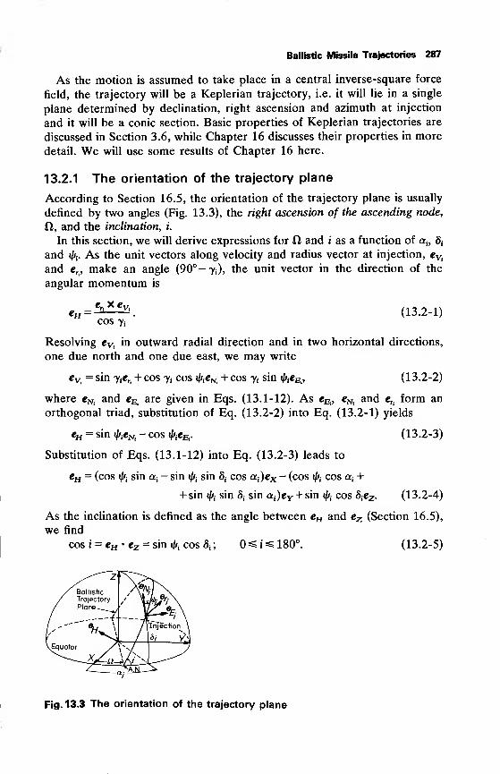
Ballistic Missile Trajectories 287
As the motion is assumed to take place in a central inverse-square force
field, the trajectory will be a Keplerian trajectory, i.e. it will lie in a single
plane determined by declination, right ascension and azimuth at injection
and it will be a conic section. Basic properties of Keplerian trajectories are
discussed in Section 3.6, while Chapter 16 discusses their properties in more
detail. We will use some results of Chapter 16 here.
13.2.1 The orientation of the trajectory plane
According to Section 16.5, the orientation of the trajectory plane is usually
defined by two angles (Fig. 13.3), the right ascension of the ascending node,
ft, and the inclination, i.
In this section, we will derive expressions for ft and i as a function of at,8
t
and «/*,. As the unit vectors along velocity and radius vector at injection, eVl
and er.,make an angle (90°-^), the unit vector in the direction of the
angular momentum is
eH =_ er.
x ev.
cos Yj
(13.2-1)
Resolving ev. in outward radial direction and in two horizontal directions,
one due north and one due east, we may write
cv.
= sin 7fer. + cos yt
cos ^cN. + cos ji sin ^e^, (13.2-2)
where eN. and e^ are given in Eqs. (13.1-12). As e^, eNi and en form an
orthogonal triad, substitution of Eq. (13.2-2) into Eq. (13.2-1) yields
eH = sin i/fjCN.
- cos «fo«E,. (13.2-3)
Substitution of Eqs. (13.1-12) into Eq. (13.2-3) leads to
eH = (cos ifo sin af— sin ifo sin S
tcos a
{)ex — (cos ifo cos a {
+
+ sin ifo sin 5j sin a^ey + sin ^ cos 8fcz . (13.2-4)
As the inclination is defined as the angle between eH and ez (Section 16.5),
we find
cos i = eH -ez = sin <fo cos 8t ; O^i^ 180°. (13.2-5)
Fig. 13.3 The orientation of the trajectory plane
288 Rocket Propulsion & Spaceflight Dynamics
The unit vector from the center of the Earth to the ascending node, eAN, lies
both in the orbital plane and in the equatorial plane and therefore is normal
to eH and ez . As the angle between eH and ez is i, we have
eAN =^^. (13.2-6)sin i
Substitution of Eq. (13.2-4) into Eq. (13.2-6) yields
_ cos ^ cos «; + sin ^ sin 8; sin a4
sin i
,
cos ifc sin ocj -sin ifc sin Stcos a
t ni->n\H :—
:
eY- (13.2-7)sin i
As ft is the angle between eAN and ex, we find
cos ij/j cos Uj + sin ifc sin g;sin a; ,iaic^cos ft = eAN • ex = :—
:
, (13.2-8a)sin i
. n cos iffj sin at- sin tfc sin 8
tcos a;
sin 11 = eAN • eY = :—
:
• (13.2-8b)sin i
These equations, together with Eq. (13.2-5), uniquely determine the right
ascension of the ascending node. Somewhat simpler expressions for ft can
be obtained by multiplying Eq. (13.2-8a) by coa atand sin a
trespectively
and adding the results, and by multiplying Eq. (13.2-8b) by sin atand cos a
{
respectively and subtracting the results. This leads to the following expres-
sions:
cos (a; -ft) = cos ifo/sin i, (13.2-9a)
sin («; - ft) = sin ^ sin 8Jsm i. (13.2-9b)
13.2.2 Trajectory geometry
We have seen that the orientation of the trajectory plane, specified by the
angles i and ft is determined by the components af ,8
tand i/f
;of the injection
state. In this section, we will discuss type and shape of the trajectory and its
orientation in the trajectory plane, as is shown in Fig. 13.4. It will turn out
that type and shape are completely determined by the quantities rh Vtand y*,
while the orientation of the trajectory in the plane will be dependent on all
components of the state vector, except at.
From Section 3.6, we know that the polar representation of a Keplerian
trajectory is given by
r =—E—z, (13.2-10)1 + e cos 6
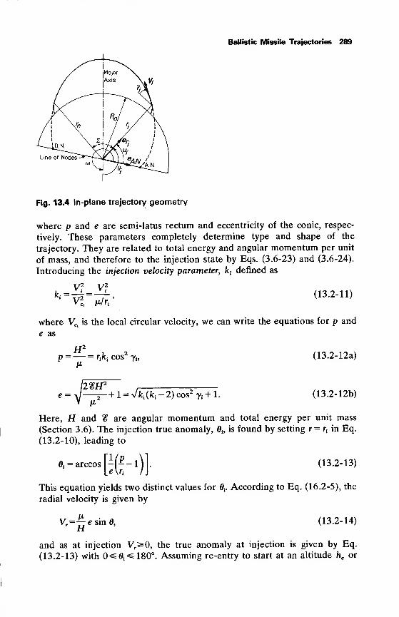
Ballistic Missile Trajectories 289
Line of Nodes
Fig. 13.4 In-plane trajectory geometry
where p and e are semi-latus rectum and eccentricity of the conic, respec-
tively. These parameters completely determine type and shape of the
trajectory. They are related to total energy and angular momentum per unit
of mass, and therefore to the injection state by Eqs. (3.6-23) and (3.6-24).
Introducing the injection velocity parameter, ktdefined as
V2 V2
]r =—-i-= '
' V2Ci
ji/r,'
(13.2-11)
where Vc . is the local circular velocity, we can write the equations for p and
e as
P =— =rt ki cos
2yi5
(13.2-12a)
\2%H2
+ l = Vki(k
i-2)cos2
7i+ l. (13.2-12b)
Here, H and % are angular momentum and total energy per unit mass
(Section 3.6). The injection true anomaly, Q„ is found by setting r= rtin Eq.
(13.2-10), leading to
0; = arccos -G-e-)}
(13.2-13)
This equation yields two distinct values fort. According to Eq. (16.2-5), the
radial velocity is given by
Vr=-^esin0, (13.2-14)
and as at injection Vr>0, the true anomaly at injection is given by Eq.
(13.2-13) with O*£0i^l8Oo. Assuming re-entry to start at an altitude he or
290 Rocket Propulsion & Spaceflight Dynamics
radius re, related by
re = R +K, (13.2-15)
we find, by the same reasoning, for the true anomaly at re-entry
ue-#e = arccos -1-^-1); 180°^ 6e ^360°. (13.2-16)
The ballistic angular range, 2, is then given by
% = e€ -eb (13.2-n)
and the ballistic linear range measured along a great circle from the
sub-vehicle point at injection to the sub-vehicle point at re-entry for a
non-rotating Earth is
Db = R X. (13.2-18)
As with the help of Eqs. (13.2-12), p and e can be expressed in the
in-plane injection state, the true anomaly at injection and the true anomaly
at re-entry, and thus angular and great circle linear range are only a function
of Vj, yh rxand re . However, substitution of Eqs. (13.2-13) and (13.2-16)
with Eqs. (13.2-12) into Eq. (13.2-17), yields a rather complicated expres-
sion for the angular range. A somewhat simpler expression can be obtained
from the equation
l + ecos(0i +X) = -,
or
l-tan2X/2 . 2tanS/2 p
l + tan2X/2
6Smdil + tan
2 XI2~rt
1 + e cos fl;^ t _ 2 v ^ - e sin 6
t T—
—
7 ^ ^ =—
.
(13.2-19)
Solution of this equation for tan 2/2 and subsequent substitution of the
expressions for *p, e cos Qtand e sin 6h which may be obtained from Eqs.
(13.2-12) to (13.2-14), yields
tan — = cos7j —-—^^—-i _ N
, (13.2-20)kj sin 7i + V/cf(l-pf cos
2 7^- 2^(1 -pj)
2" 2-k
jcos
2yi
(l + pi )
where p, stands for the ratio of injection radius and re-entry radius:
ft=-«l+V^- (13.2-21)
The quadratic equation, Eq. (13.2-19), has two solutions. The solution given
in Eq. (13.2-20) corresponds to a true anomaly, 6e = ^+2, lying between180° and 360°, which is the interval of the re-entry true anomaly as weknow. In Fig. 13.5, the angular range is given as a function of pt
for somevalues of Yj and for k
t= 0.6 and 0.9. This figure shows that as yt
increases,
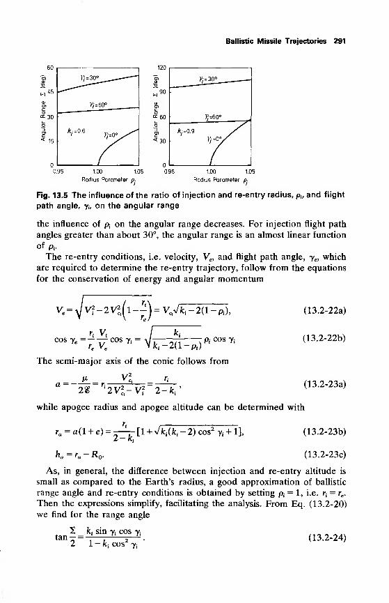
Ballistic Missile Trajectories 291
1.00 1.05
Radius Parameter p.
095 1.00 1.05
Radius Parameter p-
Fig. 13.5 The influence of the ratio of injection and re-entry radius, p„ and flight
path angle, y„ on the angular range
the influence of pfon the angular range decreases. For injection flight path
angles greater than about 30°, the angular range is an almost linear function
of ft.
The re-entry conditions, i.e. velocity, Ve , and flight path angle, ye , which
are required to determine the re-entry trajectory, follow from the equations
for the conservation of energy and angular momentum
= y]v*-2V2Ci(l--)
J=Vjk i-2(l-p
i ),
,-jcos ye =~— cosyre Ve
Pi cos yt
k,- 2(1
-
ft )
The semi-major axis of the conic follows from
2% '2VJ-V? 2-fc,*
(13.2-22a)
(13.2-22b)
(13.2-23a)
while apogee radius and apogee altitude can be determined with
ra = a(l + e) = ^-^[l + Vki(k
j-2)cos2
yi+ l],
ha= ra~ ^0-
(13.2-23b)
(13.2-23c)
As, in general, the difference between injection and re-entry altitude is
small as compared to the Earth's radius, a good approximation of ballistic
range angle and re-entry conditions is obtained by setting ft= 1, i.e. r
t= re .
Then the expressions simplify, facilitating the analysis. From Eq. (13.2-20)
we find for the range angle
S_Mmj^cos7jran — ~ 5
2 1 - ki cos2yt
(13.2-24)
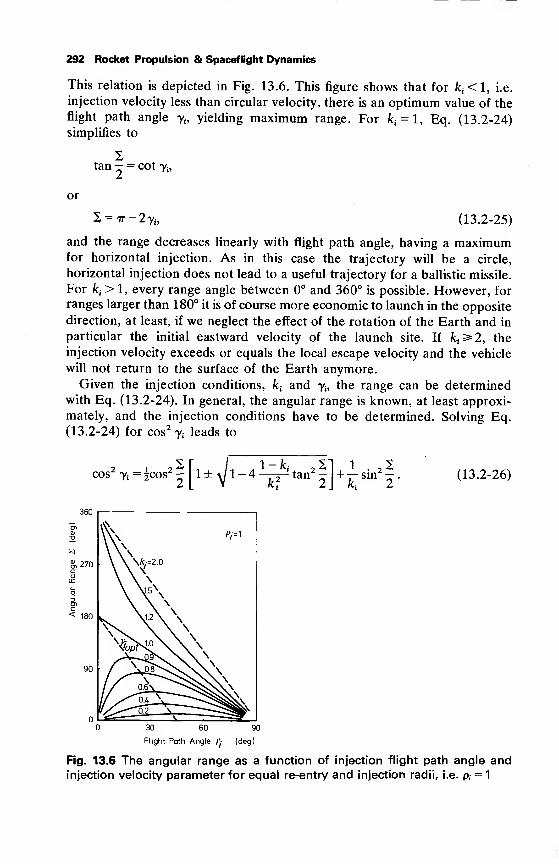
292 Rocket Propulsion & Spaceflight Dynamics
This relation is depicted in Fig. 13.6. This figure shows that for kt<l, i.e.
injection velocity less than circular velocity, there is an optimum value of the
flight path angle yt ,yielding maximum range. For k
t= l, Eq. (13.2-24)
simplifies to
tan- = cot Yi ,
or
X=7r-2 7i , (13.2-25)
and the range decreases linearly with flight path angle, having a maximumfor horizontal injection. As in this case the trajectory will be a circle,
horizontal injection does not lead to a useful trajectory for a ballistic missile.
For k; > 1, every range angle between 0° and 360° is possible. However, for
ranges larger than 180° it is of course more economic to launch in the opposite
direction, at least, if we neglect the effect of the rotation of the Earth and in
particular the initial eastward velocity of the launch site. If k^2, the
injection velocity exceeds or equals the local escape velocity and the vehicle
will not return to the surface of the Earth anymore.
Given the injection conditions, ktand yt ,
the range can be determinedwith Eq. (13.2-24). In general, the angular range is known, at least approxi-
mately, and the injection conditions have to be determined. Solving Eq.
(13.2-24) for cos2yt
leads to
cos2
7; §cos2 H1-4—-y2 tan
2 -kf 2K si— sin —
2(13.2-26)
360
30 60 90
Flight Path Angle Yj (deg)
Fig. 13.6 The angular range as a function of injection flight path angle andinjection velocity parameter for equal re-entry and injection radii, i.e. p, = 1
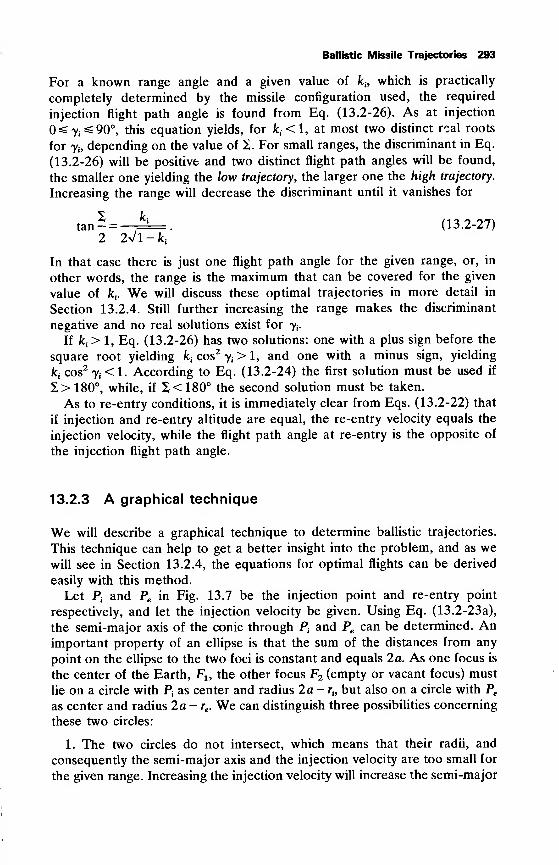
Ballistic Missile Trajectories 293
For a known range angle and a given value of kh which is practically
completely determined by the missile configuration used, the required
injection flight path angle is found from Eq. (13.2-26). As at injection
0=^7^90°, this equation yields, for /c,<l, at most two distinct real roots
for yh depending on the value of 2. For small ranges, the discriminant in Eq.
(13.2-26) will be positive and two distinct flight path angles will be found,
the smaller one yielding the low trajectory, the larger one the high trajectory.
Increasing the range will decrease the discriminant until it vanishes for
tan5 =—L=. (13.2-27)
2 2Vl - fc,
In that case there is just one flight path angle for the given range, or, in
other words, the range is the maximum that can be covered for the given
value of kj. We will discuss these optimal trajectories in more detail in
Section 13.2.4. Still further increasing the range makes the discriminant
negative and no real solutions exist for yt.
If kt> 1, Eq. (13.2-26) has two solutions: one with a plus sign before the
square root yielding ktcos
27; > 1, and one with a minus sign, yielding
ktcos
27j<1. According to Eq. (13.2-24) the first solution must be used if
2>180°, while, if £<180° the second solution must be taken.
As to re-entry conditions, it is immediately clear from Eqs. (13.2-22) that
if injection and re-entry altitude are equal, the re-entry velocity equals the
injection velocity, while the flight path angle at re-entry is the opposite of
the injection flight path angle.
13.2.3 A graphical technique
We will describe a graphical technique to determine ballistic trajectories.
This technique can help to get a better insight into the problem, and as wewill see in Section 13.2.4, the equations for optimal flights can be derived
easily with this method.
Let Pi and Pe in Fig. 13.7 be the injection point and re-entry point
respectively, and let the injection velocity be given. Using Eq. (13.2-23a),
the semi-major axis of the conic through Ptand Pe can be determined. An
important property of an ellipse is that the sum of the distances from any
point on the ellipse to the two foci is constant and equals 2 a. As one focus is
the center of the Earth, Fu the other focus F2 (empty or vacant focus) must
lie on a circle with Ptas center and radius 2a - rh but also on a circle with Pe
as center and radius 2a - re . We can distinguish three possibilities concerning
these two circles:
1. The two circles do not intersect, which means that their radii, and
consequently the semi-major axis and the injection velocity are too small for
the given range. Increasing the injection velocity will increase the semi-major
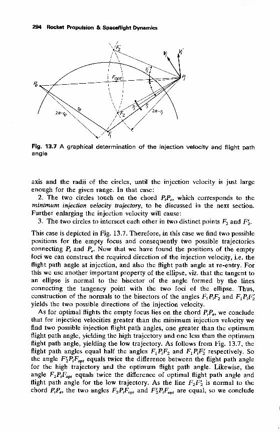
294 Rocket Propulsion & Spaceflight Dynamics
Fig. 13.7 A graphical determination of the injection velocity and flight pathangle
axis and the radii of the circles, until the injection velocity is just large
enough for the given range. In that case:
2. The two circles touch on the chord PtPe , which corresponds to the
minimum injection velocity trajectory, to be discussed in the next section.
Further enlarging the injection velocity will cause:
3. The two circles to intersect each other in two distinct points F2 and F2 .
This case is depicted in Fig. 13.7. Therefore, in this case we find two possible
positions for the empty focus and consequently two possible trajectories
connecting P{and Pe . Now that we have found the positions of the empty
foci we can construct the required direction of the injection velocity, i.e. the
flight path angle at injection, and also the flight path angle at re-entry. Forthis we use another important property of the ellipse, viz. that the tangent to
an ellipse is normal to the bisector of the angle formed by the lines
connecting the tangency point with the two foci of the ellipse. Thus,
construction of the normals to the bisectors of the angles FXP 2 ana< F\PiF2yields the two possible directions of the injection velocity.
As for optimal flights the empty focus lies on the chord PiPe , we conclude
that for injection velocities greater than the minimum injection velocity wefind two possible injection flight path angles, one greater than the optimumflight path angle, yielding the high trajectory and one less than the optimumflight path angle, yielding the low trajectory. As follows from Fig. 13.7, the
flight path angles equal half the angles F-J*^ and F^F^ respectively. Sothe angle F2PiFopt equals twice the difference between the flight path angle
for the high trajectory and the optimum flight path angle. Likewise, the
angle F2PiFopt equals twice the difference of optimal flight path angle andflight path angle for the low trajectory. As the line F2F'2 is normal to the
chord PjPe , the two angles F2PtFopt and F2PiFopt are equal, so we conclude
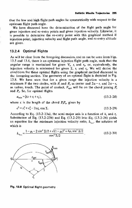
Ballistic Missile Trajectories 295
that the low and high flight path angles lie symmetrically with respect to the
optimum flight path angle.
We have discussed here the determination of the flight path angle for
given injection and re-entry points and given injection velocity. Likewise, it
is possible to determine the re-entry point with this graphical method if
injection point, injection velocity and flight path angle, and re-entry altitude
are given.
13.2.4 Optimal flights
As will be clear from the foregoing discussion, and as can be seen from Figs.
13.5 and 13.6, there is an optimum injection flight path angle, such that the
angular range is maximized for given Vj, rtand re , or, equivalently, the
injection velocity is minimized for given X, rtand re . We will derive the
conditions for these optimal flights using the graphical method discussed in
the foregoing section. The geometry of an optimal flight is depicted in Fig.
13.8. We have seen that for a given range the injection velocity is a
minimum if the two circles, with Pfand Pe as center and 2a — r
tand 2a — re
as radius, touch. The point of contact, Fopt, will lie on the chord joining P;
and Pe . So, for optimal flights
amin^ic + ri + r.), (13.2-28)
where c is the length of the chord PtPe ,
given by
c2=rf + r^-2r
ire cosS. (13.2-29)
According to Eq. (13.2-23a), the semi-major axis is a function of k; and rt.
Substitution of Eq. (13.2-23b) and Eq. (13.2-29) into Eq. (13.2-28) yields
an equation for the minimum injection velocity ratio, kimin , the solution of
which is
k_ l-pi
-2sin2X/2 + V(l-p
i )
2 +4p,.sin2 S/2(13.2-30)
,mi" cos2 2/2
Fig. 13.8 Optimal flight geometry
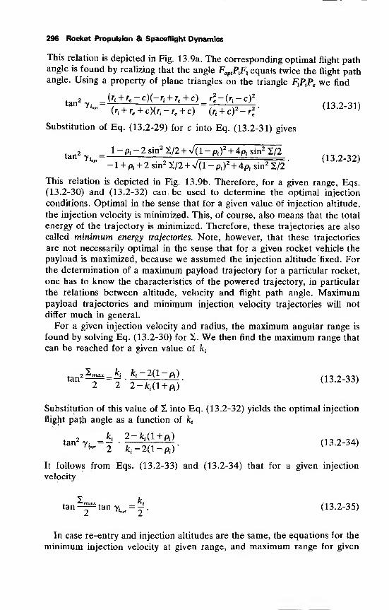
296 Rocket Propulsion & Spaceflight Dynamics
This relation is depicted in Fig. 13.9a. The corresponding optimal flight pathangle is found by realizing that the angle F^P^ equals twice the flight pathangle. Using a property of plane triangles on the triangle F^fc we find
tan2 a (r<+ r.-c)(-r
i+ r. + c)
ag^-(r
i-c)»
T 'op'
(ri + re + cXr^ + c) (r^cf-rl'(13.2 31)
Substitution of Eq. (13.2-29) for c into Eq. (13.2-31) gives
tan27i
- l-Pi-2sin2 S/2W(l-pi)
2 + 4pisin^/2
°" -l + pi+2sin2
S/2 + V(l-pi )
2 + 4pIsin
2S/2"
U '
This relation is depicted in Fig. 13.9b. Therefore, for a given range, Eqs.
(13.2-30) and (13.2-32) can.be used to determine the optimal injection
conditions. Optimal in the sense that for a given value of injection altitude,
the injection velocity is minimized. This, of course, also means that the total
energy of the trajectory is minimized. Therefore, these trajectories are also
called minimum energy trajectories. Note, however, that these trajectories
are not necessarily optimal in the sense that for a given rocket vehicle the
payload is maximized, because we assumed the injection altitude fixed. For
the determination of a maximum payload trajectory for a particular rocket,
one has to know the characteristics of the powered trajectory, in particular
the relations between altitude, velocity and flight path angle. Maximumpayload trajectories and minimum injection velocity trajectories will not
differ much in general.
For a given injection velocity and radius, the maximum angular range is
found by solving Eq. (13.2-30) for 2. We then find the maximum range that
can be reached for a given value of kt
tan2 ?== =^ •
fei~ 2(1 ~ ft)
• (13.2-33)2 2 2-M1 + A)
Substitution of this value of 2 into Eq. (13.2-32) yields the optimal injection
flight pajh angle as a function of fc;
2 = K 2-fe,(l + ft)^ 2 ki -2(1 -Pi)tan
2y io
= % ,, T* ". (13.2-34)
It follows from Eqs. (13.2-33) and (13.2-34) that for a given injection
velocity
tan^tan 7w,=|. (13.2-35)
In case re-entry and injection altitudes are the same, the equations for the
minimum injection velocity at given range, and maximum range for given
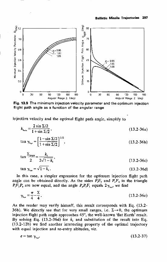
Ballistic Missile Trajectories 297
£ 90
75
£ 60
30
£ 15
\V Pr 0.95
1.00
1.05
90 120 150 180
Angular Range Z (deg)
30 60 90 120 150 180
Angular Range I (deg)
Fig. 13.9 The minimum injection velocity parameter and the optimum injection
flight path angle as a function of the angular range
injection velocity and the optimal flight path angle, simplify to
2 sin 2/2K*.
=
tan y, =
1 + sin 2/2'
_r i-sinS/2 11/2
'
iop' ll + sin 2/2 J
'
tanK
2 2Vl-fc,'
tan yiovt= Vl - fc
;
(13.2-36a)
(13.2-36b)
(13.2-36c)
(13.2-36d)
In this case, a simpler expression for the optimum injection flight path
angle can be obtained directly. As the sides P^ and PeFx in the triangle
PjFxPc are now equal, and the angle PePiFl equals 2?^, we find
TT 2* *opt 4 4
(13.2-36e)
As the reader may verify himself, this result corresponds with Eq. (13.2-
36b). We directly see that for very small ranges, i.e. 2—»0, the optimuminjection flight path angle approaches 45°, the well-known 'flat Earth' result.
By solving Eq. (13.2-36d) for ktand substitution of the result into Eq.
(13.2-12b) we find another interesting property of the optimal trajectory
with equal injection and re-entry altitudes, viz.
e = tan y,'opt* (13.2-37)
298 Rocket Propulsion & Spaceflight Dynamics
13.2.5 Time of flight
To determine the time of flight of the ballistic phase we could use Eq.
(16.3-11), i.e. Kepler's equation. This, however, would force us to determine
the eccentric anomalies at injection and re-entry. For our purpose there is a
more convenient expression for the time of flight along a conic arc between
two points, known as Lambert's equation or Lambert's theorem. This
theorem, originally discovered by Lambert and subsequently proved analyti-
cally by Lagrange, states that the time to traverse a Keplerian arc depends
only upon the semi-major axis, the sum of the distances from the initial and
final point of the arc to the center of force, and the length of the chord
joining initial and final point. Lambert's equation also plays an important
role in the analysis of interplanetary trajectories which will be discussed in
Chapter 19. We will derive Lambert's equations for elliptic motion only.
Lambert's equation. Let Fx be the initial point and P2 be the final point of
an elliptic arc and suppose that radius vector and eccentric anomaly of Px
and P2 are r x and Eu and r2 and E2 respectively. Then, according to Eqs.
(16.3-9) to (16.3-11), the time of flight from Px to P2 along the elliptic
arc is given by
*=>/?
t= J—[E2-E1 -e(sinEz-smE 1)l (13.2-38a)
or
*->/?tf=J—[E2-E1 -2ecos&E2 + E 1
)sm%(E2-E l)l (13.2-38b)
We now introduce the variables / and g, defined by
cos|(/+g) = ecos|(E2 + Ex); 0^/+g<27r, (13.2-39a)
f-g = E2-E 1 ;0^f-g<2n. (13.2-39b)
Substitution of Eqs. (13.2-39) into Eq. (13.2-38b) leads to
tf= yj— [/- g-2 cos K/+ g) sinK/- g)l
or
h= V[(/-sin/)-(g-sing)]. (13.2-40)
We now have to express / and g in a, c and rx + r2 . Therefore let eP be the
Ballistic Missile Trajectories 299
unit vector pointing towards pericenter and eQ the unit vector in the plane
of motion 90° ahead of eP in the direction of motion. Then
r 1 = rx cos Q xeP + rx sin B xeQ, (13.2-41a)
where 6 X is the true anomaly of Px . According to Eqs. (16.3-4) and (16.3-5),
Eq. (13.2-41a) can also be written as
i-i = a(cos E x- e)eP + aVl - e
2sin E xeQ . (13.2-41b)
A similar expression may be obtained for the position vector of P2 :
r2 = a(cos E2- e)eP + aVl - e
2sin E2eQ . (13.2-41c)
The length of the chord c joining Px and P2 can be found from
c2 = (r 1 -r2)-(r 1 -r2). (13.2-42)
Substitution of Eqs. (13.2-41b) and (13.2-41c) into Eq. (13.2-42) yields
c2 =4a 2
[l - e2cos
2 \(E2 + E,)] sin2 \{E2 - E x ),
or, using Eqs. (13.2-39) and the appropriate trigonometric identities,
c = a(cosg-cos/). (13.2-43)
According to Eq. (16.3-3), we have
r1 + r2 = 2a[l -|e(cos E r + cos E2)]=
= 2a[l-ecos^(E2 +E1)cosl(E2-E1 )]. (13.2-44)
Substitution of Eqs. (13.2-39) into Eq. (13.2-44) and some trigonometry
leads to
r1 + r2 = 2a[l-|(cos/ + cosg)]. (13.2-45)
Solving Eqs. (13.2-43) and (13.2-45) for cos/ and cos g yields
cos/=l -i—
2
(13.2-46a)2a
cos g = 1 + ° !}~ r2
, (13.2-46b)2a
'
or
.2 r/o _ C + rl+ r2
sin2//2 = f—^
,
(13.2-47a)4a
2 /0 _ rl+ r2-C
sin2g/2 = -^-^— . (13.2-47b)
According to Eq. (13.2-28), the minimum semi-major axis of a conic
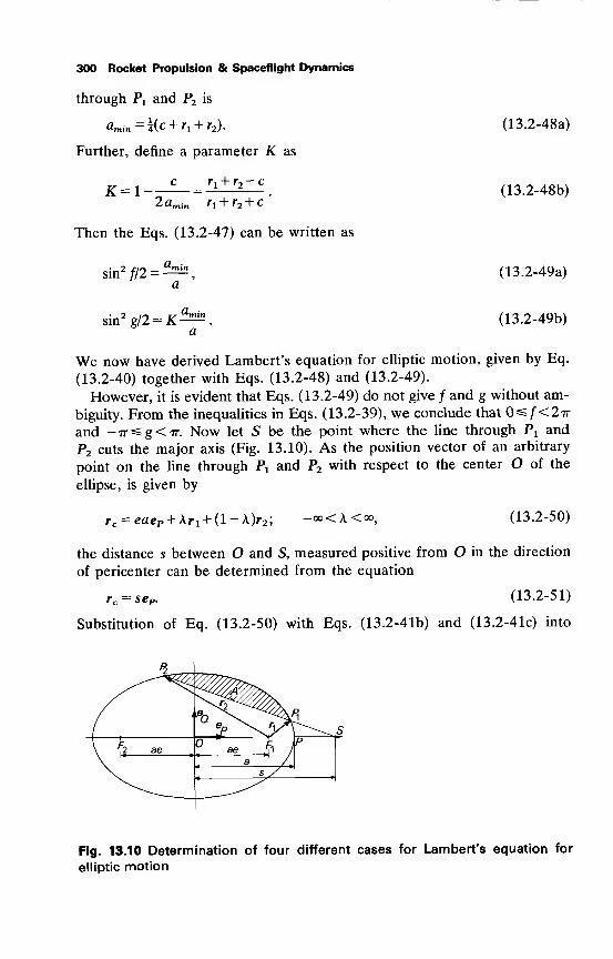
300 Rocket Propulsion & Spaceflight Dynamics
through Px and P2 is
amin=l(c + rl + r2).
Further, define a parameter K as
c r1 + r2 -cK=l —2a„ rx + r2 + c
Then the Eqs. (13.2-47) can be written as
sin f/2=
,
a
• 2 /o vmmsin g/2 = K
a
(13.2-48a)
(13.2-48b)
(13.2-49a)
(13.2-49b)
We now have derived Lambert's equation for elliptic motion, given by Eq.
(13.2-40) together with Eqs. (13.2-48) and (13.2-49).
However, it is evident that Eqs. (13.2-49) do not give / and g without am-
biguity. From the inequalities in Eqs. (13.2-39), we conclude that 0^/<27rand -7r=ssg<7r. Now let S be the point where the line through Px and
F2 cuts the major axis (Fig. 13.10). As the position vector of an arbitrary
point on the line through Px and P2 with respect to the center O of the
ellipse, is given by
r c= ea«P + Ar 1 + (l-A)r2 ;
-oo<A<°°, (13.2-50)
the distance s between O and S, measured positive from O in the direction
of pericenter can be determined from the equation
rc= seP.
(13.2-51)
Substitution of Eq. (13.2-50) with Eqs. (13.2-41b) and (13.2-41c) into
Fig. 13.10 Determination of four different cases for Lambert's equation for
elliptic motion
Ballistic Missile Trajectories 301
(13.2-51), and solution of the resulting equation for A and s yields
A=—p*Z— ,(13.2.52a)
sin E2- sin E x
^n{E2-Ex ) cos \{E2-Ex ) ,n „„Ms = a —— :
—
—=a 77= =—
.
(l3.2-52b)sin E2 - sin E x cos %E2 + Ex )
We then find for the distances FX S, F2S and PS, measured positive to the
right in Fig. 13.10:
17 ccos \(E2-E x)-e cos %(E2 +E x ) n*o«a\F1S = s-ae = a , (13.2-53a)
cos %(E2 +Ex)
F <,__ ,
cos |(E2-E^ + e cos KEa + EJ ,n ,„wF2S = s + ac = a1
, (13.2-53b)cos5(£2 + -Ei)
PS = s-a = a , (13.2-53c)cos 2\E2 +Ex )
or using Eqs. (13.2-39) and the appropriate trigonometric formulae we find
from Eqs. (13.2-53)
FlS _ sini/sinlg(13>2 _54a)
PS sin \EX sin \E2
'
F2S_ cos \f cos ^g
PS sin ^Ej sin |E2
(13.2-54b)
Now sin |/ and cos |g are always positive while, as we may take Ex between
and 360°, sin \E X is positive too. We may distinguish four cases. Let A be
the area bounded by the arc PXP2 and the chord joining Px and P2 :
F S(a) If this area includes neither Fu nor F2 ; sin^E2 >0, ~^"> ^ anc*
F2S—— >0, and so for this case we find
sin|g>0, cos|/>0. (13.2-55a)
F S(b) If the area A does not include Fx , but includes F2 ; sin |E2 > 0> ~~7T>
F2Sand -rr~<0> and we find
PS
sin£g>0, cos|/<0. (13.2-55b)
(c) If the area A includes Fl5 but not F2 ; sin|E2 <0, ~->0 and —2-<0,Xi3 I J
302 Rocket Propulsion & Spaceflight Dynamics
and consequently
sin§g<0, cos|/>0. (13.2-55c)
(d) If the area A includes both foci; sin|E2 <0, -j^r>0 and -^->0, and
we find
sin|g<0, cos|/<0. (13.2-55d)
Now define the parameters a and j8 as
a = 2 arcsin xF^
;
O^cc^tt, (13.2-56a)V a
P = 2facsmy]K^ 0^/3 =£tt. (13.2-56b)
Then, according to Eqs. (13.2-49),
f=a or /=2ir-a, (13.2-57a)
g = /3 or g = -jS. (13.2-57b)
Now the time of flight for the four different cases follows from Eq. (13.2-40)
together with Eqs. (13.2-55) and (13.2-57)
(a) A does not include Fx and F2 ,
tf= J— [(a-sina)-(|3-sin0)]. (13.2-58a)
(b) A does not include Fl5 but includes F2 ,
f,= J— [2*r-(a-sina)-(/3-sin0)]. (13.2-58b)
(c) A includes Fl5 but not F2 ,
'/= V— [(« - sin o) + (j8 - sin |8)]. (13.2-58c)
(d) A includes both Fx and F2 ,
*f= V~[2,""-(«-sina) + (/3-sinj8)].
(13.2-58d)
The cases a and b correspond with an angular range less than 180°, while c
and d correspond with an angular range greater than 180°.
Ballistic Missile Trajectories 303
For parabolic and hyperbolic motion similar equations may be derived. For
this is referred to Plummer [3] or Battin [4].
In general, for a ballistic missile the range angle is less than 180°.
According to Fig. 13.7, Eq. (13.2-58a) has to be used for low trajectories,
while Eq. (13.2-58b) has to be used for high trajectories.
For optimal trajectories: a = amin, and according to Eqs. (13.2-56), a = ir
and |3 = 2 arcsin VK and substitution of these values of a and /3 into Eq.
(13.2-58a), or equivalently into Eq. (13.2-58b), yields the flight time along
an optimal trajectory
t, = J— 1> " 2 arcsin Vk+ 2>/Kv/I:: K]. (13.2-59)
Using Eqs. (13.2-56), (13.2-58) and (13.2-59) we can now derive expres-
sions for the time of flight from injection to re-entry as a function of range
angle, injection radius and velocity, and re-entry radius. The chord, c, maybe determined with Eq. (13.2-29) as a function of rh re and X; the
semi-major axis, a, is, according to Eq. (13.2-23a), a function of rfand k
t
only. Therefore, a and /3 are functions of rh re , X and ktonly and this holds
for the time of flight too.
The time-of-flight expressions take a relatively simple form if injection
altitude equals the re-entry altitude, which we will assume in the following.
In that case
Xc = 2riSin-, (13.2-60a)
«fn in=^(l + sin-V (13.2-60b)
rjr1 -sin 2/2 , (tt X\
Now let us first consider optimal trajectories. Substitution of Eqs. (13.2-60)
into Eq. (13.2-59) yields the time of flight along a minimum velocity
trajectory as a function of angular range only
tf =\hr~ 1 + sin-lfop
' V2jll\ 2/
3/2
x
TTr . /l-sinX/2 ,V2sinX/2(l-sinX72) 1 M , 0A1 .
x —~arcsm \- r—^z + :. ^ ._ (13.2-61a)
L2 Vl+sinX/2 l+sinX/2 J
Using Eqs. (13.2-36), relating range, velocity ratio and flight path angle, we
304 Rocket Propulsion & Spaceflight Dynamics
can express the time of flight in injection velocity or in injection flight path
angle:
tfopt=J-(2- K)'
3'2 [>-2arccos 7^+2 7^(1-^)], (13.2-61b)
— cos37i[7r-arcsin (tan -ft) + 2 tan ^Vl-tan2
ys]. (13.2-61c)
For non-optimal trajectories, the flight time directly follows from Eqs.
(13.2-56) and (13.2-58) and the expressions for a, amin and K as given by
Eqs. (13.2-23a) and (13.2-60) respectively
<*=2arcsin -J^-^ (l + sin-j; O^a^ir, (13.2-62a)
j3 = 2 arcsin J^jp (l ~ sin |V ^ j3 *£ n. (13.2-62b)
Then for low trajectories:
tf= J^(2-k
ir3/2 [(«-sina)-(|8-sin^)], (13.2-63a)
and for high trajectories:
tf= W-(2-kir3/2 [27r-(a-sina)-(^-sin/3)]. (13.2-63b)
In Fig. 13.11 these flight times, as well as the flight time along an optimal
trajectory, are depicted as a function of ktand X. For this figure, the
injection altitude, and consequently the re-entry altitude, were taken zero
(/•j = R ), which corresponds to a ballistic trajectory from one point on the
surface of the Earth to another point on the Earth's spherical surface,
starting with an impulsive shot.
13.3 The re-entry phase
Re-entry is an extensive subject in itself and falls beyond the scope of this
book. We will therefore confine ourselves to some general remarks on the
re-entry phase.
The re-entry phase starts at a hypothetical 're-entry point'. From this point
on downwards, the aerodynamic forces cannot be neglected anymore with
respect to the gravitational forces. The re-entry altitude may be determined
by first estimating a re-entry altitude and subsequent determination of the
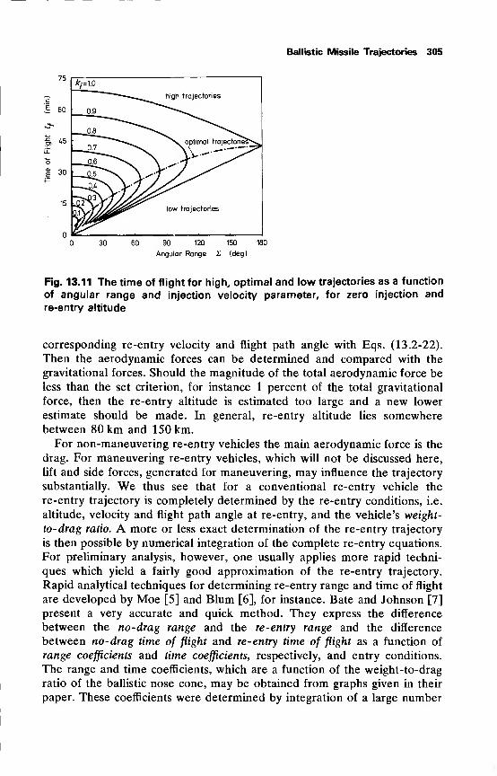
Ballistic Missile Trajectories 305
75
J. 60
30
A/=1.0
high trajectories
0.9
——Pi*
___07
-—-CX6/ "^
>w optimal trajectories*^
—^iT^N \.^'j
"—-^c\
low trajectories
30 60 90 120 150 180
Angular Range X (deg)
Fig. 13.11 The time of flight for high, optimal and low trajectories as a function
of angular range and injection velocity parameter, for zero injection and
re-entry altitude
corresponding re-entry velocity and flight path angle with Eqs. (13.2-22).
Then the aerodynamic forces can be determined and compared with the
gravitational forces. Should the magnitude of the total aerodynamic force be
less than the set criterion, for instance 1 percent of the total gravitational
force, then the re-entry altitude is estimated too large and a new lower
estimate should be made. In general, re-entry altitude lies somewherebetween 80 km and 150 km.
For non-maneuvering re-entry vehicles the main aerodynamic force is the
drag. For maneuvering re-entry vehicles, which will not be discussed here,
lift and side forces, generated for maneuvering, may influence the trajectory
substantially. We thus see that for a conventional re-entry vehicle the
re-entry trajectory is completely determined by the re-entry conditions, i.e.
altitude, velocity and flight path angle at re-entry, and the vehicle's weight-
to-drag ratio. A more or less exact determination of the re-entry trajectory
is then possible by numerical integration of the complete re-entry equations.
For preliminary analysis, however, one usually applies more rapid techni-
ques which yield a fairly good approximation of the re-entry trajectory.
Rapid analytical techniques for determining re-entry range and time of flight
are developed by Moe [5] and Blum [6], for instance. Bate and Johnson [7]
present a very accurate and quick method. They express the difference
between the no-drag range and the re-entry range and the difference
between no-drag time of flight and re-entry time of flight as a function of
range coefficients and time coefficients, respectively, and entry conditions.
The range and time coefficients, which are a function of the weight-to-drag
ratio of the ballistic nose cone, may be obtained from graphs given in their
paper. These coefficients were determined by integration of a large number
306 Rocket Propulsion & Spaceflight Dynamics
of re-entry trajectories, which covered ballistic missile ranges from about
1500 km to over 30,000 km and ballistic coefficients from 10 kPa to 70 kPa,
i.e. from very blunt heat sink type to extremely sharp ablating type ballistic
nose cones. Using their method, the errors for typical ICBM trajectories
remain well below 2 km and 4 s, respectively, for range and flight time, so it
is possible to obtain a quick and rather good approximation of re-entry
range, Se, and re-entry time of flight, tu . In the next section, we will
therefore assume that Xe and tfe
are known.
13.4 The position of the impact point
Once injection conditions are known, the ballistic range and time of flight
may be determined with Eqs. (13.2-20) and the formulae given in Section
13.2.5. An approximation of re-entry range and re-entry time of flight maybe obtained with one of the techniques referred to in the foregoing section.
The total range angle from injection to impact, % tot , then equals the sum of the
ballistic range angle and the re-entry range angle, while the total time of
flight from injection to impact, tftot
, is the sum of ballistic and re-entry flight
time.
In this section we will assume S(of and tftot
known, as well as the out-of-plane
injection conditions, at ,
8tand ifo, and determine the coordinates of the
impact point. We will first assume a spherical Earth, after which we will
discuss the determination of the impact point using the ellipsoid model for
the Earth.
13.4.1 Spherical Earth
Let er. and erfbe the unit vectors from the center of the Earth in the direction
of injection and impact respectively:
er.= cos at cos 8
tex + sin a
tcos 8
teY + sin 8
tez, ( 1 3 .4- 1 a)
er= cos a
fcos 8
fex + sin a
fcos 8
feY + sin 8
fez . (13.4- lb)
As the angle between these two vectors is %m and as both vectors are normal
to the unit vector in the direction of the angular momentum, eH, we have
eri-e r/
= cosXttt,(13.4-2a)
erXe =c„sinS
fo,(13.4-2b)
Vectorial multiplication of Eq. (13.4-2b) with er. and subsequent solution for
jads to
e = cos £toferi- sin £toteri
xeH. (13.4-3)
erf
leads to
Ballistic Missile Trajectories 307
Substitution of the expressions for eTi , e
ffand eH as given in Eqs. (13.4-1)
and (13.2-4) into Eq. (13.4-3) leads to the following three component
equations: H3 4 4 1
sin 5f= cos Stot sinSj+sin£tot cos 8
tcos ifo,
\ •~
)
cos 8fsin a
f= cos %tot sin a, cos 8
{
- sin 2,of(sin a tsin 8
tcos ^ - cos a
tsin ^), (13.4-4b)
cos 8fcos a^ = cos X tol cos a; sin 5;
- sin 2 tot(cos a . sin 8tcos ^ + sin a
;sin tfo). (13.4-4c)
As -90° «£ 8f=s90°, these equations uniquely determine declination and right
ascension of the impact point. The equation for the right ascension can be
simplified slightly by multiplying Eq. (13.4-4b) with cos atand sin a
trespec-
tively, Eq. (13.4-4c) with -sin axand cos a
trespectively, and adding the
results, leading to
. sinS tot sinifcsin(a
/-a
j )=
,(13.4-5a)
cos 8f
cos (af- «j)
= — [cos X tot cos 8t-sin S tot sin 8
tcos i^J. (13.4-5b)
cos Of
Once declination and right ascension are determined, the geocentric coordi-
nates of the impact point follow from
Af= a
f-HGo -G>e (ti + t
fJ,
or with Eq. (13.1-2a)
A/ - Aj = ctf- a
;- (oe t
ftot ,(13.4-6a)
and
<j>f= 8
f. (13.4-6b)
We see that due to the rotation of the Earth during the flight of the
missile, the geocentric longitude difference between injection and impact is
less than the right ascension difference between injection and impact. Thedifference is equal to the angle that the Earth has rotated about during the
time interval from injection to impact. For easterly launches this means that
the effect of the Earth's rotation during the flight is a reduction of the range
which can be covered, while for westerly launches the rotation of the Earth
during the flight causes an increase of the range. The effects of the Earth's
rotation during launch, causing an inertial eastward velocity of the launch
site are just the other way round: increase of range for easterly launches and
decrease of range for westerly launches. In general, we can say that for
typical ICBM flights the effect of the Earth's rotation at launch dominates
the effect of the rotation of the Earth during the flight, thus leading to larger
ranges for easterly launches than for westerly launches.
308 Rocket Propulsion & Spaceflight Dynamics
13.4.2 Oblate Earth
In determining the trajectory and impact point of a ballistic missile we have
assumed so far that the Earth is spherical and has a central inverse-square
force field. The Earth, however, is flattened at the poles and bulges at the
equator (Section 2.5.1). The Earth's oblateness has two effects on the
trajectories of long-range ballistic missiles: a dynamic effect and a geometric
effect.
The dynamic effect is the result of a non-Newtonian gravitational poten-
tial of the Earth. This potential, which can be approximated by a series of
spherical harmonics (Section 18.6) creates a non-central force field, exerting
torques normal to, and forces in the nominal trajectory plane. Therefore the
real trajectory will deviate from the trajectory as determined with a spheri-
cal Earth model, resulting in down-range and cross-range errors. The neces-
sary range corrections to account for this dynamic effect can be determined
with perturbation procedures. We will not go into this but only mention that
Wheelon [8] has derived expressions for down-range and cross-range correc-
tions to be applied to the spherical Earth trajectory impact point, which
account for the effects of the second zonal harmonic (J2-term) in the
potential. The order of magnitude of these corrections is up to about 10 km.
The effects of higher-order zonal harmonics and of the tesseral and sectorial
harmonics are a few orders of magnitude less and may therefore be
neglected.
The geometric effect is a result of the fact that the point where the
missile's trajectory intersects the Earth's surface is dependent on the shape
of the Earth. Thus assuming the Earth to be spherical will, in general, result
in down-range errors. We will now determine the coordinates of the impact
point on an oblate Earth, neglecting the dynamic effect, i.e. still assuming a
central inverse-square gravitational field. Our analysis is a somewhat mod-ified version of the analysis given by Ching-Seng Wu [9].
We approximate the oblate Earth by the Standard Ellipsoid. If <j>e is the
geocentric latitude and he the altitude of the re-entry point, the re-entry
radius may be approximated very well by
re = Re (l ~ e sin2<M + he ,
(13.4-7a)
where e is the flattening of the Earth defined by
R — R 1
e= e "* =—,
(13.4-7b)Re
298' V '
and Re and Rp
are equatorial and polar radius of the Earth. If X' is the
ballistic range angle on the oblate Earth, then, according to Eq. (13.2-10),
the re-entry radius is given by
'* =T7P,„ .w < 13 -4"8 )
1 + e cos(0j + z)
Ballistic Missile Trajectories 309
where{
is the injection true anomaly as given by Eq. (13.2-13). According
to Eqs. (13.4-4a) and (13.4-6b) the geocentric latitude of the re-entry point
follows from
sin<f>e
= cos X' sin 5; + sin X' cos 5; cos ij/p, (13.4-9)
Substitution of Eq. (13.4-9) into Eq. (13.4-7a) and setting the resulting
expression for re equal to the expression given in Eq. (13.4-8) leads to the
following equation in the ballistic range angle X':
Re [l- e(cos X' sin 8
f+ sin X' cos 8
tcos ifo)
2] + he
=
P
l + ecos(0;+X')'
(13.4-10)
This equation, which has to be solved numerically, yields the ballistic range
angle on the oblate Earth. Once this range angle is known, the re-entry
radius can be determined with Eq. (13.4-8). Then re-entry velocity and
flight path angle can be computed with Eqs. (13.2-22). Subsequently, the
re-entry range and flight time may be determined. Then total range angle
and total time of flight from injection to impact are known and the
coordinates of the impact point may be determined with Eqs. (13.4-4)
to (13.4-6). A determination of the surface range from the sub-vehicle
point of injection to the impact point, which for a spherical Earth is just
-RoXM„ gives rise to a somewhat lengthy procedure which will not be
discussed here. Escobal [10] has developed a technique which enables
calculation of this surface range on an ellipsoid.
We will now derive an approximate expression for the down-range correc-
tion which has to be applied to the spherical Earth impact point to account
for the geometric oblateness effect. Define AX as the difference between the
ballistic range angle for an oblate Earth and the ballistic range angle for a
spherical Earth,
AX = X'-X. (13.4-11)
Neglecting the difference between the re-entry range angles for an oblate
and a spherical Earth model, as well as the time of flight differences between
both models, the linear down-range correction to be applied to the range as
determined with the spherical Earth model is
AKD = Re AX. (13.4-12)
As AX is small, we may substitute Eq. (13.4-11) into Eq. (13.4-10) and
linearize, resulting in an equation for AX. Solution of this equation, and
applying Eq. (13.4-12) results in the following expression for the down-range
correction
AKD =+e
.
C°/
S
L, [J*e{l - e(cos X sin 8;+sin X cos 8
fcos i/0
2}- KJesin(0j + z)
(13.4-13a)
310 Rocket Propulsion & Spaceflight Dynamics
If the re-entry altitude is taken zero, this equation may, according to Eqs.(13.4-4a) and (13.4-6b), be written as
AR,l + ecosCflj+X)
esin(0j + 2)[i?e(l-esin
2 ^)-,R ] (13.4-13b)
This down-range correction is plotted in Fig. 13.12 as a function of the
latitude of the impact point,(f>f,
for ht= he
= 0. For three different range
angles, curves are shown for a low, an optimum and a high trajectory. It is
seen that the down-range correction increases with increasing range angle,
while for a fixed range angle it decreases with increasing flight path angle at
injection.
Latitude 4>f (deg) Latitude 0y (deg) Latitude Of (deg)
Fig. 13.12 The down-range oblateness correction as a function of the geocen-
tric latitude of the impact point for high, optimal and low trajectories
13.4.3 Influence coefficients
For classical, non-maneuverable re-entry vehicles the position of the impact
point is practically uniquely determined by position and velocity at deploy-
ment. Therefore, the guidance system of the rocket vehicle has to generate
the commands necessary to ensure correct position and velocity at the time
of release of the re-entry vehicle. To this end various guidance schemes are
being used. The more advanced guidance laws, e.g. Hybrid Explicit
Guidance, compute throughout the powered flight, using current position
and velocity data, the position of the impact point if the re-entry vehicle
were released at that time, as well as the velocity needed to go directly from
the current position to the target. When the computed impact point coin-
cides with the target a re-entry vehicle is deployed. Another widely usedguidance scheme is Delta guidance. In this case a reference trajectory is
stored in the onboard guidance computer of the rocket vehicle. During
powered flight the current state is continuously compared with the reference
Ballistic Missile Trajectories 311
or nominal state and whenever a deviation from nominal is detected the
guidance and control unit directs the missile back to its nominal flight path.
To this nominal trajectory correspond nominal shut-down conditions. How-ever, the state at shut-down of an actual missile will never exactly equal the
nominal state as a result of guidance system errors. These shut-down errors,
expressed in the perturbations Ari5Aah A8
i5AV
f ,Ay
;and Atfo, result in
impact errors, expressed by a down-range error, ARD within the nominal
trajectory plane and a cross-range error, ARC, normal to the nominal
trajectory plane. In this section, we will determine the relations between the
impact errors and the shut-down errors. In general, these relations have the
following form
AJRD = ARD {Arh Aa„ A8; ,A V„ A 7,, A<fc), (13.4-14a)
ARC = ARc(Arh Aah AS(, A V,, A 7i , A^). (13.4-14b)
Assuming the cut-off errors to be small, these equations may be linearized,
resulting in
ARD = RDr Ar;+ RDa Aa f
+ . . . + RDi(, Aifo, (13.4-15a)
ARC = RCr Art+RCa Aa, + . . . + R^ Aft, (13.4-15b)
where
„ _ BARD _dARDAn — I1 -f^n — I 1 etC.Dr
dArt
' DadActi
The coefficients RDr , RDa , . ..
, RD^ are the ballistic down-range influence
coefficients, while R^, Rca , . ..
, R^ are the ballistic cross -range influence
coefficients. They describe the relation between cut-off errors and impact
errors, at least for small cut-off errors. For instance, jRDr is the down-range
error as a result of a shut-down radius error of unity.
To simplify our analysis, without affecting the results greatly, we will
assume a spherical non-rotating Earth and a ballistic trajectory from launch
till impact. So the boost phase is approximated by an impulsive shot, while
the re-entry phase is neglected. Firstly, we observe that, with the assump-
tions made, the plane of the trajectory is uniquely determined by at , 8, and
tfo. This means that errors in the in-plane injection conditions rh y{and V; do
not cause any cross-range error. Secondly, a change in injection azimuth
causes the trajectory plane to rotate about the injection radius vector and
consequently only results in a cross-range error. Thus, we have
R-Cr= Rc
y= Rcv
= Rd* = o,
and the expressions (13.4-15) simplify to
ARD = RDr Art+ RDa Aa ;
+ RDs A8t+ RDvAVt
+RDy A 7i ,(13.4-16a)
ARC = RCa A ai + RCs Ab + R^ A«fc. (13.4-16b)
As an error in the in-plane injection state causes a down-range error,
312 Rocket Propulsion & Spaceflight Dynamics
ARD = R AX, we can write for the in-plane down-range influence coefficients
RDr = R ^-, RDv = Ro^, RDy = Ro^. (13.4-17)dr
taVj dji
XNow, tan— is given in Eq. (13.2-20), and as
d2=TT^2 dH)' (13 -4" 18a)
we can derive the partial derivatives of range angle with respect to rt ,
Vj
and yh noting that
l =-\p>ir + k^\ (13.4-18b)
and
d 2-J~kt
d
_d_
dVt
Vja/fidki
(13.4-18c)
Finally, differentiation of Eq. (13.2-20), using Eqs. (13.4-17) and (13.4-18),
and setting pt= 1 and r
f= Rq leads to
sin ytcos yt
' cos2yi(l-k
i )2 + sin
2y(
RDr = cot 7{ + 2kt_2" ""T r<
. 2 ,(13.4-19a)
V /Lt cos^ ^(1 - kj)2 + sin
2yf
RD,= 2Ro fc,
C
°f^^;>:sin> . (13.4-190
cos^y^l-kir + sin2^
These relations are plotted in Fig. 13.13. The down-range error coefficients
along an optimal trajectory are indicated by a dashed line. In Fig. 13.13c
this dashed line coincides with the line RD = 0.
The error coefficients with respect to at ,
8fand ifo could be obtained by
differentiating Eqs. (13.4-4), thus obtaining equations for the partial deriva-
tives of afand 8
fwith respect to ah 5
;and tfo. Then, using spherical
geometry, the down-range and cross-range errors can be expessed in Aafand
Afy, thus leading to the influence coefficients.
A simpler method is possible, however. Let us first consider the effect of
an error Aafin right ascension at cut-off. In this case, the trajectory plane is
rotated* about the Z-axis over an angle Aatwith respect to the nominal
trajectory plane. So the declination of the impact point remains unchanged,
but the right ascension and consequently the geographic longitude of the
impact point increases with an amount Aaf. This means that the new impact
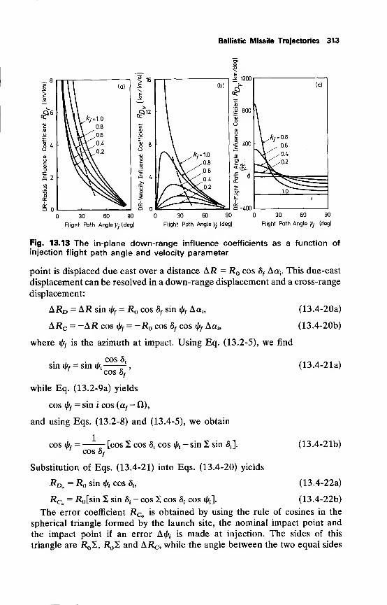
Ballistic Missile Trajectories 313
Q Q-tt»
(c)
\,fy = 0.8
\ / 06
^^V^ 04
_\f/0.2
1^0
*
30 60 90
Flight Path Angle yf- (deg)
30 60 90
Flight Path Angle y (deg)
30 60 90
Flight Path Angle yf
- (deg)
Fig. 13.13 The in-plane down-range influence coefficients as a function of
injection flight path angle and velocity parameter
point is displaced due east over a distance AR = R cos 8fAa
;. This due-east
displacement can be resolved in a down-range displacement and a cross-range
displacement:
ARD = AR sin ty= R cos 8
fsin i(f
fAa i5
(13.4-20a)
ARC = -AR cos i(ff= -Rq cos 8
fcos i/^ Aa
4 ,(13.4-20b)
where ty is the azimuth at impact. Using Eq. (13.2-5), we find
cos 8isin i{f
f= sin ifo
cos 8f
'(13.4-21a)
while Eq. (13.2-9a) yields
cos \\/f= sin i cos (a
f- ft),
and using Eqs. (13.2-8) and (13.4-5), we obtain
1cos ty
=cos 8,
[cos X cos 8j cos jfo- sin X sin 8J. (13.4-21b)
Substitution of Eqs. (13.4-21) into Eqs. (13.4-20) yields
&Da= Ro sin fa cos S„ (13.4-22a)
JRCa = i?o[sin X sin 8f
— cos 2 cos Sj cos ^]. (13.4-22b)
The error coefficient Rq is obtained by using the rule of cosines in the
spherical triangle formed by the launch site, the nominal impact point and
the impact point if an error Aifo is made at injection. The sides of this
triangle are RqI,, RqZ and ARC, while the angle between the two equal sides
314 Rocket Propulsion & Spaceflight Dynamics
is Aif/i. So, we have
AR^ j ^ , ._cos—— = cos z + sin z cos At//;,
and as —— and A^ are small, both cosines may be expanded in a Taylor
series and terms of degree higher than the second may be neglected, leading
to
(^)2
= sin2 S(A^) 2
For S<180°, a positive A^ yields a negative ARC. So we find for the
cross-range influence coefficient with respect to ipt
Rc^= -R sin 2. (13.4-23)
The error coefficients with respect to 8t ,
finally, can be obtained in the
following way. Suppose that at cut-off there are only errors in ah 8;and j/^.
Then the down-range and cross-range errors are
ARD = RDa Aa t+ RDs A8h (13.4-24a)
ARC = RCa Aa f+ RCs A8;
+ RQ Aft. (13.4-24b)
Let Aah A8tand Aft be related such that the actual injection point lies in
the nominal trajectory plane and that at actual injection the azimuth equals
the local nominal azimuth. In that case, the actual trajectory plane will
coincide with the nominal trajectory plane and only a down-range error will
result. The magnitude of this down-range error equals the distance between
the sub-vehicle points of actual injection and nominal injection. As Aaf ,AS;
and Aft are small, the requirement for the injection point to lie in the
trajectory plane is
Aa-^-f-'AS, (13.4-25)COS Oj
The local nominal azimuth, t^ + Ai/r£ ,
at position c^ + Ac^, Sj + AS; can be
found by using Eq. (13.2-5)
sin (ft + Aft) cos (8i + AS;) = sin ft; cos S;.
By linearizing this equation and solving for Aft, we obtain
Aft = tan 8ttan ft A8t
. (13.4-26)
For arbitrary AS;, with Aatand Aft as given in Eqs. (13.4-25) and (13.4-26),
the down-range error is given by
ARD =-^-A8i. (13.4-27)
cos ft
Ballistic Missile Trajectories 315
Substitution of Eqs. (13.4-25) to (13.4-27) into Eqs. (13.4-24), with
ARC = and solving the resulting equations for RDs and i?Cs yields
**--V**^, (13.4-28a)COS \\li COS Oj
RCs = -RCa^r- Re, tan 8, tan ft. (13.4-28b)cos 8
f^
Substitution of Eqs. (13.4-22) and (13.4-23) into Eqs. (13.4-28), finally
yields
RDs = Rq cos ft, (13.4-29a)
RCs= Rq cos X sin ft, (13.4-29b)
which completes the determination of the influence coefficients. We see
from Eqs. (13.4-22), (13.4-23) and (13.4-29) that the influence coefficients
with respect to the out-of-plane injection state are of the same order of
magnitude as R , which means an error of about 6000 km/rad or about
100 km/deg. An error in cut-off flight path angle is also of the order R,
while it follows from Fig. 13.13 that for a range of 10,000 km errors in rt
and Vf of 1 m and 1 m/s respectively will result in impact errors of 6 m and
6 km respectively, for a nominal optimal trajectory. For a non-guided
missile, the resulting errors will be too large to allow for an accurate kill.
Therefore all ballistic missiles are guided, which means that during the
powered flight steering commands are computed on the basis of real flight
conditions.
References
1 Anon. (1961), Explanatory Supplement to the American Ephemeris andNautical Almanac, H.M.S.O., London, p. 75.
2 Kohlhase, C. E. (1962), Launch-on-time analysis for space missions,
Progress in Astronautics and Rocketry, Vol. 8, Academic Press, New York,
p. 3-21.
3 Plummer, H. C. (1960), An Introductory Treatise on Dynamical As-tronomy, Dover Publications, New York, p. 49-60.
4 Battin, R. H. (1964), Astronautical Guidance, McGraw-Hill, NewYork, p. 70-82.
5 Moe, M. M. (1960), An approximation to the re-entry trajectory,
A.R.S. J., 30, 50-58.
6 Blum, R. (1962), Re-entry trajectories: flat earth approximation,
A.R.S. J., 32, 616-620.
7 Bate, R. R. and Johnson, R. W. (1962), Empirical formulas for ballistic
re-entry trajectories, A.R.S. J., 32, 1882-1887.
316 Rocket Propulsion & Spaceflight Dynamics
8 Wheelon, A.R.S. J., 29,915-926.
9 Ching-Sheng Wu (1960), Effect of earth's oblateness on the calculation
of the impact point of ballistic missiles, A.R.S. J., 30, 1172-1173.
10 Escobal, P. R. (1964), Calculation of the surface range of a ballistic
missile, AIAA J., 2, 571-573.
14 Rocket Motion in theAtmosphere
In Chapters 11 and 12 rocket motion in vacuum was considered, while
in Chapter 13 the atmospheric effects were neglected for the major part of
the trajectory. But the presence of the Earth's atmosphere will lead to
aerodynamic forces on the vehicle and in many cases one has to account for
the aerodynamic forces and moments to predict accurately the vehicle's
trajectory and performances.
Because of unpredictable aerodynamic forces and moments the trajectory
may deviate from the nominal trajectory. Such aerodynamic moments maybe caused by steady wind, wind-gusts, atmospheric turbulence, but also by fin
misalignment and production inaccuracies. The deviation of the trajectory of
the rocket is known as trajectory dispersion. For guided vehicles, the disper-
sion of the impact point, for instance, is minimized by means of a special
guidance system.
As an extensive discussion on aerodynamics is far beyond the scope of this
book, we restrict ourselves to a short discussion to give the reader some
understanding of the aerodynamic phenomena which play a role in rocketry,
and we will give some engineering methods, which enable the reader to
estimate the order of magnitude of the aerodynamic forces and moments.
14.1 The equations of motion
In Section 4.2.5 the dynamical equations of motion for a rigid rocket, Eqs.
(4.2-58), were derived. In these equations, Xa, Ya, Za, and L', M' and N'
stand for the aerodynamic forces and moments, respectively, which among
others, depend on the velocity of the rocket with respect to the air, and the
local atmospheric pressure, density and temperature. For simplicity, we will
assume a quiet non-rotating atmosphere. The inertial linear velocity compo-
nents are, u, v and w and the angular velocity components are p, q and r.
Some important notions, frequently used in aerodynamics are the Machnumber, Ma, the Reynolds number, Re, and the dynamic pressure, q* In
Section 5.1.2, the Mach number was defined already; here we will use the
Mach number,
Ma = VcJa, (14.1-la)
where Vcm stands for the velocity of the center of mass of the vehicle. The
* Usually the notation q is used for the dynamic pressure; to avoid ambiguity with the
angular velocity q, the notation q is used here.
318 Rocket Propulsion & Spaceflight Dynamics
Reynolds number, Re, was denned in Section 8.2.4; here we use
Re = pVcmL/n. (14.1-lb)
The dynamic pressure is defined as
4 = ipVL- (14.1-lc)
As the atmospheric quantities, p, T, /x, p, a, etc., are strongly variable
(Section 2.6), depending on time and location, one must, for practical
purposes use an estimate of their average values such as given in a Reference
Atmosphere [1].
14.1.1 Aerodynamic forces, moments and coefficients
There is a great variety in the aerodynamic configurations of missiles and
rocket vehicles. For instance, the Space Shuttle with its large wings has someaerodynamic characteristics like a plane while a launch vehicle, like the
Saturn V has only four small stabilization fins. We will restrict our discussion
to rocket vehicles without wings, having four stabilization fins, which lie in
pairs in a plane of symmetry (cruciform configuration). Those readers whowant more detailed information are referred to Nielsen [2] and Chin [3].
To simplify the treatment, we assume the vehicle's velocity vector to
coincide with one of the symmetry planes through a pair of fins. We also
assume that one of the symmetry planes coincides with the trajectory plane.
The angle in the trajectory plane between the velocity vector and the
longitudinal axis of the vehicle is the angle of attack or angle of incidence, a
(Fig. 14.1).
If the velocity vector were lying in the other symmetry plane, the
angle would be called the sideslip angle, |3. These names stem from aircraft
aerodynamics.
The total aerodynamic force, Fa, is assumed to lie in the trajectory plane.
The point where the line of force of Fa intersects the rocket's center-line, is
called the center of pressure, cp. It is evident that if there is no resultant
aerodynamic moment on the vehicle, cp coincides with the center of mass,
cm, which we also assume to lie on the center-line. If cp and cm do not
coincide, there is an aerodynamic moment about the y-axis of the vehicle,
(Section 4.1), the pitching moment*
M' = Fa xl, (14.1-2)
where
l = xcm -xcp,(14.1-3)
see Fig. 14.1.
The aerodynamic force Fa usually is resolved either in a lift, L, and a
* Usually the aerodynamic moment about the y-axis is indicated by M; to avoid ambiguity
with mass we use the notation M' here.
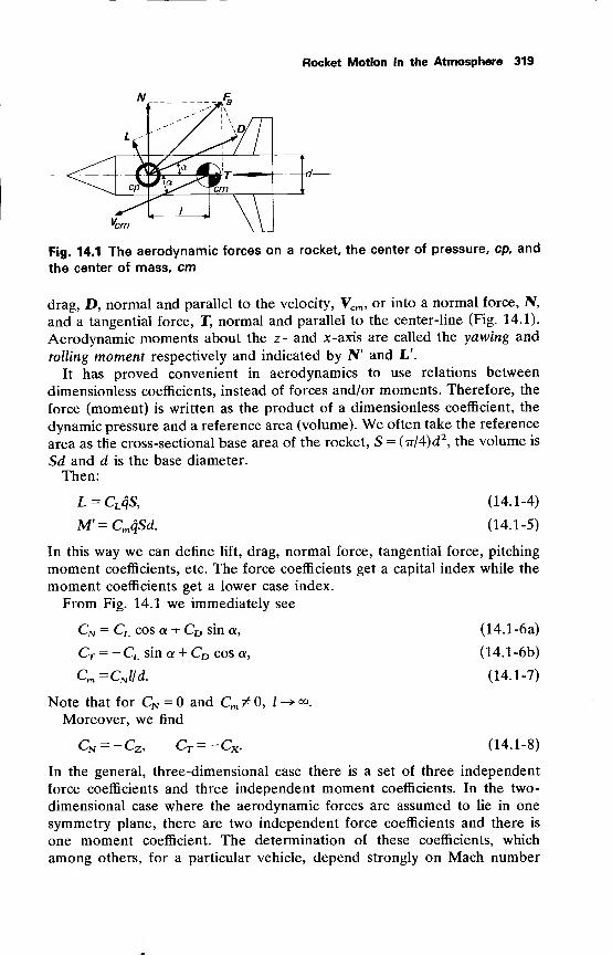
Rocket Motion in the Atmosphere 319
N __£
L -
,
^-'
3Vtic/N
*^yx
\^ *m
' - \\VCm \L
Fig. 14.1 The aerodynamic forces on a rocket, the center of pressure, cp, and
the center of mass, cm
drag, D, normal and parallel to the velocity, Vcm , or into a normal force, N,
and a tangential force, T, normal and parallel to the center-line (Fig. 14.1).
Aerodynamic moments about the z- and x-axis are called the yawing and
rolling moment respectively and indicated by N' and L'.
It has proved convenient in aerodynamics to use relations between
dimensionless coefficients, instead of forces and/or moments. Therefore, the
force (moment) is written as the product of a dimensionless coefficient, the
dynamic pressure and a reference area (volume). We often take the reference
area as the cross-sectional base area of the rocket, S = (7r/4)d2
, the volume is
Sd and d is the base diameter.
Then:
L = CLqS,
M'=CmqSd.(14.1-4)
(14.1-5)
In this way we can define lift, drag, normal force, tangential force, pitching
moment coefficients, etc. The force coefficients get a capital index while the
moment coefficients get a lower case index.
From Fig. 14.1 we immediately see
Cn = CL cos a + CD sin a,
CT = —CL sin a + CD cos a,
Note that for CN = and Cm ^0, /
Moreover, we find
Cm — C? Ct — C>
(14.1-6a)
(14.1-6b)
(14.1-7)
(14.1-8)
In the general, three-dimensional case there is a set of three independent
force coefficients and three independent moment coefficients. In the two-
dimensional case where the aerodynamic forces are assumed to lie in one
symmetry plane, there are two independent force coefficients and there is
one moment coefficient. The determination of these coefficients, which
among others, for a particular vehicle, depend strongly on Mach number
320 Rocket Propulsion & Spaceflight Dynamics
and Reynolds number, belongs to the field of aerodynamics. It is possible to
predict the aerodynamic coefficients with a fair degree of accuracy, but for a
real accurate determination one often has to rely on experiments, such as
windtunnel tests, or free -flight experiments, either with small models or with
full-scale vehicles. In those experiments, it is very important that the
dimensionless numbers, such as Re or Ma are the same for the vehicle andthe scale-model, otherwise the results may be unreliable. For instance, it is
well-known that at low Reynolds numbers, one may have laminar boundary
layers, while at high Reynolds numbers the boundary layer usually is
turbulent. The nature of the boundary layer not only strongly influences the
magnitude of the aerodynamic forces, but also determines whether or not
flow separation occurs. Such a separation may completely alter the nature of
the flow around the rocket, and hence the information as obtained from a
scale-model might be useless for application to the flight vehicle if the
dimensionless scale numbers do not match. 4
In order to investigate the stability characteristics of flight vehicles, it is
especially useful to know how the aerodynamic forces and moments vary
with small changes of the independent variables. It turns out that for small
motions of, and about, the center of mass, in the three-dimensional case, the
components of the motions about and along the body axes hardly influence
each other, so that for these small motions, the complete motion can be
approximated by superposition of the respective translational and rotational
motions, along and about the x-, y- and z-axis; i.e. the six Eqs. (4.2-58) can
be solved independently of each other. As, in this chapter, we concern
ourselves primarily with the motion in the trajectory plane, this means that
we neglect small out-of-plane motions of the center of mass or the effects of
cross-winds on the in-plane vehicle motion, etc.
As long as forces and moments remain small, we can expand any
aerodynamic force, F, or moment, M', in a Taylor series, and neglect
higher-order terms:
F=F + Faa+Fqq + Fid + --
M' = M'e +M^a+M^q+M^d + • • •
where F and M'Q are constants, equalling zero for a symmetric vehicle, and
where Fa stands for dF/da, etc. These equations can also be written as
dF={CF +CF a)qS + (CFid + CF q)qS— +-- (14.1-9a)
2V
M' = (Cmo + Cmaa)qSd + (CmAd + Cmqq)qS^+--- (14.1-9b)
The term d/(2V) arises from the use of a dimensionless time, thus
d=da/d(2Vt/d).
Terms like CFa , CF& , Cmq , etc., are called stability derivatives. It turns out
Rocket Motion in the Atmosphere 321
that for a very simple, two-dimensional description of the rocket motion
about the center of mass, the following stability derivatives are important:
CNa , C^, C^ and C^. For this reason these terms were included in the
series expansion above. When discussing the stability of rocket vehicles we
will explain their meaning.
14.2 The magnitude of the aerodynamic coefficients
The aerodynamic coefficients for a particular vehicle depend among others
on a, Re, and Ma . For low values of a, an accurate calculation of CN, Cmand CD has been possible for a long time for subsonic and supersonic speeds.
At transonic speeds, Ma = l, it is difficult to make accurate predictions.
More recent methods [4] allow predictions of CN and Cm at large values of
a, while also the dynamics at these high angles of attack have been
investigated. These investigations [5] showed that due to the dynamics of the
pitching motion, the values of the aerodynamic coefficients, especially at
high angles of attack, may deviate considerably from their static values.
We will limit our discussion to small angles of attack, and write an
aerodynamic force (moment) in the form
FT = FB + Fw + Fb (14.2-1)
or in words: the total force (moment), FT, is the sum of the force (moment)
on the body, FB, on the fins, Fw, and a force (moment) due to interference,
Fj. We have asssumed here that the vehicle only consists of a body and fins.
Dividing Eq. (14.2-1) by qSr or qSrd yields
CFt = CFb + CFw + Cf, (14.2-2)
We indicate the reference area by ST.
For small a, the Eqs. (14.1-6) usually may be approximated by
CN =CL + CDa, CD = Cr + CLa. (14.2-3)
So, in the following we will concern ourselves with CN and CD .
14.2.1 The normal force and pitching moment coefficients
For a rocket vehicle having four fins in cruciform configuration we have to
consider the components CNb for the body in absence of fins, CNw for the
fins alone and CNi , accounting for interference effects, to determine the
complete normal force coefficient. For bodies with large fineness, slender-
body theory [2] predicts
<*•%£> < l4 -2-4)
where L stands for the vehicle length considered, x for the distance from the
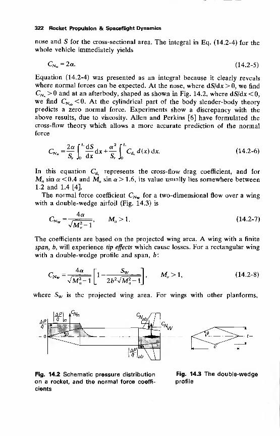
322 Rocket Propulsion & Spaceflight Dynamics
nose and S for the cross-sectional area. The integral in Eq. (14.2-4) for the
whole vehicle immediately yields
Gsr„ = 2 a. (14.2-5)
Equation (14.2-4) was presented as an integral because it clearly reveals
where normal forces can be expected. At the nose, where dS/dx > 0, we find
CNn > and at an afterbody, shaped as shown in Fig. 14.2, where dS/dx < 0,
we find CNab <0. At the cylindrical part of the body slender-body theory
predicts a zero normal force. Experiments show a discrepancy with the
above results, due to viscosity. Allen and Perkins [6] have formulated the
cross-flow theory which allows a more accurate prediction of the normalforce
£-NB — H :r dx+"H cdc d(x)dx.Sr Jo dx Sr Jo
(14.2-6)
In this equation Cdc represents the cross-flow drag coefficient, and for
Ma sin a <0.4 and Ma sin a > 1.6, its value usually lies somewhere between1.2 and 1.4 [4].
The normal force coefficient CNw for a two-dimensional flow over a wing
with a double-wedge airfoil (Fig. 14.3) is
C-7«J„,—Vm^-i'
M„>1. (14.2-7)
The coefficients are based on the projected wing area. A wing with a finite
span, b, will experience tip effects which cause losses. For a rectangular wing
with a double-wedge profile and span, b:
Cxr„, —4a
= [l fe1 Ma >l,
l|_ 2bVM2a -lJ
(14.2-8)VM*-l|/ 2bNM2
a-l\
where Sw is the projected wing area. For wings with other planforms,
\AR\ kCNn
Fig. 14.2 Schematic pressure distribution
on a rocket, and the normal force coeffi-
cients
Fig. 14.3 The double-wedgeprofile
Rocket Motion in the Atmosphere 323
corresponding expressions for CN can be derived. For more detailed infor-
mation the reader is referred to Pitts [7].
Interference effects make up for the difference between CNt and CNw +CNb . For instance, in Fig. 14.2, the pressure distribution on the body,
according to slender-body theory, is shown. Some of the pressure on the
nose is 'carried over' to the cylindrical part, as indicated by the dashed line.
This is known as the carry-over effect. In a similar way, the pressure on the
wings induces a pressure load on the body near the wing, while the presence
of the body effectively increases the span and influences the pressure
distribution on the wing. The interference effects, which may be fairly large,
can be calculated according to Pitts [7].
The pitching moment coefficient, Cm , can be determined in the same way
as CN . For a slender-body of revolution it is found to be
Cmb = ^[^ (xm - x) dx+^[V d(x)(xm - x) dx. (14.2-9)
Here xm is the coordinate of the moment axis.
For the fins we have
c = cxm~xcpw (14.2-10)
The cp for a two-dimensional wing-section lies half chord. Interference and
three-dimensional effects may shift. this a little, but for large launch vehicles
this is not of much importance. For small missiles and sounding rockets it
certainly has to be accounted for, as the ratio of finchord to vehicle length
usually is much larger for these vehicles than for launch vehicles.
14.2.2 The drag coefficient
The drag of a rocket vehicle can be split into the following components:
wave drag, due to the presence of shock waves and dependent on the Mach
number; viscous drag, due to friction; induced drag, due to the generation of
lift; base drag, due to the wake behind the vehicle; interference drag, due to
the interaction of various flow fields; and roughness drag, due to surface
roughness such as rivets and welds.
The most comprehensive reference source on drag, certainly is Hoerner's
standard work [8], to which the reader is referred for detailed information.
The wave drag, connected with a shock wave, and hence occurring only at
supersonic speeds, amounts for a conical forebody [9] to
CDn = (o.OSS+^Wse) 1 69, Ma > 1, (14.2-11)
324 Rocket Propulsion & Spaceflight Dynamics
where 8 is the half-cone angle in radians (Fig. 14.2). The wave drag of anisolated, rectangular wing of span, b, with a double-wedge profile is [3]
402r S
rhivfe} M° >h (14 -2- 12)
where 6 is the half-wedge angle (Fig. 14.3). Both wave drag coefficients are
strongly dependent on and decrease with increasing Mach numbers.
Viscous drag is the main drag component at subsonic speeds. It can beestimated by considering the friction drag coefficient, CDf, for a flat plate of
equal length and equal wetted area as the rocket vehicle. For a laminarboundary layer we may estimate
1.328c^7Si' (14 -2" 13)
and for a turbulent boundary layer [8]
0.427C^
=(log10 ^-0.407)
2- (14 -2" 14)
These coefficients are based on the wetted area as a reference area. For
most large rockets, one may assume the boundary layer to be turbulent.
Transition from laminar to turbulent takes place around Re = 106based on
the bodylength, so that for small vehicles, still a major portion of the
boundary layer may be laminar. Surface roughness may cause a transition
from laminar to turbulent at lower Reynolds numbers.
Induced drag [3] is a result of the development of lift. In the subsonic
case, the induced drag, based on the projected wing area, Sw, is
Coin=^, Ma <l, (14.2-15)
7rb c x
and at supersonic speeds it is well approximated by
C^OvlC^ Ma >\, (14.2-16)
and c 1 is a constant.
Base drag is strongly affected by the shape of the vehicle, and the
presence of a jet. The last two types of drag, base drag and roughness drag,
in many cases constitute only a small amount of the total drag.
The total drag is found by addition of all components. It turns out that the
total drag coefficient can well be approximated for preliminary calculations
by:
CD = a + bM6a , Ma <l, (14.2-17a)
Cn = a ' + TT2> Ma^l- (14.2-17b)Mi
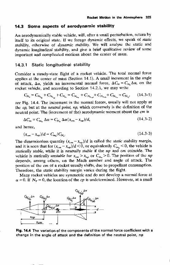
Rocket Motion in the Atmosphere 325
14.3 Some aspects of aerodynamic stability
An aerodynamically stable vehicle, will, after a small perturbation, return by
itself to its original state. If we forego dynamic effects, we speak of static
stability, otherwise of dynamic stability. We will analyse the static and
dynamic longitudinal stability, and give a brief qualitative review of some
important and complicated motions about the center of mass.
14.3.1 Static longitudinal stability
Consider a steady-state flight of a rocket vehicle. The total normal force
applies at the center of mass (Section 14.1). A small increment in the angle
of attack, Aa, yields an incremental normal force, ACN = CNa Aa, on the
rocket vehicle, and according to Section 14.2.1, we may write
C-'NJ — Cv "T Oi>j ~r Oisj — C^jvr tLu ' C-' JST_. .i {--IV ' (-^TV (14.3-1)
see Fig. 14.4. The increment in the normal forces, usually will not apply at
the cp, but at the neutral point, np, which conversely is the definition of the
neutral point. The (increment of the) aerodynamic moment about the cm is
(14.3-2)ACm = CL Aa = CNa Aa(xcm -xnp )/d,
and hence,
\Xcm Xnp)'d — CL /Cjv . (14.3-3)
The dimensionless quantity (xcm - xnp)/d is called the static stability margin,
and it is seen that for (xcm - xnp )fd < 0, or equivalently Cm<x < 0, the vehicle is
statically stable, while it is neutrally stable if the np and cm coincide. The
vehicle is statically unstable for xcm >jcnp or Cm<< >0. The position of the np
depends, among others, on the Mach number and angle of attack. The
position of the cm of a rocket usually shifts, due to propellant consumption.
Therefore, the static stability margin varies during the flight.
Many rocket vehicles are symmetric and do not develop a normal force at
a = 0. If NT = 0, the location of the cp is undetermined. However, at a small
CN<y
.Aa
aCa/ . Aa-8*9!+-.
cm
Fig. 14.4 The variation of the components of the normal force coefficient with a
change in the angle of attack and the definition of the neutral point, np
326 Rocket Propulsion & Spaceflight Dynamics
angle of attack, Aa, the total normal force, NT, equals the increment in
normal force, AN"T, and xcp = xnp .
As is shown in Fig. 14.4, the main stabilizing forces are CNw and CN.
due to fins and interference effects. This may clarify the functioning of the fins.
It is also seen from Eq. (14.3-3) that a forward position of the cm helps
too, in stabilizing the vehicle.
A large negative stability margin is very effective, but it also has disadvan-
tages. It may lead to large bending moments in the structure; especially for
large launch vehicles this may be unacceptable. For guided missiles, whichrequire a quick response to a steering command, very high aerodynamicforces and moments are required if the stability margin is large negative.
Therefore, many vehicles have Cma s= during the whole or a portion of
their flight through the atmosphere. Stabilization then may be obtained bythrust vector control or by the deflection of flaps, rudders or complete fins.
Now suppose a = and the cruciform rocket vehicle is flying in a
cross-wind. Then the above discussion holds if we replace the angle of attack,
a, by the sideslip angle, |8. It is evident that a stable rocket will try to reduce
|3, by turning its nose into the wind, thereby changing its flight path. For
obvious reasons this is known as weathercocking, and Cn@ is called the
weathercock stability.
14.3.2 Dynamic longitudinal stability
We return to the dynamical equations of motion, Eqs. (4.2-58), and simplify
the analysis by assuming the roll and yaw rate to equal zero, like the velocity
in y -direction, while the velocity in x -direction, u, is assumed constant,
which implies a two-dimensional motion. This yields two coupled differential
equations, Eq. (4.2-58c) and Eq. (4.2-58e). The pitch angle, 0, is the angle
between the horizontal plane and the longitudinal axis, and a is the angle
between the velocity vector and the longitudinal axis. Hence, 6 = a + y.
Assuming the flight path angle, y, constant, we have q = 6 = a, which
eliminates Eq. (4.2-5 8c) and we are left with
Iyya + [I
yy+ mx2]d - (MF)y
- M' = 0,
to describe the motion of a rocket vehicle about the y-axis, under the
assumptions made. The y -component of the thrust misalignment moment,(MF)y , is
(MF )y =-xeFz + zeFx . (14.3-4)
Substitution of Eq. (14.1-9b) and assuming 0^ = yields
r. d 2
Iyyd +
1
Iyy+ mxl - (Cm . + Cmq )qS
—2
a - Cm dqSot - (MF)y= 0,y
(14.3-5a,
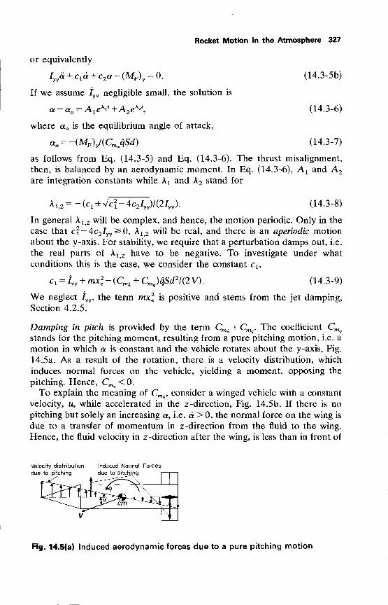
Rocket Motion in the Atmosphere 327
or equivalently
Iyya + Cld + c2a - (MF)y
= 0. (14.3-5b)
If we assume Iyy
negligible small, the solution is
a-a = A 1 ek
*t +A2e
K*\ (14.3-6)
where a is the equilibrium angle of attack,
a = -(MF)y/(CmaqSd) (14.3-7)
as follows from Eq. (14.3-5) and Eq. (14.3-6). The thrust misalignment,
then, is balanced by an aerodynamic moment. In Eq. (14.3-6), A 1 and A2
are integration constants while A x and A 2 stand for
Ai,2 = -(c 1 ±Vc?-4c2Ly)/(2L
y ). (14.3-8)
In general \ 12 will be complex, and hence, the motion periodic. Only in the
case that c? — 4c2/yy ^0, A12 will be real, and there is an aperiodic motion
about the y-axis. For stability, we require that a perturbation damps out, i.e.
the real parts of A 12 have to be negative. To investigate under what
conditions this is the case, we consider the constant c l5
c x- l
yy+ mx 2
e -(Cm, + Cm )qSd2/(2V). (14.3-9)
We neglect Jyy , the term mx 2
is positive and stems from the jet damping,
Section 4.2.5.
Damping in pitch is provided by the term Cmi + C^. The coefficient Cmq
stands for the pitching moment, resulting from a pure pitching motion, i.e. a
motion in which a is constant and the vehicle rotates about the y-axis, Fig.
14.5a. As a result of the rotation, there is a velocity distribution, which
induces normal forces on the vehicle, yielding a moment, opposing the
pitching. Hence, Cmq < 0.
To explain the meaning of Cm& , consider a winged vehicle with a constant
velocity, u, while accelerated in the z-direction, Fig. 14.5b. If there is no
pitching but solely an increasing a, i.e. a > 0, the normal force on the wing is
due to a transfer of momentum in z-direction from the fluid to the wing.
Hence, the fluid velocity in z-direction after the wing, is less than in front of
Velocity distribution
due to pitching
Induced Normal Forces
due to pitching
Fig. 14.5(a) Induced aerodynamic forces due to a pure pitching motion
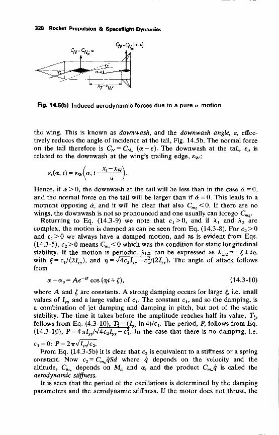
328 Rocket Propulsion & Spaceflight Dynamics
Fig. 14.5(b) Induced aerodynamic forces due to a pure a motion
the wing. This is known as downwash, and the downwash angle, e, effec-
tively reduces the angle of incidence at the tail, Fig. 14.5b. The normal force
on the tail therefore is CN = CNa (a - e). The downwash at the tail, e„ is
related to the downwash at the wing's trailing edge, ew :
et(a, t) = ewla, t
—-
-J
.
Hence, if d > 0, the downwash at the tail will be less than in the case d = 0,
and the normal force on the tail will be larger than if d = 0. This leads to a
moment opposing d, and it will be clear that also Cmi < 0. If there are no
wings, the downwash is not so pronounced and one usually can forego Cm ..
Returning to Eq. (14.3-9) we note that c 1 >0, and if Ai and A2 are
complex, the motion is damped as can be seen from Eq. (14.3-8). For c2>0and Cx>0 we always have a damped motion, and as is evident from Eqs.
(14.3-5), c2 >0 means Cma<0 which was the condition for static longitudinal
stability. If the motion is periodic, Ai,2 can be expressed as A 12 = -£±rn,with | = c 1/(2/yy ), and rj = V4c2Iyy
- c\l(2Iyy ). The angle of attack follows
from
a-a =Ae (tcos(T}f + £), (14.3-10)
where A and £ are constants. A strong damping occurs for large £ i.e. small
values of Iyy
and a large value of c x . The constant c l5 and so the damping, is
a combination of jet damping and damping in pitch, but not of the static
stability. The time it takes before the amplitude reaches half its value, T^,
follows from Eq. (4.3- 10), T\ = (Jvv In 4)/^. The period, P, follows from Eq.
(14.3-1Q), P = 4irIyy/V4c2Iyy
- c\. In the case that there is no damping, i.e.
c x= 0: P = 27rV/yy/c2 .
From Eq. (14.3-5b) it is clear that c2 is equivalent to a stiffness or a spring
constant. Now c2 = CmaqSd where q depends on the velocity and the
altitude, Cm<x depends on Ma and a, and the product Cmaq is called the
aerodynamic stiffness.
It is seen that the period of the oscillations is determined by the damping
parameters and the aerodynamic stiffness. If the motor does not thrust, the
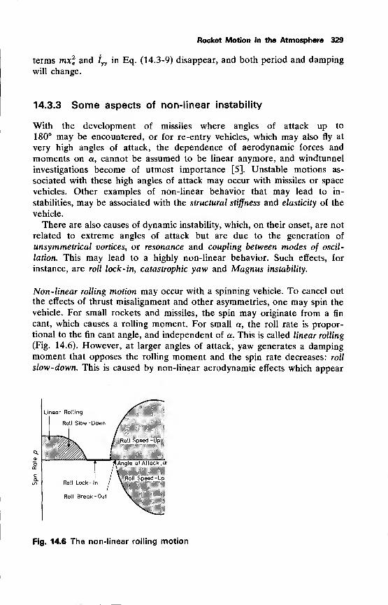
Rocket Motion in the Atmosphere 329
terms mx2e and I
yyin Eq. (14.3-9) disappear, and both period and damping
will change.
14.3.3 Some aspects of non-linear instability
With the development of missiles where angles of attack up to
180° may be encountered, or for re-entry vehicles, which may also fly at
very high angles of attack, the dependence of aerodynamic forces and
moments on a, cannot be assumed to be linear anymore, and windtunnel
investigations become of utmost importance [5]. Unstable motions as-
sociated with these high angles of attack may occur with missiles or space
vehicles. Other examples of non-linear behavior that may lead to in-
stabilities, may be associated with the structural stiffness and elasticity of the
vehicle.
There are also causes of dynamic instability, which, on their onset, are not
related to extreme angles of attack but are due to the generation of
unsymmetrical vortices, or resonance and coupling between modes of oscil-
lation. This may lead to a highly non-linear behavior. Such effects, for
instance, are roll lock-in, catastrophic yaw and Magnus instability.
Non- linear rolling motion may occur with a spinning vehicle. To cancel out
the effects of thrust misalignment and other asymmetries, one may spin the
vehicle. For small rockets and missiles, the spin may originate from a fin
cant, which causes a rolling moment. For small a, the roll rate is propor-
tional to the fin cant angle, and independent of a. This is called linear rolling
(Fig. 14.6). However, at larger angles of attack, yaw generates a dampingmoment that opposes the rolling moment and the spin rate decreases: roll
slow-down. This is caused by non-linear aerodynamic effects which appear
Linear Rolling
Roll Slow -Down
iRoll Speed -Up
|
Roll Lock- In /
Roll Break -Out
{Angle of Attack , at
Roll Speed -Up
Fig. 14.6 The non-linear rolling motion
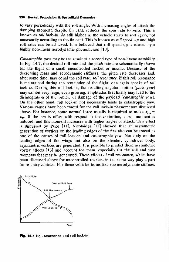
330 Rocket Propulsion & Spaceflight Dynamics
to vary periodically with the roll angle. With increasing angles of attack the
damping moment, despite fin cant, reduces the spin rate to zero. This is
known as roll lock-in. At still higher a, the vehicle starts to roll again, not
necessarily according to the fin cant. This is known as roll speed-up and high
roll rates can be achieved. It is believed that roll speed-up is caused by a
highly non-linear aerodynamic phenomenon [10].
Catastrophic yaw may be the result of a second type of non-linear instability.
In Fig. 14.7, the desired roll rate and the pitch rate are schematically shownfor the flight of a small uncontrolled rocket or missile. Because of the
decreasing mass and aerodynamic stiffness, the pitch rate decreases and,
after some time, may equal the roll rate: roll resonance. If this roll resonance
is maintained during the remainder of the flight, one again speaks of roll
lock-in. During this roll lock-in, the resulting angular motion (pitch-yaw)
may exhibit very large, even growing, amplitudes that finally may lead to the
disintegration of the vehicle or damage of the payload (catastrophic yaw).
On the other hand, roll lock-in not necessarily leads to catastrophic yaw.
Various causes have been traced for the roll lock-in phenomenon discussed
above. For instance, some normal force usually is required to make xcm =
xcp . If the cm is offset with respect to the centerline, a roll moment is
induced, and this moment increases with higher angles of attack. This effect
is discussed by Price [11]. Nicolaides [12] showed that an asymmetric
generation of vortices on the leading edges of the fins also can be traced as
one of the causes of roll lock-in and catastrophic yaw. Not only on the
leading edges of the wings but also on the slender, cylindrical body,
asymmetric vortices are generated. It is possible to predict these asymmetric
vortex effects [13] and account for them, especially for the roll and yawmoments that may be generated. These effects of roll resonance, which have
been discussed above for uncontrolled rockets, in the same way play a part
for re-entry vehicles. For these vehicles terms like the aerodynamic stiffness
k. Pitch Rate
\ IV.J Desired Roll Rate
i_n Roll Resonance ^'
\ I ^
st
A Roll Lock-In
-
Fig. 14.7 Roll resonance and roll lock-in
Rocket Motion in the Atmosphere 331
increase during descent. Here too, one meets the problem of avoiding
resonance followed by a lock-in. The problem has been analysed by Nayfeh
[14].
Magnus instability is a third type of non-linear instability. To understand it,
consider a missile flying at an angle of attack, and /3 = 0. Owing to the angle
a, there is a cross-flow normal to the longitudinal axis. If the missile is
spinning about its longitudinal axis, there will be a layer of circulating air.
This circulation in combination with the cross-flow, creates velocity differ-
ences at the periphery of the missile, thus causing pressure differences andhence sideward forces, called Magnus forces. The displacement of the missile
due to the Magnus forces may be small, though not negligible as dispersion
is concerned. The Magnus forces usually also yield a moment about the cm,the Magnus moment. This may lead to unacceptable large yaw angles. It is
seen here, that an angle of incidence, in combination with rolling, may lead
to yaw. Clearly, for such motions, it is not permitted to uncouple the
equations of motion, Eqs. (4.2-58).
Often one tries to avoid catastrophic yaw, due to roll resonance followed
by roll lock-in, by a high enough spin rate. The pitch rate and roll rate
curve, as shown in Fig. 14.7, will not intersect then, but now there is the
danger of Magnus instability.
Finally we have to mention that among the dynamic instabilities, a related
spin-yaw resonance phenomenon may occur. In this case the damping is
ineffective and hence an oscillation with a growing amplitude is possible.
The fact that the damping is ineffective is mainly due to the decrease in
aerodynamic stiffness, Cmaq, at great altitudes.
For controlled flight vehicles, the control system will suppress
aerodynamic instabilities but a thorough knowledge of the aerodynamicforces, moments and the coupling between the various motions is necessary
for a successful design of such a control mechanism.
14.4 Other atmospheric effects
We mentioned in the previous sections how aerodynamic forces are gener-ated by a vehicle flying through the atmosphere. The effects of these forces
are various: losses and gains in performance, trajectory dispersion,
aerodynamic loads and aerodynamic heating, to name only a few. We cannotdiscuss these effects in detail, but we merely mention their most importantaspects.
Performance gains as compared to vacuum performance occur mainly withwinged vehicles such as cruise missiles and the Space Shuttle. The range ofthese vehicles and their applicability is strongly enlarged by the use of lifting
surfaces. For vehicles which fly mainly vertical trajectories through the
atmosphere, and where no controlled re-entry phase is required, wings are ofno use.
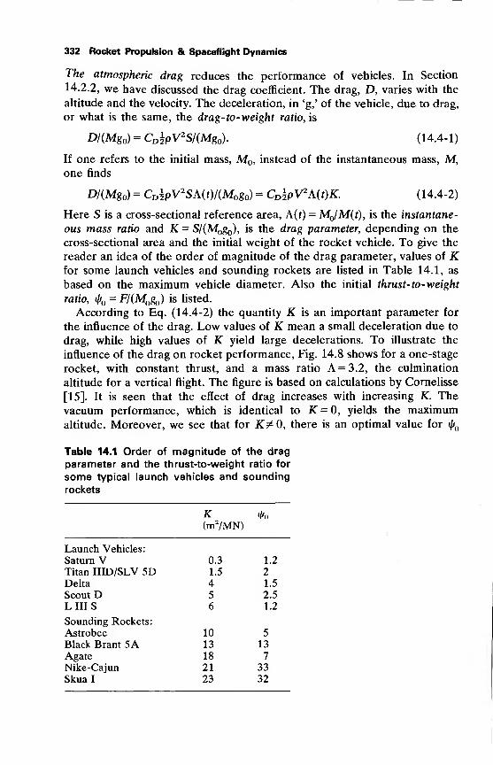
332 Rocket Propulsion & Spaceflight Dynamics
The atmospheric drag reduces the performance of vehicles. In Section
14.2.2, we have discussed the drag coefficient. The drag, D, varies with the
altitude and the velocity. The deceleration, in 'g,' of the vehicle, due to drag,
or what is the same, the drag-to-weight ratio, is
D/(Mg ) = CD\pV2SI{Mg ). (14.4*1)
If one refers to the initial mass, M , instead of the instantaneous mass, M,one finds
D/(Mg ) = CDipV2SA(0/(Mogo) = CD\pV2A(t)K. (14.4-2)
Here S is a cross-sectional reference area, A(0 = MJM(t), is the instantane-
ous mass ratio and K = S/(M g ), is the drag parameter, depending on the
cross-sectional area and the initial weight of the rocket vehicle. To give the
reader an idea of the order of magnitude of the drag parameter, values of Kfor some launch vehicles and sounding rockets are listed in Table 14.1, as
based on the maximum vehicle diameter. Also the initial thrust-to-weight
ratio, i(f = F/(M g ) is listed.
According to Eq. (14.4-2) the quantity K is an important parameter for
the influence of the drag. Low values of K mean a small deceleration due to
drag, while high values of K yield large decelerations. To illustrate the
influence of the drag on rocket performance, Fig. 14.8 shows for a one-stage
rocket, with constant thrust, and a mass ratio A = 3.2, the culmination
altitude for a vertical flight. The figure is based on calculations by Cornelisse
[15]. It is seen that the effect of drag increases with increasing K. The
vacuum performance, which is identical to K = 0, yields the maximumaltitude. Moreover, we see that for Kt^O, there is an optimal value for j^
Table 14.1 Order of magnitude of the drag
parameter and the thrust-to-weight ratio for
some typical launch vehicles and sounding
rockets
K «Ao
(m2/MN)
Launch Vehicles:
Saturn V 0.3 1.2
Titan IIID/SLV 5D 1.5 2
Delta 4 1.5
Scout D 5 2.5
LUIS 6 1.2
Sounding Rockets:
Astrobee 10 5
Black Brant 5A 13 13
Agate 18 7
Nike-Cajun 21 33Skua I 23 32
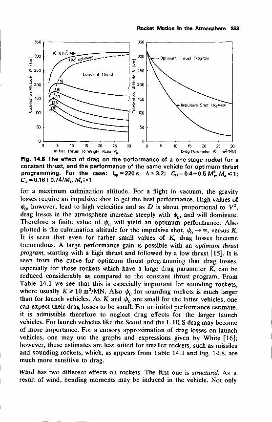
350
300
C 250
S 200
=8 150
100
50 •
/C=0m 2/MN
Rocket Motion in the Atmosphere 333
350
15 20 25 30
Drag Parameter K (m2/MN)
5 10 15 20 25
Initial Thrust to Weight Ratio </>
Fig. 14.8 The effect of drag on the performance of a one-stage rocket for a
constant thrust, and the performance of the same vehicle for optimum thrust
programming. For the case: /sp = 220s; A = 3.2; CD = 0.4+0.5M6a,M8 ^1;
CD = 0.1 6 + 0.74/Ma , Ma s= 1
for a maximum culmination altitude. For a flight in vacuum, the gravity
losses require an impulsive shot to get the best performance. High values of
«/f, however, lead to high velocities and as D is about proportional to V2
,
drag losses in the atmosphere increase steeply with iff , and will dominate.Therefore a finite value of «/r will yield an optimum performance. Alsoplotted is the culmination altitude for the impulsive shot, t(f -> <», versus K.It is seen that even for rather small values of K, drag losses becometremendous. A large performance gain is possible with an optimum thrust
program, starting with a high thrust and followed by a low thrust [15]. It is
seen from the curve for optimum thrust programming that drag losses,
especially for those rockets which have a large drag parameter K, can bereduced considerably as compared to the constant thrust program. FromTable 14.1 we see that this is especially important for sounding rockets,
where usually K s* 10 m2/MN. Also if/ for sounding rockets is much larger
than for launch vehicles. As K and i/f are small for the latter vehicles, onecan expect their drag losses to be small. For an initial performance estimate,
it is admissible therefore to neglect drag effects for the larger launch
vehicles. For launch vehicles like the Scout and the L III S drag may becomeof more importance. For a cursory approximation of drag losses on launch
vehicles, one may use the graphs and expressions given by White [16];
however, these estimates are less suited for smaller rockets, such as missiles
and sounding rockets, which, as appears from Table 14.1 and Fig. 14.8, are
much more sensitive to drag.
Wind has two different effects on rockets. The first one is structural. As a
result of wind, bending moments may be induced in the vehicle. Not only
334 Rocket Propulsion & Spaceflight Dynamics
during the flight, but also before the launch, wind loads may be considera-
ble. Schoyer [17] has shown that, in the design of rockets, by a suitable
combination of aerodynamic properties and mass distribution, windloads
may be reduced. The other effect is dispersion. Owing to the wind velocity
the vehicle is transported with the wind. On the other hand, as we saw in
Section 14.3.1, a stable vehicle will turn its nose into the wind and during
the powered flight of an uncontrolled vehicle this effect, which is opposite to
the displacement, dominates and is one of the important causes that the
trajectory deviates from the nominal trajectory.
The wind field itself varies with time, altitude and the location on Earth.
As for other atmospheric properties, one may define mean properties of the
wind field, but it is often more important to know the maximum expected
wind field. Therefore one may use standard wind profiles, of which, amongothers, Schoyer [18] presents a compilation. Not only the wind velocity
itself, but also the variation of wind velocity with altitude: windshear,
stationary and dynamic, is very important. Stationary and dynamic
windshear and gusts also cause loads on the vehicle, trajectory dispersion,
and have to be accounted for if one wants to specify the requirements of the
guidance and control system. An extensive discussion of wind effects on
launch vehicles is given by Geissler [19].
Aerodynamic heating is the result of friction between the rapidly moving
vehicle and the surrounding air. It is a well-known phenomenon for
re-entry vehicles, but it may also be important for launch vehicles. For
instance, the instant at which the protecting shrouds of a launch vehicle,
covering a satellite may be ejected is often determined by the possibility of
aerodynamic heating of the satellite or parts of it. We will not go into the
subject of aerodynamic heating. In the following chapters we will mainly
deal with satellite orbits and the trajectories of spacecraft. However, in
Chapter 17 we will once again return to the performance of a launch
vehicle.
References
1 Anon. (1972), CIRA 1972 Reference Atmosphere, Akademie Verlag,
Berlin.
2 Nielsen, J. N. (1960), Missile Aerodynamics, McGraw-Hill, New York.
3 Chin, S. S. (1961), Missile Configuration Design, McGraw-Hill, NewYork.
4 Jorgensen, L. H. (1973), Prediction of Static Aerodynamic Characteristics
for Space -Shuttle-Like and Other Bodies at Angles of Attack from 0° to
180°, NASA TN D-6996, Washington.
5 Smith, L. H. and Hunn, R. H. (1976), Aerodynamic characteristics of
an axisymmetric body undergoing a uniform pitching motion, J. Space-
craft, 13, 8-14.
Rocket Motion in the Atmosphere
6 Allen, H. J. and Perkins, E. W. (1951), A Study of Effects of Viscos ,
on Flow over Slender Inclined Bodies of Revolution, NACA Report
1048, Washington.
7 Pitts, W. C, Nielsen, J. N. and Kaatari, G. E. (1957), Lift and Center of
Pressure of Wing-Body -Tail Combinations at Subsonic, Transonic andSupersonic Speeds, NACA Report 1307, Washington.
8 Hoerner, S. F. (1965), Fluid-Dynamic Drag, 1965 edition, published
by S. F. Hoerner, Midland Park.
9 Bonney, B. A. (1950), Engineering Supersonic Aerodynamics, McGraw-Hill, New York, p. 181.
10 Daniels, P. (1970), A study of the nonlinear rolling motion of a
four-finned missile, J. Spacecraft, 7, 510-512.
11 Price, D. A. (1967), Sources, mechanisms and control of roll resonance
phenomena for sounding rockets, J. Spacecraft, 4, 1516-1525.
12 Nicolaides, J. D. (1966), A Review of Some Recent Progress in Un-derstanding Catastrophic Yaw, AGARD Report 551, AGARD, Paris.
13 Fidler, J. E. and Bateman, M. C. (1975), Asymmetric vortex effects onmissile configurations, J. Spacecraft, 12, 674-681.
14 Nayfeh, A. H. and Sarie, W. S. (1971), Nonlinear Resonances in the
Motion of Reentry Bodies, AIAA Paper 71-47, New York.
15 Cornelisse, J. W. (1973), The Culmination Altitude of One-Stage Roc-kets for a Vertical Ascent. Constant and Optimum Thrust, (in Dutch),
Memorandum VTH-M200, Delft University of Technology, Dept. of
Aerospace Eng., Delft.
16 White, J. F. (ed.) (1963), Flight Performance Handbook for PoweredFlight Operations, John Wiley, New York, 2-68 to 2-92.
17 Schoyer, H. F. R. (1968), Windloads on Vertically or About Vertically
Ascending Rockets, (in Dutch), Memorandum VTH-M119, Delft Uni-versity of Technology, Dept. of Aerospace Eng., Delft.
18 Schoyer, H. F. R. (1967), Windvelocity Profiles and Windshear up to
50 km Altitude, for Areas Between 25° North and 60° North, (in Dutch),
Memorandum VTH-M113, Delft University of Technology, Dept. of
Aerospace Eng., Delft.
19 Geissler, E. D. (ed.) (1970), Wind Effects on Launch Vehicles, AGAR-Dograph no. 115, Technivision Services, Slough.
15 The Many-Body Problem
The classical problem in celestial mechanics is the determination of the
motion of n bodies under their mutual gravitational attractions. These
bodies are supposed to possess a spherical symmetry so that they can be
regarded as point masses (Section 3.5). It is assumed that no other forces act
upon these bodies. This problem has inspired many astronomers and
mathematicians since Newton, but still no analytical solution for the general
n-body problem is known. It is even very unlikely that an analytical solution
will ever be found.
Only the two-body problem has a closed-form analytical solution. For the
three -body problem with arbitrary masses, only two kinds of exact particular
solutions have been obtained: the straight-line equilibrium solution and the
equilateral-triangular equilibrium solution. In the case of two equal masses,
we have the isosceles-triangular solution. Sundman [1] developed for the
three-body problem a solution in the form of a series expansion. These
series, however, converge so slowly that the method is of little practical
value.
Because of this mathematically clear distinction between the two-body
dynamics and the motion of bodies in systems with n > 2, we usually speak
of a many-body problem if n>2.In classical astronomy, typical examples of n-body problems are the
motion of the planets about the Sun and the motion of stars in a stellar
cluster. For the motion of interplanetary spacecraft, and to a lesser extent of
Earth satellites, we also deal with a many-body problem, because these
motions are also governed by many gravitational fields.
15.1 The general N-body problem
Consider an inertial reference frame XYZ and a system of n bodies, each
with constant mass (Fig. 15.1). The position of a body P{
(i = 1, 2, . .. , n),
with mass mh relative to the inertial frame is determined by its radius vector
Ri. According to Newton's laws (Sections 3.2 and 3.5), the equation of
motion of the body Ptrelative to the inertial frame is
at ;• rtj
where G is the universal gravitational constant and the notation £* stands
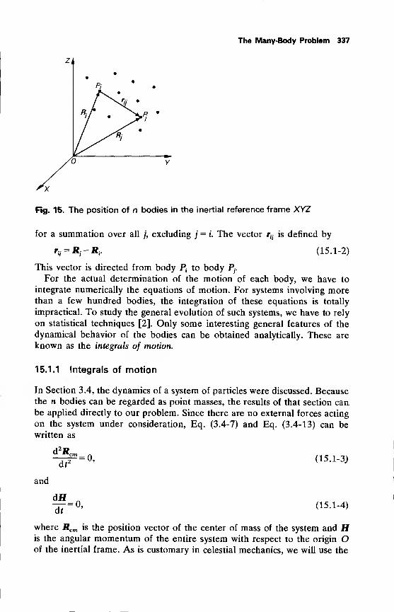
The Many-Body Problem 337
Fig. 15. The position of n bodies in the inertial reference frame XYZ
for a summation over all ;', excluding / = i. The vector r^ is defined by
r^Rj-Rt. (15.1-2)
This vector is directed from body Ptto body P
;.
For the actual determination of the motion of each body, we have to
integrate numerically the equations of motion. For systems involving morethan a few hundred bodies, the integration of these equations is totally
impractical. To study the general evolution of such systems, we have to rely
on statistical techniques [2]. Only some interesting general features of the
dynamical behavior of the bodies can be obtained analytically. These are
known as the integrals of motion.
15.1.1 Integrals of motion
In Section 3.4, the dynamics of a system of particles were discussed. Becausethe n bodies can be regarded as point masses, the results of that section can.
be applied directly to our problem. Since there are no external forces acting
on the system under consideration, Eq. (3.4-7) and Eq. (3.4-13) can bewritten as
d2Rc
dt2
= 0,
and
(15.1-3J
(15.1-4)
where Rcm is the position vector of the center of mass of the system and His the angular momentum of the entire system with respect to the origin Oof the inertial frame. As is customary in celestial mechanics, we will use the
338 Rocket Propulsion & Spaceflight Dynamics
symbol H instead of B used in Section 3.4.1 to denote the angularmomentum. Integration of Eqs. (15.1-3) and (15.1-4) yields
dRcmd ,
=* (15.1-5)
Rcm = at + b, (15.1-6)
and
H=c, (15.1-7)
where a, b and c are arbitrary constant vectors.
The Eqs. (15.1-5) and (15.1-6) state that the center of mass of the system,
often referred to as the barycenter, is at rest or moves with uniform velocity
relative to the inertial frame. According to the discussion in Section 3.1 oninertial frames, we may conclude that a non-rotating reference frame with
its origin at the center of mass of the system is an inertial reference frametoo. If we consider, for example, our solar system as a n-body system with
no external forces acting upon it, Eq. (15.1-1) describes the motion of the
Sun, the planets and other celestial bodies relative to an inertial frame with
its origin at the center of mass of the solar system. Due to the very large
solar mass compared to all other masses in the solar system (Section 2.2.1),
the barycenter lies very close to the center of the Sun. Depending on the
positions of the planets relative to the Sun, the distance between the center
of mass of the solar system and the center of the Sun is always less than onehundredth of the distance between Earth and Sun.
Equation (15.1-7) states that the total angular momentum of the system is
constant in magnitude and direction. As we consider bodies with finite
dimensions, the total angular momentum of the system includes the proper
angular momentum of the bodies due to their rotation. However, we have
assumed that the mass density distribution of each body is spherically
symmetrical, and so there will be no variations in the rotational velocity of
each body due to the gravitational interactions between the bodies. Conse-quently, the orbital angular momentum of a system of finite bodies is
constant too. The plane through the center of mass of the system normal to
H has a fixed orientation and is therefore called the invariable plane (of
Laplace). It can be used as a fundamental reference plane for the motion of
the bodies. For the solar system, this plane is inclined at about 1°39' to the
ecliptic and lies between the orbital planes of the giant planets Jupiter andSaturn.
Returning to Eq. (15.1-1), we note that by introducing a scalar function
Ui, defined as
l/i= -GX*3 +LT
io,(15.1-8)
The Many-Body Problem 339
where Uio
is a constant, Eq. (15.1-1) can be written in the form
d2JJ,
df2= -ViUh (15.1-9)
where V4denotes the gradient with respect to the coordinates of body P
t.
From Section 3.5 we know that l/{then is the potential of the force field
governing the motion of body Pt. By convention, the value of this potential
equals zero at infinity, which implies: Uio= 0. From inspection of Eq.
(15.1-8) it will be clear that the force field represented by this potential is
not central. We also note that t/; is a function of both the coordinates of P;
and the coordinates of all other bodies Pt. Even when keeping body Pj fixed
relative to the frame XYZ, the potential energy of body P, will change dueto the motion of the bodies P
y. A force field with such a time-varying
potential is not conservative, and the sum of kinetic and potential energy of
Pi will vary with time. For the entire system of n bodies, however, an energyintegral can be found as will be shown.
dJJScalar multiplication of Eq. (15.1-1) with —J and summation over all i
gives
Now
H rl'" d( H rl
r« dr H r%
r« di"'
(15 ' 1 - 11)
or
1 V V* mim
idR
i VV* d / ! \
By substituting Eq. (15.1-12) into Eq. (15.1-10), we obtain
d^
dt
As the velocity, Vt ,of P
trelative to the XYZ-frame is defined by
XTdR
iV'
=77> (15.1-14)
Equation (15.1-13) can be integrated to
llmiVf-kGH*^^=% (15.1-15)i i 1
rij
where % is a constant. The first term at the left-hand side of Eq. (15.1-15) is
340 Rocket Propulsion & Spaceflight Dynamics
the kinetic energy, %k, of the system. The second term (including the minussign), which represents the internal gravitational energy of the system, is
called the potential energy, %p, of the system. Thus, while for each individual
body the sum of kinetic and potential energy is not constant, due to a
continuous exchange of energy between the bodies, the total energy, %,
remains constant.
From Eq. (15.1-15) we conclude that if in a system of n bodies, two
bodies approach each other very close, the velocity of at least one of the n
bodies must become very large. Actual collisions should, for 'real' point
masses always be accompanied with infinitely large velocities.
The Eqs. (15.1-5), (15.1-6), (15.1-7) and (15.1-15), which can be written
as ten scalar equations, constitute the so-called ten integrals of motion of the
n-body problem. These ten integrals are very useful for the physical insight
into the dynamical behavior of a system of n bodies. In classical celestial
mechanics they can also be used to check the numerical accuracy of
integration procedures. For the motion of space vehicles, this last applica-
tion is of no importance. Due to the very small mass of a spacecraft
compared to the mass of celestial bodies, and because in numerical compu-
tations we always have a limited number of significant figures, large errors in
the vehicle's trajectory computation will hardly be noticeable in the values
of the total angular momentum and the total energy of the system.
Bruns [3] and Poincare [4] proved that the ten integrals are the only
independent algebraic integrals that can be found in the n-body problem.
The complete solution of the 3n second-order differential equations describ-
ing the motion of the n bodies requires 6n integration constants. With the
ten integrals of motion, it is possible to reduce the order of the problem to
6n- 10. Jacobi [5] showed that a further reduction by two is possible in the
three-body problem; first, by eliminating the time and by taking one of the
other variables as the independent one, and secondly by selecting a particu-
lar reference frame. The second step is known as the elimination of the
nodes. Such a reduction may also be performed in case of the n-body
problem [6]. The practical significance, however, of a reduction from 6n-10 to 6n-12 is questionable, because of the very complex analytical
expressions involved.
15.1.2 The Virial theorem
The tenth integral of motion states that the total energy, %, of the system is
constant. Some interesting remarks can be made on the value of %. Consider
the motion of the n bodies with respect to an inertial reference frame XYZwith its origin at the barycenter. The polar moment of inertia, I, of this
system is defined as
I^lmft-Rt. (15.1-16)
The Many-Body Problem 341
Differentiating this equation with respect to time, we obtain
ft
= 2l miRr^, <15.1-17a)
0=2£ m,V, • V,+2 I m,*, -^. (15.1-17b)
Substituting Eq. (15.1-1) into Eq. (15.1-17b) gives
^=2 I miVf+2Gll*^ R, • n, (15.1-18)
Analogous to the derivation of Eq. (15.1-12), it can be shown easily that
2H*^Rt.,, = -££*«. (15.1-19)
i j ***/ i j 'ij
Substituting Eq. (15.1-19) into Eq. (15.1-18), and using the definitions of %k
and %v , we find
d2!
dt
or, with Eq. (15.1-15),
d2!
df
— = 42fc+ 22
p(15.1-20a)
T3 = 4«-2«p . (15.1-20b)
The Eqs. (15.1-20) are known as the Lagrange-Jacobi identity. It should be
remembered that %p, though a function of time, is negative definite. So, if %d2I
is positive, Eq. (15.1-20b) shows that then —-5 is always positive, and
ultimately I will increase indefinitely with time. This means that the distance
from the origin of at least one body ultimately approaches infinity. We then
say that such a body escapes from the system. Consequently, for a stable
system of n bodies, i.e. a system where all bodies remain in a restricted
volume around the center of mass, % must be negative. Of course, this is
only a necessary condition and by no means a sufficient one for the stability
of the system.
The Lagrange-Jacobi identity is the basis for many qualitative methods in
the many-body problem. For instance, it can be used to prove that it is
impossible for all bodies to collide simultaneously after an infinite time, andthat a simultaneous collision of all bodies implies that the total angular
momentum of the system is zero [7]. We will discuss only one example of
these interesting qualitative results.
d2/
For the relation between the average values of —5, %vand %k over a
342 Rocket Propulsion & Spaceflight Dynamics
certain time interval Af=f1 -f , Eq. (15.1-20a) gives
1 f'd2/ 4 f'i J 2 j"*
J
Ar J, dr2
A* Jf0 A* Jt0
p
or, with Eq. (15.1-17a),
1
At= 2£k + gD ,
(15.1-21)
where §k and <£p stand for the time-averaged values of <£k and %p,
respectively. For a stable system where both the distance of a body from the
center of mass and the velocity of that body are bounded, the left-hand side
of Eq. (15.1-21) will tend to zero if the time interval is taken sufficiently
large. We then have
2ik + ip= 0, Af-»«>. (15.1-22)
Because the total energy of the system is constant, we also have
fk + fp= «. (15.1-23)
From Eq. (15.1-22) and Eq. (15.1-23) the following relation for a stable
system can be obtained:
ik= _£fp = _g. (15.1-24)
This relation, which was first found by Clausius in his studies on the kinetic
theory of gases [8], is known as the Virial theorem or Clausius' theorem. It
states that for a n-body system which is bounded in size and velocity, the
value of the kinetic energy averaged over a large time interval equals minus
half the time-averaged value of the potential energy of the entire system.
The time-averaged value of the kinetic energy also equals minus the total
energy. This Virial theorem is of great importance in stellar dynamics and
forms a basis for statistical calculations on stellar clusters [9] and clusters of
galaxies. For example, it provides the only current estimate of the mass of
clusters of galaxies.
15.2 The circular restricted three-body problem
The three-body problem deals with the motion of three bodies under their
mutual gravitational attractions, while no other forces are acting upon these
bodies. In the restricted three-body problem [10], we assume one body to
have a very small mass as compared to the masses of the other two bodies.
Then the approximation can be made that the motion of the two massive
bodies will not be influenced by the attraction of the third body. We will
denote the two massive bodies with Px and P2 , where Px has the largest
mass.
Consider an inertial frame XYZ with its origin at the center of mass of
the system (Fig. 15.2). This center of mass will, as a consequence of our
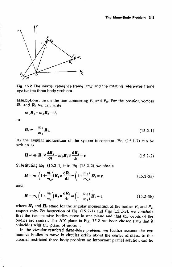
The Many-Body Problem 343
Fig. 15.2 The inertial reference frame XYZ and the rotating references framexyz for the three-body problem
assumptions, lie on the line connecting Px and P2 . For the position vectors
R t and R2 we can write
m 1R 1 + m2R2= 0,
or
JRi — R2 . (15.2-1)
As the angular momentum of the system is constant, Eq. (15.1-7) can bewritten as
„ _ dJJ x „ &R2H = m 1R 1x—-i+ m2R2 x—- = c.
dt dt
Substituting Eq. (15.2-1) into Eq. (15.2-2), we obtain
\ m2 J dt \ m2J
and
\ rriiJ dt \ mj
(15.2-2)
(15.2-3a)
(15.2-3b)
where Hx and H2 stand for the angular momentum of the bodies Px and P2 ,
respectively. By inspection of Eq. (15.2-1) and Eqs. (15.2-3), we concludethat the two massive bodies move in one plane and that the orbits of thebodies are similar. The XY-plane in Fig. 15.2 has been chosen such that it
coincides with the plane of motion.
In the circular restricted three-body problem, we further assume the twomassive bodies to move in circular orbits about the center of mass. In this
circular restricted three-body problem an important partial solution can be
344 Rocket Propulsion & Spaceflight Dynamics
found. Therefore, we introduce a reference frame xyz with its origin at the
center of mass of the system and with the x-axis coinciding with the line
joining Px and P2 ; the positive z-axis is directed along the positive Z-axis
(Fig. 15.2). The xyz -frame thus rotates relative to the XYZ-frame with a
constant angular velocity, ft, about the Z-axis. The bodies P1 and P2 are
fixed relative to the xyz -frame. If r is the position vector of the third body Pin the rotating frame, and the radius vectors from P1 and P2 to P are
denoted by rt and r2 , respectively, the equation of motion of P relative to
the rotating frame is, according to Eq. (3.3-10),
-G^r1-G^r2 =^xr+nx(nxr) + 2n X^+fi
r, (15.2-4)
Ty r2 at ot ot
where — indicates the time-derivative in the rotating frame. Because ft is aot
constant vector, Eq. (15.2-4) simplifies to
-^2 =-G^r1 +-^r2j-ftx(ftxr)-2ftx-. (15.2-5)
The second and third term on the right-hand side of this equation represent
the centripetal and Coriolis acceleration due to the rotation of the reference
frame xyz. It can be proved that the first two terms on the right-hand side of
Eq. (15.2-5) can be written as the gradient of a potential function, U, defined
as
l/=-G(^+^Vkl2
z(x2 + y
2). (15.2-6)
This potential function not only accounts for the gravitational forces but also
for the centripetal force. The introduction of this potential function is
possible because R t , R2 and ft are constant vectors in the xyz-frame, and
H = azez . (15.2-7)
It will be evident that the Coriolis acceleration term in Eq. (15.2-5) cannot
be incorporated into a potential function, because it contains the velocity of
the third body.
Using the potential function, Eq. (15.2-5) can be written in the form
^=-VU-2ftx^\ (15.2-8)8t
2St
15.2.1 Jacobi's integral
8rScalar multiplication of Eq. (15.2-8) with — gives
ot
*.£ *Vl,-2£.(nx!\ (15.2-9)8t 8t
28t 8t \ 8t)
The Many-Body Problem 345
Now
8r /«, 8r\ n 8r 8r\ A— • ftx^r )=0* hrx-r =0,St \ 8t \8t 8t
and©
5r rr/_^dx dUdy dUdz_dU
8t dx dt dy dt dz dt dt'
because U is only a function of the coordinates x, y, z of body P and not
explicitly of the time. Substitution of these relations into Eq. (15.2-9) yields
after integration
V2 +2U = -C, (15.2-10)
where V is the velocity of P relative to the rotating reference frame xyz and
C is a constant of integration. For reasons that will appear later the minus
sign is used. Equation (15.2-10) is known as JacobVs integral.
This integral, of course, can also be expressed in terms of the coordinates
and velocity components of P in the inertial frame XYZ. The velocity V of
P relative to the rotating frame is related to the velocity Va of P relative to
the inertial frame by
V=Va -nxr.
Because the origins of both reference frames coincide, we find with Eq.
(15.2-7) for the magnitude of V
V2 = Vl-2nz(x^-Y^J+a 2z(x
2 + y2). (15.2-11)
Substituting Eqs. (15.2-6) and (15.2-11) into Eq. (15.2-10), we obtain
iv- G(^^)-az(xf-.f)=-|c
The first two terms represent the total energy of P, per unit of mass, relative
to the inertial frame. The third term on the left-hand side is the product of
the constant angular velocity, Oz, and the angular momentum of body P, per
unit of mass, about the Z-axis. In Section 15.1,we found for the motion of n
bodies relative to an inertial frame that the total energy, as well as the
angular momentum of the total system, is constant. Because the bodies Px
and P2 move in circular orbits about the origin of the inertial frame, their
total energy and angular momentum about the Z-axis are constant. Wetherefore may conclude that Eq. (15.2-12), and thus also Eq. (15.2-10), is
nothing but a suitable combination of two general integrals of motion, which
degenerates to this simple form in the circular restricted three-body
problem.
346 Rocket Propulsion & Spaceflight Dynamics
15.2.2 Surfaces of zero velocity
Equation (15.2-10) shows that the velocity, V, of P relative to the rotating
frame is a function of the position of P in this frame. The constant Cdepends on the initial position and velocity of P. The velocity of P equals
zero if
2U = -C, (15.2-13a)
or
2G^+^Ua|(x2 + y2) = C. (15.2-13b)
The surfaces in three-dimensional xyz -space described by these equations
are called surfaces of zero velocity, surfaces of Hill, or in astrophysics [11]
Roche equipotentials. The surfaces are symmetrical with respect to the
xy -plane.
As for every motion V2s= 0, these surfaces form a boundary of the region
where the motion of P can take place. For the region accessible to P the
following relation holds:
2G^+^Ua|(x 2 + y2)^C. (15.2-14)
It should be realized that Eq. (15.2-14) only provides us with information on
the region accessible to body P; it does not tell us anything about the actual
motion of P within this region.
Before examining the geometry of these surfaces for various values of Cwe will non-dimensionalize our expressions, leading to a simplification of the
discussion following. We therefore select as characteristic length the distance
P^P2 between the bodies Pt and P2 , and as characteristic mass the sum of
the masses m, and m2 . We then define
H=—^-, l~n=-^—, h = -^-, etc. (15.2-15a)m 1 + m2 m 1 + m2 P\P2
By requiring /x*s§, P1 will always be the most massive body if m r and m2
are different. For the distances of Px and P2 from the origin, we then find
R t= fi, R2 =l- [x.
A non-dimensional time is introduced by
/G(mi, . , + m2)
lP2)
3 '
Because Px moves in a circular orbit about the origin of the inertial frame:
(P1P2)2
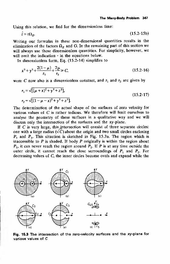
The Many-Body Problem 347
Using this relation, we find for the dimensionless time:
t = taz.(15.2-15b)
Writing our formulas in these non-dimensional quantities results in the
elimination of the factors ftz and G. In the remaining part of this section we
will always use these dimensionless quantities. For simplicity, however, we
will omit the indication - in the equations below.
In dimensionless form, Eq. (15.2-14) simplifies to
2(1 -fi) 2\i.x2 + y
2 +- +-^C,r2
(15.2-16)
were C now also is a dimensionless constant, and rx and r2 are given by
ri = V[(/x + x)2 + y
2 + z2],
r2 = V[(l-|a-x)2 +y 2 + z2].
(15.2-17)
The determination of the actual shape of the surfaces of zero velocity for
various values of C is rather tedious. We therefore will limit ourselves to
analyse the geometry of these surfaces in a qualitative way and we will
discuss only the intersection of the surfaces and the xy-plane.
If C is very large, this intersection will consist of three separate circles:
one with a large radius (Vc) about the origin and two small circles enclosing
P1 and P2 . This situation is sketched in Fig^ 15.3a. The region which is
inaccessible to P is shaded. If body P originally is within the region about
Pu it can never reach the region around P2 . If P is at any time outside the
outer circle, it cannot reach the close surroundings of Px and P2 . For
decreasing values of C, the inner circles become ovals and expand while the
Fig. 15.3 The intersection of the zero-velocity surfaces and the xy-plane for
various values of C
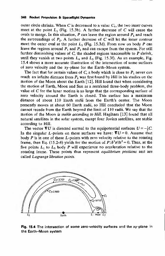
348 Rocket Propulsion & Spaceflight Dynamics
outer circle shrinks. When C is decreased to a value Cx , the two inner curves
meet at the point L x (Fig. 15.3b). A further decrease of C will cause the
ovals to merge. In this situation, P can leave the region around P1 and reach
the surroundings of P2 . A further decrease of C will let the inner contour
meet the outer oval at the point L2 (Fig. 15.3d). From now on body P can
leave the regions around Px and P2 and can escape from the system. For still
further diminishing values of C, the shaded regions inaccessible to P shrink,
until they vanish at two points L4 and L5 (Fig. 15.3f). As an example, Fig.
15.4 shows a more accurate illustration of the intersection of some surfaces
of zero velocity and the xy-plane for the Earth-Moon system.
The fact that for certain values of C, a body which is close to Px never can
reach an infinite distance from Px was first found by Hill in his studies on the
motion of the Moon about the Earth [12]. Hill found that when considering
the motion of Earth, Moon and Sun as a restricted three-body problem, the
value of C for the lunar motion is so large that the corresponding surface of
zero velocity around the Earth is closed. This surface has a maximumdistance of about 110 Earth radii from the Earth's center. The Moonpresently moves at about 60 Earth radii, so Hill concluded that the Mooncannot recede from the Earth beyond the limit of 110 radii. We say that the
motion of the Moon is stable according to Hill. Hagihara [13] found that all
natural satellites in the solar system, except four Jovian satellites, are stable
according to Hill.
The vector Vl/ is directed normal to the equipotential surfaces l/ = -§C.
In the singular L-points on these surfaces we have: Vl/=0. Assume that
body P is in one of these L-points with zero velocity relative to the rotating
frame, then Eq. (15.2-8) yields for the motion of P:8 2r/8t
2 = 0. Thus, at the
five points L x to L5 body P will experience no acceleration relative to the
rotating frame. These points thus represent equilibrium positions and are
called Lagrange libration points.
Earth /-1 Moon /-2
Fig. 15.4 The intersection of some zero-velocity surfaces and the xy-plane in
the Earth-Moon system
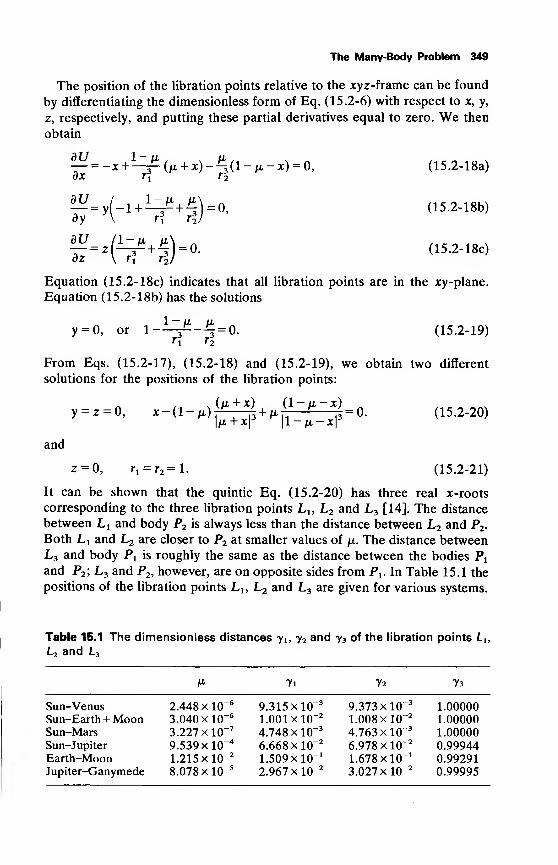
The Many-Body Problem 348
The position of the libration points relative to the xyz-frame can be found
by differentiating the dimensionless form of Eq. (15.2-6) with respect to x, y,
z, respectively, and putting these partial derivatives equal to zero. We then
obtain
dU 1 — ix ix— =-x+
—
J- (lx + x)-—Jl- ix - x) = 0,
ay 'V r\ r\)
dz \ r\ r\)
(15.2-18a)
(15.2-18b)
(15.2-18c)
Equation (15.2-18c) indicates that all libration points are in the xy-plane.
Equation (15.2-18b) has the solutions
y = 0, or 1-^-^-4=0.3 3 (15.2-19)
From Eqs. (15.2-17), (15.2-18) and (15.2-19), we obtain two different
solutions for the positions of the libration points:
/.. x (/"- + *) (1~/^ - *) „
l/* + * \\-ix-x\(15.2-20)
and
z = 0, r1 = r2 =l. (15.2-21)
It can be shown that the quintic Eq. (15.2-20) has three real x-roots
corresponding to the three libration points L lt L2 and L3 [14]. The distance
between L t and body P2 is always less than the distance between L2 and P2 .
Both h x and L2 are closer to P2 at smaller values of \x. The distance betweenL3 and body P1 is roughly the same as the distance between the bodies Px
and P2 ; L3 and P2 , however, are on opposite sides from Px . In Table 15.1 the
positions of the libration points Lu L2 and L3 are given for various systems.
Table 15.1 The dimensionless distances yu y2 and y3 of the libration points LuL2 and L3
V 7i 72 73
Sun-Venus 2.448 xlO"69.315 xlO"3
9.373 xlO"31.00000
Sun-Earth + Moon 3.040 xlO"61.001 xlO"2
1.008 xlO"21.00000
Sun-Mars 3.227 xlO"74.748 x 10"3
4.763 xlO"31.00000
Sun-Jupiter 9.539 xlO"46.668 xlO"2
6.978 xlO"20.99944
Earth-Moon 1.215 xlO-2
1.509 xlO" 11.678 xlO" 1
0.99291Jupiter-Ganymede 8.078 xlO-5
2.967 xlO"23.027 xlO"2
0.99995
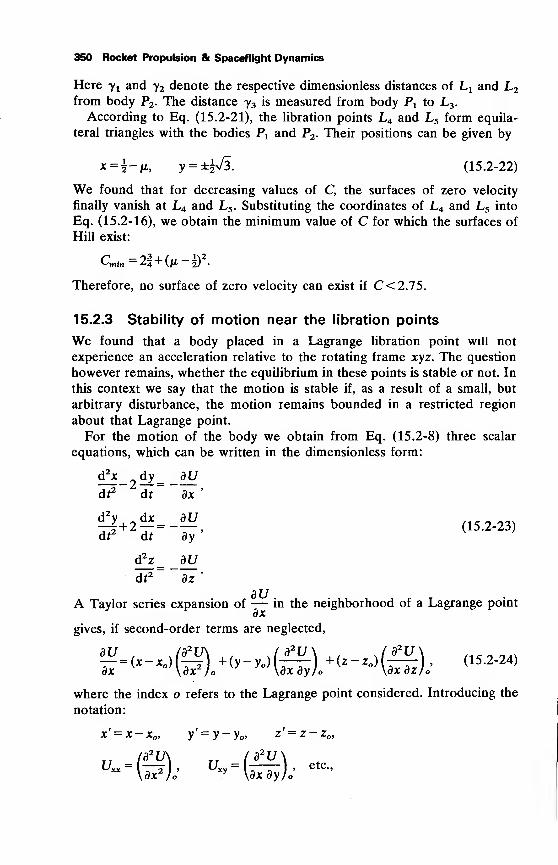
350 Rocket Propulsion & Spaceflight Dynamics
Here yt and y2 denote the respective dimensionless distances of Lj and L2
from body P2 . The distance y3 is measured from body Px to L3 .
According to Eq. (15.2-21), the libration points L4 and L5 form equila-
teral triangles with the bodies P2 and P2 . Their positions can be given by
x = i-/n, y = ±|V3. (15.2-22)
We found that for decreasing values of C, the surfaces of zero velocity
finally vanish at L4 and L5 . Substituting the coordinates of L4 and L5 into
Eq. (15.2-16), we obtain the minimum value of C for which the surfaces of
Hill exist:
(-min= 24 + (^.
_2) •
Therefore, no surface of zero velocity can exist if C<2.75.
15.2.3 Stability of motion near the libration points
We found that a body placed in a Lagrange libration point will not
experience an acceleration relative to the rotating frame xyz. The question
however remains, whether the equilibrium in these points is stable or not. In
this context we say that the motion is stable if, as a result of a small, but
arbitrary disturbance, the motion remains bounded in a restricted region
about that Lagrange point.
For the motion of the body we obtain from Eq. (15.2-8) three scalar
equations, which can be written in the dimensionless form:
d^x dy = _at/
dr2
dt~
dx'
^1+2^=-^, (15.2-23)d2y dx dU—-+2— =
df2
dr ay
d^z = _audf
2 dz'
dUA Taylor series expansion of— in the neighborhood of a Lagrange point
dx
gives, if second-order terms are neglected,
where the index o refers to the Lagrange point considered. Introducing the
notation:
x' = x-x ,y' = y-y , z' = z-z ,
u"=&; ^ =©» etc"
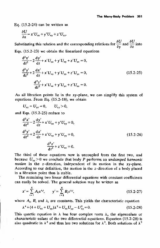
— =x'[/xx + y'LTxy + z'Lrx
The Many-Body Problem 351
Eq. (15.2-24) can be written as
dUdX
dU BUSubstituting this relation and the corresponding relations for— and— into
Eqs. (15.2-23) we obtain the linearized equations
dV dy'-^--2-^ + x'Uxx + y'Uxy + z'Uxz =0,
d2 y' „dx'+ 2— + x'Uxy + y'U
yy+ z'Uyz =0, (15.2-25)
^r+x'Uxz + y'Uyz + z'Uzz = 0.
As all libration points lie in the xy -plane, we can simplify this system of
equations. From Eq. (15.2-18), we obtain
Uxz = Uyz = 0, Uzz >0,
and Eqs. (15.2-25) reduce to
dV dy'—-2^ + x>uxx + yuxy = o,
d2y' dx'+ 2— + x'Uxy + y'U
yy= 0, (15.2-26)
+ z'£/ =0.
dt2
dtxy J yy
d2z'
dt2
The third of these equations now is uncoupled from the first two, andbecause Uzz > we conclude that body P performs an undamped harmonic
motion in the z-direction, independent of its motion in the xy-plane.
According to our definition, the motion in the z-direction of a body placed
in a libration point thus is stable.
The remaining two linear differential equations with constant coefficients
can easily be solved. The general solution may be written as
4 4
jc' = £ AteK
'1
,y' = £ B,eA'', (15,2-27)
i=l i=l
where AiyB
tand A
;are constants. This yields the characteristic equation
A4 + (4+ Uxx + Uyy)\
2 + UxxUyy- U2
xy = 0. (15.2-28)
This quartic equation in A has four complex roots A{,
the eigenvalues or
characteristic values of the two differential equations. Equation (15.2-28) is
also quadratic in A 2 and thus has two solutions for A2
. Both solutions of A2
352 Rocket Propulsion & Spaceflight Dynamics
give two eigenvalues which are equal in magnitude but opposite in sign. In
general, the motion is stable only if all A; are different and if the real part of
all Aj is less than or equal to zero. Because in our problem the eigenvalues
have two-by-two opposite signs, the motion can only be stable if all A; are
different and imaginary. Then the two values of A2are real, unequal and
negative.
We first consider the collinear Lagrange points L l5 L2 and L3 . Evaluating
the partial derivatives of U at these points and substituting these values into
Eq. (15.2-28), we obtain
A4 + (2 - K)A 2 + (1 + 2K)(1 - K) = 0,
where
n n
The two roots for A2 can only be negative if 1-K>0. However, the second
one of the Eqs. (15.2-20) can also be written in the form
—^(H)'By inspection of Fig. 15.3, and remembering our discussion on the location
of the points Ll5 L2 and L3 , it will be clear that for these points the
combination of x, rx and r2 is such that for each point: 1-K<0. Conse-
quently, the straight line solutions represent unstable equilibrium positions.
Next consider the equilibrium points L4 and L5 . Evaluating the partial
derivatives of U at these points and inserting them into Eq. (15.2-28), weobtain
A4 + A
2+ffi(l-fi) = 0.
The two roots for A 2are different and negative if
l-27fjL(l-ix)>0.
As by definition «£ /u, *£ \, the condition for stability is
^<§->/S 5S5 0.0385.
So, for ix < 0.03,85 the motion of a body placed in the libration points L4 or
L5 is stable. It should be realized, however, that we only have proved that
this motion is infinitesimally stable, as the conclusion was reached on the
basis of a linearized Taylor series expansion. A more detailed analysis [15]
will therefore require the inclusion of non-linear terms in the series expan-
sion of the derivatives of the potential function, while also the influence of
the perturbing force from a fourth body could be taken into account [16].
In the general case of the restricted three-body problem, the bodies Px
and P2 describe elliptic orbits about the center of mass of the system. Then,
The Many-Body Problem 353
the distance between Px and P2 , as well as the angular velocity of the line
connecting Px and P2 , varies. This implies that the potential function Udepends explicitly on time, so that no Jacobi integral exists for this
problem. In this elliptical restricted three-body problem the motion of a body
in the points L4 and L5 can be infinitesimally stable too, depending on the
values of jx and the eccentricity of the elliptic orbits [17, 18].
The Lagrange equilibrium positions in the three-body problem are not of
pure academic interest, but are physical realities in our solar system. Animpressive example of stable L4 and L5 positions is the presence of more
than a dozen large asteroids, called the Trojans, oscillating about the L4 and
L5 points with respect to Sun and Jupiter. In the Earth-Moon system, the L4
and L5 points also represent a stable equilibrium. These points are probably
occupied by particles, which manifest themselves as a very faint nebula only
visible under the best seeing conditions.
For a long time it was thought that the faint glow at the night sky, knownas the Gegenschein or counter glow, was produced by sunlight reflection on
material, temporarily trapped in the (unstable) L2 position of the Sun-Earth
system. Recent research [19], however, indicates that this glow is due to the
reflection of sunlight by interplanetary dust at much larger distances from
the Sun.
15.2.4 Applications to spaceflight
Jacobi's integral and the surfaces of zero velocity are very useful for a
general discussion on the trajectory of a spacecraft within the Earth-Moonspace, a so-called lunar flight [20]. For this, we neglect the solar gravita-
tional attraction and assume the orbit of the Moon about the Earth to be a
circle. The trajectory of the spacecraft then becomes a circular restricted
three-body problem where Earth and Moon represent the massive bodies.
The lunar flight starts at the Earth's surface or in a parking orbit about the
Earth. The spacecraft is accelerated by rocket engines and is injected into its
trans-lunar trajectory. The position and velocity of the vehicle relative to the
rotating xyz-frame just after shut-down of the rocket motor determine the
value of the constant C corresponding with the trajectory of the spacecraft.
This value of C can easily be calculated from Eq. (15.2-10). In order to
reach the Moon, this C-value must be less than C1} being the C-value for
which the surface of zero velocity passes through the Li-point in the
Earth-Moon system. This value of C thus dictates the minimum impulse
delivered by the rocket engines, necessary to reach the Moon. If the C-value
of the trajectory is still higher than C2 , the spacecraft can reach the vicinity
of the Moon, but still cannot escape from the Earth-Moon system. Jacobi's
integral gives no information on the actual trajectory that will be flown by
the spacecraft; many trajectories satisfy the same C-value. We therefore
have to select the initial conditions such that a suitable lunar trajectory
results. When the spacecraft arrives in the vicinity of the Moon, again rocket
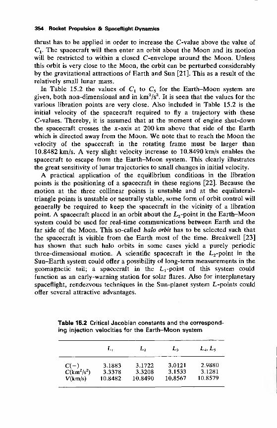
354 Rocket Propulsion & Spaceflight Dynamics
thrust has to be applied in order to increase the C-value above the value of
Ct . The spacecraft will then enter an orbit about the Moon and its motion
will be restricted to within a closed C-envelope around the Moon. Unless
this orbit is very close to the Moon, the orbit can be perturbed considerably
by the gravitational attractions of Earth and Sun [21]. This as a result of the
relatively small lunar mass.
In Table 15.2 the values of Cx to C5 for the Earth-Moon system are
given, both non-dimensional and in km2/s2
. It is seen that the values for the
various libration points are very close. Also included in Table 15.2 is the
initial velocity of the spacecraft required to fly a trajectory with these
C-values. Thereby, it is assumed that at the moment of engine shut-down
the spacecraft crosses the x-axis at 200 km above that side of the Earth
which is directed away from the Moon. We note that to reach the Moon the
velocity of the spacecraft in the rotating frame must be larger than
10.8482 km/s. A very slight velocity increase to 10.8490 km/s enables the
spacecraft to escape from the Earth-Moon system. This clearly illustrates
the great sensitivity of lunar trajectories to small changes in initial velocity.
A practical application of the equilibrium conditions in the libration
points is the positioning of a spacecraft in these regions [22]. Because the
motion at the three collinear points is unstable and at the equilateral-
triangle points is unstable or neutrally stable, some form of orbit control will
generally be required to keep the spacecraft in the vicinity of a libration
point. A spacecraft placed in an orbit about the L2-point in the Earth-Moon
system could be used for real-time communications between Earth and the
far side of the Moon. This so-called halo orbit has to be selected such that
the spacecraft is visible from the Earth most of the time. Breakwell [23]
has shown that such halo orbits in some cases yield a purely periodic
three-dimensional motion. A scientific spacecraft in the L2-point in the
Sun-Earth system could offer a possibility of long-term measurements in the
geomagnetic tail; a spacecraft in the Lx-point of this system could
function as an early-warning station for solar flares. Also for interplanetary
spaceflight, rendezvous techniques in the Sun-planet system L-points could
offer several attractive advantages.
Table 15.2 Critical Jacobian constants and the correspond-
ing injection velocities for the Earth-Moon system
Lj L2 L3 L4 , L5
C(-) 3.1883 3.1722
C(km2/s
2) 3.3378 3.3208
V(km/s) 10.8482 10.8490
3.0121 2.9880
3.1533 3.1281
10.8567 10.8579
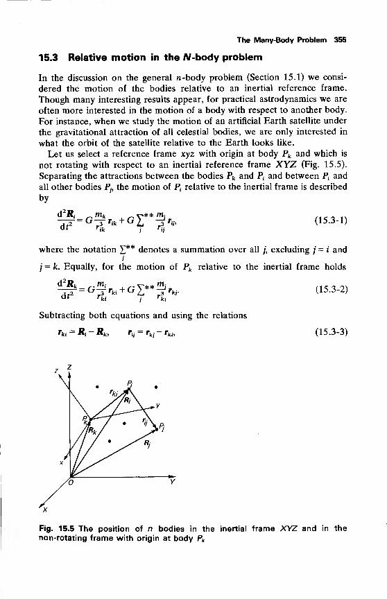
The Many-Body Problem 355
15.3 Relative motion in the A/-body problem
In the discussion on the general w-body problem (Section 15.1) we consi-
dered the motion of the bodies relative to an inertial reference frame.
Though many interesting results appear, for practical astrodynamics we are
often more interested in the motion of a body with respect to another body.
For instance, when we study the motion of an artificial Earth satellite under
the gravitational attraction of all celestial bodies, we are only interested in
what the orbit of the satellite relative to the Earth looks like.
Let us select a reference frame xyz with origin at body Pk and which is
not rotating with respect to an inertial reference frame XYZ (Fig. 15.5).
Separating the attractions between the bodies Pk and Ptand between P
tand
all other bodies P;, the motion of P
xrelative to the inertial frame is described
by
d2Ri n mk
r3
'ik•ik+ G^** m,-
(15.3-1)
where the notation £** denotes a summation over all /, excluding / = i andi
j = k. Equally, for the motion of Pk relative to the inertial frame holds
d2Ufc_m
£ , ^ v-** rrij
Uf rki jrkj
Subtracting both equations and using the relations
rki ~ "i "icj fa ~ Tki T\kb
(15.3-2)
(15.3-3)
Fig. 15.5 The position of n bodies in the inertial frame XYZ and in the
non-rotating frame with origin at body Pk
356 Rocket Propulsion & Spaceflight Dynamics
we obtain
d2rw „rnk + mi
dr2= -G -3
—
'ki + GL m/M73 -3)-
'ki j \ 'ij 'kjl
When we measure the position of P4and the bodies Pj relative to the
non-rotating frame xyz with origin at Pk, the index k in the position vectors
and distances can be omitted, and the motion of Ptrelative to this frame is
given by
i?+G^r ri=Gl mi
\T~7f)(15 -3-4)
We note that the influence of the bodies Pj on the motion of Ptabout Pk is
expressed by the right-hand side of Eq. (15.3-4). The first term in brackets
represents the acceleration of Ptdue to the attractions of all bodies Pj. The
second term in brackets is the negative of the acceleration of Pk, the origin
of our reference frame, due to the attraction by the bodies Pj. It is the
difference between these two terms that counts for the influence of the
bodies Pj on the motion of Ptrelative to Pk .
As well for the motion of a planet about the Sun as for the motion of a
satellite about the Earth, the total effect of the bodies Pj can be regarded as
very small when compared to the direct two-body attraction term in Eq.
(15.3-4). The reason for this is entirely different for both types of motion.
Considering the motion of a planet about the Sun, we note that the ratio of
the mass of a disturbing body (a planet) and that of the Sun is small. For that
reason the right-hand side of Eq. (15.3-4) has only little influence. For an
Earth satellite, on the other hand, the distance from the Earth is small as
compared to interplanetary distances and the difference between rtjand r,
takes a very small value. Consequently, in both cases mentioned the effect of
the bodies Ptcan, in a first approximation, be neglected. Then, Eq. (15.3-4)
simplifies to the equation of motion for the two-body problem which, as wewill see in Chapter 16, can be solved analytically.
Introducing a disturbing potential, Rt
:
*,—GrWf-^), < i5 -3-5>
j \'ij 'j I
Eq. (15.3-4) can be written in the form
d2 r, ^mk + mitt +(j—
1
At2
r\z+ G^hPr^-V^, (15.3-6)
where Vtdenotes the gradient with respect to the coordinates of P
{in the
non-inertial frame xyz. Because i?fis not only a function of the coordinates
of Ptbut also of the coordinates of the bodies Pj, the force field described by
the potential Ri is not conservative. The treatment of this disturbing
potential Rt
is the major problem in the general perturbations theory of
celestial mechanics.
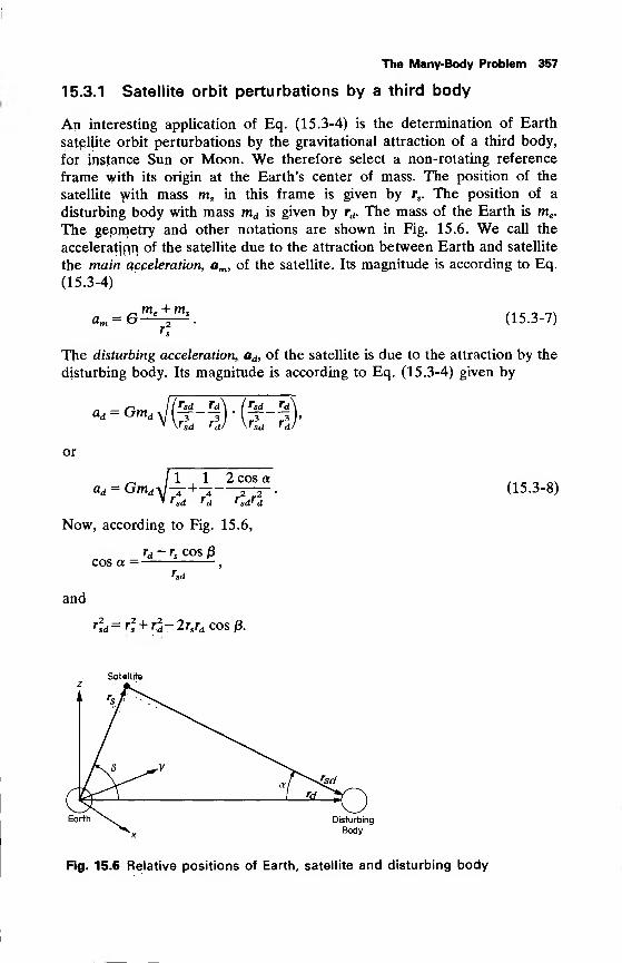
The Many-Body Problem 357
15.3.1 Satellite orbit perturbations by a third body
An interesting application of Eq. (15.3-4) is the determination of Earth
satellite orbit perturbations by the gravitational attraction of a third body,
for instance Sun or Moon. We therefore select a non-rotating reference
frame with its origin at the Earth's center of mass. The position of the
satellite with mass msin this frame is given by rs . The position of a
disturbing body with mass md is given by rd . The mass of the Earth is me .
The gepmetry and other notations are shown in Fig. 15.6. We call the
acceleratjpn of the satellite due to the attraction between Earth and satellite
the main acceleration, am , of the satellite. Its magnitude is according to Eq.
(15.3-4)
am =G^. (15.3-7)' s
The disturbing acceleration, ad, of the satellite is due to the attraction by the
disturbing body. Its magnitude is according to Eq. (15.3-4) given by
\rsd rd' \ rsd Td'
or
_ /l 1 2 cos a .„_- .
GmdJ-r+-i--r-r . (15.3-8)* T <,A 'A T*A'A
ad= _ „ ,rsd rd rsdrd
Now, according to Fig. 15.6,
rd - rs cos /3
cos a =rsd
and
rzsd= rf + ri-2rsrd cos p.
Satellite
Earth ^ Disturbing
Body
Fig. 15.6 Relative positions of Earth, satellite and disturbing body
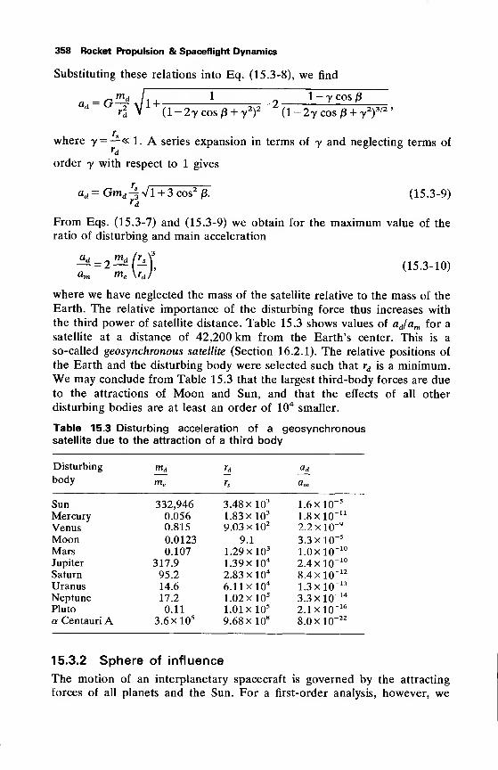
358 Rocket Propulsion & Spaceflight Dynamics
Substituting these relations into Eq. (15.3-8), we find
jnd L^ 1 „ 1-ycosjSa<i = G^\l+—- —--r-2
r2d V (l-2ycos/3 + y
2)
2 (l-2y cos j3 + 72)
3/2 '
xwhere y =—« 1. A series expansion in terms of y and neglecting terms of
rd
order y with respect to 1 gives
ad = Gmd4 V 1 + 3 cos2
j3. (15.3-9)rd
From Eqs. (15.3-7) and (15.3-9) we obtain for the maximum value of the
ratio of disturbing and main acceleration
3i =2^ fcf (15.3-10)
where we have neglected the mass of the satellite relative to the mass of the
Earth. The relative importance of the disturbing force thus increases with
the third power of satellite distance. Table 15.3 shows values of ajam for a
satellite at a distance of 42,200 km from the Earth's center. This is a
so-called geosynchronous satellite (Section 16.2.1). The relative positions of
the Earth and the disturbing body were selected such that rd is a minimum.We may conclude from Table 15.3 that the largest third-body forces are dueto the attractions of Moon and Sun, and that the effects of all other
disturbing bodies are at least an order of 104smaller.
Table 15.3 Disturbing acceleration of a geosynchronoussatellite due to the attraction of a third body
Disturbing md rd ad
body me rs &m
Sun 332,946 3.48 xlO31.6 xlO
-5
Mercury 0.056 1.83 xlO31.8 xlO-11
Venus 0.815 9.03 xlO22.2 xlO-9
Moon 0.0123 9.1 3.3 xlO-5
Mars 0.107 1.29 xlO31.0 xlO-10
Jupiter 317.9 1.39 xlO42.4 xlO-10
Saturn 95.2 2.83 xlO48.4 xlO-12
Uranus 14.6 6.11 xlO41.3 xlO-13
Neptune 17.2 1.02 xlO53.3 xlO-14
Pluto 0.11 1.01 xlO52.1 xlO-16
a Centauri A 3.6 X1059.68 xlO8
8.0 xlO-22
15.3.2 Sphere of influence
The motion of an interplanetary spacecraft is governed by the attracting
forces of all planets and the Sun. For a first-order analysis, however, we
The Many-Body Problem 359
often assume that the trajectory can be approximated by accounting only for
three gravitational fields: those of the Earth, the Sun and the target planet
(Chapter 19). We then imagine the trajectory to be composed of three
successive two-body trajectories; in each trajectory the spacecraft is as-
sumed to be attracted by only one celestial body.
We will now discuss a criterion which determines the distance from the
Earth, and from the target planet, where the switch between the successive
two-body trajectories has to be made. It is important to realize that because
of the very intense solar gravitational field, these distances will be small onthe scale of interplanetary distances.
First, we consider the motion of the spacecraft with mass mc relative to a
non-rotating reference frame with its origin at the Earth's center. Weassume that the only disturbing body is the Sun. The masses of Sun andEarth are denoted by ms and me , respectively. From Eqs. (15.3-7) and(15.3-9) we have for the magnitudes of main acceleration, ami , and disturb-
ing acceleration, adl , of the spacecraft, relative to this reference frame,
(15.3-11)
adl= Gms -f VI + 3 cos
2/3,
• es
where rec is the radius vector from the Earth to the spacecraft, and res is the
radius vector from the Earth to the Sun. Again, the mass of the spacecraft is
neglected relative to the mass of the Earth.
If we consider the motion of the spacecraft with respect to a non-rotating
reference frame with its origin at the center of mass of the Sun, and assumethat the Earth is the only disturbing body, the equation of motion for thespacecraft is
dt2'
w„3
('ce 'se \
where the spacecraft's mass is neglected with respect to the mass of the Sun.Relative to this frame, the magnitudes of main acceleration, am2 , anddisturbing acceleration, ad2 , of the spacecraft are
am2- G—,
"r- (15.3-12)
a^ Gmw(t-|)-(S-t)-
A series expansion of ad2 in terms of — yields, for —« 1,
'se 'se
ad2 =G-^. (15.3-13)
360 Rocket Propulsion & Spaceflight Dynamics
When the spacecraft is on a surface around the Earth, described by
^l = -^, (15.3-14)am . a„
we have equal right to approximate the interplanetary trajectory by a
disturbed two-body orbit about the Earth or by a disturbed two-body orbit
about the Sun. Substituting Eqs. (15.3-11), (15.3-12) and (15.3-13) into Eq.
(15.3-14), we obtain the equation of this surface:
\res ) \mj1
(15.3-15)Vl + 3cos2
|3
This surface is rotationally symmetric about the Earth-Sun line. Its shape
differs little from a sphere; the ratio of the largest and smallest value of rec is
about 1.15. For convenience, we therefore approximate this surface by a
sphere with radius equal to the maximum value of rec . This sphere is called
the sphere of influence or the activity sphere of the Earth. Equally, we can
determine for each planet such a sphere of influence. If the radius of this
sphere is denoted by Rsi, and the distance between the planet and the Sun
by rps> we thus find
*--'-gr-(i5 -3- i6)
It will be evident that for a given planet the value of Rsi still varies with the
distance of that planet from the Sun. For example, the radius of the sphere
of influence of the Earth varies between 0.91xl06 km and 0.94xl06 km.
For the other planets corresponding data will be given in Chapter 19.
The concept of a sphere of influence was introduced by Laplace [24] in his
studies on the motion of comets in the immediate neighborhood of the
planet Jupiter. Nowadays, it is widely used for feasibility studies in
interplanetary spaceflight.
References
1 Sundman, K. F. (1907), Recherches sur le probleme des trois corps,
Acta Societas Sci. Fennicae, 34, no. 6, 1-43.
2 Lecar, M. (ed.) (1972), Gravitational N-Body Problem, Reidel, Dor-
drecht.
3 Bruns, H. (1887), Uber die Integrale des Vielkorper-Problemes, Acta
Math., 11, 25-96.
4 Poincare, H. (1890), Sur le probleme des trois corps et les equations de
la dynamique, Acta Math., 13, 1-270.
5 Jacobi, C. G. J. (1843), Sur l'elimination des noeuds dans le probleme
des trois corps, Z. Reine Angew. Math., 26, 115-131.
The Many-Body Problem 361
6 Bennett, T. L. (1905), Messenger of Math., Cambridge, 34, no. 2, 1113.
7 Pollard, H. (1966), Qualitative methods in the N-body problem, in: J.
Barkley Rosser (ed.), Space Mathematics, Part 1, Amer. Math. Soc, p.
269-277.
8 Clausius, R. (1870), On a mechanical theorem applicable to heat,
Philos. Mag. and J. Science, 40, Series 4, 122-127.
9 Chandrasekhar, S. (1942), Principles of Stellar Dynamics, Univ. of
Chicago Press, Chicago. Also Dover, New York, 1960, p. 200.
10 Szebehely, V. (1967), Theory of Orbits, The Restricted Problem of Three
Bodies, Academic Press, New York.
11 Kopal, Z. (1959), Close Binary Systems, Chapman and Hall, London, p.
127, 505.
12 Hill, G. W. (1878), Researches in lunar theory, Amer. J. Math., 1, 129-
147, 245-260.
13 Hagihara, Y. (1952), On the stability of the satellite systems, Proc.
Japan Acad., 28, 182-186.
14 Moulton, F. R. (1914), An Introduction to Celestial Mechanics,
Macmillan, New York, p. 291-293.15 Breakwell, J. V. and Pringle, R. (1966), Resonances affecting motion
near the Earth-Moon equilateral libration points, Progr. Astron. Aeron.,
Vol. 17, Academic Press, New York, p. 55-74.
16 Schechter, H. B. (1968), Three-dimensional nonlinear stability analysis
of the Sun-perturbed Earth-Moon equilateral points, AIAA J., 6, no.
7, 1223-1228.
17 Danby, J. M. A. (1964), Stability of the triangular points in the elliptic
restricted problem of three bodies, Astron. J., 69, no. 2, 165-172.18 Alfriend, K. T. and Rand, R. H. (1969), Stability of the triangular
points in the elliptic restricted problem of three bodies, AIAA J., 7, no.
6, 1024-1028.
19 Hanner, M. S. and Weinberg, J. L. (1973), Gegenschein observations
from Pioneer 10, Sky and Telescope, 45, no. 4, 217-218.
20 Ehricke, K. A. (1962), Space Flight, Vol. 2: Dynamics, Van Nostrand,
Princeton, p. 245-282, 933-957.
21 Schoyer, H. F. R. (1966), Investigation on the Stability of the Orbit of aLunar Satellite (in Dutch), Thesis Delft Univ. of Techn., Dept. Aero-space Eng., Delft.
22 Farquhar, R. W. (1970), The Control and Use of Libration Point
Satellites, NASA TR R-346, Washington.
23 Breakwell, J. V. and Brown, J. V. (1976), The Halo Family of 3-
Dimensional Periodic Orbits in the Restricted 3-Body Problem,
AIAA/AAS Paper 76-825, San Diego.
24 Marquis de Laplace, P. S. (1845), Traite de Mecanique Celeste, Tome 4,
Imprimerie Royale, Paris, p. 241-254.
16 The Two-Body Problem
In Section 15.3 we found that the motion of a satellite about the Earth was
governed primarily by the attraction between Earth and satellite. Even for a
satellite at an altitude of some ten thousands of kilometers, the effects of the
gravitational attraction of Sun, Moon and planets on the satellite's orbit are
very small. If, at a first approximation, we completely neglect these effects,
we deal with a two-body problem.
This two-body approximation also holds for the motion of the planets about
the Sun. In this case, the gravitational perturbations by other planets are even
less important, because of the large distances involved and the relatively small
masses of the planets as compared to the mass of the Sun.
Unlike the many-body problem, the two-body problem can be solved
analytically, and because its solution comes very near to physical reality this
solution constitutes the basic algebra of celestial mechanics. Most of the
refined theories of celestial motion take the two-body model as a point of
departure.
16.1 Equations of motion
Consider the motion of body Ptrelative to a non-rotating reference frame
with its origin at body Pk (Fig. 15.5). We assume that the bodies can be
regarded as point masses and that the only force acting on body P; is due to
their mutual gravitational attraction. Then, the motion of body Pt
is,
according to Eq. (15.3-4), described by
djr = _jx
dr2 r
where
H = G(mlc+ m
i ),(16.1-2)
and r is the position vector of body Pt. The masses of the bodies Pk and P
t
are denoted by mk and m^ respectively, while G is the universal gravita-
tional constant. Comparing Eq. (16.1-1) and Eq. (3.6-2), which describes
the motion of a point mass in an inertial gravitational field (the one-body
problem), we may conclude that both equations of motion only differ in the
definition of ix. In Section 3.6, /x was defined as the product of G and the
mass of the body in which gravitational field the point mass moves; here, ^is defined as the product of G and the sum of the masses of the two bodies.
2= ~^r, (16.1-1)
The Two-Body Problem 363
Consequently, we can directly apply the relations derived for the one-bodyproblem. However, we have to be very careful with the physical interpreta-
tion of the results. For instance, applying Eq. (3.6-8) for the two-bodyproblem, the term -/x/r does not represent the potential energy of body P
t
per unit mass, nor does the constant % denote the total energy of body Pt
per unit mass.
In many cases, however, such as the motion of planets about the Sun or
the motion of satellites about the Earth, we deal with problems wheremk » mt
. Then, we can safely approximate fi by
V = Gmk . (16.1-3)
This approximation is equivalent to the statement that the reference frame
with body Pk as origin is an inertial one and that the actual motion can beapproximated by a one-body problem. When /x is defined according to Eq.
(16.1-3), we call jut the gravitation parameter or the attraction parameterof body Pk . For the Earth it takes the value fi = 398601.3 km3
/s2
.
16.2 General characteristics of motion
From Section 3.6 we know that the motion of body Ptabout body Pk takes
place in a single plane through Pk , the orbital plane, and that the trajectory
in this plane is a conic section with body Pk at a focus. In addition to elliptic
orbits, in which the planets and the Earth satellites move, parabolic andhyperbolic trajectories are also physical realities. In astronomy, we observethat some comets move in these trajectories about the Sun. In spaceflight,
the hyperbolic orbits are essential to interplanetary missions (Chapter 19).
In the following discussion on the motion of body Ph we will omit thoseparts which were already discussed in Section 3.6. For convenience, how-ever, some of the most important relations derived in that section will berepeated.
The trajectory of body Pt
is given by
P H2/n
r = TT~^ * = 7T *» (16.2-1)1 + e cos 6 1 + e cos 8
where 6 is the true anomaly, p is the semi-latus rectum, e is the (numerical)
eccentricity and H is the angular momentum per unit mass. In Fig. 16.1a, the
ratio between distance r and pericenter distance rp
is shown as a function of
for some values of e.
For the velocity, V, in a conic section, Eq. (3.6-34) gives
^KH)- (i6 -2-2>
According to Eq. (3.6-36) and Eq. (3.6-35), the circular and escape velocity
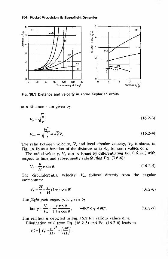
364 Rocket Propulsion & Spaceflight Dynamics
30 60
(a)
e=5
5
"5
a:
o 3o
5:
2
1
(b)
r/i
e=5
05,
2
10.2'—"-SI^0.2
90 120 150 180
True Anomaly 6 (deg)
Fig. 16.1 Distance and velocity in some Keplerian orbits
Distance rjfp
at a distance r are given by
4K
Vesc =yj^y = J2Vc
(16.2-3)
(16.2-4)
The ratio between velocity, V, and local circular velocity, Vc , is shown in
Fig. 16.1b as a function of the distance ratio r/rpfor some values of e.
The radial velocity, Vr,can be found by differentiating Eq. (16.2-1) with
respect to time and subsequently substituting Eq. (3.6-6):
Vr=-^esin0. (16.2-5)
The circumferential velocity, Ve , follows directly from the angular
momentum:
Ve=- = -^{l + ecosd).
r H
The flight path angle, y, is given by
_ Vr _ e sin 6n J ~ Ve
~ 1 + e cos '
-90° *s y^90°.
(16.2-6)
(16.2-7)
This relation is depicted in Fig. 16.2 for various values of e.
Elimination of from Eq. (16.2-5) and Eq. (16.2-6) leads to
2 l.. a\Z
v?+ ve- JLH
fie
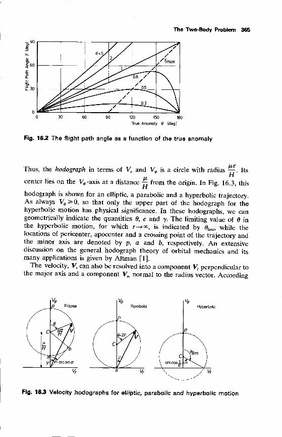
The Two-Body Problem 365
-90
5 60
30
e=5/2/
^s7/
SVmax
v^ /0.8 //
/ OS• /
// -—J>2/
30 60 90 120 150 180
True Anomaly (deg)
Fig. 16.2 The flight path angle as a function of the true anomaly
Thus, the hodograph in terms of Vr and Ve is a circle with radius — . Its
M-H
center lies on the Ve -axis at a distance -£ from the origin. In Fig. 16.3, this
hodograph is shown for an elliptic, a parabolic and a hyperbolic trajectory.As always Ve ^0, so that only the upper part of the hodograph for thehyperbolic motion has physical significance. In these hodographs, we cangeometrically indicate the quantities 6, e and y. The limiting value of 6 inthe hyperbolic motion, for which r^<», is indicated by 6lim , while thelocations of pericenter, apocenter and a crossing point of the trajectory andthe minor axis are denoted by p, a and b, respectively. An extensivediscussion on the general hodograph theory of orbital mechanics and its
many applications is given by Altman [1].
The velocity, V, can also be resolved into a component V, perpendicular tothe major axis and a component Vn normal to the radius vector. According
Hyperbola
Fig. 16.3 Velocity hodographs for elliptic, parabolic and hyperbolic motion
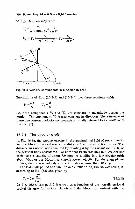
366 Rocket Propulsion & Spaceflight Dynamics
to Fig. 16.4, we may write
V,=Vr V,
V =v„ +
sin (180-0) sin0'
V.
tan (180-0)v.-z^
tan0
Major Axis F Percenter
Fig. 16.4 Velocity components in a Keplerian orbit
Substitution of Eqs. (16.2-5) and (16.2-6) into these relations yields
V-*±l v =JL1
H' nH'
So, both components V, and Vn are constant in magnitude during the
motion. The component V, is also constant in direction. The existence of
these two constant velocity components is usually referred to as Whittaker's
theorem [2].
16.2.1 The circular orbit
In Fig. 16.5a, the circular velocity in the gravitational field of some planets
and the Moon is plotted versus the distance from the attraction center. Thedistance was non-dimensionalized by dividing it by the (mean) radius, R, of
the celestial body considered. We note that Earth satellites in a low circular
orbit have a velocity of about 7.9 km/s. A satellite in a low circular orbit
about Mars or our Moon has a much lower velocity. For the giant planet
Jupiter, the circular velocity at low altitudes is more than 40 km/s.
The (sidereal) period of a satellite in a circular orbit, the circular period, is,
according to Eq. (3.6-38), given by
IPTc =2irJ—. (16.2-8)
V /J,
In Fig. 16.5b, this period is shown as a function of the non-dimensional
orbital distance for various planets and the Moon. In contrast with the
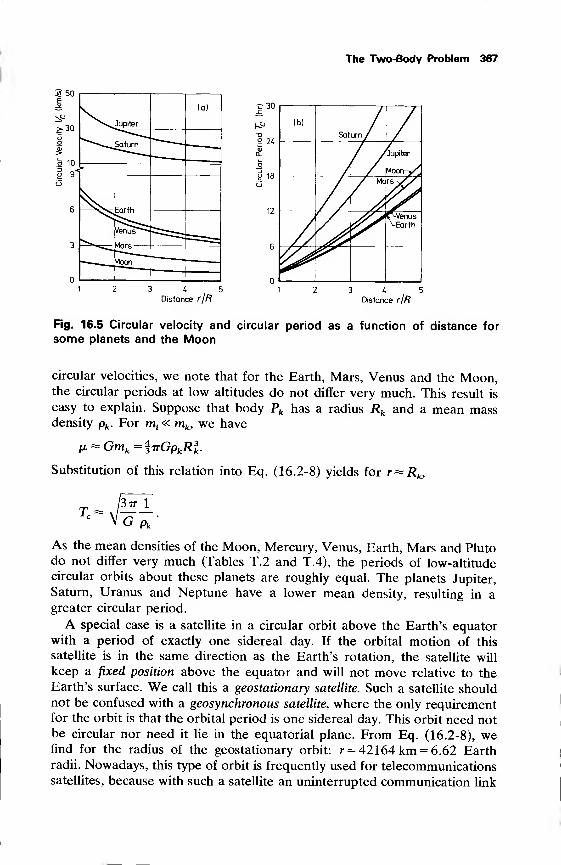
The Two-Body Problem 367
E(a)
£-30oo
3
^v^Jupiter
Saturn
a 10
n 01
o
6
Venus -
3v«^ 1
Moon
n
Distance rJR
~30
° 24
(b)
Saturn /
7/ Jupiter
^loon-j/
/ Wns-y//
ITM/enus
^Earth
3 4 5
Distance rJR
Fig. 16.5 Circular velocity and circular period as a function of distance for
some planets and the Moon
circular velocities, we note that for the Earth, Mars, Venus and the Moon,the circular periods at low altitudes do not differ very much. This result is
easy to explain. Suppose that body Pk has a radius Rk and a mean massdensity pk . For m
f« mk, we have
lx^Gmk =$TrGpkR 3k .
Substitution of this relation into Eq. (16.2-8) yields for r R.
T«W—377J_
As the mean densities of the Moon, Mercury, Venus, Earth, Mars and Plutodo not differ very much (Tables T.2 and T.4), the periods of low-altitude
circular orbits about these planets are roughly equal. The planets Jupiter,
Saturn, Uranus and Neptune have a lower mean density, resulting in agreater circular period.
A special case is a satellite in a circular orbit above the Earth's equatorwith a period of exactly one sidereal day. If the orbital motion of this
satellite is in the same direction as the Earth's rotation, the satellite will
keep a fixed position above the equator and will not move relative to the
Earth's surface. We call this a geostationary satellite. Such a satellite shouldnot be confused with a geosynchronous satellite, where the only requirementfor the orbit is that the orbital period is one sidereal day. This orbit need notbe circular nor need it lie in the equatorial plane. From Eq. (16.2-8), wefind for the radius of the geostationary orbit: r = 42164 km = 6.62 Earthradii. Nowadays, this type of orbit is frequently used for telecommunications
satellites, because with such a satellite an uninterrupted communication link
368 Rocket Propulsion & Spaceflight Dynamics
can be established between ground stations. For certain other types of
applications satellites this orbit is attractive too, since from that altitude a
large part of the Earth can be monitored continuously.
16.2.2 The elliptic orbit
From Eqs. (16.2-2), (16.2-5) to (16.2-7), a number of interesting conclu-
sions, concerning the variation of velocity with position in an elliptic orbit,
can be drawn. Here we will mention only the most important ones:
1. The velocity takes a minimum value at the apocenter:
a\l + ej
where VCa denotes the circular velocity at apocenter. The velocity at
apocenter is always less than the local circular velocity (Fig. 16.1b).
2. The maximum velocity occurs at pericenter:
V^(^)=V?p(l + e), (16.2-10)
a\l-ej
where Vc denotes the circular velocity at pericenter.
The velocity at pericenter is always larger than the local circular velocity
(Fig. 16.1b).
3. The radial velocity is an extremum at the crossing points of the orbit
and the latus rectum:
V'- = ± H= ±V-C' (16 -2_11)
where VCextr
denotes the circular velocity at that point of the orbit.
4. At the crossing points of the orbit and the minor axis, the flight path
angle takes an extreme value (Fig. 16.3):
= arctanVl-e 2 J
(16.2-12)
and the velocity equals in magnitude, but not in direction, the local circular
velocity.
From the expression for the period in an elliptic orbit, Eq. (3.6-38), weobtain after substitution of Eq. (16.1-2),
a 3GrriL. /\ m
rrz A 2 ,1+— • (16.2-13)
Tz4it
z\ mk f
This equation represents an 'improved version' of Kepler's third law as
given in Section 3.6.3. We see that Kepler's third law in its original version
only holds for m^ « mk .
The Two-Body Problem 369
16.2.3 The parabolic orbit
At any point of a parabolic orbit, the velocity is equal to the local escape
velocity as given by Eq. (16.2-4). For parabolic orbits about the Earth, the
velocity at low altitudes equals about 11.2 km/s. For Jupiter, on the otherhand, the escape velocity at low altitude is more than 60 km/s. From Eq.(16.2-7) we obtain, after some trigonometric manipulations, for the flight
path angle in a parabolic orbit:
8tan y = tan -
.
2
As, by definition, -90°^ y*£90°, we find for the variation of y with 0,
O°s=0^18O°: y = -,2
(16.2-14)
18O°<0<36O°: y = --180°.2
The flight path angle thus increases linearly with from y = 0° at pericenterto y = 90° at = 180° (Fig. 16.2).
16.2.4 The hyperbolic orbit
The most important conclusions from Eqs. (16.2-2), (16.2-5) to (16.2-7) fora hyperbolic orbit are:
1. The velocity is a maximum at pericenter:
^=(^)KH> +1 >- < i6 -2- i5 >
2. The velocity takes a minimum value for r —» o°:
V^=~- (16.2-16)
This velocity at infinitely large distance from body Pk is called the hyperbolicexcess velocity.
By substituting Eqs. (16.2-4) and (16.2-16) into Eq. (16.2-2), we obtain
V^VL+VL (16.2-17)
So, at any point in a hyperbolic trajectory, the local velocity can beexpressed in terms of local escape velocity and hyperbolic excess veloc-ity. The dependence of velocity on distance in a hyperbolic orbit about theEarth is depicted in Fig. 16.6 for two values of the eccentricity. It is assumedthat the perigee of both orbits is at 400 km above the Earth's surface. Alsoshown in this figure is a curve representing the local escape velocity. We
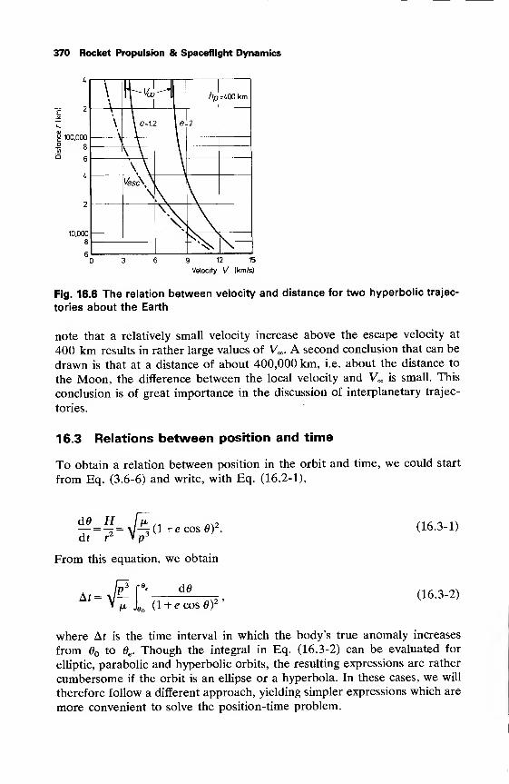
370 Rocket Propulsion & Spaceflight Dynamics
g 100,000
i 8
b 6
10,000
8
6
\ K^HI hp=400 km
\ \ e=l > \e =2
\
\ \\\Ves^ >
\
^\"SN
9 12 15
Velocity V (km/s)
Fig. 16.6 The relation between velocity and distance for two hyperbolic trajec-
tories about the Earth
note that a relatively small velocity increase above the escape velocity at
400 km results in rather large values of V*,. A second conclusion that can be
drawn is that at a distance of about 400,000 km, i.e. about the distance to
the Moon, the difference between the local velocity and V*. is small. This
conclusion is of great importance in the discussion of interplanetary trajec-
tories.
16.3 Relations between position and time
To obtain a relation between position in the orbit and time, we could start
from Eq. (3.6-6) and write, with Eq. (16.2-1),
dt r v p
From this equation, we obtain
d0Af =
(1 + e cos Of
(16.3-1)
(16.3-2)
where At is the time interval in which the body's true anomaly increases
from O to 6e . Though the integral in Eq. (16.3-2) can be evaluated for
elliptic, parabolic and hyperbolic orbits, the resulting expressions are rather
cumbersome if the orbit is an ellipse or a hyperbola. In these cases, we will
therefore follow a different approach, yielding simpler expressions which are
more convenient to solve the position-time problem.
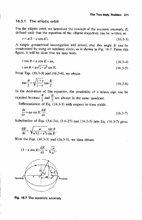
The Two-Body Problem 371
16.3.1 The elliptic orbit
For the elliptic orbit, we introduce the concept of the eccentric anomaly, E,denned such that the equation of the elliptic trajectory can be written as
r = a(l-ecosE). (16.3-3)
A simple geometrical investigation will reveal, that this angle E can beconstructed by using an auxiliary circle, as is shown in Fig. 16.7. From this
figure, it will be clear that we may write
r cos 6 = a cos E - ae,
r sin = aVl-e2sin E.
From Eqs. (16.3-3) and (16.3-4), we obtain
tan6 /!+rvTz
+ e E- tan —
.
e 2
(16.3-4)
(16.3-5)
(16.3-6)
In the derivation of this equation, the possibility of a minus sign can be
rejected because - and — are always in the same quadrant.
Differentiation of Eq. (16.3-3) with respect to time yields
dr d£— = ae smE—
.
dr dr(16.3-7)
Substitution of Eqs. (3.6-24), (3.6-27) and (16.2-5) into Eq. (16.3-7) gives
sindEdr-£ ^
- 3(l-e 2)sinE'
With the Eqs. (16.3-3) and (16.3-5), we then obtain
,* , dE rn(1-ecosE — = J4,
dr Va 3
Fig. 16.7 The eccentric anomaly
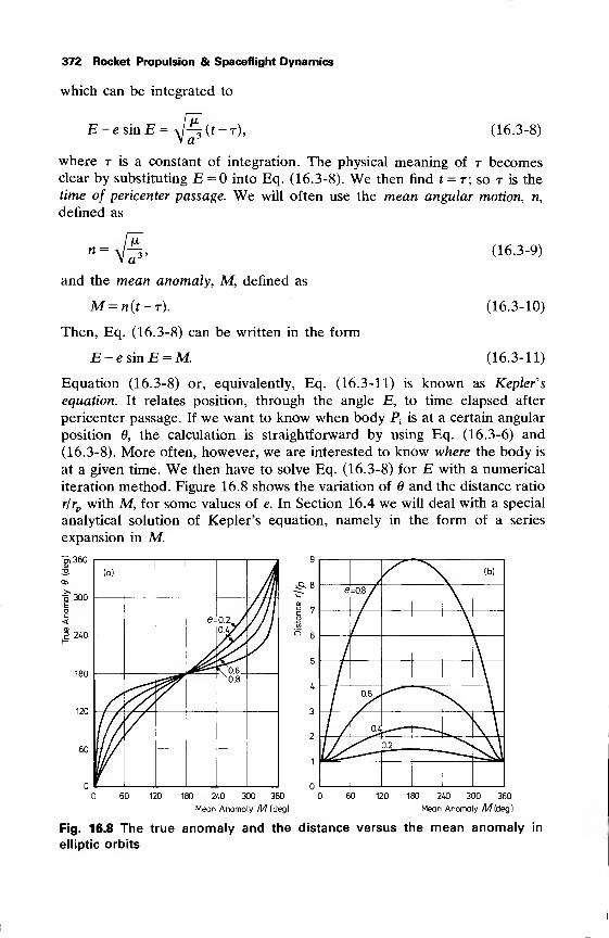
372 Rocket Propulsion & Spaceflight Dynamics
which can be integrated to
E - e sin E = (t-r), (16.3-8)
where t is a constant of integration. The physical meaning of r becomesclear by substituting E - into Eq. (16.3-8). We then find t = r; so t is the
time of pericenter passage. We will often use the mean angular motion, n,
defined as
(16.3-9)n =
and the mean anomaly, M, defined as
M=n(t-r).
Then, Eq. (16.3-8) can be written in the form
E — e sin E = M.
(16.3-10)
(16.3-11)
Equation (16.3-8) or, equivalently, Eq. (16.3-11) is known as Kepler's
equation. It relates position, through the angle E, to time elapsed after
pericenter passage. If we want to know when body Pt
is at a certain angular
position 6, the calculation is straightforward by using Eq. (16.3-6) and
(16.3-8). More often, however, we are interested to know where the body is
at a given time. We then have to solve Eq. (16.3-8) for E with a numerical
iteration method. Figure 16.8 shows the variation of and the distance ratio
r/rp with M, for some values of e. In Section 16.4 we will deal with a special
analytical solution of Kepler's equation, namely in the form of a series
expansion in M.
.360
o 300E
2 240
180
120
60
(q)
9
a>
2 7o"to
b 6
5
U
3
2
1
(b)
e=0.8/
e- o.2^y0.47/
\0.6N0.8
0.6^
0.4
<^ 0.2
60 180 240 300 360
Mean Anomaly M (deg)
60 120 180 240 300 360
Mean Anomaly /Wldeg)
Fig. 16.8 The true anomaly and the distance versus the mean anomaly in
elliptic orbits
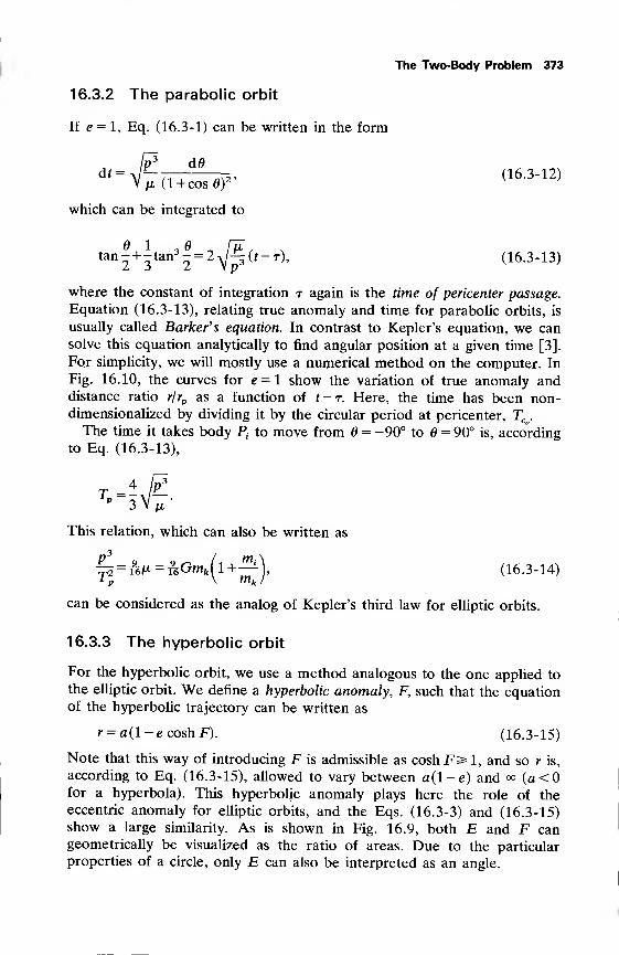
The Two-Body Problem 373
16.3.2 The parabolic orbit
If e = l, Eq. (16.3-1) can be written in the form
ju, (1 + cos 6)
which can be integrated to
d ' = \l— ,1 , „„^2 > (16.3-12)
e i . „ nrtan-+-tan3 - = 2y-^(f-r), (16.3-13)
where the constant of integration t again is the time of pericenter passage.
Equation (16.3-13), relating true anomaly and time for parabolic orbits, is
usually called Barker's equation. In contrast to Kepler's equation, we cansolve this equation analytically to find angular position at a given time [3].
For simplicity, we will mostly use a numerical method on the computer. In
Fig. 16.10, the curves for e = l show the variation of true anomaly anddistance ratio r/rp as a function of t — r. Here, the time has been non-dimensionalized by dividing it by the circular period at pericenter, TCp .
The time it takes body P;to move from 6 = -90° to = 90° is, according
to Eq. (16.3-13),
This relation, which can also be written as
.3
--^=BG%fl+-L (16.3-14)T- - -\ m
can be considered as the analog of Kepler's third law for elliptic orbits.
16.3.3 The hyperbolic orbit
For the hyperbolic orbit, we use a method analogous to the one applied to
the elliptic orbit. We define a hyperbolic anomaly, F, such that the equationof the hyperbolic trajectory can be written as
r = a(l-ecoshF). (16.3-15)
Note that this way of introducing F is admissible as cosh Fs= 1, and so r is,
according to Eq. (16.3-15), allowed to vary between a(l-e) and °° (a<0for a hyperbola). This hyperbolic anomaly plays here the role of the
eccentric anomaly for elliptic orbits, and the Eqs. (16.3-3) and (16.3-15)show a large similarity. As is shown in Fig. 16.9, both E and F cangeometrically be visualized as the ratio of areas. Due to the particular
properties of a circle, only E can also be interpreted as an angle.
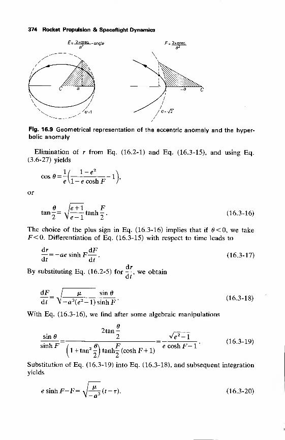
374 Rocket Propulsion & Spaceflight Dynamics
f= _2xsrga_= anglea2
Fig. 16.9 Geometrical representation of the eccentric anomaly and the hyper-bolic anomaly
Elimination of r from Eq. (16.2-1) and Eq. (16.3-15), and using Eq.
(3.6-27) yields
cos = -\-e<
e\l — e cosh F
or
6 e + 1 Ftan - = » / tanh - .
2 Ve-1 2(16.3-16)
The choice of the plus sign in Eq. (16.3-16) implies that if 0<O, we take
F<0. Differentiation of Eq. (16.3-15) with respect to time leads to
dr dF— = —ae sinh F— .
dr dt(16.3-17)
drBy substituting Eq. (16.2-5) for — , we obtain
dt
dF V sin 6
dt V-a 3(e
2 -l)sinhF"
With Eq. (16.3-16), we find after some algebraic manipulations
(16.3-18)
sin 6
62tan-
2= v^IsinhF / , 6\ , F. , ^ _ ecoshF-1
1 + tan2 -Jtanh- (cosh F+ 1)
(16.3-19)
Substitution of Eq. (16.3-19) into Eq. (16.3-18), and subsequent integration
yields
e sinh F—F=—a 2
(t-r). (16.3-20)
The Two-Body Problem 375
» 150
>« 120
90
60
30
' 1.5
(a)
3
10
30
vS*.
Q 20
(b)
e= 0/
3
1.5,
Y^
3 4
T,melt-T)/Tc Time U-r)/TcD
Fig. 16.10 The true anomaly and the distance versus the time after pericenter
passage in parabolic and hyperbolic trajectories
Again, the integration constant t is the time of pericenter passage as can be
seen by substituting F=0 into Eq. (16.3-20). This equation, which relates
position and time for a hyperbolic orbit, is analogous to Kepler's equation
for the elliptic orbit. Note that the introduction of a mean anomaly is of
little sense in this case, because hyperbolic motion is aperiodic. Like Kepler's
equation, the equation has to be solved by numerical methods for a given
time. In Fig. 16.10, the variation of and the distance ratio r/rp are shown
for some values of e as a function of the non-dimensional time after
pericenter passage. The notation TCp stands for the circular period at
pericenter.
16.4 Expansions in elliptic motion
We have found that Kepler's equation, relating time and position in anelliptic orbit, cannot be solved explicitly for position as a function of time.
As, however, r, and E are periodic functions of M, we can expand these
variables in Fourier series [4]. These series are extremely important for
analytical calculations.
Writing x = E - M, Kepler's equation can be written in the form
x = e sin(M+x). (16.4-1)
According to Eq. (16.4-1), x is of order e. Now assume that x can beexpressed as a power series in e:
x = ct 1 e + a2e2 + a3e
3 +- •
By substitution of Eq. (16.4-2) into Eq. (16.4-1), we find
a x e + a2e2 + • • • = e sinM cos x + e cosM sin jc.
(16.4-2)
(16.4-3)
376 Rocket Propulsion & Spaceflight Dynamics
A series expansion of sin x and cos jc and subsequent substitution of Eq.(16.4-2) results in an equation containing only a
t ,e and M By equating the
coefficients of equal powers of e, we obtain algebraic equations in ah withsolutions:
a^sinM, a2 = lsin2M, <*3 =.§sin 3M-|sinM, etc.
By substituting these results, and the higher-order coefficients which can beobtained in the same way, into Eq. (16.4-2), and neglecting terms of ordere6 and higher, we finally obtain
E = M+e(l-le2 + 1 e4)smM+e2&-ie2)sm2M+3
+ e3(|-fie
2) sin 3M+|e4
sin 4M+|§fe 5sin 5M. (16.4-4)
It is interesting to note that the general term of this series expansioncontains the leading factor e
ksin kM. Moreover, the parts in brackets are
polynomials in e2
. In celestial mechanics these properties are called the
d'Alembert characteristic [5]. It holds for many series expansions in as-
trodynamics and can be used as a rule of thumb to check analytical
derivations.
To obtain a series expansion of in terms of trigonometric functions of
M, we write
66 dd dEd~M
=dEdti- (16 -4 "5)
Differentiating Eq. (16.3-6) with respect to E gives
dd l + e l+cos0^ =V1 TT ^- (16.4-6)dE V 1 - e 1 + cos E
Substitution of Eq. (16.3-3) and Eq. (16.3-4) into Eq. (16.4-6) yields
dfl_ Vl-e2
dE 1 — e cos E'
Differentiating Eq. (16.3-11) with respect to M gives
dE 1
^i =i ^- (16.4-8)dm 1-e cos E
By substituting Eqs. (16.4-7) and (16.4-8) into Eq. (16.4-5), we obtain
dd . /dE\2
dM= Vl - e'Uf •
(16 -4"9)
The Two-Body Problem 377
Expanding the square root, substituting for —— from Eq. (16.4-4), integrat-
ing and again neglecting terms of order e6 and higher, finally leads to:
= M+e(2-|e2+^e4)sinM+e2(f-Me
2)sin2M+
+ e3(ii-s!e
2) sin 3M+fe4
sin4M+^e5sin 5M. (16.4-10)
The expression for 6 —M is called the equation of the center.
To obtain a corresponding series expansion of r, we substitute Eq.
(16.4-8) into Eq. (16.3-3) and find
r_/dE\- x
a VdAfJ '
dEBy substituting the expression for —— , which results by differentiating Eq.
am(16.4-4), and expanding the negative power, we obtain
-=l+|e 2 -e(l-§«2 + i§2e4)cosM
a
- e2(§-±e2
) cos 2M- e3(§-^e2
) cos 3M-ie4 cos4M-iUe5 cos5M. (16.4-11)
It can be shown that the three series converge for all values of M if
e < 0.6627 [6]. With a few exceptions, the eccentricities for the bodies in the
solar system are much lower. Also for the majority of Earth satellites, the
eccentricity is far below this limit and the series are very useful. It should be
mentioned in this context that for hyperbolic motion it is impossible to
construct series approximations which are valid over large intervals of time,
because the motion is not periodic.
16.5 Orbital elements
We have found that the motion of body Ptrelative to body Pk takes place
in one plane: the orbital plane. In the non-rotating reference frame with its
origin at Pk , the orientation of this orbital plane can be specified by twoangles. In Section 2.3 we discussed two often used reference frames: the
non-rotating geocentric equatorial frame and the non-rotating heliocentric
ecliptic frame. In these reference frames the xy-plane is the Earth's meanequatorial plane and the ecliptic plane, respectively.
The intersection of the orbital plane with the xy -plane is called the line ofnodes. This line intersects the orbit at two points. At the ascending node(A.N.) the z-coordinate of body P
tchanges from negative to positive. The
other intersection constitutes the descending node (D.N.). The position of
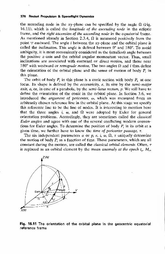
378 Rocket Propulsion & Spaceflight Dynamics
the ascending node in the xy -plane can be specified by the angle O (Fig.
16.11), which is called the longitude of the ascending node in the ecliptic
frame, and the right ascension of the ascending node in the equatorial frame.
As mentioned already in Section 2.3.4, Cl is measured positively from the
point T eastward. The angle i between the jcv -plane and the orbital plane is
called the inclination. This angle is defined between 0° and 180°. To avoid
ambiguity, it is most conveniently considered as the (smallest) angle betweenthe positive z-axis and the orbital angular momentum vector. Thus, small
inclinations are associated with eastward or direct motion, and those near180° with westward or retrograde motion. The two angles ft and i thus define
the orientation of the orbital plane and the sense of motion of body Ptin
this plane.
The orbit of body Ptin this plane is a conic section with body Pk at one
focus. Its shape is defined by the eccentricity, e, its size by the semi-major
axis, a, or, in case of a parabola, by the semi-latus rectum, p. We still have to
define the orientation of the conic in the orbital plane. In Section 3.6, weintroduced the argument of pericenter, <u, which was measured from an
arbitrarily chosen reference line in the orbital plane. At this stage we specify
this reference line to be the line of nodes. It is interesting to mention here
that the three angles i, o», and CI were adopted by Euler for general
orientation problems. Accordingly, they are sometimes called the classical
Euler angles and agree with one of the several conflicting modern conven-
tions for Euler angles. To determine the position of body P;in its orbit at a
given time, we further have to know the time of pericenter passage, r.
The six independent parameters a or p, e, i, w, fl, r uniquely determine
the motion of body Ptas a function of time. These parameters, which are all
constant during the motion, are called the classical orbital elements. Often, r
is replaced as an orbital element by the mean anomaly at the epoch t , M ,
Z(N)
Fig. 16.11 The orientation of the orbital plane in the geocentric equatorial
reference frame
The Two-Body Problem 379
defined as
M = n(t -r).
Then, the expression for the mean anomaly is
M =M + n(t-t ).
It should be clear that there have to be six orbital elements, as the motion of
body Ptis described by three scalar second-order differential equations. The
solution of this set contains six integration constants. We therefore should
consider the six orbital elements as a particular set of integration constants,
chosen for their clear geometrical interpretation.
Apart from these classical orbital elements, other orbital elements are
sometimes used as they may be more appropriate for certain problems, or
because some classical elements become ill-determined when e and/or i
approach zero. We will not go into detail on this subject as it is closely
related to problems of orbit determination from observations. We will only
mention two frequently used elements: the longitude of pericenter, <D = co + Cl,
and the mean longitude at epoch, L = a> +M . In the case e = 0, the
pericenter is not determined, and the position in the orbit should bemeasured from the ascending node. This is the reason that the circle, the
simplest of all orbits, cannot be handled by many of the formulae for elliptic
motion, because of the dependence upon the position of the pericenter. In
the case i = 0, the ascending node is not determined arid we use e.g. the
four elements a, e, (b, r to describe the motion. In the mathematical
development of refined schemes for the calculation of perturbed two-bodyorbits, certain other orbital elements are used which simplify the analytical
treatment. This will be discussed in Section 18.4.3.
16.6 Relations between orbital elements and position andvelocity
The instantaneous position and velocity of body P;in its motion about body
Pk can be described by its rectangular coordinates and velocity components:dx dy dz
x, y, z, — , — ,—
; by its spherical coordinates and velocity components: r,
a or A, 8 or <p, V, y, if/; or by the orbital elements a or p, e, i, <o, CI, t. Thereexist one-to-one relationships between these three sets of parameters. In
one respect the last set is entirely different from the first two: the six orbital
elements are constant during the motion. Therefore, the general scheme to
compute the position of Ptat some time t is as follows. First the orbital
elements are computed at t when the position and velocity of Ptare known.
Because these elements are constant, they take the same value at time t, andby an inverse transformation the position and velocity at time t may befound.
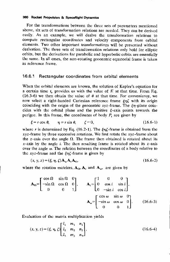
380 Rocket Propulsion & Spaceflight Dynamics
For the transformations between the three sets of parameters mentionedabove, six sets of transformation relations are needed. They can be derivedeasily. As an example, we will derive the transformation relations to
compute rectangular coordinates and velocity components from orbital
elements. Two other important transformations will be presented withoutderivation. The three sets of transformation relations only hold for elliptic
orbits, but the derivations for parabolic and hyperbolic orbits are essentially
the same. In all cases, the non-rotating geocentric equatorial frame is takenas reference frame.
16.6.1 Rectangular coordinates from orbital elements
When the orbital elements are known, the solution of Kepler's equation for
a certain time t„ provides us with the value of E at that time. From Eq.
(16.3-6) we then obtain the value of 6 at that time. For convenience, wenow select a right-handed Cartesian reference frame £n£ with its origin
coinciding with the origin of the geocentric xyz -frame. The |tj -plane coin-
cides with the orbital plane and the positive £-axis points towards the
perigee. In this frame, the coordinates of body Ptare given by
£ = r cos 6, tj = r sin 6, £ = 0, (16.6-1)
where r is determined by Eq. (16.2-1). The £Tj£-frame is obtained from the
xyz -frame by three successive rotations. We first rotate the xyz -frame about
the z-axis over the angle ft. The frame then obtained is rotated about its
x-axis by the angle /. The then resulting frame is rotated about its z-axis
over the angle &>. The relation between the coordinates of a body relative to
the xyz -frame and the £n£-frame is given by
(x, y, z) = (£ tj, £) A*,Aj A„,
where the rotation matrices, Aa,A{and A^,, are given by
(16.6-2)
r cos ft
An=l -sin ft
L
sin ft 0"
cos ft
1.
?A,=
A„=
-io o-
cos i sin i
_0 —sin i cos L-cos o) sin (o
—sin a) cos o)
_ 1
Evaluation of the imatrix multiplication yields
(x, y, z) = (£ tj
"/i m l
l2 m2
_/3 m3
n2
«3-
5
(16.6-3)
(16.6-4)
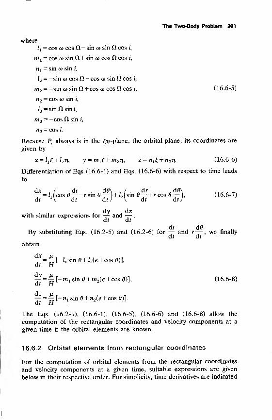
The Two-Body Problem 381
where
l x= cos co cos ft— sin <o sin ft cos i,
m 1= cos co sin ft + sin o> cos ft cos i,
n l= sin ft) sin i,
/2 = —sin tu cos ft— cos to sin ft cos i,
m2 = -sin co sin ft + cos co cos ft cos i, (16.6-5)
n2 = cos ft) sin i,
l3= sin ft sin i,
m 3 = —cos ft sin /,
n3= cos /.
Because P4always is in the £17 -plane, the orbital plane, its coordinates are
given by
x = lxi+l2 r}, y = m 1£+m2 T}, z = n 1£+rc2 17- (16.6-6)
Differentiation of Eqs. (16.6-1) and Eqs. (16.6-6) with respect to time leads
to
d* , / dr . d0\ , / . dr d0\ ... . _.— =L cos0 rsin0— + /2 sm 0— + rcos0—,
(16.6-7)dr V dr dr/ V dr dr/
dy dzwith similar expressions for — and — .
dr dr
dr d0By substituting Eqs. (16.2-5) and (16.2-6) for — and r— , we finally
obtain
— = -£ [-/i sin + l2(e + cos 0)],dr H
-^ =^[-m 1 sin0 + m2(e + cos0)], (16.6-8)dr Hdz u r .
. _..—- =—: [-ni sin + n2{e + cos 0)].
dr HThe Eqs. (16.2-1), (16.6-1), (16.6-5), (16.6-6) and (16.6-8) allow the
computation of the rectangular coordinates and velocity components at a
given time if the orbital elements are known.
16.6.2 Orbital elements from rectangular coordinates
For the computation of orbital elements from the rectangular coordinates
and velocity components at a given time, suitable expressions are given
below in their respective order. For simplicity, time derivatives are indicated
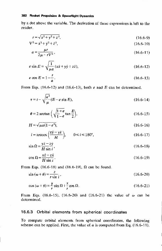
382 Rocket Propulsion & Spaceflight Dynamics
by a dot above the variable. The derivation of these expressions is left to the
reader.
r = Vx 2 + y2 + z
2, (16.6-9)
V2 = x2 +y2 + z2
, (16.6-10)
2n-rV2 (16.6-11)
e sin E = J— (xx + yy + zz), (16.6-12)V [xa
ecosE = l--. (16.6-13)a
From Eqs. (16.6-12) and (16.6-13), both e and E can be determined.
T = t- Xj— (E-e sin E), (16.6-14)
/ ll+e E\6 = 2 arctan J- tan —
, (16.6-15)
t = arccos(Xy
rr
y3:
), 0^i^l80°, (16.6-17)
H = vVa(l-e2), (16.6-16)
i —
~H
sma = yr
Z ~ Z\ (16.6-18)
Hsin i
xz — zxcosn= r . . (16.6-19)
Hsin i
From Eqs. (16.6-18) and (16.6-19), Q, can be found.
sin(eo + 0) =—^—
,
(16.6-20)r sin i
cos((o + 6) =— sinO+-cosn. (16.6-21)r r
From Eqs. (16.6-15), (16.6-20) and (16.6-21) the value of a> can bedetermined.
16.6.3 Orbital elements from spherical coordinates
To compute orbital elements from spherical coordinates, the following
scheme can be applied. First, the value of a is computed from Eq. (16.6-11).
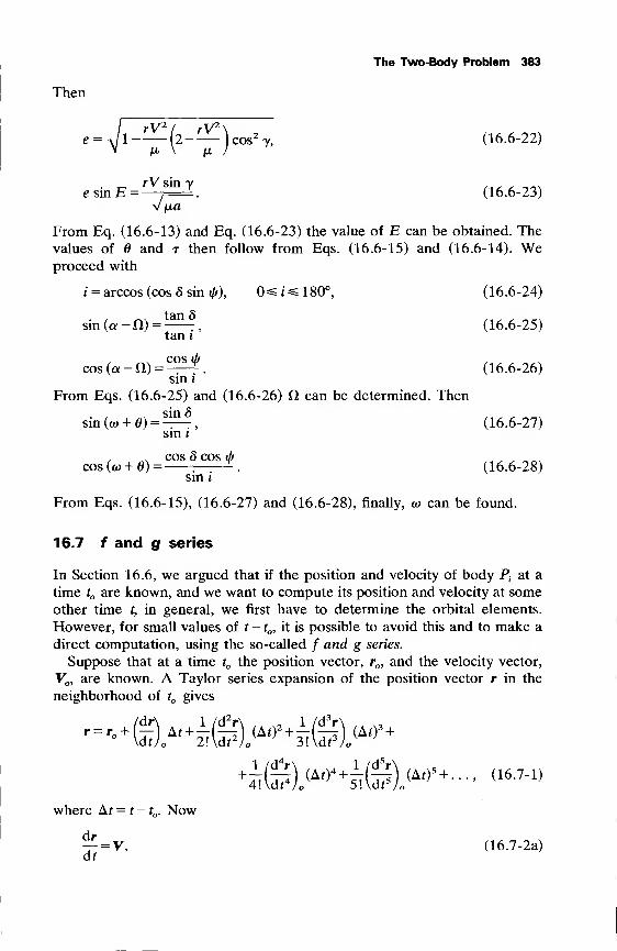
The Two-Body Problem 383
Then
e = a/1-— (2-— )cos2y, (16.6-22)
. rVsiny maao^esmE =—. (16.6-23)
From Eq. (16.6-13) and Eq. (16.6-23) the value of E can be obtained. Thevalues of 6 and t then follow from Eqs. (16.6-15) and (16.6-14). Weproceed with
i = arccos (cos 8 sin if/), ^ i ^ 1 80°, (16.6-24)
sin(a-n) =—
,
(16.6-25)tan 1
cos (a - ft) = ^-^. (16.6-26)sin 1
From Eqs. (16.6-25) and (16.6-26) O, can be determined. Then
sin(a> + 0) =^, (16.6-27)sin 1
. . COS 8 COS llf .^^ r r.^cos(w + 0) = :
-. (16.6-28)sin 1
From Eqs. (16.6-15), (16.6-27) and (16.6-28), finally, co can be found.
16.7 f and g series
In Section 16.6, we argued that if the position and velocity of body Ptat a
time t are known, and we want to compute its position and velocity at someother time t, in general, we first have to determine the orbital elements.
However, for small values of t -
1
, it is possible to avoid this and to make a
direct computation, using the so-called / and g series.
Suppose that at a time t the position vector, r , and the velocity vector,
V , are known. A Taylor series expansion of the position vector r in the
neighborhood of t gives
d7) o
A?4(d?) o
(A02+37(S!
r = r + (^) Af +^(^| (A02+^(^i)
o(Ar)
3 +
1 /d5r
where Af = t -
1
. Now
«V, (16.7-2a)at
384 Rocket Propulsion & Spaceflight Dynamics
and, as the motion takes place in a Keplerian orbit,
d r _ /a
di2- V. (16.7-2b)
Higher-order derivatives of r are obtained by differentiation of Eq. (16.7-
2b) with respect to time,
^L = E(3 L r _y\ (16.7-2c)
TS=-5(l2--3r-5)r + 65rV, (16.7-2d)_„_^12__ 3r -£)r+6^-
where for simplicity the notation
._dr „_d2r
r=dr'
r =d?
is used, and
. r-Vr = .
r
When evaluated at t , all quantities except r in the Eqs. (16.7-2) are directly
expressible in terms of the known initial values r and V . To eliminate r, wewrite Eq. (3.6-11) as
r = -(V2-r2)-4- (16.7-3)r r
By substituting Eq. (16.7-3) into Eq. (16.7-2d), we obtain
^=--^(l5r2-3V2 +2^r + 6^rV. (16.7-2e)
Differentiation of this equation with respect to time yields
^=15^(7r2-3y2 + 2^r-^('45r2-3y2+8^V, (16.7-2f)
where Eq. (3.6-8) was used to eliminate V. Higher-order derivatives of r can
be obtained in the same way, though the analytical development becomes
more and more tedious.
Substitution of the Eqs. (16.7-2) into Eq. (16.7-1) gives
r = fr + gV,
(16.7-4)
with
+l^\2--0V2o -lrl)\(At)
5 + . .. , (16.7-5)
8 r [ ja J
The Two-Body Problem 385
and
° ' o ^ ' o 1ZU 'o ^ M- J Qg 7-6)
Because r and V are constant vectors, the velocity V at time f is given by
V-gr. +gv. (16.7-7)
where one should notice that all coefficients in the power series in At are
constant.
As in a Keplerian orbit the angular momentum, H, is constant, we have
H = r XV =r*V. (16.7-8)
By substituting Eq. (16.7-4) and Eq. (16.7-7) into Eq. (16.7-8), we obtain
de df
/-f-g-f=l. (16.7-9)
This relation can be used to check the analytical expressions, if more termsare included in the / and g series.
The / and g series are basic to a number of procedures for orbit
determination and prediction, and are also useful for solving rendezvous
problems. A great advantage of the series is that they are universal, i.e. that
the same formulae hold for all conic sections. Herrick [7] gives an extensive
discussion on the use of these and other universal expressions. He also
mentions that for practical purposes the usefulness of the time series endbefore their mathematical convergence, when the higher and more compli-
cated terms become appreciable. As a rough criterion Herrick recommendsto use the time series only if ju,(Af)
2/r^<0.01. Bond [8] presents a different
way to determine the coefficients in the / and g series by using recursive
relations.
16.8 Relativistic effects
From the general theory of relativity we know that Newton's law of
gravitation describes only in a first approximation a real gravitational field.
For a body with spherical symmetric mass distribution, the geometry of
space-time is given by the so-called Schwarzschild metric. In case mt« mk ,
the motion of body Pt ,relative to a non-rotating reference frame with origin
at body Pk , is then described by [9]
d2w a
where
2 ' ""U2 1 "" , (16.8-1)
u=-, H=rV(p , a = 3^, au 2 = 3-^^f, (16.8-2)
T C HC
386 Rocket Propulsion & Spaceflight Dynamics
provided the orbit is not circular. In the equations given above, r and <p
denote the angular position, c is the velocity of light and ^ is the classical
gravitation parameter of body Pk . Comparing Eq. (16.8-1) and Eq. (3.6-18),
we note that the relativistic influence manifests itself only in the second
term at the right-hand side of Eq. (16.8-1). In celestial mechanics, always
V<p « c, indicating the relativistic term to be very small. An approximate
analytical solution of Eq. (16.8-1) can be obtained by the method ofsuccessive approximations. The zeroth-order solution is obtained by neglect-
ing the relativistic term. We then find the solution for a Keplerian orbit,
u=-^i [l + ecos(<p-o>)]. (16.8-3)
Substitution of this expression for u into the second term on the right-hand
side of Eq. (16.8-1) yields
d2W (JL fX
2
T~ 2+M =772 + a 774[l + 2e2 + 2e cos ((p — <o)+le
2 cos2 (<p — a>)].
(16.8-4)
The complete solution of this differential equation is
u = 77i[l + e cos (<p — o))] +H2
+ « 7F5 [(1 +k 2) + e<p sin (<p
- co) -\e 2 cos2 (<p - o>)]. (16.8-5)HThe first term in the relativistic part has the effect of slightly increasing u by
a constant quantity; this amount will be imperceptible. Also the effect of the
third term is negligible. Because of its steadily increasing amplitude, the
second term creates observable effects after long enough a period. Retaining
only this term for the relativistic effect, we obtain
2 [1 + e cos (<p — <o) + (3e<p sin (<p — to)], (16.8-6)
where
H 2/3 = «t^. (16.8-7)
Equation (16.8-6) can approximately be written as
f= l f/» (16 .8 .8)u 1 + e cos (<p — (o — ]8<p)
By comparing Eq. (16.8-8) and Eq. (16.2-1), we conclude that the trajectory
of body Ptabout body Pk can be visualized as an ellipse with a slowly
rotating major axis. After one revolution of body Pi5the major axis is rotated
by 2j8ir in the direction of motion of body Pt. Thus, due to the relativistic
The Two-Body Problem 387
effects, there is a change in the angular position of the pericenter after one
revolution:
2 2
Ao» = 2mr^ =6^-^ = 24^-5-^- ~ , (16.8-9)H z Hzc T c (l-e)
where T is the (Keplerian) orbital period. Computing the value of A<o for
the planet Mercury, we find a perihelion advance of 43" per century. For the
other planets, the perihelion motion is much smaller; for the Earth, we find
4" per century. For an Earth satellite with perigee at 500 km altitude and
apogee at 1000 km altitude, the relativistic perigee motion will be about
1280" per century. This rather large value will, however, not be observable
due to many other larger disturbing effects upon such a satellite.
Equation (16.8-9) was first found by Einstein [10], and is one of the three
famous tests for the general theory of relativity. Taking into account the
gravitational perturbations of the planets on the motion of Mercury whenusing the Newtonian attraction law, the perihelion motion of Mercury was
calculated to be 532" per century. Observations, however, led to a figure of
574" per century and no reasonable explanation could be found for this
difference. The predictable relativistic effect nicely fills this gap.
Because the relativistic effects are very small, the much simpler Newto-nian theory can be applied to nearly all problems in celestial mechanics,
especially for relatively short duration spaceflights.
References
Altman, S. P. (1965), Orbital Hodograph Analysis, AAS Science and
Technology Series, Vol. 3, American Astronautical Society, Baltimore.
Whittaker, E. T. (1917), A Treatise on the Analytical Dynamics ofParticles and Rigid Bodies, Cambridge University Press, London, p. 89.
Moulton, F. R. (1914), An Introduction to Celestial Mechanics, Macmil-
lan, New York, p. 156.
Brouwer, D. and Clemence, G. M. (1961), Methods of Celestial
Mechanics, Academic Press, New York, p. 60-114.
Brown, E. W. and Shook, C. A. (1933), Planetary Theory, CambridgeUniversity Press, London, p. 66, 80.
Plummer, H. C. (1960), An Introductory Treatise on Dynamical As-tronomy, Dover Publications, New York, p. 46-47.
Herrick, S. (1971), Astrodynamics, Vol. 1, Van Nostrand Reinhold,
London, p. 197-219.
Bond, V. R. (1966), Recursive Computation of the Coefficients of the
Time-Dependent f and g Series Solution of Keplerian Motion and a
Study of the Convergence Properties of the Solution, NASA TN D-3322,
Washington.
388 Rocket Propulsion & Spaceflight Dynamics
9 Eddington, A. (1923), The Mathematical Theory of Relativity, Cam-bridge University Press, London, p. 86.
10 Einstein, A. (1915), Erklarung der Perihelbewegung des Merkur aus derallgemeinen Relativitatstheorie, Sitzungsber. Deutsche Akad. Wissens.
(Math. Phys. Technik), Berlin, 831-839.
17 The Launching of a Satellite
Satellites are launched from the Earth's surface by means of multi-stage
rockets. After ignition of the first-stage rocket engine(s), these launch
vehicles first ascend vertically. A few seconds after lift-off, the rocket is tilted
and it flies a curved trajectory until at cut-off the final stage and the satellite
have a predetermined velocity and position. The determination of the
optimum ascent trajectory of a particular launch vehicle for a prescribed
satellite orbit is very complex, and is closely related to the theory of
optimum spaceflight maneuvers and to the operational constraints of that
launch vehicle. Because these topics are beyond the scope of this book, we
will discuss only some general aspects of ascent trajectories. Launch vehicle
performance data for orbital missions are presented in graphical form. Amore detailed discussion will be given on the relations between the orbital
parameters of a satellite and its position and velocity at the moment it enters
its orbit.
17.1 Launch vehicle ascent trajectories
Two basic types of ascent trajectories can be distinguished for satellite
launch vehicles (Fig. 17.1): Direct Ascent (D.A.) and Hohmann Transfer
Ascent (H.T.A.).
The D.A. trajectory is selected such that its summit point lies in the
required satellite orbit. When the satellite, which in most cases is still
attached to the final rocket stage, approaches this summit altitude, the final-
stage motor is ignited and the satellite is accelerated to the required (local)
orbital velocity. In some cases, the rocket motor required for this accelera-
tion is not the motor of the last stage, but is an integral part of the satellite
itself (apogee motor).
In the H.T.A., the satellite and the last stage first attain a low-altitude
circular parking orbit, just outside the densest part of the atmosphere.
Usually, the altitude of this parking orbit is about 200 km. For preliminary
mission and performance analyses, mostly a parking orbit is assumed at an
altitude of 185 km (100 n.mi.). Either shortly after parking orbit injection
(P.O.I.), or after a coasting period in this parking orbit, the vehicle is
injected into an elliptic transfer trajectory. At perigee, this transfer ellipse is
(about) tangential to the parking orbit and at apogee (about) tangential to
the required satellite orbit. This type of transfer trajectory has been prop-
osed in 1925 by W. Hohmann [1], and therefore is called a Hohmann
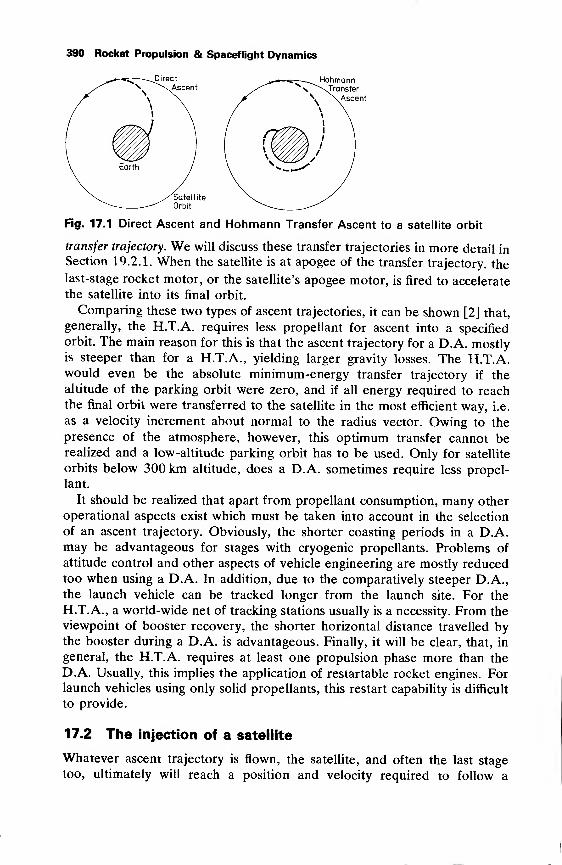
390 Rocket Propulsion & Spaceflight Dynamics
Fig. 17.1 Direct Ascent and Hohmann Transfer Ascent to a satellite orbit
transfer trajectory. We will discuss these transfer trajectories in more detail in
Section 19.2.1. When the satellite is at apogee of the transfer trajectory, the
last-stage rocket motor, or the satellite's apogee motor, is fired to accelerate
the satellite into its final orbit.
Comparing these two types of ascent trajectories, it can be shown [2] that,
generally, the H.T.A. requires less propellant for ascent into a specified
orbit. The main reason for this is that the ascent trajectory for a D.A. mostlyis steeper than for a H.T.A., yielding larger gravity losses. The H.T.A.would even be the absolute minimum-energy transfer trajectory if the
altitude of the parking orbit were zero, and if all energy required to reachthe final orbit were transferred to the satellite in the most efficient way, i.e.
as a velocity increment about normal to the radius vector. Owing to the
presence of the atmosphere, however, this optimum transfer cannot berealized and a low-altitude parking orbit has to be used. Only for satellite
orbits below 300 km altitude, does a D.A. sometimes require less propel-
lant.
It should be realized that apart from propellant consumption, many other
operational aspects exist which must be taken into account in the selection
of an ascent trajectory. Obviously, the shorter coasting periods in a D.A.may be advantageous for stages with cryogenic propellants. Problems of
attitude control and other aspects of vehicle engineering are mostly reduced
too when using a D.A. In addition, due to the comparatively steeper D.A.,
the launch vehicle can be tracked longer from the launch site. For the
H.T.A., a world-wide net of tracking stations usually is a necessity. From the
viewpoint of booster recovery, the shorter horizontal distance travelled bythe booster during a D.A. is advantageous. Finally, it will be clear, that, in
general, the H.T.A. requires at least one propulsion phase more than the
D.A. Usually, this implies the application of restartable rocket engines. Forlaunch vehicles using only solid propellants, this restart capability is difficult
to provide.
17.2 The injection of a satellite
Whatever ascent trajectory is flown, the satellite, and often the last stage
too, ultimately will reach a position and velocity required to follow a
The Launching of a Satellite 391
prescribed orbit about the Earth. Usually, the satellite then is separated
from the last stage by releasing a compressed-spring mechanism, and small
rocket motors on the last stage are fired to move the stage away from the
satellite. For liquid-propellant stages, usually the propellant residuals are
also exhausted, without combustion, through the main engine(s), in order to
increase the relative velocity between stage and satellite.
The time of separation is called the injection epoch; the position and
velocity of the satellite at this epoch constitute the injection parameters.
Injection epoch and injection parameters together completely determine the
orbit in which the satellite will encircle the Earth.
17.2.1 General aspects of satellite injection
We will now assume that at the injection epoch, th the position and velocity
of the satellite relative to a non-rotating geocentric equatorial reference
frame (Section 2.3.4) are known in terms of radial distance, rh declination,
8i5
right ascension, af ,
velocity, Vt ,
flight path angle, yh and flight path
azimuth, i/^. We then can determine the Keplerian elements of the orbit, and
other useful orbital parameters, by using the expressions given in Section
16.6.2 and 16.6.3. From these relations, we conclude:
1. The orbital elements a and e, the time difference tt— r and the true
anomaly at injection, 6h are only a function of the in-plane injection
parameters rh Vh y{.
2. The orbital elements i and ft, and the argument of latitude at injection,
Ui = (o + 0j, only depend on the out-of-plane injection parameters ah 8h ^.
3. The orbital element « is both a function of the in-plane and the out-
of-plane injection parameters.
In particular from Eq. (16.6-24), a number of important conclusions can
be drawn. Because — l^sin «fo^l, we may write
l^i^iso -^!-
For a particular injection point, the minimum orbit inclination is reached at
j/fj = 90°; i.e. an injection due east. The maximum inclination is reached if
the satellite is injected due west. For the injection of a satellite into an
equatorial orbit with i = 0°, the conditions 8j = 0° and ifo= 90° must hold; i.e.
the injection point must be located in the equatorial plane and the injection
must be due east.
If the required inclination of the orbit is within one of the ranges:
0°s£i<|<&,| or 180°-|4>,|< i^l80°,
where 4>, is the geocentric latitude of the launch site, the ascent trajectory
and the final orbit cannot be coplanar. In these cases, a plane change is
required during the ascent trajectory and/or at orbit injection. These so-
called dog- leg maneuvers, which are performed at relatively large vehicle
392 Rocket Propulsion & Space Spaceflight Dynamics
velocities, are very expensive in terms of propellant consumption [3]. In
order to launch satellites into low-inclination orbits, an equatorial launch site
is therefore very attractive. Presently, two near-equatorial launch sites are in
use: the Italian San Marco base (2.2°S, 40.2°E) in the Indian Ocean off the
coast of Kenya, and the French/European site Kourou (5.2°N, 52.7°W) in
Guiana. The other three Western launch sites are located in the USA, north
of the equator: Western Test Range (Vandenberg Air Force Base; 34.6°N,
120.6°W) in California, Eastern Test Range (Cape Canaveral; 28.5°N,
80.6°W) in Florida and Wallops Island (37.8°N, 75.5°W) in Virginia.
For all launch sites, the launch azimuths which can be used are restricted
by safety aspects and the availability of tracking stations. For example, for a
launch from the Eastern Test Range the launch azimuth, generally, must lie
within the range 45°-115°; for a launch from the Western Test Range a
launch azimuth between 170° and 300° is generally acceptable. As a
consequence, the Eastern Test Range is used primarily for launches into a
more or less eastward direction, which employ the rotation of the Earth to
increase effectively the inertial velocity of the vehicle, thereby improving the
launch vehicle's payload capability. The Western Test Range is mainly used
for near-polar orbits.
If, for a specified orbital plane, |<&i|< i< 180°— 1<£>,|, the launch site will
cross the orbital plane twice a day. Because of launch site constraints onlaunch azimuth, generally, only one of these crossings can be used to launch
a satellite into its orbit by a coplanar ascent trajectory. If small plane change
maneuvers are accepted, the satellite can be launched within a short period
around this crossing time, constituting the so-called daily launch window
[4].
We now meet another advantage of using a parking orbit. As the launch
time is fixed and the ascent trajectory for a D.A. is prescribed by the launch
vehicle capabilities, the point where the satellite enters its orbit is com-
pletely determined. Often, such as, for instance, in rendezvous missions or
for applications satellites, the satellite has to enter its orbit at a specified
location. Then, a coplanar launch within the launch window is mostly
impossible. The best alternative to long periods of inaccessibility or expen-
sive non-planar transfers is offered by the use of a parking orbit. Bycarefully selecting the orientation and altitude of the parking orbit, and the
point of departure from this parking orbit, it is possible to reach any point in
the final satellite orbit. A discussion on these phasing maneuvers for
geosynchronous missions is given by Cornelisse and Wakker [5].
17.2.2 Dependence of orbital parameters on in-plane injection
parameters
In this section, we will investigate how the size, shape and orientation of a
satellite orbit in its orbital plane depend on the injection parameters.
Therefore, we will derive expressions relating the orbital parameters a, e, p,
The Launching of a Satellite 393
ra-,
rP -> fy and t
t—r to the in-plane injection parameters r
t ,V
tand yt
. For ananalysis of the dependence of orbit parameters on the out-of-plane injection
parameters be referred to El'yasberg [6].
For the semi-major axis, a, the eccentricity, e, and the semi-latus rectum,
p, we may write, according to Eqs. (13.2-23a), (13.2-12b), (13.2-12a),
a 1r^! (17 -2- x)
e = Vl-/c1(2-/c,)cos
27„ (17.2-2)
-=kicos
27i , (17.2-3)
where kt
is defined as
V2
K=TW (17.2-4)
and Vc .is the circular velocity at the injection point. The perigee and apogee
distances, rap, are given by
ra>p = a(l±e), (17.2-5)
where the plus sign holds for the apogee and the minus sign for the perigee.
Substituting Eqs. (17.2-1) and (17.2-2) into Eq. (17.2-5) yields
7£ =^y[l±Vl-k
i(2-k
i)cos
27i ]. (17.2-6)
To obtain expressions for the true anomaly at injection, 6h we start from the
Eqs. (16.2-5) and (16.2-6), which, after substitution of Eqs. (17.2-3) and(17.2-4), can be written as
e sin 0, = ktsin yt
cos yh (17.2-7a)
e cos 4 = k, cos2
7i- 1. (17.2-7b)
To determine the time difference tt- t as a function of rh Vt
and yt ,we start
from Eq. (16.6-14):
1,-7= J— (Et- e sin E
f ), (17.2-8)y (a
where Etis the eccentric anomaly at injection. According to Eqs. (16.6-13),
(16.6-23) and (17.2-1), we may write
e sin Et= >/k
i(2-fe
i ) sin yt , (17.2-9a)
Et= arctan I
j^ _ 1sin yX (17.2-9b)
The value of E, is uniquely determined by the condition that if y,>0: sin E
{> 0, and if yt
< 0: sin E{< 0.
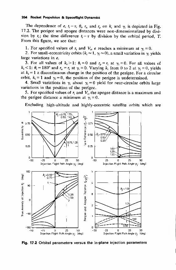
394 Rocket Propulsion & Spaceflight Dynamics
The dependence of e, tt- t, h ra and r
von k
tand y;
is depicted in Fig.
17.2. The perigee and apogee distances were non-dimensionalized by divi-
sion by rf ; the time difference ^-t by division by the orbital period, T.
From this figure, we see that:
1. For specified values of rfand Vh e reaches a minimum at yt
= 0.
2. For small-eccentricity orbits (fc£~ 1, yt
~ 0), a small variation in 7; yields
large variations in e.
3. For all values of fcj > 1: dt= and r
p= r
vat yf
= 0. For all values of
fc; < 1: 6i = 180° and ra = rtat yt
= 0. Varying ktfrom to 2 at yt
= 0, yields
at fcj = 1 a discontinuous change in the position of the perigee. For a circular
orbit, fcj = 1 and yt= 0, the position of the perigee is undetermined.
4. Small variations in ytabout yt
= yield for near-circular orbits large
variations in the position of the perigee.
5. For specified values of r{and Vj, the apogee distance is a maximum and
the perigee distance a minimum at yx= 0.
Excluding high-altitude and highly-eccentric satellite orbits which are
0.75
9> 0.50
0.25
k: =0.25,
0.50,
1.75\
1.50>-"
k
0.75, 1.25
1
-50
i> 0.75
£ 0.50 -
0.25
-25 25 50
Injection Flight Path Angle y.- (deg)
~ A/ =0.75-
0.50/
0.25'
1.00-"
1.25\1.50\
-50 -25 25 50
Injection Flight Perth Angle y- (deg)
.? 1
-25 25 50
Injection Flight Path Angle y- (deg)
-50 -25 25 50
Injection Flight Path Angle y- (deg)
Fig. 17.2 Orbital parameters versus the in-plane injection parameters
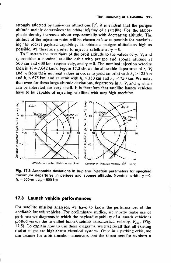
The Launching of a Satellite 395
strongly affected by luni-solar attractions [7], it is evident that the perigee
altitude mainly determines the orbital lifetime of a satellite. For the atmos-
pheric density increases about exponentially with decreasing altitude. Thealtitude of the injection point will be chosen as low as possible for maximiz-ing the rocket payload capability. To obtain a perigee altitude as high as
possible, we therefore prefer to inject a satellite at yt= 0.
To illustrate the sensitivity of the orbit altitude to the values of yh Vtand
rt ,
consider a nominal satellite orbit with perigee and apogee altitude at
500 km and 600 km, respectively, and yt= 0. The nominal injection velocity
then is Vt= 7.642 km/s. Figure 17.3 shows the allowable departures of r^ V
;
and y, from their nominal values in order to yield an orbit with hp > 425 kmand ha < 675 km, and an orbit with hp > 350 km and ha < 750 km. We note,
that even for these large altitude deviations, departures in rh Vtand yt
whichcan be tolerated are very small. It is therefore that satellite launch vehicles
have to be capable of injecting satellites with very high precision.
_ 2.0
Deviation in Injection Distance Aq (km) Deviation in Injection Velocity &V/|m /s)
Fig. 17.3 Acceptable deviations in in-plane injection parameters for specified
maximum departures in perigee and apogee altitude. Nominal orbit: y, = 0,
hp = 500 km, ha = 600 km
17.3 Launch vehicle performances
For satellite mission analyses, we have to know the performances of the
available launch vehicles. For preliminary studies, we mostly make use of
performance diagrams in which the payload capability of a launch vehicle is
plotted versus the so-called launch vehicle characteristic velocity, Vchan (Fig.
17.5). To explain how to use these diagrams, we first recall that all existing
rocket stages are high-thrust chemical systems. Once in a parking orbit, wecan assume for orbit transfer maneuvers that the thrust acts for so short a
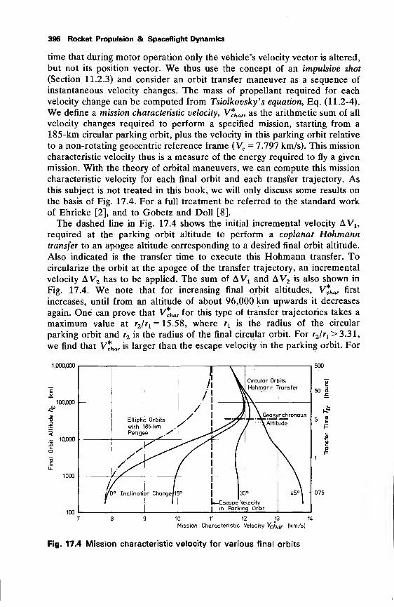
396 Rocket Propulsion & Spaceflight Dynamics
time that during motor operation only the vehicle's velocity vector is altered,
but not its position vector. We thus use the concept of an impulsive shot
(Section 11.2.3) and consider an orbit transfer maneuver as a sequence of
instantaneous velocity changes. The mass of propellant required for each
velocity change can be computed from Tsiolkovsky' s equation, Eq. (11.2-4).
We define a mission characteristic velocity, V*har, as the arithmetic sum of all
velocity changes required to perform a specified mission, starting from a
185-km circular parking orbit, plus the velocity in this parking orbit relative
to a non-rotating geocentric reference frame (
V
c = 7.797 km/s). This mission
characteristic velocity thus is a measure of the energy required to fly a given
mission. With the theory of orbital maneuvers, we can compute this mission
characteristic velocity for each final orbit and each transfer trajectory. Asthis subject is not treated in this book, we will only discuss some results on
the basis of Fig. 17.4. For a full treatment be referred to the standard work
of Ehricke [2], and to Gobetz and Doll [8].
The dashed line in Fig. 17.4 shows the initial incremental velocity AVl5
required at the parking orbit altitude to perform a coplanar Hohmanntransfer to an apogee altitude corresponding to a desired final orbit altitude.
Also indicated is the transfer time to execute this Hohmann transfer. Tocircularize the orbit at the apogee of the transfer trajectory, an incremental
velocity AV2 nas t0 be applied. The sum of AVX and AV2 is also shown in
Fig. 17.4. We note that for increasing final orbit altitudes, V*har first
increases, until from an altitude of about 96,000 km upwards it decreases
again. One can prove that V*har for this type of transfer trajectories takes a
maximum value at r2/r1= 15.58, where rx is the radius of the circular
parking orbit and r2 is the radius of the final circular orbit. For r2/r1> 3.31,
we find that V*har is larger than the escape velocity in the parking orbit. For
1.000.000
100,000
- 10,000
1000
100
{ \/' \ Circular Orbits
Hohmann Transfer
/! T
/ ! Jt\Elliptic Orbits
with 185 km .\/ \J- ) \ Geosynchronous
/'"TXltitude
Perigee /SIS j— >/ 1 //
/ / i I \/^A / i \
/yS i \
1)
i
i
j/Qo Inclination Change(15° | |30° 45°\
' ' U—Escape Velocity
1 ] | jin Parking Orbit
500
1/>
50 I
5 e
• 1
0.75
10 11 12J3
%Mission Characteristic Velocity Vchar (km/s)
Fig. 17.4 Mission characteristic velocity for various final orbits
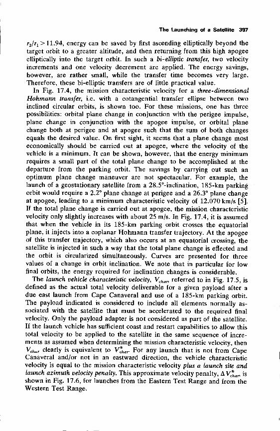
The Launching of a Satellite 397
r2/rl > 11.94, energy can be saved by first ascending elliptically beyond the
target orbit to a greater altitude, and then returning from this high apogee
elliptically into the target orbit. In such a bi- elliptic transfer, two velocity
increments and one velocity decrement are applied. The energy savings,
however, are rather small, while the transfer time becomes very large.
Therefore, these bi-elliptic transfers are of little practical value.
In Fig. 17.4, the mission characteristic velocity for a three-dimensional
Hohmann transfer, i.e. with a cotangential transfer ellipse between two
inclined circular orbits, is shown too. For these missions, one has three
possibilities: orbital plane change in conjunction with the perigee impulse,
plane change in conjunction with the apogee impulse, or orbital plane
change both at perigee and at apogee such that the sum of both changes
equals the desired value. On first sight, it seems that a plane change mosteconomically should be carried out at apogee, where the velocity of the
vehicle is a minimum. It can be shown, however, that the energy minimumrequires a small part of the total plane change to be accomplished at the
departure from the parking orbit. The savings by carrying out such an
optimum plane change maneuver are not spectacular. For example, the
launch of a geostationary satellite from a 28.5°-inclination, 185-km parking
orbit would require a 2.2° plane change at perigee and a 26.3° plane changeat apogee, leading to a minimum characteristic velocity of 12.070 km/s [5].
If the total plane change is carried out at apogee, the mission characteristic
velocity only slightly increases with about 25 m/s. In Fig. 17.4, it is assumedthat when the vehicle in its 185-km parking orbit crosses the equatorial
plane, it injects into a coplanar Hohmann transfer trajectory. At the apogeeof this transfer trajectory, which also occurs at an equatorial crossing, the
satellite is injected in such a way that the total plane change is effected andthe orbit is circularized simultaneously. Curves are presented for three
values of a change in orbit inclination. We note that in particular for lowfinal orbits, the energy required for inclination changes is considerable.
The launch vehicle characteristic velocity, Vchan referred to in Fig. 17.5, is
defined as the actual total velocity deliverable for a given payload after a
due east launch from Cape Canaveral and use of a 185-km parking orbit.
The payload indicated is considered to include all elements normally as-
sociated with the satellite that must be accelerated to the required final
velocity. Only the payload adapter is not considered as part of the satellite.
If the launch vehicle has sufficient coast and restart capabilities to allow this
total velocity to be applied to the satellite in the same sequence of incre-
ments as assumed when determining the mission characteristic velocity, then
Vchar clearly is equivalent to V*har. For any launch that is not from CapeCanaveral and/or not in an eastward direction, the vehicle characteristic
velocity is equal to the mission characteristic velocity plus a launch site andlaunch azimuth velocity penalty. This approximate velocity penalty, A V*ha„ is
shown in Fig. 17.6, for launches from the Eastern Test Range and from the
Western Test Range.
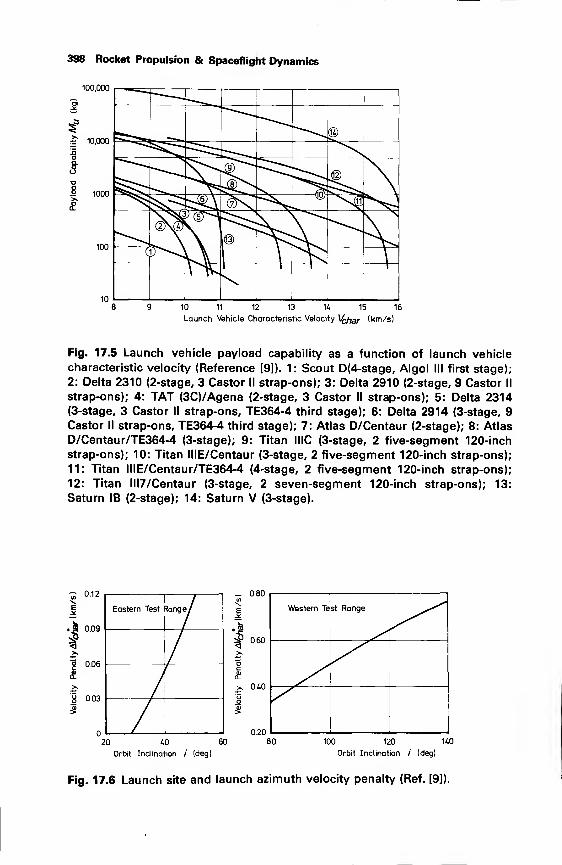
398 Rocket Propulsion & Spaceflight Dynamics
100,000
ST
£ 10,000
&
J 1000
100
10
©
4^(mT
.©
"-»s©\ ©N^ oy ^"^^
@\p^dr^
,©
y ,,s>s>I
1
10 11 12 13 14 15 16
Launch Vehicle Characteristic Velocity Vchar (km/s)
Fig. 17.5 Launch vehicle payload capability as a function of launch vehicle
characteristic velocity (Reference [9]). 1: Scout D(4-stage, Algol III first stage);
2: Delta 2310 (2-stage, 3 Castor II strap-ons); 3: Delta 2910 (2-stage, 9 Castor II
strap-ons); 4: TAT (3C)/Agena (2-stage, 3 Castor II strap-ons); 5: Delta 2314(3-stage, 3 Castor II strap-ons, TE364-4 third stage); 6: Delta 2914 (3-stage, 9
Castor II strap-ons, TE364-4 third stage); 7: Atlas D/Centaur (2-stage); 8: Atlas
D/Centaur/TE364-4 (3-stage); 9: Titan IIIC (3-stage, 2 five-segment 120-inch
strap-ons); 10: Titan IIIE/Centaur (3-stage, 2 five-segment 120-inch strap-ons);
11: Titan IIIE/Centaur/TE364-4 (4-stage, 2 five-segment 120-inch strap-ons);
12: Titan IH7/Centaur (3-stage, 2 seven-segment 120-inch strap-ons); 13:
Saturn IB (2-stage); 14: Saturn V (3-stage).
20 40 60
Orbit Inclination / (deg)
0.40
0.20
Western Test Range
80 100 120 140
Orbit Inclination / (deg)
Fig. 17.6 Launch site and launch azimuth velocity penalty (Ref. [9]).
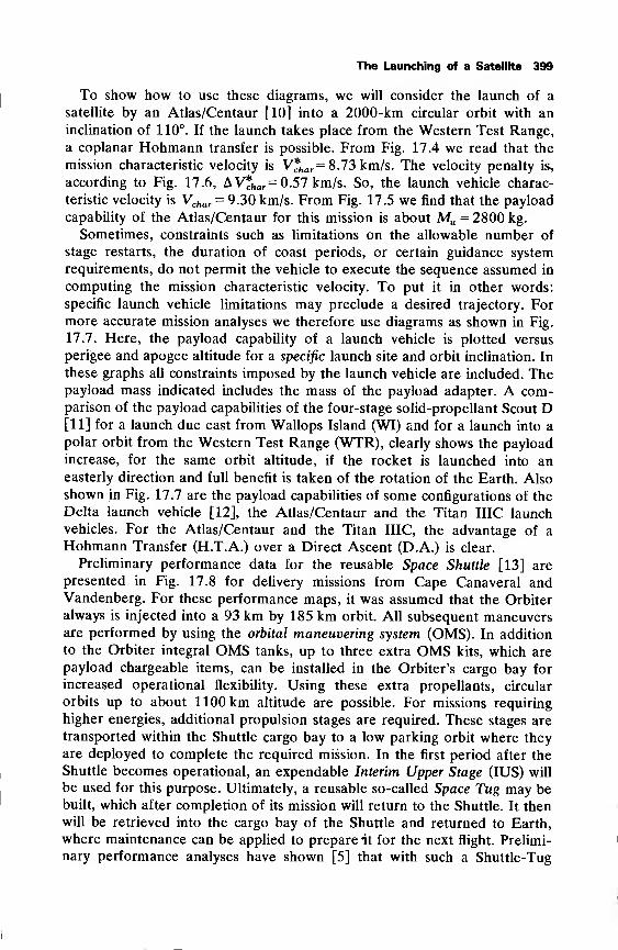
The Launching of a Satellite 399
To show how to use these diagrams, we will consider the launch of a
satellite by an Atlas/Centaur [10] into a 2000-km circular orbit with an
inclination of 110°. If the launch takes place from the Western Test Range,
a coplanar Hohmann transfer is possible. From Fig. 17.4 we read that the
mission characteristic velocity is V*har =8.73 km/s. The velocity penalty is,
according to Fig. 17.6, AV*har= 0.57 km/s. So, the launch vehicle charac-
teristic velocity is Vchar = 9.30 km/s. From Fig. 17.5 we find that the payload
capability of the Atlas/Centaur for this mission is about Mu = 2800 kg.
Sometimes, constraints such as limitations on the allowable number of
stage restarts, the duration of coast periods, or certain guidance system
requirements, do not permit the vehicle to execute the sequence assumed in
computing the mission characteristic velocity. To put it in other words:
specific launch vehicle limitations may preclude a desired trajectory. Formore accurate mission analyses we therefore use diagrams as shown in Fig.
17.7. Here, the payload capability of a launch vehicle is plotted versus
perigee and apogee altitude for a specific launch site and orbit inclination. In
these graphs all constraints imposed by the launch vehicle are included. Thepayload mass indicated includes the mass of the payload adapter. A com-parison of the payload capabilities of the four-stage solid-propellant Scout D[11] for a launch due east from Wallops Island (WI) and for a launch into a
polar orbit from the Western Test Range (WTR), clearly shows the payload
increase, for the same orbit altitude, if the rocket is launched into an
easterly direction and full benefit is taken of the rotation of the Earth. Alsoshown in Fig. 17.7 are the payload capabilities of some configurations of the
Delta launch vehicle [12], the Atlas/Centaur and the Titan IIIC launchvehicles. For the Atlas/Centaur and the Titan IIIC, the advantage of a
Hohmann Transfer (H.T.A.) over a Direct Ascent (D.A.) is clear.
Preliminary performance data for the reusable Space Shuttle [13] are
presented in Fig. 17.8 for delivery missions from Cape Canaveral andVandenberg. For these performance maps, it was assumed that the Orbiter
always is injected into a 93 km by 185 km orbit. All subsequent maneuversare performed by using the orbital maneuvering system (OMS). In addition
to the Orbiter integral OMS tanks, up to three extra OMS kits, which are
payload chargeable items, can be installed in the Orbiter's cargo bay for
increased operational flexibility. Using these extra propellants, circular
orbits up to about 1100 km altitude are possible. For missions requiring
higher energies, additional propulsion stages are required. These stages are
transported within the Shuttle cargo bay to a low parking orbit where they
are deployed to complete the required mission. In the first period after the
Shuttle becomes operational, an expendable Interim Upper Stage (IUS) will
be used for this purpose. Ultimately, a reusable so-called Space Tug may bebuilt, which after completion of its mission will return to the Shuttle. It then
will be retrieved into the cargo bay of the Shuttle and returned to Earth,
where maintenance can be applied to prepare nt for the next flight. Prelimi-
nary performance analyses have shown [5] that with such a Shuttle-Tug
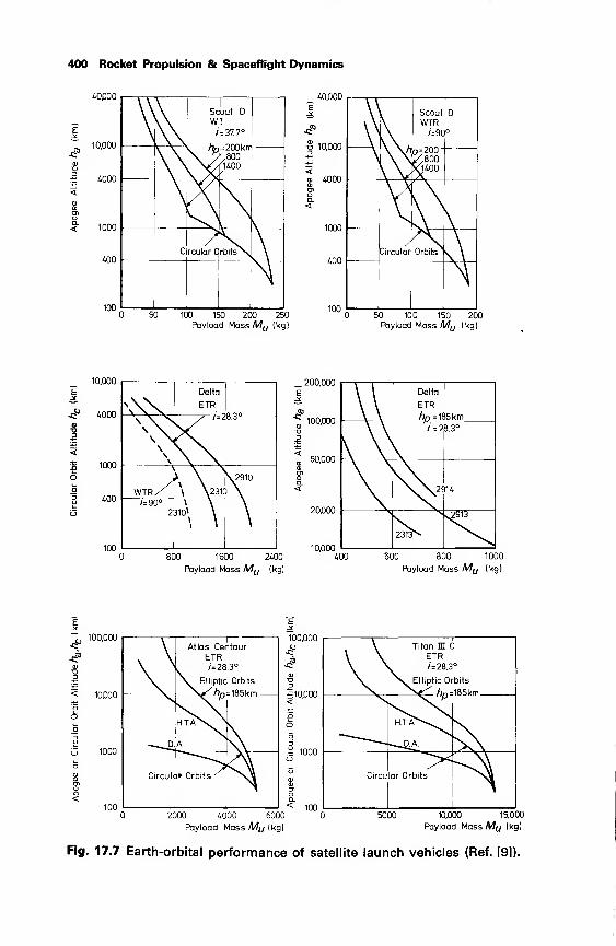
400 Rocket Propulsion & Spaceflight Dynamics
40000
10,000
4000
1000
400
100
Scout DWI1=37.7°
k hPf/8001400
c rcular C rbitsX,
_
50 100 150 200 250
Payload Mass My (kg)
40,000
-S 10,000
a) 4000
1000
400
100
Scout
WTR/=9C
I
D
°
\ \ p=200"Z800>O400
Circular Orbits
50 100 150 200Payload Mass Mu (kg)
10,000
4000
1000
400
100
Delta
\XX ETR
\ \ N\ X\ X\\\\
WTR/ \231C
S.2910
) \/=90°
2 310* \
_ 200,000
E
100,000
50,000
20,000
800 1600 2400
Payload Mass Mu (kg)
10,000
Delta
ETR
/)/i = 185km/ = 28.3°
\\^2< 14
s2913
2313s-
400 600 800 1000
Payload Mass Mu (kg)
I
Atlas Centaur
ETRk /=28.3°
\ Elliptic Orbits
10000 \V/jnX P
H.TA\ >
1000O.A.
inn
Circular Orbits '
100,000
S 10,000
2000 4000 6000
Payload Mass Mu (kg)
1000
10,000 15,000
Payload Mass My (kg)
Fig. 17.7 Earth-orbital performance of satellite launch vehicles (Ref. [9]).
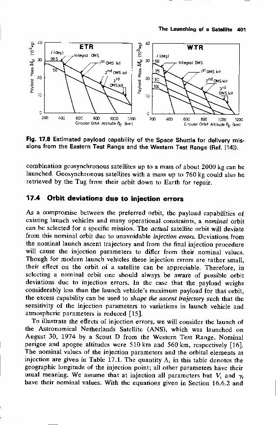
™ *o
The Launching of a Satellite 401
Integral OMS
-1st 0MSkit
2nd
OMS kit
600 800 1000 1200
Circular Orbit Altitude hc (km)
600 800 1000 1200
Circular Orbit Altitude hQ (km)
Fig. 17.8 Estimated payload capability of the Space Shuttle for delivery mis-sions from the Eastern Test Range and the Western Test Range (Ref. [14]).
combination geosynchronous satellites up to a mass of about 2000 kg can belaunched. Geosynchronous satellites with a mass up to 760 kg could also beretrieved by the Tug from their orbit down to Earth for repair.
17.4 Orbit deviations due to injection errors
As a compromise between the preferred orbit, the payload capabilities ofexisting launch vehicles and many operational constraints, a nominal orbit
can be selected for a specific mission. The actual satellite orbit will deviate
from this nominal orbit due to unavoidable injection errors. Deviations fromthe nominal launch ascent trajectory and from the final injection procedurewill cause the injection parameters to differ from their nominal values.
Though for modern launch vehicles these injection errors are rather small,
their effect on the orbit of a satellite can be appreciable. Therefore, in
selecting a nominal orbit one should always be aware of possible orbit
deviations due to injection errors. In the case that the payload weighsconsiderably less than the launch vehicle's maximum payload for that orbit,
the excess capability can be used to shape the ascent trajectory such that the
sensitivity of the injection parameters to variations in launch vehicle andatmospheric parameters is reduced [15].
To illustrate the effects of injection errors, we Will consider the launch of
the Astronomical Netherlands Satellite (ANS), which was launched onAugust 30, 1974 by a Scout D from the Western Test Range. Nominalperigee and apogee altitudes were 510 km and 560 km, respectively [16].
The nominal values of the injection parameters and the orbital elements at
injection are given in Table 17.1. The quantity A; in this table denotes the
geographic longitude of the injection point; all other parameters have their
usual meaning. We assume that at injection all parameters but Vj and yt
have their nominal values. With the equations given in Section 16.6.2 and
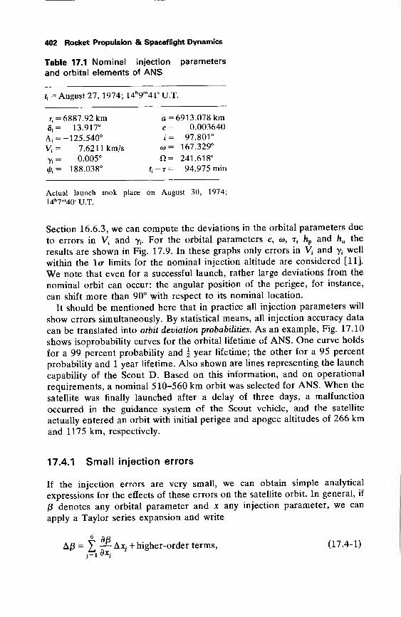
402 Rocket Propulsion & Spaceflight Dynamics
Table 17.1 Nominal injection parameters
and orbital elements of ANS
u= August 27, 1974; 14h9
r"41 S U.T
rf
= 6887.92 km a = 6913.078 km8
f
= 13.917° e = 0.003640
A,- = -125.540° i= 97.801°
V, 7.6211 km/s o> = 167.329°
Ti= -0.005° n= 241.618°
«fc= 188.038° fj--T = 94.975 min
Actual launch took place on August 30, 1974;
I4h7m40s u T
Section 16.6.3, we can compute the deviations in the orbital parameters due
to errors in Vj and yt. For the orbital parameters e, to, t, h
pand ha the
results are shown in Fig. 17.9. In these graphs only errors in V* and ytwell
within the la limits for the nominal injection altitude are considered [11].
We note that even for a successful launch, rather large deviations from the
nominal orbit can occur: the angular position of the perigee, for instance,
can shift more than 90° with respect to its nominal location.
It should be mentioned here that in practice all injection parameters will
show errors simultaneously. By statistical means, all injection accuracy data
can be translated into orbit deviation probabilities. As an example, Fig. 17.10
shows isoprobability curves for the orbital lifetime of ANS. One curve holds
for a 99 percent probability and \ year lifetime; the other for a 95 percent
probability and 1 year lifetime. Also shown are lines representing the launch
capability of the Scout D. Based on this information, and on operational
requirements, a nominal 510-560 km orbit was selected for ANS. When the
satellite was finally launched after a delay of three days, a malfunction
occurred in the guidance system of the Scout vehicle, and the satellite
actually entered an orbit with initial perigee and apogee altitudes of 266 kmand 1175 km, respectively.
17.4.1 Small injection errors
If the injection errors are very small, we can obtain simple analytical
expressions for the effects of these errors on the satellite orbit. In general, if
/3 denotes any orbital parameter and x any injection parameter, we can
apply a Taylor series expansion and write
6 -so
Aj3 = X Axj+ higher-order terms, (17.4-1)
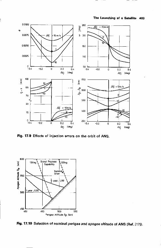
The Launching of a Satellite 403
0.0100
0.0075
0.0050
0.0025
AV'
0/
^10
-£ 100
1
260
3 210
160
110
-0.4 -0.2 0.2 0.4
AVj (deg)
60
—-.M = -10m/s
NsO \
1(3^
-0.4 -0.2
12-^85
70
._^. '*^f
/
^^¥<>
30
AVj =-10m/s
15 jS~ n. ,
/^:&-^>^-0.4 -0.2 0.2 0.4
Ay- (deg)
0.2 0.4
Ay/ (deg)
-0.4 -0.2 0.2 0.4
AVj (deg)
Fig. 17.9 Effects of injection errors on the orbit of ANS.
600
450400 450 500 550
Perigee Altitude hp (km)
Fig. 17.10 Selection of nominal perigee and apogee altitude of ANS (Ref. [17]).
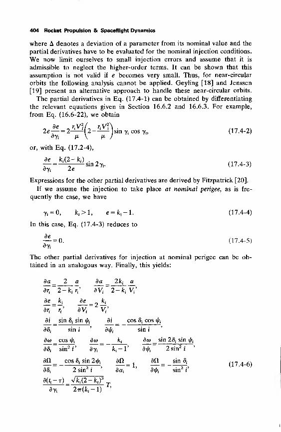
404 Rocket Propulsion & Spaceflight Dynamics
where A denotes a deviation of a parameter from its nominal value and the
partial derivatives have to be evaluated for the nominal injection conditions.
We now limit ourselves to small injection errors and assume that it is
admissible to neglect the higher-order terms. It can be shown that this
assumption is not valid if e becomes very small. Thus, for near-circular
orbits the following analysis cannot be applied. Geyling [18] and Jenssen
[19] present an alternative approach to handle these near-circular orbits.
The partial derivatives in Eq. (17.4-1) can be obtained by differentiating
the relevant equations given in Section 16.6.2 and 16.6.3. For example,
from Eq. (16.6-22), we obtain
2e— = 2-L—i 2—
—
l
- sin yfcosy*, (17.4-2)
or, with Eq. (17.2-4),
de kA2-ki) . „ ,— = l\ l 'sin2y, (17.4-3)
Expressions for the other partial derivatives are derived by Fitzpatrick [20].
If we assume the injection to take place at nominal perigee, as is fre-
quently the case, we have
Ti= 0, fcj>l, e = k
i-\. (17.4-4)
In this case, Eq. (17.4-3) reduces to
«0. (17.4-5)
The other partial derivatives for injection at nominal perigee can be ob-
tained in an analogous way. Finally, this yields:
da 2 a da 2fcj a
drt 2-W dV
t 2-ki V,'
de _
dr~
kt
de= 2±
di
d8t
'sin 8
tsin i/f
sin i
di
' aft
cos 8i cos i/fj
sin i
d(o
d8i~
cos if/,
• i • >
sin i
du> kt
1
dot sin 28; sin
dij/i 2 sin2
i
*t
dto_ cos 8i sin
2 sin2
2^ an
i ' doti
= 1,
aa_dx\f~
sin 5,
sin2
i
>
(17.4-6)
aU-T) _ A(2-fc,)3
Td 7i 2*r(k,-l) '
The Launching of a Satellite 405
dr, '
dra= 4-ktra dra 4 ra
dri 2-ktTi1
BVi 2-kjVi'
ar__3_r ar_ 3fefr
8^2-^^ dVi~2-k
iV
i
'
where T is the orbital period, and
sin i = Vl — cos25i sin
2ifo.
The remaining 36 partial derivatives all take the value zero. Of course, the
orbital parameters on the right-hand side of the expressions for the partial
derivatives denote the parameters of the nominal orbit.
From Eqs. (17.4-5), a number of important conclusions can be drawn for
an injection at nominal perigee:
1
.
The relative deviations in a and ra due to percentage errors in rfand V
t
i.e. , etc. ) strongly increase with increasing values of kt. For highly-
eccentric orbits (k4 ] 2), large deviations in a and ra may be expected.
2. The position of the perigee is only affected by errors in yt ,S; and fa.
3. The time difference tt-T is only affected by errors in y{
.
4. The perigee distance is only a function of the injection distance.
With the theory presented in this chapter, the orbital elements at injection
can be computed from the injection conditions. For a first-order analysis, wemay consider these elements as characterizing the (Keplerian) orbit in which
the satellite will encircle the Earth. In practice, however, the satellite will be
subjected to various types of perturbing forces and its orbit will deviate from
this Keplerian one. The next chapter will be devoted to the theory of
perturbed satellite orbits.
References
1 Hohmann, W. (1925), Die Erreichbarkeit der Himmelskorper, Olden-
bourg, Berlin, p. 63-75, Also: NASA TT F-44, Washington, 1960.
2 Ehricke, K. A. (1962), Space Flight, Vol. 2: Dynamics, Van Nostrand,
Princeton, p. 90-116, 289-433.
3 White, J. F. (ed.) (1963), Flight Performance Handbook for Powered
Flight Operations, Wiley, New York, p. 3-6 to 3-28.
4 Miner, W. E. and Silber, R. (1963), A variational launch window
study, AIAA J., 1, 1125-1129.
5 Cornelisse, J. W. and Wakker, K. F. (1972), Geosynchronous Space Tug
Missions, Report VTH-171, Dept. Aerospace Eng., Delft University of
Technology, Delft.
406 Rocket Propulsion & Spaceflight Dynamics
6 El'yasberg, P. E. (1967), Introduction to the Theory of Flight of Artificial
Earth Satellites, NASA TT F-391, Washington, p. 143-145.
7 Van de Graaff, R. C. (1977), A Semi-Analytical Method for Computing
Third-Body Effects on Earth's and Lunar Satellite Orbits, Report LR231, Dept. Aerospace Eng., Delft University of Technology, Delft.
8 Gobetz, F. W. and Doll, J. R. (1969), A survey of impulsive
trajectories, AIAA J., 7, 801-834.
9 McGolrick, J. E. (1973), Launch Vehicle Estimating Factors for Ad-vance Mission Planning, NHB 7100.5B, NASA, Washington.
10 Shramo, D. J. (1974), Centaur—A Major Element of the Current Space
Transportation System, IAF Paper 74-075, Amsterdam.11 Anon. (1976), Scout User's Manual, Vol. 5: Performance and Flight
Planning, Vought Corp., Dallas.
12 Bonnett, E. W. (1971), Delta Spacecraft Design Restraints, DAC-61687, revision October 1971, McDonnell Douglas, Huntington Beach.
13 Anon. (1975), Space Shuttle, NASA, Houston (paper issued at 26th
IAF Congress in Lisbon, 1975).
14 Anon. (1976), Space Shuttle System Payload Accommodations, JSC07700, Vol. 14, Rev. D, Change 15, NASA.
15 Rosenbaum, R. (1970), The Reduction of Launch Vehicle Injection
Errors by Trajectory Shaping, AIAA Paper 70-1078, New York.
16 Wakker, K. F. (1977), Orbit Prediction for the Astronomical Nether-
lands Satellite, paper presented at the B.I.S. conference on ComputerTechniques for Satellite Control and Data Processing, Slough.
17 de Leeuw, W. H. and Pouw, A. (1974), Mission Analysis of the As-tronomical Netherlands Satellite, IAF Paper 74-121, Amsterdam.
18 Geyling, F. T. and Westerman, H. R. (1971), Introduction to Orbital
Mechanics, Addison-Wesley, Reading, p. 98-104.
19 Jensen, J., Townsend, G., Kork, J. and Kraft, D. (1962), DesignGuide to Orbital Flight, McGraw-Hill, New York, p. 733-744.
20 Fitzpatrick, P. M. (1970), Principles of Celestial Mechanics, AcademicPress, New York, p. 129-132.
18 Perturbed Satellite Orbits
In Chapter 16 we discussed the motion of a body Ptrelative to a non-
rotating reference frame with its origin at the center of mass of a body Pk .
We assumed that both bodies could be regarded as point masses and that
the only force acting upon Ptwas due to the mutual gravitational attraction.
We found that the trajectory of P{was a conic section, a so-called Keplerian
orbit.
In reality, where P{represents a planet moving around the Sun, or a
satellite orbiting the Earth, there will be other forces acting upon Pt. These
forces, however, are relatively small as compared to the main gravitational
force, and the orbits of planets and satellites can be approximated very well
by conic sections. The actual trajectories of these bodies are therefore called
perturbed Keplerian orbits. For this perturbed Keplerian motion, no closed-
form analytical solution can be obtained. The approximate solution of the
equations of motion of Pfunder the influence of a main gravitational force
and perturbing forces is one of the most developed, and most interesting,
branches of celestial mechanics.
In this chapter, we will discuss only some elementary aspects of perturbed
orbits; furthermore, we will limit ourselves to orbits of artificial Earth
satellites.
The most important perturbing forces acting on artificial Earth satellites
are due to: asphericity of the Earth, aerodynamic effects, lunar and solar
attraction, solar radiation and electromagnetic effects. Baker [1] gives an
extensive survey of the origin, direction and magnitude of these perturbing
forces. We will discuss the nature of these forces only very superficially.
Asphericity of the Earth. Generally, this asphericity yields a very important
perturbing force for satellite orbits. As the Earth's mass distribution is not
perfectly spherical symmetric, gravitational force components normal to the
radius vector of the satellite will be present. Because of these components,
the actual orbit will deviate from a Keplerian orbit. It will be clear that the
effects of the asphericity decrease with increasing distance from the Earth.
For, at distances from the Earth which are large with respect to the
dimensions of the Earth, we can approximate the Earth's gravitational field
by that of a point mass. We will discuss these perturbing forces in moredetail in Section 18.6.
Aerodynamic effects. The motion of a satellite through the upper regions of
the atmosphere generates aerodynamic forces. The major force will be a
408 Rocket Propulsion & Spaceflight Dynamics
drag force, acting opposite to the satellite's velocity vector with respect to
the atmosphere, but lift and side forces will occur too. The deceleration of
the satellite due to airdrag can be expressed by the well-known aerodynamic
relationship
aD = CD 1
lPV2
£f,M
where p is the air density, V is the satellite's velocity relative to the
atmosphere, M is the satellite's mass, S is a reference area of the satellite
and CD is a drag coefficient based on that area. For a given satellite andorbit, M and V are known, and S may be chosen. The difficulties in the
analysis of the aerodynamic deceleration arise in the determination of CDand p.
At satellite altitudes, the flow is of the free-molecular type. Then, the drag
is determined by the mechanism of molecular reflection at the surfaces of
the satellite. This is a very complicated process, which is as yet only partly
understood. Between altitudes of 150 km and 500 km, the drag coefficient,
based on projected area normal to the direction of motion, is usually aboutCD =2.2-2.5. At higher altitudes it may increase to CD=3-5. The atmos-pheric density not only varies with altitude, but also with time. It turns outthat at a given altitude the density is a function of local solar time, season,
disturbances of the geomagnetic field and the solar activity (Section 2.6.2).
The exact relation between the density and these variables is not completely
understood.
Because of the uncertainties in the drag coefficient and the air density, wecan only roughly estimate the magnitude of the aerodynamic forces. Theeffects of the aerodynamic forces strongly diminish as the orbital altitude
increases. In fact, atmospheric drag is the most important perturbing force
below about 200 km altitude, and can, in most cases, completely be ne-
glected at altitudes above 1000 km. The aerodynamic drag is the cause of the
decay of Earth satellites. They dissipate their orbital energy and their orbital
altitudes decrease, through which they enter denser parts of the atmosphere,
where the drag becomes larger and larger. Ultimately, they burn in the lowEarth's atmosphere. Sometimes, parts of satellites survive the re-entry andimpact on the Earth's surface.
Lunar and solar attraction. We already discussed the effects of these attrac-
tions on the motion of an Earth satellite in Section 15.3.1. These effects
increase with increasing distance from the Earth, and lunar and solar
attractions become the major sources of perturbations above geostationary
orbital altitudes.
Radiation pressure. A satellite about the Earth is also subjected to direct
solar radiation, solar radiation reflected by the Earth (albedo), and radiation
emitted by the Earth itself. In quantum mechanics, light is regarded as a
flow of photons, which, among others, possess a momentum. If these
Perturbed Satellite Orbits 409
photons hit the satellite's surface, and are partially reflected, they impart amomentum to the satellite, which results in the so-called radiation pressure.
As the radiation pressure in the vicinity of the Earth is extremely small, it
will only have a substantial effect on the orbits of balloon-type satellites, i.e.
satellites with a small mass/area ratio. In those cases, the effects of radiation
pressure may be very significant, and should certainly be taken into account.
Electromagnetic effects. As the atmosphere at satellite altitudes is partlyionized, the possibility exists that a satellite acquires an electrical potential.
As there is also a magnetic field, electromagnetic forces will be generated.However, generally, these effects are negligible.
In the following, we will assume the perturbing forces to be known, andwe will only study some methods to compute their effects on the orbit of a
satellite.
18.1 Special and general perturbations
If the motion of a satellite is described relative to a non-rotating geocentricequatorial reference frame (Fig. 2.2) and perturbing forces are taken into
account, the equation of motion can be written in the form
tf+73r= -VR + a> (18.1-D
where R, the perturbing or disturbing potential, includes all perturbing forces
which can be expressed by a potential function, and a stands for all
perturbing forces which cannot be written as the gradient of a scalar
function. We already met an example of a perturbing potential, describing
the effects of the gravitational attraction by other bodies, in Section 15.3.
In general, Eq. (18.1-1) cannot be solved in a closed form and we have to
resort to numerical techniques or to approximate analytical solutions. In the
first case, we speak of special perturbations; in the second case, we deal withgeneral perturbations.
Special perturbations methods generate just one special trajectory for adefinite satellite, given its unique initial conditions. A determination of theorbit is made by means of a numerical step-by-step process. The variousmethods of special perturbations are usually classified according to the
formulation of the equations to be integrated. The three classical methodsare known as CowelVs method, Encke's method and the method of variation
of orbital elements. These methods will be treated in subsequent sections. Animportant topic in special perturbations is the choice of the most suitable
numerical integration technique. This highly specialized subject is beyondthe scope of this book. Allione [2] and Merson [3] present surveys of
modern advanced methods.
General perturbations cover the analytical methods in which the perturb-ing accelerations are expanded into series and integrated termwise. In
410 Rocket Propulsion & Spaceflight Dynamics
practice, only a limited number of terms of the series is taken into account.
We obtain the solution of the differential equations of motion in the form of
analytical expressions, describing the change of the orbit as a function of
time for a particular perturbing force. These methods thus yield solutions
that are generally applicable to all satellites for all initial conditions. The
most important classical general perturbations method is the method of
variation of orbital elements, which was already mentioned in connection
with special perturbations. For the analytical integration, many processes are
known, for example: the method of successive approximations, Taylor series
expansions, multivariable asymptotic expansions and averaging. A survey of
these techniques is given by Dallas [4] and Lorell [5]. The main difficulty of
all general perturbations methods always was the tremendous amount of
analytical labor involved, especially if higher-order approximations are
required. Nowadays, most of the analysis associated with the development
of higher-order theories can be performed by a computer [6].
The reader should be aware that, apart from the special and general
perturbations methods mentioned, there exist numerous other specialized,
and in most cases very complicated, methods. Geyling and Westerman [7]
give an introduction to the application of the classical methods to perturbed
satellite motion. Novel approaches to the perturbation problem are pre-
sented by Stiefel and Scheifele [8].
Comparing the special and general perturbations methods, one can makesome remarks about their respective advantages and disadvantages.
Obviously, the methods of special perturbations are directly applicable to
any orbit and to any perturbing force. As these are purely numerical
methods, we have the problem of accumulated error and these methods are
not well suited to long-term orbit predictions. Moreover, these methods
require the computation of the coordinates and velocity components of the
satellite at all intermediate epochs prior to the epoch of interest, leading to
long integration times.
An advantage of general perturbations methods is that once the analytical
expressions, describing the effects of the perturbing force, are available, the
computation of a perturbed orbit for various initial conditions is muchfaster. Their main advantage, however, is that general perturbations
methods, and in particular the method of variation of orbital elements,
clearly reveal the source of perturbations from orbital data. Major achieve-
ments of the methods of general perturbations were the discovery of the
planet Neptune in 1846, through the observed orbital perturbations of
Uranus, and, more recently, the demonstration of the Earth's pear-shape in
1959, through the analysis of the orbital data of the Vanguard 1 satellite [9].
18.2 Cowell's method
The simplest method for the computation of perturbed satellite orbits is
Cowell's method [10]. Though, originally, this method only refers to a
Perturbed Satellite Orbits 411
particular integration scheme in rectangular coordinates, the name is nowused for all direct numerical integrations of the equations of motion. Theseequations are written in the form
d2r
d?= a» (18.2-1)
where atrepresents the total acceleration,
at=-^r-VR + a. (18.2-2)
This method thus makes no use of the fact that the actual trajectory can beapproximated by a conic section, and we integrate numerically the equations
of motion in their elementary form. The simplicity of the method makes it
an extremely useful, flexible and attractive method for computer calcula-
tions. A disadvantage of the method is that, as the total acceleration canvary considerably over an orbital revolution, usually small integration steps
are required to maintain accuracy. In addition, a large number of significant
figures should be kept in the numerical integration process, in order not to
lose the effects of the smaller accelerations.
18.3 Encke's method
Encke's method [11] makes use of a reference orbit, and only the deviations
from that orbit are integrated numerically. For simplicity, we will assumethat this reference orbit is a Keplerian one, but this restriction is by nomeans a necessity. The equation of motion of a satellite is written in the
form
(18.3-1)d 2
r fx
dt2+
r3F ~ -VR + a.
For the reference Keplerian orbit, we have
d2p ix
0, (18.3-2)
where p denotes the position vector of the satellite, if the satellite wouldfollow the unperturbed reference orbit. We now assume that at some instant
the following equalities hold:
dr dp,
, ='°>
r = p' dTdT <18 - 3 "3)
Because the reference orbit is a Keplerian one, we can solve Eq. (18.3-2)
analytically to obtain position and velocity in the reference orbit at any time.
For the deviation of the actual trajectory from the reference orbit at a time
412 Rocket Propulsion & Spaceflight Dynamics
t, we write
Ar = r — p. (18.3-4)
By differentiating Eq. (18.3-4) twice with respect to time, and subsequent
substitution of Eq. (18.3-1) and Eq. (18.3-2), we obtain
da I? r
df p3
r3
VR + a. (18.3-5)
Integration of this equation would lead to the deviations of position and
velocity relative to their values in the reference orbit. The latter are
computed analytically, and the actual position and velocity at a given instant
t are simply obtained by adding p and Ar, and-f-
and , respectively.
A practical numerical difficulty arises from the form of the first term onthe right-hand side of Eq. (18.3-5). This term is the difference of two nearly
equal, and small quantities, which is always undesirable in numerical comput-
ations. Therefore, Eq. (18.3-5) is mostly written in another form. First, wetransform Eq. (18.3-5) into
d2A **
p-r + r 1-dr
2 p-
We then write
r2_ (p + Ar)-(p + Ar)
2 2P P
Defining a quantity q as
Ar-(p + §Ar)<?= 1
,
-VR + a. (18.3-6)
(18.3-7)
(18.3-8)
Eq. (18.3-7) can also be written as
;=l + 2q. (18.3-9)
Using this relation, we find
l-£=l-(l + 2q)-3/2 = qf(q). (18.3-10)
where / is a function of q. The form qf(q) can be expanded into a binomial
series, as was first done by Encke,
tfd-^U-f^l^-io^" (18.3-11)
Perturbed Satellite Orbits 413
but it can also be written as
2qqf(q)
= 1 +l+2ql l + 2q + Vl + 2q-*
(18.3-12)
As, according to Eq. (18.3-9), q is very small, we note that the quantity / is
about 3. By substituting Eq. (18.3-4) and Eq. (18.3-10) into Eq. (18.3-6),we finally obtain
d2y,—
2±r=-^[(p+Ar)qf(q)-±r]-VR+a. (18.3-13)
This form of the equation of relative motion is mostly used when Encke'smethod is applied.
As in Encke's method only the perturbing accelerations are integratednumerically to obtain deviations from a reference orbit, usually the integra-tion step can be chosen larger than in Cowell's method. However, at eachintegration step, Encke's method involves more computing time. Neverthe-less, for small but strongly varying perturbing forces, in most cases Encke'smethod yields a more efficient computing process than the method ofCowell.
If the perturbations accumulate, eventually Ar can become large and theEncke formulation loses its advantage over the simpler Cowell formulation.Then, the reference orbit should be rectified; i.e., a new reference orbit mustbe selected, such that at the instant of rectification, again Ar = and
— Ar = 0. As a very rough criterion for rectification, Herrick [12] gives:
q = 0.01. This need for rectification is a drawback of Encke's method.An extended variant of Encke's method, especially designed for comput-
ing spacecraft trajectories, is given by Stumpff and Weiss [13].
18.4 Method of variation of orbital elements
The theory of the method of variation of orbital elements [14], also called
the method of variation of parameters or the method of variation of constants,
was published by Lagrange in 1808. Nowadays, it is one of the mostimportant methods for the computation of perturbed satellite orbits.
The basic concept in this theory is the introduction of a so-called os-
culating orbit. In Section 16.6, we found that the six orbital elements a, e, i,
o>, A, t are constant for Keplerian orbits, and are uniquely determined bythe position, r, and the velocity, V, of the satellite at some instant. We nowgeneralize these results and define an imaginary conic section, such that at
any time the same transformation relations hold between position andvelocity in the perturbed orbit and the orbital elements of this imaginaryconic section. Because the perturbed orbit is not a Keplerian one, the orbital
elements obtained in this way are no longer constant, but will vary with
414 Rocket Propulsion & Spaceflight Dynamics
time. The imaginary conic section is called the osculating orbit; its elements
are the osculating orbital elements. Note that the osculating orbit for time t is
tangent to the actual trajectory at time t, and that the velocity at the point of
osculation is the same for both the actual trajectory and the osculating orbit.
To visualize such an osculating orbit, one may think of the satellite as
passing continuously from one Keplerian orbit to another. At any time, this
Keplerian orbit is the orbit the satellite were to follow, if all perturbations
disappeared instantaneously.
The concept of an osculating Keplerian orbit is extremely useful. First,
any change in the osculating elements can be ascribed directly to perturbing
forces, in contrast with, for example, rectangular coordinates of the satellite
which also vary in a Keplerian orbit due to the satellite's orbital motion.
Secondly, the osculating elements possess a clear geometric significance and
the effects of perturbing forces on the orbit can be understood physically. In
our discussions, we will assume, for the sake of simplicity, that the osculating
orbit is always elliptic. Moreover, we will first restrict ourselves to perturb-
ing forces which can be derived from a disturbing potential. In Section
18.4.3, we will generalize the results to arbitrary perturbing forces.
18.4.1 Lagrange's planetary equations
In the perturbations theories of celestial mechanics, it is customary to use a
disturbing function R instead of the disturbing potential R. Their relation is
given by
R = -R. (18.4-1)
Using this disturbing function, the equation of motion of the satellite can, in
the case that all perturbing forces are expressible through a potential, be
written in the form
%£+±r=VR. (18.4-2)dr r
From Section 16.6, we know that if there were no perturbing forces, i.e. if
R = 0, the solution of Eq. (18.4-2) could be written as
r = r(ai,t), i = 1, 2 6, (18.4-3)
where a x through a6 stand for the six orbital elements. In that case, the
orbit is a Keplerian one and the orbital elements are constant, so
and the equation of motion which is satisfied by Eq. (18.4-3) can also be
written as
^r = 0. (18.4-5)
Perturbed Satellite Orbits 415
We now use the property of the osculating orbit that the position and
velocity at any point in the perturbed orbit equal the position and velocity in
the instantaneous osculating orbit. Applying Eq. (18.4-3) to the true orbit,
we obtain after differentiation with respect to time
dr= ar+
^rdo,
dt dt Yd«, dt
In view of the properties of the osculating orbit, we must require
Z^^-0. (18.4-7)j da, at
Differentiating Eq. (18.4-6) again with respect to time, we obtain
^4%yA^. (18 .4-8)
dr2
dt2 ^da
tdtdt
We note that, in contrast to the velocities, the accelerations in the actual
orbit and the osculating orbit are not identical. By substituting Eqs. (18.4-8)
and (18.4-5) into Eq. (18.4-2), we obtain
yJ!!!^ £ (18 .4_9)
r d<*i dt dt
The Eqs. (18.4-7) and (18.4-9) represent six scalar first-order differential
equations in the time-derivatives of the osculating elements. It would be
more convenient, however, to have differential equations written explicitly
for the rates of change of the osculating elements. We therefore form the
scalar product of Eq. (18.4-7) and Eq. (18.4-9) by and — , respec-dCLj dt da,-
tively, where a, is any osculating element, and find
yi!L.J!?L^ = 0j (18.4-10a)
ylL.J?JL^=VR.lL. (18.4-I0b); da, doti dt dt d<Xj
By subtracting Eq. (18.4-10a) from Eq. (18.4-10b), we obtain
"iI.J!!L_J!!L.i!ll^ =v^.i!l. (18.4-n)_day da
tdt dot} dt da
t\ dt da,
The term within brackets is written for brevity as [a,, aj. It is called the
Lagrange bracket with reference to a;and a
t. For the right-hand side of Eq.
(18.4-11) we write
v^. ir = aRta +aRiy +
aR3z =£« (18 412)9a,- dx dot, 9y doij dz da
sda,
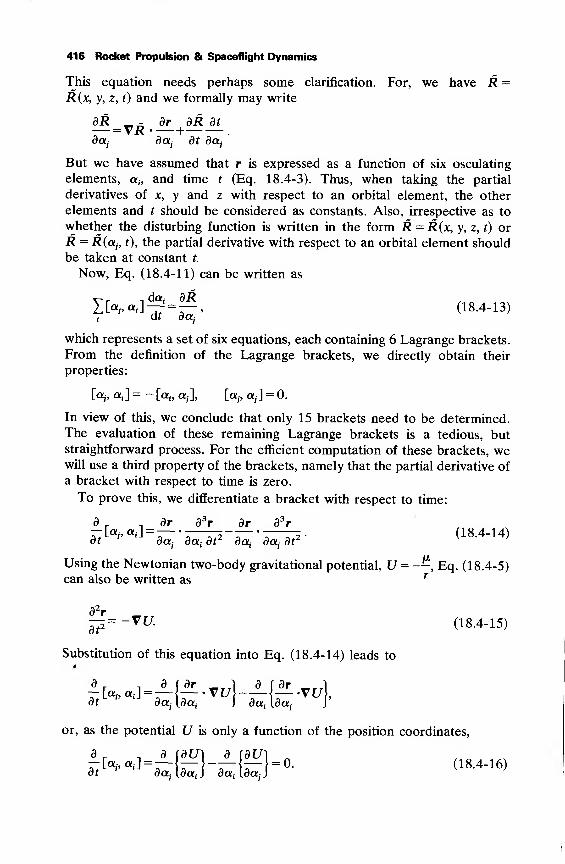
416 Rocket Propulsion & Spaceflight Dynamics
This equation needs perhaps some clarification. For, we have R =R (x, y, z, t) and we formally may write
d& „^ dr dR dt— =VR +.
daj daij dt da,-
But we have assumed that r is expressed as a function of six osculating
elements, at ,
and time t (Eq. 18.4-3). Thus, when taking the partial
derivatives of x, y and z with respect to an orbital element, the other
elements and t should be considered as constants. Also, irrespective as to
whether the disturbing function is written in the form R = R(x, y, z, t) or
R = R(<Xj, t), the partial derivative with respect to an orbital element should
be taken at constant t.
Now, Eq. (18.4-11) can be written as
v^ r ., dat
dR
V^^'w (18 -4- 13)
which represents a set of six equations, each containing 6 Lagrange brackets.
From the definition of the Lagrange brackets, we directly obtain their
properties:
[«j> «J = ~ [«» «,], [«,, a,] = °-
In view of this, we conclude that only 15 brackets need to be determined.
The evaluation of these remaining Lagrange brackets is a tedious, but
straightforward process. For the efficient computation of these brackets, wewill use a third property of the brackets, namely that the partial derivative of
a bracket with respect to time is zero.
To prove this, we differentiate a bracket with respect to time:
dr n
dr d3r dr d
3r~ [«/, «J =— ' 7-^5"— * 7-—i • 18.4-14)
dt d^ datdt da
tda, dt
Using the Newtonian two-body gravitational potential, U=--, Eq. (18.4-5)can also be written as
r
tf=-VU- (18.4-15)
Substitution of this equation into Eq. (18.4-14) leads to
d_
dt ''' dajXdoCi J dotiXdctj \
or, as the potential U is only a function of the position coordinates,
d _ _ d (dU) d (dU) n^• a< ]=4d-^fe) (18 '4" 16)
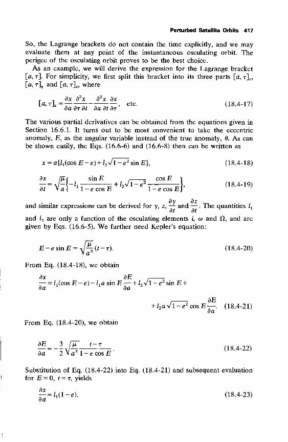
Perturbed Satellite Orbits 417
So, the Lagrange brackets do not contain the time explicitly, and we mayevaluate them at any point of the instantaneous osculating orbit. Theperigee of the osculating orbit proves to be the best choice.
As an example, we will derive the expression for the Lagrange bracket
[a, t]. For simplicity, we first split this bracket into its three parts [a, r]x ,
[a, r]yand [a, t]2 , where
dx b2x d
2x dx
[a,r]x = , etc. (18.4-17)Jxbabrbt babtbT y '
The various partial derivatives can be obtained from the equations given in
Section 16.6.1. It turns out to be most convenient to take the eccentric
anomaly, E, as the angular variable instead of the true anomaly, 0. As can
be shown easily, the Eqs. (16.6-6) and (16.6-8) then can be written as
x = aihicos E-e) + /2Vl-e 2sin E}, (18.4-18)
. cos E i
+ l2Jl-?- -, (18.4-19)1-e cos JEJ
dx [JZ r sin £,
cos Edt~ Vat x 1-e cos E
by bzand similar expressions can be derived for y, z, — and — . The quantities / x
and l2 are only a function of the osculating elements /, w and CI, and are
given by Eqs. (16.6-5). We further need Kepler's equation:
E-esmE=J^z(t-r). (18.4-20)\ a
From Eq. (18.4-18), we obtain
bx bE— = lt (cos E — e) — l r a sinE \-l2 >/l — e2 smE +
ba ba
bE
From Eq. (18.4-20), we obtain
bE 3 rjJT t — r
ba 2 V a 1 — e cos E
+ l2ay/l-e2 cosE—. (18.4-21)
ba
(18.4-22)
Substitution of Eq. (18.4-22) into Eq. (18.4-21) and subsequent evaluation
for E = 0, t = t, yields
^=hiX-e). (18.4-23)ba
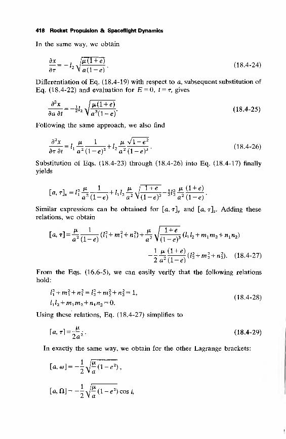
418 Rocket Propulsion & Spaceflight Dynamics
In the same way, we obtain
!h-~~2 Va(l-e)
= -h\\ , • (18.4-24)
Differentiation of Eq. (18.4-19) with respect to a, subsequent substitution of
Eq. (18.4-22) and evaluation for E = 0, t = r, gives
yj-^T—Tv (18.4-25)dad*
22 Va 3(l-e)'
Following the same approach, we also find
d2x ix 1 /u, vl-e 2
a a *=
,i "In ^+^71 ;j. (18.4-26)drdf a z (l-e) a (1-e)
Substitution of Eqs. (18.4-23) through (18.4-26) into Eq. (18.4-17) finally
yields
[a' rL -
/?^(T^ +/l/2^V(T^"^ti(l + e)
a 2 (l-e)12
a 2 V(l-e)3 22a 2 (l-e)'
Similar expressions can be obtained for [a, r]yand [a, t]2 . Adding these
relations, we obtain
r , ju, 1 2 2 , u, jl + e ., ,
La, tJ =^—^ (/i + m ! + nf) +^ y-——5 (/i
/
2 + m xm2 + n t n2)
1 ^ (1 + «), |2 , _ 2 , „ 2
2a 2 (l-e)ai+ml + ni). (18.4-27)
From the Eqs. (16.6-5), we can easily verify that the following relations
hold:
l2 + m 2 +n 2
=ll + ml + nl=l, ,„„ „ „ x22,(18.4-28)
^2+ m 1m2+n 1 n2 = 0.
Using these relations, Eq. (18.4-27) simplifies to
[CL,T] = 2^- (18.4-29)
In exactly the same way, we obtain for the other Lagrange brackets:
2 Va
[a,n]=-iJ^(l-e2)cos;,
2 V a
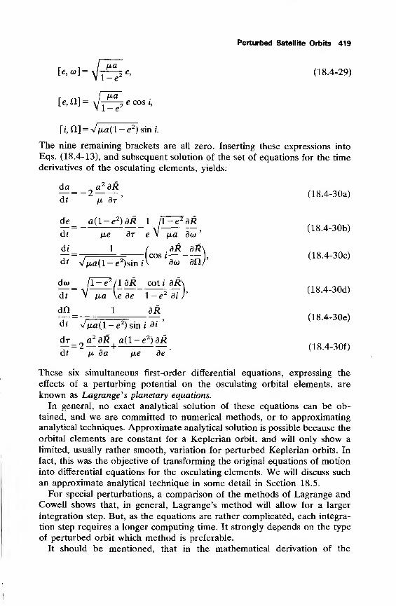
Perturbed Satellite Orbits 419
[e, w]=^YZ^ e> (18.4-29)
[e, ft] =\Y^~2
e cos ''
[i, ft] = v ixa(l — e2) sin i.
The nine remaining brackets are all zero. Inserting these expressions into
Eqs. (18.4-13), and subsequent solution of the set of equations for the time
derivatives of the osculating elements, yields:
da „a 2 dR77= -2—— , 18.4-30a)dt jli dr
de a(l-e 2)dR 1 ll-e2 dR
dt ixe dr e V fxa dco'
di 1 / .dR dR\
(18.4-30b)
dt Vju,a(l-e2)sinA d<o aft/'
da> ll-e 2 /ldR coti dR
cos/ -, (18.4-30c)
dt V fxa \e de 1 — edi
dft 1 dR
^ V/xa(l-e 2)sin i 3i
'
(18.4-30d)
(18.4-30e)
dr ^a 2 dR a(l-e 2)dR— = 2——+— -—. (18.4-30f)dt ja da (xe de
These six simultaneous first-order differential equations, expressing the
effects of a perturbing potential on the osculating orbital elements, are
known as Lagrange's planetary equations.
In general, no exact analytical solution of these equations can be ob-
tained, and we are committed to numerical methods, or to approximating
analytical techniques. Approximate analytical solution is possible because the
orbital elements are constant for a Keplerian orbit, and will only show a
limited, usually rather smooth, variation for perturbed Keplerian orbits. In
fact, this was the objective of transforming the original equations of motion
into differential equations for the osculating elements. We will discuss such
an approximate analytical technique in some detail in Section 18.5.
For special perturbations, a comparison of the methods of Lagrange andCowell shows that, in general, Lagrange's method will allow for a larger
integration step. But, as the equations are rather complicated, each integra-
tion step requires a longer computing time. It strongly depends on the type
of perturbed orbit which method is preferable.
It should be mentioned, that in the mathematical derivation of the
420 Rocket Propulsion & Spaceflight Dynamics
planetary equations, we nowhere assumed the perturbing acceleration to be
small relative to the central acceleration /u,/r2
. Consequently, these equations
can be used whatever the magnitude of the 'perturbing' forces acting on the
satellite may be. However, when the perturbing forces are large with respect
to the central force, the osculating elements will vary over a wide range,
precluding an approximate analytic solution. For numerical integrations, this
method then also loses its advantage over the simpler Cowell formulation.
18.4.2 Modification of the sixth Lagrange equation
There exists a serious inconvenience in the formulation of the equation for
dr— , Eq. (18.4-30f), as will be shown. In the evaluation of the partialat
derivatives — , we have to determine the quantities — . These can be3 a,- dctj
obtained from Kepler's equation, Eq. (18.4-20), which shows E only to be
a function of the elements a, e and t. By taking the derivative of E with
respect to e and t, we obtain expressions where E only appears as the
argument of trigonometric functions:
dE sin £ BE / yu 1
de 1 — ecos-E' dr Va 3 l-ecosE'
However, for the derivative of E with respect to a, we find
dE 3 ma t — T 3 (E - e sin E)3 []i_ t_
2 V a 5 l-eda 2 V a 51 - e cos E 2a (1 - e cos E)
'
Because of the appearance of E outside trigonometric arguments, the
evaluation of the expression for — becomes rather tedious. When thevda
planetary equations are used for general perturbations, the situation is even
worse. Then integrals may result which do not have a closed-form analytical
drsolution. From the Eqs. (18.4-30), we note that only the equation for —
atdR
contains the factor — . A classical artifice exists which circumvents theda
difficulties with this equation. We therefore recall our definition of the meananomaly, M,
M=n(t-r), (18.4-31)
where the mean angular motion, n, is given by
n=>fe'
(18.4-32)
Perturbed Satellite Orbits 421
indicating that n is only a function of a. We now consider n(a) in Kepler's
equation as another distinct variable and rewrite Eq. (18.4-30f) as
dr= 2a^/dR\|
2a 2 dRdn|
a(l-e2) dR
(18 4-33)dt fx \da/n fj>
dn da fxe Be
where the notation I—
) signifies that the derivative has to be taken without
considering the dependence of n on a, or stated in another way, at constant
n or M. We may write
dR_ dRdM_ 8R
Bt~ dM dr~ BM '
_3R_aK_3M_ _ dR
dn dM Bn 9t
or,
!* = _<£=!> I*. (18.4-34)dn n 9t
From Eq. (18.4-32), we obtain
^=-1^. (18.4-35)da 2 a
By differentiating Eq. (18.4-31) with respect to time, we obtain
dM / dr\ . .dn /i0 . _, x
where, according to Eq. (18.4-32),
^=-3^55. (18.4-37)dt 2adt
Substitution of Eqs. (18.4-32) through (18.4-35), Eq. (18.4-37) and Eq.
(18.4-30a) into Eq. (18.4-36), finally leads to
*M, n -l.P*\ -i^!»*. (18.4-38)dt na\da/n na e de
The important property of this equation is that the partial derivative of R
with respect to a is taken at constant n. The term I—J
, which must be
determined in the evaluation of (—) , now becomes (— ) =0 and we avoid
terms in which E does not appear in the arguments of trigonometric
functions. In fact, this is one of the main reasons for using the orbital
element M instead of t in perturbations theories. It should be recognized,
however, thgrt while the orbital elements a, e, i, co, Ct, t are constant in
422 Rocket Propulsion & Spaceflight Dynamics
Keplerian motion, the element M varies linearly with time. When using MdJR
as an orbital element, it is appropriate to replace the factor — in thedr
dRplanetary equations by ——
;, their relation is given by
BR _ IdRdM n dr
(18.4-39)
18.4.3 Other forms of the planetary equations
In the preceding sections, we derived the planetary equations in terms of the
classical orbital elements. As already mentioned in Section 16.5, we can
describe a Keplerian orbit by any other set of six parameters, provided that
the parameters form six independent combinations of the classical elements.
One such set is:
.JL2a
' 0i = -t,
a2 = Vjua(l-e 2), |32 = w, (18.4-40)
a 3 = y/ixa(l-e2) cos i, j83
= fl.
We recognize the parameters a x , a2 and a3 as the Keplerian total energy,
angular momentum and component of the angular momentum about the
z-axis, all per unit mass. In terms of these elements, we find for the
Lagrange brackets
[ai,/3 1 ] = -[|3 1,a 1 ]= -l,
[«2 , j82] = -[|82 , a2] = -1, (18.4-41)
[«3 ,/83] = -[/83 , «3]
= -l,
while all other brackets are zero. The planetary equations then take the
extremely simple form:
da1 _dR d^ _ dR
dt "a/Sj' df~ da^
da2 dR d/32 dR
dT-iS- "5T= "^' (18 -4-42)
da1 _dRLdj33 _ dR
dt 3/33'
df_
da 3
'
A system of equations of this form is called canonical. The function R, in
this case the disturbing function as defined by Eq. (18.4-1), is called the
Perturbed Satellite Orbits 423
perturbed Hamiltonian and the parameters /3;and a
yare said to be canoni-
cally conjugate. Apart from the variables given by Eq. (18.4-40), other sets
of canonical variables are sometimes used in celestial mechanics. The
canonical form of the planetary equations constitutes the basis of nearly all
advanced higher-order theories on perturbed satellite motion. An introduc-
tion to these canonical approaches is presented by Geyling and Westerman
[7].
In deriving the planetary equations, we assumed that the perturbing forces
could be derived from a disturbing potential. In fact, we only made this
assumption to simplify the analytical developments. A careful analysis of the
derivations in Section 18.4.1 will reveal that in case the perturbing forces
cannot be expressed through a potential function, we only have to replace
dR,
dx dy dz— by ax -—\-ay— + az—
,
where ax , ay , az are the magnitudes of the components of the perturbing
acceleration along the x-, y- and z-axis, respectively. The partial derivatives
dx dy dz, . , _ „ ,— , -^-, — can be determined easily and, finally, we obtain planetary
dctj dctj Batj
equations in terms of the perturbing accelerations ax , ay , az . It turns out,
however, to be more convenient to write these equations in terms of other
sets of orthogonal components of the perturbing acceleration. Mostly, weresolve the perturbing acceleration in the components C, S, W or T, N, W,
directed as
C in orbital plane, perpendicular to the radius vector and in the sense of
motion,
S along the radius vector,
W normal to the orbital plane, in the direction of the orbital angular
momentum vector,
T along the velocity vector,
N in the orbital plane perpendicular to the velocity vector and directed
towards the interior of the orbit.
We will not derive these forms of the planetary equations, but simply give
the results:
^ = 24L\se*m6 + cZd* v/Ltp
(18.4-43a)
a 2 V= 2^— T, (18.4-43b)
424 Rocket Propulsion & Spaceflight Dynamics
— = Ir
~ V
di r
S sin 6 + C- (e cos26 + 2 cos 6 + e)
P
d'y/~ilp
dn_ r_
dt~
2T(e+cos 6)-N-sin 1,a J
cos(w + 0)W,
sin (a> + 0)W,ixp sin i
dco dO . 1 [p— = ——cos i— a/—dt dt e V/ut
Scos0-Csm$\l +pn
dO 1= ——cos i+—
dt eV
dM~dt~
2rs-vr
H,a
IT sin +N- (2e +cos 6 + e2cos 0)
P
dco dfl1 cos /
dt dt
n — 2JT=,
vT-esinS-NP
-Vl-e2'd(x> dfl—- H——COS I
.dr df
(18.4-43c)
(18.4-43d)
(18.4-43e)
(18.4-43 f)
(18.4-43g)
(18.4-43h)
(18.4-43i)
(18.4-43J)
where p is the semi-latus rectum, 6 is the true anomaly, r is the magnitude
of the local radius vector and V is the velocity. An elegant, direct derivation
of these equations, without first considering the case of forces expressible
through a potential, is given by Dobson [15] and Fitzpatrick [16].
Planetary equations in terms of orthogonal components of a perturbing
acceleration were first obtained by Gauss in his studies on the motion of the
asteroid Pallas as perturbed by Jupiter [17]. We therefore speak of the
Gauss'1
form of Lagrange's planetary equations. In cases of forces which
cannot be derived from a potential function, e.g. airdrag and rocket thrust,
we have to use these equations instead of Eqs. (18.4-30) to calculate the
effects of these forces on the satellite's orbit. But even when dealing with
perturbing forces expressible through a potential function, the equations in
the Gauss form are mostly preferable when the planetary equations are
integrated numerically.
It should be noticed, that the Eqs. (18.4-30b), (18.4-30d), (18.4-30f),
(18.4-38) and (18.4-43g) through (18.4-43J) contain terms with e in the
denominator. Thus, for small eccentricities, the rates of change of the orbital
elements e, o>, r and M can become very large, unless the associated partial
, • • dR, . , .
derivative— , or perturbing acceleration component, contains a factor e inda,
the numerator. Evaluating the partial derivatives of R, we find that only <o, r
Perturbed Satellite Orbits 425
and M show these large variations. This result is closely connected with thefact that if the eccentricity tends to zero, the elements co, r and M becomeundefined. Similarly, we obtain from Eqs. (18.4-30d), (18.4-30e) and (18.4-43f) through (18.4-43h) that if the inclination becomes very small, largevariations in a> and Cl will occur. Geometrically, this is because ft and (o areundefined for zero inclination.
These large variations are undesirable, both from the viewpoint of numer-ical integrations and, in particular, for the general perturbations approach. It
should, however, be realized that these difficulties have nothing to do withthe method of Lagrange itself. It is solely a consequence of the choice ofparameters to describe a Keplerian orbit. One can always select otherorbital elements for which the corresponding planetary equations do notpresent such bad characteristics in the region of interest [18].
18.5 A simple general perturbations approach
As mentioned already in Section 18.1, there are many methods suggested to
obtain approximate analytical solutions of Lagrange's planetary equations.We will only discuss here a very simple technique: the method of successive
approximations. We note that the planetary equations for the five elementsa, e, i, o) and Cl can be written in a generalized form
dOt;— =e/m(f),f), (18.5-1)
where e is a small quantity, of order of the magnitude of the perturbingacceleration. Integration of Eq. (18.5-1) yields
a((t) = a
io+ ej
/
;(a
y(r), t) dt, (18.5-2)
where aio
is the value of at
at f = 0. We assume that if the perturbingacceleration is small as compared to ixjr
2, its effect on the orbit is also small
over a considerable period of time; i.e., we expect small changes in theosculating elements during this period.
For a first-order solution of Eq. (18.5-2), it is then admissible to substitute
the unperturbed values of the orbital elements into the integral, and weobtain
a\ 1\t) = a
io+ e^fi
(ajo,t)dt. (18.5-3)
Now, the integral can be evaluated and we find an analytical expression for
the first-order variation of atwith time. Substitution of this first-order
variation of the elements into the integral yields for the second-ordervariations:
aP)(0 = aio+ e
J/i(a<
1>(r), t)dt, (18.5-4)
426 Rocket Propulsion & Spaceflight Dynamics
and so on. Of course, we assume this process to converge. Though this
method looks very simple, the analytical labor involved to obtain higher-
order approximations is quite complex.
The differential equation for— presents an additional complication. It
can be written as
^=n(t)+efM(ai(t),t). (18.5-5)
Integration yields
M(t) =M + n(t)dt+e fM (aj (t),t) dt (18.5-6)
The second term on the right-hand side of this equation does not contain the
small multiplicative factor e. Therefore, to obtain a first-order solution of
Eq. (18.5-6), it will suffice to substitute the unperturbed values of a, into the
integral in the third term on the right-hand side of Eq. (18.5-6), but in the
second term we have to include the first-order variation of n. Thus,
Mw (t) =M + [n (1)(r)dr+ef/M(«Jo
, f)df. (18.5-7)
To evaluate the second term on the right-hand side of this equation, we
write
n(t)dt=\ f- -dt. (18.5-8)da y
For a first-order analysis, we use the approximation
4-&JS4 (185 -9)^
H»and thus obtain
[„u)(()d( = „Jd(_gj{^ d(
}d(> (18 . 5 .10)
where in the expression for— the unperturbed values of the elements a, hasdt
to be substituted. This procedure can be extended to obtain higher-order
approximations of M(f). We note that the penalty for replacing t by M, as
performed in Section 18.4.2, is the evaluation of a double integral.
It should be remarked, that, in reality, many perturbing forces act on the
Perturbed Satellite Orbits 427
satellite at the same time. When applying a general perturbations technique,one usually computes the effects of the various perturbing accelerationsseparately. Their joint effects are obtained either by adding them or bytaking the square root of the sum of the individual squared perturbations.There is, however, little theoretical justification for this method, in particu-lar when higher-order approximations are involved. The reason that this
technique is still widely used is that it mostly gives satisfactory results andthat one meets extreme complications when developing a theory that gives ajoint treatment of all perturbing accelerations.
18.6 First-order effects of the asphericity of the Earth
As an example of how this theory can be applied, we will now deriveanalytical expressions for the first-order effects of the asphericity of theEarth on the orbit of a satellite. These effects are the predominate perturba-tions for orbits below some tens of thousands of kilometers altitude, wheresolar and lunar attractions become about equally important. Analytical
expressions for all main orbit perturbations of Earth satellites are presentedby Kampos [19].
The external gravitational potential of the Earth can be expanded in
spherical harmonics in the following way [20]:
I/=-4l- £ /n(^)n
p„(sin$)
"I I JnJ—)
n
p:(sin<D)cosm(A-An;m )l. (18.6-1)n = 2 m = l \ r / J
Here r, 3> and A are the spherical coordinates of the satellite in the
geocentric rotating reference frame (Section 2.3.4): r is the geocentric
radius, 3> is the geocentric latitude and A is the geographic longitude. Thefunction P„(sin<I>) is Legendre's polynomial of degree n in sinO; P™(sin<£)
is the associated Legendre function of degree n and order m. The meanequatorial radius of the Earth is denoted by Re . The quantities Jn , Jnm andA„ m are numerical coefficients. The coefficient J2 takes the value1.082637 xl(T3
, all other /„ and Jnm are of order 10~6 or less [21]. It
should be remarked here, that terms with n = 1 are absent, because of the
assumption that the origin of the reference frame coincides with the center
of mass of the Earth. Also, as the axis of rotation of the Earth, the z-axis of
our reference frame, practically coincides with a principal axis of inertia, the
coefficient J2?i will be extremely small.
We recognize the first term on the right-hand side of Eq. (18.6-1), -— , asr
the classical Newtonian gravitational potential. The series in Legendre'spolynomials constitutes the so-called zonal harmonics. The terms havingJn,m> n^m, as factors are known as the tesseral harmonics; those having Jnm ,
428 Rocket Propulsion & Spaceflight Dynamics
n = m, as the sectorial harmonics. The zonal harmonics describe the devia-
tions in the north-south direction of the potential from a pure Newtonian
one; the tesseral and sectorial harmonics give the deviations in an east-west
direction. The term involving J2 is closely related to the oblateness of the
Earth. The term involving J3 is the one referred to in describing the Earth as
pear-shaped. The term with J22 describes the ellipticity of the Earth's
equator.
We know that it takes one day for the Earth to make one complete
revolution about its axis, while the Keplerian orbit of a satellite keeps a
fixed orientation in inertial space. We thus can imagine that the effects of
the tesseral and sectorial harmonics are more or less 'averaged-out' over
periods longer than one day. For most applications, it is therefore sufficient
to account only for the effects of the zonal harmonics. We then, in fact,
assume the gravitational field of the Earth to be rotational symmetric or
axial symmetric. An important exception is formed by a geostationary
satellite. Because such a satellite always keeps (nearly) the same position
relative to the Earth's surface, its orbit is very sensitive to the east-west
anomalies in the gravitational field, and one certainly may not neglect the
tesseral and sectorial harmonics.
The disturbing function R for the axial symmetric field can, according to
Eq. (18.6-1), be written as
£ = -- I /i-Vi^ (sin 4>). (18.6-2)r
For such an axial symmetric field, two exact integrals of motion can be
obtained.
We note that as in this case R is only a function of r and <£, and not of Aanymore, the gravitational potential is not explicitly dependent on time.
For, when keeping a fixed position in the reference frame, the potential
holds a constant value although the Earth rotates. As such a force field is
conservative, the sum of potential and kinetic energy of the satellite must be
constant,
^ +R= constant. (18.6-3)2a
This expression directly relates the semi-major axis of the osculating orbit to
the local perturbing potential.
A second integral can be obtained as follows. If the magnitude of the
component of the angular momentum about the z-axis is denoted by Hz , wemay write
—(H) = iL{ fl (i - e
2) cos
2i}. (18.6-4)
dt\ yu ) df
daBy evaluating the right-hand side of Eq. (18.6-4), and substituting for —
,
Perturbed Satellite Orbits 429
— and -^ the Eqs. (18.4-30a) through (18.4-30c), we finally obtain
d(Hl\ - [p .dR— =2 \ — COS i—^r.
Because the gravitational field is assumed to be axial symmetric, R is not a
function of ft, and we find for the second integral of motion
Hz= constant. (18.6-5)
These two integrals hold for any axial symmetric field. In the next
discussion, we will limit ourselves to the first-order effects of the Earth's
gravitational field and will therefore only retain the /2-term of the zonal
harmonics.
Evaluating the Legendre polynomial of the second degree and using Eq.
(16.6-27), the disturbing function can be written as
- , , „,, 1 — 3 sin2
i sin2 uR=^J2R 2
e5
, (18.6-6)r
where u is the argument of latitude, u = co + 6. Suppose we want to computethe variation of the orbital element CI due to this disturbing function. We
dRthen have, according to Eq. (18.4-30e), to find an expression for — . As
di
both u and r are independent of i, we directly obtain
BR „ , „_ sin i cos i sin2u— = - 3fjJ2R 2
e5 .
di rJ
By substituting this relation into Eq. (18.4-30e) and replacing the independ-
ent variable t by u, we find
dft « T ^1 cos i sin2u df
,— = -3iiJ2R 2
3 r- —• (18.6-7)du rviip au
For a first-order analysis, all orbital elements on the right-hand side of Eq.
(18.6-7) may be considered as constants, and we write
du d(oj + 6) dO yl~^p mqaq\— =—
—
= -r =——
'
(18.6-8)df dt dt r„
where the index o refers to the unperturbed conditions. Note, that in Eq.
(18.6-8), denotes the angular position of the satellite at a given instant, if
the satellite would follow an unperturbed trajectory with orbital elements
equal to the initial values of the osculating elements of the perturbed orbit.
This is the concept of the unperturbed true anomaly. The difference between
perturbed and unperturbed true anomaly will be proportional to J2 . Because
430 Rocket Propulsion & Spaceflight Dynamics
the right-hand side of Eq. (18.6-7) already contains the factor J2 , and we are
developing a first-order theory, this difference can be neglected in carrying
out the integration.
Substituting Eq. (18.6-8) and
Por=rn =l + e cos (u — (o )
into Eq. (18.6-7), and subsequent integration from w = to u yields
/R \2
CI— Cl = —\J2 \
—
~
) cos i [6m — 3sin2« +\Po/
+ e {6sin (w — a) ) — 3 sin(w + a> )-sin (3w-o> ) + 8sin 0)o }]. (18.6-9)
This equation clearly shows that the variation of Ct with u is composed of a
linear variation, called the secular perturbation, and periodic variations with
periods in the order of the orbital period. These constitute the short-periodic
perturbation. Corresponding relations for the variations of the other orbital
elements can be derived.
As an example, Fig. 18.1 shows the variation of the osculating orbital
elements of the ESRO-satellite TD-lA,,due to the second zonal harmonic,
during its 392nd orbital revolution [22]. This satellite was launched onMarch 12, 1972 into a near-polar, near-circular orbit at an altitude of about
540 km.
The change in CI after one orbital revolution, u = 27r, is according to Eq.
(18.6-9)
A27rn = -37r/J—\ cosi . (18.6-10a)
For the other elements, we find:
A27ra = A2„e = A2J = 0, (18.6-10b)
A27ra> = §ttJ2^2
(5 cos2
i - 1), (18.6-10c)
A27rM=n (^-0 + 37rJ2(^)2(1 + '° C0
2
6>o)3. (18.6-10d)
It should be realized, that when evaluating the first term on the right-hand
side of the last equation, the difference between perturbed and unperturbedtrue anomaly cannot be neglected. Therefore, for the computation of the
change in M between two successive passages through the equatorial plane,
one must substitute for t2v—
1 the so-called nodal period, or draconic period
[23].
The most significant perturbations are the secular effects that appear in <o
and fl. We note from Eq. (18.6-10a) that the orbital plane rotates about the
Earth's polar axis; CI increases for i>90° and decreases for i<90°. The
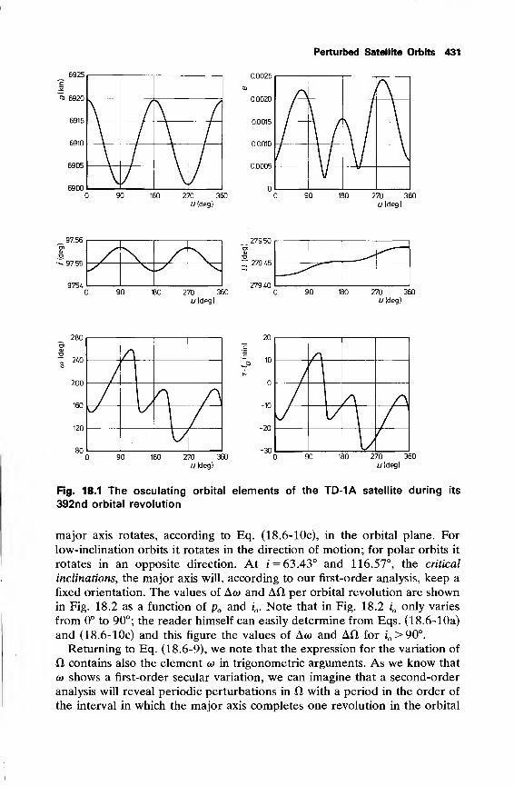
Perturbed Satellite Orbits 431
6925
Fig. 18.1 The osculating orbital elements of the TD-1A satellite during its
392nd orbital revolution
major axis rotates, according to Eq. (18.6-10c), in the orbital plane. For
low-inclination orbits it rotates in the direction of motion; for polar orbits it
rotates in an opposite direction. At i = 63.43° and 116.57°, the critical
inclinations, the major axis will, according to our first-order analysis, keep a
fixed orientation. The values of Aw and Afl per orbital revolution are shownin Fig. 18.2 as a function of p and i . Note that in Fig. 18.2 i only varies
from 0° to 90°; the reader himself can easily determine from Eqs. (18.6-10a)
and (18.6-10c) and this figure the values of Aw and Afl for i'o>90°.
Returning to Eq. (18.6-9), we note that the expression for the variation of
H contains also the element o) in trigonometric arguments. As we know that
(o shows a first-order secular variation, we can imagine that a second-order
analysis will reveal periodic perturbations in CI with a period in the order of
the interval in which the major axis completes one revolution in the orbital
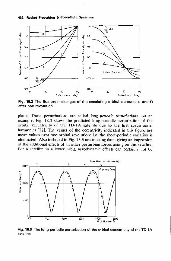
432 Rocket Propulsion & Spaceflight Dynamics
-0.2
=£ "0.3
-0M
-0.5
-0.6
3
16
%y
1.2
0.9
0.6
.° 0.3
-0.6
^4"^N12
~-^
_______3___
Critical Inclination ^^^T"~~
30 60 90
Inclination / (deg)
30 60 90
Inclination / (deg)
Fig. 18.2 The first-order changes of the osculating orbital elements <a and ft
after one revolution
plane. These perturbations are called long-periodic perturbations. As an
example, Fig. 18.3 shows the predicted long-periodic perturbation of the
orbital eccentricity of the TD-1A satellite due to the first seven zonal
harmonics [22]. The values of the eccentricity indicated in this figure are
mean values over one orbital revolution; i.e. the short-periodic variation is
eliminated. Also included in Fig. 18.3 are tracking data, giving an impression
of the additional effects of all other perturbing forces acting on this satellite.
For a satellite in a lower orbit, aerodynamic effects can certainly not be
0.003
y 0.002
0.001
Time After Launch (month)
10
A ©Sk
/ e
•Tracking Data
' \I
500 1500 2500 3500 4500 5500Orbit Number N
Fig. 18.3 The long-periodic perturbation of the orbital eccentricity of the TD-1Asatellite
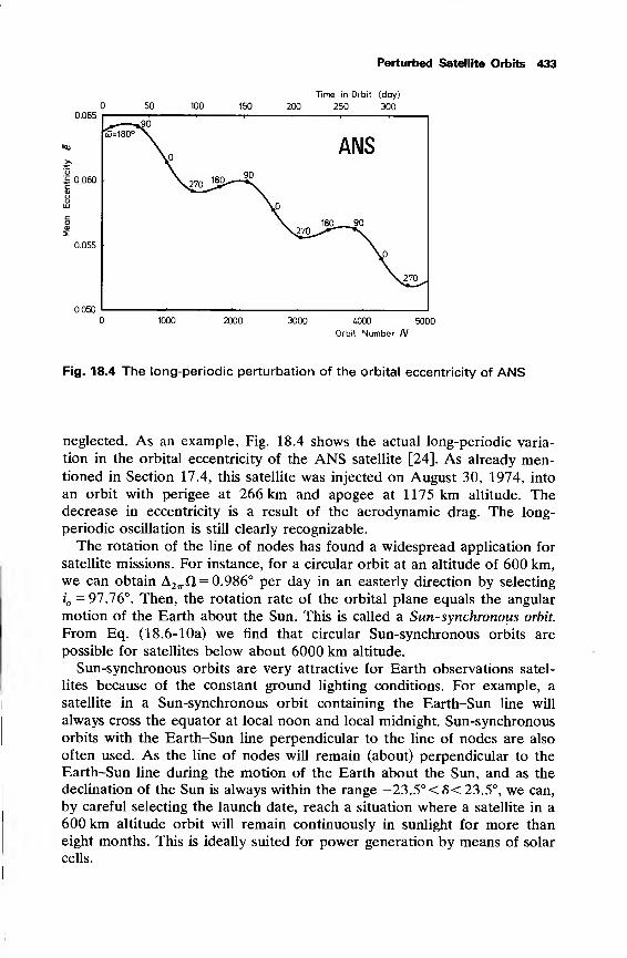
Perturbed Satellite Orbits 433
(
0.065
.fc 0.060cQlUOLU
] 50 100 150 200
Time in Orbit (day)
250 300
d> =180°*§°
VS^70j2^
90
\°
ANS
Co
\2^0,180-90
0.055
nrmn
\270^.
1000 2000 3000 «KX) 5000
Orbit Number N
Fig. 18.4 The long-periodic perturbation of the orbital eccentricity of ANS
neglected. As an example, Fig. 18.4 shows the actual long-periodic varia-
tion in the orbital eccentricity of the ANS satellite [24]. As already men-tioned in Section 17.4, this satellite was injected on August 30, 1974, into
an orbit with perigee at 266 km and apogee at 1175 km altitude. Thedecrease in eccentricity is a result of the aerodynamic drag. The long-
periodic oscillation is still clearly recognizable.
The rotation of the line of nodes has found a widespread application for
satellite missions. For instance, for a circular orbit at an altitude of 600 km,we can obtain A27rO = 0.986° per day in an easterly direction by selecting
i = 97.76°. Then, the rotation rate of the orbital plane equals the angular
motion of the Earth about the Sun. This is called a Sun-synchronous orbit.
From Eq. (18.6- 10a) we find that circular Sun-synchronous orbits are
possible for satellites below about 6000 km altitude.
Sun-synchronous orbits are very attractive for Earth observations satel-
lites because of the constant ground lighting conditions. For example, a
satellite in a Sun-synchronous orbit containing the Earth-Sun line will
always cross the equator at local noon and local midnight. Sun-synchronous
orbits with the Earth-Sun line perpendicular to the line of nodes are also
often used. As the line of nodes will remain (about) perpendicular to the
Earth-Sun line during the motion of the Earth about the Sun, and as the
declination of the Sun is always within the range —23.5°<5< 23.5°, we can,
by careful selecting the launch date, reach a situation where a satellite in a
600 km altitude orbit will remain continuously in sunlight for more than
eight months. This is ideally suited for power generation by means of solar
cells.
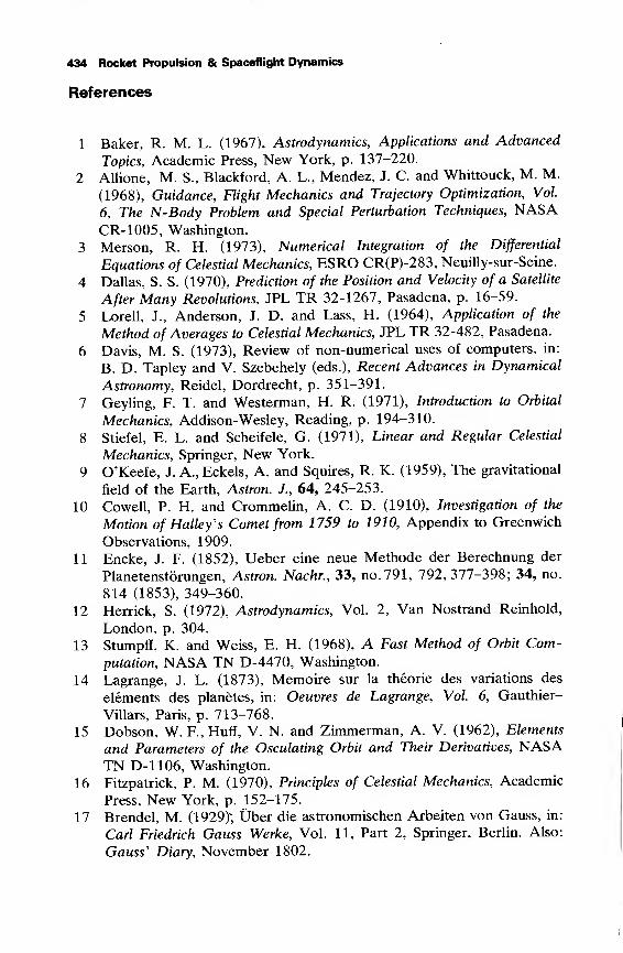
434 Rocket Propulsion & Spaceflight Dynamics
References
1 Baker, R. M. L. (1967), Astrodynamics, Applications and Advanced
Topics, Academic Press, New York, p. 137-220.
2 Allione, M. S., Blackford, A. L., Mendez, J. C. and Whittouck, M. M.
(1968), Guidance, Flight Mechanics and Trajectory Optimization, Vol
6, The N-Body Problem and Special Perturbation Techniques, NASACR-1005, Washington.
3 Merson, R. H. (1973), Numerical Integration of the Differential
Equations of Celestial Mechanics, ESRO CR(P)-283, Neuilly-sur-Seine.
4 Dallas, S. S. (1970), Prediction of the Position and Velocity of a Satellite
After Many Revolutions, JPL TR 32-1267, Pasadena, p. 16-59.
5 Lorell, J., Anderson, J. D. and Lass, H. (1964), Application of the
Method of Averages to Celestial Mechanics, JPL TR 32-482, Pasadena.
6 Davis, M. S. (1973), Review of non-numerical uses of computers, in:
B. D. Tapley and V. Szebehely (eds.), Recent Advances in Dynamical
Astronomy, Reidel, Dordrecht, p. 351-391.
7 Geyling, F. T. and Westerman, H. R. (1971), Introduction to Orbital
Mechanics, Addison-Wesley, Reading, p. 194-310.
8 Stiefel, E. L. and Scheifele, G. (1971), Linear and Regular Celestial
Mechanics, Springer, New York.
9 O'Keefe, J. A., Eckels, A. and Squires, R. K. (1959), The gravitational
field of the Earth, Astron. J., 64, 245-253.
10 Cowell, P. H. and Crommelin, A. C. D. (1910), Investigation of the
Motion of Halley's Comet from 1759 to 1910, Appendix to Greenwich
Observations, 1909.
11 Encke, J. F. (1852), Ueber eine neue Methode der Berechnung der
Planetenstorungen, Astron. Nachr., 33, no. 791, 792, 377-398; 34, no.
814 (1853), 349-360.
12 Herrick, S. (1972), Astrodynamics, Vol. 2, Van Nostrand Reinhold,
London, p. 304.
13 Stumpff, K. and Weiss, E. H. (1968), A Fast Method of Orbit Com-
putation, NASA TN D-4470, Washington.
14 Lagrange, J. L. (1873), Memoire sur la theorie des variations des
elements des planetes, in: Oeuvres de Lagrange, Vol. 6, Gauthier-
Villars, Paris, p. 713-768.
15 Dobson, W. F., Huff, V. N. and Zimmerman, A. V. (1962), Elements
and Parameters of the Osculating Orbit and Their Derivatives, NASATN D-1106, Washington.
16 Fitzpatrick, P. M. (1970), Principles of Celestial Mechanics, Academic
Press, New York, p. 152-175.
17 Brendel, M. (1929); Uber die astronomischen Arbeiten von Gauss, in:
Carl Friedrich Gauss Werke, Vol. 11, Part 2, Springer, Berlin. Also:
Gauss' Diary, November 1802.
Perturbed Satellite Orbits 435
18 Cefola, P. J. (1972), Equinoctial Orbit Elements, Application to ArtificialSatellite Orbits, AIAA Paper 72-937, New York.
19 Kampos, B. (1968), Guidance, Flight Mechanics and Trajectory Op-timization, Vol. 9, General Perturbations Theory, NASA CR-1008,Washington.
20 Wagner, C. A. (1966), The Gravity Potential and Force Field of theEarth Through Fourth Order, NASA TN D-3317, Washington
21 GaposchkhVE. M. (ed.) (1973), 1973 Smithsonian Standard Earth{III), SAO Special Report 353, p. 190, 276, 290-293.
22 Wakker, K. F. and Ambrosius, B. A. C. (1973), Comparison betweenthe Predicted and Actual Orbit of the ESRO -Satellite TD-1A,Memorandum M-202 (in Dutch), Dept. Aerospace Eng., Delft Univer-sity of Technology, Delft.
23 Blitzer, L. (1964), Nodal period of an Earth satellite, AIAA J. 2. no8, 1459.
24 Wakker, K. F. (1977), Orbit Prediction for the Astronomical Nether-lands Satellite, paper presented at the B.I.S. conference on ComputerTechniques for Satellite Control and Data Processing, Slough.
19 Interplanetary Missions
For interplanetary missions, a spacecraft is launched from the Earth and
accelerated to a velocity larger than the local escape velocity. The spacecraft
will then recede from the Earth along a hyperbolic trajectory. While its
distance from the Earth increases, the solar gravitational attraction, gradu-
ally, will become more important until, ultimately, the spacecraft enters a
heliocentric orbit. The trajectory is chosen such that the spacecraft will
perform a specified mission. If the spacecraft has to pass a target planet at a
relatively small distance, we speak of a flyby mission; if the spacecraft
should be decelerated by a rocket engine to enter an orbit about that planet,
we call it an orbiter mission. For a lander mission, the final velocity of the
spacecraft relative to the planet's surface has to be reduced to a very small
value by means of atmospheric braking and/or rocket engine deceleration.
In comparison with Earth satellite missions or lunar flights, interplanetary
missions face higher energy requirements and much longer flight times.
These flight times may range from some months to many years. A reduction
in flight time can only be achieved by advanced propulsion systems [1]
offering a sufficiently high thrust, and exhaust velocities as high as possible.
Without succeeding in the development of such propulsion systems, the
possibilities for interplanetary flight will be rather limited, in particular for
manned missions.
It will be clear that for the actual detailed computation of an interplanet-
ary trajectory, the motion of the spacecraft must be considered as a
many-body problem. Apart from the gravitational attractions of the Earth,
the Sun and the target planet, the attractions of the Moon and many planets
also have to be taken into account. In addition, solar radiation pressure maysubstantially affect the trajectory. Even if one only takes into account the
gravitational attractions of the Earth, the Sun and the target planet, the
analysis of interplanetary trajectories is quite complex. For one has to
determine the spacecraft's injection conditions such that the time of arrival
at the target planet and the spacecraft's position and velocity relative to the
planet closely meet their specified values. The search for the required
interplanetary trajectory can only be made in an iterative way. The first step
in this process is to assume that the interplanetary trajectory is part of a
heliocentric conic section between the centers of the Earth and the target
planet. After a range of possible trajectories is determined, the computa-
tions are extended" assuming that the interplanetary trajectory can be
divided into three Keplerian trajectories. Within the sphere of influence of
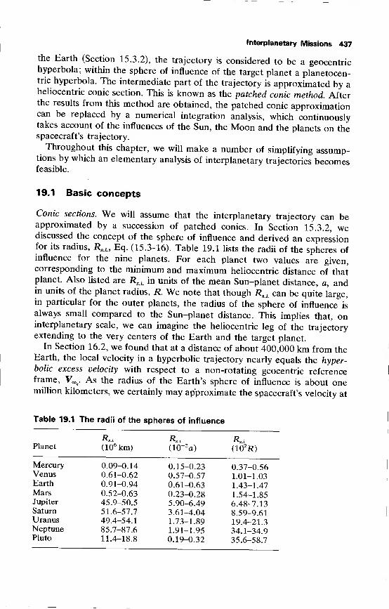
Interplanetary Missions 437
the Harth (Section 15.3.2), the trajectory is considered to be a geocentrichyperbola; within the sphere of influence of the target planet a planetocen-tric hyperbola. The intermediate part of the trajectory is approximated by aheliocentric conic section. This is known as the patched conic method. Afterthe results from this method are obtained, the patched conic approximationcan be replaced by a numerical integration analysis, which continuouslytakes account of the influences of the Sun, the Moon and the planets on thespacecraft's trajectory.
Throughout this chapter, we will make a number of simplifying assump-tions by which an elementary analysis of interplanetary trajectories becomesfeasible.
19.1 Basic concepts
Conic sections. We will assume that the interplanetary trajectory can beapproximated by a succession of patched conies. In Section 15.3.2, wediscussed the concept of the sphere of influence and derived an expressionfor its radius, RsA , Eq. (15.3-16). Table 19.1 lists the radii of the spheres ofinfluence for the nine planets. For each planet two values are given,corresponding to the minimum and maximum heliocentric distance of thatplanet. Also listed are Rsi in units of the mean Sun-planet distance, a, andin units of the planet radius, R. We note that though Rsi can be quite large,in particular for the outer planets, the radius of the sphere of influence is
always small compared to the Sun-planet distance. This implies that, oninterplanetary scale, we can imagine the heliocentric leg of the trajectoryextending to the very centers of the Earth and the target planet.
In Section 16.2, we found that at a distance of about 400,000 km from theEarth, the local velocity in a hyperbolic trajectory nearly equals the hyper-bolic excess velocity with respect to a non-rotating geocentric referenceframe, V^. As the radius of the Earth's sphere of influence is about onemillion kilometers, we certainly may approximate the spacecraft's velocity at
Table 19.1 The radii of the spheres of influence
Rsi Rsi RsiPlanet (10
6 km) (10"2a) (10
2R)
Mercury 0.09-0.14 0.15-0.23 0.37-0.56Venus 0.61-0.62 0.57-0.57 1.01-1.03Earth 0.91-0.94 0.61-0.63 1.43-1.47Mars 0.52-0.63 0.23-0.28 1.54-1.85Jupiter 45.9-50.5 5.90-6.49 6.48-7.13Saturn 51.6-57.7 3.61-4.04 8.59-9.61Uranus 49.4-54.1 1.73-1.89 19.4-21.3Neptune 85.7-87.6 1.91-1.95 34.1-34.9Pluto 11.4-18.8 0.19-0.32 35.6-58.7
438 Rocket Propulsion & Spaceflight Dynamics
the sphere of influence by V^. The required magnitude and direction of V^follows from V«,
e
z=V1- Ve , where Ve is the Earth's orbital velocity and Vx
is the spacecraft's heliocentric velocity at the start of the heliocentric leg;
both relative to a non-rotating heliocentric reference frame. On arrival at
the target planet, the planetocentric hyperbolic excess velocity, VXt , can be
obtained from V^ = V2 — Vt,where V2 is the spacecraft's heliocentric veloc-
ity at crossing the orbit of the target planet and Vt
is the target planet's
orbital velocity.
Planetary orbits. In Section 19.2 we will assume that the planets move in
circular orbits about the Sun and that all planetary orbits lie in the ecliptic
plane. From Table T.3, we note that at first sight this seems an acceptable
simplification; the errors introduced will be largest for Mercury and Pluto,
the orbits of which have both a relatively large inclination and eccentricity.
It turns out, however, that this assumption may yield large errors. In Section
19.3, we will discuss some effects of the inclination and eccentricity of the
planetary orbits on the analysis of interplanetary trajectories.
Parking orbit and impulsive shot. We will assume that the interplanetary
flight starts from a parking orbit about the Earth. For the time being,
chemical propulsion systems will be used exclusively for leaving the Earth
and for deceleration at the target planet. These high-thrust propulsion
systems have relatively short burning-times. We therefore may apply the
concept of an impulsive shot (Section 11.2.3), and assume that due to the
thrust of the rocket engine, the spacecraft experiences an instantaneous
velocity change, leaving the spacecraft's position unaltered. Data on the
errors introduced by this simplification are presented by Willis [2].
Moreover, we assume that the departure from the parking orbit about the
Earth, and the deceleration maneuver to enter an orbit about the target
planet are both accomplished by only one firing of the rocket motor.
The thrusting phase in the initial parking orbit increases the orbital energy
per unit mass, %, of the spacecraft. This energy increase must be attained at
a minimum propellant consumption. So, the question arises: how is an
impulsive velocity increment AV of given magnitude to be applied such
that a maximum A& will result? As the impulsive shot only changes the
velocity of the spacecraft and not its position, we may write
Ag = |(V£-V$aro),
(19.1-1)
where Vpar.
ois the spacecraft's velocity in the parking orbit just before the
impulsive shot and V is the spacecraft's velocity just after the impulsive
shot. We may rewrite Eq. (19.1-1) as
A£ = |(AV )
2 + Vparo• A V . (19.1-2)
From this relation we note that it is most advantageous if the impulsive shot
is applied tangentially to the parking orbit, and at a location in the parking
Interplanetary Missions 439
orbit where the orbital velocity is a maximum. In Section 17.1, however, weargued that a parking orbit altitude will be chosen as low as possible, leadingto circular orbits in which the orbital velocity is constant.For a deceleration maneuver to enter a parking orbit about the target
planet, the same arguments hold. In that case too, the impulse should beapplied at pericenter of the hyperbolic leg and normal to the radius vector.One should keep in mind, however, that operational constraints may forceone to apply other deceleration maneuvers.
19.2 Two-dimensional interplanetary trajectories
As the impulsive shot in the circular parking orbit about the Earth, AV , is
applied tangentially to the parking orbit, we may write for the spacecraft'svelocity just after the impulsive shot, V
,
V =VCo +AVQ , (192 _ 1}
where VCo
is the velocity in the circular parking orbit. In Section 16.2.3, wefound for the relation between local velocity in a hyperbolic trajectory andhyperbolic excess velocity
VJ=VL,+ V5., (192.2)
where VesCo is the local escape velocity. Substituting Eqs. (16.2-3) (16 2-4)and (19.2-2) into Eq. (19.2-1), we obtain
'2*eAWr +VWf' (19-2-3)ro
where r is the radius of the parking orbit and the perigee distance of thehyperbolic escape trajectory. The Earth's gravitation parameter is denotedby ixe .
For the magnitude of the impulse to decelerate the spacecraft in order toenter an orbit about the target planet, we find by the same reasoning
AV3=Avi-Vpar3 > (19.2-4)
where fitis the planet's gravitation parameter, r3 is the pericenter distance
of the hyperbolic trajectory about the planet and Vpar3 is the pericentervelocity just after deceleration. Of course, Vpar3 should be less than the localescape velocity, or Vpar3 <V2ju-(
/r3 . From Eq. (19.2-4), the reader can easilyverify himself that if the only requirement were that of being captured bythe target planet, a final orbit of high eccentricity and very low pericenterdistance is most economical. For orbits with constant pericenter distance,AV3 decreases with increasing values of the eccentricity. In general, there is
an optimal pericenter distance if the eccentricity (or semi-major axis) isfixed.
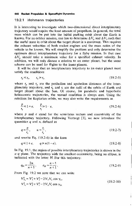
440 Rocket Propulsion & Spaceflight Dynamics
19.2.1 Hohmann trajectories
It is interesting to investigate which two-dimensional direct interplanetary
trajectory would require the least amount of propellant. In general, the total
mass which can be put into the initial parking orbit about the Earth is
known. For an orbiter mission, one has to determine AV and AV3 such that
the useful mass in orbit about the target planet is a maximum. This requires
the exhaust velocities of both rocket engines and the mass ratios of the
vehicle to be known. We will simplify the problem and only determine the
optimum direct interplanetary trajectory for a flyby mission. In that case
AV should take a minimum value for a specified exhaust velocity. In
addition, we will only discuss a mission to an outer planet, but the samescheme can be used for flights to the inner planets.
It will be clear that an interplanetary trajectory to an outer planet must
satisfy the conditions
rP^re , ra ^rt ,
(19.2-5)
where rpand ra are the perihelion and apohelion distances of the inter-
planetary trajectory, and re and rtare the radii of the orbits of Earth and
target planet about the Sun. Of course, for parabolic and hyperbolic
heliocentric trajectories, the second condition is always met. Using the
relations for Keplerian orbits, we may also write the requirements as
-ssl + e, -s*l-e, (19.2-6)re r
t
where p and e stand for the semi-latus rectum and eccentricity of the
interplanetary trajectory. Following Vertregt [3], we now introduce the
quantities q and n, defined as
<?=-, n=~, (19.2-7)' e ' e
and rewrite Eq. (19.2-6) in the form
q^l + e, q^n(l-e). (19.2-8)
In Fig. 19.1, the region of possible interplanetary trajectories is shown in the
e-q plane. The trajectory with the smallest eccentricity, being an ellipse, is
indicated with the letter H. For this trajectory:
2n n — \
«"=^TT'
e»=^i- (19 -2"9)
From Fig. 19.2 we note that we can write
VI =Vi+V2e -2V1Ve cosy 1 ,
„" „ I (19.2-10)V£,= V!+V?-2V2 V,cos72,
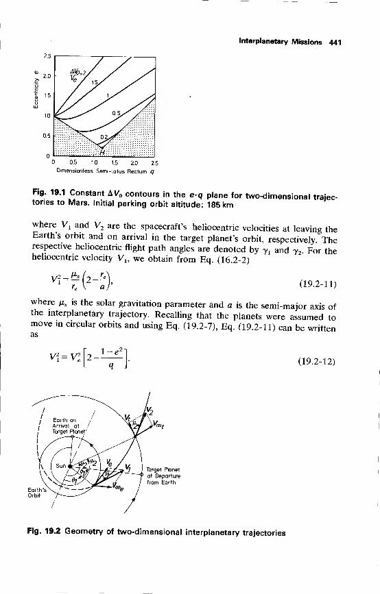
Interplanetary Missions 441
Ve7
05/y/
ssiiSs $Xf
yyyyyyyVly^:-:^ ,H .
2.5
2.0
1.5
1.0
0.5
0.5 1.0 1.5 2.0 2.5
Dimensionless Semi-latus Rectum q
Fig. 19.1 Constant AV contours in the e-q plane for two-dimensional trajec-tories to Mars. Initial parking orbit altitude: 185 km
where Vx and V2 are the spacecraft's heliocentric velocities at leaving the
Earth's orbit and on arrival in the target planet's orbit, respectively Therespective heliocentric flight path angles are denoted by 7l and y2 . For theheliocentric velocity V1? we obtain from Eq. (16.2-2)
v\=^{i- r
A, (19.2-11)
where fis is the solar gravitation parameter and a is the semi-major axis ofthe interplanetary trajectory. Recalling that the planets were assumed tomove in circular orbits and using Eq. (19.2-7), Eq. (19.2-11) can be writtenas
v\=vi 2- l~e:
<\ J(19.2-12)
Fig. 19.2 Geometry of two-dimensional interplanetary trajectories
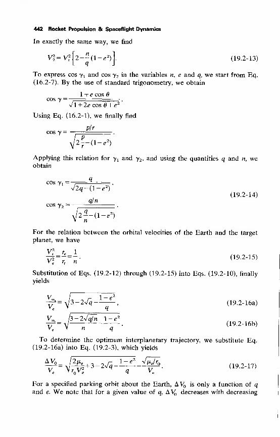
442 Rocket Propulsion & Spaceflight Dynamics
In exactly the same way, we find
VI =V? 2--(l-e 2) (19.2-13)
To express cos yt and cos y2 in the variables n, e and q, we start from Eq.
(16.2-7). By the use of standard trigonometry, we obtain
cos y1 + e cos 6
Vl+2ecos0 + e2
'
Using Eq. (16.2-1), we finally find
p/rcos y
2--(l-e 2)
Applying this relation for yx and y2 , and using the quantities q and n, weobtain
cos yx=
cos y2=
V2q-(l-e 2)'
q/n
2?--(l-e 2)
n
(19.2-14)
For the relation between the orbital velocities of the Earth and the target
planet, we have
V2r, n'
(19.2-15)
Substitution of'Eqs. (19.2-12) through (19.2-15) into Eqs. (19.2-10), finally
yields
$-*-*-¥
v.
3-2Vq/n l-e :
(19.2-16a)
(19.2-16b)
To determine the optimum interplanetary trajectory, we substitute Eq.(19.2-16a) into Eq. (19.2-3), which yields
AVV.
— +3-2Vq—q
— (19.2-17)
For a specified parking orbit about the Earth, AV is only a function of qand e. We note that for a given value of q, A% decreases with decreasing
Interplanetary Missions 443
values of e. So, for a given value of q, AV reaches a minimum if e satisfiesthe boundary conditions (Fig. 19.1):
6 = 1~n
°r e = <*~ 1 - (19.2-18)
Substituting these boundary conditions into Eq. (19.2-17), it can easily be
shown that for q<qH :—-^<0 and for q>qH:^^>0. So, it will beoq dqevident that the point H indicated in Fig. 19.1 represents the minimum -
propellant trajectory. This optimum trajectory is an ellipse, for which
q = n(l~e)=l + e,
or
re re
With Eq. (3.6-27) we can write this relation as
re = a(l-e), rt= a(l + e),
which are the expressions for pericenter and apocenter distances, and weconclude that the optimum interplanetary trajectory is a heliocentric ellipse,tangential to both the Earth's orbit and to the target planet's orbit (y 1
= y2 =0). These minimum-propellant trajectories are called Hohmann trajectories
[4].
In Table 19.2, some parameters of Hohmann trajectories from the Earthto the planets are given. We note that for flights to the planets beyondJupiter the flight time, T, becomes excessive. The parameters Tsyn , ^, ^2and D given in this table are discussed in Section 19.2.2. In Table 19.3,velocity data are summarized for the Hohmann transfers. For comparison^data for a direct heliocentric escape mission are also given. One of theconclusions which can be drawn from this table is that, except for Venus and
Table 19.2 Basic data for Hohmann transfer trajectories from Earth to theplanets
Target n a e T T«Ai if/2 D
planet (AU) (year) (year) (deg) (deg) (AU)
Mercury 0.387 0.6935 0.4419 0.289 0.317 108.3 76.0 0.981Venus 0.723 0.8617 0.1605 0.400 1.599 -54.0 36.0 0.594Mars 1.524 1.2618 0.2075 0.709 2.135 44.3 -75.1 1.594Jupiter 5.202 3.1012 0.6775 2.731 1.092 97.2 -83.0 5.177Saturn 9.548 5.2741 0.8104 6.056 1.035 106.1 159.8 10.492Uranus 19.135 10.0674 0.9007 15.972 1.012 111.3 -169.7 20.120Neptune 30.011 15.5055 0.9355 30.529 1.006 113.2 -10.1 29.027Pluto 39.289 20.1446 0.9504 45.208 1.004 113.9 105.3 39.565
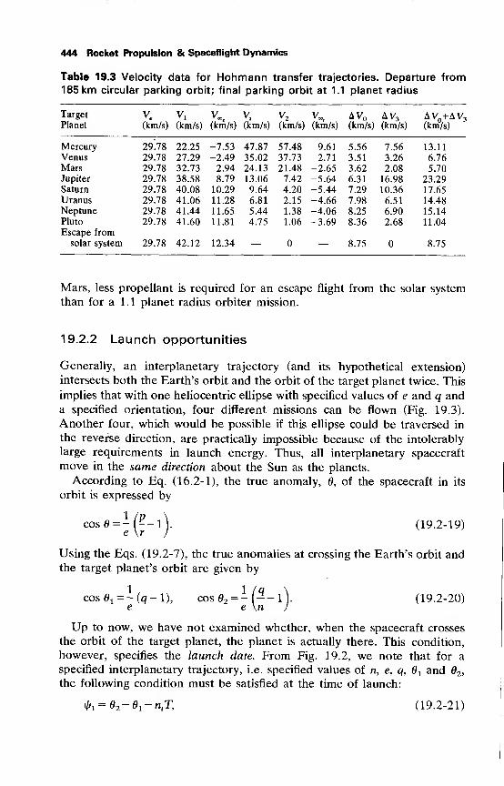
444 Rocket Propulsion & Spaceflight Dynamics
Table 19.3 Velocity data for Hohmann transfer trajectories. Departure from185 km circular parking orbit; final parking orbit at 1.1 planet radius
Target Ve Vt vx v, v2 v. AV AV3 AV +AV3Planet (km/s) (km/s) (km/s) (km/s) (km/s) (km/s) (km/s) (km/s) (km°/s)
Mercury 29/78 22.25 -7.53 47.87 57.48 9.61 5.56 7.56 13.11
Venus 29.78 27.29 -2.49 35.02 37.73 2.71 3.51 3.26 6.76
Mars 29.78 32.73 2.94 24.13 21.48 -2.65 3.62 2.08 5.70
Jupiter 29.78 38.58 8.79 13.06 7.42 -5.64 6.31 16.98 23.29Saturn 29.78 40.08 10.29 9.64 4.20 -5.44 7.29 10.36 17.65
Uranus 29.78 41.06 11.28 6.81 2.15 -4.66 7.98 6.51 14.48
Neptune 29.78 41.44 11.65 5.44 1.38 -4.06 8.25 6.90 15.14
Pluto 29.78 41.60 11.81 4.75 1.06 -3.69 8.36 2.68 11.04
Escape fromsolar system 29.78 42.12 12.34 — — 8.75 8.75
Mars, less propellant is required for an escape flight from the solar system
than for a 1.1 planet radius orbiter mission.
19.2.2 Launch opportunities
Generally, an interplanetary trajectory (and its hypothetical extension)
intersects both the Earth's orbit and the orbit of the target planet twice. This
implies that with one heliocentric ellipse with specified values of e and q anda specified orientation, four different missions can be flown (Fig. 19.3).
Another four, which would be possible if this ellipse could be traversed in
the reverse direction, are practically impossible because of the intolerably
large requirements in launch energy. Thus, all interplanetary spacecraft
move in the same direction about the Sun as the planets.
According to Eq. (16.2-1), the true anomaly, 0, of the spacecraft in its
orbit is expressed by
cos0=-^-l\ (19.2-19)
Using the Eqs. (19.2-7), the true anomalies at crossing the Earth's orbit andthe target planet's orbit are given by
cos01 =-(q-l), cos02 = -(-^-l\ (19.2-20)
e e \n J
Up to now, we have not examined whether, when the spacecraft crosses
the orbit of the target planet, the planet is actually there. This condition,
however, specifies the launch date. From Fig. 19.2, we note that for a
specified interplanetary trajectory, i.e. specified values of n, e, q, 6X and 2 ,
the following condition must be satisfied at the time of launch:
^02-01-ntT, (19.2-21)
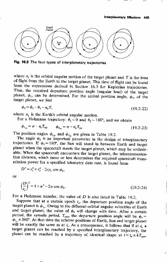
Interplanetary Missions 445
Fig. 19.3 The four types of interplanetary trajectories
where nt
is the orbital angular motion of the target planet and T is the timeof flight from the Earth to the target planet. This time of flight can be foundfrom the expressions derived in Section 16.3 for Keplerian trajectories.Thus, the required departure position angle (angular lead) of the targetplanet, fa, can be determined. For the arrival position angle, fa, of thetarget planet, we find
^2=^2 -^i-ne T, (19.2-22)
where ne is the Earth's orbital angular motion.For a Hohmann trajectory: 0^0 and 2 = 180°, and we obtain
^iH = ^-ntTH, faH = n-neTH. (19.2-23)
The position angles faH and faH are given in Table 19.2.The angle fa is an important parameter in the design of interplanetary
trajectories. If i/r2 =180°, the Sun will stand in between Earth and targetplanet when the spacecraft meets the target planet, which may be undesir-able. When the spacecraft encounters the target planet, the telecommunica-tion distance, which more or less determines the required spacecraft trans-mission power for a specified telemetry data rate, is found from
D 2 = r2 + r
2e -2rt
re cosfa,
or
<D\ 2—J=l + n -2ncos<A2 . (19.2-24)
For a Hohmann transfer, the value of D is also listed in Table 19.2.Suppose that at a certain epoch t , the departure position angle of the
target planet is fa o . Owing to the different orbital angular velocities of Earthand target planet, the value of fa will change with time. After a certainperiod, the synodic period, Tsyn, the departure position angle will be fa =fa. ±360°. At that time the relative positions of Earth, Sun and target planetwill be exactly the same as at t . As a consequence, it follows that if at t atarget planet can be reached by a specified interplanetary trajectory, theplanet can be reached by a trajectory of identical shape at t=t ± kTs n ,
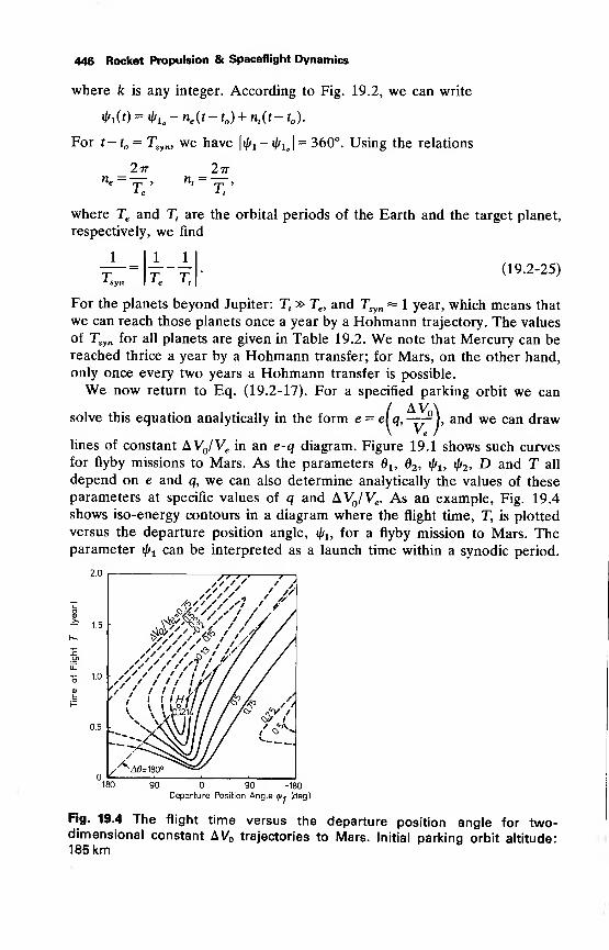
446 Rocket Propulsion & Spaceflight Dynamics
where k is any integer. According to Fig. 19.2, we can write
«M0 =*l>u ~ne (t- t ) + n
t(t-
1
).
For t-t = Tsyn, we have |^i-^ij = 360°. Using the relations
ne =2tt
T ' nt=
2tt
where Te and Ttare the orbital periods of the Earth and the target planet,
respectively, we find
1 J__J_r„ T,
(19.2-25)
For the planets beyond Jupiter: Tt» Te , and Tsyn
== 1 year, which means that
we can reach those planets once a year by a Hohmann trajectory. The values
of Tsyn for all planets are given in Table 19.2. We note that Mercury can bereached thrice a year by a Hohmann transfer; for Mars, on the other hand,only once every two years a Hohmann transfer is possible.
We now return to Eq. (19.2-17). For a specified parking orbit we can
solve this equation analytically in the form e = elq, -r^), and we can draw
lines of constant AV /Ve in an e-q diagram. Figure 19.1 shows such curves
for flyby missions to Mars. As the parameters l5 2 , fa, fa, D and T all
depend on e and q, we can also determine analytically the values of these
parameters at specific values of q and AV /Ve . As an example, Fig. 19.4
shows iso-energy contours in a diagram where the flight time, T, is plotted
versus the departure position angle, fa, for a flyby mission to Mars. Theparameter t/^ can be interpreted as a launch time within a synodic period.
90 -90 -180
Departure Position Angle ^u (deg)
Fig. 19.4 The flight time versus the departure position angle for two-dimensional constant AV trajectories to Mars. Initial parking orbit altitude:185 km
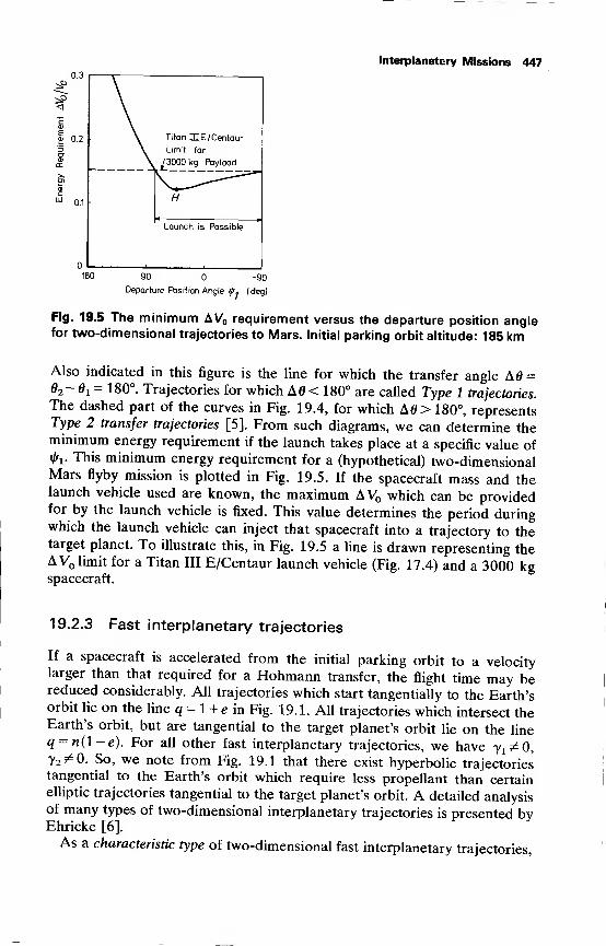
Interplanetary Missions 447
vs>
cai
| 0.2 \ Titan ICE /Centaur
3 \ Limit for
<uor
>n
ai
£0.1
/3000 kg Payload
H
Launch is Possible
180 90 -90
Departure Position Angle </ij (deg)
Fig. 19.5 The minimum AV requirement versus the departure position anglefor two-dimensional trajectories to Mars. Initial parking orbit altitude: 185 km
Also indicated in this figure is the line for which the transfer angle A0 =62 - 0i = 180°. Trajectories for which A0 < 180° are called Type 1 trajectories.
The dashed part of the curves in Fig. 19.4, for which A0> 180°, representsType 2 transfer trajectories [5]. From such diagrams, we can determine theminimum energy requirement if the launch takes place at a specific value of
*Ai- Tnis minimum energy requirement for a (hypothetical) two-dimensionalMars flyby mission is plotted in Fig. 19.5. If the spacecraft mass and thelaunch vehicle used are known, the maximum AV which can be providedfor by the launch vehicle is fixed. This value determines the period duringwhich the launch vehicle can inject that spacecraft into a trajectory to thetarget planet. To illustrate this, in Fig. 19.5 a line is drawn representing theAV limit for a Titan III E/Centaur launch vehicle (Fig. 17.4) and a 3000 kgspacecraft.
19.2.3 Fast interplanetary trajectories
If a spacecraft is accelerated from the initial parking orbit to a velocitylarger than that required for a Hohmann transfer, the flight time may bereduced considerably. All trajectories which start tangentially to the Earth'sorbit lie on the line q = 1 + e in Fig. 19.1. All trajectories which intersect theEarth's orbit, but are tangential to the target planet's orbit lie on the line
q = n(l-e). For all other fast interplanetary trajectories, we have y^O,y2 ^0. So, we note from Fig. 19.1 that there exist hyperbolic trajectoriestangential to the Earth's orbit which require less propellant than certainelliptic trajectories tangential to the target planet's orbit. A detailed analysisof many types of two-dimensional interplanetary trajectories is presented byEhricke [6].
As a characteristic type of two-dimensional fast interplanetary trajectories,
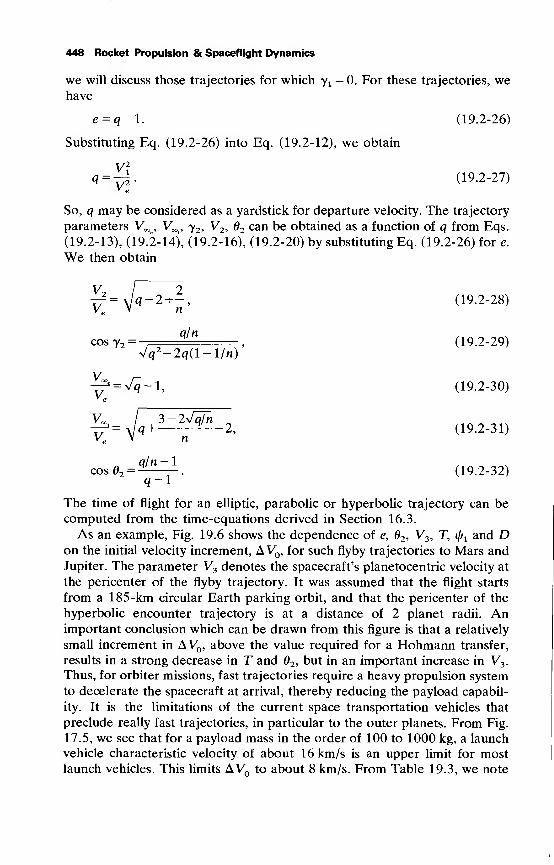
448 Rocket Propulsion & Spaceflight Dynamics
we will discuss those trajectories for which yt= 0. For these trajectories, we
have
e = q-l. (19.2-26)
Substituting Eq. (19.2-26) into Eq. (19.2-12), we obtain
V?q = T^- (19.2-27)
So, q may be considered as a yardstick for departure velocity. The trajectory
parameters V^, V^, y2 , V2 , 62 can be obtained as a function of q from Eqs.
(19.2-13), (19.2-14), (19.2-16), (19.2-20) by substituting Eq. (19.2-26) for e.
We then obtain
£ = Jq-2 + -, (19.2-28)Ve
V n
cos y2 =qlH =
, (19.2-29)<Jq
2 -2q(l-l/n)
^f = Vq-l, (19.2-30)
^ = /, +3z^M_ 2, (19 .2 .31)
cos92 =qln ~}
. (19.2-32)q-1
The time of flight for an elliptic, parabolic or hyperbolic trajectory can be
computed from the time-equations derived in Section 16.3.
As an example, Fig. 19.6 shows the dependence of e, 2 , V3 , T, i(f1 and Don the initial velocity increment, AV , for such flyby trajectories to Mars and
Jupiter. The parameter V3 denotes the spacecraft's planetocentric velocity at
the pericenter of the flyby trajectory. It was assumed that the flight starts
from a 185-km circular Earth parking orbit, and that the pericenter of the
hyperbolic encounter trajectory is at a distance of 2 planet radii. Animportant conclusion which can be drawn from this figure is that a relatively
small increment in AV , above the value required for a Hohmann transfer,
results in a strong decrease in T and 62 , but in an important increase in V3 .
Thus, for orbiter missions, fast trajectories require a heavy propulsion system
to decelerate the spacecraft at arrival, thereby reducing the payload capabil-
ity. It is the limitations of the current space transportation vehicles that
preclude really fast trajectories, in particular to the outer planets. From Fig.
17.5, we see that for a payload mass in the order of 100 to 1000 kg, a launch
vehicle characteristic velocity of about 16 km/s is an upper limit for mostlaunch vehicles. This limits AV to about 8 km/s. From Table 19.3, we note
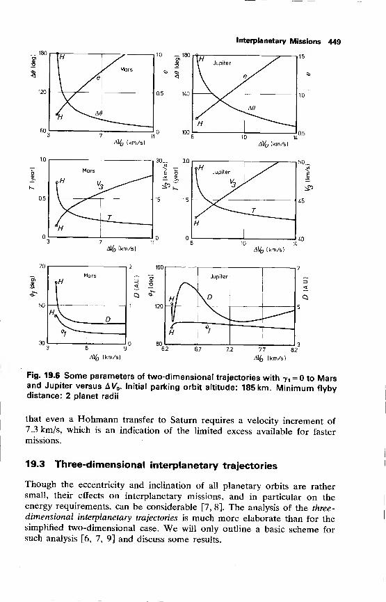
Interplanetary Missions 449
_ 180
1.0
0.5
1.0 _ 180
\ Jupiter
H
Ad
AV (km/s)10 14
AV (km/s)
1.5
1.0
0.5
Mars
?,
*H_J_
30_ 3.0in
E o
15 1.5
1H 1
1 Jupiter
H
T
50
E
^5
45
40
AV (km/s) AV (km/s)
H
Jupiter
H *> '
6.2 6.7 72
AV (km/s)
7.7
AV (km/s)
8.2
Fig. 19.6 Some parameters of two-dimensional trajectories with y, = to Marsand Jupiter versus AVQ . Initial parking orbit altitude: 185 km. Minimum flybydistance: 2 planet radii
that even a Hohmann transfer to Saturn requires a velocity increment of7.3 km/s, which is an indication of the limited excess available for faster
missions.
19.3 Three-dimensional interplanetary trajectories
Though the eccentricity and inclination of all planetary orbits are rathersmall, their effects on interplanetary missions, and in particular on theenergy requirements, can be considerable [7, 8]. The analysis of the three-
dimensional interplanetary trajectories is much more elaborate than for thesimplified two-dimensional case. We will only outline a basic scheme forsuch analysis [6, 7, 9] and discuss some results.
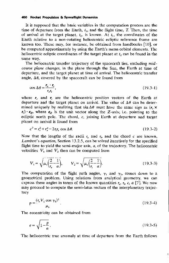
450 Rocket Propulsion & Spaceflight Dynamics
It is supposed that the basic variables in the computation process are the
time of departure from the Earth, tx , and the flight time, T. Then, the time
of arrival at the target planet, t2 , is known. At t1 , the coordinates of the
Earth relative to a non-rotating heliocentric ecliptic reference frame are
known too. These may, for instance, be obtained from handbooks [10], or
be computed approximately by using the Earth's mean orbital elements. Theheliocentric ecliptic coordinates of the target planet at t2 can be found in the
same way.
The heliocentric transfer trajectory of the spacecraft lies, excluding mid-
course plane changes, in the plane through the Sun, the Earth at time of
departure, and the target planet at time of arrival. The heliocentric transfer
angle, A0, covered by the spacecraft can be found from
cosA0=^-^*, (19.3-1)rert
where re and rt
are the heliocentric position vectors of the Earth at
departure and the target planet on arrival. The value of A0 can be deter-
mined uniquely by realizing that sin A0 must have the same sign as (re xrt) ' *z-> where ez is the unit vector along the Z-axis; i.e. pointing to the
ecliptic north pole. The chord, c, joining Earth at departure and target
planet on arrival is found from
c2 = r* + r*-2r
tre cosA6. (19.3-2)
Now that the lengths of the radii re and rt,and the chord c are known,
Lambert's equation, Section 13.2.5, can be solved iteratively for the specified
flight time to yield the semi-major axis, a, of the trajectory. The heliocentric
velocities V! and V2 then can be computed from
V,= J (xs (---\ V2 =JfjLs(---). (19.3-3)
The computation of the flight path angles, yx and y2 , comes down to a
geometrical problem. Using relations from analytical geometry, we can
express these angles in terms of the known quantities re , rt,
c, a [7]. We nowmay proceed to compute the semi-latus rectum of the interplanetary trajec-
tory
^ (r.V, cosy,)2
(1934)Us
The eccentricity can be obtained from
e=Jl-^-. (19.3-5)V a
The heliocentric true anomaly at time of departure from the Earth follows
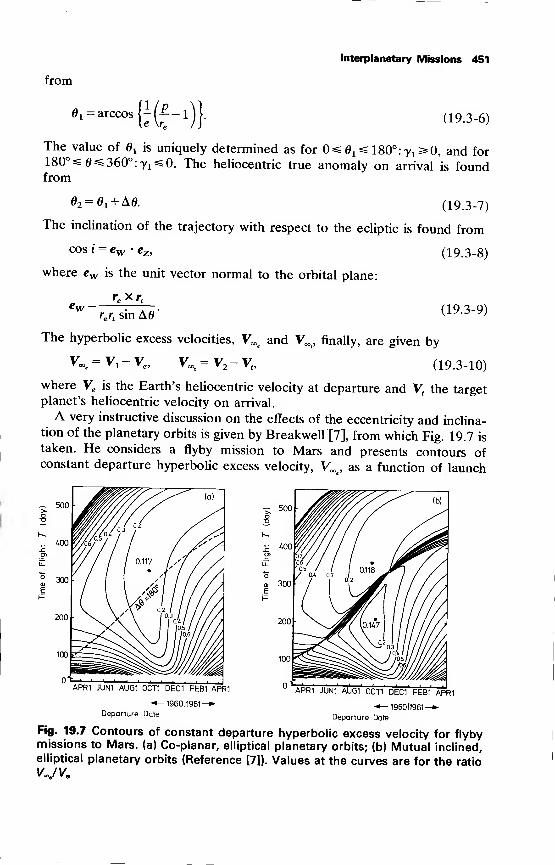
from
B x= arccosee-»
Interplanetary Missions 451
(19.3-6)
The value of e t is uniquely determined as for O^ss 180°:y^ 0, and for180°^ 0^360°: 7^0. The heliocentric true anomaly on arrival is foundfrom
2 =0j + A0. (19.3-7)
The inclination of the trajectory with respect to the ecliptic is found from
cos i = ew • ez, (19.3-8)
where ew is the unit vector normal to the orbital plane:
_ re xrt
•'VV — :
re rt sin A0
The hyperbolic excess velocities, V^ and V^, finally, are given by
(19.3-9)
v-=v,-y„ v^ = v„-v,. (19.3-10)
where Ve is the Earth's heliocentric velocity at departure and Vtthe target
planet's heliocentric velocity on arrival.
A very instructive discussion on the effects of the eccentricity and inclina-tion of the planetary orbits is given by Breakwell [7], from which Fig. 19.7 is
taken. He considers a flyby mission to Mars and presents contours ofconstant departure hyperbolic excess velocity, V^, as a function of launch
APR1 JUN1 AUG1 0CT1 DEC1 FEB1 APR1
-*— 1960J1961—•Departure Date
APR1 JUN1 AUG1 0CT1 DEC1 FEB1
-•—196011961—Departure Date
Fig. 19.7 Contours of constant departure hyperbolic excess velocitymissions to Mars, (a) Co-planar, elliptical planetary orbits; (b) Mutualelliptical planetary orbits (Reference [7]). Values at the curves are for
VJVe
for flyby
inclined,
the ratio
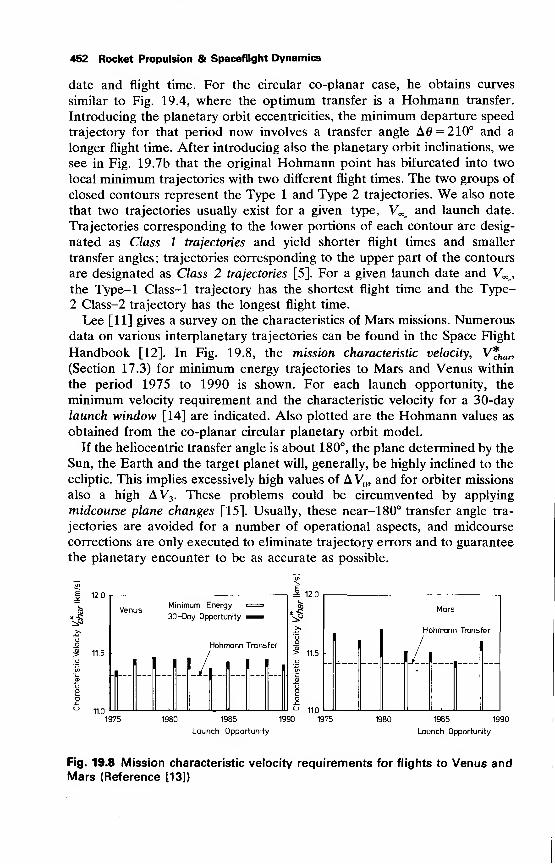
452 Rocket Propulsion & Spaceflight Dynamics
date and flight time. For the circular co-planar case, he obtains curves
similar to Fig. 19.4, where the optimum transfer is a Hohmann transfer.
Introducing the planetary orbit eccentricities, the minimum departure speed
trajectory for that period now involves a transfer angle A0 = 21O° and a
longer flight time. After introducing also the planetary orbit inclinations, wesee in Fig. 19.7b that the original Hohmann point has bifurcated into two
local minimum trajectories with two different flight times. The two groups of
closed contours represent the Type 1 and Type 2 trajectories. We also note
that two trajectories usually exist for a given type, V^ and launch date.
Trajectories corresponding to the lower portions of each contour are desig-
nated as Class 1 trajectories and yield shorter flight times and smaller
transfer angles; trajectories corresponding to the upper part of the contours
are designated as Class 2 trajectories [5]. For a given launch date and V^
,
the Type-1 Class-1 trajectory has the shortest flight time and the Type-2 Class-2 trajectory has the longest flight time.
Lee [11] gives a survey on the characteristics of Mars missions. Numerousdata on various interplanetary trajectories can be found in the Space Flight
Handbook [12]. In Fig. 19.8, the mission characteristic velocity, V*har)(Section 17.3) for minimum energy trajectories to Mars and Venus within
the period 1975 to 1990 is shown. For each launch opportunity, the
minimum velocity requirement and the characteristic velocity for a 30-day
launch window [14] are indicated. Also plotted are the Hohmann values as
obtained from the co-planar circular planetary orbit model.
If the heliocentric transfer angle is about 180°, the plane determined by the
Sun, the Earth and the target planet will, generally, be highly inclined to the
ecliptic. This implies excessively high values of AV , and for orbiter missions
also a high AV3 . These problems could be circumvented by applying
midcourse plane changes [15]. Usually, these near-180° transfer angle tra-
jectories are avoided for a number of operational aspects, and midcourse
corrections are only executed to eliminate trajectory errors and to guarantee
the planetary encounter to be as accurate as possible.
•I
12.0
11.0
1975
Minimum Energy
30 -Day Opportunity
Hohmann Transfer
I I I
12.0
^
11.0
Mars
Hohmann Transfer
1/ I
1980 1985
Launch Opportunity
1990 1975 1980 1985 1990
Launch Opportunity
Fig. 19.8 Mission characteristic velocity requirements for flights to Venus andMars (Reference [13])
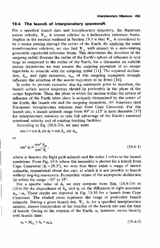
Interplanetary Missions 453
19.4 The launch of interplanetary spacecraft
For a specified launch date and interplanetary trajectory, the departure
excess velocity, V^, is known relative to a heliocentric reference frame.
Implicit in the method outlined in Section 19.3 is that V^ is considered to
be a vector passing through the center of the Earth. By applying the usual
transformation relations, we can find V^ with respect to a non-rotating
geocentric equatorial reference frame. This determines the direction of the
outgoing radial. Because the radius of the Earth's sphere of influence is very
large as compared to the radius of the Earth, for a discussion on suitable
escape trajectories we may assume the outgoing asymptote of an escape
hyperbola to coincide with the outgoing radial [11]. The required declina-
tion, 8as , and right ascension, aas , of this outgoing asymptote strongly
influence the selection of the ascent trajectory to be flown [16].
In order to prevent excessive dog-leg maneuvers prior to injection, the
launch vehicle ascent trajectory should lie preferably in the plane of the
escape hyperbola. Then, the plane in which the motion within the sphere of
influence of the Earth takes place is uniquely determined by the center of
the Earth, the launch site and the outgoing asymptote. All American (and
European) interplanetary missions start from Cape Canaveral. For this
launch site, a launch azimuth range from 90° to 115° is most desirable [17]
for interplanetary missions to take full advantage of the Earth's eastward
rotational velocity and of existing tracking facilities.
According to Eq. (16.6-24), we may write
or
xcording to Eq. (16.6-24), we ma>
cos i = cos 8lsin fa
= cos 8as sin faas
sin2^^r%, (19-4-D™ cos2 Si
where fa denotes trie flight path azimuth and the index I refers to the launch
conditions. From Fig. 19.9, where this inequality is plotted for a launch from
Cape Canaveral (5, = 28.5°), we note that there exists a range of launch
azimuths, symmetrical about due east, at which it is not possible to launch
without dog-leg maneuvers. Permissible values of the asymptotic declination
lie within the range -35° to 35°.
For a specific value of 8h we may compute from Eqs. (16.6-24) to
(16.6-26) the dependence of 8as and faxon the difference in right ascension
aas -a,. These results are depicted in Fig. 19.10 for a launch from Cape
Canaveral. The shaded areas represent the range of preferable launch
azimuths. During a given launch day, V„€
is, for a specified interplanetary
mission, almost independent of the location of the launch site and the time
of launch. Owing to the rotation of the Earth, a,, however, varies linearly
with launch time:
a, = Ho + A, + *>.$, (19.4-2)
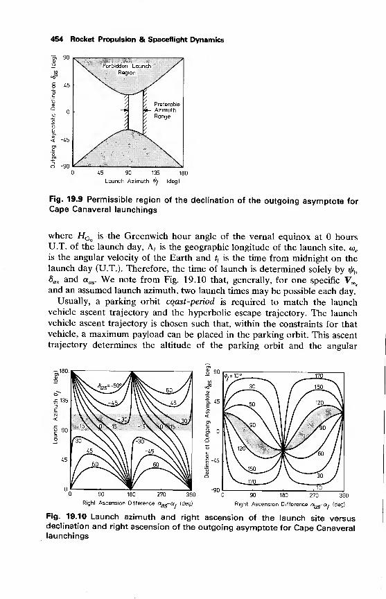
454 Rocket Propulsion & Spaceflight Dynamics
< -45
45 90 135 180
Launch Azimuthty
(deg)
Fig. 19.9 Permissible region of the declination of the outgoing asymptote forCape Canaveral launchings
where HGo is the Greenwich hour angle of the vernal equinox at hoursU.T. of the launch day, A, is the geographic longitude of the launch site, o>e
is the angular velocity of the Earth and tt
is the time from midnight on the
launch day (U.T.). Therefore, the time of launch is determined solely by t/r,,
6as and aas . We note from Fig. 19.10 that, generally, for one specific V^and an assumed launch azimuth, two launch times may be possible each day.
Usually, a parking orbit coast-period is required to match the launchvehicle ascent trajectory and the hyperbolic escape trajectory. The launchvehicle ascent trajectory is chosen such that, within the constraints for that
vehicle, a maximum payload can be placed in the parking orbit. This ascent
trajectory determines the altitude of the parking orbit and the angular
90 180 270 360 90 180 270 360
Right Ascension Difference <*as-a, (deg) Right Ascension Difference aas~a, (deg)
Fig. 19.10 Launch azimuth and right ascension of the launch site versusdeclination and right ascension of the outgoing asymptote for Cape Canaverallaunchings
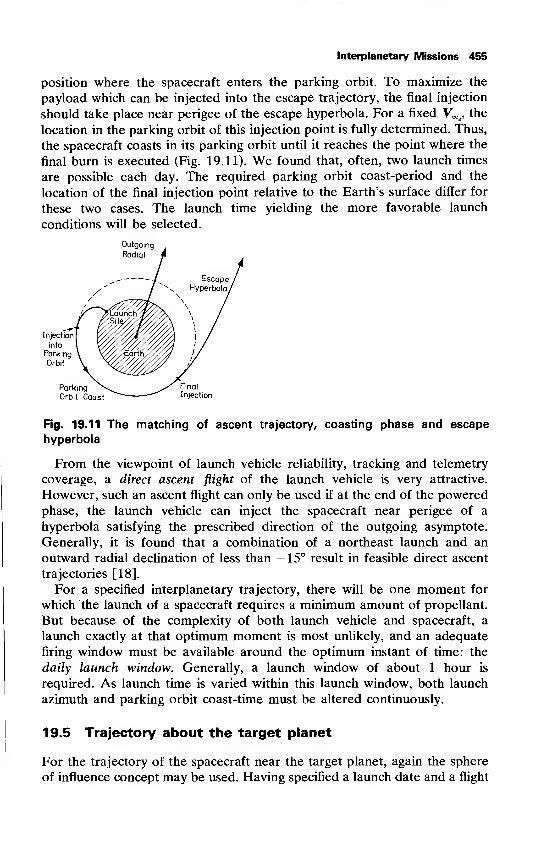
Interplanetary Missions 455
position where the spacecraft enters the parking orbit. To maximize the
payload which can be injected into the escape trajectory, the final injection
should take place near perigee of the escape hyperbola. For a fixed VXe , the
location in the parking orbit of this injection point is fully determined. Thus,
the spacecraft coasts in its parking orbit until it reaches the point where the
final burn is executed (Fig. 19.11). We found that, often, two launch times
are possible each day. The required parking orbit coast-period and the
location of the final injection point relative to the Earth's surface differ for
these two cases. The launch time yielding the more favorable launch
conditions will be selected.
Outgoing
Radial
Fig. 19.11 The matching of ascent trajectory, coasting phase and escape
hyperbola
From the viewpoint of launch vehicle reliability, tracking and telemetry
coverage, a direct ascent flight of the launch vehicle is very attractive.
However, such an ascent flight can only be used if at the end of the powered
phase, the launch vehicle can inject the spacecraft near perigee of a
hyperbola satisfying the prescribed direction of the outgoing asymptote.
Generally, it is found that a combination of a northeast launch and an
outward radial declination of less than —15° result in feasible direct ascent
trajectories [18].
For a specified interplanetary trajectory, there will be one moment for
which the launch of a spacecraft requires a minimum amount of propellant.
But because of the complexity of both launch vehicle and spacecraft, a
launch exactly at that optimum moment is most unlikely, and an adequate
firing window must be available around the optimum instant of time: the
daily launch window. Generally, a launch window of about 1 hour is
required. As launch time is varied within this launch window, both launch
azimuth and parking orbit coast-time must be altered continuously.
19.5 Trajectory about the target planet
For the trajectory of the spacecraft near the target planet, again the sphere
of influence concept may be used. Having specified a launch date and a flight
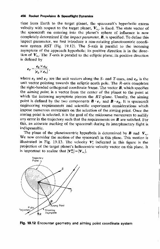
456 Rocket Propulsion & Spaceflight Dynamics
time from Earth to the target planet, the spacecraft's hyperbolic excess
velocity with respect to the target planet, V^, is fixed. The state vector of
the spacecraft on entering into the planet's sphere of influence is nowcompletely determined if the impact parameter, B, is specified. To define this
impact parameter, we first introduce a non-rotating planetocentric coordi-
nate system RST (Fig. 19.12). The S-axis is parallel to the incomingasymptote of the approach hyperbola; its positive direction is in the direc-
tion of V^. The T-axis is parallel to the ecliptic plane; its positive direction
is defined by
eT =ICo x eN
where es and eT are the unit vectors along the S- and T-axes, and eN is theunit vector pointing towards the ecliptic north pole. The i?-axis completesthe right-handed orthogonal coordinate frame. The vector B, which specifies
the aiming point, is a vector from the center of the planet to the point at
which the incoming asymptote pierces the .RT-plane. Usually, the aimingpoint is defined by the two components B • eT and B • eR . It is spacecraft
engineering requirements and scientific experiment considerations whichimpose numerous constraints on the selection of the aiming point. Once the
aiming point is selected, it is the goal of the midcourse maneuvers to nullify
any error in the trajectory such that the requirements on B are satisfied. Forthis, an accurate tracking of the spacecraft during its interplanetary flight is
indispensable.
The plane of the planetocentric hyperbola is determined by B and V^.We now consider the motion of the spacecraft in this plane. This motion is
illustrated in Fig. 19.13. The velocity \\ indicated in this figure is the
projection of the target planet's heliocentric velocity vector on this plane. It
is important to realize that |V*| = Iv^ I.
FlybyTrajectory
-Aiming Point
-IncomingAsymptote
Fig. 19.12 Encounter geometry and aiming point coordinate system
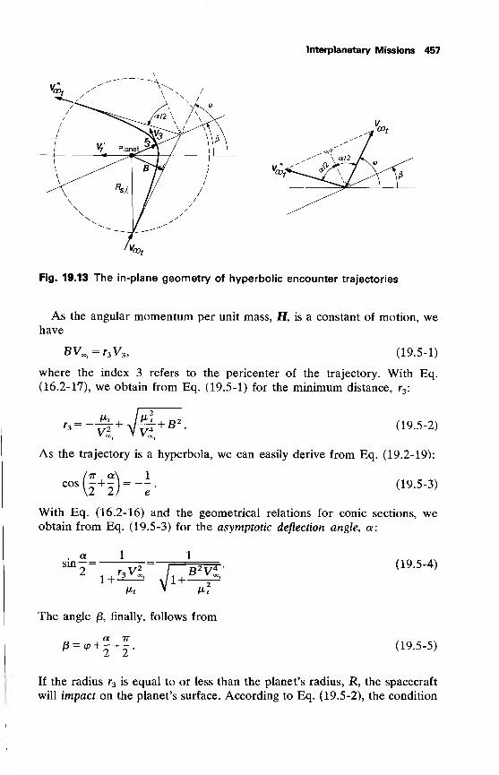
Interplanetary Missions 457
Fig. 19.13 The in-plane geometry of hyperbolic encounter trajectories
As the angular momentum per unit mass, H, is a constant of motion, wehave
BVa>t= r3V3 , (19.5-1)
where the index 3 refers to the pericenter of the trajectory. With Eq.
(16.2-17), we obtain from Eq. (19.5-1) for the minimum distance, r3 :
2' _l D2r3=-^rv^+B
•(19.5-2)
As the trajectory is a hyperbola, we can easily derive from Eq. (19.2-19):
cos (-+-)=--. (19.5-3)
With Eq. (16.2-16) and the geometrical relations for conic sections, weobtain from Eq. (19.5-3) for the asymptotic deflection angle, a:
. a 1sin—
=
2
1
, r3 Vl I B 2 Vl1+—J
V 1+ *-'
The angle /3, finally, follows from
(19.5-4)
anP * 2 2
(19.5-5)
If the radius r3 is equal to or less than the planet's radius, R, the spacecraft
will impact on the planet's surface. According to Eq. (19.5-2), the condition
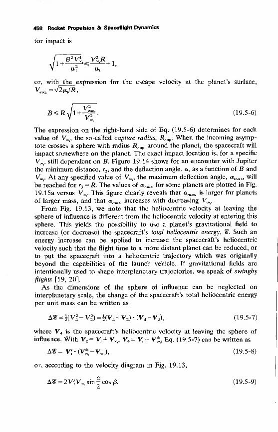
458 Rocket Propulsion & Spaceflight Dynamics
for impact is
V„ B 2 Vi VlR
,1+ 2^—*-+l,
or, with the expression for the escape velocity at the planet's surface,
Vesc =y/2txt/R,
B^R^1+^. (19.5-6)
The expression on the right-hand side of Eq. (19.5-6) determines for each
value of V^, the so-called capture radius, Rcap . When the incoming asymp-
tote crosses a sphere with radius jRcap around the planet, the spacecraft will
impact somewhere on the planet. The exact impact location is, for a specific
Voo,, still dependent on B. Figure 19.14 shows for an encounter with Jupiter
the minimum distance, r3 , and the deflection angle, a, as a function of B and
V^. At any specified value of V^, the maximum deflection angle, amax , will
be reached for r3 = R. The values of amax for some planets are plotted in Fig.
19.15a versus V^. This figure clearly reveals that amax is larger for planets
of larger mass, and that amax increases with decreasing V^.
From Fig. 19.13, we note that the heliocentric velocity at leaving the
sphere of influence is different from the heliocentric velocity at entering this
sphere. This yields the possibility to use a planet's gravitational field to
increase (or decrease) the spacecraft's total heliocentric energy, %. Such an
energy increase can be applied to increase the spacecraft's heliocentric
velocity such that the flight time to a more distant planet can be reduced, or
to put the spacecraft into a heliocentric trajectory which was originally
beyond the capabilities of the launch vehicle. If gravitational fields are
intentionally used to shape interplanetary trajectories, we speak of swingby
flights [19, 20].
As the dimensions of the sphere of influence can be neglected on
interplanetary scale, the change of the spacecraft's total heliocentric energy
per unit mass can be written as
A*=|(V2-V|) = J(V4 +V2)-(V4-V2), (19.5-7)
where V4 is the spacecraft's heliocentric velocity at leaving the sphere of
influence. With V2 = Vt+ V.,, V4=Vt
+ V*, Eq. (19.5-7) can be written as
A&= Vfr(V*t
-VXt ), (19.5-8)
or, according to the velocity diagram in Fig. 19.13,
A^ = 2V^V00isin^cos|8. (19.5-9)
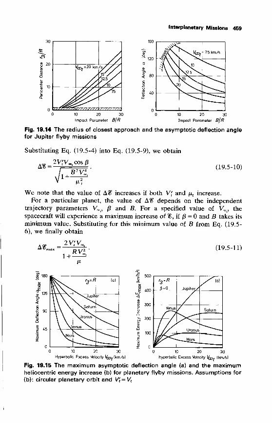
Interplanetary Missions 459
ofzz10 20 30
Impact Parameter BJR10 20 30
Impact Parameter BJR
Fig. 19.14 The radius of closest approach and the asymptotic deflection angle
for Jupiter flyby missions
Substituting Eq. (19.5-4) into Eq. (19.5-9), we obtain
A^^ 2VfV00< cos/3
/ B 2 Vi'
1+^r(19.5-10)
We note that the value of A^ increases if both V[ and jli, increase.
For a particular planet, the value of A^ depends on the independent
trajectory parameters V^, /3 and B. For a specified value of V^, the
spacecraft will experience a maximum increase of %, if /3 = and B takes its
minimum value. Substituting for this minimum value of B from Eq. (19.5-
6), we finally obtain
A£ _ 2Vt'V00[
RVl(19.5-11)
1+-V>
| 180
r3-R (a)
135^\Jupiter
90NySaturn^^
\Uranus N
US
n
\ \Venus ^s.
\Mars^V^
20 30
Hyperbolic Excess Velocity l^pjkm/s)
500
400
300
200
100
r3 -R
/}=0 Jupiter/
y^[b)
VenusSaturn
Uranus
». Mars
20 30
Hyperbolic Excess Velocity\fa,
(km/s)
Fig. 19.15 The maximum asymptotic deflection angle (a) and the maximumheliocentric energy increase (b) for planetary flyby missions. Assumptions for
(b): circular planetary orbit and V't = Vt
460 Rocket Propulsion & Spaceflight Dynamics
For some planets, this relation is plotted in Fig. 19.15b versus V„,t
. For
flights to Mercury, Venus is an attractive swingby planet; for missions to the
outer planets, Mars is unattractive but Jupiter is capable of increasing %considerably. For the actual computation of interplanetary swingby trajec-
tories, the arrival conditions at the swingby planet have to be chosen such
that for a given launch date the spacecraft will meet the (final) target planet
after the specified flight time.
Sometimes, the configuration of a number of planets is such that it is
possible to apply a multiple swingby technique where more gravitational
fields are used to shape the spacecraft's trajectory [21]. The first spacecraft
which intentionally used this swingby technique were Mariner 10 to Venus
and Mercury, and Pioneer 1 1 to Jupiter and Saturn. Undoubtedly, this very
attractive technique will be applied to many more interplanetary missions.
References
1 Moeckel, W. E. (1972), Comparison of Advanced Propulsion Concepts
for Deep Space Exploration, NASA TN D-6968, Washington.
2 Willis, E. A. (1966), Finite-Thrust Escape from and Capture into
Circular and Elliptic Orbits, NASA TN D-3606, Washington.
3 Vertregt, M. (1958), Interplanetary orbits, J. Brit. Interplanet. Soc, 16,
326-354.
4 Hohmann, W. (1925), Die Erreichbarkeit der Himmelskorper, Olden-
bourg, Berlin, p. 63-75. Also: (1960), NASA TT F-44, Washington.
5 Clarke, V. C, Bollman, W. E., Feitis, P. H. and Roth, R. Y. (1963),
Design Parameters for Ballistic Interplanetary Trajectories, JPL TR32-77, Pasadena.
6 Ehricke, K. A. (1962), Space Flight, Vol 2: Dynamics, Van Nostrand,
Princeton, p. 984-1070.
7 Breakwell, J. V., Gillespie, R. W. and Ross, S. (1961), Researches in
interplanetary transfer, A.R.S.J., 31, 201-208.
8 Gravier, J., Marchal, C. and Culp, R. D. (1973), Effects of inclination
and eccentricity on optimal trajectories between Earth and Venus,
Astron. Acta, 18, 273-279.
9 Battin, R. H. (1959), The determination of round-trip planetary recon-
naissance trajectories, J. Aero/Space Sciences, 26, 545-567.
10 Anon., The Astronomical Ephemeris, H.M.S.O., London, new Volumeappears every year.
11 Lee, V. A. and Wilson, S. W. (1967), A survey of ballistic Mars-mission
profiles, /. Spacecraft, 4, 129-142.
12 Anon., Space Flight Handbook, Vol III: Planetary Flight Handbook,
NASA SP-35, Washington, many Parts published since 1963.
13 McGolrick, J. E. (1973), Launch Vehicle Estimating Factors for Ad-vance Mission Planning, NHB 7100.5B, NASA, Washington.
Interplanetary Missions 461
14 Young, A. C. and Odom, P. R. (1967), A Computer Simulation of the
Orbital Launch Window Problem, AIAA Paper 67-615, New York.
15 Fimple, W. R. (1963), Optimum midcourse plane changes for ballistic
interplanetary trajectories, AIAA J., 1, 430-434.
16 Moeckel, W. E. (1959), Departure Trajectories for Interplanetary Vehi-
cles, NASA TN D-80, Washington.
17 Bollman, W. E. (1963), The Engineering Design of Interplanetary Bal-
listic Trajectories, AIAA Paper 63-414, New York.
18 Clarke, V. C. (1963), Design of lunar and interplanetary ascent trajec-
tories, AIAA J., 1, 1559-1567.
19 Flandro, G. A. (1966), Fast reconnaissance missions to the outer solar
system utilizing energy derived from the gravitational field of Jupiter,
Astron. Acta, 12, 329-337.
20 Deerwester, J. M. (1969), Jupiter Swingby Missions to Non-Specific
Locations in Interplanetary Space, NASA TN D-5271, Washington.
21 Bourke, R. D., Friedman, L. D., Penzo, P. A. and Stavro, W. (1971),
Design of Grand Tour Missions, AIAA Paper 71-187, New York.
20 Low-Thrust Trajectories
All current space transportation systems use chemical rocket engines. In
these propulsion systems, the propulsive energy source is contained in the
propellant itself. A very important performance parameter of these systems
is the effective exhaust velocity, c, which is even for the most energetic
propellant combinations limited to about 5 to 6 km/s. There are, however,
other types of propulsion systems feasible. One of them is the electric
propulsion system, where electrically charged particles are accelerated by
electric or magnetic fields. A survey of the various types of electric thrusters
is given by Au [1] and Clark [2]. A number of electric thruster concepts
have been developed during the last twenty years to a level where they can
be applied to a variety of space missions [3]. Many thrusters have already flown
successfully in space. Though, until now, electric motors have been
mainly used for attitude control of satellites and orbit correction purposes,
they will in the future undoubtedly be used as a primary propulsion system for
spacecraft. Unlike the chemical systems, an electric propulsion system
includes a separate power source and power conversion unit to impart the
kinetic energy to the propellant. This power plant, which may comprise a
solid-core nuclear-fission reactor or a large solar array, adds considerably to
the burnout mass of the spacecraft, reducing the payload capability of the
vehicle. Nevertheless, for certain space missions electric propulsion systems
are superior to the chemical ones, due to the fact that the exhaust velocity of
electric systems is much higher than that of chemical motors.
In this chapter, we will deal with the application of electric thrusters to the
propulsion of interplanetary spacecraft. We will restrict ourselves, andmainly discuss the escape flight from the Earth's gravitational field. It should
be realized, however, that the same methods can be applied to the computa-
tion of escape flights from other planets. For a detailed discussion on manyaspects of low-thrust trajectories the reader is referred to Ehricke's standard
work [4].
When designing an electric spacecraft for a particular interplanetary
mission, a maximum payload capability is usually required for a specified
flight time. We thus want to minimize the combined mass of propellant andpower plant. An extensive discussion on the details of such an optimization
process is given by Stuhlinger [5]. Here, we only mention that for each
mission and flight time, an optimum history for the thrust and the exhaust
velocity results. It then appears [5, 6] that for electric propulsion systems,
the optimum values of thrust, F, per initial mass, MQ , and effective exhaust
Low-Thrust Trajectories 463
velocity, c, usually lie within the range:
F— =l(T4-l(r2 m/s2, c = 50-150km/s.M
The electrical power requirement may vary from 10 kW to 10 MW. Thepropellant mass flow will be in the range m = 0.01 — 5 g/s. We note, that the
magnitudes of specific thrust, effective exhaust velocity and mass flow are
entirely different from those for the chemical propulsion systems.
As a direct consequence of the low thrust-to-mass ratio, electric propul-
sion cannot be used to launch a vehicle from the Earth's surface, nor will be
useful if appreciable atmospheric drag is encountered. But if an electrically
propelled stage is launched into a parking orbit about the Earth, even a
minute thrust will force the vehicle to recede gradually from the parking
orbit. Because the low thrust can be maintained for a considerable period of
time, electrically propelled vehicles are capable of attaining very high
velocities.
20.1 Equations of motion
Consider the motion of a spacecraft relative to a non-rotating geocentric
equatorial reference frame. We approximate the gravitational field of the
Earth by an inverse-square force field and assume that, apart from the
gravitational attraction, the thrust, F, is the only force acting dn the
spacecraft. If the instantaneous mass of the spacecraft is denoted by M, the
equation of motion for the vehicle can be written as
df2
r3 M2 +V = 77 > (20.1-1)
where ju, is the gravitation parameter of the Earth and r is the position
vector of the spacecraft.
Vectorial multiplication of Eq. (20.1-1) by r leads to (see Section 3.6.1)
^=rxa, (20.1-2)dr
where H is the (orbital) angular momentum per unit mass, and a is the
thrust acceleration, defined as
«=T7 <2(U -3)M
Scalar multiplication of Eq. (20.1-1) by V yields
— =V-a, (20.1-4)
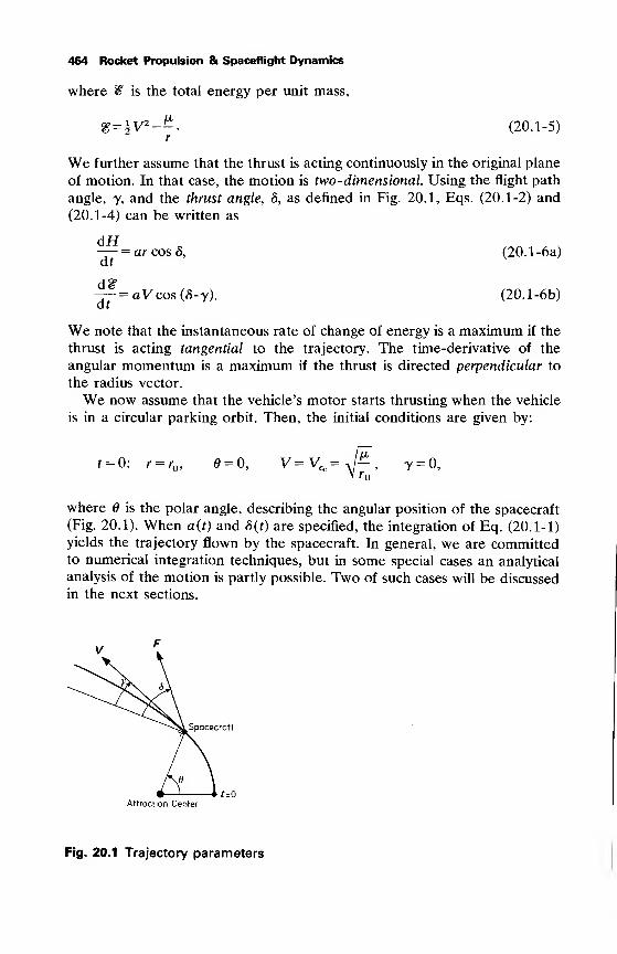
464 Rocket Propulsion & Spaceflight Dynamics
where % is the total energy per unit mass,
g = iy2_^. (20.1-5)r
We further assume that the thrust is acting continuously in the original plane
of motion. In that case, the motion is two-dimensional. Using the flight path
angle, y, and the thrust angle, 8, as defined in Fig. 20.1, Eqs. (20.1-2) and
(20.1-4) can be written as
dH—-=ar cos 8, (20.1 -6a)at
J CjP— =aVcos(S-y). (20.1-6b)at
We note that the instantaneous rate of change of energy is a maximum if the
thrust is acting tangential to the trajectory. The time-derivative of the
angular momentum is a maximum if the thrust is directed perpendicular to
the radius vector.
We now assume that the vehicle's motor starts thrusting when the vehicle
is in a circular parking orbit. Then, the initial conditions are given by:
t = 0: r=r , = 0, V=VCo=J^, y = 0,* fo
where 6 is the polar angle, describing the angular position of the spacecraft
(Fig. 20.1). When a(t) and 8(t) are specified, the integration of Eq. (20.1-1)
yields the trajectory flown by the spacecraft. In general, we are committedto numerical integration techniques, but in some special cases an analytical
analysis of the motion is partly possible. Two of such cases will be discussed
in the next sections.
Spacecraft
Attraction Center
Fig. 20.1 Trajectory parameters
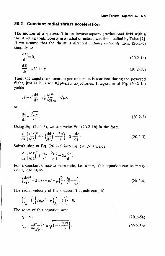
°{-£)= r°'
Low-Thrust Trajectories 465
20.2 Constant radial thrust acceleration
The motion of a spacecraft in an inverse-square gravitational field with a
thrust acting continuously in a radial direction, was first studied by Tsien [7].
If we assume that the thrust is directed radially outwards, Eqs. (20.1-6)
simplify to
^7 = 0, (20.2-la)
— = aVsiny. (20.2-lb)
Thus, the angular momentum per unit mass is constant during the poweredflight, just as it is for Keplerian trajectories. Integration of Eq. (20.2-la)
yields
2 dd 2 /d6\H = r — = rdt
or
d0 vurn37--£* (20 -2-2)
Using Eq. (20.1-5), we can write Eq. (20.2-lb) in the form
^{U) +r U)-f] =2ad7-
(20 -2-3>
Substitution of Eq. (20.2-2) into Eq. (20.2-3) yields
dtWdt) r2
r ILa
dt'
For a constant thrust-to-mass ratio, i.e. a = a , this equation can be integ-
rated, leading to
vr r2
r
The radial velocity of the spacecraft equals zero, if
\dt)= 2ao(r-ro) + n( Z-^-Th (20.2-4)
t 1)^2-^- 1^ -
The roots of this equation are:
ri = r, (20.2-5a)
r^jM^Jl-8^}. (20.2-5b)
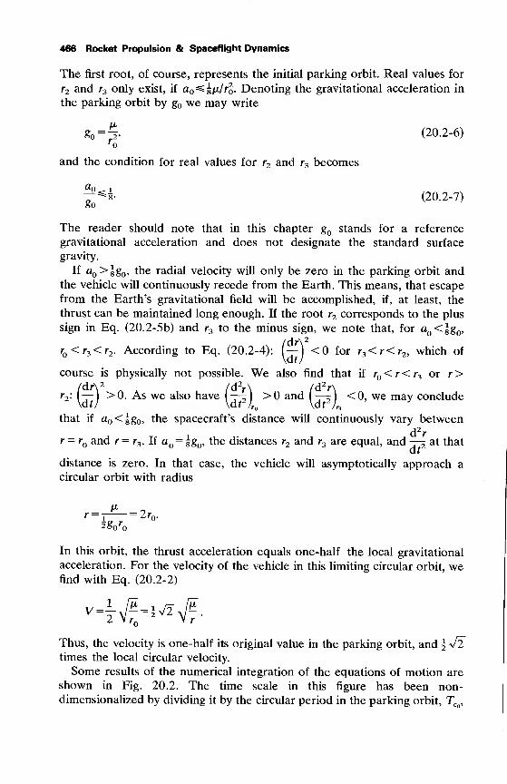
466 Rocket Propulsion & Spaceflight Dynamics
The first root, of course, represents the initial parking orbit. Real values for
r2 and r3 only exist, if a =^gja/ro- Denoting the gravitational acceleration in
the parking orbit by g we may write
'0 „2'
and the condition for real values for r9 and r, becomes
«o:
go
(20.2-6)
(20.2-7)
The reader should note that in this chapter g stands for a reference
gravitational acceleration and does not designate the standard surface
gravity.
If a >gg , the radial velocity will only be zero in the parking orbit andthe vehicle will continuously recede from the Earth. This means, that escape
from the Earth's gravitational field will be accomplished, if, at least, the
thrust can be maintained long enough. If the root r2 corresponds to the plus
sign in Eq. (20.2-5b) and r3 to the minus sign, we note that, for a <lg ,
/dr\ 2
r <r3 <r2 . According to Eq. (20.2-4): (— J <0 for r3 <r<r2 , which of
course is physically not possible. We also find that if r <r<r3 or r>
r2 : I—
) >0. As we also have (t^) >0 and (t^) <0> we may conclude
that if a <gg , the spacecraft's distance will continuously vary between
d2r
r = r and r = r3 . If a = ^g , the distances r2 and r3 are equal, and —-^ at that
distance is zero. In that case, the vehicle will asymptotically approach a
circular orbit with radius
= 2rn' i ^'o-2g r
In this orbit, the thrust acceleration equals one-half the local gravitational
acceleration. For the velocity of the vehicle in this limiting circular orbit, wefind with Eq. (20.2-2)
2 V r V r
Thus, the velocity is one-half its original value in the parking orbit, and \ 4ltimes the local circular velocity.
Some results of the numerical integration of the equations of motion are
shown in Fig. 20.2. The time scale in this figure has been non-dimensionalized by dividing it by the circular period in the parking orbit, TCo ,
Low-Thrust Trajectories 467
Fig. 20.2 Trajectories with constant radial thrust accelerations
given by
Tc =2tta - (20.2-8)
The variation of velocity with distance can be obtained as follows. First,
we write
"-©''STand then substitute Eqs. (20.2-2) and (20.2-4), which yields
Wc / g \r J r
In Fig. 20.3, this relation is depicted for some values of ajg . Also shown
(20.2-9)
Distance rjr
Fig. 20.3 Velocity ratio as a function of radial distance for constant radial thrust
accelerations
468 Rocket Propulsion & Spaceflight Dynamics
are curves for the local circular velocity, Vc , and the local escape velocity,
Vesc . We note that if a /g <l, the velocity first decreases to a minimum
value and for ajg >l increases again at larger distances. If ajg >l, the
vehicle reaches the local escape velocity at a distance
L\ =1+_L_. (20.2-10)
' esc "<- ^o' &0
For an analysis of the variation of angular position, 0, with distance the
reader is referred to Copeland [8].
Though radial thrust may be of some interest for certain orbital maneuv-
ers, it will not play a significant role as the propulsion mode for interplanet-
ary missions. The thrust level required to escape from the Earth's gravita-
tional field with radial thrust is much higher than can be achieved with
present technology.
20.3 Constant tangential thrust
The problem of programming the thrust direction of a low-thrust spacecraft
to permit its escape from a low-altitude circular parking orbit with the
minimum expenditure of propellant has been studied by many authors.
Among the various analytical solutions available, both for constant thrust
and constant thrust acceleration, in particular the publications of Lawden
[9], Breakwell and Rauch [10] and Reidelhuber and Schwenzfeger [11]
should be mentioned. These studies reveal that the actual optimal thrust
direction varies with time in quite a complex way. They, however, also show
that a tangential thrust is very close to the optimum thrust direction. In this
section, we will consider the case of constant tangential thrust.
It should be realized that the tangential thrust steering is only near
optimal if the thrust acceleration is very small relative to the local gravita-
tional acceleration. If the vehicle moves on an interplanetary trajectory
about the Sun, the situation is quite different. As at the distance of the Earth
from the Sun, the gravitational acceleration of the solar field is about
5.9xl0_3 m/s2 , a thrust acceleration of 10~3 m/s2 corresponds to about
one-sixth local gravitational acceleration just outside the Earth's sphere of
influence. For this relatively high value, the tangential steering not necessar-
ily approximates the real optimum thrust program anymore. The determina-
tion of optimal interplanetary trajectories is furthermore hampered if the
vehicle has to encounter another celestial body, leading to two-point bound-
ary value problems. Melbourne [12, 13] presents examples of such optimal
interplanetary trajectories.
Low-Thrust Trajectories 469
20.3.1 Characteristics of the motion
For a tangential thrust, Eqs. (20.1-6) simplify to
— = ar cos y, (20.3-la)dt
— = aV. (20.3-lb)dt
If both the thrust and the effective exhaust velocity are constant, the
instantaneous thrust acceleration is given by
(20.3-2)\ — a tlc
and we note that the thrust acceleration slowly increases with time. Using
Eq. (20.1-5), we can write Eq. (20.3-lb) in the form
dV ^,dr
dt r2dt
V— + Il— =aV,
or
dV f*— =a—dt r
a-^siny. (20.3-3)
For the variation of distance, r, and angular position, 0, with time, we maywrite
^=Vsiny, (20.3-4)dt
de v— = -cosy. (20.3-5)dt r
Equation (20.3-la) can also be written as
— (rV cos y) = ar cos y.dt
Substitution of Eqs. (20.3-3) and (20.3-4) into this relation, finally yields
A
fr7vKtW <20 -3-6>
The Eqs. (20.3-3) to (20.3-6) constitute a set of four first-order differential
equations, describing the variation of r, 0, V and 7 with time.
In Fig. 20.4, parameters representing distance, polar angle, velocity andflight path angle are plotted as a function of time for about one revolution.
The notation A stands for the difference between the actual value of a
parameter and its value at f = 0. Because in the initial parking orbit, the
polar angle, 6, increases linearly with time, for the variation of 6 due to the
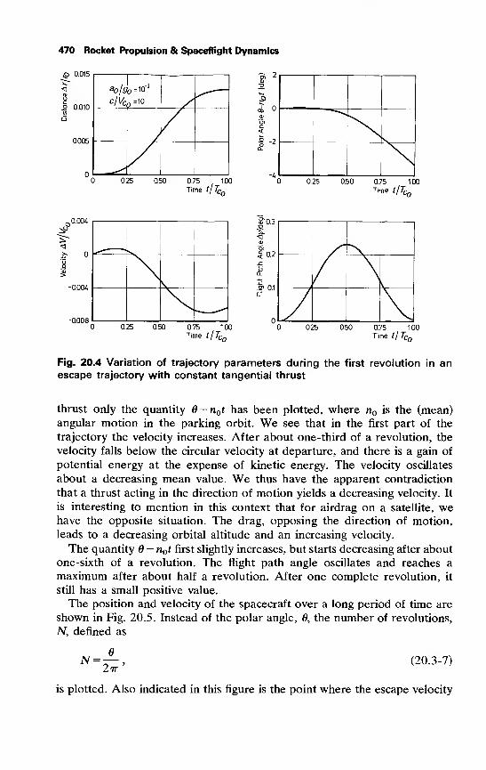
470 Rocket Propulsion & Spaceflight Dynamics
S 0.015
2 0.010
0.005
0.25 0.50 0.75 1.00
Time tJTCo
S1
"
<4 o
C
a _2<£
-L0.25 0.50 0.75 1.00
Time t/TC()
. 0.004
-0.004
-0.008
$03
0)
|0.2
£
H> 0.1
LL
0.25 0.50 0.75 1.00
Time t/TCo
0.25 0.50 0.75
Time t] TCq100
Fig. 20.4 Variation of trajectory parameters during the first revolution in anescape trajectory with constant tangential thrust
thrust only the quantity 6 — n t has been plotted, where n is the (mean)angular motion in the parking orbit. We see that in the first part of the
trajectory the velocity increases. After about one-third of a revolution, the
velocity falls below the circular velocity at departure, and there is a gain of
potential energy at the expense of kinetic energy. The velocity oscillates
about a decreasing mean value. We thus have the apparent contradiction
that a thrust acting in the direction of motion yields a decreasing velocity. It
is interesting to mention in this context that for airdrag on a satellite, wehave the opposite situation. The drag, opposing the direction of motion,
leads to a decreasing orbital altitude and an increasing velocity.
The quantity — n t first slightly increases, but starts decreasing after about
one-sixth of a revolution. The flight path angle oscillates and reaches a
maximum after about half a revolution. After one complete revolution, it
still has a small positive value.
The position and velocity of the spacecraft over a long period of time are
shown in Fig. 20.5. Instead of the polar angle, 8, the number of revolutions,
N, defined as
N = J_2 77-'
(20.3-7)
is plotted. Also indicated in this figure is the point where the escape velocity
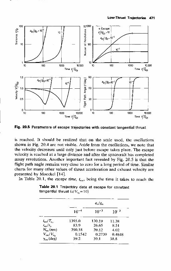
Low-Thrust Trajectories 471
1000 10.000 10
Time t\TCo
_ 90
£ 60
1000 10.000
Time tjTCo
o- 30
1000 10.000
Time tjTCc'CO
1000 10.000
Time tlTn,'CO
Fig. 20.5 Parameters of escape trajectories with constant tangential thrust
is reached. It should be realized that on the scale used, the oscillations
shown in Fig. 20.4 are not visible. Aside from the oscillations, we note that
the velocity decreases until only just before escape takes place. The escape
velocity is reached at a large distance and after the spacecraft has completedmany revolutions. Another important fact revealed by Fig. 20.5 is that the
flight path angle remains very close to zero for a long period of time. Similar
charts for many other values of thrust acceleration and exhaust velocity are
presented by Moeckel [14].
In Table 20.1, the escape time, tesc, being the time it takes to reach the
Table 20.1 Trajectdry data at escape for constanttangential thrust (c/V =10)
ITCote,
reSc/r
V IVr esc* y Cq
Yesc(deg)
10-
ao/ go
10"
1395.0
83.9
390.18
0.1542
39.2
130.19
26.65
39.12
0.2739
39.1
10"
11.38
8.51
4.02
0.4848
38.8
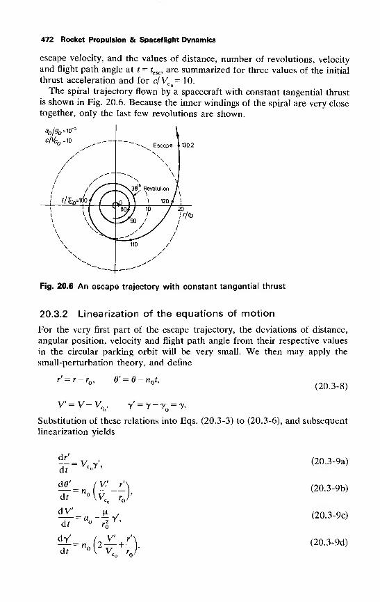
472 Rocket Propulsion & Spaceflight Dynamics
escape velocity, and the values of distance, number of revolutions, velocity
and flight path angle at t = tesc , are summarized for three values of the initial
thrust acceleration and for cjVr =10.The spiral trajectory flown by a spacecraft with constant tangential thrust
is shown in Fig. 20.6. Because the inner windings of the spiral are very close
together, only the last few revolutions are shown.
V5b= 10"3
\~~~~-^ Escapec/VCo =10 ^-^
130.2
/ X/ N
/ \/ \
/ \//
^~" ~"~~^ N1
/ / ,
iff\ \\
/
;
«/^\38 . Revolution A
1 '/£„= 00 i ( , \0 \\ \120/ !
1
1
f1 ( 80/ / 10 / 20
\
\
\ V V ^V ' / irlrO
\ \\ / / 1\
\\\
s\ ^^ 1=^--^ /110 /
/\
—"""- —-""
Fig. 20.6 An escape trajectory with constant tangential thrust
20.3.2 Linearization of the equations of motion
For the very first part of the escape trajectory, the deviations of distance,
angular position, velocity and flight path angle from their respective values
in the circular parking orbit will be very small. We then may apply the
small-perturbation theory, and define
ro>
v=v-ve _,
e' = e- n t,
(20.3-8)
y =y-7 = y-
Substitution of these relations into Eqs. (20.3-3) to (20.3-6), and subsequent
linearization yields
dr'= VcJ,
dr' c J J
dd'
dr vv c 'o'
dVdr '0
dy'
dr v Y c '0
(20.3-9a)
(20.3-9b)
(20.3-9c)
(20.3-9d)
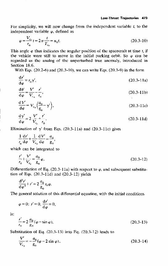
Low-Thrust Trajectories 473
For simplicity, we will now change from the independent variable t, to the
independent variable <p, defined as
(p=Y±o
t = 2Tr r =n t. (20.3-10)r *c
This angle q> thus indicates the angular position of the spacecraft at time t, if
the vehicle were still to move in the initial parking orbit. So <p can be
regarded as the analog of the unperturbed true anomaly, introduced in
Section 18.6.
With Eqs. (20.2-6) and (20.3-10), we can write Eqs. (20.3-9) in the form
^=r V, (20.3-1 la)
d <P vc r' (20.3-llb)
dy' V r'
-r-=2— + -. (20.3-lld)d <P vc r
o
Elimination of y' from Eqs. (20.3-1 la) and (20.3-1 lc) gives
J_d/ 1 dV _qrod<p V
Codcp g
'
which can be integrated to
r' V a
7+V = f<P- (20.3-12)
'0 v c S
Differentiation of Eq. (20.3- 11a) with respect to <p, and subsequent substitu-
tion of Eqs. (20.3-lld) and (20.3-12) yields
dV , „ a
d <P go
The general solution of this differential equation, with the initial conditions
<P= 0: r' = 0,^ = 0,
d<p
is:
r' a- = 2-2 (<p-sin<p). (20.3-13)r go
Substitution of Eq. (20.3-13) into Eq. (20.3-12) leads to
TT=-— (<p-2sin<p). (20.3-14)*c S*o
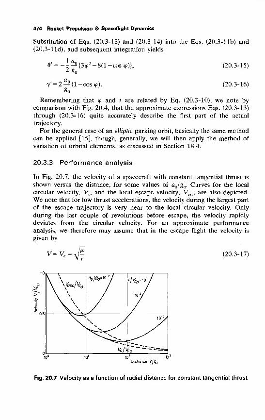
474 Rocket Propulsion & Spaceflight Dynamics
Substitution of Eqs. (20.3-13) and (20.3-14) into the Eqs. (20.3-1 lb) and(20.3-1 Id), and subsequent integration yields
0' = -^{3<P 2 -8(l-coscp)},
y = 2^(l-cos<p).go
(20.3-15)
(20.3-16)
Remembering that <p and t are related by Eq. (20.3-10), we note by
comparison with Fig. 20.4, that the approximate expressions Eqs. (20.3-13)
through (20.3-16) quite accurately describe the first part of the actual
trajectory.
For the general case of an elliptic parking orbit, basically the same methodcan be applied [15], though, generally, we will then apply the method of
variation of orbital elements, as discussed in Section 18.4.
20.3.3 Performance analysis
In Fig. 20.7, the velocity of a spacecraft with constant tangential thrust is
shown versus the distance, for some values of a /g . Curves for the local
circular velocity, Vc, and the local escape velocity, Vesc , are also depicted.
We note that for low thrust accelerations, the velocity during the largest part
of the escape trajectory is very near to the local circular velocity. Only
during the last couple of revolutions before escape, the velocity rapidly
deviates from the circular velocity. For an approximate performance
analysis, we therefore may assume that in the escape flight the velocity is
given by
V= V. = (20.3-17)
10' 10J
Distance r/r
Fig. 20.7 Velocity as a function of radial distance for constant tangential thrust
Low-Thrust Trajectories 475
This approximate relationship enables us to find approximate expressions
for the dependence of radial distance on time and of angular position on
radial distance, as well as for the escape time and for the propellant
consumption during the escape flight.
By substitution of Eq. (20.3-17) into Eqs. (20.1-5) and (20.3-lb), weobtain
'2r'(20.3-18)
and
Elimination of % from Eqs. (20.3-18) and (20.3-19) leads to
dro P
dT 2%T'or, with Eq. (20.3-2),
r-3/2 dr =
?Oo dt(20.3-20)
v/la l-a t/c
Integration leads with the initial conditions t = 0: r = r to
"\ r^l + c<vPln(l-an f/c)L \ /A .
(20.3-21)
This equation clearly shows that the distance will initially increase only very
slowly.
An approximate relation for the escape time, tesc , can be obtained from
Eq. (20.3-21). Realizing that escape will take place at a finite distance, weobtain
For VcJc« 1, we may linearize this relation to
t <—lesc ^ 5
a
or, with Eqs. (20.2-6) and (20.2-8),
^T—l-, (20.3-22)TCo 27raJgQ
where the correction factor a, being a function of a and c, follows from a
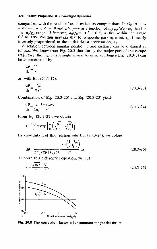
476 Rocket Propulsion & Spaceflight Dynamics
comparison with the results of exact trajectory computations. In Fig. 20.8, ais shown for c/VCo= 10 and c/VCo-»«> as a function of a /g . We see, that for
the a lgo-range of interest, a /g = 10-5 -10~3
, a lies within the range
0.8 to 0.95. We thus may say that for a specific parking orbit, tesc is nearly
inversely proportional to the initial thrust acceleration, a .
A relation between angular position 6 and distance can be obtained as
follows. We know from Fig. 20.5 that during the major part of the escape
trajectory, the flight path angle is near to zero, and hence Eq. (20.3-5) can
be approximated by
d0_ Vdt~ r'
or, with Eq. (20.3-17),
dd_ fiZ
dt~ Vr3'
Combination of Eq. (20.3-20) and Eq. (20.3-23) yields
dd (x l — aQ t/c
(20.3-23)
dr 2a r3
From Eq. (20.3-21), we obtain
a t [1 / HL HI1 = exp -I yl— a/-
c \_c V V r V r
By substitution of this relation into Eq. (20.3-24), we obtain
(20.3-24)
de = vexp l^)
dr2a exp(VcJc) r
3
To solve this differential equation, we put
Vw7 vcx= =—-.
c c
1.0
oo.9
0.8
0.7
(20.3-25)
(20.3-26)
00
ClVCo ^O^^^s^^
10"J 10"
Thrust Acceleration 3 l9
Fig. 20.8 The correction factor a for constant tangential thrust
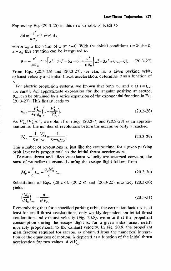
Low-Thrust Trajectories 477
Expressing Eq. (20.3-25) in this new variable x, leads to
-c4_
dd = ex°x
3exdx,
tia
where xn is the value of x at t = 0. With the initial conditions f = 0: = 0,
x = x this equation can be integrated to
ce>
; -3x 2 + 6jc-6 +— [x -3x§ + 6x -6]. (20.3-27)ju-a L
From Eqs. (20.3-26) and (20.3-27), we can, for a given parking orbit,
exhaust velocity and initial thrust acceleration, determine 9 as a function of
r.
For electric propulsion systems, we known that both x , and x at f = tesc
are small. An approximate expression for the angular position at escape,
6esc , can be obtained by a series expansion of the exponential function in Eq.
(20.3-27). This finally leads to
V4I V4
\"" '' **» (20.3-28)~ 4^a V V4
Co
As V4cJV4
Cv« 1, we obtain from Eqs. (20.3-7) and (20.3-28) as an approxi-
mation for the number of revolutions before the escape velocity is reached
IV41Nesc
=~ * = - -• (20.3-29)8 77 jua 87ra /g
This number of revolutions is, just like the escape time, for a given parking
orbit inversely proportional to the initial thrust acceleration.
Because thrust and effective exhaust velocity are assumed constant, the
mass of propellant consumed during the escape flight follows from
Mp= -tesc=^tesc . (20.3-30)
c c
Substitution of Eqs. (20.2-6), (20.2-8) and (20.3-22) into Eq. (20.3-30)
yields
Mp
Ml cIVly±n 'esc W ' c
(20.3-31)' esc
Remembering that for a specified parking orbit, the correction factor a is, at
least for small thrust accelerations, only weakly dependent on initial thrust
acceleration and exhaust velocity (Fig. 20.8), we note that the propellant
consumption during the escape flight is, for a given initial mass, nearly
inversely proportional to the exhaust velocity. In Fig. 20.9, the propellant
mass fraction required for escape, as obtained from the numerical integra-
tion of the equations of motion, is depicted as a function of the initial thrust
acceleration for two values of c/Vc .
478 Rocket Propulsion & Spaceflight Dynamics
1.0
c 0.3
S 0.1
L0.03
0.01
c/V*?
____10
Fig. 20.9
thrust
10 10 10 10 10
Thrust Acceleration SplgQ
Propellant mass fraction for an escape flight with constant tangential
It is interesting to compare, from the viewpoint of propellant consump-tion, the escape flight of a low-thrust vehicle and that of a hypothetical
high-thrust rocket with the same high exhaust velocity as the low-thrust
vehicle. Of course, we also assume for the high-thrust rocket that the escape
flight starts from a circular parking orbit, and that the thrust is acting
tangentially to the parking orbit. Using the concept of the impulsive shot, wefind for the impulsive velocity increase, AV, required to escape:
AV=(V2-l)VCo .
According to Tsiolkovsky's equation, Eq. (11.2-4), the mass of propellant
involved is expressed by
©„=—K»t|If VcJc« 1, we may approximately write
V2-1c/Vc
(20.3-32)
By comparison of Eqs. (20.3-31) and (20.3-32), we conclude that for the
same high exhaust velocity, the escape flight with a low thrust requires about
2 to 2.2 times the mass of propellant consumed during a high-thrust escape
flight. This, of course, is due to the gravity losses during the low-thrust flight.
At the present time, however, this comparison is not realistic. There is nochoice between a high and low thrust with the same high exhaust velocity.
We can only reach a high thrust by chemical or solid-core nuclear fission
propulsion with their inherently relatively low exhaust velocities. Nowadays,high exhaust velocities can only be achieved by low-thrust electric propul-
sion systems. Hopefully, in the future, other space propulsion systems that
Low-Thrust Trajectories 479
combine a high thrust and a high exhaust velocity will become available.
Only then, short-duration interplanetary spaceflights with a relatively low
propellant consumption may become feasible.
References
1 Au, G. F. (1968), Elektrische Antriebe von Raumfahrzeugen, G. BraunVerlag, Karlsruhe, p. 107-521.
2 Clark, K. E. (1974), Survey of Electric Propulsion Capability, AIAAPaper 74-1082, New York.
3 Hudson, W. R. and Finke, R. C. (1976), NASA Electric Pro-
pulsion Program, AIAA Paper 76-1068, New York.
4 Ehricke, K. A. (1962), Space Flight, Vol 2: Dynamics, Van Nostrand,
Princeton, p. 611-845.
5 Stuhlinger, E. (1964), Ion Propulsion for Space Flight, McGraw-Hill,New York, p. 73-154.
6 Chute, F. S. (1970), Electric propulsion in space, Canadian Aeron.
Space J., 16, 381-388.
7 Tsien, H. S. (1953), Take-off from satellite orbit, A.R.S. J., 23, 233-236.
8 Copeland, J. (1959), Interplanetary trajectories under low thrust radial
acceleration, A.R.S. J., 29, 267-271. Also: A.R.S. J., 30, 130-131.
9 Lawden, D. F. (1958), Optimal escape from a circular orbit, Astron.
Acta, 4, 218-233.
10 Breakwell, J. V. and Rauch H. E. (1966), Optimum guidance for a lowthrust interplanetary vehicle, AIAA J., 4, 693-704.
11 Reidelhuber, O. J. and Schwenzfeger, K. J. (1974), Optimal Low Thrust
Energy Increase Spiral Expansion, IAF Paper 74-017, Amsterdam.12 Melbourne, W. G. (1961), Interplanetary Trajectories and Payload
Capabilities ofAdvanced Propulsion Vehicles, JPL TR 32-68, Pasadena.13 Melbourne, W. G. and Sauer, C. G. (1961), Optimum Thrust Programs
for Power-Limited Propulsion Systems, JPL TR 32-118, Pasadena.14 Moeckel, W. E. (1960), Trajectories with Constant Tangential Thrust in
Central Gravitational Fields, NASA TR R-53, Washington.15 Wakker, K. F. (1967), Ion Propulsion for Interplanetary Spaceflight (in
Dutch), Thesis Delft Univ. of Technology, Dept. Aerospace Eng.,
Delft, p. 108-130.
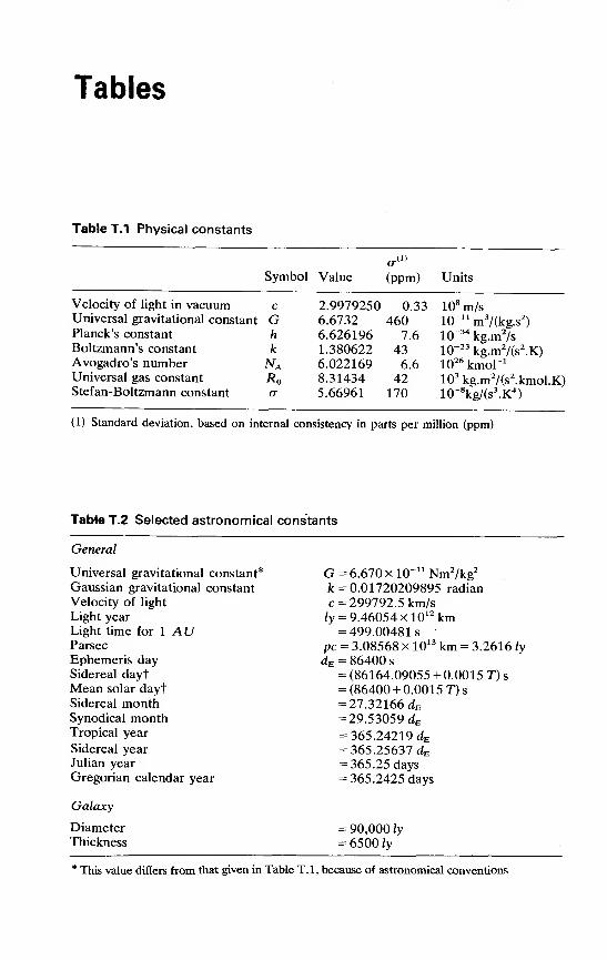
Tables
Table T.I Physical constants
<T(1)
Symbol Value (ppm) Units
Velocity of light in vacuum c 2.9979250 0.33 108m/s
Universal gravitational constant G 6.6732 460 10" 11 m3/(kg.s
2)
Planck's constant h 6.626196 7.6 10~34 kg.m2/s
Boltzmann's constant k 1.380622 43 10-23 kg.m2/(s
2.K)
Avogadro's number NA 6.022169 6.6 1026 kmoP 1
Universal gas constant Ro 8.31434 42 103 kg.m2/(s
2.kmol.K)
Stefan-Boltzmann constant <T 5.66961 170 10-8kg/(s
3.K
4)
(1) Standard deviation, based on internal consistency in parts per million (ppm)
Table T.2 Selected astronomical constants
General
Universal gravitational constant*
Gaussian gravitational constant
Velocity of light
Light year
Light time for 1 AUParsec
Ephemeris daySidereal daytMean solar daytSidereal monthSynodical monthTropical year
Sidereal yearJulian year
Gregorian calendar year
Galaxy
DiameterThickness
G = 6.670 x 10' 11 Nm2/kg
2
k =0.01720209895 radian
c= 299792.5 km/sly = 9.46054 xlO 12 km= 499.00481s
pc = 3.08568 x 10¹³ km = 3.2616 /y
dE = 86400 s
= (86164.09055 + 0.0015 T) s
= (86400 + 0.0015 T)s= 27.32166 dE= 29.53059 dE= 365.24219 dE= 365.25637 dE— 365.25 days= 365.2425 days
= 90,000 \y
= 6500 ly
* This value differs from that given in Table T.l, because of astronomical conventions
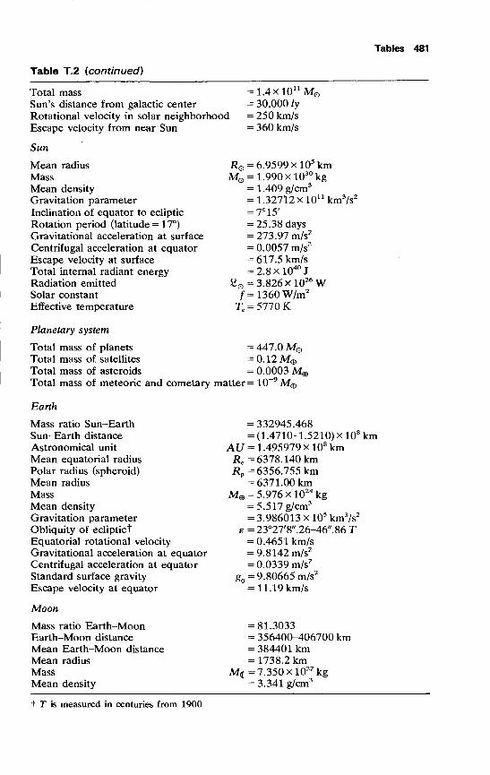
Tables 481
Table T.2 (continued)
Total massSun's distance from galactic center
Rotational velocity in solar neighborhood
Escape velocity from near Sun
= 1.4xl0 11 Mo= 30,000 ly
= 250 km/s= 360 km/s
Sun
Mean radius
MassMean density
Gravitation parameter
Inclination of equator to ecliptic
Rotation period (latitude = 17°)
Gravitational acceleration at surface
Centrifugal acceleration at equator
Escape velocity at surface
Total internal radiant energy
Radiation emitted
Solar constant
Effective temperature
Planetary system
Total mass of planets
Total mass of satellites
Total mass of asteroids
Total mass of meteoric and cometary matter = 10~9Mg
Earth
RQ = 6.9599 xlO5 kmMQ = 1.990 xlO30 kg
= 1.409 g/cm3
= 1.32712 x 10" km3/s
2
= 7°15'
= 25.38 days= 273.97 m/s
2
= 0.0057 m/s2
= 617.5 km/s= 2.8 xlO40
J
2 = 3.826 xl026W/=1360W/m2
T = 5770 K
= 447.0Me= 0.12Me= 0.0003 Mfl
Mass ratio Sun-Earth = 332945.468Sun-Earth distance = (1.4710-1.5210) x 10
8 kmAstronomical unit AL7 = 1.495979 xlO8 kmMean equatorial radius i?e = 6378.140 kmPolar radius (spheroid) Rp =6356.755 kmMean radius = 6371.00 kmMass Me = 5.976 xlO24 kgMean density = 5.517 g/cm3
Gravitation parameter = 3.986013 xl05 km3/s
2
Obliquity of ecliptict g = 23°27'8".26-46".86 TEquatorial rotational velocity = 0.4651 km/sGravitational acceleration at equator = 9.8142 m/s
2
Centrifugal acceleration at equator = 0.0339 m/s2
Standard surface gravity g = 9.80665 m/s2
Escape velocity at equator = 11.19 km/s
Moon
Mass ratio Earth-Moon = 81.3033Earth-Moon distance = 356400-406700 kmMean Earth-Moon distance = 384401 kmMean radius = 1738.2 kmMass M<j = 7.350 xlO22 kgMean density = 3.341 g/cm3
t T is measured in centuries from 1900
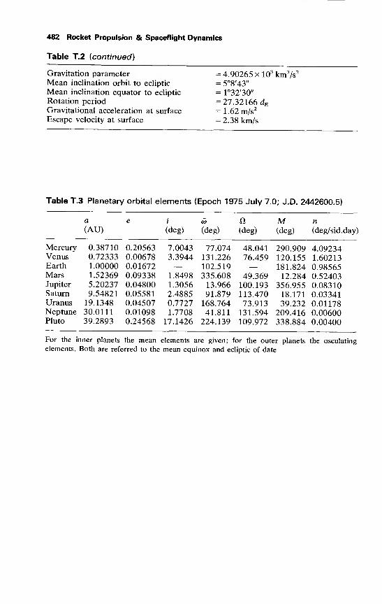
482 Rocket Propulsion & Spaceflight Dynamics
Table T.2 (continued)
Gravitation parameter = 4.90265 x 10³
Mean inclination orbit to ecliptic = 5°8'43"
Mean inclination equator to ecliptic = 1°32'30"
Rotation period = 27.32166 dEGravitational acceleration at surface = 1.62 m/s
2
Escape velocity at surface = 2.38 km/s
km3/s
2
Table T.3 Planetary orbital elements (Epoch 1975 July 7.0; J.D. 2442600.5)
a
(AU)n M
(deg) (deg) (deg) (deg) (deg/sid.day)
Mercury 0.38710 0.20563 7.0043 77.074 48.041 290.909 4.09234Venus 0.72333 0.00678 3.3944 131.226 76.459 120.155 1.60213Earth 1.00000 0.01672 — 102.519 — 181.824 0.98565Mars 1.52369 0.09338 1.8498 335.608 49.369 12.284 0.52403Jupiter 5.20237 0.04800 1.3056 13.966 100.193 356.955 0.08310Saturn 9.54821 0.05581 2.4885 91.879 113.470 18.171 0.03341Uranus 19.1348 0.04507 0.7727 168.764 73.913 39.232 0.01178Neptune 30.0111 0.01098 1.7708 41.811 131.594 209.416 0.00600Pluto 39.2893 0.24568 17.1426 224.139 109.972 338.884 0.00400
For the inner planets the mean elements are given; for the outer planets the osculating
elements. Both are referred to the mean equinox and ecliptic of date
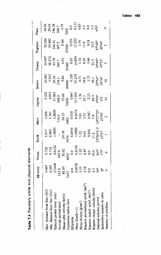
Tables 483
* <* ooa * n h00 On n© NO<t (S 't >o
cn co
oo en oTt Tt O
no
W * 't IT]
o on <* r^W N NO *
^H CNN M a *-H c _o n vi O n « Jo °°©OP^t-Hi-HOCO'"*"^o *—
i*-• cn
>nin
CN
r- cn
o\ cnO rHr-; C-; 00
o\ oo w o> *dH ^H 00 NOco
o\m «s h in \o g ..
O t' ^h 00 O ^' "* ^2 on
o q in h *O ON ON 00 o\
On Ono r- T-i int—I ^H t-» oq r-;
© in d dCO * vo
CN CO i—
I
,—
H
H>n m NO NO NO o NO CO<t On oq ON o o oq co r-; CN CO Eo
in
»
in Tf T-H 00 co o d r~ i-H •n CN d inT—
1
OnCO
inooor-
COCN NO
ONCO
On Tf COCN£f
—
NO i—
i
O o r- r-NO 00 00 CO o CO CO oNO co 00 On i—i o i—
i
ON r- o © in
O
Onr-r-
CNCNoCO
d d
o
CO co d in CO&
CN
COCN
t~- CO O CO o tj-H oo © oo o © CN r—
1
CO *fr r-o On ©1
t-; o o in 00 o CN ENOin
CN1—
1
© ^ 1 ON#0 oo d i-H in ON d T-H CO
CO>x:aocCD
CO
lai—
o
CO4-*
a)cJOa.
a>
Z(0
H
d d
CN>nt-h CNNO On pd co in cn
oo m idin o
NO
oor~ r- oNO o * r-^ CO CN On O0
d d d in r~ cn1-H -^ CO
5 S"< <
E ES o
oq cn oq qd «n oo d
ooinin co noq in r~; ©d in co d
s s
ON O O
U
w 3J3 -O T3<u .2 .2
>> M
o 3w •a
O. 0. X> _cS| § S « « ^
•* n^ aa> on
3 <T2 w
E g 8u .2 «s
™ - - .2
<u o.
S £3 -7!coJ*; <u o g <U
2 .y
™ CS 1) t/5
o o o
& 55 « - - -a tj <2 o" o* o"ESSwWWiflfiZ
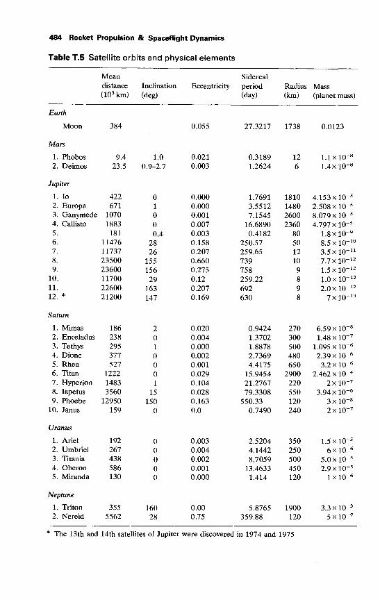
484 Rocket Propulsion & Spaceflight Dynamics
Table T.5 Satellite orbits and physical elements
Mean Sidereal
distance Inclination Eccentricity period Radius Mass(10
3 km) (deg) (day) (km) (planet mass)
Earth
Moon 384 0.055 27.3217 1738 0.0123
Mars
1. Phobos 9.4 1.0 0.021 0.3189 12 1.1 xl0~8
2. Deimos 23.5 0.9-2.7 0.003 1.2624 6 1.4 xl0~8
Jupiter
1. Io 422 0.000 1.7691 1810 4.153 xlO"5
2. Europa 671 1 0.000 3.5512 1480 2.508 xlO"5
3. Ganymede 1070 0.001 7.1545 2600 8.079 xlO"5
4. Callisto 1883 0.007 16.6890 2360 4.797 x 10~5
5. 181 0.4 0.003 0.4182 80 1.8 xlO"9
6. 11476 28 0.158 250.57 50 8.5 xlO" 10
7. 11737 26 0.207 259.65 12 3.5 xlO" 11
8. 23500 155 0.660 739 10 7.7 xlO" 12
9. 23600 156 0.275 758 9 1.5 xlO" 12
10. 11700 29 0.12 259.22 8 1.0 xlO- 12
11. 22600 163 0.207 692 9 2.0 xl0~ 12
12.* 21200 147 0.169 630 8 7 xl0~ 13
Saturn
1. Mimas 186 2 0.020 0.9424 270 6.59 xlO"8
2. Enceladus 238 0.004 1.3702 300 1.48 xlO-7
3. Tethys .295 1 0.000 1.8878 500 1.095 xl0~6
4. Dione 377 0.002 2.7369 480 2.39 xlO"6
5. Rhea 527 0.001 4.4175 650 3.2 xlO"6
6. Titan 1222 0.029 15.9454 2900 2.462 x 10"4
7. Hyperion 1483 1 0.104 21.2767 220 2 xlO"7
8. Iapetus 3560 15 0.028 79.3308 550 3.94 xlO"6
9. Phoebe 12950 150 0.163 550.33 120 3 x IO-8
10. Janus 159 0.0 0.7490 240 2 xlO"7
Uranus
1. Ariel 192 0.003 2.5204 350 1.5 xlO"5
2. Umbriel 267 0.004 4.1442 250 6xl0"6
3. Titania 438 0.002 8.7059 500 5.0 xlO-5
4. Oberon 586 0.001 13.4633 450 2.9X10⁻⁵
5. Miranda 130 0.000 1.414 120 1 x 10"6
Neptune
1. Triton 355 160 0.00 5.8765 1900 3.3 xlO"3
2. Nereid 5562 28 0.75 359.88 120 5 x 10"7
The 13th and 14th satellites of Jupiter were discovered in 1974 and 1975
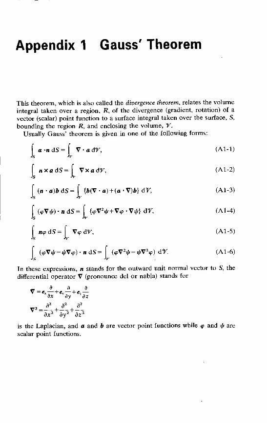
Appendix 1 Gauss' Theorem
This theorem, which is also called the divergence theorem, relates the volume
integral taken over a region, R, of the divergence (gradient, rotation) of a
vector (scalar) point function to a surface integral taken over the surface, S,
bounding the region jR, and enclosing the volume, V.
Usually Gauss' theorem is given in one of the following forms:
[andS =
fV-adT, (Al-1)
f «xadS= [ VxadT, (Al-2)
[(na)bdS =
\{b(V-a) + (a-V)b}dr, (Al-3)
[ (<pVi/0-ndS=f
{<pV2^+V(p-V^} dY, (Al-4)
[rap dS =
fV<p dY, (Al-5)
i(<pV(/r-j/rV<p) • ndS = (<pV
2^-i^V2<p) dr. (Al-6)
In these expressions, n stands for the outward unit normal vector to S, the
differential operator V (pronounce del or nabla) stands for
„ d d dV =ex hey \-ez
—dx ^dy dz
„, d2
d2
d2
dx2 dy 2dz
2
is the Laplacian, and a and b are vector point functions while <p and i/f are
scalar point functions.
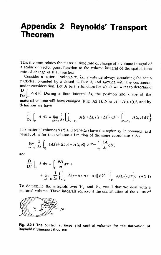
Appendix 2 Reynolds' TransportTheorem
This theorem relates the material time rate of change of a volume integral ofa scalar or vector point function to the volume integral of the spatial timerate of change of that function.
Consider a material volume T, i.e. a volume always containing the sameparticles, bounded by a closed surface S, and moving with the continuumunder consideration. Let A be the function for which we want to determineD
f— I A dT. During a time interval At, the position and shape of the
material volume will have changed, (Fig. A2.1). Now A = A{t, r(t)}, and bydefinition we have
[Adr=lim-5-{[ A{t + At,r(t + At)} dT-
fA(f,r)dr|.— AdT= lim
Dt
The material volumes V(t) and T(t + At) have the region % in common, andhence, A is for that volume a function of the same coordinate r. So
At
and
lim —[
{A(t + At,r)-A(t,r)} dV= [ — d%u-+o At )yo }y dt
DC C dA— Adr= — dr +Df L L dtl
AdH"m
ArllMt + At,r(t + At)}dY-^ AU-r)dr]. (A2-1)+
A«-
To determine the integrals over T t and V2 , recall that we deal with amaterial volume. These integrals represent the contribution of the value of
Fig. A2.1 The control surfaces and control volumes for the derivation ofReynolds' transport theorem
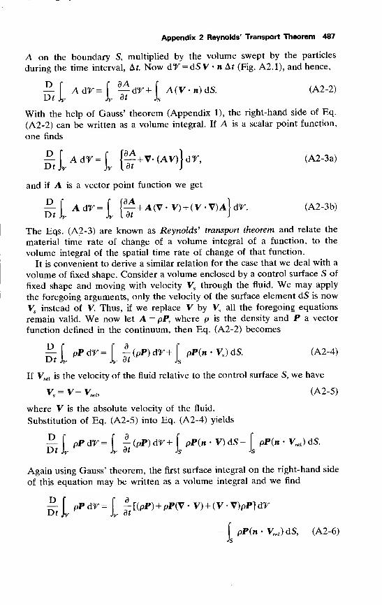
Appendix 2 Reynolds' Transport Theorem 487
A on the boundary S, multiplied by the volume swept by the particles
during the time interval, Af. Now dY = dSV • n Af (Fig. A2.1), and hence,
—f AdT =
f— dY+ f
A(V-»)dS. (A2-2)T>tj\. }r dt Js
With the help of Gauss' theorem (Appendix 1), the right-hand side of Eq.
(A2-2) can be written as a volume integral. If A is a scalar point function,
one finds
£L AdHf£+v'H dr '(A2'3a)
and if A is a vector point function we get
—fAdT=[ j— + A(V- V) + (V-V)aW. (A2-3b)
The Eqs. (A2-3) are known as Reynolds' transport theorem and relate the
material time rate of change of a volume integral of a function, to the
volume integral of the spatial time rate of change of that function.
It is convenient to derive a similar relation for the case that we deal with a
volume of fixed shape. Consider a volume enclosed by a control surface S of
fixed shape and moving with velocity Vsthrough the fluid. We may apply
the foregoing arguments, only the velocity of the surface element dS is now
Vsinstead of V. Thus, if we replace V by Vs all the foregoing equations
remain valid. We now let A = pP, where p is the density and P a vector
function defined in the continuum, then Eq. (A2-2) becomes
E>
Dr JPPdr = (pP) dY+
\pP(n • Vs ) dS. (A2-4)
d_
jy dt
If Vrel is the velocity of the fluid relative to the control surface S, we have
Vs= V-Vrel ,
(A2-5)
where V is the absolute velocity of the fluid.
Substitution of Eq. (A2-5) into Eq. (A2-4) yields
—f PPdT= f
-(PP)dT+ [pP(n • V)dS-
[ PP(n • VreI ) dS.Df Jy Jr dt Js Js
Again using Gauss' theorem, the first surface integral on the right-hand side
of this equation may be written as a volume integral and we find
§-t \v
PPdr=l ^[W + PPW- V) + (V-V)pP]dT
PP(n-Vrel )dS, (A2-6)
488 Rocket Propulsion & Spaceflight Dynamics
or
[ PPdV=\
§-f
\pPdT ^-
t
(pP)+ Pp(y-v) dT[pP(n Vrel)dS.
Using the continuity equation, i.e.
DpDf
we finally find
- + p(V. V) = 0,
^tlppdr=l¥t
pdr-[ pp{n ' y-)ds- (A2-7)
Appendix 3 The First Law of Ther-
modynamics
When we speak of a thermodynamic system, we mean a well defined amountof matter contained within material or hypothetical walls, through which
there is a controllable energy exchange with the surroundings. The first law
of thermodynamics is nothing but the experience that energy is conserved in
such a system:
dQ = d£ + dW, (A3-1)
i.e. an infinitely small amount of heat dQ (oj other forms of energy) added
to the system, causes an infinitely small increment dE of the internal energy
E of the system, and an infinitely small amount of work dW done by the
system on the surroundings. We can also write
Q = E2-E1 +W. (A3-2)
If we only consider expansion and compression work, the work being done
by the system, is
dW = pdV = d(pr)-rdp, (A3-3)
where T stands for the molar volume. So, Eq. (A3-1) can also be written as
dQ = d(E +pT)-Tdp. (A3-4)
The combination E +pT is called the heat function, or enthalpy H:
H = E + pT. (A3-5)
It is customary to use Cp , Cv , H, E etc. for molar quantities, i.e. quantities
based on the mol as basic unit and cp, cv , h, e, etc. as specific quantities, i.e.
quantities based on the unit of mass. For gases we have
h = e + plp, (A3 -6)
and
dQ = dh— dp. (A3-7)P
By definition, the heat capacity at constant volume Cv = (dQ/dT)^ and the
heat capacity at constant pressure Cp= (dQ/dT)p . Thus
CvJ-* C =—. (A3-8)
" dT p dT
490 Rocket Propulsion & Spaceflight Dynamics
For perfect gases, where the internal energy only depends on the tempera-
ture, there follows immediately,
c ==Me+li
=^{e+RTi=c" +R - (A3 -9)
Integration of the Eqs. (A3 -8) yields
E = E„ + Cv dT. (A3-10a)
H = H +\ Cp dT, (A3-10b)
where T is a reference temperature. For small temperature intervals, Cp
and Q may, in many cases, be assumed constant. For most solids, and manyliquids, the difference between Cp
and Cv is negligible, leading to
C~CV = C. (A3-11)
Index
Absorptance, 153, 154monochromatic, 154
Absorption coefficient, spectral, 155
Absorptivity, monochromatic, 155
Acceleration,
absolute, 31, 36centripetal, 32, 344Coriolis, 32, 344dragging, 32relative, 32tangential, 32thrust, 463
Activity, 135
sphere, 360Adiabatic wall, 157
Admittance function, 205Aerodynamic,
-coefficient, 318-324-drag, 319, 323, 324, 332, 408,
433, 470,
-effects on satellite orbit, 407,
408, 432, 433, 470-force, 75, 318-321, 407, 408,
433-heating, 334-moment, 76-78, 318-321-pressure force, 75-pressure moment, 76-stability, 325-331-stiffness, 328, 330
Aiming point, 456Airfoil, double-wedge, 322Albedo, 408Aldrin, Edwin, 2Ammonium perchlorate (AP), 171,
174, 179Angle,
bank, 67, 83downwash, 328flight path, 14, 83, 250, 293-295,364
kick, 257nozzle, 223-of attack or of incidence, 250,
251, 255, 318, 321, 328, 329
pitch, 67, 83, 235, 238, 254
sideslip, 318thrust, 464yaw, 67, 83, 331
Angular momentum, 27, 35, 37, 45,
61, 62, 337, 338, 345, 363, 465
conservation of, 27, 61, 62
orbital, 338proper, 338
Angular motion, mean, 372, 421,
426Anomaly,
-at epoch, mean, 378eccentric, 371hyperbolic, 373mean, 372, 420-422
true, 49, 363unperturbed true, 429, 430, 473
ANS, 401, 402, 433AP, 171, 174, 179
Apoapsis or apocenter, 49distance, 51
Apollo project, 2
Argument,-of latitude, 391, 429-of pericenter, 49, 378
Aries, First Point of, 11, 13
Armstrong, Neil, 2
Ascending node (A.N.), 287, 377
longitude of, 378right ascension of, 287, 378, 429,
430
direct (D.A.), 389, 390, 455
hohmann transfer (H.T.A.), 389,
390trajectory, 247-250, 272-280,
492 Index
389, 390, 401, 454, 455Asteroid, 8, 9, 353Astronomical,
-Netherlands Satellite (ANS),401, 402, 433
-unit (A.U.), 8
Asymptoteincoming, 456outgoing, 453
Asymptotic deflection angle, 457,458
Atmosphere, Earth, 21-24Atmospheric,
-density, 22, 23-pressure, 22, 23-temperature, 22, 23
Attraction,
gravitational, 41-44lunar or solar, 353, 354, 358, 408parameter, 45, 363
Autumnal equinox, 11
Avogadro's number, 124Axis,
major or semi-major, 51, 52, 378minor or semi-minor, 51, 52principle, 39
Azimuthflight path, 14, 83, 391, 392, 453-455
launch, 392, 453, 455
Baffle, 212, 227Ballistic,
-missile, 246, 255, 282-missile, intercontinental (ICBM),
246, 255, 282, 283, 307-phase, 283, 286-305
Bank,-angle, 67, 83-rate, 83, 84
Barker's equation, 373Barycenter, 338Beam length, equivalent, 156Bipropellants, 209Black-body, 154Bleed-off system, 208Boiling,
film, 165, 166, 229nucleate, 165, 166, 229
Boltzmann, L., 152
constant, 152Boost phase, 283-286Booster, 280Boundary layer, 100-104, 156, 157,
230, 320, 324laminar, 320, 324turbulent, 320, 324
Brahe, Tycho, 41Bray,
approximation, modified, 145-148freezing point, 145
Burner,
L*-, 205strand, 174T-, 205
Burning,
erosive, 194, 196, 203, 204mesa-, 176neutral, 196-perimeter, 185, 194plateau-, 176progressive, 196regressive, 196restricted, 180-surface, 177, 178, 194-197, 200—time, 239, 243, 245, 272
Burning rate, 174-179, 203-205-augmentation, acceleration-
induced, 205-change, pressure-induced, 204,205
-exponent or pressure exponent,
175, 182, 184, 205Burnout,
altitude, 248, 249, 275range, 242-246velocity, 248-250, 254, 255, 273-277
Calendar, 1, 18, 19
Gregorian, 18
Julian, 18Calendar year, 18
civil, 18
Gregorian, 18
Cape Canaveral, 392, 453Capillary barrier, 212Capture radius, 458Carry-over effect, 323Catastrophic yaw, 329-331
Index 493
Cavitation, 212, 219-221
Celestial,
-equator, 11
-latitude, 12
-longitude, 11, 12
-meridian, 11
-pole, 11
-sphere, 10, 11
Cellulose Nitrate, 170
Center,
-of mass, 36, 70, 73, 107, 318
-of mass flow, 70, 73, 107
-of pressure, 318Chamber,combustion or thrust, 85, 86, 120,
121, 137, 138, 208, 227, 228-conditions, 87-90, 100pre-combustion, 86, 208
Characteristic length, 120, 121
Characteristic velocity,
launch vehicle, 395, 397, 448mission, 396, 397, 452rocket motor, 118-120
Chasles' theorem, 28Chemical reaction, 100, 101, 124-
130, 134, 136Chugging, 227Circular restricted three-body prob-
lem, 342-354Circulation, 331Clausius, R., 342
theorem, 342Coast-time or period, 273, 390, 454,
455Combustion, 85, 100, 121, 136-138,
177-179, 196, 208, 227-instability, 100, 121, 196, 227-model, 177-179oscillatory, 100, 227-or thrust chamber, 85, 86, 120,
121, 137, 138, 208, 227, 228-products, 85, 86, 100, 101
staged-, 208-temperature, 101, 128-zone, 86, 100
Comet, 8, 9
Compound, 124
Compression wave, 102, 103
Condensation, 123, 135
Condensed phase, 134-136
Conduction, 152Conductivity, thermal, 152
Conic section, 49-54
Conservation law, 27, 54-62, 102
Conservative field, 42, 43, 428Constant properties flow, 139, 140
Consumption,propellant, 243, 245specific, 115
Continuity, equation of, 55, 56, 91
Convection, 152, 156-160
Coolant, 163-166, 229, 230Cooling, 100, 160, 165-168, 228-
232ablative, 231active, 160, 228-231dump, 229-231film, 229, 230heat sink, 231insulation, 228-231jacket, 165, 229passive, 160, 228, 231, 232radiation, 160, 166-168, 231regenerative, 229-231
transpiration, 229, 230Coordinate system,
inertial launch site, 284launch site, 284local horizontal, 14
non-rotating planetocentric, 456Corona, 7
Counter glow (Gegenschein), 353Cowell's method, 409-413, 419Crawford bomb, 174Critical,
-inclination, 431-NPSE, 220-pressure, 165, 230-pressure ratio, 92, 93-temperature, 230
Cross-flow theory, 322Cruciform configuration, 318Culmination,
-altitude, 248, 249, 253, 274-277,
332, 333-point, 252, 253
-time, 248, 251, 276
D'Alembert characteristic, 376Dalton's law, 132
494 Index
Dark zone, 178Date line, international, 17
Day, 15
civil, 17
mean solar, 17
sidereal, 16
solar, 16, 17
De Saint Venant's equation, 93De Vieille's or St. Robert's law, 175Declination, 12Density,
atmospheric, 22, 23mass flow, 203, 204optical, 155
Descending node (D.N.), 377Diffuser, 214, 215Diffusivity, thermal, 152Discharge coefficient, 226Dispersion, trajectory, 234, 317,
334Dissociation, 123, 129, 130Disturbing,
-function, 414, 416, 422, 428,
429-potential, 356, 409, 428
Diurnal motion, 11
Divergence theorem, 485Downwash, 328
-angle, 328Drag,
aerodynamic, 319, 323, 324, 332,
408, 433, 470base, 323, 324-coefficient, 319, 322-324, 408-coefficient, friction, 324induced, 323, 324interference, 323-parameter, 332roughness, 323, 324viscous, 323, 324wave, 323-to weight ratio, 305, 332
Earth, 7, 8, 19-24-asphericity or oblateness, 20, 21,
308-310, 407, 427-atmosphere, 21-24-climate, 22-equator, 9, 20, 21, 377, 427, 428
-equator, ellipticity of the, 21,
428-(mean) equatorial plane, 9, 20,
377-(mean) equatorial radius, 20, 427-pear-shape, 20, 410, 428-polar radius, 20, 21
-(mean) radius, 19
Eastern Test Range (E.T.R.), 392Eccentricity, 49-51, 363, 378Ecliptic, 11
axis of the, 11
obliquity of the, 11, 13
plane, 11, 13
pole, 11
Einstein, A., 387theory of relativity, 27, 385, 387
Element, orbital, 377-379, 422Ellipsoid, standard, 20, 21
Emissivity, monochromatic, 155Emittance, 153, 154Encke's method, 409, 411-413Energy
chemical, 85
conservation of, 47, 58-61, 150,
151, 187, 188, 489free, 133internal, 58, 125, 489kinetic, 47, 59, 339-342, 470potential, 43, 47, 339-342, 470total, 340, 342, 345, 458
Enthalpy, 59, 125, 128, 130, 140,
489absolute, 128free, 130sensible, 128
Entropy, 130, 140Ephemeris time (E.T.), 18
EquationBarker's, 373de Saint Venant's, 93Euler's, 58Kepler's, 372, 375Kirchoff's, 127
Lambert's, 298-305Navier-Stokes, 150Oberth's, 238-of continuity, 55, 56, 91-of motion, Euler's, 40
Index 495
-of motion of rocket, 63-84, 234-
238, 246, 247-of motion of rocket, dynamical,
69-79-of motion of rocket, kinematical,
79-81-of rotational motion, 35, 37, 39,
237-of the center, 377planetary, 419-425reaction, 124Sieder-Tate, 166
Stefan-Boltzmann, 153
Tsiolkovsky's, 2, 3, 238, 239Equator,
celestial, 11
Earth's, 9, 20, 21, 377, 427, 428ellipticity of Earth's, 21, 428
Equilibrium
chemical, 124, 130-136, 144, 148-constant, 133, 138-flow, 139, 144, 145
Equinoxautumnal, 11
vernal, 11, 13, 14
-line, 11
Erosion function, 204Error,
cross-range, 308, 311cut-off, 311down-range, 308, 311impact, 311
Escape,
-time, 471, 475-trajectory or flight, 354, 439,
453-455, 463-479-velocity, 53, 363, 369, 470-472
Euler, L., 378-angles, 66, 67, 378-equation, 58-equations of motion, 40
Eulerian description, 54Excess velocity, hyperbolic, 369,
437-439, 451Exhaust velocity, 3, 71, 87-90, 120,
140effective, 120
Exit,
-cone, extendable, 111
flexible, 110-pressure, 90, 93-96
-surface, 87, 94-98, 107, 108
Exosphere, 23, 24Expansion,
-ratio, 94, 104, 140, 143
-wave, 102, 103
Extinguishment, DP/DT, 205
/ and g series, 383-385
Feed System, propellant, 100, 213-
226Field strength, 42Fineness, 321
Fizz zone, 178
Rame,diffusion, 179monopropellant, 179premixed, 178
-temperature, adiabatic, 128,
137-141
-zone, 178Flight, optimal (ballistic missile),
295-297Flight path,
angle, 14, 83, 250, 293-295, 364azimuth, 14, 83, 391, 392, 453-
455Flow,
constant properties, 139, 140
equilibrium, 139, 144, 145
free molecular, 408frozen, 139-143-rate, volumetric, 218sonic, 90, 92subsonic, 92supersonic, 90, 92, 194two-phase, 100
Fluid injection, 109
Fluorine, 209, 211
Flyby mission, 436, 440, 446-448,
451Foam region, 178
Force,
aerodynamic, 75, 318-321, 407,
408, 433aerodynamic pressure, 75
apparent, 41, 69-71
-coefficient, normal, 319-323
496 Index
Coriolis, 32, 40, 41, 70, 71, 78dragging, 32external, 33, 41, 69, 74-76frictional, 74, 75gravitational, 19, 41, 74internal, 33Magnus, 331normal, 319perturbing, 407-409pressure, 74, 75relative, 40, 41, 71tangential, 319
Fourier, J., 152-law, 152
Friction, 86, 219Frozen flow, 139-143Fuel, 85, 86Fugacity, 134, 135
Galaxy, 6, 342Galilean transformation, 26, 27Galileo's principle of relativity, 26Gas
-constant, 89-constant, universal, 89-law, perfect or ideal, 60, 126,
188, 490-generator, 86, 208
Gauss, C. F., 424-theorem, 485
Gegenschein (counter glow), 353Geocentric latitude, 10, 12, 20, 427Geographic
-latitude, 20-longitude, 10, 12, 66, 82, 427
Geoid, geophysical, 20, 21Geopotential, 19, 427Geostationary
-orbit, 367, 408-satellite, 367, 397, 428
Geosynchronous satellite, 358, 367,392
Gibb's free energy, 130Glyceroltrinitrate, 170Goddard, R. H., 2Grain (propellant), 86, 180, 185-
203Granular diffusion flame model
(GDF), 178Graphite, pyrolitic, 231
Gravitation, 27, 41-45, 75, 362, 387Newton's law of, 27, 41, 42, 387parameter, 45, 75, 362
Gravitational,
-attraction, 41-44-constant, universal, 42, 336-field, 42-44, 385, 427, 428-force, 19, 41, 74-mass, 27-moment, 76
Gravity,
standard surface, 114, 237, 246-loss or gravitational loss, 248,
250, 260, 273, 280, 333, 390,
478-turn, 255-261
Greenwich,-mean solar time, 17
-sidereal time, 16
Growth factor, 264Guidance, 255, 282, 283, 310, 326
delta, 310hybrid explicit, 310
Hamiltonian, perturbed, 423Harmonic,
sectorial, 308, 428spherical, 427tesseral, 308, 427, 428zonal, 308, 427-429
Heading, down-range, 284Heat,
-capacity, 489-function, 489-of formation, standard, 127-130-of reaction, 125-128-of transition, 129-sink, 160, 163-transfer, 86, 100, 101, 150-168,
225-transfer coefficient, convective,
157, 161
Heating, aerodynamic, 334Heliocentric,
-latitude, 13
-longitude, 13
Herschel, F. W., 7
Hess' law, 127Hill, G. W., 348
Index 497
surface of, 346-350Hodograph, 254, 365Hohmann, W., 2, 389
transfer ascent (H.T.A.), 389, 390transfer trajectory, 396, 397, 440-446
Horizontal plane, local, 14
Hour, 15
-angle, 15, 65, 284, 354-circle, 11
Hydrazine, 86, 209Hydrogen, 90, 209, 230
-fluoride, 85-peroxide, 85, 209
Ignition,
auto-, 195
device, 180Impact,
-parameter, 456-point, 4, 253, 254, 306-315,
457, 458time of, 253
Impeller, 214, 215, 218-shroud, 214, 215
Impulse,
specific, 114-116, 147, 211, 243,
245-thrust, 77, 98, 99total, 114, 115
Impulsive shot, 243, 244, 249, 254,
333, 396, 438, 439, 478Inclination, 287, 378, 431
critical, 431Incoming asymptote, 456Inertia,
moment of, 38, 39product of, 38-tensor, 38, 73
Influence, sphere of, 358-360, 437,
456Influence coefficient, 310-315
ballistic cross-range, 311, 314ballistic down-range, 311, 312
Inhibitor, 180Injection,
-error, 401-405main tank (MTI), 213
-of satellite, 390-395-parameter, in-plane, 391-395
-parameter, out-of-plane, 391,
393parking orbit (P.O.I.), 389
-state or condition, 285, 286, 292,
391-395-velocity parameter, 289, 293-
297, 393, 394Injector, 224-226Instability,
combustion, 100, 121, 196, 225,
227magnus, 329, 331non-linear, 329-331
Interference, aerodynamic, 323
Interplanetary,
-spacecraft, 202, 336, 340, 358,
436-462-trajectory, 436-460, 468
Invariable plane of Laplace, 338Ionization, 123
Ionosphere, 23
Jacobi, C. G. J., 340-integral, 344, 345, 353
Jet,
-assisted take-off (JATO), 116
-damping, 327, 328-vanes, 109
Jetavator, 109Julian Date (J.D.), 19
modified (M.J.D.), 19
Jupiter, 7, 8
Kennedy, J. F., 2
Kepler, J., 41-equation, 372, 375-laws, 41, 46, 50, 53, 54, 368, 373
Keplerian orbit or trajectory, 4, 5,
47-54, 362-385Kerosine, 230Kinetic energy, 47, 59, 339-342,
470Kirchhoff's,
-equation, 127-law, 154
Klemmung, 182Kourou, 392
Lagrange, J. L., 298, 413-bracket, 415-419, 422
498 Index
-Jacobi identity, 341-libration point, 348-354
Lagrangian description, 54Lambert's equation or theorem,
298-305Laplace, P. S. Marquis de, 360
invariable plane of, 338Laplacian, 485Latitude,
celestial, 12
geocentric, 10, 12, 20, 427geographic or geodetic, 20heliocentric, 13
Latus rectum, 50, 363, 378Launch,
-azimuth, 392, 453, 455-opportunity, 444-447, 452-site, 392, 453-vehicle, 333, 390, 398-401, 448,
455-vehicle characteristic velocity,
395, 397, 448-vehicle performance, 396-401-window, 452-window, daily, 392, 455
Law,conservation, 27, 54-62, 102Dalton's, 132
de Vieille's or St. Robert's, 175
Fourier's, 152Hess', 127
Kepler's, 41, 46, 50, 53, 54, 368,
373Kirchhoff's, 154Newton's, 25-32Newton's gravitation, 27, 41, 42,
387-of thermodynamics, first, 58,
125, 489, 490-of thermodynamics, second, 130
perfect or ideal gas, 60, 126, 188,
490Piobert's, 194Wien's, 153
Libration point, Lagrange, 348-354Lifetime, orbital, 395Lift, 318, 319, 323, 324Light year, 6
Linear momentum, 25, 27, 56-58
conservation of, 56-58Liner, 231Loading fraction, volumetric, 197-
202Longitude,
-at epoch, mean, 379celestial, 11, 12
geographic, 10, 12, 66, 82, 427heliocentric, 13
-of ascending node, 378-of pericenter, 379
Lossdivergence, 98, 100, 106gravity or gravitational, 248, 250,
260, 273, 280, 333, 390, 478Lunar
attraction, 353, 354, 358, 408trajectory or flight, 353, 354
Mach number, 90, 92, 317Magnetosphere, 23Maneuver
dog-leg, 391, 453midcourse, 450, 452, 456phasing, 392
Many-body problem, 336-360Mars, 7, 8Mass
center of, 36, 70, 73, 107, 318conservation of, 54-56, 185, 186
gravitational, 27inertial, 27payload, 240, 263, 398, 399propellant, 240, 263, 477, 478-ratio, 3, 4, 239-241, 264, 332structural, 240, 242, 263
Mass flow, 70, 73, 87, 93-96, 101,
107, 113, 203, 204, 245center of, 70, 73, 107
-density, 203, 204-factor, 120-parameter, 217
Material volume, 56Mercury, 7, 8
perihelion advance of, 387Meridian, 9
celestial, 11
Mesosphere, 23Metals, refractory, 232
Index 499
Meteor, 9Meteorite, 9
Meteroid, 8, 9Midcourse maneuver, 450, 452, 456
Milky Way, 6
Minute, 15
Missile, 255, 282, 283, 307, 323,
326, 333Mission
flyby, 436, 440, 446-448, 451
lander, 436orbital or orbiter, 436, 440, 448-characteristic velocity, 396, 397,
452Molar quantity, 123, 124, 489Molecular weight, 89, 124, 139
Momentaerodynamic, 76-78, 318-321
aerodynamic pressure, 76apparent, 41, 69, 72, 73
coefficient, pitching, 319-323
Coriolis, 40, 41, 72, 73, 78
external, 41, 69, 76, 77
frictional, 77gravitational, 76inertial, 74jet damping, 78
Magnus, 331pitching, 318, 327pressure, 76relative, 41, 73rolling, 319thrust misalignment, 77, 78yawing, 319
Momentum,angular, 27, 35, 37, 45, 61, 62,
337, 338, 345, 363, 465linear, 25, 27, 56-58
Monopropellant, 85, 209Moon, 2, 8, 348, 353Moons, 8
Motion,
constants of, 45-47direct, 378diurnal, 11
integral of, 337-340, 345retrograde, 378rotational, 28, 35, 37, 39-41translational, 28, 34-37, 40, 41
Multiple flames model (MF), 179
N-body problem, 336-342, 355,
356Navier-Stokes equation, 150
Neptune, 7, 8, 410discovery of, 7, 410
Net positive suction energy (NPSE),
219critical, 220
Neutral point, 325
Newton, I., 157
-laws, 25-32
-law of gravitation, 27, 41, 42,
387Nitrocellulose, 170
Nitroglycerine, 170
Node,ascending (A.N.), 287, 377
descending (D.N.), 377
Nodes,elimination of the, 340
line of, 377, 378
Nozzle, 85, 90-93, 98-111, 221
-angle, 223
ball and socket, 109, 110
bell-shaped, 91, 106
contour, 91, 98, 106
-deflection, 109
de Laval, 91, 106
-efficiency, 117
-entrance, 86expansion-deflection, 106
flexible-seal, 110fluid-bearing, 110
pintle, 110, 111
plug, 106rotating, 110translating inlet, 110
truncated plug, 106
Nusselt number, 158
Nutation, 13, 14
Oberth, H., 2
equation of, 238Obliquity of the ecliptic, 11, 13
One-body problem, 45, 362Orbit,
circular, 8, 53, 366-368
500 Index
-determination, 385elliptic, 368, 371, 372, 375-377,380-383
geostationary, 367, 408halo, 354hyperbolic, 363, 369, 370, 373-375
keplerian, 4, 5, 47-54, 362-385osculating, 413-433parabolic, 363, 369, 373parking, 389, 392, 438, 439, 454,
455, 463-perturbation, 5, 407-433perturbed, 308, 354, 357, 358,
386, 387, 407-433planetary, 41, 438-prediction, 385, 410, 432sun-synchronous, 433
Orbital,
-element, 377-379,' 422-element, classical, 378, 379-element, osculating, 413-433-elements, variation of, 409, 410,413-425
-lifetime, 395-mission, 436, 440, 448-parameters, 379, 392-395-plane, 8, 377
Outgoing,
-asymptote, 453-radial, 453
Over-expansion, 102-106Oxidizer, 85, 86Oxygen, liquid (LOX), 209Ozone, 22, 23, 85
Patched conic method, 437Payload, 240, 263, 397, 399
-mass, 240, 263, 398, 399-ratio, 240-242, 264, 266-ratio, total, 264, 268-271
Performance diagram, 398-401Periapsis or pericenter, 49
-distance, 51Period, 53, 54, 366, 367, 430, 445
circular, 366, 367nodal or draconic, 430
sidereal, 366synodic, 445
Perturbations,
general, 356, 409, 410, 425-430long-periodic, 432secular, 430short-periodic, 430special, 409, 410theory, 356, 407-433
Photosphere, 7
Piobert's law, 194Pitch,
-angle, 67, 83, 235, 238, 254damping in, 327, 328-program, 237, 238-rate, 83, 84, 236, 330
Planck, M, 152constant, 152
Planet, 7, 8
Planetary orbit, 41, 438Planetary equations, 419-425
canonical form of, 422, 423Gauss' form of, 423, 424Lagrange's, 419-425
Pluto, 7, 8
Pogo, 100, 213, 219Poisson relations, 60, 88, 91-93Pole,
celestial, 11
ecliptic, 11
north, 9, 11
south, 9
Port area, 185Potential, 42, 43, 339, 344, 353,
356, 409, 427, 428disturbing or perturbing, 356,
409, 428energy, 43, 47, 339-342, 470
Prandtl, L., 156-number, 157, 160
Precession, 13
Pre-combustion, 86-chamber, 86, 208
Preparation zone, 178Prepolymers, 174Pressure,
atmospheric, 22, 23center of, 318

Index 501
critical, 165, 230dynamic, 317, 318
equilibrium, 180-185exit, 90, 93-96partial, 131
radiation, 5, 408, 409, 436supercritical, 229exponent or burning rate expo-
nent, 175, 182, 184, 205-parameter, 217-ratio, 88-94-ratio, critical, 92, 93-thrust, 75, 77, 98, 99
Primeval Fireball, 6
Principle,
-axis, 39of equivalence, 27
Problem,
many-body, 336-360N-body, 336-342, 355, 356one-body, 45, 362three-body, 336, 340, 342-354two-body, 336, 362-387
Product, 124Propellant, 3, 85
colloidal, 170composite, 86, 170-174, 178, 179
composite modified double-base
(CMDB), 170, 174cryogenic, 209, 390double-base (DB), 86, 170, 171,
178-feed system, 100, 213-226homogeneous, 170, 171
hybrid, 85, 115hypergolic, 209liquid, 85, 115, 116, 209-211,
391-mass, 240, 263, 477, 478-mass, useful, 240-ratio, 240, 242, 264-ratio, total, 264, 270-tank, 86, 211-213solid, 85, 115, 116, 170-179, 390storable, 209
Pump, 86, 213-221centrifugal, 214, 215-specific speed, 218, 219
turbo-, 86, 213, 218, 219Pumphead, 214
Radiation, 152-156
solar, 21, 408, 436Radiator, ideal, 153
Range, 242-246, 253, 254, 290-
293, 305, 306, 309ballistic angular, 290-293, 309
ballistic linear, 253, 254, 290burnout, 242-246-function, 243, 244no-drag, 305re-entry, 305total angular, 306
Reactant, 124Reaction,
chemical, 100, 101, 124-130, 134,
136endothermal, 126
-equation, 124exothermal, 126, 134extent of, 125
heat of, 125-128-time, 136
Recombination, 100, 101, 123, 130
Recovery,
-factor, 159, 192
-temperature, 158
Re-entry,
-phase, 283, 305, 306-point, 305-state or condition, 291, 305-vehicle, 282, 305, 306, 310
Reference frame, 9-14, 25-31, 64-
69, 234, 235, 338geocentric, 12
geocentric mean equinox of date,
14heliocentric, 13
inertial, 25-27, 31, 64, 234, 338non-inertial, 28-31
non-rotating geocentric equator-
ial, 12, 64-67non-rotating heliocentric ecliptic,
13rotating geocentric, 12, 64-66vehicle, 65-67, 235
502 Index
vehicle-centred horizontal, 65, 66Reference state, standard, 128Reflectance, 153Relativity,
Einstein's theory of, 27, 385, 387Galileo's principle of, 26
Rendezvous, 385Residence time, 120-123, 139Resonance,
roll, 330, 331spin-yaw, 331
Response function, 205Reynolds,
-number, 158, 317, 318-transport theorem, 486-488
Right ascension, 12
Rigid,
-body, 37-40-rocket, 63, 64
Roche equipotential, 346Rocket,
dynamical equation of motion of,
69-79equation of motion of, 63-84,
234-238, 246, 247kinematical equation of motion of,
79-81multi-stage, 240, 262-281, 389,397-401
-parameter, 239-242, 262-265rigid, 63, 64single-stage, 234-251, 277, 279sounding, 246, 323, 333-stage, 262, 263, 391, 398-step, 262sub-, 262, 263-testing, 113, 114two-stage, 276-280Vernier, 212
Rocket motor or engine,
characteristic velocity, 118-120chemical, 3, 4, 85-121, 169-232,478
electric, 3, 4, 462, 463, 477-479hybrid, 3, 4, 85, 86liquid, 3, 4, 85, 100, 106, 113,
208-232nuclear, 3, 4, 85, 478pressure-fed, 208, 213
pump-fed, 213solid, 3, 4, 85, 86, 107, 113, 169-205
Roll,
-lock-in, 329-331-rate, 330-resonance, 330, 331-slow-down, 329-speed-up, 330
Rolling, linear and non-linear, 329,330
Rotation, 28-30Rotational motion, equation of, 35,
37, 39, 237Rotor, 221, 222Roughness, surface, 104, 323, 324
San Marco, 392Satellite,
geostationary, 367, 397, 428geosynchronous, 358, 367, 392launching of, 389-405
Saturn, 7, 8
Schwarzschild metric, 385Screaming, 227Second, 15, 18
atomic, 18
ephemeris, 18
Semi-latus rectum, 50, 363, 378Semi-major axis, 51, 52, 378Semi-minor axis, 51, 52Separation,
flow, 104, 105, 320stage, 262, 280, 281, 391
Shock, 86, 102-105oblique, 103-105
Sidereal time, 15-17
Sieder-Tate equation, 166Slender-body theory, 321-323Sliver, 195, 200Solar,
-attraction, 353, 354, 358, 408-flare, 7, 354-system, 6-9
-time, 15-17
-time, apparent, 16, 17
-time, Greenwich mean, 17
-time, mean, 17
-wind, 7, 9
Index 503
Solidification principle, 40, 41
Space Shuttle, 2, 318, 399-main engine (SSME), 111, 220,
230Space Tug, 399, 401Spacecraft, interplanetary, 202, 336,
340, 358, 436-462Specific,
-impulse, 114-116, 147, 211,
243, 245-impulse, volumetric, 115, 116
-quantity, 489-speed, pump, 218, 219-thrust, 114, 242, 245, 246, 260
Speed,
subsonic, 92, 321, 324suction specific, 220supersonic, 90, 92, 321-324
Sphere of influence, 358-360, 437,
456Spin-yaw resonance, 331
Splash plate, 224St. Robert's or de Vieille's law, 175
Stability,
aerodynamic, 325-331-derivative, 320, 321dynamic longitudinal, 325-329-margin, 325, 326neutral, 325static longitudinal, 325, 326weathercock, 326
Stages,
identical, 269, 270rocket, 262, 263, 391, 398separation of, 262, 280, 281, 391
Staging,
parallel, 280, 281tandem, 280
Standard time, 17
Stanton number, 157
Stator, 221Steering program, 254, 468
Stefan, A. J., 152
—Boltzmann constant, 153
—Boltzmann equation, 153
Step, rocket, 262Stiffness,
aerodynamic, 328, 330structural, 329
Stoichiometric,
-coefficient, 125
-mixture, 125
Stratosphere, 22, 23Streamline, 86, 87
Structural,
-efficiency, 240-242, 264, 270-efficiency, total, 264, 270-mass, 240, 242, 263
Structure,
-factor, 272-ratio, 270
Sub-rocket, 262, 263Successive approximations, method
of, 386, 425-427Summerfield criterion, 104
Sun, 6, 7, 16, 17
mean, 17
Sunspot, 7
Surface,
-gravity, standard, 114, 237, 246-of constant properties, 86, 87,
97, 101
-of Hill or of zero velocity, 346-
350Swingby flight, 458-460
Tap-off system, 208TD-1A satellite, 430-432Temperature,
adiabatic flame, 128, 137-141
atmospheric, 22, 23auto-ignition, 176combustion, 101, 128
critical, 230exospheric, 23film, 158recovery, 158-sensitivity coefficient, 182
Test,
static, 77, 113, 114windtunnel, 320
Teststand, 113
Theorem,Chasles', 28Clausius', 342Gauss' or divergence, 485Reynolds' transport, 486-488Virial, 340-342

504 Index
Whittaker's, 36Thermochemistry, 123-148Thermodynamics,
chemical, 123-136first law of, 58, 125, 489, 490second law of, 130
Thermosphere, 23Thoma parameter, 220Three-body problem, 336, 340,
342-354circular restricted, 342-354(elliptical) restricted, 342, 352,353
Throat, 91, 100, 142-144, 162Thrust, 75, 77, 87, 97-99, 116, 246
-angle, 464-coefficient, 116-118-coefficient, characteristic, 117effective, 246-history, 86, 100, 180, 468impulse, 77, 98, 99-magnitude control (TMC), 110,
111, 203-misalignment, 77, 107, 108, 114-modulation, 110, 111, 226pressure, 75, 77, 98, 99-program, 333, 468specific, 114, 242, 245, 246, 260—to-mass ratio, 463, 465—to-weight ratio, 242, 249, 250,
272, 332-vector control (TVC), 77, 108-
111, 114, 326Time, 15-18
apparent solar, 16, 17
atomic (A.T.), 15, 18
burning-, 239, 243, 245, 272emphemeris (E.T.), 18
greenwich mean solar, 17
greenwich sidereal, 16
mean solar, 17
-of flight, 298-306, 447, 448,
452, 475-of flight, no-drag, 305-of flight, re-entry, 305-of pericenter passage, 372-375,378
reaction, 136residence, 120-123, 139
sidereal, 15-17
solar, 15-17
standard, 17
universal (U.T.), 17, 18
vertical rise, 257zone, (Z.T.), 17
Topping cycle, 208Total or stagnation conditions, 87,
88Trajectory,
ascent, 247-250, 272-280, 389,
390, 401, 454, 455ballistic or free-fall, 4, 282, 286-305
ballistic missile, 282-315class 1, 452class 2, 452dispersion, 234, 317, 334escape, 354, 439, 453-455, 463-479
interplanetary, 436-460, 468Keplerian, 4, 5, 47-54, 362-385low-thrust, 462-479lunar, 353, 354minimum energy or minimum
propellant, 296, 390, 438-444,
452, 468reference, 310, 411-413transfer, 396, 397, 440-452, 468type 1, 447, 452type 2, 447, 45?zero-lift, 255
Transfer trajectory, 396, 397, 440-452, 468
bi-elliptic, 397Hohmann, 396, 397, 440-446
Transmittance, 153Trojans, 353Troposphere, 22Tsiolkovsky, K. E., 2
-equation, 2, 3, 238, 239Turbine, 86, 221-224
impulse, 221, 222pressure compound impulse, 222,224
reaction, 221velocity compound impulse, 221,
224Turbopump, 86, 213, 218, 219
Index 505
Two-body problem, 336, 362-387
UDMH, 209Ullage volume, 212Under-expansion, 102, 106
Universal time (U.T.), 17, 18
Universe, 6
Uranus, 7, 8, 410discovery of, 7
Van 't Hoff, J. H., 134
-reaction isobar, 134Vandenberg Airforce Base
(V.A.F.B.), 392Vandenkerckhove function, 94Vanes, impeller, 216-218Vapor pull through, 212Variation of constants, 413-425Vehicle,
launch, 333, 390, 398-401, 448,
455re-entry, 282, 305, 306, 310
Velocity,
absolute, 30angular, 28, 73areal, 46burnout, 248-250, 254, 255, 273-
277circular, 53, 363, 366effective exhaust, 120
escape, 53, 363, 369, 470-472exhaust, 3, 71, 87-90, 120, 140hyperbolic excess, 369, 437-439,451
ideal, 239, 241, 265-272launch vehicle characteristic, 395,
397, 448mission characteristic, 396, 397,
452relative, 31
rocket motor characteristic, 118-
120-parameter, injection, 289, 293-
297, 393, 394-penalty, launch site and launch
azimuth, 397
-ratio, ideal, 268
Venus, 7, 8
Vernal equinox, 11, 13, 14
Verne, Jules, 1
Vernier rocket, 212
Vertical,
-flight or ascent, 247-250, 272-
280-rise time, 257
Vertregt, M, 266, 440Virial theorem, 340-342
Viscous effects, 101, 150, 219, 322
Vis-viva integral, 52
Vortex, 329, 330
Wake, 104, 105
Wallops Island, 392Weathercocking, 326Web,
-fraction, 196-thickness, 196
Western Test Range (W.T.R.), 392
Whittaker's theorem, 366
Wien's law, 153
Wind, 334Windtunnel test, 320
Yaw-angle, 67, 83, 331
-rate, 83, 84Year, 17-19
civil calendar, 18
Gregorian calendar, 18
Julian, 18
leap, 18
tropical, 17, 18
Zenith, 11
Zone time (Z.T.), 17


THE AUTHORS
Jacobus W Cornelisse is a Staff Member
at the European Space Research and
Technology Centre (ESTEC), Noordwijk.
Herman F R Schdyer is a Senior Faculty
Member of the Department of Aerospace
Engineering at Delft University of
Technology, and a Consultant for the
Technological Laboratory of TNO.
Karel F Wakker is a Senior Faculty Member
of the Department of Aerospace
Engineering at Delft University of
Technology.
Printed in Great Britain
Other titles available
Aircraft Electrical Systems
E H J Pallett, UK Civil Aviation Authority
\m illusti ited ISBNO 2'
Catastrophe Theory and its Applications
Tim Poston, Battelle, Geneva and Ian Stewart, University of Warwick• 09 pages illustrated ISBN OH
Mathematical Modelling Techniques (Research Note in Mathematics)
R Aris, University of Minnesota
1978 203 pages illustrated ISBN 273 08413 5
Introduction to Microprocessors
Edited by A Aspinall and E L Dagless, University College of Swansea1977 I70puges illustrated ISB I U> l 603 USA 12 064550 5
Nonlinear Analysis and Mechanics: Heriot-Watt Symposium Volumes I and II
(Research Notes in Mathematics)
Edited by R J Knops, Heriot-Watt University
I 1977, 249 poges illustrated ISBN 273 0H286
p ies illustrated ISBN 273 08 I
Ore Deposits of the USSR
Edited by V I Smirnov, Moscow State University
1977 illustrated
volume
Volume II 43 SBN 273 01037 9
Volume III 500 pages. ISBN 273 OK
Collei live ISBN 273 01073 5
Technical Literature Search and the Written Report
D J Maltha, Wageningen Agricultural University
1976 183 pages illustrated ISBN 273 00399 2
PITMANLONDON • SAN FRANCISCO MELBOURNE