robust semi-automatic depth map generation in unconstrained images and video sequences for 2d to...

122 IEEE TRANSACTIONS ON MULTIMEDIA, VOL. 16, NO. 1, JANUARY 2014

Robust Semi-Automatic Depth Map Generation

in Unconstrained Images and Video Sequences

for 2D to Stereoscopic 3D ConversionRaymond Phan, Student Member, IEEE, and Dimitrios Androutsos, Senior Member, IEEE

Abstract—We describe a system for robustly estimating syn-

thetic depth maps in unconstrained images and videos, for

semi-automatic conversion into stereoscopic 3D. Currently, this

process is automatic or done manually by rotoscopers. Automatic

is the least labor intensive, but makes user intervention or error

correction difficult. Manual is the most accurate, but time con-

suming and costly. Noting the merits of both, a semi-automatic

method blends them together, allowing for faster and accurate con-

version. This requires user-defined strokes on the image, or over

several keyframes for video, corresponding to a rough estimate of

the depths. After, the rest of the depths are determined, creating

depth maps to generate stereoscopic 3D content, with Depth

Image Based Rendering to generate the artificial views. Depth

map estimation can be considered as a multi-label segmentation

problem: each class is a depth. For video, we allow the user to label

only the first frame, and we propagate the strokes using computer

vision techniques. We combine the merits of two well-respected

segmentation algorithms: Graph Cuts and Random Walks. The

diffusion from Random Walks, with the edge preserving of Graph

Cuts should give good results. We generate good quality content,

more suitable for perception, compared to a similar framework.

Index Terms—Computer vision, depth maps, graph cuts, imagesegmentation, motion estimation, object tracking, random walks,

semi-automatic, 2D to 3D image conversion, 2D to 3D video

conversion.

I. INTRODUCTION

W HILE stereoscopic imaging has been around for many

decades, it has recently seen a rise in interest due to the

availability of consumer 3D displays and 3D films. This surge is

seen in the recent proliferation of big budget 3D movies, or with

some portions of the film being offered in 3D. 3D films show

novel views of the scene for the left and right eyes to the viewer.

Humans view the world using two views, which are processed

by the visual cortex in our brain, and we thus perceive depth.

This enhanced experience by exploiting depth perception is the

main attraction for viewing 3D films.

While much of the initial focus in stereoscopic 3D was on

creating display hardware, attention has now shifted to efficient

Manuscript received April 07, 2013; revised May 31, 2013; accepted July 10,

2013. Date of publication September 25, 2013; date of current versionDecember

12, 2013. The associate editor coordinating the review of this manuscript and

approving it for publication was Prof. Ebroul Izquierdo.

The authors are with the Department of Electrical and Computer En-

gineering, Ryerson University, Toronto, ON M5B 2K3, Canada (e-mail:

[email protected]; [email protected]).

Color versions of one or more of the figures in this paper are available online

at http://ieeexplore.ieee.org.

Digital Object Identifier 10.1109/TMM.2013.2283451

methods of creating and editing stereoscopic 3D content. 3D

films are subject to a number of constraints arising from creating

the distinct views. For example, the size of the viewing screen

can have an impact on the overall perceived depth. If any depth

errors surface, they may not be apparent on a mobile screen, but

may be so on a cinema screen. There have been remapping tech-

niques to ensure a consistent perception of depth, such as the

method by Lang et al. [1]. They propose four simple operators

for remapping, but they do not consider relative depth changes

among neighboring features, and also content preservation, such

as planes, and left/right frame coherence. This is successfully

addressed in Yan et al. [2], and was shown to outperform [1]. For

2D to 3D conversion, the current accepted method is a mostly

manual labor intensive process known as rotoscoping. An ani-

mator extracts objects from a frame, and manually manipulates

them to create the left and right views. While producing con-

vincing results, it is a difficult and time consuming, inevitably

being quite expensive, due to the large requirement of manual

operators. Despite these problems, this is a very important part

of the stereoscopic post-processing process, and should not be

dismissed. 2D to 3D conversion of single-view footage can be-

come useful in cases where filming directly in 3D is too costly,

or difficult. Research into conversion techniques is on-going,

and most currently focus on generating a depth map, which is

a monochromatic image of the same dimensions as the image

or frame to be converted. Each intensity value represents the

distance from the camera—the greater/darker the intensity, the

closer/farther the point in the image or frame is to the camera.

Novel viewpoints can be generated from this depth map using

Depth Image Based Rendering (DIBR) techniques [3]. An ex-

ample of what a depth map can look like is shown in Fig. 1

below.1

A. Related Work

Recent research in 2D to stereoscopic 3D conversion include

the following, each concentrating on a particular feature or ap-

proach to solve the problem.

1) Motion: The idea is that for objects closer to the camera,

they should move faster, whereas for objects that are far, they

should be slower. Motion estimation can be used to determine

correspondence between two consecutive frames, and to deter-

mine what the appropriate shifts of pixels are from the one frame

to the next. Wang et al. [4] perform a frame difference to elimi-

nate static backgrounds, and use block-based motion estimation

1From the Middlebury Stereo Database: http://vision.middlebury.edu/stereo.

1520-9210 © 2013 IEEE

PHAN AND ANDROUTSOS: ROBUST SEMI-AUTOMATIC DEPTH MAP GENERATION 123

Fig. 1. An example illustrating an image (left) with its associated depth map

(right).

to infer depth, with some post-processing done using morpho-

logical operators. In Liu et al. [5], each shot is classified as either

being static, or one comprised of motion. Static scenes use geo-

metric transformations while for a motion scenes, motion vec-

tors are employed with post-processing to smooth and enhance

edges. Finally, with Chen et al. [6], they fuse two depth maps to-

gether: motion and color. Motion employs the magnitude, while

color employs the Cr channel from the YCbCr color space.

2) Using Scene Features: Any method involving the direct

use of features, such as shape and edges, are of interest here. In

Kuo et al. [7], the objects within the scene are classified into one

of four types: sky, ground, man-made and natural objects. An

initial depth is assigned to each object using vanishing points,

a simplified camera projection model, and object classification

algorithms. In Zhang et al. [8], the depth maps are estimated

in a multi-cue fusion manner by leveraging motion and photo-

metric cues in video frames with a depth prior of spatial and

temporal smoothness. Finally, Schnyder et al. [9] create an au-

tomatic system for use in field-based sports by exploiting con-

text-specific priors, such as the ground plane, player size and

known background.

3) Other Conversion Methods: An example of a technique

not using any of the aforementioned methods is by Konrad et al.

[10]. Among millions of stereopairs available on the Internet,

there likely exist many stereopairs whose 3D content matches

the image of interest. They find a number of online stereopairs

whose left image is a close photometric match to the query and

extract depth information from these stereopairs. Finally, for

Park et al. [11], the goal is to identify the content within the

video that would have a high quality of depth perception to a

human observer, without recovering the actual 3D depth. They

use a trained classifier to detect pairs of video frames, separated

by time offsets, that are suitable for constructing stereo images.

B. Our Method of Focus: Semi-Automatic

At the present time, most conversion methods focus on

extracting depth automatic automatically. However, even

with minimal user intervention, these can become extremely

difficult to control conversion results—any errors cannot be

easily corrected. No provision is in place to correct objects

appearing at the wrong depths, and may require extensive

pre-/post-processing. Therefore, there are advantages to pur-

suing a user-guided, semi-automatic approach: For a single

image or frame, the user simply marks objects and regions

to what they believe is close or far from the camera, denoted

by lighter and darker intensities respectively. One question

often arising is whether or not the depths that the user mark

are indeed the right ones for perception in the scene. However,

the depth labeling need not be accurate; it only has to be

perceptually consistent, and quite often, the user labeling will

meet this criteria [12]. The end result is that the depths for the

rest of the pixels are estimated using this information. For the

case of video, the user marks certain keyframes, each in the

same fashion as the single image, and the rest of the depths

over the video are estimated. By transforming the process into a

semi-automatic one, this allows the user to correct depth errors

that surface, should they arise. This ultimately allows for faster

and more accurate 2D to 3D conversion, and provides a more

cost-effective solution.

There are some methods well known in this realm. In partic-

ular, the work by Guttmann et al. [12] solves for the depths in

a video sequence by marking strokes only on the first and last

frames. The first step is to detect anchor points over all frames.

A rough estimate of the depth for the first and last frame is found,

and Support Vector Machine (SVM) classifiers are trained on

both frames separately. Each SVM is trained on classifying a

unique depth in the rough estimate, using the Scale-Invariant

Feature Transform (SIFT), combined with the grayscale inten-

sity at the particular point as the input space. To detect anchor

points, SIFT points are detected throughout the entire video,

and are put through the SVM classifiers. For each SIFT point,

a One-Vs-All scheme is employed, choosing the highest simi-

larity out of all the classifiers. If this surpasses a high-confidence

threshold, it is an anchor point, and the depth assigned to it is

the one belonging to the SVM classifier tuned for the partic-

ular depth. To solve for the rest of the depths, an energy func-

tion is minimized by least squares. The function is a combina-

tion of spatial and temporal terms, color information, the anchor

points and user strokes. Theminimization is performed by trans-

forming the problem into a sparse linear system of equations,

and directly solved. A similar method was created by Wang et

al. [13], where holes/occlusions are handled quite well; they

are simply snapped together with nearby non-occluding areas.

However, the issue with [12] is that it is quite computationally

intensive. Not only does this require SIFT points and SVM clas-

sifiers to be computed, but it requires solving a large set of linear

equations, requiring a large amount of memory.

Upon closer inspection, we can consider semi-automatic

2D to 3D conversion as a multi-label image segmentation

problem. Each depth can be considered as a unique label, and

to create a depth map, each pixel is classified to belong to one

of these depths. Inspired by Guttmann et al., we propose a

stereoscopic conversion system to create depth maps for 2D to

3D conversion. The core of our system combines the merits of

two semi-automatic segmentation algorithms to produce high

quality depth maps: Random Walks [14] and Graph Cuts [15].

In the segmentation viewpoint, automatic methods are not an

option, as we wish to leverage the user in creating accurate

results, and would also be contrary to our viewpoint on auto-

matic 2D to 3D conversion. There are many semi-automatic

algorithms in practice. Examples are Intelligent Scissors [16],

or IT-SNAPS [17], where the user clicks on pixels, known as

control points, that surround an object of interest to extract. In


Fig. 2. A flowchart representing the general conversion framework.

between the control points, the smallest cost path is determined

that can delineate the foreground object from the background.

However, this can only be performed on objects that have a

clear separation from the background. In addition, this method

could not be used in specifying depths on background areas,

as the core of the algorithm relies on separation between the

background and foreground by strong edges. Another example

is the Simple Interactive Object Extraction (SIOX) framework

[18], which operates in the same way as Graph Cuts and

Random Walks with the use of foreground and background

strokes, but unfortunately only works on single images. We

ultimately chose Random Walks and Graph Cuts, not only

because marking regions of similar depth is more intuitive, but

these can ultimately be extended to video sequences.

For the case of single images, producing a depth map is akin

to semi-automatic image segmentation. However, video can be-

come complicated, as ambiguities in designing the system sur-

face, such as what keyframes to mark. It is natural to assume that

marking several keyframes over video is time consuming. In

this aspect, we allow the user the choice of which keyframes to

mark, as well as providing two methods for automatically prop-

agating the strokes throughout the sequence. Thesemethods will

be discussed in Section II-C, each having their merits and draw-

backs, but are chosen depending on the scene at hand. In this

paper, we first discuss the general framework for the conver-

sion of images. After, we consider video, investigating methods

for minimizing user effort in label propagation. We also show

sample depth maps and anaglyph images, and compare our ef-

forts to [12], demonstrating that our approach is more preferable

for human perception.

II. METHODOLOGY

Our framework relies on the user providing an initial estimate

of the depth, where the user marks objects and regions as closer

or farther from the camera. We allow the user to mark with

monochromatic intensities, as well as a varying color palette

from dark to light, serving in the same function as the inten-

sities. A flow chart illustrating our framework is seen in Fig. 2.

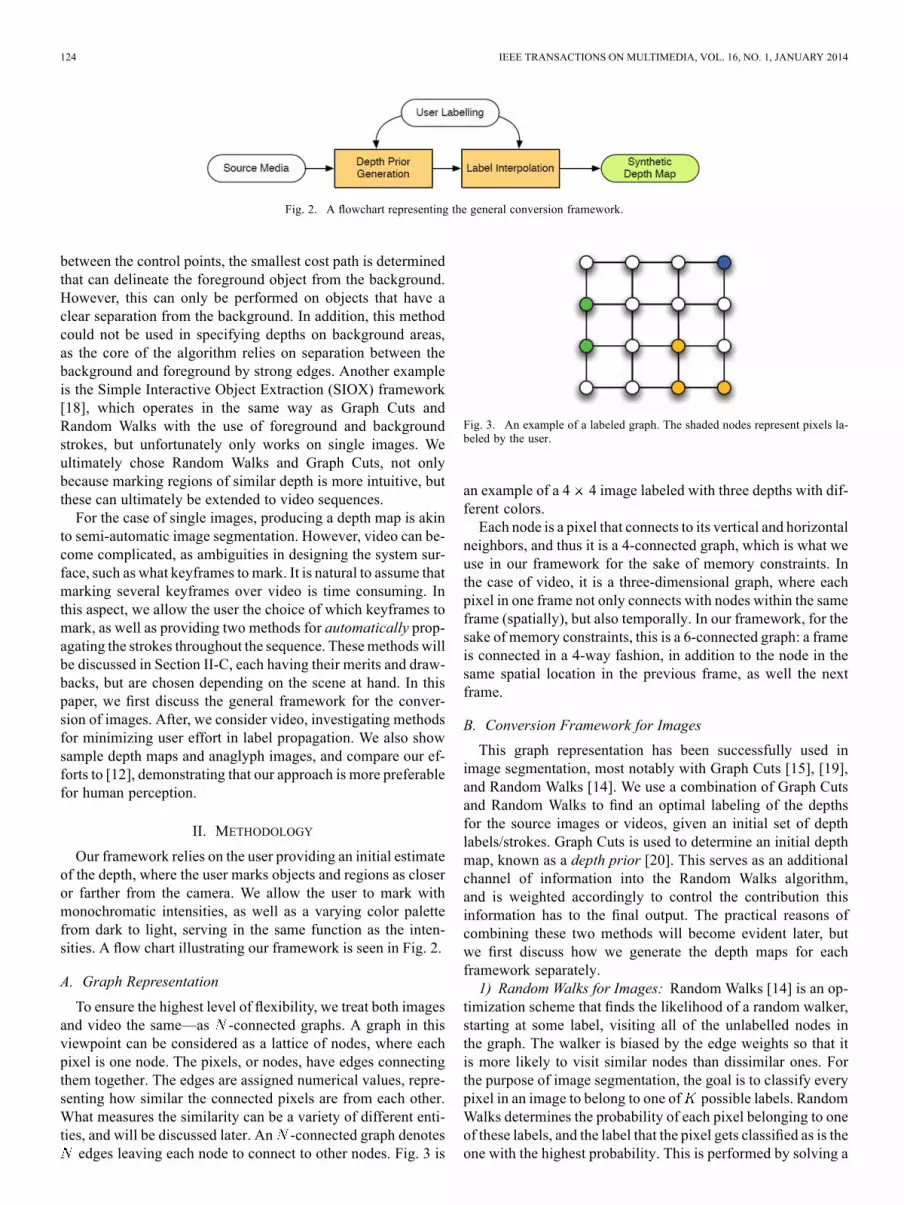
A. Graph Representation

To ensure the highest level of flexibility, we treat both images

and video the same—as -connected graphs. A graph in this

viewpoint can be considered as a lattice of nodes, where each

pixel is one node. The pixels, or nodes, have edges connecting

them together. The edges are assigned numerical values, repre-

senting how similar the connected pixels are from each other.

What measures the similarity can be a variety of different enti-

ties, and will be discussed later. An -connected graph denotes

edges leaving each node to connect to other nodes. Fig. 3 is

Fig. 3. An example of a labeled graph. The shaded nodes represent pixels la-

beled by the user.

an example of a 4 4 image labeled with three depths with dif-

ferent colors.

Each node is a pixel that connects to its vertical and horizontal

neighbors, and thus it is a 4-connected graph, which is what we

use in our framework for the sake of memory constraints. In

the case of video, it is a three-dimensional graph, where each

pixel in one frame not only connects with nodes within the same

frame (spatially), but also temporally. In our framework, for the

sake of memory constraints, this is a 6-connected graph: a frame

is connected in a 4-way fashion, in addition to the node in the

same spatial location in the previous frame, as well the next

frame.

B. Conversion Framework for Images

This graph representation has been successfully used in

image segmentation, most notably with Graph Cuts [15], [19],

and Random Walks [14]. We use a combination of Graph Cuts

and Random Walks to find an optimal labeling of the depths

for the source images or videos, given an initial set of depth

labels/strokes. Graph Cuts is used to determine an initial depth

map, known as a depth prior [20]. This serves as an additional

channel of information into the Random Walks algorithm,

and is weighted accordingly to control the contribution this

information has to the final output. The practical reasons of

combining these two methods will become evident later, but

we first discuss how we generate the depth maps for each

framework separately.

1) Random Walks for Images: Random Walks [14] is an op-

timization scheme that finds the likelihood of a random walker,

starting at some label, visiting all of the unlabelled nodes in

the graph. The walker is biased by the edge weights so that it

is more likely to visit similar nodes than dissimilar ones. For

the purpose of image segmentation, the goal is to classify every

pixel in an image to belong to one of possible labels. Random

Walks determines the probability of each pixel belonging to one

of these labels, and the label that the pixel gets classified as is the

one with the highest probability. This is performed by solving a


linear system of equations, relying on the Laplacian Matrix. If

represents the pixel in the image, that is of size ,

then the Laplacian Matrix, , of size , is defined in

Eq. (1) as the following, for row and column :

if

if and

is connected to

otherwise.

(1)

are pixels in the image , and is the degree

of the pixel , which is the sum of all of the edges leaving .

Each row of is an indication of how each pixel is connected

to each other. Additionally, let us define the vector , of size

, where the th row is the probability that the pixel will

be assigned a particular label, . By letting represent the

user-defined label of the th pixel, for a particular user-defined

label , vector is defined as:

(2)

For those pixels not user-defined (i.e. those that have no

), those are the unknown probabilities that need to be

solved. If we re-arrange the vector in (2) into two sets, such

that those pixels marked by the user appear first, , followed

by those unknown after, , we obtain a decomposition of

. By keeping track of how we rearranged the

vector , by performing the same rearranging with the rows of

, we thus obtain the following decomposition for :

(3)

Finally, to solve for the unknown probabilities for the label

, we solve the matrix equation of [14]. We

construct for each label , and solve for the unknown proba-

bilities of . Whatever label gives the maximum probability for

a pixel in , that is the label it is assigned. For use in generating

depth maps, we modify this methodology in the following way.

The probabilities within Random Walks spans between the real

set of [0,1]. Therefore, we allow the user-defined depths, and ul-

timately the solved depths for the rest of the image or frame to

be from this set, allowing for “manually” setting the probabili-

ties of the marked pixels within the vector . The goal is to solve

for only one label, the depth. As such, the user chooses values

from the set of [0,1] to brush over the image or frame, where

0/1 represents a dark/light color or intensity. After, the rest of

the depths are solved by (3). The resulting probabilities can di-

rectly be used as the depths for generating stereoscopic 3D con-

tent. As ameans of increasing accuracy, and to combat noise, we

employ Scale-Space Random Walks (SSRW) [21], which sam-

ples the image by a multi-resolution pyramid. Random Walks

is applied to each scale within the pyramid, upsampled, and are

merged using the geometric mean. For the edge weights, the

dissimilarity function is one that is frequently used in pattern

classification: the Sigmoidal function. Between two pixels,

and , it is defined in (4) as:

(4)

is the Euclidean distance of the CIE L*a*b* compo-

nents between and , and are parameters controlling

how dissimilar two colors are. These were experimentally set to

, and .

Unfortunately, Random Walks comes with certain issues. A

consequencewith specifying depths in a continuous range is that

it is possible that depths will be produced that were not origi-

nally specified. This is certainly the desired effect, allowing for

internal depth variation for objects, and would eliminate objects

being perceived as “cardboard cutouts”. In terms of weak con-

trast, this results in a “bleeding” effect, where regions at a closer

depth can bleed into regions of farther depth. We show an ex-

ample of this in Fig. 4, which is a snapshot of an area on the

Ryerson University campus. Fig. 4(a) shows the original image,

while Fig. 4(b) shows the user-defined scribbles, and Fig. 4(c) is

the depth map produced by SSRW. The user only needs to mark

a subset of the image, and a reasonable depth map is produced.

Though there is good depth variation on the objects and back-

ground, there is bleeding around some of the object boundaries.

This is unlike Graph Cuts, which provides a hard segmentation.

The depth map generated only consists of the labels provided

by the user.

2) Graph Cuts for Images: Graph Cuts is based on

solving the Maximum-A-Posteriori Markov Random Field

(MAP-MRF) labeling problem with user-defined or hard con-

straints [19]. The solution to the MAP-MRF labeling problem is

to find the most likely labeling for all pixels from the provided

hard constraints. It has been shown in [19] that the solution can

be found by minimizing the following energy function:

(5)

Here, is the set of pixels making up an image, and is

a pixel from the image. is the “energy” of the image.

represents the data cost, or the cost incurred when a

pixel is assigned to the label . is the smoothness

cost, or the cost incurred when two different labels are assigned

to two different pixels within a spatial neighborhood , which

is a 4-connected graph in our framework. Referencing graph

theory, it has been shown that the solution that minimizes

is the solution that finds the max-flow/min-cut of a graph [19].

Efficient algorithms and software have been created to perform

this minimization, and is available by referring to [19].

As depth map generation can be considered as a multi-label

classification problem, but Graph Cuts only focuses on the bi-

nary classification problem. As such, for each pixel, there are

foreground and background costs associated with them. There-

fore, each unique user-defined depth value is assigned an integer

label from the set , where represents the total

number of unique depths present in the user-defined labeling.

A binary segmentation is performed separately for each label

. The user-defined labels having the label of are as-

signed as foreground, while the other user-defined labels serve

as background. The rest of the pixels are those we wish to label.

Graph Cuts is run for a total of times, once for each label,

and the maximum flow values for the graph are recorded for

each label in . If a pixel was only assigned to one label, then


Fig. 4. (a) Example image, (b) example image with labels superimposed, (c) depth map using SSRW, (d) depth map using graph cuts, (e) combined result using

depth prior/graph cuts— . Depth label legend: darker colors (red)—far points, brighter colors (orange and yellow)—closer points, white pixels—very

close points.

TABLE I

DATA COSTS USED IN THE GRAPH CUTS SEGMENTATION FOR A LABEL ,

WHEN THE CHOSEN FOREGROUND LABEL IS

that is the label it is assigned. However, if a pixel was assigned

multiple labels, we assign the label with the highest maximum

flow, corresponding to the least amount of energy required to

classify the pixel. In some cases, even this will not always re-

sult in every pixel being classified, but region filling methods

can be used to correct this.

In our Graph Cuts framework, we use the Sigmoidal func-

tion ((4)) to reflect the smoothness costs. For the data costs, we

use a modified Potts model, rather than the negative log his-

togram probability as done in [15]. The reason why was due to

the nature of the color space to represent images. The negative

log histogram probability is computed in the RGB color space,

which is inherently discrete. However, we wish to employ the

CIE L*a*b* color space, as it naturally captures the human per-

ception of color better than RGB. In addition, CIE L*a*b* has

floating point values for each of their components, and so it is

not intuitive to determine howmany bins are required when cre-

ating a histogram. Table I shows how the data costs are com-

puted when the user-defined label is the one chosen as

foreground. In the table, the chosen foreground label during a

particular Graph Cuts minimization is denoted as , and is

defined as the following [15].

(6)

Fig. 4(d) illustrates a depth map obtained using only Graph

Cuts, using the same labels in Fig. 4(a) to be consistent. As with

Random Walks, only certain portions of the image are labeled,

and a reasonably consistent depth map was still generated suc-

cessfully. It should be noted that there are some portions of the

image that failed to be assigned any labels, such as the area

around the right of the garbage can. However, this can certainly

be rectified by using region-filling methods. Though the result

generated a depth map respecting object boundaries very well,

the internal depths of the objects, as well as some regions in the

background do not have any internal depth variation. If this were

to be visualized stereoscopically, the objects would appear as

“cardboard cutouts”. Noting that RandomWalks creates smooth

depth gradients, and combining this with the hard segmentation

of Graph Cuts, Random Walks should allow for depth variation

to make objects look more realistic, while Graph Cuts elimi-

nates the bleeding effect and respect hard boundaries.

3) Merging the Two Together: To merge the two depth maps

together, a depth prior is created, serving as an initial depth es-

timate, and provides a rough sketch of the depth. This infor-

mation is fed directly into the Random Walks algorithm. The

depth prior is essentially the Graph Cuts depth map, and should

help in maintaining the strong boundaries in the RandomWalks

depth map. Before merging, we must modify the depth prior.

The depth map of Random Walks is in the continuous range of

[0,1], while the depth map for Graph Cuts is in the integer range

of . Both depth maps correspond to each other, but one

needs to be transformed into the other to both be compatible.

As such, when the Graph Cuts depth map is generated, it is pro-

cessed through a lookup table , where is an integer label in

the Graph Cuts depth map. transforms the integer labeling

into a compatible labeling for Random Walks. This is done by

first creating a labeling within [0,1] for Random Walks, and to

sort this list into a unique one in ascending order. Each depth in

is assigned an integer label from , keeping

track of which continuous label corresponds to which integer

label. After Graph Cuts has completed, this correspondence is

used to map back to the continuous range.


Fig. 5. Labeling used for the frames 1 (a), 19 (b) and 38 (c) frames in the Sintel sequence.

To finally merge the two depth maps together, the depth prior

is fed into the Random Walks algorithm by modifying the edge

weights directly. The depth prior is incorporated by performing

a RandomWalks depth map generation, but we modify the edge

weight equation ((4)), where the distance function is appended

to include information from the depth prior. If we let repre-

sent the depth from the depth prior at pixel , after being pro-

cessed through the lookup table, the edge weight equation is

modified by modifying the Euclidean distance, which is defined

as:

(7)

and are defined in Section II-B-1. is a pos-

itive real constant, which we set to 0.5, serving as a scaling

factor determining how much contribution the depth prior has

to the output. denotes the depth at pixel from the depth

prior. However, the dynamic range of the depth values from

the depth prior is within [0,1], where as the components of the

CIE L*a*b* color space, as seen in (7), are significantly larger.

As such, these terms will overpower the terms in the depth

prior. With this, the entire image/frame is converted into the

CIE L*a*b* color space first. Each CIE L*a*b* channel is nor-

malized individually, so that all components for each channel is

within [0,1], and are the ones used in (7).

Fig. 4(e) shows an example of the merged results, where we

set . When compared to Figs. 4(c) and 4(d), Fig. 4(e)

contains the most desirable aspects between the two. The depth

prior has consistent and noticeable borders for the objects in the

scene, while the RandomWalks depthmap alone contains subtle

texture and gradients to those objects. The trees and shrubbery

in the original image are now much more differentiated from

the background and neighboring objects than before. In addi-

tion, the areas that were left unclassified in the depth prior, or

the “holes”, have been filled in after the final depth map was

produced. The reason is because the edge weights from Random

Walks ultimately considered the depth prior as only one compo-

nent of information out of the overall feature vector used, and

can still rely on the color image data to produce the final depth

map.

C. Conversion Framework for Video

Video is essentially a sequence of images at a specified frame

rate. When generating depth maps, our framework operates in

the same fashion, except that there are two fundamental areas

that need to be modified: (a) Instead of labeling one frame,

several keyframes must be labeled. (b) The graph representa-

tion needs to be modified from a 4-connected graph to a 6-con-

nected graph. This ensures that the frames connect together in a

temporal fashion, and the depth map in one frame is consistent

with the next frame. Before explaining the mechanics of how

video conversion is performed, we are assuming that there are

no abrupt changes in the video being processed, or consisting of

a single camera shot. If a video has any camera changes, then

it must be split up into smaller portions, with each not having

a change of shot. This can be done either manually, or using an

automated shot detection system.

1) Keyframes to Label: One question that a user may ask

is how many frames are required for labeling in order for the

depth map to be the most accurate? One option is to allow the

user to manually choose the frames they wish to label, and this

is an option we allow in our system. However, for the video

segmentation realm, at least the first and last frames need to be

labeled, in order for the segmentation to be consistent across the

sequence. This is the approach taken in Guttmann et al.’s work.

However, while it is possible to label only certain keyframes,

this will result in a number of different depth artifacts. Fig. 5

illustrates a sample shot, with their labels overlaid. This comes

from the Sintel sequence,2 and this shot is 38 frames. Fig. 5 is

comprised of the 1st, 19th and 38th frames, with their labels

superimposed. Fig. 6 illustrates some depth maps within the se-

quence using our framework, showing what happens when only

frames 1, 19 and 38 are labelled. Finally, Fig. 7 illustrates what

happens when all frames are labeled in the same style as Fig. 6,

again using our framework to video. In both Figs. 6 and 7, the

first row illustrates frames 1 and 13, while the second row il-

lustrates the frame 25 and 38. For the sake of brevity, we only

show the labels for frames 1, 19 and 38. The color scheme for

the labels is the same as in Fig. 4.

As can be seen, for the frames that had no labels, the rapidly

moving parts quickly “fade” in depth or appear to move away

from the camera. This is clearly not the case, since all objects in

the scene move horizontally, and not farther away. If all of the

frames are labelled appropriately, then the depth remains con-

sistent for all frames. While labeling every frame produces the

best results, it is not the easiest task to perform. For a modest

sequence, such as the 38 frame Sintel sequence, labeling each

frame manually is quite a tedious task, and would take a con-

siderable amount of time. However, if the labeling can be per-

formed in a more automated fashion, this would simplify the

task of creating a more detailed labeling, and thus increase the

accuracy of the depth maps. The idea is to only label the first

frame with the user-defined depth labels. After, these labels are

tracked throughout the entire video sequence. In addition, as the

video sequence progresses in time, it will contain areas where

the depth will need to change from what the user defined those

2http://www.sintel.org


Fig. 6. Depth maps for Sintel sequence with only three frames labeled. (a) Frame 1, (b) frame 13, (c) frame 25, (d) frame 38.

Fig. 7. Depth maps for Sintel sequence with all frames labeled. (a) Frame 1, (b) frame 13, (c) frame 25, (d) frame 38.

areas to be. As such, there has to be a way of dynamically ad-

justing those depths when those situations arise. As mentioned

earlier in Section I, we reference two methods for tracking these

labels, and depending on the scene at hand, we perform this

automatic labeling is through using one of two computer vi-

sion based algorithms: (a) An algorithm for tracking objects in

unconstrained video, since unconstrained is the type that our

framework will most likely encounter, and (b) An optical flow

based algorithm that is employed, should the scene exhibit only

horizontal motion and can avoid some of the computational

burden exhibited in (a). What is attractive about (b) is that it

determines optical flow without the use of global optimization.

This becomes very attractive for implementation in dedicated

parallel architectures, such as GPUs or FPGAs.

2) Label Tracking—Object Tracking Approach: As user-de-

fined depth strokes will inevitably vary in shape and length, it

would be computationally intensive to track all points within a

stroke. As such, the proposed system considers a single stroke

with a given user-defined depth as an ordered set of points.

As such, in our framework, each stroke is thinned using binary

morphological thinning, to reduce the stroke to aminimally con-

nected one, and is uniformly subsampled. If the user draws over-

lapping strokes at the same depth, a clustering is performed to

combine these to a single stroke. Once all points for all strokes

are collected, they are individually tracked, and their depths are

automatically adjusted when necessary. Cubic spline interpola-

tion is applied after, to connect these control points to approxi-

mate the final strokes with high fidelity, constrained to the loca-

tions of the tracked points. To reconstruct the width of the stroke

after thinning, the smallest distance between center of mass of

the thinned stroke and the perimeter of the original stroke is

found. This overall process inevitably creates “user”-defined

strokes across all frames, reducing the amount of interaction

involved.

To robustly track these points, we use a modification of one

created by Kalal et al. [22], known as the Tracking-Learning-

Detection framework (TLD). The user only draws a bounding

box around the object of interest in the first frame, and its trajec-

tory is determined over the entire video sequence. Essentially,

bounding boxes of multiple scales are examined in each frame

to determine if the object is present. However, the tracker is op-

timally designed to track objects. When the depth strokes co-

incide to background, these are handled differently, and will be

discussed later. If more than one frame is marked, the tracker

is restarted, using the strokes in each user-marked frame as the

“first” frame.

The initial location of the object is tracked using a multi-scale

pyramidal KLT [23], and the location is further refined using a

two-stage detector. This is comprised of a randomized fern de-

tector (RFD) [24] and an intensity-based nearest neighbor clas-


sifier (NNC), resizing the pixels within a bounding box to a

15 15 patch, with normalized cross-correlation as the sim-

ilarity measure. The KLT, as well as the RFD and NNC, op-

erate on monochromatic frames, and are converted accordingly

if the input is in color. However, it has been noted that color

images are naturally acquired in the RGB color space, with sig-

nificant correlation between each color component. Information

from other channels could have contributed to the acquisition of

the target channel, and simply converting to grayscale ignores

this correlation [25]. However, the KLT, as well as the RFD

can achieve good results ignoring color information. In retro-

spect, the NNC can most definitely be improved on, as this can

use color information, and can be transformed into a more per-

ceptually uniform color space so that quantitative differences in

colors reflect what is perceived by human beings.

We thus modify the NNC framework to incorporate the sim-

ilarity between two color patches using Phan et al.’s frame-

work [25], with color edge co-occurrence histograms (CECH).

These are three-dimensional histograms, indexing the frequency

of pairs of colors lying on valid edges over different spatial

distances; the first two dimensions are colors, and the third is

the spatial distance. Some quantization of colors needs to be

performed to allow for feasible memory storage, and Phan de-

vised a method that captured human color perception and recall

well, and is illumination invariant. Ultimately, the NNC was

adapted to use the similarity values from these histograms to

increase overall accuracy of detecting color distributions within

the bounding boxes, and are based on the correlation between

pairs of histograms. Further details on how these descriptors

were computed, and how they are adapted into the TLD frame-

work can be found in [26].

In order to dynamically adjust the depth of objects, the

ability of TLD to detect objects over multiple scales is used.

Let represent the scales of the

initial bounding box of size created in the first frame,

such that for a scale , the bounding box has dimensions

. When TLD tracking is performed, as the object

moves closer/farther to the camera, the size of the bounding box

required for the object will increase/decrease, as its perceived

size will increase/decrease. This kind of motion will most likely

be non-linear in nature, and so a mapping function is created,

describing the relationship between the scale of the detected

bounding box, with the labelled depth to be assigned for that

point; a simple parabolic perturbation is opted for use. If

represents the mapping function for a scale , a parabolic

relationship can be determined, where .

With TLD, two details are already known. The smallest scale

is the farthest depth, , and the largest scale is the

closest depth, , and are 0 and 255 respectively in our

framework. Finally, the initial bounding box has a scale of 1.0,

with the depth assigned from the user, , and the coefficients

are solved by the inverse of the following system:

(8)

At each frame, the bounding box scale automatically adjusts the

depth at this point along a stroke. This relationship between the

scales and depths functions quite well; if the current bounding

box is of the original scale, object will have only exhibited hor-

izontal motion. As the object moves closer and farther from the

camera, the depth is automatically adjusted within this bounding

box. This will function well when different parts of the object

appear at different depths (i.e. when the object is perceived at

an angle). The TLD framework, and ultimately ours, is designed

to track objects. As the goal of the proposed work is to deter-

mine dense depth maps, there will inevitably be strokes placed

on the background, and not on objects. As the TLD tracker

is also comprised of the KLT, if the stroke lies on a uniform

background, the online learning, RFD and NNC should be dis-

abled, and the KLT should only function. To determine when

to only enable KLT, we use the saliency detection algorithm

by Goferman et al. [27] which effectively determines salient

regions, and captures nearby pixels to faithfully represent the

scene. For each bounding box centered at a stroke point, the

mean saliency value is computed. If it surpasses a normalized

threshold, this is considered salient, and the full TLD tracker is

used. Otherwise, only KLT is used for tracking. In this work, a

threshold of 0.7 is used.

3) Label Tracking—Optical Flow: Though the modified

TLD tracker is robust, it can become computationally in-

tensive. There is an additional computational step using a

saliency detector, and additionally, a set of randomized fern

detectors is required to be trained: one per stroke point. Noting

this drawback, we offer an alternative method that the user

may choose. This is through the use of optical flow, and we

opt to use a paradigm that avoids using global optimization

to encourage implementation in parallel architectures, and

modify this so that the framework is temporally consistent

across all frames in the video. Optical flow seeks to determine

where pixels have moved from one frame to the next frame.

As such, to perform label propagation, one simply needs to

move pixels that coincide with the user-defined strokes by the

displacements determined by the optical flow vectors, and this

is exactly what is done in our framework. Most traditional

optical flow algorithms calculate the flow between two consec-

utive frames, and there may be information over neighboring

frames of video that may improve accuracy, thus leading to

our desire for temporal consistency. It should be noted that

this approach is suitable only for motion and objects that are

moving horizontally. Currently, we have not developed a way

of dynamically adjusting the depths of the objects using optical

flow like in Section II-C-2, but is currently an ongoing area of

research being pursued.

The framework that we use is the based on the one by Tao

et al. [28], known as SimpleFlow, which is a non-iterative,

multi-scale, sub-linear algorithm. However, SimpleFlow only

considers local evidence, and scenes with fast motion will in-

evitably fail. As such, we augment SimpleFlow by introducing

edge-aware filtering methods that directly operate on the optical

flow vectors, and consider information over neighboring frames

to further increase the accuracy. In most edge-aware filtering

methods, the filtered outputs are generated by considering

the content of a guidance image, which serves as additional


information to the filtering mechanism that the output must

satisfy. We can thus improve accuracy by using the frames in

the video sequence as guidance images. The flows for each

frame can be filtered independently, but in order for the vectors

to be temporally consistent, we also filter temporally. As the

optical flow vectors are only computed between two consec-

utive frames independently, it is inevitable that motion will

be non-smooth. As such, edge-aware filtering on a temporal

basis, with frames as guidance images will inevitably allow

smoothness in the flow vectors across the video, and become

temporally consistent.

The edge-aware filtering method we use is from Gastal

and Oliveira [29]. In [29], distance-preserving transforms are

the main tool for edge-aware filtering. The idea is that if an

image is transformed into another domain, such that similarity

values in the original domain are the same in the transformed

domain—one that is a lower dimensionality, filters designed in

the transformed domain will be edge preserving, and is known

as the domain transform. However, the formulation is only for

1D signals. To filter 2D signals (i.e. images), [29] show that no

2D domain transform exists, so approximations must be made,

leading to iterations. Each row is independently filtered, then

each column is filtered immediately after. Using the image

frames as guidance images should mitigate any errors in the

flow maps due to occlusions, as their edge information will

“guide” the filtered vectors. However, the current iteration

mechanism does not address temporal consistency. To address

this, one complete iteration consists of a 2D filtering operation,

with the addition of a temporal filtering operation. However,

one must be mindful when filtering temporally. The optical flow

vectors are used to determine where points in one frame map

to the next consecutive frame. To determine these, one simply

needs to take the every spatial co-ordinate in the one frame,

and use the vectors to determine where these pixel locations are

best located in the next frame. By doing this, we can determine

a binary map for each frame, , where a location is set to 1

if an optical flow vector maps a pixel to this location in the

next frame, and 0 otherwise. This binary map determines those

locations where the optical flow is reliable, and ensuring that

the flow vectors are temporally consistent. In order to filter tem-

porally, we apply the same technique performed on 1D signals

in [29] on a temporal basis. Specifically, in a video sequence of

frames, there will be an optical flow vector at a particular

location at each frame. Each location will thus

have a set of optical flow vectors—one per frame. For a

video sequence with a frame size of , we will thus have

sets of optical flow vectors, and each set is a temporal

1D signal. These signals are filtered using the method in [29].

For a particular frame in the sequence, if a location of in this

frame is 1, then the domain transform is computed normally.

However, should the location be 0, the domain transform is

computed by using information from the previous frames, as

this information is more reliable before this particular frame.

To further increase accuracy, we introduce an occlusion term,

so that those locations that are likely to be occluded do not

contribute substantially to the output. This occlusion term is

calculated by creating a confidence map that uses the forward

flow and backward flow vectors, in conjunction to a sigmoidal

function to ultimately decide how confident the optical flow

vectors are throughout the scene. Further details regarding the

overall process of achieving temporally consistent optical flow

can be found in [30].

III. EXPERIMENTAL RESULTS

In this section, we will demonstrate depth map results using

our image and video conversion framework. For images, these

are shown only for demonstration purposes, as the user has the

option of converting solely images. We will show some depth

map results using a variety of different media and sources, as

well as their corresponding anaglyph images so that the reader

has a sense of our framework works for images. However, the

main focus of our work is converting video sequences. For the

video sequences, we show depth maps for subsets of the frames

in each sequence, as well as their anaglyph images. We also

compare to Guttmann et al.’s work and show their depth maps

and anaglyph images on the same videos, using the same user-

defined strokes to be consistent in comparison.

A. Results: Images

Figs. 8, 9 and 10 shows a variety of examples from all areas

of interest. For each figure, the first column shows the original

images, with their user-defined depth labels overlaid, the second

column shows their depth maps, and the last column shows the

anaglyph images, illustrating the stereoscopic versions of the

single-view images. The anaglyph images are created so that the

left view is given a red hue, while the right view is given a cyan

hue. To create the stereoscopic image, the left view serves as the

original image, while the right view was created using simple

Depth Image Based Rendering (DIBR). To perform DIBR, the

depths are used as disparities, and serve as translating each pixel

in the original image over to the left by a certain amount. Here,

we introduce a multiplicative factor, , for each value in the

depth map, and introduce a bias, , to adjust where the conver-

gence occurs in the image. The purpose of is to adjust the dis-

parities for the particular viewing display of interest. The actual

depths in the depth maps are normalized in the range of [0,1],

and we render the right view using the aforementioned process.

Given a value in the original depth map, , the equation used

to determine the shift, , of each pixel from the left view, to

its target in the right, is .

In all of our rendered images, as well as the videos, we chose

, and so that the disparities can clearly be

seen, given the limited size of figures for this paper. In addition,

we request that the reader zoom into the figures for the fullest

stereoscopic effect. To demonstrate the full effect of labelling

with different intensities or different colors, the figures vary in

their style of labelling, and use either: (a) A grayscale range,

varying from black to white (b) Using only the red channel,

varying from dark to light red, and (c) A jet color scheme, where

black and red are the dark colors, while yellow and white are the

light colors.

Fig. 8(a) shows a frame of the Avatar movie, while

Figs. 8(b) and 8(c) illustrate the depth map and the stere-

ostopic version in anaglyph format. The scene requires very

few strokes in order to achieve good depth perception, as


Fig. 8. The first set of conversion examples using various images from different sources of media. Left Column—Original images with depth labels overlaid.

Middle Column—Depth maps for each image. Right Column—Resulting anaglyph images.

evidenced by the depth map. The edges around the prominent

objects, such as the hand, the levitating platform, and the rock

are very smooth, which will minimize the effect of “cardboard

cutouts” upon perception on stereoscopic displays. Also, along

the ground plane, there is a smooth transition near the front of

the camera, all the way to the back as expected. The same can

be said with Figs. 8(d)–8(f) and Figs. 8(g)–8(i). These are im-

ages taken from downtown Boston, and only a few strokes were

required to achieve a good quality depth map. Like the Avatar

image, there are smooth gradients from the front of the camera

to the back, and the edges are soft so that perception on stereo-

scopic displays will be comfortable. The images of Fig. 8 have

also been chosen on purpose, as there are prominent objects in

the foreground, while there are other elements that belong to the

background. By assigning these objects to have depths that are

closer to the camera, while the background has depths assigned

to those that are farther, the depth map will naturally embed this

information into the result.

For Fig. 9, the style of presentation is the same as Fig. 8.

Figs. 9(a)–9(c) illustrates an outdoor scene, that is similar what

was seen of Boston. The depthmap is a very good representation

of how an individual would perceive the scene to be. The last

two examples show conversion of cartoons, demonstrating that

our framework is not simply limited to just scenes captured by

a camera. Figs. 9(d)–9(f) and Figs. 9(g)–9(i) show a frame from

the Naruto Japanese Anime, and from Superman: The Animated

Series, both share that they require very few strokes to obtain a

stereoscopic images for good depth perception.

Finally, Fig. 10 shows examples using artwork. Specifically,

Fig. 10(a) is a picture of Bernardo Bellotto’s Florence, and

Fig. 10(d) is a picture of Thomas Kinkade’s Venice. With

these images, they required more strokes to obtain good depth

perception, as there are many soft edges around the objects.

As depth estimation is considered as a multi-label segmenta-

tion, objects that are classified as a certain depth may have

their surroundings classified as the same depth due to their

edges blending into the background. As such, extra strokes

are required to be placed around the objects to minimize this

“leaking”. Nevertheless, the depth maps that are generated

show a good estimation of how a human would perceive the

depth in the scene.

B. Results: Videos

In this section, we demonstrate conversion results on monoc-

ular videos from a variety of sources. To provide a benchmark

with our work, we also compare with our own implementation

of Guttmann et al.’s framework. To ensure proper compatibility,

Guttmann et al.’s framework only marks the first and last frames

of the video sequence.Wemaintain the fact that all video frames

in the sequence need to be marked to ensure the highest quality

possible, and so our framework will demonstrate results using

this fact. In order to be consistent, the depth map for the last


Fig. 9. The second set of conversion examples using various images from different sources of media. Left Column—Original images with depth labels overlaid.


frame created by the framework in [12] is created using the la-

bels for the last frame generated by our label tracking frame-

work, while the first frame is user-defined as required. Certain

scenes require a different label tracking algorithm. For those

scenes where the objects move perpendicular to the camera axis,

the modified TLD tracker is employed, whereas the optical flow

method is used for scenes only exhibiting horizontal motion.

The result of the system generates a set of depth maps—one per

frame—to be used for rendering in stereoscopic hardware.

We illustrate four examples of video shots, and the next sec-

tion (Section III-D) illustrates subjective results, showing some

conversion results to test subjects. We begin our results by using

a test set available on the Middlebury Optical Flow database,3

known as “army”. Though this sequence is small, it illustrates

our point that the proposed framework generates better stereo-

scopic views in comparison to [12]. The edges and objects are

well defined, and if a conversion framework does not perform

well here, the framework will most likely not work with other

video sequences. In addition, this sequence is a good candidate

for using the optical flow method, as the objects only exhibit

horizontal motion. As such, Fig. 11 illustrates a conversion re-

sult using this dataset. Figs. 11(a) and 11(b) show the original

first and last frames of the sequence, while Figs. 11(c) and 11(d)

show their user-defined labels. Figs. 11(e) and 11(f) illustrate a

sample depth maps in the middle of the video sequence, using

3http://vision.middlebury.edu/flow/

the framework in [12], and the proposed method respectively.

Finally, Figs. 11(g) and 11(h) illustrates anaglyph images, pre-

sented in the same order as Figs. 11(e) and 11(f). As seen pre-

viously, these require red/cyan anaglyph glasses to view the

results.

As can be seen, the depth map that Guttmann et al.’s frame-

work generated does not agree perceptually in comparison

to the proposed framework. There are various black “spots”,

most likely due to the misclassification of the anchor points

performed in the SVM stage. There is also noticeable streaking,

most likely because the edges are one of the factors used

when solving for the depths. If the definition of the edges are

improper, then the results will also be poor. Though some areas

of the depth map using [12] are well defined, other areas tend

to “bleed” into neighboring areas, meaning that their definition

of edges is not sufficient enough to capture these edges. Our

framework not only respects object edges, but allows some

internal variation within the objects to minimize the card-

board cutout effect. Fig. 12 illustrates a conversion using the

Shell-Ferrari-Partizan (SFP) sequence. This video shot is of

particular interest, as the race car begins in the shot to be very

close to the camera, and eventually moves away towards the

end. This scene is a good candidate for using our motion-based

label tracking approach. As the depths should dynamically

adjust themselves for the object as it moves away from the

camera. The style of presentation is the same as Fig. 11.


Fig. 10. The third set of conversion examples using various images from different sources of media. Left Column—Original images with depth labels overlaid.


Fig. 11. “Army”. First and last frames, and labels overlaid. Second row—Depth maps using the framework in [12] and the proposed, with their anaglyph images.

Again, there are misclassifications or “spots” seen in the

depth maps by Guttmann et al.’s framework, and notice-

able streaking in areas where there are no strong edges. Our

framework respects strong edges, and the depths of the car

dynamically change as it moves away from the camera. We

show two more results in Figs. 13 and 14. Fig. 13 is a clip from

the previously seen “Sintel” sequence, but in this instance,

Guttmann et al.’s framework will be used to compare with our

framework. Also, the sequence exhibits horizontal motion, and

no objects are moving perpendicular to the camera axis—a

good candidate for the optical flow based label tracking method

that we propose. Fig. 14 is a clip from the Superman: The

Animated Series cartoon, showing a flying ship starting from

the top, and moving towards the bottom, getting closer to the

viewer—again, a good candidate for our motion-based label

tracking method. In addition, to show the flexibility of our

system, we use a colored label scheme, much like the one

in Section II-B. As seen, the same observations can be said

regarding respecting the edges of objects, and the dynamic

adjustment of the depths.

C. Execution Time

The overall time taken to convert the images is dependent

on the complexity of the scene, the size of the image, and the

number of user-defined labels placed. On average, it takes be-

tween 30 seconds to 1 minute for labeling, while roughly a

couple of seconds to generate the depth map. These experiments

were all performed on an Intel Quad 2 Core Q6600 2.4 GHz

system, with 8 GB of RAM. After, should the user be unsatis-

fied with the results, they simply have to observe where the er-

rors are, place more user-defined labels, and the algorithm can

be re-run. For video however, the computational complexity has

significantly increased, thus resulting in an increase in compu-

tational time. Also, it is heavily dependent on the number of

frames. For Guttmann et al.’s framework, the time required for

the SVM training stage depended on how many user-defined la-

bels there existed. The more labels introduced, the more SVMs

that are required for training. For our results, we used between 7

to 10 unique user-defined labels per keyframe, and training took

between 75 to 90 seconds on average. To complete the depth

map estimation, creating the sparse system took 10 to 20 sec-

onds on average. Solving the actual system varied from 75 to 85

seconds. For our proposed framework, the depth maps were ob-

tained in roughly 45 to 55 seconds. However, the label tracking

is the more computationally intensive step, and took between 35

to 45 seconds on average. Even with this step, our framework is

faster than Guttmann et al.’s framework.


Fig. 12. SFP. First row—First and last frames, and labels overlaid. Second row—Depth maps using the framework in [12] and the proposed, with their anaglyph

images.

Fig. 13. Sintel Dragon. First and last frames, and labels overlaid. Second row—Depth maps using the framework in [12] and the proposed, with their anaglyph

images.

Fig. 14. Superman. First and last frames, and labels overlaid. Second row—Depth maps using the framework in [12] and the proposed, with their anaglyph images.

D. Results: User Poll

As a supplement to the previous section, performance cannot

be measured unless subjective tests are taken, as the overall goal

is to create content for stereoscopic perception. We gathered 10

graduate students, and 25 undergraduate students with different

acuities and viewpoints on their preference on viewing 3D con-

tent. The range of ages from these students is from 20 to 30. The

viewing medium was a PC, equipped with an Alienware 1080p

AW2310 23" stereoscopic 3D monitor, using the nVidia 3D Vi-

sion Kit. In addition to the results in Section III, we generated

stereoscopic content from other sources. Each student was in-

structed on how the test was to be performed: (1) The student

sat roughly 1 metre away from the screen. (2) The student was

told that 11 video shots were to be presented to them stereoscop-

ically. (3) For each shot, the student was shown one version of

the shot, and the other version immediately after. One version

of the shots was converted using the proposed method, while

the other was with Guttmann et al.’s method. The order of pre-

sentation was randomized per shot to ensure unbiased results.

(4) The student votes on which of the stereoscopic shots they


TABLE II

TABLE ILLUSTRATING SUBJECTIVE RESULTS RECORDED BY 35 STUDENTS, USING A VARIETY OF DIFFERENT SHOTS FROM DIFFERENTMEDIA

preferred. Table II shows these subjective results. As seen, an

overwhelming majority of students preferred our method, most

likely because the depth maps generated in our work are more

complete. They respect edges, and propagate the depths prop-

erly throughout the scene. With respect [12], a good amount of

points were classified as having no depth, and so no depth per-

ception could be properly perceived. However, there were a few

that did prefer this content more, most likely because they were

not receptive to 3D content in the beginning, and preferred the

monoscopic version, which are essentially the depth maps gen-

erated by [12]. The students preferred the cartoon footage more

with our method, most likely because cartoons have crisp edges,

naturally favored in our method. What performs the “worst”

are the television shows, most likely as there was a reason-

able amount of motion blur, as we chose shots exhibiting high

amounts of motion. This is understandable, as it is common for

viewers of stereoscopic content to experience visual discom-

fort with high amounts of motion, as the disparities can widely

change throughout the shot.

IV. CONCLUSION

We presented a semi-automatic system for obtaining depth

maps for unconstrained images and video sequences, for the

purpose of stereoscopic 3D conversion. With minimal effort,

good quality stereoscopic content is generated. Our work is sim-

ilar to Guttmann et al., but our results are more pleasing to

the viewer, better suited for stereoscopic viewing. The core of

our system incorporates two existing semi-automatic image seg-

mentation algorithms in a novel way to produce stereoscopic

image pairs. The incorporation of Graph Cuts into the Random

Walks framework produces a result that is better than either on

its own. A modified version that ensures temporal consistency

was created for creating stereoscopic video sequences.We allow

the user to manually mark keyframes, but also provide two com-

puter vision based methods to track labels for use, depending

on the type of scene at hand. This alleviates much user input, as

only the first frame needs to be marked.

However, the quality of the final depth maps is dependent on

the user input, and thus the depth prior. With this, we introduced

to control the depth prior contribution, mitigating some of

the less favorable effects. For future research, we are currently

investigating how to properly set this constant, as it is currently

static and selected a priori. We are investigating possible means

for adaptively changing based on some confidence measure

to determine whether one paradigm is preferred over the other.

For video, the labeling process is quite intuitive. Once the

user has provided the labeled keyframes, if there are errors, they

can simply augment or adjust the labels until the correct depth

perception is acquired. One avenue of research is to use Ac-

tive Frame Selection [31], where a prediction model determines

the best keyframes in the video sequence for the user-defined

labeling. Once determined, any user labeling that result with

these frames generates the best segmentation, and the best pos-

sible stereoscopic content. Another area of research is to dis-

card object tracking completely, and rely on the optical flow

method, as it can be more efficiently calculated. However, there

is no scheme to dynamically adjust the depths of areas and lo-

cations by only using the flow vectors. As such, some classifi-

cation scheme, similar to the SVM stage seen in Guttmann et

al.’s framework may work here. Overall, our framework is con-

ceptually simpler than other related approaches, and it is able to

achieve better results.

REFERENCES

[1] M. Lang, A. Hornung, O. Wang, S. Poulakos, A. Smolic, and M.

Gross, “Nonlinear disparity mapping for stereoscopic 3D,” ACM

Trans. Graph., vol. 29, no. 3, pp. 10–19, 2010.

[2] T. Yan, R.W. H. Lau, Y. Xu, and L. Huang, “Depth mapping for stereo-

scopic videos,” Int. J. Comput. Vis., vol. 102, pp. 293–307, 2013.

[3] C. Fehn, R. de la Barre, and S. Pastoor, “Interactive 3-DTV concepts

and key technologies,” Proc. IEEE, vol. 94, no. 3, pp. 524–538, Mar.

2006.

[4] H. Wang, Y. Yang, L. Zhang, Y. Yang, and B. Liu, “2D-to-3D conver-

sion based on depth-from-motion,” in Proc. IEEE Int. Conf. Mecha-

tronic Science, Electric Engineering and Computer, 2011.

[5] L. Liu, C. Ge, N. Zheng, Q. Li, and H. Yao, “Spatio-temporal adaptive

2D to 3D video conversion for 3DTV,” in Proc. IEEE Int. Conf. Con-

sumer Electronics, 2012.

[6] Y. Chen, R. Zhang, and M. Karczewicz, “Low-complexity 2D to 3D

video conversion,” in Proc. SPIE Electronic Imaging: Stereoscopic

Displays and Applications XXII, 2011, vol. 7863, pp. 78 631I-1–78

631I-9.

[7] T.-Y. Kuo, Y.-C. Lo, and C.-C. Lin, “2D-to-3D conversion for

single-view image based on camera projection model and dark

channel model,” in Proc. IEEE ICASSP, 2012, pp. 1433–1436.

[8] Z. Zhang, Y. Wang, T. Jiang, and W. Gao, “Visual pertinent 2D-to-3D

video conversion by multi-cue fusion,” in Proc. IEEE ICIP, 2011, pp.

909–912.

[9] L. Schnyder, O. Wang, and A. Smolic, “2D to 3D conversion of sports

content using Panoramas,” in Proc. ICIP, 2011.

[10] J. Konrad, M. Wang, and P. Ishtar, “2D-to-3D image conversion by

learning depth from examples,” in Proc. 3D Cinematography Work-

shop (3DCINE’12) at IEEE CVPR, 2012, pp. 16–22.

[11] M. Park, J. Luo, A. Gallagher, and M. Rabbani, “Learning to produce

3D media from a captured 2D video,” in Proc. ACMMultimedia, 2011,

pp. 1557–1560.

[12] M. Guttmann, L. Wolf, and D. Cohen-Or, “Semi-automatic stereo ex-

traction from video footage,” in Proc. IEEE Int. Conf. Computer Vision

(ICCV), 2009.


[13] O. Wang, M. Lang, M. Frei, A. Hornung, A. Smolic, and M. Gross,

“StereoBrush: Interactive 2D to 3D conversion using discontinuous

warps,” in Proc. 8th Eurographics Symp. Sketch-Based Interfaces and

Modeling, 2011, pp. 47–54.

[14] L. Grady, “Random walks for image segmentation,” IEEE Trans. Pat-

tern Anal. Mach. Intell., vol. 28, no. 11, pp. 1768–1783, Nov. 2006.

[15] Y. Boykov and G. Funka-Lea, “Graph cuts and efficient N-D image

segmentation,” Int. J. Comput. Vis., vol. 2, no. 70, pp. 109–131, 2006.

[16] E. N.Mortensen andW. A. Barrett, “Intelligent scissors for image com-

position,” in Proc. ACM SIGGRAPH, 1995, pp. 191–198.

[17] A. Gururajan, H. Sari-Sarraf, and E. Hequet, “Interactive texture seg-

mentation via IT-SNAPS,” in Proc. IEEE SSIAI, 2010, pp. 129–132.

[18] G. Friedland, K. Jantz, and R. Rojas, “SIOX: Simple interactive object

extraction in still images,” in Proc. IEEE ISM2005, 2005, pp. 253–259.

[19] Y. Boykov, O. Veksler, and R. Zabih, “Fast approximate energy mini-

mization via graph cuts,” IEEE Trans. Pattern Anal. Mach. Intell., vol.

23, no. 11, pp. 1222–1239, Nov. 2002.

[20] R. Phan, R. Rzeszutek, and D. Androutsos, “Semi-automatic 2D to 3D

image conversion using scale-space random walks and a graph cuts

based depth prior,” in Proc. IEEE ICIP, 2011.

[21] R. Rzeszutek, T. El-Maraghi, and D. Androutsos, “Image segmentation

using scale-space random walks,” in Proc. Int. Conf. DSP, Jul. 2009,

pp. 1–4.

[22] Z. Kalal, K. Mikolajczyk, and J. Matas, “Tracking-learning-detection,”

IEEE Trans. Pattern Anal. Mach. Intell., vol. 6, no. 1, pp. 1–14, 2010.

[23] B. D. Lucas and T. Kanade, “An iterative image registration technique

with an application to stereo vision,” in Proc. Int. Joint Conf. AI, 1981,

vol. 81, pp. 674–679.

[24] M. Ozuysal, P. Fua, and V. Lepetit, “Fast keypoint recognition in ten

lines of code,” in Proc. IEEE CVPR, 2007.

[25] R. Phan and D. Androutsos, “Content-based retrieval of logo and trade-

marks in unconstrained color image databases using color edge gra-

dient co-occurrence histograms,” Elsevier CVIU, vol. 114, no. 1, pp.

66–84, 2010.

[26] R. Phan and D. Androutsos, “A semi-automatic 2D to stereoscopic 3D

image and video conversion system in a semi-automated segmentation

perspective,” in Proc. SPIE 8648, Stereoscopic Displays and Applica-

tions XXIV, 86480V, 2013.

[27] S. Goferman, L. Zelnik-Manor, and A. Tal, “Context-aware saliency

detection,” in Proc. IEEE CVPR, 2010, pp. 2376–2383.

[28] M. W. Tao, J. Bai, P. Kohli, and S. Paris, “SimpleFlow: A non-iter-

ative, sublinear optical flow algorithm,” in Proc. Computer Graphics

Forum—Eurographics 2012, 2012, vol. 31, no. 2.

[29] E. S. L. Gastal and M. M. Oliveira, “Domain transform for edge-aware

image and video processing,” ACM Trans. Graph., vol. 30, no. 4, pp.

69:1–69:12, 2011.

[30] R. Phan and D. Androutsos, “Edge-aware temporally consistent Sim-

pleFlow: Optical flow without global optimization,” in Proc. Int. Conf.

DSP, 2013.

[31] S. Vijayanarasimhan and K. Grauman, “Active frame selection for

label propagation in videos,” in Proc. ECCV, 2012.

Raymond Phan (S’04) is currently a Ph.D. candi-

date with the Department of Electrical and Computer

Engineering at Ryerson University in Toronto,

Canada. He received his B.Eng. and M.A.Sc.

degrees in 2006 and 2008, respectively from the

same department and institution. He is currently a

Natural Sciences and Engineering Research Council

(NSERC) Vanier Canada Graduate scholar, and a

Ryerson Gold Medal winner. His current research

interests are in multimedia signal processing, image

archival and retrieval, computer vision, machine

learning, stereo vision, and 2D-to-3D conversion. He is a student member of

the IEEE, actively involved with the IEEE Toronto Section, as well as academic

and extra-curricular groups at Ryerson.

Dimitrios Androutsos (M’03–SM05) received

his B.A.Sc., M.A.Sc., and Ph.D. degrees from the

University of Toronto, Canada in 1992, 1994, and

1999, respectively, all in electrical and computer

engineering. He has held numerous industry posi-

tions in both the U.S. and Canada and currently is a

full professor at Ryerson University, Canada in the

Department of Electrical and Computer Engineering.

His recent active research interests are in the areas of

image and video processing, stereoscopy, 3-D digital

cinema, 2D-to-3D conversion and HDR imaging. He

is an IEEE Senior Member, was Associate Editor of IEEE SIGNAL PROCESSING

LETTERS, and was a guest editor of IEEE SIGNAL PROCESSINGMAGAZINE.

robust semi-automatic depth map generation in unconstrained images and video sequences for 2d to...

Documents