Struct Multidisc Optim (2012) 45:401–415DOI 10.1007/s00158-011-0683-2

RESEARCH PAPER

Min–Median–Max metamodel-based unconstrainednonlinear optimization problems

Hu Wang · Guangyao Li

Received: 21 December 2009 / Revised: 13 June 2011 / Accepted: 22 June 2011 / Published online: 9 August 2011c© Springer-Verlag 2011

Abstract An important direction of metamodeling researchfocuses on developing methods which can iteratively im-prove the accuracy of the metamodel. The intention of thesekinds of strategies is to use a space reduction strategy to leadresponse surface refinement to a smaller design space; andnew sample points are commonly generated near the opti-mum. The potential risk is that some characteristics of givenproblems might be lost, especially for nonlinear problems.Therefore, a novel metamodel-assisted optimization called“Min–Median–Max” (M3) is proposed. This algorithm clas-sifies sample points into three categories (maximum, medianand minimum) based on corresponding objective functionvalues, new sample points should be generated by consider-ing combination of three kinds of samples. In order to avoidlocal convergence and control size of sample points, par-ticle swarm optimization (PSO) algorithm and radial basisfunction (RBF) metamodeling technique are integrated toimplement the suggested M3 strategy. To validate the per-formance of the M3 strategy, multiple mathematical test func-tions are used for evaluating the accuracy and efficiency.As a practical engineering application, drawbead design ofa stamping system is optimized. The results demonstrateapplicability and effectiveness of the M3 algorithm.

Keywords Metamodel-assisted optimization ·Radial basis function · Particle swarm optimization ·M3 strategy

H. Wang (B) · G. LiThe State Key Laboratory of Advanced Technology for VehicleDesign and Manufacture, College of Mechanical and VehicleEngineering, Hunan University, Changsha, Hunan, Chinae-mail: wanghuenying@hotmail.com

G. Lie-mail: gyli@hnu.cn

1 Introduction

Metamodeling techniques are necessary in design approxi-mation when the simulation runs for the physical modelingare extremely expensive. Adaptive metamodeling techniqueis an important strategy to improve the efficiency and accu-racy iteratively. In general, two different types of strategiesof adaptive metamodeling can be found in the literature. Thefirst strategy is to reduce the number of design variables, theearly work of Box and Draper (1969) introduced a methodto gradually refine the response surface to better capturethe real function by screening out unimportant variables.The second strategy is to refine the design space accordingto iterative information during the optimization procedure.Chen (1995) intended to develop some heuristics to leadthe surface refinement to a smaller design space. Severalresearchers advocated the use of a sequential metamodelingapproach using move limits (Wujek and Renaud 1998a, b)or trust regions (Toropov et al. 1996). Wujek and Renaud(1998a) compared several move-limit strategies that focuson controlling function approximation in a more meaning-ful design space and proposed an adaptive strategy for themove-limit management based on a trust region method-ology termed as trust region ratio approximation method(TRAM; Wujek and Renaud 1998b). Toropov et al. (1996)proposed a sequential metamodeling approach using aweighted least-squares method for moving and resizing thesearch sub-regions in the design space. Wang et al. (2001)established an adaptive response surface method (ARSM)and applied it to computation-intensive design problems.Wang et al. (2008a) developed an intelligent sampling-basedmetamodeling method and applied this method to sheetforming optimization.

In this study, the space reduction adaptive strategy is con-cerned. A general space refinement approach commonly

402 H. Wang, G. Li

starts with sampling a limited number of sample points andevaluating function values at these sample points. Then thedesign space is reduced based on the feedback informationfrom modeling on these sample points. The revised designspace is reduced using smaller increments, and the objectivefunction is determined for new sample points. In this way,the focus of modeling can be in a more attractive region,which leads to more effective models. Therefore, the spacereduction strategy improves the efficiency and accuracy ofthe metamodel-based optimization due to its local char-acteristic. With the increasing complexity of engineeringproblems, we realized that the major drawback of the spacereduction strategy might be that the approximation model isbased on the optimization domain instead of global domain.For the complex engineering problems, the potential risk ofthe space reduction strategy is that some characteristic sam-ple points are not involved in optimization domain. It mightlead to a low accurate model. Furthermore, if the optimiza-tion is based on the metamodel, the accurate model mightcause error results. Although the main purpose of the pro-posed method is optimization, the major advantage of theglobal-based metamodeling technique is to avoid missingpotential optimal solutions.

Therefore, the purpose of this study is to develop ametamodel-based optimization method which collects theuseful key information as much as possible and con-struct feasible approximation model for real engineeringproblems.

The rest of this paper is organized as follows. Section 2describes the theories of the M3 metamodel-assisted opti-mization method. The assessment of performance of the M3strategy is described in Section 3. In Section 4, the proposedmethod is applied to sheet forming design. Conclusions aregiven in Section 5.

2 M3 metamodel-assisted optimization

2.1 M3 strategy

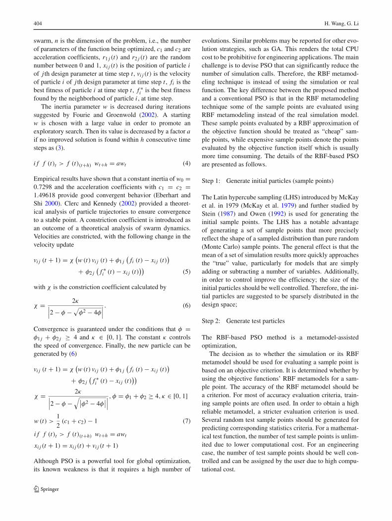
As we mentioned in Section 1, the major potential risk isto establish metamodel based on the optimization domain.If some feature sample points in the design space are notcollected, the real optimization domain might not be found(called as pseudo optimization domain) and correspondingmetamodel might not present the essences of given prob-lems. For example, approximation of a multi-hump functiondemonstrates such a risk. When the space reduction strat-egy is used, the sample points probably locate near humpsas shown in Fig. 1. If there are no sample points gener-ated in the central domain, the optimization domain shouldbe determined based on the generated sample points. Com-pared with the real function, the size of the optimizationdomain is larger and this domain is termed as pseudo one.According to Fig. 1, the approximation model based on thepseudo domain will lead to a wrong optimum It impliesthat the traditional space reduction strategies are difficultto construct a reasonable metamodel for complex nonlinearproblems.

Wang et al. (2008b) have realized this drawback and suc-cessfully used multi-level fuzzy clustering method (FCM)for overcoming it. Unfortunately, according to the multi-level FCM algorithm, with the increasing of complexity ofproblems, design space should be partitioned into multipleclusters and the size of sample points should be increaseddramatically. Therefore, such algorithm can’t solve highcomputation cost nonlinear problems in practice.

In our opinions, the key issue for a reliable metamodelis to extract the feature sample points, such as the pointsnear peaks or valleys. Obviously, it is difficult to extract

Fig. 1 An illustration ofpotential risk for spacereduction strategy True function Lower bound for metamodel

Lower bound for true function

Min based on true functionMin based on metamodel

Design variableReal optimization domain

Pseudo optimization domain

Approximation

Objective function

Unconstrained nonlinear optimization problems 403

the feature sample points for an underlying problem. For-tunately, the feature sample points (such as extremum) canbe obtained by any types of optimization methods. Even ifthe extremum is the local one, it also can be regarded asthe feature sample point because such point also can reflectthe local property. Commonly, we consider the minimumand maximum as the feature sample points. However, canthe extremum extract all characteristics of the given prob-lem? It is impossible to give a definite answer. To enhancethe robustness and stability of the metamodel, we selectthe median sample point as another kind of feature sam-ple point. Therefore, the proposed strategy is termed as“Min–Median–Max” metamodel-assisted optimization. Theminimum, maximum and median should be extracted ineach iteration of the optimization procedure. For the sake ofbrevity, Min–Median–Max metamodel-assisted optimiza-tion is simply addressed as “M3” in the following sections.

In following sections, we attempt to choose an appro-priate method to fulfill the M3 strategy. In order to obtain areliable metamodel efficiently, a metamodel-assisted optimi-zation integrated with evolution optimization is suggested.In this method, at the initial stage of the metamodel-basedoptimization, a rough metamodel should be constructed.The quality of the metamodel is then gradually improvedas more simulation data (real functions) become available.The evolution optimization is used for generating samplepoints as a design of experiments (DOE; sampling) strategy.Theoretically, the M3 can be implemented by any kinds ofoptimization methods, such as genetic algorithm (GA), sim-ulated annealing (SA), particle swarm optimization (PSO),pattern search method (PSM) and exhaustive search (ES).Similar to the sampling stage, the metamodel can also beconstructed by any kind of metamodel techniques, such asRBF, Kriging, polynomial regression response surface andothers. In this study, the M3 strategy is implemented bythe improved PSO and RBF. Compared with other evolu-tion optimization methods, the remarkable advantage of thePSO is that there are few parameters to be adjusted. TheRBF approximation has been shown to produce good fitsto arbitrary contours of both deterministic and stochasticresponse functions (Powell 1987). According to Jin’s test(Jin et al. 2001), The RBF performs the best when the accu-racy and robustness are considered. The basic theories of theRBF, RBF-assisted PSO and details of the M3 strategy areintroduced in the following sections.

2.2 The RBF metamodeling technique

The RBF has been developed for scattered multivariate datainterpolation (Hardy 1971; Dyn et al. 1986). The methoduses linear combinations of a radically symmetric function

based on Euclidean distance or other such criterion to ap-proximate response functions. A RBF model is expressed as

f̂ (x) =n∑

i=1

βiϕ (‖X − Xi‖), (1)

where βi is the coefficient of the expression and Xi is thecollected sample of input variables or the centers of RBFapproximation, φ(·) is a distance function or radial basisfunction. ‖•‖ denotes a p-norm distance and p = 1. TheRBF is a real-valued function whose value depends only onthe distance from the center sample Xi . It employs linearcombinations of a radically symmetric function based on thedistance to approximate underlying functions. The majoradvantages of the RBF are summarized as follows (Jin et al.2001; Tu and Barton 1997).

1. The number of sample points for approximation issmall;

2. The approximations are good fits for arbitrary contoursof response functions.

2.3 RBF-based particle swarm optimization

PSO is a population based optimization approach, first pub-lished by Kennedy and Eberhart in 1995 (Kennedy andEberhart 1995; Eberhart and Kennedy 1995). Since its firstpublication, a large body of research has studied the per-formance of PSOs, and improved its performance. PSO isbased on a metaphor of social interaction, searches a spaceby adjusting the trajectories of individual vectors, named“particles” as they are conceptualized as moving points inmultidimensional space. The individual particles are drawnstochastically toward the positions of their own previousbest performance and best previous performance of theirneighbors. Particles are “flown” through hyper-dimensionalsearch space, with each particle being attracted towards thebest solution found by the particles neighborhood and thebest solution found by the particle. The position, xi , of thei th particle is adjusted by a stochastic velocity vi whichdepends on the distance that the particle is chosen fromits own best solution and that of its neighborhood. For theoriginal PSO, the velocity and position are given as

vi j (t + 1) = wvi j (t) + φ1 j(

fi (t) − xi j (t))

+ φ2 j(

f ∗i (t) − xi j (t)

)(2)

xi j (t + 1) = xi j (t) + vi j (t + 1) (3)

for i = 1, . . . , m and j = 1, . . . , n, where φ1 j = c1r1 j (t)and φ2 j = c2r2 j (t), m is the total number of particles in the

404 H. Wang, G. Li

swarm, n is the dimension of the problem, i.e., the numberof parameters of the function being optimized, c1 and c2 areacceleration coefficients, r1 j (t) and r2 j (t) are the randomnumber between 0 and 1, xi j (t) is the position of particle iof j th design parameter at time step t , vi j (t) is the velocityof particle i of j th design parameter at time step t , fi is thebest fitness of particle i at time step t , f ∗

i is the best fitnessfound by the neighborhood of particle i , at time step.

The inertia parameter w is decreased during iterationssuggested by Fourie and Groenwold (2002). A startingw is chosen with a large value in order to promote anexploratory search. Then its value is decreased by a factor aif no improved solution is found within h consecutive timesteps as (3).

i f f (t)t > f (t)(t+h) wt+h = awt (4)

Empirical results have shown that a constant inertia of w0 =0.7298 and the acceleration coefficients with c1 = c2 =1.49618 provide good convergent behavior (Eberhart andShi 2000). Clerc and Kennedy (2002) provided a theoret-ical analysis of particle trajectories to ensure convergenceto a stable point. A constriction coefficient is introduced asan outcome of a theoretical analysis of swarm dynamics.Velocities are constricted, with the following change in thevelocity update

vi j (t + 1) = χ(w (t) vi j (t) + φ1 j

(fi (t) − xi j (t)

)

+ φ2 j(

f ∗i (t) − xi j (t)

))(5)

with χ is the constriction coefficient calculated by

χ = 2κ∣∣∣2 − φ − √φ2 − 4φ

∣∣∣. (6)

Convergence is guaranteed under the conditions that φ =φ1 j + φ2 j ≥ 4 and κ ∈ [0, 1]. The constant κ controlsthe speed of convergence. Finally, the new particle can begenerated by (6)

vi j (t + 1) = χ(w (t) vi j (t) + φ1 j

(fi (t) − xi j (t)

)

+ φ2 j(

f ∗i (t) − xi j (t)

))

χ = 2κ∣∣∣2 − φ −√∣∣φ2 − 4φ

∣∣∣∣∣, φ = φ1 + φ2 ≥ 4, κ ∈ [0, 1]

w (t) >1

2(c1 + c2) − 1 (7)

i f f (t)t > f (t)(t+h) wt+h = awt

xi j (t + 1) = xi j (t) + vi j (t + 1)

Although PSO is a powerful tool for global optimization,its known weakness is that it requires a high number of

evolutions. Similar problems may be reported for other evo-lution strategies, such as GA. This renders the total CPUcost to be prohibitive for engineering applications. The mainchallenge is to devise PSO that can significantly reduce thenumber of simulation calls. Therefore, the RBF metamod-eling technique is instead of using the simulation or realfunction. The key difference between the proposed methodand a conventional PSO is that in the RBF metamodelingtechnique some of the sample points are evaluated usingRBF metamodeling instead of the real simulation model.These sample points evaluated by a RBF approximation ofthe objective function should be treated as “cheap” sam-ple points, while expensive sample points denote the pointsevaluated by the objective function itself which is usuallymore time consuming. The details of the RBF-based PSOare presented as follows.

Step 1: Generate initial particles (sample points)

The Latin hypercube sampling (LHS) introduced by McKayet al. in 1979 (McKay et al. 1979) and further studied byStein (1987) and Owen (1992) is used for generating theinitial sample points. The LHS has a notable advantageof generating a set of sample points that more preciselyreflect the shape of a sampled distribution than pure random(Monte Carlo) sample points. The general effect is that themean of a set of simulation results more quickly approachesthe “true” value, particularly for models that are simplyadding or subtracting a number of variables. Additionally,in order to control improve the efficiency; the size of theinitial particles should be well controlled. Therefore, the ini-tial particles are suggested to be sparsely distributed in thedesign space;

Step 2: Generate test particles

The RBF-based PSO method is a metamodel-assistedoptimization,

The decision as to whether the simulation or its RBFmetamodel should be used for evaluating a sample point isbased on an objective criterion. It is determined whether byusing the objective functions’ RBF metamodels for a sam-ple point. The accuracy of the RBF metamodel should bea criterion. For most of accuracy evaluation criteria, train-ing sample points are often used. In order to obtain a highreliable metamodel, a stricter evaluation criterion is used.Several random test sample points should be generated forpredicting corresponding statistics criteria. For a mathemat-ical test function, the number of test sample points is unlim-ited due to lower computational cost. For an engineeringcase, the number of test sample points should be well con-trolled and can be assigned by the user due to high compu-tational cost.

Unconstrained nonlinear optimization problems 405

Step 3: Generate new particles and construct RBF-basedmetamodel

The initial particles should be evaluated by the simulation.According to (7), the new particles are generated based onthe generated particles. Consequently, a rough RBF-basedmetamodel is constructed.

Step 4: Evaluate accuracy of metamodel

In this step, the test particles generated in the Step 2 are usedfor predicting the accuracy evaluation criterion. If the con-vergence criterion expressed in (8) is satisfied, we shouldswitch to the metamodel instead of using the simulation dur-ing the optimization, else the procedure continues to use thesimulation as evaluator;

mt∑i=1

∣∣∣∣f (xtest

i )− f̂ (xtesti )

f (xtesti )

∣∣∣∣

mt< ε1 (8)

where f and f̂ denote the real and predicted objective func-tion values respectively, xtest

i denote the i th input variablevector of test particles, mt is the number of test particles. If(8) is not met in the next step, the simulation is still used forevaluating.

Step 5: Evaluate convergence criterion

The convergence condition for termination in the Step 5 ispresented as

∣∣∣∣∣f(x∗

i

) − f(x∗

i+1

)

f(x∗

i

)∣∣∣∣∣ < ε2. (9)

where x∗i and x∗

i+1 denote the best sample points of the i thand (i + 1)th iterations respectively. If the difference of x∗

iand x∗

i+1 is small enough, it suggests that no improvementin the objective function occurs with a prescribed toleranceε2, else the procedure goes back to the Step 3. Furthermore,it should be noted that PSO has various convergence condi-tions, such as the number of iteration. The user can definefitful convergence criterions according the complexity of theproblems.

2.4 RBF-based PSO motivated by M3 strategy

In this section, we apply the M3 strategy to the proposedRBF-based PSO optimization. The remarkable character-istic of the M3 strategy is to establish a metamodel byconsidering different kinds of feature sample points com-pared with other space reduction strategies. Theoretically,the generated sample points may contain several kinds of

feature sample points according to their response values,such as minima, 25%, 50%, 75% and maximum. Obvi-ously, with the increasing of the number of types of featuresample point, more features might be captured, but the num-ber of sample points should be increased and the efficiencyof the proposed method should be decreased accordingly.Meanwhile, with the decreasing of the number of types offeature sample point, some useful features might be missed.Therefore, it is difficult to determine the number of types offeature sample point. Therefore, this value should be deter-mined by the complexity of a case, it still an open issueto study further. In this study, in order to make a trade-offbetween the accuracy and efficiency, the minima, medianand maximum feature sample points are used. Thus, the fea-ture sample points are classified into three categories anddefined as: maximum sample xmax, minimum sample xmin

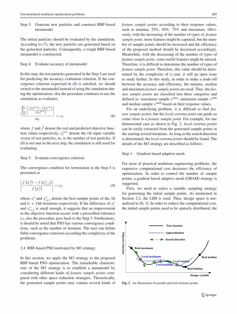
and median sample xmed based on their response values.For an underlying problem, it is difficult to find fea-

ture sample points, but the local extrema point can guide uscome close to a feature sample point. For example, for onedimensional case as shown in Fig. 2, local extrema pointscan be easily extracted from the generated sample points inthe starting several iterations. As long as the search directionis determined, the local extrema points should be found. Thedetails of the M3 strategy are described as follows.

Step 1: Gradient based adaptive mesh

For most of practical nonlinear engineering problems, theexpensive computational cost decreases the efficiency ofoptimization. In order to control the number of samplepoints, a gradient based adaptive mesh (GBAM) strategy issuggested.

First, we need to select a suitable sampling strategyfor generating the initial sample points. As mentioned inSection 2.2, the LHS is used. Thus, design space is nor-malized to [0, 1]. In order to reduce the computational cost,the initial sample points need to be sparsely distributed, the

True function

Approximation

Search direction

Real median

Real minima

Design variable

Real maximum

Local maximum

Local minimaLocal median

Objective function

Fig. 2 An illustration of pseudo and real extrema points

406 H. Wang, G. Li

number of initial sample points is 2n, where n denotes thenumber of design variables. Then, the corresponding valuesof the objective functions are evaluated. The gradient bet-ween the two neighbor sample points can be calculated by

k =∥∥∥∥∥∥

f(

xij

)− f

(xi

j+1

)

xij − xi

j+1

∥∥∥∥∥∥(10)

where k is the gradient, f (·) is the value of the objectivefunction, i and j denote the i th design variable and the j thsample point respectively.

The basic assumption of (10) is that the possible exis-tence of feature sample points in the flat space is higherthan in the steep space. Therefore, when k value is obtained,the number of grids between two neighbor sample points isdetermined as follows.

Ng =⎧⎨

⎩

0, k ≥ 2/31, 1/3 < k < 2/32, k ≤ 1/3

(11)

where Ng denotes the number of mesh lines. If k is largerthan 2/3, it means that the trend in corresponding domainis very steep. In such a sub-region, the trend of shape isvery difficult to be reformed when a new sample point isgenerated in this region. Conversely, if k is smaller than1/3, it means that the sub-region is flatter. It implies thatthere might be some feature sample points. Therefore, moresample points are generated in such region.

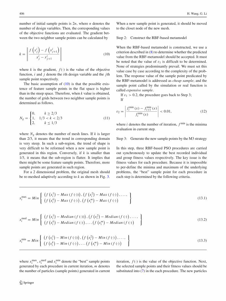
For a 2 dimensional problem, the original mesh shouldbe re-meshed adaptively according to k as shown in Fig. 3.

When a new sample point is generated, it should be movedto the closet node of the new mesh.

Step 2: Construct the RBF-based metamodel

When the RBF-based metamodel is constructed, we use acriterion described in (8) to determine whether the predictedvalue from the RBF-metamodel should be accepted. It mustbe noted that the value of ε1 is difficult to be determined.None of strategies predominantly prevail. We must set thisvalue case by case according to the complexity of the prob-lem. The response value of the sample point predicated bythe RBF-metamodel is addressed as cheap sample; and thesample point called by the simulation or real function iscalled expensive sample.

If ε1 > 0.2, the procedure goes back to Step 3;If

ε2 =∣∣∣∣∣

f mini (x) − f min

i+1 (x)

f mini (x)

∣∣∣∣∣ < 0.01, (12)

where i denotes the number of iteration, f min is the minimaevaluation in current step.

Step 3: Generate the new sample points by the M3 strategy

In this step, three RBF-based PSO procedures are carriedout synchronously to update the best recorded individualand group fitness values respectively. The key issue is thefitness values for each procedure. Because it is impossibleto per-define the minima and maximum of the underlyingproblems, the “best” sample point for each procedure ineach step is determined by the following criteria.

xmaxi = Min

{ (f(x1

i

) − Max ( f (·))) ,(

f(x2

i

) − Max ( f (·)) , . . . ,(

f(xk

i

) − Max ( f (·)) ,(

f(xm

i

) − Max ( f (·))}

(13.1)

xmedi = Min

{ (f(x1

i

) − Median ( f (·))) ,(

f(x2

i

) − Median ( f (·)) , . . . ,(

f(xk

i

) − Median ( f (·)) , . . .(

f(xm

i

) − Median ( f (·))}

(13.2)

xmini = Min

{ (f(x1

i

) − Min ( f (·))) ,(

f(x2

i

) − Min ( f (·)) , . . . ,(

f(xk

i

) − Min ( f (·)) , . . .(

f(xm

i

) − Min ( f (·))}

(13.3)

where xmaxi , xmed

i and xmini denote the “best” sample points

generated by each procedure in current iteration, m denotesthe number of particles (sample points) generated in current

iteration, f (·) is the value of the objective function. Next,the selected sample points and their fitness values should besubstituted into (7) in the each procedure. The new particles

Unconstrained nonlinear optimization problems 407

Objective function

Smooth region

Two samples

Objective function

One sample

Des

ign

vari

able

x2

Design variable x

New samples indesign space

1

Steep region

Fig. 3 An illustration of meshing by the GBAM

should be generated according to the different criteriadescribed in (13.1–13.3). In addition, similar to the Step 2,the new sample points should be moved to their closetnodes. If the node has been already assigned (occupied), thenew sample points need to be regenerated according to (14)till the unassigned closest node is free.

xi j (t + 1) = xi j (t + 1) rand (0, 1) (14)

where rand(0,1) returns a pseudorandom, scalar valuedrawn from a uniform distribution on the unit interval.

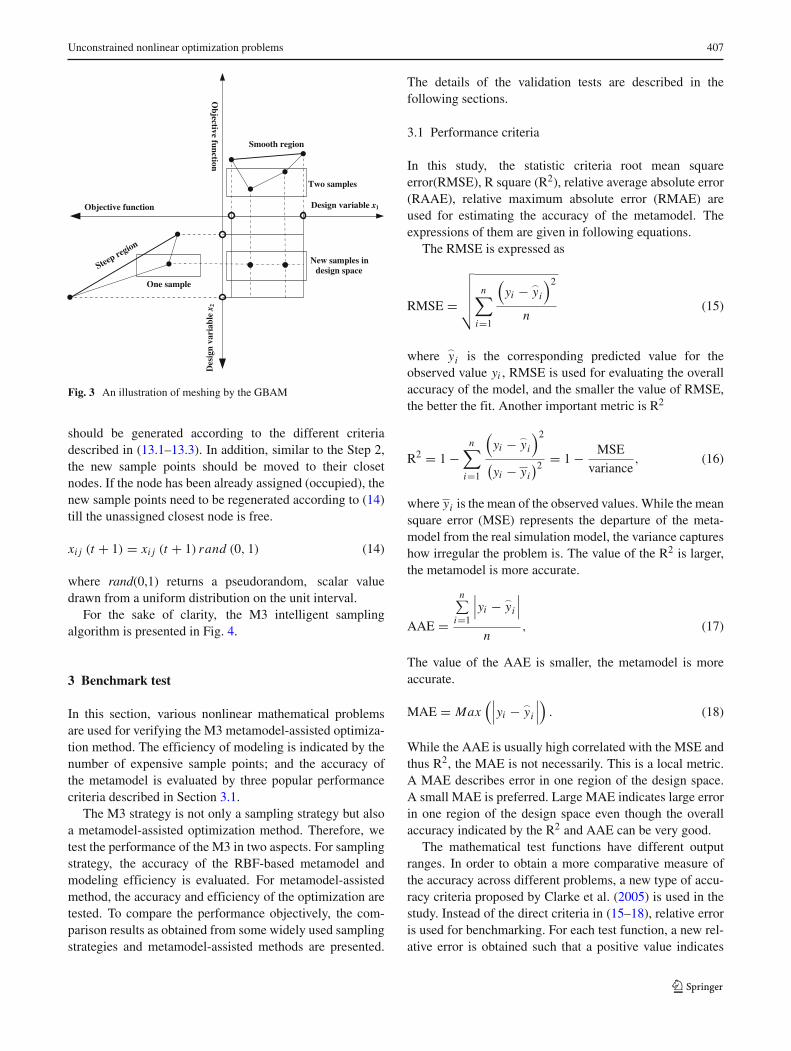
For the sake of clarity, the M3 intelligent samplingalgorithm is presented in Fig. 4.

3 Benchmark test

In this section, various nonlinear mathematical problemsare used for verifying the M3 metamodel-assisted optimiza-tion method. The efficiency of modeling is indicated by thenumber of expensive sample points; and the accuracy ofthe metamodel is evaluated by three popular performancecriteria described in Section 3.1.

The M3 strategy is not only a sampling strategy but alsoa metamodel-assisted optimization method. Therefore, wetest the performance of the M3 in two aspects. For samplingstrategy, the accuracy of the RBF-based metamodel andmodeling efficiency is evaluated. For metamodel-assistedmethod, the accuracy and efficiency of the optimization aretested. To compare the performance objectively, the com-parison results as obtained from some widely used samplingstrategies and metamodel-assisted methods are presented.

The details of the validation tests are described in thefollowing sections.

3.1 Performance criteria

In this study, the statistic criteria root mean squareerror(RMSE), R square (R2), relative average absolute error(RAAE), relative maximum absolute error (RMAE) areused for estimating the accuracy of the metamodel. Theexpressions of them are given in following equations.

The RMSE is expressed as

RMSE =

√√√√√n∑

i=1

(yi − �

yi

)2

n(15)

where�yi is the corresponding predicted value for the

observed value yi , RMSE is used for evaluating the overallaccuracy of the model, and the smaller the value of RMSE,the better the fit. Another important metric is R2

R2 = 1 −n∑

i=1

(yi − �

yi

)2

(yi − yi

)2= 1 − MSE

variance, (16)

where yi is the mean of the observed values. While the meansquare error (MSE) represents the departure of the meta-model from the real simulation model, the variance captureshow irregular the problem is. The value of the R2 is larger,the metamodel is more accurate.

AAE =

n∑i=1

∣∣∣yi − �yi

∣∣∣

n, (17)

The value of the AAE is smaller, the metamodel is moreaccurate.

MAE = Max(∣∣∣yi − �

yi

∣∣∣)

. (18)

While the AAE is usually high correlated with the MSE andthus R2, the MAE is not necessarily. This is a local metric.A MAE describes error in one region of the design space.A small MAE is preferred. Large MAE indicates large errorin one region of the design space even though the overallaccuracy indicated by the R2 and AAE can be very good.

The mathematical test functions have different outputranges. In order to obtain a more comparative measure ofthe accuracy across different problems, a new type of accu-racy criteria proposed by Clarke et al. (2005) is used in thestudy. Instead of the direct criteria in (15–18), relative erroris used for benchmarking. For each test function, a new rel-ative error is obtained such that a positive value indicates

408 H. Wang, G. Li

Generate the initial sample points by LHS

Evaluate fitness values by simulations or real functions

Construct the RBF-based metamodel

Evaluate fitness values by the RBF-based metamodel

Generate the test sample points randomly

Is criterion Eq.(8) satisfied?

No

Yes

According to the M3 strategy, sample points and their fitness values are extracted

Calculate particle velocity according and update particle position according Eq.(7)

Is convergence condition Eq.(9) satisfied?

Generate the new sample points in three procedures synchronously

Yes

Terminate

No

Generate the new mesh by the GBAM strategyMove the new sample points to the

closet nodes of new mesh

Set the initial parameters of PSO

Max Median Min

Fig. 4 Flowchart of the M3 strategy based on the RBF-based PSO method

that the method in comparison has larger error than the M3,while a negative value indicates that the method in compar-ison obtains a smaller error than the M3. The expression ofthe relative error can be written as

RERR = ERR (•) − ERR (M3)

ERR (M3)(19)

where (•) denotes other metamodeling techniques. TheERR in (18) refers to the errors defined in (15–18), andthe corresponding criteria are denoted by the RMSER, R2

R,RAAER, RMAER.

The M3 strategy can be used for metamodel-assistedoptimization. Therefore, it is necessary to compare theoptimization efficiency performance with other metamodel-assisted optimization methods, such as efficient globaloptimization (EGO; Jones et al. 1998), sequential responsesurface method (SRSM; Liu and Moses 1994), mode-pursuing sampling method (MPS; Wang et al. 2004) andparticle swarm optimization intelligent sampling method(PSOIS; Wang et al. 2008b). The performance comparisons

of four optimization methods are presented and discussed inSection 3.3.

3.2 Test functions

To verify the feasibility of the proposed strategy, ten non-linear mathematical functions are tested and correspondingdescriptions are listed in Table 1. According to dimensionsof the mathematical functions listed in Table 1, low and highdimensional cases are considered respectively.

As mentioned in the previous section, the M3 strat-egy is implemented by the RBF-based PSO optimization.The sample points generated by the RBF-based PSO opti-mization are composed of the expensive and cheap sam-ple points. Compared with the expensive sample points,the computation cost of the cheap sample points can benegligible.

Furthermore, to predict the accuracy of the RBF-basedmetamodel objectively, additional 1000 randomly generated

Unconstrained nonlinear optimization problems 409

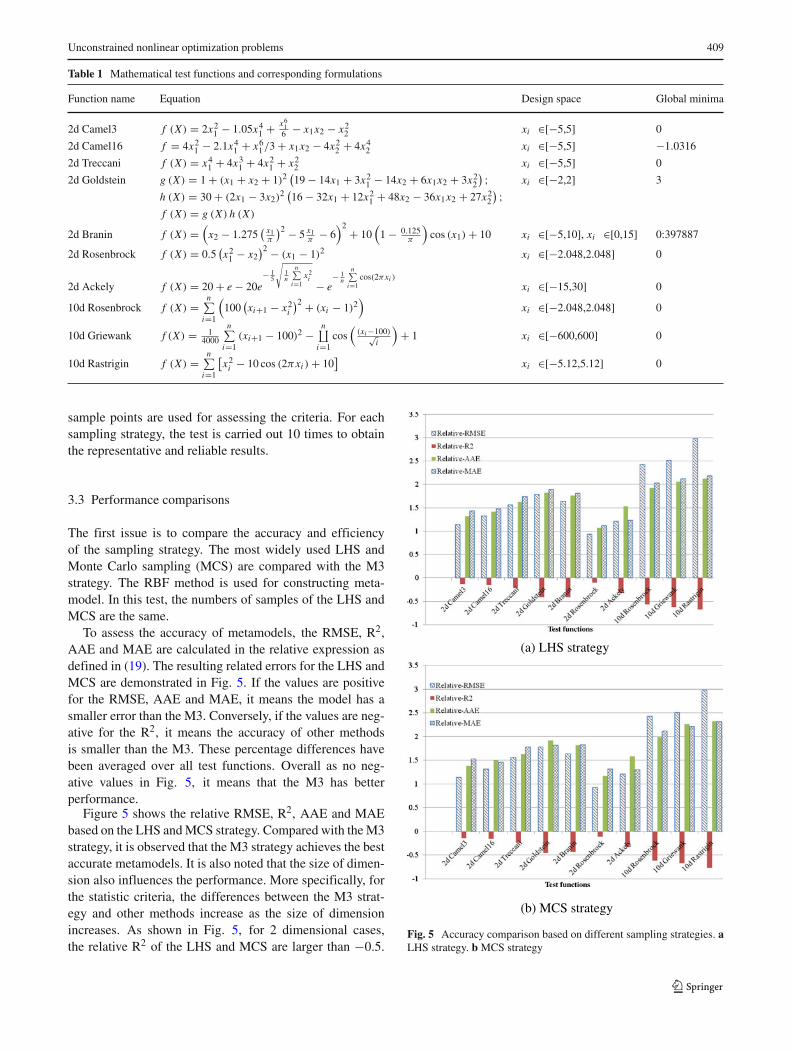
Table 1 Mathematical test functions and corresponding formulations

Function name Equation Design space Global minima

2d Camel3 f (X) = 2x21 − 1.05x4

1 + x616 − x1x2 − x2

2 xi ∈[−5,5] 0

2d Camel16 f = 4x21 − 2.1x4

1 + x61/3 + x1x2 − 4x2

2 + 4x42 xi ∈[−5,5] −1.0316

2d Treccani f (X) = x41 + 4x3

1 + 4x21 + x2

2 xi ∈[−5,5] 0

2d Goldstein g (X) = 1 + (x1 + x2 + 1)2 (19 − 14x1 + 3x2

1 − 14x2 + 6x1x2 + 3x22

) ; xi ∈[−2,2] 3

h (X) = 30 + (2x1 − 3x2)2 (

16 − 32x1 + 12x21 + 48x2 − 36x1x2 + 27x2

2

) ;f (X) = g (X) h (X)

2d Branin f (X) =(

x2 − 1.275( x1

π

)2 − 5 x1π

− 6)2 + 10

(1 − 0.125

π

)cos (x1) + 10 xi ∈[−5,10], xi ∈[0,15] 0:397887

2d Rosenbrock f (X) = 0.5(x2

1 − x2)2 − (x1 − 1)2 xi ∈[−2.048,2.048] 0

2d Ackely f (X) = 20 + e − 20e− 1

5

√1n

n∑i=1

x2i − e

− 1n

n∑i=1

cos(2πxi )

xi ∈[−15,30] 0

10d Rosenbrock f (X) =n∑

i=1

(100

(xi+1 − x2

i

)2 + (xi − 1)2)

xi ∈[−2.048,2.048] 0

10d Griewank f (X) = 14000

n∑i=1

(xi+1 − 100)2 −n∐

i=1cos

((xi −100)√

i

)+ 1 xi ∈[−600,600] 0

10d Rastrigin f (X) =n∑

i=1

[x2

i − 10 cos (2πxi ) + 10]

xi ∈[−5.12,5.12] 0

sample points are used for assessing the criteria. For eachsampling strategy, the test is carried out 10 times to obtainthe representative and reliable results.

3.3 Performance comparisons

The first issue is to compare the accuracy and efficiencyof the sampling strategy. The most widely used LHS andMonte Carlo sampling (MCS) are compared with the M3strategy. The RBF method is used for constructing meta-model. In this test, the numbers of samples of the LHS andMCS are the same.

To assess the accuracy of metamodels, the RMSE, R2,AAE and MAE are calculated in the relative expression asdefined in (19). The resulting related errors for the LHS andMCS are demonstrated in Fig. 5. If the values are positivefor the RMSE, AAE and MAE, it means the model has asmaller error than the M3. Conversely, if the values are neg-ative for the R2, it means the accuracy of other methodsis smaller than the M3. These percentage differences havebeen averaged over all test functions. Overall as no neg-ative values in Fig. 5, it means that the M3 has betterperformance.

Figure 5 shows the relative RMSE, R2, AAE and MAEbased on the LHS and MCS strategy. Compared with the M3strategy, it is observed that the M3 strategy achieves the bestaccurate metamodels. It is also noted that the size of dimen-sion also influences the performance. More specifically, forthe statistic criteria, the differences between the M3 strat-egy and other methods increase as the size of dimensionincreases. As shown in Fig. 5, for 2 dimensional cases,the relative R2 of the LHS and MCS are larger than −0.5.

(a) LHS strategy

(b) MCS strategy

Fig. 5 Accuracy comparison based on different sampling strategies. aLHS strategy. b MCS strategy

410 H. Wang, G. Li

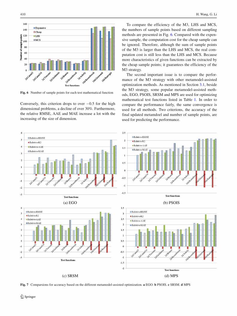
Fig. 6 Number of sample points for each test mathematical function

Conversely, this criterion drops to over −0.5 for the highdimensional problems, a decline of over 30%. Furthermore,the relative RMSE, AAE and MAE increase a lot with theincreasing of the size of dimension.

To compare the efficiency of the M3, LHS and MCS,the numbers of sample points based on different samplingmethods are presented in Fig. 6. Compared with the expen-sive sample, the computation cost for the cheap sample canbe ignored. Therefore, although the sum of sample pointsof the M3 is larger than the LHS and MCS, the real com-putation cost is still less than the LHS and MCS. Becausemore characteristics of given functions can be extracted bythe cheap sample points; it guarantees the efficiency of theM3 strategy.

The second important issue is to compare the perfor-mance of the M3 strategy with other metamodel-assistedoptimization methods. As mentioned in Section 3.1, besidethe M3 strategy, some popular metamodel-assisted meth-ods, EGO, PSOIS, SRSM and MPS are used for optimizingmathematical test functions listed in Table 1. In order tocompare the performance fairly, the same convergence isused for all methods. Two criterions, the accuracy of thefinal updated metamdoel and number of sample points, areused for predicting the performance.

(a) EGO (b) PSOIS

(c) SRSM (d) MPS

Fig. 7 Comparsions for accuracy based on the different metamodel-assisted optimization. a EGO. b PSOIS. c SRSM. d MPS

Unconstrained nonlinear optimization problems 411

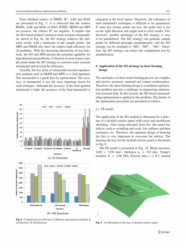
Final obtained relative of RMSE, R2, AAE and MAEare presented in Fig. 7, it is observed that the relativeRMSE, AAE and MAE of EGO, POSIS, SRSM and MPSare positive, the relative R2 are negative. It implies thatthe M3-based method constructs more accurate metamodel.As shown in Fig. 8a, the M3 strategy achieves the opti-mum results with a minimum of the sample points, theMPS and PSOIS also show the relative high efficiency for2d problems. With the increasing dimensions of test func-tions, the M3 and MPS present the potential capability forhigh dimensional problems. Collection of more feature sam-ple points helps the M3 strategy to construct more accuratemetamodel and develop the efficiency.

Actually, the key point of metamodel-assisted optimiza-tion methods such as SRSM and MPS is to find optimum.The metamodel is a guide line for optimization. The accu-racy of metamodel is not the most important factor forsuch strategies. Although the accuracy of the final updatedmetamodel is high, the accuracy of the final metamodel is

(a) 2d functions

(b) 10d functions

Fig. 8 Comparsions for efficieny of different optimization methods. a2d functions. b 10d functions

estimated in the local region. Therefore, the robustness ofsuch metamodel techniques is difficult to be guaranteed.If some key feature points are lost, the guide line is noton the right direction and might lead to error results. Fur-thermore, another advantage of the M3 strategy is easyto be parallelized. The M3 strategy can generate samplepoints by different principle simultaneously; and the M3strategy can be extended to “M4”, “M5”... “Mn”. There-fore, the M3 strategy can reduce the computation cost byparallelization.

4 Application of the M3 strategy in sheet formingdesign

The mechanics of sheet metal forming process are complexand involve geometry, material and contact nonlinearities.Therefore, the sheet forming design is a nonlinear optimiza-tion problem and also a challenge in engineering optimiza-tion research field. In this section, the M3-based metamod-eling optimization is applied to this problem. The details ofthe optimization procedure are presented as follows.

4.1 FE model

The application of the M3 method is illustrated by a draw-ing of a decklid exterior panel with crack and insufficientstretching. After being unloaded from die, this panel hasdefects, such as wrinkling and crack, low stiffness and dentresistance, etc. Therefore, the optimum design of drawingdie face is very important to overcome the defects. Thedrawing die face for the decklid exterior panel is illustratedin Fig. 9.

The FE model is presented in Fig. 10. Blank measures1640 × 1330 mm2, thickness t0 = 0.8 mm, Young’smodulus E = 2.06 GPa, Poisson ratio ν = 0.3, normal

Fig. 9 An illustration of die face of decklid exterior panel

412 H. Wang, G. Li

Blank

Die

Blank holder

Punch

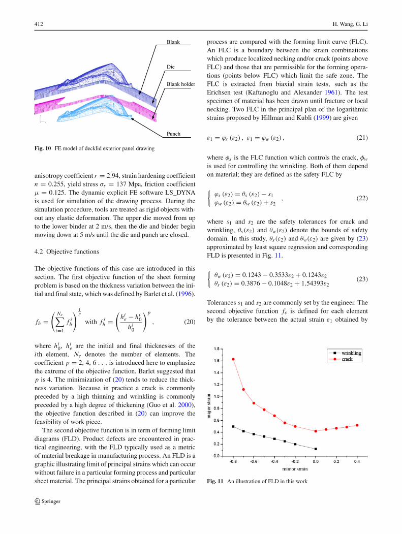
Fig. 10 FE model of decklid exterior panel drawing

anisotropy coefficient r = 2.94, strain hardening coefficientn = 0.255, yield stress σs = 137 Mpa, friction coefficientμ = 0.125. The dynamic explicit FE software LS_DYNAis used for simulation of the drawing process. During thesimulation procedure, tools are treated as rigid objects with-out any elastic deformation. The upper die moved from upto the lower binder at 2 m/s, then the die and binder beginmoving down at 5 m/s until the die and punch are closed.

4.2 Objective functions

The objective functions of this case are introduced in thissection. The first objective function of the sheet formingproblem is based on the thickness variation between the ini-tial and final state, which was defined by Barlet et al. (1996).

fh =( Ne∑

i=1

f ih

) 1p

with f ih =

(hi

e − hi0

hi0

)p

, (20)

where hi0, hi

e are the initial and final thicknesses of thei th element, Ne denotes the number of elements. Thecoefficient p = 2, 4, 6 . . . is introduced here to emphasizethe extreme of the objective function. Barlet suggested thatp is 4. The minimization of (20) tends to reduce the thick-ness variation. Because in practice a crack is commonlypreceded by a high thinning and wrinkling is commonlypreceded by a high degree of thickening (Guo et al. 2000),the objective function described in (20) can improve thefeasibility of work piece.

The second objective function is in term of forming limitdiagrams (FLD). Product defects are encountered in prac-tical engineering, with the FLD typically used as a metricof material breakage in manufacturing process. An FLD is agraphic illustrating limit of principal strains which can occurwithout failure in a particular forming process and particularsheet material. The principal strains obtained for a particular

process are compared with the forming limit curve (FLC).An FLC is a boundary between the strain combinationswhich produce localized necking and/or crack (points aboveFLC) and those that are permissible for the forming opera-tions (points below FLC) which limit the safe zone. TheFLC is extracted from biaxial strain tests, such as theErichsen test (Kaftanoglu and Alexander 1961). The testspecimen of material has been drawn until fracture or localnecking. Two FLC in the principal plan of the logarithmicstrains proposed by Hillman and Kubli (1999) are given

ε1 = ϕs (ε2) , ε1 = ϕw (ε2) , (21)

where φs is the FLC function which controls the crack, φw

is used for controlling the wrinkling. Both of them dependon material; they are defined as the safety FLC by

{ϕs (ε2) = θs (ε2) − s1

ϕw (ε2) = θw (ε2) + s2, (22)

where s1 and s2 are the safety tolerances for crack andwrinkling, θs(ε2) and θw(ε2) denote the bounds of safetydomain. In this study, θs(ε2) and θw(ε2) are given by (23)approximated by least square regression and correspondingFLD is presented in Fig. 11.

{θw (ε2) = 0.1243 − 0.3533ε2 + 0.1243ε2

θs (ε2) = 0.3876 − 0.1048ε2 + 1.54393ε2(23)

Tolerances s1 and s2 are commonly set by the engineer. Thesecond objective function fε is defined for each elementby the tolerance between the actual strain ε1 obtained by

Fig. 11 An illustration of FLD in this work

Unconstrained nonlinear optimization problems 413

Drawbead 1 Drawbead 4Drawbead 3Drawbead 2

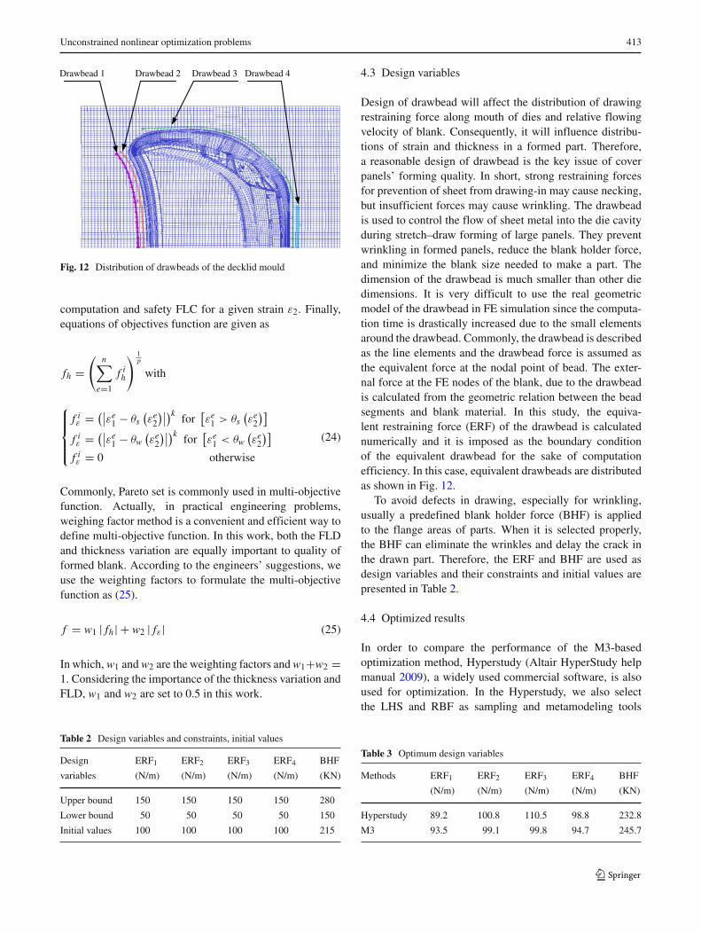
Fig. 12 Distribution of drawbeads of the decklid mould

computation and safety FLC for a given strain ε2. Finally,equations of objectives function are given as

fh =(

n∑

e=1

f ih

) 1p

with

⎧⎪⎪⎨

⎪⎪⎩

f iε = (∣∣εe

1 − θs(εe

2

)∣∣)k for[εe

1 > θs(εe

2

)]

f iε = (∣∣εe

1 − θw(εe

2

)∣∣)k for[εe

1 < θw(εe

2

)]

f iε = 0 otherwise

(24)

Commonly, Pareto set is commonly used in multi-objectivefunction. Actually, in practical engineering problems,weighing factor method is a convenient and efficient way todefine multi-objective function. In this work, both the FLDand thickness variation are equally important to quality offormed blank. According to the engineers’ suggestions, weuse the weighting factors to formulate the multi-objectivefunction as (25).

f = w1 | fh | + w2 | fε| (25)

In which, w1 and w2 are the weighting factors and w1+w2 =1. Considering the importance of the thickness variation andFLD, w1 and w2 are set to 0.5 in this work.

Table 2 Design variables and constraints, initial values

Design ERF1 ERF2 ERF3 ERF4 BHF

variables (N/m) (N/m) (N/m) (N/m) (KN)

Upper bound 150 150 150 150 280

Lower bound 50 50 50 50 150

Initial values 100 100 100 100 215

4.3 Design variables

Design of drawbead will affect the distribution of drawingrestraining force along mouth of dies and relative flowingvelocity of blank. Consequently, it will influence distribu-tions of strain and thickness in a formed part. Therefore,a reasonable design of drawbead is the key issue of coverpanels’ forming quality. In short, strong restraining forcesfor prevention of sheet from drawing-in may cause necking,but insufficient forces may cause wrinkling. The drawbeadis used to control the flow of sheet metal into the die cavityduring stretch–draw forming of large panels. They preventwrinkling in formed panels, reduce the blank holder force,and minimize the blank size needed to make a part. Thedimension of the drawbead is much smaller than other diedimensions. It is very difficult to use the real geometricmodel of the drawbead in FE simulation since the computa-tion time is drastically increased due to the small elementsaround the drawbead. Commonly, the drawbead is describedas the line elements and the drawbead force is assumed asthe equivalent force at the nodal point of bead. The exter-nal force at the FE nodes of the blank, due to the drawbeadis calculated from the geometric relation between the beadsegments and blank material. In this study, the equiva-lent restraining force (ERF) of the drawbead is calculatednumerically and it is imposed as the boundary conditionof the equivalent drawbead for the sake of computationefficiency. In this case, equivalent drawbeads are distributedas shown in Fig. 12.

To avoid defects in drawing, especially for wrinkling,usually a predefined blank holder force (BHF) is appliedto the flange areas of parts. When it is selected properly,the BHF can eliminate the wrinkles and delay the crack inthe drawn part. Therefore, the ERF and BHF are used asdesign variables and their constraints and initial values arepresented in Table 2.

4.4 Optimized results

In order to compare the performance of the M3-basedoptimization method, Hyperstudy (Altair HyperStudy helpmanual 2009), a widely used commercial software, is alsoused for optimization. In the Hyperstudy, we also selectthe LHS and RBF as sampling and metamodeling tools

Table 3 Optimum design variables

Methods ERF1 ERF2 ERF3 ERF4 BHF

(N/m) (N/m) (N/m) (N/m) (KN)

Hyperstudy 89.2 100.8 110.5 98.8 232.8

M3 93.5 99.1 99.8 94.7 245.7

414 H. Wang, G. Li

respectively. The final results obtained by the Hyperstudyand M3-based optimization method are presented in Table 3.

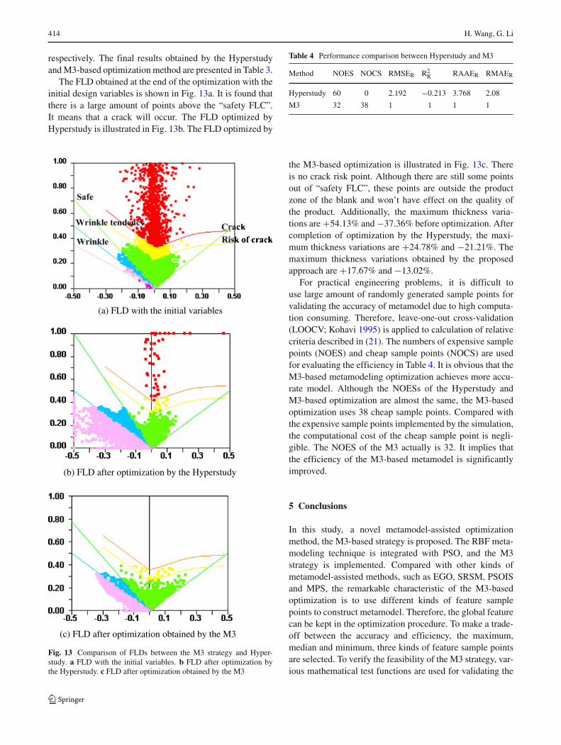
The FLD obtained at the end of the optimization with theinitial design variables is shown in Fig. 13a. It is found thatthere is a large amount of points above the “safety FLC”.It means that a crack will occur. The FLD optimized byHyperstudy is illustrated in Fig. 13b. The FLD optimized by

(a) FLD with the initial variables

(b) FLD after optimization by the Hyperstudy

(c) FLD after optimization obtained by the M3

Fig. 13 Comparison of FLDs between the M3 strategy and Hyper-study. a FLD with the initial variables. b FLD after optimization bythe Hyperstudy. c FLD after optimization obtained by the M3

Table 4 Performance comparison between Hyperstudy and M3

Method NOES NOCS RMSER R2R RAAER RMAER

Hyperstudy 60 0 2.192 −0.213 3.768 2.08

M3 32 38 1 1 1 1

the M3-based optimization is illustrated in Fig. 13c. Thereis no crack risk point. Although there are still some pointsout of “safety FLC”, these points are outside the productzone of the blank and won’t have effect on the quality ofthe product. Additionally, the maximum thickness varia-tions are +54.13% and −37.36% before optimization. Aftercompletion of optimization by the Hyperstudy, the maxi-mum thickness variations are +24.78% and −21.21%. Themaximum thickness variations obtained by the proposedapproach are +17.67% and −13.02%.

For practical engineering problems, it is difficult touse large amount of randomly generated sample points forvalidating the accuracy of metamodel due to high computa-tion consuming. Therefore, leave-one-out cross-validation(LOOCV; Kohavi 1995) is applied to calculation of relativecriteria described in (21). The numbers of expensive samplepoints (NOES) and cheap sample points (NOCS) are usedfor evaluating the efficiency in Table 4. It is obvious that theM3-based metamodeling optimization achieves more accu-rate model. Although the NOESs of the Hyperstudy andM3-based optimization are almost the same, the M3-basedoptimization uses 38 cheap sample points. Compared withthe expensive sample points implemented by the simulation,the computational cost of the cheap sample point is negli-gible. The NOES of the M3 actually is 32. It implies thatthe efficiency of the M3-based metamodel is significantlyimproved.

5 Conclusions

In this study, a novel metamodel-assisted optimizationmethod, the M3-based strategy is proposed. The RBF meta-modeling technique is integrated with PSO, and the M3strategy is implemented. Compared with other kinds ofmetamodel-assisted methods, such as EGO, SRSM, PSOISand MPS, the remarkable characteristic of the M3-basedoptimization is to use different kinds of feature samplepoints to construct metamodel. Therefore, the global featurecan be kept in the optimization procedure. To make a trade-off between the accuracy and efficiency, the maximum,median and minimum, three kinds of feature sample pointsare selected. To verify the feasibility of the M3 strategy, var-ious mathematical test functions are used for validating the

Unconstrained nonlinear optimization problems 415

performance of the M3 strategy. The test results demon-strate that the accuracy and efficiency of the M3-basedmetamodels can be guaranteed.

The ultimate purpose of this study is to apply the pro-posed method to the real engineering problems. Therefore,the M3-based metamodel-assisted optimization is imple-mented for a nonlinear practical engineering optimizationproblem: sheet forming design. Compared with the opti-mum results from the commercial software Hyperstudy, theefficiency and accuracy of the M3-based optimization arewell improved. It indicates that the M3-based optimiza-tion has the potential capability for the real engineeringproblems.

Acknowledgments This work is supported by Project of NationalScience Foundation of China (NSFC) under the grant number10902037; the National 973 Program of China under the grant num-ber 2010CB328005; Hunan Provincial Natural Science Foundationof China under the grant number 11JJA001; Fundamental ResearchFunds for the Central Universities, Hunan University; Program forChangjiang Scholar and Innovative Research Team in University andState Key Laboratory of Advanced technology for vehicle design andmanufacture.

References

Barlet O, Batoz JL, Guo YQ, Mercier F, Naceur H, Knopf-LenoirC (1996) The inverse approach and mathematical programmingtechniques for optimum design of sheet forming parts. In: Thirdbiennial european joint conference on engineering systems designand analysis, ESDA’96, July 1–4. Montpellier, France

Box GEP, Draper NR (1969) Evolutionary operation: a statisticalmethod for process management. Wiley, New York

Chen W (1995) A robust concept exploration method for configuringcomplex system. PhD Thesis, Georgia Institute of Technology

Clarke SM, Griebsch JH, Simpson TW (2005) Analysis of supportvector regression for approximation of complex engineering anal-yses. ASME Trans J Mech Des 127(6):1077–1087

Clerc M, Kennedy J (2002) The particle swarm-explosion, stability,and convergence in a multidimensional complex space. IEEETrans Evol Comput 6(1):58–73

Dyn N, Levin D, Rippa S (1986) Numerical procedures for surfacefitting of scattered data by radial basis functions. SIAM J, SciStat Comput 7:639–659

Eberhart RC, Kennedy J (1995) A new optimizer using particle swarmtheory. In: Proceedings of the sixth international symposium onmicromachine and human science, Nagoya, Japan, pp 39–43

Eberhart RC, Shi Y (2000) Comparing inertia weights and constric-tion factors in particle swarm optimization. In: Proceedings of theIEEE congress on evolutionary computation, San Diego, USA, pp84–88

Fourie P, Groenwold A (2002) The particle swarm optimization in sizeand shape optimization. Struct Multidiscipl Optim 23(4):259–267

Guo YQ, Batoz JL, Naceur H, Bouabdallah S, Mercier F, Barlet O(2000) Recent developments on the analysis and optimum designof sheet metal forming parts using a simplified inverse approach.Comput Struct 78(1–3):133–48

Hardy RL (1971) Multiquadratic equations of topography and otherirregular surfaces. J Geophys Res 76:1905–1915

Hillman M, Kubli W (1999) Optimization of sheet metal forming pro-cesses using simulation programs. In: Numisheet 99, Besanc.France 1:287–92

HyperStudy user manual (2009) Troy (MI): Altair Engineering Inc.Jin R, Chen W, Simpson TW (2001) Comparative studies of meta-

modelling techniques under multiple modelling criteria. StructMultidiscipl Optim 23:1–13

Jones D, Schonlau M, Welch W (1998) Efficient global optimiza-tion of expensive black-box functions. J Glob Optim 13:455–492

Kaftanoglu B, Alexander JM (1961) An investigation of the Erichsentest. J Inst Met 90:457–s470

Kennedy J, Eberhart RC (1995) Particle swarm optimization. In: Pro-ceedings of the IEEE international joint conference on neuralnetworks. IEEE Press, pp 1942–1948

Kohavi R (1995) A study of cross-validation and bootstrap for accuracyestimation and model selection. In: Proceedings of the 14th inter-national conference on artificial intelligence (IJCAI). MorganKaufmann, San Mateo, pp 1137–1143

Liu YW, Moses F (1994) A sequential response surface method and itsapplication in the reliability analysis of aircraft structural systems.Struct Saf 16(1–2):39–46

McKay MD, Beckman RJ, Conover WJ (1979) A comparison of threemethods for selecting values of input variables in the analysis ofoutput from a computer code. Technometrics 21:239–245

Owen AB (1992) A central limit theorem for latin hypercube sampling.J R Stat Soc Series B54(13):541–551

Powell MJD (1987) Radial basis functions for multivariable interpo-lation: a review. In: Mason JC, Cox MG (eds) Algorithms forapproximation. Oxford University Press

Stein M (1987) Large sample properties of simulations using Latinhypercube sampling. Technometrics 29(2):143–151, correction in32:367

Toropov V, van Keulen F, Markine V, de Doer H (1996) Refinementsin the multi-point approximation method to reduce the effects ofnoisy structural responses. In: Proceedings 6th AIAA/USAF/NASA/ISSMO symposium on multidisciplinary analysis and op-timization, vol 2. AIAA, Bellevue, WA, September 4–6, AIAA-96-4087-CP

Tu CH, Barton RR (1997) Production yield estimation by the meta-model method with a boundary-focused experiment design. In:Design theory and methodology conf—DTM’97, DETC97/DTM3870

Wang G, Dong Z, Aitchison P (2001) Adaptive response surfacemethod—a global optimization scheme for computation-intensivedesign problems. J Eng Optim 33(6):707–734

Wang L, Shan S, Wang GG (2004) Mode-pursuing sampling methodfor global optimization on expensive black-box functions. EngOptim 36(4):419–438

Wang H, Li EY, Li GY (2008a) A metamodel optimization methodol-ogy based on multi-level fuzzy clustering space reduction strategyand its applications. Comput Ind Eng 55(2):503–532

Wang H, Li GY, Zhong ZH (2008b) Optimization of sheet metal form-ing processes by adaptive response surface based on intelligentsampling method. J Mater Process Technol 197(1–3):77–88

Wujek BA, Renaud JE (1998a) New adaptive move-limit manage-ment strategy for approximate optimization, part 1. AIAA J36(10):1911–1921

Wujek BA, Renaud JE (1998b) New adaptive move-limit manage-ment strategy for approximate optimization, part 2. AIAA J36(10):1922–1934