robust algorithms for generalized pham systems

ROBUST ALGORITHMS FOR

GENERALIZED PHAM SYSTEMS

Ezequiel Dratman, Guillermo Matera,

and Ariel Waissbein

Abstract. We discuss the complexity of robust symbolic algorithmssolving a significant class of zero–dimensional square polynomial sys-tems with rational coefficients over the complex numbers, called gener-alized Pham systems, which represent the class of zero–dimensional ho-mogeneous complete–intersection systems with “no points at infinity”.Our notion of robustness models the behavior of all known universalmethods for solving (parametric) polynomial systems avoiding unneces-sary branchings and allowing the solution of certain limit problems. Wefirst show that any robust algorithm solving generalized Pham systemshas complexity at least polynomial in the Bezout number of the systemunder consideration. Then we exhibit a robust probabilistic algorithmwhich solves generalized Pham systems with quadratic complexity in theBezout number of the input system. The algorithm consists in a series ofhomotopies deforming the input system into a system which is “easy tosolve”, together with a “projection algorithm” which allows to move thesolutions of the known instance to the solutions of an arbitrary instancealong the parameter space.

Keywords. Polynomial system solving, robust algorithms, geometricsolutions, Newton–Hensel lifting, probabilistic algorithms, complexity.

Subject classification. Primary 14Q05, 68W30; Secondary 12Y05,13F25, 14Q20, 68W40.

1. Introduction

The design and analysis of algorithms for solving multivariate polynomial sys-tems is a central theme of computational algebraic geometry, which arises inconnection with numerous scientific and technical problems (see, e.g., Sturm-fels (2002)). In this article we are concerned with universal symbolic solvers formultivariate polynomial systems over the complex numbers (cf. Castro et al.

2 Dratman, Matera & Waissbein

(2003); see also Pardo (2000), Beltran & Pardo (2006)), i.e., with algorithmsthat output complete information about the system under consideration. Thisconcept of universality, which goes back at least to Kronecker (Giusti & Heintz(2001)), underlies the design of all known algorithms in computational alge-braic geometry (see, e.g., Cox et al. (1998) and Sturmfels (2002) for rewritingtechniques and Durvye & Lecerf (2008) for Kronecker–like elimination proce-dures).

Furthermore, we shall consider only robust universal algorithms, that is, al-gorithms which solve parametric families of polynomial systems avoiding “un-necessary” branchings and allowing the solution of certain limit problems. Ro-bust universal algorithms form an important class of elimination procedureswhich include among others comprehensive Grobner basis algorithms (see, e.g.,Becker & Weispfenning (1993)), algorithms based on resultants (see, e.g., Coxet al. (1998)) and black–box elimination algorithms (cf. Castro et al. (2003)).

In Castro et al. (2003) (see also Heintz et al. (1998), Pardo (2000), Giusti& Heintz (2001), Beltran & Pardo (2006)) it is shown that the worst–casecomplexity of robust universal algorithms solving certain polynomial systemsover the complex numbers is at least DΩ(1), where D denotes the Bezout numberof the system under consideration. Therefore, one would hope to design robustuniversal solvers with polynomial complexity as low as possible in the Bezoutnumber of the input system. In the series of papers Giusti et al. (1998), Giustiet al. (1997) (see also Heintz et al. (2001), Giusti et al. (2001) for complexityimprovements over the complex numbers, Bank et al. (2004) for real systemsolving and Cafure & Matera (2006) for finite field system solving) a new robustuniversal solver is developed. This solver deals with systems defined by areduced regular sequence and has complexity quadratic in the Bezout numberof the input system. In Lecerf (2002), Lecerf (2003) it is extended to a universalalgorithm solving an arbitrary polynomial system with complexity cubic inthe Bezout number. Nevertheless, achieving quadratic time–complexity onarbitrary polynomial systems still remains an open problem.

The symbolic solver mentioned above is based on a flat deformation ofcertain morphism of affine varieties. This deformation is isolated in Heintzet al. (2000) and refined in Schost (2003), Bompadre et al. (2004) (see alsoHeintz et al. (2002), Pardo & San Martın (2004), Jeronimo et al. (2008)) tosolve particular instances of a parametric system with a finite generically–unramified linear projection of “low” degree. The resulting (robust) algorithmshave quadratic complexity in the Bezout number of the system. In particular,Bompadre et al. (2004) considers families of Pham systems. An n–dimensionalPham system is defined by n polynomials of the form Xdi

i −gi (1 ≤ i ≤ n), where

Robust algorithms for generalized Pham systems 3

gi ∈ Q[X1, . . . , Xn] has degree less than di > 0 for 1 ≤ i ≤ n. The algorithm ofBompadre et al. (2004) for solving Pham systems improves the algorithms ofMourrain & Pan (1997), Gonzalez-Lopez & Gonzalez-Vega (1998), and seems tohave the same cost as those of Mourrain & Pan (2000), Mourrain & Trebuchet(2000).

In this article we consider a family of polynomial systems which constitutea wide generalization of Pham systems, called generalized Pham systems (cf.Pardo & San Martın (2004) and Section 2) or strict complete intersections (cf.Cattani et al. (1996)), arising in connection with several problems in compu-tational algebraic geometry (see, e.g., Mourrain & Trebuchet (2000), Moller &Sauer (2000)). A generalized Pham system may be roughly described as the re-sult of a deformation of an isolated projective complete–intersection singularityand corresponds to the intuitive notion of a system with “no points at infinity”(see Pardo & San Martın (2004, Remark 17) or Cattani et al. (1996, Section1)). More precisely, an n–dimensional generalized Pham system is defined byn polynomials of the form φi − gi (1 ≤ i ≤ n), where φi ∈ Q[X1, . . . , Xn]is homogeneous of degree di, gi has degree less than di and φ1, . . . , φn definethe empty projective variety of Pn−1. Unfortunately, the coordinate ring ofa generalized Pham system lacks the simple monomial structure arising in aPham system and therefore the methods of Mourrain & Pan (1997), Gonzalez-Lopez & Gonzalez-Vega (1998), Mourrain & Pan (2000), Mourrain & Trebuchet(2000), Bompadre et al. (2004) can no longer be applied.

1.1. Our contributions. In this article we establish lower and upper boundson the complexity of solving generalized Pham systems with robust algorithms.

In Section 4 we obtain the lower bounds. Following the approach of Castroet al. (2003) (see also Heintz et al. (1998), Pardo (2000), Giusti & Heintz(2001), Beltran & Pardo (2006)), we do not attempt to prove lower bounds forthe complexity of all possible conceivable algorithms solving generalized Phamsystems. Instead, we concentrate on the description of the notion of robustness,and its implications for the corresponding complexity estimates.

Our first main result (Theorem 4.14) asserts that a robust universal algo-rithm solving generalized Pham systems has (worst–case) complexity of orderDΩ(1), where D is the Bezout number of the input system. This result is inde-pendent of the representation of input and output, but the value of the exponentunderlying the Ω–notation does depend on such a representation. For exam-ple, if the usual dense or sparse representation (the list of all or of all nonzerocoefficients) is used, then the complexity of the corresponding algorithm is oforder Ω(D), while for the straight–line program representation a lower bound


of order Ω(D1/2) is achieved. In particular, we conclude that in order to solvegeneralized Pham systems, the search should be oriented towards algorithmshaving complexity O(Dc) with c as low as possible, as stated before. Never-theless, it should be remarked that our lower bound does not imply any lowerbound in a standard complexity model.

In Section 5 we prove our second main result (Theorem 5.25), namely, weexhibit a probabilistic robust algorithm which solves generalized Pham systemswith complexity quadratic in the Bezout number D. The algorithm is based onthe deformation technique mentioned above, which we now describe in moreprecise terms. Suppose that we are given a (zero–dimensional) n–variate gen-eralized Pham system and denote by V ⊂ Cn its solution set. Assume that wecan define an algebraic space curve V ⊂ Cn+1 and a dominant and generically–unramified morphism π : V → C such that π−1(1) = 1 × V holds. Then,from a complete description of an unramified fiber π−1(t0) we can compute acomplete description of an arbitrary fibre π−1(t), and thus of V . We call thisa “projection algorithm”.

The projection algorithm used throughout this paper relies on a new variantof the global Newton–Hensel procedure of Giusti et al. (1998) and Giusti et al.(1997), described in Section 5.4.1. This variant, essentially due to Giusti et al.(2001), is extended in Schost (2003) to the setting of our paper. Its complexityis roughly of order O(degV deg π), where degV and deg π denote the degree ofthe variety V and the degree of the morphism π respectively. In our setting,deg π ≤ degV ≤ D holds.

The critical point for the application of this method is to obtain a morphismπ as above of “low degree” with a fiber that is “easy to solve” (cf. Sections 5.1and 5.2). For this purpose, we define a sequence of homotopies π1, . . . , πn+1

such that: (i) we can easily solve the fibre π−11 (0), (ii) π−1

r (1) is unramifiedand the equalities π−1

r (1) = π−1r+1(0) (1 ≤ r < n + 1) and π−1

n+1(1) = 1 × Vhold, and (iii) our projection algorithm has complexity quadratic in the Bezoutnumber of the original input system for 1 ≤ r ≤ n + 1. These homotopies arereminiscent of certain “piecewise–linear homotopies” of numerical continuationmethods acting coordinate by coordinate (see, e.g., Saigal (1983), Duvallet(1990)).

1.2. Comparison with related work. Let f1, . . . , fn ∈ Q[X1, . . . , Xn] bethe input polynomials and set di := deg fi for 1 ≤ i ≤ n and D := d1 · · · dn.Since the input system f1 = · · · = fn = 0 has no points at infinity, deterministicalgorithms for solving zero–dimensional homogeneous systems can be appliedto the homogenizations of f1, . . . , fn. Such ideas were applied in Lazard (1983)


to deterministically solve zero–dimensional systems f1 = · · · = fn = 0 havingat most a finite number of points at infinity with complexity of order DO(1)

(see also Giusti (1989), Giusti (1991) for similar results and Bardet (2004) forthe complexity of deterministic algorithms for systems defined by a regularsequence).

In connection with the complexity of probabilistic algorithms solving gen-eralized Pham systems, we observe that our algorithm solves any generalizedPham system with complexity quadratic in the Bezout number D = d1 · · · dn,extending thus the results of Mourrain & Pan (2000), Mourrain & Trebuchet(2000) and Bompadre et al. (2004, Section 5) to generalized Pham systems.

Another probabilistic algorithm solving generalized Pham systems withcomplexity quadratic in the Bezout number D is obtained by a clever applica-tion of the algorithm of Giusti et al. (2001). Indeed, since a generalized Phamsystem is not necessarily defined by a reduced regular sequence, this inhibitsthe application of the algorithm of Giusti et al. (2001) as such. Nevertheless,if g1, . . . , gn ∈ Q[X1, . . . , Xn] are n generic linear combinations of f1, . . . , fn,then with high probability of success the polynomials g1, . . . , gn−1 form a re-duced regular sequence and g1, . . . , gn define the same variety as f1, . . . , fn (see,e.g., Krick & Pardo (1996, Section 6)). In such a case, the application of thealgorithm of Giusti et al. (2001) to the polynomials g1, . . . , gn has complexityquadratic in the Bezout number D = d1 · · · dn, rather than in maxd1, . . . , dnn,as a simple minded analysis might suggest. In Section 5.5 we make a com-parison between our algorithm and the application of Giusti et al. (2001) forgeneralized Pham systems, which indicates that, in terms of worst–case com-plexity estimates, the convenience of the former or the latter depends on thecase under consideration.

Finally, we observe that any generalized Pham system can be (partially)solved by applying the non–universal symbolic homotopy algorithm of Pardo &San Martın (2004). In such a case, for certain particular systems our complexityestimate could be significantly improved. Nevertheless, for a generic generalizedPham system, the complexity estimate of Pardo & San Martın (2004) is at leastof order Ω(D3).

2. A catalogue of generalized Pham systems

In this section we discuss some sources of interest for the notion of a generalizedPham system. For this purpose we introduce three particular classes of zero–dimensional generalized Pham systems: Pham systems, systems arising in theanalysis of the stationary solutions of certain parabolic differential equations


and generalized Reimer systems. Then we define generalized Pham systems(cf. Pardo & San Martın (2004)).

2.1. Pham Systems. Fix n, d1, . . . , dn ∈ N. Let g1, . . . , gn ∈ Q[X1, . . . , Xn]be polynomials with deg(gi) < di for 1 ≤ i ≤ n, and consider the polynomials

f1 := Xd11 − g1, . . . , fn := Xdn

n − gn.

The map f := (f1, . . . , fn) : Cn → Cn is called a Pham map in Arnold et al.(1985, Chapter 1, Section 5.2) and is considered in connection with the studyof the local multiplicity of a holomorphic map. Consistently, the system f1 =0, . . . , fn = 0 is called a Pham system (see, e.g., Gonzalez-Lopez & Gonzalez-Vega (1998), Mourrain & Pan (2000), Bompadre et al. (2004)).

2.2. Systems Coming from a Semidiscretization of certain ParabolicDifferential Equations. Let Z be an indeterminate and let f, g, h ∈ Q[Z]be given polynomials. Several problems concerning unidimensional nonlin-ear heat transfer are described by a partial differential equation of the formut = f(u)xx + g(u) in a bounded domain, say (0, 1)× [0, t0), with (Newmann)boundary conditions f(u)x(1, t) = h

(u(1, t)

)and f(u)x(0, t) = 0 in [0, t0) and

u(x, 0) ≥ 0 in [0, 1] (see, e.g., Pao (1992)). In particular, the asymptoticbehavior of the solutions of such boundary value problems has been inten-sively analyzed (cf. Samarskii et al. (1995)). This behavior is mainly describedby the corresponding stationary solutions, namely, the positive solutions ofthe ordinary differential equation 0 = f(u)′′ + g(u) with boundary conditionsf(u)′(1) = h

(u(1)

)and f(u)′(0) = 0.

The usual numeric treatment of this latter problem consists in finding anumerical approximation provided by a standard second order finite differencescheme (see, e.g., Bonder & Rossi (2001), Ferreira et al. (2002)). The solutionsof such numerical approximation are represented by the system defined by thefollowing polynomials:(2.1)

f1 := 2(n− 1)2(f(X2)− f(X1)

)− g(X1),fi := (n− 1)2

(f(Xi+1)− 2f(Xi) + f(Xi−1)

)− g(Xi), (2 ≤ i ≤ n− 1)fn := 2(n− 1)2

(f(Xn−1)− f(Xn)

)+ 2(n− 1)h(Xn)− g(Xn).

Two important cases of study are the porous medium equation with nonlinearsource terms and boundary condition (see, e.g., Henry (1981), Pao (1992)),which leads to instances of (2.1) with f = h := Zd and g := Z (see, e.g.,Ferreira et al. (2002)), and the heat equation with polynomial reaction terms


and boundary conditions, which leads to instances of (2.1) with f := Z, h :=Zd1 and g := Zd2 (see, e.g., Bonder & Rossi (2001), De Leo et al. (2004), DeLeo et al. (2005)).

2.3. Reimer Systems. We now consider another family of examples called(generalized) Reimer systems (see Bini & Mourrain (1996), Bompadre et al.(2004)). A generalized Reimer system is defined by polynomials f1, . . . , fn ∈Q[X1, . . . , Xn] of the following form:

(2.2) fi := αi +n∑

j=1

ai,jXi+1j ,

where ai,j, αi (1 ≤ i, j ≤ n) are suitable elements ofQ with αi 6= 0 for 1 ≤ i ≤ n.More precisely, in Bompadre et al. (2004, Lemma 17) it is shown that thereexists a nonempty Zariski open set U ⊂ Cn2

with the following property: forevery a := (ai,j)1≤i,j≤n ∈ U , the corresponding polynomials f1, . . . , fn in (2.2)define a zero–dimensional system with (n + 1)! distinct complex solutions. Asystem f1 = · · · = fn = 0 is called a generalized Reimer system if f1, . . . , fn aredefined as in (2.2) with αi 6= 0 for 1 ≤ i ≤ n and a := (ai,j)1≤i,j≤n ∈ U .

2.4. Generalized Pham Systems. Let f1, . . . , fn ∈ Q[X1, . . . , Xn] be givenpolynomials of (total) positive degrees d1, . . . , dn respectively. Following Pardo& San Martın (2004) we say that f1, . . . , fn define a generalized Pham systemif the projective variety x ∈ Pn−1(C) : φ1(x) = 0, . . . , φn(x) = 0 is empty,where φi ∈ Q[X1, . . . , Xn] denotes the homogeneous component of fi of degreedi for 1 ≤ i ≤ n.

It is easy to see that the systems introduced in Sections 2.1, 2.2 and 2.3 aregeneralized Pham systems. We remark that the solution set of a generalizedPham system is a zero–dimensional affine variety of Cn (see, e.g., Pardo & SanMartın (2004, Proposition 18)).

3. Preliminaries

We use standard notions and notations of commutative algebra and algebraicgeometry, which can be found in, e.g., Eisenbud (1995), Kunz (1985), Shafare-vich (1994).

For any m ∈ N, we denote by Am := Am(C) and Pm := Pm(C) them–dimensional affine space and the m–dimensional projective space over C,equipped with their respective Zariski topologies over C. Fix n ∈ N. Pointsin An+1 shall be denoted either by (t, x), with t ∈ C and x ∈ Cn, or by


(t, x1, . . . , xn) with t, x1, . . . , xn ∈ C. On the other hand, points in Pn will beusually denoted by x.

Let Q denote the field of complex algebraic numbers. Let T, X1, . . . , Xn beindeterminates over Q and let X := (X1, . . . , Xn). We denote by Q[X] andQ[T, X] the rings of polynomials in the variables X and T, X respectively withrational coefficients.

Let V be an affine subvariety of An defined over Q. We shall denote byI(V ) ⊂ Q[X] its defining ideal and by Q[V ] its coordinate ring, namely, thequotient ring Q[V ] := Q[X]/I(V ). We shall use the notation f1 = 0, . . . , fs =0 and f1 = 0, . . . , fs = 0, g 6= 0 to denote the variety V defined by f1, . . . , fs

and the open subset of V defined by the intersection of V with the complementof g = 0.

If V is irreducible over Q, we define its degree deg V as the maximumnumber of points lying in the intersection of V with an affine linear subspaceL of An of codimension dim V for which #(V ∩L) < ∞ holds. More generally,if V = C1 ∪ · · · ∪ CN is the decomposition of an arbitrary affine variety Vinto irreducible components over Q, we define the degree of V as deg V :=∑N

i=1 deg Ci (see Heintz (1983)). In the sequel we shall make use of the followingBezout inequality (Heintz (1983); see also Fulton (1984), Vogel (1984)): if Vand W are subvarieties of An, then the following inequality holds:

(3.1) deg(V ∩W ) ≤ deg V deg W.

Let V ⊂ An+1 be an equidimensional variety of dimension 1 and let π :V → A1 be the morphism defined by π(t, x) := t. Let V = C1 ∪ · · · ∪ CN

be the decomposition of V into irreducible components. Suppose that π|Ci

is dominant for 1 ≤ i ≤ N . We define the degree of π as the integer D :=∑Ni=1[Q(Ci) : Q(T )], where [Q(Ci) : Q(T )] denotes the degree of the (finite)

field extension Q(T ) → Q(Ci) for 1 ≤ i ≤ N .

Suppose further that V is a complete–intersection variety defined by poly-nomials F1, . . . , Fn ∈ Q[T, X] which generate the radical ideal of V . Wesay that π is generically unramified if the fiber π−1(t) consists of exactly Dpoints for a generic value t ∈ A1. This implies that the Jacobian determinantJ := det(∂Fi/∂Xj)1≤i,j≤n is not a zero divisor in Q[V ].

3.1. Complexity model. Algorithms in computational algebraic geometryare usually described using the standard dense (or sparse) complexity model,i.e., encoding multivariate polynomials by means of the vector of all (or of allnonzero) coefficients. Taking into account that a generic n–variate polynomial


of degree d has(

d+nn

)= O(dn) nonzero coefficients, we see that the dense rep-

resentation of multivariate polynomials requires an exponential size, and theirmanipulation usually requires an exponential number of arithmetic operationswith respect to the parameters d and n. In order to avoid this exponential be-havior, we are going to use an alternative encoding of input and intermediateresults of our computations by means of straight-line programs (cf. Burgisseret al. (1997)). A straight-line program β in Q(X) := Q(X1, . . . , Xn) is a finitesequence of rational functions (f1, . . . , fk) ∈ Q(X)k such that for 1 ≤ i ≤ k,the function fi is an element of the set X1, . . . , Xn, or an element of Q (aparameter), or there exist 1 ≤ i1, i2 < i such that fi = fi1 i fi2 holds, where i

is one of the arithmetic operations +,−,×,÷. The straight-line program β iscalled division–free if i is different from ÷ for 1 ≤ i ≤ k. A natural measureof the complexity of β is its time or length (cf. Burgisser et al. (1997)), whichis the total number of arithmetic operations performed during the evaluationprocess defined by β. We say that the straight-line program β computes orrepresents a subset S of Q(X) if S ⊂ f1, . . . , fk holds.

Our model of computation is based on the concept of straight-line programs.However, a model of computation consisting only of straight-line programs isnot expressive enough for our purposes. Therefore we allow our model toinclude decisions and selections (subject to previous decisions). For this reasonwe shall also consider computation trees, which are straight-line programs withbranchings. Time of the evaluation of a given computation tree is definedsimilarly to the case of straight-line programs (see, e.g., von zur Gathen (1986),Burgisser et al. (1997) for more details on the notion of computation trees).

3.1.1. Probabilistic identity testing. A difficult point in the manipula-tion of multivariate polynomials given by straight–line programs is the so–calledidentity testing problem: given two elements f and g of C[X] := C[X1, . . . , Xn],decide whether f and g represent the same polynomial function on Cn. In-deed, all known deterministic algorithms solving this problem have complexityat least maxdeg f, deg gΩ(1). In this article we are going to use probabilisticalgorithms to solve the identity testing problem, based on the following result(see, e.g., von zur Gathen & Gerhard (1999, Lemma 6.44)):

Theorem 3.2. Let f be a nonzero polynomial of C[X] of degree at most dand let S be a finite subset of C. Then #(V (f) ∩ Sn) ≤ d(#S)n−1 holds.

For the analysis of our algorithms, we shall interpret the statement of Theo-rem 3.2 in terms of probabilities. More precisely, given a nonzero polynomial fin C[X] of degree at most d, from Theorem 3.2 we conclude that the probabil-


ity of choosing randomly a point a ∈ Sn such that f(a) = 0 holds is boundedfrom above by d/#S (assuming a uniform distribution of probability on theelements of Sn).

3.2. Basic algorithms for univariate polynomials. Our algorithms typ-ically represent n–variate polynomials with n ≥ 3 by straight–line programsand univariate and bivariate polynomials by their dense representation. In thissection we collect the cost of basic procedures for univariate polynomials givenby their dense representations.

In the description of the cost of our procedures we shall frequently use thenotation

M(m) := m log2 m log log m.

Here and in the sequel log will denote logarithm in base 2. Let R be a com-mutative ring of characteristic zero with unity. We recall that the number ofarithmetic operations in R necessary to compute the multiplication or divisionwith remainder of two univariate polynomials in R[Y ] of degree at most m isO

(M(m)/ log(m)

)(cf. von zur Gathen & Gerhard (1999), Bini & Pan (1994)).

Multipoint evaluation and interpolation of univariate polynomials of R[Y ] ofdegree m at invertible points a1, . . . , am ∈ R can be performed with O

(M(m)

)arithmetic operations in R (see, e.g., Bostan et al. (2003)).

If R = k is a field, we use algorithms based on the Extended EuclideanAlgorithm (EEA) in order to compute the gcd or resultant of two univariatepolynomials in k[Y ] of degree at most m with O

(M(m)

)arithmetic operations

in k (cf. von zur Gathen & Gerhard (1999), Bini & Pan (1994)).

3.3. Geometric solutions. The notion of a geometric solution of an alge-braic variety was first introduced in the works of Kronecker and Konig. Nowa-days, geometric solutions are widely used in computer algebra as a suitablerepresentation of algebraic varieties, particularly in the zero–dimensional case.

Let V = ξ(1), . . . , ξ(D) be a zero–dimensional subvariety of An definedover Q. A geometric solution of V consists of

a linear form u ∈ Q[X] which separates the points of V , i.e., whichsatisfies the condition u(ξ(i)) 6= u(ξ(j)) if i 6= j,

the minimal polynomial mu :=∏

1≤i≤D(Y − u(ξ(i))) ∈ Q[Y ] of u in V ,

polynomials w1, . . . , wn ∈ Q[Y ] with deg wj < D for 1 ≤ j ≤ n satisfying

V = (w1(η), . . . , wn(η)) ∈ An; η ∈ A1, mu(η) = 0.


This notion of a geometric solution can be extended to equidimensionalvarieties of positive dimension. For our purposes, it will be sufficient to considerthe case of an algebraic curve defined over Q.

Suppose that we are given an algebraic curve V ⊂ An+1 defined by poly-nomials F1, . . . , Fn ∈ Q[T, X]. Assume that for each irreducible component Cof V , the identity Q[T ] ∩ I(C) = (0) holds. Let u be a nonzero linear formof Q[X] and πu : V → A2 the morphism defined by πu(t, x) := (t, u(x)). Ourassumptions on V imply that the Zariski closure πu(V) of the image of V un-der πu is a hypersurface of A2 defined over Q. Let Y be a new indeterminate.Then there exists a unique (up to scaling by nonzero elements of Q) polynomialMu ∈ Q[T, Y ] of minimal degree defining πu(V). Let mu ∈ Q(T )[Y ] denote the(unique) monic multiple of Mu with degY mu = degY Mu. We call mu the min-imal polynomial of u in V . In these terms, a geometric solution of the curve Vconsists of

a linear form u ∈ Q[X] for which degY mu = deg π holds,

the minimal polynomial mu ∈ Q(T )[Y ],

polynomials v1, . . . , vn ofQ(T )[Y ] such that ∂mu

∂YXi ≡ vi mod Q(T )⊗Q[V ]

and degY vi < degY mu holds for 1 ≤ i ≤ n.

3.3.1. From a minimal polynomial to a geometric solution. From thealgorithmic point of view, the crucial step towards the computation of a geo-metric solution of a zero–dimensional variety V consists in the computation ofthe minimal polynomial mu of a generic linear form u. Here we briefly mentionhow we can derive an algorithm for computing the geometric solution of V froma procedure for computing the minimal polynomial of a generic linear form u(cf. Giusti et al. (2001)).

Let Λ := (Λ1, . . . , Λn) be a vector of new indeterminates and let K := Q(Λ).Denote by IK ⊂ K[X] be the extension ideal of I(V ) ⊂ Q[X], and denote byB := K[X]/IK the corresponding quotient algebra. Write V = ξ(1), . . . , ξ(D).

Set U := Λ1X1 + · · · + ΛnXn ∈ K[X] and let mU(Λ, Y ) =∏D

j=1

(Y −

U(ξ(j))) ∈ Q[Λ, Y ] be the minimal polynomial of U in the extension K → B.

Let u := λ1X1 + · · · + λnXn ∈ Q[X] be a separating linear form for V . Sub-stituting λk for Λk in mU(Λ, Y ) and (∂mU/∂Y )(Λ, Y ) Xk + (∂mU/∂Λk)(Λ, Y )for 1 ≤ k ≤ n, we obtain the minimal polynomial mu(Y ) of u and polynomials(∂mu/∂Y )(Y ) Xk − vk(Y ) ∈ I(V ) for 1 ≤ k ≤ n. In particular, we have thatthe following identities in Q[V ]:

(3.3)∂mu

∂Y(u) Xk = vk(u) (1 ≤ k ≤ n).


Since mu(Y ) and ∂mu/∂Y (Y ) are relatively prime, from mu, v1, . . . , vn we easilyobtain polynomials mu, w1, . . . , wn ∈ Q[Y ] which form a geometric solution ofV .

Suppose that we are given an algorithm Ψ over Q(Λ) for computing theminimal polynomial of U , and a separating linear form u := λ1X1+· · ·+λnXn ∈Q[X] such that (λ1, . . . , λn) annihilates none of the denominators in Q[Λ] thatappear in an intermediate result of Ψ. In order to compute the polynomialsv1, . . . , vn of (3.3), we observe that the Taylor expansion of mU(Λ, Y ) in powersof Λ− λ := (Λ1 − λ1, . . . , Λn − λn) has the following expression:

mU(Λ, Y ) = mu(Y ) +n∑

k=1

(∂mu

∂Y(Y )Xk − vk(Y )

)(Λk − λk) mod(Λ− λ)2.

We compute this first–order Taylor expansion by computing the first–order Tay-lor expansion of each intermediate result of Ψ with O(nT) arithmetic operationsin Q, where T is the number of arithmetic operations in Q(Λ) performed by Ψ.Besides, the computation of the polynomials w1, . . . , wn requires O

(nM(D)

)arithmetic operations in Q. Summarizing, we have the following result (see,e.g., Jeronimo et al. (2008, Lemma 2.4) for a proof of the statement in thisform).

Lemma 3.4. Suppose that we are given:

(i) an algorithm Ψ in Q(Λ) which computes the minimal polynomial mU ∈Q[Λ, Y ] of U := ΛX1 + · · ·+ΛnXn with T arithmetic operations in Q(Λ),

(ii) a separating linear form u := λ1X1 + · · · + λnXn ∈ Q[X] such that thevector (λ1, . . . , λn) does not annihilate any denominator in Q[Λ] of anyintermediate result of the algorithm Ψ.

Then a geometric solution of the variety V can be (deterministically) computedwith O

(n(T + M(D))

)arithmetic operations in Q.

4. Lower bounds for robust generalized Pham systemsolving

The aim of this section is to show that all known robust symbolic algorithmswhich solve generalized Pham systems perform at least DΩ(1) arithmetic op-erations in Q, where D denotes the Bezout number of the system under con-sideration. This in particular shows that our algorithm of Section 5 is nearlyoptimal.


For this purpose, we shall exhibit a parametric family of generalized Phamsystems (GPn,d(ξ, t))n,d≥2, where GPn,d(ξ, t) consists of n polynomials of Q[X]of degree d (hence we have the Bezout number D = dn), with the followingproperty: any robust symbolic algorithm solving generalized Pham systemsperforms Ω(dn−1) arithmetic operations in Q in order to solve (GPn,d(ξ, t))n,d≥2.

Here, consistently with Section 3.3.1, by “solving” we understand com-puting the minimal polynomial of an arbitrary linear projection of the setV

(GPn,d(ξ, t)

) ⊂ An of solutions of the system GPn,d(ξ, t) under consideration.This is a central problem of effective elimination theory, as illustrated by themain classes of symbolic solvers:

The minimal polynomial of the linear projection defined by a linear formY1 is part of the reduced Grobner basis of the ideal generated by the poly-nomials defining GPn,d(ξ, t) with respect to the pure lexicographical orderdefined by Yn > · · · > Y1, where Y1, . . . , Yn is a change of coordinates (cf.Cox et al. (1998), Sturmfels (2002)).

Grobner basis solving is usually supplemented with the computation ofa Rational Univariate Representation (cf. Renegar (1992), Alonso et al.(1996), Rouillier (1997), Giusti et al. (2001)), whose output includes theminimal polynomial Mu of a generic linear form u := λ1X1 + · · ·+ λnXn.

Computing u–resultants, that is, the minimal polynomial of a linear formU := Λ1X1 + · · · + ΛnXn ∈ Q[Λ, X], is clearly a fundamental task forsolvers based on the computation of resultants (cf. Cox et al. (1998),Sturmfels (2002)).

A minimal polynomial Mu is the output of the so–called Kronecker–likeelimination procedures (cf. Pardo (1995), Castro et al. (2003), Durvye &Lecerf (2008), Beltran & Pardo (2006)).

In these terms, we may rephrase the main result of this section as follows:every robust algorithm (in the sense of Castro et al. (2003)) computing the min-imal polynomial Mu corresponding to the linear projection of V

(GPn,d(ξ, t)

)defined by a generic linear form u := λ1X1 + · · · + λnXn performs at leastΩ(dn−1) arithmetic operations.

4.1. A family of generalized Pham systems hard to solve. Let begiven n, d ≥ 2. Let Ξ be a new indeterminate over Q[T, X] and consider the


following polynomials of Q[Ξ, T, X]:

F1 := X2 −X1 − T 2

2Xd

1 ,

Fk := Xk+1 − 2Xk + Xk−1 − T 2Xdk (2 ≤ k ≤ n− 1),

Fn := ΞXdn −X1.

Observe that for t 6= 0 and ξ 6= 0, the polynomials F1(ξ, t,X), . . . , Fn(ξ, t, X)define a generalized Pham system GPn,d(ξ, t).

Although a generalized Pham system GPn,d(ξ, t) is defined by sparse poly-nomials with a very simple structure, by a recursive substitution one easilyconcludes that the minimal polynomial Mu(ξ, t, Y ) of a generic linear projec-tion turns out to be a dense polynomial. We shall consider the Zariski closureO∗ of the set of coefficient vectors of the minimal polynomials Mu(ξ, t, Y ) ofa suitable linear projection of V

(GPn,d(ξ, t)

)for all (ξ, t) ∈ (C \ 0)2. Every

elimination algorithm computes a representation of the set of output polyno-mials Mu(ξ, t, Y ), which we shall assume to be given by a constructible set D∗

and a polynomial map ω∗ : D∗ → O∗ (see Section 4.2.1 for precise definitions).The critical point is that the tangent space to O∗ at a certain “limit” paramet-ric instance (ξ0, t0) ∈ C2 has dimension Ω(dn−1), a conclusion that we obtainby exhibiting Ω(dn−1) curves in O∗ passing through the coefficient vector ofMu(ξ0, t0, Y ) with linearly independent tangent vectors. This, together withthe robustness of the algorithm, implies that the constructible set D∗ has alsodimension Ω(dn−1), which allows us to establish a lower bound on the complex-ity of solving the family of systems (GPn,d(ξ, t))n,d≥2 with robust algorithms.

In order to proving such a lower bound we need some technical results onthe monomial structure of the minimal polynomials of certain linear projectionsof the set V

(GPn,d(ξ, t)

) ⊂ An.In the sequel, we shall use the notation Nk := (dk−1 − d)/(d − 1) for 2 ≤

k ≤ n.

Lemma 4.1. For 2 ≤ k ≤ n and −1 ≤ j ≤ Nk, there exist rationals cj,k, cj,k >0 such that the following identities hold in Q[Ξ, T,X]/(F1, . . . , Fn):

Xk −Xk−1 = Pk(T,X1) :=

Nk∑j=0

cj,kT2(j+1)X

(d−1)j+d1 ,(4.2)

Xk = Pk(T,X1) :=

Nk∑j=−1

cj,kT2(j+1)X

(d−1)j+d1 .(4.3)


Proof. We argue by induction on k. For k = 2 we have N2 = 0 and

X2 −X1 =T 2

2Xd

1 mod (F1, . . . , Fn).

This proves (4.2) and (4.3) for k = 2.Next, assume that (4.2) and (4.3) hold for k − 1 ≥ 2. We have

(4.4) Xk −Xk−1 = Xk−1 −Xk−2 + T 2Xdk−1 mod (F1, . . . , Fn).

Combining the inductive hypothesis with (4.4) we easily conclude that Xk −Xk−1, and hence Xk, can be parametrized in terms of X1 and T modulo(F1, . . . , Fn), that is, there exist polynomials Pk, Pk ∈ Q[T, X1] for which

Xk −Xk−1 = Pk(T, X1) and Xk = Pk(T, X1) mod (F1, . . . , Fn)

hold. It remains to show that Pk, Pk have a monomial expansion as in (4.2)and (4.3).

Let α := (a, b) ∈ (Z≥0)2 be an exponent which arises with nonzero coefficient

in the dense representation of Pk.

Claim 4.5. There exists 0 ≤ j ≤ Nk such that a = 2(j+1) and b = (d−1)j+d.

Proof of Claim. If (TX1)α := T aXb

1 arises in the dense representation of theparametrization of Xk−1 − Xk−2, then the claim follows from the inductivehypothesis. Otherwise, from (4.4) it follows that the monomial (TX1)

α mustarise with nonzero coefficient in the dense representation of the parametrizationof T 2Xd

k−1 = T 2Pk−1(T, X1)d in terms of T and X1. This means that there exist

exponents αi := (ai, bi) (1 ≤ i ≤ d) such that α = (2, 0) + α1 + · · ·+ αd.From the inductive hypothesis it follows that for 1 ≤ i ≤ d there exists

−1 ≤ ji ≤ Nk−1 for which ai = 2(ji +1) and bi = (d− 1)ji + d hold. Therefore,

α =(2 +

d∑i=1

ai,

d∑i=1

bi

)=

(2(d +

d∑i=1

ji + 1), (d− 1)

(d +

d∑i=1

ji

)+ d

).

Since −1 ≤ ji ≤ Nk−1 for 1 ≤ i ≤ d, we conclude that 0 ≤ d + j1 + · · · + jd ≤d + dNk−1 = Nk. This finishes the proof of the claim.

From the claim and the inductive hypothesis it follows that there exist ratio-nals cj,k, cj,k such that Pk, Pk have a monomial expansion as in (4.2) and (4.3).Furthermore, inductively we see that all the coefficients of such expansions arepositive rationals.


Claim 4.6. All the rationals cj,k, cj,k are strictly positive.

Proof of Claim. The claim follows easily from (4.4) and the inductive hypothesisfor every cj,k and cj,k with −1 ≤ j ≤ Nk−1. On the other hand, if Nk−1 < j ≤Nk holds, we have that dNk−2 = Nk−1 − d < j − d ≤ Nk − d = dNk−1. Hence,there exist Nk−2 < j1, . . . , jd ≤ Nk−1 such that j − d = j1 + · · · + jd holds.Each monomial in the dense representation of the second term T 2Xd

k−1 of (4.4)consists of a sum of monomials with rational positive coefficients. In particular,for j = j1 + · · · + jd + d as above, one term in such sums is provided by themonomial

T 2

d∏i=1

cji,k−1T2(ji+1)X

(d−1)ji+d1 =

( d∏i=1

cji,k−1

)T 2(j+1)X

(d−1)j+d1 .

Since cji,k−1 > 0 holds for 1 ≤ i ≤ d, we conclude that cj,k > 0 holds. Thecorresponding assertion for cj,k follows combining the inequality cj,k > 0 with(4.4) and the inductive hypothesis. This finishes the proof of the claim.

From both claims we easily deduce the statement of the lemma. ¤

Observe that F1, . . . , Fn form a reduced Grobner basis of the ideal theygenerate in Q(Ξ, T )[X] with respect to any graded order. Let us denote by J :=det(∂Fi/∂Xj)1≤i,j≤n the Jacobian of F1, . . . , Fn with respect to the variables Xand denote by I := (F1, . . . , Fn) ⊂ Q[Ξ, T, X] the ideal generated by F1, . . . , Fn.Then the ideal Ie := (F1, . . . , Fn) ⊂ Q(Ξ, T )[X] has dimension zero and hencethe projection mapping π : V (I : J∞) → A2 defined by π(ξ, t, x) := (ξ, t) isdominant (compare with Proposition 5.5). In particular, π induces an algebraicfield extension Q(Ξ, T ) → Q(Ξ, T )[X]/Ie. Let Y be an indeterminate overQ(Ξ, T ) and let u := λ1X1 + · · · + λnXn ∈ Q[X] be a linear form. A nonzeropolynomial Q ∈ Q(Ξ, T )[Y ] such that Q(Ξ, T, u) = 0 holds in Q(Ξ, T )[X]/Ie

is called an eliminating polynomial for u modulo Ie. Analogously, a nonzeropolynomial Q ∈ Q[Ξ, T, Y ] such that Q(Ξ, T, u) = 0 holds in Q[Ξ, T, X]/(I :J∞) is called an eliminating polynomial for u modulo (I : J∞). We observethat an eliminating polynomial Q ∈ Q[Ξ, T, Y ] for u modulo Ie is also aneliminating polynomial for u modulo (I : J∞), and the reciprocal statementholds as a consequence of Lemma 4.10 below.

As a consequence of Lemma 4.1, we obtain the explicit expression of aneliminating polynomial for X1 modulo I.


Corollary 4.7. Let N := (dn − d)/(d − 1). There exists rationals cj > 0(0 ≤ j ≤ N) such that the following identity holds in Q[Ξ, T, X]/I:

(4.8)N∑

j=0

cjΞT 2jX(d−1)(j+1)+11 = X1.

Proof. We rewrite the identity Fn = 0 of Q[T,X]/I in the form ΞXdn = X1.

Replacing in the left–hand side of the identity above Xn with the correspondingparametrization Pn(T, X1) according to identity (4.3) for k = n, we obtain thefollowing identity in Q[Ξ, T, X]/I:

Ξ = X1.

Arguing as in the proof of the first claim of Lemma 4.1 we see that there existrationals cj ≥ 0 (0 ≤ j ≤ N) such that Pn(T,X1)

d has the following expansion:

Pn(T,X1)d =

N+1∑j=0

cjT2jX

(d−1)j+d1 = X1

N+1∑j=0

cjT2jX

(d−1)(j+1)1 .

Write Pn = X1

∑Nn+1j=0 cj+1,nT 2jX

(d−1)j1 . Fix 0 ≤ j ≤ N = d(Nn + 1).

Then there exists 0 ≤ j1, . . . , jd ≤ Nn + 1 such that j = j1 + · · · + jd. There-fore, similarly to the proof of the second claim of Lemma 4.1 we see that themonomial

Xd1

( d∏i=1

cji+1,nT2jiX

(d−1)ji

1

)= Xd

1

( d∏i=1

cji+1,n

)T 2jX

(d−1)j1

occurs in the monomial expansion of Pn(T, X1)d. This shows that cj > 0 for

0 ≤ j ≤ N and proves that the left–hand side of (4.8) has the form asserted. ¤

Set

P (1) :=N∑

j=0

cjT2jX

(d−1)(j+1)1 and P := X1(ΞP (1) − 1),(4.9)

where cj (0 ≤ j ≤ N) are the rationals of the statement of Corollary 4.7.Corollary 4.7 asserts that P is an eliminating polynomial for X1 modulo I.Consider a factorization P = ρ(Ξ, T )

∏si=1 Pi(Ξ, T,X1) of P over Q(Ξ, T ). Each

factor Pi can be identified with an irreducible component of the equidimensionalaffine variety V := V (I : J∞) ⊂ An+2. In particular, the factor X1 of P


represents the irreducible component C := X1 = 0, . . . , Xn = 0 of V , whichis easily seen to be an irreducible component of V from the expression of thepolynomials F1, . . . , Fn.

We consider V as the parametric family of zero–dimensional varieties de-termined by the projection mapping π : V → A2 defined by π(ξ, t, x) := (ξ, t).From this point of view, removing the irreducible component C, we will beinterested in the computation of the polynomial

P ∗(Ξ, T,X1) := ΞP (1)(T, X1)− 1.

Denote by V ∗ := V \ C the Zariski closure of V \C and by I(V ∗) ⊂ Q[Ξ, T,X]the ideal of V ∗. Set I(V ∗)e := Q(Ξ, T ) ⊗ I(V ∗). In the following result wecharacterize in more intrinsic terms the family of eliminating polynomials weshall consider:

Lemma 4.10. The polynomial P ∗(Ξ, T, Y ) is irreducible in C[Ξ, T, Y ]. In par-ticular, P ∗(Ξ, T, X1) is the minimal (primitive) polynomial of X1 in the fieldextension Q(Ξ, T ) → Q(Ξ, T )[X]/I(V ∗)e.

Proof. By construction it is clear that P ∗(Ξ, T, Y ) is an eliminating poly-nomial for X1 modulo the ideal I(V ∗)e ⊂ Q(Ξ, T )[X].

Furthermore, we have that P ∗(Ξ, T, Y ) = ΞP (1)(T, Y )−1 and degT,Y P (1) >0 hold. Taking into account that P ∗ is an element of Q[Ξ][T, Y ] of degree 1in Ξ, we conclude that it is irreducible in C(T, Y )[Ξ]. Besides, P ∗(Ξ, T, Y ) =ΞP (1)(T, Y ) − 1 is obviously primitive in C[Ξ, T ][Y ]. Then the Gauss lemmaproves that P ∗ is irreducible in C[Ξ, T, Y ]. ¤

4.2. The complexity of computing linear projections of generalizedPham systems. Considering V ∗ as the family of zero–dimensional varietiesof An defined by the projection mapping π : V ∗ → A2, we shall deal with theelimination problem of computing the polynomial P ∗(ξ, t, Y ) for given valuesξ, t ∈ A1, or more particularly, of computing the minimal polynomial

(4.11) M(ξ, t, `, Y ) := P ∗(ξt2d−1, td−1`, t−2Y ) = ξtP (1)(`, Y )− 1

of the linear projection of π−1(ξt2d−1, td−1`) determined by the linear form t2X1

for a given value ` ∈ A1. In order to establishing a precise statement on thecomplexity of solving this problem, we borrow from Castro et al. (2003) thenotions of symbolic universal elimination algorithm and robust algorithm.


4.2.1. Symbolic universal elimination procedures. We shall repre-sent the problem of computing the polynomial M(ξ, t, `, Y ) by the valuesξt2d−1, td−1, `t2. In other words, our data structure D ⊂ A3 is the followingset of “admissible” values:

D := (ξt2d−1, td−1`, t2); (ξ, t, `) ∈ A3.Each admissible instance (σ1, σ2, σ3) ∈ D, or input code, determines or

encodes an elimination problem, or input object, namely, the vector of denserepresentations

(F1(σ1, σ2, X), . . . , Fn(σ1, σ2, X), σ3X1

).

The set of input objects O ⊂ AR is called the input object class and is definedas:

O := (F1(σ1, σ2, X), . . . , Fn(σ1, σ2, X), σ3X1)) ∈ AR; (σ1, σ2, σ3) ∈ D,

where R := n(

dn+n−1n

)+ 1. In this way, we have a morphism of constructible

sets

ω : D → O(σ1, σ2, σ3) 7→ (

F1(σ1, σ2, X), . . . , Fn(σ1, σ2, X), σ3X1

)

which intuitively represents the set of admissible input varieties and projectionstogether with the corresponding encoding. We remark that every encodingconsidered here shall be given as a restriction of a polynomial map of thecorresponding ambient spaces of the data structure and the object class underconsideration. In particular, ω is a restriction of a polynomial map A3 → AR.

As stated before, the output of the elimination problem determined bythe input object ω(ξt2d−1, td−1`, t2) ∈ O is the (dense representation of the)eliminating polynomial M(ξ, t, `, Y ) ∈ C[Y ]. All these output objects constitutethe output object class O∗ of the family of varieties and projections determinedby ω : D → O, which is thus defined as follows:

O∗ := M(ξ, t, `, Y ) ∈ Adn+1; (ξt2d−1, td−1`, t2) ∈ D.Further, we have a morphism of constructible sets mapping input objects to(the dense representation of) the corresponding output objects, namely

Φ : O → O∗

ω(ξt2d−1, td−1`, t2) 7→ M(ξ, t, `, Y ).

In this terms, we now define a Kronecker–like elimination procedure.


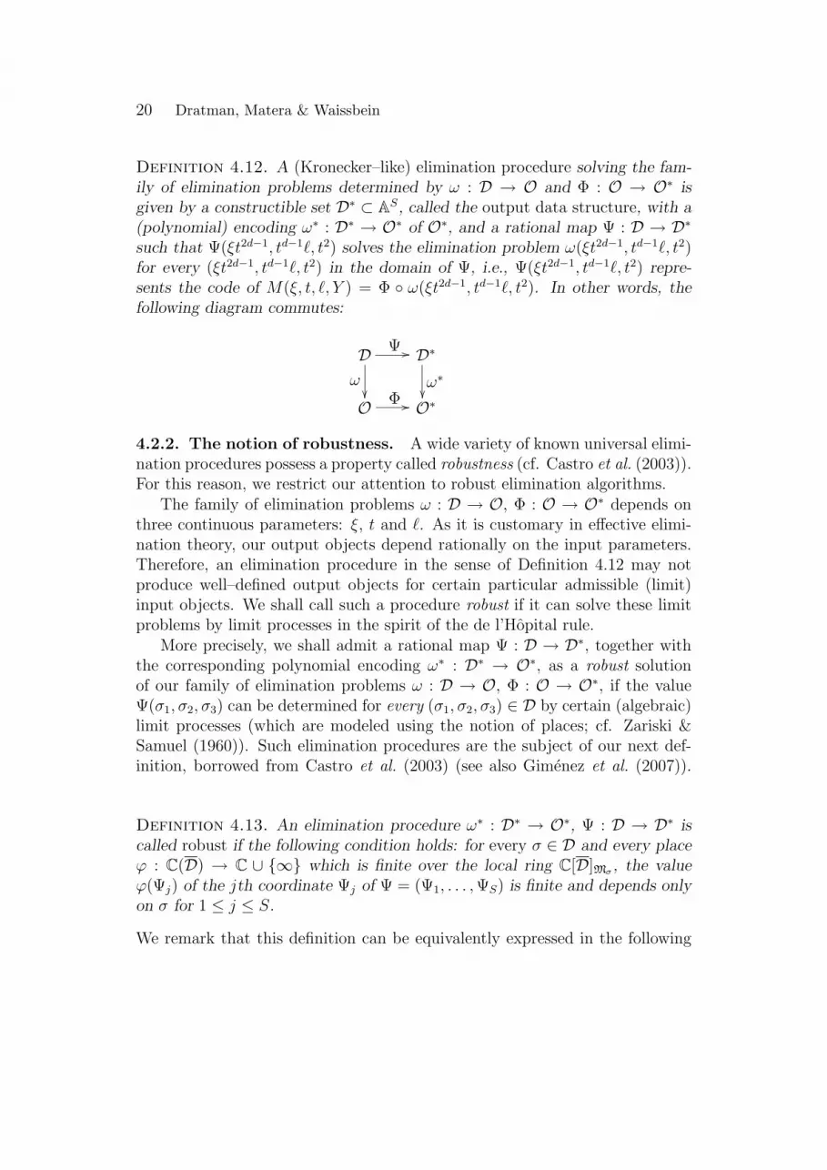
Definition 4.12. A (Kronecker–like) elimination procedure solving the fam-ily of elimination problems determined by ω : D → O and Φ : O → O∗ isgiven by a constructible set D∗ ⊂ AS, called the output data structure, with a(polynomial) encoding ω∗ : D∗ → O∗ of O∗, and a rational map Ψ : D → D∗

such that Ψ(ξt2d−1, td−1`, t2) solves the elimination problem ω(ξt2d−1, td−1`, t2)for every (ξt2d−1, td−1`, t2) in the domain of Ψ, i.e., Ψ(ξt2d−1, td−1`, t2) repre-sents the code of M(ξ, t, `, Y ) = Φ ω(ξt2d−1, td−1`, t2). In other words, thefollowing diagram commutes:

D Ψ //

ω²²

D∗

ω∗²²

O Φ // O∗

4.2.2. The notion of robustness. A wide variety of known universal elimi-nation procedures possess a property called robustness (cf. Castro et al. (2003)).For this reason, we restrict our attention to robust elimination algorithms.

The family of elimination problems ω : D → O, Φ : O → O∗ depends onthree continuous parameters: ξ, t and `. As it is customary in effective elimi-nation theory, our output objects depend rationally on the input parameters.Therefore, an elimination procedure in the sense of Definition 4.12 may notproduce well–defined output objects for certain particular admissible (limit)input objects. We shall call such a procedure robust if it can solve these limitproblems by limit processes in the spirit of the de l’Hopital rule.

More precisely, we shall admit a rational map Ψ : D → D∗, together withthe corresponding polynomial encoding ω∗ : D∗ → O∗, as a robust solutionof our family of elimination problems ω : D → O, Φ : O → O∗, if the valueΨ(σ1, σ2, σ3) can be determined for every (σ1, σ2, σ3) ∈ D by certain (algebraic)limit processes (which are modeled using the notion of places; cf. Zariski &Samuel (1960)). Such elimination procedures are the subject of our next def-inition, borrowed from Castro et al. (2003) (see also Gimenez et al. (2007)).

Definition 4.13. An elimination procedure ω∗ : D∗ → O∗, Ψ : D → D∗ iscalled robust if the following condition holds: for every σ ∈ D and every placeϕ : C(D) → C ∪ ∞ which is finite over the local ring C[D]Mσ , the valueϕ(Ψj) of the jth coordinate Ψj of Ψ = (Ψ1, . . . , ΨS) is finite and depends onlyon σ for 1 ≤ j ≤ S.

We remark that this definition can be equivalently expressed in the following


form: for every σ ∈ D, we have that C[D]Mσ → C[D]Mσ [Ψ1, . . . , ΨS] is anintegral ring extension.

An important class of examples of robust elimination procedures is thatof the invariant elimination procedures (cf. Heintz et al. (1998), Cas-tro et al. (2003)). In our context, we call two parameter points σ :=(ξt2d−1, td−1`, t2), σ′ := (ξ′(t′)2d−1, (t′)d−1`′, (t′)2) ∈ A3 equivalent (in symbols:σ ∼ σ′) if ω(σ) = ω(σ′) holds. Observe that σ ∼ σ′ implies M(ξ, t, `, Y ) =M(ξ′, t′, `′, Y ). Let Θ := (Θ1, Θ2, Θ3) be a vector of indeterminates. Wecall polynomials A ∈ C[Θ, X], B ∈ C[Θ, Y ] and C ∈ C[Θ] invariant (withrespect to ∼) if for equivalent parameter points σ, σ′ ∈ A3 the identitiesA(σ,X) = A(σ′, X), B(σ, Y ) = B(σ′, Y ) and C(σ) = C(σ′) hold.

Suppose the elimination procedure Ψ : D → D∗ is totally division–free, i.e.,the general solution M(ξ, t, `, Y ) of the given elimination problem belongs toQ[σ][Y ]. We call Ψ invariant (with respect to the equivalence relation ∼)if Ψ1, . . . , ΨS are invariant polynomials. The invariance of the eliminationprocedure Ψ means that for any input code σ ∈ A3 the code ω(σ) ∈ D∗

of the corresponding output object M(ξ, t, `, Y ) depends only on the inputobject, and not on its particular representation σ. In other words, an invariantelimination procedure produces the solution of a particular problem instancein a way which is independent of the possibly different representations of thegiven problem instance.

Since all known Kronecker–like elimination procedures produce a branchingand totally division–free representation of the output, and since they are basedon the manipulation of the input objects (and not on their particular represen-tations) by means of linear algebra or comprehensive Grobner basis techniques,we see that these algorithms are in fact invariant, and thus robust, eliminationprocedures.

4.2.3. Complexity of robust elimination procedures. For a robustelimination procedure ω∗ : D∗ ⊂ AS → O∗, Ψ : D → D∗, the dimension Sof the ambient space of D∗ is called the complexity of the elimination proce-dure ω∗, Ψ and is denoted by µ(D,O∗, Ψ). The minimal complexity µ(D,O∗, Ψ)when ω∗, Ψ runs through all the robust elimination procedures solving the fam-ily of elimination problems ω : D → O, Φ : O → O∗ is called the complexity ofthe family of elimination problems ω : D → O, Φ : O → O∗ and is denoted byµmin(D,O∗). In symbols, µmin(D,O∗) := minΨ µ(D,O∗, Ψ).

We remark that this notion of complexity is a suitable generalization of threestandard measures of complexity in effective elimination theory: the size of thedense or sparse representation and the (nonscalar) length of the straight–line


program representation. Indeed, it is clear that the minimal size of the dense orsparse representation (the number of total or nonzero monomials under consid-eration) of a given “continuous” family F := Qj; j ∈ J ⊂ C[X1, . . . , Xn] ofpolynomials of bounded degree is a lower bound for the complexity of comput-ing a generic member of F . In other words, we may estimate from below sucha complexity by the dimension of the least ambient space AM containing F .On the other hand, for a given polynomial F ∈ C[X1, . . . , Xn] we may considerthe minimal nonscalar length L(F ) of a straight–line program evaluating F .Let L ∈ N and set WL := F ∈ C[X1, . . . , Xn]; L(F ) ≤ L. From Burgisseret al. (1997, Exercise 9.18) (see also Heintz & Schnorr (1982, Theorem 3.2)) wededuce that WL is a constructible subset of A(L+n+1)2 and thus the dimension(L + n + 1)2 of the ambient space of WL reflects the (nonscalar) straight–lineprogram complexity of a generic polynomial F ∈ WL.

4.2.4. The lower bound. Now we prove that robust algorithms solving thefamily of elimination problems ω : D → O have complexity of order Ω(dn−1)or, disregarding polynomial terms in d (which are expected to be much smallerthan the Bezout number D = dn), of order Ω(D).

More precisely, we are going to show that, given a robust elimination pro-cedure Ψ : D → D∗, ω∗ : D∗ → O∗ solving our family of elimination problemsω : D → O, Φ : O → O∗, the dimension S of the ambient space AS of D∗ is atleast N + 1 = Ω(dn−1). This will be a consequence of the fact that the tangentspace of D∗ at 0 has dimension at least N + 1. In order to prove this, weshall exhibit N + 1 curves contained in D∗ passing through 0 with C–linearlyindependent tangent vectors at 0. These curves are obtained by fixing valuesξ, ` ∈ A1 \ 0 and letting t vary.

Now we state and prove our main result.

Theorem 4.14. With notations and assumptions as above, we have:

µmin(D,O∗) ≥ N + 1 = Ω(dn−1).

Proof. Let ω∗ : D∗ ⊂ AS → O∗, Ψ : D → D∗, be a robust eliminationprocedure solving the family of elimination problems ω : D → O, Φ : O → O∗.

Since D = (ξt2d−1, td−1`, t2); (ξ, t, `) ∈ A3 holds, we may identify C[D]with C[ΞT 2d−1, T d−1L, T 2] ⊂ C[T, Ξ, L], the maximal ideal M0 ⊂ C[D] with theideal (ΞT 2d−1, T d−1L, T 2) ⊂ C[T, Ξ, L], the field of rational functions C(D) withC(ΞT 2d−1, T d−1L, T 2) ⊂ C(T, Ξ, L) and the local ring C[D]M0 with the local-ization S−1C[ΞT 2d−1, T d−1L, T 2], where S is the multiplicative set

S := p(ΞT 2d−1, T d−1L, T 2); p ∈ C[Y1, Y2, Y3], p(0, 0, 0) 6= 0.


Consider Ψ1, . . . , ΨS ∈ C(D) as elements of C(ΞT 2d−1, T d−1L, T 2) ⊂ C(T, Ξ, L)according to such an identification. From the definition of robustnessit follows that Ψ1, . . . , ΨS are integral over C[D]M0 , or equivalently overS−1C[ΞT 2d−1, T d−1L, T 2] ⊂ S−1C[T, Ξ, L]. Since S−1C[T, Ξ, L] is integrallyclosed in its fraction field, we deduce that Ψ1, . . . , ΨS belong to S−1C[T, Ξ, L].In particular, we have that Ψ(T, Ξ, L) is a well–defined holomorphic functionin a neighborhood of (0, 0, 0).

Fix 1 ≤ j ≤ S and write Ψj = aj/bj with aj ∈ C[T, Ξ, L] and bj ∈ S. Wehave an equation of integral dependence

(aj

bj

)mj

+pj,mj−1

qj,mj−1

(aj

bj

)mj−1

+ · · ·+ pj,0

qj,0

= 0,

with pj,i, qj,i ∈ C[ΞT 2d−1, T d−1L, T 2] and qj,i ∈ S for 0 ≤ i ≤ mj − 1. Thecondition pj,i, qj,i ∈ C[ΞT 2d−1, T d−1L, T 2] for 0 ≤ i ≤ mj − 1 implies thatpj,i(0, Ξ, L) ∈ C, qj,i(0, Ξ, L) ∈ C and qj,i(0, Ξ, L) 6= 0 hold for 0 ≤ i ≤ mj − 1.We conclude that

(4.15) Ψj(0, Ξ, L) ∈ C for 0 ≤ j ≤ S.

Fix ξ ∈ Q \ 0 and consider N + 1 distinct rationals `0, . . . , `N ∈ Q tobe fixed. Let βj : A1 → A3 be the mapping defined by βj(t) := (t, ξ, `j) for0 ≤ j ≤ N . Our previous argument shows that the mapping σj : A1 → O∗

given by σj(t) := ω∗ (Ψ1, . . . , ΨS) βj(t) is well–defined and holomorphic ina neighborhood of T = 0 in A1. Furthermore, from (4.11) it follows that theidentity

(4.16) σj(t) = Φ ω(ξt2d−1, td−1`j, t2) = ξtP (1)(`j, Y )− 1

holds in a neighborhood of T = 0 in A1 for 0 ≤ j ≤ N . By the chain rule weobtain

Dσj(0) = ξP (1)(`j, Y ) = Dω∗(Ψ(0, ξ, `j)

) ·D(Ψ βj)(0).

From (4.15) we have that Ψ(0, ξ, `j) ∈ CS is a complex vector independent of`j. Therefore, the matrix M := Dω∗(Ψ(0, ξ, `j)) is a complex (S × dn)–matrixindependent of `j. Since Dσj(0) = M ·D(Ψ βj)(0) holds for 1 ≤ j ≤ S, weconclude that the vector Dσj(0) = ξP (1)(`j, Y ) belongs to the range of M for1 ≤ j ≤ S.

From the expression of the dense representation (4.9) of P (1) and Corol-lary 4.7 we deduce that, for generic choices of `0, . . . , `Nn+1 ∈ Q, the vec-tors Dσj(0) are linearly independent. Indeed, disregarding zero coefficients,


these vectors may be arranged so that they form a diagonal multiple of the(N + 1) × (N + 1)–Vandermonde matrix defined by `2

0, . . . , `2N . Therefore,

for any choice `0, . . . , `N ∈ Q with `2i 6= `2

j for 0 ≤ i < j ≤ N , we deducethat Dσj(0); 0 ≤ j ≤ N is a Q–linearly independent set. This shows thatS ≥ rankM≥ N + 1 holds and finishes the proof. ¤

Our result should be seen as a proof that, independently of the data struc-ture and the (robust) elimination procedure used to solve generalized Phamsystems, a factor of order DΩ(1) will necessarily appear in its worst–case com-plexity estimate, where D is the Bezout number of the system under considera-tion. On the other hand, we observe that the value of the exponent underlyingthe Ω–notation does depend on the data structure under consideration. Inthe particular case of sparse and straight–line program encodings, we have thefollowing result.

Corollary 4.17. Let ω∗ : D∗ → O∗, Ψ : D → D∗ be a robust eliminationprocedure solving the family of elimination problems ω : D → O, Φ : O → O∗.Then:

(i) if ω∗ : D∗ → O∗ corresponds to the sparse encoding of M(ξ, t, `, Y ), thenΨ performs Ω(dn−1) arithmetic operations in Q;

(ii) if ω∗ : D∗ → O∗ is the straight–line program encoding of M(ξ, t, `, Y ),then Ψ performs Ω(d(n−1)/2) arithmetic operations in Q.

Proof. Suppose first that the output encoding ω∗ : D∗ → O∗ represents thesparse encoding of the polynomials M(ξ, t, `, Y ). Then from Theorem 4.14 weconclude that at least Ω(dn−1) coefficients of the polynomials M(ξ, t, `, Y ) mustbe computed. This shows that the corresponding algorithm must perform atleast Ω(dn−1) arithmetic operations in Q and proves the first assertion of thecorollary.

Next suppose that the output encoding ω∗ : D∗ → O∗ is the straight–line program encoding of the polynomials M(ξ, t, `, Y ). This means that thecorresponding algorithm Ψ builds a straight–line program evaluating the poly-nomials M(ξ, t, `, Y ) for any admissible input instance σ(ξ, t, `). From Theorem4.14 we conclude that this straight–line program cannot be described with lessthat N +1 = (dn−1)/(d−1) parameters. Taking into account that the varietyformed by all the polynomials in C[Y ] which can be evaluated by a straight–lineprogram of length at most L belong to a constructible subset of A(L+2)2 (see,e.g., Burgisser et al. (1997, Theorem 9.9) or Heintz & Schnorr (1982, Theorem


3.2)), we conclude that the straight–line program built by the algorithm Ψ haslength at least Ω(d(n−1)/2). This finishes the proof of the corollary. ¤

We observe that the lower bounds of the corollary are nearly optimal for eachencoding. Indeed, the lower bound Ω(dn−1) of the first assertion of the corollaryis close to the optimal lower bound dn +1 for the sparse encoding of univariatepolynomials of degree dn. On the other hand, the lower bound of the secondassertion is close to the optimal Paterson–Stockmeyer lower bound dn/2 − 1for the length of the straight–line program encoding of a generic univariatepolynomial of degree dn (see, e.g., Burgisser et al. (1997, Proposition 9.2)).

5. The Solution of a Generalized Pham System

Let f1, . . . , fn be polynomials in Q[X] which can be computed by a division–free straight–line program of length T, and let V := V (f1, . . . , fn) denote theaffine subvariety of An defined by f1, . . . , fn. For 1 ≤ i ≤ n, set di := deg fi andwrite fi = φi + ϕi, where φi ∈ Q[X] is the (nonzero) homogeneous componentof fi of degree di. Finally, set D := d1 · · · dn.

Assume that f1, . . . , fn define a generalized Pham system, that is, the pro-jective variety φ1(x) = 0, , . . . , φn(x) = 0 ⊂ Pn−1 is the empty set. Thefollowing result will be important in the sequel.

Lemma 5.1 (Pardo & San Martın 2004, Proposition 18). The set of solutionsof an n–variate generalized Pham system is a zero–dimensional affine subvarietyof An.

Let fh1 , . . . , fh

n denote the homogenizations of f1, . . . , fn with homogenizingvariable X0. Observe that the polynomials fh

1 , . . . , fhn are of the form

fh1 = φ1(X) + X0ϕ1(X0, X), . . . , fh

n = φn(X) + X0ϕn(X0, X),

for some polynomials ϕ1, . . . , ϕn ∈ Q[X0, X]. From this representation wededuce that the projective variety V h := fh

1 (x) = 0, . . . , fhn (x) = 0 ⊂ Pn is

contained in the Zariski–open set x0 6= 0, or equivalently the ideal generatedby X0 is not contained in the ideal generated by fh

1 , . . . , fhn . By the Bezout

theorem in the form of Eisenbud & Harris (1999, Theorem III.71) it follows thatthe projective variety V h has precisely D points in Pn, counting multiplicities.Since V h has no points at infinity, from Caniglia et al. (1991, Proposition 1.11)we conclude that V has D points, counting multiplicities.


5.1. The architecture of our solution method. We can solve the originalsystem with a straight-forward adaptation of Schost (2003) or Bompadre et al.(2004, Section 5), i.e., applying a “projection algorithm” to the deformationπ : W → A1 determined by the morphism π(t, x) := t and the variety W ⊂An+1 of common zeros of the system

aiXdii + T (fi − aiX

dii ) + bi(1− T ) = 0 (1 ≤ i ≤ n),

where ai stands for the coefficient of Xdi in fi and bi is a randomly chosenrational for 1 ≤ i ≤ n. Unfortunately, this may lead to an algorithm withmore than quadratic complexity in the Bezout number of the input system.Indeed, considering the product deg π deg W , which is the dominant term ofthe complexity of this algorithm, in this case we have deg π = D and deg W ≤E := (d1+1) · · · (dn+1) according to the Bezout inequality (3.1). In particular,for n À maxd1, . . . , dn we have E À D and hence DE À D2.

Instead, we introduce a sequence of deformations which play the role ofcertain piecewise–linear homotopies of numerical continuation methods actingcoordinate by coordinate (cf. Saigal (1983), Duvallet (1990)). More precisely,for 1 ≤ r ≤ n + 1 we introduce a deformation πr : Vr → A1 such that thefollowing conditions are satisfied:

(i) Vr ⊂ An+1 is equidimensional of dimension 1 for 1 ≤ r ≤ n + 1,

(ii) πr is dominant and generically unramified for 1 ≤ r ≤ n + 1,

(iii) deg πr = D = #π−1r (0) and deg Vr ≤ 2D holds for 1 ≤ r ≤ n + 1,

(iv) π−1r (1) = π−1

r+1(0) for 1 ≤ r < n + 1,

(v) π−11 (0) is “easy to solve” and π−1

n+1(1) = 1 × V holds.

In order to compute a geometric solution of the fiber π−1n+1(1) = 1 × V ,

and thus of V , we shall apply repeatedly the “projection algorithm” of Schost(2003). This algorithm takes as input a geometric solution of the unramifiedfiber π−1

r+1(0) = π−1r (1) of the morphism πr+1 and outputs a geometric solution

of Vr+1 for any 1 ≤ r ≤ n. Making the substitution T = 1 in the polynomialsthat form the computed geometric solution of Vr+1 we obtain polynomials thatform a geometric solution of π−1

r+1(1) = π−1r+2(0). Since the fiber π−1

1 (0) is easy tosolve, after n applications of such a projection algorithm we obtain a geometricsolution π−1

n+1(1).Assume that we are given deformations πr : Vr → A1 (1 ≤ r ≤ n + 1)

satisfying conditions (i)–(v) above. The following is a sketch of our algorithmfor computing a geometric solution of the input system f1 = 0, . . . , fn = 0.


Algorithm 5.2 (Sketch of the algorithm for solving f1 = 0, . . . , fn = 0).

1. Find a geometric solution of the “easy–to–solve” fiber π−11 (0).

2. For r = 1 to n do:

(a) Apply a “projection algorithm” in order to compute a geometricsolution of Vr from the geometric solution of π−1

r (0) computed inthe previous step.

(b) Make the substitution T = 1 in the polynomials that form the geo-metric solution of Vr computed in the previous step. These polyno-mials form a geometric solution of π−1

r+1(0) = π−1r (1) for 1 ≤ r ≤ n−1

and may include multiplicities for r = n.

3. Clean multiplicities from the polynomials computed in the previous stepfor r = n to obtain a geometric solution of 1 × V , and thus of V .

5.2. Designing suitable deformations. In the description of our deforma-tions πr : Vr → A1 we shall make use of certain Q–linearly independent linearforms Y1, . . . , Yn ∈ Q[X] and rationals b1, . . . , bn ∈ Q \ 0 to be fixed duringthe setup stage of our algorithm (Section 5.3 below).

Fix r with 1 ≤ r ≤ n and consider the following polynomials of Q[T, X]:

(5.3)

F(r)j (T,X) := φj(X) + bj (1 ≤ j ≤ r − 1),

F(r)r (T,X) := Y dr

r + T (φr(X)− Y drr ) + br,

F(r)j (T,X) := Y

dj

j + bj (r + 1 ≤ j ≤ n),

where for r = 1 we have F(1)1 (T,X) := Y d1

1 +T (φ1(X)−Y d11 )+b1, Fj

(1) := Ydj

j +bj

(2 ≤ j ≤ n) and for r = n we have Fj(n)(T, X) := φj(X) + bj (1 ≤ j ≤ n− 1),

Fn(n) := Y dn

n + T (φn(X)− Y dnn ) + bn. Let Ir := (F

(r)1 , . . . , F

(r)n ) ⊂ Q[T, X], let

Jr := det(∂F(r)i /∂Xj)1≤i,j≤n be Jacobian of F

(r)1 , . . . , F

(r)n with respect to the

variables X and let Vr := V (Ir : J∞r ) ⊂ An+1 be the variety defined by thesaturation (Ir : J∞r ). The rth deformation πr : Vr → A1 is determined by theprojection πr(t, x) := t and the affine variety Vr ⊂ An+1.

Finally, consider the following polynomials of Q[T, X]:

(5.4) F(n+1)i (T, X) := φi(X) + T (ϕi(X)− bi) + bi (1 ≤ i ≤ n).

Let us define In+1 := (F(n+1)1 , . . . , F

(n+1)n ) ⊂ Q[T, X], set Jn+1 :=

det(∂F(n+1)i /∂Xj)1≤i,j≤n and let Vn+1 := V (In+1 : J∞n+1) ⊂ An+1 be the variety


defined by the saturation (In+1 : J∞n+1). The deformation πn+1 : Vn+1 → A1 isdetermined by the projection πn+1(t, x) := t and the affine variety Vn+1 ⊂ An+1.

Having defined the deformations πr : Vr → A1 (1 ≤ r ≤ n + 1), we discussthe validity of conditions (i)–(v) of the previous section. The fulfillment ofthese conditions relies on a suitable choice of the coefficients of the linear formsY1, . . . , Yn and the rationals b1, . . . , bn. In the next section we prove that forcertain random choice of such coefficients, the following assertions hold withhigh probability:

(A) The polynomials F(r)i (t,X) (1 ≤ i ≤ n) define a generalized Pham system

for a generic choice t ∈ A1 and every 1 ≤ r ≤ n + 1 (see Corollary 5.13below).

(B) The affine variety V(F

(r)1 (0, X), . . . , F

(r)n (0, X)

)consists of D nonsingular

points for 1 ≤ r ≤ n + 1 (see Proposition 5.14 below).

Assuming that assertions (A)–(B) hold, from (A) and Lemma 5.1 we con-

clude that F (r)1 (t,X) = 0, . . . , F

(r)n (t,X) = 0 is a zero–dimensional subvariety

of An for a generic choice t ∈ A1. This shows that the generic fiber of the pro-jection mapping πr : V (I(r)) → A1 is nonempty for 1 ≤ r ≤ n+1 (and consistsof at most D points by the Bezout inequality (3.1)). Furthermore, (B) assertsthat the fiber π−1

r (0) consists of D nonsingular points for 1 ≤ r ≤ n + 1.Summarizing, under the assumption of assertions (A)–(B) it follows that thedeformations πr : Vr → A1 satisfy the following conditions for 1 ≤ r ≤ n + 1:

(C) 0 < #π−1r (t) ≤ D holds for a generic value t ∈ A1,

(D) #π−1r (0) = D and Jr(0, x) 6= 0 holds for every (0, x) ∈ π−1

r (0).

Then we can apply the following result (compare with Jeronimo et al. (2008,Lemma 4.4)).

Proposition 5.5. Let be given polynomials F1, . . . , Fn ∈ Q[T, X], a positiveinteger D and t0 ∈ Q. Let I ⊂ Q[T, X] be the ideal generated by F1, . . . , Fn

and set W := V (I) = V (F1, . . . , Fn). Let J := det(∂Fi/∂Xj)1≤i,j≤n be theJacobian determinant of F1, . . . , Fn with respect to the variables X and letV := V (I : J∞) ⊂ An+1 be the variety defined by the saturation (I : J∞).

Let π : W → A1 denote the projection π(t, x) := t. Assume that

0 < #π−1(t) ≤ D holds for a generic value t ∈ A1,

#π−1(t0) = D and J(t0, x) 6= 0 holds for every (t0, x) ∈ π−1(t0).


Then the following assertions hold:

V is an equidimensional variety of dimension 1.

V is the union of all the irreducible components of W having a nonemptyintersection with π−1(t0).

V is the union of all the irreducible components of W projecting domi-nantly on A1.

π : V → A1 is a dominant map of degree D.

Proof. First we observe that dim(C) ≥ 1 holds for each irreducible compo-nent C of W , since W is defined by n polynomials in an (n + 1)–dimensionalspace. By definition, V consists of all irreducible components of W on whichthe Jacobian determinant J does not vanish identically.

Let C be an irreducible component of W for which π−1(t0) ∩ C 6= ∅ holds.Consider the restriction π|C : C → A1 of π. Then we have that π|−1

C (t0) is anonempty variety of dimension zero, which implies that the generic fiber of π|Cis either zero-dimensional or empty. Since dim(C) ≥ 1, the Theorem on theDimension of Fibers implies that dim(C) = 1 holds and that π|C : C → A1 is adominant map with generically finite fibers. Finally, Shafarevich (1994, §II.6,Theorem 4) shows the inclusion C ⊂ V and, in particular, that V is nonempty.

Conversely, we have that π−1(t0) ∩ C 6= ∅ holds for any irreducible compo-nent C of V . Indeed, assume on the contrary the existence of a component C0

not satisfying this condition. Then, there is a point t1 ∈ A1 having a finite fiberπ−1(t1) such that π|−1

C0(t1) and π|−1

C (t1) have maximal cardinality for every Cwith C ∩ π−1(t0) 6= ∅. This implies that #π−1(t1) > #π−1(t0) = D, leading toa contradiction.

We conclude that V is the equidimensional variety of dimension 1 whichconsists of all the irreducible components C of W with π−1(t0) ∩ C 6= ∅. Fur-thermore, this shows that the restriction π|V : V → A1 is a dominant map ofdegree D.

Finally we show that V consists of all irreducible components of W project-ing dominantly on A1. Let C be one such irreducible component of W . Thenby Shafarevich (1994, §II.6, Theorem 4) it follows that there exists an unrami-fied fiber of π|C . On such a fiber the Jacobian J does not vanish, which in turnproves that J does not vanish identically on C. Therefore, C ⊂ V holds. Onthe other hand, if C is an irreducible component of W for which the projec-tion π|C : C → A1 is not dominant, then C is the set of common zeros of thepolynomials F1, . . . , Fn, T − tC for some value tC . Since dim(C) ≥ 1, we have


that the Jacobian matrix ∂(F1, . . . , Fn, T − tC)/∂(X1, . . . , Xn, T ) is singular atevery point (x, tC) of C. Hence, its determinant, which equals J , vanishes overC. ¤

We claim that the validity of (A)–(B) implies that conditions (i)–(v) of Sec-tion 5.1 hold. Indeed, combining (A)–(B) with the first conclusion of Proposi-tion 5.5 immediately implies that Vr is an equidimensional variety of dimension1 for 1 ≤ r ≤ n + 1, that is, condition (i) holds.

By (B) and the third and fourth conclusions of Proposition 5.5 we havethat the morphism πr : Vr → A1 is dominant and generically unramified for1 ≤ r ≤ n + 1, proving thus that condition (ii) holds.

In the proof of (C)–(D) we have already shown that (A)–(B) imply that theidentity deg πr = π−1

r (0) = D holds for 1 ≤ r ≤ n + 1, which is the first part ofcondition (iii). Furthermore, by the Bezout inequality (3.1) we have:

deg V (Ir) ≤ d1 · · · dr−1(dr+1)dr+1 · · · dn ≤ 2D (1 ≤ r ≤ n), deg V (In+1) ≤ D.

From these estimates and the definition of the varieties Vr we conclude thatthe following estimates, and thus the second part of condition (iii), hold:

deg Vr ≤ d1d2 · · · dr−1(dr + 1)dr+1 · · · dn ≤ 2D (1 ≤ r ≤ n), deg Vn+1 ≤ D.

From the second conclusion of Proposition 5.5 we deduce the following iden-tities, which imply (iv):

#(V (Ir) ∩ T = 0) = #

(Vr ∩ T = 0) = D (1 ≤ r ≤ n + 1),

#(V (Ir) ∩ T = 1) = #

(Vr ∩ T = 1) (1 ≤ r ≤ n).

Finally, concerning the second assertion of condition (v), we observe thatthe identity V (In+1)∩T = 1 = Vn+1∩T = 1 holds, because In+1 = (In+1 :J∞n+1) holds since the finiteness of the projection πn+1 : V (In+1) → A1 impliesthat V (In+1) contains no vertical component. Finally, for the first assertion of(v) we observe that V (I1) ∩ T = 0 is defined by a “diagonal” square systemand therefore can be easily solved (see the algorithm underlying Lemma 5.17below). This finishes the proof of our claim.

5.3. Preparation: random choices. This section is devoted to showingthat we can choose the linear forms Y1, . . . , Yn and the vector b := (b1, . . . , bn) ∈Qn such that conditions (A)–(B) above are satisfied.

For this purpose, we need some technical results in order to establishingconditions on the coefficients of Y1, . . . , Yn which assure that the polynomials


in (5.3) and (5.4) define generalized Pham systems. In the sequel we shalluse the following simple criterion, which is a well–known consequence of theMacaulay unmixedness theorem (see, e.g., Matsumura (1980, Exercise 16.3)).

Remark 5.6. Let Q1, . . . , Qn ∈ Q[X] := Q[X1, . . . , Xn] be nonzero ho-mogeneous polynomials defining the empty projective variety Q1(x) =0, . . . , Qn(x) = 0 of Pn−1. Then Q1, . . . , Qn form a regular sequence in Q[X].

As a first consequence of this remark we observe that, since f1, . . . , fn deter-mine a generalized Pham system, the polynomials φ1, . . . , φn define the emptyprojective variety of Pn−1. Hence, applying Remark 5.6 we deduce the followingresult.

Corollary 5.7. The polynomials φ1, . . . , φn form a regular sequence in Q[X].

Next we provide a consistent condition which assures that the polynomialsφ1, . . . , φr, Y

dr+1

r+1 , . . . , Y dnn form a regular sequence in Q[X] for 1 ≤ r ≤ n.

Proposition 5.8. Fix a positive integer ρ and suppose that the coefficients ofthe linear forms Y1, . . . , Yn are randomly chosen in the set 1, . . . , 2nρD. Then

with error probability at most 1/ρ, the polynomials φ1, . . . , φr, Ydr+1

r+1 , . . . , Y dnn

form a regular sequence in Q[X] for 0 ≤ r ≤ n.

Proof. From Corollary 5.7 we deduce that the affine variety

Wr,0 := x ∈ An; φ1(x) = 0, . . . , φr(x) = 0

is equidimensional of dimension n− r for 1 ≤ r < n. This in particular showsthe condition of the statement of the Proposition for r = n is automaticallysatisfied.

Let Ai,j (1 ≤ i, j ≤ n) be new indeterminates over Q[X], and denote A(r) :=(Ar,1, . . . , Ar,2) for 1 ≤ r ≤ n and A := (Ai,j)1≤i,j≤n.

Fix arbitrarily a nonzero linear form Y1 ∈ Q[X] and an index r with 1 < r ≤n. Assume inductively that the coefficients of the linear forms Y1, . . . , Yr−1 arealready randomly chosen in the set 1, . . . , 2nρD, and with error probabilityat most

∑r−1j=1(1 +

∑j−1i=1 d1 · · · di)/2nρD the following conditions are satisfied:

for any pair (i, j) with 0 ≤ i < j ≤ r − 1, the variety

(5.9) Wi,j := x ∈ An; φ1(x) = 0, . . . , φi(x) = 0, Yi+1(x) = 0, . . . , Yj(x) = 0

is equidimensional of dimension n − j. Observe that the choice of the linearform Y1 implies that these conditions for r = 1 are satisfied.


Now we discuss the choice of the linear form Yr. For any i with 0 ≤ i ≤ r−1,let Si,r−1 ⊂ Wi,r−1 be a finite set consisting of one arbitrary nonzero point ineach irreducible component of Wi,r−1. By the Bezout inequality (3.1) we have#Si,r−1 ≤ deg Wi,r−1 ≤ d1 . . . di for i = 1, . . . , r−1 and #S0,r−1 = deg W0,r−1 =1. Let Qr ∈ Q[A(r)] be the nonzero polynomial defined in the following way:

Qr(A(r)) :=

r−1∏i=0

∏

ξ∈Si,r−1

n∑j=1

ξj Ar,j.

Let a(r) be an arbitrary point of Qn not annihilating Qr and define Yr := a(r)X.By construction, we have that Yr(ξ) 6= 0 holds for every ξ ∈ Si,r−1 and every0 ≤ i ≤ r. This shows that the hyperplane Yr = 0 cuts properly all theirreducible components of Wi,r−1 for 0 ≤ i ≤ r − 1. We conclude that thevariety

(5.10) Wi,r := x ∈ An; φ1(x) = 0, . . . , φi(x) = 0, Yi+1(x) = 0, . . . , Yr(x) = 0is equidimensional of dimension n−r and degree at most d1 · · · di for 0 ≤ i ≤ r.Combining (5.9), (5.10) we see that the varieties Wi,j are equidimensional ofdimension n−j for 0 ≤ i < j ≤ r, completing thus the rth step of our inductiveargument.

Observe that deg Qr ≤ 1 +∑r−1

i=1 d1 · · · di holds. Hence, applying Theorem3.2 we conclude that for a random choice of the coefficient vector a(r) of Yr

in the set 1, . . . , 2nρDn, the inequality Qr(a(r)) 6= 0, and thus (5.10), holds,

with error probability at most (1 +∑r−1

i=0 d1 · · · di)/2nρD.After n steps as described, we obtain linear forms Y1, . . . , Yn such that,

with error probability at most∑n

j=1(1+∑j−1

i=1 d1 · · · di)/2nρD, the variety Wi,j

is equidimensional of dimension n − j for i < j ≤ n and 0 ≤ i ≤ n. This inparticular implies that the polynomials φ1, . . . , φr, Yr+1, . . . , Yn form a regularsequence of Q[X] for 0 ≤ r ≤ n. Therefore, by Matsumura (1986, Theorem

16.1) we conclude that φ1, . . . , φr, Ydr+1

r+1 , . . . , Y dnn form a regular sequence in

Q[X] for 0 ≤ r ≤ n. Since

1

2nρD

n∑j=1

(1 +

j−1∑i=1

d1 · · · di

)=

1

2nρD

(n +

n∑j=1

(n− j)d1 · · · dj

)

=1

2ρD

n∑j=1

d1 · · · dj ≤ 1

ρ,

we deduce the statement of the proposition. ¤


As a first consequence on the choice of the linear forms Y1, . . . , Yn we deducethat for a generic value t ∈ A1 the polynomials in (5.3) define a generalizedPham system. More precisely, we have the following result.

Corollary 5.11. Let Y1, . . . , Yn ∈ Q[X] be linear forms satisfying the state-ment of Proposition 5.8. Then, for 1 ≤ r ≤ n, the polynomials

(5.12) φ1(X), . . . , φr−1(X), Ydr+1

r+1 , . . . , Y dnn , Y dr

r + T (φr(X)− Y drr )

form a regular sequence in Q[T, X]. Furthermore, for a generic value t ∈ A1

φ1(X), . . . , φr−1(X), Ydr+1

r+1 , . . . , Y dnn , Y dr

r + t(φr(X)− Y drr )

form a regular sequence in C[X].

Proof. Fix r with 1 ≤ r ≤ n. From Proposition 5.8 it follows thatthe polynomials φ1, . . . , φr, Y

dr+1

r+1 , . . . , Y dnn form a regular sequence in Q[X].

Since these are homogeneous polynomials, from Matsumura (1986, Corollary

of Theorem 16.3) we see that φ1, . . . , φr−1, Ydr+1

r+1 , . . . , Y dnn form a regular se-

quence of Q[X]. Therefore, in order to prove the lemma it suffices to showthat Hr(T, X) := Y dr

r + T (φr − arYdrr ) is not a zero divisor modulo the ideal

I∗r := (φ1, . . . , φr, Ydr+1

r+1 , . . . , Y dnn ) ⊂ Q[T, X].

Let V (Icr) := ∪j∈JCj be the decomposition of the projective subvariety

of Pn−1 defined by the ideal Icr := (φ1, . . . , φr, Y

dr+1

r+1 , . . . , Y dnn ) ⊂ Q[X]. Fix

a point p(j) in each irreducible component Cj of V (Icr). Since Y dr

r and φr

are not zero divisors modulo Icr , it follows that αj := Yr(p

(j))dr and βj :=φr(p

(j)) are nonzero complex numbers and hence αj + T (βj − αj) is a nonzeropolynomial of C[T ] for every j ∈ J . Finally, let t ∈ A1 be any value with∏

j∈J (αj + t(βj − αj)) 6= 0. Then Y drr + t(φr(X) − Y dr

r ) is not a zero divisor

modulo Icr . Furthermore, taking into account that V (I∗r ) = ∪j∈J (A1 × Cj)

is the decomposition of V (I∗r ) ⊂ Pn into irreducible components, from thecondition

∏j∈J (αj + t(βj−αj)) 6= 0 we conclude that Y dr

r +T (φr−Y drr ) is not

a zero divisor modulo I∗r . This finishes the proof. ¤

A consequence of Corollary 5.11 is that φ1, . . . , φr−1, Ydrr +t(φr−Y dr

r ), Ydr+1

r+1 ,. . . , Y dn

n define the empty projective variety of Pn−1 for all but a finite numberof t ∈ A1. Likewise, from Corollary 5.7 we conclude that (5.4) is a generalizedPham system for every substitution T = t. Therefore, we have the followingresult.


Corollary 5.13. Let Y1, . . . , Yn be linear forms satisfying the statement ofProposition 5.8. Then for all but a finite number of values t ∈ A1, makingthe substitution T = t in (5.3), (5.4) yields a generalized Pham system for1 ≤ r ≤ n + 1.

This proves that our choice of Y1, . . . , Yn implies that condition (A) in Sec-tion 5.2 holds.

Next we consider condition (B). Fix r with 1 ≤ r ≤ n + 1 and letb1, . . . , bn be nonzero rationals to be fixed. Condition (B) asserts that the

affine subvariety V (F(r)1 (0, X), . . . , F

(r)n (0, X)) of An consists of D distinct

points, none of which is annihilated by the Jacobian determinant Jr(0, X) :=det(∂Fi

(r)(0, X)/∂Xj)1≤i,j≤n.We observe that the smoothness of the variety V

(F1

(r)(0, X), . . . , Fn(r)(0, X)

)for a generic value of b is a direct consequence of the Sard theorem (see, e.g.,Guillemin & Pollack (1974, §1.7)). The next lemma is an effective version ofthis result in our context.

Proposition 5.14. Let B1, . . . , Bn be new indeterminates over Q[X] and setB := (B1, . . . , Bn). Let Y1, . . . , Yn ∈ Q[X] be linear forms satisfying the state-ment of Proposition 5.8. Then there exists a nonzero polynomial P (2) ∈ Q[B]of degree at most 2nD2 such that for every b ∈ Qn with P (2)(b) 6= 0, the affine

variety defined by the polynomials F(r)1 (0, X), . . . , F

(r)n (0, X) for this value of b

consists of D nonsingular points for 1 ≤ r ≤ n + 1.

Proof. First we observe that choosing arbitrarily b1 6= 0, . . . , bn 6= 0,the affine variety Y1(x)d1 + b1 = 0, . . . , Yn(x)dn + bn = 0 consists ofD distinct points which are not annihilated by the Jacobian J1(0, X) :=det(∂Yi(x)di/∂Xk)1≤i,j≤n, since no point of this variety has a zero coordinate.This proves the result for r = 1.

Now fix r with 2 ≤ r ≤ n and consider the following polynomials of Q[B, X]:

(5.15) φ1(X) + B1, . . . , φr−1(X) + Br−1, Ydrr + Br, . . . , Y

dnn + Bn.

Denote by Wr the affine subvariety of A2n defined by these polynomials. Sincethe polynomials in (5.15) define a generalized Pham system for any substitutionB = b, from Lemma 5.1 it follows that the morphism

θr : Wr → An, θ(b, x) := b

is surjective. Furthermore, we claim that θr is finite. Indeed, let Nr ∈ N and


h(r)i,j ∈ Q[X] (1 ≤ i, j ≤ n) be polynomials of degree Nr − dr such that

XNri =

r−1∑j=1

h(r)i,j φj +

n∑j=r

h(r)i,j Y

dj

j .

Then for every 1 ≤ i ≤ n we have

r−1∑j=1

h(r)i,j (φj + Bj) +

n∑j=r

h(r)i,j (Y

dj

j + Bj) = XNri +

n∑j=1

h(r)i,j Bj,

with deg h(r)i,j Bj < Nr for 1 ≤ i, j ≤ n. This proves that Q[B] → Q[Wr] is an

integral ring extension. Taking into account that Wr is irreducible, from theprevious assertions and Shafarevich (1994, II.6.3, Theorem 4) we conclude thatθr is generically unramified.

Let η ∈ C[X] be a linear form that induces a primitive element of the ring

extension C[B] → C[Wr]. Consider its minimal polynomial M(r)η ∈ Q[B, Y ],

and let ∆r ∈ C[B] denote its discriminant with respect to the variable Y . Forevery b ∈ Qn such that ∆r(b) 6= 0 it follows that the Mη(b, Y ) is square–free,and therefore the morphism θr is unramified at B = b.

Furthermore, for every b ∈ Qn with ∆r(b) 6= 0, the corresponding polyno-mials φ1(X)+b1, . . . , φr−1(X)+br−1, Y

drr +br, . . . , Y

dnn +bn define a generalized

Pham system and generate a radical ideal in Q[X]. Let fhr,1, . . . , f

hr,n denote the

homogenizations of φ1(X) + b1, . . . , φr−1(X) + br−1, Ydrr + br, . . . , Y

dnn + bn with

homogenizing variable X0. Then fhr,1, . . . , f

hr,n is a radical zero–dimensional

ideal. We conclude that fhr,1, . . . , f

hr,n form a regular sequence of Q[X]. Ap-

plying the Bezout theorem in the form of Eisenbud & Harris (1999, TheoremIII.71) we see that the projective variety defined by fh

r,1, . . . , fhn,r has precisely

deg V h = D distinct points in Pn. Finally, since there are no points at infinity,from Caniglia et al. (1991, Proposition 1.11) we conclude that θ−1

r (b) consistsof exactly D distinct points.

A similar argument shows that there exists a polynomial ∆n+1 ∈ Q[B] such

that, for every b ∈ Qn with ∆n+1(b) 6= 0, the polynomials F(n+1)1 (0, X), . . . ,

F(n+1)n (0, X) corresponding to this value of b have D nonsingular common zeros.

Let P (2) := (B1 · · ·Bn) · ∆2 · · ·∆n+1. From the Bezout inequality (3.1)we deduce that deg Wr ≤ D holds, which in turns implies that the minimalpolynomial of η has degree bounded by D. It follows that the degree of itsdiscriminant ∆r is bounded by 2D2 for 2 ≤ r ≤ n + 1 and hence deg P (2) ≤n + 2(n − 1)D2 ≤ 2nD2 holds. In conclusion, the polynomial P (2) satisfies allthe requirement of the proposition. ¤


Fix a positive integer ρ. From Theorem 3.2 it follows that for a random choiceof b1, . . . , bn in the set 1, . . . , 2nρD2, the inequality P (2)(b1, . . . , bn) 6= 0 holdswith error probability at most 1/ρ. Then we have the following result:

Corollary 5.16. If b1, . . . , bn are randomly chosen in the set 1, . . . , 2nρD2,then the variety defined by F

(r)1 (0, X), . . . , F

(r)n (0, X) for such values b1, . . . , bn

consists of D nonsingular points for 1 ≤ r ≤ n + 1 with error probability atmost 1/ρ.

5.4. The main algorithm. By means of Propositions 5.8 and 5.14 we obtaindeformations πr : Vr → A1 satisfying conditions (i)–(v) of Section 5.1. In thissection we present a more detailed outline of Algorithm 5.2 and estimate itscomplexity and error probability.

5.4.1. Algorithmic tools. In order to present a more detailed outline ofAlgorithm 5.2, we need to detail the following procedures arising in this algo-rithm:

the procedure for computing a geometric solution of a zero–dimensionaldiagonal square system used in the first step,

the “projection algorithm” used in the second step,

the procedure used to clean multiplicities used in the third step.

We start discussing a procedure for solving a given zero–dimensional diag-onal square system (cf. Jeronimo et al. (2008, Proposition 4.1)).

Lemma 5.17. Let be given Q–linearly independent linear forms Y1, . . . , Yn ∈Q[X] and nonzero rationals b1, . . . , bn. Set gi(X) := Yi(X)di + bi (1 ≤ i ≤ n)and let V0 ⊂ An be the affine variety defined by g1, . . . , gn.

Then, given a generic linear form u ∈ Q[X] we can compute a geometricsolution of V0 with O(nM(D2)) arithmetic operations in Q.

Proof. Suppose that we are given a linear form u := λ1X1 + · · · + λnXn ∈Q[X] that induces a primitive element of the Q–algebra extension Q → Q[V0].We can compute the minimal polynomial of u as follows: let Y, Z be newvariables and set

m1(Y ) := λ−d11 Y d1 − b1,

mr(Y ) := ResZ

(λ−dr

r (Y − Z)dr − br,mr−1(Z))

(2 ≤ r ≤ n).(5.18)


We claim that the polynomial mn equals (up to scaling by a nonzero elementof Q) the minimal polynomial mu ∈ Q[Y ] of u in Q → Q[V0]. Indeed, for every2 ≤ r ≤ n, the polynomial mr(Y ) is a linear combination of λ−dr

r (Y −Z)dr − br

and mr−1(Z) over Q[Y, Z]. Let u(r) := λ1X1 + · · · + λrXr for 1 ≤ r ≤ n.Then, the identity λ−dr

r (u(r)−u(r−1))dr −br = 0 holds in Q[V0]. Thus, assuminginductively that mr−1(u

(r−1)) = 0 holds in Q[V0], it follows that mr(u(r)) = 0

holds in Q[V0] as well. Taking into account the estimate deg mn ≤ D and thefact that mu is a nonzero polynomial of degree D = #(V0), we conclude thatour claim holds.

In order to compute the polynomial mu, we compute the resultants in (5.18).Since the resultant ResZ

(λ−dr

r (Y −Z)dr − br,mi−1(Z))

is a polynomial of Q[Y ]of degree d1 · · · dr, by univariate interpolation in the variable Y we reduce itscomputation to the computation of d1 · · · dr + 1 resultants of univariate poly-nomials in Q[Z]. This interpolation step requires O

(M(d2

1 · · · d2r)

)arithmetic

operations in Q and does not require any division by a nonconstant polynomialin the coefficients λ1, . . . , λn (see, e.g., Bostan et al. (2003), Bostan & Schost(2005)). Each univariate resultant can be computed with M(d1 · · · dr) arith-metic operations in Q (see Section 3.2). Altogether, we obtain an algorithmfor computing mu which performs O

(M(D2)


Finally, by the genericity of the linear form u we see that we can extend thisalgorithm to an algorithm computing a geometric solution of V0 as explainedin Section 3.3.1. From Lemma 3.4 we deduce the statement of the lemma. ¤

We remark that the genericity condition underlying the choice of the linearform u shall be discussed in Section 5.4.2 below.

A critical procedure we make use in the sequel is a “projection algorithm”which takes as input a geometric solution of the fiber π−1

r (0) and outputs ageometric solution of the curve Vr. The following result is an adaptation ofSchost (2003, Theorem 2), which is in turn derived from the Newton–Henselprocedure of Giusti et al. (2001, Section 4):

Lemma 5.19. Let be given a division-free straight-line program of length Tthat computes polynomials F1, . . . , Fn ∈ Q[T, X], a positive integer D, a ratio-nal number t0 and a linear form u in Q[X]. Let I ⊂ Q[T, X] be the ideal gener-ated by F1, . . . , Fn, let J := det(∂Fi/∂Xj)1≤i,j≤n be the Jacobian of F1, . . . , Fn

with respect to X1, . . . , Xn and set V := V (I : J∞) ⊂ An+1.

Define π : V → A1 by π(t, x) := t. Assume that π is dominant, deg π = Dand the fiber π−1(t0) is zero-dimensional of degree D. Suppose that we aregiven a geometric solution of π−1(t0) with u ∈ Q[X] as primitive element and


that u induces a primitive element in Q[T ] → Q[V ]. Let mu ∈ Q[T, Y ] be theminimal polynomial of u in V , and set E := degT mu. Then, we can computea geometric solution of V with O

((nT + n3)M(D)M(E)

)arithmetic operations

in Q.

Finally, under the assumption of the hypotheses of Lemma 5.19, we statethe complexity of a procedure in Giusti et al. (2001, §6.5) which computes ageometric solution of a fibre π−1(t1) with t1 ∈ Q from a geometric solution ofthe variety V .

Lemma 5.20. Let notations and assumptions be as in Lemma 5.19. Assumefurther that we are given polynomials mu, v1, . . . , vn ∈ Q[T, Y ] which form ageometric solution of V with a linear form u as primitive element. Let be givent1 ∈ Q such that u separates the points of the fiber π−1(t1). Then we cancompute a geometric solution of π−1(t1) with O(nM(D)) arithmetic operationsin Q.

5.4.2. Outline of the main algorithm and complexity and error prob-ability estimate. Now we can give a more detailed outline of the algorithmcomputing a geometric solution of the input variety V .

Algorithm 5.21 (Algorithm for solving f1 = 0, . . . , fn = 0).

1. Choose linear forms Y1, . . . , Yn ∈ Q[X] and b1, . . . , bn ∈ Q \ 0 accord-ing to Propositions 5.8, 5.14. This data determines the deformationsπ1, . . . , πn+1.

2. Choose randomly a linear form u ∈ Q[X] which induces a primitive el-ement of V and π−1

r (0) for 1 ≤ r ≤ n + 1 and such that we can applyLemma 5.17.

3. Since π−11 (0) = Yi(x)di + bi = 0; 1 ≤ i ≤ n holds, the fiber π−1

1 (0) isdefined by a diagonal system. Apply the algorithm underlying Lemma5.17 in order to compute a geometric solution of π−1

1 (0) with u as primitiveelement.

4. For r = 1 to n + 1 do:

(a) Use the “projection algorithm” underlying Lemma 5.19 in order tocompute a geometric solution of Vr with u as primitive element, fromthe geometric solution of π−1

r (0) computed in the previous step.


(b) The equalities π−1r (1) = π−1

r+1(0) (1 ≤ r ≤ n) and π−1n+1(1) = 1×V

hold. Make the substitution T = 1 in the polynomials that formthe geometric solution of Vr computed in the previous step. Theunivariate polynomials obtained form a geometric solution of π−1

r (1)for 1 ≤ r ≤ n and a complete description (eventually includingmultiplicities) of π−1

n+1(1) = 1 × V for r = n + 1.

5. Apply the algorithm underlying Lemma 5.20 to the polynomials that forma complete description of π−1

n+1(1) = 1 × V computed in the previousstep. The output is a geometric solution of V .

In order to estimate the cost of this algorithm we need to estimate the cost ofcomputing the geometric solution of the variety Vr of the step 4(a) for each rwith 2 ≤ r ≤ n+1. According to Lemma 5.19 such a cost depends on the heightEr of the projection πr : Vr → A1, namely, the degree degT Mu

(r) in T of theminimal polynomial Mu

(r) ∈ Q[T, Y ] of a generic linear form u ∈ Q[X1, . . . , Xn]in Vr. While the obvious estimate En+1 ≤ D is an immediate consequence ofthe Bezout inequality 3.1, in order to estimate Er for 1 ≤ r ≤ n, we have thefollowing result (compare with Jeronimo et al. (2008, Lemma 2.3)).

Lemma 5.22. The inequality Er ≤ D/dr holds for 2 ≤ r ≤ n.

Proof. Observe that substituting a generic value y ∈ Q for Y in M(r)u (T, Y )

we have degT Mu(r)(T, Y ) = degT Mu

(r)(T, y) = #t ∈ C; Mu(r)(t, y) = 0.

Moreover, it follows that Mu(r)(t, y) = 0 if and only if there exists x ∈ An with

y = u(x) and (t, x) ∈ Vr. Thus, it suffices to estimate the number of points

(t, x) ∈ An+1 with u(x) − y = 0, F(r)1 (t, x) = 0, . . . , F

(r)n (t, x) = 0. Being u

generic, the system

(5.23) u(X)− y = 0, F(r)1 (T, X) = 0, . . . , F (r)

n (T, X) = 0

has finitely many solutions in An+1. Furthermore, u(X)−y, F(r)1 , . . . , F

(r)r−1, F

(r)r+1

, . . . , F(r)n ∈ Q[X] define a zero–dimensional variety Wr of An of degree at most

D/dr. Let ` ∈ Q[X] be a separating linear form of Wr, and let m`, w1, . . . , wn ∈Q[Y ] be a geometric solution of Wr. Then an eliminating polynomial for T mod-

ulo (u−y, F(r)1 , . . . , F

(r)n ) is the resultant qT (Y ) := ResY

(m`(Y ), F

(r)r (T,w(Y ))

).

It is easy to see that degT qT ≤ D/dr, which implies the statement of the lemma.¤

The following result is a critical step for our error probability estimate.


Proposition 5.24. Suppose that the coefficients of the linear form u are ran-domly chosen in the set 1, . . . , 4nρD3, where ρ is a fixed positive integer.Then the following assertions hold with error probability at most 1/ρ:

u separates the points of V and the fiber π−1r (0) for 1 ≤ r ≤ n + 1,

the algorithm underlying Lemma 5.17 outputs the right result.

Proof. Fix r with 1 ≤ r ≤ n+1. From Proposition 5.14 we see that π−1r (0)

is a zero–dimensional variety of degree D. Let π−1r (0) := ξ(1), . . . , ξ(D), let

Λ1, . . . , Λn be new indeterminates and set UΛ := Λ1X1 + · · ·+ΛnXn. Then thenonzero polynomial

P (r) :=∏

1≤i<j≤D

(UΛ(ξ(i))− UΛ(ξ(j))

)

has degree D(D − 1)/2 and satisfies the following condition: for any λ ∈ Qn

with P (r)(λ) 6= 0, the linear form u := λ1X1 + · · ·+ λnXn separates the pointsof π−1

r (0). Similarly, let V := ζ(1), . . . , ζ(δ) and set

Q(n+1) :=∏

1≤i<j≤δ

(UΛ(ζ(i))− UΛ(ζ(j))

).

Finally, define P := P (1) · · ·P (n+1)Q(n+1) and observe that deg Q = (n +1)D(D − 1)/2 + δ(δ − 1)/2 ≤ nD2. For any λ ∈ Qn with P (λ) 6= 0, thelinear form u := λ1X1 + · · · + λnXn separates the points of V and the fiberπ−1

r (0) for 1 ≤ r ≤ n + 1.From Theorem 3.2 it follows that for a random choice of the coefficients of

u in the set 1, . . . , 4nρD3, the linear form u separates the points of π−1r (0)

for 1 ≤ r ≤ n + 1 and V with error probability at most 1/4ρD ≤ 1/2ρ.Next we consider the second requirement of the proposition, namely, the

computation of the univariate resultants of the generic versions of the polyno-mials in (5.18). This is required in order to extend the algorithm for computingthe minimal polynomial of u in π−1

1 (0) to an algorithm for computing a geomet-ric solution of π−1

1 (0). We use a fast algorithm for computing resultants overQ(Λ) based on the EEA (see Section 3.2). We perform the EEA over the ringof power series Q[[Λ − λ]], truncating all the intermediate results up to order2. Therefore, the choice of the coefficients of u must guarantee that all theelements of Q[Λ] which have to be inverted during the execution of the EEAare invertible elements of Q[[Λ− λ]].


For this purpose, we observe that, similarly to the proof of von zur Gathen& Gerhard (1999, Theorem 6.52), one deduces that all the denominators ofthe elements of Q(Λ) arising during the application of the EEA to the genericversion of the polynomials λ−dr

r (α−u(r−1))dr−br and mr−1(u(r−1)) are divisors of

at most d1 · · · dr−1 polynomials of Q[Λ] of degree 2d1 · · · dr for any α ∈ Q. ThisEEA step must be executed for 1+d1 · · · dr distinct values of α ∈ Q, in order toperform the interpolation step. Hence the product of the denominators arisingduring all the applications of the EEA has degree at most 2nD3. Therefore,from Theorem 3.2 we conclude that for a random choice of its coefficients inthe set 1, . . . , 4nρD3, the linear form u satisfies our second requirement witherror probability at most 1/2ρ.

Adding both probability estimates finishes the proof of the proposition. ¤

Now we can estimate the complexity and error probability of Algorithm5.21.

Theorem 5.25. Suppose that we are given a division–free straight–line pro-gram of length T evaluating polynomials φ1, . . . , φn, ϕ1, . . . , ϕn ∈ Q[X] suchthat φi is homogeneous of degree di > 0 and deg ϕi < di holds for 1 ≤ i ≤ n.Assume that f1 := φ1+ϕ1, . . . , fn := φn+ϕn define a generalized Pham system.Furthermore, fix a positive integer ρ and suppose that, for D := d1 · · · dn,

the coefficients of the linear forms Y1, . . . , Yn of step (1) of Algorithm 5.21are randomly chosen in the set 1, . . . , 6nρD,

the rationals b1, . . . , bn of step (1) of Algorithm 5.21 are randomly chosenin the set 1, . . . , 6nρD2,

the coefficients of the linear form u of step (2) of Algorithm 5.21 arerandomly chosen in the set 1, . . . , 12nρD3.

Then Algorithm 5.21 computes a geometric solution of V with

(5.26) O((nT + n3)M(D)

∑n+1r=1M(D/dr)

)

arithmetic operations in Q and error probability at most 1/ρ, where dn+1 := 1.

Proof. According to Proposition 5.8, Corollary 5.16 and Proposition 5.24,for a random choice of the coefficients of Y1, . . . , Yn, u and b1, . . . , bn as in thestatement of the theorem, with probability at least 1/ρ the following assertionshold:


(a) the linear forms Y1, . . . , Yn satisfy the statement of Proposition 5.8,

(b) the rationals b1, . . . , bn satisfy the statement of Corollary 5.16,

(c) the linear form u satisfy the statement of Proposition 5.24.

From (c) we conclude that the algorithm underlying Lemma 5.17 computesa geometric solution of π−1

1 (0) with O(nM(D)2


From (b) and (c) we see that the deformations πr : Vr → A1 satisfy allthe requirements of Lemma 5.19 for 1 ≤ r ≤ n + 1. Furthermore, from theinput straight–line program evaluating φ1, . . . , φn, ϕ1, . . . , ϕn we may easily ob-tain a straight–line program evaluating the polynomials F

(r)i (1 ≤ i ≤ n) of

(5.3) or (5.4) with T + O(n) arithmetic operations in Q. Hence, applying thealgorithm underlying Lemma 5.19 successively to the fiber π−1

r (0) and the va-riety Vr for r = 1, . . . , n + 1, we finally obtain polynomials mu, v1, . . . , vn ∈Q[T, Y ] which form a geometric solution of Vn+1. These steps require O

((nT+

n3)M(D)∑n+1

r=1 M(D/dr))

arithmetic operations in Q, where dn+1 := 1.

Finally, we apply the algorithm underlying Lemma 5.20 to the polynomialsmu, v1, . . . , vn ∈ Q[T, Y ] and obtain a geometric solution of V with O(nM(D))additional arithmetic operations in Q. This finishes the proof of the theorem. ¤

5.5. Discussion of results. In this section we make a precise comparisonof the performance of the algorithm underlying Theorem 5.25 and a cleverapplication of the algorithm of Giusti et al. (2001).

5.5.1. The complexity of the application of the algorithm of Giustiet al. (2001) to generalized Pham systems. Assume without loss ofgenerality that d1 ≥ d2 ≥ · · · ≥ dn ≥ 2, and let g1, . . . , gn ∈ Q[X1, . . . , Xn] ben generic linear combinations of f1, . . . , fn. As a consequence of Krick & Pardo(1996, Section 6), it follows that the polynomials g1, . . . , gn−1 form a reducedregular sequence and g1, . . . , gn define the same variety as f1, . . . , fn with highprobability of success. In such a case, we may apply the algorithm of Giustiet al. (2001) to g1, . . . , gn and obtain a geometric solution of our input systemf1 = · · · = fn = 0. From Giusti et al. (2001, Theorem 1) we see that the systemg1 = · · · = gn−1 = 0 can be solved with complexity O

((nT+n3)M(d1 · · · dn−1)

2),

while Giusti et al. (2001, Proposition 23) shows that the system f1 = · · · = fn =0 can be solved with additional O

(n(T + n2)M(D)M(D/dn)

). In conclusion,

this algorithm has complexity of order

(5.27) O((nT + n3)M(D)M(D/dn)

).


We observe that, although the complexity estimate (5.27) is in general(slightly) lower than (5.26), the convenience of the former or the latter ac-tually depends on the degrees d1, . . . , dn. In fact, for dn−1 “similar” to dn oneshould apply the algorithm of Giusti et al. (2001), while for dn−1 À dn thequotients D/dr arising in (5.26) could be neglected for 1 ≤ r ≤ n− 1, and thusour algorithm could be more convenient, because of the constants hidden in thebig–Oh notation. Indeed, the algorithm of Giusti et al. (2001) relies on several“lucky choices” of rationals (whose probability of success is not quantified).Such choices are likely to increase the binary size of the integers involved in thecomputations much more than in our algorithm, even if modularization mod-ulo a suitable prime number p combined with p–adic lifting is used. A secondreason why our algorithm could be preferable to the application of Giusti et al.(2001) described above is that it is much simpler and directly aimed at solvinggeneralized Pham systems, which makes it more flexible and thus convenient inorder to profit from special features of the input system, such as the presenceof a group of symmetries acting on the solution set (such symmetries would belost during the execution of the algorithm of Giusti et al. (2001)).

5.5.2. A mixed approach. Finally, we briefly comment on a mixed vari-ant of our algorithm and Giusti et al. (2001). The algorithm proceeds in thefollowing way:

1. Choose randomly b1, . . . , bn ∈ Q such that f1 − b1, . . . , fn − bn form areduced regular sequence. The probability of success of such a choice canbe estimated by an adaptation of Proposition 5.14.

2. Apply the algorithm of Giusti et al. (2001) to solve the system f1 =b1, . . . , fn = bn.

3. Use a projection algorithm as in the step 4(a) with r = n + 1 and step 5of Algorithm 5.21 to obtain a geometric solution of f1 = · · · = fn = 0.

The complexity of this algorithm is O((nT+n3)M(D)2

), which is again slightly

worse than (5.27). Nevertheless, this algorithm has the advantage over that ofSection 5.5.1 that it does not rely on generic linear combinations of the inputpolynomials f1, . . . , fn, which could be very useful in practice for particularinput systems. Regarding the comparison of this variant with the algorithmunderlying Theorem 5.25, most of the remarks of Section 5.5.1 apply.

Acknowledgements

Research was partially supported by the following grants: UNGS 30/3005,


MTM2007-62799 (2008–2010) and CIC 2007–2009. The authors wish to thankthe anonymous referees for several useful remarks, which helped to improve thepresentation of the results of this paper.

References

M.E. Alonso, E. Becker, M.-F. Roy & T. Wormann (1996). Zeroes, multi-plicities and idempotents for zerodimensional systems. In Algorithms in AlgebraicGeometry and Applications, Proceedings of MEGA’94, volume 143 of Progr. Math.,1–15. Birkhauser, Boston.

V. Arnold, S. Gusein-Zade & A. Varchenko (1985). Singularities of Differen-tiable Maps, volume I. Birkhauser, Boston.

B. Bank, M. Giusti, J. Heintz & L.M. Pardo (2004). A first approach togeneralized polar varieties. Kybernetika (Prague) 40(5), 519–550.

M. Bardet (2004). Etude des systemes algebriques surdetermines. Applications auxcodes correcteurs et a la cryptographie. Ph.D. thesis, Universite Paris 6.

T. Becker & V. Weispfenning (1993). Grobner bases. A computational approachto commutative algebra, volume 141 of Grad. Texts in Math. Springer, New York.

C. Beltran & L.M. Pardo (2006). Non universal polynomial equation solving. InFoundations of Computational Mathematics, Santander 2005, L.M. Pardo et al.,editor, volume 331 of London Math. Soc. Lecture Note Ser., 1–35. Cambridge Univ.Press, Cambridge.

D. Bini & B. Mourrain (1996). Polynomial test suite.http://www-sop.inria.fr/saga/POL.

D. Bini & V. Pan (1994). Polynomial and matrix computations. Progress in Theo-retical Computer Science. Birkhauser, Boston.

A. Bompadre, G. Matera, R. Wachenchauzer & A. Waissbein (2004). Poly-nomial equation solving by lifting procedures for ramified fibers. Theoret. Comput.Sci. 315(2–3), 335–369.

J. Fernandez Bonder & J. Rossi (2001). Blow-up vs. spurious steady solutions.Proc. Amer. Math. Soc. 129(1), 139–144.

A. Bostan, G. Lecerf & E. Schost (2003). Tellegen’s principle into practice. InProceedings of the International Symposium on Symbolic and Algebraic Computation(ISSAC’03) (Philadelphia, USA, August 3–6, 2003), J.R. Sendra, editor, 37–44.ACM Press, New York.


A. Bostan & E. Schost (2005). Polynomial evaluation and interpolation on specialsets of points. J. Complexity 21(4), 420–446.

P. Burgisser, M. Clausen & M.A. Shokrollahi (1997). Algebraic ComplexityTheory, volume 315 of Grundlehren Math. Wiss. Springer, Berlin.

A. Cafure & G. Matera (2006). Fast computation of a rational point of a varietyover a finite field. Math. Comp. 75(256), 2049–2085.

L. Caniglia, A. Galligo & J. Heintz (1991). Equations for the projective closureand effective Nullstellensatz. Discrete Appl. Math. 33, 11–23.

D. Castro, M. Giusti, J. Heintz, G. Matera & L.M. Pardo (2003). Thehardness of polynomial equation solving. Found. Comput. Math. 3(4), 347–420.

E. Cattani, A. Dickenstein & B. Sturmfels (1996). Computing multidimen-sional residues. In Algorithms in Algebraic Geometry and Applications, Proceed-ings of the MEGA-94 conference, Santander, Spain, April 5-9, 1994, T. Recio &L. Gonzalez-Vega, editors, volume 143 of Progr. Math., 135–164. Birkhauser,Basel.

D. Cox, J. Little & D. O’Shea (1998). Using algebraic geometry, volume 185 ofGrad. Texts in Math. Springer, New York.

M. De Leo, E. Dratman & G. Matera (2004). On the numerical solution ofcertain nonlinear systems arising in semilinear parabolic PDEs. Anales JAIIO (Jor-nadas Argentinas de Informatica e Investigacion Operativa) 33.

M. De Leo, E. Dratman & G. Matera (2005). Numeric vs. symbolic homotopyalgorithms in polynomial system solving: A case study. J. Complexity 21(4), 502–531.

C. Durvye & G. Lecerf (2008). A concise proof of the Kronecker polynomialsystem solver from scratch. Expo. Math., 26(2), 101–139.

J. Duvallet (1990). Computation of solutions of two–point boundary value prob-lems by a simplicial homotopy algorithm. In Computational Solution of NonlinearSystems of Equations, E. Allgower & K. Georg, editors, volume 26 of LecturesAppl. Math., 135–150. Amer. Math. Soc., Providence, RI.

D. Eisenbud (1995). Commutative Algebra with a View Toward Algebraic Geometry,volume 150 of Grad. Texts in Math. Springer, New York.

D. Eisenbud & J. Harris (1999). The Geometry of Schemes, volume 197 of Grad.Texts in Math. Springer, New York.


R. Ferreira, P. Groisman & J.D. Rossi (2002). Numerical blow–up for a non-linear problem with a nonlinear boundary condition. Math. Models Methods Appl.Sci. 12(4), 461–484.

W. Fulton (1984). Intersection Theory. Springer, Berlin Heidelberg New York.

J. von zur Gathen (1986). Parallel arithmetic computations: a survey. In Proceed-ings of the 12th International Symposium on Mathematical Foundations of ComputerScience, Bratislava, Czechoslovakia, August 25–29, 1996, J. Gruska, B. Rovan &J. Wiedermann, editors, volume 233 of Lecture Notes in Comput. Sci., 93–112.Springer, Berlin.

J. von zur Gathen & J. Gerhard (1999). Modern computer algebra. CambridgeUniv. Press, Cambridge.

N. Gimenez, J. Heintz, G. Matera & P. Solerno (2007). Lower complexitybounds for interpolation algorithms. Manuscript Universidad de Buenos Aires.

M. Giusti (1989). Complexity of standard bases in projective dimension zero. InProceedings of the European Conference on Computer Algebra, J.H. Davenport,editor, volume 378 of Lecture Notes in Comput. Sci., 333–335. Springer, Berlin.

M. Giusti (1991). Complexity of Standard Bases in Projective Dimension ZeroII. In Proceedings of Applied Algebra, Algebraic Algorithms and Error–CorrectingCodes, AAECC–8, Aug 20–24, 1990, Tokyo, Japan, S. Sakata, editor, volume 508of Lecture Notes in Comput. Sci., 322–328. Springer, Berlin.

M. Giusti, K. Hagele, J. Heintz, J.E. Morais, J.L. Montana & L.M. Pardo(1997). Lower Bounds for Diophantine Approximation. J. Pure Appl. Algebra117,118, 277–317.

M. Giusti & J. Heintz (2001). Kronecker’s smart, little black–boxes. In Proceedingsof Foundations of Computational Mathematics, FoCM’99, Oxford 1999, A. IserlesR. Devore & E. Suli, editors, volume 284 of London Math. Soc. Lecture Note Ser.,69–104. Cambridge Univ. Press, Cambridge.

M. Giusti, J. Heintz, J.E. Morais, J. Morgenstern & L.M. Pardo (1998).Straight–Line Programs In Geometric Elimination Theory. J. Pure Appl. Algebra124, 101–146.

M. Giusti, G. Lecerf & B. Salvy (2001). A Grobner free alternative for polyno-mial system solving. J. Complexity 17(1), 154–211.


M.-J. Gonzalez-Lopez & L. Gonzalez-Vega (1998). Newton Identities in themultivariate case: Pham Systems. In Grobner Bases and Applications, B. Buch-berger et al., editor, volume 251 of London Math. Soc. Lecture Note Ser., 351–366.Cambridge Univ. Press, Cambridge.

V. Guillemin & A. Pollack (1974). Differential Topology. Prentice–Hall, Engle-wood Cliffs, NJ.

J. Heintz (1983). Definability and fast quantifier elimination in algebraically closedfields. Theoret. Comput. Sci. 24(3), 239–277.

J. Heintz, G. Jeronimo, J. Sabia & P. Solerno (2002). Intersection Theoryand Deformation Algorithms. The multihomogeneous Case. Manuscript Universidadde Buenos Aires.

J. Heintz, T. Krick, S. Puddu, J. Sabia & A. Waissbein (2000). Deformationtechniques for efficient polynomial equation solving. J. Complexity 16(1), 70–109.

J. Heintz, G. Matera, L.M. Pardo & R. Wachenchauzer (1998). The intrinsiccomplexity of parametric elimination methods. Electron. J. SADIO 1(1), 37–51.

J. Heintz, G. Matera & A. Waissbein (2001). On the time–space complexityof geometric elimination procedures. Appl. Algebra Engrg. Comm. Comput. 11(4),239–296.

J. Heintz & C. P. Schnorr (1982). Testing Polynomials which are easy to com-pute. In International Symposium on Logic and Algorithmic, Zurich 1980, volume 30of Monogr. Enseig. Math., 237–254.

D. Henry (1981). Geometric theory of semilinear parabolic equations, volume 840of Lecture Notes in Math. Springer, New York.

G. Jeronimo, G. Matera, P. Solerno & A. Waissbein (2008). Deformationtechniques for sparse systems. Found. Comput. Math., in press. doi 10.1007/s10208-008-9024-2.

T. Krick & L.M. Pardo (1996). A Computational Method for Diophantine Ap-proximation. In Algorithms in Algebraic Geometry and Applications, Proceedings ofMEGA’94, L. Gonzalez-Vega & T. Recio, editors, volume 143 of Progr. Math.,193–254. Birkhauser Boston, Boston.

E. Kunz (1985). Introduction to Commutative Algebra and Algebraic Geometry.Birkhauser, Boston.


D. Lazard (1983). Grobner bases, Gaussian elimination and resolution of systemsof algebraic equations. In Computer algebra (London, 1983), number 162 in LectureNotes in Comput. Sci., 146–156. Springer, Berlin.

G. Lecerf (2002). Quadratic Newton iteration for systems with multiplicity. Found.Comput. Math. 2(3), 247–293.

G. Lecerf (2003). Computing the equidimensional decomposition of an algebraicclosed set by means of lifting fibers. J. Complexity 19(4), 564–596.

H. Matsumura (1980). Commutative Algebra. Benjamin/Cummings PublishingCo., Inc., Reading, Mass.

H. Matsumura (1986). Commutative Ring Theory. Cambridge Univ. Press, Cam-bridge.

H.M. Moller & T. Sauer (2000). H-bases for polynomial interpolation and systemsolving. Adv. Comput. Math. 12(4), 335–362.

B. Mourrain & V. Pan (1997). Solving special polynomial systems by using struc-tural matrices and algebraic residues. In Proceedings Foundations of ComputationalMathematics (FOCM’97), F. Cucker & M. Shub, editors, 287–304. Springer, BerlinHeidelberg New York.

B. Mourrain & V. Pan (2000). Multivariate polynomials, duality and structuredmatrices. J. Complexity 16(1), 110–180.

B. Mourrain & P. Trebuchet (2000). Solving projective complete intersectionfaster. In Proceedings 2000 ACM-SIGSAM International Symposium on Symbolicand Algebraic Computation ISSAC’2000 (August 6 - 10, 2000, St. Andrews, UnitedKingdom), 234–241. ACM Press, New York.

C.V. Pao (1992). Nonlinear parabolic and elliptic equations. Plenum Press, NewYork.

L.M. Pardo (1995). How lower and upper complexity bounds meet in eliminationtheory. In Applied Algebra, Algebraic Algorithms and Error Correcting Codes, Pro-ceedings of AAECC–11, G. Cohen, M. Giusti & T. Mora, editors, volume 948 ofLecture Notes in Comput. Sci., 33–69. Springer, Berlin.

L.M. Pardo (2000). Universal elimination requires exponential running time. InComputer Algebra and Applications, Proceedings of EACA–2000, Barcelona, Spain,September 2000, A. Montes, editor, 25–51.


L.M. Pardo & J. San Martın (2004). Deformation techniques to solve generalizedPham systems. Theoret. Comput. Sci. 315(2–3), 593–625.

J. Renegar (1992). On the computational complexity and geometry of the firstorder theory of the reals. J. Symbolic Comput. 13(3), 255–352.

F. Rouillier (1997). Solving zero–dimensional systems through rational univariaterepresentation. Appl. Algebra Engrg. Comm. Comput. 9(5), 433–461.

R. Saigal (1983). A homotopy for solving large, sparse and structured fixed–pointproblems. Math. Oper. Res. 8, 557–578.

A.A. Samarskii, V.A. Galaktionov, S.P. Kurdyumov & A.P. Mikhailov(1995). Blow–up in quasilinear parabolic equations, volume 19 of de Gruyter Exp.Math. de Gruyter, Berlin.

E. Schost (2003). Computing parametric geometric resolutions. Appl. AlgebraEngrg. Comm. Comput. 13, 349–393.

I.R. Shafarevich (1994). Basic Algebraic Geometry: Varieties in Projective Space.Springer, Berlin Heidelberg New York.

B. Sturmfels (2002). Solving Systems of Polynomial Equations. CBMS Reg. Conf.Ser. Math. Amer. Math. Soc., Providence, RI.

W. Vogel (1984). Results on Bezout’s theorem, volume 74 of Tata Inst. Fundam.Res. Lect. Math. Tata Inst. Fund. Res., Bombay.

O. Zariski & P. Samuel (1960). Commutative Algebra II, volume 39 of Grad. Textsin Math. Springer, New York.

Manuscript received 22 May 2007

Ezequiel DratmanInstituto de Ciencias,Universidad Nacional Gral. Sarmiento,J.M. Gutierrez 1150(1613) Los Polvorines, [email protected]

Guillermo MateraInstituto de Desarrollo Humano,Universidad Nacional Gral. Sarmiento,J.M. Gutierrez 1150(1613) Los Polvorines, [email protected], Argentina.


Ariel WaissbeinCoreLabs, CORE Security Technologies,Humboldt 1967(C1414CTU) Buenos Aires, [email protected] en Ingenierıa,Instituto Tecnologico de Buenos Aires,Av. Eduardo Madero 399(C1106ACD) Buenos Aires, Argentina.

robust algorithms for generalized pham systems

Documents