resolving lambertian surface orientation from fluctuating

Resolving Lambertian surface orientation from fluctuatingradiance

Nicholas C. Makrisa) and Ioannis BertsatosDepartment of Mechanical Engineering, Massachusetts Institute of Technology,Cambridge, Massachusetts 02139

(Received 25 January 2010; revised 28 February 2011; accepted 6 March 2011)

A maximum likelihood method for estimating remote surface orientation from multi-static acoustic,

optical, radar, or laser images is presented. It is assumed that the images are corrupted by signal-

dependent noise, known as speckle, arising from complex Gaussian field fluctuations, and that the

surface properties are effectively Lambertian. Surface orientation estimates for a single sample are

shown to have biases and errors that vary dramatically depending on illumination direction. This is

due to the signal-dependent nature of speckle noise and the nonlinear relationship between surface

orientation, illumination direction, and fluctuating radiance. The minimum number of independent

samples necessary for maximum likelihood estimates to become asymptotically unbiased and to

attain the lower bound on resolution of classical estimation theory are derived, as are practical

design thresholds. VC 2011 Acoustical Society of America. [DOI: 10.1121/1.3570949]

PACS number(s): 43.30.Pc, 43.30.Re [WLS] Pages: 1222–1231

I. INTRODUCTION

Acoustic, optical, radar, and laser images of remote

surfaces are typically corrupted by signal-dependent noise

known as speckle. This noise arises when wavelength scale

roughness on the surface causes a random interference pat-

tern in the field scattered from it by an active system. Rela-

tive motion between source, surface and receiver, or source

incoherence causes the received field to fluctuate over time

with circular complex Gaussian random (CCGR) statistics.1–5

Underlying these fluctuations, however, is the expected radi-

ance of the surface, from which its orientation may be

inferred. In many cases of practical importance, Lambert’s

law is appropriate for such inference because variations in the

projected area of a surface patch, as a function of source and

receiver orientation, often cause the predominant variations in

its radiance.

The aim of this paper is to provide a method for estimat-

ing the orientation and albedo of a remote Lambertian sur-

face from measurements of fluctuating radiance, which are

corrupted by speckle noise arising from CCGR fluctuations.

The ability to accurately resolve remote surface orientation

from measurements of fluctuating radiance is not only of

great importance to ocean acoustics,6,7 but also to optics,8,9

medical ultrasound,10 planetary terrain surveillance,11,12 and

machine vision.13 Active underwater acoustic imaging

systems such as acoustic cameras14–16 typically measure

echoes returning from the marine environment with a two-

dimensional (2D) or three-dimensional (3D) array. Images

are then formed through beamforming and focusing either

by digital signal processing or by the use of physical acoustic

lenses.14 Acoustic imaging systems of this kind are typically

implemented to reconstruct and interpret underwater scenes

that often contain a variety of objects with distinct shapes

and sizes. Acoustic cameras, for example, have recently

been used to map the microbathymetry of a seafloor strewn

with ancient pottery at an underwater archaeological site,17

inspect tubular structural members in offshore oil plat-

forms,18 detect submerged mines, and determine the shape

of individual swimming fish.19 Most Navy surface ships and

submarines employ 2D or 3D active imaging arrays that

form pencil beams for underwater surveillance.6 Acoustic

imaging systems are also widely used in medical ultrasound,

where, for example, 3D echocardiography20 employs real-

time volumetric imaging21 with a pyramidal-beam formed

by a volume array of transducers.

All measurements made from sonar imaging systems

are inherently corrupted by speckle noise. Due to the signal-

dependent nature of speckle noise, and the often nonlinear

relationship between surface orientation, illumination direc-

tion, and radiance,22 surface orientation estimates based on a

single sample typically have large biases and mean-square

errors (MSEs). A large number of samples may then be nec-

essary to yield surface orientation estimates with tolerable

biases and MSEs depending on the relative orientation of the

surface with respect to the imaging system’s source and re-

ceiver. Given the probability distribution of surface radiance

and the physical model relating it to surface orientation and

albedo, maximum likelihood estimates (MLEs) are derived

and their biases and variances are expanded in terms of the

likelihood function.23–26 The likelihood function governs the

physical and statistical behavior of surface orientation esti-

mates, so that the expansions presented here are guaranteed

to converge in inverse orders of sample size or signal-to-

noise ratio (SNR). Analytical expressions are then derived

for the sample sizes or SNRs necessary to obtain estimates

that are in the asymptotic regime where biases are negligible

and MSEs attain minimum variance. The biases and errors

are found to vary significantly with illumination direction

and measurement diversity. The minimum error in estimat-

ing the angle of incidence with respect to a Lambertian

a)Author to whom correspondence should be addressed. Electronic mail:

[email protected]

1222 J. Acoust. Soc. Am. 130 (3), September 2011 0001-4966/2011/130(3)/1222/10/$30.00 VC 2011 Acoustical Society of America

Downloaded 21 Dec 2011 to 18.38.0.166. Redistribution subject to ASA license or copyright; see http://asadl.org/journals/doc/ASALIB-home/info/terms.jsp

surface, for example, is shown to be at best proportional to

the cotangent of this angle, so that surface orientation varies

from irresolvable at normal incidence to perfectly resolvable

at shallowest grazing. A preliminary investigation of surface

orientation estimation from fluctuating intensity presented

by Makris at the SACLANT 1997 conference27 determined

sample size conditions by a Taylor series approach that is

not guaranteed to converge in inverse orders of sample size

as the approach here does since it did not involve the expan-

sion of the likelihood function. The special case of determin-

istic data, which corresponds to infinite SNR, has been

treated by Horn.13

In Sec. II, we present the necessary radiometry back-

ground and describe how measurements of surface radiance

are typically obtained, and in Sec. III, we give the probabil-

ity density for such radiometric measurements. In Sec. IV,

we review estimation theory and the maximum likelihood

method, and determine necessary conditions on sample size

or SNR to obtain estimates of the desired accuracy. Finally,

in Sec. V we present illustrative examples of estimating sur-

face orientation and albedo.

II. RADIOMETRY

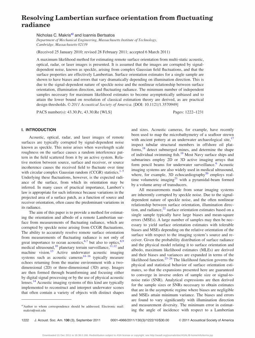
The flux dU, received in a acoustic, optical, radar, or

laser beam of solid angle db, is related to the area of the

resolved surface patch dAb (Fig. 1), the local surface radi-

ance Lb, and the solid angle subtended by the receiver aper-

ture dX, by the linear equation

dU ¼ dAbLbdX: (1)

The solid angle subtended by the receiver aperture from

the surface patch dAb is dX ¼ cos wr dA/r2, where dA is the

area of the aperture, cos wr is the foreshortening of the sur-

face patch with respect to the receiver, wr is the scattering

angle, and r is the range to the aperture. The intensity of the

received beam is then

Ib ¼dUdA¼ dAbLb

cos wr

r2: (2)

Assuming that the receiver is of sufficiently high resolution

that it resolves an elemental surface patch dAb, that is locally

planar and small enough so that

db ¼ dAbcos wr

r2; (3)

surface radiance can be directly measured by the receiver as

dIbdb¼ Lb: (4)

For a Lambertian surface,

Lb ¼ qE cos wi; (5)

so that the radiance measured in an acoustic, optical, radar,

or laser image of the scene Lb, is independent of the viewing

direction wr. It follows a linear relationship with the fore-

shortening cos wi of the surface patch, the surface irradiance

E, and the surface bidirectional reflectance distribution func-

tion q which is 1/p for a perfectly reflecting Lambertian

surface. Here wi is the angle of incident insonification and

E is defined as incident flux per unit area on the surface of

albedo pq.

III. THE LIKELIHOOD FUNCTION ANDMEASUREMENT STATISTICS

Let the stochastic measurement vector R of length Mcontain the independent statistics Rk whose expected values

�k(a)¼hRki are linearly related to measured surface radi-

ance, where the vector a contains the surface orientation pa-

rameters ar to be estimated from the measurements R for

r¼ 1, 2, 3, … , Q. More succinctly, let r(a)¼hRi.Assuming the Rk are corrupted by CCGR field fluctua-

tions, the conditional probability distribution for the meas-

urements R given parameter vector a is the product of

gamma distribution5,28

PRðR; aÞ ¼YMk¼1

lk

�kðaÞ

� �lk

ðRkÞlk�1exp �lk

Rk

�kðaÞ

� �CðlkÞ

: (6)

The quantity lk is the number of coherence cells in the mea-

surement average used to obtain Rk,5,28 the variance of which is

given by �2k=lk. It is important to note that lk is then also equal

to the squared-mean-to-variance ratio, or SNR, defined as

Rkh i2=ðhR2ki � hRki2Þ. For example, lk equals the time-band-

width product of the received field if each Rk is obtained from a

continuous but finite-time average. Additionally, lk can be

interpreted as the number of stationary speckles averaged over

a finite spatial aperture in the image plane or the number of sta-

tionary multi-look images averaged for a particular scene.28

IV. CLASSICAL ESTIMATION THEORY AND A HIGHERORDER ASYMPTOTIC APPROACH TO INFERENCE

The maximum likelihood estimator a, for the parameter

set a, maximizes the log-likelihood function l(R; a)¼ ln(PRFIG. 1. Resolved surface patch.

J. Acoust. Soc. Am., Vol. 130, No. 3, September 2011 N. C. Makris and I. Bertsatos: Surface orientation from fluctuating radiance 1223


(R; a)) with respect to a. The Cramer–Rao lower bound

(CRLB) i�1 is the minimum MSE attainable by any unbiased

estimate, regardless of the method of estimation. The CRLB is

the inverse of the Fisher information matrix, also known as

the expected information, the elements of which are given by

ibc ¼ hlblci, where lr ¼ @lðR; aÞ=@ar and ar is the rth compo-

nent of a.

For sufficiently large sample size, lk, the MLE is asymp-

totically unbiased and follows the Gaussian distribution

Paða;aÞ ¼ffiffiffiffiffiffiffiffiffiffiffiffi

ij jð2pÞM

sexp � 1

2ða� aÞTiða� aÞ

� �; (7)

with variance i�1 equal to the CRLB,29,30 where5,28

ibc ¼XM

k¼1

lk

@ ln �kðaÞ@ab

@ ln�kðaÞ@ac

�; (8)

�

and

ibc � ½i�1�bc ¼XM

k¼1

ð�kðaÞÞ2

lk

@ab

@�kðaÞ@ac

@�kðaÞ

!(9)

given the probability distribution for R described in Eq. (6).

In the deterministic limit lk!1, where the Rk are obtained

from exhaustive sample averages, Paða; aÞ becomes the delta

function dða� aÞ.Assume n independent identically distributed samples of

the total measurement vector R of length M. Let lT ¼ [l1,

l2, … , lM] be the vector of sample size lk of measurement

Rk for k¼ 1, 2, … , M. The moments of ar for r¼ 1, 2, 3, … ,

Q can be expressed as series of inverse powers of the sample

size n, as in Eqs. (3)–(5) of Ref. 26, provided that

the required derivatives of the likelihood function exist.23

The MLE bias of ar is then expressed as

biasðar; l; nÞ ¼ b1ðar; a; l; nÞ þ b2ðar; a; l; nÞþ higher order terms; (10)

where bjðar; a; l; nÞ ¼ bjðar; a; l; 1Þ =nj is the jth order

bias; so that

biasðar; l; nÞ ¼ b1ðar; a; l; 1Þn

þ b2ðar; a; l; 1Þn2

þ O1

n3

� �; (11)

where O(n�3) represents integer powers n�3 and higher.

Similarly, the MLE variance of ar can be expressed as

varðar; l; nÞ ¼ var1ðar; a; l; 1Þn

þ var2ðar; a; l; 1Þn2

þ O1

n3

� �; (12)

where the first-order variance, var1ðar; a; l; 1Þ/n, the

CRLB, is the asymptotic variance for large n.

General expressions for the first-order bias

b1ðar; a; l; 1Þ, and second-order variance var2ðar; a; l; 1Þ of

an MLE appear in Eqs. (3)–(5) of Ref. 26. For the statistical

model of Eq. (6), these expressions and Eq. (9) lead to

b1ðar; a; l; 1Þ ¼ �XM

k¼1

1

2

�2k

lk

@2ar

@�2k

; (13)

var1ðar; a; l; 1Þ ¼XM

k¼1

�2k

lk

@ar

@�k

� �2

; (14)

var2ðar; a; l; 1Þ ¼ �XM

k¼1

1

l2k

2�3k

@ar

@�k

@2ar

@�2k

�

þ �4k

@ar

@�k

@3ar

@�3k

þ 1

2�4

k

@2ar

@�2k

� �2#

(15)

Assuming for simplicity that lk¼ l for all k, the MLE bias

and variance can then also be expressed as asymptotic series

in inverse powers of l (see Appendix)

biasðar; l; 1Þ ¼ b1ðar; a; e; 1Þl

þ b2ðar; a; e; 1Þl2

þ O1

l3

� �; (16)

varðar; l; 1Þ ¼ var1ðar; a; e; 1Þl

þ var2ðar; a; e; 1Þl2

þ O1

l3

� �; (17)

where the components of the vector e are ek¼ 1 for k¼ 1, 2, … ,

M. To simplify notation, let varjðar; a; e; 1Þ � varjðar; aÞ and

bjðar; a; e; 1Þ � bjðar; aÞ:The value of l necessary for ar to become asymptoti-

cally unbiased is found by conservatively requiring the first-

order bias to be an order of magnitude smaller than the true

value of the parameter,

l ¼ 10b1ðar; aÞ

ar

�� ¼ 10

XM

k¼1

�2k

@2ar

@�2k

2ar

��: (18)

Similarly, the value of l necessary for the MLE variance to

asymptotically attain the CRLB is found by requiring the

second-order variance to be an order of magnitude smaller

than the first-order variance, so that

l¼ 10var2ðar; aÞj jvar1ðar; aÞ

¼ 10

PMk¼1

2�3k@ar@�k

@2ar

@�2k

þ �4k@ar@�k

@3ar

@�3k

þ 1

2�4

k

@2ar

@�2k

� �2��

��PMk¼1

�2k@ar@�k

� �2:

(19)

1224 J. Acoust. Soc. Am., Vol. 130, No. 3, September 2011 N. C. Makris and I. Bertsatos: Surface orientation from fluctuating radiance


Only for values of l satisfying these conditions, it is possible

for the variance to be in the asymptotic regime where it is

unbiased and continuously attains the CRLB.26,31,32

V. INFERRING LAMBERTIAN SURFACE ORIENTATION

For measurement k, a collimated source with known

unit incident direction sk irradiates a planar Lambertian

surface with unknown unit normal vector n. For each mea-

surement, the receiver measures Lambertian surface radi-

ance from any hemispherical position within view of the

surface. For convenience, a Cartesian coordinate system

(x, y, z) is adopted, with the origin in the center of the

resolved surface patch, as shown in Fig. 1. Because surface

incident irradiance Ek is presumed known, given know-

ledge of source power, directionality, and transmission

characteristics to the surface, it can be deterministically

scaled out of the measured surface radiance leaving

�Lk¼ Lkh i=Ek: When signal-independent additive CCGR

noise of intensity �NkdbkEk is also measured with the radi-

ant field from the surface, the expected measurement vec-

tor R becomes r(a)¼rL(a)þrN.Lambert’s law for the expected radiometric component

of the data is then

Rh iL¼ rLðaÞ ¼ ½�1ðaÞ;…; �MðaÞ�T ¼ Sx; (20)

where the matrix S is defined by

ST ¼ ½s1; s2; s3;…; sM�; (21)

the vector x equals qn.

The general problem is to determine both the Lamber-

tian surface normal vector n and the albedo pq from the fluc-

tuating measurements R. The surface normal is typically

expressed in terms of the surface gradient components

nT ¼ ½�pn; �qn; 1�=ð1 þ p2n þ q2

nÞ1=2; (22)

where

pn ¼@z

@x; qn ¼

@z

@y; (23)

or in terms of spherical coordinates

nT ¼ ½cos /n sin hn; sin /n sin hn; cos hn�: (24)

A. MLEs of surface orientation and albedo

The 3D parameter vector x is to be estimated from the

potentially over-determined M-dimensional measurement

vector R. From Eqs. (8) and (20), the MSE bound on any

unbiased estimate ex is

hðex � xÞðex � xÞTi � i�1x ¼ ½ST irS��1; (25)

where ½ir�ij¼dijlij=�2i is infinite when all incident vectors

sk are tangent to n in the absence of signal-independent

noise.

To derive the MLE of the vector x¼ qn, the probability

distribution for R in Eq. (6) is rewritten as

PRðR; xÞ ¼YMk¼1

lk

�kðxÞ lkðRkÞlk� 1exp �lk

Rk

�kðxÞ

� �CðlkÞ

: (26)

The MLE xr maximizes the log-likelihood function

ln(PR(R; x)) with respect to xr, so that it satisfies

@lnðPRðR; xÞÞ@xr

¼XM

k¼1

lk

�k

Rk

�k� 1

� @�k

@xr

��xr¼xr

¼ 0 (27)

where @�k

@xris the (k, r) element of S. Considering all the ele-

ments of x, Eq. (27) can be rewritten in vector form as

XM

k¼1

ðSkÞTlk

�kx¼x

¼XM

k¼1

ðSkÞTlkRk

�2k

��x¼x

; (28)

or

½STirr��x ¼ x¼ ½STirR�

��x ¼ x

(29)

where Sk is the kth row of S. The MLE, given linearity

between x and � is then given by

x ¼ ½ST irS��1STirðR � rNÞ; (30)

is unbiased and attains the error bound i�1x of Eq. (25).

Given this information, the MLEs for albedo pq ¼ p xj j;surface normal n ¼ x=q, cone and polar angles

hn ¼ cos�1 n3; /n ¼ tan�1ðn2=n1Þ; and surface gradient

components pn ¼ �ðn1=n3Þ; qn ¼ �ðn2=n3Þ; however, are

not generally unbiased and do not generally have minimum

variance except for sufficiently large sample sizes.

Taking the case where R is a 3D vector and rN is negli-

gible, for example, the joint distribution for x is27

pxðx xj Þ ¼ s1 � s2 � s3j j PRðSx rj Þ; (31)

which leads to the respective joint distributions

pgradðpn; qn; q pn; qn;j qÞ ¼ Pxð�qpnð1þ p2n þ q2

nÞ�1=2; �qqnð1 þ p2

n þ q2nÞ�1=2; qð1 þ p2

n þ q2nÞ�1=2

xj Þq2ð1 þ p2

n þ q2nÞ�3=2

�� ; (32)

and



ppolarðhn; /n; q hn;/n;j qÞ

¼ Pxðq cos /n sin hn; q sin /n sin hn; q cos hn xj Þq2 sin2 hn

�� ;(33)

for the gradient and polar coordinate MLEs.

Returning to the general case when R is an M-dimen-

sional vector, the asymptotic maximum likelihood distribu-

tions for surface orientation and albedo follow Eq. (7) when

Eqs. (18) and (19) are satisfied.

B. The angle of incidence

Suppose that the angle of incidence w is to be estimated

from a single measurement R, with mean �¼ q cosw and

variance �2/l, given that the albedo pq is known. From Eq.

(8), the resulting MSE bound is the inverse of the (scalar)

Fisher information

hðew � wÞ2i � i�1 ¼ ðcos ew þ �NÞ2

l sin2 w; (34)

for any unbiased estimate, ew which becomes

hð ~w� wÞ2i � i�1 ¼ cot2 wl

; (35)

when the signal-independent noise is negligible. These

expressions show resolution of the incident angle to be high-

est when the Lambertian surface is illuminated at shallow

grazing and lowest when the surface is illuminated near nor-

mal incidence. This can be motivated physically by noting

that for shallow-grazing angle illumination Lambert’s law

has a first-order dependence that is proportional to the inci-

dent angle. Conversely, for illumination near normal inci-

dence Lambert’s law is independent of the incident angle to

first order. It is also significant that when the root mean-

square error (RMSE) bound is finite, it can be reduced in

proportion to the square-root of the sample size l averaged

to obtain the radiometric statistic R, as shown in detail in

Sec. IV.

The MLE for the angle of incidence is

ew ¼ cos�1 R � �N

q

� �: (36)

Many of the potential benefits and difficulties associated

with maximum likelihood estimation can be illustrated by

examining the statistical properties of wFor the remainder of this section, let �N be negligible, as

may be expected in practical imaging systems expect at shal-

low grazing where w is very near p/2. First of all, because Ris a gamma variate and can take on any positive definite

value, the estimate w is real for 0 � R/q � 1 and imaginary

for R/q > 1. The probability that w is real is found to be c(l,l/cos w)/C(l) by appropriately integrating PR(Rjw). But this

leaves finite probability C(l,l/ cos w)/C(l) that w is imagi-

nary. More specifically, let the statistic w ¼ wr þ wi, where

wr, wi are the real and imaginary parts of w respectively.

Then the statistic w is distributed according to

Pwðw; wÞ ¼ q sin wPRðq cos w; wÞ over 0 � w � p=2; (37)

for w real, and

Pwðw; wÞ ¼ q sinhwPRðq cosh w; wÞ over 0 � w � 1; (38)

for w imaginary. The probability C(l, l/ cos w) /C(l) that wis imaginary decreases as the angle of incidence w and sam-

ple size l increase, as does the bias of w.

Apparently, CCGR fluctuations in the radiant field can

lead to unphysical MLEs of the incident angle w. This can

be remedied by reconditioning the MLE, given ancillary in-

formation33 that w is real, so that

Pw;Reðw; wÞ �Pwðwjw ¼ <fwg; wÞ

¼q sin wPRðq cos w; wÞ CðlÞcðl; l= cos wÞ ; (39)

for 0 � w � p=2. Similarly, the probability that w is imagi-

nary is defined as

Pw;Imðw; wÞ � Pwðwjw ¼ =fwg; wÞ

¼ q sinh wPRðq cosh w; wÞ CðlÞcðl; l= cos wÞ ; (40)

For sufficiently large sample size l, the relationship between

MLE w and data R approaches linearity, so that w obeys the

Gaussian distribution

Pw;Gðw; wÞ ¼ l2p cot2 w

1=2

exp � 1

2lðw� wÞ2

cot2 w

!; (41)

1A0@with bias vanishing and variance equaling the inverse Fisher

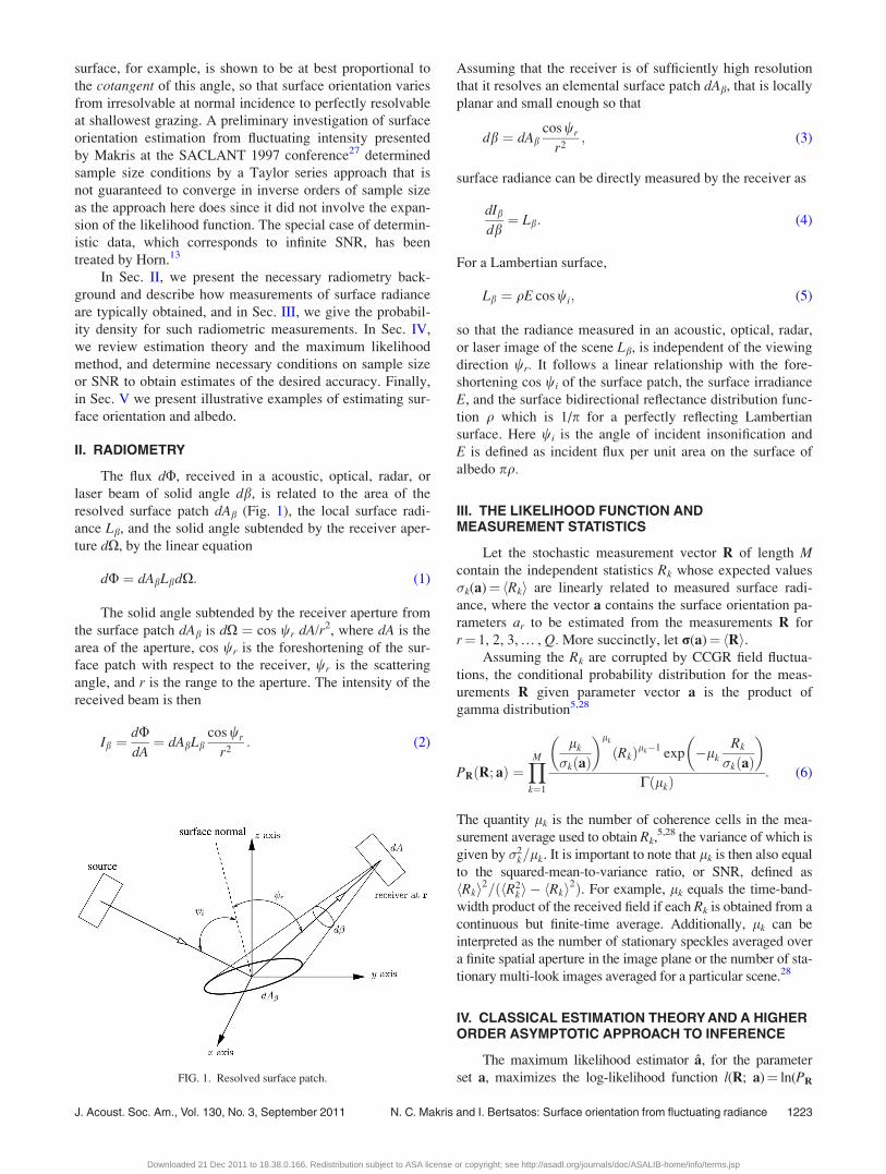
information, cot2 w/l.Figure 2 shows the probability densities of Eq. (39)

(dashed-dotted line), Eq. (40) (dashed line), and Eq. (41)

(solid line) for w¼ 30. As the sample size l increases, the

correlation between Pw;G and Pw;Reapproaches one, while

Pw;Im goes to zero. For the value of w used in these plots, a

sample size of approximately 320 is necessary for the corre-

lation between Pw;G and Pw;Reto become larger than 0.99.

As the true value w increases, the necessary sample size to

achieve a good correlation is found to decrease, as discussed

earlier.

Following Sec. IV, w is effectively unbiased when

l cot3 w2w

�� ; (42)

and effectively attains the bound i�1¼ cot2 w/l when

l cot2 w 3þ 7

2cot2 w

� �� : (43)



As the above expressions show, the sample size necessary

for w to behave as a minimum variance, unbiased estimate

varies nonlinearly from unity at shallow-grazing angles to

infinity near normal incidence.

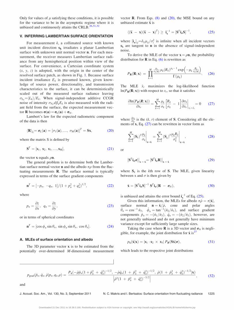
Figure 3 shows the sample sizes necessary for the MLE

to become asymptotically unbiased [Eq. (42), dashed line],

for the MLE variance to asymptotically attain the CRLB

[Eq. (43), dashed-dotted line], and for the correlation

between Pw;G and Pw;Re, to be greater than 0.99 (solid line),

as functions of the angle of incidence w. The curves have

been truncated so that the minimum necessary sample size

is 1. For most values of w, achieving a minimum variance

estimate also ensures that an unbiased estimate is obtained

that approximately obeys the Gaussian distribution of Eq.

(41). For shallow-grazing incidence angles (w approaching

90 degrees), the sample size necessary for Pw;G to be a

good approximation to Pw;Rebecomes the limiting

condition.

C. 3D surface orientation and albedo

Two independent measurements of surface radiance

with distinct illumination can lead to at most two unique sol-

utions for the two components of Lambertian surface orien-

tation.13 This ambiguity in surface orientation can be easily

resolved if one of the solutions places the surface out of the

view of the observer. Otherwise, the ambiguity can be

resolved if a third measurement is made under distinct illu-

mination. These observations can be geometrically moti-

vated by considering the intersection of the cones formed by

appropriately rotating the Lambertian surface normals about

the source direction for each measurement given the slope

estimated from that measurement. Here, specific examples

of resolution bounds on orientation estimation are presented,

as well as expressions for the CRLBs for cone and polar

angles, surface gradients and/or albedo given two or three

measurements of surface radiance.

For surface gradient aT¼ [p, q, q], or polar coordinate

aT¼ [h, /, q] parameterizations, the MSE bound on any

unbiased estimate a is

hð~a� aÞð~a� aÞTi � i�1a ¼

@a

@xi�1x

@aT

@x; (44)

where ix is given in Eq. (25). The bound i�1a becomes singu-

lar when all the sk are coplanar but not tangent to the surface

for non-zero rN, or when the Jacobian @a@x

is singular. When

rN vanishes, jixj1/2 jirj�1/2 can be interpreted as the effective

weighted volume of incident vectors sk. For example, when

R is a 3D vector, the bound i�1x is

½i�1x �ij ¼

�21

l1

½s2 � s3�i½s2 � s3�j þ�2

2

l2

½s3 � s1�i½s3 � s1�j þ�2

3

l3

½s1 � s2�i½s1 � s2�j

ðs1 � s2 � s3Þ2; (45)

FIG. 2. Probability densities given real, imaginary, or Gaussian constraint

on parameter estimate.

FIG. 3. Comparison of the necessary sample sizes to achieve (a) a correla-

tion greater than 0.99 between and Pw;Gðw; wÞ, (b) an unbiased estimate, and

(c) an estimate that attains the minimum possible variance.



so that jixj1/2 jirj�1/2 simply is the volume (s1 � s2� s3)2 of

the parallelepiped of incident vectors. Behavior of the Jaco-

bian @a@x

�� depends upon the final coordinates a, as can be seen

from the respective forms (p2þ q2þ 1)3/2/q2 and 1/(q2sin2 h)

for the surface gradient and polar systems.

Assume that the measurements Rk have the same num-

ber of coherence cells, lk¼l for all k. The stereo case is

considered where three measurements R1, R2 and R3 are used

to compute the two parameters a1 and a2. Let a1 ¼ a and a2

¼ b be the Lambertian surface orientations (azimuth and ele-

vation angles, or surface gradients). The abbreviation

Ck¼�k(a,b) ¼ cosw[k] is used, where w[k] denotes the angle

of incidence for the kth measurement. It is also convenient to

define the vector K to have the elements Kk¼ ln Ck, which

contain the natural logarithms of the positive semi-definite

measurement cosines. With this definition, the CRLB’s for

the general Lambertian surface orientations a and b follow

from Eqns. (8) and (9), and are

E½ða� aÞ2� � 1

l

@K@b

�� 2@K@a� @K@b

�� 2; (46)

E½ðb� bÞ2� � 1

l

@K@a

�� 2@K@a� @K@b

�� 2: (47)

The bounds only depend upon the cosine between the source

direction and Lambertian surface normal for each measure-

ment, Ck, and the respective partial derivatives of these

cosines with respect to the two orientation parameters to be

estimated. It is relatively easy to determine conditions in

which these expressions will attain limiting values due to the

positive semi-definiteness of terms in the numerators and

denominators. For example, the bounds are infinite when all

three measurements are coplanar with the surface normal,

such that n � (s[1]� s[2])¼ n � (s[2]� s[3])¼ 0. However, the

bounds are not necessarily infinite for coplanar illumination

directions that are not also coplanar with the surface normal,

i.e. for s[1] � (s[2]� s[3])¼ 0, but n � (s[1]� s[2])= 0, or n �(s[2]� s[3])=0. The bounds are zero when any of the two

direction cosines C1, C2, C3 are zero and the two respective

illumination directions for these have differing polar angles.

It is also possible to estimate the albedo when three

measurements with unique illumination directions are avail-

able. Let a3¼q be the surface albedo. It is useful to define

the unit all-measurements-equal vector E by its components

such that Ek¼ 1 for k¼ 1, 2, 3. With this definition, the

CRLB’s for estimation of a, b, q are given by

E½ða� aÞ2� � 1

l

@K@b� E

�� 2@K@a� @K@b

� �� E

� 2; (48)

E½ðb� bÞ2� � 1

l

@K@a� E

�� 2@K@a� @K@b

� �� E

� 2; (49)

E½ðq� qÞ2� � q2

l

@K@a� @K@b

�� 2@K@a� @K@b

� �� E

� 2; (50)

It is noteworthy that the bound for q is a function of the sur-

face orientation components a and b, as well as q. While the

bounds for a and b given in Eqs. (48) and (49) are independ-

ent of the value of q, they are affected by uncertainty in the

value of q, and Eqs. (46) and (47) are no longer applicable.

These particular bounds for a and b are infinite when all

three illumination directions are coplanar such that s[1]

� (s[2]� s[3])¼ 0, even if the directions are not coplanar to

the surface normal. Additionally, these bounds for a and bcan be zero when any of the two direction cosines are zero.

Note that for the CRLB for q to be given by q2/l, and

thereby be otherwise independent of Lambertian surface ori-

entation, it is sufficient to have

@K@a� @K@b

� �� P @K

@a� @K@b

� �¼ 0; (51)

where the permutation matrix is defined as

P ¼0 1 0

0 0 1

1 0 0

24 35: (52)

For example the CRLB for q is given by q2/l when any two

of the measurement cosines C1, C2, C3 are equal to zero.

Equations (48)–(50) are useful in providing a geometric

interpretation of the CRLB for a, b and q given three meas-

urements. For example, consider the conditions leading to the

limiting values of zero and infinity for the bounds. Inspection

of the positive semi-definite numerators and denominators of

Eqs. (48)–(50) motivates consideration of the following two

cases: (1) the partial derivative of the logarithmic measure-

ment vector with respect to the orientation component a or brespectively is orthogonal to the all-measurements-equal vec-

tor; (2) the cross product of the partial derivatives of the loga-

rithmic measurement vector with respect to the a and borientations is orthogonal to the all-measurements-equal vec-

tor. When (1) is true but (2) is not, the respective bound on

orientation component b or a is zero. When (1) is not true but

(2) is true the bound on either orientation is infinite. As noted

before, this occurs when the illumination directions for all

measurements are coplanar with the surface normal. When

both (1) and (2) are true, the bound on a or b depends only on

the number of coherence cells.

Figure 4 shows the CRLB and the necessary sample

sizes for the x-gradient p, in simultaneous estimation of p, q,and q with three incident illumination directions, s1, s2, and

s3. For illustrative purposes, only s3 is allowed to vary. Opti-

mal resolution [Fig. 4(b)], minimum necessary sample size



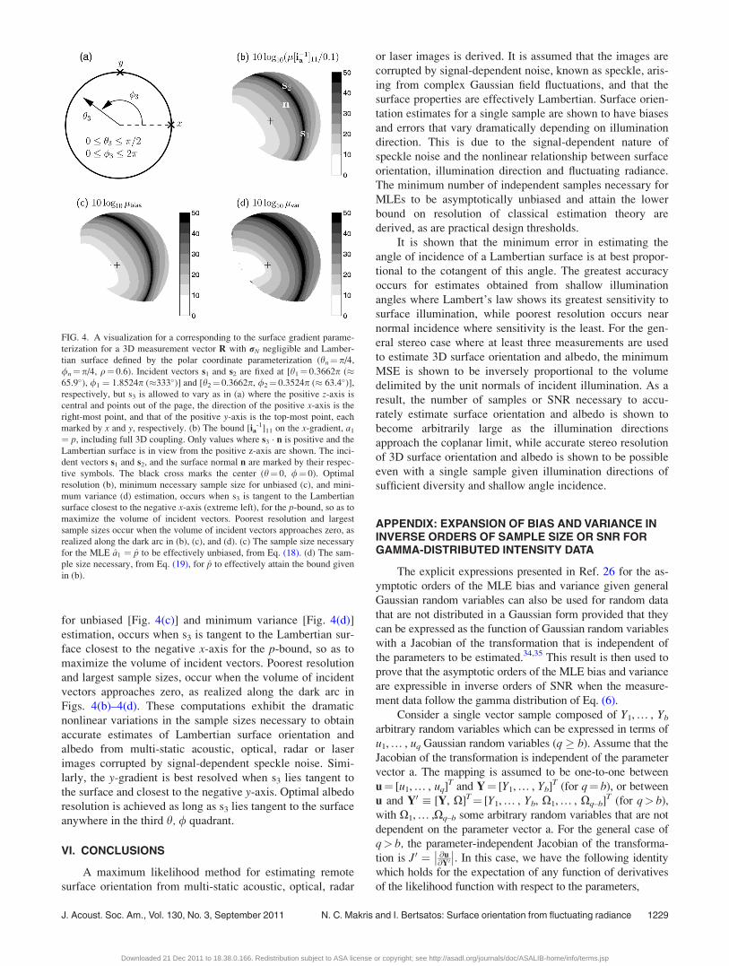
for unbiased [Fig. 4(c)] and minimum variance [Fig. 4(d)]

estimation, occurs when s3 is tangent to the Lambertian sur-

face closest to the negative x-axis for the p-bound, so as to

maximize the volume of incident vectors. Poorest resolution

and largest sample sizes, occur when the volume of incident

vectors approaches zero, as realized along the dark arc in

Figs. 4(b)–4(d). These computations exhibit the dramatic

nonlinear variations in the sample sizes necessary to obtain

accurate estimates of Lambertian surface orientation and

albedo from multi-static acoustic, optical, radar or laser

images corrupted by signal-dependent speckle noise. Simi-

larly, the y-gradient is best resolved when s3 lies tangent to

the surface and closest to the negative y-axis. Optimal albedo

resolution is achieved as long as s3 lies tangent to the surface

anywhere in the third h, / quadrant.

VI. CONCLUSIONS

A maximum likelihood method for estimating remote

surface orientation from multi-static acoustic, optical, radar

or laser images is derived. It is assumed that the images are

corrupted by signal-dependent noise, known as speckle, aris-

ing from complex Gaussian field fluctuations, and that the

surface properties are effectively Lambertian. Surface orien-

tation estimates for a single sample are shown to have biases

and errors that vary dramatically depending on illumination

direction. This is due to the signal-dependent nature of

speckle noise and the nonlinear relationship between surface

orientation, illumination direction and fluctuating radiance.

The minimum number of independent samples necessary for

MLEs to be asymptotically unbiased and attain the lower

bound on resolution of classical estimation theory are

derived, as are practical design thresholds.

It is shown that the minimum error in estimating the

angle of incidence of a Lambertian surface is at best propor-

tional to the cotangent of this angle. The greatest accuracy

occurs for estimates obtained from shallow illumination

angles where Lambert’s law shows its greatest sensitivity to

surface illumination, while poorest resolution occurs near

normal incidence where sensitivity is the least. For the gen-

eral stereo case where at least three measurements are used

to estimate 3D surface orientation and albedo, the minimum

MSE is shown to be inversely proportional to the volume

delimited by the unit normals of incident illumination. As a

result, the number of samples or SNR necessary to accu-

rately estimate surface orientation and albedo is shown to

become arbitrarily large as the illumination directions

approach the coplanar limit, while accurate stereo resolution

of 3D surface orientation and albedo is shown to be possible

even with a single sample given illumination directions of

sufficient diversity and shallow angle incidence.

APPENDIX: EXPANSION OF BIAS AND VARIANCE ININVERSE ORDERS OF SAMPLE SIZE OR SNR FORGAMMA-DISTRIBUTED INTENSITY DATA

The explicit expressions presented in Ref. 26 for the as-

ymptotic orders of the MLE bias and variance given general

Gaussian random variables can also be used for random data

that are not distributed in a Gaussian form provided that they

can be expressed as the function of Gaussian random variables

with a Jacobian of the transformation that is independent of

the parameters to be estimated.34,35 This result is then used to

prove that the asymptotic orders of the MLE bias and variance

are expressible in inverse orders of SNR when the measure-

ment data follow the gamma distribution of Eq. (6).

Consider a single vector sample composed of Y1, … , Yb

arbitrary random variables which can be expressed in terms of

u1, … , uq Gaussian random variables (q � b). Assume that the

Jacobian of the transformation is independent of the parameter

vector a. The mapping is assumed to be one-to-one between

u¼ [u1, … , uq]T and Y¼ [Y1, … , Yb]T (for q¼ b), or between

u and Y0: [Y, X]T¼ [Y1, … , Yb, X1, … , Xq–b]T (for q> b),

with X1, … ,Xq–b some arbitrary random variables that are not

dependent on the parameter vector a. For the general case of

q> b, the parameter-independent Jacobian of the transforma-

tion is J0 ¼ @u@Y0

�� . In this case, we have the following identity

which holds for the expectation of any function of derivatives

of the likelihood function with respect to the parameters,

FIG. 4. A visualization for a corresponding to the surface gradient parame-

terization for a 3D measurement vector R with rN negligible and Lamber-

tian surface defined by the polar coordinate parameterization (hn¼p/4,

/n¼p/4, q¼ 0.6). Incident vectors s1 and s2 are fixed at [h1¼ 0.3662p (�65.9), /1 ¼ 1.8524p (�333)] and [h2¼ 0.3662p, /2¼ 0.3524p (� 63.4)],respectively, but s3 is allowed to vary as in (a) where the positive z-axis is

central and points out of the page, the direction of the positive x-axis is the

right-most point, and that of the positive y-axis is the top-most point, each

marked by x and y, respectively. (b) The bound [ia-1]11 on the x-gradient, a1

¼ p, including full 3D coupling. Only values where s3 � n is positive and the

Lambertian surface is in view from the positive z-axis are shown. The inci-

dent vectors s1 and s2, and the surface normal n are marked by their respec-

tive symbols. The black cross marks the center (h¼ 0, /¼ 0). Optimal

resolution (b), minimum necessary sample size for unbiased (c), and mini-

mum variance (d) estimation, occurs when s3 is tangent to the Lambertian

surface closest to the negative x-axis (extreme left), for the p-bound, so as to

maximize the volume of incident vectors. Poorest resolution and largest

sample sizes occur when the volume of incident vectors approaches zero, as

realized along the dark arc in (b), (c), and (d). (c) The sample size necessary

for the MLE a1 ¼ p to be effectively unbiased, from Eq. (18). (d) The sam-

ple size necessary, from Eq. (19), for p to effectively attain the bound given

in (b).



hf iY ¼ð

f@lnðpðY; aÞÞ

@a;…;

@blnðpðY; aÞÞ@ab

� �pðY; aÞdY

¼ð ð

f@lnðpðY; aÞpðXÞÞ

@a;…;

@blnðpðY; aÞpðXÞÞ@ab

� �� pðY; aÞpðXÞdYdX (A1)

where the last equality is introduced so as to make the trans-

formation between Y0 and u, since p(Y; a)p(X)¼ p(u(Y, X;

a))J0 and X is parameter independent. Equation (A1) can

then be written as

hf iY ¼ð

f@lnðpðuðY;XÞ; aÞJ0Þ

@a;…;

@blnðpðuðY;XÞ; aÞJ0Þ@ab

� �� pðuðY;XÞ; aÞJ0dYdX

¼ð

f@lnðpðu; aÞÞ

@a;…;

@blnðpðu; aÞÞ@ab

� �pðu; aÞdu ¼ hf iu:

(A2)

The expected value of any function of derivatives of the like-

lihood function for Y with respect to the parameters a can

then be written as the same function of derivatives of the

likelihood function for u. Since the asymptotic orders are the

functions of expectations that have the same structure as Eq.

(A1), the asymptotic orders of the MLE of a parameter a can

be computed from measurements of the non-Gaussian quan-

tity Y.

For the problem of surface orientation considered here,

the measurements R, given parameter vector a, are distributed

according to the product of gamma distributions of Eq. (6).

The parameter a can be estimated using the set of Gaussian

random variables x1,1, … , x1;2l1, x2,1,…, x2;2l2

,…, xM,1,…,

xM;2lM, such that

Pxðx1;1;… ; xM;2lM; aÞ ¼

YMk¼1

Y2lk

i¼1

1ffiffiffiffiffiffiffiffiffiffiffiffiffiffip�kðaÞ

p exp �x2

k;i

�kðaÞ

! !;

(A3)

where �k is the mean of Rk and also twice the variance of xk,i

for i¼ 1, … , 2lk. Assuming that lk¼ l for all k, Eq. (A3)

then becomes

Pxðx1;…; x2l; aÞ ¼ 1

ð2pÞMljCðaÞjlexp � 1

2

X2l

j¼1

xTj CðaÞ�1

xj

!(A4)

where xj¼ [x1,j, … , xM,j]T is the jth sample of the M-dimen-

sional data vector for j¼ 1, … , 2l, and the M-dimensional co-

variance matrix C(a) has elements Ckl ¼ dkl�k/2. Using this

notation, the M-dimensional measurement R, with parameter-

dependent mean r(a), can be replaced by the measurement x

obtained from n ¼ 2l independent and identically distributed

M-dimensional vectors, where the parameter dependence is

instead on the covariance of the data, C(a).

The asymptotic orders of the MLE bias and variance

for the rth component of the parameter vector a can then

be determined using the existing expressions for the Gaus-

sian case, Eq. (7) of Ref. 26 and Eq. (2.4) of Ref. 35 after

substituting for n0 ¼ 2l and Ckl ¼ dkl�k/2. Since l is the

SNR of the gamma-distributed R measurement, the MLE

bias and variance given data that follow a gamma distribu-

tion can be written as asymptotic series in inverse orders of

SNR,

biasðar;l;M ¼ 1Þ ¼ b1ðar; a;e;1Þl

þ b2ðar; a; e;1Þl2

þO1

l3

� �;

(A5)

varðar; l;M ¼ 1Þ ¼ var1ðar; a; e; 1Þl

þ var2ðar; a; e; 1Þl2

þ O1

l3

� �; (A6)

where the vector e with components ek¼ 1 signifies lk¼lfor all k¼ 1, 2, … , M.

1J. C. Dainty, ed., Laser Speckle and Related Phenomena, 2nd ed.

(Springer-Verlag, Berlin, 1984), pp. 1–72J. W. Goodman, “Statistical properties of laser speckle patterns,” in LaserSpeckle and Related Phenomena, 2nd ed., edited by J. C. Dainty

(Springer-Verlag, Berlin, 1984), pp. 9–75.3J. W. Goodman, Statistical Optics (Wiley, New York, 1985), pp. 41–43.4G. Parry, “Speckle patterns in partially coherent light,” in Laser Speckleand Related Phenomena, 2nd ed., edited by J. C. Dainty (Springer-Verlag,

Berlin, 1984), pp. 77–122.5N. C. Makris, “The effect of saturated transmission scintillation on ocean

acoustic intensity measurements,” J. Acoust. Soc. Am. 100, 769–783

(1996).6R. J. Urick, Principles of Underwater Sound (McGraw-Hill, New York,

1983), pp. 29–63.7F. B. Jensen, W. A. Kuperman, M. B. Porter, and H. Schmidt, Computa-tional Ocean Acoustics (AIP, New York, 1994), pp. 50–51.

8M. Born and E. Wolf, Principles of Optics, 7th ed. (Cambridge University

Press, Cambridge, 1999), pp. 313–410.9H. C. Van Du Hulst, Light Scattering by Small Particles (Dover, New

York, 1981), pp. 110–113.10T. L. Szabo, Diagnostic Ultrasound Imaging: Inside Out (Elsevier Sci-

ence, Boston, 2004), pp. 213–240.11S. A. Drury, Image Interpretation in Geology, 2nd ed. (Chapman and Hall,

London, 1993), pp. 176–204.12W. G. Egan, Optical Remote Sensing Science and Technology (Marcel

Dekker, Inc., New York, 2004), pp. 1–27.13B. K. P. Horn, Robot Vision (MIT Press, Cambridge, 1986), pp. 202–

242.14V. Murino and A. Trucco, “Three-dimensional image generation and proc-

essing in underwater acoustic vision,” Proc. IEEE 88(12), 1903–1948

(2000).15J. L. Sutton, “Underwater acoustic imaging,” Proc. IEEE 67(4), 554–566

(1979).16R.K. Hansen and P. A. Andersen, “3D Acoustic camera for underwater

imaging,” in Acoustical Imaging, edited by Y. Wei and B. Gu (Plenum,

New York, 1993), Vol. 20, pp. 723–727.17H. Singh, L. Whitcomb, D. Yoerger, and O. Pizarro, “Microbathymetric

mapping from underwater vehicles in the deep ocean,” Comput. Vis.

Image Underst. 79, 143–161 (2000).18E. Chesters, “The use of a high-frequency pencil beam sonar to determine

the position of tubular members of underwater structures,” in OCEANS‘94. Oceans Engineering for Today’s Technology and Tomorrow’s Preser-vation, (1994), Vol. 1, pp. I/ 199–I/204.

19E. Belcher, B. Matsuyama, and G. Trimble, “Object identification with

acoustic lenses,” in Proceedings of Oceans 2001 Conference, Honolulu,

Hawaii (November 5–8, 2001), pp. 6–11.



20J. A. Panza, “Real-time three dimensional echocardiography: An over-

view,” Int. J. Cardiovasc. Imaging 17, 227–235 (2001).21O. T. Von Ramm and S. W. Smith, “Real time volumetric ultrasound

imaging system,” J. Digit. Imaging 3(4), 261–266 (1990).22C. A. Poynton, “‘Gamma’ and its disguises: The nonlinear mappings of in-

tensity in perception, CRTs, film and video,” SMPTE J. 102, 1099–1108

(1993).23L.R. Shenton and K. O. Bowman, Maximum Likelihood Estimation in

Small Samples (Griffin, New York, 1977), p. 7.24O.E. Barndorff-Nielsen and D. R. Cox, Inference and Asymptotics (Chap-

man and Hall, London, 1994), pp. 184–187.25P. McCullagh, Tensor Methods in Statistics (Monographs on Statistics and

Applied Probability) (Chapman and Hall, London, 1987), Chap. 7, p. 198.26E. Naftali and N. C. Makris, “Necessary conditions for a maximum likeli-

hood estimate to become asymptotically unbiased and attain the Cramer–

Rao Lower Bound. Part I. General approach with an application to time-

delay and Doppler shift estimation,” J. Acoust. Soc. Am. 110, 1917–1930

(2001).27N. C. Makris, “Estimating surface orientation from sonar images,” in SAC-

LANT Conference Proceedings Series CP-45 (1997), pp. 339–346.28N. C. Makris, “A foundation for logarithmic measures of fluctuating inten-

sity in pattern recognition,” Opt. Lett. 20, 2012–2014 (1995).

29C. R. Rao, Linear Statistical Inference and Its Applications (Wiley, New

York, 1966), pp. 314–443.30S. M. Kay, Fundamentals of Statistical Signal Processing: Estimation

Theory (Prentice Hall, New Jersey, 1993), pp. 27–80.31A. Thode, M. Zanolin, E. Naftali, I. Ingram, P. Ratilal, and N. C. Makris,

“Necessary conditions for a maximum likelihood estimate to become

asymptotically unbiased and attain the Cramer–Rao lower bound. Part II.

Range and depth localization of a sound source in an ocean waveguide,”

J. Acoust. Soc. Am. 112, 1890–1910 (2002).32M. Zanolin, I. Ingram, A. Thode, and N. C. Makris, “Asymptotic accu-

racy of geoacoustic inversions,” J. Acoust. Soc. Am. 116, 2031–2042

(2004).33R. A. Fisher, Statistical Methods and Scientific Inference (Hafner, New

York, 1956), pp. 1–180.34M. Zanolin, E. Naftali, and N. Makris, “Second-order bias of a multivari-

ate Gaussian maximum likelihood estimate with chain-rule for higher

moments,” Technical Report No. 13-2003-37, Massachusetts Institute of

Technology (2003).35M. Zanolin, S. Vitale, and N. Makris, “Application of asymptotic expan-

sions of maximum likelihood estimators errors to gravitational waves

from binary mergers: The single interferometer case,” Phys. Rev. D

81(12), 124048.1–124048.16 (2010).



resolving lambertian surface orientation from fluctuating

Documents