Noname manuscript No.(will be inserted by the editor)

Resisting Structural Re-identification in Anonymized SocialNetworks

Michael Hay · Gerome Miklau · David Jensen · Don Towsley · Chao Li

Received: date / Accepted: date

Abstract We identify privacy risks associated with re-leasing network datasets and provide an algorithm thatmitigates those risks. A network dataset is a graph repre-senting entities connected by edges representing relationssuch as friendship, communication, or shared activity.Maintaining privacy when publishing a network datasetis uniquely challenging because an individual’s networkcontext can be used to identify them even if other iden-tifying information is removed.

In this paper, we introduce a parameterized modelof structural knowledge available to the adversary andquantify the success of attacks on individuals in anon-ymized networks. We show that the risks of these at-tacks vary based on network structure and size, and pro-vide theoretical results that explain the anonymity riskin random networks. We then propose a novel approachto anonymizing network data that models aggregate net-work structure and allows analysis to be performed bysampling from the model. The approach guarantees ano-nymity for entities in the network while allowing accurateestimates of a variety of network measures with relativelylittle bias.

1 Introduction

A network dataset is a graph representing a set of en-tities and the connections between them. Network data

This an author-created version of an article that appearsin the The VLDB Journal, Volume 19, Number 6, 797-823,doi: 10.1007/s00778-010-0210-x. The final publication is avail-able at www.springerlink.com. An earlier version appeared atthe 34th International Conference on Very Large Data Bases(VLDB), 2008.

M. Hay · G. Miklau · D. Jensen · D. Towsley · Chao LiDepartment of Computer ScienceUniversity of Massachusetts AmherstAmherst, MA 01002E-mail: mhay,miklau,jensen,towsley,chaoli@cs.umass.edu

can describe a variety of domains: a social network mightdescribe individuals connected by friendships; an infor-mation network might describe a set of articles connectedby citations; a communication network might describeInternet hosts related by traffic flows. As our ability tocollect network data has increased, so too has the impor-tance of analyzing these networks. Networks are analyzedin many ways: to study disease transmission, to measurea publication’s influence, and to evaluate the network’sresiliency to faults and attacks. Such analyses inform ourunderstanding of network structure and function.

However, it can be difficult to obtain access to net-work data, in part because many networks contain sensi-tive information, making data owners reluctant to pub-lish them. An example of a network containing sensitiveinformation is the social network studied by Potterat etal. [37], which describes a set of individuals related bysexual contacts and shared drug injections, relationshipsthat are clearly sensitive. In this case, the researcherschose to publish the network. While society knows moreabout how HIV spreads because this network was pub-lished and analyzed, researchers had to weigh that ben-efit against possible losses of privacy to the individualsinvolved. Other kinds of networks, such as communica-tion networks, are also considered sensitive and for thatreason are rarely published. For example, to our knowl-edge, the sole publicly available network of email com-munication was published only because of litigation [7].

We consider the problem of publishing network datain such a way that permits useful analysis yet avoidsdisclosing sensitive information. Most existing work onprivacy in data publishing has focused on tabular data,where each record represents a separate entity, and anindividual may be re-identified by matching the individ-ual’s publicly known attributes with the attributes of theanonymized table. Anonymization techniques for tabulardata do not apply to network data because they fail toaccount for the interconnectedness of the entities (i.e.,they destroy the network structure).

2

Because network analysis can be performed in theabsence of entity identifiers (e.g., name, social securitynumber), a natural strategy for protecting sensitive infor-mation is to replace identifying attributes with syntheticidentifiers. We refer to this procedure as naive anonym-ization. It is a common practice and presumably, it pro-tects sensitive information by breaking the associationbetween the real-world identity and the sensitive data.

However, naive anonymization may be insufficient.A distinctive threat in network data is that an entity’sconnections (i.e., the network structure around it) can bedistinguishing, and may be used to re-identify an other-wise anonymous individual. We consider how a maliciousindividual (the adversary) might obtain partial knowl-edge about the network structure around targeted indi-viduals and then use this knowledge to re-identify themin the anonymized network. Once re-identified, the ad-versary can learn additional properties about the targets;for instance, he may able to infer the presence or absenceof edges between them. Since individual connections areoften considered sensitive information, such edge disclo-sure constitutes a violation of privacy. Whether naiveanonymization provides adequate protection depends onthe structure of the network and the adversary’s capabil-ity. In this paper, we provide a comprehensive assessmentof the privacy risks of naive anonymization.

Although an adversary may also have informationabout the attributes of nodes, the focus of this paperis on disclosures resulting from structural or topologi-cal re-identification, where the adversary’s informationis about the structure of the graph only. The use ofattribute knowledge to re-identify individuals in anon-ymized data has been well-studied, as have techniquesfor resisting it [31,32,41,42,44]. More importantly, manynetwork analyses are concerned exclusively with struc-tural properties of the graph, therefore safely publish-ing an unlabeled network is an important goal in itself.For example, the following common analyses examineonly the network structure: finding communities, fittingpower-law models, enumerating motifs, measuring diffu-sion, and assessing resiliency [35].

In this paper, we make the following contributions:

– Adversary Model We propose a flexible model ofexternal information used by an adversary to attacknaively-anonymized networks. The model allows usto evaluate re-identification risk efficiently and for arange of different adversary capabilities. We also for-malize the structural indistinguishability of a nodewith respect to an adversary with locally-boundedexternal information (Section 2).

– Empirical Risk Assessment We evaluate the ef-fectiveness of structural attacks on real and syntheticnetworks, measuring successful re-identification andedge disclosures. We find that real networks are di-verse in their resistance to attacks. Nevertheless, ourresults demonstrate that naive anonymization pro-vides insufficient protection, especially if an adver-

sary is capable of gathering knowledge beyond a tar-get’s immediate neighbors (Section 3).

– Theoretical Risk Assessment In addition to theempirical study, we perform a theoretical analysisof random graphs. We show how properties such asa graph’s density and degree distribution affect re-identification risk. A significant finding is that in suf-ficiently dense graphs, nodes can be re-identified evenwhen the graph is extremely large (Section 4).

– Privacy Definition We also propose strategies formitigating re-identification risk. First, we propose aprivacy condition, which formally specifies a limit onhow much the adversary can learn about a node’sidentity. We compare it with other definitions thathave been proposed in the literature and discuss itslimitations (Section 5).

– Anonymization Algorithm Then we propose a novelalgorithm to achieve this privacy condition. The algo-rithm produces a generalized graph, which describesthe structure of the original graph in terms of nodegroups called supernodes. The generalized graph re-tains key structural properties of the original graphyet ensures anonymity (Section 6).

– Algorithm Evaluation We perform a comprehen-sive evaluation of the utility of the generalized graphs.This includes a comparison with other state-of-the-art graph anonymization algorithms (Section 7).

We conclude the paper with a comprehensive review ofrelated work (Section 8).

2 Modeling the adversary

In this section we describe the capabilities and motiva-tions of the adversary in the context of network data.First, we describe the process of naive anonymizationand how the adversary may attack it. Second, we definethe threats of node re-identification and edge disclosure.Third, we explain how anonymity is achieved throughstructural similarity, which motivates a model of adver-sary knowledge based on degree signatures. Finally wereview alternative models of the adversary.

2.1 Naive anonymization

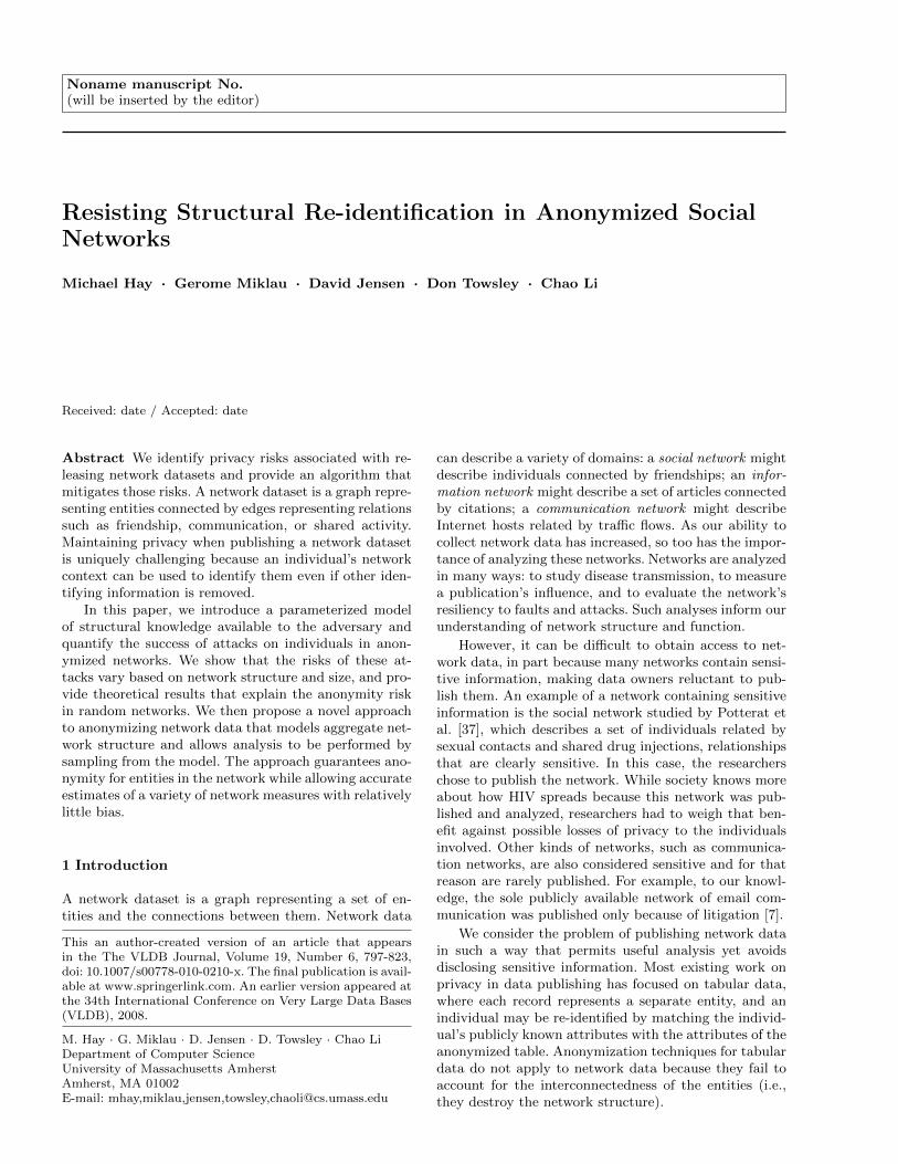
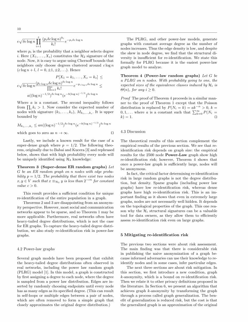
Formally, we model a network as an undirected graphG = (V,E). The naive anonymization of G is an isomor-phic graph,Ga = (Va, Ea), defined by a random bijectionΠ : V → Va. For example, Figure 1 shows a small net-work represented as a graph along with its naive anon-ymization. The anonymization mapping Π, also shown,is a random, secret mapping.

Naive anonymization prevents re-identification whenthe adversary has no information about individuals inthe original graph. Formally stated, an individual x ∈ V ,called the target, has a candidate set, denoted cand(x),

3

Alice Bob Carol

4

2

5

Dave Ed

Fred 13Greg

6

7

AliceBobCarolDaveEdFredGregHarry

68572341

Harry

8

Fig. 1 A social network represented as a graph (left), thenaive anonymization (center), and the anonymization map-ping (right).

which consists of the nodes of Ga that could feasiblycorrespond to x. To assess the risk of re-identification,we assume each element of the candidate set is equallylikely and use the size of the candidate set as a measureof resistance to re-identification. Since Π is random, inthe absence of other information, any node in Ga couldcorrespond to the target node x. Thus, given an unin-formed adversary, each individual has the same risk ofre-identification, specifically cand(x) = Va for each tar-get individual x.

However, if the adversary has access to external in-formation about the entities, he may be able to reducethe candidate set and threaten the privacy of individuals.

2.2 Threats

In practice the adversary may have access to externalinformation about the entities in the graph and their re-lationships. This information may be available througha public source beyond the control of the data owner, ormay be obtained by the adversary’s malicious actions.For example, for the graph in Figure 1, the adversarymight know that “Bob has three or more neighbors,” orthat “Greg is connected to at least two nodes, each withdegree 2.” Such information allows the adversary to re-duce the set of candidates in the anonymized graph foreach of the targeted individuals. For example, the firststatement allows the adversary to partially re-identifyBob: cand(Bob) = 2, 4, 7, 8. The second statement re-identifies Greg: cand(Greg) = 4.

Re-identification can lead to additional disclosuresunder naive anonymization. If an individual is uniquelyre-identified, then the entire structure of connections sur-rounding the individual is revealed. If two individuals areuniquely re-identified, then the presence or absence ofan edge between them is revealed directly by the naivelyanonymized graph. Such an edge disclosure, in which anadversary is able to accurately infer the presence of anedge between two identified individuals, can be a seriousprivacy threat. In the present work, we consider the gen-eral threat of re-identification as well as the more specificthreat edge disclosure.

Throughout the paper, we model the adversary’s ex-ternal information as access to a source that provides

answers to a restricted knowledge query evaluated for asingle target node of the original graph G.

An adversary attempts re-identification for a targetnode x by using Q(x) to refine the feasible candidate set.Since Ga is published, the adversary can easily evaluateany structural query directly on Ga, looking for matches.The adversary will compute the refined candidate setthat contains all nodes in the published graph Ga thatare consistent with answers to the knowledge query onthe target node.

Definition 1 (Candidate Set under Q) For a knowl-edge query Q over a graph, the candidate set of targetnode x w.r.t Q is candQ(x) = y ∈ Va | Q(x) = Q(y).

Example 1 Referring to the example graph in Figure 1,suppose Q is a knowledge query returning the degree ofa node. Then for targets Ed, Fred, Greg we have Q(Ed) =4,Q(Fred) = 2,Q(Greg) = 4, and candidate sets candQ(Ed) =candQ(Greg) = 2, 4, 7, 8 and candQ(Fred) = 1, 3.

Given two target nodes x and y, the adversary canuse the naively anonymized graph to deduce the likeli-hood that the nodes are connected. In the absence ofexternal information, the likelihood of any edge is sim-ply the density of the graph (the fraction of all possibleedges that exist in the graph).

If the candidate sets for x and y have been refined bythe adversary’s knowledge about x and/or y, then theadversary reasons about the likelihood x and y are con-nected based on the connections between the candidatesets for x and y. Thus we define the edge likelihood to bethe Bayesian posterior belief assuming each candidate isan equally likely match for the targeted nodes.

Definition 2 (Edge likelihood under Q) For a knowl-edge query Q over a graph, and a pair of target nodes xand y, the inferred likelihood of edge (x, y) under Q isdenoted probQ(x, y) and defined as:

|(u, v) | u ∈ X, v ∈ Y |+ |(u, v) | u, v ∈ X ∩ Y |

|X| · |Y |− |X ∩ Y |

where X = candQ(x) and Y = candQ(y).

The denominator represents the total number of pos-sible edges from a node of one candidate set to a node ofthe other candidate set, and accounts for the case wherethe intersection of the candidate sets is non-empty.

Example 2 Continuing the example above, the inferredlikelihood of edge (Ed, Fred) is:

probQ(Ed, Fred) = (4 + 0)/(4 ∗ 2) = 0.500

because there are 4 edges present in Ga between the dis-joint candidate sets candQ(Ed) and candQ(Fred). Theinferred edge likelihood of edge (Ed,Greg) is:

probQ(Ed,Greg) = (5 + 5)/(4 ∗ 4− 4) = 0.833

4

Alice Bob Carol

Dave Ed

Fred Greg Harry

(a) graph

Node ID H0 H1 H2

Alice 1 4Bob 4 1, 1, 4, 4Carol 1 4Dave 4 2, 4, 4, 4Ed 4 2, 4, 4, 4Fred 2 4, 4Greg 4 2, 2, 4, 4Harry 2 4, 4

(b) structural signatures

Equivalence Relation Equivalence Classes≡H0

A,B,C,D,E, F,G,H

≡H1A,C B,D,E,G F,H

≡H2A,CBD,EGF,H

≡A A,CBD,EGF,H

(c) equivalence classes

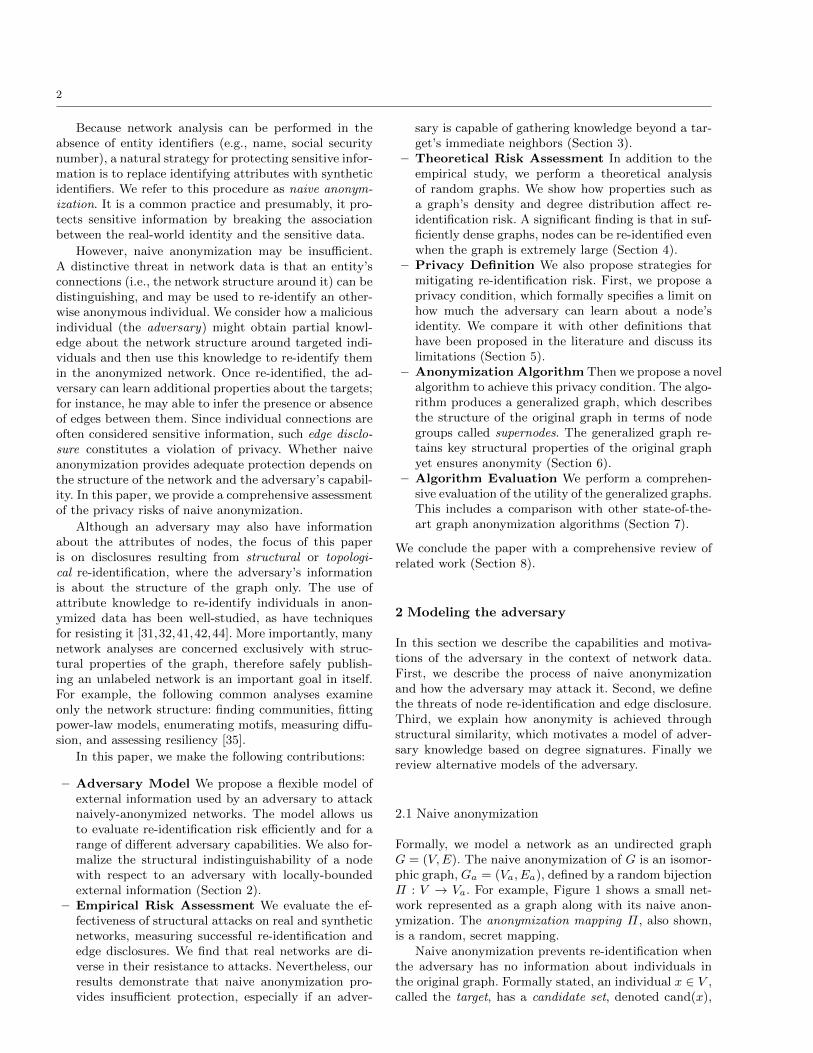
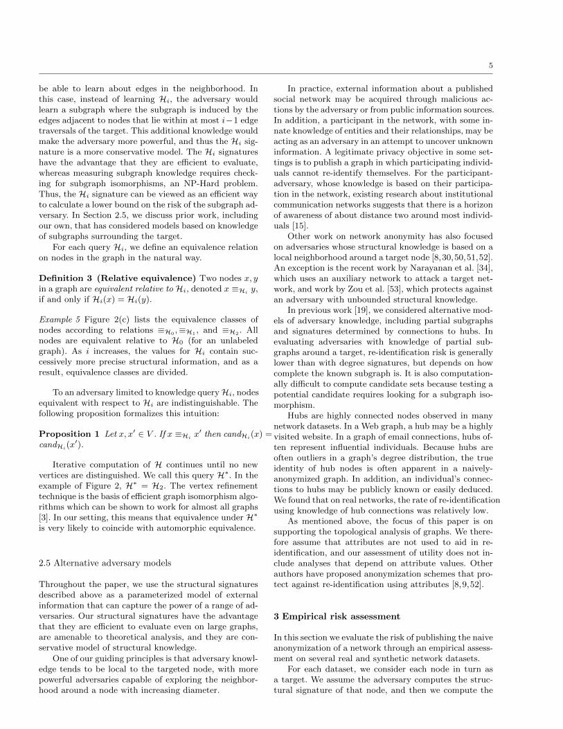
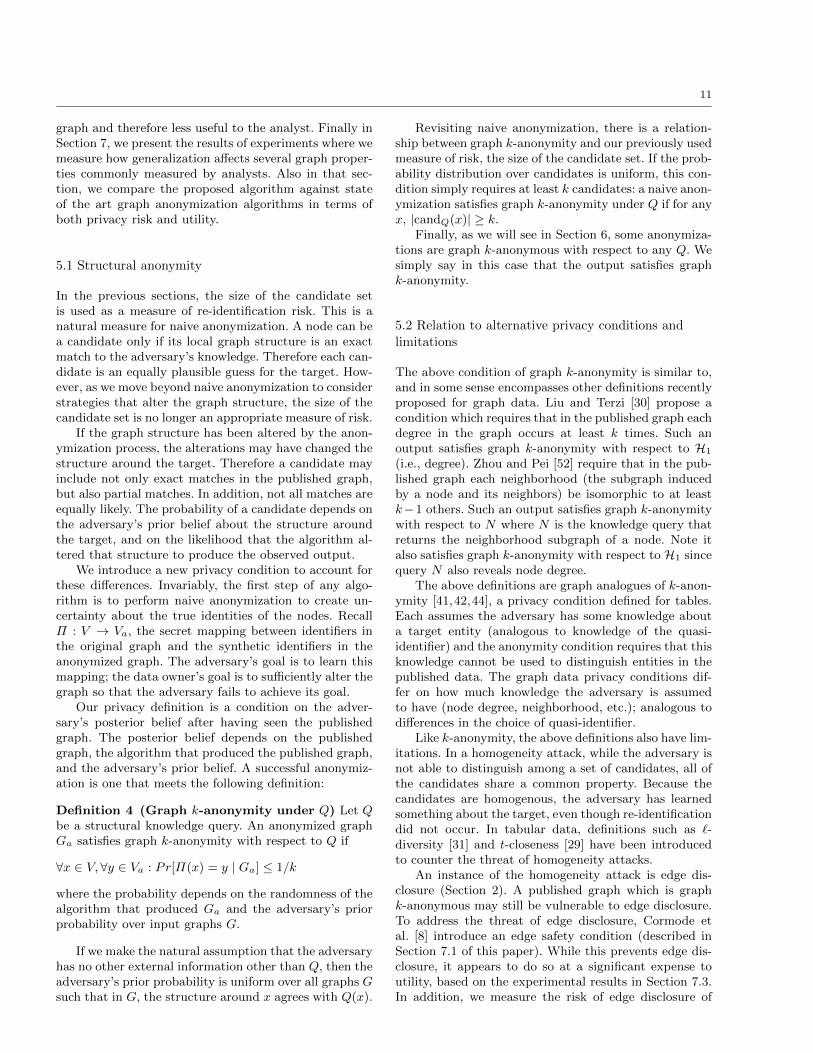
Fig. 2 (a) A sample graph, (b) external information consisting of structural signatures H0,H1 and H2 computed for eachindividual in the graph, (c) the equivalence classes of nodes implied by the structural signatures. For the sample data, ≡H2

,corresponds to automorphic equivalence, ≡A.

because 5 edges are present in Ga between the identi-cal candidate sets candQ(Ed) and candQ(Greg). Theseedge likelihoods should be compared with the prior edgedensity of 2 ∗ 11/8 ∗ 7 = .393.

In Section 3, we measure the threats of edge disclo-sure and node re-identification on real networks.

2.3 Anonymity through structural similarity

Intuitively, nodes that look structurally similar may beindistinguishable to an adversary, in spite of external in-formation. A strong form of structural similarity betweennodes is automorphic equivalence. Two nodes x, y ∈ V

are automorphically equivalent (denoted x ≡A y) if thereexists an isomorphism from the graph onto itself thatmaps x to y.

Example 3 Fred and Harry are automorphically equiva-lent nodes in the graph of Figure 1. Bob and Ed are notautomorphically equivalent: the subgraph around Bob isdifferent from the subgraph around Ed and no isomor-phism proving automorphic equivalence is possible.

Automorphic equivalence induces a partitioning on V

into sets whose members have identical structural prop-erties. It follows that an adversary — even with exhaus-tive knowledge of a target node’s structural position —cannot identify an individual beyond the set of entitiesto which it is automorphically equivalent. We say thattwo such nodes are structurally indistinguishable and ob-serve that nodes in the graph achieve anonymity by being“hidden in the crowd” of its automorphic class members.

Some special graphs have large automorphic equiv-alence classes. For example, in a complete graph, or ina graph which forms a ring, all nodes are automorphi-cally equivalent. But in most graphs we expect to findsmall automorphism classes, likely to be insufficient forprotection against re-identification.

Though automorphism classes may be small in realnetworks, automorphic equivalence is an extremely strongnotion of structural similarity. In order to distinguishtwo nodes in different automorphic equivalence classes,

it may be necessary to use complete information abouttheir positions in the graph. For a weaker adversary withlimited knowledge, nodes that are not automorphicallyequivalent may in fact be indistinguishable. For example,for an adversary who only knows the degree of targetednodes in the graph, Bob and Ed are indistinguishable(even though they are not automorphically equivalent).This motivates the notion of bounded structural knowl-edge we describe next.

2.4 Adversary model based on structural signatures

We now describe the adversary model that we will usethroughout the paper. It is based on a class of knowl-edge queries, of increasing power, which report on thelocal structure of the graph around a node. These queriesare inspired by iterative vertex refinement, a techniqueoriginally developed to efficiently test for the existenceof graph isomorphisms [10]. In Section 2.5, we discussalternative adversary models.

The queries are denoted Hi for i = 0, 1, 2, . . . . Theweakest knowledge query, H0, simply returns the labelof the node. (We consider here unlabeled graphs, so H0

returns on all input nodes.) The queries are successivelymore descriptive: H1(x) returns the degree of x, H2(x)returns the multiset of each neighbors’ degree, and soon. The queries can be defined iteratively, where Hi(x)returns the multiset of values which are the result ofevaluating Hi−1 on the set of nodes adjacent to x:

Hi(x) = Hi−1(z1),Hi−1(z2) . . . ,Hi−1(zm)

where z1 . . . zm are the nodes adjacent to x.

Example 4 Figure 2 contains the same graph from Fig-ure 1 along with the computation of H0, H1, and H2 foreach node. For example: H0 is uniformly . H1(Bob) =, , , , which we abbreviate in the table simply as4. Using this abbreviation, H2(Bob) = 1, 1, 4, 4 whichrepresents Bob’s neighbors’ degrees.

In practice, we might expect that if an adversary canlearn the degrees of the target’s neighbors, he would also

5

be able to learn about edges in the neighborhood. Inthis case, instead of learning Hi, the adversary wouldlearn a subgraph where the subgraph is induced by theedges adjacent to nodes that lie within at most i−1 edgetraversals of the target. This additional knowledge wouldmake the adversary more powerful, and thus the Hi sig-nature is a more conservative model. The Hi signatureshave the advantage that they are efficient to evaluate,whereas measuring subgraph knowledge requires check-ing for subgraph isomorphisms, an NP-Hard problem.Thus, the Hi signature can be viewed as an efficient wayto calculate a lower bound on the risk of the subgraph ad-versary. In Section 2.5, we discuss prior work, includingour own, that has considered models based on knowledgeof subgraphs surrounding the target.

For each query Hi, we define an equivalence relationon nodes in the graph in the natural way.

Definition 3 (Relative equivalence) Two nodes x, yin a graph are equivalent relative to Hi, denoted x ≡Hi y,if and only if Hi(x) = Hi(y).

Example 5 Figure 2(c) lists the equivalence classes ofnodes according to relations ≡H0 ,≡H1 , and ≡H2 . Allnodes are equivalent relative to H0 (for an unlabeledgraph). As i increases, the values for Hi contain suc-cessively more precise structural information, and as aresult, equivalence classes are divided.

To an adversary limited to knowledge queryHi, nodesequivalent with respect to Hi are indistinguishable. Thefollowing proposition formalizes this intuition:

Proposition 1 Let x, x∈ V . If x ≡Hi x

then candHi(x) =candHi(x

).

Iterative computation of H continues until no newvertices are distinguished. We call this query H

∗. In theexample of Figure 2, H∗ = H2. The vertex refinementtechnique is the basis of efficient graph isomorphism algo-rithms which can be shown to work for almost all graphs[3]. In our setting, this means that equivalence under H∗

is very likely to coincide with automorphic equivalence.

2.5 Alternative adversary models

Throughout the paper, we use the structural signaturesdescribed above as a parameterized model of externalinformation that can capture the power of a range of ad-versaries. Our structural signatures have the advantagethat they are efficient to evaluate even on large graphs,are amenable to theoretical analysis, and they are con-servative model of structural knowledge.

One of our guiding principles is that adversary knowl-edge tends to be local to the targeted node, with morepowerful adversaries capable of exploring the neighbor-hood around a node with increasing diameter.

In practice, external information about a publishedsocial network may be acquired through malicious ac-tions by the adversary or from public information sources.In addition, a participant in the network, with some in-nate knowledge of entities and their relationships, may beacting as an adversary in an attempt to uncover unknowninformation. A legitimate privacy objective in some set-tings is to publish a graph in which participating individ-uals cannot re-identify themselves. For the participant-adversary, whose knowledge is based on their participa-tion in the network, existing research about institutionalcommunication networks suggests that there is a horizonof awareness of about distance two around most individ-uals [15].

Other work on network anonymity has also focusedon adversaries whose structural knowledge is based on alocal neighborhood around a target node [8,30,50,51,52].An exception is the recent work by Narayanan et al. [34],which uses an auxiliary network to attack a target net-work, and work by Zou et al. [53], which protects againstan adversary with unbounded structural knowledge.

In previous work [19], we considered alternative mod-els of adversary knowledge, including partial subgraphsand signatures determined by connections to hubs. Inevaluating adversaries with knowledge of partial sub-graphs around a target, re-identification risk is generallylower than with degree signatures, but depends on howcomplete the known subgraph is. It is also computation-ally difficult to compute candidate sets because testing apotential candidate requires looking for a subgraph iso-morphism.

Hubs are highly connected nodes observed in manynetwork datasets. In a Web graph, a hub may be a highlyvisited website. In a graph of email connections, hubs of-ten represent influential individuals. Because hubs areoften outliers in a graph’s degree distribution, the trueidentity of hub nodes is often apparent in a naively-anonymized graph. In addition, an individual’s connec-tions to hubs may be publicly known or easily deduced.We found that on real networks, the rate of re-identificationusing knowledge of hub connections was relatively low.

As mentioned above, the focus of this paper is onsupporting the topological analysis of graphs. We there-fore assume that attributes are not used to aid in re-identification, and our assessment of utility does not in-clude analyses that depend on attribute values. Otherauthors have proposed anonymization schemes that pro-tect against re-identification using attributes [8,9,52].

3 Empirical risk assessment

In this section we evaluate the risk of publishing the naiveanonymization of a network through an empirical assess-ment on several real and synthetic network datasets.

For each dataset, we consider each node in turn asa target. We assume the adversary computes the struc-tural signature of that node, and then we compute the

6

Table 1 Descriptive statistics for the real and synthetic graphs studied.

Statistic Real Datasets Synthetic DatasetsHepTh Enron NetTrace HOT Power-Law Tree Mesh

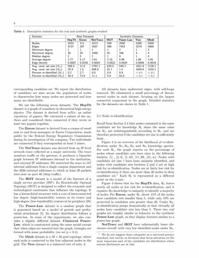
Nodes 2510 111 4213 939 2500 3280 2500Edges 4737 287 5507 988 7453 3279 4900Minimum degree 1 1 1 1 2 1 2Maximum degree 36 20 1656 91 166 4 4Median degree 2 5 1 1 4 1 4Average degree 3.77 5.17 2.61 2.10 5.96 1.99 3.92Edge density 0.0007 0.0235 0.0003 0.0022 0.0024 0.0006 0.0016Avg. cand. set size (H1) 558.5 12.0 2792.1 635.5 549.7 1821.8 2138.1Avg. cand. set size (H2) 25.4 1.5 608.6 81.1 1.4 1659.8 1818.1Percent re-identified (H1) 0.2 2.7 0.5 0.9 0.9 < 0.1 < 0.1Percent re-identified (H2) 40.4 73.9 11.1 5.9 82.5 < 0.1 < 0.1

corresponding candidate set. We report the distributionof candidate set sizes across the population of nodesto characterize how many nodes are protected and howmany are identifiable.

We use the following seven datasets. The HepThdataset is a graph of coauthors in theoretical high-energyphysics. The dataset is derived from arXiv, an onlinerepository of papers. We extracted a subset of the au-thors and considered them connected if they wrote atleast two papers together.

The Enron dataset is derived from a corpus of emailsent to and from managers at Enron Corporation, madepublic by the Federal Energy Regulatory Commissionduring its investigation of the company. Two individualsare connected if they corresponded at least 5 times.

The NetTrace dataset was derived from an IP-levelnetwork trace collected at a major university. The tracemonitors traffic at the gateway; it produces a bipartitegraph between IP addresses internal to the institution,and external IP addresses. We restricted the trace to 187internal addresses from a single campus department andthe 4026 external addresses to which at least 20 packetswere sent on port 80 (http traffic).

The HOT dataset is a model of the Internet of asingle service provider (ISP). Its Heuristically OptimalTopology (HOT) is designed to reflect the economic andtechnological constraints that influence the topology. Ithas a hierarchical structure with a core of interconnectedlow degree (high-bandwidth) routers at its center andhigh-degree (low-bandwidth) routers at its periphery [28].

The Power-Law dataset is a random graph thatis generated based on a model of growth and prefer-ential attachment [5]. Its degree distribution follows apower-law. In some of the experiments, we also con-sider a slightly different dataset, Clustered Power-Law, which is constructed using the same model exceptthat when edges are inserted into the graph, triangles areformed with some probability (we set p = 0.4).

The Mesh dataset is a 50× 50 grid topology, whereeach node is connected to the four adjacent nodes in thegrid. The Tree dataset is a balanced tree of arity 3.

All datasets have undirected edges, with self-loopsremoved. We eliminated a small percentage of discon-nected nodes in each dataset, focusing on the largestconnected component in the graph. Detailed statisticsfor the datasets are shown in Table 1.

3.1 Node re-identification

Recall from Section 2.4 that nodes contained in the samecandidate set for knowledge Hi share the same valuefor Hi, are indistinguishable according to Hi, and aretherefore protected if the candidate set size is sufficientlylarge.

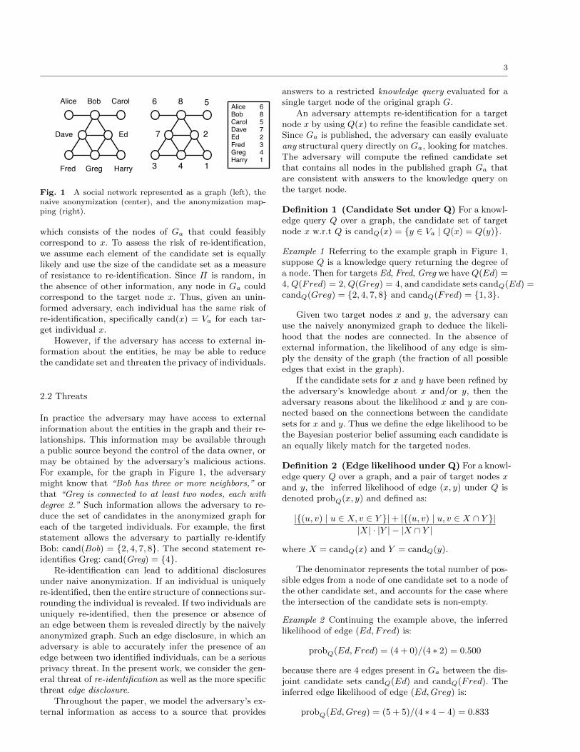
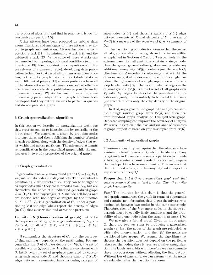
Figure 3 is an overview of the likelihood of re-ident-ification under H1,H2,H3 and H4 knowledge queries.For each Hi, the graph reports on the percentage ofnodes whose candidate sets have sizes in the followingbuckets: [1] , [2, 4], [5, 10], [11, 20], [21,∞]. Nodes withcandidate set size 1 have been uniquely identified, andnodes with candidate sets between 2 and 4 are at highrisk for re-identification. Nodes are at fairly low risk forre-identification if there are more than 20 nodes in theircandidate set.1 Each Hi is represented as a differentpoint on the x-axis.

Figure 3 shows that for the HepTh data, H1 leavesnearly all nodes at low risk for re-identification, and itrequires H3 knowledge to uniquely re-identify a majorityof nodes. For Enron, under H1 about 15% of the nodeshave candidate sets smaller than 5, while only 19% areprotected in candidate sets greater than 20. Under H2,re-identification jumps dramatically so that virtually allnodes have candidate sets less than 5. These two realgraphs are roughly similar in behavior to the syntheticPower-Law graph, as they display features similar to apower-law graph.

NetTrace and HOT have substantially lower dis-closure overall, with very few identified nodes under H1,

1 We do not suggest these categories as a universal privacystandard, but merely as divisions that focus attention on themost important part of the candidate set distribution whereserious disclosures are at risk.

7

Perc

enta

ge o

f nod

es

H1 H2 H3 H4

HepTh

020

4060

8010

0

H1 H2 H3 H4

Enron

020

4060

8010

0

H1 H2 H3 H4

NetTrace

020

4060

8010

0

H1 H2 H3 H4

HOT

020

4060

8010

0

H1 H2 H3 H4

Power−Law

020

4060

8010

0

H1 H2 H3 H4

Tree

020

4060

8010

0

H1 H2 H3 H4

Mesh

> 1910−195−92−41

020

4060

8010

0

Fig. 3 The relationship between candidate set size and structural signature knowledge Hi for i = 1..4 for four real graphsand three synthetic graphs. The trend lines show the percentage of nodes whose candidate sets have sizes in the followingbuckets: [1] (black), [2, 4], [5, 10], [11, 20], [21,∞] (white).

and even H4 knowledge does not uniquely identify morethan 10% of the nodes. For NetTrace, this results fromthe unique bipartite structure of the trace dataset: manynodes in the trace have low degree, as they are uniqueor rare web destinations contacted by only one internalhost. The HOT graph has high structural uniformitybecause it contains many degree one nodes that are con-nected to the same high degree node, and thus struc-turally equivalent to one another.

The synthetic Tree and Mesh graphs display verylow re-identification under all Hi. This is obvious giventhat these graphs have highly uniform structure: the nodesin Mesh have either degree 2 or 4, the nodes in Treehave degree 1, 3 or 4. We include them here for com-pleteness as these graphs are studied in Section 7.

A natural precondition for publication is a very lowpercentage of high-risk nodes under a reasonable assump-tion about adversary knowledge. Three datasets meetthat requirement for H1 (HepTh, NetTrace, HOT).Except for the extreme synthetic graphsTree andMesh,no datasets meet that requirement for H2.

Overall, we observe that there can be significant vari-ance across different datasets in their vulnerability to dif-ferent adversary knowledge. However, across all datasets,the most significant change in re-identification is fromH1 to H2, illustrating the increased power of adversariesthat can explore beyond the target’s immediate neigh-borhood. Re-identification tends to stabilize after H3—more information in the form of H4 does not lead to anobservable increase in re-identification in any dataset. Fi-nally, even though there are many re-identified nodes, asubstantial number of nodes are not uniquely identifiedeven with H4 knowledge.

3.2 Edge disclosure

We measure the risk of edge disclosure possible under ad-versaries with knowledge of degree signatures. Our sam-ple datasets are sparse graphs – their edge densities areall quite low, as reported in Table 1. This means that theexpectation of any particular edge existing in the graphis low.

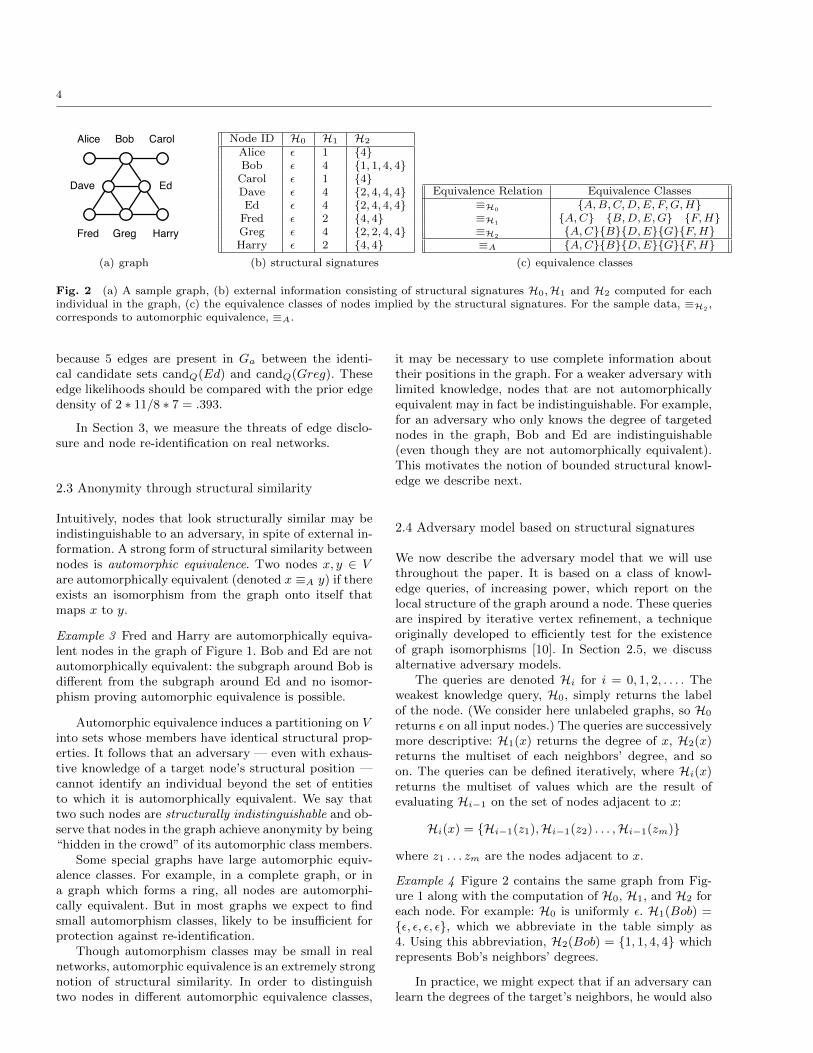
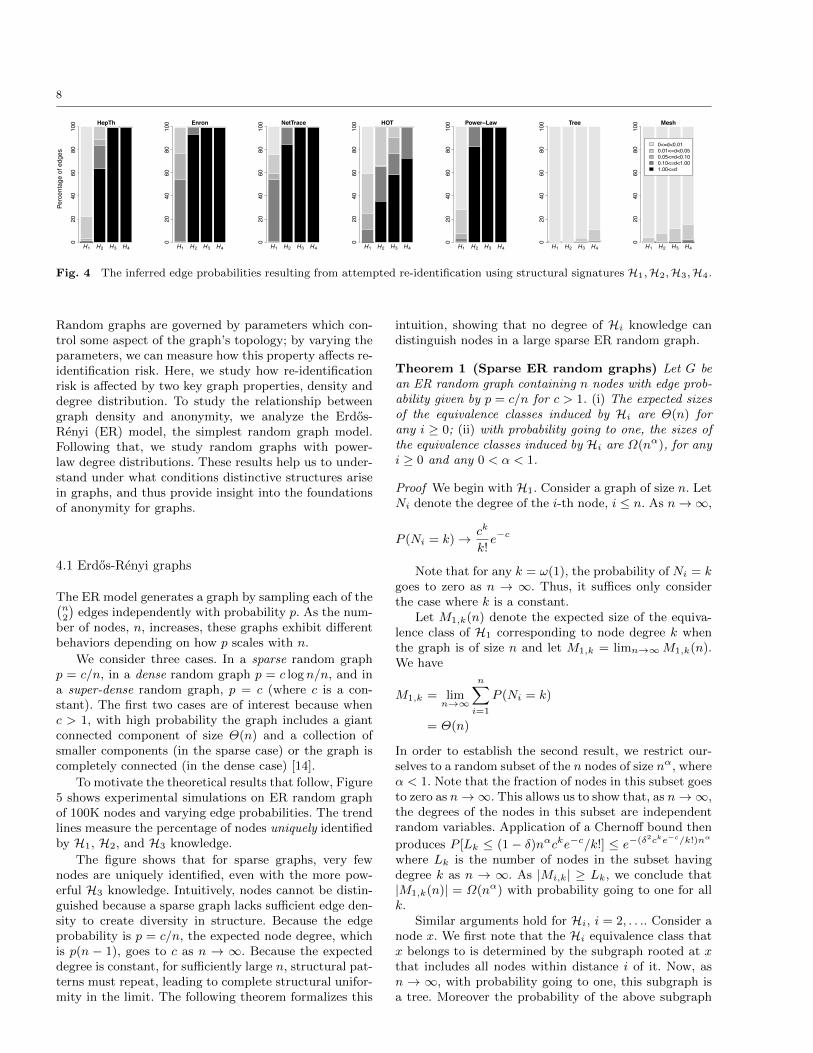
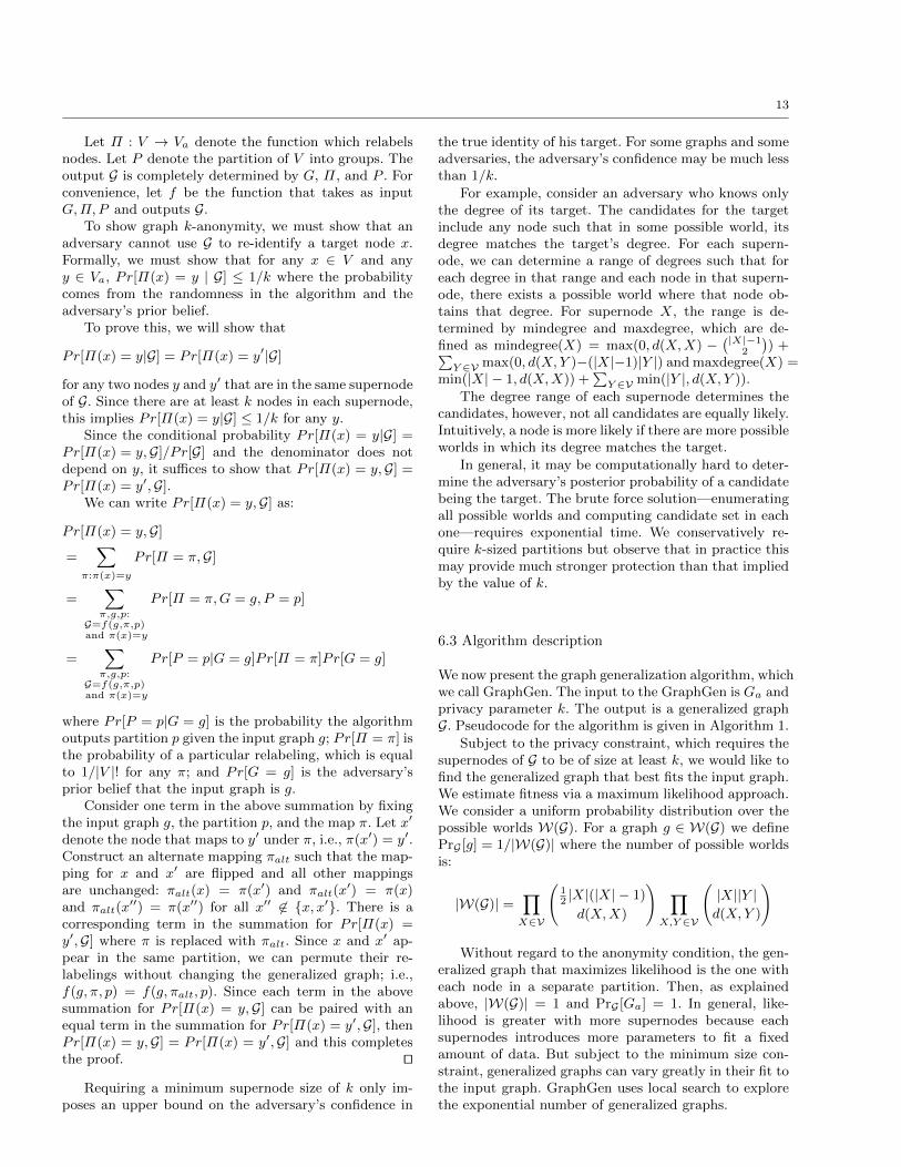
To measure the risk of edge disclosure, we consid-ered each edge present in the original graph and consid-ered its inferred edge likelihood under various Hi. Thatis, we imagine an adversary using Hi knowledge to re-identify the individuals participating in each edge of thetrue graph, and report the inferred edge probability overthe set of all true edges. For each Hi we get a range ofinferred edge probabilities, as illustrated in Figure 4.

The results show that with H1 knowledge alone, therisk of edge disclosure is relatively limited. In the Hep-Th data, 80% of the edges have an inferred edge prob-ability of less than 0.01, which constitutes a small shiftin an adversary’s certainty about the presence of thoseedges. In the Enron and NetTrace data, roughly halfthe edges have inferred probabilities between 0.10 and1, which represent a significant shift in the adversary’sexpectation.

Of much more concern, however, is the fact that withH2 knowledge (or greater) many edges are disclosed withcertainty – the inferred edge probability is 1 for a ma-jority of edges across all datasets. It is also importantto note that even when candidate sets tend to be large(such as in NetTrace and HOT), edges can be disclosedwith high likelihood. In NetTrace and HOT this likelyreflects a hub node with a unique degree connected tomany degree-one nodes. Even though the candidate setof degree one nodes may be large, every node in thatcandidate set is connected to the hub, and density ofconnections between the candidate sets is one, resultingin certain edge disclosure.

4 Theoretical risk assessment

The results of the previous section show that re-identifica-tion risk varies across graphs. We want to understandand explain this variation. In some cases, such as TreeandMesh, the low re-identification risk can be explainedby the regular topology, which makes it hard to distin-guish nodes by their local structure. However, across theother graphs, the reason for diversity in risk is unclear.

In this section, to gain insight into the factors af-fecting re-identification risk, we study random graphs.

8

Perc

enta

ge o

f edg

es

H1 H2 H3 H4

HepTh

020

4060

8010

0

H1 H2 H3 H4

Enron

020

4060

8010

0

H1 H2 H3 H4

NetTrace

020

4060

8010

0

H1 H2 H3 H4

HOT

020

4060

8010

0

H1 H2 H3 H4

Power−Law

020

4060

8010

0

H1 H2 H3 H4

Tree

020

4060

8010

0

H1 H2 H3 H4

Mesh

0<=d<0.010.01<=d<0.050.05<=d<0.100.10<=d<1.001.00<=d

020

4060

8010

0

Fig. 4 The inferred edge probabilities resulting from attempted re-identification using structural signatures H1,H2,H3,H4.

Random graphs are governed by parameters which con-trol some aspect of the graph’s topology; by varying theparameters, we can measure how this property affects re-identification risk. Here, we study how re-identificationrisk is affected by two key graph properties, density anddegree distribution. To study the relationship betweengraph density and anonymity, we analyze the Erdos-Renyi (ER) model, the simplest random graph model.Following that, we study random graphs with power-law degree distributions. These results help us to under-stand under what conditions distinctive structures arisein graphs, and thus provide insight into the foundationsof anonymity for graphs.

4.1 Erdos-Renyi graphs

The ER model generates a graph by sampling each of then2

edges independently with probability p. As the num-

ber of nodes, n, increases, these graphs exhibit differentbehaviors depending on how p scales with n.

We consider three cases. In a sparse random graphp = c/n, in a dense random graph p = c log n/n, and ina super-dense random graph, p = c (where c is a con-stant). The first two cases are of interest because whenc > 1, with high probability the graph includes a giantconnected component of size Θ(n) and a collection ofsmaller components (in the sparse case) or the graph iscompletely connected (in the dense case) [14].

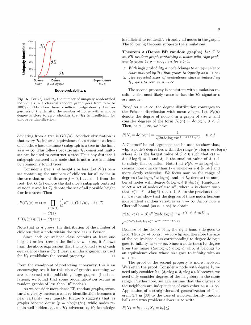
To motivate the theoretical results that follow, Figure5 shows experimental simulations on ER random graphof 100K nodes and varying edge probabilities. The trendlines measure the percentage of nodes uniquely identifiedby H1, H2, and H3 knowledge.

The figure shows that for sparse graphs, very fewnodes are uniquely identified, even with the more pow-erful H3 knowledge. Intuitively, nodes cannot be distin-guished because a sparse graph lacks sufficient edge den-sity to create diversity in structure. Because the edgeprobability is p = c/n, the expected node degree, whichis p(n − 1), goes to c as n → ∞. Because the expecteddegree is constant, for sufficiently large n, structural pat-terns must repeat, leading to complete structural unifor-mity in the limit. The following theorem formalizes this

intuition, showing that no degree of Hi knowledge candistinguish nodes in a large sparse ER random graph.

Theorem 1 (Sparse ER random graphs) Let G bean ER random graph containing n nodes with edge prob-ability given by p = c/n for c > 1. (i) The expected sizesof the equivalence classes induced by Hi are Θ(n) forany i ≥ 0; (ii) with probability going to one, the sizes ofthe equivalence classes induced by Hi are Ω(nα), for anyi ≥ 0 and any 0 < α < 1.

Proof We begin with H1. Consider a graph of size n. LetNi denote the degree of the i-th node, i ≤ n. As n → ∞,

P (Ni = k) →ck

k!e−c

Note that for any k = ω(1), the probability of Ni = k

goes to zero as n → ∞. Thus, it suffices only considerthe case where k is a constant.

Let M1,k(n) denote the expected size of the equiva-lence class of H1 corresponding to node degree k whenthe graph is of size n and let M1,k = limn→∞ M1,k(n).We have

M1,k = limn→∞

n

i=1

P (Ni = k)

= Θ(n)

In order to establish the second result, we restrict our-selves to a random subset of the n nodes of size nα, whereα < 1. Note that the fraction of nodes in this subset goesto zero as n → ∞. This allows us to show that, as n → ∞,the degrees of the nodes in this subset are independentrandom variables. Application of a Chernoff bound then

produces P [Lk ≤ (1 − δ)nαcke−c

/k!] ≤ e−(δ2cke−c/k!)nα

where Lk is the number of nodes in the subset havingdegree k as n → ∞. As |Mi,k| ≥ Lk, we conclude that|M1,k(n)| = Ω(nα) with probability going to one for allk.

Similar arguments hold for Hi, i = 2, . . .. Consider anode x. We first note that the Hi equivalence class thatx belongs to is determined by the subgraph rooted at x

that includes all nodes within distance i of it. Now, asn → ∞, with probability going to one, this subgraph isa tree. Moreover the probability of the above subgraph

9

Sparse

p=c/n

Dense

p = c log(n)/n

H1

H2

H3

0.0

0.2

0.4

0.6

0.8

1.0100%

0%

20%

40%

60%

80%

Super-dense

p = c

Un

iqu

ely

id

en

tifi

ed

Edge probability, p

Fig. 5 For H2 and H3 the number of uniquely re-identifiedindividuals in a classical random graph goes from zero to100% quickly when there is sufficient edge density. But re-gardless of the density, the number of nodes with a uniquedegree is close to zero, showing that H1 is insufficient forunique re-identification.

deviating from a tree is O(1/n). Another observation isthat every Hi induced equivalence class contains at leastone node, whose distance i subgraph is a tree in the limitas n → ∞. This follows because any Hi consistent multi-set can be used to construct a tree. Thus any distance i

subgraph centered at a node that is not a tree is hiddenby commonly found trees.

Consider a tree, t, of height i or less. Let N(t) be aset containing the numbers of children for all nodes inthe tree that are at distance j = 0, 1, . . . , i− 1 from theroot. Let Gi(x) denote the distance i subgraph centeredat node x and let Ti denote the set of all possible heighti or less trees. Then

P (Gi(x) = t) =

k∈N(t)

ck

k!e−c +O(1/n), t ∈ Ti

= Θ(1)

P (Gi(x) /∈ Ti) = O(1/n)

Note that as n grows, the distribution of the number ofchildren that a node within the tree has is Poisson.

Since each equivalence class contains at least oneheight i or less tree in the limit as n → ∞, it followsfrom the above expressions that the expected size of eachequivalence class is Θ(n). Last a similar argument as usedfor H1 establishes the second property.

From the standpoint of protecting anonymity, this is anencouraging result for this class of graphs, assuming weare concerned with publishing large graphs. (In simu-lations, we found that some re-identification occurs inrandom graphs of less than 106 nodes.)

As we consider more dense ER random graphs, struc-tural diversity increases and re-identification becomes anear certainty very quickly. Figure 5 suggests that asgraphs become dense (p = clog(n)/n), while nodes re-main well-hidden against H1 adversaries, H2 knowledge

is sufficient to re-identify virtually all nodes in the graph.The following theorem supports the simulations.

Theorem 2 (Dense ER random graphs) Let G bean ER random graph containing n nodes with edge prob-ability given by p = c log n/n for c > 1.

1. With high probability a node belongs to an equivalenceclass induced by H1 that grows to infinity as n → ∞.

2. The expected sizes of equivalence classes induced byH2 goes to zero as n → ∞.

The second property is consistent with simulation re-sults as the most likely cause is that the H2 signaturesare unique.

Proof As n → ∞, the degree distribution converges tothe Poisson distribution with mean c log n. Let Ni(n)denote the degree of node i in a graph of size n andconsider degrees of the form Ni(n) = δc log n, 0 < δ.Then, as n → ∞, we have

P [Ni = δc log n] =1

√2πδc log nnc(1−δ+δ log δ)

, 0 < δ

A Chernoff bound argument can be used to show that,whp, a node’s degree lies within the range (δ0c log n, δ1c log n)where δ0 is the largest value of δ < 0 such that c(1 −

δ + δ log δ) = 1 and δ1 is the smallest value of δ > 1to satisfy that equation. Note that P [Ni = δc log n] de-creases more quickly than 1/n whenever δ /∈ [δ0, δ1] andmore slowly otherwise. We focus now on the range ofdegrees (δ0c log n, δ1c log n), and let Lδ denote the num-ber of nodes with degree δc log n, δ ∈ [δ0, δ1]. Randomlyselect a set of nodes of size n

α, where α is chosen suchthat, c(1− δ + δ log δ) < α < 1. As in the previous theo-rem, we can show that the degrees of these nodes becomeindependent random variables as n → ∞. Apply now aChernoff bound (as n → ∞) to obtain

P [Lδ < (1− β)nα(2πδc log n)−1n−c(1−δ+δ log δ)] ≤

e−β2nα(2πδc logn)−1n−c(1−δ+δ log δ)/2

Because of the choice of α, the right hand side goes tozero. Thus Lδ → ∞ as n → ∞ whp and therefore the sizeof the equivalence class corresponding to degree δc log ngoes to infinity as n → ∞. Since a node takes its degreefrom the range (δ0c log n, δ1c log n) whp, it belongs toan equivalence class whose size goes to infinity whp asn → ∞.

The proof of the second property is more involved.We sketch the proof. Consider a node with degree k, weneed only consider k ∈ (δ0c log n, δ1c log n). Moreover, weneed only consider degrees of the neighbors in the samerange. Furthermore, we can assume that the degrees ofthe neighbors are independent of each other as n → ∞.Application of a straightforward generalization of The-orem 5.7 in [33] to the case of a non-uniformly randomballs and urns problem allows us to write

P [X1 = k1, . . . , Xs = ks] ≤

10

eδc log n

s

i=1

(piδc log n)ki

ki!e−piδc logn

where pi is the probability that a neighbor selects degreei. Here (X1, . . . , Xs) constitutes the H2 signature of thenode. Now, it is easy to argue using Chernoff bounds thatneighbors only choose degrees clustered around c log n(c log n+ l, l = 0,±1,±2, . . .). Hence

P [X1 = k1, . . . , Xs = ks] ≤

eδc log n

(pc lognδc log n)δc logn

si=1 ki!

e−pc log nδc logn

≤

a((log n)−1/2)δc logn(e−b(logn)−1/2

)δc logn

Where a is a constant. The second inequality followsfrom

i ki > 1. Now consider the expected number of

nodes with signature (k1, . . . , ks), Mk1,...,ks . It is upperbounded by

Mk1,...,ks ≤ an((log n)−1/2)δc logn(e−b(logn)−1/2

)δc logn

which goes to zero as n → ∞.

Lastly, we include a known result for the case of asuper-dense graph where p = 1/2. The following theo-rem, originally due to Babai and Kucera [3] and rephrasedbelow, shows that with high probability every node willbe uniquely identified using H3 knowledge:

Theorem 3 (Super-dense ER random graphs) LetG be an ER random graph on n nodes with edge proba-bility p = 1/2. The probability that there exist two nodesx, y ∈ V such that x ≡H3 y is less than 2−cn for constantvalue c > 0.

This result provides a sufficient condition for uniquere-identification of the entire population in a graph.

Theorems 2 and 3 are disappointing from an anonym-ity perspective. However, most social and communicationnetworks appear to be sparse, and so Theorem 1 may bemore applicable. Furthermore, real networks often haveheavy-tailed degree distributions, which is not the casefor ER graphs. To capture the heavy-tailed degree distri-bution, we also study re-identification risk in power-lawgraphs.

4.2 Power-law graphs

Several graph models have been proposed that exhibitthe heavy-tailed degree distributions often observed inreal networks, including the power law random graph(PLRG) model [1]. In this model, a graph is constructedby first assigning a degree to each node, where the degreeis sampled from a power law distribution. Edges are in-serted by randomly choosing endpoints until every nodehas as many edges as its specified degree. (This can resultin self-loops or multiple edges between a pair of nodes,which are often removed to form a simple graph thatclosely approximates the original degree distribution.)

The PLRG, and other power-law models, generategraphs with constant average degree as the number ofnodes increases. Thus the edge density is low, and despitethe skew in node degree, we find that the structural di-versity is insufficient for re-identification. We state thisformally for PLRG because it is the easiest power-lawgraph model to analyze.

Theorem 4 (Power-law random graphs) Let G bea PLRG on n nodes. With probability going to one, theexpected sizes of the equivalence classes induced by Hi isΘ(n), for any i ≥ 0.

Proof The proof of Theorem 4 proceeds in a similar man-ner to the proof of Theorem 1 except that the Poissondistribution is replaced by P (Ni = k) = ak

−α> 0, k =

0, 1, . . . where a is a constant such that

∞

k=0 P (Ni =k) = 1.

4.3 Discussion

The theoretical results of this section complement theempirical results of the previous section. We see that re-identification risk depends on graph size: the empiricalresults for the 2500 node Power-Law graph show highre-identification risk; however, Theorem 4 shows thatonce a power-law graph is sufficiently large, nodes willbe anonymous.

In fact, the critical factor determining re-identificationrisk in large random graphs is not the degree distribu-tion, but density. Sparse graphs (including power lawgraphs) have low re-identification risk, whereas densegraphs have high re-identification risk. This is an im-portant finding as it shows that even in extremely largegraphs, nodes are not necessarily well hidden. It dependson the topological properties of the graph. This one rea-son why the Hi structural signatures can be a valuabletool for data owners, as they allow them to efficientlyassess re-identification risk even on large graphs.

5 Mitigating re-identification risk

The previous two sections were about risk assessment.The main finding was that there is considerable riskin publishing the naive anonymization of a graph be-cause informed adversaries can use their knowledge to re-identify nodes and in some cases, infer particular edges.

The next three sections are about risk mitigation. Inthis section, we first introduce a new condition, graphk-anonymity, which is a bound on re-identification risk.Then we relate it to other privacy definitions proposed inthe literature. In Section 6, we present an algorithm thatachieves graph k-anonymity by transforming the graphthrough a process called graph generalization. The ben-efit of generalization is reduced risk, but the cost is thatthe generalized graph is an approximation of the original

11

graph and therefore less useful to the analyst. Finally inSection 7, we present the results of experiments where wemeasure how generalization affects several graph proper-ties commonly measured by analysts. Also in that sec-tion, we compare the proposed algorithm against stateof the art graph anonymization algorithms in terms ofboth privacy risk and utility.

5.1 Structural anonymity

In the previous sections, the size of the candidate setis used as a measure of re-identification risk. This is anatural measure for naive anonymization. A node can bea candidate only if its local graph structure is an exactmatch to the adversary’s knowledge. Therefore each can-didate is an equally plausible guess for the target. How-ever, as we move beyond naive anonymization to considerstrategies that alter the graph structure, the size of thecandidate set is no longer an appropriate measure of risk.

If the graph structure has been altered by the anon-ymization process, the alterations may have changed thestructure around the target. Therefore a candidate mayinclude not only exact matches in the published graph,but also partial matches. In addition, not all matches areequally likely. The probability of a candidate depends onthe adversary’s prior belief about the structure aroundthe target, and on the likelihood that the algorithm al-tered that structure to produce the observed output.

We introduce a new privacy condition to account forthese differences. Invariably, the first step of any algo-rithm is to perform naive anonymization to create un-certainty about the true identities of the nodes. RecallΠ : V → Va, the secret mapping between identifiers inthe original graph and the synthetic identifiers in theanonymized graph. The adversary’s goal is to learn thismapping; the data owner’s goal is to sufficiently alter thegraph so that the adversary fails to achieve its goal.

Our privacy definition is a condition on the adver-sary’s posterior belief after having seen the publishedgraph. The posterior belief depends on the publishedgraph, the algorithm that produced the published graph,and the adversary’s prior belief. A successful anonymiz-ation is one that meets the following definition:

Definition 4 (Graph k-anonymity under Q) Let Qbe a structural knowledge query. An anonymized graphGa satisfies graph k-anonymity with respect to Q if

∀x ∈ V, ∀y ∈ Va : Pr[Π(x) = y | Ga] ≤ 1/k

where the probability depends on the randomness of thealgorithm that produced Ga and the adversary’s priorprobability over input graphs G.

If we make the natural assumption that the adversaryhas no other external information other than Q, then theadversary’s prior probability is uniform over all graphs Gsuch that in G, the structure around x agrees with Q(x).

Revisiting naive anonymization, there is a relation-ship between graph k-anonymity and our previously usedmeasure of risk, the size of the candidate set. If the prob-ability distribution over candidates is uniform, this con-dition simply requires at least k candidates: a naive anon-ymization satisfies graph k-anonymity under Q if for anyx, |candQ(x)| ≥ k.

Finally, as we will see in Section 6, some anonymiza-tions are graph k-anonymous with respect to any Q. Wesimply say in this case that the output satisfies graphk-anonymity.

5.2 Relation to alternative privacy conditions and

limitations

The above condition of graph k-anonymity is similar to,and in some sense encompasses other definitions recentlyproposed for graph data. Liu and Terzi [30] propose acondition which requires that in the published graph eachdegree in the graph occurs at least k times. Such anoutput satisfies graph k-anonymity with respect to H1

(i.e., degree). Zhou and Pei [52] require that in the pub-lished graph each neighborhood (the subgraph inducedby a node and its neighbors) be isomorphic to at leastk−1 others. Such an output satisfies graph k-anonymitywith respect to N where N is the knowledge query thatreturns the neighborhood subgraph of a node. Note italso satisfies graph k-anonymity with respect to H1 sincequery N also reveals node degree.

The above definitions are graph analogues of k-anon-ymity [41,42,44], a privacy condition defined for tables.Each assumes the adversary has some knowledge abouta target entity (analogous to knowledge of the quasi-identifier) and the anonymity condition requires that thisknowledge cannot be used to distinguish entities in thepublished data. The graph data privacy conditions dif-fer on how much knowledge the adversary is assumedto have (node degree, neighborhood, etc.); analogous todifferences in the choice of quasi-identifier.

Like k-anonymity, the above definitions also have lim-itations. In a homogeneity attack, while the adversary isnot able to distinguish among a set of candidates, all ofthe candidates share a common property. Because thecandidates are homogenous, the adversary has learnedsomething about the target, even though re-identificationdid not occur. In tabular data, definitions such as -diversity [31] and t-closeness [29] have been introducedto counter the threat of homogeneity attacks.

An instance of the homogeneity attack is edge dis-closure (Section 2). A published graph which is graphk-anonymous may still be vulnerable to edge disclosure.To address the threat of edge disclosure, Cormode etal. [8] introduce an edge safety condition (described inSection 7.1 of this paper). While this prevents edge dis-closure, it appears to do so at a significant expense toutility, based on the experimental results in Section 7.3.In addition, we measure the risk of edge disclosure of

12

our proposed algorithm and find in practice it is low forreasonable k (Section 7.5).

Other attacks have been proposed on tabular dataanonymizations, and analogues of these attacks may ap-ply to graph anonymization. Attacks include the com-position attack [17], the minimality attack [48], and thedeFinetti attack [23]. While some of these attacks canbe remedied by imposing additional conditions (e.g., m-invariance [49] defends against the composition of multi-ple releases of a dynamic table), developing data publi-cation techniques that resist all of them is an open prob-lem, not only for graph data, but for tabular data aswell. Differential privacy [13] ensures protection from allof the above attacks, but it remains unclear whether ef-ficient and accurate data publication is possible underdifferential privacy [12]. As discussed in Section 8, somedifferentially private algorithms for graph data have beendeveloped, but they output answers to particular queriesand do not publish a graph.

6 Graph generalization algorithm

In this section we describe an anonymization techniquethat protects against re-identification by generalizing theinput graph. We generalize a graph by grouping nodesinto partitions, and then publishing the number of nodesin each partition, along with the density of edges that ex-ist within and across partitions. The adversary attemptsre-identification in the generalized graph, while the ana-lyst uses it to study properties of the original graph.

6.1 Graph generalization

To generalize a naively-anonymized graphGa = (Va, Ea),we partition its nodes into disjoint sets. The elements of apartitioning V are subsets of Va. They can be thought ofas supernodes since they contain nodes from Ga, but arethemselves the nodes of a undirected generalized graphG = (V, E). The superedges of E include self-loops andare labeled with non-negative weights by the functiond : E → Z

∗. GV is a generalization of Ga under a parti-tioning V if the edge labels report the density of edges(in Ga) that exist within and across the partitions:

Definition 5 (Generalization of graph) Let V bethe supernodes of Va. G is a generalization of Ga un-der V if, for all X,Y ∈ V, d(X,Y ) = |(x, y) ∈ Ea|

x ∈ X, y ∈ Y |.

G summarizes the structure of Ga, but the accuracyof that summary depends on the partitioning. For anygeneralization G of Ga, we denote by W(G), the set ofpossible worlds (graphs over Va) that are consistent withG. Intuitively, this set of graphs is generated by consid-ering each supernode X and choosing exactly d(X,X)edges between its elements, then considering each pair of

supernodes (X,Y ) and choosing exactly d(X,Y ) edgesbetween elements of X and elements of Y . The size ofW(G) is a measure of the accuracy of G as a summary ofGa.

The partitioning of nodes is chosen so that the gener-alized graph satisfies privacy goals and maximizes utility,as explained in Sections 6.2 and 6.3 respectively. In theextreme case that all partitions contain a single node,then the graph generalization G does not provide anyadditional anonymity: W(G) contains just the graph Ga

(the function d encodes its adjacency matrix). At theother extreme, if all nodes are grouped into a single par-tition, then G consists of a single supernode with a self-loop labeled with |Ea| (the total number of edges in theoriginal graph). W(G) is thus the set of all graphs overVa with |Ea| edges. In this case the generalization pro-vides anonymity, but is unlikely to be useful to the ana-lyst since it reflects only the edge density of the originalgraph.

In studying a generalized graph, the analyst can sam-ple a single random graph from W(G) and then per-form standard graph analysis on this synthetic graph.Repeated sampling can improve the accuracy of analysis.We study in Section 7 the bias and variance of estimatesof graph properties based on graphs sampled from W(G).

6.2 Anonymity of generalized graphs

To ensure anonymity we require that the adversary havea minimum level of uncertainty about the identity of anytarget node in V . We use the size of a partition to providea basic guarantee against re-identification and requirethat each partition have size at least k. This ensures thatthe output satisfies graph k-anonymity with respect toany structural query Q.

Proposition 2 Let G be a generalized graph such thateach supernode X has at least k nodes. Then G satisfiesgraph k-anonymity.

Proof The intuition for this claim is that the general-ized graph summarizes the graph in terms of supernodesand contains no information that allows the adversary todistinguish between two nodes in the same supernode.Therefore, each of the k or more nodes in the same su-pernode must be equally likely candidates and the prob-ability of any one node being the target is at most 1/k.

We now give a formal proof. Given an input graphG, there are two key steps to producing a generalizedgraph: (a) first the nodes of the graph are relabeled, aswith naive anonymization; and then (b) the nodes arepartitioned into groups. We assume the algorithm thatchooses the partition does not depend on the particularlabels on the nodes; since it receives a naive anonymiza-tion, the labels are arbitrary. Therefore we can commutethese two operations without affecting the final output.Without loss of generality, we can assume that the nodesare relabeled after the partition is chosen.

13

Let Π : V → Va denote the function which relabelsnodes. Let P denote the partition of V into groups. Theoutput G is completely determined by G, Π, and P . Forconvenience, let f be the function that takes as inputG,Π, P and outputs G.

To show graph k-anonymity, we must show that anadversary cannot use G to re-identify a target node x.Formally, we must show that for any x ∈ V and anyy ∈ Va, Pr[Π(x) = y | G] ≤ 1/k where the probabilitycomes from the randomness in the algorithm and theadversary’s prior belief.

To prove this, we will show that

Pr[Π(x) = y|G] = Pr[Π(x) = y|G]

for any two nodes y and y that are in the same supernode

of G. Since there are at least k nodes in each supernode,this implies Pr[Π(x) = y|G] ≤ 1/k for any y.

Since the conditional probability Pr[Π(x) = y|G] =Pr[Π(x) = y,G]/Pr[G] and the denominator does notdepend on y, it suffices to show that Pr[Π(x) = y,G] =Pr[Π(x) = y

,G].

We can write Pr[Π(x) = y,G] as:

Pr[Π(x) = y,G]

=

π:π(x)=y

Pr[Π = π,G]

=

π,g,p:G=f(g,π,p)and π(x)=y

Pr[Π = π, G = g, P = p]

=

π,g,p:G=f(g,π,p)and π(x)=y

Pr[P = p|G = g]Pr[Π = π]Pr[G = g]

where Pr[P = p|G = g] is the probability the algorithmoutputs partition p given the input graph g; Pr[Π = π] isthe probability of a particular relabeling, which is equalto 1/|V |! for any π; and Pr[G = g] is the adversary’sprior belief that the input graph is g.

Consider one term in the above summation by fixingthe input graph g, the partition p, and the map π. Let x

denote the node that maps to y under π, i.e., π(x) = y

.Construct an alternate mapping πalt such that the map-ping for x and x

are flipped and all other mappingsare unchanged: πalt(x) = π(x) and πalt(x

) = π(x)and πalt(x

) = π(x) for all x

∈ x, x. There is a

corresponding term in the summation for Pr[Π(x) =y,G] where π is replaced with πalt. Since x and x

ap-pear in the same partition, we can permute their re-labelings without changing the generalized graph; i.e.,f(g,π, p) = f(g,πalt, p). Since each term in the abovesummation for Pr[Π(x) = y,G] can be paired with anequal term in the summation for Pr[Π(x) = y

,G], then

Pr[Π(x) = y,G] = Pr[Π(x) = y,G] and this completes

the proof.

Requiring a minimum supernode size of k only im-poses an upper bound on the adversary’s confidence in

the true identity of his target. For some graphs and someadversaries, the adversary’s confidence may be much lessthan 1/k.

For example, consider an adversary who knows onlythe degree of its target. The candidates for the targetinclude any node such that in some possible world, itsdegree matches the target’s degree. For each supern-ode, we can determine a range of degrees such that foreach degree in that range and each node in that supern-ode, there exists a possible world where that node ob-tains that degree. For supernode X, the range is de-termined by mindegree and maxdegree, which are de-fined as mindegree(X) = max(0, d(X,X) −

|X|−1

2

) +

Y ∈Vmax(0, d(X,Y )−(|X|−1)|Y |) and maxdegree(X) =

min(|X|− 1, d(X,X)) +

Y ∈Vmin(|Y |, d(X,Y )).

The degree range of each supernode determines thecandidates, however, not all candidates are equally likely.Intuitively, a node is more likely if there are more possibleworlds in which its degree matches the target.

In general, it may be computationally hard to deter-mine the adversary’s posterior probability of a candidatebeing the target. The brute force solution—enumeratingall possible worlds and computing candidate set in eachone—requires exponential time. We conservatively re-quire k-sized partitions but observe that in practice thismay provide much stronger protection than that impliedby the value of k.

6.3 Algorithm description

We now present the graph generalization algorithm, whichwe call GraphGen. The input to the GraphGen is Ga andprivacy parameter k. The output is a generalized graphG. Pseudocode for the algorithm is given in Algorithm 1.

Subject to the privacy constraint, which requires thesupernodes of G to be of size at least k, we would like tofind the generalized graph that best fits the input graph.We estimate fitness via a maximum likelihood approach.We consider a uniform probability distribution over thepossible worlds W(G). For a graph g ∈ W(G) we definePrG [g] = 1/|W(G)| where the number of possible worldsis:

|W(G)| =

X∈V

12 |X|(|X|− 1)

d(X,X)

X,Y ∈V

|X||Y |

d(X,Y )

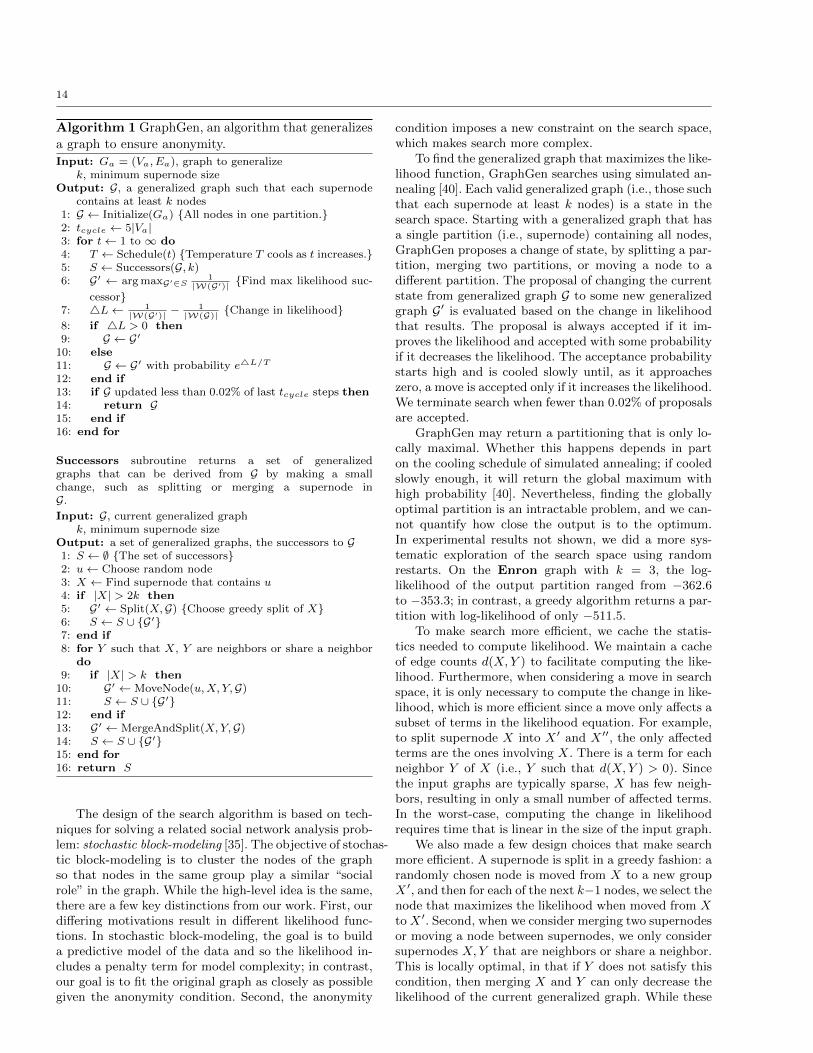
Without regard to the anonymity condition, the gen-eralized graph that maximizes likelihood is the one witheach node in a separate partition. Then, as explainedabove, |W(G)| = 1 and PrG [Ga] = 1. In general, like-lihood is greater with more supernodes because eachsupernodes introduces more parameters to fit a fixedamount of data. But subject to the minimum size con-straint, generalized graphs can vary greatly in their fit tothe input graph. GraphGen uses local search to explorethe exponential number of generalized graphs.

14

Algorithm 1 GraphGen, an algorithm that generalizes

a graph to ensure anonymity.

Input: Ga = (Va, Ea), graph to generalizek, minimum supernode size

Output: G, a generalized graph such that each supernodecontains at least k nodes

1: G ← Initialize(Ga) All nodes in one partition.2: tcycle ← 5|Va|

3: for t ← 1 to ∞ do

4: T ← Schedule(t) Temperature T cools as t increases.5: S ← Successors(G, k)6: G ← argmaxG∈S

1|W(G)|

Find max likelihood suc-

cessor7: L ←

1|W(G)|

−1

|W(G)|Change in likelihood

8: if L > 0 then

9: G ← G

10: else

11: G ← G with probability eL/T

12: end if

13: if G updated less than 0.02% of last tcycle steps then14: return G

15: end if

16: end for

Successors subroutine returns a set of generalizedgraphs that can be derived from G by making a smallchange, such as splitting or merging a supernode inG.

Input: G, current generalized graphk, minimum supernode size

Output: a set of generalized graphs, the successors to G

1: S ← ∅ The set of successors2: u ← Choose random node3: X ← Find supernode that contains u

4: if |X| > 2k then

5: G ← Split(X,G) Choose greedy split of X

6: S ← S ∪ G

7: end if

8: for Y such that X, Y are neighbors or share a neighbordo

9: if |X| > k then

10: G ← MoveNode(u,X, Y,G)11: S ← S ∪ G

12: end if

13: G ← MergeAndSplit(X,Y,G)14: S ← S ∪ G

15: end for

16: return S

The design of the search algorithm is based on tech-niques for solving a related social network analysis prob-lem: stochastic block-modeling [35]. The objective of stochas-tic block-modeling is to cluster the nodes of the graphso that nodes in the same group play a similar “socialrole” in the graph. While the high-level idea is the same,there are a few key distinctions from our work. First, ourdiffering motivations result in different likelihood func-tions. In stochastic block-modeling, the goal is to builda predictive model of the data and so the likelihood in-cludes a penalty term for model complexity; in contrast,our goal is to fit the original graph as closely as possiblegiven the anonymity condition. Second, the anonymity

condition imposes a new constraint on the search space,which makes search more complex.

To find the generalized graph that maximizes the like-lihood function, GraphGen searches using simulated an-nealing [40]. Each valid generalized graph (i.e., those suchthat each supernode at least k nodes) is a state in thesearch space. Starting with a generalized graph that hasa single partition (i.e., supernode) containing all nodes,GraphGen proposes a change of state, by splitting a par-tition, merging two partitions, or moving a node to adifferent partition. The proposal of changing the currentstate from generalized graph G to some new generalizedgraph G

is evaluated based on the change in likelihoodthat results. The proposal is always accepted if it im-proves the likelihood and accepted with some probabilityif it decreases the likelihood. The acceptance probabilitystarts high and is cooled slowly until, as it approacheszero, a move is accepted only if it increases the likelihood.We terminate search when fewer than 0.02% of proposalsare accepted.

GraphGen may return a partitioning that is only lo-cally maximal. Whether this happens depends in parton the cooling schedule of simulated annealing; if cooledslowly enough, it will return the global maximum withhigh probability [40]. Nevertheless, finding the globallyoptimal partition is an intractable problem, and we can-not quantify how close the output is to the optimum.In experimental results not shown, we did a more sys-tematic exploration of the search space using randomrestarts. On the Enron graph with k = 3, the log-likelihood of the output partition ranged from −362.6to −353.3; in contrast, a greedy algorithm returns a par-tition with log-likelihood of only −511.5.

To make search more efficient, we cache the statis-tics needed to compute likelihood. We maintain a cacheof edge counts d(X,Y ) to facilitate computing the like-lihood. Furthermore, when considering a move in searchspace, it is only necessary to compute the change in like-lihood, which is more efficient since a move only affects asubset of terms in the likelihood equation. For example,to split supernode X into X

and X, the only affected

terms are the ones involving X. There is a term for eachneighbor Y of X (i.e., Y such that d(X,Y ) > 0). Sincethe input graphs are typically sparse, X has few neigh-bors, resulting in only a small number of affected terms.In the worst-case, computing the change in likelihoodrequires time that is linear in the size of the input graph.

We also made a few design choices that make searchmore efficient. A supernode is split in a greedy fashion: arandomly chosen node is moved from X to a new groupX

, and then for each of the next k−1 nodes, we select thenode that maximizes the likelihood when moved from X

toX. Second, when we consider merging two supernodes

or moving a node between supernodes, we only considersupernodes X,Y that are neighbors or share a neighbor.This is locally optimal, in that if Y does not satisfy thiscondition, then merging X and Y can only decrease thelikelihood of the current generalized graph. While these

15

choices may exclude the optimal assignment, results indi-cate that they are effective heuristics: they greatly reduceruntime without any decrease in likelihood.

6.4 Capitalizing on limited adversaries

The GraphGen algorithm places each node in a supern-ode with at least k−1 other nodes. This is a conservativeapproach in that it ignores the fact that some nodes maybe structurally well-hidden in the original graph. Nodesmay be automorphically equivalent, or so similar thatonly an adversary with substantial structural knowledgecan distinguish them.

Such a conservative approach has consequences forutility, as graph structure is coarsened to the supernodelevel. We would like an approach that can take advantageof situations in which the adversary is known to havelimited knowledge of graph structure or where the graphscontain many structurally homogenous nodes.

We propose an extension of GraphGen that anonym-izes the graph with respect to a fixed model of adversaryknowledge. The idea is to only anonymize nodes that arevulnerable to re-identification by the given adversary. Byfocusing the anonymization on the vulnerable nodes, itmay be possible to preserve more of the structure of theinput graph.

To incorporate into the algorithm, the first step is toidentify the vulnerable nodes. Given adversary model Qand group size k, a node x is vulnerable if |candQ(x)| <k. For example, if Q is H1, then the only nodes that arevulnerable are the ones whose degree occurs less thank times. Then, the privacy condition on the generalizedgraph is altered so that the only requirement is that if asupernode contains a vulnerable node, then its size mustbe at least k. This means that an invulnerable node canbe placed in a supernode of size 1.

This relaxed privacy condition can be incorporatedinto the search procedure by allowing state changes thatplace invulnerable nodes into supernodes of size less thank. Alternatively, the search can execute as described above,and then supernodes that contain only invulnerable nodescan be replaced with individual supernodes for each in-vulnerable node. (Supernodes containing a mixture ofvulnerable and invulnerable nodes must remain intactto ensure that the vulnerable nodes are protected.) InSection 7.4, we evaluate the latter approach for the H1

and H2 adversary models and measure the improvementin utility that results. We refer to these variants of thealgorithm as GraphGen(H1) and GraphGen(H2) respec-tively. The pseudocode is shown in Algorithm 2.

These alternative anonymization algorithms satisfygraph k-anonymity, but for restricted adversaries.

Corollary 1 The output of GraphGen(H1) satisfies graphk-anonymity with respect to H1. Similarly, the output ofGraphGen(H2) satisfies graph k-anonymity with respectto H2.

Algorithm 2 GraphGen(Q) a modification of Algo-

rithm 1 that protects against Q adversaries.

Input: Ga = (Va, Ea), graph to generalizek, minimum supernode sizeQ knowledge query representing adversary capability

Output: G, a generalized graph that satisfies graph k-anonymity with respect to Q adversaries.

1: S ← u ∈ Va | |candQ(u)| < k Vulnerable nodes2: G ← GraphGen(Ga, k)

Replace supernodes that contain only invulnerablenodes

3: for supernode X in G do

4: if X ∩ S = ∅ then

5: replace X with a supernode for each u ∈ X

6: end if

7: end for

8: return G

This follows from Proposition 2: vulnerable nodes re-main in groups of size k and are therefore protected, andinvulnerable nodes are by definition nodes that the ad-versary cannot re-identify with confidence greater than1/k and therefore it is not necessary to generalize them.

7 Evaluating graph anonymization algorithms

We now present an extensive empirical evaluation of theGraphGen algorithm. We evaluate its utility, compare itto competing techniques, and measure the effectivenessof the utility enhancements proposed in Section 6.4.

The first goal of our experimental evaluation is to as-sess the overall utility of anonymized graphs. We wouldlike to quantify the extent to which the anonymized graphsproduced by GraphGen (and competing techniques) canserve as an accurate approximation of the original pri-vate graph. This is challenging because there are no well-defined metrics to determine the similarity of two graphs.As methods for producing anonymized networks emerge,it is becoming increasingly important to develop a reli-able means for assessing their utility.

Our basic approach is to consider a suite of graphproperties, measure both the original graph and the an-onymized graph and compare the difference. If the an-onymized graph differs from the original for some graphproperty, as it often does, an essential question is whetherthe difference is substantial. To help answer this ques-tion, we include, as a reference point, a random graph ofthe same size and density as the original graph. With re-spect to a particular measure, if the original graph looksvery different from a random graph, then it is useful tocompare the anonymized graph to both the original andthe random graph. The more closely the anonymizedgraph resembles a random graph, the less useful it is.With the GraphGen approach, as group size k increases,the anonymized graph converges on a random graph, andwe can measure the rate of convergence by varying k. Onthe other hand, when the original graph and a random

16

graph appear similar, then the measured property doesnot distinguish the original from a random graph andthus cannot be used to assess whether anonymizationhas preserved the structure of the original graph.

As another yardstick for measuring the loss in util-ity, we evaluate the anonymization algorithms on somecarefully chosen combinations of metrics and syntheticgraphs. Inspired by research in the networking commu-nity [2,45], we consider a few graphs that have a delib-erately engineered structure and then use metrics thatcapture how well this structure is preserved in the anon-ymized graph. For instance, we consider a graph that is atree and measure the extent to which the graph remainstree-like after anonymization. While some of these graphsare unlikely to arise in practice, we find the experimentsgive useful insights into the effect of anonymization andhelp distinguish the behavior of competing techniques. Itis also important given that real technological networksare often highly structured and poorly approximated byrandom graphs [27].

The second goal of the experimental evaluation is tocompare GraphGen against competing techniques. Onechallenge is that the privacy guarantees are not alwayscompatible and so an “apples to apples” comparison isnot straightforward. We attempt to address these dis-parities in privacy guarantees by aligning our techniquewith others so that privacy conditions are comparable(Section 7.4), and by assessing the extent to which ourapproach is vulnerable to attacks (Section 7.5). Despitethe incompatible privacy semantics in some cases, webelieve that comparisons of the algorithms are still use-ful: their strengths and weaknesses are exposed and theirtendency to bias graph measures is revealed.

We note that the goal of publishing an anonymizedgraph is not only to support the specific graph propertiesstudied here. The hope is that the released dataset canbe used for a wide range of investigations determined bygraph topology. If measuring a specific graph property isthe final objective of an analyst, alternative mechanismsfor releasing that property alone should be considered(see discussion of some techniques in Section 8). At anyrate, many analyses cannot be distilled into simple graphproperties, and analysts often require sample datasets torefine their algorithms or interpret results.

7.1 Compared anonymization algorithms

In the first set of experiments, we compare the GraphGenalgorithm described in Section 6 against two other algo-rithms for graph anonymization: the algorithm of Cor-mode et al. [8], denoted BCKS, and the algorithm of Liuand Terzi [30], denoted LT.

The BCKS algorithm is similar to GraphGen in thatit partitions nodes into supernodes and outputs a gen-eralized graph. However, in addition to preventing re-identification, the resulting generalized graph is also guar-anteed to prevent edge disclosure. The privacy condition

ensures that each supernode contains at least k nodesand that edge disclosure is bounded by 1/k. This is doneby requiring that the supernodes satisfy an additionalsafety condition, which states that if two nodes share aneighbor, they must be placed in separate supernodes.The GraphGen algorithm may not prevent edge disclo-sure, especially at small k (see Section 7.5).

Another important difference is that the BCKS al-gorithm’s strategy for choosing supernodes is guided byprivacy concerns—partitions are chosen to ensure lowedge disclosure risk—whereas the strategy of GraphGenis guided by utility. As one might expect, we find thatGraphGen achieves higher utility than BCKS.

It should also be mentioned that the approaches pro-posed by Cormode et al. [8] can handle richer graph datarepresentations, including attributes on nodes and edgesand multiple edge types. The focus of the empirical eval-uation in [8] is on queries that involve attributes andshort path queries. The focus of our study is to measurethe effects of anonymization on graph topology.

The LT algorithm alters the graph through the inser-tion and removal of edges with the goal of making nodesmore structurally uniform. The output is a single graph,not a generalized graph. The algorithm alters the graphuntil each node degree occurs at least k times. This pre-vents re-identification by an adversary whose knowledgeis limited to node degree (i.e., an H1 adversary). It maynot protect against a more powerful adversary (e.g., anH2 adversary). Given the weaker privacy condition, theLT can achieve better utility than BCKS and GraphGenon some measures.

The LT algorithm anonymizes the graph in a two-stage process. First, it finds the minimum change to thedegree sequence such that the privacy condition is satis-fied (each degree must appear at least k times), and thedegree sequence can be realized (the sequence of integersmust satisfy certain graph theoretic constraints). Then,it attempts to transform the original graph into a newgraph that matches this degree sequence.

This second stage is non-trivial and Liu and Terzi [30]consider several alternative algorithms. We implementand compare against SimultaneousSwap. This algorithmis the only one that allows both edge insertions and dele-tions and appears to perform better than some of thealternative approaches proposed in [30] that only allowedge insertions. It is a greedy algorithm that starts witha canonical graph conforming to the anonymized degreesequence and rewires it in such a way that preserves itsdegree sequence but increases the edge overlap with theoriginal graph.

7.2 Overview of experiments

To assess how anonymization impacts utility, we com-pare the original graph to the anonymized output basedon several important graph properties (described below).For each property, we measure it on the original graph

17

and on the anonymized output. For the algorithms thatoutput a single graph, we simply measure the propertyon the output graph. For the algorithms that output ageneralized graph G, we estimate the graph property bydrawing 100 sample graphs from W(G), measuring theproperty of each sample, and then aggregating measure-ments across samples. We report the average and showthe standard deviation using error bars. The error barsgive a sense of how much variation there is among thegraphs in W(G).

If the samples are drawn uniformly from W(G), thismodels an analyst who believes that each graph in W(G)is equiprobable. In these experiments, we perform biasedsampling taking samples uniformly from W(G) subjectto the constraint that the minimum degree is one. Thismakes it more likely that the sampled graph will containa large connected component. All of the input graphscontain a single connected component, and we assumethis fact is revealed to the analyst.

As a baseline, we also measure the property on a sam-ple of 100 random graphs that are the same density asthe original graph. We refer to this baseline as Random.Note this baseline is equivalent to applying a graph gen-eralization algorithm where k = |V |. It has maximumprivacy, but low utility as the only property of the orig-inal revealed is the number of nodes and edges.

We repeat this procedure for each graph and eachsetting of k ∈ 2, 5, 10, 20. Note that while k is a com-mon parameter across the algorithms that controls thesize of the group, the resulting privacy is not the same:while GraphGen and BCKS ensure graph k-anonymity,LT ensures only graph k-anonymity with respect to de-gree (H1).

We report results on the datasets that were describedearlier in Section 3.

7.3 Results

We now present a comparison of the algorithms acrossseveral different graph metrics. Results are presented onemetric at a time. We conclude with a general discussionof the findings in Section 7.3.5.

The results of the experiments are shown in Fig-ures 6-8. Each figure presents the results for a singlegraph metric. The value of the metric for the true graphis shown as a dashed black line. As a reference point,the light gray region shows the value of the metric for arandom graph. It is a region because it depicts a rangeof ±1 standard deviation around the average value overconforming random graphs. Note that for each measure,the scales of the y-axis vary across datasets, so in somecases, while the gap between lines is large, the numericaldifference is quite small.

7.3.1 Paths

We consider several measures related to paths.

Connectedness Each of the anonymization algorithmsmay alter the connectivity of the graph, either dividing aconnected component or merging two components. Eachof the input graphs contains a single connected compo-nent, so we evaluate whether anonymization divides it.Figure 6(a) shows the results. Generally, the anonym-ized graphs contain a single large component, encom-passing about 95% or more of the nodes. However, onthe sparsest graphs—NetTrace, HOT, and Tree—thelargest connected component of the anonymized graphscan contain as few as 70% of the nodes.

Shortest Path Lengths We evaluate how anonymizationaffects path lengths in the graph. We measure the lengthof a shortest path between a pair of randomly chosennodes and compute the average length over 200 randompairs. When the graph contains multiple connected com-ponents, we only sample pairs from the largest connectedcomponent. Since the measure itself is random, there canbe variation due to sampling. We measured this variationand found it small compared to the bias introduced byanonymization and so for presentation purposes we onlyreport the average from a single sample.

Figure 6(b) shows the results. The effect of anonymiz-ation varies greatly across datasets. The greatest changeoccurs on Mesh where path lengths are dramaticallyshortened. In fact, for LT and BCKS, path lengths aremuch closer to those of a random graph than to the orig-inal graph. With the GraphGen graphs, while paths areshortened, they remain considerably longer. GraphGentends to group neighboring nodes together, thus it doesnot introduce as many shortcut paths that can connectdistant regions of the mesh graph.

The distortion of path lengths on Mesh is perhapsnot too surprising. For highly-structured graphs such asa mesh or a lattice, even a small amount of perturbationcan greatly shorten paths by introducing a few shortcutspaths that can connect distant regions of the mesh withonly a few hops [47] and meshes [24].

Generally, across all input graphs, the average pathlengths of an BCKS graph appears to converge to thoseof Random as k increases. Convergence sometimes occursat small k (e.g., Mesh, Enron, HepTh). Convergenceoccurs whether or not path lengths are shorter or longerin random graphs than with the original.

LT produces graphs with shorter path lengths thanthe original graph. It is very accurate on some graphs(NetTrace, Power-Law).

There are no consistent trends for GraphGen. Some-times paths are shorter, sometimes longer. Increasing k

does not have a consistent effect on path lengths. Onsome graphs, particularly Tree, the path lengths can beconsiderably longer than on the original graph.

Tree-like shortest paths We also include a graph theo-retic measure called distortion, which in some sense cap-tures how closely a graph resembles a tree [45]. To com-pute distortion of G, we first construct a spanning tree

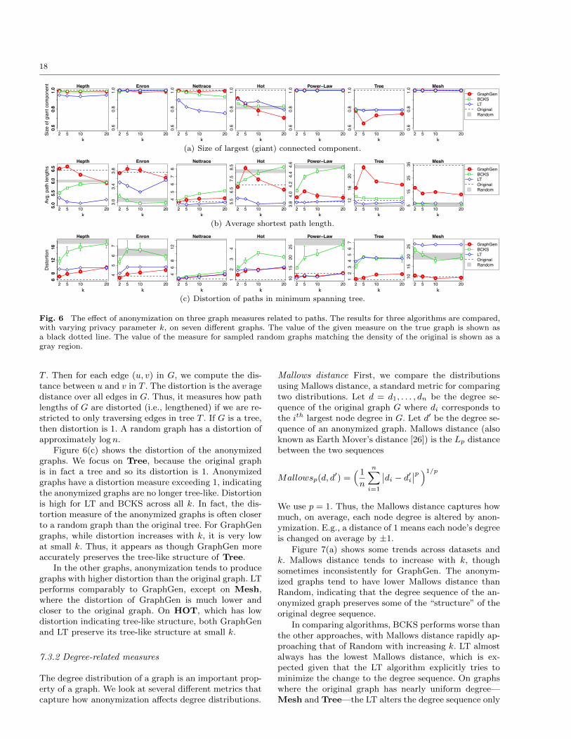
18

Hepth

2 5 10 20

0.6

0.8

1.0

k

0.6

0.8

1.0

Size

of g

iant

com

pone

nt Enron

2 5 10 20

0.6

0.8

1.0

k

Nettrace

2 5 10 20

0.6

0.8

1.0

k

Hot

2 5 10 20

0.6

0.8

1.0

k

Power−Law

2 5 10 20

0.6

0.8

1.0

k

Tree

2 5 10 20

0.6

0.8

1.0

k

Mesh

2 5 10 20

0.6

0.8

1.0

k

GraphGen

BCKSLTOriginalRandom

(a) Size of largest (giant) connected component.

Hepth

2 5 10 205.0

5.5

6.0

6.5

k

5.0

5.5

6.0

6.5

Avg.

pat

h le

ngth

s

Enron

2 5 10 20

3.0

3.4

3.8

k

Nettrace

2 5 10 20

45

67

8

k

Hot

2 5 10 20

5.5

6.5

7.5

8.5

k

Power−Law

2 5 10 20

3.8

4.0

4.2

4.4

4.6

k

Tree

2 5 10 20

1216

20

k

Mesh

2 5 10 20

515

2535

k

GraphGenBCKSLTOriginalRandom

(b) Average shortest path length.

Hepth

2 5 10 20

68

1216

k

68

1216

Distortion

Enron

2 5 10 20

45

67

k

Nettrace

2 5 10 20

46

812

k

Hot

2 5 10 20

12

34

k

Power−Law

2 5 10 2010

1520

25k

Tree

2 5 10 20

12

34

56

7

k

Mesh

2 5 10 20

1015

2025

k

GraphGenBCKSLTOriginalRandom

(c) Distortion of paths in minimum spanning tree.

Fig. 6 The effect of anonymization on three graph measures related to paths. The results for three algorithms are compared,with varying privacy parameter k, on seven different graphs. The value of the given measure on the true graph is shown asa black dotted line. The value of the measure for sampled random graphs matching the density of the original is shown as agray region.

T . Then for each edge (u, v) in G, we compute the dis-tance between u and v in T . The distortion is the averagedistance over all edges in G. Thus, it measures how pathlengths of G are distorted (i.e., lengthened) if we are re-stricted to only traversing edges in tree T . If G is a tree,then distortion is 1. A random graph has a distortion ofapproximately log n.

Figure 6(c) shows the distortion of the anonymizedgraphs. We focus on Tree, because the original graphis in fact a tree and so its distortion is 1. Anonymizedgraphs have a distortion measure exceeding 1, indicatingthe anonymized graphs are no longer tree-like. Distortionis high for LT and BCKS across all k. In fact, the dis-tortion measure of the anonymized graphs is often closerto a random graph than the original tree. For GraphGengraphs, while distortion increases with k, it is very lowat small k. Thus, it appears as though GraphGen moreaccurately preserves the tree-like structure of Tree.

In the other graphs, anonymization tends to producegraphs with higher distortion than the original graph. LTperforms comparably to GraphGen, except on Mesh,where the distortion of GraphGen is much lower andcloser to the original graph. On HOT, which has lowdistortion indicating tree-like structure, both GraphGenand LT preserve its tree-like structure at small k.

7.3.2 Degree-related measures

The degree distribution of a graph is an important prop-erty of a graph. We look at several different metrics thatcapture how anonymization affects degree distributions.

Mallows distance First, we compare the distributionsusing Mallows distance, a standard metric for comparingtwo distributions. Let d = d1, . . . , dn be the degree se-quence of the original graph G where di corresponds tothe i

th largest node degree in G. Let d be the degree se-quence of an anonymized graph. Mallows distance (alsoknown as Earth Mover’s distance [26]) is the Lp distancebetween the two sequences

Mallowsp(d, d) =

1n

n

i=1

di − d

i

p1/p

We use p = 1. Thus, the Mallows distance captures howmuch, on average, each node degree is altered by anon-ymization. E.g., a distance of 1 means each node’s degreeis changed on average by ±1.

Figure 7(a) shows some trends across datasets andk. Mallows distance tends to increase with k, thoughsometimes inconsistently for GraphGen. The anonym-ized graphs tend to have lower Mallows distance thanRandom, indicating that the degree sequence of the an-onymized graph preserves some of the “structure” of theoriginal degree sequence.

In comparing algorithms, BCKS performs worse thanthe other approaches, with Mallows distance rapidly ap-proaching that of Random with increasing k. LT almostalways has the lowest Mallows distance, which is ex-pected given that the LT algorithm explicitly tries tominimize the change to the degree sequence. On graphswhere the original graph has nearly uniform degree—Mesh and Tree—the LT alters the degree sequence only

19

Hepth

2 5 10 20

0.0

0.5

1.0

1.5

k

0.0

0.5

1.0

1.5

Mal

low

dis

tanc

e

Enron

2 5 10 20

0.0

0.4

0.8

1.2

k

Nettrace

2 5 10 20

0.0

1.0

2.0

k

Hot

2 5 10 20

0.0

0.4

0.8

1.2

k

Power−Law

2 5 10 20

0.0

1.0

2.0

k

Tree

2 5 10 20

0.0

0.2

0.4

0.6

k

Mesh

2 5 10 20

0.0

0.5

1.0

1.5

k

GraphGenBCKSLTOriginalRandom

(a) Error in degree distribution, measured by Mallows distance

Hepth

2 5 10 20

1525

35

k

1525

35M

ax d

egre

e

Enron

2 5 10 20

1014

18

k

Nettrace

2 5 10 20

050

015

00

k

Hot

2 5 10 20

2040

6080

k

Power−Law

2 5 10 20

5010

015

0

k

Tree

2 5 10 20

45

67

89

k

Mesh

2 5 10 20

46

810

12

k

GraphGenBCKSLTOriginalRandom

(b) Maximum degree

Hepth

2 5 10 200.5

0.7

0.9

1.1

k

0.5

0.7

0.9

1.1

Deg

ree

dive

rsity

Enron

2 5 10 200.45

0.55

0.65

0.75

k

Nettrace

2 5 10 20

24

68

12

k

Hot

2 5 10 20

0.8

1.2

1.6

2.0

k

Power−Law

2 5 10 200.4

0.8

1.2

k

Tree

2 5 10 20

0.62

0.66

0.70

k

Mesh

2 5 10 20

0.1

0.3

0.5

k

GraphGenBCKSLTOriginalRandom

(c) Diversity of degree distribution

Hepth

2 5 10 20

0.2

0.6

1.0

k

0.2

0.6

1.0

Deg

ree

corre

latio

n

Enron

2 5 10 20

0.2

0.6

1.0

k

Nettrace

2 5 10 20

0.2

0.6

1.0

k

Hot

2 5 10 20

0.2

0.6

1.0

k

Power−Law

2 5 10 20

0.2

0.6

1.0

k

Tree

2 5 10 20

0.2

0.6

1.0

k

Mesh

2 5 10 20

0.2

0.6

1.0

k

GraphGen

BCKSLTOriginalRandom

(d) Degree correlations

Fig. 7 The effect of anonymization on four measures related to the degree distribution. Again, the results for three algorithmsare compared, with varying privacy parameter k, on seven different graphs. The value of the given measure on the true graphis shown as a black dotted line. The value of the measure for sampled random graphs matching the density of the original isshown as a gray region.

slightly to satisfy its privacy condition, resulting in aMallows distance of zero or near zero on these graphs.GraphGen is typically between LT and BCKS.

Maximum degree Figure 7(b) compares the maximumdegree of the original graph with the maximum degreein the anonymized graph. The figure shows a clear trend:as k increases, the maximum degree of each anonymizedgraph converges to the maximum degree of Random. OnMesh and Tree, the max degree is higher in Randomand the max degree of anonymized graphs increase (ex-cept for LT which stays constant). For the other graphs,the max degree of Random is lower than that of theoriginal, sometimes much lower. For example, on Net-Trace, the maximum degree is 1656 but Random hasa max degree of around 10. For all approaches, anon-ymization reduces the max degree by more than half atk = 5. When the maximum degree is an outlier, suchdistortion is in some sense inevitable given the privacycondition: each node degree must be homogenous with atleast k−1 other node degree. Nevertheless, such a signif-icant change in degree suggests that the graph structurehas been significantly altered.

While all approaches converge to Random, their ratesof convergence differ. The max degree of BCKS changesthe most rapidly with k. Surprisingly, on the graphswhere the maximum degree is larger than that of a ran-dom graph, the max degree of GraphGen decreases lessrapidly than LT.

Degree variability In addition to measuring the maxi-mum degree, we also measure the variation in the degreedistribution. The coefficient of variation CV (d) measuresthe diversity of degree distribution d. It is defined asCV (d) = σ(d)/d where d is the average degree andσ(d) =

ni=1(di − d)2/(n − 1). Graphs with homoge-

nous degrees have low CV and graphs with diverse degreesequences, such as power-law graphs, have high CV [2].

Figure 7(c) shows that, like maximum degree, the CV

of anonymized graphs converges towards random graphsas k increases, except on Power-Law, where diversityremains high at k = 20. The comparison between algo-rithms is similar as it is with max degree.

Degree correlations We also measure degree correlations—i.e., the correlation between a node’s degree and the de-grees of its neighbors. It is an important property that

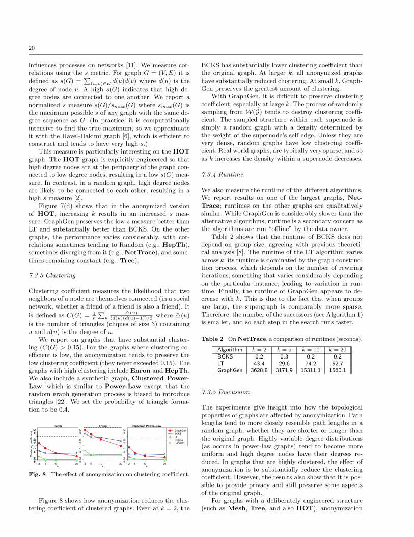
20

influences processes on networks [11]. We measure cor-relations using the s metric. For graph G = (V,E) it isdefined as s(G) =

(u,v)∈E d(u)d(v) where d(u) is the

degree of node u. A high s(G) indicates that high de-gree nodes are connected to one another. We report anormalized s measure s(G)/smax(G) where smax(G) isthe maximum possible s of any graph with the same de-gree sequence as G. (In practice, it is computationallyintensive to find the true maximum, so we approximateit with the Havel-Hakimi graph [6], which is efficient toconstruct and tends to have very high s.)

This measure is particularly interesting on the HOTgraph. The HOT graph is explicitly engineered so thathigh degree nodes are at the periphery of the graph con-nected to low degree nodes, resulting in a low s(G) mea-sure. In contrast, in a random graph, high degree nodesare likely to be connected to each other, resulting in ahigh s measure [2].

Figure 7(d) shows that in the anonymized versionof HOT, increasing k results in an increased s mea-sure. GraphGen preserves the low s measure better thanLT and substantially better than BCKS. On the othergraphs, the performance varies considerably, with cor-relations sometimes tending to Random (e.g., HepTh),sometimes diverging from it (e.g.,NetTrace), and some-times remaining constant (e.g., Tree).

7.3.3 Clustering

Clustering coefficient measures the likelihood that twoneighbors of a node are themselves connected (in a socialnetwork, whether a friend of a friend is also a friend). It

is defined as C(G) = 1n

u

(u)(d(u)(d(u)−1))/2 where (u)

is the number of triangles (cliques of size 3) containingu and d(u) is the degree of u.

We report on graphs that have substantial cluster-ing (C(G) > 0.15). For the graphs where clustering co-efficient is low, the anonymization tends to preserve thelow clustering coefficient (they never exceeded 0.15). Thegraphs with high clustering include Enron and HepTh.We also include a synthetic graph, Clustered Power-Law, which is similar to Power-Law except that therandom graph generation process is biased to introducetriangles [22]. We set the probability of triangle forma-tion to be 0.4.

Hepth

2 5 10 20

0.00

0.10

0.20

0.30

k

0.00

0.10

0.20

0.30

Clu

ster

ing

coef

ficie

nt

Enron

2 5 10 20

0.00

0.10

0.20

0.30

k

Clustered Power−Law

2 5 10 20

0.00

0.10

0.20

0.30

k

GraphGenBCKSLTOriginalRandom

Fig. 8 The effect of anonymization on clustering coefficient.

Figure 8 shows how anonymization reduces the clus-tering coefficient of clustered graphs. Even at k = 2, the

BCKS has substantially lower clustering coefficient thanthe original graph. At larger k, all anonymized graphshave substantially reduced clustering. At small k, Graph-Gen preserves the greatest amount of clustering.

With GraphGen, it is difficult to preserve clusteringcoefficient, especially at large k. The process of randomlysampling from W(G) tends to destroy clustering coeffi-cient. The sampled structure within each supernode issimply a random graph with a density determined bythe weight of the supernode’s self edge. Unless they arevery dense, random graphs have low clustering coeffi-cient. Real world graphs, are typically very sparse, and soas k increases the density within a supernode decreases.

7.3.4 Runtime

We also measure the runtime of the different algorithms.We report results on one of the largest graphs, Net-Trace; runtimes on the other graphs are qualitativelysimilar. While GraphGen is considerably slower than thealternative algorithms, runtime is a secondary concern asthe algorithms are run “offline” by the data owner.

Table 2 shows that the runtime of BCKS does notdepend on group size, agreeing with previous theoreti-cal analysis [8]. The runtime of the LT algorithm variesacross k: its runtime is dominated by the graph construc-tion process, which depends on the number of rewiringiterations, something that varies considerably dependingon the particular instance, leading to variation in run-time. Finally, the runtime of GraphGen appears to de-crease with k. This is due to the fact that when groupsare large, the supergraph is comparably more sparse.Therefore, the number of the successors (see Algorithm 1)is smaller, and so each step in the search runs faster.

Table 2 OnNetTrace, a comparison of runtimes (seconds).

Algorithm k = 2 k = 5 k = 10 k = 20BCKS 0.2 0.3 0.2 0.2LT 43.4 29.6 74.2 52.7GraphGen 3628.8 3171.9 15311.1 1560.1

7.3.5 Discussion

The experiments give insight into how the topologicalproperties of graphs are affected by anonymization. Pathlengths tend to more closely resemble path lengths in arandom graph, whether they are shorter or longer thanthe original graph. Highly variable degree distributions(as occurs in power-law graphs) tend to become moreuniform and high degree nodes have their degrees re-duced. In graphs that are highly clustered, the effect ofanonymization is to substantially reduce the clusteringcoefficient. However, the results also show that it is pos-sible to provide privacy and still preserve some aspectsof the original graph.

For graphs with a deliberately engineered structure(such as Mesh, Tree, and also HOT), anonymization

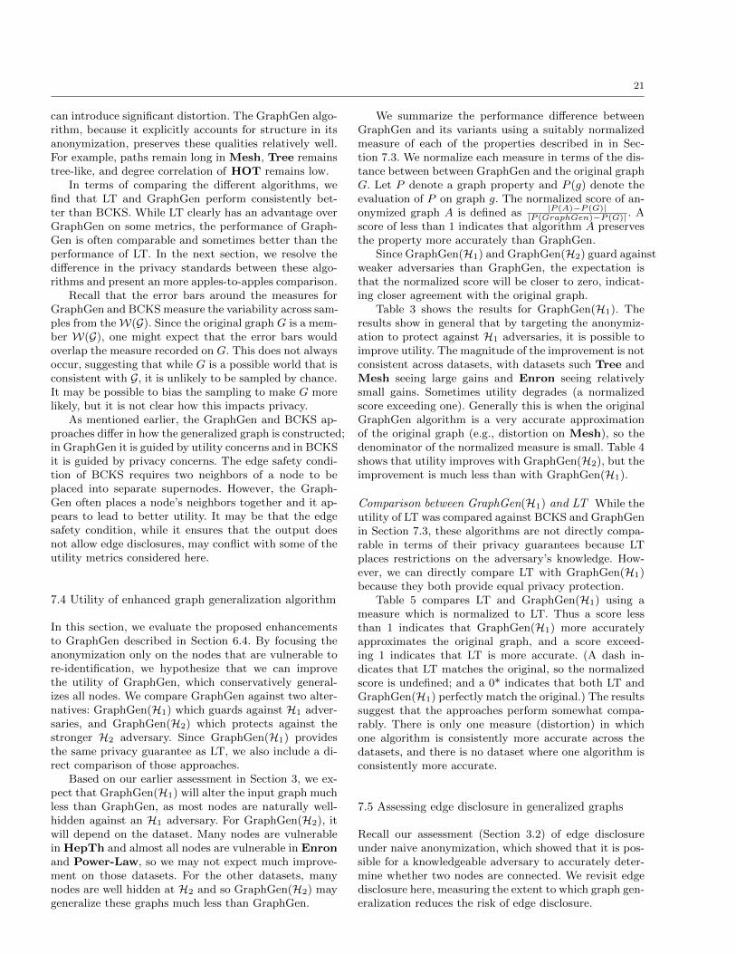
21

can introduce significant distortion. The GraphGen algo-rithm, because it explicitly accounts for structure in itsanonymization, preserves these qualities relatively well.For example, paths remain long in Mesh, Tree remainstree-like, and degree correlation of HOT remains low.

In terms of comparing the different algorithms, wefind that LT and GraphGen perform consistently bet-ter than BCKS. While LT clearly has an advantage overGraphGen on some metrics, the performance of Graph-Gen is often comparable and sometimes better than theperformance of LT. In the next section, we resolve thedifference in the privacy standards between these algo-rithms and present an more apples-to-apples comparison.

Recall that the error bars around the measures forGraphGen and BCKS measure the variability across sam-ples from the W(G). Since the original graph G is a mem-ber W(G), one might expect that the error bars wouldoverlap the measure recorded on G. This does not alwaysoccur, suggesting that while G is a possible world that isconsistent with G, it is unlikely to be sampled by chance.It may be possible to bias the sampling to make G morelikely, but it is not clear how this impacts privacy.

As mentioned earlier, the GraphGen and BCKS ap-proaches differ in how the generalized graph is constructed;in GraphGen it is guided by utility concerns and in BCKSit is guided by privacy concerns. The edge safety condi-tion of BCKS requires two neighbors of a node to beplaced into separate supernodes. However, the Graph-Gen often places a node’s neighbors together and it ap-pears to lead to better utility. It may be that the edgesafety condition, while it ensures that the output doesnot allow edge disclosures, may conflict with some of theutility metrics considered here.

7.4 Utility of enhanced graph generalization algorithm

In this section, we evaluate the proposed enhancementsto GraphGen described in Section 6.4. By focusing theanonymization only on the nodes that are vulnerable tore-identification, we hypothesize that we can improvethe utility of GraphGen, which conservatively general-izes all nodes. We compare GraphGen against two alter-natives: GraphGen(H1) which guards against H1 adver-saries, and GraphGen(H2) which protects against thestronger H2 adversary. Since GraphGen(H1) providesthe same privacy guarantee as LT, we also include a di-rect comparison of those approaches.

Based on our earlier assessment in Section 3, we ex-pect that GraphGen(H1) will alter the input graph muchless than GraphGen, as most nodes are naturally well-hidden against an H1 adversary. For GraphGen(H2), itwill depend on the dataset. Many nodes are vulnerablein HepTh and almost all nodes are vulnerable in Enronand Power-Law, so we may not expect much improve-ment on those datasets. For the other datasets, manynodes are well hidden at H2 and so GraphGen(H2) maygeneralize these graphs much less than GraphGen.

We summarize the performance difference betweenGraphGen and its variants using a suitably normalizedmeasure of each of the properties described in in Sec-tion 7.3. We normalize each measure in terms of the dis-tance between between GraphGen and the original graphG. Let P denote a graph property and P (g) denote theevaluation of P on graph g. The normalized score of an-onymized graph A is defined as |P (A)−P (G)|

|P (GraphGen)−P (G)| . Ascore of less than 1 indicates that algorithm A preservesthe property more accurately than GraphGen.

Since GraphGen(H1) and GraphGen(H2) guard againstweaker adversaries than GraphGen, the expectation isthat the normalized score will be closer to zero, indicat-ing closer agreement with the original graph.

Table 3 shows the results for GraphGen(H1). Theresults show in general that by targeting the anonymiz-ation to protect against H1 adversaries, it is possible toimprove utility. The magnitude of the improvement is notconsistent across datasets, with datasets such Tree andMesh seeing large gains and Enron seeing relativelysmall gains. Sometimes utility degrades (a normalizedscore exceeding one). Generally this is when the originalGraphGen algorithm is a very accurate approximationof the original graph (e.g., distortion on Mesh), so thedenominator of the normalized measure is small. Table 4shows that utility improves with GraphGen(H2), but theimprovement is much less than with GraphGen(H1).

Comparison between GraphGen(H1) and LT While theutility of LT was compared against BCKS and GraphGenin Section 7.3, these algorithms are not directly compa-rable in terms of their privacy guarantees because LTplaces restrictions on the adversary’s knowledge. How-ever, we can directly compare LT with GraphGen(H1)because they both provide equal privacy protection.

Table 5 compares LT and GraphGen(H1) using ameasure which is normalized to LT. Thus a score lessthan 1 indicates that GraphGen(H1) more accuratelyapproximates the original graph, and a score exceed-ing 1 indicates that LT is more accurate. (A dash in-dicates that LT matches the original, so the normalizedscore is undefined; and a 0* indicates that both LT andGraphGen(H1) perfectly match the original.) The resultssuggest that the approaches perform somewhat compa-rably. There is only one measure (distortion) in whichone algorithm is consistently more accurate across thedatasets, and there is no dataset where one algorithm isconsistently more accurate.

7.5 Assessing edge disclosure in generalized graphs

Recall our assessment (Section 3.2) of edge disclosureunder naive anonymization, which showed that it is pos-sible for a knowledgeable adversary to accurately deter-mine whether two nodes are connected. We revisit edgedisclosure here, measuring the extent to which graph gen-eralization reduces the risk of edge disclosure.

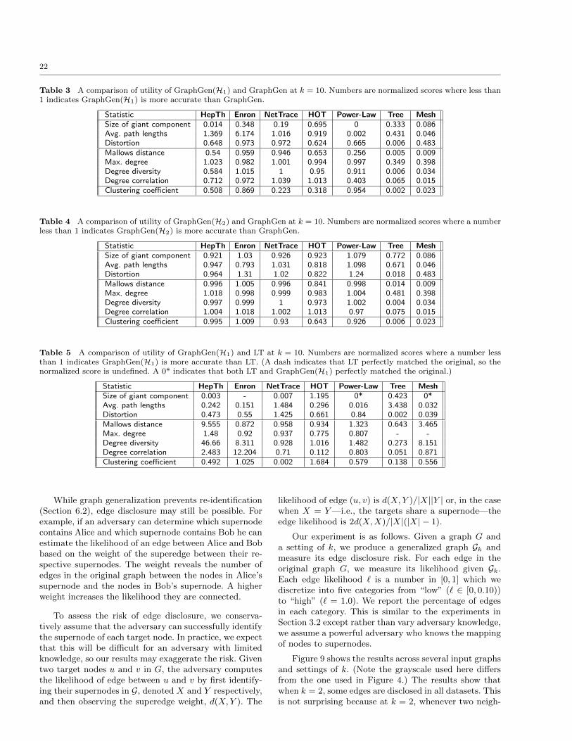
22

Table 3 A comparison of utility of GraphGen(H1) and GraphGen at k = 10. Numbers are normalized scores where less than1 indicates GraphGen(H1) is more accurate than GraphGen.

Statistic HepTh Enron NetTrace HOT Power-Law Tree MeshSize of giant component 0.014 0.348 0.19 0.695 0 0.333 0.086Avg. path lengths 1.369 6.174 1.016 0.919 0.002 0.431 0.046Distortion 0.648 0.973 0.972 0.624 0.665 0.006 0.483Mallows distance 0.54 0.959 0.946 0.653 0.256 0.005 0.009Max. degree 1.023 0.982 1.001 0.994 0.997 0.349 0.398Degree diversity 0.584 1.015 1 0.95 0.911 0.006 0.034Degree correlation 0.712 0.972 1.039 1.013 0.403 0.065 0.015Clustering coefficient 0.508 0.869 0.223 0.318 0.954 0.002 0.023

Table 4 A comparison of utility of GraphGen(H2) and GraphGen at k = 10. Numbers are normalized scores where a numberless than 1 indicates GraphGen(H2) is more accurate than GraphGen.

Statistic HepTh Enron NetTrace HOT Power-Law Tree MeshSize of giant component 0.921 1.03 0.926 0.923 1.079 0.772 0.086Avg. path lengths 0.947 0.793 1.031 0.818 1.098 0.671 0.046Distortion 0.964 1.31 1.02 0.822 1.24 0.018 0.483Mallows distance 0.996 1.005 0.996 0.841 0.998 0.014 0.009Max. degree 1.018 0.998 0.999 0.983 1.004 0.481 0.398Degree diversity 0.997 0.999 1 0.973 1.002 0.004 0.034Degree correlation 1.004 1.018 1.002 1.013 0.97 0.075 0.015Clustering coefficient 0.995 1.009 0.93 0.643 0.926 0.006 0.023

Table 5 A comparison of utility of GraphGen(H1) and LT at k = 10. Numbers are normalized scores where a number lessthan 1 indicates GraphGen(H1) is more accurate than LT. (A dash indicates that LT perfectly matched the original, so thenormalized score is undefined. A 0* indicates that both LT and GraphGen(H1) perfectly matched the original.)

Statistic HepTh Enron NetTrace HOT Power-Law Tree MeshSize of giant component 0.003 - 0.007 1.195 0* 0.423 0*Avg. path lengths 0.242 0.151 1.484 0.296 0.016 3.438 0.032Distortion 0.473 0.55 1.425 0.661 0.84 0.002 0.039Mallows distance 9.555 0.872 0.958 0.934 1.323 0.643 3.465Max. degree 1.48 0.92 0.937 0.775 0.807 - -Degree diversity 46.66 8.311 0.928 1.016 1.482 0.273 8.151Degree correlation 2.483 12.204 0.71 0.112 0.803 0.051 0.871Clustering coefficient 0.492 1.025 0.002 1.684 0.579 0.138 0.556

While graph generalization prevents re-identification(Section 6.2), edge disclosure may still be possible. Forexample, if an adversary can determine which supernodecontains Alice and which supernode contains Bob he canestimate the likelihood of an edge between Alice and Bobbased on the weight of the superedge between their re-spective supernodes. The weight reveals the number ofedges in the original graph between the nodes in Alice’ssupernode and the nodes in Bob’s supernode. A higherweight increases the likelihood they are connected.

To assess the risk of edge disclosure, we conserva-tively assume that the adversary can successfully identifythe supernode of each target node. In practice, we expectthat this will be difficult for an adversary with limitedknowledge, so our results may exaggerate the risk. Giventwo target nodes u and v in G, the adversary computesthe likelihood of edge between u and v by first identify-ing their supernodes in G, denoted X and Y respectively,and then observing the superedge weight, d(X,Y ). The

likelihood of edge (u, v) is d(X,Y )/|X||Y | or, in the casewhen X = Y—i.e., the targets share a supernode—theedge likelihood is 2d(X,X)/|X|(|X|− 1).

Our experiment is as follows. Given a graph G anda setting of k, we produce a generalized graph Gk andmeasure its edge disclosure risk. For each edge in theoriginal graph G, we measure its likelihood given Gk.Each edge likelihood is a number in [0, 1] which wediscretize into five categories from “low” ( ∈ [0, 0.10))to “high” ( = 1.0). We report the percentage of edgesin each category. This is similar to the experiments inSection 3.2 except rather than vary adversary knowledge,we assume a powerful adversary who knows the mappingof nodes to supernodes.

Figure 9 shows the results across several input graphsand settings of k. (Note the grayscale used here differsfrom the one used in Figure 4.) The results show thatwhen k = 2, some edges are disclosed in all datasets. Thisis not surprising because at k = 2, whenever two neigh-

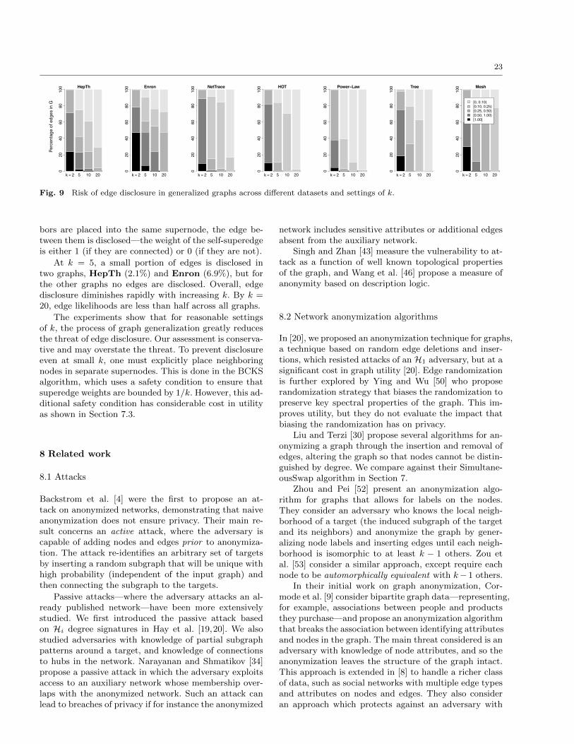
23

Perc

enta

ge o

f edg

es in

G

k = 2 5 10 20

HepTh

020

4060

8010

0

k = 2 5 10 20

Enron

020

4060

8010

0

k = 2 5 10 20

NetTrace

020

4060

8010

0

k = 2 5 10 20

HOT

020

4060

8010

0

k = 2 5 10 20

Power−Law

020

4060

8010

0

k = 2 5 10 20

Tree

020

4060

8010

0

k = 2 5 10 20

Mesh

[0, 0.10)[0.10, 0.25)[0.25, 0.50)[0.50, 1.00)[1.00]

020

4060

8010

0

Fig. 9 Risk of edge disclosure in generalized graphs across different datasets and settings of k.

bors are placed into the same supernode, the edge be-tween them is disclosed—the weight of the self-superedgeis either 1 (if they are connected) or 0 (if they are not).

At k = 5, a small portion of edges is disclosed intwo graphs, HepTh (2.1%) and Enron (6.9%), but forthe other graphs no edges are disclosed. Overall, edgedisclosure diminishes rapidly with increasing k. By k =20, edge likelihoods are less than half across all graphs.

The experiments show that for reasonable settingsof k, the process of graph generalization greatly reducesthe threat of edge disclosure. Our assessment is conserva-tive and may overstate the threat. To prevent disclosureeven at small k, one must explicitly place neighboringnodes in separate supernodes. This is done in the BCKSalgorithm, which uses a safety condition to ensure thatsuperedge weights are bounded by 1/k. However, this ad-ditional safety condition has considerable cost in utilityas shown in Section 7.3.

8 Related work

8.1 Attacks

Backstrom et al. [4] were the first to propose an at-tack on anonymized networks, demonstrating that naiveanonymization does not ensure privacy. Their main re-sult concerns an active attack, where the adversary iscapable of adding nodes and edges prior to anonymiza-tion. The attack re-identifies an arbitrary set of targetsby inserting a random subgraph that will be unique withhigh probability (independent of the input graph) andthen connecting the subgraph to the targets.

Passive attacks—where the adversary attacks an al-ready published network—have been more extensivelystudied. We first introduced the passive attack basedon Hi degree signatures in Hay et al. [19,20]. We alsostudied adversaries with knowledge of partial subgraphpatterns around a target, and knowledge of connectionsto hubs in the network. Narayanan and Shmatikov [34]propose a passive attack in which the adversary exploitsaccess to an auxiliary network whose membership over-laps with the anonymized network. Such an attack canlead to breaches of privacy if for instance the anonymized

network includes sensitive attributes or additional edgesabsent from the auxiliary network.

Singh and Zhan [43] measure the vulnerability to at-tack as a function of well known topological propertiesof the graph, and Wang et al. [46] propose a measure ofanonymity based on description logic.

8.2 Network anonymization algorithms

In [20], we proposed an anonymization technique for graphs,a technique based on random edge deletions and inser-tions, which resisted attacks of an H1 adversary, but at asignificant cost in graph utility [20]. Edge randomizationis further explored by Ying and Wu [50] who proposerandomization strategy that biases the randomization topreserve key spectral properties of the graph. This im-proves utility, but they do not evaluate the impact thatbiasing the randomization has on privacy.

Liu and Terzi [30] propose several algorithms for an-onymizing a graph through the insertion and removal ofedges, altering the graph so that nodes cannot be distin-guished by degree. We compare against their Simultane-ousSwap algorithm in Section 7.

Zhou and Pei [52] present an anonymization algo-rithm for graphs that allows for labels on the nodes.They consider an adversary who knows the local neigh-borhood of a target (the induced subgraph of the targetand its neighbors) and anonymize the graph by gener-alizing node labels and inserting edges until each neigh-borhood is isomorphic to at least k − 1 others. Zou etal. [53] consider a similar approach, except require eachnode to be automorphically equivalent with k− 1 others.

In their initial work on graph anonymization, Cor-mode et al. [9] consider bipartite graph data—representing,for example, associations between people and productsthey purchase—and propose an anonymization algorithmthat breaks the association between identifying attributesand nodes in the graph. The main threat considered is anadversary with knowledge of node attributes, and so theanonymization leaves the structure of the graph intact.This approach is extended in [8] to handle a richer classof data, such as social networks with multiple edge typesand attributes on nodes and edges. They also consideran approach which protects against an adversary with

24

knowledge of graph structure. They propose a partition-ing based approach that we compare against in Section 7.

Zheleva et al. [51] consider graphs with labeled edgesand an adversary with a predictive model for edges andknowledge of constraints on connections in the graph; thegoal of anonymization is to prevent accurate predictionof a class of sensitive edges. The data model, threatsconsidered, and adversary capabilities differ significantlyfrom those treated here.

Rastogi et al. [39] present a mechanism for tables thathas a natural interpretation for graphs. They randomlyremove a fraction of original edges and randomly add afraction of new edges. The resulting table is released inits entirety. They show that the parameters of the ran-dom process can be chosen to ensure strong protectionagainst edge disclosure while allowing a class of countingqueries to estimated accurately. Unfortunately it doesnot address queries that require joins on the edge table,which are crucial to network analysis.

8.3 Query answering approaches

Dwork et al. [13] introduce a strong notion of privacycalled differential privacy and present an interactive algo-rithm – where users pose queries and the data owner re-turns randomly perturbed answers – that achieves strongprivacy guarantees and can guarantee high utility forsome queries. Differential privacy has been an area ofactive research (for a survey, see Dwork [12]). The pri-vacy definition extends naturally to data publication, butmost work considers interactive approaches.

Some work has considered how differential privacycan be applied to network data [13,18,36,38]. The properinterpretation of differential privacy for networks is notimmediate, as the sensitive entity could be considered anedge, a set of edges, or a node along with its edges [18].

Under node-differential privacy, a node and all of itsincident edges are protected; however, with such a rig-orous privacy standard, basic network properties suchas degree distribution cannot be accurately estimated.Under edge-differential privacy, which prevents the dis-closure of individual edges, the degree distribution [18,21] and other network analyses have low sensitivity andcan be answered accurately [13].

However, even under edge-differential privacy, somecommon network analyses have high sensitivity and can-not be answered accurately. For example, measures oftransitivity have O(n) sensitivity, rendering noisy esti-mates useless. Nissim et al. [36] propose a relaxationof differential privacy and provide algorithms for queryanswering where the amount of noise depends on theparticular input database. Among other application, thistechnique can be used to accurately estimate transitivityon some graphs. Rastogi et al. [38] propose an alterna-tive weakening of differential privacy for queries involvingjoins on a relationship table, allowing transitivity to be

estimated accurately along with a more general class ofsubgraph counting queries.

8.4 Other graph privacy work

The anonymization of existing networks is not the onlyprivacy problem that arises with network data. Frikkenand Golle [16] designed a protocol for privately assem-bling a graph that is distributed among a large num-ber of parties. The output of the protocol is a naively-anonymized graph. Korolova et al. [25] consider an ad-versary who tries to re-assemble the graph from a set ofviews of local neighborhoods (obtained, for example, bybreaking into user accounts of an online social network).

9 Conclusion

We have focused on what we believe to be one of themost basic and distinctive challenges for protecting pri-vacy in network datasets—understanding the extent towhich graph structure acts as an identifier. We have for-malized adversary knowledge and evaluated their impacton real and synthetic networks as well as models of ran-dom graphs. We proposed anonymizing a graph by gen-eralizing it: partitioning the nodes and summarizing thegraph at the partition level. We show that a wide rangeof important graph analyses can be performed accuratelyon the generalized graphs published. An important areafor future investigation is to develop bounds on the dis-tortion introduced by anonymization. Analytical boundscould be developed through analysis of the generalizedgraphs, or empirical bounds could inferred through care-ful sampling of the possible worlds implied by the gen-eralized graphs. We also hope to investigate techniquesthat will safely permit the analyst to sample higher qual-ity representatives from the set of possible worlds, forexample, by biasing sampling towards the true graph.

10 Acknowledgments

Hay and Jensen were supported by the Air Force Re-search Laboratory and the Intelligence Advanced Re-search Projects Activity, under agreement number FA8750-07-2-0158. Hay, Miklau, Li, and Towsley were supportedby NSF CNS 0627642. The U.S. Government is autho-rized to reproduce and distribute reprints for Govern-mental purposes notwithstanding any copyright notationthereon. The views and conclusion contained herein arethose of the authors and should not be interpreted asnecessarily representing the official policies or endorse-ments, either expressed or implied, of the Air Force Re-search Laboratory and the Intelligence Advanced Re-search Projects Activity, or the U.S. Government.

25

References

1. W. Aiello, F. R. K. Chung, and L. Lu. A random graphmodel for massive graphs. In Proceedings of the Thirty-

second Annual ACM Symposium on Theory of Comput-

ing, pages 171–180, Portland, OR, May 2000. ACM Press,New York, NY.

2. D. L. Alderson and L. Li. Diversity of graphs with highlyvariable connectivity. Physical Review E, 75(4):046102,Apr 2007.

3. L. Babai and L. Kucera. Canonical labelling of graphs inlinear average time. In Proceedings of the Twentieth An-

nual Symposium on Foundations of Computer Science,pages 39–46, San Juan, Puerto Rico, October 1979. IEEEComputer Society.

4. L. Backstrom, C. Dwork, and J. M. Kleinberg. Whereforeart thou R3579X? Anonymized social networks, hiddenpatterns and structural steganography. In Proceedings

of the Sixteenth International World Wide Web Con-

ference, pages 181–190, Banff, AB, Canada, 2007. ACMPress, New York, NY.

5. A.-L. Barabasi and R. Albert. Emergence of scaling inrandom networks. Science, 286(5439):509–512, October1999.

6. J. Blitzstein and P. Diaconis. A sequential importancesampling algorithm for generating random graphs withprescribed degrees. Unpublished, 2006.

7. W. W. Cohen. Enron email dataset.http://www.cs.cmu.edu/˜enron/, 2005.

8. G. Cormode, D. Srivastava, S. Bhagat, and B. Krish-namurthy. Class-based graph anonymization for socialnetwork data. Proceedings of the VLDB Endowment,2(1):766–777, 2009.

9. G. Cormode, D. Srivastava, T. Yu, and Q. Zhang. Anon-ymizing bipartite graph data using safe groupings. Pro-

ceedings of the VLDB Endowment, 1(1):833–844, 2008.10. D. G. Corneil and C. C. Gotlieb. An efficient algorithm

for graph isomorphism. Journal of the ACM, 17:51–64,January 1970.

11. L. Costa, F. Rodrigues, G. Travieso, and P. Boas. Char-acterization of complex networks: A survey of measure-ments. Advances in Physics, 56(1):167–242, 2007.

12. C. Dwork. Differential privacy: A survey of results. InProceedings of the Theory and Applications of Models

of Computation Fifth International Conference, number4978 in Lecture Notes in Computer Science, pages 1–19,Xi’an, China, April 25–29, 2008. Springer.

13. C. Dwork, F. McSherry, K. Nissim, and A. Smith. Cal-ibrating noise to sensitivity in private data analysis. InProceedings of the Third Theory of Cryptography Con-

ference, number 3876 in Lecture Notes in Computer Sci-ence, pages 265–284, New York, NY, March 4–7, 2006.Springer.

14. P. Erdos and A. Renyi. On the evolution of randomgraphs. Bulletin of the Institute of International Statis-

tics, 38:343–347, 1961.15. N. Friedkin. Horizons of observability and limits of infor-

mal control in organizations. Social Forces, 62(1):54–77,1983.

16. K. B. Frikken and P. Golle. Private social network anal-ysis: How to assemble pieces of a graph privately. InProceedings of the ACM Workshop on Privacy in the

Electronic Society, pages 89–98, Alexandria, VA, Octo-ber 30 2006. ACM Press.

17. S. R. Ganta, S. P. Kasiviswanathan, and A. Smith. Com-position attacks and auxiliary information in data pri-vacy. In Proceedings of the Fourteenth ACM SIGKDD

International Conference on Knowledge Discovery and

Data Mining, pages 265–273, New York, NY, USA, 2008.ACM.

18. M. Hay, C. Li, G. Miklau, and D. Jensen. Accurate es-timation of the degree distribution of private networks.In Proceedings of the IEEE International Conference on

Data Mining, pages 169–178, Los Alamitos, CA, USA,2009. IEEE Computer Society.

19. M. Hay, G. Miklau, D. D. Jensen, D. F. Towsley, andP. Weis. Resisting structural re-identification in anon-ymized social networks. Proceedings of the VLDB En-

dowment, 1(1):102–114, August 2008.20. M. Hay, G. Miklau, D. D. Jensen, P. Weis, and S. Sri-

vastava. Anonymizing social networks. Technical ReportUM-CS-2007-19, Department of Computer Science, Uni-versity of Massachusetts, Amherst, MA, 2007.

21. M. Hay, V. Rastogi, G. Miklau, and D. Suciu. Boostingthe accuracy of differentially-private histograms throughconsistency. Proceedings of the VLDB Endowment,3(1):1021–1032, September 2010.

22. P. Holme and B. J. Kim. Growing scale-free net-works with tunable clustering. Physical Review E,65(2):026107, Jan 2002.

23. D. Kifer. Attacks on privacy and de Finetti’s theorem.In Proceedings of the Thirty-fifth SIGMOD International

Conference on Management of Data, pages 127–138, NewYork, NY, USA, 2009. ACM.

24. J. M. Kleinberg. Navigation in a small world. Nature,406(6798):845, August 2000.

25. A. Korolova, R. Motwani, S. U. Nabar, and Y. Xu. Linkprivacy in social networks. In Proceedings of the Seven-

teenth ACM Conference on Information and Knowledge

Management, pages 289–298, Napa Valley, CA, October26–30, 2008. ACM Press.

26. E. Levina and P. Bickel. The earth mover’s distance is themallows distance: some insights from statistics. In Pro-

ceedings of the Eighth IEEE International Conference on

Computer Vision, volume 2, pages 251–256, 2001.27. L. Li, D. Alderson, J. Doyle, and W. Willinger. Towards

a theory of scale-free graphs: Definition, properties, andimplications. Internet Mathematics, 2(4):431–523, 2005.

28. L. Li, D. Alderson, W. Willinger, and J. Doyle. Afirst-principles approach to understanding the internet’srouter-level topology. In Proceedings of the 2004 Con-

ference on Applications, technologies, architectures, and

protocols for computer communications, pages 3–14, NewYork, NY, USA, 2004. ACM.

29. N. Li, T. Li, and S. Venkatasubramanian. t-closeness:Privacy beyond k-anonymity and -diversity. In Pro-

ceedings of the Twenty-third International Conference

on Data Engineering, pages 106–115, Istanbul, Turkey,April 2007. IEEE Computer Society.

30. K. Liu and E. Terzi. Towards identity anonymizationon graphs. In Proceedings of the ACM SIGMOD In-

ternational Conference on Management of Data, pages93–106, Vancouver, BC, June 10–12, 2008. ACM Press,New York, NY.

31. A. Machanavajjhala, J. Gehrke, D. Kifer, and M. Venki-tasubramaniam. -diversity: Privacy beyond k-anonymity. In Proceedings of the Twenty-second Inter-

national Conference on Data Engineering, page 24, At-lanta, GA, April 2006. IEEE Computer Society.

32. D. J. Martin, D. Kifer, A. Machanavajjhala, J. Gehrke,and J. Y. Halpern. Worst-case background knowledgefor privacy-preserving data publishing. In Proceedings of

the Twenty-third International Conference on Data En-

gineering, pages 126–135, Istanbul, Turkey, April 2007.IEEE Computer Society.

26

33. M. Mitzenmacher and E. Upfal. Probability and comput-

ing: Randomized algorithms and probabilistic analysis.Cambridge University Press, 2005.

34. A. Narayanan and V. Shmatikov. De-anonymizing socialnetworks. In Proceedings of the IEEE Symposium on

Security and Privacy, pages 173–187, Oakland, CA, May17–20 2009. IEEE Computer Society.

35. M. E. J. Newman. The structure and function of complexnetworks. SIAM Review, 45(2):167–256, 2003.

36. K. Nissim, S. Raskhodnikova, and A. Smith. Smoothsensitivity and sampling in private data analysis. In Pro-

ceedings of the Thirty-ninth Annual ACM Symposium on

Theory of Computing, pages 75–84, San Diego, CA, June11–13, 2007. ACM Press, New York, NY.

37. J. J. Potterat, L. Phillips-Plummer, S. Q. Muth, R. B.Rothenberg, D. E. Woodhouse, T. S. Maldonado-Long,H. P. Zimmerman, and J. B. Muth. Risk network struc-ture in the early epidemic phase of HIV transmissionin Colorado Springs. Sexually Transmitted Infections,78(Suppl. 1):i159–i163, 2002.

38. V. Rastogi, M. Hay, G. Miklau, and D. Suciu. Rela-tionship privacy: Output perturbation for queries withjoins. In Proceedings of the Twenty-Eighth ACM

SIGACT-SIGMOD-SIGART Symposium on Principles

of Database Systems, pages 107–116, Providence, RI,June 29–July 2, 2009. ACM Press.

39. V. Rastogi, S. Hong, and D. Suciu. The boundary be-tween privacy and utility in data publishing. In Pro-

ceedings of the Thirty-third International Conference on

Very Large Data Bases, pages 531–542, Vienna, Austria,September 2007. ACM Press, New York, NY.

40. S. J. Russell and P. Norvig. Artificial Intelligence: A

Modern Approach. Prentice Hall, Upper Saddle River,NJ, 2nd edition, 2003.

41. P. Samarati. Protecting respondents’ privacy in micro-data release. IEEE Transactions on Knowledge and Data

Engineering, 13(6):1010–1027, November 2001.42. P. Samarati and L. Sweeney. Protecting privacy when

disclosing information: k-anonymity and its enforcementthrough generalization and suppression. Technical Re-port SRI-CSL-98-04, Computer Science Laboratory, SRIInternational, 1998.

43. L. Singh and J. Zhan. Measuring topological anonym-ity in social networks. In Proceedings of the IEEE In-

ternational Conference on Granular Computing, pages770–770, November 2007.

44. L. Sweeney. K-anonymity: A model for protecting pri-vacy. International Journal of Uncertainty, Fuzziness

and Knowledge-Based Systems, 10(5):557–570, 2002.45. H. Tangmunarunkit, R. Govindan, S. Jamin, S. Shenker,

and W. Willinger. Network topology generators: degree-based vs. structural. In Proceedings of the 2002 con-

ference on Applications, technologies, architectures, and

protocols for computer communications, pages 147–159,New York, NY, USA, 2002. ACM.

46. D.-W. Wang, C.-J. Liau, and T. sheng Hsu. Privacy pro-tection in social network data disclosure based on granu-lar computing. In Proceedings of the IEEE International

Conference on Fuzzy Systems, pages 997–1003, 2006.47. D. J. Watts and S. H. Strogatz. Collective dynamics of

‘small-world’ networks. Nature, 393(6684):409–410, June1998.

48. R. C.-W. Wong, A. W.-C. Fu, K. Wang, and J. Pei.Minimality attack in privacy preserving data publishing.In Proceedings of the 33rd International Conference on

Very Large Data Bases, pages 543–554. VLDB Endow-ment, 2007.

49. X. Xiao and Y. Tao. M-invariance: towards privacy pre-serving re-publication of dynamic datasets. In Proceed-

ings of the 2007 ACM SIGMOD International Confer-

ence on Management of Data, pages 689–700, New York,NY, USA, 2007. ACM.

50. X. Ying and X. Wu. Randomizing social networks: Aspectrum preserving approach. In Proceedings of the

SIAM International Conference on Data Mining, pages739–750, Atlanta, GA, April 24–26 2008. Society for In-dustrial and Applied Mathematics.

51. E. Zheleva and L. Getoor. Preserving the privacy of sensi-tive relationships in graph data. In First ACM SIGKDD

International Workshop on Privacy, Security, and Trust

in KDD, Revised Selected Papers, number 4890 in Lec-ture Notes in Computer Science, pages 153–171, San Jose,CA, August 2007. Springer.

52. B. Zhou and J. Pei. Preserving privacy in social net-works against neighborhood attacks. In Proceedings of

the Twenty-fourth International Conference on Data En-

gineering, pages 506–515, Cancun, Mexico, April 2008.IEEE Computer Society.

53. L. Zou, L. Chen, and M. T. Ozsu. K-Automorphism: Ageneral framework for privacy preserving network publi-cation. Proceedings of the VLDB Endowment, 2(1):946–957, 2009.