Remote Health Monitoring for Asset Management

Final ReportJuly 2008

Sponsored byUniversity Transportation Centers Program,U.S. Department of Transportation(MTC Project 2007-05)

Area for photos

About the MTC

The mission of the University Transportation Centers (UTC) program is to advance U.S. technology and expertise in the many disciplines comprising transportation through the mechanisms of education, research, and technology transfer at university-based centers of excellence. The Midwest Transportation Consortium (MTC) is a Tier 1 University Transportation Center that includes Iowa State University, the University of Iowa, and the University of Northern Iowa. Iowa State University, through its Institute for Transportation (InTrans), is the MTC’s lead institution.

Disclaimer Notice

The contents of this report refl ect the views of the authors, who are responsible for the facts and the accuracy of the information presented herein. The opinions, fi ndings and conclusions expressed in this publication are those of the authors and not necessarily those of the sponsors.

The sponsors assume no liability for the contents or use of the information contained in this document. This report does not constitute a standard, specifi cation, or regulation.

The sponsors do not endorse products or manufacturers. Trademarks or manufacturers’ names appear in this report only because they are considered essential to the objective of the document.

Non-discrimination Statement

Iowa State University does not discriminate on the basis of race, color, age, religion, national origin, sexual orientation, gender identity, sex, marital status, disability, or status as a U.S. veteran. Inquiries can be directed to the Director of Equal Opportunity and Diversity, (515) 294-7612.

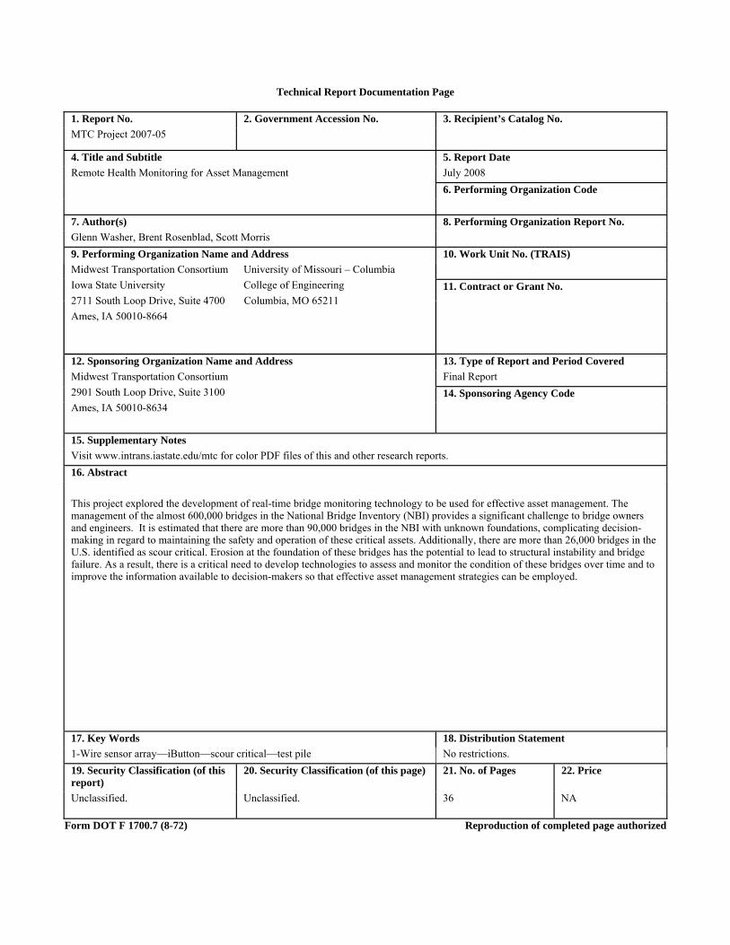
Technical Report Documentation Page

1. Report No. 2. Government Accession No. 3. Recipient’s Catalog No. MTC Project 2007-05

4. Title and Subtitle 5. Report Date Remote Health Monitoring for Asset Management July 2008

6. Performing Organization Code

7. Author(s) 8. Performing Organization Report No. Glenn Washer, Brent Rosenblad, Scott Morris 9. Performing Organization Name and Address 10. Work Unit No. (TRAIS) Midwest Transportation Consortium Iowa State University 2711 South Loop Drive, Suite 4700 Columbia, MO 65211 Ames, IA 50010-8664

University of Missouri – Columbia College of Engineering

11. Contract or Grant No.

12. Sponsoring Organization Name and Address 13. Type of Report and Period Covered Midwest Transportation Consortium 2901 South Loop Drive, Suite 3100 Ames, IA 50010-8634

Final Report 14. Sponsoring Agency Code

15. Supplementary Notes Visit www.intrans.iastate.edu/mtc for color PDF files of this and other research reports. 16. Abstract This project explored the development of real-time bridge monitoring technology to be used for effective asset management. The management of the almost 600,000 bridges in the National Bridge Inventory (NBI) provides a significant challenge to bridge owners and engineers. It is estimated that there are more than 90,000 bridges in the NBI with unknown foundations, complicating decision-making in regard to maintaining the safety and operation of these critical assets. Additionally, there are more than 26,000 bridges in the U.S. identified as scour critical. Erosion at the foundation of these bridges has the potential to lead to structural instability and bridge failure. As a result, there is a critical need to develop technologies to assess and monitor the condition of these bridges over time and to improve the information available to decision-makers so that effective asset management strategies can be employed.

17. Key Words 18. Distribution Statement 1-Wire sensor array—iButton—scour critical—test pile No restrictions. 19. Security Classification (of this report)

20. Security Classification (of this page) 21. No. of Pages 22. Price

Unclassified. Unclassified. 36 NA

Form DOT F 1700.7 (8-72) Reproduction of completed page authorized

REMOTE HEALTH MONITORING FOR ASSET MANAGEMENT

Final Report July 2008

Principal Investigator Glenn Washer

Associate Professor of Civil/Environmental Engineering University of Missouri – Columbia

Co-Principal Investigator

Brent Rosenblad Assistant Professor of Civil/Environmental Engineering

University of Missouri – Columbia

Research Assistant Scott Morris

Sponsored by the Midwest Transportation Consortium

the U.S. DOT University Transportation Center for Federal Region 7

A report from Midwest Transportation Consortium

Iowa State University 2711 South Loop Drive, Suite 4700

Ames, IA 50010-8664 Phone: 515-294-8103 Fax: 515-294-0467

www.intrans.iastate.edu/mtc

v

TABLE OF CONTENTS

EXECUTIVE SUMMARY .......................................................................................................... IX

1. INTRODUCTION .......................................................................................................................1

2. BACKGROUND .........................................................................................................................3

3. PROJECT INSTRUMENTATION .............................................................................................5 3.1 Sensors ...........................................................................................................................5 3.2 Array Design ..................................................................................................................7 3.3 Software .......................................................................................................................13

4. LABORATORY TESTING .......................................................................................................14 4.1 Test Design ..................................................................................................................14 4.2 Results ..........................................................................................................................16

5. FUTURE WORK .......................................................................................................................24

6. CONCLUSIONS ........................................................................................................................25

7. REFERENCES ..........................................................................................................................26

vii

LIST OF FIGURES

Figure 2.1. Photograph of the Skoharie Creek Bridge collapse, 1987 .............................................3 Figure 3.1. DS2480B usage layout ..................................................................................................6 Figure 3.2. Image and pin layout of DS18S20.................................................................................7 Figure 3.3. AutoCAD drawing used for printing circuit boards ......................................................8 Figure 3.4. Setup for exposing circuit boards ..................................................................................9 Figure 3.5. Photonegative used for exposure ...................................................................................9 Figure 3.6. Exposed boards in the chemical bath ..........................................................................10 Figure 3.7. Excess copper being removed from the printed .........................................................10 Figure 3.8. Photograph of small test sensor array with two sensors ..............................................11 Figure 3.9. Photograph of the milling operation to level epoxy ....................................................11 Figure 3.10. Small sensor array test setup .....................................................................................12 Figure 3.11. Diagram of the 24 in. sensor array, showing individual sensor locations and

addresses ............................................................................................................................12 Figure 3.12. Pouring epoxy into large test array............................................................................13 Figure 4.1. Schematic diagram of test set-up showing heaters, sensor array, and sand/water

interface .............................................................................................................................14 Figure 4.2. Both sides of large test pile, showing heater and array locations ...............................15 Figure 4.3. Image of sensor array and water-filled test pile ..........................................................16 Figure 4.4. Front panel of Labview program .................................................................................17 Figure 4.5. Sensor array measurement during heating to and cooling ..........................................17 Figure 4.6. Sensor array output during one-day, 55º test ..............................................................18 Figure 4.7. Temperature gradient in the test pile during heating ..................................................19 Figure 4.8. Temperature gradient in the test pile during heating and cooling ...............................20 Figure 4.9. Thermocouple and DS18S20 readings during cooling and heating ...........................20 Figure 4.10. Thermal gradient along the length of the test pile during cold water test ................21 Figure 4.11. Results of monitoring the sensor array over a five-day period .................................22 Figure 4.12. Schematic diagram of prototype pile for field installation ........................................23 Figure 5.1. Front and back image of LPC-350 ..............................................................................24

viii

ix

EXECUTIVE SUMMARY

This project explored the development of real-time bridge monitoring technology to be used for effective asset management. The management of the almost 600,000 bridges in the National Bridge Inventory (NBI) provides a significant challenge to bridge owners and engineers. It is estimated that there are more than 90,000 bridges in the NBI with unknown foundations, complicating decision-making in regard to maintaining the safety and operation of these critical assets. Additionally, there are more than 26,000 bridges in the U.S. identified as scour critical. Erosion at the foundation of these bridges has the potential to lead to structural instability and bridge failure. As a result, there is a critical need to develop technologies to assess and monitor the condition of these bridges over time and to improve the information available to decision-makers so that effective asset management strategies can be employed. This project investigated the development of an instrumented pile that could provide real-time data on bridge scour, allowing for the remote monitoring of bridge conditions by key managers and engineers. The developed technology has the potential to identify hazardous conditions at a bridge site so that managers and owners can be notified automatically and appropriate actions can be taken. The instrumented pile monitors the temperature along the length of a pile embedded in the soil in a river bed. Monitoring the temperature profile along the length of the pile shows the thermal variations that exist in the water and in the soil, as a means of estimating where the soil/ water interface exists. If a scour hole develops in the area of the pile, the depth of the soil/water interface is consequently changed, and this change is detected by thermal variations detected along the length of the pile. This technology provides a practical means of managing a bridge asset by reporting on potentially dangerous scour conditions so that mitigation strategies can be employed. An innovative new sensor array technology was developed that improves the reliability of field measurements by eliminating the majority of the wires required to make the measurements. A low-cost digital temperature sensor was selected for this application. New manufacturing processes were developed to provide a sensor array that can be integrated into a pile to be embedded at the bridge site. Laboratory studies of prototype sensor arrays were conducted to determine the adequacy of the sensor for this application. Software was developed and tested that supports long-term monitoring of sensor outputs. Two small test piles were developed and utilized for laboratory testing. A final array design for implementation in the field was developed. The construction of a test pile for testing the developed technology in the field is on-going at the time of this report.

1

1. INTRODUCTION

A key challenge to managing fixed assets such as bridges and other transportation infrastructure is monitoring their condition over time. Under typical service conditions, deterioration resulting from traffic loading and difficult environmental conditions can result in a reduction or loss of service of a particular asset, or even life threatening and dangerous failures. Extreme events such as earthquakes and floods present a still greater challenge in that the service condition of the asset may change abruptly and without warning, leaving managers without key information they need to respond to the event. The goal of this project was to develop remote health monitoring technology that will provide managers and owners with timely information on the condition of civil infrastructure assets. Specifically, the project sought to develop an instrumented pile that could be installed at a bridge either as part of the original construction or installed post-construction to monitor conditions at the bridge. The pile was to be instrumented using a series of thermal sensors that would be used to detect the level of scour adjacent to a bridge substructure by evaluating which portions of the pile were embedded in soil and which portions of the pile were exposed to water. This report documents efforts made toward meeting these goals. During the course of the project, a new method of measuring temperature profiles along the length of a pile embedded in the soil adjacent to a highway bridge was developed. Significant efforts were required to develop the necessary technology to manufacture and assemble the temperature sensor array. Progress was made toward developing a unique instrumentation system that would enable the long-term monitoring of highway bridges using a unique and highly durable temperature sensor array. Manufacturing processes were developed to produce a temperature sensor array that could be installed in the difficult environment of a highway bridge and be expected to perform adequately over a long time period. A design for implementation of the new sensor array technology along the length of a steel H-pile has been developed. The construction of this test pile is ongoing. Due to scheduling constraints, the installation of the pile in the field was not achieved as originally planned. However, it is expected that field testing will be completed outside the scheduling constraints of this project, and it is anticipated that this final report would be updated at a later point in time to indicate the work completed outside the scheduling constraints of this project. A field installation site has been selected. A permit with the Corp of Engineers is currently in process, which has caused delays in field implementation of this technology. Following field deployment, the pile will be monitored to evaluate its effectiveness and determine the overall performance and utility of the technology. Project partners included the State of Missouri and Tennessee, each of which provided some funding to support the project. The State of Missouri assumed the project lead state status, organizing the team to provide quarterly progress meetings held via teleconference. The project team provided progress overviews to the partner states as a means of technology transfer and to ensure that progress on the project was directed toward meeting the needs of State Departments of Transportation. The project team prepared detailed slide presentations that documented progress and efforts on the project, and these slides were presented to the project team. Significant input on the direction of the project and specific design assistance was provided by the partner states. In particular, Terry Leatherwood, Tennessee Department of Transportation,

2

provided useful input on past experiences and specific design advice on the development of the instrumented pile.

3

2. BACKGROUND

The collapse of the Skoharie Creek Bridge in 1987 (shown in Figure 2.1) introduced a new era of concern regarding the structural stability of highway bridges and the fidelity of the substructure systems supporting them. The tragic collapse and others that have followed have focused attention on the need for dependable methods of monitoring the structural stability of highway structures. Bridge scour that results in a loss of structural stability is the most common reason for collapse of highway bridges, and innovative, cost-effective monitoring methods are urgently needed. Presently there are more than 26,000 bridges in the U.S. identified as scour critical (1, 2). More than 3,700 bridges were damaged by scour during the period of 1985–1995 (2).

Figure 2.1. Photograph of the Skoharie Creek Bridge collapse, 1987

A number of technologies have been developed to address the issue of scour in the area of bridge foundations. Many of these technologies, such as fathometers and ground-penetrating radar, are aimed at detecting scour holes adjacent and beneath bridge footings. These and similar techniques are based on periodic inspections and do not provide real-time data about sudden events that may occur on a structure. Efforts to use these techniques during extreme events, such as floods, are hampered by high-water velocities and increased flow depth. In-place, or fixed, monitoring systems have also been widely applied. These include fixed fathometers, simple depth rods, piezoelectric films, float-out devices buried in the stream bed, and magnetic sliding collar instruments (3). Dataloggers have been applied to collect data electronically during extreme events, and a number of telemetry devices have been used to transmit critical data to state agencies. However, these systems have several disadvantages. First, portions of the systems must be placed in the water flow so that they are susceptible to debris damage. Second, the scour must occur at the location and in the manner predicted, as

4

these systems make measurements in relatively small areas adjacent to a pier. It is estimated that there are more than 90,000 bridges in the United States with unknown foundations which make required analysis simply impossible (4). Even with known foundation conditions, the behavior of scour under flood conditions may be difficult to fully define. A remote monitoring system consisting of inclinometers was fielded on a bridge in California in 1999 (5). This system consisted of two inclinometers mounted on each face of the pier, wired to a central data acquisition system that collected tilt data from each of the 18 piers on an hourly basis. This data was made available to state personnel by dialing into the system using the program P.C. anywhere. Initial results from outputs of these sensors indicated that significant diurnal variations in inclinometer output were experienced, making interpretation of data difficult. However, applications of this type illustrate the application of target monitoring technology for the purpose of asset management, to provide real-time or near real-time data on the conditions in the field at a valuable fixed asset. This project explored the development of an instrumented pile that could provide real-time data on bridge scour, allowing for the remote monitoring of bridge conditions by key managers and engineers. The developed technology has potential to identify hazardous conditions at a bridge site, so that managers and owners can be notified automatically and appropriate actions can be taken. The instrumented pile monitors the temperature along the length of a pile embedded in the soil in a river bed. Monitoring the temperature profile along the length of the pile shows the thermal variations that exist in the water and in the soil, as a means of estimating where the soil/ water interface exists. If a scour hole develops in the area of the pile, the depth of the soil/water interface is consequently changed, and this change is detected by thermal variations detected along the length of the pile. This technology provides a practical means of managing a bridge asset by reporting on potentially dangerous scour conditions so that mitigation strategies can be employed. A digital, semi-conductor based sensor was selected for application on this project. The sensor is a 1-Wire device manufactured by Dallas Semiconductor. The model DS18S20 sensor is also a high precision 1-Wire digital thermometer. A data acquisition system for these sensors was developed to read data from the sensors and enable data storage. Two small test piles have been constructed and tested in the laboratory. The larger of the test piles is currently using 16 DS18S20 sensors and is connected to a ceramic heater capable of temperatures up to 200˚ C to allow for thermal gradients in the test pile to be adjusted to demonstrate and test the operation of sensor arrays. The final design for installing the sensor array along a real pile has been developed.

5

3. PROJECT INSTRUMENTATION

A significant portion of the project was dedicated to developing a new method of detecting temperature profiles along the length of a pile. This portion of the report will describe the development of a unique, 1-Wire sensor array that was the focus of efforts during the project. First, detailed information about the sensors used will be provided. An overview of software that was developed will follow, as well as a description of the manufacturing process developed to enable the array to be installed in the field. 3.1 Sensors

The goals of the project required that a suitable temperature sensor device be identified to enable the long-term, stable measurement of thermal conditions in the pile. Thermocouples are a traditional method of measuring temperatures, due to their low cost and durability. Thermocouples operate by measuring the potential difference across a bi-metal interface. Two wires of differing alloy composition are joined together, and the potential difference across the metal interface is a function of the temperature at the interface. These sensors have several advantages, including high temperature sensitivity and low cost. Supporting instrumentation to measure the output of thermocouples is widely available; therefore, minimal development is required to implement thermocouples as a temperature monitoring device. However, thermocouples also have a number of disadvantages. First, the bi-metal interface is susceptible to corrosion when placed in an environment where water and oxygen are widely available, such as when embedded in a stream. Second, it requires two wires for each individual sensor to provide the bi-metal interface, so that developing an array with a large number of sensors requires a large number of wires. This is a particular challenge for the present project, as each wire provides a potential source of failure so that long-term reliability of a system of thermocouples is problematic. Additionally, the large number of wires that would be required to instrument a pile with a large number of sensors requires an intrusive sensor measurement system to provide a data collection bus and measure each channel individually. Most importantly, the sensor outputs are low-level signals that must be conditioned and measured by an analog circuit, digitized and stored. When installed in an uncontrolled environment such as along a pile embedded in a stream bed, ground loops and other electromagnetic noise provide a significant challenge to the long-term measurement of sensor outputs. As a result, an alternative to thermocouples was sought to provide a suitable sensor for measurement of temperature profiles along the length of the pile. A literature search and interactions with the project partners led researchers to pursue an alternative to thermocouples for the temperature array designed for this project. The iButton, an automated temperature sensor that can be installed without attached wires and read through a specialized inductive hand-reader, was suggested by the project partners as an alternative to thermocouples. A comprehensive literature search and interactions with the iButton manufacturer led to an alternative, 1-Wire temperature sensor. New sensors known as 1-Wire Devices manufactured by Dallas Semiconductor are a relatively new alternative to thermocouples for temperature measurement. These devices are semi-conductor based digital temperature sensors. The sensors have been used for many applications, such as for timekeepers, current sensors, battery monitors, and for identity verification. The main

6

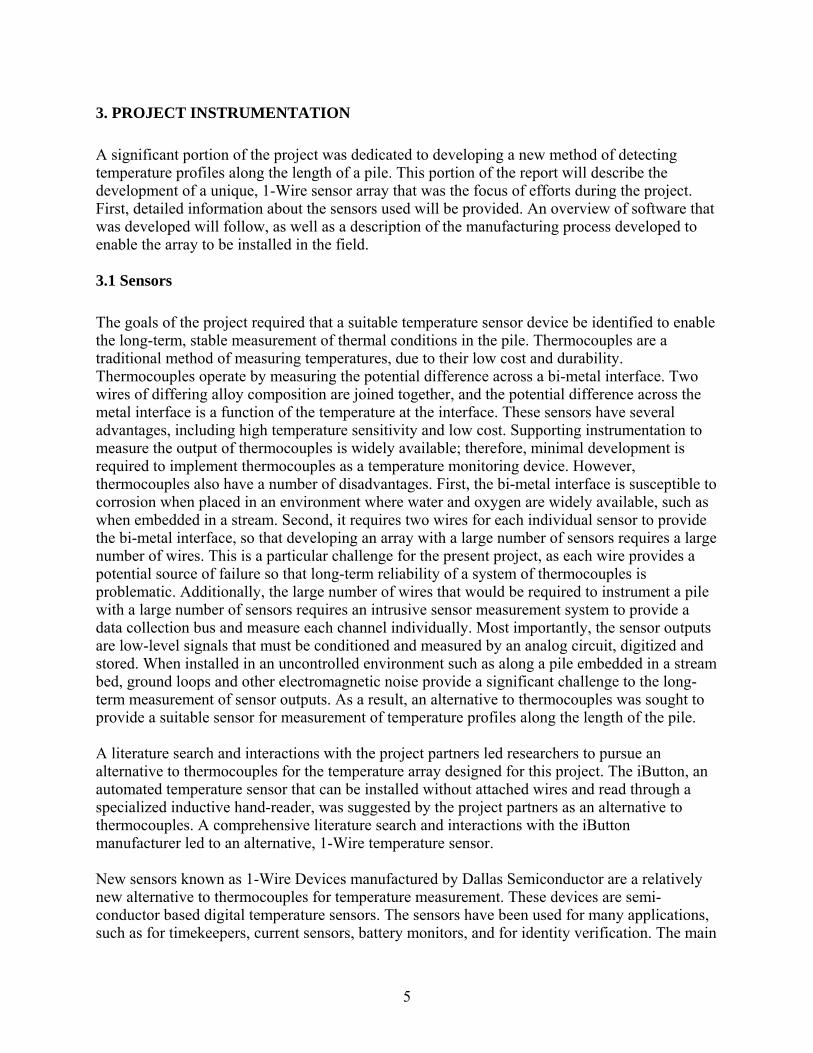
benefit of these devices is that they need a limited amount of wiring and hardware to be functional. Also, each device has its own unique 64 bit serial number assigned to it when it is fabricated, allowing over 281 trillion combinations. These features allow a large number of slave devices to be daisy-chained together along a single wire connection to one microcontroller. They need to be connected to a ground wire for reference, but this wire is conventionally ignored. Unlike a thermocouple system that requires a cold junction compensation box and many wires, there are few items needed to create a 1-Wire temperature system. Just the sensor, a connector, a PC, and the suitable software are needed. The 1-Wire system being used utilizes a DS2480B microcontroller, a DS18S20 temperature sensor, and a DS9097U PC serial port connector. The 1-Wire interface is described in many of the Application Notes on the Dallas Semiconductor website. Information is transferred by the use of high and low voltages present in the line along with the use of “time slots.” To read information from a sensor, the micro-controller pulls the bus master voltage to low for 1μs then releases and allows the slave sensor to control the line. A voltage of 2.2V or higher is read as logic 1 and voltages of less than 0.8V is read as logic 0. The voltage must stay in that range for between 60 and 120μs. The DS2480B is used as a microcontroller for 1-Wire applications. It is described as a “serial bridge to the 1-Wire network protocol.” A simplified image of the usage of a DS2480B is shown below in Figure 3.1 with two slave devices (DS18S20) attached in a daisy-chain configuration.

Figure 3.1. DS2480B usage layout

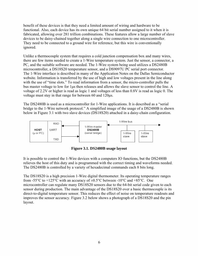
It is possible to control the 1-Wire devices with a computers IO functions, but the DS2480B relieves the host of this duty and is programmed with the correct timing and waveforms needed. The DS2480B is controlled by a variety of hexadecimal commands each 8 bits long. The DS18S20 is a high precision 1-Wire digital thermometer. Its operating temperature ranges from -55°C to +125°C with an accuracy of ±0.5°C between -10°C and +85°C. One microcontroller can regulate many DS18S20 sensors due to the 64-bit serial code given to each sensor during production. The main advantage of the DS18S20 over a basic thermocouple is its direct-to-digital temperature sensor. This reduces the effect of noise on temperature readouts and improves the sensor accuracy. Figure 3.2 below shows a photograph of a DS18S20 and the pin layout.

7

Figure 3.2. Image and pin layout of DS18S20

The DS18S20 can be powered by a technique called parasite power. In this mode, the sensor is powered by stealing electricity from DQ line (Figure 3.2) when the bus is high. A capacitor in the sensor is charged during this time to allow the sensor to operate while the bus is low. The simpler way to power the devices is by connecting the VDD pin to a power supply, which is how the sensor is implemented in this project. The manufacturer does not recommend the use of parasite power for temperatures over 100°C due to high leakage currents, and encourages the use of the VDD pin for power connection in applications where the extra wire connection is possible and allowable. Using parasite power makes operation much more difficult because the bus must always be held high during any 1-Wire device function. This causes problems with the timing and voltage requirements for reading the data. For this project, researchers decided to use a three-wire connection to power and read the sensor. This included a ground wire, a data wire and separate power wire. The arrangement was selected to provide long-term durability and simplify software developments. Additionally, there was little disadvantage to using three wires within the instrumentation cable. Developing this technology allowed for a single cable containing three wires to be utilized as the only data acquisition cable, greatly simplifying the system overall and providing improved reliability over a thermocouple system that would require a large number of wire pairs. One significant advantage of the 1-Wire sensors is the low cost of the sensor. In small quantities, the sensors cost ~$2.00 each, with lower cost when purchased in large numbers. The low cost of the sensor makes it practical to envision a large number of sensors being implemented in the field. Additionally, the sensors consume very little power, so that a large number of sensors can be powered from a common battery for long periods of time. The low power requirement of the sensor could enable the development of a battery or solar powered system for final implementation of the technology. 3.2 Array Design

To implement these unique sensors within the instrumented pile being designed for this project, it was necessary to develop a system by which a multitude of sensors could be connected along a single set of wires, and subsequently installed along the length of a pile. Initial testing utilized individual wires to test the sensors and help researchers develop the software necessary to read and store data. This requires that the insulation of the wires be breached at each sensor location, and three solder joints be applied to connect the sensor to the wire. However, it became apparent that there were several challenges to implementing this design in the field. The primary disadvantage stemmed from the reliability of the wire connections. Attaching a loose wire to the

8

pile, and expecting the high number of individual solder joints to remain reliable over long time periods was unrealistic. Therefore, an alternative to this configuration was sought. A literature search and discussions with manufacturing experts illuminated an alternative to using a three-wire configuration. Printable circuit boards, widely used in a variety of electronic devices, provided an alternative that would enable the sensors to be secured to a rigid polymer backplane, and this rigid back plane can then be connected to a suitable housing for installation in the stream bed. Three “trunk lines” printed onto the polymer backplane would improve the solder connections, simplify manufacturing, and provide a more durable long-term solution. However, the disadvantage of this approach is that it required a significant amount of development to manufacture the printed boards. The process for manufacturing a printed circuit board includes the following steps:

1. Creating an AutoCAD drawing of desired conductor layout 2. Developing a photonegative of the conductor layout 3. Exposing board to ultraviolet light to print pattern onto backplane 4. Etching of exposed boards

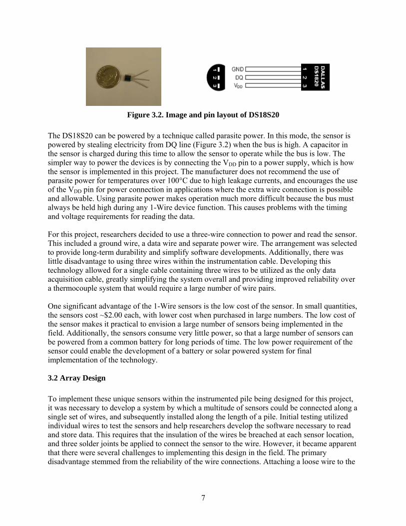
The AutoCAD drawing of the trunk line design is shown in Figure 3.3. The trunkline design consisted of three conductor lines that run the length of a 24 in. board, a commonly available size for the circuit board materials. Solder tabs are etched at either end of the trunklines to enable the board to be connected by short wires, so that a 24 in. module can be manufactured and then several boards could be connected to create the appropriate length sensor array. The sensors themselves can be soldered to the trunk lines at any spacing interval; a sensor every three or four in. was selected as a suitable spacing for this project. This allows for up to four measurements per ft of pile, adequate for estimating the soil line depth along the pile. This spacing was based on discussions with bridge maintenance engineers that indicated that information on the depth of scour holes to the nearest ft was adequate for effective decision making and asset management. By placing three sensors per ft, measurement redundancy would exist to provide improved reliability in field applications, and ensure that system resolution met the requirement of determining the depth of a scour hole to the nearest foot.

Figure 3.3. AutoCAD drawing used for printing circuit boards

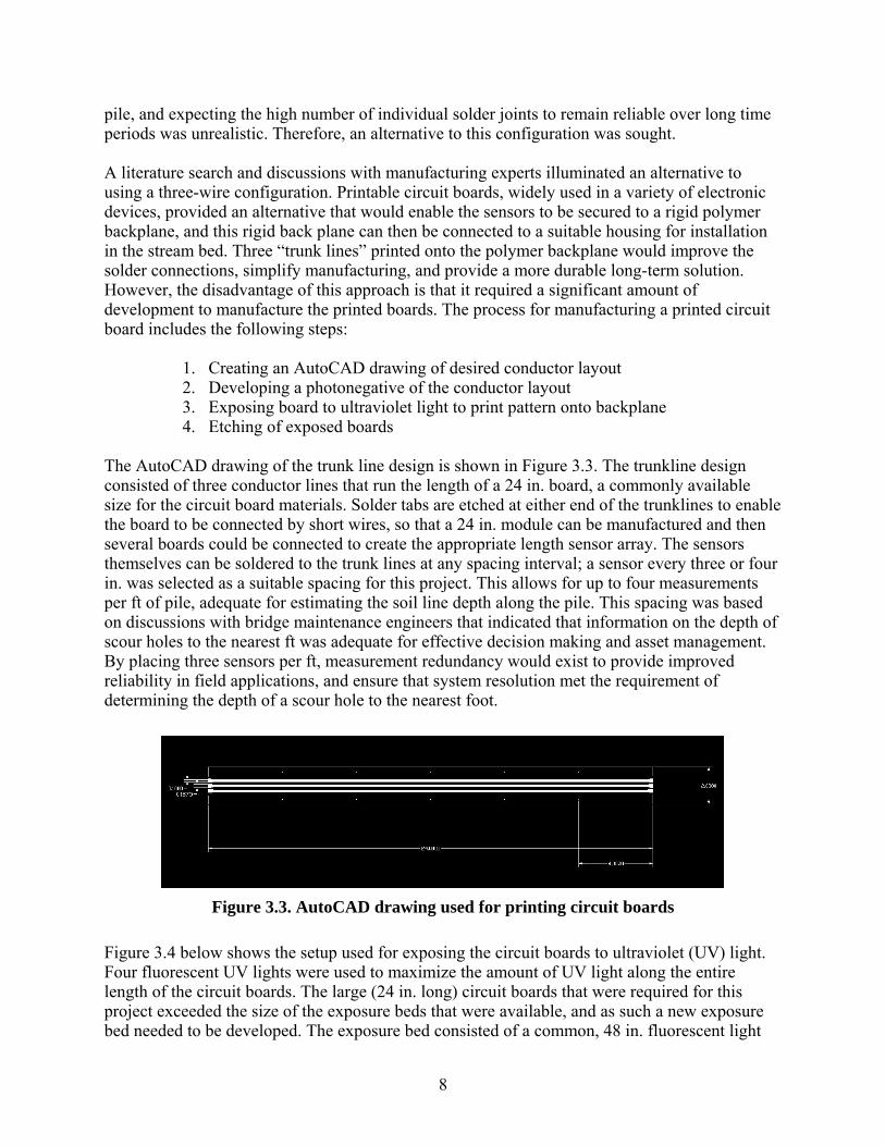
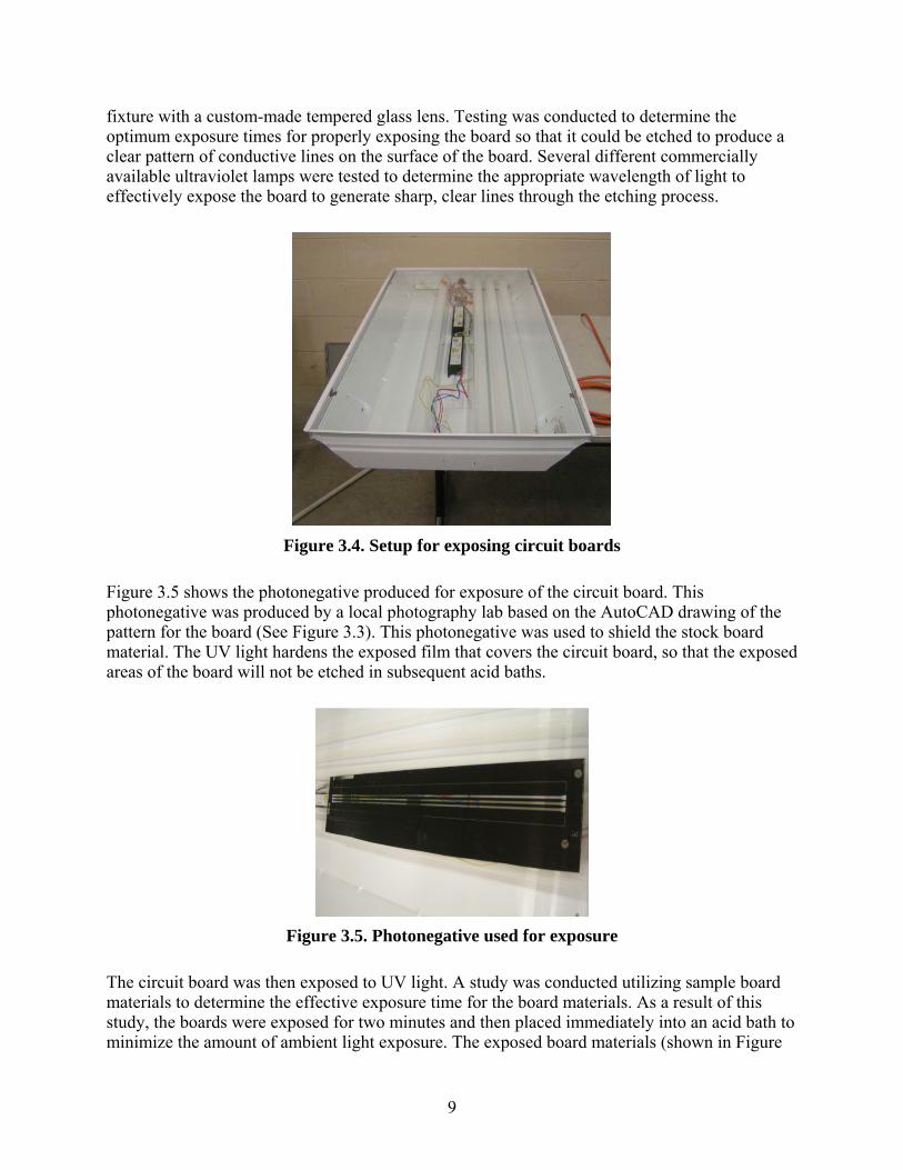
Figure 3.4 below shows the setup used for exposing the circuit boards to ultraviolet (UV) light. Four fluorescent UV lights were used to maximize the amount of UV light along the entire length of the circuit boards. The large (24 in. long) circuit boards that were required for this project exceeded the size of the exposure beds that were available, and as such a new exposure bed needed to be developed. The exposure bed consisted of a common, 48 in. fluorescent light

9

fixture with a custom-made tempered glass lens. Testing was conducted to determine the optimum exposure times for properly exposing the board so that it could be etched to produce a clear pattern of conductive lines on the surface of the board. Several different commercially available ultraviolet lamps were tested to determine the appropriate wavelength of light to effectively expose the board to generate sharp, clear lines through the etching process.

Figure 3.4. Setup for exposing circuit boards

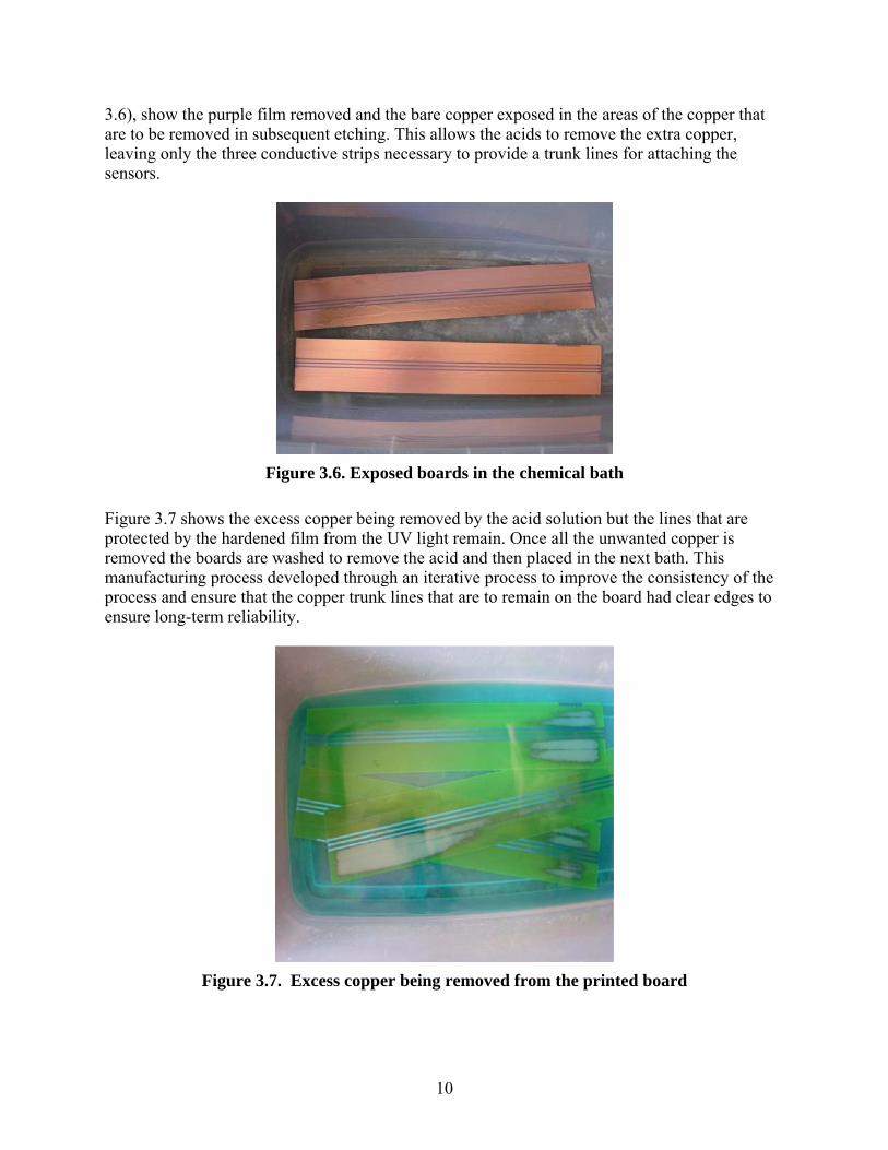
Figure 3.5 shows the photonegative produced for exposure of the circuit board. This photonegative was produced by a local photography lab based on the AutoCAD drawing of the pattern for the board (See Figure 3.3). This photonegative was used to shield the stock board material. The UV light hardens the exposed film that covers the circuit board, so that the exposed areas of the board will not be etched in subsequent acid baths.

Figure 3.5. Photonegative used for exposure

The circuit board was then exposed to UV light. A study was conducted utilizing sample board materials to determine the effective exposure time for the board materials. As a result of this study, the boards were exposed for two minutes and then placed immediately into an acid bath to minimize the amount of ambient light exposure. The exposed board materials (shown in Figure

10

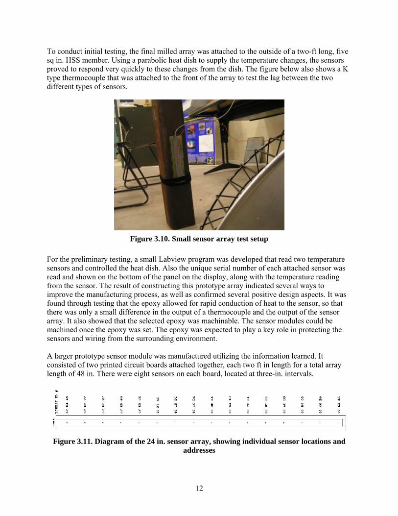
3.6), show the purple film removed and the bare copper exposed in the areas of the copper that are to be removed in subsequent etching. This allows the acids to remove the extra copper, leaving only the three conductive strips necessary to provide a trunk lines for attaching the sensors.

Figure 3.6. Exposed boards in the chemical bath

Figure 3.7 shows the excess copper being removed by the acid solution but the lines that are protected by the hardened film from the UV light remain. Once all the unwanted copper is removed the boards are washed to remove the acid and then placed in the next bath. This manufacturing process developed through an iterative process to improve the consistency of the process and ensure that the copper trunk lines that are to remain on the board had clear edges to ensure long-term reliability.

Figure 3.7. Excess copper being removed from the printed board

11

Two different sized test arrays were created in the lab. The goals were to prove that the temperature measurement system worked effectively and expand our knowledge of what to expect from the actual pile deployment. A photograph of a small, two-sensor array can be seen below in Figure 3.8. In this photograph, the two DS18S20 sensors are soldered to the trunk lines along with the attachment cable that leads back to a standard PC. Communication with the sensors is achieved through the serial port of a standard personnel computer. The board material was attached to a polycarbonate frame as shown in the photograph. This frame allowed for the sensors to be potted inside a special epoxy that provides protection from damage to the sensors and supporting trunk lines, and has a high thermal conductivity (close to that of steel). Potting of the sensor array in the special epoxy allows for rapid conduction of changes in the thermal environment of the array, in addition to stabilizing the sensors to provide protection from the environment.

Figure 3.8. Photograph of small test sensor array with two sensors

After allowing the epoxy to harden for over 24 hr, it went through a mill to level the surface of the epoxy to the elevation of the polycarbonate walls. This provided a machined surface that could then be mounted onto the surface of any type of structure, for example, the side of a steel pile. The flat surface of the sensor array allowed for direct contact with the surface of the steel to ensure effective heat transfer across the joint.

Figure 3.9. Photograph of the milling operation to level epoxy

12

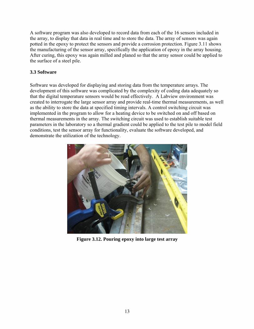
To conduct initial testing, the final milled array was attached to the outside of a two-ft long, five sq in. HSS member. Using a parabolic heat dish to supply the temperature changes, the sensors proved to respond very quickly to these changes from the dish. The figure below also shows a K type thermocouple that was attached to the front of the array to test the lag between the two different types of sensors.

Figure 3.10. Small sensor array test setup

For the preliminary testing, a small Labview program was developed that read two temperature sensors and controlled the heat dish. Also the unique serial number of each attached sensor was read and shown on the bottom of the panel on the display, along with the temperature reading from the sensor. The result of constructing this prototype array indicated several ways to improve the manufacturing process, as well as confirmed several positive design aspects. It was found through testing that the epoxy allowed for rapid conduction of heat to the sensor, so that there was only a small difference in the output of a thermocouple and the output of the sensor array. It also showed that the selected epoxy was machinable. The sensor modules could be machined once the epoxy was set. The epoxy was expected to play a key role in protecting the sensors and wiring from the surrounding environment. A larger prototype sensor module was manufactured utilizing the information learned. It consisted of two printed circuit boards attached together, each two ft in length for a total array length of 48 in. There were eight sensors on each board, located at three-in. intervals.

Figure 3.11. Diagram of the 24 in. sensor array, showing individual sensor locations and

addresses

13

A software program was also developed to record data from each of the 16 sensors included in the array, to display that data in real time and to store the data. The array of sensors was again potted in the epoxy to protect the sensors and provide a corrosion protection. Figure 3.11 shows the manufacturing of the sensor array, specifically the application of epoxy in the array housing. After curing, this epoxy was again milled and planed so that the array sensor could be applied to the surface of a steel pile. 3.3 Software

Software was developed for displaying and storing data from the temperature arrays. The development of this software was complicated by the complexity of coding data adequately so that the digital temperature sensors would be read effectively. A Labview environment was created to interrogate the large sensor array and provide real-time thermal measurements, as well as the ability to store the data at specified timing intervals. A control switching circuit was implemented in the program to allow for a heating device to be switched on and off based on thermal measurements in the array. The switching circuit was used to establish suitable test parameters in the laboratory so a thermal gradient could be applied to the test pile to model field conditions, test the sensor array for functionality, evaluate the software developed, and demonstrate the utilization of the technology.

Figure 3.12. Pouring epoxy into large test array

14

4. LABORATORY TESTING

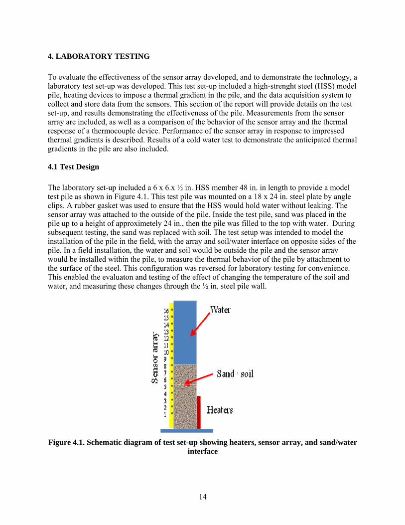
To evaluate the effectiveness of the sensor array developed, and to demonstrate the technology, a laboratory test set-up was developed. This test set-up included a high-strenght steel (HSS) model pile, heating devices to impose a thermal gradient in the pile, and the data acquisition system to collect and store data from the sensors. This section of the report will provide details on the test set-up, and results demonstrating the effectiveness of the pile. Measurements from the sensor array are included, as well as a comparison of the behavior of the sensor array and the thermal response of a thermocouple device. Performance of the sensor array in response to impressed thermal gradients is described. Results of a cold water test to demonstrate the anticipated thermal gradients in the pile are also included. 4.1 Test Design

The laboratory set-up included a 6 x 6.x ½ in. HSS member 48 in. in length to provide a model test pile as shown in Figure 4.1. This test pile was mounted on a 18 x 24 in. steel plate by angle clips. A rubber gasket was used to ensure that the HSS would hold water without leaking. The sensor array was attached to the outside of the pile. Inside the test pile, sand was placed in the pile up to a height of approximetely 24 in., then the pile was filled to the top with water. During subsequent testing, the sand was replaced with soil. The test setup was intended to model the installation of the pile in the field, with the array and soil/water interface on opposite sides of the pile. In a field installation, the water and soil would be outside the pile and the sensor array would be installed within the pile, to measure the thermal behavior of the pile by attachment to the surface of the steel. This configuration was reversed for laboratory testing for convenience. This enabled the evaluaton and testing of the effect of changing the temperature of the soil and water, and measuring these changes through the ½ in. steel pile wall.

Figure 4.1. Schematic diagram of test set-up showing heaters, sensor array, and sand/water

interface

15

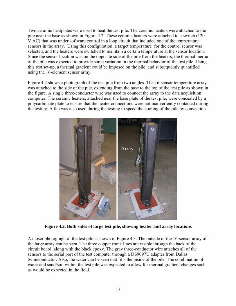
Two ceramic heatplates were used to heat the test pile. The ceremic heaters were attached to the pile near the base as shown in Figure 4.2. These ceramic heaters were attached to a switch (120 V AC) that was under software control in a loop circuit that included one of the temperature sensors in the array. Using this configuration, a target temperature for the control sensor was selected, and the heaters were switched to maintain a certain temperature at the sensor location. Since the sensor location was on the opposite side of the pile from the heaters, the thermal inertia of the pile was expected to provide some variation in the thermal behavior of the test pile. Using this test set-up, a thermal gradient could be imposed on the pile, and subsequently quantified using the 16-element sensor array. Figure 4.2 shows a photograph of the test pile from two angles. The 16-sensor temperature array was attached to the side of the pile, extending from the base to the top of the test pile as shown in the figure. A single three-conducter wire was used to connect the array to the data acquisition computer. The ceramic heaters, attached near the base plate of the test pile, were concealed by a polycarbonate plate to ensure that the heater connections were not inadvertently contacted during the testing. A fan was also used during the testing to speed the cooling of the pile by convection.

Figure 4.2. Both sides of large test pile, showing heater and array locations

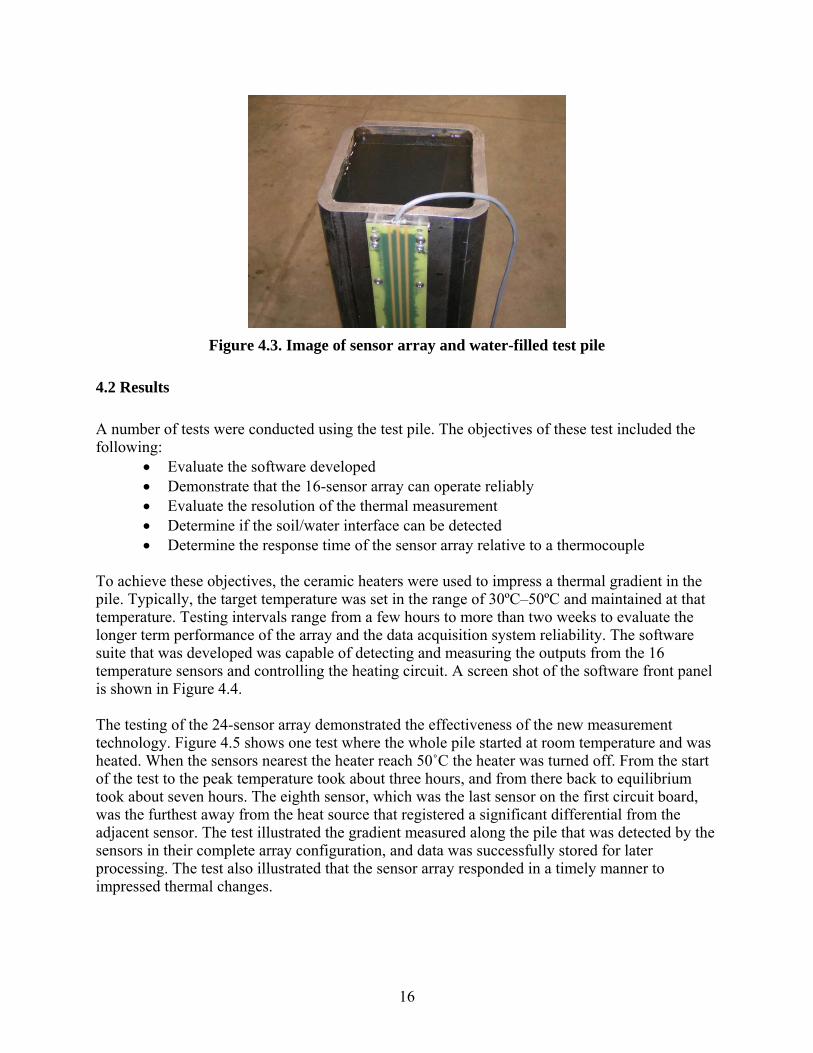
A closer photogragh of the test pile is shown in Figure 4.3. The outside of the 16-sensor array of the large array can be seen. The three copper trunk lines are visible through the back of the circuit board, along with the black epoxy. The gray three-conductor wire attaches all of the sensors to the serial port of the test computer through a DS9097U adapter from Dallas Semiconductor. Also, the water can be seen that fills the inside of the pile. The combination of water and sand/soil within the test pile was expected to allow for thermal gradient changes such as would be expected in the field.

Array

16

Figure 4.3. Image of sensor array and water-filled test pile

4.2 Results

A number of tests were conducted using the test pile. The objectives of these test included the following:

• Evaluate the software developed • Demonstrate that the 16-sensor array can operate reliably • Evaluate the resolution of the thermal measurement • Determine if the soil/water interface can be detected • Determine the response time of the sensor array relative to a thermocouple

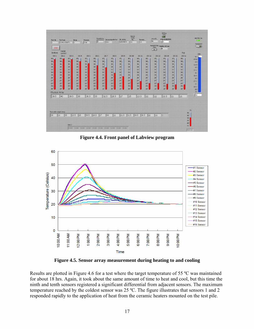
To achieve these objectives, the ceramic heaters were used to impress a thermal gradient in the pile. Typically, the target temperature was set in the range of 30ºC–50ºC and maintained at that temperature. Testing intervals range from a few hours to more than two weeks to evaluate the longer term performance of the array and the data acquisition system reliability. The software suite that was developed was capable of detecting and measuring the outputs from the 16 temperature sensors and controlling the heating circuit. A screen shot of the software front panel is shown in Figure 4.4. The testing of the 24-sensor array demonstrated the effectiveness of the new measurement technology. Figure 4.5 shows one test where the whole pile started at room temperature and was heated. When the sensors nearest the heater reach 50˚C the heater was turned off. From the start of the test to the peak temperature took about three hours, and from there back to equilibrium took about seven hours. The eighth sensor, which was the last sensor on the first circuit board, was the furthest away from the heat source that registered a significant differential from the adjacent sensor. The test illustrated the gradient measured along the pile that was detected by the sensors in their complete array configuration, and data was successfully stored for later processing. The test also illustrated that the sensor array responded in a timely manner to impressed thermal changes.

17

Figure 4.4. Front panel of Labview program

Figure 4.5. Sensor array measurement during heating to and cooling

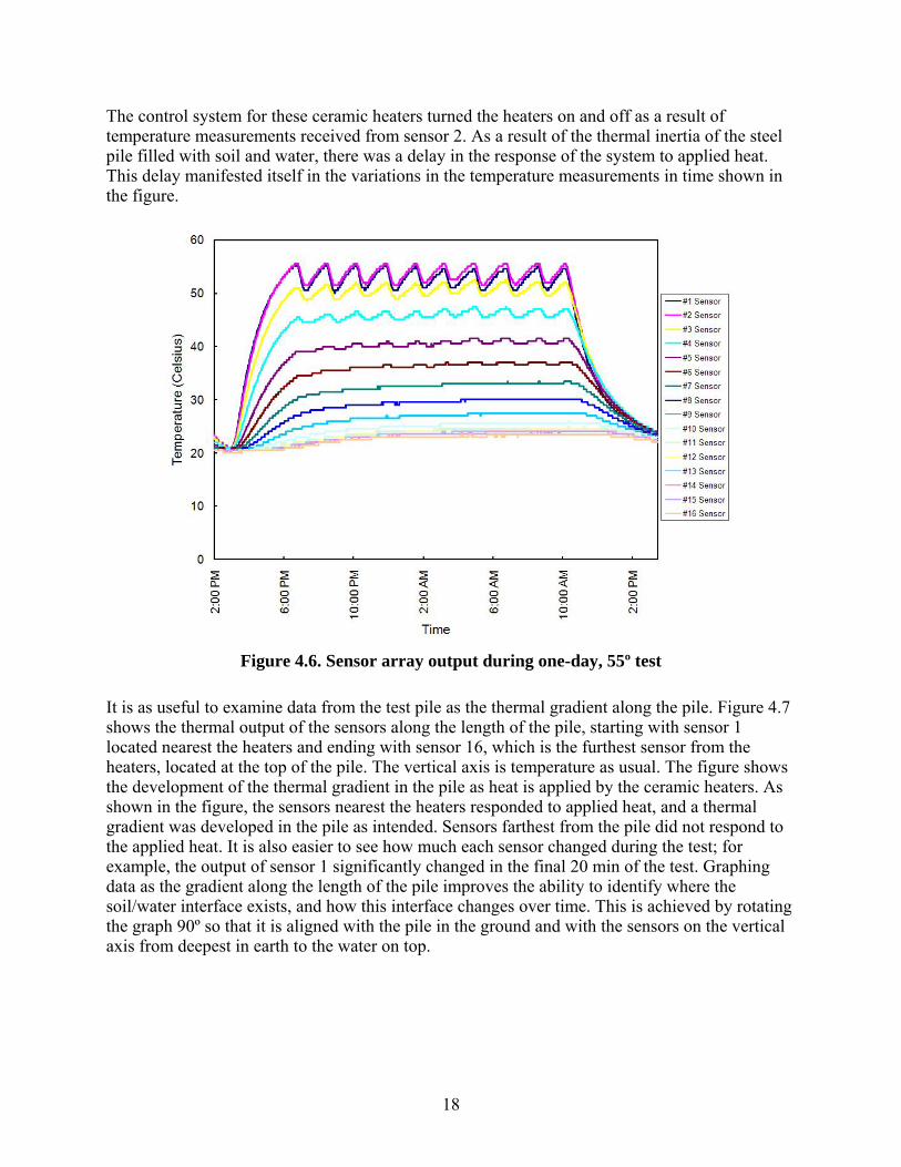
Results are plotted in Figure 4.6 for a test where the target temperature of 55 ºC was maintained for about 18 hrs. Again, it took about the same amount of time to heat and cool, but this time the ninth and tenth sensors registered a significant differential from adjacent sensors. The maximum temperature reached by the coldest sensor was 25 ºC. The figure illustrates that sensors 1 and 2 responded rapidly to the application of heat from the ceramic heaters mounted on the test pile.

18

The control system for these ceramic heaters turned the heaters on and off as a result of temperature measurements received from sensor 2. As a result of the thermal inertia of the steel pile filled with soil and water, there was a delay in the response of the system to applied heat. This delay manifested itself in the variations in the temperature measurements in time shown in the figure.

Figure 4.6. Sensor array output during one-day, 55º test

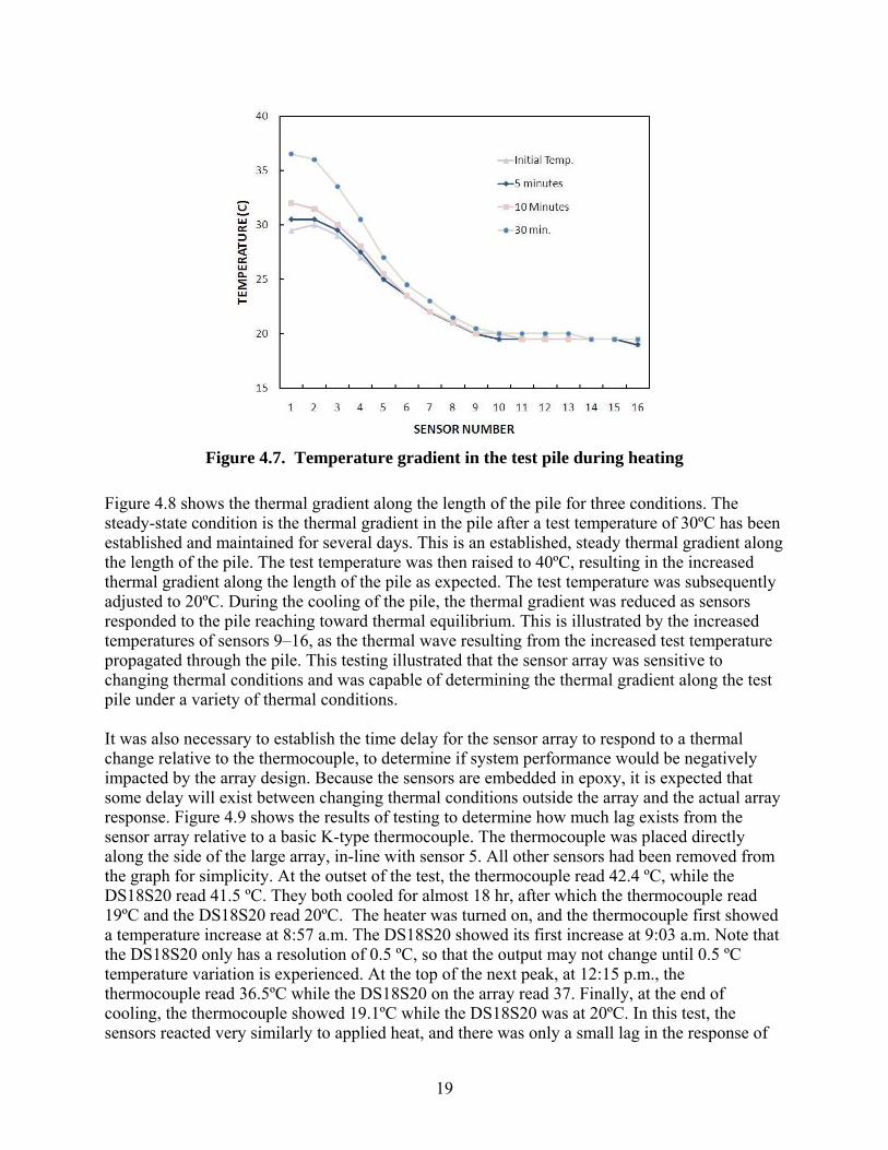
It is as useful to examine data from the test pile as the thermal gradient along the pile. Figure 4.7 shows the thermal output of the sensors along the length of the pile, starting with sensor 1 located nearest the heaters and ending with sensor 16, which is the furthest sensor from the heaters, located at the top of the pile. The vertical axis is temperature as usual. The figure shows the development of the thermal gradient in the pile as heat is applied by the ceramic heaters. As shown in the figure, the sensors nearest the heaters responded to applied heat, and a thermal gradient was developed in the pile as intended. Sensors farthest from the pile did not respond to the applied heat. It is also easier to see how much each sensor changed during the test; for example, the output of sensor 1 significantly changed in the final 20 min of the test. Graphing data as the gradient along the length of the pile improves the ability to identify where the soil/water interface exists, and how this interface changes over time. This is achieved by rotating the graph 90º so that it is aligned with the pile in the ground and with the sensors on the vertical axis from deepest in earth to the water on top.

19

Figure 4.7. Temperature gradient in the test pile during heating

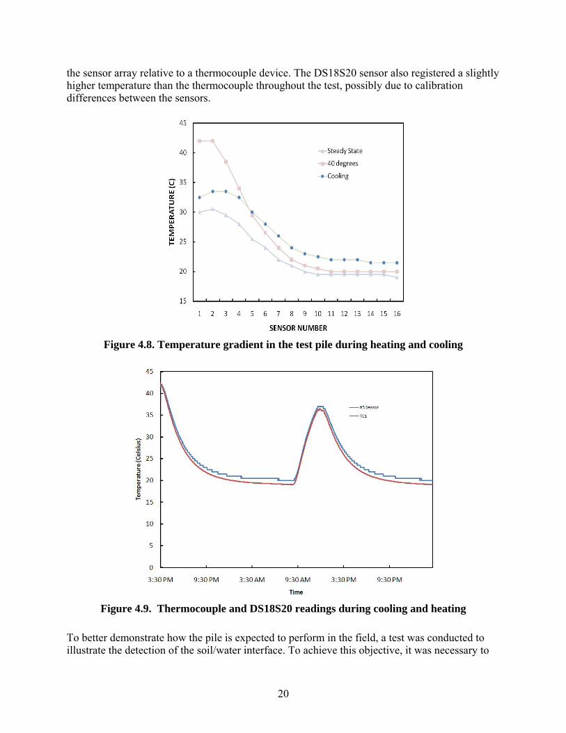
Figure 4.8 shows the thermal gradient along the length of the pile for three conditions. The steady-state condition is the thermal gradient in the pile after a test temperature of 30ºC has been established and maintained for several days. This is an established, steady thermal gradient along the length of the pile. The test temperature was then raised to 40ºC, resulting in the increased thermal gradient along the length of the pile as expected. The test temperature was subsequently adjusted to 20ºC. During the cooling of the pile, the thermal gradient was reduced as sensors responded to the pile reaching toward thermal equilibrium. This is illustrated by the increased temperatures of sensors 9–16, as the thermal wave resulting from the increased test temperature propagated through the pile. This testing illustrated that the sensor array was sensitive to changing thermal conditions and was capable of determining the thermal gradient along the test pile under a variety of thermal conditions. It was also necessary to establish the time delay for the sensor array to respond to a thermal change relative to the thermocouple, to determine if system performance would be negatively impacted by the array design. Because the sensors are embedded in epoxy, it is expected that some delay will exist between changing thermal conditions outside the array and the actual array response. Figure 4.9 shows the results of testing to determine how much lag exists from the sensor array relative to a basic K-type thermocouple. The thermocouple was placed directly along the side of the large array, in-line with sensor 5. All other sensors had been removed from the graph for simplicity. At the outset of the test, the thermocouple read 42.4 ºC, while the DS18S20 read 41.5 ºC. They both cooled for almost 18 hr, after which the thermocouple read 19ºC and the DS18S20 read 20ºC. The heater was turned on, and the thermocouple first showed a temperature increase at 8:57 a.m. The DS18S20 showed its first increase at 9:03 a.m. Note that the DS18S20 only has a resolution of 0.5 ºC, so that the output may not change until 0.5 ºC temperature variation is experienced. At the top of the next peak, at 12:15 p.m., the thermocouple read 36.5ºC while the DS18S20 on the array read 37. Finally, at the end of cooling, the thermocouple showed 19.1ºC while the DS18S20 was at 20ºC. In this test, the sensors reacted very similarly to applied heat, and there was only a small lag in the response of

20

the sensor array relative to a thermocouple device. The DS18S20 sensor also registered a slightly higher temperature than the thermocouple throughout the test, possibly due to calibration differences between the sensors.

Figure 4.8. Temperature gradient in the test pile during heating and cooling

Figure 4.9. Thermocouple and DS18S20 readings during cooling and heating

To better demonstrate how the pile is expected to perform in the field, a test was conducted to illustrate the detection of the soil/water interface. To achieve this objective, it was necessary to

21

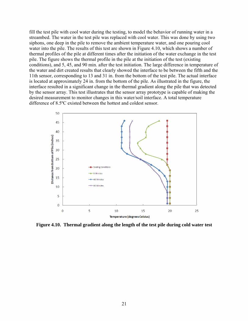
fill the test pile with cool water during the testing, to model the behavior of running water in a streambed. The water in the test pile was replaced with cool water. This was done by using two siphons, one deep in the pile to remove the ambient temperature water, and one pouring cool water into the pile. The results of this test are shown in Figure 4.10, which shows a number of thermal profiles of the pile at different times after the initiation of the water exchange in the test pile. The figure shows the thermal profile in the pile at the initiation of the test (existing conditions), and 5, 45, and 90 min. after the test initiation. The large difference in temperature of the water and dirt created results that clearly showed the interface to be between the fifth and the 11th sensor, corresponding to 13 and 31 in. from the bottom of the test pile. The actual interface is located at approximately 24 in. from the bottom of the pile. As illustrated in the figure, the interface resulted in a significant change in the thermal gradient along the pile that was detected by the sensor array. This test illustrates that the sensor array prototype is capable of making the desired measurement to monitor changes in this water/soil interface. A total temperature difference of 8.5ºC existed between the hottest and coldest sensor.

Figure 4.10. Thermal gradient along the length of the test pile during cold water test

22

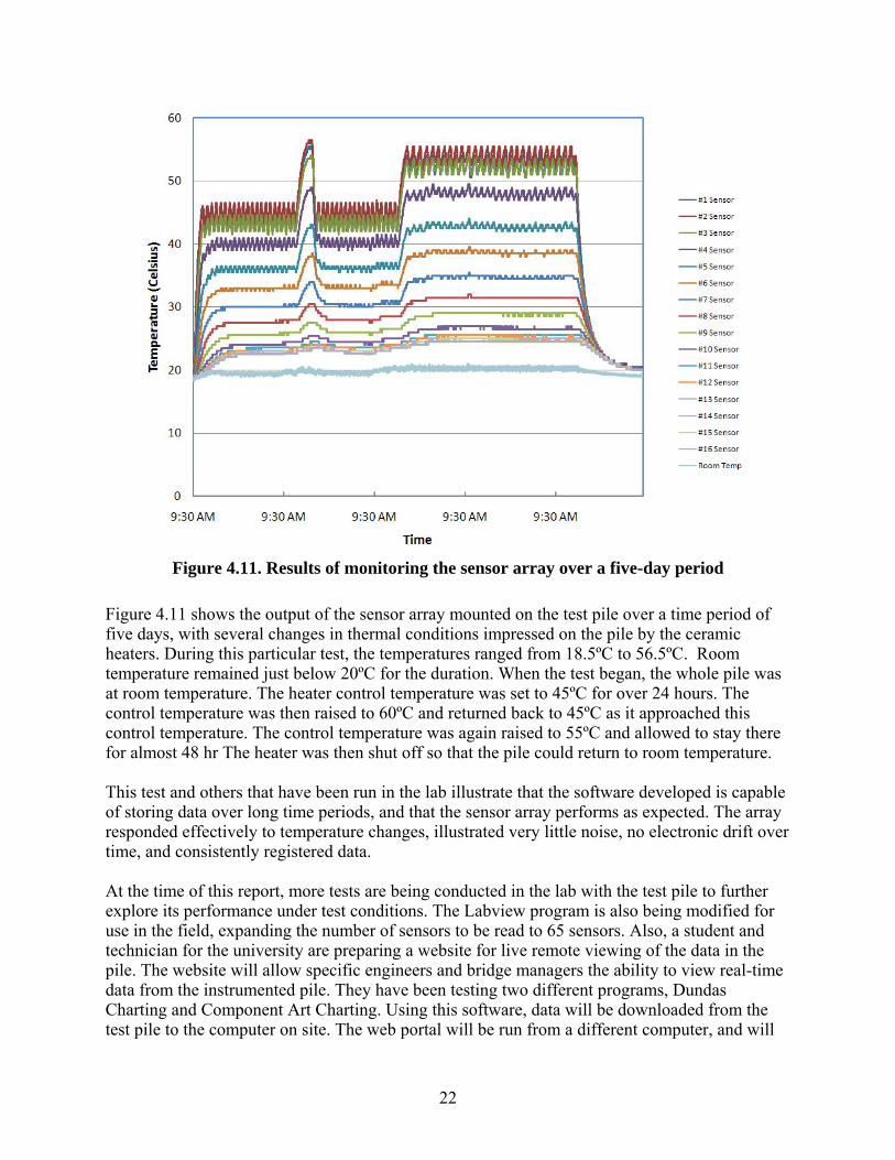
Figure 4.11. Results of monitoring the sensor array over a five-day period

Figure 4.11 shows the output of the sensor array mounted on the test pile over a time period of five days, with several changes in thermal conditions impressed on the pile by the ceramic heaters. During this particular test, the temperatures ranged from 18.5ºC to 56.5ºC. Room temperature remained just below 20ºC for the duration. When the test began, the whole pile was at room temperature. The heater control temperature was set to 45ºC for over 24 hours. The control temperature was then raised to 60ºC and returned back to 45ºC as it approached this control temperature. The control temperature was again raised to 55ºC and allowed to stay there for almost 48 hr The heater was then shut off so that the pile could return to room temperature. This test and others that have been run in the lab illustrate that the software developed is capable of storing data over long time periods, and that the sensor array performs as expected. The array responded effectively to temperature changes, illustrated very little noise, no electronic drift over time, and consistently registered data. At the time of this report, more tests are being conducted in the lab with the test pile to further explore its performance under test conditions. The Labview program is also being modified for use in the field, expanding the number of sensors to be read to 65 sensors. Also, a student and technician for the university are preparing a website for live remote viewing of the data in the pile. The website will allow specific engineers and bridge managers the ability to view real-time data from the instrumented pile. They have been testing two different programs, Dundas Charting and Component Art Charting. Using this software, data will be downloaded from the test pile to the computer on site. The web portal will be run from a different computer, and will

23

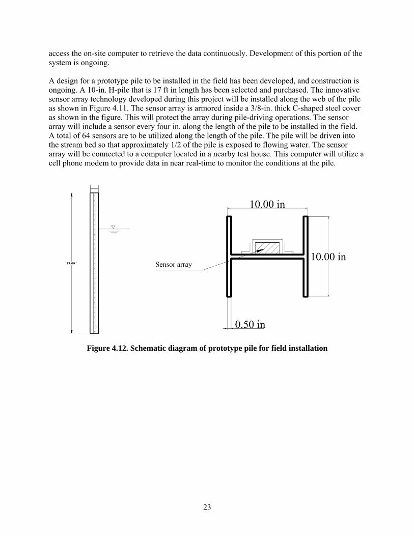
access the on-site computer to retrieve the data continuously. Development of this portion of the system is ongoing. A design for a prototype pile to be installed in the field has been developed, and construction is ongoing. A 10-in. H-pile that is 17 ft in length has been selected and purchased. The innovative sensor array technology developed during this project will be installed along the web of the pile as shown in Figure 4.11. The sensor array is armored inside a 3/8-in. thick C-shaped steel cover as shown in the figure. This will protect the array during pile-driving operations. The sensor array will include a sensor every four in. along the length of the pile to be installed in the field. A total of 64 sensors are to be utilized along the length of the pile. The pile will be driven into the stream bed so that approximately 1/2 of the pile is exposed to flowing water. The sensor array will be connected to a computer located in a nearby test house. This computer will utilize a cell phone modem to provide data in near real-time to monitor the conditions at the pile.

Figure 4.12. Schematic diagram of prototype pile for field installation

24

5. FUTURE WORK

The next step of the project is to prepare and deploy the full-size test pile in a creek on campus. The site that was chosen is on Hinkson Creek, near A.L. Gustin Golf Course. It was selected for the following reasons:

• There is enough access to the side of the creek to use a small backhoe for driving the pile.

• It is on the University of Missouri (MU) property, near another MU research project that will let us use electricity from their setup.

• The stream is known to rise and fall a few feet during storms, so that changes in the conditions at the pile can be effectively monitored by the sensor array.

To prepare the test pile, some large steel pieces have been purchased and machined. Two 10-ft long C-shapes have been delivered and will be welded together. Inside of those, the sensors will be attached and covered with the epoxy. The C-shapes will then be laid flush against the side of the HP shape, and both will be driven into the stream bed. An LPC-350 Mini PC from Stealth Computer Corporation was recently purchased for the on-site data collection. It was selected due to its small footprint and because it has a serial connection, which was needed for data acquisition through our setup. Figure 5.1 shows the front and back of the Mini PC. An on-site enclosure will house the computer and data acquisition system. This enclosure will include the Mini PC, keyboard, mouse, monitor, and a small air conditioner. Future research and development is required to develop a final implementation of this new technology. Because the 1-Wire sensors utilized are extremely low power and require a minimal amount of wiring, it is anticipated that this technology can be brought to maturity by the design of the solar- or battery-powered data acquisition system that can be installed on a pile in the field. Using a single-board computer, a data acquisition system with a very small footprint could be developed. This would enable the technology to be widely implemented for the monitoring of bridge assets in the field.

Figure 5.1. Front and back image of LPC-350

25

6. CONCLUSIONS

This research has explored the development of an instrumented pile for monitoring the scour conditions at a bridge. This monitoring technology is intended to improve the tools available for asset management by providing real-time data to owners and engineers on the site conditions at a bridge. An innovative new design for a temperature array that can be used in the field and that can be mounted on a pile has been developed and tested in the laboratory. This sensor array consists of a series of 1-Wire digital temperature sensors that are mounted on a polymer substrate of a printed circuit board. The technology for manufacturing printed circuit boards that will provide a durable trunk line system for assembling the sensor array has been developed as part of the project. Laboratory testing showed that the sensor array responded effectively to changing thermal conditions, and that software and data acquisition hardware performed reliably over long periods of time. The laboratory testing also showed that the temperature array responded with only a slight delay relative to thermocouples, which are commonly applied for temperature measurements in the field. The time lag for detecting thermal changes was only a few minutes, which is not expected to impact the effectiveness of the system in the field. A final design for a test pile to be implemented in the field has been developed. The construction of the field test pile is ongoing, and installation in the field is anticipated in the summer of 2008. Future research could include the development of a low-power, small-footprint data acquisition system that could be widely implemented in the field. Using the 1-Wire sensors developed through this research, a low-cost system could be developed for monitoring bridge assets effectively in the field.

26

7. REFERENCES

(1) Richardson, E.P.-O., JE; Schall, JD; Price, GR. MONITORING AND PLANS FOR ACTION FOR BRIDGE SCOUR: INSTRUMENTS AND STATE DEPARTMENTS OF TRANSPORTATION EXPERIENCES. in 9th International Bridge Management Conference 2003.

(2) Schall, J.P., GR, PORTABLE SCOUR MONITORING EQUIPMENT. NCHRP Report, 2004(515).

(3) FHWA, Evaluating Scour at Bridges, in HEC-18. 1995, Federal Highway Administration. (4) Olson, L.D. Determination of Unknown Depths of Bridge Foundations for Scour Safety

Investigations. in Structural Materials Technology V: An NDE Conference. 2004. Cincinnati, OH: American Society for Nondestructive Evaluation.

(5) Marron, D. Remote Monitoring of Structural Stability Using Electronic Clinometers. in Structural materials Technology IV. 2000. Atlantic City, NJ: Technomics, Inc.