remote estimation of in water constituents in coastal waters using neural networks

Remote estimation of in water constituents in coastal waters using

neural networks Ioannis Ioannou*a, Alexander Gilersona, Michael Ondrusekb, Soe Hlainga, Robert Fostera, Ahmed

El-Habashia, Kaveh Bastania and Samir Ahmeda

aOptical Remote Sensing Laboratory, Department of Electrical Engineering, City College of the City

University of New York, New York, New York, 10031, USA bNOAA/ NESDIS/STAR/SOCD, 5830 University Research Ct.

College Park, MD 20740

ABSTRACT

Remote estimations of oceanic constituents from optical reflectance spectra in coastal waters are challenging because of

the complexity of the water composition as well as difficulties in estimation of water leaving radiance in several bands

possibly due to inadequacy of current atmospheric correction schemes. This work focuses on development of a

multiband inversion algorithm that combines remote sensing reflectance measurements at several wavelengths in the

blue, green and red for retrievals of the absorption coefficients of phytoplankton, color dissolved organic matter and non-

algal particulates at 443nm as well as the particulate backscatter coefficient at 443nm. The algorithm was developed,

using neural networks (NN), and was designed to use as input measurements on ocean color bands matching those of the

Visible Infrared Imaging Radiometer Suite (VIIRS). The NN is trained on a simulated data set generated through a bio-

optical model for a broad range of typical coastal water parameters. The NN was evaluated using several statistical

indicators, initially on the simulated data-set, as well as on field data from the NASA bio-Optical Marine Algorithm

Data set, NOMAD, and data from our own field campaigns in the Chesapeake Bay which represent well the range of

water optical properties as well as chlorophyll concentrations in coastal regions.

The algorithm was also finally applied on a satellite - in situ databases that were assembled for the Chesapeake Bay

region using MODIS and VIIRS satellite data. These databases were created using in-situ chlorophyll concentrations

routinely measured in different locations throughout Chesapeake Bay and satellite reflectance overpass data that coexist

in time with these in-situ measurements. NN application on this data-sets suggests that the blue (412 and 443nm)

satellite bands are erroneous. The NN which was assessed for retrievals from VIIRS using only the 486, 551 and 671

bands showed that retrievals that omitted the 671 nm band was the most effective, possibly indicating an inaccuracy in

the VIIRS 671 band that needs to be further investigated.

Keywords: neural network, inversion, ocean color, chlorophyll, phytoplankton, CDOM, non algal particulates

1. INTRODUCTION

The need to produce robust algorithms for the remote assessment of chlorophyll-a biomass [Chl] in Chesapeake Bay has

been well described in recent work1, 2. The Chesapeake Bay estuary is a highly productive region dynamically variable

both spatially and temporally, with the water composition changing continuously. Inherent optical properties (IOP) of

the Chesapeake Bay waters are dominated by phytoplankton, color dissolved organic matter (CDOM), and non-algal

particulates (NAP) that are typically suspended sediment (TSS)3-6.

These optically significant constituents often do not co-vary, and the latter two can dominate light absorption at blue

wavelengths1, 4, 5, complicating the retrieval of phytoplankton absorption and thus the estimation of [Chl] when using

blue green band ratio algorithms7. These studies highlight the need to produce more precise algorithms for Case 2

waters. Nevertheless, in certain regions in Chesapeake Bay proper estimation of [Chl] may be difficult given the current

state of ocean color remote sensing as the natural variation of the water leaving signal due to the change in optical

properties is smaller than the effect of the uncertainty of the assessment of the signal due to inaccuracies of atmospheric

corrections8.

*[email protected]; phone 1 212 650-5876

Remote Sensing of the Ocean, Sea Ice, Coastal Waters, and Large Water Regions 2014, edited by Charles R. Bostater Jr., Stelios P. Mertikas, Xavier Neyt, Proc. of SPIE Vol. 9240, 92400T

© 2014 SPIE · CCC code: 0277-786X/14/$18 · doi: 10.1117/12.2067772

Proc. of SPIE Vol. 9240 92400T-1

Downloaded From: http://proceedings.spiedigitallibrary.org/ on 10/31/2015 Terms of Use: http://spiedigitallibrary.org/ss/TermsOfUse.aspx

Name of input parameter Mathematical model

total absorption a(λ)= aw(λ)+ aph(λ)+ ag(λ)+ ad(λ)

total scattering b(λ)= bw(λ)+ bph(λ)+ bNAP(λ)

total backscattering bb(λ)= 0.5*bw(λ)+ bbph(λ)+ bbNAP(λ)

CDOM spectral absorption slope Sg

CDOM absorption ag(λ) = ag(λo) * exp{Sg*(λo- λ)}

phytoplankton size parameter Sf

phytoplankton specific absorption aph*(λ) = Sf * apico

*(λ) + (1- Sf ) * amicro*(λ)

phytoplankton absorption aph(λ) = aph*(λ)/aph

*(443) * 0.05 * [Chl]0.62

phytoplankton attenuation cph(λ) = cph*( λo) * (λo/λ)Ychl * [Chl]

phytoplankton attenuation slope Ychl

phytoplankton scattering bph(λ) = cph(λ) - aph(λ)

phytoplankton backscattering ratio bbrph

phytoplankton backscattering bbph(λ) = bbrph * bph(λ)

NAP spectral absorption slope Sdm

NAP specific absorption ad*(λ) = ad

*(λo) * exp{Sdm*(λo- λ)}

NAP absorption ad(λ) = ad*(λ) * [NAP]

NAP specific scattering bdm*(λ) = bdm

*( λo) * (λo/λ)Ydm

NAP scattering bdm(λ) = bdm*( λ) * [NAP]

NAP scattering slope Ydm

NAP backscattering ratio bbrNAP

NAP backscattering bbNAP(λ) = bbrNAP * bNAP(λ)

Furthermore, these inaccuracies are more pronounced in the blue bands 410 and 440 nm when compared to the other

bands, making semi-analytical algorithms9, 10 for retrieval of water inherent optical properties (IOPs) also subject to large

errors, because these algorithms rely heavily especially on the 410nm band to estimate phytoplankton absorptions and

consequently [Chl].

Algorithms that use the red bands of the spectrum11, 12 (for MERIS 665 and 708nm bands) make more sense to be used in

this type of environment as they are not influenced by the CDOM and NAP absorption in the blue, or by atmospheric

correction13 since they are closer to the NIR bands used for atmospheric correction, but they were also found to be not

always stable when used together with MERIS atmospheric correction. In addition, current satellite sensors (MODIS and

VIIRS) don't have the required red band around 708nm.

Finally algorithms proposed in recent studies1, 2, that use the red and green bands for [Chl] retrieval, don't seem to have a

strong theoretical basis. Although they appear to work well in several regions, the underlying mechanism is not clearly

understood. They are probably based on co-variation of CDOM and NAP absorption and phytoplankton absorption in

530 – 670nm spectral region, but these relationships should be very region specific. That is probably why these

algorithms2 have a large bias in their calibration coefficients to accommodate the average [Chl] in that region. Another

promising method is the application of multilayer perceptron, MLP, neural networks (NN)14-16, as they are seen as a class

of universal approximators17. A NN, if trained properly, can yield retrievals that are accurate and relatively insensitive to

reasonable noise levels, since noise can be introduced during the training process to smooth the data and force the

network to find a more general model for the solution to a problem. The benefit of NNs is that no real understanding of

the inversion is necessary, but such inversion is highly dependent on the parameterization of the training data set. If this

data set is composed from measurements, it might be prone to instrumentation errors and other factors that can introduce

biases and that will be embedded into the algorithm. On the other hand, if the data are modeled and simulated, the

algorithm will have biases when tested on the real situation. The origin of these mismatches is difficult to assess.

Table 1. Bio-optical model inputs

2. DATA

2.1 Simulated Dataset

A four component bio-optical model dataset with constituent inputs typical for the Chesapeake Bay region, was

generated for the purposes of this study and consists of a total of 10000 data points. The four components are water,

phytoplankton, colored dissolved organic matter (CDOM) and non algal particulates (NAP). The phytoplankton



Parameter Value/Range

aph( λo) | λo=443nm lognormal (μ=-1.6,σ=0.75)

ag(λo) | λo=443nm f(aph( λo))a

ad(λo) | λo=443nm f(aph( λo))b

ad*(λo) | λo=443nm 0.02-0.08 (uniform)

Sf 0.75/(1+5[Chl])+0.25Ψ1 |Ψ1 =uniform

Sg 0.0175+0.001Ψ2 | Ψ2 =normal

SNAP 0.01+0.001Ψ3 | Ψ3 =normal

Cph*( λo) | λo=550nm 0.3+0.03Ψ4 | Ψ4 =normal

bNAP*( λo) | λo=550nm 0.2-1.5 (uniform)

YChl f([Chl])c

YNAP f([NAP])d

bbrph 0.006+0.0005Ψ5 | Ψ5 =normal

bbrNAP 0.02+0.001Ψ6 | Ψ6 =normal

absorption spectral shape was modeled as a function of cell size parameter, Sf 18 and [Chl]. CDOM and NAP absorptions

were modeled as exponential decay functions with different slopes. Phytoplankton scattering was modeled as the

difference between the attenuation and absorption of phytoplankton cells. For the modeling of each parameter and for

the range and distribution of each parameter refer to Table1 and Table 2 respectively. Several studies illustrate in detail

how bio-optical models are generated.10, 15, 19. To generate Rrs we used the coefficients proposed in a previous study that

are derived using HydrolightTM.19

Table 2. Range and distribution of parameters in bio-optical model

a10(0.41+0.15Ψ7) aph( λo)1.15/(1+3.3 aph( λo)1.1) | Ψ7 = normal

b7.5x10-4+10(0.51+0.2Ψ8) aph( λo)1.83/(1+6.5 aph( λo)2) | Ψ8 = normal

c(2.5+0.25Ψ9)./(1+5[Chl]1.5)+0.2Ψ10+0.3 | Ψ9, Ψ10 = normal d(2.5+0.25Ψ11)./(1+5[NAP]1.5)+0.3Ψ12+0.4 | Ψ11, Ψ12 = normal

Ψ1-12 = random variables

2.2 Field measurements

Field data collected at 43 stations (Figure 1a) in the Chesapeake Bay during an August 2013 cruise were used in this

study (CCNY dataset). This dataset consists of co-located apparent and inherent optical properties (AOP and IOP)

measurements. IOP measurements include under water measurements of absorption and attenuation coefficients using an

ac-s instrument (WetLABs). Absorption of CDOM was measured separately with the 0.2 um filter attached prior to the

absorption tube. The backscattering coefficient was measured at 7 wavelengths by a bb-9 instrument (WetLABs).

Particulate matter was also measured by filtration of samples onto a glass filter in accordance with NASA protocols20.

Methanol was used for the removal of organic matter and absorption was obtained using path length amplification 21.

Thus we obtained the independent components of the absorption coefficient that are due to phytoplankton, CDOM and

NAP. Upwelling radiance was measured by a GER instrument (SpectraVista) with the 6m fiber attached and with the tip

of the fiber positioned just below the water surface. Above water radiance was measured by the same fiber with the

sunlight reflected from the Lambertian plate (Labsphere). The ratio of these measurements was transformed to the

remote sensing reflectance (Rrs) spectra above water. The NASA Bio-Optical Marine Dataset (NOMAD)22 with

locations (Figure 1b) within the Bay were also used in the study for the validation.

2.3 MODIS matched-up dataset

MODIS-aqua Rrs data were used and matched up with in-situ [Chl] data from the Water Quality Monitoring Program,

which is a part of the Chesapeake Bay Program (CBP - http://www.chesapeakebay.net/). [Chl] is measured among 19

water quality parameters at 49 fixed stations every month since 1984 throughout the Bay region. This is the same dataset

that was assembled and used in a similar manner for the purposes of a previous study2 and kindly shared with our group

by Drs C. Le and C. Hu (University of South Florida). The total dataset consists of about 1100 records.



US

U!

37S

»sLongilude

me s » s

2.4 VIIRS dataset

VIIRS Rrs data sets were acquired from more than 2000 images over the Chesapeake Bay which had concurrent in-situ

measurements of [Chl]. After a very strict data filtering following approaches executed in the recent study23 only 63

records were left for consideration. Specifically, for VIIRS Rrs and [Chl] data used for match-up comparison with

Chesapeake Bay program, in-situ [Chl] data are all extracted from the relevant 3 × 3 pixel box centered at the specific

site locations where the in-situ [Chl] measurements were actually made. Then satellite data are spatially averaged and

compared with the in-situ [Chl]. In the averaging of satellite data, any individual pixel is excluded from the match-up

comparison process if it has been flagged, through the data processing, by at least one of the following conditions: land,

cloud, failure in atmospheric correction, stray light, bad navigation quality, both high and moderate glint, negative

Rayleigh-corrected radiance, viewing angle larger than 60°, and solar zenith angle larger than 70°. Moreover, data of any

individual pixels which have water-leaving radiance spectra with negative values in one of the wavelength are also

excluded from spatial averaging. Furthermore, any individual pixel with its center location more than 2 km away from

the in-situ site locations are also excluded from this spatial averaging.

Figure 1. Station locations of August 2013 field campaign (a) and locations of the NOMAD stations within Chesapeake Bay

(b).

3. METHODS

3.1 Neural networks techniques

A neural network is used to model the relationship between Rrs values at 486, 551 and 671nm available on the VIIRS

sensor and phytoplankton absorption (aph), non-phytoplankton absorption (adg) and particulate backscattering bbp

coefficients at 443nm. Thereafter the aph(443) can be converted to [Chl] using an assumed for the region specific

absorption of phytoplankton of 0.03 m2mg-1. The Rrs values at 410 and 443nm were intentionally omitted from the inputs

as their use significantly degrades the performance of the algorithms when applied to satellite data. Both the inputs and

the outputs to the neural network were transformed to their log10 domain and standardized by removing the mean and

scaling the variances before the training stage.

We have used one-hidden-layer multilayer percepton (MLP) with four neurons in the hidden layer to train both

networks. We chose five neurons since we have five inputs, and since this architecture was able to model our problem

well we did not explore how this relationship would be improved by increasing the number of neurons or layers. The

network was trained using all 10000 Rrs - IOPs combinations. To make this network insensitive to noise, we choose to

train the network with 5% (of the intensity at each Rrs) uniformly distributed noise at each input.



o10

Data (R2 = 0.982 a = 0.209. N = 10000)

- -e- Y -1.004 X +0.008Y-X

- - -Y=2X&X2

10Data =0.97& s=0.255. N=10000)

-9- Y- 1.007X+0.010Y-X

- - -Y=2X&X/2

1Ó

10 10

retrieved a (443), m1Ph

10

I Data (121 = 0978, s= 0321. N= 10000-9- Y - 1.003X+0 006

Y-X- - -Y=2X&X2

10v

16' 10

retrieved a(443), m -1

010

10

10

10b 10 io

retrieved aß443), m -1

10

..:

10

I

10 10 10

retrieved bb (443), m -1

o10

The Levenberg-Marquardt optimization with Bayesian Regularization algorithm was used to train this network24. The

algorithm combines Levenberg-Marquardt, a combination of steepest descent and Gauss-Newton method, and regulates

the network with Bayes’ rule in order to minimize the combination of squared errors and weights and determine the

correct combination of coefficients to create a network which is robust and generalizes well without a validation dataset

being necessary. Once these criteria are met it automatically ends the training without external end condition. The exact

implementation algorithm, with the default parameters that was used, can be found in the neural network toolbox of

MatLabTM 7.12.0 (2011a).

4. RESULTS

4.1 CCNY synthetic data

Figure 2. Performance of the Neural Network on the part of our simulated dataset that was not used in the training stage.

Retrieved aph(443) m-1, ag(443) m-1, ad(443) m-1 and bbp(443) m-1 (x-axis) plotted against the “input” values for these

parameters from our simulated dataset.

We first test the NN on 10000 noiseless additional testing data. The retrieval performance of the NN for the simulated

dataset with different noise levels is shown in Figure 2. These show that the retrieval performance of the phytoplankton,

CDOM and NAP absorption coefficient and backscattering coefficient at 443 nm is excellent, with R2 coefficients of

over 98% and a linear percentage error (ε) of 20%, 26%, 33% and 13% for each parameter respectively, where,



10°

Data (Rz=0.840, e=0.284, N = 43)-9- Y= 1.054 X +0.008 /

Y = X .---Y=2X&X2 , /

i'i

/"/

/

.-..o /

/

10' 10°

retrieved aah(443'' m-1

Data (Rz=0.839,s=0.320,N=43)-9- Y= 1.052 X +-0.02 /

Y-X- - Y=2X&X2 . //

/ .q

t/ ./

t/

/'u

/

10'

retrieved ad (443), m

10.

Data (Rz=0.784, e=0.212, N = 43) /-e- Y = 0.786 X +-0.06 / -- Y = X

---Y=2X&X2/, ri/ . /'

iZ/" /

/,c

/ /y

/10' 10D

retrieved aß(443), m

/Data (Rz=0.866,s=0.330,N=43) /'

-9- Y = 1.109 X +0.095 / j ¡----Y -X /" :---.Y=2X&X/2 ,- / -/ /'/' . . /'

/' O/' .. .

/I/

102 10'

retrieved bb (443), m-1

ε =log1010 1

RMSE (1)

and

1

22

10 101

1ˆlog log

N

log10 i iiRMSE x x

N

(2)

with ix and ˆix being the measured and estimated value of a parameter respectively.

4.2 CCNY Field Data

We observe the effectiveness of the NN algorithm on our field data in Figures 3 and 4.Although R2 values degrade, due

to the narrower range of the measured parameters when compared to the range in our simulation data, the algorithm

seems very effective with a linear percentage error for each parameter close the values derived when testing on

simulated data. This is an unambiguous test clearly demonstrating the efficacy of the NN for excellent retrievals from in-

situ measured Rrs values that are un-impacted by atmospheric effects etc. [Chl] was calculated from the NN retrieved

phytoplankton absorption at 443 nm by using the relationship aph(443) =0.07[Chl]0.76. We need to note here that this

values in relationship are different from those used as input to our simulated dataset.

Figure 3. Performance of the Neural Network on our field data. Retrieved aph(443) m-1, ag(443) m-1, ad(443) m-1 and

bbp(443) m-1 (x-axis) plotted against the measured values for these parameters from our simulated dataset.



M

Eoc

10'

Ú

Z 1o°

e -

: Aata(R2=0723:=0515,N=43)

,"..,,

,!'. i

,",;

),

,-e-Y0991X*-001-Y'X--Y=2X6X/!

,,

, . .,,

Neural Network

10°

1o'

10°

Nis (fl1 0.631, :. 0.728, N .13)-A- Y - 1.209 X -0 32-Y=X--Y2X6X/1 r j,

10' 10°

retrieved [ChM] 0C3, mg M-3

10'

Das (Rr=0473 e=0á3D,N=16bY 0714X+-0 .12-Y X

Y2X6XQ:!,

y t Sr . .4, 0.,%.: ,r.:as

.

.

t0°

cO.ts(R1=0487, e=0638, N. 182)

. -0- Y 0657X+-0 23-Y X

1Ò 10'

retrieved aaph(443), ni

10°

10° tÒ'

retrieved a j443), mtt0°

Oats (R1=0272 e=0324,N=184-0Y=0437X+-022-Y X

Y2X6X/2

.

i.

'.,i. 4!* .% ¡:+ .

«

'tÒ' 10

retrieved 8(443), m-1

Figure 4. Performance of the Neural Network on the NOMAD data within Chesapeake Bay. Retrieved [Chl] using NN (left)

and OC3(right) against the in-situ measured value. NN retrieved [Chl] was calculated as (aph(443)/0.07)(1/0.76).

4.3 NOMAD

Figure 5. Performance of the Neural Network on the NOMAD data within Chesapeake Bay. Retrieved aph(443) m-1,

ag(443) m-1 and ad(443) m-1 and apg(443) m-1 (x-axis) plotted against the measured values for these parameters.



102 Cots (R2 0265. s 0951, N 2[7)-0-Y=0.756X0.179-Y-X- - Y=2X6X/2 '",; ,

,/y., .v ... ;:4.*'.'='t.':.ï ;.i!'' _. t.

i ..' i Neumal Network.: '

to

retrieved ph /-1431 0.03, t10'

102

10'

10

retrieved [ChM], mg /m3

10'

ao'OttS(R? 0260, s. 0767, N 767)

-0- Y 0622X .0352 I-Y X--Y.2XdX/2 ; , .

añ' t11 .' -r':' =: ti

s..,. ..w 'wí ';

% se , r -

+Ó

retrieved áh m(443)/0.03, 1

+o'

to'

+o°

+o= +o° +o' +o°

retrieved [Chi], mg /m3

We also observe the efficacy of the NN algorithm when applied to the NOMAD in Figures 5 and 6. Although R2 values

degrade even more, most likely due to increased uncertainties in the data measured by multiple groups, the algorithm

still seems quite effective with a linear percentage error for each parameter about double the values derived when testing

on simulated data. Unfortunately there are not bbp(443) available in the nomad for comparison. The relationship of the

NN retrieved phytoplankton absorption to [Chl] for the NOMAD is linear with [Chl] and is given by 0.03[Chl] which is

different than both the relationship we used as input to our simulation as well as the one derived in our field

measurements. This specific absorption remains constant and is used next when we apply the algorithm on MODIS and

VIIRS data.

Figure 6. Performance of the Neural Network on the NOMAD data within Chesapeake Bay. Retrieved [Chl] using NN (left)

and OC3 (right) against the in-situ measured value.

4.4 MODIS

Figure 7. Performance of the Neural Network on MODIS data within Chesapeake Bay. Retrieved [Chl] using NN (left) and

OC3 (right) against the in-situ measured value.



[ChlbiN [Chl]oc_v

20

18

16

14

12

10

ij

6

4

150

40

30

20

10

0

-10

-20

-30

-40

-50

200x([Chl]-[Chl]oc;--)([Chl]-N+[Chl]oc3-0

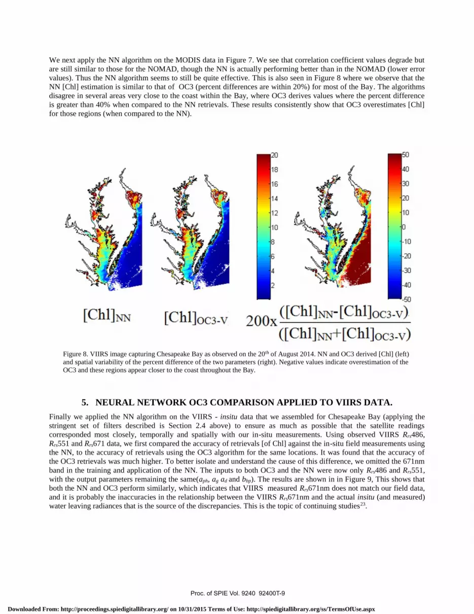
We next apply the NN algorithm on the MODIS data in Figure 7. We see that correlation coefficient values degrade but

are still similar to those for the NOMAD, though the NN is actually performing better than in the NOMAD (lower error

values). Thus the NN algorithm seems to still be quite effective. This is also seen in Figure 8 where we observe that the

NN [Chl] estimation is similar to that of OC3 (percent differences are within 20%) for most of the Bay. The algorithms

disagree in several areas very close to the coast within the Bay, where OC3 derives values where the percent difference

is greater than 40% when compared to the NN retrievals. These results consistently show that OC3 overestimates [Chl]

for those regions (when compared to the NN).

Figure 8. VIIRS image capturing Chesapeake Bay as observed on the 20th of August 2014. NN and OC3 derived [Chl] (left)

and spatial variability of the percent difference of the two parameters (right). Negative values indicate overestimation of the

OC3 and these regions appear closer to the coast throughout the Bay.

5. NEURAL NETWORK OC3 COMPARISON APPLIED TO VIIRS DATA.

Finally we applied the NN algorithm on the VIIRS - insitu data that we assembled for Chesapeake Bay (applying the

stringent set of filters described is Section 2.4 above) to ensure as much as possible that the satellite readings

corresponded most closely, temporally and spatially with our in-situ measurements. Using observed VIIRS Rrs486,

Rrs551 and Rrs671 data, we first compared the accuracy of retrievals [of Chl] against the in-situ field measurements using

the NN, to the accuracy of retrievals using the OC3 algorithm for the same locations. It was found that the accuracy of

the OC3 retrievals was much higher. To better isolate and understand the cause of this difference, we omitted the 671nm

band in the training and application of the NN. The inputs to both OC3 and the NN were now only Rrs486 and Rrs551,

with the output parameters remaining the same(aph, ag ad and bbp). The results are shown in in Figure 9, This shows that

both the NN and OC3 perform similarly, which indicates that VIIRS measured Rrs671nm does not match our field data,

and it is probably the inaccuracies in the relationship between the VIIRS Rrs671nm and the actual insitu (and measured)

water leaving radiances that is the source of the discrepancies. This is the topic of continuing studies23.



data (R20231,s0.721,N63)-0- Y = 0.652 X +0276-YX /--Y=2X6XR i

lo'

retrieved aPh(443)/0.03, m"1

to'

Data (R2=0250, s=0.818, N=63)--0- V -0 713 X +.160-Y-X .--V=2X6XR ;.

lot

retrieved [ChM], mg m3

Figure 9. Performance of the Neural Network with only Rrs 486 and 551nm inputs on VIIRS data within Chesapeake Bay.

Retrieved [Chl] using NN (left) and OC3 (right) against the in-situ measured value. As expected the result is very similar.

6. SUMMARY

We have developed a neural network retrieval algorithm, primarily for the Chesapeake Bay region, that depends on the

optical signal that is measured just above water at specific wavelengths available from all ocean color sensors. We used

a neural network to model the inverse problem and retrieved 4 components of the water body; the phytoplankton,

CDOM and NAP absorption coefficients as well as the particulate backscattering coefficient at 443 nm. We successfully

retrieve these parameters in our simulated dataset, and further validated the algorithm on our field measurements and the

NOMAD stations within Chesapeake Bay.

We further applied the neural network on satellite Rrs data measured for pixels where the in-situ [Chl] was available.

Satellite data consisted measurements from both the VIIRS and MODIS sensors. The algorithm appeared to perform

better on MODIS data and less accurately on VIIRS. In contrast, OC3 performed better than the NN on the VIIRS data

and worse on MODIS data. To further investigate this mismatch of the NN with the VIIRS data, we choose to train a

new neural network based on the same input bands that OC3 uses in coastal waters, namely Rrs486 and Rrs551. Upon

application of this new neural network, we observed that both NN and OC3 algorithms exhibit similar retrieval

performance, leading to the conclusion that the Rrs671nm band on VIIRS may have glitches that need to be further

investigated.

ACKNOWLEDGMENTS

This work was partially supported by grants from ONR and NOAA.

REFERENCES

[1] M. Tzortziou, A. Subramaniam, J. R. Herman et al., “Remote sensing reflectance and inherent optical properties in

the mid Chesapeake Bay,” Estuarine, Coastal and Shelf Science, 72(1–2), 16-32 (2007).

[2] C. Le, C. Hu, J. Cannizzaro et al., “Long-term distribution patterns of remotely sensed water quality parameters in

Chesapeake Bay,” Estuarine, Coastal and Shelf Science, 128(0), 93-103 (2013).

[3] J. E. Tyler, & Preisendorfer, R. W., [In The Sea, Vol. 2] Interscience., New York(1962).

[4] A. Magnuson, L. W. Harding Jr, M. E. Mallonee et al., “Bio-optical model for Chesapeake Bay and the Middle

Atlantic Bight,” Estuarine, Coastal and Shelf Science, 61(3), 403-424 (2004).



[5] A. A. Gitelson, J. F. Schalles, and C. M. Hladik, “Remote chlorophyll-a retrieval in turbid, productive estuaries:

Chesapeake Bay case study,” Remote Sensing of Environment, 109(4), 464-472 (2007).

[6] C. L. Gallegos, D. L. Correll, and J. W. Pierce, “Modeling spectral diffuse attenuation, absorption, and scattering

coefficients in a turbid estuary,” Limnology and Oceanography, 35(7), 1486-1502 (1990).

[7] M. Tzortziou, J. R. Herman, C. L. Gallegos et al., “Bio-optics of the Chesapeake Bay from measurements and

radiative transfer closure,” Estuarine, Coastal and Shelf Science, 68(1–2), 348-362 (2006).

[8] L. W. Harding Jr, A. Magnuson, and M. E. Mallonee, “SeaWiFS retrievals of chlorophyll in Chesapeake Bay and

the mid-Atlantic bight,” Estuarine, Coastal and Shelf Science, 62(1–2), 75-94 (2005).

[9] P. Wang, E. S. Boss, and C. Roesler, “Uncertainties of inherent optical properties obtained from semianalytical

inversions of ocean color,” Applied Optics, 44(19), 4074-4085. (2005).

[10] Z. P. Lee, K. L. Carder, and R. A. Arnone, “Deriving inherent optical properties from water color: a multiband

quasi-analytical algorithm for optically deep waters,” Applied Optics, 41(27), 5755-5772. (2002).

[11] A. A. Gitelson, G. Dall'Olmo, W. Moses et al., “A simple semi-analytical model for remote estimation of

chlorophyll-a in turbid waters: Validation,” Remote Sensing of Environment, 112(9), 3582-3593 (2008).

[12] A. A. Gilerson, A. A. Gitelson, J. Zhou et al., “Algorithms for remote estimation of chlorophyll-a in coastal and

inland waters using red and near infrared bands,” Optics Express, 18(23), 24109-24125 (2010).

[13] H. R. Gordon, and M. Wang, “Retrieval of water-leaving radiance and aerosol optical thickness over the oceans

with SeaWiFS: a preliminary algorithm,” Applied Optics, 33, 443-452 (1994).

[14] I. Ioannou, A. Gilerson, B. Gross et al., “Deriving ocean color products using neural networks,” Remote Sensing of

Environment, 134(0), 78-91 (2013).

[15] I. Ioannou, A. Gilerson, B. Gross et al., “Neural network approach to retrieve the inherent optical properties of the

ocean from observations of MODIS,” Applied Optics, 50(19), 3168-3186. (2011).

[16] R. Doerffer, and H. Schiller, “The MERIS case 2 water algorithm,” International Journal of Remote Sensing, 28(3-

4), 517-535. (2007).

[17] K. Hornik, M. Stinchcombe, and H. White, “Multilayer feedforward networks are universal approximators,” Neural

networks, 2(5), 359-366 (1989).

[18] A. M. Ciotti, M. R. Lewis, and J. J. Cullen, “Assessment of the relationships between dominant cell size in natural

phytoplankton communities and the spectral shape of the absorption coefficient,” Limnology and Oceanography,

47(2), 404-417. (2002).

[19] Z. Lee, K. L. Carder, C. D. Mobley et al., “Hyperspectral remote sensing for shallow waters. 2. Deriving bottom

depths and water properties by optimization,” Applied Optics, 38(18), 3831-3843 (1999).

[20] J. L. Mueller, G. S. Fargion, C. R. McClain et al., “Ocean Optics Protocols For Satellite Ocean Color Sensor

Validation, Revision 5, Volume VI: Special Topics in Ocean Optics Protocols, Part 2,” (2003).

[21] A. Bricaud, and D. Stramski, “Spectral absorption coefficients of living phytoplankton and nonalgal biogenous

matter: A comparison between the Peru upwelling area and the Sargasso Sea.”

[22] P. J. Werdell, and S. W. Bailey, “An improved in-situ bio-optical data set for ocean color algorithm development

and satellite data product validation,” Remote Sensing of Environment, 98(1), 122-140. (2005).

[23] S. Hlaing, A. Gilerson, R. Foster et al., “Radiometric calibration of ocean color satellite sensors using AERONET-

OC data,” Optics Express, 22(19), 23385-23401 (2014).

[24] F. D. Foresee, & Hagan, M.T. , "Gauss-Newton approximation to Bayesian learning." In Proceedings of the 1997

international joint conference on neural networks, vol. 3, pp. 1930-1935. Piscataway: IEEE, (1997).



remote estimation of in water constituents in coastal waters using neural networks

Documents