reliability of computer systems and networks
TRANSCRIPT
Reliability of Computer Systems and Networks: Fault Tolerance, Analysis, and DesignMartin L. Shooman
Copyright 2002 John Wiley & Sons, Inc.ISBNs: 0-471-29342-3 (Hardback); 0-471-22460-X (Electronic)
RELIABILITY OFCOMPUTER SYSTEMSAND NETWORKS
RELIABILITY OFCOMPUTER SYSTEMSAND NETWORKS
Fault Tolerance, Analysis, andDesign
MARTIN L. SHOOMANPolytechnic University
andMartin L. Shooman & Associates
A Wiley-Interscience Publication
JOHN WILEY & SONS, INC.
Designations used by companies to distinguish their products are often claimed as trademarks.In all instances where John Wiley & Sons, Inc., is aware of a claim, the product names appearin initial capital or ALL CAPITAL LETTERS. Readers, however, should contact the appropriatecompanies for more complete information regarding trademarks and registration.
Copyright 2002 by John Wiley & Sons, Inc., New York. All rights reserved.
No part of this publication may be reproduced, stored in a retrieval system or transmittedin any form or by any means, electronic or mechanical, including uploading, downloading,printing, decompiling, recording or otherwise, except as permitted under Sections 107 or 108of the 1976 United States Copyright Act, without the prior written permission of the Publisher.Requests to the Publisher for permission should be addressed to the Permissions Department,John Wiley & Sons, Inc., 605 Third Avenue, New York, NY 10158-0012, (212) 850-6011, fax(212) 850-6008, E-Mail: PERMREQ @ WILEY.COM.
This publication is designed to provide accurate and authoritative information in regard to thesubject matter covered. It is sold with the understanding that the publisher is not engaged inrendering professional services. If professional advice or other expert assistance is required, theservices of a competent professional person should be sought.
ISBN 0-471-22460-X
This title is also available in print as ISBN 0-471-29342-3.
For more information about Wiley products, visit our web site at www.Wiley.com.

To Danielle Leah and Aviva Zissel
vii
CONTENTS
Preface xix
1 Introduction 1
1.1 What is Fault-Tolerant Computing?, 11.2 The Rise of Microelectronics and the Computer, 4
1.2.1 A Technology Timeline, 41.2.2 Moore’s Law of Microprocessor Growth, 51.2.3 Memory Growth, 71.2.4 Digital Electronics in Unexpected Places, 9
1.3 Reliability and Availability, 101.3.1 Reliability Is Often an Afterthought, 101.3.2 Concepts of Reliability, 111.3.3 Elementary Fault-Tolerant Calculations, 121.3.4 The Meaning of Availability, 141.3.5 Need for High Reliability and Safety in Fault-
Tolerant Systems, 151.4 Organization of the Book, 18
1.4.1 Introduction, 181.4.2 Coding Techniques, 191.4.3 Redundancy, Spares, and Repairs, 191.4.4 N-Modular Redundancy, 201.4.5 Software Reliability and Recovery Techniques, 201.4.6 Networked Systems Reliability, 211.4.7 Reliability Optimization, 221.4.8 Appendices, 22
viii CONTENTS
General References, 23References, 25Problems, 27
2 Coding Techniques 30
2.1 Introduction, 302.2 Basic Principles, 34
2.2.1 Code Distance, 342.2.2 Check-Bit Generation and Error Detection, 35
2.3 Parity-Bit Codes, 372.3.1 Applications, 372.3.2 Use of Exclusive OR Gates, 372.3.3 Reduction in Undetected Errors, 392.3.4 Effect of Coder–Decoder Failures, 43
2.4 Hamming Codes, 442.4.1 Introduction, 442.4.2 Error-Detection and -Correction Capabilities, 452.4.3 The Hamming SECSED Code, 472.4.4 The Hamming SECDED Code, 512.4.5 Reduction in Undetected Errors, 522.4.6 Effect of Coder–Decoder Failures, 532.4.7 How Coder–Decoder Failures Effect SECSED
Codes, 562.5 Error-Detection and Retransmission Codes, 59
2.5.1 Introduction, 592.5.2 Reliability of a SECSED Code, 592.5.3 Reliability of a Retransmitted Code, 60
2.6 Burst Error-Correction Codes, 622.6.1 Introduction, 622.6.2 Error Detection, 632.6.3 Error Correction, 66
2.7 Reed–Solomon Codes, 722.7.1 Introduction, 722.7.2 Block Structure, 722.7.3 Interleaving, 732.7.4 Improvement from the RS Code, 732.7.5 Effect of RS Coder–Decoder Failures, 73
2.8 Other Codes, 75References, 76Problems, 78
3 Redundancy, Spares, and Repairs 83
3.1 Introduction, 853.2 Apportionment, 85
CONTENTS ix
3.3 System Versus Component Redundancy, 863.4 Approximate Reliability Functions, 92
3.4.1 Exponential Expansions, 923.4.2 System Hazard Function, 943.4.3 Mean Time to Failure, 95
3.5 Parallel Redundancy, 973.5.1 Independent Failures, 973.5.2 Dependent and Common Mode Effects, 99
3.6 An r-out-of-n Structure, 1013.7 Standby Systems, 104
3.7.1 Introduction, 1043.7.2 Success Probabilities for a Standby System, 1053.7.3 Comparison of Parallel and Standby Systems, 108
3.8 Repairable Systems, 1113.8.1 Introduction, 1113.8.2 Reliability of a Two-Element System with
Repair, 1123.8.3 MTTF for Various Systems with Repair, 1143.8.4 The Effect of Coverage on System
Reliability, 1153.8.5 Availability Models, 117
3.9 RAID Systems Reliability, 1193.9.1 Introduction, 1193.9.2 RAID Level 0, 1223.9.3 RAID Level 1, 1223.9.4 RAID Level 2, 1223.9.5 RAID Levels 3, 4, and 5, 1233.9.6 RAID Level 6, 126
3.10 Typical Commercial Fault-Tolerant Systems: Tandemand Stratus, 1263.10.1 Tandem Systems, 1263.10.2 Stratus Systems, 1313.10.3 Clusters, 135References, 137Problems, 139
4 N-Modular Redundancy 145
4.1 Introduction, 1454.2 The History of N-Modular Redundancy, 1464.3 Triple Modular Redundancy, 147
4.3.1 Introduction, 1474.3.2 System Reliability, 1484.3.3 System Error Rate, 1484.3.4 TMR Options, 150
x CONTENTS
4.4 N-Modular Redundancy, 1534.4.1 Introduction, 1534.4.2 System Voting, 1544.4.3 Subsystem Level Voting, 154
4.5 Imperfect Voters, 1564.5.1 Limitations on Voter Reliability, 1564.5.2 Use of Redundant Voters, 1584.5.3 Modeling Limitations, 160
4.6 Voter Logic, 1614.6.1 Voting, 1614.6.2 Voting and Error Detection, 163
4.7 N-Modular Redundancy with Repair, 1654.7.1 Introduction, 1654.7.2 Reliability Computations, 1654.7.3 TMR Reliability, 1664.7.4 N-Modular Reliability, 170
4.8 N-Modular Redundancy with Repair and ImperfectVoters, 176
4.8.1 Introduction, 1764.8.2 Voter Reliability, 1764.8.3 Comparison of TMR, Parallel, and Standby
Systems, 1784.9 Availability of N-Modular Redundancy with
Repair and Imperfect Voters, 1794.9.1 Introduction, 1794.9.2 Markov Availability Models, 1804.9.3 Decoupled Availability Models, 183
4.10 Microcode-Level Redundancy, 1864.11 Advanced Voting Techniques, 186
4.11.1 Voting with Lockout, 1864.11.2 Adjudicator Algorithms, 1894.11.3 Consensus Voting, 1904.11.4 Test and Switch Techniques, 1914.11.5 Pairwise Comparison, 1914.11.6 Adaptive Voting, 194
References, 195Problems, 196
5 Software Reliability and Recovery Techniques 202
5.1 Introduction, 2025.1.1 Definition of Software Reliability, 2035.1.2 Probabilistic Nature of Software
Reliability, 2035.2 The Magnitude of the Problem, 205
CONTENTS xi
5.3 Software Development Life Cycle, 2075.3.1 Beginning and End, 2075.3.2 Requirements, 2095.3.3 Specifications, 2095.3.4 Prototypes, 2105.3.5 Design, 2115.3.6 Coding, 2145.3.7 Testing, 2155.3.8 Diagrams Depicting the Development Process, 218
5.4 Reliability Theory, 2185.4.1 Introduction, 2185.4.2 Reliability as a Probability of Success, 2195.4.3 Failure-Rate (Hazard) Function, 2225.4.4 Mean Time To Failure, 2245.4.5 Constant-Failure Rate, 224
5.5 Software Error Models, 2255.5.1 Introduction, 2255.5.2 An Error-Removal Model, 2275.5.3 Error-Generation Models, 2295.5.4 Error-Removal Models, 229
5.6 Reliability Models, 2375.6.1 Introduction, 2375.6.2 Reliability Model for Constant Error-Removal
Rate, 2385.6.3 Reliability Model for Linearly Decreasing Error-
Removal Rate, 2425.6.4 Reliability Model for an Exponentially Decreasing
Error-Removal Rate, 2465.7 Estimating the Model Constants, 250
5.7.1 Introduction, 2505.7.2 Handbook Estimation, 2505.7.3 Moment Estimates, 2525.7.4 Least-Squares Estimates, 2565.7.5 Maximum-Likelihood Estimates, 257
5.8 Other Software Reliability Models, 2585.8.1 Introduction, 2585.8.2 Recommended Software Reliability Models, 2585.8.3 Use of Development Test Data, 2605.8.4 Software Reliability Models for Other Development
Stages, 2605.8.5 Macro Software Reliability Models, 262
5.9 Software Redundancy, 2625.9.1 Introduction, 2625.9.2 N-Version Programming, 2635.9.3 Space Shuttle Example, 266
xii CONTENTS
5.10 Rollback and Recovery, 2685.10.1 Introduction, 2685.10.2 Rebooting, 2705.10.3 Recovery Techniques, 2715.10.4 Journaling Techniques, 2725.10.5 Retry Techniques, 2735.10.6 Checkpointing, 2745.10.7 Distributed Storage and Processing, 275
References, 276Problems, 280
6 Networked Systems Reliability 283
6.1 Introduction, 2836.2 Graph Models, 2846.3 Definition of Network Reliability, 2856.4 Two-Terminal Reliability, 288
6.4.1 State-Space Enumeration, 2886.4.2 Cut-Set and Tie-Set Methods, 2926.4.3 Truncation Approximations, 2946.4.4 Subset Approximations, 2966.4.5 Graph Transformations, 297
6.5 Node Pair Resilience, 3016.6 All-Terminal Reliability, 302
6.6.1 Event-Space Enumeration, 3026.6.2 Cut-Set and Tie-Set Methods, 3036.6.3 Cut-Set and Tie-Set Approximations, 3056.6.4 Graph Transformations, 3056.6.5 k-Terminal Reliability, 3086.6.6 Computer Solutions, 308
6.7 Design Approaches, 3096.7.1 Introduction, 3106.7.2 Design of a Backbone Network Spanning-Tree
Phase, 3106.7.3 Use of Prim’s and Kruskal’s Algorithms, 3146.7.4 Design of a Backbone Network: Enhancement
Phase, 3186.7.5 Other Design Approaches, 319
References, 321Problems, 324
7 Reliability Optimization 331
7.1 Introduction, 3317.2 Optimum Versus Good Solutions, 332
CONTENTS xiii
7.3 A Mathematical Statement of the OptimizationProblem, 334
7.4 Parallel and Standby Redundancy, 3367.4.1 Parallel Redundancy, 3367.4.2 Standby Redundancy, 336
7.5 Hierarchical Decomposition, 3377.5.1 Decomposition, 3377.5.2 Graph Model, 3377.5.3 Decomposition and Span of Control, 3387.5.4 Interface and Computation Structures, 3407.5.5 System and Subsystem Reliabilities, 340
7.6 Apportionment, 3427.6.1 Equal Weighting, 3437.6.2 Relative Difficulty, 3447.6.3 Relative Failure Rates, 3457.6.4 Albert’s Method, 3457.6.5 Stratified Optimization, 3497.6.6 Availability Apportionment, 3497.6.7 Nonconstant-Failure Rates, 351
7.7 Optimization at the Subsystem Level via Enumeration, 3517.7.1 Introduction, 3517.7.2 Exhaustive Enumeration, 351
7.8 Bounded Enumeration Approach, 3537.8.1 Introduction, 3537.8.2 Lower Bounds, 3547.8.3 Upper Bounds, 3587.8.4 An Algorithm for Generating Augmentation
Policies, 3597.8.5 Optimization with Multiple Constraints, 365
7.9 Apportionment as an Approximate OptimizationTechnique, 366
7.10 Standby System Optimization, 3677.11 Optimization Using a Greedy Algorithm, 369
7.11.1 Introduction, 3697.11.2 Greedy Algorithm, 3697.11.3 Unequal Weights and Multiple Constraints, 3707.11.4 When Is the Greedy Algorithm Optimum?, 3717.11.5 Greedy Algorithm Versus Apportionment
Techniques, 3717.12 Dynamic Programming, 371
7.12.1 Introduction, 3717.12.2 Dynamic Programming Example, 3727.12.3 Minimum System Design, 3727.12.4 Use of Dynamic Programming to Compute
the Augmentation Policy, 373
xiv CONTENTS
7.12.5 Use of Bounded Approach to Check DynamicProgramming Solution, 378
7.13 Conclusion, 379References, 379Problems, 381
Appendix A Summary of Probability Theory 384
A1 Introduction, 384A2 Probability Theory, 384A3 Set Theory, 386
A3.1 Definitions, 386A3.2 Axiomatic Probability, 386A3.3 Union and Intersection, 387A3.4 Probability of a Disjoint Union, 387
A4 Combinatorial Properties, 388A4.1 Complement, 388A4.2 Probability of a Union, 388A4.3 Conditional Probabilities and
Independence, 390A5 Discrete Random Variables, 391
A5.1 Density Function, 391A5.2 Distribution Function, 392A5.3 Binomial Distribution, 392A5.4 Poisson Distribution, 395
A6 Continuous Random Variables, 395A6.1 Density and Distribution Functions, 395A6.2 Rectangular Distribution, 397A6.3 Exponential Distribution, 397A6.4 Rayleigh Distribution, 399A6.5 Weibull Distribution, 399A6.6 Normal Distribution, 400
A7 Moments, 401A7.1 Expected Value, 401A7.2 Moments, 402
A8 Markov Variables, 403A8.1 Properties, 403A8.2 Poisson Process, 404A8.3 Transition Matrix, 407
References, 409Problems, 409
Appendix B Summary of Reliability Theory 411
B1 Introduction, 411B1.1 History, 411
CONTENTS xv
B1.2 Summary of the Approach, 411B1.3 Purpose of This Appendix, 412
B2 Combinatorial Reliability, 412B2.1 Introduction, 412B2.2 Series Configuration, 413B2.3 Parallel Configuration, 415B2.4 An r-out-of-n Configuration, 416B2.5 Fault-Tree Analysis, 418B2.6 Failure Mode and Effect Analysis, 418B2.7 Cut-Set and Tie-Set Methods, 419
B3 Failure-Rate Models, 421B3.1 Introduction, 421B3.2 Treatment of Failure Data, 421B3.3 Failure Modes and Handbook Failure
Data, 425B3.4 Reliability in Terms of Hazard Rate and Failure
Density, 429B3.5 Hazard Models, 432B3.6 Mean Time To Failure, 435
B4 System Reliability, 438B4.1 Introduction, 438B4.2 The Series Configuration, 438B4.3 The Parallel Configuration, 440B4.4 An r-out-of-n Structure, 441
B5 Illustrative Example of Simplified Auto DrumBrakes, 442B5.1 Introduction, 442B5.2 The Brake System, 442B5.3 Failure Modes, Effects, and Criticality
Analysis, 443B5.4 Structural Model, 443B5.5 Probability Equations, 444B5.6 Summary, 446
B6 Markov Reliability and Availability Models, 446B6.1 Introduction, 446B6.2 Markov Models, 446B6.3 Markov Graphs, 449B6.4 Example—A Two-Element Model, 450B6.5 Model Complexity, 453
B7 Repairable Systems, 455B7.1 Introduction, 455B7.2 Availability Function, 456B7.3 Reliability and Availability of Repairable
Systems, 457B7.4 Steady-State Availability, 458B7.5 Computation of Steady-State Availability, 460
xvi CONTENTS
B8 Laplace Transform Solutions of Markov Models, 461B8.1 Laplace Transforms, 462B8.2 MTTF from Laplace Transforms, 468B8.3 Time-Series Approximations from Laplace
Transforms, 469References, 471Problems, 472
Appendix C Review of Architecture Fundamentals 475
C1 Introduction to Computer Architecture, 475C1.1 Number Systems, 475C1.2 Arithmetic in Binary, 477
C2 Logic Gates, Symbols, and Integrated Circuits, 478C3 Boolean Algebra and Switching Functions, 479C4 Switching Function Simplification, 484
C4.1 Introduction, 484C4.2 K Map Simplification, 485
C5 Combinatorial Circuits, 489C5.1 Circuit Realizations: SOP, 489C5.2 Circuit Realizations: POS, 489C5.3 NAND and NOR Realizations, 489C5.4 EXOR, 490C5.5 IC Chips, 491
C6 Common Circuits: Parity-Bit Generators and Decoders, 493C6.1 Introduction, 493C6.2 A Parity-Bit Generator, 494C6.3 A Decoder, 494
C7 Flip-Flops, 497C8 Storage Registers, 500
References, 501Problems, 502
Appendix D Programs for Reliability Modeling and Analysis 504
D1 Introduction, 504D2 Various Types of Reliability and Availability Programs, 506
D2.1 Part-Count Models, 506D2.2 Reliability Block Diagram Models, 507D2.3 Reliability Fault Tree Models, 507D2.4 Markov Models, 507D2.5 Mathematical Software Systems: Mathcad, Mathematica,
and Maple, 508D2.6 Fault-Tolerant Computing Programs, 509D2.7 Risk Analysis Programs, 510D2.8 Software Reliability Programs, 510
D3 Testing Programs, 510
CONTENTS xvii
D4 Partial List of Reliability and AvailabilityPrograms, 512
D5 An Example of Computer Analysis, 514References, 515Problems, 517
Name Index 519Subject Index 523
xix
PREFACE
INTRODUCTION
This book was written to serve the needs of practicing engineers and computerscientists, and for students from a variety of backgrounds—computer scienceand engineering, electrical engineering, mathematics, operations research, andother disciplines—taking college- or professional-level courses. The field ofhigh-reliability, high-availability, fault-tolerant computing was developed forthe critical needs of military and space applications. NASA deep-space mis-sions are costly, for they require various redundancy and recovery schemes toavoid total failure. Advances in military aircraft design led to the developmentof electronic flight controls, and similar systems were later incorporated in theAirbus 330 and Boeing 777 passenger aircraft, where flight controls are tripli-cated to permit some elements to fail during aircraft operation. The reputationof the Tandem business computer is built on NonStop computing, a compre-hensive redundancy scheme that improves reliability. Modern computer storageuses redundant array of independent disks (RAID) techniques to link 50–100disks in a fast, reliable system. Various ideas arising from fault-tolerant com-puting are now used in nearly all commercial, military, and space computersystems; in the transportation, health, and entertainment industries; in institu-tions of education and government; in telephone systems; and in both fossil andnuclear power plants. Rapid developments in microelectronics have led to verycomplex designs; for example, a luxury automobile may have 30–40 micropro-cessors connected by a local area network! Such designs must be made usingfault-tolerant techniques to provide significant software and hardware reliabil-ity, availability, and safety.

xx PREFACE
Computer networks are currently of great interest, and their successful oper-ation requires a high degree of reliability and availability. This reliability isachieved by means of multiple connecting paths among locations within a net-work so that when one path fails, transmission is successfully rerouted. Thusthe network topology provides a complex structure of redundant paths that, inturn, provide fault tolerance, and these principles also apply to power distri-bution, telephone and water systems, and other networks.
Fault-tolerant computing is a generic term describing redundant design tech-niques with duplicate components or repeated computations enabling uninter-rupted (tolerant) operation in response to component failure (faults). Some-times, system disasters are caused by neglecting the principles of redundancyand failure independence, which are obvious in retrospect. After the September11th, 2001, attack on the World Trade Center, it was revealed that although onecompany had maintained its primary system database in one of the twin tow-ers, it wisely had kept its backup copies at its Denver, Colorado office. Anothercompany had also maintained its primary system database in one tower but,unfortunately, kept its backup copies in the other tower.
COVERAGE
Much has been written on the subject of reliability and availability sinceits development in the early 1950s. Fault-tolerant computing began between1965 and 1970, probably with the highly reliable and widely available AT&Telectronic-switching systems. Starting with first principles, this book developsreliability and availability prediction and optimization methods and appliesthese techniques to a selection of fault-tolerant systems. Error-detecting and-correcting codes are developed, and an analysis is made of the probabilitythat such codes might fail. The reliability and availability of parallel, standby,and voting systems are analyzed and compared, and such analyses are alsoapplied to modern RAID memory systems and commercial Tandem and Stratusfault-tolerant computers. These principles are also used to analyze the primaryavionics software system (PASS) and the backup flight control system (BFS)used on the Space Shuttle. Errors in software that control modern digital sys-tems can cause system failures; thus a chapter is devoted to software reliabilitymodels. Also, the use of software redundancy in the BFS is analyzed.
Computer networks are fundamental to communications systems, and localarea networks connect a wide range of digital systems. Therefore, the principlesof reliability and availability analysis for computer networks are developed,culminating in an introduction to network design principles. The concludingchapter considers a large system with multiple possibilities for improving reli-ability by adding parallel or standby subsystems. Simple apportionment andoptimization techniques are developed for designing the highest reliability sys-tem within a fixed cost budget.
Four appendices are included to serve the needs of a variety of practitioners
PREFACE xxi
and students: Appendices A and B, covering probability and reliability princi-ples for readers needing a review of probabilistic analysis; Appendix C, cov-ering architecture for readers lacking a computer engineering or computer sci-ence background; and Appendix D, covering reliability and availability mod-eling programs for large systems.
USE AS A REFERENCE
Often, a practitioner is faced with an initial system design that does not meetreliability or availability specifications, and the techniques discussed in Chap-ters 3, 4, and 7 help a designer rapidly evaluate and compare the reliability andavailability gains provided by various improvement techniques. A designer orsystem engineer lacking a background in reliability will find the book’s devel-opment from first principles in the chapters, the appendices, and the exercisesideal for self-study or intensive courses and seminars on reliability and avail-ability. Intuition and quick analysis of proposed designs generally direct theengineer to a successful system; however, the efficient optimization techniquesdiscussed in Chapter 7 can quickly yield an optimum solution and a range ofgood suboptima.
An engineer faced with newly developed technologies needs to consult theresearch literature and other more specialized texts; the many references pro-vided can aid such a search. Topics of great importance are the error-correct-ing codes discussed in Chapter 2, the software reliability models discussed inChapter 5, and the network reliability discussed in Chapter 6. Related exam-ples and analyses are distributed among several chapters, and the index helpsthe reader to trace the evolution of an example.
Generally, the reliability and availability of large systems are calculatedusing fault-tolerant computer programs. Most industrial environments havethese programs, the features of which are discussed in Appendix D. The mosteffective approach is to preface a computer model with a simplified analyti-cal model, check the results, study the sensitivity to parameter changes, andprovide insight if improvements are necessary.
USE AS A TEXTBOOK
Many books that discuss fault-tolerant computing have a broad coverage oftopics, with individual chapters contributed by authors of diverse backgroundsusing different notations and approaches. This book selects the most importantfault-tolerant techniques and examples and develops the concepts from firstprinciples by using a consistent notation-and-analytical approach, with proba-bilistic analysis as the unifying concept linking the chapters.
To use this book as a teaching text, one might: (a) cover the materialsequentially—in the order of Chapter 1 to Chapter 7; (b) preface approach
xxii PREFACE
(a) by reviewing probability; or (c) begin with Chapter 7 on optimization andcover Chapters 3 and 4 on parallel, standby, and voting reliability; then aug-ment by selecting from the remaining chapters. The sequential approach of (a)covers all topics and increases the analytical level as the course progresses;it can be considered a bottom-up approach. For a college junior- or senior-undergraduate–level or introductory graduate–level course, an instructor mightchoose approach (b); for an experienced graduate–level course, an instructormight choose approach (c). The homework problems at the end of each chapterare useful for self-study or classroom assignments.
At Polytechnic University, fault-tolerant computing is taught as a one-termgraduate course for computer science and computer engineering students at themaster’s degree level, although the course is offered as an elective to senior-undergraduate students with a strong aptitude in the subject. Some considerfault-tolerant computing as a computer-systems course; others, as a secondcourse in architecture.
ACKNOWLEDGMENTS
The author thanks Carol Walsh and Joann McDonald for their help in prepar-ing the class notes that preceded this book; the anonymous reviewers for theiruseful suggestions; and Professor Joanne Bechta Dugan of the University ofVirginia and Dr. Robert Swarz of Miter Corporation (Bedford, Massachusetts)and Worcester Polytechnic for their extensive, very helpful comments. He isgrateful also to Wiley editors Dr. Philip Meyler and Andrew Prince who pro-vided valuable advice. Many thanks are due to Dr. Alan P. Wood of CompaqCorporation for providing detailed information on Tandem computer design,discussed in Chapter 3, and to Larry Sherman of Stratus Computers for detailedinformation on Stratus, also discussed in Chapter 3. Sincere thanks are due toSylvia Shooman, the author’s wife, for her support during the writing of thisbook; she helped at many stages to polish and improve the author’s prose anddiligently proofread with him.
MARTIN L. SHOOMAN
Glen Cove, NYNovember 2001
1INTRODUCTION
Reliability of Computer Systems and Networks: Fault Tolerance, Analysis, and DesignMartin L. Shooman
Copyright 2002 John Wiley & Sons, Inc.ISBNs: 0-471-29342-3 (Hardback); 0-471-22460-X (Electronic)
1
The central theme of this book is the use of reliability and availability com-putations as a means of comparing fault-tolerant designs. This chapter definesfault-tolerant computer systems and illustrates the prime importance of suchtechniques in improving the reliability and availability of digital systems thatare ubiquitous in the 21st century. The main impetus for complex, digital sys-tems is the microelectronics revolution, which provides engineers and scien-tists with inexpensive and powerful microprocessors, memories, storage sys-tems, and communication links. Many complex digital systems serve us inareas requiring high reliability, availability, and safety, such as control of airtraffic, aircraft, nuclear reactors, and space systems. However, it is likely thatplanners of financial transaction systems, telephone and other communicationsystems, computer networks, the Internet, military systems, office and homecomputers, and even home appliances would argue that fault tolerance is nec-essary in their systems as well. The concluding section of this chapter explainshow the chapters and appendices of this book interrelate.
1.1 WHAT IS FAULT-TOLERANT COMPUTING?
Literally, fault-tolerant computing means computing correctly despite the exis-tence of errors in a system. Basically, any system containing redundant com-ponents or functions has some of the properties of fault tolerance. A desktopcomputer and a notebook computer loaded with the same software and withfiles stored on floppy disks or other media is an example of a redundant sys-
2 INTRODUCTION
tem. Since either computer can be used, the pair is tolerant of most hardwareand some software failures.
The sophistication and power of modern digital systems gives rise to a hostof possible sophisticated approaches to fault tolerance, some of which are aseffective as they are complex. Some of these techniques have their origin inthe analog system technology of the 1940s–1960s; however, digital technologygenerally allows the implementation of the techniques to be faster, better, andcheaper. Siewiorek [1992] cites four other reasons for an increasing need forfault tolerance: harsher environments, novice users, increasing repair costs, andlarger systems. One might also point out that the ubiquitous computer systemis at present so taken for granted that operators often have few clues on howto cope if the system should go down.
Many books cover the architecture of fault tolerance (the way a fault-tolerantsystem is organized). However, there is a need to cover the techniques requiredto analyze the reliability and availability of fault-tolerant systems. A propercomparison of fault-tolerant designs requires a trade-off among cost, weight,volume, reliability, and availability. The mathematical underpinnings of theseanalyses are probability theory, reliability theory, component failure rates, andcomponent failure density functions.
The obvious technique for adding redundancy to a system is to provide aduplicate (backup) system that can assume processing if the operating (on-line)system fails. If the two systems operate continuously (sometimes called hotredundancy), then either system can fail first. However, if the backup systemis powered down (sometimes called cold redundancy or standby redundancy),it cannot fail until the on-line system fails and it is powered up and takes over.A standby system is more reliable (i.e., it has a smaller probability of failure);however, it is more complex because it is harder to deal with synchronizationand switching transients. Sometimes the standby element does have a smallprobability of failure even when it is not powered up. One can further enhancethe reliability of a duplicate system by providing repair for the failed system.The average time to repair is much shorter than the average time to failure.Thus, the system will only go down in the rare case where the first system failsand the backup system, when placed in operation, experiences a short time tofailure before an unusually long repair on the first system is completed.
Failure detection is often a difficult task; however, a simple scheme calleda voting system is frequently used to simplify such detection. If three systemsoperate in parallel, the outputs can be compared by a voter, a digital comparatorwhose output agrees with the majority output. Such a system succeeds if allthree systems or two or the three systems work properly. A voting system canbe made even more reliable if repair is added for a failed system once a singlefailure occurs.
Modern computer systems often evolve into networks because of the flexibleway computer and data storage resources can be shared among many users.Most networks either are built or evolve into topologies with multiple pathsbetween nodes; the Internet is the largest and most complex model we all use.
WHAT IS FAULT-TOLERANT COMPUTING? 3
If a network link fails and breaks a path, the message can be routed via one ormore alternate paths maintaining a connection. Thus, the redundancy involvesalternate paths in the network.
In both of the above cases, the redundancy penalty is the presence of extrasystems with their concomitant cost, weight, and volume. When the trans-mission of signals is involved in a communications system, in a network, orbetween sections within a computer, another redundancy scheme is sometimesused. The technique is not to use duplicate equipment but increased transmis-sion time to achieve redundancy. To guard against undetected, corrupting trans-mission noise, a signal can be transmitted two or three times. With two trans-missions the bits can be compared, and a disagreement represents a detectederror. If there are three transmissions, we can essentially vote with the majority,thus detecting and correcting an error. Such techniques are called error-detect-ing and error-correcting codes, but they decrease the transmission speed bya factor of two or three. More efficient schemes are available that add extrabits to each transmission for error detection or correction and also increasetransmission reliability with a much smaller speed-reduction penalty.
The above schemes apply to digital hardware; however, many of the relia-bility problems in modern systems involve software errors. Modeling the num-ber of software errors and the frequency with which they cause system failuresrequires approaches that differ from hardware reliability. Thus, software reli-ability theory must be developed to compute the probability that a softwareerror might cause system failure. Software is made more reliable by testing tofind and remove errors, thereby lowering the error probability. In some cases,one can develop two or more independent software programs that accomplishthe same goal in different ways and can be used as redundant programs. Themeaning of independent software, how it is achieved, and how partial softwaredependencies reduce the effects of redundancy are studied in Chapter 5, whichdiscusses software.
Fault-tolerant design involves more than just reliable hardware and software.System design is also involved, as evidenced by the following personal exam-ples. Before a departing flight I wished to change the date of my return, but thereservation computer was down. The agent knew that my new return flight wasseldom crowded, so she wrote down the relevant information and promised toenter the change when the computer system was restored. I was advised to con-firm the change with the airline upon arrival, which I did. Was such a procedurepart of the system requirements? If not, it certainly should have been.
Compare the above example with a recent experience in trying to purchasetickets by phone for a concert in Philadelphia 16 days in advance. On myMonday call I was told that the computer was down that day and that nothingcould be done. On my Tuesday and Wednesday calls I was told that the com-puter was still down for an upgrade, and so it took a week for me to receivea call back with an offer of tickets. How difficult would it have been to printout from memory files seating plans that showed seats left for the next weekso that tickets could be sold from the seating plans? Many problems can be
4 INTRODUCTION
avoided at little cost if careful plans are made in advance. The planners mustalways think “what do we do if . . .?” rather than “it will never happen.”
This discussion has focused on system reliability: the probability that thesystem never fails in some time interval. For many systems, it is acceptablefor them to go down for short periods if it happens infrequently. In such cases,the system availability is computed for those involving repair. A system is saidto be highly available if there is a low probability that a system will be downat any instant of time. Although reliability is the more stringent measure, bothreliability and availability play important roles in the evaluation of systems.
1.2 THE RISE OF MICROELECTRONICS AND THE COMPUTER
1.2.1 A Technology Timeline
The rapid rise in the complexity of tasks, hardware, and software is why faulttolerance is now so important in many areas of design. The rise in complexityhas been fueled by the tremendous advances in electrical and computer tech-nology over the last 100–125 years. The low cost, small size, and low powerconsumption of microelectronics and especially digital electronics allow prac-tical systems of tremendous sophistication but with concomitant hardware andsoftware complexity. Similarly, the progress in storage systems and computernetworks has led to the rapid growth of networks and systems.
A timeline of the progress in electronics is shown in Shooman [1990, TableK-1]. The starting point is the 1874 discovery that the contact between a metalwire and the mineral galena was a rectifier. Progress continued with the vacuumdiode and triode in 1904 and 1905. Electronics developed for almost a half-cen-tury based on the vacuum tube and included AM radio, transatlantic radiotele-phony, FM radio, television, and radar. The field began to change rapidly afterthe discovery of the point contact and field effect transistor in 1947 and 1949and, ten years later in 1959, the integrated circuit.
The rise of the computer occurred over a time span similar to that of micro-electronics, but the more significant events occurred in the latter half of the20th century. One can begin with the invention of the punched card tabulatingmachine in 1889. The first analog computer, the mechanical differential ana-lyzer, was completed in 1931 at MIT, and analog computation was enhanced bythe invention of the operational amplifier in 1938. The first digital computerswere electromechanical; included are the Bell Labs’ relay computer (1937–40),the Z1, Z2, and Z3 computers in Germany (1938–41), and the Mark I com-pleted at Harvard with IBM support (1937–44). The ENIAC developed at theUniversity of Pennsylvania between 1942 and 1945 with U.S. Army supportis generally recognized as the first electronic computer; it used vacuum tubes.Major theoretical developments were the general mathematical model of com-putation by Alan Turing in 1936 and the stored program concept of computingpublished by John von Neuman in 1946. The next hardware innovations werein the storage field: the magnetic-core memory in 1950 and the disk drive
THE RISE OF MICROELECTRONICS AND THE COMPUTER 5
in 1956. Electronic integrated circuit memory came later in 1975. Softwareimproved greatly with the development of high-level languages: FORTRAN(1954–58), ALGOL (1955–56), COBOL (1959–60), PASCAL (1971), the Clanguage (1973), and the Ada language (1975–80). For computer advancesrelated to cryptography, see problem 1.25.
The earliest major computer systems were the U.S. Airforce SAGE airdefense system (1955), the American Airlines SABER reservations system(1957–64), the first time-sharing systems at Dartmouth using the BASIC lan-guage (1966) and the MULTICS system at MIT written in the PL-I language(1965–70), and the first computer network, the ARPA net, that began in 1969.The concept of RAID fault-tolerant memory storage systems was first pub-lished in 1988. The major developments in operating system software werethe UNIX operating system (1969–70), the CM operating system for the 8086Microprocessor (1980), and the MS-DOS operating system (1981). The choiceof MS-DOS to be the operating system for IBM’s PC, and Bill Gates’ fledglingcompany as the developer, led to the rapid development of Microsoft.
The first home computer design was the Mark-8 (Intel 8008 Microproces-sor), published in Radio-Electronics magazine in 1974, followed by the Altairpersonal computer kit in 1975. Many of the giants of the personal computingfield began their careers as teenagers by building Altair kits and programmingthem. The company then called Micro Soft was founded in 1975 when Gateswrote a BASIC interpreter for the Altair computer. Early commercial personalcomputers such as the Apple II, the Commodore PET, and the Radio ShackTRS-80, all marketed in 1977, were soon eclipsed by the IBM PC in 1981.Early widely distributed PC software began to appear in 1978 with the Word-star word processing system, the VisiCalc spreadsheet program in 1979, earlyversions of the Windows operating system in 1985, and the first version of theOffice business software in 1989. For more details on the historical develop-ment of microelectronics and computers in the 20th century, see the followingsources: Ditlea [1984], Randall [1975], Sammet [1969], and Shooman [1983].Also see www.intel.com and www.microsoft.com.
This historical development leads us to the conclusion that today one canbuild a very powerful computer for a few hundred dollars with a handful ofmemory chips, a microprocessor, a power supply, and the appropriate input,output, and storage devices. The accelerating pace of development is breath-taking, and of course all the computer memory will be filled with softwarethat is also increasing in size and complexity. The rapid development of themicroprocessor—in many ways the heart of modern computer progress—isoutlined in the next section.
1.2.2 Moore’s Law of Microprocessor Growth
The growth of microelectronics is generally identified with the growth ofthe microprocessor, which is frequently described as “Moore’s Law” [Mann,2000]. In 1965, Electronics magazine asked Gordon Moore, research director
6 INTRODUCTION
TABLE 1.1 Complexity of Microchips and Moore’s Law
Microchip Complexity: Moore’s LawYear Transistors Complexity: Transistors
1959 1 20c 1
1964 32 25c 32
1965 64 26c 64
1975 64,000 216c 65,536
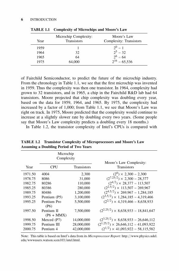
of Fairchild Semiconductor, to predict the future of the microchip industry.From the chronology in Table 1.1, we see that the first microchip was inventedin 1959. Thus the complexity was then one transistor. In 1964, complexity hadgrown to 32 transistors, and in 1965, a chip in the Fairchild R&D lab had 64transistors. Moore projected that chip complexity was doubling every year,based on the data for 1959, 1964, and 1965. By 1975, the complexity hadincreased by a factor of 1,000; from Table 1.1, we see that Moore’s Law wasright on track. In 1975, Moore predicted that the complexity would continue toincrease at a slightly slower rate by doubling every two years. (Some peoplesay that Moore’s Law complexity predicts a doubling every 18 months.)
In Table 1.2, the transistor complexity of Intel’s CPUs is compared with
TABLE 1.2 Transistor Complexity of Microprocessors and Moore’s LawAssuming a Doubling Period of Two Years
MicrochipComplexity
Moore’s Law Complexity:Year CPU Transistors Transistors
1971.50 4004 2,300 (20) × 2,300 c 2,3001978.75 8086 31,000 (27.25/ 2) × 2,300 c 28,3771982.75 80286 110,000 (24/ 2) × 28,377 c 113,5071985.25 80386 280,000 (22.5/ 2) × 113,507 c 269,9671989.75 80486 1,200,000 (24.5/ 2) × 269,967 c 1,284,1851993.25 Pentium (P5) 3,100,000 (23.5/ 2) × 1,284,185 c 4,319,4661995.25 Pentium Pro 5,500,000 (22/ 2) × 4,319,466 c 8,638,933
(P6)1997.50 Pentium II 7,500,000 (22.25/ 2) × 8,638,933 c 18,841,647
(P6 + MMX)1998.50 Merced (P7) 14,000,000 (23.25/ 2) × 8,638,933 c 26,646,1121999.75 Pentium III 28,000,000 (21.25/ 2) × 26,646,112 c 41,093,9222000.75 Pentium 4 42,000,000 (21/ 2) × 41,093,922 c 58,115,582
Note: This table is based on Intel’s data from its Microprocessor Report: http:/ / www.physics.udel.edu/ wwwusers.watson.scen103/ intel.html.
THE RISE OF MICROELECTRONICS AND THE COMPUTER 7
Moore’s Law, with a doubling every two years. Note that there are manyclosely spaced releases with different processor speeds; however, the tablerecords the first release of the architecture, generally at the initial speed.The Pentium P5 is generally called Pentium I, and the Pentium II is a P6with MMX technology. In 1993, with the introduction of the Pentium, theIntel microprocessor complexities fell slightly behind Moore’s Law. Somesay that Moore’s Law no longer holds because transistor spacing cannot bereduced rapidly with present technologies [Mann, 2000; Markov, 1999]; how-ever, Moore, now Chairman Emeritus of Intel Corporation, sees no funda-mental barriers to increased growth until 2012 and also sees that the physicallimitations on fabrication technology will not be reached until 2017 [Moore,2000].
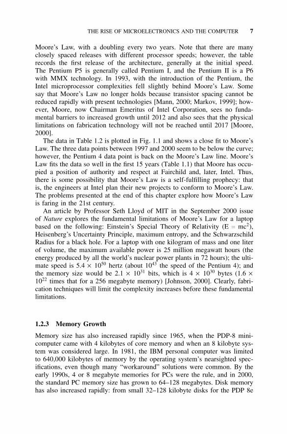
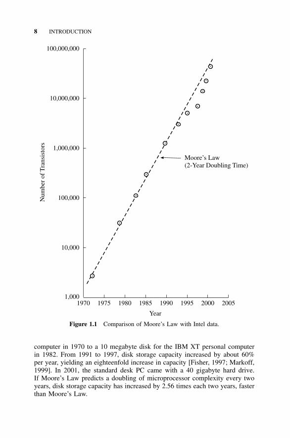
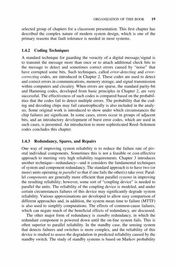
The data in Table 1.2 is plotted in Fig. 1.1 and shows a close fit to Moore’sLaw. The three data points between 1997 and 2000 seem to be below the curve;however, the Pentium 4 data point is back on the Moore’s Law line. Moore’sLaw fits the data so well in the first 15 years (Table 1.1) that Moore has occu-pied a position of authority and respect at Fairchild and, later, Intel. Thus,there is some possibility that Moore’s Law is a self-fulfilling prophecy: thatis, the engineers at Intel plan their new projects to conform to Moore’s Law.The problems presented at the end of this chapter explore how Moore’s Lawis faring in the 21st century.
An article by Professor Seth Lloyd of MIT in the September 2000 issueof Nature explores the fundamental limitations of Moore’s Law for a laptopbased on the following: Einstein’s Special Theory of Relativity (E c mc2),Heisenberg’s Uncertainty Principle, maximum entropy, and the SchwarzschildRadius for a black hole. For a laptop with one kilogram of mass and one literof volume, the maximum available power is 25 million megawatt hours (theenergy produced by all the world’s nuclear power plants in 72 hours); the ulti-mate speed is 5.4 × 1050 hertz (about 1043 the speed of the Pentium 4); andthe memory size would be 2.1 × 1031 bits, which is 4 × 1030 bytes (1.6 ×10²² times that for a 256 megabyte memory) [Johnson, 2000]. Clearly, fabri-cation techniques will limit the complexity increases before these fundamentallimitations.
1.2.3 Memory Growth
Memory size has also increased rapidly since 1965, when the PDP-8 mini-computer came with 4 kilobytes of core memory and when an 8 kilobyte sys-tem was considered large. In 1981, the IBM personal computer was limitedto 640,000 kilobytes of memory by the operating system’s nearsighted spec-ifications, even though many “workaround” solutions were common. By theearly 1990s, 4 or 8 megabyte memories for PCs were the rule, and in 2000,the standard PC memory size has grown to 64–128 megabytes. Disk memoryhas also increased rapidly: from small 32–128 kilobyte disks for the PDP 8e
8 INTRODUCTION
1970 1975 1980 1985 1990 1995 2000 20051,000
10,000
100,000
1,000,000
10,000,000
100,000,000
Moore’s Law(2-Year Doubling Time)
Year
Num
ber
ofT
rans
isto
rs
Figure 1.1 Comparison of Moore’s Law with Intel data.
computer in 1970 to a 10 megabyte disk for the IBM XT personal computerin 1982. From 1991 to 1997, disk storage capacity increased by about 60%per year, yielding an eighteenfold increase in capacity [Fisher, 1997; Markoff,1999]. In 2001, the standard desk PC came with a 40 gigabyte hard drive.If Moore’s Law predicts a doubling of microprocessor complexity every twoyears, disk storage capacity has increased by 2.56 times each two years, fasterthan Moore’s Law.
THE RISE OF MICROELECTRONICS AND THE COMPUTER 9
1.2.4 Digital Electronics in Unexpected Places
The examples of the need for fault tolerance discussed previously focused onmilitary, space, and other large projects. There is no less a need for fault toler-ance in the home now that electronics and most electrical devices are digital,which has greatly increased their complexity. In the 1940s and 1950s, the mostcomplex devices in the home were the superheterodyne radio receiver with 5vacuum tubes, and early black-and-white television receivers with 35 vacuumtubes. Today, the microprocessor is ubiquitous, and, since a large percentage ofmodern households have a home computer, this is only the tip of the iceberg.In 1997, the sale of embedded microcomponents (simpler devices than thoseused in computers) totaled 4.6 billion, compared with about 100 million micro-processors used in computers. Thus computer microprocessors only represent2% of the market [Hafner, 1999; Pollack, 1999].
The bewildering array of home products with microprocessors includesthe following: clothes washers and dryers; toasters and microwave ovens;electronic organizers; digital televisions and digital audio recorders; homealarm systems and elderly medic alert systems; irrigation systems; pacemak-ers; video games; Web-surfing devices; copying machines; calculators; tooth-brushes; musical greeting cards; pet identification tags; and toys. Of coursethis list does not even include the cellular phone, which may soon assumethe functions of both a personal digital assistant and a portable Internet inter-face. It has been estimated that the typical American home in 1999 had 40–60microprocessors—a number that could grow to 280 by 2004. In addition, amodern family sedan contains about 20 microprocessors, while a luxury carmay have 40–60 microprocessors, which in some designs are connected via alocal area network [Stepler, 1998; Hafner, 1999].
Not all these devices are that simple either. An electronic toothbrush has3,000 lines of code. The Furby, a $30 electronic–robotic pet, has 2 main pro-cessors, 21,600 lines of code, an infrared transmitter and receiver for Furby-to-Furby communication, a sound sensor, a tilt sensor, and touch sensors onthe front, back, and tongue. In short supply before Christmas 1998, Web siteprices rose as high as $147.95 plus shipping! [USA Today, 1998]. In 2000, thesensation was Billy Bass, a fish mounted on a wall plaque that wiggled, talked,and sang when you walked by, triggering an infrared sensor.
Hackers have even taken an interest in Furby and Billy Bass. They havemodified the hardware and software controlling the interface so that one Furbycontrols others. They have modified Billy Bass to speak the hackers’ dialogand sing their songs.
Late in 2000, Sony introduced a second-generation dog-like robot calledAibo (Japanese for “pal”); with 20 motors, a 32-bit RISC processor, 32megabytes of memory, and an artificial intelligence program. Aibo acts likea frisky puppy. It has color-camera eyes and stereo-microphone ears, touchsensors, a sound-synthesis voice, and gyroscopes for balance. Four different“personality” modules make this $1,500 robot more than a toy [Pogue, 2001].
10 INTRODUCTION
What is the need for fault tolerance in such devices? If a Furby fails, youdiscard it, but it would be disappointing if that were the only sensible choicefor a microwave oven or a washing machine. It seems that many such devicesare designed without thought of recovery or fault-tolerance. Lawn irrigationtimers, VCRs, microwave ovens, and digital phone answering machines are allupset by power outages, and only the best designs have effective battery back-ups. My digital answering machine was designed with an effective recoverymode. The battery backup works well, but it “locks up” and will not functionabout once a year. To recover, the battery and AC power are disconnected forabout 5 minutes; when the power is restored, a 1.5-minute countdown begins,during which the device reinitializes. There are many stories in which failureof an ignition control computer stranded an auto in a remote location at night.Couldn’t engineers develop a recovery mode to limp home, even if it did use alittle more gas or emit fumes on the way home? Sufficient fault-tolerant tech-nology exists; however, designers have to use it. Fortunately, the cellular phoneallows one to call for help!
Although the preceding examples relate to electronic systems, there is noless a need for fault tolerance in mechanical, pneumatic, hydraulic, and othersystems. In fact, almost all of us need a fault-tolerant emergency procedure toheat our homes in case of prolonged power outages.
1.3 RELIABILITY AND AVAILABILITY
1.3.1 Reliability Is Often an Afterthought
The attainment of high reliability and availability is very difficult to achieve invery complex systems. Thus, a system designer should formulate a number ofdifferent approaches to a problem and weigh the pluses and minuses of eachdesign before recommending an approach. One should be careful to base con-clusions on an analysis of facts, not on conjecture. Sometimes the best solutionincludes simplifying the design a bit by leaving out some marginal, complexfeatures. It may be difficult to convince the authors of the requirements thatsometimes “less is more,” but this is sometimes the best approach. Design deci-sions often change as new technology is introduced. At one time any attempt todigitize the Library of Congress would have been judged infeasible because ofthe storage requirement. However, by using modern technology, this could beaccomplished with two modern RAID disk storage systems such as the EMCSymmetrix systems, which store more than nine terabytes (9 × 1012 bytes)[EMC Products-At-A-Glance, www.emc.com]. The computation is outlined inthe problems at the end of this chapter.
Reliability and availability of the system should always be two factors thatare included, along with cost, performance, time of development, risk of fail-ure, and other factors. Sometimes it will be necessary to discard a few designobjectives to achieve a good design. The system engineer should always keep
RELIABILITY AND AVAILABILITY 11
in mind that the design objectives generally contain a list of key features and alist of desirable features. The design must satisfy the key features, but if one ortwo of the desirable features must be eliminated to achieve a superior design,the trade-off is generally a good one.
1.3.2 Concepts of Reliability
Formal definitions of reliability and availability appear in Appendices A andB; however, the basic ideas are easy to convey without a mathematical devel-opment, which will occur later. Both of these measures apply to how good thesystem is and how frequently it goes down. An easy way to introduce reliabil-ity is in terms of test data. If 50 systems operate for 1,000 hours on test andtwo fail, then we would say the probability of failure, Pf , for this system in1,000 hours of operation is 2/ 50 or Pf (1,000) c 0.04. Clearly the probabilityof success, Ps, which is known as the reliability, R, is given by R(1,000) c
Ps(1,000) c 1 − Pf (1,000) c 48/ 50 c 0.96. Thus, reliability is the probabilityof no failure within a given operating period. One can also deal with a fail-ure rate, f r, for the same system that, in the simplest case, would be f r c 2failures/ (50 × 1,000) operating hours—that is, f r c 4 × 10⁻⁵ or, as it is some-times stated, f r c z c 40 failures per million operating hours, where z is oftencalled the hazard function. The units used in the telecommunications industryare fits (failures in time), which are failures per billion operating hours. Moredetailed mathematical development relates the reliability, the failure rate, andtime. For the simplest case where the failure rate z is a constant (one gener-ally uses l to represent a constant failure rate), the reliability function can beshown to be R(t) c e−lt . If we substitute the preceding values, we obtain
R(1, 000) c e−4 × 10−5 × 1,000c 0.96
which agrees with the previous computation.It is now easy to show that complexity causes serious reliability problems.
The simplest system reliability model is to assume that in a system with ncomponents, all the components must work. If the component reliability is Rc,then the system reliability, Rsys, is given by
Rsys(t) c [Rc(t)]nc [e−lt]n
c e−nlt
Consider the case of the first supercomputer, the CDC 6600 [Thornton,1970]. This computer had 400,000 transistors, for which the estimated fail-ure rate was then 4 × 10⁻⁹ failures per hour. Thus, even though the failurerate of each transistor was very small, the computer reliability for 1,000 hourswould be
R(1, 000) c e−400,000 × 4 × 10−9 × 1,000c 0.20
12 INTRODUCTION
If we repeat the calculation for 100 hours, the reliability becomes 0.85.Remember that these calculations do not include the other components in thecomputer that can also fail. The conclusion is that the failure rate of deviceswith so many components must be very low to achieve reasonable reliabilities.Integrated circuits (ICs) improve reliability because each IC replaces hundredsof thousands or millions of transistors and also because the failure rate of anIC is low. See the problems at the end of this chapter for more examples.
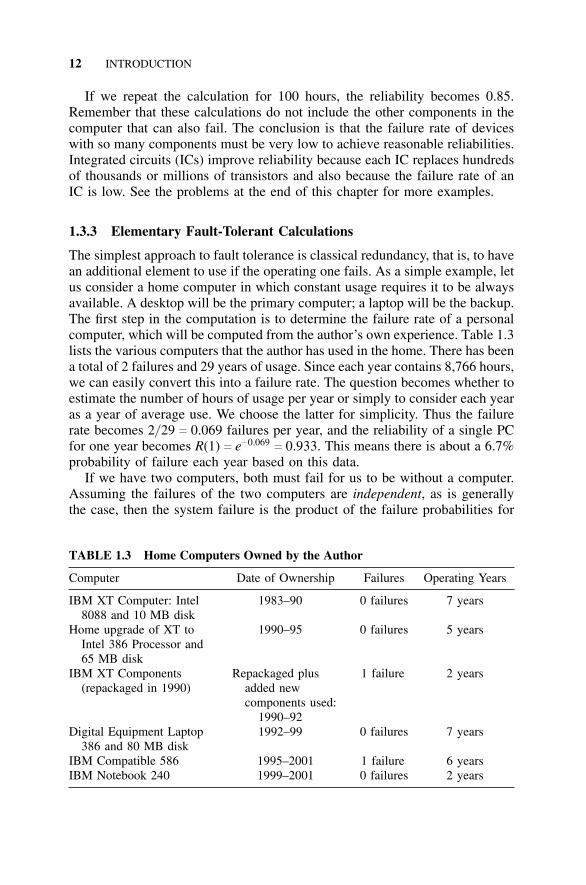
1.3.3 Elementary Fault-Tolerant Calculations
The simplest approach to fault tolerance is classical redundancy, that is, to havean additional element to use if the operating one fails. As a simple example, letus consider a home computer in which constant usage requires it to be alwaysavailable. A desktop will be the primary computer; a laptop will be the backup.The first step in the computation is to determine the failure rate of a personalcomputer, which will be computed from the author’s own experience. Table 1.3lists the various computers that the author has used in the home. There has beena total of 2 failures and 29 years of usage. Since each year contains 8,766 hours,we can easily convert this into a failure rate. The question becomes whether toestimate the number of hours of usage per year or simply to consider each yearas a year of average use. We choose the latter for simplicity. Thus the failurerate becomes 2/ 29 c 0.069 failures per year, and the reliability of a single PCfor one year becomes R(1) c e−0.069
c 0.933. This means there is about a 6.7%probability of failure each year based on this data.
If we have two computers, both must fail for us to be without a computer.Assuming the failures of the two computers are independent, as is generallythe case, then the system failure is the product of the failure probabilities for
TABLE 1.3 Home Computers Owned by the Author
Computer Date of Ownership Failures Operating Years
IBM XT Computer: Intel 1983–90 0 failures 7 years8088 and 10 MB disk
Home upgrade of XT to 1990–95 0 failures 5 yearsIntel 386 Processor and65 MB disk
IBM XT Components Repackaged plus 1 failure 2 years(repackaged in 1990) added new
components used:1990–92
Digital Equipment Laptop 1992–99 0 failures 7 years386 and 80 MB disk
IBM Compatible 586 1995–2001 1 failure 6 yearsIBM Notebook 240 1999–2001 0 failures 2 years
RELIABILITY AND AVAILABILITY 13
Boston
New York
PhiladelphiaPittsburgh
Boston
New York
PhiladelphiaPittsburgh
(a)
(b)
Figure 1.2 Examples of simple computer networks: (a), a tree network connectingthe four cities; (b), a Hamiltonian network connecting the four cities.
computer 1 (the primary) and computer 2 (the backup). Using the precedingfailure data, the probability of one failure within a year should be 0.067; oftwo failures, 0.067 × 0.067 c 0.00449. Thus, the probability of having at leastone computer for use is 0.9955 and the probability of having no computer atsome time during the year is reduced from 6.7% to 0.45%—a decrease by afactor of 15. The probability of having no computer will really be much lesssince the failed computer will be rapidly repaired.
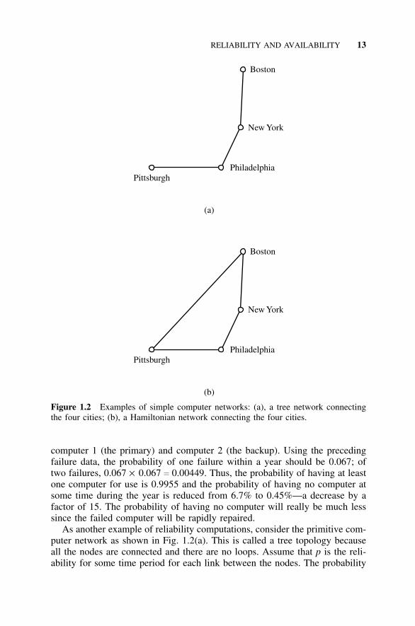
As another example of reliability computations, consider the primitive com-puter network as shown in Fig. 1.2(a). This is called a tree topology becauseall the nodes are connected and there are no loops. Assume that p is the reli-ability for some time period for each link between the nodes. The probability
14 INTRODUCTION
that Boston and New York are connected is the probability that one link isgood, that is, p. The same probability holds for New York–Philadelphia and forPhiladelphia–Pittsburgh, but the Boston–Philadelphia connection requires twolinks to work, the probability of which is p2. More commonly we speak of theall-terminal reliability, which is the probability that all cities are connected—p3
in this example—because all three links must be working. Thus if p c 0.9, theall-terminal reliability is 0.729.
The reliability of a network is raised if we add more links so that loopsare created. The Hamiltonian network shown in Fig. 1.2(b) has one more linkthan the tree and has a higher reliability. In the Hamiltonian network, all nodesare connected if all four links are working, which has a probability of p4. Allnodes are still connected if there is a single link failure, which has a probabilityof three successes and one failure given by p3 (1 − p). However, there are 4ways for one link to fail, so the probability of one link failing is 4p3(1− p). Thereliability is the probability that there are zero failures plus the probability thatthere is one failure, which is given by [p4 + 4p3(1 − p)]. Assuming that p c 0.9as before, the reliability becomes 0.9477—a considerable improvement overthe tree network. Some of the basic principles for designing and analyzing thereliability of computer networks are discussed in this book.
1.3.4 The Meaning of Availability
Reliability is the probability of no failures in an interval, whereas availabilityis the probability that an item is up at any point in time. Both reliability andavailability are used extensively in this book as measures of performance and“yardsticks” for quantitatively comparing the effectiveness of various fault-tol-erant methods. Availability is a good metric to measure the beneficial effects ofrepair on a system. Suppose that an air traffic control system fails on the aver-age of once a year; we then would say that the mean time to failure (MTTF),was 8,766 hours (the number of hours in a year). If an airline’s reservationsystem went down 5 times in a year, we would say that the MTTF was 1/ 5 ofthe air traffic control system, or 1,753 hours. One would say that, based on theMTTF, the air traffic control system was much better; however, suppose weconsider repair and calculate typical availabilities. A simple formula for cal-culating the system availability (actually, the steady-state availability), basedon the Uptime and Downtime of the system, is given as follows:
A c
UptimeUptime + Downtime
If the air traffic control system goes down for about 1 hour whenever it fails,the availability would be calculated by substitution into the preceding formulayielding A c (8,765)/ (8,765 + 1) c 0.999886. In the case of the airline reserva-tion system, let us assume that the outages are short, averaging 1 minute each.Thus the cumulative downtime per year is five minutes c 0.083333 hours, and
RELIABILITY AND AVAILABILITY 15
the availability would be A c (8,765.916666)/ (8,766) c 0.9999905. Comparingthe unavailabilities (U c 1 − A), we see (1 − 0.999886)/ (1 − 0.9999905) c 12.Thus, we can say that based on availability the reservation system is 12 timesbetter than the air traffic control system. Clearly one must use both reliabilityand availability to compare such systems.
A mathematical technique called Markov modeling will be used in this bookto compute the availability for various systems. Rapid repair of failures inredundant systems greatly increases both the reliability and availability of suchsystems.
1.3.5 Need for High Reliability and Safety in Fault-Tolerant Systems
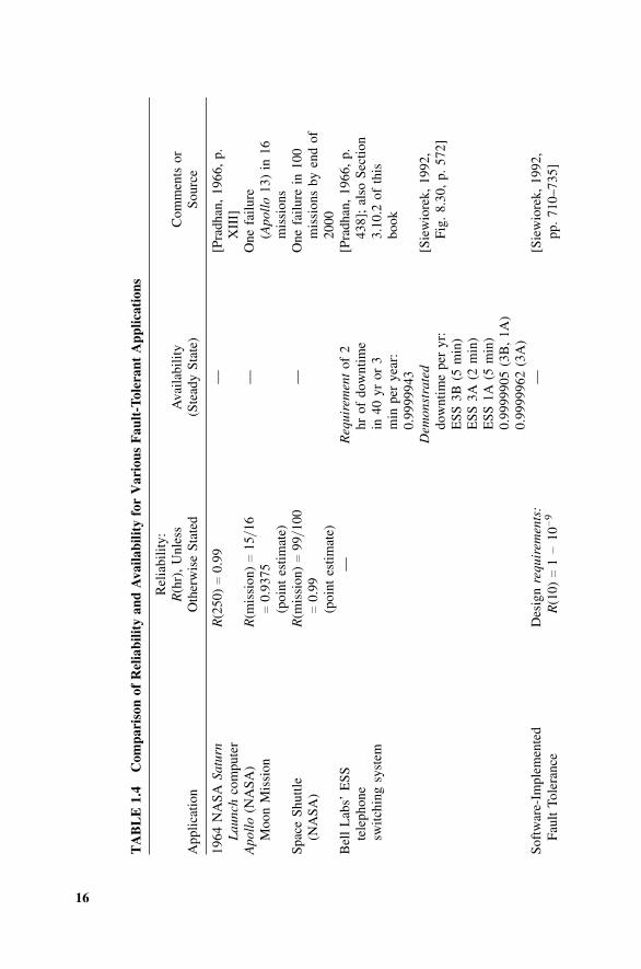
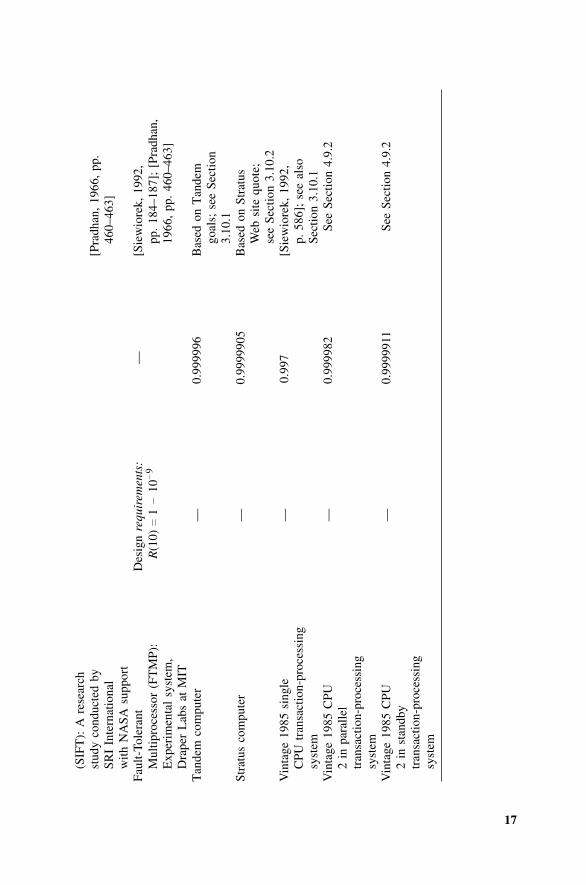
Fault-tolerant systems are generally required in applications involving a highlevel of safety, since a failure can injure or kill many people. A number of spec-ifications, field failure data, and calculations are listed in Table 1.4 to give thereader some appreciation of the ranges of reliability and availability requiredand realized for various fault-tolerant systems.
A pattern emerges after some study of Table 1.4. The availability of severalof the highly reliable fault-tolerant systems is similar. The availability require-ment for the ESS telephone switching system (0.9999943), which is spoken ofas “5 nines 43” in shorthand fashion, is seen to be equaled or bettered by actualperformance of “5 nines 05” for (3B, 1A) and “5 nines 62” for (3A). Oftenone will compare system availability by quoting the downtime: for example,5.7 hours per million for ESS requirements, 0.5 hours per million for (3B,1A), and 3.8 hours per million for (3A). The Tandem goal was “5 nines 60”and the Stratus quote was “5 nines 05.” Lastly, a standby system (if one couldconstruct a fault-tolerant standby architecture) using 1985 technology wouldyield an availability of “5 nines 11.” It is interesting to speculate whether thisrepresents some level of performance one is able to achieve under certain lim-itations or whether the only proven numbers (the ESS switching systems) havebecome the goal others are quoting. The reader should remember that neitherTandem nor Stratus provides data on their field-demonstrated availability.
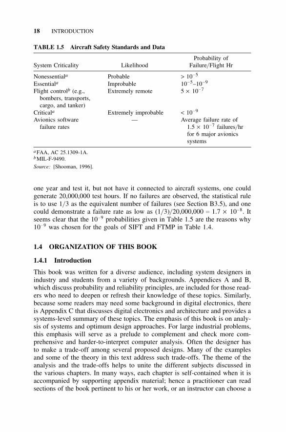
In the aircraft field there are some established system safety standards forthe probability of catastrophe. These are extracted in Table 1.5, which alsoshows data on avionics-software-problem occurrence rates.
The two standards plus the software data quoted in Table 1.5 provide arough but “overlapping” hierarchy of values. Some researchers have been pes-simistic about the possibility of proving before use the reliability of hardwareor software with reliabilities of < 10−9. To demonstrate such a probability, wewould need to test 10,000 systems for 10 years (about 100,000 hours) with 1 or0 failures. Clearly this is not feasible, and one must rely on modeling and testdata accumulated for major systems. However, from Shooman [1996], we canestimate that the U.S. air fleet of larger passenger aircraft flew about 12,000,000flight hours in 1994 and today must fly about 20,000,000 hours. Thus if it werecommercially feasible to install a new piece of equipment in every aircraft for
16
TA
BL
E1.
4C
ompa
riso
n of
Rel
iabi
lity
and
Ava
ilabi
lity
for
Var
ious
Fau
lt-T
oler
ant
App
licat
ions
Rel
iabi
lity:
R(h
r),
Unl
ess
Ava
ilabi
lity
Com
men
ts o
rA
pplic
atio
nO
ther
wis
e St
ated
(Ste
ady
Stat
e)So
urce
1964
NA
SASa
turn
R(2
50)c
0.99
—[P
radh
an,
1966
, p.
Lau
nch
com
pute
rX
III]
Apo
llo
(NA
SA)
R(m
issi
on)c
15/1
6—
One
fai
lure
Moo
n M
issi
onc
0.93
75(A
poll
o13
) in
16(p
oint
est
imat
e)m
issi
ons
Spac
e Sh
uttle
R(m
issi
on)c
99/1
00—
One
fai
lure
in
100
(NA
SA)
c0.
99m
issi
ons
by e
nd o
f(p
oint
est
imat
e)20
00B
ell
Lab
s’ E
SS—
Req
uire
men
tof
2[P
radh
an,
1966
, p.
tele
phon
ehr
of
dow
ntim
e43
8];
also
Sec
tion
switc
hing
sys
tem
in40
yr o
r3
3.10
.2of
thi
sm
in p
er y
ear:
book
0.99
9994
3D
emon
stra
ted
[Sie
wio
rek,
1992
,do
wnt
ime
per
yr:
Fig.
8.30
, p.
572]
ESS
3B (
5m
in)
ESS
3A (
2m
in)
ESS
1A (
5m
in)
0.99
9990
5(3
B,
1A)
0.99
9996
2(3
A)
Soft
war
e-Im
plem
ente
dD
esig
nre
quir
emen
ts:
—[S
iew
iore
k,19
92,
Faul
t To
lera
nce
R(1
0)c
1−
10−
9pp
.71
0–73
5]
17
(SIF
T):
A r
esea
rch
stud
y co
nduc
ted
by[P
radh
an,
1966
, pp
.SR
I In
tern
atio
nal
460–
463]
with
NA
SA s
uppo
rtFa
ult-
Tole
rant
Des
ign
requ
irem
ents
:—
[Sie
wio
rek,
1992
,M
ultip
roce
ssor
(FT
MP)
:R
(10)
c1−
10−
9pp
.18
4–18
7];
[Pra
dhan
,E
xper
imen
tal
syst
em,
1966
, pp
.46
0–46
3]D
rape
r L
abs
at M
ITT
ande
m c
ompu
ter
—0.
9999
96B
ased
on
Tan
dem
goal
s; s
ee S
ectio
n3.
10.1
Stra
tus
com
pute
r—
0.99
9990
5B
ased
on
Stra
tus
Web
site
quo
te;
see
Sect
ion
3.10
.2V
inta
ge19
85si
ngle
—0.
997
[Sie
wio
rek,
1992
,C
PU t
rans
actio
n-pr
oces
sing
p.58
6];
see
also
syst
emSe
ctio
n3.
10.1
Vin
tage
1985
CPU
—0.
9999
82Se
e Se
ctio
n4.
9.2
2in
par
alle
ltr
ansa
ctio
n-pr
oces
sing
syst
emV
inta
ge19
85C
PU—
0.99
9991
1Se
e Se
ctio
n4.
9.2
2in
sta
ndby
tran
sact
ion-
proc
essi
ngsy
stem
18 INTRODUCTION
TABLE 1.5 Aircraft Safety Standards and Data
Probability ofSystem Criticality Likelihood Failure/ Flight Hr
Nonessentiala Probable > 10−5
Essentiala Improbable 10−5–10−9
Flight controlb (e.g., Extremely remote 5 × 10⁻⁷
bombers, transports,cargo, and tanker)
Criticala Extremely improbable < 10−9
Avionics software — Average failure rate offailure rates 1.5 × 10⁻⁷ failures/ hr
for 6 major avionicssystems
a FAA, AC 25.1309-1A.b MIL-F-9490.
Source: [Shooman, 1996].
one year and test it, but not have it connected to aircraft systems, one couldgenerate 20,000,000 test hours. If no failures are observed, the statistical ruleis to use 1/ 3 as the equivalent number of failures (see Section B3.5), and onecould demonstrate a failure rate as low as (1/ 3)/ 20,000,000 c 1.7 × 10⁻⁸. Itseems clear that the 10−9 probabilities given in Table 1.5 are the reasons why10−9 was chosen for the goals of SIFT and FTMP in Table 1.4.
1.4 ORGANIZATION OF THIS BOOK
1.4.1 Introduction
This book was written for a diverse audience, including system designers inindustry and students from a variety of backgrounds. Appendices A and B,which discuss probability and reliability principles, are included for those read-ers who need to deepen or refresh their knowledge of these topics. Similarly,because some readers may need some background in digital electronics, thereis Appendix C that discusses digital electronics and architecture and provides asystems-level summary of these topics. The emphasis of this book is on analy-sis of systems and optimum design approaches. For large industrial problems,this emphasis will serve as a prelude to complement and check more com-prehensive and harder-to-interpret computer analysis. Often the designer hasto make a trade-off among several proposed designs. Many of the examplesand some of the theory in this text address such trade-offs. The theme of theanalysis and the trade-offs helps to unite the different subjects discussed inthe various chapters. In many ways, each chapter is self-contained when it isaccompanied by supporting appendix material; hence a practitioner can readsections of the book pertinent to his or her work, or an instructor can choose a
ORGANIZATION OF THIS BOOK 19
selected group of chapters for a classroom presentation. This first chapter hasdescribed the complex nature of modern system design, which is one of theprimary reasons that fault tolerance is needed in most systems.
1.4.2 Coding Techniques
A standard technique for guarding the veracity of a digital message/ signal isto transmit the message more than once or to attach additional check bits tothe message to detect and sometimes correct errors caused by “noise” thathave corrupted some bits. Such techniques, called error-detecting and error-correcting codes, are introduced in Chapter 2. These codes are used to detectand correct errors in communications, memory storage, and signal transmissionwithin computers and circuitry. When errors are sparse, the standard parity-bitand Hamming codes, developed from basic principles in Chapter 2, are verysuccessful. The effectiveness of such codes is compared based on the probabil-ities that the codes fail to detect multiple errors. The probability that the cod-ing and decoding chips may fail catastrophically is also included in the analy-sis. Some original work is introduced to show under which circumstances thechip failures are significant. In some cases, errors occur in groups of adjacentbits, and an introductory development of burst error codes, which are used insuch cases, is presented. An introduction to more sophisticated Reed–Solomoncodes concludes this chapter.
1.4.3 Redundancy, Spares, and Repairs
One way of improving system reliability is to reduce the failure rate of piv-otal individual components. Sometimes this is not a feasible or cost-effectiveapproach to meeting very high reliability requirements. Chapter 3 introducesanother technique—redundancy—and it considers the fundamental techniquesof system and component redundancy. The standard approach is to have two (ormore) units operating in parallel so that if one fails the other(s) take over. Paral-lel components are generally more efficient than parallel systems in improvingthe resulting reliability; however, some sort of “coupling device” is needed toparallel the units. The reliability of the coupling device is modeled, and undercertain circumstances failures of this device may significantly degrade systemreliability. Various approximations are developed to allow easy comparison ofdifferent approaches and, in addition, the system mean time to failure (MTTF)is also used to simplify computations. The effects of common-cause failures,which can negate much of the beneficial effects of redundancy, are discussed.
The other major form of redundancy is standby redundancy, in which theredundant component is powered down until the on-line system fails. This isoften superior to parallel reliability. In the standby case, the sensing systemthat detects failures and switches is more complex, and the reliability of thisdevice is studied to assess the degradation in predicted reliability caused by thestandby switch. The study of standby systems is based on Markov probability
20 INTRODUCTION
models that are introduced in the appendices and deliberately developed inChapter 3 because they will be used throughout the book.
Repair improves the reliability of both parallel and standby systems, andMarkov probability models are used to study the relative benefits of repair forboth approaches. Markov modeling generates a set of differential equations thatrequire a solution to complete the analysis. The Laplace transform approach isintroduced and used to simplify the solution of the Markov equations for bothreliability and availability analysis.
Several computer architectures for fault tolerance are introduced and dis-cussed. Modern memory storage systems use the various RAID architecturesbased on an array of redundant disks. Several of the common RAID techniquesare analyzed. The class of fault-tolerant computer systems called nonstop sys-tems is introduced. Also introduced and analyzed are two other systems: theTandem system, which depends primarily on software fault tolerance, and theStratus system, which uses hardware fault tolerance. A brief description of asimilar system approach, a Sun computer system cluster, concludes the chapter.
1.4.4 N-Modular Redundancy
The problem of comparing the proper functioning of parallel systems was dis-cussed earlier in this chapter. One of the benefits of a digital system is that alloutputs are strings of 1s or 0s so that the comparison of outputs is simplified.Chapter 4 describes an approach that is often used to compare the outputs ofthree identical digital circuits processing the same input: triple modular redun-dancy (TMR). The most common circuit output is used as the system output(called majority voting). In the case of TMR, we assume that if outputs dis-agree, those two that are the same will together have a much higher probabilityof succeeding rather than failing. The voting device is simple, and the resultingsystem is highly reliable. As in the case of parallel or standby redundancy, thevoting can be done at the system or subsystem level, and both approaches aremodeled and compared.
Although the voter circuit is simple, it can fail; the effect of voter reliabil-ity, much like coupler reliability in a parallel system, must then be included.The possibility of using redundant voters is introduced. Repair can be used toimprove the reliability of a voter system, and the analysis utilizes a Markovmodel similar to that of Chapter 3. Various simplified approximations are intro-duced that can be used to analyze the reliability and availability of repairablesystems. Also introduced are more advanced voting and consensus techniques.The redundant system of Chapter 3 is compared with the voting techniques ofChapter 4.
1.4.5 Software Reliability and Recovery Techniques
Programming of the computer in early digital systems was largely done in com-plex machine language or low-level assembly language. Memory was limited,
ORGANIZATION OF THIS BOOK 21
and the program had to be small and concise. Expert programmers often usedtricks to fit the required functions into the small memory. Software errors—thenas now—can cause the system to malfunction. The failure mode is differentbut no less disastrous than catastrophic hardware failures. Chapter 5 relatesthese program errors to resulting system failures.
This chapter begins by describing in some detail the way programs arenow developed in modern higher-level languages such as FORTRAN, COBOL,ALGOL, C, C+ +, and Ada. Large memories allow more complex tasks, andmany more programmers are involved. There are many potential sources oferrors, such as the following: (a), complex, error-prone specifications; (b), logicerrors in individual modules (self-contained sections of the program); and (c),communications among modules. Sometimes code is incorporated from previ-ous projects without sufficient adaptation analysis and testing, causing subtlebut disastrous results. A classical example of the hazards of reused code is theAriane-5 rocket. The European Space Agency (ESA) reused guidance softwarefrom Ariane-4 in Ariane-5. On its maiden flight, June 4, 1996, Ariane-5 had tobe destroyed 40 seconds into launch—a $500 million loss. Ariane-5 developeda larger horizontal velocity than Ariane-4, and a register overflowed. The soft-ware detected an exception, but instead of taking a recoverable action it shutoff the processor as the specifications required. A more appropriate recoveryaction might have saved the flight. To cite the legendary Murphy’s Law, “Ifthings can go wrong, they will,” and they did. Even better, we might devise acorollary that states “then plan for it” [Pfleeger, 1998, pp. 37–39].
Various mathematical models describing errors are introduced. The intro-ductory model is based on a simple assumption: the failure rate (error discov-ery rate) is proportional to the number of errors remaining in the software afterit is tested and released. Combining this software failure rate with reliabilitytheory leads to a software reliability model. The constants in such models areevaluated from test data recorded during software development. Applying suchmodels during the test phase allows one to predict the reliability of the softwareonce it is released for operational use. If the predicted reliability appears unsat-isfactory, the developer can improve testing to remove more errors, rewrite cer-tain problem modulus, or take other action to avoid the release of an unreliableproduct.
Software redundancy can be utilized in some cases by using independentlydeveloped but functionally identical software. The extent to which commonerrors in independent software reduces the reliability gains is discussed; as apractical example, the redundant software in the NASA Space Shuttle is con-sidered.
1.4.6 Networked Systems Reliability
Networks are all around us. They process our telephone calls, connect us to theInternet, and connect private industry and government computer and informa-tion systems. In general, such systems have a high reliability and availability
22 INTRODUCTION
because there is more than one path that connects all of the terminals in the net-work. Thus a single link failure will seldom interrupt communications becausea duplicate path will exist. Since network geometry (topology) is usually com-plex, there are many paths between terminals, and therefore computation ofnetwork reliability is often difficult. Computer programs are available for suchcomputations, two of which are referenced in the chapter. This chapter sys-tematically develops methods based on graph theory (cut-sets and tie-sets) foranalysis of a network. Alternate methods for computation are also discussed,and the chapter concludes with the application of such methods to the designof a reliable backbone network.
1.4.7 Reliability Optimization
Initial design of a large, complex system focuses on several issues: (a), how tostructure the project to perform the required functions; (b), how to meet the per-formance requirements; and (c), how to achieve the required reliability. Design-ers always focus on issues (a) and (b), but sometimes, at the peril of develop-ing an unreliable system, they spend a minimum of effort on issue (c). Chap-ter 7 develops techniques for optimizing the reliability of a proposed designby parceling out the redundancy to various subsystems. Choice among opti-mized candidate designs should be followed by a trade-off among the feasibledesigns, weighing the various pros and cons that include reliability, weight,volume, and cost. In some ways, one can view this chapter as a generalizationof Chapter 3 for larger, more complex system designs.
One simplified method of achieving optimum reliability is to meet the overallsystem reliability goal by fixing the level of redundancy for the various subsys-tems according to various apportionment rules. The other end of the optimizationspectrum is to obtain an exact solution by means of exhaustively computing thereliability for all the possible system combinations. The Dynamic Programmingmethod was developed as a way to eliminate many of the cases in an exhaustivecomputation scheme. Chapter 7 discusses the above methods as well as an effec-tive approximate method—a greedy algorithm, where the optimization is dividedinto a series of steps and the best choice is made for each step.
The best method developed in this chapter is to establish a set of upper andlower bounds on the number of redundancies that can be assigned for eachsubsystem. It is shown that there is a modest number of possible cases, soan exhaustive search within the allowed bounds is rapid and computationallyfeasible. The bounded method displays the optimal configuration as well asmany other close-to-optimum alternatives, and it provides the designer with anumber of good solutions among which to choose.
1.4.8 Appendices
This book has been written for practitioners and students from a wide varietyof disciplines. In cases where the reader does not have a background in either
GENERAL REFERENCES 23
probability or digital circuitry, or needs a review of principles, these appen-dices provide a self-contained development of the background material of thesesubjects.
Appendix A develops probability from basic principles. It serves as a tuto-rial, review, or reference for the reader.
Appendix B summarizes reliability theory and develops the relationshipsamong reliability theory, conventional probability density and distributionsfunctions, and the failure rate (hazard) function. The popular MTTF metric, aswell as sample calculations, are given. Availability theory and Markov modelsare developed.
Appendix C presents a concise introduction to digital circuit design and ele-mentary computer architecture. This will serve the reader who needs a back-ground to understand the architecture applications presented in the text.
Appendix D discusses reliability, availability, and risk-modeling programs.Most large systems will require such software to aid in analysis. This appendixcategorizes these programs and provides information to aid the reader in con-tacting the suppliers to make an informed choice among the products offered.
GENERAL REFERENCES
The references listed here are a selection of textbooks and proceedings thatapply to several chapters in this book. Specific references for Chapter 1 appearin the following section.Aktouf, C. et al. Basic Concepts and Advances in Fault-Tolerant Design. World Sci-
entific Publishing, River Edge, NJ, 1998.
Anderson, T. Resilient Computing Systems, vol. 1. Wiley, New York, 1985.
Anderson, T., and P. A. Lee. Fault Tolerance: Principles and Practice. Prentice-Hall,New York, 1981.
Arazi, B. A Commonsense Approach to the Theory of Error-Correcting Codes. MITPress, Cambridge, MA, 1988.
Avizienis, A. The Evolution of Fault-Tolerant Computing. Springer-Verlag, New York,1987.
Avresky, D. R. (ed.). Fault-Tolerant Parallel and Distributed Systems. Kluwer Aca-demic Publishers, Hingham, MA, 1998.
Bolch, G., S. Greiner, H. de Meer, and K. S. Trivedi. Queueing Networks and MarkovChains: Modeling and Performance Evaluation with Computer Science Applica-tions. Wiley, New York, 1998.
Breuer, M. A., and A. D. Friedman. Diagnosis and Reliable Design of Digital Systems.Computer Science Press, Woodland Hills, CA, 1976.
Christian, F. (ed.). Dependable Computing for Critical Applications. Springer-Verlag,New York, 1995.
Special Issue on Fault-Tolerant Systems. IEEE Computer Magazine, New York (July1990).
24 INTRODUCTION
Special Issue on Dependability Modeling. IEEE Computer Magazine, New York (Octo-ber 1990).
Dacin, M. et al. Dependable Computing for Critical Applications. IEEE ComputerSociety Press, New York, 1997.
Davies, D. W. Distributed Systems—Architecture and Implementation, Lecture Notesin Computer Science. Springer-Verlag, New York, 1981, ch. 8, 10, 13, 17, and 20.
Dougherty, E. M. Jr., and J. R. Fragola. Human Reliability Analysis. Wiley, New York,1988.
Echte, K. Dependable Computing—EDCC-1. Proceedings of the First EuropeanDependable Computing Conference, Berlin, Germany, 1994.
Fault-Tolerant Computing Symposium, 25th Anniversary Compendium. IEEE Com-puter Society Press, New York, 1996. (Author’s note: Symposium proceedings arepublished yearly by the IEEE.)
Gibson, G. A. Redundant Disk Arrays. MIT Press, Cambridge, MA, 1992.Hawicska, A. et al. Dependable Computing—EDCC-2. Second European Dependable
Computing Conference, Taormina, Italy, 1996.Johnson, B. W. Design and Analysis of Fault Tolerant Digital Systems. Addison-Wes-
ley, Reading, MA, 1989.Kanellakis, P. C., and A. A. Shvartsman. Fault-Tolerant Parallel Computation. Kluwer
Academic Publishers, Hingham, MA, 1997.Kaplan, G. The X-29: Is it Coming or Going? IEEE Spectrum, New York (June 1985):
54–60.Lala, P. K. Self-Checking and Fault-Tolerant Digital Design. Academic Press, San
Diego, CA, 2000.Lee, P. A., and T. Anderson. Fault Tolerance, Principles and Practice, 2d ed. Springer-
Verlag, New York, 1990.Lyu, M. R. (ed.). Handbook of Software Reliability Engineering. McGraw-Hill, New
York, 1996.McCormick, N. Reliability and Risk Analysis. Academic Press, New York, 1981.Ng, Y. W., and A. A. Avizienis. A Unified Reliability Model for Fault-Tolerant Com-
puters. IEEE Transactions on Computers C-29, New York, no. 11 (November 1980):1002–1011.
Osaki, S., and T. Nishio. Reliability Evaluation of Some Fault-Tolerant ComputerArchitectures, Lecture Notes in Computer Science. Springer-Verlag, New York,1980.
Patterson, D., R. Katz, and G. Gibson. A Case for Redundant Arrays of InexpensiveDisks (RAID). Proceedings of the 1988 ACM SIG on Management of Data (ACMSIGMOD), Chicago, IL, June 1988, pp. 109–116.
Pham, H. Fault-Tolerant Software Systems, Techniques and Applications. IEEE Com-puter Society Press, New York, 1992.
Pierce, W. H. Fault-Tolerant Computer Design. Academic Press, New York, 1965.Pradhan, D. K. Fault-Tolerant Computing Theory and Technique, vols. I and II.
Prentice-Hall, Englewood Cliffs, NJ, 1986.Pradhan, D. K. Fault-Tolerant Computing, vol. I, 2d ed. Prentice-Hall, Englewood
Cliffs, NJ, 1993.
REFERENCES 25
Rao, T. R. N., and E. Fujiwara. Error-Control Coding for Computer Systems. Prentice-Hall, Englewood Cliffs, NJ, 1989.
Shooman, M. L. Software Engineering, Design, Reliability, Management. McGraw-Hill, New York, 1983.
Shooman, M. L. Probabilistic Reliability: An Engineering Approach, 2d ed. Krieger,Melbourne, FL, 1990.
Siewiorek, D. P., and R. S. Swarz. The Theory and Practice of Reliable System Design.The Digital Press, Bedford, MA, 1982.
Siewiorek, D. P., and R. S. Swarz. Reliable Computer Systems Design and Evaluation,2d ed. The Digital Press, Bedford, MA, 1992.
Siewiorek, D. P., and R. S. Swarz. Reliable Computer Systems Design and Evaluation,3d ed. A. K. Peters, www.akpeters.com, 1998.
Smith, B. T. The Fault-Tolerant Multiprocessor Computer. Noyes Data Corporation,1986.
Trivedi, K. S. Probability and Statistics with Reliability, Queuing and Computer Sci-ence Applications, 2d ed. Wiley, New York, 2002.
Workshop on Defect and Fault-Tolerance in VLSI Systems. IEEE Computer SocietyPress, New York, 1995.
REFERENCES
Anderson, T. Resilient Computing Systems. Wiley, New York, 1985.
Bell, C. G. Computer Structures: Readings and Examples. McGraw-Hill, New York,1971.
Bell, T. (ed.). Special Report: Designing and Operating a Minimum-Risk System. IEEESpectrum, New York (June 1989): pp. 22–52.
Braun, E., and S. McDonald. Revolution in Miniature—The History and Impact ofSemiconductor Electronics. Cambridge University Press, London, 1978.
Burks, A. W., H. H. Goldstine, and J. von Neuman. Preliminary Discussion of theLogical Design of an Electronic Computing Instrument. Report to the U.S. ArmyOrdinance Department, 1946. Reprinted in Randell (p. 371–385) and Bell (1971, p.92–119).
Clark, R. The Man Who Broke Purple the Life of W. F. Friedman. Little, Brown andCompany, Boston, 1977.
Ditlea, S. (ed.). Digital Deli. Workman Publishing, New York, 1984.
Federal Aviation Administration Advisory Circular, AC 25.1309-1A.
Fisher, L. M. “IBM Plans to Announce Leap in Disk-Drive Capacity.” New York Times,December 30, 1997, p. D2.
Fragola, J. R. Forecasting the Reliability and Safety of Future Space TransportationSystems. Proceedings, Annual Reliability and Maintainability Symposium, 2000.IEEE, New York, NY, pp. 292–298.
Friedman, M. B. RAID keeps going and going and. . . . IEEE Spectrum, New York(1996): pp. 73–79.
26 INTRODUCTION
Giloth, P. K. No. 4 ESS—Reliability and Maintainability Experience. Proceedings,Annual Reliability and Maintainability Symposium, 1980. IEEE, New York, NY.
Hafner, K. “Honey, I Programmed the Blanket—The Omnipresent Chip has InvadedEverything from Dishwashers to Dogs.” New York Times, May 27, 1999,p. G1.
Iaciofano, C. Computer Time Line, in Digital Deli, Ditlea (ed.). Workman Publishing,New York, 1984, pp. 20–34.
Johnson, G. “The Ultimate, Apocalyptic Laptop.” New York Times, September 5, 2000,p. F1.
Lewis, P. H. “With 2 New Chips, the Gigahertz Decade Begins.” New York Times,March 9, 2000, p. G1.
Mann, C. C. The End of Moore’s Law? Technology Review, Cambridge, MA(May–June 2000): p. 42.
Markoff, J. “IBM Sets a New Record for Magnetic-Disk Storage.” New York Times,May 12, 1999.
Markoff, J. “Chip Progress may soon Be Hitting Barrier.” New York Times (on theInternet), October 9, 1999.
Markoff, J. “A Tale of the Tape from the Days when it Was Still Micro Soft.” NewYork Times, September, 2000, p. C1.
Military Standard. General Specification for Flight Control Systems—Design, Install,and Test of Aircraft. MIL-F-9490, 1975.
Moore, G. E. Intel Developers Forum, 2000 [http://developer.intel.com/update/archive/issue2/feature.html].
Norwall, B. D. FAA Claims Progress on ATC Improvements. Aviation Week and SpaceTechnology (September 25, 1995): p. 44.
Patterson, D., R. Katz, and G. Gibson. A Case for Redundant Arrays of InexpensiveDisks (RAID). Proceedings of the 1988 ACM SIG on Management of Data (ACMSIGMOD), Chicago, IL, June 1988, pp. 109–116.
Pfleeger, S. L. Software Engineering Theory and Practice. Prentice Hall, Upper SaddleRiver, NJ, 1998.
Pogue, D. “Who Let the Robot Out?” New York Times, January 25, 2001, p. G1.Pollack, A. “Chips are Hidden in Washing Machines, Microwaves and Even Reser-
voirs.” New York Times, January 4, 1999, p. C17.Randall, B. The Origins of Digital Computers. Springer-Verlag, New York, 1975.Rogers, E. M., and J. K. Larsen. Silicon Valley Fever—Growth of High-Technology
Culture. Basic Books, New York, 1984.Sammet, J. E. Programming Languages: History and Fundamentals. Prentice-Hall,
Englewood Cliffs, NJ, 1969.Shooman, M. L. Probabilistic Reliability: An Engineering Approach, 2d ed. Krieger,
Melbourne, FL, 1990.Shooman, M. L. Software Engineering, Design, Reliability, Management. McGraw-
Hill, New York, 1983.Shooman, M. L. Avionics Software Problem Occurrence Rates. Proceedings of Soft-
ware Reliability Engineering Conference, ISSRE ’96, 1996. IEEE, New York, NY,pp. 55–64.
PROBLEMS 27
Siewiorek, D. P., and R. S. Swarz. The Theory and Practice of Reliable System Design.The Digital Press, Bedford, MA, 1982.
Siewiorek, D. P., and R. S. Swarz. Reliable Computer Systems Design and Evaluation,2d ed. The Digital Press, Bedford, MA, 1992.
Siewiorek, D. P., and R. S. Swarz. Reliable Computer Systems Design and Evaluation,3d ed. A. K. Peters, www.akpeters.com, 1998.
Stepler, R. “Fill it Up, with RAM—Cars Get More Megs Under the Hood.” New YorkTimes, August 27, 1998, p. G1.
Turing, A. M. On Computable Numbers, with an Application to the Entscheidungsproblem. Proc. London Mathematical Soc., 42, 2 (1936): pp. 230–265.
Turing, A. M. Corrections. Proc. London Mathematical Soc., 43 (1937): pp. 544–546.Wald, M. L. “Ambitious Update of Air Navigation Becomes a Fiasco.” New York
Times, January 29, 1996. p. 1.Wirth, N. The Programming Language PASCAL. Acta Informatica 1 (1971): pp.
35–63.Zuckerman, L., and M. L. Wald. “Crisis for Air Traffic Systems: More Passengers,
More Delays.” New York Times, September 5, 2000, front page.USA Today, December 2, 1998, p. 1D.www.emc.com (the EMC Products-At-A-Glance Web site).www.intel.com (the Intel Web site).www.microsoft.com (the Microsoft Web site).
PROBLEMS
1.1. Show that the combined capacity of several (two or three) moderndisk storage systems, such as the EMC Symmetrix System that storesmore than nine terabytes (9 × 1012 bytes) [EMC Products-At-A-Glance,www.emc.com], could contain all the 26 million texts in the Library ofCongress [Web search, Library of Congress].(a) Assume that the average book has 400 pages.(b) Estimate the number of lines per page by counting lines in three
different books.(c) Repeat (b) for the number of words per line.(d) Repeat (b) for the number of characters per word.(e) Use the above computations to find the number of characters in the
26 million books.Assume that one character is stored in one byte and calculate the numberof Symmetrix units needed.
1.2. Estimate the amount of storage needed to store all the papers in a stan-dard four-drawer business filing cabinet.
1.3. Estimate the cost of digitizing the books in the Library of Congress.How would you do this?
28 INTRODUCTION
1.4. Repeat problem 1.3 for the storage of problem 1.2.
1.5. Visit the Intel Web site and check the release dates and transistor com-plexities given in Table 1.2.
1.6. Repeat problem 1.5 for microprocessors from other manufacturers.
1.7. Extend Table 1.2 for newer processors from Intel and other manufactur-ers.
1.8. Search the Web for articles about the change of mainframes in the airtraffic control system and identify the old and new computers, the pastproblems, and the expected improvements from the new computers.Hint: look at IEEE Computer and Spectrum magazines and the New YorkTimes.
1.9. Do some research and try to determine if the storage density for opticalcopies (one page of text per square millimeter) is feasible with today’soptical technology. Compare this storage density with that of a moderndisk or CD-ROM.
1.10. Make a list of natural, human, and equipment failures that could bringdown a library system stored on computer disks. Explain how you couldincorporate design features that would minimize such problems.
1.11. Complex solutions are not always needed. There are many good pro-grams for storing cooking recipes. Many cooks use a few index cards ora cookbook with paper slips to mark their favorite recipes. Discuss thepros and cons of each approach. Under what circumstances would youfavor each approach?
1.12. An improved version of Basic, called GW Basic, followed the originalMicro Soft Basic. “GW” did not stand for our first president or the uni-versity that bears his name. Try to find out what GW stands for and theorigin of the software.
1.13. Estimate the number of failures per year for a family automobile andcompute the failure rate (failures per mile). Assuming 10,000 milesdriven per year, compute the number of failures per year. Convert thisinto failures per hour assuming that one drives 10,000 miles per year atan average speed of 40 miles per hour.
1.14. Assume that an auto repair takes 8 hours, including drop-off, storage,and pickup of the car. Using the failure rate computed in problem 1.13and this information, compute the availability of an automobile.
1.15. Make a list of safety critical systems that would benefit from fault tol-erance. Suggest design features that would help fault tolerance.
1.16. Search the Web for examples of the systems in problem 1.15 and listthe details you can find. Comment.

PROBLEMS 29
1.17. Repeat problems 1.15 and 1.16 for systems in the home.
1.18. Repeat problems 1.15 and 1.16 for transportation, communication,power, heating and cooling, and entertainment systems in everyday use.
1.19. To learn of a 180 terabyte storage project, search the EMC Web site forthe movie producer Steven Spielberg, or see the New York Times: Jan.13, 2001, p. B11. Comment.
1.20. To learn of some of the practical problems in trying to improve an exist-ing fault-tolerant system, consider the U.S. air traffic control system.Search the Web for information on the current delays, the effects ofderegulation, and former President Ronald Reagan’s dismissal of strik-ing air traffic controllers; also see Zuckerman [2000]. A large upgradeto the system failed and incremental upgrades are being planned instead.Search the Web and see [Wald, 1996] for a discussion of why theupgrade failed.(a) Write a report analyzing what you learned.(b) What is the present status of the system and any upgrades?
1.21. Devise a scheme for emergency home heating in case of a prolongedpower outage for a gas-fired, hot-water heating system. Consider the fol-lowing: (a), fireplace; (b), gas stove; (c), emergency generator; and (d),other. How would you make your home heating system fault tolerant?
1.22. How would problem 1.21 change for the following:(a) An oil-fired, hot-water heating system?(b) A gas-fired, hot-air heating system?(c) A gas-fired, hot-water heating system?
1.23. Present two designs for a fault-tolerant voting scheme.
1.24. Investigate the speed of microprocessors and how rapidly it hasincreased over the years. You may wish to use the microprocessors inTable 1.2 or others as data points. A point on the curve is the 1.7 giga-hertz Pentium 4 microprocessor [New York Times, April 23, 2001, p.C1]. Plot the data in a format similar to Fig. 1.1. Does a law hold forspeed?
1.25. Some of the advances in mechanical and electronic computers occurredduring World War II in conjunction with message encoding and decodingand cryptanalysis (code breaking). Some of the details were, and still are,classified as secret. Find out as much as you can about these machinesand compare them with those reported on in Section 1.2.1. Hint: Lookin Randall [1975, pp. 327, 328] and Clark [1977, pp. 134, 135, 140,151, 195, 196]. Also, search the Web for key words: Sigaba, Enigma,T. H. Flowers, William F. Friedman, Alan Turing, and any patents byFriedman.
2CODING TECHNIQUES
Reliability of Computer Systems and Networks: Fault Tolerance, Analysis, and DesignMartin L. Shooman
Copyright 2002 John Wiley & Sons, Inc.ISBNs: 0-471-29342-3 (Hardback); 0-471-22460-X (Electronic)
30
2.1 INTRODUCTION
Many errors in a computer system are committed at the bit or byte level wheninformation is either transmitted along communication lines from one computerto another or else within a computer from the memory to the microprocessoror from microprocessor to input/ output device. Such transfers are generallymade over high-speed internal buses or sometimes over networks. The simplesttechnique to protect against such errors is the use of error-detecting and error-correcting codes. These codes are discussed in this chapter in this context. InSection 3.9, we see that error-correcting codes are also used in some versionsof RAID memory storage devices.
The reader should be familiar with the material in Appendix A and SectionsB1–B4 before studying the material of this chapter. It is suggested that thismaterial be reviewed briefly or studied along with this chapter, depending onthe reader’s background.
The word code has many meanings. Messages are commonly coded anddecoded to provide secret communication [Clark, 1977; Kahn, 1967], a prac-tice that technically is known as cryptography. The municipal rules governingthe construction of buildings are called building codes. Computer scientistsrefer to individual programs and collections of programs as software, but manyphysicists and engineers refer to them as computer codes. When informationin one system (numbers, alphabet, etc.) is represented by another system, wecall that other system a code for the first. Examples are the use of binary num-bers to represent numbers or the use of the ASCII code to represent the letters,numerals, punctuation, and various control keys on a computer keyboard (see
INTRODUCTION 31
Table C.1 in Appendix C for more information). The types of codes that wediscuss in this chapter are error-detecting and -correcting codes. The principlethat underlies error-detecting and -correcting codes is the addition of speciallycomputed redundant bits to a transmitted message along with added checkson the bits of the received message. These procedures allow the detection andsometimes the correction of a modest number of errors that occur during trans-mission.
The computation associated with generating the redundant bits is called cod-ing; that associated with detection or correction is called decoding. The useof the words message, transmitted, and received in the preceding paragraphreveals the origins of error codes. They were developed along with the math-ematical theory of information largely from the work of C. Shannon [1948],who mentioned the codes developed by Hamming [1950] in his original article.(For a summary of the theory of information and the work of the early pio-neers in coding theory, see J. R. Pierce [1980, pp. 159–163].) The precedinguse of the term transmitted bits implies that coding theory is to be applied todigital signal transmission (or a digital model of analog signal transmission), inwhich the signals are generally pulse trains representing various sequences of0s and 1s. Thus these theories seem to apply to the field of communications;however, they also describe information transmission in a computer system.Clearly they apply to the signals that link computers connected by modemsand telephone lines or local area networks (LANs) composed of transceivers,as well as coaxial wire and fiber-optic cables or wide area networks (WANs)linking computers in distant cities. A standard model of computer architectureviews the central processing unit (CPU), the address and memory buses, theinput/ output (I/ O) devices, and the memory devices (integrated circuit memorychips, disks, and tapes) as digital signal (computer word) transmission, stor-age, manipulation, generation, and display devices. From this perspective, it iseasy to see how error-detecting and -correcting codes are used in the design ofmodems, memory stems, disk controllers (optical, hard, or floppy), keyboards,and printers.
The difference between error detection and error correction is based on theuse of redundant information. It can be illustrated by the following electronicmail message:
Meet me in Manhattan at the information desk at Senn Station on July 43. I willarrive at 12 noon on the train from Philadelphia.
Clearly we can detect an error in the date, for extra information about the cal-endar tells us that there is no date of July 43. Most likely the digit should be a 1or a 2, but we can’t tell; thus the error can’t be corrected without further infor-mation. However, just a bit of extra knowledge about New York City railroadstations tells us that trains from Philadelphia arrive at Penn (Pennsylvania) Sta-tion in New York City, not the Grand Central Terminal or the PATH Terminal.Thus, Senn is not only detected as an error, but is also corrected to Penn. Note
32 CODING TECHNIQUES
that in all cases, error detection and correction required additional (redundant)information. We discuss both error-detecting and error-correcting codes in thesections that follow. We could of course send return mail to request a retrans-mission of the e-mail message (again, redundant information is obtained) toresolve the obvious transmission or typing errors.
In the preceding paragraph we discussed retransmission as a means of cor-recting errors in an e-mail message. The errors were detected by a redundantsource and our knowledge of calendars and New York City railroad stations. Ingeneral, with pulse trains we have no knowledge of “the right answer.” Thus ifwe use the simple brute force redundancy technique of transmitting each pulsesequence twice, we can compare them to detect errors. (For the moment, weare ignoring the rare situation in which both messages are identically corruptedand have the same wrong sequence.) We can, of course, transmit three times,compare to detect errors, and select the pair of identical messages to provideerror correction, but we are again ignoring the possibility of identical errorsduring two transmissions. These brute force methods are inefficient, as theyrequire many redundant bits. In this chapter, we show that in some cases theaddition of a single redundant bit will greatly improve error-detection capabili-ties. Also, the efficient technique for obtaining error correction by adding morethan one redundant bit are discussed. The method based on triple or N copiesof a message are covered in Chapter 4. The coding schemes discussed so farrely on short “noise pulses,” which generally corrupt only one transmitted bit.This is generally a good assumption for computer memory and address busesand transmission lines; however, disk memories often have sequences of errorsthat extend over several bits, or burst errors, and different coding schemes arerequired.
The measure of performance we use in the case of an error-detecting codeis the probability of an undetected error, Pue, which we of course wish to min-imize. In the case of an error-correcting code, we use the probability of trans-mitted error, Pe, as a measure of performance, or the reliability, R, (probabilityof success), which is (1 − Pe). Of course, many of the more sophisticated cod-ing techniques are now feasible because advanced integrated circuits (logic andmemory) have made the costs of implementation (dollars, volume, weight, andpower) modest.
The type of code used in the design of digital devices or systems largelydepends on the types of errors that occur, the amount of redundancy that is cost-effective, and the ease of building coding and decoding circuitry. The sourceof errors in computer systems can be traced to a number of causes, includingthe following:
1. Component failure
2. Damage to equipment
3. “Cross-talk” on wires
4. Lightning disturbances
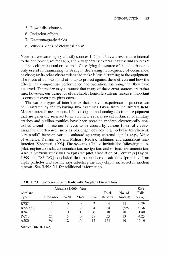
INTRODUCTION 33
5. Power disturbances
6. Radiation effects
7. Electromagnetic fields
8. Various kinds of electrical noise
Note that we can roughly classify sources 1, 2, and 3 as causes that are internalto the equipment; sources 4, 6, and 7 as generally external causes; and sources 5and 6 as either internal or external. Classifying the source of the disturbance isonly useful in minimizing its strength, decreasing its frequency of occurrence,or changing its other characteristics to make it less disturbing to the equipment.The focus of this text is what to do to protect against these effects and how theeffects can compromise performance and operation, assuming that they haveoccurred. The reader may comment that many of these error sources are ratherrare; however, our desire for ultrareliable, long-life systems makes it importantto consider even rare phenomena.
The various types of interference that one can experience in practice canbe illustrated by the following two examples taken from the aircraft field.Modern aircraft are crammed full of digital and analog electronic equipmentthat are generally referred to as avionics. Several recent instances of militarycrashes and civilian troubles have been noted in modern electronically con-trolled aircraft. These are believed to be caused by various forms of electro-magnetic interference, such as passenger devices (e.g., cellular telephones);“cross-talk” between various onboard systems; external signals (e.g., Voiceof America Transmitters and Military Radar); lightning; and equipment mal-function [Shooman, 1993]. The systems affected include the following: auto-pilot, engine controls, communication, navigation, and various instrumentation.Also, a previous study by Cockpit (the pilot association of Germany) [Taylor,1988, pp. 285–287] concluded that the number of soft fails (probably fromalpha particles and cosmic rays affecting memory chips) increased in modernaircraft. See Table 2.1 for additional information.
TABLE 2.1 Increase of Soft Fails with Airplane Generation
Altitude (1,000s feet) SoftAirplane Total No. of FailsType Ground-5 5–20 20–30 30+ Reports Aircraft per a/ c
B707 2 0 0 2 4 14 0.29B727/ 737 11 7 2 4 24 39/ 28 0.36B747 11 0 1 6 18 10 1.80DC10 21 5 0 29 55 13 4.23A300 96 12 6 17 131 10 13.10
Source: [Taylor, 1988].
34 CODING TECHNIQUES
It is not clear how the number of flight hours varied among the differentairplane types, what the computer memory sizes were for each of the aircraft,and the severity level of the fails. It would be interesting to compare this datato that observed in the operation of the most advanced versions of B747 andA320 aircraft, as well as other more recent designs.
There has been much work done on coding theory since 1950 [Rao, 1989].This chapter presents a modest sampling of theory as it applies to fault-tolerantsystems.
2.2 BASIC PRINCIPLES
Coding theory can be developed in terms of the mathematical structure ofgroups, subgroups, rings, fields, vector spaces, subspaces, polynomial algebra,and Galois fields [Rao, 1989, Chapter 2]. Another simple yet effective devel-opment of the theory based on algebra and logic is used in this text [Arazi,1988].
2.2.1 Code Distance
We will deal with strings of binary digits (0 or 1), which are of specified lengthand called the following synonymous terms: binary block, binary vector, binaryword, or just code word. Suppose that we are dealing with a 3-bit message (b1,b2, b3) represented by the bits x1, x2, x3. We can speak of the eight combi-nations of these bits—see Table 2.2(a)—as the code words. In this case theyare assigned according to the sequence of binary numbers. The distance of acode is the minimum number of bits by which any one code word differs fromanother. For example, the first and second code words in Table 2.2(a) differonly in the right-most digit and have a distance of 1, whereas the first and thelast code words differ in all 3 digits and have a distance of 3. The total numberof comparisons needed to check all of the word pairs for the minimum codedistance is the number of combinations of 8 items taken 2 at a time � 8
2 � , whichis equal to 8!/ 2!6! c 28.
A simpler way of visualizing the distance is to use the “cube method” ofdisplaying switching functions. A cube is drawn in three-dimensional space (x,y, z), and a main diagonal goes from x c y c z c 0 to x c y c z c 1. The distanceis the number of cube edges between any two code words that represent thevertices of the cube. Thus, the distance between 000 and 001 is a single cubeedge, but the distance between 000 and 111 is 3 since 3 edges must be traversedto get between the two vertices. (In honor of one of the pioneers of codingtheory, the code distance is generally called the Hamming distance.) Supposethat noise changes a single bit of a code word from 0 to 1 or 1 to 0. Thefirst code word in Table 2.2(a) would be changed to the second, third, or fifth,depending on which bit was corrupted. Thus there is no way to detect a single-bit error (or a multibit error), since any change in a code word transforms it
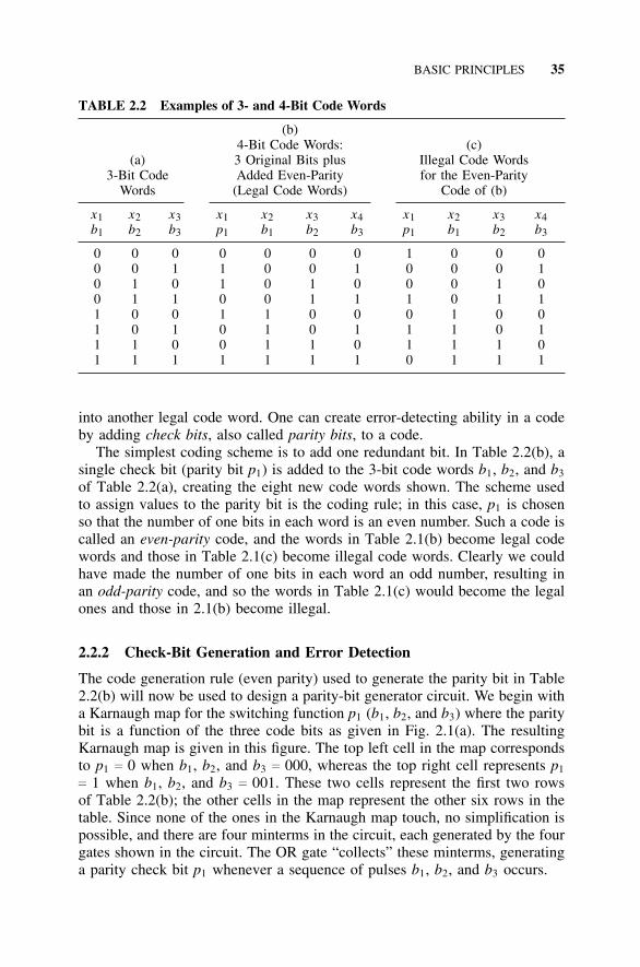
BASIC PRINCIPLES 35
TABLE 2.2 Examples of 3- and 4-Bit Code Words
(b)4-Bit Code Words: (c)
(a) 3 Original Bits plus Illegal Code Words3-Bit Code Added Even-Parity for the Even-Parity
Words (Legal Code Words) Code of (b)
x1 x2 x3 x1 x2 x3 x4 x1 x2 x3 x4b1 b2 b3 p1 b1 b2 b3 p1 b1 b2 b3
0 0 0 0 0 0 0 1 0 0 00 0 1 1 0 0 1 0 0 0 10 1 0 1 0 1 0 0 0 1 00 1 1 0 0 1 1 1 0 1 11 0 0 1 1 0 0 0 1 0 01 0 1 0 1 0 1 1 1 0 11 1 0 0 1 1 0 1 1 1 01 1 1 1 1 1 1 0 1 1 1
into another legal code word. One can create error-detecting ability in a codeby adding check bits, also called parity bits, to a code.
The simplest coding scheme is to add one redundant bit. In Table 2.2(b), asingle check bit (parity bit p1) is added to the 3-bit code words b1, b2, and b3
of Table 2.2(a), creating the eight new code words shown. The scheme usedto assign values to the parity bit is the coding rule; in this case, p1 is chosenso that the number of one bits in each word is an even number. Such a code iscalled an even-parity code, and the words in Table 2.1(b) become legal codewords and those in Table 2.1(c) become illegal code words. Clearly we couldhave made the number of one bits in each word an odd number, resulting inan odd-parity code, and so the words in Table 2.1(c) would become the legalones and those in 2.1(b) become illegal.
2.2.2 Check-Bit Generation and Error Detection
The code generation rule (even parity) used to generate the parity bit in Table2.2(b) will now be used to design a parity-bit generator circuit. We begin witha Karnaugh map for the switching function p1 (b1, b2, and b3) where the paritybit is a function of the three code bits as given in Fig. 2.1(a). The resultingKarnaugh map is given in this figure. The top left cell in the map correspondsto p1 c 0 when b1, b2, and b3 c 000, whereas the top right cell represents p1
c 1 when b1, b2, and b3 c 001. These two cells represent the first two rowsof Table 2.2(b); the other cells in the map represent the other six rows in thetable. Since none of the ones in the Karnaugh map touch, no simplification ispossible, and there are four minterms in the circuit, each generated by the fourgates shown in the circuit. The OR gate “collects” these minterms, generatinga parity check bit p1 whenever a sequence of pulses b1, b2, and b3 occurs.
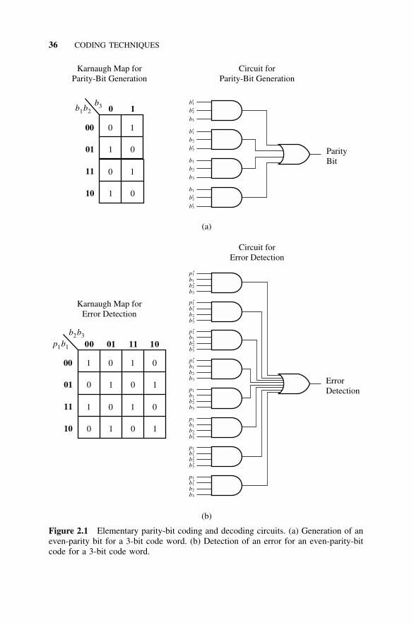
36 CODING TECHNIQUES
b′1
b′1
b1
b1
b′2
b2
b2
b′2
b3
b′3
b3
b′3
ParityBit
Circuit forParity-Bit Generation
0 1
00 0 1
0 1
01
11
10
1 0
1 0
b3b1 2b
Karnaugh Map forParity-Bit Generation
p1′
p1′
p1′
p1′
p1
p1
b1
b1′
b1
b1
b1
b1′
b2′
b2
b2′
b2
b2′
b2
b3
b3′
b3′
b3
b3
p1b1′b2′b3′
p1b1b2b3′
b3
ErrorDetection
Circuit forError Detection
00 1101 10
00 1 10 0
1 10 0
01
11
10
0 01 1
0 01 1
p1 1bb2 3b
Karnaugh Map forError Detection
(a)
(b)
Figure 2.1 Elementary parity-bit coding and decoding circuits. (a) Generation of aneven-parity bit for a 3-bit code word. (b) Detection of an error for an even-parity-bitcode for a 3-bit code word.
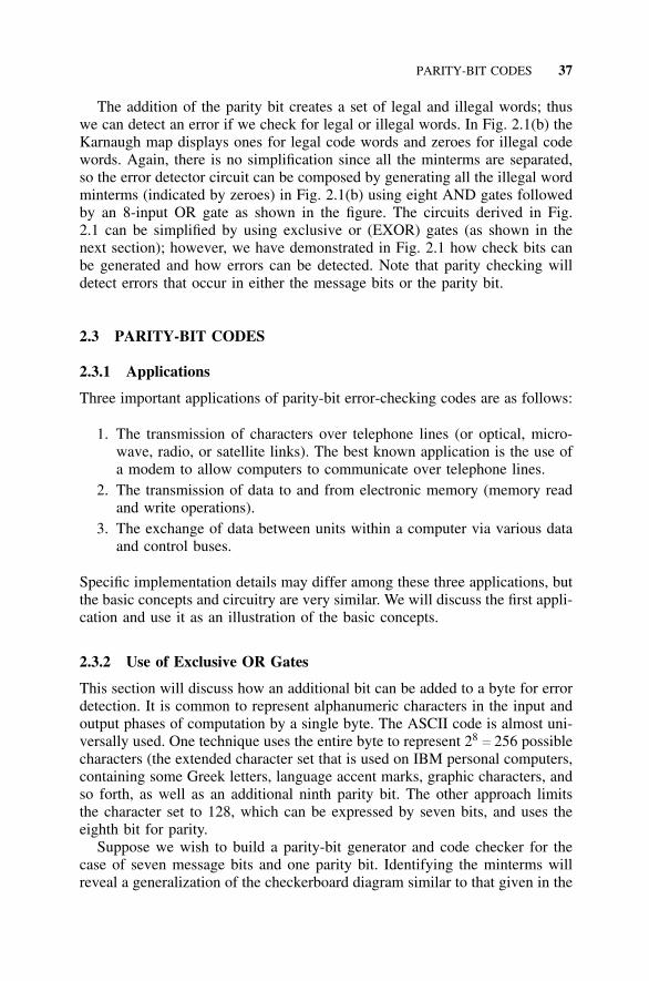
PARITY-BIT CODES 37
The addition of the parity bit creates a set of legal and illegal words; thuswe can detect an error if we check for legal or illegal words. In Fig. 2.1(b) theKarnaugh map displays ones for legal code words and zeroes for illegal codewords. Again, there is no simplification since all the minterms are separated,so the error detector circuit can be composed by generating all the illegal wordminterms (indicated by zeroes) in Fig. 2.1(b) using eight AND gates followedby an 8-input OR gate as shown in the figure. The circuits derived in Fig.2.1 can be simplified by using exclusive or (EXOR) gates (as shown in thenext section); however, we have demonstrated in Fig. 2.1 how check bits canbe generated and how errors can be detected. Note that parity checking willdetect errors that occur in either the message bits or the parity bit.
2.3 PARITY-BIT CODES
2.3.1 Applications
Three important applications of parity-bit error-checking codes are as follows:
1. The transmission of characters over telephone lines (or optical, micro-wave, radio, or satellite links). The best known application is the use ofa modem to allow computers to communicate over telephone lines.
2. The transmission of data to and from electronic memory (memory readand write operations).
3. The exchange of data between units within a computer via various dataand control buses.
Specific implementation details may differ among these three applications, butthe basic concepts and circuitry are very similar. We will discuss the first appli-cation and use it as an illustration of the basic concepts.
2.3.2 Use of Exclusive OR Gates
This section will discuss how an additional bit can be added to a byte for errordetection. It is common to represent alphanumeric characters in the input andoutput phases of computation by a single byte. The ASCII code is almost uni-versally used. One technique uses the entire byte to represent 28
c 256 possiblecharacters (the extended character set that is used on IBM personal computers,containing some Greek letters, language accent marks, graphic characters, andso forth, as well as an additional ninth parity bit. The other approach limitsthe character set to 128, which can be expressed by seven bits, and uses theeighth bit for parity.
Suppose we wish to build a parity-bit generator and code checker for thecase of seven message bits and one parity bit. Identifying the minterms willreveal a generalization of the checkerboard diagram similar to that given in the
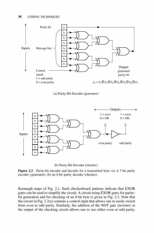
38 CODING TECHNIQUES
p1
b1
b2
b3
b4
b5
b6
b7
Parity bit
Message bits
Controlsignal1 = odd parity0 = even parity
Inputs
Output-generatedparity bit
p b b b b b b b1 = 1 2 3 4 5 6 7⊕ ⊕ ⊕ ⊕ ⊕ ⊕
Inputs
Outputs
p1
b1
b2
b3
b4
b5
b6
b7
even parity odd parity
1 = error0 = OK
1 = error0 = OK
(a) Parity-Bit Encoder (generator)
(b) Parity-Bit Decoder (checker)
Figure 2.2 Parity-bit encoder and decoder for a transmitted byte: (a) A 7-bit parityencoder (generator); (b) an 8-bit parity decoder (checker).
Karnaugh maps of Fig. 2.1. Such checkerboard patterns indicate that EXORgates can be used to simplify the circuit. A circuit using EXOR gates for parity-bit generation and for checking of an 8-bit byte is given in Fig. 2.2. Note thatthe circuit in Fig. 2.2(a) contains a control input that allows one to easily switchfrom even to odd parity. Similarly, the addition of the NOT gate (inverter) atthe output of the checking circuit allows one to use either even or odd parity.
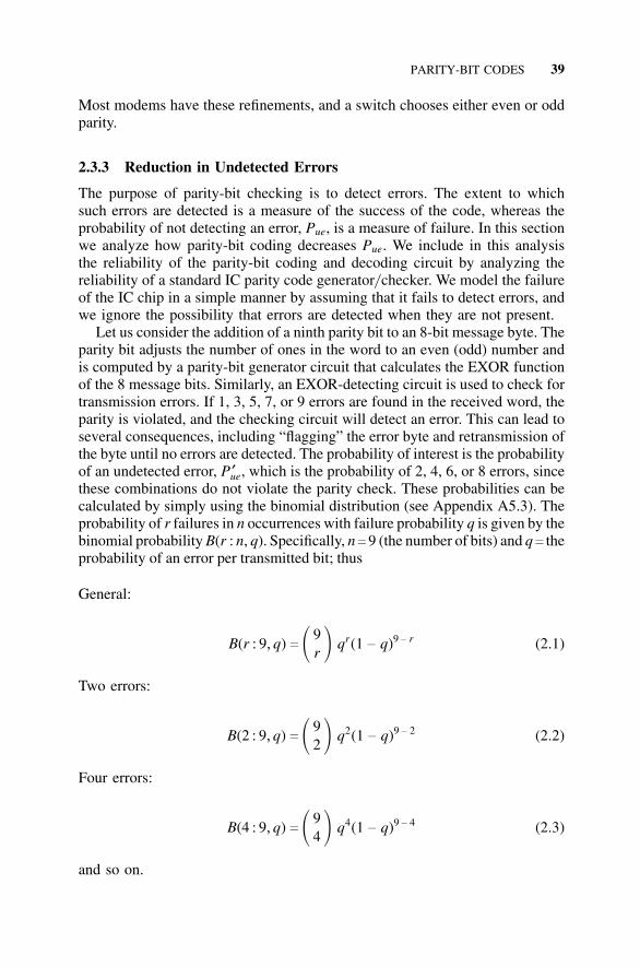
PARITY-BIT CODES 39
Most modems have these refinements, and a switch chooses either even or oddparity.
2.3.3 Reduction in Undetected Errors
The purpose of parity-bit checking is to detect errors. The extent to whichsuch errors are detected is a measure of the success of the code, whereas theprobability of not detecting an error, Pue, is a measure of failure. In this sectionwe analyze how parity-bit coding decreases Pue. We include in this analysisthe reliability of the parity-bit coding and decoding circuit by analyzing thereliability of a standard IC parity code generator/ checker. We model the failureof the IC chip in a simple manner by assuming that it fails to detect errors, andwe ignore the possibility that errors are detected when they are not present.
Let us consider the addition of a ninth parity bit to an 8-bit message byte. Theparity bit adjusts the number of ones in the word to an even (odd) number andis computed by a parity-bit generator circuit that calculates the EXOR functionof the 8 message bits. Similarly, an EXOR-detecting circuit is used to check fortransmission errors. If 1, 3, 5, 7, or 9 errors are found in the received word, theparity is violated, and the checking circuit will detect an error. This can lead toseveral consequences, including “flagging” the error byte and retransmission ofthe byte until no errors are detected. The probability of interest is the probabilityof an undetected error, P ′ue, which is the probability of 2, 4, 6, or 8 errors, sincethese combinations do not violate the parity check. These probabilities can becalculated by simply using the binomial distribution (see Appendix A5.3). Theprobability of r failures in n occurrences with failure probability q is given by thebinomial probability B(r : n, q). Specifically, n c 9 (the number of bits) and q c theprobability of an error per transmitted bit; thus
General:
B(r : 9, q) c � 9r � qr(1 − q)9 − r (2.1)
Two errors:
B(2 : 9, q) c � 92 � q2(1 − q)9 − 2 (2.2)
Four errors:
B(4 : 9, q) c � 94 � q4(1 − q)9 − 4 (2.3)
and so on.

40 CODING TECHNIQUES
For q, relatively small (10−4), it is easy to see that Eq. (2.3) is much smallerthan Eq. (2.2); thus only Eq. (2.2) needs to be considered (probabilities for rc 4, 6, and 8 are negligible), and the probability of an undetected error withparity-bit coding becomes
P ′ue c B(2 : 9, q) c 36q2(1 − q)7 (2.4)
We wish to compare this with the probabilty of an undetected error for an 8-bittransmission without any checking. With no checking, all errors are undetected;thus we must compute B(1 : 8, q) + · · · + B(8 : 8, q), but it is easier to compute
Pue c 1 − P(0 errors) c 1 − B(0 : 8, q) c 1 − � 80 � q0(1 − q)8 − 0
c 1 − (1 − q)8 (2.5)
Note that our convention is to use Pue for the case of no checking, and P ′ue forthe case of checking.
The ratio of Eqs. (2.5) and (2.4) yields the improvement ratio due to theparity-bit coding as follows:
Pue/ P ′ue c [1 − (1 − q)8]/ [36q2(1 − q)7] (2.6)
For small q we can simplify Eq. (2.6) by replacing (1 ± q)n by 1 ± nq and[1/ (1 − q)] by 1 + q, which yields
Pue/ P ′ue c [2(1 + 7q)/ 9q] (2.7)
The parameter q, the probability of failure per bit transmitted, is quoted as10−4 in Hill and Peterson [1981]. The failure probability q was 10−5 or 10−6
in the 1960s and ’70s; now, it may be as low as 10−7 for the best telephonelines [Rubin, 1990]. Equation (2.7) is evaluated for the range of q values; theresults appear in Table 2.3 and in Fig. 2.3.
The improvement ratio is quite significant, and the overhead—adding 1 par-ity bit out of 8 message bits—is only 12.5%, which is quite modest. This prob-ably explains why a parity-bit code is so frequently used.
In the above analysis we assumed that the coder and decoder are perfect. Wenow examine the validity of that assumption by modeling the reliability of thecoder and decoder. One could use a design similar to that of Fig. 2.2; however,it is more realistic to assume that we are using a commercial circuit device: theSN74180, a 9-bit odd/ even parity generator/ checker (see Texas Instruments[1988]), or the newer 74LS280 [Motorola, 1992]. The SN74180 has an equiv-alent circuit (see Fig. 2.4), which has 14 gates and inverters, whereas the pin-compatible 74LS280 with improved performance has 46 gates and inverters in
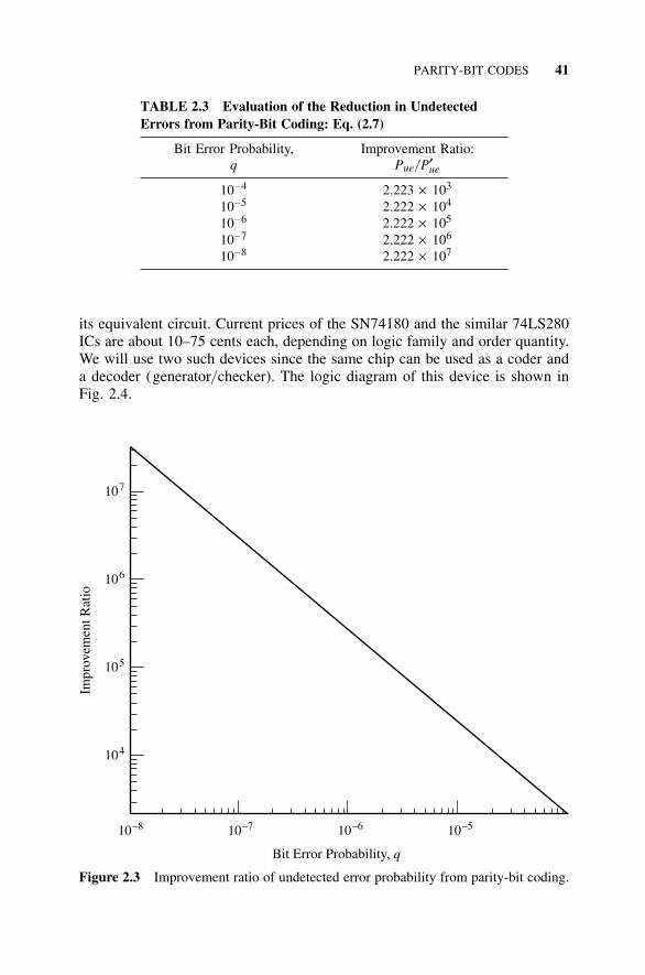
PARITY-BIT CODES 41
TABLE 2.3 Evaluation of the Reduction in UndetectedErrors from Parity-Bit Coding: Eq. (2.7)
Bit Error Probability, Improvement Ratio:q Pue/ P′ue
10−4 2.223 × 10³
10−5 2.222 × 10⁴
10−6 2.222 × 10⁵
10−7 2.222 × 10⁶
10−8 2.222 × 10⁷
its equivalent circuit. Current prices of the SN74180 and the similar 74LS280ICs are about 10–75 cents each, depending on logic family and order quantity.We will use two such devices since the same chip can be used as a coder anda decoder (generator/ checker). The logic diagram of this device is shown inFig. 2.4.
104
105
106
107
10–8 10–7 10–6 10–5
Bit Error Probability, q
Impr
ovem
ent R
atio
Figure 2.3 Improvement ratio of undetected error probability from parity-bit coding.
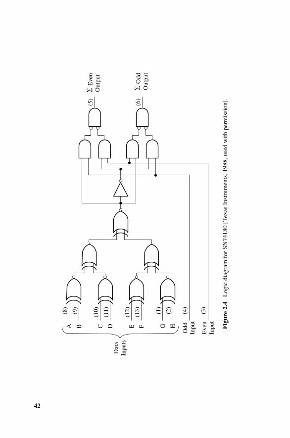
42
Dat
aIn
puts
A B C D E F G H
(8)
(9)
(10)
(11)
(12)
(13) (1
)
(4)
(2)
(3)
(5)
(6)
Eve
nO
utpu
t
Odd
Out
put
Odd
Inpu
t
Eve
nIn
put
∑ ∑
Fig
ure
2.4
Log
ic d
iagr
am f
or S
N74
180
[Tex
as I
nstr
umen
ts, 1
988,
use
d w
ith p
erm
issi
on].
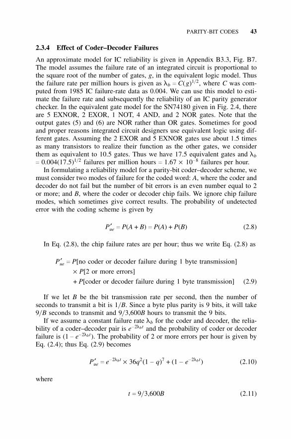
PARITY-BIT CODES 43
2.3.4 Effect of Coder–Decoder Failures
An approximate model for IC reliability is given in Appendix B3.3, Fig. B7.The model assumes the failure rate of an integrated circuit is proportional tothe square root of the number of gates, g, in the equivalent logic model. Thusthe failure rate per million hours is given as lb c C(g)1/ 2, where C was com-puted from 1985 IC failure-rate data as 0.004. We can use this model to esti-mate the failure rate and subsequently the reliability of an IC parity generatorchecker. In the equivalent gate model for the SN74180 given in Fig. 2.4, thereare 5 EXNOR, 2 EXOR, 1 NOT, 4 AND, and 2 NOR gates. Note that theoutput gates (5) and (6) are NOR rather than OR gates. Sometimes for goodand proper reasons integrated circuit designers use equivalent logic using dif-ferent gates. Assuming the 2 EXOR and 5 EXNOR gates use about 1.5 timesas many transistors to realize their function as the other gates, we considerthem as equivalent to 10.5 gates. Thus we have 17.5 equivalent gates and lb
c 0.004(17.5)1/ 2 failures per million hours c 1.67 × 10⁻⁸ failures per hour.In formulating a reliability model for a parity-bit coder–decoder scheme, we
must consider two modes of failure for the coded word: A, where the coder anddecoder do not fail but the number of bit errors is an even number equal to 2or more; and B, where the coder or decoder chip fails. We ignore chip failuremodes, which sometimes give correct results. The probability of undetectederror with the coding scheme is given by
P ′ue c P(A + B) c P(A) + P(B) (2.8)
In Eq. (2.8), the chip failure rates are per hour; thus we write Eq. (2.8) as
P ′ue c P[no coder or decoder failure during 1 byte transmission]
× P[2 or more errors]
+ P[coder or decoder failure during 1 byte transmission] (2.9)
If we let B be the bit transmission rate per second, then the number ofseconds to transmit a bit is 1/ B. Since a byte plus parity is 9 bits, it will take9/ B seconds to transmit and 9/ 3,600B hours to transmit the 9 bits.
If we assume a constant failure rate lb for the coder and decoder, the relia-bility of a coder–decoder pair is e−2lbt and the probability of coder or decoderfailure is (1 − e−2lbt). The probability of 2 or more errors per hour is given byEq. (2.4); thus Eq. (2.9) becomes
P ′ue c e−2lbt × 36q2(1 − q)7 + (1 − e−2lbt) (2.10)
where
t c 9/ 3,600B (2.11)
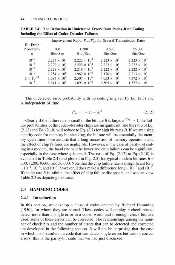
44 CODING TECHNIQUES
TABLE 2.4 The Reduction in Undetected Errors from Parity-Rate CodingIncluding the Effect of Coder–Decoder Failures
Improvement Ratio: Pue/ P′ue for Several Transmission RatesBit Error
Probability 300 1,200 9,600 56,000q Bits/ Sec Bits/ Sec Bits/ Sec Bits/ Sec
10−4 2.223 × 10³ 2.223 × 10³ 2.223 × 10³ 2.223 × 10³
10−5 2.222 × 10⁴ 2.222 × 10⁴ 2.222 × 10⁴ 2.222 × 10⁴
10−6 2.228 × 10⁵ 2.218 × 10⁵ 2.222 × 10⁵ 2.222 × 10⁵
10−7 1.254 × 10⁶ 1.962 × 10⁶ 2.170 × 10⁶ 2.213 × 10⁶
5 × 10⁻⁸ 1.087 × 10⁶ 2.507 × 10⁶ 4.053 × 10⁶ 4.372 × 10⁶
10−8 2.841 × 10⁵ 1.093 × 10⁶ 6.505 × 10⁶ 1.577 × 10⁷
The undetected error probability with no coding is given by Eq. (2.5) andis independent of time
Pue c 1 − (1 − q)8 (2.12)
Clearly if the failure rate is small or the bit rate B is large, e−2lbt ≈ 1, the fail-ure probabilities of the coder–decoder chips are insignificant, and the ratio of Eq.(2.12) and Eq. (2.10) will reduce to Eq. (2.7) for high bit rates B. If we are usinga parity code for memory bit checking, the bit rate will be essentially the mem-ory cycle time if we assume that a long succession of memory operations andthe effect of chip failures are negligible. However, in the case of parity-bit cod-ing in a modem, the baud rate will be lower and chip failures can be significant,especially in the case where q is small. The ratio of Eq. (2.12) to Eq. (2.10) isevaluated in Table 2.4 (and plotted in Fig. 2.5) for typical modem bit rates B c
300, 1,200, 9,600, and 56,000. Note that the chip failure rate is insignificant for qc 10−4, 10−5, and 10−6; however, it does make a difference for q c 10−7 and 10−8.If the bit rate B is infinite, the effect of chip failure disappears, and we can viewTable 2.3 as depicting this case.
2.4 HAMMING CODES
2.4.1 Introduction
In this section, we develop a class of codes created by Richard Hamming[1950], for whom they are named. These codes will employ c check bits todetect more than a single error in a coded word, and if enough check bits areused, some of these errors can be corrected. The relationships among the num-ber of check bits and the number of errors that can be detected and correctedare developed in the following section. It will not be surprising that the casein which c c 1 results in a code that can detect single errors but cannot correcterrors; this is the parity-bit code that we had just discussed.
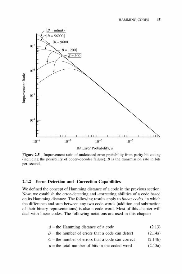
HAMMING CODES 45
104
105
106
107
10–8 10–7 10–6 10–5
Bit Error Probability, q
Impr
ovem
ent R
atio
B = 9600
B = 1200
B = 300
B = 56000
B = infinity
Figure 2.5 Improvement ratio of undetected error probability from parity-bit coding(including the possibility of coder–decoder failure). B is the transmission rate in bitsper second.
2.4.2 Error-Detection and -Correction Capabilities
We defined the concept of Hamming distance of a code in the previous section.Now, we establish the error-detecting and -correcting abilities of a code basedon its Hamming distance. The following results apply to linear codes, in whichthe difference and sum between any two code words (addition and subtractionof their binary representations) is also a code word. Most of this chapter willdeal with linear codes. The following notations are used in this chapter:
d c the Hamming distance of a code (2.13)
D c the number of errors that a code can detect (2.14a)
C c the number of errors that a code can correct (2.14b)
n c the total number of bits in the coded word (2.15a)
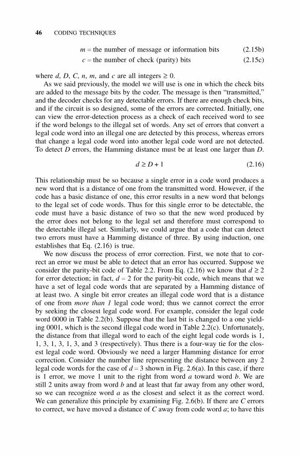
46 CODING TECHNIQUES
m c the number of message or information bits (2.15b)
c c the number of check (parity) bits (2.15c)
where d, D, C, n, m, and c are all integers ≥ 0.As we said previously, the model we will use is one in which the check bits
are added to the message bits by the coder. The message is then “transmitted,”and the decoder checks for any detectable errors. If there are enough check bits,and if the circuit is so designed, some of the errors are corrected. Initially, onecan view the error-detection process as a check of each received word to seeif the word belongs to the illegal set of words. Any set of errors that convert alegal code word into an illegal one are detected by this process, whereas errorsthat change a legal code word into another legal code word are not detected.To detect D errors, the Hamming distance must be at least one larger than D.
d ≥ D + 1 (2.16)
This relationship must be so because a single error in a code word produces anew word that is a distance of one from the transmitted word. However, if thecode has a basic distance of one, this error results in a new word that belongsto the legal set of code words. Thus for this single error to be detectable, thecode must have a basic distance of two so that the new word produced bythe error does not belong to the legal set and therefore must correspond tothe detectable illegal set. Similarly, we could argue that a code that can detecttwo errors must have a Hamming distance of three. By using induction, oneestablishes that Eq. (2.16) is true.
We now discuss the process of error correction. First, we note that to cor-rect an error we must be able to detect that an error has occurred. Suppose weconsider the parity-bit code of Table 2.2. From Eq. (2.16) we know that d ≥ 2for error detection; in fact, d c 2 for the parity-bit code, which means that wehave a set of legal code words that are separated by a Hamming distance ofat least two. A single bit error creates an illegal code word that is a distanceof one from more than 1 legal code word; thus we cannot correct the errorby seeking the closest legal code word. For example, consider the legal codeword 0000 in Table 2.2(b). Suppose that the last bit is changed to a one yield-ing 0001, which is the second illegal code word in Table 2.2(c). Unfortunately,the distance from that illegal word to each of the eight legal code words is 1,1, 3, 1, 3, 1, 3, and 3 (respectively). Thus there is a four-way tie for the clos-est legal code word. Obviously we need a larger Hamming distance for errorcorrection. Consider the number line representing the distance between any 2legal code words for the case of d c 3 shown in Fig. 2.6(a). In this case, if thereis 1 error, we move 1 unit to the right from word a toward word b. We arestill 2 units away from word b and at least that far away from any other word,so we can recognize word a as the closest and select it as the correct word.We can generalize this principle by examining Fig. 2.6(b). If there are C errorsto correct, we have moved a distance of C away from code word a; to have this
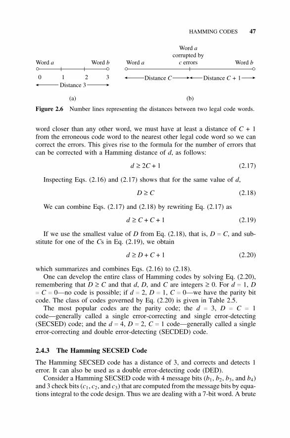
HAMMING CODES 47
Word a Word b
0 1 2 3Distance 3
Word a Word b
Distance C Distance 1C +
Wordcorrupted by
errors
a
c
(a) (b)
Figure 2.6 Number lines representing the distances between two legal code words.
word closer than any other word, we must have at least a distance of C + 1from the erroneous code word to the nearest other legal code word so we cancorrect the errors. This gives rise to the formula for the number of errors thatcan be corrected with a Hamming distance of d, as follows:
d ≥ 2C + 1 (2.17)
Inspecting Eqs. (2.16) and (2.17) shows that for the same value of d,
D ≥ C (2.18)
We can combine Eqs. (2.17) and (2.18) by rewriting Eq. (2.17) as
d ≥ C + C + 1 (2.19)
If we use the smallest value of D from Eq. (2.18), that is, D c C, and sub-stitute for one of the Cs in Eq. (2.19), we obtain
d ≥ D + C + 1 (2.20)
which summarizes and combines Eqs. (2.16) to (2.18).One can develop the entire class of Hamming codes by solving Eq. (2.20),
remembering that D ≥ C and that d, D, and C are integers ≥ 0. For d c 1, Dc C c 0—no code is possible; if d c 2, D c 1, C c 0—we have the parity bitcode. The class of codes governed by Eq. (2.20) is given in Table 2.5.
The most popular codes are the parity code; the d c 3, D c C c 1code—generally called a single error-correcting and single error-detecting(SECSED) code; and the d c 4, D c 2, C c 1 code—generally called a singleerror-correcting and double error-detecting (SECDED) code.
2.4.3 The Hamming SECSED Code
The Hamming SECSED code has a distance of 3, and corrects and detects 1error. It can also be used as a double error-detecting code (DED).
Consider a Hamming SECSED code with 4 message bits (b1, b2, b3, and b4)and 3 check bits (c1, c2, and c3) that are computed from the message bits by equa-tions integral to the code design. Thus we are dealing with a 7-bit word. A brute
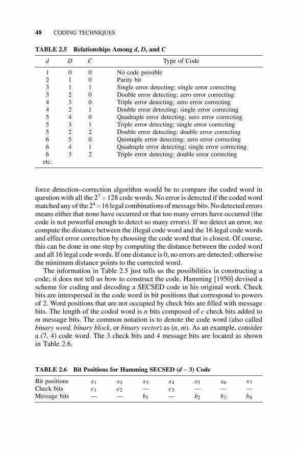
48 CODING TECHNIQUES
TABLE 2.5 Relationships Among d, D, and C
d D C Type of Code
1 0 0 No code possible2 1 0 Parity bit3 1 1 Single error detecting; single error correcting3 2 0 Double error detecting; zero error correcting4 3 0 Triple error detecting; zero error correcting4 2 1 Double error detecting; single error correcting5 4 0 Quadruple error detecting; zero error correcting5 3 1 Triple error detecting; single error correcting5 2 2 Double error detecting; double error correcting6 5 0 Quintuple error detecting; zero error correcting6 4 1 Quadruple error detecting; single error correcting6 3 2 Triple error detecting; double error correcting
etc.
force detection–correction algorithm would be to compare the coded word inquestion with all the 27
c 128 code words. No error is detected if the coded wordmatched any of the 24
c 16 legal combinations of message bits. No detected errorsmeans either that none have occurred or that too many errors have occurred (thecode is not powerful enough to detect so many errors). If we detect an error, wecompute the distance between the illegal code word and the 16 legal code wordsand effect error correction by choosing the code word that is closest. Of course,this can be done in one step by computing the distance between the coded wordand all 16 legal code words. If one distance is 0, no errors are detected; otherwisethe minimum distance points to the corrected word.
The information in Table 2.5 just tells us the possibilities in constructing acode; it does not tell us how to construct the code. Hamming [1950] devised ascheme for coding and decoding a SECSED code in his original work. Checkbits are interspersed in the code word in bit positions that correspond to powersof 2. Word positions that are not occupied by check bits are filled with messagebits. The length of the coded word is n bits composed of c check bits added tom message bits. The common notation is to denote the code word (also calledbinary word, binary block, or binary vector) as (n, m). As an example, considera (7, 4) code word. The 3 check bits and 4 message bits are located as shownin Table 2.6.
TABLE 2.6 Bit Positions for Hamming SECSED (d c 3) Code
Bit positions x1 x2 x3 x4 x5 x6 x7Check bits c1 c2 — c3 — — —Message bits — — b1 — b2 b3 b4
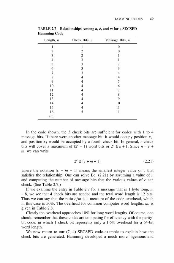
HAMMING CODES 49
TABLE 2.7 Relationships Among n, c, and m for a SECSEDHamming Code
Length, n Check Bits, c Message Bits, m
1 1 02 2 03 2 14 3 15 3 26 3 37 3 48 4 49 4 5
10 4 611 4 712 4 813 4 914 4 1015 4 1116 5 11etc.
In the code shown, the 3 check bits are sufficient for codes with 1 to 4message bits. If there were another message bit, it would occupy position x9,and position x8 would be occupied by a fourth check bit. In general, c checkbits will cover a maximum of (2c
− 1) word bits or 2c ≥ n + 1. Since n c c +m, we can write
2c ≥ [c + m + 1] (2.21)
where the notation [c + m + 1] means the smallest integer value of c thatsatisfies the relationship. One can solve Eq. (2.21) by assuming a value of nand computing the number of message bits that the various values of c cancheck. (See Table 2.7.)
If we examine the entry in Table 2.7 for a message that is 1 byte long, mc 8, we see that 4 check bits are needed and the total word length is 12 bits.Thus we can say that the ratio c/ m is a measure of the code overhead, whichin this case is 50%. The overhead for common computer word lengths, m, isgiven in Table 2.8.
Clearly the overhead approaches 10% for long word lengths. Of course, oneshould remember that these codes are competing for efficiency with the parity-bit code, in which 1 check bit represents only a 1.6% overhead for a 64-bitword length.
We now return to our (7, 4) SECSED code example to explain how thecheck bits are generated. Hamming developed a much more ingenious and
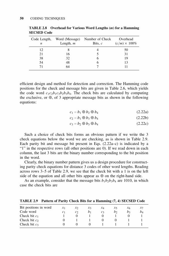
50 CODING TECHNIQUES
TABLE 2.8 Overhead for Various Word Lengths (m) for a HammingSECSED Code
Code Length, Word (Message) Number of Check Overheadn Length, m Bits, c (c/ m) × 100%
12 8 4 5021 16 5 3138 32 6 1954 48 6 1371 64 7 11
efficient design and method for detection and correction. The Hamming codepositions for the check and message bits are given in Table 2.6, which yieldsthe code word c1c2b1c3b2b3b4. The check bits are calculated by computingthe exclusive, or ⊕, of 3 appropriate message bits as shown in the followingequations:
c1 c b1 ⊕ b2 ⊕ b4 (2.22a)
c2 c b1 ⊕ b3 ⊕ b4 (2.22b)
c3 c b2 ⊕ b3 ⊕ b4 (2.22c)
Such a choice of check bits forms an obvious pattern if we write the 3check equations below the word we are checking, as is shown in Table 2.9.Each parity bit and message bit present in Eqs. (2.22a–c) is indicated by a“1” in the respective rows (all other positions are 0). If we read down in eachcolumn, the last 3 bits are the binary number corresponding to the bit positionin the word.
Clearly, the binary number pattern gives us a design procedure for construct-ing parity check equations for distance 3 codes of other word lengths. Readingacross rows 3–5 of Table 2.9, we see that the check bit with a 1 is on the leftside of the equation and all other bits appear as ⊕ on the right-hand side.
As an example, consider that the message bits b1b2b3b4 are 1010, in whichcase the check bits are
TABLE 2.9 Pattern of Parity Check Bits for a Hamming (7, 4) SECSED Code
Bit positions in word x1 x2 x3 x4 x5 x6 x7Code word c1 c2 b1 c3 b2 b3 b4Check bit c1 1 0 1 0 1 0 1Check bit c2 0 1 1 0 0 1 1Check bit c3 0 0 0 1 1 1 1
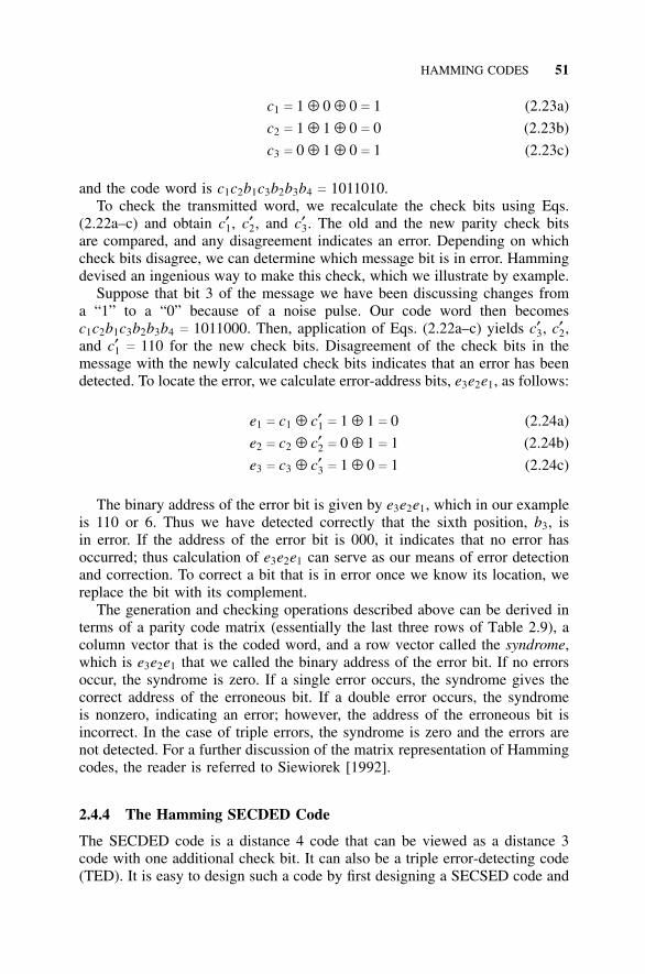
HAMMING CODES 51
c1 c 1 ⊕ 0 ⊕ 0 c 1 (2.23a)
c2 c 1 ⊕ 1 ⊕ 0 c 0 (2.23b)
c3 c 0 ⊕ 1 ⊕ 0 c 1 (2.23c)
and the code word is c1c2b1c3b2b3b4 c 1011010.To check the transmitted word, we recalculate the check bits using Eqs.
(2.22a–c) and obtain c′1, c′2, and c′3. The old and the new parity check bitsare compared, and any disagreement indicates an error. Depending on whichcheck bits disagree, we can determine which message bit is in error. Hammingdevised an ingenious way to make this check, which we illustrate by example.
Suppose that bit 3 of the message we have been discussing changes froma “1” to a “0” because of a noise pulse. Our code word then becomesc1c2b1c3b2b3b4 c 1011000. Then, application of Eqs. (2.22a–c) yields c′3, c′2,and c′1 c 110 for the new check bits. Disagreement of the check bits in themessage with the newly calculated check bits indicates that an error has beendetected. To locate the error, we calculate error-address bits, e3e2e1, as follows:
e1 c c1 ⊕ c′1 c 1 ⊕ 1 c 0 (2.24a)
e2 c c2 ⊕ c′2 c 0 ⊕ 1 c 1 (2.24b)
e3 c c3 ⊕ c′3 c 1 ⊕ 0 c 1 (2.24c)
The binary address of the error bit is given by e3e2e1, which in our exampleis 110 or 6. Thus we have detected correctly that the sixth position, b3, isin error. If the address of the error bit is 000, it indicates that no error hasoccurred; thus calculation of e3e2e1 can serve as our means of error detectionand correction. To correct a bit that is in error once we know its location, wereplace the bit with its complement.
The generation and checking operations described above can be derived interms of a parity code matrix (essentially the last three rows of Table 2.9), acolumn vector that is the coded word, and a row vector called the syndrome,which is e3e2e1 that we called the binary address of the error bit. If no errorsoccur, the syndrome is zero. If a single error occurs, the syndrome gives thecorrect address of the erroneous bit. If a double error occurs, the syndromeis nonzero, indicating an error; however, the address of the erroneous bit isincorrect. In the case of triple errors, the syndrome is zero and the errors arenot detected. For a further discussion of the matrix representation of Hammingcodes, the reader is referred to Siewiorek [1992].
2.4.4 The Hamming SECDED Code
The SECDED code is a distance 4 code that can be viewed as a distance 3code with one additional check bit. It can also be a triple error-detecting code(TED). It is easy to design such a code by first designing a SECSED code and
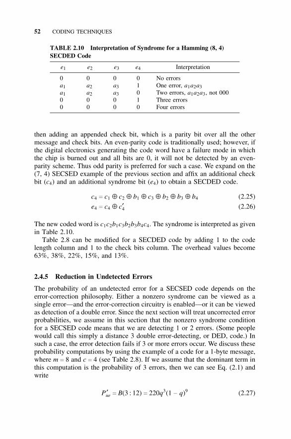
52 CODING TECHNIQUES
TABLE 2.10 Interpretation of Syndrome for a Hamming (8, 4)SECDED Code
e1 e2 e3 e4 Interpretation
0 0 0 0 No errorsa1 a2 a3 1 One error, a1a2a3a1 a2 a3 0 Two errors, a1a2a3, not 0000 0 0 1 Three errors0 0 0 0 Four errors
then adding an appended check bit, which is a parity bit over all the othermessage and check bits. An even-parity code is traditionally used; however, ifthe digital electronics generating the code word have a failure mode in whichthe chip is burned out and all bits are 0, it will not be detected by an even-parity scheme. Thus odd parity is preferred for such a case. We expand on the(7, 4) SECSED example of the previous section and affix an additional checkbit (c4) and an additional syndrome bit (e4) to obtain a SECDED code.
c4 c c1 ⊕ c2 ⊕ b1 ⊕ c3 ⊕ b2 ⊕ b3 ⊕ b4 (2.25)
e4 c c4 ⊕ c′4 (2.26)
The new coded word is c1c2b1c3b2b3b4c4. The syndrome is interpreted as givenin Table 2.10.
Table 2.8 can be modified for a SECDED code by adding 1 to the codelength column and 1 to the check bits column. The overhead values become63%, 38%, 22%, 15%, and 13%.
2.4.5 Reduction in Undetected Errors
The probability of an undetected error for a SECSED code depends on theerror-correction philosophy. Either a nonzero syndrome can be viewed as asingle error—and the error-correction circuitry is enabled—or it can be viewedas detection of a double error. Since the next section will treat uncorrected errorprobabilities, we assume in this section that the nonzero syndrome conditionfor a SECSED code means that we are detecting 1 or 2 errors. (Some peoplewould call this simply a distance 3 double error-detecting, or DED, code.) Insuch a case, the error detection fails if 3 or more errors occur. We discuss theseprobability computations by using the example of a code for a 1-byte message,where m c 8 and c c 4 (see Table 2.8). If we assume that the dominant term inthis computation is the probability of 3 errors, then we can see Eq. (2.1) andwrite
P ′ue c B(3 : 12) c 220q3(1 − q)9 (2.27)
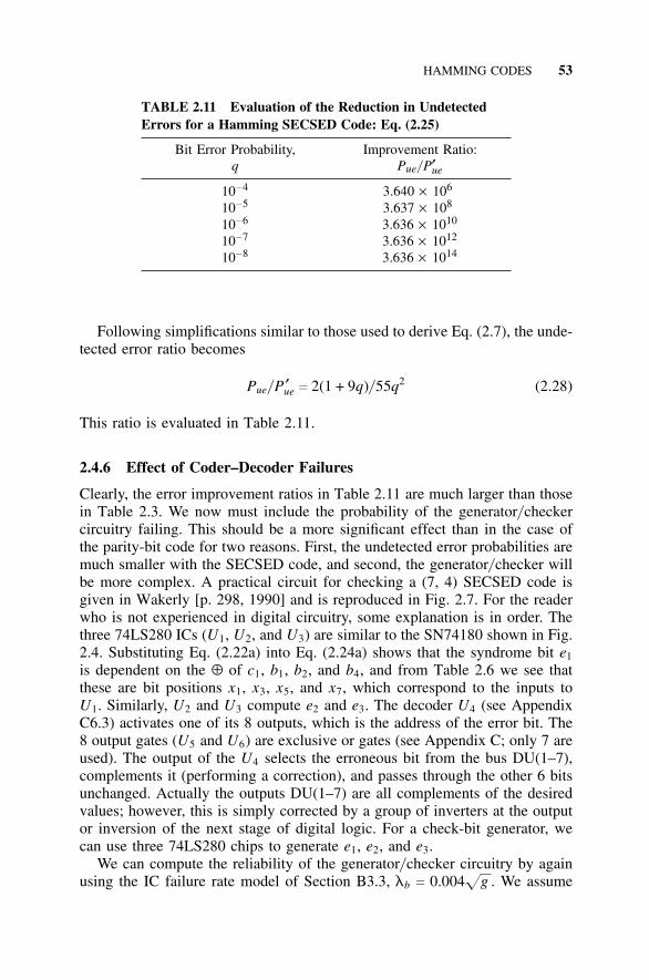
HAMMING CODES 53
TABLE 2.11 Evaluation of the Reduction in UndetectedErrors for a Hamming SECSED Code: Eq. (2.25)
Bit Error Probability, Improvement Ratio:q Pue/ P′ue
10−4 3.640 × 10⁶
10−5 3.637 × 10⁸
10−6 3.636 × 10¹⁰
10−7 3.636 × 10¹²
10−8 3.636 × 10¹⁴
Following simplifications similar to those used to derive Eq. (2.7), the unde-tected error ratio becomes
Pue/ P ′ue c 2(1 + 9q)/ 55q2 (2.28)
This ratio is evaluated in Table 2.11.
2.4.6 Effect of Coder–Decoder Failures
Clearly, the error improvement ratios in Table 2.11 are much larger than thosein Table 2.3. We now must include the probability of the generator/ checkercircuitry failing. This should be a more significant effect than in the case ofthe parity-bit code for two reasons. First, the undetected error probabilities aremuch smaller with the SECSED code, and second, the generator/ checker willbe more complex. A practical circuit for checking a (7, 4) SECSED code isgiven in Wakerly [p. 298, 1990] and is reproduced in Fig. 2.7. For the readerwho is not experienced in digital circuitry, some explanation is in order. Thethree 74LS280 ICs (U1, U2, and U3) are similar to the SN74180 shown in Fig.2.4. Substituting Eq. (2.22a) into Eq. (2.24a) shows that the syndrome bit e1
is dependent on the ⊕ of c1, b1, b2, and b4, and from Table 2.6 we see thatthese are bit positions x1, x3, x5, and x7, which correspond to the inputs toU1. Similarly, U2 and U3 compute e2 and e3. The decoder U4 (see AppendixC6.3) activates one of its 8 outputs, which is the address of the error bit. The8 output gates (U5 and U6) are exclusive or gates (see Appendix C; only 7 areused). The output of the U4 selects the erroneous bit from the bus DU(1–7),complements it (performing a correction), and passes through the other 6 bitsunchanged. Actually the outputs DU(1–7) are all complements of the desiredvalues; however, this is simply corrected by a group of inverters at the outputor inversion of the next stage of digital logic. For a check-bit generator, wecan use three 74LS280 chips to generate e1, e2, and e3.
We can compute the reliability of the generator/ checker circuitry by againusing the IC failure rate model of Section B3.3, lb c 0.004
fg . We assume
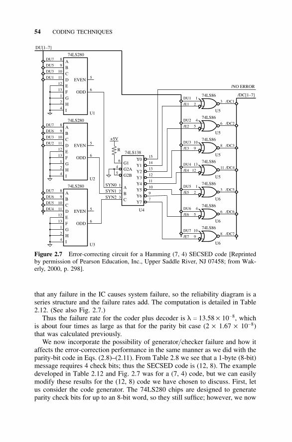
54 CODING TECHNIQUES
74LS86
74LS86
74LS86
74LS86
74LS86
74LS86
74LS86
DU1
DU2
DU3
DU4
DU5
DU6
DU7
1
4
10
13
1
4
10
2
5
9
12
2
5
9
/E1
/E2
/E3
/E4
/E5
/E6
/E7
3
6
8
11
3
6
8
/DC1
/DC2
/DC3
/DC4
/DC5
/DC6
/DC7
U5
U5
U5
U5
U6
U6
U6
U4
/DC[1–7]
/NO ERROR
15
14
13
12
11
10
9
7
Y0Y1Y2Y3
EVEN
EVEN
EVEN
ODD
ODD
ODD
Y4Y5Y6Y7
G1G2AG2B
A
A
A
A B
B
B
B C
C
C
C
D
D
D
E
E
E
F
F
F
G
G
G
H
H
H
I
I
I
+5V
R74LS138
74LS280
74LS280
74LS280
6
4
5
1
2
3
SYN0SYN1SYN2
5
5
5
6
6
6
DU[1–7]
8
8
8
DU7
DU7
DU7
DU5
DU6
DU6
DU3
DU3
DU5
DU1
DU2
DU4
9
9
9
10
10
10
11
11
11
12
12
12
13
13
13
1
1
1
2
2
2
4
4
4
U1
U2
U3
Figure 2.7 Error-correcting circuit for a Hamming (7, 4) SECSED code [Reprintedby permission of Pearson Education, Inc., Upper Saddle River, NJ 07458; from Wak-erly, 2000, p. 298].
that any failure in the IC causes system failure, so the reliability diagram is aseries structure and the failure rates add. The computation is detailed in Table2.12. (See also Fig. 2.7.)
Thus the failure rate for the coder plus decoder is l c 13.58 × 10⁻⁸, whichis about four times as large as that for the parity bit case (2 × 1.67 × 10−8)that was calculated previously.
We now incorporate the possibility of generator/ checker failure and how itaffects the error-correction performance in the same manner as we did with theparity-bit code in Eqs. (2.8)–(2.11). From Table 2.8 we see that a 1-byte (8-bit)message requires 4 check bits; thus the SECSED code is (12, 8). The exampledeveloped in Table 2.12 and Fig. 2.7 was for a (7, 4) code, but we can easilymodify these results for the (12, 8) code we have chosen to discuss. First, letus consider the code generator. The 74LS280 chips are designed to generateparity check bits for up to an 8-bit word, so they still suffice; however, we now
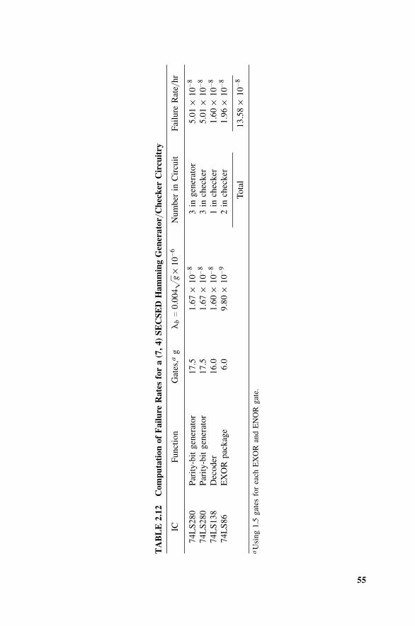
55
TA
BL
E2.
12C
ompu
tati
on o
f F
ailu
re R
ates
for
a (
7,4)
SE
CSE
D H
amm
ing
Gen
erat
or/C
heck
er C
ircu
itry
ICFu
nctio
nG
ates
,ag
lbc
0.00
4fg
×10−6
Num
ber
in C
ircu
itFa
ilure
Rat
e /hr
74L
S280
Pari
ty-b
it ge
nera
tor
17.5
1.67
×10−8
3in
gen
erat
or5.
01×
10−8
74L
S280
Pari
ty-b
it ge
nera
tor
17.5
1.67
×10−8
3in
che
cker
5.01
×10−8
74L
S138
Dec
oder
16.0
1.60
×10−8
1in
che
cker
1.60
×10−8
74L
S86
EX
OR
pac
kage
6.0
9.80
×10−9
2in
che
cker
1.96
×10−8
Tota
l13
.58
×10−8
aU
sing
1.5
gate
s fo
r ea
ch E
XO
R a
nd E
NO
R g
ate.
56 CODING TECHNIQUES
need to generate 4 check bits, so a total of 4 will be required. In the case of thechecker (see Fig. 2.7), we will also require four 74LS280 chips to generate they-syndrome bits. Instead of a 3-to-8 decoder we will need a 4-to-16 decoderfor the next stage, which can be implemented by using two 74LS138 chipsand the appropriate connections at the enable inputs (G1, G2A, and G2B), asexplained in Appendix C6.3. The output stage composed of 74LS86 chips willnot be required if we are only considering error detection, since the nonerroroutput is sufficient for this. Thus we can modify Table 2.12 to compute thefailure rate that is shown in Table 2.13. Note that one could argue that since weare only computing the error-detection probabilities, the decoders and outputcorrection EXOR gates are not needed, and only an OR gate with the syndromeinputs is needed to detect a 0000 syndrome that indicates no errors.
Using the information in Table 2.13 and Eq. (2.27), we obtain an expressionsimilar to Eq. (2.10), as follows:
P ′ue c e−l t220q3(1 − q)9 + (1 − e−l t) (2.29)
where l is 19.50 × 10⁻⁸ failures per hour and t is 12/ 3600B.We formulate the improvement ratio by dividing Eq. (2.29) by Eq. (2.12);
the ratio is given in Table 2.14 and is plotted in Fig. 2.8. The data presentedin Table 2.11 is also plotted in Fig. 2.8 and represents the line labeled B b ∞,which represents the case for a nonfailing generator/ checker.
2.4.7 How Coder–Decoder Failures Affect SECSED Codes
Because the Hamming SECSED code results in a lower value for undetectederrors than the parity-bit code, the effect of chip failures is even more pro-nounced. Of course the coding is still a big improvement, but not as much asone would predict. In fact, by comparing Figs. 2.8 and 2.5 we see that for Bc 300, the parity-bit scheme is superior to the SECSED scheme for values ofq less than about 2 × 10⁻⁷; for B c 1,200, the parity-bit scheme is superior tothe SECSED scheme for values of q less than about 10−7. The general con-clusion is that for more complex error detection schemes, one should evaluatethe effects of generator/ checker failures, since these may be of considerableimportance for small values of q. (Chip-specific failure rates may be required.)
More generally, we should compute whether generator/ checker failures sig-nificantly affect the code performance for the given values of q and B. If suchfailures are significant, we can consider the following alternatives:
1. Consider a simpler coding scheme if q is very small and B is low.2. Consider other coding schemes if they use simpler generator/ checker
circutry.3. Use other digital logic designs that utilize fewer but larger chips. Since
the failure rate is proportional tof
g , larger-scale integration improvesreliability.
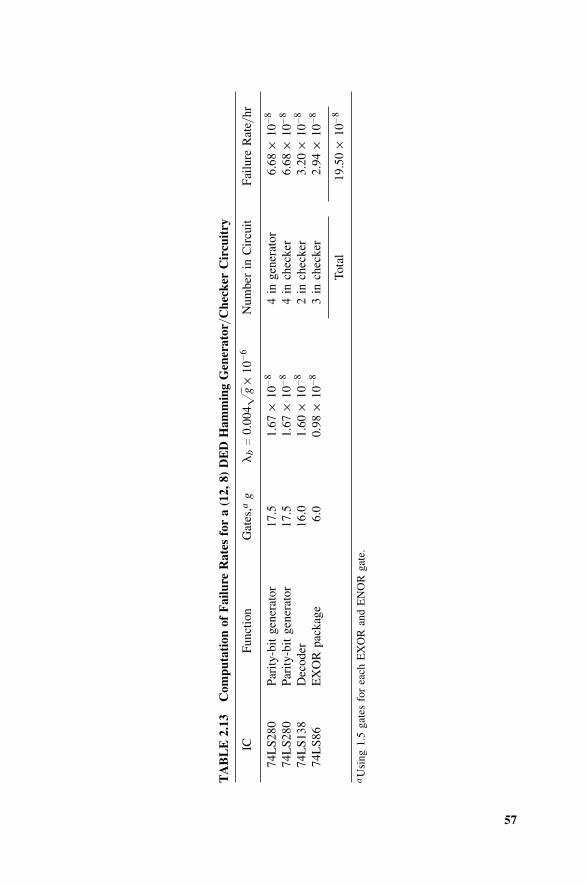
57
TA
BL
E2.
13C
ompu
tati
on o
f F
ailu
re R
ates
for
a (
12,8
) D
ED
Ham
min
g G
ener
ator
/Che
cker
Cir
cuit
ry
ICFu
nctio
nG
ates
,ag
lbc
0.00
4fg
×10−6
Num
ber
in C
ircu
itFa
ilure
Rat
e /hr
74L
S280
Pari
ty-b
it ge
nera
tor
17.5
1.67
×10−8
4in
gen
erat
or6.
68×
10−8
74L
S280
Pari
ty-b
it ge
nera
tor
17.5
1.67
×10−8
4in
che
cker
6.68
×10−8
74L
S138
Dec
oder
16.0
1.60
×10−8
2in
che
cker
3.20
×10−8
74L
S86
EX
OR
pac
kage
6.0
0.98
×10−8
3in
che
cker
2.94
×10−8
Tota
l19
.50
×10−8
aU
sing
1.5
gate
s fo
r ea
ch E
XO
R a
nd E
NO
R g
ate.
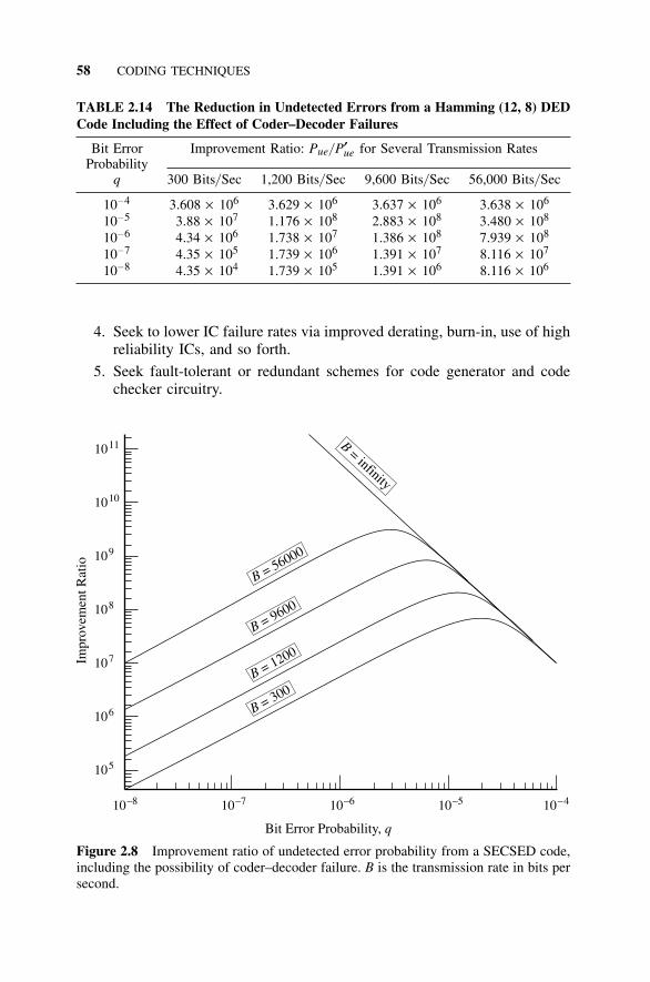
58 CODING TECHNIQUES
TABLE 2.14 The Reduction in Undetected Errors from a Hamming (12, 8) DEDCode Including the Effect of Coder–Decoder Failures
Bit Error Improvement Ratio: Pue/ P′ue for Several Transmission RatesProbability
q 300 Bits/ Sec 1,200 Bits/ Sec 9,600 Bits/ Sec 56,000 Bits/ Sec
10−4 3.608 × 10⁶ 3.629 × 10⁶ 3.637 × 10⁶ 3.638 × 10⁶
10−5 3.88 × 10⁷ 1.176 × 10⁸ 2.883 × 10⁸ 3.480 × 10⁸
10−6 4.34 × 10⁶ 1.738 × 10⁷ 1.386 × 10⁸ 7.939 × 10⁸
10−7 4.35 × 10⁵ 1.739 × 10⁶ 1.391 × 10⁷ 8.116 × 10⁷
10−8 4.35 × 10⁴ 1.739 × 10⁵ 1.391 × 10⁶ 8.116 × 10⁶
4. Seek to lower IC failure rates via improved derating, burn-in, use of highreliability ICs, and so forth.
5. Seek fault-tolerant or redundant schemes for code generator and codechecker circuitry.
105
106
107
108
109
1010
1011
10–8 10–7 10–6 10–5 10–4
Bit Error Probability, q
Impr
ovem
ent R
atio
B = 9600
B = 1200
B = 300
B = 56000
B= infinity
Figure 2.8 Improvement ratio of undetected error probability from a SECSED code,including the possibility of coder–decoder failure. B is the transmission rate in bits persecond.
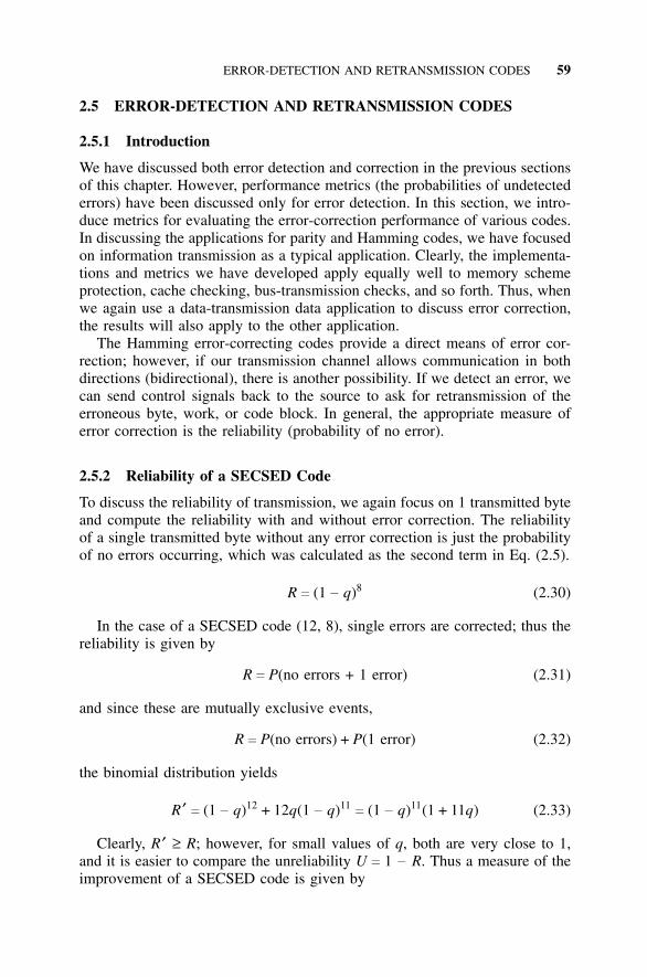
ERROR-DETECTION AND RETRANSMISSION CODES 59
2.5 ERROR-DETECTION AND RETRANSMISSION CODES
2.5.1 Introduction
We have discussed both error detection and correction in the previous sectionsof this chapter. However, performance metrics (the probabilities of undetectederrors) have been discussed only for error detection. In this section, we intro-duce metrics for evaluating the error-correction performance of various codes.In discussing the applications for parity and Hamming codes, we have focusedon information transmission as a typical application. Clearly, the implementa-tions and metrics we have developed apply equally well to memory schemeprotection, cache checking, bus-transmission checks, and so forth. Thus, whenwe again use a data-transmission data application to discuss error correction,the results will also apply to the other application.
The Hamming error-correcting codes provide a direct means of error cor-rection; however, if our transmission channel allows communication in bothdirections (bidirectional), there is another possibility. If we detect an error, wecan send control signals back to the source to ask for retransmission of theerroneous byte, work, or code block. In general, the appropriate measure oferror correction is the reliability (probability of no error).
2.5.2 Reliability of a SECSED Code
To discuss the reliability of transmission, we again focus on 1 transmitted byteand compute the reliability with and without error correction. The reliabilityof a single transmitted byte without any error correction is just the probabilityof no errors occurring, which was calculated as the second term in Eq. (2.5).
R c (1 − q)8 (2.30)
In the case of a SECSED code (12, 8), single errors are corrected; thus thereliability is given by
R c P(no errors + 1 error) (2.31)
and since these are mutually exclusive events,
R c P(no errors) + P(1 error) (2.32)
the binomial distribution yields
R ′ c (1 − q)12 + 12q(1 − q)11c (1 − q)11(1 + 11q) (2.33)
Clearly, R ′ ≥ R; however, for small values of q, both are very close to 1,and it is easier to compare the unreliability U c 1 − R. Thus a measure of theimprovement of a SECSED code is given by
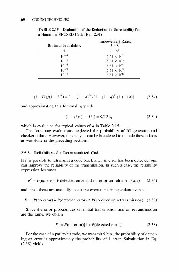
60 CODING TECHNIQUES
TABLE 2.15 Evaluation of the Reduction in Unreliability fora Hamming SECSED Code: Eq. (2.35)
Improvement Ratio:Bit Error Probability,
q1 − U1 − U ′
10−4 6.61 × 10²
10−5 6.61 × 10³
10−6 6.61 × 10⁴
10−7 6.61 × 10⁵
10−8 6.61 × 10⁶
(1 − U )/ (1 − U ′) c [1 − (1 − q)8]/ [1 − (1 − q)11(1 + 11q)] (2.34)
and approximating this for small q yields
(1 − U)/ (1 − U ′) c 8/ 121q (2.35)
which is evaluated for typical values of q in Table 2.15.The foregoing evaluations neglected the probability of IC generator and
checker failure. However, the analysis can be broadened to include these effectsas was done in the preceding sections.
2.5.3 Reliability of a Retransmitted Code
If it is possible to retransmit a code block after an error has been detected, onecan improve the reliability of the transmission. In such a case, the reliabilityexpression becomes
R ′ c P(no error + detected error and no error on retransmisson) (2.36)
and since these are mutually exclusive events and independent events,
R ′ c P(no error) + P(detected error) × P(no error on retransmission) (2.37)
Since the error probabilities on initial transmission and on retransmissionare the same, we obtain
R ′ c P(no error)[1 + P(detected error)] (2.38)
For the case of a parity-bit code, we transmit 9 bits; the probability of detect-ing an error is approximately the probability of 1 error. Substitution in Eq.(2.38) yields
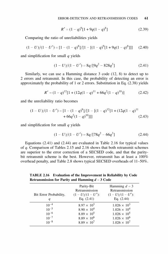
ERROR-DETECTION AND RETRANSMISSION CODES 61
R ′ c (1 − q)9[1 + 9q(1 − q)8] (2.39)
Comparing the ratio of unreliabilities yields
(1 − U )/ (1 − U ′) c [1 − (1 − q)8]/ [1 − [(1 − q)9[1 + 9q(1 − q)8]]] (2.40)
and simplification for small q yields
(1 − U )/ (1 − U ′) c 8q/ [9q2− 828q3] (2.41)
Similarly, we can use a Hamming distance 3 code (12, 8) to detect up to2 errors and retransmit. In this case, the probability of detecting an error isapproximately the probability of 1 or 2 errors. Substitution in Eq. (2.38) yields
R ′ c (1 − q)12[1 + (12q(1 − q)11 + 66q2(1 − q)10)] (2.42)
and the unreliability ratio becomes
(1 − U )/ (1 − U ′) c [1 − (1 − q)8]/ [1 − [(1 − q)12[1 + (12q(1 − q)11
+ 66q2(1 − q)10]]] (2.43)
and simplification for small q yields
(1 − U )/ (1 − U ′) c 8q/ [78q2− 66q3] (2.44)
Equations (2.41) and (2.44) are evaluated in Table 2.16 for typical valuesof q. Comparison of Tables 2.15 and 2.16 shows that both retransmit schemesare superior to the error correction of a SECSED code, and that the parity-bit retransmit scheme is the best. However, retransmit has at least a 100%overhead penalty, and Table 2.8 shows typical SECSED overheads of 11–50%.
TABLE 2.16 Evaluation of the Improvement in Reliability by CodeRetransmission for Parity and Hamming d c 3 Code
Parity-Bit Hamming d c 3Retransmission Retransmission
Bit Error Probability, (1 − U)/ (1 − U ′): (1 − U)/ (1 − U′):q Eq. (2.41) Eq. (2.44)
10−4 8.97 × 10³ 1.026 × 10³
10−5 8.90 × 10⁴ 1.026 × 10⁴
10−6 8.89 × 10⁵ 1.026 × 10⁵
10−7 8.89 × 10⁶ 1.026 × 10⁶
10−8 8.89 × 10⁷ 1.026 × 10⁷
62 CODING TECHNIQUES
The foregoing evaluations neglected the probability of IC generator andchecker failure as well as the circuitry involved in controlling retransmission.However, the analysis can be broadened to include these effects, and a moredetailed comparison can be made.
2.6 BURST ERROR-CORRECTION CODES
2.6.1 Introduction
The codes previously discussed have all been based on the assumption that theprobability that bit bi is corrupted by an error is largely independent of whetherbit bi − 1 is correct or is in error. Furthermore, the probability of a single biterror, q, is relatively small; thus the probability of more than one error in aword is quite small. In the case of a burst error, the probability that bit bi iscorrupted by an error is much larger if bit bi − 1 is incorrect than if bit bi − 1 iscorrect. In other words, the errors commonly come in bursts rather than singly.One class of applications that are subject to burst errors are rotational magneticand optical storage devices (e.g., music CDs, CD-ROMs, and hard and floppydisk drives). Magnetic tape used for pictures, sound, or data is also affectedby burst errors.
Examples of the patterns of typical burst errors are given in the four 12-bitmessages (m1–m4) shown in the forthcoming equations. The common notationis used where b represents a correct message bit and x represents an erroneousmessage bit. (For the purpose of identification, assume that the bits are num-bered 1–12 from left to right.)
m1 c bbbxxbxbbbbb (2.45a)
m2 c bxbxxbbbbbbb (2.45b)
m3 c bbbbxbxbbbbb (2.45c)
m4 c bxxbbbbbbbbb (2.45d)
Messages 1 and 2 each have 3 errors that extend over 4 bits (e.g., in m1
the error bits are in positions 4, 5, and 7); we would refer to them as burstsof length 4. In message 3, the burst is of length 3; in message 4, the burst isof length 2. In general, we call the burst length t. The burst length is really amatter of definition; for example, one could interpret messages 1 and 2 as 2bursts—one of length 1 and one of length 2. In practice, this causes no con-fusion, for t is a parameter of a burst code and is fixed in the initial design ofthe code. Thus if t is chosen as length 4, all 4 of the messages would have 1burst. If t is chosen as length 3, messages 1 and 2 would have two bursts, andmessages 3 and 4 would have 1 burst.
Most burst error codes are more complex than the Hamming codes thatwere just discussed; thus the remainder of this chapter will present a succinct
BURST ERROR-CORRECTION CODES 63
introduction to the basis of such codes and will briefly introduce one of themost popular burst codes: the Reed–Solomon code [Golumb, 1986].
2.6.2 Error Detection
We begin by giving an example of a burst error-detection code [Arazi, 1988].Consider a 12-bit-long code word (also called a code block or code vector, V),which includes both message and check bits as follows:
V c (x1x2x3x4x5x6x7x8x9x10x11x12) (2.46)
Let us choose to deal with bursts of length t c 4. Equations for calculating thecheck bits in terms of the message bits can be developed by writing a set ofequations in which the bits are separated by t positions. Thus for t c 4, eachequation contains every fourth bit.
x1 ⊕ x5 ⊕ x9 c 0 (2.47a)
x2 ⊕ x6 ⊕ x10 c 0 (2.47b)
x3 ⊕ x7 ⊕ x11 c 0 (2.47c)
x4 ⊕ x8 ⊕ x12 c 0 (2.47d)
Each bit appears in only one equation. Assume there is either 0 or only 1burst in the code vector (multiple bursts in a single word are excluded). Thuseach time there is 1 erroneous bit, one of the four equations will equal 1 ratherthan 0, indicating a single error. To illustrate this, suppose x2 is an error bit.Since we are assuming a burst length of 4 and at most 1 burst per code vector,the only other possible erroneous bits are x3, x4, and x5. (At this point, we don’tknow if 0, 1, 2, or 3 errors occur in bits 3–5.) Examining Eq. (2.47b), we seethat it is not possible for x6 or x10 to be erroneous bits, so it is not possiblefor 2 errors to cancel out in evaluating Eq. (2.47b). In fact, if we analyze theset of Eqs. (2.47a–d), we see that the number of nonzero equations in the setis equal to the number of bit errors in the burst.
Since there are 4 check equations, we need 4 check bits; any set of 4 bitsin the vector can be chosen as check bits, provided that 1 bit is chosen fromeach equation (2.47a–d). For clarity, it probably makes sense to choose the 4check bits as the first or last 4 bits in the vector; such a choice in any type ofcode is referred to as a systematic code. Suppose we choose the first 4 bits.We then obtain a (12, 8) systematic burst code of length 4, where ci stands fora check bit and bi a message bit.
V c (c1c2c3c4b1b2b3b4b5b6b7b8) (2.48)
A moment’s reflection shows that we have now maneuvered Eqs. (2.47a–d)so that with cs and bs substituted for the xs, we obtain
64 CODING TECHNIQUES
c1 ⊕ b1 ⊕ b5 c 0 (2.49a)
c2 ⊕ b2 ⊕ b6 c 0 (2.49b)
c3 ⊕ b3 ⊕ b7 c 0 (2.49c)
c4 ⊕ b4 ⊕ b8 c 0 (2.49d)
which can be used to compute the check bits. These equations are thereforethe basis of the check-bit generator, which can be done with 74180 or 74280IC chips.
The same set of equations form the basis of the error-checking circuitry.Based on the fact that the number of nonzero equations in the set of Eqs.(2.47a–d) is equal to the number of bit errors in the burst, we can modify Eqs.(2.47a–c) so that they explicitly yield bits of a syndrome vector, e1e2e3e4.
e1 c x1 ⊕ x5 ⊕ x9 (2.50a)
e2 c x2 ⊕ x6 ⊕ x10 (2.50b)
e3 c x3 ⊕ x7 ⊕ x11 (2.50c)
e4 c x4 ⊕ x8 ⊕ x12 (2.50d)
The nonerror condition occurs when all the syndrome bits are 0. In general,the number of errors detected is the arithmetic sum: e1 + e2 + e3 + e4. Note thatbecause we originally chose t c 4 in this design, no more than 4 errors canbe detected. Again, the checker can be done with 74180 or 74280 IC chips.Alternatively, one can use individual gates. To generate the check bits, 4 EXORgates are sufficient; 8 EXOR gates and an output OR gate are sufficient forerror checking (cf. Fig. 2.2). However, if one wishes to determine how manyerrors have occurred, the output OR gate in the checker can be replaced by afew half-adders or full-adders to compute the arithmetic sum: e1 + e2 + e3 + e4.
We can now state some properties of burst codes that were illustrated by theabove discussion. The reader is referred to the references for proof [Arazi, 1988].
Properties of Burst Codes
1. For a burst length of t, t check bits are needed for error detection. (Note:this is independent of the message length m.)
2. For m message bits and a burst length of t, the code word length n c m+ t.
3. There are t check-bit equations:(a) The first check-bit equation starts with bit 1 and contains all the bits
that are t + 1, 2t + 1, . . . kt + 1 (where kt + 1 ≤ n).(b) The second check-bit equation starts with bit 2 and contains all the
bits that are t + 2, 2t + 2, . . . kt + 2 (where kt + 2 ≤ n).. . . . . . . . . . . . . . . . . . . . . . . . . . . . . . . . . . . . . . . . . . . . . . . . . . . . . . . . . . . . . . . . . .
(t) The t′th check-bit equation starts with bit t and contains all the bitsthat are 2t, 3t, . . . kt (where kt ≤ n).
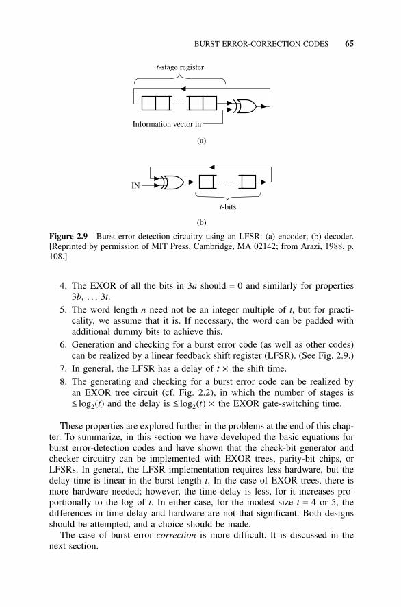
BURST ERROR-CORRECTION CODES 65
Information vector in
t-stage register
(a)
(b)
t-bits
IN
Figure 2.9 Burst error-detection circuitry using an LFSR: (a) encoder; (b) decoder.[Reprinted by permission of MIT Press, Cambridge, MA 02142; from Arazi, 1988, p.108.]
4. The EXOR of all the bits in 3a should c 0 and similarly for properties3b, . . . 3t.
5. The word length n need not be an integer multiple of t, but for practi-cality, we assume that it is. If necessary, the word can be padded withadditional dummy bits to achieve this.
6. Generation and checking for a burst error code (as well as other codes)can be realized by a linear feedback shift register (LFSR). (See Fig. 2.9.)
7. In general, the LFSR has a delay of t × the shift time.8. The generating and checking for a burst error code can be realized by
an EXOR tree circuit (cf. Fig. 2.2), in which the number of stages is≤ log2(t) and the delay is ≤ log2(t) × the EXOR gate-switching time.
These properties are explored further in the problems at the end of this chap-ter. To summarize, in this section we have developed the basic equations forburst error-detection codes and have shown that the check-bit generator andchecker circuitry can be implemented with EXOR trees, parity-bit chips, orLFSRs. In general, the LFSR implementation requires less hardware, but thedelay time is linear in the burst length t. In the case of EXOR trees, there ismore hardware needed; however, the time delay is less, for it increases pro-portionally to the log of t. In either case, for the modest size t c 4 or 5, thedifferences in time delay and hardware are not that significant. Both designsshould be attempted, and a choice should be made.
The case of burst error correction is more difficult. It is discussed in thenext section.
66 CODING TECHNIQUES
2.6.3 Error Correction
We now state some additional properties of burst codes that will lead us toan error-correction procedure. In general, these are properties associated witha shifting of the error syndrome of a burst code and an ancient theorem ofnumber theory related to the mod function. The theorem from number theoryis called the Chinese Remainder Theorem [Rosen, 1991, p. 134] and was firstgiven as a puzzle by the first-century Chinese mathematician Sun-Tsu. It willturn out that the method of error correction will depend on first locating aregion in the code word of t consecutive bits that contains the start of the errorburst, followed by pinpointing which of these t bits is the start of the burst. Themethodology is illustrated by applying the principles to the example given inEq. (2.46). For a development of the theory and proofs, the reader is referredto Arazi [1988] and Rosen [1991].
The error syndrome can be viewed as a cyclic shift of the burst error pat-tern. For example, if we assume a single burst and t c 4, then substitutionof error pattern for x1x2x3x4 into Eqs. (2.50a–d) will yield a particular syn-drome pattern. To compute what the syndrome would be, we note that ifx1x2x3x4 c bbbb, all the bits are correct and the syndrome must be 0000.If bit 1 is in error (either changed from a correct 1 to an erroneous 0 or from acorrect 0 to an erroneous 1), then Eq. (4.50a) will yield a 1 for e1 (since thereis only 1 burst, bits x5–x12 must be all valid bs). Suppose the error pattern isx1x2x3x4 c xbxx, then all other bits in the 12-bit vector are b and substitutioninto Eqs. (2.50a–d) yields
e1 c x ⊕ x5 ⊕ x9 c 1 (2.51a)
e2 c b ⊕ x6 ⊕ x10 c 0 (2.51b)
e3 c x ⊕ x7 ⊕ x11 c 1 (2.51c)
e4 c x ⊕ x8 ⊕ x12 c 1 (2.51d)
which is a syndrome pattern e1e2e3e4 c 1011. Similarly, error patternx4x5x6x7 c xbxx, where all other bits are b, yields syndrome equations asfollows:
e1 c x1 ⊕ b ⊕ x9 c 0 (2.52a)
e2 c x2 ⊕ x ⊕ x10 c 1 (2.52b)
e3 c x3 ⊕ x ⊕ x11 c 1 (2.52c)
e4 c x ⊕ x8 ⊕ x12 c 1 (2.52d)
which is a syndrome pattern e1e2e3e4 c 0111. We can view 0111 as a patternthat can be transformed into 1011 by cyclic-shifting left (end-around-rotationleft) three times. We will show in the following material that the same syn-drome is obtained by shifting the code vector right four times.
We begin marking a burst error pattern with the first erroneous bit in the
BURST ERROR-CORRECTION CODES 67
word; thus burst error patterns always start with an x. Since the burst is t bitslong, the syndrome equations (2.50a–d) include bits that differ by t positions.Therefore, if we shift the burst error pattern in the code vector by t positionsto the right, the burst error pattern generates the same syndrome. There canbe at most u placements of the burst pattern in a code vector that results inthe same syndrome; if the code vector is n bits long, u is the largest integersuch that ut ≤ n. Without loss of generality, we can always pad the messagebits with dummy bits such that ut c n. We define the mod function x mod yas the remainder that is obtained when we divide the integer x by the integery. Thus, if ut c n, we can then say that n mod u c 0. These relationships willsoon be used to devise an algorithm for burst error correction.
The location of the start of the burst error pattern in a word is related to theamount of shift (end-around and cyclic) of the pattern that is observed in thesyndrome. We can illustrate this relationship by using the burst pattern xbxxas an example, where xbxx is denoted by 1011: meaning incorrect, correct,incorrect, incorrect. In Table 2.17, we illustrate the relationship between thestart of the error burst and the rotational shift (end-around shift) in the detectederror syndrome. We begin by renumbering the code vector, Eq. (2.46), so itstarts with bit 0:
V c (x0x1x2x3x4x5x6x7x8x9x10x11) (2.53)
A study of Table 2.17 shows that the number of syndrome shifts is relatedto the bit number by (bit number) mod 4. For example, if the burst starts withbit no. 3, we have 3 mod 4 (which is 3), so the syndrome is the error patternshifted 3 places to the right. If we want to recover the syndrome, we shift 3places to the left. In the case of a burst starting with bit no. 4, 4 mod 4 is 0,so the syndrome pattern and the burst pattern agree.
Thus, if we know the position in the code word at which the burst starts(defined as x), and if the burst length is t, then we can obtain the burst pattern byshifting the syndrome x mod t places to the left. Knowing the starting positionof the burst (x) and the burst pattern, we can correct any erroneous bits. Thusour task is now to find x.
The procedure for solving for x depends on the Chinese Remainder The-orem, a previously mentioned mathematical theorem in number theory. Thistheorem states that if p and q are relatively prime numbers (meaning their onlycommon factor is 1), and if 0 ≤ x ≤ (pq − 1), then knowledge of x mod p and xmod q allows us to solve for x. We already have one equation: x mod t; to gen-erate another equation, we define u c 2t−1 and calculate x from x mod u [Arazi,1988]. Note that t and 2t − 1 are relatively prime since if a number divides t,it also divides 2t but not 2t − 1. Also, we must show that 0 ≤ x ≤ (tu − 1);however, we already showed that tu ≤ n. Substitution yields 0 ≤ x ≤ (n − 1),which must be true since the latest bit position to start a burst error (x) for aburst of length t is n − t < n − 1.
The above relationships show that it is possible to solve for the beginning
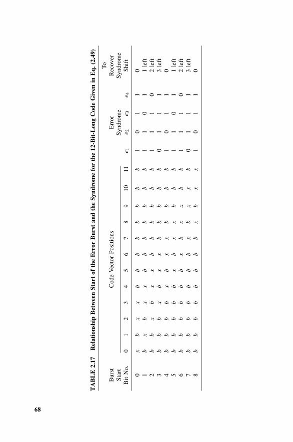
68
TA
BL
E2.
17R
elat
ions
hip
Bet
wee
n St
art
of t
he E
rror
Bur
st a
nd t
he S
yndr
ome
for
the
12-B
it-L
ong
Cod
e G
iven
in E
q. (
2.49
)
ToB
urst
Cod
e V
ecto
r Po
sitio
nsE
rror
Rec
over
Star
tSy
ndro
me
Synd
rom
eB
it N
o.0
12
34
56
78
910
11e 1
e 2e 3
e 4Sh
ift
0x
bx
xb
bb
bb
bb
b1
01
10
1b
xb
xx
bb
bb
bb
b1
10
11
left
2b
bx
bx
xb
bb
bb
b1
11
02
left
3b
bb
xb
xx
bb
bb
b0
11
13
left
4b
bb
bx
bx
xb
bb
b1
01
10
5b
bb
bb
xb
xx
bb
b1
10
11
left
6b
bb
bb
bx
bx
xb
b1
11
02
left
7b
bb
bb
bb
xb
xx
b0
11
13
left
8b
bb
bb
bb
bx
bx
x1
01
10
INTRODUCTION 69
of the burst error x and the burst error pattern. Given this information, bysimply complementing the incorrect bits, error correction is performed. Theremainder of this section details how we set up equations to calculate the checkbits (generator) and to calculate the burst pattern and location (checker); thisis done by means of an illustrative example. One circuit implementation usingshift registers is discussed as well.
The number of check bits is equal to u + t, and since u c 2c − 1 and n c ut,the number of message bits is determined. We formulate check bit equationsin a manner analogous to that used in error checking.
The following example illustrates how the two sets of check bits are gen-erated, how one formulates and solves for x mod u and x mod t to solve forx, and how the burst error pattern is determined. In our example, we let t c 3and calculate u c 2t − 1 c 2 × 3 − 1 c 5. In this case, the word length n c u × tc 5 × 3 c 15. The code vector is given by
V c (x0x1x2x3x4x5x6x7x8x9x10x11x12x13x14) (2.54)
The t + u check equations are generated from a set of u equations that form theauxiliary syndrome. For our example, the u c 5 auxiliary syndrome equationsare:
s0 c x0 ⊕ x5 ⊕ x10 (2.55a)
s1 c x1 ⊕ x6 ⊕ x11 (2.55b)
s2 c x2 ⊕ x7 ⊕ x12 (2.55c)
s3 c x3 ⊕ x8 ⊕ x13 (2.55d)
s4 c x4 ⊕ x9 ⊕ x14 (2.55e)
and the set of t c 3 equations that form the syndrome are
e1 c x0 ⊕ x3 ⊕ x6 ⊕ x9 ⊕ x12 (2.56a)
e2 c x1 ⊕ x4 ⊕ x7 ⊕ x10 ⊕ x13 (2.56b)
e3 c x2 ⊕ x5 ⊕ x8 ⊕ x11 ⊕ x14 (2.56c)
If we want a systematic code, we can place the 8 check bits at the beginningor the end of the word. Let us assume that they go at the end (x7–x14) and thatthese check bits c0–c7 are calculated from Eqs. (2.55a–e) and (2.56a–c). Thefirst 7 bits (x0–x6) are message bits, and the transmitted word is
V c (b0b1b2b3b4b5b6c0c1c2c3c4c5c6c7) (2.57)
As an example, let us assume that the message bits b0–b6 are 1011010.Substitution of these values in Eqs. (2.55a–e) and (2.56a–c) that must initiallybe 0 yields a set of equations that can be solved for the values of c0–c7. One canshow by substitution that the values c0–c7 c 10000010 satisfy the equations.
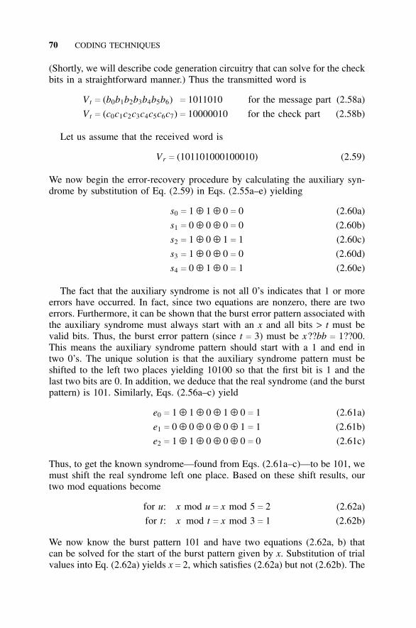
70 CODING TECHNIQUES
(Shortly, we will describe code generation circuitry that can solve for the checkbits in a straightforward manner.) Thus the transmitted word is
Vt c (b0b1b2b3b4b5b6) c 1011010 for the message part (2.58a)
Vt c (c0c1c2c3c4c5c6c7) c 10000010 for the check part (2.58b)
Let us assume that the received word is
Vr c (101101000100010) (2.59)
We now begin the error-recovery procedure by calculating the auxiliary syn-drome by substitution of Eq. (2.59) in Eqs. (2.55a–e) yielding
s0 c 1 ⊕ 1 ⊕ 0 c 0 (2.60a)
s1 c 0 ⊕ 0 ⊕ 0 c 0 (2.60b)
s2 c 1 ⊕ 0 ⊕ 1 c 1 (2.60c)
s3 c 1 ⊕ 0 ⊕ 0 c 0 (2.60d)
s4 c 0 ⊕ 1 ⊕ 0 c 1 (2.60e)
The fact that the auxiliary syndrome is not all 0’s indicates that 1 or moreerrors have occurred. In fact, since two equations are nonzero, there are twoerrors. Furthermore, it can be shown that the burst error pattern associated withthe auxiliary syndrome must always start with an x and all bits > t must bevalid bits. Thus, the burst error pattern (since t c 3) must be x??bb c 1??00.This means the auxiliary syndrome pattern should start with a 1 and end intwo 0’s. The unique solution is that the auxiliary syndrome pattern must beshifted to the left two places yielding 10100 so that the first bit is 1 and thelast two bits are 0. In addition, we deduce that the real syndrome (and the burstpattern) is 101. Similarly, Eqs. (2.56a–c) yield
e0 c 1 ⊕ 1 ⊕ 0 ⊕ 1 ⊕ 0 c 1 (2.61a)
e1 c 0 ⊕ 0 ⊕ 0 ⊕ 0 ⊕ 1 c 1 (2.61b)
e2 c 1 ⊕ 1 ⊕ 0 ⊕ 0 ⊕ 0 c 0 (2.61c)
Thus, to get the known syndrome—found from Eqs. (2.61a–c)—to be 101, wemust shift the real syndrome left one place. Based on these shift results, ourtwo mod equations become
for u: x mod u c x mod 5 c 2 (2.62a)
for t: x mod t c x mod 3 c 1 (2.62b)
We now know the burst pattern 101 and have two equations (2.62a, b) thatcan be solved for the start of the burst pattern given by x. Substitution of trialvalues into Eq. (2.62a) yields x c 2, which satisfies (2.62a) but not (2.62b). The
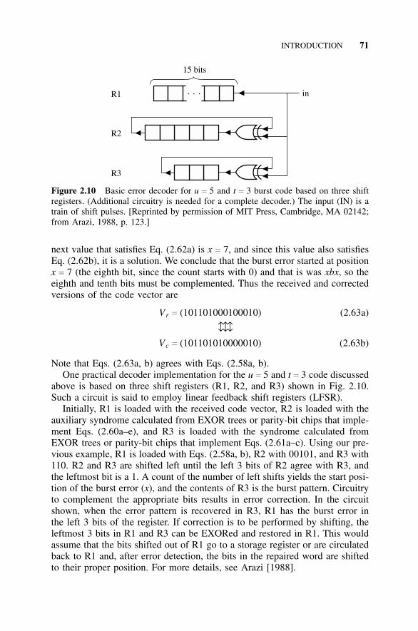
INTRODUCTION 71
15 bits
inR1
R2
R3
Figure 2.10 Basic error decoder for u c 5 and t c 3 burst code based on three shiftregisters. (Additional circuitry is needed for a complete decoder.) The input (IN) is atrain of shift pulses. [Reprinted by permission of MIT Press, Cambridge, MA 02142;from Arazi, 1988, p. 123.]
next value that satisfies Eq. (2.62a) is x c 7, and since this value also satisfiesEq. (2.62b), it is a solution. We conclude that the burst error started at positionx c 7 (the eighth bit, since the count starts with 0) and that is was xbx, so theeighth and tenth bits must be complemented. Thus the received and correctedversions of the code vector are
Vr c (101101000100010) (2.63a)
↔ ↔ ↔Vc c (101101010000010) (2.63b)
Note that Eqs. (2.63a, b) agrees with Eqs. (2.58a, b).One practical decoder implementation for the u c 5 and t c 3 code discussed
above is based on three shift registers (R1, R2, and R3) shown in Fig. 2.10.Such a circuit is said to employ linear feedback shift registers (LFSR).
Initially, R1 is loaded with the received code vector, R2 is loaded with theauxiliary syndrome calculated from EXOR trees or parity-bit chips that imple-ment Eqs. (2.60a–e), and R3 is loaded with the syndrome calculated fromEXOR trees or parity-bit chips that implement Eqs. (2.61a–c). Using our pre-vious example, R1 is loaded with Eqs. (2.58a, b), R2 with 00101, and R3 with110. R2 and R3 are shifted left until the left 3 bits of R2 agree with R3, andthe leftmost bit is a 1. A count of the number of left shifts yields the start posi-tion of the burst error (x), and the contents of R3 is the burst pattern. Circuitryto complement the appropriate bits results in error correction. In the circuitshown, when the error pattern is recovered in R3, R1 has the burst error inthe left 3 bits of the register. If correction is to be performed by shifting, theleftmost 3 bits in R1 and R3 can be EXORed and restored in R1. This wouldassume that the bits shifted out of R1 go to a storage register or are circulatedback to R1 and, after error detection, the bits in the repaired word are shiftedto their proper position. For more details, see Arazi [1988].
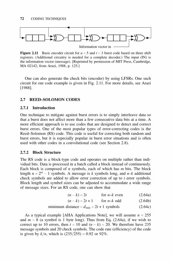
72 CODING TECHNIQUES
Information vector in
Figure 2.11 Basic encoder circuit for u c 5 and t c 3 burst code based on three shiftregisters. (Additional circuitry is needed for a complete decoder.) The input (IN) isthe information vector (message). [Reprinted by permission of MIT Press, Cambridge,MA 02142; from Arazi, 1988, p. 125.]
One can also generate the check bits (encoder) by using LFSRs. One suchcircuit for our code example is given in Fig. 2.11. For more details, see Arazi[1988].
2.7 REED–SOLOMON CODES
2.7.1 Introduction
One technique to mitigate against burst errors is to simply interleave data sothat a burst does not affect more than a few consecutive data bits at a time. Amore efficient approach is to use codes that are designed to detect and correctburst errors. One of the most popular types of error-correcting codes is theReed–Solomon (RS) code. This code is useful for correcting both random andburst errors, but it is especially popular in burst error situations and is oftenused with other codes in a convolutional code (see Section 2.8).
2.7.2 Block Structure
The RS code is a block-type code and operates on multiple rather than indi-vidual bits. Data is processed in a batch called a block instead of continuously.Each block is composed of n symbols, each of which has m bits. The blocklength n c 2m
− 1 symbols. A message is k symbols long, and n–k additionalcheck symbols are added to allow error correction of up to t error symbols.Block length and symbol sizes can be adjusted to accommodate a wide rangeof message sizes. For an RS code, one can show that
(n − k) c 2t for n–k even (2.64a)
(n − k) c 2t + 1 for n–k odd (2.64b)
minimum distance c dmin c 2t + 1 symbols (2.64c)
As a typical example [AHA Applications Note], we will assume n c 255and m c 8 (a symbol is 1 byte long). Thus from Eq. (2.64a), if we wish tocorrect up to 10 errors, then t c 10 and (n − k) c 20. We therefore have 235message symbols and 20 check symbols. The code rate (efficiency) of the codeis given by k/ n, which is (235/ 255) c 0.92 or 92%.
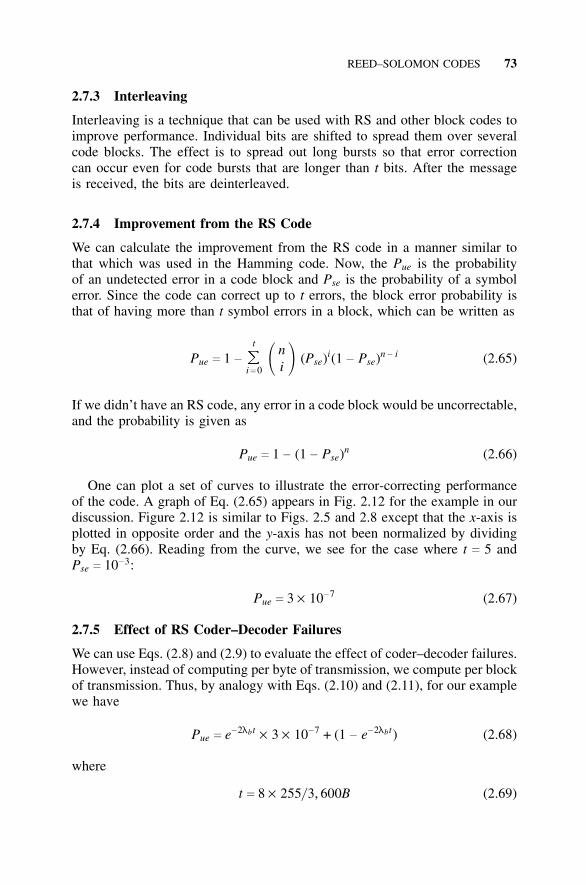
REED–SOLOMON CODES 73
2.7.3 Interleaving
Interleaving is a technique that can be used with RS and other block codes toimprove performance. Individual bits are shifted to spread them over severalcode blocks. The effect is to spread out long bursts so that error correctioncan occur even for code bursts that are longer than t bits. After the messageis received, the bits are deinterleaved.
2.7.4 Improvement from the RS Code
We can calculate the improvement from the RS code in a manner similar tothat which was used in the Hamming code. Now, the Pue is the probabilityof an undetected error in a code block and Pse is the probability of a symbolerror. Since the code can correct up to t errors, the block error probability isthat of having more than t symbol errors in a block, which can be written as
Pue c 1 −
t
���i c 0 �
ni � (Pse)i(1 − Pse)n − i (2.65)
If we didn’t have an RS code, any error in a code block would be uncorrectable,and the probability is given as
Pue c 1 − (1 − Pse)n (2.66)
One can plot a set of curves to illustrate the error-correcting performanceof the code. A graph of Eq. (2.65) appears in Fig. 2.12 for the example in ourdiscussion. Figure 2.12 is similar to Figs. 2.5 and 2.8 except that the x-axis isplotted in opposite order and the y-axis has not been normalized by dividingby Eq. (2.66). Reading from the curve, we see for the case where t c 5 andPse c 10−3:
Pue c 3 × 10⁻⁷ (2.67)
2.7.5 Effect of RS Coder–Decoder Failures
We can use Eqs. (2.8) and (2.9) to evaluate the effect of coder–decoder failures.However, instead of computing per byte of transmission, we compute per blockof transmission. Thus, by analogy with Eqs. (2.10) and (2.11), for our examplewe have
Pue c e−2lbt × 3 × 10−7 + (1 − e−2lbt) (2.68)
where
t c 8 × 255/ 3, 600B (2.69)
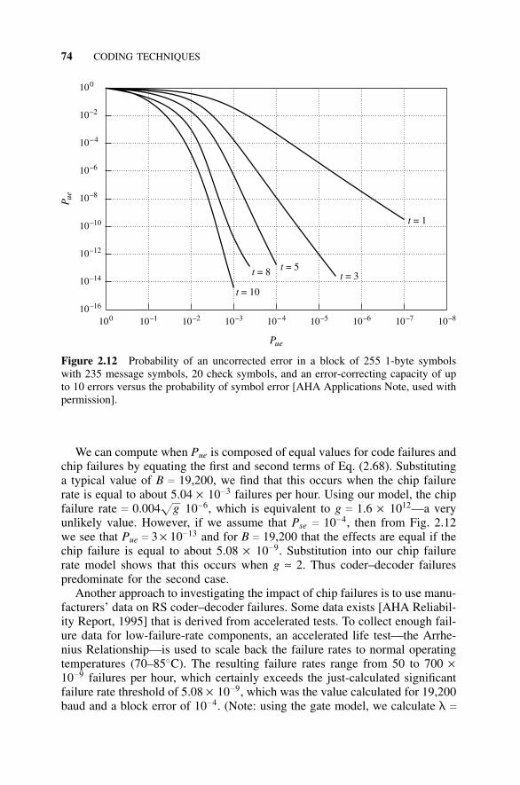
74 CODING TECHNIQUES
10–16
10–14
10–12
10–10
10–8
10–6
10–4
10–2
100
100 10–1 10–2 10–3 10–4 10–5 10–6 10–7 10–8
t = 10
t = 8 t = 5t = 3
t = 1
Pue
P ue
Figure 2.12 Probability of an uncorrected error in a block of 255 1-byte symbolswith 235 message symbols, 20 check symbols, and an error-correcting capacity of upto 10 errors versus the probability of symbol error [AHA Applications Note, used withpermission].
We can compute when Pue is composed of equal values for code failures andchip failures by equating the first and second terms of Eq. (2.68). Substitutinga typical value of B c 19,200, we find that this occurs when the chip failurerate is equal to about 5.04 × 10⁻³ failures per hour. Using our model, the chipfailure rate c 0.004
fg 10−6, which is equivalent to g c 1.6 × 10¹²—a very
unlikely value. However, if we assume that Pse c 10−4, then from Fig. 2.12we see that Pue c 3 × 10⁻¹³ and for B c 19,200 that the effects are equal if thechip failure is equal to about 5.08 × 10⁻⁹. Substitution into our chip failurerate model shows that this occurs when g ≈ 2. Thus coder–decoder failurespredominate for the second case.
Another approach to investigating the impact of chip failures is to use manu-facturers’ data on RS coder–decoder failures. Some data exists [AHA Reliabil-ity Report, 1995] that is derived from accelerated tests. To collect enough fail-ure data for low-failure-rate components, an accelerated life test—the Arrhe-nius Relationship—is used to scale back the failure rates to normal operatingtemperatures (70–858C). The resulting failure rates range from 50 to 700 ×10−9 failures per hour, which certainly exceeds the just-calculated significantfailure rate threshold of 5.08 × 10⁻⁹, which was the value calculated for 19,200baud and a block error of 10−4. (Note: using the gate model, we calculate l c

OTHER CODES 75
700 × 10−9 as equivalent to about 30,000 gates.) Clearly we conclude that thechip failures will predominate for some common ranges of the system param-eters.
2.8 OTHER CODES
There are many other types of error codes. We will briefly discuss the specialfeatures of the more popular codes and refer the reader to the references foradditional details.
1. Burst error codes. All the foregoing codes assume that errors occurinfrequently and are independent, generally corrupting a single bit or afew bits in a word. In some cases, errors may occur in bursts. If a studyof the failure modes of the device or medium we wish to protect by ourcoding indicates that errors occur in bursts to affect all the bits in a word,other coding techniques are required. The reader should consult the ref-erences for works that discuss Binary Block codes, m-out-of-n codes,Berger codes, Cyclic codes, and Reed–Solomon codes [Pradhan, 1986,1993].BCH codes. This is a code that was independently discovered by Bose,Chaudhury, and Hocquenghem. (Reed–Solomon codes are a subclass ofBCH codes.) These codes can be viewed as extensions of Hammingcodes, which are easier to design and implement for a large number ofcorrectable errors.Concatenated codes. This refers to the process of lumping more than onecode word together to reduce the overhead—generally less for long codewords (cf., Table 2.8). Disadvantages include higher error probability(since check bits cover several words), more complexity and depth, anda delay for associated decoding trees.Convolutional codes. Sometimes, codes are “nested”; for example, infor-mation can be coded by an inner code, and the resulting alphabet of legalcode words can be treated as a “symbol” subjected to an outer code. Anexample might be the use of a Hamming SECSED code as the inner codeword and a Reed–Solomon code as an outer code scheme.Check sum. The sum of all the numbers in a block of words is added,modulo 2, and the block and the sum are transmitted. The words in thereceived block are added again and the check sum is recomputed andchecked with the transmitted sum. This is an error-detecting code.Duplication. One can always transmit the result twice and check the twocopies. Although this may be inefficient, it is the only technique in somecases: for example, if we wish to check logical operations, AND, OR,and NAND.Fire code. An interleaved code for burst errors. The similar Reed–
76 CODING TECHNIQUES
Solomon code is now more popular since it is somewhat more efficient.
Hamming codes. Other codes in the family use more error-correctingand -detecting bits, thereby achieving higher levels of fault tolerance.
IC chip parity. Can be one bit per word, one bit per byte, or interlacedparity where b bits are watched over by i check bits. Thus each checkbit “watches over” b/ i bits.
Interleaving. One approach to dealing with burst codes is to disassemblecodes into a number of words, then reassemble them so that one bit ischosen from each word. For example, one could take 8 bytes and inter-leave (also called interlace) the bits so that a new byte is constructedfrom all the first bits of the original 8 bytes, another is constructed fromall the second bits, and so forth. In this example, as long as the burstlength is less than 8 bits and we have only one burst per 8 bytes, we areguaranteed that each new word can contain at most one error.
Residue m codes. This is used for checking certain arithmetic operations,such as addition, multiplication, and shifting. One computes the code bits(residue, R) that are concatenated (| , i.e., appended) to the message N tofrom N |R. The residue is the remainder left when N/ m. After transmis-sion or computation, the new message bits N ′ are divided by m to formR ′. Disagreement of R and R ′ indicates an error.
Viterby decoding. A decoding algorithm for error correction of aReed–Solomon or other convolutional code based on enumerating all thelegal code words and choosing the one closest to the received words. Formedium-sized search spaces, an organized search resembling a branch-ing tree was devised by Viterbi in 1967; it is often used to shorten thesearch. Forney recognized in 1968 that such trees are repetitive, so hedevised an improvement that led to a diagram looking like a “lattice”used for supporting plants and trees.
REFERENCES
AHA Reliability Report No. 4011. Reed–Solomon Coder/ Decoder. Advanced Hard-ware Architectures, Inc., Pullman, WA, 1995.
AHA Applications Note. Primer: Reed–Solomon Error Correction Codes (ECC).Advanced Hardware Architectures, Pullman, WA, Inc.
Arazi, B. A Commonsense Approach to the Theory of Error Correcting Codes. MITPress, Cambridge, MA, 1988.
Forney, G. D. Jr. Concatenated Codes. MIT Press Research Monograph, no. 37. MITPress, Cambridge, MA, 1966.
Golomb, S. W. Optical Disk Error Correction. Byte (May 1986): 203–210.
Gravano, S. Introduction to Error Control Codes. Oxford University Press, New York,2000.
REFERENCES 77
Hamming, R. W. Error Detecting and Correcting Codes. Bell System Technical Journal29 (April 1950): 147–160.
Houghton, A. D. The Engineer’s Error Coding Handbook. Chapman and Hall, NewYork, 1997.
Johnson, B. W. Design and Analysis of Fault Tolerant Digital Systems. Addison-Wes-ley, Reading, MA, 1989.
Johnson, B. W. Design and Analysis of Fault Tolerant Digital Systems, 2d ed. Addison-Wesley, Reading, MA, 1994.
Jones, G. A., and J. M. Jones. Information and Coding Theory. Springer-Verlag, NewYork, 2000.
Lala, P. K. Fault Tolerant and Fault Testable Hardware Design. Prentice-Hall, Engle-wood Cliffs, NJ, 1985.
Lala, P. K. Self-Checking and Fault-Tolerant Digital Design. Academic Press, SanDiego, CA, 2000.
Lee, C. Error-Control Block Codes for Communications Engineers. Telecommunica-tion Library, Artech House, Norwood, MA, 2000.
Peterson, W. W. Error-Correcting Codes. MIT Press (Cambridge, MA) and Wiley(New York), 1961.
Peterson, W. W., and E. J. Weldon Jr. Error Correcting Codes, 2d ed. MIT Press,Cambridge, MA, 1972.
Pless, V. Introduction to the Theory of Error-Correcting Codes. Wiley, New York,1998.
Pradhan, D. K. Fault-Tolerant Computing Theory and Technique, vol. I. Prentice-Hall,Englewood Cliffs, NJ, 1986.
Pradhan, D. K. Fault-Tolerant Computing Theory and Technique, vol. II. Prentice-Hall,Englewood Cliffs, NJ, 1993.
Rao, T. R. N., and E. Fujiwara. Error-Control Coding for Computer Systems. Prentice-Hall, Englewood Cliffs, NJ, 1989.
Shooman, M. L. Probabilistic Reliability: An Engineering Approach. McGraw-Hill,New York, 1968.
Shooman, M. L. Probabilistic Reliability: An Engineering Approach, 2d ed. Krieger,Melbourne, FL, 1990.
Shooman, M. L. The Reliability of Error-Correcting Code Implementations. Proceed-ings Annual Reliability and Maintainability Symposium, Las Vegas, NV, January22–25, 1996.
Shooman, M. L., and F. A. Cassara. The Reliability of Error-Correcting Codes onWireless Information Networks. International Journal of Reliability, Quality, andSafety Engineering, special issue on Reliability of Wireless Communication Sys-tems, 1996.
Siewiorek, D. P., and F. S. Swarz. The Theory and Practice of Reliable System Design.The Digital Press, Bedford, MA, 1982.
Siewiorek, D. P., and R. S. Swarz. Reliable Computer Systems Design and Evaluation,2d ed. The Digital Press, Bedford, MA, 1992.
Siewiorek, D. P., and R. S. Swarz. Reliable Computer Systems Design and Evaluation,3d ed. A. K. Peters, www.akpeters.com, 1998.
78 CODING TECHNIQUES
Spencer, J. L. The Highs and Lows of Reliability Predictions. Proceedings Annual Reli-ability and Maintainability Symposium, 1986. IEEE, New York, NY, pp. 156–162.
Stapper, C. H. et al. High-Reliability Fault-Tolerant 16-M Bit Memory Chip. Proceed-ings Annual Reliability and Maintainability Symposium, January 1991. IEEE, NewYork, NY, pp. 48–56.
Taylor, L. Air Travel How Safe Is It? BSP Professional Books, Cambridge, MA, 1988.Texas Instruments, TTL Logic Data Book. 1988, pp. 2-597–2-599.Wakerly, J. F. Digital Design Principles and Practice. Prentice-Hall, Englewood Cliffs,
NJ, 1994.Wakerly, J. F. Digital Design Principles and Practice, 3d. ed. Prentice-Hall, Englewood
Cliffs, NJ, 2000.Wells, R. B. Applied Coding and Information Theory for Engineers. Prentice-Hall,
Englewood Cliffs, NJ, 1998.Wicker, S. B., and V. K. Bhargava. Reed–Solomon Codes and their Applications. IEEE
Press, New York, 1994.Wiggert, D. Codes for Error Control and Synchronization. Communications and
Defense Library, Artech House, Norwood, MA, 1998.Wolf, J. J., M. L. Shooman, and R. R. Boorstyn. Algebraic Coding and Digital Redun-
dancy. IEEE Transactions on Reliability R-18, 3 (August 1969): 91–107.
PROBLEMS
2.1. Find a recent edition of Jane’s all the World’s Aircraft in a technical orpublic library. Examine the data given in Table 2.1 for soft failures forthe 6 aircraft types listed. From the book, determine the approximatenumber of electronic systems (aircraft avionics) for each of the aircraftthat are computer-controlled (digital rather than analog). You may haveto do some intelligent estimation to determine this number. One sectionin the book gives information on the avionics systems installed. Also,it may help to know that the U.S. companies (all mergers) that providemost of the avionics systems are Bendix/ King/ Allied, Sperry/ Honeywell,and Collins/ Rockwell. (Hint: You may have to visit the Web sites ofthe aircraft manufacturers or the avionics suppliers for more details.(a) Plot the number of soft fails per aircraft versus the number of avion-
ics systems on board. Comment on the results.(b) It would be better to plot soft fails per aircraft versus the number of
words of main memory for the avionics systems on board. Do youhave any ideas on how you could obtain such data?
2.2. Compute the minimum code distance for all the code words given inTable 2.2.(a) Compute for column (a) and comment.(b) Compute for column (b) and comment.(c) Compute for column (c) and comment.
PROBLEMS 79
2.3. Repeat the parity-bit coder and decoder designs given in Fig. 2.1 for an8-bit word with 7 message bits and 1 parity bit. Does this approach todesign of a coder and decoder present any difficulties?
2.4. Compare the design of problem 2.3 with that given in Fig. 2.2 on thebasis of ease of design, complexity, practicality, delay time (assume allgates have a delay of D), and number of gates.
2.5. Compare the results of problem 2.4 with the circuit of Fig. 2.4.
2.6. Compute the binomial probabilities B(r : 8, q) for r c 1 to 8.(a) Does the sum of these probabilities check with Eq. (2.5)?(b) Show for what values of q the term B(1 : 8, q) dominates all the error-
occurrence probabilities.
2.7. Find a copy of the latest military failure-rate manual (MIL-HDBK-217)and plot the data on Fig. B7 of Appendix B. Does it agree? Can youfind any other IC failure-rate information? (Hint: The telecommunicationindustry and the various national telephone companies maintain largefailure-rate databases. Also, the Annual Reliability and MaintainabilitySymposium from the IEEE regularly publishes papers with failure-ratedata.) Does this data agree with the other results? What advances havebeen made in the last decade or so?
2.8. Assume that a 10% reduction in the probability of undetected error fromcoder and decoder failures is acceptable.(a) Compute the value of B at which a 10% reduction occurs for fixed
values of q.(b) Plot the results of part (a) and interpret.
2.9. Check the results given in Table 2.5. How is the distance d related tothe number of check bits? Explain.
2.10. Check the values given in Tables 2.7 and 2.8.
2.11. The Hamming SECSED code with 4 message bits and 3 check bits isused in the text as an example (Section 2.4.3). It was stated that we coulduse a brute force technique of checking all the legal or illegal code wordsfor error detection, as was done for the parity-bit code in Fig. 2.1.(a) List all the legal and illegal code words for this example and show
that the code distance is 3.(b) Design an error-detector circuit using minimized two-level logic (cf.
Fig. 2.1).
2.12. Design a check bit generating circuit for problem 2.11 using Eqs.(2.22a–c) and EXOR gates.
2.13. One technique for error correction is to pick the nearest code word asthe correct word once an error has been detected.
80 CODING TECHNIQUES
(a) Devise a software algorithm that can be used to program a micro-processor to perform such error correction.
(b) Devise a hardware design that performs the error correction bychoosing the closest word.
(c) Compare complexity and speed of designs (a) and (b).
2.14. An error-correcting circuit for a Hamming (7, 4) SECSED is given inFig. 2.7. How would you generate the check bits that are defined in Eqs.(2.22a–c)? Is there a better way than that suggested in problem 2.12?
2.15. Compare the designs of problems 2.11, 2.12, and 2.13 with Hamming’stechnique in problem 2.14.
2.16. Give a complete design for the code generator and checker for a Ham-ming (12, 8) SECSED code following the approach of Fig. 2.7.
2.17. Repeat problem 2.16 for a SECDED code.
2.18. Repeat problem 2.8 for the design referred to in Table 2.14.
2.19. Retransmission as described in Section 2.5 tends to decrease the effec-tive baud rate (B) of the transmission. Compare the unreliability and theeffective baud rate for the following designs:(a) Transmit each word twice and retransmit when they disagree.(b) Transmit each word three times and use the majority of the three
values to determine the output.(c) Use a parity-bit code and only retransmit when the code detects an
error.(d) Use a Hamming SECSED code and only retransmit when the code
detects an error.
2.20. Add the probabilities of generator and checker failure for the reliabilityexamples given in Section 2.5.3.
2.21. Assume we are dealing with a burst code design for error detectionwith a word length of 12 bits and a maximum burst length of 4, asnoted in Eqs. (2.46)–(2.50). Assume the code vector V(x1, x2, . . . , x12) cV(c1c2c3c410100011).(a) Compute c1c2c3c4.(b) Assume no errors and show how the syndrome works.(c) Assume one error in bit c2 and show how the syndrome works.(d) Assume one error in bit x9; then show how the syndrome works.(e) Assume two errors in bits x8 and x9; then show how the syndrome
works.(f) Assume three errors in bits x8, x9, and x10; then show how the syn-
drome works.
PROBLEMS 81
(g) Assume four errors in bits x7, x8, x9, and x10; then show how thesyndrome works.
(h) Assume five errors in bits x7, x8, x9, x10, and x11; then show howthe syndrome fails.
(i) Repeat the preceding computations using a different set of four equa-tions to calculate the check bits.
2.22. Draw a circuit for generating the check bits, the syndrome vector, andthe error-detection output for the burst error-detecting code example ofSection 2.6.2.(a) Use parallel computation and use EXOR gates.(b) Use serial computation and a linear feedback shift register.
2.23. Compute the probability of undetected error for the code of problem2.22 and compare with the probability of undetected error for the caseof no error detection. Assume perfect hardware.
2.24. Repeat problem 2.23 assuming that the hardware is imperfect.(a) Assume a model as in Section 2.3.4 and 2.4.5.(b) Plot the results as in Figs. 2.5 and 2.8.
2.25. Repeat problem 2.22 for the burst error-detecting code in Section 2.6.3.
2.26. Repeat problem 2.23 for the burst error-detecting code in Section 2.6.3.
2.27. Repeat problem 2.24 for the burst error-detecting code in Section 2.6.3.
2.28. Analyze the design of Fig. 2.4 and show that it is equivalent to Fig. 2.2.Also, explain how it can be used as a generator and checker.
2.29. Explain in detail the operation of the error-correcting circuit given inFig. 2.7.
2.30. Design a check bit generator circuit for the SECDED code example inSection 2.4.4.
2.31. Design an error-correcting circuit for the SECDED code example in Sec-tion 2.4.4.
2.32. Explain how a distance 3 code can be implemented as a double error-detecting code (DED). Give the circuit for the generator and checker.
2.33. Explain how a distance 4 code can be implemented as a triple error-detecting code (TED). Give the circuit for the generator and checker.
2.34. Construct a table showing the relationship between the burst length t,the auxiliary check bits u, the total number of check bits, the numberof message bits, and the length of the code word. Use a tabular formatsimilar to Table 2.7.

82 CODING TECHNIQUES
2.35. Show for the u c 5 and t c 3 code example given in Section 2.6.3 thatafter x shifts, the leftmost bits of R2 and R3 in Fig. 2.10 agree.
2.36. Show a complete circuit for error correction that includes Fig. 2.10 inaddition to a counter, a decoder, a bit-complementing circuit, and a cor-rected word storage register, as well as control logic.
2.37. Show a complete circuit for error correction that includes Fig. 2.10 inaddition to a counter, an EXOR-complementing circuit, and a correctedword storage register, as well as control logic.
2.38. Show a complete circuit for error correction that includes Fig. 2.10 inaddition to a counter, an EXOR-complementing circuit, and a circulatingregister for R1 to contain the corrected word, as well as control logic.
2.39. Explain how the circuit of Fig. 2.11 acts as a coder. Input the messagebits; then show what is generated and which bits correspond to the auxil-iary syndrome and which ones correspond to the real syndrome.
2.40. What additional circuitry is needed (if any) to supplement Fig. 2.11 toproduce a coder. Explain.
2.41. Using Fig. 2.12 for the Reed–Solomon code, plot a graph similar to Fig.2.8.
3REDUNDANCY, SPARES, ANDREPAIRS
Reliability of Computer Systems and Networks: Fault Tolerance, Analysis, and DesignMartin L. Shooman
Copyright 2002 John Wiley & Sons, Inc.ISBNs: 0-471-29342-3 (Hardback); 0-471-22460-X (Electronic)
83
3.1 INTRODUCTION
This chapter deals with a variety of techniques for improving system reliabilityand availability. Underlying all these techniques is the basic concept of redun-dancy, providing alternate paths to allow the system to continue operation evenwhen some components fail. Alternate paths can be provided by parallel com-ponents (or systems). The parallel elements can all be continuously operated,in which case all elements are powered up and the term parallel redundancyor hot standby is often used. It is also possible to provide one element that ispowered up (on-line) along with additional elements that are powered down(standby), which are powered up and switched into use, either automaticallyor manually, when the on-line element fails. This technique is called standbyredundancy or cold redundancy. These techniques have all been known formany years; however, with the advent of modern computer-controlled digitalsystems, a rich variety of ways to implement these approaches is available.Sometimes, system engineers use the general term redundancy managementto refer to this body of techniques. In a way, the ultimate cold redundancytechnique is the use of spares or repairs to renew the system. At this levelof thinking, a spare and a repair are the same thing—except the repair takeslonger to be effected. In either case for a system with a single element, wemust be able to tolerate some system downtime to effect the replacement orrepair. The situation is somewhat different if we have a system with two hotor cold standby elements combined with spares or repairs. In such a case, onceone of the redundant elements fails and we detect the failure, we can replaceor repair the failed element while the system continues to operate; as long as the
84 REDUNDANCY, SPARES, AND REPAIRS
replacement or repair takes place before the operating element fails, the systemnever goes down. The only way the system goes down is for the remainingelement(s) to fail before the replacement or repair is completed.
This chapter deals with conventional techniques of improving system orcomponent reliability, such as the following:
1. Improving the manufacturing or design process to significantly lowerthe system or component failure rate. Sometimes innovative engineer-ing does not increase cost, but in general, improved reliability requireshigher cost or increases in weight or volume. In most cases, however, thegains in reliability and decreases in life-cycle costs justify the expendi-tures.
2. Parallel redundancy, where one or more extra components are operatingand waiting to take over in case of a failure of the primary system. Inthe case of two computers and, say, two disk memories, synchronizationof the primary and the extra systems may be a bit complex.
3. A standby system is like parallel redundancy; however, power is off inthe extra system so that it cannot fail while in standby. Sometimes thesensing of primary system failure and switching over to the standby sys-tem is complex.
4. Often the use of replacement components or repairs in conjunction withparallel or standby systems increases reliability by another substantialfactor. Essentially, once the primary system fails, it is a race to fix orreplace it before the extra system(s) fails. Since the repair rate is gener-ally much higher than the failure rate, the repair almost always wins therace, and reliability is greatly increased.
Because fault-tolerant systems generally have very low failure rates, it ishard and expensive to obtain failure data from tests. Thus second-order factors,such as common mode and dependent failures, may become more importantthan they usually are.
The reader will need to use the concepts of probability in Appendix A,Sections A1–A6.3 and those of reliability in Appendix B3 for this chapter.Markov modeling will appear later in the chapter; thus the principles of theMarkov model given in Appendices A8 and B6 will be used. The reader whois unfamiliar with this material or needs review should consult these sections.
If we are dealing with large complex systems, as is often the case, it isexpedient to divide the overall problem into a number of smaller subproblems(the “divide and conquer” strategy). An approximate and very useful approachto such a strategy is the method of apportionment discussed in the next section.
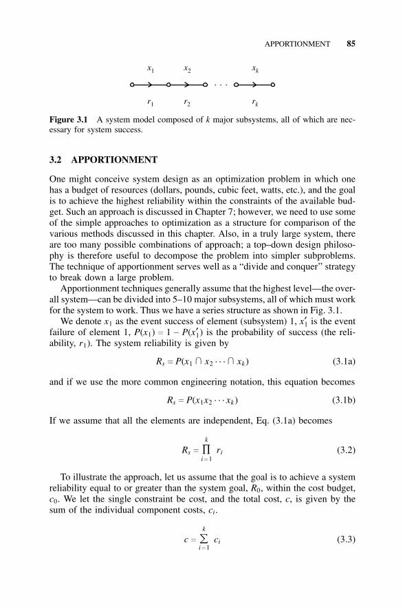
APPORTIONMENT 85
r1
x1
r2
x2
rk
xk
Figure 3.1 A system model composed of k major subsystems, all of which are nec-essary for system success.
3.2 APPORTIONMENT
One might conceive system design as an optimization problem in which onehas a budget of resources (dollars, pounds, cubic feet, watts, etc.), and the goalis to achieve the highest reliability within the constraints of the available bud-get. Such an approach is discussed in Chapter 7; however, we need to use someof the simple approaches to optimization as a structure for comparison of thevarious methods discussed in this chapter. Also, in a truly large system, thereare too many possible combinations of approach; a top–down design philoso-phy is therefore useful to decompose the problem into simpler subproblems.The technique of apportionment serves well as a “divide and conquer” strategyto break down a large problem.
Apportionment techniques generally assume that the highest level—the over-all system—can be divided into 5–10 major subsystems, all of which must workfor the system to work. Thus we have a series structure as shown in Fig. 3.1.
We denote x1 as the event success of element (subsystem) 1, x′1 is the eventfailure of element 1, P(x1) c 1 − P(x′1) is the probability of success (the reli-ability, r1). The system reliability is given by
Rs c P(x1U
x2 · · ·U
xk) (3.1a)
and if we use the more common engineering notation, this equation becomes
Rs c P(x1x2 · · · xk) (3.1b)
If we assume that all the elements are independent, Eq. (3.1a) becomes
Rs c
k
∏i c 1
ri (3.2)
To illustrate the approach, let us assume that the goal is to achieve a systemreliability equal to or greater than the system goal, R0, within the cost budget,c0. We let the single constraint be cost, and the total cost, c, is given by thesum of the individual component costs, ci.
c c
k
���i c 1
ci (3.3)
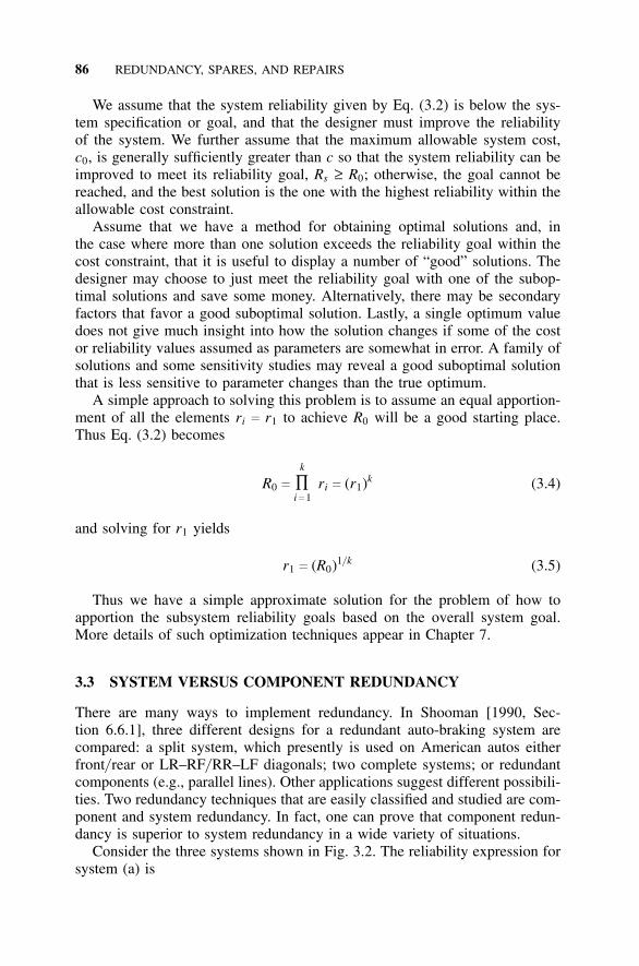
86 REDUNDANCY, SPARES, AND REPAIRS
We assume that the system reliability given by Eq. (3.2) is below the sys-tem specification or goal, and that the designer must improve the reliabilityof the system. We further assume that the maximum allowable system cost,c0, is generally sufficiently greater than c so that the system reliability can beimproved to meet its reliability goal, Rs ≥ R0; otherwise, the goal cannot bereached, and the best solution is the one with the highest reliability within theallowable cost constraint.
Assume that we have a method for obtaining optimal solutions and, inthe case where more than one solution exceeds the reliability goal within thecost constraint, that it is useful to display a number of “good” solutions. Thedesigner may choose to just meet the reliability goal with one of the subop-timal solutions and save some money. Alternatively, there may be secondaryfactors that favor a good suboptimal solution. Lastly, a single optimum valuedoes not give much insight into how the solution changes if some of the costor reliability values assumed as parameters are somewhat in error. A family ofsolutions and some sensitivity studies may reveal a good suboptimal solutionthat is less sensitive to parameter changes than the true optimum.
A simple approach to solving this problem is to assume an equal apportion-ment of all the elements ri c r1 to achieve R0 will be a good starting place.Thus Eq. (3.2) becomes
R0 c
k
∏i c 1
ri c (r1)k (3.4)
and solving for r1 yields
r1 c (R0)1/ k (3.5)
Thus we have a simple approximate solution for the problem of how toapportion the subsystem reliability goals based on the overall system goal.More details of such optimization techniques appear in Chapter 7.
3.3 SYSTEM VERSUS COMPONENT REDUNDANCY
There are many ways to implement redundancy. In Shooman [1990, Sec-tion 6.6.1], three different designs for a redundant auto-braking system arecompared: a split system, which presently is used on American autos eitherfront/ rear or LR–RF/ RR–LF diagonals; two complete systems; or redundantcomponents (e.g., parallel lines). Other applications suggest different possibili-ties. Two redundancy techniques that are easily classified and studied are com-ponent and system redundancy. In fact, one can prove that component redun-dancy is superior to system redundancy in a wide variety of situations.
Consider the three systems shown in Fig. 3.2. The reliability expression forsystem (a) is
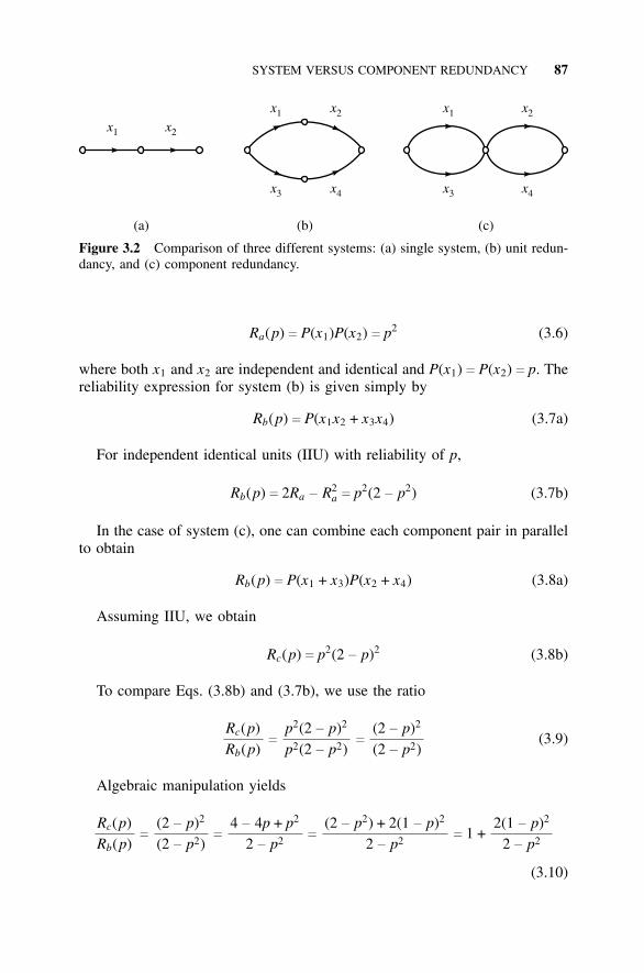
SYSTEM VERSUS COMPONENT REDUNDANCY 87
x1 x2
x1
x3
x2
x4
x1
x3
x2
x4
(a) (b) (c)
Figure 3.2 Comparison of three different systems: (a) single system, (b) unit redun-dancy, and (c) component redundancy.
Ra(p) c P(x1)P(x2) c p2 (3.6)
where both x1 and x2 are independent and identical and P(x1) c P(x2) c p. Thereliability expression for system (b) is given simply by
Rb(p) c P(x1x2 + x3x4) (3.7a)
For independent identical units (IIU) with reliability of p,
Rb(p) c 2Ra − R2a c p2(2 − p2) (3.7b)
In the case of system (c), one can combine each component pair in parallelto obtain
Rb(p) c P(x1 + x3)P(x2 + x4) (3.8a)
Assuming IIU, we obtain
Rc(p) c p2(2 − p)2 (3.8b)
To compare Eqs. (3.8b) and (3.7b), we use the ratio
Rc(p)Rb(p)
c
p2(2 − p)2
p2(2 − p2)c
(2 − p)2
(2 − p2)(3.9)
Algebraic manipulation yields
Rc(p)Rb(p)
c
(2 − p)2
(2 − p2)c
4 − 4p + p2
2 − p2c
(2 − p2) + 2(1 − p)2
2 − p2c 1 +
2(1 − p)2
2 − p2
(3.10)
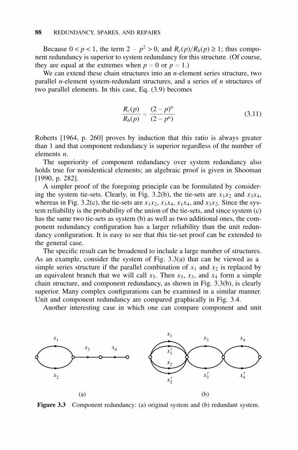
88 REDUNDANCY, SPARES, AND REPAIRS
Because 0 < p < 1, the term 2 − p2 > 0, and Rc(p)/ Rb(p) ≥ 1; thus compo-nent redundancy is superior to system redundancy for this structure. (Of course,they are equal at the extremes when p c 0 or p c 1.)
We can extend these chain structures into an n-element series structure, twoparallel n-element system-redundant structures, and a series of n structures oftwo parallel elements. In this case, Eq. (3.9) becomes
Rc(p)Rb(p)
c
(2 − p)n
(2 − pn)(3.11)
Roberts [1964, p. 260] proves by induction that this ratio is always greaterthan 1 and that component redundancy is superior regardless of the number ofelements n.
The superiority of component redundancy over system redundancy alsoholds true for nonidentical elements; an algebraic proof is given in Shooman[1990, p. 282].
A simpler proof of the foregoing principle can be formulated by consider-ing the system tie-sets. Clearly, in Fig. 3.2(b), the tie-sets are x1x2 and x3x4,whereas in Fig. 3.2(c), the tie-sets are x1x2, x3x4, x1x4, and x3x2. Since the sys-tem reliability is the probability of the union of the tie-sets, and since system (c)has the same two tie-sets as system (b) as well as two additional ones, the com-ponent redundancy configuration has a larger reliability than the unit redun-dancy configuration. It is easy to see that this tie-set proof can be extended tothe general case.
The specific result can be broadened to include a large number of structures.As an example, consider the system of Fig. 3.3(a) that can be viewed as asimple series structure if the parallel combination of x1 and x2 is replaced byan equivalent branch that we will call x5. Then x5, x3, and x4 form a simplechain structure, and component redundancy, as shown in Fig. 3.3(b), is clearlysuperior. Many complex configurations can be examined in a similar manner.Unit and component redundancy are compared graphically in Fig. 3.4.
Another interesting case in which one can compare component and unit
x3 x4
x1
x2
x1
x1′
x2′
x2
x3 x4
x3′ x4′
(a) (b)
Figure 3.3 Component redundancy: (a) original system and (b) redundant system.
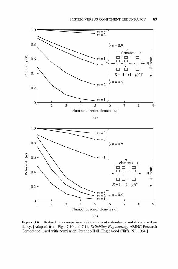
SYSTEM VERSUS COMPONENT REDUNDANCY 89
1
1
2
2
3
3
4
4
5
5
6
6
7
7
8
8
9
9
0
0
0.2
0.2
0.4
0.4
0.6
0.6
0.8
0.8
1.0
1.0
mm
= 3= 2
m
m
= 3
= 2
m = 1
m = 1
m = 3
m = 3
m = 2
m = 2
m = 1
m = 1
p = 0.9
p = 0.9
p = 0.5
p = 0.5
mel
emen
tsm
elem
ents
nelements
nelements
R p= [1 – (1 – ) ]m n
R p= 1 – (1 – )n m
Number of series elements ( )n
Number of series elements ( )n
(a)
(b)
Rel
iabi
lity
()
RR
elia
bilit
y (
)R
Figure 3.4 Redundancy comparison: (a) component redundancy and (b) unit redun-dancy. [Adapted from Figs. 7.10 and 7.11, Reliability Engineering, ARINC ResearchCorporation, used with permission, Prentice-Hall, Englewood Cliffs, NJ, 1964.]
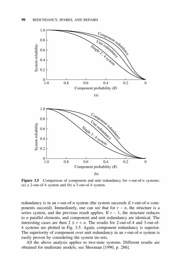
90 REDUNDANCY, SPARES, AND REPAIRS
1.0
1.0
0.8
0.8
0.6
0.6
0.4
0.4
0.2
0.2
0
0
0
0
0.2
0.2
0.4
0.4
0.6
0.6
0.8
0.8
1.0
1.0
Component probability ( )R
Component probability ( )R
(a)
(b)
Syst
em r
elia
bilit
ySy
stem
rel
iabi
lity
Component redundancy
Component redundancy
Unit redundancy
Unit re
y
dunc
nda
Single 2 : 4
esyst m
Single 3 : 4 system
Figure 3.5 Comparison of component and unit redundancy for r-out-of-n systems:(a) a 2-out-of-4 system and (b) a 3-out-of-4 system.
redundancy is in an r-out-of-n system (the system succeeds if r-out-of-n com-ponents succeed). Immediately, one can see that for r c n, the structure is aseries system, and the previous result applies. If r c 1, the structure reducesto n parallel elements, and component and unit redundancy are identical. Theinteresting cases are then 2 ≤ r < n. The results for 2-out-of-4 and 3-out-of-4 systems are plotted in Fig. 3.5. Again, component redundancy is superior.The superiority of component over unit redundancy in an r-out-of-n system iseasily proven by considering the system tie-sets.
All the above analysis applies to two-state systems. Different results areobtained for multistate models; see Shooman [1990, p. 286].
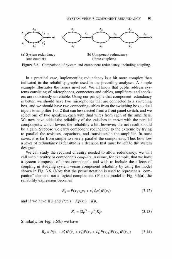
SYSTEM VERSUS COMPONENT REDUNDANCY 91
(a) System redundancy(one coupler)
(b) Component redundancy(three couplers)
x3 xcx1
x2
x2’x1’ x3’
x1xc1
xc2xc3
x2
x1’ x2’
x3
x3’
Figure 3.6 Comparison of system and component redundancy, including coupling.
In a practical case, implementing redundancy is a bit more complex thanindicated in the reliability graphs used in the preceding analyses. A simpleexample illustrates the issues involved. We all know that public address sys-tems consisting of microphones, connectors and cables, amplifiers, and speak-ers are notoriously unreliable. Using our principle that component redundancyis better, we should have two microphones that are connected to a switchingbox, and we should have two connecting cables from the switching box to dualinputs to amplifier 1 or 2 that can be selected from a front panel switch, and weselect one of two speakers, each with dual wires from each of the amplifiers.We now have added the reliability of the switches in series with the parallelcomponents, which lowers the reliability a bit; however, the net result shouldbe a gain. Suppose we carry component redundancy to the extreme by tryingto parallel the resistors, capacitors, and transistors in the amplifier. In mostcases, it is far from simple to merely parallel the components. Thus how lowa level of redundancy is feasible is a decision that must be left to the systemdesigner.
We can study the required circuitry needed to allow redundancy; we willcall such circuitry or components couplers. Assume, for example, that we havea system composed of three components and wish to include the effects ofcoupling in studying system versus component reliability by using the modelshown in Fig. 3.6. (Note that the prime notation is used to represent a “com-panion” element, not a logical complement.) For the model in Fig. 3.6(a), thereliability expression becomes
Ra c P(x1x2x3 + x′1x′2x′3)P(xc) (3.12)
and if we have IIU and P(xc) c Kp(xc) c Kp,
Ra c (2p3− p6)Kp (3.13)
Similarly, for Fig. 3.6(b) we have
Rb c P(x1 + x′1)P(x2 + x′2)P(x3 + x′3)P(xc1)P(xc2)P(xc3) (3.14)
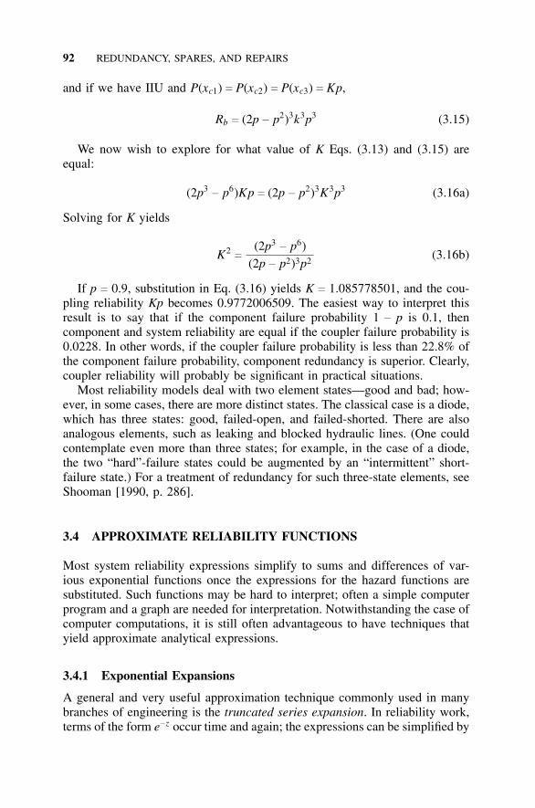
92 REDUNDANCY, SPARES, AND REPAIRS
and if we have IIU and P(xc1) c P(xc2) c P(xc3) c Kp,
Rb c (2p − p2)3k3p3 (3.15)
We now wish to explore for what value of K Eqs. (3.13) and (3.15) areequal:
(2p3− p6)Kp c (2p − p2)3K3p3 (3.16a)
Solving for K yields
K2c
(2p3− p6)
(2p − p2)3p2(3.16b)
If p c 0.9, substitution in Eq. (3.16) yields K c 1.085778501, and the cou-pling reliability Kp becomes 0.9772006509. The easiest way to interpret thisresult is to say that if the component failure probability 1 − p is 0.1, thencomponent and system reliability are equal if the coupler failure probability is0.0228. In other words, if the coupler failure probability is less than 22.8% ofthe component failure probability, component redundancy is superior. Clearly,coupler reliability will probably be significant in practical situations.
Most reliability models deal with two element states—good and bad; how-ever, in some cases, there are more distinct states. The classical case is a diode,which has three states: good, failed-open, and failed-shorted. There are alsoanalogous elements, such as leaking and blocked hydraulic lines. (One couldcontemplate even more than three states; for example, in the case of a diode,the two “hard”-failure states could be augmented by an “intermittent” short-failure state.) For a treatment of redundancy for such three-state elements, seeShooman [1990, p. 286].
3.4 APPROXIMATE RELIABILITY FUNCTIONS
Most system reliability expressions simplify to sums and differences of var-ious exponential functions once the expressions for the hazard functions aresubstituted. Such functions may be hard to interpret; often a simple computerprogram and a graph are needed for interpretation. Notwithstanding the case ofcomputer computations, it is still often advantageous to have techniques thatyield approximate analytical expressions.
3.4.1 Exponential Expansions
A general and very useful approximation technique commonly used in manybranches of engineering is the truncated series expansion. In reliability work,terms of the form e−z occur time and again; the expressions can be simplified by
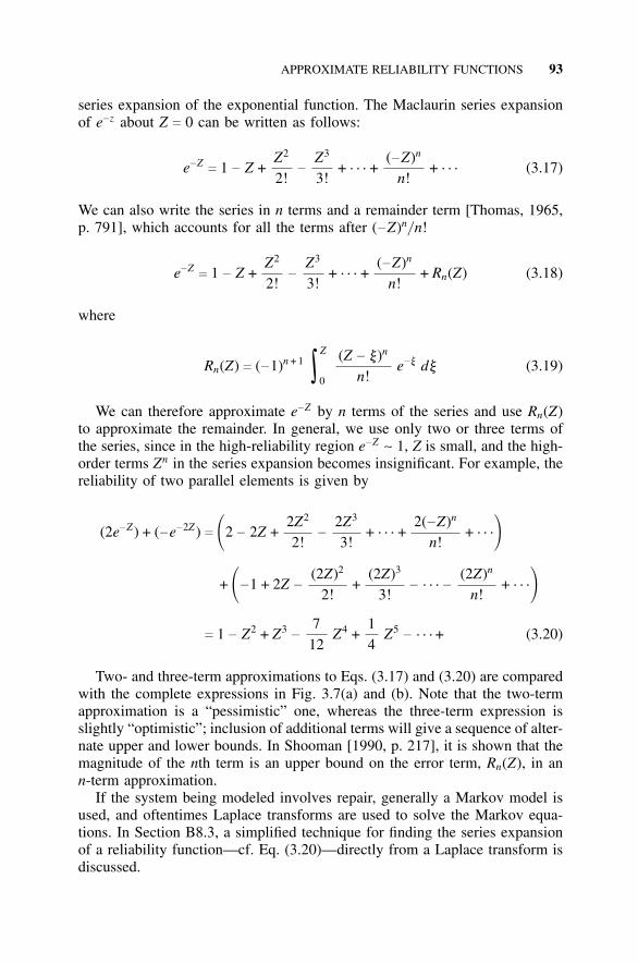
APPROXIMATE RELIABILITY FUNCTIONS 93
series expansion of the exponential function. The Maclaurin series expansionof e−z about Z c 0 can be written as follows:
e−Zc 1 − Z +
Z2
2!−
Z3
3!+ · · · +
(−Z)n
n!+ · · · (3.17)
We can also write the series in n terms and a remainder term [Thomas, 1965,p. 791], which accounts for all the terms after (−Z)n/ n!
e−Zc 1 − Z +
Z2
2!−
Z3
3!+ · · · +
(−Z)n
n!+ Rn(Z) (3.18)
where
Rn(Z) c (−1)n + 1 ∫Z
0
(Z − y)n
n!e−y dy (3.19)
We can therefore approximate e−Z by n terms of the series and use Rn(Z)to approximate the remainder. In general, we use only two or three terms ofthe series, since in the high-reliability region e−Z ∼ 1, Z is small, and the high-order terms Zn in the series expansion becomes insignificant. For example, thereliability of two parallel elements is given by
(2e−Z) + (−e−2Z) c �2 − 2Z +2Z2
2!−
2Z3
3!+ · · · +
2(−Z)n
n!+ · · ·�
+ �−1 + 2Z −
(2Z)2
2!+
(2Z)3
3!− · · · −
(2Z)n
n!+ · · ·�
c 1 − Z2 + Z3−
712
Z4 +14
Z5− · · · + (3.20)
Two- and three-term approximations to Eqs. (3.17) and (3.20) are comparedwith the complete expressions in Fig. 3.7(a) and (b). Note that the two-termapproximation is a “pessimistic” one, whereas the three-term expression isslightly “optimistic”; inclusion of additional terms will give a sequence of alter-nate upper and lower bounds. In Shooman [1990, p. 217], it is shown that themagnitude of the nth term is an upper bound on the error term, Rn(Z), in ann-term approximation.
If the system being modeled involves repair, generally a Markov model isused, and oftentimes Laplace transforms are used to solve the Markov equa-tions. In Section B8.3, a simplified technique for finding the series expansionof a reliability function—cf. Eq. (3.20)—directly from a Laplace transform isdiscussed.
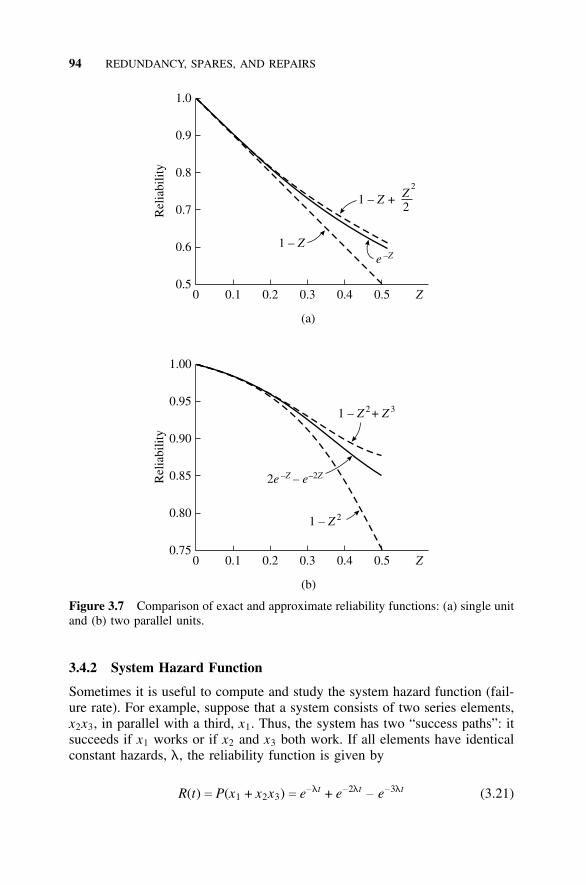
94 REDUNDANCY, SPARES, AND REPAIRS
0
0
0.1
0.1
0.2
0.2
0.3
0.3
0.4
0.4
0.5
0.5
Z
Z
0.5
0.75
0.6
0.80
0.7
0.85
0.8
0.90
0.9
0.95
1.0
1.00
(a)
(b)
Rel
iabi
lity
Rel
iabi
lity
1 – Z
1 –2
Z + Z2
1 – +Z Z2 3
1 – Z 2
e –Z
2e –Z – e–2Z
Figure 3.7 Comparison of exact and approximate reliability functions: (a) single unitand (b) two parallel units.
3.4.2 System Hazard Function
Sometimes it is useful to compute and study the system hazard function (fail-ure rate). For example, suppose that a system consists of two series elements,x2x3, in parallel with a third, x1. Thus, the system has two “success paths”: itsucceeds if x1 works or if x2 and x3 both work. If all elements have identicalconstant hazards, l, the reliability function is given by
R(t) c P(x1 + x2x3) c e−lt + e−2lt− e−3lt (3.21)
APPROXIMATE RELIABILITY FUNCTIONS 95
From Appendix B, we see that z(t) is given by the density function dividedby the reliability function, which can be written as the negative of the timederivative of the reliability function divided by the reliability function.
z(t) cf (t)R(t)
c −
R(t)R(t)
c
l(1 + 2e−lt− 3e−2lt)
1 + e−lt− e−2lt
(3.22)
Expanding z(t) in a Taylor series,
z(t) c 1 + lt − 3l2t2/ 2 + · · · (3.23)
We can use such approximations to compare the equivalent hazard of varioussystems.
3.4.3 Mean Time to Failure
In the last section, it was shown that reliabiilty calculations become very com-plicated in a large system when there are many components and a diverse reli-ability structure. Not only was the reliability expression difficult to write downin such a case, but computation was lengthy, and interpretation of the individualcomponent contributions was not easy. One method of simplifying the situa-tion is to ask for less detailed information about the system. A useful figureof merit for a system is the mean time to failure (MTTF).
As was derived in Eq. (B51) of Appendix B, the MTTF is the expected valueof the time to failure. The standard formula for the expected value involvesthe integral of t f (t); however, this can be expressed in terms of the reliabilityfunction.
MTTF c ∫∞
0R(t) dt (3.24)
We can use this expression to compute the MTTF for various configura-tions. For a series reliability configuration of n elements in which each of theelements has a failure rate zi(t) and Z(t) c ∫ z(t) dt, one can write the reliabilityexpression as
R(t) c exp [ − n
���i c 1
Zi(t)] (3.25a)
and the MTTF is given by
MTTF c ∫∞
0{exp [ − n
���i c 1
Zi(t)]} dt (3.25b)
96 REDUNDANCY, SPARES, AND REPAIRS
If the series system has components with more than one type of hazardmodel, the integral in Eq. (3.25b) is difficult to evaluate in closed form but canalways be done using a series approximation for the exponential integrand; seeShooman [1990, p. 20].
Different equations hold for a parallel system. For two parallel elements,the reliability expression is written as R(t) c e−Z1(t) + e−Z2(t)
− e[−Z1(t) + Z2(t)]. Ifboth system components have a constant-hazard rate, and we apply Eq. (3.24)to each term in the reliability expression,
MTTF c
1l1
+1l2
+1
l1 + l2(3.26)
In the general case of n parallel elements with constant-hazard rate, theexpression becomes
MTTF c � 1l1
+1l2
+ · · · +1ln
� − � 1l1 + l2
+1
l1 + l3+ · · · +
1li + lj
�+ � 1
l1 + l2 + l3+
1l1 + l2 + l4
+ · · · +1
li + lj + lk�
− · · · + (−1)n + 1 1n
���i c 1
li
(3.27)
If the n units are identical—that is, l1 c l2 c · · · c ln c l—then Eq. (3.27)becomes
MTTF c
� n
1 �1
−
� n2 �2
+� n
3 �3
− · · · + (−1)n + 1� n
n �n
c
1l
n
���i c 1
1i
(3.28a)
The preceding series is called the harmonic series; the summation form isgiven in Jolley [1961, p. 26, Eq. (200)] or Courant [1951, pp. 380]. This seriesoccurs in number theory, and a series expansion is attributed to the famousmathematician Euler; the constant in the expansion (0.577) is called Euler’sconstant [Jolley, 1961, p. 14, Eq. (70)].
1l
n
���i c 1
1ic
1l [ 0.577 + ln n +
12n
−
112n(n + 1)
· · ·] (3.28b)
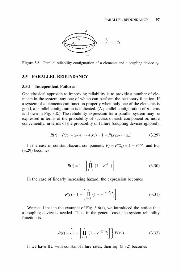
PARALLEL REDUNDANCY 97
x3
xn
x1
xcx2
Figure 3.8 Parallel reliability configuration of n elements and a coupling device xc.
3.5 PARALLEL REDUNDANCY
3.5.1 Independent Failures
One classical approach to improving reliability is to provide a number of ele-ments in the system, any one of which can perform the necessary function. Ifa system of n elements can function properly when only one of the elements isgood, a parallel configuration is indicated. (A parallel configuration of n itemsis shown in Fig. 3.8.) The reliability expression for a parallel system may beexpressed in terms of the probability of success of each component or, moreconveniently, in terms of the probability of failure (coupling devices ignored).
R(t) c P(x1 + x2 + · · · + xn) c 1 − P(x1x2 · · · xn) (3.29)
In the case of constant-hazard components, Pf c P(xi) c 1 − e−li t , and Eq.(3.29) becomes
R(t) c 1 − [ n
∏i − 1
(1 − e−li t)] (3.30)
In the case of linearly increasing hazard, the expression becomes
R(t) c 1 − [ n
∏i − 1
(1 − e−Kit2/ 2)] (3.31)
We recall that in the example of Fig. 3.6(a), we introduced the notion thata coupling device is needed. Thus, in the general case, the system reliabilityfunction is
R(t) c {1 − [ n
∏i − 1
(1 − e−Zi(t))]} P(xc) (3.32)
If we have IIU with constant-failure rates, then Eq. (3.32) becomes
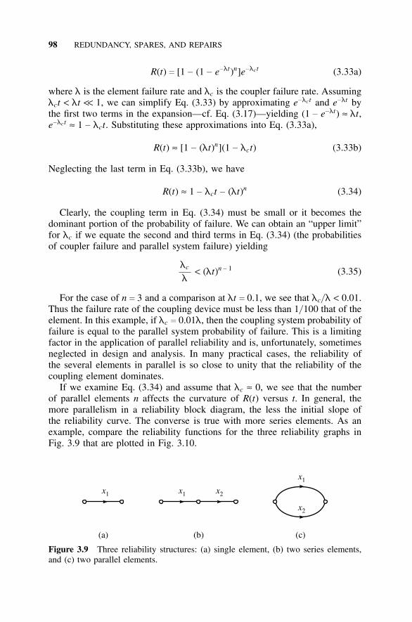
98 REDUNDANCY, SPARES, AND REPAIRS
R(t) c [1 − (1 − e−lt)n]e−lct (3.33a)
where l is the element failure rate and lc is the coupler failure rate. Assuminglct < lt << 1, we can simplify Eq. (3.33) by approximating e−lct and e−lt bythe first two terms in the expansion—cf. Eq. (3.17)—yielding (1 − e−lt) ≈ lt,e−lct ≈ 1 − lct. Substituting these approximations into Eq. (3.33a),
R(t) ≈ [1 − (lt)n](1 − lct) (3.33b)
Neglecting the last term in Eq. (3.33b), we have
R(t) ≈ 1 − lct − (lt)n (3.34)
Clearly, the coupling term in Eq. (3.34) must be small or it becomes thedominant portion of the probability of failure. We can obtain an “upper limit”for lc if we equate the second and third terms in Eq. (3.34) (the probabilitiesof coupler failure and parallel system failure) yielding
lc
l< (lt)n − 1 (3.35)
For the case of n c 3 and a comparison at lt c 0.1, we see that lc/l < 0.01.Thus the failure rate of the coupling device must be less than 1/ 100 that of theelement. In this example, if lc c 0.01l, then the coupling system probability offailure is equal to the parallel system probability of failure. This is a limitingfactor in the application of parallel reliability and is, unfortunately, sometimesneglected in design and analysis. In many practical cases, the reliability ofthe several elements in parallel is so close to unity that the reliability of thecoupling element dominates.
If we examine Eq. (3.34) and assume that lc ≈ 0, we see that the numberof parallel elements n affects the curvature of R(t) versus t. In general, themore parallelism in a reliability block diagram, the less the initial slope ofthe reliability curve. The converse is true with more series elements. As anexample, compare the reliability functions for the three reliability graphs inFig. 3.9 that are plotted in Fig. 3.10.
x1 x1 x2
x1
x2
(a) (b) (c)
Figure 3.9 Three reliability structures: (a) single element, (b) two series elements,and (c) two parallel elements.
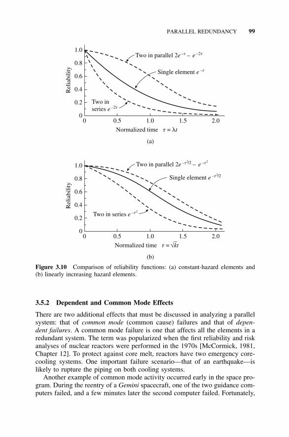
PARALLEL REDUNDANCY 99
0
0
0.5
0.5
1.0
1.0
1.5
1.5
2.0
2.0
0
0
0.2
0.2
0.4
0.4
0.6
0.6
0.8
0.8
1.0
1.0
(a)
(b)
Rel
iabi
lity
Rel
iabi
lity
Two in parallel 2e –t – e –2t
Two in parallel 2e – 2/2 –t te – 2
Two inseries e –2t
Two in series e –t2
Single element e –t
Single element e –t2/2
Normalized time =t lt
Normalized time =t kt√
Figure 3.10 Comparison of reliability functions: (a) constant-hazard elements and(b) linearly increasing hazard elements.
3.5.2 Dependent and Common Mode Effects
There are two additional effects that must be discussed in analyzing a parallelsystem: that of common mode (common cause) failures and that of depen-dent failures. A common mode failure is one that affects all the elements in aredundant system. The term was popularized when the first reliability and riskanalyses of nuclear reactors were performed in the 1970s [McCormick, 1981,Chapter 12]. To protect against core melt, reactors have two emergency core-cooling systems. One important failure scenario—that of an earthquake—islikely to rupture the piping on both cooling systems.
Another example of common mode activity occurred early in the space pro-gram. During the reentry of a Gemini spacecraft, one of the two guidance com-puters failed, and a few minutes later the second computer failed. Fortunately,
100 REDUNDANCY, SPARES, AND REPAIRS
the astronauts had an additional backup procedure. Based on rehearsed pro-cedures and precomputations, the Ground Control advised the astronauts tomaneuver the spacecraft, to align the horizon with one of a set of horizontalscribe marks on the windows, and to rotate the spacecraft so that the Sun wasaligned with one set of vertical scribe marks. The Ground Control then gavethe astronauts a countdown to retro-rocket ignition and a second countdownto rocket cutoff. The spacecraft splashed into the ocean—closer to the recov-ery ship than in any previous computer-controlled reentry. Subsequent analysisshowed that the temperature inside the two computers was much higher thanexpected and that the diodes in the separate power supply of each computerhad burned out. From this example, we learn several lessons:
1. The designers provided two computers for redundancy.2. Correctly, two separate power supplies were provided, one for each com-
puter, to avoid a common power-supply failure mode.3. An unexpectedly high ambient temperature caused identical failues in the
diodes, resulting in a common mode failure.4. Fortunately, there was a third redundant mode that depended on a com-
pletely different mechanism, the scribe marks, and visual alignment.When parallel elements are purposely chosen to involve devices withdifferent failure mechanisms to avoid common mode failures, the termdiversity is used.
In terms of analysis, common mode failures behave much like failures ofa coupling mechanism that was studied previously. In fact, we can use Eq.(3.33) to analyze the effect if we use lc to represent the sum of coupling andcommon mode failure rates. (A fortuitous choice of subscript!)
Another effect to consider in parallel systems is the effect of dependentfailures. Suppose we wish to use two parallel satellite channels for reliablecommunication, and the probability of each channel failure is 0.01. For a singlechannel, the reliability would be 0.99; for two parallel channels, c1 and c2, wewould have
R c P(c1 + c2) c 1 − P(c1c2) (3.36)
Expanding the last term in Eq. (3.36) yields
R c 1 − P(c1c2) c 1 − P(c1)P(c2 |c1) (3.37)
If the failures of both channels, c1 and c2, are independent, Eq. (3.37) yieldsR c 1 − 0.01 × 0.01 c 0.9999. However, suppose that one-quarter of satel-lite transmission failures are due to atmospheric interference that would affectboth channels. In this case, P(c2 |c1) is 0.25, and Eq. (3.37) yields R c 1 −
0.01 × 0.25 c 0.9975. Thus for a single channel, the probability of failure is
AN r-OUT-OF-n STRUCTURE 101
0.01; with two independent parallel channels, it is 0.0001, but for dependentchannels, it is 0.0025. This means that dependency has reduced the expected100-fold reduction in failure probabilities to a reduction by only a factor of 4.In general, a modeling of dependent failures requires some knowledge of thefailure mechanisms that result in dependent modes.
The above analysis has explored many factors that must be consideredin analyzing parallel systems: coupling failures, common mode failures, anddependent failures. Clearly, only simple models were used in each case. Morecomplex models may be formulated by using Markov process models—to bediscussed in Section 3.7, where we analyze standby redundancy.
3.6 AN r-OUT-OF-n STRUCTURE
Another simple structure that serves as a useful model for many reliabilityproblems is an r-out-of-n structure. Such a model represents a system of ncomponents in which r of the n items must be good for the system to succeed.(Of course, r is less than n.) An example of an r-out-of-n structure is a fiber-optic cable, which has a capacity of n circuits. If the application requires rchannels of the transmission, this is an r-out-of-n system (r : n). If the capacityof the cable n exceeds r by a significant amount, this represents a form ofparallel redundancy. We are of course assuming that if a circuit fails it can beswitched to one of the n–r “extra circuits.”
We may formulate a structural model for an r-out-of-n system, but it issimpler to use the binomial distribution if applicable. The binomial distributioncan be used only when the n components are independent and identical. If thecomponents differ or are dependent, the structural-model approach must beused. Success of exactly r-out-of-n identical and independent items is givenby
B(r : n) c � nr � pr(1 − p)n − r (3.38)
where r : n stands for r out of n, and the success of at least r-out-of-n items isgiven by
Ps c
n
���k c r
B(k : n) (3.39)
For constant-hazard components, Eq. (3.38) becomes
R(t) cn
���k c r �
nk � e−klt(1 − e−lt)n − k (3.40)
102 REDUNDANCY, SPARES, AND REPAIRS
Similarly, for linearly increasing or Weibull components, the reliability func-tions are
R(t) cn
���k c r �
nk � e−kKt2/ 2(1 − e−Kt2/ 2)n − k (3.41a)
and
R(t) cn
���k c r �
nk � e−kKtm + 1/ (m + 1)(1 − e−Ktm + 1/ (m + 1))n − k (3.41b)
Clearly, Eqs. (3.39)–(3.41) can be studied and evaluated by a parametriccomputer study. In many cases, it is useful to approximate the result, althoughnumerical evaluation via a computer program is not difficult. For an r-out-of-nstructure of identical components, the exact reliability expression is given byEq. (3.38). As is well known, we can approximate the binomial distribution bythe Poisson or normal distributions, depending on the values of n and p (seeShooman, 1990, Sections 2.5.6 and 2.6.8). Interestingly, we can also developsimilar approximations for the case in which the n parameters are not identical.
The Poisson approximation to the binomial holds for p ≤ 0.05 and n ≥ 20,which represents the low-reliability region. If we are interested in the high-reliability region, we switch to failure probabilities, requiring q c 1 − p ≤ 0.05and n ≥ 20. Since we are assuming different components, we define averageprobabilities of success and failure p and q as
p c
1n
n
���i c 1
pi c 1 − q c 1 −
1n
n
���i c 1
(1 − pi) (3.42)
Thus, for the high-reliability region, we compute the probability of n–r or fewerfailures as
R(t) cn − r
���k c 0
(nq)ke−nq
k!(3.43)
and for the low-reliability region, we compute the probability of r or moresuccesses as
R(t) cn
���k c r
(np)ke−np
k!(3.44)
Equations (3.43) and (3.44) avoid a great deal of algebra in dealing withnonidentical r-out-of-n components. The question of accuracy is somewhat dif-
AN r-OUT-OF-n STRUCTURE 103
ficult to answer since it depends on the system structure and the range of valuesof p that make up p. For example, if the values of q vary only over a 2 : 1 range,and if q ≤ 0.05 and n ≥ 20, intuition tells us that we should obtain reasonablyaccurate results. Clearly, modern computer power makes explicit enumerationof Eqs. (3.39)–(3.41) a simple procedure, and Eqs. (3.43) and (3.44) are usefulmainly as simplified analytical expressions that provide a check on computa-tions. [Note that Eqs. (3.43) and (3.44) also hold true for IIU with p c p andq c q.]
We can appreciate the power of an r : n design by considering the followingexample. Suppose we have a fiber-optic cable with 20 channels (strands) and asystem that requires all 20 channels for success. (For simplicity of the discus-sion, assume that the associated electronics will not fail.) Suppose the proba-bility of failure of each channel within the cable is q c 0.0005 and p c 0.9995.Since all 20 channels are needed for success, the reliability of a 20-channelcable will be R20 c (0.9995)20
c 0.990047. Another option is to use two paral-lel 20-channel cables and associated electronics switch from cable A to cableB whenever there is any failure in cable A. The reliability of such an ordinaryparallel system of two 20-channel cables is given by R2/ 20 c 2(0.990047) −
(0.990047)2c 0.9999009. Another design option is to include extra channels
in the single cable beyond the 20 that are needed—in such a case, we have anr : n system. Suppose we approach the design in a trial-and-error fashion. Webegin by trying n c 21 channels, in which case we have
R21 c B(21 : 21) + B(20 : 21) c p21q0 + 21p20q
c (0.9995)21 + 21(0.9995)20(0.0005) c 0.98755223 + 0.010395497
c 0.999947831 (3.45)
Thus R21 exceeds the design with two 20-channel cables. Clearly, all thedesigns require some electronic steering (couplers) for the choice of channels,and the coupler reliability should be included in a detailed comparison. Ofcourse, one should worry about common mode failures, which could com-pletely change the foregoing results. Construction damage—that is, line-sev-ering by a contractor’s excavating maching (backhoe)—is a significant failuremode for in-soil fiber-optic telephone lines.
As a check on Eq. (3.45), we compute the approximation Eq. (3.43) for nc 21, r c 20.
R(t) c1
���k c 0
(nq)ke−nq
k!c (1 + nq)e−nq
c [1 + 21(0.0005)]e−22 × 0.0005
c 0.999831687 (3.46)
These values are summarized in Table 3.1.
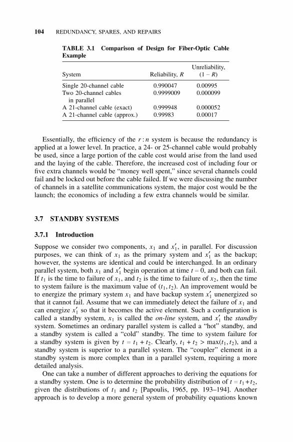
104 REDUNDANCY, SPARES, AND REPAIRS
TABLE 3.1 Comparison of Design for Fiber-Optic CableExample
Unreliability,System Reliability, R (1 − R)
Single 20-channel cable 0.990047 0.00995Two 20-channel cables 0.9999009 0.000099
in parallelA 21-channel cable (exact) 0.999948 0.000052A 21-channel cable (approx.) 0.99983 0.00017
Essentially, the efficiency of the r : n system is because the redundancy isapplied at a lower level. In practice, a 24- or 25-channel cable would probablybe used, since a large portion of the cable cost would arise from the land usedand the laying of the cable. Therefore, the increased cost of including four orfive extra channels would be “money well spent,” since several channels couldfail and be locked out before the cable failed. If we were discussing the numberof channels in a satellite communications system, the major cost would be thelaunch; the economics of including a few extra channels would be similar.
3.7 STANDBY SYSTEMS
3.7.1 Introduction
Suppose we consider two components, x1 and x′1, in parallel. For discussionpurposes, we can think of x1 as the primary system and x′1 as the backup;however, the systems are identical and could be interchanged. In an ordinaryparallel system, both x1 and x′1 begin operation at time t c 0, and both can fail.If t1 is the time to failure of x1, and t2 is the time to failure of x2, then the timeto system failure is the maximum value of (t1, t2). An improvement would beto energize the primary system x1 and have backup system x′1 unenergized sothat it cannot fail. Assume that we can immediately detect the failure of x1 andcan energize x′1 so that it becomes the active element. Such a configuration iscalled a standby system, x1 is called the on-line system, and x′1 the standbysystem. Sometimes an ordinary parallel system is called a “hot” standby, anda standby system is called a “cold” standby. The time to system failure fora standby system is given by t c t1 + t2. Clearly, t1 + t2 > max(t1, t2), and astandby system is superior to a parallel system. The “coupler” element in astandby system is more complex than in a parallel system, requiring a moredetailed analysis.
One can take a number of different approaches to deriving the equations fora standby system. One is to determine the probability distribution of t c t1 + t2,given the distributions of t1 and t2 [Papoulis, 1965, pp. 193–194]. Anotherapproach is to develop a more general system of probability equations known
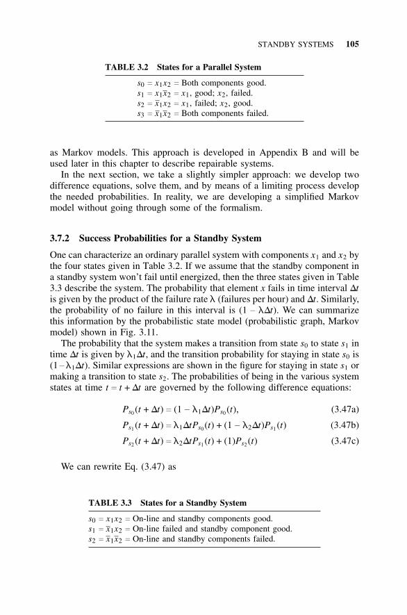
STANDBY SYSTEMS 105
TABLE 3.2 States for a Parallel System
s0 c x1x2 c Both components good.s1 c x1x2 c x1, good; x2, failed.s2 c x1x2 c x1, failed; x2, good.s3 c x1x2 c Both components failed.
as Markov models. This approach is developed in Appendix B and will beused later in this chapter to describe repairable systems.
In the next section, we take a slightly simpler approach: we develop twodifference equations, solve them, and by means of a limiting process developthe needed probabilities. In reality, we are developing a simplified Markovmodel without going through some of the formalism.
3.7.2 Success Probabilities for a Standby System
One can characterize an ordinary parallel system with components x1 and x2 bythe four states given in Table 3.2. If we assume that the standby component ina standby system won’t fail until energized, then the three states given in Table3.3 describe the system. The probability that element x fails in time interval Dtis given by the product of the failure rate l (failures per hour) and Dt. Similarly,the probability of no failure in this interval is (1 − lDt). We can summarizethis information by the probabilistic state model (probabilistic graph, Markovmodel) shown in Fig. 3.11.
The probability that the system makes a transition from state s0 to state s1 intime Dt is given by l1Dt, and the transition probability for staying in state s0 is(1−l1Dt). Similar expressions are shown in the figure for staying in state s1 ormaking a transition to state s2. The probabilities of being in the various systemstates at time t c t + Dt are governed by the following difference equations:
Ps0 (t + Dt) c (1 − l1Dt)Ps0 (t), (3.47a)
Ps1 (t + Dt) c l1DtPs0 (t) + (1 − l2Dt)Ps1 (t) (3.47b)
Ps2 (t + Dt) c l2DtPs1 (t) + (1)Ps2 (t) (3.47c)
We can rewrite Eq. (3.47) as
TABLE 3.3 States for a Standby System
s0 c x1x2 c On-line and standby components good.s1 c x1x2 c On-line failed and standby component good.s2 c x1x2 c On-line and standby components failed.
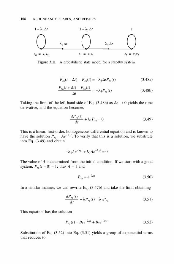
106 REDUNDANCY, SPARES, AND REPAIRS
1 – l1 Dt
l1 Dt l2 Dt
s x= 10 2x
1 – l2 Dt 1
s x= 11 2x s x= 12 2x
Figure 3.11 A probabilistic state model for a standby system.
Ps0 (t + Dt) − Ps0 (t) c −l1DtPs0 (t) (3.48a)
Ps0 (t + Dt) − Ps0 (t)Dt
c −l1Ps0 (t) (3.48b)
Taking the limit of the left-hand side of Eq. (3.48b) as Dt b 0 yields the timederivative, and the equation becomes
dPs0 (t)dt
+ l1Ps0 c 0 (3.49)
This is a linear, first-order, homogeneous differential equation and is known tohave the solution Ps0 c Ae−l1t . To verify that this is a solution, we substituteinto Eq. (3.49) and obtain
−l1Ae−l1t + l1Ae−l1tc 0
The value of A is determined from the initial condition. If we start with a goodsystem, Ps0 (t c 0) c 1; thus A c 1 and
Ps0 c e−l1t (3.50)
In a similar manner, we can rewrite Eq. (3.47b) and take the limit obtaining
dPs1 (t)dt
+ lPs1 (t) c l1Ps0 (3.51)
This equation has the solution
Ps1 (t) c B1e−l1t + B2e−l2t (3.52)
Substitution of Eq. (3.52) into Eq. (3.51) yields a group of exponential termsthat reduces to
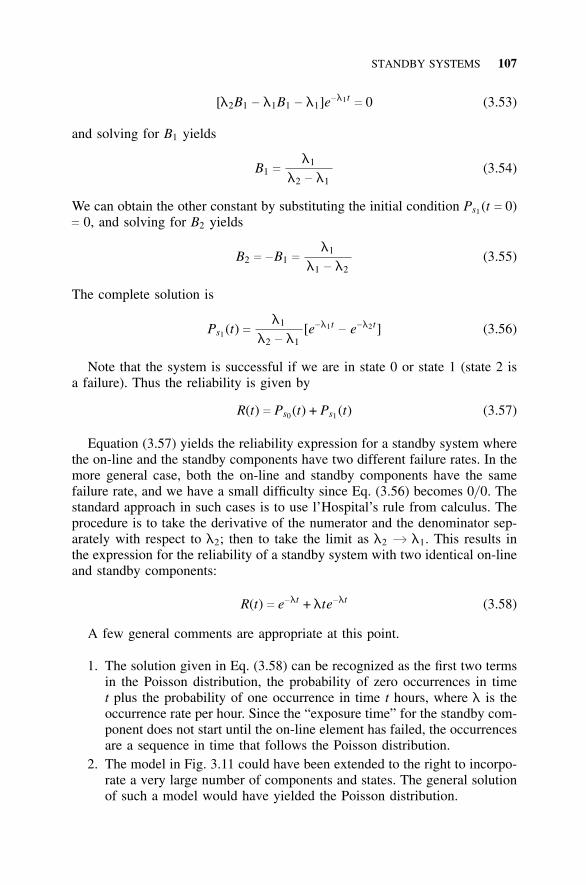
STANDBY SYSTEMS 107
[l2B1 − l1B1 − l1]e−l1tc 0 (3.53)
and solving for B1 yields
B1 cl1
l2 − l1(3.54)
We can obtain the other constant by substituting the initial condition Ps1 (t c 0)c 0, and solving for B2 yields
B2 c −B1 cl1
l1 − l2(3.55)
The complete solution is
Ps1 (t) cl1
l2 − l1[e−l1t
− e−l2t] (3.56)
Note that the system is successful if we are in state 0 or state 1 (state 2 isa failure). Thus the reliability is given by
R(t) c Ps0 (t) + Ps1 (t) (3.57)
Equation (3.57) yields the reliability expression for a standby system wherethe on-line and the standby components have two different failure rates. In themore general case, both the on-line and standby components have the samefailure rate, and we have a small difficulty since Eq. (3.56) becomes 0/ 0. Thestandard approach in such cases is to use l’Hospital’s rule from calculus. Theprocedure is to take the derivative of the numerator and the denominator sep-arately with respect to l2; then to take the limit as l2 b l1. This results inthe expression for the reliability of a standby system with two identical on-lineand standby components:
R(t) c e−lt + lte−lt (3.58)
A few general comments are appropriate at this point.
1. The solution given in Eq. (3.58) can be recognized as the first two termsin the Poisson distribution, the probability of zero occurrences in timet plus the probability of one occurrence in time t hours, where l is theoccurrence rate per hour. Since the “exposure time” for the standby com-ponent does not start until the on-line element has failed, the occurrencesare a sequence in time that follows the Poisson distribution.
2. The model in Fig. 3.11 could have been extended to the right to incorpo-rate a very large number of components and states. The general solutionof such a model would have yielded the Poisson distribution.
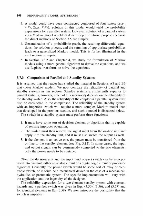
108 REDUNDANCY, SPARES, AND REPAIRS
3. A model could have been constructed composed of four states: (x1x2,x1x2, x1x2, x1x2). Solution of this model would yield the probabilityexpressions for a parallel system. However, solution of a parallel systemvia a Markov model is seldom done except for tutorial purposes becausethe direct methods of Section 3.5 are simpler.
4. Generalization of a probabilistic graph, the resulting differential equa-tions, the solution process, and the summing of appropriate probabilitiesleads to a generalized Markov model. This is further illustrated in thenext section on repair.
5. In Section 3.8.2 and Chapter 4, we study the formulation of Markovmodels using a more general algorithm to derive the equations, and weuse Laplace transforms to solve the equations.
3.7.3 Comparison of Parallel and Standby Systems
It is assumed that the reader has studied the material in Sections A8 and B6that cover Markov models. We now compare the reliability of parallel andstandby systems in this section. Standby systems are inherently superior toparallel systems; however, much of this superiority depends on the reliability ofthe standby switch. Also, the reliability of the coupler in a parallel system mustalso be considered in the comparison. The reliability of the standby systemwith an imperfect switch will require a more complex Markov model thanthat developed in the previous section, and such a model is discussed below.
The switch in a standby system must perform three functions:
1. It must have some sort of decision element or algorithm that is capableof sensing improper operation.
2. The switch must then remove the signal input from the on-line unit andapply it to the standby unit, and it must also switch the output as well.
3. If the element is an active one, the power must be transferred from theon-line to the standby element (see Fig. 3.12). In some cases, the inputand output signals can be permanently connected to the two elements;only the power needs to be switched.
Often the decision unit and the input (and output) switch can be incorpo-rated into one unit: either an analog circuit or a digital logic circuit or processoralgorithm. Generally, the power switch would be some sort of relay or elec-tronic switch, or it could be a mechanical device in the case of a mechanical,hydraulic, or pneumatic system. The specific implementation will vary withthe application and the ingenuity of the designer.
The reliability expression for a two-element standby system with constanthazards and a perfect switch was given in Eqs. (3.50), (3.56), and (3.57) andfor identical elements in Eq. (3.58). We now introduce the possibility that theswitch is imperfect.
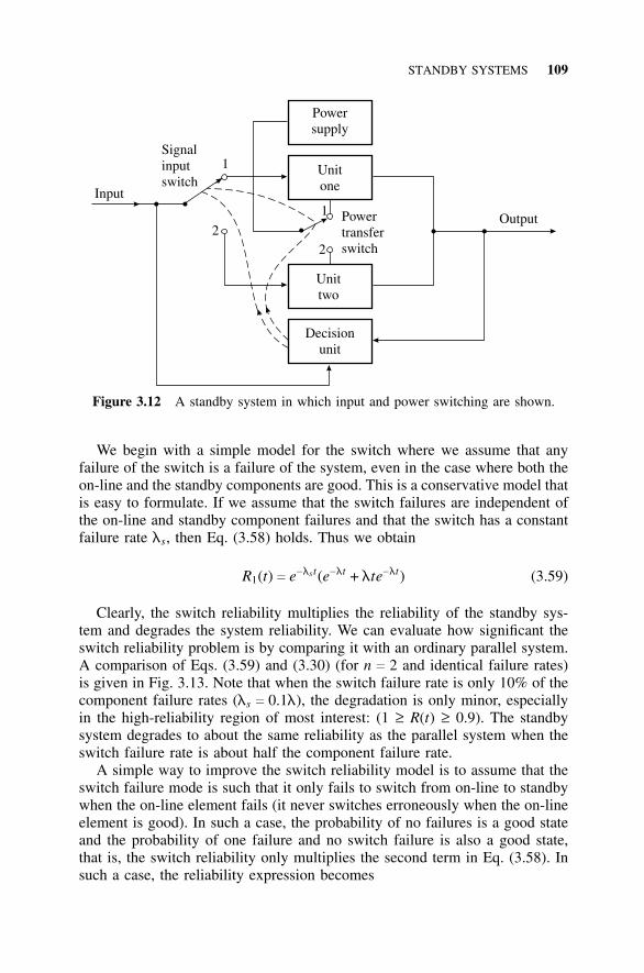
STANDBY SYSTEMS 109
Powersupply
Unitone
Unittwo
Decisionunit
Powertransferswitch
Signalinputswitch
Input
Output
1
2
1
2
Figure 3.12 A standby system in which input and power switching are shown.
We begin with a simple model for the switch where we assume that anyfailure of the switch is a failure of the system, even in the case where both theon-line and the standby components are good. This is a conservative model thatis easy to formulate. If we assume that the switch failures are independent ofthe on-line and standby component failures and that the switch has a constantfailure rate ls, then Eq. (3.58) holds. Thus we obtain
R1(t) c e−lst(e−lt + lte−lt) (3.59)
Clearly, the switch reliability multiplies the reliability of the standby sys-tem and degrades the system reliability. We can evaluate how significant theswitch reliability problem is by comparing it with an ordinary parallel system.A comparison of Eqs. (3.59) and (3.30) (for n c 2 and identical failure rates)is given in Fig. 3.13. Note that when the switch failure rate is only 10% of thecomponent failure rates (ls c 0.1l), the degradation is only minor, especiallyin the high-reliability region of most interest: (1 ≥ R(t) ≥ 0.9). The standbysystem degrades to about the same reliability as the parallel system when theswitch failure rate is about half the component failure rate.
A simple way to improve the switch reliability model is to assume that theswitch failure mode is such that it only fails to switch from on-line to standbywhen the on-line element fails (it never switches erroneously when the on-lineelement is good). In such a case, the probability of no failures is a good stateand the probability of one failure and no switch failure is also a good state,that is, the switch reliability only multiplies the second term in Eq. (3.58). Insuch a case, the reliability expression becomes
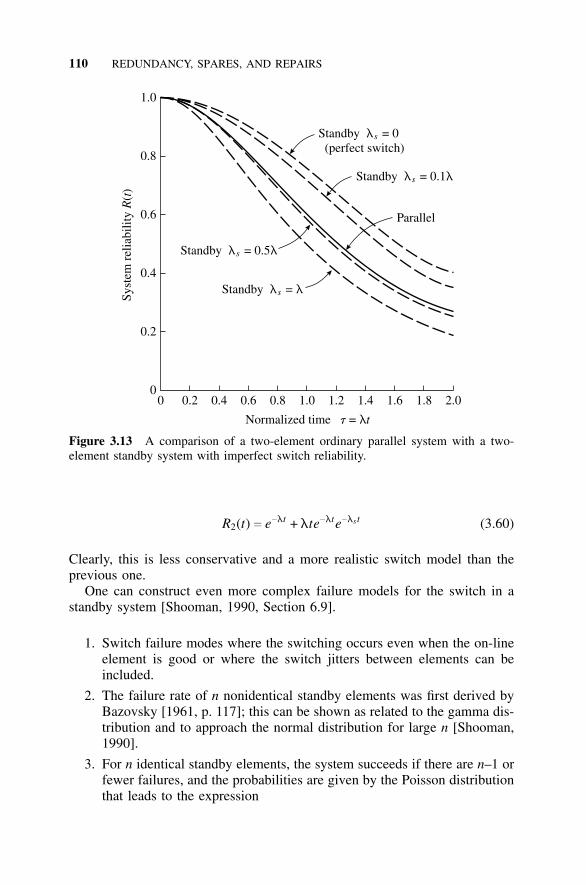
110 REDUNDANCY, SPARES, AND REPAIRS
0 0.2 0.4 0.6 0.8 1.0 1.2 1.4 1.6 1.8 2.00
0.2
0.4
0.6
0.8
1.0
Normalized time =t lt
Syst
em r
elia
bilit
y(
)R
tStandby = 0(perfect switch)
ls
Standby = 0.1l ls
Standby = 0.5l ls
Standby =l ls
Parallel
Figure 3.13 A comparison of a two-element ordinary parallel system with a two-element standby system with imperfect switch reliability.
R2(t) c e−lt + lte−lte−lst (3.60)
Clearly, this is less conservative and a more realistic switch model than theprevious one.
One can construct even more complex failure models for the switch in astandby system [Shooman, 1990, Section 6.9].
1. Switch failure modes where the switching occurs even when the on-lineelement is good or where the switch jitters between elements can beincluded.
2. The failure rate of n nonidentical standby elements was first derived byBazovsky [1961, p. 117]; this can be shown as related to the gamma dis-tribution and to approach the normal distribution for large n [Shooman,1990].
3. For n identical standby elements, the system succeeds if there are n–1 orfewer failures, and the probabilities are given by the Poisson distributionthat leads to the expression
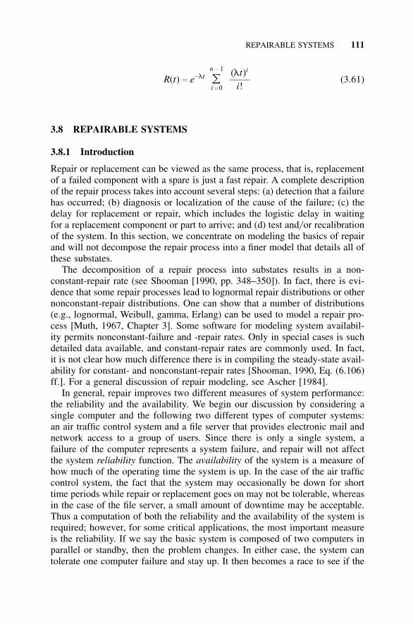
REPAIRABLE SYSTEMS 111
R(t) c e−ltn − 1
���i c 0
(lt)i
i!(3.61)
3.8 REPAIRABLE SYSTEMS
3.8.1 Introduction
Repair or replacement can be viewed as the same process, that is, replacementof a failed component with a spare is just a fast repair. A complete descriptionof the repair process takes into account several steps: (a) detection that a failurehas occurred; (b) diagnosis or localization of the cause of the failure; (c) thedelay for replacement or repair, which includes the logistic delay in waitingfor a replacement component or part to arrive; and (d) test and/ or recalibrationof the system. In this section, we concentrate on modeling the basics of repairand will not decompose the repair process into a finer model that details all ofthese substates.
The decomposition of a repair process into substates results in a non-constant-repair rate (see Shooman [1990, pp. 348–350]). In fact, there is evi-dence that some repair processes lead to lognormal repair distributions or othernonconstant-repair distributions. One can show that a number of distributions(e.g., lognormal, Weibull, gamma, Erlang) can be used to model a repair pro-cess [Muth, 1967, Chapter 3]. Some software for modeling system availabil-ity permits nonconstant-failure and -repair rates. Only in special cases is suchdetailed data available, and constant-repair rates are commonly used. In fact,it is not clear how much difference there is in compiling the steady-state avail-ability for constant- and nonconstant-repair rates [Shooman, 1990, Eq. (6.106)ff.]. For a general discussion of repair modeling, see Ascher [1984].
In general, repair improves two different measures of system performance:the reliability and the availability. We begin our discussion by considering asingle computer and the following two different types of computer systems:an air traffic control system and a file server that provides electronic mail andnetwork access to a group of users. Since there is only a single system, afailure of the computer represents a system failure, and repair will not affectthe system reliability function. The availability of the system is a measure ofhow much of the operating time the system is up. In the case of the air trafficcontrol system, the fact that the system may occasionally be down for shorttime periods while repair or replacement goes on may not be tolerable, whereasin the case of the file server, a small amount of downtime may be acceptable.Thus a computation of both the reliability and the availability of the system isrequired; however, for some critical applications, the most important measureis the reliability. If we say the basic system is composed of two computers inparallel or standby, then the problem changes. In either case, the system cantolerate one computer failure and stay up. It then becomes a race to see if the
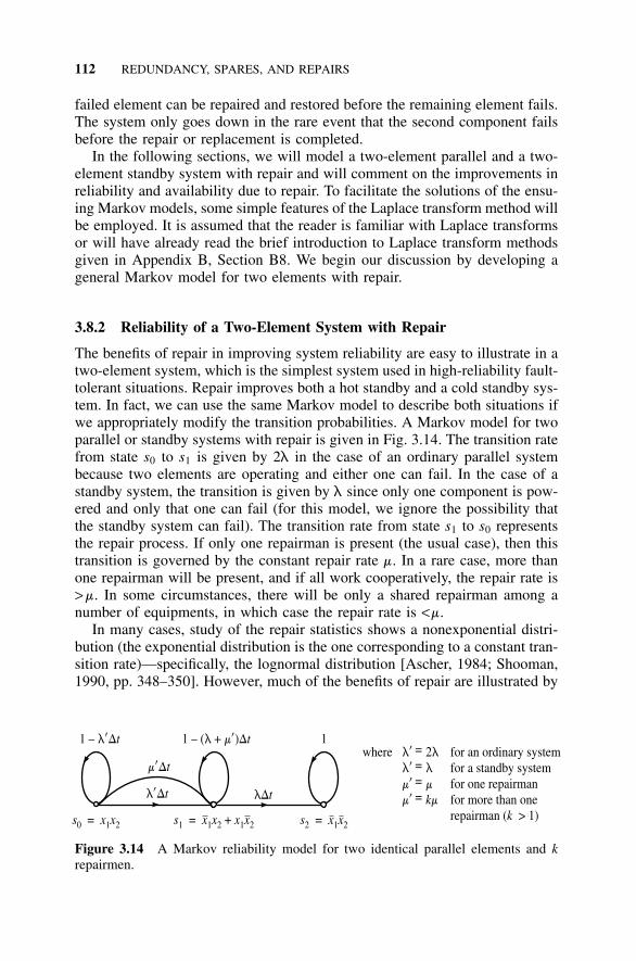
112 REDUNDANCY, SPARES, AND REPAIRS
failed element can be repaired and restored before the remaining element fails.The system only goes down in the rare event that the second component failsbefore the repair or replacement is completed.
In the following sections, we will model a two-element parallel and a two-element standby system with repair and will comment on the improvements inreliability and availability due to repair. To facilitate the solutions of the ensu-ing Markov models, some simple features of the Laplace transform method willbe employed. It is assumed that the reader is familiar with Laplace transformsor will have already read the brief introduction to Laplace transform methodsgiven in Appendix B, Section B8. We begin our discussion by developing ageneral Markov model for two elements with repair.
3.8.2 Reliability of a Two-Element System with Repair
The benefits of repair in improving system reliability are easy to illustrate in atwo-element system, which is the simplest system used in high-reliability fault-tolerant situations. Repair improves both a hot standby and a cold standby sys-tem. In fact, we can use the same Markov model to describe both situations ifwe appropriately modify the transition probabilities. A Markov model for twoparallel or standby systems with repair is given in Fig. 3.14. The transition ratefrom state s0 to s1 is given by 2l in the case of an ordinary parallel systembecause two elements are operating and either one can fail. In the case of astandby system, the transition is given by l since only one component is pow-ered and only that one can fail (for this model, we ignore the possibility thatthe standby system can fail). The transition rate from state s1 to s0 representsthe repair process. If only one repairman is present (the usual case), then thistransition is governed by the constant repair rate m. In a rare case, more thanone repairman will be present, and if all work cooperatively, the repair rate is>m. In some circumstances, there will be only a shared repairman among anumber of equipments, in which case the repair rate is <m.
In many cases, study of the repair statistics shows a nonexponential distri-bution (the exponential distribution is the one corresponding to a constant tran-sition rate)—specifically, the lognormal distribution [Ascher, 1984; Shooman,1990, pp. 348–350]. However, much of the benefits of repair are illustrated by
1 – l’Dt
l Dt’
m Dt’
lDt
s x= 10 2x
1 – ( +l m Dt’) 1
s x= 11 2 1 2x x x+ s x= 12 2x
l ll lm mm m
’’’’
= 2=== k
where for an ordinary systemfor a standby systemfor one repairmanfor more than onerepairman ( > 1)k
Figure 3.14 A Markov reliability model for two identical parallel elements and krepairmen.
REPAIRABLE SYSTEMS 113
the constant transition rate repair model. The Markov equations correspondingto Fig. 3.14 can be written by utilizing a simple algorithm:
1. The terms with 1 and Dt in the Markov graph are deleted.
2. A first-order Markov differential equation is written for each node wherethe left-hand side of the equation is the first-order time derivative of theprobability of being in that state at time t.
3. The right-hand side of each equation is a sum of probability terms foreach branch that enters the node in question. The coefficient of eachprobability term is the transition probability for the entering branch.
We will illustrate the use of these steps in formulating the Markov of Fig.3.14.
dPs0 (t)dt
c −l′Ps0 (t) + m′Ps1 (t) (3.62a)
dPs1 (t)dt
c l′Ps0 (t) − (l + m′)Ps1 (t) (3.62b)
dPs2 (t)dt
c l′Ps1 (t) (3.62c)
Assuming that both systems are initially good, the initial conditions are
Ps0 (0) c 1, Ps1 (0) c Ps2 (0) c 0
One great advantage of the Laplace transform method is that it deals simplywith initial conditions. Another is that it transforms differential equations in thetime domain into a set of algebraic equations in the Laplace transform domain(often called the frequency domain), which are written in terms of the Laplaceoperator s.
To transform the set of equations (3.62a–c) into the Laplace domain, weutilize transform theorem 2 (which incorporates initial conditions) from TableB7 of Appendix B, yielding
sPs0 (s) − 1 c −l′Ps0 (s) + m′Ps1 (s) (3.63a)
sPs1 (s) − 0 c l′Ps0 (s) − (l + m′)Ps1 (s) (3.63b)
sPs2 (s) − 0 c lPs1 (s) (3.63c)
Writing these equations in a more symmetric form yields
114 REDUNDANCY, SPARES, AND REPAIRS
(s + l′)Ps0 (s) − m′Ps1 (s) c 1 (3.64a)
−l′Ps0 (s) + (s + m′ + l)Ps1 (s) c 0 (3.64b)
−lPs1 (s) + sPs2 (s) c 0 (3.64c)
Clearly, Eqs. (3.64a–c) lead to a matrix formulation if desired. However,we can simply solve these equations using Cramer’s rule since they are nowalgebraic equations.
Ps0 (s) c(s + l + m′)
[s2 + (l + l′ + m′)s + ll′](3.65a)
Ps1 (s) cl′
[s2 + (l + l′ + m′)s + ll′](3.65b)
Ps2 (s) cll′
s[s2 + (l + l′ + m′)s + ll′](3.65c)
We must now invert these equations—transform them from the frequencydomain to the time domain—to find the desired time solutions. There are sev-eral alternatives at this point. One can apply transform No. 10 from Table B6of Appendix B to Eqs. (3.65a, b) to obtain the solution as a sum of two expo-nentials, or one can use a partial fraction expansion as illustrated in Eq. (B104)of the appendix. An algebraic solution of these equations using partial fractionsappears in Shooman [1990, pp. 341–342], and further solution and plotting ofthese equations is covered in the problems at the end of this chapter as well asin Appendix B8. One can, however, make a simple comparison of the effectsof repair by computing the MTTF for the various models.
3.8.3 MTTF for Various Systems with Repair
Rather than compute the complete reliabiity function of the several systemswe wish to compare, we can simplify the analysis by comparing the MTTFfor these systems. Furthermore, the MTTF is given by an integral of the reli-ability function, and by using Laplace theory we can show [Section B8.2, Eqs.(B105)–(B106)] that the MTTF is just given by the limit of the Laplace trans-form expression as s b 0.
For the model of Fig. 3.14, the reliability expression is the sum of the firsttwo-state probabilities; thus, the MTTF is the limit of the sum of Eqs. (3.65a,b) as s b 0, which yields
MTTF cl + m′ + l′
(ll′)(3.66)
REPAIRABLE SYSTEMS 115
TABLE 3.4 Comparison of MTTF for Several Systems
For l c 1,Element Formula m c 10
Single element 1/l 1.0Two parallel elements—no repair 1.5/l 1.5Two standby elements—no repair 2/l 2.0Two parallel elements—with repair (3l + m)/ 2l2 6.5Two standby elements—with repair (2l + m)/l2 12.0
We substitute the various values of l′ shown in Fig. 3.14 in the expression;since we are assuming a single repairman, m′ c m. The MTTF for several sys-tems is compared in Table 3.4. Note how repair strongly increases the MTTFof the last two systems in the table. For large m/l ratios, which are commonin practice, the MTTF of the last two systems approaches 0.5m/l2 and m/l2.
3.8.4 The Effect of Coverage on System Reliability
In Fig. 3.12, we portrayed a fairly complex block diagram for a standby sys-tem. We have already modeled the possibility of imperfection in the switch-ing mechanism. In this section, we develop a model for imperfections in thedecision unit that detects failures and switches from the on-line system to thestandby system. In some cases, even in the n-ordinary parallel system (hotstandby), it is not possible to have both systems fully connected, and a deci-sion unit and switch are needed. Another way of describing this phenomenonis to say that the decision unit cannot detect 100% of all the on-line unit fail-ures; it only “covers” (detects) the fraction c (0 < c < 1) of all the possiblefailures. (The formulation of this concept is generally attributed to Bouricius,Carter, and Schneider [1969].) The problem is that if the decision unit doesnot detect a failure of the on-line unit, input and output remain connected tothe failed on-line element. The result is a system failure, because although thestandby unit is good, there is no indication that it must be switched into use.We can formulate a Markov model in Fig. 3.15, which allows us to evaluatethe effect of coverage. (Compare with the model of Fig. 3.14.) In fact, we canuse Fig. 3.15 to model the effects of coverage on either a hot or cold standbysystem. Note that the symbol D stands for the decision unit correctly detectinga failure in the on-line unit, and the symbol D means that the decision unithas not been able to (failed to) detect a failure in the on-line unit. Also, a newarc has been added in the figure from the good state s0 to the failed state s2
for modeling the failure of the decision unit to “cover” a failure of the on-lineelement.
The Markov equations for Fig. 3.15 become the following:
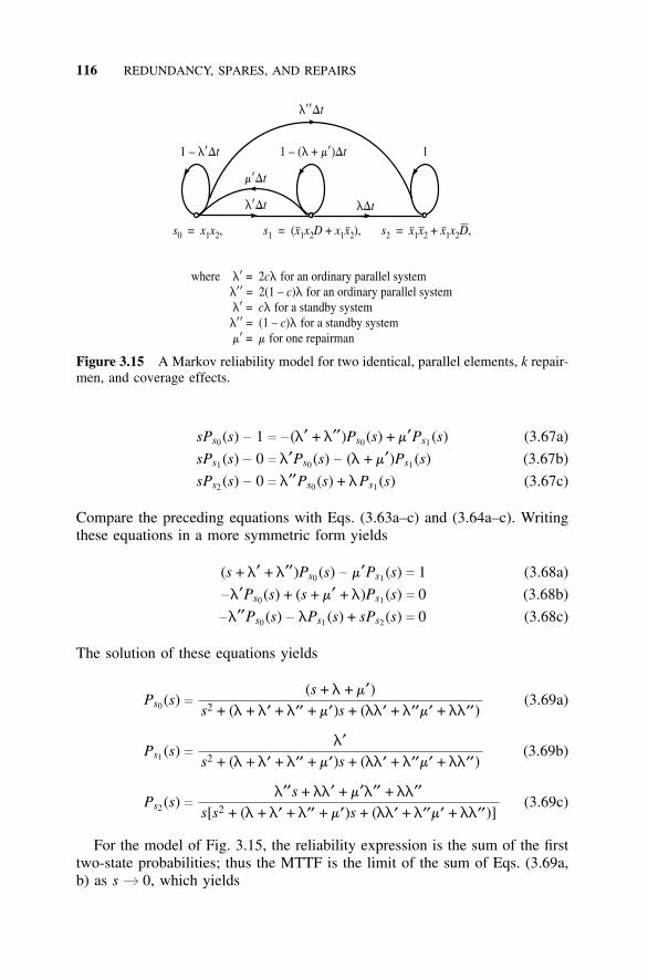
116 REDUNDANCY, SPARES, AND REPAIRS
1 – l’Dt
l’ Dt’
l Dt’
m Dt’
lDt
s x= 10 2x ,
1 – ( +l m Dt’) 1
s x= ( 11 2 1 2x x xD + ), s x= 12 2 1 2x x x+ D,
l ll ll ll lm m
’’’’’’’
= 2 for an ordinary parallel system= 2(1 – ) for an ordinary parallel system= for a standby system= (1 – ) for a standby system= for one repairman
cc
cc
where
Figure 3.15 A Markov reliability model for two identical, parallel elements, k repair-men, and coverage effects.
sPs0 (s) − 1 c − (l′ + l′′)Ps0 (s) + m′Ps1 (s) (3.67a)
sPs1 (s) − 0 c l′Ps0 (s) − (l + m′)Ps1 (s) (3.67b)
sPs2 (s) − 0 c l′′Ps0 (s) + lPs1 (s) (3.67c)
Compare the preceding equations with Eqs. (3.63a–c) and (3.64a–c). Writingthese equations in a more symmetric form yields
(s + l′ + l′′)Ps0 (s) − m′Ps1 (s) c 1 (3.68a)
−l′Ps0 (s) + (s + m′ + l)Ps1 (s) c 0 (3.68b)
−l′′Ps0 (s) − lPs1 (s) + sPs2 (s) c 0 (3.68c)
The solution of these equations yields
Ps0 (s) c(s + l + m′)
s2 + (l + l′ + l′′ + m′)s + (ll′ + l′′m′ + ll′′)(3.69a)
Ps1 (s) cl′
s2 + (l + l′ + l′′ + m′)s + (ll′ + l′′m′ + ll′′)(3.69b)
Ps2 (s) cl′′s + ll′ + m′l′′ + ll′′
s[s2 + (l + l′ + l′′ + m′)s + (ll′ + l′′m′ + ll′′)](3.69c)
For the model of Fig. 3.15, the reliability expression is the sum of the firsttwo-state probabilities; thus the MTTF is the limit of the sum of Eqs. (3.69a,b) as s b 0, which yields
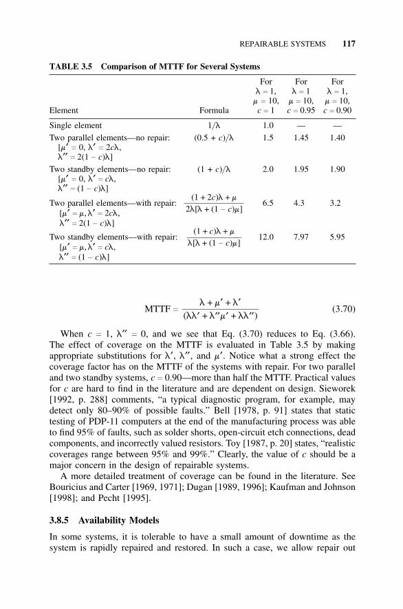
REPAIRABLE SYSTEMS 117
TABLE 3.5 Comparison of MTTF for Several Systems
For For Forl c 1, l c 1 l c 1,m c 10, m c 10, m c 10,
Element Formula c c 1 c c 0.95 c c 0.90
Single element 1/l 1.0 — —
Two parallel elements—no repair: (0.5 + c)/l 1.5 1.45 1.40[m′ c 0, l′ c 2cl,l′′ c 2(1 − c)l]
Two standby elements—no repair: (1 + c)/l 2.0 1.95 1.90[m′ c 0, l′ c cl,l′′ c (1 − c)l]
Two parallel elements—with repair:[m′ c m,l′ c 2cl,l′′ c 2(1 − c)l]
(1 + 2c)l + m
2l[l + (1 − c)m]6.5 4.3 3.2
Two standby elements—with repair:[m′ c m,l′ c cl,l′′ c (1 − c)l]
(1 + c)l + m
l[l + (1 − c)m]12.0 7.97 5.95
MTTF c
l + m′ + l′(ll′ + l′′m′ + ll′′)
(3.70)
When c c 1, l′′ c 0, and we see that Eq. (3.70) reduces to Eq. (3.66).The effect of coverage on the MTTF is evaluated in Table 3.5 by makingappropriate substitutions for l′, l′′, and m′. Notice what a strong effect thecoverage factor has on the MTTF of the systems with repair. For two paralleland two standby systems, c c 0.90—more than half the MTTF. Practical valuesfor c are hard to find in the literature and are dependent on design. Sieworek[1992, p. 288] comments, “a typical diagnostic program, for example, maydetect only 80–90% of possible faults.” Bell [1978, p. 91] states that statictesting of PDP-11 computers at the end of the manufacturing process was ableto find 95% of faults, such as solder shorts, open-circuit etch connections, deadcomponents, and incorrectly valued resistors. Toy [1987, p. 20] states, “realisticcoverages range between 95% and 99%.” Clearly, the value of c should be amajor concern in the design of repairable systems.
A more detailed treatment of coverage can be found in the literature. SeeBouricius and Carter [1969, 1971]; Dugan [1989, 1996]; Kaufman and Johnson[1998]; and Pecht [1995].
3.8.5 Availability Models
In some systems, it is tolerable to have a small amount of downtime as thesystem is rapidly repaired and restored. In such a case, we allow repair out
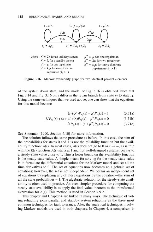
118 REDUNDANCY, SPARES, AND REPAIRS
1 – l’Dt
l’ Dt’
l Dt’
m Dt’
lDt
s x= 10 2x
1 – ( +l m Dt’) 1 – m’’Dt
s x= 11 2 1 2x x x+ s x= 12 2x
l ll lm mm m
’’’’
= 2 for an ordinary system= for a standby system= for one repairman= for more than one
repairman (k
k1
1 > 1)
where m mm mm m
’’’’’’
= for one repairman= 2 for two repairmen= for more than one
repairman (k
k2
2 > 1)
Figure 3.16 Markov availability graph for two identical parallel elements.
of the system down state, and the model of Fig. 3.16 is obtained. Note thatFig. 3.14 and Fig. 3.16 only differ in the repair branch from state s2 to state s1.Using the same techniques that we used above, one can show that the equationsfor this model become
(s + l′)Ps0 (s) − m′Ps1 (s) c 1 (3.71a)
−l′Ps0 (s) + (s + m′ + l)Ps1 (s) − m′′Ps2 (s) c 0 (3.71b)
−lPs1 (s) + (s + m′′)Ps2 (s) c 0 (3.71c)
See Shooman [1990, Section 6.10] for more information.The solution follows the same procedure as before. In this case, the sum of
the probabilities for states 0 and 1 is not the reliability function but the avail-ability function: A(t). In most cases, A(t) does not go to 0 as t b ∞, as is truewith the R(t) function. A(t) starts at 1 and, for well-designed systems, decays toa steady-state value close to 1. Thus a lower bound on the availability functionis the steady-state value. A simple means for solving for the steady-state valueis to formulate the differential equations for the Markov model and set all thetime derivatives to 0. The set of equations now becomes an algebraic set ofequations; however, the set is not independent. We obtain an independent setof equations by replacing any of these equations by the equation—the sum ofall the state probabilities c 1. The algebraic solution for the steady-state avail-ability is often used in practice. An even simpler procedure for computing thesteady-state availability is to apply the final value theorem to the transformedexpression for A(s). This method is used in Section 4.9.2.
This chapter and Chapter 4 are linked in many ways. The technique of vot-ing reliability joins parallel and standby system reliability as the three mostcommon techniques for fault tolerance. Also, the analytical techniques involv-ing Markov models are used in both chapters. In Chapter 4, a comparison is
RAID SYSTEMS RELIABILITY 119
made of the reliability and availability of parallel, standby, and voting systems;in addition, some of the Markov modeling begun in this chapter is extendedin Chapter 4 for the purpose of this comparison. The following chapter alsohas a more extensive discussion of the many shortcuts provided by Laplacetransforms.
3.9 RAID SYSTEMS RELIABILITY
3.9.1 Introduction
The reliability techniques discussed in Chapter 2 involved coding to detectand correct errors in data streams. In this chapter, various parallel and standbytechniques have been introduced that significantly increase the reliability ofvarious systems and components. This section will discuss a newly developedtechnology for constructing computer secondary-storage systems that utilizethe techniques of both Chapters 2 and 3 for the design of reliable, compact,high-performance storage systems. The generic term for such memory sys-tem technology is redundant disk arrays [Gibson, 1992]; however, it was soonchanged to redundant array of inexpensive disks (RAID), and as technologyevolved so that the quality and capacity of small disks rapidly increased, theword “inexpensive” was replaced by “independent.” The term “array,” whenused in this context, means a collection of many disks organized in a specificfashion to improve speed of data transfer and reliability. As the RAID tech-nology evolved, cache techniques (the use of small, very high-speed memoriesto accelerate processing by temporarily retaining items expected to be neededagain soon) were added to the mix. Many varieties of RAID have been devel-oped and more will probably emerge in the future. The RAID systems thatemploy cache techniques for speed improvement are sometimes called cachedarray of inexpensive disks (CAID) [Buzen, 1993]. The technology is drivenby the variety of techniques available for connecting multiple disks, as well asvarious coding techniques, alternative read-and-write techniques, and the flexi-bility in organization to “tune” the architecture of the RAID system to matchvarious user needs.
Prior to 1990, the dominant technology for secondary storage was a groupof very large disks, typically 5–15, in a cabinet the size of a clothes washer.Buzen [1993] uses the term single large expensive disk (SLED) to refer tothis technology. RAID technology utilizes a large number, typically 50–100,of small disks the size of those used in a typical personal computer. Each diskdrive is assumed to have one actuator to position reads or writes, and largeand small drives are assumed to have the same I/ O read- or write-time. Thebandwidth (BW) of such a disk is the reciprocal of the read-time. If data is bro-ken into “chunks” and read (written) in parallel chunks to each of the n smalldisks in a RAID array, the effective BW increases. There is some “overhead”in implementing such a parallel read-write scheme, however, in the limit:
120 REDUNDANCY, SPARES, AND REPAIRS
effective bandwidth b nBW (3.72)
Thus, one possible beneficial effect of a RAID configuration in which manydisks are written in parallel is a large increase in the BW.
If the RAID configuration depends on all the disks working, then the reli-ability of so many disks is lower than a smaller number of large disks. If thefailure rate of each of the n disks is denoted by l c 1/ MTTF, then the failurerate and MTTF of n disks is given by
effective failure rate c nl c 1/ effective MTTF c n/ MTTF (3.73)
The failure rate is n times as large and the MTTF is n times smaller. If datais stored in “chunks” over many disks so that the write operation occurs inparallel for increased BW, the reliability of the block of data decreases signif-icantly as per Eq. (3.73). Writing data in a distributed manner over a groupof disks is called striping or interleaving. The size of the “chunk” is a designparameter in striping. To increase the reliability of a striped array, one can useredundant disks and/ or error-detecting and -correcting codes for “chunks” ofdata of various sizes. We have purposely used the nonspecific term “chunk”because one of the design choices, which will soon be discussed, is the sizeof the “chunk” and how “the chunk” is distributed across various disks.
The various trade-offs among objectives and architectural approaches havechanged over the decade (1990–2000) in which RAID storage systems weredeveloped. At the beginning, small disks had modest capacity, longer accessand transfer times, higher cost, and lower reliability. The improvements in allthese parameters have had major effects on design.
The designers of RAID systems utilize various techniques of redundancyand error-correcting codes to raise the reliability of the RAID sysem [Buzen,1993]. The early literature defined six levels of RAID [Patterson, 1987, 1988;Gibson, 1992], and most manufacturers followed these levels as guidelines indescribing their products. However, as variations and options developed, classi-fication became difficult, and some marketing managers took the classificationsystem to mean that a higher level of RAID meant a better system. Thus, onevendor whose system included features of RAID 2 and RAID 5 decided to callhis product RAID 10, claiming the levels multiplied! [Friedman, 1996.] Situ-ations such as these led to the creation of the RAID Advisory Board, whichserves as an industry standards body to define seven (and possibly more) lev-els of RAID [RAID, 1995; Massaglia, 1997]. The basic levels of RAID aregiven in Table 3.6, and the reader is cautioned to remember that because thevarious levels of RAID are to differentiate architectural approach, an increasein level does not necessarily correspond to an increase in BW or reliability.Complexity, however, does probably increase as the RAID level increases.
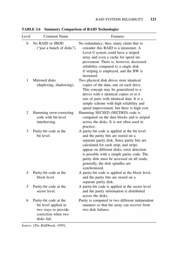
RAID SYSTEMS RELIABILITY 121
TABLE 3.6 Summary Comparison of RAID Technologies
Level Common Name Features
0 No RAID or JBOD No redundancy; thus, many claim that to(“just a bunch of disks”). consider this RAID is a misnomer. A
Level 0 system could have a stripedarray and even a cache for speed im-provement. There is, however, decreasedreliability compared to a single diskif striping is employed, and the BW isincreased.
1 Mirrored disks Two physical disk drives store identical(duplexing, shadowing). copies of the data, one on each drive.
This concept may be generalized to ndrives with n identical copies or to ksets of pairs with identical data. It is asimple scheme with high reliability andspeed improvement, but there is high cost.
2 Hamming error-correcting Hamming SECSED (SECDED) code iscode with bit-level computed on the data blocks and is stripedinterleaving. across the disks. It is not often used in
practice.3 Parity-bit code at the A parity-bit code is applied at the bit level
bit level. and the parity bits are stored on aseparate parity disk. Since parity bits arecalculated for each strip, and stripsappear on different disks, error detectionis possible with a simple parity code. Theparity disk must be accessed on all reads;generally, the disk spindles aresynchronized.
4 Parity-bit code at the A parity-bit code is applied at the block level,block level. and the parity bits are stored on a
separate parity disk.5 Parity-bit code at the A parity-bit code is applied at the sector level
sector level. and the parity information is distributedacross the disks.
6 Parity-bit code at the Parity is computed in two different independentbit level applied in manners so that the array can recover fromtwo ways to provide two disk failures.correction when twodisks fail.
Source: [The RAIDbook, 1995].
122 REDUNDANCY, SPARES, AND REPAIRS
3.9.2 RAID Level 0
This level was introduced as a means of classifying techniques that utilizea disk array and striping to improve the BW; however, no redundancy isincluded, and the reliability decreases. Equations (3.72) and (3.73) describethese basic effects. The BW of the array has increased over individual disks,but the reliability has decreased. Since high reliability is generally requiredin the disk storage system, this level would rarely be used except for specialapplications.
3.9.3 RAID Level 1
The use of mirrored disks is an obvious way to improve reliability; if the twodisks are written in parallel, the BW is increased. If the data is striped acrossthe two disks, the parallel reading of a transaction can increase the BW bya factor of 2. However, the second (backup) copy of the transaction must bewritten, and if there is a continuous transaction stream, the duplicate data copyrequirement reduces the BW by a factor of 2, resulting in no change in the BW.However, if transactions occur in bursts with delays between bursts, the pri-mary copy can be written at twice the BW during the burst, and the backupcopy can be performed during the pauses between bursts. Thus the doubling ofBW can be realized under those circumstances. Since memory systems repre-sent 40%–60% of the cost of computer systems [Gibson, 1992, pp. 50–51], theuse of mirrored disks greatly increases the cost of a computer system. Also,since the reliability is that of a parallel system, the reliability function is givenby Eq. (3.8) and the MTTF by Eq. (3.26) for constant disk failure rates. If bothdisks are identical and have the same failure rates, the MTTF of the mirroreddisks becomes 1.5 times greater than that of a single disk system. The Tan-dem line of “Nonstop” computers (discussed in Section 3.10.1) are essentiallymirrored disks with the addition of duplicate computers, disk controllers, andI/ O buses. The RAIDbook [1995, p. 45] calls the Tandem configuration a fullyredundant system.
RAID systems of Level 2 and higher all have at least one hot spare disk.When a disk error is detected via an error-detecting code or other form of built-in disk monitoring, the disk system takes the remaining stored and redundantinformation and reconstructs a valid copy on the hot disk, which is switched-in,instead of the failed disk. Sometime later during maintenance, the failed diskis repaired or replaced. The differences among the following RAID levels aredetermined by the means of error detection, the size of the chunk that hasassociated error checking, and the pattern of striping.
3.9.4 RAID Level 2
This level of RAID introduces Hamming error-correcting codes similar to thosediscussed in Chapter 2 to detect and correct data errors. The error-correcting
RAID SYSTEMS RELIABILITY 123
codes are added to the “chunks” of data and striped across the disks. In general,this level of RAID employs a SECSED code or a SECDED code such as onedescribed in Chapter 2. The code is applied to data blocks, and the disk spindlesmust be synchronized. One can roughly compare the reliability of this schemewith a Level 1 system. For the Level 1 RAID system to fail, both disks mustfail, and the probability of failure is
Pf 1 c q2 (3.74)
For a Level 2 system to fail, one of the two disks must fail that has a prob-ability of 2q, and the Hamming code must fail to detect an error. The exampleused in the The RAIDbook [1995] to discuss a Level 2 system is for ten datadisks and four check disks, representing a 40% cost overhead for redundancycompared with a 100% overhead for a Level 1 system. In Chapter 2, we com-puted the probability of undetected error for eight data bits and four check bitsin Eq. (2.27) and shall use these results to estimate the probability of failureof a typical Level 2 system. For this example,
Pf 2 c (2q) × [220q3(1 − q)9] (3.75)
Clearly, for very small q, the Level 2 system has a smaller probability of failure.The two equations—(3.74) and (3.75)—are approximately equal for q c 0.064,at which level the probability of failure is 0.0642
c 0.00041.To appreciate how this level would apply to a typical disk, let us assume
that the MTTF for a typical disk is 300,000 hours. Assuming a constant failure-rate model, l c 1/ 300,000 c 3.3 × 10⁻⁶. The associated probability of failurefor a single disk would be 1 − exp(−3.3 × 10⁻⁶t), and setting this expressionto 0.064 shows that a single disk reaches this probability of failure at about20,000 hours. Since a year is roughly 10,000 hours (8,766), a mirrored disksystem would be superior for a few years of operation. A detailed reliabilitycomparison would require a prior design of a Level 2 system with the appro-priate number of disks, choice of chunk level (bit, byte, block, etc.), inclusionof a swapping disk, disk striping, and other details.
Detailed design of a Level 2 system such a disk system leads to nonstandarddisks, significantly raising the cost of the system, and the technique is seldomused in practice.
3.9.5 RAID Levels 3, 4, and 5
In Chapter 2, we discussed the fact that a single parity bit is an inexpensiveand fairly effective way of significantly increasing reliability. Levels 3, 4, and5 apply such a parity-bit code to different size data “chunks” in various ways toincrease the reliability of a disk array at a lower cost than a mirrored disk. Wewill model the reliability of a Level 3 system as an example. A disk can fail in
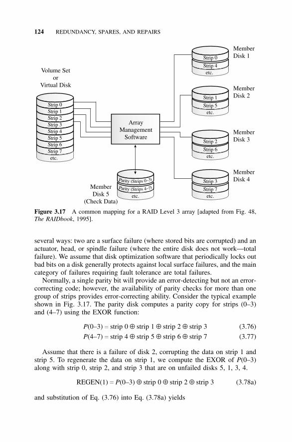
124 REDUNDANCY, SPARES, AND REPAIRS
Strip 0Strip 1Strip 2Strip 3Strip 4Strip 5Strip 6Strip 7etc.
Volume Setor
Virtual Disk
ArrayManagement
Software
MemberDisk 1
MemberDisk 2
MemberDisk 3
MemberDisk 4
MemberDisk 5
(Check Data)etc.
Parity (Strips 0–3)
Parity (Strips 4–7)
Strip 0
Strip 1
Strip 2
Strip 3
Strip 4
Strip 5
Strip 6
Strip 7
etc.
etc.
etc.
etc.
Figure 3.17 A common mapping for a RAID Level 3 array [adapted from Fig. 48,The RAIDbook, 1995].
several ways: two are a surface failure (where stored bits are corrupted) and anactuator, head, or spindle failure (where the entire disk does not work—totalfailure). We assume that disk optimization software that periodically locks outbad bits on a disk generally protects against local surface failures, and the maincategory of failures requiring fault tolerance are total failures.
Normally, a single parity bit will provide an error-detecting but not an error-correcting code; however, the availability of parity checks for more than onegroup of strips provides error-correcting ability. Consider the typical exampleshown in Fig. 3.17. The parity disk computes a parity copy for strips (0–3)and (4–7) using the EXOR function:
P(0–3) c strip 0 ⊕ strip 1 ⊕ strip 2 ⊕ strip 3 (3.76)
P(4–7) c strip 4 ⊕ strip 5 ⊕ strip 6 ⊕ strip 7 (3.77)
Assume that there is a failure of disk 2, corrupting the data on strip 1 andstrip 5. To regenerate the data on strip 1, we compute the EXOR of P(0–3)along with strip 0, strip 2, and strip 3 that are on unfailed disks 5, 1, 3, 4.
REGEN(1) c P(0–3) ⊕ strip 0 ⊕ strip 2 ⊕ strip 3 (3.78a)
and substitution of Eq. (3.76) into Eq. (3.78a) yields
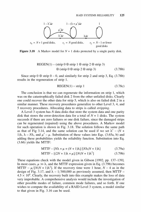
RAID SYSTEMS RELIABILITY 125
1 – l’Dt
l Dt’
m Dt’
lDt
s N= + 1 good disks,0
1 – ( +l m Dt’) 1
s N= good disks,1 s N= – 1 or fewergood disks
2
Figure 3.18 A Markov model for N + 1 disks protected by a single parity disk.
REGEN(1) c (strip 0 ⊕ strip 1 ⊕ strip 2 ⊕ strip 3)
⊕ (strip 0 ⊕ strip 2 ⊕ strip 3) (3.78b)
Since strip 0 ⊕ strip 0 c 0, and similarly for strip 2 and strip 3, Eq. (3.78b)results in the regeneration of strip 1.
REGEN(1) c strip 1 (3.78c)
The conclusion is that we can regenerate the information on strip 1, whichwas on the catastrophically failed disk 2 from the other unfailed disks. Clearlyone could recover the other data for strip 5, which is also on failed disk 2 in asimilar manner. These recovery procedures generalize to other Level 3, 4, and5 recovery procedures. Allocating data to strips is called stripping.
A Level 3 system has N data disks that store the system data and one paritydisk that stores the error-detection data for a total of N + 1 disks. The systemsucceeds if there are zero failures or one disk failure, since the damaged stripscan be regenerated (repaired) using the above procedures. A Markov modelfor such operation is shown in Fig. 3.18. The solution follows the same pathas that of Fig 3.14, and the same solution can be used if we set l′ c (N +1)l, l c Nl, and m′ c m. Substitution of these values into Eqs. (3.65a, b) andadding these probabilities yields the reliability function. Substitution into Eq.(3.66) yields the MTTF:
MTTF c [Nl + m + (N + 1)l]/ [Nl(N + 1)l] (3.79a)
MTTF c [(2N + 1)l + m]/ [N(N + 1)l2] (3.79b)
These equations check with the model given in Gibson [1992, pp. 137–139].In most cases, m >> l, and the MTTF expression given in Eq. (3.79b) becomesMTTF c m/ [N(N + 1)l2]. If the recovery time were 1 hour, N c 4 as in thedesign of Fig. 3.17, and l c 1/ 300,000 as previously assumed, then MTTF c
4.5 × 10⁹. Clearly, the recovery built into this example makes the loss of datavery improbable. A comprehensive analysis would include the investigation ofother possible modes of failure, common mode failures, and so forth. If onewishes to compute the availability of a RAID Level 3 system, a model similarto that given in Fig. 3.16 can be used.
126 REDUNDANCY, SPARES, AND REPAIRS
3.9.6 RAID Level 6
There are several choices for establishing two independent parity checks. Oneapproach is a horizontal–vertical parity approach. A parity bit for a string iscomputed in two different ways. Several rows of strings are written, fromwhich a set of horizontal parity bits are computed for each row and a set ofvertical parity bits are computed for each column. Actually, this description isjust one approach to Level 6; any technique that independently computes twoparity bits is classified as Level 6 (e.g., applying parity to two sets of bits, usingtwo different algorithms for computing parity, and Reed–Solomon codes). Formore comprehensive analysis of RAID systems, see Gibson [1992]. A com-parison of the various RAID levels was given in Table 3.6, on page 121.
3.10 TYPICAL COMMERCIAL FAULT-TOLERANT SYSTEMS:TANDEM AND STRATUS
3.10.1 Tandem Systems
In the 1980s, Tandem captured a significant share of the business market withits “NonStop” computer systems. The name was a great asset, since it capturedthe aspirations of many customers in the on-line transaction processing marketwho required high reliability, such as banks, airlines, and financial institutions.Since 1997, Tandem Computers has been owned by the Compaq Computer Cor-poration, and it still stresses fault-tolerant computer systems. A 1999 survey esti-mates that 66% of credit card transactions, 95% of securities transactions, and80% of automated teller machine transactions are processed by Tandem com-puters (now called NonStop Himalaya computers). “As late as 1985 it was esti-mated that a conventional, well-managed, transaction-processing system failedabout once every two weeks for about an hour” [Siewiorek, 1992, p. 586]. Sincethere are 168 hours in a week, substitution into the basic steady-state equationfor availability Eq. (B95a) yields an availability of 0.997. (Remember that l c
1/ MTTF and m c 1/ MTTR for constant failure and repair rates.) To appreciatehow mediocre such an availability is for a high-reliability system, let us considerthe availability of an automobile. Typically an auto may require one repair peryear (sometimes referred to as nonscheduled maintenance to eliminate inclusionof scheduled maintenance, such as oil changes, tire replacements, and new sparkplugs), which takes one day (drop-off to pickup time). The repair rate becomes1 per day; the failure rate, 1/ 365 per day. Substitution into Eq. (B95a) yields asteady-state availability of 0.99726—nearly identical to our computer computa-tion. Clearly, a highly reliable computer system should have a much better avail-ability than a car! Tandem’s original goal was to build a system with an MTTFof 100 years! There was clearly much to do to improve the availability in termsof increasing the MTTF, decreasing the MTTR, and structuring a system config-uration with greatly increased reliability and availability. Suppose one chooses agoal of 1 hour for repair. This may be realistic for repairs such as board-swapping,
TYPICAL COMMERCIAL FAULT-TOLERANT SYSTEMS 127
but suppose the replacement part is not available? If we assume that 1 hour repre-sents 90% of the repairs but that 10% of the repairs require a replacement part thatis unavailable and must be obtained by overnight mail (24 hours), the weightedrepair time is then (0.9 × 1 + 0.1 × 24) c 3.3 hours. Clearly, the MTTR will dependon the distribution of failure modes, the stock of spare parts on hand, and the effi-ciency of ordering procedures for spare parts that must be ordered from the manu-facturer. If one were to achieve an MTTF of 100 years and an MTTR of 3.3 hours,the availability given by Eq. (B95) would be an impressive 0.999996.
The design objectives of Tandem computers were the following [Anderson,1985]:
• No single hardware failure should stop the system.
• Hardware elements should be maintainable with the on-line system.
• Database integrity should be ensured.
• The system should be modularly extensible without incurring applicationsoftware changes.
The last objective, extensibility of the system without a software change,played a role in Tandem’s success. The software allowed the system to grow byadding new pairs of Tandem computers while the operation continued. Manyof Tandem’s competitors required that the system be brought down for systemexpansion, that new software and hardware be installed, and that the expandedsystem be regenerated.
The original Tandem system was a combination of hardware and softwarefault tolerance. (The author thanks Dr. Alan P. Wood of Compaq Corporationfor his help in clarifying the Tandem architecture and providing details for thissection [Wood, 2001].) Each major hardware subsystem (CPUs, disks, powersupplies, controllers, and so forth) was (and still is) implemented with parallelunits continuously operating (hot redundancy). A diagram depicting the Tan-dem architecture is shown in Fig. 3.19. The architecture supports N processorsin which N is at an even number between 2 and 16.
The Tandem processor subsystem uses hardware fault detection and soft-ware fault tolerance to recover from processor failures. The Tandem operatingsystem called Guardian creates and manages heartbeat signals, saying “I’malive,” which each processor sends to all the other processors every second. Ifa processor has not received a heartbeat signal from another processor withintwo seconds, each operating processor enters a system state called regroup. Theregroup algorithm determines the hardware element(s) that has failed (whichcould be a processor or the communications between a group of processors, orit could be multiple failures) and also determines which system resources arestill available, avoiding bisection of the system, called the split-brain condi-tion, in which communications are lost between two processor groups and eachgroup tries to continue on its own. At the end of the regroup, each processorknows the available system resources.
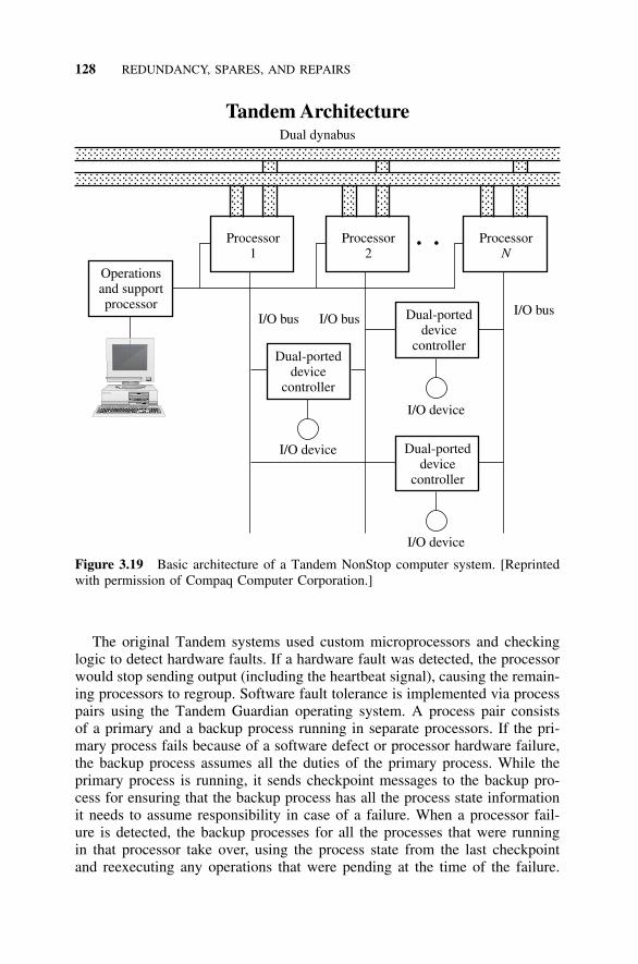
128 REDUNDANCY, SPARES, AND REPAIRS
Tandem ArchitectureDual dynabus
Processor1
Processor2
ProcessorN
Operationsand supportprocessor
Dual-porteddevice
controller
Dual-porteddevice
controller
Dual-porteddevice
controller
I/O device
I/O device
I/O device
I/O busI/O bus I/O bus
. .
Figure 3.19 Basic architecture of a Tandem NonStop computer system. [Reprintedwith permission of Compaq Computer Corporation.]
The original Tandem systems used custom microprocessors and checkinglogic to detect hardware faults. If a hardware fault was detected, the processorwould stop sending output (including the heartbeat signal), causing the remain-ing processors to regroup. Software fault tolerance is implemented via processpairs using the Tandem Guardian operating system. A process pair consistsof a primary and a backup process running in separate processors. If the pri-mary process fails because of a software defect or processor hardware failure,the backup process assumes all the duties of the primary process. While theprimary process is running, it sends checkpoint messages to the backup pro-cess for ensuring that the backup process has all the process state informationit needs to assume responsibility in case of a failure. When a processor fail-ure is detected, the backup processes for all the processes that were runningin that processor take over, using the process state from the last checkpointand reexecuting any operations that were pending at the time of the failure.
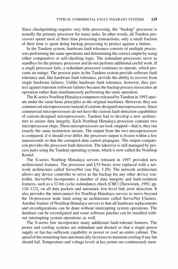
TYPICAL COMMERCIAL FAULT-TOLERANT SYSTEMS 129
Since checkpointing requires very little processing, the “backup” processor isactually the primary processor for many tasks. In other words, all Tandem pro-cessors spend most of their time processing transactions; only a small fractionof their time is spent doing backup processing to protect against a failure.
In the Tandem system, hardware fault tolerance consists of multiple proces-sors performing the same operations and determining the correct output by usingeither comparative or self-checking logic. The redundant processors serve asstandbys for the primary processor and do not perform additional useful work. Ifa single processor fails, a redundant processor continues to operate, which pre-vents an outage. The process pairs in the Tandem system provide software faulttolerance and, like hardware fault tolerance, provide the ability to recover fromsingle hardware failures. Unlike hardware fault tolerance, however, they pro-tect against transient software failures because the backup process reexecutes anoperation rather than simultaneously performing the same operation.
The K-series NonStop Himalaya computers released by Tandem in 1992 oper-ate under the same basic principles as the original machines. However, they usecommercial microprocessors instead of custom-designed microprocessors. Sincecommercial microprocessors do not have the custom fault-detection capabilitiesof custom-designed microprocessors, Tandem had to develop a new architec-ture to ensure data integrity. Each NonStop Himalaya processor contains twomicroprocessor chips. These microprocessors are lock-stepped—that is, they runexactly the same instruction stream. The output from the two microprocessorsis compared; if it should ever differ, the processor output is frozen within a fewnanoseconds so that the corrupted data cannot propagate. The output compari-son provides the processor fault detection. The takeover is still managed by pro-cess pairs using the Tandem operating system, which is now called the NonStopKernel.
The S-series NonStop Himalaya servers released in 1997 provided newarchitectural features. The processor and I/ O buses were replaced with a net-work architecture called ServerNet (see Fig. 3.20). The network architectureallows any device controller to serve as the backup for any other device con-troller. ServerNet incorporates a number of data integrity and fault-isolationfeatures, such as a 32-bit cyclic redundancy check (CRC) [Siewiorek, 1992, pp.120–123], on all data packets and automatic low-level link error detection. Italso provides the interconnect for NonStop Himalaya servers to move beyondthe 16-processor node limit using an architecture called ServerNet Clusters.Another feature of NonStop Himalaya servers is that all hardware replacementsand reconfigurations can be done without interrupting system operations. Thedatabase can be reconfigured and some software patches can be installed with-out interrupting system operations as well.
The S-series line incorporates many additional fault-tolerant features. Thepower and cooling systems are redundant and derated so that a single powersupply or fan has sufficient capability to power or cool an entire cabinet. Thespeed of the remaining fans automatically increases to maintain cooling if any fanshould fail. Temperature and voltage levels at key points are continuously mon-
130 REDUNDANCY, SPARES, AND REPAIRS
SecondaryCache
SecondaryCache
InterfaceASIC
InterfaceASIC
Microprocessor Microprocessor
Memory
Check
ServerNet
Figure 3.20 S-Series NonStop Himalaya architecture. (Supplied courtesy of Wood[2001].)
itored, and alarms are sounded whenever the levels exceed safe thresholds. Bat-tery backup is provided to continue operation through any short-duration poweroutages (up to 30 seconds) and to preserve the contents of memory to provide afast restart from outages shorter than 2 hours. (If it is necessary to protect againstlonger power outages, the common solution for high-availability systems is toprovide a power supply with backup storage batteries plus DC–AC convertersand diesel generators to recharge the batteries. The superior procedure is to haveautostart generators, which automatically start when a power outage is detected;however, they must be tested—perhaps once a week—to see if they will start.)All controllers are redundant and dual-ported to serve the primary and secondaryconnection paths. Each hardware and software module is self-checking and haltsimmediately instead of permitting an error to propagate—a concept known as thefail-fast design, which makes it possible to determine the source of errors and cor-rect them. NonStop systems incorporate state-of-the-art memory-detection and-correction codes to correct single-bit errors, detect double-bit errors, and detect“nibble” errors (3 or 4 bits in a row). Tandem has modified the memory vendor’serror-correcting code (ECC) to include address bits, which helps avoid the read-ing from or writing to the wrong block of memory. Active techniques are used tocheck for latent faults. A background memory “sniffer” checks the entire mem-ory every few hours.
System data is protected in many ways. The multiple data paths providedfor fault tolerance are alternately used to ensure correct operation. Data onall the buses is parity-protected, and parity errors cause immediate interruptsto trigger error recovery. Disk-driver software provides an end-to-end check-sum that is appended to a standard 512-byte disk sector. For structured data,such as SQL files, an additional end-to-end checksum (called a block check-sum) encodes data values, the physical location of the data, and transactioninformation. These checksums protect against corrupted data values, partialwrites, and misplaced or misaligned data. NonStop systems can use the Non-Stop remote duplicate database facility (NonStop RDF) to help recover from
TYPICAL COMMERCIAL FAULT-TOLERANT SYSTEMS 131
disasters such as earthquakes, hurricanes, fires, and floods. NonStop RDF sendsdatabase updates to a remote site up to thousands of miles away. If a disas-ter occurs, the remote system takes over within a few minutes without losingany transactions. NonStop Himalaya servers are even “coffee fault-tolerant,”meaning the air vents are on the sides to protect against coffee spills on top ofthe processor cabinet (or, more likely, if the sprinkler system in the computerroom is triggered). One would hope that Tandem has also thought about pro-tection against failure modes caused by inadvertant operator errors. Tandemplans to use the alpha microprocessor sometime in the future.
To analyze the Tandem fault-tolerant system, one would formulate a Markovmodel and proceed as was done previously in this chapter (but for more detail,consult Chapter 4). One must also anticipate the possibilities of errors of com-mission and omission in generating and detecting the heartbeat signals. Thiscould be modeled by a coverage factor representing the fraction of proces-sor faults that the heartbeat signal would diagnose. (This basic approach isexplored in the problems at the end of this chapter.) In Chapter 4, the avail-ability formulas are derived for a parallel system to compare with the avail-ability of a voting system [see Eq. (4.48) and Table 4.9]. Typical computationsat the end of Section 4.9.2 for a parallel system apply to the Tandem system.A complete analysis would require the use of a Markov modeling program andmultiple models that include more detail and fault-tolerant features.
The original Guardian operating system was responsible for creating, destroy-ing, and monitoring processes, reporting on the failure or restoration of proces-sors, and handling the conventional functions of operating systems in addition tomultiprogramming system functions and I/ O handling. The early Guardian sys-tem required the user to exactingly program the checkpointing, the record lock-ing, and other functions. Thus expert programmers were needed for these tasks,which were often slow in addition to exacting. To avoid such problems, Tandemdeveloped two simpler software systems: the terminal control program (TCP)called Pathway, which provided users with a control program having screen-handling modules written in a higher level (COBOL-like) language to issuecheckpoints and dealt with process management and processor failure; and thetransaction-monitoring facility (TMF) program, which dealt with the consistencyand recoverability of the database and provided concurrence control. The newHimalaya software greatly simplifies such programming, and it provides optionsto increase throughput. It also supports Tuxedo, Corba, and Java to allow users towrite to industry-standard interfaces and still get the benefits of fault tolerance.For further details, see Anderson [1985], Baker [1995], Siewiorek [1992, p. 586],Wood [1995], and the Tandem Web site: [http:/ / himalaya.compaq.com]. Also,see the discussion in Chapter 5, Section 5.10.
3.10.2 Stratus Systems
The Stratus line of continuous processing systems is designed to provide unin-terrupted operation without loss of data and performance degradation, as well
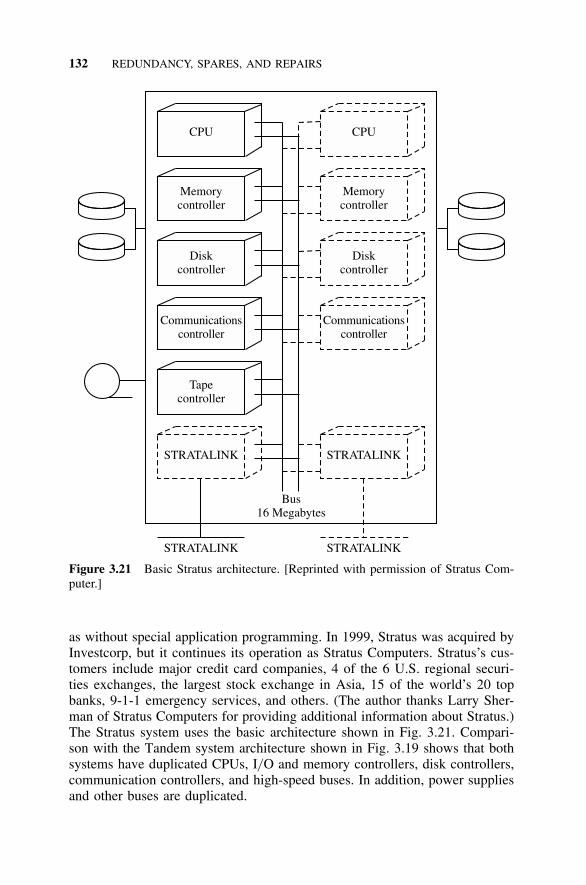
132 REDUNDANCY, SPARES, AND REPAIRS
CPU
Memorycontroller
Diskcontroller
Communicationscontroller
Tapecontroller
STRATALINK
STRATALINK
CPU
Memorycontroller
Diskcontroller
Communicationscontroller
STRATALINK
STRATALINK
Bus16 Megabytes
Figure 3.21 Basic Stratus architecture. [Reprinted with permission of Stratus Com-puter.]
as without special application programming. In 1999, Stratus was acquired byInvestcorp, but it continues its operation as Stratus Computers. Stratus’s cus-tomers include major credit card companies, 4 of the 6 U.S. regional securi-ties exchanges, the largest stock exchange in Asia, 15 of the world’s 20 topbanks, 9-1-1 emergency services, and others. (The author thanks Larry Sher-man of Stratus Computers for providing additional information about Stratus.)The Stratus system uses the basic architecture shown in Fig. 3.21. Compari-son with the Tandem system architecture shown in Fig. 3.19 shows that bothsystems have duplicated CPUs, I/ O and memory controllers, disk controllers,communication controllers, and high-speed buses. In addition, power suppliesand other buses are duplicated.
TYPICAL COMMERCIAL FAULT-TOLERANT SYSTEMS 133
The Stratus lockstepped microprocessor architecture appears similar to theTandem architecture described in the previous section, but fault toleranceis achieved through different mechanisms. The Stratus architecture is hard-ware fault-tolerant, with four microprocessors (all running the same instructionstream) configured as redundant pairs of physical processors. Processor failureis detected by a microprocessor miscompare, and the redundant processor (pairof microprocessors) continues processing with no takeover time. The Tandemarchitecture is software fault-tolerant; although failure of a processor is alsodetected by a microprocessor miscomparison, takeover is managed by softwarerequiring a few seconds’ delay.
To summarize the comparison, the Tandem system is more complex, higherin cost, and aimed at the upper end of the market. The Stratus system, on theother hand, is more simple, lower in cost, and competes in the middle andlower end portion of the market.
Each major Stratus circuit board has self-checking hardware that contin-uously monitors operation, and if the checks fail, the circuit board removesitself from service. In addition, each CPU board has two or more CPUs thatprocess the same data, and the outputs are compared at each clock cycle. Ifthe comparison fails, the CPU board removes itself from service and its twinboard continues processing without stop. Stratus calls the architecture with twoCPUs being checked pair and spare, and claims that its architecture is superiorin detecting transient errors, is lower in cost, and does not require intensiveprogramming. Tandem points out that software fault tolerance also protectsagainst software faults (90% of all software faults are transient); note, how-ever, that there is the small possibility of missed or imagined software errors.The Stratus approach requires a dedicated backup processor, whereas the Tan-dem system can use the backup processor in a two-processor configuration todo “useful work” before a failure occurs.
For a further description of the pair-and-spare architecture, consider logicalprocessor A and B. As previously discussed in the case of Tandem, logicalprocessor A is composed of lockstepped microprocesors A1 and A2 and logicalprocessor B is composed of lockstepped microprocessors B1 and B2. ProcessorsA1 and A2 compare outputs and will lock out processor A if there is disagree-ment. A similar comparison is made for processor B, as lockout of processor Boccurs if processors B1 and B2 disagree. The basic mode of failure is if thereis a failure of one processor from logical A and one processor from logicalB. The outputs of logical processors A and B are not further checked and areORED on the output bus. Thus, if a very rare failure mode occurs where bothprocessors A1 and A2 fail in the same manner and if both have the same wrongoutput, the comparitor would be fooled, the faulty output of logical processorA would be ORED with the correct output of logical processor B, and wrongresults would appear on the output bus. Because of symmetry, identical failuresof B1 and B2 would also pass the comparitor and corrupt the output. Althoughthese two failure modes would be rare, they should be included and evaluatedin a detailed analysis.
134 REDUNDANCY, SPARES, AND REPAIRS
Recovery of partially completed transactions is performed by software usingthe Stratus virtual operating system (VOS) and the transaction protection facil-ity (TPF). The latest Stratus servers also support Microsoft Windows 2000operating systems. The Stratus Continuum 400 systems are based on theHewlett-Packard (HP) PA-RISC microprocessor family and run a version ofthe HP-UX operating system.
The system can be expanded vertically by adding more processor boards orhorizontally via the StrataLINK. The StrataLINK will connect modules withina building or miles away if extenders are used. Networking allows distributedprocessing at remote distances under control of the VOS: one module couldrun a program, another could acess a file, and a third could print the results. Toshorten repair time, a board taken out of service is self-tested to determine if itis a transient or permanent fault. In the former case, the system automaticallyreturns the board to service. In the case of a permanent failure, however, thecustomer assistance center can immediately ship replacement parts or aid in thediagnosis of problems by means of a secured, built-in communications link.
Stratus claims that its systems have about five minutes of downtime peryear. One can relate this statistic to availability if we start with Eq. (4.53),which was derived for a single element; however, in this case the element isa system. Repair rates are related to the amount of downtime in an intervaland failure rates to the amount of uptime in an interval. For convenience, welet the interval be one year and denote the average uptime by U and the aver-age downtime by D. The repair rate, in repairs per year, is the reciprocal ofthe years per repair, which is the downtime per year; thus, m c 1/ D. Similarreasoning leads to a relationship for the failure rate, l c 1/ U. Substituting theabove expressions for l and m into Eq. (B95a) yields (also see Section 1.3.4):
Ass cm
m + lc
1D
1D
+1U
c
U
U + D(3.80)
Since a year contains 8,766 hours, and 5 minutes of downtime is 5/ 60 of anhour, we can substitute in Eq. (3.80) and obtain
Ass c
8, 766 −
560
8, 766c 0.9999905 (3.81)
Stratus calls this result a “five-nines availability.” The quoted value isslightly less than the Bell Labs’ ESS No. 1A goal of 2 hours downtime in40 years (which yields an availability of 0.9999943) and is equivalent to 3minutes of downtime per year (see Section 1.3.5). Of course, it is easier tocompare the unavailability, A c 1 − A, of such highly reliable systems. ThusESS No. 1 had an unavailability goal of 57 × 10−7, and Stratus claims that itachieves an unavailability of 95 × 10−7, which is (5/ 3) larger. The availability

TYPICAL COMMERCIAL FAULT-TOLERANT SYSTEMS 135
formulation given in Eq. (3.80) is often used to estimate availability based onmeasured up- and downtimes. For more details on the derivation, see Shooman[1990, pp. 358–359].
To analyze such a system, one would formulate a Markov model and pro-ceed as was done in this chapter and also in Chapter 4. One must also anti-cipate the possibilities of errors of commission and omission in the hardwarecomparisons of the various processors. This could be modeled by a coveragefactor representing the fraction of processor faults that go undetected by thecomparison logic. This basic approach is explored in the problems at the endof this chapter.
Considerable effort must be expended during the design of a high-availabil-ity computer system to decrease the mean time between repairs and increasethe mean time between failures. Stratus provides a number of diagnostic LEDs(light-emitting diodes) to aid in diagnosis and repair. The status of various sub-systems is indicated by green, red, and sometimes amber lights (there may alsobe flashing red lights). Also, considerable emphasis is given to the power sup-ply. Manufacturers of high-reliability equipment know that the power supplyof a computer system is sometimes an overlooked feature but that it is of greatimportance. During the late 1960s, the SABRE airlines reservation system wasone of the first large-scale multilocation transaction systems. During the earlystages of operation, many of the system outages were caused by power supplyproblems [Shooman, 1983, p. 502]. As was previously stated, power suppliesfor such large critical installations as air traffic control and nuclear plant con-trol are dual systems with a local power company as a primary supply backedup by storage batteries with DC–AC converters and diesel generators as a thirdline of defense. Small details must be attended to, such as running the dieselgenerators for a few minutes a week to ensure that they will start in an emer-gency. The Stratus power supply system contains three or four power supplyunits as well as backup batteries and battery-temperature monitoring. The bat-teries have sufficient load capacity to power the system for up to four minutes,which is sufficient for one minute of operation during a power fluctuation plustime for safe shutdown, or four consecutive outages of less than one minutewithout time to recharge the batteries. Clearly, long power outages will bringdown the system unless there are backup batteries and generators. High batterytemperature and low battery voltage are monitored. To increase the MTTF ofthe fan system (and to reduce acoustic noise), fans are normally run at two-thirds speed, and in the case of overtemperature, failures, or other warningconditions, they increase to full speed to enhance cooling.
For more details on Stratus systems, see Anderson [1985], Siewiorek [1992,p. 648], and the Stratus Web site: [http:/ / www.stratus.com].
3.10.3 Clusters
In general, the term cluster refers to a group of off-the-shelf computers orga-nized by software to serve a specific purpose requiring very large computing
136 REDUNDANCY, SPARES, AND REPAIRS
power or high availability, fault tolerance, and on-line repairability. We are ofcourse interested in the latter application of clustering; however, we should firstcite two historic achievements of clusters designed for the former applicationclass [Hennessy, 1998, pp. 734–736].
• In 1997, the IBM SP2 computer, a cluster of 32 IBM nodes similar tothe RS/ 6000 workstation with added hardware accelerators for chessboardevaluation, beat the then-reigning world chess champion Gary Kasparovin a human–machine contest.
• A cluster of 100 Sun UltraSPARC computers at the University ofCalifornia–Berkeley, connected by 160 MB/ sec Myrinet switches, set twoworld records: (a), 8.6 gigabytes of data stored on disk was sorted in 1minute; and (b), a 40-bit DES key encrypted message was cracked in 3.5hours.
Fault-tolerant applications of clusters involve a different architecture. Thesimplest scheme is to have two computers: one that is processing on-line andthe other that is operating in standby. If the operating system senses a fail-ure of the on-line computer, a recovery procedure is started to bring the sec-ond computer on line. Unfortunately, such an architecture results in downtimeduring the recovery period, which may be either satisfactory or unsatisfactorydepending on the application. For a university-computing center, downtime isacceptable as long as it is minimal, but even a small amount of downtimewould be inadequate for electronic funds transfer. A superior procedure is tohave facilities in the operating system that allow transfer from the on-line tothe standby computer without the system going down and without the loss ofinformation. The Tandem system can be considered a cluster, and some of theVAX clusters in the 1980s were very popular.
As an example, we will discuss the hardware and Solaris operating-systemfeatures used by a Sun cluster [www.sun.com, 2000]. Some of the incorporatedfault-tolerant features are the following:
• Error-correcting codes are used on all memories and caches.• RAID controllers.• Redundant power supplies and cooling fans, each with overcapacity.• The system can lock out bad components during operation or when the
server is rebooted.• The Solaris 8 operating system has error-capture capabilities, and more
such capabilities will be included in future releases.• The Solaris 8 operating system provides recovery with a reboot, though
outages occur.• The Sun Cluster 2.2 software, which is an add-on to the Solaris system,
will handle up to four nodes, providing networking and fiber-channel inter-
REFERENCES 137
connections as well as some form of nonstop processing when failuresoccur.
• The Sun Cluster 3.0 software, released in 2000, will improve on Sun Clus-ter 2.2 by increasing the number of nodes and simplifying the software.
It seems that the Sun Cluster software is now beginning to develop fault-tol-erant features that have been available for many years in the Tandem systems.For a comprehensive discussion of clusters, see Pfister [1995].
REFERENCES
Advanced Computer and Networks Corporation. White Paper on RAID (http:/ / www.raid-storage.com/ aboutacnc.html), 1997.
Anderson, T. Resilient Computing Systems. Wiley, New York, 1985.ARINC Research Corporation. Reliability Engineering. Prentice-Hall, Englewood
Cliffs, NJ, 1964.Ascher, H., and H. Feingold. Repairable Systems Reliability. Marcel Dekker, New
York, 1984.Baker, W. A Flexible ServerNet-Based Fault-Tolerant Architecture. Proceedings of
the 25th International Symposium on Fault-Tolerant Computing, 1995. IEEE, NewYork, NY.
Bazovsky, I. Reliability Theory and Practice. Prentice-Hall, Englewood Cliffs, NJ,1961.
Berlot, A. et al. Unavailability of a Repairable System with One or Two ReplacementOptions. Proceedings Annual Reliability and Maintainability Symposium, 2000.IEEE, New York, NY, pp. 51–57.
Bouricius, W. G., W. C. Carter, and P. R. Schneider. Reliability Modeling Techniquesfor Self-Repairing Computer Systems. Proceedings of 24th National Conference ofthe ACM, 1969. ACM, pp. 295–309.
Bouricius, W. G., W. C. Carter, and P. R. Schneider. Reliability Modeling Techniquesand Trade-Off Studies for Self-Repairing Computers. IBM RC2378, 1969.
Bouricius, W. G. et al. Reliability Modeling for Fault-Tolerant Computers. IEEE Trans-actions on Computers C-20 (November 1971): 1306–1311.
Buzen, J. P., and A. W. Shum. RAID, CAID, and Virtual Disks: I/ O Performance atthe Crossroads. Computer Measurement Group (CMG), 1993, pp. 658–667.
Coit, D. W., and J. R. English. System Reliability Modeling Considering the Depen-dence of Component Environmental Influences. Proceedings Annual Reliability andMaintainability Symposium, 1999. IEEE, New York, NY, pp. 214–218.
Courant, R. Differential and Integral Calculus, vol. I. Interscience Publishers, NewYork, 1957.
Dugan, J. B., and K. S. Trivedi. Coverage Modeling for Dependability Analysis ofFault-Tolerant Systems. IEEE Transactions on Computers 38, 6 (1989): 775–787.
Dugan, J. B. “Software System Analysis Using Fault Trees.” In Handbook of SoftwareReliability Engineering, M. R. Lyu (ed.). McGraw-Hill, New York, 1996, ch. 15.
138 REDUNDANCY, SPARES, AND REPAIRS
Elks, C. R., J. B. Dugan, and B. W. Johnson. Reliability Analysis of Hard Real-TimeSystems in the Presence of Controller Malfunctions. Proceedings Annual Reliabilityand Maintainability Symposium, 2000. IEEE, New York, NY, pp. 58–64.
Elrath, J. G. et al. Reliability Management and Engineering in a Commercial Com-puter Environment [Tandem]. Proceedings Annual Reliability and MaintainabilitySymposium, 1999. IEEE, New York, NY, pp. 323–329.
Flynn, M. J. Computer Architecture Pipelined and Parallel Processor Design. Jonesand Bartlett Publishers, Boston, 1995.
Friedman, M. B. Raid Keeps Going and Going and . . . from its Conception as a Small,Simple, Inexpensive Array of Redundant Magnetic Disks, RAID Has Grown intoa Sophisticated Technology. IEEE Spectrum (April 1996): pp. 73–79.
Gibson, G. A. Redundant Disk Arrays: Reliable, Parallel Secondary Storage. MITPress, Cambridge, MA, 1992.
Hennessy, J. L., and D. A. Patterson. Computer Organization and Design TheHardware/ Software Interface. Morgan Kaufman, San Francisco, 1998.
Huang, J., and M. J. Zuo. Multi-State k-out-of-n System Model and its Applications.Proceedings Annual Reliability and Maintainability Symposium, 2000. IEEE, NewYork, NY, pp. 264–268.
Jolley, L. B. W. Summation of Series. Dover Publications, New York, 1961.
Kaufman, L. M., and B. W. Johnson. The Importance of Fault Detection Coveragein Safety Critical Systems. Proceedings of the Twenty-Sixth Water Reactor SafetyInformation Meeting. NUCREG/ CP-0166, vol. 2, October 1998, pp. 5–28.
Kaufman, L. M., S. Bhide, and B. W. Johnson. Modeling of Common-Mode Failuresin Digital Embedded Systems. Proceedings Annual Reliability and MaintainabilitySymposium, 2000. IEEE, New York, NY, pp. 350–357.
Massiglia, P. (ed.). The Raidbook: A Storage Systems Technology, 6th ed. (www.peer-to-peer.com), 1997.
McCormick, N. J. Reliability and Risk Analysis. Academic Press, New York, 1981.
Muth, E. J. Stochastic Theory of Repairable Systems. Ph.D. dissertation, PolytechnicInstitute of Brooklyn, New York, June 1967.
Osaki, S. Stochastic System Reliability Modeling. World Scientific, Philadelphia,1985.
Papoulis, A. Probability, Random Variables, and Stochastic Processes. McGraw-Hill,New York, 1965.
Paterson, D., R. Katz, and G. Gibson. A Case for Redundant Arrays of Inexpen-sive Disks (RAID). UCB/ CSD 87/ 391, University of California Technical Report,Berkeley, CA, December 1987. [Also published in Proceedings of the 1988 ACMConference on Management of Data (SIGMOD), Chicago, IL, June 1988, pp.109–116.]
Pecht, M. G. (ed.). Product Reliability, Maintainability, and Supportability Handbook.CRC Pub. Co (www.crcpub.com), 1995.
Pfister, G. In Search of Clusters. Prentice-Hall, Englewood Cliffs, NJ, 1995.
RAID Advisory Board (RAB). The RAIDbook A Source Book for Disk Array Technol-ogy, 5th ed. The RAID Advisory Board, 13 Marie Lane, St. Peter, MN, September1995.
PROBLEMS 139
Roberts, N. H. Mathematical Methods in Reliability Engineering. McGraw-Hill, NewYork, 1964.
Sherman, L. Stratus Computers private communication, January 2001. See also theStratus Web site for papers written by this author.
Shooman, M. L. Probabilistic Reliability: An Engineering Approach. McGraw-Hill,New York, 1968.
Shooman, M. L. Probabilistic Reliability: An Engineering Approach, 2d ed. Krieger,Melbourne, FL, 1990.
Siewiorek, D. P., and R. S. Swarz. The Theory and Practice of Reliable System Design.The Digital Press, Bedford, MA, 1982.
Siewiorek, D. P., and R. S. Swarz. Reliable Computer Systems Design and Evaluation,2d ed. The Digital Press, Bedford, MA, 1992.
Siewiorek, D. P. and R. S. Swarz. Reliable Computer Systems Design and Evaluation,3d ed. A. K. Peters, www.akpeters.com, 1998.
Stratus Web site: http:/ / www.stratus.com.Tandem Web site: http:/ / himalaya.compaq.com.Thomas, G. B. Calculus and Analytic Geometry, 3d ed. Addison-Wesley, Reading, MA,
1965.Toy, W. N. Dual Versus Triplication Reliability Estimates. AT&T Technical Journal
(November/ December 1987): p. 15.Wood, A. P. Predicting Client/ Server Availability. IEEE Computer Magazine 28, 4
(April 1995).Wood, A. P. Compaq Computers (Tandem Division Reliability Engineering) private
communication, January 2001.www.sun.com/ software/ white-papers: A Developer’s Perspective on Sun Solaris Oper-
ating Environment, Reliability, Availability, Serviceability. D. H. Brown Associates,Port Chester, NY, February 2000.
PROBLEMS
3.1. Assume that a system consists of five series elements. Each of the elementshas the same reliability p, and the system goal is Rs c 0.9. Find p.
3.2. Assume that a system consists of five series elements. Three of the ele-ments have the same reliability p, and two have known reliabilities of0.95 and 0.97. The system goal is Rs c 0.9. Find p.
3.3. Assume that a system consists of five series elements. The initial reli-ability of all the elements is 0.9, each costing $1,000. All componentsmust be improved so that they have a lower failure rate for the sys-tem to meet its goal of Rs c 0.9. Suppose that for three of the elements,each 50% reduction in failure probability adds $200 to the element cost;for the other two components, each 50% reduction in failure probabilityadds $300 to the element cost. Find the lowest cost system that meetsthe system goal of Rs c 0.9.
140 REDUNDANCY, SPARES, AND REPAIRS
3.4. Would it be cheaper to use component redundancy for some or all of theelements in problem 3.3? Explain. Give the lowest cost system design.
3.5. Compute the reliability of the system given in problem 3.1, assumingthat one is to use(a) System reliability for all elements.(b) Component reliability for all elements.(c) Component reliability for selected elements.
3.6. Compute the reliability of the system given in problem 3.2, assumingthat one is to use(a) System reliability for all elements.(b) Component reliability for all elements.(c) Component reliability for selected elements.
3.7. Verify the curves for m c 3 for Fig. 3.4.
3.8. Verify the curves for Fig. 3.5.
3.9. Plot the system reliability versus K (0 < K < 2) for Eqs. (3.13) and(3.15).
3.10. Verify that Eq. (3.16) leads to the solution Kp c 0.9772 for p c 0.9.
3.11. Find the solution for problem 3.10 corresponding to p c 0.95.
3.12. Use the approximate exponential expansion method discussed in Section3.4.1 to compute an approximate reliability expression for the systemsshown in Figs. 3.3(a) and 3.3(b). Use these expressions to compare thereliability of the two configurations.
3.13. Repeat problem 3.12 for the systems of Fig. 3.6(a) and 3.6(b). Are youable to verify the result given in problem 3.10 using these equations?Explain.
3.14. Compute the system hazard function as discussed in Section 3.4.2 forthe systems of Fig. 3.3(a) and Fig. 3.3(b). Do these expressions allowyou to compare the reliability of the two configurations?
3.15. Repeat problem 3.14 for the systems of Fig. 3.6(a) and 3.6(b). Are youable to verify the result given in problem 3.10 using these equations?Explain.
3.16. The mean time to failure, MTTF, is defined as the mean (expected value,first moment) of the time to failure distribution [density function f (t)].Thus, the basic definition is
MTTF c ∫∞
t c 0t f(t) dt
PROBLEMS 141
Using integration by parts, show that this expression reduces to Eq.(3.24).
3.17. Compute the MTTF for Fig. 3.2(a)–(c) and compare.
3.18. Compute the MTTF for(a) Fig. 3.3(a) and (b).(b) Fig. 3.6(a) and (b).(c) Fig. 3.8.(d) Eq. (3.40).
3.19. Sometimes a component may have more than one failure state. Forexample, consider a diode that has 3 states: good, x1; failed as an opencircuit, xo; failed as a short circuit, xs;(a) Make an RBD model.(b) Write the reliability equation for a single diode.(c) Write the reliability equation for two diodes in series.(d) Write the reliability equation for two diodes in parallel.(e) If the P(x1) c 0.9, P(xo) c 0.07, P(xs) c 0.03, calculate the reliability
for parts (b), (c), and (d).
3.20. Suppose that in problem 3.19 you had only made a two-statemodel—diode either good or bad, P(xg) c 0.9, P(xb) c 0.1. Would thereliabilities of the three systems have been the same? Explain.
3.21. A mechanical component, such as a valve, can have two modes of fail-ure: leaking and blocked. Can we treat this with a three-state model aswe did in problem 3.19? Explain.
3.22. It is generally difficult to set up a reliability model for a system withcommon mode failures. Oftentimes, making a three-state model willhelp. Suppose x1 denotes element 1 that is good, xc denotes element1 that has failed in a common mode, and xi denotes element 1 thathas failed in an independent mode. Set up reliability models and equa-tions for a single element, two series elements, and two parallel elementsbased on the one success and two failures modes. Given the probabili-ties P(x1) c 0.9, P(xc) c 0.03, P(xi) c 0.07, evaluate the reliabilities ofthe three systems.
3.23. Suppose we made a two-state model for problem 3.22 in which the ele-ment was either good or bad, P(x1) c 0.9, P(x1) c 0.10. Would the reli-abilities of the single element, two in series, and two in parallel be thesame as computed in problem 3.22?
3.24. Show that the sum of Eqs. (3.65a–c) is unity in the time domain. Is thisresult correct? Explain why.
3.25. Make a model of a standby system with one on-line element and two
142 REDUNDANCY, SPARES, AND REPAIRS
standby elements, all with identical failure rates. Formulate the Markovmodel, write the equations, and solve for the reliability.
3.26. Compute the MTTF for problem 3.25.
3.27. Extend the model of Fig. 3.11 to n states. If all the transition probabilitiesare equal, show that the state probabilities follow the Poisson distribu-tion. (This is one way of deriving the Poisson distribution.). Hint: useof Laplace transforms helps in the derivation.
3.28. Compute the MTTF for problem 3.27.
3.29. Compute the reliability of a two-element standby system with unequalon-line failure rates for the two components. Modify Fig. 3.11.
3.30. Compute the MTTF for problem 3.29.
3.31. Compute the reliability of a two-element standby system with equal on-line failure rates and a nonzero standby failure rate.
3.32. Compute the MTTF for problem 3.31.
3.33. Verify Fig. 3.13.
3.34. Plot a figure similar to Fig. 3.13, where Eq. (3.60) replaces Eq. (3.58).Under what conditions are the parallel and standby systems now approx-imately equal? Compare with Fig. 3.13 and comment.
3.35. Reformulate the Markov model of Fig. 3.14 for two nonidentical parallelelements with one repairman; then write the equations and solve for thereliability.
3.36. Compute the MTTF for problem 3.35.
3.37. Reformulate the Markov model of Fig. 3.14 for two identical parallelelements with one repairman and a nonzero standby failure rate. Writethe equations and solve for the reliability.
3.38. Compute the MTTF for problem 3.37.
3.39. Compute the reliability of a two-element standby system with unequalon-line failure rates for the two components. Include coverage. ModifyFig. 3.11 and Fig. 3.15.
3.40. Compute the MTTF for problem 3.39.
3.41. Compute the reliability of a two-element standby system with equal on-line and a nonzero standby failure rate. Include coverage.
3.42. Compute the MTTF for problem 3.1.
3.43. Plot a figure similar to Fig. 3.13 where we compare the effect of cov-erage (rather than an imperfect switch) in reducing the reliability ofa standby system. For what value of coverage are the parallel and
PROBLEMS 143
standby systems approximately equal? Compare with Fig. 3.13 andcomment.
3.44. Reformulate the Markov model of Fig. 3.14 for two nonidentical parallelelements with one repairman; then write the equations and solve for thereliability. Include coverage.
3.45. Compute the MTTF for problem 3.44.
3.46. Reformulate the Markov model of Fig. 3.14 for two identical parallelelements with one repairman and a nonzero standby failure rate. Writethe equations and solve for the reliability. Include coverage.
3.47. Compute the MTTF for problem 3.46.
(In the following problems, you may wish to use a program that solvesdifferential equations or Laplace transform equations algebraically ornumerically: Maple, Mathcad, and so forth. See Appendix D.)
3.48. Compute the availability of a single element with repair. Draw theMarkov model and show that the availability becomes
A(t) cm
l + m+
l
l + me− (l + m)t
Plot this availability function for m c 10l, m c 100l, and m c 1, 000l.
3.49. If we apply the MTTF formula to the A(t) function, what quantity dowe get? Compute for problem 3.48 and explain.
3.50. Show how we can get the steady-state value of A(t) for problem 3.48,
A(t b ∞) cm
l + m
in the following two ways:(a) Set the time derivatives equal to zero in the Markov equations and
and combine with the equation that states that the sum of all theprobabilities is unity.
(b) Use the Laplace transform final value theorem.
3.51. Solve the model of Fig. 3.16 for one repairman, an ordinary parallelsystem, and values of m c 10l, m c 100l, and m c 1, 000l. Plot theresults.
3.52. Find the steady-state value of A(t b ∞) for problem 3.51.
3.53. Solve the model of Fig. 3.16 for one repairman, a standby system, andvalues of m c 10l, m c 100l, and m c 1, 000l. Plot the results.
3.54. Find the steady-state value of A(t b ∞) for problem 3.53.
144 REDUNDANCY, SPARES, AND REPAIRS
3.55. Solve the model of Fig. 3.16 augmented to include coverage for onerepairman, an ordinary parallel system, and values of m c 10l, m c 100l,m c 1, 000l, c c 0.95, and c c 0.90. Plot the results.
3.56. Find the steady-state value of A(t b ∞) for problem 3.55.
3.57. Solve the model of Fig. 3.16 augmented to include coverage for onerepairman, a standby system, and values of m c 10l, m c 100l, m c
1, 000l, c c 0.95, and c c 0.90. Plot the results.
3.58. Find the steady-state value of A(t b ∞) for problem 3.57.
3.59. Show by induction that Eq. (3.11) is always greater than unity.
3.60. Derive Eqs. (3.22) and (3.23).
3.61. Derive Eqs. (3.27) and (3.28).
3.62. Consider the effect of common mode failures on the computation of Eq.(3.45). How large would the probability of common mode failures haveto be to negate the advantage of a 20 : 21 system?
3.63. Formulate a Markov model for a Tandem computer system. Includethe possibilities of errors of commission and omission in generating theheartbeat signal—a coverage factor representing the fraction of proces-sor faults that the heartbeat signal would diagnose. Discuss, but do notsolve.
3.64. Formulate a Markov model for a Stratus computer system. Include thepossibilities of errors of commission and omission in the hardware com-parison of the various processors. This could be modeled by a coveragefactor representing the fraction of processor faults that go undetected bythe comparison logic. Discuss, but do not solve.
3.65. Compare the models of problems 3.63 and 3.64. What factors will deter-mine which system has a higher availability?
3.66. Determine what fault-tolerant features are supported by the latest releaseof the Sun operating system.
3.67. Model the reliability of the system described in problem 3.66.
3.68. Model the availability of the system described in problem 3.66.
3.69. Search the Web to see if the Digital Equipment Corporation’s popularVAX computer clusters are still being produced by Digital now that theyare owned by Compaq. (Note: Tandem is also owned by Compaq.) Ifso, compare with the Sun cluster system.
4N-MODULAR REDUNDANCY
Reliability of Computer Systems and Networks: Fault Tolerance, Analysis, and DesignMartin L. Shooman
Copyright 2002 John Wiley & Sons, Inc.ISBNs: 0-471-29342-3 (Hardback); 0-471-22460-X (Electronic)
145
4.1 INTRODUCTION
In the previous chapter, parallel and standby systems were discussed as meansof introducing redundancy and ways to improve system reliability. After theconcepts were introduced, we saw that one of the complicating design fea-tures was that of the coupler in a parallel system and that of the decision unitand switch in a standby system. These complications are present in the designof analog systems as well as digital systems. However, a technique known asvoting redundancy eliminates some of these problems by taking advantage ofthe digital nature of the output of digital elements. The concept is simple toexplain if we view the output of a digital circuit as a string of bits. Withoutloss of generality, we can view the output as a parallel byte (8 bits long). (Theconcept generalizes to serial or parallel outputs n bits long.) Assume that weapply the same input to two identical digital elements and compare the out-puts. If each bit agrees, then either they are both working properly (likely) orthey have both failed in an identical manner (unlikely). Using the concepts ofcoding theory, we can describe this as an error-detection, not an error-correc-tion, method. If we detect a difference between the two outputs, then there isan error, although we cannot tell which element is in error. Suppose we adda third element and compare all three. If all three outputs agree bitwise, theneither all three are working properly (most likely) or all three have failed in thesame manner (most unlikely). If two of the element outputs (say, one and three)agree, then most likely element two has failed and we can rely on the outputof elements one and three. Thus with three elements, we are able to correctone error. If two errors have occurred, it is very possible that they will fail in the
146 N-MODULAR REDUNDANCY
same manner, and the comparison will agree (vote along) with the majority.The bitwise comparison of the outputs (which are 1s or 0s) can be done easilywith simple digital logic. The next section references some early works thatled to the development of this concept, now called N-modular redundancy.
This chapter and Chapter 3 are linked in many ways. For example, the tech-nique of voting reliability joins the parallel and standby system reliability ofthe previous chapter as the three most common techniques for fault tolerance.(Also, the analytical techniques involving binomial probabilities and Markovmodels are used in both chapters.) Thus many of the analyses in this chapterthat are aimed at comparing the three techniques constitute a continuation ofthe analyses that were begun in the previous chapter.
The reader not familiar with the binomial distribution discussed in SectionsA5.3 and B2.4 or the concepts of Markov modeling in Sections A8 and B7should read the material in these appendix sections first. Also, the introductorymaterial on digital logic in Appendix C is used in this chapter for discussingvoter circuitry.
4.2 THE HISTORY OF N-MODULAR REDUNDANCY
The history of majority voting begins with the work of some of the most illus-trious mathematicians of the 20th century, as outlined by Pierce [1965, pp.2–7]. There were underlying currents of thought (linked together by theoreti-cians) that focused on the following:
1. How to use automata theory (logic gates and state machines) to modeldigital circuit and digital computer operation.
2. A model of the human nervous system based on an interconnection oflogic elements.
3. A means of making reliable computing machines from unreliable com-ponents.
The third topic was driven by the maintenance problems of the early com-puters related to relay and vacuum tube failures. A study of the Univac com-puter that was undertaken by Bell and Newell [1971, pp. 157–169] yieldsinsight into these problems. The first Univac system passed its acceptance testsand was put into operation by the Bureau of the Census in March 1951. Thismachine was designed to operate 24 hours per day, 7 days per week (168hours), except for approximately 32 hours of regularly scheduled preventa-tive maintenance per week. Thus the availability would be 136/ 168 (81%) ifthere were no failures. In the 7-month period from June to December 1951, thecomputer experienced about 22 hours of nonscheduled engineering time (repairtime due to failures), which reduced availability to 114/ 168 (68%). Some ofthe stated causes of troubles were uniservo failures, noise, long time constants,
TRIPLE MODULAR REDUNDANCY 147
and tube failures occurring at a rate of about 2 per week. It is therefore clearthat reliability was a compelling issue.
Moore and Shannon of Bell Labs in a classic article [1956] developed meth-ods for making reliable relay circuits by various series and parallel connectionsof relay contacts. (The relay was the active element of its time in the switchingnetworks of the telephone company as well as many elevator control systemsand many early computers built at Bell Labs starting in 1937. See Randell[1975, Chapter VI] and Shooman [1990, pp. 310–320] for more information.)The classic paper on majority logic was written by John von Neuman (pub-lished in the work of Moore and Shannon [1956]), who developed the basicidea of majority voting into a sophisticated scheme with many NAND elementsin parallel. Each input to the NAND element is supplied by a bundle of N iden-tical inputs, and the 2N inputs are cross-coupled so that each NAND elementhas one input from each bundle. One of von Neuman’s elements was calleda restoring organ, since erroneous data that entered at the input was com-pared with the correct input data, producing the correct output and restoringthe data.
4.3 TRIPLE MODULAR REDUNDANCY
4.3.1 Introduction
The basic modular redundancy circuit is triple modular redundancy (oftencalled TMR). The system shown in Fig. 4.1 consists of three parallel digi-tal circuits—A, B, and C—all with the same input. The outputs of the threecircuits are compared by the voter, which sides with the majority and givesthe majority opinion as the system output. If all three circuits are operatingproperly, all outputs agree; thus the system output is correct. However, if oneelement has failed so that it has produced an incorrect output, the voter choosesthe output of the two good elements as the system output because they bothagree; thus the system output is correct. If two elements have failed, the voteragrees with the majority (the two that have failed); thus the system output isincorrect. The system output is also incorrect if all three circuits have failed.All the foregoing conclusions assume that a circuit fault is such that it alwaysyields the complement of the correct input. A slightly different failure modelis often used that assumes the digital circuit to have a fault that makes it stuck-at-one (s-a-1) or stuck-at-zero (s-a-0). Assuming that rapidly changing signalsare exciting the circuit, a failure occurs within fractions of a microsecond ofthe fault occurrence regardless of the failure model assumed. Therefore, forreliability purposes, the two models are essentially equivalent; however, theerror-rate computation differs from that discussed in Section 4.3.3. For furtherdiscussion of fault models, see Siewiorek [1982, pp. 17; 105–107] and [1992,pp. 22; 32; 35; 37; 357; 804].
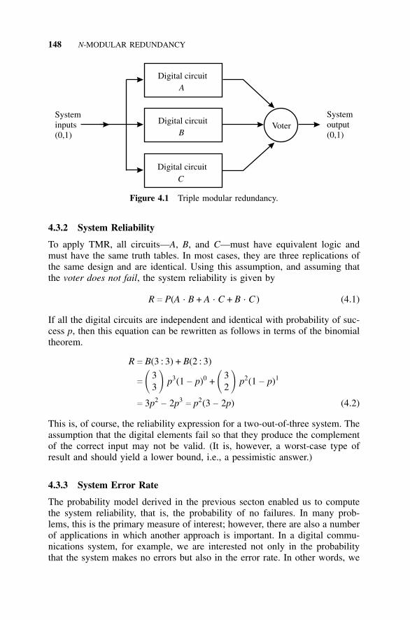
148 N-MODULAR REDUNDANCY
Digital circuit
Digital circuit
Digital circuit
A
C
BVoter
Systeminputs(0,1)
Systemoutput(0,1)
Figure 4.1 Triple modular redundancy.
4.3.2 System Reliability
To apply TMR, all circuits—A, B, and C—must have equivalent logic andmust have the same truth tables. In most cases, they are three replications ofthe same design and are identical. Using this assumption, and assuming thatthe voter does not fail, the system reliability is given by
R c P(A . B + A . C + B . C ) (4.1)
If all the digital circuits are independent and identical with probability of suc-cess p, then this equation can be rewritten as follows in terms of the binomialtheorem.
R c B(3 : 3) + B(2 : 3)
c � 33 � p3(1 − p)0 + � 3
2 � p2(1 − p)1
c 3p2− 2p3
c p2(3 − 2p) (4.2)
This is, of course, the reliability expression for a two-out-of-three system. Theassumption that the digital elements fail so that they produce the complementof the correct input may not be valid. (It is, however, a worst-case type ofresult and should yield a lower bound, i.e., a pessimistic answer.)
4.3.3 System Error Rate
The probability model derived in the previous secton enabled us to computethe system reliability, that is, the probability of no failures. In many prob-lems, this is the primary measure of interest; however, there are also a numberof applications in which another approach is important. In a digital commu-nications system, for example, we are interested not only in the probabilitythat the system makes no errors but also in the error rate. In other words, we
TRIPLE MODULAR REDUNDANCY 149
assume that errors from temporary equipment malfunction or noise are notcatastrophic if they occur only rarely, and we wish to compute the probabilityof such occurrence. Similarly, in digital computer processing of non-safety-critical data, we could occasionally tolerate an error without shutting downthe operation for repair. A third, less clear-cut example is that of an inertialguidance computer for a rocket. At every computation cycle, the computer gen-erates a course change and directs the missile control system accordingly. Anerror in one computation will direct the missile off course. If the error is large,the time between computations moderately long, the missile control systemand dynamics quick to respond, and the flight near its end, the target may bemissed, from which a catastrophic failure occurs. If these factors are reversed,however, a small error will temporarily steer the missile off course, much asa wind gust does. As long as the error has cleared in one or two computa-tion cycles, the missile will rapidly return to its proper course. A model forcomputing transmission-error probabilities is discussed below.
To construct the type of failure model discussed previously, we assume thatone good state and two failed states exist:
A1 c element A gives a one output regardless of input (stuck-at-one, or s-a-1)
A0 c element A gives a zero output regardless of input (stuck-at-zero, ors-a-0)
To work with this three-state model, we shall change our definition of reliabilityto “the probability that the digital circuit gives the correct output to any giveninput.” Thus, for the circuits of Fig. 4.1, if the correct output is to be a one,the probability expression is
P1 c 1 − P(A0B0 + A0C0 + B0C0) (4.3a)
Equation (4.3a) states that the probability of correctly indicating a one output isgiven by unity minus the probability of two or more “zero failures.” Similarly,the probability of correctly indicating zero output is given by Eq. (4.3b):
P0 c 1 − P(A1B1 + A1C1 + B1C1) (4.3b)
If we assume that a one output and a zero output have equal probability ofoccurrence, 1/ 2, on any particular transmisson, then the system reliability isthe average of Eqs. (4.3a) and (4.3b). If we let
P(A) c P(B) c P(C ) c p (4.4a)
P(A1) c P(B1) c P(C1) c q1 (4.4b)
P(A0) c P(B0) c P(C0) c q0 (4.4c)
150 N-MODULAR REDUNDANCY
and assume that all states and all elements fail independently, keeping in mindthat the expansion of the second term in Eq. (4.3a) has seven terms, then sub-stitution of Eqs. (4.4a–c) in Eq. (4.3a) yields the following equations:
P1 c 1 − P(A0B0) − P(A0C0) − P(B0C0) + 2P(A0B0C0) (4.5a)
c 1 − 3q20 + 2q3
0 (4.5b)
Similarly, Eq. (4.3b) becomes
P0 c 1 − P(A1B1) − P(A1C1) − P(B1C1) + 2P(A1B1C1) (4.6a)
c 1 − 3q21 + 2q3
1 (4.6b)
Averaging Eq. (4.5a) and Eq. (4.6a) gives
P c
P0 + P1
2(4.7a)
c −
12
(3q20 + 3q2
1 − 2q30 − 2q3
1) (4.7b)
To compare Eq. (4.7b) with Eq. (4.2), we choose the same probability forboth failure modes q0 c q1 c q; therefore, p + q0 + q1 c p + q + q c 1, andq c (1 − p)/ 2. Substitution in Eq. (4.7b) yields
P c
12
+34
p −
14
p3 (4.8)
The two probabilities, Eq. (4.2) and Eq. (4.8), are compared in Fig. 4.2.To interpret the results, it is assumed that the digital circuit in Fig. 4.1 is
turned on at t c 0 and that initially the probability of each digital circuit beingsuccessful is p c 1.00. Thus both the reliability and probability of successfultransmission are unity. If after 1 year of continuous operation p drops to 0.750,the system reliability becomes 0.844; however, the probability that any onemessage is successfully transmitted is 0.957. To put the result another way,if 1,000 such digital circuits were operated for 1 year, on average 156 wouldnot be operating properly at that time. However, the mistakes made by thesemachines would amount to 43 mistakes per 1,000 on the average. Thus, forthe entire group, the error rate would be 4.3% after 1 year.
4.3.4 TMR Options
Systems with N-modular redundancy can be designed to behave in differentways in practice [Toy, 1987; Arsenault, 1980, p. 137]. Let us examine in moredetail the way a TMR system works. As previously described, the TMR sys-
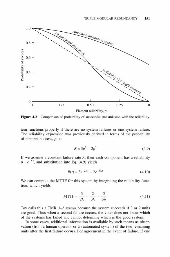
TRIPLE MODULAR REDUNDANCY 151
0
0.2
0.4
0.6
0.8
1.0
1 0.75 0.50 0.25 0
Element reliability, p
Prob
abili
ty o
f su
cces
s
Any one transmission correct
All transmissions correct
Reliability of a single element
Figure 4.2 Comparison of probability of successful transmission with the reliability.
tem functions properly if there are no system failures or one system failure.The reliability expression was previously derived in terms of the probabilityof element success, p, as
R c 3p2− 2p3 (4.9)
If we assume a constant-failure rate l, then each component has a reliabilityp c e−l t , and substitution into Eq. (4.9) yields
R(t) c 3e−2l t− 2e−3l t (4.10)
We can compute the MTTF for this system by integrating the reliability func-tion, which yields
MTTF c
32l
−
23l
c
56l
(4.11)
Toy calls this a TMR 3–2 system because the system succeeds if 3 or 2 unitsare good. Thus when a second failure occurs, the voter does not know whichof the systems has failed and cannot determine which is the good system.
In some cases, additional information is available by such means as obser-vation (from a human operator or an automated system) of the two remainingunits after the first failure occurs. For agreement in the event of failure, if one
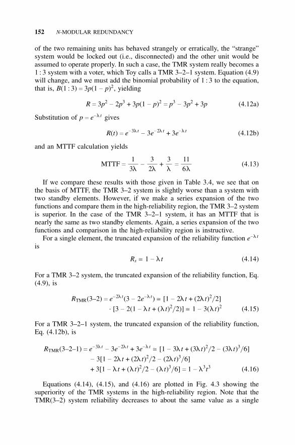
152 N-MODULAR REDUNDANCY
of the two remaining units has behaved strangely or erratically, the “strange”system would be locked out (i.e., disconnected) and the other unit would beassumed to operate properly. In such a case, the TMR system really becomes a1 : 3 system with a voter, which Toy calls a TMR 3–2–1 system. Equation (4.9)will change, and we must add the binomial probability of 1 : 3 to the equation,that is, B(1 : 3) c 3p(1 − p)2, yielding
R c 3p2− 2p3 + 3p(1 − p)2
c p3− 3p2 + 3p (4.12a)
Substitution of p c e−l t gives
R(t) c e−3l t− 3e−2l t + 3e−l t (4.12b)
and an MTTF calculation yields
MTTF c
13l
−
32l
+3l
c
116l
(4.13)
If we compare these results with those given in Table 3.4, we see that onthe basis of MTTF, the TMR 3–2 system is slightly worse than a system withtwo standby elements. However, if we make a series expansion of the twofunctions and compare them in the high-reliability region, the TMR 3–2 systemis superior. In the case of the TMR 3–2–1 system, it has an MTTF that isnearly the same as two standby elements. Again, a series expansion of the twofunctions and comparison in the high-reliability region is instructive.
For a single element, the truncated expansion of the reliability function e−l t
is
Rs � 1 − l t (4.14)
For a TMR 3–2 system, the truncated expansion of the reliability function, Eq.(4.9), is
RTMR(3–2) c e−2l t(3 − 2e−l t) � [1 − 2l t + (2l t)2/ 2]. [3 − 2(1 − l t + (l t)2/ 2)] � 1 − 3(l t)2 (4.15)
For a TMR 3–2–1 system, the truncated expansion of the reliability function,Eq. (4.12b), is
RTMR(3–2–1) c e−3l t− 3e−2l t + 3e−l t � [1 − 3l t + (3l t)2/ 2 − (3l t)3/ 6]
− 3[1 − 2l t + (2l t)2/ 2 − (2l t)3/ 6]
+ 3[1 − l t + (l t)2/ 2 − (l t)3/ 6] c 1 − l3t3 (4.16)
Equations (4.14), (4.15), and (4.16) are plotted in Fig. 4.3 showing thesuperiority of the TMR systems in the high-reliability region. Note that theTMR(3–2) system reliability decreases to about the same value as a single
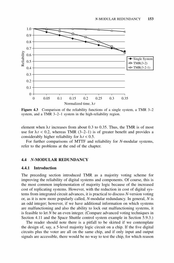
N-MODULAR REDUNDANCY 153
0
0.1
0.2
0.3
0.4
0.5
0.6
0.7
0.8
0.9
1.0
0 0.05 0.1 0.15 0.2 0.25 0.3 0.35Normalized time, l t
Rel
iabi
lity
Single SystemTMR(3-2)TMR(3-2-1)
Figure 4.3 Comparison of the reliability functions of a single system, a TMR 3–2system, and a TMR 3–2–1 system in the high-reliability region.
element when l t increases from about 0.3 to 0.35. Thus, the TMR is of mostuse for l t < 0.2, whereas TMR (3–2–1) is of greater benefit and provides aconsiderably higher reliability for l t < 0.5.
For further comparisons of MTTF and reliability for N-modular systems,refer to the problems at the end of the chapter.
4.4 N-MODULAR REDUNDANCY
4.4.1 Introduction
The preceding section introduced TMR as a majority voting scheme forimproving the reliability of digital systems and components. Of course, this isthe most common implementation of majority logic because of the increasedcost of replicating systems. However, with the reduction in cost of digital sys-tems from integrated circuit advances, it is practical to discuss N-version votingor, as it is now more popularly called, N-modular redundancy. In general, N isan odd integer; however, if we have additional information on which systemsare malfunctioning and also the ability to lock out malfunctioning systems, itis feasible to let N be an even integer. (Compare advanced voting techniques inSection 4.11 and the Space Shuttle control system example in Section 5.9.3.)
The reader should note there is a pitfall to be skirted if we contemplatethe design of, say, a 5-level majority logic circuit on a chip. If the five digitalcircuits plus the voter are all on the same chip, and if only input and outputsignals are accessible, there would be no way to test the chip, for which reason
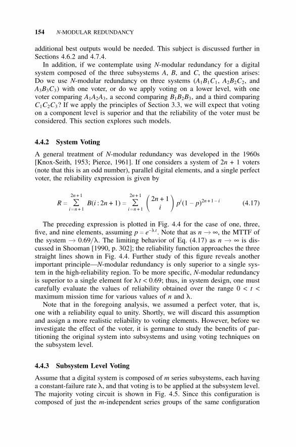
154 N-MODULAR REDUNDANCY
additional best outputs would be needed. This subject is discussed further inSections 4.6.2 and 4.7.4.
In addition, if we contemplate using N-modular redundancy for a digitalsystem composed of the three subsystems A, B, and C, the question arises:Do we use N-modular redundancy on three systems (A1B1C1, A2B2C2, andA3B3C3) with one voter, or do we apply voting on a lower level, with onevoter comparing A1A2A3, a second comparing B1B2B3, and a third comparingC1C2C3? If we apply the principles of Section 3.3, we will expect that votingon a component level is superior and that the reliability of the voter must beconsidered. This section explores such models.
4.4.2 System Voting
A general treatment of N-modular redundancy was developed in the 1960s[Knox-Seith, 1953; Pierce, 1961]. If one considers a system of 2n + 1 voters(note that this is an odd number), parallel digital elements, and a single perfectvoter, the reliability expression is given by
R c2n + 1
���i c n + 1
B(i : 2n + 1) c2n + 1
���i c n + 1 �
2n + 1i � pi(1 − p)2n + 1 − i (4.17)
The preceding expression is plotted in Fig. 4.4 for the case of one, three,five, and nine elements, assuming p c e−l t . Note that as n b ∞, the MTTF ofthe system b 0.69/ l. The limiting behavior of Eq. (4.17) as n b ∞ is dis-cussed in Shooman [1990, p. 302]; the reliability function approaches the threestraight lines shown in Fig. 4.4. Further study of this figure reveals anotherimportant principle—N-modular redundancy is only superior to a single sys-tem in the high-reliability region. To be more specific, N-modular redundancyis superior to a single element for l t < 0.69; thus, in system design, one mustcarefully evaluate the values of reliability obtained over the range 0 < t <maximum mission time for various values of n and l.
Note that in the foregoing analysis, we assumed a perfect voter, that is,one with a reliability equal to unity. Shortly, we will discard this assumptionand assign a more realistic reliability to voting elements. However, before weinvestigate the effect of the voter, it is germane to study the benefits of par-titioning the original system into subsystems and using voting techniques onthe subsystem level.
4.4.3 Subsystem Level Voting
Assume that a digital system is composed of m series subsystems, each havinga constant-failure rate l, and that voting is to be applied at the subsystem level.The majority voting circuit is shown in Fig. 4.5. Since this configuration iscomposed of just the m-independent series groups of the same configuration
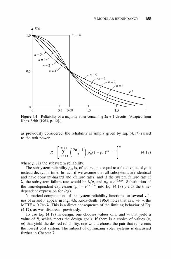
N-MODULAR REDUNDANCY 155
0
0.5
1.0
0 0.5 0.69 1.0 1.5 t
R t( )
n t ∞
n = 0
n = 0
n = 1
n = 1
n = 2
n = 2
n = 4
n = 4
e–t
Figure 4.4 Reliability of a majority voter containing 2n + 1 circuits. (Adapted fromKnox-Seith [1963, p. 12].)
as previously considered, the reliability is simply given by Eq. (4.17) raisedto the mth power.
R c [ 2n + 1
���i c n + 1 �
2n + 1i � pi
ss(1 − pss)2n + 1 − i] m
(4.18)
where pss is the subsystem reliability.The subsystem reliability pss is, of course, not equal to a fixed value of p; it
instead decays in time. In fact, if we assume that all subsystems are identicaland have constant-hazard and -failure rates, and if the system failure rate ifl, the subsystem failure rate would be l/ n, and pss c e−l t/ m. Substitution ofthe time-dependent expression (pss c e−l t/ m) into Eq. (4.18) yields the time-dependent expression for R(t).
Numerical computations of the system reliability functions for several val-ues of m and n appear in Fig. 4.6. Knox-Seith [1963] notes that as n b ∞, theMTTF ≈ 0.7m/ l. This is a direct consequence of the limiting behavior of Eq.(4.17), as was discussed previously.
To use Eq. (4.18) in design, one chooses values of n and m that yield avalue of R, which meets the design goals. If there is a choice of values (n,m) that yield the desired reliability, one would choose the pair that representsthe lowest cost system. The subject of optimizing voter systems is discussedfurther in Chapter 7.
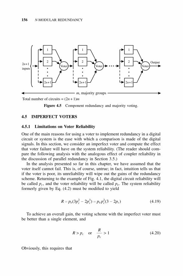
156 N-MODULAR REDUNDANCY
1 1 1
2 2 2
2 +1n 2 +1n 2 +1n
2 +1inputs
nVoter Voter Voter
•••
•••
•••
� • • •Output
m, majority groups
Total number of circuits = (2 + 1)n m
Figure 4.5 Component redundancy and majority voting.
4.5 IMPERFECT VOTERS
4.5.1 Limitations on Voter Reliability
One of the main reasons for using a voter to implement redundancy in a digitalcircuit or system is the ease with which a comparison is made of the digitalsignals. In this section, we consider an imperfect voter and compute the effectthat voter failure will have on the system reliability. (The reader should com-pare the following analysis with the analogous effect of coupler reliability inthe discussion of parallel redundancy in Section 3.5.)
In the analysis presented so far in this chapter, we have assumed that thevoter itself cannot fail. This is, of course, untrue; in fact, intuition tells us thatif the voter is poor, its unreliability will wipe out the gains of the redundancyscheme. Returning to the example of Fig. 4.1, the digital circuit reliability willbe called pc, and the voter reliability will be called pv. The system reliabilityformerly given by Eq. (4.2) must be modified to yield
R c pv(3p2c − 2p3
c) c pvp2c(3 − 2pc) (4.19)
To achieve an overall gain, the voting scheme with the imperfect voter mustbe better than a single element, and
R > pc orRpc
> 1 (4.20)
Obviously, this requires that
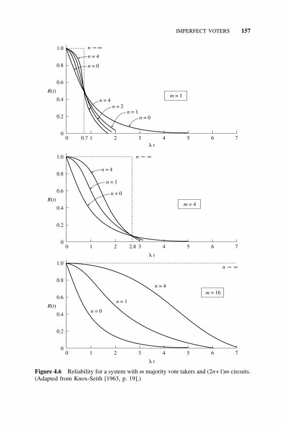
IMPERFECT VOTERS 157
0
0
0
0.2
0.2
0.2
0.4
0.4
0.4
0.6
0.6
0.6
0.8
0.8
0.8
1.0
1.0
1.0
0
0
0
0.7
2.8
1
1
1
2
2
2
3
3
3
4
4
4
5
5
5
6
6
6
7
7
7
R t( )
R t( )
R t( )
n t∞
n t ∞
n t ∞
n = 0
n = 0
n = 0
n = 4n = 2
n = 1
n = 1
n = 1
n = 4
n = 4
n = 4
n = 0
m = 1
m = 4
m = 16
l t
l t
l t
Figure 4.6 Reliability for a system with m majority vote takers and (2n+1)m circuits.(Adapted from Knox-Seith [1963, p. 19].)
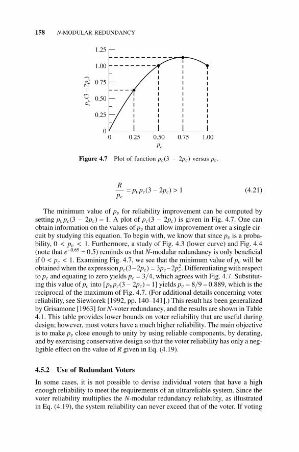
158 N-MODULAR REDUNDANCY
0
0.25
0.50
0.75
1.00
1.25
0 0.25 0.50 0.75 1.00pc
p c(3
– 2
p c)
Figure 4.7 Plot of function pc(3 − 2pc) versus pc.
Rpc
c pvpc(3 − 2pc) > 1 (4.21)
The minimum value of pv for reliability improvement can be computed bysetting pvpc(3 − 2pc) c 1. A plot of pc(3 − 2pc) is given in Fig. 4.7. One canobtain information on the values of pv that allow improvement over a single cir-cuit by studying this equation. To begin with, we know that since pv is a proba-bility, 0 < pv < 1. Furthermore, a study of Fig. 4.3 (lower curve) and Fig. 4.4(note that e−0.69
c 0.5) reminds us that N-modular redundancy is only beneficialif 0 < pc < 1. Examining Fig. 4.7, we see that the minimum value of pv will beobtained when the expression pc(3−2pc) c 3pc−2p2
c . Differentiating with respectto pc and equating to zero yields pc c 3/ 4, which agrees with Fig. 4.7. Substitut-ing this value of pc into [pvpc(3 − 2pc) c 1] yields pv c 8/ 9 c 0.889, which is thereciprocal of the maximum of Fig. 4.7. (For additional details concerning voterreliability, see Siewiorek [1992, pp. 140–141].) This result has been generalizedby Grisamone [1963] for N-voter redundancy, and the results are shown in Table4.1. This table provides lower bounds on voter reliability that are useful duringdesign; however, most voters have a much higher reliability. The main objectiveis to make pv close enough to unity by using reliable components, by derating,and by exercising conservative design so that the voter reliability has only a neg-ligible effect on the value of R given in Eq. (4.19).
4.5.2 Use of Redundant Voters
In some cases, it is not possible to devise individual voters that have a highenough reliability to meet the requirements of an ultrareliable system. Since thevoter reliability multiplies the N-modular redundancy reliability, as illustratedin Eq. (4.19), the system reliability can never exceed that of the voter. If voting
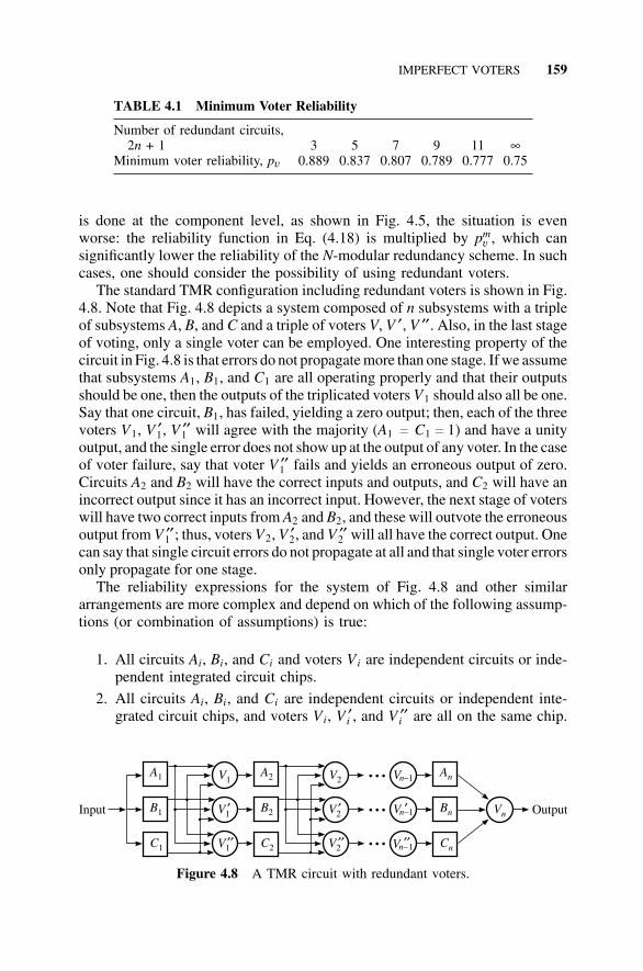
IMPERFECT VOTERS 159
TABLE 4.1 Minimum Voter Reliability
Number of redundant circuits,2n + 1 3 5 7 9 11 ∞
Minimum voter reliability, pv 0.889 0.837 0.807 0.789 0.777 0.75
is done at the component level, as shown in Fig. 4.5, the situation is evenworse: the reliability function in Eq. (4.18) is multiplied by pm
v , which cansignificantly lower the reliability of the N-modular redundancy scheme. In suchcases, one should consider the possibility of using redundant voters.
The standard TMR configuration including redundant voters is shown in Fig.4.8. Note that Fig. 4.8 depicts a system composed of n subsystems with a tripleof subsystems A, B, and C and a triple of voters V, V ′, V ′′. Also, in the last stageof voting, only a single voter can be employed. One interesting property of thecircuit in Fig. 4.8 is that errors do not propagate more than one stage. If we assumethat subsystems A1, B1, and C1 are all operating properly and that their outputsshould be one, then the outputs of the triplicated voters V1 should also all be one.Say that one circuit, B1, has failed, yielding a zero output; then, each of the threevoters V1, V ′1, V ′′1 will agree with the majority (A1 c C1 c 1) and have a unityoutput, and the single error does not show up at the output of any voter. In the caseof voter failure, say that voter V ′′1 fails and yields an erroneous output of zero.Circuits A2 and B2 will have the correct inputs and outputs, and C2 will have anincorrect output since it has an incorrect input. However, the next stage of voterswill have two correct inputs from A2 and B2, and these will outvote the erroneousoutput from V ′′1 ; thus, voters V2, V ′2, and V ′′2 will all have the correct output. Onecan say that single circuit errors do not propagate at all and that single voter errorsonly propagate for one stage.
The reliability expressions for the system of Fig. 4.8 and other similararrangements are more complex and depend on which of the following assump-tions (or combination of assumptions) is true:
1. All circuits Ai, Bi, and Ci and voters Vi are independent circuits or inde-pendent integrated circuit chips.
2. All circuits Ai, Bi, and Ci are independent circuits or independent inte-grated circuit chips, and voters Vi, V ′i , and V ′′i are all on the same chip.
A1 A2 An
B1 B2 Bn
C1 C2 Cn
V1 V2 Vn–
Vn– Vn
Vn–
V1 V2
V1 V2
′ ′ ′
′′ ′′ ′′
• • •
• • •
• • •
OutputInput
1
1
1
Figure 4.8 A TMR circuit with redundant voters.
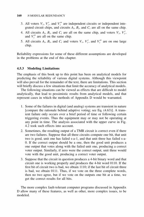
160 N-MODULAR REDUNDANCY
3. All voters Vi, V ′i , and V ′′i are independent circuits or independent inte-grated circuit chips, and circuits Ai, Bi, and Ci are all on the same chip.
4. All circuits Ai, Bi, and Ci are all on the same chip, and voters Vi, V ′i ,and V ′′i are all on the same chip.
5. All circuits Ai, Bi, and Ci and voters Vi, V ′i , and V ′′i are on one largechip.
Reliability expressions for some of these different assumptions are developedin the problems at the end of this chapter.
4.5.3 Modeling Limitations
The emphasis of this book up to this point has been on analytical models forpredicting the reliability of various digital systems. Although this viewpointwill also prevail for the remainder of the text, there are limitations. This sectionwill briefly discuss a few situations that limit the accuracy of analytical models.
The following situations can be viewed as effects that are difficult to modelanalytically, that lead to pessimistic results from analytical models, and thatrepresent cases in which the methods of Appendix D would be warranted.
1. Some of the failures in digital (and analog) systems are transient in nature[compare the rationale behind adaptive voting; see Eq. (4.63)]. A trans-ient failure only occurs over a brief period of time or following certaintriggering events. Thus the equipment may or may not be operating atany point in time. The analysis associated with the upper curve in Fig.4.2 took such effects into account.
2. Sometimes, the resulting output of a TMR circuit is correct even if thereare two failures. Suppose that all three circuits compute one bit, that unittwo is good, unit one has failed s-a-1, and that unit three has failed s-a-0. If the correct output should be a one, then the good unit produces aone output that votes along with the failed unit one, producing a correctvoter output. Similarly, if zero were the correct output, unit three wouldvote with the good unit, producing a correct voter output.
3. Suppose that the circuit in question produces a 4-bit binary word and thatcircuit one is working properly and produces the 4-bit word 0110. If thefirst bit of circuit two is bad, we obtain 1110; if the last bit of circuit threeis bad, we obtain 0111. Thus, if we vote on the three complete words,then no two agree, but if we vote on the outputs one bit at a time, weget the correct results for all bits.
The more complex fault-tolerant computer programs discussed in AppendixD allow many of these features, as well as other, more complex issues, to bemodeled.
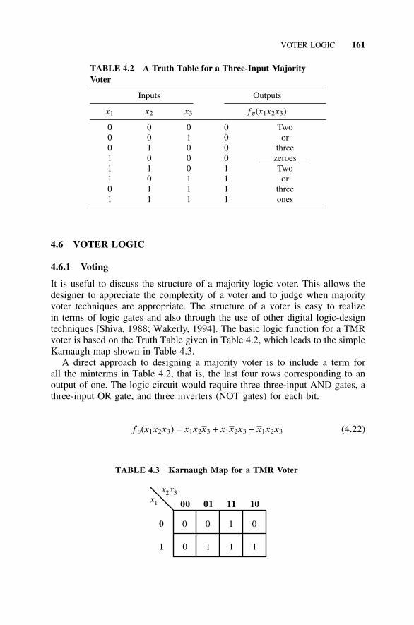
VOTER LOGIC 161
TABLE 4.2 A Truth Table for a Three-Input MajorityVoter
Inputs Outputs
x1 x2 x3 f v(x1x2x3)
0 0 0 0 Two0 0 1 0 or0 1 0 0 three1 0 0 0 zeroes1 1 0 1 Two1 0 1 1 or0 1 1 1 three1 1 1 1 ones
4.6 VOTER LOGIC
4.6.1 Voting
It is useful to discuss the structure of a majority logic voter. This allows thedesigner to appreciate the complexity of a voter and to judge when majorityvoter techniques are appropriate. The structure of a voter is easy to realizein terms of logic gates and also through the use of other digital logic-designtechniques [Shiva, 1988; Wakerly, 1994]. The basic logic function for a TMRvoter is based on the Truth Table given in Table 4.2, which leads to the simpleKarnaugh map shown in Table 4.3.
A direct approach to designing a majority voter is to include a term forall the minterms in Table 4.2, that is, the last four rows corresponding to anoutput of one. The logic circuit would require three three-input AND gates, athree-input OR gate, and three inverters (NOT gates) for each bit.
f v(x1x2x3) c x1x2x3 + x1x2x3 + x1x2x3 (4.22)
TABLE 4.3 Karnaugh Map for a TMR Voter
00 01 11 10
0 0 0 1 0
1 0 1 1 1
x1
x2 3x
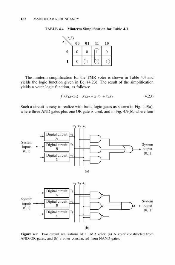
162 N-MODULAR REDUNDANCY
TABLE 4.4 Minterm Simplification for Table 4.3
00 01 11 10
0 0 0 1 0
1 0 1 1 1
x1
x2 3x
The minterm simplification for the TMR voter is shown in Table 4.4 andyields the logic function given in Eq. (4.23). The result of the simplificationyields a voter logic function, as follows:
f v(x1x2x3) c x1x2 + x1x3 + x2x3 (4.23)
Such a circuit is easy to realize with basic logic gates as shown in Fig. 4.9(a),where three AND gates plus one OR gate is used, and in Fig. 4.9(b), where four
Digital circuitA
Digital circuitA
Digital circuitB
Digital circuitB
Digital circuitC
Digital circuitC
Systeminputs(0,1)
Systeminputs(0,1)
Systemoutput(0,1)
Systemoutput(0,1)
x1
x1
x1
x1
x2
x2
x2
x2
x3
x3
x3
x3
(a)
(b)
Figure 4.9 Two circuit realizations of a TMR voter. (a) A voter constructed fromAND/ OR gates; and (b) a voter constructed from NAND gates.
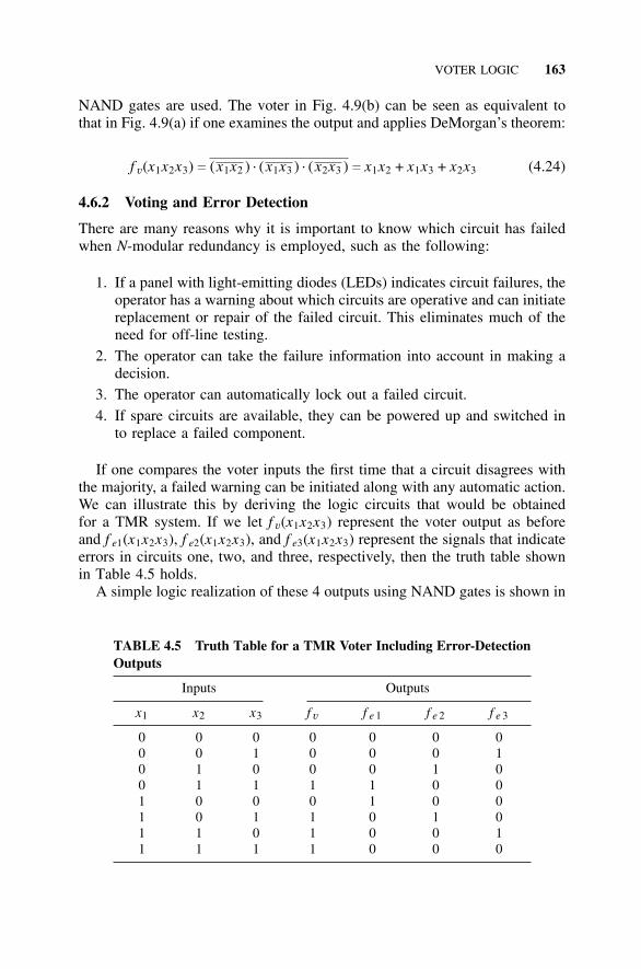
VOTER LOGIC 163
NAND gates are used. The voter in Fig. 4.9(b) can be seen as equivalent tothat in Fig. 4.9(a) if one examines the output and applies DeMorgan’s theorem:
f v(x1x2x3) c (x1x2 ) . (x1x3 ) . (x2x3 ) c x1x2 + x1x3 + x2x3 (4.24)
4.6.2 Voting and Error Detection
There are many reasons why it is important to know which circuit has failedwhen N-modular redundancy is employed, such as the following:
1. If a panel with light-emitting diodes (LEDs) indicates circuit failures, theoperator has a warning about which circuits are operative and can initiatereplacement or repair of the failed circuit. This eliminates much of theneed for off-line testing.
2. The operator can take the failure information into account in making adecision.
3. The operator can automatically lock out a failed circuit.4. If spare circuits are available, they can be powered up and switched in
to replace a failed component.
If one compares the voter inputs the first time that a circuit disagrees withthe majority, a failed warning can be initiated along with any automatic action.We can illustrate this by deriving the logic circuits that would be obtainedfor a TMR system. If we let f v(x1x2x3) represent the voter output as beforeand f e1(x1x2x3), f e2(x1x2x3), and f e3(x1x2x3) represent the signals that indicateerrors in circuits one, two, and three, respectively, then the truth table shownin Table 4.5 holds.
A simple logic realization of these 4 outputs using NAND gates is shown in
TABLE 4.5 Truth Table for a TMR Voter Including Error-DetectionOutputs
Inputs Outputs
x1 x2 x3 f v f e 1 f e 2 f e 3
0 0 0 0 0 0 00 0 1 0 0 0 10 1 0 0 0 1 00 1 1 1 1 0 01 0 0 0 1 0 01 0 1 1 0 1 01 1 0 1 0 0 11 1 1 1 0 0 0
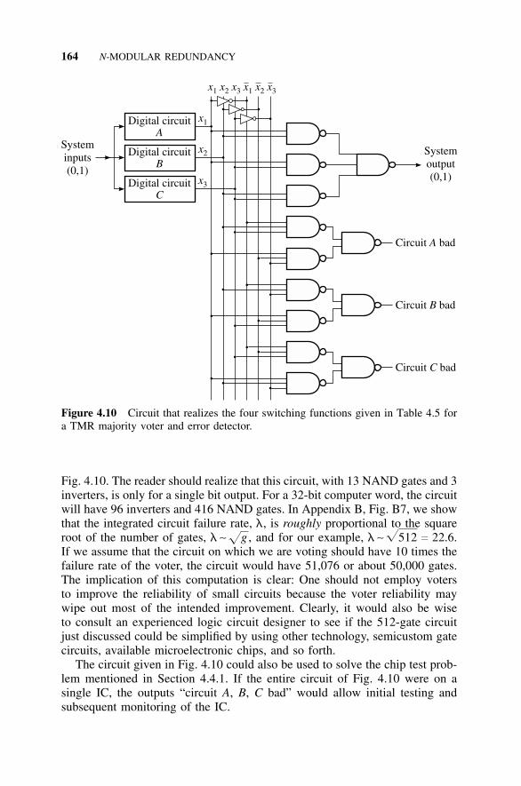
164 N-MODULAR REDUNDANCY
Digital circuitA
Digital circuitB
Digital circuitC
Systeminputs(0,1)
Systemoutput(0,1)
x1 x2 x3 x1 x2 x3
x1
x2
x3
Circuit badA
Circuit badB
Circuit badC
Figure 4.10 Circuit that realizes the four switching functions given in Table 4.5 fora TMR majority voter and error detector.
Fig. 4.10. The reader should realize that this circuit, with 13 NAND gates and 3inverters, is only for a single bit output. For a 32-bit computer word, the circuitwill have 96 inverters and 416 NAND gates. In Appendix B, Fig. B7, we showthat the integrated circuit failure rate, l, is roughly proportional to the squareroot of the number of gates, l ∼
fg , and for our example, l ∼
f512 c 22.6.
If we assume that the circuit on which we are voting should have 10 times thefailure rate of the voter, the circuit would have 51,076 or about 50,000 gates.The implication of this computation is clear: One should not employ votersto improve the reliability of small circuits because the voter reliability maywipe out most of the intended improvement. Clearly, it would also be wiseto consult an experienced logic circuit designer to see if the 512-gate circuitjust discussed could be simplified by using other technology, semicustom gatecircuits, available microelectronic chips, and so forth.
The circuit given in Fig. 4.10 could also be used to solve the chip test prob-lem mentioned in Section 4.4.1. If the entire circuit of Fig. 4.10 were on asingle IC, the outputs “circuit A, B, C bad” would allow initial testing andsubsequent monitoring of the IC.
N-MODULAR REDUNDANCY WITH REPAIR 165
4.7 N-MODULAR REDUNDANCY WITH REPAIR
4.7.1 Introduction
In Chapter 3, we argued that as long as the operating system possesses redun-dancy, the addition of repair raises the reliability. One might ask at the outsetwhy N-modular redundancy should be used with repair when ordinary parallelor standby redundancy with repair is very effective in achieving highly reli-able and available systems. The answer to this question involves the couplingdevice reliability that was explored in Chapter 3. To be specific, suppose thatwe wish to compare the reliability of two parallel systems with that of a TMRsystem. Both systems fail if two of the elements fail, but in the TMR case,there are three systems that could fail; thus the probability of failure is higher.However, in general, the coupler in a parallel system will be more complexthan a TMR voter, so a comparison of the two designs requires a detailed eval-uation of coupler versus voter reliability. Analysis of TMR system reliabilityand availability can be found in Siewiorek [1992, p. 335] and in Toy [1987].
4.7.2 Reliability Computations
One might expect that it would be most efficient to seek a general solutionfor the reliability and availability of a system with N-modular redundancy andrepair, then specify that N c 3 for a TMR system, N c 5 for 5-level voting, andso on. A moment’s thought, however, suggests quite a different approach. Theconventional solution for the reliability and availability of a system with repairinvolves making a Markov model and solving it much as was done in Chapter3. In the process, the Laplace transform was computed, and a partial fractionexpansion was used to find the individual exponential terms in the solution. Forthe case of repair, in general the repair rates couple the n states, and solutionof the set of n first-order differential equations leads to the solution of an nth-order differential equation. If one applies Laplace transform theory, solutionof the nth-order differential equation is “transformed into” a simpler sequenceof steps. However, one step involves the solution for the roots of an nth-orderpolynomial.
Unfortunately, closed-form solutions exist only for first- through fourth-order polynomials, and solution procedures for cubic and quadratic polynomi-als are lengthy and seldom used. We learned in high-school algebra the formulafor the roots of a quadratic equation (polynomial). A somewhat more complexsolution exists for the solution of a cubic, which is listed in various handbooks[Iyanaga, p. 1396], and also for a fourth-order equation [Iyanaga, p. 1396].
A brief historical note about the origin of closed-form solutions is of interest.The formula for the third-order equation is generally attributed to GiordamoCardano (also known as Jerome Cardan) [Cardano, 1545; Cardan, 1963]; how-ever, he obtained the solution from Nicolo Tartaglia, and apparently it was dis-covered by Scipio Ferreo in circa 1505 [Hall, 1957, pp. 480–481]. LudovicoFerrari, a pupil of Cardan, developed the formula for the fourth-order equation.
166 N-MODULAR REDUNDANCY
Neils Henrik Abel developed a proof that no closed-form solution exists forn ≥ 5 [Iyanaga, p. 1].
The conclusion from the foregoing information on polynomial roots is thatwe should start with TMR and other simpler systems if we wish to use alge-braic solutions. Numerical solutions are always possible for higher-order equa-tions, and the mathematical software discussed in Appendix D expedites suchan approach; however, the insight of an analytical solution is generally lacking.Another approach is to use simplifications and approximations such as thosediscussed in Appendix B (Sections B8.2 and B8.3). We will use the tried andtrue three-step engineering approach:
1. Represent the main features of the system by a low-order model that isamenable to closed-form solution.
2. Add further effects one at a time that complicate the model; study theeffect (if necessary, use simplifying assumptions and approximations ornumerical results computed over a range of parameters).
3. Put all the effects into a comprehensive model and solve numerically.
Our development begins by studying the reliability and availability of aTMR system, assuming that the design is truly TMR or that we are using aTMR model as step one in our solution approach.
4.7.3 TMR Reliability
Markov Model. We begin the analysis of voting systems with repair by ana-lyzing the reliability of a TMR system. The Markov reliability diagram for aTMR system composed of a voter, V, and three digital subsystems x1, x2, andx3 is given in Fig. 4.11. It is assumed that the xs are identical and have thesame failure rate, l, and that the voter does not fail.
If we compare Fig. 4.11 with the model given in Fig. 3.14 of Chapter 3,we see that they are essentially the same, only with different parameter values(transition rates). There are three states in both models: repair occurs fromstate s1 to s0, and state s2 is an absorbing state. (Actually, a complete modelfor Fig. 4.11 would have a fourth state, s3, which is reached by an additionalfailure from state s2. However, we have included both states in state s2 sinceeither two or three failures both represent system failure. As a rule, it is almostalways easier to use a Markov model with fewer states even if one or more ofthe states represent combined states. State s2 is actually a combined state, alsoknown as a merged state, and a complete discussion of the rules for mergingappears in Shooman [1990, p. 529]. One could decompose the third state inFig. 4.11 into s2 c x1x2x3 + x1x2x3 + x1x2x3 and s3 c x1x2x3 by reformulatingthe model as a more complex four-state model. However, the four-state modelis not needed to solve for the upstate probabilities Ps0 and Ps1 . Thus the simplerthree-state model of Fig. 4.11 will be used.)
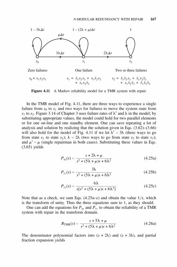
N-MODULAR REDUNDANCY WITH REPAIR 167
s = x x + x x x+ x x x
1 2 3 1 2 3
1 2 3
x1 s = x x + x x x+ x x x + x x x
2 2 3 1 2 3
1 2 3 1 2 3
x1s = x x x0 1 2 3
Zero failures One failure Two or three failures
3
1 – 3 1 – (2
2l
l l
lD
D D
D
Dt
t tt
t
m
+ m) 1
s0 s1 s2
Figure 4.11 A Markov reliability model for a TMR system with repair.
In the TMR model of Fig. 4.11, there are three ways to experience a singlefailure from s0 to s1 and two ways for failures to move the system state froms1 to s2. Figure 3.14 of Chapter 3 uses failure rates of l′ and l in the model; bysubstituting appropriate values, the model could hold for two parallel elementsor for one on-line and one standby element. One can save repeating a lot ofanalysis and solution by realizing that the solution given in Eqs. (3.62)–(3.66)will also hold for the model of Fig. 4.11 if we let l′ c 3l (three ways to gofrom state s1 to state s2); l c 2l (two ways to go from state s2 to state s3);and m′ c m (single repairman in both cases). Substituting these values in Eqs.(3.65) yields
Ps0 (s) cs + 2l + m
s2 + (5l + m)s + 6l2(4.25a)
Ps1 (s) c3l
s2 + (5l + m)s + 6l2(4.25b)
Ps2 (s) c6l
s[s2 + (5l + m)s + 6l2](4.25c)
Note that as a check, we sum Eqs. (4.25a–c) and obtain the value 1/ s, whichis the transform of unity. Thus the three equations sum to 1, as they should.
One can add the equations for Ps0 and Ps1 to obtain the reliability of a TMRsystem with repair in the transform domain.
RTMR(s) cs + 5l + m
s2 + (5l + m)s + 6l2(4.26a)
The denominator polynomial factors into (s + 2l) and (s + 3l), and partialfraction expansion yields
168 N-MODULAR REDUNDANCY
RTMR(s) c� 3l + m
l �s + 2l
−
� 2l + m
l �s + 3l
(4.26b)
Using transform #4 in Table B6 in Appendix B, we obtain the time function:
RTMR(t) c �3 +m
l � e−2l t− �2 +
m
l � e−3l t (4.26c)
One can check the above result by letting m c 0 (no repair), which yieldsRTMR(t) c 3e−2l t
− 2e−3l t , and if p c e−l t , this becomes RTMR c 3p2− 2p3,
which of course agrees with the result previously computed [see Eq. (4.2)].
Initial Behavior. The complete solution for the reliability of a TMR systemwith repair is given in Eq. (4.26c). It is useful to practice with the simplifyingeffects of initial behavior, final behavior, and MTTF solutions on this simpleproblem before they are applied later in this chapter to more complex modelswhere the simplification is needed. One can evaluate the effects of repair onthe initial behavior of the TMR system simply by using the transform for t n,which is discussed in Appendix B, Section B8.3. We begin with Eq. (4.26a),where division of the denominator into the numerator using polynomial longdivision yields for the first three terms:
RTMR(s) c1s
−
6l2
s3+
6l2(5l + m)s4
− · · · (4.27a)
Using inverse transform no. 5 of Table B6 of Appendix B yields
L { 1(n − 1)!
t n − 1e−at} c
1(s + a)n
(4.27b)
Setting a c 0 yields
L { 1(n − 1)!
t n − 1} c
1(s)n
(4.27c)
Using the transform in Eq. (4.27c) converts Eq. (4.27a) into the time function,which is a three-term polynomial in t (the first three terms in the Taylor seriesexpansion of the time function).
RTMR(t) c 1 − 3l2t2 + l2(5l + m)t3 · · · (4.27d)
We previously studied the first two terms in the Taylor series expansion of
N-MODULAR REDUNDANCY WITH REPAIR 169
the TMR reliability expansion in Eq. (4.15). In Eq. (4.27d), we have a three-term solution, and one can compare Eqs. (4.15) and (4.27b) by calculating anadditional third term in the expansion of Eq. (4.15). The expansions in Eq.(4.15) are augmented by including the cubic terms in the expansions of thebracketed terms, that is, −4l3t3/ 3 in the first bracket and +l3t3/ 3 in the secondbracket. Carrying out the algebra adds a third term, and Eq. (4.15) becomesexpanded as follows:
RTMR(3–2) c 1 − 3l2t2 + 5l3t3 (4.27e)
Thus the first three terms of Eq. (4.15) and Eq. (4.27d) are identical for thecase of no repair, m c 0. Equation (4.27d) is larger (closer to unity) than theexpanded version of Eq. (4.15) because of the additional term +l2mt3 that issignificant for large values of repair rate; we therefore see that repair improvesthe reliability. However, we note that repair only affects the cubic term in Eq.(4.27d) and not the quadratic term. Thus, for very small t, repair does notaffect the initial behavior; however, from the above solution, we can see thatit is beneficial for small and modest size t.
A numerical example will illustrate the improvement in initial reliabilitydue to repair. Let m c 10l; then the third term in Eq. (4.27d) becomes +15l3t3
rather than +5l3t3 with no repair. One can evaluate the increase due to m c 10lat one point in time by letting t c 0.1/ l. At this point in time, the TMRreliability without repair is equal to 0.975; with repair, it is 0.985. Furthercomparisons of the effects of repair appear in the problems at the end of thechapter.
The approximate analysis of this section led to a useful evaluation of theeffects of repair through the computation of the power series expansion of thetime function for the model with repair. This approximate result avoids the needto factor the denominator polynomial in the Laplace transform solution, whichwas found to be a stumbling block in obtaining a complete closed solution forhigher-order systems. The next section will discuss the mean time to failure(MTTF) as another approximate solution that also avoids polynomial factoring.
Mean Time to Failure. As we saw in the preceding chapter, the computa-tion of MTTF greatly simplifies the analysis, but it is not without pitfalls. TheMTTF computes the “area under the reliability curve” (see also Section 3.8.3).Thus, for a single element with a reliability function of e−l t , the area under thecurve yields 1/ l; however, the MTTF calculation for the TMR system givenin Eq. (4.11) yields a value of 5/ 6l. This implies that a single element is bet-ter than TMR, but we know that TMR has a higher reliability than a singleelement (see also Siewiorek [1992, p. 294]). The explanation of this apparentcontradiction is simple if we examine the n c 0 and n c 1 curves in Fig. 4.4.In the region of primary interest, 0 < lt < 0.69, TMR is superior to a singleelement, but in the region 0.69 < lt < ∞ (not a region of primary interest),
170 N-MODULAR REDUNDANCY
the single element has a superior reliability. Thus, in computing the integralbetween t c 0 and t c ∞, the long tail controls the result. The lesson is thatwe should not trust an MTTF comparison without further study unless there isa significant superiority or unless the two reliability functions have the sameshape. Clearly, if the two functions have the same shape, then a comparisonof the MTTF values should be definitive. Graphing of reliability functions inthe high-reliability region should always be included in an analysis, especiallywith the ready availability, power, and ease provided by software on a modernPC. One can also easily integrate the functions in question by using an analysisprogram to compute MTTF.
We now apply the simple method given in Appendix B, Section B8.2 toevaluate the MTTF by letting s approach zero in the Laplace transform of thereliability function—Eq. (4.26a). The result is
MTTF c
5 + m/ l
6l(4.28)
To evaluate the effect of repair, let m c 10l. The MTTF without repair increasesfrom 5/ 6l to 16/ 6l—a threefold improvement.
Final Behavior. The Laplace transform has a simple theorem that allows usto easily calculate the final value of a time function based on its transform.(See Appendix B, Table B7, Theorem 7.) The final-value theorem states thatthe value of the time function f (t) as t b ∞ is given by sF(s) (the transformmultiplied by s) as s b 0. Applying this to Eq. (4.26a), we obtain
limsb 0
{sRTMR} c limsb 0
s(s + 5l + m)s2 + (5l + m)s + 6l2
c 0 (4.29)
A little thought shows that this is the correct result since all reliability func-tions go to zero as time increases. However, when we study the availabilityfunction later in this chapter, we will see that the final value of the availabilityis nonzero. This value is an important measure of system behavior.
4.7.4 N-Modular Reliability
Having explored the analysis of the reliability of a TMR system with repair,it would be useful to develop general expressions for the reliability, MTTF,and initial behavior for N-modular systems. This task is difficult and probablyunnecessary since most practical systems have 3- or 5-level majority voting.(An intermediate system with 4-level voting used by NASA in the Space Shut-tle will be discussed later in this chapter.) The main focus of this section willtherefore be the analysis.
Markov Model. We begin the analysis of 5-level modular reliability with
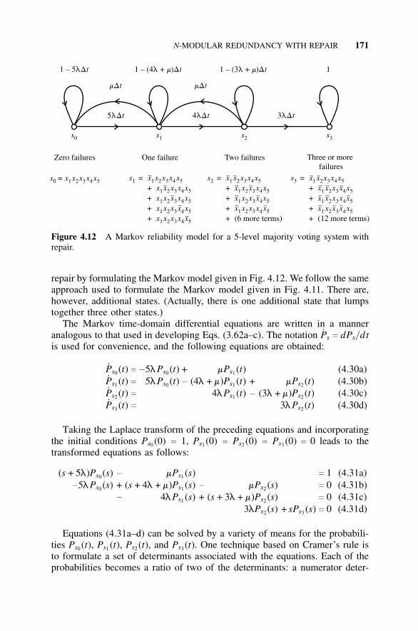
N-MODULAR REDUNDANCY WITH REPAIR 171
s = x x x x x0 1 2 3 4 5
Zero failures
s =1 x x x x x1 2 3 4 5+ x x x x x1 2 3 4 5+ x x x x x1 2 3 4 5+ x x x x x1 2 3 4 5+ x x x x x1 2 3 4 5
One failure
s =2 x x x x x1 2 3 4 5+ x x x x x1 2 3 4 5+ x x x x x1 2 3 4 5+ x x x x x1 2 3 4 5+ (6 more terms)
Two failures
s =3 x x x x x1 2 3 4 5+ x x x x x1 2 3 4 5+ x x x x x1 2 3 4 5+ x x x x x1 2 3 4 5+ (12 more terms)
Three or morefailures
11 – 5 1 – (4 1 – (3l l lD D D
3lDt
t t t
5lD
D
t
tm
4lD
D
t
tm
+ +m m) )
s0 s1 s2 s3
Figure 4.12 A Markov reliability model for a 5-level majority voting system withrepair.
repair by formulating the Markov model given in Fig. 4.12. We follow the sameapproach used to formulate the Markov model given in Fig. 4.11. There are,however, additional states. (Actually, there is one additional state that lumpstogether three other states.)
The Markov time-domain differential equations are written in a manneranalogous to that used in developing Eqs. (3.62a–c). The notation Ps c dPs/ dtis used for convenience, and the following equations are obtained:
Ps0 (t) c −5lPs0 (t) + mPs1 (t)Ps1 (t) c 5lPs0 (t) − (4l + m)Ps1 (t)Ps2 (t) c 4lPs1 (t)Ps3 (t) c
+ mPs2 (t)− (3l + m)Ps2 (t)
3lPs2 (t)
(4.30a)(4.30b)(4.30c)(4.30d)
Taking the Laplace transform of the preceding equations and incorporatingthe initial conditions Ps0 (0) c 1, Ps1 (0) c Ps2 (0) c Ps3 (0) c 0 leads to thetransformed equations as follows:
(s + 5l)Ps0 (s)−5lPs0 (s)
− mPs1 (s)+ (s + 4l + m)Ps1 (s)− 4lPs1 (s)
− mPs2 (s)+ (s + 3l + m)Ps2 (s)
3lPs2 (s)
c 1c 0c 0
+ sPs3 (s) c 0
(4.31a)(4.31b)(4.31c)(4.31d)
Equations (4.31a–d) can be solved by a variety of means for the probabili-ties Ps0 (t), Ps1 (t), Ps2 (t), and Ps3 (t). One technique based on Cramer’s rule isto formulate a set of determinants associated with the equations. Each of theprobabilities becomes a ratio of two of the determinants: a numerator deter-
172 N-MODULAR REDUNDANCY
minant divided by a denominator determinant. The denominator determinantis the same for each ratio; it is generally denoted by D and is the determinantof the coefficients of the equations. (One can develop the form of these equa-tions in a more elaborate fashion using matrix theory; see Shooman [1990, pp.239–243].) A brief inspection of Eqs. (4.31a–d) shows that the first three areuncoupled from the last and can be solved separately, simplifying the algebra(this will always be true in a Markov model with repair when the last state isan absorbing one). Thus, for the first three equations,
D c
||||||
s + 5l −m 0−5l s + 4l + m −m
0 −4l s + 3l + m
||||||
(4.32)
The numerator determinants in the solution are similar to the denominatordeterminants; however, one column is replaced by the right-hand side of theEqs. (4.31a–d); that is,
D1 c
||||||
1 −m 00 s + 4l + m −m
0 −4l s + 3l + m
||||||
(4.33a)
D2 c
||||||
s + 5l 1 0−5l 0 −m
0 0 s + 3l + m
||||||
(4.33b)
D3 c
||||||
s + 5l −m 1−5l s + 4l + m 0
0 −4l 0
||||||
(4.33c)
In terms of this group of determinants, the probabilities are
Ps0 (s) cD1
D(4.34a)
Ps1 (s) cD2
D(4.34b)
Ps2 (s) cD3
D(4.34c)
The reliability of the 5-level modular redundancy system is given by
R5 MR(t) c Ps0 (t) + Ps1 (t) + Ps2 (t) (4.35)
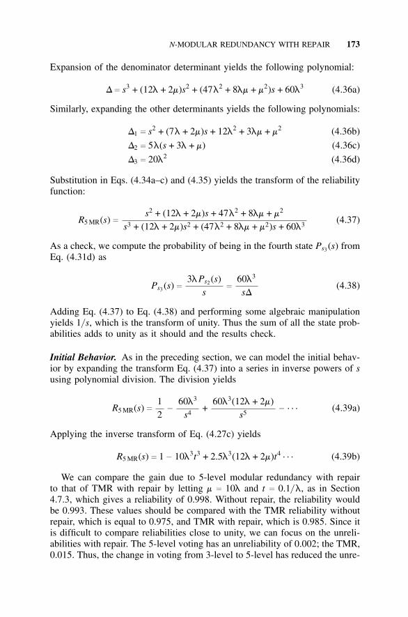
N-MODULAR REDUNDANCY WITH REPAIR 173
Expansion of the denominator determinant yields the following polynomial:
D c s3 + (12l + 2m)s2 + (47l2 + 8lm + m2)s + 60l3 (4.36a)
Similarly, expanding the other determinants yields the following polynomials:
D1 c s2 + (7l + 2m)s + 12l2 + 3lm + m2 (4.36b)
D2 c 5l(s + 3l + m) (4.36c)
D3 c 20l2 (4.36d)
Substitution in Eqs. (4.34a–c) and (4.35) yields the transform of the reliabilityfunction:
R5 MR(s) cs2 + (12l + 2m)s + 47l2 + 8lm + m2
s3 + (12l + 2m)s2 + (47l2 + 8lm + m2)s + 60l3(4.37)
As a check, we compute the probability of being in the fourth state Ps3 (s) fromEq. (4.31d) as
Ps3 (s) c3lPs2 (s)
sc
60l3
sD(4.38)
Adding Eq. (4.37) to Eq. (4.38) and performing some algebraic manipulationyields 1/ s, which is the transform of unity. Thus the sum of all the state prob-abilities adds to unity as it should and the results check.
Initial Behavior. As in the preceding section, we can model the initial behav-ior by expanding the transform Eq. (4.37) into a series in inverse powers of susing polynomial division. The division yields
R5 MR(s) c12
−
60l3
s4+
60l3(12l + 2m)s5
− · · · (4.39a)
Applying the inverse transform of Eq. (4.27c) yields
R5 MR(s) c 1 − 10l3t3 + 2.5l3(12l + 2m)t4 · · · (4.39b)
We can compare the gain due to 5-level modular redundancy with repairto that of TMR with repair by letting m c 10l and t c 0.1/ l, as in Section4.7.3, which gives a reliability of 0.998. Without repair, the reliability wouldbe 0.993. These values should be compared with the TMR reliability withoutrepair, which is equal to 0.975, and TMR with repair, which is 0.985. Since itis difficult to compare reliabilities close to unity, we can focus on the unreli-abilities with repair. The 5-level voting has an unreliability of 0.002; the TMR,0.015. Thus, the change in voting from 3-level to 5-level has reduced the unre-
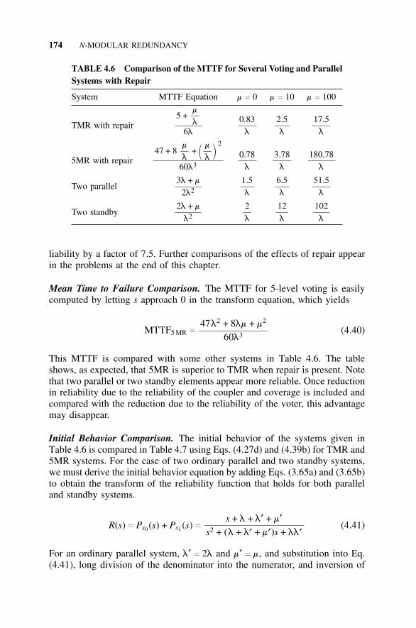
174 N-MODULAR REDUNDANCY
TABLE 4.6 Comparison of the MTTF for Several Voting and ParallelSystems with Repair
System MTTF Equation m c 0 m c 10 m c 100
TMR with repair5 +
m
l6l
0.83l
2.5l
17.5l
5MR with repair47 + 8
m
l+ �
m
l �2
60l3
0.78l
3.78l
180.78l
Two parallel3l + m
2l2
1.5l
6.5l
51.5l
Two standby2l + m
l2
2l
12l
102l
liability by a factor of 7.5. Further comparisons of the effects of repair appearin the problems at the end of this chapter.
Mean Time to Failure Comparison. The MTTF for 5-level voting is easilycomputed by letting s approach 0 in the transform equation, which yields
MTTF5 MR c
47l2 + 8lm + m2
60l3(4.40)
This MTTF is compared with some other systems in Table 4.6. The tableshows, as expected, that 5MR is superior to TMR when repair is present. Notethat two parallel or two standby elements appear more reliable. Once reductionin reliability due to the reliability of the coupler and coverage is included andcompared with the reduction due to the reliability of the voter, this advantagemay disappear.
Initial Behavior Comparison. The initial behavior of the systems given inTable 4.6 is compared in Table 4.7 using Eqs. (4.27d) and (4.39b) for TMR and5MR systems. For the case of two ordinary parallel and two standby systems,we must derive the initial behavior equation by adding Eqs. (3.65a) and (3.65b)to obtain the transform of the reliability function that holds for both paralleland standby systems.
R(s) c Ps0 (s) + Ps1 (s) cs + l + l′ + m′
s2 + (l + l′ + m′)s + ll′(4.41)
For an ordinary parallel system, l′ c 2l and m′ c m, and substitution into Eq.(4.41), long division of the denominator into the numerator, and inversion of
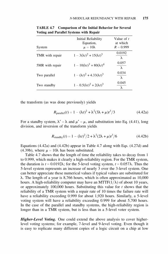
N-MODULAR REDUNDANCY WITH REPAIR 175
TABLE 4.7 Comparison of the Initial Behavior for SeveralVoting and Parallel Systems with Repair
Initial Reliability Value of tEquation, at which
System m c 10l R c 0.999
TMR with repair 1 − 3(lt)2 + 15(lt)3 0.0192l
5MR with repair 1 − 10(lt)3 + 80(lt)4 0.057l
Two parallel 1 − (lt)2 + 4.33(lt)3 0.034l
Two standby 1 − 0.5(lt)2 + 2(lt)3 0.045l
the transform (as was done previously) yields
Rparallel(t) c 1 − (lt)2 + l2(3l + m)t3/ 3 (4.42a)
For a standby system, l′ c l and m′ c m, and substitution into Eq. (4.41), longdivision, and inversion of the transform yields
Rstandby(t) c 1 − (lt)2/ 2 + l2(2l + m)t3/ 6 (4.42b)
Equations (4.42a) and (4.42b) appear in Table 4.7 along with Eqs. (4.27d) and(4.39b), where m c 10l has been substituted.
Table 4.7 shows that the length of time the reliability takes to decay from 1to 0.999, which makes it clearly a high-reliability region. For the TMR system,the duration is t c 0.0192l; for the 5-level voting system, t c 0.057l. Thus the5-level system represents an increase of nearly 3 over the 3-level system. Onecan better appreciate these numerical values if typical values are substituted forl. The length of a year is 8,766 hours, which is often approximated as 10,000hours. A high-reliability computer may have an MTTF(1/ l) of about 10 years,or approximately 100,000 hours. Substituting this value for t shows that thereliability of a TMR system with a repair rate of 10 times the failure rate willhave a reliability exceeding 0.999 for about 1,920 hours. Similarly, a 5-levelvoting system will have a reliability exceeding 0.999 for about 5,700 hours.In the case of the parallel and standby systems, the high-reliability region islonger than in a TMR system, but is less than in a 5-level voter system.
Higher-Level Voting. One could extend the above analysis to cover higher-level voting systems; for example, 7-level and 9-level voting. Even though itis easy to replicate many different copies of a logic circuit on a chip at low
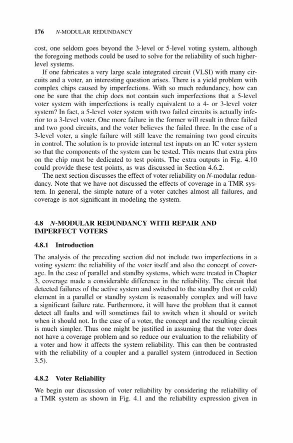
176 N-MODULAR REDUNDANCY
cost, one seldom goes beyond the 3-level or 5-level voting system, althoughthe foregoing methods could be used to solve for the reliability of such higher-level systems.
If one fabricates a very large scale integrated circuit (VLSI) with many cir-cuits and a voter, an interesting question arises. There is a yield problem withcomplex chips caused by imperfections. With so much redundancy, how canone be sure that the chip does not contain such imperfections that a 5-levelvoter system with imperfections is really equivalent to a 4- or 3-level votersystem? In fact, a 5-level voter system with two failed circuits is actually infe-rior to a 3-level voter. One more failure in the former will result in three failedand two good circuits, and the voter believes the failed three. In the case of a3-level voter, a single failure will still leave the remaining two good circuitsin control. The solution is to provide internal test inputs on an IC voter systemso that the components of the system can be tested. This means that extra pinson the chip must be dedicated to test points. The extra outputs in Fig. 4.10could provide these test points, as was discussed in Section 4.6.2.
The next section discusses the effect of voter reliability on N-modular redun-dancy. Note that we have not discussed the effects of coverage in a TMR sys-tem. In general, the simple nature of a voter catches almost all failures, andcoverage is not significant in modeling the system.
4.8 N-MODULAR REDUNDANCY WITH REPAIR ANDIMPERFECT VOTERS
4.8.1 Introduction
The analysis of the preceding section did not include two imperfections in avoting system: the reliability of the voter itself and also the concept of cover-age. In the case of parallel and standby systems, which were treated in Chapter3, coverage made a considerable difference in the reliability. The circuit thatdetected failures of the active system and switched to the standby (hot or cold)element in a parallel or standby system is reasonably complex and will havea significant failure rate. Furthermore, it will have the problem that it cannotdetect all faults and will sometimes fail to switch when it should or switchwhen it should not. In the case of a voter, the concept and the resulting circuitis much simpler. Thus one might be justified in assuming that the voter doesnot have a coverage problem and so reduce our evaluation to the reliability ofa voter and how it affects the system reliability. This can then be contrastedwith the reliability of a coupler and a parallel system (introduced in Section3.5).
4.8.2 Voter Reliability
We begin our discussion of voter reliability by considering the reliability ofa TMR system as shown in Fig. 4.1 and the reliability expression given in
N-MODULAR REDUNDANCY WITH REPAIR AND IMPERFECT VOTERS 177
Eq. (4.19). In Section 4.5, we asked how small the voter reliability, pv, canbe so that the gains of TMR still exceed the reliability of a single circuit.The analysis was given in Eqs. (3.34) and (3.35). Now, we perform a similaranalysis for a TMR system with an imperfect voter. The computation proceedsfrom a consideration of Eq. (4.19). If the voter were perfect, pv c 1, then thereliability would be computed as
RTMR c 3p2c − 2p3
c (4.43a)
If we include an imperfect voter, this expression becomes
RTMR c 3pvp2c − 2pvp3
c c pv(3p2c − 2p3
c) (4.43b)
If we assume constant-failure rates for the voter and the circuits in the TMRconfiguration, then for the voter we have pv c e−lvt , and for the TMR circuits,p c e−l t . If we use a three-term approximation for the exponential and sub-stitute into Eq. (4.43b), one obtains an expression for the initial reliability, asfollows:
RTMR c �1 − lvt +(lvt)2
2!−
(lvt)3
3! � × [ 3 �1 − 2lvt +(2l t)2
2!−
(2l t)3
3! �− 2 �1 − 3l t +
(3l t)2
2!−
(3lvt)3
3! � ] (4.44a)
Expanding the preceding equation and retaining only the first four terms yields
RTMR c 1 − lvt +(lvt)2
2− 3(l t)2 (4.44b)
Furthermore, we are mainly interested in the cases where lv < l; thus we canomit the third term (which is a second-order term in lv) and obtain
RTMR c 1 − lvt − 3(l t)2 (4.44c)
If we want the effect of the voter to be negligible, we let lvt < 3(l t)2,
lv
l< 3l t (4.45)
One can compare this result with that given in Eq. (3.35) for two parallel sys-tems by setting n c 2, yielding
178 N-MODULAR REDUNDANCY
lc
l< l t (3.35)
The approximate result is that the coupler must have a failure rate three timessmaller than that of the voter for the same decrease in reliability.
One can examine the effect of repair on the above results by examiningEq. (4.27d) and Eq. (4.42). In both cases, the effect of the repair rate doesnot appear until the cubic term is encountered. The above comparisons onlyinvolved the linear and quadratic terms, so the effect of repair would onlybecome apparent if the repair rate were very large and the time interval ofinterest were extended.
4.8.3 Comparison of TMR, Parallel, and Standby Systems
Another advantage of voter reliability over parallel and standby reliability isthat there is a straightforward scheme for implementing voter redundancy (e.g.,Fig. 4.8). Of course, one can also make redundant couplers for parallel orstandby systems, but they may be more complex than redundant voters.
It is easy to make a simple model for Fig. 4.8. Assume that the voters failso that their outputs are stuck-at-zero or stuck-at-one and that voter failuresdo not corrupt the outputs of the circuits that feed the voters (e.g., A1, B1, andC1). Assume just a single stage (A1, B1, and C1) and a single redundant votersystem (V1, V′1, and V′′1 ). The voter works if two or three of the three voterswork. Thus this is the same formula for TMR systems, and the reliability ofthe system becomes
RTMR × Rvoter c (3p2c − 2p3
c) × (3p2v − 2p3
v) (4.46)
It is easy to evaluate the advantages of redundant voters. Assume that pc c
0.9 and that the voter is 10 times as reliable: (1 − pc) c 0.1, (1 − pv) c 0.01,and pv c 0.99. With a single voter, R c 0.99[3(0.9)2
− 2(0.9)3] c 0.99 × 0.972c 0.962. In the case of a redundant voter, we have [3(0.99)2
− 2(0.99)3] ×[3(0.9)2
− 2(0.9)3] c 0.999702 × 0.972 c 0.9717. The redundant voter is thussignificant; if the voter is less reliable, voter redundancy is even more effective.Assume that pv c 0.95; for a single voter, R c 0.95 [3(0.9)2
− 2(0.9)3] c 0.95 ×0.972 c 0.923. In the case of a redundant voter, we have [3(0.95)2
− 2(0.95)3]× [3(0.9)2
− 2(0.9)3] c 0.99275 × 0.972 c 0.964953.The foregoing calculations and discussions were performed for a TMR cir-
cuit with a single voter or redundant voters. It is possible to extend these com-putations to the subsystem level for a system such as that depicted in Fig. 4.8.In addition, one can repair a failed component of a redundant voter; thus onecan use the analysis techniques previously derived for TMR and 5MR systemswhere the systems and voters can both be repaired. However, repair of votersreally begs a larger question: How will we modularize the system architecture?
AVAILABILITY OF N-MODULAR REDUNDANCY WITH REPAIR 179
Assume one is going to design the system architecture with redundant votersand voting at a subsystem level. If the voters are to be placed on a single chipalong with the circuits, then there is no separate repair of a voter system—onlyrepair of the circuit and voter subsystem. The alternative is to make a separatechip for the N circuits and a separate chip for the redundant voter. The properstrategy to choose depends on whether there will be scheduled downtime forthe system during which testing and replacement can occur and also whetherthe chips have sufficient test points. No general conclusion can be reached; thesystem architecture should be critiqued with these issues in mind.
4.9 AVAILABILITY OF N-MODULAR REDUNDANCY WITHREPAIR AND IMPERFECT VOTERS
4.9.1 Introduction
When repair is present in a system, it is often possible for the system to failand be down for a short period of time without serious operational effects.Suppose a computer used for electronic funds transfers is down for a shortperiod of time. This is not catastrophic if the system is designed so that it cantolerate brief outages and perform the funds transfers at a later time period. Ifthe system is designed to be self-diagnostic, and if a technician and a replace-ment plug in boards are both available, the machine can be restored quicklyto operational status. For such systems, availability is a useful measure of sys-tem performance, as with reliability, and is the probability that the system isup at any point in time. It can be measured during operation by recording thedowntimes and operating times for several failure and repair cycles. The avail-ability is given by the ratio of the sum of the uptimes for the system dividedby the sum of the uptimes and the downtimes. (Formally, this ratio becomesthe availability in the limit as the system operating time approaches infinity.)The availability A(t) is the probability that the system is up at time t, whichcan be written as a sum of probabilities:
A(t) c P(no failures) + P(one failure + one repair)
+ P(two failures + two repairs)
+ · · · + P(n failures + n repairs) + · · · (4.47)
Availability is always higher than reliability, since the first term in Eq. (4.47)is the reliability and all the other terms are positive numbers. Note that onlythe first few terms in Eq. (4.47) are significant for a moderate time intervaland higher-order terms become negligible. Thus one could evaluate availabilityanalytically by computing the terms in Eq. (4.47); however, the use of theMarkov model simplifies such a computation.
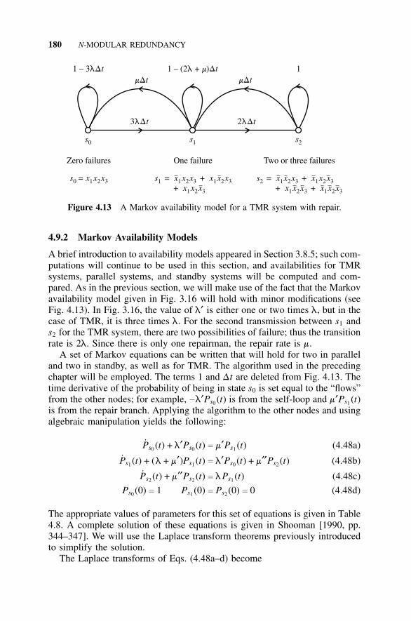
180 N-MODULAR REDUNDANCY
s = x x + x x x+ x x x
1 2 3 1 2 3
1 2 3
x1 s = x x + x x x+ x x x + x x x
2 2 3 1 2 3
1 2 3 1 2 3
x1s = x x x0 1 2 3
Zero failures One failure Two or three failures
3
1 – 3 1 – (2
2l
l l
lD
D D
D D
Dt
t tt t
t
m m
+ m) 1
s0 s1 s2
Figure 4.13 A Markov availability model for a TMR system with repair.
4.9.2 Markov Availability Models
A brief introduction to availability models appeared in Section 3.8.5; such com-putations will continue to be used in this section, and availabilities for TMRsystems, parallel systems, and standby systems will be computed and com-pared. As in the previous section, we will make use of the fact that the Markovavailability model given in Fig. 3.16 will hold with minor modifications (seeFig. 4.13). In Fig. 3.16, the value of l′ is either one or two times l, but in thecase of TMR, it is three times l. For the second transmission between s1 ands2 for the TMR system, there are two possibilities of failure; thus the transitionrate is 2l. Since there is only one repairman, the repair rate is m.
A set of Markov equations can be written that will hold for two in paralleland two in standby, as well as for TMR. The algorithm used in the precedingchapter will be employed. The terms 1 and Dt are deleted from Fig. 4.13. Thetime derivative of the probability of being in state s0 is set equal to the “flows”from the other nodes; for example, −l′Ps0 (t) is from the self-loop and m′Ps1 (t)is from the repair branch. Applying the algorithm to the other nodes and usingalgebraic manipulation yields the following:
Ps0 (t) + l′Ps0 (t) c m′Ps1 (t) (4.48a)
Ps1 (t) + (l + m′)Ps1 (t) c l′Ps0 (t) + m′′Ps2 (t) (4.48b)
Ps2 (t) + m′′Ps2 (t) c lPs1 (t) (4.48c)
Ps0 (0) c 1 Ps1 (0) c Ps2 (0) c 0 (4.48d)
The appropriate values of parameters for this set of equations is given in Table4.8. A complete solution of these equations is given in Shooman [1990, pp.344–347]. We will use the Laplace transform theorems previously introducedto simplify the solution.
The Laplace transforms of Eqs. (4.48a–d) become
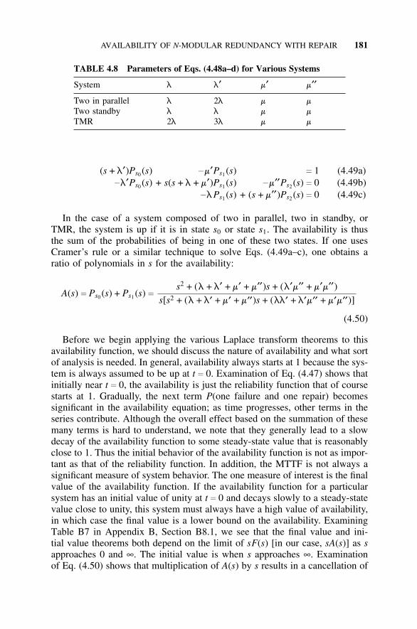
AVAILABILITY OF N-MODULAR REDUNDANCY WITH REPAIR 181
TABLE 4.8 Parameters of Eqs. (4.48a–d) for Various Systems
System l l′ m′ m′′Two in parallel l 2l m mTwo standby l l m mTMR 2l 3l m m
(s + l′)Ps0 (s)−l′Ps0 (s)
−m′Ps1 (s)+ s(s + l + m′)Ps1 (s)
−lPs1 (s)
c 1−m′′Ps2 (s) c 0
+ (s + m′′)Ps2 (s) c 0
(4.49a)(4.49b)(4.49c)
In the case of a system composed of two in parallel, two in standby, orTMR, the system is up if it is in state s0 or state s1. The availability is thusthe sum of the probabilities of being in one of these two states. If one usesCramer’s rule or a similar technique to solve Eqs. (4.49a–c), one obtains aratio of polynomials in s for the availability:
A(s) c Ps0 (s) + Ps1 (s) cs2 + (l + l′ + m′ + m′′)s + (l′m′′ + m′m′′)
s[s2 + (l + l′ + m′ + m′′)s + (ll′ + l′m′′ + m′m′′)]
(4.50)
Before we begin applying the various Laplace transform theorems to thisavailability function, we should discuss the nature of availability and what sortof analysis is needed. In general, availability always starts at 1 because the sys-tem is always assumed to be up at t c 0. Examination of Eq. (4.47) shows thatinitially near t c 0, the availability is just the reliability function that of coursestarts at 1. Gradually, the next term P(one failure and one repair) becomessignificant in the availability equation; as time progresses, other terms in theseries contribute. Although the overall effect based on the summation of thesemany terms is hard to understand, we note that they generally lead to a slowdecay of the availability function to some steady-state value that is reasonablyclose to 1. Thus the initial behavior of the availability function is not as impor-tant as that of the reliability function. In addition, the MTTF is not always asignificant measure of system behavior. The one measure of interest is the finalvalue of the availability function. If the availability function for a particularsystem has an initial value of unity at t c 0 and decays slowly to a steady-statevalue close to unity, this system must always have a high value of availability,in which case the final value is a lower bound on the availability. ExaminingTable B7 in Appendix B, Section B8.1, we see that the final value and ini-tial value theorems both depend on the limit of sF(s) [in our case, sA(s)] as sapproaches 0 and ∞. The initial value is when s approaches ∞. Examinationof Eq. (4.50) shows that multiplication of A(s) by s results in a cancellation of
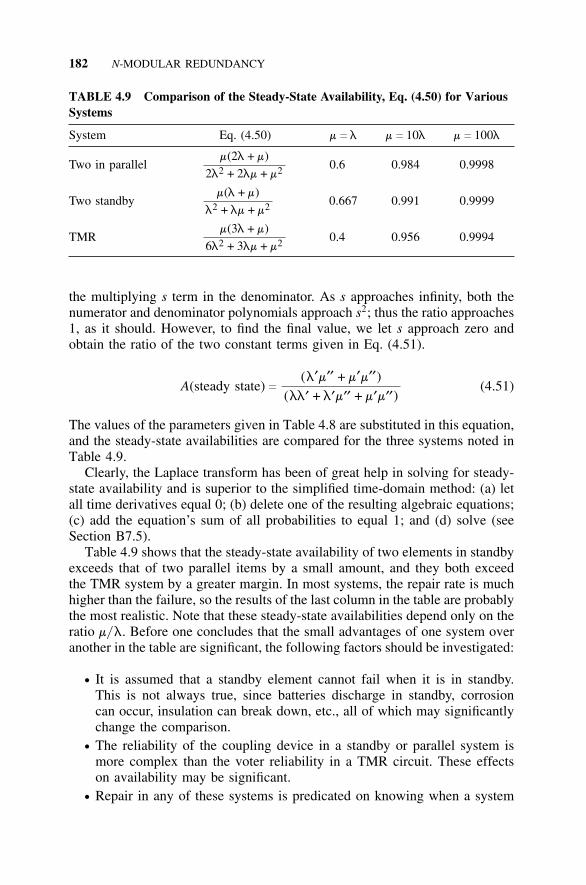
182 N-MODULAR REDUNDANCY
TABLE 4.9 Comparison of the Steady-State Availability, Eq. (4.50) for VariousSystems
System Eq. (4.50) m c l m c 10l m c 100l
Two in parallelm(2l + m)
2l2 + 2lm + m2 0.6 0.984 0.9998
Two standbym(l + m)
l2 + lm + m2 0.667 0.991 0.9999
TMRm(3l + m)
6l2 + 3lm + m2 0.4 0.956 0.9994
the multiplying s term in the denominator. As s approaches infinity, both thenumerator and denominator polynomials approach s2; thus the ratio approaches1, as it should. However, to find the final value, we let s approach zero andobtain the ratio of the two constant terms given in Eq. (4.51).
A(steady state) c(l′m′′ + m′m′′)
(ll′ + l′m′′ + m′m′′)(4.51)
The values of the parameters given in Table 4.8 are substituted in this equation,and the steady-state availabilities are compared for the three systems noted inTable 4.9.
Clearly, the Laplace transform has been of great help in solving for steady-state availability and is superior to the simplified time-domain method: (a) letall time derivatives equal 0; (b) delete one of the resulting algebraic equations;(c) add the equation’s sum of all probabilities to equal 1; and (d) solve (seeSection B7.5).
Table 4.9 shows that the steady-state availability of two elements in standbyexceeds that of two parallel items by a small amount, and they both exceedthe TMR system by a greater margin. In most systems, the repair rate is muchhigher than the failure, so the results of the last column in the table are probablythe most realistic. Note that these steady-state availabilities depend only on theratio m/ l. Before one concludes that the small advantages of one system overanother in the table are significant, the following factors should be investigated:
• It is assumed that a standby element cannot fail when it is in standby.This is not always true, since batteries discharge in standby, corrosioncan occur, insulation can break down, etc., all of which may significantlychange the comparison.
• The reliability of the coupling device in a standby or parallel system ismore complex than the voter reliability in a TMR circuit. These effectson availability may be significant.
• Repair in any of these systems is predicated on knowing when a system
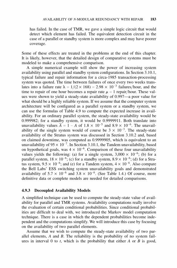
AVAILABILITY OF N-MODULAR REDUNDANCY WITH REPAIR 183
has failed. In the case of TMR, we gave a simple logic circuit that woulddetect which element has failed. The equivalent detection circuit in thecase of a parallel or standby system is more complex and may have poorercoverage.
Some of these effects are treated in the problems at the end of this chapter.It is likely, however, that the detailed design of comparative systems must bemodeled to make a comprehensive comparison.
A simple numerical example will show the power of increasing systemavailability using parallel and standby system configurations. In Section 3.10.1,typical failure and repair information for a circa-1985 transaction-processingsystem was quoted. The time between failures of once every two weeks trans-lates into a failure rate l c 1/ (2 × 168) c 2.98 × 10⁻³ failures/ hour, and thetime to repair of one hour becomes a repair rate m c 1 repair/ hour. These val-ues were shown to yield a steady-state availability of 0.997—a poor value forwhat should be a highly reliable system. If we assume that the computer systemarchitecture will be configured as a parallel system or a standby system, wecan use the formulas of Table 4.9 to compute the expected increase in avail-ability. For an ordinary parallel system, the steady-state availability would be0.999982; for a standby system, it would be 0.9999911. Both translate intounavailability values A c 1 − A of 1.8 × 10⁻⁵ and 8.9 × 10⁻⁶. The unavail-ability of the single system would of course be 3 × 10⁻³. The steady-stateavailability of the Stratus system was discussed in Section 3.10.2 and, basedon claimed downtime, was computed as 0.9999905, which is equivalent to anunavailability of 95 × 10−7. In Section 3.10.1, the Tandem unavailability, basedon hypothetical goals, was 4 × 10⁻⁶. Comparison of these four unavailabilityvalues yields the following: (a) for a single system, 3,000 × 10−6; (b) for aparallel system, 18 × 10−6; (c) for a standby system, 8.9 × 10⁻⁶; (d) for a Stra-tus system, 9.5 × 10⁻⁶; and (e) for a Tandem system, 4 × 10⁻⁶. Also comparethe Bell Labs’ ESS switching system unavailability goals and demonstratedavailability of 5.7 × 10⁻⁶ and 3.8 × 10⁻⁶. (See Table 1.4.) Of course, moredefinitive data or complete models are needed for detailed comparisons.
4.9.3 Decoupled Availability Models
A simplified technique can be used to compute the steady-state value of avail-ability for parallel and TMR systems. Availability computations really involvethe evaluation of certain conditional probabilities. Since conditional probabil-ities are difficult to deal with, we introduced the Markov model computationtechnique. There is a case in which the dependent probabilities become inde-pendent and the computations simplify. We will introduce this case by focusingon the availability of two parallel elements.
Assume that we wish to compute the steady-state availability of two par-allel elements, A and B. The reliability is the probability of no system fail-ures in interval 0 to t, which is the probability that either A or B is good,
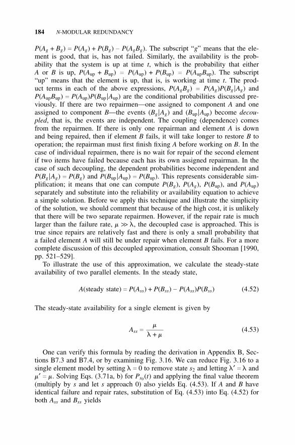
184 N-MODULAR REDUNDANCY
P(Ag + Bg) c P(Ag) + P(Bg) − P(AgBg). The subscript “g” means that the ele-ment is good, that is, has not failed. Similarly, the availability is the prob-ability that the system is up at time t, which is the probability that eitherA or B is up, P(Aup + Bup) c P(Aup) + P(Bup) c P(AupBup). The subscript“up” means that the element is up, that is, is working at time t. The prod-uct terms in each of the above expressions, P(AgBg) c P(Ag)P(Bg |Ag) andP(AupBup) c P(Aup)P(Bup |Aup) are the conditional probabilities discussed pre-viously. If there are two repairmen—one assigned to component A and oneassigned to component B—the events (Bg |Ag) and (Bup |Aup) become decou-pled, that is, the events are independent. The coupling (dependence) comesfrom the repairmen. If there is only one repairman and element A is downand being repaired, then if element B fails, it will take longer to restore B tooperation; the repairman must first finish fixing A before working on B. In thecase of individual repairmen, there is no wait for repair of the second elementif two items have failed because each has its own assigned repairman. In thecase of such decoupling, the dependent probabilities become independent andP(Bg |Ag) c P(Bg) and P(Bup |Aup) c P(Bup). This represents considerable sim-plification; it means that one can compute P(Bg), P(Ag), P(Bup), and P(Aup)separately and substitute into the reliability or availability equation to achievea simple solution. Before we apply this technique and illustrate the simplicityof the solution, we should comment that because of the high cost, it is unlikelythat there will be two separate repairmen. However, if the repair rate is muchlarger than the failure rate, m >> l, the decoupled case is approached. This istrue since repairs are relatively fast and there is only a small probability thata failed element A will still be under repair when element B fails. For a morecomplete discussion of this decoupled approximation, consult Shooman [1990,pp. 521–529].
To illustrate the use of this approximation, we calculate the steady-stateavailability of two parallel elements. In the steady state,
A(steady state) c P(Ass) + P(Bss) − P(Ass)P(Bss) (4.52)
The steady-state availability for a single element is given by
Ass cm
l + m(4.53)
One can verify this formula by reading the derivation in Appendix B, Sec-tions B7.3 and B7.4, or by examining Fig. 3.16. We can reduce Fig. 3.16 to asingle element model by setting l c 0 to remove state s2 and letting l′ c l andm′ c m. Solving Eqs. (3.71a, b) for Ps0 (t) and applying the final value theorem(multiply by s and let s approach 0) also yields Eq. (4.53). If A and B haveidentical failure and repair rates, substitution of Eq. (4.53) into Eq. (4.52) forboth Ass and Bss yields
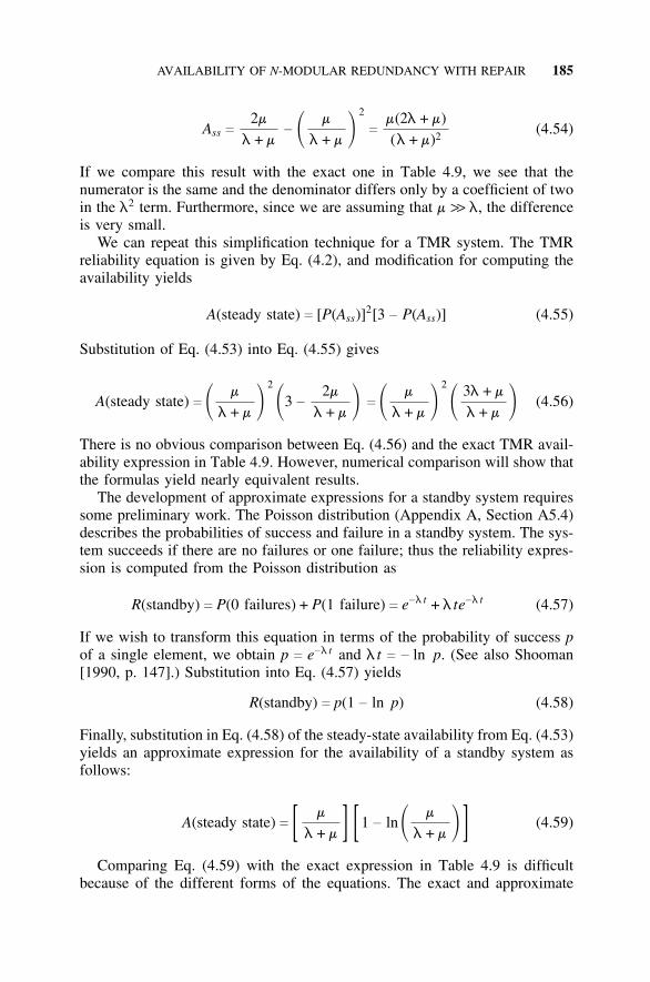
AVAILABILITY OF N-MODULAR REDUNDANCY WITH REPAIR 185
Ass c2m
l + m− � m
l + m �2
c
m(2l + m)(l + m)2
(4.54)
If we compare this result with the exact one in Table 4.9, we see that thenumerator is the same and the denominator differs only by a coefficient of twoin the l2 term. Furthermore, since we are assuming that m >> l, the differenceis very small.
We can repeat this simplification technique for a TMR system. The TMRreliability equation is given by Eq. (4.2), and modification for computing theavailability yields
A(steady state) c [P(Ass)]2[3 − P(Ass)] (4.55)
Substitution of Eq. (4.53) into Eq. (4.55) gives
A(steady state) c � m
l + m �2
�3 −
2m
l + m � c � m
l + m �2
� 3l + m
l + m � (4.56)
There is no obvious comparison between Eq. (4.56) and the exact TMR avail-ability expression in Table 4.9. However, numerical comparison will show thatthe formulas yield nearly equivalent results.
The development of approximate expressions for a standby system requiressome preliminary work. The Poisson distribution (Appendix A, Section A5.4)describes the probabilities of success and failure in a standby system. The sys-tem succeeds if there are no failures or one failure; thus the reliability expres-sion is computed from the Poisson distribution as
R(standby) c P(0 failures) + P(1 failure) c e−l t + l te−l t (4.57)
If we wish to transform this equation in terms of the probability of success pof a single element, we obtain p c e−l t and l t c − ln p. (See also Shooman[1990, p. 147].) Substitution into Eq. (4.57) yields
R(standby) c p(1 − ln p) (4.58)
Finally, substitution in Eq. (4.58) of the steady-state availability from Eq. (4.53)yields an approximate expression for the availability of a standby system asfollows:
A(steady state) c [ m
l + m ] [ 1 − ln � m
l + m � ] (4.59)
Comparing Eq. (4.59) with the exact expression in Table 4.9 is difficultbecause of the different forms of the equations. The exact and approximate
186 N-MODULAR REDUNDANCY
expressions are compared numerically in Table 4.10. Clearly, the approxima-tions are close to the exact values. The best way to compare availability num-bers, since they are all so close to unity, is to compare the differences withthe unavailability 1 − A. Thus, in Table 4.10, the difference in the resultsfor the parallel system is (0.99990197 − 0.99980396)/ (1 − 0.99980396) c
0.49995, or about 50%. Similarly, for the standby system, the difference inthe results is (0.999950823 − 0.999901)/ (1 − 0.999901) c 0.50326, which isalso 50%. For the TMR system, the difference in the results is (0.999707852− 0.999417815)/ (1 − 0.999417815) c 0.498819—again, 50%. The reader willnote that these results are good approximations, all approximations yield aslightly higher result than the exact value, and all are satisfactory for prelimi-nary calculations. It is recommended that an exact computation be made once adesign is chosen; however, these approximations are always useful in checkingmore exact results obtained from analysis or a computer program.
The foregoing approximations are frequently used in industry. However, itis important to check their accuracy. The first reference known to the authorof such approximations appears in Calabro [1962, pp. 136–139].
4.10 MICROCODE-LEVEL REDUNDANCY
One can employ redundancy at the microcode level in a computer.Microcode consists of the elementary instructions that control the CPU ormicroprocessor—the heart of modern computers. Microinstructions performsuch elementary operations as the addition of two numbers, the complement ofa number, and shift left or right operations. When one structures the microcodeof the computing chip, more than one algorithm can often be used to realizea particular operation. If several equivalent algorithms can be written, eachone can serve the same purpose as the independent circuits in the N-modularredundancy. If the algorithms are processed in parallel, there is no reduction incomputing speed except for the time to perform a voting algorithm. Of course,if all the algorithms use some of the same elements, and if those elements arefaulty, the computations are not independent. One of the earliest works onmicroinstruction redundancy is Miller [1967].
4.11 ADVANCED VOTING TECHNIQUES
The voting techniques described so far in this chapter have all followed a sim-ple majority voting logic. Many other techniques have been proposed, someof which have been implemented. This section introduces a number of thesetechniques.
4.11.1 Voting with Lockout
When N-modular redundancy is employed and N is greater than three, addi-tional considerations emerge. Let us consider a 4-level majority voter as an
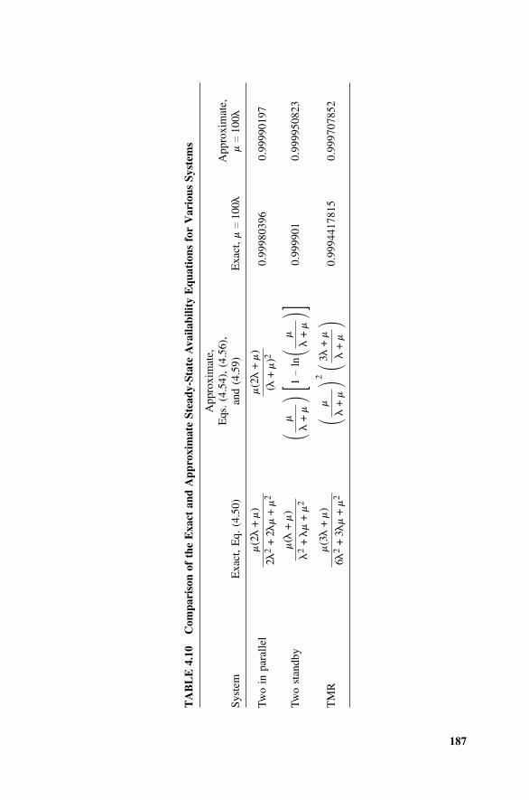
187
TA
BL
E4.
10C
ompa
riso
n of
the
Exa
ct a
nd A
ppro
xim
ate
Stea
dy-S
tate
Ava
ilabi
lity
Equ
atio
ns f
or V
ario
us S
yste
ms
App
roxi
mat
e,E
qs.
( 4.5
4),
(4.5
6),
App
roxi
mat
e,Sy
stem
Exa
ct,
Eq.
(4.
50)
and
(4.5
9)E
xact
,mc
100l
mc
100l
Two
in p
aral
lel
m(2
l+
m)
2l2
+2l
m+
m2
m(2
l+
m)
(l+
m)2
0.99
9803
960.
9999
0197
Two
stan
dby
m(l
+m
)l
2+
lm
+m
2�
m
l+
m� [1
−ln�
m
l+
m� ]
0.99
9901
0.99
9950
823
TM
Rm
(3l
+m
)6l
2+
3lm
+m
2�
m
l+
m�2
�3l+
m
l+
m�
0.99
9441
7815
0.99
9707
852
188 N-MODULAR REDUNDANCY
example. (This is essentially the same architecture that is embedded into theSpace Shuttle’s primary flight control system—discussed in Chapter 5 as anexample of software redundancy and shown in Fig. 5.19. However, if we focuson the first four computers in the primary flight control system, we have anexample of 4-level voting with lockout. The backup flight control system servesas an additional level of redundancy; it will be discussed in Chapter 5.)
The question arises of what to do with a failed system when N is greaterthan three. To provide a more detailed discussion, we introduce the fact thatfailures can be permanent as well as transient. Suppose that hardware B in Fig.5.19 experiences a failure and we know that it is permanent. There is no reasonto leave it in the circuit if we have a way to remove it. The reasoning is thatif there is a second failure, there is a possibility that the two failed elementswill agree and the two good elements will agree, creating a standoff. Clearly,this can be avoided if the first element is disconnected (locked out) from thecomparison. In the Space Shuttle control system, this is done by an astronautwho has access to onboard computer diagnostic information and also by con-sultation with Ground Control, which has access to telemetered data on thecontrol system. The switch shown at the output of each computer in Fig. 5.19is activated by an astronaut after appropriate deliberation and can be reversedat any time. NASA refers to this system as fail-safe–fail-operational, mean-ing that the system can experience two failures, can disconnect the two failedcomputers, and can have two remaining operating computers connected in acomparison arrangement. The flight rules that NASA uses to decide on safemodes of shuttle operation would rule on whether the shuttle must terminatea mission if only two valid computers in the primary system remain. In anyevent, there would clearly be an emergency situation in which the shuttle isstill in orbit and one of the two remaining computers fails. If other tests coulddetermine which computer gives valid information, then the system could con-tinue with a single computer. One such test would be to switch out one of thecomputers and see if the vehicle is still stable and handles properly. The com-puters could then be swapped, and stability and control can be observed forthe second computer. If such a test identifies the failed computer, the systemis still operating with one good computer. Clearly, with Ground Control andan astronaut dealing with an emergency, there is the possibility of switchingback in a previously disconnected computer in the hope that the old failurewas only a transient problem that no longer exists. Many of these cases areanalyzed and compared in the following paragraphs.
If we consider that the lockout works perfectly, the system will succeed ifthere are 0, 1, or 2 failures. The probability computation is simple using thebinomial distribution.
R(2 : 4) c B(4 : 4) + B(3 : 4) + B(2 : 4)
c [p4] + [4p3− 4p4] + [6p2
− 12p3 + 6p4]
c 3p4− 8p3 + 6p2 (4.60)
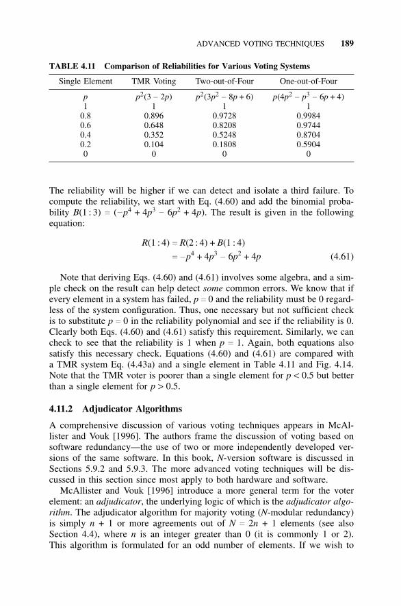
ADVANCED VOTING TECHNIQUES 189
TABLE 4.11 Comparison of Reliabilities for Various Voting Systems
Single Element TMR Voting Two-out-of-Four One-out-of-Four
p p2(3 − 2p) p2(3p2− 8p + 6) p(4p2
− p3− 6p + 4)
1 1 1 10.8 0.896 0.9728 0.99840.6 0.648 0.8208 0.97440.4 0.352 0.5248 0.87040.2 0.104 0.1808 0.59040 0 0 0
The reliability will be higher if we can detect and isolate a third failure. Tocompute the reliability, we start with Eq. (4.60) and add the binomial proba-bility B(1 : 3) c (−p4 + 4p3
− 6p2 + 4p). The result is given in the followingequation:
R(1 : 4) c R(2 : 4) + B(1 : 4)
c −p4 + 4p3− 6p2 + 4p (4.61)
Note that deriving Eqs. (4.60) and (4.61) involves some algebra, and a sim-ple check on the result can help detect some common errors. We know that ifevery element in a system has failed, p c 0 and the reliability must be 0 regard-less of the system configuration. Thus, one necessary but not sufficient checkis to substitute p c 0 in the reliability polynomial and see if the reliability is 0.Clearly both Eqs. (4.60) and (4.61) satisfy this requirement. Similarly, we cancheck to see that the reliability is 1 when p c 1. Again, both equations alsosatisfy this necessary check. Equations (4.60) and (4.61) are compared witha TMR system Eq. (4.43a) and a single element in Table 4.11 and Fig. 4.14.Note that the TMR voter is poorer than a single element for p < 0.5 but betterthan a single element for p > 0.5.
4.11.2 Adjudicator Algorithms
A comprehensive discussion of various voting techniques appears in McAl-lister and Vouk [1996]. The authors frame the discussion of voting based onsoftware redundancy—the use of two or more independently developed ver-sions of the same software. In this book, N-version software is discussed inSections 5.9.2 and 5.9.3. The more advanced voting techniques will be dis-cussed in this section since most apply to both hardware and software.
McAllister and Vouk [1996] introduce a more general term for the voterelement: an adjudicator, the underlying logic of which is the adjudicator algo-rithm. The adjudicator algorithm for majority voting (N-modular redundancy)is simply n + 1 or more agreements out of N c 2n + 1 elements (see alsoSection 4.4), where n is an integer greater than 0 (it is commonly 1 or 2).This algorithm is formulated for an odd number of elements. If we wish to
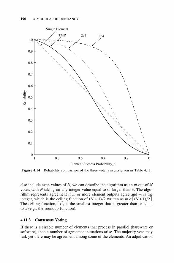
190 N-MODULAR REDUNDANCY
0
0.1
0.2
0.3
0.4
0.5
0.6
0.7
0.8
0.9
1.0
1 0.8 0.6 0.4 0.2 0
Element Success Probability, p
Rel
iabi
lity
Single Element
TMR 2:4 1:4
Figure 4.14 Reliability comparison of the three voter circuits given in Table 4.11.
also include even values of N, we can describe the algorithm as an m-out-of-Nvoter, with N taking on any integer value equal to or larger than 3. The algo-rithm represents agreement if m or more element outputs agree and m is theinteger, which is the ceiling function of (N + 1)/ 2 written as m ≥ (N + 1)/ 2.The ceiling function, x, is the smallest integer that is greater than or equalto x (e.g., the roundup function).
4.11.3 Consensus Voting
If there is a sizable number of elements that process in parallel (hardware orsoftware), then a number of agreement situations arise. The majority vote mayfail, yet there may be agreement among some of the elements. An adjudication
ADVANCED VOTING TECHNIQUES 191
algorithm can be defined for the consensus case, which is more complex thanmajority voting. Again, N is the number of parallel elements (N > 1) and k isthe largest number of element outputs that agree. The symbol Ok denotes theset of k-element outputs that agree. In some cases, there can be more than oneset of agreements, resulting in Oki , and the adjudication must choose betweenthe multiple agreements. A flow chart is given in Fig. 4.15 that is based onthe consensus voting algorithm in McAllister and Vouk [1996, p. 578].
If k c 1, there are obviously ties in the consensus algorithm. A similar situ-ation ensues if k > 1, but because there is more then one group with the samevalue of k, a tie-breaking algorithm must be used. One such algorithm is a randomchoice among the ties; another is to test the elements for correct operation, whichin terms of software version consensus is called acceptance testing of the soft-ware. Initially, such testing may seem better suited to software than to hardware;in reality, however, such is not the case because hardware testing has been used inthe past. The Carousel Inertial Navigation System used on the early Boeing 747and other aircraft had three stable platforms, three computers, and a redundancymanagement system that performed majority voting. One means of checking thevalidity of any of the computers was to submit a stored problem for solution andto check the results with a stored solution. The purpose was to help diagnose com-puter malfunctions and lock a defective computer out of the system. Also duringthe time when adaptive flight control systems were in use, some designs used testsignals mixed with the normal control signals. By comparing the input test sig-nals and the output response, one could measure the parameters of the aircraft(the coefficients of the governing differential equations) and dynamically adjustthe feedback signals for best control.
4.11.4 Test and Switch Techniques
The discussion in the previous section established the fact that hardware test-ing is possible in certain circumstances. Assuming that such testing has a highprobability of determining success or failure of an element and that two or moreelements are present, we can operate with element one alone as long as it testsvalid. When a failure of element one is detected, we can switch to element two,etc. The logic of such a system differs little from that of the standby systemshown in Fig. 3.12 for the case of two elements, but the detailed implementa-tion of test and switch may differ somewhat from the standby system. Whenthese concepts are applied to software, the adjudication algorithm becomes anacceptance test. The switch to an earlier state of the process before failure wasdetected and the substitution of a second version of the software is called roll-back and recovery, but the overall philosophy is generally referred to as therecovery block technique.
4.11.5 Pairwise Comparison
We assume that the number of elements is divisible by two, that is, N c 2n,where n is an integer greater than one. The outputs of modules are compared
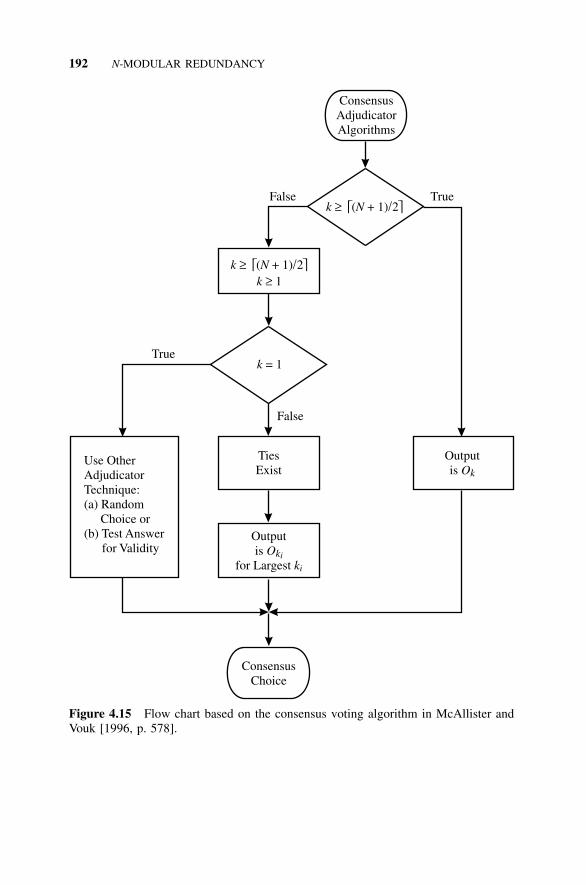
192 N-MODULAR REDUNDANCY
ConsensusAdjudicatorAlgorithms
k N( + 1) 2 /≥
k N( + 1) 2 /≥
k 1≥
k = 1
TiesExist
Outputis Ok
Outputis
for LargestO
kki
i
Use OtherAdjudicatorTechnique:(a) Random
Choice or(b) Test Answer
for Validity
ConsensusChoice
False True
True
False
Figure 4.15 Flow chart based on the consensus voting algorithm in McAllister andVouk [1996, p. 578].
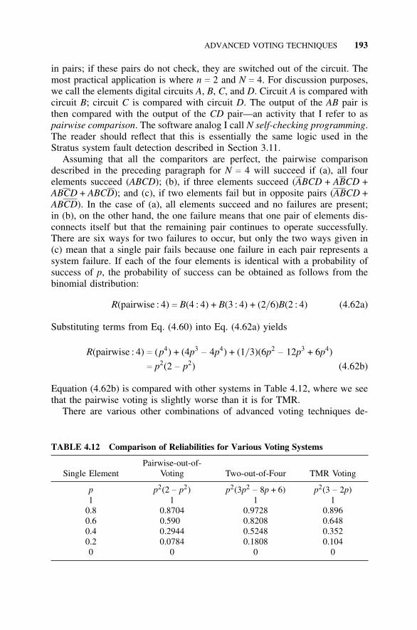
ADVANCED VOTING TECHNIQUES 193
in pairs; if these pairs do not check, they are switched out of the circuit. Themost practical application is where n c 2 and N c 4. For discussion purposes,we call the elements digital circuits A, B, C, and D. Circuit A is compared withcircuit B; circuit C is compared with circuit D. The output of the AB pair isthen compared with the output of the CD pair—an activity that I refer to aspairwise comparison. The software analog I call N self-checking programming.The reader should reflect that this is essentially the same logic used in theStratus system fault detection described in Section 3.11.
Assuming that all the comparitors are perfect, the pairwise comparisondescribed in the preceding paragraph for N c 4 will succeed if (a), all fourelements succeed (ABCD); (b), if three elements succeed (ABCD + ABCD +ABCD + ABCD); and (c), if two elements fail but in opposite pairs (ABCD +ABCD). In the case of (a), all elements succeed and no failures are present;in (b), on the other hand, the one failure means that one pair of elements dis-connects itself but that the remaining pair continues to operate successfully.There are six ways for two failures to occur, but only the two ways given in(c) mean that a single pair fails because one failure in each pair represents asystem failure. If each of the four elements is identical with a probability ofsuccess of p, the probability of success can be obtained as follows from thebinomial distribution:
R(pairwise : 4) c B(4 : 4) + B(3 : 4) + (2/ 6)B(2 : 4) (4.62a)
Substituting terms from Eq. (4.60) into Eq. (4.62a) yields
R(pairwise : 4) c (p4) + (4p3− 4p4) + (1/ 3)(6p2
− 12p3 + 6p4)
c p2(2 − p2) (4.62b)
Equation (4.62b) is compared with other systems in Table 4.12, where we seethat the pairwise voting is slightly worse than it is for TMR.
There are various other combinations of advanced voting techniques de-
TABLE 4.12 Comparison of Reliabilities for Various Voting Systems
Pairwise-out-of-Single Element Voting Two-out-of-Four TMR Voting
p p2(2 − p2) p2(3p2− 8p + 6) p2(3 − 2p)
1 1 1 10.8 0.8704 0.9728 0.8960.6 0.590 0.8208 0.6480.4 0.2944 0.5248 0.3520.2 0.0784 0.1808 0.1040 0 0 0
194 N-MODULAR REDUNDANCY
scribed by McAllister and Vouk [1996], who also compute and compare thereliability of many of these systems by assuming independent as well as depen-dent failures.
4.11.6 Adaptive Voting
Another technique for voting makes use of the fact that some circuit failuremodes are intermittent or transient. In such a case, one does not wish to lockout (i.e., ignore) a circuit when it is behaving well (but when it is malfunc-tioning, it should be ignored). The technique of adaptive voting can be used toautomatically switch between these situations [Pierce, 1961; Shooman, 1990,p. 324; Siewiorek, 1992, pp. 174, 178–182].
An ordinary majority voter may be visualized as a device that takes theaverage of the outputs and gives a one output if the average is > 0.5 and azero output if the average is ≤ 0.5. (In the case of software outputs, a range ofvalues not limited to the range 0–1 will occur, and one can deal with variouspoint estimates such as the average, the arithmetic mean of the min and maxvalues, or, as McAllister and Vouk suggest, the median.) An adaptive voter maybe viewed as a weighted sum where each outpt xi is weighted by a coefficient.The coefficient ai could be adjusted to equal the probability that the output xi
was correct. Thus the test quantity of the adaptive voter (with an even numberof elements) would be given by
a1x1 + a2x2 + · · · + a2n + 1x2n + 1
a1 + a2 + · · · + a2n + 1(4.63)
The coefficients ai can be adjusted dynamically by taking statistics on theagreement between each xi and the voter output over time. Another techniqueis to periodically insert test inputs and compare each output xi with the known(i.e., precomputed) correct output. If some xi is frequently in error, it should bedisconnected. The adaptive voter adjusts ai to be a very small number, whichis in essence the same thing. The reliability of the adaptive-voter scheme issuperior to the ordinary voter; however, there are design issues that must beresolved to realize an adaptive voter in practice.
The reader will appreciate that there are many choices for an adjudicatoralgorithm that yield an associated set of architectures. However, cost, volume,weight, and simplicity considerations generally limit the choices to a few ofthe simpler configurations. For example, when majority voting is used, it isgenerally limited to TMR or, in the case of the Space Shuttle example, 4-levelvoting with lockout. The most complex arrangement the author can rememberis a 5-level majority logic system used to control the Apollo Mission’s mainSaturn engine. For the Space Shuttle and Carousel navigation system exam-ples, the astronauts/ pilots had access to other information, such as previousproblems with individual equipment and ground-based measurements or obser-vations. Thus the accessibility of individual outputs and possible tests allow
REFERENCES 195
human operators to organize a wide variety of behaviors. Presently, commer-cial airliners are switching from inertial navigation systems to navigation usingthe satellite-based Global Positioning System (GPS). Handheld GPS receivershave dropped in price to the $100–$200 range, so one can imagine every airlinepilot keeping one in his or her flight bag as a backup. A similar trend occurredin the 1780s when pocket chronometers dropped in price to less than £65.Ship captains of the East India Company as well as those of the Royal Navy(who paid out of their own pockets) eagerly bought these accurate watches tocalculate longitude while at sea [Sobel, 1995, p. 162].
REFERENCES
Arsenault, J. E., and J. A. Roberts. Reliability and Maintainability of Electronic Sys-tems. Computer Science Press, Rockville, MD, 1980.
Avizienis, A., H. Kopetz, and J.-C. Laprie (eds.). Dependable Computing and Fault-Tolerant Systems. Springer-Verlag, New York, 1987.
Battaglini, G., and B. Ciciani. Realistic Yield-Evaluation of Fault-Tolerant Program-mable-Logic Arrays. IEEE Transactions on Reliability (September 1998): 212–224.
Bell, C. G., and A. Newel-Pierce. Computer Structures: Readings and Examples.McGraw-Hill, New York, 1971.
Calabro, S. R. Reliability Principles and Practices. McGraw-Hill, New York, 1962.
Cardan, J. The Book of my Life (trans. J. Stoner). Dover, New York, 1963.
Cardano, G. Ars Magna. 1545.
Grisamone, N. T. Calculation of Circuit Reliability by Use of von Neuman RedundancyLogic Analysis. IEEE Proceedings of the Fourth Annual Conference on ElectronicReliability, October 1993. IEEE, New York, NY.
Hall, H. S., and S. R. Knight. Higher Algebra. 1887. Reprint, Macmillan, New York,1957.
Iyanaga, S., and Y. Kawanda (eds.). Encyclopedic Dictionary of Mathematics. MITPress, Cambridge, MA, 1980.
Knox-Seith, J. K. A Redundancy Technique for Improving the Reliability of DigitalSystems. Stanford Electronics Laboratory Technical Report No. 4816-1. StanfordUniversity, Stanford, CA, December 1963.
McAllister, D. F., and M. A. Vouk. “Fault-Tolerant Software Reliability Engineering.”In Handbook of Software Reliability Engineering, M. R. Lyu (ed.). McGraw-Hill,New York, 1996, ch. 14, pp. 567–614.
Miller, E. Reliability Aspects of the Variable Instruction Computer. IEEE Transactionson Electronic Computing 16, 5 (October 1967): 596.
Moore, E. F., and C. E. Shannon. Reliable Circuits Using Less Reliable Relays. Journalof the Franklin Institute 2 (October 1956).
Pham, H. (ed.). Fault-Tolerant Software Systems: Techniques and Applications. IEEEComputer Society Press, New York, 1992.
Pierce, W. H. Improving the Reliability of Digital Systems by Redundancy and Adap-
196 N-MODULAR REDUNDANCY
tation. Stanford Electronics Laboratory Technical Report No. 1552-3, Stanford, CA:Stanford University, July 17, 1961.
Pierce, W. H. Failure-Tolerant Computer Design. Academic Press, Rockville, NY,1965.
Randell, B. The Origins of Digital Computers—Selected Papers. Springer-Verlag, NewYork, 1975.
Shannon, C. E., and J. McCarthy (eds.). Probabilistic Logics and the Synthesis of Reli-able Organisms from Unreliable Components. In Automata Studies, by J. von Neu-man. Princeton University Press, Princeton, NJ, 1956.
Shiva, S. G. Introduction to Logic Design. Scott Foresman and Company, Glenview,IL, 1988.
Shooman, M. L. Probabilistic Reliability: An Engineering Approach. McGraw-Hill,New York, 1968.
Shooman, M. L. Probabilistic Reliability: An Engineering Approach, 2d ed. Krieger,Melbourne, FL, 1990.
Siewiorek, D. P., and R. S. Swarz. The Theory and Practice of Reliable System Design.The Digital Press, Bedford, MA, 1982.
Siewiorek, D. P., and R. S. Swarz. Reliable Computer Systems Design and Evaluation,2d ed. The Digital Press, Bedford, MA, 1992.
Siewiorek, D. P., and R. S. Swarz. Reliable Computer Systems Design and Evaluation,3d ed. A. K. Peters, www.akpeters.com, 1998.
Sobel, D. Longitude. Walker and Company, New York, 1995.Toy, W. N. Dual Versus Triplication Reliability Estimates. AT&T Technical Journal
(November/December 1987): 15–20.Traverse, P. AIRBUS and ATR System Architecture and Specification. In Software
Diversity in Computerized Control Systems, U. Voges (ed.), vol. 2 of DependableComputing and Fault-Tolerant Systems, A. Avizienis (ed.). Springer-Verlag, NewYork, 1987, pp. 95–104.
Vouk, M. A., D. F. McAllister, and K. C. Tai. Identification of Correlated Failures ofFault-Tolerant Software Systems. Proceedings of COMSAC ’85, 1985, pp. 437–444.
Vouk, M. A., A. Pradkar, D. F. McAllister, and K. C. Tai. Modeling Execution Times ofMultistage N-Version Fault-Tolerant Software. Proceedings of COMSAC ’90, 1990,pp. 505–511. (Also printed in Pham [1992], pp. 55–61.)
Vouk, M. A. et al. An Empirical Evaluation of Consensus Voting and Consensus Recov-ery Block Reliability in the Presence of Failure Correlation. Journal of Computerand Software Engineering 1, 4 (1993): 367–388.
Wakerly, J. F. Digital Design Principles and Practice, 2d ed. Prentice-Hall, EnglewoodCliffs, NJ, 1994.
Wakerly, J. F. Digital Design Principles 2.1. Student CD-ROM package. Prentice-Hall,Englewood Cliffs, NJ, 2001.
PROBLEMS
4.1. Derive the equation analogous to Eq. (4.9) for a four-element majorityvoting scheme.
PROBLEMS 197
4.2. Derive the equation analogous to Eq. (4.9) for a five-element majorityvoting scheme.
4.3. Verify the reliability functions sketched in Fig. 4.2.
4.4. Compute the reliability of a 3-level majority voting system for the casewhere the failure rate is constant, l c 10−4 failures per hour, and t c1,000 hours. Compare this with the reliability of a single system.
4.5. Repeat problem 4.4 for a 5-level majority voting system.
4.6. Compare the results of problem 4.4 with a single system: two elementsin parallel, two elements in standby.
4.7. Compare the results of problem 4.5 with a single system: two elementsin parallel, two elements in standby.
4.8. What should the reliability of the voter be if it increases the probabilityof failure of the system of problem 4.4 by 10%?
4.9. Compute the reliability at t c 1,000 hours of a system composed of aseries connection of module 1 and module 2, each with a constant failurerate of l1 c 0.5 × 10⁻⁴ failures per hour. If we design a 3-level majorityvoting system that votes on the outputs of module 2, we have the samesystem as in problem 4.4. However, if we vote at the outputs of modules1 and 2, we have an improved system. Compute the reliability of thissystem and compare it with problem 4.4.
4.10. Expand the reliability functions in series in the high-reliability region forthe TMR 3–2–1 system and the TMR 3–2 system for the three systemsof Fig. 4.3. [Include more terms than in Eqs. (4.14)–(4.16).]
4.11. Compute the MTTF for the expansions of problem 4.10, compare thesewith the exact MTTF for these systems, and comment.
4.12. Verify that an expansion of Eqs. (4.3a, b) leads to seven terms in additionto the term one, and that this leads to Eqs. (4.5a, b) and (4.6a, b).
4.13. The approximations used in plotting Fig. 4.3 are less accurate for thelarger values of l t. Recompute the values using the exact expressionsand comment on the accuracy of the approximations.
4.14. Inspection of Fig. 4.4 shows that N-modular redundancy is of no advan-tage over a single unit at t c 0 (they both have a reliability of 1) and atl t c 0.69 (they both have a reliability of 0.5). The maximum advantageof N-modular redundancy is realized somewhere in between them. Com-pute the ratio of the N-modular redundancy given by Eq. (4.17) dividedby the reliability of a single system that equals p. Maximize (i.e., dif-ferentiate this ratio with respect to p and set equal to 0) to solve for thevalue of p that gives the biggest improvement in reliability. Since p c e−l t ,what is the value of l t that corresponds to the optimum value of p?
198 N-MODULAR REDUNDANCY
4.15. Repeat problem 4.14 for the case of component redundancy and majorityvoting as shown in Fig. 4.5 by using the reliability equation given in Eq.(4.18).
4.16. Verify Grisamone’s results given in Table 4.1.
4.17. Develop a reliability expression for the system of Fig. 4.8 assuming that(1): All circuits Ai, Bi, Ci, and the voters Vi are independent circuits orindependent integrated circuit chips.
4.18. Develop a reliability expression for the system of Fig. 4.8 assuming that(2): All circuits Ai, Bi, and Ci are independent circuits or independentintegrated circuit chips and the voters Vi, V′i , and V′′i are all on the samechip.
4.19. Develop a reliability expression for the system of Fig. 4.8 assuming that(3): All voters Vi, V′i , and V′′i are independent circuits or independentintegrated circuit chips and circuits Ai, Bi, and Ci are all on the samechip.
4.20. Develop a reliability expression for the system of Fig. 4.8 assuming that(4): All circuits Ai, Bi, and Ci and all voters Vi, V′i , and V′′i are all onthe same chip.
4.21. Section 4.5.3 discusses the difference between various failure models.Compare the reliability of a 1-bit TMR system under the following fail-ure model assumptions:(a) The failures are always s-a-1.(b) The failures are always s-a-0.(c) The circuits fail so that they always give the complement of the
correct output.(d) The circuits fail at a transient rate lt and produce the complement
of the correct output.
4.22. Repeat problem 4.21, but instead of calculating the reliability, calculatethe probability that any one transmission is in error.
4.23. The circuit of Fig. 4.10 for a 32-bit word leads to a 512-gate circuitas described in this chapter. Using the information in Fig. B7, calculatethe reliability of the voter and warning circuit. Using Eq. (4.19) andassuming that the voter reliability decreases the system reliability to 90%of what would be achieved with a perfect voter, calculate pc. Again usingFig. B7, calculate the equivalent gate complexity of the digital circuit inthe TMR scheme.
4.24. Repeat problem 4.10 for an r-level voting system.
4.25. Drive a set of Markov equations for the model given in Fig. 4.11 andshow that the solution of each equation leads to Eqs. (4.25a–c).
PROBLEMS 199
4.26. Formulate a four-state model related to Fig. 4.11, as discussed in thetext, where the component states two failures and three failures are notmerged but are distinct. Solve the model for the four-state probabilitiesand show that the first two states are identical with Eqs. (4.25a, b) andthat the sum of the third and fourth states equals Eq. (4.25c).
4.27. Compare the effects of repair on TMR reliability by plotting Eq. (4.27e),including the third term, with Eq. (4.27d). Both equations are to be plot-ted versus time for the cases where m c 10l, m c 25l, and m c 100l.
4.28. Over what time range will the graphs in the previous problem be valid?(Hint: When will the next terms in the series become significant?)
4.29. The logic function for a voter was simplified in Eq. (4.23) and Table 4.5.Suppose that all four minterms given in Table 4.5 were included withoutsimplification, which provides some redundancy. Compare the reliabilityof the unminimized voter with the minimized voter (cf. Shooman [1990,p. 324]).
4.30. Make a model for coupler reliability and for a TMR voter. Compare thereliability of two elements in parallel with that for a TMR.
4.31. Repeat problem 4.30 when both systems include repair.
4.32. Compare the MTTF of the systems in Table 3.4 with TMR and 5MRvoter systems.
4.33. Repeat problem 4.32 for Table 3.5.
4.34. Compute the initial reliability for the systems of Tables 3.4 and 3.5 andcompare with TMR and 5MR voter systems.
4.35. Sketch and compare the initial reliabilities of TMR and 5MR Eqs.(4.27d) and (4.39b). Both equations are to be plotted versus time forthe cases where m c 0, m c 10l, m c 25l, and m c 100l. Note that form c 100l and for points where the reliability has decreased to 0.99 or0.95, the series approximations may need additional terms.
4.36. Check the values in Table 4.6.
4.37. Check the series expansions and the values in Table 4.7.
4.38. Plot the initial reliability of the four systems in Table 4.7. Calculate thenext term in the series expansion and evaluate the time at which it rep-resents a 10% correction in the unreliability. Draw a vertical bar on thecurve at this point. Repeat for each of the systems yielding a comparisonof the reliabilities and a range of validity of the series expressions.
4.39. Compare the voter circuit and reliability of (a) a TMR system, (b) a5MR system, and (c) five parallel elements with a coupler. Assume thevoters and the coupler are imperfect. Compute and plot the reliability.
200 N-MODULAR REDUNDANCY
4.40. What time interval will be needed before the repair terms in the com-parison made in problem 4.39 become significant?
4.41. It is assumed that a standby element cannot fail when it is in standby.However, this is not always true for many reasons; for example, batter-ies discharge in standby, corrosion can occur, and insulation can breakdown, all of which may significantly change the comparison. How largecan the standby failure rate be and still be ignored?
4.42. The reliability of the coupling device in a standby or parallel system ismore complex than the voter reliability in a TMR circuit. These effectson availability may be significant. How large can the coupling failurerate be and still be ignored?
4.43. Repair in any of these systems is predicted by knowing when a systemhas failed. In the case of TMR, we gave a simple logic circuit that woulddetect which element has failed. What is the equivalent detection circuitin the case of a parallel or standby system and what are the effects?
4.44. Check the values in Table 4.9.
4.45. Check the values in Table 4.10.
4.46. Add another line to Table 4.10 for 5-level modular redundancy.
4.47. Check the computations given in Tables 4.11 and 4.12.
4.48. Determine the range of p for which the various systems in Table 4.11are superior to a single element.
4.49. Determine the range of p for which the various systems in Table 4.12are superior to a single element.
4.50. Explain how a system based on the adaptive voting algorithm of Eq.(4.63) will operate if 50% of all failures are transient and clear in ashort period of time.
4.51. Explain how a system based on the adaptive voting algorithm of Eq.(4.63) will operate if it is basically a TMR system and 50% of all elementone failures are transient and 25% of all elements two and three failuresare transient.
4.52. Repeat and verify the availability computations in the last paragraph ofSection 4.9.2.
4.53. Compute the auto availability of a two-car family in which both the hus-band and wife need a car every day. Repeat the computation if a singlecar will serve the family in a pinch while the other car gets repaired.(See the brief discussion of auto reliability in Section 3.10.1 for failureand repair rates.)
4.54. At the end of Section 4.9.2 before the final numerical example, three
PROBLEMS 201
factors not included in the model were listed. Discuss how you wouldmodel these effects for a more complex Markov model.
4.55. Can you suggest any approximate procedures to determine if any of theeffects in problem 4.54 are significant?
4.56. Repeat problem 4.39 for the system availability. Make approximationswhere necessary.
4.57. Repeat problem 4.30 for system availability.
4.58. Repeat the derivation of Eq. (4.26c).
4.59. Repeat the derivation of Eq. (4.37).
4.60. Check the values given in Table 4.9.
4.61. Derive Eq. (4.59).
5SOFTWARE RELIABILITY ANDRECOVERY TECHNIQUES
Reliability of Computer Systems and Networks: Fault Tolerance, Analysis, and DesignMartin L. Shooman
Copyright 2002 John Wiley & Sons, Inc.ISBNs: 0-471-29342-3 (Hardback); 0-471-22460-X (Electronic)
202
5.1 INTRODUCTION
The general approach in this book is to treat reliability as a system problemand to decompose the system into a hierarchy of related subsystems or com-ponents. The reliability of the entire system is related to the reliability of thecomponents by some sort of structure function in which the components mayfail independently or in a dependent manner. The discussion that follows willmake it abundantly clear that software is a major “component” of the systemreliability,1 R. The reason that a separate chapter is devoted to software reli-ability is that the probabilistic models used for software differ from those usedfor hardware; moreover, hardware and software (and human) reliability can becombined only at a very high system level. (Section 5.8.5 discusses a macro-software reliability model that allows hardware and software to be combined ata lower level.) Specifically, if the hardware, software, and human failures areindependent (often, this is not the case), one can express the system reliabil-ity, RSY, as the product of the hardware reliability, RH , the software reliability,RS, and the human operator reliability, RO. Thus, if independence holds, onecan model the reliability of the various factors separately and combine them:RSY c RH × RS × RO [Shooman, 1983, pp. 351–353].
This chapter will develop models that can be used for the software reliabil-ity. These models are built upon the principles of continuous random variables
1Another important “component” of system reliability is human reliability if an operator isinvolved in any control, monitoring, input, or similar task. A discussion of human reliabilitymodels is beyond the scope of this book; the reader is referred to Dougherty and Fragola [1988].
INTRODUCTION 203
developed in Appendix A, Sections A6 and A7, and Appendix B, Section B3;the reader may wish to review these concepts while reading this chapter.
Clearly every system that involves a digital computer also includes a signif-icant amount of software used to control system operation. It is hard to thinkof a modern business system, such as that used for information, transportation,communication, or government, that is not heavily computer-dependent. Themicroelectronics revolution has produced microprocessors and memory chipsthat are so cheap and powerful that they can be included in many commercialproducts. For example, a 1999 luxury car model contained 20–40 micropro-cessors (depending on which options were installed), and several models usedlocal area networks to channel the data between sensors, microprocessors, dis-plays, and target devices [New York Times, August 27, 1998]. Consumer prod-ucts such as telephones, washing machines, and microwave ovens use a hugenumber of embedded microcomponents. In 1997, 100 million microprocessorswere sold, but this was eclipsed by the sale of 4.6 billion embedded microcom-ponents. Associated with each microprocessor or microcomponent is memory,a set of instructions, and a set of programs [Pollack, 1999].
5.1.1 Definition of Software Reliability
One can define software engineering as the body of engineering and manage-ment technologies used to develop quality, cost-effective, schedule-meeting soft-ware. Software reliability measurement and estimation is one such technologythat can be defined as the measurement and prediction of the probability that thesoftware will perform its intended function (according to specifications) withouterror for a given period of time. Oftentimes, the design, programming, and test-ing techniques that contribute to high software reliability are included; however,we consider these techniques as part of the design process for the developmentof reliable software. Software reliability complements reliable software; both, infact, are important topics within the discipline of software engineering. Softwarerecovery is a set of fail-safe design techniques for ensuring that if some seriouserror should crash the program, the computer will automatically recover to reini-tialize and restart its program. The software succeeds during software recoveryif no crucial data is lost, or if an operational calamity occurs, but the recoverytransforms a total failure into a benign or at most a troubling, nonfatal “hiccup.”
5.1.2 Probabilistic Nature of Software Reliability
On first consideration, it seems that the outcome of a computer program isa deterministic rather than a probabilistic event. Thus one might say that theoutput of a computer program is not a random result. In defining the conceptof a random variable, Cramer [Chapter 13, 1991] talks about spinning a coin asan experiment and the outcome (heads or tails) as the event. If we can controlall aspects of the spinning and repeat it each time, the result will always bethe same; however, such control needs to be so precise that it is practically
204 SOFTWARE RELIABILITY AND RECOVERY TECHNIQUES
impossible to repeat the experiment in an identical manner. Thus the event(heads or tails) is a random variable. The remainder of this section developsa similar argument for software reliability where the random element in thesoftware is the changing set of inputs.
Our discussion of the probabilistic nature of software begins with an exam-ple. Suppose that we write a computer program to solve the roots r1 and r2
of a quadratic equation, Ax2 + Bx + C c 0. If we enter the values 1, 5, and 6for A, B, and C, respectively, the roots will be r1 c −2 and r2 c −3. A sin-gle test of the software with these inputs confirms the expected results. Exactrepetition of this experiment with the same values of A, B, and C will alwaysyield the same results, r1 c −2 and r2 c −3, unless there is a hardware failureor an operating system problem. Thus, in the case of this computer program,we have defined a deterministic experiment. No matter how many times werepeat the computation with the same values of A, B, and C, we obtain the sameresult (assuming we exclude outside influences such as power failures, hard-ware problems, or operating system crashes unrelated to the present program).Of course, the real problem here is that after the first computation of r1 c −2and r2 c −3 we do no useful work to repeat the same identical computation.To do useful work, we must vary the values of A, B, and C and compute theroots for other input values. Thus the probabilistic nature of the experiment,that is, the correctness of the values obtained from the program for r1 and r2,is dependent on the input values A, B, and C in addition to the correctness ofthe computer program for this particular set of inputs.
The reader can readily appreciate that when we vary the values of A, B, andC over the range of possible values, either during test or operation, we wouldsoon see if the software developer achieved an error-free program. For exam-ple, was the developer wise enough to treat the problem of imaginary roots?Did the developer use the quadratic formula to solve for the roots? How, then,was the case of A c 0 treated where there is only one root and the quadraticformula “blows up” (i.e., leads to an exponential overflow error)? Clearly, weshould test for all these values during development to ensure that there are noresidual errors in the program, regardless of the input value. This leads to theconcept of exhaustive testing, which is always infeasible in a practical problem.Suppose in the quadratic equation example that the values of A, B, and C wererestricted to integers between +1,000 and −1,000. Thus there would be 2,000values of A and a like number of values of B and C. The possible input spacefor A, B, and C would therefore be (2,000)3
c 8 billion values.2 Suppose that
2In a real-time system, each set of input values enters when the computer is in a different “initialstate,” and all the initial states must also be considered. Suppose that a program is designed tosum the values of the inputs for a given period of time, print the sum, and reset. If there is ahigh partial sum, and a set of inputs occurs with large values, overflow may be encountered. Ifthe partial sum were smaller, this same set of inputs would therefore cause no problems. Thus,in the general case, one must consider the input space to include all the various combinations ofinputs and states of the system.
THE MAGNITUDE OF THE PROBLEM 205
we solve for each value of roots, substitute in the original equation to check,and only print out a result if the roots when substituted do not yield a zeroof the equation. If we could process 1,000 values per minute, the exhaustivetest would require 8 million minutes, which is 5,556 days or 15.2 years. Thisis hardly a feasible procedure: any such computation for a practical probleminvolves a much larger test space and a more difficult checking procedure thatis impossible in any practical sense. In the quadratic equation example, therewas a ready means of checking the answers by substitution into the equation;however, if the purpose of the program is to calculate satellite orbits, and if1 million combinations of input parameters are possible, then a person(s) orcomputer must independently obtain the 1 million right answers and checkthem all! Thus the probabilistic nature of software reliability is based on thevarying values of the input, the huge number of input cases, the initial systemstates, and the impossibility of exhaustive testing.
The basis for software reliability is quite different than the most commoncauses of hardware reliability. Software development is quite different fromhardware development, and the source of software errors (random discoveryof latent design and coding defects) differs from the source of most hard-ware errors (equipment failures). Of course, some complex hardware does havelatent design and assembly defects, but the dominant mode of hardware fail-ures is equipment failures. Mechanical hardware can jam, break, and becomeworn-out, and electrical hardware can burn out, leaving a short or open circuitor some other mode of failure. Many who criticize probabilistic modeling ofsoftware complain that instructions do not wear out. Although this is a truestatement, the random discovery of latent software defects is indeed just asdamaging as equipment failures, even though it constitutes a different modeof failure.
The development of models for software reliability in this chapter beginswith a study of the software development process in Section 5.3 and continueswith the formulation of probabilistic models in Section 5.4.
5.2 THE MAGNITUDE OF THE PROBLEM
Modeling, predicting, and measuring software reliability is an important quan-titative approach to achieving high-quality software and growth in reliabil-ity as a project progresses. It is an important management and engineeringdesign metric; most software errors are at least troublesome—some are veryserious—so the major flaws, once detected, must be removed by localization,redesign, and retest.
The seriousness and cost of fixing some software problems can be appreci-ated if we examine the Year 2000 Problem (Y2K). The largely overrated fearsoccurred because during the early days of the computer revolution in the 1960sand 1970s, computer memory was so expensive that programmers used manytricks and shortcuts to save a little here and there to make their programs oper-
206 SOFTWARE RELIABILITY AND RECOVERY TECHNIQUES
ate with smaller memory sizes. In 1965, the cost of magnetic-core computermemory was expensive at about $1 per word and used a significant operatingcurrent. (Presently, microelectronic memory sells for perhaps $1 per megabyteand draws only a small amount of current; assuming a 16-bit word, this costhas therefore been reduced by a factor of about 500,000!) To save memory,programmers reserved only 2 digits to represent the last 2 digits of the year.They did not anticipate that any of their programs would survive for morethan 5–10 years; moreover, they did not contemplate the problem that for theyear 2000, the digits “00” could instead represent the year 1900 in the soft-ware. The simplest solution was to replace the 2-digit year field with a 4-digitone. The problem was the vast amount of time required not only to search forthe numerous instances in which the year was used as input or output data orused in intermediate calculations in existing software, but also to test that thechanges have been successful and have not introduced any new errors. Thisproblem was further exacerbated because many of these older software pro-grams were poorly documented, and in many cases they were translated fromone version to another or from one language to another so they could be usedin modern computers without the need to be rewritten. Although only minorproblems occurred at the start of the new century, hundreds of millions of dol-lars had been expended to make a few changes that would only have been triv-ial if the software programs had been originally designed to prevent the Y2Kproblem.
Sometimes, however, efforts to avert Y2K software problems created prob-lems themselves. One such case was that of the 7-Eleven convenience storechain. On January 1, 2001, the point-of-sale system used in the 7-Eleven storesread the year “2001” as “1901,” which caused it to reject credit cards if theywere used for automatic purchases (manual credit card purchases, in additionto cash and check purchases, were not affected). The problem was attributedto the system’s software, even though it had been designed for the 5,200-storechain to be Y2K-compliant, had been subjected to 10,000 tests, and worked fineduring 2000. (The chain spent 8.8 million dollars—0.1% of annual sales—forY2K preparation from 1999 to 2000.) Fortunately, the bug was fixed within 1day [The Associated Press, January 4, 2001].
Another case was that of Norway’s national railway system. On the morningof December 31, 2000, none of the new 16 airport-express trains and 13 high-speed signature trains would start. Although the computer software had beenchecked thoroughly before the start of 2000, it still failed to recognize thecorrect date. The software was reset to read December 1, 2000, to give theGerman maker of the new trains 30 days to correct the problem. None of theolder trains were affected by the problem [New York Times, January 3, 2001].
Before we leave the obvious aspects of the Y2K problem, we should con-sider how deeply entrenched some of these problems were in legacy software:old programs that are used in their original form or rejuvenated for extendeduse. Analysts have found that some of the old IBM 9020 computers usedin outmoded components of air traffic control systems contain an algorithm

SOFTWARE DEVELOPMENT LIFE CYCLE 207
in their microcode for switching between the two redundant cooling pumpseach month to even the wear. (For a discussion of cooling pumps in typi-cal IBM computers, see Siewiorek [1992, pp. 493, 504].) Nobody seemed toknow how this calendar-sensitive algorithm would behave in the year 2000!The engineers and programmers who wrote the microcode for the 9020s hadretired before 2000, and the obvious answer—replace the 9020s with moderncomputers—proceeded slowly because of the cost. Although no major prob-lems occurred, the scare did bring to the attention of many managers the poten-tial problems associated with the use of legacy software.
Software development is a lengthy, complex process, and before the focus ofthis chapter shifts to model building, the development process must be studied.
5.3 SOFTWARE DEVELOPMENT LIFE CYCLE
Our goal is to make a probabilistic model for software, and the first step in anymodeling is to understand the process [Boehm, 2000; Brooks, 1995; Pfleerer,1998; Schach, 1999; and Shooman, 1983]. A good approach to the study of thesoftware development process is to define and discuss the various phases ofthe software development life cycle. A common partitioning of these phasesis shown Table 5.1. The life cycle phases given in this table apply directlyto the technique of program design known as structured procedural program-ming (SPP). In general, it also applies with some modification to the newerapproach known as object-oriented programming (OOP). The details of OOP,including the popular design diagrams used for OOP that are called the uni-versal modeling language (UMLs), are beyond the scope of this chapter; thereader is referred to the following references for more information: [Booch,1999; Fowler, 1999; Pfleerer, 1998; Pooley, 1999; Pressman, 1997; and Schach,1999]. The remainder of this section focuses on the SPP design technique.
5.3.1 Beginning and End
The beginning and end of the software development life cycle are the startof the project and the discard of the software. The start of a project is gen-erally driven by some event; for example, the head of the Federal AviationAdministration (FAA) or of some congressional committee decides that theUnited States needs a new air traffic control system, or the director of mar-keting in a company proposes to a management committee that to keep thecompany’s competitive edge, it must develop a new database system. Some-times, a project starts with a written needs document, which could be an inter-nal memorandum, a long-range plan, or a study of needed improvements in aparticular field. The necessity is sometimes a business expansion or evolution;for example, a company buys a new subsidiary business and finds that its oldpayroll program will not support the new conglomeration, requiring an updatedpayroll program. The needs document generally specifies why new software is

208 SOFTWARE RELIABILITY AND RECOVERY TECHNIQUES
TABLE 5.1 Project Phases for the Software Development Life Cycle
Phase Description
Start of project Initial decision or motivation for the project, includingoverall system parameters.
Needs A study and statement of the need for the software andwhat it should accomplish.
Requirements Algorithms or functions that must be performed, includingfunctional parameters.
Specifications Details of how the tasks and functions are to beperformed.
Design of prototype Construction of a prototype, including coding and testing.Prototype: System Evaluation by both the developer and the customer of
test how well the prototype design meets the requirements.Revision of Prototype system tests and other information may reveal
specifications needed changes.Final design Design changes in the prototype software in response to
discovered deviations from the original specificationsor the revised specifications, and changes to improveperformance and reliability.
Code final design The final implementation of the design.Unit test Each major unit (module) of the code is individually
tested.Integration test Each module is successively inserted into the pretested
control structure, and the composite is tested.System test Once all (or most) of the units have been integrated,
the system operation is tested.Acceptance test The customer designs and witnesses a test of the system to
see if it meets the requirements.Field deployment The software is placed into operational use.Field maintenance Errors found during operation must be fixed.Redesign of the A new contract is negotiated after a number of years of
system operation to include changes and additional features.The aforementioned phases are repeated.
Software discard Eventually, the software is no longer updated or correctedbut discarded, perhaps to be replaced by new software.
needed. Generally, old software is discarded once new, improved software isavailable. However, if one branch of an organization decides to buy new soft-ware and another branch wishes to continue with its present version, it maybe difficult to define the end of the software’s usage. Oftentimes, the discard-ing takes place many years beyond what was originally envisioned when thesoftware was developed or purchased. (In many ways, this is why there wasa Y2K problem: too few people ever thought that their software would last tothe year 2000.)
SOFTWARE DEVELOPMENT LIFE CYCLE 209
5.3.2 Requirements
The project formally begins with the drafting of a requirements document forthe system in response to the needs document or equivalent document. Initially,the requirements constitute high-level system requirements encompassing boththe hardware and software. In a large project, as the requirements document“matures,” it is expanded into separate hardware and software requirements;the requirements will specify what needs to be done. For an air traffic controlsystem (ATC), the requirements would deal with the ATC centers that theymust serve, the present and expected future volume of traffic, the mix of air-craft, the types of radar and displays used, and the interfaces to other ATCcenters and the aircraft. Present travel patterns, expected growth, and expectedchanges in aircraft, airport, and airline operational characteristics would alsobe reflected in the requirements.
5.3.3 Specifications
The project specifications start with the requirements and the details of howthe software is to be designed to satisfy these requirements. Continuing withour air traffic control system example, there would be a hardware specifica-tions document dealing with (a) what type of radar is used; (b) the kinds ofdisplays and display computers that are used; (c) the distributed computers ormicroprocessors and memory systems; (d) the communications equipment; (e)the power supplies; and (f) any networks that are needed for the project. Thesoftware specifications document will delineate (a) what tracking algorithm touse; (b) how the display information for the aircraft will be handled; (c) howthe system will calculate any potential collisions; (d) how the information willbe displayed; and (e) how the air traffic controller will interact with both thesystem and the pilots. Also, the exact nature of any required records of a tech-nical, managerial, or legal nature will be specified in detail, including howthey will be computed and archived. Particular projects often use names dif-ferent from requirements and specifications (e.g., system requirements versussoftware specifications and high-level versus detailed specifications), but theircontent is essentially the same. A combined hardware–software specificationmight be used on a small project.
It is always a difficult task to define when requirements give way to specifi-cations, and in the practical world, some specifications are mixed in the require-ments document and some sections of the specifications document actuallyseem like requirements. In any event, it is important that the why, the what,and the how of the project be spelled out in a set of documents. The complete-ness of the set of documents is more important than exactly how the variousideas are partitioned between requirements and specifications.
Several researchers have outlined or developed experimental systems thatuse a formal language to write the specifications. Doing so has introduced a for-malism and precision that is often lacking in specifications. Furthermore, since
210 SOFTWARE RELIABILITY AND RECOVERY TECHNIQUES
the formal specification language would have a grammar, one could build anautomated specification checker. With some additional work, one could alsodevelop a simulator that would in some way synthetically execute the specifi-cations. Doing so would be very helpful in many ways for uncovering missingspecifications, incomplete specifications, and conflicting specifications. More-over, in a very simple way, it would serve as a preliminary execution of thesoftware. Unfortunately, however, such projects are only in the experimentalor prototype stages [Wing, 1990].
5.3.4 Prototypes
Most innovative projects now begin with a prototype or rapid prototype phase.The purpose of the prototype is multifaceted: developers have an opportunity totry out their design ideas, the difficult parts of the project become rapidly appar-ent, and there is an early (imperfect) working model that can be shown to the cus-tomer to help identify errors of omission and commission in the requirements andspecification documents. In constructing the prototype, an initial control struc-ture (the main program coordinating all the parts) is written and tested along withthe interfaces to the various components (subroutines and modules). The variouscomponents are further decomposed into smaller subcomponents until the mod-ule level is reached, at which time programming or coding at the module levelbegins. The nature of a module is described in the paragraphs that follow.
A module is a block of code that performs a well-described function orprocedure. The length of a module is a frequently debated issue. Initially, itslength was defined as perhaps 50–200 source lines of code (SLOC). The SLOClength of a module is not absolute; it is based on the coder’s “intellectual spanof control.” Since a program listing contains about 50 lines, this means that amodule would be 1–4 pages long. The reasoning behind this is that it wouldbe difficult to read, analyze, and trace the control structures of a program thatextend beyond a few pages and keep all the logic of the program in mind;hence the term intellectual span of control. The concept of a module, moduleinterface, and rough bounds on module size are more directly applicable to anSPP approach than to that of an OOP; however, as with very large and complexmodules, very large and complex objects are undesirable.
Sometimes, the prototype progresses rapidly since old code from relatedprojects can be used for the subroutines and modules, or a “first draft” of thesoftware can be written even if some of the more complex features are left out.If the old code actually survives to the final version of the program, we speakof such code as reused code or legacy code, and if such reuse is significant,the development life cycle will be shortened somewhat and the cost will bereduced. Of course, the prototype code must be tested, and oftentimes when aprototype is shown to the customer, the customer understands that some fea-tures are not what he or she wanted. It is important to ascertain this as earlyas possible in the project so that revisions can be made in the specificationsthat will impact the final design. If these changes are delayed until late in

SOFTWARE DEVELOPMENT LIFE CYCLE 211
the project, they can involve major changes in the code as well as significantredesign and extensive retesting of the software, for which large cost overrunsand delays may be incurred. In some projects, the contracting is divided intotwo phases: delivery and evaluation of the prototype, followed by revisionsin the requirements and specifications and a second contract for the deliveredversion of the software. Some managers complain that designing a prototypethat is to be replaced by a final design is doing a job twice. Indeed it is; how-ever, it is the best way to develop a large, complex project. (See Chapter 11,“Plan to Throw One Away,” of Brooks [1995].) The cost of the prototype isnot so large if one considers that much of the prototype code (especially thecontrol structure) can be modified and reused for the final design and that theprototype test cases can be reused in testing the final design. It is likely thatthe same manager who objects to the use of prototype software would heartilyendorse the use of a prototype board (breadboard), a mechanical model, ora computer simulation to “work out the bugs” of a hardware design withoutrealizing that the software prototype is the software analog of these well-triedhardware development techniques.
Finally, we should remark that not all projects need a prototype phase. Con-sider the design of a fourth payroll system for a customer. Assume that thedevelopment organization specializes in payroll software and had developedthe last three payroll systems for the customer. It is unlikely that a prototypewould be required by either the customer or the developer. More likely, thedeveloper would have some experts with considerable experience study thepresent system, study the new requirements, and ask many probing questionsof the knowledgeable personnel at the customer’s site, after which they couldwrite the specifications for the final software. However, this payroll exampleis not the usual case; in most cases, prototype software is generally valuableand should be considered.
5.3.5 Design
Design really begins with the needs, requirements, and specifications docu-ments. Also, the design of a prototype system is a very important part ofthe design process. For discussion purposes, however, we will refer to thefinal design stage as program design. In the case of SPP, there are two basicdesign approaches: top–down and bottom–up. The top–down process beginswith the complete system at level 0; then, it decomposes this into a num-ber of subsystems at level 1. This process continues to levels 2 and 3, thendown to level n where individual modules are encountered and coded asdescribed in the following section. Such a decomposition can be modeledby a hierarchy diagram (H-diagram) such as that shown in Fig. 5.1(a). Thediagram, which resembles an inverted tree, may be modeled as a mathe-matical graph where each “box” in the diagram represents a node in thegraph and each line connecting the boxes represents a branch in the graph.A node at level k (the predecessor) has several successor nodes at level
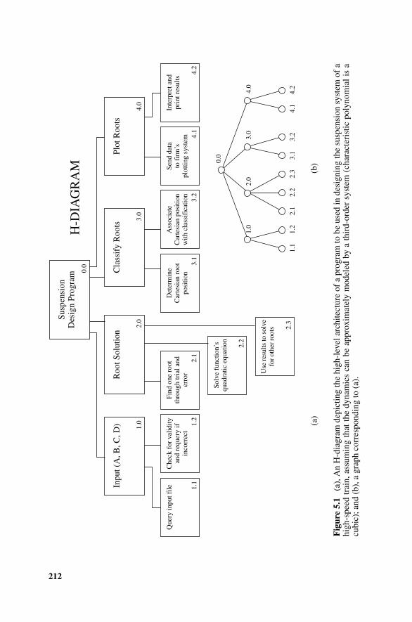
212
Ass
ocia
teC
arte
sian
posi
tion
with
clas
sifi
catio
n
Det
erm
ine
Car
tesi
anro
otpo
sitio
n
Find
one
root
thro
ugh
tria
l and
erro
r
Solv
efu
nctio
n’s
quad
ratic
equa
tion
Use
resu
ltsto
solv
efo
r oth
erro
ots
Che
ckfo
rva
lidity
and
requ
ery
ifin
corr
ect
Que
ryin
put f
ileSe
ndda
tato
firm
’spl
ottin
gsy
stem
Inte
rpre
t and
prin
t res
ults
Inpu
t (A
, B, C
, D)
Roo
t Sol
utio
n
Susp
ensi
onD
esig
n Pr
ogra
m Cla
ssif
y R
oots
Plot
Roo
ts
0.0
1.0
2.0
3.0
4.0
1.1
1.2
2.1
2.2
2.3
3.1
3.2
4.1
4.2
0.0
1.0
2.0
3.0
4.0
1.1
1.2
2.1
2.2
2.3
3.1
3.2
4.1
4.2
H-D
IAG
RA
M
(a)
(b)
Fig
ure
5.1
(a)
, An
H-d
iagr
am d
epic
ting
the
high
-lev
el a
rchi
tect
ure
of a
pro
gram
to b
e us
ed in
des
igni
ng th
e su
spen
sion
sys
tem
of
ahi
gh-s
peed
tra
in, a
ssum
ing
that
the
dyn
amic
s ca
n be
app
roxi
mat
ely
mod
eled
by
a th
ird-
orde
r sy
stem
(ch
arac
teri
stic
pol
ynom
ial
is a
cubi
c); a
nd (
b), a
gra
ph c
orre
spon
ding
to (
a).
SOFTWARE DEVELOPMENT LIFE CYCLE 213
(k + 1) (sometimes, the terms ancestor and descendant or parent and childare used). The graph has no loops (cycles), all nodes are connected (you cantraverse a sequence of branches from any node to any other node), and thegraph is undirected (one can traverse all branches in either direction). Such agraph is called a tree (free tree) and is shown in Fig. 5.1(b). For more detailson trees, see Cormen [p. 91ff.].
The example of the H-diagram given in Fig. 5.1 is for the top-level archi-tecture of a program to be used in the hypothetical design of the suspensionsystem for a high-speed train. It is assumed that the dynamics of the suspen-sion system can be approximated by a third-order differential equation and thatthe stability of the suspension can be studied by plotting the variation in theroots of the associated third-order characteristic polynomial (Ax3 + Bx2 + Cx+ D c 0), which is a function of the various coefficients A, B, C, and D. It isalso assumed that the company already has a plotting program (4.1) that is tobe reused. The block (4.2) is to determine whether the roots have any positivereal parts, since this indicates instability. In a different design, one could movethe function 4.2 to 2.4. Thus the H-diagram can be used to discuss differencesin high-level design architecture of a program. Of course, as one decomposesa problem, modules may appear at different levels in the structure, so the H-diagram need not be as symmetrical as that shown in Fig. 5.1.
One feature of the top–down decomposition process is that the decision ofhow to design lower-level elements is delayed until that level is reached inthe design decomposition and the final decision is delayed until coding of therespective modules begins. This hiding process, called information hiding, isbeneficial, as it allows the designer to progress with his or her design whilemore information is gathered and design alternatives are explored before acommitment is made to a specific approach. If at each level k the project isdecomposed into very many subproblems, then that level becomes clutteredwith many concepts, at which point the tree becomes very wide. (The numberof successor nodes in a tree is called the degree of the predecessor node.) If thedecomposition only involves two or three subproblems (degree 2 or 3), the treebecomes very deep before all the modules are reached, which is again cum-bersome. A suitable value to pick for each decomposition is 5–9 subprograms(each node should have degree 5–9). This is based on the work of the exper-imental psychologist Miller [1956], who found that the classic human senses(sight, smell, hearing, taste, and touch) could discriminate 5–9 logarithmic lev-els. (See also Shooman [1983, pp. 194, 195].) Using the 5–9 decompositionrule provides some bounds to the structure of the design process for an SPP.
Assume that the program size is N source lines of code (SLOC) in length.If the graph is symmetrical and all the modules appear at the lowest level k,as shown in Fig. 5.1(a), and there are 5–9 successors at each node, then:
1. All the levels above k represent program interfaces.
2. At level 0, there are between 50c 1 and 90
c 1 interfaces. At level 1, the
214 SOFTWARE RELIABILITY AND RECOVERY TECHNIQUES
top level node has between 51c 5 and 91
c 9 interfaces. Also at level 2are between 52
c 25 and 92c 81 interfaces. Thus, for k levels starting
with level 0, the sum of the geometric progression r0 + r1 + r2 + · · · + rk isgiven by the equations that follow. (See Hall and Knight [1957, p. 39]or a similar handbook for more details.)
Sum c (r k− 1)/ (r − 1) (5.1a)
and for r c 5 to 9, we have
(5k− 1)/ 4 ≤ number of interfaces ≤ (9k
− 1)/ 8 (5.1b)
3. The number of modules at the lowest level is given by
5k ≤ number of modules ≤ 9k (5.1c)
4. If each module is of size M, the number of lines of code is
M × 5k ≤ number of SLOC ≤ M × 9k (5.1d)
Since modules generally vary in size, Eq. (5.1d) is still approximately correctif M is replaced by the average value M.
We can better appreciate the use of Eqs. (5.1a–d) if we explore the followingexample. Suppose that a module consists of 100 lines of code, in which caseM c 100, and it is estimated that a program design will take about 10,000SLOC. Using Eq. (5.1c, d), we know that the number of modules must beabout 100 and that the number of levels are bounded by 5k
c 100 and 9kc
100. Taking logarithms and solving the resulting equations yields 2.09 ≤ k ≤2.86. Thus, starting with the top-level 0, we will have about 2 or 3 successorlevels. Similarly, we can bound the number of interfaces by Eq. (5.1b), andsubstitution of k c 3 yields the number of interfaces between 31 and 91. Ofcourse, these computations are for a symmetric graph; however, they give usa rough idea of the size of the H-diagram design and the number of modulesand interfaces that must be designed and tested.
5.3.6 Coding
Sometimes, a beginning undergraduate student feels that coding is the mostimportant part of developing software. Actually, it is only one of the six-teen phases given in Table 5.1. Previous studies [Shooman, 1983, Table 5.1]have shown that coding constitutes perhaps 20% of the total developmenteffort. The preceding phases of design—“start of project” through the “finaldesign”—entail about 40% of the development effort; the remaining phases,starting with the unit (module) test, are another 40%. Thus coding is an impor-tant part of the development process, but it does not represent a large fractionof the cost of developing software. This is probably the first lesson that thesoftware engineering field teaches the beginning student.
SOFTWARE DEVELOPMENT LIFE CYCLE 215
The phases of software development that follow coding are various types oftesting. The design is an SPP, and the coding is assumed to follow the struc-tured programming approach where the minimal basic control structures areas follows: IF THEN ELSE and DO WHILE. In addition, most languages alsoprovide DO UNTIL, DO CASE, BREAK, and PROCEDURE CALL ANDRETURN structures that are often called extended control structures. Prior tothe 1970s, the older, dangerous, and much-abused control structure GO TOLABEL was often used indiscriminately and in a poorly thought-out manner.One major thrust of structured programming was to outlaw the GO TO andimprove program structure. At the present, unless a programmer must correct,modify, or adapt a very old (legacy) code, he or she should never or very sel-dom encounter a GO TO. In a few specialized cases, however, an occasionalwell-thought-out, carefully justified GO TO is warranted [Shooman, 1983].
Almost all modern languages support structured programming. Thus thechoice of a language is based on other considerations, such as how familiarthe programmers are with the language, whether there is legacy code available,how well the operating system supports the language, whether the code mod-ules are to be written so that they may be reused in the future, and so forth.Typical choices are C, Ada, and Visual Basic. In the case of OOP, the mostcommon languages at the present are C++ and Ada.
5.3.7 Testing
Testing is a complex process, and the exact nature of it depends on the designphilosophy and the phase of the project. If the design has progressed under atop–down structured approach, it will be much like that outlined in Table 5.1.If the modern OOP techniques are employed, there may be more testing ofinterfaces, objects, and other structures within the OOP philosophy. If proof ofprogram correctness is employed, there will be many additional layers added tothe design process involving the writing of proofs to ensure that the design willsatisfy a mathematical representation of the program logic. These additionalphases of design may replace some of the testing phases.
Assuming the top–down structured approach, the first step in testing thecode is to perform unit (module) testing. In general, the first module to bewritten should be the main control structure of the program that contains thehighest interface levels. This main program structure is coded and tested first.Since no additional code is generally present, sometimes “dummy” modules,called test stubs, are used to test the interfaces. If legacy code modules areavailable for use, clearly they can serve to test the interfaces. If a prototypeis to be constructed first, it is possible that the main control structure will bedesigned well enough to be reused largely intact in the final version.
Each functional unit of code is subjected to a test, called unit or moduletesting, to determine whether it works correctly by itself. For example, sup-pose that company X pays an employee a base weekly salary determined by theemployee’s number of years of service, number of previous incentive awards,
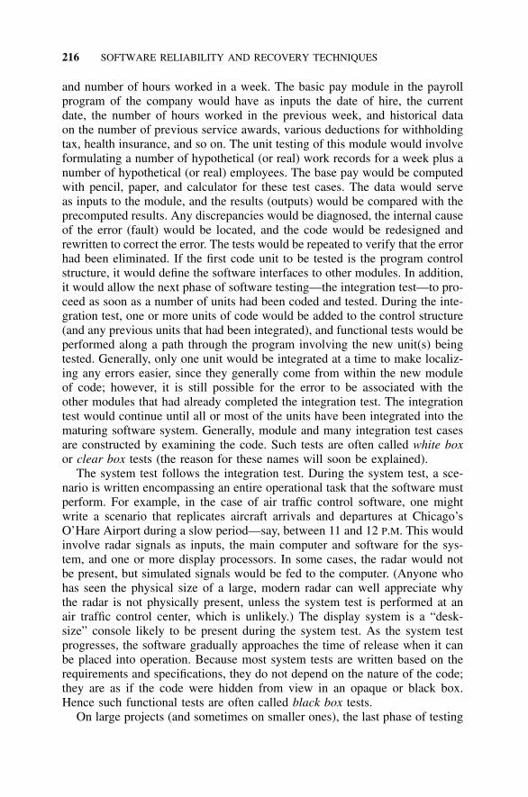
216 SOFTWARE RELIABILITY AND RECOVERY TECHNIQUES
and number of hours worked in a week. The basic pay module in the payrollprogram of the company would have as inputs the date of hire, the currentdate, the number of hours worked in the previous week, and historical dataon the number of previous service awards, various deductions for withholdingtax, health insurance, and so on. The unit testing of this module would involveformulating a number of hypothetical (or real) work records for a week plus anumber of hypothetical (or real) employees. The base pay would be computedwith pencil, paper, and calculator for these test cases. The data would serveas inputs to the module, and the results (outputs) would be compared with theprecomputed results. Any discrepancies would be diagnosed, the internal causeof the error (fault) would be located, and the code would be redesigned andrewritten to correct the error. The tests would be repeated to verify that the errorhad been eliminated. If the first code unit to be tested is the program controlstructure, it would define the software interfaces to other modules. In addition,it would allow the next phase of software testing—the integration test—to pro-ceed as soon as a number of units had been coded and tested. During the inte-gration test, one or more units of code would be added to the control structure(and any previous units that had been integrated), and functional tests would beperformed along a path through the program involving the new unit(s) beingtested. Generally, only one unit would be integrated at a time to make localiz-ing any errors easier, since they generally come from within the new moduleof code; however, it is still possible for the error to be associated with theother modules that had already completed the integration test. The integrationtest would continue until all or most of the units have been integrated into thematuring software system. Generally, module and many integration test casesare constructed by examining the code. Such tests are often called white boxor clear box tests (the reason for these names will soon be explained).
The system test follows the integration test. During the system test, a sce-nario is written encompassing an entire operational task that the software mustperform. For example, in the case of air traffic control software, one mightwrite a scenario that replicates aircraft arrivals and departures at Chicago’sO’Hare Airport during a slow period—say, between 11 and 12 P.M. This wouldinvolve radar signals as inputs, the main computer and software for the sys-tem, and one or more display processors. In some cases, the radar would notbe present, but simulated signals would be fed to the computer. (Anyone whohas seen the physical size of a large, modern radar can well appreciate whythe radar is not physically present, unless the system test is performed at anair traffic control center, which is unlikely.) The display system is a “desk-size” console likely to be present during the system test. As the system testprogresses, the software gradually approaches the time of release when it canbe placed into operation. Because most system tests are written based on therequirements and specifications, they do not depend on the nature of the code;they are as if the code were hidden from view in an opaque or black box.Hence such functional tests are often called black box tests.
On large projects (and sometimes on smaller ones), the last phase of testing

SOFTWARE DEVELOPMENT LIFE CYCLE 217
is acceptance testing. This is generally written into the contract by the cus-tomer. If the software is being written “in house,” an acceptance test would beperformed if the company software development procedures call for it. A typi-cal acceptance test would contain a number of operational scenarios performedby the software on the intended hardware, where the location would be chosenfrom (a) the developer’s site, (b) the customer’s site, or (c) the site at whichthe system is to be deployed. In the case of air traffic control (ATC), the ATCcenter contains the present on-line system n and the previous system, n − 1, asa backup. If we call the new system n + 1, it would be installed alongside nand n − 1 and operate on the same data as the on-line system. Comparing theoutputs of system n+1 with system n for a number of months would constitutea very good acceptance test. Generally, the criterion for acceptance is that thesoftware must operate on real or simulated system data for a specified numberof hours or be subjected to a certain number of test inputs. If the acceptancetest is passed, the software is accepted and the developer is paid; however, ifthe test is failed, the developer resumes the testing and correcting of softwareerrors (including those found during the acceptance test), and a new acceptancetest date is scheduled.
Sometimes, “third party” testing is used, in which the customer hires an out-side organization to make up and administer integration, system, or acceptancetests. The theory is that the developer is too close to his or her own work andcannot test and evaluate it in an unbiased manner. The third party test groupis sometimes an independent organization within the developer’s company. Ofcourse, one wonders how independent such an in-house group can be if it andthe developers both work for the same boss.
The term regression testing is often used, describing the need to retest thesoftware with the previous test cases after each new error is corrected. In the-ory, one must repeat all the tests; however, a selected subset is generally usedin the retest. Each project requires a test plan to be written early in the develop-ment cycle in parallel with or immediately following the completion of speci-fications. The test plan documents the tests to be performed, organizes the testcases by phase, and contains the expected outputs for the test cases. Generally,testing costs and schedules are also included.
When a commercial software company is developing a product for sale tothe general business and home community, the later phases of testing are oftensomewhat different, for which the terms alpha testing and beta testing are oftenused. Alpha testing means that a test group within the company evaluates thesoftware before release, whereas beta testing means that a number of “selectedcustomers” with whom the developer works are given early releases of thesoftware to help test and debug it. Some people feel that beta testing is just away of reducing the cost of software development and that it is not a thoroughway of testing the software, whereas others feel that the company still doesadequate testing and that this is just a way of getting a lot of extra field testingdone in a short period of time at little additional cost.
During early field deployment, additional errors are found, since the actual
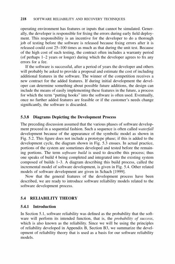
218 SOFTWARE RELIABILITY AND RECOVERY TECHNIQUES
operating environment has features or inputs that cannot be simulated. Gener-ally, the developer is responsible for fixing the errors during early field deploy-ment. This responsibility is an incentive for the developer to do a thoroughjob of testing before the software is released because fixing errors after it isreleased could cost 25–100 times as much as that during the unit test. Becauseof the high cost of such testing, the contract often includes a warranty period(of perhaps 1–2 years or longer) during which the developer agrees to fix anyerrors for a fee.
If the software is successful, after a period of years the developer and otherswill probably be asked to provide a proposal and estimate the cost of includingadditional features in the software. The winner of the competition receives anew contract for the added features. If during initial development the devel-oper can determine something about possible future additions, the design caninclude the means of easily implementing these features in the future, a processfor which the term “putting hooks” into the software is often used. Eventually,once no further added features are feasible or if the customer’s needs changesignificantly, the software is discarded.
5.3.8 Diagrams Depicting the Development Process
The preceding discussion assumed that the various phases of software develop-ment proceed in a sequential fashion. Such a sequence is often called waterfalldevelopment because of the appearance of the symbolic model as shown inFig. 5.2. This figure does not include a prototype phase; if this is added to thedevelopment cycle, the diagram shown in Fig. 5.3 ensues. In actual practice,portions of the system are sometimes developed and tested before the remain-ing portions. The term software build is used to describe this process; thusone speaks of build 4 being completed and integrated into the existing systemcomposed of builds 1–3. A diagram describing this build process, called theincremental model of software development, is given in Fig. 5.4. Other relatedmodels of software development are given in Schach [1999].
Now that the general features of the development process have beendescribed, we are ready to introduce software reliability models related to thesoftware development process.
5.4 RELIABILITY THEORY
5.4.1 Introduction
In Section 5.1, software reliability was defined as the probability that the soft-ware will perform its intended function, that is, the probability of success,which is also known as the reliability. Since we will be using the principlesof reliability developed in Appendix B, Section B3, we summarize the devel-opment of reliability theory that is used as a basis for our software reliabilitymodels.
RELIABILITY THEORY 219
RequirementsPhase
ChangedRequirements
SpecificationPhase
DesignPhase
ImplementationPhase
IntegrationPhase
OperationsMode
Retirement
Verify Verify
Verify
Verify
Test
Test
SOFTWARE LIFE-CYCLEDEVELOPMENT MODELS
(WATERFALL MODEL)
DevelopmentMaintenance
Figure 5.2 Diagram of the waterfall model of software development.
5.4.2 Reliability as a Probability of Success
The reliability of a system (hardware, software, human, or a combinationthereof) is the probability of success, Ps, which is unity minus the probabilityof failure, Pf . If we assume that t is the time of operation, that the operationstarts at t c 0, and that the time to failure is given by tf , we can then expressthe reliability as
R(t) c Ps c P(tf ≥ t) c 1 − Pf c 1 − P(0 ≤ tf ≤ t) (5.2)
220 SOFTWARE RELIABILITY AND RECOVERY TECHNIQUES
RapidPrototype
ChangedRequirements
SpecificationPhase
DesignPhase
ImplementationPhase
IntegrationPhase
OperationsMode
Retirement
Verify Verify
Verify
Verify
Test
Test
SOFTWARE LIFE-CYCLEDEVELOPMENT MODELS
(RAPID PROTOTYPE MODEL)
DevelopmentMaintenance
Figure 5.3 Diagram of the rapid prototype model of software development.
The notation, P(0 ≤ tf ≤ t), in Eq. (5.2) stands for the probability that the timeto failure is less than or equal to t. Of course, time is always a positive value,so the time to failure is always equal to or greater than 0. Reliability can alsobe expressed in terms of the cumulative probability distribution function forthe random variable time to failure, F(t), and the probability density function,f (t) (see Appendix A, Section A6). The density function is the derivative ofthe distribution function, f (t) c dF(t)/ dt, and the distribution function is the
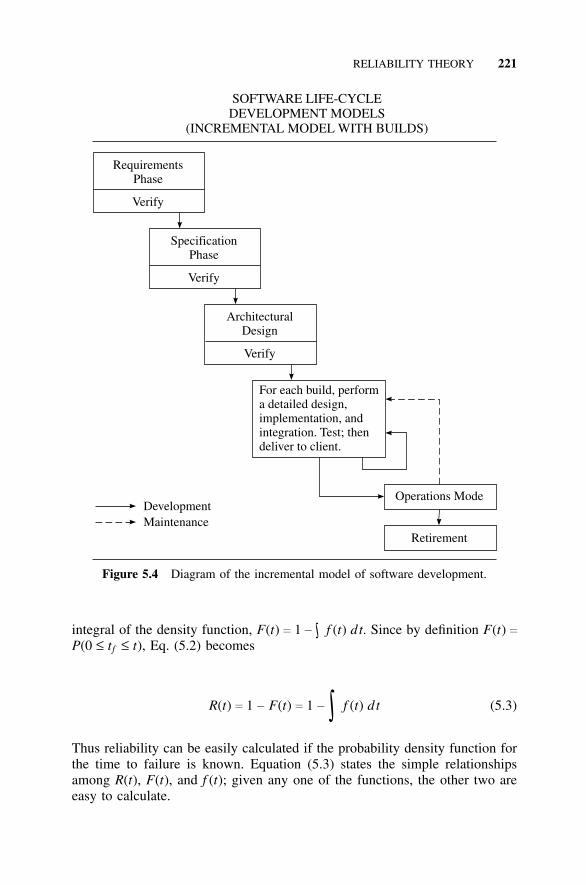
RELIABILITY THEORY 221
RequirementsPhase
SpecificationPhase
ArchitecturalDesign
Verify
Verify
Verify
Operations Mode
Retirement
SOFTWARE LIFE-CYCLEDEVELOPMENT MODELS
(INCREMENTAL MODEL WITH BUILDS)
DevelopmentMaintenance
For each build, performa detailed design,implementation, andintegration. Test; thendeliver to client.
Figure 5.4 Diagram of the incremental model of software development.
integral of the density function, F(t) c 1 − ∫ f (t) dt. Since by definition F(t) cP(0 ≤ tf ≤ t), Eq. (5.2) becomes
R(t) c 1 − F(t) c 1 − ∫ f (t) dt (5.3)
Thus reliability can be easily calculated if the probability density function forthe time to failure is known. Equation (5.3) states the simple relationshipsamong R(t), F(t), and f (t); given any one of the functions, the other two areeasy to calculate.
222 SOFTWARE RELIABILITY AND RECOVERY TECHNIQUES
5.4.3 Failure-Rate (Hazard) Function
Equation (5.3) expresses reliability in terms of the traditional mathematicalprobability functions, F(t), and f (t); however, reliability engineers have foundthese functions to be generally ill-suited for study if we want intuition, fail-ure data interpretation, and mathematics to agree. Intuition suggests that westudy another function—a conditional probability function called the failurerate (hazard), z(t). The following analysis develops an expression for the reli-ability in terms of z(t) and relates z(t) to f (t) and F(t).
The probability density function can be interpreted from the following rela-tionship:
P(t < tf < t + dt) c P(failure in interval t to t + dt) c f (t) dt (5.4)
One can relate the probability functions to failure data analysis if we begin withN items placed on the life test at time t. The number of items surviving thelife test up to time t is denoted by n(t). At any point in time, the probability offailure in interval dt is given by (number of failures)/ N. (To be mathematicallycorrect, we should say that this is only true in the limit as dt b 0.) Similarly,the reliability can be expressed as R(t) c n(t)/ N. The number of failures ininterval dt is given by [n(t) − n(t + dt)], and substitution in Eq. (5.4) yields
n(t) − n(t + dt)N
c f (t) dt (5.5)
However, we can also write Eq. (5.4) as
f (t) dt c P(no failure in interval 0 to t)
× P(failure in interval dt | no failure in interval 0 to t) (5.6a)
The last expression in Eq. (5.6a) is a conditional failure probability, and thesymbol | is interpreted as “given that.” Thus P(failure in interval dt | no failurein interval 0 to t) is the probability of failure in 0 to t given that there was nofailure up to t, that is, the item is working at time t. By definition, P(failurein interval dt | no failure in interval 0 to t) is called the hazard function, z(t);its more popular name is the failure-rate function. Since the probability of nofailure is just the reliability function, Eq. (5.6a) can be written as
f (t) dt c R(t) × z(t) dt (5.6b)
This equation relates f (t), R(t), and z(t); however, we will develop a moreconvenient relationship shortly.
Substitution of Eq. (5.6b) into Eq. (5.5) along with the relationship R(t) cn(t)/ N yields
RELIABILITY THEORY 223
n(t) − n(t + dt)N
c R(t)z(t) dt cn(t)N
z(t) dt (5.7)
Solving Eqs. (5.5) and (5.7) for f (t) and z(t), we obtain
f (t) cn(t) − n(t + dt)
N dt(5.8)
z(t) cn(t) − n(t + dt)
n(t) dt(5.9)
Comparing Eqs. (5.8) and (5.9), we see that f (t) reflects the rate of failurebased on the original number N placed on test, whereas z(t) gives the instan-taneous rate of failure based on the number of survivors at the beginning ofthe interval.
We can develop an equation for R(t) in terms of z(t) from Eq. (5.6b):
z(t) cf (t)R(t)
(5.10)
and from Eq. (5.3), differentiation of both sides yields
dR(t)dt
c − f (t) (5.11)
Substituting Eq. (5.11) into (5.10) and solving for z(t) yields
z(t) c −
dR(t)dt �R(t) (5.12)
This differential equation can be solved by integrating both sides, yielding
ln{R(t)} c − ∫ z(t) dt (5.13a)
Eliminating the natural logarithmic function in this equation by exponentiatingboth sides yields
R(t) c e− ∫ z(t) dt (5.13b)
which is the form of the reliability function that is used in the following modeldevelopment.
If one substitutes limits for the integral, a dummy variable, x, is requiredinside the integral, and a constant of integration must be added, yielding
224 SOFTWARE RELIABILITY AND RECOVERY TECHNIQUES
R(t) c e− ∫t0 z(x) dx + Ac Be− ∫t0 z(x) dx (5.13c)
As is normally the case in the solution of differential equations, the constantB c e−A is evaluated from the initial conditions. At t c 0, the item is good andR(t c 0) c 1. The integral from 0 to 0 is 0; thus B c 1 and Eq. (5.13c) becomes
R(t) c e− ∫t0 z(x) dx (5.13d)
5.4.4 Mean Time To Failure
Sometimes, the complete information on failure behavior, z(t) or f (t), is notneeded, and the reliability can be represented by the mean time to failure(MTTF) rather than the more detailed reliability function. A point estimate(MTTF) is given instead of the complete time function, R(t). A rough analogyis to rank the strength of a hitter in baseball in terms of his or her batting aver-age, rather than the complete statistics of how many times at bat, how manyfirst-base hits, how many second-base hits, and so on.
The mean value of a probability function is given by the expected value,E(t), of the random variable, which is given by the integral of the product ofthe random variable (time to failure) and its density function, which has thefollowing form:
MTTF c E(t) c ∫∞
0t f(t) dt (5.14)
Some mathematical manipulation of Eq. (5.14) involving integration by parts[Shooman, 1990] yields a simpler expression:
MTTF c E(t) c ∫∞
0R(t) dt (5.15)
Sometimes, the mean time to failure is called mean time between failure(MTBF), and although there is a minor difference in their definitions, we willuse the terms interchangeably.
5.4.5 Constant-Failure Rate
In general, a choice of the failure-rate function defines the reliability model.Such a choice should be made based on past studies that include failure-ratedata or reasonable engineering assumptions. In several practical cases, the fail-ure rate is constant in time, z(t) c l, and the mathematics becomes quite simple.Substitution into Eqs. (5.13d) and (5.15) yields
SOFTWARE ERROR MODELS 225
R(t) c e− ∫t0 l dx c e−lt (5.16)
MTTF c E(t) c ∫∞
0e−lt d t c 1
l(5.17)
The result is particularly simple: the reliability function is a decreasing expo-nential function where the exponent is the negative of the failure rate l. Asmaller failure rate means a slower exponential decay. Similarly, the MTTF isjust the reciprocal of the failure rate, and a small failure rate means a largeMTTF.
As an example, suppose that past life tests have shown that an item fails ata constant-failure rate. If 100 items are tested for 1,000 hours and 4 of thesefail, then l c 4/ (100 × 1,000) c 4 × 10⁻⁵. Substitution into Eq. (5.17) yieldsMTTF c 25,000 hours. Suppose we want the reliability for 5,000 hours; in thatcase, substitution into Eq. (5.16) yields R(5,000) c e− (4/ 100,000) × 5,000 c e−0.2 c0.82. Thus, if the failure rate were constant at 4 × 10⁻⁵, the MTTF is 25,000hours, and the reliability (probability of no failures) for 5,000 hours is 0.82.
More complex failure rates yield more complex results. If the failure rateincreases with time, as is often the case in mechanical components that even-tually “wear out,” the hazard function could be modeled by z(t) c kt. Thereliability and MTTF then become the equations that follow [Shooman, 1990].
R(t) c e− ∫t0 kx dx c e−kt2/ 2 (5.18)
MTTF c E(t) c ∫∞
0e−kt2/ 2 dt c
hp
2k(5.19)
Other choices of hazard functions would give other results.The reliability mathematics of this section applies to hardware failure and
human errors, and also to software errors if we can characterize the softwareerrors by a failure-rate function. The next section discusses how one can for-mulate a failure-rate function for software based on a software error model.
5.5 SOFTWARE ERROR MODELS
5.5.1 Introduction
Many reliability models discussed in the remainder of this chapter are relatedto the number of residual errors in the software; therefore, this section dis-cusses software error models. Generally, one speaks of faults in the code thatcause errors in the software operation; it is these errors that lead to systemfailure. Software engineers differentiate between a fault, a software error, anda software-caused system failure only when necessary, and the slang expres-
226 SOFTWARE RELIABILITY AND RECOVERY TECHNIQUES
sion “software bug” is commonly used in normal conversation to describe asoftware problem.3
Software errors occur at many stages in the software life cycle. Errors mayoccur in the requirements-and-specifications phase. For example, the specifi-cations might state that the time inputs to the system from a precise cesiumatomic clock are in hours, minutes, and seconds when actually the clock out-put is in hours and decimal fractions of an hour. Such an erroneous specifica-tion might be found early in the development cycle, especially if a hardwaredesigner familiar with the cesium clock is included in the specification review.It is also possible that such an error will not be found until a system test, whenthe clock output is connected to the system. Errors in requirements and speci-fications are identified as separate entities; however, they will be added to thecode faults in this chapter. If the range safety officer has to destroy a satellitebooster because it is veering off course, it matters little to him or her whetherthe problem lies in the specifiations or whether it is a coding error.
Errors occur in the program logic. For example, the THEN and ELSEclauses in an IF THEN ELSE statement may be interchanged, creating an error,or a loop is erroneously executed n−1 times rather than the correct value, whichis n times. When a program is coded, syntax errors are always present and arecaught by the compiler. Such syntax errors are too frequent, embarrassing, anduniversal to be considered errors.
Actually, design errors should be recorded once the program managementreviews and endorses a preliminary design expressed by a set of design repre-sentations (H-diagrams, control graphs, and maybe other graphical or abbrevi-ated high-level control-structure code outlines called pseudocodes) in additionto requirements and specifications. Often, a formal record of such changes isnot kept. Furthermore, errors found by code reading and testing at the middle(unit) code level (called module errors) are often not carefully kept. A changein the preliminary design and the occurrence of module test errors should bothbe carefully recorded.
Oftentimes, the standard practice is not to start counting software errors,
3The origin of the word “bug” is very interesting. In the early days of computers, many of themachines were constructed of vacuum tubes and relays, used punched cards for input, and usedmachine language or assembly language. Grace Hopper, one of the pioneers who developedthe language COBOL and who spent most of her career in the U.S. Navy (rising to the rankof admiral), is generally credited with the expression. One hot day in the summer of 1945 atHarvard, she was working on the Mark II computer (successor to the pioneering Mark I) whenthe machine stopped. Because there was no air conditioning, the windows were opened, whichpermitted the entry of a large moth that (subsequent investigation revealed) became stuck betweenthe contacts of one of the relays, thereby preventing the machine from functioning. Hopper andthe team removed the moth with tweezers; later, it was mounted in a logbook with tape (it is nowdisplayed in the Naval Museum at the Naval Surface Weapons Center in Dahlgren, Virginia).The expression “bug in the system” soon became popular, as did the term “debugging” to denotethe fixing of program errors. It is probable that “bug” was used before this incident during WorldWar II to describe system or hardware problems, but this incident is clearly the origin of the term“software bug” [Billings, 1989, p. 58].
SOFTWARE ERROR MODELS 227
regardless of their cause, until the software comes under configuration con-trol, generally at the start of integration testing. Configuration control occurswhen a technical manager or management board is put in charge of the officialversion of the software and records any changes to the software. Such a change(error fix) is submitted in writing to the configuration control manager by theprogrammer who corrected the error and retested the code of the module withthe design change. The configuration control manager retests the present ver-sion of the software system with the inserted change; if he or she agrees that itcorrects the error and does not seem to cause any problems, the error is addedto the official log of found and corrected errors. The code change is addedto the official version of the program at the next compilation and release ofa new, official version of the software. It is desirable to start recording errorsearlier in the program than in the configuration control stage, but better latethan never! The origin of configuration control was probably a reaction to theearly days of program patching, as explained in the following paragraph.
In the early days of programming, when the compilation of code for a largeprogram was a slow, laborious procedure, and configuration control was notstrongly enforced, programmers inserted their own changes into the compiledversion of the program. These additions were generally done by inserting amachine language GO TO in the code immediately before the beginning of thebad section, transferring program flow to an unused memory block. The correctcode in machine language was inserted into this block, and a GO TO at the endof this correction block returned the program flow to an address in the compiledcode immediately after the old, erroneous code. Thus the error was bypassed;such insertions were known as patches. Oftentimes, each programmer had hisor her own collection of patches, and when a new compilation of softwarewas begun, these confusing, sometimes overlapping and chaotic sets of patcheshad to be analyzed, recoded in higher-level language, and officially inserted inthe code. No doubt configuration control was instituted to do away with thisterrible practice.
5.5.2 An Error-Removal Model
A software error-removal model can be formulated at the beginning of an inte-gration test (system test). The variable t is used to represent the number ofmonths of development time, and one arbitrarily calls the start of configurationcontrol t c 0. At t c 0, we assume that the software contains ET total errors.As testing progresses, Ec(t) errors are corrected, and the remaining number oferrors, Er(t), is given by
Er(t) c ET − Ec(t) (5.20)
If some corrections made to discovered errors are imperfect, or if new errorsare caused by the corrections, we call this error generation. Equation (5.20) isbased on the assumption that there is no error generation—a situation that is
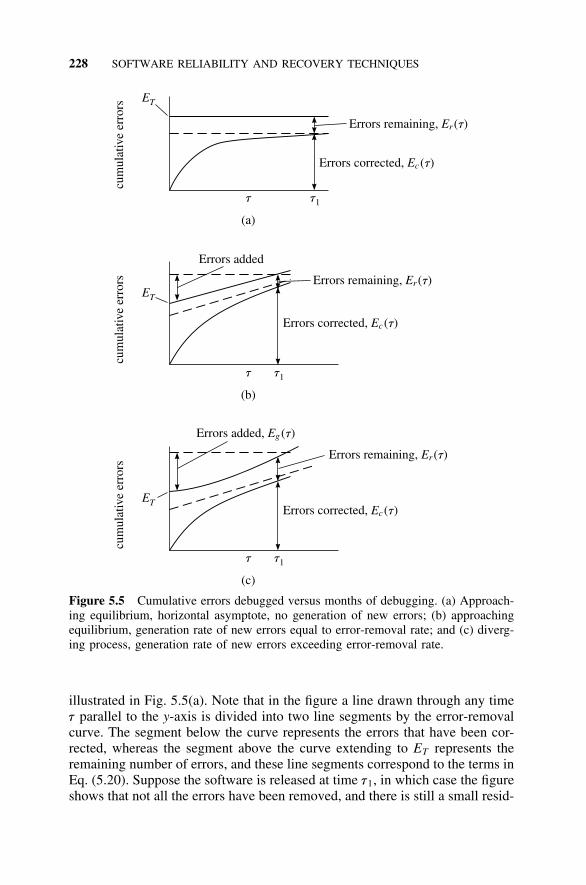
228 SOFTWARE RELIABILITY AND RECOVERY TECHNIQUES
ET
ET
ET
Errors remaining, ( )Er t
Errors remaining, ( )Er t
Errors remaining, ( )Er t
Errors corrected, ( )Ec t
Errors corrected, ( )Ec t
Errors corrected, ( )Ec t
Errors added
Errors added, Eg ( )t
t
t
t
t1
t1
t1
cum
ulat
ive
erro
rscu
mul
ativ
e er
rors
cum
ulat
ive
erro
rs
(a)
(b)
(c)
Figure 5.5 Cumulative errors debugged versus months of debugging. (a) Approach-ing equilibrium, horizontal asymptote, no generation of new errors; (b) approachingequilibrium, generation rate of new errors equal to error-removal rate; and (c) diverg-ing process, generation rate of new errors exceeding error-removal rate.
illustrated in Fig. 5.5(a). Note that in the figure a line drawn through any timet parallel to the y-axis is divided into two line segments by the error-removalcurve. The segment below the curve represents the errors that have been cor-rected, whereas the segment above the curve extending to ET represents theremaining number of errors, and these line segments correspond to the terms inEq. (5.20). Suppose the software is released at time t1, in which case the figureshows that not all the errors have been removed, and there is still a small resid-
SOFTWARE ERROR MODELS 229
ual number remaining. If all the coding errors could be removed, there clearlywould be no code-related reasons for software failures (however, there wouldstill be requirements-and-specifications errors). By the time integration test-ing is reached, we assume that the number of requirements-and-specificationserrors is very small and that the number of code errors gradually decreases asthe test process finds more errors to be subsequently corrected.
5.5.3 Error-Generation Models
In Fig. 5.5(b), we assume that there is some error generation and that the errordiscovery and correction process must be more effective or must take longerto leave the software with the same number of residual errors at release as inFig. 5.5(a). Figure 5.5(c) depicts an extraordinary situation in which the errorremoval and correction initially exceeds the error generation; however, gen-eration does eventually exceed correction, and the residual number of errorsincreases. In this case, the most obvious choices are to release at time t1 andsuffer poor reliability from the number of residual errors, or else radicallychange the test and correction process so that the situation of Fig. 5.5(a) or(b) ensues and then continue testing. One could also return to an earlier savedrelease of the software where error generation was modest, change the test andcorrection process, and, starting with this baseline, return to testing. The lastand most unpleasant choice is to discard the software and start again. (Quan-titative error-generation models are given in Shooman [1983, pp. 340–350].)
5.5.4 Error-Removal Models
Various models can be proposed for the error-correction function, Ec(t), givenin Eq. (5.20). The direct approach is to use the raw data. Error-removal datacollected over a period of several months can be plotted. Then, an empiricalcurve can be fitted to the data, which can be extrapolated to forecast the futureerror-removal behavior. A better procedure is to propose a model based onpast observations of error-removal curves and use the actual data to determinethe model parameters. This blends the past information on the general shapeof error-removal curves with the early data on the present project, and it alsomakes the forecasting less vulnerable to a few atypical data values at the startof the program (the statistical noise). Generally, the procedure takes a smallernumber of observations, and a useful model emerges early in the developmentcycle—soon after t c 0. Of course, the estimate of the model parameters willhave an associated statistical variance that will be larger at the beginning, whenonly a few data values are available, and smaller later in the project after moredata is collected. The parameter variance will of course affect the range of theforecasts. If the project in question is somewhat like the previous projects, thechosen model will in effect filter out some of the statistical noise and yield bet-ter forecasts. However, what if for some reason the project is quite differentfrom the previous ones? The “inertia” of the model will temporarily mask these
230 SOFTWARE RELIABILITY AND RECOVERY TECHNIQUES
differences. Also, suppose that in the middle of testing some of the test per-sonnel or strategies are changed and the error-removal curve is significantlychanged (for better or for worse). Again, the model inertia will temporarilymask these changes. Thus it is important to plot the actual data and examine itwhile one is using the model and making forecasts. There are many statisticaltests to help the observer determine if differences represent statistical noise ordifferent behavior; however, plotting, inspection, and thinking are all the initialbasic steps.
One must keep in mind that with modern computer facilities, complex mod-eling and statistical parameter estimation techniques are easily accomplished;the difficult part is collecting enough data for accurate, stable estimates ofmodel parameters and for interpretation of the results. Thus the focus of thischapter is on understanding and interpretation, not on complexity. In manycases, the error removal is too scant or inaccurate to support a sophisticatedmodel over a simple one, and the complex model shrouds our understanding.Consider this example: Suppose we wish to estimate the math skills of 1,000first-year high-school students by giving them a standardized test. It is tooexpensive to test all the students. If we decide to test 10 students, it is unlikelythat the most sophisticated techniques for selecting the sample or processingthe data will give us more than a wide range of estimates. Similarly, if we findthe funds to test 250 students, then any elementary statistical techniques shouldgive us good results. Sophisticated statistical techniques may help us make abetter estimate if we are able to test, say, 50 students; however, the simplertechniques should still be computed first, since they will be understood by awider range of readers.
Constant Error-Removal Rate. Our development starts with the simplest mod-els. Assuming that the error-detection rate is constant leads to a single-param-eter error-removal model. In actuality, even if the removal rate were constant,it would fluctuate from week to week or month to month because of statisticalnoise, but there are ample statistical techniques to deal with this. Another fac-tor that must be considered is the delay of a few days or, occasionally, a fewweeks between the discovery of errors and their correction. For simplicity, wewill assume (as most models do) that such delays do not cause problems.
If one assumes a constant error-correction (removal) rate of r0 errors/ month[Shooman, 1972, 1983], Eq. (5.20) becomes
Er(t) c ET − r0t (5.21)
We can also derive Eq. (5.21) in a more basic fashion by letting the error-removal rate be given by the derivative of the number of errors remaining.Thus, differentiation of Eq. (5.20) yields
error-correction rate c
dEr(t)dt
c −
dEc(t)dt
(5.22a)
SOFTWARE ERROR MODELS 231
Since we assume that the error-correction rate is constant, Eq. (5.22a) becomes
error-correction rate c
dEr(t)dt
c −
dEc(t)dt
c −r0 (5.22b)
Integration of Eq. (5.22b) yields
Er(t) c C − r0t (5.22c)
The constant C is evaluated from the initial condition at t c 0, Er(t) c ET c C,and Eq. (5.22c) becomes
Er(t) c ET − r0t (5.22d)
which is, of course, identical to Eq. (5.21). The cumulative number of errorscorrected is given by the second term in the equation, Ec(t) c r0t.
Although there is some data to support a constant error-removal rate[Shooman and Bolsky, 1975], most practitioners observe that the error-removalrate decreases with development time, t.
Note that in the foregoing discussion we always assumed that the same effortis applied to testing and debugging over the interval in question. Either thesame number of programmers is working on the given phase of development,the same number of worker hours is being expended, or the same number anddifficulty level of tests is being employed. Of course, this will vary from dayto day; we are really talking about the average over a week or a month. Whatwould really destroy such an assumption is if two people worked on testingduring the first two weeks in a month and six tested during the last two weeksof the month. One could always deal with such a situation by substituting fort the number of worker hours, WH; r0 would then become the number oferrors removed per worker hour. One would think that WH is always availablefrom the business records for the project. However, this is sometimes distortedby the “big project phenomenon,” which means that sometimes the managerof big project Z is told by his boss that there will be four programmers notworking on the project who will charge their salaries to project Z for the nexttwo weeks because they have no project support and Z is the only project thathas sufficient resources to cover their salaries. In analyzing data, one shouldalways be alert to the fact that such anomalies can occur, although the recordof WH is generally reliable.
As an example of how a constant error-removal rate can be used, consider a10,000-line program that enters the integration test phase. For discussion pur-poses, assume we are omniscient and know that there are 130 errors. Supposethat the error removal proceeds at the rate of 15 per month and that the error-removal curve will be as shown in Fig. 5.6. Suppose that the schedule calls forrelease of the software after 8 months. There will be 130 − 120 c 10 errorsleft after 8 months of testing and debugging, but of course this information
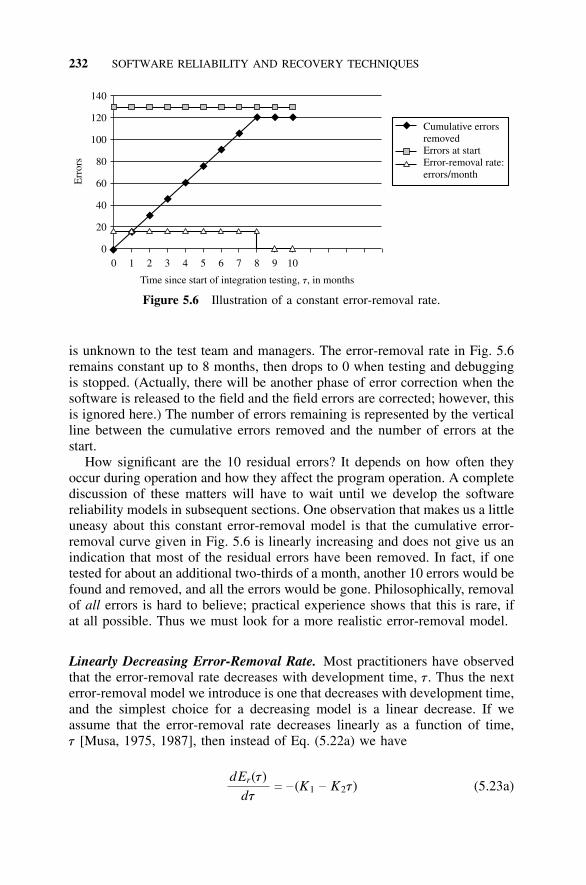
232 SOFTWARE RELIABILITY AND RECOVERY TECHNIQUES
Cumulative errorsremovedErrors at startError-removal rate:errors/month
0 1 2 3 4 5 6 7 8 9 100
20
40
60
80
100
120
140
Err
ors
Time since start of integration testing, , in monthst
Figure 5.6 Illustration of a constant error-removal rate.
is unknown to the test team and managers. The error-removal rate in Fig. 5.6remains constant up to 8 months, then drops to 0 when testing and debuggingis stopped. (Actually, there will be another phase of error correction when thesoftware is released to the field and the field errors are corrected; however, thisis ignored here.) The number of errors remaining is represented by the verticalline between the cumulative errors removed and the number of errors at thestart.
How significant are the 10 residual errors? It depends on how often theyoccur during operation and how they affect the program operation. A completediscussion of these matters will have to wait until we develop the softwarereliability models in subsequent sections. One observation that makes us a littleuneasy about this constant error-removal model is that the cumulative error-removal curve given in Fig. 5.6 is linearly increasing and does not give us anindication that most of the residual errors have been removed. In fact, if onetested for about an additional two-thirds of a month, another 10 errors would befound and removed, and all the errors would be gone. Philosophically, removalof all errors is hard to believe; practical experience shows that this is rare, ifat all possible. Thus we must look for a more realistic error-removal model.
Linearly Decreasing Error-Removal Rate. Most practitioners have observedthat the error-removal rate decreases with development time, t. Thus the nexterror-removal model we introduce is one that decreases with development time,and the simplest choice for a decreasing model is a linear decrease. If weassume that the error-removal rate decreases linearly as a function of time,t [Musa, 1975, 1987], then instead of Eq. (5.22a) we have
dEr(t)dt
c − (K1 − K2t) (5.23a)

SOFTWARE ERROR MODELS 233
which represents a linearly decreasing error-removal rate. At some time t0, thelinearly decreasing failure rate should go to 0, and substitution into Eq. (5.23a)yields K2 c K1/t0. Substitution into Eq. (5.23a) yields
dEr(t)dt
c −K1 �1 −
t
t0� c −K �1 −
t
t0� (5.23b)
which clearly shows the linear decrease. For convenience, the subscript on Kwas dropped since it was no longer needed. Integration of Eq. (5.23b) yields
Er(t) c C − Kt �1 −
t
2t0� (5.23c)
The constant C is evaluated from the initial condition at t c 0, Er(t) c ET c C,and Eq. (5.23c) becomes
Er(t) c ET − Kt �1 −
t
2t0� (5.23d)
Inspection of Eq. (5.23b) shows that K is determined by the initial error-removal rate at t c 0.
We now repeat the example introduced above to illustrate a linearly decreas-ing error-removal rate. Since we wish the removal of 120 errors after 8 monthsto compare with the previous example, we set ET c 130, and at t c 8, Er(t c 8)is equal to 10. Solving for K, we obtain a value of 30, and the equations forthe error-correction rate and number of remaining errors become
dEr(t)dt
c −30 �1 −
t
8 � (5.24a)
Er(t) c 130 − 30t �1 −
t
16 � (5.24b)
The error-removal curve will be as shown in Fig. 5.7 and decreases to 0 at8 months. Suppose that the schedule calls for release of the software after 8months. There will be 130 − 120 c 10 errors left after 8 months of testingand debugging, but of course this information is unknown to the test teamand managers. The error-removal rate in Fig. 5.7 drops to 0 when testing anddebugging is stopped. The number of errors remaining is represented by thevertical line between the cumulative errors removed and the number of errorsat the start. These results give an error-removal curve that seems to becomeasymptotic as we approach 8 months of testing and debugging. Of course, the
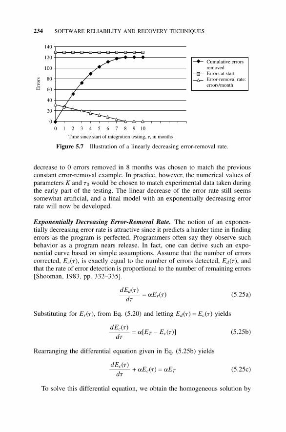
234 SOFTWARE RELIABILITY AND RECOVERY TECHNIQUES
Cumulative errorsremovedErrors at startError-removal rate:errors/month
0 1 2 3 4 5 6 7 8 9 100
20
40
60
80
100
120
140
Err
ors
Time since start of integration testing, , in monthst
Figure 5.7 Illustration of a linearly decreasing error-removal rate.
decrease to 0 errors removed in 8 months was chosen to match the previousconstant error-removal example. In practice, however, the numerical values ofparameters K and t0 would be chosen to match experimental data taken duringthe early part of the testing. The linear decrease of the error rate still seemssomewhat artificial, and a final model with an exponentially decreasing errorrate will now be developed.
Exponentially Decreasing Error-Removal Rate. The notion of an exponen-tially decreasing error rate is attractive since it predicts a harder time in findingerrors as the program is perfected. Programmers often say they observe suchbehavior as a program nears release. In fact, one can derive such an expo-nential curve based on simple assumptions. Assume that the number of errorscorrected, Ec(t), is exactly equal to the number of errors detected, Ed(t), andthat the rate of error detection is proportional to the number of remaining errors[Shooman, 1983, pp. 332–335].
dEd(t)dt
c aEr(t) (5.25a)
Substituting for Er(t), from Eq. (5.20) and letting Ed(t) c Ec(t) yields
dEc(t)dt
c a[ET − Ec(t)] (5.25b)
Rearranging the differential equation given in Eq. (5.25b) yields
dEc(t)dt
+ aEc(t) c aET (5.25c)
To solve this differential equation, we obtain the homogeneous solution by
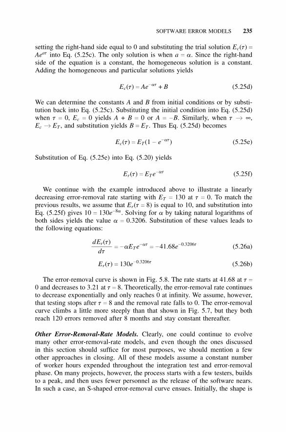
SOFTWARE ERROR MODELS 235
setting the right-hand side equal to 0 and substituting the trial solution Ec(t) cAeat into Eq. (5.25c). The only solution is when a c a. Since the right-handside of the equation is a constant, the homogeneous solution is a constant.Adding the homogeneous and particular solutions yields
Ec(t) c Ae−at + B (5.25d)
We can determine the constants A and B from initial conditions or by substi-tution back into Eq. (5.25c). Substituting the initial condition into Eq. (5.25d)when t c 0, Ec c 0 yields A + B c 0 or A c −B. Similarly, when t b ∞,Ec b ET , and substitution yields B c ET . Thus Eq. (5.25d) becomes
Ec(t) c ET (1 − e−at) (5.25e)
Substitution of Eq. (5.25e) into Eq. (5.20) yields
Er(t) c ETe−at (5.25f)
We continue with the example introduced above to illustrate a linearlydecreasing error-removal rate starting with ET c 130 at t c 0. To match theprevious results, we assume that Er(t c 8) is equal to 10, and substitution intoEq. (5.25f) gives 10 c 130e−8a. Solving for a by taking natural logarithms ofboth sides yields the value a c 0.3206. Substitution of these values leads tothe following equations:
dEr(t)dt
c −aETe−atc −41.68e−0.3206t (5.26a)
Er(t) c 130e−0.3206t (5.26b)
The error-removal curve is shown in Fig. 5.8. The rate starts at 41.68 at t c0 and decreases to 3.21 at t c 8. Theoretically, the error-removal rate continuesto decrease exponentially and only reaches 0 at infinity. We assume, however,that testing stops after t c 8 and the removal rate falls to 0. The error-removalcurve climbs a little more steeply than that shown in Fig. 5.7, but they bothreach 120 errors removed after 8 months and stay constant thereafter.
Other Error-Removal-Rate Models. Clearly, one could continue to evolvemany other error-removal-rate models, and even though the ones discussedin this section should suffice for most purposes, we should mention a fewother approaches in closing. All of these models assume a constant numberof worker hours expended throughout the integration test and error-removalphase. On many projects, however, the process starts with a few testers, buildsto a peak, and then uses fewer personnel as the release of the software nears.In such a case, an S-shaped error-removal curve ensues. Initially, the shape is
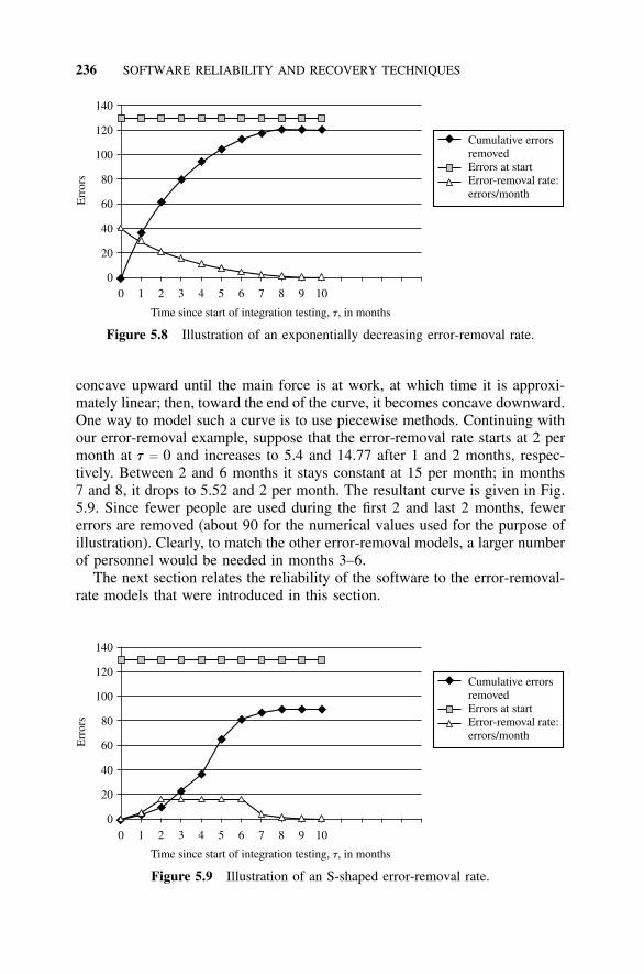
236 SOFTWARE RELIABILITY AND RECOVERY TECHNIQUES
Cumulative errorsremovedErrors at startError-removal rate:errors/month
0 1 2 3 4 5 6 7 8 9 100
20
40
60
80
100
120
140
Err
ors
Time since start of integration testing, , in monthst
Figure 5.8 Illustration of an exponentially decreasing error-removal rate.
concave upward until the main force is at work, at which time it is approxi-mately linear; then, toward the end of the curve, it becomes concave downward.One way to model such a curve is to use piecewise methods. Continuing withour error-removal example, suppose that the error-removal rate starts at 2 permonth at t c 0 and increases to 5.4 and 14.77 after 1 and 2 months, respec-tively. Between 2 and 6 months it stays constant at 15 per month; in months7 and 8, it drops to 5.52 and 2 per month. The resultant curve is given in Fig.5.9. Since fewer people are used during the first 2 and last 2 months, fewererrors are removed (about 90 for the numerical values used for the purpose ofillustration). Clearly, to match the other error-removal models, a larger numberof personnel would be needed in months 3–6.
The next section relates the reliability of the software to the error-removal-rate models that were introduced in this section.
Cumulative errorsremovedErrors at startError-removal rate:errors/month
0 1 2 3 4 5 6 7 8 9 100
20
40
60
80
100
120
140
Err
ors
Time since start of integration testing, , in monthst
Figure 5.9 Illustration of an S-shaped error-removal rate.

RELIABILITY MODELS 237
5.6 RELIABILITY MODELS
5.6.1 Introduction
In the preceding sections, we established the mathematical basis of the reli-ability function and related it to the failure-rate function. Also, a number oferror-removal models were developed. Both of these efforts were preludes toformulating a software reliability model. Before we become absorbed in thedetails of reliability model development, we should review the purpose of soft-ware reliability models.
Software reliability models are used to answer two main questions duringproduct development: When should we stop testing? and Will the product func-tion well and be considered reliable? Both are technical management questions;the former can be restated as follows: When are there few enough errors sothat the software can be released to the field (or at least to the last stage oftesting)? To continue testing is costly, but to release a product with too manyerrors is more costly. The errors must be fixed in the field at high cost, andthe product develops a reputation for unreliability that will hurt its acceptance.The software reliability models to be developed quantify the number of errorsremaining and especially provide a prediction of the field reliability, helpingtechnical and business management reach a decision regarding when to releasethe product. The contract or marketing plan contains a release date, and penal-ties may be assessed by a contract for late delivery. However, we wish to avoidthe dilemma of the on-time release of a product that is too “buggy” and thusdefective.
The other job of software reliability models is to give a prediction of fieldreliability as early as possible. Two many software products are released and,although they operate, errors occur too frequently; in retrospect, the projectsbecome failures because people do not trust the results or tire of dealing withfrequent system crashes. Most software products now have competitors, soconsequently an unreliable product loses out or must be fixed up after releaseat great cost. Many software systems are developed for a single user for a spe-cial purpose, for example, air traffic control, IRS tax programs, social services’record systems, and control systems for radiation-treatment devices. Failuresof such systems can have dire consequences and huge impact. Thus, givenrequirements and a quality goal, the types of reliability models we seek arethose that are easy to understand and use and also give reasonable results. Therelative accuracy of two models in which one predicts one crash per week andanother predicts two crashes per week may seem vastly different in a math-ematical sense. However, suppose a good product should have less than onecrash a month or, preferably, a few crashes per year. In this case, both mod-els tell the same story—the software is not nearly good enough! Furthermore,suppose that these predictions are made early in the testing when only a littlefailure data is available and the variance produces a range of estimates thatvary by more than two to one. The real challenge is to get practitioners to
238 SOFTWARE RELIABILITY AND RECOVERY TECHNIQUES
collect data, use simple models, and make predictions to guide the program.One can always apply more sophisticated models to the same data set once thebasic ideas are understood. The biggest mistake is to avoid making a reliabilityestimate because (a) it does not work, (b) it is too costly, and (c) we do nothave the data. None of these reasons is correct or valid, and this fact representspoor management. The next biggest mistake is to make a model, obtain poorreliability predictions, and ignore them because they are too depressing.
5.6.2 Reliability Model for Constant Error-Removal Rate
The basic simplicity and some of the drawbacks of the simple constant error-removal model were discussed in the previous section on error-removal mod-els. Even with these limitations, this is the simplest place to start for us todevelop most of the features of software reliability models based on this modelbefore we progress to more complex ones [Shooman, 1972].
The major assumption needed to relate an error-removal model to a softwarereliability model is how the failure rate is related to the remaining number oferrors. For the remainder of this chapter, we assume that the failure rate isproportional to the remaining number of errors:
z(t) c kEr(t) (5.27)
The bases of this assumption are as follows:
1. It seems reasonable to assume that more residual errors in the softwareresult in higher software failure rates.
2. Musa [1987] has experimental data supporting this assumption.3. If the rate of error discovery is a random process dependent on input and
initial conditions, then the discovery rate is proportional to the numberof residual errors.
If one combines Eq. (5.27) with one of the software error-removal models ofthe previous section, then a software reliability model is defined. Substitutionof the failure rate into Eqs. (5.13d) and (5.15) yields a reliability model R(t)and an expression for the MTTFs.
As an example, we begin with the constant error-removal model, Eq.(5.22d),
Er(t) c ET − r0t (5.28a)
Using the assumption of Eq. (5.27), one obtains
z(t) c kEr(t) c k(ET − r0t) (5.29)
and the reliability and MTTF expressions become
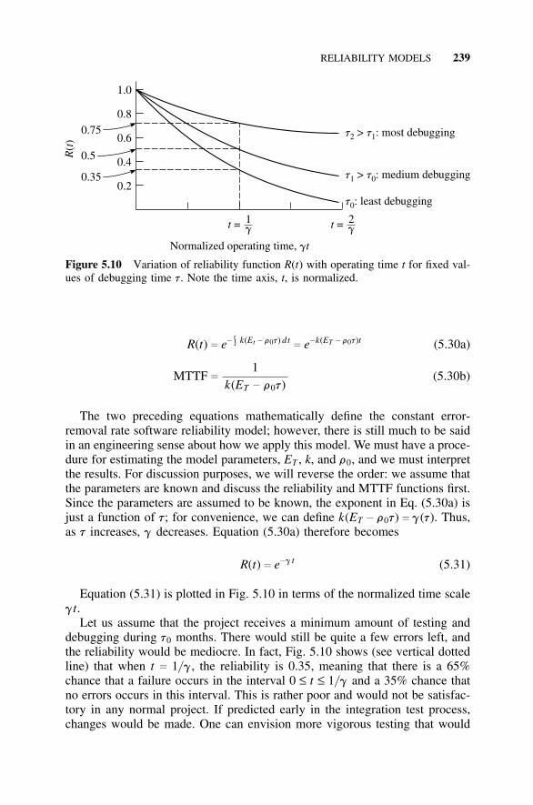
RELIABILITY MODELS 239
t = 1g t = 2
g
0.2
0.4
0.6
0.8
1.0
0.75
0.5
0.35
Rt()
Normalized operating time, gt
t t2 1> : most debugging
t t1 0> : medium debugging
t0: least debugging
Figure 5.10 Variation of reliability function R(t) with operating time t for fixed val-ues of debugging time t. Note the time axis, t, is normalized.
R(t) c e− ∫ k(Et − r0t) dtc e−k(ET − r0t)t (5.30a)
MTTF c
1k(ET − r0t)
(5.30b)
The two preceding equations mathematically define the constant error-removal rate software reliability model; however, there is still much to be saidin an engineering sense about how we apply this model. We must have a proce-dure for estimating the model parameters, ET , k, and r0, and we must interpretthe results. For discussion purposes, we will reverse the order: we assume thatthe parameters are known and discuss the reliability and MTTF functions first.Since the parameters are assumed to be known, the exponent in Eq. (5.30a) isjust a function of t; for convenience, we can define k(ET − r0t) c g(t). Thus,as t increases, g decreases. Equation (5.30a) therefore becomes
R(t) c e−g t (5.31)
Equation (5.31) is plotted in Fig. 5.10 in terms of the normalized time scalegt.
Let us assume that the project receives a minimum amount of testing anddebugging during t0 months. There would still be quite a few errors left, andthe reliability would be mediocre. In fact, Fig. 5.10 shows (see vertical dottedline) that when t c 1/g, the reliability is 0.35, meaning that there is a 65%chance that a failure occurs in the interval 0 ≤ t ≤ 1/g and a 35% chance thatno errors occurs in this interval. This is rather poor and would not be satisfac-tory in any normal project. If predicted early in the integration test process,changes would be made. One can envision more vigorous testing that would
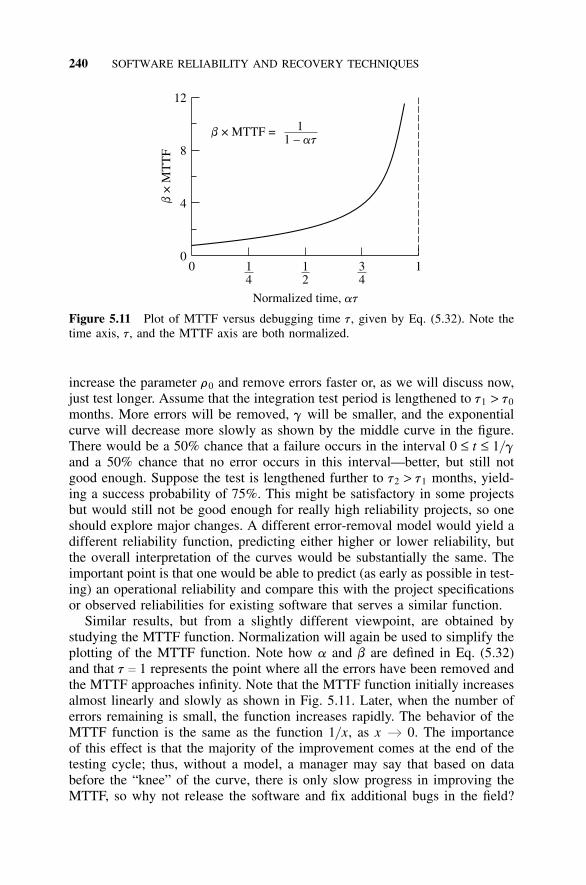
240 SOFTWARE RELIABILITY AND RECOVERY TECHNIQUES
00 1
412
34
1
4
8
12
Normalized time, at
b × MTTF =
b×
MT
TF
11 – at
Figure 5.11 Plot of MTTF versus debugging time t, given by Eq. (5.32). Note thetime axis, t, and the MTTF axis are both normalized.
increase the parameter r0 and remove errors faster or, as we will discuss now,just test longer. Assume that the integration test period is lengthened to t1 > t0
months. More errors will be removed, g will be smaller, and the exponentialcurve will decrease more slowly as shown by the middle curve in the figure.There would be a 50% chance that a failure occurs in the interval 0 ≤ t ≤ 1/gand a 50% chance that no error occurs in this interval—better, but still notgood enough. Suppose the test is lengthened further to t2 > t1 months, yield-ing a success probability of 75%. This might be satisfactory in some projectsbut would still not be good enough for really high reliability projects, so oneshould explore major changes. A different error-removal model would yield adifferent reliability function, predicting either higher or lower reliability, butthe overall interpretation of the curves would be substantially the same. Theimportant point is that one would be able to predict (as early as possible in test-ing) an operational reliability and compare this with the project specificationsor observed reliabilities for existing software that serves a similar function.
Similar results, but from a slightly different viewpoint, are obtained bystudying the MTTF function. Normalization will again be used to simplify theplotting of the MTTF function. Note how a and b are defined in Eq. (5.32)and that t c 1 represents the point where all the errors have been removed andthe MTTF approaches infinity. Note that the MTTF function initially increasesalmost linearly and slowly as shown in Fig. 5.11. Later, when the number oferrors remaining is small, the function increases rapidly. The behavior of theMTTF function is the same as the function 1/ x, as x b 0. The importanceof this effect is that the majority of the improvement comes at the end of thetesting cycle; thus, without a model, a manager may say that based on databefore the “knee” of the curve, there is only slow progress in improving theMTTF, so why not release the software and fix additional bugs in the field?
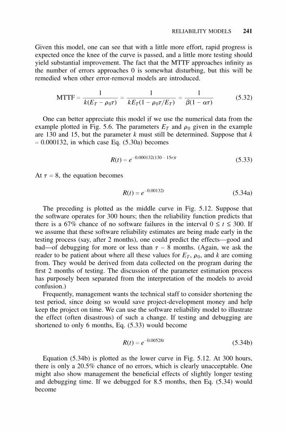
RELIABILITY MODELS 241
Given this model, one can see that with a little more effort, rapid progress isexpected once the knee of the curve is passed, and a little more testing shouldyield substantial improvement. The fact that the MTTF approaches infinity asthe number of errors approaches 0 is somewhat disturbing, but this will beremedied when other error-removal models are introduced.
MTTF c
1k(ET − r0t)
c
1kET (1 − r0t/ ET )
c
1b(1 − at)
(5.32)
One can better appreciate this model if we use the numerical data from theexample plotted in Fig. 5.6. The parameters ET and r0 given in the exampleare 130 and 15, but the parameter k must still be determined. Suppose that kc 0.000132, in which case Eq. (5.30a) becomes
R(t) c e−0.000132(130 − 15t)t (5.33)
At t c 8, the equation becomes
R(t) c e−0.00132t (5.34a)
The preceding is plotted as the middle curve in Fig. 5.12. Suppose thatthe software operates for 300 hours; then the reliability function predicts thatthere is a 67% chance of no software failures in the interval 0 ≤ t ≤ 300. Ifwe assume that these software reliability estimates are being made early in thetesting process (say, after 2 months), one could predict the effects—good andbad—of debugging for more or less than t c 8 months. (Again, we ask thereader to be patient about where all these values for ET , r0, and k are comingfrom. They would be derived from data collected on the program during thefirst 2 months of testing. The discussion of the parameter estimation processhas purposely been separated from the interpretation of the models to avoidconfusion.)
Frequently, management wants the technical staff to consider shortening thetest period, since doing so would save project-development money and helpkeep the project on time. We can use the software reliability model to illustratethe effect (often disastrous) of such a change. If testing and debugging areshortened to only 6 months, Eq. (5.33) would become
R(t) c e−0.00528t (5.34b)
Equation (5.34b) is plotted as the lower curve in Fig. 5.12. At 300 hours,there is only a 20.5% chance of no errors, which is clearly unacceptable. Onemight also show management the beneficial effects of slightly longer testingand debugging time. If we debugged for 8.5 months, then Eq. (5.34) wouldbecome
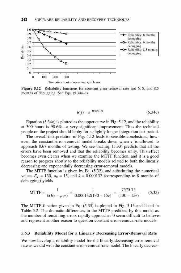
242 SOFTWARE RELIABILITY AND RECOVERY TECHNIQUES
Reliability: 8 monthsdebuggingReliability: 6 monthsdebuggingReliability: 8.5 monthsdebugging
0 100 200 3000
0.10.20.30.40.50.60.70.80.91.0
Rel
iabi
lity
Time since start of operation, , in hourst
Figure 5.12 Reliability functions for constant error-removal rate and 6, 8, and 8.5months of debugging. See Eqs. (5.34a–c).
R(t) c e−0.00033t (5.34c)
Equation (5.34c) is plotted as the upper curve in Fig. 5.12, and the reliabilityat 300 hours is 90.6%—a very significant improvement. Thus the technicalpeople on the project should lobby for a slightly longer integration test period.
The overall interpretation of Fig. 5.12 leads to sensible conclusions; how-ever, the constant error-removal model breaks down when t is allowed toapproach 8.67 months of testing. We see that Eq. (5.33) predicts that all theerrors have been removed and that the reliability becomes unity. This effectbecomes even clearer when we examine the MTTF function, and it is a goodreason to progress shortly to the reliability models related to both the linearlydecreasing and exponentially decreasing error-removal models.
The MTTF function is given by Eq. (5.32), and substituting the numericalvalues ET c 130, r0 c 15, and k c 0.000132 (corresponding to 8 months ofdebugging) yields
MTTF c
1k(ET − r0t)
c
10.000132(130 − 15t)
c
7575.75(130 − 15t)
(5.35)
The MTTF function given in Eq. (5.35) is plotted in Fig. 5.13 and listed inTable 5.2. The dramatic differences in the MTTF predicted by this model asthe number of remaining errors rapidly approaches 0 seem difficult to believeand represent another reason to question constant error-removal-rate models.
5.6.3 Reliability Model for a Linearly Decreasing Error-Removal Rate
We now develop a reliability model for the linearly decreasing error-removalrate as we did with the constant error-removal-rate model. The linearly decreas-
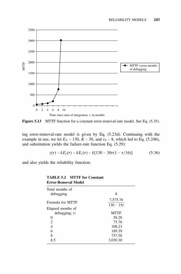
RELIABILITY MODELS 243
MTTF versus monthsof debugging
0 2 4 6 8 100
500
1000
1500
2000
2500
3000
3500
MT
TF
Time since start of integration, , in monthst
Figure 5.13 MTTF function for a constant error-removal-rate model. See Eq. (5.35).
ing error-removal-rate model is given by Eq. (5.23d). Continuing with theexample in use, we let ET c 130, K c 30, and t0 c 8, which led to Eq. (5.24b),and substitution yields the failure-rate function Eq. (5.29):
z(t) c kEr(t) c kEr(t) c k[130 − 30t(1 − t/ 16)] (5.36)
and also yields the reliability function:
TABLE 5.2 MTTF for ConstantError-Removal Model
Total months ofdebugging 8
Formula for MTTF7,575.76
130 − 15tElapsed months of
debugging, t: MTTF0 58.282 75.764 108.236 189.398 757.588.5 3,030.30
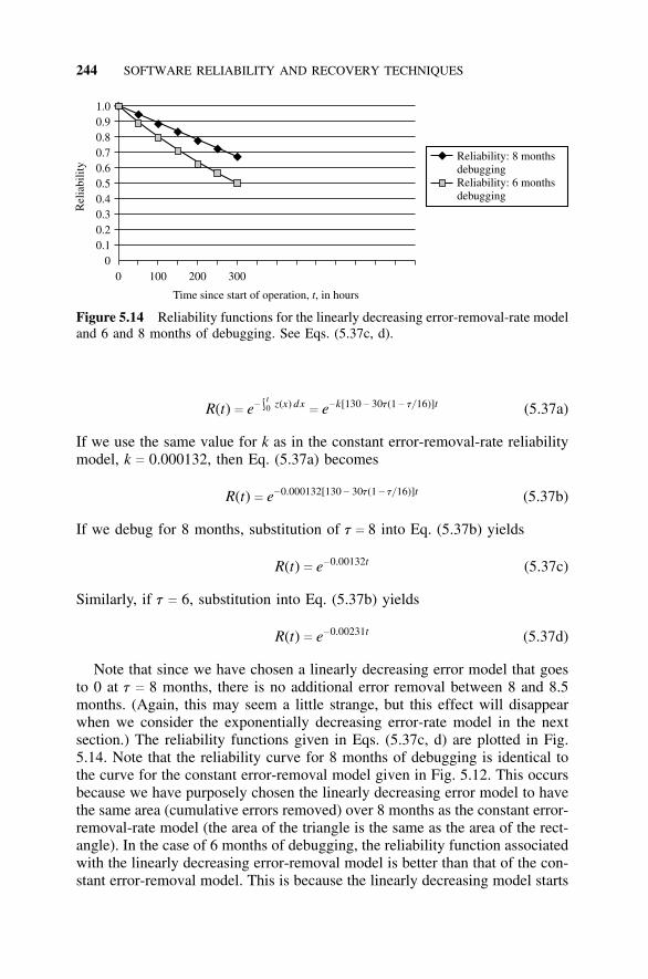
244 SOFTWARE RELIABILITY AND RECOVERY TECHNIQUES
Reliability: 8 monthsdebuggingReliability: 6 monthsdebugging
0 100 200 3000
0.10.20.30.40.50.60.70.80.91.0
Rel
iabi
lity
Time since start of operation, , in hourst
Figure 5.14 Reliability functions for the linearly decreasing error-removal-rate modeland 6 and 8 months of debugging. See Eqs. (5.37c, d).
R(t) c e− ∫t0 z(x) dxc e−k[130 − 30t(1 − t/ 16)]t (5.37a)
If we use the same value for k as in the constant error-removal-rate reliabilitymodel, k c 0.000132, then Eq. (5.37a) becomes
R(t) c e−0.000132[130 − 30t(1 − t/ 16)]t (5.37b)
If we debug for 8 months, substitution of t c 8 into Eq. (5.37b) yields
R(t) c e−0.00132t (5.37c)
Similarly, if t c 6, substitution into Eq. (5.37b) yields
R(t) c e−0.00231t (5.37d)
Note that since we have chosen a linearly decreasing error model that goesto 0 at t c 8 months, there is no additional error removal between 8 and 8.5months. (Again, this may seem a little strange, but this effect will disappearwhen we consider the exponentially decreasing error-rate model in the nextsection.) The reliability functions given in Eqs. (5.37c, d) are plotted in Fig.5.14. Note that the reliability curve for 8 months of debugging is identical tothe curve for the constant error-removal model given in Fig. 5.12. This occursbecause we have purposely chosen the linearly decreasing error model to havethe same area (cumulative errors removed) over 8 months as the constant error-removal-rate model (the area of the triangle is the same as the area of the rect-angle). In the case of 6 months of debugging, the reliability function associatedwith the linearly decreasing error-removal model is better than that of the con-stant error-removal model. This is because the linearly decreasing model starts
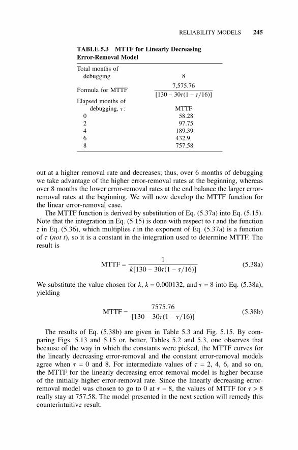
RELIABILITY MODELS 245
TABLE 5.3 MTTF for Linearly DecreasingError-Removal Model
Total months ofdebugging 8
Formula for MTTF7,575.76
[130 − 30t(1 − t/ 16)]Elapsed months of
debugging, t: MTTF0 58.282 97.754 189.396 432.98 757.58
out at a higher removal rate and decreases; thus, over 6 months of debuggingwe take advantage of the higher error-removal rates at the beginning, whereasover 8 months the lower error-removal rates at the end balance the larger error-removal rates at the beginning. We will now develop the MTTF function forthe linear error-removal case.
The MTTF function is derived by substitution of Eq. (5.37a) into Eq. (5.15).Note that the integration in Eq. (5.15) is done with respect to t and the functionz in Eq. (5.36), which multiplies t in the exponent of Eq. (5.37a) is a functionof t (not t), so it is a constant in the integration used to determine MTTF. Theresult is
MTTF c
1k[130 − 30t(1 − t/ 16)]
(5.38a)
We substitute the value chosen for k, k c 0.000132, and t c 8 into Eq. (5.38a),yielding
MTTF c
7575.76[130 − 30t(1 − t/ 16)]
(5.38b)
The results of Eq. (5.38b) are given in Table 5.3 and Fig. 5.15. By com-paring Figs. 5.13 and 5.15 or, better, Tables 5.2 and 5.3, one observes thatbecause of the way in which the constants were picked, the MTTF curves forthe linearly decreasing error-removal and the constant error-removal modelsagree when t c 0 and 8. For intermediate values of t c 2, 4, 6, and so on,the MTTF for the linearly decreasing error-removal model is higher becauseof the initially higher error-removal rate. Since the linearly decreasing error-removal model was chosen to go to 0 at t c 8, the values of MTTF for t > 8really stay at 757.58. The model presented in the next section will remedy thiscounterintuitive result.
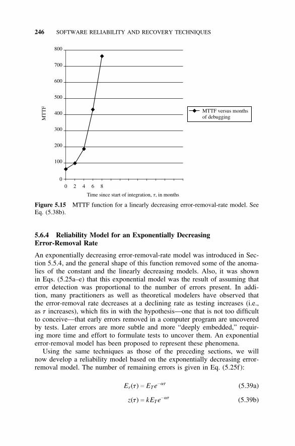
246 SOFTWARE RELIABILITY AND RECOVERY TECHNIQUES
MTTF versus monthsof debugging
0 2 4 6 80
100
200
300
400
500
600
700
800M
TT
F
Time since start of integration, , in monthst
Figure 5.15 MTTF function for a linearly decreasing error-removal-rate model. SeeEq. (5.38b).
5.6.4 Reliability Model for an Exponentially DecreasingError-Removal Rate
An exponentially decreasing error-removal-rate model was introduced in Sec-tion 5.5.4, and the general shape of this function removed some of the anoma-lies of the constant and the linearly decreasing models. Also, it was shownin Eqs. (5.25a–e) that this exponential model was the result of assuming thaterror detection was proportional to the number of errors present. In addi-tion, many practitioners as well as theoretical modelers have observed thatthe error-removal rate decreases at a declining rate as testing increases (i.e.,as t increases), which fits in with the hypothesis—one that is not too difficultto conceive—that early errors removed in a computer program are uncoveredby tests. Later errors are more subtle and more “deeply embedded,” requir-ing more time and effort to formulate tests to uncover them. An exponentialerror-removal model has been proposed to represent these phenomena.
Using the same techniques as those of the preceding sections, we willnow develop a reliability model based on the exponentially decreasing error-removal model. The number of remaining errors is given in Eq. (5.25f):
Er(t) c ETe−at (5.39a)
z(t) c kETe−at (5.39b)
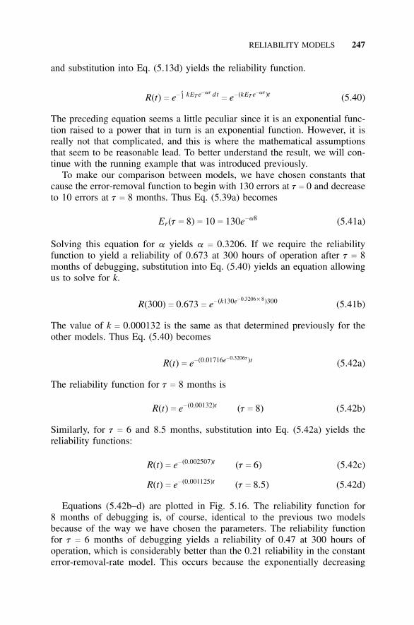
RELIABILITY MODELS 247
and substitution into Eq. (5.13d) yields the reliability function.
R(t) c e− ∫ kET e−at dtc e− (kET e−at )t (5.40)
The preceding equation seems a little peculiar since it is an exponential func-tion raised to a power that in turn is an exponential function. However, it isreally not that complicated, and this is where the mathematical assumptionsthat seem to be reasonable lead. To better understand the result, we will con-tinue with the running example that was introduced previously.
To make our comparison between models, we have chosen constants thatcause the error-removal function to begin with 130 errors at t c 0 and decreaseto 10 errors at t c 8 months. Thus Eq. (5.39a) becomes
Er(t c 8) c 10 c 130e−a8 (5.41a)
Solving this equation for a yields a c 0.3206. If we require the reliabilityfunction to yield a reliability of 0.673 at 300 hours of operation after t c 8months of debugging, substitution into Eq. (5.40) yields an equation allowingus to solve for k.
R(300) c 0.673 c e− (k130e−0.3206 × 8)300 (5.41b)
The value of k c 0.000132 is the same as that determined previously for theother models. Thus Eq. (5.40) becomes
R(t) c e− (0.01716e−0.3206t )t (5.42a)
The reliability function for t c 8 months is
R(t) c e− (0.00132)t (t c 8) (5.42b)
Similarly, for t c 6 and 8.5 months, substitution into Eq. (5.42a) yields thereliability functions:
R(t) c e− (0.002507)t (t c 6) (5.42c)
R(t) c e− (0.001125)t (t c 8.5) (5.42d)
Equations (5.42b–d) are plotted in Fig. 5.16. The reliability function for8 months of debugging is, of course, identical to the previous two modelsbecause of the way we have chosen the parameters. The reliability functionfor t c 6 months of debugging yields a reliability of 0.47 at 300 hours ofoperation, which is considerably better than the 0.21 reliability in the constanterror-removal-rate model. This occurs because the exponentially decreasing
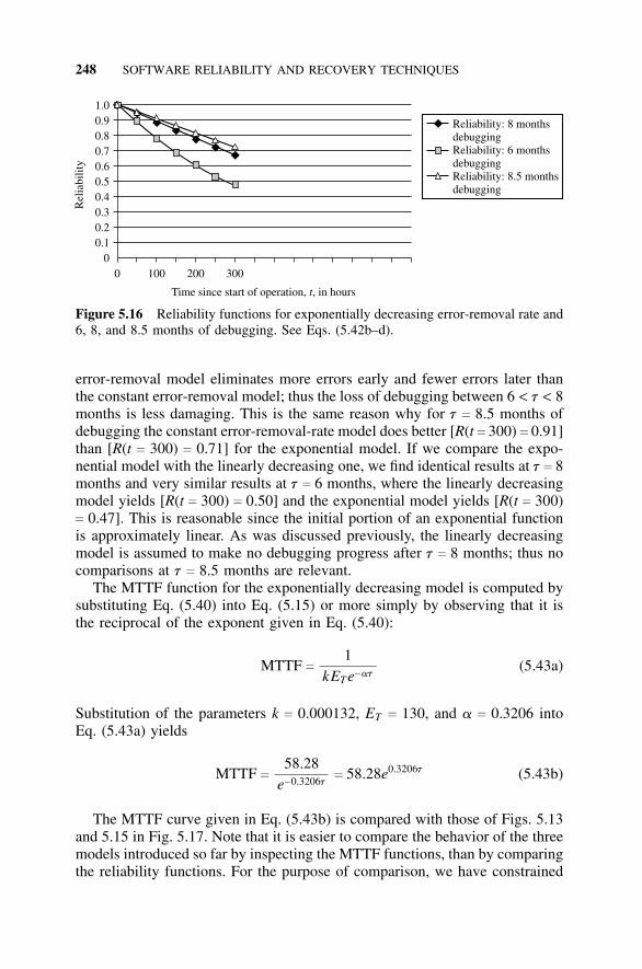
248 SOFTWARE RELIABILITY AND RECOVERY TECHNIQUES
Reliability: 8 monthsdebuggingReliability: 6 monthsdebuggingReliability: 8.5 monthsdebugging
0 100 200 3000
0.10.20.30.40.50.60.70.80.91.0
Rel
iabi
lity
Time since start of operation, , in hourst
Figure 5.16 Reliability functions for exponentially decreasing error-removal rate and6, 8, and 8.5 months of debugging. See Eqs. (5.42b–d).
error-removal model eliminates more errors early and fewer errors later thanthe constant error-removal model; thus the loss of debugging between 6 < t < 8months is less damaging. This is the same reason why for t c 8.5 months ofdebugging the constant error-removal-rate model does better [R(t c 300) c 0.91]than [R(t c 300) c 0.71] for the exponential model. If we compare the expo-nential model with the linearly decreasing one, we find identical results at t c 8months and very similar results at t c 6 months, where the linearly decreasingmodel yields [R(t c 300) c 0.50] and the exponential model yields [R(t c 300)c 0.47]. This is reasonable since the initial portion of an exponential functionis approximately linear. As was discussed previously, the linearly decreasingmodel is assumed to make no debugging progress after t c 8 months; thus nocomparisons at t c 8.5 months are relevant.
The MTTF function for the exponentially decreasing model is computed bysubstituting Eq. (5.40) into Eq. (5.15) or more simply by observing that it isthe reciprocal of the exponent given in Eq. (5.40):
MTTF c
1kETe−at
(5.43a)
Substitution of the parameters k c 0.000132, ET c 130, and a c 0.3206 intoEq. (5.43a) yields
MTTF c
58.28e−0.3206t
c 58.28e0.3206t (5.43b)
The MTTF curve given in Eq. (5.43b) is compared with those of Figs. 5.13and 5.15 in Fig. 5.17. Note that it is easier to compare the behavior of the threemodels introduced so far by inspecting the MTTF functions, than by comparingthe reliability functions. For the purpose of comparison, we have constrained
RELIABILITY MODELS 249
MTTF for constanterror-removal-rate modelMTTF for linearlydecreasing error-removal-rate modelMTTF for exponentiallydecreasing error-removal-rate model
0 2 4 6 8 100
500
1000
1500
2000
2500
3000
3500
MT
TF
Time since start of integration, , in monthst
Figure 5.17 MTTF function for constant, linearly decreasing, and exponentiallydecreasing error-removal-rate models.
all the reliability functions to have the same reliability at t c 300 hours (0.67);of course, all the reliability curves start at unity at t c 0. Thus, the only com-parison we can make is how fast the reliability curves decay between t c 0and t c 300 hours. Comparison of the MTTF curves yields a bit more infor-mation since the curves are plotted versus t, which is the resource variable.All three curves in Fig. 5.17 start at 58 hours and increase to 758 hours after8 months of testing and debugging; however, the difference in the concaveupward curvature between t c 2 and 8 months is quite apparent. The linearlydecreasing and exponentially decreasing curves are about the same becauseat t c 6 months, the linear curve achieves an MTTF of 433 hours and theexponential curve is 399 hours, whereas the constant model only reaches 139errors. Thus, if we had data for the first 2 months of debugging and wished topredict the progress as we approached the release time t c 8 months, any ofthe three models would yield approximately the same results. In applying themodels, one would plot the actual error-removal rate and choose a model thatbest matches the actual data (experience would lead us to guess that this wouldbe the exponential model). The real differences among the models are obvi-ous in the region between t c 8 and 10 months. The constant error-removalmodel climbs to ∞ when the debugging time approaches 8.66 months, whichis anomalous. The linearly decreasing model ceases to make progress after8 months, which is again counterintuitive. Only the exponentially decreasingmodel continues to display progress after 8 months at a reasonable rate. Clearly,other more advanced reliability models can be (and have been) developed.
250 SOFTWARE RELIABILITY AND RECOVERY TECHNIQUES
However, the purpose of this development is to introduce simple models thatcan easily be applied and interpreted, and a worthwhile working model appearsto be the exponentially decreasing error-removal-rate model. The next sectiondeals with the very important issue of how we estimate the constants of themodel.
5.7 ESTIMATING THE MODEL CONSTANTS
5.7.1 Introduction
The previous sections assumed values for the various model constants; forexample, k, ET , and a in Eq. (5.40). In this section, we discuss the way to esti-mate values for these constants based on current project data (measurements)or past data. One can view this parameter estimation procedure as curve fit-ting to experimental data or as statistical parameter estimation. Essentially, thisis the same idea from a slightly different viewpoint and using different meth-ods; however, the end result is the same: to determine parameters of the modelbased on early measurements of the project (or past data) that allow predic-tion of the future of the project. Before we begin our discussion of parameterestimation, it is useful to consider other phases of the project.
In the previous section, we focused on the integration test phase. Softwarereliability models, however, can be applied to other phases of the project. Reli-ability predictions are most useful when they are made in the very early stagesof the project, but during these phases so little detailed information is knownthat any predictions have a wide range of uncertainty (nevertheless, they arestill useful guides). Toward the end of the project, during early field deploy-ment, a rash of software crashes indicates that more expensive (at this late date)debugging must be done. The use of a software reliability model can predictquantitatively how much more work must be done. If conditions are goingwell during deployment, the model can quantify how well, which is especiallyimportant if the contract contains a cost incentive. The same models alreadydiscussed can be used during the deployment phase. To apply software reli-ability to the earlier module (unit) test phase, another type of reliability modelmust be employed (this is discussed in Section 5.8 on other models). Perhapsthe most challenging and potentially most useful phase for software reliabilitymodeling is during the contracting and early design phases. Because no codehas been written and none can be tested, any estimates that can be made dependon past project data. In fact, we will treat reliability model constant estimationbased on past data as a general technique and call it handbook estimation.
5.7.2 Handbook Estimation
The simplest use of past data in reliability estimation may be illustrated asfollows. Suppose your company specializes in writing payroll programs for
ESTIMATING THE MODEL CONSTANTS 251
large organizations, and in the last 10 years you have written 78 systems ofvarious sizes and complexities. In the last 5 years, reliability data has beenkept and analyzed for 27 different systems. The data has been compiled alongwith explanations and analyses in a report that is called the company’s Reli-ability Handbook. The most significant events recorded in this handbook aresystem crashes that occur between one and four times per year for the 27 dif-ferent projects. In addition, data is recorded on minor errors that occur morefrequently. A new client, company X, wants to have its antiquated, inadequatepayroll program updated, and this new project is being called system b. Com-pany X wants a quote for the development of system b, and the reliabilityof the system is to be included in the quote along with performance details,development of system b, and the reliability of the system is to be includedin the quote along with performance details, and development schedule, theprice, and so on. A study of the handbook reveals that the less complex sys-tems have an MTTF of one-half to one year. System b looks like a projectof simple to medium complexity. It seems that the company could safely saythat the MTTF for the system should be about one-half year but might varyfrom one-quarter to one year. This is a very comfortable situation, but sup-pose that the only recorded reliability data is on two systems. One data setrepresents in-house data; the other is a copy of a reliability report written bya conscientious customer during the first two years of operation who sharedthe report with you. Such data is better than nothing, but it is too weak todraw very detailed conclusions. The best action to take is to search for otherdata sources for system b and make it a company decision to improve yourfuture position by beginning the collection of data on all new projects as wellas those currently under development, and query past customers to see if theyhave any data to be shared. You could even propose that the “business dataprocessing professional organization” to which you belong sponsors a reliabil-ity data collection process to be run by an industry committee. This committeecould start the process by collecting papers reporting on relevant systems thathave appeared in the literature. An anonymous questionnaire could be circu-lated to various knowledgeable people, encouraging them to contribute datawith sufficient technical details to make listing these projects in a compositehandbook useful, but not enough information so that the company or projectcan be identified. Clearly, the largest software development companies havesuch handbooks and the smaller companies do not. The subject of hardwarereliability started in the late 1940s with the collection of component and somesystem reliability data spearheaded by Department of Defense funds. Unfortu-nately, no similar efforts have been sponsored to date in the software reliabilityfield by Department of Defense funds or professional organizations. For a mod-est initial collection of such data, see Shooman [1983, p. 368, Table 5.10] andMusa [1987, p. 116, Table 5.2].
From the data that does exist, we are able to compute a rough estimate forthe parameter ET first introduced in Eq. (5.20) and present in all the modelsdeveloped to this point. It seems unreasonable to report the same value for ET
252 SOFTWARE RELIABILITY AND RECOVERY TECHNIQUES
for both large and small programs; thus Shooman and Musa both normalizethe value by dividing by the total number of source instructions IT . For thedata from Shooman, we exclude the values for the end-of-integration testing,acceptance testing, and simulation testing. This results in a mean value forET / IT of 5.14 × 10⁻³ and a standard deviation of 4.23 × 10⁻³ for seven datapoints. Similarly, we make the same computation for the data in Table 5.2 ofMusa [1987] for the 25 system test values and obtain a mean value for ET / IT
of 7.85 × 10⁻³ and a standard deviation of 5.27 × 10⁻³. These values are inrough agreement, considering the diverse data sources and the imperfection indefining what constitutes not only an error but the phases of development aswell. Thus we can state that based on these two data sets we would expect amean value of about 5–9 × 10⁻³ for ET / IT and a range from m − j (lowest forShooman data) of about 1 × 10⁻³ to m +j (highest for Musa data) of about 13× 10−3. Of course, to obtain the value of ET for any of the models, we wouldmultiply these values by the value of IT for the project in question.
What about handbook data for the initial estimation of any of the othermodel parameters? Unfortunately, little such data exists in collected form. Fortypical values, see Shooman [1983, p. 368, Table 5.10] and Musa [1987].
5.7.3 Moment Estimates
The best way to proceed with parameter estimation for a reliability model is toplot the error-removal rate versus t on a simple graph with whatever intervalsare used in recording the data (generally, daily or weekly). One could employvarious statistical means to test which model best fits the data: a constant, a lin-ear, an exponential, or another model, but inspection of the graph is generallysufficient to make such a determination.
Constant Error-Removal-Rate Data. Suppose that the error-removal datalooks approximately constant and that the time axis is divided into regularor irregular intervals, Dti, corresponding to the data, and that in each intervalthere are Ec(Dti) corrected errors. Thus the data for the error-correction rateis a sequence of values Ec(Dti)/ Dti. The simplest way to estimate the valueof r0 is to take the mean value of the error-correction rates:
r0 c1i
���i
Ec(Dti)Dti
(5.44)
Thus, by examining Eqs. (5.30a, b), we see that there are two additional param-eters to estimate: k and ET .
The estimate given in Eq. (5.44) utilizes the mean value that is the firstmoment and belongs to a general class of statistical estimates called momentestimates. The general idea of applying moment estimation to the evaluation ofparameters for probability distributions (models) is to first compute a numberof moments of the probability distribution equal to the number of parameters
ESTIMATING THE MODEL CONSTANTS 253
to be estimated. The moments are then computed from the numerical data; thefirst moment formula is equated to the first moment of the data, the secondmoment formula is equated to the second moment of the data, and so on untilenough equations are formulated to solve for the parameters. Since we wishto estimate k and ET in Eqs. (5.30a, b), two moment equations are needed.Rather than compute the first and second moments, we use a slight variationin the method and compute the first moment at two different values of ti, t1,and t2. Since the random variable is time to failure, the first moment (mean)is given by Eq. (5.30b). To compute the mean of the data, we require a setof test data from which we can calculate mean time to failure. The best datawould of course be operational data, but since the software is being integrated,it would be difficult to place it into operation. The next best data is simulatedoperational data, generally obtained by testing the software in a simulated oper-ational mode by using specially prepared software. Such software is generallywritten for use at the end of the test cycle when comprehensive system tests areperformed. It is best that such software be developed early in the test cycle sothat it is available for “reliability testing” during integration. Such simulationtesting is time-consuming, it can be employed during off hours (e.g., secondand third shift) so that it does not interrupt the normal development schedule.(Musa [1987] has written extensively on the use of ordinary integration testresults when simulation testing is not available. This subject will be discussedlater.) Simulation testing is based on a number of scenarios representing dif-ferent types of operation and results in n total runs, with r failures and n − rsuccesses. The n − r successful runs represent T1, T2, . . . , Tn − r hours of suc-cessful operation and the r unsuccessful runs represent t1, t2, . . . , tr hours ofsuccessful operation before the failures occur. Thus the testing produces H totalhours of successful operation.
H c
n − r
���i c 1
Ti +r
���i c 1
ti (5.45)
Assuming that the failure rate is constant over the test interval (no debuggingoccurs while we are testing), the failure rate is given by z c l:
l c
rH
(5.46a)
and since the MTTF is the reciprocal,
MTTF c
1l
c
Hr
(5.46b)
Thus, applying the moment method reduces to matching Eqs. (5.30b) and(5.46b) at times ta and tb in the development cycle, yielding
254 SOFTWARE RELIABILITY AND RECOVERY TECHNIQUES
MTTFa c
Ha
rac
1k(ET − r0ta)
(5.47a)
MTTFb c
Hb
rbc
1k(ET − r0tb)
(5.47b)
Because r0 is already known, the two preceding equations can be solved forthe parameters k and ET , and our model is complete. [One could have skippedthe evaluation of r0 using Eq. (5.44) and generated a third MTTF equationsimilar to Eqs. (5.47a, b) at a third development time t3. The three equationscould then have been solved for the three parameters. The author feels thatfitting as many parameters as possible from the error-removal data followedby using the test data to estimate the remaining data is a superior procedure.]If we apply this model as integration continues, a sequence of test data will beaccumulated and the question arises: Which two sets of test data will be usedin Eqs. (5.47a, b)—the last two or the first and the last? This issue is settledif we use least-squares or maximum-likelihood methods of estimation (whichwill soon be discussed) since they both use all available sets of test data. In anyevent, the use of the moment estimates described in this section is always agood starting point in building a model, even if more advanced methods will beused later. The reader must realize that the significant costs and waiting periodsfor applying such models are associated with the test results. The analysis takesat most one-half of a day, and if calculation programs are used, even less timethan that. Thus it is suggested that several models be calculated and comparedas the project progresses whenever new test data is available.
Linearly Decreasing Error-Removal-Rate Data. Suppose that inspection ofthe error-removal data reveals that the error-removal rate decreases in anapproximately linear manner. Examination of Eq. (5.23b) shows that there aretwo parameters in the error-removal-rate model: K and t0. In addition, thereis the parameter ET and, from Eq. (5.27), the additional parameter k. We haveseveral choices regarding the evaluation of these four constants. One can usethe error-removal-rate curve to evaluate two of these parameters, K and t0, anduse the test data to evaluate k and ET as was done in the previous section inEqs. (5.47a, b).
The simplest procedure is to evaluate K and t0 using the error-removal ratesduring the first two test intervals. The error-removal rate is found by differen-tiating [cf. Eqs. (5.23d) and (5.24a)].
dEr(t)dt
c K �1 −
t
2t0� (5.48a)
If we adopt the same notation as used in Eq. (5.44), the error-removal ratebecomes Ec(Dti)/ Dti. If we match Eq. (5.48a) at the midpoints of the first twointervals, ta/ 2 and ta + tb/ 2, the following two equations result:
ESTIMATING THE MODEL CONSTANTS 255
Ec(Dta)Dta
c K �1 −
ta
4t0� (5.48b)
Ec(Dtb)Dtb
c K �1 −
ta + tb/ 22t0
� (5.48c)
and they can be solved for K and t0. This leaves the two parameters k and ET ,which can be evaluated from test data in much the same way as Eqs. (5.47a,b). The two equations are
MTTFa c
Ha
rac
1
k [ ET − K �1 −
ta
2t0� ] (5.49a)
MTTFb c
Hb
rbc
1
k [ ET − K �1 −
tb
2t0� ] (5.49b)
Exponentially Decreasing Error-Removal-Rate Data. Suppose that inspec-tion of the error-removal data reveals that the error-removal rate decreases inan approximately exponential manner. One good way of testing this assump-tion is to plot the error-removal-rate data on a log–log graph by computer or ongraph paper. An exponential curve rectifies on log–log axes. (There are moresophisticated statistical tests to check how well a set of data fits an exponentialcurve. See Shooman [1983, p. 28, problem 1.3] or Hoel [1971].) If Eq. (5.40)is examined, we see that there are three parameters to estimate k, ET , and a.As before, we can estimate some of these parameters from the error-removal-rate data and some from simulation test data. One can probably investigatewhich parameters should be estimated from one set of data and which from theother sets should be estimated via theoretical arguments; however, the practicalapproach is to use the better data to estimate as many parameters as possible.Error-removal data is universally collected whenever the software comes underconfiguration control, but simulation test data requires more effort and expense.Error-removal data is therefore more plentiful, allowing the estimation of asmany model parameters as possible. Examination of Eq. (5.25e) reveals thatET and a can be estimated from the error data. Estimation equations for ET
and a begin with Eq. (5.25e). Taking the natural logarithm of both sides ofthe equation yields
ln{Er(t)} c ln{ET} − at (5.50a)
If we have two sets of error-removal data at ta and tb, Eq. (5.50a) can be usedto solve for the two parameters. Substitution yields
256 SOFTWARE RELIABILITY AND RECOVERY TECHNIQUES
ln{Er(ta)} c ln{ET} − ata (5.50b)
ln{Er(tb)} c ln{ET} − atb (5.50c)
Subtracting the second equation from the first and solving for a yields
a c
ln{Ec(ta)} − ln{Ec(tb)}tb − ta
(5.51)
Knowing the value of a, one could substitute into either Eq. (5.50b) or (5.50c)to solve for ET . However, there is a simple way to use information from bothequations (which should be a better estimate) by adding the two equations andsolving for ET .
ln{ET} c
ln{Ec(ta)} + ln{Ec(tb)} + a(ta + tb)2
(5.52)
Once we know ET and a, one set of integration test data can be used to deter-mine k. From Eq. (5.43a), we proceed in the same manner as Eq. (5.47a);however, only one test time is needed.
MTTFa c
Ha
rac
1kETe−ata
(5.53)
5.7.4 Least-Squares Estimates
The moment estimates of the preceding sections have a number of goodattributes:
1. They require the least amount of data.2. They are computationally simple.3. They serve as a good starting point for more complex estimates.
The computational simplicity is not too significant in this era of cheap, fastcomputers. Nevertheless, it is still a good idea to use a calculator, pencil, andpaper to get a feeling for data values before a more complex, less transparent,more accurate computer algorithm is used.
The main drawback of moment estimates is the lack of clear direction forhow to proceed when several data sets are available. The simplest procedurein such a case is to use least-squares estimation. A complete development ofleast-squares estimation appears in Shooman [1990] and is applied to soft-ware reliability modeling in Shooman [1983, pp. 372–374]. However, com-puter mathematics packages such as Mathematica, Mathcad, Macsyma, andMaple all have least-squares programs that are simple to use; any increasedcomplexity is buried within the program, and computational time is not signif-
ESTIMATING THE MODEL CONSTANTS 257
icant with modern computers. We will briefly discuss the use of least-squaresestimation for the case of an exponentially decreasing error-removal rate.
Examination of Eq. (5.50a) shows that on log–log paper, the equationbecomes a straight line. It is recommended that the data be initially plottedand a straight line be fitted by inspection through the data. When t c 0, they-axis intercept, Ec(t c 0) is equal to ET , and the slope of the straight line is−a. Once these initial estimates have been determined, one can use a least-squares program to find the mean values of the parameters and their variances.
In a similar manner, one can determine the value of k by substitution in Eq.(5.53) for one set of simulation data. Assuming that we have several sets ofsimulation data at tj c a, b, . . . , we can write the equation as
ln{MTTFj} c
Hj
rjc − [ln{k} + ln{ET} − atj] (5.54)
The preceding equation is used as the basis of a least-squares estimationto determine the mean value and variance of k. Again, it is useful to plot Eq.(5.54) and fit a straight line to the data as a precursor to program estimation.
5.7.5 Maximum-Likelihood Estimates
In England in the 1930s, Fisher developed the elegant theory called maximum-likelihood estimation (MLE) for estimating the values of parameters of proba-bility distributions from data [Shooman, 1983, pp. 537–540; Shooman, 1990,pp. 80–96]. We can explain some of the ideas underlying MLE in a simplefashion. If R(t) is the reliability function, then f (t) is the associated densityfunction for the time to failure, and the parameters are v1, v2, and so forth,and we have f (v1, v2, . . . , v i, t). The data are the several values of time to fail-ure t1, t2, . . . , ti, and the task is to estimate the best values for v1, v2, . . . , v i
from the data. Suppose there are two parameters, v1 and v2, and three val-ues of time data: t1 c 50, t2 c 200, and t3 c 490. If we know the values ofv1 and v2, then the probability of obtaining the test values is related to thejoint likelihood function (assuming independence), L(v1, v2) c f (v1, v2, 50) .f (v1, v2, 200) . f (v1, v2, 490). Fisher’s brilliant procedure was to compute val-ues of v1 and v2, which maximized L. To find the maximum of L, one computesthe partial derivatives of L with respect to v1 and v2 and sets these values tozero. The resultant equations are solved for the MLE values of v1 and v2.If there are more than two parameters, more partial derivative equations areneeded. The application of MLE to software reliability models is discussed inShooman [1983, pp. 370–372, 544–548].
The advantages of MLE estimates are as follows:
1. They automatically handle multiple data sets.
2. They provide variance estimates.
258 SOFTWARE RELIABILITY AND RECOVERY TECHNIQUES
3. They have some sophisticated statistical evaluation properties.
Note that least-squares estimation also possesses the first two properties.Some of the disadvantages of MLE estimates are as follows:
1. They are more complex and more difficult to understand than momentor least-squares estimates.
2. MLE estimates involve the solution of a set of complex equations thatoften requires numerical solution. (Moment or least-squares estimatescan be used as starting values to expedite the numerical solution.)
The way of overcoming the first problem in the preceding list is to startwith moment or least-squares estimates to develop insight, whereas the secondproblem requires development of a computer estimation program, which takessome development effort. Fortunately, however, such programs are available;among them are SMERFS [Farr, 1991; Lyu, 1996, pp. 733–735]; SoRel [Lyu,1996, pp. 737–739]; CASRE [Lyu, 1996, pp. 739–745]; and others [Strark,Appendix A in Lyu, 1996, pp. 729–745].
5.8 OTHER SOFTWARE RELIABILITY MODELS
5.8.1 Introduction
Since the first software reliability models were introduced [Jelinski andMoranda, 1972; Shooman, 1972], there have been many software reliabilitymodels developed. The ones introduced in the preceding section are simpleto understand and apply. In fact, depending on how one counts, the 4 models(constant, linearly decreasing, exponentially decreasing, and S-shaped) alongwith the 3 parameter estimation methods (moment, least-squares, and MLE)actually form a group of 12 models. Some of the other models developed inthe literature are said to have better “mathematical properties” than these sim-ple models. However, the real test of a model is how well it performs, thatis, if data is taken between months 1 and 2 of an 8-month project, how welldoes it predict at the end of month 2 the growth in MTTF or the decreasingfailure rate between months 3 and 8. Also, how does the prediction improveafter data for months 3 and 4 is added, and so forth.
5.8.2 Recommended Software Reliability Models
Software reliability models are not used as universally in software developmentas they should be. Some reasons that project managers give for this are thefollowing:
1. It costs too much to do such modeling and I can’t afford it within myproject budget.
OTHER SOFTWARE RELIABILITY MODELS 259
2. There are so many software reliability models to use that I don’t knowwhich is best; therefore, I choose not to use any.
3. We are using the most advanced software development strategies andtools and produce high-quality software; thus we don’t need reliabilitymeasurements.
4. Even if a model told me that the reliability will be poor, I would just testsome more and remove more errors.
5. If I release a product with too many errors, I can always fix those thatget discovered during early field deployment.
Almost all of these responses are invalid. Regarding response (1), it does notcost that much to employ software reliability models. During integration test-ing, error collection is universally done, and the analysis is relatively inexpen-sive. The only real cost is the scheduling of the simulation/ system test early inintegration testing, and since this can be done during off hours (second and thirdshift), it is not that expensive and does not delay development. (Why do managersalways state that there is not enough money to do the job right, yet always findlots of money to fix residual errors that should have been eliminated much earlierin the development process?) Response (3) has been the universal cry of softwaredevelopment managers since the dawn of software, and we know how often thisleads to grief. Responses (4) and (5) are true and have some merit; however, thecost of fixing a lot of errors at these late stages is prohibitive, and the deliveryschedule and early reputation of a product are imperiled by such an approach.This leaves us with response (2), which is true and for which some of the modelsare mathematically sophisticated. This is one of the reasons why the precedingsection’s treatment of software reliability models focused on the simplest mod-els and methods of parameter estimation in the hope that the reader would followthe development and absorb the principles.
As a direct rebuttal to response (2), a group of experienced reliabilitymodelers (including this author) began work in the early 1990s to producea document called Recommended Practice for Software Reliability (a soft-ware reliability standard) [AIAA/ ANSI, 1993]. This standard recommendsfour software reliability models: the Schneidewind model, the generalizedexponential model [Shooman, April 1990], the Musa/ Okumoto model, and theLittlewood/ Verrall model. A brief study of the models shows that the general-ized exponential model is identical with the three models discussed previouslyin this chapter. The basic development described in the previous section corre-sponds to the earliest software reliability models [Jelinski and Moranda, 1972;Shooman, 1972], and the constant error-removal-rate model [Shooman, 1972].The linearly decreasing error-removal-rate model is essentially Musa’s basicmodel [1975], and the exponentially decreasing error-removal-rate model isMusa’s logarithmic model [1987]. Comprehensive parameter estimation equa-tions appear in the AIAA/ ANSI standard [1993] and in Shooman [1990]. Thereader is referred to these references for further details.
260 SOFTWARE RELIABILITY AND RECOVERY TECHNIQUES
5.8.3 Use of Development Test Data
Several authors, notably Musa, have observed that it would be easiest to usedevelopment test data where the tests are performed and the system operatesfor T hours rather than simulating real operation where the software runs for thours of operation. We assume that development tests stress the system more“rapidly” than simulated testing—that T c Ct and that C > 1. In practice, Musafound that values of 10–15 are typical for C. If we introduce the parameter Cinto the exponentially decreasing error-rate model (Musa’s logarithmic model),we have an additional parameter to estimate. Parameters ET and a can be esti-mated from the error-removal data; k and C, from the development test data.This author feels that the use of simulation data not requiring the introductionof C is superior; however, the use of development data and the necessary intro-duction of the fourth parameter C is certainly convenient. If such a method isto be used, a handbook with data listing previous values of C and judiciouschoices from the previous results would be necessary for accurate prediction.
5.8.4 Software Reliability Models for Other Development Stages
The software reliability models introduced so far are immediately applicableto integration testing or early field deployment stages. (Later field deployment,too, is applicable, but by then it is often too late to improve a bad product; agood product is apparent to everybody and needs little further debugging.) Theearlier one can employ software reliability, the more useful the models are inpredicting the future. However, during unit (module testing), other models arerequired [Shooman, 1983, 1990].
Software reliability estimation is of great use in the specification and earlydesign phases as a means of estimating how good the product can be made.Such estimates depend on the availability of field data on other similar pastprojects. Previous project data would be tabulated in a “handbook” of previ-ous projects, and such data can be used to obtain initial values of parametersfor the various models by matching the present project with similar historicalprojects. Such handbook data does exist within the databases of large softwaredevelopment organizations, but this data is considered proprietary and is onlyavailable to workers within the company. The existence of a “software reliabil-ity handbook” in the public domain would require the support of a professionalor government organization to serve as a sponsor.
Assuming that we are working within a company where such data is avail-able early in the project (perhaps even during the proposal phase), early esti-mates can be made based on the use of historical data to estimate the modelparameters. Accuracy of the parameters depends on the closeness of the matchbetween handbook projects and the current one in question. If a few projectsare acceptable matches, one can estimate the parameter range.
If one is fortunate enough to possess previous data and, later, to obtainsystem test data, one is faced with the decision regarding when the previous
OTHER SOFTWARE RELIABILITY MODELS 261
project data is to be discarded and when the system test data can be used toestimate model parameters. The initial impulse is to discard neither data setbut to average them. Indeed, the statistical approach would be to use Bayesianestimation procedures (see Mood and Graybill [1963, p. 187]), which may beviewed as an elaborate statistical-weighting scheme. A more direct approach isto use a linear-weighting scheme. Assume that the historical project data leadsto a reliability estimate for the software given by R0(t), and the reliability esti-mate from system test data is given by R1(t). The composite estimate is givenby
R(t) c a0R0(t) + a1R1(t) (5.55)
It is not difficult to establish that a0 +a1 should be set equal to unity. Beforetest data is available, a0 will be equal to unity and a1 will be 0; as test databecomes available, a0 will approach 0 and a1 will approach unity. The weight-ing procedure is derived by minimizing the variance of R(t), assuming that thevariance of R0(t) is given by j2
0 and that of R1(t) by j21. The end result is a
set of weighting formulas given by the equations that follow. (For details, seeShooman [1971].)
a0 c
1
j20
1
j20
+1
j21
(5.56a)
a1 c
1
j21
1
j20
+1
j21
(5.56b)
The reader who has studied electric-circuit theory can remember the formof these equations by observing that they are analogous to how resistors com-bine in parallel. To employ these equations, the analyst must estimate a valueof j2
0 based on the variability of the previous project data and use the value ofj2
1 given by applying the least-squares (or another) method to the system testdata.
The problems at the end of this chapter provide further exploration of othermodels, the parameter estimation, the numerical differences among the meth-ods, and the effect on the reliability and MTTF functions. For further detailson software reliability models, the reader is referred to AIAA/ ANSI standard[1993], Musa [1987], and Lyu [1996].
262 SOFTWARE RELIABILITY AND RECOVERY TECHNIQUES
5.8.5 Macro Software Reliability Models
Most of the software reliability models in the literature are black box models.There is one clear box model that relates the software reliability to some fea-tures of the program structure [Shooman, 1983, pp. 377–384; Shooman, 1991].This model decomposes the software into major execution paths of the controlstructure. The software failure rate is developed in terms of the frequency ofpath execution, the probability of error along a path, and the traversal time forthe path. For more details, see Shooman [1983, 1991].
5.9 SOFTWARE REDUNDANCY
5.9.1 Introduction
Chapters 3 and 4 discussed in detail the various ways one can employ redundancyto enhance the reliability of the hardware. After a little thought, we raise the ques-tion: Can we employ software redundancy? The answer is yes; however, there areseveral issues that must be explored. A good way to introduce these considera-tions is to assume that one has a TMR system composed of three identical digitalcomputers and a voter. The preceding chapter detailed the hardware reliabilityfor such a system, but what about the software? If each computer contains a copyof the same program, then when one computer experiences a software error, theother two should as well. Thus the three copies of the software provide no redun-dancy. The system model would be a hardware TMR system in series with thesoftware reliability, and the system reliability, Rsys, would be given by the prod-uct of the hardware voting system, RTMR, and the software reliability, Rsoftware,assuming independence between the hardware and software errors. We shouldactually speak of two types of software errors. The first type is the most commonone due to a scenario with a set of inputs that uncovers a latent fault in the soft-ware. Clearly, all copies of the same software will have that same fault and shouldprocess the scenario identically; thus there is no software redundancy. However,some software errors are due to the interaction of the inputs, the state of the hard-ware, and any residual faults. By the state of the hardware we mean the storagevalues in registers (maybe other storage devices) at the time the scenario is begun.Since these storage values are dependent on when the computer is powered upand cleared as well as the past data processed, the states of the three processorsmay differ. There may be a small amount of redundancy due to these effects, butwe will ignore state-dependent errors.
Based on the foregoing discussion, the only way one can provide softwarereliability is to write different independent versions of the software. The costis higher, of course, and there is always the chance that even independent pro-gramming groups will incorporate the same (common mode) software errors,degrading the amount of redundancy provided. A complete discussion appearsin Shooman [1990, pp. 582–587]. A summary of the relevant analysis appearsin the following paragraphs, as well as an example of how modular hardware
SOFTWARE REDUNDANCY 263
and software redundancy is employed in the Space Shuttle orbital flight controlsystem.
5.9.2 N-Version Programming
The official term for separately developed but functionally identical versions ofsoftware is N-version software. We provide only a brief summary of these tech-niques here; the reader is referred to the following references for details: Lala[1985, pp. 103–107]; Pradhan [1986, pp. 664–667]; and Siewiorek [1982, pp.119–121, 169–175]. The term N-version programming was probably coined byChen and Avizienis [1978] to liken the use of redundant software to N-modu-lar redundancy in hardware. To employ this technique, one writes two or moreindependent versions of the program and uses them in a voting-type arrange-ment. The heart of the matter is to discuss what we mean by independent soft-ware. Suppose we have three processors in a TMR arrangement, all runningthe same program. We assume that hardware and software failures are indepen-dent except for natural or manmade disasters that can affect all three computers(earthquake, fire, power failure, sabotage, etc.). In the case of software error,we would expect all three processors to err in the same manner and the voter todutifully pass on the same erroneous output without detection of an error. (Aswas discussed previously, the only possible differences lie in the rare case inwhich the processors have different states.) To design independent programs toachieve software reliability, we need independent development groups (prob-ably in different companies), different design approaches, and perhaps evendifferent languages. A simplistic example would be the writing of a programto find the roots of a quadratic equation, f (x), which has only real roots. Theobvious approach would be to use the quadratic formula. A different designwould be to use the theorem from the theory of equations, which states that iff (a) > 0 and if f (b) < 0, then at least one root lies between a and b. One couldbisect the interval (a, b), check the sign of f ([a + b]/ 2), and choose a new,smaller interval. Once iteration determines the first root, polynomial divisioncan be used to determine the second root. We could ensure further diversityof the two approaches by coding one in C++ and the other in Ada. There aresome difficulties in ensuring independent versions and in synchronizing differ-ent versions, as well as possible problems in comparing the outputs of differentversions.
It has been suggested that the following procedures be followed to ensurethat we develop independent versions:
1. Each programmer works from the same requirements.
2. Each programmer or programming group works independently of theothers, and communication between groups is not permitted except bypassing messages (which can be edited or blocked) through the contract-ing organization.
264 SOFTWARE RELIABILITY AND RECOVERY TECHNIQUES
3. Each version of the software is subjected to the same comprehensiveacceptance tests.
Dependence among errors in various versions can occur for a variety ofreasons, such as the following:
1. Identical misinterpretation of the requirements.2. Identical, incorrect treatment of boundary problems.3. Identical (or equivalent), incorrect designs for difficult portions of the
problem.
The technique of N-version programming has been used or proposed for avariety of situations, such as the following:
1. For Space Shuttle flight control software (discussed in Section 5.9.3).2. For the slat-and-flap control system of A310 Airbus Industry aircraft.3. For point switching, signal control, and traffic control in the Goteborg
area of the Swedish State Railway.4. For nuclear reactor control systems (proposed by several authors).
If the software versions are independent, we can use the same mathematicalmodels as were introduced in Chapter 4. Consider the triple-modular redundant(TMR) system as an example. If we assume that there are three independentversions of the software and that the voting is perfect, then the reliability ofthe TMR system is given by
R c p2i (3 − 2pi) (5.57)
where pi is the identical reliability of each of the three versions of the software.We assume that all of the software faults are independent and affect only oneof the three versions.
Now, we consider a simple model of dependence. If we assume that thereare two different ways in which common-mode dependencies exist, that is,requirements and program, then we can make the model given in Fig. 5.18.The reliability expression for this model is given by Shooman [1988].
R c pcmrpcms[p2i (3 − 2pi)] (5.58)
This expression is the same mathematical formula as that of a TMR systemwith an imperfect voter (i.e., the common-mode errors play an analogous roleto voter failures).
The results of the above analysis will be more meaningful if we evalu-ate the effects of common-mode failures for a set of data. Although common
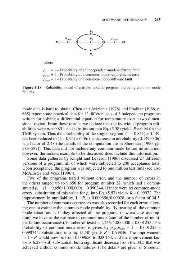
SOFTWARE REDUNDANCY 265
pcmr
pi
pi
pi
pcms
where
= 1 – Probability of an independent-mode-software fault= 1 – P= 1 – P
robability of a common-mode-requirements errorrobability of a common-mode-software fault
ppp
i
cmr
cms
Figure 5.18 Reliability model of a triple-modular program including common-modefailures.
mode data is hard to obtain, Chen and Avizienis [1978] and Pradhan [1986, p.665] report some practical data for 12 different sets of 3 independent programswritten for solving a differential equation for temperature over a two-dimen-sional region. From these results, we deduce that the individual program reli-abilities were pi c 0.851, and substitution into Eq. (5.58) yields R c 0.94 for theTMR system. Thus the unreliability of the single program, (1 − 0.851) c 0.149,has been reduced to (1 − 0.94) c 0.06; the decrease in unreliability (0.149/ 0.06)is a factor of 2.48 (the details of the computation are in Shooman [1990, pp.583–587]). This data did not include any common-mode failure information;however, the second example to be discussed does include this information.
Some data gathered by Knight and Leveson [1986] discussed 27 differentversions of a program, all of which were subjected to 200 acceptance tests.Upon acceptance, the program was subjected to one million test runs (see alsoMcAllister and Vouk [1996]).
Five of the programs tested without error, and the number of errors inthe others ranged up to 9,656 for program number 22, which had a demon-strated pi c (1 − 9,656/ 1,000,000) c 0.990344. If there were no common-modeerrors, substitution of this value for pi into Eq. (5.57) yields R c 0.99972. Theimprovement in unreliability, 1 − R, is 0.009656/ 0.00028, or a factor of 34.5.
The number of common occurrences was also recorded for each error, allow-ing one to estimate the common-mode probability. By treating all the commonmode situations as if they affected all the programs (a worst-case assump-tion), we have as the estimate of common mode (sum of the number of multi-ple failure occurrences)/ (number of tests) c 1,255/ 1,000,000 c 0.001255. Theprobability of common-mode error is given by pcmrpcms c 1 − 0.001255 c
0.998745. Substitution into Eq. (5.58) yields R c 0.99846. The improvementin 1 − R would now be from 0.009656 to 0.00154, and the improvement fac-tor is 6.27—still substantial, but a significant decrease from the 34.5 that wasachieved without common-mode failures. (The details are given in Shooman
266 SOFTWARE RELIABILITY AND RECOVERY TECHNIQUES
[1990, pp. 582–587].) Another case is computed in which the initial value ofpi c (1 − 1,368/ 1,000,000) c 0.998632 is much higher. In this case, TMRproduces a reliability of 0.99999433 for an improvement in unreliability by afactor of 241. However, the same estimate of common-mode failures reducesthis factor to only 1.1! Clearly, such a small improvement factor would not beworth the effort, and either the common-mode failures must be reduced or othermethods of improving the software reliability should be pursued. Although thisdata varies from program to program, it does show the importance of common-mode failures. When one wishes to employ redundant software, clearly onemust exercise all possible cautions to minimize common-mode failures. Also,it is suggested that modeling be done at the outset of the project using the bestestimates of independent and common-mode failure probabilities and that thiscontinue throughout the project based on the test results.
5.9.3 Space Shuttle Example
One of the best known examples of hardware and software reliability is theSpace Shuttle Orbiter flight control system. Once in orbit, the flight controlsystem must maintain the vehicle’s altitude (rotations about 3 axes fixed ininertial space). Typically, one would use such rotations to lock onto a view ofthe earth below, travel along a line of sight to an object that the Space Shuttleis approaching, and so forth. The Space Shuttle uses a combination of vari-ous large and small gas jets oriented about the 3 axes to produce the necessaryrotations. Orbit-change maneuvers, including the crucial reentry phase, are alsocarried out by the flight control system using somewhat larger orbit-maneuver-ing system (OMS) engines. There is much hardware redundancy in terms ofsensors, various groupings of the small gas jets, and even the use of a com-bination of small gas jets for sustained firing should the OMS engines fail. Inthis section, we focus on the computer hardware and software in this system,which is shown in Fig. 5.19.
There are five identical computers in the system, denoted as Hardware A,B, C, D, and E, and two different software systems, denoted by Software Aand B. Computers A–D are connected in a voting arrangement with lockoutswitches at the inputs to the voter as shown. Each of these computers uses thecomplete software system—Software A. The four computers and associatedsoftware comprise the primary avionics software system (PASS), which is atwo-out-of-four system. If a failure in one computer occurs and is confirmedby subsequent analysis and by disagreement with the other three computers aswell as by other tests and telemetered data to Ground Control, this computeris then disconnected by the crew from the arrangement, and the remainingsystem becomes a TMR system. Thus this system will sustain two failuresand still be functional rather than tolerating only a single failure, as is the casewith an ordinary TMR system. Because of all the monitoring and test programsavailable in space and on the ground, it is likely that even after two failures, if athird malfunction occurred, it would still be possible to determine and switch
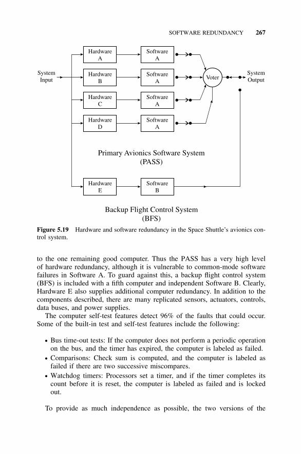
SOFTWARE REDUNDANCY 267
Primary Avionics Software System( )PASS
Backup Flight Control System( )BFS
HardwareA
SoftwareA
HardwareB
SoftwareA
HardwareC
SoftwareA
HardwareD
HardwareE
SoftwareA
SoftwareB
VoterSystemInput
SystemOutput
Figure 5.19 Hardware and software redundancy in the Space Shuttle’s avionics con-trol system.
to the one remaining good computer. Thus the PASS has a very high levelof hardware redundancy, although it is vulnerable to common-mode softwarefailures in Software A. To guard against this, a backup flight control system(BFS) is included with a fifth computer and independent Software B. Clearly,Hardware E also supplies additional computer redundancy. In addition to thecomponents described, there are many replicated sensors, actuators, controls,data buses, and power supplies.
The computer self-test features detect 96% of the faults that could occur.Some of the built-in test and self-test features include the following:
• Bus time-out tests: If the computer does not perform a periodic operationon the bus, and the timer has expired, the computer is labeled as failed.
• Comparisons: Check sum is computed, and the computer is labeled asfailed if there are two successive miscompares.
• Watchdog timers: Processors set a timer, and if the timer completes itscount before it is reset, the computer is labeled as failed and is lockedout.
To provide as much independence as possible, the two versions of the
268 SOFTWARE RELIABILITY AND RECOVERY TECHNIQUES
software were developed by different organizations. The programs were bothwritten in the HAL/ S language developed by Intermetrics. The primary sys-tem was written by IBM Federal Systems Division, and the backup softwarewas written by Rockwell and Draper Labs. Both Software A and Software Bperform all the critical functions, such as ascent to orbit, descent from orbit,and reentry, but Software A also includes various noncritical functions, suchas data logging, that are not included in the backup software.
In addition to the redundant features of Software A and B, great emphasishas been applied to the life-cycle management of the Space Shuttle software.Although the software for each mission is unique, many of its componentsare reused from previous missions. Thus, if an error is found in the softwarefor flight number 76, all previous mission software (all of which is stored)containing the same code is repaired and retested. Also, the reason why suchan error occurred is analyzed, and any possibilities for similar mechanisms tocause errors in the rest of the code for this mission and previous missions areinvestigated. This great care, along with other features, resulted in the SpaceShuttle software team being one of the first organizations to earn the highestrating of “level 5” when it was examined by the Software Engineering Instituteof Carnegie Mellon University and judged with respect to the capability matu-rity model (CMM) levels. The reduction in error rate for the first 11 flightsindicates the progress made and is shown in Fig. 5.20. An early reliabilitystudy of ground-based Space Shuttle software appears in Shooman [1984]; themodel predicted the observed software error rate on flight number 1.
The more advanced voting techniques discussed in Section 4.11 also applyto N-version software. For a comprehensive discussion of voting techniques,see McAllister and Vouk [1996].
5.10 ROLLBACK AND RECOVERY
5.10.1 Introduction
The term recovery technique includes a class of approaches that attempts todetect a software error and, in various ways, retry the computation. Suppose, forexample, that the track of an aircraft on the display in an air traffic control systembecomes corrupted. If the previous points on the path and the current input dataare stored, then the computation of the corrupted points can be retried based onthe stored values of the current input data. Assuming that no critical situation is inprogress (e.g., a potential air collision), the slight delay in recomputing and fillingin these points causes no harm. At the very worst, these few points may be lost,but the software replaces them by a projected flight path based on the past pathdata, and soon new actual points are available. This is also a highly acceptablesolution. The worst outcomes that must be strenuously avoided are from thosecases in which the errors terminate the track or cause the entire display to crash.Some designers would call such recovery techniques rollback because the com-
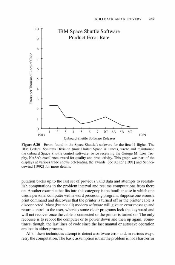
ROLLBACK AND RECOVERY 269
1989
Err
ors
per
Tho
usan
d L
ines
of
Cod
e
19831 2 3 4 5 6 7 7C 8A 8B 8C
0
1
2
3
4
5
6
7
8
9
10
Onboard Shuttle Software Releases
IBM Space Shuttle SoftwareProduct Error Rate
Figure 5.20 Errors found in the Space Shuttle’s software for the first 11 flights. TheIBM Federal Systems Division (now United Space Alliance), wrote and maintainedthe onboard Space Shuttle control software, twice receiving the George M. Low Tro-phy, NASA’s excellence award for quality and productivity. This graph was part of thedisplays at various trade shows celebrating the awards. See Keller [1991] and Schnei-dewind [1992] for more details.
putation backs up to the last set of previous valid data and attempts to reestab-lish computations in the problem interval and resume computations from thereon. Another example that fits into this category is the familiar case in which oneuses a personal computer with a word processing program. Suppose one issues aprint command and discovers that the printer is turned off or the printer cable isdisconnected. Most (but not all) modern software will give an error message andreturn control to the user, whereas some older programs lock the keyboard andwill not recover once the cable is connected or the printer is turned on. The onlyrecourse is to reboot the computer or to power down and then up again. Some-times, though, the last lines of code since the last manual or autosave operationare lost in either process.
All of these techniques attempt to detect a software error and, in various ways,retry the computation. The basic assumption is that the problem is not a hard error
270 SOFTWARE RELIABILITY AND RECOVERY TECHNIQUES
but a transient error. A transient software error is one due to a software fault thatresults only in a system error for particular system states. Thus, if we repeat thecomputation again and the system state has changed, there is a good probabilitythat the error will not be repeated on the second trial.
Recovery techniques are generally classified as forward or backward error-recovery techniques. The general philosophy of forward error recovery is tocontinue operation while knowing that there is an error in computation andcorrect for this error a little later. Techniques such as this work only in certaincircumstances; for example, in the case of a tracking algorithm for an air trafficcontrol system. In the case of backward error recovery, we wish to restart orroll back the computation process to some point before the occurrence of theerror and restart the computation. In this section, we discuss four types ofbackward error recovery:
1. Reboot/ restart techniques2. Journaling techniques3. Retry techniques4. Checkpoint techniques
For a more complete discussion of the topics introduced in this section, seeSieworek [1982] and Section 3.10.
5.10.2 Rebooting
The simplest—but weakest—recovery technique from the implementationstandpoint is to reboot or restart the system. The process of rebooting is wellknown to users of PCs who, without thinking too much about it, employ it oneor more times a week to recover from errors. Actually, this raises a philosophi-cal point: Is it better to have software that is well debugged and has very fewerrors that occur infrequently, or is having software with more residual errorsthat can be cleared by frequent rebooting also acceptable? The author remem-bers having a conversation with Ed Yourdon about an old computer when hewas preparing a paper on reliability measurements [Yourdon, 1972]. Yourdonstated that a lot of computer crashes during operation were not recorded forthe Burroughs B5500 computer (popular during the mid-1960s) because it waseasy to reboot; the operator merely pushed the HALT button to stop the sys-tem and pushed the LOAD button to load a fresh version of the operatingsystem. Furthermore, Yourdon stated, “The restart procedure requires two tofive minutes. This can be contrasted with most IBM System/ 360s, where arestart usually required fifteen to thirty minutes.” As a means of comparison,the author collected some data on reboot times that appears in Table 5.4.
It would seem that a restarting time of under one minute is now consideredacceptable for a PC. It is more difficult to quantify the amount of informationthat is lost when a crash occurs and a reboot is required. We consider threetypical applications: (a) word processing, (b) reading and writing e-mail, and
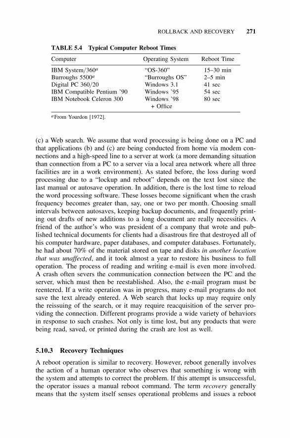
ROLLBACK AND RECOVERY 271
TABLE 5.4 Typical Computer Reboot Times
Computer Operating System Reboot Time
IBM System/ 360a “OS-360” 15–30 minBurroughs 5500a “Burroughs OS” 2–5 minDigital PC 360/ 20 Windows 3.1 41 secIBM Compatible Pentium ’90 Windows ’95 54 secIBM Notebook Celeron 300 Windows ’98 80 sec
+ Office
a From Yourdon [1972].
(c) a Web search. We assume that word processing is being done on a PC andthat applications (b) and (c) are being conducted from home via modem con-nections and a high-speed line to a server at work (a more demanding situationthan connection from a PC to a server via a local area network where all threefacilities are in a work environment). As stated before, the loss during wordprocessing due to a “lockup and reboot” depends on the text lost since thelast manual or autosave operation. In addition, there is the lost time to reloadthe word processing software. These losses become significant when the crashfrequency becomes greater than, say, one or two per month. Choosing smallintervals between autosaves, keeping backup documents, and frequently print-ing out drafts of new additions to a long document are really necessities. Afriend of the author’s who was president of a company that wrote and pub-lished technical documents for clients had a disastrous fire that destroyed all ofhis computer hardware, paper databases, and computer databases. Fortunately,he had about 70% of the material stored on tape and disks in another locationthat was unaffected, and it took almost a year to restore his business to fulloperation. The process of reading and writing e-mail is even more involved.A crash often severs the communication connection between the PC and theserver, which must then be reestablished. Also, the e-mail program must bereentered. If a write operation was in progress, many e-mail programs do notsave the text already entered. A Web search that locks up may require onlythe reissuing of the search, or it may require reacquisition of the server pro-viding the connection. Different programs provide a wide variety of behaviorsin response to such crashes. Not only is time lost, but any products that werebeing read, saved, or printed during the crash are lost as well.
5.10.3 Recovery Techniques
A reboot operation is similar to recovery. However, reboot generally involvesthe action of a human operator who observes that something is wrong withthe system and attempts to correct the problem. If this attempt is unsuccessful,the operator issues a manual reboot command. The term recovery generallymeans that the system itself senses operational problems and issues a reboot
272 SOFTWARE RELIABILITY AND RECOVERY TECHNIQUES
command. In some cases, the software problem is more severe and a simplereboot is insufficient. Recovery may involve the reloading of some or all ofthe operating system. If this is necessary on a PC, the BIOS stored in ROMprovides a basic means of communication to enable such a reloading. The mostserious problems could necessitate a lower-level fix of the disk that stores theoperating system. If we wish such a process to be autonomous, a special soft-ware program must be included that performs these operations in response toan “initiate recovery command.” Some of the clearest examples of such recov-ery techniques are associated with robotic space-research vehicles.
Consider a robotic deep-space mission that loses control and begins to spinor tumble in space. The solar cells lose generating capacity, and the antennae nolonger point toward Earth. The system must be designed from the start to recoverfrom such a situation, as battery power provides a limited amount of time forsuch recovery to take place. Once the spacecraft is stabilized, the solar cells mustbe realigned with the Sun and the antennae must be realigned with Earth. Thisis generally provided by a small, highly secure kernel in the operating systemthat takes over in such a situation. In addition to hardware redundancy for allcritical equipment, the software is generally subjected to a proof-of-correctnessand an unusually high level of testing to ensure that it will perform its intendedtask. Many of NASA’s spacecraft have recovered from such situations, but somehave not. The main point of this discussion is that reboot or recovery for all theseexamples must be contained in the requirements and planned for during the entiredesign, not added later in the process as almost an afterthought.
5.10.4 Journaling Techniques
Journaling techniques are slightly more complex and somewhat better thanreboot or restart techniques. Such techniques are also somewhat quicker toemploy than reboot or restart techniques since only a subset of the inputs mustbe saved. To employ these techniques requires that
1. a copy of the original database, disk, and filename be stored,2. all transactions (inputs) that affect the data must be stored during exe-
cution, and3. the process be backed up to the beginning and the computation be retried.
Clearly, items (2) and (3) require a lot of storage; in practice, journalingcan only be executed for a given time period, after which the inputs and theprocess must be erased and a new journaling time period created. The choiceof the time period between journaling refreshes is an important design param-eter. Storage of inputs and processes is continuous during operation regardlessof the time period. The commands to refresh the journaling process shouldnot absorb too much of the operating time budget for the system. The maintrade-off will be between the amount of storage and the amount of processingtime for computational retry, which increases with the length of the journaling
ROLLBACK AND RECOVERY 273
period versus the impact of system overhead for journaling, which decreases asthe interval between journaling refresh increases. It is possible that the storagerequirements dominate and the optimum solution is to refresh when storage isfilled up.
These techniques of journaling are illustrated by an example. The XeroxAlto personal computer used an editor called Bravo. Journaling was used torecover if a computer crash occurred during an editing session. Most modernPC-based word processing systems use a different technique to avoid loss ofdata during a session. A timer is set, and every few minutes the data in the inputbuffer (representing new input data since the last manual or automatic saveoperation) is stored. The addition of journaling to the periodic storage processwould ensure no data loss. (Perhaps the keystrokes that occurred immediatelypreceding a crash would be lost, but this at most would constitute the last wordor the last command.)
5.10.5 Retry Techniques
Retry techniques are quicker than those discussed previously, but they are morecomplex since more redundant process-state information must be stored. Retryis begun immediately after the error is detected. In the case of transient errors,one waits for the transient to die out and then initiates retry, whereas in thecase of hard errors, the approach is to reconfigure the system. In either case, theoperation affected by the error is then retried, which requires a complete knowl-edge of the system state (kept in storage) before the operation was attempted.If the interrupted operation or the error has irrevocably modified some data,the retry fails. Several examples of retry operation are as follows:
1. Disk controllers generally use disk-read reentry to minimize the numberof disk-read errors. Consider the case of an MS-DOS personal computersystem executing a disk-read command when an error is encountered.The disk-read operation is terminated, and the operator is asked whetherhe or she wishes to retry or abort. If the retry command is issued andthe transient error has cleared, recovery is successful. However, if thereis a hard error (e.g., a damaged floppy), retry will not clear the problem,and other processes must be employed.
2. The Univac 1100/ 60 computer provided retry for macroinstructions aftera failure.
3. The IBM System/ 360 provided extensive retry capabilities, performingretries for both CPU and I/ O operations.
Sometimes, the cause of errors is more complex and the retry may not work.Consider the following example that puzzled and plagued the author for a fewmonths. A personal computer with a bad hard-disk sector worked fine with allprograms except with a particular word processor. During ordinary save oper-
274 SOFTWARE RELIABILITY AND RECOVERY TECHNIQUES
ations, the operating system must have avoided the bad sector in storing diskfiles. However, the word processor automatically saved the workspace everyfew minutes. Small text segments in the workspace were fine, but medium-sized text segments were sometimes subjected to disk-read errors during theautosave operation but not during a normal (manually issued) save command.In response to the error message “abort or retry,” a simple retry response gen-erally worked the first time or, at worst, required an abort followed by a savecommand. With large text segments in the workspace, real trouble occurred:When a disk-read error was encountered during automatic saving, one or moreparagraphs of text from previous word processing sessions that were stored inthe buffer were often randomly inserted into the present workspace, therebycorrupting the document. This is a graphic example of a retry failure. Theauthor was about to attempt to lock out the bad disk sectors so they wouldnot be used; however, the problem disappeared with the arrival of the secondrelease of the word processor. Most likely, the new software used a slightlydifferent buffer autosave mechanism.
5.10.6 Checkpointing
One advantage of checkpoint techniques is that they can generally be imple-mented using only software, as contrasted with retry techniques that mayrequire additional dedicated hardware in addition to the necessary softwareroutines. Also in the case of retry, the entire time history of the system stateduring the relevant period is saved, whereas in checkpointing the time historyof the system state is saved only at specific points (checkpoints); thus lessstorage is required. A major disadvantage of checkpointing is the amount anddifficulty of the programming that is required to employ checkpoints. The stepsin the checkpointing process are as follows:
1. After the error is detected, recovery is initiated as soon as transient errorsdie out or, in the case of hard errors, the system is reconfigured.
2. The system is rolled back to the most recent checkpoint, and the systemstate is set to the stored checkpoint state and the process is restarted. If theoperation is successfully restored, the process continues, and only sometime and any new input data during the recovery process are lost. If oper-ation is not restored, rollback to an earlier checkpoint can be attempted.
3. If the interrupted operation or the error has irrevocably modified somedata, the checkpoint technique fails.
One better-developed example of checkpointing is within the Guardian oper-ating system used for the Tandem computer system. The system consists of aprimary process that does all the work and a backup process that operates onthe same inputs and is ready to take over if the primary process fails. At criticalpoints, the primary process sends checkpoint messages to the backup process.

ROLLBACK AND RECOVERY 275
For further details on the Guardian operating system, the reader is referred toSiewiorek [1992, pp. 635–648]. Also, see the discussion in Section 3.10.
Some comments are necessary with respect to the way customers generallyuse Tandem computer systems and the Guardian operating system:
1. The initial interest in the Tandem computer system was probably due tothe marketing value of the term “NonStop architecture” that was usedto describe the system. Although proprietary studies probably exist, theauthor does not know of any reliability or availability studies in the openliterature that compared the Tandem architecture with a competitive sys-tem such as a Digital Equipment VAX Cluster or an IBM system config-ured for high reliability. Thus it is not clear how these systems comparedto the competition, although most users are happy.
2. Once the system was studied by potential customers, one of the mostimportant selling points was its modular structure. If the capacity of anexisting Tandem system was soon to be exceeded, the user could simplybuy additional Tandem machines, connect them in parallel, and easilyintegrate the expanded capacity with the existing system, which some-times could be accomplished without shutting down system operation.This was a clear advantage over competitors, so it was built into thebasic design.
3. The use of the Guardian operating system’s checkpointing features couldeasily be turned on or off in configuring the system. Many users turnedthis feature off because it slowed down the system somewhat, but moreimportantly because to use it required some complex system program-ming to be added to the application programs. Newer Tandem systemshave made such programming easier to use, as discussed in Section3.10.1.
5.10.7 Distributed Storage and Processing
Many modern computer systems have a client–server architecture—typically,PCs or workstations are the clients, and the server is a more powerful pro-cessor with large disk storage attached. The clients and server are generallyconnected by local area networks (LANs). In fact, processing and data storageboth tend to be decentralized, and several servers with their sets of clients areoften connected by another network. In such systems, there is considerable the-oretical and practical interest in devising algorithms to synchronize the variousservers and to prevent two or more users from colliding when they attempt toaccess data from the same file. Even more important is the prevention of sys-tem lockup when one user is writing to a device and another user tries to readthe device. For more information, the reader is referred to Bhargava [1987]and to the literature.
276 SOFTWARE RELIABILITY AND RECOVERY TECHNIQUES
REFERENCES
AIAA/ ANSI R-013-1992. Recommended Practice Software Reliability. The AmericanInstitute of Aeronautics and Astronautics, The Aerospace Center, Washington, DC,ISBN 1-56347-024-1, February 23, 1993.
The Associated Press. “Y2K Bug Bites 7-Eleven Late.” Newsday, January 4, 2001, p.A49.
Basili, V., and D. Weiss. A Methodology for Collecting Valid Software EngineeringData. IEEE Transactions on Software Engineering 10, 6 (1984): 42–52.
Bernays, A. “Carrying On About Carry-Ons.” New York Times, January 25, 1998, p.33 of Travel Section.
Beiser, B. Software Testing Techniques, 2d ed. Van Nostrand Reinhold, New York,1990.
Bhargava, B. K. Concurrency Control and Reliability in Distributed Systems. Van Nos-trand Reinhold, New York, 1987.
Billings, C. W. Grace Hopper Naval Admiral and Computer Pioneer. Enslow Publish-ers, Hillside, NJ, 1989.
Boehm, B. Software Engineering Economics. Prentice-Hall, Englewood Cliffs, NJ,1981.
Boehm, B. et al. Avoiding the Software Model-Crash Spiderweb. New York: IEEEComputer Magazine (November 2000): 120–122.
Booch, G. et al. The Unified Modeling Language User Guide. Addison-Wesley, Read-ing, MA, 1999.
Brilliant, S. S., J. C. Knight, and N. G. Leveson. The Consistent Comparison Problemin N-Version Software. ACM SIGSOFT Software Engineering Notes 12, 1 (January1987): 29–34.
Brooks, F. P. The Mythical Man-Month Essays on Software Engineering. Addison-Wesley, Reading, MA, 1995.
Butler, R. W., and G. B. Finelli. The Infeasibility of Experimental Quantification ofLife-Critical Real-Time Software Reliability. IEEE Transactions on Software Reli-ability Engineering 19 (January 1993): 3–12.
Chen, L., and A. Avizienis. N-Version Programming: A Fault-Tolerance Approachto Reliability of Software Operation. Digest of Eighth International Fault-Toler-ant Computing Symposium, Toulouse, France, 1978. IEEE Computer Society, NewYork, pp. 3–9.
Chillarege, R., and D. P. Siewiorek. Experimental Evaluation of Computer SystemsReliability. IEEE Transactions on Reliability 39, 4 (October 1990).
Cormen, T. H. et al. Introduction to Algorithms. McGraw-Hill, New York, 1992.
Cramer, H. Mathematical Methods of Statistics. Princeton University Press, Princeton,NJ, 1991.
Dougherty, E. M. Jr., and J. R. Fragola. Human Reliability Analysis. Wiley, New York,1988.
Everett, W. W., and J. D. Musa. A Software-Reliability Engineering Practice. NewYork, IEEE Computer Magazine 26, 3 (1993): 77–79.
REFERENCES 277
Fowler, M., and K. Scott. UML Distilled Second Edition. Addison-Wesley, Reading,MA, 1999.
Fragola, J. R., and M. L. Shooman. Significance of Zero Failures and Its Effecton Risk Decision Making. Proceedings International Conference on ProbabilisticSafety Assessment and Management, New York, NY, September 13–18, 1998, pp.2145–2150.
Garman, J. R. The “Bug” Heard ’Round The World. ACM SIGSOFT Software Engi-neering Notes (October 1981): 3–10.
Hall, H. S., and S. R. Knight. Higher Algebra, 1887. Reprint, Macmillan, New York,1957.
Hamlet, D., and R. Taylor. Partition Testing does not Inspire Confidence. IEEE Trans-actions on Software Engineering 16, 12 (1990): 1402–1411.
Hatton, L. Software Faults and Failure. Addison-Wesley, Reading, MA, 2000.Hecht, H. Fault-Tolerant Software. IEEE Transactions on Reliability 28 (August 1979):
227–232.Hiller, S., and G. J. Lieberman. Operations Research. Holden-Day, San Francisco,
1974.Hoel, P. G. Introduction to Mathematical Statistics. Wiley, New York, 1971.Howden, W. E. Functional Testing. IEEE Transactions on Software Engineering 6, 2
(March 1980): 162–169.IEEE Computer Magazine, Special Issue on Managing OO Development. (September
1996.)Jacobson, I. et al. Making the Reuse Business Work. IEEE Computer Magazine, New
York (October 1997): 36–42.Jacobson, I. The Road to the Unified Software Development Process. Cambridge Uni-
versity Press, New York, 2000.Jelinski, Z., and P. Moranda. “Software Reliability Research.” In Statistical Computer
Performance Evaluation, W. Freiberger (ed.). Academic Press, New York, 1972,pp. 465–484.
Kahn, E. H. et al. Object-Oriented Programming for Structured Procedural Program-mers. IEEE Computer Magazine, New York (October 1995): 48–57.
Kanon, K., M. Kaaniche, and J.-C. Laprie. Experiences in Software Reliability: FromData Collection to Quantitative Evaluation. Proceedings of the Fourth InternationalSymposium on Software Reliability Engineering (ISSRE ’93), 1993. IEEE, NewYork, NY, pp. 234–246.
Keller, T. W. et al. Practical Applications of Software Reliability Models. Proceed-ings International Symposium on Software Reliability Engineering, IEEE ComputerSociety Press, Los Alamitos, CA, 1991, pp. 76–78.
Knight, J. C., and N. G. Leveson. An Experimental Evaluation of Independence inMultiversion Programming. IEEE Transactions on Software Engineering 12, 1 (Jan-uary 1986): 96–109.
Lala, P. K. Fault Tolerant and Fault Testable Hardware Design. Prentice-Hall, Engle-wood Cliffs, NJ, 1985.
Lala, P. K. Self-Checking and Fault-Tolerant Digital Design. Academic Press, divisionof Elsevier Science, New York, 2000.
278 SOFTWARE RELIABILITY AND RECOVERY TECHNIQUES
Leach, R. J. Introduction to Software Engineering. CRC Press, Boca Raton, FL,2000.
Littlewood, B. Software Reliability: Achievement and Assessment. Blackwell, Oxford,U.K., 1987.
Lyu, M. R. Software Fault Tolerance. Wiley, Chichester, U.K., 1995.Lyu, M. R. (ed.). Handbook of Software Reliability Engineering. McGraw-Hill, New
York, 1996.McAllister, D. F., and M. A. Voulk. “Fault-Tolerant Software Reliability Engineering.”
In Handbook of Software Reliability Engineering, M. R. Lyu (ed.). McGraw-Hill,New York, 1996, ch. 14, p. 567–609.
Miller, G. A. The Magical Number Seven, Plus or Minus Two: Some Limits on ourCapacity for Processing Information. The Psychological Review 63 (March 1956):81–97.
Mood, A. M., and F. A. Graybill. Introduction to the Theory of Statistics, 2d ed.McGraw-Hill, New York, 1963.
Musa, J. A Theory of Software Reliability and its Application. IEEE Transactions onSoftware Engineering 1, 3 (September 1975): 312–327.
Musa, J., A. Iannino, and K. Okumoto. Software Reliability: Measurement, Prediction,Application. McGraw-Hill, New York, 1987.
Musa, J. Sensitivity of Field Failure Intensity to Operational Profile Errors. Proceedingsof the 5th International Symposium on Software Reliability Engineering, Monterey,CA, 1994. IEEE, New York, NY, pp. 334–337.
New York Times, “Circuits Section.” August 27, 1998, p. G1.New York Times, “The Y2K Issue Shows Up, a Year Late.” January 3, 2001, p. A3.Pfleerer, S. L. Software Engineering Theory and Practice. Prentice-Hall, Upper Saddle
River, NJ, 1998, pp. 31–33, 181, 195–198, 207.Pooley, R., and P. Stevens. Using UML: Software Engineering with Objects and Com-
ponents. Addison-Wesley, Reading, MA, 1999.Pollack, A. “Chips are Hidden in Washing Machines, Microwaves. . . .” New York
Times, Media and Technology Section, January 4, 1999, p. C17.Pradhan, D. K. Fault-Tolerant Computing Theory and Techniques, vols. I and II.
Prentice-Hall, Englewood Cliffs, NJ, 1986.Pradhan, D. K. Fault-Tolerant Computing Theory and Techniques, vol. I, 2d ed.
Prentice-Hall, Englewood Cliffs, NJ, 1993.Pressman, R. H. Software Engineering: A Practitioner’s Approach, 4th ed. McGraw-
Hill, New York, 1997, pp. 348–363.Schach, S. R. Classical and Object-Oriented Software Engineering with UML and
C++, 4th ed. McGraw-Hill, New York, 1999.Schach, S. R. Classical and Object-Oriented Software Engineering with UML and
Java. McGraw-Hill, New York, 1999.Schneidewind, N. F., and T. W. Keller. Application of Reliability Models to the Space
Shuttle. IEEE Software (July 1992): 28–33.Shooman, M. L., and M. Messinger. Use of Classical Statistics, Bayesian Statistics,
and Life Models in Reliability Assessment. Consulting Report, U.S. Army ResearchOffice, June 1971.
REFERENCES 279
Shooman, M. L. Probabilistic Models for Software Reliability Prediction. In Statisti-cal Computer Performance Evaluation, W. Freiberger (ed.). Academic Press, NewYork, 1972, pp. 485–502.
Shooman, M. L., and M. Bolsky. Types, Distribution, and Test and Correction Timesfor Programming Errors. Proceedings 1975 International Conference on ReliableSoftware. IEEE, New York, NY, Catalog No. 75CHO940-7CSR, p. 347.
Shooman, M. L. Software Engineering: Design, Reliability, and Management.McGraw-Hill, New York, 1983, ch. 5.
Shooman, M. L., and G. Richeson. Reliability of Shuttle Mission Control Center Soft-ware. Proceedings Annual Reliability and Maintainability Symposium, 1984. IEEE,New York, NY, pp. 125–135.
Shooman, M. L. Validating Software Reliability Models. Proceedings of the IFACWorkshop on Reliability, Availability, and Maintainability of Industrial Process Con-trol Sysems. Pergamon Press, division of Elsevier Science, New York, 1988.
Shooman, M. L. A Class of Exponential Software Reliability Models. Workshop onSoftware Reliability. IEEE Computer Society Technical Committee on SoftwareReliability Engineering, Washington, DC, April 13, 1990.
Shooman, M. L., Probabilistic Reliability: An Engineering Approach, 2d ed. Krieger,Melbourne, FL, 1990, Appendix H.
Shooman, M. L. A Micro Software Reliability Model for Prediction and Test Appor-tionment. Proceedings International Symposium on Software Reliability Engineer-ing, 1991. IEEE, New York, NY, p. 52–59.
Shooman, M. L. Software Reliability Models for Use During Proposal and EarlyDesign Stages. Proceedings ISSRE ’99, Symposium on Software Reliability Engi-neering. IEEE Computer Society Press, New York, 1999.
Spectrum, Special Issue on Engineering Software. IEEE Computer Society Press, NewYork (April 1999).
Siewiorek, D. P., and R. S. Swarz. The Theory and Practice of Reliable System Design.The Digital Press, Bedford, MA, 1982.
Siewiorek, D. P., and R. S. Swarz. Reliable Computer Systems Design and Evaluation,2d ed. The Digital Press, Bedford, MA, 1992.
Siewiorek, D. P. and R. S. Swarz. Reliable Computer Systems Design and Evaluation,3d ed. A. K. Peters, www.akpeters.com, 1998.
Stark, G. E. Dependability Evaluation of Integrated Hardware/ Software Systems. IEEETransactions on Reliability (October 1987).
Stark, G. E. et al. Using Metrics for Management Decision-Making. IEEE ComputerMagazine, New York (September 1994).
Stark, G. E. et al. An Examination of the Effects of Requirements Changes on Soft-ware Maintenance Releases. Software Maintenance: Research and Practice, vol. 15,August 1999.
Stork, D. G. Using Open Data Collection for Intelligent Software. IEEE ComputerMagazine, New York (October 2000): 104–106.
Tai, A. T., J. F. Meyer, and A. Avizienis. Software Performability, From Concepts toApplications. Kluwer Academic Publishers, Hingham, MA, 1995.
280 SOFTWARE RELIABILITY AND RECOVERY TECHNIQUES
Wing, J. A Specifier’s Introduction to Formal Methods. New York: IEEE ComputerMagazine 23, 9 (September 1990): 8–24.
Yanini, E. New York Times, Business Section, December 7, 1997, p. 13.Yourdon, E. Reliability Measurements for Third Generation Computer Systems. Pro-
ceedings Annual Reliability and Maintainability Symposium, 1972. IEEE, NewYork, NY, pp. 174–183.
PROBLEMS
5.1. Consider a software project with which you are familiar (past, in-progress, or planned). Write a few sentences or a paragraph describingthe phases given in Table 5.1 for this project. Make sure you start bydescribing the project in succinct form.
5.2. Draw an H-diagram similar to that shown in Fig. 5.1 for the softwareof problem 5.1.
5.3. How well does the diagram of problem 5.2 agree with Eqs. (5.1 a–d)?Explain.
5.4. Write a short version of a test plan for the project of problem 5.1. Includethe number and types of tests for the various phases. (Note: A completetest plan will include test data and expected answers.)
5.5. Would (or did) the development follow the approach of Figs. 5.2, 5.3,or 5.4? Explain.
5.6. We wish to develop software for a server on the Internet that keeps adatabase of locations for new cars that an auto manufacturer is tracking.Assume that as soon as a car is assembled, a reusable electronic box isinstalled in the vehicle that remains there until the car is delivered to apurchaser. The box contains a global positioning system (GPS) receiverthat determines accurate location coordinates from the GPS satellites anda transponder that transmits a serial number and these coordinates viaanother satellite to the server. The server receives these transponder sig-nals and stores them in a file. The server has a geographical databaseso that it can tell from the coordinates if each car is (a) in the manufac-turer’s storage lot, (b) in transit, or (c) in a dealer’s showroom or lot.The database is accessed by an Internet-capable cellular phone or anycomputer with Internet access [Stork, 2000, p. 18].(a) How would you design the server software for this system? (Figs.
5.2, 5.3, or 5.4?)(b) Draw an H-diagram for the software.
5.7. Repeat problem 5.3 for the software in problem 5.6.
5.8. Repeat problem 5.4 for the software in problem 5.6.
PROBLEMS 281
5.9. Repeat problem 5.5 for the software in problem 5.6.
5.10. A component with a constant-failure rate of 4 × 10⁻⁵ is discussed inSection 5.4.5.(a) Plot the failure rate as a function of time.(b) Plot the density function as a function of time.(c) Plot the cumulative distribution function as a function of time.(d) Plot the reliability as a function of time.
5.11. It is estimated that about 100 errors will be removed from a program dur-ing the integration test phase, which is scheduled for 12 months duration.(a) Plot the error-removal curve assuming that the errors will follow a
constant-removal rate.(b) Plot the error-removal curve assuming that the errors will follow a
linearly decreasing removal rate.(c) Plot the error-removal curve assuming that the errors will follow an
exponentially decreasing removal rate.
5.12. Assume that a reliability model is to be fitted to problem 5.11. The num-ber of errors remaining in the program at the beginning of integrationtesting is estimated to be 120. From experience with similar programs,analysts believe that the program will start integration testing with anMTTF of 150 hours.(a) Assuming a constant error-removal rate during integration, formulate
a software reliability model.(b) Plot the reliability function versus time at the beginning of integra-
tion testing—after 4, 8, and 12 months of debugging.(c) Plot the MTTF as a function of the integration test time, t.
5.13. Repeat problem 5.12 for a linearly decreasing error-removal rate.
5.14. Repeat problem 5.12 for an exponentially decreasing error-removal rate.
5.15. Compare the reliability functions derived in problems 5.12, 5.13, and5.14 by plotting them on the same time axis for t c 0, t c 4, t c 8, andt c 12 months.
5.16. Compare the MTTF functions derived in problems 5.12, 5.13, and 5.14by plotting them on the same time axis versus t.
5.17. After 1 month of integration testing of a program, the MTTF c 10 hours,and 15 errors have been removed. After 2 months, the MTTF c 15 hours,and 25 total errors have been removed.(a) Assuming a constant error-removal rate, fit a model to this data
set. Estimate the parameters by using moment-estimation techniques[Eqs. (5.47a, b)].
(b) Sketch MTTF versus development time t.
282 SOFTWARE RELIABILITY AND RECOVERY TECHNIQUES
(c) How much integration test time will be required to achieve a 100-hour MTTF? How many errors will have been removed by this timeand how many will remain?
5.18. Repeat problem 5.17 assuming a linearly decreasing error-rate modeland using Eqs. (5.49a, b).
5.19. Repeat problem 5.17 assuming an exponentially decreasing error-ratemodel and using Eqs. (5.51) and (5.52).
5.20. After 1 month of integration testing, 20 errors have been removed, theMTTF of the software is measured by testing it with the use of simulatedoperational data, and the MTTF c 10 hours. After 2 months, the MTTFc 20 hours, and 50 total errors have been removed.(a) Assuming a constant error-removal rate, fit a model to this data
set. Estimate the parameters by using moment-estimation techniques[Eqs. (5.47a, b)].
(b) Sketch the MTTF versus development time t.(c) How much integration test time will be required to achieve a 60-hour
MTTF? How many errors will have been removed by this time andhow many will remain?
(d) If we release the software when it achieves a 60-hour MTTF, sketchthe reliability function versus time.
(e) How long can the software operate, if released as in part (d) above,before the reliability drops to 0.90?
5.21. Repeat problem 5.20 assuming a linearly decreasing error-rate modeland using Eqs. (5.49a, b).
5.22. Repeat problem 5.20 assuming an exponentially decreasing error-ratemodel and using Eqs. (5.51) and (5.52).
5.23. Assume that the company developing the software discussed in problem5.17 has historical data for similar systems that show an average MTTFof 50 hours with a variance j2 of 30 hours. The variance of the reliabilitymodeling is assumed to be 20 hours. Using Eqs. (5.55) and (5.56a, b),compute the reliability function.
5.24. Assume that the model of Fig. 5.18 holds for three independent ver-sions of reliable software. The probability of error for 10,000 hours ofoperation of each version is 0.01. Compute the reliability of the TMRconfiguration assuming that there are no common-mode failures. Recom-pute the reliability of the TMR configuration if 1% of the errors are dueto common-mode requirement errors and 1% are due to common-modesoftware faults.
6NETWORKED SYSTEMSRELIABILITY
Reliability of Computer Systems and Networks: Fault Tolerance, Analysis, and DesignMartin L. Shooman
Copyright 2002 John Wiley & Sons, Inc.ISBNs: 0-471-29342-3 (Hardback); 0-471-22460-X (Electronic)
283
6.1 INTRODUCTION
Many physical problems (e.g., computer networks, piping systems, and powergrids) can be modeled by a network. In the context of this chapter, the wordnetwork means a physical problem that can be modeled as a mathematicalgraph composed of nodes and links (directed or undirected) where the brancheshave associated physical parameters such as flow per minute, bandwidth, ormegawatts. In many such systems, the physical problem has sources and sinksor inputs and outputs, and the proper operation is based on connection betweeninputs and outputs. Systems such as computer or communication networks havemany nodes representing the users or resources that desire to communicate andalso have several links providing a number of interconnected pathways. Thesemany interconnections make for high reliability and considerable complexity.Because many users are connected to such a network, a failure affects manypeople; thus the reliability goals must be set at a high level.
This chapter focuses on computer networks. It begins by discussing the sev-eral techniques that allow one to analyze the reliability of a given network, afterwhich the more difficult problem of optimum network design is introduced.The chapter concludes with a brief introduction to one of the most difficultcases to analyze—where links can be disabled because of two factors: (a) linkcongestion (a situation in which flow demand exceeds flow capacity and a linkis blocked or an excessive queue builds up at a node), and (b) failures frombroken links.
A new approach to reliability in interconnected networks is called surviv-ability analysis [Jia and Wing, 2001]. The concept is based on the design of
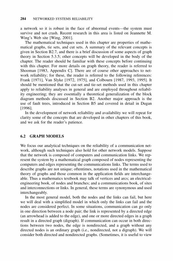
284 NETWORKED SYSTEMS RELIABILITY
a network so it is robust in the face of abnormal events—the system mustsurvive and not crash. Recent research in this area is listed on Jeannette M.Wing’s Web site [Wing, 2001].
The mathematical techniques used in this chapter are properties of mathe-matical graphs, tie sets, and cut sets. A summary of the relevant concepts isgiven in Section B2.7, and there is a brief discussion of some aspects of graphtheory in Section 5.3.5; other concepts will be developed in the body of thechapter. The reader should be familiar with these concepts before continuingwith this chapter. For more details on graph theory, the reader is referred toShooman [1983, Appendix C]. There are of course other approaches to net-work reliability; for these, the reader is referred to the following references:Frank [1971], Van Slyke [1972, 1975], and Colbourn [1987, 1993, 1995]. Itshould be mentioned that the cut-set and tie-set methods used in this chapterapply to reliability analyses in general and are employed throughout reliabil-ity engineering; they are essentially a theoretical generalization of the blockdiagram methods discussed in Section B2. Another major approach is theuse of fault trees, introduced in Section B5 and covered in detail in Dugan[1996].
In the development of network reliability and availability we will repeat forclarity some of the concepts that are developed in other chapters of this book,and we ask for the reader’s patience.
6.2 GRAPH MODELS
We focus our analytical techniques on the reliability of a communication net-work, although such techniques also hold for other network models. Supposethat the network is composed of computers and communication links. We rep-resent the system by a mathematical graph composed of nodes representing thecomputers and edges representing the communications links. The terms used todescribe graphs are not unique; oftentimes, notations used in the mathematicaltheory of graphs and those common in the application fields are interchange-able. Thus a mathematics textbook may talk of vertices and arcs; an electrical-engineering book, of nodes and branches; and a communications book, of sitesand interconnections or links. In general, these terms are synonymous and usedinterchangeably.
In the most general model, both the nodes and the links can fail, but herewe will deal with a simplified model in which only the links can fail and thenodes are considered perfect. In some situations, communication can go onlyin one direction between a node pair; the link is represented by a directed edge(an arrowhead is added to the edge), and one or more directed edges in a graphresult in a directed graph (digraph). If communication can occur in both direc-tions between two nodes, the edge is nondirected, and a graph without anydirected nodes is an ordinary graph (i.e., nondirected, not a digraph). We willconsider both directed and nondirected graphs. (Sometimes, it is useful to view
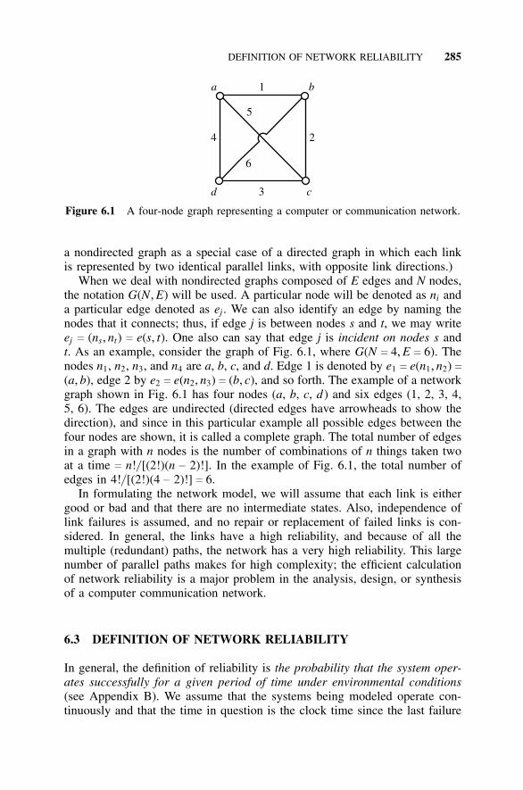
DEFINITION OF NETWORK RELIABILITY 285
a b1
4 2
d c3
5
6
Figure 6.1 A four-node graph representing a computer or communication network.
a nondirected graph as a special case of a directed graph in which each linkis represented by two identical parallel links, with opposite link directions.)
When we deal with nondirected graphs composed of E edges and N nodes,the notation G(N, E) will be used. A particular node will be denoted as ni anda particular edge denoted as ej . We can also identify an edge by naming thenodes that it connects; thus, if edge j is between nodes s and t, we may writeej c (ns, nt) c e(s, t). One also can say that edge j is incident on nodes s andt. As an example, consider the graph of Fig. 6.1, where G(N c 4, E c 6). Thenodes n1, n2, n3, and n4 are a, b, c, and d. Edge 1 is denoted by e1 c e(n1, n2) c(a, b), edge 2 by e2 c e(n2, n3) c (b, c), and so forth. The example of a networkgraph shown in Fig. 6.1 has four nodes (a, b, c, d) and six edges (1, 2, 3, 4,5, 6). The edges are undirected (directed edges have arrowheads to show thedirection), and since in this particular example all possible edges between thefour nodes are shown, it is called a complete graph. The total number of edgesin a graph with n nodes is the number of combinations of n things taken twoat a time c n!/ [(2!)(n − 2)!]. In the example of Fig. 6.1, the total number ofedges in 4!/ [(2!)(4 − 2)!] c 6.
In formulating the network model, we will assume that each link is eithergood or bad and that there are no intermediate states. Also, independence oflink failures is assumed, and no repair or replacement of failed links is con-sidered. In general, the links have a high reliability, and because of all themultiple (redundant) paths, the network has a very high reliability. This largenumber of parallel paths makes for high complexity; the efficient calculationof network reliability is a major problem in the analysis, design, or synthesisof a computer communication network.
6.3 DEFINITION OF NETWORK RELIABILITY
In general, the definition of reliability is the probability that the system oper-ates successfully for a given period of time under environmental conditions(see Appendix B). We assume that the systems being modeled operate con-tinuously and that the time in question is the clock time since the last failure
286 NETWORKED SYSTEMS RELIABILITY
or restart of the system. The environmental conditions include not only tem-perature, atmosphere, and weather, but also system load or traffic. The termsuccessful operation can have many interpretations. The two primary ones arerelated to how many of the n nodes can communicate with each other. Weassume that as time increases, a number of the m links fail. If we focus oncommunication between a pair of nodes where s is the source node and t isthe target node, then successful operation is defined as the presence of one ormore operating paths between s and t. This is called the two-terminal problem,and the probability of successful communication between s and t is called two-terminal reliability. If successful operation is defined as all nodes being ableto communicate, we have the all-terminal problem, for which it can be statedthat node s must be able to communicate with all the other n − 1 nodes, sincecommunication between any one node s and all others nodes, t1, t2, . . . , tn − 1,is equivalent to communication between all nodes. The probability of success-ful communication between node s and nodes t1, t2, . . . , tn − 1 is called the all-terminal reliability.
In more formal terms, we can state that the all-terminal reliability is theprobability that node ni can communicate with node nj for all pairs ninj (wherei � j ). We wish to show that this is equivalent to the proposition that node scan communicate with all other nodes t1 c n2, t2 c n3, . . . , tn − 1 c nn. Chooseany other node nx (where x � 1). By assumption, nx can communicate with sbecause s can communicate with all nodes and communication is in both direc-tions. However, once nx reaches s, it can then reach all other nodes becauses is connected to all nodes. Thus all-terminal connectivity for x c 1 results inall-terminal connectivity for x � 1, and the proposition is proved.
In general, reliability, R, is the probability of successful operation. In thecase of networks, we are interested in all-terminal reliability, Rall:
Rall c P(that all n nodes are connected) (6.1)
or the two-terminal reliability:
Rst c P(that nodes s and t are connected) (6.2)
Similarly, k-terminal reliability is the probability that a subset of k nodes 2 ≤k ≤ n) are connected. Thus we must specify what type of reliability we arediscussing when we begin a problem.
We stated previously that repairs were not included in the analysis of net-work reliability. This is not strictly true; for simplicity, no repair was assumed.In actuality, when a node-switching computer or a telephone communicationsline goes down, each is promptly repaired. The metric used to describe arepairable system is availability, which is defined as the probabilty that at anyinstant of time t, the system is up and available. Remember that in the caseof reliability, there were no failures in the interval 0 to t. The notation is A(t),and availability and reliability are related as follows by the union of events:
DEFINITION OF NETWORK RELIABILITY 287
A(t) c P(no failure in interval 0 to t + 1 failure and
1 repair in interval 0 to t + 2 failures and
2 repairs in interval 0 to t + · · ·) (6.3)
The events in Eq. (6.3) are all mutually exclusive; thus Eq. (6.3) can beexpanded as a sum of probabilities:
A(t) c P(no failure in interval 0 to t)
+ P(1 failure and 1 repair in interval 0 to t)
+ P(2 failures and 2 repairs in interval 0 to t) + · · · (6.4)
Clearly,
• The first term in Eq. (6.4) is the reliability, R(t)• A(t) c R(t) c 1 at t c 0• For t > 0, A(t) > R(t)• R(t) b 0 as t b ∞• It is shown in Appendix B that A(t) b Ass as t b ∞ and, as long as repair
is present, Ass > 0
Availability is generally derived using Markov probability models (seeAppendix B and Shooman [1990]). The result of availability derivations fora single element with various failure and repair probability distributions canbecome quite complex. In general, the derivations are simplified by assumingexponential probability distributions for the failure and repair times (equiv-alent to constant-failure rate, l, and constant-repair rate, m). Sometimes, themean time to failure (MTTF) and the mean time to repair (MTTR) are usedto describe the repair process and availability. In many cases, the terms meantime between failure (MTBF) and mean time between repair (MTBR) are usedinstead of MTTF and MTTR. For constant-failure and -repair rates, the meantimes become MTBF c 1/ l and MTBR c 1/m. The solution for A(t) has anexponentially decaying transient term and a constant steady-state term. After afew failure repair cycles, the transient term dies out and the availability can berepresented by the simpler steady-state term. For the case of constant-failureand -repair rates for a single item, the steady-state availability is given by theequation that follows (see Appendix B).
Ass c m/ (l + m) c MTBF/ (MTBF + MTBR) (6.5)
Since the MTBF >> MTBR in any well-designed system, Ass is close tounity. Also, alternate definitions for MTTF and MTTR lead to slightly differentbut equivalent forms for Eq. (6.5) (see Kershenbaum [1993].)
Another derivation of availability can be done in terms of system uptime,U(t), and system downtime, D(t), resulting in the following different formulafor availability:
288 NETWORKED SYSTEMS RELIABILITY
Ass c U(t)/ [U(t) + D(t)] (6.6)
The formulation given in Eq. (6.6) is more convenient than that of Eq. (6.5)if we wish to estimate Ass based on collected field data. In the case of a com-puter network, the availability computations can become quite complex if therepairs of the various elements are coupled, in which case a single repairmanmight be responsible for maintaining, say, two nodes and five lines. If sev-eral failures occur in a short period of time, a queue of failed items wait-ing for repairs might build up and the downtime is lengthened, and the term“repairman-coupled” is used. In the ideal case, if we assume that each elementin the system has its own dedicated repairman, we can guarantee that the ele-ments are decoupled and that the steady-state availabilities can be substitutedinto probability expressions in the same way as reliabilities are. In a practi-cal case, we do not have individual repairmen, but if the repair rate is muchlarger than the failure rate of the several components for which the repairmansupports, then approximate decoupling is a good assumption. Thus, in mostnetwork reliability analyses there will be no distinction made between reli-ability and availability; the two terms are used interchangeably in the networkfield in a loose sense. Thus a reliability analyst would make a combinatorialmodel of a network and insert reliability values for the components to calculatesystem reliability. Because decoupling holds, he or she would substitute com-ponent availabilities in the same model and calculate the system availability;however, a network analyst would perform the same availability computationand refer to it colloquially as “system reliability.” For a complete discussionof availability, see Shooman [1990].
6.4 TWO-TERMINAL RELIABILITY
The evaluation of network reliability is a difficult problem, but there are severalapproaches. For any practical problem of significant size, one must use a com-putational program. Thus all the techniques we discuss that use a “pencil-paper-and-calculator” analysis are preludes to understanding how to write algorithmsand programs for network reliability computation. Also, it is always valuable tohave an analytical solution of simpler problems for use to test reliability com-putation programs until the user becomes comfortable with such a program.Since two-terminal reliability is a bit simpler than all-terminal reliability, wewill discuss it first and treat all-terminal reliability in the following section.
6.4.1 State-Space Enumeration
Conceptually, the simplest means of evaluating the two-terminal reliability ofa network is to enumerate all possible combinations where each of the e edgescan be good or bad, resulting in 2e combinations. Each of these combinations ofgood and bad edges can be treated as an event Ei. These events are all mutually
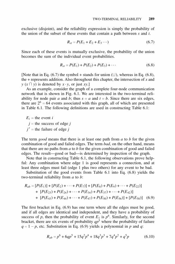
TWO-TERMINAL RELIABILITY 289
exclusive (disjoint), and the reliability expression is simply the probability ofthe union of the subset of these events that contain a path between s and t.
Rst c P(E1 + E2 + E3 · · ·) (6.7)
Since each of these events is mutually exclusive, the probability of the unionbecomes the sum of the individual event probabilities.
Rst c P(E1) + P(E2) + P(E3) + · · · (6.8)
[Note that in Eq. (6.7) the symbol + stands for union (U), whereas in Eq. (6.8),the + represents addition. Also throughout this chapter, the intersection of x andy (x
Uy) is denoted by x . y, or just xy.]
As an example, consider the graph of a complete four-node communicationnetwork that is shown in Fig. 6.1. We are interested in the two-terminal reli-ability for node pair a and b; thus s c a and t c b. Since there are six edges,there are 26
c 64 events associated with this graph, all of which are presentedin Table 6.1. The following definitions are used in constructing Table 6.1:
Ei c the event ij c the success of edge j
j ′ c the failure of edge j
The term good means that there is at least one path from a to b for the givencombination of good and failed edges. The term bad, on the other hand, meansthat there are no paths from a to b for the given combination of good and failededges. The result—good or bad—is determined by inspection of the graph.
Note that in constructing Table 6.1, the following observations prove help-ful: Any combination where edge 1 is good represents a connection, and atleast three edges must fail (edge 1 plus two others) for any event to be bad.
Substitution of the good events from Table 6.1 into Eq. (6.8) yields thetwo-terminal reliability from a to b:
Rab c [P(E1)] + [P(E2) + · · · + P(E7)] + [P(E8) + P(E9) + · · · + P(E22)]
+ [P(E23) + P(E24) + · · · + P(E34) + P(E37) + · · · + P(E42)]
+ [P(E43) + P(E44) + · · · + P(E47) + P(E50) + P(E56)] + [P(E58)] (6.9)
The first bracket in Eq. (6.9) has one term where all the edges must be good,and if all edges are identical and independent, and they have a probability ofsuccess of p, then the probability of event E1 is p6. Similarly, for the secondbracket, there are six events of probability qp5 where the probability of failureq c 1 − p, etc. Substitution in Eq. (6.9) yields a polynomial in p and q:
Rab c p6 + 6qp5 + 15q2p4 + 18q3p3 + 7q4p2 + q5p (6.10)
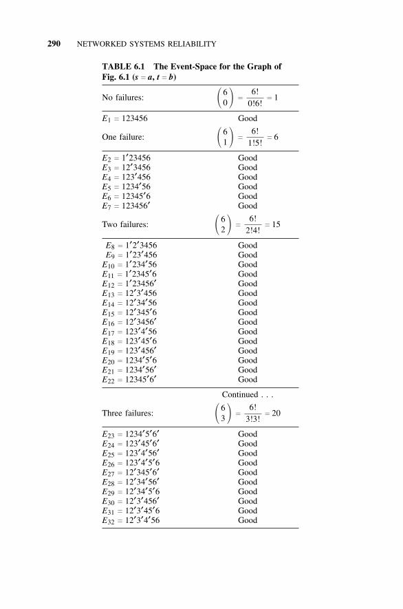
290 NETWORKED SYSTEMS RELIABILITY
TABLE 6.1 The Event-Space for the Graph ofFig. 6.1 (s c a, t c b)
No failures: � 60 � c
6!0!6!
c 1
E1 c 123456 Good
One failure: � 61 � c
6!1!5!
c 6
E2 c 1′23456 GoodE3 c 12′3456 GoodE4 c 123′456 GoodE5 c 1234′56 GoodE6 c 12345′6 GoodE7 c 123456′ Good
Two failures: � 62 � c
6!2!4!
c 15
E8 c 1′2′3456 GoodE9 c 1′23′456 Good
E10 c 1′234′56 GoodE11 c 1′2345′6 GoodE12 c 1′23456′ GoodE13 c 12′3′456 GoodE14 c 12′34′56 GoodE15 c 12′345′6 GoodE16 c 12′3456′ GoodE17 c 123′4′56 GoodE18 c 123′45′6 GoodE19 c 123′456′ GoodE20 c 1234′5′6 GoodE21 c 1234′56′ GoodE22 c 12345′6′ Good
Continued . . .
Three failures: � 63 � c
6!3!3!
c 20
E23 c 1234′5′6′ GoodE24 c 123′45′6′ GoodE25 c 123′4′56′ GoodE26 c 123′4′5′6 GoodE27 c 12′345′6′ GoodE28 c 12′34′56′ GoodE29 c 12′34′5′6 GoodE30 c 12′3′456′ GoodE31 c 12′3′45′6 GoodE32 c 12′3′4′56 Good
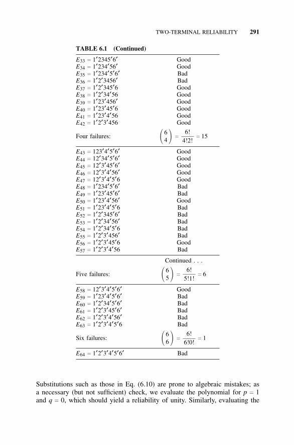
TWO-TERMINAL RELIABILITY 291
TABLE 6.1 (Continued)
E33 c 1′2345′6′ GoodE34 c 1′234′56′ GoodE35 c 1′234′5′6′ BadE36 c 1′2′3456′ BadE37 c 1′2′345′6 GoodE38 c 1′2′34′56 GoodE39 c 1′23′456′ GoodE40 c 1′23′45′6 GoodE41 c 1′23′4′56 GoodE42 c 1′2′3′456 Good
Four failures: � 64 � c
6!4!2!
c 15
E43 c 123′4′5′6′ GoodE44 c 12′34′5′6′ GoodE45 c 12′3′45′6′ GoodE46 c 12′3′4′56′ GoodE47 c 12′3′4′5′6 GoodE48 c 1′234′5′6′ BadE49 c 1′23′45′6′ BadE50 c 1′23′4′56′ GoodE51 c 1′23′4′5′6 BadE52 c 1′2′345′6′ BadE53 c 1′2′34′56′ BadE54 c 1′2′34′5′6 BadE55 c 1′2′3′456′ BadE56 c 1′2′3′45′6 GoodE57 c 1′2′3′4′56 Bad
Continued . . .
Five failures: � 65 � c
6!5!1!
c 6
E58 c 12′3′4′5′6′ GoodE59 c 1′23′4′5′6′ BadE60 c 1′2′34′5′6′ BadE61 c 1′2′3′45′6′ BadE62 c 1′2′3′4′56′ BadE63 c 1′2′3′4′5′6 Bad
Six failures: � 66 � c
6!6!0!
c 1
E64 c 1′2′3′4′5′6′ Bad
Substitutions such as those in Eq. (6.10) are prone to algebraic mistakes; asa necessary (but not sufficient) check, we evaluate the polynomial for p c 1and q c 0, which should yield a reliability of unity. Similarly, evaluating the
292 NETWORKED SYSTEMS RELIABILITY
polynomial for p c 0 and q c 1 should yield a reliability of 0. (Any networkhas a reliability of unity regardless of its topology if all edges are perfect; ithas a reliability of 0 if all its edges have failed.)
Numerical evaluation of the polynomial for p c 0.9 and q c 0.1 yields
Rab c 0.96 + 6(0.1)(0.9)5 + 15(0.1)2(0.9)4 + 18(0.1)3(0.9)3
+ 7(0.1)4(0.9)2 + (0.1)5(0.9) (6.11a)
Rab c 0.5314 + 0.35427 + 0.0984 + 0.0131 + 5.67 × 10⁻⁴ + 9 × 10⁻⁶ (6.11b)
Rab c 0.997848 (6.11c)
Usually, event-space-reliability calculations require much effort and time eventhough the procedure is clear. The number of events builds up exponentiallyas 2e. For e c 10, we have 1,024 terms, and if we double the e, there are overa million terms. However, we seek easier methods.
6.4.2 Cut-Set and Tie-Set Methods
One can reduce the amount of work in a network reliability analysis below the2e complexity required for the event-space method if one focuses on the min-imal cut sets and minimal tie sets of the graph (see Appendix B and Shooman[1990, Section 3.6.5]). The tie sets are the groups of edges that form a pathbetween s and t. The term minimal implies that no node or edge is traversedmore than once, but another way of defining this is that minimal tie sets haveno subsets of edges that are a tie set. If there are i tie sets between s and t,then the reliability expression is given by the expansion of
Rst c P(T1 + T2 + · · · + Ti) (6.12)
Similarly, one can focus on the minimal cut sets of a graph. A cut set is agroup of edges that break all paths between s and t when they are removedfrom the graph. If a cut set is minimal, no subset is also a cut set. The reliabilityexpression in terms of the j cut sets is given by the expansion of
Rst c 1 − P(C1 + C2 + · · · + Cj) (6.13)
We now apply the above theory to the example given in Fig. 6.1. The min-imal cut sets and tie sets are found by inspection for s c a and t c b and aregiven in Table 6.2.
Since there are fewer cut sets, it is easier to use Eq. (6.13) rather than Eq.(6.12); however, there is no general rule for when j < i or vice versa.
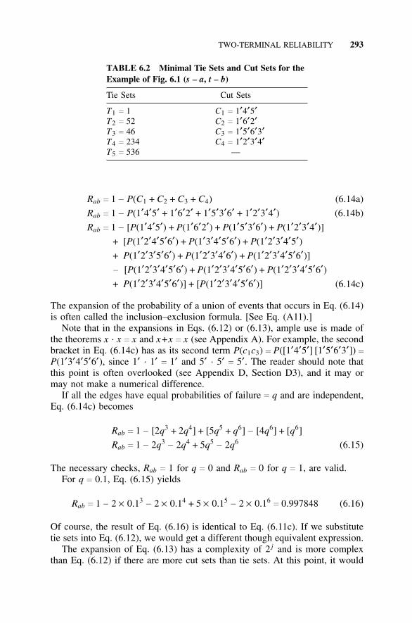
TWO-TERMINAL RELIABILITY 293
TABLE 6.2 Minimal Tie Sets and Cut Sets for theExample of Fig. 6.1 (s c a, t c b)
Tie Sets Cut Sets
T1 c 1 C1 c 1′4′5′T2 c 52 C2 c 1′6′2′T3 c 46 C3 c 1′5′6′3′T4 c 234 C4 c 1′2′3′4′T5 c 536 —
Rab c 1 − P(C1 + C2 + C3 + C4) (6.14a)
Rab c 1 − P(1′4′5′ + 1′6′2′ + 1′5′3′6′ + 1′2′3′4′) (6.14b)
Rab c 1 − [P(1′4′5′) + P(1′6′2′) + P(1′5′3′6′) + P(1′2′3′4′)]+ [P(1′2′4′5′6′) + P(1′3′4′5′6′) + P(1′2′3′4′5′)+ P(1′2′3′5′6′) + P(1′2′3′4′6′) + P(1′2′3′4′5′6′)]− [P(1′2′3′4′5′6′) + P(1′2′3′4′5′6′) + P(1′2′3′4′5′6′)+ P(1′2′3′4′5′6′)] + [P(1′2′3′4′5′6′)] (6.14c)
The expansion of the probability of a union of events that occurs in Eq. (6.14)is often called the inclusion–exclusion formula. [See Eq. (A11).]
Note that in the expansions in Eqs. (6.12) or (6.13), ample use is made ofthe theorems x . x c x and x +x c x (see Appendix A). For example, the secondbracket in Eq. (6.14c) has as its second term P(c1c3) c P([1′4′5′] [1′5′6′3′]) cP(1′3′4′5′6′), since 1′ . 1′ c 1′ and 5′ . 5′ c 5′. The reader should note thatthis point is often overlooked (see Appendix D, Section D3), and it may ormay not make a numerical difference.
If all the edges have equal probabilities of failure c q and are independent,Eq. (6.14c) becomes
Rab c 1 − [2q3 + 2q4] + [5q5 + q6] − [4q6] + [q6]
Rab c 1 − 2q3− 2q4 + 5q5
− 2q6 (6.15)
The necessary checks, Rab c 1 for q c 0 and Rab c 0 for q c 1, are valid.For q c 0.1, Eq. (6.15) yields
Rab c 1 − 2 × 0.13− 2 × 0.14 + 5 × 0.15
− 2 × 0.16c 0.997848 (6.16)
Of course, the result of Eq. (6.16) is identical to Eq. (6.11c). If we substitutetie sets into Eq. (6.12), we would get a different though equivalent expression.
The expansion of Eq. (6.13) has a complexity of 2 j and is more complexthan Eq. (6.12) if there are more cut sets than tie sets. At this point, it would
294 NETWORKED SYSTEMS RELIABILITY
seem that we should analyze the network and see how many tie sets and cutsets exist between s and t, and assuming that i and j are manageable numbers(as is the case in the example to follow), then either Eq. (6.12) or Eq. (6.13)is feasible. In a very large problem (assume i < j < e), even 2i is too largeto deal with, and the approximations of Section 6.4.3 are required. Of course,large problems will utilize a network reliability computation program, but anapproximation can be used to check the program results or to speed up thecomputation in a truly large problem [Colbourn, 1987, 1993; Shooman, 1990].
The complexity of the cut-set and tie-set methods depends on two factors:the order of complexity involved in finding the tie sets (or cut sets) and theorder of complexity for the inclusion–exclusion expansion. The algorithms forfinding the number of cut sets are of polynomial complexity; one discussed inShier [1991, p. 63] is of complexity order O(n + e + ie). In the case of cut sets,the finding algorithms are also of polynomial complexity, and Shier [1991, p.69] discusses one that is of order O([n + e] j). Observe that the notation O( f )is called the order of f or “big O of f.” For example, if f c 5x3 + 10x2 + 12, theorder of f would be the dominating term in f as x becomes large, which is 5x3.Since the constant 5 is a multiplier independent of the size of x, it is ignored,so O(5x3 + 10x2 + 12) c x3 (see Rosen [1999, p. 105]).
In both cases, the dominating complexity is that of expansion for theinclusion–exclusion algorithm for Eqs. (6.12) and (6.13), where the orders ofcomplexity are exponential, O(2i) or O(2 j) [Colbourn, 1987, 1993]. This isthe reason why approximate methods are discussed in the next two sections.In addition, some of these algorithms are explored in the problems at the endof this chapter.
If we examine Eqs. (6.12) and (6.13), we see that the complexity ofthese expressions is a function of the cut sets or tie sets, the number ofedges in the cut sets or tie sets, and the number of “brackets” that must beexpanded (the number of terms in the union of cut sets or tie sets—i.e., inthe inclusion–exclusion formula). We can approximate the cut-set or tie-setexpression by dropping some of the less-significant brackets of the expansion,by dropping some of the less-significant cut sets or tie sets, or by both.
6.4.3 Truncation Approximations
The inclusion–exclusion expansions of Eqs. (6.12) and (6.13) sometimes yielda sequence of probabilities that decrease in size so that many of the higher-order terms in the sequence can be neglected, resulting in a simpler approxi-mate formula. These terms are products of probabilities, so if these probabil-ities are small, the higher-order product terms can be neglected. In the caseof tie-set probabilities, this is when the probabilities of success are small—theso-called low-reliability region, which is not the region of practical interest.Cut-set analysis is preferred since this is when the probabilities of failure aresmall—the so-called high-reliability region, which is really the region of prac-tical interest. Thus cut-set approximations are the ones most frequently used
TWO-TERMINAL RELIABILITY 295
in practice. If only the first bracket in Eq. (6.14c) is retained in addition to theunity term, one obtains the same expression that would have ensued had thecuts been disjoint (but they are not). Thus we will call the retention of onlythe first two terms the disjoint approximation.
In Shooman [1990, Section 3.6.5], it is shown that a disjoint cut-set approx-imation is a lower bound. For the example of Fig. 6.1, we obtain Eq. (6.17)for the disjoint approximation, and assuming q c 0.1:
Rab ≥ 1 − [2q3 + 2q4] c 1 − 0.002 − 0.0002 c 0.9978 (6.17)
which is quite close to the exact value given in Eq. (6.16). If we include thenext bracket in Eq. (6.14c), we get a closer approximation at the expense ofcomputing [ j + ( j
2)] c [ j( j − 1)/ 2] terms.
Rab ≤ 1 − [2q3 + 2q4] + [5q5 + q6]
c 0.9978 + 5 × 0.15 + 0.16c 0.997851 (6.18)
Equation (6.18) is not only an approximation but an upper bound. In fact, asmore terms are included in the inclusion–exclusion formula, we obtain a set ofalternating bounds (see Shooman [1990, Section 3.6.5]). Note that Eq. (6.17)is a sharp lower bound and that Eq. (6.18) is ever sharper, but both equa-tions effectively bracket the exact result. Clearly, the sharpness of these boundsincreases as qi c 1 − pi decreases for the i edges of the graph.
0.997800 ≤ Rab ≤ 0.997851 (6.19)
We can approximate Rab by the midpoint of the two bounds.
Rab c0.997800 + 0.997851
2c 0.9978255 (6.20)
The accuracy of the preceding approximation can be evaluated by examiningthe deviation in the computed probability of failure Fab c 1− Rab. In the regionof high reliability, all the values of Rab are very close to unity, and differencesare misleadingly small. Thus, as our error criterion, we will use
% error c |Fab(estimate) − Fab(exact)|Fab(exact)
× 100 (6.21)
Of course, the numerator of Eq. (6.21) would be the same if we took the dif-ferences in the reliabilities. Evaluation of Eq. (6.21) for the results given inEqs. (6.16) and (6.20) yields
% error c |0.0021745 − 0.002152|0.002152
× 100% c 1.05 (6.22)
296 NETWORKED SYSTEMS RELIABILITY
Clearly, this approximation is good for this example and will be good in mostcases. Of course, in approximate evaluations of a large network, we do notknow the exact reliability, but we can still approximate Eq. (6.21) by usingthe difference between the two-term and three-term approximations. For thenumerator and the average of the denominator:
% error ≈ |0.002200 − 0.002149|0.0021745
× 100% c 2.35 (6.23)
A moment’s reflection leads to the conclusion that the highest-order approx-imation will always be the closest and should be used in the denominator ofan error bound. The numerator, on the other hand, should be the differencebetween the two highest-order terms. Thus, for our example,
% error ≈ |0.002200 − 0.002149|0.0021749
× 100% c 2.37 (6.24)
Therefore, a practical approach in designing a computer analysis program isto ask the analyst to input the accuracy he or she desires, then to compute asuccession of bounds involving more and more terms in the expansion of Eq.(6.13) at each stage. An equation similar to Eq. (6.24) would be used for thelast two terms in the computation to determine when to stop computing alter-nating bounds. The process truncates when the error approximation yields anestimated value that has a smaller error bound that that of the required error.We should take note that the complexity of the “one-at-a-time” approximationis of order j (number of cut sets) and that of the “two-at-a-time” approxima-tion is of order j2. Thus, even if the error approximation indicates that moreterms are needed, the complexity will only be of order j3 or perhaps j 4. Theinclusion–exclusion complexity is therefore reduced from order 2 j to a poly-nomial in j (perhaps j2 or j3).
6.4.4 Subset Approximations
In the last section, we discussed approximation by truncating the inclusion–exclusion expression. Now we discuss approximation by exclusion of low-probability cut sets or tie sets. Clearly, the occurrence probability of the lower-order (fewer edges) cut sets is higher than the higher-order (more edges) ones.Thus, we can approximate Eq. (6.14a) dropping C3 and C4 fourth-order cutsets and retaining the third-order cut set to yield an upper bound (since wehave dropped cut sets, we are making an optimistic approximation).
Rab ≤ 1 − P(C1 + C2) c 1 − P(C1) − P(C2) + P(C1)P(C2)
c 1 − P(1′4′5′) − P(1′6′2′) + P(1′2′4′5′6′) (6.25a)
For q c 0.1,
TWO-TERMINAL RELIABILITY 297
Rab ≤ 1 − 2 × 0.13 + 0.15c 0.99801 (6.25b)
We can use similar reasoning to develop a lower bound (we drop tie sets,thereby making a pessimistic approximation) by dropping all but the “one-hop” tie sets (T1) and the “two-hop” tie sets (T2, T3)—compare Eq. (6.12) andTable 6.2.
Rab ≥ P(T1 + T2 + T3) c P(1 + 25 + 46) c P(1) + P(25) + P(46)
− [P(125) + P(146) + P(2456)] + [P(12456)] (6.26a)
For p c 0.9,
Rab ≥ p + 2p2− 2p3
− p4 + p5c 0.9 + 2 × 0.92
− 2 × 0.93− 0.94 + 0.95
c 0.99639 (6.26b)
Given Eq. (6.25b) and (6.26b), we can bound Rab by
0.99639 ≤ Rab ≤ 0.99801 (6.27)
and approximate Rab by the midpoint of the two bounds:
Rab c0.99639 + 0.99801
2c 0.9971955 (6.28)
The error bound for this approximation is computed in the same manner asEq. (6.23).
% error ≈ |0.00361 − 0.00199|0.0028045
× 100% c 57.8 (6.29)
The percentage error is larger than in the case of the truncation approxima-tions, but it remains small enough for the approximation to be valid. The com-plexity is still exponential—of order 2x; however, x is now a small integer and2x is of modest size. Furthermore, the tie-set and cut-set algorithms take lesstime since we now do not need to find all cut sets and tie sets—only those oforder ≤ x. Of course, one can always combine both approximation methods bydropping out higher-order cut sets and then also truncating the expansion. Formore details on network reliability approximations, see Murray [1992, 1993].
6.4.5 Graph Transformations
Anyone who has studied electric-circuit theory in a physics or engineeringclass knows that complex networks of resistors can be reduced to an equiva-lent single resistance through various combinations of series, parallel, and Y–Dtransformations. Such knowledge has obviously stimulated the development
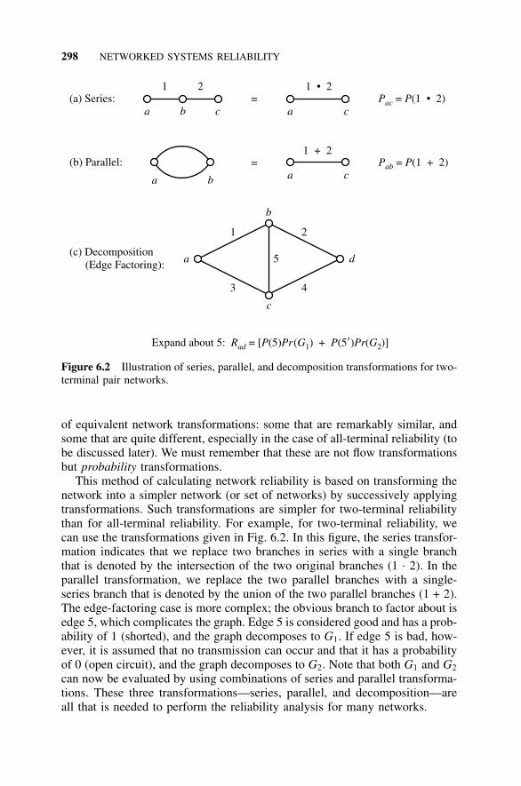
298 NETWORKED SYSTEMS RELIABILITY
(a) Series: P Pac = (1 • 2)
P Pab = (1 + 2)
=
=
1 2
a b c
1 • 2
1 + 2
a
aa
c
cb
(b) Parallel:
(c) Decomposition(Edge Factoring): a
c
b
d
1
3
2
4
5
Expand about 5: = [ (5) ( ) + (5 ) ( )]R P Pr G P Pr Gad 1 2’
Figure 6.2 Illustration of series, parallel, and decomposition transformations for two-terminal pair networks.
of equivalent network transformations: some that are remarkably similar, andsome that are quite different, especially in the case of all-terminal reliability (tobe discussed later). We must remember that these are not flow transformationsbut probability transformations.
This method of calculating network reliability is based on transforming thenetwork into a simpler network (or set of networks) by successively applyingtransformations. Such transformations are simpler for two-terminal reliabilitythan for all-terminal reliability. For example, for two-terminal reliability, wecan use the transformations given in Fig. 6.2. In this figure, the series transfor-mation indicates that we replace two branches in series with a single branchthat is denoted by the intersection of the two original branches (1 . 2). In theparallel transformation, we replace the two parallel branches with a single-series branch that is denoted by the union of the two parallel branches (1 + 2).The edge-factoring case is more complex; the obvious branch to factor about isedge 5, which complicates the graph. Edge 5 is considered good and has a prob-ability of 1 (shorted), and the graph decomposes to G1. If edge 5 is bad, how-ever, it is assumed that no transmission can occur and that it has a probabilityof 0 (open circuit), and the graph decomposes to G2. Note that both G1 and G2
can now be evaluated by using combinations of series and parallel transforma-tions. These three transformations—series, parallel, and decomposition—areall that is needed to perform the reliability analysis for many networks.
TWO-TERMINAL RELIABILITY 299
Now we discuss a more difficult network configuration. In the first transfor-mation in Fig. 6.2(a) series, we readily observe that both (intersection) edges1 and 2 must be up for a connection between a and b to occur. However, thistransformation only works if there is no third edge connected to node b; ifa third edge exists, a more elaborate transformation is needed (which will bediscussed in Section 6.6 on all-terminal reliability). Similarly, in the case ofthe parallel transformation, nodes a and b are connected if either (union) a orb is up.
Assume that any failures of edge 1 and edge 2 are independent and theprobabilities of success for edges 1 and 2 are p1 and p2 (probabilities of failureare q1 c 1 − p1, q2 c 1 − p2). Then for the series subnetwork of Fig. 6.2(a),pac c p1p2, and for the parallel subnetwork in Fig. 6.2(b), pab c p1 +p2 − p1p2 c
1 − q1q2.The case of decomposition (called the keystone component method in sys-
tem reliability [Shooman, 1990] or the edge-factoring method in network reli-ability) is a little more subtle; it is used to eliminate an edge x from a graph.Since all edges must either be up or down, we reduce the original network totwo other networks G1 (given that edge x is up) and G2 (given that edge x isdown). In general, one uses series and parallel transformations first, resortingto edge-factoring only when no more series or parallel transformations can bemade. In the subnetwork of Fig. 6.2(c), we see that neither series nor paralleltransformation is immediately possible because of edge 5, for which reasondecomposition should be used.
The mathematical basis of the decomposition transformation lies in the lawsof conditional probability and Bayesian probability [Mendenhall, 1990, pp.64–65]. These laws lead to the following probability equation for terminal pairst and edge x.
P(there is a path between s and t)
c P(x is good) × P(there is a path between s and t |x is good)
+ P(x is bad) × P(there is a path between s and t |x is bad) (6.30)
The preceding equation can be rewritten in a more compact notation as follows:
Pst c P(x)P(G1) + P(x′)P(G2) (6.31)
The term P(G1) is the probability of a connection between s and t for themodified network where x is good, that is, the terminals at either end of edgex are connected to the graph [see Fig. 6.2(c)]. Similarly, the term P(G2) is theprobability that there is a connection between s and t for the modified networkG2 where x is bad, that is, the edge x is removed from the graph [again, seeFig. 6.2(c)]. Thus Eq. (6.31) becomes for st c ad:
Pst c p5(1 − q1q3)(1 − q2q4) + q5(p1p2 + p3p4 − p1p2p3p4) (6.32)
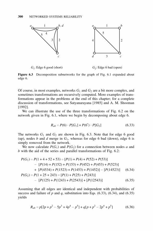
300 NETWORKED SYSTEMS RELIABILITY
a b1
4 2
d c3
5
a b, d1
2
c
5 4
3
G1: Edge 6 good (short) G2: Edge 6 bad (open)
Figure 6.3 Decomposition subnetworks for the graph of Fig. 6.1 expanded aboutedge 6.
Of course, in most examples, networks G1 and G2 are a bit more complex, andsometimes transformations are recursively computed. More examples of trans-formations appear in the problems at the end of this chapter; for a completediscussion of transformations, see Satyanarayana [1985] and A. M. Shooman[1992].
We can illustrate the use of the three transformations of Fig. 6.2 on thenetwork given in Fig. 6.1, where we begin by decomposing about edge 6.
Rab c P(6) . P[G1] + P(6′) . P[G2] (6.33)
The networks G1 and G2 are shown in Fig. 6.3. Note that for edge 6 good(up), nodes b and d merge in G1, whereas for edge 6 bad (down), edge 6 issimply removed from the network.
We now calculate P(G1) and P(G2) for a connection between nodes a andb with the aid of the series and parallel transformations of Fig. 6.2:
P(G1) c P(1 + 4 + 52 + 53) c [P(1) + P(4) + P(52) + P(53)]
− [P(14) + P(152) + P(153) + P(452) + P(453) + P(523)]
+ [P(4534) + P(1523) + P(1453) + P(1452)] − [P(14523)] (6.34)
P(G2) c P(1 + 25 + 243) c [P(1) + P(25) + P(243)]
− [P(125) + P(1243) + P(2543)] + [P(12543)] (6.35)
Assuming that all edges are identical and independent with probabilities ofsuccess and failure of p and q, substitution into Eqs. (6.33), (6.34), and (6.35)yields
Rab c p[2p + p2− 5p3 + 4p4
− p5] + q[p + p2− 2p4 + p5] (6.36)
NODE PAIR RESILIENCE 301
Substitution of p c 0.9 and q c 0.1 into Eq. (6.36) yields
Rab c 0.9[0.99891] + 0.1[0.98829] c 0.997848 (6.37)
Of course, this result agrees with the previous computation given in Eq. (6.16).
6.5 NODE PAIR RESILIENCE
All-terminal reliability, in which all the node pairs can communicate, is dis-cussed in the next section. Also, k-terminal reliability will be treated as a speci-fied subset (2 ≤ k ≤ all-terminal pairs) of all-terminal reliability. In this section,another metric, essentially one between two-terminal and all-terminal, is dis-cussed.
Van Slyke and Frank [1972] proposed a measure they called resilience forthe expected number of node pairs that can communicate (i.e., they are con-nected by one or more tie sets). Let s and t represent a node pair. The numberof node pairs in a network with N nodes is the number of combinations of Nchoose 2, that is, the number of combinations of 2 out of N.
Number of node pairs c �N2 � c
N!2!(N − 2)!
c
N(N − 1)2
(6.38)
Our notation for the set of s, t node pairs contained in an N node network is{s, t} ⊂ N, and the expected number of node pairs that can communicate isdenoted as resilience, res(G):
res(G ) c ���{s, t} ⊂ N
Rst (6.39)
We can illustrate a resilience calculation by applying Eq. (6.39) to the net-work of Fig. 6.1. We begin by observing that if p c 0.9 for each edge, symmetrysimplifies the computation. The node pairs divide into two categories: the edgepairs (ab, ad, bc, and cd) and the diagonal pairs (ac and bd). The edge-pairreliabilities were already computed in Eqs. (6.36) and (6.37). For the diago-nals, we can use the decomposition given in Fig. 6.3 (where s c a and t c c)and compute Rac as shown in the following equations:
302 NETWORKED SYSTEMS RELIABILITY
P(G1) c P[5 + (1 + 4)(2 + 5)]
c P(5) + P(1 + 4)P(2 + 5) − P(5)P(1 + 4)P(2 + 5)
c [p + (1 − p)(2p − p2)2] (6.40a)
P(6)P(G1) c p[p + (1 − p)(2p − p2)2] c 0.898209 (6.40b)
P(G2) c P[5 + 12 + 43] c P(5) + P(12) + P(43)
− [P(512) + P(543) + P(1243)]
+ [P(51243)] c p + 2p2− 2p3
− p4 + p5 (6.41a)
P(6′)P(G2) c q[p + 2p2− 2p3
− p4 + p5] c 0.099639 (6.41b)
Rac c 0.98209 + 0.099639 c 0.997848 (6.42)
Substitution of Eqs. (6.37) and (6.42) into (6.39) yields
res(G ) c 4 × 0.997848 + 2 × 0.997848 c 5.987 (6.43)
Note for this particular example that because all edge reliabilities are equaland because it is a complete graph, symmetry would have predicted that Rst
values were the same for node pairs ab, ad, bc, and cd, and similarly for nodepairs ac and bd. Clearly, for a very reliable network, the resilience will beclose to the maximum N(N − 1)/ 2, which for this example is 6. In fact, it maybe useful to normalize the resilience by dividing it by N(N − 1)/ 2 to yield a“normalized” resilience metric. In our example, res(G)/ 6 c 0.997848. In gen-eral, if we divide Eq. (6.39) by Eq. (6.38), we obtain the average reliability forall the two-terminal pairs in the network. Although this requires considerablecomputation, the metric may be useful when the pi are unequal.
6.6 ALL-TERMINAL RELIABILITY
The all-terminal reliability problem is somewhat more difficult than the two-terminal reliability problem. Essentially, we must modify the two-terminalproblem to account for all-terminal pairs. Each of the methods of Section 6.4is discussed in this section for the case of all-terminal reliability.
6.6.1 Event-Space Enumeration
We may proceed as we did in Section 6.4.1 except that now we examine allthe good events for two-terminal reliability and strike out (i.e., classify as bad)those that do not connect all the terminal pairs. By applying these restrictionsto Table 6.1, we obtain Table 6.3. From this table, we can formulate an all-terminal reliability expression similar to the two-terminal case.
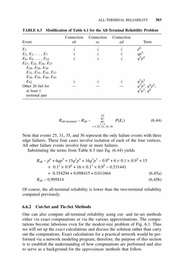
ALL-TERMINAL RELIABILITY 303
TABLE 6.3 Modification of Table 6.1 for the All-Terminal Reliability Problem
Connection Connection ConnectionEvent ab ac ad Term
E1 √ √ √ p6
E2, E3, . . . , E7 √ √ √ qp5
E8, E9, . . . , E22 √ √ √ q2p4
E23, E24, E26, E27E28, E29, E30E32, E33, E34, E37E38, E39, E40, E41E42 √ √ √ q3p3
Other 26 fail for — — — q3p3, q4p2,at least 1 q3p1, q6
terminal pair
Rall-terminal c Rall c
42
���i c 1
i � 25, 31, 35, 36
P(Ei) (6.44)
Note that events 25, 31, 35, and 36 represent the only failure events with threeedge failures. These four cases involve isolation of each of the four vertices.All other failure events involve four or more failures.
Substituting the terms from Table 6.3 into Eq. (6.44) yields
Rall c p6 + 6qp5 + 15q2p4 + 16q3p3c 0.96 + 6 × 0.1 × 0.95 + 15
× 0.12 × 0.94 + 16 × 0.13 × 0.99c 0.531441
+ 0.354294 + 0.098415 + 0.011664 (6.45a)
Rall c 0.995814 (6.45b)
Of course, the all-terminal reliability is lower than the two-terminal reliabilitycomputed previously.
6.6.2 Cut-Set and Tie-Set Methods
One can also compute all-terminal reliability using cut- and tie-set methodseither via exact computations or via the various approximations. The compu-tations become laborious even for the modest-size problem of Fig. 6.1. Thuswe will set up the exact calculations and discuss the solution rather than carryout the computations. Exact calculations for a practical network would be per-formed via a network modeling program; therefore, the purpose of this sectionis to establish the understanding of how computations are performed and alsoto serve as a background for the approximate methods that follow.
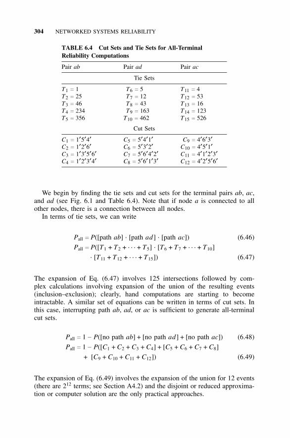
304 NETWORKED SYSTEMS RELIABILITY
TABLE 6.4 Cut Sets and Tie Sets for All-TerminalReliability Computations
Pair ab Pair ad Pair ac
Tie Sets
T1 c 1 T6 c 5 T11 c 4T2 c 25 T7 c 12 T12 c 53T3 c 46 T8 c 43 T13 c 16T4 c 234 T9 c 163 T14 c 123T5 c 356 T10 c 462 T15 c 526
Cut Sets
C1 c 1′5′4′ C5 c 5′4′1′ C9 c 4′6′3′C2 c 1′2′6′ C6 c 5′3′2′ C10 c 4′5′1′C3 c 1′3′5′6′ C7 c 5′6′4′2′ C11 c 4′1′2′3′C4 c 1′2′3′4′ C8 c 5′6′1′3′ C12 c 4′2′5′6′
We begin by finding the tie sets and cut sets for the terminal pairs ab, ac,and ad (see Fig. 6.1 and Table 6.4). Note that if node a is connected to allother nodes, there is a connection between all nodes.
In terms of tie sets, we can write
Pall c P([path ab] . [path ad] . [path ac]) (6.46)
Pall c P([T1 + T2 + · · · + T5] . [T6 + T7 + · · · + T10]. [T11 + T12 + · · · + T15]) (6.47)
The expansion of Eq. (6.47) involves 125 intersections followed by com-plex calculations involving expansion of the union of the resulting events(inclusion–exclusion); clearly, hand computations are starting to becomeintractable. A similar set of equations can be written in terms of cut sets. Inthis case, interrupting path ab, ad, or ac is sufficient to generate all-terminalcut sets.
Pall c 1 − P([no path ab] + [no path ad] + [no path ac]) (6.48)
Pall c 1 − P([C1 + C2 + C3 + C4] + [C5 + C6 + C7 + C8]
+ [C9 + C10 + C11 + C12]) (6.49)
The expansion of Eq. (6.49) involves the expansion of the union for 12 events(there are 212 terms; see Section A4.2) and the disjoint or reduced approxima-tion or computer solution are the only practical approaches.
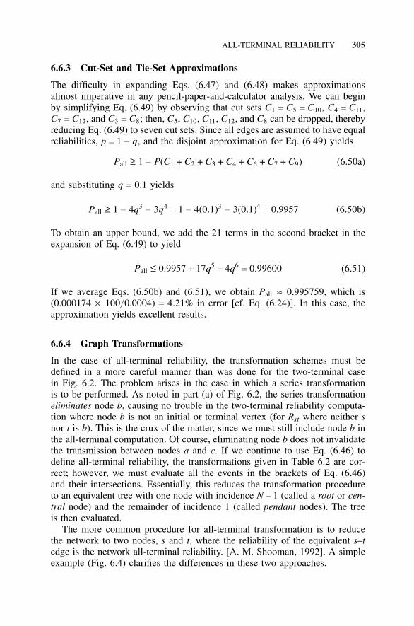
ALL-TERMINAL RELIABILITY 305
6.6.3 Cut-Set and Tie-Set Approximations
The difficulty in expanding Eqs. (6.47) and (6.48) makes approximationsalmost imperative in any pencil-paper-and-calculator analysis. We can beginby simplifying Eq. (6.49) by observing that cut sets C1 c C5 c C10, C4 c C11,C7 c C12, and C3 c C8; then, C5, C10, C11, C12, and C8 can be dropped, therebyreducing Eq. (6.49) to seven cut sets. Since all edges are assumed to have equalreliabilities, p c 1 − q, and the disjoint approximation for Eq. (6.49) yields
Pall ≥ 1 − P(C1 + C2 + C3 + C4 + C6 + C7 + C9) (6.50a)
and substituting q c 0.1 yields
Pall ≥ 1 − 4q3− 3q4
c 1 − 4(0.1)3− 3(0.1)4
c 0.9957 (6.50b)
To obtain an upper bound, we add the 21 terms in the second bracket in theexpansion of Eq. (6.49) to yield
Pall ≤ 0.9957 + 17q5 + 4q6c 0.99600 (6.51)
If we average Eqs. (6.50b) and (6.51), we obtain Pall ≈ 0.995759, which is(0.000174 × 100/ 0.0004) c 4.21% in error [cf. Eq. (6.24)]. In this case, theapproximation yields excellent results.
6.6.4 Graph Transformations
In the case of all-terminal reliability, the transformation schemes must bedefined in a more careful manner than was done for the two-terminal casein Fig. 6.2. The problem arises in the case in which a series transformationis to be performed. As noted in part (a) of Fig. 6.2, the series transformationeliminates node b, causing no trouble in the two-terminal reliability computa-tion where node b is not an initial or terminal vertex (for Rst where neither snor t is b). This is the crux of the matter, since we must still include node b inthe all-terminal computation. Of course, eliminating node b does not invalidatethe transmission between nodes a and c. If we continue to use Eq. (6.46) todefine all-terminal reliability, the transformations given in Table 6.2 are cor-rect; however, we must evaluate all the events in the brackets of Eq. (6.46)and their intersections. Essentially, this reduces the transformation procedureto an equivalent tree with one node with incidence N − 1 (called a root or cen-tral node) and the remainder of incidence 1 (called pendant nodes). The treeis then evaluated.
The more common procedure for all-terminal transformation is to reducethe network to two nodes, s and t, where the reliability of the equivalent s–tedge is the network all-terminal reliability. [A. M. Shooman, 1992]. A simpleexample (Fig. 6.4) clarifies the differences in these two approaches.
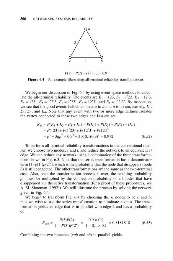
306 NETWORKED SYSTEMS RELIABILITY
a
b1
2
c
3
P P P p(1) = (2) = (3) = = 0.9
Figure 6.4 An example illustrating all-terminal reliability transformations.
We begin our discussion of Fig. 6.4 by using event-space methods to calcu-late the all-terminal reliability. The events are E1 c 123, E2 c 1′23, E3 c 12′3,E4 c 123′, E5 c 1′2′3, E6 c 1′23′, E7 c 12′3′, and E8 c 1′2′3′. By inspection,we see that the good events (which connect a to b and a to c) are, namely, E1,E2, E3, and E4. Note that any event with two or more edge failures isolatesthe vertex connected to these two edges and is a cut set.
Rall c P(E1 + E2 + E3 + E4) c P(E1) + P(E2) + P(E3) + (E4)
c P(123) + P(1′23) + P(12′3) + P(123′)c p3 + 3qp2
c 0.93 + 3 × 0.1(0.9)2c 0.972 (6.52)
To perform all-terminal reliability transformations in the conventional man-ner, we choose two modes, s and t, and reduce the network to an equivalent stedge. We can reduce any network using a combination of the three transforma-tions shown in Fig. 6.5. Note that the series transformation has a denominatorterm [1−p(1′)p(2′)], which is the probability that the node that disappears (nodeb) is still connected. The other transformations are the same as the two-terminalcase. Also, once the transformation process is over, the resulting probabilitypst must be multiplied by the connection probability of all nodes that havedisappeared via the series transformation (for a proof of these procedures, seeA. M. Shooman [1992]). We will illustrate the process by solving the networkgiven in Fig. 6.4.
We begin to transform Fig. 6.4 by choosing the st nodes to be c and b;thus we wish to use the series transformation to eliminate node a. The trans-formation yields an edge that is in parallel with edge 2 and has a probabilityof
Pcab cP(3)P(2)
1 − P(3′)P(2′)c
0.9 × 0.91 − 0.1 × 0.1
c 0.8181818 (6.53)
Combining the two branches (cab and cb) in parallel yields
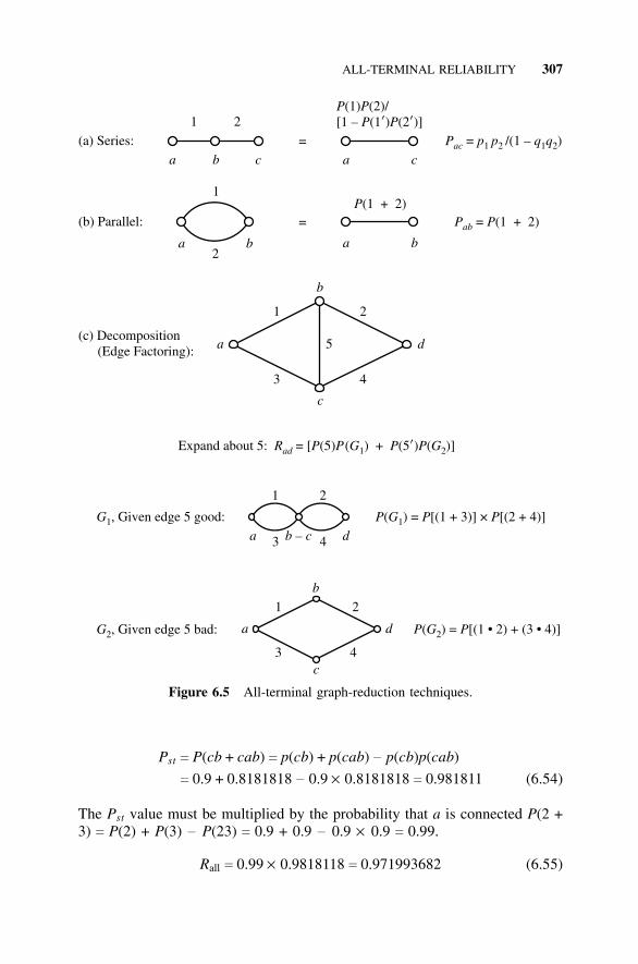
ALL-TERMINAL RELIABILITY 307
(a) Series: P p p q qac = /(1 – )1 2 1 2
P Pab = (1 + 2)
=
=
1 2
a b c
P(1 + 2)
a
a
a
c
ba b
b – c d
(b) Parallel:
(c) Decomposition(Edge Factoring): a
c
b
d
1
3
2
4
5
a
c
b
d
1
3
2
4
Expand about 5: = [ (5) ( ) + (5 ) ( )]R P P G P P Gad 1 2’
P PP
(1) (2)/[1 – (1’ ’) (2 )]P
G1, Given edge 5 good:
G2, Given edge 5 bad:
P G P P( ) = [(1 + 3)] × [(2 + 4)]1
P G P( ) = [(1 • 2) + (3 • 4)]2
3 4
1 2
1
2
Figure 6.5 All-terminal graph-reduction techniques.
Pst c P(cb + cab) c p(cb) + p(cab) − p(cb)p(cab)
c 0.9 + 0.8181818 − 0.9 × 0.8181818 c 0.981811 (6.54)
The Pst value must be multiplied by the probability that a is connected P(2 +3) c P(2) + P(3) − P(23) c 0.9 + 0.9 − 0.9 × 0.9 c 0.99.
Rall c 0.99 × 0.9818118 c 0.971993682 (6.55)
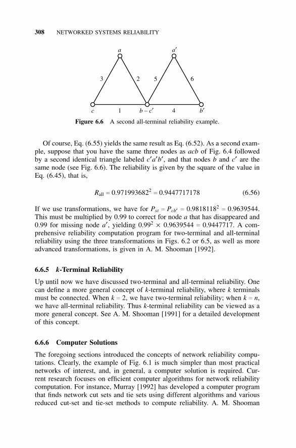
308 NETWORKED SYSTEMS RELIABILITY
a
b – c′1
2
c
3
a′
b′4
65
Figure 6.6 A second all-terminal reliability example.
Of course, Eq. (6.55) yields the same result as Eq. (6.52). As a second exam-ple, suppose that you have the same three nodes as acb of Fig. 6.4 followedby a second identical triangle labeled c′a′b′, and that nodes b and c′ are thesame node (see Fig. 6.6). The reliability is given by the square of the value inEq. (6.45), that is,
Rall c 0.9719936822c 0.9447717178 (6.56)
If we use transformations, we have for Pst c Pcb′ c 0.98181182c 0.9639544.
This must be multiplied by 0.99 to correct for node a that has disappeared and0.99 for missing node a′, yielding 0.992 × 0.9639544 c 0.9447717. A com-prehensive reliability computation program for two-terminal and all-terminalreliability using the three transformations in Figs. 6.2 or 6.5, as well as moreadvanced transformations, is given in A. M. Shooman [1992].
6.6.5 k-Terminal Reliability
Up until now we have discussed two-terminal and all-terminal reliability. Onecan define a more general concept of k-terminal reliability, where k terminalsmust be connected. When k c 2, we have two-terminal reliability; when k c n,we have all-terminal reliability. Thus k-terminal reliability can be viewed as amore general concept. See A. M. Shooman [1991] for a detailed developmentof this concept.
6.6.6 Computer Solutions
The foregoing sections introduced the concepts of network reliability compu-tations. Clearly, the example of Fig. 6.1 is much simpler than most practicalnetworks of interest, and, in general, a computer solution is required. Cur-rent research focuses on efficient computer algorithms for network reliabilitycomputation. For instance, Murray [1992] has developed a computer programthat finds network cut sets and tie sets using different algorithms and variousreduced cut-set and tie-set methods to compute reliability. A. M. Shooman
DESIGN APPROACHES 309
[1991, 1992] has developed a computer program for network reliability that isbased on the transformations of Section 6.5 and is modified for the k-termi-nal problem, in addition to other more advanced transformations. His modelincludes the possibility of node failure.
6.7 DESIGN APPROACHES
The previous sections treated the problem of network analysis. This section,however, treats the problem of design. We assume that there is a group of Ncities or sites represented by nodes that are to be connected by E edges to formthe network and that the various links have different costs and reliabilities. Ourjob is to develop design procedures that yield a good network—that is, at lowcost with high reliability. (The reader is referred to the books by Colbourn[1987] and Shier [1991] for a comprehensive introduction to the literature inthis field.)
The problem stated in the previous paragraph is actually called the topo-logical design problem and is an abstraction of the complete design problem.The complete design problem includes many other considerations, such as thefollowing:
1. The capacity in bits per second of each line is an important consideration,and connections between nodes can fail if the number of messages perminute is too large for the capacity of the line, if congestion ensues, andif a queue of waiting messages forms that causes unacceptable delays intransmission.
2. If messages do not go through because of interrupted transmission pathsor excessive delays, information is fed back to various nodes. An algo-rithm, called the routing algorithm, is stored at one or more nodes, andalternate routes are generally invoked to send such messages via alternatepaths.
3. When edge or node failures occur, messages are rerouted, which maycause additional network congestion.
4. Edges between nodes are based on communication lines (twisted-copperand fiber-optic lines as well as coaxial cables, satellite links, etc.) andrepresent a discrete (rather than continuous) choice of capacities.
5. Sometimes, the entire network design problem is divided into a backbonenetwork design (discussed previously) and a terminal concentrator design(for the connections within a building).
6. Political considerations sometimes govern node placement. For example,suppose that we wish to connect the cities New York and Baltimore andthat engineering considerations point to a route via Atlantic City. Forpolitical considerations, however, it is likely that the route would insteadgo through Philadelphia.
310 NETWORKED SYSTEMS RELIABILITY
For more information on this subject, the reader is referred to Kirshenbaum[1993]. The remainder of this chapter considers the topological design of abackbone network.
6.7.1 Introduction
The general problem of network design is quite complex. If we start with nnodes to connect, we have the problem of determining which set of edges(arcs) is optimum. Optimality encompasses parameters such as best reliability,lowest cost, shortest delay, maximum bandwidth, and most flexibility for futureexpansion. The problem is too complex for direct optimization of any practicalnetwork, so subsets and/ or approximate optimizations are used to reduce thegeneral problem to a tractable one.
At the present, most network design focuses on minimizing cost with con-straints on time delay and/ or throughput. Semiquantitative reliability con-straints are often included, such as that contained in the statement “the networkshould be at least two-connected,” that is, there should be no fewer than twopaths between each node pair. This may not produce the best design when reli-ability is of great importance, and furthermore, a two-connected criterion maynot yield a minimum cost design. This section approaches network design as aproblem in maximization of network reliability within a specified cost budget.
High-capacity fiber-optic networks make it possible to satisfy networkthroughput constraints with significantly fewer lines than required with oldertechnology. Thus such designs have less inherent redundancy and generallylower reliability. (A detailed study requires a comparison of the link reliabili-ties of conventional media versus fiber optics.) In such cases, reliability there-fore must be the focus of the design process from the outset to ensure thatadequate reliability goals are met at a reasonable cost.
Assume that network design is composed of three phases: (a) a backbonedesign, (b) a local access design, and (c) a local area network within the build-ing (however, here we focus our attention on backbone design). Assume alsothat backbone design can be broken into two phases: A1 and A2. Phase A1 is thechoice of an initial connected configuration, whereas phase A2 is augmentationwith additional arcs to improve performance under constraint(s). Each new arc ingeneral increases the reliability, cost, and throughput and may decrease the delay.
6.7.2 Design of a Backbone Network Spanning-Tree Phase
We begin our discussion of design by focusing on phase A1. A connected graphis one where all nodes are connected by branches. A connected graph with thesmallest number of arcs is a spanning tree. In general, a complete network(all edges possible) with n nodes will have n(n − 2) spanning trees, each withes c (n − 1) edges (arcs). For example, for the four-node network of Fig. 6.1,there are 4(4 − 2)
c 16 spanning trees with (4 − 1) c 3 arcs; these are shown inFig. 6.7.
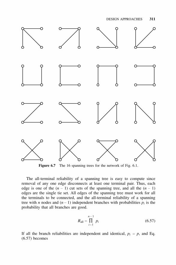
DESIGN APPROACHES 311
Figure 6.7 The 16 spanning trees for the network of Fig. 6.1.
The all-terminal reliability of a spanning tree is easy to compute sinceremoval of any one edge disconnects at least one terminal pair. Thus, eachedge is one of the (n − 1) cut sets of the spanning tree, and all the (n − 1)edges are the single tie set. All edges of the spanning tree must work for allthe terminals to be connected, and the all-terminal reliability of a spanningtree with n nodes and (n − 1) independent branches with probabilities pi is theprobability that all branches are good.
Rall c
n − 1
∏i c 1
pi (6.57)
If all the branch reliabilities are independent and identical, pi c p, and Eq.(6.57) becomes
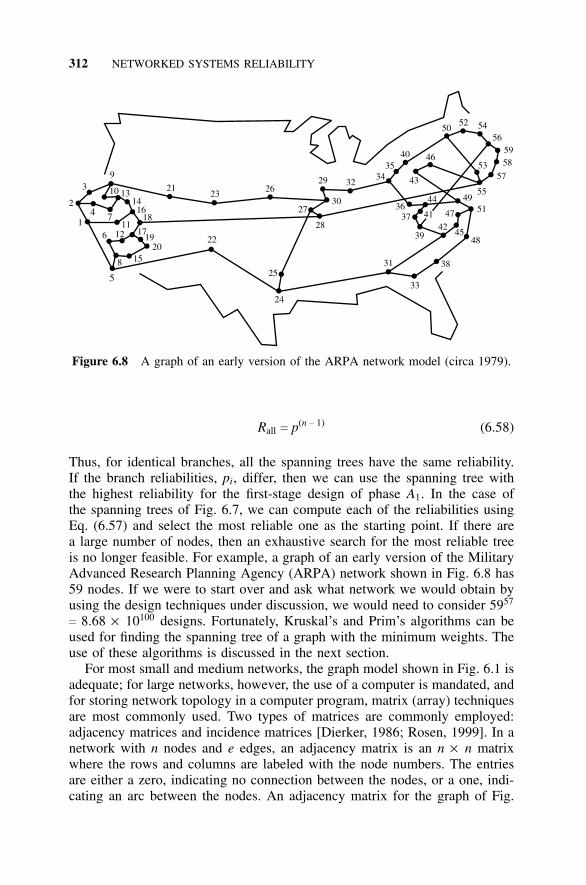
312 NETWORKED SYSTEMS RELIABILITY
1
2
39
10 131416
18
1719
20
8 15
116 12
2123
22
26
25
27
28
29
30
32
24
3435
40
43
46
5052 54
565958
57
55
53
3644 49
37 41
39
5147
4245
48
38
33
31
4 7
5
Figure 6.8 A graph of an early version of the ARPA network model (circa 1979).
Rall c p(n − 1) (6.58)
Thus, for identical branches, all the spanning trees have the same reliability.If the branch reliabilities, pi, differ, then we can use the spanning tree withthe highest reliability for the first-stage design of phase A1. In the case ofthe spanning trees of Fig. 6.7, we can compute each of the reliabilities usingEq. (6.57) and select the most reliable one as the starting point. If there area large number of nodes, then an exhaustive search for the most reliable treeis no longer feasible. For example, a graph of an early version of the MilitaryAdvanced Research Planning Agency (ARPA) network shown in Fig. 6.8 has59 nodes. If we were to start over and ask what network we would obtain byusing the design techniques under discussion, we would need to consider 5957
c 8.68 × 10100 designs. Fortunately, Kruskal’s and Prim’s algorithms can beused for finding the spanning tree of a graph with the minimum weights. Theuse of these algorithms is discussed in the next section.
For most small and medium networks, the graph model shown in Fig. 6.1 isadequate; for large networks, however, the use of a computer is mandated, andfor storing network topology in a computer program, matrix (array) techniquesare most commonly used. Two types of matrices are commonly employed:adjacency matrices and incidence matrices [Dierker, 1986; Rosen, 1999]. In anetwork with n nodes and e edges, an adjacency matrix is an n × n matrixwhere the rows and columns are labeled with the node numbers. The entriesare either a zero, indicating no connection between the nodes, or a one, indi-cating an arc between the nodes. An adjacency matrix for the graph of Fig.
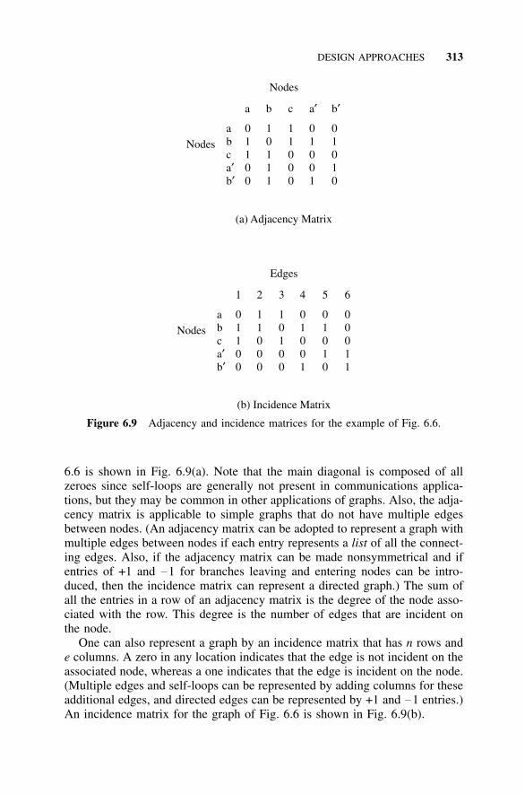
DESIGN APPROACHES 313
a b c a b
a 0 1 1 0 0b 1 0 1 1 1c 1 1 0 0 0a 0 1 0 0 1b 0 1 0 1 0
′ ′
′′
Nodes
Nodes
(a) Adjacency Matrix
1 2 3 4 5 6
a 0 1 1 0 0 0b 1 1 0 1 1 0c 1 0 1 0 0 0a 0 0 0 0 1 1b 0 0 0 1 0 1′′
Nodes
Edges
(b) Incidence Matrix
Figure 6.9 Adjacency and incidence matrices for the example of Fig. 6.6.
6.6 is shown in Fig. 6.9(a). Note that the main diagonal is composed of allzeroes since self-loops are generally not present in communications applica-tions, but they may be common in other applications of graphs. Also, the adja-cency matrix is applicable to simple graphs that do not have multiple edgesbetween nodes. (An adjacency matrix can be adopted to represent a graph withmultiple edges between nodes if each entry represents a list of all the connect-ing edges. Also, if the adjacency matrix can be made nonsymmetrical and ifentries of +1 and −1 for branches leaving and entering nodes can be intro-duced, then the incidence matrix can represent a directed graph.) The sum ofall the entries in a row of an adjacency matrix is the degree of the node asso-ciated with the row. This degree is the number of edges that are incident onthe node.
One can also represent a graph by an incidence matrix that has n rows ande columns. A zero in any location indicates that the edge is not incident on theassociated node, whereas a one indicates that the edge is incident on the node.(Multiple edges and self-loops can be represented by adding columns for theseadditional edges, and directed edges can be represented by +1 and −1 entries.)An incidence matrix for the graph of Fig. 6.6 is shown in Fig. 6.9(b).
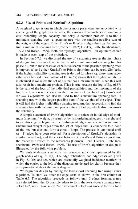
314 NETWORKED SYSTEMS RELIABILITY
6.7.3 Use of Prim’s and Kruskal’s Algorithms
A weighted graph is one in which one or more parameters are associated witheach edge of the graph. In a network, the associated parameters are commonlycost, reliability, length, capacity, and delay. A common problem is to find aminimum spanning tree—a spanning tree with the smallest possible sum ofthe weights of the edges. Either Prim’s or Kruskal’s algorithms can be used tofind a minimum spanning tree [Cormen, 1992; Dierker, 1986; Kershenbaum,1993; and Rosen, 1999]. Both are “greedy” algorithms—an optimum choiceis made at each step of the procedure.
In Section 6.7.2, we discussed the use of a spanning tree as the first phaseof design. An obvious choice is the use of a minimum-cost spanning tree forphase A1, but in most cases an exhaustive search of the possible spanning treesis impractical and either Kruskal’s or Prim’s algorithm can be used. Similarly,if the highest-reliability spanning tree is desired for phase A1, these same algo-rithms can be used. Examination of Eq. (6.57) shows that the highest reliabilityis obtained if we select the set of pis that has a maximum sum, since this willalso result in a maximum product. [This is true because the log of Eq. (6.57)is the sum of the logs of the individual probabilties, and the maximum of thelog of a function is the same as the maximum of the function.] Prim’s andKruskal’s algorithms can also be used to find a maximum spanning tree—aspanning tree with the largest possible sum of the weights of the edges. Thusit will find the highest-reliability spanning tree. Another approach is to find thespanning tree with the minimum probabilities of failure, which also maximizesthe reliability.
A simple statement of Prim’s algorithm is to select an initial edge of mini-mum (maximum) weight, by search or by first ordering all edges by weight, andto use this edge to begin the tree. Subsequent edges are selected as minimum(maximum) weight edges from the set of edges that is connected to a nodeof the tree but does not form a circuit (loop). The process is continued until(n − 1) edges have been selected. For a description of Kruskal’s algorithm (asimilar procedure), and the choice between Kruskal’s and Prim’s algorithms,the reader is directed to the references [Cormen, 1992; Dierker, 1986; Ker-shenbaum, 1993; and Rosen, 1999]. The use of Prim’s algorithm in design isillustrated by the following problem.
We wish to design a network that connects six cities represented by thegraph nodes of Fig. 6.10(a). The edge reliabilities and edge costs are givenin Fig. 6.10(b) and (c), which are essentially weighted incidence matrices inwhich the entries to the left of the diagonal are deleted for clarity because theyare symmetrical about the main diagonal.
We begin our design by finding the lowest-cost spanning tree using Prim’salgorithm. To start, we order the edge costs as shown in the first column ofTable 6.5. The algorithm proceeds as follows until 5 edges forming a treeare selected from the 15 possible edges to form the lowest-cost spanning tree:select 1–2; select 1–4; select 2–3; we cannot select 2–4 since it forms a loop
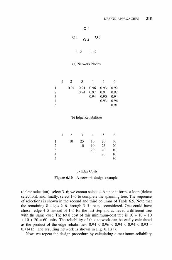
DESIGN APPROACHES 315
1 2 3 4 5 6
1 10 25 10 20 302 10 10 25 203 20 40 104 20 105 30
(c) Edge Costs
1 2 3 4 5 6
1 0.94 0.91 0.96 0.93 0.922 0.94 0.97 0.91 0.923 0.94 0.90 0.944 0.93 0.965 0.91
(b) Edge Reliabilities
(a) Network Nodes
1 3
2
4
5 6
Figure 6.10 A network design example.
(delete selection); select 3–6; we cannot select 4–6 since it forms a loop (deleteselection); and, finally, select 1–5 to complete the spanning tree. The sequenceof selections is shown in the second and third columns of Table 6.5. Note thatthe remaining 8 edges 2–6 through 3–5 are not considered. One could havechosen edge 4–5 instead of 1–5 for the last step and achieved a different treewith the same cost. The total cost of this minimum-cost tree is 10 + 10 + 10+ 10 + 20 c 60 units. The reliability of this network can be easily calculatedas the product of the edge reliabilities: 0.94 × 0.96 × 0.94 × 0.94 × 0.93 c
0.71415. The resulting network is shown in Fig. 6.11(a).Now, we repeat the design procedure by calculating a maximum-reliability
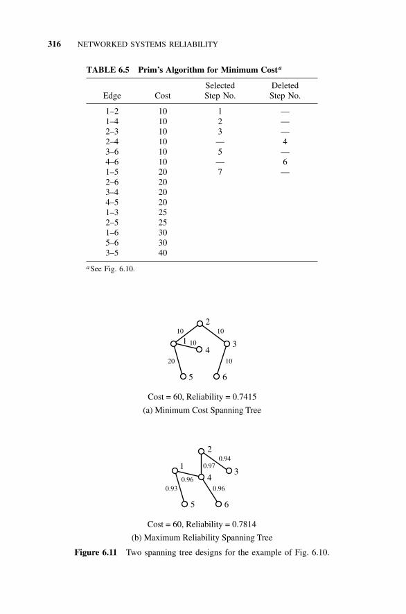
316 NETWORKED SYSTEMS RELIABILITY
TABLE 6.5 Prim’s Algorithm for Minimum Costa
Selected DeletedEdge Cost Step No. Step No.
1–2 10 1 —1–4 10 2 —2–3 10 3 —2–4 10 — 43–6 10 5 —4–6 10 — 61–5 20 7 —2–6 203–4 204–5 201–3 252–5 251–6 305–6 303–5 40
a See Fig. 6.10.
(a) Minimum Cost Spanning Tree
1 3
2
4
5 6
20
10
10
10
10
Cost = 60, Reliability = 0.7415
(b) Maximum Reliability Spanning Tree
Cost = 60, Reliability = 0.7814
13
2
4
5 6
0.930.96
0.94
0.96
0.97
Figure 6.11 Two spanning tree designs for the example of Fig. 6.10.
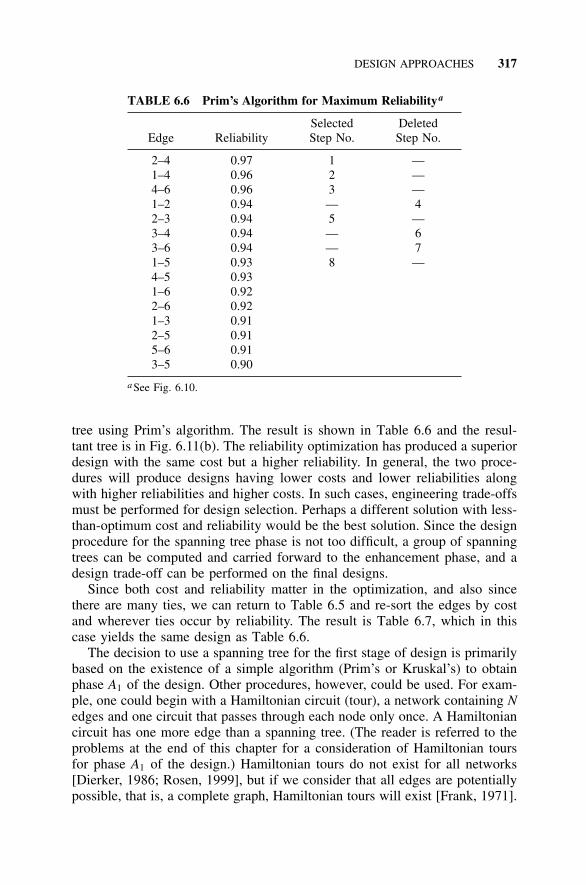
DESIGN APPROACHES 317
TABLE 6.6 Prim’s Algorithm for Maximum Reliabilitya
Selected DeletedEdge Reliability Step No. Step No.
2–4 0.97 1 —1–4 0.96 2 —4–6 0.96 3 —1–2 0.94 — 42–3 0.94 5 —3–4 0.94 — 63–6 0.94 — 71–5 0.93 8 —4–5 0.931–6 0.922–6 0.921–3 0.912–5 0.915–6 0.913–5 0.90
a See Fig. 6.10.
tree using Prim’s algorithm. The result is shown in Table 6.6 and the resul-tant tree is in Fig. 6.11(b). The reliability optimization has produced a superiordesign with the same cost but a higher reliability. In general, the two proce-dures will produce designs having lower costs and lower reliabilities alongwith higher reliabilities and higher costs. In such cases, engineering trade-offsmust be performed for design selection. Perhaps a different solution with less-than-optimum cost and reliability would be the best solution. Since the designprocedure for the spanning tree phase is not too difficult, a group of spanningtrees can be computed and carried forward to the enhancement phase, and adesign trade-off can be performed on the final designs.
Since both cost and reliability matter in the optimization, and also sincethere are many ties, we can return to Table 6.5 and re-sort the edges by costand wherever ties occur by reliability. The result is Table 6.7, which in thiscase yields the same design as Table 6.6.
The decision to use a spanning tree for the first stage of design is primarilybased on the existence of a simple algorithm (Prim’s or Kruskal’s) to obtainphase A1 of the design. Other procedures, however, could be used. For exam-ple, one could begin with a Hamiltonian circuit (tour), a network containing Nedges and one circuit that passes through each node only once. A Hamiltoniancircuit has one more edge than a spanning tree. (The reader is referred to theproblems at the end of this chapter for a consideration of Hamiltonian toursfor phase A1 of the design.) Hamiltonian tours do not exist for all networks[Dierker, 1986; Rosen, 1999], but if we consider that all edges are potentiallypossible, that is, a complete graph, Hamiltonian tours will exist [Frank, 1971].
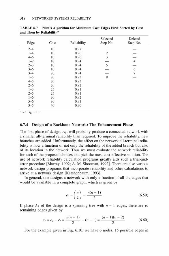
318 NETWORKED SYSTEMS RELIABILITY
TABLE 6.7 Prim’s Algorithm for Minimum Cost Edges First Sorted by Costand Then by Reliabilitya
Selected DeletedEdge Cost Reliability Step No. Step No.
2–4 10 0.97 1 —1–4 10 0.96 2 —4–6 10 0.96 3 —1–2 10 0.94 — 42–3 10 0.94 5 —3–6 10 0.94 — 63–4 20 0.94 — 71–5 20 0.93 8 —4–5 20 0.932–6 20 0.921–3 25 0.912–5 25 0.911–6 30 0.925–6 30 0.913–5 40 0.90
a See Fig. 6.10.
6.7.4 Design of a Backbone Network: The Enhancement Phase
The first phase of design, A1, will probably produce a connected network witha smaller all-terminal reliability than required. To improve the reliability, newbranches are added. Unfortunately, the effect on the network all-terminal relia-bility is now a function of not only the reliability of the added branch but alsoof its location in the network. Thus we must evaluate the network reliabilityfor each of the proposed choices and pick the most cost-effective solution. Theuse of network reliability calculation programs greatly aids such a trial-and-error procedure [Murray, 1992; A. M. Shooman, 1992]. There are also variousnetwork design programs that incorporate reliability and other calculations toarrive at a network design [Kershenbaum, 1993].
In general, one designs a network with only a fraction of all the edges thatwould be available in a complete graph, which is given by
ec c � n2 � c
n(n − 1)2
(6.59)
If phase A1 of the design is a spanning tree with n − 1 edges, there are er
remaining edges given by
er c ec − et cn(n − 1)
2− (n − 1) c
(n − 1)(n − 2)2
(6.60)
For the example given in Fig. 6.10, we have 6 nodes, 15 possible edges in
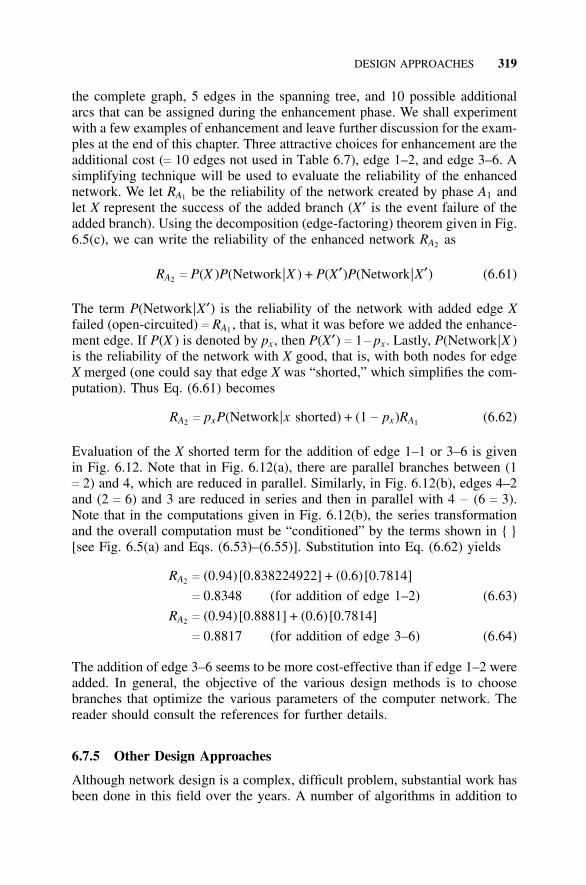
DESIGN APPROACHES 319
the complete graph, 5 edges in the spanning tree, and 10 possible additionalarcs that can be assigned during the enhancement phase. We shall experimentwith a few examples of enhancement and leave further discussion for the exam-ples at the end of this chapter. Three attractive choices for enhancement are theadditional cost (c 10 edges not used in Table 6.7), edge 1–2, and edge 3–6. Asimplifying technique will be used to evaluate the reliability of the enhancednetwork. We let RA1 be the reliability of the network created by phase A1 andlet X represent the success of the added branch (X′ is the event failure of theadded branch). Using the decomposition (edge-factoring) theorem given in Fig.6.5(c), we can write the reliability of the enhanced network RA2 as
RA2 c P(X )P(Network|X ) + P(X′)P(Network|X′) (6.61)
The term P(Network|X′) is the reliability of the network with added edge Xfailed (open-circuited) c RA1 , that is, what it was before we added the enhance-ment edge. If P(X ) is denoted by px , then P(X′) c 1− px . Lastly, P(Network|X )is the reliability of the network with X good, that is, with both nodes for edgeX merged (one could say that edge X was “shorted,” which simplifies the com-putation). Thus Eq. (6.61) becomes
RA2 c pxP(Network|x shorted) + (1 − px)RA1 (6.62)
Evaluation of the X shorted term for the addition of edge 1–1 or 3–6 is givenin Fig. 6.12. Note that in Fig. 6.12(a), there are parallel branches between (1c 2) and 4, which are reduced in parallel. Similarly, in Fig. 6.12(b), edges 4–2and (2 c 6) and 3 are reduced in series and then in parallel with 4 − (6 c 3).Note that in the computations given in Fig. 6.12(b), the series transformationand the overall computation must be “conditioned” by the terms shown in { }[see Fig. 6.5(a) and Eqs. (6.53)–(6.55)]. Substitution into Eq. (6.62) yields
RA2 c (0.94)[0.838224922] + (0.6)[0.7814]
c 0.8348 (for addition of edge 1–2) (6.63)
RA2 c (0.94)[0.8881] + (0.6)[0.7814]
c 0.8817 (for addition of edge 3–6) (6.64)
The addition of edge 3–6 seems to be more cost-effective than if edge 1–2 wereadded. In general, the objective of the various design methods is to choosebranches that optimize the various parameters of the computer network. Thereader should consult the references for further details.
6.7.5 Other Design Approaches
Although network design is a complex, difficult problem, substantial work hasbeen done in this field over the years. A number of algorithms in addition to
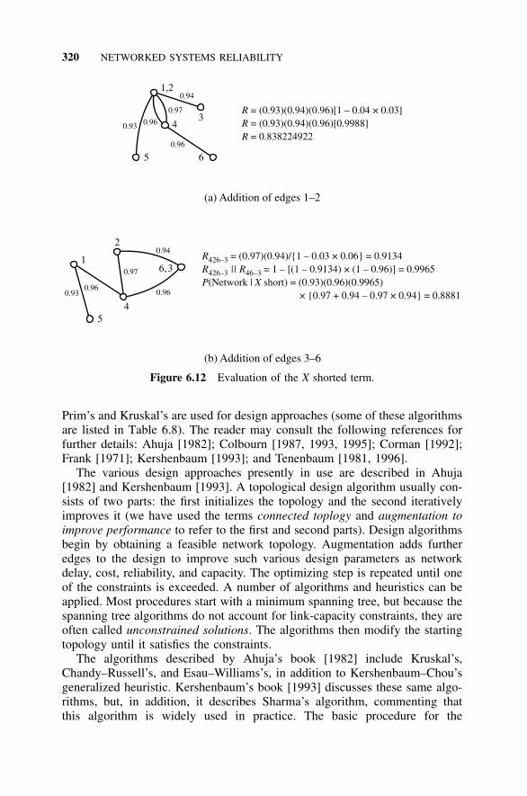
320 NETWORKED SYSTEMS RELIABILITY
(a) Addition of edges 1–2
(b) Addition of edges 3–6
3
1,2
4
5 6
0.93 0.96
0.96
0.94
0.97 RRR
= (0.93)(0.94)(0.96)[1 – 0.04 × 0.03]= (0.93)(0.94)(0.96)[0.9988]= 0.838224922
6,3
5
0.930.96
0.96
0.94
0.97
RRP X
426–3 = (0.97)(0.94)/{1 – 0.03 × 0.06} = 0.9134|| = 1 – [(1 – 0.9134) × (1 – 0.96)] = 0.9965
(Network | short) = (0.93)(0.96)(0.9965)× {0.97 + 0.94 – 0.97 × 0.94} = 0.8881
426–3 46–3R
2
4
1
Figure 6.12 Evaluation of the X shorted term.
Prim’s and Kruskal’s are used for design approaches (some of these algorithmsare listed in Table 6.8). The reader may consult the following references forfurther details: Ahuja [1982]; Colbourn [1987, 1993, 1995]; Corman [1992];Frank [1971]; Kershenbaum [1993]; and Tenenbaum [1981, 1996].
The various design approaches presently in use are described in Ahuja[1982] and Kershenbaum [1993]. A topological design algorithm usually con-sists of two parts: the first initializes the topology and the second iterativelyimproves it (we have used the terms connected toplogy and augmentation toimprove performance to refer to the first and second parts). Design algorithmsbegin by obtaining a feasible network topology. Augmentation adds furtheredges to the design to improve such various design parameters as networkdelay, cost, reliability, and capacity. The optimizing step is repeated until oneof the constraints is exceeded. A number of algorithms and heuristics can beapplied. Most procedures start with a minimum spanning tree, but because thespanning tree algorithms do not account for link-capacity constraints, they areoften called unconstrained solutions. The algorithms then modify the startingtopology until it satisfies the constraints.
The algorithms described by Ahuja’s book [1982] include Kruskal’s,Chandy–Russell’s, and Esau–Williams’s, in addition to Kershenbaum–Chou’sgeneralized heuristic. Kershenbaum’s book [1993] discusses these same algo-rithms, but, in addition, it describes Sharma’s algorithm, commenting thatthis algorithm is widely used in practice. The basic procedure for the
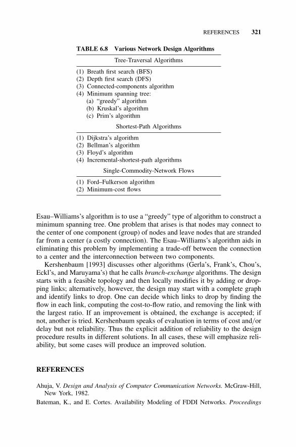
REFERENCES 321
TABLE 6.8 Various Network Design Algorithms
Tree-Traversal Algorithms
(1) Breath first search (BFS)(2) Depth first search (DFS)(3) Connected-components algorithm(4) Minimum spanning tree:
(a) “greedy” algorithm(b) Kruskal’s algorithm(c) Prim’s algorithm
Shortest-Path Algorithms
(1) Dijkstra’s algorithm(2) Bellman’s algorithm(3) Floyd’s algorithm(4) Incremental-shortest-path algorithms
Single-Commodity-Network Flows
(1) Ford–Fulkerson algorithm(2) Minimum-cost flows
Esau–Williams’s algorithm is to use a “greedy” type of algorithm to construct aminimum spanning tree. One problem that arises is that nodes may connect tothe center of one component (group) of nodes and leave nodes that are strandedfar from a center (a costly connection). The Esau–Williams’s algorithm aids ineliminating this problem by implementing a trade-off between the connectionto a center and the interconnection between two components.
Kershenbaum [1993] discusses other algorithms (Gerla’s, Frank’s, Chou’s,Eckl’s, and Maruyama’s) that he calls branch-exchange algorithms. The designstarts with a feasible topology and then locally modifies it by adding or drop-ping links; alternatively, however, the design may start with a complete graphand identify links to drop. One can decide which links to drop by finding theflow in each link, computing the cost-to-flow ratio, and removing the link withthe largest ratio. If an improvement is obtained, the exchange is accepted; ifnot, another is tried. Kershenbaum speaks of evaluation in terms of cost and/ ordelay but not reliability. Thus the explicit addition of reliability to the designprocedure results in different solutions. In all cases, these will emphasize reli-ability, but some cases will produce an improved solution.
REFERENCES
Ahuja, V. Design and Analysis of Computer Communication Networks. McGraw-Hill,New York, 1982.
Bateman, K., and E. Cortes. Availability Modeling of FDDI Networks. Proceedings
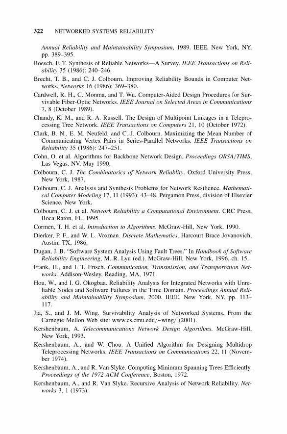
322 NETWORKED SYSTEMS RELIABILITY
Annual Reliability and Maintainability Symposium, 1989. IEEE, New York, NY,pp. 389–395.
Boesch, F. T. Synthesis of Reliable Networks—A Survey. IEEE Transactions on Reli-ability 35 (1986): 240–246.
Brecht, T. B., and C. J. Colbourn. Improving Reliability Bounds in Computer Net-works. Networks 16 (1986): 369–380.
Cardwell, R. H., C. Monma, and T. Wu. Computer-Aided Design Procedures for Sur-vivable Fiber-Optic Networks. IEEE Journal on Selected Areas in Communications7, 8 (October 1989).
Chandy, K. M., and R. A. Russell. The Design of Multipoint Linkages in a Telepro-cessing Tree Network. IEEE Transactions on Computers 21, 10 (October 1972).
Clark, B. N., E. M. Neufeld, and C. J. Colbourn. Maximizing the Mean Number ofCommunicating Vertex Pairs in Series-Parallel Networks. IEEE Transactions onReliability 35 (1986): 247–251.
Cohn, O. et al. Algorithms for Backbone Network Design. Proceedings ORSA/ TIMS,Las Vegas, NV, May 1990.
Colbourn, C. J. The Combinatorics of Network Reliablity. Oxford University Press,New York, 1987.
Colbourn, C. J. Analysis and Synthesis Problems for Network Resilience. Mathemati-cal Computer Modeling 17, 11 (1993): 43–48, Pergamon Press, division of ElsevierScience, New York.
Colbourn, C. J. et al. Network Reliability a Computational Environment. CRC Press,Boca Raton, FL, 1995.
Cormen, T. H. et al. Introduction to Algorithms. McGraw-Hill, New York, 1990.Dierker, P. F., and W. L. Voxman. Discrete Mathematics. Harcourt Brace Jovanovich,
Austin, TX, 1986.Dugan, J. B. “Software System Analysis Using Fault Trees.” In Handbook of Software
Reliability Engineering, M. R. Lyu (ed.). McGraw-Hill, New York, 1996, ch. 15.Frank, H., and I. T. Frisch. Communication, Transmission, and Transportation Net-
works. Addison-Wesley, Reading, MA, 1971.Hou, W., and I. G. Okogbaa. Reliability Analysis for Integrated Networks with Unre-
liable Nodes and Software Failures in the Time Domain. Proceedings Annual Reli-ability and Maintainability Symposium, 2000. IEEE, New York, NY, pp. 113–117.
Jia, S., and J. M. Wing. Survivability Analysis of Networked Systems. From theCarnegie Mellon Web site: www.cs.cmu.edu/ ∼wing/ (2001).
Kershenbaum, A. Telecommunications Network Design Algorithms. McGraw-Hill,New York, 1993.
Kershenbaum, A., and W. Chou. A Unified Algorithm for Designing MultidropTeleprocessing Networks. IEEE Transactions on Communications 22, 11 (Novem-ber 1974).
Kershenbaum, A., and R. Van Slyke. Computing Minimum Spanning Trees Efficiently.Proceedings of the 1972 ACM Conference, Boston, 1972.
Kershenbaum, A., and R. Van Slyke. Recursive Analysis of Network Reliability. Net-works 3, 1 (1973).
REFERENCES 323
Lawler, E. Combinatorial Optimization: Network and Materials. Holt, Rinehart, andWinston, Austin, TX, 1976.
Liu, H.-L., and M. L. Shooman. Simulation of Computer Network Reliability withCongestion. Proceedings Annual Reliability and Maintainability Symposium, 1999.IEEE, New York, NY, pp. 208–213.
Mendenhall, W. et al. Mathematical Statistics with Applications, 4th ed. PWS-Kent,Boston, 1990.
Messinger, M., and M. L. Shooman. Techniques for Optimum Spares Allocation: ATutorial Review (Dynamic Programming). IEEE Transactions on Reliability 19, 4(November 1970).
Monma, C. L., and D. F. Shallcross. Methods for Designing Communications Net-works with Certain Two-Connected Survivability Constraints. Operations Research37 (1989): 531–541.
Murray, K. “Path Set and Cut Set Approximations and Bounds for Network ReliabilityAnalysis.” Ph.D. thesis, Polytechnic University, 1992.
Murray, K., A. Kershenbaum, and M. L. Shooman. “A Comparison of Two DifferentPath Set and Cut Set Approximations for Network Reliability Analysis. ProceedingsAnnual Reliability and Maintainability Symposium, 1993. IEEE, New York, NY.
Naor, D. et al. A Fast Algorithm for Optimally Increasing Edge-Connectivity. Proceed-ings IEEE Symposium on Foundations of Computer Science, St. Louis, MO, 1990.IEEE, New York, NY.
Ponta, A. et al. Reliability Analysis of Torino Sud District Heating System [Network].Proceedings Annual Reliability and Maintainability Symposium, 1999. IEEE, NewYork, NY, pp. 336–342.
Provan, J. S. The Complexity of Reliability Computations in Planar and AcyclicGraphs. SIAM J. Computing 15 (1986): 36–61.
Provan, J. S., and M. O. Ball. Computing Network Reliability in Time Polynomial inthe Number of Cuts. Operations Research 32 (1984): 516–526.
Rosen, K. H. Discrete Mathematics and its Applications. WCB–McGraw-Hill, NewYork, 1999.
Rosenthal, A. Computing the Reliability of Complex Networks. SIAM J. of AppliedMathematics 32, 2 (March 1977).
Satyanarayana, A. A Unified Formula for Analysis of Some Network Reliability Prob-lems. IEEE Transactions on Reliability 31 (1982): 23–32.
Satyanarayana, A., and R. K. Wood. A Linear Time Algorithm for Computing k-Terminal Reliability on Series-Parallel Networks. SIAM J. Computing 14 (1985):818–832.
Schwartz, M. Computer Communication Network Design and Analysis. Prentice-Hall,Englewood Cliffs, NJ, 1977.
Schweber, W. Electronic Communication Systems. Prentice-Hall, Upper Saddle River,NJ, 1999.
Sharma, R. Network Topology Optimization. Van Nostrand Reinhold, New York,1991.
Shier, D. R. Network Reliability and Algebraic Structures. Oxford University Press,New York, 1991.
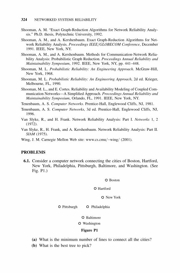
324 NETWORKED SYSTEMS RELIABILITY
Shooman, A. M. “Exact Graph-Reduction Algorithms for Network Reliability Analy-sis.” Ph.D. thesis, Polytechnic University, 1992.
Shooman, A. M., and A. Kershenbaum. Exact Graph-Reduction Algorithms for Net-work Reliability Analysis. Proceedings IEEE/ GLOBECOM Conference, December1991. IEEE, New York, NY.
Shooman, A. M., and A. Kershenbaum. Methods for Communication-Network Relia-bility Analysis: Probabilistic Graph Reduction. Proceedings Annual Reliability andMaintainability Symposium, 1992. IEEE, New York, NY, pp. 441–448.
Shooman, M. L. Probabilistic Reliability: An Engineering Approach. McGraw-Hill,New York, 1968.
Shooman, M. L. Probabilistic Reliability: An Engineering Approach, 2d ed. Krieger,Melbourne, FL, 1990.
Shooman, M. L., and E. Cortes. Reliability and Availability Modeling of Coupled Com-munication Networks—A Simplified Approach. Proceedings Annual Reliability andMaintainability Symposium, Orlando, FL, 1991. IEEE, New York, NY.
Tenenbaum, A. S. Computer Networks. Prentice-Hall, Englewood Cliffs, NJ, 1981.
Tenenbaum, A. S. Computer Networks, 3d ed. Prentice-Hall, Englewood Cliffs, NJ,1996.
Van Slyke, R., and H. Frank. Network Reliability Analysis: Part I. Networks 1, 2(1972).
Van Slyke, R., H. Frank, and A. Kershenbaum. Network Reliability Analysis: Part II.SIAM (1975).
Wing, J. M. Carnegie Mellon Web site: www.cs.cmu/ ∼wing/ (2001).
PROBLEMS
6.1. Consider a computer network connecting the cities of Boston, Hartford,New York, Philadelphia, Pittsburgh, Baltimore, and Washington. (SeeFig. P1.)
Boston
Hartford
New York
PhiladelphiaPittsburgh
Baltimore
Washington
Figure P1
(a) What is the minimum number of lines to connect all the cities?(b) What is the best tree to pick?
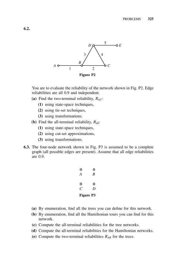
PROBLEMS 325
6.2.
AB
1C
2
3 4
D E5
Figure P2
You are to evaluate the reliability of the network shown in Fig. P2. Edgereliabilities are all 0.9 and independent.
(a) Find the two-terminal reliability, RAC:
(1) using state-space techniques,
(2) using tie-set techniques,
(3) using transformations.
(b) Find the all-terminal reliability, Rall:
(1) using state-space techniques,
(2) using cut-set approximations,
(3) using transformations.
6.3. The four-node network shown in Fig. P3 is assumed to be a completegraph (all possible edges are present). Assume that all edge reliabilitiesare 0.9.
A
C
B
D
Figure P3
(a) By enumeration, find all the trees you can define for this network.
(b) By enumeration, find all the Hamiltonian tours you can find for thisnetwork.
(c) Compute the all-terminal reliabilities for the tree networks.
(d) Compute the all-terminal reliabilities for the Hamiltonian networks.
(e) Compute the two-terminal reliabilities RAB for the trees.
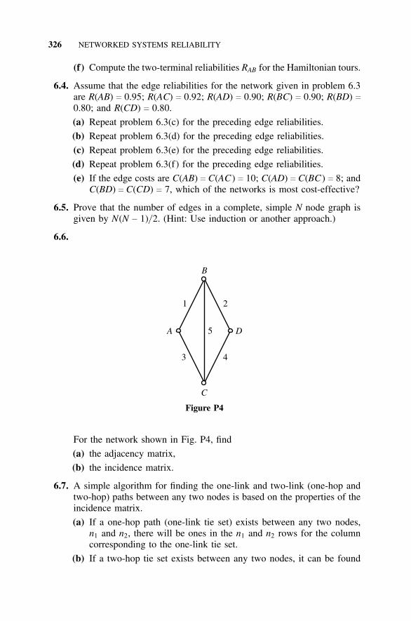
326 NETWORKED SYSTEMS RELIABILITY
(f) Compute the two-terminal reliabilities RAB for the Hamiltonian tours.
6.4. Assume that the edge reliabilities for the network given in problem 6.3are R(AB) c 0.95; R(AC) c 0.92; R(AD) c 0.90; R(BC) c 0.90; R(BD) c0.80; and R(CD) c 0.80.
(a) Repeat problem 6.3(c) for the preceding edge reliabilities.
(b) Repeat problem 6.3(d) for the preceding edge reliabilities.
(c) Repeat problem 6.3(e) for the preceding edge reliabilities.
(d) Repeat problem 6.3(f) for the preceding edge reliabilities.
(e) If the edge costs are C(AB) c C(AC) c 10; C(AD) c C(BC) c 8; andC(BD) c C(CD) c 7, which of the networks is most cost-effective?
6.5. Prove that the number of edges in a complete, simple N node graph isgiven by N(N − 1)/ 2. (Hint: Use induction or another approach.)
6.6.
A D
B
C
1 2
3 4
5
Figure P4
For the network shown in Fig. P4, find
(a) the adjacency matrix,
(b) the incidence matrix.
6.7. A simple algorithm for finding the one-link and two-link (one-hop andtwo-hop) paths between any two nodes is based on the properties of theincidence matrix.
(a) If a one-hop path (one-link tie set) exists between any two nodes,n1 and n2, there will be ones in the n1 and n2 rows for the columncorresponding to the one-link tie set.
(b) If a two-hop tie set exists between any two nodes, it can be found
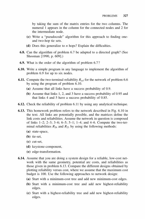
PROBLEMS 327
by taking the sum of the matrix entries for the two columns. Thenumeral 1 appears in the column for the connected nodes and 2 forthe intermediate node.
(c) Write a “pseudocode” algorithm for this approach to finding one-and two-hop tie sets.
(d) Does this generalize to n hops? Explain the difficulties.
6.8. Can the algorithm of problem 6.7 be adapted to a directed graph? (SeeShooman [1990, p. 609].)
6.9. What is the order of the algorithm of problem 6.7?
6.10. Write a simple program in any language to implement the algorithm ofproblem 6.9 for up to six nodes.
6.11. Compute the two-terminal reliability Rad for the network of problem 6.6by using the program of problem 6.10.
(a) Assume that all links have a success probability of 0.9.
(b) Assume that links 1, 2, and 3 have a success probability of 0.95 andthat links 4 and 5 have a success probability of 0.85.
6.12. Check the reliability of problem 6.11 by using any analytical technique.
6.13. This homework problem refers to the network described in Fig. 6.10 inthe text. All links are potentially possible, and the matrices define thelink costs and reliabilities. Assume the network in question is composedof links 1–2; 2–3; 3–6; 6–5; 5–1; 1–4; and 4–6. Compute the two-ter-minal reliabilities R26 and R23 by using the following methods:
(a) state-space,
(b) tie-set,
(c) cut-set,
(d) keystone-component,
(e) edge-transformation.
6.14. Assume that you are doing a system design for a reliable, low-cost net-work with the same geometry, potential arc costs, and reliabilities asthose given in problem 6.13. Compare the different designs obtained byplotting reliability versus cost, where we assume that the maximum costbudget is 100. Use the following approaches to network design:
(a) Start with a minimum-cost tree and add new minimum-cost edges.
(b) Start with a minimum-cost tree and add new highest-reliabilityedges.
(c) Start with a highest-reliability tree and add new highest-reliabilityedges.
328 NETWORKED SYSTEMS RELIABILITY
(d) Start with a highest-reliability Hamiltonian tour and add newhighest-reliability edges.
(e) Start with a minimum-cost Hamiltonian tour and add new highest-reliability edges.
6.15. For a Hamiltonian tour in which the n branch probabilities are inde-pendent and equal, show that the all-terminal reliability is given by thebinomial distribution:
Rall c P(no branch failure + one branch failure)
c pn + np(n − 1)(1 − p)
6.16. Repeat problem 6.15 for a Hamiltonian tour in which the branch prob-abilities are all different. Instead of the binomial distribution, you willhave to write out a series of terms that yields a formula different fromthat of problem 6.15, but one that also reduces to the same formula forequal probabilities.
6.17. Clearly, a Hamiltonian network of n identical elements has a higher reli-ability than that of a spanning tree for n nodes. Show that the improve-ment ratio is [p + n(1 − p)].
6.18. In this problem, we make a rough analysis to explore how the capacityof communication lines affects a communication network.
(a) Consider the nodes of problem 6.1 and connect them in aHamiltonian tour network in Table P1: Boston–Hartford–NewYork–Philadelphia–Pittsburgh–Baltimore–Washington–Boston. As-sume that the Hartford–Baltimore–Pittsburgh traffic is small (2 unitseach way) compared to the Boston–New York–Philadelphia–Wash-ington traffic (10 units each way). Fill in Table P1 with total trafficunits, assuming that messages are always sent (routed) via the short-est possible way. Assume full duplex (simultaneous communicationin both directions).
(b) Assume a break on the Philadelphia–Pittsburgh line. Some messagesmust now be rerouted over different, longer paths because of thisbreak. For example, the Washington–Boston line must handle all ofthe traffic between Philadelphia, New York, Boston, and Washing-ton. Recompute the traffic table (Table P2).
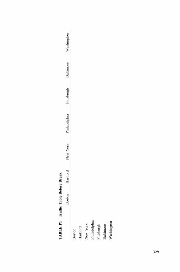
329
TA
BL
E P
1T
raffi
c T
able
Bef
ore
Bre
ak
Bos
ton
Har
tfor
dN
ew Y
ork
Phila
delp
hia
Pitts
burg
hB
altim
ore
Was
hing
ton
Bos
ton
Har
tfor
d
New
Yor
k
Phila
delp
hia
Pitts
burg
h
Bal
timor
e
Was
hing
ton
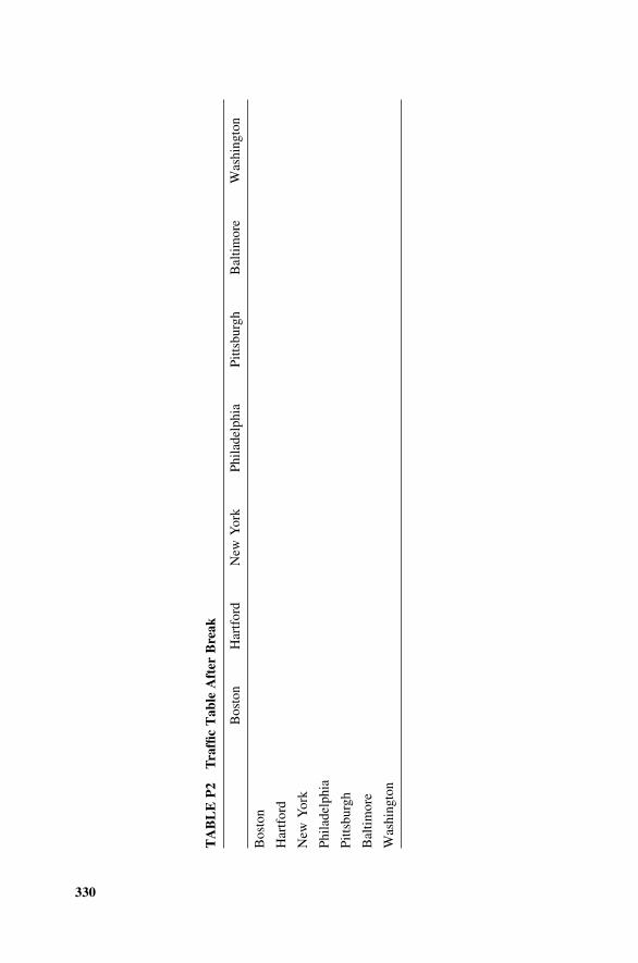
330
TA
BL
E P
2T
raffi
c T
able
Aft
er B
reak
Bos
ton
Har
tfor
dN
ew Y
ork
Phila
delp
hia
Pitts
burg
hB
altim
ore
Was
hing
ton
Bos
ton
Har
tfor
d
New
Yor
k
Phila
delp
hia
Pitts
burg
h
Bal
timor
e
Was
hing
ton
7RELIABILITY OPTIMIZATION
Reliability of Computer Systems and Networks: Fault Tolerance, Analysis, and DesignMartin L. Shooman
Copyright 2002 John Wiley & Sons, Inc.ISBNs: 0-471-29342-3 (Hardback); 0-471-22460-X (Electronic)
331
7.1 INTRODUCTION
The preceding chapters of this book discussed a wide range of different tech-niques for enhancing system or device fault tolerance. In some applications,only one of these techniques is practical, and there is little choice among themethods. However, in a fair number of applications, two or more techniquesare feasible, and the question arises regarding which technique is the mostcost-effective. To address this problem, if one is given two alternatives, onecan always use one technique for design A and use the other technique fordesign B. One can then analyze both designs A and B to study the trade-offs.In the case of a standby or repairable system, if redundancy is employed at acomponent level, there are many choices based on the number of spares andwhich component will be spared. At the top level, many systems appear as aseries string of elements, and the question arises of how we are to distributethe redundancy in a cost-effective manner among the series string. Specifically,we assume that the number of redundant elements that can be added is limitedby cost, weight, volume, or some similar constraint. The object is to determinethe set of redundant components that still meets the constraint and raises thereliability by the largest amount. Some authors refer to this as redundancy opti-mization [Barlow, 1965]. Two practical works—Fragola [1973] and Mancino[1986]—are given in the references that illustrate the design of a system witha high degree of parallel components. The reader should consult these papersafter studying the material in this chapter.
In some ways, this chapter can be considered an extension of the materialin Chapter 4. However, in this chapter we discuss the optimization approach,

332 RELIABILITY OPTIMIZATION
where rather than having the redundancy apply to a single element, it is dis-tributed over the entire system in such a way that it optimizes reliability. Theoptimization approach has been studied in the past, but is infrequently used inpractice for many reasons, such as (a) the system designer does not understandthe older techniques and the resulting mathematical formulation; (b) the solu-tion takes too long; (c) the parameters are not well known; and (d) constraintschange rapidly and invalidate the previous solution. We propose a techniquethat is clear, simple to explain, and results in the rapid calculation of a familyof good suboptimal solutions along with the optimal solution. The designer isthen free to choose among this family of solutions, and if the design featuresor parameters change, the calculations can be repeated with modest effort.
We now postulate that the design of fault-tolerant systems can be dividedinto three classes. In the first class, only one design approach (e.g., parallel,standby, voting) is possible, or intuition and experience points only to a sin-gle approach. Thus it is simple to decide on the level of redundancy requiredto meet the design goal or the level allowed by the constraint. To simplifyour discussion, we will refer to cost, but we must keep in mind that all thetechniques to be discussed can be adapted to any other single constraint or,in many cases, multiple constraints. Typical multiple constraints are cost, reli-ability, volume, and weight. Sometimes, the optimum solution will not satisfythe reliability goal; then, either the cost constraint must be increased or thereliability goal must be lowered. In the second class, if there are two or threealternative designs, we would merely repeat the optimization for each classas discussed previously and choose the best result. The second class is onein which there are many alternatives within the design approach because wecan apply redundancy at the subsystem level to many subsystems. The thirdclass, where a mixed strategy is being considered, also has many combinations.To deal with the complexity of the third-class designs, we will use computercomputations and an optimization approach to guide us in choosing the bestalternative or set of alternatives.
7.2 OPTIMUM VERSUS GOOD SOLUTIONS
Because of practical considerations, an approximate optimization yielding agood system is favored over an exact one yielding the best solution. The param-eters of the solution, as well as the failure rates, weight, volume, and cost, aregenerally only known approximately at the beginning of a design; moreover, insome cases, we only know the function that the component must perform, nothow that function will be implemented. Thus the range of possible parametersis often very broad, and to look for an exact optimization when the parametersare known only over a broad range may be an elegant mathematical formula-tion but is not a practical engineering solution. In fact, sometimes choosing theexact optimum can involve considerable risk if the solution is very sensitiveto small changes in parameters.
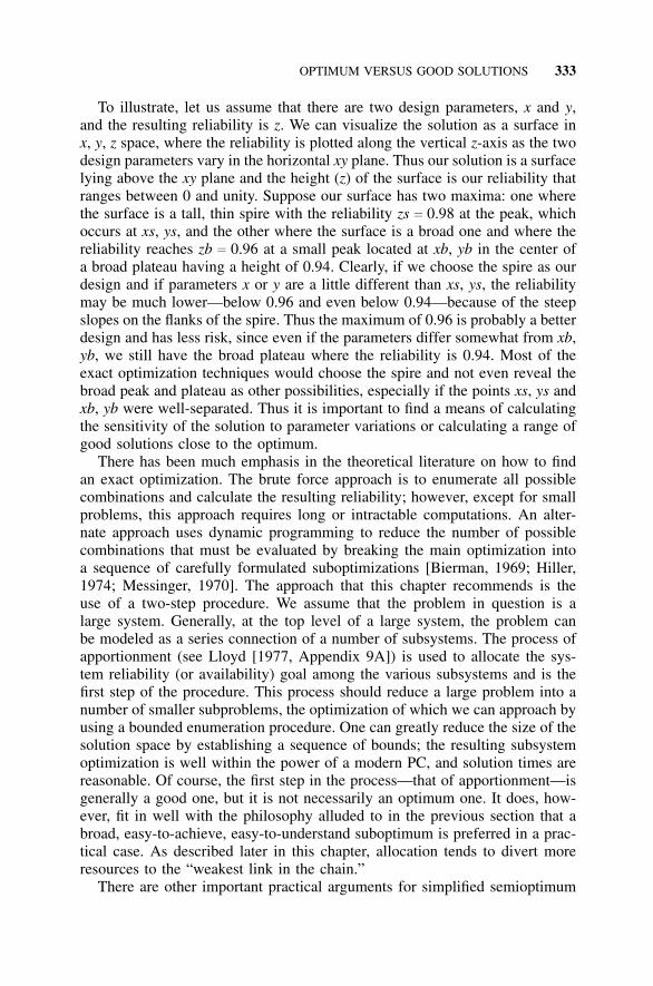
OPTIMUM VERSUS GOOD SOLUTIONS 333
To illustrate, let us assume that there are two design parameters, x and y,and the resulting reliability is z. We can visualize the solution as a surface inx, y, z space, where the reliability is plotted along the vertical z-axis as the twodesign parameters vary in the horizontal xy plane. Thus our solution is a surfacelying above the xy plane and the height (z) of the surface is our reliability thatranges between 0 and unity. Suppose our surface has two maxima: one wherethe surface is a tall, thin spire with the reliability zs c 0.98 at the peak, whichoccurs at xs, ys, and the other where the surface is a broad one and where thereliability reaches zb c 0.96 at a small peak located at xb, yb in the center ofa broad plateau having a height of 0.94. Clearly, if we choose the spire as ourdesign and if parameters x or y are a little different than xs, ys, the reliabilitymay be much lower—below 0.96 and even below 0.94—because of the steepslopes on the flanks of the spire. Thus the maximum of 0.96 is probably a betterdesign and has less risk, since even if the parameters differ somewhat from xb,yb, we still have the broad plateau where the reliability is 0.94. Most of theexact optimization techniques would choose the spire and not even reveal thebroad peak and plateau as other possibilities, especially if the points xs, ys andxb, yb were well-separated. Thus it is important to find a means of calculatingthe sensitivity of the solution to parameter variations or calculating a range ofgood solutions close to the optimum.
There has been much emphasis in the theoretical literature on how to findan exact optimization. The brute force approach is to enumerate all possiblecombinations and calculate the resulting reliability; however, except for smallproblems, this approach requires long or intractable computations. An alter-nate approach uses dynamic programming to reduce the number of possiblecombinations that must be evaluated by breaking the main optimization intoa sequence of carefully formulated suboptimizations [Bierman, 1969; Hiller,1974; Messinger, 1970]. The approach that this chapter recommends is theuse of a two-step procedure. We assume that the problem in question is alarge system. Generally, at the top level of a large system, the problem canbe modeled as a series connection of a number of subsystems. The process ofapportionment (see Lloyd [1977, Appendix 9A]) is used to allocate the sys-tem reliability (or availability) goal among the various subsystems and is thefirst step of the procedure. This process should reduce a large problem into anumber of smaller subproblems, the optimization of which we can approach byusing a bounded enumeration procedure. One can greatly reduce the size of thesolution space by establishing a sequence of bounds; the resulting subsystemoptimization is well within the power of a modern PC, and solution times arereasonable. Of course, the first step in the process—that of apportionment—isgenerally a good one, but it is not necessarily an optimum one. It does, how-ever, fit in well with the philosophy alluded to in the previous section that abroad, easy-to-achieve, easy-to-understand suboptimum is preferred in a prac-tical case. As described later in this chapter, allocation tends to divert moreresources to the “weakest link in the chain.”
There are other important practical arguments for simplified semioptimum
334 RELIABILITY OPTIMIZATION
techniques instead of exact mathematical optimization. In practice, optimiz-ing a design is a difficult problem for many reasons. Designers, often harriedby schedule and costs, look for a feasible solution to meet the performanceparameters; thus reliability may be treated as an afterthought. This approachseldom leads to a design with optimum reliability—much less a good sub-optimal design. The opposite extreme is the classic optimization approach, inwhich a mathematical model of the system is formulated along with constraintson cost, volume, weight, and so forth, where all the allowable combinationsof redundant parallel and standby components are permitted and where theunderlying integer programming problem is solved. The latter approach is sel-dom taken for the previously stated reasons: (a) the system designer does notunderstand the mathematical formulation or the solution process; (b) the solu-tion takes too long; (c) the parameters are not well known; and (d) the con-straints rapidly change and invalidate the previous solution. Therefore, clear,simple, and rapid calculation of a family of good suboptimal solutions is asensible approach. The study of this family should reveal which solutions, ifany, are very sensitive to changes in the model parameters. Furthermore, thecomputations are simple enough that they can be repeated should significantchanges occur during the design process. Establishing such a range of solutionsis an ideal way to ensure that reliability receives adequate consideration amongthe various conflicting constraints and system objectives during the trade-offprocess—the preferred approach to choosing a good, well-balanced design.
7.3 A MATHEMATICAL STATEMENT OF THE OPTIMIZATIONPROBLEM
One can easily define the classic optimization approach as a mathematicalmodel of the system that is formulated along with constraints on cost, vol-ume, weight, and so forth, in which all the allowable combinations of redun-dant parallel and standby components are permitted and the underlying integerprogramming problem must be solved.
We begin with a series model for the system with k components where x1
is the event success of element one, x1 is the event failure of element one,and P(x1) c 1 − P(x1) is the probability of success of element one, whichis the reliability, r1 (see Fig. 7.1). Clearly, the components in the foregoingmathematical model can be subsystems if we wish.
The system reliability is given by the probability of the event in which allthe components succeed (the intersection of their successes):
Rs c P(x1U
x2U
· · ·U
xk) (7.1a)
If we assume that all the elements are independent, Eq. (7.1a) becomes
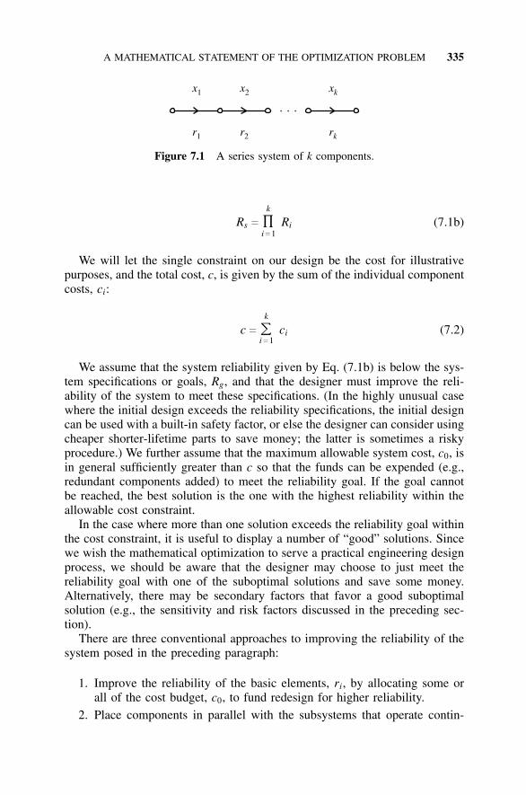
A MATHEMATICAL STATEMENT OF THE OPTIMIZATION PROBLEM 335
r1
x1
r2
x2
rk
xk
Figure 7.1 A series system of k components.
Rs c
k
∏i c 1
Ri (7.1b)
We will let the single constraint on our design be the cost for illustrativepurposes, and the total cost, c, is given by the sum of the individual componentcosts, ci:
c c
k
���i c 1
ci (7.2)
We assume that the system reliability given by Eq. (7.1b) is below the sys-tem specifications or goals, Rg, and that the designer must improve the reli-ability of the system to meet these specifications. (In the highly unusual casewhere the initial design exceeds the reliability specifications, the initial designcan be used with a built-in safety factor, or else the designer can consider usingcheaper shorter-lifetime parts to save money; the latter is sometimes a riskyprocedure.) We further assume that the maximum allowable system cost, c0, isin general sufficiently greater than c so that the funds can be expended (e.g.,redundant components added) to meet the reliability goal. If the goal cannotbe reached, the best solution is the one with the highest reliability within theallowable cost constraint.
In the case where more than one solution exceeds the reliability goal withinthe cost constraint, it is useful to display a number of “good” solutions. Sincewe wish the mathematical optimization to serve a practical engineering designprocess, we should be aware that the designer may choose to just meet thereliability goal with one of the suboptimal solutions and save some money.Alternatively, there may be secondary factors that favor a good suboptimalsolution (e.g., the sensitivity and risk factors discussed in the preceding sec-tion).
There are three conventional approaches to improving the reliability of thesystem posed in the preceding paragraph:
1. Improve the reliability of the basic elements, ri, by allocating some orall of the cost budget, c0, to fund redesign for higher reliability.
2. Place components in parallel with the subsystems that operate contin-
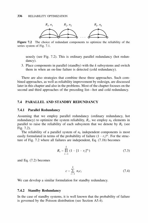
336 RELIABILITY OPTIMIZATION
R ,1 1n R ,2 2n R ,k kn
... ... ...
Figure 7.2 The choice of redundant components to optimize the reliability of theseries system of Fig. 7.1.
uously (see Fig. 7.2). This is ordinary parallel redundancy (hot redun-dancy).
3. Place components in parallel (standby) with the k subsystems and switchthem in when an on-line failure is detected (cold redundancy).
There are also strategies that combine these three approaches. Such com-bined approaches, as well as reliability improvement by redesign, are discussedlater in this chapter and also in the problems. Most of the chapter focuses on thesecond and third approaches of the preceding list—hot and cold redundancy.
7.4 PARALLEL AND STANDBY REDUNDANCY
7.4.1 Parallel Redundancy
Assuming that we employ parallel redundancy (ordinary redundancy, hotredundancy) to optimize the system reliability, Rs, we employ nk elements inparallel to raise the reliability of each subsystem that we denote by Rk (seeFig. 7.2).
The reliability of a parallel system of nk independent components is mosteasily formulated in terms of the probability of failure (1 − ri)ni . For the struc-ture of Fig. 7.2 where all failures are independent, Eq. (7.1b) becomes
Rs c
k
∏i c 1
(1 − [1 − ri]ni ) (7.3)
and Eq. (7.2) becomes
c c
k
���i c 1
nici (7.4)
We can develop a similar formulation for standby redundancy.
7.4.2 Standby Redundancy
In the case of standby systems, it is well known that the probability of failureis governed by the Poisson distribution (see Section A5.4).
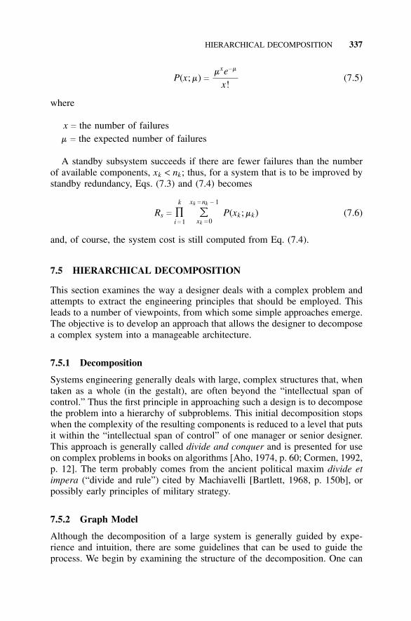
HIERARCHICAL DECOMPOSITION 337
P(x; m) cmxe−m
x!(7.5)
where
x c the number of failuresm c the expected number of failures
A standby subsystem succeeds if there are fewer failures than the numberof available components, xk < nk; thus, for a system that is to be improved bystandby redundancy, Eqs. (7.3) and (7.4) becomes
Rs c
k
∏i c 1
xk c nk − 1
���xk c 0
P(xk; mk) (7.6)
and, of course, the system cost is still computed from Eq. (7.4).
7.5 HIERARCHICAL DECOMPOSITION
This section examines the way a designer deals with a complex problem andattempts to extract the engineering principles that should be employed. Thisleads to a number of viewpoints, from which some simple approaches emerge.The objective is to develop an approach that allows the designer to decomposea complex system into a manageable architecture.
7.5.1 Decomposition
Systems engineering generally deals with large, complex structures that, whentaken as a whole (in the gestalt), are often beyond the “intellectual span ofcontrol.” Thus the first principle in approaching such a design is to decomposethe problem into a hierarchy of subproblems. This initial decomposition stopswhen the complexity of the resulting components is reduced to a level that putsit within the “intellectual span of control” of one manager or senior designer.This approach is generally called divide and conquer and is presented for useon complex problems in books on algorithms [Aho, 1974, p. 60; Cormen, 1992,p. 12]. The term probably comes from the ancient political maxim divide etimpera (“divide and rule”) cited by Machiavelli [Bartlett, 1968, p. 150b], orpossibly early principles of military strategy.
7.5.2 Graph Model
Although the decomposition of a large system is generally guided by expe-rience and intuition, there are some guidelines that can be used to guide theprocess. We begin by examining the structure of the decomposition. One can
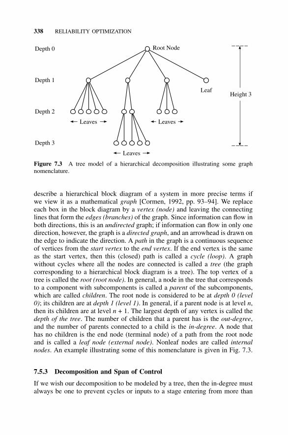
338 RELIABILITY OPTIMIZATION
Leaves
Leaves
Leaves
LeafHeight 3
Depth 0
Depth 1
Depth 2
Depth 3
Root Node
Figure 7.3 A tree model of a hierarchical decomposition illustrating some graphnomenclature.
describe a hierarchical block diagram of a system in more precise terms ifwe view it as a mathematical graph [Cormen, 1992, pp. 93–94]. We replaceeach box in the block diagram by a vertex (node) and leaving the connectinglines that form the edges (branches) of the graph. Since information can flow inboth directions, this is an undirected graph; if information can flow in only onedirection, however, the graph is a directed graph, and an arrowhead is drawn onthe edge to indicate the direction. A path in the graph is a continuous sequenceof vertices from the start vertex to the end vertex. If the end vertex is the sameas the start vertex, then this (closed) path is called a cycle (loop). A graphwithout cycles where all the nodes are connected is called a tree (the graphcorresponding to a hierarchical block diagram is a tree). The top vertex of atree is called the root (root node). In general, a node in the tree that correspondsto a component with subcomponents is called a parent of the subcomponents,which are called children. The root node is considered to be at depth 0 (level0); its children are at depth 1 (level 1). In general, if a parent node is at level n,then its children are at level n + 1. The largest depth of any vertex is called thedepth of the tree. The number of children that a parent has is the out-degree,and the number of parents connected to a child is the in-degree. A node thathas no children is the end node (terminal node) of a path from the root nodeand is called a leaf node (external node). Nonleaf nodes are called internalnodes. An example illustrating some of this nomenclature is given in Fig. 7.3.
7.5.3 Decomposition and Span of Control
If we wish our decomposition to be modeled by a tree, then the in-degree mustalways be one to prevent cycles or inputs to a stage entering from more than
HIERARCHICAL DECOMPOSITION 339
one stage. Sometimes, however, it is necessary to have more than one inputto a node, in which case one must worry about synchronization and couplingbetween the various nodes. Thus, if node x has inputs from nodes p and q,then any change in either p or q will affect node x. Imposing this restrictionon our hierarchical decomposition leads to simplicity in the interfacing of thevarious system elements.
We now discuss the appropriate size of the out-degree. If we wish to decom-pose the system, then the minimum size of the out-degree at each node mustbe two, although this will result in a tree of great height. Of course, if any nodehas a great number of children (a large out-degree), we begin to strain the intel-lectual span of control. The experimental psychologist Miller [1956] studied alarge number of experiments related to sensory perception and concluded thathumans can process about 5–9 levels of “complexity.” (A discussion of howMiller’s numbers relate to the number of mental discriminations that one canmake appears in Shooman [1983, pp. 194, 195].) If we specify the out-degreeto be seven for each node and all the leaves (terminal nodes) to be at level(depth) h, then the number of leaves at level h (NLh) is given by
NLh c 7h (7.7)
In practice, each leaf is the lowest level of replaceable unit, which is gen-erally called a line replaceable unit (LRU). In the case of software, we wouldprobably call the analog of an LRU a module or an object. The total numberof nodes, N, in the graph can be computed if we assume that all the leavesappear at level h.
N c NL0 + NL1 + NL2 + · · · + NLh (7.8a)
If each parent node has seven children, Eq. (7.8a) becomes
N c 1 + 7 + 72 + · · · + 7h (7.8b)
Using the formula for the sum of the terms in a geometric progression,
N c a(rn− 1)/ (r − 1) (7.9a)
where
r c
n c
a c
the common ratio (in our case, 7)the number of terms (in our case, h + 1)the first term (in our case, 1)
Substitution in Eq. (7.9a) yields
N c (7h + 1− 1)/ 6 (7.9b)
If h c 2, we have N c (73− 1)/ 6 c 57. We can check this by substitution in
Eq. (7.8b), yielding 1 + 7 + 49 c 57.
340 RELIABILITY OPTIMIZATION
7.5.4 Interface and Computation Structures
Another way of viewing a decomposition structure is to think in terms of twoclasses of structures, interfaces, and computational elements—a breakdownthat applies to either hardware or software. In the case of hardware, the com-putational elements are LRUs; for software, they are modules or classes. Inthe case of hardware, the interfaces are analog or digital signals (electrical,light, sound) passed from one element (depth, level) to another; the joining ofmechanical surfaces, hydraulics or pneumatic fluids; or similar physical phe-nomena. In the case of software, the interfaces are generally messages, vari-ables, or parameters passed between procedures or objects. Both hardware andsoftware have errors (failure rates, reliability) associated with either the com-putational elements or the interfaces. If we again assume that leaves appearonly at the lowest level of the tree, the number of computational elementsis given by the last term in Eq. (7.8a), NLh. In counting interfaces, there isthe interface out of an element at level i and the interface to the correspond-ing element at level i + 1. In electrical terms, we might call this the outputimpedance and the corresponding input impedance. In the case of software,we would probably be talking about the passing of parameters and their scopebetween a procedure call and the procedure that is called, or else the passingof messages between classes and objects. For both hardware and software, wecount the interface (information-out–information-in) pair as a single interface.Thus all modules except level 0 have a single associated interface pair. Thereis no structural interface at level 0; however, let us consider the system specifi-cations as a single interface at level 0. Thus, we can use Eqs. (7.8) and (7.9) tocount the number of interfaces, which is equivalent to the number of elements.Continuing the foregoing example where h c 2, we have 72
c 49 computationalelements and (73
− 1)/ 6 c 57 interfaces. Of course, in a practical example, notall the leaves will appear at depth (level) h, since some of the paths will ter-minate before level h; thus the preceding computations and formulas can onlybe considered upper bounds on an actual (less-idealized) problem.
One can use these formulas for many interfaces and computational units toconjecture models for complexity, errors, reliability, and cost.
7.5.5 System and Subsystem Reliabilities
The structure of the system at level 1 in the graph model of the hierarchicaldecomposition is a group of subsystems equal in number to the out-degree ofthe root node. Based on Miller’s work, we have decided to let the out-degreebe 7 (or 5 to 9). As an example, let us consider an overview of an air trafficcontrol (ATC) system for an airport [Gilbert, 1973, p. 39, Fig. 61]. Level 0 inour decomposition is the “air traffic control system.” At level 1, we have themajor subsystems that are given in Table 7.1.
An expert designer of a new ATC system might view things a little dif-ferently (in fact, two expert designers working for different companies might
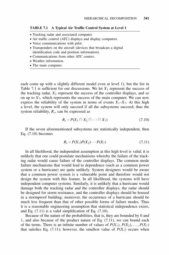
HIERARCHICAL DECOMPOSITION 341
TABLE 7.1 A Typical Air Traffic Control System at Level 1
• Tracking radar and associated computer.• Air traffic control (ATC) displays and display computers.• Voice communications with pilot.• Transponders on the aircraft (devices that broadcast a digital
identification code and position information).• Communications from other ATC centers.• Weather information.• The main computer.
each come up with a slightly different model even at level 1), but the list inTable 7.1 is sufficient for our discussions. We let X1 represent the success ofthe tracking radar, X2 represent the success of the controller displays, and soon up to X7, which represents the success of the main computer. We can nowexpress the reliability of the system in terms of events X1–X7. At this higha level, the system will only succeed if all the subsystems succeed; thus thesystem reliability, Rs, can be expressed as
Rs c P(X1U
X2U
· · ·U
X7) (7.10)
If the seven aforementioned subsystems are statistically independent, thenEq. (7.10) becomes
Rs c P(X1)P(X2) · · · P(X7) (7.11)
In all likelihood, the independent assumption at this high level is valid; it isunlikely that one could postulate mechanisms whereby the failure of the track-ing radar would cause failure of the controller displays. The common modefailure mechanisms that would lead to dependence (such as a common powersystem or a hurricane) are quite unlikely. System designers would be awarethat a common power system is a vulnerable point and therefore would notdesign the system with this feature. In all likelihood, the systems will haveindependent computer systems. Similarly, it is unlikely that a hurricane woulddamage both the tracking radar and the controller displays; the radar shouldbe designed for storm resistance, and the controller displays should be housedin a stormproof building; moreover, the occurrence of a hurricane should bemuch less frequent than that of other possible forms of failure modes. Thusit is a reasonable engineering assumption that statistical independence exists,and Eq. (7.11) is a valid simplification of Eq. (7.10).
Because of the nature of the probabilities, that is, they are bounded by 0 and1, and also because of the product nature of Eq. (7.11), we can bound eachof the terms. There is an infinite number of values of P(X1), P(X2), . . . , P(X7)that satisfies Eq. (7.11); however, the smallest value of P(X1) occurs when
342 RELIABILITY OPTIMIZATION
P(X2), . . . , P(X7) assume their largest values—that is, unity. We can repeat thissolution for each of the subsystems to yield a set of minimum values.
P(X1) ≥ Rs (7.12a)
P(X2) ≥ Rs (7.12b)
and so on up to
P(X7) ≥ Rs (7.12c)
These minimum bounds are true in general for any subsystem if the systemstructure is series; thus we can write
P(Xi) ≥ Rs (7.13)
The equality only holds in Eqs. (7.12) and (7.13) if all the other subsystemshave a reliability equal to unity (i.e., they never fail); thus, in the real world, theequality conditions can be deleted. These minimum bounds will play a largerole in the optimization technique developed later in this chapter.
7.6 APPORTIONMENT
As was discussed in the previous section, one of the first tasks in approachingthe design of a large, complex system is to decompose it. Another early taskis to establish reliability allocations or budgets for the various subsystems thatemerge during the decomposition, a process often referred to as apportionmentor allocation. At this point, we must discuss the difference between a math-ematician’s and an engineer’s approach to optimization. The mathematicianwould ask for a precise system model down to the LRU level, the failure rate,and cost, weight, volume, etc., of each LRU; then, the mathematician invokesan optimization procedure to achieve the exact optimization. The engineer, onthe other hand, knows that this is too complex to calculate and understand inmost cases and therefore seeks an alternate approach. Furthermore, the engi-neer knows that many of the details of lower-level LRUs will not be knownuntil much later and that estimates of their failure rates at that point would berather vague, so he or she adopts a much simpler design approach: beginning atop–down process to apportion the reliability goal among the major subsystemsat depth 1.
Apportionment has historically been recognized as an important reliabilitysystem goal [AGREE Report, 1957, pp. 52–57; Henney, 1956, Chapter 1; VonAlven, 1964, Chapter 6]; many of the methods discussed in this section arean outgrowth of this early work. We continue to assume that there are about7 subsystems at depth 1. Our problem is how to allocate the reliability goalamong the subsystems, for which several procedures exist on which to basesuch an allocation early in the design process; these are listed in Table 7.2.
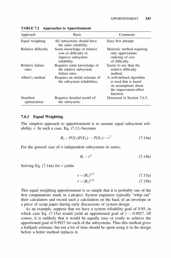
APPORTIONMENT 343
TABLE 7.2 Approaches to Apportionment
Approach Basis Comments
Equal weighting All subsystems should have Easy first attempt.the same reliability.
Relative difficulty Some knowledge of relative Heuristic method requiringcost or difficulty to only approximateimprove subsystem ordering of costreliability. of difficulty.
Relative failure Requires some knowledge of Easier to use than therates the relative subsystem relative difficulty
failure rates. method.Albert’s method Requires an initial estimate of A well-defined algorithm
the subsystem reliabilities. is used that is basedon assumptions aboutthe improvment-effortfunction.
Stratified Requires detailed model of Discussed in Section 7.6.5.optimization the subsystem.
7.6.1 Equal Weighting
The simplest approach to apportionment is to assume equal subsystem reli-ability, r. In such a case, Eq. (7.11) becomes
Rs c P(X1)P(X2) · · · P(X7) c r7 (7.14a)
For the general case of n independent subsystems in series,
Rs c rn (7.14b)
Solving Eq. (7.14a) for r yields
r c (Rs)1/ 7 (7.15a)
r c (Rs)1/ n (7.15b)
This equal weighting apportionment is so simple that it is probably one of thefirst computations made in a project. System engineers typically “whip out”their calculators and record such a calculation on the back of an envelope ora piece of scrap paper during early discussions of system design.
As an example, suppose that we have a system reliability goal of 0.95, inwhich case Eq. (7.15a) would yield an apportioned goal of r c 0.9927. Ofcourse, it is unlikely that it would be equally easy or costly to achieve theapportioned goal of 0.9927 for each of the subsystems. Thus this method givesa ballpark estimate, but not a lot of time should be spent using it in the designbefore a better method replaces it.
344 RELIABILITY OPTIMIZATION
7.6.2 Relative Difficulty
Suppose that we have some knowledge of the subsystems and can use it inthe apportionment process. Assume that we are at level 1, that we have sevensubsystems to deal with, and that we know for three of the subsystems achiev-ing a high level of reliability (e.g., the level required for equal apportionment)will be difficult. We envision that these three systems could meet their goals ifthey can be realized by two parallel elements. We then would have reliabilityexpressions similar to those of Eq. (7.14b) for the four “easier” systems anda reliability expression 2r − r2 for the three “harder systems.” The resultantexpression is
Rs c r4(2r − r2)3 (7.16)
Solving Eq. (7.16) numerically for a system goal of 0.95 yields r c 0.9874.Thus the four “easier” subsystems would have a single system with a reliabil-ity of 0.9874, and the three harder systems would have two parallel systemswith the same reliability. Another solution is to keep the goal of r c 0.9927,calculated previously for the easier subsystems. Then, the three harder systemswould have to meet the goal of 0.95/ 0.99274 c 0.9783. The three harder sys-tems would have to meet a somewhat lower goal: (2r − r2)3
c 0.9783, or r c
0.953. Other similar solutions can easily be obtained.The previous paragraph dealt with unequal apportionments by considering
a parallel system for the three harder systems. If we assume that parallel sys-tems are not possible at this level, we must choose a solution where the easiersystems exceed a reliability of 0.9927 so that the harder systems can have asmaller reliability. For convenience, we could rewrite Eq. (7.11) in terms ofunreliabilities, ri c 1 − ui, obtaining
Rs c (1 − u1)(1 − u2) · · · (1 − u7) (7.17a)
Again, suppose there are four easier systems with a failure probability ofu1 c u2 c u3 c u4 c u. The harder systems will have twice the failure proba-bility u5 c u6 c 2u, and Eq. (7.17a) becomes
Rs c (1 − u)4(1 − 2u)3
that yields a 7th-order polynomial.The easiest way to solve the polynomial is through trial and error with a
calculator or by writing a simple program loop to calculate a range of values.The equal reliability solution was r c 0.9927 c 1 − 0.0073. If we try reasy c
0.995 c 1 − 0.005, rhard c 0.99 c 1 − 0.01, and substitute in Eq. (7.17a), theresult is
0.951038 c (0.995)4(0.99)3 (7.17b)
APPORTIONMENT 345
Trying some slightly larger values of u results in a solution of
0.950079 c (0.9949)4(0.9898)3 (7.17c)
The accuracy of this method depends largely on how realistic the guesses areregarding the hard and easy systems. The method of the next section is similar,but the calculations are easier.
7.6.3 Relative Failure Rates
It is simpler to use knowledge about easier and harder systems during appor-tionment if we work with failure rates. We assume that each subsystem has aconstant-failure rate li and that the reliability for each subsystem is given by
ri c e−li (7.18a)
and substitution of Eq. (7.18a) into Eq. (7.11) yields
Rs c P(X1)P(X2) · · · P(X7) c e−l1 e−l2 · · · e−l7 (7.18b)
and Eq. (7.18b) can be written as
Rs c e−ls (7.19)
where
ls c l1 + l2 + · · · + l7
Continuing with our example of the previous section, in which the goal is0.95, the four “easier” systems have a failure rate of l, and the three harderones have a failure rate of 5l, Eq. (7.19) becomes
Rs c 0.95 c e−19l t (7.20)
Solving for l t, we obtain l t c 0.0026996, and the reliabilities are e−0.0026996
c 0.9973, and e−5 × 0.0026996c 0.9865. Thus our apportioned goals for the four
easier systems are 0.9973; for the three harder systems, 0.9865. As a check,we see that 0.99734 × 0.98653
c 0.9497. Clearly, one can use this procedureto achieve other allocations based on some relative knowledge of the nomi-nal failure rates of the various subsystems or on how difficult it is to achievevarious failure rates.
7.6.4 Albert’s Method
A very interesting method that results in an algorithm rather than a designprocedure is known as Albert’s method and is based on some analytical prin-
346 RELIABILITY OPTIMIZATION
ciples [Albert, 1958; Lloyd, 1977, pp. 267–271]. The procedure assumes thatinitially there are some estimates of what reliabilities can be achieved for thesubsystems to be apportioned. In terms of our notation, we will say that P(X1),P(X2), . . . , P(X7) are given by some nominal values: R1, R2, . . . , R7. Note thatwe continue to speak of seven subsystems at level 1; however, this clearly canbe applied to any number of subsystems. The fact that we assume nominalvalues for the Ri implies that we have a preliminary design. However, in anylarge system there are many iterations in system design, and this method isquite useful even if it is not the first one attempted. Adopting the terminologyof government contracting (which generally has parallels in the commercialworld), we might say that the methods of Sections 7.6.1–7.6.3 are useful in for-mulating the request for proposal (RFQ) (the requirements) and that Albert’smethod is useful during the proposal preparation phase (specifications and pro-posed design) and during the early design phases after the contract award. Aproperly prepared proposal will have some early estimates of the subsystemreliabilities. Furthermore, we assume that the system specification or goal isdenoted by Rg, and the preliminary estimates of the subsystem reliabilities yielda system reliability estimate given by
Rs c R1R2 · · · R7 (7.21)
If the design team is lucky, Rs > Rg, and the first concerns about reliabilityare thus satisfied. In fact, one might even think about trading off some reli-ability for reduced cost. An experienced designer would tell us that this almostnever happens and that we are dealing with the situation where Rs < Rg. Thismeans that one or more of the Ri values must be increased. Albert’s methoddeals with finding which of the subsystem reliability goals must be increasedand by how much so that Rs is increased to the point where Rs c Rg.
Based on the bounds developed in Eq. (7.13), we can comment that any sub-system reliability that is less than the system goal, Ri < Rg, must be increased(others may also need to be increased). For convenience in developing ouralgorithm, we assume that the subsystems have been renumbered so that thereliabilities are in ascending order: R1 < R2 < · · · < R7. Thus, in the specialcase where R7 < Rg, all the subsystem goals must be increased. In this case,Albert’s method reduces to equal apportionment and Eqs. (7.14) and (7.15)hold. In the more general case, j of the i subsystems must have the reliabilityincreased. Albert’s method requires that all the j subsystems have their reli-ability increased to the same value, r, and that the reliabilities of the (i − j )subsystems remain unchanged. Thus, Eq. (7.21) becomes
Rg c R1R2 · · · RjRj + 1 · · · R7 (7.22)
where
R1 c R2 c · · · c Rj c r (7.23)
APPORTIONMENT 347
Substitution of Eq. (7.23) into Eq. (7.22) yields
Rg c (r j)(Rj + 1 · · · R7) (7.24)
We solve Eq. (7.24) for the value of r (or, more generally, ri):
r jc Rg/ (Rj + 1 · · · R7) (7.25a)
r c (Rg/ [Rj + 1 · · · R7])1/ j (7.25b)
Equations (7.22)–(7.25) describe Albert’s method, but an important stepmust still be discussed: how to determine the value of j. Again, we turn toEq. (7.13) to shed some light on this question. We can place a lower boundon j and say that all the subsystems having reliabilities smaller than or equalto the goal, Ri < Rg, must be increased. It is possible that if we choose j equalto this lower bound and substitute into Eq. (7.25b), the computed value ofr will be >1, which is clearly impossible; thus we must increase j by 1 andtry again. This process is repeated until the values of r obtained are <1. Wenow have a feasible value for j, but we may be requiring too much “effort” toraise all the 1 through j subsystems to the resulting high value of r. It may bebetter to increment j by 1 (or more), reducing the value of r and “spreading”this value over more subsystems. Albert showed that based on certain effortassumptions, the optimum value of j is bounded from above when the valuefor r first decreases to the point where r < Rj . The optimum value of j is theprevious value of j, where r > Rj . More succinctly, the optimum value for j isthe largest value for j, where r > Rj . Clearly it is not too hard to formulate acomputer program for this algorithm; however, since we are assuming aboutseven systems and have bounded j from below and above, the most efficientsolution is probably done with paper, pencil, and a scientific calculator.
The reader may wonder why we have spent quite a bit of time explain-ing Albert’s method rather than just stating it. The original exposition of themethod is somewhat terse, and the notation may be confusing to some; thus theenhanced development is warranted. The remainder of this section is devotedto an example and a discussion of when this method is “optimum.” The readerwill note that some of the underlying philosophy behind the method can besummarized by the following principle: “The most efficient way to improvethe reliability of a series structure (sometimes called a chain) is by improvingthe weakest links in the chain.” This principle will surface a few more timesin later portions of this chapter.
A simple example should clarify the procedure. Suppose that we have foursubsystems with initial reliabilities R1 c 0.7, R2 c 0.8, R3 c 0.9, and R4 c 0.95,and the system reliability goal is Rg c 0.8. The existing estimates predict asystem reliability of Rs c 0.7 × 0.8 × 0.9 × 0.95 c 0.4788. Clearly, some or allof the subsystem goals must be raised for us to meet the system goal. Based onEq. (7.13), we know that we must improve subsystems 1 and 2, so we begin
348 RELIABILITY OPTIMIZATION
our calculations at this point. The system reliability goal, Rg c 0.8, and Eq.(7.25b) yields
r c (Rg/ [Rj + 1 · · · R7])1/ jc (0.8/ 0.9 × 0.95)1/ 2
c (0.93567)0.5c 0.96730 (7.26)
Since 0.96730 > 0.9, we continue our calculation. We now recompute forsubsystems 1, 2, and 3, and Eq. (7.25b) yields
r c (0.8/ 0.95)1/ 3c 0.9443 (7.27)
Now, 0.9443 < 0.95, and we choose the previous value of j c 2 as our optimum.As a check, we now compute the system reliability.
0.96730 × 0.96730 × 0.9 × 0.95 c 0.7999972 c Rg
which equals our goal of 0.8 when rounded to one place. Thus, the conclusionfrom the use of Albert’s method is that the apportionment goals for the foursystems are R1 c R2 c 0.96730; R3 c 0.90; and R4 c 0.95. This solution assumesequal effort for improving the reliability of all subsystems.
The use of Albert’s method produces an optimum allocation policy if thefollowing assumptions hold [Albert, 1958; Lloyd, 1977, pp. 267–271]:
1. Each subsystem has the same effort function that governs the amount ofeffort required to raise the reliability of the i th subsystem from Ri to ri.This effort function is denoted by G(Ri, ri), and increased effort alwaysincreases the reliability: G(Ri, ri) ≥ 0.
2. The effort function G(x, y) is nondecreasing in y for fixed x, that is, givenan initial value of Ri, it will always require more effort to increase ri toa higher value. For example,
G(0.35, 0.65) ≤ G(0.35, 0.75)
The effort function G(x, y) is nonincreasing in x for fixed y, that is, givenan increase to ri, it will always require less effort if we start from a largervalue of Ri. For example,
G(0.25, 0.65) ≥ G(0.35, 0.65)
3. If x ≤ y ≤ z, then G(x, y) + G(y, z) c G(x, z). This is a superposition(linearity) assumption that states that if we increase the reliability in twosteps, the sum of the efforts for each step is the same as if we did theincrease in a single step.
4. G(0, x) has a derivative h(x) such that xh(x) is strictly increasing in (0 <x < 1).
APPORTIONMENT 349
The proof of the algorithm is given in Albert [1958]. If the assumptionsof Albert’s method are not met, the equal effort rule is probably violated, forwhich the methods of Sections 7.6.2 and 7.6.3 are suggested.
7.6.5 Stratified Optimization
In a very large system, we might consider continuing the optimization to level2 by applying apportionment again to each of the subsystem goals. In fact,we can continue this process until we reach the LRU level and then utilizeEqs. (7.3) or (7.6) (or else improve the LRU reliability) to achieve our systemdesign. Such decisions require some intuition and design experience on thepart of the system engineers; however, the foregoing methods provide someengineering calculations to help guide intuition.
7.6.6 Availability Apportionment
Up until now, the discussion of apportionment has dealt entirely with systemand subsystem reliabilities. Now, we discuss the question of how to proceedif system availabilities are to be apportioned. Under certain circumstances, thesubsystem availabilities are essentially independent, and the system availabil-ity is given by the same formula as for the reliabilities, with the availabili-ties replacing the reliabilties. A discussion of availability modeling in general,and a detailed discussion of the circumstances under which such substitutionsare valid appears in Shooman [1990, Appendices F]. One situation in whichthe availabilities are independent is where each subsystem has its own repair-man (or repaircrew). This is called repairman decoupling in Shooman [1990,Appendices F-4 and F-5]. In the decoupled case, one can use the same sys-tem structural model that is constructed for reliability analysis to compute sys-tem availability. The steady-state availability probabilities are substituted in themodel just as the reliability probabilities would be. Clearly, this is a convenientsituation and is often, but not always, approximately valid.
Suppose, however, that the same repairman or repaircrew serves one or moresubsystems. In such a case, there is the possibility that a failure will occur insubsystem y while the repairman is still busy working on a repair for subsystemx. In such a case, a queue of repair requests develops. The queuing phenomenaresult in dependent coupled subsystems that can be denoted as being repair-man coupling. When repairman coupling is significant, one should formulate aMarkov model to solve for the resulting availability. Since Markov modelingfor a large subsystem can be complicated, as the reader can appreciate fromthe analytical solutions of Chapter 3, a practical designer would be happy touse a decoupled solution even if the results were only a good approximation.
Intuition tells us that the possibility of a queue forming is a function of theratio of repair rate to failure rate (l/m). If the repair rate is much larger than thefailure rate, the approximation should be quite satisfactory. These approxima-tions were explored extensively in Section 4.9.3, and the reader should review
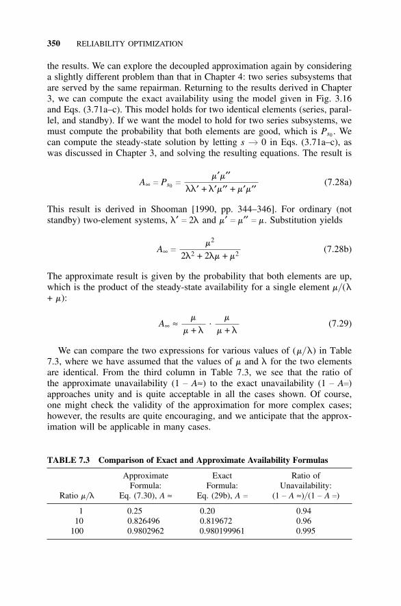
350 RELIABILITY OPTIMIZATION
the results. We can explore the decoupled approximation again by consideringa slightly different problem than that in Chapter 4: two series subsystems thatare served by the same repairman. Returning to the results derived in Chapter3, we can compute the exact availability using the model given in Fig. 3.16and Eqs. (3.71a–c). This model holds for two identical elements (series, paral-lel, and standby). If we want the model to hold for two series subsystems, wemust compute the probability that both elements are good, which is Ps0 . Wecan compute the steady-state solution by letting s b 0 in Eqs. (3.71a–c), aswas discussed in Chapter 3, and solving the resulting equations. The result is
A∞ c Ps0 cm′m′′
ll′ + l′m′′ + m′m′′(7.28a)
This result is derived in Shooman [1990, pp. 344–346]. For ordinary (notstandby) two-element systems, l′ c 2l and m′ c m′′ c m. Substitution yields
A∞ cm2
2l2 + 2lm + m2(7.28b)
The approximate result is given by the probability that both elements are up,which is the product of the steady-state availability for a single element m/ (l+ m):
A∞ ≈m
m + l. m
m + l(7.29)
We can compare the two expressions for various values of (m/ l) in Table7.3, where we have assumed that the values of m and l for the two elementsare identical. From the third column in Table 7.3, we see that the ratio ofthe approximate unavailability (1 − A≈) to the exact unavailability (1 − Ac)approaches unity and is quite acceptable in all the cases shown. Of course,one might check the validity of the approximation for more complex cases;however, the results are quite encouraging, and we anticipate that the approx-imation will be applicable in many cases.
TABLE 7.3 Comparison of Exact and Approximate Availability Formulas
Approximate Exact Ratio ofFormula: Formula: Unavailability:
Ratio m/l Eq. (7.30), A ≈ Eq. (29b), A c (1 − A ≈)/ (1 − A c)
1 0.25 0.20 0.9410 0.826496 0.819672 0.96
100 0.9802962 0.980199961 0.995
OPTIMIZATION AT THE SUBSYSTEM LEVEL VIA ENUMERATION 351
7.6.7 Nonconstant-Failure Rates
In many cases, the apportionment approaches discussed previously depend onconstant-failure rates (see especially Table 7.2, third row). If the failure ratesvary with time, it is possible that the optimization results will hold only overa certain time range and therefore must be recomputed for other ranges. Theanalyst should consider this approach if nonconstant-failure rates are signifi-cant. In most cases, detailed information on nonconstant-failure rates will notbe available until late in design, and approximate methods using upper andlower bounds on failure rates or computations for different ranges assuminglinear variation will be adequate.
7.7 OPTIMIZATION AT THE SUBSYSTEM LEVEL VIAENUMERATION
7.7.1 Introduction
In the previous section, we introduced apportionment as an approximate opti-mization procedure at the system level. Now, we assume that we are at thesubsystem level. At this point, we assume that each subsystem is at a levelwhere we can speak of subsystem redundancy and where we can now con-sider exact optimization. (It is possible that in some smaller problems, the useof apportionment at the system level as a precursor is not necessary and we canbegin exact optimization at this level. Also, it is possible that we are dealingwith a system that is so complex that we have to apportion the subsystems intosub-subsystems—or even lower—before we can speak of redundant elements.)In all cases, we view apportionment as an approximate optimization process,which may or may not come first.
The subject of system optimization has been extensively discussed in the reli-ability literature [Barlow, 1965, 1975; Bellman, 1958; Messinger, 1970; Myers,1964; Tillman, 1980] and also in more general terms [Aho, 1974; Bellman, 1957;Bierman, 1969; Cormen, 1992; Hiller, 1974]. The approach used was gener-ally dynamic programming or greedy methods; these approaches will be brieflyreviewed later in this chapter. This section will discuss a bounded enumerationapproach [Shooman and Marshall, 1993] that the author proposes as the simplestand most practical method for redundancy optimization. We begin our develop-ment by defining the brute force approach of exhaustive enumeration.
7.7.2 Exhaustive Enumeration
This approach is straightforward, but it represents a brute force approach tothe problem. Suppose we have subsystem i that has five elements and we wishto improve the subsystem reliabiity to meet the apportioned subsystem goalRg. If practical considerations of cost, weight, or volume limit us to choosingat most a single parallel subsystem for each of the five elements, each of the
352 RELIABILITY OPTIMIZATION
five subsystems has zero or one element in parallel, and the total number ofpossibilities is 25
c 32. Given the powerful computational power of a modernpersonal computer, one could certainly write a computer program and evaluateall 32 possibilities in a short period of time. The designer would then choosethe combination with the highest reliability or some other combination of goodproperties and use the complete set of possibilities as the basis of design. Aspreviously stated, sometimes a close suboptimum solution is preferred becauseof risk, uncertainty, sensitivity, or other factors. Suppose we could consider atmost two parallel subsystems for each of the five elements, in which case thetotal number of possibilities is 35
c 243. This begins to approach an unwieldynumber for computation and interpretation.
The actual number of computations involved in exhaustive enumeration ismuch larger if we do not impose a restriction such as “considering at most twoparallel subsystems for each of the five elements.” To illustrate, we considerthe following two examples [Shooman, 1994]:
Example 1: The initial design of a system yields 3 subsystems at the first levelof decomposition. The system reliability goal, Rg, is 0.9 for a given numberof operating hours. The initial estimates of the subsystem reliabilities are R1 c
0.85, R2 c 0.5, and R3 c 0.3. Parallel redundancy is to be used to improve theinitial design so that it meets the reliability goal. The constraint is cost; eachsubsystem is assumed to cost 1 unit, and the total cost budget is 16 units.
The existing estimates predict an initial system reliability of Rs0 c 0.85 × 0.5× 0.3 c 0.1275. Clearly, some or all of the subsystem reliabilities must be raisedfor us to meet the system goal. Lacking further analysis, we can state that theinitial system costs 3 units and that 13 units are left for redundancy. Thus wecan allocate 0 or 1 or 2 or any number up to 13 parallel units to subsystem 1, asimilar number to subsystem 2, and a similar number to subsystem 3. An upperbound on the number of states that must be considered would therefore be 143
c 2,744. Not all of these states are possible because some of them violate theweight constraint; for example, the combination of 13 parallel units for eachof the 3 subsystems costs 39 units, which is clearly in excess of the 13-unitbudget. However, even the actual number will be too cumbersome if not toocostly in computer time to deal with. In the next section, we will show that byusing the bounded enumeration technique, only 10 cases must be considered!
Example 2: The initial design of a system yields 5 subsystems at the first levelof decomposition. The system reliability goal, Rg, is 0.95 for a given numberof operating hours. The initial estimates of the subsystem reliabilities are R1
c 0.8, R2 c 0.8, R3 c 0.8, R4 c 0.9, and R5 c 0.9. Parallel redundancy is tobe used to improve the initial design so that it meets the reliability goal. Theconstraint is cost; the subsystems are assumed to cost 2, 2, 2, 3, and 3 units,respectively, and the total cost budget is 36 units.
The existing estimates predict an initial system reliability of Rs0 c 0.83× 0.92
c 0.41472. Clearly, some or all of the subsystem reliabilities must be raised
BOUNDED ENUMERATION APPROACH 353
for us to meet the system goal. Lacking further analysis, we can state that theinitial system costs 12 units; thus we can allocate up to 24 cost units to each ofthe subsystems. For subsystems 1, 2, and 3, we can allocate 0 or 1 or 2 or anynumber up to 12 parallel units. For subsystems 4 and 5, we can allocate 0 or 1or 2 or any number up to 8 parallel units. Thus an upper bound on the numberof states that must be considered would be 133 × 92
c 177,957. Not all of thesestates are possible because some of them violate the cost constraint. In the nextsection, we will show that by using the bounded enumeration technique, only31 cases must be considered!
Now, we begin our discussion of the significant and simple method of opti-mization that results when we apply bounds to constrain the enumeration pro-cess.
7.8 BOUNDED ENUMERATION APPROACH
7.8.1 Introduction
An analyst is often so charmed by the neatness and beauty of a closed-formsynthesis process that they overlook the utility of an enumeration procedure.Engineering design is inherently a trial-and-error iterative procedure, and sel-dom are the parameters known so well that an analyst can stand behind a designand defend it as the true optimum solution to the problem. In fact, presentinga designer with a group of good designs rather than a single one is generallypreferable since there may be many ancillary issues to consider in making achoice. Some of these issues are the following:
• Sensitivity to variations in the parameters that are only approximatelyknown.
• Risk of success for certain state-of-the-art components presently underdesign or contemplated.
• Preferences on the part of the customer. (The old cliche about the “GoldenRule”—he who has the gold makes the rules—really does apply.)
• Conflicts between designs that yield high reliability but only moderateavailability (because of repairability problems), and the converse.
• Effect of maintenance costs on the chosen solution.• Difficulty in mathematically including multiple prioritized constraints
(some independent multiple constraints are easy to deal with; these arediscussed below).
Of course, the main argument against generating a family of designs andchoosing among them is the effort and confusion involved in obtaining such afamily. The prediction of the number of cases needed for direct enumeration inthe two simple examples discussed previously are not encouraging. However,
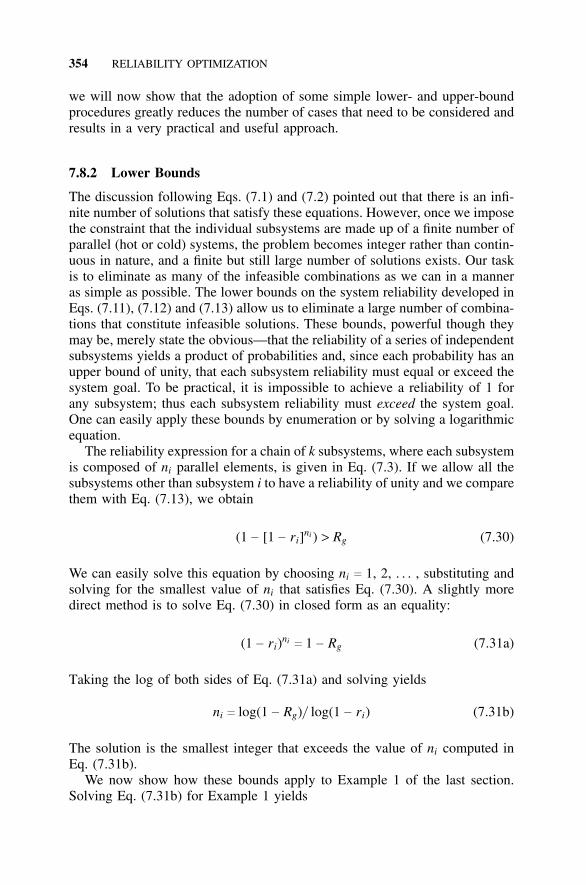
354 RELIABILITY OPTIMIZATION
we will now show that the adoption of some simple lower- and upper-boundprocedures greatly reduces the number of cases that need to be considered andresults in a very practical and useful approach.
7.8.2 Lower Bounds
The discussion following Eqs. (7.1) and (7.2) pointed out that there is an infi-nite number of solutions that satisfy these equations. However, once we imposethe constraint that the individual subsystems are made up of a finite number ofparallel (hot or cold) systems, the problem becomes integer rather than contin-uous in nature, and a finite but still large number of solutions exists. Our taskis to eliminate as many of the infeasible combinations as we can in a manneras simple as possible. The lower bounds on the system reliability developed inEqs. (7.11), (7.12) and (7.13) allow us to eliminate a large number of combina-tions that constitute infeasible solutions. These bounds, powerful though theymay be, merely state the obvious—that the reliability of a series of independentsubsystems yields a product of probabilities and, since each probability has anupper bound of unity, that each subsystem reliability must equal or exceed thesystem goal. To be practical, it is impossible to achieve a reliability of 1 forany subsystem; thus each subsystem reliability must exceed the system goal.One can easily apply these bounds by enumeration or by solving a logarithmicequation.
The reliability expression for a chain of k subsystems, where each subsystemis composed of ni parallel elements, is given in Eq. (7.3). If we allow all thesubsystems other than subsystem i to have a reliability of unity and we comparethem with Eq. (7.13), we obtain
(1 − [1 − ri]ni ) > Rg (7.30)
We can easily solve this equation by choosing ni c 1, 2, . . . , substituting andsolving for the smallest value of ni that satisfies Eq. (7.30). A slightly moredirect method is to solve Eq. (7.30) in closed form as an equality:
(1 − ri)nic 1 − Rg (7.31a)
Taking the log of both sides of Eq. (7.31a) and solving yields
ni c log(1 − Rg)/ log(1 − ri) (7.31b)
The solution is the smallest integer that exceeds the value of ni computed inEq. (7.31b).
We now show how these bounds apply to Example 1 of the last section.Solving Eq. (7.31b) for Example 1 yields
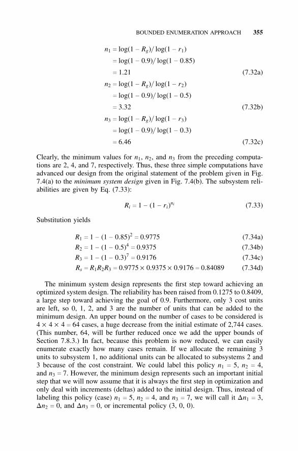
BOUNDED ENUMERATION APPROACH 355
n1 c log(1 − Rg)/ log(1 − r1)
c log(1 − 0.9)/ log(1 − 0.85)
c 1.21 (7.32a)
n2 c log(1 − Rg)/ log(1 − r2)
c log(1 − 0.9)/ log(1 − 0.5)
c 3.32 (7.32b)
n3 c log(1 − Rg)/ log(1 − r3)
c log(1 − 0.9)/ log(1 − 0.3)
c 6.46 (7.32c)
Clearly, the minimum values for n1, n2, and n3 from the preceding computa-tions are 2, 4, and 7, respectively. Thus, these three simple computations haveadvanced our design from the original statement of the problem given in Fig.7.4(a) to the minimum system design given in Fig. 7.4(b). The subsystem reli-abilities are given by Eq. (7.33):
Ri c 1 − (1 − ri)ni (7.33)
Substitution yields
R1 c 1 − (1 − 0.85)2c 0.9775 (7.34a)
R2 c 1 − (1 − 0.5)4c 0.9375 (7.34b)
R3 c 1 − (1 − 0.3)7c 0.9176 (7.34c)
Rs c R1R2R3 c 0.9775 × 0.9375 × 0.9176 c 0.84089 (7.34d)
The minimum system design represents the first step toward achieving anoptimized system design. The reliability has been raised from 0.1275 to 0.8409,a large step toward achieving the goal of 0.9. Furthermore, only 3 cost unitsare left, so 0, 1, 2, and 3 are the number of units that can be added to theminimum design. An upper bound on the number of cases to be considered is4 × 4 × 4 c 64 cases, a huge decrease from the initial estimate of 2,744 cases.(This number, 64, will be further reduced once we add the upper bounds ofSection 7.8.3.) In fact, because this problem is now reduced, we can easilyenumerate exactly how many cases remain. If we allocate the remaining 3units to subsystem 1, no additional units can be allocated to subsystems 2 and3 because of the cost constraint. We could label this policy n1 c 5, n2 c 4,and n3 c 7. However, the minimum design represents such an important initialstep that we will now assume that it is always the first step in optimization andonly deal with increments (deltas) added to the initial design. Thus, instead oflabeling this policy (case) n1 c 5, n2 c 4, and n3 c 7, we will call it Dn1 c 3,Dn2 c 0, and Dn3 c 0, or incremental policy (3, 0, 0).
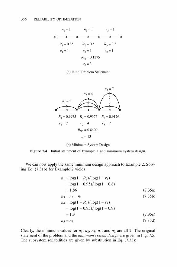
356 RELIABILITY OPTIMIZATION
n1 = 1
R1 = 0.85
Rs0= 0.1275
R2 = 0.5 R3 = 0.3
n2 = 1 n3 = 1
c2 = 1
cs = 3
c1 = 1 c3 = 1
(a) Initial Problem Statement
(b) Minimum System Design
R1 = 0.9975 R2 = 0.9375 R3 = 0.9176
Rsm = 0.8409
cs = 13
c1 = 2 c2 = 4 c3 = 7
n1 = 2
n2 = 4n3 = 7
.
.
.
.
Figure 7.4 Initial statement of Example 1 and minimum system design.
We can now apply the same minimum design approach to Example 2. Solv-ing Eq. (7.31b) for Example 2 yields
n1 c log(1 − Rg)/ log(1 − r1)
c log(1 − 0.95)/ log(1 − 0.8)
c 1.86 (7.35a)
n3 c n2 c n1 (7.35b)
n4 c log(1 − Rg)/ log(1 − r4)
c log(1 − 0.95)/ log(1 − 0.9)
c 1.3 (7.35c)
n5 c n4 (7.35d)
Clearly, the minimum values for n1, n2, n3, n4, and n5 are all 2. The originalstatement of the problem and the minimum system design are given in Fig. 7.5.The subsystem reliabilities are given by substitution in Eq. (7.33):
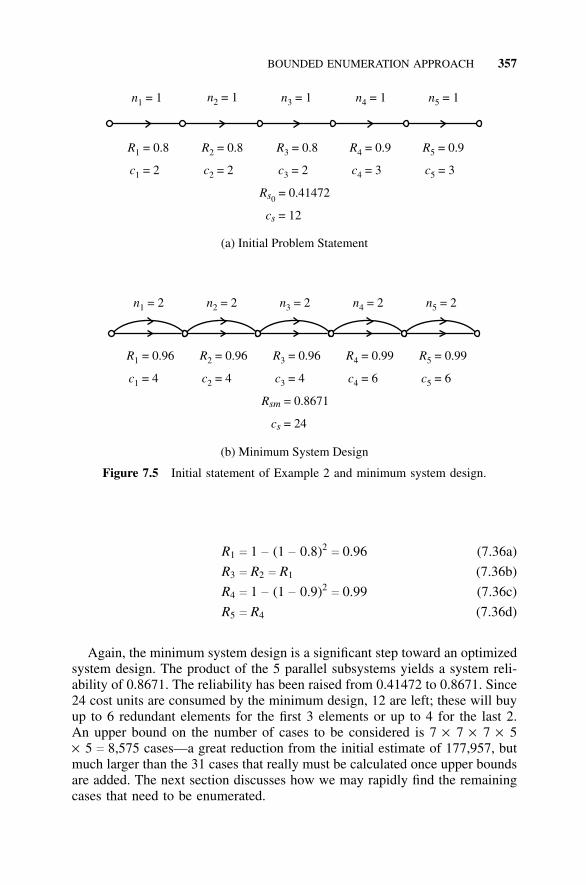
BOUNDED ENUMERATION APPROACH 357
Rs0= 0.41472
cs = 12
n1 = 1
R1 = 0.8 R2 = 0.8 R3 = 0.8 R4 = 0.9 R5 = 0.9
n2 = 1 n3 = 1 n4 = 1 n5 = 1
c2 = 2c1 = 2 c3 = 2 c4 = 3 c5 = 3
(a) Initial Problem Statement
(b) Minimum System Design
Rsm = 0.8671
cs = 24
R1 = 0.96 R2 = 0.96 R3 = 0.96 R4 = 0.99 R5 = 0.99
c1 = 4 c2 = 4 c3 = 4 c4 = 6 c5 = 6
n1 = 2 n2 = 2 n3 = 2 n4 = 2 n5 = 2
Figure 7.5 Initial statement of Example 2 and minimum system design.
R1 c 1 − (1 − 0.8)2c 0.96 (7.36a)
R3 c R2 c R1 (7.36b)
R4 c 1 − (1 − 0.9)2c 0.99 (7.36c)
R5 c R4 (7.36d)
Again, the minimum system design is a significant step toward an optimizedsystem design. The product of the 5 parallel subsystems yields a system reli-ability of 0.8671. The reliability has been raised from 0.41472 to 0.8671. Since24 cost units are consumed by the minimum design, 12 are left; these will buyup to 6 redundant elements for the first 3 elements or up to 4 for the last 2.An upper bound on the number of cases to be considered is 7 × 7 × 7 × 5× 5 c 8,575 cases—a great reduction from the initial estimate of 177,957, butmuch larger than the 31 cases that really must be calculated once upper boundsare added. The next section discusses how we may rapidly find the remainingcases that need to be enumerated.
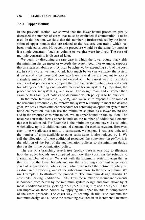
358 RELIABILITY OPTIMIZATION
7.8.3 Upper Bounds
In the previous section, we showed that the lower-bound procedure greatlydecreased the number of cases that must be evaluated if enumeration is to beused. In this section, we show that this number is further reduced by the impo-sition of upper bounds that are related to the resource constraint, which hasbeen modeled as cost. However, the procedure would be the same for anotherif a single constraint (such as volume or weight) were involved. The case ofmultiple constraints is discussed later.
We begin by discussing the rare case in which the lower bound that yieldsthe minimum design meets or exceeds the system goal. For example, supposethat a system reliability Rs > Rg, can be achieved by expending 90% of the cost,co. In such a case, we wish to ask how much better can we make the systemif we spend a bit more and how much we save if we are content to accepta slightly smaller Rs that does not exceed Rg. The easiest way to formulatesuch a set of policies is to compute the resultant system reliabilities and costsfor adding or deleting one parallel element for subsystem X1, repeating theprocedure for subsystem X2, and so on. The design team and customer thenexamine this family of policies to determine which policy is to be pursued.
In the more familiar case, Rs < Rg, and we wish to expend all or some ofthe remaining resource co to improve the system reliability to meet the desiredgoal. We seek a more efficient procedure for achieving an optimum system thanblind enumeration. We can use the minimum solution as a lower bound andadd in the resource constraint to achieve an upper bound on the solution. Theresource constraint forms upper bounds on the number of additional elementsthat can be allocated. For Example 1, the minimum system leaves 3 cost units,which allow up to 3 additional parallel elements for each subsystem. However,each time we allocate a unit to a subsystem, we expend 1 resource unit, andthe number of units available to other subsystems is also reduced by 1. Wecall the allocation of these additional resources the augmentation policy; it isthe addition of the best of the augmentation policies to the minimum designthat results in the optimization policy.
The use of a branching search tree (policy tree) is one way to illustratehow the upper bounds are computed and how they constrain the solution toa small number of cases. We start with the minimum system design that isthe result of the lower bounds and use the remaining constraint to generatea set of augmentation policies from which we select the optimum policy or,as discussed previously, one of the suboptima close to the true optimum. Weuse Example 1 to illustrate the procedure. The minimum design absorbs 13cost units, leaving 3 additional units. Thus the number of redundant elementsis bounded from below by the minimum system design and from above by atmost 3 additional units, yielding 2 ≤ n1 ≤ 5; 4 ≤ n2 ≤ 7; and 7 ≤ n3 ≤ 10. Onecan improve on these bounds by applying the upper bounds as computationof the cases proceeds. The easist way to accomplish this is to compute theminimum design and allocate the remaining resource in an incremental manner.
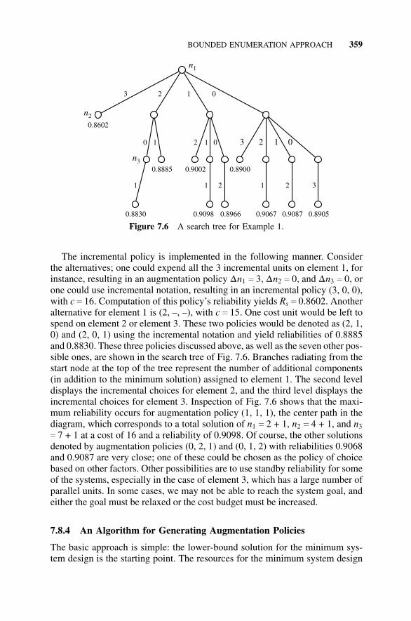
BOUNDED ENUMERATION APPROACH 359
0.8602
1 1 2 1 2 3
Figure 7.6 A search tree for Example 1.
The incremental policy is implemented in the following manner. Considerthe alternatives; one could expend all the 3 incremental units on element 1, forinstance, resulting in an augmentation policy Dn1 c 3, Dn2 c 0, and Dn3 c 0, orone could use incremental notation, resulting in an incremental policy (3, 0, 0),with c c 16. Computation of this policy’s reliability yields Rs c 0.8602. Anotheralternative for element 1 is (2, –, –), with c c 15. One cost unit would be left tospend on element 2 or element 3. These two policies would be denoted as (2, 1,0) and (2, 0, 1) using the incremental notation and yield reliabilities of 0.8885and 0.8830. These three policies discussed above, as well as the seven other pos-sible ones, are shown in the search tree of Fig. 7.6. Branches radiating from thestart node at the top of the tree represent the number of additional components(in addition to the minimum solution) assigned to element 1. The second leveldisplays the incremental choices for element 2, and the third level displays theincremental choices for element 3. Inspection of Fig. 7.6 shows that the maxi-mum reliability occurs for augmentation policy (1, 1, 1), the center path in thediagram, which corresponds to a total solution of n1 c 2 + 1, n2 c 4 + 1, and n3
c 7 + 1 at a cost of 16 and a reliability of 0.9098. Of course, the other solutionsdenoted by augmentation policies (0, 2, 1) and (0, 1, 2) with reliabilities 0.9068and 0.9087 are very close; one of these could be chosen as the policy of choicebased on other factors. Other possibilities are to use standby reliability for someof the systems, especially in the case of element 3, which has a large number ofparallel units. In some cases, we may not be able to reach the system goal, andeither the goal must be relaxed or the cost budget must be increased.
7.8.4 An Algorithm for Generating Augmentation Policies
The basic approach is simple: the lower-bound solution for the minimum sys-tem design is the starting point. The resources for the minimum system design
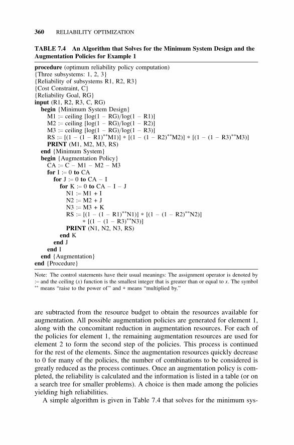
360 RELIABILITY OPTIMIZATION
TABLE 7.4 An Algorithm that Solves for the Minimum System Design and theAugmentation Policies for Example 1
procedure (optimum reliability policy computation){Three subsystems: 1, 2, 3}{Reliability of subsystems R1, R2, R3}{Cost Constraint, C}{Reliability Goal, RG}input (R1, R2, R3, C, RG)
begin {Minimum System Design}M1 :c ceiling [log(1 − RG)/ log(1 − R1)]M2 :c ceiling [log(1 − RG)/ log(1 − R2)]M3 :c ceiling [log(1 − RG)/ log(1 − R3)]RS :c [(1 − (1 − R1)**M1)] ∗ [(1 − (1 − R2)**M2)] ∗ [(1 − (1 − R3)**M3)]PRINT (M1, M2, M3, RS)
end {Minimum System}begin {Augmentation Policy}
CA :c C − M1 − M2 − M3for I :c 0 to CA
for J :c 0 to CA − Ifor K :c 0 to CA − I − J
N1 :c M1 + IN2 :c M2 + JN3 :c M3 + KRS :c [(1 − (1 − R1)**N1)] ∗ [(1 − (1 − R2)**N2)]
∗ [(1 − (1 − R3)**N3)]PRINT (N1, N2, N3, RS)
end Kend J
end Iend {Augmentation}
end {Procedure}
Note: The control statements have their usual meanings: The assignment operator is denoted by:c and the ceiling (x) function is the smallest integer that is greater than or equal to x. The symbol** means “raise to the power of” and ∗ means “multiplied by.”
are subtracted from the resource budget to obtain the resources available foraugmentation. All possible augmentation policies are generated for element 1,along with the concomitant reduction in augmentation resources. For each ofthe policies for element 1, the remaining augmentation resources are used forelement 2 to form the second step of the policies. This process is continuedfor the rest of the elements. Since the augmentation resources quickly decreaseto 0 for many of the policies, the number of combinations to be considered isgreatly reduced as the process continues. Once an augmentation policy is com-pleted, the reliability is calculated and the information is listed in a table (or ona search tree for smaller problems). A choice is then made among the policiesyielding high reliabilities.
A simple algorithm is given in Table 7.4 that solves for the minimum sys-
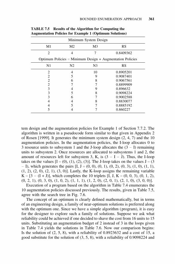
BOUNDED ENUMERATION APPROACH 361
TABLE 7.5 Results of the Algorithm for Computing theAugmentation Policies for Example 1 (Optimum Solutions)
Minimum System Design
M1 M2 M3 RS
2 4 7 0.8409362
Optimum Policies c Minimum Design + Augmentation Policies
N1 N2 N3 RS
2 4 10 0.89052012 5 9 0.90874012 6 8 0.90675612 7 7 0.88999093 4 9 0.8966323 5 8 0.90982243 6 7 0.90025884 4 8 0.88300774 5 7 0.88851925 4 7 0.860227
tem design and the augmentation policies for Example 1 of Section 7.7.2. Thealgorithm is written in a pseudocode form similar to that given in Appendix 2of Rosen [1999]. It generates the minimum system design (2, 4, 7) and the 10augmentation policies. In the augmentation policies, the I-loop allocates 0 to3 resource units to subsystem 1 and the J-loop allocates the (3 − I) remainingunits to subsystem 2. Once resources are allocated to subsystems 1 and 2, theamount of resources left for subsystem 3, K, is (3 − I − J). Thus, the I-looptakes on the values [I c (0), (1), (2), (3)]. The J-loop takes on the values J c (3− I), which generates the pairs [I, J c (0, 0), (0, 1), (0, 2), (0, 3), (1, 0), (1, 1),(1, 2), (2, 0), (2, 1), (3, 0)]. Lastly, the K-loop assigns the remaining variableK c [3 − (I + J)], which completes the 10 triplets [I, J, K c (0, 0, 3), (0, 1, 2),(0, 2, 1), (0, 3, 0), (1, 0, 2), (1, 1, 1), (1, 2, 0), (2, 0, 1), (2, 1, 0), (3, 0, 0)].
Execution of a program based on the algorithm in Table 7.4 enumerates the10 augmentation policies discussed previously. The results, given in Table 7.5,agree with the search tree in Fig. 7.6.
The concept of an optimum is clearly defined mathematically, but in termsof an engineering design, a family of near-optimum solutions is preferred alongwith the optimum one. Since we have a simple algorithm (program), it is easyfor the designer to explore such a family of solutions. Suppose we ask whatreliability could be achieved if one decided to shave the cost from 16 units to 15units. Substituting an augmentation budget of 2 instead of 3 in the loops givenin Table 7.4 yields the solutions in Table 7.6. Now our comparison begins:Is the solution of (2, 5, 8), with a reliability of 0.8923632 and a cost of 15, agood substitute for the solution of (3, 5, 8), with a reliability of 0.9098224 and
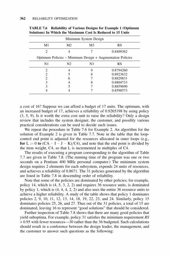
362 RELIABILITY OPTIMIZATION
TABLE 7.6 Reliability of Various Designs for Example 1 (OptimumSolutions) In Which the Maximum Cost Is Reduced to 15 Units
Minimum System Design
M1 M2 M3 RS
2 4 7 0.8409362
Optimum Policies c Minimum Design + Augmentation Policies
N1 N2 N3 RS
2 4 9 0.87942602 5 8 0.89236322 6 7 0.88298313 4 8 0.88047333 5 7 0.88596904 4 7 0.8598573
a cost of 16? Suppose we can afford a budget of 17 units. The optimum, withan increased budget of 17, achieves a reliability of 0.9265198 by using policy(3, 5, 9). Is it worth the extra cost unit to raise the reliability? Only a designreview that includes the system designer, the customer, and possibly variouspractical considerations can be used to decide such issues.
We repeat the procedure in Table 7.6 for Example 2. An algorithm for thesolution of Example 2 is given in Table 7.7. Note in the table that the loop-control end point is adjusted for the resources allocated in outer loops (e.g.,for L :c 0 to (CA − I − J − K)/ C4), and note that the end point is divided bythe item weight, C4, so that L is incremented in multiples of C4.
The results of executing a program corresponding to the algorithm of Table7.7 are given in Table 7.8. (The running time of the program was one or twoseconds on a Pentium 400 MHz personal computer.) The minimum systemdesign requires 2 elements for each subsystem, expends 24 units of resources,and achieves a reliability of 0.8671. The 31 policies generated by the algorithmare listed in Table 7.8 in descending order of reliability.
Note that some of the policies are dominated by other policies; for example,policy 14, which is (4, 5, 3, 2, 2) and requires 36 resource units, is dominatedby policy 1, which is (4, 4, 4, 2, 2) and also uses the entire 36 resource units toachieve a higher reliability. A study of the table shows that policy 1 dominatespolicies 2, 9, 10, 11, 12, 13, 14, 18, 19, 22, 23, and 24. Similarly, policy 15dominates policies 25, 26, and 27. Thus out of the 31 policies, a total of 15 aredominated, leaving 16 to represent “good solutions” that should be considered.
Further inspection of Table 7.8 shows that there are many good policies thatyield suboptima. For example, policy 31 satisfies the minimum requirement RS> 0.95 with fewer resources—30 rather than the 36 budgeted. Such calculationsshould result in a conference between the design leader, the management, andthe customer to answer such questions as the following:
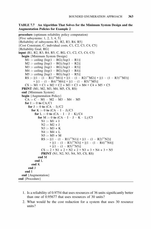
BOUNDED ENUMERATION APPROACH 363
TABLE 7.7 An Algorithm That Solves for the Minimum System Design and theAugmentation Policies for Example 2
procedure (optimum reliability policy computation){Five subsystems: 1, 2, 3, 4, 5}{Reliability of subsystems R1, R2, R3, R4, R5}{Cost Constraint, C; individual costs, C1, C2, C3, C4, C5}{Reliability Goal, RG}input (R1, R2, R3, R4, R5, C, RG, C1, C2, C3, C4, C5)
begin {Minimum System Design}M1 :c ceiling [log(1 − RG)/ log(1 − R1)]M2 :c ceiling [log(1 − RG)/ log(1 − R2)]M3 :c ceiling [log(1 − RG)/ log(1 − R3)]M4 :c ceiling [log(1 − RG)/ log(1 − R4)]M5 :c ceiling [log(1 − RG)/ log(1 − R5)]RS :c [(1 − (1 − R1)**M1)] ∗ [(1 − (1 − R2)**M2)] ∗ [(1 − (1 − R3)**M3)]
∗ [(1 − (1 − R4)**M4)] ∗ [(1 − (1 − R5)**M5)]CS :c M1 ∗ C1 + M2 ∗ C2 + M3 ∗ C3 + M4 ∗ C4 + M5 ∗ C5
PRINT (M1, M2, M3, M4, M5, CS, RS)end {Minimum System}begin {Augmentation Policy}
CA :c C − M1 − M2 − M3 − M4 − M5for I :c 0 to CA/ C1
for J :c 0 to (CA − I)/ C2for K :c 0 to (CA − I − J)/ C3
for L :c 0 to (CA − I − J − K)/ C4for M :c 0 to (CA − I − J − K − L)/ C5
N1 :c M1 + IN2 :c M2 + JN3 :c M3 + KN4 :c M4 + LN5 :c M5 + MRS :c [(1 − (1 − R1)**N1)] ∗ [(1 − (1 − R2)**N2)]
∗ [(1 − (1 − R3)**N3)] ∗ [(1 − (1 − R4)**N4)]∗ [(1 − (1 − R5)**N5)]
CS :c 2 ∗ N1 + 2 ∗ N2 + 2 ∗ N3 + 3 ∗ N4 + 3 ∗ N5PRINT (N1, N2, N3, N4, N5, CS, RS)
end Mend L
end Kend J
end Iend {Augmentation}
end {Procedure}
1. Is a reliability of 0.9754 that uses resources of 36 units significantly betterthan one of 0.95677 that uses resources of 30 units?
2. What would be the cost reduction for a system that uses 30 resourceunits?
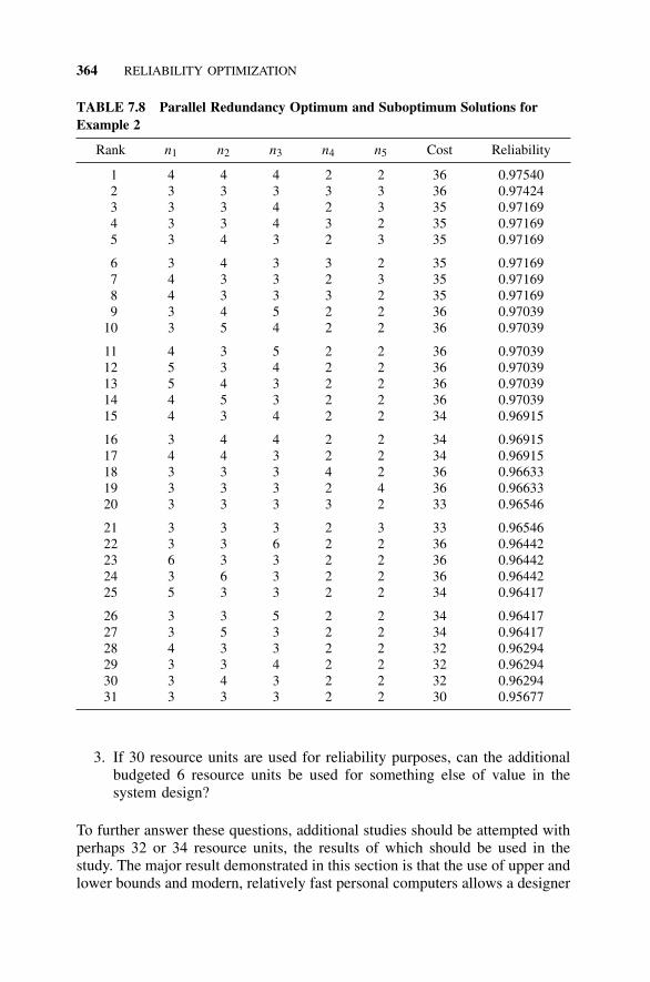
364 RELIABILITY OPTIMIZATION
TABLE 7.8 Parallel Redundancy Optimum and Suboptimum Solutions forExample 2
Rank n1 n2 n3 n4 n5 Cost Reliability
1 4 4 4 2 2 36 0.975402 3 3 3 3 3 36 0.974243 3 3 4 2 3 35 0.971694 3 3 4 3 2 35 0.971695 3 4 3 2 3 35 0.97169
6 3 4 3 3 2 35 0.971697 4 3 3 2 3 35 0.971698 4 3 3 3 2 35 0.971699 3 4 5 2 2 36 0.97039
10 3 5 4 2 2 36 0.97039
11 4 3 5 2 2 36 0.9703912 5 3 4 2 2 36 0.9703913 5 4 3 2 2 36 0.9703914 4 5 3 2 2 36 0.9703915 4 3 4 2 2 34 0.96915
16 3 4 4 2 2 34 0.9691517 4 4 3 2 2 34 0.9691518 3 3 3 4 2 36 0.9663319 3 3 3 2 4 36 0.9663320 3 3 3 3 2 33 0.96546
21 3 3 3 2 3 33 0.9654622 3 3 6 2 2 36 0.9644223 6 3 3 2 2 36 0.9644224 3 6 3 2 2 36 0.9644225 5 3 3 2 2 34 0.96417
26 3 3 5 2 2 34 0.9641727 3 5 3 2 2 34 0.9641728 4 3 3 2 2 32 0.9629429 3 3 4 2 2 32 0.9629430 3 4 3 2 2 32 0.9629431 3 3 3 2 2 30 0.95677
3. If 30 resource units are used for reliability purposes, can the additionalbudgeted 6 resource units be used for something else of value in thesystem design?
To further answer these questions, additional studies should be attempted withperhaps 32 or 34 resource units, the results of which should be used in thestudy. The major result demonstrated in this section is that the use of upper andlower bounds and modern, relatively fast personal computers allows a designer
BOUNDED ENUMERATION APPROACH 365
the luxury of computing a range of design solutions and comparing them; ingeneral, the more complex methods discussed later in this chapter are seldomneeded. Using the results of the discussion of availability in Section 7.4.6, itis easy to adapt any of the foregoing algorithms to availability apportionmentby substituting probabilities in the algorithms that represent unit availabilitiesrather than reliabilities.
7.8.5 Optimization with Multiple Constraints
The preceding material in this chapter has dealt with a single constraint and hasused cost to illustrate the constraint. Sometimes, however, there are multipleconstraints—cost, volume, and weight, for instance. Of obvious importance isthe use of these three constraints in satellites, spacecraft, and aircraft. Withoutloss of generality, we can assume that there are three constraints: cost, volume,and weight (c, v, and w) and that the constraints (given in the forthcomingequations) are similar to those of Eq. (7.4). Clearly, these constraints as wellas the following equations can represent other variables and/ or can be extendedto more than three constraints.
c c
k
���i c 1
nici (7.37a)
v c
k
���i c 1
nivi (7.37b)
w c
k
���i c 1
niwi (7.37c)
Generally, optimization techniques such as dynamic programming becomemuch more difficult when more than one variable is involved. Since we aredealing with discrete optimization and enumeration, however, the extra workof multiple constraints is modest. First of all, the computation of the minimumsystem design is not affected by the constraints; thus lower bounds are com-puted as in the case of a single constraint (cf. Section 7.6.2). Once the minimumdesign (lower bound) is obtained, the values are substituted in Eqs. (7.37a–c)and the remaining values of the constraints are computed for the augmenta-tion phase. In some cases, the minimum system design exceeds one or moreof the constraints and the reliabilty goal and constraints are incompatible (onecan call such a situation an ill-formulated problem). The only recourse in thecase of an ill-formulated problem is to have a high-level design review withall members of the designer’s and the customer’s senior management presentto change the requirements so that the problem is solvable.
Assume that the minimum system design still leaves some values of all theconstraints for the augmentation phase. The constraints are still used to com-
366 RELIABILITY OPTIMIZATION
pute the upper bounds; however, we now have more than one upper bound. Forthe case under discussion, we have three upper bounds—one governed by cost,one by weight, and one by volume—that result in three values of n: (ni, n′i , n′′i ).The bound we choose is the minimum value of the three bounds, that is, theminimum value of (ni, n′i , n′′i ) [Rice, 1999]. Computation of the augmentationpolicy proceeds in the same manner as discussed in Section 7.6.3; however,at each stage, three upper bounds are computed, and the minimum is used ineach case. Once the augmentation policy is obtained, the system reliability iscomputed. If the reliability goal cannot be obtained, a high-level design reviewis enacted. The designer should compute beforehand some alternative designsfor presentation that violate one or more of the constraints but still achieve thegoals.
7.9 APPORTIONMENT AS AN APPROXIMATE OPTIMIZATIONTECHNIQUE
The bounded solutions of the previous section led to a family of solutions thatincluded the maximum reliability combination. The apportionment techniquesdiscussed in Section 7.6 can be viewed as an approximate solution. In thissection, we explore how these solutions compare with the optimum solutionsof the previous section.
We begin by considering Example 1 given in Section 7.7.2. The system goalRg c 0.9, and by using Eq. (7.15b) we obtain a goal of 0.9655 for each of thethree subsystems. We can determine how many parallel components are neededfor each subsystem if we use the reliability goal of 0.9655 and each subsystemreliability (0.85, 0.5, 0.3) and substitute into Eq. (7.31b). The results for thesubsystem are
n1 c log(1 − Rg)/ log(1 − r1) (7.38a)
n1 c log(1 − 0.9655)/ log(1 − 0.85) c 1.77 (7.38b)
n2 c log(1 − 0.9655)/ log(1 − 0.5) c 4.86 (7.38c)
n3 c log(1 − 0.9655)/ log(1 − 0.3) c 9.44 (7.38d)
This represents a solution of n1, n2, n3 c 2, 5, 10, using 17 cost units andexceeding both the reliability goal and the cost budget. One could then tryremoving one unit from each of the subsystems to arrive at approximate solu-tions. If we remove one unit from subsystem 2 or 3, we obtain the 16-unitsolutions n1, n2, n3 c 2, 4, 10 and n1, n2, n3 c 2, 5, 9, which correspond to theoptimum designs given in Table 7.5 (rows 1 and 2). If we remove one unitfrom subsystem 1, we obtain solution n1, n2, n3 c 1, 5, 10, corresponding to areliability of 0.8002 that is clearly inferior to all the 10 solutions in Table 7.5.
We now consider the apportionment solutions for Example 2 given in Sec-tion 7.7.2. The system goal is Rg c 0.95, and by using Eq. (7.15b), we obtain
STANDBY SYSTEM OPTIMIZATION 367
a goal of 0.9898 for each of the five subsystems. We can determine how manyparallel components are needed for each subsystem to meet the reliability goalof 0.9898 with each subsystem reliability (0.8, 0.8, 0.8, 0.9, 0.9). Substitutioninto Eq. (7.31b) yields the desired results that need to be calculated only forthe subsystem values of 0.8 and 0.9; these are
n1 c log(1 − Rg)/ log(1 − r1) (7.39a)
n1, 2, 3 c log(1 − 0.9898)/ log(1 − 0.8) c 2.85 (7.39b)
n4, 5 c log(1 − 0.9898)/ log(1 − 0.9) c 1.99 (7.39c)
Thus rounding up represents a solution of n1, n2, n3, n4, n5 c 3, 3, 3, 2, 2.Since the costs are 2, 2, 2, 3, 3 units per subsystem, respectively, this appor-tioned solution expends 30 cost units and yields a reliability of 0.9568. Thisis the last policy in Table 7.8. We conclude that the simplest equal apportion-ment method is a good approximation, and since it only takes a few minuteswith paper, pencil, and calculator, it is a valuable check on the results of theprevious section.
7.10 STANDBY SYSTEM OPTIMIZATION
In principle, the optimization of a standby system is the same procedure asthat of a parallel system, but instead of the reliability expression for n items inparallel given in Eq. (7.3), the expression given in Eqs. (7.5) and (7.6) is used.Because Eq. (7.6) is a series, the simple solution for the number of elements inthe minimum system design given in Eqs. (7.30) and (7.31) is not applicable.A slightly more complicated solution for a standby system involves the evalua-tion of Eq. (7.6) for increasing values of k until the right-hand side exceeds thereliability goal Rg. This is a little more complicated for paper-pencil-and-cal-culator computation, but the complexity increase is insignificant when a com-puter program is used. Another approach is to use cumulative Poisson tablesor graphs to solve Eq. (7.6), the Chebyschev bound, or the normal approxi-mation to the Poisson (these later techniques are explained and compared inMessinger [1970]). The reader should note that the techniques for a standbysystem also apply to a system with spares. We assume that a standby systemswitches in the standby component quickly enough for the system performanceto not be affected. In other systems, a set of spare components is kept near anoperating system that has self-diagnostics to rapidly signal the failure. If thereplacement of a spare is rapid (e.g., opening a panel and putting in a printedcircuit board spare), the system would not be down for a significant interval(this is essentially a standby system). If the time to switch a standby system islong enough to interrupt system performance or if the downtime in replacinga spare is significant, we must treat the system as an availability problem andformulate a Markov model.
368 RELIABILITY OPTIMIZATION
One can use Example 1 of Section 7.7.2 to illustrate a standby system reli-ability optimization [Shooman, 1994]. Since standby systems are generallymore complex than parallel ones because of the failure detection and switchinginvolved, we assume that each element costs 1.5 units rather than 1 unit. Fur-thermore, we equate the probability of no failures (x c 0) for the Poisson, e−m ,to the reliabilities of each unit and solve for the expected number of failures,m: m1 c ln(0.85) c 0.1625189; m2 c ln(0.5) c 0.6931471; and m3 c ln(0.3) c
1.2039728. Substitution into Eqs. (7.5) and (7.6) yields
e−m1 (1 + m1 + m21/ 2! + · · · +)
≥ 0.90 for two terms 0.85(1 + 0.1625189)
c 0.9881 ≥ 0.9 (7.40a)
e−m2 (1 + m2 + m22/ 2! + · · · +)
≥ 0.90 for three terms 0.5(1 + 0.6931471 + 0.2402264)
c 0.9667 ≥ 0.9 (7.40b)
e−m3 (1 + m3 + m23/ 2! + · · · +)
≥ 0.90 for four terms 0.3(1 + 0.12039728 + 0.7247752 + 0.2908735)
c 0.9659 ≥ 0.9 (7.40c)
Thus, the minimum values for standby system reliability are n1 c 2, n2 c
3, n3 c 4. The minimum system cost is 9 × 1.5 c 13.5 and the reliability is0.9881 × 0.9667 × 0.9659 c 0.9226. Since this exceeds the reliability goal,this is the optimum solution, and the augmentation policy phase is not needed.If augmentation had been required, we could use an algorithm similar to thatof Table 7.4; however, instead of equations for M1, M2, and M3, do whileR ≤ Rg loops that increment n are used. Similarly, the RS:c equation becomes aproduct of the series expansions for the Poisson that are computed by for loopsin a manner similar to that of Eqs. (7.40a–c). If the assumed cost of 1.5 fora standby element is accurate, and if there are no other overriding factors, thestandby system would be preferred to that of any of the parallel system policiesof Table 7.5 since the resource cost is less and the reliability is higher.
It is also possible to adapt the foregoing optimization techniques to an r-out-of-n system design; see Shooman [1994, p. 946].
One should not forget that reliability can be improved by componentimprovement as an alternative to parallel or standby system redundancy. Ingeneral, there are extra costs involved (development and production), and typi-cally such an improved design begins by listing all the ways in which theelement can fail in the order of frequency. Design engineers then proposeschemes to eliminate, mitigate, or reduce the frequency of occurrence. Thedesign changes are made, sometimes one at a time or a few at a time, and theprototype is tested to confirm the success of the redesign. Sometimes overstress(accelerated) testing is used in such a process to demonstrate unknown failure
OPTIMIZATION USING A GREEDY ALGORITHM 369
modes that must be fixed. A model comparing the costs of improved designwith the costs of parallel redundancy is given in Shooman and Marshall [1993and 1994, p. 947].
7.11 OPTIMIZATION USING A GREEDY ALGORITHM
7.11.1 Introduction
If one studies the optimum solutions of various optimization procedures, wefind that the allocation of parallel subsystems tends to raise all the subsystemsto nearly the same reliability. For example, consider the optimum solutionsgiven in Table 7.5. The subsystem reliabilities start out (0.85, 0.5, 0.3) and theminimal system design (with 2, 4, and 7 parallel systems) yields upon substitu-tion into Eq. (7.3), giving (0.9775, 0.9375, 0.9176), and the optimum solutionof 3, 5, 8 results in reliabilities of (0.9966, 0.9688, 0.9424). This is one ofthe reasons that the equal apportionment approximation gave reasonably goodresults, leading one to a heuristic procedure for optimization. If one starts withthe initial design or, better, with the minimal system design, one can allocateadditional parallel systems to the subsystems by computing which allocation tosubsystem 1, 2, or 3 will produce the largest increase in reliability. Such an allo-cation is made and the computations are repeated with the new parallel systemadded. Based on these new computations, a second parallel system is added,and the procedure is repeated until the entire resource has been expended. Thisprocedure generates an augmentation policy that, when added to the minimalsystem design, generates a good policy.
7.11.2 Greedy Algorithm
The foregoing algorithm that makes an optimal choice at each step is oftenreferred to as a “greedy” algorithm [Cormen, Chapter 17]. Starting with theminimum system design, we compute the increase in reliability obtained byadding a single element to each subsystem. In the case of Example 1, Fig.7.4(b) shows that the minimum system design requires n1 c 2, n2 c 4, and n3 c
7, yielding a reliability Rsm c 0.9775 × 0.9375 × 0.9176 c 0.8409. The additionof one element to n1 raises the reliability of this subsystem to 0.996625 and Rsm
to 0.8573, which represents a reliability increment DR of 0.0164. Repeatingthis process for an increase in n2 from 4 to 5 results in raising subsystem 2to a reliability of 0.96875 and Rsm to 0.8689, which represents a reliabilityincrement DR of 0.0280. Increasing n3 to 8 yields a subsystem reliability of0.9424, and Rsm increases to 0.8636, which represents a reliability incrementDR of 0.0227. Raising subsystem 2 from 4 to 5 parallel elements produces thelargest DR; thus the first stage of the greedy algorithm yields the following:
1. Stage 0, minimum system design:
370 RELIABILITY OPTIMIZATION
n1 c 2, n2 c 4, n3 c 7,Rsm c 0.9775 × 0.9375 × 0.9176 c 0.8409
2. Stage 1, add one to n2:
n1 c 2, n2 c 5, n3 c 7,Rsm c 0.9775 × 0.96875 × 0.9176 c 0.86875
Continuing the greedy process yields the following:
1. Stage 2, add one to n3:
n1 c 2, n2 c 5, n3 c 8,Rsm c 0.9775 × 0.96875 × 0.9424 c 0.8924
2. Stage 3, add one to n1:
n1 c 3, n2 c 5, n3 c 8,Rsm c 0.996625 × 0.96875 × 0.95424 c 0.909868
When we compare the solution of stage 3 with Table 7.5, we see that theyboth have reached the same policy and the same optimum reliability (withinround-off errors). The greedy algorithm always yields a good solution, but itis not always the optimum (cf. Section 7.11.4).
7.11.3 Unequal Weights and Multiple Constraints
There is something special about Example 1—it is that all the weights areequal. If we consider Example 2, where there are unequal weights, it may notbe fair to compare the reliability increase, DR, achieved through the adding ofone additional parallel component. For example, a component with a cost of 2should be compared to adding two components with costs of 1 each. Thus, abetter procedure in implementing the greedy algorithm is to compare values ofDR/ DC as the single constraint of cost. When there are multiple constraints,say, c, w, and v, then the comparison should be made based on some functionof c, w, and v; f (c, w, v), that is, use DR/ Df (c, w, v) as the comparison factor.One possible function to use is a linear combination of the fraction of theconstraints expended. If m represents the stage of the augmentation policy, thenwe would view the ratio Cm/ Ca as the fraction of the augmentation cost that hasbeen allocated. Thus, if at the first stage we allocate 20% of the augmentationcost, then Cm/ Ca c 0.2 and the inverse ratio Ca/ Cm c 5. If we let f (c, w, v) ck1(Cm/ Ca) + k2(Wm/ Wa) + k3(Vm/ Va), and also let k1 c k2 c k3 c 1, then theconstraint with the most available capacity has a stronger influence. Obviously,there are many other good choices for f (c, w, v).
DYNAMIC PROGRAMMING 371
7.11.4 When Is the Greedy Algorithm an Optimum?
The greedy algorithm seems like a fine approach to generating a sequence ofgood policies that lead to an optimum or a good semioptimum policy. The mainquestion is when the greedy solution is an optimum and when it is a semiop-timum, a question that has been studied by many [Barlow, 1965, 1975]. Thegeometrical model discussed in Section 7.2 can be used to explain optimizationtechniques. Suppose that the reliability surface has two spires: one at x1y1 thatreaches a reliability peak of 0.98 and another at x2y2 that reaches a reliabilitypeak of 0.99. If we start the greedy algorithm at the base of spire one, it ispossible that it will reach a reliability maximum of 0.98 rather than 0.99. Thereare similarities between the greedy algorithm and the gradient algorithm forcontinuous functions [Hiller, 1974, p. 729]. Recent work has focused on devel-oping a theory (called the matroid theory) that provides the basis for greedyalgorithms [Cormen, p. 345]. However, as long as the upper and lower boundsdiscussed previously provide a family of solutions that includes the optimumas well as a group of good suboptimum policies, and if the computer time ismodest, the use of the greedy algorithm is probably unnecessary.
7.11.5 Greedy Algorithm Versus Apportionment Techniques
We can understand how the apportionment algorithm reaches an approximatesolution if we compare it with a greedy approximation to exact optimization.The greedy approximation adds a new redundant component at each step,which yields the highest gain in reliability on each iteration. The result isto “spread the redundancy around the system” in a bottom–up fashion. Theapportionment process also spreads the redundancy about the system, but in atop–down fashion. In general, the two techniques will yield a different set ofsuboptima; most of the time, both will yield good solutions. The apportion-ment approach has a number of advantages, including the following: (a) it fitsin well with the philosophy of system design, which is generally adopted bydesigners of large systems; (b) its computations will in general be simpler; and(c) it may provide more insight into when the suboptimal solutions it generatesare good.
7.12 DYNAMIC PROGRAMMING
7.12.1 Introduction
Dynamic programming provides a different approach to optimization thatrequires fewer steps than exhaustive enumeration and always leads to an opti-mal policy. The discussion of this section is included for completeness, sincethe author believes that the application of lower bounds to obtain a minimumsystem design and the subsequent use of upper bounds to obtain an augmenta-tion policy both require less effort but still yield the optimum. The incremental
372 RELIABILITY OPTIMIZATION
reliability method is a competitor to the bounding techniques, but unless onemakes a careful study, it is not possible to be sure that this method does indeedyield an optimum.
Dynamic programming is based on an optimality principle established byBellman [1957, 1958], who states, “An optimal policy has the property thatwhatever the initial state and initial decision are, the remaining decisions mustconstitute an optimal policy with regard to the state resulting from the firstdecision.” Clearly, this is a high-level principle that can apply to a large vari-ety of situations. A large number of examples that describe how dynamic pro-gramming can be applied to various situations appear in Hiller [1974, Chapter6]. The best way to understand its application to reliability optimization is toapply it to a problem.
7.12.2 Dynamic Programming Example
The following example used to illustrate dynamic programming is a modifica-tion of Example 1 of Section 7.7.2.
Example 3 (Modification of Example 1): The initial design of a system yields3 subsystems at the first level of decomposition. The system reliability goal,Rg, is 0.8 for a given number of operating hours. The initial estimates of thesubsystem reliabilities are R1 c 0.85, R2 c 0.5, and R3 c 0.3. Parallel redundancyis to be used to improve the initial design so that it meets the reliability goal.The constraint is cost; subsystem 1 is assumed to cost 2 units and subsystems2 and 3 to cost 1 unit each. The total cost budget is 16 units.
7.12.3 Minimum System Design
Dynamic programming can deal with the optimization problem as stated. How-ever, one should take advantage of the minimum system design procedures(lower bounds) to reduce the size of the problem. Thus the minimum designis computed and dynamic programming is used to solve for the augmentationpolicy. The minimum system design is computed in a manner similar to thatof Eqs. (7.35a–d).
n1 c log(1 − 0.8)/ (1 − 0.85) c 0.848 (7.41a)
n2 c log(1 − 0.8)/ (1 − 0.5) c 2.322 (7.41b)
n3 c log(1 − 0.8)/ (1 − 0.3) c 4.512 (7.41c)
Thus the minimum system design consists of one subsystem 1, three subsystem2, and five subsystem 3. The cost of the minimum design is C c 1 × 2 + 3 ×1 + 5 × 1 c 10, and the cost available for the augmentation policy is DC c 16− 10 c 6. The reliability of the minimum system design is
DYNAMIC PROGRAMMING 373
Rsm c [1 − (1 − 0.85)] × [1 − (1 − 0.5)3] × [1 − (1 − 0.3)5]
c (0.85) × (0.875) × (0.83193) c 0.6187 (7.42)
7.12.4 Use of Dynamic Programming to Compute the AugmentationPolicy
Thus we now wish to use dynamic programming to determine what is thebest augmentation policy from which to raise the reliability 0.6187 to 0.8 byexpending the remaining six cost units. Dynamic programming for this prob-lem consists of two phases: I and II. Phase I is used to construct a series oftables that correspond to the best solution for cost allocation for various com-binations of the subsystems. The first table considers the first subsystem only.The second table corresponds to the best cost allocation for the first and secondsubsystem; its construction uses information from the first table. A third tableis constructed that gives the best allocation for the third system based on thesecond table, which depicts the best allocation for the first and second subsys-tems. For phase II, certain features of the three tables of phase I are combinedto construct a new table that displays cost allocation per subsystem and alsothe resulting reliability optimization. A “backtracking” solution-procedure isused to compute the optimal policy for the cost constraint. The solution proce-dure automatically allows backtracking to compute optimization solutions forsmaller cost constraints. The description of these procedures will be clearerwhen they are applied to Example 3.
We begin our discussion by constructing the first table of phase I of thesolution, which is found in Table 7.9 and labeled as “Table 1.” The first col-umn in Table 1 is the amount of cost constraint allocated to subsystem 1. Themaximum allocation is 6 cost units; the minimum, 0 cost units. The incrementsbetween 0 and 6 are sized to be equal to the greatest common divisor of all thesubsystem costs, gcd (C1, C2, C3). In the case of Example 3, this is the gcd(2,1, 1) c 1. Thus the first column in Table 1 comprises the cost allocations 0, 1,2, 3, 4, 5, and 6.
The details of constructing Table 1 are as follows:
1. Consider the bottom line of Table 1. This table considers only the allo-cation of cost to buy additional parallel units for subsystem 1. If 0 cost isallocated to subsystem 1 for the augmentation policy, then no additionalcomponents can be allocated above the single subsystem of the minimalsystem design, and the optimal reliability is the same as the minimumsystem design—that is, 0.6187.
2. Because subsystem 1 costs 2 units, no additional units can be purchasedwith 1 cost unit, and the solution is the same as the 0 cost allocation.
3. If we increase the cost allocation to 2 units, we can allocate 1 addi-tional unit to subsystem 1 for a total cost of 2, from which the reliability
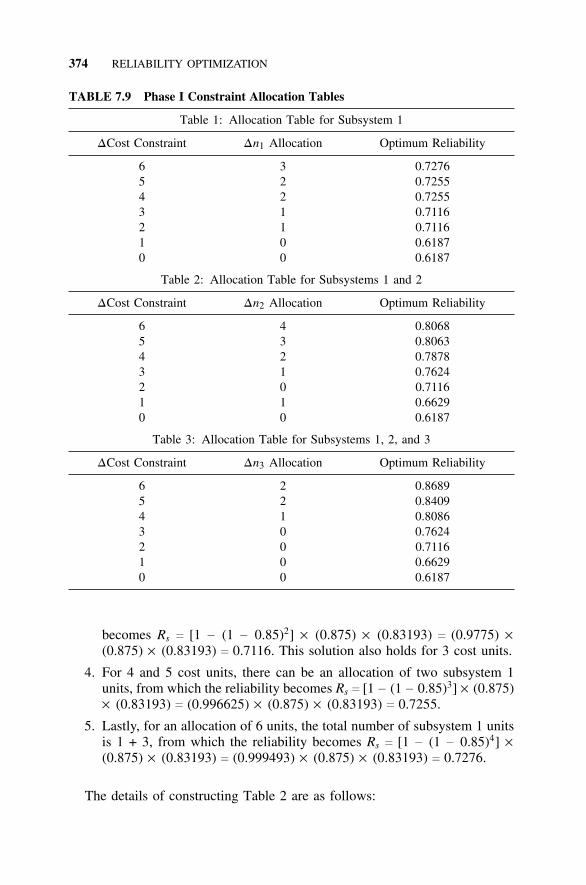
374 RELIABILITY OPTIMIZATION
TABLE 7.9 Phase I Constraint Allocation Tables
Table 1: Allocation Table for Subsystem 1
DCost Constraint Dn1 Allocation Optimum Reliability
6 3 0.72765 2 0.72554 2 0.72553 1 0.71162 1 0.71161 0 0.61870 0 0.6187
Table 2: Allocation Table for Subsystems 1 and 2
DCost Constraint Dn2 Allocation Optimum Reliability
6 4 0.80685 3 0.80634 2 0.78783 1 0.76242 0 0.71161 1 0.66290 0 0.6187
Table 3: Allocation Table for Subsystems 1, 2, and 3
DCost Constraint Dn3 Allocation Optimum Reliability
6 2 0.86895 2 0.84094 1 0.80863 0 0.76242 0 0.71161 0 0.66290 0 0.6187
becomes Rs c [1 − (1 − 0.85)2] × (0.875) × (0.83193) c (0.9775) ×(0.875) × (0.83193) c 0.7116. This solution also holds for 3 cost units.
4. For 4 and 5 cost units, there can be an allocation of two subsystem 1units, from which the reliability becomes Rs c [1 − (1 − 0.85)3] × (0.875)× (0.83193) c (0.996625) × (0.875) × (0.83193) c 0.7255.
5. Lastly, for an allocation of 6 units, the total number of subsystem 1 unitsis 1 + 3, from which the reliability becomes Rs c [1 − (1 − 0.85)4] ×(0.875) × (0.83193) c (0.999493) × (0.875) × (0.83193) c 0.7276.
The details of constructing Table 2 are as follows:

DYNAMIC PROGRAMMING 375
1. Consider the bottom line of Table 2. If there are 0 cost units allocated,then there can be no additional parallel elements for subsystem 2 andnone for subsystem 1. Thus the reliability is the same as the bottom linein Table 1—that is, 0.6187.
2. If there is 1 cost unit allocated in Table 2, we can allocate 1 additionalunit to subsystem 2 or we can consult Table 1 to see the result of allocat-ing 1 cost unit to subsystem 1 instead. Since subsystem 1 is 2 cost units,there is no gain obtained by the allocation of 1 cost unit to subsystem 1.Therefore, the optimum is to allocate 1 additional element to subsystem2 (for a total of 4), from which the reliability is Rs c (0.85) × [1 − (1− 0.5)4] × (0.83193) c (0.85) × (0.9375) × (0.83193) c 0.6629. Notethat this is actually the optimum for subsystems 1 and 2, which is themeaning of Table 2.
3. For a cost allocation of 2, we have three choices: (a) 1 additional elementfor Dn2 and 0 for Dn1; (b) two additional elements for Dn2 and 0 for Dn1;and (c) 0 additional elements for Dn2 and 1 for Dn1. Clearly, choice (b)is superior to choice (a), so for the optimum policy we need to comparechoices (b) and (c). Note that for choice (c), we can obtain the achievedreliability by reading the appropriate row in Table 1, which indicates Rs
c 0.7116. For choice (2), we obtain Rs c (0.85) × [1 − (1 − 0.5)5] ×(0.83193) c (0.85) × (0.96875) × (0.83193) c 0.6850. Thus choice (b)is superior, and we allocate 0 elements to Dn2.
4. In the case of a cost constraint of 3, there are again three choices: (a)1 additional element for Dn2 and 1 for Dn1; (b) 2 additional elementsfor Dn2 and 0 for Dn1; and (c) 3 additional elements for Dn2 and 0 forDn1. Clearly, choice (c) is superior to choice (b). To compare choice (c)with choice (a), we say that it is a comparison of 1 additional elementfor n2 and 1 for n1 versus 1 additional element for n2 along with 2 moreadditional elements for n2. However, we already showed that 1 for n1
is better that 2 for n2; therefore, choice (a) is superior, from which thereliability is Rs c [1 − (1 − 0.85)2] × [1 − (1 − 0.5)4] × [1 − (1 − 0.3)5
c (0.9775) × (0.9375) × (0.83193) c 0.7624.5. For the case of 4 units of incremental cost, there are again three choices:
(a) 0 additional elements for Dn2 and 2 for Dn1; (b) 2 additional elementsfor Dn2 and 1 for Dn1; and (c) 4 additional elements for Dn2 and 0 forDn1. From Table 1, we see that choice (a) yields a reliability of 0.7255,which is smaller than the previous allocation in Table 2; thus we shouldconsider choice (b) or choice (c). The reliability for these two choices isgiven by Rs c [1 − (1 − 0.85)2] × [1 − (1 − 0.5)5] × [1 − (1 − 0.3)5] c(0.9775) × (0.96875) × (0.83193) c 0.7878, and Rs c [1 − (1 − 0.85)1]× [1 − (1 − 0.5)6] × [1 − (1 − 0.3)5] c (0.85) × (0.9844) × (0.83193)c 0.6961]. Thus choice (b) is superior.
6. For the case of 5 cost units, one choice is 2 units for n1 and 1 for n2,which gives a reliability of Rs c [1 − (1 − 0.85)3] × [1 − (1 − 0.5)5] × [1
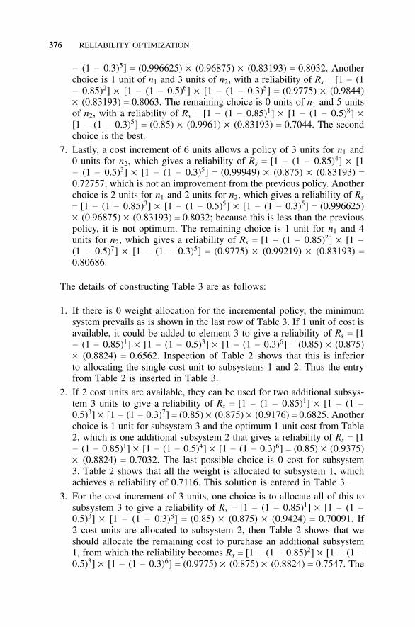
376 RELIABILITY OPTIMIZATION
− (1 − 0.3)5] c (0.996625) × (0.96875) × (0.83193) c 0.8032. Anotherchoice is 1 unit of n1 and 3 units of n2, with a reliability of Rs c [1 − (1− 0.85)2] × [1 − (1 − 0.5)6] × [1 − (1 − 0.3)5] c (0.9775) × (0.9844)× (0.83193) c 0.8063. The remaining choice is 0 units of n1 and 5 unitsof n2, with a reliability of Rs c [1 − (1 − 0.85)1] × [1 − (1 − 0.5)8] ×[1 − (1 − 0.3)5] c (0.85) × (0.9961) × (0.83193) c 0.7044. The secondchoice is the best.
7. Lastly, a cost increment of 6 units allows a policy of 3 units for n1 and0 units for n2, which gives a reliability of Rs c [1 − (1 − 0.85)4] × [1− (1 − 0.5)3] × [1 − (1 − 0.3)5] c (0.99949) × (0.875) × (0.83193) c
0.72757, which is not an improvement from the previous policy. Anotherchoice is 2 units for n1 and 2 units for n2, which gives a reliability of Rs
c [1 − (1 − 0.85)3] × [1 − (1 − 0.5)5] × [1 − (1 − 0.3)5] c (0.996625)× (0.96875) × (0.83193) c 0.8032; because this is less than the previouspolicy, it is not optimum. The remaining choice is 1 unit for n1 and 4units for n2, which gives a reliability of Rs c [1 − (1 − 0.85)2] × [1 −
(1 − 0.5)7] × [1 − (1 − 0.3)5] c (0.9775) × (0.99219) × (0.83193) c
0.80686.
The details of constructing Table 3 are as follows:
1. If there is 0 weight allocation for the incremental policy, the minimumsystem prevails as is shown in the last row of Table 3. If 1 unit of cost isavailable, it could be added to element 3 to give a reliability of Rs c [1− (1 − 0.85)1] × [1 − (1 − 0.5)3] × [1 − (1 − 0.3)6] c (0.85) × (0.875)× (0.8824) c 0.6562. Inspection of Table 2 shows that this is inferiorto allocating the single cost unit to subsystems 1 and 2. Thus the entryfrom Table 2 is inserted in Table 3.
2. If 2 cost units are available, they can be used for two additional subsys-tem 3 units to give a reliability of Rs c [1 − (1 − 0.85)1] × [1 − (1 −
0.5)3] × [1 − (1 − 0.3)7] c (0.85) × (0.875) × (0.9176) c 0.6825. Anotherchoice is 1 unit for subsystem 3 and the optimum 1-unit cost from Table2, which is one additional subsystem 2 that gives a reliability of Rs c [1− (1 − 0.85)1] × [1 − (1 − 0.5)4] × [1 − (1 − 0.3)6] c (0.85) × (0.9375)× (0.8824) c 0.7032. The last possible choice is 0 cost for subsystem3. Table 2 shows that all the weight is allocated to subsystem 1, whichachieves a reliability of 0.7116. This solution is entered in Table 3.
3. For the cost increment of 3 units, one choice is to allocate all of this tosubsystem 3 to give a reliability of Rs c [1 − (1 − 0.85)1] × [1 − (1 −
0.5)3] × [1 − (1 − 0.3)8] c (0.85) × (0.875) × (0.9424) c 0.70091. If2 cost units are allocated to subsystem 2, then Table 2 shows that weshould allocate the remaining cost to purchase an additional subsystem1, from which the reliability becomes Rs c [1 − (1 − 0.85)2] × [1 − (1 −
0.5)3] × [1 − (1 − 0.3)6] c (0.9775) × (0.875) × (0.8824) c 0.7547. The
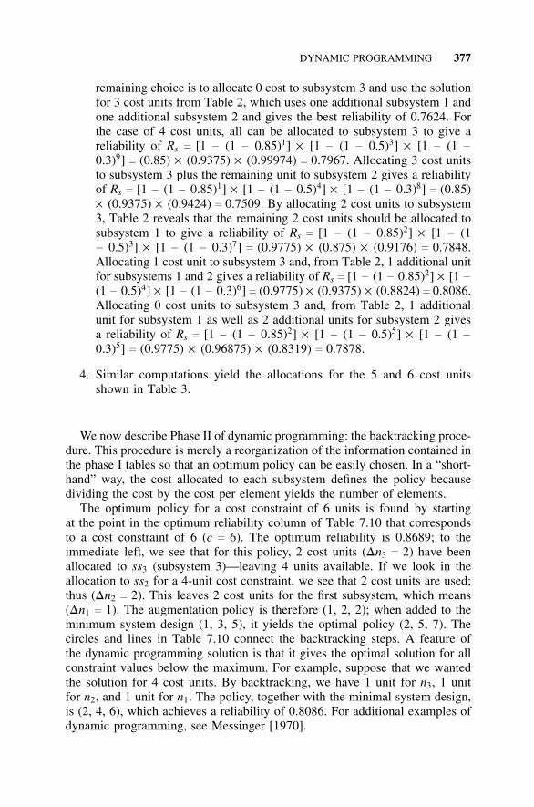
DYNAMIC PROGRAMMING 377
remaining choice is to allocate 0 cost to subsystem 3 and use the solutionfor 3 cost units from Table 2, which uses one additional subsystem 1 andone additional subsystem 2 and gives the best reliability of 0.7624. Forthe case of 4 cost units, all can be allocated to subsystem 3 to give areliability of Rs c [1 − (1 − 0.85)1] × [1 − (1 − 0.5)3] × [1 − (1 −
0.3)9] c (0.85) × (0.9375) × (0.99974) c 0.7967. Allocating 3 cost unitsto subsystem 3 plus the remaining unit to subsystem 2 gives a reliabilityof Rs c [1 − (1 − 0.85)1] × [1 − (1 − 0.5)4] × [1 − (1 − 0.3)8] c (0.85)× (0.9375) × (0.9424) c 0.7509. By allocating 2 cost units to subsystem3, Table 2 reveals that the remaining 2 cost units should be allocated tosubsystem 1 to give a reliability of Rs c [1 − (1 − 0.85)2] × [1 − (1− 0.5)3] × [1 − (1 − 0.3)7] c (0.9775) × (0.875) × (0.9176) c 0.7848.Allocating 1 cost unit to subsystem 3 and, from Table 2, 1 additional unitfor subsystems 1 and 2 gives a reliability of Rs c [1 − (1 − 0.85)2] × [1 −
(1 − 0.5)4] × [1 − (1 − 0.3)6] c (0.9775) × (0.9375) × (0.8824) c 0.8086.Allocating 0 cost units to subsystem 3 and, from Table 2, 1 additionalunit for subsystem 1 as well as 2 additional units for subsystem 2 givesa reliability of Rs c [1 − (1 − 0.85)2] × [1 − (1 − 0.5)5] × [1 − (1 −
0.3)5] c (0.9775) × (0.96875) × (0.8319) c 0.7878.
4. Similar computations yield the allocations for the 5 and 6 cost unitsshown in Table 3.
We now describe Phase II of dynamic programming: the backtracking proce-dure. This procedure is merely a reorganization of the information contained inthe phase I tables so that an optimum policy can be easily chosen. In a “short-hand” way, the cost allocated to each subsystem defines the policy becausedividing the cost by the cost per element yields the number of elements.
The optimum policy for a cost constraint of 6 units is found by startingat the point in the optimum reliability column of Table 7.10 that correspondsto a cost constraint of 6 (c c 6). The optimum reliability is 0.8689; to theimmediate left, we see that for this policy, 2 cost units (Dn3 c 2) have beenallocated to ss3 (subsystem 3)—leaving 4 units available. If we look in theallocation to ss2 for a 4-unit cost constraint, we see that 2 cost units are used;thus (Dn2 c 2). This leaves 2 cost units for the first subsystem, which means(Dn1 c 1). The augmentation policy is therefore (1, 2, 2); when added to theminimum system design (1, 3, 5), it yields the optimal policy (2, 5, 7). Thecircles and lines in Table 7.10 connect the backtracking steps. A feature ofthe dynamic programming solution is that it gives the optimal solution for allconstraint values below the maximum. For example, suppose that we wantedthe solution for 4 cost units. By backtracking, we have 1 unit for n3, 1 unitfor n2, and 1 unit for n1. The policy, together with the minimal system design,is (2, 4, 6), which achieves a reliability of 0.8086. For additional examples ofdynamic programming, see Messinger [1970].
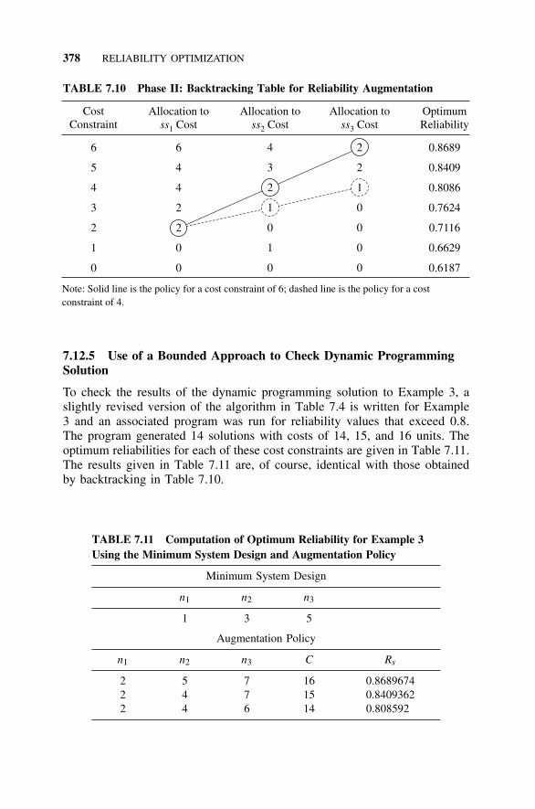
378 RELIABILITY OPTIMIZATION
TABLE 7.10 Phase II: Backtracking Table for Reliability Augmentation
6
5
4
3
2
1
0
6
4
4
2
2
0
0
4
3
2
1
0
1
0
2
2
1
0
0
0
0
0.8689
0.8409
0.8086
0.7624
0.7116
0.6629
0.6187
CostConstraint
Allocation toCostss1
Allocation toCostss2
Allocation toCostss3
OptimumReliability
Note: Solid line is the policy for a cost constraint of 6; dashed line is the policy for a costconstraint of 4.
7.12.5 Use of a Bounded Approach to Check Dynamic ProgrammingSolution
To check the results of the dynamic programming solution to Example 3, aslightly revised version of the algorithm in Table 7.4 is written for Example3 and an associated program was run for reliability values that exceed 0.8.The program generated 14 solutions with costs of 14, 15, and 16 units. Theoptimum reliabilities for each of these cost constraints are given in Table 7.11.The results given in Table 7.11 are, of course, identical with those obtainedby backtracking in Table 7.10.
TABLE 7.11 Computation of Optimum Reliability for Example 3Using the Minimum System Design and Augmentation Policy
Minimum System Design
n1 n2 n3
1 3 5
Augmentation Policy
n1 n2 n3 C Rs
2 5 7 16 0.86896742 4 7 15 0.84093622 4 6 14 0.808592
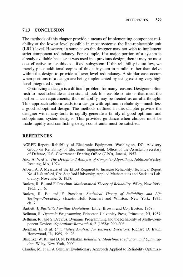
REFERENCES 379
7.13 CONCLUSION
The methods of this chapter provide a means of implementing component reli-ability at the lowest level possible in most systems: the line-replaceable unit(LRU) level. However, in some cases the designer may not wish to implementstrict component redundancy. For example, if a major portion of a system isalready available because it was used in a previous design, then it may be mostcost-effective to use this as a fixed subsystem. If the reliability is too low, wemerely place additional copies of this subsystem in parallel rather than delvewithin the design to provide a lower-level redundancy. A similar case occurswhen portions of a design are being implemented by using existing very highlevel integrated circuits.
Optimizing a design is a difficult problem for many reasons. Designers oftenrush to meet schedule and costs and look for feasible solutions that meet theperformance requirements; thus reliability may be treated as an afterthought.This approach seldom leads to a design with optimum reliability—much lessa good suboptimal design. The methods outlined in this chapter provide thedesigner with many tools to rapidly generate a family of good optimum andsuboptimum system designs. This provides guidance when choices must bemade rapidly and conflicting design constraints must be satisfied.
REFERENCES
AGREE Report. Reliability of Electronic Equipment. Washington, DC: AdvisoryGroup on Reliability of Electronic Equipment, Office of the Assistant Secretaryof Defense, U.S. Government Printing Office (GPO), June 4, 1957.
Aho, A. V. et al. The Design and Analysis of Computer Algorithms. Addison-Wesley,Reading, MA, 1974.
Albert, A. A Measure of the Effort Required to Increase Reliability. Technical ReportNo. 43. Stanford, CA: Stanford University, Applied Mathematics and Statistics Lab-oratory, November 5, 1958.
Barlow, R. E., and F. Proschan. Mathematical Theory of Reliability. Wiley, New York,1965, ch. 6.
Barlow, R. E., and F. Proschan. Statistical Theory of Reliability and LifeTesting—Probability Models. Holt, Rinehart and Winston, New York, 1975,ch. 7.
Bartlett, J. Bartlett’s Familiar Quotations. Little, Brown, and Co., Boston, 1968.Bellman, R. Dynamic Programming. Princeton University Press, Princeton, NJ, 1957.Bellman, R., and S. Dreyfus. Dynamic Programming and the Reliability of Multi-Com-
ponent Devices. Operations Research 6, 2 (1958): 200–206.Bierman, H. et al. Quantitative Analysis for Business Decisions. Richard D. Irwin,
Homewood, IL, 1969, ch. 23.Blischke, W. R., and D. N. Prabhakar. Reliability: Modeling, Prediction, and Optimiza-
tion. Wiley, New York, 2000.Claudio, M. et al. A Cellular, Evolutionary Approach Applied to Reliability Optimiza-
380 RELIABILITY OPTIMIZATION
tion of Complex Systems. Proceedings Annual Reliability and Maintainability Sym-posium, 2000. IEEE, New York, NY, pp. 210–215.
Coit, D. W., and A. E. Smith, Reliability Optimization of Series-Parallel Systems Usinga Genetic Algorithm. IEEE Transactions on Reliability 45 (1996): 254–260.
Cormen, T. H., C. E. Leiserson, and R. L. Riverset. Introduction to Algorithms.McGraw-Hill, New York, 1992.
Fragola, J. R., and J. F. Spahn. Economic Models for Satellite System Effectiveness.Proceedings Annual Reliability and Maintainability Symposium, 1973. IEEE, NewYork, NY, pp. 167–176.
Gilbert, G. A. Air Traffic Control: The Uncrowded Sky. Smithsonian Institution Press,Washington, DC, 1973.
Henney, K. et al. Reliability Factors for Ground Electronic Equipment. McGraw-Hill,New York, 1956.
Hiller, S. F., and G. J. Lieberman. Operations Research. Holden-Day, San Francisco,1974, ch. 6.
Lloyd, D. K., and M. Lipow. Reliability: Management, Methods, and Mathematics.Prentice-Hall, Englewood Cliffs, NJ, 1962.
Lloyd, D. K., and M. Lipow. Reliability: Management, Methods, and Mathematics, 2ded. ASQC, Milwaukee, WI, 1977.
Mancino, V. J. et al. Reliability Considerations for Communications Satellites. Pro-ceedings Annual Reliability and Maintainability Symposium, 1986. IEEE, NewYork, NY, pp. 389–396.
Marseguerra, M., and E. Zio. System Design Optimization by Genetic Algorithms.Proceedings Annual Reliability and Maintainability Symposium, 2000. IEEE, NewYork, NY, pp. 222–227.
Messinger, M. and M. L. Shooman. Techniques for Optimum Spares Allocation: ATutorial Review. IEEE Transactions on Reliability 19, 4 (November 1970).
Mettas, A. Reliability Allocation and Optimization for Complex Systems. ProceedingsAnnual Reliability and Maintainability Symposium, 2000. IEEE, New York, NY, pp.216–221.
Miller, G. A. The Magical Number Seven, Plus or Minus Two: Some Limits on ourCapacity for Processing Information. The Psychological Review 63, 2 (March 1956):p. 81.
Myers, R. H. et al. (eds.). Reliability Engineering for Electronic Systems. Wiley, NewYork, 1964.
Oliveto, F. E. An Algorithm to Partition the Operational Availability Parts of an Opti-mal Provisioning Strategy. Proceedings Annual Reliability and Maintainability Sym-posium, January 1999. IEEE, NY, pp. 310–316.
Rice, W. F., C. R. Cassady, and T. R. Wise. Simplifying the Solution of RedundancyAllocation Problems. Proceedings Annual Reliability and Maintainability Sympo-sium, January 1999. IEEE, New York, NY.
Rosen, K. H. Discrete Mathematics and its Applications. McGraw-Hill, New York,1999.
Shooman, M. L. Software Engineering, Design, Reliability, and Management.McGraw-Hill, New York, 1983.
PROBLEMS 381
Shooman, M. L. Probabilistic Reliability: An Engineering Approach, 2d ed. Krieger,Melbourne, FL, 1990.
Shooman, M. L., and C. Marshall. A Mathematical Formulation of Reliability Opti-mized Design. Proceedings IFIP 16th Conference on System Modeling and Opti-mization, Compiegne, France, July 5–9, 1993. (Also published in Henry, J., and J.-P.Yvon. System Modeling and Optimization. Lecture Notes in Control and Informa-tion Sciences 197. Springer-Verlag, London, 1994, pp. 941–950.)
Tillman, F. A., C. L. Hwang, and W. Kuo. Optimization Techniques for System Reli-ability with Redundancy—A Review. IEEE Transactions on Reliability 26, 1977,3, pp. 148–155.
Tillman, F. A., C. L. Hwang, and W. Kuo. Optimization of Systems Reliability. MarcelDekker, New York, 1980.
Von Alven, W. H., and ARINC Research Corporation Staff. Reliability Engineering.Prentice-Hall, Englewood Cliffs, NJ, 1964.
PROBLEMS
7.1. Why was Eq. (7.3) written in terms of probability of failure rather thanprobability of success?
7.2. There have been many studies of software errors that relate the numberof errors to the number of interfaces. Suppose that many of the hardwaredesign errors are also related to the number of interfaces. What can yousay about the complexity of the design and the number of errors basedon the results of Sections 7.5.2 and 7.5.3?
7.3. Repeat the apportionment example of Section 7.6.1 for reliability goalsof 0.90 and 0.99.
7.4. Repeat the apportionment example of Section 7.6.2 for reliability goalsof 0.90 and 0.99.
7.5. Repeat the apportionment example of Section 7.6.3 for reliability goalsof 0.90 and 0.99.
7.6. Repeat the apportionment example of Section 7.6.4 for reliability goalsof 0.90 and 0.99.
7.7. Comment on the results of problems 7.3–7.6 with respect to the difficultyof the computations, how close the results agree, and which results youthink are the most realistic.
7.8. Derive Eqs. (7.28a, b) by formulating a Markov model and solving theassociated equations.
7.9. Suppose the reliability goal for Example 1 of Section 7.7.2 is 0.95 andcompute the minimum system design. Repeat for a reliability goal of0.99.
382 RELIABILITY OPTIMIZATION
7.10. Repeat problem 7.9 for Example 2.
7.11. Write a computer program corresponding to the algorithm of Table 7.4and verify the results of Tables 7.5 and 7.6.
7.12. Change the program of problem 7.11 so that it prints out the results indescending order of reliability.
7.13. Repeat problem 7.11 for the algorithm of Table 7.7.
7.14. Repeat problem 7.12 for Example 2.
7.15. Rewrite the algorithm of Table 7.4 to include volume and weight con-straints as discussed in Section 7.8.5.
7.16. Repeat problem 7.15 for the algorithm of Table 7.7.
7.17. Compare the results of apportionment with the optimum system designfor Example 1 where the reliability goals are 0.95 and 0.99, as was donein Section 7.9.
7.18. Compare the results of apportionment with the optimum system designfor Example 2 where the reliability goals are 0.95 and 0.99, as was donein Section 7.9.
7.19. Repeat problem 7.9 for Example 3 given in Section 7.12.2, with reli-ability goals of 0.85, 0.90, and 0.95.
7.20. Write a computer program to solve for the minimum system design andthe augmentation policy of Example 3 of Section 7.12.2.
7.21. Modify the algorithm of Table 7.4 for the case of standby systems asdiscussed in Section 7.10.
7.22. Repeat problem 7.21 for Example 2.
7.23. Repeat problem 7.21 for Example 3.
7.24. Write a general program for bounded optimization that includes the fol-lowing features: (a) the input of the number of series subsystems andtheir reliability, cost, weight, and volume; and (b) the input of the sys-tem reliability goals and the cost, weight, and volume constraints. Then,specify which subsystems will use parallel and which will use standbyredundancy. Policies are to be printed in descending reliability order.
7.25. Write a program to solve the greedy algorithm of Section 7.11.2.
7.26. Use the greedy algorithm of Section 7.11.2 to solve for the optimum forExample 1.
7.27. Repeat problem 7.26 for Example 2.
7.28. Repeat problem 7.26 for Example 3.
PROBLEMS 383
7.29. Repeat problem 7.26 for the multiple constraints discussed in Section7.11.3.
7.30. Write a program to solve for the dynamic programming algorithm ofSection 7.12 and verify Tables 7.9 and 7.10.
7.31. A satellite communication system design is discussed in the article byMancino [1986]. The structure is essentially a series system with manycomponents paralleled to increase the reliability. Practical failure ratesare given for the system. Use the article to redesign the system by incor-porating optimum design principles, making any reasonable assump-tions. How does your design compare with that in the article? How wasthe design in the article achieved?
7.32. Starting with a component that has a failure rate of l, compare two dif-ferent ways of improving reliability: (a) by placing a second componentin parallel and (b) by improving the reliability of a single componentby high-quality design. What is the reduced equivalent failure rate of(a)? Comment on what you think the cost would be to achieve the samereductions if (b) is used.
7.33. Starting with a component that has a failure rate of l, compare two dif-ferent ways of improving reliability: (a) by placing a second componentin parallel and (b) by placing a second component in standby. What isthe reduced equivalent failure rate of (a)? Of (b)? Comment on what youthink the comparative cost would be to achieve the same reductions if(b) is used.
7.34. Choose a project with which you are familiar. Decompose the structureas was done in Fig. 7.3; then discuss.
APPENDIX A
SUMMARY OF PROBABILITYTHEORY*
Reliability of Computer Systems and Networks: Fault Tolerance, Analysis, and DesignMartin L. Shooman
Copyright 2002 John Wiley & Sons, Inc.ISBNs: 0-471-29342-3 (Hardback); 0-471-22460-X (Electronic)
384
A1 INTRODUCTION
Several of the analytical techniques discussed in this text are based on prob-ability theory. Many readers have an adequate background in probability andneed only refer to this appendix for notation and brief review. However, somereaders may not have studied probability, and this appendix should serve as abrief and concise introduction for them. If additional explanation is required,an introductory probability text should be consulted [Meeker, 1998; Menden-hall, 1990; Stone, 1996; Wadsworth and Bryan, 1960].
A2 PROBABILITY THEORY
“Probability had its beginnings in the 17th century when the Chevalier de Mere,supposedly an ardent gambler, became puzzled over how to divide the win-nings in a game of chance. He consulted the French mathematician BlaisePascal (1623–1662), who in turn wrote about this matter to Pierre Fermat(1601–1665); it is this correspondence which is generally considered the ori-gin of modern probability theory” [Freund, 1962]. In the 18th century KarlGauss (1777–1855) and Pierre Laplace (1749–1827) further developed proba-bility theory and applied it to fields other than games of chance.
Today, probability theory is viewed in three different ways: the a pri-
*This appendix is largely extracted from Appendix A of Software Engineering: Design,Reliability, and Management, by M. L. Shooman, McGraw-Hill, New York, 1983.
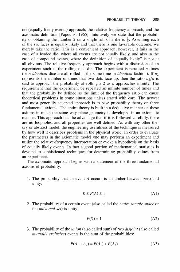
PROBABILITY THEORY 385
ori (equally-likely-events) approach, the relative-frequency approach, and theaxiomatic definition [Papoulis, 1965]. Intuitively we state that the probabil-ity of obtaining the number 2 on a single roll of a die is 1
6 . Assuming eachof the six faces is equally likely and that there is one favorable outcome, wemerely take the ratio. This is a convenient approach; however, it fails in thecase of a loaded die, where all events are not equally likely, and also in thecase of compound events, where the definition of “equally likely” is not atall obvious. The relative-frequency approach begins with a discussion of anexperiment such as the rolling of a die. The experiment is repeated n times(or n identical dice are all rolled at the same time in identical fashion). If n2
represents the number of times that two dots face up, then the ratio n2/ n issaid to approach the probability of rolling a 2 as n approaches infinity. Therequirement that the experiment be repeated an infinite number of times andthat the probability be defined as the limit of the frequency ratio can causetheoretical problems in some situations unless stated with care. The newestand most generally accepted approach is to base probability theory on threefundamental axioms. The entire theory is built in a deductive manner on theseaxioms in much the same way plane geometry is developed in an axiomaticmanner. This approach has the advantage that if it is followed carefully, thereare no loopholes, and all properties are well defined. As with any other the-ory or abstract model, the engineering usefulness of the technique is measuredby how well it describes problems in the physical world. In order to evaluatethe parameters in the axiomatic model one may perform an experiment andutilize the relative-frequency interpretation or evoke a hypothesis on the basisof equally likely events. In fact a good portion of mathematical statistics isdevoted to sophisticated techniques for determining probability values froman experiment.
The axiomatic approach begins with a statement of the three fundamentalaxioms of probability:
1. The probability that an event A occurs is a number between zero andunity:
0 ≤ P(A) ≤ 1 (A1)
2. The probability of a certain event (also called the entire sample space orthe universal set) is unity:
P(S ) c 1 (A2)
3. The probability of the union (also called sum) of two disjoint (also calledmutually exclusive) events is the sum of the probabilities:
P(A1 + A2) c P(A1) + P(A2) (A3)
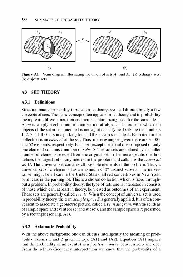
386 SUMMARY OF PROBABILITY THEORY
A1 A2A1 A2
C1 C2 C3
S
(a) (b)
Figure A1 Venn diagram illustrating the union of sets A1 and A2: (a) ordinary sets;(b) disjoint sets.
A3 SET THEORY
A3.1 Definitions
Since axiomatic probability is based on set theory, we shall discuss briefly a fewconcepts of sets. The same concept often appears in set theory and in probabilitytheory, with different notation and nomenclature being used for the same ideas.A set is simply a collection or enumeration of objects. The order in which theobjects of the set are enumerated is not significant. Typical sets are the numbers1, 2, 3, all 100 cars in a parking lot, and the 52 cards in a deck. Each item in thecollection is an element of the set. Thus, in the examples given there are 3, 100,and 52 elements, respectively. Each set (except the trivial one composed of onlyone element) contains a number of subsets. The subsets are defined by a smallernumber of elements selected from the original set. To be more specific one firstdefines the largest set of any interest in the problem and calls this the universalset U. The universal set contains all possible elements in the problem. Thus, auniversal set of n elements has a maximum of 2n distinct subsets. The univer-sal set might be all cars in the United States, all red convertibles in New York,or all cars in the parking lot. This is a chosen collection which is fixed through-out a problem. In probability theory, the type of sets one is interested in consistsof those which can, at least in theory, be viewed as outcomes of an experiment.These sets are generally called events. When the concept of universal set is usedin probability theory, the term sample space S is generally applied. It is often con-venient to associate a geometric picture, called a Venn diagram, with these ideasof sample space and event (or set and subset), and the sample space is representedby a rectangle (see Fig. A1).
A3.2 Axiomatic Probability
With the above background one can discuss intelligently the meaning of prob-ability axioms 1 and 2 given in Eqs. (A1) and (A2). Equation (A1) impliesthat the probability of an event A is a positive number between zero and one.From the relative-frequency interpretation we know that the probability of a
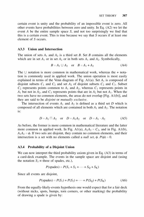
SET THEORY 387
certain event is unity and the probability of an impossible event is zero. Allother events have probabilities between zero and unity. In Eq. (A2) we let theevent A be the entire sample space S, and not too surprisingly we find thatthis is a certain event. This is true because we say that S occurs if at least oneelement of S occurs.
A3.3 Union and Intersection
The union of sets A1 and A2 is a third set B. Set B contains all the elementswhich are in set A1 or in set A2 or in both sets A1 and A2. Symbolically,
B c A1 U A2 or B c A1 + A2 (A4)
The U notation is more common in mathematical work, whereas the + nota-tion is commonly used in applied work. The union operation is most easilyexplained in terms of the Venn diagram of Fig. A1(a). Set A1 is composed ofdisjoint subsets C1 and C2 and set A2 of disjoint subsets C2 and C3. SubsetC2 represents points common to A1 and A2, whereas C1 represents points inA1 but not in A2, and C3 represents points that are in A2 but not A1. When thetwo sets have no common elements, the areas do not overlap [Fig. A1(b)], andthey are said to be disjoint or mutually exclusive.
The intersection of events A1 and A2 is defined as a third set D which iscomposed of all elements which are contained in both A1 and A2. The notationis:
D c A1U
A2 or D c A1A2 or D c A1 . A2 (A5)
As before, the former is more common in mathematical literature and the lattermore common in applied work. In Fig. A1(a), A1A2 c C2, and in Fig. A1(b),A1A2 c f. If two sets are disjoint, they contain no common elements, and theirintersection is a set with no elements called a null set, f. P(f) c 0.
A3.4 Probability of a Disjoint Union
We can now interpret the third probability axiom given in Eq. (A3) in terms ofa card-deck example. The events in the sample space are disjoint and (usingthe notation S3 ≡ three of spades, etc.),
P(spades) c P(S1 + S2 + · · · + SQ + SK)
Since all events are disjoint,
P(spades) c P(S1) + P(S2) + · · · + P(SQ) + P(SK) (A6)
From the equally-likely-events hypothesis one would expect that for a fair deck(without nicks, spots, bumps, torn corners, or other marking) the probabilityof drawing a spade is given by:
388 SUMMARY OF PROBABILITY THEORY
P(spades) c 152 + 1
52 + · · · + 152 + 1
52 c
1352 c
14
A4 COMBINATORIAL PROPERTIES
A4.1 Complement
The complement of set A, written as A, is another set B. The notation A′ issometimes used for complement, and both notations will be used interchange-ably in this book. Set B c A is composed of all the elements of the universalset which are not in set A. (The term A not is often used in engineering circlesinstead of A complement.) By definition the union of A and A is the universalset.
A + A c U (A7)
Applying axioms 2 and 3 from Eqs. (A3) and (A2) to Eq. (A7) yields
P(A + A) c P(A) + P(A) c P(S ) c 1
This is valid since A and A are obviously disjoint events (we have substitutedthe notation S for U, since the former is more common in probability work).Because probabilities are merely numbers, the above algebraic equation canbe written in three ways:
P(A) + P(A) c 1
P(A) c 1 − P(A)
P(A) c 1 − P(A) (A8)
There is considerable similarity between the logic operations presented aboveand the digital logic of Section C1.
A4.2 Probability of a Union
Perhaps the first basic relationship to be deduced is the probability of a unionof two events which are not mutually exclusive. We begin by extending theaxiom of Eq. (A3) to three or more events. Assuming that event A2 is the unionof two other disjoint events B1 + B2, we obtain
A2 c B1 + B2
P(A2 + A2) c P(A1) + P(B1 + B2) c P(A1) + P(B1) + P(B2)
By successive application of this stratagem of splitting events into unions ofother mutually exclusive events, we obtain the general result by induction
COMBINATORIAL PROPERTIES 389
P(A1 + A2 + · · · + An) c P(A1) + P(A2) + · · · + P(An) for disjoint A’s
(A9)
If we consider the case of two events A1 and A2 which are not disjoint,we can divide each event into the union of two subevents. This is most easilydiscussed with reference to the Venn diagram shown in Fig. A1(a). The event(set) A1 is divided into those elements (1) which are contained in A1 and notin A2, C1 and (2) which are common to A1 and A2, C2. Then A1 c C1 + C2.Similarly we define A2 c C3 +C2. We have now broken A1 and A2 into disjointevents and can apply Eq. (A9):
P(A1 + A2) c P(C1 + C2 + C2 + C3) c P[C1 + C3 + (C2 + C2)]
By definition, the union of C2 with itself is C2; therefore
P(A1 + A2) c P(C1 + C2 + C3) c P(C1) + P(C2) + P(C3)
We can manipulate this result into a more useful form if we add and subtractthe number P(C2) and apply Eq. (A3) in reverse
P(A1 + A2) c [P(C1) + P(C2)] + [P(C2) + P(C3)] − P(C2)
c P(A1) + P(A2) − P(A1A2) (A10)
Thus, when events A1 and A2 are not disjoint, we must subtract the probabilityof the union of A1 and A2 from the sum of the probabilities. Note that Eq.(A10) reduces to Eq. (A3) if events A1 and A2 are disjoint since P(A1A2) c 0for disjoint events.
Equation (A10) can be extended to apply to three or more events:
P(A1 + A2 + · · · + An)
c [P(A1) + P(A2) + · · · + P(An)] a � n1 � c n terms
− [ P(A1A2) + P(A1A3) + · · · + P � Aii � j
Aj� ] a � n2 � terms
+ [P(A1A2A3) + P(A1A2A4) + · · · + P�Ai Aji � j � k
Ak�] a � n3 � terms
. . . . . . . . . . . . . . . . . . . . . . . . . . . . . . . . . . . . . . . . . . . . . . . .
(−1)n − 1[P(A1A2 · · · An)] a � nn � c 1 term
(A11)
390 SUMMARY OF PROBABILITY THEORY
The complete expansion of Eq. (A11) involves (2n− 1) terms.
A4.3 Conditional Probabilities and Independence
It is important to study in more detail the probability of an intersection of twoevents, that is, P(A1A2). We are especially interested in how P(A1A2) is relatedto P(A1) and P(A2).
Before proceeding further we must define conditional probability and intro-duce a new notation. Suppose we want the probability of obtaining the four ofclubs on one draw from a deck of cards. The answer is of course 1/ 52, whichcan be written: P(C4) c 1/ 52. Let us change the problem so it reads: What isthe probability of drawing the four of clubs given that a club is drawn? Theanswer is 1/ 13.
In such a situation we call the probability statement a conditional probabil-ity. The notation P(C4 |C) c 1/ 13 is used to represent the conditional proba-bility of drawing a four of clubs given that a club is drawn. We read P(A2 |A1)as the probability of A2 occurring conditioned on the previous occurrence ofA1, or more simply as the probability of A2 given A1.
P(A1A2) c P(A1)P(A2 |A1) (A12a)
P(A1A2) c P(A2)P(A1 |A2) (A12b)
Intuition tells us that there must be many cases in which
P(A2 |A1) c P(A2)
In other words, the probability of occurrence of event A2 is independent of theoccurrence of event A1. From Eq. (A12a) we see that this implies P(A1A2) cP(A1)P(A2), and this latter result in turn implies
P(A1 |A2) c P(A1)
Thus we define independence by any one of the three equivalent relations
P(A1A2) c P(A1)P(A2) (A13a)
or
P(A1 |A2) c P(A1) (A13b)
or
P(A2 |A1) c P(A2) (A13c)
Conditional probabilities are sometimes called dependent probabilities.One can define conditional probabilities for three events by splitting event
DISCRETE RANDOM VARIABLES 391
B into the intersection of events A2 and A3. Then letting A c A1 and B c A2A3,we have
P(AB) c P(A)P(B |A) c P(A1)P(A2A3 |A1)
c P(A1)P(A2 |A1)P(A3 |A1A2)
Successive application of this technique leads to the general result
P(A1A2 · · · An) c P(A1)P(A2 |A1)P(A3 |A1A2) · · ·
P(An |A1A2 · · · An − 1) (A14)
Thus, the probability of the union of n terms is expressed as the joint productof one independent probability and n − 1 dependent probabilities.
A5 DISCRETE RANDOM VARIABLES
A5.1 Density Function
We can define x as a random variable if we associate each value of x withan element in event A defined on sample space S. If the random variable xassumes a finite number of values, then x is called a discrete random variable.In the case of a discrete random variable, we associate with each value ofx a number xi and a probability of occurrence P(xi). We could describe theprobabilities associated with the random variable by a table of values, but it iseasier to write a formula that permits calculation of P(xi) by substitution of theappropriate value of xi. Such a formula is called a probability function for therandom variable x. More exactly, we use the notation f (x) to mean a discreteprobability density function associated with the discrete random variable x.(The reason for the inclusion of the word “density” will be clear once theparallel development for continuous random variables is completed.) Thus,
P(x c xi) c P(xi) c f (xi) (A15)
In general we use the sequence of positive integers 0, 1, 2, . . . , n to representthe subscripts of the n + 1 discrete values of x. Thus, the random variable isdenoted by x and particular values of the random variable by x1, x2, . . . , xn. Ifthe random variable under consideration is a nonnumerical quantity, e.g., thecolors of the spectrum (red, orange, yellow, green, blue, indigo, violet), thenthe colors (or other quantity) would first be coded by associating a number 1to 7 with each. If the random variable x is defined over the entire sample spaceS, P(A) is given by
P(A) c ��� P(xi)for all xi
values whichare elements of A
c ��� f (xi)for all xi
in A
(A16)
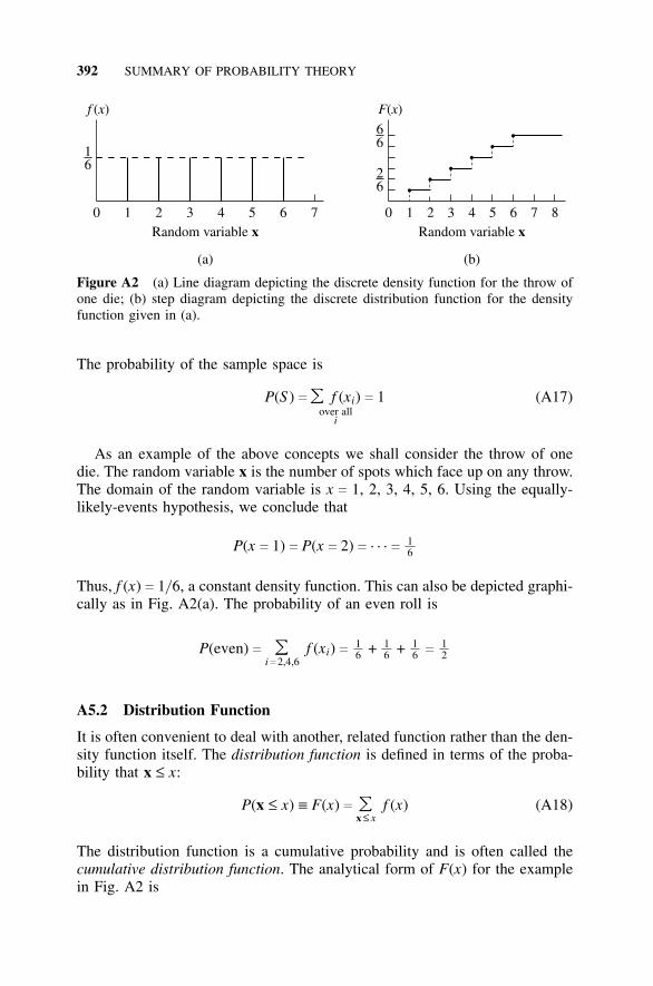
392 SUMMARY OF PROBABILITY THEORY
0 01 1 2 3 4 5 6 7 82 3 4 5 6 7
f x( ) F x( )
16
66
26
Random variable x Random variable x
(a) (b)
Figure A2 (a) Line diagram depicting the discrete density function for the throw ofone die; (b) step diagram depicting the discrete distribution function for the densityfunction given in (a).
The probability of the sample space is
P(S ) c ��� f (xi)over all
i
c 1 (A17)
As an example of the above concepts we shall consider the throw of onedie. The random variable x is the number of spots which face up on any throw.The domain of the random variable is x c 1, 2, 3, 4, 5, 6. Using the equally-likely-events hypothesis, we conclude that
P(x c 1) c P(x c 2) c · · · c 16
Thus, f (x) c 1/ 6, a constant density function. This can also be depicted graphi-cally as in Fig. A2(a). The probability of an even roll is
P(even) c ���i c 2,4,6
f (xi) c 16 + 1
6 + 16 c
12
A5.2 Distribution Function
It is often convenient to deal with another, related function rather than the den-sity function itself. The distribution function is defined in terms of the proba-bility that x ≤ x:
P(x ≤ x) ≡ F(x) c ���x ≤ x
f (x) (A18)
The distribution function is a cumulative probability and is often called thecumulative distribution function. The analytical form of F(x) for the examplein Fig. A2 is
DISCRETE RANDOM VARIABLES 393
F(x) cx6
for 1 ≤ x ≤ 6 (A19)
Equation (A19) related F(x) to f (x) by a process of summation. One canwrite an inverse relation1 defining f (x) in terms of the difference between twovalues of F(x)
f (x) c F(x+) − F(x− ) (A20)
In other words, f (x) is equal to the value of the discontinuity at x in the stepdiagram of F(x). There are a few basic properties of density and distributionfunctions which are of importance: (1) since f (x) is a probability, 0 ≤ f (x) ≤ 1;(2) because P(S ) c 1,
���allx
f (x) c 1
A5.3 Binomial Distribution
Many discrete probability models are used in applications, the foremost beingthe binomial distribution and the Poisson distribution. The binomial distri-bution (sometimes called the Bernoulli distribution) applies to a situation inwhich an event can either occur or not occur (the more common terms aresuccess or failure, a legacy from the days when probability theory centeredaround games of chance). The terms success and failure, of course, are ideallysuited to reliability applications. The probability of success on any one trial isp, and that of failure is 1 − p. The number of independent trials is denoted byn, and the number of successes by r. Thus, the probability of r successes in ntrials with the probability of one success being p is
B(r; n, p) c � nr � pr(1 − p)n − r for r c 0, 1, 2, . . . , n (A21)
where
� nr � c n!/ r!(n − r)! ≡ number of combinations of n things taken r at a time
A number of line diagrams for the binomial density function2 are given inFig. A3. In Fig. A3 the number of trials is fixed at nine, and the probabil-ity of success on each trial is changed from 0.2 to 0.5 to 0.8. Intuition tells us
1The notations F(x+) and F(x− ) mean the limits approached from the right and left, respectively.2We use the notation B(r; n, p) rather than the conventional and less descriptive notation f (x).
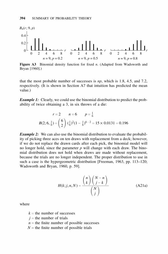
394 SUMMARY OF PROBABILITY THEORY
B r pn( ; 9, )
Figure A3 Binomial density function for fixed n. (Adapted from Wadsworth andBryan [1960].)
that the most probable number of successes is np, which is 1.8, 4.5, and 7.2,respectively. (It is shown in Section A7 that intuition has predicted the meanvalue.)
Example 1: Clearly, we could use the binomial distribution to predict the prob-ability of twice obtaining a 3, in six throws of a die:
r c 2 n c 6 p c
16
B(2; 6, 16 ) c � 6
2 � ( 16 )2(1 −
16 )6 − 2
c 15 × 0.0131 c 0.196
Example 2: We can also use the binomial distribution to evaluate the probabil-ity of picking three aces on ten draws with replacement from a deck; however,if we do not replace the drawn cards after each pick, the binomial model willno longer hold, since the parameter p will change with each draw. The bino-mial distribution does not hold when draws are made without replacement,because the trials are no longer independent. The proper distribution to use insuch a case is the hypergeometric distribution [Freeman, 1963, pp. 113–120;Wadsworth and Bryan, 1960, p. 59].
H(k; j, n, N ) c� n
k � �N − nj − k �
�Nj �
(A21a)
where
k c
j cn c
N c
the number of successesthe number of trialsthe finite number of possible successesthe finite number of possible trials
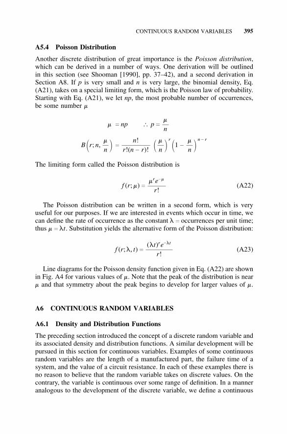
CONTINUOUS RANDOM VARIABLES 395
A5.4 Poisson Distribution
Another discrete distribution of great importance is the Poisson distribution,which can be derived in a number of ways. One derivation will be outlinedin this section (see Shooman [1990], pp. 37–42), and a second derivation inSection A8. If p is very small and n is very large, the binomial density, Eq.(A21), takes on a special limiting form, which is the Poisson law of probability.Starting with Eq. (A21), we let np, the most probable number of occurrences,be some number m
m c np � p c
m
n
B �r; n,m
n � c
n!r!(n − r)! �
m
n �r
�1 −
m
n �n − r
The limiting form called the Poisson distribution is
f (r; m) cmre−m
r!(A22)
The Poisson distribution can be written in a second form, which is veryuseful for our purposes. If we are interested in events which occur in time, wecan define the rate of occurrence as the constant l c occurrences per unit time;thus m c lt. Substitution yields the alternative form of the Poisson distribution:
f (r;l, t) c(lt)re−lt
r!(A23)
Line diagrams for the Poisson density function given in Eq. (A22) are shownin Fig. A4 for various values of m. Note that the peak of the distribution is nearm and that symmetry about the peak begins to develop for larger values of m.
A6 CONTINUOUS RANDOM VARIABLES
A6.1 Density and Distribution Functions
The preceding section introduced the concept of a discrete random variable andits associated density and distribution functions. A similar development will bepursued in this section for continuous variables. Examples of some continuousrandom variables are the length of a manufactured part, the failure time of asystem, and the value of a circuit resistance. In each of these examples there isno reason to believe that the random variable takes on discrete values. On thecontrary, the variable is continuous over some range of definition. In a manneranalogous to the development of the discrete variable, we define a continuous
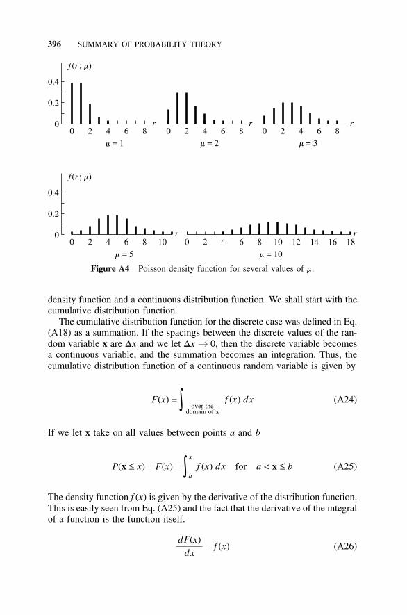
396 SUMMARY OF PROBABILITY THEORY
Figure A4 Poisson density function for several values of m.
density function and a continuous distribution function. We shall start with thecumulative distribution function.
The cumulative distribution function for the discrete case was defined in Eq.(A18) as a summation. If the spacings between the discrete values of the ran-dom variable x are Dx and we let Dx b 0, then the discrete variable becomesa continuous variable, and the summation becomes an integration. Thus, thecumulative distribution function of a continuous random variable is given by
F(x) c ∫ over thedomain of x
f (x) dx (A24)
If we let x take on all values between points a and b
P(x ≤ x) c F(x) c ∫x
af (x) dx for a < x ≤ b (A25)
The density function f (x) is given by the derivative of the distribution function.This is easily seen from Eq. (A25) and the fact that the derivative of the integralof a function is the function itself.
dF(x)dx
c f (x) (A26)
CONTINUOUS RANDOM VARIABLES 397
The probability that x lies in an interval x < x < x + dx is given by
P(x < x < x + dx) c P(x ≤ x + dx) − P(x ≤ x)
c ∫x + dx
af (x) dx − ∫
x
af (x) dx c ∫
x + dx
xf (x) dx
c F(x + dx) − F(x) (A27)
It is easy to see from Eq. (A27) that if F(x) is continuous and we let dx b 0,P(x c x) is zero. Thus, when we deal with continuous probability, it makessense to talk of the probability that x is within an interval rather than at onepoint. In fact since the P(x c x) is zero, the numerical value is the same in thecontinuous case whether the interval is open or closed since
P(a ≤ x ≤ b) c P(a < x < b) c P(a ≤ x < b) c P(a < x ≤ b)
Thus, the density function f (x) is truly a density, and like any other densityfunction it has a value only when integrated over some finite interval. The basicproperties of density and distribution functions previously discussed in the dis-crete case hold in the continuous case. At the lower limit of x we have F(a)c 0, and at the upper limit F(b) c 1. These two statements, coupled with Eq.(A27), lead to ∫
ba f (x) dx c 1. Since f (x) is a probability, f (x) is nonnegative,
and F(x), its integral, is a nondecreasing function.
A6.2 Rectangular Distribution
The simplest continuous variable distribution is the uniform or rectangular dis-tribution shown in Fig. A5(a). The two parameters of this distribution are thelimits a and b. This model predicts a uniform probability of occurrence in anyinterval
P(x < x ≤ x + Dx) c Dx(b − a)−1
between a and b.
A6.3 Exponential Distribution
Another simple continuous variable distribution is the exponential distribution.The exponential density function is
f (x) c le−lx 0 < x ≤ +∞ (A28)
which is sketched in Fig. A5(b). This distribution recurs time and time againin reliability work. The exponential is the distribution of the time to failure tfor a great number of electronic-system parts. The parameter l is constant and
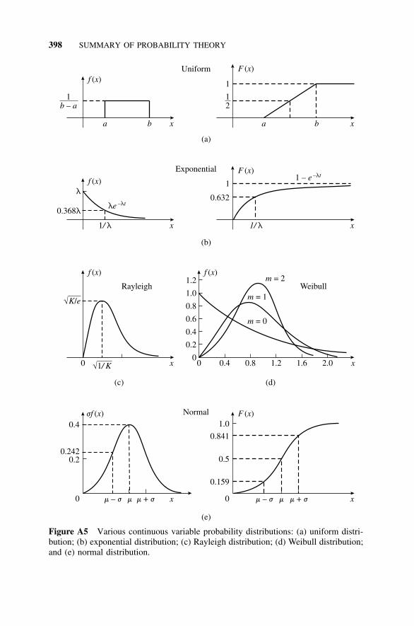
398 SUMMARY OF PROBABILITY THEORY
(a)
(b)
(e)
1–b a
12
1
a ab x xb
f x( )F x( )Uniform
1
0.632
1/ l 1/ lx x
f x( )F x( )Exponential
l
0.368lle –lt
1 – e –lt
m j– m j–m j+ m j+m mx x
jf x( ) F x( )Normal
0 0
0.159
0.5
0.841
1.0
0.20.242
0.4
1/ K x0
f x( )
K e/
Rayleigh
x0 0.4 0.8 1.2 1.6 2.00
0.2
0.4
0.6
0.8
1.0
1.2f x( )
Weibullm = 2
m = 1
m = 0
(c) (d)
Figure A5 Various continuous variable probability distributions: (a) uniform distri-bution; (b) exponential distribution; (c) Rayleigh distribution; (d) Weibull distribution;and (e) normal distribution.
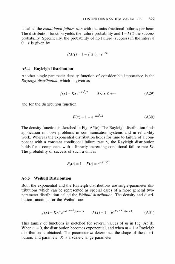
CONTINUOUS RANDOM VARIABLES 399
is called the conditional failure rate with the units fractional failures per hour.The distribution function yields the failure probability and 1 − F(t) the successprobability. Specifically, the probability of no failure (success) in the interval0 − t is given by
Ps(t1) c 1 − F(t1) c e−lt1
A6.4 Rayleigh Distribution
Another single-parameter density function of considerable importance is theRayleigh distribution, which is given as
f (x) c Kxe−Kx2/ 2 0 < x ≤ +∞ (A29)
and for the distribution function,
F(x) c 1 − e−Kx2/ 2 (A30)
The density function is sketched in Fig. A5(c). The Rayleigh distribution findsapplication in noise problems in communication systems and in reliabilitywork. Whereas the exponential distribution holds for time to failure of a com-ponent with a constant conditional failure rate l, the Rayleigh distributionholds for a component with a linearly increasing conditional failure rate Kt.The probability of success of such a unit is
Ps(t) c 1 − F(t) c e−Kt2/ 2
A6.5 Weibull Distribution
Both the exponential and the Rayleigh distributions are single-parameter dis-tributions which can be represented as special cases of a more general two-parameter distribution called the Weibull distribution. The density and distri-bution functions for the Weibull are
f (x) c Kxme−Kx m + 1/ (m + 1) F(x) c 1 − e−Kx m + 1/ (m + 1) (A31)
This family of functions is sketched for several values of m in Fig. A5(d).When m c 0, the distribution becomes exponential, and when m c 1, a Rayleighdistribution is obtained. The parameter m determines the shape of the distri-bution, and parameter K is a scale-change parameter.
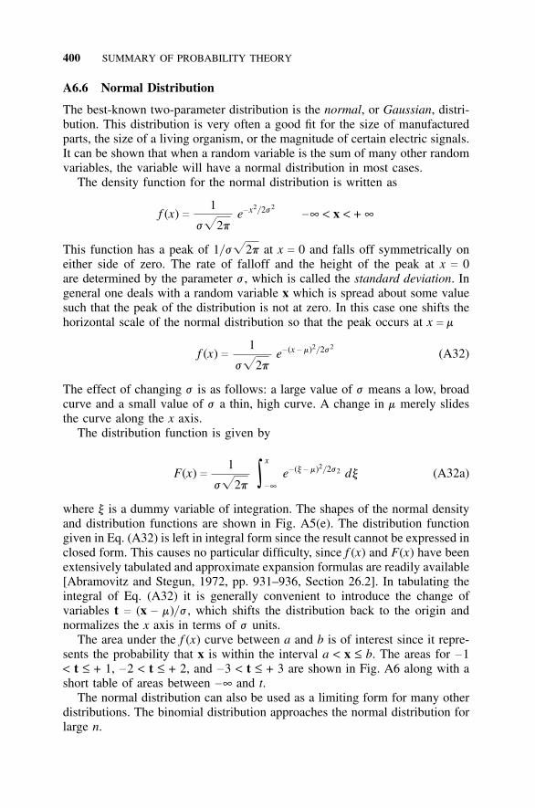
400 SUMMARY OF PROBABILITY THEORY
A6.6 Normal Distribution
The best-known two-parameter distribution is the normal, or Gaussian, distri-bution. This distribution is very often a good fit for the size of manufacturedparts, the size of a living organism, or the magnitude of certain electric signals.It can be shown that when a random variable is the sum of many other randomvariables, the variable will have a normal distribution in most cases.
The density function for the normal distribution is written as
f (x) c1
jf
2pe−x2/ 2j2 −∞ < x < + ∞
This function has a peak of 1/ jf
2p at x c 0 and falls off symmetrically oneither side of zero. The rate of falloff and the height of the peak at x c 0are determined by the parameter j , which is called the standard deviation. Ingeneral one deals with a random variable x which is spread about some valuesuch that the peak of the distribution is not at zero. In this case one shifts thehorizontal scale of the normal distribution so that the peak occurs at x c m
f (x) c 1
jf
2pe− (x − m)2/ 2j2
(A32)
The effect of changing j is as follows: a large value of j means a low, broadcurve and a small value of j a thin, high curve. A change in m merely slidesthe curve along the x axis.
The distribution function is given by
F(x) c 1
jf
2p ∫x
−∞e− (y − m)2/ 2j2 dy (A32a)
where y is a dummy variable of integration. The shapes of the normal densityand distribution functions are shown in Fig. A5(e). The distribution functiongiven in Eq. (A32) is left in integral form since the result cannot be expressed inclosed form. This causes no particular difficulty, since f (x) and F(x) have beenextensively tabulated and approximate expansion formulas are readily available[Abramovitz and Stegun, 1972, pp. 931–936, Section 26.2]. In tabulating theintegral of Eq. (A32) it is generally convenient to introduce the change ofvariables t c (x − m)/ j , which shifts the distribution back to the origin andnormalizes the x axis in terms of j units.
The area under the f (x) curve between a and b is of interest since it repre-sents the probability that x is within the interval a < x ≤ b. The areas for −1< t ≤ + 1, −2 < t ≤ + 2, and −3 < t ≤ + 3 are shown in Fig. A6 along with ashort table of areas between −∞ and t.
The normal distribution can also be used as a limiting form for many otherdistributions. The binomial distribution approaches the normal distribution forlarge n.
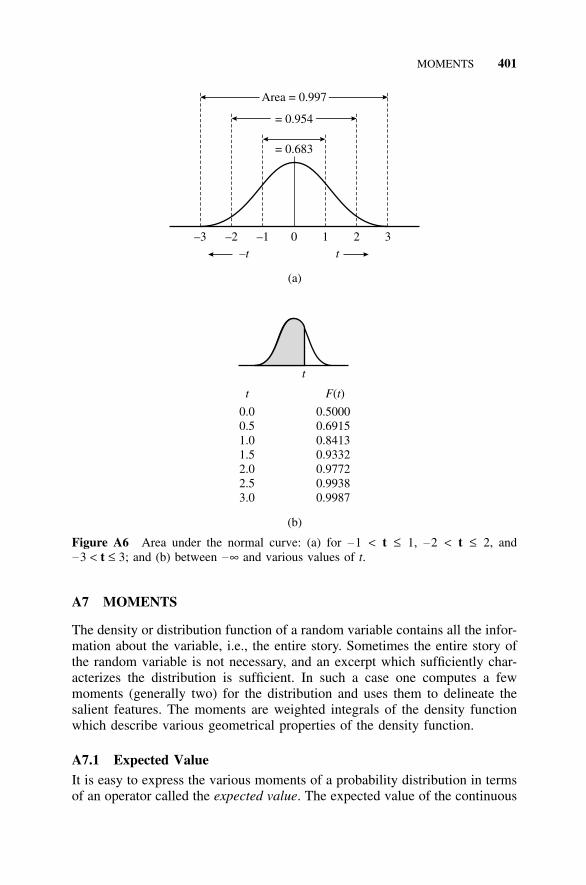
MOMENTS 401
Area = 0.997
= 0.954
= 0.683
–3 –2 –1 0 1 2 3–t t
t
t F t( )
0.00.51.01.52.02.53.0
0.50000.69150.84130.93320.97720.99380.9987
(a)
(b)
Figure A6 Area under the normal curve: (a) for −1 < t ≤ 1, −2 < t ≤ 2, and−3 < t ≤ 3; and (b) between −∞ and various values of t.
A7 MOMENTS
The density or distribution function of a random variable contains all the infor-mation about the variable, i.e., the entire story. Sometimes the entire story ofthe random variable is not necessary, and an excerpt which sufficiently char-acterizes the distribution is sufficient. In such a case one computes a fewmoments (generally two) for the distribution and uses them to delineate thesalient features. The moments are weighted integrals of the density functionwhich describe various geometrical properties of the density function.
A7.1 Expected ValueIt is easy to express the various moments of a probability distribution in termsof an operator called the expected value. The expected value of the continuous
402 SUMMARY OF PROBABILITY THEORY
random variable x defined over the range a < x ≤ b with density function f (x)is
E(x) c ∫b
ax f(x) dx (A33)
For a discrete random variable x taking on values x c x1, x2, . . . , xn the expectedvalue is defined in terms of a summation
E(x) cn
���i c 1
xi f (xi) (A34)
A7.2 Moments
To be more general one defines an entire set of moments. The nth moment ofthe random variable x computed about the origin and defined over the rangea < x ≤ b is given by
mr c ∫+∞
−∞xrf (x) dx (A35)
The zero-order moment m0 is the area under the density function, which is, ofcourse, unity. The first-order moment is simply the expected value, which iscalled the mean and is given the symbol m
m1 c E(x) c m (A36)
The origin moments for a discrete random variable which takes on the valuesx1, x2, . . . , xn are given by
mr c
n
���i c 1
xri f (xi) (A37)
It is often of importance to compute moments about the mean rather than theorigin. The set of moments about the mean are defined as follows:
For continuous random variables:
m′r c E[(x − m)r] c ∫+∞
−∞(x − m)rf (x) dx (A38)
For discrete random variables:
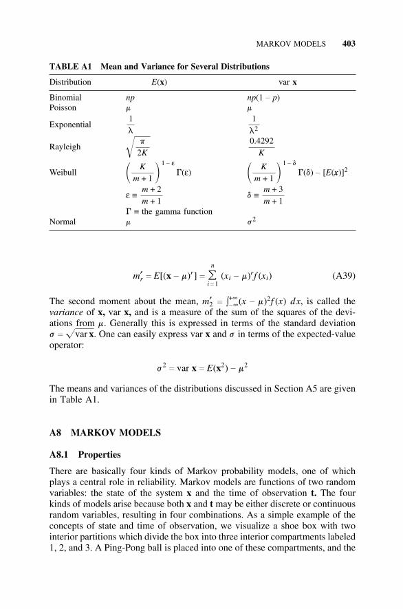
MARKOV MODELS 403
TABLE A1 Mean and Variance for Several Distributions
Distribution E(x) var x
Binomial np np(1 − p)Poisson m m
Exponential1l
1
l2
Rayleigh
hp
2K0.4292
K
Weibull � Km + 1 �
1 − εG(ε) � K
m + 1 �1 − d
G(d) − [E(x)]2
ε ≡m + 2m + 1
d ≡m + 3m + 1
G ≡ the gamma functionNormal m j2
m′r c E[(x − m)r] c n
���i c 1
(xi − m)rf (xi) (A39)
The second moment about the mean, m′2 c ∫+∞−∞(x − m)2f (x) dx, is called thevariance of x, var x, and is a measure of the sum of the squares of the devi-ations from m. Generally this is expressed in terms of the standard deviationj c fvar x. One can easily express var x and j in terms of the expected-valueoperator:
j2 c var x c E(x2) − m2
The means and variances of the distributions discussed in Section A5 are givenin Table A1.
A8 MARKOV MODELS
A8.1 Properties
There are basically four kinds of Markov probability models, one of whichplays a central role in reliability. Markov models are functions of two randomvariables: the state of the system x and the time of observation t. The fourkinds of models arise because both x and t may be either discrete or continuousrandom variables, resulting in four combinations. As a simple example of theconcepts of state and time of observation, we visualize a shoe box with twointerior partitions which divide the box into three interior compartments labeled1, 2, and 3. A Ping-Pong ball is placed into one of these compartments, and the
404 SUMMARY OF PROBABILITY THEORY
box is periodically tapped on the bottom, causing the Ping-Pong ball to jumpup and fall back into one of the three compartments. (For the moment weneglect the possibility that it falls out onto the floor.) The states of the systemare the three compartments in the box. The time of observation is immediatelyafter each rap, when the ball has fallen back into one of the compartments.Since we specified that the raps occur periodically, the model is discrete in bothstate and time. This sort of model is generally called a Markov chain model ora discrete-state discrete-time model. When the raps at the bottom of the boxoccur continuously, the model becomes a discrete-state continuous-time model,called a Markov process. If we remove the partitions and call the long axis ofthe box the x axis, we can visualize a continuum of states from x c − l/ 2to x c +l/ 2. If the ball is coated with rubber cement, it will stick whereverit hits when it falls back into the box. In this manner we can visualize theother two types of models, which involve a continuous-state variable. We shallbe concerned only with the discrete-state continuous-time model, the Markovprocess.
Any Markov model is defined by a set of probabilities pij which define theprobability of transition from any state i to any state j. If in the discrete-statecase we make our box compartments and the partitions equal in size, all thetransition probabilities should be equal. (In the general case, where each com-partment is of different size, the transition probabilities are unequal.) One ofthe most important features of any Markov model is that the transition prob-ability pij depends only on states i and j and is completely independent of allpast states except the last one, state i. This seems reasonable in terms of ourshoe-box model since transitions are really dependent only on the height of thewall between adjacent compartments i and j and the area of the compartmentsand not on the sequence of states the ball has occupied before arriving in statei. Before delving further into the properties of Markov processes, an exampleof great importance, the Poisson process, will be discussed.
A8.2 Poisson Process
In Section A5.4 the Poisson distribution was introduced as a limiting formof the binomial distribution. In this section we shall derive the Poisson dis-tribution as the governing probability law for a Poisson process, a particularkind of Markov process. In a Poisson process we are interested in the numberof occurrences in time, the probability of each occurrence in a small time Dtbeing a constant which is the parameter of the process. Examples of Poissonprocesses are the number of atoms transmuting as a function of time in theradioactive decay of a substance, the number of noise pulses as a function oftime in certain types of electric systems, and the number of failures for a groupof components operating in a standby mode or in an instantaneous-replacementsituation. The occurrences are discrete, and time is continuous; therefore thisis a discrete-state continuous-time model. The basic assumptions which arenecessary in deriving a Poisson process model are as follows:
MARKOV MODELS 405
1. The probability that a transition occurs from the state of n occurrencesto the state of n + 1 occurrences in time Dt as lDt. The parameter lis a constant and has the dimensions of occurrences per unit time. Theoccurrences are irreversible, which means that the number of occurrencescan never decrease with time.
2. Each occurrence is independent of all other occurrences.3. The transition probability of two or more occurrences in interval Dt
is negligible. Another way of saying this is to make use of theindependence-of-occurrence property and write the probability of twooccurrences in interval Dt as the product of the probability of each occur-rence, that is, (lDt)(lDt). This is obviously an infinitesimal of secondorder for Dt small and can be neglected.
We wish to solve for the probability of n occurrences in time t, and to thatend we set up a system of difference equations representing the state prob-abilities and transition probabilities. The probability of n occurrences havingtaken place by time t is denoted by
P(x c n, t) ≡ Pn(t)
For the case of zero occurrences at time t + Dt we write the following differ-ence equation:
P0(t + Dt) c (1 − lDt)P0(t) (A40)
which says that the probability of zero occurrences at time t + Dt is P0(t + Dt).This probability is given by the probability of zero occurrences at time t, P0(t),multiplied by the probability of no occurrences in interval Dt, 1 − lDt. For thecase of one occurrence at time t + Dt we write
P1(t + Dt) c (lDt)P0(t) + (1 − lDt)P1(t) (A41)
The probability of one occurrence at t + Dt, P1(t + Dt), can arise in two ways:(1) either there was no occurrence at time t, P0(t), and one happened in theinterval Dt (with probability lDt), or (2) there had already been one occurrenceat time t, P1(t), and no additional ones came along in the time interval Dt(probability 1 − lDt). It is clear that Eq. (A41) can be generalized, yielding
Pn(t + Dt) c (lDt)Pn − 1(t) + (1 − lDt)Pn(t) for n c 1, 2, . . . (A42)
The difference equations (A40) and (A41) really describe a discrete-timesystem, since time is divided into intervals Dt, but by taking limits as Dt b 0we obtain a set of differential equations which truly describe the continuous-time Poisson process. Rearranging Eq. (A40) and taking the limit of both sidesof the equation at Dt b 0 leads to
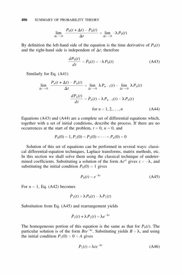
406 SUMMARY OF PROBABILITY THEORY
limDtb 0
P0(t + Dt) − P0(t)Dt
c limDtb 0
−lP0(t)
By definition the left-hand side of the equation is the time derivative of P0(t)and the right-hand side is independent of Dt; therefore
dP0(t)dt
c P0(t) c −lP0(t) (A43)
Similarly for Eq. (A41)
limDtb 0
Pn(t + Dt) − Pn(t)Dt
c limDtb 0
lPn − 1(t) − limDtb 0
lPn(t)
dPn(t)dt
c Pn(t) c lPn − 1(t) − lPn(t)
for n c 1, 2, . . . , n (A44)
Equations (A43) and (A44) are a complete set of differential equations which,together with a set of initial conditions, describe the process. If there are nooccurrences at the start of the problem, t c 0, n c 0, and
P0(0) c 1, P1(0) c P2(0) c · · · c Pn(0) c 0
Solution of this set of equations can be performed in several ways: classi-cal differential-equation techniques, Laplace transforms, matrix methods, etc.In this section we shall solve them using the classical technique of undeter-mined coefficients. Substituting a solution of the form Aest gives s c −l, andsubstituting the initial condition P0(0) c 1 gives
P0(t) c e−lt (A45)
For n c 1, Eq. (A42) becomes
P1(t) c lP0(t) − lP1(t)
Substitution from Eq. (A45) and rearrangement yields
P1(t) + lP1(t) c le−lt
The homogeneous portion of this equation is the same as that for P0(t). Theparticular solution is of the form Bte−lt . Substituting yields B c l, and usingthe initial condition P1(0) c 0 c A gives
P1(t) c lte−lt (A46)
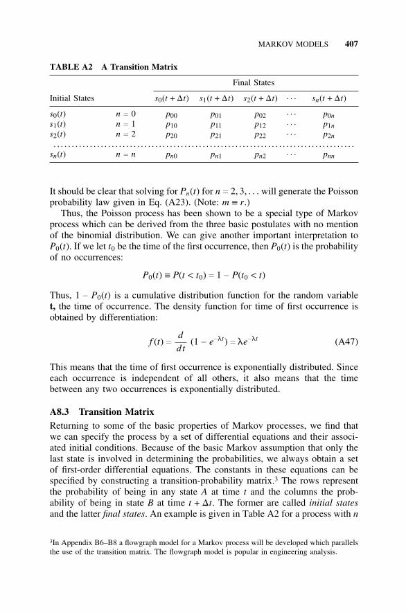
MARKOV MODELS 407
TABLE A2 A Transition Matrix
Final States
Initial States s0(t + Dt) s1(t + Dt) s2(t + Dt) · · · sn(t + Dt)
s0(t) n c 0 p00 p01 p02 · · · p0ns1(t) n c 1 p10 p11 p12 · · · p1ns2(t) n c 2 p20 p21 p22 · · · p2n. . . . . . . . . . . . . . . . . . . . . . . . . . . . . . . . . . . . . . . . . . . . . . . . . . . . . . . . . . . . . . . . . . . . . . . . . . . . . . . . . . .
sn(t) n c n pn0 pn1 pn2 · · · pnn
It should be clear that solving for Pn(t) for n c 2, 3, . . . will generate the Poissonprobability law given in Eq. (A23). (Note: m ≡ r.)
Thus, the Poisson process has been shown to be a special type of Markovprocess which can be derived from the three basic postulates with no mentionof the binomial distribution. We can give another important interpretation toP0(t). If we let t0 be the time of the first occurrence, then P0(t) is the probabilityof no occurrences:
P0(t) ≡ P(t < t0) c 1 − P(t0 < t)
Thus, 1 − P0(t) is a cumulative distribution function for the random variablet, the time of occurrence. The density function for time of first occurrence isobtained by differentiation:
f (t) cddt
(1 − e−lt) c le−lt (A47)
This means that the time of first occurrence is exponentially distributed. Sinceeach occurrence is independent of all others, it also means that the timebetween any two occurrences is exponentially distributed.
A8.3 Transition MatrixReturning to some of the basic properties of Markov processes, we find thatwe can specify the process by a set of differential equations and their associ-ated initial conditions. Because of the basic Markov assumption that only thelast state is involved in determining the probabilities, we always obtain a setof first-order differential equations. The constants in these equations can bespecified by constructing a transition-probability matrix.3 The rows representthe probability of being in any state A at time t and the columns the prob-ability of being in state B at time t + Dt. The former are called initial statesand the latter final states. An example is given in Table A2 for a process with n
3In Appendix B6–B8 a flowgraph model for a Markov process will be developed which parallelsthe use of the transition matrix. The flowgraph model is popular in engineering analysis.
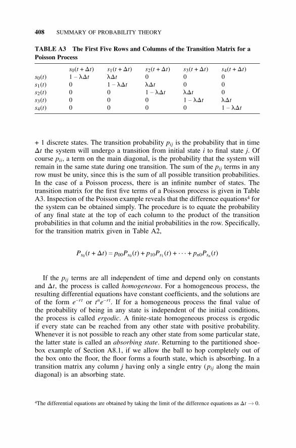
408 SUMMARY OF PROBABILITY THEORY
TABLE A3 The First Five Rows and Columns of the Transition Matrix for aPoisson Process
s0(t + Dt) s1(t + Dt) s2(t + Dt) s3(t + Dt) s4(t + Dt)s0(t) 1 − lDt lDt 0 0 0s1(t) 0 1 − lDt lDt 0 0s2(t) 0 0 1 − lDt lDt 0s3(t) 0 0 0 1 − lDt lDts4(t) 0 0 0 0 1 − lDt
+ 1 discrete states. The transition probability pij is the probability that in timeDt the system will undergo a transition from initial state i to final state j. Ofcourse pii, a term on the main diagonal, is the probability that the system willremain in the same state during one transition. The sum of the pij terms in anyrow must be unity, since this is the sum of all possible transition probabilities.In the case of a Poisson process, there is an infinite number of states. Thetransition matrix for the first five terms of a Poisson process is given in TableA3. Inspection of the Poisson example reveals that the difference equations4 forthe system can be obtained simply. The procedure is to equate the probabilityof any final state at the top of each column to the product of the transitionprobabilities in that column and the initial probabilities in the row. Specifically,for the transition matrix given in Table A2,
Ps0 (t + Dt) c p00Ps0 (t) + p10Ps1 (t) + · · · + pn0Psn (t)
If the pij terms are all independent of time and depend only on constantsand Dt, the process is called homogeneous. For a homogeneous process, theresulting differential equations have constant coefficients, and the solutions areof the form e−rt or tne−rt. If for a homogeneous process the final value ofthe probability of being in any state is independent of the initial conditions,the process is called ergodic. A finite-state homogeneous process is ergodicif every state can be reached from any other state with positive probability.Whenever it is not possible to reach any other state from some particular state,the latter state is called an absorbing state. Returning to the partitioned shoe-box example of Section A8.1, if we allow the ball to hop completely out ofthe box onto the floor, the floor forms a fourth state, which is absorbing. In atransition matrix any column j having only a single entry (pij along the maindiagonal) is an absorbing state.
4The differential equations are obtained by taking the limit of the difference equations as Dt b 0.
PROBLEMS 409
REFERENCES
Abramovitz, M., and I. Stegun (eds.). Handbook of Mathematical Functions. Washing-ton, DC: National Bureau of Standards, U.S. Government Printing Office (GPO),1972.
Freeman, H. Introduction to Statistical Inference. Addison-Wesley, Reading, MA,1963.
Freund, J. E. Mathematical Statistics. Prentice-Hall, Englewood Cliffs, NJ, 1962.Meeker, W. Q., and L. A. Escobar. Statistical Methods for Reliability Data. Wiley,
New York, 1998.Mendenhall, W. et al. Mathematical Statistics with Applications, 4th ed. PWS-Kent,
Boston, 1990.Papoulis, A. Probability, Random Variables, and Stochastic Processes. McGraw-Hill,
New York, 1965.Shooman, M. L. Probabilistic Reliability: An Engineering Approach. McGraw-Hill,
New York, 1968.Shooman, M. L. Software Engineering: Design, Reliability, and Management.
McGraw-Hill, New York, 1983.Shooman, M. L. Probabilistic Reliability: An Engineering Approach, 2d ed. Krieger,
Melbourne, FL, 1990.Stone, C. J. A Course in Probability and Statistics. Wadsworth Publishers, New York,
1996.Wadsworth, G. P., and J. G. Bryan. Introduction to Probability and Random Variables.
McGraw-Hill, New York, 1960.
PROBLEMS
Note: Problems A1–A5 are taken from Shooman [1990].
A1. The following two theorems are known as De Morgan’s theorems:
A + B + C c A B C
ABC c A + B + C
Prove these two theorems using a Venn diagram. Do these theorems holdfor more than three events? Explain.
A2. We wish to compute the probability of winning on the first roll of a pairof dice by throwing a seven or an eleven.(a) Define a sample space for the sum of the two dice.(b) Delineate the favorable and unfavorable outcomes.(c) Compute the probability of winning and losing.(d) List any assumptions you made in this problem.
410 SUMMARY OF PROBABILITY THEORY
A3. Suppose a resistor has a resistance R with mean of 100 Q and a toleranceof 5%, i.e., variation of 5 Q .(a) If the resistance values are normally distributed with m c 100 Q and
j c 5 Q , sketch f (R).(b) Assume that the resistance values have a Rayleigh distribution. If the
peak is to occur at 100 Q , what is the value of K? Plot the Rayleighdistribution on the same graph as the normal distribution of part (a).
A4. A certain resistor has a nominal value (mean) of 100 Q .(a) Assume a normal distribution and compute the value of j if we wish
P(95 < R < 105) c 0.95.(b) Repeat part (a) assuming a Weibull distribution and specify the values
of K and m.(c) Plot the density function for parts (a) and (b) on the same graph paper.
A5. Let a component have a good, a fair, and a bad state. Assume the transitionprobabilities of failure are from good to fair, lg f Dt; from good to bad,lgbDt; and from fair to bad, lf bDt.(a) Formulate a Markov model.(b) Compute the probabilities of being in any state.
APPENDIX B
SUMMARY OF RELIABILITYTHEORY*
Reliability of Computer Systems and Networks: Fault Tolerance, Analysis, and DesignMartin L. Shooman
Copyright 2002 John Wiley & Sons, Inc.ISBNs: 0-471-29342-3 (Hardback); 0-471-22460-X (Electronic)
411
B1 INTRODUCTION
B1.1 History
Since its beginnings following World War II, reliability theory has grown intoan engineering science in its own right. (The early development is discussedin Chapter 1 of Shooman [1990].) Much of the initial theory, engineering, andmanagement techniques centered about hardware; however, human and proce-dural elements of a system were often included. Since the late 1960s the termsoftware reliability has become popular, and now reliability theory refers toboth software and hardware reliability.
B1.2 Summary of the Approach
The conventional approach to reliability is to decompose the system intosmaller subsystems and units. Then by the use of combinatorial reliability,the system probability of success is expressed in terms of the probabilitiesof success of the elements. Then by the use of failure rate models, the elementprobabilities of success are computed. These two concepts are combined tocalculate the system reliability.
When reliability or availability of repairable systems is the appropriate fig-
*Parts of this appendix have been abstracted from Appendix B of Software Engineering: Design,Reliability, and Management, by M. L. Shooman, McGraw-Hill, New York, 1983; and alsoProbabilistic Reliability: An Engineering Approach, 2d ed., by M. L. Shooman, Krieger, 1990.
412 SUMMARY OF RELIABILITY THEORY
ure of merit, Markov models are generally used to compute the associatedprobabilities.
Often a proposed system does not meet its reliability specifications, and var-ious techniques of reliability improvement are utilized to improve the predictedreliability of the design.
Readers desiring more detail are referred to Shooman [1990] and the refer-ences cited in that text.
B1.3 Purpose of This Appendix
This appendix was written to serve several purposes. The prime reason is toprovide additional background for those techniques and principles of reliabiltytheory which are used in the software reliability models developed in Chap-ter 5. A second purpose is to expose software engineers who are not familiarwith reliability theory to some of the main methods and techniques. This isespecially important since many discussions of software reliability end up dis-cussing how much of “hardware reliability theory” is applicable to software.This author feels the correct answer is “some”; however, the only way to reallyappreciate this answer is to learn something about reliability.
The third purpose is to allow readers who are software engineers to talkwith and understand hardware reliability engineers. If a reliability and qual-ity control (R&QC) engineer handles the hardware reliability estimates andthe software engineer generates software reliability estimates, they must meetat the interface. Even if the R&QC engineer computes reliability estimatesfor both the hardware and the software, it is still necessary for the softwareengineer to work with him or her and provide information as well as roughlyevaluate the thoroughness and quality of the software effort.
B2 COMBINATORIAL RELIABILITY
B2.1 Introduction
In performing the reliability analysis of a complex system, it is almost impos-sible to treat the system in its entirety. The logical approach is to decomposethe system into functional entities composed of units, subsystems, or compo-nents. Each entity is assumed to have two states, one good and one bad. Thesubdivision generates a block-diagram or fault-tree description of system oper-ation. Models are then formulated to fit this logical structure, and the calculusof probability is used to compute the system reliability in terms of the subdivi-sion reliabilities. Series and parallel structures often occur, and their reliabilitycan be described very simply. In many cases the structure is of a more com-plicated nature, and more general techniques are needed.
The formulation of a structural-reliability model can be difficult in a large,sophisticated system and requires much approximation and judgment. This is
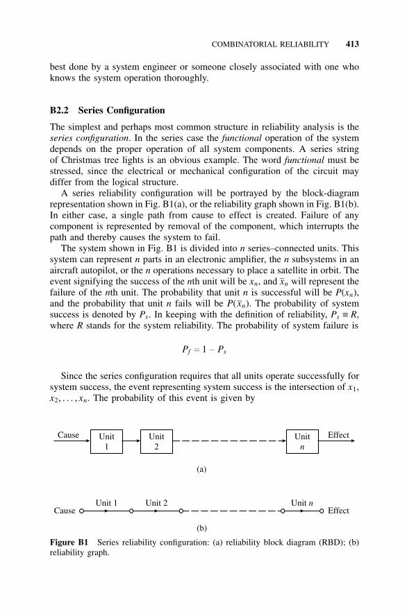
COMBINATORIAL RELIABILITY 413
best done by a system engineer or someone closely associated with one whoknows the system operation thoroughly.
B2.2 Series Configuration
The simplest and perhaps most common structure in reliability analysis is theseries configuration. In the series case the functional operation of the systemdepends on the proper operation of all system components. A series stringof Christmas tree lights is an obvious example. The word functional must bestressed, since the electrical or mechanical configuration of the circuit maydiffer from the logical structure.
A series reliability configuration will be portrayed by the block-diagramrepresentation shown in Fig. B1(a), or the reliability graph shown in Fig. B1(b).In either case, a single path from cause to effect is created. Failure of anycomponent is represented by removal of the component, which interrupts thepath and thereby causes the system to fail.
The system shown in Fig. B1 is divided into n series–connected units. Thissystem can represent n parts in an electronic amplifier, the n subsystems in anaircraft autopilot, or the n operations necessary to place a satellite in orbit. Theevent signifying the success of the nth unit will be xn, and xn will represent thefailure of the nth unit. The probability that unit n is successful will be P(xn),and the probability that unit n fails will be P(xn). The probability of systemsuccess is denoted by Ps. In keeping with the definition of reliability, Ps ≡ R,where R stands for the system reliability. The probability of system failure is
Pf c 1 − Ps
Since the series configuration requires that all units operate successfully forsystem success, the event representing system success is the intersection of x1,x2, . . . , xn. The probability of this event is given by
Unit 1 Unit 2 Unit nCause Effect
Unit1
Unit2
Unitn
Cause Effect
(b)
(a)
Figure B1 Series reliability configuration: (a) reliability block diagram (RBD); (b)reliability graph.
414 SUMMARY OF RELIABILITY THEORY
R c Ps c P(x1x2x3 · · · xn) (B1)
Expansion of Eq. (B1) yields
Ps c P(x1)P(x2 | x1)P(x3 | x1x2) · · · P(xn | x1x2 · · · xn − 1) (B2)
The expression appearing in Eq. (B2) contains conditional probabilities,which must be evaluated with care. For example, P(x3 | x1x2) is the probabil-ity of success of unit 3 evaluated under the condition that units 1 and 2 areoperating. In the case where the power dissipation from units 1 and 2 affectsthe temperature of unit 3 and thereby its failure rate, a conditional probabilityis involved. If the units do not interact, the failures are independent, and Eq.(B2) simplifies to
Ps c P(x1)P(x2)P(x3) · · · P(xn) (B3)
The reliability of a series system is always smaller than the smallest reli-ability of the set of components. The lowest relability in the series is oftenreferred to as “the weakest link in the chain.” An alternative approach is tocompute the probability of failure. The system fails if any of the units fail,and therefore we have a union of events
Pf c P(x1 + x2 + x3 + · · · + xn) (B4)
Expansion of Eq. (B4) yields
Pf c [P(x1) + P(x2) + P(x3) + · · · + P(xn)]
− [P(x1x2) + P(x1x3) + · · · + P (xixj)i � j
]
+ · · · + (−1)n − 1[P(x1x2 · · · xn)] (B5)
Since
Ps c 1 − Pf (B6)
the probability of system success becomes
Ps c 1 − P(x1) − P(x2) − P(x3) − · · · − P(xn) + P(x1)P(x2 | x1)
+ P(x1)P(x3 | x1) + · · · + P(xi)P (xi | xj)i � j
− · · · + (−1)nP(x1)P(x2 | x1) · · · P(xn | x1 · · · xn − 1) (B7)
The reliability expression in Eq. (B7) is equivalent to that in Eq. (B2) but ismuch more difficult to evaluate because of the many terms involved. Equation
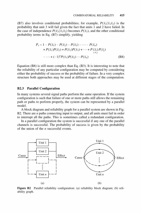
COMBINATORIAL RELIABILITY 415
(B7) also involves conditional probabilities; for example, P(x3 | x1x2) is theprobability that unit 3 will fail given the fact that units 1 and 2 have failed. Inthe case of independence P(x3 | x1x2) becomes P(x3), and the other conditionalprobability terms in Eq. (B7) simplify, yielding
Ps c 1 − P(x1) − P(x2) − P(x3) − · · · − P(xn)
+ P(x1)P(x2) + P(x1)P(x3) + · · · + P (xi)i � j
P(xj)
− · · · + (−1)nP(x1)P(x2) · · · P(xn) (B8)
Equation (B8) is still more complex than Eq. (B3). It is interesting to note thatthe reliability of any particular configuration may be computed by consideringeither the probability of success or the probability of failure. In a very complexstructure both approaches may be used at different stages of the computation.
B2.3 Parallel Configuration
In many systems several signal paths perform the same operation. If the systemconfiguration is such that failure of one or more paths still allows the remainingpath or paths to perform properly, the system can be represented by a parallelmodel.
A block diagram and reliability graph for a parallel system are shown in Fig.B2. There are n paths connecting input to output, and all units must fail in orderto interrupt all the paths. This is sometimes called a redundant configuration.
In a parallel configuration the system is successful if any one of the parallelchannels is successful. The probability of success is given by the probabilityof the union of the n successful events.
(a) (b)
Unit 1
Unit 2
Unit n
Cause Effect
•••
Unit n
Unit 1
Unit 2
Effect•••
Cause
Figure B2 Parallel reliability configuration: (a) reliability block diagram; (b) reli-ability graph.
416 SUMMARY OF RELIABILITY THEORY
Ps c P(x1 + x2 + x3 + · · · + xn) (B9)
Expansion of Eq. (B9) yields
Ps c [P(x1) + P(x2) + P(x3) + · · · + P(xn)]
− [P(x1x2) + P(x1x3) + · · · + P (xixj)i � j
]
+ · · · + (−1)n − 1P(x1x2 · · · xn) (B10)
The conditional probabilties which occur in Eq. (B10) when the intersectionterms are expanded must be interpreted properly, as in the previous section[see Eq. (B7)]. A simpler formula can be developed in the parallel case if onedeals with the probability of system failure. System failure occurs if all thesystem units fail, yielding the probability of their intersection.
Pf c P(x1x2x3 · · · xn) (B11)
where
Ps c 1 − Pf (B12)
Substitution of Eq. (B11) into Eq. (B12) and expansion yields
Ps c 1 − P(x1)P(x2 | x1)P(x3 | x1x2) · · · P(xn | x1x2 · · · xn − 1) (B13)
If the unit failures are independent, Eq. (B13) simplifies to
Ps c 1 − P(x1)P(x2) · · · P(xn) (B14)
B2.4 An r-out-of-n Configuration
In many problems the system operates if r out of n units function, e.g., a bridgesupported by n cables, r of which are necessary to support the maximum load.If each of the n units is identical, the probabiality of exactly r successes outof n units is given by Eq. (A21)
B(r ; n, p) c � nr � pr(1 − p)n − r for r c 0, 1, 2 · · · n (B15)
where p is the probability of success of any unit. The system will succeed if r,r + 1 · · · n − 1, or n units succeed. The probability of system success is givenby
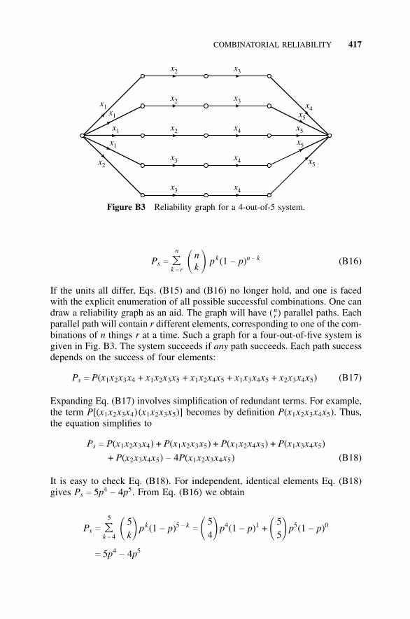
COMBINATORIAL RELIABILITY 417
x2
x2
x2
x3
x3
x3
x3
x4 x5x1
x5x1
x5x1
x4x1
x5x2x4
x4
Figure B3 Reliability graph for a 4-out-of-5 system.
Ps c
n
���k c r �
nk � pk(1 − p)n − k (B16)
If the units all differ, Eqs. (B15) and (B16) no longer hold, and one is facedwith the explicit enumeration of all possible successful combinations. One candraw a reliability graph as an aid. The graph will have (n
r ) parallel paths. Eachparallel path will contain r different elements, corresponding to one of the com-binations of n things r at a time. Such a graph for a four-out-of-five system isgiven in Fig. B3. The system succeeds if any path succeeds. Each path successdepends on the success of four elements:
Ps c P(x1x2x3x4 + x1x2x3x5 + x1x2x4x5 + x1x3x4x5 + x2x3x4x5) (B17)
Expanding Eq. (B17) involves simplification of redundant terms. For example,the term P[(x1x2x3x4)(x1x2x3x5)] becomes by definition P(x1x2x3x4x5). Thus,the equation simplifies to
Ps c P(x1x2x3x4) + P(x1x2x3x5) + P(x1x2x4x5) + P(x1x3x4x5)
+ P(x2x3x4x5) − 4P(x1x2x3x4x5) (B18)
It is easy to check Eq. (B18). For independent, identical elements Eq. (B18)gives Ps c 5p4
− 4p5. From Eq. (B16) we obtain
Ps c
5
���k c 4 �
5k� pk(1 − p)5 − k
c � 54� p4(1 − p)1 + � 5
5� p5(1 − p)0
c 5p4− 4p5
418 SUMMARY OF RELIABILITY THEORY
B2.5 Fault-Tree Analysis
Fault-tree analysis (FTA) is an application of deductive logic to produce afailure- or fault-oriented pictorial diagram, which allows one to analyze systemsafety and reliability. Various failure modes that can contribute to a specifiedundesirable event are organized deductively and represented pictorially.
First the top undesired event is defined and drawn. Below this, secondaryundesired events are drawn. These secondary undesired events include thepotential hazards and failures that are immediate causes of the top event.Below each of these subevents are drawn second-level events, which are theimmediate causes of the subevents. The process is continued until basic eventsare reached (often called elementary faults). Since the diagram branches outand there are more events at each lower level, it resembles an inverted tree.The treelike structure of the diagram illustrates the various critical paths ofsubevents leading to the occurrence of the top undesired event. A fault treefor an auto braking system example is given in Section B5, Fig. B13.
Both FTAs and RBDs are useful for both qualitative and quantitative anal-yses:
1. They force the analyst to actively seek out failure events (success events)in a deductive manner.
2. They provide a visual display of how a system can fail, and thus aidunderstanding of the system by persons other than the designer.
3. They point out critical aspects of systems failure (system success).
4. They provide a systematic basis for quantitative analysis of reliability.
Often in a difficult practical problem one utilizes other techniques to decom-pose the system prior to effecting either an RBD or an FTA.
B2.6 Failure Mode and Effect Analysis
Failure mode and effect analysis (FMEA) is a systematic procedure for iden-tifying the modes of failures and for evaluating their consequences. It is atabular procedure which considers hazards in terms of single-event chains andtheir consequences. The FMEA is generally performed on the basis of lim-ited design information during the early stages of design and is periodicallyupdated to reflect changes in design and improved knowledge of the system.The basic questions which must be answered by the analyst in performing anFMEA are:
1. How can each component or subsystem fail? (What is the failure mode?)
2. What cause might produce this failure? (What is the failure mechanism?)
3. What are the effects of each failure if it does occur?
COMBINATORIAL RELIABILITY 419
Once the FMEA is completed, it assists the analyst in:
1. Selecting, during initial stages, various design alternatives with high reli-ability and high safety potential
2. Ensuring that all possible failure modes, and their effects on operationalsuccess of the system, have been taken into account
3. Identifying potential failures and the magnitude of their effects on thesystem
4. Developing testing and checkout methods5. Providing a basis for qualitative reliability, availability, and safety anal-
ysis6. Providing input data for construction of RBD and FTA models7. Providing a basis for establishing corrective measures8. Performing an objective evaluation of design requirements related to
redundancy, failure detection systems, and fail-safe character
An FMEA for the auto braking example is given in Section B5, Table B3.
B2.7 Cut-Set and Tie-Set Methods
A very efficient general method for computing the reliability of any systemnot containing dependent failures can be developed from the properties of thereliability graph. The reliability graph consists of a set of branches which rep-resent the n elements. There must be at least n branches in the graph, but therecan be more if the same branch must be repeated in more than one path (seeFig. B3). The probability of element success is written above each branch. Thenodes of the graph tie the branches together and form the structure. A path hasalready been defined, but a better definition can be given in terms of graph the-ory. The term tie set, rather than path, is common in graph nomenclature. A tieset is a group of branches which forms a connection between input and outputwhen traversed in the arrow direction. We shall primarily be concerned withminimal tie sets, which are those containing a minimum number of elements.If no node is traversed more than once in tracing out a tie set, the tie set isminimal. If a system has i minimal tie sets denoted by T1, T2, . . . , Ti, thenthe system has a connection between input and output if at least one tie set isintact. The system reliability is thus given by
R c P(T1 + T2 + · · · + Ti) (B19)
One can define a cut set of a graph as a set of branches which interruptsall connections between input and output when removed from the graph. Theminimal cut sets are a group of distinct cut sets containing a minimum numberof terms. All system failures can be represented by the removal of at least oneminimal cut set from the graph. The probability of system failure is, therefore,
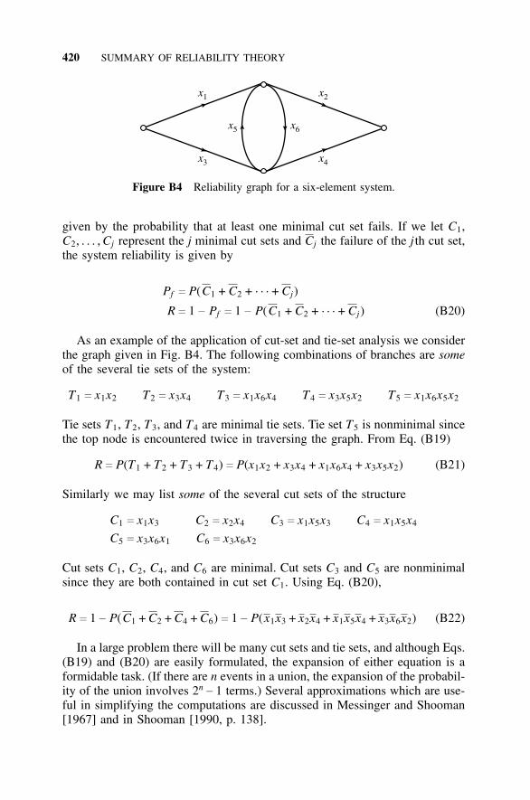
420 SUMMARY OF RELIABILITY THEORY
x1
x5 x6
x3
x2
x4
Figure B4 Reliability graph for a six-element system.
given by the probability that at least one minimal cut set fails. If we let C1,C2, . . . , Cj represent the j minimal cut sets and Cj the failure of the j th cut set,the system reliability is given by
Pf c P(C1 + C2 + · · · + Cj)
R c 1 − Pf c 1 − P(C1 + C2 + · · · + Cj) (B20)
As an example of the application of cut-set and tie-set analysis we considerthe graph given in Fig. B4. The following combinations of branches are someof the several tie sets of the system:
T1 c x1x2 T2 c x3x4 T3 c x1x6x4 T4 c x3x5x2 T5 c x1x6x5x2
Tie sets T1, T2, T3, and T4 are minimal tie sets. Tie set T5 is nonminimal sincethe top node is encountered twice in traversing the graph. From Eq. (B19)
R c P(T1 + T2 + T3 + T4) c P(x1x2 + x3x4 + x1x6x4 + x3x5x2) (B21)
Similarly we may list some of the several cut sets of the structure
C1 c x1x3 C2 c x2x4 C3 c x1x5x3 C4 c x1x5x4
C5 c x3x6x1 C6 c x3x6x2
Cut sets C1, C2, C4, and C6 are minimal. Cut sets C3 and C5 are nonminimalsince they are both contained in cut set C1. Using Eq. (B20),
R c 1 − P(C1 + C2 + C4 + C6) c 1 − P(x1x3 + x2x4 + x1x5x4 + x3x6x2) (B22)
In a large problem there will be many cut sets and tie sets, and although Eqs.(B19) and (B20) are easily formulated, the expansion of either equation is aformidable task. (If there are n events in a union, the expansion of the probabil-ity of the union involves 2n
− 1 terms.) Several approximations which are use-ful in simplifying the computations are discussed in Messinger and Shooman[1967] and in Shooman [1990, p. 138].
FAILURE-RATE MODELS 421
B3 FAILURE-RATE MODELS
B3.1 IntroductionThe previous section has shown how one constructs various combinatorial reli-ability models which express system reliability in terms of element reliabil-ity. This section introduces several different failure models for the system ele-ments. These element failure models are related to life-test results and failure-rate data via probability theory.
The first step in constructing a failure model is to locate test data or plan atest on parts substantially the same as those to be used. From these data the partfailure rate is computed and graphed. On the basis of the graph, any physicalfailure information, engineering judgment, and sometimes statistical tests, afailure-rate model is chosen. The parameters of the model are estimated fromthe graph or computed using the statistical principles of estimation, which aredeveloped in Section A9. This section discusses the treatment of the data andthe choice of a model.
The emphasis is on simple models, which are easy to work with and con-tain one or two parameters. This simplifies the problems of interpretation andparameter determination. Also in most cases the data are not abundant enoughand the test conditions are not sufficiently descriptive of the proposed usageto warrant more complex models.
B3.2 Treatment of Failure DataPart failure data are generally obtained from either of two sources: the failuretimes of various items in a population placed on a life test, or repair reports list-ing operating hours of replaced parts in equipment already in field use. Expe-rience has shown that a very good way to prevent these data is to compute andplot either the failure density function or the hazard rate as a function of time.
The data we are dealing with are a sequence of times to failure, but the failuredensity function and the hazard rate are continuous variables. We first computea piecewise-continuous failure density function and hazard rate from the data.
We begin by defining piecewise-continuous failure density and hazard-ratefunctions in terms of the data. It can be shown that these discrete functionsapproach the continuous functions in the limit as the number of data becomeslarge and the interval between failure times approaches zero. Assume that ourdata describe a set of N items placed in operation at time t c 0. As time progresses,items fail, and at any time t the number of survivors is n(t). The data densityfunction (also called empirical density function) defined over the time intervalti < t ≤ ti + Dti is given by the ratio of the number of failures occurring in theinterval to the size of the original population, divided by the length of the timeinterval1
1In general a sequence of time intervals t0 < t ≤ t0 + Dt0, t1 < t ≤ t1 + Dt1, etc., is defined, wheret1 c t0 + Dt0, t2 c t1 + Dt1, etc.
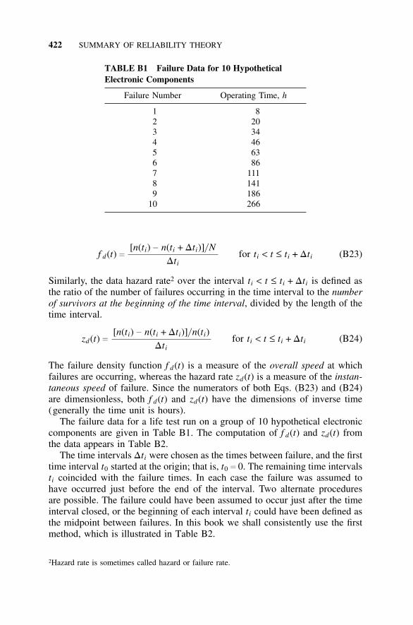
422 SUMMARY OF RELIABILITY THEORY
TABLE B1 Failure Data for 10 HypotheticalElectronic Components
Failure Number Operating Time, h
1 82 203 344 465 636 867 1118 1419 186
10 266
f d(t) c[n(ti) − n(ti + Dti)]/ N
Dtifor ti < t ≤ ti + Dti (B23)
Similarly, the data hazard rate2 over the interval ti < t ≤ ti + Dti is defined asthe ratio of the number of failures occurring in the time interval to the numberof survivors at the beginning of the time interval, divided by the length of thetime interval.
zd(t) c[n(ti) − n(ti + Dti)]/ n(ti)
Dtifor ti < t ≤ ti + Dti (B24)
The failure density function f d(t) is a measure of the overall speed at whichfailures are occurring, whereas the hazard rate zd(t) is a measure of the instan-taneous speed of failure. Since the numerators of both Eqs. (B23) and (B24)are dimensionless, both f d(t) and zd(t) have the dimensions of inverse time(generally the time unit is hours).
The failure data for a life test run on a group of 10 hypothetical electroniccomponents are given in Table B1. The computation of f d(t) and zd(t) fromthe data appears in Table B2.
The time intervals Dti were chosen as the times between failure, and the firsttime interval t0 started at the origin; that is, t0 c 0. The remaining time intervalsti coincided with the failure times. In each case the failure was assumed tohave occurred just before the end of the interval. Two alternate proceduresare possible. The failure could have been assumed to occur just after the timeinterval closed, or the beginning of each interval ti could have been defined asthe midpoint between failures. In this book we shall consistently use the firstmethod, which is illustrated in Table B2.
2Hazard rate is sometimes called hazard or failure rate.
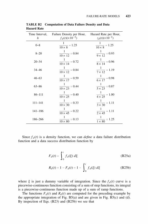
FAILURE-RATE MODELS 423
TABLE B2 Computation of Data Failure Density and DataHazard Rate
Time Interval, Failure Density per Hour, Hazard Rate per Hour,h f d(t)(×10−2) zd(t)(×10−2)
0–81
10 × 8c 1.25
110 × 8
c 1.25
8–201
10 × 12c 0.84
19 × 12
c 0.93
20–341
10 × 14c 0.72
18 × 14
c 0.96
34–461
10 × 12c 0.84
17 × 12
c 1.19
46–631
10 × 17c 0.59
16 × 17
c 0.98
63–861
10 × 23c 0.44
15 × 23
c 0.87
86–1111
10 × 25c 0.40
14 × 25
c 1.00
111–1411
10 × 30c 0.33
13 × 30
c 1.11
141–1861
10 × 45c 0.22
12 × 45
c 1.11
186–2661
10 × 80c 0.13
11 × 80
c 1.25
Since f d(t) is a density function, we can define a data failure distributionfunction and a data success distribution function by
Fd(t) c ∫t
0f d(y) dy (B25a)
Rd(t) c 1 − Fd(t) c 1 − ∫t
0f d(y) dy (B25b)
where y is just a dummy variable of integration. Since the f d(t) curve is apiecewise-continuous function consisting of a sum of step functions, its integralis a piecewise-continuous function made up of a sum of ramp functions.
The functions Fd(t) and Rd(t) are computed for the preceding example bythe appropriate integration of Fig. B5(a) and are given in Fig. B5(c) and (d).By inspection of Eqs. (B23) and (B25b) we see that
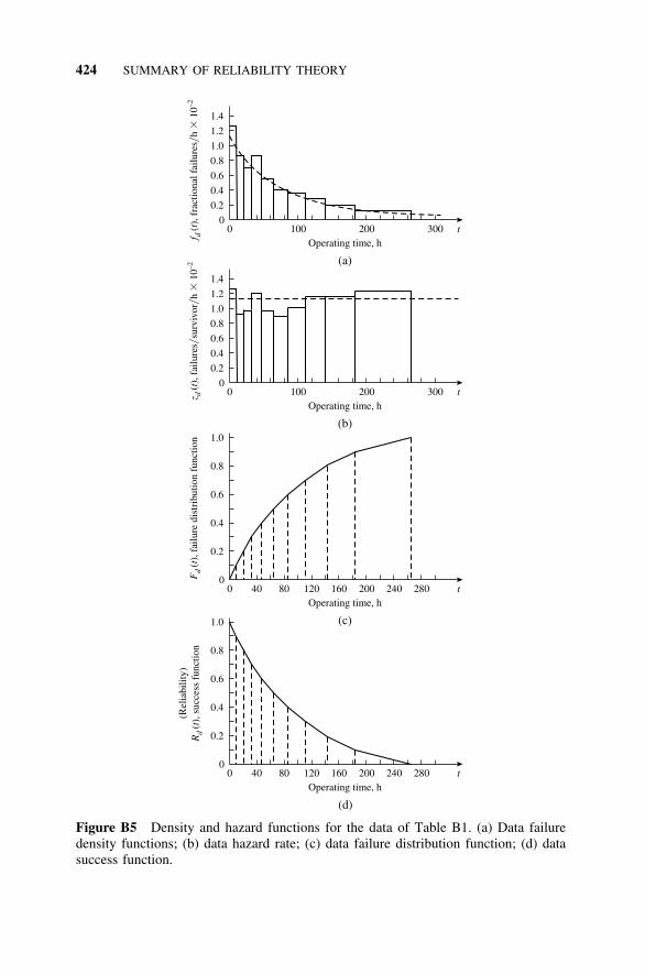
424 SUMMARY OF RELIABILITY THEORY
100
100
40
40
80
80
120
120
160
160
0
0
0
0
200
200
200
200
240
240
280
280
300
300
t
t
t
t
0
0
0
0
0.2
0.2
0.2
0.2
0.4
0.4
0.6
0.6
0.8
0.8
1.0
1.0
0.4
0.4
0.6
0.6
0.8
0.8
1.0
1.0
1.2
1.2
1.4
1.4
Operating time, h
Operating time, h
Operating time, h
Operating time, h
ft
d(
), f
ract
iona
l fai
lure
sh
10�
�–2
zt
d(
), f
ailu
res
h10
��
–2�s
urvi
vor
Ft
d(
), f
ailu
re d
istr
ibut
ion
func
tion
(Rel
iabi
lity)
(),
suc
cess
fun
ctio
nR
td
(a)
(b)
(c)
(d)
Figure B5 Density and hazard functions for the data of Table B1. (a) Data failuredensity functions; (b) data hazard rate; (c) data failure distribution function; (d) datasuccess function.
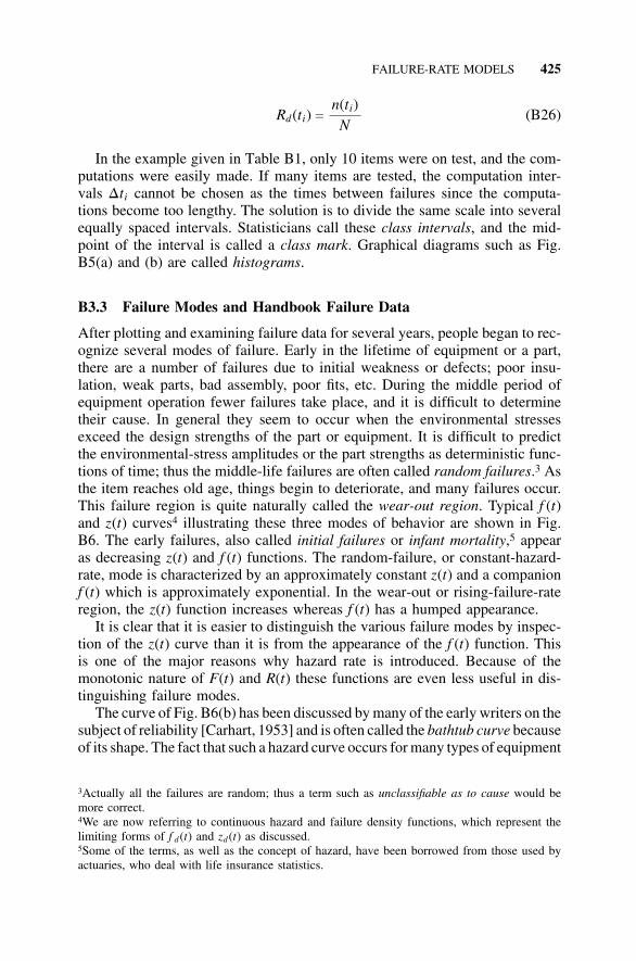
FAILURE-RATE MODELS 425
Rd(ti) cn(ti)
N(B26)
In the example given in Table B1, only 10 items were on test, and the com-putations were easily made. If many items are tested, the computation inter-vals Dti cannot be chosen as the times between failures since the computa-tions become too lengthy. The solution is to divide the same scale into severalequally spaced intervals. Statisticians call these class intervals, and the mid-point of the interval is called a class mark. Graphical diagrams such as Fig.B5(a) and (b) are called histograms.
B3.3 Failure Modes and Handbook Failure Data
After plotting and examining failure data for several years, people began to rec-ognize several modes of failure. Early in the lifetime of equipment or a part,there are a number of failures due to initial weakness or defects; poor insu-lation, weak parts, bad assembly, poor fits, etc. During the middle period ofequipment operation fewer failures take place, and it is difficult to determinetheir cause. In general they seem to occur when the environmental stressesexceed the design strengths of the part or equipment. It is difficult to predictthe environmental-stress amplitudes or the part strengths as deterministic func-tions of time; thus the middle-life failures are often called random failures.3 Asthe item reaches old age, things begin to deteriorate, and many failures occur.This failure region is quite naturally called the wear-out region. Typical f (t)and z(t) curves4 illustrating these three modes of behavior are shown in Fig.B6. The early failures, also called initial failures or infant mortality,5 appearas decreasing z(t) and f (t) functions. The random-failure, or constant-hazard-rate, mode is characterized by an approximately constant z(t) and a companionf (t) which is approximately exponential. In the wear-out or rising-failure-rateregion, the z(t) function increases whereas f (t) has a humped appearance.
It is clear that it is easier to distinguish the various failure modes by inspec-tion of the z(t) curve than it is from the appearance of the f (t) function. Thisis one of the major reasons why hazard rate is introduced. Because of themonotonic nature of F(t) and R(t) these functions are even less useful in dis-tinguishing failure modes.
The curve of Fig. B6(b) has been discussed by many of the early writers on thesubject of reliability [Carhart, 1953] and is often called the bathtub curve becauseof its shape. The fact that such a hazard curve occurs for many types of equipment
3Actually all the failures are random; thus a term such as unclassifiable as to cause would bemore correct.4We are now referring to continuous hazard and failure density functions, which represent thelimiting forms of f d(t) and zd(t) as discussed.5Some of the terms, as well as the concept of hazard, have been borrowed from those used byactuaries, who deal with life insurance statistics.
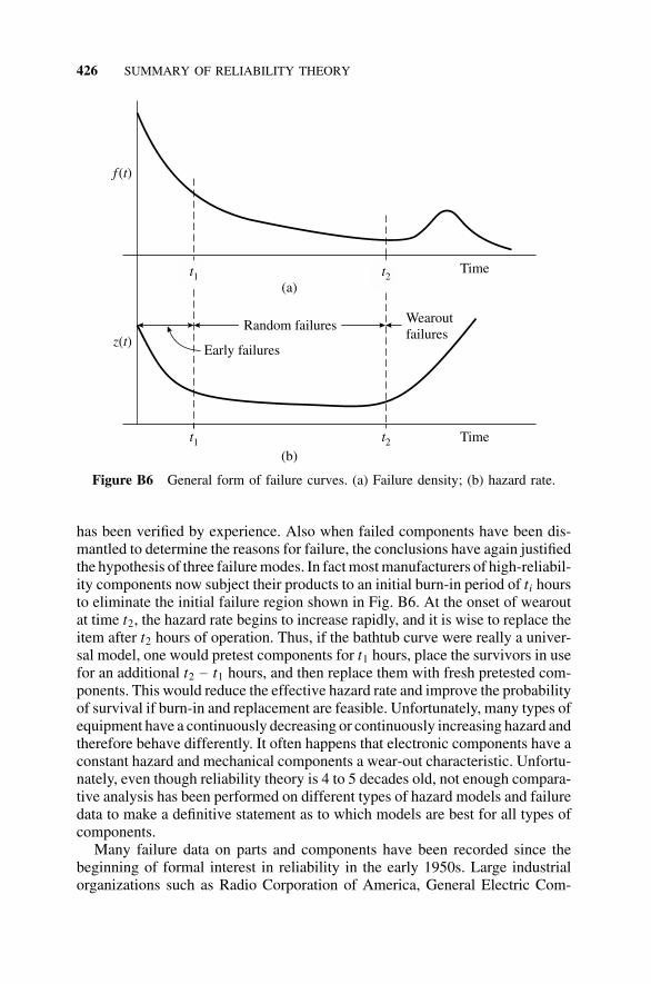
426 SUMMARY OF RELIABILITY THEORY
t1 t2 Time
Time
(b)
t1 t2
z t( )
f t( )
Random failures Wearoutfailures
Early failures
(a)
Figure B6 General form of failure curves. (a) Failure density; (b) hazard rate.
has been verified by experience. Also when failed components have been dis-mantled to determine the reasons for failure, the conclusions have again justifiedthe hypothesis of three failure modes. In fact most manufacturers of high-reliabil-ity components now subject their products to an initial burn-in period of ti hoursto eliminate the initial failure region shown in Fig. B6. At the onset of wearoutat time t2, the hazard rate begins to increase rapidly, and it is wise to replace theitem after t2 hours of operation. Thus, if the bathtub curve were really a univer-sal model, one would pretest components for t1 hours, place the survivors in usefor an additional t2 − t1 hours, and then replace them with fresh pretested com-ponents. This would reduce the effective hazard rate and improve the probabilityof survival if burn-in and replacement are feasible. Unfortunately, many types ofequipment have a continuously decreasing or continuously increasing hazard andtherefore behave differently. It often happens that electronic components have aconstant hazard and mechanical components a wear-out characteristic. Unfortu-nately, even though reliability theory is 4 to 5 decades old, not enough compara-tive analysis has been performed on different types of hazard models and failuredata to make a definitive statement as to which models are best for all types ofcomponents.
Many failure data on parts and components have been recorded since thebeginning of formal interest in reliability in the early 1950s. Large industrialorganizations such as Radio Corporation of America, General Electric Com-
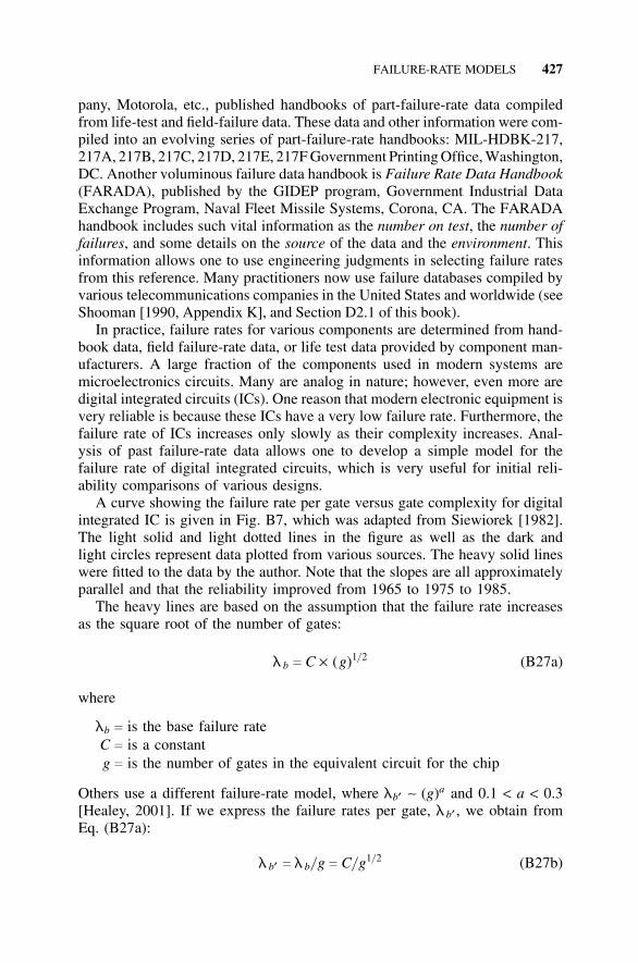
FAILURE-RATE MODELS 427
pany, Motorola, etc., published handbooks of part-failure-rate data compiledfrom life-test and field-failure data. These data and other information were com-piled into an evolving series of part-failure-rate handbooks: MIL-HDBK-217,217A, 217B, 217C, 217D, 217E, 217F Government Printing Office, Washington,DC. Another voluminous failure data handbook is Failure Rate Data Handbook(FARADA), published by the GIDEP program, Government Industrial DataExchange Program, Naval Fleet Missile Systems, Corona, CA. The FARADAhandbook includes such vital information as the number on test, the number offailures, and some details on the source of the data and the environment. Thisinformation allows one to use engineering judgments in selecting failure ratesfrom this reference. Many practitioners now use failure databases compiled byvarious telecommunications companies in the United States and worldwide (seeShooman [1990, Appendix K], and Section D2.1 of this book).
In practice, failure rates for various components are determined from hand-book data, field failure-rate data, or life test data provided by component man-ufacturers. A large fraction of the components used in modern systems aremicroelectronics circuits. Many are analog in nature; however, even more aredigital integrated circuits (ICs). One reason that modern electronic equipment isvery reliable is because these ICs have a very low failure rate. Furthermore, thefailure rate of ICs increases only slowly as their complexity increases. Anal-ysis of past failure-rate data allows one to develop a simple model for thefailure rate of digital integrated circuits, which is very useful for initial reli-ability comparisons of various designs.
A curve showing the failure rate per gate versus gate complexity for digitalintegrated IC is given in Fig. B7, which was adapted from Siewiorek [1982].The light solid and light dotted lines in the figure as well as the dark andlight circles represent data plotted from various sources. The heavy solid lineswere fitted to the data by the author. Note that the slopes are all approximatelyparallel and that the reliability improved from 1965 to 1975 to 1985.
The heavy lines are based on the assumption that the failure rate increasesas the square root of the number of gates:
l b c C × (g)1/ 2 (B27a)
where
lb c
C c
g c
is the base failure rateis a constantis the number of gates in the equivalent circuit for the chip
Others use a different failure-rate model, where lb′ ∼ (g)a and 0.1 < a < 0.3[Healey, 2001]. If we express the failure rates per gate, l b′ , we obtain fromEq. (B27a):
l b′ c l b/ g c C/ g1/ 2 (B27b)
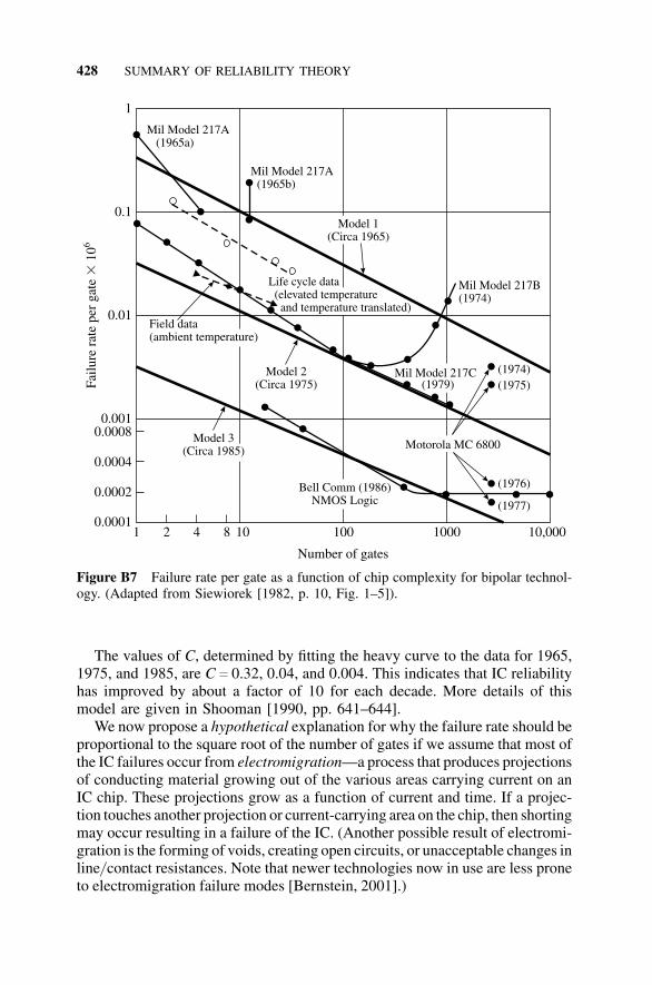
428 SUMMARY OF RELIABILITY THEORY
Motorola MC 6800
(1976)
(1974)
(1977)
(1975)
Mil Model 217B(1974)
(1979)Mil Model 217C
Bell Comm (1986)NMOS Logic
Model 3(Circa 1985)
Model 2(Circa 1975)
Field data(ambient temperature)
Life cycle data(elevated temperature
and temperature translated)
Model 1(Circa 1965)
Mil Model 217A(1965b)
Mil Model 217A(1965a)
1 2 4 8 10 100 1000 10,0000.0001
0.0002
0.0004
0.00080.001
0.01
0.1
1
Number of gates
Failu
re r
ate
per
gate
10�
6
Figure B7 Failure rate per gate as a function of chip complexity for bipolar technol-ogy. (Adapted from Siewiorek [1982, p. 10, Fig. 1–5]).
The values of C, determined by fitting the heavy curve to the data for 1965,1975, and 1985, are C c 0.32, 0.04, and 0.004. This indicates that IC reliabilityhas improved by about a factor of 10 for each decade. More details of thismodel are given in Shooman [1990, pp. 641–644].
We now propose a hypothetical explanation for why the failure rate should beproportional to the square root of the number of gates if we assume that most ofthe IC failures occur from electromigration—a process that produces projectionsof conducting material growing out of the various areas carrying current on anIC chip. These projections grow as a function of current and time. If a projec-tion touches another projection or current-carrying area on the chip, then shortingmay occur resulting in a failure of the IC. (Another possible result of electromi-gration is the forming of voids, creating open circuits, or unacceptable changes inline/ contact resistances. Note that newer technologies now in use are less proneto electromigration failure modes [Bernstein, 2001].)
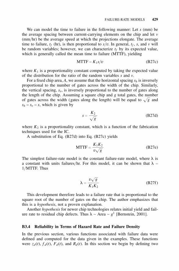
FAILURE-RATE MODELS 429
We can model the time to failure in the following manner: Let s (mm) bethe average spacing between current-carrying elements on the chip and let v(mm/ hr) be the average speed at which the projections elongate. The averagetime to failure, tf (hr), is then proportional to s/ v. In general, tf , s, and v willbe random variables; however, we can characterize tf by its expected value,which is generally called the mean time to failure (MTTF), yielding
MTTF c K1s/ v (B27c)
where K1 is a proportionality constant computed by taking the expected valueof the distribution for the ratio of the random variables s and v.
For a fixed chip area, A, we assume that the horizontal spacing sh is inverselyproportional to the number of gates across the width of the chip. Similarly,the vertical spacing, sv, is inversely proportional to the number of gates alongthe length of the chip. Assuming a square chip and g total gates, the numberof gates across the width (gates along the length) will be equal to
fg and
sh c sv c s, which is given by
s c K2fg
(B27d)
where K2 is a proportionality constant, which is a function of the fabricationtechniques used for the IC.
A substitution of Eq. (B27d) into Eq. (B27c) yields
MTTF c K1K2
vf
g(B27e)
The simplest failure-rate model is the constant failure-rate model, where l isa constant with units failures/ hr. For this model, it can be shown that l c1/ MTTF. Thus
l cvf
g
K1K2(B27f)
This development therefore leads to a failure rate that is proportional to thesquare root of the number of gates on the chip. The author emphasizes thatthis is a hypothesis, not a proven explanation.
Another hypothesis for newer chip technologies relates initial yield and fail-ure rate to residual chip defects. Thus l ∼ Area ∼ g1 [Bernstein, 2001].
B3.4 Reliability in Terms of Hazard Rate and Failure Density
In the previous section, various functions associated with failure data weredefined and computed for the data given in the examples. These functionswere zd(t), f d(t), Fd(t), and Rd(t). In this section we begin by defining two
430 SUMMARY OF RELIABILITY THEORY
random variables and deriving in a careful manner the basic definitions andrelations between the theoretical hazard, failure density function, failure dis-tribution function, and reliability function.
The random variable t is defined as the failure time of the item in question.6
Thus, the probability of failure as a function of time is given as
P(t ≤ t) c F(t) (B28)
which is simply the definition of the failure distribution function. We can definethe reliability, which is a probability of success in terms of F(t), as
R(t) c Ps(t) c 1 − F(t) c P(t ≥ t) (B29)
The failure density function is of course given by
dF(t)dt
c f (t) (B30)
We now consider a population of N items with the same failure-time dis-tribution. The items fail independently with probability of failure given byF(t) c 1 − R(t) and probability of success given by R(t). If the random vari-able N(t) represents the number of units surviving at time t, then N(t) has abinomial distribution with p c R(t). Therefore,
P[N(t) c n] c B[n; N, R(t)] cN!
n!(N − n)![R(t)]n[1 − R(t)]N − n
n c 0, 1, . . . , N (B31)
The number of units operating at any time t is a random variable and is notfixed; however, we can compute the expected value N(t). From Table A1 wesee that the expected value of a random variable with a binomial distributionis given by NR(t) and leads to
n(t) ≡ E[N(t)] c NR(t) (B32)
Solving for the reliability yields
R(t) cn(t)N
(B33)
Thus, the reliability at time t is the average fraction of surviving units at time t.This verifies Eq. (B27), which was obtained as a consequence of the definitionof f d(t). From Eq. (B29) we obtain
6In some problems, a more appropriate random variable is the number of miles, cycles, etc. Theresults are analogous.
FAILURE-RATE MODELS 431
F(t) c 1 −n(t)N
c
N − n(t)N
(B34)
and from Eq. (B30)
f (t) cdF(t)
dtc −
1N
dn(t)dt
f (t) ≡ limDtb 0
n(t) − n(t + Dt)NDt
(B35)
Thus, we see that Eq. (B23) is valid, and as N becomes large and Dti becomessmall, Eq. (B23) approaches Eq. (B35) in the limit. From Eq. (B34) we seethat F(t) is the average fraction of units having failed between 0 and time t,and Eq. (B35) states that f (t) is the rate of change of F(t), or its slope. FromEq. (B35) we see that the failure density function f (t) is normalized in termsof the size of the original population N. In many cases it is more informativeto normalize with respect to n(t), the number of survivors. Thus, we define thehazard rate as
z(t) ≡ − limDtb 0
n(t) − n(t + Dt)n(t)Dt
(B36)
The definition of z(t) in Eq. (B36) of course agrees with the definition of zd(t)in Eq. (B24). We can relate z(t) and f (t) using Eqs. (B35) and (B36):
z(t) c − limDt r 0
n(t) − n(t + Dt)Dt
1n(t)
c N f(t)1
n(t)
Substitution of Eq. (B33) yields
z(t) cf (t)R(t)
(B37)
We now wish to relate R(t) to f (t) and to z(t). From Eqs. (B29) and (B30) wesee that
R(t) c 1 − F(t)
c 1 − ∫t
0f (y) dy (B38)
where y is merely a dummy variable. Substituting into Eq. (B37) from Eqs.(B35) and (B33), we obtain
432 SUMMARY OF RELIABILITY THEORY
z(t) c −
1N
dn(t)dt
Nn(t)
c −
ddt
ln n(t)
Solving the differential equation yields:
ln n(t) c − ∫t
0z(y) dy + c
where y is a dummy variable and c is the constant of integration. Taking theantilog of both sides of the equation gives:
n(t) c ec exp [ − ∫t
0z(y) dy]
Inserting initial conditions
n(0) c N c ec
gives
n(t) c N exp [ − ∫t
0z(y) dy]
Substitution of Eq. (B33) completes the derivation
R(t) c exp [ − ∫t
0z(y) dy] (B39)
Equations (B35) and (B36) serve to define the failure density function and thehazard rate, and Eqs. (B37) to (B39) relate R(t) to f (t) and z(t).7
B3.5 Hazard Models
On first consideration it might appear that if failure data and graphs such asFig. B5(a–d) are available, there is no need for a mathematical model. How-ever, in drawing conclusions from test data on the behavior of other, similarcomponents it is necessary to fit the failure data with a mathematical model.The discussion will start with several simple models and gradually progress tothe more involved problem of how to choose a general model which fits allcases through adjustment of constants.
7An alternative derivation of these expressions is given in Shooman [1990, p. 183].
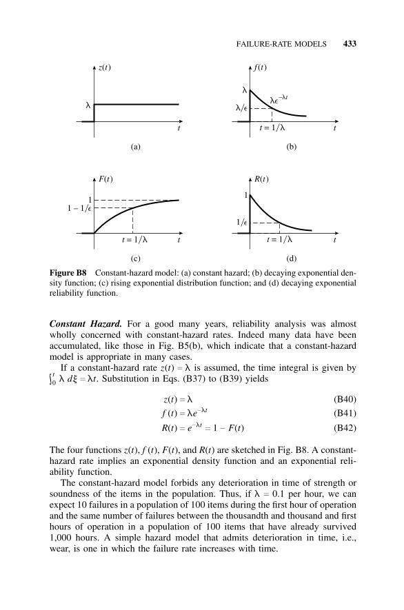
FAILURE-RATE MODELS 433
z t( )
F t( )
f t( )
R t( )
l
l
l e�
1 – 1�e
1�e
1 1
t = 1�l
t = 1�l t = 1�l
t
t
t
t
(a)
(c)
(b)
(d)
le–lt
Figure B8 Constant-hazard model: (a) constant hazard; (b) decaying exponential den-sity function; (c) rising exponential distribution function; and (d) decaying exponentialreliability function.
Constant Hazard. For a good many years, reliability analysis was almostwholly concerned with constant-hazard rates. Indeed many data have beenaccumulated, like those in Fig. B5(b), which indicate that a constant-hazardmodel is appropriate in many cases.
If a constant-hazard rate z(t) c l is assumed, the time integral is given by∫t0 l dy c lt. Substitution in Eqs. (B37) to (B39) yields
z(t) c l (B40)
f (t) c le−lt (B41)
R(t) c e−ltc 1 − F(t) (B42)
The four functions z(t), f (t), F(t), and R(t) are sketched in Fig. B8. A constant-hazard rate implies an exponential density function and an exponential reli-ability function.
The constant-hazard model forbids any deterioration in time of strength orsoundness of the items in the population. Thus, if l c 0.1 per hour, we canexpect 10 failures in a population of 100 items during the first hour of operationand the same number of failures between the thousandth and thousand and firsthours of operation in a population of 100 items that have already survived1,000 hours. A simple hazard model that admits deterioration in time, i.e.,wear, is one in which the failure rate increases with time.
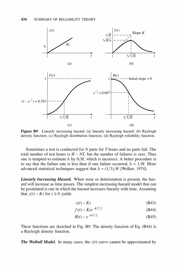
434 SUMMARY OF RELIABILITY THEORY
z t( )
F t( ) R t( )
f t( )
l
K
K�e
1�K
1�K 1�K
(1 – ) = 0.393e–
e– = 0.607
1 1
t
t t
t
(a)
(c) (d)
(b)
Kt�
�
� �
�
12
12
Initial slope = 0
Slope K
Figure B9 Linearly increasing hazard: (a) linearly increasing hazard; (b) Rayleighdensity function; (c) Rayleigh distribution function; (d) Rayleigh reliability function.
Sometimes a test is conducted for N parts for T hours and no parts fail. Thetotal number of test hours is H c NT, but the number of failures is zero. Thusone is tempted to estimate l by 0/ H, which is incorrect. A better procedure isto say that the failure rate is less than if one failure occurred, l < 1/ H. Moreadvanced statistical techniques suggest that l ≈ (1/ 3)/ H [Welker, 1974].
Linearly Increasing Hazard. When wear or deterioration is present, the haz-ard will increase as time passes. The simplest increasing-hazard model that canbe postulated is one in which the hazard increases linearly with time. Assumingthat z(t) c Kt for t ≥ 0 yields
z(t) c Kt (B43)
f (t) c Kte−Kt2/ 2 (B44)
R(t) c e−Kt2/ 2 (B45)
These functions are sketched in Fig. B9. The density function of Eq. (B44) isa Rayleigh density function.
The Weibull Model. In many cases, the z(t) curve cannot be approximated by
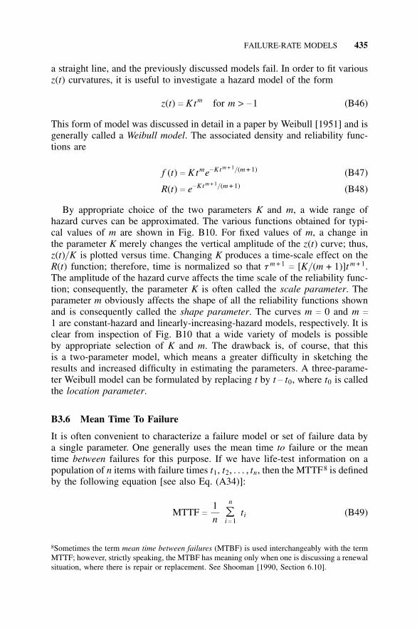
FAILURE-RATE MODELS 435
a straight line, and the previously discussed models fail. In order to fit variousz(t) curvatures, it is useful to investigate a hazard model of the form
z(t) c Ktm for m > −1 (B46)
This form of model was discussed in detail in a paper by Weibull [1951] and isgenerally called a Weibull model. The associated density and reliability func-tions are
f (t) c Ktme−Kt m + 1/ (m + 1) (B47)
R(t) c e−Kt m + 1/ (m + 1) (B48)
By appropriate choice of the two parameters K and m, a wide range ofhazard curves can be approximated. The various functions obtained for typi-cal values of m are shown in Fig. B10. For fixed values of m, a change inthe parameter K merely changes the vertical amplitude of the z(t) curve; thus,z(t)/ K is plotted versus time. Changing K produces a time-scale effect on theR(t) function; therefore, time is normalized so that t m + 1
c [K/ (m + 1)]t m + 1.The amplitude of the hazard curve affects the time scale of the reliability func-tion; consequently, the parameter K is often called the scale parameter. Theparameter m obviously affects the shape of all the reliability functions shownand is consequently called the shape parameter. The curves m c 0 and m c
1 are constant-hazard and linearly-increasing-hazard models, respectively. It isclear from inspection of Fig. B10 that a wide variety of models is possibleby appropriate selection of K and m. The drawback is, of course, that thisis a two-parameter model, which means a greater difficulty in sketching theresults and increased difficulty in estimating the parameters. A three-parame-ter Weibull model can be formulated by replacing t by t − t0, where t0 is calledthe location parameter.
B3.6 Mean Time To Failure
It is often convenient to characterize a failure model or set of failure data bya single parameter. One generally uses the mean time to failure or the meantime between failures for this purpose. If we have life-test information on apopulation of n items with failure times t1, t2, . . . , tn, then the MTTF8 is definedby the following equation [see also Eq. (A34)]:
MTTF c
1n
n
���i c 1
ti (B49)
8Sometimes the term mean time between failures (MTBF) is used interchangeably with the termMTTF; however, strictly speaking, the MTBF has meaning only when one is discussing a renewalsituation, where there is repair or replacement. See Shooman [1990, Section 6.10].
436
12
t012345
zt K()
m=
+3
m=
+2
m=
+1
m=
+
m=
–m
= 0
1 2 1 2
+1 2
–1 2
10
32
12
t0
0.2
0.4
0.6
0.8
1.0
Ft()
m=
+1
m=
0m
= +
1 2
+1 2
–1 2
m=
–1 2
+1
0
+3
+3 +
2
+2
12
t0
0.2
0.4
0.6
0.8
1.0
ft K()
m=
+1
m=
+
m=
–
m=
01 21 2
+1 2
–1 2
+1
0
+3
+3
+2
+2(
+ 1
)m
K[
]mm
�(+
1)
Km
+ 1
t=
[(
)]t
1(
+ 1
)�
m
12
t0
0.2
0.4
0.6
0.8
1.0
Rt()
m=
+1
m=
+2
m=
+3
m=
+0.
5
m=
–0.
5m
= 0
1 2
+1
+3
+2 K
m+
1t
= [
()
]t1
(+
)
�m
Km
+ 1
t=
[(
)]t
1(
+ 1
)�
m
(b)
(d)
(a)
(c)
Reliability
+0.
5 0–
0.5
Fig
ure
B10
R
elia
bilit
y fu
nctio
ns f
or th
e W
eibu
ll m
odel
: (a)
haza
rd f
unct
ion;
(b)
den
sity
fun
ctio
n; (
c) d
istr
ibut
ion
func
-tio
n; (
d) r
elia
bilit
y fu
nctio
n.
FAILURE-RATE MODELS 437
If one is discussing a hazard model, the MTTF for the probability distribu-tion defined by the model is given by Eq. (A33) as
MTTF c E(t) c ∫∞
0t f(t) dt (B50)
In a single-parameter distribution, specification of the MTTF fixes theparameter. In a multiple-parameter distribution, fixing the MTTF only placesone constraint on the model parameters.
One can express Eq. (B50) by a simpler computational expression involvingthe reliability function:9
MTTF c ∫∞
0R(t) dt (B51)
As an example of the use of Eq. (B51) the MTTF for several different haz-ards will be computed. For a single component with a constant hazard:
MTTF c ∫∞
0e−lt d t c e−lt
−l||||
∞
0
c 1l
(B52)
For a linearly increasing hazard:
MTTF c ∫∞
0e−Kt 2/ 2 dt c G( 1
2 )
2f
K/ 2ch
p
2K(B53)
For a Weibull distribution:
MTTF c ∫∞
0e−Kt (m + 1)/ (m + 1) dt c G[(m + 2)/ (m + 1)]
[K/ (m + 1)]1/ (m + 1)(B54)
In Eq. (B52) the MTTF is simply the reciprocal of the hazard, whereas in Eq.(B53) it varies as the reciprocal of the square root of the hazard slope. In Eq.(B54) the relationship between MTTF, K, and m is more complex (see TableA1).
In many cases we assume an exponential density (constant hazard) for sim-plicity, and for this case we frequently hear the statement “the MTBF is thereciprocal of the failure rate.” The reader should not forget the assumptionsnecessary for this statement to hold.
9For the derivation, see Shooman [1990, p. 197].
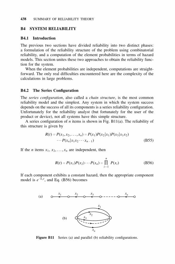
438 SUMMARY OF RELIABILITY THEORY
B4 SYSTEM RELIABILITY
B4.1 Introduction
The previous two sections have divided reliability into two distinct phases:a formulation of the reliability structure of the problem using combinatorialreliability, and a computation of the element probabilities in terms of hazardmodels. This section unites these two approaches to obtain the reliability func-tion for the system.
When the element probabilities are independent, computations are straight-forward. The only real difficulties encountered here are the complexity of thecalculations in large problems.
B4.2 The Series Configuration
The series configuration, also called a chain structure, is the most commonreliability model and the simplest. Any system in which the system successdepends on the success of all its components is a series reliability configuration.Unfortunately for the reliability analyst (but fortunately for the user of theproduct or device), not all systems have this simple structure.
A series configuration of n items is shown in Fig. B11(a). The reliability ofthis structure is given by
R(t) c P(x1, x2, . . . , xn) c P(x1)P(x2 |x1)P(x3 |x1x2)
· · · P(xn |x1x2 · · · xn − 1) (B55)
If the n items x1, x2, . . . , xn are independent, then
R(t) c P(x1)P(x2) · · · P(xn) cn
∏i c 1
P(xi) (B56)
If each component exhibits a constant hazard, then the appropriate componentmodel is e−l i t , and Eq. (B56) becomes
x1 x2 x3 xn(a)
x3
xn
x1
x2(b)
Figure B11 Series (a) and parallel (b) reliability configurations.
SYSTEM RELIABILITY 439
R(t) cn
∏i c 1
e−l i tc exp �−
n
���i c 1
l it� (B57)
Equation (B57) is the most commonly used and the most elementary systemreliability formula. In practice this formula is often misused (probably becauseit is so simple and does work well in many situations, people have becomeoverconfident). The following assumptions must be true if Eq. (B57) is to holdfor a system:
1. The system reliability configuration must truly be a series one.2. The components must be independent.3. The components must be governed by a constant-hazard model.
If assumptions 1 and 2 hold but the components have linearly increasing haz-ards zi(t) c Kit, Eq. (B56) then becomes
R(t) cn
∏i c 1
e−Kit 2/ 2c exp �−
n
���i c 1
Kit 2
2 � (B58)
If p components have a constant hazard and n − p components a linearlyincreasing hazard, the reliability becomes
R(t) c �p
∏i c 1
e−li t� �n
∏i c p + 1
e−li t 2/ 2�c exp�−
p
���i c 1
lit� exp � −
n
���i c p + 1
Kit 2
2 � (B59)
In some cases no simple composite formula exists, and the reliability mustbe expressed as a product of n terms. For example, suppose each componentis governed by the Weibull distribution, z(t) c Kit mi . If m and K are differentfor each component,
R(t) cn
∏i c 1
exp � −Kit mi + 1
mi + 1 � c exp �−n
���i c 1
Kit mi + 1
mi + 1 � (B60)
The series reliability structure serves as a lower-bound configuration. Toillustrate this principle we pose a hypothetical problem. Given a collection ofn elements, from the reliability standpoint what is the worst possible reliabilitystructure they can assume? The intutitive answer, of course, is a series struc-ture. (A proof is given in Shooman [1990, p. 205]; see also Section B6.4 ofthis book.)
440 SUMMARY OF RELIABILITY THEORY
B4.3 The Parallel Configuration
If a system of n elements can function properly when only one of the elementsis good, a parallel configuration is indicated. A parallel configuration of n itemsis shown in Fig. B11(b). The reliability expression for a parallel system maybe expressed in terms of the probability of success of each component or, moreconveniently, in terms of the probability of failure
R(t) c P(x1 + x2 + · · · + xn) c 1 − P(x1x2 · · · xn) (B61)
In the case of constant-hazard components, Pf c P(xi) c 1 − e−li t , and Eq.(B61) becomes
R(t) c 1 −
n
∏i c 1
(1 − e−li t) (B62)
In the case of linearly increasing hazard, the expression becomes
R(t) c 1 −
n
∏i c 1
(1 − e−Kit 2/ 2) (B63)
In the general case, the system reliability function is
R(t) c 1 −
n
∏i c 1
(1 − e−Zi(t)) (B64)
where Zi(t) ≡ ∫t0 z(y) dy.
In order to permit grouping of terms in Eq. (B64) to simplify computationand/ or interpretation, the equation must be expanded. The expansion resultsin
R(t) c (e−Z1 + e−Z2 + · · · + e−Zn ) − (e− (Z1 + Z2) + e− (Z1 + Z3) + · · ·)
+ (e− (Z1 + Z2 + Z3) + e− (Z1 + Z2 + Z4) + · · ·) − · · · e− (Z1 + Z2 + Z3 + ··· + Zn) (B65)
Note that the signs of the terms in parentheses alternate and that in the firstset of parentheses, the exponents are all the Zs taken singly; in the second, allthe sums of Zs taken two at a time; and in the last term, the sum of all the Zs.The r th parentheses in Eq. (B65) contain n!/ [r!(n − r)!] terms.
Just as the series configuration served as a lower-bound structure, the par-allel model can be thought of as an upper-bound structure.
If we have a system of n elements with information on each element reli-ability but little or no information on their interconnection, we can bound thereliability function from below by Eq. (B56) and from above by Eq. (B64).We would in general expect these bounds to be quite loose; however, they do
SYSTEM RELIABILITY 441
provide some information even when we are grossly ignorant of the systemstructure.
B4.4 An r-out-of-n Structure
Another simple structure which serves as a useful model for many reliabilityproblems is an r-out-of-n structure. Such a model represents a system of ncomponents in which r of the n items must be good for the system to succeed.Of course r is less than n. Two simple examples of an r-out-of-n system are(1) a piece of stranded wire with n strands in which at least r are necessaryto pass the required current and (2) a battery composed of n series cells of Evolts each where the minimum voltage for system operation10 is rE.
We may formulate a structural model for an r-out-of-n system, but it issimpler to use the binomial distribution if applicable. The binomial distributioncan be used only when the n components are independent and identical. If thecomponents differ or are dependent, the structural-model approach must beused.11 Success of exactly r out of n identical, independent items is given by
B(r : n) c � nr � pr(1 − p)n − r (B66)
where r : n stands for r out of n, and the success of at least r out of n items isgiven by
Ps c
n
���k c r
B(k : n) (B67)
For constant-hazard components Eq. (B66) becomes
R(t) cn
���k c r �
nk � e−klt(1 − e−lt)n − k (B68)
Similarly for linearly increasing or Weibull components, the reliability func-tions are
10Actually when one cell of a series of n cells fails, the voltage of the string does not become(n − 1)E unless a special circuit arrangement is used. Such a circuit is discussed in Shooman[1990, p. 2.9].11The reader should refer to the example given in Eq. (B17) and Fig. B3.
442 SUMMARY OF RELIABILITY THEORY
R(t) c [ n
���k c r �
nk � e−kKt 2/ 2] (1 − e−Kt 2/ 2)n − k (B69)
R(t) c [ n
���k c r �
nk � e−kKt m + 1/ (m + 1)] (1 − e−Kt m + 1/ (m + 1))n − k (B70)
It is of interest to note that for r c 1, the structure becomes a parallel systemand for r c n the structure becomes a series system. Thus, in a sense seriesand parallel systems are subclasses of an r-out-of-n structure.
B5 ILLUSTRATIVE EXAMPLE OF SIMPLIFIED AUTO DRUMBRAKES
B5.1 Introduction
The preceding sections have attempted to summarize the pertinent aspects ofreliability theory and show the reader how analysis can be performed. Thissection illustrates via an example how the theory can be applied.
The example chosen for this section is actually a safety analysis. In thecase of the automobile, the only difference between a reliability and a safetyanalysis is in the choice of subsystems included in the analysis. In the caseof safety, we concentrate on the subsystems whose failure could cause injuryto the occupants, other passengers, pedestrians, etc. In the case of reliabilityanalysis, we would include all subsystems whose failure either makes the autoinoperative or necessitates a repair (depending on our definition of success).
B5.2 The Brake System
The example considers the braking system of a typical older auto, withoutpower brakes or antilock brakes and excluding the parking (emergency) brakeand the dash warning light. An analysis at the detailed (piece-part) level is adifficult task. The major subsystems in a typical braking system may containseveral hundred parts and assemblies.
The major subsystems and approximate parts counts are: pressure differen-tial valve (8 parts), self-adjusting drum brakes (4 × 15 parts), wheel cylinder (4× 9 parts), tubing, brackets, and connectors (50 parts), dual master cylinder (22parts), and master cylinder installation parts (20 parts). Frequently, because oflack of data, analysis is not carried out at this piece-part level. Even with scantydata, an analysis is still important, since often it will show obvious weaknessesof such a braking system which can be improved when redesigning it. In sucha case, redesign is warranted, based on engineering judgment, even withoutstatistics on frequencies of the failure modes. The example will be performed

ILLUSTRATIVE EXAMPLE OF SIMPLIFIED AUTO DRUM BRAKES 443
TABLE B3 A Simplified Braking System FMECA
SafetyFailure Mode Mechanism Criticality Comments
M1: Differential Leakage or Medium Reducesvalve failure Blockage braking(1/ 2 system) efficiency
M2: Differential Leakage affecting High Loss ofvalve failure both front and both systems(total system) back systems
M3: Master cylinder Leakage or Medium Reducesfailure blockage braking(1/ 2 system) efficiency
M4: Master cylinder Leakage High Loss offailure (front and back) both systems(total system)
M5: Drum brakes Leakage or Medium Unbalance ofself-adjusting blockage of brakes causes
one assembly erratic behaviorM6: Tubing, brackets, Leakage or Medium Reduces
and connectors blockage braking(1/ 2 system) efficiency
M7: Pedal and Broken or High Loss oflinkage jammed both systems
at a higher level, and will group together all failure mechanisms which causethe particular failure mode in question.
B5.3 Failure Modes, Effects, and Criticality Analysis
An FMECA12 for the simplified braking system is given in Table B3. Inspec-tion of the table shows that the modes which most seriously affect safety aremodes M2, M4, and M7, and the design should be scrutinized in a designreview to assure that the probability of occurrence for these modes is mini-mized.
B5.4 Structural Model
The next step in analysis would be the construction of an SBD or an FT.13
Assume that a safety failure occurs if modes M2, M4, or M7 occur singly and
12Sometimes a column is added to an FMEA analysis which discusses (evaluates) the severityor criticality of the failure mode. In such a case, the analysis is called an FMECA.13Safety block diagram or fault tree.
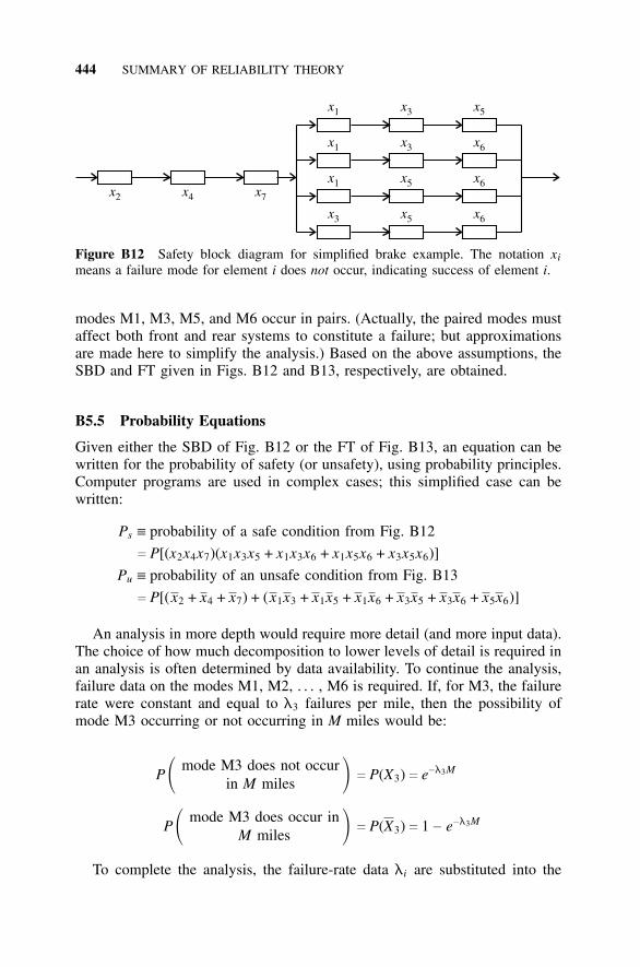
444 SUMMARY OF RELIABILITY THEORY
x2 x4 x7
x1
x1
x1
x3
x3
x3
x5
x5
x5
x6
x6
x6
Figure B12 Safety block diagram for simplified brake example. The notation ximeans a failure mode for element i does not occur, indicating success of element i.
modes M1, M3, M5, and M6 occur in pairs. (Actually, the paired modes mustaffect both front and rear systems to constitute a failure; but approximationsare made here to simplify the analysis.) Based on the above assumptions, theSBD and FT given in Figs. B12 and B13, respectively, are obtained.
B5.5 Probability Equations
Given either the SBD of Fig. B12 or the FT of Fig. B13, an equation can bewritten for the probability of safety (or unsafety), using probability principles.Computer programs are used in complex cases; this simplified case can bewritten:
Ps ≡ probability of a safe condition from Fig. B12
c P[(x2x4x7)(x1x3x5 + x1x3x6 + x1x5x6 + x3x5x6)]
Pu ≡ probability of an unsafe condition from Fig. B13
c P[(x2 + x4 + x7) + (x1x3 + x1x5 + x1x6 + x3x5 + x3x6 + x5x6)]
An analysis in more depth would require more detail (and more input data).The choice of how much decomposition to lower levels of detail is required inan analysis is often determined by data availability. To continue the analysis,failure data on the modes M1, M2, . . . , M6 is required. If, for M3, the failurerate were constant and equal to l3 failures per mile, then the possibility ofmode M3 occurring or not occurring in M miles would be:
P � mode M3 does not occurin M miles � c P(X3) c e−l3M
P � mode M3 does occur inM miles � c P(X3) c 1 − e−l3M
To complete the analysis, the failure-rate data li are substituted into the
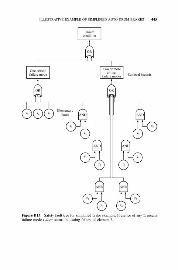
ILLUSTRATIVE EXAMPLE OF SIMPLIFIED AUTO DRUM BRAKES 445
Unsafecondition
OR
One criticalfailure mode
Two or morecritical
failure modes Sublevel hazards
x2
x1 x3
x1 x3
x1 x5
x3 x5
x5 x6
x6 x6
x4 x7Elementary
faults
OR OR
AND AND
AND AND
AND AND
Figure B13 Safety fault tree for simplified brake example. Presence of any xi meansfailure mode i does occur, indicating failure of element i.
446 SUMMARY OF RELIABILITY THEORY
equations to determine P(Xi) or P(Xi); then these terms are substituted into theequations for Ps or Pu; and last, Ps or Pu is substituted into a system safetyequation along with probabilities for all subsystems that affect safety. For moreadvanced FT concepts, see Dugan [1996].
B5.6 Summary
The safety analysis consists of:
1. Decomposing the system into subsystems or piece-parts.2. Drawing a safety block diagram (SBD) or fault tree (FT) (computer pro-
grams are available for this purpose). See Appendix D.3. Computation of the probability of safety or unsafety from the SBD or
FT (computer programs are also available for this purpose).4. Determining the failure rates of each component element. This is a data
collection and estimation problem.5. Substitution of failure rates into expression of step 3 (also done by com-
puter programs).
B6 MARKOV RELIABILITY AND AVAILABILITY MODELS
B6.1 Introduction
Dependent failures, repair, or standby operation complicates the direct calcu-lation of element reliabilities. In this section we shall discuss three differentapproaches to reliability computations for systems involving such computa-tions. The first technique is the use of Markov models, which works well andhas much appeal as long as the failure hazards z(t) and repair hazards w(t) areconstant. When z(t) and w(t) become time-dependent, the method breaks down,except in a few special cases. (See Shooman [1990, pp. 348–359].) A secondmethod, using joint density functions, and a third method, using convolution-like integrations, are more difficult to set up, but they are still valid when z(t)or w(t) is time-dependent.14
Some of the Markov modeling programs discussed in Appendix D deal withnonconstant hazards. In many cases, there is a paucity of failure-rate data; bothconstant-failure rates and -repair rates are used by default.
B6.2 Markov Models
The basic properties of Markov models have already been discussed in SectionA8. In this section we shall briefly review some of the assumptions necessary
14See Shooman [1990, Section 5.8].
MARKOV RELIABILITY AND AVAILABILITY MODELS 447
for formulation of a Markov model and show how it can be used to makereliability computations.
In order to formulate a Markov model (to be more precise we are talkingabout continuous-time and discrete-state models) we must first define all themutually exclusive states of the system. For example, in a system composedof a single nonrepairable element x1 there are two possible states: s0 c x1, inwhich the element is good, and s1 c x1, in which the element is bad. The statesof the system at t c 0 are called the initial states, and those representing a finalor equilibrium state are called final states. The set of Markov state equationsdescribes the probabilistic transitions from the initial to the final states.
The transition probabilities must obey the following two rules:
1. The probability of transition in time Dt from one state to another is givenby z(t)Dt, where z(t) is the hazard associated with the two states in ques-tion. If all the zi(t)’s are constant, zi(t) c li, and the model is calledhomogeneous. If any hazards are time functions, the model is called non-homogeneous.
2. The probabilities of more than one transition in time Dt are infinitesimalsof a higher order and can be neglected.
For the example under discussion the state-transition equations can be for-mulated using the above rules. The probability of being in state s0 at time t+ Dt is written Ps0 (t + Dt). This is given by the probability that the systemis in state s0 at time t, Ps0 (t), times the probability of no failure in time Dt,1 − z(t)Dt, plus the probability of being in state s1 at time t, Ps1 (t), times theprobability of repair in time Dt, which equals zero.
The resulting equation is
Ps0 (t + Dt) c [1 − z(t)Dt]Ps0 (t) + 0Ps1 (t) (B71)
Similarly, the probability of being in state s1 at t + Dt is given by
Ps1 (t + Dt) c [z(t)Dt]Ps0 (t) + 1Ps1 (t) (B72)
The transition probability z(t)Dt is the probability of failure (change from states0 to s1), and the probability of remaining in state s1 is unity.15 One can summa-rize the transition Eqs. (B71) and (B72) by writing the transition matrix givenin Table B4. Note that it is a property of transition matrices that its rows mustsum to unity. Rearrangement of Eqs. (B71) and (B72) yields
15Conventionally, state s1 would be called an absorbing state since transitions out of the state arenot permitted.
448 SUMMARY OF RELIABILITY THEORY
TABLE B4 State Transition Matrix for a SingleElement
Final States
Initial States s0 s1
s0 1 − z(t)Dt z(t)Dts1 0 1
Ps0 (t + Dt) − Ps0 (t)Dt
c −z(t)Ps0 (t)
Ps1 (t + Dt) − Ps1 (t)Dt
c z(t)Ps0 (t)
Passing to a limit as Dt becomes small, we obtain
dPs0 (t)dt
+ z(t)Ps0 (t) c 0 (B73)
dPs1 (t)dt
c z(t)Ps0 (t) (B74)
Equations (B73) and (B74) can be solved in conjunction with the appropriateinitial conditions for Ps0 (t) and Ps1 (t), the probabilities of ending up in state s0
or state s1, respectively. The most common initial condition is that the systemis good at t c 0, that is, Ps0 (t c 0) c 1 and Ps1 (t c 0) c 0. Equations (B73) and(B74) are simple first-order linear differential equations which are easily solvedby classical theory. Equation (B73) is homogeneous (no driving function), andseparation of variables yields
dPs0 (t)Ps0 (t)
c −z(t) dt
ln Ps0 (t) c − ∫t
0z(y) dy + C1
Ps0 (t) c exp [ − ∫t
0z(y) dy + C1] c C2 exp [ − ∫
t
0z(y) dy] (B75)
Inserting the initial condition Ps0 (t c 0) c 1,
MARKOV RELIABILITY AND AVAILABILITY MODELS 449
Ps0 (t c 0) c 1 c C2e−0
� C2 c 1
and one obtains the familiar reliability function
R(t) c Ps0 (t) c exp [ − ∫t
0z(y) dy] (B76)
Formal solution of Eq. (B76) proceeds in a similar manner.
Ps1 (t) c 1 − exp [ ∫ t
0z(y) dy] (B77)
Of course a formal solution of Eq. (B74) is not necessary to obtain Eq.(B77), since it is possible to recognize at the outset that
Ps0 (t) + Ps1 (t) c 1.
The role played by the initial conditions is clearly evident from Eq. (B75).Since C2 c Ps0 (0), if the system was initially bad, Ps0 (t) c 0, and R(t) c 0. Ifthere is a fifty-fifty chance that the system is good at t c 0, then Ps0 (t) c
12 ,
and
R(t) c 12 exp [ − ∫
t
0z(y) dy]
This method of computing the system reliability function yields the sameresults, of course, as the techniques of Sections B3 to B5. Even in a single-ele-ment problem it generates a more general model. The initial condition allowsone to include the probability of initial failure before the system in questionis energized.
B6.3 Markov Graphs
It is often easier to characterize Markov models by a graph composed of nodesrepresenting system states and branches labeled with transition probabilities.Such a Markov graph for the problem described by Eqs. (B73) and (B74) orTable B4 is given in Fig. B14. Note that the sum of transition probabilitiesfor the branches leaving each node must be unity. Treating the nodes as sig-nal sources and the transition probabilities as transmission coefficients, we canwrite Eqs. (B73) and (B74) by inspection. Thus, the probability of being at anynode at time t + Dt is the sum of all signals arriving at that node. All other
450 SUMMARY OF RELIABILITY THEORY
Ps0Ps1
z t t( )D
1 ( )– z t tD 1
Figure B14 Markov graph for a single nonrepairable element.
nodes are considered probability sources at time t, and all transition probabili-ties serve as transmission gains. A simple algorithm for writing Eqs. (B73) and(B74) by inspection is to equate the derivative of the probability at any nodeto the sum of the transmissions coming into the node. Any unity gain factorsof the self-loops must first be set to zero, and the Dt factors are dropped fromthe branch gains. Referring to Fig. B14, the self-loop on Ps1 disappears, andthe equation becomes Ps1 c zPs0 . At node Ps0 the self-loop gain becomes −z,and the equation is Ps0 c −zPs0 . The same algorithm holds at each node formore complex graphs.
B6.4 Example—A Two-Element Model
One can illustrate dependent failures,16 standby operation, and repair by dis-cussing a two-element system. For simplicity repair is ignored at first. If atwo-element system consisting of elements x1 and x2 is considered, there arefour system states: s0 c x1x2, s1 c x1x2, s2 c x1x2, and s3 c x1x2. The statetransition matrix is given in Table B5 and the Markov graph in Fig. B15.
The probability expressions for these equations can be written by inspection,using the algorithms previously stated.
dPs0 (t)dt
c − [z01(t) + z02(t)]Ps0 (t) (B78)
dPs1 (t)dt
c − [z13(t)]Ps1 (t) + [z01(t)]Ps0 (t) (B79)
dPs2 (t)dt
c − [z23(t)]Ps2 (t) + [z02(t)]Ps0 (t) (B80)
dPs3 (t)dt
c [z13(t)]Ps1 (t) + [z23(t)]Ps2 (t) (B81)
16For dependent failures, see Shooman [1990, p. 235].
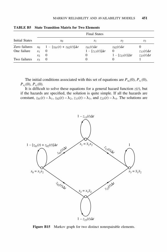
MARKOV RELIABILITY AND AVAILABILITY MODELS 451
TABLE B5 State Transition Matrix for Two Elements
Final States
Initial States s0 s1 s2 s3
Zero failures s0 1 − [z01(t) + z02(t)]Dt z01(t)Dt z02(t)Dt 0One failure s1 0 1 − [z13(t)]Dt 0 z13(t)Dt
s2 0 0 1 − [z23(t)]Dt z23(t)DtTwo failures s3 0 0 0 1
The initial conditions associated with this set of equations are Ps0 (0), Ps1 (0),Ps2 (0), Ps3 (0).
It is difficult to solve these equations for a general hazard function z(t), butif the hazards are specified, the solution is quite simple. If all the hazards areconstant, z01(t) c l1, z02(t) c l2, z13(t) c l3, and z23(t) c l 4. The solutions are
1 ( )– z t t13 D
1 – [ ( ) +z t t01 Dz t02( )]
1 ( )– z t t23 D
s x x3 = 1 2s x x0 = 1 2
s x x2 = 1 2
s x x1 = 1 2 zt
t13 ( )D
zt
t
01( )D
zt
t02 ( )D
zt
t
23( )D
1
Figure B15 Markov graph for two distinct nonrepairable elements.
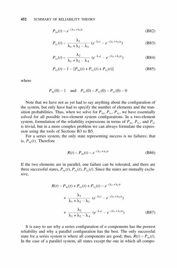
452 SUMMARY OF RELIABILITY THEORY
Ps0 (t) c e− (l1 +l2)t (B82)
Ps1 (t) cl1
l1 + l2 − l3(e−l3t
− e− (l1 +l2)t) (B83)
Ps2 (t) cl2
l1 + l2 − l 4(e−l 4t
− e− (l1 +l2)t) (B84)
Ps3 (t) c 1 − [Ps0 (t) + Ps1 (t) + Ps2 (t)] (B85)
where
Ps0 (0) c 1 and Ps1 (0) c Ps2 (0) c Ps3 (0) c 0
Note that we have not as yet had to say anything about the configuration ofthe system, but only have had to specify the number of elements and the tran-sition probabilities. Thus, when we solve for Ps0 , Ps1 , Ps2 , we have essentiallysolved for all possible two-element system configurations. In a two-elementsystem, formulation of the reliability expressions in terms of Ps0 , Ps1 , and Ps2
is trivial, but in a more complex problem we can always formulate the expres-sion using the tools of Sections B3 to B5.
For a series system, the only state representing success is no failures; thatis, Ps0 (t). Therefore
R(t) c Ps0 (t) c e− (l1 +l2)t (B86)
If the two elements are in parallel, one failure can be tolerated, and there arethree successful states, Ps0 (t), Ps1 (t), Ps2 (t). Since the states are mutually exclu-sive,
R(t) c Ps0 (t) + Ps1 (t) + Ps2 (t) c e− (l1 +l2)t
+l1
l1 + l2 − l3(e−l3t
− e− (l1 +l2)t)
+l2
l1 + l2 − l 4(e−l 4t
− e− (l1 +l2)t) (B87)
It is easy to see why a series configuration of n components has the poorestreliability and why a parallel configuration has the best. The only successfulstate for a series system is where all components are good; thus, R(t) c Ps0 (t).In the case of a parallel system, all states except the one in which all compo-
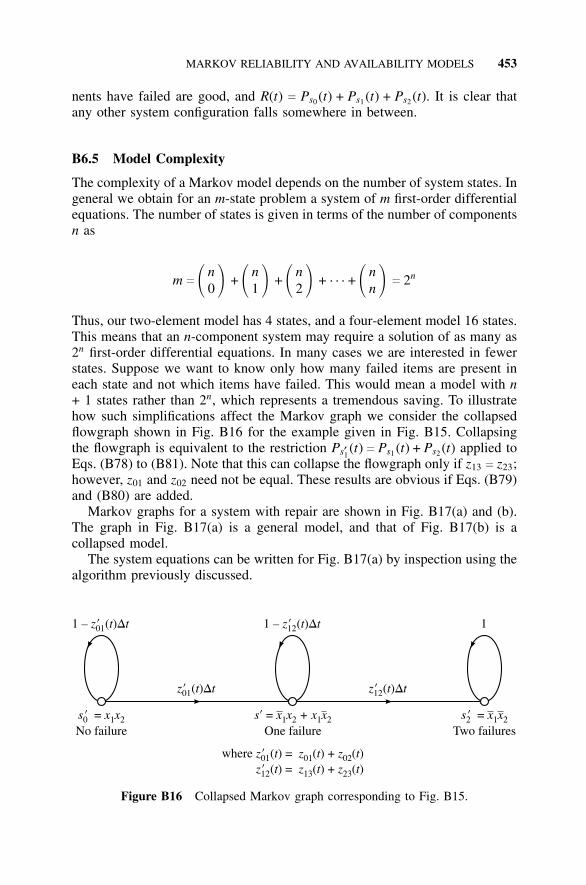
MARKOV RELIABILITY AND AVAILABILITY MODELS 453
nents have failed are good, and R(t) c Ps0 (t) + Ps1 (t) + Ps2 (t). It is clear thatany other system configuration falls somewhere in between.
B6.5 Model Complexity
The complexity of a Markov model depends on the number of system states. Ingeneral we obtain for an m-state problem a system of m first-order differentialequations. The number of states is given in terms of the number of componentsn as
m c � n0 � + � n
1 � + � n2 � + · · · + � n
n � c 2n
Thus, our two-element model has 4 states, and a four-element model 16 states.This means that an n-component system may require a solution of as many as2n first-order differential equations. In many cases we are interested in fewerstates. Suppose we want to know only how many failed items are present ineach state and not which items have failed. This would mean a model with n+ 1 states rather than 2n, which represents a tremendous saving. To illustratehow such simplifications affect the Markov graph we consider the collapsedflowgraph shown in Fig. B16 for the example given in Fig. B15. Collapsingthe flowgraph is equivalent to the restriction Ps′1 (t) c Ps1 (t) + Ps2 (t) applied toEqs. (B78) to (B81). Note that this can collapse the flowgraph only if z13 c z23;however, z01 and z02 need not be equal. These results are obvious if Eqs. (B79)and (B80) are added.
Markov graphs for a system with repair are shown in Fig. B17(a) and (b).The graph in Fig. B17(a) is a general model, and that of Fig. B17(b) is acollapsed model.
The system equations can be written for Fig. B17(a) by inspection using thealgorithm previously discussed.
1 ( )– z t t01’ D
where ( ) =z t01’ z t z t01 02( ) + ( )
z t t01’ ( )D z t t12’ ( )D
1 ( )– z t t12’ D 1
s x x0 =’ 1 2No failure
s x x2 =’ 1 2Two failures
s x x=’ 1 2 1 2+ x xOne failure
z t z t z t12 13 23’ ( ) = ( ) + ( )
Figure B16 Collapsed Markov graph corresponding to Fig. B15.
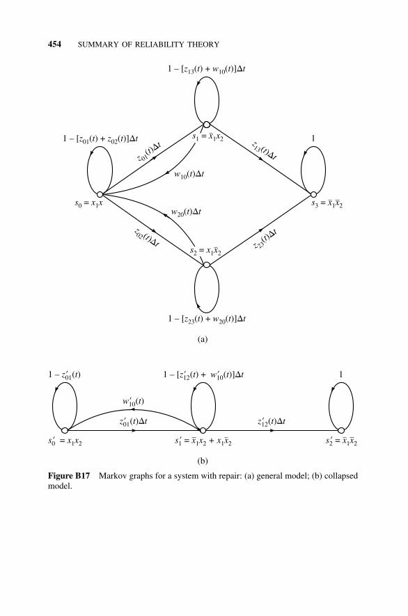
454 SUMMARY OF RELIABILITY THEORY
1 ( )– z t01’
z t t01’ ( )D
w t10’ ( )
z t t12’ ( )D
1 [ ( ) +– z t t12’ Dw t10’ ( )] 1
s x x0 =’ 1 2 s x x2 =’ 1 2s + x x1 1 2 1 2’ = x x
(b)
(a)
1 [ ( ) +– z t t13 Dw t10( )]
1 – [ ( ) +z t t01 Dz t02( )]
1 [ ( ) +– z t t23 Dw t20( )]
s x x3 = 1 2s x x0 = 1
zt
t13 ( )D
zt
t
01( )D
zt
t02 ( )D
zt
t
23( )D
1
w t t10( )D
w t t20( )D
s x x2 = 1 2
s x x1 = 1 2
Figure B17 Markov graphs for a system with repair: (a) general model; (b) collapsedmodel.
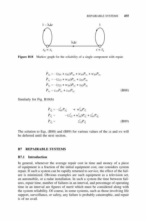
REPAIRABLE SYSTEMS 455
s = x0 1 s = x1
lDt
1 – tlD 1
Figure B18 Markov graph for the reliability of a single component with repair.
Ps0 c − (z01 + z02)Ps0 + w10Ps1 + w20Ps2
Ps1 c − (z13 + w10)Ps1 + z01Ps0
Ps2 c − (z23 + w20)Ps2 + z02Ps0
Ps3 c z13Ps1 + z23Ps2 (B88)
Similarly for Fig. B18(b)
Ps′0 c −z′01Ps′0 + w′10Ps′1
Ps′1 c − (z′12 + w′10)Ps′1 + z′01Ps′0
Ps′2 c z′12Ps′1 (B89)
The solution to Eqs. (B88) and (B89) for various values of the zs and ws willbe deferred until the next section.
B7 REPAIRABLE SYSTEMS
B7.1 Introduction
In general, whenever the average repair cost in time and money of a pieceof equipment is a fraction of the initial equipment cost, one considers systemrepair. If such a system can be rapidly returned to service, the effect of the fail-ure is minimized. Obvious examples are such equipment as a television set,an automobile, or a radar installation. In such a system the time between fail-ures, repair time, number of failures in an interval, and percentage of operatingtime in an interval are figures of merit which must be considered along withthe system reliability. Of course, in some systems, such as those involving lifesupport, surveillance, or safety, any failure is probably catastrophic, and repairis of no avail.
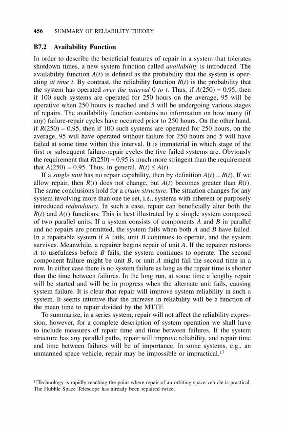
456 SUMMARY OF RELIABILITY THEORY
B7.2 Availability Function
In order to describe the beneficial features of repair in a system that toleratesshutdown times, a new system function called availability is introduced. Theavailability function A(t) is defined as the probability that the system is oper-ating at time t. By contrast, the reliability function R(t) is the probability thatthe system has operated over the interval 0 to t. Thus, if A(250) c 0.95, thenif 100 such systems are operated for 250 hours on the average, 95 will beoperative when 250 hours is reached and 5 will be undergoing various stagesof repairs. The availability function contains no information on how many (ifany) failure-repair cycles have occurred prior to 250 hours. On the other hand,if R(250) c 0.95, then if 100 such systems are operated for 250 hours, on theaverage, 95 will have operated without failure for 250 hours and 5 will havefailed at some time within this interval. It is immaterial in which stage of thefirst or subsequent failure-repair cycles the five failed systems are. Obviouslythe requirement that R(250) c 0.95 is much more stringent than the requirementthat A(250) c 0.95. Thus, in general, R(t) ≤ A(t).
If a single unit has no repair capability, then by definition A(t) c R(t). If weallow repair, then R(t) does not change, but A(t) becomes greater than R(t).The same conclusions hold for a chain structure. The situation changes for anysystem involving more than one tie set, i.e., systems with inherent or purposelyintroduced redundancy. In such a case, repair can beneficially alter both theR(t) and A(t) functions. This is best illustrated by a simple system composedof two parallel units. If a system consists of components A and B in paralleland no repairs are permitted, the system fails when both A and B have failed.In a repairable system if A fails, unit B continues to operate, and the systemsurvives. Meanwhile, a repairer begins repair of unit A. If the repairer restoresA to usefulness before B fails, the system continues to operate. The secondcomponent failure might be unit B, or unit A might fail the second time in arow. In either case there is no system failure as long as the repair time is shorterthan the time between failures. In the long run, at some time a lengthy repairwill be started and will be in progress when the alternate unit fails, causingsystem failure. It is clear that repair will improve system reliability in such asystem. It seems intuitive that the increase in reliability will be a function ofthe mean time to repair divided by the MTTF.
To summarize, in a series system, repair will not affect the reliability expres-sion; however, for a complete description of system operation we shall haveto include measures of repair time and time between failures. If the systemstructure has any parallel paths, repair will improve reliability, and repair timeand time between failures will be of importance. In some systems, e.g., anunmanned space vehicle, repair may be impossible or impractical.17
17Technology is rapidly reaching the point where repair of an orbiting space vehicle is practical.The Hubble Space Telescope has already been repaired twice.
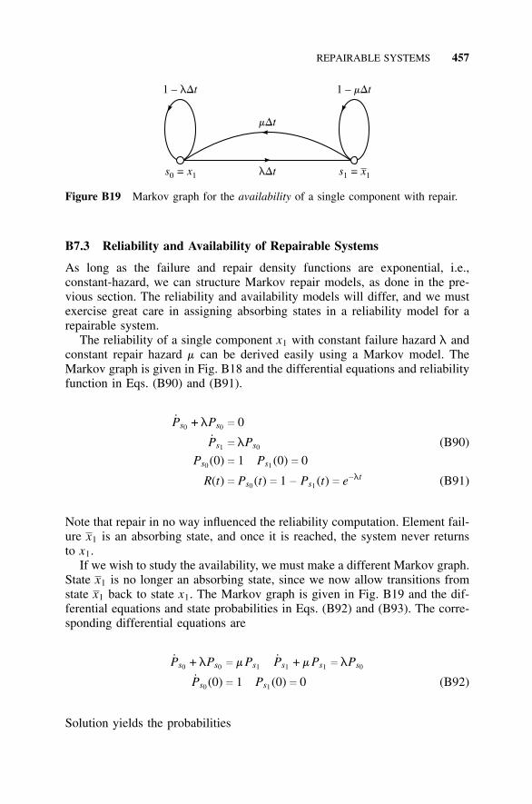
REPAIRABLE SYSTEMS 457
s = x0 1 s = x1 1
mDt
lDt
1 – tlD 1 – tmD
Figure B19 Markov graph for the availability of a single component with repair.
B7.3 Reliability and Availability of Repairable Systems
As long as the failure and repair density functions are exponential, i.e.,constant-hazard, we can structure Markov repair models, as done in the pre-vious section. The reliability and availability models will differ, and we mustexercise great care in assigning absorbing states in a reliability model for arepairable system.
The reliability of a single component x1 with constant failure hazard l andconstant repair hazard m can be derived easily using a Markov model. TheMarkov graph is given in Fig. B18 and the differential equations and reliabilityfunction in Eqs. (B90) and (B91).
Ps0 + lPs0 c 0
Ps1 c lPs0 (B90)
Ps0 (0) c 1 Ps1 (0) c 0
R(t) c Ps0 (t) c 1 − Ps1 (t) c e−lt (B91)
Note that repair in no way influenced the reliability computation. Element fail-ure x1 is an absorbing state, and once it is reached, the system never returnsto x1.
If we wish to study the availability, we must make a different Markov graph.State x1 is no longer an absorbing state, since we now allow transitions fromstate x1 back to state x1. The Markov graph is given in Fig. B19 and the dif-ferential equations and state probabilities in Eqs. (B92) and (B93). The corre-sponding differential equations are
Ps0 + lPs0 c mPs1 Ps1 + mPs1 c lPs0
Ps0 (0) c 1 Ps1 (0) c 0 (B92)
Solution yields the probabilities
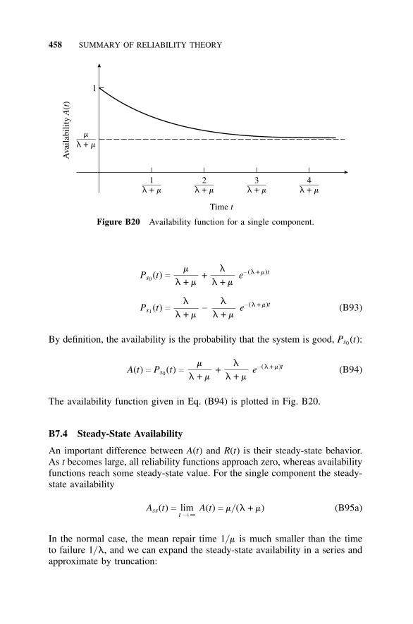
458 SUMMARY OF RELIABILITY THEORY
1+l m
ml m+
2+l m
3+l m
4+l m
1
Time t
Ava
ilabi
lity
()
At
Figure B20 Availability function for a single component.
Ps0 (t) cm
l + m+
l
l + me− (l + m)t
Ps1 (t) cl
l + m−
l
l + me− (l + m)t (B93)
By definition, the availability is the probability that the system is good, Ps0 (t):
A(t) c Ps0 (t) cm
l + m+
l
l + me− (l + m)t (B94)
The availability function given in Eq. (B94) is plotted in Fig. B20.
B7.4 Steady-State Availability
An important difference between A(t) and R(t) is their steady-state behavior.As t becomes large, all reliability functions approach zero, whereas availabilityfunctions reach some steady-state value. For the single component the steady-state availability
Ass(t) c limtb∞
A(t) c m/ (l + m) (B95a)
In the normal case, the mean repair time 1/m is much smaller than the timeto failure 1/ l, and we can expand the steady-state availability in a series andapproximate by truncation:
REPAIRABLE SYSTEMS 459
Ass(t) c A(∞) c1
1 + l/m c 1 −l
m+
l2
2m2+ · · · ≈ 1 −
l
m(B95b)
The transient part of the availability function decays to zero fairly rapidly.The time at which the transient term is negligible with respect to the steady-state term depends on l and m. As an upper bound we know that the terme−at ≤ 0.02 for t > 4/ a; therefore, we can state that the transient term is overbefore t c 4/ (l + m). If m > l, the transient is over before t c 4/m. Theinteraction between reliability and availability specifications is easily seen inthe following example.
Suppose a system is to be designed to have a reliability of greater than 0.90over 1,000 hours and a minimum availability of 0.99 over that period. Thereliability specification yields
R(t) c e−lt ≥ 0.90 0 < t < 1, 000
e−1,000l ≈ 1 − 103l c 0.90 l ≥ 10−4
Assuming A(∞) for the minimum value of the availability, Eq. (B95) yields
A(∞) c 1 −l
mc 0.99
m c 100l c 10−2
Thus, we use a component with an MTTF of 104 hours, a little over 1 year, anda mean repair time of 100 hours (about 4 days). The probability of any failurewithin 1,000 hours (about 6 weeks) is less than 10%. Furthermore, the prob-ability that the system is down and under repair at any chosen time betweent c 0 and t c 103 hours is less than 1%. Now to check the approximations.The transient phase of the availability function lasts for 4/ (10−2 + 10−4) ≈ 400hours; thus the availability will be somewhat greater than 0.99 for 400 hoursand then settle down at 0.99 for the remaining 600 hours. Since m is 100l, theapproximation of Eq. (B95) is valid. Also since lt c 10−4 × 10³
c 10−1, thetwo-term series expansion of the exponential is also satisfactory.
The availability function has been defined as a probability function, just asthe reliability function was. There is another statistical interpretation whichsheds some light on the concept. Suppose that a large number of system oper-ating hours are accumulated. This can be done either by operating one sys-tem for a long time, so that many failure and repair cycles are obtained andrecorded, or by operating a large number of identical systems (an ensemble)for a shorter period of time and combining the data. If the ratio of cumulativeoperating time to total test time is computed, it approaches A(∞) as t b ∞.Actually the data taken during the transient period of availability should bediscarded to avoid any distortions. In fact if one wished to compute the trans-ient phase of availability from experimental data, one would be forced to use
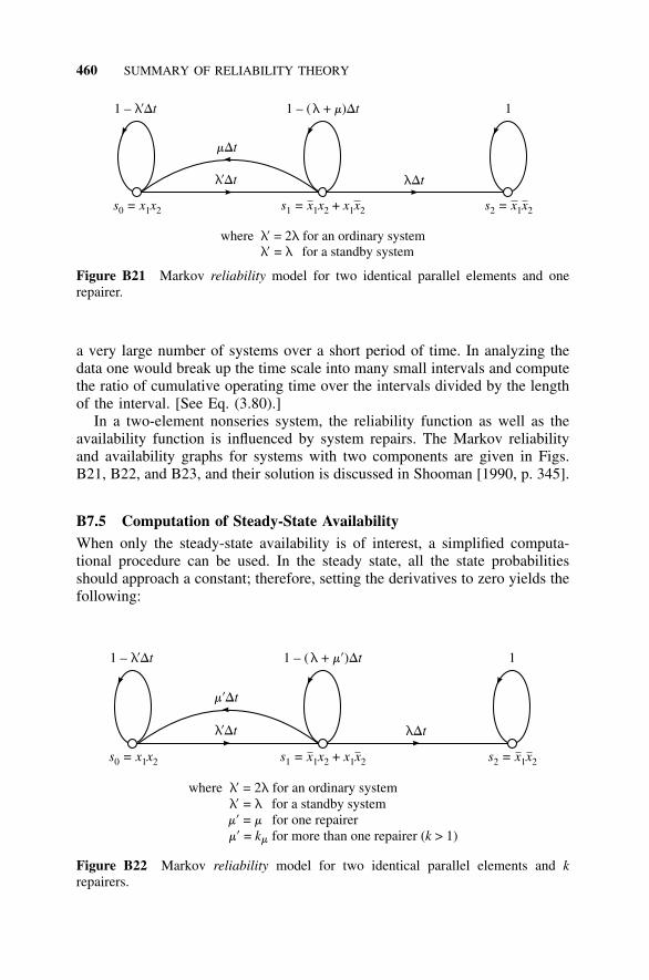
460 SUMMARY OF RELIABILITY THEORY
s = x x0 1 2 s = x x x x1 1 2 1 2+ s = x x2 1 2
mDt
lD’ t lDt
1 – tlD’ 1 ( + )– tl m D 1
where l ll l’’
= 2 for an ordinary system= for a standby system
Figure B21 Markov reliability model for two identical parallel elements and onerepairer.
a very large number of systems over a short period of time. In analyzing thedata one would break up the time scale into many small intervals and computethe ratio of cumulative operating time over the intervals divided by the lengthof the interval. [See Eq. (3.80).]
In a two-element nonseries system, the reliability function as well as theavailability function is influenced by system repairs. The Markov reliabilityand availability graphs for systems with two components are given in Figs.B21, B22, and B23, and their solution is discussed in Shooman [1990, p. 345].
B7.5 Computation of Steady-State AvailabilityWhen only the steady-state availability is of interest, a simplified computa-tional procedure can be used. In the steady state, all the state probabilitiesshould approach a constant; therefore, setting the derivatives to zero yields thefollowing:
s = x x0 1 2 s = x x x x1 1 2 1 2+ s = x x2 1 2
m’Dt
lD’ t lDt
1 – tlD’ 1 ( + )– tl Dm’ 1
where
k k
l ll lm mm
’’’’
= 2 for an ordinary system= for a standby system= for one repairer= for more than one repairer ( > 1)m
Figure B22 Markov reliability model for two identical parallel elements and krepairers.
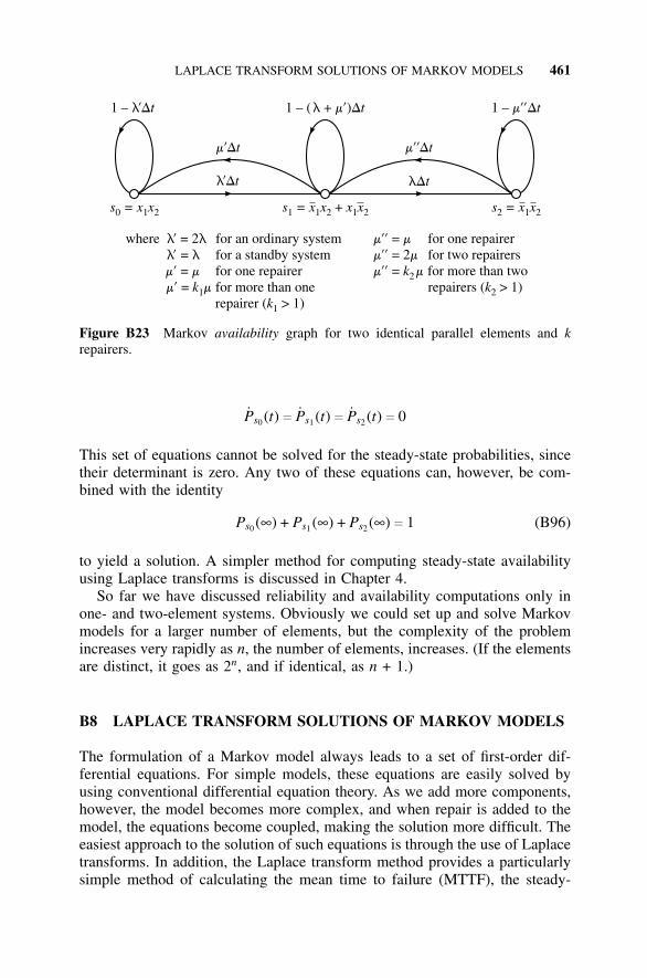
LAPLACE TRANSFORM SOLUTIONS OF MARKOV MODELS 461
s = x x0 1 2 s = x x x x1 1 2 1 2+ s = x x2 1 2
m’Dt m’’Dt
lD’ t lDt
1 – tlD’ 1 ( + )– tl Dm’ 1 – tDm’’
where
kk
l ll lm mm m
’’’’
= 2 for an ordinary system= for a standby system= for one repairer= for more than one
repairer ( > 1)1
1
m mm mm m
’’’’’’
= for one repairer= 2 for two repairers= for more than two
repairers ( > 1)k
k2
2
Figure B23 Markov availability graph for two identical parallel elements and krepairers.
Ps0 (t) c Ps1 (t) c Ps2 (t) c 0
This set of equations cannot be solved for the steady-state probabilities, sincetheir determinant is zero. Any two of these equations can, however, be com-bined with the identity
Ps0 (∞) + Ps1 (∞) + Ps2 (∞) c 1 (B96)
to yield a solution. A simpler method for computing steady-state availabilityusing Laplace transforms is discussed in Chapter 4.
So far we have discussed reliability and availability computations only inone- and two-element systems. Obviously we could set up and solve Markovmodels for a larger number of elements, but the complexity of the problemincreases very rapidly as n, the number of elements, increases. (If the elementsare distinct, it goes as 2n, and if identical, as n + 1.)
B8 LAPLACE TRANSFORM SOLUTIONS OF MARKOV MODELS
The formulation of a Markov model always leads to a set of first-order dif-ferential equations. For simple models, these equations are easily solved byusing conventional differential equation theory. As we add more components,however, the model becomes more complex, and when repair is added to themodel, the equations become coupled, making the solution more difficult. Theeasiest approach to the solution of such equations is through the use of Laplacetransforms. In addition, the Laplace transform method provides a particularlysimple method of calculating the mean time to failure (MTTF), the steady-
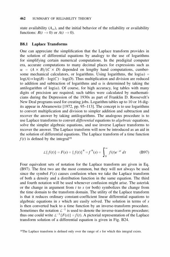
462 SUMMARY OF RELIABILITY THEORY
state availability (Ass), and the initial behavior of the reliability or availabilityfunctions: R(t b 0) or A(t b 0).
B8.1 Laplace Transforms
One can appreciate the simplification that the Laplace transform provides inthe solution of differential equations by analogy to the use of logarithmsfor simplifying certain numerical computations. In the predigital computerera, accurate computations to many decimal places for expressions such asa c (A × B)/ (C × D) depended on lengthy hand computations, cumber-some mechanical calculators, or logarithms. Using logarithms, the log(a) clog(A)+ log(B) − log(C ) − log(D). Thus multiplication and division are reducedto addition and subtraction of logarithms and a is determined by taking theantilogarithm of log(a). Of course, for high accuracy, log tables with manydigits of precision are required; such tables were calculated by mathemati-cians during the Depression of the 1930s as part of Franklin D. Roosevelt’sNew Deal programs used for creating jobs. Logarithm tables up to 10 or 16 dig-its appear in Abramowitz [1972, pp. 95–113]. The concept is to use logarithmsto convert multiplication and division to simpler addition and subtraction andrecover the answer by taking antilogarithms. The analogous procedure is touse Laplace transforms to convert differential equations to algebraic equations,solve the simpler algebraic equations, and use inverse Laplace transforms torecover the answer. The Laplace transform will now be introduced as an aid inthe solution of differential equations. The Laplace transform of a time functionf (t) is defined by the integral18
L{ f (t)} c F(s) c { f (t)}*c f *(s) c ∫
∞
0f (t)e−st d t (B97)
Four equivalent sets of notation for the Laplace transform are given in Eq.(B97). The first two are the most common, but they will not always be usedsince the symbol F(s) causes confusion when we take the Laplace transformof both a density and a distribution function in the same equation. The thirdand fourth notation will be used whenever confusion might arise. The asteriskor the change in argument from t to s (or both) symbolizes the change fromthe time domain to the transform domain. The utility of the Laplace transformis that it reduces ordinary constant-coefficient linear differential equations toalgebraic equations in s which are easily solved. The solution in terms of sis then converted back to a time function by an inverse-transform procedure.Sometimes the notation L −1 is used to denote the inverse-transform procedure;thus one could write L −1{F(s)} c f (t). A pictorial representation of the Laplacetransform solution of a differential equation is given in Fig. B24.
18The Laplace transform is defined only over the range of s for which this integral exists.
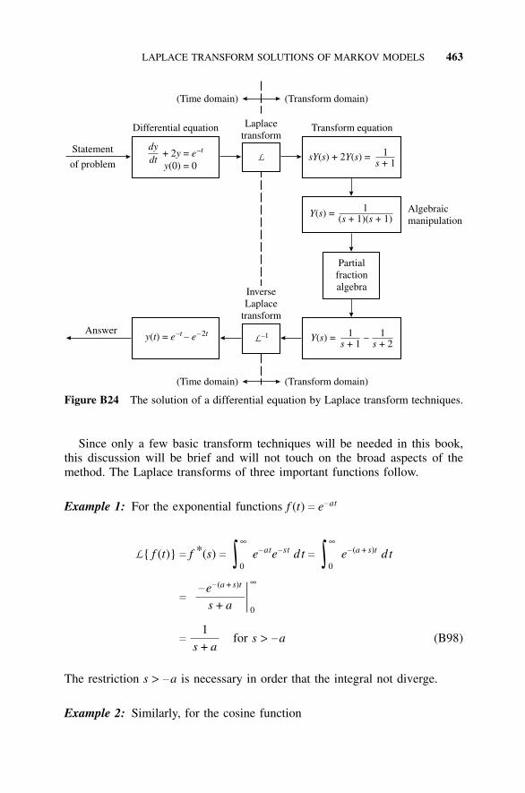
LAPLACE TRANSFORM SOLUTIONS OF MARKOV MODELS 463
Differential equation Transform equation
dydt
+ 2 =y e–t
y(0) = 0
y t e( ) = ––t e–
Statement
of problem
Answer
sY s Y s( ) + 2 ( ) = 1+ 1s
Laplacetransform
(Time domain)
(Time domain)
(Transform domain)
(Transform domain)
L
1( + 1)s ( + 1)sY s( ) =
Partialfractionalgebra
Y s( ) = 1+ 1s
1+ 2s
–
InverseLaplace
transform
L–1
Algebraicmanipulation
2t
Figure B24 The solution of a differential equation by Laplace transform techniques.
Since only a few basic transform techniques will be needed in this book,this discussion will be brief and will not touch on the broad aspects of themethod. The Laplace transforms of three important functions follow.
Example 1: For the exponential functions f (t) c e−at
L{ f (t)} c f *(s) c ∫∞
0e−ate−st d t c ∫
∞
0e− (a + s)t d t
c
−e− (a + s)t
s + a
||||
∞
0
c
1s + a
for s > −a (B98)
The restriction s > −a is necessary in order that the integral not diverge.
Example 2: Similarly, for the cosine function
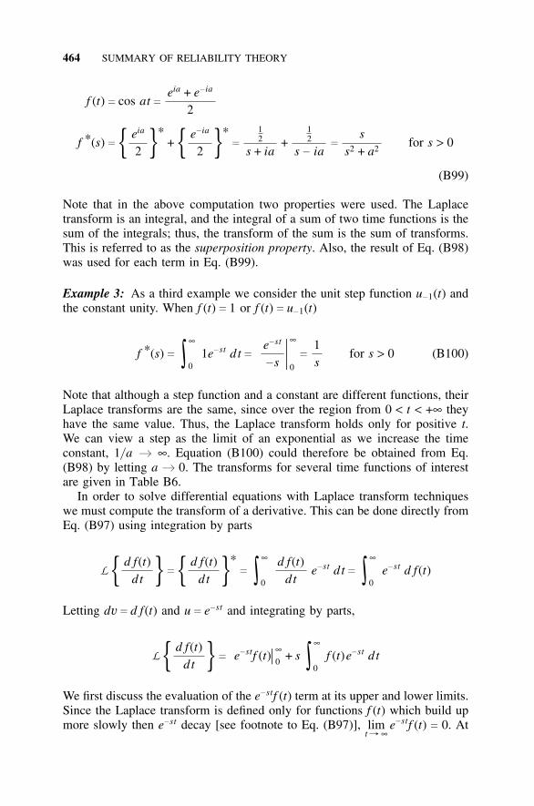
464 SUMMARY OF RELIABILITY THEORY
f (t) c cos at ceia + e− ia
2
f *(s) c { eia
2 }∗+ { e− ia
2 }∗c
12
s + ia+
12
s − iac
ss2 + a2
for s > 0
(B99)
Note that in the above computation two properties were used. The Laplacetransform is an integral, and the integral of a sum of two time functions is thesum of the integrals; thus, the transform of the sum is the sum of transforms.This is referred to as the superposition property. Also, the result of Eq. (B98)was used for each term in Eq. (B99).
Example 3: As a third example we consider the unit step function u−1(t) and
the constant unity. When f (t) c 1 or f (t) c u−1(t)
f *(s) c ∫∞
01e−st d t c
e−st
−s
||||
∞
0
c
1s
for s > 0 (B100)
Note that although a step function and a constant are different functions, theirLaplace transforms are the same, since over the region from 0 < t < +∞ theyhave the same value. Thus, the Laplace transform holds only for positive t.We can view a step as the limit of an exponential as we increase the timeconstant, 1/ a b ∞. Equation (B100) could therefore be obtained from Eq.(B98) by letting a b 0. The transforms for several time functions of interestare given in Table B6.
In order to solve differential equations with Laplace transform techniqueswe must compute the transform of a derivative. This can be done directly fromEq. (B97) using integration by parts
L { d f(t)dt } c { d f(t)
dt }∗c ∫
∞
0
d f(t)dt
e−st d t c ∫∞
0e−st d f(t)
Letting dv c d f(t) and u c e−st and integrating by parts,
L { d f(t)dt } c e−stf (t)|
|∞0 + s ∫
∞
0f (t)e−st d t
We first discuss the evaluation of the e−stf (t) term at its upper and lower limits.Since the Laplace transform is defined only for functions f (t) which build upmore slowly then e−st decay [see footnote to Eq. (B97)], lim
t r ∞e−stf (t) c 0. At
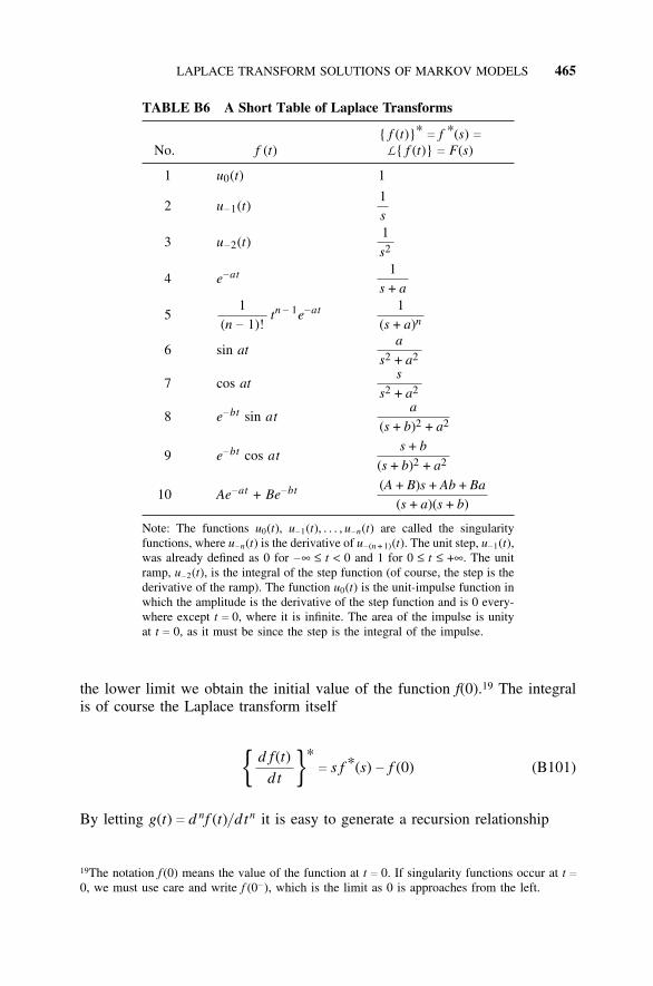
LAPLACE TRANSFORM SOLUTIONS OF MARKOV MODELS 465
TABLE B6 A Short Table of Laplace Transforms
{ f (t)}*c f *(s) c
No. f (t) L{ f (t)} c F(s)
1 u0(t) 1
2 u−1(t)
1s
3 u−2(t)
1
s2
4 e−at 1s + a
51
(n − 1)!tn − 1e−at 1
(s + a)n
6 sin ata
s2 + a2
7 cos ats
s2 + a2
8 e−bt sin ata
(s + b)2 + a2
9 e−bt cos ats + b
(s + b)2 + a2
10 Ae−at + Be−bt (A + B)s + Ab + Ba(s + a)(s + b)
Note: The functions u0(t), u−1(t), . . . , u
−n(t) are called the singularityfunctions, where u
−n(t) is the derivative of u− (n + 1)(t). The unit step, u
−1(t),was already defined as 0 for −∞ ≤ t < 0 and 1 for 0 ≤ t ≤ +∞. The unitramp, u
−2(t), is the integral of the step function (of course, the step is thederivative of the ramp). The function u0(t) is the unit-impulse function inwhich the amplitude is the derivative of the step function and is 0 every-where except t c 0, where it is infinite. The area of the impulse is unityat t c 0, as it must be since the step is the integral of the impulse.
the lower limit we obtain the initial value of the function f(0).19 The integralis of course the Laplace transform itself
{ d f(t)dt }∗
c s f *(s) − f (0) (B101)
By letting g(t) c d nf (t)/ dtn it is easy to generate a recursion relationship
19The notation f (0) means the value of the function at t c 0. If singularity functions occur at t c0, we must use care and write f (0− ), which is the limit as 0 is approaches from the left.
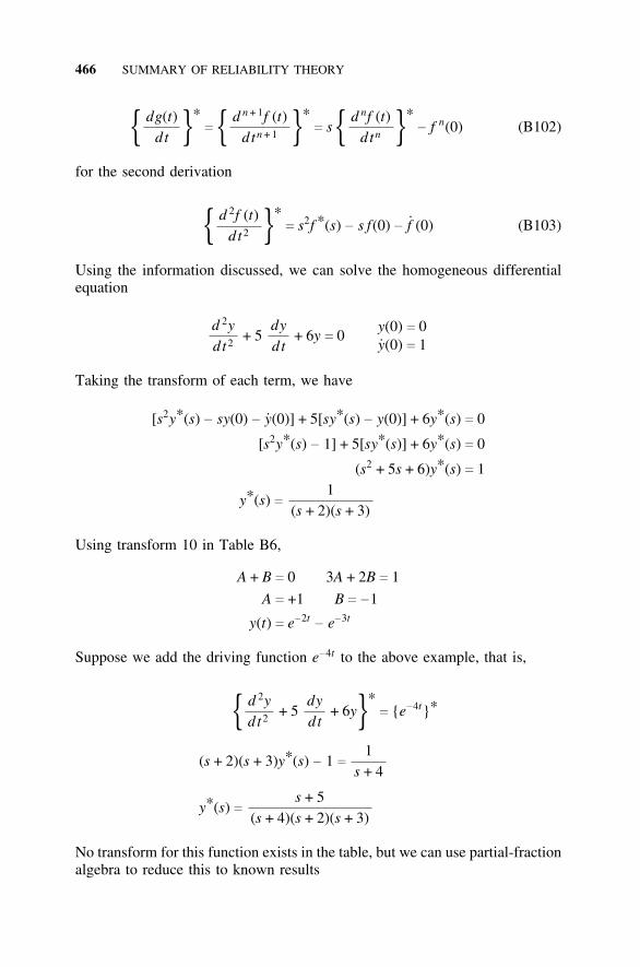
466 SUMMARY OF RELIABILITY THEORY
{ dg(t)dt }∗
c { d n + 1f (t)dtn + 1 }∗
c s { d nf (t)dtn }∗
− f n(0) (B102)
for the second derivation
{ d 2f (t)dt2 }∗
c s2f *(s) − s f(0) − f (0) (B103)
Using the information discussed, we can solve the homogeneous differentialequation
d 2ydt2
+ 5dydt
+ 6y c 0y(0) c 0y(0) c 1
Taking the transform of each term, we have
[s2y*(s) − sy(0) − y(0)] + 5[sy*(s) − y(0)] + 6y*(s) c 0
[s2y*(s) − 1] + 5[sy*(s)] + 6y*(s) c 0
(s2 + 5s + 6)y*(s) c 1
y*(s) c1
(s + 2)(s + 3)
Using transform 10 in Table B6,
A + B c 0 3A + 2B c 1
A c +1 B c −1
y(t) c e−2t− e−3t
Suppose we add the driving function e−4t to the above example, that is,
{ d 2ydt2
+ 5dydt
+ 6y}∗c {e−4t}*
(s + 2)(s + 3)y*(s) − 1 c
1s + 4
y*(s) cs + 5
(s + 4)(s + 2)(s + 3)
No transform for this function exists in the table, but we can use partial-fractionalgebra to reduce this to known results
LAPLACE TRANSFORM SOLUTIONS OF MARKOV MODELS 467
s + 5(s + 4)(s + 2)(s + 3)
c
12
s + 4+
32
s + 2+
−2s + 3
Thus, each term represents an exponential, and
y(t) c 12 e−4t + 3
2 e−2t− 2e−3t
The e−4t term represents the particular solution (driving function), and the e−2t
and e−3t terms represent the homogeneous solution (natural response).The partial-fraction-expansion coefficients can be found by conventional
means or by the following shortcut formula
f (s) cN(s)D(s)
c
N(s)n
∏i c 1
(s + ri)
c
A1
s + r1+
A2
s + r2+ · · · +
An
s + rn
where
Ai c [ N(s)D(s)
(s + ri)]s c −ri
(B104)
For the above example
A1 c [ s + 5(s + 4)(s + 2)(s + 3)
(s + 4)]s c −4
c
12
A2 c [ s + 5(s + 4)(s + 2)(s + 3)
(s + 2)]s c −2
c
32
A3 c [ s + 5(s + 4)(s + 2)(s + 3)
(s + 3)]s c −3
c −2
The derivation of Eq. (B104) as well as a similar one for the case of repeatedroots can be found in any text on Laplace transforms.
We have already discussed two Laplace transform theorems, superpositionand derivative property. Some additional ones useful in solving Markov modelsappear in Table B7.
The first and second theorems have already been discussed. The third theo-rem is simply the integral equivalent of the differentiation theorems. The con-volution theorem is important since it describes the time-domain equivalent ofa product of two Laplace transforms. Theorems 6 and 7 are useful in computingthe initial and final behavior of reliability functions.
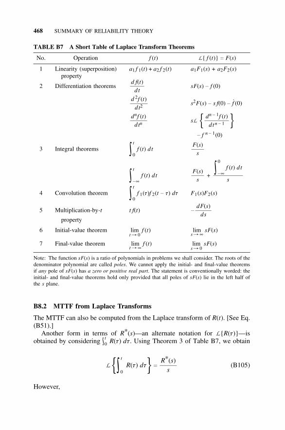
468 SUMMARY OF RELIABILITY THEORY
TABLE B7 A Short Table of Laplace Transform Theorems
No. Operation f (t) L{ f (t)} c F(s)
1 Linearity (superposition) a1 f 1(t) + a2 f 2(t) a1F1(s) + a2F2(s)property
2 Differentiation theoremsd f(t)
dtsF(s) − f (0)
d 2f (t)dt2
s2F(s) − s f(0) − f (0)
dnf (t)dtn
sL { dn − 1f (t)dtn − 1 }
− f n − 1(0)
3 Integral theorems ∫t
0f (t) dt
F(s)s
∫t
−∞f (t) dt
F(s)s
+∫
0
−∞f (t) dt
s
4 Convolution theorem ∫t
0f 1(t)f 2(t − t) dt F1(s)F2(s)
5 Multiplication-by-t t f(t) −
dF(s)ds
property
6 Initial-value theorem limt r 0
f (t) lims r ∞
sF(s)
7 Final-value theorem limt r ∞
f (t) lims r 0
sF(s)
Note: The function sF(s) is a ratio of polynomials in problems we shall consider. The roots of thedenominator polynomial are called poles. We cannot apply the initial- and final-value theoremsif any pole of sF(s) has a zero or positive real part. The statement is conventionally worded: theinitial- and final-value theorems hold only provided that all poles of sF(s) lie in the left half ofthe s plane.
B8.2 MTTF from Laplace Transforms
The MTTF can also be computed from the Laplace transform of R(t). [See Eq.(B51).]
Another form in terms of R*(s)—an alternate notation for L{R(t)}—isobtained by considering ∫
t0 R(t) dt. Using Theorem 3 of Table B7, we obtain
L {∫t
0R(t) dt} c
R*(s)s
(B105)
However,
LAPLACE TRANSFORM SOLUTIONS OF MARKOV MODELS 469
MTTF c limtb∞ ∫
t
0R(t) dt
Using Theorem 7 of Table B12,
MTTF c limtb∞ ∫
t
0R(t) dt c lim
s r 0sL {∫
t
0R(t) dt} c lim
s r 0s
R*(s)s
Thus,
MTTR c lims r 0
R*(s) (B106)
The above formula is extremely useful for computing the MTTF for a Markovmodel.
B8.3 Time-Series Approximations from Laplace Transforms
One of the objectives of the MTTF computations of the previous section is tosimplify the algebra involved in obtaining time functions from the transformedfunction. In most practical cases, the transform expression (ratio of two poly-nomials in s) has a denominator that is of second, third, or higher order. Thesolution requires the factoring of the polynomial (generally requiring numeri-cal methods) and subsequent partial-fraction expansion. Calculating the MTTFfrom F(s) by taking the limit as given in Eq. (B106), is simple; however, it pro-vides only partial information. In Section 3.4.1, we discussed approximatingthe system-time function in the high-reliability region by the leading terms inthe Taylor-series expansion. If this is our objective, and if we have the Laplacetransform, we can find the Taylor-series coefficients simply and directly with-out first finding the time function.
Any function f (t), whose various derivatives exist, can be expanded in aTaylor series:
f (t) c f (0) + f ′(0)t/ 1! + f ′′(0)t 2/ 2! + f ′′′(0)t 3/ 3! + · · · (B107)
Where f ′′′(0) is the third time derivative of f (t) evaluated at t c 0, and similarlyfor f (0), f ′, and so on.
Note that the derivatives of f (t) always exist for a reliability function thatis a linear combination of exponential terms, since all derivatives exist for anexponential function. We can rewrite this equation in terms of a set of constantKi, which stand for the time derivatives, and obtain
470 SUMMARY OF RELIABILITY THEORY
f (t) c K0 + K1t/ 1! + K2t 2/ 2! + · · · +∞
���n c 0
Knt n/ n! (B108)
If we take L{ f (t)} for the function in Eq. (B108), we obtain a series of simpleLaplace transforms for the right-hand side of the equation. These transformscan easily be obtained from entry no. 5 in Table B6 by setting a c 0, yielding
L{ f (t)} c F(s) c∞
���n c 0
Kn
s n + 1(B109)
Knowing that f (t) in Eq. (B108) is a reliability function, we know that R(0) c1; thus K0 c 1. We can easily manipulate F(s) into the series form given by Eq.(B109) by the simple process of long division. Of course, this method presup-poses that we have the transform, which is generally true if we are solving aMarkov model. If we already have the time function, it is probably easier to usethe expansions discussed in Section 3.4.1 than to first compute the transformand use this approach. The following example illustrates the method.
Let us suppose that in the process of solving a Markov model we obtainthe following Laplace transform of a reliability function:20
R(s) cs + l + l′ + m′
s 2 + [l + l′ + m′]s + ll′(B110)
Performing long division of the numerator and denominator polynomials, weobtain
1s
−
ll′s3
+ll[l + l′ + m′]
s 4+ · · ·
s 2 + [l + l′ + m′]s + ll′ s + [l + l′ + m′](B111)
Thus, by using Table B6, entry no. 5 to obtain the inverse transform, that is,the expression for R(t) that corresponds to R(s) given in Eq. (B111),
R(t) ≈ 1 −
ll′t 2
2+
ll′[l + l′ + m′]t 3
6+ · · · (B112)
For a parallel system, l′ c 2l and m′ c m, and substitution in Eq. (B112) yields
20This example is actually the Laplace transform of the reliability of two parallel elements withrepair. For hot standby, l′ c 2l, and for cold standby, l′ c l. See Eqs. (3.65a, b).
REFERENCES 471
R(t) ≈ 1 − l2t 2 +l2[3l + m]t 3
3+ · · · (B113)
For a standby system, l′ c l and m′ c m, and substitution in Eq. (B112) yields
R(t) ≈ 1 −
l2t 2
2+
l2[2l + m]t 3
6+ · · · (B114)
Comparing Eq. (B113) with (B114), we see from the coefficients of the t 2 termthat the standby system is superior.
REFERENCES
Abramowitz, M., and I. A. Stegun (eds.). Handbook of Mathematical Functions withFormulas, Graphs, and Mathematical Tables. Washington, DC: National Bureau ofStandards, U.S. Government Printing Office (GPO), 1972.
Bernstein, J. Private communication. University of Maryland, October 2001.Carhart, R. R. A Survey of the Current Status of the Reliability Problem. Rand Cor-
poration No. RM-1131, August 14, 1953.Chang, C. Y., and S. M. Size. VLSI Technology. McGraw-Hill, New York, 1996, pp.
668–672.Defect and Fault-Tolerance in VLSI Systems. International Symposium. IEEE Com-
puter Society Press, New York, 1997.Dugan, J. B. Software System Analysis Using Fault Trees. In Handbook of Software
Reliability Engineering, Michael R. Lyu (ed.). McGraw-Hill, New York, 1996, ch.15.
Dugan, J. B., S. J. Bavuso, and M. A. Boyd. Dynamic Fault-Tree Models for Fault-Tolerant Computer Systems. IEEE Transactions on Reliability 41, 3 (June 1992):363–376.
Elsayed, A. Reliability Engineering. Addison-Wesley, Reading, MA, 1996.Grace, K. Jr. Approximate System Availability Models. Proceedings 1969 Annual Sym-
posium on Reliability, January 1969. IEEE, New York, NY, pp. 146–152.Grace, K. Jr. Repair Queuing Models for System Availability. Proceedings 1970 Annual
Symposium on Reliability, February 1970. IEEE, New York, NY, pp. 331–336.Haldar, A., and S. Manadevan. Probability, Reliability, and Statistical Methods in Engi-
neering Design. Wiley, New York, 2000.Healey, J. T. Private communication. Telcordia Technologies, October 2001.Jensen, F. Electronic Component Reliability. Wiley, New York, 1995, app. J, p. 344.Leemis, L. M. Reliability: Probabilistic Models and Statistical Methods. Prentice-Hall,
Englewood Cliffs, NJ, 1994.Meshkat, L., J. B. Dugan, and J. D. Andrews. Analysis of Safety Systems with On-
Demand and Dynamic Failure Modes. Proceedings Annual Reliability and Main-tainability Symposium, 2000. IEEE, New York, NY, pp. 14–21.
472 SUMMARY OF RELIABILITY THEORY
Messinger, M., and M. L. Shooman. Approximations for Complex Structures. Proceed-ings 1967 Annual Symposium on Reliability. IEEE, New York, NY.
Mok, Y.-L., and L.-M. Ten. A Review of Plastic-Encapsulated-Microcircuit Reliability-Prediction Models. Proceedings Annual Reliability and Maintainability Symposium,2000. IEEE, New York, NY, pp. 200–205.
Ohring, M. Reliability and Failure of Electronic Materials and Devices. AcademicPress, New York, 1998, p. 340.
Pecht, M. G. (ed.). Product Reliability, Maintainability, and Supportability Handbook.CRC Press (www.crcpub.com), Boca Raton, FL, 1995.
Pham, H., and S. Upadhyaya. Reliability Analysis of a Class of Fault-Tolerant Systems(Digital Data Communications). Proceedings Annual Reliability and MaintainabilitySymposium, 1989. IEEE, New York, NY, pp. 114–118.
Pukiate, J., and P. Pukite. Modeling for Reliability Analysis. IEEE Press, New York,1998.
Shooman, M. L. Probabilistic Reliability: An Engineering Approach. McGraw-Hill,New York, 1968.
Shooman, M. L. Software Engineering: Design, Reliability, and Management.McGraw-Hill, New York, 1983.
Shooman, M. L. Probabilistic Reliability: An Engineering Approach, 2d ed. Krieger,Melbourne, FL, 1990.
Siewiorek, D. P., and R. S. Swarz. Reliable Computer Systems Design and Evaluation.The Digital Press, New Bedford, MA, 1982.
Size, S. M. (ed.). VLSI Technology, 2d ed. McGraw-Hill, New York, 1988, pp.409–414.
Weibull, W. A Statistical Distribution Function of Wide Application. Journal of AppliedMechanics 18 (1951): 293–297.
Welker, E. L., and M. Lipow. Estimating the Exponential Failure Rate from Data withNo Failure Events. Proceedings Annual Reliability and Maintainability Symposium,1974. IEEE, New York, NY, pp. 420–427.
PROBLEMS
Note: Problems B1–B4, B6, and B10–B12 are taken from Shooman [1990].
B1. A series system is composed of n identical independent components. Thecomponent probability of success is pc and qc c 1 − pc.(a) Show that if qc << 1, the system reliability R is approximately given
by R ≈ 1 − nqc.(b) If the system has 10 components and R must be 0.99, how good
must the components be?
B2. A parallel system is composed of 10 identical independent components.If the system reliability R must be 0.99, what is the minimum componentreliability?
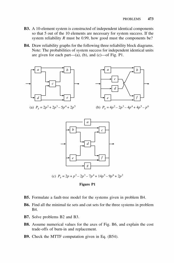
PROBLEMS 473
B3. A 10-element system is constructed of independent identical componentsso that 5 out of the 10 elements are necessary for system success. If thesystem reliability R must be 0.99, how good must the components be?
B4. Draw reliability graphs for the following three reliability block diagrams.Note: The probabilities of system success for independent identical unitsare given for each part—(a), (b), and (c)—of Fig. P1.
a b
c
d e
(a) = 2 + 2 – 5 + 2P p p p ps2 3 4 5 (b) = 4 – 2 – 4 + 4P p p p ps
2 3 4 5 6– p
a b
c
d
e f
(c) = 2 + – 2 – 7 + 14P p p p p ps2 3 4 5 6 2– 9 + 2p p
b c
d
e f
a
g
Figure P1
B5. Formulate a fault-tree model for the systems given in problem B4.
B6. Find all the minimal tie sets and cut sets for the three systems in problemB4.
B7. Solve problems B2 and B3.
B8. Assume numerical values for the axes of Fig. B6, and explain the costtrade-offs of burn-in and replacement.
B9. Check the MTTF computation given in Eq. (B54).
474 SUMMARY OF RELIABILITY THEORY
B10. A communication system is composed of a fixed-frequency transmitterT1 and a fixed-frequency receiver R1. The fixed frequency is f 1 and bothreceiver and transmitter have constant hazards l. In order to improve thereliability, a second receiver and transmitter operating on frequency f 2
are used to provide a redundant channel. Both channels are identical,except for frequency. Construct a reliability diagram for the system andwrite the reliability function. In order to improve reliability, a tuning unitis added to each receiver so that it can operate at frequency f 1 or f 2.The hazard for each tuning unit is given by l′. Draw the new reliabilitydiagram and write the reliability function. Sketch the reliability of theimproved system and the original two-channel system. Assume that l′ c0.1l and repeat for l′ c 10l. (Use series approximations, if necessary.)
B11. Solve for the reliability expression for a three-element standby systemusing a Markov model. All elements are independent identical units withconstant-hazard l.
B12. For a single component with repair, R(t) and A(t) are given by Eqs. (B91)and (B94). If we specify that R(t1) c 0.9,(a) What can you say about A(t1)?(b) How are l and m constrained if A(t1) ≥ 0.99?
APPENDIX C
REVIEW OF ARCHITECTUREFUNDAMENTALS
Reliability of Computer Systems and Networks: Fault Tolerance, Analysis, and DesignMartin L. Shooman
Copyright 2002 John Wiley & Sons, Inc.ISBNs: 0-471-29342-3 (Hardback); 0-471-22460-X (Electronic)
475
C1 INTRODUCTION TO COMPUTER ARCHITECTURE
Most readers of this book probably have an electrical engineering or com-puter science background and are familiar with the material presented in thisappendix; thus they can skip it altogether or thumb through it as a refresher.However, some readers may have a background in mathematics, operationsresearch, or some similar field; for them, this appendix will serve as a concisebackground. The reader is referred to the following references for more detailedinformation: Hill, 1981; Kohavi, 1978; Mano, 1995; Roth, 1995; Shiva, 1988;Wakerly, 2001.
C1.1 Number SystemsComputers are constructed from switching elements that are two-state devices;thus it is common to utilize the binary number system (base 2) for computercomputation, design of arithmetic algorithms, and construction of computerhardware. A number, N, written in radix (base), r, takes on the general poly-nomial form.
N c anr n + an − 1r n − 1 + · · · + a1r1 + a0r0 . a−1r−1 + a
−2r−2 + · · ·
a−−−−−−−− whole number portion −−−−−−−−b |||
a−− fraction portion −−b
radixpoint
(C1)
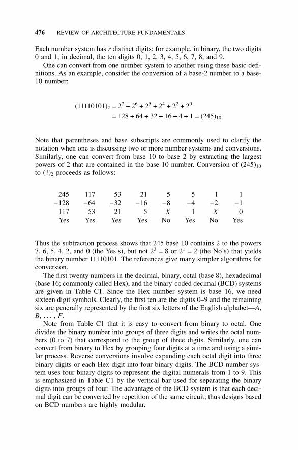
476 REVIEW OF ARCHITECTURE FUNDAMENTALS
Each number system has r distinct digits; for example, in binary, the two digits0 and 1; in decimal, the ten digits 0, 1, 2, 3, 4, 5, 6, 7, 8, and 9.
One can convert from one number system to another using these basic defi-nitions. As an example, consider the conversion of a base-2 number to a base-10 number:
(11110101)2 c 27 + 26 + 25 + 24 + 22 + 20
c 128 + 64 + 32 + 16 + 4 + 1 c (245)10
Note that parentheses and base subscripts are commonly used to clarify thenotation when one is discussing two or more number systems and conversions.Similarly, one can convert from base 10 to base 2 by extracting the largestpowers of 2 that are contained in the base-10 number. Conversion of (245)10
to (?)2 proceeds as follows:
245 117 53 21 5 5 1 1−128 −64 −32 −16 −8 −4 −2 −1
117 53 21 5 X 1 X 0Yes Yes Yes Yes No Yes No Yes
Thus the subtraction process shows that 245 base 10 contains 2 to the powers7, 6, 5, 4, 2, and 0 (the Yes’s), but not 23
c 8 or 21c 2 (the No’s) that yields
the binary number 11110101. The references give many simpler algorithms forconversion.
The first twenty numbers in the decimal, binary, octal (base 8), hexadecimal(base 16; commonly called Hex), and the binary-coded decimal (BCD) systemsare given in Table C1. Since the Hex number system is base 16, we needsixteen digit symbols. Clearly, the first ten are the digits 0–9 and the remainingsix are generally represented by the first six letters of the English alphabet—A,B, . . . , F.
Note from Table C1 that it is easy to convert from binary to octal. Onedivides the binary number into groups of three digits and writes the octal num-bers (0 to 7) that correspond to the group of three digits. Similarly, one canconvert from binary to Hex by grouping four digits at a time and using a simi-lar process. Reverse conversions involve expanding each octal digit into threebinary digits or each Hex digit into four binary digits. The BCD number sys-tem uses four binary digits to represent the digital numerals from 1 to 9. Thisis emphasized in Table C1 by the vertical bar used for separating the binarydigits into groups of four. The advantage of the BCD system is that each deci-mal digit can be converted by repetition of the same circuit; thus designs basedon BCD numbers are highly modular.
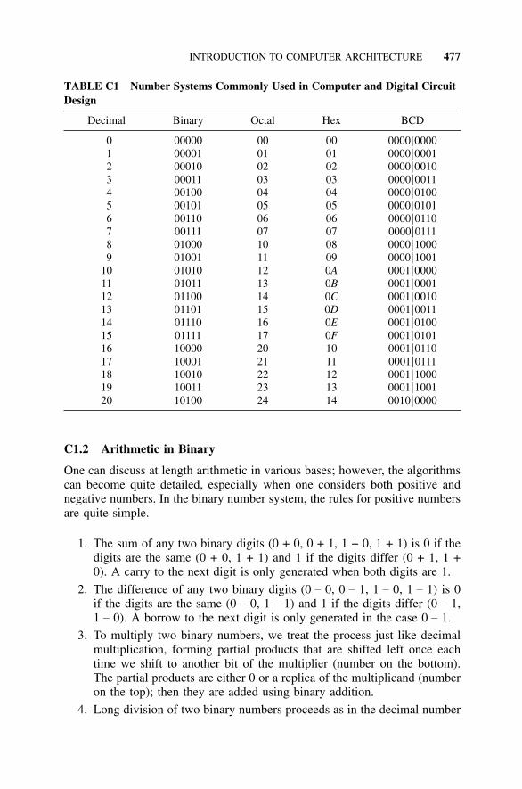
INTRODUCTION TO COMPUTER ARCHITECTURE 477
TABLE C1 Number Systems Commonly Used in Computer and Digital CircuitDesign
Decimal Binary Octal Hex BCD
0 00000 00 00 0000|00001 00001 01 01 0000|00012 00010 02 02 0000|00103 00011 03 03 0000|00114 00100 04 04 0000|01005 00101 05 05 0000|01016 00110 06 06 0000|01107 00111 07 07 0000|01118 01000 10 08 0000|10009 01001 11 09 0000|1001
10 01010 12 0A 0001|000011 01011 13 0B 0001|000112 01100 14 0C 0001|001013 01101 15 0D 0001|001114 01110 16 0E 0001|010015 01111 17 0F 0001|010116 10000 20 10 0001|011017 10001 21 11 0001|011118 10010 22 12 0001|100019 10011 23 13 0001|100120 10100 24 14 0010|0000
C1.2 Arithmetic in Binary
One can discuss at length arithmetic in various bases; however, the algorithmscan become quite detailed, especially when one considers both positive andnegative numbers. In the binary number system, the rules for positive numbersare quite simple.
1. The sum of any two binary digits (0 + 0, 0 + 1, 1 + 0, 1 + 1) is 0 if thedigits are the same (0 + 0, 1 + 1) and 1 if the digits differ (0 + 1, 1 +0). A carry to the next digit is only generated when both digits are 1.
2. The difference of any two binary digits (0 − 0, 0 − 1, 1 − 0, 1 − 1) is 0if the digits are the same (0 − 0, 1 − 1) and 1 if the digits differ (0 − 1,1 − 0). A borrow to the next digit is only generated in the case 0 − 1.
3. To multiply two binary numbers, we treat the process just like decimalmultiplication, forming partial products that are shifted left once eachtime we shift to another bit of the multiplier (number on the bottom).The partial products are either 0 or a replica of the multiplicand (numberon the top); then they are added using binary addition.
4. Long division of two binary numbers proceeds as in the decimal number
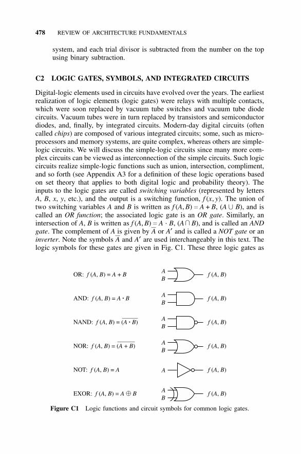
478 REVIEW OF ARCHITECTURE FUNDAMENTALS
system, and each trial divisor is subtracted from the number on the topusing binary subtraction.
C2 LOGIC GATES, SYMBOLS, AND INTEGRATED CIRCUITS
Digital-logic elements used in circuits have evolved over the years. The earliestrealization of logic elements (logic gates) were relays with multiple contacts,which were soon replaced by vacuum tube switches and vacuum tube diodecircuits. Vacuum tubes were in turn replaced by transistors and semiconductordiodes, and, finally, by integrated circuits. Modern-day digital circuits (oftencalled chips) are composed of various integrated circuits; some, such as micro-processors and memory systems, are quite complex, whereas others are simple-logic circuits. We will discuss the simple-logic circuits since many more com-plex circuits can be viewed as interconnection of the simple circuits. Such logiccircuits realize simple-logic functions such as union, intersection, compliment,and so forth (see Appendix A3 for a definition of these logic operations basedon set theory that applies to both digital logic and probability theory). Theinputs to the logic gates are called switching variables (represented by lettersA, B, x, y, etc.), and the output is a switching function, f (x, y). The union oftwo switching variables A and B is written as f (A, B) c A + B, (A U B), and iscalled an OR function; the associated logic gate is an OR gate. Similarly, anintersection of A, B is written as f (A, B) c A . B, (A
UB), and is called an AND
gate. The complement of A is given by A or A′ and is called a NOT gate or aninverter. Note the symbols A and A′ are used interchangeably in this text. Thelogic symbols for these gates are given in Fig. C1. These three logic gates as
A
A
A
A
A
A
B
B
B
B
B
f A B( , )
f A B( , )
f A B( , )
f A B( , )
f A B( , )
f A B( , )
OR: ( , ) = +f A B A B
AND: ( , ) =f A B A B·
NAND: ( , ) = ( )f A B A B·
NOR: ( , ) = ( + )f A B A B
NOT: ( , ) =f A B A
EXOR: ( , ) =f A B A B�
Figure C1 Logic functions and circuit symbols for common logic gates.
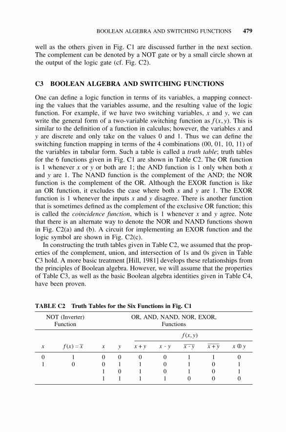
BOOLEAN ALGEBRA AND SWITCHING FUNCTIONS 479
well as the others given in Fig. C1 are discussed further in the next section.The complement can be denoted by a NOT gate or by a small circle shown atthe output of the logic gate (cf. Fig. C2).
C3 BOOLEAN ALGEBRA AND SWITCHING FUNCTIONS
One can define a logic function in terms of its variables, a mapping connect-ing the values that the variables assume, and the resulting value of the logicfunction. For example, if we have two switching variables, x and y, we canwrite the general form of a two-variable switching function as f (x, y). This issimilar to the definition of a function in calculus; however, the variables x andy are discrete and only take on the values 0 and 1. Thus we can define theswitching function mapping in terms of the 4 combinations (00, 01, 10, 11) ofthe variables in tabular form. Such a table is called a truth table; truth tablesfor the 6 functions given in Fig. C1 are shown in Table C2. The OR functionis 1 whenever x or y or both are 1; the AND function is 1 only when both xand y are 1. The NAND function is the complement of the AND; the NORfunction is the complement of the OR. Although the EXOR function is likean OR function, it excludes the case where both x and y are 1. The EXORfunction is 1 whenever the inputs x and y disagree. There is another functionthat is sometimes defined as the complement of the exclusive OR function; thisis called the coincidence function, which is 1 whenever x and y agree. Notethat there is an alternate way to denote the NOR and NAND functions shownin Fig. C2(a) and (b). A circuit for implementing an EXOR function and thelogic symbol are shown in Fig. C2(c).
In constructing the truth tables given in Table C2, we assumed that the prop-erties of the complement, union, and intersection of 1s and 0s given in TableC3 hold. A more basic treatment [Hill, 1981] develops these relationships fromthe principles of Boolean algebra. However, we will assume that the propertiesof Table C3, as well as the basic Boolean algebra identities given in Table C4,have been proven.
TABLE C2 Truth Tables for the Six Functions in Fig. C1
NOT (Inverter) OR, AND, NAND, NOR, EXOR,Function Functions
f (x, y)
x f (x) c x x y x + y x . y x . y x + y x ⊕ y
0 1 0 0 0 0 1 1 01 0 0 1 1 0 1 0 1
1 0 1 0 1 0 11 1 1 1 0 0 0
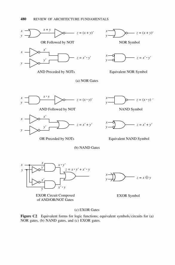
480 REVIEW OF ARCHITECTURE FUNDAMENTALS
(a) NOR Gates
(b) NAND Gates
(c) EXOR Gates
xy
x y+z = x y( + )’
x
y
z = x y’ ’·
x’
y’
xy
z = x y( + )’
xy
z = x y’ ’·
OR Followed by NOT
AND Preceded by NOTs
NOR Symbol
Equivalent NOR Symbol
xy
x y·z = x y( )· ’
x
y
z = +x y’ ’
x’
y’
xy
z = x y( )· ’
xy
z = +x y’ ’
AND Followed by NOT
OR Preceded by NOTs
NAND Symbol
Equivalent NAND Symbol
xy z = x y�
EXOR Circuit Composedof AND/OR/NOT Gates
EXOR Symbol
xy z = +x y x y· ·’ ’
x y’·
x y’ ·
x’
xy’
y
Figure C2 Equivalent forms for logic functions; equivalent symbols/ circuits for (a)NOR gates, (b) NAND gates, and (c) EXOR gates.
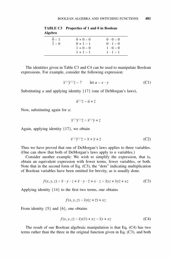
BOOLEAN ALGEBRA AND SWITCHING FUNCTIONS 481
TABLE C3 Properties of 1 and 0 in BooleanAlgebra
0 c 1 0 + 0 c 0 0 . 0 c 01 c 0 0 + 1 c 1 0 . 1 c 0
1 + 0 c 0 1 . 0 c 01 + 1 c 1 1 . 1 c 1
The identities given in Table C3 and C4 can be used to manipulate Booleanexpressions. For example, consider the following expression:
x . y . z c ? let a c x . y (C1)
Substituting a and applying identity {17} (one of DeMorgan’s laws),
a . z c a + z
Now, substituting again for a:
x . y . z c x . y + z
Again, applying identity {17}, we obtain
x . y . z c x + y + z (C2)
Thus we have proved that one of DeMorgan’s laws applies to three variables.(One can show that both of DeMorgan’s laws apply to n variables.)
Consider another example: We wish to simplify the expression, that is,obtain an equivalent expression with fewer terms, fewer variables, or both.Note that in the second form of Eq. (C3), the “dots” indicating multiplicationof Boolean variables have been omitted for brevity, as is usually done.
f (x, y, z) c x . y . z + x . y . z + x . z c xyz + xyz + xz (C3)
Applying identity {14} to the first two terms, one obtains
f (x, y, z) c xy(z + z) + xz
From identity {5} and {6}, one obtains
f (x, y, z) c xy(1) + xz c xy + xz (C4)
The result of our Boolean algebraic manipulation is that Eq. (C4) has twoterms rather than the three in the original function given in Eq. (C3), and both
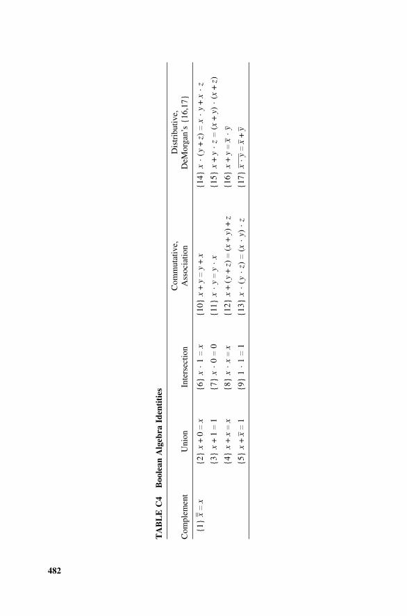
482
TA
BL
E C
4B
oole
an A
lgeb
ra I
dent
itie
s
Com
mut
ativ
e,D
istr
ibut
ive,
Com
plem
ent
Uni
onIn
ters
ectio
nA
ssoc
iatio
nD
eMor
gan’
s{1
6,17
}
{1}
xc
x{2
}x
+0c
x{6
}x
.1c
x{1
0}x
+yc
y+
x{1
4}x
.(y
+z)
cx
.y
+x
.z
{3}
x+
1c
1{7
}x
.0c
0{1
1}x
.yc
y.
x{1
5}x
+y
.zc
(x+
y).
(x+
z)
{4}
x+
xc
x{8
}x
.xc
x{1
2}x
+ (
y+
z)c
(x+
y) +
z{1
6}x
+yc
x.
y
{5}
x+
xc
1{9
}1
.1c
1{1
3}x
.(y
.z)
c(x
.y)
.z
{17}
x. y
cx
+y
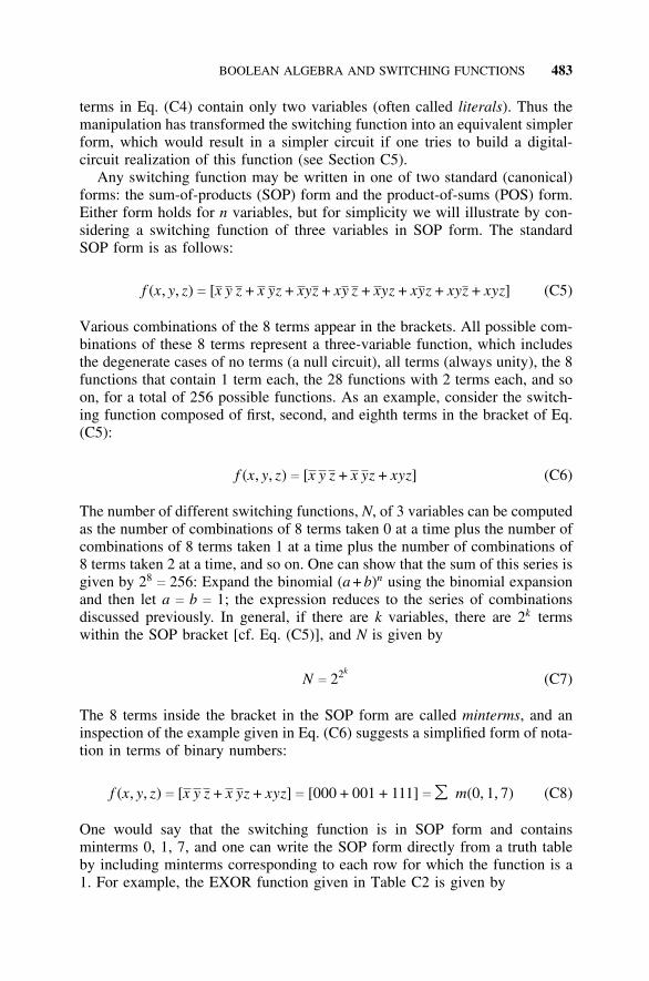
BOOLEAN ALGEBRA AND SWITCHING FUNCTIONS 483
terms in Eq. (C4) contain only two variables (often called literals). Thus themanipulation has transformed the switching function into an equivalent simplerform, which would result in a simpler circuit if one tries to build a digital-circuit realization of this function (see Section C5).
Any switching function may be written in one of two standard (canonical)forms: the sum-of-products (SOP) form and the product-of-sums (POS) form.Either form holds for n variables, but for simplicity we will illustrate by con-sidering a switching function of three variables in SOP form. The standardSOP form is as follows:
f (x, y, z) c [x y z + x yz + xyz + xy z + xyz + xyz + xyz + xyz] (C5)
Various combinations of the 8 terms appear in the brackets. All possible com-binations of these 8 terms represent a three-variable function, which includesthe degenerate cases of no terms (a null circuit), all terms (always unity), the 8functions that contain 1 term each, the 28 functions with 2 terms each, and soon, for a total of 256 possible functions. As an example, consider the switch-ing function composed of first, second, and eighth terms in the bracket of Eq.(C5):
f (x, y, z) c [x y z + x yz + xyz] (C6)
The number of different switching functions, N, of 3 variables can be computedas the number of combinations of 8 terms taken 0 at a time plus the number ofcombinations of 8 terms taken 1 at a time plus the number of combinations of8 terms taken 2 at a time, and so on. One can show that the sum of this series isgiven by 28
c 256: Expand the binomial (a + b)n using the binomial expansionand then let a c b c 1; the expression reduces to the series of combinationsdiscussed previously. In general, if there are k variables, there are 2k termswithin the SOP bracket [cf. Eq. (C5)], and N is given by
N c 22k(C7)
The 8 terms inside the bracket in the SOP form are called minterms, and aninspection of the example given in Eq. (C6) suggests a simplified form of nota-tion in terms of binary numbers:
f (x, y, z) c [x y z + x yz + xyz] c [000 + 001 + 111] c ��� m(0, 1, 7) (C8)
One would say that the switching function is in SOP form and containsminterms 0, 1, 7, and one can write the SOP form directly from a truth tableby including minterms corresponding to each row for which the function is a1. For example, the EXOR function given in Table C2 is given by
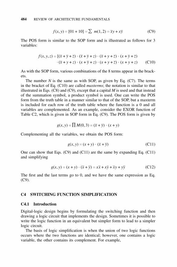
484 REVIEW OF ARCHITECTURE FUNDAMENTALS
f (x, y) c [01 + 10] c ��� m(1, 2) c xy + xy (C9)
The POS form is similar to the SOP form and is illustrated as follows for 3variables:
f (x, y, z) c [(x + y + z) . (x + y + z) . (x + y + z) . (x + y + z). (x + y + z) . (x + y + z) . (x + y + z) . (x + y + z) (C10)
As with the SOP form, various combinations of the 8 terms appear in the brack-ets.
The number N is the same as with SOP, as given by Eq. (C7). The termsin the bracket of Eq. (C10) are called maxterms; the notation is similar to thatillustrated in Eqs. (C8) and (C9), except that a capital M is used and that insteadof the summation symbol, a product symbol is used. One can write the POSform from the truth table in a manner similar to that of the SOP, but a maxtermis included for each row of the truth table where the function is a 0 and allvariables are complemented. As an example, consider the EXOR function ofTable C2, which is given in SOP form in Eq. (C9). The POS form is given by
g(x, y) c ∏ M(0, 3) c (x + y) . (x + y)
Complementing all the variables, we obtain the POS form:
g(x, y) c (x + y) . (x + y) (C11)
One can show that Eqs. (C9) and (C11) are the same by expanding Eq. (C11)and simplifying
g(x, y) c (x + y) . (x + y) c xx + xy + xy + yy (C12)
The first and the last terms go to 0, and we have the same expression as Eq.(C9).
C4 SWITCHING FUNCTION SIMPLIFICATION
C4.1 Introduction
Digital-logic design begins by formulating the switching function and thendrawing a logic circuit that implements the design. Sometimes it is possible towrite the logic function in an equivalent but simpler form to lead to a simplerlogic circuit.
The basis of logic simplification is when the union of two logic functionsoccurs where the two functions are identical; however, one contains a logicvariable, the other contains its complement. For example,
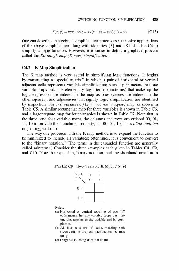
SWITCHING FUNCTION SIMPLIFICATION 485
f (x, y) c xyz . xyz c xy(z + z) c (xy)(1) c xy (C13)
One can describe an algebraic simplification process as successive applicationsof the above simplification along with identities {5} and {8} of Table C4 tosimplify a logic function. However, it is easier to define a graphical processcalled the Karnaugh map (K map) simplification.
C4.2 K Map Simplification
The K map method is very useful in simplifying logic functions. It beginsby constructing a “special matrix,” in which a pair of horizontal or verticaladjacent cells represents variable simplification; such a pair means that onevariable drops out. The elementary logic terms (minterms) that make up thelogic expression are entered in the map as ones (zeroes are entered in theother squares), and adjacencies that signify logic simplification are identifiedby inspection. For two variables, f (x, y), we use a square map as shown inTable C5. A similar rectangular map for three variables is shown in Table C6,and a larger square map for four variables is shown in Table C7. Note that inthe three- and four-variable maps, the columns and rows are ordered 00, 01,11, 10 to provide the “touching” property, not 00, 01, 10, 11 as blind intuitionmight suggest to do.
The way one proceeds with the K map method is to expand the function tobe minimized to include all variables; oftentimes, it is convenient to convertto the “binary notation.” (The terms in the expanded function are generallycalled minterms.) Consider the three examples each given in Tables C8, C9,and C10. Note the expansion, binary notation, and the shorthand notation in
TABLE C5 Two-Variable K Map, f (x, y)
0 x
1 x
xy 0
y1y
Rules:(a) Horizontal or vertical touching of two “1”
cells means that one variable drops out—theone that appears as the variable and its com-plement.
(b) All four cells are “1” cells, meaning both(two) variables drop out; the function becomesunity.
(c) Diagonal touching does not count.
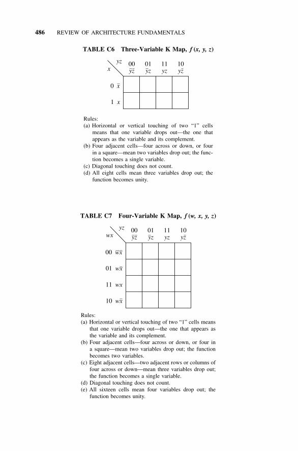
486 REVIEW OF ARCHITECTURE FUNDAMENTALS
TABLE C6 Three-Variable K Map, f (x, y, z)
0 x
1 x
xyz 00
yz01yz
11yz
10yz
Rules:(a) Horizontal or vertical touching of two “1” cells
means that one variable drops out—the one thatappears as the variable and its complement.
(b) Four adjacent cells—four across or down, or fourin a square—mean two variables drop out; the func-tion becomes a single variable.
(c) Diagonal touching does not count.(d) All eight cells mean three variables drop out; the
function becomes unity.
TABLE C7 Four-Variable K Map, f (w, x, y, z)
00 wx
01 wx
11 wx
10 wx
wxyz 00
yz01yz
11yz
10yz
Rules:(a) Horizontal or vertical touching of two “1” cells means
that one variable drops out—the one that appears asthe variable and its complement.
(b) Four adjacent cells—four across or down, or four ina square—mean two variables drop out; the functionbecomes two variables.
(c) Eight adjacent cells—two adjacent rows or columns offour across or down—mean three variables drop out;the function becomes a single variable.
(d) Diagonal touching does not count.(e) All sixteen cells mean four variables drop out; the
function becomes unity.
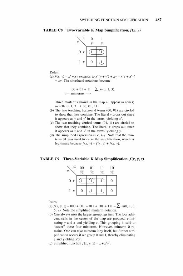
SWITCHING FUNCTION SIMPLIFICATION 487
TABLE C8 Two-Variable K Map Simplification, f (x, y)
0 x 1
0
1
11 x
xy 0
y1y
Rules:(a) f (x, y) c x′ + xy expands to x′(y + y′) + xy c x′y + x′y′
+ xy. The shorthand notations become
00 + 01 + 11 c ��� m(0, 1, 3).a− minterms −b
Three minterms shown in the map all appear as (ones)in cells 0, 1, 3 r 00, 01, 11.
(b) The two touching horizontal terms (00, 01) are circledto show that they combine. The literal y drops out sinceit appears as y and y′ in the terms, yielding x′.
(c) The two touching vertical terms (01, 11) are circled toshow that they combine. The literal x drops out sinceit appears as x and x′ in the terms, yielding y.
(d) The simplified expression is x′ + y. Note that the min-term 01 was used twice in the simplification, which islegitimate because f (x, y) c f (x, y) + f (x, y).
TABLE C9 Three-Variable K Map Simplification, f (x, y, z)
0 x 1
0
1
1
1
1
0
01 x
xyz 00
yz01yz
11yz
10yz
Rules:(a) f (x, y, z) c 000 + 001 + 011 + 101 + 111 c��� m(0, 1, 3,
5, 7). Note the simplified minterm notation.(b) One always uses the largest groupings first. The four adja-
cent cells in the center of the map are grouped, elimi-nating y and x and yielding z. This grouping is said to“cover” these four minterms. However, minterm 0 re-mains. One can take minterm 0 by itself, but further sim-plification occurs if we group 0 and 1, thereby eliminatingz and yielding x′y′.
(c) Simplified function f (x, y, z) c z + x′y′.
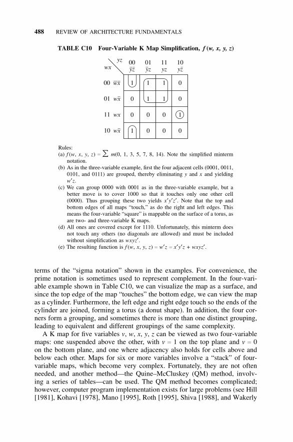
488 REVIEW OF ARCHITECTURE FUNDAMENTALS
TABLE C10 Four-Variable K Map Simplification, f (w, x, y, z)
00 wx 1
0
0
1
1
1
0
0
1
1
0
0
0
0
1
0
01 wx
11 wx
10 wx
wxyz 00
yz01yz
11yz
10yz
Rules:(a) f (w, x, y, z) c ��� m(0, 1, 3, 5, 7, 8, 14). Note the simplified minterm
notation.(b) As in the three-variable example, first the four adjacent cells (0001, 0011,
0101, and 0111) are grouped, thereby eliminating y and x and yieldingw′z.
(c) We can group 0000 with 0001 as in the three-variable example, but abetter move is to cover 1000 so that it touches only one other cell(0000). Thus grouping these two yields x′y′z′. Note that the top andbottom edges of all maps “touch,” as do the right and left edges. Thismeans the four-variable “square” is mappable on the surface of a torus, asare two- and three-variable K maps.
(d) All ones are covered except for 1110. Unfortunately, this minterm doesnot touch any others (no diagonals are allowed) and must be includedwithout simplification as wxyz′.
(e) The resulting function is f (w, x, y, z) c w′z c x′y′z + wxyz′.
terms of the “sigma notation” shown in the examples. For convenience, theprime notation is sometimes used to represent complement. In the four-vari-able example shown in Table C10, we can visualize the map as a surface, andsince the top edge of the map “touches” the bottom edge, we can view the mapas a cylinder. Furthermore, the left edge and right edge touch so the ends of thecylinder are joined, forming a torus (a donut shape). In addition, the four cor-ners form a grouping, and sometimes there is more than one distinct grouping,leading to equivalent and different groupings of the same complexity.
A K map for five variables v, w, x, y, z can be viewed as two four-variablemaps: one suspended above the other, with v c 1 on the top plane and v c 0on the bottom plane, and one where adjacency also holds for cells above andbelow each other. Maps for six or more variables involve a “stack” of four-variable maps, which become very complex. Fortunately, they are not oftenneeded, and another method—the Quine–McCluskey (QM) method, involv-ing a series of tables—can be used. The QM method becomes complicated;however, computer program implementation exists for large problems (see Hill[1981], Kohavi [1978], Mano [1995], Roth [1995], Shiva [1988], and Wakerly
COMBINATORIAL CIRCUITS 489
[2001]). The physical problem is sometimes such that a particular minterm orminterms cannot exist; thus we do not care whether they exist or not. Suchterms, called don’t-cares, are entered as d in the K map and are treated asones if they help the simplification and as zeroes if they are of no aid. Thecells in the map that are not ones (minterms) are called maxterms; these aregenerally labeled as zeroes. The zeroes can also be grouped to yield the sim-plified function called the product-of-sums form (POS) mentioned previously.The application of don’t-cares and the POS form are treated in the problemsat the end of this appendix and also in the references.
C5 COMBINATORIAL CIRCUITS
C5.1 Circuit Realizations: SOP
Once the logic functions are minimized, the designer produces circuits thatrealize the logic function. The resulting minimizations from grouping the onesin the K map produce a union of intersection terms (in common engineeringterms, a sum of products, or SOP). The product terms are developed usingAND gates, and their outputs feed into an OR gate. If complements of thevariables are needed as inputs to the AND gates, inverters are required. Thusany SOP form can be realized using only {AND, OR, NOT} gates; this set oflogic functions is called a complete set. There are other combinations of logicgates that also form a complete set (e.g., NAND gates or NOR gates). Threeexamples of SOP circuits are shown in Fig. C3.
C5.2 Circuit Realizations: POS
As was discussed in the previous section, one can group zeroes in the K mapand obtain a POS design. The resulting circuit is similar to those in Fig. C3;however, instead of a multiple input OR preceded by a number of AND gates,the circuit is a group of OR gates followed by an AND gate. For examples,the reader is referred to the problems at the end of this appendix.
C5.3 NAND and NOR Realizations
Up until now, we have discussed the circuit realizations that all involved thecomplete set of {AND, OR, NOT} gates. Sometimes, it is more convenientor simpler to deal with other types of logic gates. It turns out that two othercomplete sets of logic gates are often used: {NAND} and {NOR} gates. Westate without proof (see the problems at the end of this appendix) that each ofthe AND and OR gates in the SOP form can be replaced with a NAND gate.Furthermore, if one does not wish to use an inverter, a two-input NAND gatewith inputs tied together can suffice. Similarly, in a POS design, we can replaceOR and AND gates by NOR gates and the inverter by a two-input NOR withinputs tied together. With a little more effort, one can also use NAND gates
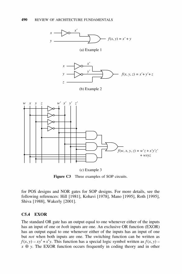
490 REVIEW OF ARCHITECTURE FUNDAMENTALS
(a) Example 1
(b) Example 2
(c) Example 3
x
y f x y =( , ) +x y’
x’
x
y
z
x’
y’
f w x y z = wwxyz
( , , , )+
’ ’ ’ ’z x y z+
f x y z =( , , ) x y z’ ’+ +
w w’x x’y y’z z’
Figure C3 Three examples of SOP circuits.
for POS designs and NOR gates for SOP designs. For more details, see thefollowing references: Hill [1981], Kohavi [1978], Mano [1995], Roth [1995],Shiva [1988], Wakerly [2001].
C5.4 EXOR
The standard OR gate has an output equal to one whenever either of the inputshas an input of one or both inputs are one. An exclusive OR function (EXOR)has an output equal to one whenever either of the inputs has an input of onebut not when both inputs are one. The switching function can be written asf (x, y) c xy′ + x′y. This function has a special logic symbol written as f (x, y) cx ⊕ y. The EXOR function occurs frequently in coding theory and in other
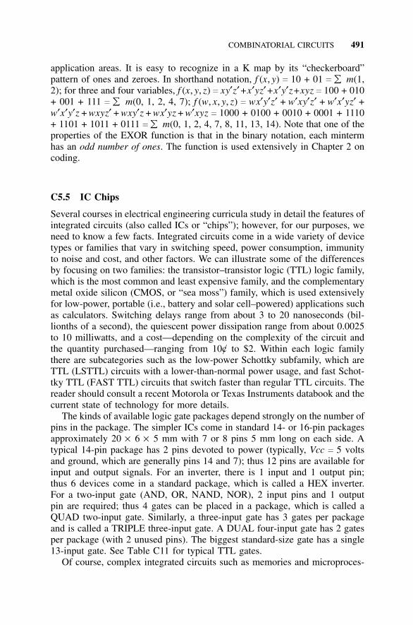
COMBINATORIAL CIRCUITS 491
application areas. It is easy to recognize in a K map by its “checkerboard”pattern of ones and zeroes. In shorthand notation, f (x, y) c 10 + 01 c ��� m(1,2); for three and four variables, f (x, y, z) c xy′z′ +x′yz′ +x′y′z+xyz c 100 + 010+ 001 + 111 c ��� m(0, 1, 2, 4, 7); f (w, x, y, z) c wx′y′z′ + w′xy′z′ + w′x′yz′ +w′x′y′z + wxyz′ + wxy′z + wx′yz + w′xyz c 1000 + 0100 + 0010 + 0001 + 1110+ 1101 + 1011 + 0111 c ��� m(0, 1, 2, 4, 7, 8, 11, 13, 14). Note that one of theproperties of the EXOR function is that in the binary notation, each mintermhas an odd number of ones. The function is used extensively in Chapter 2 oncoding.
C5.5 IC Chips
Several courses in electrical engineering curricula study in detail the features ofintegrated circuits (also called ICs or “chips”); however, for our purposes, weneed to know a few facts. Integrated circuits come in a wide variety of devicetypes or families that vary in switching speed, power consumption, immunityto noise and cost, and other factors. We can illustrate some of the differencesby focusing on two families: the transistor–transistor logic (TTL) logic family,which is the most common and least expensive family, and the complementarymetal oxide silicon (CMOS, or “sea moss”) family, which is used extensivelyfor low-power, portable (i.e., battery and solar cell–powered) applications suchas calculators. Switching delays range from about 3 to 20 nanoseconds (bil-lionths of a second), the quiescent power dissipation range from about 0.0025to 10 milliwatts, and a cost—depending on the complexity of the circuit andthe quantity purchased—ranging from 10c/ to $2. Within each logic familythere are subcategories such as the low-power Schottky subfamily, which areTTL (LSTTL) circuits with a lower-than-normal power usage, and fast Schot-tky TTL (FAST TTL) circuits that switch faster than regular TTL circuits. Thereader should consult a recent Motorola or Texas Instruments databook and thecurrent state of technology for more details.
The kinds of available logic gate packages depend strongly on the number ofpins in the package. The simpler ICs come in standard 14- or 16-pin packagesapproximately 20 × 6 × 5 mm with 7 or 8 pins 5 mm long on each side. Atypical 14-pin package has 2 pins devoted to power (typically, Vcc c 5 voltsand ground, which are generally pins 14 and 7); thus 12 pins are available forinput and output signals. For an inverter, there is 1 input and 1 output pin;thus 6 devices come in a standard package, which is called a HEX inverter.For a two-input gate (AND, OR, NAND, NOR), 2 input pins and 1 outputpin are required; thus 4 gates can be placed in a package, which is called aQUAD two-input gate. Similarly, a three-input gate has 3 gates per packageand is called a TRIPLE three-input gate. A DUAL four-input gate has 2 gatesper package (with 2 unused pins). The biggest standard-size gate has a single13-input gate. See Table C11 for typical TTL gates.
Of course, complex integrated circuits such as memories and microproces-
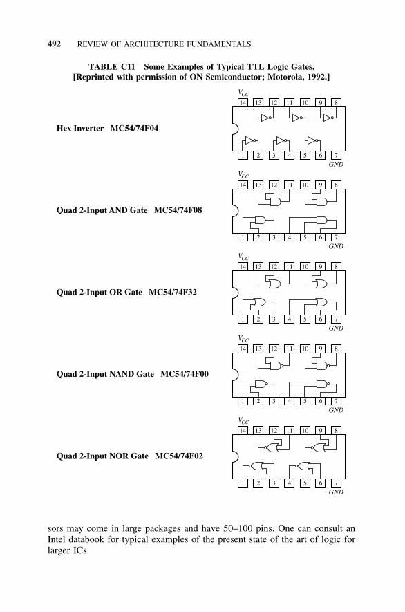
492 REVIEW OF ARCHITECTURE FUNDAMENTALS
TABLE C11 Some Examples of Typical TTL Logic Gates.[Reprinted with permission of ON Semiconductor; Motorola, 1992.]
Hex Inverter MC54/74F04
Quad 2-Input AND Gate MC54/74F08
Quad 2-Input OR Gate MC54/74F32
Quad 2-Input NOR Gate MC54/74F02
Quad 2-Input NAND Gate MC54/74F00
14
1
13 11
2
12
3 4
10
5
9
6
8
7
VCC
GND
14
14
14
14
1
1
1
1
2
2
2
2
3
3
3
3
4
4
4
4
10
10
10
10
5
5
5
5
9
9
9
9
6
6
6
6
8
8
8
8
7
7
7
7
VCC
VCC
VCC
VCC
GND
GND
GND
GND
13 1112
13 1112
13 1112
13 1112
sors may come in large packages and have 50–100 pins. One can consult anIntel databook for typical examples of the present state of the art of logic forlarger ICs.
COMMON CIRCUITS: PARITY-BIT GENERATORS AND DECODERS 493
TABLE C11 (Continued)
Triple 3-Input NAND Gate MC54/74F10
Dual 4-Input AND Gate MC54/74F21
13-Input NAND Gate SN54/74LS133
14
14
16
1
1
1
2
2
2
3
3
3
4
4
4
10
10
12
5
5
5
9
9
11
6
6
6
8
8
10 9
7
7
7 8
VCC
VCC
VCC
GND
GND
GND
13
13
15
11
11
13
12
12
14
C6 COMMON CIRCUITS: PARITY-BIT GENERATORS ANDDECODERS
C6.1 Introduction
The short discussion of digital integrated circuits in the preceding section mayhave left the reader with the notion that there are only small IC packages,such as QUAD two-input AND gates (called small-scale integration, or SSI)and large-memory and microprocessor chips (called large-scale integrated cir-cuits, or LSI, or very large scale integrated circuits, or VLSI). Such is notthe case, however, and IC designers have been active for several decades pro-ducing medium-scale integrated (MSI) circuits. The MSI devices are availablefor a large range of practical functions that could be built out of ICs but at agreater cost and size. In essence, it is easier and cheaper to do the wiring andconstructing on the IC chip rather than externally. Formally, we can classifythe scale of ICs in terms of the number of gates in their equivalent circuits: 1 <SSI < 20; 20 < MSI < 200; 200 < LSI < 200,000; and VLSI > 200,000 (somesay VLSI > 500,000). We will discuss two MSI devices: a parity-bit generatorand a decoder, both of which were used in Chapter 2.
494 REVIEW OF ARCHITECTURE FUNDAMENTALS
C6.2 A Parity-Bit Generator
In Chapter 2, we discussed the use of a parity-bit code to help detect simpleerrors in transmission of digital words. The most common scheme is to addcheck bit to the word so that all the words have an odd number of ones. Aftertransmission, we can count the number of ones in the word; if the count iseven, we know that one error has occurred (actually, an odd number of errors),and we signal “transmission error.” Sometimes we set the parity bit so thatthe number of ones in the word is an even number; we call this even parity.From our discussion in Section C5.4, we see that EXOR gates could be used toaccomplish both the generation of a parity bit and the checking of parity for thetransmitted word. Rather than use a group of AND gates (as shown in Fig. 2.1)or a “tree” of EXOR gates (shown in Fig. 2.2), one can use an MSI device—theSN74180, a 9-bit odd/ even parity generator/ checker (see Fig. 2.4). This circuitand the similar (newer and faster) 74LS280 shown in Fig. 2.7 and repeated inFig. C4 can be used to compute parity-bit generation or checking for up to 9bits. By studying Fig. C4(a) and (b), one can see that inputs 8–13 and 1, 2, 4(note that pin 3 is not used; this is denoted as NC c no connection) labeled A,B, C, D, E, F, G, H, I are used for up to nine inputs. Outputs 5 and 6 yieldthe EXOR function of all the inputs and its complement; these are labeled byequivalent wording of even or odd parity. Suppose that one wishes to checkthe parity of a 16-bit word (labeled as bits 0–15) in a computer circuit. Onecan use two 74LS280 chips in cascade. Bits 0–7 go into inputs A–H of chip1 and bits 8–15 go into inputs A–H of chip 2. The output of chip 1 goes intoinput I of chip 2. When an input is not used (e.g., input I of chip 1), it can beleft unconnected in some logic families, but in others it serves as an “antenna”that picks up stray inputs that may interfere with operation. The safest courseof operation is to connect an unused input to +5 volts or ground, depending onthe logic family and the function of the input. Unused inputs for a 74LS280are connected to ground. The details of Fig. C4(b) are best left to an electricalengineer who has studied IC design.
C6.3 A Decoder
Another MSI circuit used in Chapter 2 was a decoder. A decoder (sometimescalled a demultiplexer) converts the binary representation of n variables into2n outputs. One can liken the functional operation of the decoder to a selectorswitch such as the one found on the ventilation systems in many automobiles:Rotation of the knob switches from “off” to “interior air circulation” to “ventair conditioner” to “floor air conditioner” to “outside air vent” and so on. Ina decoder, the binary input is analogous to the number of clicks of switchrotation; which one of the 2n outputs selected is analogous to the air circulationfunction selected.
For example, the 74LS138 3-to-8 decoder (shown in Fig. 2.7 and repeatedin Fig. C5) converts the three digits of the input variable A2A1A0 (pins 1, 2,
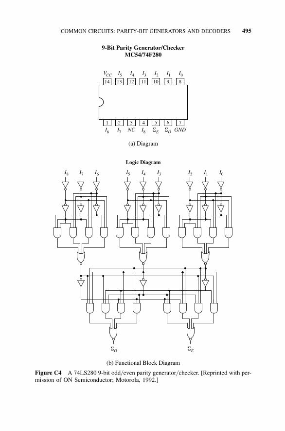
COMMON CIRCUITS: PARITY-BIT GENERATORS AND DECODERS 495
14
1
13
2
12
3
11
4
10
5
9
6
8
7
VCC I5
I6 I7 NC I8 SE SO GND
I4 I3 I2 I1 I0
9-Bit Parity Generator/CheckerMC54/74F280
(a) Diagram
I8 I5 I2I7 I4 I1I6 I3 I0
SESO
(b) Functional Block Diagram
Logic Diagram
Figure C4 A 74LS280 9-bit odd/ even parity generator/ checker. [Reprinted with per-mission of ON Semiconductor; Motorola, 1992.]
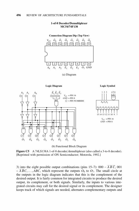
496 REVIEW OF ARCHITECTURE FUNDAMENTALS
1-of-8 Decoder/DemultiplexerMC54/74F138
(b) Functional Block Diagram
(a) Diagram
16
1
15
2
14
3
13
4
12
5
11
6
10 9
7 8
VCC O0
A0 A1 A2 E1 E2 E3 O7 GND
O1 O2 O3 O4 O5 O6
Connection Diagram Dip (Top View)
VCC = PIN 16GND = PIN 8
VCC = PIN 16A2 A1 A0 E1 E2 E3
O7 O6 O5 O4 O3 O2 O1 O0
GND = PIN 8= PIN NUMBERS
7 9
3 42 51 6
10 11 12 13 14 15
Logic Diagram Logic Symbol
15
1 2 3 4 5 6
14 13 12 11 10 9 7
O0
A0 A1A2
O1 O2 O3 O4 O5 O6 O7
1 2 3
Figure C5 A 74LS138A 1-of-8 decoder/ demultiplexer (also called a 3-to-8 decoder).[Reprinted with permission of ON Semiconductor; Motorola, 1992.]
3) into the eight possible output combinations (pins 15–7): 000 c A B C, 001c A BC, . . . , ABC, which represent the outputs O0 to O7. The small circle atthe outputs in the logic diagram indicates that this is the complement of thedesired output. It is fairly common for integrated circuits to produce the desiredoutput, its complement, or both signals. Similarly, the inputs to various inte-grated circuits may call for the desired signal or its complement. The designerkeeps track of which signals are needed, alternates complementary outputs and
FLIP-FLOPS 497
inputs (which cancel), or occasionally uses inverters where needed. There is anadditional set of three inputs (4, 5, 6; G1, G2A, G2B), which are called enableinputs. These inputs are designed for expansion of certain ICs in groups towork with larger combinations of inputs and outputs and also serve to connector disconnect all the inputs or outputs. (Note that output of the enable ANDgate is shown in the logic diagram to be an input to all the output gates soit can switch all the outputs on or off.) For example, one can design a 4-to-16 decoder by using two 74LS138 3-to-8 decoders. One bank of 8 outputs ishandled by the first decoder; the other bank of 8 outputs is handled by thesecond decoder. The enable inputs are configured so that they switch on or offthe appropriate bank. Thus, by inserting the extra variable (fourth input) intothe G1 input of one decoder and the variable into the G2A input of the otherdecoder that complements the variable, the extra variable switches between thetwo banks. The enable input AND gate has an output if G1 c 1, G2A c 0, andG2B c 0. Thus, if any enable input is not used, it must be connected to 1 (5volts) if it is G1 or connected to 0 (grounded) if it is the G2A or G2B input.In Fig. 2.7, we only need a 3-to-8 decoder; thus none of the enable inputs areused, and G1 is connected to +5 volts and G2A, G2B are grounded (0 volts).Note that the G1 connection to +5 volts also uses a resistor to limit the currentinto the input to protect it when switching occurs and that the decoder requiresa 16-pin package.
C7 FLIP-FLOPS
Computers and digital circuits are composed of three broad classes of facili-ties: the computational units called central processing units (CPUs) (frequentlymicroprocessors); the memory units (flip-flops, electronic memory, and disk,card, tape, CD, and other media); and input/ output facilities (keyboards, moni-tors, communication connections, etc.). The fastest of the memory storage unitsare flip-flops (FFs), which are individually connected or connected in bankscalled registers. Registers, discussed briefly in Chapter 2, are storage devicesmade up of cascaded single-bit FF storage circuits with switching time delaysof several nanoseconds (about the same as logic gates).
In addition, there are single-input FFs; among them is the trigger or toggleFF (T FF). When the input T is 0, the output Q (and its complement Q′) holds(stores) its previous state (either a 0 or 1). When T c 1, the values of Q and Q′flip from their previous states to the complement (0 or 1). There is also a delayFF (D FF), which stores as output whatever the D input is after a switchingdelay. Both the T and D FF are single-input devices. A symbolic diagram ofa T FF is shown in Fig. C6 along with a state table. A state table is similar toa truth table, but it contains an additional column (serving like an additionalinput) that is the previous output. Note the first line of the state table revealsthat if the previous storage state Qn is 0 and there is no T input (0 input), thenthe new state Qn + 1 is the same as the old—that is, 0. The second line in the
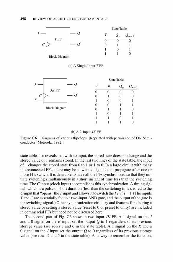
498 REVIEW OF ARCHITECTURE FUNDAMENTALS
(a) A Single Input FFT
(b) A 2-Input FFJK
Block Diagram
T Q
C Q’
State Table
T Q Qn n + 1
0 0 00 1 11 0 11 1 0
Block Diagram
J
K
Q
C Q’
State Table
J K Q Qn n + 1
0 0 0 00 1 0 01 0 0 10 0 1 10 1 1 01 0 1 11 1 0 11 1 1 0
T FF
JK FF
Figure C6 Diagrams of various flip-flops. [Reprinted with permission of ON Semi-conductor; Motorola, 1992.]
state table also reveals that with no input, the stored state does not change and thestored value of 1 remains stored. In the last two lines of the state table, the inputof 1 changes the stored state from 0 to 1 or 1 to 0. In a large circuit with manyinterconnected FFs, there may be unwanted signals that propagate after one ormore FFs switch. It is desirable to have all the FFs synchronized so that they ini-tiate switching simultaneously in a short instant of time less than the switchingtime. The C input (clock input) accomplishes this synchronization. A timing sig-nal, which is a pulse of short duration (less than the switching time), is fed to theC input that “opens” the T input and allows it to switch the FF if T c 1. (The inputsT and C are essentially fed to a two-input AND gate, and the output of the gate isthe switching signal.) Other synchronization circuitry and features for clearing astored value or setting a stored value (reset to 0 or preset to unity) are includedin commercial FFs but need not be discussed here.
The second part of Fig. C6 shows a two-input JK FF. A 1 signal on the Jand a 0 signal on the K input set the output Q to 1 regardless of its previousstorage value (see rows 3 and 6 in the state table). A 1 signal on the K and a0 signal on the J input set the output Q to 0 regardless of its previous storagevalue (see rows 2 and 5 in the state table). As a way to remember the function,
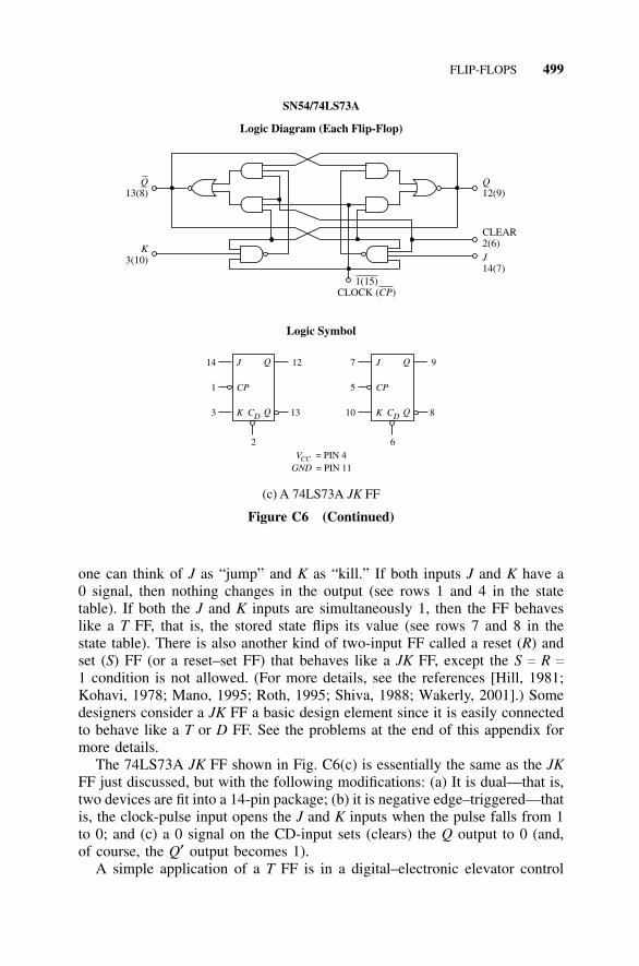
FLIP-FLOPS 499
(c) A 74LS73A FFJK
Logic Diagram (Each Flip-Flop)
Q13(8)
Q12(9)
CLEAR2(6)J14(7)
1(15)CLOCK ( )CP
K3(10)
Logic Symbol
VCC = PIN 4GND = PIN 11
1 5
14 7J J12 9
CP CP
K KQ Q
Q Q
CD CD3 1013 8
2 6
SN54/74LS73A
Figure C6 (Continued)
one can think of J as “jump” and K as “kill.” If both inputs J and K have a0 signal, then nothing changes in the output (see rows 1 and 4 in the statetable). If both the J and K inputs are simultaneously 1, then the FF behaveslike a T FF, that is, the stored state flips its value (see rows 7 and 8 in thestate table). There is also another kind of two-input FF called a reset (R) andset (S) FF (or a reset–set FF) that behaves like a JK FF, except the S c R c
1 condition is not allowed. (For more details, see the references [Hill, 1981;Kohavi, 1978; Mano, 1995; Roth, 1995; Shiva, 1988; Wakerly, 2001].) Somedesigners consider a JK FF a basic design element since it is easily connectedto behave like a T or D FF. See the problems at the end of this appendix formore details.
The 74LS73A JK FF shown in Fig. C6(c) is essentially the same as the JKFF just discussed, but with the following modifications: (a) It is dual—that is,two devices are fit into a 14-pin package; (b) it is negative edge–triggered—thatis, the clock-pulse input opens the J and K inputs when the pulse falls from 1to 0; and (c) a 0 signal on the CD-input sets (clears) the Q output to 0 (and,of course, the Q′ output becomes 1).
A simple application of a T FF is in a digital–electronic elevator control
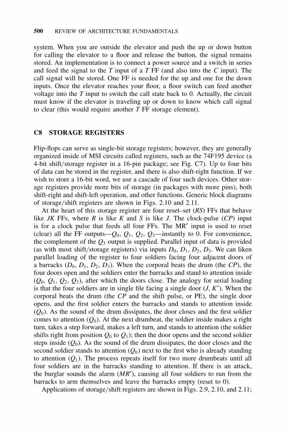
500 REVIEW OF ARCHITECTURE FUNDAMENTALS
system. When you are outside the elevator and push the up or down buttonfor calling the elevator to a floor and release the button, the signal remainsstored. An implementation is to connect a power source and a switch in seriesand feed the signal to the T input of a T FF (and also into the C input). Thecall signal will be stored. One FF is needed for the up and one for the downinputs. Once the elevator reaches your floor, a floor switch can feed anothervoltage into the T input to switch the call state back to 0. Actually, the circuitmust know if the elevator is traveling up or down to know which call signalto clear (this would require another T FF storage element).
C8 STORAGE REGISTERS
Flip-flops can serve as single-bit storage registers; however, they are generallyorganized inside of MSI circuits called registers, such as the 74F195 device (a4-bit shift/ storage register in a 16-pin package; see Fig. C7). Up to four bitsof data can be stored in the register, and there is also shift-right function. If wewish to store a 16-bit word, we use a cascade of four such devices. Other stor-age registers provide more bits of storage (in packages with more pins), bothshift-right and shift-left operation, and other functions. Generic block diagramsof storage/ shift registers are shown in Figs. 2.10 and 2.11.
At the heart of this storage register are four reset–set (RS) FFs that behavelike JK FFs, where R is like K and S is like J. The clock-pulse (CP) inputis for a clock pulse that feeds all four FFs. The MR′ input is used to reset(clear) all the FF outputs—Q0, Q1, Q2, Q3—instantly to 0. For convenience,the complement of the Q3 output is supplied. Parallel input of data is provided(as with most shift/ storage registers) via inputs D0, D1, D2, D3. We can likenparallel loading of the register to four soldiers facing four adjacent doors ofa barracks (D0, D1, D2, D3). When the corporal beats the drum (the CP), thefour doors open and the soldiers enter the barracks and stand to attention inside(Q0, Q1, Q2, Q3), after which the doors close. The analogy for serial loadingis that the four soldiers are in single file facing a single door (J, K′). When thecorporal beats the drum (the CP and the shift pulse, or PE), the single dooropens, and the first soldier enters the barracks and stands to attention inside(Q0). As the sound of the drum dissipates, the door closes and the first soldiercomes to attention (Q0). At the next drumbeat, the soldier inside makes a rightturn, takes a step forward, makes a left turn, and stands to attention (the soldiershifts right from position Q0 to Q1); then the door opens and the second soldiersteps inside (Q0). As the sound of the drum dissipates, the door closes and thesecond soldier stands to attention (Q0) next to the first who is already standingto attention (Q1). The process repeats itself for two more drumbeats until allfour soldiers are in the barracks standing to attention. If there is an attack,the burglar sounds the alarm (MR′), causing all four soldiers to run from thebarracks to arm themselves and leave the barracks empty (reset to 0).
Applications of storage/ shift registers are shown in Figs. 2.9, 2.10, and 2.11;
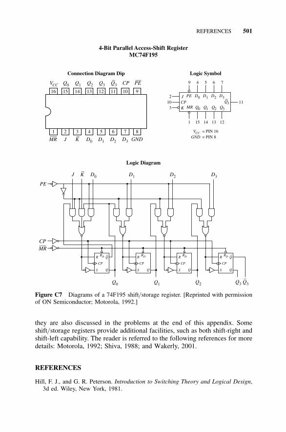
REFERENCES 501
4-Bit Parallel Access-Shift RegisterMC74F195
16
1
15
2
14
3
13
4
12
5
11
6
10 9
7 8
VCC Q0
MR J K D0 D1 D2 D3 GND
Q1 Q2 Q3 Q3 CP PE
Connection Diagram Dip Logic Symbol
VCC = PIN 16GND = PIN 8
1
210 113
15 14 13 12
9 4 5 6 7
MR
PEJCPK
D0 D1 D2 D3
Q0 Q1 Q2 Q3
Q3
Logic Diagram
D3D2D1D0KJ
PE
CPMR
Q3Q2Q1Q0 Q3
SSSS
RRRR QQ
QQQQ
RDRDRDRD
CPCPCPCP
Figure C7 Diagrams of a 74F195 shift/ storage register. [Reprinted with permissionof ON Semiconductor; Motorola, 1992.]
they are also discussed in the problems at the end of this appendix. Someshift/ storage registers provide additional facilities, such as both shift-right andshift-left capability. The reader is referred to the following references for moredetails: Motorola, 1992; Shiva, 1988; and Wakerly, 2001.
REFERENCES
Hill, F. J., and G. R. Peterson. Introduction to Switching Theory and Logical Design,3d ed. Wiley, New York, 1981.
502 REVIEW OF ARCHITECTURE FUNDAMENTALS
Kohavi, Z. Switching and Automata Theory, 2d ed. McGraw-Hill, New York, 1978.
Mano, M. M. Digital Design, 2d ed. Prentice-Hall, Englewood Cliffs, NJ, 1995.
Motorola Logic Integrated Circuits Division. FAST and LS TTL Data, 5th ed.,DL121/ D, rev. 5. Motorola Literature Distribution, Phoenix, AZ, 1992.
Roth, C. H. Jr. Fundamentals of Logic Design, 4th ed. PWS Publishing, Boston, 1995.
Shiva, S. G. Introduction to Logic Design. Scott Foresman and Company, Glenview,IL, 1988.
Tinder, R. F. Engineering Digital Design. Academic Press, San Diego, CA, 2000.
Wakerly, J. F. Digital Design Principles and Practice, 3d ed. Prentice-Hall, EnglewoodCliffs, NJ, 1994.
Wakerly, J. F. Digital Design Principles 2.1. Student CD-ROM Package. Prentice-Hall,Englewood Cliffs, NJ, 2001.
PROBLEMS
C1. Convert the following base-2 number to base 10, base 8, base 16:(1011110101)2.
C2. As a check, convert the base-10, base-8, and base-16 numbers obtainedback to base 2.
C3. Expand Table C1 for numbers between 20 and 30.
C4. Prove the identities of Table C4 by substituting all possible combinationsof ones and zeroes for the variables and computing the results.
C5. Add the following base-2 numbers and check the results by convertingto base 10: (1011110101)2 + (11110101)2 c ?
C6. Repeat problem C5 for the subtraction problem: (1011110101)2 −
(11110101)2 c ?
C7. Repeat the problems in Tables C8–C10 using the POS form. To usethe POS form, draw a K map and enter ones for the maxterms (notethe minterms are ones in the SOP map and the maxterms are zeroes).Proceed to minimize the K map as with the POS form and write theminimum function in SOP form. Then complement all variables.
C8. Which method is better for the problems of Tables C8–C10: the SOPmethod shown or the POS method of problem C7?
C9. Consider the three examples that are each given in Tables C8–C10.Assume that you can replace one of the zeroes in each K map. For eachproblem in the tables, choose the best location to insert a don’t-care (d)and decide whether it should become a 1 or a 0 for best minimization.Explain your reasoning. Minimize the function and draw an SOP circuitfor the minimized function.
PROBLEMS 503
C10. Repeat problem C9 for a POS design. (Hint: Study the solution of prob-lem C1 to learn how to do a POS design.)
C11. Prove that the NAND gate is a complete set. (Hint: Since we know thatthe set of AND, OR, NOT gates is a complete set, we can perform ourproof by showing that we can construct an AND, an OR, and a NOTgate from one or more NAND gates.
C12. Repeat problem C11 and show that a NOR gate is a complete set.
C13. Draw a circuit for the examples of Tables C8–C10 in the SOP form forusing only NAND gates.
C14. Draw a circuit for the examples of Tables C8–C10 in the POS form forusing only NOR gates.
C15. Consider the four-variable K map given in Table C7. Fill the entire mapwith a “checkerboard pattern” of ones and zeroes, starting with a 0 inthe top left-hand corner. Minimize the function and draw an SOP circuitusing AND, OR, NOT gates. Repeat the circuit using EXOR gates; thencompare the two circuits.
C16. Repeat problem C15 for a “checkerboard pattern,” starting with a 1 inthe top left-hand corner.
C17. Draw a diagram to show how a 74LS280 IC can be used to check an8-bit word for even parity and for odd parity.
C18. Repeat problem C17 for a 16-bit word.
C19. Show how to connect two 74LS138 3-to-8 decoders to implement a4-to-16 decoder.
C20. Start with a JK FF and show how the two inputs can be connected tooperate like a T FF. Explain.
C21. Start with a JK FF and show how the two inputs can be connected tooperate like a D FF. (Hint: You will need an inverter to take the com-plement of one of the inputs.) What will the delay time of the D FFbe?
C22. Fill in the details of the elevator-floor-button-control system outlined inSection C7 and draw the circuit diagram. Explain the operation.
C23. Use a 74F195 storage/ shift register to design the storage applicationshown in Fig. 2.9. Explain how to connect the inputs and outputs ofthe 74F195.
C24. Repeat problem C23 for the application shown in Fig. 2.10.
C25. Repeat problem C23 for the application shown in Fig. 2.11.
APPENDIX D
PROGRAMS FOR RELIABILITYMODELING AND ANALYSIS
Reliability of Computer Systems and Networks: Fault Tolerance, Analysis, and DesignMartin L. Shooman
Copyright 2002 John Wiley & Sons, Inc.ISBNs: 0-471-29342-3 (Hardback); 0-471-22460-X (Electronic)
504
D1 INTRODUCTION
Analysis is the theme of this book; indeed, Chapters 1–7 stressed both exactand approximate analytical approaches. However, it is clear that a large, prac-tical system will involve computer analysis. Thus the focus of this appendixis to briefly discuss a sampling of the many available computer programs andpoint the reader to references that discuss such programs in more detail. In allcases, the intent is to provide a smooth transition from analysis to computation.
Analysis programs are important for many reasons, including the following:
1. to replace laborious computation;2. to model complex effects that are difficult to solve analytically;3. to solve a system that is so large or complex that it is intractable, even
with approximations and simplifications;4. to provide a graphic- and text-based record of the system model under
consideration; and5. to document parameter values and computations based on the model.
The reader should not underestimate the utility of a well-thought-out computerprogram to aid in documentation to satisfy reasons (4) and (5) of the precedinglist. A program might be used for documentation even if all the computationsare done analytically.
In the early days of reliability analysis, the size of a computational program,the speed of the computer, and the size of memory were of prime importance.
INTRODUCTION 505
To put this in perspective, the reader should consider the title, subtitle, and pub-lication date of the following article written by Schmidt and Busch, two engi-neers with the GE Controls Department, in The Electronic Engineer: “An Elec-tronic Digital Slide Rule—If This Hand-Sized Calculator Ever Becomes Com-mercial, the Conventional Slide Rule Will Become Another Museum Piece”[1968]. The authors were speaking of the forerunner of the scientific calculatornow available in any stationery store or drugstore for $12 (as low as $8 duringfall back-to-school sales). The first pocket-sized commercial scientific calcu-lator, introduced in the early 1970s, was the Hewlett-Packard HP-35; it soldfor about $400! To the author’s knowledge, the first comprehensive reliabil-ity computation program (one that models repair via solution of the analyticalequations) was the GEM Markov modeling program developed by the NavalApplied Sciences Lab in the late 1960s [Orbach, 1968]. This program used thesupercomputer of the day—the CDC 6600, and complex problem solutions ranone-half to one hour.
Computer solutions of reliability or availability models fall into a number ofmajor classes. All the approaches to be discussed in this appendix are practicalbecause of the great power and memory size of modern desktop and laptopcomputers. The main choice hinges on ease of use and cost of the program.The least desirable approach is to write a custom analysis program in somemodern version of a standard computer language, such as C or FORTRAN.This certainly works, but unless someone within your organization has alreadydeveloped such a program, the overhead cost is too great.
The next choice is to formulate a set of equations for the analysis and useone of the standard mathematical solution tools such as Mathematica [1999],Mathcad [1995], Matlab [1992], Macsyma [Ralston, 1976], and Maple [Ellis,1992] to solve the equations. All these systems are powerful and can solvelogic equations for combinatorial reliability or availability expressions or dif-ferential equations for Markov model solutions. The choice should be based oncost, ease of use, familiarity, availability within your organization, availabil-ity of “readable” manuals describing how the program is used in reliability oravailability modeling, and other practical factors.
Another class of reliability analysis programs is a Monte Carlo solution (seeRubinstein [1981] and Shooman [1990]). Such a simulation approach is veryflexible and allows one to model highly complex behaviors. However, solu-tion requires the generation of random values for the times to failure, times torepair, and other parameters for each “run” of the simulation program. The pro-gram must be repeated N times, and the probabilities must be estimated fromthe ratios of the number of favorable outcomes divided by N. As N b ∞,these ratios approach the true probabilities. The main limitation of such anapproach is the size of N required and how long one must wait for the runningof N simulations. At one time, simulation required supercomputers and longrunning times. The method, invented by von Neuman and Ulam, was usedinitially to solve complex nuclear calculations during the Manhattan Projectat Los Alamos Laboratories in New Mexico and went under the code name
506 PROGRAMS FOR RELIABILITY MODELING AND ANALYSIS
“Monte Carlo” for secrecy. (Of course, Monte Carlo evoked the image of thegames of chance in the casinos of the famous city in Monaco.) Many simu-lation programs are written in the language SIMSCRIPT (and its successors),developed by the RAND corporation in the early 1960s and implemented onearly IBM computers [Sammet, 1969, p. 657]. We again comment that thepower and speed of modern desktop and laptop computers makes the MonteCarlo method practical for many solutions that previously required prohibitiverunning times. For further details, see Shooman [1990, Section 5.10.4].
The methods introduced in the preceding paragraphs are discussed in theremainder of this chapter. The next section, however, focuses on the customizedcommercial programs commonly thought of as reliability and availability mode-ling programs. All such programs start with a model building phase that is basedon interactive or tabular input or, in more modern cases, an interactive graphicaleditor. The next step is to choose from available component density functions,including databases for some components, or to provide input of failure-rate data;the program should then formulate the equations for the model without user assis-tance. The next step is solution of the model equations, which only requires infor-mation from the user regarding the points in time at which reliability or availabil-ity values are required. The final phase is the output section, which provides tab-ular and graphical output in addition to model documentation as selected by theuser. Most of the programs to be discussed run on Windows ’95, ’98, or 2000 andlater versions. Some of these programs have alternate versions that can be run ona Macintosh- or UNIX-based operating system.
D2 VARIOUS TYPES OF RELIABILITY AND AVAILABILITYPROGRAMS
D2.1 Part-Count Models
Reliability and availability programs have been developed by universities, gov-ernment agencies, military contractors, and various commercial organizations.Such programs generally can be grouped under a number of headings. The sim-plest of such programs are those that implement a so-called part-count model.Such a model assumes that all parts are vital to system operation; thus they areall in series in a reliability sense. For such a model, the system failure rate isthe sum of the part failure rates, so programs of this type are essentially largedatabases of part and component failure rates. The analyst starts with a partslist, identifies each component, and enters the environmental parameters; theprogram computes the failure rates based on the database and environmentaland other adjustment factors, or else the user inputs failure-rate parameters.One of the most popular failure-rate databases was that contained in the mili-tary handbook MIL-HDBK-217A, B, C, D, E, and F, published from 1962 to1992. Thus many of the earlier part-count programs used these handbooks astheir databases and were sometimes called MIL-HDBK-217 programs. Newer
VARIOUS TYPES OF RELIABILITY AND AVAILABILITY PROGRAMS 507
programs frequently use data collected by the telecommunications industry[Bellcore, 1997; Shooman, 1990, p. 643].
D2.2 Reliability Block Diagram Models
The part-count method assumes that all components are in series. This is oftennot the case, however, and an improved model is needed for reliability estima-tion. The simpler reliability block diagram (RBD) models consider elementsin various series and parallel combinations. The more general RBD programsutilize cut-set or tie-set algorithms, such as those discussed in Section B2.7.Sometimes, such models are combined with a failure-rate database; in othercases, the analyst must input the set of required failure rates to the program.The programs generally include a plotting option that graphs the system R ver-sus t. Generally, the program allows one to deal with discrete probabilities atsome point in time (often called demand probabilities). If the system containsrepair and the system is decoupled, then discrete availabilities can be used inthe model to compute steady-state availability.
D2.3 Reliability Fault Tree Models
The fault tree (FT) method discussed in Section B2.5 and shown in Fig. B13introduces an analysis technique that is a competitor to the RBD method. Sys-tem analysts and designers who focus on system success paths often favor theRBD method. Many feel that it is easier to list modes of failure and build asystem model from these modes; this results in an FT model. Also, those whoperform safety analysis often claim that the FT method is more intuitive. Inany event, however, the two methods are mathematically equivalent [Shooman,1970]. One can describe the RBD method as a probability of success viewpointand the FT method as a probability of failure viewpoint. The classic FT mod-eling method is described in McCormick [1981, Chapter 8]; the recent workon FT modeling can be found in Dugan [1996]. The exact analytical solutionof the FT and the RBD methods can both be based on cut sets or tie sets,and approximations are frequently incorporated. Cut sets are generally usedbecause they represent failure combinations that have small probability in reli-able systems, and the omission of a cut set in error only has a small effect onthe computation of reliability or availability.
D2.4 Markov Models
If repair is involved in a system, the components are decoupled, and steady-state availability solutions are satisfactory, the availability probabilities canthen be substituted into an RBD or an FT model. If the components are notdecoupled, discrete-state and continuous-time Markov models would be theconventional approaches. Such Markov models result in a set of differentialequations. The following are five approaches to solving such models:
508 PROGRAMS FOR RELIABILITY MODELING AND ANALYSIS
1. Solve the differential equations and obtain a closed-form time functionthat can be plotted.
2. Solve the differential equations and obtain a numerical solution that canbe plotted.
3. Use Laplace transforms to help solve the differential equations and obtaina closed-form time function that can be plotted.
4. Use Laplace transforms to help solve the differential equations and obtaina numerical solution that can be plotted.
5. Solve only for the steady-state values that reduce the differential equa-tions to a set of algebraic equations that can be more easily solved foran algebraic solution.
The analysis techniques discussed in Chapters 3 and 4 are based on a com-bination of these five approaches. In many cases, the analytical approach isall that is required. For large, complex problems, however, a computer pro-gram may be required to check analytical approximations, to obtain a solutionin intractable complex cases, and to document the model solution. The vari-ous Markov modeling programs allow one or more of these approaches, andthe simpler ones only use approach (5) for steady state. The more compre-hensive programs include graphical input programs for constructing a Markovstate model to define the problem and provide facilities for printing a copy ofthe Markov diagram to document the model. Sometimes the Markov modelis built around a simulation program that allows great flexibility in modelingthe repair process. A discussion of the use of one program to perform Markovmodeling is given in Section D5.
D2.5 Mathematical Software Systems: Mathcad, Mathematica, andMaple
The vast power of the digital computer stimulated two areas in numerical com-putation. The most obvious was the consolidation and improvement of themany algorithms that were available for computing roots of polynomials, solv-ing systems of algebraic equations and differential equations, and so on. Inaddition, much research was done on the symbolic solution of expressions; forexample, integration, differentiation, the closed-form solution of differentialequations, and the factoring of polynomials. These developments culminatedin a wide variety of mathematical packages that are very helpful in many anal-ysis and solution tasks. Some of the leading programs are Mathematica [1999],Mathcad [1995], Matlab [1992], Macsyma [Ralston, 1976], and Maple [Ellis,1992]. There is a great amount of overlap among these programs, for whichreason the initial comparison should be based on whether the program supportssymbolic manipulation. The choice of which program to use may be based onspecific features as well as availability and prior experience with a particularprogram at work. However, if the program must be acquired, its flexibility and
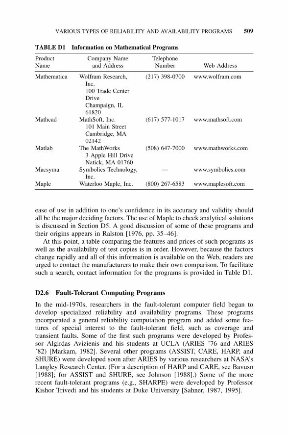
VARIOUS TYPES OF RELIABILITY AND AVAILABILITY PROGRAMS 509
TABLE D1 Information on Mathematical Programs
Product Company Name TelephoneName and Address Number Web Address
Mathematica Wolfram Research, (217) 398-0700 www.wolfram.comInc.100 Trade CenterDriveChampaign, IL61820
Mathcad MathSoft, Inc. (617) 577-1017 www.mathsoft.com101 Main StreetCambridge, MA02142
Matlab The MathWorks (508) 647-7000 www.mathworks.com3 Apple Hill DriveNatick, MA 01760
Macsyma Symbolics Technology, — www.symbolics.comInc.
Maple Waterloo Maple, Inc. (800) 267-6583 www.maplesoft.com
ease of use in addition to one’s confidence in its accuracy and validity shouldall be the major deciding factors. The use of Maple to check analytical solutionsis discussed in Section D5. A good discussion of some of these programs andtheir origins appears in Ralston [1976, pp. 35–46].
At this point, a table comparing the features and prices of such programs aswell as the availability of test copies is in order. However, because the factorschange rapidly and all of this information is available on the Web, readers areurged to contact the manufacturers to make their own comparison. To facilitatesuch a search, contact information for the programs is provided in Table D1.
D2.6 Fault-Tolerant Computing Programs
In the mid-1970s, researchers in the fault-tolerant computer field began todevelop specialized reliability and availability programs. These programsincorporated a general reliability computation program and added some fea-tures of special interest to the fault-tolerant field, such as coverage andtransient faults. Some of the first such programs were developed by Profes-sor Algirdas Avizienis and his students at UCLA (ARIES ’76 and ARIES’82) [Markam, 1982]. Several other programs (ASSIST, CARE, HARP, andSHURE) were developed soon after ARIES by various researchers at NASA’sLangley Research Center. (For a description of HARP and CARE, see Bavuso[1988]; for ASSIST and SHURE, see Johnson [1988].) Some of the morerecent fault-tolerant programs (e.g., SHARPE) were developed by ProfessorKishor Trivedi and his students at Duke University [Sahner, 1987, 1995].

510 PROGRAMS FOR RELIABILITY MODELING AND ANALYSIS
D2.7 Risk Analysis Programs
Risk analysis programs represent another class of large, comprehensive reli-ability and availability analysis programs. The term risk analysis generallyimplies that the analysis includes the consequences of failure [Shooman, 1990,Appendix J]. The impetus of such programs was the first probabilistic riskanalysis for a nuclear power reactor performed for the U.S. Nuclear Regula-tory Commission (NRC) by a team of experts lead by Professor Neils Ras-mussen of MIT [McCormick, 1981, p. 240; NRC, 1975]. Risk analysis gen-erally includes a final stage that predicts the probability of various classes offailures (accidents, calamities) and the result of such accidents (property loss,injuries, deaths). In addition, the team that conducted the NRC study (knownin familiar terms as Wash 1400) found that it was difficult to include all thepossible effects with such a large, complex system as a nuclear power reac-tor by using reliability block diagrams and fault trees. New techniques calledevent trees and event sequence diagrams were developed to help in the analy-sis, along with fault tree methods [McCormick, 1981, p. 193]. Such programshave been developed for analysis of nuclear reactors and other similar risksituations [McCormick, Chapter 10].
Several risk analysis programs have been evolved over the past fewdecades, namely: SAPHIRE [Long, 1999]; RISKMAN [Wakefield]; NUPRA,REBECCA, and CAFTA/ ETA [Smith]. Presently, NASA Headquarters isdeveloping a comprehensive risk analysis program called QRAS for its spaceprojects [Safie, 1998; Shooman, 2000]. The analyst must judge whether oneof these risk programs is suitable for fault-tolerant studies.
D2.8 Software Reliability Programs
Software reliability models and the supporting programs differ from those ofhardware reliability. Many programs have been developed by researchers andcompanies; however, three multimodel programs exist: SMERFS, CASRE, andSoRel. The best description and comparison of software reliability modelingprograms is in Appendix A of the Handbook of Software Reliability Engineer-ing [Stark, 1996]. The SMERFS program was developed in 1983 by the U.S.Naval Surface Warfare Center in Dahlgren, Virginia. In 1991, the LAAS Labo-ratory at the National Center for Scientific Research in Toulouse, France devel-oped SoRel. The Jet Propulsion Laboratory developed CASRE in 1993. Forfurther details, see Stark [1996].
D3 TESTING PROGRAMS
The development of large, comprehensive reliability and availability programsrequires the technical skills of reliability analysts who know probability andreliability methods and those of skilled programmers who can translate the
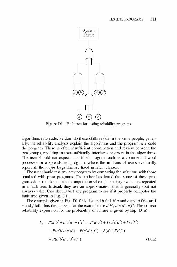
TESTING PROGRAMS 511
a’ e’b’ f ’
a’ c’ d’
SystemFailure
Figure D1 Fault tree for testing reliability programs.
algorithms into code. Seldom do these skills reside in the same people; gener-ally, the reliability analysts explain the algorithms and the programmers codethe program. There is often insufficient coordination and review between thetwo groups, resulting in user-unfriendly interfaces or errors in the algorithms.The user should not expect a polished program such as a commercial wordprocessor or a spreadsheet program, where the millions of users eventuallyreport all the major bugs that are fixed in later releases.
The user should test any new program by comparing the solutions with thoseobtained with prior programs. The author has found that some of these pro-grams do not make an exact computation when elementary events are repeatedin a fault tree. Instead, they use an approximation that is generally (but notalways) valid. One should test any program to see if it properly computes thefault tree given in Fig. D1.
The example given in Fig. D1 fails if a and b fail, if a and c and d fail, or ife and f fail; thus the cut sets for the example are a′b′, a′c′d′, e′f ′. The correctreliability expression for the probability of failure is given by Eq. (D1a).
Pf c P(a′b′ + a′c′d′ + e′f ′) c P(a′b′) + P(a′c′d′) + P(e′f ′)
− P(a′b′a′c′d′) − P(a′b′e′f ′) − P(a′c′d′e′f ′)
+ P(a′b′a′c′d′e′f ′) (D1a)
512 PROGRAMS FOR RELIABILITY MODELING AND ANALYSIS
The intersection of two like elements obeys the following logic law: x . x c x.Thus Eq. (D1a) becomes
Pf c P(a′b′ + a′c′d′ + e′f ′) c P(a′b′) + P(a′c′d′) + P(e′f ′)
− P(a′b′c′d′) − P(a′b′e′f ′) − P(a′c′d′e′f ′)
+ P(a′b′c′d′e′f ′) (D1b)
If all the elements are independent and have a probability of failure of q, thatis, P(a′) c P(b′) c P(c′) c P(d′) c P(e′) c P( f ′) c q, the probability of failurebecomes
Pf c 2q2 + q3− 2q4
− q5 + q6 (D1c)
Many programs do not perform the step given in Eq. (D1b); rather, they expandEq. (D1a) as
Pf c 2q2 + q3− q4
− 2q5 + q7 (D1d)
Equations (D1c) and (D1d) have the same first two terms, but the followingthree terms differ. If q is small, the higher-order powers of q are negligible,and the two expressions give approximately the same numerical result. If q isnot small, however, the two expressions differ. If q c 0.2, Eq. (D1c) gives Pf
c 0.084544, and Eq. (D1d) yields 0.0857728. Larger values of q result in evena larger difference—thus caveat emptor! (“let the buyer beware”).
D4 PARTIAL LIST OF RELIABILITY AND AVAILABILITYPROGRAMS
Many reliability and availability programs exist, all varying greatly in theirease of use, facilities provided, and cost. The purchaser should be wary of thebasic validity of some of these programs, as was discussed in the precedingsection. The contact information provided in Table D2 should allow users toconduct their own search and comparison via the Web.
Additional reliability and availability software advertisements can be foundin the end pages of the Proceedings Annual Reliability and MaintainabilitySymposium. Sometimes, specialized reliability programs appear in the litera-ture, such as the NAVY TIGER program [Luetjen, 1982], which was designedto analyze reliability and availability of naval ships and incorporates certainpreventive maintenance programs used by the U.S. Navy.

513
TA
BL
E D
2In
form
atio
n on
Rel
iabi
lity
and
Ava
ilabi
lity
Pro
gram
s
Prod
uct
Com
pany
Nam
eTe
leph
one
Nam
ean
d A
ddre
ssN
umbe
rW
eb A
ddre
ss
Gid
epG
over
nmen
t–In
dust
ry D
ata
Exc
hang
e Pr
ogra
m(9
09)
273-
4677
ww
w.g
idep
.cor
ona.
navy
.mil
P.O
. B
ox80
00C
oron
a, C
A91
718
Item
RA
MS
Soft
war
e To
ols
(049
)26
0-09
00w
ww
.item
soft
.com
2030
Mai
n St
reet
Suite
1130
Irvi
ne,
CA
9261
4Pr
ism
Rel
iabi
lity
Ana
lysi
s C
ente
r(8
88)
RA
C-U
SER
http
: //ra
c.itt
ri.o
rg20
1M
ill S
tree
tR
ome,
NY
1344
0M
eade
pSo
HaR
, In
c.(3
23)
653-
4717
ww
w.s
ohar
.com
8421
Wils
hire
Bou
leva
rdB
ever
ly H
ills,
CA
9021
1A
SEN
TR
ayth
eon
(972
)57
5-61
72ht
tp: //
asen
t.ray
theo
n.co
mR
AM
Com
man
der
—(8
00)
292-
4519
—Is
ogra
ph D
irec
t—
—w
ww
.isog
raph
.com
Rel
exR
elex
Sof
twar
e C
orpo
ratio
n( 7
24)
836-
8800
ww
w.r
elex
soft
war
e.co
m54
0Pe
llis
Roa
dG
reen
sbur
g, P
A15
601
—R
elia
Soft
Cor
pora
tion
115
Sout
h Sh
erw
ood
Vill
age
Dri
ve(8
88)
886-
0410
ww
w.R
elia
soft
.com
Suite
103
Tuc
son,
AZ
8571
0C
AR
E M
odul
esB
QR
Rel
iabi
lity
Eng
inee
ring
Ltd
.(9
72)
3-96
6-35
69w
ww
.bqr
.com
7B
ialik
Str
eet
P.O
. B
ox20
8R
isho
n–L
eZio
n75
101,
Isr
ael
Mar
kov
ID
ecis
ion
Syst
em A
ssoc
iate
s( 4
15)
851-
7591
—42
44Je
ffer
son
Ave
nue
orW
oods
ide,
CA
9406
2(4
15)
369-
0501
514 PROGRAMS FOR RELIABILITY MODELING AND ANALYSIS
D5 AN EXAMPLE OF COMPUTER ANALYSIS
As part of a consulting assignment, the author was asked to derive a closed-form analytical solution for a spacecraft system with one on-line element andtwo different standby elements with dormancy failure rates. By dormancy fail-ure rates, one means that the two standby elements have small but nonzerofailure rates while on standby. A full Markov model for the three elementswould require eight states, resulting in eight differential equations. Normally,one would use a numerical solution; however, the company staff for whom theauthor was consulting wished to include the solution in a proposal and felt thata closed-form solution would be more impressive and that it had to be checkedfor validity. (Errors had been found in previous company derivations). Assum-ing that the two standby elements had identical on-line and standby failurerates allowed a reduction to a six-state model. Formulation of the six equa-tions, computing the Laplace transforms, and checking the resulting pencil-and-paper equations and solutions took the author a day while he worked withone of the company’s engineers.
To check the results, the six basic differential equations were submitted inalgebraic form to the Maple symbolic equation program, and an algebraic solu-tion was requested. The first four of the state probabilities were easily checked,but the fifth equation took about half a page in printed form and was difficultto check. The Maple program provided a factoring function; when it was askedto factor the equation, another form was printed. Careful checking showed thatthe second form and the pencil-and-paper solution were both identical. The last(sixth) equation was the most complex, for which the Maple solution producedan algebraic form with many terms that covered more than a page. Even afterusing the Maple factoring function, it was not possible to show that the twoequations were identical. As an alternative, the numerical values of the failurerates were substituted into the pencil-and-paper solution and numerical valueswere obtained. Failure rates were substituted into the Maple equations, andthe program was asked for numerical solutions of the differential equations.These numerical solutions were identical (within round-off error to many dec-imal places) and easily checked.
There are several lessons to be learned from this discussion. The Maplesymbolic equation program is very useful in checking solutions. However, asproblems become larger, numerical solutions may be required, though it is pos-sible that newer versions of Maple or some of the other symbolic programsmay be easier to use with large problems. Checking an analytical solution is agood way of ensuring the accuracy of your results. Even in a very large prob-lem, it is common to make a simplified model that could be checked in thisway. Because of potential errors in modeling or in computational programs, itis wise to check all results in two ways: (a) by using two different modelingprograms, or (b) by using an analytical solution (sometimes an approximatesolution) as well as a modeling program.

REFERENCES 515
REFERENCES
Bavuso, S. J. A User’s View of CARE III. Proceedings Annual Reliability and Main-tainability Symposium, January 1984. IEEE, New York, NY, pp. 382–389.
Bavuso, S. J., and A. Martensen. A Fourth Generation Reliability Predictor. Proceed-ings Annual Reliability and Maintainability Symposium, 1988. IEEE, New York,NY, pp. 11–16.
Bavuso, S. J. et al. CARE III Hands-On Demonstration and Tutorial. NASA TechnicalMemorandum 85811. Langley Research Center, Hampton, VA, May 1984.
Bavuso, S. J. et al. CARE III Model Overview and User’s Guide. NASA Tech-nical Memorandum 85810. Langley Research Center, Hampton, VA, June 1984.[Updated, NASA Technical Memorandum 86404, April 1985.]
Bavuso, S. J. et al. Analysis of Typical Fault-Tolerant Architectures Using HARP. IEEETransactions on Reliability 36, 2 (June 1987).
Bellcore. Reliability Prediction Procedure for Electronic Equipment. TR-NWT-000332, Issue 6, 1997.
Bryant, L. A., and J. J. Stiffler. CARE III, Version 6 Enhancements. NASA ContractorReport 177963. Langley Research Center, Hampton, VA, November 1985.
Butler, R. W. An Abstract Language for Specifying Markov Reliability Models. IEEETransactions on Reliability 35, 5 (December 1986).
Butler, R. W., and P. H. Stevenson. The PAWS and STEM Reliability Analysis Pro-gram. NASA Technical Memorandum 100572. Langley Research Center, Hampton,VA, March 1988.
Butler, R. W., and A. L. Martensen. The FTC Fault Tree Program. Draft, NASA Tech-nical Memorandum. Langley Research Center, Hampton, VA, December 1988.
Butler, R. W., and A. L. White. SHURE Reliability Analysis—Program and Mathemat-ics. NASA Technical Paper 2764. Langley Research Center, Hampton, VA, March1988.
Dugan, J. B. “Software System Analysis Using Fault Trees.” In Handbook of SoftwareReliability Engineering, M. R. Lyu (ed.). McGraw-Hill, New York, 1996.
Ellis, W. Jr. et al. Maple V Flight Manual. Brooks/ Cole Division of Wadsworth Pub-lishers, Pacific Grove, CA, 1992.
Gedam, S. G., and S. T. Beaudet. Monte Carlo Simulation Using Excel Spreadsheetfor Predicting Reliability of a Complex System. Proceedings Annual Reliability andMaintainability Symposium, 2000. IEEE, New York, NY, pp. 188–193.
Hayhurst, K. J. Testing of Reliability—Analysis Tools. Proceedings Annual Reliabilityand Maintainability Symposium, 1989. IEEE, New York, NY, pp. 487–490.
Huff, D. S. The ProphetTM Risk Management Toolset. Proceedings Annual Reliabilityand Maintainability Symposium, 1999. IEEE, New York, NY, pp. 426–431.
Johnson, S. C. ASSIST User’s Manual. NASA Technical Memorandum 87735. Lang-ley Research Center, Hampton, VA, August 1986.
Johnson, S. C. Reliability Analysis of Large, Complex Systems Using ASSIST.Eighth Digital Avionics Systems Conference, AIAA/ IEEE, San Jose, CA, October1988.
Johnson, S. C., and R. W. Butler. Automated Generation of Reliability Models. Pro-
516 PROGRAMS FOR RELIABILITY MODELING AND ANALYSIS
ceedings Annual Reliability and Maintainability Symposium, 1988. IEEE, NewYork, NY, pp. 17–25.
Laviron, A. SESCAF: Sequential Complex Systems Are Analyzed with ESCAFThrough an Add-On Option. IEEE Transactions on Reliability (August 1985).
Laviron, A. et al. ESCAF—A New and Cheap System for Complex Reliability Anal-ysis and Computation. IEEE Transactions on Reliability 31 4 (October 1982).
Long, S. M. Current Status of the SAPHIRE Models for ASP Evaluations. ProbabilisticSafety Assessment and Management, PSAM 4, A. Mosleh and R. A. Bari (eds.).Springer-Verlag, New York, 1998, pp. 1195–1199.
Luetjen, P., and P. Hartman. Simulation with the Restricted Erlang Distribution. Pro-ceedings Annual Reliability and Maintainability Symposium, 1982. IEEE, NewYork, NY, pp. 233–237.
Markam, S., A. Avizienis, and G. Grusas. ARIES ’82 Users’ Guide. TechnicalReport No. CSD-820830/ UCLA-ENG-8262. University of California at Los Ange-les (UCLA), Computer Science Department, August 1982.
MathSoft, Inc. Users’ Guide Mathcad. MathSoft, Inc., Cambridge, MA, 1995.
Math Works, Inc. The Student Edition of MATHLAB. Prentice-Hall, Englewood Cliffs,NJ, 1992.
McCormick, N. Reliability and Risk Analysis. Academic Press, New York, 1981.
Mulvihill, R. J., and Safie, F. M. Application of the NASA Risk Assessment Tool tothe Evaluation of the Space Shuttle External Tank Re-Welding Process. ProceedingsAnnual Reliability and Maintainability Symposium, 2000. IEEE, New York, NY, pp.364–369.
National Aeronautics and Space Administration (NASA). Practical Reliability—VolumeII Computation. NASA Contractor Report, NASA CR-1127. Research TriangleInstitute, August 1968.
Ng, Y. W., and A. A. Avizienis. ARIES—An Automated Reliability Estimation Systemfor Redundant Digital Structures. Proceedings Annual Reliability and Maintainabil-ity Symposium, 1977. IEEE, New York, NY, pp. 108–113.
Nuclear Regulatory Commission (NRC). Reactor Safety Study—An Assessment ofAccident Risks in U.S. Commercial Nuclear Power Plants. Report Wash 1400,NUCREG 75/ 014, 1995.
Orbach, S. The Generalized Effectiveness Methodology (GEM) Analysis Program.Lab. Project 920-71-1, SF 013-14-03, Task 1604, Progress Report 1. U.S. NavalApplied Science Lab., Brooklyn, NY, May 8, 1968.
Ralston, A. Encyclopedia of Computer Science. Van Nostrand Reinhold, New York,1976.
Rubinstein, R. Y. Simulation and the Monte Carlo Method. Wiley, New York,1981.
Safie, F. M. An Overview of Quantitative Risk Assessment of Space Shuttle PropulsionElements. Probabilistic Safety Assessment and Management, PSAM 4, A. Moslehand R. A. Bari (eds.). Springer-Verlag, New York, 1998, pp. 425–430.
Safie, F. M. NASA New Approach [QRAS Risk Tool] for Evaluating Risk ReductionDue To Space Shuttle Upgrades. Proceedings Annual Reliability and Maintainabil-ity Symposium, 2000. IEEE, New York, NY, pp. 288–291.
PROBLEMS 517
Sahner, R. A., and K. S. Trivedi. Reliability Modeling Using SHARPE. IEEE Trans-actions on Reliability 36, 2 (June 1987): 186–193.
Sahner, R., K. S. Trivedi, and A. Puliafito. Performance and Reliability Analysisof Computer Systems: An Example-Based Approach Using the SHARPE SoftwarePackage. Kluwer Academic Publishers, Boston, MA, 1995.
Sammet, J. E. Programming Languages: History and Fundamentals. Prentice-Hall,Englewood Cliffs, NJ, 1969.
Schmidt, H., and D. Busch. An Electronic Digital Slide Rule—If This Hand-SizedCalculator Ever Becomes Commercial, the Conventional Slide Rule Will BecomeAnother Museum Piece. The Electronic Engineer (July 1968).
Shooman, M. L. The Equivalence of Reliability Diagrams and Fault Tree Analysis.IEEE Transactions on Reliability (May 1970): 74–75.
Shooman, M. L. Probabilistic Reliability: An Engineering Approach, 2d ed. Krieger,Melbourne, FL, 1990.
Shooman, M. L. and four others participated in a review of QRAS for NASA in late1999 and early 2000.
Smith, D. CAFTA, SAIC Facilities Group (http:// fsg.saic.com).Stark, G. Software Reliability Tools, Handbook of Software Reliability Engineering,
M. R. Lyu (ed.). McGraw-Hill, New York, 1995, app. A.Trivedi, K. S., and R. M. Geist. A Tutorial on the CARE III Approach to Reliabiity
Modeling. NASA Contractor Report 3488. Langley Research Center, Hampton, VA,1981.
Trivedi, K. S. et al. HARP: The Hybrid Automated Reliability Predictor: Introductionand Guide for Users. NASA, Langley Research Center, Hampton, VA, September1986.
Trivedi, K. S. et al. HARP Programmer’s Maintenance Manual. NASA, LangleyResearch Center, Hampton, VA, April 1988.
Turconi, G., and E. Di Perma. A Design Tool for Fault-Tolerant Systems. ProceedingsAnnual Reliability and Maintainability Symposium, 2000. IEEE, New York, NY, pp.317–326.
Vesley, W. E. et al. PREP and KITT: Computer Codes for the Automatic Evaluationof a Fault Tree. Idaho Nuclear Corporation, Report for the U.S. Atomic EnergyCommission, No. IN-1349, August 1970.
Wakefield. RISKMAN ([email protected]).White, A. Motivating the SURE Bounds. Proceedings Annual Reliability and Main-
tainability Symposium, 1989. IEEE, New York, NY, pp. 277–282.Wolfram, S. The Mathematica Book, 4th ed. Cambridge University Press, New York,
1999.
PROBLEMS
D1. Search the Web for reliability and availability analysis programs. Makea table comparing the type of program, the platforms supported, and thecost.
518 PROGRAMS FOR RELIABILITY MODELING AND ANALYSIS
D2. Use a reliability analysis program to compute the reliability for the firstthree systems in Table 7.8 and check the reliability.
D3. Use a symbolic modeling program to check Eq. (3.56).
D4. Use a Markov modeling program to check the results given in Eq. (3.58).
D5. Use a fault tree program to solve the model of Fig. D1 to see if the resultsagree with Eqs. (D1c) or (d).

Reliability of Computer Systems and Networks: Fault Tolerance, Analysis, and DesignMartin L. Shooman
Copyright 2002 John Wiley & Sons, Inc.ISBNs: 0-471-29342-3 (Hardback); 0-471-22460-X (Electronic)
519
NAME INDEX
Numbers in parentheses that follow page references indicate “Problems.”
Abramovitz, M., 400, 462Advanced Hardware Architectures (AHA), 74AGREE Report, 342Aho, A. V., 337, 351Ahuja, V., 320AIAA/ ANSI, 259, 261Aktouf, C., 23Albert, 345, 346, 348, 349Anderson, T., 25, 131, 135Arazi, B. A., 34, 65, 71, 72ARINC, 89Ascher, 111, 112Aversky, D. R., 23Avizienis, A., 23, 263, 265, 509, 516
Baker, W. A., 131Barlow, R. E., 331, 351Bartlett, J., 337Bavuso, S. J., 509Bazovsky, I., 110Bell, C. G., 25, 146Bell, T., 25Bellman, R., 351, 372Bernstein, J., 428Bhargava, B. K., 275Bierman, H., 333, 351Billings, C. W., 226Bloch, G. S, 23
Boehm, B., 207Booch, G., 207Bouricius, 115, 117Braun, E., 25Breuer, M. A, 23.Brooks, F. P., 207, 211Burks, A. W., 25Buzen, J. P. 119, 120
Calabro, S. R., 186Carhart, R. R., 425Carter, W. C. 115, 117Cassady, C. R., 366Chen, L., 263, 265Christian, F., 23Clark, R., 25Colbourn, C. J., 284, 294, 309, 320Computer Magazine, 23, 24Cormen, T. H., 213, 314, 320, 337, 351, 369,
371Cramer, H., 203
Dacin, M., 24Daves, D. W., 24Dierker, P. F., 312, 314, 317Ditlea, S., 5, 25Dougherty, E. M., 24, 202Dugan, J. B., 117, 284, 446, 507

520 NAME INDEX
Echte, K., 24Ellis, W., 505, 508
Farr, W., 258Fault-Tolerant Computing Symposium, 24Federal Aviation Administration, 25Fisher, L. M., 25Fowler, M., 207Fragola, J. R., 24, 25, 202, 331Frank, H., 284, 301, 317, 320Freeman, H., 394Friedman, A. D., 23Friedman, M. B., 25, 120Friedman, W. F. (see Clark, R.)Frisch, I. T., 284, 317Fujiwara, E., 25, 77
Gibson, G., 24, 119, 120, 126Gilbert, G. A., 340Giloth, P. K., 26Goldstine, H. H., 25Graybill, F. A., 261Greiner, H. de Meer, 23Grisamore, 158, 159
Hafner, K., 26Hall, H. S., 214Hamming, R. W., 31Hawicska, A., 24Healey, J. T., 427Hennessy, J. L., 136Henney, K., 342Hill, F. J., 475, 479, 488, 490Hiller, S. F., 333, 351, 371, 372Hoel, P. G., 255Hopper, G., 226Hwang, C. L., 351
Iaciofano, C., 26
Jelinski, Z., 258, 259Jia, S., 283Johnson, B. W., 24, 117.Johnson, G., 26Johnson, S. C., 509
Kanellakis, P. C., 24Kaplan, G., 24Kaufman, L. M. 117Karnaugh, M., 35Katz, R., 24, 26Keller, T. W., 269
Kershenbaum, A., 287, 308, 309, 310, 314,318, 320, 321
Knight, J. C., 265Knight, S. R., 214Knox-Seith, 154, 155, 157Kohavi, Z., 475, 488, 490Kuo, W., 351
Lala, P. K., 24, 263Larsen, J. K., 24Lee, P. A., 23, 24Leveson, N. G., 265Lewis, P. H., 26Lipow, M., 333, 346, 348, 434Littlewood, B., 259Lloyd, D. K., 333, 346, 348Long, S. M., 510Luetjen, P., 512Lyu, M. R., 24, 258, 261
Mancino, V. J., 331, 383Mann, C. C., 5, 26Mano, M. M., 475, 488, 490Markam, S., 509Markoff, J., 26Marshall, 351, 369Massaglia, P., 120McAllister, D. F., 189, 191, 192, 194, 268McCormick, N., 24, 507, 510McDonald, S., 25Meeker, W. Q., 384Mendenhall, W., 299, 384Messinger, M, 333, 351, 377, 420Meyers, R. H., 351Military Handbook MIL-HDBK-217–217F,
79 (2.7), 427, 506Military Standard MIL-F-9409, 26Miller, E., 186Miller, G. A., 213, 339Mood, A. M., 261Moore, G. E., 5–8, 26, 147Moranda, P., 258, 259Motorola (ON Semiconductor), 492, 495,
496, 499, 501Murray, K., 297, 308, 318Musa, J., 232, 238, 251, 252, 253, 259, 260,
261
Neuman, J. von, 147Newell, A. 146Ng, Y. W., 516Nishio, T., 24Norwall, B. D., 26

NAME INDEX 521
Orbach, S., 505Osaki, S., 24
Papoulis, 104, 385Paterson, D., 24, 120, 136Pecht, M. G., 117Pfister, G., 137Pfleeger, S. L., 26, 207Pham, H., 24Pierce, J. R., 31Pierce, W. H., 24, 194Pogue, D., 26Pollack, A., 26, 203Pooley, R., 207Pradhan, D. K., 24, 263, 265Pressman, R. H., 207
Ralston, A., 505, 508Randall, B., 5, 26, 147Rao, T. R. N., 25, 34, 77Rice, W. F., 366Rogers, E. M, 26Rosen, K. H., 66, 294, 312, 314, 361Roth, C. H., 475, 488, 490Rubinstein, R. Y., 505
Safie, F. M., 510Sahner, R., 509Sammet, J. E., 5, 26, 506Satyanarayana, A. A., 300Schach, S. R., 207, 218Schmidt, H, 505Schneider, 115Schneidewind, 259, 269Scott, K., 207Shannon, C. 31, 147Sherman, L., 132Shier, D. R., 323Shiva, S. G., 161, 475, 488, 490, 501Shooman, A. M., 300, 305, 306, 308, 309,
318Shooman, M. L., 4, 5, 25, 26, 90, 110, 111,
112, 135, 166, 172, 180, 185, 194, 199(4.29), 202, 207, 214, 215, 225, 229,230, 234, 238, 251, 252, 255, 256, 257,258, 259, 260, 261, 262, 264, 265, 268,284, 287, 288, 292, 295, 299, 337, 349,351, 369, 384, 395, 409, 411, 420, 427,428, 432, 435, 437, 439, 441, 446, 450,460, 472, 505, 506, 507, 510
Shvartsman, A. A., 24Siewiorek, D. P., 1, 25, 26, 27, 126, 129, 131,
135, 147, 158, 165, 169, 194, 207, 263,270, 275, 427, 428
Smith, B. T., 25Smith, D., 510Sobel, D., 195Stark, G. E., 258, 510Stone, C. J., 384Stork, D. G., 280 (5.6)Stepler, R., 27Stevens, P., 207Swarz, R. S., 1, 25, 26, 27, 126, 129, 131,
135, 147, 158, 165, 169, 194, 207, 263,270, 275, 427, 428
Taylor, L., 33Tenenbaum, A. S., 320Tillman, F. A., 351Toy, W. N., 165Trivedi, K. S., 23, 25, 509Turing, A. M., 4, 27, 29 (1.25)
Van Slyke, R., 284, 301Verall, J. L., 258von Alven, W. H., 342von Neuman, J., 4Vouk, M. A., 189, 191, 192, 194, 268
USA Today, 27
Wadsworth, G. P., 384, 394Wakefield, 510Wakerly, J. F., 161, 475, 488, 490, 501Wald, M. L., 27Welker, E. L., 434Wing, J. A., 210,Wing, J. M., 283, 284Wirth, N., 27Wise, T. R., 366Wood, A. P., 127, 130, 131Workshop on Defect and Fault-Tolerance in
VLSI Systems, 25www.emc.com, 27www.intel.com, 27www.microsoft.com, 27
Yourdon, E., 270
Zuckerman, L., 27
523
SUBJECT INDEX
Numbers in parentheses that follow page references indicate “Problems.”
Aibo, 9Air traffic control (ATC), 29 (1.20), 209, 215,
216, 217, 340, 341Aircraft reliability, 15–18Apportionment (see Reliability optimization,
apportionment)Architecture, Boolean algebra, 479–482
decoder, 494–497DeMorgan’s theorems, 409 (A1)flip-flops, 487–499gates, 37, 38, 478–480number systems, 475–477
arithmetic, 477, 478parity-bit generators, 494set theory, historical development, 384–
386union, 388–390Venn diagram, 386, 409 (A1)
storage registers, 500, 501switching functions, 483, 484
combinatorial circuits, product of sums(POS), 489, 490
sum of products (SOP), 489–491integrated circuits (IC chips), 491–493maxterms, 484minterms, 483simplification, 484, 485
don’t-cares, 489
Karnaugh map (K map), 485–488Quine–McClusky (QM) method, 488
truth tables, 479–482ARPA network (see network reliability)Availability, concepts, 14, 15, 286–288
coupling and decoupling, 183–186 (see alsoMarkov models, uncoupled)
definition, 14, 134, 135, 179Markov models, 117–119, 180–186,
454–461steady-state, 458–461typical computer systems, 16, 17
Bell Labs’ ESS, 134, 183Stratus, 134, 135, 183Tandem, 126, 127, 183Univac, 146, 147
Billy Bass, 9Burst, 62
code, decoder, 65decoder failure, 73–75encoder, 65errors, 32, 62properties, 64, 65Reed–Solomon, 72–75, 126
CAID, 119 (see also RAID)Chinese Remainder Theorem, 66–71
524 SUBJECT INDEX
Cluster, of computers, 135, 136Coding methods, burst codes (see Burst)
check bits, 35cryptanalysis, 29 (1.25), 30error-correcting, 2, 31error-detecting, 2, 31errors, 32, 33Hamming codes, 31, 44–47, 54Hamming distance, 34, 45, 46other codes, 45, 75, 76parity-bit codes, 35, 37
coder (encoder, generator), 37, 38, 40,42
coder–decoder failures, 43, 53–59decoder (checker), 37, 38, 40, 42probability of undetected errors, 32,
39–42, 45, 52–53, 59–62RAID levels 2–6, 121–126Reed–Solomon codes (see Burst)reliability models (see also Probability of
undetected errors)retransmission codes, 59–62single error-detecting and double error-
detecting (SECDED), 47, 51–52single error-correcting and single error-
detecting (SECSED), 47–51soft fails, 33
Cold redundancy, cold standby (see Standbysystems)
Computer, CDC 6600, 11ENIAC, 4history, 4, 5Mark I, 4
Conditional reliability, 390, 391Coverage, 115, 117Cryptography (see Coding methods,
cryptanalysis)Cut-set methods (see also Network reliability,
definition; Reliability modeling)
Dependent failures (Common mode failures),(see Reliability theory, combinatorialreliability)
Downtime, 14, 134 (see also Availability)
EMC (see RAID)ESS (see Availability, typical computer
systems)
Fault-tolerant computing, calculations, 12, 13definition, 1
Furby, 9
Global Positioning System (GPS), 195,280 (5.6)
Hamming codes (see Coding methods)Hamming distance (see Coding methods)Hazard (see also Reliability modeling, failure
rate), derivation, 222–224function of system, 94, 95
Himalaya computers (see Tandem)Hot redundancy, hot standby (see Parallel
systems)Human operator reliability, 202
Laplace transforms, as an aid in computingMTTF, 169, 170, 174, 175, 468, 469
definition, 462–464of derivatives, 465, 466final value computation, 170, 182initial value approximation, 469–471initial value computation, 173, 174of Markov models, 93partial fractions, 466, 467table of theorems, 468table of transforms, 465
Library of Congress, 10, 27 (1.1), (1.3),(1.19)
Maintenance, 146Markov models (see also Laplace transforms,
Probability)algorithms for writing equations, 113collapsed graphs (see merger)complexity, 453, 454, 461decoupling (see uncoupled)formulation, 104–108, 112–117, 446–450graphs, 450Laplace transforms, 461–468merger of states, 166, 453, 454RAID, 125solution of Markov equations, 106, 108,
115–117, 118, 166–179theory, chain, 404
Poisson process, 404–407process, 404properties, 403, 404transition matrix, 407, 408
two-element model, 450–453uncoupled, 172, 349, 350 (see also
Availability, coupling and decoupling)Mean time between failure (MTBF) (see
Mean time to failure)Mean time to failure (MTTF), 95, 96, 114,
115, 117, 140 (3.16), 169, 170, 174
SUBJECT INDEX 525
constant-failure rate (hazard), 224, 225definition, 234linearly increasing hazard, 225RAID, 120, 123, 125tables of, 115, 117TMR, 151–153
Mean time to repair (MTTR), 112–119, 126,127
Memory, growth, 7, 8Microelectronic, revolution, 1, 4, 5Microsoft, 5MIL-HDBK-217, 79 (2.7), 427, 506Moore’s Law, 5–8
NASA,Apollo, 194Space Shuttle, 188, 194, 266–269
Network reliability, concepts, 13, 14, 31,283–285
ARPA network, 312availability, 286–288computer solutions, 308, 309definition, 285, 288
all-terminal, 286cut-set and tie-set methods, 303–305event-space, 302, 303graph transformations, 305–308
k-terminal, 286, 308two-terminal, 286, 288–301
cut-set and tie-set methods, 292–294graph transformations, 297–301node pair resilience, 301state-space, 288–292subset approximations, 296, 297truncation approximations, 294–296
design approaches, 309–321adjacency matrices, 312, 313backbone network-spanning tree,
310–312enhancement phase, 318–321Hamiltonian tours, 317, 327 (6.14),
328 (6.15)–(6.17)incidence matrices, 312, 313Kruskal’s and Prim’s algorithms, 312,
314–318spanning trees, 314–318
graph models, 284, 285N-modular redundancy, 2, 145, 146, 153–161
history, 146, 147repair, 165–183, 454–461triple modular redundancy (TMR), 147,
148, 149–153,comparison with parallel and standby
systems 178, 179Markov models, 166–170MTTF, 151–153
voter logic, 161–165adaptive voting, 194adjudicator algorithms, 189–195comparison of reliability, 193consensus voting, 190–192pairwise comparison, 191, 193test and switch, 191
voters, 154–161voting with lockout, 186, 188, 189
NMR (see N-modular redundancy)N-version (see Software reliability)
Parallel systems, 2, 83, 97–99, 104 (see alsoReliability optimization)
comparison with standby, 108–111, 178,179
MTTF, 96, 114, 115Polynomial roots, 165, 166Probability, complement, 388
conditional, 390–391continuous random variables, 395–401
density and distribution function,395–397
exponential distribution, 397–399, 403,433, 434
Normal (Gaussian) distribution, 398, 400,401, 403
Rayleigh distribution, 398, 399, 403, 434rectangular (uniform) distribution, 397,
398Weibull distribution, 398, 399, 403,
434–438discrete random variables, 391–395
binomial (Bernoulli) distribution, 393,394, 403
density function, 391, 392distribution function, 392, 393Poisson distribution, 185, 395, 396,
403–407Markov models (see Markov models)moments, 401–403
expected value, 401, 402mean 402, 403variance, 403
Probability of undetected error (see Codingmethods)
RAID, Advisory Board, 120EMC Symmetrix, 10, 27 (1.1)levels, 121–126
526 SUBJECT INDEX
mirrored disks, 122reliability, 119–126stripping, 125
RBD (see Reliability modeling)Redundancy (see also Parallel systems,
Reliability optimization),component, 86–92couplers, 91, 92system, 86–92
Reliability allocation (see Reliabilityoptimization)
Reliability analysis programsexample, 514fault-tolerant computing programs, ARIES,
509ASSIST, 509CARE, 509HARP, 509SHAPE, 509SHURE, 509
mathematics packages, Macsyma, 256, 505,508, 509
Maple, 256, 505, 508, 509Mathcad, 256, 505, 508, 509Mathematica, 256, 505, 508, 509Matlab, 505, 508, 509
partial list, 512, 513risk analysis, CAFTA, 510
NUPRA, 510QRAS, 510REBECCA, 510RISKMAN, 510SAPHIRE, 510
software reliability (see Software reliability,programs)
testing programs, 510–512Reliability modeling (see also Reliability
theory),block diagram (RBD), 413, 444cut-set methods, 292–294, 419, 420density function, 218–221distribution function, 218–221event-space, 288–292failure rate, 222–224 (see also Hazard)graph (see block diagram)probability of success, 219–221reliability function, 218–221system, example, auto-brake system,
442–446parallel, 440, 441r-out-of-n structure, 441, 442series 438–440
theory, 218–221
tie-set methods, 292–294, 419, 420Reliability optimization, algorithms, 359–365
apportionment 85, 86, 342–349, 366, 367Albert’s method, 345–349availability, 349–351equal weighting, 343relative difficulty, 344, 345relative failure rates, 345
communication system, 383 (7.31)concepts, 11, 12, 85, 86, 332–334decomposition, 337–340 (see also Software
development, graph model)definition, 2, 4, 334–336dynamic programming, 371–379greedy algorithm, 369–371interfaces, 340minimum bounds, 341, 342multiple constraints, 365, 366parallel redundancy, 336redundant components, 336subsystem, 340–342
bounded enumeration, 353–359lower bounds (minimum system
design), 354–357upper bounds (augmentation policy),
358, 359exhaustive enumeration, 351–353series system, 335standby redundancy, 336, 337standby system, 367–369
Reliability theory (see also Reliabilitymodeling)
combinatorial reliability, 412, 413exponential expansions, 92–94parallel configuration, 415, 416r-out-of-n configuration, 416, 417series configuration, 413–415
common mode effects, 99–101cut-set and tie-set methods, 419, 420failure mode and effect analysis (FMEA),
418, 419, 443failure-rate models, 421–429
density function, 422–425, 429–431distribution function, 423–425failure data, 421–425
bathtub curve, 425, 426handbook, 425–427integrated circuits, 427–429
hazard function, 422–424, 432–438reliability function, 423–425
fault-tree analysis (FTA), 418, 445history, 411, 412reliability block diagram (RBD), 413
SUBJECT INDEX 527
reliability graph, 413Repairable systems, 111–117
availability function, 111, 117–119reliability function, 111single-element Markov models, 115two-element Markov models, 112, 115, 116
Redundancy (see parallel systems)couplers, 91, 92microcode-level, 186
Rollback and recovery (recovery block), 191,203, 268–275
checkpointing, 274, 275distributed storage, 275journaling, 272, 273rebooting, 270, 271recovery, 271, 272retry, 273, 274
r-out-of-n system, 101–104
SABRE, 135SECDED (see Coding methods)Software development, 203, 205
build, 218, 221coding, 208, 214, 215error, 225–227 (see also Software
Reliability, error models)fault, 225, 226graph model, 211–214hierarchy diagram (H-diagram), 211–214life cycle, 207–218
deployment, 208design, 208, 211–214incremental model, 221maintenance, 208needs document, 207, 208object-oriented programming (OOP), 207phases, 208pseudocode, 226rapid prototype model, 208, 210, 220redesign, 208, 218requirements document, 208, 209specifications document, 208–210structured procedural programming
(SPP), 207, 215warranty, 218waterfall model, 219
process diagrams, 218–221reused code (legacy code), 210source lines of code (SLOC), 210, 211, 214testing, 208, 215–218
Software engineering (see Softwaredevelopment)
Software Engineering Institute, 268
Software fail-safe, 203Software redundancy, 262Software reliability, 203, 204
data, error, 203, 225–227generation, 227–229models, 225–236removal, 227–229
constant-rate, 230–232exponentially decreasing rate, 234–236linearly decreasing rate, 232–234S-shaped, 235, 236
hardware, operator, software, 202independence, 202
macro models, 262mean time to failure (MTTF), 238–241,
245–246,models, 237–250
Bayesian, 261comparison, 249–250constant error-removal-rate, 238–242exponentially decreasing error-removal
rate, 246–248linearly decreasing error-removal rate,
242–246model-constant estimation, 250–258
from development test data, 260handbook estimation, 250–252least-squares estimation, 256, 257maximum-likelihood estimation,
257–258moment estimation, 252–256
other models, 258–262N-version programming, 263–268programs, CASRE, 258
Markov models, 507, 508reliability block diagram, 507reliability fault tree models, 507reliable software, 203SMERFS, 258software development, 205SoRel, 258
Space Shuttle (see NASA)Standby systems, 83, 104
comparison with parallel, 108–111, 178,179
redundancy, 2Storage errors, CD, 62
CD-ROM, 62STRATUS, 122, 131–135
availability, 134, 135Continuum, 134
Stuck-at-one, 147Stuck-at-zero, 147
528 SUBJECT INDEX
Sun, 136, 137Syndrome, 51–56, 66
Tandem, 122, 126–131, 136Guardian, 127Himalaya, 126, 129
Technology timeline, 4Telephone switching systems, 15, 16Three-state elements, 92Tie-set methods (see Reliability modeling;
Network reliability, definition)
Triple modular redundancy (TMR) (seeN-modular redundancy)
Undetected errors, 32Uptime, 14, 134 (see also Availability)
VAX, 136Voting (see N-modular redundancy)
Year 2000 Problem (Y2K), 205–208