Regularized finite element

discretizations of a grade-two fluid model

by M. Amara1, C. Bernardi2, V. Girault2 and F. Hecht2

Abstract: We consider a system with three unknowns in a two-dimensional boundeddomain which models the flow of a grade-two non-Newtonian fluid. We propose to computean approximation of the solution of this problem in two steps: addition of a regularizationterm, finite element discretization of the regularized problem. We prove optimal a prioriand a posteriori error estimates and present some numerical experiments.

Resume: Nous considerons un systeme a trois inconnues dans un domaine borne dedimension 2 qui modelise l’ecoulement d’un fluide non newtonien de grade 2. Nous pro-posons de calculer une approximation de la solution de ce probleme en deux etapes: addi-tion d’un terme de regularisation, discretisation par elements finis du probleme regularise.Nous demontrons des estimations d’erreur a priori et a posteriori optimales et presentonsquelques experiences numeriques.

Key words: Non-Newtonian fluids, regularization method, finite elements.

1I.P.R.A. - L.M.A. (F.R.E. 2570 du C.N.R.S.), Universite de Pau,

avenue de l’Universite, 64000 Pau, France.2

Laboratoire Jacques-Louis Lions, C.N.R.S. & Universite Pierre et Marie Curie,

B.C. 187, 4 place Jussieu, 75252 Paris Cedex 05, France.

1. Introduction.

In a connected bounded open set Ω in R2 with a Lipschitz–continuous boundary, we

consider the following system

−ν∆u+ grad p+ z × u = f in Ω,

div u = 0 in Ω,

ν z + αu · ∇z = α curl f + ν curl u in Ω,

u = 0 on ∂Ω,

(1.1)

where, for a vector field u with components u1 and u2 and a scalar function z, z×u denotesthe vector field with components −zu2 and zu1, u · ∇z is the function u1∂x1

z + u2∂x2z

and curl u is equal to ∂x1u2 − ∂x2

u1. Here, α and ν are real constants, with ν > 0,representing respectively the normal stress modulus and the viscosity (both divided bythe constant density), and f denotes a density of body forces. The unknowns are thevelocity u, a modified pressure p and an auxiliary variable z. It is checked in [19] (seealso the references therein) that this problem is equivalent to the grade-two model ofnon-Newtonian fluid:

−ν∆u+ grad p+ curl (u− α∆u) × u = f in Ω,

div u = 0 in Ω,

u = 0 on ∂Ω,

(1.2)

and that the unknown z is equal to curl (u − α∆u). Note that, if α is equal to zero,problem (1.1) reduces to the standard Navier–Stokes system, provided that p is replacedby p− 1

2 |u|2.

The grade-two fluid model has been extensively studied since a long time, and we referamong others to [34] for the derivation of the model and to [3], [7], [8], [9], [15] and [16] forthe main results of analysis (see also [2], [30] and [31] and the references therein). We referto [28] for a similar but more complex model with application to an ice flow. Formulation(1.1) is more recent and its properties have been investigated in [19], where its equivalentvariational formulation is written. Moreover the existence of a solution is proven. Howeverit seems that not so much work has been done concerning its discretization. So the aimof this paper is to propose a finite element discretization of this problem, to perform itsnumerical analysis and to check its efficiency via numerical experiments.

The choice of the discretization relies on the fact that the third line in (1.1) is atransport equation and that the solution of such a problem is known to have very weakregularity properties. So the main idea is to add a regularization term to it, namely theterm −ε∆z for a positive small parameter ε, as first proposed in [1]. We perform theanalysis of the regularized problem, prove the existence of a solution and a convergenceresult when ε tends to zero, together with an a posteriori estimate of the error induced bythe regularization which gives an idea of the convergence order. Next, we propose a finite

1

element discretization of the regularized problem, relying on a standard pair of finite ele-ments for the Stokes problem for the u and p unknowns. Several coherent approximationsof the z unknown are possible, we choose the simplest one. We check that the correspond-ing discrete problem has a solution in the neighbourhood of a non singular solution of theregularized problem and we prove optimal error estimates in appropriate norms.

In a final step, we perform the a posteriori analysis of the problem. Note that thisanalysis is now standard for the Stokes problem, even with a nonlinear term as in thefirst two lines of (1.1), see [36] for instance. But not so much has been done concerningthe transport equation which appears in the third line of (1.1). We refer to [24] for veryinteresting estimates concerning a simple transport equation, however with a stabilizationterm different from ours, and also to [37] for recent results on a convection-diffusion equa-tion with small diffusion coefficient. Here, we exhibit two types of error indicators, relatedto the addition of the regularization term and to the finite element discretization, and weprove nearly optimal a posteriori estimates. The aim of this part is to provide a tool first tooptimize the choice of the parameter ε with respect to the finite element mesh and secondto perform mesh adaptivity in order to increase the efficiency of the algorithm. We proposetwo iterative algorithms for solving the discrete problem: both of them are semi-implicitbut, as first proposed in [21], the second one involves a further upwind treatment of thetransport term, which is well-known to enhance the convergence. Numerical experimentsare then described, they are coherent with the analysis and we think that they justify thechoices we make in this paper.

Acknowledgement: We thank Roger Lewandowski for very fruitful discussions on severaltypes of fluids.

An outline of the paper is as follows:• In Section 2, we recall from [19] the properties of the continuous problem.• Section 3 is devoted to the analysis of the regularized problem and to the proof ofestimates between the solutions of the initial and regularized problems.• In Section 4, we propose a discrete problem, relying on finite element conformingapproximation of the three unknowns and built from the variational formulation of theregularized problem by the Galerkin method. We prove optimal a priori error estimates.• In Section 5, we describe the two types of error indicators and prove a posterioriestimates and upper bounds for the indicators.• Section 6 is devoted to the description of the iterative algorithms that are used tosolve the discrete problem and to the presentation of numerical tests.

2

2. The continuous problem.

In what follows, for 1 < p < ∞, we denote by Lp(Ω) the space of measurable real-valued functions v such that |v|p is integrable, with obvious extension to the case p = ∞.We also consider the corresponding Sobolev spaces Wm,p(Ω) for any nonnegative integerm. We introduce the subspace L2

0(Ω) of functions in L2(Ω) which have a null integral on Ω.For any nonnegative real number s, we need the Hilbert Sobolev spaces Hs(Ω), providedwith the norm ‖ · ‖Hs(Ω) and semi-norm | · |Hs(Ω). As usual, Hs

0(Ω) stands for the closurein Hs(Ω) of the space D(Ω) of infinitely differentiable functions with a compact supportin Ω. Finally, we consider the space

H(curl,Ω) =

g ∈ L2(Ω)2; curl g ∈ L2(Ω)

, (2.1)

equipped with the natural norm

‖g‖H(curl,Ω) =(

‖g‖2L2(Ω)2 + ‖curl g‖2

L2(Ω)

)12 .

Assume that the data f belong to H(curl,Ω). We consider the variational problem:

Find (u, p, z) in H10 (Ω)2 × L2

0(Ω) × L2(Ω) such that

∀v ∈ H10 (Ω)2, a(u, v) + b(v, p) + A(z;u, v) =

∫

Ω

f · v dx,

∀q ∈ L20(Ω), b(u, q) = 0,

∀t ∈ L2(Ω), c(z, t) + C(u; z, t) = α

∫

Ω

(curl f) t dx+ ν

∫

Ω

(curl u) t dx,

(2.2)

where the bilinear forms a(·, ·), b(·, ·) and c(·, ·) are given by

a(u, v) = ν

∫

Ω

grad u : grad v dx, b(v, q) = −∫

Ω

(div v)q dx,

c(z, t) = ν

∫

Ω

z t dx,

(2.3)

while the trilinear forms A(·; ·, ·) and C(·; ·, ·) associated with the nonlinear terms aredefined, in a formal way for the moment, by

A(z;u, v) =

∫

Ω

(z × u) · v dx, C(u; z, t) = α

∫

Ω

(u · ∇z) t dx. (2.4)

It follows from the density of D(Ω) in H10 (Ω) and L2(Ω) that system (2.2) is equivalent to

problem (1.1) when all the equations in this problem are taken in the distribution sense.

The forms a(·, ·), b(·, ·) and c(·, ·) are continuous on H1(Ω)2×H1(Ω)2, H1(Ω)2×L2(Ω)and L2(Ω)×L2(Ω), respectively. Moreover the form a(·, ·) is elliptic on H1

0 (Ω)2. As usualfor the Stokes problem, we introduce the subspace

V (Ω) =

v ∈ H10 (Ω)2; div v = 0 in Ω

. (2.5)

3

Indeed, since the range of H10 (Ω)2 by the divergence operator is contained in L2

0(Ω), V (Ω)coincides with the kernel of b(·, ·), hence is closed in H1

0 (Ω)2 (as follows from the continuityof b(·, ·)). This leads to the reduced problem:

Find (u, z) in V (Ω) × L2(Ω) such that

∀v ∈ V (Ω), a(u, v) +A(z;u, v) =

∫

Ω

f · v dx,

∀t ∈ L2(Ω), c(z, t) + C(u; z, t) = α

∫

Ω

(curl f) t dx+ ν

∫

Ω

(curl u) t dx.

(2.6)

It is readily checked that, for any (u, p, z) solution of (2.2), (u, z) is a solution of (2.6).Conversely, thanks to the inf-sup condition [18, Chap. I, Cor. 2.4]

∀q ∈ L20(Ω), sup

v∈H10(Ω)2

b(v, q)

|v|H1(Ω)2≥ β ‖q‖L2(Ω) (2.7)

(where β is a positive constant), for any solution (u, z) of (2.6), there exists a unique p inL2

0(Ω) such that (u, p, z) is a solution of (2.2).

We now recall that, for any z in L2(Ω), the bilinear form A(z; ·, ·) is continuous onL4(Ω)2 ×L4(Ω)2 and that, for any u in L2(Ω)2, the bilinear form C(u; ·, ·) is continous onZu × L2(Ω), where Zu stands for the space

Zu =

t ∈ L2(Ω); u · ∇t ∈ L2(Ω)

. (2.8)

Moreover, these two forms are antisymmetric, in the sense that

∀z ∈ L2(Ω), ∀v ∈ L4(Ω)2, A(z; v, v) = 0, (2.9)

∀u ∈ V (Ω), ∀t ∈ Zu, C(u; t, t) = 0 (2.10)

(we check (2.10) thanks to the density of the space D(Ω)2 of infinitely differentiable vectorfields into Zu, which is established in [19, Thm 3.12]). So taking v equal to u and t equalto z in the first and second line of (2.6), respectively, and using (2.7) lead to the followingstatement.

Lemma 2.1. There exists a constant c only depending on the geometry of Ω such thatthe following a priori estimates hold for any solution (u, p, z) of problem (2.2):

ν |u|H1(Ω)2 ≤ c ‖f‖L2(Ω)2 , ν ‖z‖L2(Ω) ≤ c(

‖f‖L2(Ω)2 + |α| ‖curlf‖L2(Ω)

)

‖p‖L2(Ω) ≤ c ‖f‖L2(Ω)2

(

1 + ν−2(

‖f‖L2(Ω)2 + |α| ‖curlf‖L2(Ω)

)

)

.(2.11)

From these estimates, it can be checked that, for any fixed z in L2(Ω), the first twolines in (2.2) have a unique solution (u, p) and that, for any fixed u in V (Ω), the third linein (2.2) has a unique solution z (this follows from the analysis of the standard transportequation, see for instance [26] or [22, Lemma 4.4.4.1] for the existence and [14] and [19]

4

for the uniqueness). Establishing the existence of a solution for the global system relies onBrouwer’s fixed point theorem, the details of this proof can be found in [19, §2].

Theorem 2.2. For any data f in H(curl,Ω), problem (2.2) admits a solution (u, p, z) inH1

0 (Ω)2 × L20(Ω) × L2(Ω). Moreover the function z belongs to Zu.

Remark 2.3. A sufficient condition on the data for the uniqueness of the solutions (u, p, z)of problem (2.2) such that z belongs to H1(Ω) is given in [20], however this condition seemstoo restrictive in most practical situations.

The regularity properties of the solutions of problem (2.2) are proven in [20] thanksto arguments in [1], [22] and [29], see also [11] and [12]. Their proof relies on the idea thatthe first two lines in (2.6) can be interpreted as a Stokes problem with data f − z × u

together with a boot-strap argument on this problem. We sum up these results in the nexttwo propositions.

Proposition 2.4. For any data f in H(curl,Ω), any solution (u, p, z) of problem (2.2) issuch that the pair (u, p) belongs

(i) to W 2, 43 (Ω)2 ×W 1, 4

3 (Ω),(ii) and moreover, if the domain Ω is convex, to H2(Ω)2 ×H1(Ω).Furthermore, if curl f belongs to Lp(Ω), the function z belongs to Lp(Ω), for all p < +∞.

Further regularity on z, namely the fact that z belongs to H1(Ω), is established onlywith a further assumption on u (note however that u belongs to W 1,∞(Ω)2 if Ω is a convexpolygon and curl f belongs to Lp(Ω) for some p > 2). We refer to [1] and [20] for the proofof the following statement in the case of a convex polygon, but it can be checked that,since the function u vanishes on ∂Ω, this regularity property still holds with the sameassumptions for nonconvex domains Ω (this can be checked by extending u by zero to anopen ball containing Ω and writing the transport equation in this ball).

Proposition 2.5. For any data f in H1(Ω)2 and any solution (u, p, z) of problem (2.2)such that the velocity u belongs to H2(Ω)2 ∩W 1,∞(Ω)2 and satisfies

|α| |u|W 1,∞(Ω)2 < ν, (2.12)

the function z belongs to H1(Ω).

5

3. The regularized problem.

Let ε be a parameter which satisfies 0 < ε ≤ 1. We are interested in the regularizedproblem

−ν∆uε + grad pε + zε × uε = f in Ω,

div uε = 0 in Ω,

−ε∆zε + ν zε + αuε · ∇zε = α curl f + ν curl uε in Ω,

uε = 0 on ∂Ω,

ε ∂nzε = 0 on ∂Ω,

(3.1)

where the equation on zε is now of Helmholtz type. In a first step we write the variationalformulation of this problem and prove that it admits a solution. We study the convergenceof this solution when ε tends to zero. Next, we prove an estimate for the distance betweenthe solutions of problems (1.1) and (3.1).

With the notation of Section 2, the variational formulation of problem (3.1) writes

Find (uε, pε, zε) in H10 (Ω)2 × L2

0(Ω) ×H1(Ω) such that

∀v ∈ H10 (Ω)2, a(uε, v) + b(v, pε) +A(zε;uε, v) =

∫

Ω

f · v dx,

∀q ∈ L20(Ω), b(uε, q) = 0,

∀t ∈ H1(Ω), cε(zε, t) + C(uε; zε, t) = α

∫

Ω

(curl f) t dx+ ν

∫

Ω

(curl uε) t dx,

(3.2)

where the bilinear form cε(·, ·) is now given by

cε(z, t) = ε

∫

Ω

grad z · grad t dx+ ν

∫

Ω

z t dx.

There also, the equivalence of this formulation with problem (3.1) is readily checked fromdensity results.

A reduced formulation of problem (3.2) involves the kernel V (Ω) defined in (2.5). Itreads:

Find (uε, zε) in V (Ω) ×H1(Ω) such that

∀v ∈ V (Ω), a(uε, v) +A(zε;uε, v) =

∫

Ω

f · v dx,

∀t ∈ H1(Ω), cε(zε, t) + C(uε; zε, t) = α

∫

Ω

(curl f) t dx+ ν

∫

Ω

(curl uε) t dx.

(3.3)

Relying on this formulation and using the same arguments as for Lemma 2.1, we can derivea priori bounds for the solutions of problem (3.2). For simplicity, we define the ε-dependentnorm

‖t‖ε = cε(t, t)12 . (3.4)

6

Lemma 3.1. There exists a constant c only depending on the geometry of Ω such that,for all ε, 0 < ε ≤ 1, the following a priori estimates hold for any solution (uε, pε, zε) ofproblem (3.2):

ν |uε|H1(Ω)2 ≤ c ‖f‖L2(Ω)2 , ‖zε‖ε ≤ ν−12

(

c ‖f‖L2(Ω)2 + |α| ‖curlf‖L2(Ω)

)

‖pε‖L2(Ω) ≤ c ‖f‖L2(Ω)2

(

1 + ν−2(

‖f‖L2(Ω)2 + |α| ‖curlf‖L2(Ω)

)

)

.(3.5)

In order to prove the existence of a solution of problem (3.2) or (3.3), we denote byX the product space V (Ω)×H1(Ω) and we consider the mapping Φε defined from X intoits dual space X ′ by

∀U = (u, z) ∈ X , ∀V = (v, t) ∈ X ,

〈Φε(U), V 〉 = a(u, v) +A(z;u, v) −∫

Ω

f · v dx

+ cε(z, t) + C(u; z, t) − α

∫

Ω

(curl f) t dx− ν

∫

Ω

(curl u) t dx,

where 〈·, ·〉 stands for the duality pairing between X ′ and X . It can be checked that themapping Φε is continuous on X and moreover satisfies for all U = (u, z) in X ,

〈Φε(U), U〉 ≥ ν |u|2H1(Ω)2 − c0 ‖f‖L2(Ω)2 |u|H1(Ω)2

+ ε |z|2H1(Ω) + ν ‖z‖2L2(Ω) − |α| ‖curl f‖L2(Ω)‖z‖L2(Ω) − ν |u|H1(Ω)2‖z‖L2(Ω),

where c0 denotes the constant of the Poincare–Friedrichs inequality (note that, since u be-longs to V (Ω), the inequality ‖curlu‖L2(Ω) ≤ |u|H1(Ω)2 is derived thanks to an integrationby parts). This yields

〈Φε(U), U〉 ≥ ν

4|u|2H1(Ω)2−

c20ν

‖f‖2L2(Ω)2+ε |z|2H1(Ω)+

ν

4‖z‖2

L2(Ω)−α2

ν‖curl f‖2

L2(Ω). (3.6)

The existence result relies on this last estimate.

Theorem 3.2. For any data f in H(curl,Ω), problem (3.2) admits a solution (uε, pε, zε)in H1

0 (Ω)2 × L20(Ω) ×H1(Ω).

Proof: It is performed in two steps.1) Let (Xn)n be an increasing sequence of finite-dimensional subspaces of X such thattheir union is dense in X (the existence of such a sequence is due to the separability ofX ). We set:

µ2 =c20ν

‖f‖2L2(Ω)2 +

α2

ν‖curl f‖2

L2(Ω).

For all n, using (3.6), we see that 〈Φε(Un), Un〉 is nonnegative for all Un = (un, zn) in Xn

such thatν

4|un|2H1(Ω)2 + ε |zn|2H1(Ω) +

ν

4‖zn‖2

L2(Ω) = µ2.

7

So Brouwer’s fixed point theorem implies the existence of a solution Un in Xn of theproblem

∀Vn ∈ Xn, 〈Φε(Un), Vn〉 = 0,

and such thatν

4|un|2H1(Ω)2 + ε |zn|2H1(Ω) +

ν

4‖zn‖2

L2(Ω) ≤ µ2.

2) From the previous estimate, there exists a subsequence (Un′)n′ of (Un)n which convergesweakly in X . Since the imbedding of H1(Ω) into L4(Ω) is compact, there exists anothersubsequence (Un′′)n′′ of (Un′)n′ which converges towards Uε strongly in L4(Ω)2 × L4(Ω).Then, standard arguments yield that Uε is a solution of problem (3.3).3) By setting Uε = (uε, zε) and using the inf-sup condition (2.7), we derive the existenceof a function pε in L2

0(Ω) such that the triple (uε, pε, zε) is a solution of problem (3.2).

In contrast to problem (2.2), the uniqueness of the solution of problem (3.2) does notrequire any further regularity, however the condition needed for that is rather disappoint-ing. We skip the proof that relies on fully standard arguments, combined with the factthat the norm of the imbedding of H1(Ω) into Lp(Ω) behaves like p

12 for large values of p,

see [35].

Proposition 3.3. For any data f in H(curl,Ω) and any ε such that, for some real numberp, 2 < p < +∞, and an appropriate constant c only depending on the geometry of Ω,

c

ν2‖f‖L2(Ω)2

(

1 +|α| p 1

2

ε12 ν2

(1 +ν

1p

ε1p

)(

‖f‖L2(Ω)2 + |α| ‖curlf‖L2(Ω)

)

)

< 1, (3.7)

problem (3.2) admits at most a solution (uε, pε, zε) in H10 (Ω)2 × L2

0(Ω) ×H1(Ω).

Note that condition (3.7) for α = 0 is exactly the sufficient condition for the uniquenessof the solution of Navier–Stokes equations, see [18, Chap. IV, Thm 2.2]. The dependenceon ε in condition (3.7) can be optimized thanks to an appropriate choice of p. However,even for this choice, this condition is not satisfied in practical situations, so it is not used inwhat follows. The regularity properties of any solution (uε, pε, zε) are now easily derivedfrom the regularity properties of the Stokes problem and Laplace equation together witha boot-strap argument, see [22] for the details of the proof.

Proposition 3.4. For any data f in H(curl,Ω), any solution (uε, pε, zε) of problem (3.2)belongs to Hs+1(Ω)2 ×Hs(Ω) ×Hs+1(Ω),(i) for all s, 0 ≤ s ≤ 1

2, in the general case,

(ii) for all s ≤ s0 when Ω is a polygon, where the parameter s0 satisfies 12 < s0 ≤ 1 and

only depends on the largest angle of Ω,(iii) for all s ≤ 1 when Ω is convex.Moreover, for these values of s, there exists a constant cf only depending on the geometryof Ω, the norm of f in H(curl,Ω), ν, α and s such that

‖uε‖Hs+1(Ω)2 + ‖pε‖Hs(Ω) + εs+ 12 ‖zε‖Hs+1(Ω) ≤ cf . (3.8)

8

We now prove the convergence of a subsequence of the solutions (uε, pε, zε) of problem(3.2) when ε tends to zero. From now on, we assume that the data f belong to H(curl,Ω).

Theorem 3.5. There exists a sequence (un, pn, zn)n of H10 (Ω)2 × L2

0(Ω) × H1(Ω) suchthat(i) each (un, pn, zn)n is a solution of problem (3.2) with ε = εn,(ii) the sequence (εn)n tends to zero,(iii) the sequence (un, pn, zn)n converges towards a solution (u, p, z) of problem (2.2)weakly in H1

0 (Ω)2 × L20(Ω) × L2(Ω).

Proof: It follows from Lemma 3.1 that the family of solutions (uε, pε, zε) is bounded inH1

0 (Ω)2 × L20(Ω) × L2(Ω) independently of ε. Moreover, it follows from the imbedding of

H1(Ω) into L4(Ω) that each product zε × uε is bounded in L43 (Ω). Thus writing the first

line of problem (3.2) as

∀v ∈ H10 (Ω)2, a(uε, v) + b(v, pε) =

∫

Ω

f · v dx−A(zε;uε, v),

and using the standard regularity properties of the Stokes problem [22] yield that each uε

belongs to W 2, 43 (Ω)2 and satisfies

‖uε‖W

2, 43 (Ω)2

≤ c ν−1 ‖f‖L2(Ω)2(1 + ν−2(

‖f‖L2(Ω)2 + |α| ‖curlf‖L2(Ω)

)

. (3.9)

By combining (3.5) and (3.9), we derive the existence of a sequence (un, pn, zn)n satisfyingparts (i) and (ii) of the theorem, which converges towards a triple (u, z, p) weakly in(

H32 (Ω)∩H1

0 (Ω))2 ×L2

0(Ω)×L2(Ω) and such that the sequence (un)n converges towards

u strongly in H43 (Ω)2 for instance. So it remains to check that (u, p, z) is a solution of

problem (2.2).1) In the first line of problem (3.2), since (un)n converges strongly in L∞(Ω)2, the sequenceof nonlinear terms (zn × un) converges to z × u weakly in L2(Ω). So the triple (u, p, z)satisfies the first line of (2.2).2) Since the second line of (3.2) is a linear equation, it is obvious that the triple (u, p, z)satisfies the second line of (2.2).3) In the third line of (3.2), we consider a fixed t in H1(Ω) and we note that

|εn

∫

Ω

grad zn · grad t dx| ≤ ε12n ‖zn‖εn

|t|H1(Ω).

So it follows from (3.5) that this term tends to zero. On the other hand, we derive byintegration by parts that

C(un; zn, t) = −C(un; t, zn).

Then, the strong convergence of (un)n in L∞(Ω)2 implies that

limn→+∞

C(un; zn, t) = C(u; t, z).

Letting now t run through D(Ω) yields that the pair (u, z) satisfies the third line of problem(1.1) in the distribution sense. Since z, curlu and curl f belong to L2(Ω), this implies that

9

the function z belongs to the space Zu defined in (2.8). So, by combining all this with adensity argument, we derive that the triple (u, p, z) satisfies the third line of (2.2) for allt in L2(Ω).This concludes the proof.

By combining the previous arguments with an energy inequality (see [19] for analogousresults), we can prove that there exists a subsequence of the previous sequence (un, pn, zn)n

which converges towards a solution (u, p, z) of problem (2.2) strongly in H10 (Ω)2×L2

0(Ω)×L2(Ω) (or even strongly in Hs+1(Ω)2 ×Hs(Ω) × L2(Ω), 0 < s < 1

2). We conclude with afirst a posteriori type estimate.

In order to prove this estimate, we introduce the Stokes operator S defined as follows:for any data f in H−1(Ω)2, Sf is equal to the part u of the solution (u, p) in H1

0 (Ω)2 ×L2

0(Ω) of the equations (we do not make explicit the definition of the duality pairings whenobvious)

∀v ∈ H10 (Ω)2, a(u, v) + b(v, p) = 〈f , v〉,

∀q ∈ L20(Ω), b(u, q) = 0.

(3.10)

Let also s be a fixed real number , 0 < s < 12. It can be noted from the standard regularity

properties of the Stokes problem that the operator S maps Hs−1(Ω)2 intoHs+1(Ω)2. Next,we consider the mapping Ψ which associates with any u in Hs+1(Ω)2 the solution z = Ψ(u)in L2(Ω) of the problem

ν z + αu · ∇z = α curl f + ν curl u in Ω. (3.11)

Indeed it follows from the previous arguments that this equation has a unique solution zin L2(Ω), which moreover belongs to the space Zu introduced in (2.8). Now, it can beobserved that a triple (u, p, z) which belongs to Hs+1(Ω)2 ×Hs(Ω) × L2(Ω) is a solutionof problem (2.2) if and only if the velocity u satisfies

Λ(u) = u+ S(Ψ(u) × u− f) = 0. (3.12)

In a preliminary step, we prove some properties of the mapping Ψ. This requires theintroduction of the segment

Iε(u) =

u− τ(u− uε), 0 ≤ τ ≤ 1

, (3.13)

where both functions u and uε are assumed to belong to V (Ω) ∩ L∞(Ω)2.

Lemma 3.6. If Ψ(Iε(u)) is contained in H1(Ω), then the mapping Ψ is locally Lipschitz–continuous at each function of Iε(u) with values in L2(Ω).

Proof: For any functions u and u∗ in Iε(u), we set z = Ψ(u) and z∗ = Ψ(u∗). From thedefinition of Ψ, we have for all t in L2(Ω),

c(z∗ − z, t) + C(u∗; z∗, t) − C(u; z, t) = ν

∫

Ω

curl (u∗ − u) t dx,

10

or equivalently

c(z∗ − z, t) = ν

∫

Ω

curl (u∗ − u) t dx− C(u∗ − u; z, t) − C(u∗; z∗ − z, t).

Taking t equal to z∗ − z yields

‖z∗ − z‖2L2(Ω) ≤ c

(

|u∗ − u|H1(Ω)2 + ‖u∗ − u‖L∞(Ω)2 |z|H1(Ω)

)

‖z∗ − z‖L2(Ω),

whence we derive

‖z∗ − z‖L2(Ω) ≤ c(

1 + |z|H1(Ω)

)

‖u∗ − u‖H1(Ω)2∩L∞(Ω)2 .

So the mapping Ψ is Lipschitz–continuous in u with a Lipschitz constant only dependingon ‖Ψ(u)‖H1(Ω).

Lemma 3.7. If Ψ(Iε(u)) is contained in a bounded set of H1(Ω), then the mapping Ψis differentiable in the direction u− uε at each point of Iε(u). Moreover, if the followingassumptions hold:(i) The velocities u and uε belong to H2(Ω)2 ∩W 1,∞(Ω)2,(ii) The mapping DΨ(u).(u− uε) satisfies for a positive constant c0

‖DΨ(u).(u− uε)‖H1(Ω) ≤ c0 ‖u− uε‖H2(Ω)2∩W 1,∞(Ω)2 , (3.14)

(iii) The mapping Ψ is Lipschitz–continuous in u with values in H1(Ω),then the mapping: u 7→ DΨ(u).(u − uε) is Lipschitz–continuous in u on Iε(u), moreprecisely it satisfies, for any u in Iε(u),

‖DΨ(u).(u− uε)−DΨ(u).(u− uε)‖L2(Ω)

≤ c ‖u− u‖H1(Ω)2∩L∞(Ω)2‖u− uε‖H2(Ω)2∩W 1,∞(Ω)2 .(3.15)

Proof: We check separately the two assertions.1) For any function u in Iε(u), we now set u∗ = u+τ (u−uε), z = Ψ(u) and z∗ = Ψ(u∗),for any τ , −1 < τ < 1, such that u∗ belongs to Iε(u). As in the previous proof, we observethat, for all t in L2(Ω),

c(z∗ − z, t) + C(u∗; z∗, t) − C(u; z, t) = ν τ

∫

Ω

curl (u− uε) t dx,

or equivalently that

c(z∗ − z

τ, t) + C(u;

z∗ − z

τ, t) + C(u− uε; z

∗, t) = ν

∫

Ω

curl (u− uε) t dx.

Thus taking t equal to z∗−zτ

and noting that z∗ belongs to a bounded set of H1(Ω) yield

that the quantities ζτ = z∗−zτ

are bounded independently of τ in L2(Ω). So there exists a

11

sequence (τn)n tending to zero such that (ζτn)n converges to a function ζ weakly in L2(Ω).

We also derive that, for any t in D(Ω),

limn→+∞

C(u; ζτn, t) = − lim

n→+∞C(u; t, ζτn

) = −C(u; t, ζ) = α 〈u · ∇ζ, t〉,

the last product being taken in the distribution sense. Combining all this implies thatζ = DΨ(u).(u− uε) is independent of the sequence (τn)n, belongs to the space Zu and isthe unique solution of the equation

∀t ∈ L2(Ω), c(ζ, t) + C(u; ζ, t) + C(u− uε; z, t) = ν

∫

Ω

curl (u− uε) t dx. (3.16)

2) Let ζ denote the solution of (3.16) for u = u (and z = Ψ(u)). We have, for all t inL2(Ω),

c(ζ − ζ, t) = −C(u− u; ζ, t) − C(u; ζ − ζ, t) − C(u− uε; z − z, t).

Thus, taking t equal to ζ − ζ and using the following estimates

|C(u− u; ζ, ζ − ζ)| ≤ |α| ‖u− u‖L∞(Ω)2 |ζ|H1(Ω) ‖ζ − ζ‖L2(Ω),

|C(u− uε; z − z, ζ − ζ)| ≤ |α| ‖u− uε‖L∞(Ω)2 |z − z|H1(Ω) ‖ζ − ζ‖L2(Ω),

yield that

‖ζ − ζ‖L2(Ω) ≤ c(

‖u− u‖L∞(Ω)2 |ζ|H1(Ω) + ‖u− uε‖L∞(Ω)2 |z − z|H1(Ω)

)

.

Using assumptions (ii) and (iii) to bound the two terms in the right-hand side leads to thedesired property.

Remark 3.8. The assumptions of Lemmas 3.6 and 3.7 hold in the case α = 0 of theNavier–Stokes equations whenever Ω is convex. They require some further regularity ofthe solution in the case α 6= 0 (for instance the derivative of order 2 of Ψ(u) in the directionu− uε must belong to L2(Ω)). However they seem less restrictive than condition (2.12).

The same arguments as for the proof of Lemma 3.7 imply that the function Ψ isGateaux–differentiable at u on Hs(Ω)2, s > 1. Indeed, for each w in Hs(Ω)2, the functionζ = DΨ(u).w is the unique solution in L2(Ω) of the problem

ζ + u · ∇ζ +w · ∇Ψ(u) = ν curlw in Ω. (3.17)

So we are in a position to state the next proposition. The idea for its proof is due to Pousinand Rappaz, see [32, Thm. 3] and also [36, Prop. 2.1] for a modified version. However theassumptions which are made in both references are not satisfied in the present situation,so we prove the desired result directly.

Proposition 3.9. Let U = (u, z) be a solution of problem (2.6) in(

H2(Ω)2∩W 1,∞(Ω)2)

×H1(Ω) such that the operator

DΛ(u) = I + SD(Ψ(u) × u) (3.18)

12

is an automorphism of Hs+1(Ω)2 for a real number s, 0 < s < 12 . There exist a neighbour-

hood U of U in H2(Ω)2 × H1(Ω) and a constant c(U) only depending on U and s suchthat any solution Uε = (uε, zε) of problem (3.3) in U such that(i) Ψ(Iε(u)) is contained in a bounded set of H1(Ω),(ii) the mapping Ψ is Lipschitz–continuous in u with values in H1(Ω),(iii) inequality (3.14) holds for the mapping DΨ(u).(u− uε),satisfies

‖u− uε‖Hs+1(Ω)2 ≤ c(U) ε ‖∆zε‖L2(Ω). (3.19)

Proof: We define the function λ from [0, 1] into Hs+1(Ω)2 by

λ(τ) = Λ(

u− τ (u− uε))

, 0 ≤ τ ≤ 1.

It follows from Lemma 3.7 that this function is continuously differentiable on [0, 1]. So wehave

Λ(uε) = Λ(uε) − Λ(u) = λ(1) − λ(0) =

∫ 1

0

λ′(τ) dτ = λ′(0) +

∫ 1

0

(

λ′(τ) − λ′(0))

dτ.

We note that λ′(0) is equal to −DΛ(u).(u − uε) and observe from Lemmas 3.6 and 3.7that λ′ is Lipschitz-continuous in 0. So denoting by γ the norm of the inverse of DΛ(u)and choosing U such that (see (3.15))

‖λ′(τ) − λ′(0)‖Hs+1(Ω)2 ≤ τ

2γ‖u− uε‖Hs+1(Ω)2 ,

yield the existence of a constant c0(U) such that

‖u− uε‖Hs+1(Ω)2 ≤ c′0(U) ‖Λ(uε)‖Hs+1(Ω)2 .

In order to estimate the residual ‖Λ(uε)‖Hs+1(Ω)2 , we note that

Λ(uε) = S(

(Ψε − Ψ)(uε) × uε

)

,

where Ψε(uε) denotes the part zε of the solution Uε. Setting zε = Ψ(uε), we have

zε − zε + uε · ∇(zε − zε) = ε∆zε.

Multiplying this equation by zε − zε yields that

‖zε − zε‖L2(Ω) ≤ ε ‖∆zε‖L2(Ω),

and combining this with (3.5) and the standard properties of S gives estimate (3.19).

Of course, an estimate of the errors p− pε and z − zε can be derived from (3.19) in ausual way.

13

Corollary 3.10. If the assumption of Proposition 3.9 holds, there exists a constant c′(U)only depending on U such that any solution (uε, pε, zε) of problem (3.2) with (uε, zε) inU satisfies

‖p− pε‖L2(Ω) + ‖z − zε‖L2(Ω) ≤ c′(U) ε ‖∆zε‖L2(Ω). (3.20)

Proof: We first prove the estimate for ‖z − zε‖L2(Ω). Indeed, we have

ν z + αu · ∇z = α curl f + ν curl u, ν zε + αuε · ∇zε = α curl f + ν curl uε + ε∆zε.

Subtracting the second equation from the first one, multiplying by z − zε and using thesame arguments as in the proof of Proposition 3.6 give

ν ‖z − zε‖L2(Ω) ≤ c(

1 + ‖z‖H1(Ω)

)

‖u− uε‖Hs(Ω)2 + ε ‖∆zε‖L2(Ω),

so that the desired estimate follows from (3.19). The estimate for p − pε is then derivedfrom this estimate and (3.19), combined with the inf-sup condition (2.7).

Remark 3.11. Note that, in the assumption of Proposition 3.9 and in all the previousestimates, the space Hs+1(Ω) can be replaced by H1(Ω) ∩ L∞(Ω).

Remark 3.12. It is readily checked that, if (un, pn, zn)n denotes the sequence exhibitedin Theorem 3.5,

lim infn→+∞

εn ‖∆zn‖L2(Ω) = 0. (3.21)

Note to conclude that the main assumption of Proposition 3.9, i.e. the fact thatDΛ(u) is an automorphism of Hs+1(Ω)2, can equivalently be expressed as follows: Forany data g in Hs−1(Ω)2, the following problem has a unique solution (w, π, r) in

(

H10 (Ω)∩

Hs+1(Ω))2 × L2

0(Ω) × L2(Ω)

∀v ∈ H10 (Ω)2, a(w, v) + b(v, π) + A(z;w, v) + A(r;u, v) = 〈g, v〉,

∀q ∈ L20(Ω), b(w, q) = 0,

∀t ∈ L2(Ω), c(r, t) + C(u; r, t) + C(w; z, t) = ν

∫

Ω

(curl w) t dx.

This assumption seems less restrictive than the uniqueness conditions, see Remark 2.3.

14

4. The conforming discrete problem.

From now on, we work with a fixed, positive value of ε, and we describe a conformingfinite element discretization of problem (3.2) which is obtained by the Galerkin method.For simplicity and from now on, we assume that the domain Ω is a polygon. We introducea regular family (Th)h of triangulations by closed triangles, in the usual sense that• for each h, Ω is the union of all elements of Th,• for each h, the intersection of two different elements of Th, if not empty, is a corner ora whole edge of both of them,• the ratio of the diameter hK of an element K in Th to the diameter of its inscribed circleis bounded by a constant σ independent of K and h.As standard, h denotes the maximum of the diameters of the elements of Th. For any Kin Th, we denote by nK the unit outward normal vector to K on ∂K. In all that follows,c stands for a generic constant independent of h and ε but possibly depending on theparameters α and ν.

In order to describe the discretization, we first present the conforming approximationof the Stokes operator S defined by problem (3.10). The discrete space of pressures isdefined by

Mh =

qh ∈ L20(Ω); ∀K ∈ Th, qh |K ∈ P0(K)

, (4.1)

where P0(K) denotes the space of constant functions on K. As far as the discrete spaceof velocities is concerned, two choices are considered:

Xh =

vh ∈ H10 (Ω)2; ∀K ∈ Th, vh |K ∈ P(K)

, (4.2)

where P(K) is either• the space P2(K)2 of restrictions to K of polynomials with degree ≤ 2,• the space spanned by the subspace P1(K)2 of affine vector fields on K and the threefunctions ψe associated with the three edges e of K, equal to the normal vector nK on etimes the product of the two barycentric coordinates associated with the endpoints of e(the corresponding finite element is studied in [5]).Next, we introduce the discrete Stokes operator Sh which, with any data f in H−1(Ω)2,associates the velocity uh of the solution (uh, ph) in Xh × Mh of the system

∀vh ∈ Xh, a(uh, vh) + b(vh, ph) = 〈f , vh〉,∀qh ∈ Mh, b(uh, qh) = 0.

(4.3)

Indeed, the following inf-sup condition is proven in [18, Chap. II, §2] (see also [5, LemmaII.4]): there exists a positive constant β independent of h such that

∀qh ∈ Mh, supvh∈Xh

b(vh, qh)

|vh|H1(Ω)2≥ β ‖qh‖L2(Ω), (4.4)

so that problem (4.3) has a unique solution.

We also recall from [18, Chap. II, §2] two results concerning the operator Sh:(i) The following stability property holds

‖Shf‖H1(Ω)2 ≤ c ‖f‖H−1(Ω)2 . (4.5)

15

(ii) If the data f belongs to Hs−1(Ω)2 and the solution Sf belongs toHs+1(Ω)2, 0 < s ≤ 1,the following error estimate holds

‖(

S − Sh

)

f‖H1(Ω)2 ≤ c hs(

‖f‖Hs−1(Ω)2 + ‖Sf‖Hs+1(Ω)2)

. (4.6)

Similarly, we introduce the space

Zh =

th ∈ H1(Ω); ∀K ∈ Th, th |K ∈ P1(K)

, (4.7)

where P1(K) stands for the space of restrictions to K of affine functions on R2. Let Lε

denote the ε-dependent Laplace operator which associates with any data g in H1(Ω)′ thesolution z in H1(Ω) of the problem

∀t ∈ H1(Ω), cε(z, t) = 〈g, t〉. (4.8)

The approximation Lεh of this operator is defined as follows: For any data g in H1(Ω)′,the function zh = Lεhg belongs to Zh and satisfies

∀th ∈ Zh, cε(zh, th) = 〈g, th〉. (4.9)

For completeness we recall two results which are fully standard for ε = 1.(i) The following stability properties hold

‖Lεhg‖ε ≤ c ε−12 ‖g‖H1(Ω)′ , ‖Lεhg‖ε ≤ c ‖g‖L2(Ω). (4.10)

(ii) If the solution Lεg belongs to Hs+1(Ω), 0 < s ≤ 1, the following error estimate holds

‖(

Lε − Lεh

)

g‖ε ≤ c hs (h+ ε12 ) ‖Lεg‖Hs+1(Ω). (4.11)

The discrete problem associated with problem (3.2) now writes:

Find (uεh, pεh, zεh) in Xh × Mh × Zh such that

∀vh ∈ Xh, a(uεh, vh) + b(vh, pεh) +A(zεh;uεh, vh) =

∫

Ω

f · vh dx,

∀qh ∈ Mh, b(uεh, qh) = 0,

∀th ∈ Zh, cε(zεh, th) + C(uεh; zεh, th)

=

∫

Ω

(curl f) th dx+ ν

∫

Ω

(curl uεh) th dx.

(4.12)

It is readily checked that, for a fixed zεh in Zh, the first two lines in (4.12) have a uniquesolution (uεh, pεh) and that the velocity uεh belongs to

Vh =

vh ∈ Xh; ∀qh ∈ Mh, b(vh, qh) = 0

. (4.13)

16

However the study of the full coupled problem (4.12) is more complex and requiresa different formulation of this problem. Indeed, the analysis of this problem relies on thetheorem due to Brezzi, Rappaz and Raviart [6] (see also [10, Thm 3.1] or [18, Chap. IV,Thm 3.1]). To apply it, we first introduce a new formulation of problem (3.3), which makesuse of the operator S and Lε. We also define the mapping F from H1

0 (Ω)2 × L2(Ω) intoH−1(Ω)2 by

∀U = (u, z) ∈ H10 (Ω)2 × L2(Ω), ∀v ∈H1

0 (Ω),

〈F (U), v〉 = A(z;u, v)−∫

Ω

f · v dx,(4.14)

and the mapping G from Hs(Ω)2 ×H1(Ω), 1 < s < 32 , into L2(Ω) by

∀U = (u, z) ∈Hs(Ω)2 ×H1(Ω), ∀t ∈ L2(Ω),

〈G(U), t〉 = C(u; z, t) − α

∫

Ω

(curl f) t dx− ν

∫

Ω

(curl u) t dx.(4.15)

We define the space Yε as the product H10 (Ω)2 ×H1(Ω), provided with the norm

‖V ‖Yε=(

|v|2H1(Ω)2 + ‖t‖2ε

)12

, with V = (v, t). (4.16)

With this set of notation, it is readily checked that the pair Uε = (uε, zε) is a solutionof problem (3.3) if and only if it belongs to Yε and satisfies

Hε(Uε) = Uε +

(

S 00 Lε

) (

F (Uε)G(Uε)

)

= 0. (4.17)

Similarly, the pair Uεh = (uεh, zεh) is the part of a solution (uεh, pεh, zεh) of problem(4.12) if and only if it belongs to the discrete space Yh = Xh × Zh and satisfies

Hεh(Uεh) = Uεh +

(

Sh 00 Lεh

) (

F (Uεh)G(Uεh)

)

= 0. (4.18)

We now prove some properties of the previous mappings.

Lemma 4.1. Let Uε be a solution of problem (4.17) in Yε such that the operator

Kε(Uε) = I +

(

S 00 Lε

) (

DF (Uε)DG(Uε)

)

(4.19)

is an automorphism of Yε, and let γε denote the norm of its inverse. Then, there exists anh0 > 0 only depending on ε and γε such that, for all h ≤ h0, the operator

Kεh(Uε) = I +

(

Sh 00 Lεh

) (

DF (Uε)DG(Uε)

)

(4.20)

is an automorphism of Yε with the norm of its inverse smaller than 2γε.

17

Proof: Thanks to the formula

Kεh(Uε) = Kε(Uε)

(

I − K−1ε (Uε)

(

S − Sh 00 Lε − Lεh

) (

DF (Uε)DG(Uε)

)

)

,

it suffices to check that the norm of the operator(

S − Sh 00 Lε − Lεh

) (

DF (Uε)DG(Uε)

)

in the space L (Yε) of linear mappings from Yε into itself tends to 0 when h tends tozero. This follows from (4.6) and (4.11) combined with the compactness of DF (Uε) fromYε into H−1(Ω)2 and of DG(Uε) from Yε into H1(Ω)′, both being a consequence of thecompactness of the imbedding of H1(Ω) into L4(Ω).

Lemma 4.2. There exists a constant λ independent of ε such that the following Lipschitzproperty holds for any solution Uε of problem (4.17) in Yε and any U in Yε such that‖Uε − U‖Yε

≤ τ

‖Kεh(U) −Kεh(Uε)‖L (Yε) ≤ λ ε−12 | log ε| 12 τ. (4.21)

Proof: We prove the Lipschitz property successively for the two lines of Kεh.1) By combining the stability property (4.5) and the fact that the mapping U 7→ DF (U)is linear, we easily derive with obvious notation

‖Sh

(

DF (U) −DF (Uε))

‖L(Yε,H10(Ω)2) ≤ c

(

|u− uε|H1(Ω)2 + ‖z − zε‖L2(Ω)

)

.

2) Here we have, for W = (w, r),

∀t ∈ H1(Ω), 〈DG(U).W, t〉 = C(w; z, t) + C(u; r, t) − ν

∫

Ω

(curl w) t dx,

whence

∀t ∈ H1(Ω), 〈(

DG(U) −DG(Uε))

.W, t〉 = C(w; z − zε, t) + C(u− uε; r, t).

Using once more the fact [35] that the norm of the imbedding of H1(Ω) into Lp(Ω) is

smaller than c p12 and defining p′ such that 1

p+ 1

p′ = 12 , we have

|C(w; z − zε, t)| ≤ c p12 |w|H1

0(Ω)2 ε

− 12 ‖z − zε‖ε ‖t‖Lp′(Ω).

Assuming without restriction that p is > 4 and noting that the norm of the imbeddingof Hs(Ω) with s = 2

pinto Lp′

(Ω) is bounded independently of p (this follows by an

interpolation argument), we obtain

|C(w; z − zε, t)| ≤ c p12 |w|H1

0(Ω)2 ε

− 12 ‖z − zε‖ε ‖t‖Hs(Ω),

and a similar bound holds for the term C(u−uε; r, t). On the other hand, it can be notedthat, since s is < 1

2, the spaces Hs(Ω) and Hs

0(Ω) coincide. So, an interpolation argumentrelying on [27, Chap. I, Th. 6.2] between the two inequalities in (4.10) leads to

‖Lεhg‖ε ≤ c ε−s2 ‖g‖H−s(Ω).

18

Combining all this yields

‖Lεh

(

DG(U) −DG(Uε))

.W‖ε ≤ c p12 ε−

12− 1

p

(

|w|H10(Ω)2 ‖z − zε‖ε + |u− uε|H1

0(Ω)2 ‖r‖ε

)

.

We conclude the proof by taking p = c | log ε|.

Lemma 4.3. For any data f in H(curl,Ω), let Uε be a solution of problem (4.17) inHs+1(Ω)2×Hs+1(Ω), 0 < s ≤ 1. The following estimate holds for a constant c(Uε, f) onlydepending on the norms of Uε and f in these spaces

‖Hεh(Uε)‖Yε≤ c(Uε, f) hs. (4.22)

Proof: This follows from the formula

Hεh(Uε) = −(

S − Sh 00 Lε −Lεh

) (

F (Uε)G(Uε)

)

,

together with (4.6) and (4.11).

Remark 4.4. A more precise application of (4.6) and (4.11), combined with Lemma 3.1leads to the improved (but less simple) estimate

‖Hεh(Uε)‖Yε≤ c hs ‖uε‖Hs+1(Ω)2 (1 + ‖f‖H(curl,Ω)) + c′ hs(h+ ε

12 ) ‖zε‖Hs+1(Ω). (4.23)

We are now in a position to state and prove the main result of this section.

Theorem 4.5. For any data f in H(curl,Ω), let (uε, pε, zε) be a solution of problem(3.2) such that the pair Uε = (uε, zε) belongs to Hs+1(Ω)2 × Hs+1(Ω), 0 < s ≤ 1 andthe operator Kε(Uε) defined in (4.19) is an automorphism of Yε. Then, there exists twopositive constants h∗0 and µ only depending on ε and the constant γε defined in Lemma4.1 such that, for all h ≤ h∗0, problem (4.12) has a unique solution (uεh, pεh, zεh) satisfying

‖Uε − Uεh‖Yε≤ µ, with Uεh = (uεh, zεh). (4.24)

Moreover the following a priori error estimate holds for a constant c(Uε, f) only dependingon the norms of Uε and f in the previous spaces

|uε − uεh|H1(Ω)2 + ‖pε − pεh‖L2(Ω) + ‖zε − zεh‖ε ≤ c(Uε, f) hs. (4.25)

Proof: Since the assumptions of Brezzi–Rappaz–Raviart theorem [6] can be derived fromLemmas 4.1 to 4.3, applying this theorem yields the existence of a solution Uεh of problem(4.18) satisfying (4.24), together with the error estimate for ‖Uε−Uεh‖Yε

. The existence ofa discrete pressure pεh and the estimate for ‖pε−pεh‖L2(Ω) are then an obvious consequenceof the inf-sup condition (4.4).

It can be noted that the constant µ in (4.24) must only satisfy, for a constant cdepending on the geometry of Ω and the regularity parameter σ,

4γε ε− 1

2 | log ε| 12 µ < c. (4.26)

19

This upper bound limits ε, but the limitation is completely independent of h. Estimate(4.25) is optimal. Moreover, by replacing its right-hand side by that of (4.23) and combin-ing this with (3.8), we obtain the following result.

Corollary 4.6. If the assumptions of Theorem 4.5 are satisfied, the following a priorierror estimate holds for a constant c(f) only depending on the norm of f in H(curl,Ω)and for the values of s indicated in Proposition 3.4,

|uε − uεh|H1(Ω)2 + ‖pε − pεh‖L2(Ω) + ‖zε − zεh‖ε ≤ c(f) hs(

1 + h ε−s− 12 + ε−s

)

. (4.27)

As a consequence and in the case of a convex domain for instance, taking h of thesame order as ε

32 leads to a convergence of order ε

12 or h

13 .

20

5. A posteriori analysis.

Since a non-discrete intermediate problem, namely problem (3.2), is introduced be-tween the continuous problem (2.2) and the discrete problem (4.12), the a posteriori anal-ysis relies on the ideas presently in [4] in a similar case. More precisely, we introduce twotypes of error indicators: One is linked to the regularization step and the other ones, whichare linked to the finite element discretization, are the sum of two parts which correspondto the equation on (u, p) and z, respectively. Indeed the aim of this is to optimize thechoice of the parameter ε when working with adaptive meshes. We separately introducethe two types of error indicators and prove upper and lower bounds for each of them. Weconclude with a global a posteriori error estimate.

From now on, we fix an approximation fh of the data f in the space associated withthe Raviart–Thomas finite element [33]

Th =

kh ∈ H(curl,Ω); ∀K ∈ Th, kh |K ∈ PRT (K)

, (5.1)

where PRT (K) stands for the space of restrictions to K of polynomials of the form a+b×x(here x is the vector with components x and y).

5.a. A posteriori estimate of the regularization error

The error indicator ηε is defined by

ηε = ‖α curl fh + ν curluεh − ν zεh − αuεh · ∇zεh‖L2(Ω). (5.2)

It only deals with the residual of the equation on z and is global on the whole domain Ω.Note that it is very easy to compute once the discrete solution is known since the norm inL2(Ω) which appears in its definition is the Hilbertian sum of norms in L2(K) of quantitieswhich are quadratic on K.

The a posteriori error estimate is simply derived by combining (3.19) and (3.20) with atriangle inequality. From now on, we denote by hmin the smallest diameter of the trianglesK in Th.

Proposition 5.1. If the assumptions of Proposition 3.9 and Theorem 4.5 hold, thereexists a constant c1(U) only depending on U and s and a constant c2(f) only dependingon the data f such that

‖u− uε‖(H1(Ω)∩L∞(Ω)

)2 + ‖p− pε‖L2(Ω) + ‖z − zε‖L2(Ω)

≤ c1(U)(

ηε + c2(f) ε−12

(

| loghmin|12 ‖uε − uεh‖H1(Ω)2 + ‖zε − zεh‖ε

)

+ ‖curl(f − fh)‖L2(Ω)

)

,

(5.3)

where (uεh, pεh, zεh) denotes the unique solution of problem (4.12) satisfying (4.24).

Proof: Thanks to (3.19) and (3.20), the term in the left-hand side of (5.3) is smaller than(

C(U)+C′(U))

ε ‖∆zε‖L2(Ω). To bound this last quantity, we first observe from (3.1) that

ε ‖∆zε‖L2(Ω) = ‖α curl f + ν curluε − ν zε − αuε · ∇zε‖L2(Ω),

21

whence

ε ‖∆zε‖L2(Ω) ≤ ηε+|α| ‖curl(f − fh)‖L2(Ω) + ν ‖curl (uε − uεh)‖L2(Ω)

+ ν ‖zε − zεh‖L2(Ω) + |α| ‖uε · ∇zε − uεh · ∇zεh‖L2(Ω).

To estimate the nonlinear term, we use the further triangle inequality, for any p > 2 andwith 1

p+ 1

p′= 1

2,

‖uε · ∇zε−uεh · ∇zεh‖L2(Ω)

≤ ‖uε‖L∞(Ω)2‖∇(zε − zεh)‖L2(Ω)2 + ‖∇zεh‖Lp′(Ω)2‖uε − uεh‖Lp(Ω)2 .

We use a further inverse inequality for ‖∇zεh‖Lp′(Ω)2 , note that ‖∇zεh‖L2(Ω)2 is bounded

from (4.22). Thus, since the norm of the embedding of H1(Ω) into Lp(Ω) behaves like p12 ,

taking p = | loghmin| gives the desired result.

The proof of the converse estimate relies on exactly the same triangle inequalities aspreviously, so we present it in an abridged way.

Proposition 5.2. If the assumptions of Proposition 3.9 and Theorem 4.5 hold, thereexists a constant c3(U) only depending on U such that

ηε ≤ c3(U)(

ε−12

(

‖u−uε‖(H1(Ω)∩L∞(Ω))2 + ‖z − zε‖ε

+ | loghmin|12 ‖uε − uεh‖H1(Ω)2 + ‖zε − zεh‖ε

)

+ ‖curl(f − fh)‖L2(Ω)

)

,(5.4)

where (uεh, pεh, zεh) denotes the unique solution of problem (4.12) satisfying (4.24).

Proof: The arguments used in the proof of Proposition 5.1 yield that

ηε ≤ ‖α curlf + ν curluε − ν zε − αuε · ∇zε‖L2(Ω)

+ c2(f) ε−12

(

| loghmin|12 ‖uε − uεh‖H1(Ω)2 + ‖zε − zεh‖ε

)

+ ‖curl(f − fh)‖L2(Ω),

Next, replacing α curl f by −ν curlu+ ν z + αu · ∇z gives

‖α curl f + ν curluε − ν zε − αuε · ∇zε‖L2(Ω)

≤ c(

‖u− uε‖H1(Ω)2 + ‖z − zε‖L2(Ω) + ‖u · ∇z − uε · ∇zε‖L2(Ω)

)

.

Using the next inequality to bound the nonlinear term

‖u · ∇z − uε · ∇zε‖L2(Ω)

≤ ‖u‖L∞(Ω)2‖∇(z − zε)‖L2(Ω)2 + ‖∇zε‖L2(Ω)2‖u− uε‖L∞(Ω)2 ,

leads to the desired estimate.

22

5.b. A posteriori estimate of the finite element error

We first introduce some notation: For any K in Th, we denote by hK the diameter ofK, by EK the set of the three edges of K and by E0

K the subset of EK made of all edgesthat are not contained in ∂Ω. For each element e of EK , he stands for the length of e and,for any function v, the quantity [v]e denotes the trace of v on e if e is contained in ∂Ω, thejump of v through e otherwise (making the sign precise is useless in what follows).

With each K in Th, we associate two error indicators, related to the residuals of theequations on (u, p) and z, respectively.

• error indicators linked to (u, p)These indicators are of standard residual type, see [36, §2.1]. For each K in Th, theindicator ηK♯ is defined by

ηK♯ = hK ‖fh + ν∆uεh − zεh × uεh‖L2(K)2

+∑

e∈E0K

h12e ‖ [∂nK

uεh − pεh nK ]e ‖L2(e)2 + ‖divuεh‖L2(K).(5.5)

Note that the two lines in this definition correspond to the residuals of the first two linesin problem (1.1) since grad pεh is zero on each triangle.

• error indicators linked to zThese indicators are rather similar to those introduced in [37] for an uncoupled convection–diffusion equation. For each K in Th, the indicator ηK is defined by

ηK = ε−12 hK‖α curlfh + ν curluεh − ν zεh−αuεh · ∇zεh‖L2(K)

+ ε12

∑

e∈EK

h12e ‖ [∂nK

zεh]e ‖L2(e).(5.6)

To prove the a posteriori error estimate, we need a formulation of (3.2) which is slightlydifferent to that introduced in Section 4, see (4.17). Indeed, let S∗ denote the generalizedStokes operator which, with any data (f , ℓ) in H−1(Ω)2 × L2

0(Ω), associates the solution(u, p) in H1

0 (Ω)2 × L20(Ω) of the equations

∀v ∈ H10 (Ω)2, a(u, v) + b(v, p) = 〈f , v〉,

∀q ∈ L20(Ω), b(u, q) = 〈ℓ, q〉.

(5.7)

We also define the space Y ∗ε as the product H1

0 (Ω)2 ×L20(Ω)×H1(Ω) and we observe that

a triple U∗ε = (uε, pε, zε) is a solution of problem (3.2) if and only if it belongs to Y ∗

ε andsatisfies (with obvious notation for Uε)

H∗ε(U

∗ε ) = U∗

ε +

(

S∗ 00 Lε

)

F (Uε)0

G(Uε)

= 0, (5.8)

23

where F and G are defined in (4.14) and (4.15), respectively. Similarly, any triple U∗εh =

(uεh, pεh, zεh) which is a solution of problem (4.12) satisfies

H∗ε(U

∗εh) =

(

S∗ 00 Lε

)

R1(U∗εh)

R2(U∗εh)

R3(U∗εh)

,

where the residuals Ri are defined by

∀v ∈ H10 (Ω)2, 〈R1(U

∗εh), v〉 = a(uεh, v) + b(v, pεh) + A(zεh;uεh, v) −

∫

Ω

f · v dx,

∀q ∈ L2(Ω), 〈R2(U∗εh), q〉 = b(uεh, q),

and

∀t ∈ H1(Ω), 〈R3(U∗εh), t〉 = cε(zεh, t) + C(uεh; zεh, t)

− α

∫

Ω

(curl f) t dx− ν

∫

Ω

(curl uεh) t dx.

Proposition 5.3. Let U∗ε = (uε, pε, zε) be a solution of problem (3.2) in Y ∗

ε such thatthe operator DH∗

ε(U∗ε ) is an automorphism of Y ∗

ε . There exist a neighbourhood U∗ε of U∗

ε

in Y ∗ε and a constant c3(U

∗ε ) only depending on U∗

ε such that any solution (uεh, pεh, zεh)of problem (4.12) which belongs to U∗

ε satisfies

‖uε − uεh‖H1(Ω)2 + ‖pε − pεh‖L2(Ω) + ‖zε − zεh‖ε

≤ c3(U∗ε )(

∑

K∈Th

(

η2K♯ + η2

K + h2K‖f − fh‖2

L2(K)2 + h2Kε

−1‖curl (f − fh)‖2L2(K)

)

)12

.

(5.9)

Proof: The Lipschitz property of the mapping: U∗ 7→ DH∗ε(U

∗) in L (Y ∗ε ) can easily be

verified in a neighbourhood of U∗ε thanks to the same arguments as for Lemma 3.6. Then,

applying [36, Prop. 2.1] leads to the following estimate

‖U∗ε − U∗

εh‖Y ∗

ε≤ c(U∗

ε ) ‖(

S∗ 00 Lε

)

R1(U∗εh)

R2(U∗εh)

R3(U∗εh)

‖Y ∗

ε.

Combining this with the stability properties of the operator S∗ and Lε gives

‖U∗ε − U∗

εh‖Y ∗

ε≤ c(U∗

ε )(

‖R1(U∗εh)‖H−1(Ω)2 + ‖R2(U

∗εh)‖L2(Ω)

+ ε−12 ‖R3(U

∗εh)‖H1(Ω)′

)

,

We now bound successively the three Ri(U∗εh).

1) Noting that, for any v in H10 (Ω)2 and vh in Xh,

〈R1(U∗εh), v〉 = 〈R1(U

∗εh), v − vh〉,

24

integrating by parts on each K in the right-hand side of this equation and taking vh equalto the image of v by a Clement type regularization operator (see [18, Chap. I, Thm A.4]),we derive

‖R1(U∗εh)‖H−1(Ω)2 ≤ c

(

∑

K∈Th

(

hK ‖f + ν∆uεh − zεh × uεh‖L2(K)2

+∑

e∈E0K

h12e ‖ [∂nK

uεh − pεh nK ]e ‖L2(e)2)2) 1

2 .

2) A Cauchy–Schwarz inequality leads to

‖R2(U∗εh)‖L2(Ω) ≤ ‖divuεh‖L2(Ω).

3) We note that, for any t in H1(Ω) and th in Zh,

〈R3(U∗εh), t〉 = 〈R3(U

∗εh), t− th〉,

whence, by integration by parts on each K and noting that ∆zεh is zero on each K,

〈R3(U∗εh), t〉 ≤

∑

K∈Th

(

‖α curl f + ν curluεh − ν zεh − αuεh · ∇zεh‖L2(K)‖t− th‖L2(K)

+ ε∑

e∈EK

‖ [∂nKzεh]e ‖L2(e)‖t− th‖L2(e)

)

.

There also, taking th equal to the image of t by a regularization operator yields

‖R3(U∗εh)‖H1(Ω)′ ≤ c

(

∑

K∈Th

(

h2K ‖α curl f+ν curluεh − ν zεh − αuεh · ∇zεh‖2

L2(Ω)

+ ε∑

e∈EK

he ‖ [∂nKzεh]e ‖2

L2(e)

)

)12

.

We conclude by combining all these estimates and using a triangle inequality for the termsinvolving the data f .

Remark 5.4. It is readily checked from the inf-sup condition (2.7) that, for any solutionU∗

ε = (uε, pε, zε) of problem (3.2) in Y ∗ε , the pair Uε = (uε, zε) is a solution of problem

(4.17) and moreover that the operator DH∗ε(U

∗ε ) is an automorphism of Y ∗

ε if and only ifKε(Uε) = DHε(Uε) is an automorphism of Yε. So the assumptions of Theorem 4.5 andProposition 5.3 are fully equivalent.

We now prove upper bounds for the indicators ηK♯ and ηK. The first estimate relieson the residual equations

∀v ∈ H10 (Ω)2,

a(uε − uεh, v) + b(v, pε − pεh) + A(zε;uε, v) − A(zεh;uεh, v)

=∑

K∈Th

(

∫

K

(f + ν∆uεh − zεh × uεh) · v dx+1

2

∑

e∈E0K

∫

e

[∂nKuεh − pεh nK ]e · v dτ

)

,

(5.10)

25

and

∀q ∈ L2(Ω), b(uε − uεh, q) =

∫

Ω

(divuεh)q dx. (5.11)

Since the proof of the next proposition is fully standard, see [36, Chap. 3], we only recallthe main arguments. Let ωK denote the union of elements of Th that share at least anedge with K.

Proposition 5.5. There exists a constant c4(f) only depending on the data f such thatthe following estimate holds for each indicator ηK♯, K ∈ Th,

ηK♯ ≤ c4(f)(

‖uε − uεh‖H1(ωK)2 + ‖pε − pεh‖L2(ωK) + ‖zε − zεh‖L2(ωK)

+ hK‖f − fh‖L2(ωK)2)

.(5.12)

Proof: The estimate is derived from two successive choices of the function v in (5.10) andone choice of the function q in (5.11).1) We first take v in (5.10) equal to

vK =

(

fh + ν∆uεh − zεh × uεh)ψK on K,0 elsewhere,

where ψK denotes the bubble function on K (equal for instance to the product of thethree barycentric coordinates on K). This gives (the norm of the embedding of H1

0 (K)into L4(K) is evaluated by going to a reference triangle)

‖(fh + ν∆uεh − zεh × uεh)ψ12

K‖2L2(K)2 ≤ c

(

‖uε − uεh‖H1(K)2

+ ‖pε − pεh‖L2(K) + h12

K ‖uε × zε − uεh × zεh‖L

43 (K)2

)

|vK |H1(K)2

+ ‖f − fh‖L2(K)2‖vK‖L2(K)2 .

Since w = fh + ν∆uεh − zεh × uεh is a polynomial of degree ≤ 3 on K, we have thestandard direct and inverse inequalities

‖vK‖L2(K)2 ≤ ‖w‖L2(K)2 ≤ c ‖wψ12

K‖L2(K)2 and |vK |H1(K)2 ≤ c h−1K ‖vK‖L2(K)2 .

This gives

‖fh + ν∆uεh − zεh × uεh‖L2(K)2

≤ c h−1K

(

‖uε − uεh‖H1(K)2 + ‖pε − pεh‖L2(K)

+ c h12

K ‖uε × zε − uεh × zεh‖L

43 (K)2

)

+ ‖f − fh‖L2(K)2 .

To evaluate the nonlinear term, we write the triangle inequality

‖uε × zε −uεh × zεh‖L

43 (K)2

≤ ‖uε‖L4(K)2‖zε − zεh‖L2(K) +‖uε −uεh‖L4(K)2‖zεh‖L2(K).

26

Using now the fact that the norm of the embedding of H1(K) into L4(K) behaves like

c h− 1

2

K together with the stability properties (3.5) and (4.24), we derive

‖uε × zε − uεh × zεh‖L

43 (K)2

≤ c(f) h− 1

2

K

(

‖zε − zεh‖L2(K) + ‖uε − uεh‖H1(K)2)

.

Combining all this and multiplying by hK gives

hK ‖fh + ν∆uεh − zεh × uεh‖L2(K)2

≤ c(f)(

‖uε − uεh‖H1(K)2 + ‖pε − pεh‖L2(K) + ‖zε − zεh‖L2(K) + hK ‖f − fh‖L2(K)2)

.(5.13)

2) Let e be an edge in E0K , and let K ′ denote the other triangle of Th that contains e. The

idea here is to choose v in (5.10) equal to

ve =

Re,K([∂nKuεh − pεh nK)]e ψe) on K,

Re,K′([∂nKuεh − pεh nK ]e ψe) on K ′,

0 elsewhere,

where ψe is now the bubble function on e and Re,K and Re,K′ are lifting operators,constructed by affine transformation from a fixed lifting operator that, for a referencetriangle K with edge e, maps polynomials in H1

0 (e) into polynomials in H1(K) whichvanish on ∂K \ e. Thus, we have

‖[∂nKuεh − pεh nK ]e ψ

12e ‖2

L2(e)2 ≤ c(

‖uε − uεh‖H1(K∪K′)2

+ ‖pε − pεh‖L2(K∪K′) + c′ h12

K ‖uε × zε − uεh × zεh‖L

43 (K∪K′)2

)

|ve|H1(K∪K′)2

+(

‖f − fh‖L2(K∪K′)2 + ‖fh + ν∆uεh − zεh × uεh‖L2(K∪K′)2)

‖ve‖L2(K∪K′)2 .

Using the same direct and inverse inequalities as previously, together with the stabilityproperties valid for any polynomial w in H1

0 (K)

‖Re,Kw‖L2(K) + hK |Re,Kw|H1(K) ≤ c h12e ‖w‖L2(e),

and their analogues on K ′, we obtain

‖ [∂nKuεh − pεh nK ]e ‖2

L2(e)2 ≤ c(

h− 1

2e

(

‖uε − uεh‖H1(K∪K′)2

+ ‖pε − pεh‖L2(K∪K′) + h12

K ‖uε × zε − uεh × zεh‖L

43 (K∪K′)2

)

+ h12e

(

‖f − fh‖L2(K∪K′)2 + ‖fh + ν∆uεh − zεh × uεh‖L2(K∪K′)2)

)

‖ve‖L2(e)2 .

The same arguments as in the first part of the proof for evaluating the nonlinear term,combined with (5.13) then lead to

h12e ‖ [∂nK

uεh − pεh nK ]e ‖L2(e)2

≤ c(f)(

‖uε − uεh‖H1(K∪K′)2 + ‖pε − pεh‖L2(K∪K′)

+ ‖zε − zεh‖L2(K∪K′) + hK ‖f − fh‖L2(K∪K′)2)

.

(5.14)

27

3) Finally, taking q in (5.11) equal to

qK = (div uεh)χK ,

where χK denotes the characteristic function of K leads in an obvious way

‖divuεh‖L2(K) ≤ c |uε − uεh|H1(K)2 . (5.15)

Combining estimates (5.13) to (5.15) gives (5.12).

Estimating ηK relies on the same arguments, now combined with the residual equation

∀t ∈ H1(Ω), cε(zε − zεh, t) + C(uε; zε, t) − C(uεh; zεh, t)

=∑

K∈Th

(

∫

K

(α curl f + ν curluε − ν zεh − αuεh · ∇zεh)t dx

+ ε∑

e∈EK

δe

∫

e

[∂nKzεh]e t dτ

)

,

(5.16)

where δe is equal to 1 or 12 , according as e is contained in ∂Ω or not. Let ‖ · ‖ε,ω stand for

the restriction of the norm ‖ · ‖ε to any ω contained in Ω.

Proposition 5.6. There exists a constant c5(f) only depending on the data f such thatthe following estimate holds for each indicator ηK, K ∈ Th,

ηK ≤ c5(f) ε−1(

‖uε − uεh‖H1(ωK)2 + (ε+ hK) ‖zε − zεh‖ε,ωK

+ ε12hK ‖curl (f − fh)‖L2(ωK)2

)

.(5.17)

Proof: With the same notation as in the proof of Proposition 5.5, we now take t in (5.16)equal to

tK =

(

α curl fh + ν curluεh − ν zεh − αuεh · ∇zεh

)

ψK on K,0 elsewhere.

Using the same direct and inverse inequalities as previously yields

‖α curl fh + ν curluεh − ν zεh − αuεh · ∇zεh‖L2(K)

≤ c(

(1 + ε12 h−1

K ) ‖zε − zεh‖ε,K + ‖uε · ∇zε − uεh · ∇zεh‖L2(K)

+ ‖curl (uε − uεh)‖L2(K) + ‖curl (f − fh)‖L2(K)

)

.

To bound the nonlinear term, we write

‖uε · ∇zε − uεh · ∇zεh‖L2(K)

≤ ‖uε‖L∞(Ω)2‖grad (zε − zεh)‖L2(K)2 + ‖uε − uεh‖L2(K)2‖grad zεh‖L∞(K)2 ,

whence, using (3.8) and an inverse inequality for ‖grad zεh‖L∞(K)2 ,

‖uε · ∇zε − uεh · ∇zεh‖L2(K) ≤ c(f) ε−12

(

‖zε − zεh‖ε,K + h−1K ‖uε − uεh‖L2(K)2

)

.

28

Combining all this and multiplying by ε−12 hK leads to

ε−12 hK ‖α curl fh + ν curluεh − ν zεh − αuεh · ∇zεh‖L2(K)

≤ c(

(1 + ε−1 hK)‖zε − zεh‖ε,K + ε−1 ‖uε − uεh‖H1(K)2

+ ε−12 hK‖curl (f − fh)‖L2(K)

)

.

Next, for any edge in E0K which is also an edge of another triangle K ′ of Th. we take t in

(5.16) equal to

te =

Re,K([∂nKzεh]e ψe) on K,

Re,K′([∂nKzεh]e ψe) on K ′,

0 elsewhere.The same arguments as in the proof of Proposition 5.5, combined with the previous esti-mate, lead to the desired result.

Since ωK is the union of at most 4 elements of Th, both estimates (5.12) and (5.17)are local. When comparing them with (5.9), we see that the finite element error

Eh = ‖uε − uεh‖H1(Ω)2 + ‖pε − pεh‖L2(Ω) + ‖zε − zεh‖ε,

is equivalent, up to some terms only involving the data f , to the Hilbertian sum

ηh =(

∑

K∈Th

(η2K♯ + η2

K))

12 , (5.18)

with one of the equivalence constants only depending on U∗ε and the other one equal to ε−1

times a constant only depending on U∗ε . So these estimates are fully optimal concerning

the dependence with respect to h, but they are not with respect to ε (which is not verysurprising).

5.c. Conclusions

To conclude, let us introduce the full error

Eεh = ‖u− uε‖(H1(Ω)∩L∞(Ω))2+‖p− pε‖L2(Ω) + ‖z − zε‖L2(Ω)

+ ‖uε − uεh‖H1(Ω)2 + ‖pε − pεh‖L2(Ω) + ‖zε − zεh‖ε.(5.19)

We deduce from Propositions 5.1 and 5.3 the bound for Eεh.

Corollary 5.7. If the assumptions of Propositions 5.1 and 5.3 hold, there exists a constantc5(U

∗ε ) only depending on U∗

ε such that

Eεh ≤ c3(U∗ε )(

η2ε + ε−1 | loghmin|

∑

K∈Th

(

η2K♯ + η2

K + h2K‖f − fh‖2

L2(K)2 + (ε+ h2Kε

−1) ‖curl (f − fh)‖2L2(K)

)

)12

.

(5.20)

Even if this estimate is not fully optimal when compared with the converse ones, itprovides an explicit bound for the global error, which leads to explicit upper and lowerbounds for the energy norm of the exact soluion. Moreover, the error indicators ηε, ηK♯

and ηK are appropriate tools for optimizing the choice of ε when adapting the mesh. Apossible strategy for that is recalled from [4, §5] in the next section.

29

6. Numerical algorithms and experiments.

The numerical experiments below are realized on the code FreeFem++, see [23]. Theyrely on the discrete problem (4.12). However, since this problem is nonlinear, we firstdescribe the iterative algorithm that is used for solving it. Next, some numerical testsare presented, first for some analytic solutions in order to validate the code and check theefficiency of the error indicators, next in more realistic situations.

6.a. The algorithm for solving the discrete problem

We start from an initial guess z0 in Zh and, for each n ≥ 1, we successively solve theproblems (we have omitted the index εh for simplicity):

Find (un, pn) in Xh × Mh such that

∀vh ∈ Xh, a(un, vh) + b(vh, pn) + A(zn−1;un, vh) =

∫

Ω

f · vh dx,

∀qh ∈ Mh, b(un, qh) = 0,

(6.1)

Find zn in Zh such that

∀th ∈ Zh, cε(zn, th)+Cεh(un; zn, th)

= α

∫

Ω

(curl f) th dx+ ν

∫

Ω

(curl un) th dx,(6.2)

with different approximations of the trilinear form C(·; ·, ·), that we denote by Cεh(·; ·, ·).Note that each of them results into a square linear system. We work with two versions ofthe algorithm, corresponding to two different choices of the trilinear form Cεh(·; ·, ·):• Galerkin algorithm. In this case, the form Cεh(·; ·, ·) simply coincides with C(·; ·, ·).• Upwind algorithm. According to the ideas presented in [25] and [13] for instance, wedenote by E0

h the set of edges of elements of Th which are not contained in ∂Ω. Withany edge e in E0

h, we associate a unit normal vector ne directed from a triangle K of Th

towards another triangle K ′. We introduce the mean value ue of the quantity u · ne on e,where u is a vector field continuous on Ω, and also, for any function t in L2(Ω), the jump[t]e = tK′ −tK , where tK and tK′ stand for the mean values of t on K and K ′, respectively.Then, the form Cεh(·; ·, ·) is defined by

Cεh(u; z, t) = −α∑

e∈E0h

z+e [t]e

∫

e

u · ne dτ, (6.3)

where z+e denotes the mean value of z on K if αue is nonnegative, the mean value of z

on K ′ otherwise. Such a technique is known to enhance the convergence of the algorithmwhen the transport term is the leading one, i.e. when |α| is large enough.

We now check the boundedness of the sequence resulting from the Galerkin algorithm.

Lemma 6.1. Let us assume that, for a constant c(Ω, σ) only depending on Ω and theregularity parameter σ of the family (Th)h and a fixed value of a real number q > 2, theparameters h and ε satisfy

c(Ω, σ) |α| ‖f‖L2(Ω)2 ε−1 q

12 h1− 2

q < 1. (6.4)

30

Then, in the case of the Galerkin method, the sequence (un, pn, zn)n≥1 of solutions ofproblem (6.1) − (6.2) is bounded in Y ∗

ε .

Proof: We check successively the boundedness of (un)n≥1, (zn)n≥1 and (pn)n≥1.1) By taking vh equal to un in (6.1) and noting that A(zn−1;un,un) is zero, we obtain

c1(Ω) ‖un‖H1(Ω)2 ≤ ‖f‖L2(Ω)2 , (6.5)

where c1(Ω) stands for the constant of the Poincare–Friedrichs inequality on Ω.2) Taking th equal to zn in (6.2), gives

‖zn‖2ε + C(un; zn, zn) ≤ c

(

‖curl f‖L2(Ω) + ‖curlun‖L2(Ω)

)

‖zn‖L2(Ω).

To evaluate the nonlinear term, we observe that

C(un; zn, zn) =α

2

∫

Ω

un · ∇(zn)2 dx = −α2

∫

Ω

(divun) (zn)2 dx.

Thus, we derive from the second line of (6.1) that, for any th in Mh,

C(un; zn, zn) = −α2

∫

Ω

(divun)(

(zn)2 − th)

dx,

whence

|C(un; zn, zn)| ≤√

2

2|α| ‖un‖H1(Ω)2‖(zn)2 − th‖L2(Ω).

We have for any q∗, 1 < q∗ ≤ 2,

infth∈Mh

‖(zn)2 − th‖L2(Ω) ≤ c2(σ) h2(1− 1

q∗) |(zn)2|W 1,q∗(Ω),

and also, by setting 1q

+ 12 = 1

q∗ and using the imbedding of H1(Ω) into Lq(Ω),

|(zn)2|W 1,q∗(Ω) ≤ 2‖zn‖Lq(Ω)‖grad zn‖L2(Ω)2 ≤ c3(Ω) q12 ‖zn‖2

H1(Ω)2 .

Combining all this with (6.5), we obtain

‖zn‖2ε − C0 ‖zn‖2

ε ≤ c ‖f‖H(curl,Ω) ‖zn‖ε, (6.6)

where C0 denotes the quantity in the left-hand side of (6.4). Since C0 is < 1 by assumption,this leads to the estimate for ‖zn‖ε.3) And finally the bound for ‖pn‖L2(Ω) follows from the inf-sup condition (4.4) combinedwith (6.5) and (6.6).

For a fixed value of ε, the boundedness is only proven for h small enough, which is ingood coherency with Theorem 4.5. It must be noted that Lemma 6.1 is not sufficient toderive the convergence of the method. Moreover the convergence of the upwind algorithmis much more difficult to establish, even in the simple case of an uncoupled transportequation (see [13]). On the other hand, it follows from the arguments in [6] (see also [18,Chap. IV, Thm 6.3]) tht, if the assumptions of Theorem 4.5 hold, for a fixed value of ε,

31

there exists a neighbourhood of any solution of problem (3.2) independent of h such thatthe Newton method with inital guess in this neighbourhood produces a sequence whichconverges towards this solution. However Newton’s algorithm seems too expensive for thepresent model.

Remark 6.2. The implementation of the upwind method is also slightly more expensivethan that of the Galerkin method, for the following reason: Let ai, 1 ≤ i ≤ Nh, be thevertices of the triangles of Th, and, for 1 ≤ i ≤ Nh, let ϕi denote the Lagrange functionin Zh associated with the node ai; then, the coefficient Cεh(un;ϕi, ϕj) of the matrixassociated with the transport term in problem (6.2) vanishes whenever ai and aj do notbelong to the same triangle in the case of the Galerkin method and only when ai and aj

do not belong to adjacent triangles for the upwind method; so the matrix is less sparse inthis last case.

6.b. Validation of the iterative algorithm

From now on, we work with the first choice of the space Xh, i.e. piecewise quadraticdiscrete velocities. The first tests deal with the academic case of a domain Ω equal to thesquare ]0, π[2, with the viscosity ν equal to 1 and an analytical solution (u, p, z) of problem(1.1) given by u = curlψ and z = curl (u− α∆u), with

ψ =(

y(π − y) sinx)2, p = cosx cos(2y). (6.7)

The data f are computed as a function of α and of this solution.

In a first step, we construct a uniform triangulation of Ω into 800 triangles and take

h =π√

2

8× 10−1 and ε = 10−3.

We start with the initial guess z0 = 0, so that problem (6.1) for n = 1 is nothing else thana Stokes problem. Let En denote the relative error

En =|u− un|H1(Ω)2

|u|H1(Ω)2+

‖z − zn‖L2(Ω)

‖z‖L2(Ω).

We first consider the case α = 0 of the Navier–Stokes equations. Since there is noconvection term in (6.2) in this case, the two algorithms coincide. Table 1 gives the valuesof the error En for even values of n, 2 ≤ n ≤ 20.

n 2 4 6 8 10

0.124 0.084 0.066 0.045 0.035

n 12 14 16 18 20

0.029 0.021 0.020 0.016 0.013

Table 1: Convergence for the Navier–Stokes equations (α = 0)

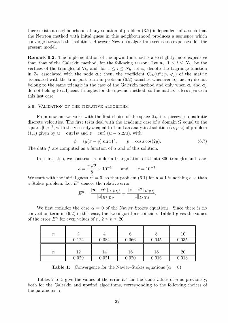
Tables 2 to 5 give the values of the error En for the same values of n as previously,both for the Galerkin and upwind algorithms, corresponding to the following choices ofthe parameter α:

32

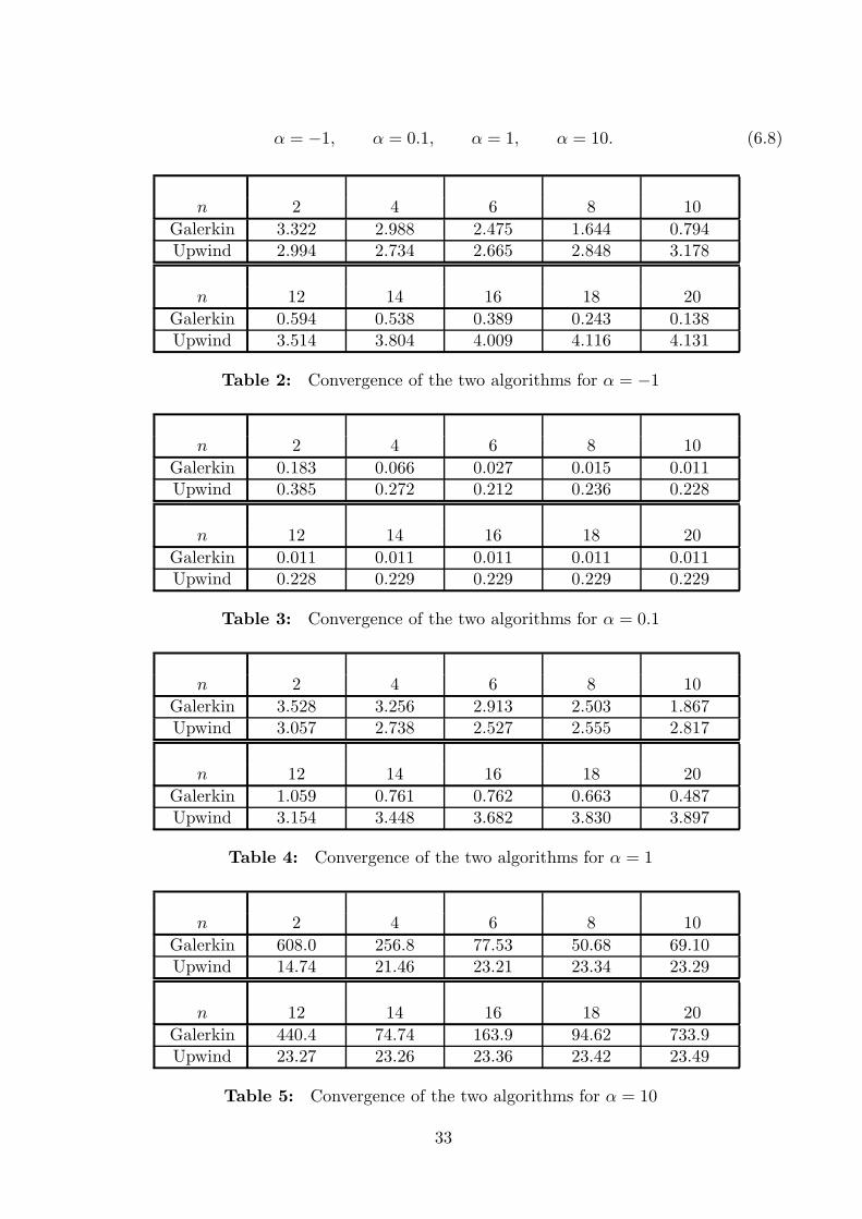
α = −1, α = 0.1, α = 1, α = 10. (6.8)

n 2 4 6 8 10

Galerkin 3.322 2.988 2.475 1.644 0.794Upwind 2.994 2.734 2.665 2.848 3.178

n 12 14 16 18 20

Galerkin 0.594 0.538 0.389 0.243 0.138Upwind 3.514 3.804 4.009 4.116 4.131

Table 2: Convergence of the two algorithms for α = −1

n 2 4 6 8 10

Galerkin 0.183 0.066 0.027 0.015 0.011Upwind 0.385 0.272 0.212 0.236 0.228

n 12 14 16 18 20

Galerkin 0.011 0.011 0.011 0.011 0.011Upwind 0.228 0.229 0.229 0.229 0.229

Table 3: Convergence of the two algorithms for α = 0.1

n 2 4 6 8 10

Galerkin 3.528 3.256 2.913 2.503 1.867Upwind 3.057 2.738 2.527 2.555 2.817

n 12 14 16 18 20

Galerkin 1.059 0.761 0.762 0.663 0.487Upwind 3.154 3.448 3.682 3.830 3.897

Table 4: Convergence of the two algorithms for α = 1

n 2 4 6 8 10

Galerkin 608.0 256.8 77.53 50.68 69.10Upwind 14.74 21.46 23.21 23.34 23.29

n 12 14 16 18 20

Galerkin 440.4 74.74 163.9 94.62 733.9Upwind 23.27 23.26 23.36 23.42 23.49

Table 5: Convergence of the two algorithms for α = 10

33

These tables call for two comments:(i) The convergence rate decreases when |α| increases and at least the Galerkin algorithmdoes not converge for α = 10. This seems in good agreement with Lemma 6.1, see condition(6.4). Fortunately the physical values of α are usually small enough to avoid the lack ofconvergence.(ii) The convergence of the upwind algorithm seems a little faster than for the Galerkinalgorithm. However the final error E20 is higher for the upwind algorithm, which may bedue to the lack of consistency of the scheme.

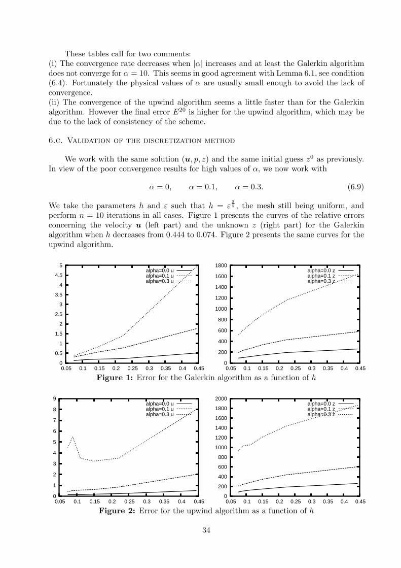
6.c. Validation of the discretization method

We work with the same solution (u, p, z) and the same initial guess z0 as previously.In view of the poor convergence results for high values of α, we now work with

α = 0, α = 0.1, α = 0.3. (6.9)

We take the parameters h and ε such that h = ε32 , the mesh still being uniform, and

perform n = 10 iterations in all cases. Figure 1 presents the curves of the relative errorsconcerning the velocity u (left part) and the unknown z (right part) for the Galerkinalgorithm when h decreases from 0.444 to 0.074. Figure 2 presents the same curves for theupwind algorithm.

0

0.5

1

1.5

2

2.5

3

3.5

4

4.5

5

0.05 0.1 0.15 0.2 0.25 0.3 0.35 0.4 0.45

alpha=0.0 ualpha=0.1 ualpha=0.3 u

0

200

400

600

800

1000

1200

1400

1600

1800

0.05 0.1 0.15 0.2 0.25 0.3 0.35 0.4 0.45

alpha=0.0 zalpha=0.1 zalpha=0.3 z

Figure 1: Error for the Galerkin algorithm as a function of h

0

1

2

3

4

5

6

7

8

9

0.05 0.1 0.15 0.2 0.25 0.3 0.35 0.4 0.45

alpha=0.0 ualpha=0.1 ualpha=0.3 u

0

200

400

600

800

1000

1200

1400

1600

1800

2000

0.05 0.1 0.15 0.2 0.25 0.3 0.35 0.4 0.45

alpha=0.0 zalpha=0.1 zalpha=0.3 z

Figure 2: Error for the upwind algorithm as a function of h

34

The convergence of both methods for the choice h = ε32 seems now clear, which is in

good coherency with the a priori analysis. It can be noted that the error increases with αand also that the error on z is very large but does not seem to pollute too much the erroron the velocity. It can also be noted that the error is not smaller for the upwind algorithmthan for the Galerkin method (and even is larger for α = 0.3). Since the implementationof the former is more expensive than for the latter, for reasons explained in Remark 6.2,from now on we work with the Galerkin algorithm.

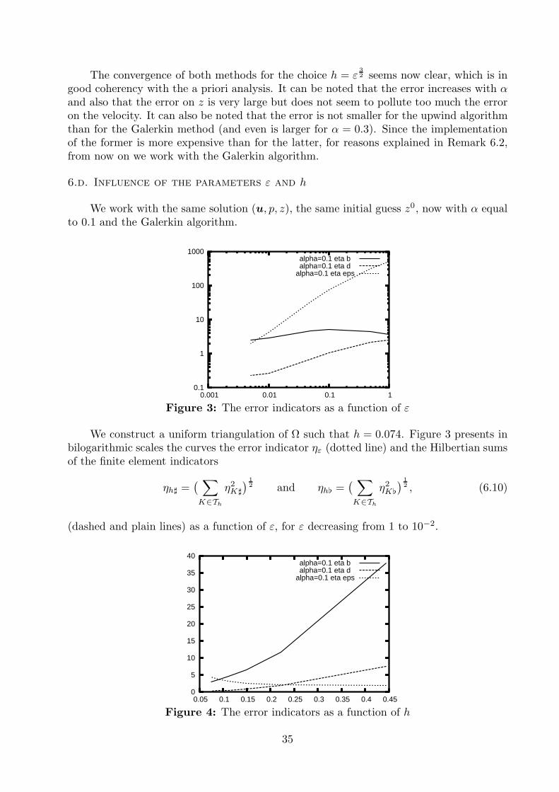
6.d. Influence of the parameters ε and h

We work with the same solution (u, p, z), the same initial guess z0, now with α equalto 0.1 and the Galerkin algorithm.

0.1

1

10

100

1000

0.001 0.01 0.1 1

alpha=0.1 eta b alpha=0.1 eta d

alpha=0.1 eta eps

Figure 3: The error indicators as a function of ε

We construct a uniform triangulation of Ω such that h = 0.074. Figure 3 presents inbilogarithmic scales the curves the error indicator ηε (dotted line) and the Hilbertian sumsof the finite element indicators

ηh♯ =(

∑

K∈Th

η2K♯

)12 and ηh =

(

∑

K∈Th

η2K

)12 , (6.10)

(dashed and plain lines) as a function of ε, for ε decreasing from 1 to 10−2.

0

5

10

15

20

25

30

35

40

0.05 0.1 0.15 0.2 0.25 0.3 0.35 0.4 0.45

alpha=0.1 eta b alpha=0.1 eta d

alpha=0.1 eta eps

Figure 4: The error indicators as a function of h

35

Similarly, we fix ε equal to 10−2. Figure 4 presents the curves of ηε (dotted line), ηh♯

(dashed line) and ηh (plain line) as a function of h, for h decreasing from 0.444 to 0.074.

It can be noted in Figure 4 that the indicator ηε is nearly independent of h, so at leastfor this indicator the two types of error are uncoupled. Further computations indicate thatthese curves are similar for other values of α.

6.e. Some real life experiments

In the following simulations, we try to optimize the value of ε when working withadaptive meshes, according to the following strategy (see [4, §5] for its first implementationfor a different problem).

We first choose a tolerance η∗, we make a first computation on a quasi-uniform meshand compute the ηε.• Step 1: If ηε is smaller than η∗, we go to Step 2. Otherwise, we divide ε by the ratioηε/η

∗ and make a new computation.• Step 2: We compute the ηK♯, the ηK and their sum ηK , next the mean value ηh ofthese ηK . For all K such that ηK is larger than ηh, we divide K into smaller triangles ortetrahedra such that the diameter of these new elements behaves like hK multiplied by theratio ηh/ηK (details on the procedure for realizing this can be found in [17, §7.5.1]).

Step 2 is iterated 4 or 5 times.• Step 3: We compute ηε and the Hilbertian sum ηh of the ηK . If ηε is smaller than ηh,we go back to Step 2. Otherwise, we divide ε by a constant times the ratio ηε/ηh and goback to Step 2.

The union of Steps 2 and 3 can also be iterated, at most 3 times in order not touselessly increase the computational cost.

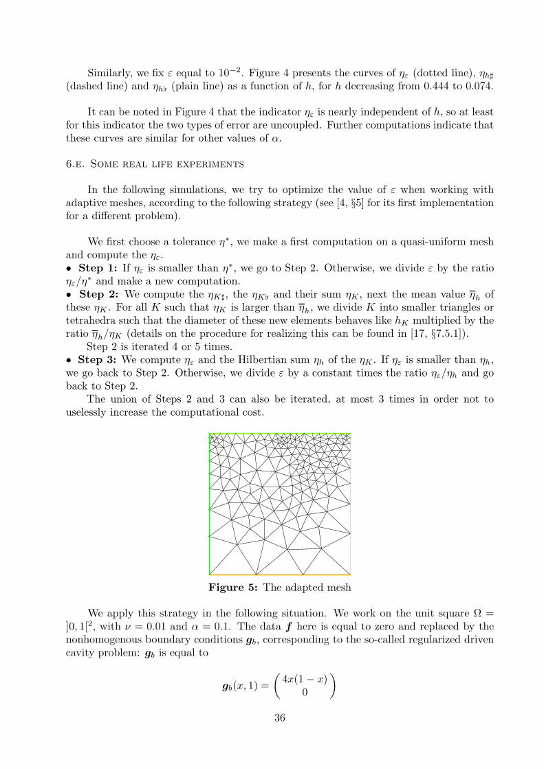
Figure 5: The adapted mesh

We apply this strategy in the following situation. We work on the unit square Ω =]0, 1[2, with ν = 0.01 and α = 0.1. The data f here is equal to zero and replaced by thenonhomogenous boundary conditions gb, corresponding to the so-called regularized drivencavity problem: gb is equal to

gb(x, 1) =

(

4x(1 − x)0

)

36

on the top edge ]0, 1[×1 and zero elsewhere. We start with a uniform mesh made of 188triangles (h = 0.141) and ε equal to 0.01. We take η∗ equal to 0.01 and z0 equal to zero.

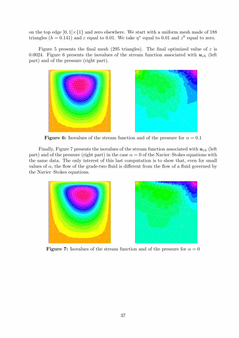
Figure 5 presents the final mesh (295 triangles). The final optimized value of ε is0.0024. Figure 6 presents the isovalues of the stream function associated with uεh (leftpart) and of the pressure (right part).

Figure 6: Isovalues of the stream function and of the pressure for α = 0.1

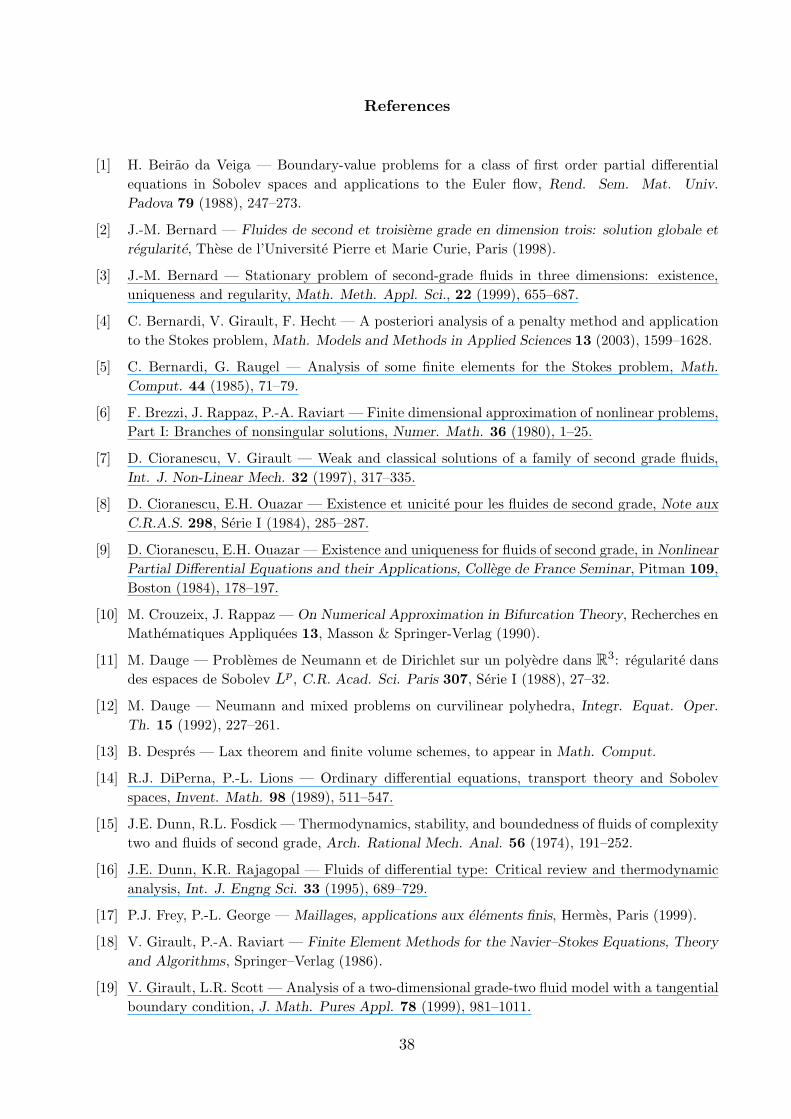
Finally, Figure 7 presents the isovalues of the stream function associated with uεh (leftpart) and of the pressure (right part) in the case α = 0 of the Navier–Stokes equations withthe same data. The only interest of this last computation is to show that, even for smallvalues of α, the flow of the grade-two fluid is different from the flow of a fluid governed bythe Navier–Stokes equations.

Figure 7: Isovalues of the stream function and of the pressure for α = 0

37

References

[1] H. Beirao da Veiga — Boundary-value problems for a class of first order partial differential

equations in Sobolev spaces and applications to the Euler flow, Rend. Sem. Mat. Univ.

Padova 79 (1988), 247–273.

[2] J.-M. Bernard — Fluides de second et troisieme grade en dimension trois: solution globale et

regularite, These de l’Universite Pierre et Marie Curie, Paris (1998).

[3] J.-M. Bernard — Stationary problem of second-grade fluids in three dimensions: existence,

uniqueness and regularity, Math. Meth. Appl. Sci., 22 (1999), 655–687.

[4] C. Bernardi, V. Girault, F. Hecht — A posteriori analysis of a penalty method and application

to the Stokes problem, Math. Models and Methods in Applied Sciences 13 (2003), 1599–1628.

[5] C. Bernardi, G. Raugel — Analysis of some finite elements for the Stokes problem, Math.

Comput. 44 (1985), 71–79.

[6] F. Brezzi, J. Rappaz, P.-A. Raviart — Finite dimensional approximation of nonlinear problems,

Part I: Branches of nonsingular solutions, Numer. Math. 36 (1980), 1–25.

[7] D. Cioranescu, V. Girault — Weak and classical solutions of a family of second grade fluids,

Int. J. Non-Linear Mech. 32 (1997), 317–335.

[8] D. Cioranescu, E.H. Ouazar — Existence et unicite pour les fluides de second grade, Note aux

C.R.A.S. 298, Serie I (1984), 285–287.

[9] D. Cioranescu, E.H. Ouazar — Existence and uniqueness for fluids of second grade, in Nonlinear

Partial Differential Equations and their Applications, College de France Seminar, Pitman 109,

Boston (1984), 178–197.

[10] M. Crouzeix, J. Rappaz — On Numerical Approximation in Bifurcation Theory, Recherches en

Mathematiques Appliquees 13, Masson & Springer-Verlag (1990).

[11] M. Dauge — Problemes de Neumann et de Dirichlet sur un polyedre dans R3: regularite dans

des espaces de Sobolev Lp, C.R. Acad. Sci. Paris 307, Serie I (1988), 27–32.

[12] M. Dauge — Neumann and mixed problems on curvilinear polyhedra, Integr. Equat. Oper.

Th. 15 (1992), 227–261.

[13] B. Despres — Lax theorem and finite volume schemes, to appear in Math. Comput.

[14] R.J. DiPerna, P.-L. Lions — Ordinary differential equations, transport theory and Sobolev

spaces, Invent. Math. 98 (1989), 511–547.

[15] J.E. Dunn, R.L. Fosdick — Thermodynamics, stability, and boundedness of fluids of complexity

two and fluids of second grade, Arch. Rational Mech. Anal. 56 (1974), 191–252.

[16] J.E. Dunn, K.R. Rajagopal — Fluids of differential type: Critical review and thermodynamic

analysis, Int. J. Engng Sci. 33 (1995), 689–729.

[17] P.J. Frey, P.-L. George — Maillages, applications aux elements finis, Hermes, Paris (1999).

[18] V. Girault, P.-A. Raviart — Finite Element Methods for the Navier–Stokes Equations, Theory

and Algorithms, Springer–Verlag (1986).

[19] V. Girault, L.R. Scott — Analysis of a two-dimensional grade-two fluid model with a tangential

boundary condition, J. Math. Pures Appl. 78 (1999), 981–1011.

38

[20] V. Girault, L.R. Scott — Finite-element discretizations of a two-dimensional grade-two fluid

model, Model. Math. et Anal. Numer. 35 (2001), 1007–1053.

[21] V. Girault, L.R. Scott — Upwind discretizations of a steady grade-two fluid model in two di-

mensions, in Nonlinear Partial Differential Equations and their Applications, College de France

Seminar XIV, North-Holland, Amsterdam (2002), 393–414.

[22] P. Grisvard — Elliptic Problems in Nonsmooth Domains, Pitman (1985).

[23] F. Hecht, O. Pironneau — FreeFem++, see www.freefem.org.

[24] P. Houston, R. Rannacher, E. Suli — A posteriori error analysis for stabilised finite element

approximations of transport problems, Comput. Methods. Appl. Mech. Engrg. 190 (2000),

1483–1508.

[25] P. Lesaint, P.-A. Raviart — On a finite element method for solving the neutron transport

equation, in Mathematical Aspects of Finite Elements in Partial Differential Equations, C. de

Boor ed., Academic Press (1974).

[26] J.-L. Lions — Sur les problemes aux limites du type derivee oblique, Annals of Maths. 64

(1956).

[27] J.-L. Lions, E. Magenes — Problemes aux limites non homogenes et applications, Vol. 1, Dunod

(1968).

[28] C.-S. Man — Nonsteady channel flow of ice as a modified second-order fluid with power-law

viscosity, Arch. Rational Mech. Anal. 119 (1992), 35–57.

[29] R.R. Ortega — Contribucion al estudio teorico de algunas E.D.P. no lineales relacionadas con

fluidos no Newtonianos, Thesis, Universidad de Sevilla (1995).

[30] E.H. Ouazar — Sur les fluides de second grade, These de l’Universite Pierre et Marie Curie,

Paris (1981).

[31] K.H. Park — Least-Squares Methods for the Simulation of the Flow of an Incompressible Fluid

of Second Grade, Ph.D. Thesis, The University of Houston (1998).

[32] J. Pousin, J. Rappaz — Consistency, stability, a priori and a posteriori errors for Petrov–

Galerkin methods applied to nonlinear problems, Numer. Math. 69 (1994), 213–231.

[33] P.-A. Raviart, J.-M. Thomas — A mixed finite element method for second order elliptic prob-

lems, in Mathematical Aspects of Finite Element Methods, Lecture Notes in Mathematics 606,

Springer, Berlin (1977), 292–315.

[34] R.S. Rivlin, J.L. Ericksen — Stress-deformation relations for isotropic materials, Arch. Rational

Mech. Anal. 4 (1955), 323–425.

[35] G. Talenti — Best constant in Sobolev inequality, Ann. Math. Pura Appl. 110 serie IV (1976),

353–372.

[36] R. Verfurth — A Review of A Posteriori Error Estimation and Adaptive Mesh-Refinement

Techniques, Wiley & Teubner (1996).

[37] R. Verfurth — Robust a posteriori error estimates for stationary convection-diffusion equations,

submitted.

39