High-order adaptive space-discretizations for the

Black–Scholes equation

Gunilla Linde, Jonas Persson and Lina von Sydow

April 19, 2006

Abstract

In this paper we develop a high-order adaptive finite differencespace-discretization for the Black–Scholes (B–S) equation. The finalcondition is discontinuous in the first derivative yielding that the effec-tive rate of convergence is two, both for low-order and high-order stan-dard finite difference (FD) schemes. To obtain a sixth-order schemewe use an extra grid in a limited space- and time-domain. The newsixth-order method is called FD6G2. The FD6G2-method is combinedwith space- and time-adaptivity to further enhance the method. Toobtain solutions of high accuracy in several dimensions the adaptiveFD6G2-method is superior to both standard and adaptive second-orderFD-methods.

1 Introduction

In option pricing problems, centered second-order finite differences (FDs)are commonly used for solving the Black–Scholes (B–S) equation. B–S isa parabolic final-value partial differential equation (PDE) that gives thearbitrage free price of an option. The main problem when solving the multi-dimensional B–S numerically is the “curse of dimensionality”, i.e. the num-ber of unknowns in the discretized problem grows exponentially in the num-ber of dimensions. In recent years different approaches to improve the ac-curacy of the standard second-order FD-schemes have been presented. Thisoffers the possibility to reduce the number of unknowns and hence increasethe effectiveness of the method.

By using a coordinate transformation, stretching the region around the strikeprice where there is a discontinuity in the first derivative of the final condi-tion, Clarke and Parrott found that the accuracy of their implicit FD-schemewas improved [2]. However, it is not obvious how this coordinate transfor-mation generalizes for the multi-dimensional problem.

1

Another way of obtaining more grid-points around the discontinuity is touse a nonuniform mesh and adaptivity as Persson and von Sydow [10]. Zhaoand Wei used discrete singular convolution together with an adaptive meshand obtained results more accurate than FD-results from the same adaptivemesh [17].

Arciniega and Allen [1] used Richardson extrapolation and by that increasedthe accuracy of the results obtained by the Crank-Nicolson scheme. Noconvergence rate of the scheme was presented, and the numerical resultspresented indicate that the method is only second-order accurate. During,Fournie and Jungel [3] used Rigal’s schemes R2 and R3 [12] together witha new scheme called R3C on a nonlinear B–S equation. Those schemes aresecond-order accurate in time and fourth-order accurate in space. Duringet. al. obtained third-order convergence in space for the nonlinear problem,since they used the R2 or R3 schemes in combination with spline interpola-tion of higher-order to smooth the initial data.

McCartin and Labadie [9] used the Crandall-Douglas scheme. They showedthat the results obtained with the Crandall-Douglas scheme are more accu-rate than results from Crank-Nicolson, but did not investigate the rate ofconvergence of the scheme for this particular problem. The authors onlystate that the Crandall–Douglas scheme “is (at least) fourth-order accurateand unconditionally stable” and that experiments with mesh refinementconfirm the accuracy of their numerical results.

FD methods for sharp gradients and shock resolution have been studiedin physics, for instance for problems in fluid dynamics [4],[14]. The mostcommon procedure is to refine the mesh around discontinuities or sharpgradients. Gerritsen and Olsson [4] showed that for problems with a sharpgradient, all the considered FD methods, both lower-order classical andhigher-order compact schemes, exhibited qualitatively the same rates of con-vergence when used on a uniform mesh.

In this paper, pricing of European call options is considered and the B–Sequation is solved by a new sixth-order FD method called FD6G2. Standardsixth-order FD-discretizations yield only second-order accurate results dueto the discontinuity in the final solution. Hence, FD6G2 uses an extra (fine)grid around the discontinuity in a limited space- and time-domain. TheFD6G2-method is also used in combination with space- and time-adaptivity.The paper is an extension of a Master Thesis project presented in [7].

The paper is organized as follows. In Section 2 the B–S equation is described.In Section 3, the problem is discretized with different FD schemes. Section 3also contains a description of the FD6G2-method. Space and time adaptivityis presented in Section 4. Convergence results are presented in Section 5 andresults using our adaptive methods are studied in in Section 6. Finally, in

2

Section 7, we make some concluding remarks.

2 The Black-Scholes equation

When the option depends on several underlying assets, the B–S equationreads �F�t +

dXi=1

rsi�F�si +1

2

dXi;j=1

[���]ij sisj �2F�si�sj � rF = 0; (1)F (s; T ) = Φ(s);where d is the number of underlying assets. In Equation (1), F is the valueof the option and K is the strike price. The expiry date is denoted by T ,si is the value of underlying stock i, and s = (s1; : : : ; sd). Finally, r 2 R+

is the short rate of interest and � is the volatility-matrix. An example ofa contract function for the multi-dimensional European call option is themean-value European basket option

Φ(s) =�1d dXi=1

si �K�+:We transform (1) from a final-value-problem into a non-dimensional initial-value problem and solve the transformed problem. The transformation ofthe time-scale has the advantage that standard texts on time integration isapplicable. The following coordinate transformations are used:s = Kx; r = r�2 ; KP (x; t) = F (s; t);� = �� ; t = 1

2 �2(T � t); KΨ(x) = Φ(s); (2)

where � is a constant chosen as maxij[���]ij , and x = (x1; : : : ; xd). Thesecoordinate transformations result in�P�t = LP: (3)

where L is defined byL = 2r dXi=1

xi ��xi +dXi;j=1

[���]ijxixj �2�xi�xj � 2r: (4)

In the next section the operator L is discretized.

3

3 Discretization

3.1 Wide sixth-order scheme for a uniform grid

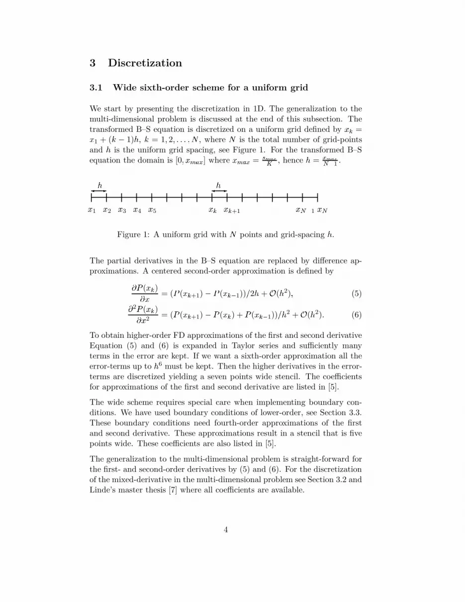
We start by presenting the discretization in 1D. The generalization to themulti-dimensional problem is discussed at the end of this subsection. Thetransformed B–S equation is discretized on a uniform grid defined by xk =x1 + (k � 1)h, k = 1; 2; : : : ; N , where N is the total number of grid-pointsand h is the uniform grid spacing, see Figure 1. For the transformed B–Sequation the domain is [0; xmax] where xmax = smaxK , hence h = xmaxN�1 .

x1 x2 x3 x4 x5 xk xk+1 xN�1 xN-�h-�hFigure 1: A uniform grid with N points and grid-spacing h.

The partial derivatives in the B–S equation are replaced by difference ap-proximations. A centered second-order approximation is defined by�P (xk)�x = (P (xk+1) � P (xk�1))=2h + O(h2); (5)�2P (xk)�x2

= (P (xk+1) � P (xk) + P (xk�1))=h2 + O(h2): (6)

To obtain higher-order FD approximations of the first and second derivativeEquation (5) and (6) is expanded in Taylor series and sufficiently manyterms in the error are kept. If we want a sixth-order approximation all theerror-terms up to h6 must be kept. Then the higher derivatives in the error-terms are discretized yielding a seven points wide stencil. The coefficientsfor approximations of the first and second derivative are listed in [5].

The wide scheme requires special care when implementing boundary con-ditions. We have used boundary conditions of lower-order, see Section 3.3.These boundary conditions need fourth-order approximations of the firstand second derivative. These approximations result in a stencil that is fivepoints wide. These coefficients are also listed in [5].

The generalization to the multi-dimensional problem is straight-forward forthe first- and second-order derivatives by (5) and (6). For the discretizationof the mixed-derivative in the multi-dimensional problem see Section 3.2 andLinde’s master thesis [7] where all coefficients are available.

4

3.2 Wide sixth-order scheme for a nonuniform grid

When using adaptivity in space it is necessary to create finite differenceapproximations on a nonuniform grid. In this case the coefficients will de-pend on the space coordinate in contrast to the coefficients for the uniformgrid. For the first and second derivative a seven points wide stencil will beneeded and by using Taylor expansions around the center point, like in theequidistant case, we can find a linear systems of equations that determinethe coefficients. Of course, also here we need difference approximations oflower order at the boundaries. The coefficients for these approximations arederived in the same way. How to do this in practise is described in detail in[7].

For the multi-dimensional problem, the discretization of the mixed-derivativesresults in a seven points wide stencil. Hence, the discretization of the mixed-derivative results in a stencil that involves 7 � 7 = 49 grid-points. Thecoefficients can be found in [7], where also coefficients for the fourth- andsecond-order approximations of the mixed-derivative are presented.

3.3 Boundary conditions

We present the boundary conditions used in 1D. The generalization to themulti-dimensional problem is straight-forward. For the standard second-order scheme (FD2) there are several possible boundary conditions for theB–S equation. Two boundary conditions often used are�2P (0;t)�x2 = 0; �2P (xmax;t)�x2 = 0;P (0; t) = 0; P (xmax; t) = xmax � e�2rt:These and other boundary conditions are discussed in [16].

For the sixth-order scheme (FD6) additional numerical boundary conditionsare needed since the wide stencils cannot be applied to grid-points near theboundary. Since we aim for problems in higher dimensions it is importantwith boundary conditions that easily can be applied also to these problems.

The boundary condition we have used is that the second derivative of thesolution across a boundary is zero and the rest of the operator is discretizedas in all inner grid-points. For the uniform grid the boundary condition indimension i across the boundary isP (xk�1) � 2P (xk) + P (xk+1)h2

= 0; k = 2; N � 1; (7)

where a second-order approximation of the second derivative is used.

5

The boundary condition in Equation (7) is combined with a second-orderapproximation of B–S equation in x2 and xN�1. At grid-points x3 andxN�2 the second-order FD2-scheme applied to B–S equation is used. Atgrid-points x4 and xN�3 a fourth-order approximation of B–S equation isapplied.x1 x2 x3 x4 x5 x6

� inner pointsu e 3-points stencil + Equation (7)e u e 3-points stencile e u e e 5-points stencil

Figure 2: The different stencils used at the left boundary.

These boundary conditions could probably be improved for better accuracy,but in one space-dimension they work well enough if Smax is chosen largeenough. Here we have used Smax = 8K.

The maximum error in the solution in one space dimension is usually lo-cated around K and the boundary points where the lower-order boundaryconditions are applied are sufficiently far away from K and do not causeany problems. This is not the case in higher dimensions. For the two-dimensional problem we see larger errors where the discontinuity of the firstderivative meets the boundary.

A thorough study of the boundary conditions for the B–S equation dis-cretized with higher-order FDs is needed but is beyond the scope of thispaper.

3.4 Two grids initially - the FD6G2-method

The initial condition for the transformed B–S equation for European calloption is discontinuous in the first derivative at the strike price. Hence,the effective convergence rate of the higher-order schemes are reduced, seeresults in Section 5.1. There is a sharp gradient at the strike price duringthe first time-steps. The effects on the effective rate of convergence werestudied by starting the calculations at time t = �2

2 0:1 with the exact solutioninstead of at t = 0 with the initial data. These calculations showed thatthe anticipated order of accuracy for the higher order scheme was achievedand we could conclude that the order of accuracy of a higher order standardscheme is lost due to the sharp gradient in the initial data.

To overcome the reduced rate of convergence a special procedure with an

6

extra fine mesh around the strike price is used during the first time-steps.This method, where two grids are used in parallel initially, will from hereon be called FD6G2. This refers to a 6th order FD-scheme with 2 grids atthe start. Sixth-order FD approximations were implemented also for G2 -a finer grid around the strike price - and the numerical results presented inSection 5.1 and 5.2 show that the FD6G2-method obtains results that areover-all sixth-order accurate.

The coarse grid over the whole domain has spacing h and the small gridG2 around the strike price has grid-spacing ~ < h. This is illustrated for a1D-problem in Figure 3.

-� -�h ~Grid-points in G1HHHY ���*

Grid-points in G2BBN��Figure 3: The coarse grid G1 and the second grid G2. In this case G2 hasrefinement 4.

We know from experiments that the error close to the strike price in thebeginning is O(~2). To construct a method with over all spatial error O(h6)the error close to the strike price must be reduced to O(h6) even though theeffective rate of convergence there is only O(~2). This can be achieved byusing a smaller step there so that approximatively~2 = C2h6; (8)

where C depends on higher derivatives of the solution. Equation (8) can berewritten as h~ =

1Ch2: (9)

The refinement R of the grid is defined asR = dh=~e: (10)

For a nonuniform grid with space-steps hk, the refinement is defined asR = d1=(C(min hk)2)e: (11)

If R = 4, three equidistant grid-points are inserted between the grid-pointsin the coarse grid, see Figure 3.

7

The stencil of the sixth-order wide scheme is seven points wide and if thestencil is applied to a grid-point four points away from the strike price, pointsg�4 and g4 in Figure 4, the stencil will not cross the discontinuity and theobtained error in the solution in this grid-point should be small. In thegrid-points closer to the strike price the stencil will cross the discontinuityand a solution with a larger error is expected. Intuitively the second gridshould stretch over six coarse grid-points, see Figure 4.

��������������Kg�6 g�5 g�4 g�3 g�2 g�1 g1 g2 g3 g4 g5

Grid-points in G1�� CCWInitial condition��RGrid-point - 4 pointsaway from KCCCCW -�

Width of G2b1 b2 b3 b4 b5 b6

Figure 4: Intuitive width of G2. Here R = 2.

Every time-step with two grids consists of three phases. In the first phasethe problem is solved on the coarse grid, G1, with the wide sixth-orderscheme. In the second phase the problem is solved on G2 with the samesixth-order scheme. Since the stencil for the sixth-order scheme is sevenpoints wide, values of three additional points, on each side of the grid arerequired. In Figure 4 these boundary points are called bk; k = 1; : : : ; 6. Thesolution computed on the coarse grid is used to determine the values of theboundary points bk. Interpolation from the coarse grid G1 is used if thereis not a direct correspondence between points on the coarse grid and thepoints bk.

In the third phase the values of the grid-points in G1 covered by G2, pointsgk, k = �3;�2;�1; 1; 2; 3 in Figure 4, are updated using values computedin the second phase. The refinement R is chosen as an integer. Hence, thegrid-points in the coarse grid will correspond to a grid-point in G2 in theregion with two grids and the update process is straight forward.

The FD6G2-method can be summarized by this algorithm where T hangedefines when to change from using two grids to one.

Algorithm 1� For every time-step where t < T hange.8

1. Compute the solution on grid G1 for t.2. Compute the solution on grid G2 for t.3. Update the value of the grid-points in G1 that have a correspond-

ing point in G2.� For t � T hange.1. Compute the solution on grid G1 for t.

If the number of grid-points in G1 to the left of K are too few the leftboundary condition used at s = 0 will be used also to the left of the finegrid G2.

Studying equations (9)-(11) we note that with a large value of C and a smallN the refinement R can be one. It is obvious that in that case nothingis gained and the procedure with the second grid is worthless. Thereforea lower bound on R, called Rmin, is needed to achieve a sixth-order spaceapproximation. The use of an extra grid increases the memory requirementsand the computational work to some extent, but higher accuracy is gained.To reduce the overhead introduced by the extra grid we want a high valueon C, a narrow grid G2 and a low value of Rmin and T hange, so that theextra work introduced is minimized. The FD6G2-method is discussed withrespect to these parameters in the Master thesis by Linde, see [7].

For more than one space-dimension the fine grid G2 would ideally be usedonly around the discontinuity of the initial data. However, since that wouldcomplicate the implementation we have used a rectangle that enclose thediscontinuity. Our regular boundary conditions are used when the boundaryof the fine and coarse grid coincide and interpolation from the coarse gridis used on the other boundaries.

3.5 Temporal discretization

The time-derivative in Equation (3) is approximated with the second-orderaccurate backward differentiation formula, BDF2 [6]. It is an implicit andunconditionally stable scheme. The BDF2 algorithm for non-constant step-lengths reads�n0P n = ∆tnAP n � �n1P n�1 � �n2P n�2; (12)�n0 =

1 + 2�n1 + �n ; �n1 = �(1 + �n); �n2 =

(�n)2

1 + �n ;�n =∆tn

∆tn�1

9

where A denotes the discretization of the spatial operator L, see Equation(4). Note also that ∆tn = tn� tn�1 and tn is the value of the scaled time attime-step n. Since BDF2 is a multi-step scheme another method must beused for the first time-step. We have used the first-order accurate implicitbackward Euler method for this first step. This will not degrade the overall accuracy of the BDF2 method.

The method requires small time-steps for a short period of time in the be-ginning of the time-stepping process in order to achieve sixth-order accuracyin space (see Section 6). In Section 4.2 we show how we can use an adap-tive BDF2 method that automatically adjusts the time-steps to keep thediscretization error at a pre-described level. This technique was also suc-cessfully used in [8] and [10].

4 Adaptivity in space and time

4.1 Adaptivity in space

An adaptive technique is used to reduce the number of grid-points and stillkeep the discretization error at a prescribed level. We use the same idea ofspace adaptivity as presented in [10] and we refer all readers to that sorcefor details on the method. Here we only present the basic idea about theadaptivity. The adaptive spatial process works like this:

Algorithm 2

1. Solve the problem once with a coarse grid with Ne grid-points, givingan estimate of the local discretization error.

2. Create a new grid in space such that the required accuracy criteria ismet. The number of grid-points in the new grid will be denoted Na.

3. Solve the problem again on the new grid.

Note that the problem has to be solved twice. The idea is that the firsttime the problem is solved it should be done quickly on a coarse grid. Thesolution will be of low accuracy but will give an estimate of where to placethe grid-points in the second grid.

Assume that for any smooth solution u(x) it holds thatAhuh = Au + �hwhere uh is a vector of unknowns and Ah is the the discrete approximationof the operator L. Au is the exact operator Lu evaluated in the grid-points and thus �h is the discretization error for the FD-approximation with

10

step-length h. We estimate the discretization error using two grids with atechnique similar to Richardson extrapolation which gives us an estimate of�h. Assuming that �h can be approximated by its leading order term andrequiring that �h should be less than some constant �h > 0 we find that weshould choose our new discretization ash(x) = h � � �hj�h(x)j� 1p : (13)

Here h is the step-length used to measure �h(x) and p is the order of the dis-cretization. This technique to estimate the discretization error is presentedin [15] in the context of option pricing and the adaptive technique was usedand described in detail in [10] and [11].

In many dimensions we make the assumption that [���]ij � [���]ii to sim-plify the theory . The same assumption was used in e.g. [10] and allows usto study the discretization one dimension at the time and create an adaptivegrid for each dimension separately.

4.2 Adaptive time-integration

The adaptive time-stepping scheme used here consists of two parts, an ex-plicit predictor and the implicit corrector BDF2 with non-equidistant time-steps. For the algorithm BDF2 see Equation (12) in Section 3.5. We usethe adaptive algorithm used by e.g. Persson and von Sydow in [10] in thecontext of option pricing and by Soderberg et. al. in [8] where a slightlydifferent approach was used for fluid problems. The difference to [10] is thathere we use a logarithmic distribution of the time-steps for the first solvewhen the local discretization error is estimated while an equidistant distri-bution is used in [10]. The reason for using a logarithmic distribution isthat it is necessary to have many small time-steps in the beginning, duringthe phase where we use two grids, to get a good approximation of the localdiscretization error. This is necessary for the second solve to be sixth orderaccurate.

The idea is to estimate �t, the local truncation error in the approximationof the time derivative in BDF2 by comparing a solution computed with anexplicit and an implicit method. By using knowledge about the local trun-cation error in the two methods a good estimate of the local truncation errorof BDF2 can be found. The information about the truncation error can thenbe used in different ways. In [8], Soderberg et. al. continously recompute thesolution with smaller and smaller time-steps until they find a step that givesa small enough truncation error. Here we use a slightly different approach.Since we calculate the solution on a coarse grid to estimate the local errorsin space we take the opportunity to simultaneously calculate the truncation

11

error from the time-discretization. Then we compute the time-steps neededto achieve the desired accuracy level �t on the adaptive time-grid using amethod similar to the one used in space. Since the same method was usedbefore by the authors we will not repeat the details here but refer the readerto [10] for details.

5 Convergence results

5.1 Results in one space-dimension

All computations have been performed with the transformed PDE, Equation(3), and were done in Matlab 6.5.0. Results presented with an executiontime were carried out on a Sun Fire 15k server unless something else isstated. One UltraSPARC III+ CPU at 900MHz was used and 4 GB RAMwas accessible. The default parameters used in one space-dimension are:� = 0:3, r = 0:05 and K = 20. For the wide schemes, FD6 and FD6G2,Smax = 8K is used due to the boundary conditions. When results from theFD6G2-method are compared to results from the FD2-scheme, the samevalue of Smax is used. Hence, Smax = 8K is also used for the FD2-schemein this case, except for when results of different methods are compared withrespect to efficiency and the lowest possible value of Smax is used for eachmethod.

BDF2 is used for time-integration and the length of the time-step is constantat ∆t = �2

2 0:0002 for all tests concerning the space adaptivity. Note that∆t and the value given for the parameter T hange are both given in scaledtime t. Usually T = 0:1 year or T = 2 years are used. The exercise date, T ,is in non-transformed time, see Equation (2).

Since BDF2 is an implicit method, a sparse linear system of equations hasto be solved in each time-step. For the FD6G2-method two systems mustbe solved during the first time-steps when two grids are used. In one spacedimension Matlab’s built-in solver ’n’ has been used.

On equidistant grids the errors calculated are the maximum of the absolutevalue of the error, denoted by max jerrorj, and the root mean square, l2error.

max jerrorj = max jFk � F (xk)j; (14)l2 error =

vuuthN�1Xk=2

�Fk � F (xk)�2; (15)

12

Where F (xk) is the analytic solution in point xk and Fk = KPk where Pkis the numerical solution in transformed coordinates. For adaptive gridsonly max jerrorj is computed. To verify the rate of convergence of the FD-schemes we are interested in the error from the approximations of the spacederivatives. For these tests we have therefore used small time-steps to keepthe error from the time-discretization negligible.

The discretization errors in space, for a pth-order method is of the form

error = hp + O(hp+1) (16)

where is independent of h. The logarithm of Equation (16) and the use ofh = xmaxN�1 giveslog(error) = �p log(N � 1) + 0; (17)

where 0 depends on xmax, and higher-order terms.

For the FD6G2-method T hange = �2

2 35 � 0:0002, C = 40, Rmin = 4 and theintuitive width of the grid were used. These values of the parameters aretaken from [7] where appropriate values are determined.

Figure 5 show that the rate of convergence is two, both for the wide sixth-order scheme (FD6) and the standard FD-scheme of second-order (FD2).The rate of convergence for the FD6G2-method is close to six, when T = 2:0years. For a much smaller T we found that the rate of convergence wasreduced to fifth-order. This is probably due to errors from approximatingderivatives over the discontinuity in space not being damped out.

13

101

102

10−5

100

max

|err

or|

101

102

10−5

100

N−1

l 2 err

or

FD2FD6line slope −2.08FD6G2line slope −5.85

FD2FD6line slope −2.10FD6G2line slope −5.74

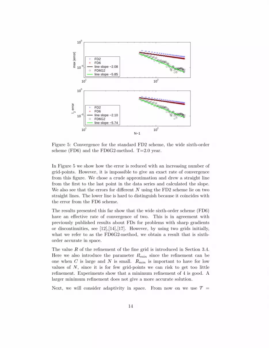
Figure 5: Convergence for the standard FD2 scheme, the wide sixth-orderscheme (FD6) and the FD6G2-method. T=2.0 year.

In Figure 5 we show how the error is reduced with an increasing number ofgrid-points. However, it is impossible to give an exact rate of convergencefrom this figure. We chose a crude approximation and drew a straight linefrom the first to the last point in the data series and calculated the slope.We also see that the errors for different N using the FD2 scheme lie on twostraight lines. The lower line is hard to distinguish because it coincides withthe error from the FD6 scheme.

The results presented this far show that the wide sixth-order scheme (FD6)have an effective rate of convergence of two. This is in agreement withpreviously published results about FDs for problems with sharp gradientsor discontinuities, see [12],[14],[17]. However, by using two grids initially,what we refer to as the FD6G2-method, we obtain a result that is sixth-order accurate in space.

The value R of the refinement of the fine grid is introduced in Section 3.4.Here we also introduce the parameter Rmin since the refinement can beone when C is large and N is small. Rmin is important to have for lowvalues of N , since it is for few grid-points we can risk to get too littlerefinement. Experiments show that a minimum refinement of 4 is good. Alarger minimum refinement does not give a more accurate solution.

Next, we will consider adaptivity in space. From now on we use T =

14

2. The local discretization error � is measured at three different times,[T=3; 2T=3; T ]. In each grid-point we use the largest of the three � :s tocompute the new grid, see Equation (13). In the first phase of the adap-tive process, see Algorithm 2, an equidistant grid is used and throughoutthis section we have used Ne;G1 = 61 (Ne;G2 = 27) for the equidistant grid.We observed that other values did not change the final computational gridmuch.

Figure 6 shows max jerrorj for the adaptive FD6G2-method. Different valuesof � are used to obtain grids with different number of points. For comparisonthe figure also contains the errors for the standard FD6G2, also presentedin Figure 5, and errors for standard and adaptive FD2. Instead of using thesame value of Smax for all schemes, the lowest possible Smax, that still givesthe maximum error around K, was used in the experiment in this section.

The figure shows that the rate of convergence of the adaptive FD6G2-methodis approximately six and that the adaptive FD6G2-method requires feweror much fewer grid-points than the other methods examined to obtain asolution of the same accuracy.

101

102

10−8

10−6

10−4

10−2

100

max

|err

or|

N−1

FD6G2FD6G2 adaptiveline slope −6.83line slop −5.71FD2 adaptiveFD2

Figure 6: Convergence for the adaptive FD6G2-method.

The figure also shows that the second-order adaptive method is competi-tive with the higher-order methods only if low accuracy is acceptable. The

15

efficiency of the methods will be discussed in Section 6 where adaptive time-stepping have been used together with the space-adaptive method.

5.2 Results in two space-dimensions

All numerical experiments in two space-dimensions were performed on thesame computer as the experiments in one dimension. Values for the param-eters are r = 0:05, K = 20, C = 40, Rmin = 4, T hange = �2

2 35 � 0:0002 andSmax = 2 � 8K for the FD6G2-method and Smax = 2 � 6K for FD2. Thevolatility matrix � has the value 0.3 on the diagonal and 0.05 in the othertwo elements in the matrix.

BDF2 with variable step-length, see Equation (12), is used for time inte-gration. In the beginning, when two grids are used the constant time-step∆t = �2

2 0:0002 is used, then the length of the time-step is increased with

20% each time-step until ∆tmax = �2

2 4 � 0:0002. The reason for this is toreduce the number of time-steps. We use these small time-steps so that wecan study the discretization error in space. The increasing time-steps wasconfirmed to not lower the accuracy. Adaptive time-steps have also beenstudied, see Section 6.

Using the implicit BDF2 requires the solution of large sparse linear systemsof equations. In two space-dimensions we used the iterative restarted GMRES,see [13], with an incomplete LU factorization as preconditioner. The LU-factorization was computed only for the first time-step and the iterationswere stopped when the relative residual was less than 10�10. The restartlimit was set to 6.

For the two-dimensional problem we had no analytical solution so a referencesolution was used instead. The reference solution was calculated with theadaptive FD6G2-method with time-steps ∆t = �2

2 0:0001, ∆tmax = �2

2 0:0004and � = 10�8, resulting in Na;G1 = 177, Na;G2 = 359. These parameter val-ues should give us a solution with small enough error to be used as referencesolution.

Our experiments show that the largest errors are found at or close to theboundary. This is to be expected since we use lower order boundary con-ditions there. Since the error is of most interest in the inner of the domain(away from default of the stocks) we define the inner domain as all grid-points where a higher-order approximation is applied. Hence, the inner partis the region [x1;5; x1;N�4] � [x2;5; x2;N�4].

To calculate the error in a solution, the inner part of the reference solutionis interpolated by cubic interpolation obtaining values in the same points asthe numerical solution. All errors stated here are in the original variables

16

of B–S. Therefore jerrorj is the maximum absolute value of the error in theoriginal variable F . The solver for the two-dimensional problem works fordifferent number of grid-points in the first and second space-dimension, butall results presented in this paper are obtained with the same number ofgrid-points in both dimensions since our model problem is symmetric. Inthe first phase of the adaptive process we have used Ne;G1 = 61 (Ne;G2 = 45).

Our experiments show that the expected rate of convergence is obtained.We note that if the whole computational domain in space is studied we onlyhave second order accuracy. That is the anticipated result though since theboundary conditions are only second-order accurate. If we study only theinner points we see that we have sixth-order accuracy. See the convergenceplots in Figure 7 and 8 for details.

102

10−8

10−6

10−4

10−2

100

max

|err

or|

N−1

FD6G2 1DFD2 1DFD6G2 2DFD6G2 inner 2DFD2 2D

Figure 7: Convergence for FD2 and FD6G2 applied to the two-dimensionalproblem.

17

101

102

10−10

10−8

10−6

10−4

10−2

100

max

|err

or|

N−1

FD6G2 adaptive 1Dline slope −5.71FD2 adaptive 1DFD6G2 adaptive 2DFD6G2 adaptive inner 2DFD2 adaptive 2D

Figure 8: Convergence for adaptive FD2 and adaptive FD6G2 applied thetwo-dimensional problem.

6 Adaptivity results

In Section 5 we showed that our method FD6G2 can achieve sixth-orderaccuracy in space. Here we compare the efficiency of the adaptive second-order scheme and the adaptive FD6G2, both using the same second-orderadaptive time-stepping described in Section 4.2. From here on FD6G2 willdenote the adaptive sixth-order method.

In [10] a very coarse equidistant grid in both space and time was used to com-pute the initial solution where all local discretization errors are estimated.Here we must use a slightly different approach. For the space adaptivityto work properly we need to use small time-steps for a number of steps inthe beginning of the time-stepping process. For the adaptive methods to beefficient, the first part where discretization errors are estimated has to beinexpensive and thus small time-steps must be avoided where possible. Wehave used a log-distribution of the time-steps in the initial solve in order toautomatically use small time-steps in the beginning and then progressivelylarger time-steps towards the end. This allows us to use few time-stepsduring the first solve and still have a fine mesh in time in the very begin-ning. This is essential for the space-adaptivity to work properly as describedearlier.

An example of how the algorithm controls the local truncation error �t isdepicted in Figure 9. Here we have used �t = 10�3 as tolerance level.

18

0 0.2 0.4 0.6 0.8 1 1.2 1.4 1.6 1.8 210

−6

10−5

10−4

10−3

10−2

10−1

Time

Loca

l dis

cret

izat

ion

erro

r

Estimates of the local discretization error

τt log−distributed ∆ t

τt adaptive ∆ t

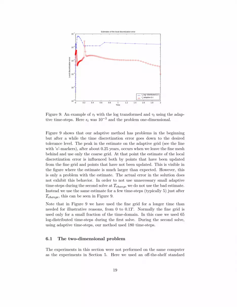
Figure 9: An example of �t with the log transformed and �t using the adap-tive time-steps. Here �t was 10�3 and the problem one-dimensional.

Figure 9 shows that our adaptive method has problems in the beginningbut after a while the time discretization error goes down to the desiredtolerance level. The peak in the estimate on the adaptive grid (see the linewith ’o’-markers), after about 0:25 years, occurs when we leave the fine meshbehind and use only the coarse grid. At that point the estimate of the localdiscretization error is influenced both by points that have been updatedfrom the fine grid and points that have not been updated. This is visible inthe figure where the estimate is much larger than expected. However, thisis only a problem with the estimate. The actual error in the solution doesnot exhibit this behavior. In order to not use unnecessary small adaptivetime-steps during the second solve at T hange we do not use the bad estimate.Instead we use the same estimate for a few time-steps (typically 5) just afterT hange, this can be seen in Figure 9.

Note that in Figure 9 we have used the fine grid for a longer time thanneeded for illustrative reasons, from 0 to 0:1T . Normally the fine grid isused only for a small fraction of the time-domain. In this case we used 65log-distributed time-steps during the first solve. During the second solve,using adaptive time-steps, our method used 180 time-steps.

6.1 The two-dimensional problem

The experiments in this section were not performed on the same computeras the experiments in Section 5. Here we used an off-the-shelf standard

19

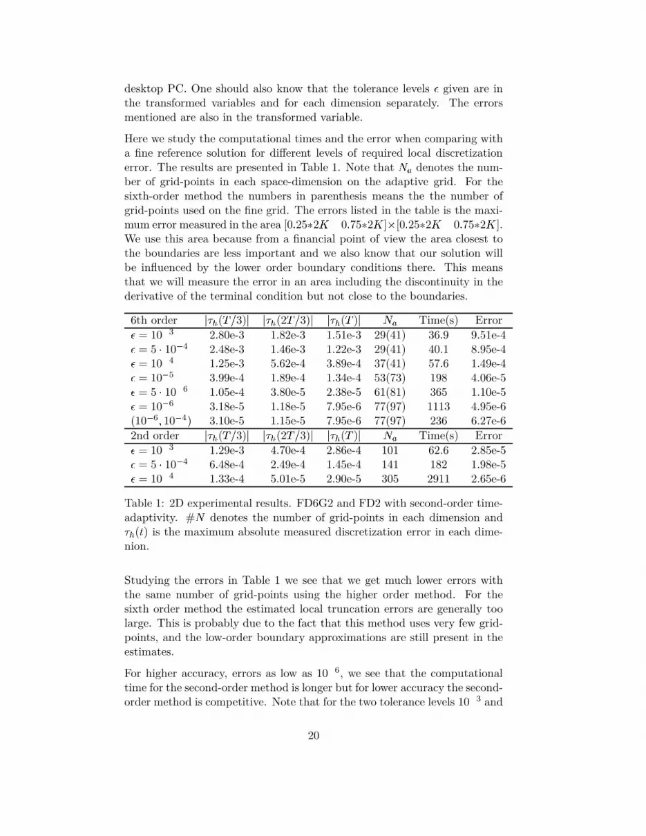
desktop PC. One should also know that the tolerance levels � given are inthe transformed variables and for each dimension separately. The errorsmentioned are also in the transformed variable.

Here we study the computational times and the error when comparing witha fine reference solution for different levels of required local discretizationerror. The results are presented in Table 1. Note that Na denotes the num-ber of grid-points in each space-dimension on the adaptive grid. For thesixth-order method the numbers in parenthesis means the the number ofgrid-points used on the fine grid. The errors listed in the table is the maxi-mum error measured in the area [0:25�2K 0:75�2K]�[0:25�2K 0:75�2K].We use this area because from a financial point of view the area closest tothe boundaries are less important and we also know that our solution willbe influenced by the lower order boundary conditions there. This meansthat we will measure the error in an area including the discontinuity in thederivative of the terminal condition but not close to the boundaries.

6th order j�h(T=3)j j�h(2T=3)j j�h(T )j Na Time(s) Error� = 10�3 2.80e-3 1.82e-3 1.51e-3 29(41) 36.9 9.51e-4� = 5 � 10�4 2.48e-3 1.46e-3 1.22e-3 29(41) 40.1 8.95e-4� = 10�4 1.25e-3 5.62e-4 3.89e-4 37(41) 57.6 1.49e-4� = 10�5 3.99e-4 1.89e-4 1.34e-4 53(73) 198 4.06e-5� = 5 � 10�6 1.05e-4 3.80e-5 2.38e-5 61(81) 365 1.10e-5� = 10�6 3.18e-5 1.18e-5 7.95e-6 77(97) 1113 4.95e-6(10�6; 10�4) 3.10e-5 1.15e-5 7.95e-6 77(97) 236 6.27e-6

2nd order j�h(T=3)j j�h(2T=3)j j�h(T )j Na Time(s) Error� = 10�3 1.29e-3 4.70e-4 2.86e-4 101 62.6 2.85e-5� = 5 � 10�4 6.48e-4 2.49e-4 1.45e-4 141 182 1.98e-5� = 10�4 1.33e-4 5.01e-5 2.90e-5 305 2911 2.65e-6

Table 1: 2D experimental results. FD6G2 and FD2 with second-order time-adaptivity. #N denotes the number of grid-points in each dimension and�h(t) is the maximum absolute measured discretization error in each dime-nion.

Studying the errors in Table 1 we see that we get much lower errors withthe same number of grid-points using the higher order method. For thesixth order method the estimated local truncation errors are generally toolarge. This is probably due to the fact that this method uses very few grid-points, and the low-order boundary approximations are still present in theestimates.

For higher accuracy, errors as low as 10�6, we see that the computationaltime for the second-order method is longer but for lower accuracy the second-order method is competitive. Note that for the two tolerance levels 10�3 and

20

5 � 10�4 there were really too few time-steps used with the fine grid in theFD6G2 method which could give a larger error than expected.

The last row in the table for ’6th order’ shows the results for �h = 10�6

in space and �t = 10�4 in time. We see that this results in very little lossof accuracy, compared to �h = �t = 10�6, even though the computationaltime needed is less than a fourth. This is because the number of adaptivetime-steps is much smaller. A natural next step to improve the method isto use a high-order discretization also in time.

In all experiments performed the higher order method needs less or muchless grid-points than the second-order method. This means that they willin general use less memory. This is even more important when the numberof dimensions in the problem increases.

7 Conclusions

The final condition is discontinuous in the first derivative at the strike priceand therefore only second-order accurate results are obtained, both withthe standard FD2 scheme and higher-order schemes using one grid. Wehave shown that with the new FD6G2-method that uses two grids initially,sixth-order accurate results are obtained. The FD6G2-method can easily becombined with space adaptivity obtaining more accurate results than thestandard FD6G2, using the same number of grid-points.

The two dimensional results presented here show that for high accuracy thehigher order method FD6G2 outperforms the second-order method. This isdue to the much lower number of grid-points needed in each space dimension.It also means that the higher order method needs much less memory thanthe second-order method. However, the linear systems of equations are moredense than for the second order method, but since the number of unknownsis substantially smaller the execution times is shorter.

References

[1] A. Arciniega, E. Allen. Extrapolation of difference methods in optionvaluation, Applied Mathematics and Computation 153, 165-186, 2004.

[2] N. Clarke, K. Parrott. Multigrid for American option pricing withstochastic volatility, Applied Mathematical Finance 6, 177-195, 1999.

21

[3] B. During, M. Fournie, A. Jungel. High order compact finite differenceschemes for a nonlinear Black–Scholes equation, International Journalof Theoretical and Applied Finance Vol. 6, No. 7, 767-789, 2003.

[4] M. Gerritsen, P. Olsson. Designing an Efficient Solution Strategy forFluid Flows 1. A Stable High Order Finite Difference Scheme and SharpShock Resolution for the Euler Equations, Journal of ComputationalPhysics 129,245-262, 1996.

[5] Bengt Fornberg. Generation of Finite Difference Formulas on Arbitrar-ily Spaced Grids, Mathematics of Computation Vol. 51, No. 184, 1988.

[6] E. Hairer, S.P. Norsett, G. Wanner. Solving ordinary differential equa-tions 2nd ed.. Springer-Verlag, Berlin 1993.

[7] G. Linde. High-order Adaptive Space Discretizations for the Black-Scholes Equation. Master thesis. Uppsala University. 2005

[8] P. Lotstedt, S. Soderberg, A. Ramage, L. Hemmingsson-Franden. Im-plicit solution of hyperbolic equations with space-time adaptivity, BIT,42:1:128-153, 2002.

[9] B.J. McCartin, S.M Labadie. Accurate and efficient pricing of vanillastock options via the Crandall–Douglas scheme, Applied Mathematicsand Computation 143, 39-60, 2003.

[10] J. Persson, L. von Sydow. Pricing European Multi-asset Options Usinga Space-time Adaptive FD-method, Department of Information Tech-nology, Uppsala University, Technical report 2003-59, 2003 (Acceptedin Computing and Visualization in Science).

[11] J. Persson, L. von Sydow, P. Lotstedt and J. Tysk. Space-Time Adap-tive Finite Difference Method for European Multi-Asset Option s,Dept.of Information Technology, Uppsala University, 2004.

[12] A. Rigal. High Order Schemes for Unsteady One-DimensionalDiffusion–Convection Problems, Journal of Computational Physics114, 59-76, 1994.

[13] Y. Saad, M.H. Schultz. GMRES: A generalized minimal residual algorithmfor solving nonsymmetric linear systems. SIAM Journal of ScientificComputing, 7:856-869, 1986.

[14] A.S. Sabau, P.E. Raad. Comparisons of compact and classical finitedifference solutions of stiff problems on nonuniform grids, Computer &Fluids 28, 361-384, 1999.

[15] R. Seydel. Tools for Computational Finance., Springer Verlag, Secondedition, 2003

22

[16] D. Tavella, C. Randall. Pricing Financial Instruments- The Finite Dif-

ference Method, John Wiley & Sons, Chichester, 2000.

[17] S. Zhao, G.W. Wei. Option valuation by using a discrete singular con-volution, Applied Mathematics and Computation, article in press.

23