Reducing decision errors in the paired comparison of the diagnostic

accuracy of screening tests with Gaussian outcomes

Brandy M Ringham , Todd A Alonzo , John T Brinton , Sarah M Kreidler , Aarti Munjal ,1* 2 1 1 1

Keith E Muller , and Deborah H Glueck3 1

1Department of Biostatistics and Informatics, Colorado School of Public Health, University of

Colorado, Anschutz Medical Campus, Aurora, Colorado 80045, U.S.A.

2Department of Preventive Medicine, University of Southern California, Los Angeles, California

90089, U.S.A.

3Department of Health Outcomes and Policy, University of Florida, Gainesville, FL 32611,

U.S.A.

*Correspondence: brandy.ringham@ucdenver.edu

Email:

Brandy M Ringham brandy.ringham@ucdenver.edu

Todd A Alonzo talonzo@childrensoncologygroup.org

John T Brinton john.brinton@ucdenver.edu

Sarah M Kreidler sarah.kreidler@ucdenver.edu

Aarti Munjal aarti.munjal@ucdenver.edu

Keith E Muller kmuller@ufl.edu

Deborah H Glueck deborah.glueck@ucdenver.edu

1

Abstract

Background: Scientists often use a paired comparison of the areas under the receiver operating

characteristic curves to decide which continuous cancer screening test has the best diagnostic

accuracy. In the paired design, all participants are screened with both tests. Participants with

unremarkable screening results enter a follow-up period. Participants with suspicious screening

results and those who show evidence of disease during follow-up receive the gold standard test.

The remaining participants are classified as non-cases, even though some may have occult

disease. The standard analysis includes all study participants in the analysis, which can create

bias in the estimates of diagnostic accuracy. If the bias affects the area under the curve for one

screening test more than the other screening test, scientists may make the wrong decision as to

which screening test has better diagnostic accuracy. We propose a weighted maximum

likelihood bias correction method to reduce decision errors.

Methods: Using simulation studies, we assessed the ability of the bias correction method to

reduce decision errors. The simulations compared the Type I error rate and power of the

standard analysis with that of the bias-corrected analysis. We varied four factors in the

simulation: the disease prevalence, the correlation between screening test scores, the rate of

interval cases, and the proportion of cases who receive the gold standard test. We demonstrate

the proposed method with an application to a hypothetical oral cancer screening study.

Results: The amount of bias in the study and the performance of the bias correction method

depend on characteristics of the screening tests and the disease, and on the percentage of study

participants who receive the gold standard test. In studies with a large amount of bias in the

difference in the full area under the curve, the bias correction method reduces the Type I error

rate and improves power for the correct decision.

Conclusion: The bias correction method reduces decision errors for some paired screening

trials. In order to determine if bias correction is needed for a specific screening trial, we

recommend the investigator conduct a simulation study using our software.

2

Keywords: cancer screening, differential verification bias, area under the curve, type I error,

power, paired screening trial, receiver operating characteristic analysis

3

Background

Paired screening trials are common in cancer screening. For instance, one of the designs

considered for a planned oral cancer screening study was a paired comparison of the oral tactile

visual exam with the VELscope imaging device 1 . Two recent breast cancer screening studies used a paired design to compare film and digital mammography 2, 3 . In paired cancer screening trials, investigators screen all participants with both screening tests. Participants with

unremarkable screening test scores on both tests enter a follow-up period. Participants with

suspicious screening test scores or who show signs and symptoms of disease during the follow-

up period, undergo further workup leading to the gold standard test, biopsy. The remaining

participants are assumed to be disease-free. In truth, they may have occult disease.

In the trial by Lewin 2 , the investigators used the standard analysis to compare the fullet al. areas under the receiver operating characteristic curves. The standard analysis includes all

participants, even those whose disease status is not verified with the gold standard test. Because

some cases are misclassified as non-cases, the receiver operating characteristic curves and the

corresponding areas under the curves may be biased, thus causing decision errors 4 . We use bias in the epidemiological sense of the word as the difference between what the study

investigator and the , unobservable state of nature 5 . If the bias is severe enough,observes true investigators can detect a difference between screening tests when there is none, or decide that

the tests are different, but conclude incorrectly that the inferior test is superior. Choosing the

inferior screening test can delay diagnosis of cancer and increase morbidity and mortality.

We propose a bias-corrected hypothesis test to reduce decision errors in paired cancer

screening trials. Under the assumption that the screening test scores follow a bivariate Gaussian

distribution, conditional on disease status, we use an iterative, maximum likelihood approach to

reduce the bias in the estimates of the mean, variance, and correlation. The resulting estimates

are then used to reduce bias in the estimates of the diagnostic accuracy of the screening tests.

Screening trials are subject to different biases depending on the choice of reference standard

and analysis plan 6 9 . Imperfect reference standard bias occurs when the investigator

4

evaluates all study participants with an imperfect reference standard 7, 8, 10 . Partial verification bias occurs if 1) the investigator evaluates only some participants with a gold

standard, 2) the decision to use the gold standard test depends on the screening test outcome, and

3) the investigator only includes participants with gold standard results in the analysis, a

complete case analysis 11 . Differential verification bias occurs when 1) the investigator uses a gold standard test for a portion of participants and an imperfect reference standard for the

remaining participants, 2) the decision to use the gold standard test depends on the results of the

screening test, and 3) the investigator includes data from all participants in the analysis 8 . Paired screening trial bias 4 , the focus of our research, is a special case of differential verification bias. Paired screening trial bias occurs in paired screening trials when three

conditions hold: 1) The investigator analyzes data from all the participants 2) the screening tests

are subject to differential verification bias and 3) each screening test has associated with it a

different threshold score that leads to the gold standard test 4 . In the following sections we describe the bias correction method and evaluate its performance

by simulation. In the Methods section, we explain the study design of interest, outline the

assumptions and notation, delineate the bias correction algorithm, and describe the design of the

simulation studies. In the Results section, we report on the results of the simulation studies and

demonstrate the utility of the method using a hypothetical oral cancer screening study. Finally,

in the Discussion section, we discuss the implications of our method.

Methods

Study Design

The study design of interest is a paired study of two continuous cancer screening tests. The

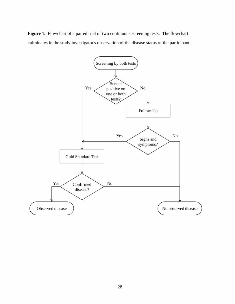
design was considered by Lingen 1 in a planned oral cancer screening trial, and was used in two recent breast cancer screening trials 2, 3 . A flowchart of the study design is shown in Figure 1.

We consider the screening studies from two points of view 12 . We consider the point of

view of the omniscient observer who knows the disease status for each participant.true We also

5

consider the point of view of the study investigator, who can only see the results of theobserved

study.

The study investigator determines disease status in two ways: through follow-up, or through a

definitive method for the ascertainment of disease status. Any score that exceeds the threshold

of suspicion defined for each screening test triggers the use of a gold standard test. Cases

identified due to remarkable screening test scores are referred to as .screen-detected cases

Participants with unremarkable screening test scores on both screening tests enter a follow-up

period. Some participants may show signs and symptoms of disease during the follow-up

period, leading to a gold standard test. Participants who are diagnosed as cases because of signs

and symptoms during the follow-up period are referred to as . We refer to theinterval cases

collection of screen-detected cases and interval cases as the observed cases. Participants with

unremarkable screening test scores who do not show signs and symptoms of disease during the

follow-up period are assumed to be disease-free.

Under the assumption that the gold standard test is 100% sensitive and specific, the study

design described above will correctly identify all non-cases. However, the design may cause

some cases to be missed. cases occur when study participants who actually have diseaseMissed

receive unremarkable screening test scores and show no signs or symptoms of disease.

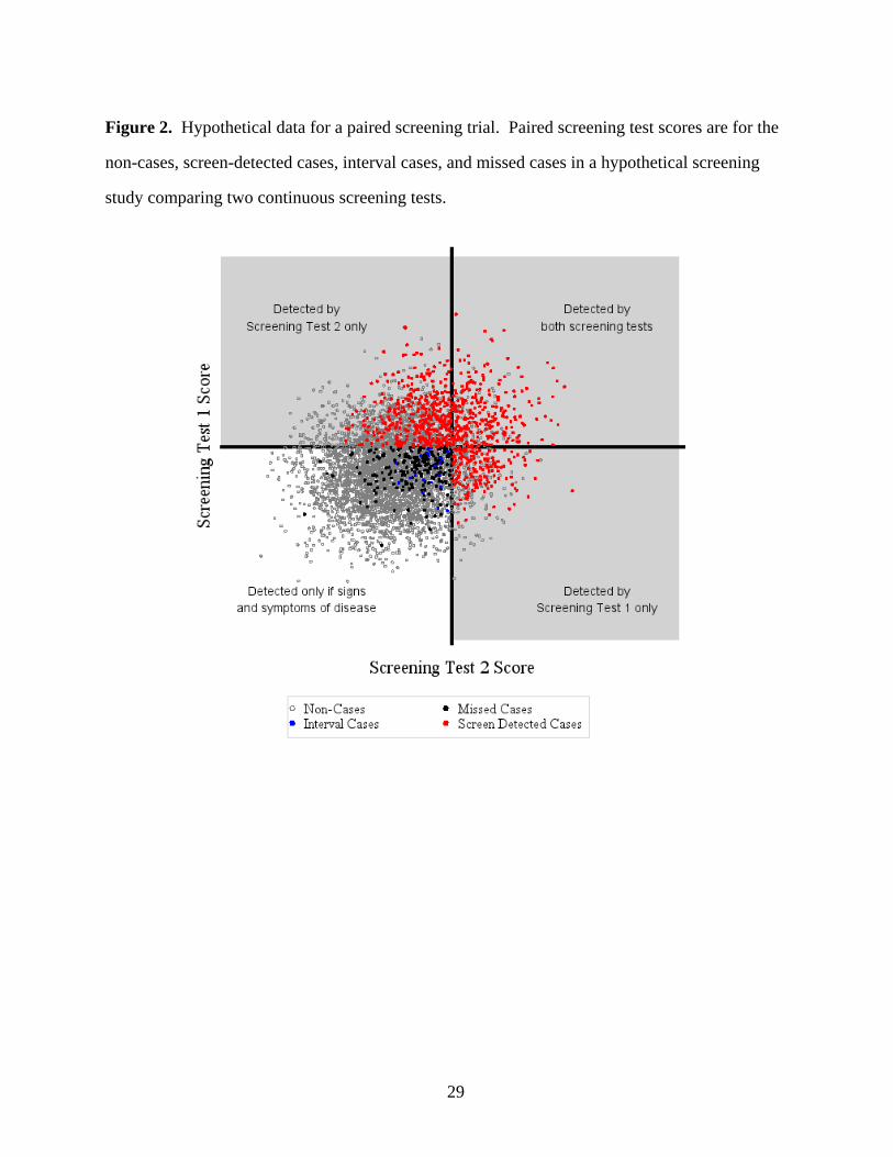
We present a graph of a hypothetical dataset of screening test scores (Figure 2) to illustrate

how the study investigator disease status. The axes represent the thresholds ofobserves

suspicion for each screening test. The study investigator every case in the gray region,observes

but a smaller portion of cases in the white region. We can identify the missed cases because we

present this graph from an omniscient point of view.

Standard Analysis

In the standard analysis, the study investigator compares the diagnostic accuracy of the two

screening tests, measured by the full area under the receiver operating characteristic curve. The

receiver operating characteristic curves are calculated using data from all cases and non-cases

observed in the study. When cases are missed, the study investigator calculates the sensitivity

6

and specificity of the screening test incorrectly. The error in sensitivity and specificity causes

concomitant errors in the area under the curve. Thus, the area under the curve canobserved

differ from the area under the curve.true

The error in sensitivity may be large 4 . However, the error in specificity is negligible. Thus, our proposed bias correction method only corrects the estimation of the sensitivity and does not

correct specificity. In fact, a specificity correction is typically not possible, because very few

non-cases actually receive the gold standard test.

Assumptions, Definitions, and Notation

We make a series of assumptions. Let be the total number of study participants, and the8 1

prevalence of disease in the population. Assuming simple random sampling, the number of

participants with disease is , and is distributedQ − !ß 8 Q µ Ð8ß ÑBinomial . 11

Let index participants, index the screening test, and 3 − "ß #ßá ß 8 4 − "ß # 5 − !ß " indicate the presence ( ) or absence ( ) of disease. Let denote the screening test5 œ " 5 œ ! \345

score for the participant on the screening test with disease status . For each disease3 4 5th th true

status, , and participant , the pair of test scores, and , are independently and5 3 \ \3"5 3 52

identically distributed bivariate Gaussian random variables with means, , variances, , and. 545 45#

correlation, .35

Let be the threshold of suspicion for screening test . All scores above the threshold will+ 44

trigger the use of a gold standard test. Let be the event that a participant shows signs andM

symptoms of disease during a follow-up period and . We assume thatT Ml5 œ " œ <

T Ml5 œ ! œ ! .

For screening test , the is 100 times the number of participants with4 percent ascertainment

disease who score above the threshold on screening test , divided by the total number of4

participants with disease.observed

7

Bias Correction Algorithm

We describe an algorithm to reduce bias in estimates of the area under the curve. The

algorithm requires four steps.

Step 1. Partition. The cases can be stratified into two sets, shown in Figure 2. Let observed E

(data in the gray area) be the set of cases with at least one screening test score above itstrue

respective threshold. Let (data in the white area) be the set of cases where the scores onF true

both screening tests fall below their respective thresholds. The percentages of participants with

observed observed disease in sets and differ: all cases of disease in set are , but only aE F E

fraction of cases are in set . We handle the estimation for each set separately, andobserved F

combine the estimates using weighting proportional to the sampling fraction

13; Equation 3.3.1, p. 81 .

Step 2. Maximum Likelihood Estimation. We obtain maximum likelihood estimates of the

bivariate Gaussian parameters for the cases. The estimation process follows an iterative method

suggested by Nath 14 . The method allows unbiased estimation of bivariate Gaussian parameters from sample spaces truncated to be convex. Set is not a convex set. To obtainE

convex sets, we further partition the sample space into quadrants , , as shownU 6 − "ß #ß $ß %6 in Table 1Þ

The starting values for the iteration are the sample statistics for the cases in eachobserved

quadrant. From the four quadrant specific estimates, we choose the set that maximizes the log

likelihood of the full bivariate Gaussian distribution with respect to the data. We referobserved

to that set as the Nath estimates, denoted by , , , , and . Note that the. . 5 5 3s s ss s""ßR #"ßR "ßR# #""ßR #"ßR

5 index is always equal to one since we only estimate parameters for the bivariate Gaussian

distribution of cases.

We require the sample variance as a starting value for the Nath algorithm. However, we can

only calculate the sample variance for quadrants with two or more observations. Thus, if hasU6

only one observation, we do not calculate the quadrant specific estimates for that quadrant.

8

Step 3. Weighting. The Nath estimates are only based on one quadrant of data. We use the

weighting described below to incorporate data from all quadrants and thereby lower the variance.

We refer to the weighted estimates as the estimates and use them to calculate thecorrected

corrected areas under the receiver operating characteristic curves. If either set or set E F

contain only one observation, we do not conduct the weighting and instead use the Nath

estimates as the .corrected estimates

The Nath estimates are used as inputs for calculating the sampling fraction for sets and .E F

Define the estimated probability of asE

. 2

- F 3

. .

5 5s œ " ß ß

+ + s s

s ss " #""ßR #"ßR

""ßR #"ßR"ßR

Let if a participant is to have disease and otherwise. For the screen positive5 œ " !w observed

cases, let be the sample mean, be the sample standard deviation for screening test ,\ W 4

45 ßE 45 ßEw w

and be the sample correlation between the screening tests. For the interval cases, let < \

5 ßE 45 ßFw w

be the sample mean, be the sample standard deviation for screening test , and be theW 4 <45 ßF 5 ßFw w

sample correlation between the screening tests. Let , , and be the weighted. 5 3s s s4"ß[ "ß[#4"ß[

estimates of the mean, variance, and correlation for the screening test scores for the cases.

We derived expressions for the weighted parameter estimates using the conditional covariance

formula 15; Proposition 5.2, p. 348 and the definition of the weighted mean

13; Equation 3.2.1, p. 77 . We define the estimates as follows:

. - -s œ \ " \s s ""ß[ ""ßE ""ßF , 3 . - -s œ \ " \s s #"ß[ #"ßE #"ßF , 4 5 Z [ .s œ s#""ß[ " " ""ß[

# , 5 5 Z [ .s œ s##"ß[ # # #"ß[

# , 6 and

9

3 5 5 c d . .s œ s s s s"ß[ ""ß[ #"ß[# #""ß[ #"ß[

7

where

Z -

[ -

c - -

4#4"ßE 4"ßE

#

4#4"ßF 4"ßF

#

""ßE #"ßE ""ßE #"ßE "ßE

œ \ Ws

œ " \ Ws

œ \ \ W W <s s

,

,

,

and

d - -œ " \ \ " W W <s s ""ßF #"ßF ""ßF #"ßF "ßF .

Evaluation of Bias Correction

We compared the Type I error and power of the observed corrected true, , and analyses. For

the observed observed analysis, we used the disease status as inputs for the paired comparison of

the diagnostic accuracy of the screening tests. The analysis replicates the standardobserved

analysis performed by the study investigator of a cancer screening trial. For the corrected

analysis, we used the proposed bias correction approach. Finally, both the andobserved

corrected true true analyses were compared to the analysis. The analysis assumes that the study

investigator knows the disease status of every participant.true

For each analysis, we tested the null hypothesis that there is no difference in the areas under

the receiver operating characteristic curves. We calculated the areas under the binormal receiver

operating characteristic curves 16; p. 122 . We then calculated the variance of the difference in

the areas under the curves and conducted a hypothesis test using the method of Obuchowski and

McClish 17 . Ethically, we can only conduct a screening trial if we have clinical equipoise, ,i.e.

if we do not have evidence to favor one screening strategy over the other. Thus, we used a two-

sided hypothesis test.

To assess screening , we compared the Type I error and power for thetest performance

observed corrected true, and analyses, . Power is the probability that we reject the null

hypothesis. When the hypothesis test detects a difference between the screening tests, the study

10

investigator uses the estimates of diagnostic accuracy to decide which screening test to

implement. However, the estimates of diagnostic accuracy can be biased. Consequently, even

though the study investigator correctly concludes that there is a difference between the two

screening tests, the investigator may incorrectly choose to implement the screening test with the

lower diagnostic accuracy. To quantify the decision error, we divided power into the correct

rejection fraction wrong rejection fraction. correct rejection fraction and the The is the

probability that the hypothesis test rejects and the screening test with the larger areaobserved

under the curve is the screening test with larger area under the curve. The true wrong rejection

fraction is the probability that the hypothesis test rejects but the screening test with the larger

observed true area under the curve is the screening test with the smaller area under the curve.

Design of Simulation Studies under the Gaussian Assumption

We conducted simulations under the assumptions listed in Assumptions, Definitions, and

Notation. We considered two states of nature; one where the null hypothesis holds and one

where the alternative hypothesis holds. When the null holds, the two screening tests have the

same diagnostic accuracy. When the alternative holds, the screening tests have different

diagnostic accuracies.

The simulation studies varied four factors: 1) the disease prevalence, 2) the proportion of

cases that exhibit signs and symptoms of disease during follow-up, 3) the correlation between

Test 1 and 2 scores, and 4) the thresholds that trigger a gold standard test. The four factors

change the amount of bias in the estimates of the diagnostic accuracy of each screening test. In

addition, the factors change the number and proportion of cases. For brevity, we doobserved

not present the correlation study results in this manuscript. The correlation between the

screening tests had a negligible effect on the performance of the bias correction method.

For each combination of parameter values, we simulated paired screening test scores and a

binary indicator of disease status. Based on the described study design, we deduced thetrue

observed true observed corrected disease status. We calculated the , , and areas under the curves

and assessed the results of the simulation study using the metrics introduced in the Evaluation of

11

Bias Correction section. We used 10,000 realizations of the simulated data to ensure that the

error in the estimation of probabilities occurred in the second decimal place.

Design of Non-Gaussian Simulation Studies

We conducted a second set of simulation studies to examine the robustness of the bias

correction method to deviations from the Gaussian assumption. We considered two possible

deviations: zero-weighted data, which corresponds to screening test scores with zero values, and

a multinomial distribution, which corresponds to reader preferences for a subset of the possible

screening test scores. We evaluated the performance of the bias correction method as described

in the Evaluation of Bias Correction section.

To generate the zero-weighted data where the occurrence of zeroes is correlated between the

two screening tests, we generated two sets of correlated Bernoulli random variables, one for

cases and one for non-cases, so that the probability that the score on Test 1 is zero is , the:"5

probability that the score on Test 2 is zero is and the probability that both screening test:#5

scores are zero is . If the Bernoulli random variable was one, we replaced the associated;5

screening test score with a zero. Otherwise, the screening test score remained as it was. We set

: !Þ!" !Þ*!45 equal to a range of values between and , creating a series of datasets. The marginal

probabilities put constraints on the possible values for 18 . We set to the median allowed; ;5 5 agreement for each pairing of .:45

To generate the multinomial data, we binned the bivariate Gaussian data. We created a series

of datasets, each with a different bin size. The bin sizes were , , , , and times the"Î"! "Î# " # &

variance. We set the disease prevalence to (low), (medium) and (high).!Þ!" !Þ"% !Þ#%

Results

Effect of Disease Prevalence

C disease prevalence affects both the case and non-case case sample size. In turn,hanging the

this changes the number of observations used to calculate sensitivity and specificity, which

affects the Type I error rate and power of the analysis.

12

Choice of Parameter Values. The diagnostic accuracy of the screening tests are similar to

those found in the study by Pisano 3 . When the null holds, we fixed the area underet al. true

both curves to be the alternative holds, we fixed the area under the curve to be!Þ(). When true

!Þ() !Þ(% !Þ!%Þ for Test 1 and for Test 2 for a difference of The sample size was fixed attrue

&!ß !!! !Þ"! and the rate of signs and symptoms at . The thresholds of suspicion were set to

confer a large degree of paired screening trial bias.

We varied the disease prevalence between and . The choice reflects cancer rates!Þ!" !Þ#%

seen in published cancer studies (prevalence of prostate cancer in Tobago men aged 70-79 is

0.28 in 19 ; rate of breast cancer i s roughly per in 2 and 3 ; prevalence of oral lesions' "!!! is in 20 ; prevalences of all major cancers conditional on age and gender fall between and!Þ"% ! !Þ"( per SEER Tables 4.25, 5.15, 15.27, 16.21, 20.27, 23.15 21 ). Type I Error. As shown in panel A of Figure 3, in the presence of paired screening trial bias,

the Type I error rate ranges between and . The Type I error rateobserved corrected!Þ!' !Þ**

ranges between and . Higher disease prevalence has higher Type I error rates.!Þ!$ !Þ!)

Power. In panels B and C of Figure 3, the analysis corrected has a high correct rejection

fraction across all disease prevalences likely to be encountered in a cancer screening study. The

correct rejection fraction ranges between and . By contrast, the !Þ&) !Þ*' observed analysis often

wrongly concludes that the worst screening test is best. For the example shown, the correct

rejection fraction for the analysis is zero while the wrong rejection fraction rangesobserved

between and .!Þ)' "Þ!!

Effect of the Rate of Signs and Symptoms

When the rate of signs and symptoms is low, there is a higher potential for occult disease and,

hence, error in the estimates of diagnostic accuracy.

Choice of Parameter Values. We defined the fixed parameter values as in the Effect of Disease

Prevalence section. We varied the rate of signs and symptoms across a range of clinically

relevant values. In cancer screening, the rate of signs and symptoms is not typically reported,

but can be approximated using surrogates. In the trial by Lewin et al. 2 , we can use the

13

proportion of interval cancers out of all cancers as an estimate of the largest possibleobserved

rate of signs and symptoms. An earlier breast cancer screening trial by Bobo, Lee and Thames

22 evaluated the performance of clinical breast exams for early identification of breast cancer.

If we assume an abnormal clinical breast exam is the same as showing signs and symptoms of

disease, then having an abnormal breast exam but a benign mammogram is akin to a woman

screening negative on mammography but then showing signs and symptoms of disease. Based

on these surrogates, the approximate values for the rate of signs and symptoms were 2!Þ"" and

!Þ!& 22 . We chose a range of to for our simulation studies.! !Þ#!

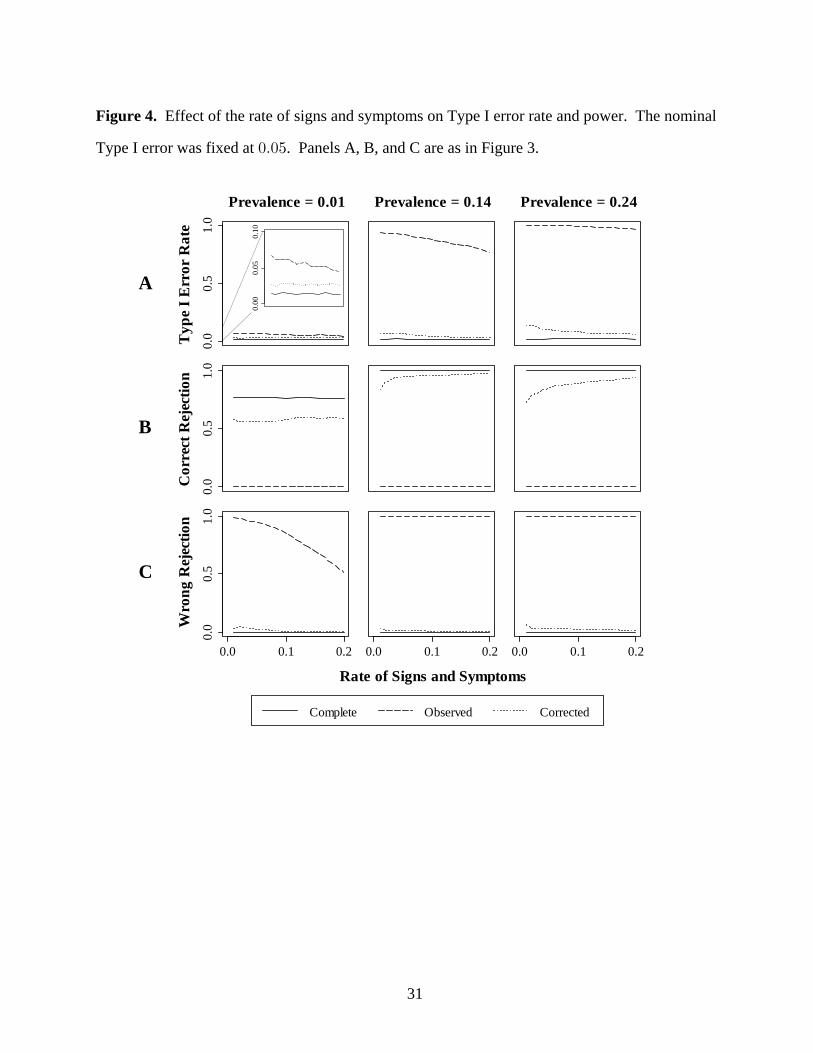
Type I Error. In panel A of Figure 4, Type I error declines with increasing rate of signs and

symptoms. The Type I error rate of the analysis is below nominal at low diseasecorrected

prevalence, and ranges from to at medium and high disease prevalence. Type I error!Þ!$ !Þ"%

rate of the analysis ranges between and at low disease prevalence, and toobserved !Þ!& !Þ!( !Þ((

"Þ!! at medium and high disease prevalence.

Power. In panels B and C of Figure 4, increasing the rate of signs and symptoms improves the

correct rejection fraction. The correct rejection fraction for the analysis is at lowtrue !Þ((

disease prevalence and at medium and high disease prevalence. The correct rejection"Þ!!

fraction of the corrected analysis ranges from to at low disease prevalence and to!Þ&' !Þ&* !Þ(#

!Þ*( at medium and high disease prevalence. The analysis has a correct rejectionobserved

fraction of zero, while the wrong rejection fraction ranges from to . Under the extreme!Þ&" "Þ!!

bias conditions of the simulation, the study investigator using the results will eitherobserved

incorrectly decide that the worst screening test is best, or conclude there is no difference between

the two screening tests.

Effect of Percent Ascertainment

The threshold of suspicion for each screening test determines what percentage of cases receive

the gold standard test. We chose a threshold for each screening test that corresponds to around

15%, 50% and 80% ascertainment. Percentages are approximate because the case numbers are

discrete.

14

Paired screening trial bias occurs when the percent ascertainment is different for the two

screening tests. When the percent ascertainment is equivalent for the two screening tests,

estimates of diagnostic accuracy for each screening test may still be subject to differential

verification bias. However, since each test is biased by the same amount, the difference in the

areas under the curves will remain unchanged.

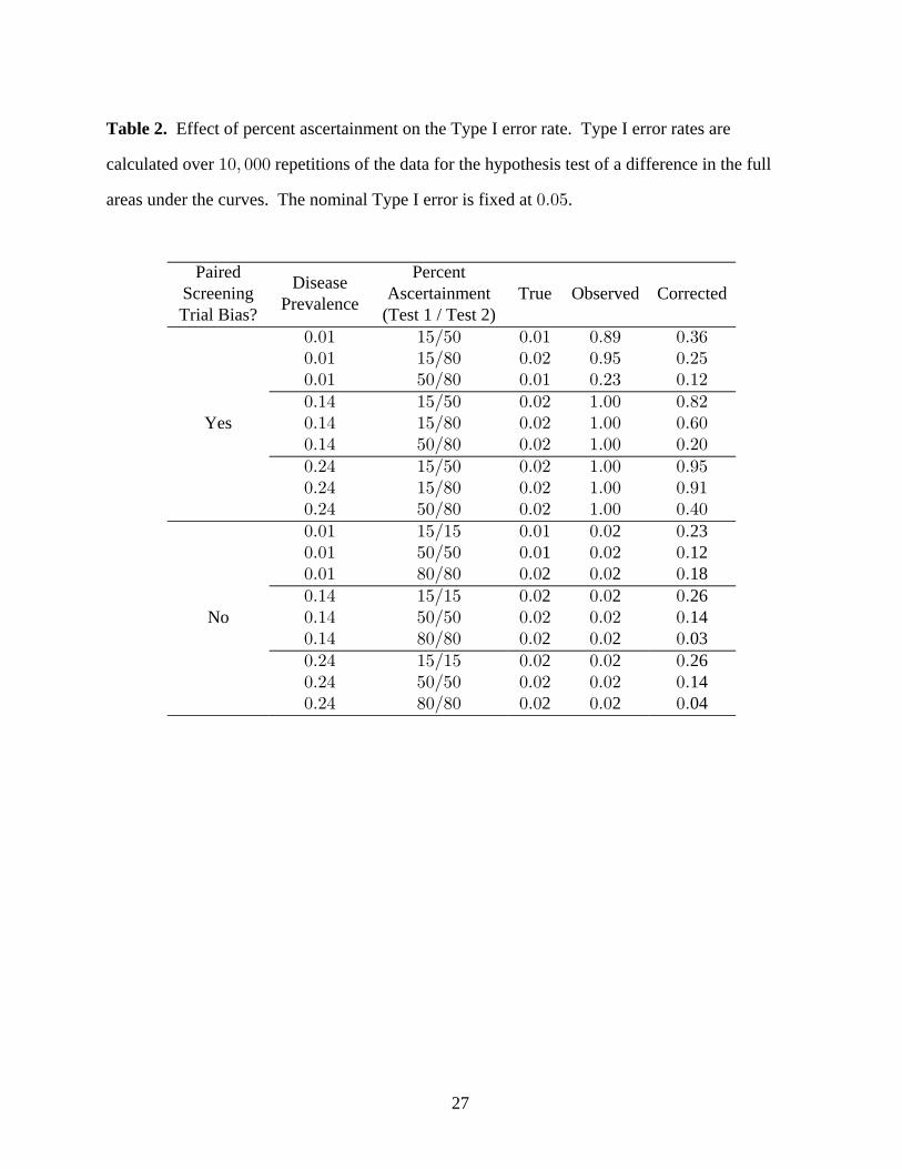
Table 2 shows the Type I error of the and analyses for a selection oftrue observed corrected,

percent ascertainment levels. We do not discuss the power results since the Type I error of the

observed analysis is so high and power is bounded below by Type I error rate.

Choice of Parameter Values. We defined the fixed parameter values as in the Effect of Disease

Prevalence. We chose values for the thresholds that allowed the amount and source of the bias

(Test 1 or Test 2) to vary across a wide range of possible screening study scenarios.

Type I Error. In general, when the study is biased, the Type I error rate of the observed

analysis is too high ( to ). !Þ#$ "Þ!! The Type I error rate of the analysis is closer tocorrected

nominal than that of the analysis, but is also too high ( to ). For the pairingsobserved !Þ"# !Þ*&

with no paired screening trial bias, the analysis has lower than nominal Type I errorobserved

rates ( ) while the analysis has Type I error rates up to . When the percent!Þ!# !Þ#'corrected

ascertainment is high ( ) for both screening tests, the Type I error rate of the )!Î)! corrected

analysis is below nominal.

Robustness to Non-Gaussian Data

Although the bias correction method was developed under an assumption that the data were

bivariate Gaussian, screening data may not follow the Gaussian distribution. Multinomial and

zero-weighted data are common in imaging studies. Often, in imaging studies, readers give the

image a score of zero to indicate that no disease is seen, resulting in a data set where multiple

values are zero. In addition, reader preferences for a subset of scores can produce a multinomial

data set.

The bias correction method can still be used if data are multinomial or zero-weighted. For

multinomial data, the method performs well when the bins for the multinomial are scaled to less

15

than half the variance. For zero-weighted data, the bias correction algorithm can reduce decision

errors when up to 30% of the non-cases and 1% of the cases receive a score of zero. The study

investigator can obtain a rough estimate of the percentage of cases that receive zero scores from

the published rate of interval cancers.

Demonstration

Figure 5 shows the receiver operating characteristic curves for a hypothetical oral cancer

screening trial similar to that considered by Lingen 1 . One of the designs considered by Lingen was a paired trial comparing two oral cancer screening modalities: 1) examination by a dentist

using a visual and tactile oral examination, and referral for biopsy only for frank cancers (Test

1); and 2) examination by a dentist using a visual and tactile oral exam, a second look with the

VELscope oral cancer screening device, and stringent instructions to biopsy any lesion detected

during either examination (Test 2).

We could find no published oral cancer screening trials of paired continuous tests. Instead, we

chose parameter values from a breast cancer screening study 3 and an oral cancer screening demonstration study 20 . We fixed the sample size at 50,000 3 and the rate of visible lesions at 0.1 (rate of suspicious oral cancer and precancerous lesions reported in 28 studies between 1971

and 2002 ranges from 0.02 to 0.17, Table 6, 20 ). We approximated the disease prevalence as !Þ!" based on the number of Americans with cancer of the oral cavity and pharynx 21 and the 2011 population estimate from the U.S. Census Bureau 23 . For the purposes of the illustration,

the areas under the curves for Test 1 and Test 2 were fixed at and , respectively,true !Þ(( !Þ("

similar to the areas under the curves reported for digital and film mammography 3 . In truth, we

have no data to support the superiority of the visual tactile oral exam over the visual tactile oral

exam plus scope.

The trial by Pisano compared digital and film mammography 3 . Since the recall rateet al. for both modalities was 8.4%, the trial was unlikely to be biased. In the hypothetical oral cancer

screening trial, however, we posit that there would be a large difference in the percent

ascertainments for each screening modality. In the first arm, the dentist only recommends

16

biopsy for participants with highly suspicious lesions. Thus, we fixed the percent ascertainment

to be very low, only 0.01%. The oral pathologist recommends biopsy for almost any lesion so

we set the percent ascertainment at 97%. The large difference in percent ascertainment between

the two screening tests creates extreme paired screening trial bias.

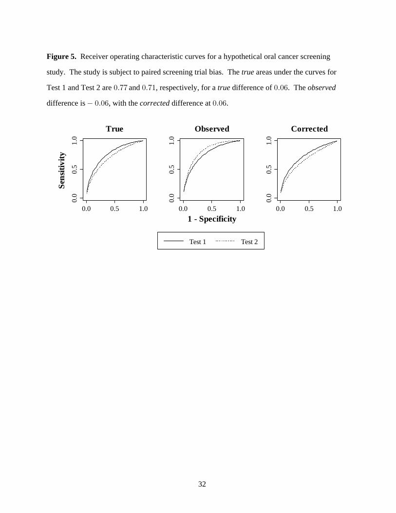
Under conditions of extreme bias, our bias correction method performs well, as shown in

Figure 5. The difference in the areas under the curves is the true observed!Þ!' (p = ),!Þ!!"

difference is , and the difference is . In the !Þ!' !Þ!'(p = ) (p = )!Þ!!& !Þ!!"corrected

observed analysis, the receiver operating characteristic curves have the opposite orientation to

the true state of nature. The analysis removes the bias and the curves are realignedcorrected

with the true state of nature.

In reality, the study investigator would not know which analysis had results closest to the

truth. To validate our choice of analysis, we simulated the hypothetical study design using the

parameter values specified above. The simulated Type I error rate of the corrected analysis is

below nominal at , while the Type I error rate of the observed analysis is above nominal at!Þ!$

!Þ!' !Þ&). The correct rejection fraction of the bias-corrected analysis is , while that of the

observed analysis is zero. In fact, using the observed analysis, the study investigator would

wrongly conclude that Test 2 is superior to Test 1 86% of the time. Based on this simulation, we

would recommend the study investigator use the bias correction method to correct the results of

the hypothetical oral cancer screening study.

Discussion

We could find no other methods that attempted to ameliorate paired screening trial bias for

paired cancer screening studies that use the difference in the full area under the curve as a metric.

Re-weighting, generalized estimating equations, imputation and Bayesian approaches have been

proposed to reduce the effect of partial verification bias , 11, 24 29 . Maximum likelihood e.g.

methods 30 and latent class models 31 have been proposed to estimate diagnostic accuracy in the presence of imperfect reference standard bias.

17

The amount of bias in the study and the performance of the bias correction method depend

on fourteen factors: the means, variances, and correlation of the case and non-case test scores,

the disease prevalence, the rate of signs and symptoms, and the percent ascertainment for each

screening test. After careful analysis of over combinations of the parameter values, we"(!ß !!!

were unable to determine a definitive pattern upon which to base recommendations for using the

standard analysis versus a bias-corrected approach.

In order to determine if bias correction is indicated for a specific screening trial, we

recommend the investigator conduct a simulation study similar to those described in the

manuscript. The simulation software will be made available at www.samplesizeshop.com. The

software will simulate Type I error rate and power for both the standard and bias-corrected

analyses. The study investigator should choose the analysis that has the Type I error rate closest

to the nominal level and the highest correct rejection fraction.

The software will request that the study investigator specify the values of each of the

fourteen factors. Estimates can be based on previous studies or auxiliary information. For

instance, the rate of signs and symptoms is usually not described in the literature. In the Results

section, we calculated an estimate for the rate of signs and symptoms using surrogate values

published in two breast cancer screening studies. When convincing values cannot be found, the

study investigator can conduct a sensitivity analysis using a range of values to see how strongly

that parameter affects the choice of analysis.

In this article, we treat the prevalence of disease as a fixed feature of our study population.

However, the disease prevalence may be higher or lower for different subgroups of the

population. For instance, in the DMIST study, women younger than 50 years of age had a much

lower prevalence of invasive breast carcinoma than women greater than 50 years of age 3 . At this time, the method does not allow for a heterogeneous case mixture. To allow for differences

in disease prevalence in the study population, the study investigator can stratify participants into

subgroups with a homogeneous disease prevalence. The investigator would then conduct

separate analyses for each subgroup.

18

In some instances, both the standard analysis and the corrected analysis will have higher than

nominal Type I error rates. In this case, we recommend that investigators avoid using a paired

screening study design. Another option would be to randomize study participants to one of two

possible screening modalities. However, a randomized trial is inefficient relative to a paired

screening trial, and may still be subject to differential verification bias. A more clinically useful

endpoint may be to consider mortality, as was done in the National Lung Screening Trial

(NLST) 32 . Unlike receiver operating characteristic analysis, mortality trials such as the NLST are not vulnerable to paired screening trial bias, or verification bias in general.

The bias correction method is a maximum likelihood method. Thus, the accuracy of the

estimation depends on the number of cases. We do not recommend using the method for studies

with a very small number of cases ( ), and interval cases ( 5). &!!

This paper provides two contributions to the statistical literature. First, we describe a method

to correct for paired screening trial bias, a bias which has not been addressed by other correction

techniques. Due to the increasing use of continuous biomarkers for cancer (see, , 33 ), ae.g. growing number of screening trials have the potential to be subject to paired screening trial bias.

The proposed method will counteract bias in the paired trials and allow investigators to compare

screening tests with fewer decision errors. Second, we introduce an important metric for

evaluating the performance of bias correction techniques, that of reducing decision errors. We

recommend that every new bias correction method be evaluated with a study of Type I error and

power.

Conclusions

The proposed bias correction method reduces decision errors in the paired comparison of the

full area under the curve of screening tests with Gaussian outcomes. Because the performance of

the bias correction method is affected by characteristics of the screening tests and the disease

being examined, we recommend conducting a simulation study using our free software before

choosing a bias-corrected or standard analysisÞ

19

Competing Interests

The authors declare that they have no competing interests.

20

Authors' contributions

BMR conducted the literature review, derived the mathematical results, designed and

programmed the simulation studies, interpreted the results, and prepared the manuscript. TAA

assisted with the literature review and provided expertise on the context of the topic in relation to

other work in the field. JTB assisted with the mathematical derivations. SMK provided

guidance for the design and programming of the simulation studies. AM improved the software

and packaged it for public release. KEM reviewed the intellectual content of the work and gave

important editorial suggestions. DHG conceived of the topic and guided the development of the

work. All authors read and approved the manuscript.

21

Acknowledgements

The research presented in this paper was supported by two grants. The mathematical

derivations, programming of the algorithm and early simulation studies were funded by the NCI

1R03CA136048-01A1, a grant awarded to the Colorado School of Public Health, Deborah

Glueck, Principal Investigator. Completion of the simulation studies, including the Type I error

and power analyses, was funded by NIDCR 3R01DE020832-01A1S1, a minority supplement

awarded to the University of Florida, Keith Muller, Principal Investigator, with a subaward to

the Colorado School of Public Health. The content of this paper is solely the responsibility of

the authors, and does not necessarily represent the official views of the National Cancer Institute,

the National Institute of Dental and Craniofacial Research, nor the National Institutes of Health.

22

References

1. Lingen, MW. National Institute of Dental and Craniofacial Research. Efficacy of oral cancer

screening adjunctive techniques. Bethesda (MD): National Institute of Dental and

Craniofacial Research, National Institutes of Health, US Department of Health and Human

Services; (NIH Project Number: 1RC2DE020779-01) 2009 [cited 2012 February 17].

2. Lewin JM, D'Orsi CJ, Hendrick RE, Moss LJ, Isaacs PK, Karellas A, Cutter GR: Clinical

comparison of full-field digital mammography and screen-film mammography for

detection of breast cancer. 179 2002, :671-677.AJR Am J Roentgenol

3. Pisano ED, Gatsonis C, Hendrick E, Yaffe M, Baum JK, Acharyya S, Conant EF, Fajardo

LL, Bassett L, D'Orsi C, Jong R, Rebner M: Diagnostic performance of digital versus film

mammography for breast-cancer screening. 353 2005, :1773-1783.N Engl J Med

4. Glueck DH, Lamb MM, O'Donnell CI, Ringham BM, Brinton JT, Muller KE, Lewin JM,

Alonzo TA, Pisano ED: Bias in trials comparing paired continuous tests can cause

researchers to choose the wrong screening modality. 9 2009, :4.BMC Med Res Methodol

5. Szklo M, Nieto J. Jones and Bartlett Publishers;Epidemiology: Beyond the Basics. 2nd ed.

2006.

6. Lijmer JG, Mol BW, Heisterkamp S, Bonsel GJ, Prins MH, van der Meulen JH, Bossuyt PM:

Empirical evidence of design-related bias in studies of diagnostic tests. 1999,JAMA

282:1061-1066.

7. Reitsma JB, Rutjes AWS, Khan KS, Coomarasamy A, Bossuyt PM: A review of solutions

for diagnostic accuracy studies with an imperfect or missing reference standard. J Clin

Epidemiol 2009, :797-806.62

8. Rutjes AWS, Reitsma JB, Di Nisio M, Smidt N, van Rijn JC, Bossuyt PMM: Evidence of

bias and variation in diagnostic accuracy studies. 174 2006, :469-476.CMAJ

9. Whiting P, Rutjes AWS, Reitsma JB, Glas AS, Bossuyt PMM, Kleijnen J: Sources of

variation and bias in studies of diagnostic accuracy: a systematic review. Ann Intern Med

2004, :189-202.140

23

10. Baker SG: Evaluating a new test using a reference test with estimated sensitivity and

specificity. 20 1991, :2739-2752.Communications in Statistics - Theory and Methods

11. Begg CB, Greenes RA: Assessment of diagnostic tests when disease verification is

subject to selection bias. 39 1983, :207-215.Biometrics

12. Ringham BM, Alonzo TA, Grunwald GK, Glueck DH: Estimates of sensitivity and

specificity can be biased when reporting the results of the second test in a screening

trial conducted in series. 10 2010, :3.BMC Med Res Methodol

13. Kish L: Wiley-Interscience; 1995.Survey Sampling.

14. Nath GB: Estimation in Truncated Bivariate Normal Distributions. Journal of the Royal

Statistical Society Series C (Applied Statistics) 1971, :313-319.20

15. Ross S: 8th edition. Prentice Hall; 2009.First Course in Probability, A.

16. Zhou X-H, McClish DK, Obuchowski NA: 1stStatistical Methods in Diagnostic Medicine.

edition. Wiley-Interscience; 2002.

17. Obuchowski NA, McClish DK: Sample size determination for diagnostic accuracy

studies involving binormal ROC curve indices. 16 1997, :1529-1542.Stat Med

18. Alonzo TA: Verification bias-corrected estimators of the relative true and false positive

rates of two binary screening tests. 24 2005, :403-417.Stat Med

19. Bunker CH, Patrick AL, Konety BR, Dhir R, Brufsky AM, Vivas CA, Becich MJ, Trump

DL, Kuller LH: High prevalence of screening-detected prostate cancer among Afro-

Caribbeans: the Tobago Prostate Cancer Survey. Cancer Epidemiol Biomarkers Prev

2002, :726-729.11

20. Lim K, Moles DR, Downer MC, Speight PM: Opportunistic screening for oral cancer and

precancer in general dental practice: results of a demonstration study. 2003,Br Dent J

194:497-502; discussion 493.

21. Howlader N, Noone AM, Krapcho M, Neyman N, Aminou R, Waldron W, Altekruse SF,

Kosary CL, Ruhl J, Tatalovich Z, Cho H, Mariotto A, Eisner MP, Lewis DR, Chen HS,

Feuer EJ, Cronin KA, Edwards BK (eds). SEER Cancer Statistics Review, 1975-2008,

24

National Cancer Institute. Bethesda, MD, http://seer.cancer.gov/csr/1975_2009_pops09/,

based on November 2010 SEER data submission, posted to the SEER web site, 2011.

22. Bobo JK, Lee NC, Thames SF: Findings from 752,081 clinical breast examinations

reported to a national screening program from 1995 through 1998. J Natl Cancer Inst

2000, :971-976.92

23. U.S. Census Bureau. State and County Quickfacts: Allegany County, N.Y. Retrieved June, 7,

2012, from http://quickfacts.census.gov.

24. Alonzo TA, Pepe MS: Assessing Accuracy of a Continuous Screening Test in the

Presence of Verification Bias. Journal of the Royal Statistical Society Series C (Applied

Statistics) 2005, :173-190.54

25. Buzoianu M, Kadane JB: Adjusting for verification bias in diagnostic test evaluation: A

Bayesian approach. 27 2008, :2453-2473.Statistics in Medicine

26. Martinez EZ, Alberto Achcar J, Louzada-Neto F: Estimators of sensitivity and specificity

in the presence of verification bias: A Bayesian approach. 2006,Comput Stat Data Anal

51:601-611.

27. Rotnitzky A, Faraggi D, Schisterman E: Doubly Robust Estimation of the Area Under the

Receiver-Operating Characteristic Curve in the Presence of Verification Bias. Journal

of the American Statistical Association 2006, :1276-1288.101

28. Toledano AY, Gatsonis C: Generalized estimating equations for ordinal categorical data:

arbitrary patterns of missing responses and missingness in a key covariate. Biometrics

1999, :488-496.55

29. Zhou X: Maximum likelihood estimators of sensitivity and specificity corrected for

verification bias. 22 1993, :3177-3198.Communications in Statistics - Theory and Methods

30. Vacek PM: The effect of conditional dependence on the evaluation of diagnostic tests.

Biometrics 1985, :959-968.41

31. Torrance-Rynard VL, Walter SD: Effects of dependent errors in the assessment of

diagnostic test performance. 16 1997, :2157-2175.Stat Med

25

32. Aberle DR, Adams AM, Berg CD, Black WC, Clapp JD, Fagerstrom RM, Gareen IF,

Gatsonis C, Marcus PM, Sicks JD: Reduced lung-cancer mortality with low-dose

computed tomographic screening. 365 2011, :395-409.N Engl J Med

33. Elashoff D, Zhou H, Reiss J, Wang J, Xiao H, Henson B, Hu S, Arellano M, Sinha U, Le A,

Messadi D, Wang M, Nabili V, Lingen M, Morris D, Randolph T, Feng Z, Akin D,

Kastratovic DA, Chia D, Abemayor E, Wong DTW: Prevalidation of Salivary Biomarkers

for Oral Cancer Detection. 21 2012, :664-672.Cancer Epidemiol Biomarkers Prev

26

Table 1. Quadrant definitions.

Quadrant Name DefinitionU B   + à B   +U B   + à B +U B + à B   +U B + à B +

" 3"5 " 3#5 #

# 3"5 " 3#5 #

$ 3"5 " 3#5 #

% 3"5 " 3#5 #

27

Table 2. Effect of percent ascertainment on the Type I error rate. Type I error rates are

calculated over repetitions of the data for the hypothesis test of a difference in the full"!ß !!!

areas under the curves. The nominal Type I error is fixed at .!Þ!&

Paired PercentScreening AscertainmentTrial Bias? (Test 1 / Test 2)

DiseasePrevalence

True Observed Corrected

!Þ!" "&Î&!!Þ!" "&Î)!!Þ!" &!Î)!

!Þ!" !Þ)* !Þ$'!Þ!# !Þ*& !Þ#&!Þ!" !Þ#$ !Þ"#

!Þ"% "&Î&! !Þ!# "Þ!! !Þ)#!Þ"% "&Î)! !Þ!# "Þ!! !Þ'!!Þ"% &!Î)! !Þ!# "Þ!! !Þ#!!Þ#% "&Î&!!Þ#% "&Î)!!Þ#% &!Î)

Yes

! !Þ!# "Þ!! !Þ%!

!Þ!# "Þ!! !Þ*&!Þ!# "Þ!! !Þ*"

!Þ!" "&Î"& !Þ!" !Þ! !Þ!Þ!" &!Î&! !Þ! !Þ!# !Þ!Þ!" )!Î)! !Þ! !Þ! !Þ!Þ"% "&Î"&!Þ"% &!Î&!!Þ"% )!Î)

1 122 2 18

2 23

No! !Þ! !Þ! !Þ

!Þ! !Þ! !Þ!Þ!# !Þ!# !Þ

!Þ#% "&Î"& !Þ! !Þ! !Þ!Þ#% &!Î&! !Þ!# !Þ!# !Þ!Þ#% )!Î)! !Þ! !Þ! !Þ

2 2 26

2 2 0314

2 2 26

2 2 0414

28

Figure 1. Flowchart of a paired trial of two continuous screening tests. The flowchart

culminates in the study investigator's observation of the disease status of the participant.

Signs and symptoms?

Screenpositive on one or both

tests?

Gold Standard Test

Follow-Up

No observed diseaseObserved disease

Yes

No

No

Yes Confirmed disease?

Yes No

Screening by both tests

29

Figure 2. Hypothetical data for a paired screening trial. Paired screening test scores are for the

non-cases, screen-detected cases, interval cases, and missed cases in a hypothetical screening

study comparing two continuous screening tests.

30

Figure 3. Effect of disease prevalence on Type I error rate and power. The nominal Type I

error was fixed at Graphs show the proportion of times the hypothesis test rejects and A)!Þ!&Þ

the null holds, B) the alternative holds and the conclusion of the hypothesis test agrees with the

true state of nature, or C) the alternative holds but the conclusion of the hypothesis test is

opposite the true state of nature.

0.0

0.5

1.0

0.000 0.125 0.250

0.0

0.5

1.0

0.000 0.125 0.250

Complete Observed Corrected

0.0

0.5

1.0

0.000 0.125 0.250

Typ

e I

Err

or R

ate

Cor

rect

Rej

ecti

on

Wro

ng R

ejec

tion

Disease Prevalence

A B C

31

Figure 4. Effect of the rate of signs and symptoms on Type I error rate and power. The nominal

Type I error was fixed at . Panels A, B, and C are as in Figure 3.!Þ!&

0.00

0.05

0.10

0.0

0.5

1.0

0.0

0.5

1.0

0.0 0.1 0.2

0.0

0.5

1.0

0.0 0.1 0.2

Complete Observed Corrected

0.0 0.1 0.2

Prevalence = 0.01 Prevalence = 0.14 Prevalence = 0.24T

ype

I E

rror

Rat

eC

orre

ct R

ejec

tion

Wro

ng

Rej

ecti

on

Rate of Signs and Symptoms

A

B

C

32

Figure 5. Receiver operating characteristic curves for a hypothetical oral cancer screening

study. The study is subject to paired screening trial bias. The areas under the curves fortrue

Test 1 and Test 2 are and , respectively, for a difference of . The !Þ(( !Þ(" !Þ!'true observed

difference is , with the difference at . !Þ!' !Þ!'corrected

0.0

0.5

1.0

0.0 0.5 1.0

0.0

0.5

1.0

0.0 0.5 1.0

Test 1 Test 2

0.0

0.5

1.0

0.0 0.5 1.0

True Observed Corrected

Sen

siti

vity

1 - Specificity