reconstruction d'images pour un imageur hyperspectral
TRANSCRIPT
HAL Id: tel-03404224https://tel.archives-ouvertes.fr/tel-03404224
Submitted on 26 Oct 2021
HAL is a multi-disciplinary open accessarchive for the deposit and dissemination of sci-entific research documents, whether they are pub-lished or not. The documents may come fromteaching and research institutions in France orabroad, or from public or private research centers.
L’archive ouverte pluridisciplinaire HAL, estdestinée au dépôt et à la diffusion de documentsscientifiques de niveau recherche, publiés ou non,émanant des établissements d’enseignement et derecherche français ou étrangers, des laboratoirespublics ou privés.
Reconstruction d’images pour un imageur hyperspectralconfigurable
Ibrahim Ardi
To cite this version:Ibrahim Ardi. Reconstruction d’images pour un imageur hyperspectral configurable. Instrumenta-tion et méthodes pour l’astrophysique [astro-ph.IM]. Université Paul Sabatier - Toulouse III, 2020.Français. NNT : 2020TOU30302. tel-03404224
THÈSEEn vue de l’obtention du
DOCTORAT DE L’UNIVERSITÉ DE TOULOUSE
Délivré par l'Université Toulouse 3 - Paul Sabatier
Présentée et soutenue par
Ibrahim ARDI
Le 21 octobre 2020
Reconstruction d'images pour un imageur hyperspectral
Ecole doctorale : EDMITT - Ecole Doctorale Mathématiques, Informatique etTélécommunications de Toulouse
Spécialité : Informatique et Télécommunications
Unité de recherche :IRAP - Institut de Recherche en Astrophysique et Planetologie
Thèse dirigée parHervé CARFANTAN et Antoine MONMAYRANT
JuryMme Anne SENTENAC, Rapporteure
M. Jean-François GIOVANNELLI, RapporteurM. Charles SOUSSEN, ExaminateurM. Simon LACROIX, Examinateur
M. Hervé CARFANTAN, Directeur de thèseM. Antoine MONMAYRANT, Co-directeur de thèse
configurable

Résumé
Une image hyperspectrale (HS) d’une scène correspond à un cube de données avec deuxdimensions spatiales et une dimension spectrale : elle peut être vue comme un grand nombred’images de la scène dans différentes bandes spectrales ou comme un ensemble de spectres àchaque position spatiale. Un problème central de l’imagerie hyperspectrale est lié à la naturetridimensionnelle des données qui doivent être acquises avec des capteurs 2D. Bien que certainsdispositifs optiques complexes ont cherché à imager l’ensemble du cube en une seule acquisi-tion (imageurs dits « snapshot »), l’approche la plus classique consiste à effectuer un balayage,spatial, spectral ou autre de l’ensemble du cube. Plus récemment, des dispositifs effectuant desacquisitions de projections incomplètes du cube HS ont été proposés, associés à des méthodesde reconstruction pour obtenir le cube HS à partir d’un faible nombre de données (beaucoupmoins de données que donnerait un balayage du cube). Les algorithmes associés à ces méthodesnécessitent des temps de calcul généralement longs.
Cette thèse se place dans ce cadre et vise à proposer des méthodes de reconstruction d’imagesHS pour un dispositif pilotable. Cet instrument est composé de deux lignes 4f (assemblage dedeux lentilles et d’un réseau de diffraction) symétriques et séparées par une matrice de micro-miroirs (DMD pour Digital Micromirror Device) placée dans le plan de symétrie. L’ensembleagit comme un filtre spatio-spectral programmable. La configuration du DMD permet de fairel’acquisition de différentes projections du cube. Notons que l’image panchromatique de la scèneest acquise simplement et avec le même échantillonnage que les données HS en positionnanttous les miroirs en réflexion. L’objectif est de reconstruire le cube HS avec un faible nombred’acquisitions pour des configurations aléatoires du DMD et avec un coût de calcul limité.
Nous proposons deux méthodes de reconstruction qui prennent en compte les caractéristiquesde l’imageur et exploitent la connaissance de l’image panchromatique. En particulier, nous noussommes appuyés sur l’hypothèse que l’image HS est constituée de zones spatiales homogènesayant des spectres similaires et que ces zones homogènes et les contours entre ces zones peuventêtre détectés sur l’image panchromatique.
La première méthode définit la solution comme minimisant un terme quadratique de fidélitéaux données pénalisé par un terme de régularisation de type Tikhonov, soit une pénalisationquadratique des gradients dans les trois directions spatiales et spectrale. Cette pénalisationdes gradients spatiaux favorisant la présence de zones homogènes sur l’ensemble du cube HS,elle a tendance à lisser les contours de l’image. Pour remédier à cela, nous avons proposé dedétecter les contours spatiaux de l’image HS à partir de l’image panchromatique et de ne paspénaliser les gradients spatiaux de part et d’autre de ces contours. On aboutit ainsi à uneméthode de reconstruction par régularisation quadratique permettant de préserver les contoursde l’image HS. Pour calculer la solution de l’équation normale correspondant à ce problème,nous avons porté une attention particulière à l’implémentation d’un algorithme de type gradientsconjugués et ceci de deux manières. D’une part, nous avons exploité les propriétés du dispositifinstrumental pour implémenter de façon efficace le calcul du modèle direct et adjoint à faiblecoût de calcul. D’autre part, nous avons profité de l’aspect configurable du dispositif pour réduirele conditionnement de la matrice normale et accélérer la convergence de l’algorithme. Pour cefaire, nous avons proposé d’exploiter des configurations dites orthogonales du DMD.
Pour la deuxième méthode, nous nous sommes appuyés sur une hypothèse supplémentairede séparabilité des régions homogènes, en supposant que l’on pouvait extraire de telles régionshomogènes fermées à partir l’image panchromatique. Dans ce cadre, l’image HS sur ces régionsest décrite comme un unique spectre multiplié par une carte d’intensité correspondant à l’imagepanchromatique. La reconstruction de l’image HS consiste alors simplement à estimer le spectresur chacune des régions et nous avons proposé, là encore, d’utiliser une simple régularisation de
- 3 -

Tikhonov, uniquement spectrale cette fois ci. L’hypothèse de séparabilité est simple mais forte etrequiert une identification minutieuse des zones homogènes. Pour ce faire, nous avons exploitéune méthode de segmentation basée sur une approche de ligne de partage des eaux et sur lefiltrage anisotrope adaptée aux besoins du modèle séparable.
Nous avons procédé à une analyse qualitative et quantitative de ces deux méthodes et uneétude approfondie des différents paramètres entrant en jeux à partir de données simulées. Nousavons également pu tester la première méthode sur des données réelles et montrer l’intérêt desconfigurations orthogonales proposées.
Mots clés : Imagerie Hyperspectrale, Imageur configurable, Problèmes inverses, Reconstruc-tion d’images, Régularisation quadratique préservant les contours, Homogénéïté spatio-spectrale,Séparabilité spatio-spectrale.
- 4 -
Abstract
A hyperspectral (HS) image of a scene corresponds to a cube of data with two spatial and onespectral dimension : it can be seen as a large number of images of the scene in different spectralbands or as a set of spectra at each spatial position. A central problem with hyperspectralimaging is related to the three-dimensional nature of the data that must be acquired with 2Dsensors. Some complex optical devices are able to image the entire cube in a single acquisition (so-called « snapshot » imagers), but the most conventional approach is to scan, spatially, spectrallyor alternatively, the entire cube. More recently, devices performing acquisitions of incompleteprojections of the HS cube have been proposed, combined with reconstruction methods to obtainthe HS cube from a small amount of data (much less data than a scan of the whole cube).However, the associated algorithms generally require long computation times.
In this context, this thesis proposes HS images reconstruction methods for a re-configurablehyperspectral imager. This instrument is composed of two symmetrical 4f lines (assembly of twolenses and a diffraction grating) separated by a matrix of micro-mirrors (Digital MicromirrorDevice, DMD) placed in the symmetry plane. The DMD plays a role of programmable spatio-spectral filter and its configurations allow acquisitions of different projections of the cube. Notethat the panchromatic image of the scene is easily acquired, with the same sampling as theHS data, by setting all the mirrors in reflection mode. The aim is to reconstruct the HS cubewith a low number of acquisitions for random configurations of the DMD and with a limitedcomputation cost.
We propose two reconstruction methods that take into account the characteristics of theimager and exploit the panchromatic image. In particular, we have assumed that the HS imageconsists of spatially homogeneous areas with similar spectra and that these homogeneous areasand the contours between these areas can be detected in the panchromatic image.
The first method defines the solution as the minimizer of a quadratic data fidelity termpenalized by a Tikhonov regularization term, i.e. a quadratic penalization of gradients in thethree directions. This spatial gradient penalization favors the presence of homogeneous areasover the entire HS cube and tends to smooth the image contours. To address this, we proposedto detect the spatial contours of the HS image from the panchromatic image and to relx thepenalization of the spatial gradients on these contours. This leads to a quadratic regularizationedge-preserving reconstruction method. To compute the solution of the corresponding normalequation, we paid particular attention to the implementation of a conjugated gradient algorithmin two ways. On the one hand, we have exploited the properties of the instrumental device toefficiently implement the computation of the direct and adjoint models at low computationalcost. On the other hand, we took advantage of the configurable aspect of the device to reducethe condition number of the normal matrix and accelerate the convergence of the algorithm. Todo so, we proposed to exploit so-called orthogonal configurations of the DMD.
The second method is based on an additional separability assumption on closed homogeneousregions, assuming that such regions could be extracted from the panchromatic image. In thisframework, the HS image over these regions is described as a single spectrum multiplied by anintensity map corresponding to the panchromatic image. The reconstruction of the HS imagethen consists simply in estimating the spectrum on each of the regions and we proposed, onceagain, to use a simple Tikhonov spectral regularization. The separability asumption is simplebut very strong and requires careful identification of homogeneous regions. To do this, we useda segmentation method based on a watershed approach and anisotropic filtering adapted to theneeds of the separable model.
We conducted a qualitative and quantitative analysis of these two methods and an in-depthstudy of the various parameters involved using simulated data. We were also able to test the
- 5 -

first method on real data and show the interest of the proposed orthogonal configurations.
Keywords : Hyperspectral imaging, Reconfigurable imager, Inverse Problems, Image Recons-truction, Edge-preserving quadratic regularization, Spatio-spectral homogeneïty, Spatio-spectralseparability.
- 6 -
Table des matières
1 Introduction 111.1 L’imagerie Hyperspectrale . . . . . . . . . . . . . . . . . . . . . . . . . . . . . . . 12
1.1.1 Définition . . . . . . . . . . . . . . . . . . . . . . . . . . . . . . . . . . . . 121.1.2 Intérêt et applications . . . . . . . . . . . . . . . . . . . . . . . . . . . . . 131.1.3 Contraintes . . . . . . . . . . . . . . . . . . . . . . . . . . . . . . . . . . . 14
1.2 Imageurs hyperspectraux . . . . . . . . . . . . . . . . . . . . . . . . . . . . . . . 141.2.1 Imageurs conventionnels à balayage . . . . . . . . . . . . . . . . . . . . . 151.2.2 Imageurs non conventionnels snapshot figés . . . . . . . . . . . . . . . . . 171.2.3 Imageurs non conventionnels configurables . . . . . . . . . . . . . . . . . . 211.2.4 Synthèse . . . . . . . . . . . . . . . . . . . . . . . . . . . . . . . . . . . . . 23
1.3 Propriétés des scènes hyperspectrales . . . . . . . . . . . . . . . . . . . . . . . . 231.3.1 Présentation des corrélations . . . . . . . . . . . . . . . . . . . . . . . . . 231.3.2 L’exploitation des corrélations spatio-spectrales . . . . . . . . . . . . . . . 241.3.3 Diverses exploitations possibles . . . . . . . . . . . . . . . . . . . . . . . . 261.3.4 Prise en compte de la corrélation spatio-spectrale pour la reconstruction
d’images hyperspectrales . . . . . . . . . . . . . . . . . . . . . . . . . . . . 281.4 Cadre de travail et contributions de cette thèse . . . . . . . . . . . . . . . . . . . 30
1.4.1 Contexte de la thèse : projet ImHypAd . . . . . . . . . . . . . . . . . . . 301.4.2 L’imageur hyperspectral pilotable considéré . . . . . . . . . . . . . . . . . 301.4.3 Position du problème et enjeux . . . . . . . . . . . . . . . . . . . . . . . . 311.4.4 Une première approche régularisée : la méthode RA (Regularization Ap-
proach) . . . . . . . . . . . . . . . . . . . . . . . . . . . . . . . . . . . . . 321.4.5 Une deuxième approche avec hypothèse de séparabilité : la méthode SA . 341.4.6 Contributions et structure du manuscrit . . . . . . . . . . . . . . . . . . . 35
2 Article EUSPICO 2018 37I. Introduction . . . . . . . . . . . . . . . . . . . . . . . . . . . . . . . . . . . . . . . . 40II. Device modeling . . . . . . . . . . . . . . . . . . . . . . . . . . . . . . . . . . . . . . 40
A. Acquisition device . . . . . . . . . . . . . . . . . . . . . . . . . . . . . . . . . . 40B. Optical modeling . . . . . . . . . . . . . . . . . . . . . . . . . . . . . . . . . . 40C. Matrix modeling . . . . . . . . . . . . . . . . . . . . . . . . . . . . . . . . . . . 41
III Hyperspectral image reconstruction . . . . . . . . . . . . . . . . . . . . . . . . . . . 42A. Reconstruction using a quadratic penalization . . . . . . . . . . . . . . . . . . 42B. Implementation . . . . . . . . . . . . . . . . . . . . . . . . . . . . . . . . . . . 42
IV Results and discussion . . . . . . . . . . . . . . . . . . . . . . . . . . . . . . . . . . 42IV Conclusion . . . . . . . . . . . . . . . . . . . . . . . . . . . . . . . . . . . . . . . . . 43
7
Table des matières
3 Article sur l’étude des méthodes RA et SA 45Abstract . . . . . . . . . . . . . . . . . . . . . . . . . . . . . . . . . . . . . . . . . . . . 481. Introduction . . . . . . . . . . . . . . . . . . . . . . . . . . . . . . . . . . . . . . . . 482. Programmable HyperSpectral Imager (PHSI) . . . . . . . . . . . . . . . . . . . . . . 51
2.1 Principle and key features . . . . . . . . . . . . . . . . . . . . . . . . . . . . . 512.2 Discrete model . . . . . . . . . . . . . . . . . . . . . . . . . . . . . . . . . . . 522.3 Matrix model . . . . . . . . . . . . . . . . . . . . . . . . . . . . . . . . . . . . 52
3 Reconstruction using a quadratic Regularization Approach (RA) . . . . . . . . . . . 534 Reconstruction using a Separability Assumption (SA) . . . . . . . . . . . . . . . . . 565 Parameters selection . . . . . . . . . . . . . . . . . . . . . . . . . . . . . . . . . . . . 58
5.1 Simulated data and reconstruction quality criteria . . . . . . . . . . . . . . . 585.2 Ratio of open mirrors (ROM) . . . . . . . . . . . . . . . . . . . . . . . . . . . 605.3 Parameters for the regularization approach (RA) . . . . . . . . . . . . . . . . 615.4 Parameters for the separability assumption (SA) . . . . . . . . . . . . . . . . 63
6 Results . . . . . . . . . . . . . . . . . . . . . . . . . . . . . . . . . . . . . . . . . . . 656.1 Regularization approach (RA) . . . . . . . . . . . . . . . . . . . . . . . . . . 666.2 Separability Assumption (SA) . . . . . . . . . . . . . . . . . . . . . . . . . . . 676.3 Comparison of SA and RA performances . . . . . . . . . . . . . . . . . . . . . 68
7 Discussion and perspectives . . . . . . . . . . . . . . . . . . . . . . . . . . . . . . . . 728 Acknowledgement . . . . . . . . . . . . . . . . . . . . . . . . . . . . . . . . . . . . . 73References . . . . . . . . . . . . . . . . . . . . . . . . . . . . . . . . . . . . . . . . . . . 73
4 Complément sur la reconstruction par régularisation quadratique (RA) 794.1 Implémentation de la méthode RA par gradients conjugués (CGNR) . . . . . . . 80
4.1.1 Équation normale et algorithme CGNR . . . . . . . . . . . . . . . . . . . 804.1.2 Étude du calcul de A · . . . . . . . . . . . . . . . . . . . . . . . . . . . . . 814.1.3 Étude du calcul de At · . . . . . . . . . . . . . . . . . . . . . . . . . . . . 824.1.4 Coût de calcul de l’algorithme CGNR . . . . . . . . . . . . . . . . . . . . 82
4.2 Vitesse de convergence du CGNR . . . . . . . . . . . . . . . . . . . . . . . . . . . 834.2.1 Majoration de condL . . . . . . . . . . . . . . . . . . . . . . . . . . . . 844.2.2 Structure de la matrice HtΓ−1H . . . . . . . . . . . . . . . . . . . . . . . 864.2.3 Cas de configurations orthogonales normalisées du DMD . . . . . . . . . . 874.2.4 Cas d’un modèle de bruit blanc . . . . . . . . . . . . . . . . . . . . . . . . 894.2.5 Illustration du conditionnement et de la vitesse de convergence sur des
simulations . . . . . . . . . . . . . . . . . . . . . . . . . . . . . . . . . . . 90
5 Article sur la validation expérimentale de la méthode RA 931. Introduction . . . . . . . . . . . . . . . . . . . . . . . . . . . . . . . . . . . . . . . . 962. Ideal Model of Dual Disperser System . . . . . . . . . . . . . . . . . . . . . . . . . . 973. Reconstruction of the Hyperspectral Datacube via Edge Preserving Regularization . 98
A. Properties of the Filtering Cube . . . . . . . . . . . . . . . . . . . . . . . . . . 994. Experimental System . . . . . . . . . . . . . . . . . . . . . . . . . . . . . . . . . . . 100
A. Optical Setup . . . . . . . . . . . . . . . . . . . . . . . . . . . . . . . . . . . . 100B. DMD Mask . . . . . . . . . . . . . . . . . . . . . . . . . . . . . . . . . . . . . 103C. Ground Truth Comparison . . . . . . . . . . . . . . . . . . . . . . . . . . . . . 104
5. Testing Reconstruction Performance with Small Homogenous Scene . . . . . . . . . 105A. Scene and Variables . . . . . . . . . . . . . . . . . . . . . . . . . . . . . . . . . 105B. Results - SAM . . . . . . . . . . . . . . . . . . . . . . . . . . . . . . . . . . . . 105C. Results - Number of Iterations . . . . . . . . . . . . . . . . . . . . . . . . . . . 106
6. Reconstruction of a Large Multispectrum Scene . . . . . . . . . . . . . . . . . . . . 106
- 8 -

Table des matières
A. Scene A - Stacked Filters . . . . . . . . . . . . . . . . . . . . . . . . . . . . . . 106B. Scene B - Checkerboard . . . . . . . . . . . . . . . . . . . . . . . . . . . . . . 110
7. Conclusion . . . . . . . . . . . . . . . . . . . . . . . . . . . . . . . . . . . . . . . . . 115References . . . . . . . . . . . . . . . . . . . . . . . . . . . . . . . . . . . . . . . . . . . 115
6 Conclusion et perspectives 1176.1 Conclusion . . . . . . . . . . . . . . . . . . . . . . . . . . . . . . . . . . . . . . . 1176.2 Perspectives . . . . . . . . . . . . . . . . . . . . . . . . . . . . . . . . . . . . . . . 118
6.2.1 Amélioration des performances des méthodes de reconstruction proposées 1196.2.2 Exploitations des images reconstruites . . . . . . . . . . . . . . . . . . . . 1216.2.3 Vers une exploitation adaptative des scènes hyperspectrales. . . . . . . . . 121
Annexes 123
A Article GRETSI 2017 1251. Introduction . . . . . . . . . . . . . . . . . . . . . . . . . . . . . . . . . . . . . . . . 1282. Modélisation du dispositif . . . . . . . . . . . . . . . . . . . . . . . . . . . . . . . . . 128
2.1 Dispositif d’acquisition . . . . . . . . . . . . . . . . . . . . . . . . . . . . . . . 1282.2 Modélisation optique . . . . . . . . . . . . . . . . . . . . . . . . . . . . . . . . 1292.2 Modélisation matricielle . . . . . . . . . . . . . . . . . . . . . . . . . . . . . . 130
3. Reconstruction du cube hypertspectral . . . . . . . . . . . . . . . . . . . . . . . . . 1304. Premiers résultats . . . . . . . . . . . . . . . . . . . . . . . . . . . . . . . . . . . . . 131
- 9 -

Chapitre 1
Introduction
Sommaire1.1 L’imagerie Hyperspectrale . . . . . . . . . . . . . . . . . . . . . . . . . 12
1.1.1 Définition . . . . . . . . . . . . . . . . . . . . . . . . . . . . . . . . . . . 121.1.2 Intérêt et applications . . . . . . . . . . . . . . . . . . . . . . . . . . . . 131.1.3 Contraintes . . . . . . . . . . . . . . . . . . . . . . . . . . . . . . . . . . 14
1.2 Imageurs hyperspectraux . . . . . . . . . . . . . . . . . . . . . . . . . . 141.2.1 Imageurs conventionnels à balayage . . . . . . . . . . . . . . . . . . . . 151.2.2 Imageurs non conventionnels snapshot figés . . . . . . . . . . . . . . . . 171.2.3 Imageurs non conventionnels configurables . . . . . . . . . . . . . . . . . 211.2.4 Synthèse . . . . . . . . . . . . . . . . . . . . . . . . . . . . . . . . . . . . 23
1.3 Propriétés des scènes hyperspectrales . . . . . . . . . . . . . . . . . . 231.3.1 Présentation des corrélations . . . . . . . . . . . . . . . . . . . . . . . . 231.3.2 L’exploitation des corrélations spatio-spectrales . . . . . . . . . . . . . . 241.3.3 Diverses exploitations possibles . . . . . . . . . . . . . . . . . . . . . . . 261.3.4 Prise en compte de la corrélation spatio-spectrale pour la reconstruction
d’images hyperspectrales . . . . . . . . . . . . . . . . . . . . . . . . . . . 281.4 Cadre de travail et contributions de cette thèse . . . . . . . . . . . . 30
1.4.1 Contexte de la thèse : projet ImHypAd . . . . . . . . . . . . . . . . . . 301.4.2 L’imageur hyperspectral pilotable considéré . . . . . . . . . . . . . . . . 301.4.3 Position du problème et enjeux . . . . . . . . . . . . . . . . . . . . . . . 311.4.4 Une première approche régularisée : la méthode RA (Regularization Ap-
proach) . . . . . . . . . . . . . . . . . . . . . . . . . . . . . . . . . . . . 321.4.5 Une deuxième approche avec hypothèse de séparabilité : la méthode SA 341.4.6 Contributions et structure du manuscrit . . . . . . . . . . . . . . . . . . 35
11
1.1. L’imagerie Hyperspectrale
La présente thèse s’intéresse au développement de méthodes de reconstruction d’imageshyperspectrales (HS) pour un imageur non-conventionnel pilotable. Dans ce chapitre on introduitles notions, les problématiques et les travaux nécessaires à la compréhension du contexte généralde la thèse. À cet effet, on présentera respectivement l’imagerie hyperspectrale, les imageurshyperspectraux existants, les propriétés des images HS et leur exploitation et l’on conclura parle cadre de travail et les contributions de cette thèse.
Dans la section 1.1 on procédera à la définition de l’imagerie hyperspectrale et à la descriptiondes données hyperspectrales notamment leur caractère discret et l’origine de cette discrétisation.On présentera quelques applications de l’imagerie HS et on exposera le grand potentiel infor-matif de ces données. Enfin, on traitera des deux grandes contraintes inhérentes à l’imageriehyperspectrale, qui font obstacle à son utilisation.
La section 1.2 propose un rapide état de l’art des imageurs hyperspectraux existants. Ilexiste dans la littérature 3 générations technologiques d’imageurs hyperspectraux, soit par ordrechronologique d’apparition : les imageurs à balayage spatial, spectral et spatio-spectral ditsconventionnels ; les imageurs non-conventionnels à configuration figée ; et les imageurs non-conventionnels pilotables. Ces deux dernières générations d’imageurs nécessitent des méthodesde reconstructions que l’on décrira brièvement.
La section 1.3 est dédiée aux propriétés des images hyperspectrales et plus particulièrementdes corrélations spatiales et spectrale et spatio-spectrale présentes dans les scènes HS, à leursexploitations, notamment pour la reconstruction d’images hyperspectrales.
Le contexte de cette thèse sera présenté section 1.4, en insistant sur la problématique consi-dérée et les contributions proposées. Le contexte comprendra la description du projet s’appuyantsur un imageur HS non conventionnel configurable. La problématique considérée est décrite entenant compte des contraintes de l’imagerie HS et des particularités de l’imageur. Les contribu-tions sont ensuite détaillées, cela comprendra les hypothèses utilisées, les formulations mathé-matiques des problèmes associés et les méthodes de résolution en résultant. Ces contributionsseront développées dans les autres chapitres du manuscrit.
1.1 L’imagerie Hyperspectrale
1.1.1 Définition
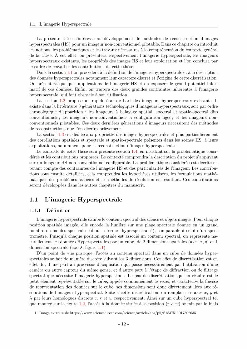
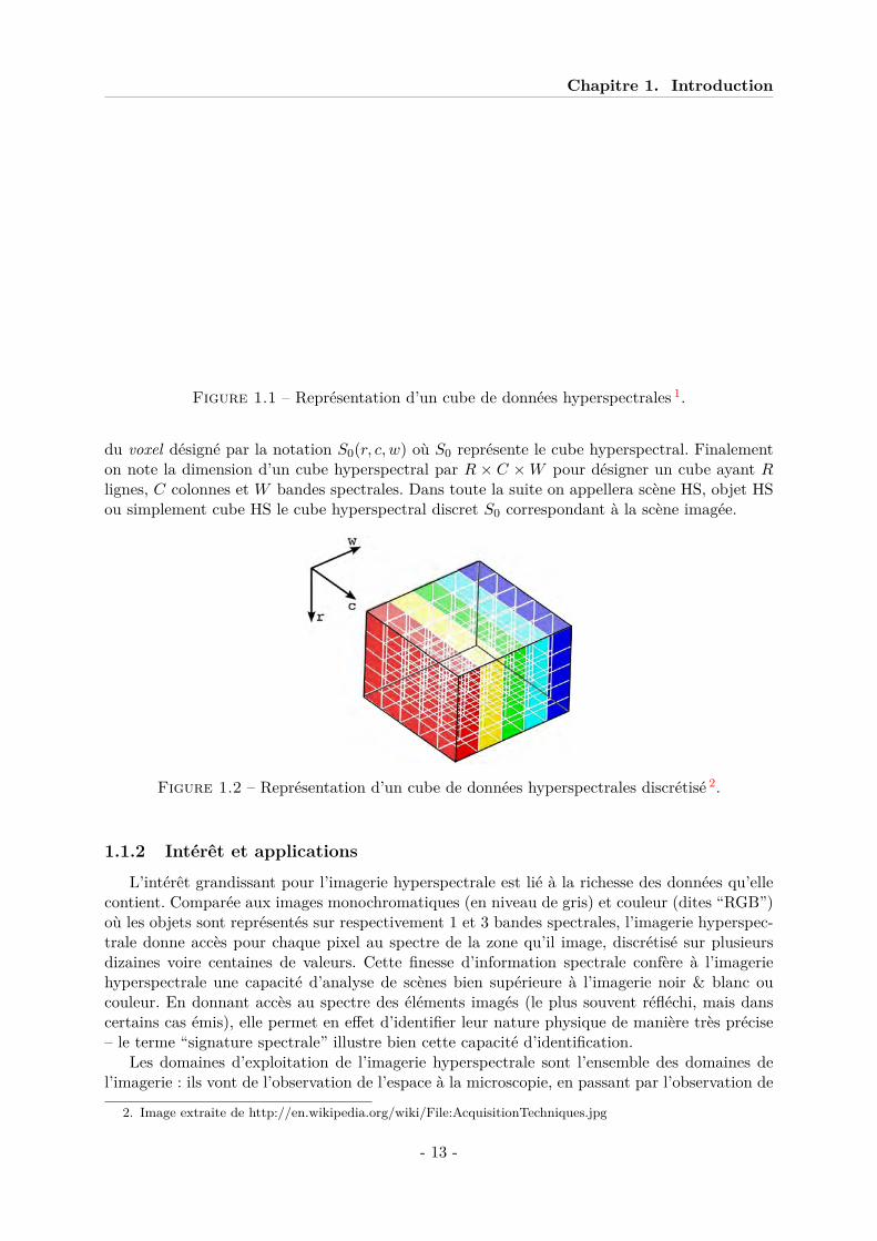
L’imagerie hyperspectrale exhibe le contenu spectral des scènes et objets imagés. Pour chaqueposition spatiale imagée, elle encode la lumière sur une plage spectrale donnée en un grandnombre de bandes spectrales (d’où le terme “hyperspectrale”), comparable à celui d’un spec-tromètre. Puisqu’à chaque position spatiale est associé un contenu spectral, on représente na-turellement les données Hyperspectrales par un cube, de 2 dimensions spatiales (axes x, y) et 1dimension spectrale (axe λ, figure 1.1).
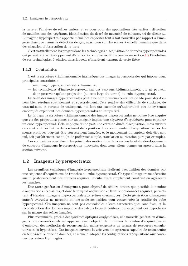
D’un point de vue pratique, l’accès au contenu spectral dans un cube de données hyper-spectrales se fait de manière discrète suivant les 3 dimensions. Cet effet de discrétisation est eneffet du, d’une part au processus d’acquisition qui passe nécessairement par l’utilisation d’unecaméra ou autre capteur du même genre, et d’autre part à l’étape de diffraction ou de filtragespectral que nécessite l’imagerie hyperspectrale. Le pas de discrétisation qui en résulte est lepetit élément représentable sur le cube, appelé communément le voxel, et caractérise la finessede représentation des données sur le cube, ses dimensions sont donc directement liées aux ré-solutions de l’imageur hyperspectral. Suite à cette discrétisation, on remplace les axes x, y etλ par leurs homologues discrets c, r et w respectivement. Ainsi sur un cube hyperspectral telque montré sur la figure 1.2, l’accès à la donnée située à la position (r, c, w) se fait par le biais
1. Image extraite de https://www.sciencedirect.com/science/article/abs/pii/S1537511017302635
- 12 -
Chapitre 1. Introduction
Figure 1.1 – Représentation d’un cube de données hyperspectrales 1.
du voxel désigné par la notation S0(r, c, w) où S0 représente le cube hyperspectral. Finalementon note la dimension d’un cube hyperspectral par R × C ×W pour désigner un cube ayant Rlignes, C colonnes et W bandes spectrales. Dans toute la suite on appellera scène HS, objet HSou simplement cube HS le cube hyperspectral discret S0 correspondant à la scène imagée.
Figure 1.2 – Représentation d’un cube de données hyperspectrales discrétisé 2.
1.1.2 Intérêt et applications
L’intérêt grandissant pour l’imagerie hyperspectrale est lié à la richesse des données qu’ellecontient. Comparée aux images monochromatiques (en niveau de gris) et couleur (dites “RGB”)où les objets sont représentés sur respectivement 1 et 3 bandes spectrales, l’imagerie hyperspec-trale donne accès pour chaque pixel au spectre de la zone qu’il image, discrétisé sur plusieursdizaines voire centaines de valeurs. Cette finesse d’information spectrale confère à l’imageriehyperspectrale une capacité d’analyse de scènes bien supérieure à l’imagerie noir & blanc oucouleur. En donnant accès au spectre des éléments imagés (le plus souvent réfléchi, mais danscertains cas émis), elle permet en effet d’identifier leur nature physique de manière très précise– le terme “signature spectrale” illustre bien cette capacité d’identification.
Les domaines d’exploitation de l’imagerie hyperspectrale sont l’ensemble des domaines del’imagerie : ils vont de l’observation de l’espace à la microscopie, en passant par l’observation de
2. Image extraite de http://en.wikipedia.org/wiki/File:AcquisitionTechniques.jpg
- 13 -
1.2. Imageurs hyperspectraux
la terre et l’analyse de scènes variées, et ce pour pour des applications très variées : détectionde maladies sur des végétaux, identification du degré de maturité de cultures, tri de déchets...L’imagerie hyperspectrale apporte même des capacités tout à fait nouvelles par rapport à l’ima-gerie classique : ainsi la détection de gaz, aussi bien sur des scènes à échelle humaine que dansdes situation d’observation de la terre.
C’est naturellement les progrès dans les technologies d’acquisition de données hyperspectralesqui permettent le développement d’applications nouvelles. Nous verrons en section 1.2 l’évolutionde ces technologies, évolution dans laquelle s’inscrivent travaux de cette thèse.
1.1.3 Contraintes
C’est la structure tridimensionnelle intrinsèque des images hyperspectrales qui impose deuxprincipales contraintes :
— une image hyperspectrale est volumineuse,— les technologies d’imagerie reposent sur des capteurs bidimensionnels, qui ne peuvent
donc percevoir qu’une projection (au sens large du terme) du cube hyperspectral.La taille des images hyperspectrales peut atteindre plusieurs centaines de Mo pour des don-
nées bien résolues spatialement et spectralement. Cela soulève des difficultés de stockage, detransmission, et surtout de traitement, qui font par exemple qu’aujourd’hui peu de systèmesembarqués exploitent des données hyperspectrales en temps réel.
Le fait que la structure tridimensionnelle des images hyperspectrales ne puisse être acquiseque via des projections planes sur un imageur impose une séquence d’acquisitions pour capturerun cube hyperspectral. Cela implique d’une part une certaine durée d’acquisition, mais surtoutcela contraint l’évolution de la scène et de la position du capteur pendant l’acquisition : seules desscènes statiques peuvent être correctement imagées, et le mouvement du capteur doit être soitnul, soit parfaitement connu (et de préférence simple, translation ou rotation pure par exemple).
Ces contraintes constituent les principales motivations de la recherche et du développementde concepts d’imageurs hyperspectraux innovants, dont nous allons donner un aperçu dans lasection suivante.
1.2 Imageurs hyperspectraux
Les premières techniques d’imagerie hyperspectrale réalisent l’acquisition des données parune séquence d’acquisitions de tranches du cube hyperspectral. Ce type d’imageurs ne nécessiteaucun post-traitement des données acquises, le cube étant simplement construit en agrégeantles tranches.
Une autre génération d’imageurs a pour objectif de réduire autant que possible le nombred’acquisitions nécessaires, et donc le temps d’acquisition et la taille des données acquises, permet-tant d’étendre l’imagerie hyperspectrale aux scènes dynamiques. Cette génération d’imageursappelés snapshot ne nécessite qu’une seule acquisition pour reconstruire la totalité du cubehyperspectral. Ces imageurs ne sont pas contrôlables : leurs caractéristiques sont fixes, et lareconstruction des données implique des calculs longs et coûteux, qui exploitent des hypothèsessur la nature des scènes imagées.
Plus récemment, grâce à des systèmes optiques configurables, une nouvelle génération d’ima-geurs non conventionnels est apparue, avec l’objectif de minimiser le nombre d’acquisitions etd’employer des méthodes de reconstruction moins exigeantes en termes de ressources calcula-toires et en hypothèses. Ces imageurs ouvrent la voie vers des systèmes capables de reconstruireen temps-réel le cube de données, et même d’adapter les configurations d’acquisitions aux conte-nus des scènes HS imagées.
- 14 -
Chapitre 1. Introduction
Nous présentons dans cette partie quelques exemples d’imageurs de chacune de ces famillesd’imageurs, conventionnels, non conventionnels figés et non conventionnels configurables, endécrivant brièvement leur système optique/physique ainsi que les méthodes de traitement dedonnées associées.
1.2.1 Imageurs conventionnels à balayage
Les imageurs conventionnels ne nécessitent pas de traitement pour former le cube HS de lascène imagée. En effet l’acquisition du cube HS par cette famille d’imageurs s’opère dans unpremier temps par acquisitions successives de “tranches” du cube HS, le cube étant formé parsimple compilation des projections.
Balayage spatial "Push-broom"
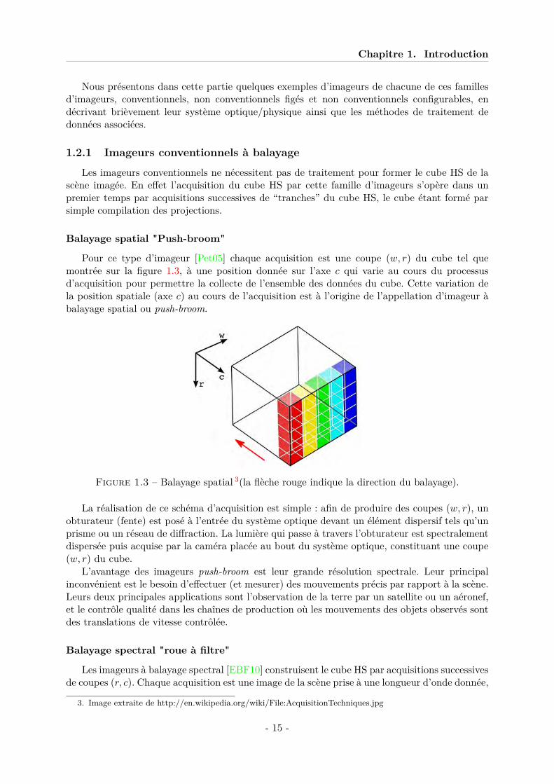
Pour ce type d’imageur [Pet05] chaque acquisition est une coupe (w, r) du cube tel quemontrée sur la figure 1.3, à une position donnée sur l’axe c qui varie au cours du processusd’acquisition pour permettre la collecte de l’ensemble des données du cube. Cette variation dela position spatiale (axe c) au cours de l’acquisition est à l’origine de l’appellation d’imageur àbalayage spatial ou push-broom.
Figure 1.3 – Balayage spatial 3(la flèche rouge indique la direction du balayage).
La réalisation de ce schéma d’acquisition est simple : afin de produire des coupes (w, r), unobturateur (fente) est posé à l’entrée du système optique devant un élément dispersif tels qu’unprisme ou un réseau de diffraction. La lumière qui passe à travers l’obturateur est spectralementdispersée puis acquise par la caméra placée au bout du système optique, constituant une coupe(w, r) du cube.
L’avantage des imageurs push-broom est leur grande résolution spectrale. Leur principalinconvénient est le besoin d’effectuer (et mesurer) des mouvements précis par rapport à la scène.Leurs deux principales applications sont l’observation de la terre par un satellite ou un aéronef,et le contrôle qualité dans les chaînes de production où les mouvements des objets observés sontdes translations de vitesse contrôlée.
Balayage spectral "roue à filtre"
Les imageurs à balayage spectral [EBF10] construisent le cube HS par acquisitions successivesde coupes (r, c). Chaque acquisition est une image de la scène prise à une longueur d’onde donnée,
3. Image extraite de http://en.wikipedia.org/wiki/File:AcquisitionTechniques.jpg
- 15 -
1.2. Imageurs hyperspectraux
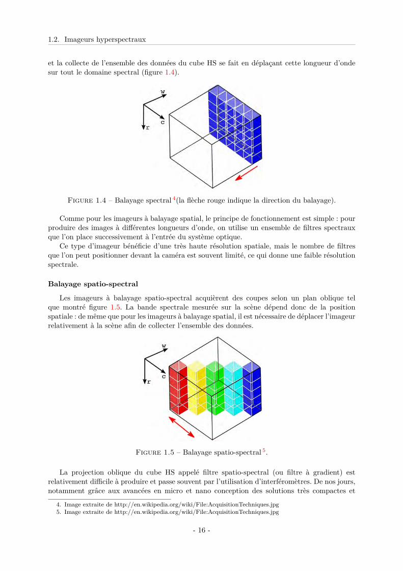
et la collecte de l’ensemble des données du cube HS se fait en déplaçant cette longueur d’ondesur tout le domaine spectral (figure 1.4).
Figure 1.4 – Balayage spectral 4(la flèche rouge indique la direction du balayage).
Comme pour les imageurs à balayage spatial, le principe de fonctionnement est simple : pourproduire des images à différentes longueurs d’onde, on utilise un ensemble de filtres spectrauxque l’on place successivement à l’entrée du système optique.
Ce type d’imageur bénéficie d’une très haute résolution spatiale, mais le nombre de filtresque l’on peut positionner devant la caméra est souvent limité, ce qui donne une faible résolutionspectrale.
Balayage spatio-spectral
Les imageurs à balayage spatio-spectral acquièrent des coupes selon un plan oblique telque montré figure 1.5. La bande spectrale mesurée sur la scène dépend donc de la positionspatiale : de même que pour les imageurs à balayage spatial, il est nécessaire de déplacer l’imageurrelativement à la scène afin de collecter l’ensemble des données.
Figure 1.5 – Balayage spatio-spectral 5.
La projection oblique du cube HS appelé filtre spatio-spectral (ou filtre à gradient) estrelativement difficile à produire et passe souvent par l’utilisation d’interféromètres. De nos jours,notamment grâce aux avancées en micro et nano conception des solutions très compactes et
4. Image extraite de http://en.wikipedia.org/wiki/File:AcquisitionTechniques.jpg5. Image extraite de http://en.wikipedia.org/wiki/File:AcquisitionTechniques.jpg
- 16 -
Chapitre 1. Introduction
intégrées sur silicium ont été développées, ainsi l’imageur CMOS [LGG+14] à interféromètreFabry-Pérot.
Les imageurs à balayage spatio-spectral ont une très bonne résolution spatio-spectrale. Deplus l’intégration sur puces CMOS facilite grandement leur utilisation. Cependant l’inconvénientprincipal de ce type d’imageur à balayage est la sensibilité aux mouvements relatifs de la scèneimagée.
Conclusion
Les imageurs à projection conventionnelle ou à balayage sont très simples d’utilisation carils ne nécessitent pas d’algorithme pour construire le cube HS de la scène imagée. La complexitédes systèmes optiques utilisés est peu à modérément complexe et facilite leur conception etcalibration. Les résolutions spatiales et spectrales atteintes sont généralement bonnes surtoutavec les imageurs à balayage spatio-spectral qui offrent un très bon compris entre résolutionspatiale et spectrale.
Bien qu’ils répondent aux besoins de l’imagerie hyperspectrale, la famille des imageurs àbalayage souffre cependant de temps d’acquisition longs à cause du balayage. Ces contraintesd’utilisation les rendent inutilisables pour de nombreuses applications.
1.2.2 Imageurs non conventionnels snapshot figés
Pour ces imageurs, l’objectif en effet est de reconstruire le cube HS à partir d’une seuleacquisition de l’imageur – d’où leur qualification de snapshot. Puisque la taille des donnéesacquises est très inférieure à celle du cube HS, la construction parfaite du cube à partir de cesdonnées est a priori impossible, aussi ces imageurs visent à définir une acquisition qui contientle plus d’informations possibles. Ensuite, le cube HS est reconstruit grâce à des algorithmes quiexploitent des hypothèses sur la nature et les caractéristiques de la scène imagée.
Il existe dans la littérature de nombreux imageurs non conventionnels snapshot figés, aussinous n’en décrivons ici que quatre, de nature assez différente, classés ainsi :
— imageur à dispersion simple,— imageur à dispersion multiple tomographique,— imageur à dispersion avec masque spatial,— imageur sans dispersion, avec multiplexage dans le domaine de Fourier.
Imageur à dispersion simple
Pour ce type d’imageurs le cube HS est dispersé une fois puis le résultat est directementacquis par une caméra.
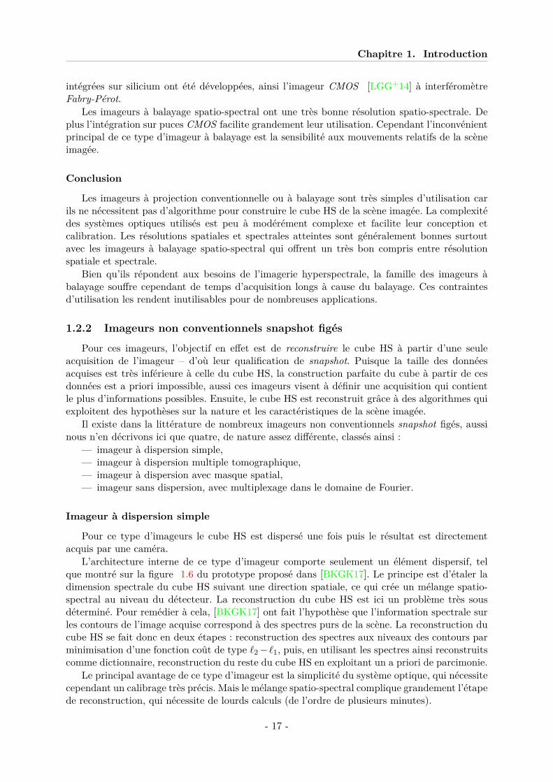
L’architecture interne de ce type d’imageur comporte seulement un élément dispersif, telque montré sur la figure 1.6 du prototype proposé dans [BKGK17]. Le principe est d’étaler ladimension spectrale du cube HS suivant une direction spatiale, ce qui crée un mélange spatio-spectral au niveau du détecteur. La reconstruction du cube HS est ici un problème très sousdéterminé. Pour remédier à cela, [BKGK17] ont fait l’hypothèse que l’information spectrale surles contours de l’image acquise correspond à des spectres purs de la scène. La reconstruction ducube HS se fait donc en deux étapes : reconstruction des spectres aux niveaux des contours parminimisation d’une fonction coût de type `2− `1, puis, en utilisant les spectres ainsi reconstruitscomme dictionnaire, reconstruction du reste du cube HS en exploitant un a priori de parcimonie.
Le principal avantage de ce type d’imageur est la simplicité du système optique, qui nécessitecependant un calibrage très précis. Mais le mélange spatio-spectral complique grandement l’étapede reconstruction, qui nécessite de lourds calculs (de l’ordre de plusieurs minutes).
- 17 -
1.2. Imageurs hyperspectraux
Lentille
Figure 1.6 – Schéma du principe optique d’un imageur à dispersion simple [BKGK17]
Imageur à dispersion multiple
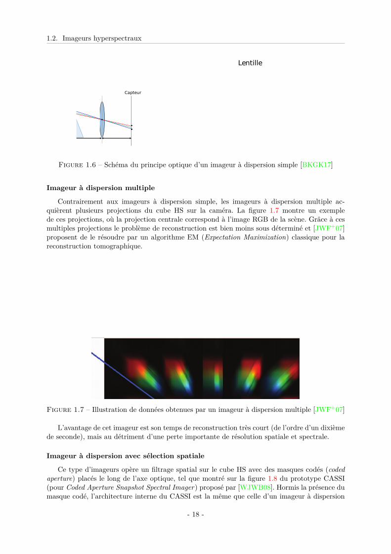
Contrairement aux imageurs à dispersion simple, les imageurs à dispersion multiple ac-quièrent plusieurs projections du cube HS sur la caméra. La figure 1.7 montre un exemplede ces projections, où la projection centrale correspond à l’image RGB de la scène. Grâce à cesmultiples projections le problème de reconstruction est bien moins sous déterminé et [JWF+07]proposent de le résoudre par un algorithme EM (Expectation Maximization) classique pour lareconstruction tomographique.
Figure 1.7 – Illustration de données obtenues par un imageur à dispersion multiple [JWF+07]
L’avantage de cet imageur est son temps de reconstruction très court (de l’ordre d’un dixièmede seconde), mais au détriment d’une perte importante de résolution spatiale et spectrale.
Imageur à dispersion avec sélection spatiale
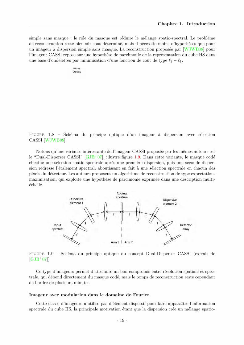
Ce type d’imageurs opère un filtrage spatial sur le cube HS avec des masques codés (codedaperture) placés le long de l’axe optique, tel que montré sur la figure 1.8 du prototype CASSI(pour Coded Aperture Snapshot Spectral Imager) proposé par [WJWB08]. Hormis la présence dumasque codé, l’architecture interne du CASSI est la même que celle d’un imageur à dispersion
- 18 -
Chapitre 1. Introduction
simple sans masque : le rôle du masque est réduire le mélange spatio-spectral. Le problèmede reconstruction reste bien sûr sous déterminé, mais il nécessite moins d’hypothèses que pourun imageur à dispersion simple sans masque. La reconstruction proposée par [WJWB08] pourl’imageur CASSI repose sur une hypothèse de parcimonie de la représentation du cube HS dansune base d’ondelettes par minimisation d’une fonction de coût de type `2 − `1.
Figure 1.8 – Schéma du principe optique d’un imageur à dispersion avec sélectionCASSI [WJWB08]
Notons qu’une variante intéressante de l’imageur CASSI proposée par les mêmes auteurs estle “Dual-Disperser CASSI” [GJB+07], illustré figure 1.9. Dans cette variante, le masque codéeffectue une sélection spatio-spectrale après une première dispersion, puis une seconde disper-sion redresse l’étalement spectral, aboutissant en fait à une sélection spectrale en chacun despixels du détecteur. Les auteurs proposent un algorithme de reconstruction de type expectation-maximization, qui exploite une hypothèse de parcimonie exprimée dans une description multi-échelle.
Figure 1.9 – Schéma du principe optique du concept Dual-Disperser CASSI (extrait de[GJB+07])
Ce type d’imageurs permet d’atteindre un bon compromis entre résolution spatiale et spec-trale, qui dépend directement du masque codé, mais le temps de reconstruction reste cependantde l’ordre de plusieurs minutes.
Imageur avec modulation dans le domaine de Fourier
Cette classe d’imageurs n’utilise pas d’élément dispersif pour faire apparaître l’informationspectrale du cube HS, la principale motivation étant que la dispersion crée un mélange spatio-
- 19 -
1.2. Imageurs hyperspectraux
spectral difficile à traiter. Les imageurs sans dispersion modulent l’information spectrale dansun domaine symbolique de sorte qu’il n’y a pas de recouvrement entre les spectres modulés, lareconstruction s’opérant alors par simple démodulation.
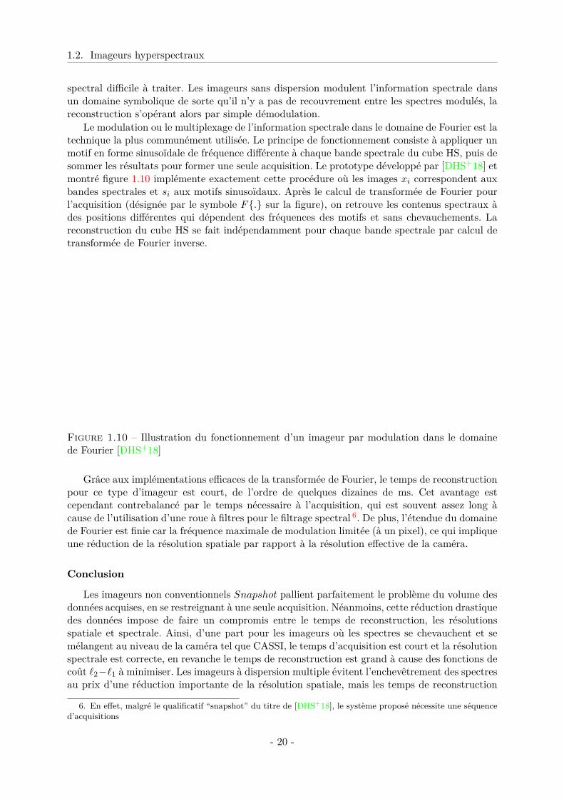
Le modulation ou le multiplexage de l’information spectrale dans le domaine de Fourier est latechnique la plus communément utilisée. Le principe de fonctionnement consiste à appliquer unmotif en forme sinusoïdale de fréquence différente à chaque bande spectrale du cube HS, puis desommer les résultats pour former une seule acquisition. Le prototype développé par [DHS+18] etmontré figure 1.10 implémente exactement cette procédure où les images xi correspondent auxbandes spectrales et si aux motifs sinusoïdaux. Après le calcul de transformée de Fourier pourl’acquisition (désignée par le symbole F. sur la figure), on retrouve les contenus spectraux àdes positions différentes qui dépendent des fréquences des motifs et sans chevauchements. Lareconstruction du cube HS se fait indépendamment pour chaque bande spectrale par calcul detransformée de Fourier inverse.
Figure 1.10 – Illustration du fonctionnement d’un imageur par modulation dans le domainede Fourier [DHS+18]
Grâce aux implémentations efficaces de la transformée de Fourier, le temps de reconstructionpour ce type d’imageur est court, de l’ordre de quelques dizaines de ms. Cet avantage estcependant contrebalancé par le temps nécessaire à l’acquisition, qui est souvent assez long àcause de l’utilisation d’une roue à filtres pour le filtrage spectral 6. De plus, l’étendue du domainede Fourier est finie car la fréquence maximale de modulation limitée (à un pixel), ce qui impliqueune réduction de la résolution spatiale par rapport à la résolution effective de la caméra.
Conclusion
Les imageurs non conventionnels Snapshot pallient parfaitement le problème du volume desdonnées acquises, en se restreignant à une seule acquisition. Néanmoins, cette réduction drastiquedes données impose de faire un compromis entre le temps de reconstruction, les résolutionsspatiale et spectrale. Ainsi, d’une part pour les imageurs où les spectres se chevauchent et semélangent au niveau de la caméra tel que CASSI, le temps d’acquisition est court et la résolutionspectrale est correcte, en revanche le temps de reconstruction est grand à cause des fonctions decoût `2−`1 à minimiser. Les imageurs à dispersion multiple évitent l’enchevêtrement des spectresau prix d’une réduction importante de la résolution spatiale, mais les temps de reconstruction
6. En effet, malgré le qualificatif “snapshot” du titre de [DHS+18], le système proposé nécessite une séquenced’acquisitions
- 20 -
Chapitre 1. Introduction
et d’acquisition sont très courts. Finalement, pour atteindre un temps de reconstruction courtet une résolution spatiale correcte, les imageurs à modulation sacrifient le temps d’acquisitionqui est long.
La restriction à une seule acquisition a été un choix très ambitieux qui impose des compromisdifficiles et peu pratiques entre le temps et la qualité de la reconstruction du cube HS. Lagénération d’imageurs qui succédera à celle-ci va permettre relâcher cette contrainte d’acquisitionunique, avec l’objectif d’atteindre des compromis plus intéressants.
1.2.3 Imageurs non conventionnels configurables
Le développement des imageurs non conventionnels configurables a été fortement influencépar les imageurs snapshot figés à dispersion simple et ouverture codée de type CASSI. L’objectifest de profiter des avantages de l’architecture CASSI en termes de temps d’acquisition et derésolution spatiale, et d’accélérer l’étape de reconstruction par ajout de données (acquisitionssupplémentaires) grâce à des algorithmes plus rapides et des hypothèses plus simples.
Sur CASSI, le cube HS est dans premier temps dispersé puis filtré par le masque codéavant d’atteindre la caméra et de former la projection souhaitée. Ainsi le modèle du masquecodé définit entièrement la projection, et modifier le masque modifie la projection. L’originede la conception de ces imageurs non conventionnels configurables est le développement detechnologies de masques codés configurables : DMD (Digital micromirror device) ou LCOS(Liquid crystal on silicon), qui permettent de modifier très rapidement les projections opéréespar le système.
Deux types de filtrage ont été adoptés : le filtrage spatial et le filtrage spatio-spectral. Nousdécrivons ci-dessous deux imageurs correspondant à ces deux types de filtrage.
Imageur à filtrage spatial configurable de type CASSI
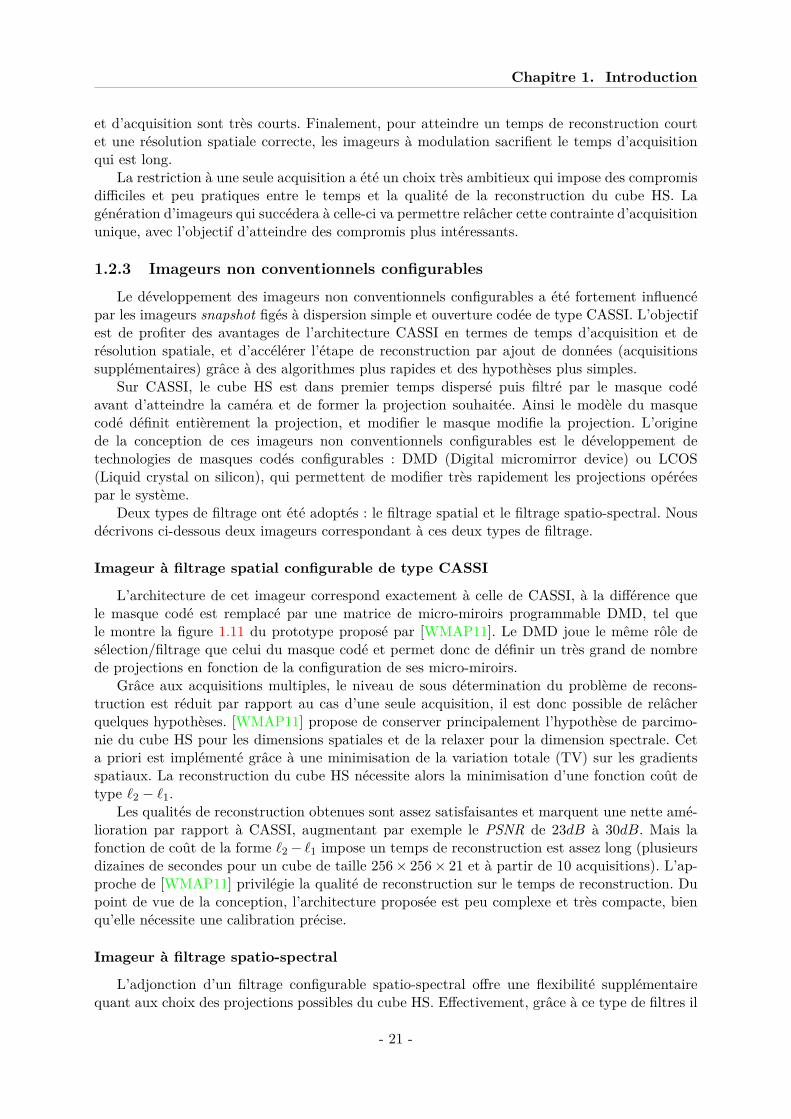
L’architecture de cet imageur correspond exactement à celle de CASSI, à la différence quele masque codé est remplacé par une matrice de micro-miroirs programmable DMD, tel quele montre la figure 1.11 du prototype proposé par [WMAP11]. Le DMD joue le même rôle desélection/filtrage que celui du masque codé et permet donc de définir un très grand de nombrede projections en fonction de la configuration de ses micro-miroirs.
Grâce aux acquisitions multiples, le niveau de sous détermination du problème de recons-truction est réduit par rapport au cas d’une seule acquisition, il est donc possible de relâcherquelques hypothèses. [WMAP11] propose de conserver principalement l’hypothèse de parcimo-nie du cube HS pour les dimensions spatiales et de la relaxer pour la dimension spectrale. Ceta priori est implémenté grâce à une minimisation de la variation totale (TV) sur les gradientsspatiaux. La reconstruction du cube HS nécessite alors la minimisation d’une fonction coût detype `2 − `1.
Les qualités de reconstruction obtenues sont assez satisfaisantes et marquent une nette amé-lioration par rapport à CASSI, augmentant par exemple le PSNR de 23dB à 30dB. Mais lafonction de coût de la forme `2− `1 impose un temps de reconstruction est assez long (plusieursdizaines de secondes pour un cube de taille 256× 256× 21 et à partir de 10 acquisitions). L’ap-proche de [WMAP11] privilégie la qualité de reconstruction sur le temps de reconstruction. Dupoint de vue de la conception, l’architecture proposée est peu complexe et très compacte, bienqu’elle nécessite une calibration précise.
Imageur à filtrage spatio-spectral
L’adjonction d’un filtrage configurable spatio-spectral offre une flexibilité supplémentairequant aux choix des projections possibles du cube HS. Effectivement, grâce à ce type de filtres il
- 21 -
1.2. Imageurs hyperspectraux
Figure 1.11 – Schéma du principe optique d’un imageur à filtrage spatial configurable de typeCASSI [WMAP11]
est possible de choisir des projections qui privilégient la préservation de l’information spectrale,ou de l’information spatiale, avec de plus la possibilité de faire un compromis entre ces différentesinformations. Le développement de ce type d’imageurs a été possible grâce aux filtres spectrauxoptroniques tel que les filtres à cristaux liquides LCOS dont le temps de rafraîchissement esttrès court.
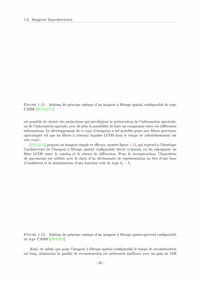
[LWLD14] propose un imageur simple et efficace, montré figure 1.12, qui reprend à l’identiquel’architecture de l’imageur à filtrage spatial configurable décrit ci-dessus, en lui adjoignant unfiltre LCOS entre la caméra et le réseau de diffraction. Pour la reconstruction, l’hypothèsede parcimonie est utilisée avec le choix d’un dictionnaire de représentation au lieu d’une based’ondelettes et la minimisation d’une fonction coût de type `2 − `1.
Figure 1.12 – Schéma du principe optique d’un imageur à filtrage spatio-spectral configurablede type CASSI [LWLD14]
Ainsi, de même que pour l’imageur à filtrage spatial configurable le temps de reconstructionest long, néanmoins la qualité de reconstruction est nettement meilleure avec un gain de 7dB
- 22 -
Chapitre 1. Introduction
sur le PSNR. Les configurations du LCOS sont choisies de façon à améliorer le rapport signalsur bruit des acquisitions et la qualité du mélange spatio-spectral.
Conclusion
Le développement des imageurs configurables a été fortement influencé par l’architecturede l’imageur snapshot figé CASSI, qui a pu être transformé en système configurable grâce auxtechnologies telles que les DMD ou les LCOS. Les acquisitions multiples permettent de relaxer lesfortes hypothèses nécessaires à CASSI, et ainsi accélérer l’étape de reconstruction. Néanmoins,la plupart des méthodes de reconstruction développées pour ces systèmes privilégient la qualitédes données reconstruites sur le temps de reconstruction.
1.2.4 Synthèse
Ce rapide aperçu des technologies d’acquisition d’images hyperspectrales montre qu’entre lessystèmes d’acquisition classiques qui collectent l’ensemble des données au prix de nombreusesacquisitions et les systèmes qui reconstruisent une estimée des données à partir d’une seuleacquisition mais au prix de calculs lourds, ce sont les systèmes configurables qui permettent decontrôler le compromis entre la quantité de données acquises et le temps de reconstruction.
En ce qui concerne les techniques de reconstruction à partir de données incomplètes, nousavons vu qu’elles exploitent différentes hypothèses sur la nature des scènes observées. La sectionsuivante étudie la nature des scènes hyperspectrales, qui va permettre de formuler de telleshypothèses et la façon dont ces hypothèses peuvent être prises en compte dans les applicationset plus particulièrement pour la reconstruction.
1.3 Propriétés des scènes hyperspectrales
1.3.1 Présentation des corrélations
Le terme de corrélation est employé pour décrire une relation ou dépendance (causale ounon-causale) entre deux objets, événements ou actions. On parle donc de corrélation temporelleentre deux événements A et B pour indiquer une relation causale (B est la conséquence de A)ou bien non-causale (A et B sont liés à un événement commun). En traitement d’image, pourdes applications tels que la compression, le débruitage ou encore la restauration, on s’intéresseaux corrélations entre les pixels qui forment l’image. Pour ce faire et selon la nature de l’imagetraitée (panchromatique, RGB, multispectrales ou hyperspectrales), on définit trois types decorrélations :
— la corrélation spatiale s’intéresse aux pixels voisins spatialement ;— la corrélation spectrale s’intéresse aux pixels voisins spectralement ;— la corrélation spatio-spectrale s’intéresse aux pixels voisins conjointement suivant les
dimensions spatiales et spectrale.Les scènes naturelles sont fortement corrélées ce qui se manifeste visuellement par la présence
d’objets, structures, textures et couleurs redondants [PL03]. Ce constat a d’abord été étudié pourson rôle dans la perception humaine par la communauté des sciences cognitives [SLD82, Bad97],il est ensuite devenu un axe majeur de recherche en traitement d’images. L’une des premièresapplications fut naturellement la compression d’image [DJL92] qui exploite directement la pré-sence de corrélation pour réduire le poids de l’image (au sens quantité d’information stockée)sans en altérer le contenu. Le succès rapide de cette première application permit de découvrir legrand potentiel informatif des corrélations, et depuis la recherche dans ce domaine n’a cessé dese développer.
- 23 -
1.3. Propriétés des scènes hyperspectrales
Cependant, si d’un coté la mise en évidence des corrélations est relativement facile grâcenotamment à la covariance statistique, l’exploitation des corrélations quant à elle est complexe.Il a donc été nécessaire de développer de nouveaux outils à même de prendre en compte cetteinformation.
L’analyse discriminante tels que l’ACP (analyse en composantes principales), l’ACI (analyseen composantes indépendantes), la LDA (Analyse discriminante linéaire) a notamment joué unrôle important dans la compréhension et la modélisation des corrélations [SLD82, HBS92, Bad97,LWS00]. Parallèlement et de manière indépendante, l’analyse harmonique en pleine émergencealors avec l’apparition des ondelettes [LM86, Dau88] et plus particulièrement de la transforméeen ondelettes discrètes orthogonale DWT (discrete wavelet transform) [Dau92] a constitué uneautre voie de recherche très prometteuse. Par la suite, ces deux approches, qui ont d’ailleurspermis d’arriver à des conclusions similaires [HBS92, CZ11], ont été utilisées conjointementpour atteindre des modélisations plus fines des corrélations [RB05, WF07].
Les outils et méthodes d’exploitation des corrélations sont en général spécifiques aux carac-téristiques de la modalité d’acquisition (imageur), telles que la résolution spatiale et spectrale etla taille de l’acquisition. Ainsi, l’avènement de l’image hyperspectrale a nécessité le développe-ment de nouveaux outils pour répondre à ces contraintes (volume de données) et particularités(résolutions spatiale et spectrale et forte corrélation spatio-spectrale). Cela fut premièrement enadaptant les méthodes existantes [CZ11] puis grâce à des outils propres à l’imagerie hyperspec-trale [RBB08] capables de tirer avantage de la corrélation spatio-spectrale en particulier.
1.3.2 L’exploitation des corrélations spatio-spectrales
Dans cette partie, on présentera dans un premier temps une brève littérature dédiée à l’ex-ploitation de la corrélation spatiale et spectrale pour les images en niveaux de gris, couleur(RGB) et multispectrale. Puis on exposera plus en détails les méthodes dédiées spécialement àl’imagerie hyperspectrale. Pour les besoins de cette partie on citera principalement la littératureliée à la compression d’images pour son besoin évident d’exploitation des corrélations.
Corrélation spatiale
Les corrélations spatiales présente dans les images (niveaux de gris, RGB, Mutlispectrales) engénéral ont été utilisées depuis des décennies et avant l’avènement de l’imagerie hyperspectrale.Chronologiquement, la corrélation spatiale a d’abord été étudiée et exploitée pour les imagesen niveaux de gris grâce au développement de la DCT (discrete cosinus transform) pour lacompression JPEG [Int94]. L’objectif de la transformation DCT est de décomposer l’image dansun autre domaine de représentation où les corrélations spatiales sont plus concentrées. De cefait, le nombre de coefficients nécessaire à la représentation est très inférieur aux nombres depixels de l’image.
Néanmoins, pour JPEG, la DCT été appliqué par bloc (typiquement de 8 × 8 pixels), cequi compromettait le potentiel de compression, révélant d’éventuels effets de blocs. Ce principea alors été peu à peu délaissé pour l’utilisation des ondelettes (DWT) [LM86, Dau92] et del’analyse multi-résolution qui offrent de bien meilleures performances [GKG99] même pour lesimages de très haute résolution [DJL92].
Corrélation spectrale
Avec l’avènement de l’image couleur (RGB) on commença à s’intéresser à la corrélation spec-trale. L’approche adoptée été d’adapter les méthodes existantes pour les images en niveaux degris avec notamment JPEG2000 [Int00] et la DWT [ROM15]. L’idée était d’exploiter principa-lement la corrélation spatiale qui est très prépondérante par rapport à la corrélation spectrale à
- 24 -
Chapitre 1. Introduction
cause du faible nombre de bandes dans les images couleurs (3 bandes). La corrélation spectraleseule et en elle même n’était pas très intéressante. De plus, l’acquisition couleur se faisait avecdes filtres en mosaïque tel que Bayer et non avec des filtres dédiés pour chaque couleur [CT04].
Ce n’est qu’avec l’image multispectrale puis hyperspectrale que l’on chercha à exploiterréellement la corrélation spectrale, premièrement de manière disjointe de la corrélation spatialepuis simultanément (spatio-spectrale).
Corrélation spatio-spectrale
Jusqu’alors, la résolution spatiale pour les images RGB était considérablement supérieure àla résolution spectrale, ainsi le principal de l’information nécessaire au traitement des imagesprovenait de la dimension spatiale. Pour l’imagerie multispectrale et hyperspectrale les dimen-sions spatiale et spectrale sont du même ordre de grandeur, il a donc été nécessaire de revoirces méthodes et outils pour prendre en compte simultanément des corrélations spatiale etspectrale par l’exploitation de la corrélation spatio-spectrale.
Les méthodes de compression basées sur la DWT ont été massivement utilisées et adaptéespour les images HS, et ce pour les excellentes performances en terme de qualité et taux decompression qu’elle permet d’atteindre avec les images en niveaux de gris. Ainsi, l’algorithmeJPEG2000, initialement développé pour des images RGB (3 bandes) a été adapté pour sup-porter plusieurs dizaines de bandes spectrales [RFY05, PTMO06, KBM+06]. Typiquement, lastratégie était de coupler une méthode de compression spectrale à la DCT spatiale utilisée parJPEG au lieu de traiter indépendamment les bandes spectrales. La compression spectrale a éténotamment implémentée par l’utilisation d’une DCT et DWT spectrale [AMH95, TP06, FR06].En particulier, l’utilisation de la DWT spectrale a aboutit à la compression DWT-JPEG2000[Int00, TP06].
Ces méthodes nécessitent cependant de traiter l’image HS par bloc souvent de petite taille(8 × 8 pixels pour JPEG2000 et DWT-JPEG2000) et se restreignent donc à l’exploitation descorrélations locales ce qui réduit considérablement l’efficacité de la compression. Ce découpageest effectivement indispensable pour obtenir une compression significative avec la DCT et laDWT et en général en analyse harmonique.
Afin de remédier à ce problème, l’analyse harmonique a été substituée par des méthodesd’analyse discriminante déterministes ACP (analyse en composantes principales) ou statistiquesKLT (Karhunen-Loeve Transform). Cette substitution s’est avérée particulièrement intéressantevis-à-vis de la qualité et du taux de compression [DF07], ce qui favorisa le développementd’autres méthodes suivant ce schéma [ZFL08, DZYF09, CCTH11] et devint un important axede recherche.
Cela marqua alors un grand tournant dans l’exploitation des corrélations qui jusque là étaientutilisées en analyse harmonique de manière disjointes, la corrélation spatiale d’une part et spec-trale d’un autre ce qui compromettait considérablement l’efficacité de la compression [PR06].Effectivement, les méthodes discriminantes et l’ACP entre autres permettent quant à elles detenir compte simultanément des deux corrélations et donc de la corrélation spatio-spectrale. Ceciest d’ailleurs possible car les composantes principales produites ne sont pas nécessairement desbases harmoniques séparables telles que utilisés par la DCT et la DWT ou la FFT [CZ11].
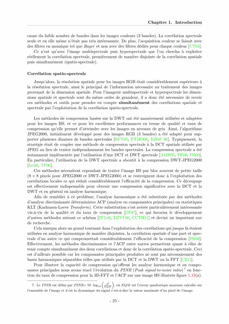
Pour illustrer la capacité de compression qu’offrent les analyse harmonique et en compo-santes principales nous avons tracé l’évolution du PSNR (Peak signal-to-noise ratio) 7 en fonc-tion du taux de compression pour la 3D-FFT et l’ACP sur une image HS illustrée figure 1.13(a).
7. Le PSNR est défini par PSNR= 10 · log10
(d2
EQM
), où EQM est l’erreur quadratique moyenne calculée sur
l’ensemble de l’image et d est la dynamique du signal c’est-à-dire la valeur maximale d’un pixel de l’image.
- 25 -
1.3. Propriétés des scènes hyperspectrales
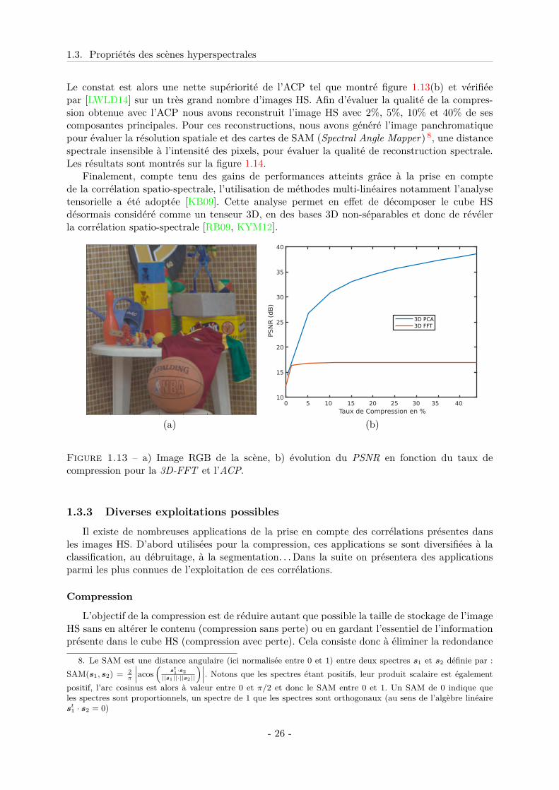
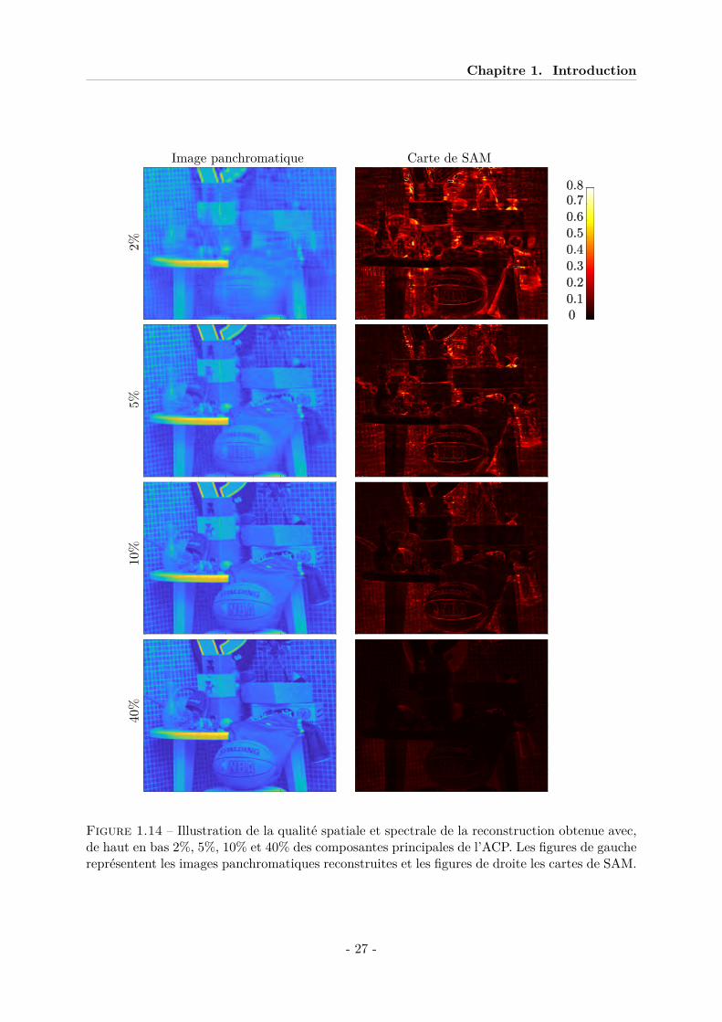
Le constat est alors une nette supériorité de l’ACP tel que montré figure 1.13(b) et vérifiéepar [LWLD14] sur un très grand nombre d’images HS. Afin d’évaluer la qualité de la compres-sion obtenue avec l’ACP nous avons reconstruit l’image HS avec 2%, 5%, 10% et 40% de sescomposantes principales. Pour ces reconstructions, nous avons généré l’image panchromatiquepour évaluer la résolution spatiale et des cartes de SAM (Spectral Angle Mapper) 8, une distancespectrale insensible à l’intensité des pixels, pour évaluer la qualité de reconstruction spectrale.Les résultats sont montrés sur la figure 1.14.
Finalement, compte tenu des gains de performances atteints grâce à la prise en comptede la corrélation spatio-spectrale, l’utilisation de méthodes multi-linéaires notamment l’analysetensorielle a été adoptée [KB09]. Cette analyse permet en effet de décomposer le cube HSdésormais considéré comme un tenseur 3D, en des bases 3D non-séparables et donc de révélerla corrélation spatio-spectrale [RB09, KYM12].
0 5 10 15 20 25 30 35 40Taux de Compression en %
10
15
20
25
30
35
40
PSN
R (d
B)
3D PCA3D FFT
(a) (b)
Figure 1.13 – a) Image RGB de la scène, b) évolution du PSNR en fonction du taux decompression pour la 3D-FFT et l’ACP.
1.3.3 Diverses exploitations possibles
Il existe de nombreuses applications de la prise en compte des corrélations présentes dansles images HS. D’abord utilisées pour la compression, ces applications se sont diversifiées à laclassification, au débruitage, à la segmentation. . . Dans la suite on présentera des applicationsparmi les plus connues de l’exploitation de ces corrélations.
Compression
L’objectif de la compression est de réduire autant que possible la taille de stockage de l’imageHS sans en altérer le contenu (compression sans perte) ou en gardant l’essentiel de l’informationprésente dans le cube HS (compression avec perte). Cela consiste donc à éliminer la redondance
8. Le SAM est une distance angulaire (ici normalisée entre 0 et 1) entre deux spectres s1 et s2 définie par :SAM(s1, s2) = 2
π
∣∣∣acos(
st1·s2
||s1||·||s2||
)∣∣∣. Notons que les spectres étant positifs, leur produit scalaire est égalementpositif, l’arc cosinus est alors à valeur entre 0 et π/2 et donc le SAM entre 0 et 1. Un SAM de 0 indique queles spectres sont proportionnels, un spectre de 1 que les spectres sont orthogonaux (au sens de l’algèbre linéairest1 · s2 = 0)
- 26 -
Chapitre 1. Introduction
Image panchromatique Carte de SAM
2%
00.10.20.30.40.5
0.8
0.60.7
00.10.20.30.40.5
0.8
0.60.7
5%10%
40%
Figure 1.14 – Illustration de la qualité spatiale et spectrale de la reconstruction obtenue avec,de haut en bas 2%, 5%, 10% et 40% des composantes principales de l’ACP. Les figures de gauchereprésentent les images panchromatiques reconstruites et les figures de droite les cartes de SAM.
- 27 -
1.3. Propriétés des scènes hyperspectrales
(information superflu) qui est caractérisée par la présence de fortes corrélations. La contrainteest donc de dé-corréler l’image HS au maximum tout en conservant l’information essentielle[KYM12, KBM+06, TP06].
Classification
Sur une image HS chaque position spatiale (pixel) possède une signature spectrale qui corres-pond simplement au spectre du matériau présent à cette position. Étant donné le grand nombrede bandes spectrales que comprend l’image HS, il est possible de différencier les matériaux entreeux bien qu’ils soient visuellement ressemblants. Pour la grande majorité des applications l’imageHS ne comprend qu’un petit nombre de classes de spectres alors que le nombre de pixels esttrès grand. Il y a donc une forte corrélation spectrale entre les pixels appartenant à la mêmeclasse et l’objectif de la classification est de segmenter convenablement l’image HS pour associerà chaque groupe de pixels une seule classe de spectre [MB04, RB09, LMM+16].
Débruitage et Inpainting
Les images HS sont souvent entachées de bruit lors de l’acquisition, à cause du processusd’acquisition (bruit de photon et thermique) ou à cause de facteurs extérieurs tels que les per-turbations atmosphériques. Le bruit a généralement pour effet de dé-corréler l’information HSet augmenter artificiellement la variabilité des spectres qui sont normalement et naturellementtrès corrèles. Le débruitage est typiquement implémenté en considérant que l’image débruitée estreprésentable par un petit nombre de composantes qui résident dans un sous-espace de l’imageHS bruitée [RBB08, GZZF14, LLF+16].
L’inpainting (remplissage de parties manquantes dans une image) adresse le même problèmeque le débruitage à la différence que l’altération n’est pas nécessairement aléatoire et est due,par exemple, à des pixels morts ou à des problèmes de lecture sur le capteur. Les méthodes dedébruitage servent parfois également pour l’inpainting, bien que certains solutions existent pourtenir compte spécifiquement de certaines altérations [BSFG09, LRS+18].
Super-résolution et pan-sharpening
À cause, des contraintes inhérentes à l’imagerie hyperspectrale il n’est bien souvent paspossible de faire l’acquisition d’images HS simultanément à très hautes résolutions spatialeset spectrale. Les imageurs HS conventionnels dégradent généralement une de ces résolutionspour pouvoir imager des scènes HS. L’objectif de la super-résolution est donc d’augmenter larésolution des données par post-traitement en tirant avantage des corrélations. Cela s’apparentedonc à une interpolation qui doit être menée correctement afin de ne pas créer d’artefact. Pource faire, des acquisitions de la même scène obtenues par d’autres voies sont utilisées pour guidercette interpolation. Notamment, l’approche la plus connue est le pan-sharpening où l’imagepanchromatique est utilisée (après recalage) pour augmenter la résolution spatiale de la scènemultispectrale ou hyperspectrale [FHC+20, ABS07, LZGY16, HZCF19].
1.3.4 Prise en compte de la corrélation spatio-spectrale pour la reconstruc-tion d’images hyperspectrales
Cette thèse portant sur la reconstruction d’images hyperspectrales à partir d’un faible nombrede projections du cube hyperspectral, nous nous focalisons ici sur les différentes approches utili-sées pour prendre en compte la corrélation spatio-spectrale pour une telle reconstruction, associéeà des imageurs non conventionnels. La particularité de cette reconstruction est qu’elle vise à esti-mer le cube HS complet à partir d’un faible nombre de données, typiquement beaucoup moins de
- 28 -
Chapitre 1. Introduction
données que d’inconnues. La régularisation du problème via la prise en compte des corrélationsspatio-spectrales est donc nécessaire car les problèmes de reconstruction sont sous-déterminés.On peut distinguer dans la littérature deux grandes classes de méthodes : celles s’appuyant surdes hypothèses de parcimonie et celles s’appuyant sur des hypothèses de type variation totale.Dans les deux cas, ces méthodes amènent à minimiser des critères, parfois non, convexes doncavec de possibles minima locaux, non lisses (non dérivables en certains points).
Depuis les travaux sur le Compressed sensing [CRT06, DET06, Don06], l’hypothèse de par-cimonie a été souvent exploiter pour la régularisation de problèmes inverses. L’hypothèse deparcimonie suppose que l’objet à reconstruire peut se représenter comme une combinaison li-néaires d’un faible nombre d’éléments (appelés atomes) pris dans une famille redondante (appeléedictionnaire). Une telle hypothèse a été exploitée sous diverses formes pour la reconstructiond’images HS, mais généralement en s’appuyant sur une base de représentation plutôt qu’unefamille redondante, ce qui s’explique par la grande dimension des espaces entrant en jeu. Dansce cadre, on peut trouver 3 déclinaisons de l’exploitation de la parcimonie, selon que cette baseest une base fixée a priori, construite par apprentissage a priori sur un ensemble de données, ouconstruite par apprentissage simultanément à la reconstruction.Un grand nombre de travaux ont exploité des base classiques, fixées a priori, ayant déjà montréleur efficacité pour la compression d’images telles que les bases DCT et DWT, prises individuel-lement ou conjointement [WJWB08, WMAP11, RAA14, DRA15, AdH16, GLM+17, WZM+18,DHS+18]. En particulier, une restriction à une base séparable 1D-DCT (spectrale) et 2D-DWT(spatiale) est très souvent utilisée.Certains auteurs ont proposé d’apprendre le dictionnaire à partir d’un certain nombre de cube HSpris comme exemple [LWLD14, LLWD14, WXG+15, CJN+17, XWL+17, TZS+20]. Notons quela plupart des travaux exploitent des dictionnaires de faible dimension en prenant des éléments(patch) petits spatialement (typiquement 8 × 8 pixels) Cette étape est généralement accompliepar décomposition en valeurs singulières [LWLD14], une alternative plus récente propose l’ex-ploitation d’un réseau de neurones auto-encodeur Auto-CNN [CJN+17].L’inconvénient majeur d’un tel apprentissage de dictionnaire est qu’il nécessite de disposer d’ungrand nombre de cube HS, semblables aux types de scènes observées. Afin de remédier à ceproblème, certains auteurs ont proposé d’apprendre le dictionnaire simultanément à la recons-truction (approche aveugle). Pour cela, des hypothèses générales peuvent être considérées, parexemple que le nombre de spectres présents dans le cube HS est faible [KMW+11]. De mêmedes modèles de dictionnaire de type gaussiennes [YTZ+15] ou mélange de gaussiennes (Gau-sian Mixture Model) [RKT+13] sont exploités. Un autre moyen de procéder sans modèle précisconsiste à apprendre un dictionnaire de tenseur en appliquant une PCA avec noyau reproduisant(KPCA) au cube HS reconstruit à chaque itération [YWL+15].
La régularisation par pénalisation de la variation totale (TV) [ROF92] consiste en pratiqueà pénaliser le critère de fidélité aux données par un terme linéaire (de type valeur absolue)en les gradients de l’image. Une telle régularisation va forcer les images a prendre des valeursproches dans les zones homogènes tout en autorisant des discontinuités au niveau des contours,sans connaître a priori la position des contours. Les zones homogènes étant principalement deszones spatiales, la TV a dans un premier temps été appliquée à chaque bande spectrale séparé-ment [KCWB10, WXS+16], puis couplées à des propriétés supplémentaires liées à la corrélationspectrale, de type parcimonie sur la DCT-1D [AdH16] ou de type TV [BKGK17]. D’autre moyensde prendre en compte la présence de zones spatio-spectrales homogènes sans la TV ont été propo-sés, tel qu’un partitionnement dyadique de l’image [GJB+07] ou des hypothèses de dépendancelinaire entre spectres d’une zone homogène [FZSS16] (a priori de rang minimal) sur des zonesde faibles dimensions (patches de 6× 6 pixels spatiaux).
Dans la plupart de ces travaux, le calcul de la solution se fait par minimisation d’un critère
- 29 -
1.4. Cadre de travail et contributions de cette thèse
quadratique de fidélité aux données, pénalisé par un terme prenant en compte la corrélationspatio-spectrale (parcimonie, variation totale,. . . ) Strictement parlant, l’hypothèse de parcimo-nie mène à un problème d’optimisation combinatoire qui est généralement relâché en une pé-nalisation `1 (en valeur absolue) [CJN+17, LLWD14, LWLD14, TZS+20] ou en exploitant desalgorithmes gloutons(OMP, Orthogonal Maching Pursuit) [WXG+15, XWL+17]. Dans ce cas,de même que pour la variation totale, le problème d’optimisation est dit non lisse (critère non dé-rivable en certains points) et nécessite des algorithmes d’optimisation spécifiques, généralementlourds en coût de calcul. De plus, dans le cas de l’apprentissage du dictionnaire simultanémentà la reconstruction, ou de l’utilisation de réseaux de neurones, les critères sont non convexes etles algorithmes d’optimisation utilisés peuvent rester bloqués dans des minima locaux.
1.4 Cadre de travail et contributions de cette thèse
1.4.1 Contexte de la thèse : projet ImHypAd
Cette thèse a été effectuée dans le cadre d’une collaboration entre le LAAS (Laboratoired’Analyse et d’Architecture des Systèmes – CNRS), en particulier les équipes PHOTO (Photo-nique) et RIS (Robotique et InteractionS), et l’IRAP (Institut de Recherche en Astrophysiqueet Planétologie – UPS/CNRS/CNES), plus particulièrement son équipe SISU (Signal Images enSciences de l’Univers). Cette collaboration sur le traitement et l’analyse d’images hyperspectralesa démarré en 2015 suite au développement par le LAAS d’un dispositif imageur hyperspectralpilotable par l’intermédiaire de matrices de micro-miroirs [MLM15]. L’objectif de cette collabo-ration est d’étudier les possibilités de traitement et analyse des images hyperspectrales offertespar ce dispositif et le rendre adaptatif en fonction de la scène observée.
Cette thèse a été financée par l’Université Fédérale de Toulouse Midi-Pyrénées et la régionOccitanie dans le cadre de l’appel à projets de recherche 2016. L’objectif de cette thèse étaitde se focaliser sur la reconstruction de l’image hyperspectrale à partir d’un faiblenombre d’acquisitions pour des configurations aléatoires du DMD, avec un coût decalcul réduit.
L’équipe de ce projet est financée depuis janvier 2019 par l’Agence Nationale de la Recherche(Appel a projet Astrid 2018) sur le projet ImHypAd (Imageur Hyperspectral Adaptatif, ANR-18-ASTR-0012-01). Grace à ce financement, Elizabeth Hemsley, a été recrutée en tant que post-doctorante pour travailler sur les aspect instrumentaux de ce projet. Elizabeth a dans un premiertemps travaillé sur la calibration de cet instrument, puis nous avons collaboré pour appliquer surdes données réelles les méthodes développées durant cette thèse. J’ai également eu l’occasion deco-encadrer un stagiaire (Tony Rouvier, stage de fin d’études INSA Toulouse) avec lequel nousavons démarré nos travaux exploitant une hypothèse de séparabilité.
1.4.2 L’imageur hyperspectral pilotable considéré
L’imageur hyperspectral pilotable développé au LAAS [MLM15] est composé de deux lignes4f (assemblage de deux lentilles et d’un réseau de diffraction) symétriques et séparées parune matrice de micro-miroirs (DMD pour Digital Micromirror Device) placée dans le plan desymétrie. Chacun des micro-miroirs du DMD peut être configuré en position de transmission oude réjection du signal lumineux, effectuant ainsi un filtrage spatial du signal. Ce dispositif esttrès similaire à l’imageur DD-CASSI (CASSI à double dispersion) [GJB+07], présenté Fig. 1.9avec pour différence fondamentale le fait d’être pilotable par l’intermédiaire de la configurationdu DMD, alors que DD-CASSI utilise un masque codé figé.
Nous n’entrerons pas ici en détail dans le fonctionnement de ce dispositif qui sera étudiéedans l’article du chapitre 3, mais nous insisterons sur certaines de ses caractéristiques qui seront
- 30 -
Chapitre 1. Introduction
détaillées Chapitre 3, § 3 :— Indépendance des lignes : la dispersion se faisant dans la direction des colonnes de l’image
chaque ligne est obtenue indépendamment des autres lignes de l’image ;— Colocalisation : les données acquises sur le pixel de coordonnées (r, c) du détecteurs
contiennent uniquement de l’information pour ces mêmes coordonnées (r, c) de la scènehyperspectrale observée.
— Image panchromatique disponible : l’image panchromatique (c’est-à-dire intégrée sur l’en-semble des longueurs d’ondes considérées) peut être acquise à la même résolution spatiale,avec le même échantillonnage spatial et la même sensibilité spectrale que les données hy-perspectrales en configurant tous les miroirs du DMD en mode transmission.
1.4.3 Position du problème et enjeux
Le modèle de formation des données par ce dispositif peut être considéré comme linéaire etl’on peut donc écrire formellement ce modèle direct sans bruit sous forme matricielle :
m = Ho (1.1)
où m, contenant l’ensemble des données mesurées, est un vecteur de dimension RCN, où R etC sont les nombres de lignes et de colonnes de l’image et N le nombre d’acquisitions, et o estl’image hyperspectrale (l’objet) à reconstruire, soit un vecteur de dimension RCW, où W est lenombre de longueurs d’ondes considérées. La construction de ce modèle matriciel à partir despropriétés optiques du dispositif est détaillée § 3 de l’article du chapitre 3
La matrice H est de grandes dimensions RCN × RCW mais est très creuse grâce auxpropriétés d’indépendance des lignes et de colocalisation du dispositif. La structure de cettematrice, qui dépend de la configuration de la matrice de micro-miroirs, est étudiée plus endétail § 4.2.2. Bien entendu, en pratique, du bruit vient perturber ce modèle idéal.
Notre objectif est de reconstruire l’image hyperspectrale avec moins d’acquisitions que né-cessaire pour l’acquisition de l’ensemble du cube par balayage comme dans les instrumentsclassiques. Dans ce cas, N W et nous sommes donc confrontés à un problème inverse linéairesous-déterminé (moins de données que d’inconnues) dont la résolution nécessite une régulari-sation. La régularisation est bien souvent utilisée pour la résolution de problèmes inverses afinde réduire la forte sensibilité de la solution de tels problèmes au bruit sur les mesures [I+01],liée au mauvais conditionnement de la matrice H. Ici, nous devons également, comme pour tousproblèmes sous-déterminés, pallier le manque d’information contenu dans les données.
Un moyen bien souvent utilisé pour régulariser les problèmes inverses est de définir la solutioncomme minimisant un critère quadratique pénalisé, soit :
o = arg mino||m−Ho||2Γ−1 + Ω(o), (1.2)
avec la norme quadratique pondérée définie par ||u||2Γ−1 = utΓ−1u.Le premier terme de ce critère correspond à un terme de fidélité de la solution, c’est-à-direqu’il contraint la solution de l’équation (1.1) à être proche des observations (mesures) au sensd’une distance quadratique. D’un point de vue statistique, un tel terme peut inférer de la priseen compte d’un bruit additif gaussien centré de matrice de covariance Γ sur les données. Laminimisation de ce terme quadratique seul correspond à l’estimation de l’objet au sens dumaximum de vraisemblance. Le problème étant sous-déterminé, il existe une infinité de tellessolutions, aussi l’ajout du second terme est indispensable. Notons que, vu le caractère Poissonienauquel obéissent les mesures (acquisitions de type comptage de photons), ce terme quadratiquen’est pas totalement satisfaisant physiquement. Mais la prise en compte d’une vraisemblancePoissonienne ne modifierait pas le caractère sous-déterminé du problème. De plus, on peut
- 31 -
1.4. Cadre de travail et contributions de cette thèse
considérer ce terme quadratique comme une approximation gaussienne du modèle de bruit dePoisson, qui est valable dans le cas de grands flux de photons qui peuvent être obtenus par deschoix convenables des temps d’exposition. On peut également effectuer une approximation detype bruit blanc en prenant Γ ∝ I.La pénalisation par le second terme terme Ω(o) vise à rendre la solution plus conforme à nosattentes et doit donc incorporer les informations a priori disponibles sur l’objet. Une autre façonde régulariser le problème est de considérer des contraintes sur l’objet à reconstruire, par exemplela positivité. Le problème devient alors un problème d’optimisation sous contraintes.
Un des objectifs de cette thèse était de reconstruire l’image hyperspectrale avec un coût decalcul réduit. Cela limite donc le choix de la fonction de pénalisation Ω(o). En effet, la plupart desméthodes vues § 1.3.4, prennent en compte la parcimonie de la solution sur un dictionnaire ou lavariation totale de la solution, via des fonctions Ω(o) non différentiables. Le calcul de la solutionnécessite alors la mise en œuvre d’algorithmes d’optimisation non lisse dont le coût de calculest élevé. Pour contourner ce problème, certaines méthodes présentées § 1.3.4, reconstruisentla solution par bloc, ce qui est sous-optimal et peut rendre visible certains effets de blocs,comme cela est parfois constaté sur les images compressées au format JPEG. Les fonctions Ω(o)quadratiques sont celles pour lesquelles le coût de calcul de la solution est le plus limité, puisquecela revient à la résolution d’un système linéaire. Nous nous sommes donc focalisés durant cettethèse sur de telles régularisations quadratiques. Bien sûr, il est indispensable de bien étudierle modèle matriciel de l’équation (1.1) pour implémenter une telle solution afin d’exploiter defaçon efficace les propriétés du dispositif instrumental.
Un des principaux problèmes lié à la régularisation quadratique, telle que la régularisationde Tikhonov [TA77], est qu’elle induit bien souvent une perte de résolution spatiale de l’imagereconstruite. Pour pallier ce problème, nous proposons de tirer parti d’une propriété importantede notre dispositif : la possibilité d’obtenir l’image panchromatique de la scène. Une telle ac-quisition est en effet simple à obtenir en laissant ouvert l’ensemble des miroirs du DMD. Undes enjeux de cette thèse a donc été de prendre en compte l’information spatiale contenue dansl’image panchromatique pour la reconstruction de l’image hyperspectrale. Notons que l’on serapproche alors de la problématique des méthodes de pan-sharpening mentionnées § 1.3.2 maisdans un cadre fondamentalement différent. L’objectif principal du pan-sharpening est d’amélio-rer la résolution spatiale de l’image hyperspectrale à partir de celle de l’image panchromatique,mais il est nécessaire au préalable de les recaler précisément spatialement (avec une précisioninférieur au pixel de l’image hyperspectrale). Au contraire, on dispose ici de l’image panchro-matique à la même résolution spatiale et avec la même réponse spectrale que les acquisitions etl’ensemble de ces données est co-régistré. Mais ces acquisitions correspondent à des observationsincomplètes spectralement de l’image hyperspectrale.
Les deux méthodes développées durant cette thèse, qui sont introduites dans les sectionssuivantes, s’appuient donc sur l’exploitation de l’information spatiale apportée par l’image pan-chromatique pour une reconstruction de l’image hyperspectrale via une régularisation quadra-tique.
1.4.4 Une première approche régularisée : la méthode RA (RegularizationApproach)
Le second terme Ω(o) correspond à la régularisation quadratique, qui peut prendre plusieursformes et dont le choix est crucial pour le processus de régularisation. En effet, ce terme derégularisation doit renforcer des caractéristiques connues a priori sur la solution. Dans le cadrede cette thèse, l’existence de fortes corrélations spatio-spectrales au sein des scènes imagées(voir section 1.3.2) constitue le principal a priori à prendre en compte. Mais la régularisationquadratique limite fortement la prise en compte de telles corrélations.
- 32 -
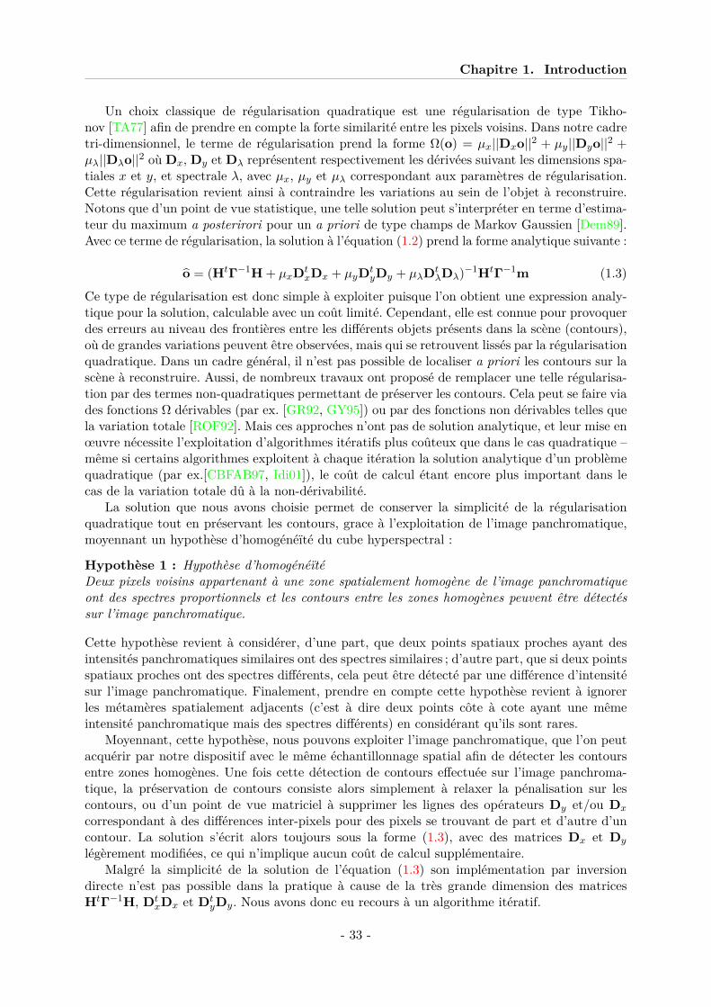
Chapitre 1. Introduction
Un choix classique de régularisation quadratique est une régularisation de type Tikho-nov [TA77] afin de prendre en compte la forte similarité entre les pixels voisins. Dans notre cadretri-dimensionnel, le terme de régularisation prend la forme Ω(o) = µx||Dxo||2 + µy||Dyo||2 +µλ||Dλo||2 où Dx, Dy et Dλ représentent respectivement les dérivées suivant les dimensions spa-tiales x et y, et spectrale λ, avec µx, µy et µλ correspondant aux paramètres de régularisation.Cette régularisation revient ainsi à contraindre les variations au sein de l’objet à reconstruire.Notons que d’un point de vue statistique, une telle solution peut s’interpréter en terme d’estima-teur du maximum a posterirori pour un a priori de type champs de Markov Gaussien [Dem89].Avec ce terme de régularisation, la solution à l’équation (1.2) prend la forme analytique suivante :
o = (HtΓ−1H + µxDtxDx + µyDt
yDy + µλDtλDλ)−1HtΓ−1m (1.3)
Ce type de régularisation est donc simple à exploiter puisque l’on obtient une expression analy-tique pour la solution, calculable avec un coût limité. Cependant, elle est connue pour provoquerdes erreurs au niveau des frontières entre les différents objets présents dans la scène (contours),où de grandes variations peuvent être observées, mais qui se retrouvent lissés par la régularisationquadratique. Dans un cadre général, il n’est pas possible de localiser a priori les contours sur lascène à reconstruire. Aussi, de nombreux travaux ont proposé de remplacer une telle régularisa-tion par des termes non-quadratiques permettant de préserver les contours. Cela peut se faire viades fonctions Ω dérivables (par ex. [GR92, GY95]) ou par des fonctions non dérivables telles quela variation totale [ROF92]. Mais ces approches n’ont pas de solution analytique, et leur mise enœuvre nécessite l’exploitation d’algorithmes itératifs plus coûteux que dans le cas quadratique –même si certains algorithmes exploitent à chaque itération la solution analytique d’un problèmequadratique (par ex.[CBFAB97, Idi01]), le coût de calcul étant encore plus important dans lecas de la variation totale dû à la non-dérivabilité.
La solution que nous avons choisie permet de conserver la simplicité de la régularisationquadratique tout en préservant les contours, grace à l’exploitation de l’image panchromatique,moyennant un hypothèse d’homogénéïté du cube hyperspectral :
Hypothèse 1 : Hypothèse d’homogénéïtéDeux pixels voisins appartenant à une zone spatialement homogène de l’image panchromatiqueont des spectres proportionnels et les contours entre les zones homogènes peuvent être détectéssur l’image panchromatique.
Cette hypothèse revient à considérer, d’une part, que deux points spatiaux proches ayant desintensités panchromatiques similaires ont des spectres similaires ; d’autre part, que si deux pointsspatiaux proches ont des spectres différents, cela peut être détecté par une différence d’intensitésur l’image panchromatique. Finalement, prendre en compte cette hypothèse revient à ignorerles métamères spatialement adjacents (c’est à dire deux points côte à cote ayant une mêmeintensité panchromatique mais des spectres différents) en considérant qu’ils sont rares.
Moyennant, cette hypothèse, nous pouvons exploiter l’image panchromatique, que l’on peutacquérir par notre dispositif avec le même échantillonnage spatial afin de détecter les contoursentre zones homogènes. Une fois cette détection de contours effectuée sur l’image panchroma-tique, la préservation de contours consiste alors simplement à relaxer la pénalisation sur lescontours, ou d’un point de vue matriciel à supprimer les lignes des opérateurs Dy et/ou Dx
correspondant à des différences inter-pixels pour des pixels se trouvant de part et d’autre d’uncontour. La solution s’écrit alors toujours sous la forme (1.3), avec des matrices Dx et Dy
légèrement modifiées, ce qui n’implique aucun coût de calcul supplémentaire.Malgré la simplicité de la solution de l’équation (1.3) son implémentation par inversion
directe n’est pas possible dans la pratique à cause de la très grande dimension des matricesHtΓ−1H, Dt
xDx et DtyDy. Nous avons donc eu recours à un algorithme itératif.
- 33 -
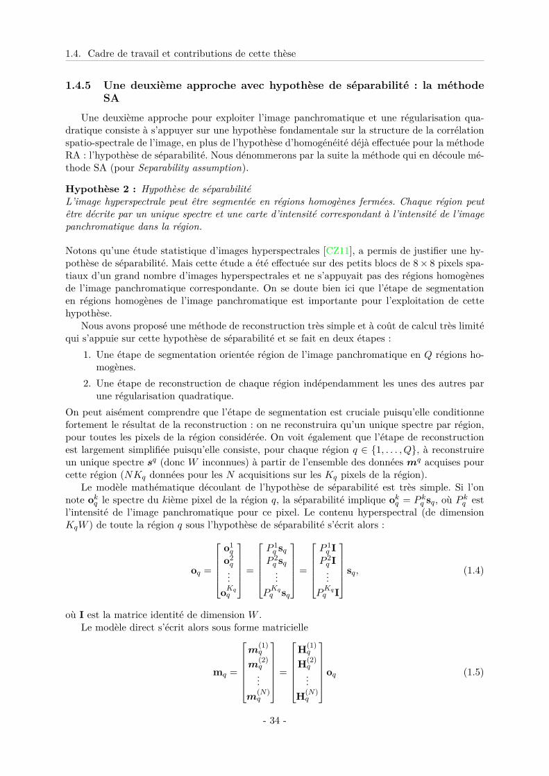
1.4. Cadre de travail et contributions de cette thèse
1.4.5 Une deuxième approche avec hypothèse de séparabilité : la méthodeSA
Une deuxième approche pour exploiter l’image panchromatique et une régularisation qua-dratique consiste à s’appuyer sur une hypothèse fondamentale sur la structure de la corrélationspatio-spectrale de l’image, en plus de l’hypothèse d’homogénéité déjà effectuée pour la méthodeRA : l’hypothèse de séparabilité. Nous dénommerons par la suite la méthode qui en découle mé-thode SA (pour Separability assumption).
Hypothèse 2 : Hypothèse de séparabilitéL’image hyperspectrale peut être segmentée en régions homogènes fermées. Chaque région peutêtre décrite par un unique spectre et une carte d’intensité correspondant à l’intensité de l’imagepanchromatique dans la région.
Notons qu’une étude statistique d’images hyperspectrales [CZ11], a permis de justifier une hy-pothèse de séparabilité. Mais cette étude a été effectuée sur des petits blocs de 8× 8 pixels spa-tiaux d’un grand nombre d’images hyperspectrales et ne s’appuyait pas des régions homogènesde l’image panchromatique correspondante. On se doute bien ici que l’étape de segmentationen régions homogènes de l’image panchromatique est importante pour l’exploitation de cettehypothèse.
Nous avons proposé une méthode de reconstruction très simple et à coût de calcul très limitéqui s’appuie sur cette hypothèse de séparabilité et se fait en deux étapes :
1. Une étape de segmentation orientée région de l’image panchromatique en Q régions ho-mogènes.
2. Une étape de reconstruction de chaque région indépendamment les unes des autres parune régularisation quadratique.
On peut aisément comprendre que l’étape de segmentation est cruciale puisqu’elle conditionnefortement le résultat de la reconstruction : on ne reconstruira qu’un unique spectre par région,pour toutes les pixels de la région considérée. On voit également que l’étape de reconstructionest largement simplifiée puisqu’elle consiste, pour chaque région q ∈ 1, . . . , Q, à reconstruireun unique spectre sq (donc W inconnues) à partir de l’ensemble des données mq acquises pourcette région (NKq données pour les N acquisitions sur les Kq pixels de la région).
Le modèle mathématique découlant de l’hypothèse de séparabilité est très simple. Si l’onnote okq le spectre du kième pixel de la région q, la séparabilité implique okq = P kq sq, où P kq estl’intensité de l’image panchromatique pour ce pixel. Le contenu hyperspectral (de dimensionKqW ) de toute la région q sous l’hypothèse de séparabilité s’écrit alors :
oq =
o1q
o2q...
oKqq
=
P 1q sqP 2q sq...
PKqq sq
=
P 1q IP 2q I...
PKqq I
sq, (1.4)
où I est la matrice identité de dimension W .Le modèle direct s’écrit alors sous forme matricielle
mq =
m(1)q
m(2)q...
m(N)q
=
H(1)q
H(2)q...
H(N)q
oq (1.5)
- 34 -
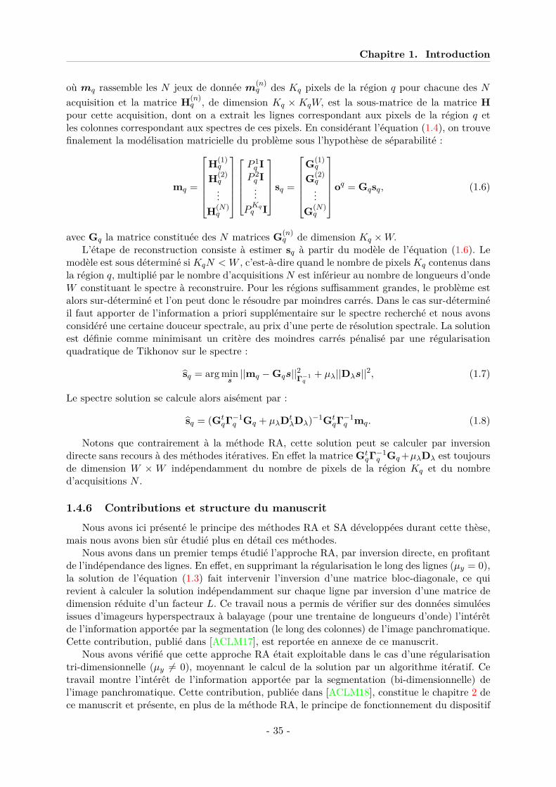
Chapitre 1. Introduction
où mq rassemble les N jeux de donnée m(n)q des Kq pixels de la région q pour chacune des N
acquisition et la matrice H(n)q , de dimension Kq × KqW, est la sous-matrice de la matrice H
pour cette acquisition, dont on a extrait les lignes correspondant aux pixels de la région q etles colonnes correspondant aux spectres de ces pixels. En considérant l’équation (1.4), on trouvefinalement la modélisation matricielle du problème sous l’hypothèse de séparabilité :
mq =
H(1)q
H(2)q...
H(N)q
P 1q IP 2q I...
PKqq I
sq =
G(1)q
G(2)q...
G(N)q
oq = Gqsq, (1.6)
avec Gq la matrice constituée des N matrices G(n)q de dimension Kq ×W.
L’étape de reconstruction consiste à estimer sq à partir du modèle de l’équation (1.6). Lemodèle est sous déterminé siKqN < W , c’est-à-dire quand le nombre de pixelsKq contenus dansla région q, multiplié par le nombre d’acquisitions N est inférieur au nombre de longueurs d’ondeW constituant le spectre à reconstruire. Pour les régions suffisamment grandes, le problème estalors sur-déterminé et l’on peut donc le résoudre par moindres carrés. Dans le cas sur-déterminéil faut apporter de l’information a priori supplémentaire sur le spectre recherché et nous avonsconsidéré une certaine douceur spectrale, au prix d’une perte de résolution spectrale. La solutionest définie comme minimisant un critère des moindres carrés pénalisé par une régularisationquadratique de Tikhonov sur le spectre :
sq = arg mins||mq −Gqs||2Γ−1
q+ µλ||Dλs||2, (1.7)
Le spectre solution se calcule alors aisément par :
sq = (GtqΓ−1
q Gq + µλDtλDλ)−1Gt
qΓ−1q mq. (1.8)
Notons que contrairement à la méthode RA, cette solution peut se calculer par inversiondirecte sans recours à des méthodes itératives. En effet la matrice Gt
qΓ−1q Gq+µλDλ est toujours
de dimension W × W indépendamment du nombre de pixels de la région Kq et du nombred’acquisitions N .
1.4.6 Contributions et structure du manuscrit
Nous avons ici présenté le principe des méthodes RA et SA développées durant cette thèse,mais nous avons bien sûr étudié plus en détail ces méthodes.
Nous avons dans un premier temps étudié l’approche RA, par inversion directe, en profitantde l’indépendance des lignes. En effet, en supprimant la régularisation le long des lignes (µy = 0),la solution de l’équation (1.3) fait intervenir l’inversion d’une matrice bloc-diagonale, ce quirevient à calculer la solution indépendamment sur chaque ligne par inversion d’une matrice dedimension réduite d’un facteur L. Ce travail nous a permis de vérifier sur des données simuléesissues d’imageurs hyperspectraux à balayage (pour une trentaine de longueurs d’onde) l’intérêtde l’information apportée par la segmentation (le long des colonnes) de l’image panchromatique.Cette contribution, publié dans [ACLM17], est reportée en annexe de ce manuscrit.
Nous avons vérifié que cette approche RA était exploitable dans le cas d’une régularisationtri-dimensionnelle (µy 6= 0), moyennant le calcul de la solution par un algorithme itératif. Cetravail montre l’intérêt de l’information apportée par la segmentation (bi-dimensionnelle) del’image panchromatique. Cette contribution, publiée dans [ACLM18], constitue le chapitre 2 dece manuscrit et présente, en plus de la méthode RA, le principe de fonctionnement du dispositif
- 35 -
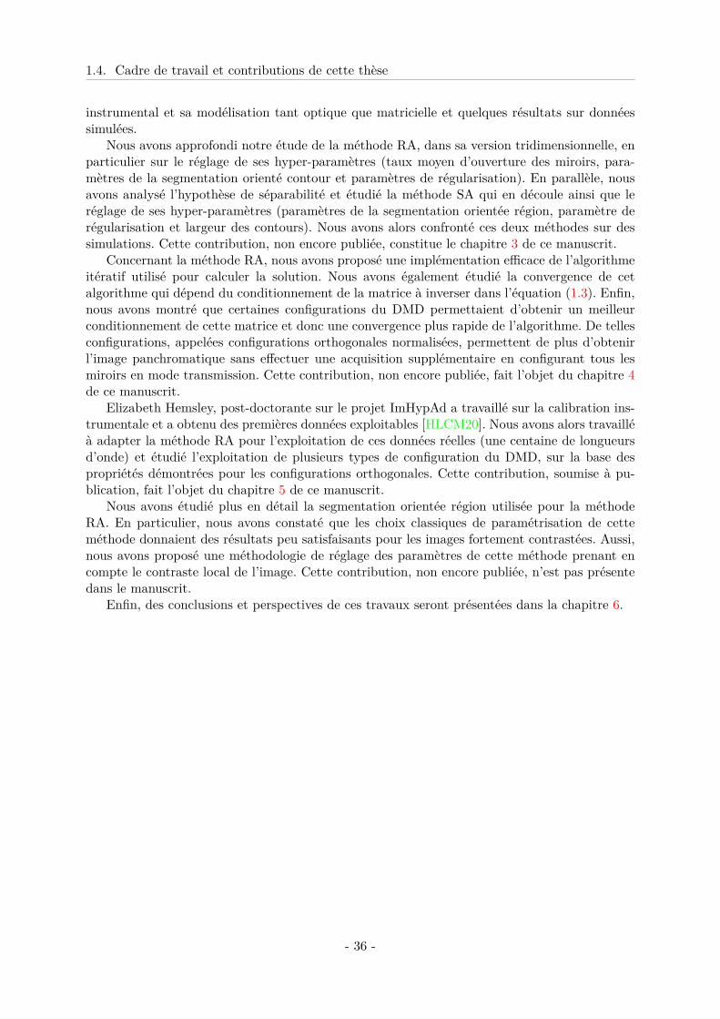
1.4. Cadre de travail et contributions de cette thèse
instrumental et sa modélisation tant optique que matricielle et quelques résultats sur donnéessimulées.
Nous avons approfondi notre étude de la méthode RA, dans sa version tridimensionnelle, enparticulier sur le réglage de ses hyper-paramètres (taux moyen d’ouverture des miroirs, para-mètres de la segmentation orienté contour et paramètres de régularisation). En parallèle, nousavons analysé l’hypothèse de séparabilité et étudié la méthode SA qui en découle ainsi que leréglage de ses hyper-paramètres (paramètres de la segmentation orientée région, paramètre derégularisation et largeur des contours). Nous avons alors confronté ces deux méthodes sur dessimulations. Cette contribution, non encore publiée, constitue le chapitre 3 de ce manuscrit.
Concernant la méthode RA, nous avons proposé une implémentation efficace de l’algorithmeitératif utilisé pour calculer la solution. Nous avons également étudié la convergence de cetalgorithme qui dépend du conditionnement de la matrice à inverser dans l’équation (1.3). Enfin,nous avons montré que certaines configurations du DMD permettaient d’obtenir un meilleurconditionnement de cette matrice et donc une convergence plus rapide de l’algorithme. De tellesconfigurations, appelées configurations orthogonales normalisées, permettent de plus d’obtenirl’image panchromatique sans effectuer une acquisition supplémentaire en configurant tous lesmiroirs en mode transmission. Cette contribution, non encore publiée, fait l’objet du chapitre 4de ce manuscrit.
Elizabeth Hemsley, post-doctorante sur le projet ImHypAd a travaillé sur la calibration ins-trumentale et a obtenu des premières données exploitables [HLCM20]. Nous avons alors travailléà adapter la méthode RA pour l’exploitation de ces données réelles (une centaine de longueursd’onde) et étudié l’exploitation de plusieurs types de configuration du DMD, sur la base despropriétés démontrées pour les configurations orthogonales. Cette contribution, soumise à pu-blication, fait l’objet du chapitre 5 de ce manuscrit.
Nous avons étudié plus en détail la segmentation orientée région utilisée pour la méthodeRA. En particulier, nous avons constaté que les choix classiques de paramétrisation de cetteméthode donnaient des résultats peu satisfaisants pour les images fortement contrastées. Aussi,nous avons proposé une méthodologie de réglage des paramètres de cette méthode prenant encompte le contraste local de l’image. Cette contribution, non encore publiée, n’est pas présentedans le manuscrit.
Enfin, des conclusions et perspectives de ces travaux seront présentées dans la chapitre 6.
- 36 -
Chapitre 2
Article EUSPICO 2018
SommaireI. Introduction . . . . . . . . . . . . . . . . . . . . . . . . . . . . . . . . . . . 40II. Device modeling . . . . . . . . . . . . . . . . . . . . . . . . . . . . . . . . 40
A. Acquisition device . . . . . . . . . . . . . . . . . . . . . . . . . . . . . . . . . 40B. Optical modeling . . . . . . . . . . . . . . . . . . . . . . . . . . . . . . . . . 40C. Matrix modeling . . . . . . . . . . . . . . . . . . . . . . . . . . . . . . . . . . 41
III Hyperspectral image reconstruction . . . . . . . . . . . . . . . . . . . . 42A. Reconstruction using a quadratic penalization . . . . . . . . . . . . . . . . . 42B. Implementation . . . . . . . . . . . . . . . . . . . . . . . . . . . . . . . . . . 42
IV Results and discussion . . . . . . . . . . . . . . . . . . . . . . . . . . . . . 42IV Conclusion . . . . . . . . . . . . . . . . . . . . . . . . . . . . . . . . . . . . 43
Nous reprenons ici l’article [ACLM18] :I. Ardi, H. Carfantan, S. Lacroix and A. Monmayrant, Fast hyperspectral cube re-construction for a double dispersion imager, European Signal Processing Conference(EUSIPCO 2018), Rome, Italie, septembre 2018.
37

Chapitre 2. Article EUSPICO 2018
Fast hyperspectral cube reconstruction for a doubledisperser imager
Ibrahim Ardi∗†, Herve Carfantan∗, Simon Lacroix†, Antoine Monmayrant†∗IRAP, Universite de Toulouse, CNRS, CNES,
14 Avenue Edouard Belin, 31400 Toulouse, France†LAAS-CNRS, Universite de Toulouse, CNRS,
Avenue de Colonel Roche, 31031 Toulouse, France
Abstract—We consider the problem of hyperspectral cubereconstruction with a new controllable imaging system. Thereconstruction with a small number of images acquired withdifferent configurations of the imager avoids a complete scanningof the hyperspectral cube. We focus here on a quadratic penaltyreconstruction approach, which provides a fast resolution thanksto the high sparsity of the involved matrices. While such a regu-larization is known to smooth the restored images, we propose toexploit the system capability to acquire the panchromatic imageof the scene, to introduce prior information on the sharp edgesof the image, leading to a fast and edge-preserved reconstructionof the image.
I. INTRODUCTION
Hyperspectral (HS) Imaging, that is, acquisition of imageswith a large number of narrow spectral bands, has applicationsin numerous contexts. Conventional HS imaging technologiesproceed by spatial or spectral scanning: they are not instan-taneous and are restricted to the acquisition of static scenes,where the imager is either static or follows precisely controlledmotions in the case of spatial scanning.
To circumvent this limitation various snapshot devices wereproposed [1]. Some require complex optical systems, whichinclude, for example, a series of imagers mounted behind aseries of dichroic mirrors or spectral filters. Others exploitreconstruction algorithms using a spatio-spectral mixture ofthe HS cube obtained through an optical system definedonce and for all, at the design phase. In the latter case, theacquisitions of the three-dimensional structure of the cubemade by a two-dimensional matrix, necessarily induces aloss of spatial and/or spectral information. The reconstructionalgorithms then require assumptions on the scene, and areexpensive in computing resources. In addition, these systemsrequire an accurate spatio-spectral calibration.
In this article we are interested in the reconstruction ofhyperspectral cubes using a recently proposed device [2]. Thisimager has a dual disperser configuration analogous to theone presented in [3]. It does not suffer from any dependentwavelength shift effect thanks to co-location property: all thespectral components of a given spatial position (x,y) in thecube are imaged at the same point on the CCD. Besides, it isprogrammable via the control of a matrix of micro-mirrors(Digital Micromirror Device, DMD). This allows the defi-nition of adaptive acquisition schemes, i.e. that sequentiallyadapt the DMD configurations to the spectral content of the
observed scene. For these acquisition schemes to be relevant,the reconstruction step at each iteration needs to be as fast aspossible, ideally in real time. To implement such schemes, itis thus necessary to be able to reconstruct an HS cube from asmall number of acquisitions in different configurations, at areduced computation cost.
Section II presents the device and its optical and numericalmodeling. In section 3, we address the reconstruction of anHS cube using quadratic regularization, fast and adapted to thesystem properties. Due to the size of the sparse matrices in-volved in the reconstruction process, typically 30.106×30.106
for a 1Mpixel-image with 30 spectral bands, a straightforwardinverse is not feasible. In section 4 we expose the implemen-tation of an alternative iterative algorithm CGNE (ConjugateGradient for Normal Equations) and the speed up gainedowing to the characteristics of the device. Finally, we presentsome reconstruction results obtained by simulating the deviceto acquire data from a HS cube.
II. DEVICE MODELING
A. Acquisition device
The device described in [2], is composed of two symmetri-cal 4f -lines (assembly of two lenses and a diffraction grating),separated by a DMD placed in the plane of symmetry asshown in Fig. 1. Each of the micro-mirrors of the DMD canbe configured to transmit or block the incoming light, thusperforming a spatial filtering of the signal. The first 4f -linebehaves as a spectrometer with a completely open slit thatoutputs a diffracted image of the observed scene, which isthen spatially filtered accordingly to the micro-mirrors config-urations of the DMD. The joint effect of the first 4f -line andthe micro-mirrors, is thus equivalent to a spatio-spectral filtercompletely characterized by the DMD configuration. Finally,the second 4f -line compensates the diffraction introduced bythe first one: it cancels the wavelength-dependent shift anduntangles the spatial and spectral components reaching theCCD. So, in the particular case where all the DMD mirrors areopen, the CCD captures a panchromatic image of the observedscene.
B. Optical modeling
This section describes the different transformations thatthe image undergoes in the optical system, by modeling the
- 39 -
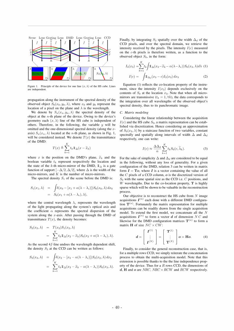
Figure 1. Principle of the device for one line (x,λ) of the HS cube. Linesare independent.
propagation along the instrument of the spectral density of theobserved object S0(x0, y0,λ), where x0 and y0 represent thelocation of a pixel on the plane and λ is the wavelength.
We denote by Sn(xn, yn,λ) the spectral density of theobject at the n-th plane of the device. Owing to the device’sgeometry each (x,λ) line of the HS cube is independent ofothers. Therefore, in the following, the variable y will beomitted and the one-dimensional spectral density (along the x-axis) Sn(xn,λ) located at the n-th plane, as shown in Fig. 1,will be considered instead. We denote T (x) the transmittanceof the DMD:
T (x) K
k=1
tk11Δ(x − xk)
where x is the position on the DMD’s plane, xk and theboolean variable tk represent respectively the location andthe state of the k-th micro-mirror of the DMD, 11Δ is a gatefunction of support [−Δ/2,Δ/2], where Δ is the width of themicro-mirrors, and K is the number of micro-mirrors.
The spectral density S1 of the scene before the DMD is:
S1(x1,λ) =
δ(x0 − [x1 + α(λ− λc)])S0(x0,λ) dx0
= S0(x1 + α(λ− λc),λ),
where the central wavelength λc represents the wavelengthof the light propagating along the system’s optical axis andthe coefficient α represents the spectral dispersion of thesystem along the x-axis. After passing through the DMD oftransmittance T (x), the density becomes:
S2(x2,λ) = T (x2)S1(x2,λ)
=K
k=1
tk11Δ(x2 − xk)S0(x2 + α(λ− λc),λ).
As the second 4f -line undoes the wavelength dependent shift,the density S3 at the CCD can be written as follows:
S3(x3,λ) =
δ(x2 − [x3 − α(λ− λc)])S2(x2,λ) dx2
=K
k=1
tk11Δ(x3 − xk − α(λ− λc))S0(x3,λ).
Finally, by integrating S3 spatially over the width Δd of theCCD pixels, and over the spectral domain, we retrieve theintensity received by the pixels. The intensity I(c) measuredon the c-th pixels is therefore written, as a function to theobserved object S0, in the form:
I3(x3) =K
k=1
tk
11Δ(x3−xk− α(λ−λc))S0(x3,λ)dλ (1)
I(c) =
11Δd
(x3 − c)I3(x3) dx3 (2)
Equation (1) reflects the co-location property of the instru-ment, since the intensity I(x3) depends exclusively on thecontents of S0 at the location x3. Note that when all micro-mirrors are transmissive (tk = 1, ∀k), the data corresponds tothe integration over all wavelengths of the observed object’sspectral density, thus to its panchromatic image.
C. Matrix modeling
Considering the linear relationship between the acquisitionI(c) and the HS cube S0, a matrix representation can be estab-lished via discretization. Hence considering an approximationof S0(x3,λ) by a staircase function of two variables, constantspectrally and spatially along intervals of width Δ and Δd
respectively, one can write:
I(c) ≈ ΔΔd
α
K
k=1
tkS0(c, λk). (3)
For the sake of simplicity Δ and Δd are considered to be equalin the following, without any loss of generality. For a givenconfiguration of the DMD, relation 3 can be written in matrixform I = To, where I is a vector containing the value of allthe C pixels of a CCD column, o is the discretized version ofS0 with the same spatial size as the CCD i.e. C positions, andW wavelengths. Due to the co-location property, T is highlysparse which will be shown to be valuable in the reconstructionprocess.
Our objective is to reconstruct the HS cube from N imageacquisitions I(n) each done with a different DMD configura-tion T(n). Fortunately the matrix representation for multipleacquisitions can be readily drawn from the single acquisitionmodel. To extend the first model, we concatenate all the Nacquisitions I(n) to form a vector d of dimension N C andlikewise for the DMD configuration matrices T(n) to form amatrix H of size NC × CW :
d =
I(1)
...I(N)
=
T(1)
...T(N)
o = Ho. (4)
Finally, to consider the general reconstruction case, that is,for a multiple rows CCD, we simply reiterate the concatenationprocess to obtain the multi-acquisition model. Note that thisextension is possible thanks to the the line independence prop-erty of the device. Thus for a R rows CCD, the dimensions ofd, H and o are NRC, NRC ×RCW and RCW respectively.
- 40 -
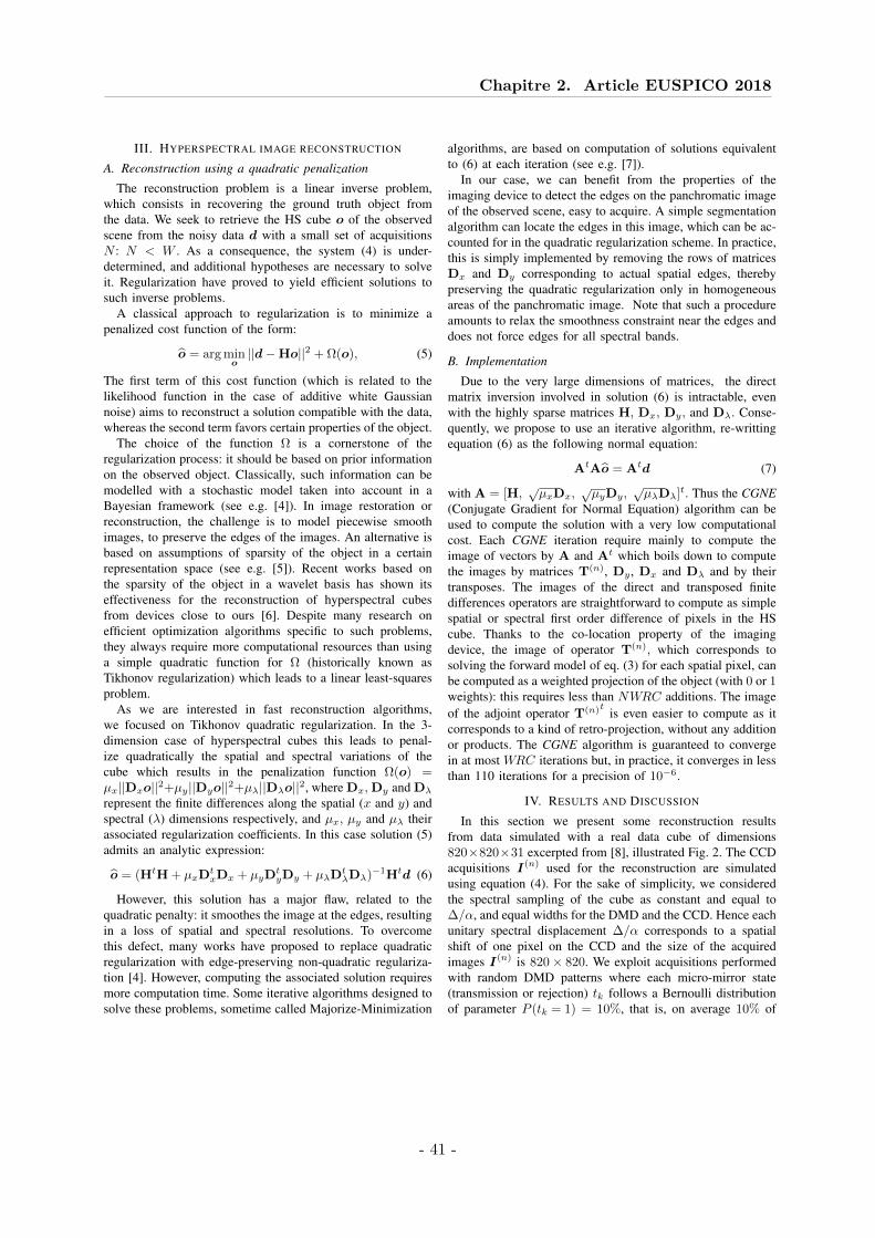
Chapitre 2. Article EUSPICO 2018
III. HYPERSPECTRAL IMAGE RECONSTRUCTION
A. Reconstruction using a quadratic penalization
The reconstruction problem is a linear inverse problem,which consists in recovering the ground truth object fromthe data. We seek to retrieve the HS cube o of the observedscene from the noisy data d with a small set of acquisitionsN : N < W . As a consequence, the system (4) is under-determined, and additional hypotheses are necessary to solveit. Regularization have proved to yield efficient solutions tosuch inverse problems.
A classical approach to regularization is to minimize apenalized cost function of the form:
o = arg mino
||d − Ho||2 + Ω(o), (5)
The first term of this cost function (which is related to thelikelihood function in the case of additive white Gaussiannoise) aims to reconstruct a solution compatible with the data,whereas the second term favors certain properties of the object.
The choice of the function Ω is a cornerstone of theregularization process: it should be based on prior informationon the observed object. Classically, such information can bemodelled with a stochastic model taken into account in aBayesian framework (see e.g. [4]). In image restoration orreconstruction, the challenge is to model piecewise smoothimages, to preserve the edges of the images. An alternative isbased on assumptions of sparsity of the object in a certainrepresentation space (see e.g. [5]). Recent works based onthe sparsity of the object in a wavelet basis has shown itseffectiveness for the reconstruction of hyperspectral cubesfrom devices close to ours [6]. Despite many research onefficient optimization algorithms specific to such problems,they always require more computational resources than usinga simple quadratic function for Ω (historically known asTikhonov regularization) which leads to a linear least-squaresproblem.
As we are interested in fast reconstruction algorithms,we focused on Tikhonov quadratic regularization. In the 3-dimension case of hyperspectral cubes this leads to penal-ize quadratically the spatial and spectral variations of thecube which results in the penalization function Ω(o) =µx||Dxo||2+µy||Dyo||2+µλ||Dλo||2, where Dx, Dy and Dλ
represent the finite differences along the spatial (x and y) andspectral (λ) dimensions respectively, and µx, µy and µλ theirassociated regularization coefficients. In this case solution (5)admits an analytic expression:
o = (HtH + µxDtxDx + µyD
tyDy + µλD
tλDλ)−1Htd (6)
However, this solution has a major flaw, related to thequadratic penalty: it smoothes the image at the edges, resultingin a loss of spatial and spectral resolutions. To overcomethis defect, many works have proposed to replace quadraticregularization with edge-preserving non-quadratic regulariza-tion [4]. However, computing the associated solution requiresmore computation time. Some iterative algorithms designed tosolve these problems, sometime called Majorize-Minimization
algorithms, are based on computation of solutions equivalentto (6) at each iteration (see e.g. [7]).
In our case, we can benefit from the properties of theimaging device to detect the edges on the panchromatic imageof the observed scene, easy to acquire. A simple segmentationalgorithm can locate the edges in this image, which can be ac-counted for in the quadratic regularization scheme. In practice,this is simply implemented by removing the rows of matricesDx and Dy corresponding to actual spatial edges, therebypreserving the quadratic regularization only in homogeneousareas of the panchromatic image. Note that such a procedureamounts to relax the smoothness constraint near the edges anddoes not force edges for all spectral bands.
B. Implementation
Due to the very large dimensions of matrices, the directmatrix inversion involved in solution (6) is intractable, evenwith the highly sparse matrices H, Dx, Dy, and Dλ. Conse-quently, we propose to use an iterative algorithm, re-writtingequation (6) as the following normal equation:
AtAo = Atd (7)
with A = [H,√
µxDx,√
µyDy,√
µλDλ]t. Thus the CGNE(Conjugate Gradient for Normal Equation) algorithm can beused to compute the solution with a very low computationalcost. Each CGNE iteration require mainly to compute theimage of vectors by A and At which boils down to computethe images by matrices T(n), Dy , Dx and Dλ and by theirtransposes. The images of the direct and transposed finitedifferences operators are straightforward to compute as simplespatial or spectral first order difference of pixels in the HScube. Thanks to the co-location property of the imagingdevice, the image of operator T(n), which corresponds tosolving the forward model of eq. (3) for each spatial pixel, canbe computed as a weighted projection of the object (with 0 or 1weights): this requires less than NWRC additions. The imageof the adjoint operator T(n)t
is even easier to compute as itcorresponds to a kind of retro-projection, without any additionor products. The CGNE algorithm is guaranteed to convergein at most WRC iterations but, in practice, it converges in lessthan 110 iterations for a precision of 10−6.
IV. RESULTS AND DISCUSSION
In this section we present some reconstruction resultsfrom data simulated with a real data cube of dimensions820×820×31 excerpted from [8], illustrated Fig. 2. The CCDacquisitions I(n) used for the reconstruction are simulatedusing equation (4). For the sake of simplicity, we consideredthe spectral sampling of the cube as constant and equal toΔ/α, and equal widths for the DMD and the CCD. Hence eachunitary spectral displacement Δ/α corresponds to a spatialshift of one pixel on the CCD and the size of the acquiredimages I(n) is 820 × 820. We exploit acquisitions performedwith random DMD patterns where each micro-mirror state(transmission or rejection) tk follows a Bernoulli distributionof parameter P (tk = 1) = 10%, that is, on average 10% of
- 41 -
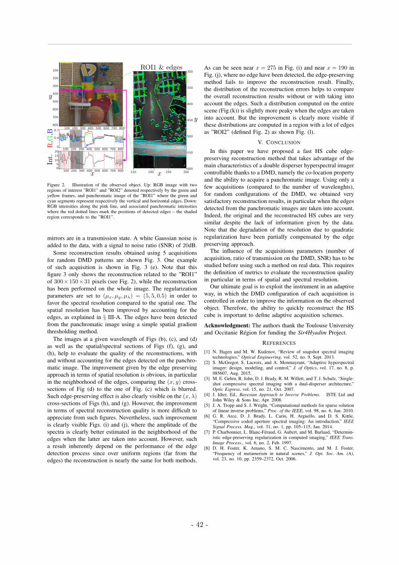
100 200 300 400 500 600 700 800
100
200
300
400
500
600
700
800
150 200 250 300
350
400
450
500
550100 200 300 400 500 600 700 800
0
0.4
0.7
100 200 300 400 500 600 700 8000510
15
20
600
300
Figure 2. Illustration of the observed object. Up: RGB image with tworegions of interest ”ROI1” and ”ROI2” denoted respectively by the green andyellow frames, and panchromatic image of the ”ROI1” where the green andcyan segments represent respectively the vertical and horizontal edges. Down:RGB intensities along the pink line, and associated panchromatic intensitieswhere the red dotted lines mark the positions of detected edges – the shadedregion corresponds to the ”ROI1”.
mirrors are in a transmission state. A white Gaussian noise isadded to the data, with a signal to noise ratio (SNR) of 20dB.
Some reconstruction results obtained using 5 acquisitionsfor random DMD patterns are shown Fig. 3. One exampleof such acquisition is shown in Fig. 3 (e). Note that thisfigure 3 only shows the reconstruction related to the ”ROI1”of 300×150×31 pixels (see Fig. 2), while the reconstructionhas been performed on the whole image. The regularizationparameters are set to (µx, µy, µλ) = (5, 5, 0.5) in order tofavor the spectral resolution compared to the spatial one. Thespatial resolution has been improved by accounting for theedges, as explained in § III-A. The edges have been detectedfrom the panchromatic image using a simple spatial gradientthresholding method.
The images at a given wavelength of Figs (b), (c), and (d)as well as the spatial/spectral sections of Figs (f), (g), and(h), help to evaluate the quality of the reconstructions, withand without accounting for the edges detected on the panchro-matic image. The improvement given by the edge preservingapproach in terms of spatial resolution is obvious, in particularin the neighborhood of the edges, comparing the (x, y) cross-sections of Fig (d) to the one of Fig. (c) which is blurred.Such edge-preserving effect is also clearly visible on the (x,λ)cross-sections of Figs (h), and (g). However, the improvementin terms of spectral reconstruction quality is more difficult toappreciate from such figures. Nevertheless, such improvementis clearly visible Figs. (i) and (j), where the amplitude of thespectra is clearly better estimated in the neighborhood of theedges when the latter are taken into account. However, sucha result inherently depend on the performance of the edgedetection process since over uniform regions (far from theedges) the reconstruction is nearly the same for both methods.
As can be seen near x = 275 in Fig. (i) and near x = 190 inFig. (j), where no edge have been detected, the edge-preservingmethod fails to improve the reconstruction result. Finally,the distribution of the reconstruction errors helps to comparethe overall reconstruction results without or with taking intoaccount the edges. Such a distribution computed on the entirescene (Fig.(k)) is slightly more peaky when the edges are takeninto account. But the improvement is clearly more visible ifthese distributions are computed in a region with a lot of edgesas ”ROI2” (defined Fig. 2) as shown Fig. (l).
V. CONCLUSION
In this paper we have proposed a fast HS cube edge-preserving reconstruction method that takes advantage of themain characteristics of a double disperser hyperspectral imagercontrollable thanks to a DMD, namely the co-location propertyand the ability to acquire a panchromatic image. Using only afew acquisitions (compared to the number of wavelenghts),for random configurations of the DMD, we obtained verysatisfactory reconstruction results, in particular when the edgesdetected from the panchromatic images are taken into account.Indeed, the original and the reconstructed HS cubes are verysimilar despite the lack of information given by the data.Note that the degradation of the resolution due to quadraticregularization have been partially compensated by the edgepreserving approach.
The influence of the acquisitions parameters (number ofacquisition, ratio of transmission on the DMD, SNR) has to bestudied before using such a method on real data. This requiresthe definition of metrics to evaluate the reconstruction qualityin particular in terms of spatial and spectral resolution.
Our ultimate goal is to exploit the instrument in an adaptiveway, in which the DMD configuration of each acquisition iscontrolled in order to improve the information on the observedobject. Therefore, the ability to quickly reconstruct the HScube is important to define adaptive acquisition schemes.
Acknowledgment: The authors thank the Toulouse Universityand Occitanie Region for funding the Sir4Hyadim Project.
REFERENCES
[1] N. Hagen and M. W. Kudenov, “Review of snapshot spectral imagingtechnologies,” Optical Engineering, vol. 52, no. 9, Sept. 2013.
[2] S. McGregor, S. Lacroix, and A. Monmayrant, “Adaptive hyperspectralimager: design, modeling, and control,” J. of Optics, vol. 17, no. 8, p.085607, Aug. 2015.
[3] M. E. Gehm, R. John, D. J. Brady, R. M. Willett, and T. J. Schulz, “Single-shot compressive spectral imaging with a dual-disperser architecture,”Optic Express, vol. 15, no. 21, Oct. 2007.
[4] J. Idier, Ed., Bayesian Approach to Inverse Problems. ISTE Ltd andJohn Wiley & Sons Inc, Apr. 2008.
[5] J. A. Tropp and S. J. Wright, “Computational methods for sparse solutionof linear inverse problems,” Proc. of the IEEE, vol. 98, no. 6, Jun. 2010.
[6] G. R. Arce, D. J. Brady, L. Carin, H. Arguello, and D. S. Kittle,“Compressive coded aperture spectral imaging: An introduction,” IEEESignal Process. Mag., vol. 31, no. 1, pp. 105–115, Jan. 2014.
[7] P. Charbonnier, L. Blanc-Feraud, G. Aubert, and M. Barlaud, “Determin-istic edge-preserving regularization in computed imaging,” IEEE Trans.Image Process., vol. 6, no. 2, Feb. 1997.
[8] D. H. Foster, K. Amano, S. M. C. Nascimento, and M. J. Foster,“Frequency of metamerism in natural scenes,” J. Opt. Soc. Am. (A),vol. 23, no. 10, pp. 2359–2372, Oct. 2006.
- 42 -
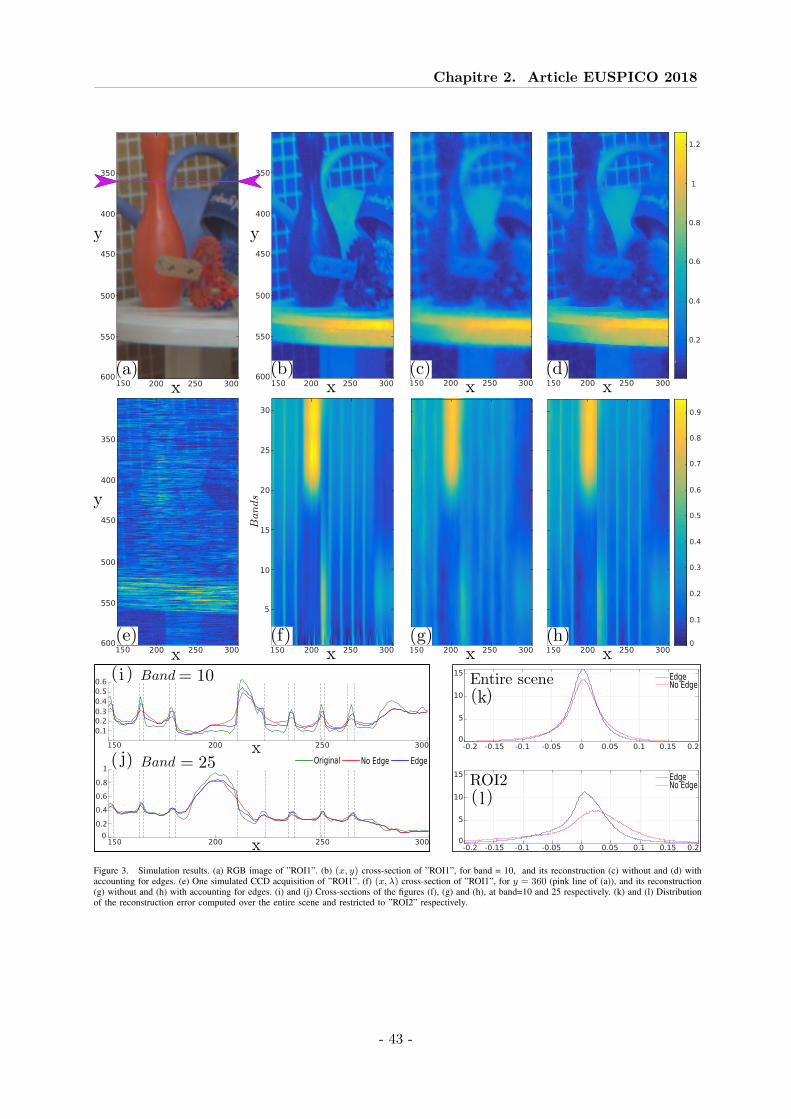
Chapitre 2. Article EUSPICO 2018
350
400
450
500
550
600200 250 300
350
400
450
500
550
600200 250 300
350
400
450
500
550
600200 250 300
0.2
0.4
0.6
0.8
1
1.2
200 250 300
5
10
15
20
25
30
200 250 300
200 250 300
200 250 300
Original No Edge Edge
-0.2 -0.15 -0.1 -0.05 0 0.05 0.1 0.15 0.20
5
10
15
0
5
10
15
-0.2 -0.15 -0.1 -0.05 0 0.05 0.1 0.15 0.2
0
0.1
0.2
0.3
0.4
0.5
0.6
0.7
0.8
0.9
200 250 300
200 250 300 200 250 300
No EdgeEdge
No EdgeEdge
Figure 3. Simulation results. (a) RGB image of ”ROI1”. (b) (x, y) cross-section of ”ROI1”, for band = 10, and its reconstruction (c) without and (d) withaccounting for edges. (e) One simulated CCD acquisition of ”ROI1”. (f) (x,λ) cross-section of ”ROI1”, for y = 360 (pink line of (a)), and its reconstruction(g) without and (h) with accounting for edges. (i) and (j) Cross-sections of the figures (f), (g) and (h), at band=10 and 25 respectively. (k) and (l) Distributionof the reconstruction error computed over the entire scene and restricted to ”ROI2” respectively.
- 43 -

Chapitre 3
Article sur l’étude des méthodes RAet SA
SommaireAbstract . . . . . . . . . . . . . . . . . . . . . . . . . . . . . . . . . . . . . . . 481. Introduction . . . . . . . . . . . . . . . . . . . . . . . . . . . . . . . . . . . 482. Programmable HyperSpectral Imager (PHSI) . . . . . . . . . . . . . . . 51
2.1 Principle and key features . . . . . . . . . . . . . . . . . . . . . . . . . . . . 512.2 Discrete model . . . . . . . . . . . . . . . . . . . . . . . . . . . . . . . . . . 522.3 Matrix model . . . . . . . . . . . . . . . . . . . . . . . . . . . . . . . . . . . 52
3 Reconstruction using a quadratic Regularization Approach (RA) . . . 534 Reconstruction using a Separability Assumption (SA) . . . . . . . . . . 565 Parameters selection . . . . . . . . . . . . . . . . . . . . . . . . . . . . . . 58
5.1 Simulated data and reconstruction quality criteria . . . . . . . . . . . . . . 585.2 Ratio of open mirrors (ROM) . . . . . . . . . . . . . . . . . . . . . . . . . . 605.3 Parameters for the regularization approach (RA) . . . . . . . . . . . . . . . 615.4 Parameters for the separability assumption (SA) . . . . . . . . . . . . . . . 63
6 Results . . . . . . . . . . . . . . . . . . . . . . . . . . . . . . . . . . . . . . . 656.1 Regularization approach (RA) . . . . . . . . . . . . . . . . . . . . . . . . . 666.2 Separability Assumption (SA) . . . . . . . . . . . . . . . . . . . . . . . . . . 676.3 Comparison of SA and RA performances . . . . . . . . . . . . . . . . . . . . 68
7 Discussion and perspectives . . . . . . . . . . . . . . . . . . . . . . . . . . 728 Acknowledgement . . . . . . . . . . . . . . . . . . . . . . . . . . . . . . . . 73References . . . . . . . . . . . . . . . . . . . . . . . . . . . . . . . . . . . . . . 73
Nous reprenons ici l’article [ARC+20] en préparation :I. Ardi, T. Rouvier, H. Carfantan, S. Lacroix and A. Monmayrant, Two fast reconstructionapproaches leveraging the panchromatic image for a configurable dual-disperser imager,Rapport Technique IRAP–UPS/CNRS/CNES et LAAS–CNRS, juillet 2020.
45

Chapitre 3. Article sur l’étude des méthodes RA et SA
Noname manuscript No.(will be inserted by the editor)
Two fast reconstruction approaches leveraging thepanchromatic image for a configurable dual-disperserimager
Ibrahim Ardi · Tony Rouvier · Herve
Carfantan · Simon Lacroix · Antoine
Monmayrant
Received: date / Accepted: date
Abstract We propose two computationally efficient methods to reconstruct anhyperspectral cube from a small number of images acquired with a programmabledual-disperser coded aperture imaging device. Taking advantage of the specificcharacteristics of the device, these methods do not require a systematic scan ofall the hyperspectral cube. They are based on simple assumptions on the spatial-spectral correlation structure of the scene, using information deduced from thepanchromatic image. The first method is a Thikonov quadratic regularization tai-lored to prevent smoothing at the spatial edges. The second method is a leastsquare reconstruction taking advantage of the spatial and spectral separabilityof the hyperspectral cube over small homogeneous regions. Insights on the def-inition of the optimal sequence of acquisitions and parameter values of the twomethods are given, through an extensive assessment of the reconstruction perfor-mance. A comparison highlights the respective advantages and drawbacks of bothapproaches.
Keywords Hyperspectral image reconstruction, quadratic regularization, spatio-spectral correlations
1 Introduction
By conveying precise spectral information, hyperspectral (HS) images benefit awide range of applications, from microscopy to deep space observation, earth ob-servation, scene and material analyses, gas detection... Classic HS imagers exploita scanning process to recover the three dimensions, two spatial and one spectral,
Ibrahim Ardi · Tony Rouvier · Herve CarfantanIRAP, Universite de Toulouse, Universite Toulouse 3 - Paul Sabatier, CNRS, CNES,14 Avenue Edouard Belin, 31400 Toulouse, FranceE-mail: [email protected]
Ibrahim Ardi · S. Lacroix · A. MonmayrantLAAS-CNRS, Universite de Toulouse, CNRS, Toulouse, FranceAvenue de Colonel Roche, 31031 Toulouse, FranceE-mail: [email protected]
- 47 -
2 Ibrahim Ardi et al.
of the HS data, referred to as a “HS cube”. Typically, their spectral componentsare separated by a dispersive element such as a prism or a grating, and measuredon a two dimensional detector. This scanning process is time consuming and im-poses strong constraints on the acquisition, during which the imager and scenemust be static (alternatively, the scanning can be achieved by a regular motion ofa slit imager, as in airborne HS imagery). To alleviate such constraints, variousalternative optical systems that allow “snapshot HS imaging” have been proposed,most relying on a complex optical design [1].
The design of non-scanning HS imagers has been significantly renewed by theadvent of computational sensing approaches, in which only a single or a smallnumber of acquisitions are processed to recover the whole HS cube or specificinformation defined by the task at hand. Computational sensing approaches relyon the tight integration of specific sensor designs and associated data processingalgorithms. Depending on the optical design, tedious and precise spatio-spectralcalibration are required [2,3]. The data processing algorithms palliate the lackof acquired information by resorting to hypotheses and priors, such as sparsityof the scene content in a given basis, and are most often computationally heavy.Noticeable work on computational HS imagers are [4,5,6,7].
The work presented here pertains to computational HS imaging, and proposesfast reconstruction techniques. It relies on a programmable dual-disperser codedaperture imager, whose key properties are exploited to develop efficient reconstruc-tion algorithms, both in terms of computational cost and reconstruction quality.
Dual-disperser coded aperture imager. The principle of a dual disperser HS imagerwas originally introduced in [8], and this setup has been used in various acquisitionconfigurations since (see e.g. [9,4,10,11,12]). Its main interest is that spectraland spatial information are not mixed on the imaging detector, thus avoidingcumbersome calibration issues, and yielding simpler reconstruction algorithms. Werely on such an imaging architecture, referred to as “programmable hyperspectralimager” (PHSI), in which the spatial filtering is achieved by a programmabledigital mirror device (DMD) [11,13].
Leveraging panchromatic information. Analyses on the structural properties of colourimages [14,15]) revealed a particular role of the panchromatic image (luminance),and have had a major impact on image processing, such as compression, de-noisingand restoration algorithms [16,17,18]. Similarly, as it conveys precise spatial in-formation on the scene, the panchromatic image is often used in HS imaging. Forinstance, it is exploited in pansharpening processes to improve the spatial reso-lution [19], or as a similarity metric that coerces structural resemblance on theHS cube regions [12]. For high-frame rate HS video, high-frame rate panchromaticvideo is used to interpolate in-between frames of a low-frame rate HS video [20].In practice though, the discriminative information brought by the panchromaticimage should be dealt with caution. Moreover, when the panchromatic image isrecorded on a different imager, precise calibration and registration are required.
The advent of snapshot and near snapshot hyperspectral imagers has fosteredresearch on the structure of HS images. The intrinsic spatio-spectral correlationsproperties of scenes, as analysed in [21], has driven the development of a varietyof algorithms that process sparse HS data, to achieve e.g. reconstruction [22,23],de-noising [24,25], or compression [26].
- 48 -
Chapitre 3. Article sur l’étude des méthodes RA et SA
Two fast reconstruction approaches for an adaptive dual-disperser imager 3
In this work, our key assumption is that the panchromatic image is an accuraterepresentation of the spatial structure of the HS scene, and preserves well thediscriminative features of the spectra. In particular, two identical spectra alwaysgive the same panchromatic intensity, while different spectra usually give differentintensities. Furthermore, true metamers are unlikely to be adjacent: in other words,adjacent regions with different spectral content are unlikely to share the samepanchromatic intensity.
Contributions. In this paper, we focus on a HS cube reconstruction using a set ofacquisitions significantly smaller than the number of spectral bands (the panchro-matic image, and a small set of acquisitions obtained with random configurationsof the DMD). We present two computationally efficient reconstruction processesthat ensure good precision by taking full advantage of the PHSI imager features.
Our reconstruction methods exploit simple spatio-spectral assumptions of theHS cube. They are based on a regularity assumption, which assumes that the spec-tra are similar on spatially homogeneous regions of the HS scene, and that thespatial structure of the HS scene can be roughly extracted from the panchromaticimage. In the first approach, we benefit from the edges detected on the panchro-matic image to implement a simple and fast quadratic regularization method thatpreserves these edges, faithfully matching the spatial structure of the HS scene. Amodified spatio-spectral quadratic Tikhonov regularization is applied across theHS cube, except on the detected spatial edges. In the second approach, we accountfor an additional separability assumption between spatial and spectral variations inspatially homogeneous regions of the HS scene. This leads the reconstruction of aunique spectrum and a spatial intensity map for each region. This reconstructionmethod consists first of segmenting the panchromatic image into small homo-geneous regions, and then in reconstructing the spectrum of each region via aleast-squares minimization, accounting for the intensity map obtained from thepanchromatic image.
Outline. In section 2, the optical principle of the PHSI is presented, its key fea-tures are depicted, and its numerical model is defined. The regularity assumptionand the first proposed reconstruction method are presented in section 3. The ad-ditional separability assumption and the second proposed reconstruction methodare described in section 4. We address the problem of parameters selection forthe two reconstruction methods and for the acquisition process in section 5, inwhich impact analyses are conducted on numerous simulations with real-world HSscenes. Section 6 analyses the reconstruction results. The performances of bothreconstruction methods are assessed independently and a thorough comparison ofthe two methods is performed to highlight their respective advantages and draw-backs. A concluding section discusses the methods, and presents some perspectivesand future work.
- 49 -
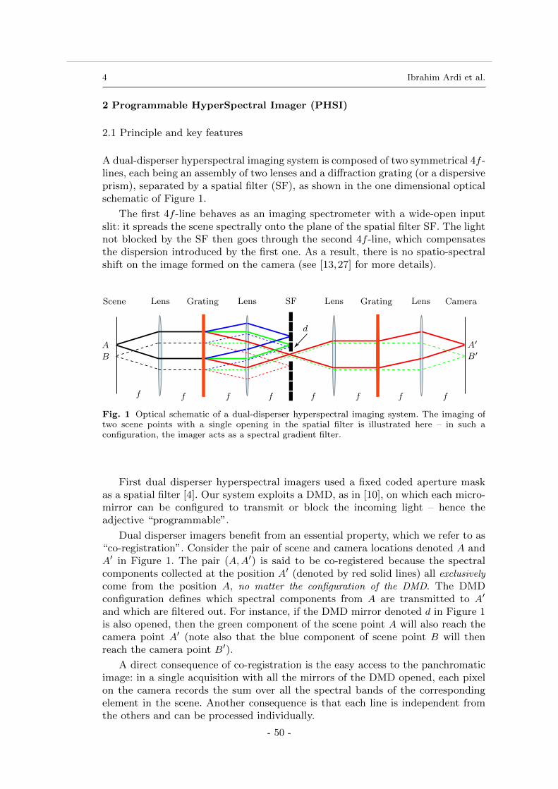
4 Ibrahim Ardi et al.
2 Programmable HyperSpectral Imager (PHSI)
2.1 Principle and key features
A dual-disperser hyperspectral imaging system is composed of two symmetrical 4f -lines, each being an assembly of two lenses and a diffraction grating (or a dispersiveprism), separated by a spatial filter (SF), as shown in the one dimensional opticalschematic of Figure 1.
The first 4f -line behaves as an imaging spectrometer with a wide-open inputslit: it spreads the scene spectrally onto the plane of the spatial filter SF. The lightnot blocked by the SF then goes through the second 4f -line, which compensatesthe dispersion introduced by the first one. As a result, there is no spatio-spectralshift on the image formed on the camera (see [13,27] for more details).
Scene Lens Lens Lens LensGratingGrating SF Camera
f f f f f f f f
A
B
A′
B′
d
Fig. 1 Optical schematic of a dual-disperser hyperspectral imaging system. The imaging oftwo scene points with a single opening in the spatial filter is illustrated here – in such aconfiguration, the imager acts as a spectral gradient filter.
First dual disperser hyperspectral imagers used a fixed coded aperture maskas a spatial filter [4]. Our system exploits a DMD, as in [10], on which each micro-mirror can be configured to transmit or block the incoming light – hence theadjective “programmable”.
Dual disperser imagers benefit from an essential property, which we refer to as“co-registration”. Consider the pair of scene and camera locations denoted A andA′ in Figure 1. The pair (A,A′) is said to be co-registered because the spectralcomponents collected at the position A′ (denoted by red solid lines) all exclusively
come from the position A, no matter the configuration of the DMD. The DMDconfiguration defines which spectral components from A are transmitted to A′
and which are filtered out. For instance, if the DMD mirror denoted d in Figure 1is also opened, then the green component of the scene point A will also reach thecamera point A′ (note also that the blue component of scene point B will thenreach the camera point B′).
A direct consequence of co-registration is the easy access to the panchromaticimage: in a single acquisition with all the mirrors of the DMD opened, each pixelon the camera records the sum over all the spectral bands of the correspondingelement in the scene. Another consequence is that each line is independent fromthe others and can be processed individually.
- 50 -
Chapitre 3. Article sur l’étude des méthodes RA et SA
Two fast reconstruction approaches for an adaptive dual-disperser imager 5
2.2 Discrete model
Let O(r, c, w) be the 3D observed hyperspectral scene (“object”), where (r, c) and ware respectively the spatial and spectral dimensions row, column and wavelength.The size of O(r, c, w) is RCW . Each spectral plane O(r, c, w)r,c of the objectO is imaged onto the DMD with a lateral shift (column-wise) defined by thegrating dispersion and the wavelength w. The DMD displays a binary spatialfilter, represented by a pattern D(r, c). The DMD thus acts as a set of binaryspatial filters, each filter being a shifted version of the DMD pattern, the shiftbeing defined by the wavelength w [13]. This is illustrated in Figure 2, whichschematizes the two-dimensional optical system.
Consider a discrete coordinate system with a one to one ratio for the spatialcoordinates (r, c) between the object O, the DMD D and the camera M (the latteris then of size RC), and a spectral discretization rate w such that adjacent spectralplanes in O are shifted laterally on the DMD D by exactly one pixel1. In thiscoordinate system, the dual-disperser imager can be represented by a filtering cube
FC(r, c, w) of size RCW , which is built by stacking the W shifted DMD patternsalong the w dimension: FC(r, c, w) = D(r, c−w+w0), with a reference wavelengthw0. This reference wavelength corresponds to the wavelength that is not laterallyshifted on the DMD and thus imaged at its center, it is represented in green onfigures 1 and 2. The measurement M(r, c) at the camera pixel (r, c) is the sum ofall spectral components of the object point O(c, r) that passes through the binarymask defined by the line (r, c) of the filtering cube FC. This can be written as:
M(r, c) =W∑
w=1
FC(r, c, w)O(r, c, w). (1)
2.3 Matrix model
Equation (1) stands for one pixel M(r, c) of the camera. As it is linear with respectto the object, the entire image acquisition process can be encoded in the matrixform m = Ho. In this form, m is a vector containing the value of all the R × Cpixels of a camera measurement, o is the vectorized version of the HS scene O andH is a RC×RCW binary matrix that corresponds to the filtering cube (instrumenttransfer function).
This matrix equation models one single acquisition, but can be extended torepresent a sequence of acquisitions with varying configuration of the DMD. In-deed, for a given set of N acquisitions m(n), each made with a different DMDconfiguration H(n), the matrix representation for the N acquisitions can be readilydrawn from the single acquisition model by concatenating all the N acquisitionsm(n) to form a vector m of dimension NRC, and likewise concatenating all the N
1 This particular discretization does not imply any loss of generality – see [13] for a generalgeometric model which accounts for different DMD and camera pixel sizes and [27] for adetailed experimental analysis.
- 51 -
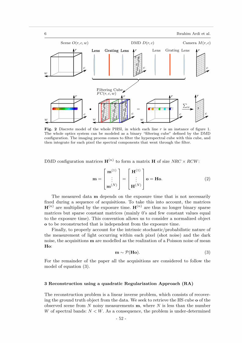
6 Ibrahim Ardi et al.
DMD D(r, c)Scene O(r, c, w) Camera M(r, c)
Lens LensGratingLens LensGrating Lens LensGratingr
c
w
r
c c
r
w
r
c c
r
∑w
r
c
w
r
c
w
=•
Filtering CubeFC(r, c, w)
Fig. 2 Discrete model of the whole PHSI, in which each line r is an instance of figure 1.The whole optics system can be modeled as a binary “filtering cube” defined by the DMDconfiguration. The imaging process comes to filter the hyperspectral cube with this cube, andthen integrate for each pixel the spectral components that went through the filter.
DMD configuration matrices H(n) to form a matrix H of size NRC ×RCW :
m =
m(1)
...
m(N)
=
H(1)
...
H(N)
o = Ho. (2)
The measured data m depends on the exposure time that is not necessarilyfixed during a sequence of acquisitions. To take this into account, the matricesH(n) are multiplied by the exposure time. H(n) are thus no longer binary sparsematrices but sparse constant matrices (mainly 0’s and few constant values equalto the exposure time). This convention allows us to consider a normalized objecto to be reconstructed that is independent from the exposure time.
Finally, to properly account for the intrinsic stochastic/probabilistic nature ofthe measurement of light occurring within each pixel (shot noise) and the darknoise, the acquisitions m are modelled as the realization of a Poisson noise of meanHo:
m ∼ P(Ho). (3)
For the remainder of the paper all the acquisitions are considered to follow themodel of equation (3).
3 Reconstruction using a quadratic Regularization Approach (RA)
The reconstruction problem is a linear inverse problem, which consists of recover-ing the ground truth object from the data. We seek to retrieve the HS cube o of theobserved scene from N noisy measurements m, where N is less than the numberW of spectral bands: N < W . As a consequence, the problem is under-determined
- 52 -
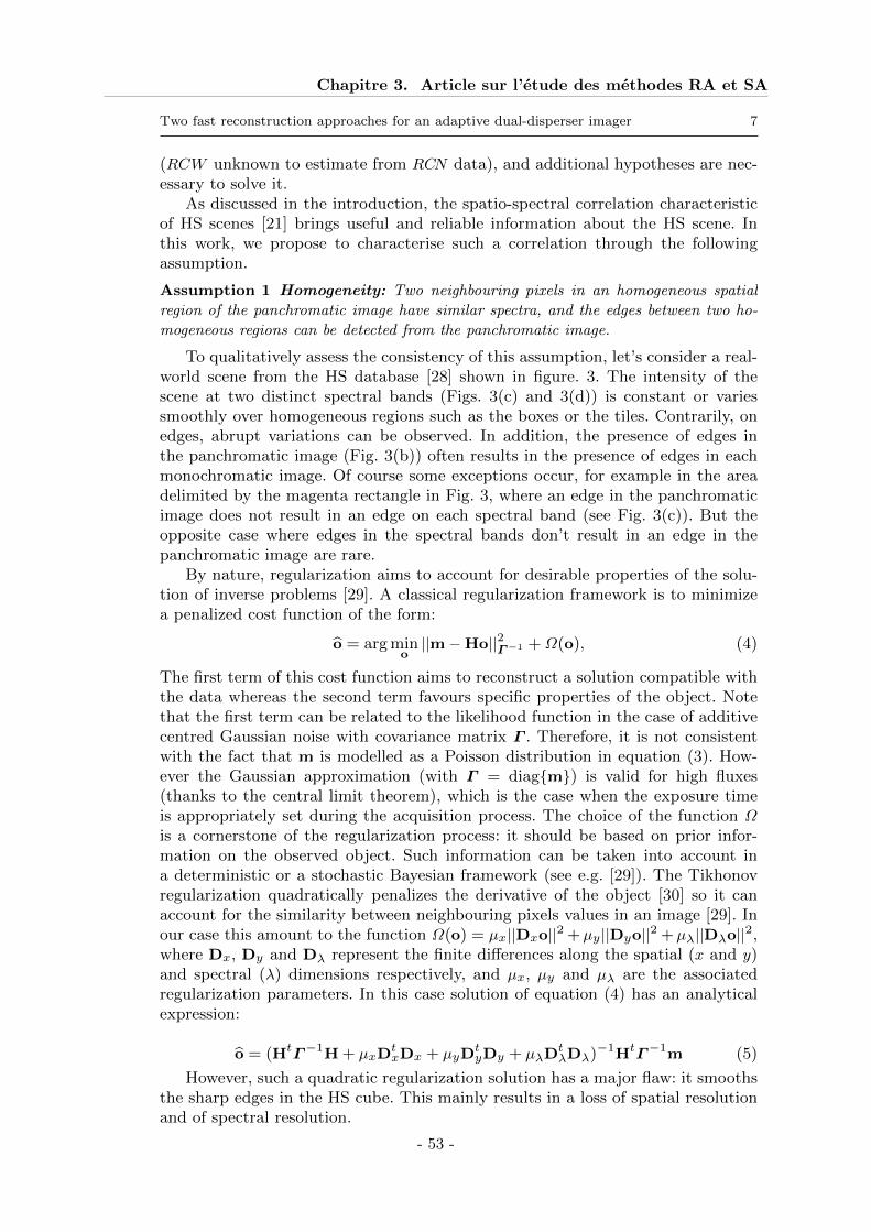
Chapitre 3. Article sur l’étude des méthodes RA et SA
Two fast reconstruction approaches for an adaptive dual-disperser imager 7
(RCW unknown to estimate from RCN data), and additional hypotheses are nec-essary to solve it.
As discussed in the introduction, the spatio-spectral correlation characteristicof HS scenes [21] brings useful and reliable information about the HS scene. Inthis work, we propose to characterise such a correlation through the followingassumption.
Assumption 1 Homogeneity: Two neighbouring pixels in an homogeneous spatial
region of the panchromatic image have similar spectra, and the edges between two ho-
mogeneous regions can be detected from the panchromatic image.
To qualitatively assess the consistency of this assumption, let’s consider a real-world scene from the HS database [28] shown in figure. 3. The intensity of thescene at two distinct spectral bands (Figs. 3(c) and 3(d)) is constant or variessmoothly over homogeneous regions such as the boxes or the tiles. Contrarily, onedges, abrupt variations can be observed. In addition, the presence of edges inthe panchromatic image (Fig. 3(b)) often results in the presence of edges in eachmonochromatic image. Of course some exceptions occur, for example in the areadelimited by the magenta rectangle in Fig. 3, where an edge in the panchromaticimage does not result in an edge on each spectral band (see Fig. 3(c)). But theopposite case where edges in the spectral bands don’t result in an edge in thepanchromatic image are rare.
By nature, regularization aims to account for desirable properties of the solu-tion of inverse problems [29]. A classical regularization framework is to minimizea penalized cost function of the form:
o = arg mino||m−Ho||2Γ−1 +Ω(o), (4)
The first term of this cost function aims to reconstruct a solution compatible withthe data whereas the second term favours specific properties of the object. Notethat the first term can be related to the likelihood function in the case of additivecentred Gaussian noise with covariance matrix Γ . Therefore, it is not consistentwith the fact that m is modelled as a Poisson distribution in equation (3). How-ever the Gaussian approximation (with Γ = diagm) is valid for high fluxes(thanks to the central limit theorem), which is the case when the exposure timeis appropriately set during the acquisition process. The choice of the function Ω
is a cornerstone of the regularization process: it should be based on prior infor-mation on the observed object. Such information can be taken into account ina deterministic or a stochastic Bayesian framework (see e.g. [29]). The Tikhonovregularization quadratically penalizes the derivative of the object [30] so it canaccount for the similarity between neighbouring pixels values in an image [29]. Inour case this amount to the function Ω(o) = µx||Dxo||2 +µy||Dyo||2 +µλ||Dλo||2,where Dx, Dy and Dλ represent the finite differences along the spatial (x and y)and spectral (λ) dimensions respectively, and µx, µy and µλ are the associatedregularization parameters. In this case solution of equation (4) has an analyticalexpression:
o = (HtΓ−1H + µxDtxDx + µyD
tyDy + µλDt
λDλ)−1HtΓ−1m (5)
However, such a quadratic regularization solution has a major flaw: it smoothsthe sharp edges in the HS cube. This mainly results in a loss of spatial resolutionand of spectral resolution.
- 53 -
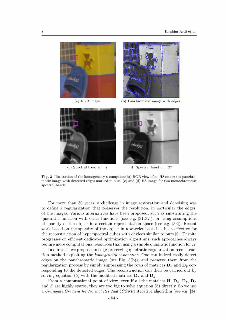
8 Ibrahim Ardi et al.
(a) RGB image (b) Panchromatic image with edges
(c) Spectral band w = 7 (d) Spectral band w = 27
Fig. 3 Illustration of the homogeneity assumption: (a) RGB view of an HS scene; (b) panchro-matic image with detected edges marked in blue; (c) and (d) HS image for two monochromaticspectral bands.
For more than 30 years, a challenge in image restoration and denoising wasto define a regularization that preserves the resolution, in particular the edges,of the images. Various alternatives have been proposed, such as substituting thequadratic function with other functions (see e.g. [31,32]), or using assumptionsof sparsity of the object in a certain representation space (see e.g. [33]). Recentwork based on the sparsity of the object in a wavelet basis has been effective forthe reconstruction of hyperspectral cubes with devices similar to ours [6]. Despiteprogresses on efficient dedicated optimization algorithms, such approaches alwaysrequire more computational resources than using a simple quadratic function for Ω.
In our case, we propose an edge-preserving quadratic regularization reconstruc-tion method exploiting the homogeneity assumption. One can indeed easily detectedges on the panchromatic image (see Fig. 3(b)), and preserve them from theregularization process by simply suppressing the rows of matrices Dx and Dy cor-responding to the detected edges. The reconstruction can then be carried out bysolving equation (5) with the modified matrices Dx and Dy.
From a computational point of view, even if all the matrices H, Dx, Dy, Dλ
and Γ are highly sparse, they are too big to solve equation (5) directly. So we usea Conjugate Gradient for Normal Residual (CGNR) iterative algorithm (see e.g. [34,
- 54 -
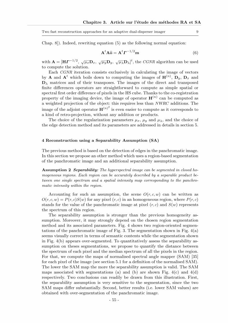
Chapitre 3. Article sur l’étude des méthodes RA et SA
Two fast reconstruction approaches for an adaptive dual-disperser imager 9
Chap. 8]). Indeed, rewriting equation (5) as the following normal equation:
AtAo = AtΓ−1/2m (6)
with A = [HΓ−1/2,√µxDx,
õyDy,
√µλDλ]t, the CGNR algorithm can be used
to compute the solution.Each CGNR iteration consists exclusively in calculating the image of vectors
by A and At which boils down to computing the images of H(n), Dy, Dx andDλ matrices and of their transposes. The images of the direct and transposedfinite differences operators are straightforward to compute as simple spatial orspectral first order difference of pixels in the HS cube. Thanks to the co-registrationproperty of the imaging device, the image of operator H(n) can be computed asa weighted projection of the object: this requires less than NWRC additions. The
image of the adjoint operator H(n)t is even easier to compute as it corresponds toa kind of retro-projection, without any addition or products.
The choice of the regularization parameters µx, µy and µλ, and the choice ofthe edge detection method and its parameters are addressed in details in section 5.
4 Reconstruction using a Separability Assumption (SA)
The previous method is based on the detection of edges in the panchromatic image.In this section we propose an other method which uses a region-based segmentationof the panchromatic image and an additional separability assumption.
Assumption 2 Separability: The hyperspectral image can be segmented in closed ho-
mogeneous regions. Each region can be accurately described by a separable product be-
tween one single spectrum and a spatial intensity map corresponding to the panchro-
matic intensity within the region.
Accounting for such an assumption, the scene O(r, c, w) can be written asO(r, c, w) = P (r, c)S(w) for any pixel (r, c) in an homogeneous region, where P (r, c)stands for the value of the panchromatic image at pixel (r, c) and S(w) representsthe spectrum of this region.
The separability assumption is stronger than the previous homogeneity as-sumption. Moreover, it may strongly depend on the chosen region segmentationmethod and its associated parameters. Fig. 4 shows two region-oriented segmen-tations of the panchromatic image of Fig. 3. The segmentation shown in Fig. 4(a)seems visually correct in terms of semantic contents while the segmentation shownin Fig. 4(b) appears over-segmented. To quantitatively assess the separability as-sumption on theses segmentations, we propose to quantify the distance betweenthe spectrum of each pixel and the median spectrum of all the pixels in the region.For that, we compute the maps of normalised spectral angle mapper (SAM) [35]for each pixel of the image (see section 5.1 for a definition of the normalised SAM).The lower the SAM map the more the separability assumption is valid. The SAMmaps associated with segmentations (a) and (b) are shown Fig. 4(c) and 4(d)respectively. Two conclusions can readily be drawn from this illustration. First,the separability assumption is very sensitive to the segmentation, since the twoSAM maps differ substantially. Second, better results (i.e. lower SAM values) areobtained with over-segmentation of the panchromatic image.
- 55 -
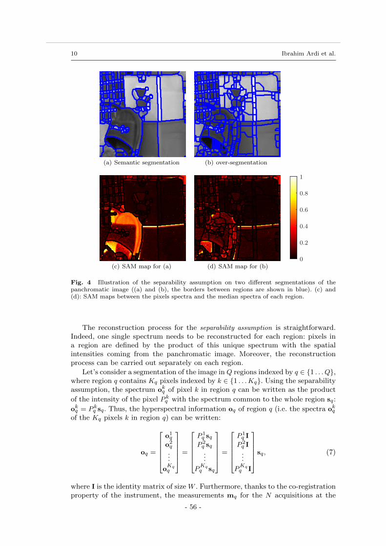
10 Ibrahim Ardi et al.
(a) Semantic segmentation (b) over-segmentation
(c) SAM map for (a)0
0.2
0.4
0.6
0.8
1
(d) SAM map for (b)
Fig. 4 Illustration of the separability assumption on two different segmentations of thepanchromatic image ((a) and (b), the borders between regions are shown in blue). (c) and(d): SAM maps between the pixels spectra and the median spectra of each region.
The reconstruction process for the separability assumption is straightforward.Indeed, one single spectrum needs to be reconstructed for each region: pixels ina region are defined by the product of this unique spectrum with the spatialintensities coming from the panchromatic image. Moreover, the reconstructionprocess can be carried out separately on each region.
Let’s consider a segmentation of the image in Q regions indexed by q ∈ 1 . . . Q,where region q contains Kq pixels indexed by k ∈ 1 . . .Kq. Using the separabilityassumption, the spectrum okq of pixel k in region q can be written as the product
of the intensity of the pixel P kq with the spectrum common to the whole region sq:
okq = P kq sq. Thus, the hyperspectral information oq of region q (i.e. the spectra okqof the Kq pixels k in region q) can be written:
oq =
o1q
o2q
...
oKqq
=
P 1q sqP 2q sq...
PKqq sq
=
P 1q I
P 2q I...
PKqq I
sq, (7)
where I is the identity matrix of size W . Furthermore, thanks to the co-registrationproperty of the instrument, the measurements mq for the N acquisitions at the
- 56 -
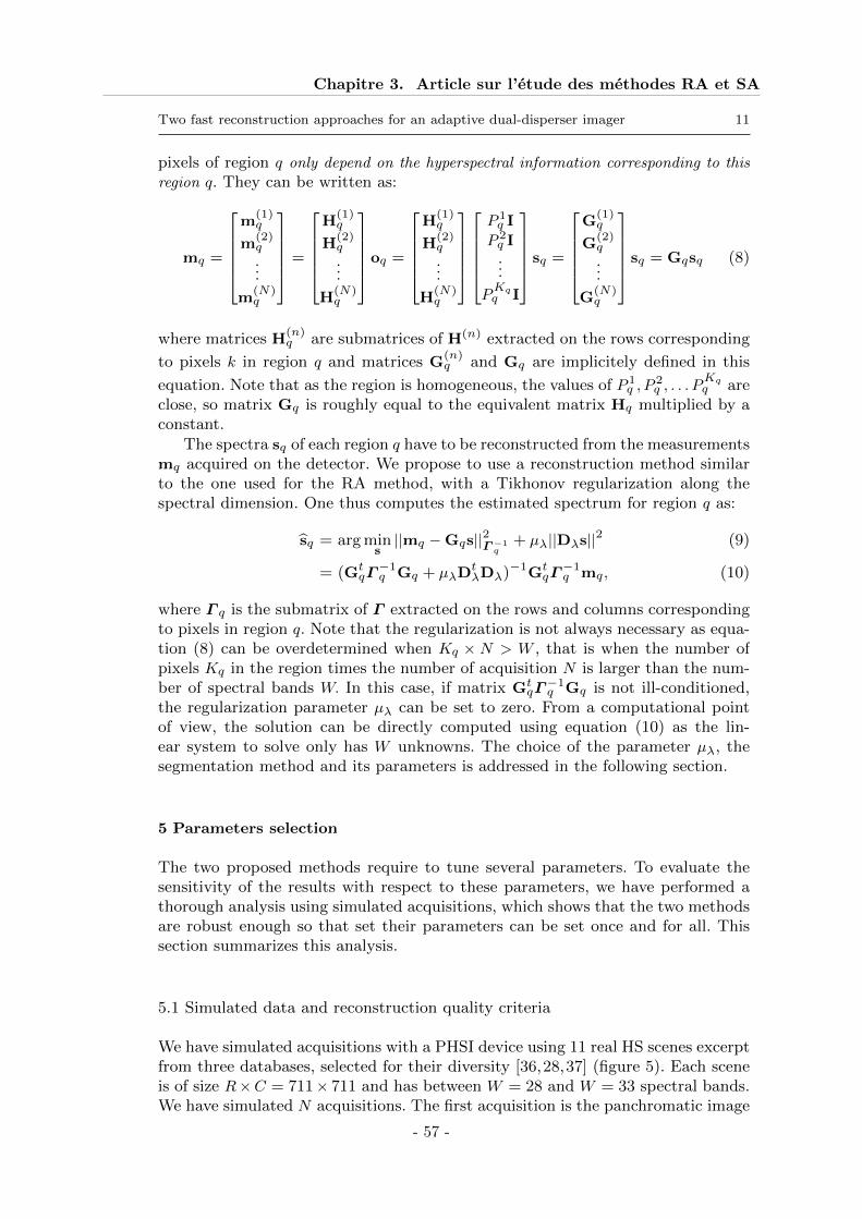
Chapitre 3. Article sur l’étude des méthodes RA et SA
Two fast reconstruction approaches for an adaptive dual-disperser imager 11
pixels of region q only depend on the hyperspectral information corresponding to this
region q. They can be written as:
mq =
m(1)q
m(2)q
...
m(N)q
=
H(1)q
H(2)q
...
H(N)q
oq =
H(1)q
H(2)q
...
H(N)q
P 1q I
P 2q I...
PKqq I
sq =
G(1)q
G(2)q
...
G(N)q
sq = Gqsq (8)
where matrices H(n)q are submatrices of H(n) extracted on the rows corresponding
to pixels k in region q and matrices G(n)q and Gq are implicitely defined in this
equation. Note that as the region is homogeneous, the values of P 1q , P
2q , . . . P
Kqq are
close, so matrix Gq is roughly equal to the equivalent matrix Hq multiplied by aconstant.
The spectra sq of each region q have to be reconstructed from the measurementsmq acquired on the detector. We propose to use a reconstruction method similarto the one used for the RA method, with a Tikhonov regularization along thespectral dimension. One thus computes the estimated spectrum for region q as:
sq = arg mins||mq −Gqs||2Γ−1
q+ µλ||Dλs||2 (9)
= (GtqΓ−1q Gq + µλDt
λDλ)−1GtqΓ−1q mq, (10)
where Γ q is the submatrix of Γ extracted on the rows and columns correspondingto pixels in region q. Note that the regularization is not always necessary as equa-tion (8) can be overdetermined when Kq × N > W , that is when the number ofpixels Kq in the region times the number of acquisition N is larger than the num-ber of spectral bands W. In this case, if matrix Gt
qΓ−1q Gq is not ill-conditioned,
the regularization parameter µλ can be set to zero. From a computational pointof view, the solution can be directly computed using equation (10) as the lin-ear system to solve only has W unknowns. The choice of the parameter µλ, thesegmentation method and its parameters is addressed in the following section.
5 Parameters selection
The two proposed methods require to tune several parameters. To evaluate thesensitivity of the results with respect to these parameters, we have performed athorough analysis using simulated acquisitions, which shows that the two methodsare robust enough so that set their parameters can be set once and for all. Thissection summarizes this analysis.
5.1 Simulated data and reconstruction quality criteria
We have simulated acquisitions with a PHSI device using 11 real HS scenes excerptfrom three databases, selected for their diversity [36,28,37] (figure 5). Each sceneis of size R×C = 711× 711 and has between W = 28 and W = 33 spectral bands.We have simulated N acquisitions. The first acquisition is the panchromatic image
- 57 -
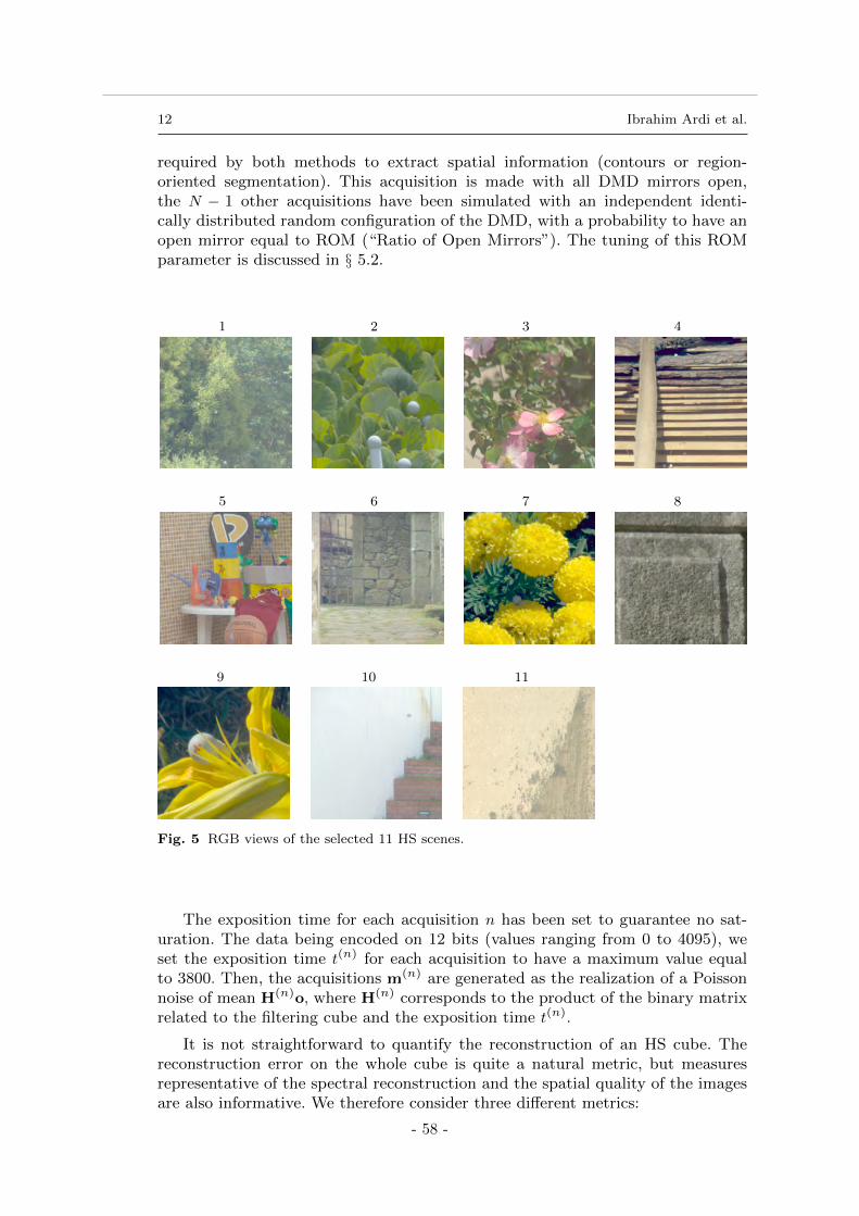
12 Ibrahim Ardi et al.
required by both methods to extract spatial information (contours or region-oriented segmentation). This acquisition is made with all DMD mirrors open,the N − 1 other acquisitions have been simulated with an independent identi-cally distributed random configuration of the DMD, with a probability to have anopen mirror equal to ROM (“Ratio of Open Mirrors”). The tuning of this ROMparameter is discussed in § 5.2.
3 41 2
11109
5 76 8
Fig. 5 RGB views of the selected 11 HS scenes.
The exposition time for each acquisition n has been set to guarantee no sat-uration. The data being encoded on 12 bits (values ranging from 0 to 4095), weset the exposition time t(n) for each acquisition to have a maximum value equalto 3800. Then, the acquisitions m(n) are generated as the realization of a Poissonnoise of mean H(n)o, where H(n) corresponds to the product of the binary matrixrelated to the filtering cube and the exposition time t(n).
It is not straightforward to quantify the reconstruction of an HS cube. Thereconstruction error on the whole cube is quite a natural metric, but measuresrepresentative of the spectral reconstruction and the spatial quality of the imagesare also informative. We therefore consider three different metrics:
- 58 -
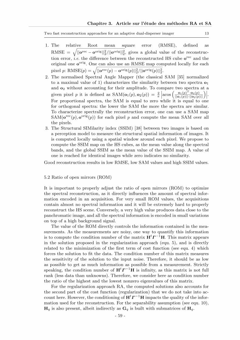
Chapitre 3. Article sur l’étude des méthodes RA et SA
Two fast reconstruction approaches for an adaptive dual-disperser imager 13
1. The relative Root mean square error (RMSE), defined as
RMSE =√||orec − oorig||22/||oorig||22, gives a global value of the reconstruc-
tion error, i.e. the difference between the reconstructed HS cube orec and theoriginal one oorig. One can also use an RMSE map computed locally for each
pixel p: RMSE(p) =√||orec(p)− oorig(p)||22/||oorig(p)||22.
2. The normalised Spectral Angle Mapper (the classical SAM [35] normalizedto a maximal value of 1) characterizes the similarity between two spectra o1
and o2 without accounting for their amplitude. To compare two spectra at a
given pixel p it is defined as SAM(o1(p),o2(p)) = 2π
∣∣∣acos(
o1(p)T ·o2(p)
||o1(p)||·||o2(p)||)∣∣∣.
For proportional spectra, the SAM is equal to zero while it is equal to onefor orthogonal spectra: the lower the SAM the more the spectra are similar.To characterize spectrally the reconstruction error, one can use a SAM mapSAM(orec(p),oorig(p)) for each pixel p and compute the mean SAM over allthe pixels.
3. The Structural SIMilarity index (SSIM) [38] between two images is based ona perception model to measure the structural spatial information of images. Itis computed locally using a spatial window around each pixel. We propose tocompute the SSIM map on the HS cubes, as the mean value along the spectralbands, and the global SSIM as the mean value of the SSIM map. A value ofone is reached for identical images while zero indicates no similarity.
Good reconstruction results in low RMSE, low SAM values and high SSIM values.
5.2 Ratio of open mirrors (ROM)
It is important to properly adjust the ratio of open mirrors (ROM) to optimizethe spectral reconstruction, as it directly influences the amount of spectral infor-mation encoded in an acquisition. For very small ROM values, the acquisitionscontain almost no spectral information and it will be extremely hard to properlyreconstruct the HS scene. Conversely, a very high value produces data close to thepanchromatic image, and all the spectral information is encoded in small variationson top of a high background signal.
The value of the ROM directly controls the information contained in the mea-surements. As the measurements are noisy, one way to quantify this informationis to compute the condition number of the matrix HtΓ−1H. This matrix appearsin the solution proposed in the regularization approach (equ. 5), and is directlyrelated to the minimization of the first term of cost function (see equ. 4) whichforces the solution to fit the data. The condition number of this matrix measuresthe sensitivity of the solution to the input noise. Therefore, it should be as lowas possible to get as much information as possible from a measurement. Strictlyspeaking, the condition number of HtΓ−1H is infinity, as this matrix is not fullrank (less data than unknowns). Therefore, we consider here as condition numberthe ratio of the highest and the lowest nonzero eigenvalues of this matrix.
For the regularization approach RA, the computed solutions also accounts forthe second part of the cost function (regularization) that we do not take into ac-count here. However, the conditioning of HtΓ−1H impacts the quality of the infor-mation used for the reconstruction. For the separability assumption (see equ. 10),Hq is also present, albeit indirectly as Gq is built with submatrices of Hq.
- 59 -
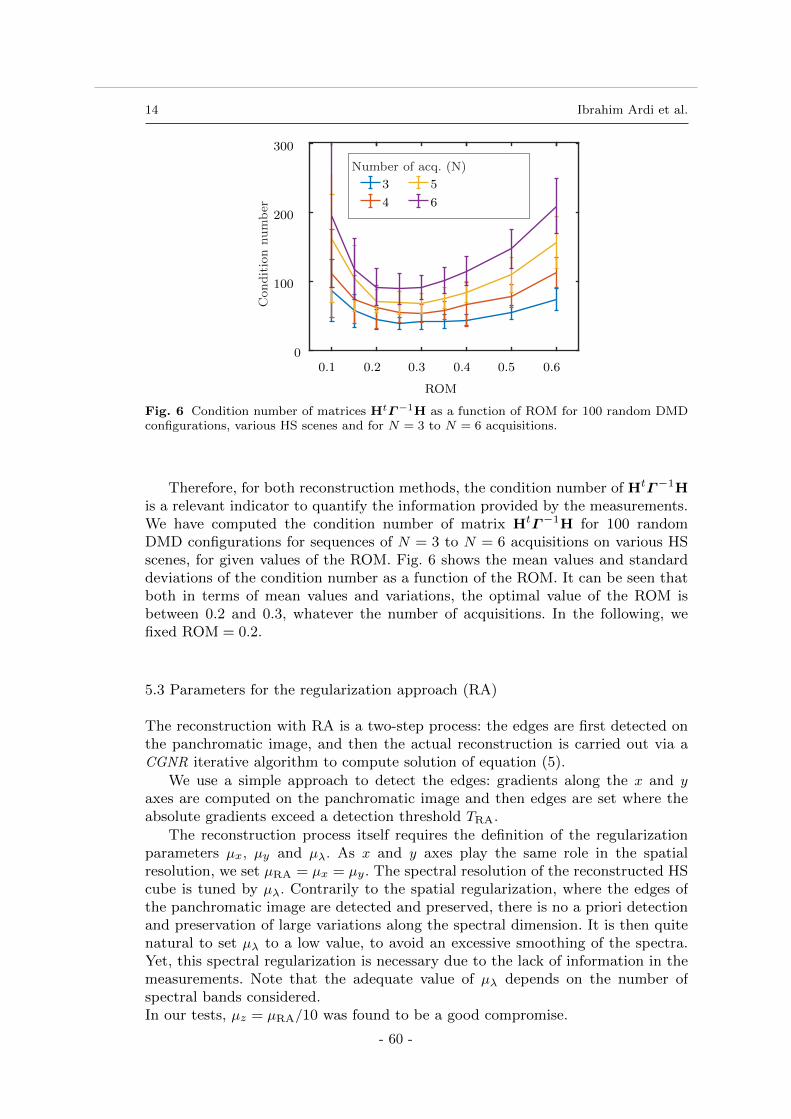
14 Ibrahim Ardi et al.
0.2 0.4 0.6
ROM
0
100
200
300
Con
dit
ion
nu
mb
er
Number of acq. (N)
3
4
5
6
0.1 0.3 0.5
Fig. 6 Condition number of matrices HtΓ−1H as a function of ROM for 100 random DMDconfigurations, various HS scenes and for N = 3 to N = 6 acquisitions.
Therefore, for both reconstruction methods, the condition number of HtΓ−1H
is a relevant indicator to quantify the information provided by the measurements.We have computed the condition number of matrix HtΓ−1H for 100 randomDMD configurations for sequences of N = 3 to N = 6 acquisitions on various HSscenes, for given values of the ROM. Fig. 6 shows the mean values and standarddeviations of the condition number as a function of the ROM. It can be seen thatboth in terms of mean values and variations, the optimal value of the ROM isbetween 0.2 and 0.3, whatever the number of acquisitions. In the following, wefixed ROM = 0.2.
5.3 Parameters for the regularization approach (RA)
The reconstruction with RA is a two-step process: the edges are first detected onthe panchromatic image, and then the actual reconstruction is carried out via aCGNR iterative algorithm to compute solution of equation (5).
We use a simple approach to detect the edges: gradients along the x and y
axes are computed on the panchromatic image and then edges are set where theabsolute gradients exceed a detection threshold TRA.
The reconstruction process itself requires the definition of the regularizationparameters µx, µy and µλ. As x and y axes play the same role in the spatialresolution, we set µRA = µx = µy. The spectral resolution of the reconstructed HScube is tuned by µλ. Contrarily to the spatial regularization, where the edges ofthe panchromatic image are detected and preserved, there is no a priori detectionand preservation of large variations along the spectral dimension. It is then quitenatural to set µλ to a low value, to avoid an excessive smoothing of the spectra.Yet, this spectral regularization is necessary due to the lack of information in themeasurements. Note that the adequate value of µλ depends on the number ofspectral bands considered.In our tests, µz = µRA/10 was found to be a good compromise.
- 60 -
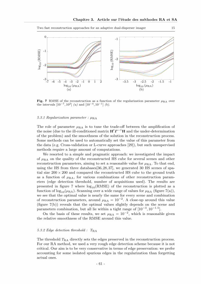
Chapitre 3. Article sur l’étude des méthodes RA et SA
Two fast reconstruction approaches for an adaptive dual-disperser imager 15
0
-1
-2
-3
log10
(RM
SE
)
-7 -6 -5 -4 -3 -2 -1 0 1 2log10 (µRA)
(a)
-1
-2
-3-3.5 -3 -2.5 -2 -1.5 -1
log10 (µRA)
log10
(RM
SE
)
(b)
Fig. 7 RMSE of the reconstruction as a function of the regularization parameter µRA overthe intervals [10−7, 102] (a) and [10−4, 10−1] (b).
5.3.1 Regularization parameter : µRA
The role of parameter µRA is to tune the trade-off between the amplification ofthe noise (due to the ill-conditioned matrix HtΓ−1H and the under-determinationof the problem) and the smoothness of the solution in the reconstruction process.Some methods can be used to automatically set the value of this parameter fromthe data (e.g. Cross-validation or L-curve approaches [29]), but such unsupervisedmethods require a large amount of computations.
We resorted to a simple and pragmatic approach: we investigated the impactof µRA on the quality of the reconstructed HS cube for several scenes and otherreconstruction parameters, aiming to set a reasonable value for µRA. To that end,using the HS from three databases[36,28,37], we generated 30 HS scenes of spa-tial size 200 × 200 and compared the reconstructed HS cube to the ground truthas a function of µRA, for various combinations of other reconstruction param-eters (edge detection threshold, number of acquisitions used). The results arepresented in figure 7 where log10(RMSE) of the reconstruction is plotted as afunction of log10(µRA). Scanning over a wide range of values for µRA (figure 7(a)),we see that the optimal value is nearly the same for every scene and combinationof reconstruction parameters, around µRA = 10−2. A close-up around this value(figure 7(b)) reveals that the optimal values slightly depends on the scene andparameters combination, but all lie within a tight range of [10−3, 10−1.5].
On the basis of these results, we set µRA = 10−2, which is reasonable giventhe relative smoothness of the RMSE around this value.
5.3.2 Edge detection threshold : TRA
The threshold TRA directly sets the edges preserved in the reconstruction process.For our RA method, we used a very rough edge detection scheme because it is notcritical. Our aim is to be very conservative in terms of edge preservation: we preferaccounting for some isolated spurious edges in the regularization than forgettingactual ones.
- 61 -
16 Ibrahim Ardi et al.
Indeed, spurious edges only zero few coefficients in the Dx and Dy matrices,thus lowering slightly the strength of the regularization. On the contrary, notaccounting for an actual edge in the panchromatic image would result in undesiredsmoothing in the reconstructed HS cube.
On this basis, our method is not very sensitive to the TRA threshold, providedthat its value is sufficiently low. Considering the intensities of the panchromaticimage in the interval [0, 3800], we set TRA = 50 which is very low (an example ofedge detection with this value of TRA is shown in figure 3(b)). Of course, any moresophisticated edge detection method could be used and may improve the result ifcorrectly tuned.
5.4 Parameters for the separability assumption (SA)
The HS scenes reconstruction under SA is also a two-step process. The panchro-matic image is first segmented into homogeneous closed regions, and then thereconstruction is carried out independently for each region via a least-square mi-nimization.
It is worth noting two key differences between the segmentation carried outhere and the one used in RA. First, for RA, one only needs to detect edges, evenisolated ones, while for SA we need to define closed regions. Moreover, while theedge detection in RA is not critical at all, the segmentation for SA is a key step.
For the region-oriented segmentation, we used the classical watershed algo-rithm [39], which only depends on one parameter: the segmentation threshold TSA.An additional parameter is however introduced: the width wSA of the contours.Indeed, because of the point spread function of the optical system, the spectra ofthe pixels near the contours between regions is a mixture of the spectral contents ofadjacent regions and thus does not satisfy our separability assumption. Therefore,we propose to enlarge this contours, giving them a width wSA.
Note that with the SA approach, pixels belonging to a contour are not part ofany region and thus excluded from the reconstruction process, but more advancedmethods could be implemented to reconstruct these pixels spectra.
Once the image is segmented, the reconstruction is carried out independentlyfor each region by solving equation (10) for which the regularization parameterµSA = µλ has to be tuned.
5.4.1 Segmentation threshold: TSA
As the Separability Assumption in each region is strong, the segmentation processis a crucial stage of the SA approach: a particular attention has to be paid to thetuning of TSA.
The choice of the segmentation threshold TSA is the result of a compromise. Atoo low value yields over-segmentation, with small regions. This ensures that theseparability assumption is satisfied, but small regions may not contains enoughpixels, hence too little information on their spectral content, thus hindering thereconstruction of the spectrum. On the opposite, a too large value of TSA yieldslarge regions that surely contain enough redundant information for spectrum re-construction, but in which the separability assumption might not be satisfied. As
- 62 -
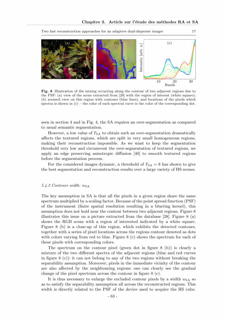
Chapitre 3. Article sur l’étude des méthodes RA et SA
Two fast reconstruction approaches for an adaptive dual-disperser imager 17
2010 30Bands
(c)(b)(a)
Inte
nsi
ty[a
rb.
u.]
Fig. 8 Illustration of the mixing occurring along the contour of two adjacent regions due tothe PSF: (a) view of the scene extracted from [28] with the region of interest (white square);(b) zoomed view on this region with contours (blue lines), and locations of the pixels whichspectra is shown in (c) – the color of each spectral curve is the color of the corresponding dot.
seen in section 4 and in Fig. 4, the SA requires an over-segmentation as comparedto usual semantic segmentation.
However, a low value of TSA to obtain such an over-segmentation dramaticallyaffects the textured regions, which are split in very small homogeneous regions,making their reconstruction impossible. As we want to keep the segmentationthreshold very low and circumvent the over-segmentation of textured regions, weapply an edge preserving anisotropic diffusion [40] to smooth textured regionsbefore the segmentation process.
For the considered images dynamic, a threshold of TSA = 8 has shown to givethe best segmentation and reconstruction results over a large variety of HS scenes.
5.4.2 Contours width: wSA
The key assumption in SA is that all the pixels in a given region share the samespectrum multiplied by a scaling factor. Because of the point spread function (PSF)of the instrument (finite spatial resolution resulting in a blurring kernel), thisassumption does not hold near the contour between two adjacent regions. Figure 8illustrates this issue on a picture extracted from the database [28]. Figure 8 (a)shows the RGB scene with a region of interested indicated by a white square.Figure 8 (b) is a close-up of this region, which exhibits the detected contours,together with a series of pixel locations across the regions contour denoted as dotswith colors varying from red to blue. Figure 8 (c) shows the spectrum for each ofthese pixels with corresponding colors.
The spectrum on the contour pixel (green dot in figure 8 (b)) is clearly amixture of the two different spectra of the adjacent regions (blue and red curvesin figure 8 (c)): it can not belong to any of the two regions without breaking theseparability assumption. Moreover, pixels in the immediate vicinity of the contourare also affected by the neighbouring regions: one can clearly see the gradualchange of the pixel spectrum across the contour in figure 8 (c).
It is thus necessary to enlarge the excluded contour pixels by a width wSA soas to satisfy the separability assumption all across the reconstructed regions. Thiswidth is directly related to the PSF of the device used to acquire the HS cube.
- 63 -
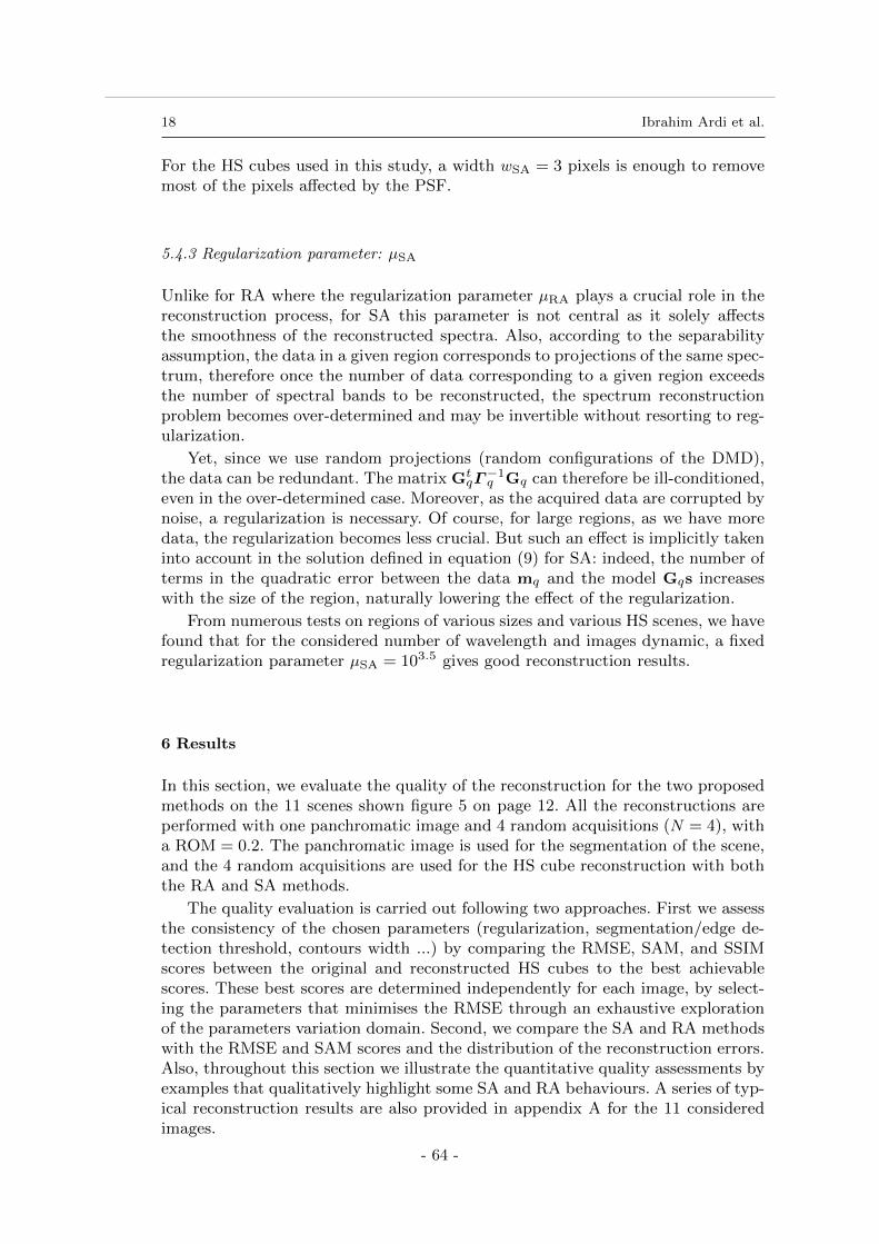
18 Ibrahim Ardi et al.
For the HS cubes used in this study, a width wSA = 3 pixels is enough to removemost of the pixels affected by the PSF.
5.4.3 Regularization parameter: µSA
Unlike for RA where the regularization parameter µRA plays a crucial role in thereconstruction process, for SA this parameter is not central as it solely affectsthe smoothness of the reconstructed spectra. Also, according to the separabilityassumption, the data in a given region corresponds to projections of the same spec-trum, therefore once the number of data corresponding to a given region exceedsthe number of spectral bands to be reconstructed, the spectrum reconstructionproblem becomes over-determined and may be invertible without resorting to reg-ularization.
Yet, since we use random projections (random configurations of the DMD),the data can be redundant. The matrix Gt
qΓ−1q Gq can therefore be ill-conditioned,
even in the over-determined case. Moreover, as the acquired data are corrupted bynoise, a regularization is necessary. Of course, for large regions, as we have moredata, the regularization becomes less crucial. But such an effect is implicitly takeninto account in the solution defined in equation (9) for SA: indeed, the number ofterms in the quadratic error between the data mq and the model Gqs increaseswith the size of the region, naturally lowering the effect of the regularization.
From numerous tests on regions of various sizes and various HS scenes, we havefound that for the considered number of wavelength and images dynamic, a fixedregularization parameter µSA = 103.5 gives good reconstruction results.
6 Results
In this section, we evaluate the quality of the reconstruction for the two proposedmethods on the 11 scenes shown figure 5 on page 12. All the reconstructions areperformed with one panchromatic image and 4 random acquisitions (N = 4), witha ROM = 0.2. The panchromatic image is used for the segmentation of the scene,and the 4 random acquisitions are used for the HS cube reconstruction with boththe RA and SA methods.
The quality evaluation is carried out following two approaches. First we assessthe consistency of the chosen parameters (regularization, segmentation/edge de-tection threshold, contours width ...) by comparing the RMSE, SAM, and SSIMscores between the original and reconstructed HS cubes to the best achievablescores. These best scores are determined independently for each image, by select-ing the parameters that minimises the RMSE through an exhaustive explorationof the parameters variation domain. Second, we compare the SA and RA methodswith the RMSE and SAM scores and the distribution of the reconstruction errors.Also, throughout this section we illustrate the quantitative quality assessments byexamples that qualitatively highlight some SA and RA behaviours. A series of typ-ical reconstruction results are also provided in appendix A for the 11 consideredimages.
- 64 -
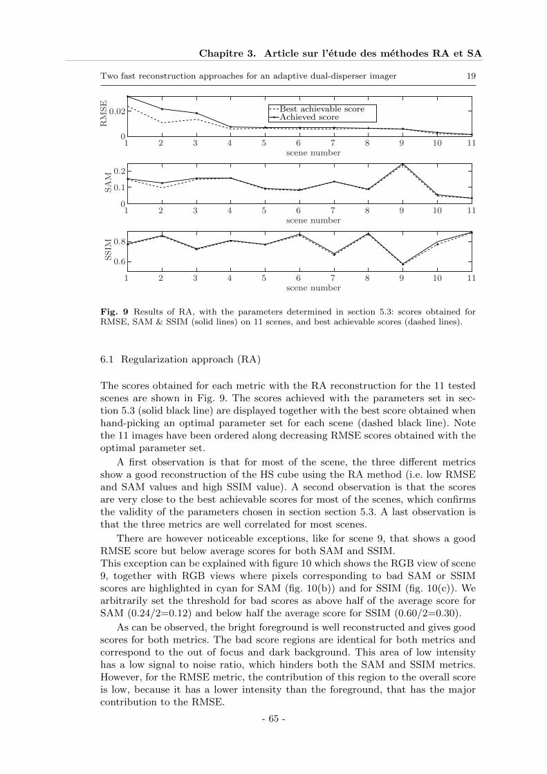
Chapitre 3. Article sur l’étude des méthodes RA et SA
Two fast reconstruction approaches for an adaptive dual-disperser imager 19
1 2 3 4 5 6 7 8 9 10 11scene number
0.6
0.8
SS
IM
1 2 3 4 5 6 7 8 9 10 11scene number
0
0.1
0.2
SA
M
1 2 3 4 5 6 7 8 9 10 11scene number
0
0.02R
MS
EBest achievable scoreAchieved score
Fig. 9 Results of RA, with the parameters determined in section 5.3: scores obtained forRMSE, SAM & SSIM (solid lines) on 11 scenes, and best achievable scores (dashed lines).
6.1 Regularization approach (RA)
The scores obtained for each metric with the RA reconstruction for the 11 testedscenes are shown in Fig. 9. The scores achieved with the parameters set in sec-tion 5.3 (solid black line) are displayed together with the best score obtained whenhand-picking an optimal parameter set for each scene (dashed black line). Notethe 11 images have been ordered along decreasing RMSE scores obtained with theoptimal parameter set.
A first observation is that for most of the scene, the three different metricsshow a good reconstruction of the HS cube using the RA method (i.e. low RMSEand SAM values and high SSIM value). A second observation is that the scoresare very close to the best achievable scores for most of the scenes, which confirmsthe validity of the parameters chosen in section section 5.3. A last observation isthat the three metrics are well correlated for most scenes.
There are however noticeable exceptions, like for scene 9, that shows a goodRMSE score but below average scores for both SAM and SSIM.This exception can be explained with figure 10 which shows the RGB view of scene9, together with RGB views where pixels corresponding to bad SAM or SSIMscores are highlighted in cyan for SAM (fig. 10(b)) and for SSIM (fig. 10(c)). Wearbitrarily set the threshold for bad scores as above half of the average score forSAM (0.24/2=0.12) and below half the average score for SSIM (0.60/2=0.30).
As can be observed, the bright foreground is well reconstructed and gives goodscores for both metrics. The bad score regions are identical for both metrics andcorrespond to the out of focus and dark background. This area of low intensityhas a low signal to noise ratio, which hinders both the SAM and SSIM metrics.However, for the RMSE metric, the contribution of this region to the overall scoreis low, because it has a lower intensity than the foreground, that has the majorcontribution to the RMSE.
- 65 -
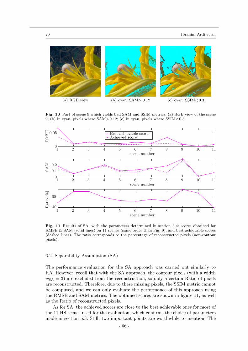
20 Ibrahim Ardi et al.
(a) RGB view (b) cyan: SAM> 0.12 (c) cyan: SSIM<0.3
Fig. 10 Part of scene 9 which yields bad SAM and SSIM metrics. (a) RGB view of the scene9; (b) in cyan, pixels where SAM>0.12; (c) in cyan, pixels where SSIM<0.3
1 2 3 4 5 6 7 8 9 10 11scene number
40
60
Rati
o[%
]
1 2 3 4 5 6 7 8 9 10 11scene number
0
0.1
0.2
SA
M
1 2 3 4 5 6 7 8 9 10 11scene number
0
0.05
RM
SE Best achievable score
Achieved score
Fig. 11 Results of SA, with the parameters determined in section 5.4: scores obtained forRMSE & SAM (solid lines) on 11 scenes (same order than Fig. 9), and best achievable scores(dashed lines). The ratio corresponds to the percentage of reconstructed pixels (non-contourpixels).
6.2 Separability Assumption (SA)
The performance evaluation for the SA approach was carried out similarly toRA. However, recall that with the SA approach, the contour pixels (with a widthwSA = 3) are excluded from the reconstruction, so only a certain Ratio of pixelsare reconstructed. Therefore, due to these missing pixels, the SSIM metric cannotbe computed, and we can only evaluate the performance of this approach usingthe RMSE and SAM metrics. The obtained scores are shown in figure 11, as wellas the Ratio of reconstructed pixels.
As for SA, the achieved scores are close to the best achievable ones for most ofthe 11 HS scenes used for the evaluation, which confirms the choice of parametersmade in section 5.3. Still, two important points are worthwhile to mention. The
- 66 -
Chapitre 3. Article sur l’étude des méthodes RA et SA
Two fast reconstruction approaches for an adaptive dual-disperser imager 21
first is that similarly to RA, SA approach suffers from the low-contrast problem,as indicated by the high SAM score value achieved for the HS scene 9. The secondpoint concerns the achieved scores both for RMSE and SAM metrics for the HSscene 8, which, unlike other HS scenes, are far below the optimal scores.
To investigate this particularly poor result, we have compared the SA recon-struction obtained for this scene with the default parameters with the one ob-tained with optimal set of parameters. This comparison is shown figure 12. TheRGB image shows the scene is made of one single textured greyish stone material,contrary to the other scenes which exhibit various types of materials and colors.For the default parameter set defined in section 5.4, the scene is segmented inmany small regions, as shown figure 12 (b), with the notable exception of two size-able regions corresponding to dark areas. This high over-segmentation explainsthe poor performance of the SA reconstruction with default parameters, as canbe seen in figure 12 (c), which shows the reconstructed RGB image, with the ex-tracted contours in blue and pixels with high SAM score highlighted in cyan2. Wecan observe that these high SAM score pixels belong either to the smallest regionsor to one of the two large dark regions. For the small regions, the reconstructionwith SA is sub-optimal because there are not enough data to achieve an accuratereconstruction of the spectrum. The low-contrast problem observed and discussedpreviously explains that the dark regions are not well reconstructed either.
The main difference between the default parameters and the optimum onesis the segmentation threshold TSA, which value is respectively TSA = 8 andTSA = 50. The segmentation obtained with this optimal threshold is shown fig-ure 12 (d): most of the scene is now considered as one single region. With such asegmentation, the SA reconstruction is overdetermined and the spectrum is accu-rately reconstructed in most of the pixels of the scene, as shown figure 12 (e). Inthis figure, the number of pixels with high SAM (in cyan) is considerably reducedwith respect to reconstruction with TSA = 50, and they mainly correspond to thedarkest areas (low-contrast problem).
To sum up, the SA method shows a reasonable degree of robustness regardingthe chosen set of parameters used for the reconstructions and its performances forthe selected parameters are in average close to the best achievable ones. Concerningthe scores, SA achieves in average, over the 11 HS scenes tested, a score of 0.19 forthe SAM and reconstructs in average 55% of the scenes pixels. These performancesare however sensitive to the scenes characteristics, such as the presence of finetexture as in scene 8, and similarly to RA, to the presence of broad low contrastedregions.
6.3 Comparison of SA and RA performances
In this section we compare the results and scores achieved by the two proposedmethods. This comparison is delicate to perform, as the SA approach providesan incomplete reconstruction of the scenes (extracted contours are left unrecon-structed), whereas the RA approach gives a complete reconstruction.
To address this limitation, we have at first focused exclusively on the com-parison of the quality of the reconstruction restricted to reconstructed regions
2 As in figure 10, high SAM scores are defined as over half of the average SAM score forreconstruction of this scene with default parameters: here as SAM> 0.09.
- 67 -
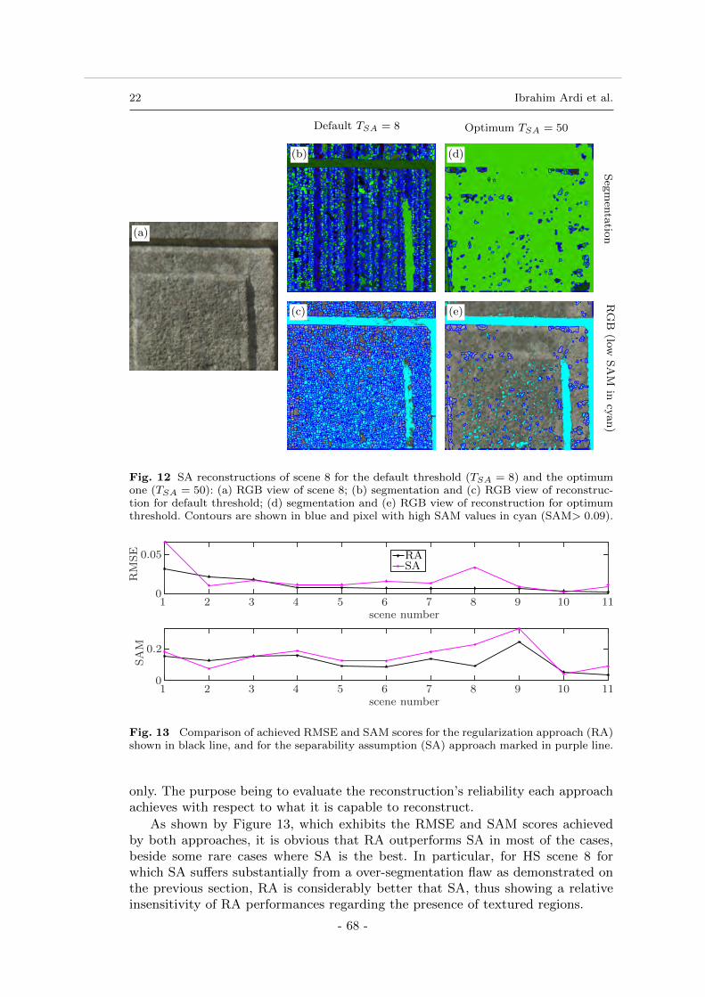
22 Ibrahim Ardi et al.S
egm
enta
tion
RG
B(lo
wS
AM
incy
an
)
Optimum TSA = 50Default TSA = 8
(a)
(b)
(c)
(d)
(e)
Fig. 12 SA reconstructions of scene 8 for the default threshold (TSA = 8) and the optimumone (TSA = 50): (a) RGB view of scene 8; (b) segmentation and (c) RGB view of reconstruc-tion for default threshold; (d) segmentation and (e) RGB view of reconstruction for optimumthreshold. Contours are shown in blue and pixel with high SAM values in cyan (SAM> 0.09).
1 2 3 4 5 6 7 8 9 10 11scene number
0
0.2
SA
M
RASA
1 2 3 4 5 6 7 8 9 10 11scene number
0
0.05
RM
SE
Fig. 13 Comparison of achieved RMSE and SAM scores for the regularization approach (RA)shown in black line, and for the separability assumption (SA) approach marked in purple line.
only. The purpose being to evaluate the reconstruction’s reliability each approachachieves with respect to what it is capable to reconstruct.
As shown by Figure 13, which exhibits the RMSE and SAM scores achievedby both approaches, it is obvious that RA outperforms SA in most of the cases,beside some rare cases where SA is the best. In particular, for HS scene 8 forwhich SA suffers substantially from a over-segmentation flaw as demonstrated onthe previous section, RA is considerably better that SA, thus showing a relativeinsensitivity of RA performances regarding the presence of textured regions.
- 68 -
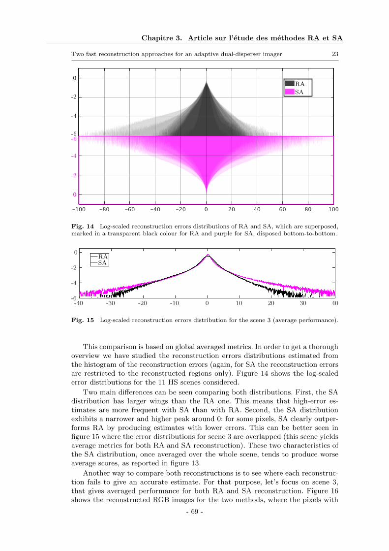
Chapitre 3. Article sur l’étude des méthodes RA et SA
Two fast reconstruction approaches for an adaptive dual-disperser imager 23
RA
SA
Fig. 14 Log-scaled reconstruction errors distributions of RA and SA, which are superposed,marked in a transparent black colour for RA and purple for SA, disposed bottom-to-bottom.
-40 -30 -20 -10 0 10 20 30 40-6
-4
-2
0RASA
Fig. 15 Log-scaled reconstruction errors distribution for the scene 3 (average performance).
This comparison is based on global averaged metrics. In order to get a thoroughoverview we have studied the reconstruction errors distributions estimated fromthe histogram of the reconstruction errors (again, for SA the reconstruction errorsare restricted to the reconstructed regions only). Figure 14 shows the log-scalederror distributions for the 11 HS scenes considered.
Two main differences can be seen comparing both distributions. First, the SAdistribution has larger wings than the RA one. This means that high-error es-timates are more frequent with SA than with RA. Second, the SA distributionexhibits a narrower and higher peak around 0: for some pixels, SA clearly outper-forms RA by producing estimates with lower errors. This can be better seen infigure 15 where the error distributions for scene 3 are overlapped (this scene yieldsaverage metrics for both RA and SA reconstruction). These two characteristics ofthe SA distribution, once averaged over the whole scene, tends to produce worseaverage scores, as reported in figure 13.
Another way to compare both reconstructions is to see where each reconstruc-tion fails to give an accurate estimate. For that purpose, let’s focus on scene 3,that gives averaged performance for both RA and SA reconstruction. Figure 16shows the reconstructed RGB images for the two methods, where the pixels with
- 69 -
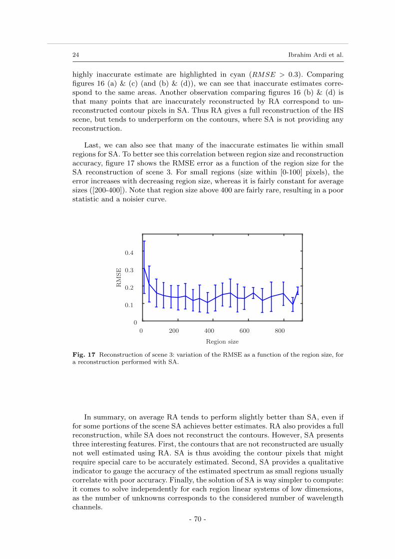
24 Ibrahim Ardi et al.
highly inaccurate estimate are highlighted in cyan (RMSE > 0.3). Comparingfigures 16 (a) & (c) (and (b) & (d)), we can see that inaccurate estimates corre-spond to the same areas. Another observation comparing figures 16 (b) & (d) isthat many points that are inaccurately reconstructed by RA correspond to un-reconstructed contour pixels in SA. Thus RA gives a full reconstruction of the HSscene, but tends to underperform on the contours, where SA is not providing anyreconstruction.
Last, we can also see that many of the inaccurate estimates lie within smallregions for SA. To better see this correlation between region size and reconstructionaccuracy, figure 17 shows the RMSE error as a function of the region size for theSA reconstruction of scene 3. For small regions (size within [0-100] pixels), theerror increases with decreasing region size, whereas it is fairly constant for averagesizes ([200-400]). Note that region size above 400 are fairly rare, resulting in a poorstatistic and a noisier curve.
0 200 400 600 800
Region size
0
0.1
0.2
0.3
0.4
RM
SE
Fig. 17 Reconstruction of scene 3: variation of the RMSE as a function of the region size, fora reconstruction performed with SA.
In summary, on average RA tends to perform slightly better than SA, even iffor some portions of the scene SA achieves better estimates. RA also provides a fullreconstruction, while SA does not reconstruct the contours. However, SA presentsthree interesting features. First, the contours that are not reconstructed are usuallynot well estimated using RA. SA is thus avoiding the contour pixels that mightrequire special care to be accurately estimated. Second, SA provides a qualitativeindicator to gauge the accuracy of the estimated spectrum as small regions usuallycorrelate with poor accuracy. Finally, the solution of SA is way simpler to compute:it comes to solve independently for each region linear systems of low dimensions,as the number of unknowns corresponds to the considered number of wavelengthchannels.
- 70 -
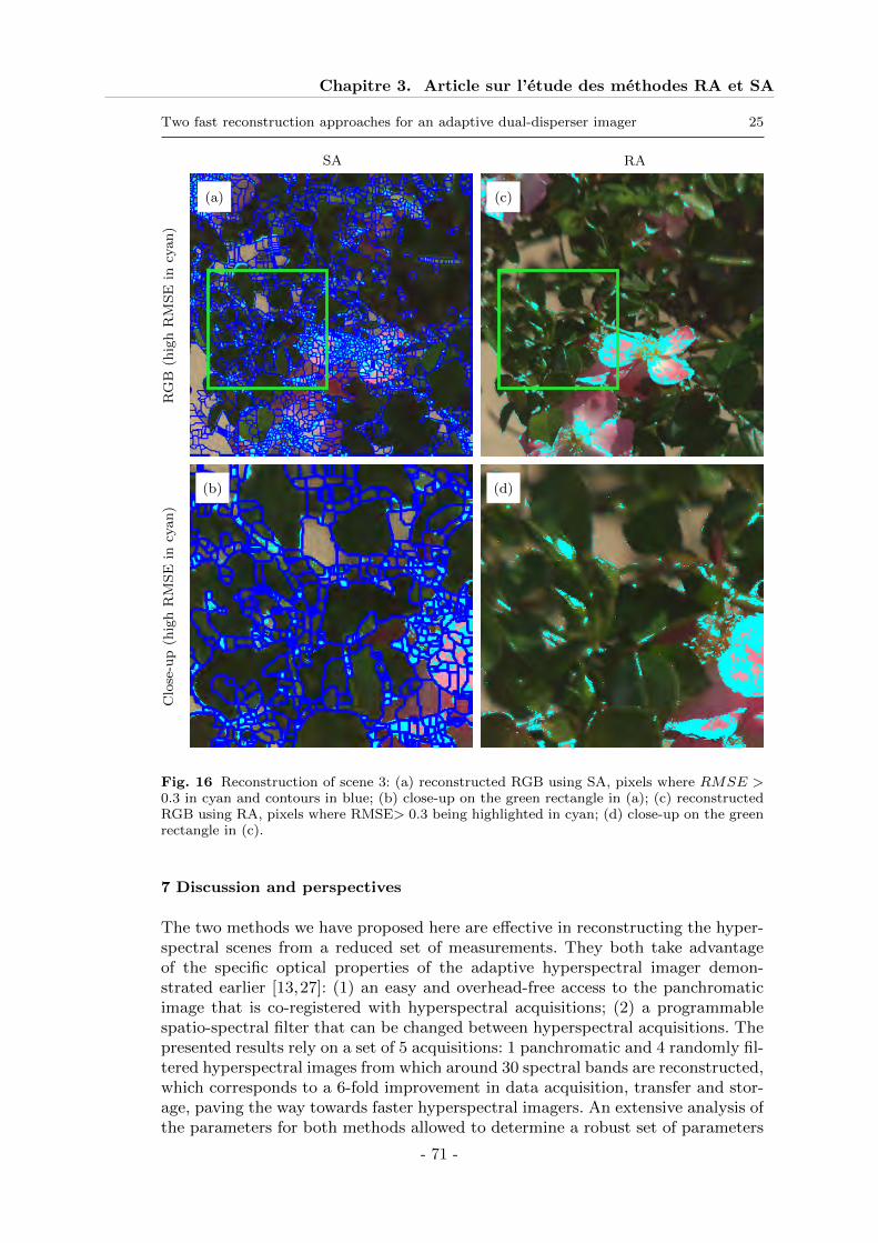
Chapitre 3. Article sur l’étude des méthodes RA et SA
Two fast reconstruction approaches for an adaptive dual-disperser imager 25
(a)
(b)
(c)
(d)
RASAR
GB
(hig
hR
MS
Ein
cyan
)C
lose
-up
(hig
hR
MS
Ein
cyan
)
Fig. 16 Reconstruction of scene 3: (a) reconstructed RGB using SA, pixels where RMSE >0.3 in cyan and contours in blue; (b) close-up on the green rectangle in (a); (c) reconstructedRGB using RA, pixels where RMSE> 0.3 being highlighted in cyan; (d) close-up on the greenrectangle in (c).
7 Discussion and perspectives
The two methods we have proposed here are effective in reconstructing the hyper-spectral scenes from a reduced set of measurements. They both take advantageof the specific optical properties of the adaptive hyperspectral imager demon-strated earlier [13,27]: (1) an easy and overhead-free access to the panchromaticimage that is co-registered with hyperspectral acquisitions; (2) a programmablespatio-spectral filter that can be changed between hyperspectral acquisitions. Thepresented results rely on a set of 5 acquisitions: 1 panchromatic and 4 randomly fil-tered hyperspectral images from which around 30 spectral bands are reconstructed,which corresponds to a 6-fold improvement in data acquisition, transfer and stor-age, paving the way towards faster hyperspectral imagers. An extensive analysis ofthe parameters for both methods allowed to determine a robust set of parameters
- 71 -
26 Ibrahim Ardi et al.
that compares well to cherry-picked parameter set for each of the 11 scenes usedfor this study. Both methods offer accurate reconstructions close to the groundtruth for several metrics. The SA method is based on the additional separabilityassumptions, which precludes the reconstruction of the HS image nearby the con-tours, but its computation load is lower than RA. But neither RA nor SA methodis a clear best approach for all the scenes.
Various straightforward improvements to the RA and SA methods could beeasily considered:
– Both methods are currently based on fairly rough segmentation methods andcould benefit from more advanced ones. For RA a simple gradient thresholdinghas been used, while various other classical edge detection methods can beapplied. Using such a method, care should be taken to ensure some inter-pixelcontour continuity in order to avoid leakage between homogeneous regions dueto quadratic regularization. For SA, the region oriented segmentation methodused is efficient, but we have noticed that the tuning of this method is not easywhen the intensity of the panchromatic image has a high dynamic range. Anintensity adaptive tuning should improve this.
– Both methods have been tested with a constant regularisation parameter, whilean adaptative parameter can be considered, based on the panchromatic imageand the signal to noise ratio.
– as the SA method does not reconstruct the HS image nearby contours, a pos-terior reconstruction can be considered, for example by explicitly taking intoaccount the mixing effect of the neighboring regions spectra caused by theinstrument’s PSF.
– Finally, our implementation of the RA and SA methods is not optimized so farand can of course benefit from parallel computing. A first parallel implementa-tion is easy defined from the structure of the SA method, which independentlysolves linear systems of small dimensions for each region, but a more efficientparallelisation might also be considered. For the RA method, whose solutionis computed by a conjugate gradients algorithm, the direct model and the ad-joint model of the problem have to be computed at each iteration, which couldeasily be parallelized. Of course a parallel implementation on a GPU, whichseems possible, would greatly reduce the computation time.
Besides, there is room for further improvements in the definition of the DMDpatterns. For instance, one could specify patterns so as to minimize the amountof redundant data in the acquired images, or to improve the speed of convergenceof the CGNR reconstruction algorithm. Beyond the use of a set of predefinedpatterns, one could also design an approach that interleaves the reconstructionand acquisition steps, which would iteratively specify an optimal DMD pattern toapply to the next acquisition by analysing the data acquired data so far.
8 Acknowledgements
This work was partially supported by the Universite Federale de Toulouse and theRegion Occitanie through the funding of the Sir4Hyadim project. We acknowledgefinancial support from Agence Nationale de la Recherche under grant ANR-18-ASTR-0012-01.
- 72 -
Chapitre 3. Article sur l’étude des méthodes RA et SA
Two fast reconstruction approaches for an adaptive dual-disperser imager 27
References
1. N. Hagen and M. W. Kudenov. Review of snapshot spectral imaging technologies. OpticalEngineering, 52(9):090901–090901, September 2013.
2. A. A. Wagadarikar, N. P Pitsianis, X. Sun, and D. J. Brady. Video rate spectral imagingusing a coded aperture snapshot spectral imager. Optics Express, 17(8):6368, April 2009.
3. M. J. Dunlop, P. K. Poon, D. R. Golish, E. M. Vera, and M. E. Gehm. Calibrationchallenges and initial experimental demonstration of an adaptive, feature-specific spectralimaging classifier. In Imaging and Applied Optics. OSA, 2013.
4. M. E. Gehm, R John, D. J. Brady, R. M. Willett, and T. J. Schulz. Single-shot compressivespectral imaging with a dual-disperser architecture. Optics Express, 15(21), October 2007.
5. D. Kittle, K. Choi, A. Wagadarikar, and D. J. Brady. Multiframe image estimation forcoded aperture snapshot spectral imagers. Applied Optics, 49(36):6824–6833, December2010.
6. G. R. Arce, D. J. Brady, L. Carin, H. Arguello, and D. S. Kittle. Compressive codedaperture spectral imaging: An introduction. IEEE Signal Processing Magazine, 31(1):105–115, January 2014.
7. I. Choi, D. S. Jeon, G. Nam, D. Gutierrez, and M. H. Kim. High-quality hyperspectralreconstruction using a spectral prior. ACM Transactions on Graphics, 36(6):218:1–218:13,November 2017.
8. J. A. Decker. Experimental realization of the multiplex advantage with a hadamard-transform spectrometer. Applied Optics, 10(3):510–514, March 1971.
9. C. M. Wehlburg, J. C. Wehlburg, S. M. Gentry, and J. L. Smith. Optimization andcharacterization of an imaging Hadamard spectrometer. In Algorithms for Multispectral,Hyperspectral, and Ultraspectral Imagery VII, volume 4381, 2001.
10. S. P. Love. Programmable matched filter and hadamard transform hyperspectral imagersbased on micromirror arrays. In Emerging Digital Micromirror Device Based Systems andApplications, volume 7210, 2009.
11. J. Xu, Z. Zhu, C. Liu, and Z. Huang. The processing method of spectral data in hadamardtransforms spectral imager based on DMD. Optics Communications, 325:122 – 128, August2014.
12. L. Wang, Z. Xiong, G. Shi, F. Wu, and W. W. Zeng. Adaptive nonlocal sparse representa-tion for dual-camera compressive hyperspectral imaging. IEEE Transactions on PatternAnalalysis and Machine Intelligence, 39(10):2104–2111, October 2017.
13. S. McGregor, A. Monmayrant, and S. Lacroix. Adaptive, hyperspectral imager: Design,modeling, and control. Journal of Optics, 17(8), August 2015.
14. J. O. Limb and C.B. Rubinstein. Statistical dependence between components of a dif-ferentially quantized color signal. IEEE Transactions on Communications, 20:890–899,October 1971.
15. P. J. B. Hancock, R. J. Baddeley, and L. S. Smith. The principal components of naturalimages. Network: Computation in Neural Systems, 3(1):61–70, 1992.
16. L. Goffman-Vinopal and M. Porat. Color image compression using inter-color correlation.In IEEE International Conference on Image Processing, volume 2, pages II–II, September2002.
17. J. Portilla, V. Strela, M. J. Wainwright, and E. P. Simoncelli. Image denoising using scalemixtures of gaussians in the wavelet domain. IEEE Transactions on Image Processing,12(11):1338–1351, November 2003.
18. J. Cai, H Ji, C. Liu, and Z. Shen. Blind motion deblurring from a single image using sparseapproximation. In IEEE Conference on Computer Vision and Pattern Recognition, pages104–111, June 2009.
19. L. Loncan, L. B. de Almeida, J. M. Bioucas-Dias, X. Briottet, J. Chanussot, N. Dobi-geon, S. Fabre, W. Liao, G. A. Licciardi, M. Simoes, J.-Y. Tourneret, M. A. Veganzones,G. Vivone, Q. Wei, and N. Yokoya. Hyperspectral pansharpening: A review. IEEE Geo-science and Remote Sensing Magazine, 3(3):27–46, September 2015.
20. L. Wang, Z. Xiong, D. Gao, G. Shi, W. Zeng, and F. Wu. High-speed hyperspectral videoacquisition with a dual-camera architecture. In IEEE Conference on Computer Visionand Pattern Recognition, pages 4942–4950, June 2015.
21. A. Chakrabarti and T. Zickler. Statistics of real-world hyperspectral images. In IEEEConference on Computer Vision and Pattern Recognition, pages 193–200, June 2011.
22. Y. Fu, Y. Zheng, I. Sato, and Y. Sato. Exploiting spectral-spatial correlation for codedhyperspectral image restoration. In IEEE Conference on Computer Vision and PatternRecognition, pages 3727–3736, June 2016.
- 73 -
28 Ibrahim Ardi et al.
23. R. Arablouei and F. de Hoog. Hyperspectral image recovery via hybrid regularization.IEEE Transactions on Image Processing, 25(12):5649–5663, December 2016.
24. Y. Fu, A. Lam, I. Sato, and Y. Sato. Adaptive spatial-spectral dictionary learning forhyperspectral image denoising. In IEEE International Conference on Computer, pages343–351, December 2015.
25. J. Li, Q. Yuan, H. Shen, and L. Zhang. Noise removal from hyperspectral image with jointspectral–spatial distributed sparse representation. IEEE Transactions on Geoscience andRemote Sensing, 54(9):5425–5439, September 2016.
26. A. Karami, M. Yazdi, and G. Mercier. Compression of hyperspectral images using disceretewavelet transform and tucker decomposition. IEEE Journal of Selected Topics in AppliedEarth Observations and Remote Sensing, 5(2):444–450, April 2012.
27. E. Hemsley, S. Lacroix, H. Carfantan, and A. Monmayrant. Calibration of programmablespectral imager with dual disperser architecture. Optics Communications, 468:125767,August 2020.
28. S. M. C. Nascimento, K. Amano, and D. H. Foster. Spatial distributions of local illumi-nation color in natural scenes. Vision Research, 120:39 – 44, March 2016. Vision and theStatistics of the Natural Environment.
29. J. Idier, editor. Bayesian Approach to Inverse Problems. ISTE Ltd and John Wiley &Sons Inc, April 2008.
30. A.N. Tikhonov and V.A.J. Arsenin, editors. Solution of Ill-posed Problems. Winston andSons, Washington, 1977.
31. L. I. Rudin, S. Osher, and E Fatemi. Nonlinear total variation based noise removal algo-rithms. Physica D: Nonlinear Phenomena, 60(1):259–268, April 1992.
32. P. Charbonnier, L. Blanc-Feraud, G. Aubert, and M. Barlaud. Deterministic edge-preserving regularization in computed imaging. IEEE Transactions on Image Processing,6(2):298–311, February 1997.
33. J. A. Tropp and S. J. Wright. Computational methods for sparse solution of linear inverseproblems. Proceedingd of IEEE, 98(6), June 2010.
34. Y. Saad. Iterative Methods for Sparse Linear Systems. SIAM, January 2003.35. F. A. Kruse, A. B. Lefkoff, J. W. Boardman, K. B. Heidebrecht, A. T. Shapiro, P. J.
Barloon, and A. F. H. Goetz. The spectral image processing system (SIPS)—interactivevisualization and analysis of imaging spectrometer data. Remote Sensing of Environment,44(2–3):145, May 1993.
36. S. M. C. Nascimento, F. P. Ferreira, and D. H. Foster. Statistics of spatial cone-excitationratios in natural scenes. Journal of the Optical Society of America A, 19(8):1484, August2002.
37. B. Arad and O. Ben-Shahar. Sparse recovery of hyperspectral signal from natural rgbimages. In European Conference on Computer Vision, pages 19–34. Springer, 2016.
38. Z. Wang, A.C. Bovik, H.R. Sheikh, and E.P. Simoncelli. Image quality assessment: from er-ror visibility to structural similarity. IEEE Transactions on Image Processing, 13(4):600–612, April 2004.
39. J. B. T. M. Roerdink and A. Meijster. The watershed transform: Definitions, algorithmsand parallelization strategies. Fundamenta informaticae, 41(1, 2):187–228, January 2000.
40. P. Perona, T. Shiota, and J. Malik. Anisotropic diffusion. Geometry-Driven Diffusion inComputer Vision, 1:73–92, January 1994.
A Reconstruction results
- 74 -
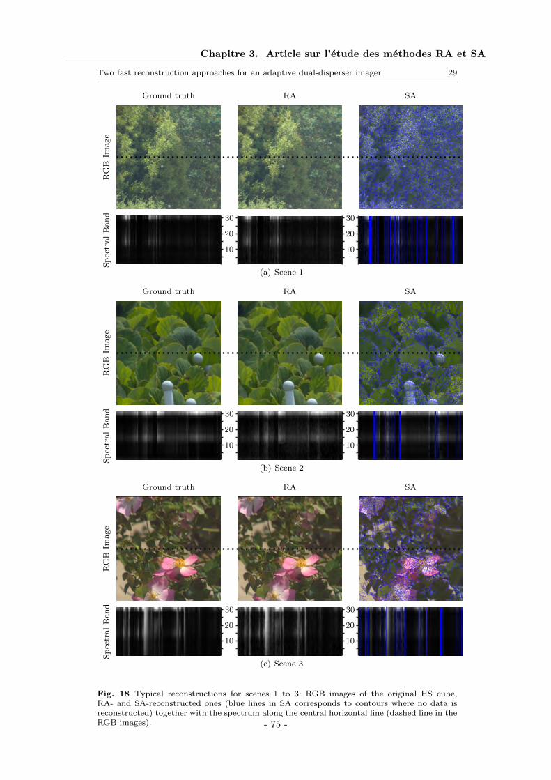
Chapitre 3. Article sur l’étude des méthodes RA et SA
Two fast reconstruction approaches for an adaptive dual-disperser imager 29
Ground truth RA SAS
pec
tral
Ban
dR
GB
Image
10
20
30
10
20
30
(a) Scene 1
Ground truth RA SA
Sp
ectr
al
Ban
dR
GB
Image
10
20
30
10
20
30
(b) Scene 2
Ground truth RA SA
Sp
ectr
al
Ban
dR
GB
Image
10
20
30
10
20
30
(c) Scene 3
Fig. 18 Typical reconstructions for scenes 1 to 3: RGB images of the original HS cube,RA- and SA-reconstructed ones (blue lines in SA corresponds to contours where no data isreconstructed) together with the spectrum along the central horizontal line (dashed line in theRGB images). - 75 -
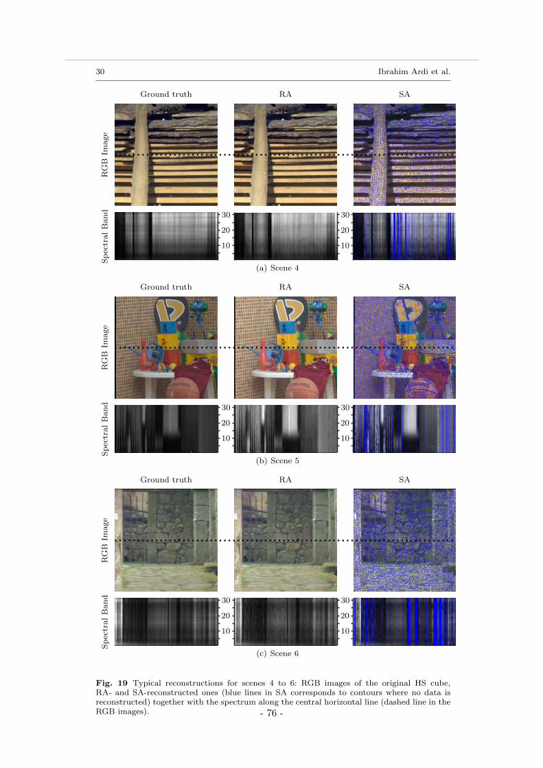
30 Ibrahim Ardi et al.
Ground truth RA SAS
pec
tral
Ban
dR
GB
Image
10
20
30
10
20
30
(a) Scene 4
Ground truth RA SA
Sp
ectr
al
Ban
dR
GB
Image
10
20
30
10
20
30
(b) Scene 5
Ground truth RA SA
Sp
ectr
al
Ban
dR
GB
Image
10
20
30
10
20
30
(c) Scene 6
Fig. 19 Typical reconstructions for scenes 4 to 6: RGB images of the original HS cube,RA- and SA-reconstructed ones (blue lines in SA corresponds to contours where no data isreconstructed) together with the spectrum along the central horizontal line (dashed line in theRGB images). - 76 -
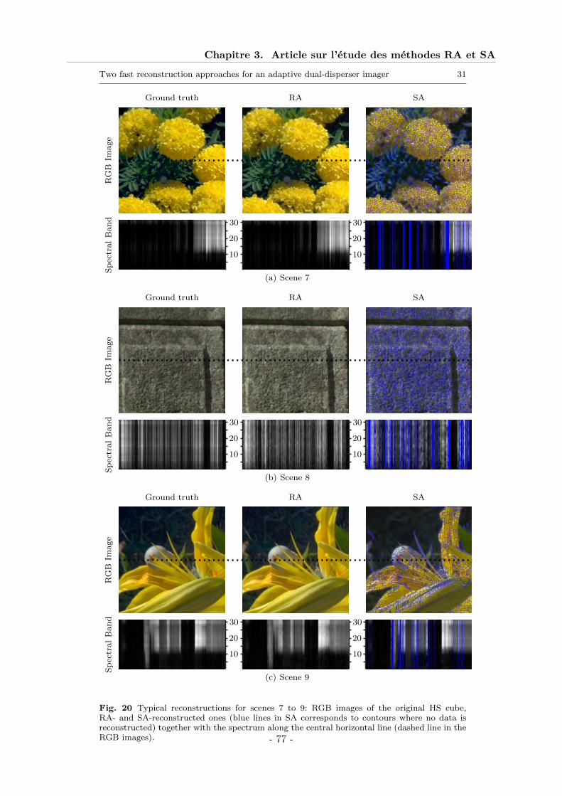
Chapitre 3. Article sur l’étude des méthodes RA et SA
Two fast reconstruction approaches for an adaptive dual-disperser imager 31
Ground truth RA SAS
pec
tral
Ban
dR
GB
Image
10
20
30
10
20
30
(a) Scene 7
Ground truth RA SA
Sp
ectr
al
Ban
dR
GB
Image
10
20
30
10
20
30
(b) Scene 8
Ground truth RA SA
Sp
ectr
al
Ban
dR
GB
Image
10
20
30
10
20
30
(c) Scene 9
Fig. 20 Typical reconstructions for scenes 7 to 9: RGB images of the original HS cube,RA- and SA-reconstructed ones (blue lines in SA corresponds to contours where no data isreconstructed) together with the spectrum along the central horizontal line (dashed line in theRGB images). - 77 -

Chapitre 4
Complément sur la reconstructionpar régularisation quadratique (RA)
Sommaire4.1 Implémentation de la méthode RA par gradients conjugués (CGNR) 80
4.1.1 Équation normale et algorithme CGNR . . . . . . . . . . . . . . . . . . 804.1.2 Étude du calcul de A · . . . . . . . . . . . . . . . . . . . . . . . . . . . . 814.1.3 Étude du calcul de At · . . . . . . . . . . . . . . . . . . . . . . . . . . . 824.1.4 Coût de calcul de l’algorithme CGNR . . . . . . . . . . . . . . . . . . . 82
4.2 Vitesse de convergence du CGNR . . . . . . . . . . . . . . . . . . . . 834.2.1 Majoration de condL . . . . . . . . . . . . . . . . . . . . . . . . . . . 844.2.2 Structure de la matrice HtΓ−1H . . . . . . . . . . . . . . . . . . . . . . 864.2.3 Cas de configurations orthogonales normalisées du DMD . . . . . . . . . 874.2.4 Cas d’un modèle de bruit blanc . . . . . . . . . . . . . . . . . . . . . . . 894.2.5 Illustration du conditionnement et de la vitesse de convergence sur des
simulations . . . . . . . . . . . . . . . . . . . . . . . . . . . . . . . . . . 90
Dans ce chapitre, on s’intéresse à la reconstruction d’images hyperspectrales par une régulari-sation quadratique de type Thikonov [TA77] préservant les contours, comme présenté section 1.4et étudiée en détail dans l’article du chapitre 3. La solution est donc définie par :
o = arg mino||m−Ho||2Γ−1 + µx||Dxo||2 + µy||Dyo||2 + µλ||Dλo||2. (4.1)
La solution de ce problème de minimisation d’un critère quadratique possède une expressionanalytique :
(HtΓ−1H + µxDtxDx + µyDt
yDy + µλDtλDλ)o = HtΓ−1m. (4.2)
Nous présentons § 4.1 une implémentation efficace du calcul de cette solution par un algo-rithme de type gradients conjugués, l’algorithme CGNR, dont chaque itération a un coût decalcul faible si l’on prend en compte les caractéristiques de l’instrument. Nous étudions ensuite§ 4.2 la vitesse de convergence de l’algorithme pour le dispositif utilisé et nous proposons dessolutions permettant d’accélérer la convergence de l’algorithme sans pour autant augmenter soncoût de calcul. Nous proposons en particulier d’exploiter certaines configurations du DMD per-mettent d’améliorer le conditionnement des matrices entrant en jeu dans cet algorithme et ainsiaccélérer la convergence de l’algorithme, en particulier dans le cas d’un modèle de bruit blanc :les configurations orthogonales normalisées.
79
4.1. Implémentation de la méthode RA par gradients conjugués (CGNR)
4.1 Implémentation de la méthode RA par gradients conjugués(CGNR)
Bien que la reconstruction du cube HS par inversion directe de la matrice dans l’équation (4.2)soit envisageable, elle n’est cependant pas possible dans notre cas à cause des dimensions de lamatrice à inverser. En effet, la taille de celle-ci pour un cube de R×C×W est de RCW ×RCW ,valeur supérieure à 1013 éléments pour un cube de dimension 200 × 200 × 100, ce qui requiertplusieurs gigaoctets d’espace mémoire de stockage, et ce pour des cubes de faibles dimensions.L’inversion directe nécessite alors une quantité de mémoire et un temps de calcul prohibitifs.
Il est immédiat d’écrire cette solution comme solution d’une équation normale et exploiterdes algorithmes itératifs spécifiques à ce type d’équations [Saa03]. Plus particulièrement, nousproposons de mettre en œuvre un algorithme itératif de type gradients conjugués pour la réso-lution des équations normales (en anglais Conjugate Gradient for Normal Residual ou CGNR)(voir par exemple [Saa03, Chap. 8]). Cet algorithme est particulièrement adapté à notre pro-blème car on peut exploiter les caractéristiques du dispositif imageur pour une implémentationefficace.
4.1.1 Équation normale et algorithme CGNR
On notera dans la suite L la matrice (HtΓ−1H + µxDtxDx + µyDt
yDy + µλDtλDλ) et b le
vecteur HtΓ−1m. Sous cette notation la solution de l’équation (4.2) est solution du systèmelinéaire :
Lo = b (4.3)Il est alors immédiat de noter que l’équation (4.3) est une équation normale. En effet, la matriceL peut s’écrire :
L = HtΓ−1H + µxDtxDx + µyDt
yDy + µλDtλDλ = AtA (4.4)
avec A la matrice définie par blocs :
A = [HtΓ− 12√µxDt
xõyDt
y
√µλDt
λ]t (4.5)
Par ailleurs, on peut exprimer le vecteur b en fonction de la matrice A :
b = HtΓ−1m = Atb (4.6)
avec le vecteur b construit par bloc : b = [Γ− 12 m 0 0 0]. Ainsi, la solution de l’équation (4.2)
recherchée est solution de l’équation normale :
AtAo = Atb (4.7)
L’algorithme CGNR (voir Algorithme 1) est un algorithme itératif de type gradient conjuguéspécialisé pour la résolution des équations normales telles que l’équation (4.7). D’un point devue calculatoire, cet algorithme nécessite principalement le calcul de deux produits matricielsfaisant intervenir la matrice A, à savoir A · et At· où · dénote un vecteur quelconque de di-mension appropriée. Les autres opérations correspondent à des calculs de normes et d’additionsvectorielles.
Il est important de noter que pour mettre en œuvre cet algorithme, il n’est pas nécessaire destocker en mémoire la matrice A mais qu’il suffit de pouvoir calculer les produits A · et At · . Onpeut donc pour ces calculs, bénéficier des caractéristiques de notre modèle instrumental (matriceH) et de la régularisation quadratique choisie (matrices Dx, Dy et Dλ) pour effectuer ces calculssans stocker en mémoire ces matrices, ce qui réduit considérablement le besoin en mémoire vive.
- 80 -
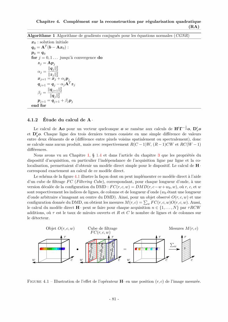
Chapitre 4. Complément sur la reconstruction par régularisation quadratique(RA)
Algorithme 1 Algorithme de gradients conjugués pour les équations normales (CGNR)x0 : solution initialeq0 = AT (b−Ax0) :p0 = q0for j = 0, 1 . . . jusqu’à convergence dozj = Apj
αj =‖qj‖22‖zj‖22
xj+1 = xj + αjpjqj+1 = qj − αjATzj
βj =‖qj+1‖22‖qj‖22
pj+1 = qj+1 + βjpjend for
4.1.2 Étude du calcul de A ·Le calcul de Ao pour un vecteur quelconque o se ramène aux calculs de HtΓ− 1
2o, Dtxo
et Dtyo. Chaque ligne des trois derniers termes consiste en une simple différence de valeurs
entre deux éléments de o (différence entre pixels voisins spatialement ou spectralement), doncse calcule sans aucun produit, mais avec respectivement R(C − 1)W, (R− 1)CW et RC(W − 1)différences.
Nous avons vu au Chapitre 1, § 1.4 et dans l’article du chapitre 3 que les propriétés dudispositif d’acquisition, en particulier l’indépendance de l’acquisition ligne par ligne et la co-localisation, permettaient d’obtenir un modèle direct simple pour le dispositif. Le calcul de H ·correspond exactement au calcul de ce modèle direct.
Le schéma de la figure 4.1 illustre la façon dont on peut implémenter ce modèle direct à l’aided’un cube de filtrage FC (Filtering Cube), correspondant, pour chaque longueur d’onde, à uneversion décalée de la configuration du DMD : FC(r, c, w) = DMD(r, c−w+w0, w), où r, c, et wsont respectivement les indices de lignes, de colonne et de longueur d’onde (w0 étant une longueurd’onde arbitraire s’imageant au centre du DMD). Ainsi, pour un objet observé O(r, c, w) et uneconfiguration donnée du DMD, on obtient les mesuresM(r, c) = ∑
w FC(r, c, w)O(r, c, w). Aussi,le calcul du modèle direct H · peut se faire pour chaque acquisition n ∈ 1, . . . , N par τRCWadditions, où τ est le taux de miroirs ouverts et R et C le nombre de lignes et de colonnes surle détecteur.
Objet O(r, c, w) Mesures M(r, c)Cube de filtrageFC(r, c, w)
w
r
c c
r
∑w
r
cw
r
cw
=•
Figure 4.1 – Illustration de l’effet de l’opérateur H· en une position (r, c) de l’image mesurée.
- 81 -
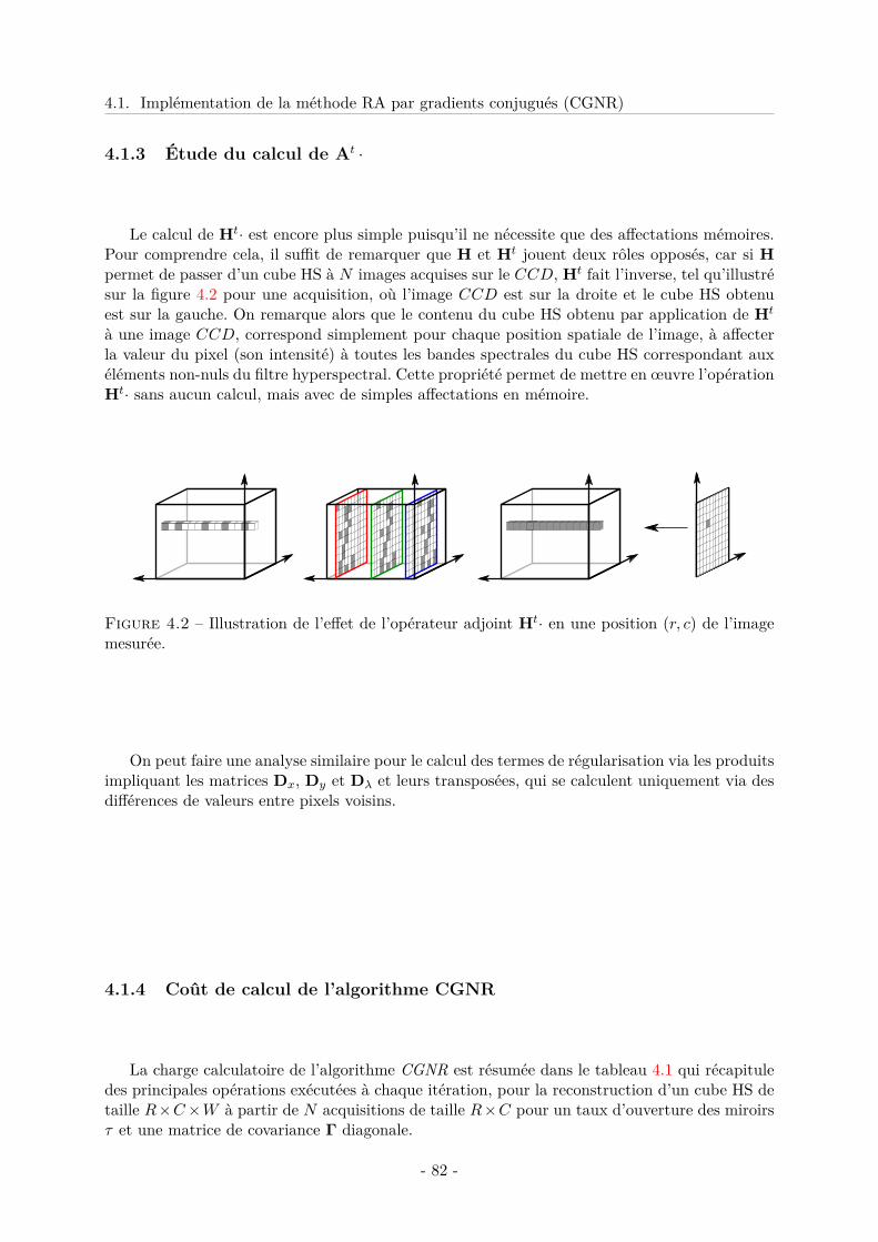
4.1. Implémentation de la méthode RA par gradients conjugués (CGNR)
4.1.3 Étude du calcul de At ·
Le calcul de Ht· est encore plus simple puisqu’il ne nécessite que des affectations mémoires.Pour comprendre cela, il suffit de remarquer que H et Ht jouent deux rôles opposés, car si Hpermet de passer d’un cube HS à N images acquises sur le CCD, Ht fait l’inverse, tel qu’illustrésur la figure 4.2 pour une acquisition, où l’image CCD est sur la droite et le cube HS obtenuest sur la gauche. On remarque alors que le contenu du cube HS obtenu par application de Ht
à une image CCD, correspond simplement pour chaque position spatiale de l’image, à affecterla valeur du pixel (son intensité) à toutes les bandes spectrales du cube HS correspondant auxéléments non-nuls du filtre hyperspectral. Cette propriété permet de mettre en œuvre l’opérationHt· sans aucun calcul, mais avec de simples affectations en mémoire.
Figure 4.2 – Illustration de l’effet de l’opérateur adjoint Ht· en une position (r, c) de l’imagemesurée.
On peut faire une analyse similaire pour le calcul des termes de régularisation via les produitsimpliquant les matrices Dx, Dy et Dλ et leurs transposées, qui se calculent uniquement via desdifférences de valeurs entre pixels voisins.
4.1.4 Coût de calcul de l’algorithme CGNR
La charge calculatoire de l’algorithme CGNR est résumée dans le tableau 4.1 qui récapituledes principales opérations exécutées à chaque itération, pour la reconstruction d’un cube HS detaille R×C×W à partir de N acquisitions de taille R×C pour un taux d’ouverture des miroirsτ et une matrice de covariance Γ diagonale.
- 82 -
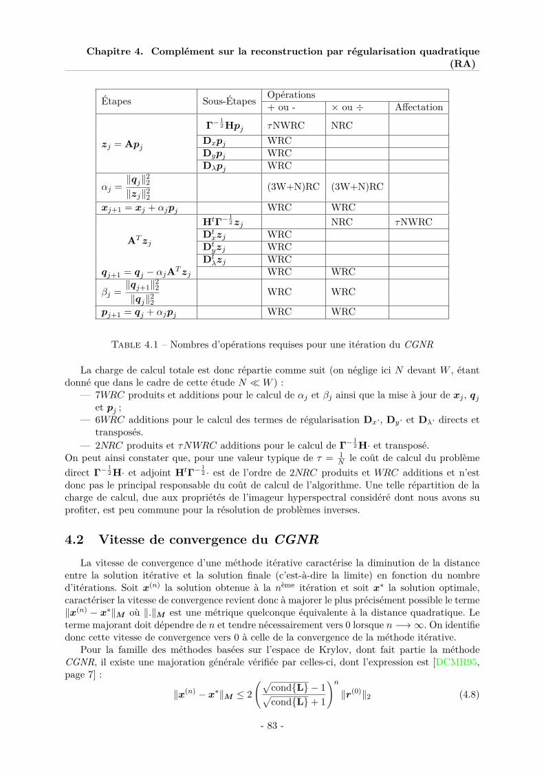
Chapitre 4. Complément sur la reconstruction par régularisation quadratique(RA)
Étapes Sous-Étapes Opérations+ ou - × ou ÷ Affectation
zj = Apj
Γ− 12 Hpj τNWRC NRC
Dxpj WRCDypj WRCDλpj WRC
αj =‖qj‖22‖zj‖22
(3W+N)RC (3W+N)RC
xj+1 = xj + αjpj WRC WRC
ATzj
HtΓ− 12zj NRC τNWRC
Dtxzj WRC
Dtyzj WRC
Dtλzj WRC
qj+1 = qj − αjATzj WRC WRC
βj =‖qj+1‖22‖qj‖22
WRC WRC
pj+1 = qj + αjpj WRC WRC
Table 4.1 – Nombres d’opérations requises pour une itération du CGNR
La charge de calcul totale est donc répartie comme suit (on néglige ici N devant W , étantdonné que dans le cadre de cette étude N W ) :
— 7WRC produits et additions pour le calcul de αj et βj ainsi que la mise à jour de xj , qjet pj ;
— 6WRC additions pour le calcul des termes de régularisation Dx·, Dy· et Dλ· directs ettransposés.
— 2NRC produits et τNWRC additions pour le calcul de Γ− 12 H· et transposé.
On peut ainsi constater que, pour une valeur typique de τ = 1N le coût de calcul du problème
direct Γ− 12 H· et adjoint HtΓ− 1
2 · est de l’ordre de 2NRC produits et WRC additions et n’estdonc pas le principal responsable du coût de calcul de l’algorithme. Une telle répartition de lacharge de calcul, due aux propriétés de l’imageur hyperspectral considéré dont nous avons suprofiter, est peu commune pour la résolution de problèmes inverses.
4.2 Vitesse de convergence du CGNRLa vitesse de convergence d’une méthode itérative caractérise la diminution de la distance
entre la solution itérative et la solution finale (c’est-à-dire la limite) en fonction du nombred’itérations. Soit x(n) la solution obtenue à la nème itération et soit x∗ la solution optimale,caractériser la vitesse de convergence revient donc à majorer le plus précisément possible le terme‖x(n) − x∗‖M où ‖.‖M est une métrique quelconque équivalente à la distance quadratique. Leterme majorant doit dépendre de n et tendre nécessairement vers 0 lorsque n −→∞. On identifiedonc cette vitesse de convergence vers 0 à celle de la convergence de la méthode itérative.
Pour la famille des méthodes basées sur l’espace de Krylov, dont fait partie la méthodeCGNR, il existe une majoration générale vérifiée par celles-ci, dont l’expression est [DCMR95,page 7] :
‖x(n) − x∗‖M ≤ 2(√
condL − 1√condL+ 1
)n‖r(0)‖2 (4.8)
- 83 -
4.2. Vitesse de convergence du CGNR
où r(0) = b − Lx(0) est le résidu initial et condL le conditionnement de la matrice L, c’est-à-dire le rapport entre sa plus grande et sa plus petite valeur propre. L’équation (4.8) montrel’impact du conditionnement de L sur la vitesse de convergence de l’algorithme et la nécessitéde garder cette valeur le plus proche possible de 1. Un des moyens les plus utilisés pour as-surer une telle condition sur condL, est de modifier L en la multipliant par une matrice Pchoisie judicieusement de sorte que le conditionnement condPL de la matrice PL soit pluspetit que condL et se rapproche donc de 1. Cette technique connue sous le nom de pré-conditionnement [BSvD99, DCMR95], permet de modifier l’équation (4.3) à résoudre en uneéquation équivalente, dont la résolution nécessite moins d’itérations et donc potentiellementmoins de calcul. Néanmoins, le coût de calcul du pré-conditionneur s’ajoute au coût de cal-cul de l’algorithme. Remédier au problème de conditionnement passe donc par un compromisentre le coût calculatoire du pré-conditionneur et le gain en nombre d’itérations nécessaires à laconvergence de l’algorithme.
Dans le cadre de cette thèse, on peut jouer sur un autre paramètre pour améliorer le condi-tionnement de la matrice L. En effet, le dispositif imageur étant pilotable, par l’intermédiairede sa matrice de micro-miroirs (DMD), il est possible de modifier la matrice H intervenantdans la matrice L et viser à améliorer le conditionnement de cette matrice sans avoir à faireappel à un préconditionneur. . . Il est donc important d’étudier ce conditionnement d’envisagerdes configurations du DMDpermettant de l’améliorer.
La matrice HtΓ−1H correspond à la contribution de l’imageur que l’on peut modifier enpilotant le filtrage effectué par le DMD, afin d’améliorer le conditionnement de la matrice L etdonc la vitesse de convergence de l’algorithme CGNR. L’idée est donc de déterminer les matricesHtΓ−1H qui soient réalisables par l’imageur hyperspectral tout en permettant de minimiser leconditionnement condL.
Pour contrôler le conditionnement condL à l’aide du DMD, nous proposons dans un pre-mier temps de le majorer par une fonction de condHtΓ−1H. Ensuite, nous verrons commecertaines configurations particulières du DMD permettent d’exprimer aisément condHtΓ−1Het de le réduire à 1 dans le cas d’un modèle de bruit blanc.
Dans la suite, nous travaillerons uniquement avec des matrices symétriques à valeurs réelles,dont la décomposition en valeurs propres et vecteur propres est définie, avec des valeurs proprespositives ou nulles (les matrices considérées s’écrivant sous la forme MtM elles sont définies non-négatives). Pour une matrice symétrique M on notera eMn ses vecteurs propres de norme unitéassociés aux valeurs propres λM
n . On notera par ailleurs, par eMmax et eMmin les vecteurs propresassociés aux valeurs propres maximale λM
max et minimale non nulle λMmin. Ainsi, par définition,
condM = λMmaxλMmin
.
Afin d’alléger les notations, nous introduisons les matrices J et R telles que L = J + R avecJ = HtΓ−1H et R = µxDt
xDx + µyDtyDy + µλDt
λDλ
4.2.1 Majoration de condL
Théorème 1 : D’après les notations précédentes, si l’on défini τR,Jmax = λR
maxλJ
max, on a :
condL ≤ (1 + τR,Jmax)
∑rg(J)n=1 < eL
min, eJn >
2condJ (4.9)
Démonstration : Soit λL` une valeur propre quelconque de L et eL` son vecteur propre associé
de norme unité, on a :(eL` )tLeL
` = λL` (eL
` )teL` = λL
` . (4.10)
- 84 -
Chapitre 4. Complément sur la reconstruction par régularisation quadratique(RA)
En remplaçant L par J + R dans cette expression et en écrivant la décomposition en valeurs etvecteurs propres de R et L sous la forme
J =rg(J)∑
n=1λJne
Jn(eJ
n)t et R =rg(R)∑
k=1λRk e
Rk (eR
k )t (4.11)
on obtient :
λL` = (eL
` )t(J + R)eL` =
rg(J)∑
n=1λJn < e
L` , e
Jn >
2 +rg(R)∑
k=1λRk < eL
` , eRk >2 . (4.12)
Dans un premier temps on peut montrer que dans notre cas toutes les valeurs propres λLn
sont strictement positives, donc que la matrice L est inversible, hormis dans un cas extrêmementparticulier mathématiquement. En effet, l’équation (4.12) nous dit que toute valeur propre s’écritcomme la somme de termes positifs ou nuls. Pour qu’une valeur propre soit nulle, il faut doncque tous les termes soient nuls. Les sommes se faisant uniquement sur les rg(J) et rg(R) valeurspropres non nulles des matrices J et R, cela signifie donc que tous les produits scalaires doiventêtre nuls. Or, par construction, si les paramètres de régularisation µx, µy et µλ sont non nuls lamatrice R est de rang RCW − 1 et le seul vecteur propre eR
RCW associé à la valeur propre nulleest le vecteur constant. En effet utRu = 0 est nul uniquement pour les vecteurs u proportionnelsà eR
RCW puisque cette quantité correspond à la somme (pondérée) du carré des différences inter-pixels le long des lignes, des colonnes et des longueurs d’ondes. Aussi, les termes < eL
` , eRk >2
ne peuvent être tous nuls (pour k ∈ 1, . . . , RCW − 1) que si eL` = eR
RCW . Pour que ce vecteurconstant soit vecteur propre de la matrice L il faudrait, d’après la définition (4.5) de la matriceA que AeRRCW = 0 et donc par construction, que HeRRCW = 0. Autrement dit, que pour lesN configurations du DMD des différentes acquisitions, les mesures soient insensibles à l’ajoutd’une grandeur constante à l’objet observé. Cela ne sera donc bien évidemment jamais le cas enpratique.
Dans un second temps, on peut trouver une borne supérieure à λLmax. Si l’on applique la
propriété (4.12) à λLmax, en majorant λJ
n par λJmax, et λR
k par λRmax, on obtient :
λLmax ≤ λJmax
rg(J)∑
n=1< eL
max, eJn >
2
+ λR
max
rg(R)∑
k=1< eL
max, eRk >2
(4.13)
Or, comme les matrice J et R ne sont pas de rang plein, on a∑rg(J)n=1 < eLλmax , e
Jn >
2≤ ‖eLλmax‖2 =1 et ∑rg(R)
k=1 < eLλmax , eRk >2≤ 1, ainsi on obtient :
λLmax ≤ λJmax + λRmax =
(1 + τR,J
max)λJmax, (4.14)
d’après la définition de τR,Jmax.
Si maintenant on applique la propriété de l’Eq. (4.12) à λLmin et étant donné que :
rg(R)∑
k=1λRk < eL
min, eRk >2 > 0 (4.15)
puisque eLmin 6= eR
RCW comme vu précédemment, on obtient :
λLmin >
rg(J)∑
n=1λJn < e
Lmin, e
Jn >
2 ≥ λJmin
rg(J)∑
n=1< eL
min, eJn >
2 (4.16)
- 85 -
4.2. Vitesse de convergence du CGNR
Finalement, à partir des équations (4.16) et (4.14) et sachant que condL = λLmaxλLmin
et condJ =λJ
maxλJmin
, on retrouve bien (4.9) :
condL ≤ (1 + τR,Jmax)
∑rg(J)n=1 < eL
min, eJn >
2condJ (4.17)
L’équation (4.9) montre l’impact que peut avoir la configuration du DMD, via la ma-
trice H, sur un majorant du conditionnement de la matrice L du problème. En cherchantdes configurations du DMD permettant de réduire la valeur de ce majorant, on peut espé-rer diminuer condL et donc augmenter la vitesse de convergence de l’algorithme CGNR.La matrice H, apparaît à la fois dans le terme condJ = condHtΓ−1H et dans le terme(1 + τR,J
max)(∑rg(HtΓ−1H)
n=1 < eLλmin
, eJn >
2)−1
. Pour réduire le majorant sur condL il faudraitveiller à ce que ces deux termes soient les plus faibles possible. Le lien entre le second termeet la configuration du dispositif instrumental n’étant pas simple, nous nous sommes focalisés,dans le cadre cette thèse sur la minimisation de condHtΓ−1H, car les propriétés de l’imageurhyperspectral permettent de traiter ce problème simplement, en choisissant convenablement lesconfigurations du DMD.
Dans la suite de cette section, on étudiera le lien entre condHtΓ−1H, la structure de lamatrice H et les configurations du DMD. Ensuite on proposera deux solutions pour réduirecondHtΓ−1H à la valeur de minimale de 1.
4.2.2 Structure de la matrice HtΓ−1H
Le conditionnement de la matrice HtΓ−1H dépend des matrices H et Γ−1, nous allonsrappeler les caractéristiques principales de ces dernières, afin d’étudier la structure de la matriceHtΓ−1H.
La matrice H correspond au modèle direct d’acquisition des mesures et modélise le processusde filtrage de l’imageur hyperspectral : m = Ho. Dans le cas d’une seule acquisition elle contientla configuration du DMD utilisée pour cette acquisition et est de dimension RC ×RCW où R,C etW correspondent respectivement au nombre de lignes et de colonnes du capteur CCD et aunombre de bandes spectrales du cube hyperspectral imagé. Grace à la propriété de colocalisation,chaque ligne de la matrice correspond au filtre spectral appliqué à une position spatiale donnée,et contient donc au plus W éléments non-nuls, où chaque élément représente l’état d’un miroirdu DMD (1 : état passant et 0 : état bloquant).
La structure de la matrice H dépend de l’ordre dans lequel sont arrangées les mesures dansle vecteur m et le cube hyperspectral dans le vecteur o. Si l’on ordonne le cube en balayantl’ensemble des longueurs d’onde pour chaque position spatiale et que l’on ordonne les mesuresselon les mêmes dimensions spatiales, on obtient une matrice H avec la structure suivante :
H =
ht1 0 . . . . . . . . . 00 ht2 0 . . . . . . 0...
......
......
...0 . . . . . . 0 htRC−1 00 . . . . . . . . . 0 htRC
(4.18)
où hi est un vecteur àW lignes contenant des un ou des zéros suivant les composantes spectralesacquises pour le pixel i ∈ 1, . . . , RC pour la configuration du DMD (propriété de colocalisa-tion).
Dans un cadre statistique, la matrice de pondération Γ correspond à la matrice de covariancedes mesures mi. Nous considérons ici uniquement du bruit indépendant sur chaque détecteur : la
- 86 -
Chapitre 4. Complément sur la reconstruction par régularisation quadratique(RA)
matrice Γ est une matrice diagonale de dimension RC avec sur la diagonale la variance γi du bruitde mesure sur chaque mesure mi, i ∈ 1, . . . , RC, soit, Γ = diagγi et donc Γ−1 = diagγ−1
i .Finalement, à partir de l’expression de Γ−1 et H on constate que la matrice HtΓ−1H est
bloc-diagonale, composée de RC matrices de dimension W ×W : Zi = 1γi
hihti :
HtΓ−1H =
Z1 0 . . . 00 Z2 0 0...
......
...0 . . . 0 ZRC
(4.19)
Dans le cas d’acquisitions multiples (N acquisitions), en ordonnant les mesures de chaqueacquisition mn, n = 1, . . . N, les unes au dessous des autres, il en va de même pour les matricesHn, la matrice Γ devenant bloc diagonale avec des blocs Γ = diagγn. La matrice HtΓ−1Hconserve alors sa forme bloc diagonale ci-dessus avec pour chaque bloc :
Zi =N∑
n=1
1γni
hni (hni )t. (4.20)
Dans la suite, pour évaluer le conditionnement de HtΓ−1H, on exploitera cette structurebloc-diagonale afin de ramener l’analyse à celle des matrices de la diagonale Zi. En effet, cettestructure implique que les valeurs propres de HtΓ−1H correspondent simplement à l’ensembledes valeurs propres de ses sous-matrices Zi. L’étude des valeurs propres de HtΓ−1H peut doncêtre ramenée à celle des valeurs propres λi des sous-matrices Zi.
Notons que le conditionnement d’une matrice de rang plein (inversible) est défini comme lerapport de la plus grande sur la plus petite valeur propre. Cependant, HtΓ−1H n’est pas derang plein car dans notre contexte, le nombre d’acquisitions N est inférieur au nombre de bandesspectrales W : rg(HtΓ−1H) ≤ NRC WRC. Par abus de langage, on appellera donc par lasuite « conditionnement » pour une matrice non-inversible le rapport de la plus grande valeurpropre sur la plus petite valeur propre non-nulle.
4.2.3 Cas de configurations orthogonales normalisées du DMD
On appelle ici configurations orthogonales du DMD, les situations pour lesquelles pour chaquepixel i ∈ 1, . . . , RC les vecteurs hni pour n = 1 . . . N sont orthogonaux :
∀i ∈ 1, . . . , RC,∀(n, k) ∈ 1, . . . , N2 < hni ,hki >= δk,n||hki ||2, (4.21)
où δk,n est le symbole de Kronecker.Un cas particulier des configurations orthogonales est le cas normalisé, où tous les vecteurs
hki ont la même norme : ||hki ||2 =cte. Ce cas particulier est intéressant pour la raison suivante :
Théorème 2 : Dans le cas de configurations orthogonales normalisées du DMD, on a :
condHtΓ−1H = maxi,k γkimini,k γki
. (4.22)
Démonstration : Dans le cas de configurations orthogonales, il est immédiat de montrer queles vecteurs hki sont des vecteurs propres de Zi car :
Zihki =
N∑
n=1
1γnihni (hni )thki =
N∑
n=1
1γnihni < h
ni ,h
ki >=
N∑
n=1
1γnihni δk,n||hki ||2 = 1
γki||hki ||2hki . (4.23)
- 87 -
4.2. Vitesse de convergence du CGNR
Les valeurs propres associées à ces vecteurs propres sont λik = 1γki||hki ||2.
Les valeurs propres de HtΓ−1H étant les valeurs propres des matrice Zi, On a donc :
condHtΓ−1H = λmaxλmin
=maxi,k ||h
ki ||2γki
mini,k ||hki ||2γki
(4.24)
Si de plus les vecteurs hki ont la même norme, alors :
condHtΓ−1H =maxi,k 1
γki
mini,k 1γki
= maxi,k γkimini,k γki
. (4.25)
Le cas des configurations orthogonales normalisées est donc intéressant pour leurs propriétésmathématiques, mais l’on peut se demander à quelle condition cela correspond en pratique pourla configuration du DMD et s’il est possible et simple de construire de telles configurations.Rappelons que ces vecteurs hni sont constitués soit de 0, soit de 1. En pratique, pour avoirdes configurations orthogonales, il faut donc que tous les éléments des vecteurs hni vérifient∀w, i,∑N
n=1[hni ]w ≤ 1. D’après la définition de la matrice H de l’équation (4.18) et le modèlem = Ho, le vecteur hi correspond au cube de filtrage pour l’acquisition de la donnée mi
sur le pixel i pour une configuration du DMD. En effet, l’opération matricielle donne pour cepixel : mi = (hi)toi où oi contient le spectre de l’objet pour le pixel i ce qui correspond enterme de filtrage du cube pour une configuration du DMD à l’opération illustrée figure 4.1 :M(r, c) = ∑W
w=1 FC(r, c, w)O(r, c, w), où (r, c) sont les indices de ligne et colonne du pixel i. Lesvecteurs hni correspondent aux vecteurs pour les N configurations du DMD (pour les N cubesde filtrage FCn(r, c, w)) des N acquisitions. Pour que les configurations soient orthogonales, ilfaut donc que ∀w, r, c,∑N
n=1 FCn(r, c, w) ≤ 1. Cela signifie en pratique qu’aucun des éléments
du cube O(r, c, w) ne participe à plus d’une des acquisitions.Le cas particulier des configurations orthogonales normalisées correspond au cas où tous lesvecteurs hni ont la même norme : ∀i, n, ||hni ||2 =cte. Cette constante, correspondant au nombred’éléments à 1 de ces vecteurs, est liée au nombre d’éléments du cube O(r, c, w) participant àchaque acquisition. Afin d’obtenir dans les données de l’information sur tous les éléments ducube, il faudrait avoir ||hni ||n = W
N (dans le cas ou W est un multiple de N) et dans ce cas ona : ∀i ∈ 1, . . . , RC,∑N
n=1 hni = 1 (où 1 est un vecteur ne contenant que des 1) ou, ce qui est
équivalent, ∀w, r, c,∑Nn=1 FC
n(r, c, w) = 1. Notons que dans ce cas, le taux de miroirs ouvertest τ = 1
N .
Comme le cube de filtrage est construit, aux différentes longueurs d’ondes, à partir de laconfiguration du DMD par un simple décalage le long des colonnes, il suffit donc, pour avoir desconfigurations orthogonales, que la propriété précédente soit vraie sur les différentes configura-tions du DMD, à savoir ∀r, c,∑N
n=1DMDn(r, c) = 1, ce qui implique que chaque miroir doitêtre ouvert une fois et une seule sur l’ensemble des acquisitions. Il est donc aisé de générer Nconfigurations des DMD correspondant à des configurations orthogonales normalisées. Une façonde procéder est, par exemple, pour chaque (r, c) de tirer aléatoirement un indice n ∈ 1, . . . , Ncorrespondant à l’acquisition pour laquelle le miroir à la position (r, c) est ouvert.
Enfin, ces configurations orthogonales normalisées ont une autre propriété intéressante.
Propriété 1 : Dans le cas de configurations orthogonales normalisées du DMD, on obtientl’image panchromatique par simple addition des données obtenues par toutes les acquisitions
- 88 -
Chapitre 4. Complément sur la reconstruction par régularisation quadratique(RA)
Démonstration : La démonstration est immédiate puisque les données correspondant à lanième acquisition s’écriventMn(r, c) = ∑W
w=1 FCn(r, c, w)O(r, c, w). Si l’on fait la somme des N
acquisitions, en exploitant la propriété des configurations orthogonales normalisées, on obtient :
N∑
n=1Mn(r, c) =
N∑
n=1
W∑
w=1FCn(r, c, w)O(r, c, w)
=W∑
w=1
(N∑
n=1FCn(r, c, w)
)O(r, c, w) =
W∑
w=1O(r, c, w),
soit l’intégration de l’image hyperspectrale sur l’ensemble des longueurs d’onde ce qui correspondbien à la définition de l’image panchromatique.
Insistons sur le fait que cette propriété est intéressant pour les deux méthodes proposéesdurant cette thèse, puisque, grâce à de telles configurations, nous disposons, sans aucune ac-quisition supplémentaire, de l’image panchromatique nécessaire pour effectuer la segmentationorientée contours pour la méthode RA et orientée région pour la méthode SA. Bien entendue,en pratique cette image panchromatique sera bruitée, mais avec un rapport signal sur bruit plusélevé que celui chacune des acquisitions, puisque cela revient à dire que le temps d’acquisitionde l’image panchromatique est N fois plus élevé que celui de chacune des acquisitions.
4.2.4 Cas d’un modèle de bruit blanc
Dans une interprétation statistique de la solution de l’équation (4.2), la matrice Γ correspondà la matrice de covariance des données, issue d’un bruit additif Gaussien centré, soit un modèled’acquisition : m = Ho+ ε avec ε ∼ N (0,Γ).
Pour un dispositif expérimental comme le notre, le modèle de bruit le plus cohérent est unmodèle de bruit de Poisson m ∼ P(Ho) (« phénomène de comptage de photons »), auquelpourrait s’ajouter un bruit blanc gaussien centré (« bruit de lecture »). En négligeant ce dernier,généralement faible, la matrice de covariance des données est donc égale à Γ = diag(Ho).Bien sûr, l’objet est inconnu et on peut en pratique approximer la matrice de covariance parΓ = diag(m). Utiliser une telle matrice de covariance dans le critère (4.1) définissant la solutionrevient à approximer un modèle de bruit de Poisson par un modèle de bruit Gaussien. Une telleapproximation est valable lorsque le flux est suffisamment grand (théorème de la limite centrale).Avec un tel modèle, l’égalité (4.22) nous donne condHtΓ−1H = maxi,kmk
i
mini,kmki
et l’on constate ainsique le conditionnement de la matrice HtΓ−1H est très sensible au contraste des données. Eneffet, si les données contiennent à la fois des pixels sombres et des pixels clairs, donc un contrasteimportant, ce terme deviendra élevé.
Une autre approximation possible pour le modèle de bruit est de considérer un bruit ad-ditif blanc Gaussien centré, dans ce cas, Γ = σ2
ε I, ce qui implique que ∀k, i,γki =cte et doncmaxi,k γki = mini,k γki d’où condHtΓ−1H = 1.Si un tel modèle est moins satisfaisant statistiquement et physiquement, il est intéressant numé-riquement car il permet d’obtenir une borne plus faible pour le conditionnement de la matriceHtΓ−1H et potentiellement une convergence plus rapide de l’algorithme CGNR. Bien entendu,il faut vérifier que cette approximation grossière ne dégrade pas la qualité des images hyperspec-trales ainsi reconstruite par rapport à un modèle plus réaliste.
- 89 -
4.2. Vitesse de convergence du CGNR
4.2.5 Illustration du conditionnement et de la vitesse de convergence sur dessimulations
Afin de vérifier en pratique les propriétés énoncées ci-dessus et l’intérêt d’utiliser des configu-rations orthogonales normalisées des DMD, nous avons effectué des simulations. Pour cela, nousavons travaillé sur des images hyperspectrales de dimension réduites (spatialement 100 × 100pixels et spectralement de l’ordre de 30 longueurs d’ondes suivant les images) afin de pouvoircalculer le conditionnement de la matrice L. Sur un grand nombre de telles images, nous avonscalculé le paramètre µRA = µx = µy (en considérant µλ = µRA/10) donnant l’erreur quadra-tique moyenne de reconstruction la plus faible (un unique paramètre optimal en moyenne surl’ensemble des données). Les configurations du DMD étaient générées aléatoirement pour diffé-rents taux d’ouverture des miroirs τ, sauf pour les configurations orthogonales normalisées pourlesquelles τ = 1
N .Deux situations sont testées pour la matrice de covariance Γ correspondant au modèle de
bruit : soit Γ = diagm ce qui correspond à approximer le bruit de Poisson par un bruitGaussien dont on estime la variance par les données m, soit Γ ∝ I ce qui correspond à un bruitblanc (indépendant et identiquement distribué). Dans le cas des configurations orthogonales, onprend en compte un bruit blanc.
Sur la figure 4.3, colonne de gauche, on affiche le conditionnement de la matrice L (enéchelle logarithmique, moyenne +/- écart-type sur les différentes images) pour différents nombresd’acquisition N ∈ 3, 4, 5. Sur la colonne de droite, on affiche le nombre d’itérations (en échellelogarithmique, moyenne +/- écart-type sur les différentes images) nécessaires à la convergencede l’algorithme CGNR. On considère ici que l’algorithme a convergé lorsque la solution o, àdeux itérations successives, vérifie
√||o(i) − o(i−1)||2/||o(i−1)||2 < ε = 10−3 (on s’est assuré, en
pratique que l’erreur relative de reconstruction était également inférieure à ε.)On constate tout d’abord sur ces figures une forte similarité de la variation du conditionne-
ment de L et de la convergence de l’algorithme. On s’attendait bien sûr à cela du point de vuethéorique (au sens de la convergence vers la solution exacte) mais cela est vérifié en pratique pourla convergence définie précédemment (différence de la solution entre deux itérations successivesinférieure à ε). Ensuite, on constate une faible variation du conditionnement et de la convergenceen fonction du taux d’ouverture des miroirs τ tant que celui-ci reste entre 0,2 et 0,8, quel quesoit le modèle pris en compte pour le bruit. Enfin, on constate que le conditionnement et lavitesse de convergence sont toujours meilleurs (moyennes et variances plus faibles) dans le casd’un modèle de bruit blanc (courbes en bleu) que dans l’approximation d’un bruit de Poisson(courbes en rouge). Pour finir, ces courbes confirment nos résultats théoriques concernant lemeilleur conditionnement des configurations orthogonales normalisées, quel que soit le nombred’acquisition N. Rappelons que dans ce cas, le taux d’ouverture des miroirs est τ = 1
N
- 90 -
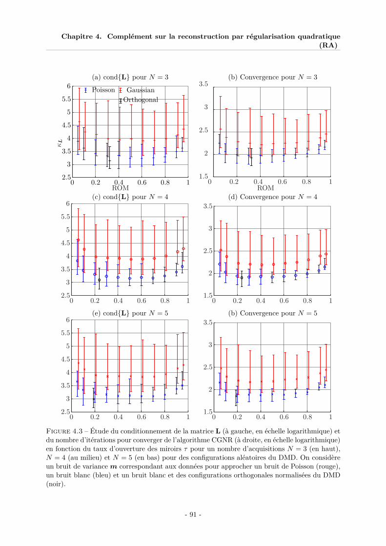
Chapitre 4. Complément sur la reconstruction par régularisation quadratique(RA)
(a) condL pour N = 3 (b) Convergence pour N = 3
0 0.2 0.4 0.6 0.8 12.5
3
3.5
4
4.5
5
5.5
6
ROM
κL
Poisson GaussianOrthogonal
0 0.2 0.4 0.6 0.8 11.5
2
2.5
3
3.5
ROM(c) condL pour N = 4 (d) Convergence pour N = 4
0 0.2 0.4 0.6 0.8 12.5
3
3.5
4
4.5
5
5.5
6
0 0.2 0.4 0.6 0.8 11.5
2
2.5
3
3.5
(e) condL pour N = 5 (b) Convergence pour N = 5
0 0.2 0.4 0.6 0.8 12.5
3
3.5
4
4.5
5
5.5
6
0 0.2 0.4 0.6 0.8 11.5
2
2.5
3
3.5
Figure 4.3 – Étude du conditionnement de la matrice L (à gauche, en échelle logarithmique) etdu nombre d’itérations pour converger de l’algorithme CGNR (à droite, en échelle logarithmique)en fonction du taux d’ouverture des miroirs τ pour un nombre d’acquisitions N = 3 (en haut),N = 4 (au milieu) et N = 5 (en bas) pour des configurations aléatoires du DMD. On considèreun bruit de variancem correspondant aux données pour approcher un bruit de Poisson (rouge),un bruit blanc (bleu) et un bruit blanc et des configurations orthogonales normalisées du DMD(noir).
- 91 -

Chapitre 5
Article sur la validationexpérimentale de la méthode RA
Sommaire1. Introduction . . . . . . . . . . . . . . . . . . . . . . . . . . . . . . . . . . . 962. Ideal Model of Dual Disperser System . . . . . . . . . . . . . . . . . . . 973. Reconstruction of the Hyperspectral Datacube via Edge Preserving
Regularization . . . . . . . . . . . . . . . . . . . . . . . . . . . . . . . . 98A. Properties of the Filtering Cube . . . . . . . . . . . . . . . . . . . . . . . . . 99
4. Experimental System . . . . . . . . . . . . . . . . . . . . . . . . . . . . . . 100A. Optical Setup . . . . . . . . . . . . . . . . . . . . . . . . . . . . . . . . . . . 100B. DMD Mask . . . . . . . . . . . . . . . . . . . . . . . . . . . . . . . . . . . . 103C. Ground Truth Comparison . . . . . . . . . . . . . . . . . . . . . . . . . . . . 104
5. Testing Reconstruction Performance with Small Homogenous Scene . 105A. Scene and Variables . . . . . . . . . . . . . . . . . . . . . . . . . . . . . . . . 105B. Results - SAM . . . . . . . . . . . . . . . . . . . . . . . . . . . . . . . . . . . 105C. Results - Number of Iterations . . . . . . . . . . . . . . . . . . . . . . . . . . 106
6. Reconstruction of a Large Multispectrum Scene . . . . . . . . . . . . . 106A. Scene A - Stacked Filters . . . . . . . . . . . . . . . . . . . . . . . . . . . . . 106B. Scene B - Checkerboard . . . . . . . . . . . . . . . . . . . . . . . . . . . . . 110
7. Conclusion . . . . . . . . . . . . . . . . . . . . . . . . . . . . . . . . . . . . 115References . . . . . . . . . . . . . . . . . . . . . . . . . . . . . . . . . . . . . . 115
Nous reprenons ici l’article [HAL+20] :E. Hemsley, I. Ardi, S. Lacroix, H. Carfantan and A. Monmayrant, Optimized codedaperture for frugal hyperspectral image recovery using a dual-disperser system, Journalof the Optical Society of America A, soumis en juillet 2020.
93

Chapitre 5. Article sur la validation expérimentale de la méthode RA
- 95 -
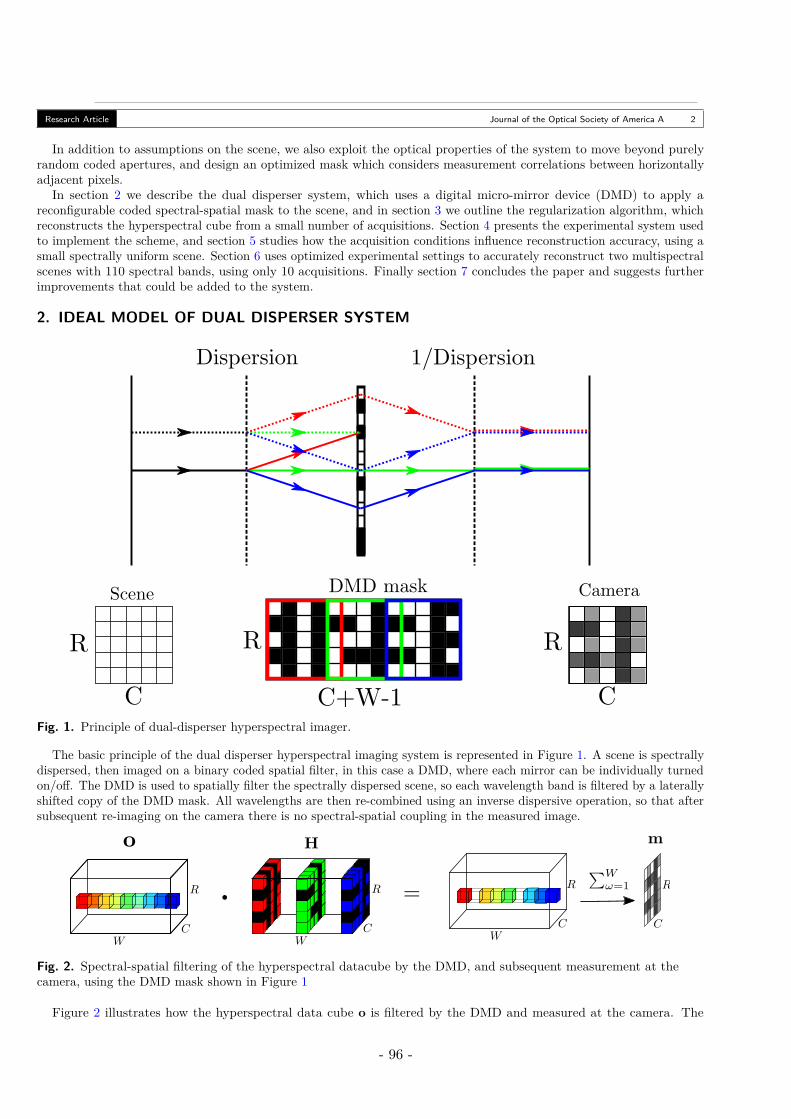
Research Article Journal of the Optical Society of America A 2
In addition to assumptions on the scene, we also exploit the optical properties of the system to move beyond purelyrandom coded apertures, and design an optimized mask which considers measurement correlations between horizontallyadjacent pixels.
In section 2 we describe the dual disperser system, which uses a digital micro-mirror device (DMD) to apply areconfigurable coded spectral-spatial mask to the scene, and in section 3 we outline the regularization algorithm, whichreconstructs the hyperspectral cube from a small number of acquisitions. Section 4 presents the experimental system usedto implement the scheme, and section 5 studies how the acquisition conditions influence reconstruction accuracy, using asmall spectrally uniform scene. Section 6 uses optimized experimental settings to accurately reconstruct two multispectralscenes with 110 spectral bands, using only 10 acquisitions. Finally section 7 concludes the paper and suggests furtherimprovements that could be added to the system.
2. IDEAL MODEL OF DUAL DISPERSER SYSTEM
Fig. 1. Principle of dual-disperser hyperspectral imager.
The basic principle of the dual disperser hyperspectral imaging system is represented in Figure 1. A scene is spectrallydispersed, then imaged on a binary coded spatial filter, in this case a DMD, where each mirror can be individually turnedon/off. The DMD is used to spatially filter the spectrally dispersed scene, so each wavelength band is filtered by a laterallyshifted copy of the DMD mask. All wavelengths are then re-combined using an inverse dispersive operation, so that aftersubsequent re-imaging on the camera there is no spectral-spatial coupling in the measured image.
Fig. 2. Spectral-spatial filtering of the hyperspectral datacube by the DMD, and subsequent measurement at thecamera, using the DMD mask shown in Figure 1
Figure 2 illustrates how the hyperspectral data cube o is filtered by the DMD and measured at the camera. The
- 96 -
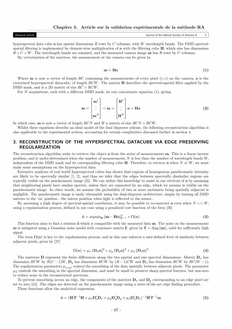
Chapitre 5. Article sur la validation expérimentale de la méthode RAResearch Article Journal of the Optical Society of America A 3
hyperspectral data cube o has spatial dimensions R rows by C columns, with W wavelength bands. The DMD spectral-spatial filtering is implemented by element-wise multiplication of o with the filtering cube H, which also has dimensionsR×C ×W . The wavelength bands are summed, and the measured camera image m has R rows by C columns.
By vectorization of the matrices, the measurement at the camera can be given by
m = Ho (1)
Where m is now a vector of length RC containing the measurements of every pixel (r, c) on the camera, o is thevectorized hyperspectral datacube, of length RCW . The matrix H describes the spectral-spatial filter applied by theDMD mask, and is a 2D matrix of size RC ×RCW .
For N acquisitions, each with a different DMD mask, we can concatenate equation (1), giving
m =
m1
...
mN
= m =
H1
...
HN
o = Ho (2)
In which case, m is now a vector of length RCN and H a matrix of size RCN ×RCW .Whilst these equations describe an ideal model of the dual disperser scheme, the following reconstruction algorithm is
also applicable to the experimental system, accounting for certain complexities discussed further in section 4.
3. RECONSTRUCTION OF THE HYPERSPECTRAL DATACUBE VIA EDGE PRESERVINGREGULARIZATION
The reconstruction algorithm seeks to retrieve the object o from the series of measurements m. This is a linear inverseproblem, and is under-determined when the number of measurements N is less than the number of wavelength bands W ,independent of the DMD mask and its corresponding filtering cube H. Therefore, to retrieve o when N W , we mustmake some assumptions on the hyperspectral data.
Extensive analyses of real world hyperspectral cubes has shown that regions of homogenous panchromatic intensityare likely to be spectrally similar [1, 2], and thus we infer that the edges between spectrally dissimilar regions aretypically visible on the panchromatic image [25]. We can utilize this knowledge to assist in our retrieval of o by assumingthat neighboring pixels have similar spectra, unless they are separated by an edge, which we assume is visible on thepanchromatic image. In other words, we assume the probability of two or more metamers being spatially adjacent isnegligible. The panchromatic image is easily obtainable using the dual-disperser architecture, simply by turning all DMDmirrors to the ‘on’ position - the mirror position when light is reflected to the sensor..
By assuming a high degree of spectral-spatial correlation, it may be possible to reconstruct o even when N << W ,using a regularization process, defined in our case using a penalized cost function of the form [26]
o = argmino ‖m−Ho‖2Γ−1 + Ω(o) (3)
This function aims to find a solution o which is compatible with the measured data m. The noise on the measurementsm is mitigated using a Gaussian noise model with covariance matrix Γ, given by Γ = diag m, valid for sufficiently highsignal.
The term Ω(o) is key to the regularization process, and in this case enforces a user-defined level of similarity betweenadjacent pixels, given by [27]
Ω(o) = µx ‖Dxo‖2 + µy ‖Dyo‖2 + µλ ‖Dλo‖2 (4)
The matrices D represent the finite differences along the two spatial and one spectral dimensions. Matrix Dx hasdimension RCW by R(C − 1)W , Dy has dimension RCW by (R− 1)CW and Dλ has dimension RCW by RC(W − 1).The regularization parameters µ(x,y) control the smoothing of the data spatially between adjacent pixels. The parameterµλ controls the smoothing in the spectral dimension, and must be small to preserve sharp spectral features, but non-zeroto reduce noise in the reconstructed spectrum.
To prevent smoothing across an edge, the components of the matrices Dx and Dy corresponding to an edge pixel areset to zero [24]. The edges are detected on the panchromatic image using a state-of-the-art edge finding procedure.
These functions allow the analytical expression
o = (HtΓ−1H+ µxDtxDx + µyDt
yDy + µλDtλDλ)
−1HtΓ−1m (5)
- 97 -
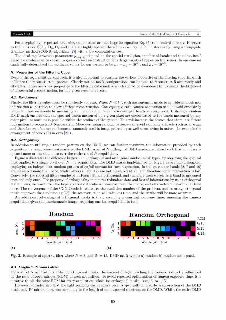
Research Article Journal of the Optical Society of America A 4
For a typical hyperspectral datacube, the matrices are too large for equation Eq. (5) to be solved directly. However,as the matrices H,Dx,Dy,Dλ and Γ are all highly sparse, the solution o may be found iteratively using a ConjugateGradient method (CGNR) algorithm [28] with a low computation cost.
The ideal regularization parameters µ(x,y,λ), depend on the spatial resolution, number of bands and the data itself.Fixed parameters can be chosen to give a correct reconstruction for a large variety of hyperspectral scenes. In our case weempirically determined the optimum values for our system to be µx = µy = 10−2, and µλ = 10−5.
A. Properties of the Filtering CubeDespite the regularization approach, it is also important to consider the various properties of the filtering cube H, whichinfluence the reconstruction process. Clearly not all mask configurations can be used to reconstruct o accurately andefficiently. There are a few properties of the filtering cube matrix which should be considered to maximize the likelihoodof a successful reconstruction, for any given scene or spectra.
A.1. RandomnessFirstly, the filtering cubes must be sufficiently random. When N W , each measurement needs to provide as much newinformation as possible, to allow efficient reconstruction. Consequently, each camera acquisition should avoid excessivelyredundant measurements by measuring a different combination of wavelength bands at every pixel. Utilizing a randomDMD mask ensures that the spectral bands measured by a given pixel are uncorrelated to the bands measured by anyother pixel, as much as is possible within the confines of the system. This will increase the chance that there is sufficientinformation to reconstruct o accurately. Moreover, using random patterns can avoid sampling artifacts such as aliasing,and therefore we often see randomness commonly used in image processing as well as occurring in nature (for example thearrangement of cone cells in eyes [29]).
A.2. OrthogonalityIn addition to utilizing a random pattern on the DMD, we can further maximize the information provided by eachacquisition by using orthogonal masks on the DMD. A set of N orthogonal DMD masks are defined such that no mirror isopened more or less than once over the entire set of N acquisitions.
Figure 3 illustrates the difference between non-orthogonal and orthogonal random mask types, by observing the spectralfilter applied to a single pixel over N = 3 acquisitions. The DMD masks implemented for Figure 3a are non-orthogonal,employing an independent random pattern of on/off mirrors for each acquisition. In this case some bands (2, 7 and 10)are measured more than once, whilst others (6 and 12) are not measured at all, and therefore some information is lost.Conversely, the spectral filters employed in Figure 3b are orthogonal, and therefore each wavelength band is measuredonce and only once. The property of orthogonality minimizes redundant data and loss of information; by using orthogonalDMD masks, no voxel from the hyperspectral datacube is measured more than once, and all voxels are measured at leastonce. The convergence of the CGNR code is related to the condition number of the problem, and as using orthogonalmasks improves the conditioning [25], the reconstruction will take less time, and the results will be more accurate.
An additional advantage of orthogonal masks is that, assuming a constant exposure time, summing the cameraacquisitions gives the panchromatic image, requiring one less acquisition in total.
1 2 3 4 5 6 7 8 9 10 11 12 13 14 15
123
(a)
1 2 3 4 5 6 7 8 9 10 11 12 13 14 15
123
7/154/154/15
6/155/154/15
(b)
Fig. 3. Example of spectral filter where N = 3, and W = 15. DMD mask type is a) random b) random orthogonal.
A.3. Length-N Random PatternFor a set of N acquisitions utilizing orthogonal masks, the amount of light reaching the camera is directly influencedby the ratio of open mirrors (ROM) of each acquisition. To avoid repeated optimization of camera exposure time, it isintuitive to use the same ROM for every acquisition, which for orthogonal masks, is equal to 1/N .
However, consider also that the light reaching each camera pixel is spectrally filtered by a sub-section of the DMDmask, only W mirrors long, corresponding to the length of the dispersed spectrum on the DMD. Whilst the entire DMD
- 98 -
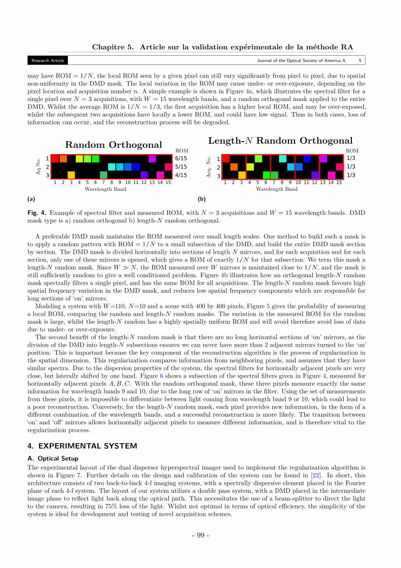
Chapitre 5. Article sur la validation expérimentale de la méthode RAResearch Article Journal of the Optical Society of America A 5
may have ROM = 1/N , the local ROM seen by a given pixel can still vary significantly from pixel to pixel, due to spatialnon-uniformity in the DMD mask. The local variation in the ROM may cause under- or over-exposure, depending on thepixel location and acquisition number n. A simple example is shown in Figure 4a, which illustrates the spectral filter for asingle pixel over N = 3 acquisitions, with W = 15 wavelength bands, and a random orthogonal mask applied to the entireDMD. Whilst the average ROM is 1/N = 1/3, the first acquisition has a higher local ROM, and may be over-exposed,whilst the subsequent two acquisitions have locally a lower ROM, and could have low signal. Thus in both cases, loss ofinformation can occur, and the reconstruction process will be degraded.
1 2 3 4 5 6 7 8 9 10 11 12 13 14 15
123
7/154/154/15
6/155/154/15
(a)
1 2 3 4 5 6 7 8 9 10 11 12 13 14 15
123
1/31/31/3
(b)
Fig. 4. Example of spectral filter and measured ROM, with N = 3 acquisitions and W = 15 wavelength bands. DMDmask type is a) random orthogonal b) length-N random orthogonal.
A preferable DMD mask maintains the ROM measured over small length scales. One method to build such a mask isto apply a random pattern with ROM = 1/N to a small subsection of the DMD, and build the entire DMD mask sectionby section. The DMD mask is divided horizontally into sections of length N mirrors, and for each acquisition and for eachsection, only one of these mirrors is opened, which gives a ROM of exactly 1/N for that subsection. We term this mask alength-N random mask. Since W N , the ROM measured over W mirrors is maintained close to 1/N , and the mask isstill sufficiently random to give a well conditioned problem. Figure 4b illustrates how an orthogonal length-N randommask spectrally filters a single pixel, and has the same ROM for all acquisitions. The length-N random mask favours highspatial frequency variation in the DMD mask, and reduces low spatial frequency components which are responsible forlong sections of ‘on’ mirrors.
Modeling a system with W=110, N=10 and a scene with 400 by 400 pixels, Figure 5 gives the probability of measuringa local ROM, comparing the random and length-N random masks. The variation in the measured ROM for the randommask is large, whilst the length-N random has a highly spatially uniform ROM and will avoid therefore avoid loss of datadue to under- or over-exposure.
The second benefit of the length-N random mask is that there are no long horizontal sections of ‘on’ mirrors, as thedivision of the DMD into length-N subsections ensures we can never have more than 2 adjacent mirrors turned to the ‘on’position. This is important because the key component of the reconstruction algorithm is the process of regularization inthe spatial dimension. This regularization compares information from neighboring pixels, and assumes that they havesimilar spectra. Due to the dispersion properties of the system, the spectral filters for horizontally adjacent pixels are veryclose, but laterally shifted by one band. Figure 6 shows a subsection of the spectral filters given in Figure 4, measured forhorizontally adjacent pixels A,B,C. With the random orthogonal mask, these three pixels measure exactly the sameinformation for wavelength bands 9 and 10, due to the long row of ‘on’ mirrors in the filter. Using the set of measurementsfrom these pixels, it is impossible to differentiate between light coming from wavelength band 9 or 10, which could lead toa poor reconstruction. Conversely, for the length-N random mask, each pixel provides new information, in the form of adifferent combination of the wavelength bands, and a successful reconstruction is more likely. The transition between‘on’ and ‘off’ mirrors allows horizontally adjacent pixels to measure different information, and is therefore vital to theregularization process.
4. EXPERIMENTAL SYSTEMA. Optical SetupThe experimental layout of the dual disperser hyperspectral imager used to implement the regularization algorithm isshown in Figure 7. Further details on the design and calibration of the system can be found in [22]. In short, thisarchitecture consists of two back-to-back 4-f imaging systems, with a spectrally dispersive element placed in the Fourierplane of each 4-f system. The layout of our system utilizes a double pass system, with a DMD placed in the intermediateimage plane to reflect light back along the optical path. This necessitates the use of a beam-splitter to direct the lightto the camera, resulting in 75% loss of the light. Whilst not optimal in terms of optical efficiency, the simplicity of thesystem is ideal for development and testing of novel acquisition schemes.
- 99 -
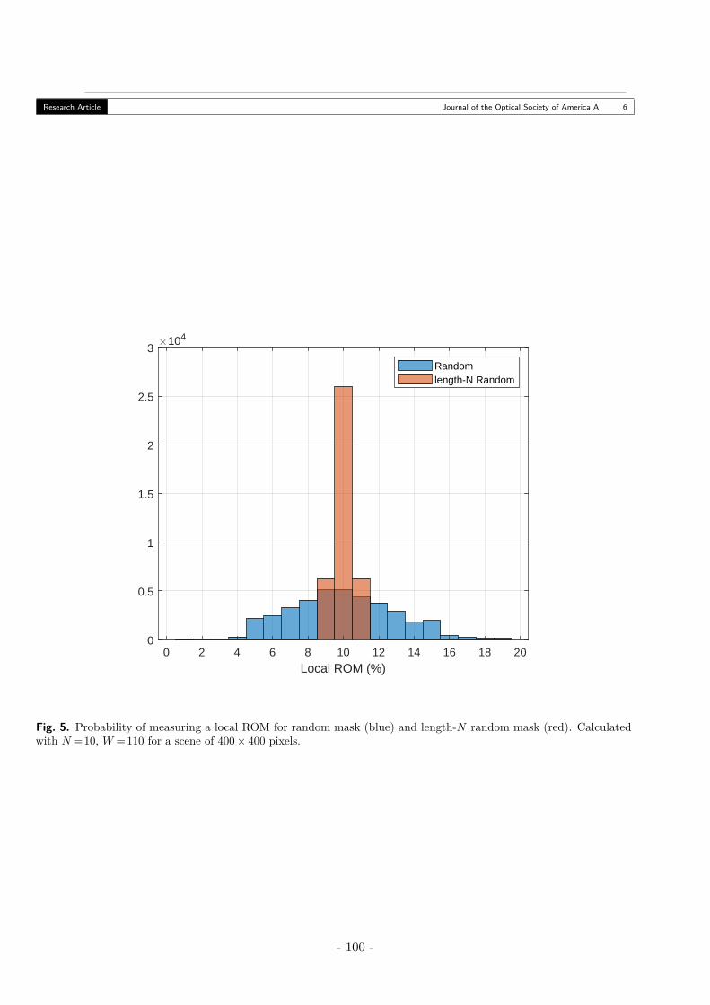
Research Article Journal of the Optical Society of America A 6
0 2 4 6 8 10 12 14 16 18 20
Local ROM (%)
0
0.5
1
1.5
2
2.5
3104
Randomlength-N Random
Fig. 5. Probability of measuring a local ROM for random mask (blue) and length-N random mask (red). Calculatedwith N=10, W =110 for a scene of 400× 400 pixels.
- 100 -
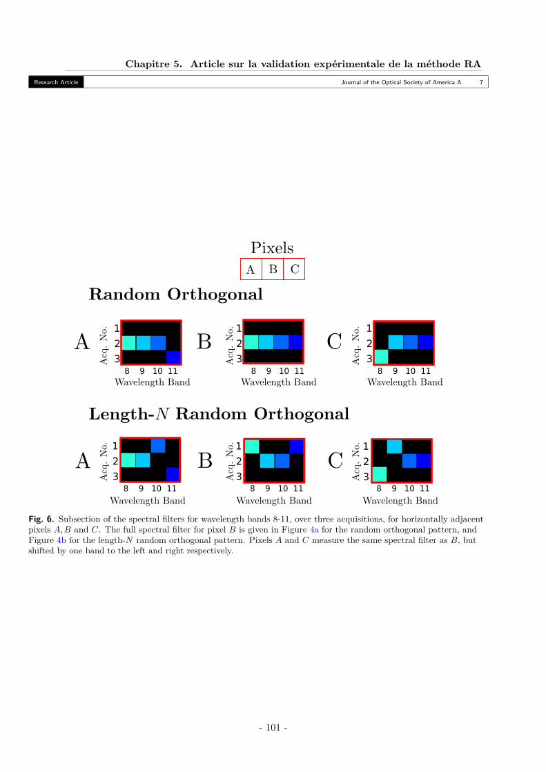
Chapitre 5. Article sur la validation expérimentale de la méthode RAResearch Article Journal of the Optical Society of America A 7
123
123
123
8 9 10 11 8 9 10 11 8 9 10 11
123
123
123
8 9 10 11 8 9 10 11 8 9 10 11
Fig. 6. Subsection of the spectral filters for wavelength bands 8-11, over three acquisitions, for horizontally adjacentpixels A,B and C. The full spectral filter for pixel B is given in Figure 4a for the random orthogonal pattern, andFigure 4b for the length-N random orthogonal pattern. Pixels A and C measure the same spectral filter as B, butshifted by one band to the left and right respectively.
- 101 -
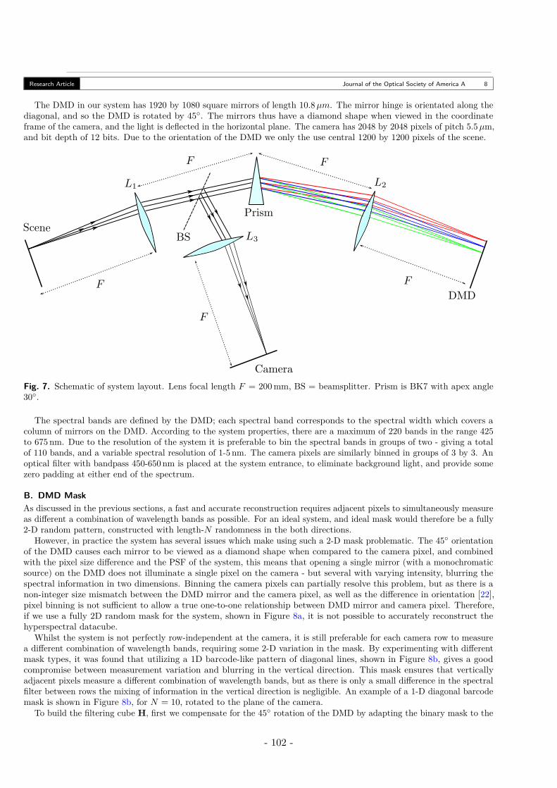
Research Article Journal of the Optical Society of America A 8
The DMD in our system has 1920 by 1080 square mirrors of length 10.8µm. The mirror hinge is orientated along thediagonal, and so the DMD is rotated by 45. The mirrors thus have a diamond shape when viewed in the coordinateframe of the camera, and the light is deflected in the horizontal plane. The camera has 2048 by 2048 pixels of pitch 5.5µm,and bit depth of 12 bits. Due to the orientation of the DMD we only the use central 1200 by 1200 pixels of the scene.
Fig. 7. Schematic of system layout. Lens focal length F = 200mm, BS = beamsplitter. Prism is BK7 with apex angle30.
The spectral bands are defined by the DMD; each spectral band corresponds to the spectral width which covers acolumn of mirrors on the DMD. According to the system properties, there are a maximum of 220 bands in the range 425to 675 nm. Due to the resolution of the system it is preferable to bin the spectral bands in groups of two - giving a totalof 110 bands, and a variable spectral resolution of 1-5 nm. The camera pixels are similarly binned in groups of 3 by 3. Anoptical filter with bandpass 450-650 nm is placed at the system entrance, to eliminate background light, and provide somezero padding at either end of the spectrum.
B. DMD MaskAs discussed in the previous sections, a fast and accurate reconstruction requires adjacent pixels to simultaneously measureas different a combination of wavelength bands as possible. For an ideal system, and ideal mask would therefore be a fully2-D random pattern, constructed with length-N randomness in the both directions.
However, in practice the system has several issues which make using such a 2-D mask problematic. The 45 orientationof the DMD causes each mirror to be viewed as a diamond shape when compared to the camera pixel, and combinedwith the pixel size difference and the PSF of the system, this means that opening a single mirror (with a monochromaticsource) on the DMD does not illuminate a single pixel on the camera - but several with varying intensity, blurring thespectral information in two dimensions. Binning the camera pixels can partially resolve this problem, but as there is anon-integer size mismatch between the DMD mirror and the camera pixel, as well as the difference in orientation [22],pixel binning is not sufficient to allow a true one-to-one relationship between DMD mirror and camera pixel. Therefore,if we use a fully 2D random mask for the system, shown in Figure 8a, it is not possible to accurately reconstruct thehyperspectral datacube.
Whilst the system is not perfectly row-independent at the camera, it is still preferable for each camera row to measurea different combination of wavelength bands, requiring some 2-D variation in the mask. By experimenting with differentmask types, it was found that utilizing a 1D barcode-like pattern of diagonal lines, shown in Figure 8b, gives a goodcompromise between measurement variation and blurring in the vertical direction. This mask ensures that verticallyadjacent pixels measure a different combination of wavelength bands, but as there is only a small difference in the spectralfilter between rows the mixing of information in the vertical direction is negligible. An example of a 1-D diagonal barcodemask is shown in Figure 8b, for N = 10, rotated to the plane of the camera.
To build the filtering cube H, first we compensate for the 45 rotation of the DMD by adapting the binary mask to the
- 102 -
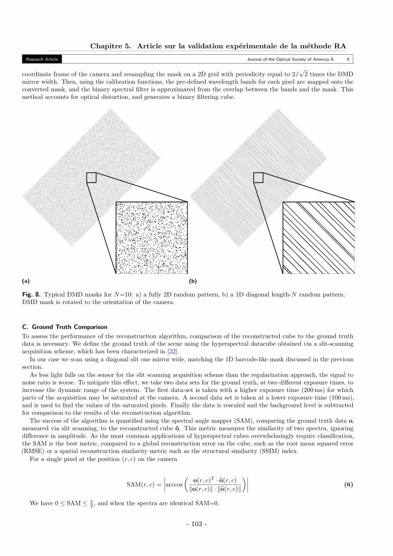
Chapitre 5. Article sur la validation expérimentale de la méthode RAResearch Article Journal of the Optical Society of America A 9
coordinate frame of the camera and resampling the mask on a 2D grid with periodicity equal to 2/√
2 times the DMDmirror width. Then, using the calibration functions, the pre-defined wavelength bands for each pixel are mapped onto theconverted mask, and the binary spectral filter is approximated from the overlap between the bands and the mask. Thismethod accounts for optical distortion, and generates a binary filtering cube.
(a) (b)
Fig. 8. Typical DMD masks for N=10: a) a fully 2D random pattern, b) a 1D diagonal length-N random pattern.DMD mask is rotated to the orientation of the camera.
C. Ground Truth ComparisonTo assess the performance of the reconstruction algorithm, comparison of the reconstructed cube to the ground truthdata is necessary. We define the ground truth of the scene using the hyperspectral datacube obtained via a slit-scanningacquisition scheme, which has been characterized in [22].
In our case we scan using a diagonal slit one mirror wide, matching the 1D barcode-like mask discussed in the previoussection.
As less light falls on the sensor for the slit scanning acquisition scheme than the regularization approach, the signal tonoise ratio is worse. To mitigate this effect, we take two data sets for the ground truth, at two different exposure times, toincrease the dynamic range of the system. The first data-set is taken with a higher exposure time (200ms) for whichparts of the acquisition may be saturated at the camera. A second data set is taken at a lower exposure time (100ms),and is used to find the values of the saturated pixels. Finally the data is rescaled and the background level is subtractedfor comparison to the results of the reconstruction algorithm.
The success of the algorithm is quantified using the spectral angle mapper (SAM), comparing the ground truth data o,measured via slit scanning, to the reconstructed cube o. This metric measures the similarity of two spectra, ignoringdifference in amplitude. As the most common applications of hyperspectral cubes overwhelmingly require classification,the SAM is the best metric, compared to a global reconstruction error on the cube, such as the root mean squared error(RMSE) or a spatial reconstruction similarity metric such as the structural similarity (SSIM) index.
For a single pixel at the position (r, c) on the camera
SAM(r, c) =∣∣∣∣arccos
(o(r, c)T · o(r, c)‖o(r, c)‖ · ‖o(r, c)‖
)∣∣∣∣ (6)
We have 0 ≤ SAM ≤ π2 , and when the spectra are identical SAM=0.
- 103 -
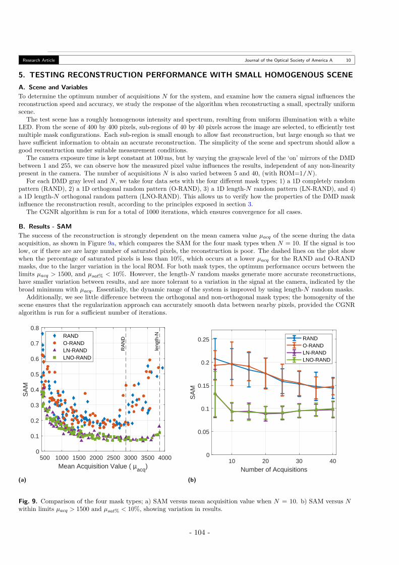
Research Article Journal of the Optical Society of America A 10
5. TESTING RECONSTRUCTION PERFORMANCE WITH SMALL HOMOGENOUS SCENEA. Scene and VariablesTo determine the optimum number of acquisitions N for the system, and examine how the camera signal influences thereconstruction speed and accuracy, we study the response of the algorithm when reconstructing a small, spectrally uniformscene.
The test scene has a roughly homogenous intensity and spectrum, resulting from uniform illumination with a whiteLED. From the scene of 400 by 400 pixels, sub-regions of 40 by 40 pixels across the image are selected, to efficiently testmultiple mask configurations. Each sub-region is small enough to allow fast reconstruction, but large enough so that wehave sufficient information to obtain an accurate reconstruction. The simplicity of the scene and spectrum should allow agood reconstruction under suitable measurement conditions.
The camera exposure time is kept constant at 100ms, but by varying the grayscale level of the ‘on’ mirrors of the DMDbetween 1 and 255, we can observe how the measured pixel value influences the results, independent of any non-linearitypresent in the camera. The number of acquisitions N is also varied between 5 and 40, (with ROM=1/N).
For each DMD gray level and N , we take four data sets with the four different mask types; 1) a 1D completely randompattern (RAND), 2) a 1D orthogonal random pattern (O-RAND), 3) a 1D length-N random pattern (LN-RAND), and 4)a 1D length-N orthogonal random pattern (LNO-RAND). This allows us to verify how the properties of the DMD maskinfluence the reconstruction result, according to the principles exposed in section 3.
The CGNR algorithm is run for a total of 1000 iterations, which ensures convergence for all cases.
B. Results - SAMThe success of the reconstruction is strongly dependent on the mean camera value µacq of the scene during the dataacquisition, as shown in Figure 9a, which compares the SAM for the four mask types when N = 10. If the signal is toolow, or if there are are large number of saturated pixels, the reconstruction is poor. The dashed lines on the plot showwhen the percentage of saturated pixels is less than 10%, which occurs at a lower µacq for the RAND and O-RANDmasks, due to the larger variation in the local ROM. For both mask types, the optimum performance occurs between thelimits µacq > 1500, and µsat% < 10%. However, the length-N random masks generate more accurate reconstructions,have smaller variation between results, and are more tolerant to a variation in the signal at the camera, indicated by thebroad minimum with µacq. Essentially, the dynamic range of the system is improved by using length-N random masks.
Additionally, we see little difference between the orthogonal and non-orthogonal mask types; the homogenity of thescene ensures that the regularization approach can accurately smooth data between nearby pixels, provided the CGNRalgorithm is run for a sufficient number of iterations.
500 1000 1500 2000 2500 3000 3500 4000
Mean Acquisition Value ( µacq)
0
0.1
0.2
0.3
0.4
0.5
0.6
0.7
0.8
SA
M
RA
ND
leng
th-NRAND
O-RANDLN-RANDLNO-RAND
(a)
10 20 30 40
Number of Acquisitions
0
0.05
0.1
0.15
0.2
0.25
SA
M
RANDO-RANDLN-RANDLNO-RAND
(b)
Fig. 9. Comparison of the four mask types; a) SAM versus mean acquisition value when N = 10. b) SAM versus Nwithin limits µacq > 1500 and µsat% < 10%, showing variation in results.
- 104 -
Chapitre 5. Article sur la validation expérimentale de la méthode RAResearch Article Journal of the Optical Society of America A 11
Figure 9b shows how the number of acquisitions N influences the SAM for the different mask types. The data for thisplot has been selected when the signal at the camera falls within the limits described by the previous plot (µacq > 1500and µsat% < 10%). Compared to the RAND type masks, the length-N masks generate more accurate results (lower SAM),with optimum N > 10. This indicates that as long as N > 10, sufficient information is provided by the acquisition data toaccurately reconstruct the hyperspectral datacube.
Conversely, for the RAND type masks, the variation in the local ROM leads to loss of data, and so for a given N thereconstruction of the hyperspectral datacube is less accurate. In this case, increasing N continues to improve the accuracyof the result, by providing more information to the solver, which outweighs the detrimental influence of noise. However,even with a high number of acquisitions the reconstruction is still less accurate than the length-N case, with a largervariation in the results.
C. Results - Number of IterationsAnother important metric is how many iterations the CGNR algorithm requires to reach convergence. The evolution ofthe SAM with CGNR iteration number is shown in Figure 10a. The orthogonal masks start with a lower SAM, but whilethe random type masks quickly converge to an inaccurate solution, the length-N random masks converge slowly but toa more accurate solution. Clearly, a fast reconstruction does not necessarily mean an accurate reconstruction, as withinsufficient data the algorithm can converge quickly to a wrong solution.
Without access to the ground truth, the stopping point for the algorithm can be determined by measuring the evolutionof the data using the first residual, given by the parameter η
η = log(‖oi−1 − oi‖2
‖oi‖2
)(7)
The η corresponding to the data in Figure 10a is shown in Figure 10b. A suitable stopping condition for the CGNRalgorithm in this case is η < −3. It is confirmed that the orthogonal mask types converge faster, especially for the firstfew iterations, shown in Figure 10c.
Figure 11 demonstrates how the number of iterations required to reach the stopping condition is influenced by N . Asincreasing the number of acquisitions N increases the amount of information available to the algorithm, fewer iterationsare required to reach convergence. Additionally, orthogonal masks converge slightly faster as the condition number of theproblem is smaller.
These initial tests confirm that the LNO-RAND mask performs the best, both in terms of reconstruction accuracy andspeed.
6. RECONSTRUCTION OF A LARGE MULTISPECTRUM SCENEWe now test the reconstruction algorithm on two scenes with simple multi-spectral structure, using a LNO-RAND mask.The number of acquisitions is chosen to be N = 10, the minimum number of acquisitions possible as determined in section4. As the scene has 110 spectral bands, this gives over a ten-fold reduction in the amount of information needed toreconstruct the data cube, compared to standard acquisition schemes.
Both scenes have a large variation in panchromatic intensity, so DMD grey level is set as high as possible to obtainmaximum signal, but without saturation on the acquisition image, for a camera exposure time of 100ms. The scene islarger and more complex than the test scenes in the previous section, and in this case a suitable stopping condition wasfound to be when η < −4. Using non-optimized matlab code, each iteration of the CGNR algorithm takes around 6 s,which can be reduced to 0.6 s by implementing parallel computing techniques using a mid-range graphics card (NVIDIAGeForce GTX 1060).
A. Scene A - Stacked FiltersScene A consists of stacked red and green polyester filters, backlit by a white LED, shown in Figure 12a, giving regionswith different spectra and intensity over the scene. The edges shown in Figure 12b are found using the panchromaticimage, which is made by averaging the acquisition values for each pixel - shown in Figure 12c. The panchromatic intensityalso gives the mean µacq for each pixel. A single acquisition image is shown in Figure 12d. The scene has large regionswith uniform, smooth spectra, and well defined edges, so should be straightforward to reconstruct.
The CGNR algorithm reached the stopping condition after 626 iterations. A comparison between two monochromaticimages for the ground truth and the reconstructed cube are shown in Figure 13a and 13b. There is a good correspondenceto the ground truth, but in the dark regions where there is low signal the reconstructed cube has some faint diagonalartifacts. Figure 13c shows the resulting SAM map for the scene, where the SAM value of each pixel is found by comparisonto the ground truth. A close-up of the region marked by the rectangle is shown in Figure 13d, with the edges superimposed.Over the scene, the mean and variation in the SAM is 0.16± 0.05, with the highest values for the SAM in the darkest
- 105 -
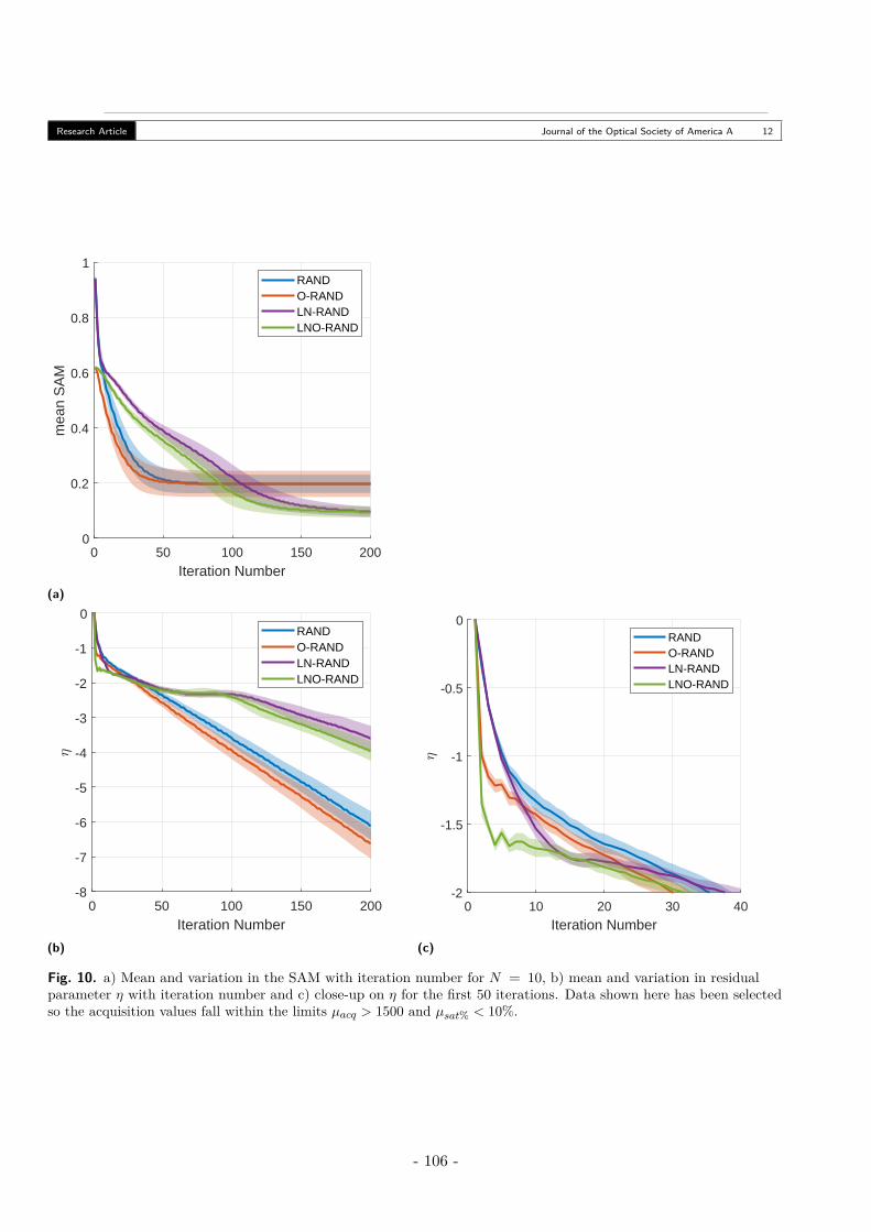
Research Article Journal of the Optical Society of America A 12
0 50 100 150 200
Iteration Number
0
0.2
0.4
0.6
0.8
1
mea
n S
AM
RANDO-RANDLN-RANDLNO-RAND
(a)
0 50 100 150 200
Iteration Number
-8
-7
-6
-5
-4
-3
-2
-1
0RANDO-RANDLN-RANDLNO-RAND
(b)
0 10 20 30 40
Iteration Number
-2
-1.5
-1
-0.5
0RANDO-RANDLN-RANDLNO-RAND
(c)
Fig. 10. a) Mean and variation in the SAM with iteration number for N = 10, b) mean and variation in residualparameter η with iteration number and c) close-up on η for the first 50 iterations. Data shown here has been selectedso the acquisition values fall within the limits µacq > 1500 and µsat% < 10%.
- 106 -
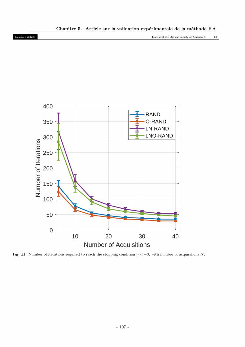
Chapitre 5. Article sur la validation expérimentale de la méthode RAResearch Article Journal of the Optical Society of America A 13
10 20 30 40
Number of Acquisitions
0
50
100
150
200
250
300
350
400
Num
ber
of It
erat
ions
RANDO-RANDLN-RANDLNO-RAND
Fig. 11. Number of iterations required to reach the stopping condition η < −3, with number of acquisitions N .
- 107 -
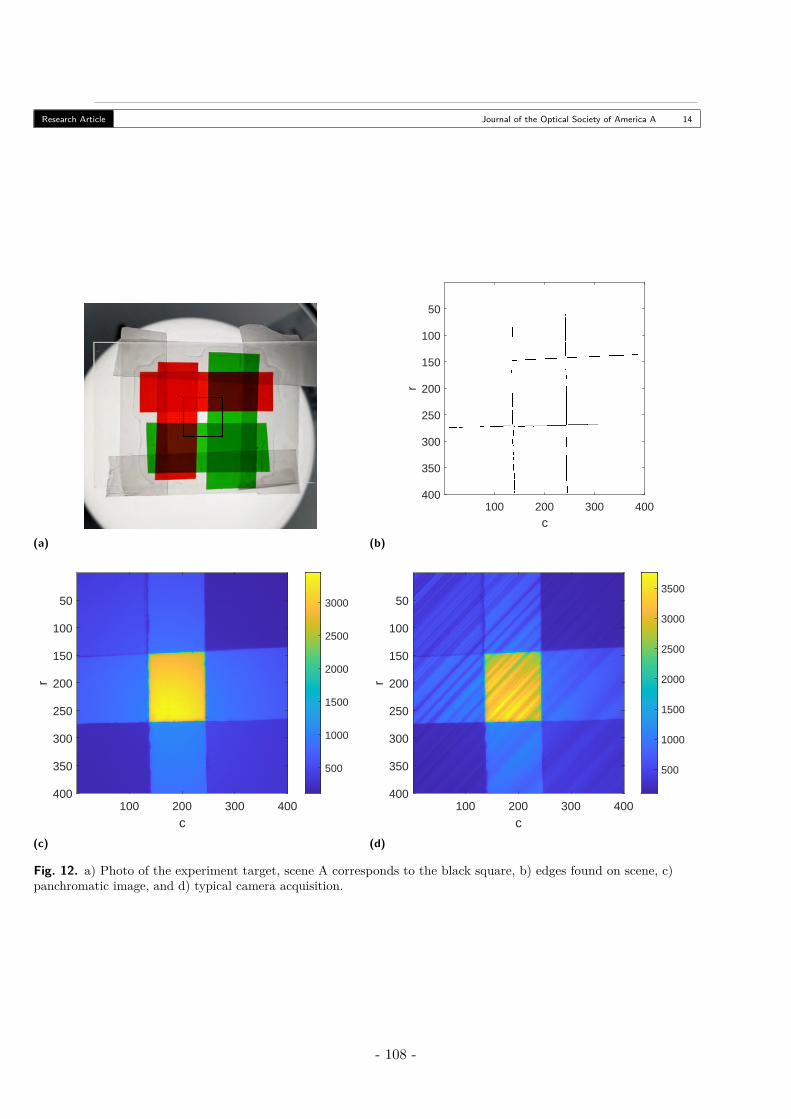
Research Article Journal of the Optical Society of America A 14
(a)
100 200 300 400
c
50
100
150
200
250
300
350
400
r
(b)
100 200 300 400
c
50
100
150
200
250
300
350
400
r
500
1000
1500
2000
2500
3000
(c)
100 200 300 400
c
50
100
150
200
250
300
350
400
r
500
1000
1500
2000
2500
3000
3500
(d)
Fig. 12. a) Photo of the experiment target, scene A corresponds to the black square, b) edges found on scene, c)panchromatic image, and d) typical camera acquisition.
- 108 -
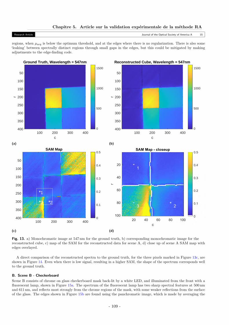
Chapitre 5. Article sur la validation expérimentale de la méthode RAResearch Article Journal of the Optical Society of America A 15
regions, when µacq is below the optimum threshold, and at the edges where there is no regularization. There is also some‘leaking’ between spectrally distinct regions through small gaps in the edges, but this could be mitigated by makingadjustments to the edge-finding code.
Ground Truth, Wavelength = 547nm
100 200 300 400
c
50
100
150
200
250
300
350
400
r
0
500
1000
1500
(a)
Reconstructed Cube, Wavelength = 547nm
100 200 300 400
c
50
100
150
200
250
300
350
400
r
0
500
1000
1500
(b)
SAM Map
1
23
100 200 300 400
50
100
150
200
250
300
350
400 0
0.1
0.2
0.3
0.4
0.5
(c) (d)
Fig. 13. a) Monochromatic image at 547 nm for the ground truth, b) corresponding monochromatic image for thereconstructed cube, c) map of the SAM for the reconstructed data for scene A, d) close up of scene A SAM map withedges overlayed.
A direct comparison of the reconstructed spectra to the ground truth, for the three pixels marked in Figure 13c, areshown in Figure 14. Even when there is low signal, resulting in a higher SAM, the shape of the spectrum corresponds wellto the ground truth.
B. Scene B - CheckerboardScene B consists of chrome on glass checkerboard mask back-lit by a white LED, and illuminated from the front with afluorescent lamp, shown in Figure 15a. The spectrum of the fluorescent lamp has two sharp spectral features at 500 nmand 611 nm, and reflects most strongly from the chrome regions of the mask, with some weaker reflections from the surfaceof the glass. The edges shown in Figure 15b are found using the panchromatic image, which is made by averaging the
- 109 -
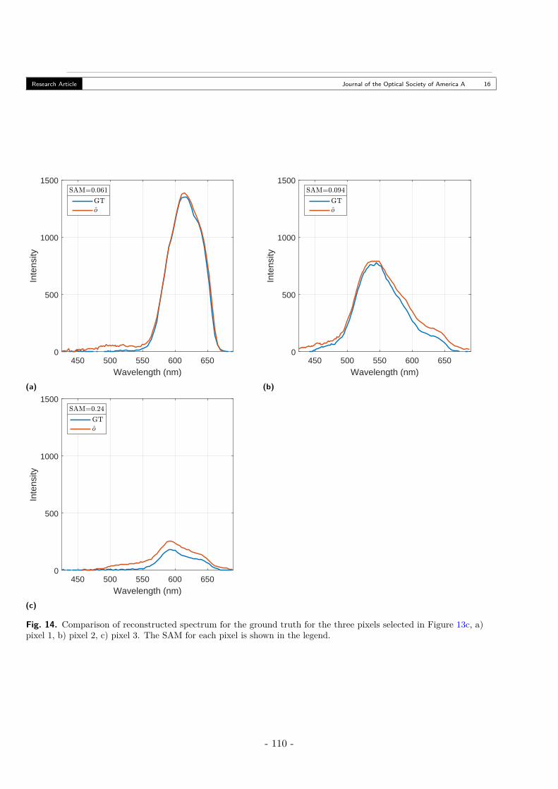
Research Article Journal of the Optical Society of America A 16
450 500 550 600 650
Wavelength (nm)
0
500
1000
1500
Inte
nsity
(a)
450 500 550 600 650
Wavelength (nm)
0
500
1000
1500
Inte
nsity
(b)
450 500 550 600 650
Wavelength (nm)
0
500
1000
1500
Inte
nsity
(c)
Fig. 14. Comparison of reconstructed spectrum for the ground truth for the three pixels selected in Figure 13c, a)pixel 1, b) pixel 2, c) pixel 3. The SAM for each pixel is shown in the legend.
- 110 -
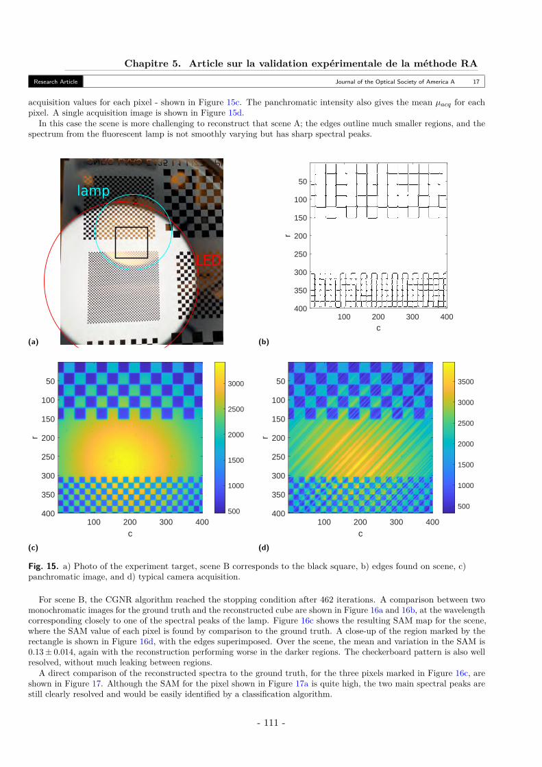
Chapitre 5. Article sur la validation expérimentale de la méthode RAResearch Article Journal of the Optical Society of America A 17
acquisition values for each pixel - shown in Figure 15c. The panchromatic intensity also gives the mean µacq for eachpixel. A single acquisition image is shown in Figure 15d.
In this case the scene is more challenging to reconstruct that scene A; the edges outline much smaller regions, and thespectrum from the fluorescent lamp is not smoothly varying but has sharp spectral peaks.
LED
lamp
(a)
100 200 300 400
c
50
100
150
200
250
300
350
400
r
(b)
100 200 300 400
c
50
100
150
200
250
300
350
400
r
500
1000
1500
2000
2500
3000
(c)
100 200 300 400
c
50
100
150
200
250
300
350
400
r
500
1000
1500
2000
2500
3000
3500
(d)
Fig. 15. a) Photo of the experiment target, scene B corresponds to the black square, b) edges found on scene, c)panchromatic image, and d) typical camera acquisition.
For scene B, the CGNR algorithm reached the stopping condition after 462 iterations. A comparison between twomonochromatic images for the ground truth and the reconstructed cube are shown in Figure 16a and 16b, at the wavelengthcorresponding closely to one of the spectral peaks of the lamp. Figure 16c shows the resulting SAM map for the scene,where the SAM value of each pixel is found by comparison to the ground truth. A close-up of the region marked by therectangle is shown in Figure 16d, with the edges superimposed. Over the scene, the mean and variation in the SAM is0.13± 0.014, again with the reconstruction performing worse in the darker regions. The checkerboard pattern is also wellresolved, without much leaking between regions.
A direct comparison of the reconstructed spectra to the ground truth, for the three pixels marked in Figure 16c, areshown in Figure 17. Although the SAM for the pixel shown in Figure 17a is quite high, the two main spectral peaks arestill clearly resolved and would be easily identified by a classification algorithm.
- 111 -
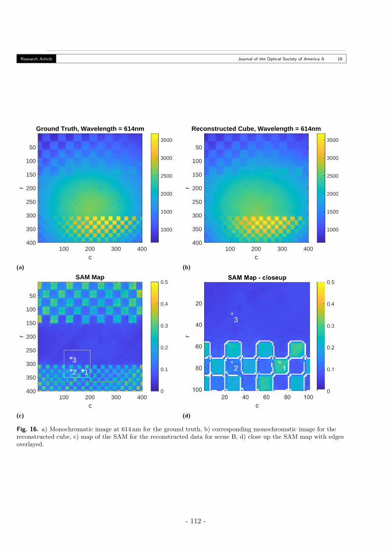
Research Article Journal of the Optical Society of America A 18
Ground Truth, Wavelength = 614nm
100 200 300 400
c
50
100
150
200
250
300
350
400
r
1000
1500
2000
2500
3000
3500
(a)
Reconstructed Cube, Wavelength = 614nm
100 200 300 400
c
50
100
150
200
250
300
350
400
r
1000
1500
2000
2500
3000
3500
(b)
SAM Map
12
3
100 200 300 400
c
50
100
150
200
250
300
350
400
r
0
0.1
0.2
0.3
0.4
0.5
(c) (d)
Fig. 16. a) Monochromatic image at 614 nm for the ground truth, b) corresponding monochromatic image for thereconstructed cube, c) map of the SAM for the reconstructed data for scene B, d) close up the SAM map with edgesoverlayed.
- 112 -
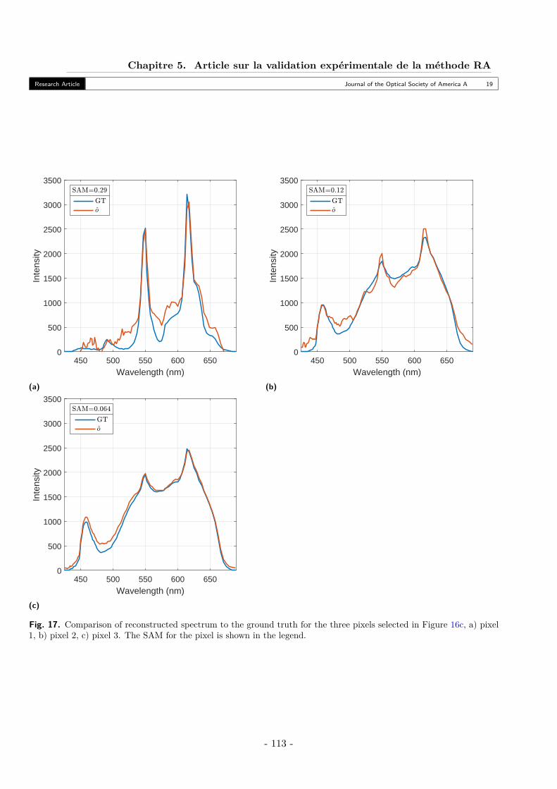
Chapitre 5. Article sur la validation expérimentale de la méthode RAResearch Article Journal of the Optical Society of America A 19
450 500 550 600 650
Wavelength (nm)
0
500
1000
1500
2000
2500
3000
3500
Inte
nsity
(a)
450 500 550 600 650
Wavelength (nm)
0
500
1000
1500
2000
2500
3000
3500
Inte
nsity
(b)
450 500 550 600 650
Wavelength (nm)
0
500
1000
1500
2000
2500
3000
3500
Inte
nsity
(c)
Fig. 17. Comparison of reconstructed spectrum to the ground truth for the three pixels selected in Figure 16c, a) pixel1, b) pixel 2, c) pixel 3. The SAM for the pixel is shown in the legend.
- 113 -
Research Article Journal of the Optical Society of America A 20
7. CONCLUSIONTo conclude, this algorithm provides a method to reconstruct a hyperspectral data cube accurately from only a fewacquisitions, using the key assumption of spatial-spectral correlations. We have demonstrated the accurate reconstructionof a hyperspectral data-cube with 110 wavelength bands and 400 by 400 spatial pixels, using only 10 acquisitions, thusproviding a 11-fold reduction in data.
The reconstruction algorithm uses quadratic regularization, relying on the assumption of spectral-spatial correlationswithin the scene, and on the assumption that the boundary between two regions of different spectra is typically visible onthe panchromatic image, i.e. there are no adjacent metamers.
Additionally, we use prior knowledge of the optical system, specifically the straightforward mapping between DMDmirror and camera pixel, to optimize the coded aperture implemented by the DMD. By utilizing a length-N mask weensure there is only a small variation in signal strength pixel-to-pixel, leading to measurement data which is more likelyto fall within the dynamic range of the camera. Similarly, the use of orthogonal masks reduces the convergence time,and ensures the panchromatic image is easily accessible by summing the acquisitions, reducing the total number ofacquisitions needed. In this case we use a mask with 1-D variation along the diagonal direction, but it is expected thatwith adaptations to the system (such as changing the orientation of the DMD), the use of a fully 2-D LNO-RAND maskwould further decrease the reconstruction times by providing more information in a single acquisition.
We have found that the success of the reconstruction depends on the signal at the camera for each acquisition, leadingdark or over-saturated regions to be less accurately reconstructed. Information from the panchromatic image could beused to simultaneously tune the exposure time and the local gray level of the DMD mask, to enhance the signal in over orunder-exposed regions, leading to an improved signal-to-noise ratio for the entire scene. This adaptive approach couldincrease the dynamic range of the system by 8 bits and improve the overall accuracy of the reconstruction. In this case,the CGNR algorithm needs to be adjusted to account for non-binary values in the filtering cube, which must be weightedby the DMD gray level.
ACKNOWLEDGEMENTSThis work was funded by the Agence Nationale de la Recherche (ANR-18-ASTR-0012-01 (ImHypAd project))
DISCLOSURESThe authors declare no conflicts of interest.
REFERENCES1. A. Chakrabarti and T. Zickler, “Statistics of real-world hyperspectral images,” in CVPR 2011, (IEEE, 2011), pp. 193–200.2. S. M. Nascimento, K. Amano, and D. H. Foster, “Spatial distributions of local illumination color in natural scenes,” Vis. Res. 120, 39–44 (2016).3. S. Andriani, G. Calvagno, and G. A. Mian, “A lossless image coding technique exploiting spectral correlation on the RGB space,” in 2004 12th
European Signal Processing Conference, (IEEE, 2004), pp. 1305–1308.4. U. Srinivas, Y. Chen, V. Monga, N. M. Nasrabadi, and T. D. Tran, “Exploiting sparsity in hyperspectral image classification via graphical models,”
IEEE Geosci. Remote. Sens. Lett. 10, 505–509 (2012).5. R. Arablouei and F. De Hoog, “Hyperspectral image recovery via hybrid regularization,” IEEE Transactions on Image Process. 25, 5649–5663
(2016).6. J. Li, Q. Yuan, H. Shen, and L. Zhang, “Noise removal from hyperspectral image with joint spectral–spatial distributed sparse representation,”
IEEE Transactions on Geosci. Remote. Sens. 54, 5425–5439 (2016).7. A. Karami, M. Yazdi, and G. Mercier, “Compression of hyperspectral images using discerete wavelet transform and tucker decomposition,” IEEE
journal selected topics applied earth observations remote sensing 5, 444–450 (2012).8. H. Rueda, H. Arguello, and G. R. Arce, “Dmd-based implementation of patterned optical filter arrays for compressive spectral imaging,” JOSA A
32, 80–89 (2015).9. X. Lin, G. Wetzstein, Y. Liu, and Q. Dai, “Dual-coded compressive hyperspectral imaging,” Opt. letters 39, 2044–2047 (2014).10. X. Lin, Y. Liu, J. Wu, and Q. Dai, “Spatial-spectral encoded compressive hyperspectral imaging,” ACM Transactions on Graph. 33, 1–11 (2014).11. A. A. Wagadarikar, N. P. Pitsianis, X. Sun, and D. J. Brady, “Video rate spectral imaging using a coded aperture snapshot spectral imager,” Opt.
Express 17, 6368 (2009).12. A. A. Wagadarikar, R. John, R. Willett, and D. J. Brady, “Single disperser design for compressive, single-snapshot spectral imaging,” in Adaptive
Coded Aperture Imaging and Non-Imaging Sensors, vol. 6714 (2007), p. 67140A.13. C. Deng, X. Hu, J. Suo, Y. Zhang, Z. Zhang, and Q. Dai, “Snapshot hyperspectral imaging via spectral basis multiplexing in Fourier domain,”
Opt. Express 26, 32509 (2018).14. M. E. Gehm, R. John, D. J. Brady, R. M. Willett, and T. J. Schulz, “Single-shot compressive spectral imaging with a dual-disperser architecture,”
Opt. express 15, 14013–14027 (2007).15. Y. Fu, Y. Zheng, I. Sato, and Y. Sato, “Exploiting spectral-spatial correlation for coded hyperspectral image restoration,” in Proceedings of the
IEEE Conference on Computer Vision and Pattern Recognition, (2016), pp. 3727–3736.16. Y. Fu, A. Lam, I. Sato, and Y. Sato, “Adaptive spatial-spectral dictionary learning for hyperspectral image restoration,” Int. J. Comput. Vis. 122,
228–245 (2017).
- 114 -

Chapitre 5. Article sur la validation expérimentale de la méthode RAResearch Article Journal of the Optical Society of America A 21
17. X. Cao, T. Yue, X. Lin, S. Lin, X. Yuan, Q. Dai, L. Carin, and D. J. Brady, “Computational snapshot multispectral cameras: toward dynamiccapture of the spectral world,” IEEE Signal Process. Mag. 33, 95–108 (2016).
18. D. L. Graff and S. P. Love, “Adaptive hyperspectral imaging with a MEMS-based full-frame programmable spectral filter,” in Next-GenerationSpectroscopic Technologies VII, vol. 9101 M. A. Druy and R. A. Crocombe, eds. (SPIE, 2014), p. 910111.
19. M. Dunlop-Gray, P. K. Poon, D. Golish, E. Vera, and M. E. Gehm, “Experimental demonstration of an adaptive architecture for direct spectralimaging classification,” Opt. Express 24, 18307 (2016).
20. D. L. Graff and S. P. Love, “Real-time matched-filter imaging for chemical detection using a DMD-based programmable filter,” Proc. SPIE 8618,Emerg. Digit. Micromirror Device Based Syst. Appl. V 8618, 86180F(1) – 86180F(10) (2013).
21. D. L. Graff and S. P. Love, “Real-time video imaging of gas plumes using a DMD-enabled full-frame programmable spectral filter,” in EmergingDigital Micromirror Device Based Systems and Applications VIII, vol. 9761 (2016), p. 97610C.
22. E. Hemsley, S. Lacroix, H. Carfantan, and A. Monmayrant, “Calibration of programmable spectral imager with dual disperser architecture,” Opt.Commun. p. 125767 (2020).
23. S. McGregor, S. Lacroix, and A. Monmayrant, “Adaptive hyperspectral imager: design, modeling, and control,” J. Opt. 17, 085607 (2015).24. I. Ardi, H. Carfantan, S. Lacroix, and A. Monmayrant, “Fast hyperspectral cube reconstruction for a double disperser imager,” in 2018 26th
European Signal Processing Conference (EUSIPCO), (IEEE, 2018), pp. 2225–2229.25. I. Ardi, “Reconstruction d’images hyperspectrales pour un imageur non conventionnel pilotable,” Ph.D. thesis, Université de Toulouse (2020).26. J. Idier, Bayesian approach to inverse problems (John Wiley & Sons, 2013).27. A. N. Tikhonov and V. Y. Arsenin, Solutions of Ill-posed problems (W.H. Winston, 1977).28. R. Barrett, M. W. Berry, T. F. Chan, J. Demmel, J. Donato, J. Dongarra, V. Eijkhout, R. Pozo, C. Romine, and H. Van der Vorst, Templates for
the solution of linear systems: building blocks for iterative methods, vol. 43 (Siam, 1994).29. N. R. Council, Advances in Photoreception: Proceedings of a Symposium on Frontiers of Visual Science (The National Academies Press,
Washington, DC, 1990).
- 115 -

Chapitre 6
Conclusion et perspectives
6.1 Conclusion
Dans cette thèse nous nous sommes intéressés à la reconstruction d’images hyperspectrales àpartir d’un faible nombre d’acquisitions obtenues par un imageur hyperspectral non-convention-nel configurable. La configuration de cet instrument est modifiable aisément via le pilotaged’une matrice de micro-miroirs (appelée DMD), que l’on peut placer en mode réflexion ou réjec-tion. Ainsi, chaque acquisition correspond à une projection, parfaitement maîtrisée, du contenuspatio-spectral de la scène observé sur un détecteur dont le nombre de pixels correspond à celuide la dimension spatiale de la scène. Notons que lorsque l’on place tous les miroirs en moderéflexion, l’acquisition correspond exactement à l’image panchromatique de la scène (c’est-à-direintégrée sur l’ensemble des longueurs d’onde), avec le même échantillonnage que les donnéeshyperspectrales, La reconstruction avec un faible nombre d’acquisition signifie alors que l’oncherche à reconstruire un cube hyperspectral avec typiquement dix fois moins de projections quele nombre de longueurs d’ondes du cube, soit dix fois moins de données que d’inconnues.Nous avons proposé deux méthodes de reconstruction, pour des configurations aléatoires duDMD, qui exploitent les fortes corrélations spatio-spectrales présentes dans le cube par le biaisde deux hypothèses : l’hypothèse d’homogénéité pour la méthode RA et l’hypothèse supplémen-taire de séparabilité pour SA. Pour ce faire, nous avons utilisé l’information fournie par l’imagepanchromatique pour tenir compte convenablement des hypothèses pour chacune des méthodes.Ces deux méthodes nécessitent un faible coût de calcul car elles s’appuient sur une régularisationquadratique et le calcul de la solution se ramène à la résolution de systèmes linéaires.
Pour la méthode RA, l’hypothèse d’homogénéité stipule qu’il existe des régions spatiales surlesquelles les spectres des différents pixels sont très corrélés. Pour tenir compte de cette hypothèsenous avons considéré une régularisation quadratique de type Tikhonov pour favoriser la présencede telles régions. Pour remédier au problème habituel de lissage au niveau des contours séparantles régions homogènes produit par une telle régularisation nous avons localisé ces contours surl’image panchromatique puis relâché la régularisation aux niveaux de ces derniers. Grâce à celanous avons conservé la forme quadratique du problème de reconstruction tout en préservant lescontours. Pour une telle régularisation quadratique, le calcul de la solution nécessite la résolu-tion d’un système linéaire de grande dimension, que nous avons résolu grâce à un algorithme degradient conjugué (CGNR). Notons qu’une telle approche permet de s’affranchir de l’utilisationde régularisation non quadratique, telle que la variation totale, et d’algorithmes d’optimisationcoûteux associés, tout en préservant les contours.Pour cette méthode, nous avons étudié le problème du choix des paramètres de la régularisationet nous avons montré la présence d’un jeu de paramètres qui permet d’approcher les perfor-
117
6.2. Perspectives
mances des paramètres optimaux. Ceci a été démontré pour les données de simulation ou réelleset nous a permis de confirmer la robustesse et la cohérence et la robustesse de cette approche.Finalement nous avons étudié le problème de la vitesse de convergence CGNR et du temps dereconstruction en général. A cet effet, nous avons étudié la structure de la matrice de trans-fert de l’imageur et de sa relation avec la vitesse de convergence du CGNR. L’imageur étantpilotable, par l’intermédiaire de la matrice des micro-miroirs (DMD), nous avons proposé d’ex-ploiter des configurations orthogonales du DMD qui améliorent le conditionnement du problèmeet accélèrent la convergence du CGNR. De plus, ces configurations permettent d’obtenir l’imagepanchromatique sans acquisitions supplémentaires. Nous avons ainsi pu atteindre des temps dereconstruction inférieurs à 1 seconde pour les données de simulations (30 longueurs d’ondes) etd’une dizaine de minutes pour des données réelles (une centaine de longueurs d’ondes).
Pour la méthode SA l’hypothèse supplémentaire de séparabilité suppose que la scène hyper-spectrale est composée de régions spatiales fermées spectralement homogènes et que chacune deces régions est modélisée par le produit d’un unique spectre par la carte d’intensité (issue de l’in-tensité de l’image panchromatique). Cette hypothèse est très forte et nécessite une segmentationcorrecte de la scène hyperspectrale en régions homogènes, que l’on effectue à partir de l’imagepanchromatique. L’implémentation de la segmentation s’est faite grâce à l’usage conjoint de l’al-gorithme Watershed et du filtrage anisotrope de Perona-Malik. La reconstruction du spectre dechaque région, quant à elle, s’effectue par simple régularisation quadratique de type Tikhonov,suivant la dimension spectrale.Pour cette méthode SA le choix des paramètres de la segmentation est le plus crucial, le co-efficient de régularisation l’est moins. En effet, l’hypothèse de séparabilité n’est généralementvérifiée que pour des régions de faibles dimensions, une sur-segmentation de l’image est requise.De plus, cette hypothèse étant généralement fausse de part et d’autre des contours (ne serait-ceà cause de la réponse impulsionnelle de l’instrument qui a tendance à lisser les contours), descontours de plusieurs pixels doivent être pris en compte et exclus de la reconstruction. Nousavons montré, pour des données simulées, qu’un jeu de paramètres permettait d’approcher lesperformances des paramètres optimaux, confirmant la robustesse et la cohérence de cette ap-proche. Notons que pour cette méthode, la reconstruction de chaque région se fait de façonindépendante et à faible coût puisque seul un spectre par région est à estimer et une résolutiondirecte du système linéaire peut-être utilisée. La reconstruction du cube est donc très rapideet aisément parallélisable, les temps de reconstruction totale sur les données simulées sont del’ordre de quelques secondes.
6.2 Perspectives
Les perspectives de se travail se placent dans le cadre général du projet ImHypAd (ANRASTRID 2019-2021, ANR-18-ASTR-0012-01), associé à la conception de l’imageur hyperspectralet visent, à long terme, à rendre cet imageur adaptatif. Nous nous sommes focalisés durant cettethèse sur une première étape de reconstruction rapide des scènes hyperspectrales à partir d’unfaible nombre d’acquisitions.
Les perspectives envisageables des travaux menés pendant cette thèse sont variées : nous enprésentons trois :
— amélioration des performances des méthodes de reconstruction proposées, notammentaccélération du temps de calcul et de la qualité des images reconstruites ;
— Utilisation et exploitation des images reconstruites par ces méthodes ;— Et enfin une reconstruction adaptative des scènes hyperspectrales.
- 118 -
Chapitre 6. Conclusion et perspectives
6.2.1 Amélioration des performances des méthodes de reconstruction propo-sées
Pour la méthode RA, 3 pistes peuvent être explorées pour améliorer significativement laméthode :
— L’étape de détection des contours n’est pas cruciale pour la méthode, mais nous l’avonstraitée de façon relativement fruste, par seuillage de gradients. Elle fournit des contoursnon-fermés, ce qui n’est pas en soi un problème, mais peut provoquer des « fuites »d’une région homogène vers une autre alors que l’on constate visuellement, sur l’imagepanchromatique, que les régions sont aisément séparables par des contours. Sans allervers une segmentation en contours fermés, comme cela est nécessaire dans la méthodeSA, on peut aisément imaginer améliorer cette détection de contours. Dans un premiertemps on pense bien sûr à l’utilisation de méthodes existantes plus performantes que desimples seuillages de gradients. Mais on peut également tenter d’améliorer la continuitédes contours horizontaux et verticaux, qui sont pour l’instant détectés indépendamment.Ce problème est à notre connaissance peu traité dans la littérature, car nous exploitonsici la notion de contours inter-pixels alors que les contours exploités le plus souvent entraitement d’images sont sur les pixels et qu’il est plus simple dans ce cas d’obtenirla continuité de tels contours par simple 4 ou 8-connexité. Un stage s’est déroulé dansl’équipe ces derniers mois 1 et a permis de premières avancées dans ce sens.
— Une deuxième amélioration possible au niveau méthodologique porte sur la régularisa-tion dans le voisinage des contours. En effet, la détection des contours est exploitée pourl’instant de façon binaire dans la reconstruction, en supprimant la régularisation de partet d’autre des contours. Cependant, les contours ne sont pas nets entre les régions homo-gènes, notamment à cause de l’étalement induit par la réponse impulsionnelle de l’optiquedu système. Une autre façon de procéder serait de prendre en compte des paramètres derégularisation variables dans l’image en fonction de la proximité des contours. Cela chan-gerait très peu la méthode et la modification de son implémentation est immédiate. Leplus délicat est donc le choix du mode de variation des paramètres de régularisation.
— L’implémentation de la méthode RA peut également être améliorée. En particulier, ilparait intéressant d’exploiter le calcul parallèle. Nous disposons actuellement de deuximplémentations de cette méthode : une première, en Matlab, exploitant pour les pro-blèmes directs et adjoint des produits par le cube de filtrage, codé en sparse ; une seconde,développée par un stagiaire 2 en langage C à l’aide de boucles, évitant de tels produits, enprenant soin d’exploiter la proximité des données dans la mémoire cache du processeur.Bien que Matlab exploite automatiquement plusieurs cœurs nous avons pu réduire d’unfacteur 10 le temps de calcul avec le code en C. Il est donc aisé d’imaginer que la paral-lélisation du code en C permettrait de réduire encore le temps de calcul. Enfin, on peutégalement envisager d’exploiter le calcul sur GPU. De premiers tests à l’aide de Matlabexploitant le calcul sur GPU (en demandant à Matlab d’exécuter la version produit parle cube de filtrage sur GPU) ont permis de réduire le temps de calcul d’un facteur 10. Unemise en œuvre sur GPU, en évitant les produits par le cube de filtrage devrait permettrede réduire encore le temps de calcul.Un autre moyen de réduire le coût de calcul pour la méthode RA serait d’effectuer unereconstruction sous-optimale en calculant la solution par sous-cubes découpés suivant ladimension spatiale. Typiquement une taille de sous-cubes de 200×200 pixels serait idéale,car ces dimensions spatiales sont assez grandes pour permettre l’exploitation des corré-
1. Stage de césure de Yvan Gary, étudiant en deuxième année de l’ISAE-Supaéro, février à juillet 2020.2. Stage de Julien Bidan étudiant en master 1 SIA-AMS de l’Université Toulouse 3 – Paul Sabatier, juin-
juillet 2019.
- 119 -
6.2. Perspectives
lations et le temps de reconstruction serait significativement réduit. La parallélisationserait alors immédiate en effectuant la reconstruction des blocs en parallèle. Bien sûr ilfaudrait gérer la fusion des blocs ainsi reconstruits.Enfin, si l’on effectue une segmentation en régions fermées, avec des régions de grandesdimension (contrairement à RA), on pourrait également appliquer la méthode RA in-dépendamment sur chaque région, ce qui permettrait également de réduire le temps decalcul en calculant les solutions sur les différentes régions en parallèle. . .
Concernant la méthode SA, nous envisageons cinq axes d’amélioration :— Le premier concerne la segmentation qui est cruciale pour la reconstruction sous l’hypo-
thèse de séparabilité. Ce problème a été en partie traité durant de cette thèse mais n’apas pu être présenté dans ce manuscrit par manque de temps. Typiquement, nous avonsobservé que les seuils optimaux de segmentation sont généralement petit, afin de segmen-ter correctement les régions de faible intensité, ce qui produit des zones sur-segmentées.D’une part, cet effet est bénéfique car il permet d’assurer l’hypothèse de séparabilité.Cependant la taille moyenne des zones segmentées est petite ce qui affecte considérable-ment la qualité des spectres reconstruits. Pour remédier à cela, nous avons développé uneméthode de segmentation avec seuil adaptatif en modifiant judicieusement le filtrage dePerona-Malik. En pratique, l’idée est de tenir compte de la puissance du bruit (bruit dephoton, lié à l’intensité) en chaque pixel lors du filtrage grâce au coefficient de diffusionκ du filtrage de Perona-Malik.
— A l’opposé de la méthode RA, la régularisation n’est pas très importante pour la mé-thode SA et une simple régularisation de Tikhonov avec un paramètre de régularisationfixé pour toutes les régions nous a permis d’obtenir de bons résultats. On peut envisagerde régler différemment le coefficient de régularisation, en prenant en compte la quantitéd’information disponible dans les données et le rapport signal sur bruit, lié à la dyna-mique des données dans les différentes régions.De même, le calcul de la solution par la méthode RA se faisant indépendamment surchaque région, on peut envisager des méthodes de reconstruction plus élaborées que larégularisation de Tikhonov. On peut évidemment penser à des hypothèses de parcimo-nie sur des dictionnaires. Mais, il est possible de rester avec un critère quadratique etde prendre des contraintes supplémentaires, telles que la positivité (si la solution noncontrainte n’est pas positive), ou la prise en compte des pixels saturés, ce qui donne lieuà la résolution d’un problème de programmation quadratique (QP- Quadratic Program-ming). Bien sûr, cela augmentera le coût de calcul, mais la dimension du problème étanttrès réduite (seulement un spectre à reconstruire par région), cette augmentation seraraisonnable.
— La méthode SA ne reconstruit que partiellement le cube hyperspectral, sur des régionshomogènes et non sur les contours. On peut alors envisager une reconstruction a posterioride ces contours, en bénéficiant de la reconstruction sur les régions homogènes voisines,par exemple par une méthode de type démélange. En effet, on peut sans doute considérerque le spectre du contour est un mélange des spectres des régions voisines et il faut alorsestimer les coefficients de ce mélange. Nos premiers tests rapides sur une telle approche nesont pas très concluants et il faudrait donc approfondir cette étude. Notons que la méthodeRA a également des difficultés à reconstruire les images HS au niveau des contours, cequi est effectivement un problème difficile vu le manque d’information (10 fois moins dedonnées que d’inconnues).
— Enfin, on sait que l’on possède plus d’informations pour reconstruire les spectres dansles grandes régions, mais que l’hypothèse de séparabilité est sans doute plus souvent sa-tisfaite sur des petites régions. Aussi, il serait intéressant d’arriver à quantifier la qualité
- 120 -
Chapitre 6. Conclusion et perspectives
de la reconstruction de la méthode SA en particulier afin de vérifier l’hypothèse de sépa-rabilité (surtout aux bords des régions). On peut sans doute pour cela s’appuyer sur leserreurs entre les données disponibles et les données simulées qui seraient produites parl’instrument pour l’image HS reconstruite (résidus de reconstruction).
— Notons que la parallélisation de la méthode SA, est immédiate si l’on exécute en parallèlela reconstruction sur chaque région, plutôt que comme actuellement, de façon séquentielle.Cela impliquera de fait une réduction du coût de calcul de l’ordre du nombre de cœursutilisés. Une telle réduction est cependant à modérer légèrement par le fait que les calculssont actuellement effectués sous Matlab, qui exploite automatiquement plusieurs cœurspour la reconstruction de chaque région. Le calcul sur GPU pourrait également êtreenvisagé. Néanmoins la méthode SA est déjà actuellement très rapide et ce n’est pas cellequi nécessite le plus d’améliorations en termes de temps de calcul.
6.2.2 Exploitations des images reconstruites
Compte tenu de la qualité satisfaisante de la reconstruction obtenue avec les méthodes pro-posées, les données reconstruites se prêtent sans effort supplémentaire à leur exploitation, parexemple pour le démélange spectral et la classification, comme cela est fait classiquement surdes images hyperspectrales acquises par balayage.
Pour la méthode RA, les résultats montrent une bonne qualité de reconstruction sur lesgrandes régions homogènes. Sur les bords et dans les régions texturés, RA a cependant tendanceà mélanger les spectres, ce qui est du à l’étalement lié à la réponse impulsionnelle de l’optiquedu système. Ainsi, les données produites par RA se prêtent naturellement à des applications dedémélange spectral qui pourraient utiliser les spectres des grandes régions homogènes commea priori (end-members), au moins dans une phase d’initialisation. Bien sûr, un tel démélangespectral peut également être effectué sur l’ensemble de l’image pour la reconstruction effectuéepar la méthode SA, en plus du démélange visant à combler les pixels non reconstruits au niveaudes contours. Cela permettrait d’ailleurs peut-être de corriger (ou au moins détecter) quelquesdéfauts pour les pixels ne satisfaisant pas l’hypothèse de séparabilité.
Les données obtenues avec la méthode SA sont particulièrement adaptées à la classification(même partielle) des scènes imagées puisque l’image est déjà découpée en régions homogènes,donc constituées de pixels appartenant à une même classe. Nous nous somme d’ailleurs intéressésà cette application et les premiers résultats sont concluants et encourageants. En effet, nous avonsréussi à obtenir des classifications avec les données reconstruites à partir de 10% du cube HSoriginal comparables à celles obtenues avec les cubes HS originaux complets. De plus, on sait queles spectres reconstruits sont de qualités différentes, suivant la taille des régions et la satisfactionde l’hypothèse de séparabilité. Exploiter un tel indice de qualité pour la classification des spectresreconstruits parait alors une piste intéressante. Les premiers travaux menés en ce sens lors d’unstage 3 nous ont confirmé dans l’idée que cette piste était à approfondir. . .
6.2.3 Vers une exploitation adaptative des scènes hyperspectrales. . .
Concevoir un imageur hyperspectral adaptatif est ambitieux puisqu’il vise à adapter la confi-guration du dispositif, dans notre cas la configuration de la matrice de micro-miroirs (DMD), à lascène hyperspectrale observée pour une meilleure analyse, toujours avec pour objectif d’optimi-ser le nombre d’acquisitions. Le grand obstacle à l’approche adaptative est bien sûr le manqued’information a priori sur la scène imagée, avant l’acquisition. Un idée naturelle est donc decommencer par collecter quelques données sur la scène afin de piloter les acquisitions suivantes.La contrainte de temps de calcul court pour exploiter ces premières données est dans ce cadre
3. Stage de césure de Yvan Gary, étudiant en deuxième année de l’ISAE-Supaéro, février à juillet 2020.
- 121 -
6.2. Perspectives
primordiale, ce que l’on a pris en compte, dans une certaine mesure, pour les deux méthodesRA et SA proposées dans cette thèse.
On peut illustrer par quelques exemples comment les zones segmentées sur l’image panchro-matique et les reconstructions obtenues pourrait servir à configurer le DMD pour des acquisitionssupplémentaires.
— L’acquisition de l’image panchromatique permet de connaître l’intensité locale de la scène.Si cette scène est très contrastée, on peut exploiter cette connaissance a priori pouraugmenter la dynamique des acquisitions. En effet, le DMD n’est pas seulement pilotableen mode binaire mais en niveau de gris : on peut donc prévoir des masques en niveauxde gris avec des valeurs faibles pour les zone sombres et des valeurs élevées pour les zoneslumineuses. Cela revient à faire des acquisitions avec des temps d’acquisition différentssuivant la zone de l’image et donc améliorer le rapport signal sur bruit, sans pour autantsubir les saturations du détecteur . . .
— En pilotant le DMD en niveau de gris conjointement à la lecture sur le détecteur (moderolling-shutter) on peut obtenir une image de corrélation entre un spectre donné et l’imagehyperspectrale. On peut imaginer utiliser une telle technique pour effectuer de façoninstrumentale un démélange d’images hyperspectrales à partir de quelques images decorrélations pour des spectres prédéterminés obtenus par reconstruction RA ou SA ouaprès classification de ces spectres.
— On pourrait également utiliser de nouvelles acquisitions pour tester (avec un test d’hy-pothèse de type Fisher) la validité des hypothèses considérées lors de la reconstruction(typiquement la séparabilité). Des méthodes avec des hypothèses moins fortes, ou dumoins différentes telle que la parcimonie, pourraient alors être utilisées localement auniveau des régions concernées. Dans ce cas l’utilisation de telles approches bien que gour-mandes en ressources calculatoires serait justifiée par le fait que, d’une part, les régionssont de petites tailles et d’autre part parce que l’hypothèse simple exploitée n’est passatisfaite et la reconstruction de ces régions n’est pas satisfaisante.
- 122 -

Annexes
123


Annexe A
Article GRETSI 2017
Nous reprenons ici l’article [ACLM17] :I. Ardi, H. Carfantan, S. Lacroix and A. Monmayrant, Reconstruction d’images hyper-spectrales à faible coût pour un imageur pilotable à double dispersion, Colloque GRETSIsur le traitement du signal et des images (GRETSI 2017), Juan les Pins, France, sep-tembre 2017
125

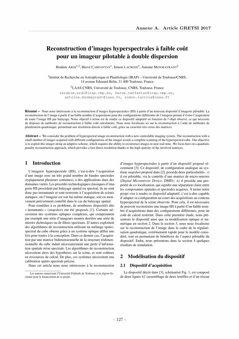
Annexe A. Article GRETSI 2017
Reconstruction d’images hyperspectrales à faible coûtpour un imageur pilotable à double dispersionIbrahim ARDI1,2, Hervé CARFANTAN1, Simon LACROIX2, Antoine MONMAYRANT2
1Institut de Recherche en Astrophysique et Planétologie (IRAP) – Université de Toulouse/CNRS,14 avenue Edouard Belin, 31 400 Toulouse, France
2LAAS-CNRS, Université de Toulouse, CNRS, Toulouse, [email protected], [email protected],
[email protected], [email protected]
Résumé – Nous nous intéressons à la reconstruction d’images hyperspectrales (HS) à partir d’un nouveau dispositif d’imagerie pilotable. Lareconstruction de l’image à partir d’un faible nombre d’acquisitions pour des configurations différentes de l’imageur permet d’éviter l’acquisitionde toute l’image HS par balayage. Notre objectif à terme est de rendre ce dispositif adaptatif en fonction de l’objet observé, ce qui nécessitede disposer de méthodes de reconstruction à faible coût calculatoire. Nous nous focalisons ici sur la reconstruction à l’aide de méthodes depénalisation quadratique, permettant une résolution directe à faible coût, grâce au caractère très creux des matrices.
Abstract – We consisder the problem of hyperspectral image reconstruction with a new controlable imaging system. The reconstruction with asmall number of images acquired with different configurations of the imager avoids a complete scanning of the hyperspectral cube. Our objectiveis to exploit this imager along an adaptive scheme, which requires the ability to reconstruct images in near real-time. We focus here on a quadraticpenalty reconstruction approach, which provides a fast direct resolution thanks to the high sparsity of the involved matrices.
1 IntroductionL’imagerie hyperspectrale (HS), c’est-à-dire l’acquisition
d’une image avec un très grand nombre de bandes spectrales(typiquement plusieurs centaines), a des applications dans desdomaines variés. Les procédés technologiques classiques d’ima-gerie HS procèdent par balayage spatial ou spectral, ils ne sontdonc pas instantanés et sont restreints à l’acquisition de scènesstatiques, où l’imageur est soit lui-même statique, soit en mou-vement précisément contrôlé dans le cas du balayage spatial.
Pour remédier à ce problème, de nombreux dispositifs dits« instantanés » (snapshot) ont été proposés [1]. Certains né-cessitent des systèmes optiques complexes, qui comprennentpar exemple une série d’imageurs montés derrière une série demiroirs dichroïques ou de filtres spectraux. D’autres exploitentdes algorithmes de reconstruction utilisant un mélange spatio-spectral du cube obtenu grâce à un système optique défini unefois pour toutes à la conception. Dans ce dernier cas, l’acquisi-tion par une matrice bidimensionnelle de la structure tridimen-sionnelle du cube induit nécessairement une perte d’informa-tion spatiale et/ou spectrale. Les algorithmes de reconstructionnécessitent alors des hypothèses sur la scène, et sont coûteuxen ressources de calcul. De plus, ces systèmes nécessitent unecalibration spatio-spectrale précise.
Dans cet article nous nous intéressons à la reconstruction
Les auteurs remercient l’Université Fédérale de Toulouse et la région Oc-citanie pour le financement de ce projet.
d’images hyperspectrales à partir d’un dispositif proposé ré-cemment [3]. Ce dispositif, de configuration analogue au sys-tème snapshot proposé dans [2], possède deux particularités : i)il est pilotable, via le contrôle d’une matrice de micro-miroirs(Digital Micromirror Device, DMD) ; ii) il possède une pro-priété de co-localisation, qui signifie une séparation claire entreles composantes spatiales et spectrales acquises. À terme notreprojet vise à rendre ce dispositif adaptatif, c’est-à-dire capabled’adapter sa configuration au cours des acquisitions au contenuhyperspectral de la scène observée. Pour cela, il est nécessairede pouvoir reconstruire une image HS à partir d’un faible nom-bre d’acquisitions dans des configurations différentes, pour uncoût de calcul restreint. Dans cette première étude, nous pré-sentons le dispositif ainsi que sa modélisation optique et nu-mérique en section 2. Dans la section 3, nous nous focalisonssur la reconstruction de l’image dans le cadre de la régulari-sation quadratique, extrêmement rapide pour le modèle consi-déré, tout en permettant de bénéficier de l’aspect pilotable dudispositif. Enfin, nous présentons dans la section 4 quelquesrésultats de simulation.
2 Modélisation du dispositif
2.1 Dispositif d’acquisitionLe dispositif décrit dans [3], schématisé Fig. 1, est composé
de deux lignes 4f (assemblage de deux lentilles et d’un réseau
- 127 -
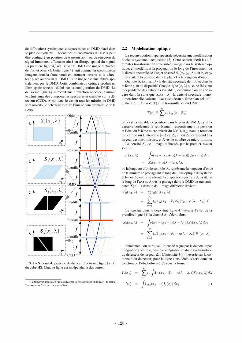
de diffraction) symétriques et séparées par un DMD placé dansle plan de symétrie. Chacun des micro-miroirs du DMD peutêtre configuré en position de transmission1 ou de réjection dusignal lumineux, effectuant ainsi un filtrage spatial du signal.La première ligne 4f réalise sur le DMD une image diffractéede l’objet observé. Cette ligne 4f agit comme un spectromètreimageur dont la fente serait entièrement ouverte et le détec-teur placé au niveau du DMD. Cette image est ainsi filtrée spa-tialement par le DMD. Cette combinaison optique produit unfiltre spatio-spectral défini par la configuration du DMD. Ladeuxième ligne 4f introduit une diffraction opposée, assurantle démélange des composantes spectrales et spatiales sur le dé-tecteur (CCD). Ainsi, dans le cas où tous les miroirs du DMDsont ouverts, le détecteur mesure l’image panchromatique de lascène.
Objet
Lentille
Réseau
Lentille
DMD
Lentille
Réseau
Lentille
CCD
FIG. 1 – Schéma de principe du dispositif pour une ligne (x,λ)du cube HS. Chaque ligne est indépendante des autres.
1La transmission est en fait assurée par la réflexion sur un miroir – le terme“transmission” est cependant préféré
2.2 Modélisation optiqueLa reconstruction hyperspectrale nécessite une modélisation
fidèle du système d’acquisition [3]. Cette section décrit les dif-férentes transformations que subit l’image dans le système op-tique, en modélisant la propagation le long de l’instrument dela densité spectrale de l’objet observé S0(x0, y0,λ), où x0 et y0
représentent la position dans le plan et λ la longueur d’onde.On note Sn(xn, yn,λ) la densité spectrale de l’objet dans le
n-ième plan du dispositif. Chaque ligne (x,λ) du cube HS étantindépendante des autres, la variable y est omise : on ne consi-dère dans la suite que Sn(xn,λ), la densité spectrale mono-dimensionnelle (suivant l’axe x) située au n-ième plan, tel qu’il-lustré Fig. 1. On note T (x) la transmittance du DMD :
T (x) K
k=1
tk11Δ(x − xk)
où x est la variable de position dans le plan du DMD, xk et lavariable booléenne tk représentant respectivement la positionet l’état du k-ième micro-miroir du DMD, 11Δ étant la fonctionindicatrice sur l’intervalle [−Δ/2,Δ/2], où Δ correspond à lalargeur des miro-miroirs, et K est le nombre de micro-miroirs.
La densité S1 de l’image diffractée par le premier réseaus’écrit :
S1(x1,λ) =
δ(x0 − [x1 + α(λ− λ0)])S0(x0,λ) dx0
= S0(x1 + α(λ− λ0),λ),
où la longueur d’onde centrale λ0 représente la longueur d’ondede la lumière se propageant le long de l’axe optique du systèmeet le coefficient α représente la dispersion spectrale du systèmele long de l’axe x. Après le passage dans le DMD de transmit-tance T (x), la densité de l’image diffractée devient :
S2(x2,λ) = T (x2)S1(x2,λ)
=K
k=1
tk11Δ(x2 − xk)S0(x2 + α(λ− λ0),λ).
Le passage dans la deuxième ligne 4f inverse l’effet de lapremière ligne 4f , la densité S3 s’écrit alors :
S3(x3,λ) =
δ(x2 − [x3 − α(λ− λ0)])S2(x2,λ) dx2
=K
k=1
tk11Δ(x3 − xk − α(λ− λ0))S0(x3,λ).
Finalement, on retrouve l’intensité reçue par le détecteur parintégration spectrale, puis par intégration spatiale sur la surfacedu détecteur de largeur Δd. L’intensité I(c) mesurée sur la co-lonne c du détecteur, pour la ligne considérée, s’écrit donc enfonction de l’objet observé S0 sous la forme :
I3(x3) =K
k=1
tk
11Δ(x3 − xk − α(λ− λc))S0(x3,λ) dλ
I(c) =
11Δd
(x3 − c)I3(x3) dx3 (1)
- 128 -
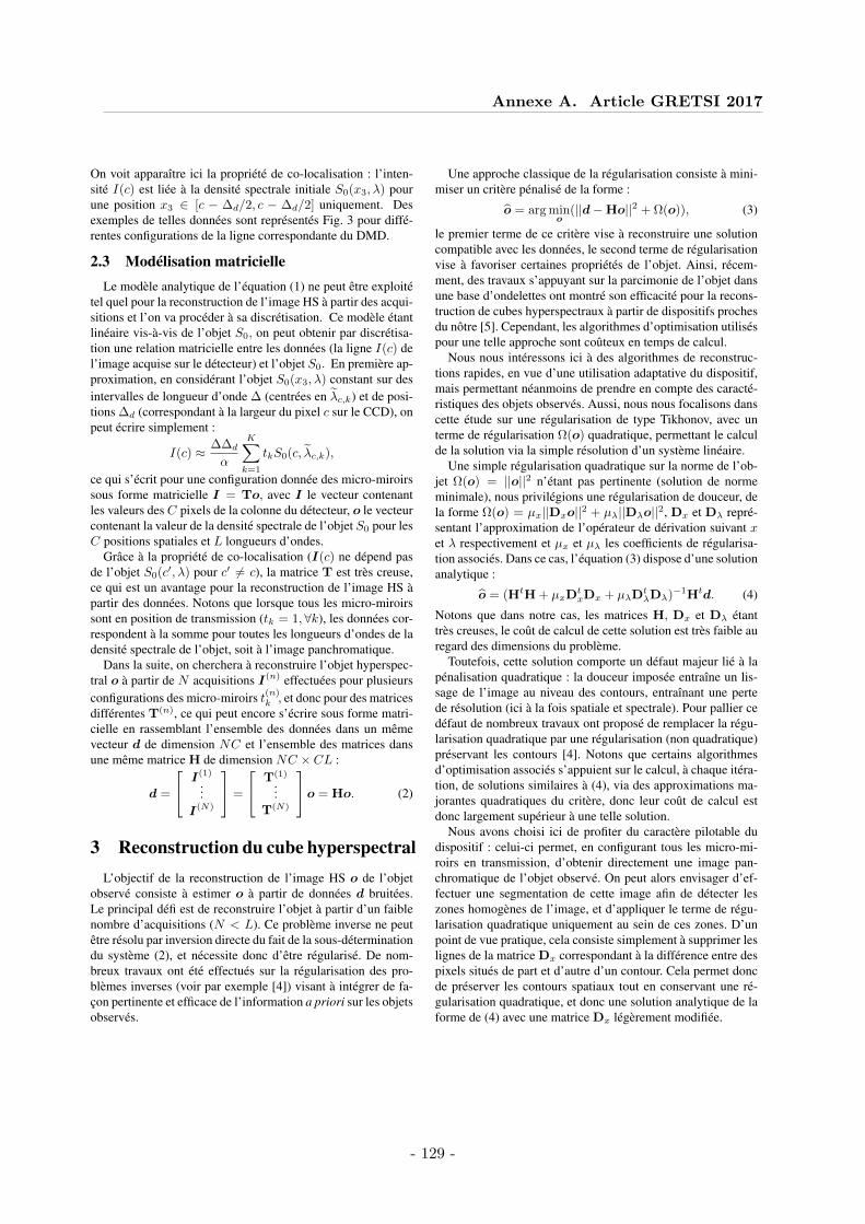
Annexe A. Article GRETSI 2017
On voit apparaître ici la propriété de co-localisation : l’inten-sité I(c) est liée à la densité spectrale initiale S0(x3,λ) pourune position x3 ∈ [c − Δd/2, c − Δd/2] uniquement. Desexemples de telles données sont représentés Fig. 3 pour diffé-rentes configurations de la ligne correspondante du DMD.
2.3 Modélisation matricielleLe modèle analytique de l’équation (1) ne peut être exploité
tel quel pour la reconstruction de l’image HS à partir des acqui-sitions et l’on va procéder à sa discrétisation. Ce modèle étantlinéaire vis-à-vis de l’objet S0, on peut obtenir par discrétisa-tion une relation matricielle entre les données (la ligne I(c) del’image acquise sur le détecteur) et l’objet S0. En première ap-proximation, en considérant l’objet S0(x3,λ) constant sur desintervalles de longueur d’onde Δ (centrées en λc,k) et de posi-tions Δd (correspondant à la largeur du pixel c sur le CCD), onpeut écrire simplement :
I(c) ≈ ΔΔd
α
K
k=1
tkS0(c, λc,k),
ce qui s’écrit pour une configuration donnée des micro-miroirssous forme matricielle I = To, avec I le vecteur contenantles valeurs des C pixels de la colonne du détecteur, o le vecteurcontenant la valeur de la densité spectrale de l’objet S0 pour lesC positions spatiales et L longueurs d’ondes.
Grâce à la propriété de co-localisation (I(c) ne dépend pasde l’objet S0(c
,λ) pour c = c), la matrice T est très creuse,ce qui est un avantage pour la reconstruction de l’image HS àpartir des données. Notons que lorsque tous les micro-miroirssont en position de transmission (tk = 1,∀k), les données cor-respondent à la somme pour toutes les longueurs d’ondes de ladensité spectrale de l’objet, soit à l’image panchromatique.
Dans la suite, on cherchera à reconstruire l’objet hyperspec-tral o à partir de N acquisitions I(n) effectuées pour plusieursconfigurations des micro-miroirs t
(n)k , et donc pour des matrices
différentes T(n), ce qui peut encore s’écrire sous forme matri-cielle en rassemblant l’ensemble des données dans un mêmevecteur d de dimension NC et l’ensemble des matrices dansune même matrice H de dimension NC × CL :
d =
I(1)
...I(N)
=
T(1)...
T(N)
o = Ho. (2)
3 Reconstruction du cube hyperspectralL’objectif de la reconstruction de l’image HS o de l’objet
observé consiste à estimer o à partir de données d bruitées.Le principal défi est de reconstruire l’objet à partir d’un faiblenombre d’acquisitions (N < L). Ce problème inverse ne peutêtre résolu par inversion directe du fait de la sous-déterminationdu système (2), et nécessite donc d’être régularisé. De nom-breux travaux ont été effectués sur la régularisation des pro-blèmes inverses (voir par exemple [4]) visant à intégrer de fa-çon pertinente et efficace de l’information a priori sur les objetsobservés.
Une approche classique de la régularisation consiste à mini-miser un critère pénalisé de la forme :
o = arg mino
(||d − Ho||2 + Ω(o)), (3)
le premier terme de ce critère vise à reconstruire une solutioncompatible avec les données, le second terme de régularisationvise à favoriser certaines propriétés de l’objet. Ainsi, récem-ment, des travaux s’appuyant sur la parcimonie de l’objet dansune base d’ondelettes ont montré son efficacité pour la recons-truction de cubes hyperspectraux à partir de dispositifs prochesdu nôtre [5]. Cependant, les algorithmes d’optimisation utiliséspour une telle approche sont coûteux en temps de calcul.
Nous nous intéressons ici à des algorithmes de reconstruc-tions rapides, en vue d’une utilisation adaptative du dispositif,mais permettant néanmoins de prendre en compte des caracté-ristiques des objets observés. Aussi, nous nous focalisons danscette étude sur une régularisation de type Tikhonov, avec unterme de régularisation Ω(o) quadratique, permettant le calculde la solution via la simple résolution d’un système linéaire.
Une simple régularisation quadratique sur la norme de l’ob-jet Ω(o) = ||o||2 n’étant pas pertinente (solution de normeminimale), nous privilégions une régularisation de douceur, dela forme Ω(o) = µx||Dxo||2 + µλ||Dλo||2, Dx et Dλ repré-sentant l’approximation de l’opérateur de dérivation suivant xet λ respectivement et µx et µλ les coefficients de régularisa-tion associés. Dans ce cas, l’équation (3) dispose d’une solutionanalytique :
o = (HtH + µxDtxDx + µλD
tλDλ)−1Htd. (4)
Notons que dans notre cas, les matrices H, Dx et Dλ étanttrès creuses, le coût de calcul de cette solution est très faible auregard des dimensions du problème.
Toutefois, cette solution comporte un défaut majeur lié à lapénalisation quadratique : la douceur imposée entraîne un lis-sage de l’image au niveau des contours, entraînant une pertede résolution (ici à la fois spatiale et spectrale). Pour pallier cedéfaut de nombreux travaux ont proposé de remplacer la régu-larisation quadratique par une régularisation (non quadratique)préservant les contours [4]. Notons que certains algorithmesd’optimisation associés s’appuient sur le calcul, à chaque itéra-tion, de solutions similaires à (4), via des approximations ma-jorantes quadratiques du critère, donc leur coût de calcul estdonc largement supérieur à une telle solution.
Nous avons choisi ici de profiter du caractère pilotable dudispositif : celui-ci permet, en configurant tous les micro-mi-roirs en transmission, d’obtenir directement une image pan-chromatique de l’objet observé. On peut alors envisager d’ef-fectuer une segmentation de cette image afin de détecter leszones homogènes de l’image, et d’appliquer le terme de régu-larisation quadratique uniquement au sein de ces zones. D’unpoint de vue pratique, cela consiste simplement à supprimer leslignes de la matrice Dx correspondant à la différence entre despixels situés de part et d’autre d’un contour. Cela permet doncde préserver les contours spatiaux tout en conservant une ré-gularisation quadratique, et donc une solution analytique de laforme de (4) avec une matrice Dx légèrement modifiée.
- 129 -
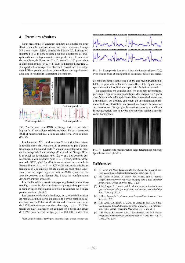
4 Premiers résultats
Nous présentons ici quelques résultats de simulations pourillustrer la méthode de reconstruction. Nous exploitons l’imageHS d’une scène réelle2, extraite de l’étude [6]. L’image estillustrée Fig. 2, la ligne utilisée pour nos simulations est indi-quée en blanc. La figure montre la coupe du cube HS au niveaude cette ligne, de dimension C × L, avec C = 200 pixels dansla dimension spatiale et L = 49 dans la dimension spectrale λ.Il s’agit des données que l’on cherche à reconstruire. Les inten-sités RGB et panchromatique de cette ligne sont représentées,ainsi que le résultat de la détection de contours.
Lon
gueu
rd’o
ndeλ
Position spatiale x
Position spatiale x Position spatiale x
FIG. 2 – En haut : vue RGB de l’image test, et coupe dansle plan (x,λ) de la ligne exhibée en blanc. En bas : intensitésRGB et panchromatique le long de cette ligne, avec contoursdétectés.
Les Intensités I(n), de dimension C, sont simulées suivantle modèle direct de l’équation (1) en prenant un pas d’échan-tillonnage en longueur d’onde Δ
α afin qu’un décalage d’un pixelen λ corresponde à un décalage d’un pixel de l’image HS età un pixel sur le détecteur (soit Δd = Δ). Les données cor-respondent à ces intensités pour N = 10 configurations diffé-rentes du DMD, générées aléatoirement suivant une variable deBernoulli avec P (tk = 1) = 40% (40% des micro-miroirs entransmission), auxquelles ont été ajouté un bruit blanc Gaus-sien, pour un rapport signal à bruit de 20dB. Quatre de cesjeux de données sont illustrés Fig. 3 avec les configurationsdes micro-miroirs associées.
Les résultats de la reconstruction par régularisation sont illus-trés Fig. 4 : avec la régularisation classique (gauche), puis avecla régularisation exploitant la détection de contours sur l’imagepanchromatique (droite).
Les paramètres de régularisation µx et µλ ont été déterminésde manière à minimiser la puissance de l’erreur relative de re-construction. En l’absence d’extraction de contours une erreurde 6.45% a été obtenue pour des valeurs (µx, µλ) = (50, 200),tandis qu’avec l’extraction de contours on obtient une erreurde 4.02% pour des valeurs (µx, µλ) = (50, 70). La détection
2L’image est ré-orientée de 90 pour obtenir une ligne avec un spectre varié.
FIG. 3 – Exemple de données : 4 jeux de données (lignes I(c))avec et sans bruit, et configuration des micro-miroirs associées.
de contours permet donc tout d’abord une reconstruction plusfidèle. De plus, elle se fait avec un coefficient de régularisationspectrale moins fort, limitant la perte de résolution spectrale.
En conclusion, on constate que l’on peut bien reconstruire,par simple régularisation quadratique, des images HS à partird’un faible nombre d’acquisitions (5 fois moins de données qued’inconnues). On constate également qu’une modification mi-nime de la régularisation, en prenant en compte la détectionde contours sur l’image panchromatique, permet d’améliorerla reconstruction, tant au niveau des contours spatiaux que deszones homogènes.
FIG. 4 – Exemple de reconstruction sans détection de contours(gauche) et avec (droite.)
Références[1] N. Hagen and M.W. Kudenov, Review of snapshot spectral ima-
ging technologies, Optical Engineering, 52(9), sep. 2013.[2] ME Gehm, R John, DJ Brady, RM Willett, and TJ Schulz,
Single-shot compressive spectral imaging with a dual-disperserarchitecture. Optics Express, 15(21), 2007.
[3] S. McGregor, S. Lacroix and A. Monmayrant, Adaptive hyper-spectral imager : design, modeling, and control. Journal of Op-tics, 17(8), aug. 2015.
[4] J. Idier, Approche bayésienne pour les problèmes inverses. Her-mès, nov. 2001.
[5] G.R. Arce, D.J. Brady, L. Carin, H. Arguello and D.S. Kittle,Compressive Coded Aperture Spectral Imaging : An Introduc-tion, IEEE Signal Processing Magazine, 31(1), jan. 2015.
[6] D.H. Foster, K. Amano, S.M.C. Nascimento, and M.J. Foster,Frequency of metamerism in natural scenes, J. Opt. Soc. Am. A,(23)10, oct. 2006.
- 130 -

Annexe A. Article GRETSI 2017
- 131 -

Bibliographie
[ABS07] B. Aiazzi, S. Baronti, and M. Selva. Improving component substitution panshar-pening through multivariate regression of MS +Pan data. IEEE Transactions onGeoscience and Remote Sensing, 45(10) :3230–3239, October 2007.
[ACLM17] I. Ardi, H. Carfantan, S. Lacroix, and A. Monmayrant. Reconstruction d’imageshyperspectrales à faible coût pour un imageur pilotable à double dispersion. InColloque GRETSI sur le traitement du signal et des images (GRETSI 2017), Juanles Pins, France, September 2017.
[ACLM18] I. Ardi, H. Carfantan, S. Lacroix, and A. Monmayrant. Fast hyperspectral cubereconstruction for a double disperser imager. In 26th European Signal ProcessingConference (EUSIPCO 2018), Roma, Italy, September 2018.
[AdH16] R. Arablouei and F. de Hoog. Hyperspectral image recovery via hybrid regula-rization. IEEE Transactions on Image Processing, 25(12) :5649–5663, December2016.
[AMH95] G. P. Abousleman, M. W. Marcellin, and B. R. Hunt. Compression of hyperspectralimagery using the 3-D DCT and hybrid DPCM/DCT. IEEE Transactions onGeoscience and Remote Sensing, 33(1) :26–34, January 1995.
[ARC+20] I. Ardi, T. Rouvier, H. Carfantan, S. Lacroix, and A. Monmayrant. Two fast re-construction approaches leveraging the panchromatic image for a configurable dual-disperser imager. Technical report, IRAP–UPS/CNRS/CNES et LAAS–CNRS,France, July 2020.
[Bad97] R. Baddeley. The correlational structure of natural images and the calibration ofspatial representations. Cognitive Science, 21(3) :351 – 371, July 1997.
[BKGK17] S.-H. Baek, I. Kim, D. Gutierrez, and M. H. Kim. Compact single-shot hyperspectralimaging using a prism. ACM Transactions on Graphics, 36(6), November 2017.
[BSFG09] C. Barnes, E. Shechtman, A. Finkelstein, and D. B Goldman. Patchmatch : A ran-domized correspondence algorithm for structural image editing. ACM Transactionson Graphics, 28(3), July 2009.
[BSvD99] M. Benzi, D. B. Szyld, and A. van Duin. Orderings for incomplete factorizationpreconditioning of nonsymmetric problems. SIAM Journal on Scientific Computing,20(5) :1652–1670, July 1999.
[CBFAB97] P. Charbonnier, L. Blanc-Féraud, G. Aubert, and M. Barlaud. Deterministic edge-preserving regularization in computed imaging. IEEE Transactions on Image Pro-cessing, IP-6(2) :298–311, February 1997.
[CCTH11] L. Chang, Y. Chang, Z. S. Tang, and B. Huang. Group and region based parallelcompression method using signal subspace projection and band clustering for hyper-spectral imagery. IEEE Journal of Selected Topics in Applied Earth Observationsand Remote Sensing, 4(3) :565–578, September 2011.
133
Bibliographie
[CJN+17] I. Choi, D. S. Jeon, G. Nam, D. Gutiérrez, and M. H. Kim. High-quality hyper-spectral reconstruction using a spectral prior. ACM Transactions on Graphics,36(6) :1–13, November 2017.
[CRT06] E. J. Candes, J. Romberg, and T. Tao. Robust uncertainty principles : exact signalreconstruction from highly incomplete frequency information. IEEE Transactionson Information Theory, 52(2) :489–509, February 2006.
[CT04] L. Chang and Y. P. Tan. Effective use of spatial and spectral correlations for colorfilter array demosaicking. IEEE Transactions on Consumer Electronics, 50(1) :355–365, February 2004.
[CZ11] A. Chakrabarti and T. Zickler. Statistics of real-world hyperspectral images. InIEEE Conference on Computer Vision and Pattern Recognition (CVPR 2011),pages 193–200, June 2011.
[Dau88] Ingrid Daubechies. Orthonormal bases of compactly supported wavelets. Commu-nications on Pure and Applied Mathematics, 41(7) :909–996, 1988.
[Dau92] Ingrid Daubechies. Ten Lectures on Wavelets. SIAM, USA, 1992.[DCMR95] G. M. Del Corso, O. Menchi, and F. Romani. Krylov subspace methods for solving
linear systems. Technical report, Università di Pisa, Dipartimento di Informatica,1995.
[Dem89] G. Demoment. Image reconstruction and restoration : Overview of common estima-tion structure and problems. IEEE Transactions on Acoustics, Speech and SignalProcessing, ASSP-37(12) :2024–2036, December 1989.
[DET06] D. L. Donoho, M. Elad, and V. N. Temlyakov. Stable recovery of sparse overcom-plete representations in the presence of noise. IEEE Transactions on InformationTheory, 52(1) :6–18, January 2006.
[DF07] Q. Du and J. E. Fowler. Hyperspectral image compression using JPEG2000 andprincipal component analysis. IEEE Geoscience and Remote Sensing Letters,4(2) :201–205, October 2007.
[DHS+18] C. Deng, X. Hu, J. Suo, Y. Zhang, Z. Zhang, and Q. Dai. Snapshot hyperspec-tral imaging via spectral basis multiplexing in Fourier domain. Optic Express,26(25) :32509–32521, December 2018.
[DJL92] R. A. DeVore, B. Jawerth, and B. J. Lucier. Image compression through wave-let transform coding. IEEE Transactions on Information Theory, 38(2) :719–746,March 1992.
[Don06] D. L. Donoho. Compressed sensing. IEEE Transactions on Information Theory,52(4) :1289–1306, April 2006.
[DRA15] N. Diaz, H. Rueda, and H. Arguello. High-dynamic range compressive spectralimaging by adaptive filtering. In International Workshop on Compressed SensingTheory and its Applications to Radar, Sonar and Remote Sensing (CoSeRa 2015),pages 89–93, 2015.
[DZYF09] Q. Du, W. Zhu, H. Yang, and J. E. Fowler. Segmented principal component analysisfor parallel compression of hyperspectral imagery. IEEE Geoscience and RemoteSensing Letters, 6(4) :713–717, October 2009.
[EBF10] J. M. Eichenholz, N. Barnett, and D. Fish. Sequential filter wheel multispectral ima-ging systems. In Imaging and Applied Optics Congress. Optical Society of America,June 2010.
- 134 -
Bibliographie
[FHC+20] X. Feng, L. He, Q. Cheng, X. Long, and Y. Yuan. Hyperspectral and multispectralremote sensing image fusion based on endmember spatial information. RemoteSensing, 12 :1009, March 2020.
[FR06] J.E. Fowler and J. T. Rucker. Three-Dimensional Wavelet-Based Compression ofHyperspectral Imagery, chapter 14, pages 379–407. John Wiley & Sons, Ltd, Sep-tember 2006.
[FZSS16] Y. Fu, Y. Zheng, I. Sato, and Y. Sato. Exploiting spectral-spatial correlation forcoded hyperspectral image restoration. In IEEE Conference on Computer Visionand Pattern Recognition (CVPR 2016), pages 3727–3736, 2016.
[GJB+07] M. E. Gehm, R John, D. J. Brady, R. M. Willett, and T. J. Schulz. Single-shotcompressive spectral imaging with a dual-disperser architecture. Optic Express,15(21), October 2007.
[GKG99] S. Grgic, K. Kers, and M. Grgic. Image compression using wavelets. In IEEEInternational Symposium on Industrial Electronics (ISIE 1999), volume 1, pages99–104 vol.1, 1999.
[GLM+17] L. Galvis, D. Lau, X. Ma, H. Arguello, and G. R. Arce. Coded aperture de-sign in compressive spectral imaging based on side information. Aplied Optics,56(22) :6332–6340, August 2017.
[GR92] D. Geman and G. Reynolds. Constrained restoration and recovery of discontinui-ties. IEEE Transactions on Pattern Analysis and Machine Intelligence, PAMI-14(3) :367–383, March 1992.
[GY95] D. Geman and C. Yang. Nonlinear image recovery with half-quadratic regulariza-tion. IEEE Transactions on Image Processing, IP-4(7) :932–946, July 1995.
[GZZF14] S. Gu, L. Zhang, W. Zuo, and X. Feng. Weighted nuclear norm minimizationwith application to image denoising. In IEEE Conference on Computer Vision andPattern Recognition (CVPR 2014), pages 2862–2869, 2014.
[HAL+20] E. Hemsley, I. Ardi, S. Lacroix, H. Carfantan, and A. Monmayrant. Optimized co-ded aperture for frugal hyperspectral image recovery using a dual-disperser system.submitted to the Journal of the Optical Society of America A, July 2020.
[HBS92] P. J. B. Hancock, R. J. Baddeley, and L. S. Smith. The principal components ofnatural images. Network : Computation in Neural Systems, 3(1) :61–70, July 1992.
[HLCM20] E. Hemsley, S. Lacroix, H. Carfantan, and A. Monmayrant. Calibration of program-mable spectral imager with dual disperser architecture. Optics Communications,468 :125767, August 2020.
[HZCF19] L. He, Y. Zhu, X. Chang, and X. Feng. Image fusion for high-resolution opticalsatellites based on panchromatic spectral decomposition. Sensors, 19 :2619, June2019.
[I+01] J. Idier et al. Approche bayésienne pour les problèmes inverses. Hermès, Paris,2001.
[Idi01] J. Idier. Convex half-quadratic criteria and interacting auxiliary variables for imagerestoration. IEEE Transactions on Image Processing, 10(7) :1001–1009, July 2001.
[Int94] International Organization for Standardization. ISO/IEC 10918-1 :1994 : Informa-tion technology — Digital compression and coding of continuous-tone still images :Requirements and guidelines. International Organization for Standardization, Ge-neva, Switzerland, 1994.
- 135 -
Bibliographie
[Int00] International Organization for Standardization. ISO/IEC 15444-1 :2000 : Informa-tion technology — JPEG 2000 image coding system — Part 1 : Core coding system,volume 226. International Organization for Standardization, Geneva, Switzerland,2000.
[JWF+07] W. R. Johnson, D. W. Wilson, W. Fink, M. S. Humayun, and G. H. Bearman.Snapshot hyperspectral imaging in ophthalmology. Journal of Biomedical Optics,12(1) :1 – 7, January 2007.
[KB09] T. G. Kolda and B. W. Bader. Tensor decompositions and applications. SIAMReview, 51(3) :455–500, August 2009.
[KBM+06] P. Kulkarni, A. Bilgin, M. W. Marcellin, J. Dagher, J. H. Kasner, T. J. Flohr,and J. C. Rountree. Compression of Earth Science Data with JPEG2000, pages347–378. Springer US, Boston, MA, June 2006.
[KCWB10] D. Kittle, K. Choi, A. Wagadarikar, and D. J. Brady. Multiframe image estimationfor coded aperture snapshot spectral imagers. Aplied Optics, 49(36) :6824–6833,December 2010.
[KMW+11] R. Kawakami, Y. Matsushita, J. Wright, M. Ben-Ezra, Y. Tai, and K. Ikeuchi. High-resolution hyperspectral imaging via matrix factorization. In IEEE Conference onComputer Vision and Pattern Recognition (CVPR 2011), pages 2329–2336, 2011.
[KYM12] A. Karami, M. Yazdi, and G. Mercier. Compression of hyperspectral images usingdiscrete wavelet transform and Tucker decomposition. IEEE Journal of SelectedTopics in Applied Earth Observations and Remote Sensing, 5(2) :444–450, April2012.
[LGG+14] A. Lambrechts, P. Gonzalez, B. Geelen, P. Soussan, K. Tack, and M. Jayapala. ACMOS-compatible, integrated approach to hyper- and multispectral imaging. InIEEE International Electron Devices Meeting, pages 10.5.1–10.5.4, 2014.
[LLF+16] T. Lu, S. Li, L. Fang, Y. Ma, and J. A. Benediktsson. Spectral–spatial adaptivesparse representation for hyperspectral image denoising. IEEE Transactions onGeoscience and Remote Sensing, 54(1) :373–385, January 2016.
[LLWD14] X. Lin, Y. Liu, J. Wu, and Q. Dai. Spatial-spectral encoded compressive hyper-spectral imaging. ACM Transactions on Graphics, 33(6), November 2014.
[LM86] P. G. Lemarié and Yves Meyer. Ondelettes et bases hilbertiennes. Revista Matemá-tica Iberoamericana, 2(1-2) :1–18, 1986.
[LMM+16] C. Li, Y. Ma, X. Mei, C. Liu, and J. Ma. Hyperspectral image classificationwith robust sparse representation. IEEE Geoscience and Remote Sensing Letters,13(5) :641–645, May 2016.
[LRS+18] G. Liu, F. A. Reda, K. J. Shih, T.-C. Wang, A. Tao, and B. Catanzaro. Imageinpainting for irregular holes using partial convolutions. In European Conferenceon Computer Vision (ECCV 2018), pages 85–100, September 2018.
[LWLD14] X. Lin, G. Wetzstein, Y. Liu, and Q. Dai. Dual-coded compressive hyperspectralimaging. Optics Letters, 39(7) :2044–2047, April 2014.
[LWS00] T-W. Lee, T. Wachtler, and T. J. Sejnowski. The spectral independent componentsof natural scenes. In S.-W. Lee, H. H. Bülthoff, and T. Poggio, editors, BiologicallyMotivated Computer Vision, pages 527–534. Springer Berlin Heidelberg, 2000.
[LZGY16] X. Li, Y. Zhang, Y. Gao, and S. Yue. Using guided filtering to improve Gram-Schmidt based pansharpening method for GeoEye-1 satellite images. In Procee-dings of the 4th International Conference on Information Systems and ComputingTechnology, December 2016.
- 136 -
Bibliographie
[MB04] F. Melgani and L. Bruzzone. Classification of hyperspectral remote sensing imageswith support vector machines. IEEE Transactions on Geoscience and Remote Sen-sing, 42(8) :1778–1790, August 2004.
[MLM15] S. McGregor, S. Lacroix, and A. Monmayrant. Adaptive hyperspectral imager :design, modeling, and control. Journal of Optics, 17(8) :085607, August 2015.
[Pet05] G. Petrie. Airborne pushbroom line scanners : An alternative to digital framecameras. GeoInformatics, 8 :50–57, January 2005.
[PL03] B. Potetz and T. S. Lee. Statistical correlations between two-dimensional imagesand three-dimensional structures in natural scenes. Journal of the Optical Societyof America A, 20(7) :1292–1303, July 2003.
[PR06] M. R. Pickering and M. J. Ryan. An Architecture for the Compression of Hyper-spectral Imagery, pages 1–34. Springer US, Boston, MA, 2006.
[PTMO06] B. Penna, T. Tillo, E. Magli, and G. Olmo. Progressive 3-D coding of hyperspec-tral images based on JPEG 2000. IEEE Geoscience and Remote Sensing Letters,3(1) :125–129, January 2006.
[RAA14] H. Rueda, H. Arguello, and G. R. Arce. Compressive spectral imaging based oncolored coded apertures. In IEEE International Conference on Acoustics, Speechand Signal Processing (ICASSP 2014), pages 7799–7803, 2014.
[RB05] S. Roth and M. J. Black. Fields of experts : a framework for learning image priors.In IEEE Conference on Computer Vision and Pattern Recognition (CVPR 2005),volume 2, pages 860–867 vol. 2, 2005.
[RB09] N. Renard and S. Bourennane. Dimensionality reduction based on tensor modelingfor classification methods. IEEE Transactions on Geoscience and Remote Sensing,47(4) :1123–1131, April 2009.
[RBB08] N. Renard, S. Bourennane, and J. Blanc-Talon. Denoising and dimensionality re-duction using multilinear tools for hyperspectral images. IEEE Geoscience andRemote Sensing Letters, 5(2) :138–142, April 2008.
[RFY05] J.T. Rucker, J. Fowler, and N.H. Younan. JPEG2000 coding strategies for hyper-spectral data. In IEEE International Geoscience and Remote Sensing Symposium(IGARSS 2005), volume 1, August 2005.
[RKT+13] A. Rajwade, D. Kittle, T.-H. Tsai, D. Brady, and L. Carin. Coded hyperspec-tral imaging and blind compressive sensing. SIAM Journal on Imaging Sciences,6(2) :782–812, April 2013.
[ROF92] L. Rudin, S. Osher, and C. Fatemi. Nonlinear total variation based noise removalalgorithm. Physica D, 60 :259–268, November 1992.
[ROM15] N. R. Rema, B. A. Oommen, and P. Mythili. Image compression using SPIHTwith modified spatial orientation trees. Procedia Computer Science, 46 :1732–1738,December 2015. Proceedings of the International Conference on Information andCommunication Technologies (ICICT 2014).
[Saa03] Y. Saad. Iterative Methods for Sparse Linear Systems. SIAM, January 2003.[SLD82] M. V. Srinivasan, S. B. Laughlin, and A. Dubs. Predictive coding : a fresh view of
inhibition in the retina. Cognitive Science, 21(3) :351–371, November 1982.[TA77] A.N. Tikhonov and V.A.J. Arsenin, editors. Solution of Ill-posed Problems. Winston
and Sons, Washington, 1977.[TP06] X. Tang and W. A. Pearlman. Three-Dimensional Wavelet-Based Compression of
Hyperspectral Images, pages 273–308. Springer US, Boston, MA, 2006.
- 137 -
Bibliographie
[TZS+20] C. Tao, H. Zhu, P. Sun, R. Wu, and Z. Zheng. Hyperspectral image recovery basedon fusion of coded aperture snapshot spectral imaging and RGB images by guidedfiltering. Optics Communications, 458, October 2020.
[WF07] Y. Weiss and W. T. Freeman. What makes a good model of natural images ?In IEEE Conference on Computer Vision and Pattern Recognition (CVPR 2007),pages 1–8, 2007.
[WJWB08] A. Wagadarikar, R. John, R. Willett, and D. Brady. Single disperser design forcoded aperture snapshot spectral imaging. Applied Optics, 47(10) :B44–B51, April2008.
[WMAP11] Y. Wu, I. O. Mirza, G. R. Arce, and D. W. Prather. Development of a digital-micromirror-device-based multishot snapshot spectral imaging system. Optics Let-ters, 36(14) :2692–2694, July 2011.
[WXG+15] L. Wang, Z. Xiong, D. Gao, G. Shi, W Zeng, and F. Wu. High-speed hyperspec-tral video acquisition with a dual-camera architecture. In IEEE Conference onComputer Vision and Pattern Recognition (CVPR 2015), pages 4942–4950, 2015.
[WXS+16] L. Wang, Z. Xiong, G. Shi, W. Zeng, and F. Wu. Compressive hyperspectral imagingwith complementary RGB measurements. In 2016 Visual Communications andImage Processing (VCIP), pages 1–4, 2016.
[WZM+18] X. Wang, Y. Zhang, X. Ma, T. Xu, and G. R. Arce. Compressive spectral imagingsystem based on liquid crystal tunable filter. Optic Express, 26(19) :25226–25243,September 2018.
[XWL+17] Z. Xiong, L. Wang, H. Li, D. Liu, and F. Wu. Snapshot hyperspectral light fieldimaging. In IEEE Conference on Computer Vision and Pattern Recognition (CVPR2017), pages 6873–6881, 2017.
[YTZ+15] X. Yuan, T. Tsai, R. Zhu, P. Llull, D. Brady, and L. Carin. Compressive hyper-spectral imaging with side information. IEEE Journal of Selected Topics in SignalProcessing, 9(6) :964–976, September 2015.
[YWL+15] S. Yang, M. Wang, P. Li, L. Jin, v Wu, and L. Jiao. Compressive hyperspectralimaging via sparse tensor and nonlinear compressed sensing. IEEE Transactionson Geoscience and Remote Sensing, 53(11) :5943–5957, November 2015.
[ZFL08] J. Zhang, J. E. Fowler, and G. Liu. Lossy-to-lossless compression of hyperspectralimagery using three-dimensional TCE and an integer KLT. IEEE Geoscience andRemote Sensing Letters, 5(4) :814–818, October 2008.
- 138 -