JOURNAL OF GEOPHYSICAL RESEARCH, VOL. 102, NO. C6, PAGES 12,575-12,586, JUNE 15, 1997

Reconstructing the origin and trajectory of drifting Arctic sea ice

S.L. Pfirman, • R. Colony, 2'3 D. Niirnberg, 4 H. Eicken, 5 and I. Rigor 6

Abstract. Recent studies have indicated that drifting Arctic sea ice plays an important role in the redistribution of sediments and contaminants. Here we present a method to reconstruct the back- ward trajectory of sea ice from its sampling location in the Eurasian Arctic to its possible site of ori- gin on the shelf, based on historical drift data from the International Arctic Buoy Program. This method is verified by showing that origins derived from the backward trajectories are generally con- sistent with other indicators, such as comparison of the predicted backward trajectories with known buoy drifts and matching the clay mineralogy of sediments sampled from the sea ice with that of the seafloor in the predicted shelf source regions. The trajectories are then used to identify regions where sediment-laden ice is exported to the Transpolar Drift Stream: from the New Siberian Islands and the Central Kara Plateau. Calculation of forward trajectories shows that the Kara Sea is a major contributor of ice to the Barents Sea and the southern limb of the Transpolar Drift Stream.

Introduction

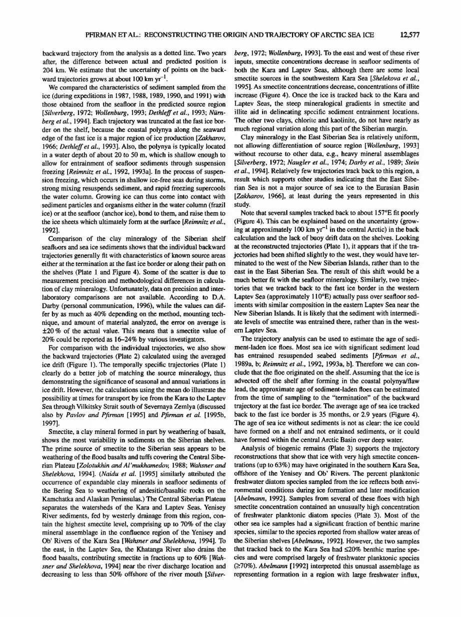
Although studies show that central Arctic sea ice originates in a number of different source areas [Colony and Thomdike, 1985], sea ice in the Arctic has typically been considered as an undistin- guished aggregation of floes. Knowing the source of individual ice floes only became important when expeditions to the central Arctic rediscovered the large quantities of sediment and other material incorporated in the sea ice originally noted by Nansen [ 1897] and attempted to derive their origin [e.g., Pfirman et al., 1989a; Abel- mann, 1992; Niimberg et al., 1994]. Using the mean ice drift pat- tern [Colony and Thomdike, 1985], clay mineralogy, and biological assemblages, the wide, shallow, Siberian shelves, and particularly the Laptev Sea [Zakharov, 1966], were identified as the probable source region of much of the sediment-laden ice observed in the Eurasian Arctic [Pfirman et al., 1989a; Wollen- burg, 1993; Niimberg et al., 1994; Eicken et al., 1997]. Once advected off the shelf, the ice is transported in the Transpolar Drift Stream, mostly exiting the central Arctic Basin several years later through Fram Strait (Figure 1). Because of the generally minor contribution from wind-blown lithogenic sediment [Pfirman et al., 1989b], ice floes containing a large sediment load can be assumed to have formed originally on a shallow shelf, probably in water depths less than 50 m where suspension freezing, including frazil and anchor ice formation, can most efficiently entrain seafloor sed- iments [Reimnitz et al., 1992, 1993a,b]. However, aside from these general conclusions, until now there was no way to determine the actual trajectory of an individual ice floe from the time that it left the shelf to the time that it was sampled. And, for ice that does not

1Barnard College, Columbia University, New York 2International Arctic Climate System Study Office, Oslo, Norway 3Also at Polar Science Center, University of Washington, Seattle 4GEOMAR Research Center for Marine Geosciences, Christian

Albrechts University, Kiel, Germany 5Alfred-Wegener Institute for Polar and Marine Research, Bremer-

haven, Germany 6polar Science Center, University of Washington, Seattle

Copyright 1997 by the American Geophysical Union

Paper number 96JC03980. 0148-0227/97/96J C-03980509.00

contain sediment, you can only surmise its history from the gen- eral ice drift pattern and laborious analysis of physical, chemical, and biological characteristics [•rnason, 1985; Abelmann, 1992]. Because of seasonal, interannual, and decadal variability in ice drift patterns [McLaren et al., 1987; Mysak and Manak, 1989; Ser- reze et al., 1989; Kotchetov et al., 1994; Zakharov, 1994], general- ized information on ice drift is not reliable in deriving source regions for individual ice floes.

In addition, there is a growing awareness that ice may play a role in the redistribution of contaminants in the Arctic [Weeks, 1994; Pfirman et al., 1995a; Chemyak et al., 1996]. Widespread distribution of polluted Arctic haze, dumping of radioactive waste on the Siberian shelf, contamination of thYArctic watershed, and observations of high levels of heavy metals and organochlorines in some Arctic people, polar bears, whales, and seabirds have led to concern about transport of contaminants across the Arctic Basin [Raatz, 1991; Muir et al., 1992; Dewailly et al., 1993; Yablokov et al., 1993], by atmospheric, oceanic, and sea ice conduits. Sea ice may be contaminated by atmospheric deposition and/or by entrainment from the marine environment. Deposition of atmo- spheric pollutants [Melnikov, 1991] transported in Arctic haze is likely to increase the contaminant load of the snow and ice [Pfir- man et al., 1995a]. Drifting ice may entrain organochlorines from the surface microlayer [Gaul, 1989]. In addition, ice formed in the shallow shelf seas often incorporates fine-grained sediment and organic material [Pfirman et al., 1989a]. Because contaminants, such as organochlorines and metals, including radionuclides, are known to sorb preferentially on fine-grained material [Stumm and Morgan, 1981], if the ice forms in regions polluted by rivers or dumping, the entrained sediment is likely to be contaminated. The few data available do indeed indicate that particle-laden sea ice contains elevated levels of some contaminants relative to the

underlying ocean water [Campbell and Yeats, 1982; Gaul, 1989; Meese et al., 1997]. However, unless there is a way to determine the trajectory and origin of the ice, it is difficult to ascertain the source of any contamination found.

Here we show that backward trajectories calculated from archives of ice motion and observed pressure fields can be used to reconstruct the drift path of individual ice floes with some confi- dence over a period of several years. If mineralogical or other information is also available, the origin and trajectory are con- strained with greater certainty.

12,575

12,576 PFIRMAN ET AL.: RECONSTRUCTING THE ORIGIN AND TRAJECTORY OF ARCTIC SEA ICE

Finally, we also take advantage of the relationship between the geostrophic winds and the ice motion and use this information in the analysis. The surface geostrophic wind is defined as

G = (Gx, Gy) = 1/(pf) (dp/dy, dp/dx)

where (dp/dy, dp/dx) is the horizontal gradient of the sea level pressure field, p is the density of the air, and f is the Coriolis parameter. As a first approximation, the surface geostrophic wind is determined by the horizontal gradient of the sea level pressure. In the mean, a strong high persists over the Arctic Basin, creating what is commonly known as the Beaufort Gyre of sea ice motion. In contrast, however, periods of cyclonic ice motion have been noted during late summer and early autumn [McLaren et al., 1987; Serreze et al., 1989].

Using the same data from the Arctic Buoy Program from 1979 to 1994, Walsh et al. [1995] found oktadal changes in the mean fields of pressure. Since 1988, the Beaufort High has decreased and shifted. As seen from the ice motion equation given below, interannual changes in the pressure field imply corresponding changes in the wind forcing of sea ice.

While the supplement of the sea level pressure data makes little difference in areas of dense buoy coverage, it does improve the analysis during times when the buoy array has waned to fewer than 10 buoys and in areas of the basin which have been poorly popu- lated by buoys.

The International Arctic Buoy Program has deployed buoys on ice for tracking by satellite since 1979. Because observed drift tra- jectories are available only for the central Arctic, the backward calculation of trajectories is most certain in the central basin. As the trajectories approach the shelf break and continue on the shelves, they are often not constrained by buoy data. However, we chose to continue the trajectories to the fast ice border which is located on the shelves, because this is where much of the ice

forms. It is clear that the final part of the backward trajectory between the shelf break and the fast ice border is subject to greater error than in the central basin.

Ice motion is calculated for the entire Arctic for each month

using techniques of optimal interpolation [Thomdike and Colony, 1982; Gandin, 1963] as follows:

Uint(X,t) = Uguess(X,t ) + AT[ Uobs(X,t ) _ Uguess(X,t )] where Uint(X,t) is the optimal estimate of ice velocity at the location x, for the month, t; A are the weights chosen to minimize the vari- ance of the interpolation error; Uobs(X,t ) is the observed monthly velocity; and Uguess(X,t) is the first-guess estimate of ice motion.

The weights, A, are chosen to minimize the variance of the inter- polation error by solving the linear equation:

A=M.S

where M is the covariance matrix between observed monthly pairs of ice velocity and S are the covariance vectors between the observed monthly ice velocities and the interpolation grid point.

The covariance matrix, M, and the covariance vectors, S, are

filled using perpendicular and parallel correlations functions [Thomdike, 1986] for monthly observations of ice velocity shown in Figure 2. As previously stated, the correlation length scale for monthly observations of ice motion is 1400 km.

The first-guess estimate, Ugues s, is defined as

Uguess(X,t) = Am(x)G(x,t) + C(x) + U*(x,t)

whereAm(x) is the climatic monthly mean spatial pattern of

the wind drift factor, G'(x,t) = G(x,t) - Gm(x) is the departure of the monthly wind field from the climatic monthly mean, C(x) is the climatic monthly mean field of ocean currents, and U*(x,t) is the monthly field of ice motion departure from the sum of simple wind-driven response and ocean current advection.

The optimal estimate of ice motion is thus defined as the devia- tion from the guess field of the monthly observations of ice veloc- ity. In data sparse areas and months, the optimal estimate at a grid point reduces to the first-guess estimate of ice motion. Since the long-term mean ice motion reflects roughly equal contributions from the mean ocean currents and geostrophic winds, and in the short term, the geostrophic winds explain more than 70% of the variance of ice motion [Thorndike and Colony, 1982], in the absence of observations, the first guess is still a good approxima- tion of the ice motion.

Given a sampling location and date, we estimate the individual backward trajectories by integrating the monthly averaged motion vectors. The first position on the trajectory is the sample location. The next position backward in time is found by interpolating the velocity from one monthly ice motion field to the next. Forward trajectories from the sample location can also be calculated by this method.

Trajectory Verification

We tested the accuracy of the backward trajectory analysis in two ways: (1) by back tracking known buoy trajectories and (2) by comparing the composition of sediments and diatoms sampled from the ice with that of the predicted source areas.

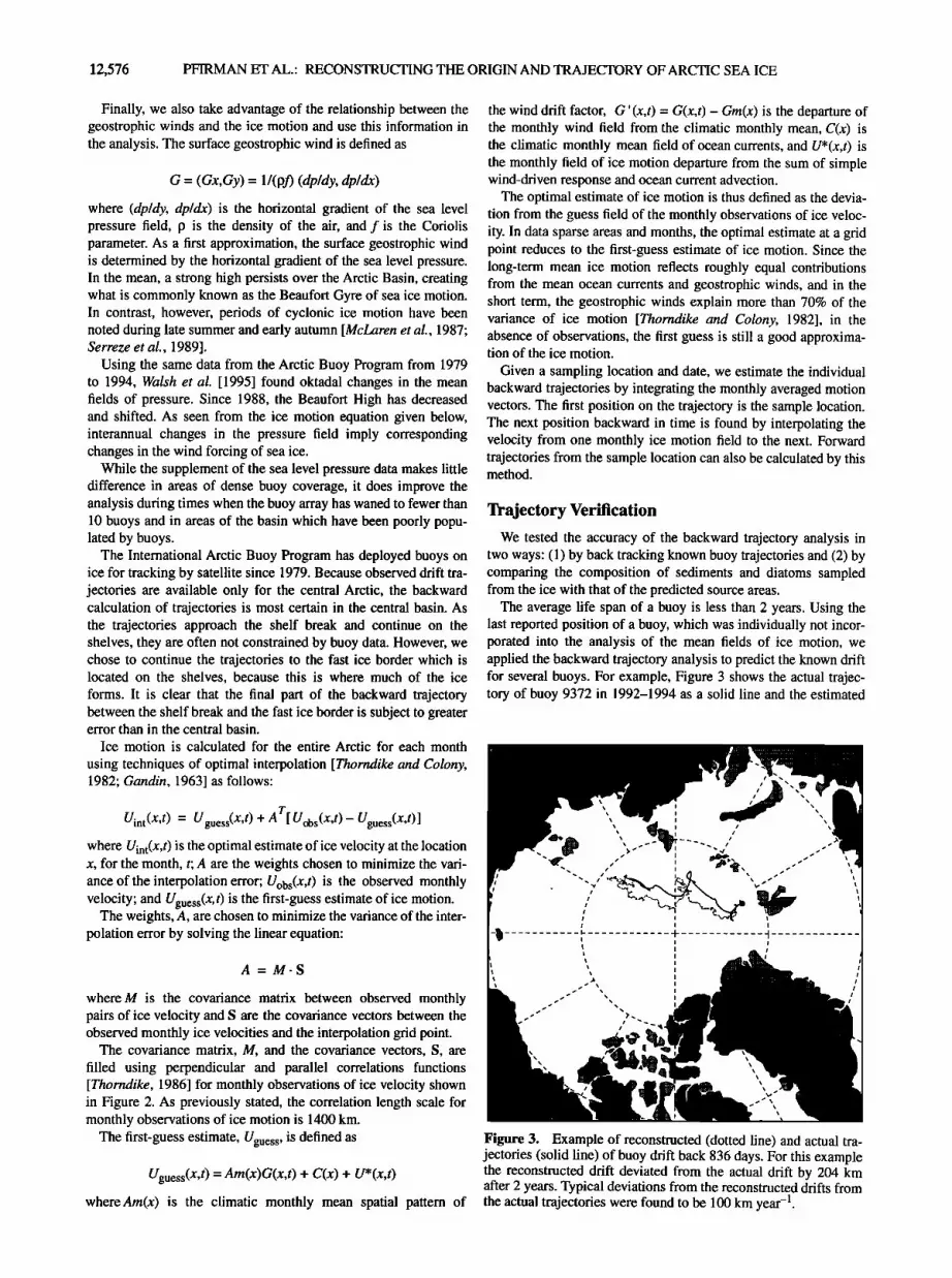
The average life span of a buoy is less than 2 years. Using the last reported position of a buoy, which was individually not incor- porated into the analysis of the mean fields of ice motion, we applied the backward trajectory analysis to predict the known drift for several buoys. For example, Figure 3 shows the actual trajec- tory of buoy 9372 in 1992-1994 as a solid line and the estimated

Figure 3. Example of reconstructed (dotted line) and actual tra- jectories (solid line) of buoy drift back 836 days. For this example the reconstructed drift deviated from the actual drift by 204 km after 2 years. Typical deviations from the reconstructed drifts from the actual trajectories were found to be 100 km year -1.

PFIRMAN ET AL.: RECONSTRUCTING THE ORIGIN AND TRAJECTORY OF ARCTIC SEA ICE 12,577

backward trajectory from the analysis as a dotted line. Two years after, the difference between actual and predicted position is 204 km. We estimate that the uncertainty of points on the back-

ward trajectories grows at about 100 km yr --1. We compared the characteristics of sediment sampled from the

ice (during expeditions in 1987, 1988, 1989, 1990, and 1991) with those obtained from the seafloor in the predicted source region [Silverberg, 1972; Wollenburg, 1993; Dethleff et al., 1993; N//rn- berg et al., 1994]. Each trajectory was truncated at the fast ice bor- der on the shelf, because the coastal polynya along the seaward edge of the fast ice is a major region of ice production [Zakharov, 1966; Dethleffet al., 1993]. Also, the polynya is typically located in a water depth of about 20 to 50 m, which is shallow enough to allow for entrainment of seafloor sediments through suspension freezing [Reimnitz et al., 1992, 1993a]. In the process of suspen- sion freezing, which occurs in shallow ice-free seas during storms, strong mixing resuspends sediment, and rapid freezing supercools the water column. Growing ice can thus come into contact with sediment particles and organisms either in the water column (frazil ice) or at the seafloor (anchor ice), bond to them, and raise them to the ice sheets which ultimately form at the surface [Reimnitz et al., 1992].

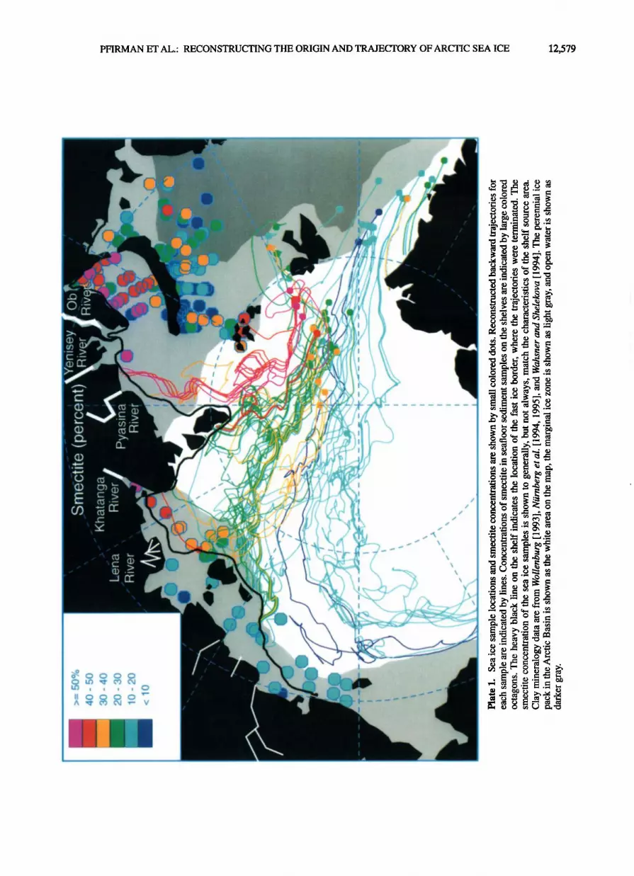
Comparison of the clay mineralogy of the Siberian shelf seafloors and sea ice sediments shows that the individual backward

trajectories generally fit with characteristics of known source areas either at the termination at the fast ice border or along their path on the shelves (Plate 1 and Figure 4). Some of the scatter is due to measurement precision and methodological differences in calcula- tion of clay mineralogy. Unfortunately, data on precision and inter- laboratory comparisons are not available. According to D.A. Darby (personal communication, 1996), while the values can dif- fer by as much as 40% depending on the method, mounting tech- nique, and amount of material analyzed, the error on average is +20 % of the actual value. This means that a smectite value of

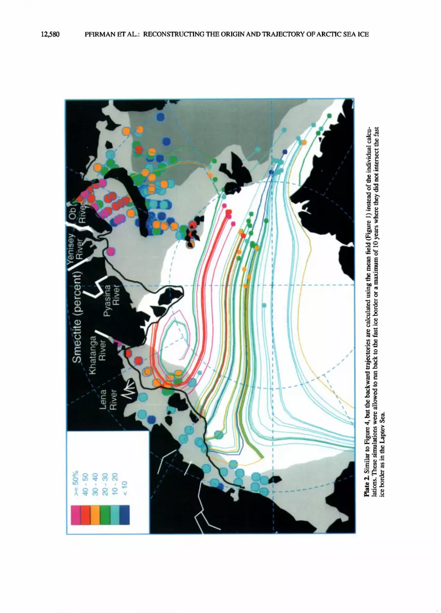
20% could be reported as 16-24% by various investigators. For comparison with the individual trajectories, we also show

the backward trajectories (Plate 2) calculated using the averaged ice drift (Figure 1). The temporally specific trajectories (Plate 1) clearly do a better job of matching the source mineralogy, thus demonstrating the significance of seasonal and annual variations in ice drift. However, the calculations using the mean do illustrate the possibility at times for transport by ice from the Kara to the Laptev Sea through Vilkitsky Strait south of Severnaya Zemlya (discussed also by Pavlov and Pfirman [1995] and Pfirman et al. [1995b, 1997].

Smectite, a clay mineral formed in part by weathering of basalt, shows the most variability in sediments on the Siberian shelves. The prime source of smectite to the Siberian seas appears to be weathering of the flood basalts and tuffs covering the Central Sibe- rian Plateau [Zolotukhin and Al'mukhamedov, 1988; Wahsner and Shelekhova, 1994]. (Naidu et al. [1995] similarly attributed the occurrence of expandable clay minerals in seafloor sediments of the Bering Sea to weathering of andesitic/basaltic rocks on the Kamchatka and Alaskan Peninsulas.) The Central Siberian Plateau separates the watersheds of the Kara and Laptev Seas. Yenisey River sediments, fed by westerly drainage from this region, con- tain the highest smectite level, comprising up to 70% of the clay mineral assemblage in the confluence region of the Yenisey and Ob' Rivers of the Kara Sea [Wahsner and Shelekhova, 1994]. To the east, in the Laptev Sea, the Khatanga River also drains the flood basalts, contributing smectite in fractions up to 60% [Wah- sner and Shelekhova, 1994] near the river discharge location and decreasing to less than 50% offshore of the river mouth [Silver-

berg, 1972; 13bllenburg, 1993]. To the east and west of these river inputs, smectite concentrations decrease in seafloor sediments of both the Kara and Laptev Seas, although there are some local smectite sources in the southwestern Kara Sea [Shelekova et al., 1995]. As smectite concentrations decrease, concentrations of illite increase (Figure 4). Once the ice is tracked back to the Kara and Laptev Seas, the steep mineralogical gradients in smectite and illite aid in delineating specific sediment entrainment locations. The other two clays, chlorite and kaolinite, do not have nearly as much regional variation along this part of the Siberian margin.

Clay mineralogy in the East Siberian Sea is relatively uniform, not allowing differentiation of source region [Wollenburg, 1993] without recourse to other data, e.g., heavy mineral assemblages [Silverberg, 1972; Naugler et al., 1974; Darby et al., 1989; Stein et al., 1994]. Relatively few trajectories track back to this region, a result which supports other studies indicating that the East Sibe- rian Sea is not a major source of sea ice to the Eurasian Basin [Zakharov, 1966], at least during the years represented in this study.

Note that several samples tracked back to about 157øE fit poorly (Figure 4). This can be explained based on the uncertainty (grow- ing at approximately 100 km yr -4 in the central Arctic) in the back calculation and the lack of buoy drift data on the shelves. Looking at the reconstructed trajectories (Plate 1), it appears that if the tra- jectories had been shifted slightly to the west, they would have ter- minated to the west of the New Siberian Islands, rather than to the east in the East Siberian Sea. The result of this shift would be a

much better fit with the seafloor mineralogy. Similarly, two trajec- tories that we tracked back to the fast ice border in the western

Laptev Sea (approximately 110øE) actually pass over seafloor sed- iments with similar composition in the eastern Laptev Sea near the New Siberian Islands. It is likely that the sediment with intermedi- ate levels of smectite was entrained there, rather than in the west-

ern Laptev Sea. The trajectory analysis can be used to estimate the age of sedi-

ment-laden ice floes. Most sea ice with significant sediment load has entrained resuspended seabed sediments [Pfirman et al., 1989a, b; Reimnitz et al., 1992, 1993a, b]. Therefore we can con- clude that the floe originated on the shelf. Assuming that the ice is advected off the shelf after forming in the coastal polynya/flaw lead, the approximate age of sediment-laden floes can be estimated from the time of sampling to the "termination" of the backward trajectory at the fast ice border. The average age of sea ice tracked back to the fast ice border is 35 months, or 2.9 years (Figure 4). The age of sea ice without sediments is not as clear: the ice could have formed on a shelf and not entrained sediments, or it could

have formed within the central Arctic Basin over deep water. Analysis of biogenic remains (Plate 3) supports the trajectory

reconstructions that show that ice with very high smectite concen- trations (up to 63%) may have originated in the southern Kara Sea, offshore of the Yenisey and Ob' Rivers. The percent planktonic freshwater diatom species sampled from the ice reflects both envi- ronmental conditions during ice formation and later modification [Abelmann, 1992]. Samples from several of these floes with high smectite concentration contained an unusually high concentration of freshwater planktonic diatom species (Plate 3). Most of the other sea ice samples had a significant fraction of benthic marine species, similar to the species reported from shallow water areas of the Siberian shelves [Abelmann, 1992]. However, the two samples that tracked back to the Kara Sea had <20% benthic marine spe- cies and were comprised largely of freshwater planktonic species (>70%). Abelmann [1992] interpreted this unusual assemblage as representing formation in a region with large freshwater influx,

12,578 PFIRMAN ET AL.' RECONSTRUCTING THE ORIGIN AND TRAJECTORY OF ARCTIC SEA ICE

90 ø E

180 ø

1979 - 1994 10 cm/s =

'Sea•'"•'l: ) Kara i

i \

! \ !

!

-,. , Barents Sea-'

East .' - '813•N' ',

90 ø W

o

Figure 1. Mean field of ice drift in the Arctic Ocean derived from buoy drift from 1979 to 1994. Velocities are indi- cated by arrows (see scale on figure). Numbered lines indicate the average number of years required for ice in this location to exit the Arctic through Fram Strait.

Calculation of Backward Trajectories

As observed by Nansen [1902], Zubov [1943], and others, sea ice motion in the Arctic Basin is primarily forced by local surface winds and ocean currents. Nansen observed that compact ice tends to drift about 35 ø to the right of and at 2% of the surface wind speed. At lower ice concentrations, the ice drift can reach 3-4% of the surface wind speed. On daily timescales, Thorndike and Col- ony [1982] found typical winter values for the multiplier IAI of 0.008 and a turning angle theta of-18 ø and determined that the geostrophic winds account for 70% of the variance of the ice motion.

To produce analyzed fields of ice motion, Thorndike and Colony [1982] used techniques of optimal interpolation [Gandin, 1963] which require the specification of certain statistics inherent in the data, such as the mean field of ice motion (Figure 1), the variance of the individual observations about this mean, and correlation

functions which quantify the statistical relationship between sepa- rate observations. For this study we extend the work of Thorndike and Colony [ 1982] and apply the techniques of optimal interpola- tion to monthly rather than to daily observations of ice drift.

The advantages of using monthly data are that the measurement error of ice velocities is greatly reduced and the correlation length scale (Figure 2) between observations is much longer. Since the error in the position of a buoy by satellite is typically about 300 m [Argos Incorporated, 1996], the approximate error in monthly ice velocities is

J 3002 ) 2 -! (2x m = 0.02 cm s eu = 30d

For the monthly observations we found a correlation length scale of 1400 km (Figure 2) as compared to 900 km found by

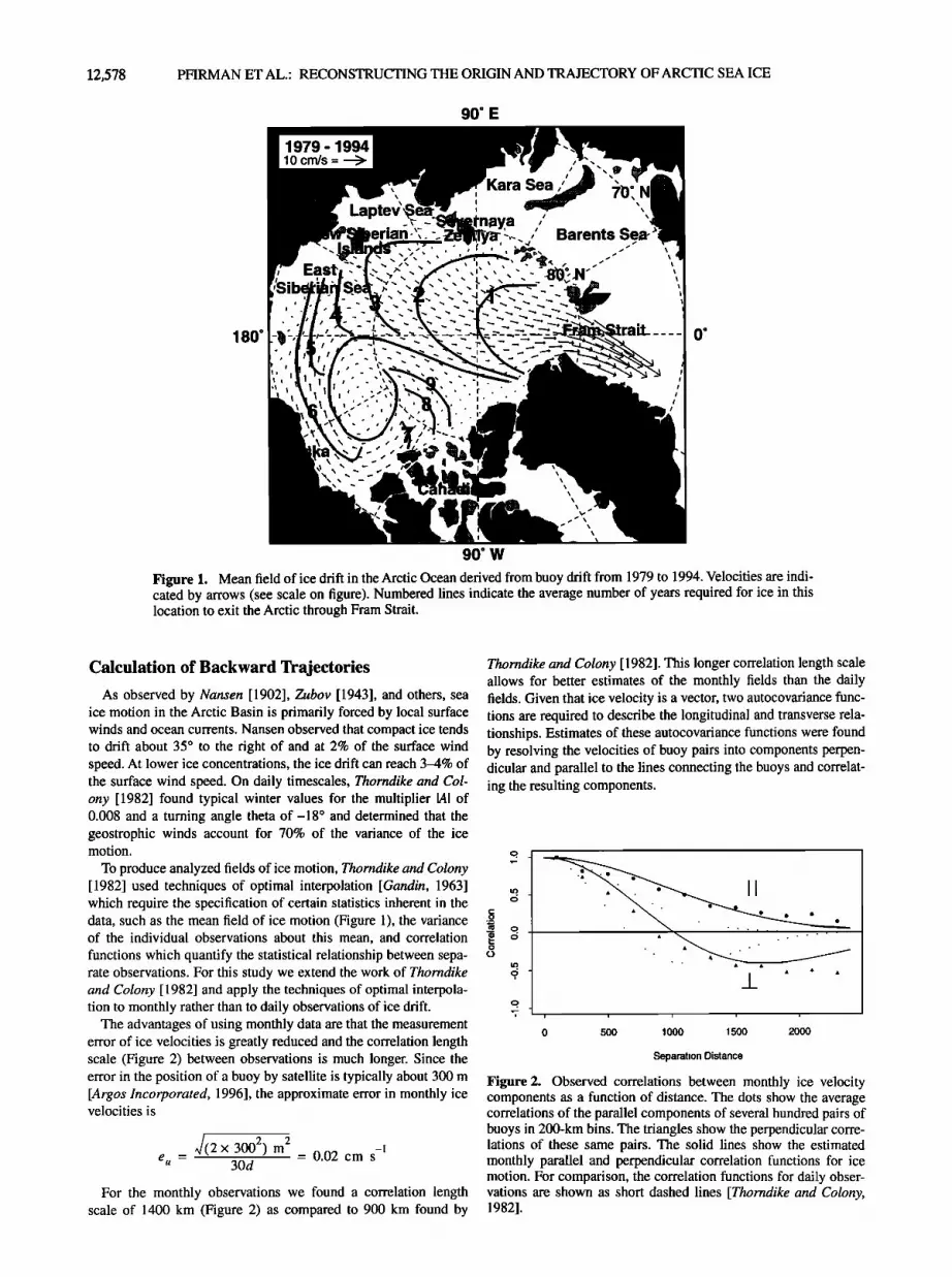
Thorndike and Colony [ 1982]. This longer correlation length scale allows for better estimates of the monthly fields than the daily fields. Given that ice velocity is a vector, two autocovariance func- tions are required to describe the longitudinal and transverse rela- tionships. Estimates of these autocovariance functions were found by resolving the velocities of buoy pairs into components perpen- dicular and parallel to the lines connecting the buoys and correlat- ing the resulting components.

II

i i i i i

0 500 1000 1500 2000

Separation Distance

Figure 2. Observed correlations between monthly ice velocity components as a function of distance. The dots show the average correlations of the parallel components of several hundred pairs of buoys in 200-km bins. The triangles show the perpendicular corre- lations of these same pairs. The solid lines show the estimated monthly parallel and perpendicular correlation functions for ice motion. For comparison, the correlation functions for daily obser- vations are shown as short dashed lines [Thomdike and Colony, 1982].

PFIRMAN ET AL.' RECONSTRUCTING THE ORIGIN AND TRAJECTORY OF ARCTIC SEA ICE 12,579

I /

12,580 PFIRMAN ET AL.' RECONSTRUCTING THE ORIGIN AND TRAJECTORY OF ARCTIC SEA ICE

XC >

\

- V

! !

i _

I

PFIRMAN ET AL.: RECONSTRUCTING THE ORIGIN AND TRAJECTORY OF ARCTIC SEA ICE 12,581

!

!

t-

t

t

1

t

I !

!

I

t

!

I

! I

I

1

I

I

I

I

I

I

I

I

I

I

1

I

I

I

I I

!

t

I I \ i \

I

I

I

!

I

I

I

t

I

12,582 PFIRMAN ET AL.: RECONSTRUCTING THE ORIGIN AND TRAJECTORY OF ARCTIC SEA ICE

I

•0

I

!

% %

I t

I

t

I

! i

1.

/

PFIRMAN ET AL.' RECONSTRUCTING THE ORIGIN AND TRAJECTORY OF ARCTIC SEA ICE 12,583

•ø o o O

12,584 PFIRMAN ET AL.: RECONSTRUCTING THE ORIGIN AND TRAJECTORY OF ARCTIC SEA ICE

Laptev Sea East Siberian Sea

::::::::::::::::

::::::::::::::::::

::::::::::::::::::

,:.:.:.:.:.:.:.:.

:::::::::::::::::: :::::::::::::::::: ::::::::::::::::::

::::::::::::::::::: ::::::::::::::::::: :::::::::::::::::::

:.:.:.:.:.:.:.:.:.. ::::::::::::::::::

:::::::::::::::::::

:.:.:.:.:.:,:.:.:.:

2•3 35

x x xi!!iiiiiiiiii!•;• • xX x • x x x x

12"O•i"g]tude

?:iii::?:iiiii!iii • . X • 41 :::::::::::::::::::::::::::::::::::: :::::::::::::::::

:::::::::::::::::::::::::: x • •3 ii:::.•".•i:iiii?•

::::::::::::::::::::::::: X

:::::::::::::::::::::::::: :::::::::::::::::: ::::::::::::::::::

' i ! , i

120 140 160 180

Longitude

Figure 4. Concentrations of the clay minerals smectite and illite in seafloor sediments (crosses) are plotted against the longitude of the reconstructed origin for sea ice samples (numbers indicate duration (in months) from the sample location to the fast ice bor- der). If the fit were perfect, the two should match within the error of the clay mineralogies (approximately +20 % of the actual value (D.A. Darby, personal communication, 1996). Concentrations of the other clay minerals, chlorite and kaolinite, do not vary signifi- cantly in the Laptev and East Siberian seas. Clay mineralogy data are from Wollenburg [ 1993] and Niirnberg et al. [ 1994].

most likely in the vicinity of river discharge, such as the Ob' and/ or Yenisey Rivers.

Discussion

Once verified, we can use the backward trajectories to under- stand better the characteristics of entrained material. For example, sediment concentrations might provide an indication of sources of sediment-laden ice. Note, however, that the sediment concentra-

tion data used in this study reflect both the amount of sediment entrained as well as the amount of ice ablated during drift. The samples used for analysis of sediment concentration were typically obtained by scraping sediment-rich ice from the upper several cen- timeters of the floe. Data are not available on total sediment load

per unit area of ice, which would have been a better measure of total sediment entrainment. Most of the ice sampled was several years old (Figure 4), and about 40 cm of ice will be lost from the floe surface each year [Romenov, 1993]. As the ice ablates, sedi- ment distributed throughout the original section of ice collapses into a sediment-rich layer on the ice surface which may represent much of the sediment load carded by the ice [Pfirmen et el., 1990; Wollenburg, 1993; Niirnberg et el., 1994]. Another source of uncertainty is the amount of material lost to the underlying water column during drift by runoff, brine drainage, and other processes [Pfirmen et el., 1990; Reimnit• et el., 1993b]. Furthermore, sedi-

ment is redistributed on the surface of floes by meltwater and winds, resulting in uneven concentrations even on one floe. As a result, sediment concentration data are quite variable and cannot be used for detailed analysis, although we believe that, in aggre- gate and spanning 5 orders of magnitude (Plate 4), they do repre- sent general trends.

Earlier studies indicated that most of the sediment-laden ice

sampled in the Eurasian Arctic came from the Laptev Sea [Wollen- burg, 1993; Niirnberg et al., 1994; Stein et al., 1994; Eicken et al., 1997). The backward trajectories support this in showing that sea ice with the greatest sediment concentrations crossed the shelf edge primarily in the vicinity of the New Siberian Islands which protrudes into the Arctic Basin (Plate 4), separating the broad, shallow shelves of the Laptev and the East Siberian Seas. In addi- tion, this study also identifies the north-central to eastern Kara Sea as a secondary source for sediment-laden ice that moves into the southern part of the Eurasian Arctic. These parts of the Kara Sea are shallow, perhaps allowing sediment entrainment, and there is an offshore movement of ice resulting in its export to the Arctic Basin. As pointed out by other investigators [Vize, 1937; Niirnberg et al., 1995], the southwestern Kara Sea does not appear to be an active source area for ice to the Arctic Ocean.

Another characteristic of sea ice sediment is that it is primarily fine-grained, generally clayey silt or silty clay (up to 75% silt and 90% clay [Niirnberg et al., 1994]). Comparison of the grain size of seafloor sediments relative to the sediments in the pack ice indi- cates that sediment incorporated in the pack ice is finer-grained than seafloor sediments in the source area [Wollenburg, 1993; Niirnberg et al., 1994] (Plate 5). This difference is consistent with suspension freezing as the main mode of sediment entrainment [Reimnitz et al., 1993b]. Fine sediment particles remain suspended in the water column longer than coarse and are more likely to be incorporated into growing ice; conversely, fine sediments are win- nowed from the seabed. Size fractionation is important, because most contaminants of concern in the Arctic, organochlorines and heavy metals, including radionuclides, sorb preferentially onto fine-grained material [Stumm and Morgan, 1981]. Therefore sedi- ment-laden sea ice is likely to have concentrations of contaminants greater than those of shelf sediments, which are "diluted" with higher proportions of sand [Pfirman et al., 1995b].

Forward trajectories can also be calculated to identify regions influenced by sea ice from different source areas. Simulations of Lagrangian drifters were started along the mid-September multi- year ice edge each month from 1979 to 1994 and were allowed to drift forward in time as long as the drifter remained within the bounds of our velocity fields, shown on Figure 5 as a rectangular box, or 12 years, whichever came first (Figure 5). Note that, as with the backward trajectory analysis (Plate 1), trajectories were not allowed to pass through islands. Ice from the Kara Sea has a strong influence on the Laptev Sea, Barents Sea, Svalbard, the southern portion of the Transpolar Drift Stream, and eastern Fram Strait. Ice from the Laptev Sea is mostly advected through Fram Strait and to a lesser degree into the Barents Sea. Ice from the East Siberian Sea is either advected through Fram Strait or is caught up in the Beaufort Gyre and is transported along the northern North American coast.

Conclusions

This study shows that using an analysis of backward trajectories calculated individually for each sea ice sample and available min- eralogical and biological data, the source of Arctic sea ice, as well as its trajectory and possible age, i.e., time elapsed since leaving

PFIRMAN ET AL.: RECONSTRUCTING THE ORIGIN AND TRAJECTORY OF ARCTIC SEA ICE 12,585

in ice, its likely area of release, possible uptake by ice-associated organisms, and entrance to the Arctic ecosystem. For example, this study shows that sea ice from the Kara Sea contributes signifi- cantly to the ice cover of the Barents Sea and the so•athern part of the Eurasian Basin. The Kara Sea has the potential to be contami- nated by agricultural and industrial chemicals: it lies just north of the industrial complex of Nori!sk, Russia, and a main atmospheric transport conduit for Eurasiaa sources of Arctic haze passes over the Kara Sea [Raatz, 1991; Shaw, 1995]. Rivers discharging to the Kara Sea drain a large watershed with a variety of potential con- taminant sources [Pavlov and Pfirman, 1995]. The amount and fate of material entrained in sea ice formed in this region are important to determine by future studies.

Acknowledgments. This research was supported by the U.S. Office of Naval Research, the U.S. National Science Foundation, and, under the direction of J. Thiede (GEOMAR, Research Center for Marine Geosciences, Kiel, Germany), the German Bundesmin- isterium ftir Forschung und Technologie. We thank Terry Tucker for his helpful review of the manuscript.

Figure 5. This figure shows the possible seas of origin of samples taken from sea ice in the Arctic Basin. Simulations of Lagrangian drifters were started along the mid-September multiyear ice edge each month from 1979 to 1994 and were allowed to drift forward in time as long as the drifter remained within the bounds of our velocity fields. The top panel shows export from the Kara Sea, the middle panel shows export from the Laptev Sea, and the bottom panel shows export from the East Siberian Sea.

the fast ice border, can be distinguished in the Eurasian Arctic. Although the method has been demonstrated and verified using sediment-laden ice, trajectories can also be estimated for ice with- out sediment; it is just more difficult to verify their accuracy.

Using reconstructed backward and forward trajectories, we can identify regions of sediment entrainment, main pathways of sedi- ment-laden ice, and regions of possible release of sediments from the ice, thus contributing to understanding Arctic sediment flux. Similarly, we can assess the potential for contaminant entrainment

References

Abelmann, A., Diatom assemblages in Arctic sea ice--Indicator for ice drift pathways, Deep Sea Res., Part A, 39, special issue, S525- S538, 1992.

Argos Incorporated, Argos Users Handbook, Landover, Maryland, 1996.

Arnason, B., The use of deuterium to trace the origin of drifting ice, Rit Fiskideildar J. Mar. Res. Inst. Reykjavik, 10, 85-89, 1985.

Campbell, J.A., and P.A. Yeats, The distribution of manganese, iron, nickel, copper and cadmium in the waters of Baffin Bay and the Canadian Arctic Archipelago, Oceanol. Acta, 4(2), 161-168, 1982.

Chernyak, S.M., C.P. Rice, and L.L. McConnell, Evidence of cur- rently-used pesticides in air, ice, fog, seawater and surface micro- layer in the Bering and Chukchi Seas, Mar. Pollut. Bull., 32(5), 410-419, 1996.

Colony, R., and A.S. Thorndike, Sea ice motion as a drunkard's walk, J. Geophys. Res., 90, 965-974, 1985.

Darby, D.A., A.S. Naidu, T.C. Mowatt, and G. Jones, Sediment com- position and sedimentary processes in the Arctic Ocean, in The Arctic Seas, edited by Yvonne Herman, pp. 657-720, Van Nostrand Reinhold, New York, 1989.

Dethleff, D., D. Ntirnberg, E. Reimnitz, M. Saarso, and Y.P. Savchenko, East Siberian Arctic region expedition '92: Its signifi- cance for Arctic sea ice formation and transpolar sediment flux, Ber. Polarforschung, 120, 1-44, 1993.

Dewailly, W., P. Ayotte, S. Bruneau, C. Lalibertd, D.C.G. Muir, and R.J. Norstrom, Inuit exposure to organochlorines through the aquatic food chain in Arctic Qu6bec, Environ. Health Perspect., 101(7), 618-620, 1993.

Eicken, H., E. Reimnitz, V. Alexandrov, T. Martin, H. Kassens, and T. Viehoff, Sea-ice processes in the Laptev Sea and their impor- tance for export of sediments, Cont. Shelf Res., 17(2), 205-233, 1997.

Gandin, L.S., The Objective Analysis of Meteorological Fields, Hydrometeorol. Publ. House, St. Petersburg, Russia, 1963. (English translation, Is. Program for Sci. Trans., Jerusalem, 1965.)

Gaul, H., Organochlorine compounds in water and sea ice of the Euro- pean Arctic Sea, in Proceedings of the Conference of the Comitd Arctique International on the Global Significance of the Transport and Accumulation of Polychlorinated Hydrocarbons in the Arctic, edited by F. Roots and R. Shearer, pp. 18-22, Plenum, New York, 1989.

Kotchetov, S.V., I.Y. Kulakov, V.K. Kurajov, L.A. Timokhov, and Y.A. Vanda, Hydrometeorological Regime of the Laptev Sea, Arct. and Antarct. Res. Inst., St. Petersburg, Russia, 1994.

McLaren, A.S., M.C. Serreze, and M.G. Barry, Seasonal variations of

12,586 PFIRMAN ET AL.: RECONSTRUCTING THE ORIGIN AND TRAJECTORY OF ARCTIC SEA ICE

sea ice motion in the Canada Basin and their implications, Geo- phys. Res. Lett., 14, 1123-1126, 1987.

Meese, D., E. Reimnitz, W. Tucker, A. Gow, J. Bischof, and D. Darby, Evidence for Cesium-137 transport by Arctic sea ice, Sci. Total Environ., in press, 1997.

Melnikov, S.A., Report on heavy metals, State Arct. Environ. Rep., 2, pp. 82-153, Arct. Cent., Univ. of Lapland, Rovaniemi, Finland, 1991.

Muir, D.C.G., R. Wagemann, B.T. Hargrave, D.J. Thomas, D.B. Peakall, and R.J. Norstrom, Arctic marine ecosystem contamina- tion, Sci. Total Environ., 122, 75-134, 1992.

Mysak, L.A., and D.K. Manak, Arctic sea-ice extent and anomalies, 1953-1984, Atmos. Ocean, 27(2), 376-405, 1989.

Naidu, A.S., M.W. Han, T.C. Mowatt, and W. Wajda, Clay minerals as indicators of sources of terrigenous sediments, their transportation and deposition: Bering Basin, Russian-Alaskan Arctic, Mar. Geol., 127, 87-104, 1995.

Nansen, F., Farthest North, Archibald Constable, London, England, 1897.

Nansen, F., Norwegian North Polar Expedition 1893-1896, Scientific Results, vol. 3, The Oceanography of the North Pole Basin, 427 pp., Longmans, Green, Toronto, Ont., Canada, 1902.

Naugler, F.P., N. Silverberg, and J.S. Creager, in Marine Geology and Oceanography of the Arctic Seas, edited by Y. Herman, pp. 191- 210, Springer-Verlag, New York, 1974.

Ntirnberg, D., I. Wollenburg, D. Dethleff, H. Eicken, H. Kassens, T. Letzig, E. Reimnitz, and J. Thiede, Sediments in Arctic sea ice: Implications for entrainment, transport and release, Mar. Geol., 119, 185-214, 1994.

Ntirnberg, D., M.A. Levitan, J.A. Pavlidis, and E.S. Shelekhova, Dis- tribution of clay minerals in surface sediments from the eastern Barents and south-western Kara Seas, Geol. Rundsch., 84, 665- 682, 1995.

Pavlov, V., and S.L. Pfirman, Hydrographic structure and variability of the Kara Sea: Implications for pollutant distribution, Deep Sea Res., Part II, 42(6), 1369-1390, 1995.

Pfirman, S.L., J.-C. Gascard, I. Wollenburg, P. Mudie, and A. Abel- mann, Particle-laden Eurasian Arctic sea ice: Observations from July and August 1987, Polar Res., 7, 59-66,1989a.

Pfirman, S.L., I. Wollenburg, J. Thiede, and M.A. Lange, Lithogenic sediment on Arctic pack ice: Potential aeolian flux and contribu- tion to deep sea sediments, in Paleoclimatology and Paleometeo- rology: Modem and Past Patterns of Global Atmospheric Transport, NATO ASI Ser. C, vol. 282, edited by M. Leinen and M. Sarnthein, pp. 463-493, Kluwer Acad., Norwell, Mass., 1989b.

Pfirman, S., M.A. Lange, I. Wollenburg, and P. Schlosser, Sea ice char- acteristics and the role of sediment inclusions in deep-sea deposi- tion: Arctic-Antarctic comparisons, in Geological History of the Polar Oceans: Arctic Versus Antarctic, edited by U. Bleil and J. Thiede, pp. 187-211, Kluwer Acad., Norwell, Mass., 1990.

Pfirman, S.L., H. Eicken, D. Bauch, and W. Weeks, The potential transport of pollutants by Arctic sea ice, Sci. Total Environ., 159, 129-146, 1995a.

Pfirman, S.L., J. Koegler, and Brice Anselme, Coastal environments of the western Kara and eastern Barents Seas, Deep Sea Res., Part II, 42(6), 1391-1412, 1995b.

Pfirman, S.L., J.W. KOgeler, and I. Rigor, Potential rapid transport of contaminants from the Kara Sea, Sci. Total Environ., in press, 1997.

Raatz, W.E., The climatology and meteorology of Arctic air pollution, in Pollution of the Arctic Atmosphere, edited by W.T. Sturges, pp. 13-42, Elsevier, New York, 1991.

Reimnitz, E., L. Marincovich Jr., M. McCormick, and W.M. Briggs, Suspension freezing of bottom sediment and biota in the Northwest Passage and implications for Arctic Ocean sedimentation, Can. J. Earth Sci., 29, 693-703, 1992.

Reimnitz, E., M. McCormick, K. McDougall, and E. Brouwers, Sedi- ment export by ice rafting from a coastal polynya, Arctic Alaska, U.S.A.,Arct. Alp. Res., 25(2), 83-98, 1993a.

Reimnitz, E., P.W. Barnes, and W.S. Weber, Particulate matter in ice of the Beaufort Gyre, J. Glaciol., 39(131), 186-198, 1993b.

Romanov, I.P., The Ice Cover of the Arctic Ocean., 211 pp., Arct. and Antarct. Res. Inst., St. Petersburg, Russia, 1993.

Sen'eze, M.C., R.G. Barry, and A.S. McLaren, Seasonal variations in sea ice motion and effects on sea ice concentration in the Canada

Basin, J. Geophys. Res., 94, 10,955-10,970, 1989. Shaw, G.E., The Arctic haze phenomenon, Bull. Am. Meteorol. Soc.,

76(12), 2403-2413, 1995. Shelekova, E.S., M.A. Levitan, Y.A. Pavlids, D. Ntirnberg, and M.

Wahsner, Clay mineral distribution in surface sediments of the Southwestern Kara Sea, Oceanology, 35(3), 403-406, 1995.

Silverberg, N., Sedimentology of the surface sediments of the East Siberian and Laptev Seas, Ph.D. thesis, 185 pp, Univ. of Wash., 1972.

Stein, R., H. Grobe, and M. Wahsner, Organic carbon, carbonate, and clay mineral distributions in eastern Central Arctic Ocean surface sediments, Mar. Geol., 1!9, 269-285, 1994.

Stumm, W., and J.J. Morgan, Aquatic Chemistry, John Wiley, New York, 1981.

Thorndike, A.S., Kinematics of sea ice, in Air-Sea-Ice Interactions, edited by N. Untersteiner, pp. 489-549, Plenum, New York, 1986.

Thorndike, A.S., and R. Colony, Sea ice motion in response to geo- strophic winds, J. Geophys. Res., 87, 5845-5852, 1982.

Vize, V.J., Ice drift from the Kara Sea into the Greenland Sea, Prob. Arck., 1,103-116, 1937.

Wahsner, M., and E.S. Shelekhova, Clay-mineral distribution in Arctic deep sea and shelf surface sediments (abstract), Greifswald. Geol. Beitr., A(2), 234, 1994.

Walsh, J. E., W. L. Chapman, and T. L. Shy, Recent decrease of sea level pressure in the Central Arctic Basin, J. Clim., 9, 480-486, 1995.

Weeks, W., Possible roles of sea ice in the transport of hazardous material, Arct. Res. U.S., 8, 34-52, 1994.

Wollenburg, I., Sediment transport by Arctic sea ice: The recent sedi- ment load of lithogenic and biogenic material, Ber. Polar- forschung, 127, 1-159, 1993.

Yablokov, A.V., V.K. Karasev, V.M. Rumyantsev, M.Y. Kokeyev, O.I. Petrov, V.N. Lytsov, A.F. Yemelyanenkov, and P.M. Rubtsov, Facts and Problems Related to Radioactive Waste Disposal in Seas Adja- cent to the Territory of the Russian Federation (also known as "The Yablokov Report"), 72 pp., Off. of the Pres. of the Russ. Fed., Mos- cow, 1993

Zakharov, V.F., The role of flaw leads off the edge of fast ice in the hydrological and ice regime of the Laptev Sea, Oceanology, 6(1), 815-821, 1966.

Zakharov, V.F., On the character of cause and effect relationships between sea ice and thermal conditions of the atmosphere, Ber. Polarforschung, 144, 33-43, 1994.

Zolotukhin, V.V., and A.I. Al'mukhamedov, Traps of the Siberian plat- form, in Continental Flood Basalts, edited by J.D. Macdougall, pp. 273-310, Kluwer Acad., Norwell, Mass., 1988.

Zubov, N.N., Arctic Ice (in Russian), Glavsevmorputi, Moscow, 1943. (English translation, Transl. 103, U.S. Navy Electr. Lab., San Diego, Calif., 1943.)

R. Colony, International Arctic Climate System Study Office, Post- boks 5072 Majorstua, N-0301 Oslo, Norway

H. Eicken, Alfred-Wegener Institute for Polar and Marine Research, Columbusstrasse, Postfach 120161, Bremerhaven, D-27515, Germany

Do Ntirnberg, GEOMAR Research Center for Marine Geosciences, Christian Albrechts University, Wischhofstrasse 1-3, D-24148 Kiel, Germany

So Pfirman, Barnard College, Columbia University, 3009 Broadway, New York, NY, 10027. (e-mail: spfirman@barnard.columbia.edu)

I. Rigor, Polar Science Center, University of Washington, 1013 NE 40th Street, Seattle, WA, 98105 (e-mail: igr@apl.washington.edu)

(Received May 3, 1995; revised November 26, 1996; accepted December 2, 1996.)