reconstructing ancestral gene content by coevolution

10.1101/gr.096115.109Access the most recent version at doi: 2010 20: 122-132 originally published online November 30, 2009Genome Res.

Tamir Tuller, Hadas Birin, Uri Gophna, et al. Reconstructing ancestral gene content by coevolution

MaterialSupplemental http://genome.cshlp.org/content/suppl/2009/11/04/gr.096115.109.DC1.html

References http://genome.cshlp.org/content/20/1/122.full.html#ref-list-1

This article cites 63 articles, 34 of which can be accessed free at:

serviceEmail alerting

click heretop right corner of the article orReceive free email alerts when new articles cite this article - sign up in the box at the

http://genome.cshlp.org/subscriptions go to: Genome ResearchTo subscribe to

Copyright © 2010 by Cold Spring Harbor Laboratory Press

Cold Spring Harbor Laboratory Press on February 20, 2010 - Published by genome.cshlp.orgDownloaded from

http://genome.cshlp.org/lookup/doi/10.1101/gr.096115.109

http://genome.cshlp.org/content/suppl/2009/11/04/gr.096115.109.DC1.html

http://genome.cshlp.org/content/20/1/122.full.html#ref-list-1

http://genome.cshlp.org/cgi/alerts/ctalert?alertType=citedby&addAlert=cited_by&saveAlert=no&cited_by_criteria_resid=genome;20/1/122&return_type=article&return_url=http://genome.cshlp.org/content/20/1/122.full.pdf

http://genome.cshlp.org/subscriptions

http://genome.cshlp.org/

http://www.cshlpress.com

Methods

Reconstructing ancestral gene content by coevolutionTamir Tuller,1,2,3,4,5 Hadas Birin,1,4 Uri Gophna,2 Martin Kupiec,2 and Eytan Ruppin1,3

1School of Computer Sciences, Tel Aviv University, Ramat Aviv 69978, Israel; 2Department of Molecular Microbiology and

Biotechnology, Tel Aviv University, Ramat Aviv 69978, Israel; 3School of Medicine, Tel Aviv University, Ramat Aviv 69978, Israel

Inferring the gene content of ancestral genomes is a fundamental challenge in molecular evolution. Due to the statisticalnature of this problem, ancestral genomes inferred by the maximum likelihood (ML) or the maximum-parsimony (MP)methods are prone to considerable error rates. In general, these errors are difficult to abolish by using longer genomicsequences or by analyzing more taxa. This study describes a new approach for improving ancestral genome reconstruction,the ancestral coevolver (ACE), which utilizes coevolutionary information to improve the accuracy of such reconstructionsover previous approaches. The principal idea is to reduce the potentially large solution space by choosing a single optimal(or near optimal) solution that is in accord with the coevolutionary relationships between protein families. Simulationexperiments, both on artificial and real biological data, show that ACE yields a marked decrease in error rate comparedwith ML or MP. Applied to a large data set (95 organisms, 4873 protein families, and 10,000 coevolutionary relationships),some of the ancestral genomes reconstructed by ACE were remarkably different in their gene content from thosereconstructed by ML or MP alone (more than 10% in some nodes). These reconstructions, while having almost similarlikelihood/parsimony scores as those obtained with ML/MP, had markedly higher concordance with the coevolutionaryinformation. Specifically, when ACE was implemented to improve the results of ML, it added a large number of proteins tothose encoded by LUCA (last universal common ancestor), most of them ribosomal proteins and components of the F0F1-type ATP synthase/ATPases, complexes that are vital in most living organisms. Our analysis suggests that LUCA appearsto have been bacterial-like and had a genome size similar to the genome sizes of many extant organisms.

[Supplemental material is available online at http://www.genome.org.]

The problem of reconstructing ancestral states is as old as the field

of molecular evolution, pioneered by Fitch around 40 yr ago (Fitch

1971). This first algorithm assumed a binary alphabet and was

based on the maximum parsimony (MP) criterion, i.e., find the

labels to the internal nodes of a tree that minimize the number of

changes or mutations along the tree edges. Over the years this basic

algorithm was generalized in many ways. Sankoff (1975) showed

how to efficiently solve versions of the MP problem with a non-

binary alphabet and with multiple edge weights. Algorithms for

inferring ancestral sequences based on the maximum likelihood

(ML) principle (instead of MP) were suggested more than 15 yr later

(Barry and Hartigan 1987; Felsenstein 1993; Pagel 1999; Pupko

et al. 2000; Krishnan et al. 2004; Elias and Tuller 2007), aiming to

identify the ancestral sequences that are most likely, given the

current data in probabilistic terms. In a manner analogous to in-

ferring an ancestral sequence such as a protein or gene (Pupko et al.

2000; Blanchette et al. 2004; Ma et al. 2006), many studies have

aimed to reconstruct ancestral genomes (genomic content or gene

content; e.g., see Boussau et al. 2004; Ouzounis et al. 2006; Putnam

et al. 2007). Most existing phylogenetic reconstruction algorithms

can be adapted to reconstructing ancestral gene content (e.g., see

Felsenstein 1993; Yang 1997; Swofford 2002).

The main problem related to reconstructing ancestral se-

quences and gene inventories is that, in practice, the reconstructed

sequences often contain a large number of errors. A major source of

this phenomenon is the existence of multiple local and/or global

maxima (i.e., solutions that are different but have the same scores

of ‘‘goodness’’) in the solution space searched by both the ML and

the MP approaches (e.g., see Fig. 1; Chor et al. 2000). Furthermore,

due to the statistical nature of the problem, and as both ML/MP

assume that different sites and different genes/proteins evolve

independently, increasing the amount of information used (the

lengths of the sequences and the number of organisms) (Li et al.

2008) does not guarantee a decrease in the error rate. Thus, in

many cases, the confidence that we may assign to the most likely

or most parsimonious reconstructed ancestral state is not very

high.

In this work we describe a novel approach for improving the

accuracy of reconstructed ancestral genomes. Our approach is

based on utilizing information embedded in the coevolution of

interacting proteins. The potential utility of this strategy is in-

tuitively simple: If the ancestral reconstruction of protein A is

ambiguous (e.g., different solutions achieve similar scores), but the

ancestral reconstruction of protein B is unambiguous, then,

knowing that A and B have coevolved (usually due to some func-

tional interaction) can help us disambiguate the ancestral re-

construction of A. A simple illustration of this idea is described in

Figure 1. As demonstrated further on, our approach can success-

fully distinguish between solutions with similar parsimony/like-

lihood scores.

Importantly, coevolutionary relations between proteins are

quite ubiquitous and have been traced and reported in numerous

studies (Pazos et al. 1997; Chen and Dokholyan 2006; Marino-

Ramirez et al. 2006; Barker et al. 2007; Wapinski et al. 2007; Felder

and Tuller 2008; Tuller et al. 2009). One such source is protein–

protein interactions (PPIs): Several studies have already demon-

strated a link between coevolution and physical interactions.

These investigations used the fact that interacting proteins tend to

coevolve in order to successfully predict physical interactions (e.g.,

see Wu et al. 2003; Sato et al. 2005; Juan et al. 2008). Here, we take

the opposite approach and use data on physical interactions be-

tween proteins as a proxy for their coevolution. Large-scale PPI

datasets currently exist only for relatively few organisms, but as

4These authors contributed equally to this work.5Corresponding author.E-mail [email protected]; fax 972-3-640-9357.Article published online before print. Article and publication date are athttp://www.genome.org/cgi/doi/10.1101/gr.096115.109.

122 Genome Researchwww.genome.org

20:122–132 � 2010 by Cold Spring Harbor Laboratory Press; ISSN 1088-9051/10; www.genome.org




physical interactions tend to be conserved across species, at least to

some extent, (e.g., see Wu et al. 2003; Liang et al. 2006; Hirsh and

Sharan 2007), it is plausible to assume that existing PPIs testify to

coevolutionary relations across the ancestral tree. Another source

of coevolution information that we utilize is metabolic adjacency:

Following the studies of Spirin et al. (2006) and Zhao et al. (2007)

we assume that metabolic enzymes that catalyze consecutive re-

actions in the same pathway tend to coevolve. We also incorporate

additional sources of coevolution information, including genomic

proximity, coexpression, and gene fusion, which have all been

shown to be good predictors of coevolution (Lee et al. 2004; Chen

and Dokholyan 2006; Jensen et al. 2009; Tuller et al. 2009).

The coevolution data from all of these sources is combined to

reconstruct the evolutionary history of 95 unicellular bacteria,

archaea, and eukaryotes.

Results

The ancestral coevolver algorithm (ACE)

The ancestral coevolver method incorporates information about

the coevolutionary relationships between pairs of proteins and the

evolutionary distance between organisms (an evolutionary tree[s])

to improve the accuracy of ancestral pro-

tein content reconstruction. In this sec-

tion we briefly describe our approach,

model, and definitions. More formal def-

initions appear in Supplementary Note 1.

For simplicity, we will relate similarly to

proteins and the genes that encode them.

A phylogenetic tree is a rooted bi-

nary tree (i.e., the input degree of each

node is one and the output degree is two)

together with leaf labels. In this work, we

assume that each node in a phylogenetic

tree corresponds to a different organism

(i.e., this is a species tree) and one can use

this phylogenetic tree to describe the

evolution of each protein family. In the

simplest binary case, each label is either

‘‘0’’ (the gene does not appear in the ge-

nome of the organism) or ‘‘1’’ (the protein

is encoded in the genome of an organ-

ism). In the nonbinary case each label is

a natural number that denotes the num-

ber of paralogous copies of a gene in the

corresponding genome. The leaves in

a phylogenetic tree correspond to extant

species, while the internal nodes corre-

spond to ancestral organisms.

A coevolving forest is a set of phy-

logenetic trees with identical topology

that correspond to the same organisms,

each tracking the evolution of a different

gene/protein. The forest includes an ad-

ditional set of coevolutionary edges that

connect pairs of nodes, each node in an

edge belonging to a different phyloge-

netic tree. Each such coevolutionary edge

connects a pair of nodes that correspond

to the same organism (Fig. 1). The edges

that are part of the evolutionary tree (the

standard evolutionary transition edges) are termed ‘‘tree edges’’

here. For example, Figure 1 illustrates a coevolving forest spanning

two gene/protein trees (the coevolutionary edges are dashed wavy

arrows, while the tree edges are continuous). In this work we as-

sume that pairs of coevolutionary edges that connect the roots of

two evolutionary trees are ‘‘inherited’’ by the other pairs of nodes

of the evolutionary trees (as described in Fig. 1), i.e., our mathe-

matical model is capable of dealing with cases where co-

evolutionary edges appear/disappear during evolution. However,

overall, we assume that the events where new coevolutionary

edges appear or disappear are relatively rare.

A coevolutionary forest additionally includes a weight table

for each coevolutionary edge and each tree edge. These weight

tables include the cost of each pair of labels at the two ends of the

edge. In the case of tree edges, these weights reflect the probability

of gaining/losing a copy number along the edge (Methods). For

coevolutionary edges, these weights reflect the distribution of

mutual occurrences of the labels of the nodes connected by the

edge. As we discuss later, these tables can be further weighted to

reflect our confidence in these two types of information (the

evolutionary transitions vs. coevolution information).

Another basic term needed for the description of our method

is the notion of a coevolutionary graph, which is an undirected

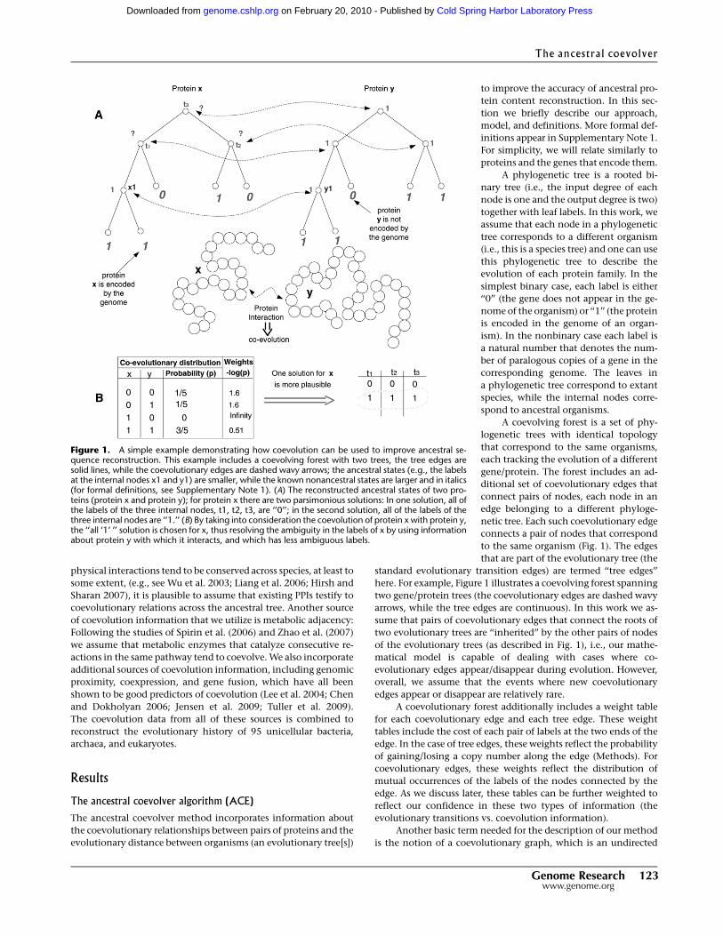
Figure 1. A simple example demonstrating how coevolution can be used to improve ancestral se-quence reconstruction. This example includes a coevolving forest with two trees, the tree edges aresolid lines, while the coevolutionary edges are dashed wavy arrows; the ancestral states (e.g., the labelsat the internal nodes x1 and y1) are smaller, while the known nonancestral states are larger and in italics(for formal definitions, see Supplementary Note 1). (A) The reconstructed ancestral states of two pro-teins (protein x and protein y); for protein x there are two parsimonious solutions: In one solution, all ofthe labels of the three internal nodes, t1, t2, t3, are ‘‘0’’; in the second solution, all of the labels of thethree internal nodes are ‘‘1.’’ (B) By taking into consideration the coevolution of protein x with protein y,the ‘‘all ‘1’ ’’ solution is chosen for x, thus resolving the ambiguity in the labels of x by using informationabout protein y with which it interacts, and which has less ambiguous labels.

Genome Research 123www.genome.org

The ancestral coevolver




graph that describes the coevolutionary relationships in the co-

evolutionary forest. In such a graph, each node corresponds to

a tree in the coevolutionary forest, and two nodes are connected by

an edge if there is at least one coevolutionary edge between their

corresponding trees. For example, the coevolutionary graph corre-

sponding to the coevolutionary forest in Figure 1A includes two

nodes (as there are two evolutionary trees in the forest), and one

edge that connects these nodes (as there are coevolutionary edges

between the two evolutionary trees). A connected component in

the coevolutionary forest is a subset of trees whose corresponding

nodes in the coevolutionary graph induce a connected component

(i.e., a set of nodes such that there is a path between each pair of

nodes in the set. For example, in the coevolutionary forest that

appears in Figure 1A the two trees induce a connected component).

The coevolutionary edges used in this work are drawn from various

sources of information: protein interactions, coexpression, prox-

imity in the metabolic networks, and other measures of cofunc-

tionality (see Methods). As it is not clear how to model the evo-

lution of a network with many types of interactions, we decided to

use the generalized MP as an objective function.

This leads us to the definition of the computational problem

we are concerned with, the ancestral coevolution problem: Given

a coevolutionary forest (a set of trees, a set of coevolutionary edges

that connect pairs of nodes in these trees, and weight tables for

each tree edge and each coevolutionary edge) we want to find la-

bels for the internal nodes of all of the trees in the coevolutionary

forest, such that the sum of the corresponding weights along all of

the tree edges and the coevolutionary edges (the total cost) is

minimal.

We designed an algorithm for solving this problem—the an-

cestral coevolver (ACE). The goal of ACE is to find labels for all of

the nodes of all of the trees in a coevolutionary forest by opti-

mizing the ancestral coevolution problem.

The sum of coevolutionary weights that are induced by

choosing labels (a solution) for all of the

internal nodes in a coevolutionary forest

composes the coevolutionary score. In

this work we normalize this score by di-

viding it by the minimal possible co-

evolutionary score. Similarly, the sum of

tree weights that are induced by choosing

labels (a solution) for all of the internal

nodes in a coevolutionary forest is named

the maximum likelihood or the maxi-

mum parsimony score (for a ML/MP

problem, correspondingly). Also, in this

case we normalized this score by dividing

it by the minimal possible ML/MP score.

By changing the relative weights assigned

to the coevolutionary edges relative to

those of the tree edges we can control the

comparative influence of these two sour-

ces of information on the inferred labels.

For sufficiently small weights of the co-

evolutionary edges, ACE will choose one

of the solutions obtained by the common

ML/MP approaches, solving the problem

of multiple optima of ML/MP (the ex-

treme case of ancestral coevolution prob-

lem without coevolutionary edges de-

scribes a conventional MP/ML problem).

On the other hand, using very large co-

evolutionary weights will result in a solution that is mostly influ-

enced by the coevolutionary relations (see Supplementary Notes 1

and 2; Methods). We name such weighting procedure as either ML/

CE weighting or MP/CE weighting, (depending on the algorithm

used).

In the next section we demonstrate three different ways for

choosing the ML/CE weighting (see more details in Supplementary

Notes 1, 2; Methods): The first is called the ‘‘conservative way’’:

choose small enough weights for the coevolutionary edges such

that the solution will be one of the ML/MP solutions. This ap-

proach should be used if one strongly believes in the conventional

ML/MP approach and the corresponding tree edge weight tables

(this approach is demonstrated in section The Simple Parsimony

Case: A Classical Example of Multiple Maxima). The second is

called the ‘‘weighted average’’: Choose the weights of the co-

evolutionary edges such that the weighted average of the co-

evolutionary score and the ML/MP score are optimized. If one has

similar beliefs in the two sources of information, a simple average

should be used; otherwise, a weighted average, reflecting the rel-

ative confidence in each of the information sources should be used

(this approach is demonstrated in section The ML Case: A Detailed

Biological Case Stud). The third approach is called the learning

approach: In this case we ‘‘flip’’ a small fraction of the sites at the

leaves and try to correct them by using the entire model. We chose

the weights with the best performances (more details in the section

The ACE Reconstructs Missing Values at the Leaves of the Evolu-

tionary Tree Better Than ML/MP).

The general steps of the algorithm appear in Figure 2. The

preprocessing steps required for generating the input to the ACE

algorithm include (Fig. 2A): reconstructing a phylogenetic tree,

inferring groups of orthologs, gathering functional/physical in-

teractions between orthologs, and computing edge weights. Next,

ACE is implemented (Fig. 2B). The algorithm has four main steps:

(1) the coevolutionary forest is partitioned into smaller subforests;

Figure 2. (A) The preprocessing step: generating an input for ACE. The input includes an evolutionarytree with tree edge weights as well as coevolutionary edges with corresponding weights (see moredetails in Methods). (B) The ACE algorithm has four main steps: (1) partitioning of the coevolutionarygraph to smaller subgraphs, (2) finding the optimal ancestral states in these subgraph, (3) mergingthese subgraphs, (4) improving the solution greedily (see a detailed description in the Methods sectionand in Supplementary Note 1).

Tuller et al.





(2) an optimal labeling is inferred for

each of these subforests; (3) the solutions

are merged; and (4) a final step of greedy

optimization is performed. A detailed

description of the algorithm is presented

in the Methods section, in Supplemen-

tal Figure 1, and in Supplementary Note

1. Note that an ancestral genome may

include more genes than each of the

genomes at the leaves (Supplementary

Note 3).

Here, we show an application of ACE

within the MP framework. However, the

optimization problem of inferring the

ancestral states of a phylogenetic tree

when the optimization criterion used is

ML (e.g., see Pupko et al. 2000) under in-

dependently and identically distributed

(i.i.d.) probabilistic models such as Jukes

and Cantor (1969) (JC), Neyman (1971),

or the model of Yang et al. (1995) can be

formalized as a MP problem for a non-

binary alphabet with multiple edge

weights (Sankoff 1975) (Supplementary

Note 4). Thus, the ACE algorithm can be

used for improving both ML and MP al-

gorithms.

A comparative simulation studyof ACE vs. MP/ML

To demonstrate the performance of ACE

we designed a simulation incorporating

coevolution, where the genes/proteins

evolve along the corresponding evolu-

tionary trees, but also coevolve with each

other (Supplementary Note 5; Supple-

mental Fig. 2). We examined the perfor-

mance of the ACE algorithm in compari-

son to the standard MP/ML approaches

while varying the following parameters:

(1) the amount of coevolutionary edges:

the number of edges per node in the co-

evolutionary graph; (2) the introduction

of errors in the weights of the tree edges

and the coevolutionary graph; and (3) varying the probability of

mutations along the tree edges (corresponding to the weights of

the tree edges; Supplementary Note 5; Supplemental Fig. 2). The

aims of the simulation are: (1) to demonstrate the robustness of the

ACE algorithm to various parameters; (2) to compare the ACE ap-

proach to the conventional approaches (MP/ML) that do not use

coevolutionary information (currently, there are no previous ap-

proaches that use coevolutionary information to infer genome

content that can be compared to the ACE).

A summary of the simulation results is provided in Figure 3.

First we investigated the effect of modifying coevolution levels,

quantified by the mean number of edges per node in the co-

evolutionary graph. Figure 3 clearly demonstrates that ACE out-

performs the MP/ML approaches, even at low levels of co-

evolution. Both the performance of ACE (Fig. 3A), as measured

by the error rate (the frequency of ancestral states inferred in-

correctly), and its superiority over the other approaches (Fig. 3C),

increases with the level of coevolution. The error rate of ACE

undergoes a decrease of more than 50% (to an error rate of just a

few percent) when the level of coevolution increases from 0 to 5

(Fig. 3A). Note that this level of coevolution is reasonable in real

biological terms: For example, there are more than five PPI in-

teractions for each protein, on average, in the yeast PPI network

(which includes 39,396 interactions and around 6400 open read-

ing frames [ORFs]; see Methods). If we incorporate a number of

sources of coevolutionary information (see above), the average

degree in the resulting coevolutionary graph turns out to be much

higher (e.g., the mean node degree [connections per protein] in the

coevolutionary graph underlying the biological case analyzed in

the next section was larger than 14).

As can be seen in Figure 3B, ACE is more robust than the

standard MP/ML approaches to errors in the weights of tree edges.

ACE performs better at all error rates, but predominantly when the

error level is particularly high. Moreover, ACE also performs better

Figure 3. Summary of the simulation results, reporting the mean over 10 runs using coevolutionaryforests with 100 trees, each with 20 leaves and branch lengths in the range of from 0.1 to 0.4. (A) Theerror rate (frequency of sites inferred with error, y-axis) vs. the level of coevolution (normalized by thenumber of trees, x-axis). The inset shows the typical behavior at very low levels of coevolution. (B)The error rate vs. errors in the weights of the tree edges. (C ) Difference between the error rate of ACE andthe error rate of MP or ML (in %) vs. level of coevolution. (D) The error rate vs. error in the coevolutionarygraph, the latter denoting the mean number of coevolutionary edges changed between a node (rep-resenting an organism) and its descendant in the evolutionary trees; the ACE was based on the co-evolutionary graph in one of the nodes. The inset shows the difference (in %) between the error rates vs.the error in coevolutionary edges. Note that the gap between ML and ACE decreases when the error incoevolutionary edges increases. (E ) The error rate vs. mean weight of the tree edges. The inset shows thedifference (in %). Note that the gap between ML/MP and ACE increases when the mean weight of thetree edges (the probability to gain/loss a protein) increases.






than MP/ML when coevolutionary edges

disappear/appear in evolution (this pro-

cess can also reflect errors in the topology

of the assumed coevolutionary graph,

another possible source of error) (Fig. 3D;

D’haeseleer and Church 2004). Finally,

Figure 3E shows that a higher probability

of gene gain/loss events along the tree

edges (Supplementary Note 5) improves

the performance of ACE compared with

the other methods. Thus, we conclude

that ACE outperforms the other methods,

especially in the presence of some un-

reliable/noisy data, as typically found in

large biological datasets.

Applying ACE to biological data

Using ACE we reconstructed ancestral genomes from a large set of

organisms from the three domains of life, Bacteria, Archaea, and

Eukarya. Figure 2 summarizes the different steps in generating the

biological inputs (Methods). We used the 95 genomes of unicel-

lular organisms represented in the COG database (Tatusov et al.

2003; Jensen et al. 2009) (see Supplemental Fig. 3). We studied

a binary case where ‘‘1’’ represents the presence of a gene/protein

and ‘‘0’’ represents its absence. Using the 4873 groups of orthologs

that appear in COG, we represented each of the 95 genomes by

a binary string having a length of 4873 characters. We inferred the

ancestral genomes by using two main versions of edge weights

(Methods): (1) Binary MP; (2) binary ML (details about the results

on additional versions of MP appear in Supplementary Notes 6 and

7 and Supplemental Fig. 4). In each case, we examined a range

of ML/CE or MP/CE weightings and chose one of the MP/CE

weightings according to the approaches mentioned before. As

mentioned earlier, the two extreme cases are when the weight of

the coevolutionary edges is very small relative to the tree edges and

vice versa, when the weight of the tree edges is very small relative

to the weight of the coevolutionary edges.

ACE reconstructs missing values at the leaves of the evolutionarytree better than ML/MP

At the first stage, to further demonstrate the advantages of ACE

over conventional ML/MP we performed the following procedure:

(1) We randomly flipped 3%–5% of the values with co-

evolutionary relations in 3%–5% of the genomes, from ab-

sence to presence, or vice versa.

(2) We reconstructed the ancestral states of the coevolutionary

forest based on the altered genomic contents.

(3) We then ‘‘fixed’’ the values at the leaves that were flipped by

choosing labels that optimize the score of the coevolutionary

network given the states inferred in step 2.

(4) Steps 1–3 were repeated seven times.

The mean error-rates of the inferred values at the leaves for the

above procedure and for different MP/CE or ML/CE weightings,

MP and ML, as well as for different percents of flipping are pro-

vided in Table 1.

As can be seen, using the coevolutionary information reduces

the error rate by more than 50%, where usually most of the im-

provement is achieved in the case of the second weighting (whose

ML/MP score is also relatively high). This analysis further supports

the use of coevolutionary information in addition to conventional

ML/MP approaches. Additionally, as evident, the approach de-

scribed here can be used for selecting an optimal ML/CE weighting.

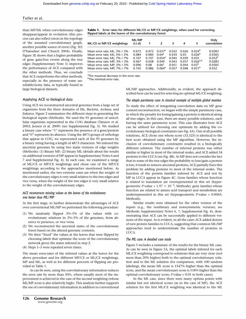
The simple parsimony case: A classical example of multiple global maxima

To study the effect of integrating coevolution data on MP gene

content reconstruction, we began with the simple parsimony case,

in which the penalty for losing/gaining a protein is identical along

all tree edges. In this case, there are many possible solutions, each

having the same parsimony score. This case illustrates how ACE

can be utilized for choosing one optimum by adding the co-

evolutionary biological constraints (see Fig. 4A). Out of all possible

solutions, ACE chose one whose score (33,525) is identical to the

best score obtained using the MP algorithm. However, the in-

clusion of coevolutionary constraints resulted in a biologically

different solution: The number of inferred proteins was either

similar or higher in most of the internal nodes, and ACE added 34

proteins to the LUCA (see Fig. 4B). As MP does not consider the fact

that in some of the tree edges the probability to lose/gain a protein

is low, it tends to remove ancestral proteins; ACE partially fixes this

problem by adding proteins to most of the internal nodes. The

function of the protein families inferred by ACE and not by

MP in LUCA appear in Figure 4C. Gene families whose function

is related to translation are overrepresented in this set (hyper-

geometric P-value = 1.97 3 10�5; Methods); gene families whose

function are related to amino acid transport and metabolism are

underrepresented in this set (hypergeometric P-value = 0.0065;

Methods).

Similar results were obtained for the other version of the

inputs (e.g., the nonbinary and nonsymmetric versions; see

Methods; Supplementary Notes 6, 7; Supplemental Fig. 4), dem-

onstrating that ACE can be successfully applied to different ver-

sions of the input. As is evident, in all the cases ACE added dozens

of new protein families to LUCA, suggesting that common ML/MP

approaches tend to underestimate the number of proteins in

LUCA.

The ML case: A detailed case study

Figure 5 includes a summary of the results for the binary ML case.

As can be seen in Figure 5A, the optimal labels inferred for each

ML/CE weighting correspond to solutions that are very close (not

more than 20% higher) both to the optimal coevolutionary solu-

tion and to the ML solution (for comparison, with 100 random

labelings, the mean ML score is 1547% higher than the optimal

score, and the mean coevolutionary score is 518% higher than the

optimal coevolutionary score; P-value < 0.01 in both cases).

In the ML case, since there were many optima points with

similar but not identical scores (as in the case of MP), the ACE

solution for the first ML/CE weighting was identical to the ML

Table 1. Error rates for different ML/CE or MP/CE weightings, when used for correctingflipped labels at the leaves of the coevolutionary forest

ML/CE or MP/CE weightingsML/MP(i.i.d) 1 2 3 4 5

Onlycoevolution

Mean error rate; ML; 3%33% 0.072 0.072 0.037a 0.032 0.026 0.024b 0.0283Mean error rate; ML; 5%35% 0.084 0.084 0.04a 0.034 0.03 0.026b 0.0305Mean error rate; ML; 7%37% 0.107 0.107 0.054a 0.045 0.039 0.035 0.032b

Mean error rate; MP; 3%33% 0.067 0.058 0.049 0.043 0.037 0.026a,b 0.0283Mean error rate; MP; 5%35% 0.096 0.08 0.06a 0.051 0.044 0.03b 0.0305Mean error rate; MP; 7%37% 0.105 0.086 0.064a 0.057 0.048 0.031b 0.032

aThe maximal decrease in the error rate.bThe minimal error rate.

Tuller et al.





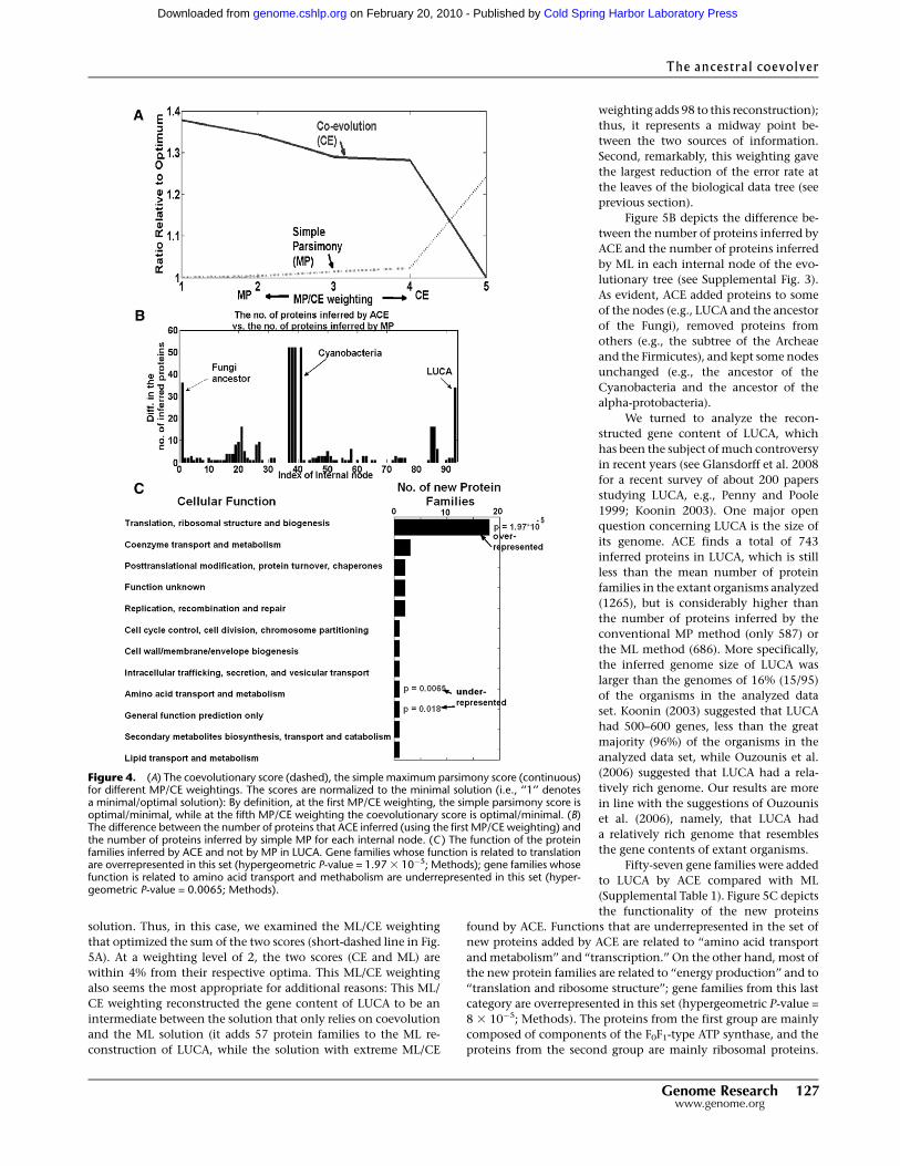
solution. Thus, in this case, we examined the ML/CE weighting

that optimized the sum of the two scores (short-dashed line in Fig.

5A). At a weighting level of 2, the two scores (CE and ML) are

within 4% from their respective optima. This ML/CE weighting

also seems the most appropriate for additional reasons: This ML/

CE weighting reconstructed the gene content of LUCA to be an

intermediate between the solution that only relies on coevolution

and the ML solution (it adds 57 protein families to the ML re-

construction of LUCA, while the solution with extreme ML/CE

weighting adds 98 to this reconstruction);

thus, it represents a midway point be-

tween the two sources of information.

Second, remarkably, this weighting gave

the largest reduction of the error rate at

the leaves of the biological data tree (see

previous section).

Figure 5B depicts the difference be-

tween the number of proteins inferred by

ACE and the number of proteins inferred

by ML in each internal node of the evo-

lutionary tree (see Supplemental Fig. 3).

As evident, ACE added proteins to some

of the nodes (e.g., LUCA and the ancestor

of the Fungi), removed proteins from

others (e.g., the subtree of the Archeae

and the Firmicutes), and kept some nodes

unchanged (e.g., the ancestor of the

Cyanobacteria and the ancestor of the

alpha-protobacteria).

We turned to analyze the recon-

structed gene content of LUCA, which

has been the subject of much controversy

in recent years (see Glansdorff et al. 2008

for a recent survey of about 200 papers

studying LUCA, e.g., Penny and Poole

1999; Koonin 2003). One major open

question concerning LUCA is the size of

its genome. ACE finds a total of 743

inferred proteins in LUCA, which is still

less than the mean number of protein

families in the extant organisms analyzed

(1265), but is considerably higher than

the number of proteins inferred by the

conventional MP method (only 587) or

the ML method (686). More specifically,

the inferred genome size of LUCA was

larger than the genomes of 16% (15/95)

of the organisms in the analyzed data

set. Koonin (2003) suggested that LUCA

had 500–600 genes, less than the great

majority (96%) of the organisms in the

analyzed data set, while Ouzounis et al.

(2006) suggested that LUCA had a rela-

tively rich genome. Our results are more

in line with the suggestions of Ouzounis

et al. (2006), namely, that LUCA had

a relatively rich genome that resembles

the gene contents of extant organisms.

Fifty-seven gene families were added

to LUCA by ACE compared with ML

(Supplemental Table 1). Figure 5C depicts

the functionality of the new proteins

found by ACE. Functions that are underrepresented in the set of

new proteins added by ACE are related to ‘‘amino acid transport

and metabolism’’ and ‘‘transcription.’’ On the other hand, most of

the new protein families are related to ‘‘energy production’’ and to

‘‘translation and ribosome structure’’; gene families from this last

category are overrepresented in this set (hypergeometric P-value =

8 3 10�5; Methods). The proteins from the first group are mainly

composed of components of the F0F1-type ATP synthase, and the

proteins from the second group are mainly ribosomal proteins.

Figure 4. (A) The coevolutionary score (dashed), the simple maximum parsimony score (continuous)for different MP/CE weightings. The scores are normalized to the minimal solution (i.e., ‘‘1’’ denotesa minimal/optimal solution): By definition, at the first MP/CE weighting, the simple parsimony score isoptimal/minimal, while at the fifth MP/CE weighting the coevolutionary score is optimal/minimal. (B)The difference between the number of proteins that ACE inferred (using the first MP/CE weighting) andthe number of proteins inferred by simple MP for each internal node. (C ) The function of the proteinfamilies inferred by ACE and not by MP in LUCA. Gene families whose function is related to translationare overrepresented in this set (hypergeometric P-value = 1.97 3 10�5; Methods); gene families whosefunction is related to amino acid transport and methabolism are underrepresented in this set (hyper-geometric P-value = 0.0065; Methods).






Interestingly, while F0F1-type ATP synthases are presently found

primarily in aerobic bacteria and mitochondria, they are believed

to be descended from ancient anaerobic enzymes, and thus their

antiquity is highly plausible (Cross and Muller 2004). Strikingly,

the additional ribosomal proteins that are conserved in extant

bacteria, but absent in archaea and eukaryotes, were inferred to be

encoded by LUCA. This may imply a bacterial-like LUCA from

which archaea later diverged (Gogarten et al. 1989; Iwabe et al.

1989), rather than a parallel emergence of the two prokaryotic

domains (Woese 1998). Furthermore, the

presence of the methionyl-tRNA for-

myltransferase in LUCA implies that

the bacterial-like ancestor already used

formyl-methionine to initiate transla-

tion, and that this formylation was sub-

sequently lost in Archaea and Eukarya as

their translation system diverged from

the bacterial one. Another interesting

observation is that the preprotein trans-

locase subunits SecF and SecD, which are

absent in some bacteria and nonessential

in others, (Wooldridge 2009) are pre-

dicted to be ancestral, as is the YidC

translocase subunit, which is involved in

integration of membrane proteins (Serek

et al. 2004).

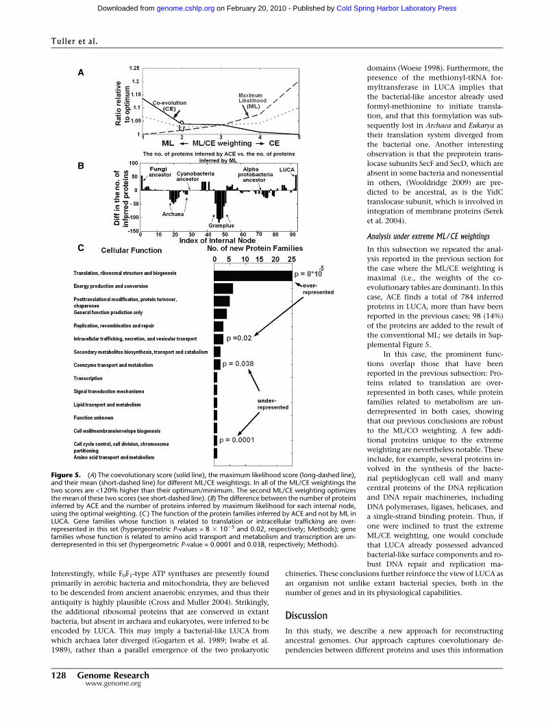
Analysis under extreme ML/CE weightings

In this subsection we repeated the anal-

ysis reported in the previous section for

the case where the ML/CE weighting is

maximal (i.e., the weights of the co-

evolutionary tables are dominant). In this

case, ACE finds a total of 784 inferred

proteins in LUCA, more than have been

reported in the previous cases; 98 (14%)

of the proteins are added to the result of

the conventional ML; see details in Sup-

plemental Figure 5.

In this case, the prominent func-

tions overlap those that have been

reported in the previous subsection: Pro-

teins related to translation are over-

represented in both cases, while protein

families related to metabolism are un-

derrepresented in both cases, showing

that our previous conclusions are robust

to the ML/CO weighting. A few addi-

tional proteins unique to the extreme

weighting are nevertheless notable. These

include, for example, several proteins in-

volved in the synthesis of the bacte-

rial peptidoglycan cell wall and many

central proteins of the DNA replication

and DNA repair machineries, including

DNA polymerases, ligases, helicases, and

a single-strand binding protein. Thus, if

one were inclined to trust the extreme

ML/CE weighting, one would conclude

that LUCA already possessed advanced

bacterial-like surface components and ro-

bust DNA repair and replication ma-

chineries. These conclusions further reinforce the view of LUCA as

an organism not unlike extant bacterial species, both in the

number of genes and in its physiological capabilities.

DiscussionIn this study, we describe a new approach for reconstructing

ancestral genomes. Our approach captures coevolutionary de-

pendencies between different proteins and uses this information

Figure 5. (A) The coevolutionary score (solid line), the maximum likelihood score (long-dashed line),and their mean (short-dashed line) for different ML/CE weightings. In all of the ML/CE weightings thetwo scores are <120% higher than their optimum/minimum. The second ML/CE weighting optimizesthe mean of these two scores (see short-dashed line). (B) The difference between the number of proteinsinferred by ACE and the number of proteins inferred by maximum likelihood for each internal node,using the optimal weighting. (C ) The function of the protein families inferred by ACE and not by ML inLUCA. Gene families whose function is related to translation or intracellular trafficking are over-represented in this set (hypergeometric P-values = 8 3 10�5 and 0.02, respectively; Methods); genefamilies whose function is related to amino acid transport and metabolism and transcription are un-derrepresented in this set (hypergeometric P-value = 0.0001 and 0.038, respectively; Methods).

Tuller et al.





to disambiguate the gene contents of the reconstructed ancestral

genomic contents. ACE is geared to tackle an inherent problem

that plagues the MP and ML approaches, whose solution space

tends to be populated with multiple maxima (e.g., see Fig. 1; Chor

et al. 2000). We demonstrate the superiority of the new approach

over existing methods in a simulated scenario where coevo-

lutionary information is available: Using ACE with biologically

plausible levels of coevolutionary information reduces the error

rate of the ancestral genome reconstruction by more than 50%.

When ACE was applied to the study of ancestral genomes, our

analysis showed that it can find solutions whose likelihood/par-

simony score is very similar or identical to the ML/MP scores.

These solutions, however, are often significantly different from the

ML/MP solutions and, since they incorporate coevolution data,

are more plausible from a biological standpoint. Accordingly, ACE

finds dozens of additional proteins in LUCA, many of which are

ribosomal proteins or part of the ATP synthase, complexes that are

essential for life.

Our coevolution-based approach is presented here in the

framework of ancestral genome reconstruction due to its impor-

tance for evolutionary biology and because coevolutionary in-

formation can be readily obtained at the gene/protein level.

However, its potential scope goes far beyond inferring ancestral

gene content: ACE can be used to tackle any general problem of

ancestral sequence reconstruction, including the reconstruction of

different sites or domains in proteins, or the reconstruction of

individual sites in DNA or RNA sequences (see Noller and Woese

1981; Gutell et al. 1986; Knudsen and Hein 1999; Lockless and

Ranganathan 1999; Pedersen et al. 2006; Yeang and Haussler 2007;

Yeang et al. 2007). The success of such future applications depends

on the existence of reliable coevolutionary information at the

position/site level. Coevolution information may be obtained

from proximity in the three-dimensional structure of the protein

itself, from information on coevolution of amino acids sharing

specific binding site(s) or information about binding sites shared

between interacting proteins. Finally, as already partially demon-

strated here, the ACE approach can be generalized in the future

to more complex reconstruction models, e.g., using nonbinary

alphabets, dependency between adjacent sites, and various prob-

abilistic models (Akerborg et al. 2009).

Additionally, we intend to design algorithms (e.g., algorithms

that are based on the belief propagation approach) that may im-

prove the accuracy and running time of the basic ACE algorithm

described in this work.

Methods

Coevolutionary informationThe coevolutionary edges used here were gathered from threesources of information: (1) Proximity in the protein interactionnetwork of E. coli and S. cerevisiae (for example, Wu et al. [2003],Sato et al. [2005], and Juan et al. [2008] reported a relation betweencoevolution and protein interactions). (2) Proximity in the meta-bolic networks of the analyzed organisms (for example, Spirin et al.[2006] and Zhao et al. [2007] reported the relation between co-evolution and proximity in metabolic networks). (3) Variousphysical and functional interactions that were downloaded fromString (Jensen et al. 2009) (http://string.embl.de/; for example,Chen and Dokholyan [2006] and Tuller et al. [2009] reported therelation between coevolution and similar functionality).

A coevolutionary edge was added to the model if the follow-ing two conditions were satisfied: (1) The corresponding pair of

orthologs physically or functionally interact according to the threesources of information described above (see more details below).(2) The two orthologs exhibit a pattern of co-occurrence that issignificantly different from random in the genome of the organ-isms studied (in our case, the ratio between the highest and lowestprobability in the co-occurrence distribution table is at least 4.25).The initial set of coevolutionary edges included more than 70,000edges, and after the filtering it included 10,000 edges.

The weights in the tables of the coevolutionary edges werecomputed according to the co-occurrence probabilities of thecorresponding pairs of proteins.

The following subsections include more details about thethree sources of coevolutionary information used in this work.

The protein interaction networks of S. cerevisiae and E. coli

The protein interaction network of S. cerevisiae was obtained fromrecently published manuscripts (Gavin et al. 2006; Krogan et al.2006; Reguly et al. 2006) and from public databases (Xenarios et al.2002; Christie et al. 2004). High-throughput mass spectrometrydata (Gavin et al. 2006; Krogan et al. 2006) was translated intobinary protein–protein interactions using the spoke model (Baderand Hogue 2002). The final yeast protein–protein network in-cluded 39,396 interactions. The E. coli network was generatedbased on Mori et al. (2000), Xenarios et al. (2002), and Arifuzzamanet al. (2006). The final E. coli protein–protein network included16,756 interactions. As coevolutionary edges, we only considerededges that appeared in the two protein interaction networks. E. coliand S. cerevisiae are the only organisms in our data set whose PPInetworks have been reconstructed on a large scale. These in-teractions were mapped to the corresponding COGs by mapping toE. coli genes. In the final set of coevolutionary edges, 256 werebased on this source of information.

The metabolic networks of the organisms analyzed

We used the representation of Ma and Zeng (2003) for constructingthe metabolic networks, i.e., two enzymes are connected with anedge if they catalyze successive (or the same) steps in a metabolicpathway (see the Introduction for the motivation for using adja-cency as evidence for coevolution). Each metabolic network wasreconstructed by the following stages: First we parsed all datapertaining reactions, compounds, and enzymes from KEGG release46 (Kanehisa 2002) and created a list of the existing enzymes ineach species in our collection, the reactions they catalyze, the re-action products and substrates, and their directionality.

The metabolic network of each organism was generated fromits list of enzymes as follows: Each enzyme is represented as a nodein the network. Let E1 = [e11, e11,.., e1n] denote the set of enzymesthat catalyze reaction R1, and E2 = [e21, e21,.., e2n] denote the set ofenzymes that catalyze reaction R2. If a product of R1 is a substrateof R2, then undirected edges are assigned between all nodes of E1and all nodes of E2. Edges are also assigned within E1 nodes andwithin E2 nodes. As coevolutionary edges, we considered enzymesthat are connected in at least 10% of the metabolic networks inKEGG that are larger than 50% of the E. coli’s metabolic network.The set of enzymes were mapped to COG groups by mapping to E.coli and S. cerevisiae genes (these data were downloaded fromKEGG) (Kanehisa 2002). In the final set of coevolutionary edges,250 were based on this source of information.

Other types of cofunctionality (the String database)

As an additional source of coevolutionary edges we used in-formation downloaded from the String database ( Jensen et al.






2009). This database includes various sources of coevolutionary/functional relations that are different from the two types of in-formation mentioned above. Specifically, it includes informa-tion on genomic neighborhood, coexpression, gene fusion, coex-pression, and more. Each coevolutionary relation in this data setwas based on a composite score that is a weighted average of thesesources of information (more details about the different compo-nent of a score were not available). Most of the edges (98%) in thefinal file set of coevolutionary edges were based on this source ofinformation.

The phylogenetic tree

The phylogenetic tree is based on the following sources of infor-mation. The subtree related to alpha-proteobacteria was down-loaded from Boussau et al. (2004). The subtree related to Cyano-bacteria was downloaded from Shi and Falkowski (2008). Thesubtree related to fungi was downloaded from Wapinski et al.(2007). The reconstruction of other parts of the tree and themerging of all these trees were based on maximum likelihood(Dagan and Martin 2007) and iTOL (Letunic and Bork 2007). Thefinal phylogenetic tree included 95 organisms from the three do-mains of life: eukaryotes (18 organisms), prokaryotes (65 organisms),and archaea (12 organisms). The list of organism names and theirtaxa i.d. appear in Supplemental Table 2.

We used Neyman’s two-state model (Neyman 1971), a versionof Jukes Cantor ( JC) model ( Jukes and Cantor 1969) for inferringthe edge lengths of the tree by maximum likelihood. This was doneby PAML (Yang 1997). These edge lengths correspond to theprobabilities that a protein family will appear/vanish along thecorresponding lineage.

Clusters of orthologs

Clusters of orthologs were gathered from various sources. COGmapping to most of the organisms (83 out of 95) were downloadedfrom the String database (Jensen et al. 2009). Some of the fungi andthe cyanobacteria (see Supplemental Table 2) do not appear in theString database; the clusters in the missing fungi were generated inthe following way: (1) We downloaded the data set of fungalclusters of orthologs from Wapinski et al. (2007) and the cluster ofcyanobacterial orthologs from Shi and Falkowski (2008). (2) Weconsidered the fungi/cyanobacteria that appear in the COG dataset and mapped each fungal/cyanobacterial cluster to the COGthat has at least 90% overlap with it. (3) After the mapping, wereconstructed ortholog clusters in the organism that are missing inCOG from their corresponding cluster in the fungal/cyanobacte-rial data set. The smallest genome (M. genitalium) in the analyzeddata set included 393 genes (sum of copy numbers from each COGfamily), while the largest genome (B. japonicum) included 6162genes (Supplemental Table 3 includes the COGs distributions in allthe analyzed genomes).

Annotation of ancestral proteins and enrichment P-values

The annotation of ancestral proteins was based on COG annota-tions (Tatusov et al. 2003) and the Gene Ontology (GO) annota-tions of S. cerevisiae and E. coli (http://www.geneontology.org/index.shtml).

Enrichment P-values for the proteins that were added by theACE were computed according to the COG annotations. For eachfunction, we computed an hypergeometric P-value based on thetotal number of COG families that have this function in LUCA, thetotal number of COG families added by the ACE, and the numberof COG families with this function that were added by the ACE.

The ancestral coevolver (ACE) algorithm

The input to ACE is a set of phylogenetic trees (a tree for each

protein) with the same topology and with coevolutionary edges

between pairs of internal nodes of the trees (corresponding to pairs

of protein that coevolve). ACE has three main steps (Fig. 2; Sup-

plemental Fig. 1): (1) By removing some of the coevolutionary

edges, the input (set of trees and edges between them) is parti-

tioned into smaller groups of trees such that there are edges only

between pairs of trees that are in the same group. (2) Optimal labels

(not considering the removed edges) are assigned to the internal

nodes of each of these smaller coevolutionary forests by an algo-

rithm that is a generalization of algorithms for finding ancestral

states by maximum likelihood or maximum parsimony (Fitch

1971; Sankoff 1975; Pupko et al. 2000); in total, these labels are

an approximate solution for the input coevolutionary forest. (3)

Finally, the solution is further improved in a greedy manner.We begin by briefly describing stage 2 of the algorithm and

then explain why stage 1 is necessary. Similarly to many algorithms

for computing the optimal labels of internal tree nodes (by MP or

ML criterion) (Fitch 1971; Sankoff 1975; Pupko et al. 2000), our al-

gorithm has two phases: In the first phase, it traverses the coevo-

lutionary forest from the leaves to the root; in the second phase,

it traverses the coevolutionary forest from the root to the leaves.However, our algorithm is performed jointly for all the trees in

each connected component.Let e = (i, j ) denote a coevolutionary edge or a tree edge. Let

Wce;ða;bÞ = Wc

ði;jÞ;ða;bÞ denote the cost corresponding to assigning

a at node i, and b at node j where (i, j) is a coevolutionary edge.

Similarly, if e = (i, j ) is a tree edge, we use Wbe;ða;bÞ = Wb

ði;jÞ;ða;bÞ to de-

note the cost of assigning a and b at the two nodes of e.Let S�xð�vÞ denote the optimal cost (the minimal sum of

weights) of the sub-coevolutionary forest that corresponds to the

coevolutionary subforest whose roots are �v, such that all the nodes

in such a vector of roots correspond to the same ancestral organism

in the phylogenetic trees, and when assigning �x in these roots.

For example, consider Figure 1, the optimal cost when consider-

ing the coevolutionary forest whose roots are �v = ½x1; y1�, and

when assigning �x = ½1;1� in these roots is 0.51 (due to the co-

evolutionary edge).In the first phase, the algorithm traverses the coevolutionary

forest from the leaves to the root and computes the cost S�xð�vÞ for

each set of internal nodes, �v, such that all of these nodes corre-

spond to the same ancestral organism in all of the phylogenetic

trees, after the costs of the two sets of internal nodes that are de-

scendant of �v were computed (see Supplemental Fig. 1 B; Supple-

mentary Note 1). In the second phase, the algorithm traverses the

subforest from the roots to the leaves, and chooses optimal labels

for each set of internal nodes, given the optimal labels of its cor-

responding set of parents (see Supplemental Fig. 1B; Supplemen-

tary Note 1).As the running time of the algorithm is exponential with the

size of the coevolutionary forest, the algorithm has an initial stage

(stage 1), where the input graph is partitioned into small enough

connected components. The algorithm used at this stage, Partite,

recursively clusters the trees to groups according to the edge

weights between them (thus minimizing the number of edges

between different clusters), such that the number of trees in each

cluster is small enough (less than a predetermined parameter K;

Supplemental Fig. 1C; Supplementary Note 8). We used hierar-

chical k-means (MacQueen 1967) for clustering (but obviously

other clustering algorithms can be used too).The input to the Partite algorithm is a weighted graph whose

edges correspond to the edges in the coevolutionary graph. The

weights of the graph edges can be any measure that represents that

Tuller et al.





strength of the coevolution between the corresponding proteins(trees/subtrees) in a certain part of the evolution. We used the ratiobetween the maximal and the minimal values of the edges in theweight tables. The clustering parameter K induces a trade-off be-tween accuracy and speed: larger maximal cluster/subgraph (K)increases the running time, but also increases the accuracy of thesolution.

The final stage of the ancestral coevolver algorithm is a greedystage (Supplemental Fig. 1F; Supplementary Note 1). In each stepof the greedy algorithm, it considers all of the edges; then, itchooses an edge (tree edge or coevolutionary edge) and new labelsto its ends in a way that gives improvement of the cost of the co-evolutionary forest. In each step, the new labels are updated; thealgorithm stops when it does not find new labels that improve thecost of the coevolutionary forest.

The total running time of the algorithm is exponential withthe size of the largest connected component, but behaves quitelinearly with the other parameters (including the number of trees).For detailed explanations see Supplementary Note 1. The typicalrunning time for an input with several hundred trees and largestconnected component of size eight trees is up to a few minutes. Forinputs with several thousand trees and largest connected compo-nent of size 9, the running time is a few hours. So, as long as onetakes care to partition the coevolutionary graph to connectedcomponents of sufficiently small size in the preprocessing phase(which can always be done by a corresponding choice of a clus-tering algorithm), the algorithm can be run within a reasonabletime frame.

The models of evolution used in the analysisof the biological inputs

We checked several models for the weights of the tree edges. In thebinary parsimony case, there are two possible states for eachcharacter (i.e., for each COG): ‘‘0’’ denotes that the COG is notencoded in a genome, and ‘‘1’’ denotes that the COG is encoded inthe genome. The penalty to switch from ‘‘1’’ to ‘‘0’’ and vice versa isidentical (e.g., 1) in all the branches.

In the binary likelihood case, as in the binary parsimony case,there are two similar possible characters for each state (COG).However, in this case, each tree edge, (a, b), has a different length(gain/loss probability, pa,b) that induces a different weight table(see the previous section about how pa,b can be computed). Thepenalty (the corresponding entry in the weight matrix) fora change from ‘‘0’’ to ‘‘1’’ or vice versa, in this case, is �log(pa,b); ifthere is no change, the cost is �log(1�pa,b). These models appearin the main text. We decided to use models where the penalty forgain or loss of a gene is identical following the work of Mirkin et al.(2003), who showed that this is the most reasonable/suitablepenalty in our context.

We also checked additional models whose results are reportedin Supplemental Figure 4 and Supplementary Notes 6 and 7: In thenonbinary parsimony case, there are a few possible states for eachcharacter (COG). Each state is a positive integer that denotes thenumber of genes from a COG in a certain genome (note that only6% of the states in the analyzed biological input are larger than‘‘1’’). Let Cx denote the number of genes from a COG C in node x. Inthe symmetric nonbinary case, the penalty for a change in thenumber of genes corresponding to a COG C along the tree edge(a, b) is �log(pa,b)*|Ca�Cb|. In the nonbinary nonsymmetric case,the penalty for losing a gene from a COG C along the tree edge(a, b) where a is the ancestor of b is �2log(pa,b)*|Ca�Cb|, while thepenalty for gaining a COG is �log(pa,b)*|Ca�Cb|.

In the nonbinary cases, we use binary coevolutionary edgeweight tables (Cx > 0 or Cx = 0). This was done for two main reasons:

(1) The coevolution between a pair of COGs usually corresponds tothe relation(s) between any protein from one COG to any proteinfrom the other COG. (2) Considering the limited number of ana-lyzed organisms, a too-large coevolutionary table would includetoo many parameters (weights) that need to be estimated.

Weighting of the edge weights in the analysisof the biological inputs

In the biological analysis, we checked five specific values of theML/CE weighting and MP/CE weighting. These values are de-scribed in Supplementary Note 2.

AcknowledgmentsT.T. was supported by the Edmond J. Safra Bioinformatics programat Tel Aviv University and by the Yeshaya Horowitz Associationthrough the Center for Complexity Science, and is currentlya Koshland Scholar at the Weizmann Institute. U.G., M.K., and E.R.are supported by the James S. McDonnell Foundation. U.G. is alsosupported by the Bi-national Science Foundation. M.K. and E.R.were also supported by grants from the Israel Science Foundationand the Israeli Ministry of Science and Technology (M.K.).

References

Akerborg O, Sennblad B, Arvestad L, Lagergren J. 2009. SimultaneousBayesian gene tree reconstruction and reconciliation analysis. Proc NatlAcad Sci 106: 5714–5719.

Arifuzzaman M, Maeda M, Itoh A, Nishikata K, Takita C, Saito R, Ara T,Nakahigashi K, Huang HC, Hirai A, et al. 2006. Large-scale identificationof protein–protein interaction of Escherichia coli K-12. Genome Res 16:686–691.

Bader GD, Hogue CW. 2002. Analyzing yeast protein-protein interactiondata obtained from different sources. Nat Biotechnol 20: 991–997.

Barker D, Meade A, Pagel M. 2007. Constrained models of evolution lead toimproved prediction of functional linkage from correlated gain and lossof genes. Bioinformatics 23: 14–20.

Barry D, Hartigan J. 1987. Statistical analysis of humanoid molecularevolution. Stat Sci 2: 191–210.

Blanchette M, Green ED, Miller W, Haussler D. 2004. Reconstructing largeregions of an ancestral mammalian genome in silico. Genome Res 14:2412–2423.

Boussau B, Karlberg EO, Frank AC, Legault BA, Andersson SG. 2004.Computational inference of scenarios for alpha-proteobacterial genomeevolution. Proc Natl Acad Sci 101: 9722–9727.

Chen Y, Dokholyan NV. 2006. The coordinated evolution of yeast proteins isconstrained by functional modularity. Trends Genet 22: 416–419.

Chor B, Hendy MD, Holland BR, Penny D. 2000. Multiple maxima oflikelihood in phylogenetic trees: An analytic approach. Mol Biol Evol 17:1529–1541.

Christie KR, Weng S, Balakrishnan R, Costanzo MC, Dolinski K, Dwight SS,Engel SR, Feierbach B, Fisk DG, Hirschman JE, et al. 2004. SaccharomycesGenome Database (SGD) provides tools to identify and analyzesequences from Saccharomyces cerevisiae and related sequences fromother organisms. Nucleic Acids Res 32: D311–D314.

Cross RL, Muller V. 2004. The evolution of A-, F-, and V-type ATP synthasesand ATPases: Reversals in function and changes in the H+/ATP couplingratio. FEBS Lett 576: 1–4.

D’haeseleer P, Church GM. 2004. Estimating and improving proteininteraction error rates. Proc IEEE Comput Syst Bioinform Conf 2004: 216–223.

Dagan T, Martin W. 2007. Ancestral genome sizes specify the minimum rateof lateral gene transfer during prokaryote evolution. Proc Natl Acad Sci104: 870–875.

Elias I, Tuller T. 2007. Reconstruction of ancestral genomic sequences usinglikelihood. J Comput Biol 14: 216–237.

Felder Y, Tuller T. 2008. Discovering local patterns of co-evolution. InRECOMB-CG, (ed. CE Nelson, S Vialette) pp. 55–71. Springer-Verlag,Heidelberg, Germany.

Felsenstein J. 1993. PHYLIP (phylogeny inference package) version 3.5c.Distributed by the author. Department of Genetics, University ofWashington, Seattle, WA.

Fitch WM. 1971. Toward defining the course of evolution: Minimumchange for a specified tree topology. Syst Zool 20: 406–416.






Gavin AC, Aloy P, Grandi P, Krause R, Boesche M, Marzioch M, Rau C, JensenLJ, Bastuck S, Dumpelfeld B, et al. 2006. Proteome survey revealsmodularity of the yeast cell machinery. Nature 440: 631–636.

Glansdorff N, Xu Y, Labedan B. 2008. The last universal common ancestor:Emergence, constitution and genetic legacy of an elusive forerunner.Biol Direct 3: 29. doi: 10.1186/1745-6150-3-29.

Gogarten JP, Kibak H, Dittrich P, Taiz L, Bowman EJ, Bowman BJ, ManolsonMF, Poole RJ, Date T, Oshima T, et al. 1989. Evolution of the vacuolarH+-ATPase: Implications for the origin of eukaryotes. Proc Natl Acad Sci86: 6661–6665.

Gutell RR, Noller HF, Woese CR. 1986. Higher order structure in ribosomalRNA. EMBO J 5: 1111–1113.

Hirsh E, Sharan R. 2007. Identification of conserved protein complexesbased on a model of protein network evolution. Bioinformatics 23: e170–e176.

Iwabe N, Kuma K, Hasegawa M, Osawa S, Miyata T. 1989. Evolutionaryrelationship of archaebacteria, eubacteria, and eukaryotes inferred fromphylogenetic trees of duplicated genes. Proc Natl Acad Sci 86: 9355–9359.

Jensen LJ, Kuhn M, Stark M, Chaffron S, Creevey C, Muller J, Doerks T, JulienP, Roth A, Simonovic M, et al. 2009. STRING 8—a global view onproteins and their functional interactions in 630 organisms. NucleicAcids Res 37: D412–D416.

Juan D, Pazos F, Valencia A. 2008. High-confidence prediction of globalinteractomes based on genome-wide coevolutionary networks. Proc NatlAcad Sci 105: 934–939.

Jukes TH, Cantor CR. 1969. Evolution of protein molecules. In Mammalianprotein metabolism (ed. HN Munro), pp. 21–123. Academic Press, NewYork.

Kanehisa M. 2002. The KEGG database. Novartis Found Symp 247: 91–101.Knudsen B, Hein J. 1999. RNA secondary structure prediction using

stochastic context-free grammars and evolutionary history.Bioinformatics 15: 446–454.

Koonin EV. 2003. Comparative genomics, minimal gene-sets and the lastuniversal common ancestor. Nat Rev Microbiol 1: 127–136.

Krishnan NM, Seligmann H, Stewart C, Koning APJ, Pollock DD. 2004.Ancestral sequence reconstruction in primate mitochondrial DNA:Compositional bias and effect on functional inference. Mol Biol Evol 21:1871–1883.

Krogan NJ, Cagney G, Yu H, Zhong G, Guo X, Ignatchenko A, Li J, Pu S,Datta N, Tikuisis AP, et al. 2006. Global landscape of protein complexesin the yeast Saccharomyces cerevisiae. Nature 440: 637–643.

Lee I, Date SV, Adai AT, Marcotte EM. 2004. A probabilistic functionalnetwork of yeast genes. Science 306: 1555–1558.

Letunic I, Bork P. 2007. Interactive Tree Of Life (iTOL): An online tool forphylogenetic tree display and annotation. Bioinformatics 23: 127–128.

Li G, Steel M, Zhang L. 2008. More taxa are not necessarily better for thereconstruction of ancestral character states. Syst Biol 57: 647–653.

Liang Z, Xu M, Teng M, Niu L. 2006. Comparison of protein interactionnetworks reveals species conservation and divergence. BMCBioinformatics 7: 457. doi: 10.1186/1471-2105-7-457.

Lockless SW, Ranganathan R. 1999. Evolutionarily conserved pathways ofenergetic connectivity in protein families. Science 286: 295–299.

Ma H, Zeng AP. 2003. Reconstruction of metabolic networks from genomedata and analysis of their global structure for various organisms.Bioinformatics 19: 270–277.

Ma J, Zhang L, Suh BB, Raney BJ, Burhans RC, Kent WJ, Blanchette M,Haussler D, Miller W. 2006. Reconstructing contiguous regions of anancestral genome. Genome Res 16: 1557–1565.

MacQueen JB. 1967. Some methods for classification and analysis ofmultivariate observations. In Proceedings of the 5th Berkeley Symposium onMathematical Statistics and Probability, pp. 281–297. University ofCalifornia Press, Berkeley, CA.

Marino-Ramirez L, Bodenreider O, Kantz N, Jordan IK. 2006. Co-evolutionary rates of functionally related yeast genes. Evol BioinformOnline 2: 295–300.

Mirkin BG, Fenner TI, Galperin MY, Koonin EV. 2003. Algorithms forcomputing parsimonious evolutionary scenarios for genome evolution,the last universal common ancestor and dominance of horizontal genetransfer in the evolution of prokaryotes. BMC Evol Biol 3: 2. doi: 10.1186/1471-2148-3-2.

Mori H, Isono K, Horiuchi T, Miki T. 2000. Functional genomics ofEscherichia coli in Japan. Res Microbiol 151: 121–128.

Neyman J. 1971. Molecular studies of evolution: A source of novel statisticalproblems. In Statistical decision theory and related topics (ed. S Gupta, YJackel), pp. 1–27. Academic Press, New York.

Noller HF, Woese CR. 1981. Secondary structure of 16S ribosomal RNA.Science 212: 403–411.

Ouzounis CA, Kunin V, Darzentas N, Goldovsky L. 2006. A minimalestimate for the gene content of the last universal commonancestor—exobiology from a terrestrial perspective. Res Microbiol 157:57–68.

Pagel M. 1999. The maximum likelihood approach to reconstructingancestral character states of discerete characters on phylogenies. Syst Biol48: 612–622.

Pazos F, Helmer-Citterich M, Ausiello G, Valencia A. 1997. Correlatedmutations contain information about protein–protein interaction. J MolBiol 271: 511–523.

Pedersen JS, Bejerano G, Siepel A, Rosenbloom K, Lindblad-Toh K, LanderES, Kent J, Miller W, Haussler D. 2006. Identification and classification ofconserved RNA secondary structures in the human genome. PLoSComput Biol 2: e33. doi: 10.1371/journal.pcbi.0020033.

Penny D, Poole A. 1999. The nature of the last universal common ancestor.Curr Opin Genet Dev 9: 672–677.

Pupko T, Pe’er I, Shamir R, Graur D. 2000. A fast algorithm for jointreconstruction of ancestral amino acid sequences. Mol Biol Evol 17: 890–896.

Putnam NH, Srivastava M, Hellsten U, Dirks B, Chapman J, Salamov A, TerryA, Shapiro H, Lindquist E, Kapitonov VV, et al. 2007. Sea anemonegenome reveals ancestral eumetazoan gene repertoire and genomicorganization. Science 317: 86–94.

Reguly T, Breitkreutz A, Boucher L, Breitkreutz BJ, Hon GC, Myers CL,Parsons A, Friesen H, Oughtred R, Tong A, et al. 2006. Comprehensivecuration and analysis of global interaction networks in Saccharomycescerevisiae. J Biol 5: 11. doi: 10.1186/jbiol36.

Sankoff D. 1975. Minimal mutation trees of sequences. SIAM J Appl Math 28:35–42.

Sato T, Yamanishi Y, Kanehisa M, Toh H. 2005. The inference of protein–protein interactions by co-evolutionary analysis is improved byexcluding the information about the phylogenetic relationships.Bioinformatics 21: 3482–3489.

Serek J, Bauer-Manz G, Struhalla G, van den Berg L, Kiefer D, Dalbey R,Kuhn A. 2004. Escherichia coli YidC is a membrane insertase forSec-independent proteins. EMBO J 23: 294–301.

Shi T, Falkowski PG. 2008. Genome evolution in cyanobacteria: The stablecore and the variable shell. Proc Natl Acad Sci 105: 2510–2515.

Spirin V, Gelfand MS, Mironov AA, Mirny LA. 2006. A metabolic network inthe evolutionary context: Multiscale structure and modularity. Proc NatlAcad Sci 103: 8774–8779.

Swofford DL. 2002. PAUP*. Phylogenetic analysis using parsimony (*and othermethods). Sinauer Associates, Sunderland, MA.

Tatusov RL, Fedorova ND, Jackson JD, Jacobs AR, Kiryutin B, Koonin EV,Krylov DM, Mazumder R, Mekhedov SL, Nikolskaya AN, et al. 2003. TheCOG database: An updated version includes eukaryotes. BMCBioinformatics 4: 41. doi: 10.1186/1471-2105-4-41.

Tuller T, Kupiec M, Ruppin E. 2009. Co-evolutionary networks of genes andcellular processes across fungal species. Genome Biol 10: R48. doi:10.1186/gb-2009-10-5-r48.

Wapinski I, Pfeffer A, Friedman N, Regev A. 2007. Natural history andevolutionary principles of gene duplication in fungi. Nature 449:54–61.

Woese C. 1998. The universal ancestor. Proc Natl Acad Sci 95: 6854–6859.Wooldridge K. 2009. Bacterial secreted proteins: Secretory mechanisms and role

in pathogenesis. Caister Academic Press, Norfolk, UK.Wu J, Kasif S, DeLisi C. 2003. Identification of functional links between

genes using phylogenetic profiles. Bioinformatics 19: 1524–1530.Xenarios I, Salwinski L, Duan XJ, Higney P, Kim SM, Eisenberg D. 2002.

DIP, the Database of Interacting Proteins: A research tool for studyingcellular networks of protein interactions. Nucleic Acids Res 30: 303–305.

Yang Z. 1997. PAML: A program package for phylogenetic analysis bymaximum likelihood. Comput Appl Biosci 13: 555–556.

Yang Z, Kumar S, Nei M. 1995. A new method of inference of ancestralnucleotide and amino acid sequences. Genetics 141: 1641–1650.

Yeang CH, Haussler D. 2007. Detecting coevolution in and among proteindomains. PLoS Comput Biol 3: e211. doi: 10.1371/journal.pcbi.0030211.

Yeang CH, Darot JF, Noller HF, Haussler D. 2007. Detecting the coevolutionof biosequences–an example of RNA interaction prediction. Mol Biol Evol24: 2119–2131.

Zhao J, Ding GH, Tao L, Yu H, Yu ZH, Luo JH, Cao ZW, Li YX. 2007. Modularco-evolution of metabolic networks. BMC Bioinformatics 8: 311 10.1186/1471-2105-8-311.

Received May 20, 2009; accepted in revised form October 5, 2009.

Tuller et al.





reconstructing ancestral gene content by coevolution

Documents