reconstructing 2d images with natural neighbour interpolation

1 Introduction

Reconstructing 2D imageswith natural neighbourinterpolation

François Anton1,2, Darka Mioc3,Alain Fournier1

1 Department of Computer Science, University ofBritish Columbia, 203-2366 Main Mall, Vancouver,BC, V6T 1Z4, Canadae-mail: [email protected] Projet Prisme, INRIA Sophia Antipolis, B.P. 93,06902 Sophia Antipolis Cedex, France3 Département des Sciences Géomatiques, UniversitéLaval, Pavillon Casault, Ste-Foy, QC, G1K 7P4,Canadae-mail: [email protected]

In this paper, we explore image reconstruc-tion by natural neighbour interpolation fromirregularly spaced samples. We sample theimage irregularly with techniques based onthe Laplacian or the derivative in the direc-tion of the gradient. Local coordinates basedon the Voronoi diagram are used in natu-ral neighbour interpolation to quantify the“neighbourliness” of data sites. Then we usenatural neighbour interpolation in order toreconstruct the image. The main result is thatthe image quality is always very good in thecase of the sampling techniques based on theLaplacian.

Key words: Image reconstruction – Irregu-larly spaced samples – Natural neighbour in-terpolation – Local coordinates

Correspondence to: F. Anton

In this paper, we explore image reconstruction bynatural neighbour interpolation. This implies sam-pling the image irregularly, and then applying thenatural neighbour interpolation. In our case, the in-terpolant is the level of gray, since we will applysampling and reconstruction on black and white im-ages. Spatial interpolation has been used in computergraphics, in order to generate intermediate imagesin animation [also called “inbetweening”, see (Foleyet al. 1990)], or in 3D visual model reconstruction(Kuo and Chen 1998), or in order to reconstruct ra-diosity over a patch (Hinkenjann 1998). In spatialinterpolation, local techniques have been used in or-der to get an interpolation that is continuous at datapoints and smooth around the data points. In theselocal techniques, the data points that influence theinterpolant are the ones neighbouring the given in-terpolation point. The interpolation is thus based onthe definition of adjacency or of neighbourliness. Inone dimension, the neighbourliness is given by thenatural topology of the real line, induced by its to-tal order. In two dimensions, there is no such rela-tionship, and the neighbourliness can be defined bysome topological structure. Such structures includethe Delaunay triangulation, that is, the dual of theVoronoi diagram. The Delaunay triangulation hasbeen extensively used in linear interpolation [whichcorresponds to convolving with the triangle or Bar-lett filter (Foley et al. 1990)]. Another local tech-nique is the natural neighbour interpolation (Sibson1981) based on local coordinates (Sibson 1980).These local coordinates were introduced by Sibson(1980). Local coordinates based on the Voronoi di-agram are used in natural neighbour interpolation[also studied by Gold and Roos (1994) as “stolenarea” interpolation], to quantify the “neighbourli-ness” of data sites. The properties of these local co-ordinates have been extensively studied by Sibson(1980) and Piper (1993). Farin (1990) gave a for-mula for the gradient of the volume stolen fromneighbouring Voronoi regions due to the insertion ofa query point, obtained from two directional deriva-tives. The natural neighbour or stolen area interpo-lation technique has been extended from ordinaryVoronoi diagrams to Voronoi diagrams for sets ofpoints and line segments in Anton et al. (1998). An-ton et al. (1998) extend the results presented by Goldand Roos (1994) by providing direct vectorial for-mulas for the first-order and second-order derivativesfor the stolen area. The analysis presented by Antonet al. (1998) generalizes the analysis of Piper (1993)

The Visual Computer (2001) 17:134–146c© Springer-Verlag 2001

F. Anton: Reconstructing 2D images with natural neighbour interpolation 135

based on the formalism of partial derivatives, to theformalism of derivatives of a function on a normedspace.In Sect. 2, we present three techniques to sampleirregularly an image. In Sect. 3, we present the nat-ural neighbour interpolation technique. In Sect. 4,we present the image reconstruction algorithm thatuses the natural neighbour interpolation technique.Finally, in Sect. 5, we present the experimental re-sults of the 2D image reconstruction.

2 The irregular sampling

Different kinds of irregular sampling techniquescan be used: irregular point sampling, irregular areasampling (unweighted and weighted), importancesampling, stochastic sampling, or adaptive stochas-tic sampling (Foley et al. 1990). Since the derivativeof the natural neighbour interpolant that we use forreconstruction is continuous except at data points,it is best to select data points where the variationof the intensity (the quantity to be reconstructed) isgreatest, therefore the edges in the image. A wide va-riety of edge detection algorithms exist, but the setof basic tools on which the most general algorithmsare built is reduced to differencing: the derivativein the gradient direction, the Laplacian, the direc-tional derivatives and the statistical differencing. Weused two edge detection algorithms based on theLaplacian, and one edge detection algorithm basedon the derivative in the direction of the gradient,in order to get samples around the high-frequencychanges in the image. We now present the threeedge detection algorithms that we have used forsampling.The gradient is the first-order differential of the in-terpolant at the point. The derivative in the direc-tion of the gradient gives the greatest variation ofthe interpolant (in our case the level of gray) at thepoint. This derivative in the direction of the gradi-ent equals the greatest magnitude of the derivative,i.e. the square root of the sum of the squares ofthe derivatives in any pair of orthogonal directions,

e.g.

[(∂ f∂x

)2 +(

∂ f∂y

)2] 1

2

(Rosenfeld 1969). This is

a well-behaved function used in image sharpeningand edge detection, e.g. in the Prewitt and Sobel edgedetectors (Ritter 1996). In the gradient-based sam-pling that we used, we took the square root of thesum of the square of the difference between the three

neighbours from the row above and the neighbouringpixels from the row below the pixel, and the square ofthe difference between the neighbouring pixels in theleft column and the three neighbours on the right ofthe pixel.

The Laplacian(∇2 f = ∂2 f

∂x2 + ∂2 f∂y2

)is proportional

to the variation of the derivative of the interpolantat the point with respect to an annulus centeredat the point. We used two different computationsfor the Laplacian, the standard Laplacian, and analternative Laplacian where the “annulus” is com-posed of eight pixels instead of four. In this al-ternative Laplacian, a 1√

2factor is used to com-

pensate for the wider diagonal pixel separation.These two Laplacian-based sampling techniques arethe other two sampling techniques we used in ourexperimentation.The sampling consists in selecting all the pixelswhose derivative operator value floor is bigger thansome threshold. Recently, we improved our resultsby systematically (i.e. for any threshold) adding, assamples, the four corner pixels of the image. Afterthe image is irregularly sampled, the Voronoi dia-gram (and its dual graph, the Delaunay triangulation)of the set of samples is computed with an incremen-tal algorithm based on the Quad-Edge data structure[see Guibas and Stolfi (1985) for an introduction tothe Quad-Edge data structure and the algorithms forthe construction of the Voronoi diagram based on thisdata structure].

3 The natural neighbour interpolation

In this section, we make a brief introduction to thenatural neighbour interpolation work developed byAnton et al. (1998). We have a set O = {O1, ..., On}of neighbouring data points, at which we know thevalue of the interpolant, and we want to interpolatethe value of the interpolant at some unknown loca-tion M in the convex hull of O. In order to interpolatethe value of the interpolant at M from the values atneighbouring data sites, we compute the local coor-dinates of M.These local coordinates are defined as follows:uk (M) = λk(M)∑

i λi(M), where λk (M) is the area of the

intersection of the “old” tile of Ok and the “new” tileof M (e.g. λ1(M) is the area of the region marked asV1 on Fig. 1), and λi(M) is the area of the intersec-tion of the “old” tile of Oi and the “new” tile of M.

136 F. Anton: Reconstructing 2D images with natural neighbour interpolation

1

2

Fig. 1. Natural neighbour interpolationFig. 2. Decomposition into triangles

The vectorial expression for the Voronoi vertex (cir-cumcentre) of Pi , Pj , and M is:

vi i+1 = mi i+1 + Pi+1 M · Pi M2ni i+1 · Pi M

ni i+1,

where mi i+1 is the middle of[Pi Pi+1

], and

ni i+1 =(

Pi+1 2 − Pi 2

Pi 1 − Pi+1 1

).

From this expression, we find that the Voronoi ver-tex is defined, continuous, and differentiable exceptat data sites, and its derivative at the point M is:

Dvi i+1 (M) = dM ·vi i+1 Mni i+1 · Oi M

ni i+1.

In order to determine λk (M), we decompose the cor-responding area into triangles (see Fig. 2). The firsttriangle is vk−1 k , vk k+1, Ck 1 and the following tri-angles are the vk−1 k , Ck j , Ck j+1, where Ck j is thejth Voronoi vertex of V (Ok)∩ Vk in the counter-clockwise orientation from vk−1 kvk k+1, and Jk is thenumber of Voronoi vertices of V (Ok)∩ Vk. Then weget the following result:

2λk (M) = det (vk−1 kvk k+1, vk−1 kCk 1)

+Jk∑

j=1

det(vk−1 kCk j , vk−1 kCk j+1

).

Therefore, the local coordinates are defined, contin-uous, and differentiable everywhere except at datasites, and we get:

2Dλk (M) = det(dvk−1 k, Ck Jkvk k+1

)+det (dvk k+1, vk−1 kCk 1) .

By the chain rule Dλk (M) = ∇λk (M) ·dM, we getthe direct formula for the gradient of the area stolenfrom Ok by M.

4 The reconstruction

The reconstruction of the image follows the sam-pling and the construction of the Delaunay triangu-lation and the Voronoi diagram for the set of sam-ples. The reconstruction is achieved by the naturalneighbour interpolation technique. The image is re-constructed by interpolating the gray level of eachpixel. In order to interpolate the gray level of a pixel,the algorithm locates an edge of the triangle of theDelaunay triangulation in which the pixel lies. Then,it determines whether the pixel is a vertex of the tri-angle in which it lies. If this is the case, it means thatthe pixel is one of the samples, and therefore its graylevel is the gray level of the sample. If this is notthe case, the algorithm computes the list of verticesfrom which the pixel would steal some area if it wereinserted in the Delaunay triangulation. This is donewithout inserting the pixel in the Delaunay triangula-tion. Starting from the located edge, and visiting the


three edges of the enclosing triangle, the algorithmtests whether the given edge is safe [an edge is notsafe if it should be swapped, resulting in a triangleswap by exchange of the common edge of two adja-cent triangles (Guibas and Stolfi 1985)]. If an edgeis safe, then it is added to the circular list of safeedges enclosing the interpolated pixel. If an edge isnot safe, the edge having the same origin and appear-ing immediately after it in the clockwise orientation[the edge pointed by its Oprev operator (Guibas andStolfi 1985)], and the edge having the same destina-tion and immediately after it in the counterclockwiseorientation [the edge pointed by its D-next operator(Guibas and Stolfi 1985)] are successively checked.The safe edges detected by this algorithm are in-serted in a circular list in the counterclockwise or-der, and the “previous” pointer points to the previousedge in the counterclockwise orientation. The originof the edge pointed by the Rot operator (Guibas andStolfi 1985) of each edge of this circular list is a nat-ural neighbour of the pixel being interpolated.Once the list of enclosing safe edges is computed,the area stolen by the interpolated point from the as-sociated neighbours and the interpolated gray levelare computed. The total area stolen from the neigh-bours and the sum of interpolated gray levels aremaintained. Once all the neighbours have been vis-ited, the sum of the interpolated gray levels is di-vided by the total area in order to get the inter-polated value of the gray level for the pixel. Theconstruction of the Quad–Edge data structure re-quires, like the Voronoi diagram, O (n log n) worst-case time, where n is the number of sampled pixels.The reconstruction requires O (N log n) expectedtime (like an incremental algorithm for the Voronoidiagram), where N is the number of pixels in theimage.

5 Experimental results

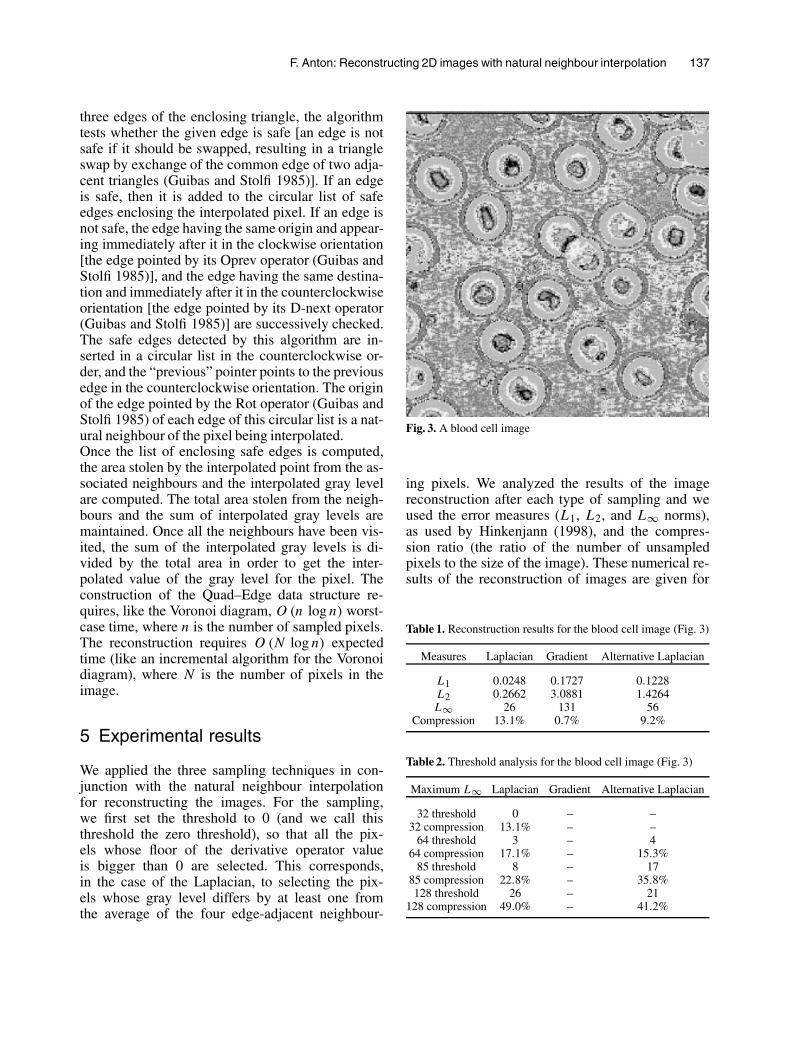
We applied the three sampling techniques in con-junction with the natural neighbour interpolationfor reconstructing the images. For the sampling,we first set the threshold to 0 (and we call thisthreshold the zero threshold), so that all the pix-els whose floor of the derivative operator valueis bigger than 0 are selected. This corresponds,in the case of the Laplacian, to selecting the pix-els whose gray level differs by at least one fromthe average of the four edge-adjacent neighbour-

Fig. 3. A blood cell image

ing pixels. We analyzed the results of the imagereconstruction after each type of sampling and weused the error measures (L1, L2, and L∞ norms),as used by Hinkenjann (1998), and the compres-sion ratio (the ratio of the number of unsampledpixels to the size of the image). These numerical re-sults of the reconstruction of images are given for

Table 1. Reconstruction results for the blood cell image (Fig. 3)

Measures Laplacian Gradient Alternative Laplacian

L1 0.0248 0.1727 0.1228L2 0.2662 3.0881 1.4264L∞ 26 131 56

Compression 13.1% 0.7% 9.2%

Table 2. Threshold analysis for the blood cell image (Fig. 3)

Maximum L∞ Laplacian Gradient Alternative Laplacian

32 threshold 0 – –32 compression 13.1% – –

64 threshold 3 – 464 compression 17.1% – 15.3%

85 threshold 8 – 1785 compression 22.8% – 35.8%128 threshold 26 – 21

128 compression 49.0% – 41.2%


4

5

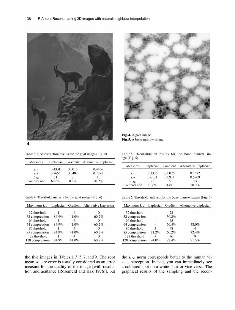
Fig. 4. A goat imageFig. 5. A bone marrow image

Table 3. Reconstruction results for the goat image (Fig. 4)


L1 0.4331 0.0015 0.4466L2 0.7655 0.0402 0.7871L∞ 11 2 11

Compression 60.6% 0.8% 60.2%

Table 4. Threshold analysis for the goat image (Fig. 4)


32 threshold 1 4 032 compression 84.9% 41.0% 60.2%


85 threshold 1 4 085 compression 84.9% 41.0% 60.2%128 threshold 1 4 0

128 compression 84.9% 41.0% 60.2%

the five images in Tables 1, 3, 5, 7, and 9. The rootmean square error is usually considered as an errormeasure for the quality of the image [with resolu-tion and acutance (Rosenfeld and Kak 1976)], but

Table 5. Reconstruction results for the bone marrow im-age (Fig. 5)


L1 0.1336 0.0026 0.1572L2 0.6131 0.0914 0.5909L∞ 73 6 53

Compression 19.6% 0.4% 20.2%

Table 6. Threshold analysis for the bone marrow image (Fig. 5)


32 threshold – 22 –32 compression – 30.2% –

64 threshold – 45 164 compression – 50.4% 38.0%


128 compression 94.0% 72.4% 91.5%

the L∞ norm corresponds better to the human vi-sual perception. Indeed, you can immediately seea coloured spot on a white shirt or vice versa. Thegraphical results of the sampling and the recon-


6

7

Fig. 6. A figure imageFig. 7. A mailbox image

Table 7. Reconstruction results for the figure image (Fig. 6)


L1 0.0407 0.2528 0.1615L2 0.2438 1.9380 0.7784L∞ 17 43 24

Compression 35.7% 4.2% 32.0%

Table 8. Threshold analysis for the figure image (Fig. 6)





128 compression 89.7% 64.8% 85.4%

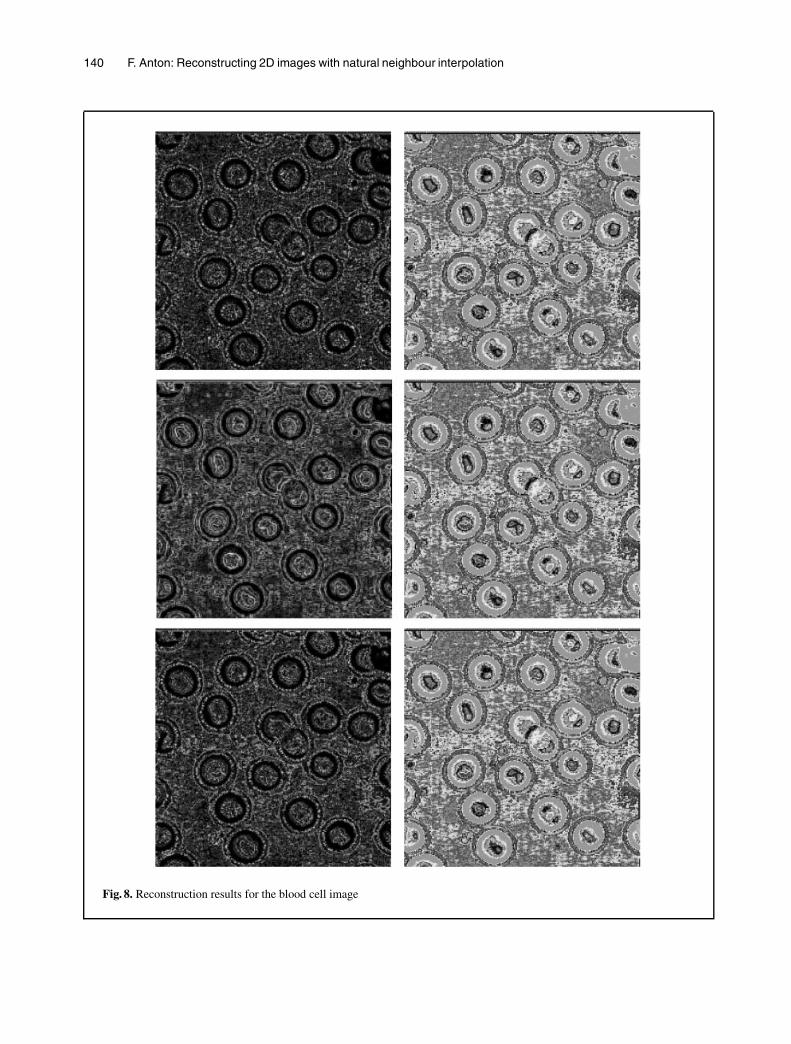
struction for the five images shown in Figs. 3–7are presented in Figs. 8–12. In each one of thesefigures, the results of the sampling appear on theleft column, while the reconstructed images ap-pear on the right column. The three rows of im-ages from the top to the bottom correspond to theLaplacian-based sampling, the sampling based onthe derivative in the direction of the gradient, andthe alternative Laplacian-based sampling. We alsoshow an analysis of the threshold required and the

Table 9. Reconstruction results for the mailbox image (Fig. 7)


L1 0.0646 12.5351 0.0569L2 0.2907 38.0251 0.2386L∞ 12 255 1

Compression 64.6% 50.4% 56.2%

Table 10. Threshold analysis for the mailbox image (Fig. 7)




85 threshold 30 – 1785 compression 64.6% – 57.4%128 threshold 62 – 36

128 compression 70.0% – 62.2%

compression obtained for different L∞ norms in Ta-bles 2, 4, 6, 8, and 10. The threshold shown in thesetables is the maximum threshold that will give anL∞ norm smaller than or equal to the correspond-ing threshold number in the first column. A “-”symbol implies that such a precision cannot be ob-tained with any threshold greater than or equal tothe zero threshold. The compression obtained withthis maximum threshold is shown on the followingline.


Fig. 8. Reconstruction results for the blood cell image


Fig. 9. Reconstruction results for the goat image


Fig. 10. Reconstruction results for the bone marrow image


Fig. 11. Reconstruction results for the figure image

6 Discussion

The main result is that the image quality is al-ways very good for the zero threshold in the caseof the sampling techniques based on the Lapla-cian: it is difficult to see the differences between

the reconstructed image and the original. On theaverage, the level of gray of a pixel of the re-constructed image and that of the correspondingpixel of the original image do not differ by morethan 1 with the Laplacian-based sampling tech-niques. The alternative Laplacian sampling tech-


Fig. 12. Reconstruction results for the mailbox image


nique very often gives a smaller maximum error.The best compression ratios for the zero thresh-old are almost always obtained by the ordinaryLaplacian sampling technique. The sampling tech-nique based on the derivative in the direction ofthe gradient does not give visually satisfying re-constructed images in all the cases (e.g. the mail-box image: see Table 9 and Fig. 7). However, thisreconstruction technique based on natural neigh-bour interpolation gives reconstructed images ofgood quality. The best compression ratios we canget for which the reconstructed image has whatwe think is a very good visual quality (L∞ ≤ 32)vary from 13.1% in the case of the blood cellimage (Fig. 3) to 84.9% in the case of the goatimage (Fig. 4). In general, the compression ra-tios obtained for a reconstructed image that sat-isfies a given L∞ are higher for the Laplacianthan for the alternative Laplacian. We feel thatthis technique is useful when one is presentedwith irregularly spaced samples, or when one candetermine the representative samples oneself, inwhich case using the standard Laplacian appearsto give the best results. In colour images, an ob-vious solution is to treat the three colour channelsas three independent images to be dealt with sep-arately. Better results can be obtained if we con-sider the fact that luminance edges are much betterdetected by the human visual system than chromi-nance edges, and therefore use a higher thresholdon the Laplacian for the chrominance than for theluminance.

Acknowledgements. This research work has received the financialsupport of the Natural Sciences and Engineering Research Coun-cil of Canada (NSERC). We would like to express our gratitudeto Dr. G. Dretakkis and the Imagis-Gravir laboratory at INRIASophia Antipolis for giving us access to their silicon graphicsserver.

References

1. Anton F, Gold CM, Mioc D (1998) Local coordinates andinterpolation in a Voronoi diagram for a set of points andline segments. Voronoi Conference on Analytic NumberTheory and Space Tillings, Kiev, Ukraine, pp 9–12

2. Farin G (1990) Surfaces over Dirichlet tessellations. Com-put Aided Geom Des 7:281–292

3. Foley JD, Dam A van, Feiner SK, Hughes JF (1990) Com-puter Graphics – Principles and Practice. Addison-Wesley,Reading, Mass, p 1174

4. Gold CM, Roos T (1994) Surface modelling with guaran-teed consistency – an object-based approach. In: NievergeltJ, Roos T, Schek H-J, Widmayer P (eds) IGIS ’94: Geo-graphic information systems, Springer, Berlin HeidelbergNew York, pp 70–87

5. Guibas L, Stolfi J (1985) Primitives for the manipulation ofgeneral subdivisions and the computation of Voronoi dia-grams. ACM Trans Graph 4:74–123

6. Hinkenjann A, Pietrek G (1998) Reconstructing radios-ity by scattered data interpolation. Proceedings of the 6thInternational Conference in Central Europe on ComputerGraphics and Visualization ’98, vol. I, University of WestBohemia, Plzen, Czech Republic, pp 133–140

7. Kuo MH, Chen MC (1998) Biomedical data interpolationfor 3D visual models. Proceedings of the 6th InternationalConference in Central Europe on Computer Graphics andVisualization ’98, vol. II, University of West Bohemia,Plzen, Czech Republic, pp 208–214

8. Piper B (1993) Properties of local coordinates based onDirichlet tessellations. Comput Suppl vol. 8, Springer,Berlin Heidelberg New York, pp 227–239

9. Ritter GX (1996) Handbook of computer vision algorithmsin image algebra. CRC Press, Boca Raton, Fla, p 420

10. Rosenfeld A (1969) Picture processing by computer. Aca-demic Press, New York, p 196

11. Rosenfeld A, Kak AC (1976) Digital picture processing.Academic Press, New York, p 457

12. Sibson R (1980) A vector identity for the Dirichlet tessella-tions. Math Proc Cambridge Philos Soc 87:151–155

13. Sibson R (1981) A brief description of the natural neigh-bour interpolant. In: Barnett DV (ed) Interpreting multivari-ate data. Wiley, New York, pp 21–26

Photographs of the authors and their biographies are given onthe next page.


FRANÇOIS ANTON is a PhDstudent in the Department ofComputer Science at the Uni-versity of British Columbia,Canada. He is currently in ex-change at the Prisme (compu-tational geometry) Project, IN-RIA, Sophia Antipolis, France.His research interests includecomputational geometry, com-putational algebraic geometry,computer graphics, visualiza-tion, and image processing.

DARKA MIOC is a PhD stu-dent in Geomatics at Laval Uni-versity, Quebec City, Canada.Her research interests includegeographic information systems,computational geometry, com-pute r graphics, visualization ofspatio-temporal data, and imageprocessing.

ALAIN FOURNIER wasa Professor in the Department ofComputer Science at the Univer-sity of British Columbia (UBC),Canada. He was a Co-director ofthe Imager Computer GraphicsLaboratory at UBC. He receivedhis PhD from the Universityof Texas at Dallas in 1980. Hewas a professor of computer sci-ence from 1980 to 2000. Hisresearch interests included com-puter graphics, object modelling,

graphic algorithms, display systems architecture, and computa-tional geometry. He passed away in August 2000.

reconstructing 2d images with natural neighbour interpolation

Documents