recognizing macroeconomic fluctuations in value based management
TRANSCRIPT
THE RESEARCH INSTITUTE OF INDUSTRIAL ECONOMICS
Working Paper No. 574, 2002 Recognizing Macroeconomic Fluctuations in Value Based Management
by Lars Oxelheim and Clas Wihlborg
IUI, The Research Institute of Industrial Economics P.O. Box 5501 SE-114 85 Stockholm Sweden

Recognizing Macroeconomic Fluctuations in Value Based Management
Lars OxelheimInstitute of Economic Research, Lund University, P.O.Box 7080, 220 07 Lund, Sweden, e-mail:[email protected], and IUI, P.O.Box 5501, SE-114 85 Stockholm, Sweden, e-mail: [email protected]
and
Clas WihlborgDepartment of Finance, Copenhagen Business School, Solbjerg Plads 3, DK-2000 Fredriksberg, Denmark, e-
mail: [email protected], and Department of Economics, School of Economics and Commercial Law, GöteborgUniversity, Box 640, 405 30 Göteborg, Sweden
January 2002
Forthcoming in Journal of Applied Corporate Finance
Abstract
Value Based Management (VBM) has become a common tool for ex ante and ex postevaluation of corporate strategies and projects from the perspective of shareholder valuemaximization (SVM). VBM-frameworks are designed to support investment and divestmentdecisions, ex post evaluation of management and their major strategic decisions, and bonus-systems. Traditional VBM frameworks make no distinction between sources of temporarychanges in performance, and sources of performance reflecting the intrinsic competitivenessof the firm. Temporary changes in performance are often caused by macroeconomicfluctuations. In this article we develop an approach for “filtering” the impact ofmacroeconomic fluctuations out of measures of performance in order for management toobtain better information for purposes of investment, divestment, and exposure managementdecisions. We focus on filtering for purposes of performance assessment employed incompensation schemes. A case study illustrates the approach, and shows the potentialmagnitude of effects from macroeconomic events.
JEL classification: D81, G31, M22
Key words: Value Based Management (VBM), Shareholder Value Analysis (SVA), Economic Value Added(EVA), performance measurement, macroeconomic fluctuations, bonus system
2
2002-01-30
Recognizing Macroeconomic Fluctuations in Value Based Management
Value Based Management (VBM) has become a key instrument for ex ante and ex post
evaluation of corporate strategies and projects from the perspective of shareholder value
maximization (SVM). VBM-methods are designed to support, for example, investment and
divestment decisions, and ex post evaluation of major strategic decisions. Measures of
performance of management are another important component of VBM. The performance
measures are used in bonus systems in order to align managerial incentives with those of
shareholders.
There are a number of VBM frameworks. Shareholder Value Analysis (SVA), developed
in Rapaport (1986) and Economic Value Analysis (EVA) developed by Stern Stewart (1990)
are the two most well known ones. However, there exist many challengers as described in
Black, Wright, and Backman (2001). Cash Value Analysis (CVA) developed by Ottoson and
Weissenrieder (1996), and Cash Flow Return on Investment (CFROI), (Madden, 1999) are
two offering serious alternatives to the different versions of EVA.
All the mentioned VBM frameworks have in common that they make no distinction
between changes in cash flows that reflect a firm’s competitive position, and changes caused
by relatively short term influences from the firm’s macroeconomic environment. A firm’s
competitive position may be attributed to its (and its management’s) specific skills and
knowledge relative to the market and competitors. Short-term influences on the other hand,
are often caused by macroeconomic events, and observed most rapidly as changes in
exchange rates, interest rates and aggregate price levels domestically and abroad.
Macroeconomic factors have in common that they are completely beyond management’s
control although the cash flow effects of such factors may be affected by managerial actions.
Thus, management may gain useful information about current and future prospects of the
firm by “filtering” out macroeconomic influences on current performance measures. Such
“filtering” would allow management to estimate performance “under neutral macroeconomic
conditions”. What is meant by “neutral” may from a practical point of view be seen as
debatable. We circumvent this problem in the practical analysis below by focusing on
changes in performance-related variables.

3
If cash flow forecasts for a new project are generated without distinguishing between
sustainable demand and cost conditions, and temporary demand and cost conditions
generated by macroeconomic events, an estimated positive project value may not be
sustainable under normal macroeconomic conditions. Alternatively, if forecasts are generated
based on observations under unfavorable macroeconomic conditions, then project values
may be underestimated and the project abandoned prematurely. For instance, an undervalued
currency can lead the management of an exporting firm to believe that the company is
competitive whereas its profits “filtered” of the under-valuation may be decreasing. An
unsustainable good performance may lead to demand for wage and dividend increases that
are not motivated by the firm’s longer term competitiveness. Hence, the cost to shareholders
of ignoring or remaining uninformed about the temporary impact of macroeconomic
fluctuations may be very high at the end of the day.
In this paper we focus on correcting performance measures for influences of
macroeconomic events. From the point of view of performance evaluation macroeconomic
effects on cash flows and value could be considered noise to the extent they are not
predictable. It is well known in the incentive contract literature that if risk-averse managers’
remuneration is linked to noise factors beyond their control without strong linkage to
shareholder value, then their incentive to exert effort on behalf of shareholders may be
weakened.1 Thus, from a SVM perspective it could be desirable to “cleanse” performance
measures of macroeconomic influences with the aim of strengthening the incentives of
managers.
An additional argument for filtering out macroeconomic influences on measures of firms’
performance is that they represent a possible explanation for large observed differences
between economic values as measured by EVA-analysis and market values (O’Byrne, 1997).
Such differences could occur if market participants were better able to identify
macroeconomic influences than the EVA-analyst.
Oxelheim and Wihlborg (1997) discuss how management can develop a Macroeconomic
Uncertainty Strategy (MUST) - analysis to manage exposure caused by macroeconomic
events observed in, for example, exchange rates. A key component of this analysis is the
estimation of exposure coefficients – within a multivariate framework - for the impact of
macroeconomic price variables on commercial (non-financial) cash flows, or on the value of
the assets generating such cash flows. Here we argue that these exposure coefficients can be
useful in a VBM context as well. Changes in a firm’s cash flows or value from one period to
another can be “cleansed” from some or all macroeconomic influences once exposure
4
coefficients are known. Thereby sustainable changes in cash flows or value that should be
attributable to a firm’s inherent competitiveness would be identified.
The basic framework for decomposing changes in cash flows and value using exposure
coefficients is laid out in Section 2. As an illustration of the decomposition procedure and the
magnitude of macroeconomic influences the case of Electrolux is presented in Section 3. In
Section 4 we turn to decomposition for purposes of performance assessment. The appropriate
decomposition depends on the flexibility in a firm’s operations, and on the existence of real
options. Conclusions follow in Section 5.
2. VBM and macroeconomic fluctuations – A framework
Value Based Management springs from the measure of firm value employed in conventional
corporate finance. According to this measure the value of corporate assets (VA) is the net
present value of cash flows generated by those assets:
∞ jVA,t = ∑ δ E [Xt+j ] + PVRO (1)
j=0
where δj is the discount factor for j periods, Xt+j refers to cash flows in period t+j, and PVRO
represents the value of real options that cannot be captured in conventional present value
analysis. The value of equity, VS,t, is the value of assets minus the value of debt VD,t. Thus,
VS,t = VA,t - VD,t (2)
In VBM the objective of management is commonly to maximize the value of equity, VS,t. If
markets for debt are well-functioning, then maximization of the value of assets, VA, leads to
the maximization of the value of equity, VS. In the following, we focus on the value of non-
financial assets that depends on expected cash flows and the risk adjusted cost of capital, δ.
SVM implies a concern with cash flows, as well as with the minimization of the cost of
capital. Investments in real options also increase a firm’s value by increasing the average level
of cash flows.
Cash flows in any period can be decomposed into two components. One component is cash
flows that would occur in the absence of macroeconomic fluctuations under hypothetical

5
“neutral” or “normal” macroeconomic conditions in countries of relevance for any particular
firm. These cash flows for any individual firm vary as a result of changes in the firm’s
competitiveness in the market place and the growth rate of demand for the firm’s output.
Given a firm’s technology, knowledge among employees, managerial competence, and
demand, there is at any time a level of cash flows that may be called the sustainable level of
cash flows for the period. This sustainable level, denoted XL, occurs under “neutral”
macroeconomic conditions. It may not usually be observed, and it is not constant. It is
independent of influences of macroeconomic events, however, and reflects the ability of
management to employ resources productively. The fact that the sustainable level is not
directly observable does not mean that it lacks practical significance. On the contrary, we
argue that management should estimate it and use it as key-input in major business decisions.
The cash flows during a period that depend on macroeconomic conditions in countries
where the firm has a presence are denoted XM. These cash flows may be positive or negative
and more or less transitory. They are by definition never permanent. Thus:
Xt+j = XL,t+j + XM,t+j (3)
The pattern of both components on the right side of (3) can be influenced by investments in
real options. We defer the discussion of this issue to Section 4.
Macroeconomic events, causing fluctuations in a firm’s cash flows and economic value,
may be triggered by a variety of policy and non-policy shocks originating at home or abroad.
Monetary and fiscal policy shocks are the policy shocks most commonly referred to, while
non-policy shocks may be caused by changes in private sector aggregate demand and supply.
The cash flows caused by macroeconomic shocks may have a substantial effect on a firm’s
value in a period t.
Most directly and immediately macroeconomic events are observed as changes in
macroeconomic price variables among which exchange rates, interest rates, and price levels
are most prominent. Underlying macroeconomic events are usually not directly observed,
however. In most macroeconomic models different shocks affect these particular price
variables in different combinations. The price variables are essentially signals of
macroeconomic conditions. Economic models differ about the magnitude and duration of
change in the price variables in response to different macroeconomic shocks but most open
economy models have in common the mentioned price variables. The “market return” on

6
stocks could be added in order to cover price responses to macroeconomic shocks more
completely but this variable seems to be less systematically related to macroeconomic shocks.
We need not link the discussion here to any specific macroeconomic model. The main point is
that there is a set of price variables that serve as indicators of macroeconomic conditions. For
each firm there is then a more detailed and firm-specific set of these variables. For an
individual firm, exchange rate vulnerability may be specified as vulnerability to changes in,
for instance, the JPY/USD and Euro/USD rates, interest rates vulnerability as, for instance,
vulnerability to changes in the short term euro rate and long-term US rate, and, finally, the
inflation vulnerability as vulnerability to changes in German producer prices and Japanese
consumer prices.
The correction to commercial cash flows that would be made to arrive at “sustainable”
cash flows under neutral macroeconomic conditions in a particular period can be expressed in
the following way when macroeconomic conditions are observed in exchange rates, interest
rates, and prices:
tM
tM
tM
tM ppp
Xii
i
Xee
e
XX )()()(, −+−+−=
δδ
δδ
δδ (4)
In (4) tee )( − , tii )( − , and tpp )( − represent deviations from the exchange rates, interest
rates, price levels that correspond to neutral macroeconomic conditions in period t. Each of
these variables can be seen as a vector of domestic and foreign variables of relevance to a
firm. The partial derivatives represent sensitivity or vulnerability coefficients with the same
properties as exposure coefficients.
The coefficients in (4) capture not only the direct impact of each variable on cash flows.
Each coefficient depends on correlations between the variable and all other macro-effects of
the event, as well as between these effects and cash flows. In contrast, exposure management
in most firms seems to presume that changes in exchange rates, interest rates, and price levels
as shocks occurring independently of each other and other variables affecting a firm’s cash
flows. We have discussed problems with this view of macroeconomic exposure in Oxelheim
and Wihlborg (1987, 1997), and recommended that firms measure coefficients as those in (4)
above for the firm-specific set of variables from the three mentioned categories of
macroeconomic variables for relevant countries employing multivariate regression or scenario
analysis.
7
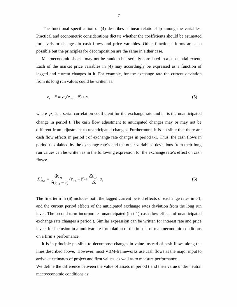
The functional specification of (4) describes a linear relationship among the variables.
Practical and econometric considerations dictate whether the coefficients should be estimated
for levels or changes in cash flows and price variables. Other functional forms are also
possible but the principles for decomposition are the same in either case.
Macroeconomic shocks may not be random but serially correlated to a substantial extent.
Each of the market price variables in (4) may accordingly be expressed as a function of
lagged and current changes in it. For example, for the exchange rate the current deviation
from its long run values could be written as:
ttet seeee +−=− − )( 1ρ (5)
where eρ is a serial correlation coefficient for the exchange rate and s t is the unanticipated
change in period t. The cash flow adjustment to anticipated changes may or may not be
different from adjustment to unanticipated changes. Furthermore, it is possible that there are
cash flow effects in period t of exchange rate changes in period t-1. Thus, the cash flows in
period t explained by the exchange rate’s and the other variables’ deviations from their long
run values can be written as in the following expression for the exchange rate’s effect on cash
flows:
tM
tt
MetM s
s
Xee
ee
XX
δδ
δδ
+−−
= −−
)()( 1
1, (6)
The first term in (6) includes both the lagged current period effects of exchange rates in t-1,
and the current period effects of the anticipated exchange rates deviation from the long run
level. The second term incorporates unanticipated (in t-1) cash flow effects of unanticipated
exchange rate changes a period t. Similar expression can be written for interest rate and price
levels for inclusion in a multivariate formulation of the impact of macroeconomic conditions
on a firm’s performance.
It is in principle possible to decompose changes in value instead of cash flows along the
lines described above. However, most VBM-frameworks use cash flows as the major input to
arrive at estimates of project and firm values, as well as to measure performance.
We define the difference between the value of assets in period t and their value under neutral
macroeconomic conditions as:

8
[ ]∑∞
=+=−=∆
1,,,,
jjtMt
jMtALtAtA XEVVV δ ,
(7)
where
XM =XeM +Xi
M +XpM, (8)
and δM is the discount factor for cash flows caused by macroeconomic conditions.2
Superscripts indicate cash flow effects of different macroeconomic variables in (4). Each of
these variables can be expressed as in (6) in terms of an anticipated component and a noise
component.
The formulation for value effects of cash flows caused by macroeconomic events in (7)
implies that the value of real options, PVRO, is part of the “sustainable” value VAL. The
rationale for viewing the value of real options this way is that they are very much the result of
managerial activity. We return to this issue in Section 4.
It is also possible to define the difference between the value of equity and the long run
sustainable value of equity in the following way using (2):
∆VS,t = VS,t – VSL,t = (VA,t – VD,,t) – (VAL,,t – VDL,t) = ∆VA,t - ∆VD,t = VMA - VMD (9)
In (9) VDL is the value of debt under neutral macroeconomic conditions. Thus ∆VD,t is the
value of debt caused by macroeconomic variables’ deviations from values corresponding to
neutral conditions. These deviations cause financial cash flows and capital gains or losses on
financial positions in a period. Corporate financial exposure management can be thought of as
adjusting financial positions including derivatives, ∆VD, in order to create an offset between
the sensitivities of ∆VD and ∆VA - or the corresponding sensitivities for cash flows - to
macroeconomic price variables. (See Oxelheim and Wihlborg, 1997)
3. Cash flow decomposition and valuation: The case of Electrolux
Electrolux AB is one of the world’s largest manufacturers of white goods equipment. Through
acquisitions the company has become a truly global player. Its headquarter is located in
Sweden, and it is controlled by the so-called Wallenberg group through its holding company

9
Investor. In spite of widespread Swedish and international ownership of equity, control is held
by Investor and the Wallenberg group through a dual-class share system.
The changes in quarterly real operating cash flows for the Electrolux group from 1986
through 1994 were obtained from the firm. The purpose was to decompose the changes into
the components described in the previous section. In an initial fundamental analysis3 key
variables with potential economic explanatory power were identified following the answers to
a battery of questions: Where does Electrolux produce, where does Electrolux buy its input
from, where are these inputs produced, which are the major markets for Electrolux and which
are the major currencies and interest rates of Electrolux’s financial positions? After this initial
part of the fundamental analysis the major competitors were identified and the same questions
were asked for them. The fundamental analysis for Electrolux in the period under
investigation generated a set of 11 macroeconomic price variables with a potential
explanatory power.
The changes in real4 operating cash flows5 were then regressed on changes in the variables
from the fundamental analysis consisting of some exchange rates between the Swedish and a
number of major currencies, interest rates, and inflation rates. Total European housing was
included to control for changes in the industry’s conditions. Dummy variables were used to
adjust cash flows for seasonality. Since the number of observations is limited combinations of
the currencies were used. Regressions were run for the whole period 1986-94, as well as for
1986-92, and 1986-93. The latter regressions made it possible to use coefficients for out-of-
sample analysis. Without going into econometric methodology and problems we present
results of the analysis as an illustration of the decomposition. The following set of significant
coefficients were obtained using contemporaneous dependent and independent variables:6
INSERT TABLE 1 HERE
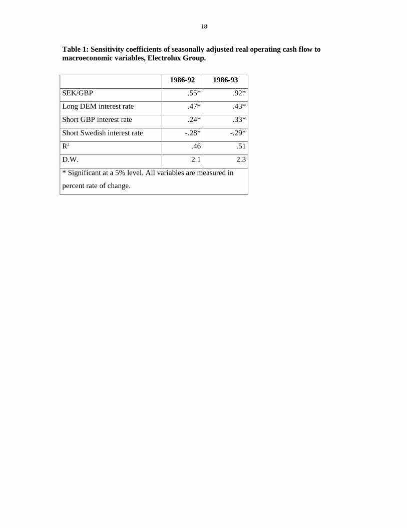
Table 1 shows that the macroeconomic price variables explain about 50% of the fluctuations
in seasonally adjusted changes in quarterly real operating cash flows. It is found that a
depreciation of the Swedish Krona vis-à-vis the British Pound is beneficial for Electrolux.
One percent increase in the SEK/GBP rate causes a .55 percent increase in seasonal adjusted
real operating cash flow. This reflects that the Swedish Krona is the home currency of
Electrolux and that the group will benefit whatever the transaction is when a net positive

10
foreign position is converted into that currency. In addition to that benefit, the company also
benefits from a stronger competitive position in Sweden vis-à-vis foreign producing
competitors. An increase in the Swedish short-term interest rate has a significant adverse
impact on the real operational cash flows of Electrolux. The negative effect of an increase in
the short-term Swedish interest rate captures the general decrease in the demand for capital
goods as a response to raises in interest rates. The two other interest rate components are
positive as they are when interest rates are correlated with business cycle developments.
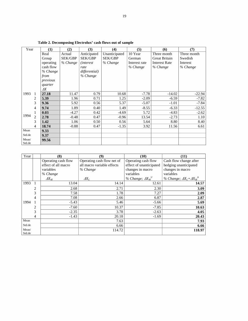
The coefficients were employed out-of-sample in such a way that the 1986-92
coefficients were used to estimate the impact of macroeconomic events in 1993, and the 1986-
93 coefficients were used to estimate the impact in 1994. Table 2 shows the data and the
results of the out of sample analysis. Column (1) shows actual quarterly cash flow changes in
1993 and 1994. Columns (2), (5), (6) and (7) list the changes in the price variables, which are
multiplied by the coefficients in Table 1 to obtain the changes in cash flows caused by
changes in the macro economy (∆XM) in column (8). Changes in “sustainable” cash flows
(∆XL) are registered in column (9).
INSERT TABLE 2 HERE
A second decomposition in Table 2 is obtained by removing only changes in cash flows
caused by unanticipated macroeconomic events. The interest rate differential in the previous
quarter is a proxy for the anticipated exchange rate changes in column (3). Unanticipated
exchange rate changes follow in column (4). It is assumed that all changes in interest rates are
unanticipated in columns (5), (6), and (7). After multiplying unanticipated changes with the
coefficients in Table 1, unanticipated cash flow changes caused by macroeconomic events
(∆XMU) are registered in column (10). Finally column (11) shows “sustainable” cash flow
changes plus cash flow changes caused by anticipated macroeconomic events (∆XL+∆XMA).
The distinction between the two decompositions is particularly important for performance
assessments. We turn to this issue in the next section. However, the distinction can also be
important for the estimation of changes in the net present value of the firm’s assets within a
VBM framework, because an assumption must be made about the time pattern of expected
exchange and interest rate changes.
Within EVA analysis the economic value added for a period is estimated based on the
difference between a period’s actual cash flows and the cash flows required to cover the cost

11
of capital for the same period. Assume as an example that Electrolux at the end of 1994
employed a 15 percent cost of capital, and that the expected growth rate of cash flows was
9.33 percent. This figure is the average growth rate during 1993 and 1994 as shown in Table
2. Using the constant growth formula for estimating the present value of a dividend of 1 in
1994 would lead to a present value of 1.0933/(.15-.0933)=19.28.
If instead the true long run growth rate is the average of the growth of “sustainable” cash
flow in (8), then the corrected present value is 1.0763/(.15-.0763)=14.60, if the same cost of
capital is used. Thus, disregarding the temporary nature of some cash flows, the value of the
firm would be exaggerated by 32% in this example. The exaggeration presumes that
management has interpreted temporary growth caused by macroeconomic effects in 1993 and
1994 as sustainable growth.
In the latter estimation of the firm’s net present value it was assumed that there are no
expected cash flow effects of macroeconomic shocks. If we instead would assume that current
macroeconomic effects will continue but decrease over time then the present value of the firm
would lie between the two examples above.
A second source of error in the economic value estimation within a VBM-framework is
that the discount rate is assumed to be the same for all cash flows. Most likely the risk-
adjustment on the cost of capital for cash flows caused by macroeconomic events should be
lower than the risk-adjustment for the sustainable cash flows generated by the business itself.
If so, the difference between the present values including and excluding the macroeconomic
components of cash flows would be even larger.
4. Performance assessment and real options in VBM
An important aspect of VBM is to link bonus for management to changes in shareholder value
or value-enhancing cash flows. In the following it is assumed that either cash flows during a
period or changes in the estimated present value of cash flows provide the basis for a bonus
for the period. Thus, stock market values do not exist for the entity or are considered
excessively noisy to be used as a basis for compensation. In this case the key element of
performance is the operating (or commercial) cash flows. These cash flows would provide the
information based on which an economic value would be estimated. One issue here is which
component or components of operating cash flows should be the major input in performance
assessment for the purpose of determining managerial compensation. The choices we have
12
from Section 2 and Table 2 are the total operating cash flows (X, column (1)), the
“sustainable” cash flows (XL, column (9)), or the total cash flows minus those caused by
unanticipated macroeconomic events (XL + XMA, column (11)). A second issue addressed in
this section is whether the coefficients estimated as above in a linear model are appropriate
when decomposing cash flows. Real options in particular imply a non-linear relation between
shocks and cash flows.
Unanticipated and anticipated cash flow effects from macroeconomic events
If management has no or negligible influence on cash flows caused by macroeconomic
events, an efficient compensation scheme should be linked to “sustainable” cash flows alone,
or the present value of expected such cash flows. In this case the compensation based on
“sustainable” cash flows creates the strongest incentives for management to devote effort
towards enhancement of the firm’s long run competitiveness, while cash flows beyond its
control do not affect compensation. To the extent a bonus system is linked to cash flows and
value changes over which management has no control, effort may be diverted towards
speculation about macroeconomic developments or towards obfuscation of information about
them. Furthermore, the incentives of risk-averse managers to exert effort are weakened, if the
variable to which bonus is linked contains noise relative to the variable that is of concern to
shareholders as noted above. The link between effort and outcome is weakened7.
It could be argued that management should be induced to take advantage of anticipated
changes in the macroeconomic environment. Naturally, if the firm’s operations in various
ways can be adjusted to changes in expectations about macroeconomic events, then
management should have the incentive to implement such adjustment in sales effort,
production pattern, or where adjustment can be made in time to take advantage of the
expectations. In this case the adjustment to total cash flows would be limited to those caused
by unanticipated changes such as st in (6) and column (10) in Table 2. The compensation
would be linked to cash flows in column (11) of Table 2. Even if cash flows can be adjusted a
reason for not linking the bonus to anticipated flows is that these can be affected by
managerial decisions to a lesser degree relative to effort, than sustainable flow. In the latter
case, scarce managerial time is most productively used to enhance the firm’s competitiveness.
The ability of management to take advantage of anticipated macroeconomic conditions may
vary among industries. Differences in compensation schemes may therefore be observed
without any implication that one system is superior to another.
13
The data presented in Table 2 indicate that a very large proportion of the variability of
operating cash flows is caused by macroeconomic fluctuations. Comparing columns (8) for all
macro-effects and (10) for unanticipated macro-effects it can be seen that the unanticipated
component dominates very strongly over the anticipated component in the particular case
presented. Or to phrase it differently, more or less all macro effects seems to be unanticipated.
Cash flows and value created by investments in real options
In eq. (1) the present value of real options is one component of the value of a firm. Real
options are created by investments in “flexibility”. Such investments reduce irreversible costs
associated with changes in operations, and enhance a firm’s ability to take advantage of
positive changes in cost and demand conditions and to reduce the impact of negative changes.
By investing in flexibility the firm can narrow the range of conditions within which it cannot
adjust its operations to changes in the environment. This range is defined by “trigger levels”
for demand and cost conditions beyond which adjustment of operations is profitable (See, for
example, Dixit and Pindyck, 1994).
Investments in real options--or “flexibility”--can be motivated by uncertainty about factors
affecting “sustainable” cash flows, as well as about macroeconomic conditions. Here we are
concerned with the effects of investments in “flexibility” in response to uncertainty about
macroeconomic conditions. For example, investments reducing irreversible costs of switching
suppliers, location of production, or marketing efforts between countries enable a firm to
reduce the cash flow impact of negative changes in real exchange rates, and increase the cash
flow impact of positive changes (see Capel, 1997). Another example is that investments in
customer relations may enable a firm to pass through large exchange rate or interest rate
changes into prices by reducing costs associated with changes in prices. This flexibility could
extend even to unanticipated changes.
The options to change prices, switch suppliers, etc. in response to price incentives of certain
magnitudes imply that the cash flow sensitivity coefficients tend to become smaller for large
deviations from neutral macroeconomic conditions. A linear relation between cash flows
caused by macroeconomic factors, and deviations from levels corresponding to neutral
macroeconomic conditions is completely correct only when there are no real options that
management can exercise in response to relatively large price incentives.

14
Figure 1 illustrates the cash flow effects of unanticipated macroeconomic shocks. The
size of the shock is measured along the x-axis. The straight line shows the cash flow effects of
the disturbance if there are no real options, i.e. if there is no flexibility in pricing, sourcing,
location of production etc. no matter how large the shock is. The broken line shows the cash
flow effects of the same shock, when an increasing number of real options are triggered as the
magnitude of the shock increases. When the option is triggered, cash flows denoted XR,t arise.
They add increasingly to the cash flows as the magnitude of a positive event increases. When
the event is increasingly negative, the cash flows created by the option reduce the impact on
cash flow increasingly.
INSERT FIGURE 1
The framework developed in Section 2 can now be expanded to include cash flows, XR,
that occur in a period as a result of previous investments in real options. Total cash flows in
period t can be decomposed as in e.q. (3) above into sustainable and macroeconomic
components. The latter component, XM, described above in the linear expressions (4) and (6)
must now be extended to include the cash flows from real options. Using Mt to denote the
level of a vector of macroeconomic variables describing macroeconomic conditions in period
t, the cash flow effects caused by macroeconomic events can be written in the following way:
( )( ) tRt
M
t
t
M
tM Xmm
XMM
MM
XX ,1
1
, ±+−−
= −− δ
δδ
δ, (10)
where the first term represents anticipated effects of lagged changes in M, the second term
captures unanticipated effects, and XR,t as described in Figure 1 represents cash flow effects
of real options triggered by M in period t. As in expression 6 above
( ) ttMt mMMM +−= −1ρ , (11)
where Mρ is a serial correlation coefficient and mt is the unanticipated change in
macroeconomic conditions.
15
The partial derivatives in the first two terms on the right hand side are assumed to be linear
coefficients independent of the magnitude of change in M. Estimated coefficients for changes
in cash flows were estimated and used in Table 2 to decompose cash flows into “sustainable”
cash flows, XL, and cash flows caused by macroeconomic events, XM. The nonlinear cash
flows created by investments in real options were not accounted for, however.
The issue now is how the last term in (10), XR,t, should be treated when estimating the
performance of management with the objective of providing incentives for management to
maximize shareholder value. Clearly, shareholder wealth maximization includes maximizing
the value of real options (PVRO in (1)) whether the options refer to flexibility in responses to
competitive conditions or macroeconomic events. Thus, it is clearly desirable to include the
cash flows trigged by real options on macroeconomic conditions, XR,t or the value of real
options, PVRO, in measures of managers’ performance.
An econometric problem may sometimes follow from the suggested consideration of
real options. Their presence implies that it is no longer appropriate to take a linear relation
between cash flows and macroeconomic price-variables for granted, although the linear
sensitivity coefficients in expressions like (4) and (6) are the appropriate ones to use for the
decomposition of cash flows. If the relationship between cash flows and macroeconomic
variables are described by the non-linear broken line in Figure 1, the analyst estimating the
linear sensitivity coefficients for macroeconomic effects on cash flows may have to limit the
regression to observations of macroeconomic changes within the range bounded by the trigger
levels for which the relation can be assumed to be linear. The linear coefficients measured this
way apply nevertheless outside this range whenever cash flows unaffected by management
are to be estimated.8
5. Concluding remarks
Value Based Management is a tool that should help management maximize shareholder
value in large and small investment and divestment decisions. It should also help shareholders
designing bonus-systems based on performance in order to induce managers to have
shareholder value as their prime objective.
Macroeconomic fluctuations affect firms’ cash flows as well as market values. These
fluctuations are beyond management control. However, cash flow effects caused by them can
sometimes be influenced by management to the extent macroeconomic developments can be

16
forecast, or if firms can invest in flexibility with respect to sourcing, pricing, location of
production, or location of sales in response to anticipated and/or unanticipated
macroeconomic development.
We have here argued that for purposes of project evaluation, ex post analysis of projects,
and performance assessment it is valuable to decompose cash flows of firms into
“sustainable” cash flows, i.e. cash flows under “neutral” macroeconomic conditions, and cash
flows caused by macroeconomic fluctuations around these conditions. The latter flows can be
decomposed further into anticipated and unanticipated cash flows. When implemented,
focusing on period-to-period changes of macroeconomic effects helps circumventing the
problem of defining “neutral” conditions in an absolute sense.
We have suggested that sensitivity-coefficients describing the impact of key
macroeconomic price variables on cash flows should be estimated within a multivariate
framework and used as input to filter out the cash flow effects of macroeconomic fluctuations.
The data used as input in investment decisions, ex post analysis of projects and strategies, and
performance measures for compensation-systems could be substantially improved if cash
flows were decomposed each period as suggested above. Inclusion of this type of analysis as a
key component of Value Based Management would improve conditions for shareholder
wealth maximization. In particular, it would be possible to base compensation systems on
measures of performance under the actual control of management.
References
Black, A., P. Wright and J.E. Bechman, 2001, In Search of Shareholder Value - Managing theDrivers of Performance, Price Waterhouse, FT Prentice Hall, London.
Capel, J., 1997, “A real option approach to economic exposure management”, Journal ofInternational Financial Management and Accounting 8, 87-113.
Dixit, A. and R. S. Pindyck, 1995, “The option approach to capital investment”, HarvardBusiness Review 64, May/June, 105-115.
Lessard, D.R. and P. Lorange, 1977, “Currency changes and management control: resolvingthe centralization/decentralization dilemma”, Accounting Review, July, 628-637.
Madden, B.J., 1999, A total system approach to valuing the firm, Butterworth-Heinemann.Milgrom, R. and J. Roberts, 1992, Economics, Organization and Management, Prentice-Hall,
New York.O’Byrne, F., 1997, “EVA and Shareholder Return”, Conference paper, Financial
Management Association Annual Conference, Honolulu.Ottosson, E. and F. Weissenrieder, 1996, “Cash Value Added (CVA) - A New Method for
Measuring Financial Performance”, Gothenburg Studies in FinancialEconomics, 1996:1, Department of Economics, Gothenburg university.

17
Oxelheim, L. and C. Wihlborg, 1987, Macroeconomic Uncertainty – International Risks andOpportunities for the Corporation, John Wiley and Sons, Chichester and NewYork.
Oxelheim, L. and C. Wihlborg, 1995, “Measuring Macroeconomic Exposure – the Case ofVolvo Cars”, European Financial Management 1, 241-263.
Oxelheim, L. and C. Wihlborg, 1997, Managing in the Turbulent World Economy –Corporate Performance and Risk Exposure, John Wiley and Sons, Chichesterand New York.
Rapaport, A., 1986, Creating Shareholder Value. The New Standard for BusinessPerformance, Free press, London.
Stewart, G. 1990, The Quest for Value: The EVA-TM Management Guide, Harper Business,New York.
18
Table 1: Sensitivity coefficients of seasonally adjusted real operating cash flow tomacroeconomic variables, Electrolux Group.
1986-92 1986-93
SEK/GBP .55* .92*
Long DEM interest rate .47* .43*
Short GBP interest rate .24* .33*
Short Swedish interest rate -.28* -.29*
R2 .46 .51
D.W. 2.1 2.3
* Significant at a 5% level. All variables are measured in
percent rate of change.
19
Table 2. Decomposing Electrolux’ cash flows out of sample
Year (1) (2) (3) (4) (5) (6) (7)RealGroupoperatingcash flow% Changefrompreviousquarter∆X
ActualSEK/GBP% Change
AnticipatedSEK/GBP(interestratedifferential)% Change
UnanticipatedSEK/GBP% Change
10 YearGermanInterest rate% Change
Three monthGreat BritainInterest Rate% Change
Three monthSwedishInterest% Change
1 27.18 11.47 0.79 10.68 -7.78 -14.02 -22.942 5.39 1.96 0.71 1.25 -2.09 -6.59 -7.823 9.36 5.92 0.56 5.37 -5.07 -1.01 -7.844 9.74 1.89 0.40 1.49 -8.55 -6.33 -12.551 0.03 -4.27 0.42 -4.69 5.72 -4.83 -2.622 2.78 -0.48 0.47 -0.96 13.54 -2.73 1.103 1.42 1.06 0.50 0.56 5.64 8.80 8.40
1993
1994
4 18.74 -0.88 0.47 -1.35 3.92 11.56 6.61Mean 9.33Std.de 9.37Mean/Std.de
99.56
Year (8) (9) (10) (11)Operating cash floweffect of all macrovariables% Change
∆XM
Operating cash flow net ofall macro variable effects% Change
∆XL
Operating cash floweffect of unanticipatedchanges in macrovariables% Change; ∆XM
U
Cash flow change afterhedging unanticipatedchanges in macrovariables% Change; ∆XL+∆XM
A
1993 1 13.04 14.14 12.61 14.572 2.68 2.71 2.30 3.093 7.58 1.78 7.27 2.094 7.08 2.66 6.87 2.87
1994 1 -5.43 5.46 -5.66 5.692 -7.60 10.37 -7.85 10.633 -2.35 3.78 -2.63 4.054 -1.43 20.18 -1.69 20.43
Mean 7.63 7.93Std.de 6.66 6.66Mean/Std.de
114.72 118.97

20
Figure 1.Cash flows caused by macroeconomic factors when real options are present.
Trigger Level
Trigger level
Macroeconomic deviationfrom “ neutral conditions”
XR
Cash flows caused by macroeconomic factors
XR
21
End
note
s
1Se
efo
rex
ampl
e,M
ilgr
oman
dR
ober
ts(1
992)
,Ch.
5.
2T
heri
skpr
emiu
mfo
rca
shfl
ows
caus
edby
mac
roec
onom
icfl
uctu
atio
nsm
aydi
ffer
from
the
risk
prem
ium
for
cash
flow
sat
“neu
tral
”co
nditi
ons.
See
belo
w.
3T
hefu
ndam
enta
lana
lysi
sw
asca
rrie
dou
tfol
low
ing
the
trad
ition
ofth
eM
US
T-a
naly
sis
used
inri
skm
anag
e-m
ent.
See
Oxe
lhei
man
dW
ihlb
org
(199
7).
4D
efla
ted
bypr
oduc
erpr
ices
inm
anuf
actu
ring
.
5M
easu
red
asth
eco
mm
erci
alne
tinc
ome;
reve
nues
from
good
sso
ldm
inus
cost
sof
good
sso
ld.
6L
agge
dva
riab
les
wer
ein
trod
uced
butw
itho
utsu
bsta
ntia
lcha
nges
inre
sult
s.
7L
essa
rdan
dL
oran
ge(1
977)
disc
uss
ince
ntiv
eef
fect
sof
the
choi
ceof
exch
ange
rate
inbu
dget
ing
deci
sion
s.In
thei
ran
alys
isth
ech
oice
ofex
chan
gera
tein
flue
nces
mea
sure
sof
perf
orm
ance
and
ther
efor
ein
cent
ives
.
8T
here
gres
sion
sre
sulti
ngin
the
coef
fici
ents
pres
ente
din
Tab
les
1an
d2
did
notr
evea
lerr
ors
that
coul
dbe
inte
rpre
ted
asno
n-li
near
itie
sof
the
type
disc
usse
dhe
re.