recent vs. historical seismicity analysis for banat seismic region (western part of romania)
TRANSCRIPT

SCIENTIFIC JOURNAL OF THE TECHNICAL UNIVERSITY OF CIVIL ENGINEERING
Mathematical Modelling in Civil Engineering
BUCHAREST
Volume 11 No. 1 - March – 2015

Disclaimer With respect to documents available from this journal neither U.T.C.B. nor any of its employees make any warranty, express or implied, or assume any legal liability or responsibility for the accuracy, completeness, or usefulness of any information, apparatus, product, or process disclosed. Reference herein to any specific commercial products, process, or service by trade name, trademark, manufacturer, or otherwise, does not necessarily constitute or imply its endorsement, recommendation, or favoring by the U.T.C.B. The views and opinions of authors expressed herein do not necessarily state or reflect those of U.T.C.B., and shall not be used for advertising or product endorsement purposes
CONTENTS
EVALUATION OF BUCHAREST SOIL LIQUEFACTION POTENTIAL ........................................5
Arion Cristian, Calarasu Elena, Neagu Cristian
ANALYSIS OF MASONRY INFILLED RC FRAME STRUCTURES UNDER LATERAL LOADING .................................................................................................................................................. 13
Mircea Barnaure, Daniel Nicolae Stoica
RECENT VS. HISTORICAL SEISMICITY ANALYSIS FOR BANAT SEISMIC REGION (WESTERN PART OF ROMANIA) ....................................................................................................... 24
Eugen Oros, Mihai Diaconescu
CHARACTERISTICS AND RESULTS OF THE NEAR REAL-TIME SYSTEM FOR ESTIMATING THE SEISMIC DAMAGE IN ROMANIA .................................................................. 33
Toma-Danila Dragos, Cioflan Carmen Ortanza, Balan Stefan Florin, Manea Elena Florinela
A THREE-DIMENSIONAL ANALYSIS OF THE WHEEL - RAILWAY CONTACT IN CASE OF A CHARGE TRANSFER ................................................................................................ 42
Cristina Tudorache, Ioan Sebeşan

Mathematical Modelling in Civil Engineering, no. 1/2015 5
EVALUATION OF BUCHAREST SOIL LIQUEFACTION POTENTIAL
ARION CRISTIAN - Lecturer, PhD, Technical University of Civil Engineering, e-mail: [email protected] CALARASU ELENA –Researcher, PhD, URBAN-INCERC Bucharest NEAGU CRISTIAN – Researcher, PhD Student, Technical University of Civil Engineering, e-mail: [email protected]
Abstract: The paper contains the experimental research performed in Bucharest like the borehole data (Standard Penetration Test) and the data obtained from seismic investigations (down-hole prospecting and surface-wave methods). The evaluation of the soils liquefaction resistance based on the results of the SPT, down-hole prospecting and surface-wave method tests and the use of the earthquake records will be presented.
Keywords: Bucharest, liquefaction, SPT, seismic prospecting
1. Introduction
The Bucharest metropolitan area is located in the Romanian Plain, along the Colentina and Dambovita rivers, in the central part of the Moesian Sub-plate (age: Precambrian and Paleozoic). Over Cretaceous and Miocene deposits (having the top at about 1000 m depth) a Pliocene shallow water deposit (~700m thick) was settled. The surface geology consists mainly of Quaternary alluvial deposits with distinct peculiarities and large intervals of thickness characterize the city of Bucharest. Later loess covered these deposits and rivers shaped the present landscape [1].
The main source of earthquakes for Bucharest is the Vrancea seismic zone. When strong ground motions were recorded, they provided instrumental proofs of site effects. Site effects were firstly observed on the basis of damage pattern within the city.
The borehole data and the experimental research performed in the last years revealed a new series of elements regarding the stratification and soil characteristics and of the long predominant period of soil vibration that characterize Bucharest [2].
The strong November 10, 1940 Vrancea earthquake (moment magnitude MW=7.7) represents the starting point of earthquake engineering in Romania. The earthquake triggered liquefaction at many sites including Bucharest, the water blowing out up to 1m height. During March 4, 1977 Vrancea strong earthquake (MW=7.5), the most destructive earthquake ever experienced in Romania, not only man-made structures and buildings suffered, but also geological and hydrological elements were disturbed at many sites in Romania. Permanent ground settlement in Bucharest measured after 1977 event was uniform of 0.2-2.5cm for 11-12 storeys buildings [3].
2. In situ prospecting methods used at various sites in Bucharest area
2.1 Standard Penetration Test (Spt)
The method represents one of the most used geotechnical method for in situ soil investigation. The SPT is a combined method of sampling and in situ testing applied in a borehole. The Standard Penetration Test is used to identify the soil stratification, the layer thickness in order to estimate the geological and hydrogeological conditions, to determine the strength, deformation soil characteristics and other engineering properties of soil layers being generally recommended for geotechnical investigations of soil surface (<40m). The method is easy and possible to apply to different soil types. It is most often used in granular materials but also in other materials when simple in-place bearing strengths are required. The results of the SPT measurements are quantified in the number of blows required to affect that segment of penetration, NSPT. The

6 Mathematical Modelling in Civil Engineering, no. 1/2015
relative firmness or consistency of cohesive soils or density of cohesionless soils can be estimated from the blow count data. In addition, there are many geotechnical correlations, which relate SPT blow count, or N-value, and geotechnical behavior. The N-value becomes a guideline of hardness and softness of soil (the foundation material). Many local correlations as well as widely published correlations, which relate SPT blow count and the engineering behavior of earthworks and foundations are available. The resistance to penetration is obtained by counting the number of blows required to drive a steel tube of specified dimensions into the subsoil to a specified distance using a hammer of a specified weight (mass). The SPT equipment, SPT split-barrel sampler and the drill rods used for soil penetration test are shown in Figure 1, and the soil sampling is presented in Figure 2.
Fig. 1 - Standard Penetration equipment Fig. 2 - Soil sampling using SPT
In many countries, Standard Penetration Test remains the subsurface investigation technique of choice for geotechnical engineers. The testing procedure varies in different parts of the world. Therefore, standardization of SPT was essential in order to facilitate the comparison of results from different investigations. SPT standards used in different countries are as follows: Japan – JIS A 1219-2001, United States of America (USA) – ASTM, D 1586-2000, United Kingdom (UK) –BS 5930:1981, European Standard – ISO 22476-3:2005 „Standard Penetration Test”, EUROCODE 7 (ENV), Part 3 „Design assisted by field testing”, 1997, revised in 1999, Romania – SR EN ISO 22476-3:2006 “Geotechnical investigation and testing – Field testing – Part 3: Standard Penetration Test.
2.2 Geophysical measurements
2.2.1 Downhole method
The geophysical measurements of surface geology in Romania were developed in last years, especially by the promoting of down-hole types by using PS Logging method. The method use the measurement of seismic waves arrival times generated by an impulse source, located at ground surface and seismic waves travel to a sensor placed at some specific borehole depth. The analysis of travel-time data coordinated with the site stratigraphy revealed the seismic velocity profiles and other related parameters as Young’s modulus (Edin), shear modulus (Gdin) and Poisson’s ratio (υdin).
2.1.2 Surface wave method (SASW)
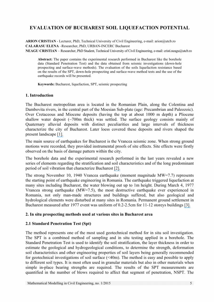
Surface-wave (Rayleigh wave) is elastic waves propagating along the ground surface and its energy concentrates near the ground surface. The surface-wave velocity of propagation strongly depends on S-wave velocity. The surface wave method is the seismic exploration method in which the dispersion character of the surface-waves is analyzed. The surface-wave method can be carried out from ground surface non-destructively [4]. Figure 3 shows the schematic view of a
Mathematical Modelling in Civil Engineering, no. 1/2015 7
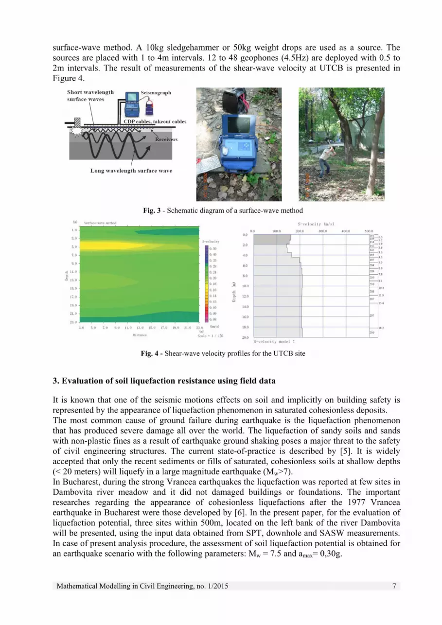
surface-wave method. A 10kg sledgehammer or 50kg weight drops are used as a source. The sources are placed with 1 to 4m intervals. 12 to 48 geophones (4.5Hz) are deployed with 0.5 to 2m intervals. The result of measurements of the shear-wave velocity at UTCB is presented in Figure 4.
Fig. 3 - Schematic diagram of a surface-wave method
Fig. 4 - Shear-wave velocity profiles for the UTCB site
3. Evaluation of soil liquefaction resistance using field data
It is known that one of the seismic motions effects on soil and implicitly on building safety is represented by the appearance of liquefaction phenomenon in saturated cohesionless deposits. The most common cause of ground failure during earthquake is the liquefaction phenomenon that has produced severe damage all over the world. The liquefaction of sandy soils and sands with non-plastic fines as a result of earthquake ground shaking poses a major threat to the safety of civil engineering structures. The current state-of-practice is described by [5]. It is widely accepted that only the recent sediments or fills of saturated, cohesionless soils at shallow depths (< 20 meters) will liquefy in a large magnitude earthquake (Mw>7). In Bucharest, during the strong Vrancea earthquakes the liquefaction was reported at few sites in Dambovita river meadow and it did not damaged buildings or foundations. The important researches regarding the appearance of cohesionless liquefactions after the 1977 Vrancea earthquake in Bucharest were those developed by [6]. In the present paper, for the evaluation of liquefaction potential, three sites within 500m, located on the left bank of the river Dambovita will be presented, using the input data obtained from SPT, downhole and SASW measurements. In case of present analysis procedure, the assessment of soil liquefaction potential is obtained for an earthquake scenario with the following parameters: Mw = 7.5 and amax= 0,30g.
8 Mathematical Modelling in Civil Engineering, no. 1/2015
3.1 Evaluation of soil liquefaction resistance using SPT results
The liquefaction resistance of soil deposits and prediction of the liquefied thickness is based on Standard Penetration Test blow counts in a single boring log. Starting in the 1970’s, H.B. Seed and his colleagues worked to develop a reliable method for assessing the liquefaction potential based on SPT data. Their framework for SPT-based assessments of liquefaction potential was developed in a series of papers that includes [7], [8], [9], significant contributions were also suggested in the work of Tokimatsu [10] and [11].
The empirical method in evaluating the soil liquefaction resistance from Standard Penetration Test blow counts is based on corrected values of (N1)60 and cyclic resistance ratio, CSR.
The first step in evaluating the soil liquefaction resistance is to correct the measured SPT blow counts NSPT. The measured SPT blow counts is first normalized for the overburden stress at the depth of the test and corrected to a standardized value of (N1)60:
1 60( ) SPT N E B S RN N C C C C C (1)
where: NSPT represents the blow counts necessary for 30 cm soil penetration; CN, CE, CB, CS, CR are the correction factors. The next step in the liquefaction analysis procedure is to find the cyclic resistance ratio (CRR) for the soil based on the computed clean-sand equivalent ((N1)60cs). This is done using the empirical base curve drawn from the liquefaction catalogue for a magnitude 7.5 earthquake, according to [12] recommendation. The mathematical expression implemented for determining the cyclic resistance ratio for soil is:
1 607.5
1 60
( )95 1100
34 ( ) 1.3 2cs
Mcs
NCRR
N (2)
where:
CRR is the cyclic resistance ratio for a Mw=7.5 earthquake;
1 60( ) csN represents the clean-sand equivalent SPT value.
The value of CRRM=7.5 must be adjusted for the magnitude of the earthquake under consideration. This is adjusted with a magnitude scaling factor, MSF:
7.5MCRR CRR MSF K (3)
where:
CRR is the cyclic resistance ratio of the soil for an earthquake magnitude corresponding to MSF, which can be considered by assuming that the main effect of different magnitude earthquakes on liquefaction resistance is the number of significant stress cycles generated. The magnitude scaling factors is considered MSF=1 for an earthquake with moment magnitude Mw=7,5 according to [9]. The Kσ factor, a correction for overload, is calculated from the following formula:
'1 ln 1.1v
a
K CP
(4)
Once the liquefaction resistance is known at a certain depth, the average cyclic shear stress generated by an earthquake must be estimated. The representative horizontal shear stress is computed with a simplified equation suggested by [7] and expressed in terms of the cyclic stress ratio (CSR):

Mathematical Modelling in Civil Engineering, no. 1/2015 9
max'
0.65 vod
vo
aCSR r
g
(5)
where:
g=9.81m/s2 is the acceleration due to gravity, vo is the total vertical overburden stress, 'vo is
the effective vertical overburden stress at the depth of interest, amax is the maximum horizontal acceleration that would occur at the ground surface in the absence of excess pore pressures or liquefaction generated by the earthquake. The last parameter is the stress reduction factor, rd, which accounts for soil flexibility as a function of depth, as simple linear equations [7].
The last step in the liquefaction analysis is to compute the factor of safety at each SPT location and the liquefied thickness. If the computed cyclic resistance ratio (CRR) of the soil is less than or equal to cyclic stress ratio (CSR) generated by an earthquake, liquefaction is assumed to occur at that location. The factor of safety against liquefaction, FSliq, is defined [13], [14] and [15]:
liq
CRRFS
CSR
FSliq ≤ 1.0 indicates that the soil at the depth of the measured SPT is predicted to liquefy
FSliq > 1.0 indicates no liquefaction
One of the investigated sites (RD1) is located near Dambovita meadow, with a lithological profile represented by thick sandy soils and interposed clay and sandy clay intercalations and ground water table at 5,00 meters depth. The SPT N-values and the computed parameters, including the necessary corrections used in the literature, are summary presented in Table 1.
Table 1
Liquefaction parameters obtained from SPT-values (RD1 site)
Point Depth
(m)
Overburden stress (kPa) NSPT N1(60) N1(60)cs CSR CRR FSliq
Total Effective 1 3,50 55,30 55,30 6 8.01 8.01 0,32 0,09 0,28 2 5,50 85,10 80,20 4 4.84 4.84 0,37 0,07 0,18 3 7,50 122,10 97,58 13 15.45 15.45 0,17 0,17 0,45 4 9,50 162,10 117,96 22 25.63 25.63 0,37 2,00 5,00 5 11,50 200,10 136,34 26 29.69 29.69 0,37 0,43 1,17 6 15,50 284,10 181,10 21 20.81 20.81 0,36 0,32 0,88 7 17,50 322,70 200,08 19 17.91 17.91 0,36 0,19 0,54 8 20,00 370,20 223,05 43 38.39 38.39 0,36 2,00 5,00
The results of liquefaction potential analysis performed for RD1 site is presented in Figure 5. The safety factor against liquefaction FSliq less than 1 was obtained for saturated sandy layers at the depth of 3.5, 5.5, 7.5, 15.5 and 17.5m, respectively in the points 1, 2, 3, 6 and 7.
3.2 Evaluation of soil liquefaction resistance using shear wave velocities results
The preferable practice when using Vs measurements to evaluate liquefaction resistance is to drill sufficient boreholes and conduct sufficient tests to detect and delineate thin liquefiable strata, to identify non-liquefiable clay-rich soils, etc. One method of direct determination of dynamic soil properties in the field is to measure the velocity of shear waves in the soil. The waves are generated by impacts produced by a hammer or by detonating charges of explosives, and the travel times are recorded. This is usually done in or between boreholes. The use of Vs as an index of liquefaction resistance is justified since both Vs and liquefaction resistance are influenced by many of the same factors (void ratio, effective confining pressure, stress history, geologic age).

10 Mathematical Modelling in Civil Engineering, no. 1/2015
Fig. 5 - Assessment of soil liquefaction potential from SPT data for RD1 site
The resistance of the soil, expressed as the cyclic resistance ratio is generally established by separating liquefied cases from non-liquefied cases in actual earthquakes. Here, following empirical equation defined by [16] and [17] is used:
cVcb
VaCRR
s
s 11
100 1
21
(6)
2
1
'v
ssPa
VV
(7)
where:
a,b,c are parameters (a=0.022, b=2.8, c=200~215m/s),
Vs1 is the overburden stress corrected shear wave velocity defined by [18] as:
where:
Vs = measured shear-wave velocity (m/s), Pa =reference stress (100kPa), 'v = initial effective
overburden stress (kPa).
The values of shear wave velocities used for the assessment of liquefaction potential are collected from geophysical measurements based on downhole (PRI site) and surface wave methods (SASW) for UTCB site. For the PRI site, the lithological profile is dominated by thick sandy and gravelly soils, with ground water table around 9,00 meters depth. On the UTCB site, the deposits are characterized by interposed thick sandy layers and clay lenses, with ground water table intercepted at 10,00 meters. The parameters calculated based on shear wave velocities corresponding to these locations are summary presented in Table 2, respectively in Table 3.
Table 2
Liquefaction parameters obtained from Vs values for PRI site
Point Depth
(m)
Overburden stress (kPa) Vs
(m/s) Vs1
(m/s) CSR CRR FSliq
Total Effective 1 9,00 169,20 169,20 140 122,75 0,34 0,05 0,15 2 20,00 373,80 265,89 280 219,27 0,28 2,00 5,00

Mathematical Modelling in Civil Engineering, no. 1/2015 11
Table 3
Liquefaction parameters obtained from Vs values for UTCB site
Point Depth
(m)
Overburden stress (kPa) Vs
(m/s) Vs1
(m/s) CSR CRR FSliq
Total Effective 1 0,50 9,00 9,00 165 301,25 0,19 2,00 5,00 2 1,20 21,6 21,6 167 244,96 0,21 0,01 5,00 3 1,90 34,2 34,2 160 209,22 0,26 0,34 1,33 4 2,60 47,5 47,5 151 181,89 0,29 0,16 0,56 5 3,50 64,6 64,6 154 171,78 0,31 0,12 0,41 6 4,50 85,6 85,6 162 168,42 0,31 0,12 0,37 7 5,50 106,6 106,6 167 164,35 0,32 0,11 0,34 8 6,60 126,4 126,4 170 160,33 0,33 0,09 0,28 9 7,80 145,6 145,6 172 156,58 0,34 0,09 0,25
10 9,10 166,4 166,4 173 152,32 0,35 0,08 0,23 11 10,40 192,4 188,4 173 147,65 0,34 0,08 0,24 12 11,90 222,4 203,7 173 144,80 0,33 0,08 0,23 13 13,40 249,4 216,1 172 141,87 0,33 0,07 0,21 14 18,20 335,8 255,4 172 136,06 0,30 0,06 0,20 15 20,00 368,2 270,1 182 141,97 0,29 0,07 0,24
The graphical representations related to liquefaction potential analysis performed at PRI and UTCB sites based on shear wave velocities values are presented in Figure 6 and in Figure 7.
Fig. 6 - Assessment of soil liquefaction potential from Vs
data at PRI site Fig. 7 - Assessment of soil liquefaction potential from
Vs data at UTCB site
Considering the liquefaction potential analysis at PRI site, the saturated sandy layer with 9,00 meters thickness is corresponding to safety factors against liquefaction less than 1, with certain liquefaction (LPI=34%) during an earthquake with parameters selected in the scenario. In case of UTCB site, it can be observed that the liquefied layers are extended up to the limit depth of analysis.
4. Conclusions
The different local soil conditions in Bucharest area lead to a variability of the soil response at seismic ground motions, which can occur at small distances and can be observed even for the same city area. This is the reason why in the case of the large urban areas, microzonation studies must take into account the mapping of the soil profile and the ground parameters. We have applied different methods for field investigation to evaluate the liquefaction potential of the sites. Taking into account the complexity and the importance of dynamic stability of cohesionless soil in building safety, it was considered useful to perform an analysis regarding the liquefaction potential assessment on Bucharest sites. The data processing highlights safety factors against liquefaction

12 Mathematical Modelling in Civil Engineering, no. 1/2015
less than 1 and high liquefaction probabilities. Taking into consideration the correlation of soil characteristics, the sites can manifest liquefaction phenomenon during strong earthquakes. The liquefaction potential is related to the location of sites near Dambovita meadow, where recent alluvial deposits, saturated and non-cohesive soils at shallow depths are predominant. Creating an informational database concerning the characteristics of superficial geology of Bucharest is the basis for determining the correlation between seismic velocities and SPT results and soil parameters at seismic motions. The database will set basis for the requirements of Romanian seismic codes, harmonized with the European and international codes.
Acknowledgements
The paper was presented at the “5th National Conference on Earthquake Engineering and the 1st National Conference on Earthquake Engineering and Seismology”, June 19-20 2014, Bucuresti”; it was published in the volume of the Conference.
References
[1]. Liteanu, E., (1951). Geology of Bucharest city zone, St.Tehn.Econ., E, 1, Bucharest (in Romanian) [2]. Arion, C., 2004: Report on soil tests and investigations (laboratory and field experiments), JICA/CNRRS. [3]. Bălan, Ştefan; Cristescu, Valeriu; Cornea, Ion: Cutremurul de pămant din Romậnia de la 4 martie 1977.
Editura Academiei Republicii Socialiste Romậnia, Bucureşti, 1982. [4]. Hayashi, K, and Suzuki, H, (2004). "CMP cross-correlation analysis of multi-channel surface-wave data,"
Exploration Geophysics, Vol 35, pp7-13. [5]. Youd, T.L., Idriss I.M., Andrus R., Arango I., Castro G., Christian J., Dobry R., Liam Finn W., Harder Jr. L.,
Hynes M.E., Ishihara K., Koester J., Liao S., Marcuson III W., Martin G., Mitchell J., Moriwaki Y., Power M., Robertson P., Seed R., Stokoe II K. (2001) „Liquefaction resistance of soils: summary report from the 1996 NCEER and 1998 NCEER/NSF workshops on evaluation of liquefaction of soils”, Journal of Geotechnical and Geoenvironmental Engineering, ASCE, Vol. 127, No. 10, 817- 883.
[6]. Ishihara, K. & Perlea V. (1984). Liquefaction-associated ground damage during the Vrancea earthquake of March 4, 1977, Soils and Foundations, Japanese Soc. of Soil Mech. And Found. Engineering, vol.24, no.1, 90-112.
[7]. Seed, H.B., Idriss, I.M. (1971). Simplified Procedure for Evaluating Soil Liquefaction Potential, J. Soil. Mech. Foundat. Div., ASCE vol. 97, no. SM9, 1971, 1249-1273.
[8]. Seed, H.B. (1979). Soil Liquefaction and Cyclic Mobility Evaluation for Level Ground During Earthquakes, J. Geotech. Engg Div., ASCE vol. 105, no. GT2, 201-255.
[9]. Seed, H.B., Idriss, I.M., Arango, I. (1983). Evaluation of Liquefaction Potential Using Field Performance Data, J. of Geotech. Eng vol. 109, no. 3, 458-482.
[10]. Seed, H.B., Tokimatsu, K., Harder, L.F., Chung, R.M. (1984). The Influence of SPT Procedures in Soil Liquefaction Resistance Evaluations, Report no. UCB/EERC-84/15. Berkeley, California.
[11]. Seed, H.B., Tokimatsu K., Harder L.F., Chung R. (1985). Influence of SPT procedures in soil liquefaction resistance evaluations, J. Geotechnical Eng., ASCE 111(12), 1425-1445.
[12]. NCEER (1997) “Proceedings of the NCEER Workshop on Evaluation of Liquefaction Resistance of Soils”, Youd,T.L., Idriss,I.M., eds., Technical Report No. NCEER-97-0022, 41-88.
[13]. Ishihara K. (1985). Stability of natural deposits during earthquakes. In Eleventh International Conference on Soil Mechanics and Foundation Engineering, (pp. 321–376).
[14]. Ishihara, K. (1993). Liquefaction and flow failure during earthquakes, Geotechnique, Vol.43, No.3, pp.351- 415. [15]. Seed, H.B., Harder L.F. (1990). SPT-based analysis of cyclic pore pressure generation and undrained residual
strength, Proc. Seed Memorial Symposium, J.M. Duncan, BiTech Publishers, Vancouver, pp.351-376. [16]. Andrus, R.D. & Stokoe K.H. (1997). Liquefaction Resistance of Soils from Shear-Wave Velocity. In NCEER
Workshop on Evaluation of Liquefaction Resistance of Soils, NCEER (pp. 89-128). Buffalo, USA. [17]. Andrus, R.D., Stokoe K.H., Chung R.M. & Juang C.H. (2003). Guidelines for evaluating liquefaction
resistance using shear wave velocity measurements and simplified procedures, NIST GCR 03-854, MD. [18]. Robertson, P.K., Woeller D.J., Finn W.D.L. (1992). Seismic Cone Penetration Test for evaluating liquefaction
potential under cyclic loading, Canada Geotechnical Journal, Ottawa, Canada, vol.29, pp. 686-695.
Mathematical Modelling in Civil Engineering, no. 1/2015 13
ANALYSIS OF MASONRY INFILLED RC FRAME STRUCTURES UNDER LATERAL LOADING
MIRCEA BARNAURE - Assistant Lecturer, PhD, Technical University of Civil Engineering, Faculty of Civil, Industrial and Agricultural Buildings, e-mail: [email protected] DANIEL NICOLAE STOICA - Associate Professor, PhD, Technical University of Civil Engineering, Faculty of Civil, Industrial and Agricultural Buildings, e-mail: [email protected]
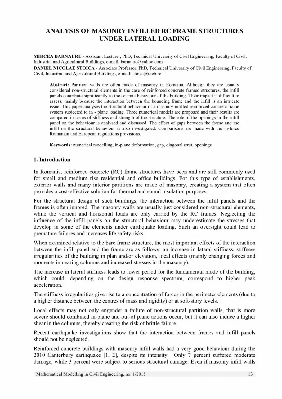
Abstract: Partition walls are often made of masonry in Romania. Although they are usually considered non-structural elements in the case of reinforced concrete framed structures, the infill panels contribute significantly to the seismic behaviour of the building. Their impact is difficult to assess, mainly because the interaction between the bounding frame and the infill is an intricate issue. This paper analyses the structural behaviour of a masonry infilled reinforced concrete frame system subjected to in - plane loading. Three numerical models are proposed and their results are compared in terms of stiffness and strength of the structure. The role of the openings in the infill panel on the behaviour is analysed and discussed. The effect of gaps between the frame and the infill on the structural behaviour is also investigated. Comparisons are made with the in-force Romanian and European regulations provisions.
Keywords: numerical modelling, in-plane deformation, gap, diagonal strut, openings
1. Introduction
In Romania, reinforced concrete (RC) frame structures have been and are still commonly used for small and medium rise residential and office buildings. For this type of establishments, exterior walls and many interior partitions are made of masonry, creating a system that often provides a cost-effective solution for thermal and sound insulation purposes.
For the structural design of such buildings, the interaction between the infill panels and the frames is often ignored. The masonry walls are usually just considered non-structural elements, while the vertical and horizontal loads are only carried by the RC frames. Neglecting the influence of the infill panels on the structural behaviour may underestimate the stresses that develop in some of the elements under earthquake loading. Such an oversight could lead to premature failures and increases life safety risks.
When examined relative to the bare frame structure, the most important effects of the interaction between the infill panel and the frame are as follows: an increase in lateral stiffness, stiffness irregularities of the building in plan and/or elevation, local effects (mainly changing forces and moments in nearing columns and increased stresses in the masonry).
The increase in lateral stiffness leads to lower period for the fundamental mode of the building, which could, depending on the design response spectrum, correspond to higher peak acceleration.
The stiffness irregularities give rise to a concentration of forces in the perimeter elements (due to a higher distance between the centres of mass and rigidity) or at soft-story levels.
Local effects may not only engender a failure of non-structural partition walls, that is more severe should combined in-plane and out-of plane actions occur, but it can also induce a higher shear in the columns, thereby creating the risk of brittle failure.
Recent earthquake investigations show that the interaction between frames and infill panels should not be neglected.
Reinforced concrete buildings with masonry infill walls had a very good behaviour during the 2010 Canterbury earthquake [1, 2], despite its intensity. Only 7 percent suffered moderate damage, while 3 percent were subject to serious structural damage. Even if masonry infill walls

14 Mathematical Modelling in Civil Engineering, no. 1/2015
were not a part of the structure of these buildings, they contributed to the global stiffness in the early stages of the strong ground motion. The damage mostly consisted in the cracking of the masonry in the partition walls. In contrast, incipient brittle failure modes of the RC members were very rarely observed. Most of the structures that suffered damage were built before 1970.
In the 2011 Lorca earthquake [3], some of the buildings that had no effective mechanism to resist lateral loads performed well, and showed damage similar to better designed buildings. Still, many buildings with masonry partition walls suffered serious damage, especially those with asymmetrical horizontal stiffness, akin to the corner buildings of apartment blocks. One of them even collapsed. For other buildings, a soft storey mechanism developed after the deterioration of the ground floor masonry walls. Another type of observed damage comprised of failures of the beam–column joint and shear damaged columns.
In the 2008 Wenchuan earthquake [4,5], many residential and commercial buildings experienced severe damage to the ground floor when less infill walls were at this level as compared to the upper stories. After breakage of the masonry infill walls at the ground floor and prior to the flexural yielding of the columns, the stiffness of the first story significantly reduced and suddenly overloaded the first story columns in shear. This led to the brittle failure mechanism. In some cases, the soft storey mechanism led to building collapse. In the case of infill walls made with hollow tiles, the damage only occurred in the walls, with bricks breaking under compression stresses and the parts of the wall collapsing. In the case of solid bricks, damage was mainly seen in the walls, but also in the columns. The columns located between windows were particularly damaged, as the short column behaviour led to high shear deformations.
Experimental research investigations [6-8] confirm these possible failure mechanisms.
It is clear that only if the infill is separated from the frame and a sufficient gap exists, then it can be considered that the frame and the panel do not interact. This solution is rarely used in common practice due to the difficulties related to connecting the walls to the frame. Out-of plane loads need to be withstood, while allowing free in-plane deformations and ensuring a good thermal and sound insulation. Moreover, if there is a gap only at the top of the wall, between the infill and the frame, a negative effect could occur: the compression strut acts more on the columns, which leads to a faster increase of shear forces [9].
Because of this, the current engineering practice has to take into account the masonry panels when designing RC or steel frames. For the design of new buildings, the Romanian and European seismic codes [9, 10] recommend to consider the effect of the masonry infill panels by equivalent compression struts connecting on the joints of the structure.
Even if infilled frames have demonstrated good earthquake-resistant behaviour at times, it is recommended [9] not to consider the possible positive effects of masonry framed panels in the design model. This is because of the uncertainties related to ensuring a good connection between the infill and the frames during construction.
Over the past decades, researchers proposed various models that allow considering the effects of infills. A first class of models [11], generically named macro-models, involved replacing the masonry by an equivalent pin-jointed diagonal strut. The effective width of the diagonal proposed by authors varies from 1/4 of the length [12] to 1/10 of the length [9]. Others [13] proposed a formula where width depends on the panel geometry, varying from d/4 for square panels to d/11 for a 5:1 panel.
While the single diagonal strut can represent the general behaviour of the building, it cannot describe the local effects resulting from the interaction between the frames and the panel. In order to better predict the bending moments and shear forces in the frame members, multiple-strut models were proposed [14-16]. Recent models [17] consist of bi-diagonal compression struts with a central strut element.

Mathematical Modelling in Civil Engineering, no. 1/2015 15
A second class of models, generically named micro-models, rely on complex analysis using the finite element method (FEM). These models allow to better represent the interaction between the masonry and the frames and to identify all modes of failure and all local effects. They are though more difficult to implement as they require high computational time. The first models [18] used link elements in the contact region, which can transmit compressive forces but not tensile ones. Other models [19] also use plastic theory related to the modes of failure. More recent models [20] use the frame-infill separation criteria to find the length of contact between the infill and the frame for a certain loading pattern. Finally, some models [8, 21-23] simulate the behaviour of masonry infilled RC frames using a combination of discrete and smeared crack elements for the RC frame and the infill panel.
This paper examines the structural behaviour of masonry infilled RC frames under in-plane loading. A FEM modelling approach is adopted, with the robustness of the numerical results being ascertained across several alternative configurations. Our focus lies on the following aspects. First, the main differences in the structural behaviour of the bare and the infilled frames are identified. Second, the influence of any physical gap between the frame and the infill is evaluated. Third, the ability of the diagonal frame model to replicate the actual behaviour is closely examined. Fourth, the impact that any openings in the infill might have on the structural response is measured. Last, the soft storey mechanism is analysed.
Previous literature points to the existence of five ways in which masonry infilled frames may fail: corner crushing, diagonal compression, sliding shear, diagonal cracking and frame failure [24, 25]. Crushing of the infill at the corners occurs when the masonry used has low compressive strength. Diagonal compression results when the infill is relatively slender and failure stems from out-of-plane buckling of the infill. Horizontal sliding shear is associated with strong frame and weak mortar joints. Diagonal cracking often happens if the infill has high strength and the appearance of the first two failure modes is prevented. Frame failure corresponds to the development of plastic hinges in the columns or in the beam-column connections, when the infill is very strong. The numerical models put forward in this paper are evaluated based on their ability to predict some of these failure modes.
2. Numerical models considered
A four storey single span frame structure with reinforced concrete members and masonry infill is analysed. The FEM modelling is conducted using the SAP2000 software.
The values chosen for the beam length and the storey height are 410 cm and 300 cm respectively. The reinforced concrete elements (columns and beams) are modelled using frame elements while the infill is modelled using shell elements.
The concrete class is C20/25 [26] and the reinforcement type is PC52 (fyd=300 MPa). The beams are 30x45 cm, with As = As' = 3d20 reinforcement. The columns have a 40x40 cm section with 4d25 (corners) + 4d20 (intermediate) reinforcement.
By assumption, the infill is made with 30x15x10 bricks. The Young modulus was considered E = 3600 N/mm2 corresponding to masonry with strong mortar [27]. The compressive strength of masonry was computed in accordance with current European regulations [28] for two scenarios. For hollow bricks with fb = 20 MPa and fm = 15 MPa mortar, fk = 8.3 MPa. For solid bricks with fb = 30 MPa and fm = 15 MPa, fk = 13.4 MPa.
The connection between the frame and the infill is modelled using nonlinear gap elements, which allow compression and shear but not tension forces. This type of connection elements also allow to assume that a physical gap exists between the elements and while this gap is not closed due to the deformation of the structure, no interaction occurs.
16 Mathematical Modelling in Civil Engineering, no. 1/2015
Nonlinear hinges are assigned to the beams and frames (M for beams, P-M for columns).
The vertical and horizontal loads are applied as distributed on each beam. The chosen value for vertical loads at each level is 50 kN/m. The lateral forces have an inverted triangular distribution.
a. Bare frame b. Diagonal frame c. Diagonal shell d. Full infill
e. Soft storey f. Window opening g. Central door opening h. Side door opening
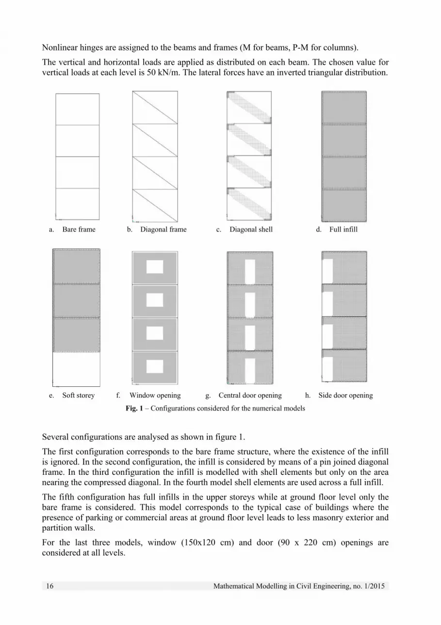
Fig. 1 – Configurations considered for the numerical models
Several configurations are analysed as shown in figure 1.
The first configuration corresponds to the bare frame structure, where the existence of the infill is ignored. In the second configuration, the infill is considered by means of a pin joined diagonal frame. In the third configuration the infill is modelled with shell elements but only on the area nearing the compressed diagonal. In the fourth model shell elements are used across a full infill.
The fifth configuration has full infills in the upper storeys while at ground floor level only the bare frame is considered. This model corresponds to the typical case of buildings where the presence of parking or commercial areas at ground floor level leads to less masonry exterior and partition walls.
For the last three models, window (150x120 cm) and door (90 x 220 cm) openings are considered at all levels.

Mathematical Modelling in Civil Engineering, no. 1/2015 17
3. Comparison between the bare frame and the infilled frame behaviour
For the bare frame model, the nonlinear static pushover analysis shows that increasing lateral loads leads to development of plastic hinges at the ends of the beams and at the base of the columns before reaching the structural capacity.
Fig. 2 – Development of plastic hinges in the RC elements for the bare frame model
For the full infill model, the behaviour is different. The analysis shows that increasing lateral loads leads to development of plastic hinges only in the columns.
Fig. 3 – Development of plastic hinges in the RC elements for the full infill model
This can be explained by the fact that compressive stresses that develop in the infill panel act as a diagonal and the flexural behaviour of the members is replaced by a compression – tension behaviour.
Fig. 4 – Evolution of principal compression stresses, Smin (N/mm2) in the masonry panel

18 Mathematical Modelling in Civil Engineering, no. 1/2015
This is accompanied by an important increase of the stiffness of the building. In figure 5 the pushover curves for the bare frame and the full infill models are traced. The computed stiffness of the bare frame is 3.5 times lower than the stiffness of the infilled frame.
Fig. 5 – Comparison between structural behaviour for bare frame and infilled frame
For the bare frame, the fundamental period is 0.6 s and the maximum lateral load is 180 kN. For the infilled frame, the maximum load is 800 kN. The maximum displacement of the bare frame is 150 mm, while for the infilled frame it is only 60 mm. For the infilled frame, the triggering event that stopped the displacement was the failure of the concrete column in tension. For the final state, the computed von Mises stress, SVM, at the corners of the masonry panels reaches values higher than 8.3 MPa, up to 19 MPa. This means that corner crushing failure can occur prior to failure of the column, in particular for hollow bricks. Still, as masonry compressive strength can sometimes be much higher than the strength computed using Eurocode formulas [27], the column failure criterion was considered
4. Influence of construction gaps on the behaviour
The influence of physical gaps between the masonry and the frame on the nonlinear response of the structure is analysed. These gaps could be required by design in order to ensure separation or they could be a result of poor construction of the partition walls. The same dimensions of the gaps were considered on top of the panel as well as on its sides.
Fig. 6 – Influence of physical gap between frame and infill on the nonlinear response
y = 6.0018x
y = 21.272x
0
100
200
300
400
500
600
700
800
0 25 50 75 100 125 150
Bas
e sh
ear f
orce
(kN
)
Displacement at the top of the building (mm)
Bare frameFull infill
0
100
200
300
400
500
600
700
800
900
0 25 50 75 100 125 150 175 200 225 250
Bas
e she
ar fo
rce (
kN)
Displacement at the top of the building (mm)
Bare frame Infill no gap Infill 2mm gap
Infill 5 mm gap Infill 7 mm gap Infill 10 mm gap
Infill 15 mm gap Infill 20 mm gap Infill 50 mm gap
Mathematical Modelling in Civil Engineering, no. 1/2015 19
The results show that it is very important to account for such eventual gap because the overall behaviour of the frame is significantly affected. The behaviour of the structure corresponds to that observed in experimental testing [29]. While there is no contact between the frame and the infill, the structure behaves exactly as the bare frame. After contact, there is a sudden rise in stiffness and the structure behaves similar to the fully infilled one. For the analysed building, 20 mm gaps are sufficient to ensure that there is no interaction between the frame and the infill which could influence structural behaviour.
5. Comparison between the equivalent diagonal and the full panel
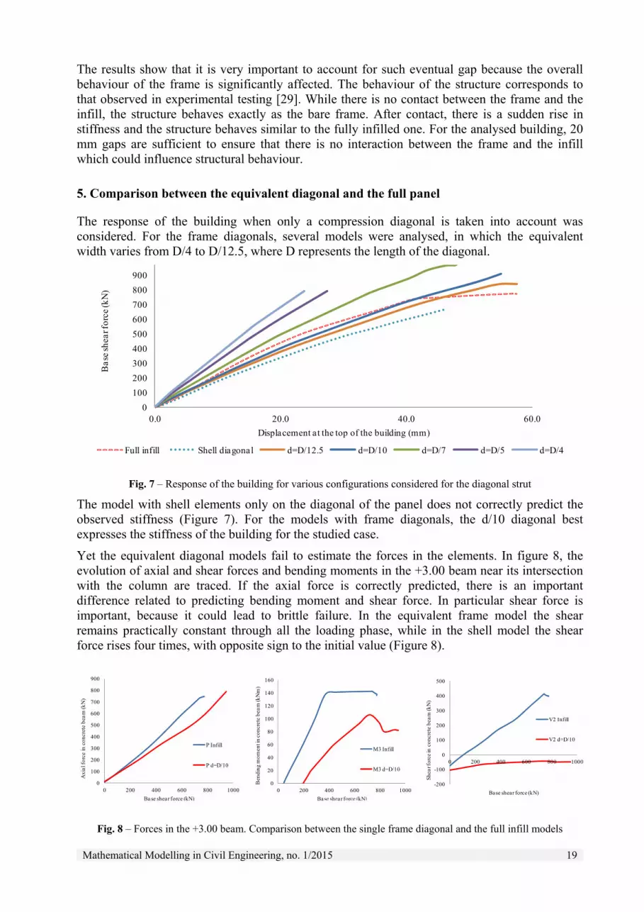
The response of the building when only a compression diagonal is taken into account was considered. For the frame diagonals, several models were analysed, in which the equivalent width varies from D/4 to D/12.5, where D represents the length of the diagonal.
Fig. 7 – Response of the building for various configurations considered for the diagonal strut
The model with shell elements only on the diagonal of the panel does not correctly predict the observed stiffness (Figure 7). For the models with frame diagonals, the d/10 diagonal best expresses the stiffness of the building for the studied case.
Yet the equivalent diagonal models fail to estimate the forces in the elements. In figure 8, the evolution of axial and shear forces and bending moments in the +3.00 beam near its intersection with the column are traced. If the axial force is correctly predicted, there is an important difference related to predicting bending moment and shear force. In particular shear force is important, because it could lead to brittle failure. In the equivalent frame model the shear remains practically constant through all the loading phase, while in the shell model the shear force rises four times, with opposite sign to the initial value (Figure 8).
Fig. 8 – Forces in the +3.00 beam. Comparison between the single frame diagonal and the full infill models
0
100
200
300
400
500
600
700
800
900
0.0 20.0 40.0 60.0
Bas
e sh
ear f
orce
(kN
)
Displacement at the top of the building (mm)
Full infill Shell diagonal d=D/12.5 d=D/10 d=D/7 d=D/5 d=D/4
0
100
200
300
400
500
600
700
800
900
0 200 400 600 800 1000
Axi
al f
orce
in c
oncr
ete
beam
(kN
)
Base shear force (kN)
P Infill
P d=D/10
0
20
40
60
80
100
120
140
160
0 200 400 600 800 1000
Ben
ding
mom
ent i
n co
ncre
te b
eam
(kN
m)
Base shear force (kN)
M3 Infill
M3 d=D/10
-200
-100
0
100
200
300
400
500
0 200 400 600 800 1000
Shea
r for
ce in
con
cret
e be
am (k
N)
Base shear force (kN)
V2 Infill
V2 d=D/10

20 Mathematical Modelling in Civil Engineering, no. 1/2015
6. Influence of the openings on the structural behaviour
The effects that window openings in the infill have on the response of the structure were analysed. As the window prevents the formation of a direct diagonal strut, inclined struts appear above and below the windows as shown in figure 9. This leads to a high increase in stresses around the angles of the windows. Failure patterns observed in experimental tests [8, 25, 30, 31] indicate that these areas are most likely to fail first and should be carefully designed.
Fig. 9 – Evolution of principal compression stresses, Smin (N/mm2) around window openings
For the door openings, a similar pattern is observed. A high concentration of compression stresses appears near the top angle of the opening. For the central door opening (Figure 10), the diagonal strut acts more on the compressed column, when compared to the full infill model, with an increase in the shear force. A similar effect is observed at the top of the storey, where the diagonal compresses the beam. Under normal circumstances, the central part of the beam has little shear reinforcement provided, given that the shear value is low. As a result, the effect can be particularly dangerous and requires careful consideration. For the side door opening (Figure 11), the increase in shear appears near the joint.
Failure patterns observed in experimental tests [8, 25] correspond to this behaviour highlighted by the numerical models.
Fig. 10 – Evolution of principal compression stresses, Smin (N/mm2) around central door opening

Mathematical Modelling in Civil Engineering, no. 1/2015 21
Fig. 11 – Evolution of principal compression stresses, Smin (N/mm2) around lateral door opening
The central door openings lead to a significant decrease of the building stiffness, while the decrease for windows and lateral doors is minimal (Figure 12).
Fig. 12 – Influence of openings in the infill on the structural response
7. Soft storey mechanism
For the soft storey model, the nonlinear static pushover analysis shows that increasing lateral loads leads to development of plastic hinges only in the ground floor columns (Figure 13).
Fig. 13 – Development of plastic hinges in the RC elements for the soft storey model
This decreases the post-elastic deformation capacity of the building by more than 50%. As shown in Figure 14, the ultimate displacement predicted by the soft-storey model is 66 mm, while for the bare frame model the ultimate displacement is 147 mm.
0
200
400
600
800
0 25 50 75 100 125 150
Ba
se s
hea
r fo
rce
(kN
)
Displacement at the top of the building (mm)
Bare frameInfill no gapInfill windowInfill central doorInfill side door

22 Mathematical Modelling in Civil Engineering, no. 1/2015
Fig. 14 – Soft storey structural response
8. Conclusions
The results obtained from the numerical models show the important influence of the masonry infill on the RC frame behaviour for in-plane lateral loads.
The numerical simulations indicate that masonry infill highly increases the stiffness of the structure, up to 3.5 times when compared to the bare frame structure. The openings in the infill influence this effect, particularly door openings.
Masonry infill also increases the strength of the structure (as long as the seismic demand does not exceed the deformation capacity of the infills). Still, the presence of gaps between the infill and the frame can limit this beneficial effect of masonry. For the studied case, separating the infill from the frames by 20 mm gaps at the top and on the sides is sufficient to allow the frame to freely deform, similarly to the no-infill case.
Simple modelling with equivalent diagonal struts, which carry loads only in compression, is able to simulate the global seismic response of the infilled frames. The dimension of the equivalent strut proposed by the current Romanian seismic code, d=D/10 offers a very good estimate of the building stiffness for the studied case. But diagonal frame models cannot estimate the evolution of forces in frame members. Shear forces, which could lead to brittle failure, are particularly underestimated.
The window and door openings in the infill lead to the formation of inclined struts with high concentration of stresses near the corners of the openings, which could lead to failure in the masonry.
The soft storey mechanism is particularly dangerous, as the displacement capacity of the building is reduced to less than 50% when compared to the bare frame. This could result in premature failure of the building.
It is extremely important to take these possible failure mechanisms into account when designing new buildings.
References
[1]. Kam, W. Y., Pampanin, S., Dhakal, R. P., Gavin, H., & Roeder, C. W. (2010). Seismic performance of reinforced concrete buildings in the September 2010 Darfield (Canterbury) earthquakes. Bulletin of New Zealand Society of Earthquake Engineering. Vol. 43, No. 4, pp. 340-350
[2]. Dhakal, R.P. (2010) Damage to Non-Structural Components and Contents in 2010 Darfield Earthquake. Bulletin of the New Zealand Society of Earthquake Engineering. Vol. 43, No. 4, pp. 404-411.
0
100
200
300
400
500
600
700
800
0 25 50 75 100 125 150
Bas
e sh
ear f
orce
(kN
)
Displacement at the top of the building (mm)
Bare frameFull infill Soft storey

Mathematical Modelling in Civil Engineering, no. 1/2015 23
[3]. Hermanns, L., Fraile, A., Alarcón, E., & Álvarez, R. (2014). Performance of buildings with masonry infill walls during the 2011 Lorca earthquake. Bulletin of Earthquake Engineering. Vol. 12, No. 55, pp. 1977-1997. DOI 10.1007/s10518-013-9499-3
[4]. Li, B., Wang, Z., Mosalam, K. M., & Xie, H. (2008). Wenchuan earthquake field reconnaissance on reinforced concrete framed buildings with and without masonry infill walls. The 14th World Conference on Earthquake Engineering. Beijing, China.
[5]. Zhao, B., Taucer, F., & Rossetto, T. (2009). Field investigation on the performance of building structures during the 12 May 2008 Wenchuan earthquake in China. Engineering Structures, Vol. 31, No.8, pp. 1707-1723.
[6]. Žarnić, R., Gostič, S., Crewe, A. J., & Taylor, C. A. (2001). Shaking table tests of 1: 4 reduced‐scale models of masonry infilled reinforced concrete frame buildings. Earthquake engineering & structural dynamics. Vol. 30 No. 6, pp. 819-834.
[7]. Calvi, G. M., Bolognini, D., & Penna, A. (2004). Seismic performance of masonry-infilled RC frames: benefits of slight reinforcements. Invited lecture to Sísmica 6, pp. 14-16.
[8]. Stavridis, A. (2009). Analytical and experimental study of seismic performance of reinforced concrete frames infilled with masonry walls. Doctoral dissertation. University of California, San Diego, USA.
[9]. TUCEB (2013) Code for seismic design - Part I – Design rules for buildings. P100-1/2013. Bucharest [10]. CEN (2004) Eurocode 8: Design of structures for earthquake resistance - Part 1: General rules, seismic actions
and rules for buildings. EN 1998-1:2004. Brussels [11]. Polyakov, S. V. (1960). On the interaction between masonry filler walls and enclosing frame when loaded in
the plane of the wall. Earthquake engineering. pp. 36-42. [12]. Paulay, T., & Priestley, M. J. N. (1992) Seismic design of reinforced concrete and masonry buildings. John
Wiley & Sons, Inc, Hoboken, New Jersey. pp 768. [13]. Smith, B. S. (1962). Lateral stiffness of infilled frames. Journal of the Structural Division, ASCE. Vol. 88 No.
6, pp. 183-199. [14]. Crisafulli, F. J. (1997). Seismic behaviour of reinforced concrete structures with masonry infills. [15]. Chrysostomou, C. Z., Gergely, P., & Abel, J. F. (2002). A six-strut model for nonlinear dynamic analysis of
steel infilled frames. International Journal of Structural Stability and Dynamics. Vol. 2, No.3, pp. 335-353. [16]. Crisafulli, F. J., & Carr, A. J. (2007). Proposed macro-model for the analysis of infilled frame structures.
Bulletin of the New Zealand Society for Earthquake Engineering. Vol. 40, No.2, pp. 69-77. [17]. Rodrigues, H., Varum, H., & Costa, A. (2010). Simplified macro-model for infill masonry panels. Journal of
Earthquake Engineering. Vol. 14 No.3, pp.390-416. [18]. Mallick, D. V., & Severn, R. T. (1967). The behaviour of infilled frames under static loading. ICE
Proceedings. Vol. 38, No. 4, pp. 639-656 [19]. Te-Chang, L., & Kwok-Hung, K. (1984). Nonlinear behaviour of non-integral infilled frames. Computers &
structures. Vol. 18 No. 3, pp. 551-560. [20]. Asteris, P. G. (2003). Lateral stiffness of brick masonry infilled plane frames. Journal of Structural
Engineering. Vol. 129 No.8, pp. 1071-1079. [21]. Mehrabi, A. B., & Shing, P. B. (1997). Finite element modeling of masonry-infilled RC frames. Journal of
structural engineering. Vol. 123, No.5, pp. 604-613. [22]. Attard, M. M., Nappi, A., & Tin-Loi, F. (2007). Modeling fracture in masonry. Journal of Structural
Engineering. Vol. 133, No.10, pp. 1385-1392. [23]. Stavridis, A., & Shing, P. B. (2010). Finite-element modeling of nonlinear behavior of masonry-infilled RC
frames. Journal of structural engineering. Vol. 136, No. 3, pp. 285-296. [24]. El-Dakhakhni, W. W., Elgaaly, M., & Hamid, A. A. (2003). Three-strut model for concrete masonry-infilled
steel frames. Journal of Structural Engineering. Vol. 129, No.2, pp. 177-185. [25]. Asteris, P. G., Kakaletsis, D. J., Chrysostomou, C. Z., & Smyrou, E. E. (2011). Failure modes of In-filled
frames. Electronic Journal of Structural Engineering. Vol. 11, No. 1, pp. 11-20. [26]. CEN (2004) Eurocode 2: Design of Concrete Structures: Part 1-1: General Rules and Rules for Buildings. EN
1992-1-1:2004. Brussels. [27]. Kaushik, H. B., Rai, D. C., & Jain, S. K. (2007). Stress-strain characteristics of clay brick masonry under
uniaxial compression. Journal of materials in Civil Engineering, Vol. 19, No. 9, pp. 728-739. [28]. CEN (2005) Eurocode 6: Design of masonry structures—Part 1-1: General rules for reinforced and
unreinforced masonry structures. EN 1996-1-1:2005+A1:2012. Brussels. [29]. Lin, K., Totoev, Y. Z., Liu, H. J., & Page, A. W. (2014). Modeling of dry-stacked masonry panel confined by
reinforced concrete frame. Archives of Civil and Mechanical Engineering. Vol. 14, No.3, pp. 497-509. [30]. Chen, X., & Liu, Y. (2015). Numerical study of in-plane behaviour and strength of concrete masonry infills
with openings. Engineering Structures. Vol. 82, pp. 226-235. [31]. Koutromanos, I., Stavridis, A., Shing, P. B., & Willam, K. (2011). Numerical modeling of masonry-infilled RC
frames subjected to seismic loads. Computers & Structures. Vol. 89, No.11, pp. 1026-1037.
24 Mathematical Modelling in Civil Engineering, no. 1/2015
RECENT VS. HISTORICAL SEISMICITY ANALYSIS FOR BANAT SEISMIC REGION (WESTERN PART OF ROMANIA)
EUGEN OROS – Senior Researcher, PhD, National Institute for Earth Physics, e-mail: [email protected] MIHAI DIACONESCU – Senior Researcher, PhD, National Institute for Earth Physics, e-mail: [email protected]
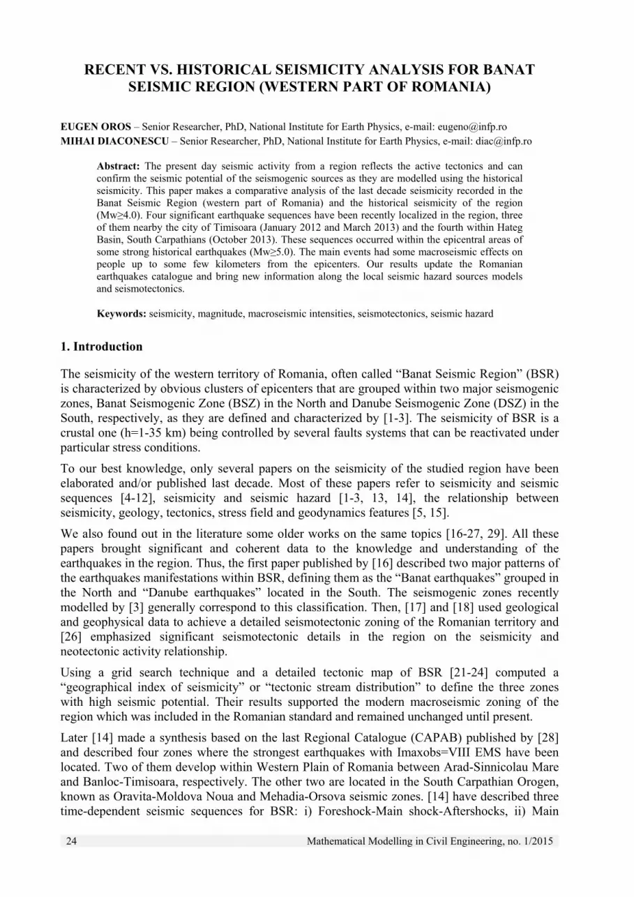
Abstract: The present day seismic activity from a region reflects the active tectonics and can confirm the seismic potential of the seismogenic sources as they are modelled using the historical seismicity. This paper makes a comparative analysis of the last decade seismicity recorded in the Banat Seismic Region (western part of Romania) and the historical seismicity of the region (Mw≥4.0). Four significant earthquake sequences have been recently localized in the region, three of them nearby the city of Timisoara (January 2012 and March 2013) and the fourth within Hateg Basin, South Carpathians (October 2013). These sequences occurred within the epicentral areas of some strong historical earthquakes (Mw≥5.0). The main events had some macroseismic effects on people up to some few kilometers from the epicenters. Our results update the Romanian earthquakes catalogue and bring new information along the local seismic hazard sources models and seismotectonics.
Keywords: seismicity, magnitude, macroseismic intensities, seismotectonics, seismic hazard
1. Introduction
The seismicity of the western territory of Romania, often called “Banat Seismic Region” (BSR) is characterized by obvious clusters of epicenters that are grouped within two major seismogenic zones, Banat Seismogenic Zone (BSZ) in the North and Danube Seismogenic Zone (DSZ) in the South, respectively, as they are defined and characterized by [1-3]. The seismicity of BSR is a crustal one (h=1-35 km) being controlled by several faults systems that can be reactivated under particular stress conditions.
To our best knowledge, only several papers on the seismicity of the studied region have been elaborated and/or published last decade. Most of these papers refer to seismicity and seismic sequences [4-12], seismicity and seismic hazard [1-3, 13, 14], the relationship between seismicity, geology, tectonics, stress field and geodynamics features [5, 15].
We also found out in the literature some older works on the same topics [16-27, 29]. All these papers brought significant and coherent data to the knowledge and understanding of the earthquakes in the region. Thus, the first paper published by [16] described two major patterns of the earthquakes manifestations within BSR, defining them as the “Banat earthquakes” grouped in the North and “Danube earthquakes” located in the South. The seismogenic zones recently modelled by [3] generally correspond to this classification. Then, [17] and [18] used geological and geophysical data to achieve a detailed seismotectonic zoning of the Romanian territory and [26] emphasized significant seismotectonic details in the region on the seismicity and neotectonic activity relationship.
Using a grid search technique and a detailed tectonic map of BSR [21-24] computed a “geographical index of seismicity” or “tectonic stream distribution” to define the three zones with high seismic potential. Their results supported the modern macroseismic zoning of the region which was included in the Romanian standard and remained unchanged until present.
Later [14] made a synthesis based on the last Regional Catalogue (CAPAB) published by [28] and described four zones where the strongest earthquakes with Imaxobs=VIII EMS have been located. Two of them develop within Western Plain of Romania between Arad-Sinnicolau Mare and Banloc-Timisoara, respectively. The other two are located in the South Carpathian Orogen, known as Oravita-Moldova Noua and Mehadia-Orsova seismic zones. [14] have described three time-dependent seismic sequences for BSR: i) Foreshock-Main shock-Aftershocks, ii) Main
Mathematical Modelling in Civil Engineering, no. 1/2015 25
shock-Aftershocks and iii) Swarms. They also speculate some long-time behavior of the seismic activity with its possible migration between the North and the South seismic zones.
Recently, [2] compiled the most complete earthquakes catalogue located within BSR and its surroundings and he modeled the newest seismic zoning of RSB using a comprehensive dataset on geology, geophysics, tectonics and seismicity. He defined three zones of particular seismicity that correlate to the geotectonic units on Mw≥5.3 (Io≥VII-VIII EMS) earthquakes distribution basis: i) the Northern Zone with Sinnicolau Mare-Arad epicentral areas, ii) the Central Zone having two epicentral areas (Timisoara and Banloc-Voiteg) and iii) the Southern Zone inside which he defined Oravita-Moldova Noua and Mehadia-Orsova epicentral areas. The author described also a new seismo-active zone within Poiana Rusca Mts - Hateg Basin - Bistra Valley area.
The main objective of this paper focuses on i) the investigation of the seismic activity recorded in the region over last decade, especially the past five years when several events produced macroseismic effects, and ii) performing a comparative analysis with the strong historical seismicity models and local seismic hazard sources. We also analyzed and compiled all available databases to update the regional parametric catalogue of earthquakes for Banat (CAPAB) developed by [3].
2. Data and processing
We compiled a new up to date earthquakes catalogue using seismic bulletins and catalogues. Two earthquakes catalogues, CAPAB by [3, 28] and ROMPLUS (updated version from www.infp.ro) furnished hypocentral parameters of all earthquakes used in the paper. For many significant earthquakes we also collected primary seismological data, like waveforms, travel times, polarities, amplitudes recorded by:
i) the Romanian Seismic Network
ii) national and international seismological services, such as for example CSEM (www.emsc-csem.org), GFZ-GEOFON (www.geofon.gfz-potsdam.de/waveform), ISC (www.isc.ac.uk) and Serbian Seismological Survey (www.seismo.gov.rs).
The core of the new database is CAPAB Regional Catalogue compiled for 1443-2006 period by [3]. All seismic events recorded since 2007 have been imported from ROMPLUS Catalogue and ISC Bulletins. We relocated all imported hypocenters using a local velocity model [2] and the Seisan free software package [30] to respect the procedure used for CAPAB_1443-2006.
The final database contains a generic magnitude M that is referring to Mw until 2006 and mainly MD between 2007 and 2013. This magnitude should not be used for quantitative investigation of seismicity.
A complex problem for seismicity studies appeared since 2000 when the Romanian Seismic Network systematically developed and very sensitive seismic sensors have been installed all over the Romanian territory. As a direct consequence, ROMPLUS included a large number of seismic events that could be explosions and so, these events can contaminate the natural phenomena under investigation. The same problem could appear in ISC bulletins from the data supplied by the Seismological Service of Serbia.
We investigated the compilation between 1988-2013 to identify and eliminate, as it is possible, all this type of events. The charts presented in Fig. 1 show anomalous values of some relevant parameters for highlighting the events suspected to be explosions. Thus, we simply could notice:
i) a very sharp increase in the cumulative number of events after 2005 without any significant increase in seismic moment;

26 Mathematical Modelling in Civil Engineering, no. 1/2015
Fig. 1 – ROMPLUS catalogue and ISC bulletin compilation (1988-2013): magnitude analysis. All distributions
show anomalous values that support inclusions of explosions between 2006 and 2013. The entire aftershocks series of the strongest (M=5.5-5.6) earthquakes occurred in Banloc (12.07.1991 and 02.12.1991) and Mehadia
(18.07.1991) zones are not included.
i. a large number of the events with M=2.3 between 2006 and 2013,
ii. a very sharp increase in the number of events with M=2.3-2.5 since 2006,
iii. a large value of the b coefficient of Gutemberg-Richter relationship (b>1.5).
To localize the zones with possible quarry and/or mining blasts we firstly investigated the ratio of daytime to nighttime number of events as an efficient technique described by [31]. High values of this ratio estimate the possible distribution of explosions in the region. We applied this technique using a grid search of 10x10 km, sample size N=100 and a daytime interval between 7 and 15 hours. Finally, we removed 1386 of the 2847 (56%) events recorded during 2007-2013. Most of them were located in Apuseni Mts, Poiana Rusca Mts and Moldova Noua areas (Fig. 2).
Magnitude histogram
Seismic Moment
Number
Num
ber
Time histogram
Gutemberg_Richter relationship
Time – magnitude distribution

Mathematical Modelling in Civil Engineering, no. 1/2015 27
However, we applied additional criteria before eliminating the suspected explosions: first polarities of P wave (direct P waves from explosions expose compressions), waveforms, magnitude, information about the locations of quarries, mines, etc. We kept in the final catalogue more events located in areas Siria-Arad, Deva-Hateg and Moldova on the direct P wave polarity and spatial distribution of epicenters criteria basis. We obtained the histograms and the maps shown in Fig. 1 and Fig. 2 using Zmap software [32].
The new updated regional catalogue elaborated for BSR by [3] contains 8690 entries of which 1080 occurred between 2007 and 2013.
3. Results and discussions
Figure 3 displays the distribution of seismic events identified and localized in BSR between 1 January 2007 and 31 December 2013. Even there is a trend of dispersion of the epicenters within entire region we notice several obvious clusters. Four significant earthquakes, defined here as events with macroseismic effects, occurred in the region over last years (Table 1).
Fig. 2 – Database analysis (1988-2013): quarry identification using the ratio of daytime to nighttime number of events. Hourly histograms of the number of events (a) and the 2D distributions of the ratio of daytime to
nighttime number of events (b) obtained with and without suspected explosions.
Timisoara
Hateg
Moldova Noua
Deva
Apuseni Mts
Poiana Rusca Mts
Siria Arad
Orsova
South Carpathians
Siria Arad
Orsova
South Carpathians
Timisoara
Hateg
Moldova Noua
Deva
Apuseni Mts
Poiana Rusca Mts
with explosions without explosions
a)
b)

28 Mathematical Modelling in Civil Engineering, no. 1/2015
Fig. 3 – a) Banat Seismic Region (BSR): Map of epicenters without explosions (1081 events, period: 2007-2013). Red circles define the four significant seismic sequences (main event with macroseismic effects) located within
Timisoara-Sanandrei (A), Timisoara-Sag (B), Recas-Topolovatu Mare (C) and Hateg zones. Green rectangles mark the other recent earthquakes clusters - some of them can be correlated with significant historical earthquakes shown
in Fig. 4 (Lovrin-Teremia, Srbski Ittebej/Serbia, Banloc-Voiteg, Sag-Parta, Moldova Noua, Mehadia-Orsova). Bocsa and Lipova-Siria areas have no known significant seismic history [2]. b) The frequency of occurrence - magnitude relationship: the value of the b regression coefficient (b=0.97) is specific for the whole region [2].
Srbski Ittebej
Lipova-Siria
Bocsa
Lovrin-Teremia
Mehadia
Banloc-Voiteg
Sag-Parta
A
B
C D
bb== 00..9977

Mathematical Modelling in Civil Engineering, no. 1/2015 29
Table 1
Hypocentral parameters of the main events recorded in BSR between 2009 and 2013 years. *Mw computed from spectral analysis; #Pre-shock: 08.09.2013, H=13:00:43.8, 45.58/22.83, h=5.1 km,
Mw=3.6±0.2, ML=3.6, MD=4.3.
Date Origin Time
Geografical cordinates Focal
Depth (km)
Magnitude Mw*
Observations LatN
(degree) LongE
(degree)
07.01.2012 05 43 24.7 45.70 21.15 9.8 3.1±0.2 ML=3.0, MD=3.8 (SE Timisoara), after [21]; Felt in Timisoara (I=III-IV EMS)
09.01.2012 19 56 24.6 45.77 21.68 12.0 3.3±0.2
ML=3.4, MD=4.0 (E Timisoara, Topolovatu Mare), after [21]
Felt in Timisoara (I=III EMS), Lugoj, Buzias.
26.03.2013 12 07 16.4 45.83 21.24 5.7 2.7±0.2 ML=2.6, MD=3.4 (N-NE Timisoara),
Felt in Timisoara I=III-IV EMS
08.09.2013# 13 22 13.9 45.65 22.86 7.7 4.0±0.2 ML=4.1, MD=4.5
Io=V-VI EMS (computed), Felt in Hateg and surroundings
Their fore- and aftershocks show a 2D space distribution on certain alignments or as small areas, specifically defined as Timisoara-Sanandrei, Timisoara-Sag, Recas-Topolovatu Mare and Hateg seismic active zones. These events are the first ones felt in the region since 2002, when a significant Mw=4.3 (Io=VII EMS) earthquake occurred in the Moldova Noua area.
Timisoara-Sanandrei zone (23 events, main shock on 26.03.2013) is located north of the city of Timisoara where there is a significant historical seismic activity [2]. A strong earthquake occurred on 19.11.1879 (Mw=5.4) and other one with M≈5.6 is mentioned in the historical documents on 20 June 1443. The last one needs additional detailed documentation to localize it more accurately in time and space [2]. It is worth to mention several historical events, which confirm the seismic potential of the local fault system, e.g. 25.04.1846, Mw=4.8, (I=VI-VIIEMS); 29.02.1904, Mw=4.5 (I=VIEMS); 27.01.1972 Mw=4.5 (I=VIEMS) and 23.08.1973, Mw=4.5 (I=VIEMS).
Timisoara-Sag zone (23 events, main shock on 07.01.2012) is one of the most dangerous for the city of Timisoara. Here an Mw=5.4 (Iobs=VIII EMS) earthquake hit the city and the neighboring localities on 27.05.1959. This event had a large number of aftershocks that lasted for a long time. In 1960, on 22 October other strong earthquake (Mw=5.0) occurred in this epicentral area. Since that time the seismicity is characterized by small to moderate events such as the Mw=4.5, 04.01.1978 earthquake and then only the recent one (Mw=3.1, 07.01.2013). Also, about 23 years ago there was recorded a significant seismic activity with the major event occurred on 06.09.1936 (Mw=5.2±0.2, Io=VII EMS) [12].
Recas-Topolovatu Mare zone (92 events, main shock on 09.01.2012) is the largest epicentral area of the four investigated in this work. The recent seismic activity was analyzed on detail by [8]. Historical seismicity confirms the seismic potential of the system faults in this area [6]. The major events recorded are the following [19]: 08.02.1896, Mw=4.2; 28.11.1896, Mw=4.1; 12.08.1905, Mw=4.9; 14.01.1932, Mw=4.3; 01.10.1956, ML=4.0; 21.01.1972, Mw=4.5. The last earthquake with significant macroseismic effects (Io=VI EMS) occurred near the city of Buzias on 29.11.1988 (ML=3.7). Even in the time of writing this paper an earthquake with ML=3.2 (19.03.2014) occurred in this area and it was felt (I=III EMS) in Timisoara.
Hateg zone (111 events, main shock on 08.09.2013) is located in the eastern edge of BSR, within a small Neogene Basin. The historical strong seismicity of the zone is not well known, but some authors localized here several strong earthquakes [2, 29]. Thus, [2] localized nearby Hateg area the 19.01.1665 (Mw=4.5) event even if it is very little documented and the authors of

30 Mathematical Modelling in Civil Engineering, no. 1/2015
ROMPLUS fixed the epicenter in the Portile de Fier - Orsova zone. Here and in other surrounding zones were, also, located some events with M≥4.0. Thus, the earthquakes occurred in the Deva-Mures Valley zone (30.04.1886 and 05.10.1890, Mw=4.0) and Lupeni-Jiu Valley zone (20.10.1909, Mw=5.0) are known. From what we know so far the recently recorded Mw=4.0, 08.09.2013 event is the first local earthquake with certain location that produced macroseismic effects. The 09.07.1912 (Mw=5.2, Ms=4.9) appear as a significant event that needs more investigations because it has uncertain locations in Hateg Basin or in Targu Jiu area. Different authors located it in different zones: i) Ho=21:46, 45.7/22.8, Mw=5.2 (Poiana Rusca Mts zone after [2] with corrections), ii) Ho=21:46, 45.0/23.3, Mw=4.5 (Tirgu Jiu zone after ROMPLUS) and iii) Ho=21:46, 45.4/22.8, Ms=4.9 (Hateg zone, after [29]). Even when we wrote this paper for the conference, an earthquake with ML=3.0 occurred in this zone; thus confirming that it is a seismic area to which we must pay a particular attention in the future (monitoring and historical investigations).
We localized on the map displayed in Fig. 3 many other recent earthquakes clusters, such as Lovrin-Teremia, Srbski Ittebej (Serbia-Romania border), Banloc-Voiteg, Sag-Parta, Moldova Noua-Oravita and Mehadia seismic zones. All of them have no significant main event but they were associated with the major historical earthquakes (M≥4.0/I≥VI EMS) mapped in Fig. 4 and with the main seismotectonic sources defined and used for seismic hazard assessment by [2].
Fig. 4 – Historical seismicity of BSR, Mw≥4.0 [2] completed with data from this study. Red written earthquakes are uncertain events (Szeged 1444, Timisoara 1443, Poiana Rusca Mountains 1912). BA and DA are Banat Seismogenic Zone and Danube Seismogenic Zone, senso [3]. Insert: the configuration of the seismic hazard sources defined by [2].
We also identified some new zones of recent high seismic activity: 1) The Lipova-Siria zone with two obvious E-W alignments defined by the epicenters
distribution;
2) The Bocsa zone with a group of epicenters rather scattered within a small area.
These two seismo-active areas may be connected with human activities, like quarry and/or mining blasts as we before analyzed (Fig. 2). However, the seismic history and the almost linear distributions of the epicenters from Lipova-Siria zone argue their tectonic origin. Thus, the following significant earthquakes occurred within or nearby this area [2]: 15.10.1847, Mw=5.0 (Arad), 10.01.1892, Mw=4.6 (Ghioroc-Lipova) and 26.09.1910, Mw=4.7 (Masloc), 19.12.1991, ML=4.1 (Masloc).
Bocsa seismic zone remains a questionable one that needs a future monitoring.
In the central part of BSR, between Siria and Mehadia, where [2] defined a local seismic hazard source (Fig.4, insert), two NNW-SSE oriented alignments of the epicenters distributions can be also observed (Fig. 3). The alignments fit the above mentioned source configuration (S1, Fig 4,
Moldova Noua
Mehadia
Banloc‐Voiteg
Timisoara
AradSinnicolau Mare
Lovrin Vinga‐Varias
Poana Rusca Mts
Srbski Ittbej
Szeged
5.2
S1
B
D
Mathematical Modelling in Civil Engineering, no. 1/2015 31
insert) and the earthquakes distribution displayed in Fig. 4 (h<20.3 km, South to Arad and NE to Timisoara). Only one significant, but uncertain, earthquake we know in the zone [2], the Mw=5.4, 19.10.1797 event. We need future seismic monitoring and detailed geological and geophysical investigations to clarify their seismotectonic features.
Generally, seismic activity recorded over last decade in BSR correlates very well with historical seismicity model defined by Mw≥4.0 earthquakes and the seismic hazard sources defined by [2]. All zones with high seismic hazard (M≥5.2) seem to be very active, especially Mehadia, Timisoara and Banloc-Voiteg (prolonged up to Sag-Parta). Exceptions are Sinnicolau Mare-Arad (28 events, Mmax=2.8) and Moldova Noua-Oravita (47 events, Mmax=2.6) areas where recent seismic activity is insignificant, both in number and in magnitude of recorded events.
Last events that occurred near Timisoara, the greatest city in the region, are the first ones that produced macroseismic effects after the Mw=4.3/Io=V-VI EMS 17.01.1978 earthquake [2]. The city of Timisoara experienced strong effects from the earthquakes occurred in the seismic history. We can mention the following major events:
i. events occurred close to the city, such as the M=5.5, 1443 (uncertain event that needs more investigations) and the Ms=4.7/Io=VII-VIII EMS, 19.11.1879 earthquakes;
ii. events occurred far from the city (27.05.1959, Mw=5.4, Dist=20 km, 12.07.1991, Mw=5.5 and 02.12.1991, Mw=5.4, Dist=35 km).
The larger clusters of recent seismicity (2007-2013, Fig. 3) are localized within the most important seismic hazard sources in the region: Banloc-Voiteg and Mehadia.
A high seismic activity is grouped on the eastern part of Mehadia-Orsova zone but we do not analyze here because it is a source located outside of the studied region.
4. Conclusions
The recent and historical seismicity models show an important and continuous seismic activity within the entire investigated region. The recent seismicity model fits the historical one and generally confirms the number, configuration and seismic potential of the newest local seismic hazard sources modelled by [2].
The paper brings data about new zones with high seismic activity that could change and/or improve the known seismotectonic setting and the seismic hazard input.
We will make new observations, detailed documentations and a continuous monitoring of the region for clarifying all uncertainties about historical seismicity and its relationship with recent micro-seismicity and tectonics, especially within Hateg Basin and Siria-Mehadia, Lipova-Caransebes and Bocsa areas.
Acknowledgements
The paper was presented at the “5th National Conference on Earthquake Engineering and the 1st National Conference on Earthquake Engineering and Seismology”, June 19-20 2014, Bucuresti”; it was published in the volume of the Conference. We used data recorded by the Romanian Seismic Network. Partly, the study was funded by the project “Nucleu” of the National Plan for Research, Development and Innovation of the Romanian Ministry of National Education, Contract no. PN 09-30/27.02.2009.
References
[1] Ardeleanu L., Leydecker G., Bonjer K., Busche H., Kaiser D. Schmitt R. (2005). Probabilistic seismic hazard map for Romania basis for new building code. Natural Hazards and Earth System Sciences, 5, 679-684.
[2] Oros E. (2011). Researches on seismic hazard for Banat Seismic region (in Romanian). Phd. Thesis –unpublished dissertation. University of Bucharest, Bucharest, Romania.
[3] Radulian M., Mandrescu N., Panza G.F., Popescu E., Utale A., (2000). Characterization of Sesimogenic Zones of Romania. Pure and Applied Geophysics, 157, 57-77.

32 Mathematical Modelling in Civil Engineering, no. 1/2015
[4] Oros E. (2008). Review of Historical Seismicity in the western and south-western territory of Romania (Banat Seismic Region). Acta Geodaetica et Geofisica Hungarica, 43, 2-3, 153-161, Budapest.
[5] Oros E. (2004). The April-August Moldova Noua earthquakes sequence and its seismotectonic significance. Revue Roumaine de Geophysique, 48, 49-68, Bucharest.
[6] Oros E. (2010). Seismicitatea Regiunii Seismice Banat – Monitorizare, caracteristici, hazard seismic local. Bulletin AGIR, 2-3, 30-35, Bucharest.
[7] Oros E. (2012). Seismicitatea, seismotectonica si hazardul seismic specifice zonei Timisoara. Bulletin AGIR, 3, 16-19, Bucharest.
[8] Oros E. (2013). Analysis of two earthquake sequences occured in 2012 in the Timisoara area, Romania. Romanian Journal of Physics, 58, 7-8, 970-986, Bucharest.
[9] Popescu E., Radulian, M. (2001). Fractal characteristics of time, space and size distributions of the Banat earthquake sequences occurred in 1991. Romanian Journal of Physics; 46(7-8), 485-498;
[10] Toth L., Monus P., Zsiros T., Kiszely M. (2002). Seismicity in the Pannonian Region-earthquake data. EGU Stephan Mueller Special Publication, 3, 9-28.
[11] Zsiros T. (2007). Seismicity of the Banat Region. Acta Geodaetica Geophysica Montanist Hungarica,42,361-374, Budapest.
[12] Oros E., Oros V. (2008). The study of the 20th century strong Romanian earthquakes using historical instrumental data-a success of EUROSEISMOS 2002-2006 Project. Proceedings, 31st General Assembly of the ESC 2008 Hersonissos, 7-12 September 2008, 304-311, Crete.
[13] Oros E., (2001). Surse de hazard seismic pentru zona de Vest a României. Anals of Univ. “Eftimie Murgu” Reşiţa, Enginering section, VII, 2, 577-686, Resita.
[14] Oros E., Oros V. (2009). New and updated information about the local hazard seismic sources in the Banat Seismic Region. In Volumul Editat pentru a „4-a Conferinta Nationala de Inginerie Seismica, Bucuresti, 18.12.2009”, Ed. CONPRESS, Vol. 1, 133-139, Bucharest.
[15] Marovic M., Djokovic I., Pesic L., Radovanovic S., Toljic M., Gerzina N. (2002). Neotectonics and seismicity of the southern margin of Pannonian basin in Serbia. EGU Stephan Mueller Special Publication, 3, 277-295.
[16] Atanasiu I (1961). Cutremurele de pământ şi sensibilitatea seismică în România. Ed. Romanian Academy, Bucharest..
[17] Constantinescu L., Cornea I., Lăzărescu V. (1974). Seismotectonic map of Romania. UNDP/UNESCO, Proc. of the seminar on the seismotetctonic map of Balkan Region, Dubrovnik, 17-26 Apr. 1973, 118-137.
[18] Cornea I., Lazarescu V. (1982). Geologia si seismotectonica Romaniei. În “Cutremurul de pamint din Romania de la 4 Martie 1977”, Ed. Romanian Academy, Bucharest.
[19] Dimoiu I., Oros E., Nitoiu L. (1997). Cutremurele banatene si acţiunea acestora asupra constructiilor din zona. Ed. Technical University Bucharest, Vol. I, „Conferinta Nationala de Inginerie Seismica”, 18-18.09.1997, 51 – 62, Bucharest.
[20] Karnik V. (1968). Seismicity of the European Area. Part 1. Catalogue of earthquakes (1901-1955). Publishing House of the Czechoslocak Academy of Sciences, Praga.
[21] Oros E., Nitoiu L. (1990). Asupra activităţii seismice în Cîmpia de Vest a României si relaţia ei cu structura geologică. Perioada 1739-1978. Research Report NIEP, Bucharest.
[22] Oros E. (1990a). Activitatea seismică în Cîmpia de Vest a României în perioada 1739-1978. Nat. Conf. of Physics, 24-27.10.1990, Cluj-Napoca.
[23] Oros E. (1990b). Asupra relatiei dintre cîmpul geotermic si seismicitate în Cîmpia de Vest a României. Nat. Conf. of Physics, 24-27.10.1990, Cluj-Napoca.
[24] Oros E. (1991). Activitatea seismică în sud-vestul României si relaţia ei cu structura geologică. Research Report NIEP, 30.86.1/1991, Bucharest.
[25] Polonic G., Malita Z. (1997). Geodynamic processes and seismicity in Banat (Romania). Revue Roumaine de Geophysique, 41, 67-78.
[26] Polonic G. (1985). Neotectonic activity at the Eastern Border of the Pannonian Depression and its seismic implications. Tectonophysics, 47, 109-115,
[27] Radu C., Oncescu M.C., Utale A., Nitoiu L., Oros E., Petrovici M. (1992). New data about the seismicity of the Banat (Romania) Region. Abstracts, XXIIth General Assemble of ESC, 7-12.10.1992, Praga.
[28] Oros E., Popa M., Moldovan I. A. (2008). Seismological DataBase for Banat Seismic Region (Romania)- Part 1: The Parametric Earthquake Catalogue. Romanian Journal of Physics, 53, 7–8, 955–964, Bucharest.
[29] Shebalin N. V., Leydecker G., Mokrusina N. G., Tatevossian R. E., Erteleva O. O, Vassiliev V. YU. (1998). Earthquake Catalogue for Central-Southeastern Europe 342BC-1990AD. European Commission, Report No. ETNU CT 93 - 0087, Brussels.
[30] Havskov and Ottemoller, SeisAn Earthquake analysis software, Seis. Res. Lett., 70, 1999. http://www.seismosoc.org/publications/SRL/SRL_70/srl_70-5_es.html
[31] Wiemer S, Baer W. (2000). Mapping and removing quarry blast events from seismicity catalogs. Bulletin of Seismological Society of America, 90, 2, 525-530.
[32] Wiemer, S., Zuniga F. (1994). ZMAP-a software package to analyze seismicity. EOS,Transactions, Fall Meeting, AGU, 75, 456.

Mathematical Modelling in Civil Engineering, no. 1/2015 33
CHARACTERISTICS AND RESULTS OF THE NEAR REAL-TIME SYSTEM FOR ESTIMATING THE SEISMIC DAMAGE IN ROMANIA
TOMA-DANILA DRAGOS - Researcher, National Institute for Earth Physics, Romania, e-mail: [email protected] CIOFLAN CARMEN ORTANZA – Senior Researcher, National Institute for Earth Physics, Romania BALAN STEFAN FLORIN – Senior Researcher, National Institute for Earth Physics, Romania MANEA ELENA FLORINELA – Research assistant, National Institute for Earth Physics, Romania
Abstract: The Near Real-Time System for Estimating the Seismic Damage in Romania, implemented in 2012 at the National Institute for Earth Physics, is one of the automated systems that can directly contribute to saving many lives right after a major earthquake, by translating earthquake parameters into damage probabilities for different areas within Romanian counties and showing emergency intervention necessities, and can also lead to mitigation actions before an earthquake, through raising awareness and highlighting vulnerable aspects of the building stock and economic and social impacts. This paper aims to present the scientific background of this constantly upgrading system, and to show different results for relevant scenarios, for intermediate-depth Vrancea earthquakes and other crustal earthquakes. Several important questions are tried to be answered, like: “How credible are the estimated losses?”, “What are the most vulnerable aspects?” or “How can the damage maps be useful for authorities?”. Currently, the system uses for building loss estimation the analytical methods (as the Improved-Displacement Capacity Method - I-DCM) implemented within the open-source software SELENA (SEismic Loss EstimatioN using a logic tree Approach), together with HAZUS methods for estimating the human casualties. The building stock is defined through 48 different capacity and fragility curves, depending on construction material, height and age. As hazard data, PGA and SA values obtained through the ShakeMap System and based on real recordings and attenuation relations are used. The area currently analyzed by the system consists of 19 Romanian Counties, capital Bucharest and 9 regions in northern Bulgaria; resolution of the data is at administrative unit (commune or city) level. We aim to provide an insight of each part of this system, justify the choices made and also discuss the improvement possibilities.
Keywords: loss assessment, seismic risk, SELENA
1. Introduction
Over past decades, in order to assist decision-makers, planners and structural engineers in assessing the seismic risk on buildings and infrastructure, Earthquake Loss Estimation Software (ELES) tools were developed, based on various approaches (analytical, empirical, hybrid). The use of GIS (Geographic Information Systems) and the ad of social and economic loss assessment modules greatly improved the impact on stake-holders.
The research has been pioneered by projects in the US and Japan (starting in ‘70), with notable impact of the development of HAZUS multi-hazard software (©FEMA, US). In Europe, due to the lack of a coordinator institution at above-state level, many ELES emerged from the HAZUS core and tried to adapt it to each country’s specific. Within recent projects like RISK-UE, SAFER, LESSLOSS or NERIES, the state-of-the-art was studied and new generally applicable risk tools were created (some of them open-source), based on new risk assessment methods (improvements of the Capacity Spectrum Methodology in HAZUS, pushover and displacement-based methods). In table 1, a descriptive list of the most important ELES nowadays is showed.
Newer ELES can be used within near real-time loss estimation systems, by using directly values of acceleration as input, together with vulnerability data. At European level, seismic prone countries like Turkey, Italy and Romania tested with proper results this types of systems, in order to validate the quality of the estimations. National authorities are interested in risk analysis and maps – as an applicative result of research, but the degree of error that ELES software will always have to be dealt accordingly.

34 Mathematical Modelling in Civil Engineering, no. 1/2015
Table 1
State-of-the art ELES (D-district, Ci-city, DP-deterministic predicted, DO-deterministic observed, P-probabilistic)
ELES Modifiable Region Exposure Hazard Vulnerability DBELA Yes World D, Ci DP, DO, P Analytical ELER Yes Europe D, Ci DP, DO, P Both EQSIM Yes Europe D, Ci DP, DO Analytical HAZUS-MH North-America Multi DP, DO, P Analytical OPENRISK Yes World Multi DP, DO, P Empirical SAFER World D, Ci DP, DO, P Both SELENA Yes World D, Ci DP, DO, P Analytical
In Romania it is much needed an estimation of the potential losses, since it is clear that a major earthquake will occur and cause effects on a significant extent, in short time. The seismicity is characterized mainly by the Vrancea intermediate depth source, which statistically produces 2-3 events per century with magnitude greater than 7. There are also other crustal areas that can have a strong impact locally. All these can be depicted from figure 1.
Fig. 1 – Map of the earthquake epicenters from the ROMPLUS Catalogue (Jan 2014 edition) [1],
for events with moment magnitude ≥ 3
Up to now, some of the efforts of analyzing the possible losses in Romania included:
- The individual evaluation of buildings: starting from 1993, 373 old buildings in Bucharest (out of 2563) evaluated by experts [2] and 294 in 19 other cities were included in the 1st seismic risk class [3]. Only 38 buildings were consolidated. But the total number of residential buildings was 113900 (in 2011) in Bucharest and more than 4.8 million (in 2010) at country level [4].
- Within the SHARE Project, an experimental study [5] was conducted in order to assess the seismic losses for Bucharest. It used SELENA, and building typologies defined according to main structural material (7 types), height (3 types) and level of code design (before and after 1977). Four different ground motion predicting equations (GMPE) were

Mathematical Modelling in Civil Engineering, no. 1/2015 35
used, and the results consisted in an overview of the damaged buildings, economic losses and people affected, at city level.
Due to the complexity of obtaining veridical results, very few studies have been published. Through this paper we present a system meant to fill the gap and make use a newly compiled vulnerability database together with real recorded data and past events.
The objectives of this study are:
- To present the characteristics and the current state of the Near Real-Time System for Estimating the Seismic Damage in Romania, operated by the National Institute for Earth Physics (NIEP)
- To present relevant results of this system, proving it’s functionality and utility
- To highlight the future improvements needed to be taken into consideration
2. System characteristics
The Near Real-Time System for Estimating the Seismic Damage in Romania started functioning from 2011, and it is under continuous upgrading. The flowchart of the current system can be seen in figure 1. Right after an earthquake occurs on or near the Romanian territory (in the Vrancea subcrustal area or in crustal areas like Banat, Shabla, Fagaras-Campulung, Black-Sea), an automatic evaluation of the basic parameters (like epicenter location, depth and magnitude) is performed by the Antelope software, based on the digital recordings of more than 150 seismic stations. If the magnitude is ≥ 4 ML, ground motion parameters from each station together with the seismic bulletin are sent to the ShakeMap software; this transfers the data and bias it (if needed) with specific GMPE in order to generate a grid of points covering the entire country, with information about the peak ground acceleration (PGA) and spectral acceleration (SA).
The ShakeMap output is later used by the software for estimating the losses at city/commune level: SELENA. This is an open-source software developed by the NORSAR Institute and adapted to the Romanian-Bulgarian specific within the DACEA Project (DAnube Cross-border system for Earthquake Alert). Its purpose is to link the seismic behavior previously defined at local site and at surface to the comportment of building structures that are defined in the associated vulnerability database, obtaining probabilities for damage states and later probabilities for socio-economic damage. It is based on the analytical approach described in Subchapter 2.1. With the current vulnerability database used by SELENA, the processing time is 5 minutes for 1483 calculation points (geounits), including calculations, maps, tables and GIS data generation and forwarding to external applications or email lists. Since its first implementation for the Danube crossborder region, the area analyzed was extended, covering today 19 Romanian Counties, the 6 sector of the Bucharest Capital and 9 Bulgarian northern provinces.
Another relatively similar software used in parallel is THIMA – which was developed within the DACEA Project by the Technical University of Civil Engineering Bucharest (UTCB). The specific task of THIMA is to estimate the potential seismic failure of important buildings (like schools, hospitals, city halls or emergency unit centers) in the project Area. Computing time is 2 minutes, for 722 buildings. Due to the fact that it is hardcoded and intimately addressed to the DACEA Project, it will not make the subject of this article.

36 Mathematical Modelling in Civil Engineering, no. 1/2015
Fig. 2 – Flowchart of the Near Real-Time System for Estimating the Seismic Damage
2.1. Methodology for computing loss estimates
Analytical methods used by SELENA and THIMA are based on the idea that any building (generally modeled as a single degree of freedom system - SDOF) is structurally damaged by the spectral displacement and not by the spectral acceleration itself. For each building, the inter-story drift is a function of the applied lateral force that can be analytically determined and transformed into building capacity curves, based on yield or ultimate points [6].
In SELENA, the I-DCM method was preferred because it provided a good fit in simulations with the actual damage reported in real earthquakes and because it is one the recommended methods of SELENA, due to the algorithm that allows fast computation time and to the scientific base. Differently from other capacity spectrum methods (like CSM or MADRS), I-DCM modifies the displacement demand of the equivalent SDOF by multiplying it by a series of coefficients in order to generate an estimate of the maximum displacement demand of the nonlinear oscillator [7]. In THIMA, the more classic approach of the CSM method was preferred.
In order to express the probability distributions of the damage, fragility functions (curves) are developed, based on observed behavior of the structures in real situations or after computer-based analysis (like numerically simulated seismic response). Usually, the damage is characterized by specific damage states, like no damage, slight, moderate, extensive and complete (as in [8]). For each building typology, a specific damage probability is obtained by plotting on the fragility functions the spectral displacement coordinates of the target displacement point (δt).
The specific hazard input (in terms of PGA and SA at different periods) is used in generating an elastic response spectrum, which can be obtained through different methods, like Eurocode 8 and IBC2006. In order to use this spectrum with I-DCM, it is needed to convert it into ADRS format, through the following formula:
(1)

Mathematical Modelling in Civil Engineering, no. 1/2015 37
Fig. 3 – Illustration of the methodology for computing damage state probabilities for a certain building typology; the left graph shows how the performance point is derived and the right graph shows how probabilities are
found, using fragility curves [8]
The socio-economic damage estimates are calculated using empirical models, based also on the results of the building analysis. For the human casualties (Kij), the empirical calculated casualty rates (derived from real earthquakes assessment) are used. The formula used also in the system presented is presented below (2).
(2)
2.2. Hazard data
As mentioned before, for the description of the ground motion parameters we use real-time data from the seismic stations of the National Seismic Network managed by NIEP. Most of them have a good noise-signal report, are free field and they’re instrumentation consist generally both on velocity (broadband or short period) and strong motion sensors.
Due to the inter-event variability effect [9], a bias between the data values at the seismic stations and the estimated values at these locations is computed by ShakeMap. This require a GMPE; for the Vrancea intermediate-depth seismic source, a specific GMPE developed by Sokolov et al. (2008) [10] is used. This equation is described in a GEM report [11] as the only one that “passes the selection criteria of Cotton et al. for areas of deep focus non-subduction earthquakes”, and it is in the form:
ln(PGA or SA)=a1+a2*ln Mw−(exp(a3+a4*ln H))*R+a5*H (3)
in which PGA or SA is in cm/s2, Mw is moment magnitude, H is the depth (in km), R is the epicentral distance (in km) and the a coefficients are region dependent.
For crustal earthquakes, the GMPE used is Boore et al. (1997) [9].
The system can also be used with scenarios, by either providing an input similar to the ShakeMap grid or by following the specifications of the SELENA hazard modules. The Sokolov GMPE is not yet implemented in SELENA for a deterministic scenario, however the Marmureanu et al. (2006) [5] equation can be used for Vrancea earthquakes as an alternative. Also, when spectral acceleration values are not available, the spectrum can be calculated through Eurocode8 default parameters for SA at 0.3 s and 1 s.
2.3. Vulnerability data
The task of obtaining a detailed enough vulnerability database corresponding to the specific needs was hard, but it was accomplished through the DACEA Project, by NIEP, UTCB (Technical University of Constructions Bucharest) and NORSAR Institute. A complex database with information about buildings and their residents dating 1999, at city/commune level was used for

38 Mathematical Modelling in Civil Engineering, no. 1/2015
SELENA. Giving that not a lot have changed and new buildings are expected to perform much better than older buildings, the data can be considered also fit for present. As seen in figure 4, this database covers 19 Romanian counties and Bucharest capital, and 9 Bulgarian northern provinces.
Fig. 4 – Map showing the extent of the SELENA building and population database and the total number of
residential buildings
In order to associate capacity and fragility curves to the specific buildings by SELENA, buildings in the database were classified according to building material, height and construction year. These parameters determined a specific vulnerability curve correspondent, as defined in Table 2. As it can be seen, some curves are borrowed from universal literature and not calculated for buildings constructed according to local practices and seismic design codes, so the uncertainties are not to be neglected. Also, in the SELENA analysis, the vulnerability curves have to account for multiple types of buildings, providing somehow a mean for an entire class.
Table 2
Structure of the buildings database compiled in DACEA Project for SELENA, with 48 associated vulnerability curves (from [12])
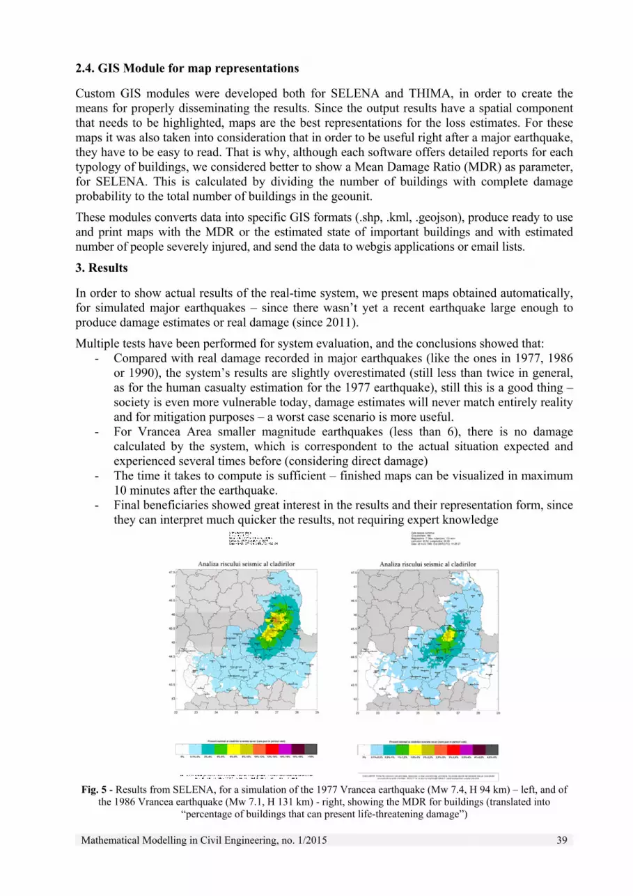
Mathematical Modelling in Civil Engineering, no. 1/2015 39
2.4. GIS Module for map representations
Custom GIS modules were developed both for SELENA and THIMA, in order to create the means for properly disseminating the results. Since the output results have a spatial component that needs to be highlighted, maps are the best representations for the loss estimates. For these maps it was also taken into consideration that in order to be useful right after a major earthquake, they have to be easy to read. That is why, although each software offers detailed reports for each typology of buildings, we considered better to show a Mean Damage Ratio (MDR) as parameter, for SELENA. This is calculated by dividing the number of buildings with complete damage probability to the total number of buildings in the geounit.
These modules converts data into specific GIS formats (.shp, .kml, .geojson), produce ready to use and print maps with the MDR or the estimated state of important buildings and with estimated number of people severely injured, and send the data to webgis applications or email lists.
3. Results
In order to show actual results of the real-time system, we present maps obtained automatically, for simulated major earthquakes – since there wasn’t yet a recent earthquake large enough to produce damage estimates or real damage (since 2011).
Multiple tests have been performed for system evaluation, and the conclusions showed that: - Compared with real damage recorded in major earthquakes (like the ones in 1977, 1986
or 1990), the system’s results are slightly overestimated (still less than twice in general, as for the human casualty estimation for the 1977 earthquake), still this is a good thing – society is even more vulnerable today, damage estimates will never match entirely reality and for mitigation purposes – a worst case scenario is more useful.
- For Vrancea Area smaller magnitude earthquakes (less than 6), there is no damage calculated by the system, which is correspondent to the actual situation expected and experienced several times before (considering direct damage)
- The time it takes to compute is sufficient – finished maps can be visualized in maximum 10 minutes after the earthquake.
- Final beneficiaries showed great interest in the results and their representation form, since they can interpret much quicker the results, not requiring expert knowledge
Fig. 5 - Results from SELENA, for a simulation of the 1977 Vrancea earthquake (Mw 7.4, H 94 km) – left, and of
the 1986 Vrancea earthquake (Mw 7.1, H 131 km) - right, showing the MDR for buildings (translated into “percentage of buildings that can present life-threatening damage”)
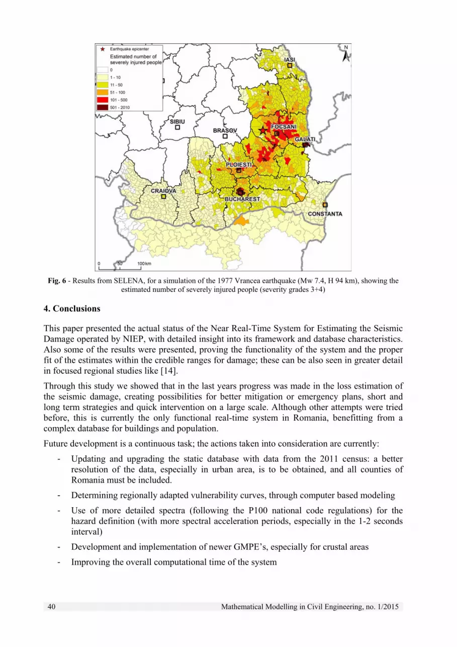
40 Mathematical Modelling in Civil Engineering, no. 1/2015
Fig. 6 - Results from SELENA, for a simulation of the 1977 Vrancea earthquake (Mw 7.4, H 94 km), showing the estimated number of severely injured people (severity grades 3+4)
4. Conclusions
This paper presented the actual status of the Near Real-Time System for Estimating the Seismic Damage operated by NIEP, with detailed insight into its framework and database characteristics. Also some of the results were presented, proving the functionality of the system and the proper fit of the estimates within the credible ranges for damage; these can be also seen in greater detail in focused regional studies like [14].
Through this study we showed that in the last years progress was made in the loss estimation of the seismic damage, creating possibilities for better mitigation or emergency plans, short and long term strategies and quick intervention on a large scale. Although other attempts were tried before, this is currently the only functional real-time system in Romania, benefitting from a complex database for buildings and population.
Future development is a continuous task; the actions taken into consideration are currently:
- Updating and upgrading the static database with data from the 2011 census: a better resolution of the data, especially in urban area, is to be obtained, and all counties of Romania must be included.
- Determining regionally adapted vulnerability curves, through computer based modeling
- Use of more detailed spectra (following the P100 national code regulations) for the hazard definition (with more spectral acceleration periods, especially in the 1-2 seconds interval)
- Development and implementation of newer GMPE’s, especially for crustal areas
- Improving the overall computational time of the system

Mathematical Modelling in Civil Engineering, no. 1/2015 41
Acknowledgements
The contribution of the Danube Cross-border system for Earthquakes Alert (DACEA) Project (Contract Number: 52570/05.08.2010) is greatly appreciated. Also authors would like to mention the financial support provided through doctoral scholarships. The paper was presented in the 5th National Conference of Earthquake Engineering and The 1st National Conference on Earthquake Engineering and Seismology (19-20 June 2014).
References
[1] National Institute for Earth Physics (January 2014). Romplus Earthquake Catalogue. [2] Bucharest Local Administration (May 2014). List of expertised buildings. Retrieved May 2014, from
http://www.pmb.ro/servicii/alte_informatii/lista_imobilelor_exp/docs/Lista_imobilelor_expertizate.pdf [3] Gandul Newspaper (November 2013). The map of buildings that can collapse in an earthquake similar to the
one in 1977. Retrieved May 2014, from http://storage0.dms.mpinteractiv.ro/media/1/186/3927/11538171/3/risc-seismic.png
[4] Lungu C. (2012). Evaluarea fondului de cladiri din Romania in perspectiva aplicarii directivei 2010/CE/31; Conferinta Internationala despre Constructii Sustenabile si Eficienta Energetica. Retrieved May 2014 from http://www.euroconferinte.ro/prezentari/Tema1-17.pdf
[5] Lang D., Molina-Palacios S., Lindholm C., Balan S.F. (2012). Deterministic earthquake damage and loss assessment for the city of Bucharest, Romania. Journal of Seismology, 16, 67-88. DOI: 10.1007/s10950-011-9250-y
[6] Erduran E., Toma-Danila D., Aldea A. et al. (2012). Real Time Earthquake Damage Assessment in Romanian-Bulgarian Border. 15 World Conference on Earthquake Engineering, Lisbon, Portugal
[7] Molina, S., Lang, D.H., Lindholm, C.D., Lingvall, F. (2010). SEismic Loss EstimatioN using a logic tree Approach (SELENA) [computer software]. Norway: NORSAR.
[8] Federal Emergency Management Agency (FEMA) (2004). Multi-hazard Loss Estimation Methodology, Earthquake Model, Advanced Engineering Building Module (HAZUS-MH) [computer software]. Washington DC: FEMA
[9] Boore, D. M., W. B. Joyner, and T.E. Fumal (1997). Equations for Estimating Horizontal Response Spectra and Peak Accelerations from Western North American Earthquakes: A Summary of Recent Work, Seism. Res. Lett., 68,128-153.
[10] Sokolov, V., Bonjer, K.P., Wenzel, F. (2004). Accounting for site effect in probabilistic assessment of seismic hazard for Romania and Bucharest: a case of deep seismicity in Vrancea zone. Soil Dynamics and Earthquake Engineering, 24, 929–947. DOI: 10.1016/j.soildyn.2004.06.021
[11] Douglas, J., Cotton, F., Abrahamson, N., Akkar, S., Boore, D.M., Di Alessandro. C. (2011). Pre-selection of ground-motion prediction equations. Global GMPEs Project, deliverable: Task 2
[12] Toma-Danila D., Zulfikar C., Manea E.F., Cioflan C.O. (2015) - Improved seismic risk estimation for Bucharest, based on multiple hazard scenarios and analytical methods; Soil Dynamics and Earthquake Engineering, accepted for publishing.
[13] Cattari S., Curti E., Giovinazzi S., Lagomarsino S., Parodi S., Penna A. (2004) - Un modello meccanico per l'analisi di vulnerabilita del costruito in muratura a scala urbana. 11th Conference "L'ingegneria Sismica in Italia", Genova, Italy.
[14] Toma-Danila D. (2012) – Real-Time Earthquake damage assessment and GIS analysis of two vulnerable counties in the Vrancea Seismic Area, Romania; Environmental Engineering and Management Journal, 11 (12), 2265-2274. WOS:000314169000018

42 Mathematical Modelling in Civil Engineering, no. 1/2015
A THREE-DIMENSIONAL ANALYSIS OF THE WHEEL - RAILWAY CONTACT IN CASE OF A CHARGE TRANSFER
CRISTINA TUDORACHE - Assistant Ph.D., Railway Vehicles Engineering Department, University Politehnica of Bucharest, Romania, [email protected] IOAN SEBEŞAN - Ph.D. Professor, Railway Vehicles Engineering Department, University Politehnica of Bucharest, Romania, [email protected]
Abstract: A series of factors are acting are acting on the wheels of the railway vehicle causing load transfers capable of having an effect on safety transportation The evaluation of vehicle – runway interaction phenomena establishes traffic safety conditions. In this paper we present a three-dimensional approach of the wheel - railway contact in case of load transfer and for a path with shortfall or with profile S78 super-elevation excess. The vehicle – runway interaction phenomena establishes traffic safety conditions. In this paper we present a three-dimensional approach of the wheel - railway contact in case of load transfer and for a path with shortfall or with profile S78 super-elevation excess is analyzed.
Keywords: contact ellipse, sliding/adherence area, contact forces, safety against derailment.
1. Introduction
Over the years there have been a number of theories developed on the wheel-railway contact in order to resolve the problems relate to the interaction with the railway track and to improve the dynamic performances of vehicles.
One of those who laid the foundations of the theory of rolling friction was Carter [1], who used a two-dimensional model that assimilates the wheel with a cylinder and the railway with a board. The bodies found in direct contact are elastically deformable and between them only longitudinal sliding occurs. Later on, Johnson and Vermeulen [2], extended the two-dimensional theory developed by Carter for arbitrary half-spaces. According to these the contact surface between the two bodies engaged in a rotary movement is divided into a bonding zone called stick and a sliding one called slip. Also, the stick zone has an elliptic form being arranged tangential to the inside of contact ellipse.
Halling, Haines and Ollerton, [3], developed approximately the same theory regarding the elliptic contact with longitudinal pseudo-sliding. The contact area was divided in a series of strips displayed parallel with the rolling direction and then each band was studied by expanding Carter’s two-dimensional theory.
In the end, starting from the hypothesis of his predecessors, Kalker, [4] laid the foundations of an exact three-dimensional analysis of the contact with friction. He takes into account, for each of the points within the contact area, the local sliding speeds and the local distortions of the bodies found in contact. The relations established by Kalker are valid though only for the small pseudo-sliding movement, being used in studies regarding the stability of moving vehicles.
Kalker’s merit, [5], consists in the fact that he introduced the effect of spinning movement and invalidated Lévi’s isotropy principle [6]. The value of the friction index is strongly influenced by the shape of the rolling profiles and by the load carried on the wheel. On the other hand, the linear relations established by Kalker are valid only for the small pseudo-sliding movements, being used in studies carried out for establishing the stability of moving vehicles.
The stability of a vehicle is influenced also by the load transfers caused by quasi-static and dynamic forces generated primarily by the unevenness of the railway. The position of the normal load shifts during rolling. A shift of the load over the first rolling wheel of the leading axle implies an increase in the stability limit in derailment imposed by the safety against derailment [7].

Mathematical Modelling in Civil Engineering, no. 1/2015 43
The literature from this field presents numerous criteria for assessing the safety against derailment; criteria, which take into account, the ratio between the forces displayed vertically and tangentially. Among these, Nadal’s formula [8], Weinstock’s [9] limit criterion and the limitation of the contact area on the wheel [10, 11, 12] are noticeable.
The present paper proposes a three-dimensional approach of the contact between the wheel and the railway in the case of a shift in load. The analysis is done by using the CONTACT software, which assimilates the contact area through half-space units and divides it through the method of the end element. In the contact area the theory of linear elasticity is applied. CONTACT establishes the shape and size of the contact area between the elastically deformable bodies found in tangential contact (normal loads). This is achievable only if the shape of the profiles from the contact point is known.
Consequently, after this short presentation of the current state of the rolling contact analysis we will present in sections no. 2 and 3 aspects of the load transferring ratio and the tangential contact conditions. Section no. 4 is dedicated to an example of numerical analysis for a contact between a wheel having the S78 profile and a UIC 60 1:20 railway showing a roll with shortfall and super-elevation excess, while in the very end section the main aspects of the present study will be presented.
2. Load transfers on the vehicle axles
The forces from the interaction area created between the wheel and the railway are in balance with the exterior forces that are transmitted to the axles in the form of linking forces (fig.1):
Fig.1 - Forces transmitted to the vehicle’s axle
At the level of each axle mounted wheel load Q0 acts which originates from the gravitational forces. If the axle rolls on a smooth railway, without super-elevation, then the total load 2Q0 is uniformly spread on the two wheels. But, due to the unevenness of the railway and of the quasi-static or dynamic forces, transfers of load take place during the rolling on the wheels, which lead to a disequilibrium of the contact forces. The transfer of load on the axle represents the half-difference between the loads applied on the two wheels, i.e.:
221 QQ
Q
(1)
Where Q1 – the load on the first wheel, Q2 – load on the second wheel. If we relate to the transfer the load Q, then the loads on the two wheels are given by the following equations:
QQQ
QQQ
o
o
2
1 (2)
The factors that produce load transfers on the axle are of various origins. The external forces represent one of these factors as they are transmitted through the springs of the vertical
44 Mathematical Modelling in Civil Engineering, no. 1/2015
suspension of the wheel that are also containing the vertical resistance of the dampers caused by the torsion of the railway. Thus, the load transfer caused by these forces, noted as F1 and F2, is given by the following equation:
e
bFFQo
)(
2
1 21 (3)
The equation (3) is valid if the following condition is respected:
oo QGFFQQ 22121
where G0 is the weight of the axle. Another factor is the transversal force called H, or chassis leading force, which appears in the axle hub and is transmitted to the vehicle chassis though the axle bed. This force contains inertia forces caused by shifts in the vehicle direction as well as the opposing forces appeared in its rotation. The transversal force creates a turning point of the axle acting above the contact area between the wheel and the railway track and is also creating a transfer of load
e
HrQH 2
(4)
If the load transfers ΔQ0 and ΔQH are taken into consideration, then the load on each wheel will be:
Hoo QQQQ 1
Hoo QQQQ 2 (5)
and the equilibrium condition Q1 + Q2= 2Q0 will be achieved.
According to the ORE B-55 Committee, the maximum accepted shifts of load in quasi-static conditions and on a twisted railway must not exceed ΔQ0 / Q0 ≤ 0,6 (where ΔQ0 / Q0 is defined as transfer coefficient) for a flank angle of the wheel edge angle of 700 and for a situation where the H transversal force is almost equal to 0. This situation is applied for vehicles fitted with steerable axles. The limit of the load transfers on axles is established according to the criteria regarding safety against derailment.
When talking about the scenario regarding the unload of the first rolling wheel while going over a curve at low speed, a maximum super-elevation and a high twist of the railway result:
- if the rolling is done with super-elevation excess: Hoo QQQQ 1
- if the rolling is done with super-elevation deficiency: Hoo QQQQ 1
With the same value of the transfer coefficient the ΔQ0 / Q0 , (Y1 / Q0)lim is reduced at the same ratio as the wheel radius; with smaller wheels the derailment coefficient is higher. On the other hand, increasing the flank maximum angle of the wheel edge is favorable for increasing the safety against derailment as it increases both the minimum and the maximum guiding capacity of the axle.
3. The issue regarding the tangential contact
The analysis of the wheel-railway tangential contact consists in determining the distribution of the traction force, namely the contact pressures and relative sliding speeds in relation to the dimensions of the contact area [13, 14]. The distribution of pressure within the contact area, if Hertz’s hypotheses are respected, is done following an elliptic paraboloid, as described in the equation [7, 15]:
22
1,
b
y
a
xpyxp o (6)
where p0 represents the maximum pressure developed in the center of the contact ellipse, a and b represent the semi-axes of the contact ellipse.
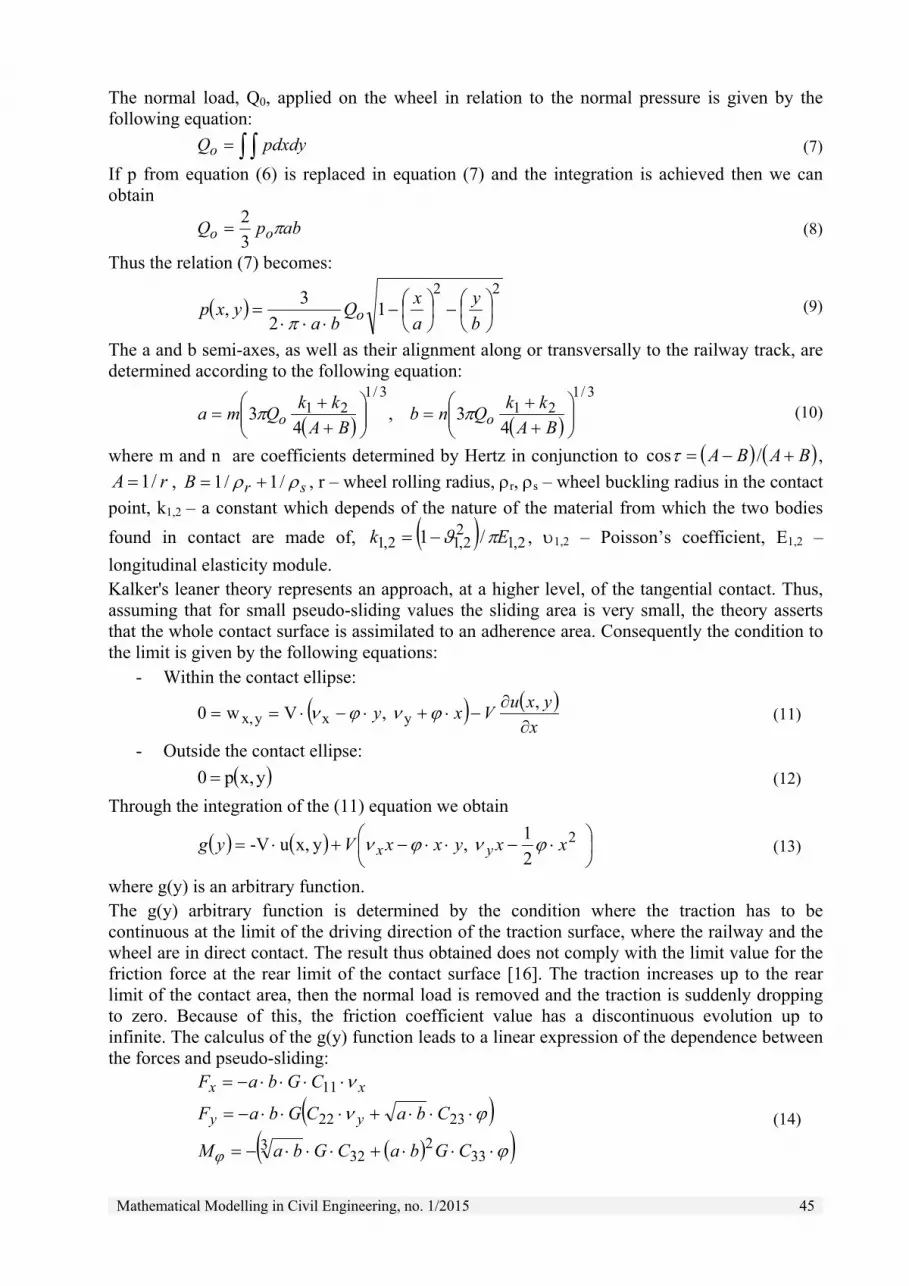
Mathematical Modelling in Civil Engineering, no. 1/2015 45
The normal load, Q0, applied on the wheel in relation to the normal pressure is given by the following equation:
pdxdyQo (7)
If p from equation (6) is replaced in equation (7) and the integration is achieved then we can obtain
abpQ oo 3
2 (8)
Thus the relation (7) becomes:
22
12
3,
b
y
a
xQ
bayxp o
(9)
The a and b semi-axes, as well as their alignment along or transversally to the railway track, are determined according to the following equation:
3/121
3/121
43 ,
43
BA
kkQnb
BA
kkQma oo (10)
where m and n are coefficients determined by Hertz in conjunction to BABA /cos ,
rA /1 , srB /1/1 , r – wheel rolling radius, r, s – wheel buckling radius in the contact
point, k1,2 – a constant which depends of the nature of the material from which the two bodies
found in contact are made of, 2,122,12,1 /1 Ek , 1,2 – Poisson’s coefficient, E1,2 –
longitudinal elasticity module. Kalker's leaner theory represents an approach, at a higher level, of the tangential contact. Thus, assuming that for small pseudo-sliding values the sliding area is very small, the theory asserts that the whole contact surface is assimilated to an adherence area. Consequently the condition to the limit is given by the following equations:
- Within the contact ellipse:
x
yxuVxy
,
,Vw0 yxyx,
- Outside the contact ellipse:
(11)
yx,p0 (12)
Through the integration of the (11) equation we obtain
2
1 ,yx,u-V 2xxyxxVyg yx (13)
where g(y) is an arbitrary function. The g(y) arbitrary function is determined by the condition where the traction has to be continuous at the limit of the driving direction of the traction surface, where the railway and the wheel are in direct contact. The result thus obtained does not comply with the limit value for the friction force at the rear limit of the contact surface [16]. The traction increases up to the rear limit of the contact area, then the normal load is removed and the traction is suddenly dropping to zero. Because of this, the friction coefficient value has a discontinuous evolution up to infinite. The calculus of the g(y) function leads to a linear expression of the dependence between the forces and pseudo-sliding:
332
323
2322
11
CGbaCGbaM
CbaCGbaF
CGbaF
yy
xx
(14)
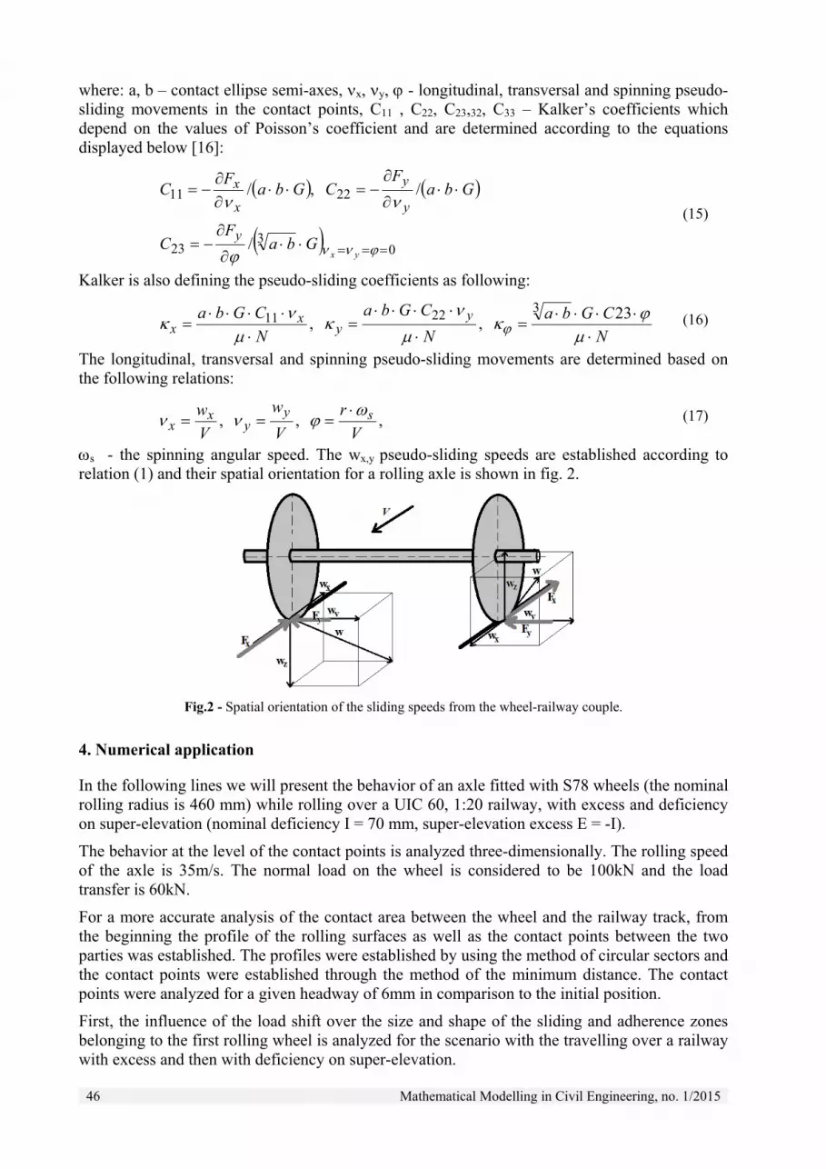
46 Mathematical Modelling in Civil Engineering, no. 1/2015
where: a, b – contact ellipse semi-axes, x, y, - longitudinal, transversal and spinning pseudo-sliding movements in the contact points, C11 , C22, C23,32, C33 – Kalker’s coefficients which depend on the values of Poisson’s coefficient and are determined according to the equations displayed below [16]:
03
23
2211
/
/ ,/
yxGba
FC
GbaF
CGbaF
C
y
y
y
x
x
(15)
Kalker is also defining the pseudo-sliding coefficients as following:
N
CGba
N
CGba
N
CGba yy
xx
23 , ,
32211 (16)
The longitudinal, transversal and spinning pseudo-sliding movements are determined based on the following relations:
, , ,V
r
V
w
V
w syy
xx
(17)
s - the spinning angular speed. The wx,y pseudo-sliding speeds are established according to relation (1) and their spatial orientation for a rolling axle is shown in fig. 2.
Fig.2 - Spatial orientation of the sliding speeds from the wheel-railway couple.
4. Numerical application
In the following lines we will present the behavior of an axle fitted with S78 wheels (the nominal rolling radius is 460 mm) while rolling over a UIC 60, 1:20 railway, with excess and deficiency on super-elevation (nominal deficiency I = 70 mm, super-elevation excess E = -I).
The behavior at the level of the contact points is analyzed three-dimensionally. The rolling speed of the axle is 35m/s. The normal load on the wheel is considered to be 100kN and the load transfer is 60kN.
For a more accurate analysis of the contact area between the wheel and the railway track, from the beginning the profile of the rolling surfaces as well as the contact points between the two parties was established. The profiles were established by using the method of circular sectors and the contact points were established through the method of the minimum distance. The contact points were analyzed for a given headway of 6mm in comparison to the initial position.
First, the influence of the load shift over the size and shape of the sliding and adherence zones belonging to the first rolling wheel is analyzed for the scenario with the travelling over a railway with excess and then with deficiency on super-elevation.

Mathematical Modelling in Civil Engineering, no. 1/2015 47
Thus, in figure 3, it can easily be observed that in both situations the distribution of the sliding areas is in accordance with the strips theory, that is, with the behavior of the null pseudo-sliding [17]. Moreover, the influence of load transfer over the size of the contact point and of the adherence area can be observed. one can also notice that when rolling over the portions of the track that have super-elevation deficiency the contact area is excessively reduced in the case of a load transfer while the sliding area along the rail is extended.
a)
b)
Fig. 3- The distribution of sliding and adherence areas in the case of a load shift over the first rolling wheel. a) – rolling on a railway with excess of super-elevation ; b) rolling on a railway with deficiency of super-elevation.
In fig. 4-a, b the distribution of the tangential traction force is presented. Taking into consideration that in the analysis a wheel with fray profile was introduced, for which the greater axis of the contact ellipse is orientated perpendicularly on the rail, one can observe that the tangential traction force intensifies towards the neck tor of the wheel edge.
This is explained by the fact that the guidance of the wheel is ensured by the edge of this when rolling on a track in both situations: with excess and with deficiency of super-elevation.
a)
-7.250 -4.250 -1.250 1.750 4.750
-2.450
-1.450
-0.450
0.550
1.550
X-coordinate [mm]
Y-c
oord
inat
e [m
m]
exter
stick
slip
exter
stick
-11.400 -6.600 -1.800 3.000 7.800
-4.500
-3.000
-1.500
0.000
1.500
X-coordinate [mm]
Y-c
oord
inat
e [m
m]
exter
stick
slip
exter
stick
-7.250 -4.250 -1.250 1.750 4.750
-2.450
-1.450
-0.450
0.550
1.550
X-coordinate [mm]
Y-c
oord
inat
e [m
m]

48 Mathematical Modelling in Civil Engineering, no. 1/2015
b)
Fig. 4 - The distribution of the tangential traction force; a) – when rolling on a rail with excess of super-elevation; b) – when rolling on a rail with deficiency on super-elevation.
In figure number 5 the distribution of the friction power density from within the contact area is presented. The tribological aspect from within the contact area is strongly influenced by the load shift and by the state of the railway track. Thus a tribological build-up is observed in the contact area for the case when ravelling over an area with deficiency on super-elevation. This fact implies a tilt of the vehicle towards the exterior of the railway, which then leads to a transfer of load on the first rolling wheel; this explains the increase of the wear on the rolling surface of the wheel.
Fig. 5a - The distribution of the friction power; – rolling on a railway with excess of super-elevation
Fig. 5b - The distribution of the friction power; - rolling on a railway with deficiency on super-elevation
-11.400 -6.600 -1.800 3.000 7.800
-4.500
-3.000
-1.500
0.000
1.500
X-coordinate [mm]
Y-c
oord
inat
e [m
m]
-7.250-4.250
-1.2501.750
4.750
-2.450-1.450
-0.4500.550
1.550 -50
0
50
100
X-coordinate [mm]Y-coordinate [mm]
Fri
ctio
nal
pow
er d
ensi
ty [
W/m
m2 ]
0
10
20
30
40
50
60
70
-11.400-6.600
-1.800 3.000
7.800
-4.500-3.000
-1.5000.000
1.500
-50
0
50
100
150
X-coordinate [mm]Y-coordinate [mm]
Fri
ctio
nal
pow
er d
ensi
ty [
W/m
m2 ]
0
20
40
60
80
100
120
140

Mathematical Modelling in Civil Engineering, no. 1/2015 49
5. Conclusions
The present paper presents a tri-dimensional analysis method of the contact between the wheel and the railway. In this analysis Kalker's theory and Hertz's validity regarding simplifying hypotheses are taken into consideration, and are applied through the interactive CONTACT software.
The analysis set forth in the present paper validates the applicability of the CONTACT software for the profiles used by CFR (Romanian Railways). Also this approach leaves open the path for an evaluation from the tribological point of view of the vehicle behavior when rolling on a surface showing both excess and deficiency on super-elevation.
Finally, the analysis developed in the present paper ensures the knowledge of the phenomena, which occur in the contact area between the wheel and the railway and the effects they have on the safety of transportation.
Acknowledgment
The present paper was made within the framework of PN II PCCA tip 2, research contract ID 192/2012, financed by the Romanian Government through UEFISCDI.
Bibliography
[1]. Carter, F.W. (1926) On the action of locomotive driving wheel, in: Proc. Roy. Soc. A112, 151-7. [2]. Johnson K. L. & Vermeulen, P. J. (1964) Contact on non-spherical bodies transmitting tangential forces, J.
Appl. Mech., 31, (p. 338-340). [3]. Haines D. J. & Ollerton, E. (1963) Contact stress distribution on elliptical contact surfaces subjected to radial
and tangential forces, Proc. Inst. Mech. Eng. 177, (p.95-144). [4]. Kalker, J. J. (1990) Three-dimensional elastic bodies in rolling contact, Dordrecht, Kluwer Academic
Publishers. [5]. Kalker, J. J. (2003) Rolling contact phenomena, Delft University of Technology, Netherlands, [6]. Lévi, R. (1935) Étude relative au contact des roues sur le rail, Rev. Gen. Chem. Fer., 69, (p. 57-63), (in
Franch). [7]. Sebeşan, I. (2011) Dinamica vehiculelor feroviare, Editura MatrixRom, 2011. [8]. Nadal, M. J. (1896) Théorie de la stabilité des locomotives, Mouvement de lacet. Ann. Mines Part II 10, (p.
232–255). [9]. Weinstock, H. (1984) Wheel climb derailment criteria for evaluation of rail vehicle safety, Proceedings of the
American Society of Mechanical Engineers Winter Annual Meeting, New Orleans (LA), 84–WA/RT–1: 1–7. [10]. Jin, X., Ling L, Xiao X, Zhu M, Zhou Z. (2011) Dynamic behavior numerical simulation and safety boundary
analysis for high speed trains in severe environments. Computer Aided Eng. 20 (3):29–41. Chinese. [11]. Miyamoto, M, (1996) Mechanism of derailment phenomena of railway vehicles. QR RTRI. 37, (3):147–155. [12]. Zhai, W. M., Chen, G. (2001) Method and criteria for evaluation of wheel derailment based on wheel vertical
rise. Journal of the China Railway Society, 23(2):17–26, (in Chinese). [13]. Vollebregt, E.A.H. (2012) User guide for CONTACT, Vollebregt & Kalker’s rolling and sliding contact model,
Technical Raport, VORtech computing, Delft, The Netherlands. [14]. Tudorache, M. C. (2013) The influence of wheel-rail phenomena upon guiding safety for railway vehicle, PhD
Thesis, Bucharest. [15]. Deeg, E. W. (1992) New Algorithms for Calculating Hertzian Stresses, Deformations, and Contact Zone
Parameters, AMP Journal of Technology Vol. 2. [16]. Kalker, J. J. (1991) Wheel-rail rolling contact theory, wear 144, pp. 243-261. [17]. Kalker, J. J. (1967) A strip theory for rolling with slip and spin , Proc. Kon. Ned. Akad. Van Wetenschappern,
B70,10, 261-263.