reanalysis of the 1992 south pole millimetre-wavelength atmospheric opacity data

CSIRO PUBLISHING

Publications of the Astronomical Society of Australia, 2004, 21, 264–274 www.publish.csiro.au/journals/pasa

Reanalysis of the 1992 South Pole Millimetre-Wavelength AtmosphericOpacity Data

Richard A. ChamberlinA,B

A Caltech Submillimeter Observatory, Hilo, HI 96720, USAB E-mail: [email protected]

Received 2003 January 20, accepted 2004 March 11

Abstract: In 1992 an NRAO 225-GHz site survey heterodyne radiometer was placed at the GeographicalSouth Pole. The instrument operated over an entire annual cycle and provided direct measurements of themillimetre-wave sky brightness temperature as a function of zenith angle. Interpreted in a single-slab ‘skydip’radiation transfer model of the atmosphere, these sky brightness measurements provided a time series of themillimetre atmospheric opacity. Statistics derived from this opacity time series were important for makingcomparisons with other candidate millimetre and sub-millimetre wave astronomy sites. This paper reexaminesthe 1992 measurements and the original analysis. Details of the skydip fit model, radiometer gain error,instrument stability, and a mid-season replacement to a window in the instrument enclosure combined to causea modest under-reporting of the atmospheric opacity in previous reports. Unchanged are earlier conclusionsthat dry air makes a significant contribution to the total opacity at 225 GHz.

Keywords: instrumentation: miscellaneous — methods: data analysis — site testing — atmospheric effects

1 225-GHz Opacity at the South Pole

In 1992, a National Radio Astronomy Observatory(NRAO) 225-GHz heterodyne site testing radiometer (‘τ-meter’; Liu 1987; McKinnon 1987) was placed at theSouth Pole. This instrument provided measurements ofthe millimetre sky opacity for an entire annual cycle(Chamberlin & Bally 1994, 1995). One result of thesemeasurements was the finding of a significant dry-aircontribution to the millimetre-wave atmospheric opacity(Chamberlin & Bally 1995). The existence and approxi-mate magnitude of this dry-air component was confirmedby South Pole opacity measurements made near 273 GHz(R. de Zafra, private communication 1994) and by latermeasurements with the Antarctic Submillimeter Tele-scope and Remote Observatory (AST/RO) instrument(Chamberlin 2001).

The finding of significant dry-air opacity in site sur-veys has recently called into question by Calisse (2004)who suggested that incorrect modelling of ‘radome’opac-ity may lead to over-estimates of atmospheric opacity:“… unless radome transparency is correctly modelled,some previous site studies may have significantly under-estimated the quality of the best submillimetre sites …”.1

There is an implication that incorrect modelling of radomeopacity may be responsible for the magnitude of thedry-air terms reported previously (e.g. Chamberlin &Bally 1995; Chamberlin et al. 1997; Chamberlin 2001).Concerns about uncompensated window opacity expressed

1From Calisse (2002), published Calisse (2004).

by Calisse and others (e.g. R.A. Chamberlin to J. Peterson,private communication 2001 October) may apply to opac-ity results reported at 857 GHz (Peterson et al. 2003), butas will be shown in Section 4, Calisse’s specific concernsdo not apply to results previously reported from otherSouth Pole opacity measurements.

2 The 225-GHz Radiometer

The hardware and data acquisition method used by thesite test radiometer are well described in Liu (1987) andChamberlin & Bally (1994). Of interest is the effect ofa mylar window installed in the instrument enclosurebetween the internal calibration load chopper system andthe external, off-axis paraboloidal tipping mirror. As orig-inally installed, this mylar window was very thin and isbelieved to have made only a modest contribution to thereceived signal, perhaps about 5 K. The thickness of theoriginal mylar membrane was not measured. However, webelieve it was thin because it broke very easily and inspec-tion of the signal from loads of known temperature (seeSection 5) showed no evidence of a bias toward warmerradiometer signal temperatures. Measurements with a Cal-tech Submillimeter Observatory facility receiver (J. Kooi,private communication) show that 12–25 µm thick mylarmembranes in the 230-GHz radio beam add about 5 to10 K to the receiver noise temperature. The mylar opacityimplied by that noise temperature increase is about 0.01to 0.02 nepers. Here, nepers to refers to power attenu-ation (Kraus 1986). A low-opacity window would have

© Astronomical Society of Australia 2004 10.1071/AS03012 1323-3580/04/03264

Reanalysis of the 1992 South Pole Millimetre-Wavelength Atmospheric Opacity Data 265

had almost no effect on our original method of comput-ing atmospheric opacity (Chamberlin & Bally 1994), seeSection 3. The original, thin window was punctured bymechanical cleaning and replaced with a thicker and moreemissive mylar film on Day 90 (1992 March 30). Theeffects of the this window replacement were only partlyaccounted for in the earlier analysis (Chamberlin & Bally1994).

3 Skydip Fitting Models

In Chamberlin & Bally (1994) the skydip data-fittingroutine was presented with calibrated data in the formTsky(A) versus A, where Tsky(A) was the apparent skytemperature and A was the airmass which depends zenithangle ZA, such that A≈ 1/ cos(ZA). Tsky(A) includedsky emissivity as well as emissivity from all other sourceswhich terminated the radio beam beyond the calibrationloads.

In Chamberlin & Bally (1994) the skydip data (Tsky(A)

versus A) were fitted to

Tsky(A) = T0 + Tsur[1− exp(−τ′A)] (1)

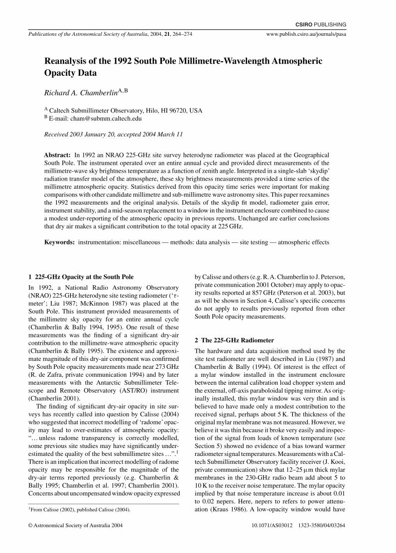
where T0 was the combined contribution to excess signalnoise from mylar window emission, ground spillover, etc.(i.e. T0 was a static contribution to Tsky(A) independent ofA), τ′ was the apparent sky opacity, and Tsur was the atmo-spheric temperature measured at the instrument enclosure.Figure 1 is a reproduction (Chamberlin & Bally 1994) ofan example of a typical 1992 skydip measurement and fitto Equation (1). The second term on the right hand sideof Equation (1) is merely an application of phenomeno-logical radiation transfer modelling (Rohlfs 1986 p. 7) tothe atmosphere, and it is the so-called single-slab skydipmodel.

A more appropriate fit equation would have been

Tsky(A) = T0 + exp(−τwindow)Tatm[1− exp(−τA)] (2)

which is basically the same as Equation (1) except that theportion of the signal which passes through a thin mylarwindow in the instrument enclosure is attenuated by thewindow opacity, τwindow. Also in Equation (2), Tatm isused instead of Tsur. Tatm is the properly weighted averagetemperature computed from daily radiosonde data — seethe Appendix. At middle latitude sites, generally Tatm <

Tsur due to the normal adiabatic lapse rate of the atmo-sphere. In contrast, at the South Pole, typically Tatm >Tsur

because of the deep inversion layer which forms most ofthe year and particularly in winter (Schwerdtfeger 1984;Chamberlin 2001; Chamberlin et al. 2002). In Equation (2)opacity τ instead of τ′ is obtained.

Skydip models like Equation (2) are widely used inradio astronomy often with many extra terms added toaccount for instrumental effects, such as increases insystem noise temperature due to emissive membranes(Meeks & Ruze 1971) and ground spillover, and antennagain losses due to radome attenuation (Meeks & Ruze1971), beam coupling efficiency, and so forth (Ulich &

1040

0 2 4 6 8

80

60

100

Tsk

y (z

) (º

K)

140

120

A(z) (airmass)

Figure 1 225-GHz skydip figure, reproduced from Chamberlin &Bally (1994).

Haas 1976). For just one example of a more elaborateform of Equation (2), see Equation (II-4) in Lane (1982).2

Since exp(−τwindow) is an instrumental constant forconvenience, we can define η≡ exp(−τwindow) andrewrite Equation (2) as

Tsky(A) = T0 + ηTatm[1− exp(−τA)] (3)

Under low 225-GHz opacity skies, such as at the SouthPole, τ 1, and at low airmass Equations (1) & (3) can

2Equation (II-4) from Lane (1982) was developed for use in the sky-dip/calibration program written for the Five College Radio AstronomyObservatory (FCRAO) (Lane 1978). For convenience, we repeat it here:

Tobs(A) = Trx + Trad[1− exp(−τrad)] + (1− ηl)Tamb[exp(−τrad)]+ ηlTatm[exp(−τrad)][1− exp(−τoA)]

Tobs(A) corresponds to the total noise power received at airmass A. Aswe can see from this Equation, the total noise power has contributionsfrom receiver noise Trx, radome emission Trad[1− exp(−τrad)], groundspillover from outside the radome (1− ηl)Tamb[exp(−τrad)], and fromthe directed power on the sky ηlTatm[exp(−τrad)][1− exp(−τoA)]. Inthis context, the term ηl was called the ‘antenna loss efficiency’ andrepresents the fraction of power from outside the radome which wasreceived in the directed radio beam, that is ηl is the fraction of powerfrom outside the radome which changes with airmass A. In earlier liter-ature (Davis & Vanden Bout 1973), ηl “refer(s) to loss mechanisms, i.e.,spillover, blockage, and Ohmic losses.” Accordingly, it would be naturalto include radome loss in ηl, but in Lane (1982) radome contribution toefficiency loss was explicitly quantified in the skydip model probablybecause it was relatively easy to do so. Tamb is the ambient air tempera-ture, Tatm the properly weighted atmospheric temperature, τo the zenithopacity, Trad the radome temperature, and τrad the radome opacity.

266 R. A. Chamberlin

be well approximated by the linear forms

Tsky(A) = T0 + Tsurτ′A (4)

orTsky(A) = T0 + ηTatmτA (5)

where τ′ is the apparent sky opacity when window opacityis neglected and Tsur is used, and τ is a more accurate skyopacity which would have been found if Equation (3) wasused to fit the skydip data. We can see from Equation (5),that for the very low opacities typical of winter, the ini-tial slope of the skydip, Tsky(A) versus A, is the productηTatmτ.

It is obvious from comparing Equations (4) & (5) that

τ = Tsur

Tatm

τ′

η(6)

If T0 is dominated by window emission as apparently wasthe case after Day 90 when the window was replaced, againapplying the phenomenological radiation transfer model(Rohlfs 1986 p. 7) we get

T0 = Twindow(1− η) (7)

orη = 1− T0/Twindow (8)

where Twindow was the physical temperature of the win-dow. From inspection of the zero intercept in data likeFigure 1, previously we found that T0 45 K subsequentto the window replacement on Day 90 (Chamberlin &Bally 1994).

The instrument enclosure temperature was maintainedat 10◦C by an external heating system (Chamberlin &Bally 1994). So Twindow was some intermediate tempera-ture between the enclosure temperature and Tsur. For ouranalysis here we assumed Twindow= 250 K. This assumedvalue of Twindow was used because it is intermediatebetween the enclosure temperature and the average win-tertime surface temperature — in 1992, Days 100 to 300,〈Tsur〉= 216.4± 9.3 K. If the assumed value of Twindow isused, from Equation (8) we obtain η≈ 1− 45/250= 0.82,suggesting that the previously reported opacities (Cham-berlin & Bally 1994) may be about 18% too low fromneglecting window opacity in Equation (1).

Somewhat mitigating possible earlier underreportingof the opacities is that fact that Tsur is often significantlylower than Tatm due to the deep inversion layer which typ-ically forms at the surface. For example, during the lowestopacity weather, it is often the case that Tsur ≈ 205 K andTatm ≈ 230 K. Thus from Equation (6)

τ = 0.89

0.82τ′ = τ′

0.92(9)

implying that, during the best weather periods, the earlierunderreporting of opacity (Chamberlin & Bally 1994) wason the order of 10%.

4 Comparison to Analysis in Calisse (2004)

In Calisse (2004) it is suggested that window-inducedinstrumental artifacts may be responsible for excess ‘dry-air’ opacity at very good submillimetre sites where watervapor opacity is very low. The abstract and conclusionin the Calisse paper suggest that results from site sur-veys other than those accomplished with the CMU/NRAO350-µm τ-meter may be affected (Peterson et al. 2003).However, other than the CMU/NRAO instrument, we donot know of any other South Pole site survey results thatare affected by the specific analysis in Calisse (2004).

For example, in the AST/RO instrument (Stark 2001;Chamberlin 2001) no windows were used in the beam pathfrom the calibration system to the sky, thus the windowopacity effect described in Calisse does not apply.

In a South Pole atmospheric Fourier transform spec-trometer (Chamberlin et al. 2002), a removable windowwas usually in the beam path between the cold load chop-per and the external tipping mirror but the effects ofwindow emission and absorption were included in the dataanalysis.

Regarding the topic of this paper, 1992 opacity resultsfrom a NRAO 225-GHz τ-meter, a window with a non-negligible absorption was used during a part of 1992,but Calisse’s analysis (Calisse 2004) does not apply hereeither. Calisse’s Equation (1) assumes a modelling errorof the form

T = Tatm[1− exp(−τ′′A)] − Tref (10)

or, equivalently

Tsky(A) = Tatm[1− exp(−τ′′A)] (11)

with Tsky≡ T + Tref . In Calisse (2004) Tref is the black-body temperature of a synchronously detected calibrationload. Equation (11) is not the same as Equation (1).Equation (11) neglects the emissive contribution from theinstrument window which was not an error made in theprevious analysis of the 1992 225-GHz skydip data set.That is to say, the fit parameter T0 in Equation (1) includeswindow emissivity. If the radiometer performance is idealin every other respect, then T0 is related to the windowopacity by Equation (7). Since T0 includes window emis-sivity, it is similar to using the second term on the righthand side of Equation (5) of Calisse (2004) in his preferredform of the skydip model.

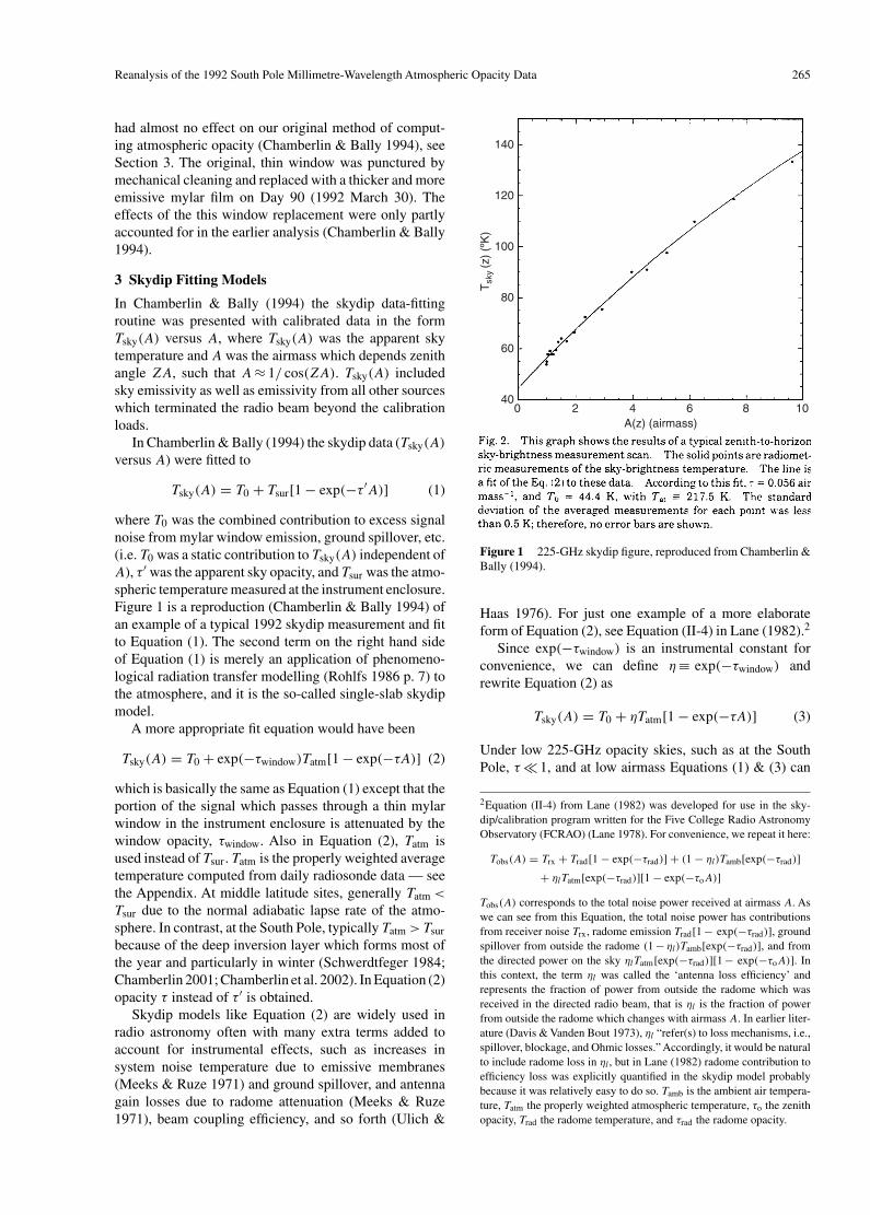
To illustrate the point that Equation (1) does not makethe modelling error discussed by Calisse, consider Fig-ure 2. The solid line is the fit of Equation (1) to the skydipdata and it gives T0= 44.4 K and τ′ = 0.056. Tsur was con-strained to be the surface temperature 217.5 K. In contrast,the dashed line shows the result of the least-squared bestfit to Equation (11) and it gives τ′′ = 0.145. Tatm is con-strained to be the surface temperature 217.5 K but clearlyno reasonable choice of Tatm could make Equation (11)appropriate to use on this skydip data. If the same sky-dip data is fit to Equation (3) (dotted line), we find thatT0= 43.6 K and τ= 0.067 with η constrained to be 0.82


100

0 2 4 6 8

50

100

Tsk

y (A

)150

A (airmass)

Figure 2 Different model fits to 225-GHz skydip data from Figure1. The solid line is a fit to Equation (1), the dotted line is a fit toEquation (3), and the dashed line is a fit to Equation (11).

and Tatm constrained to be 230.0 K, which is near the aver-age value determined from radiosonde. As expected fromSection 3, the error in the opacity determination from usingmodel Equation (1) instead of Equation (3) was moderateand τ′<τ.

5 Other NRAO 225-GHz τ -Meter SystematicErrors

In the previous Sections we saw that uncompensated trans-mission loss through a non-ideal window put in the signalbeam path after Day 90 had the likely effect of mod-erately reducing the 225-GHz sky opacities reported inChamberlin & Bally (1994) and Chamberlin et al. (1997).

We also explained that using a properly weightedatmospheric temperature, rather than just the surfacetemperature, made the skydip model we use more realistic.

Besides uncompensated transmission loss through awindow in the instrument enclosure, other systematicerrors can result from gain error, gain drift, snow on theoptics, and perhaps some other sources not yet identified.

5.1 The Chopper Calibration System and Validationwith LN2 Test Loads

As described previously (Liu 1987; Chamberlin & Bally1994), the NRAO 225-GHz τ-meter has a four-bladedchopper system which switches the input of the radiome-ter between two reference loads and the sky signal fromthe external mirror. The gain of the radiometer systemwas established by synchronously detecting its outputpower with the input switching between thermally con-trolled 45 and 65◦C ‘reference’ and ‘hot’ loads. Actualsky brightness temperatures can be lower than −263◦Cso the gain established by comparing two warm referenceloads had to be extrapolated to much colder temperatures.

To check that whole system was giving reasonable val-ues, during the first few months of operation the τ-meterwas periodically monitored with a liquid nitrogen (LN2)load until the LN2 at the South Pole station ran out onDay 73. The average of 97 separate measurements com-bined gave TLN2 = 74.8± 10.7 K. The large uncertaintywas dominated by long-term gain drifts between moni-toring periods, rather than variation between consecutivemeasurements. These measurements of the liquid nitro-gen load were accomplished with the radiometer lookingthrough its original, thin mylar window (see Section 2).

The latent heat of evaporation and the boiling temper-ature of LN2 (at sea-level pressures) are established so weused the Clausius–Clapeyron equation to extrapolate thepressure versus temperature liquid/gas coexistence curveto a typical South Pole surface pressure of 690 mbar. Doingso, we found thatTLN2 = 74.1 K, very close to the tempera-ture the radiometer measured. However, the measurementswere made through the original, thin mylar window, whichwas expected to add about 2 to 4 K to the observed signal(see Section 2),3 thus indicating a slight radiometer gainerror of 1 to 2% and a tendency to measure a lower thanexpected signal temperature.

5.2 Other Measurements in the Data Stream

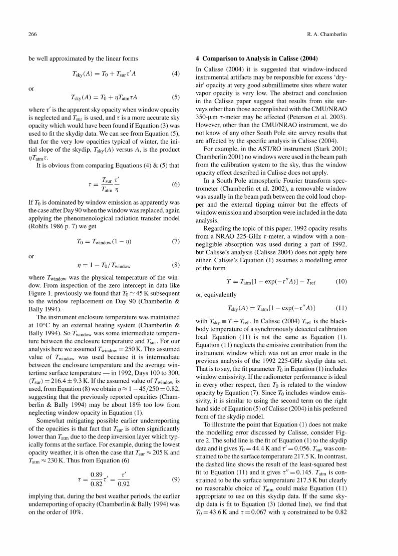
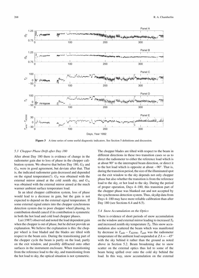
Besides doing skydips, the 1992 data stream from theradiometer was programmed to include periods when itmonitored an outside ambient surface temperature loadat ZA=−45◦, and the cold zenith sky at ZA= 0◦. Alsoreported in the data stream was the radiometer gain. Thesedata, not reported previously, are shown in Figure 3.GZ (Figure 3, Panel A) was the radiometer gain with theexternal tipping mirror on the cold zenith sky, ZA= 0◦.GA (Panel B) was the radiometer gain with external tip-ping mirror directed onto the ambient load, ZA=−45◦.TZ (Panel C) was the measured zenith sky temperature.T0 is the excess temperature found from fitting Equa-tion (1) to skydip data. Tamb− TAD590 was the differencebetween radiometer’s measurement of the external loadtemperature and the actual load temperature, assumedequal to the value detected at an AD590 sensor just belowthe external mirror. The units of radiometer gain (PanelsA & B) are mV K−1. The units of temperature (Panels C,D, & E) are K. For use in Equation (1), and for othercomparisons made here, TAD590 was assumed equal to thesurface temperature Tsur.

In Figure 3, quantities are boxcar-averaged with a fewadjacent points to reduce noise. At Day 90, a suddenincrease in T0, TZ, and Tamb was evident and it was dueto the installation of the replacement window which wasmore opaque.

3Whether or not the window adds much to the observed tem-perature depends on the difference between window and sourcetemperature. If we define Texcess as the difference between theobserved temperature and the source temperature, Tsource, then it iseasy to show that Texcess= (Twindow− Tsource)[1− exp(−τwindow)], orTexcess= (Twindow− Tsource)τwindow when τwindow 1.


GZ

TZ

T0

Tam

b�T

AD

590

GA

0.75

1.25

0.75

1.25

0

100

�50

0

100

�50

30

�30

0

0 100 200 300

0 100 200 300

0 100 200 300

0 100 200 300

0 100 200 300

Panel A

Panel B

Panel C

Panel D

Days, Year 1992

Panel E

Figure 3 A time series of some useful diagnostic indicators. See Section 5 definitions and discussion.

5.3 Chopper Phase Drift after Day 180

After about Day 180 there is evidence of change in theradiometer gain due to loss of phase in the chopper cali-bration system. We observe that before Day 180, GZ andGA were in good agreement, but deviate after that. Thatis, the indicated radiometer gain decreased and dependedon the signal temperature(!). GZ was obtained with theexternal mirror aimed at the cold zenith sky, and GA

was obtained with the external mirror aimed at the muchwarmer ambient surface temperature load.

In an ideal chopper calibration system, loss of phasewould lead to a decrease in gain, but the gain is notexpected to depend on the external signal temperature. Ifsome external signal enters into the chopper synchronousdetection system due to poor chopper wheel phasing, itscontribution should cancel if its contribution is symmetricin both the hot load and cold load chopper phases.

Lui (1987) observed and noted the load dependent gainwhen the chopper is out of phase, but he did not provide anexplanation. We believe the explanation is this: the chop-per wheel is four bladed and the blades are tilted withrespect to the beam axis. During the transitioning part ofthe chopper cycle the beam is partly on the load, partlyon the exit window, and possibly diffracted onto othersurfaces in the instrument enclosure. When transitioningfrom the reference load to the sky, and transitioning fromthe hot load to sky, the optical situation is not symmetric.

The chopper blades are tilted with respect to the beam indifferent directions in these two transition cases so as todirect the radiometer to either the reference load which isat about 90◦ to the interrupted beam direction, or direct itto the hot load which is opposite at about −90◦. That is,during the transition period, the size of the illuminated spoton the exit window to the sky depends not only chopperphase but also whether the transition is from the referenceload to the sky, or hot load to the sky. During the periodof proper operation, Days 4–180, this transition part ofthe chopper phase was blanked out and not accepted bythe synchronous detection system. Thus, skydip data fromDays 4–180 may have more reliable calibration than afterDay 180 (see Sections 6.4 and 6.5).

5.4 Snow Accumulation on the Optics

There is evidence of short periods of snow accumulationon the window and external mirror leading to increased T0

and increased zenith sky temperature TZ. This snow accu-mulation also scattered the beam which was manifestedby decrease in Tamb− TAD590. Tamb was the radiometertemperature of the ambient load suspended atZA=−45◦with the sky behind it rather than the ground as notedabove in Section 5.2. Beam broadening due to snowscatter on the external optics thus led to some of thebeam being spilled over onto the cold sky behind theload. In this way, snow accumulation on the external


25 30 35 40

Panel A

0.75

1.25

25 30 35 40

Panel B

0.75

1.25

25 30 35 40

0

100Panel C

�50

25 30 35 40

0

100Panel D

�50

25 30 35 40

Days, Year 1992

Panel E30

�30

0

GZ

TZ

T0

Tam

b�T

AD

590

GA

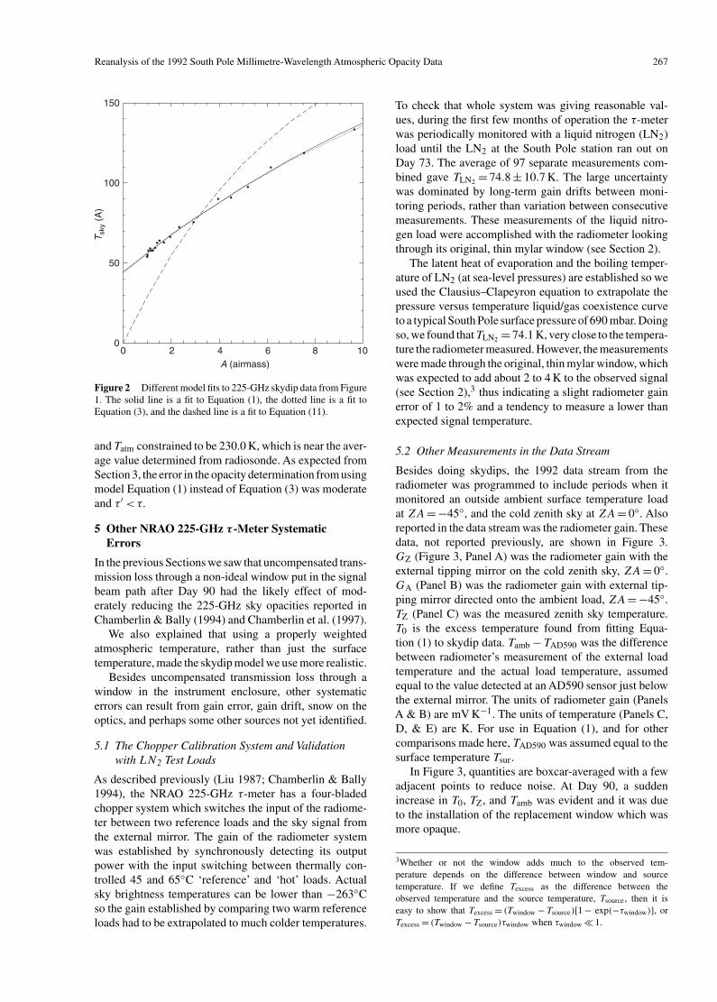
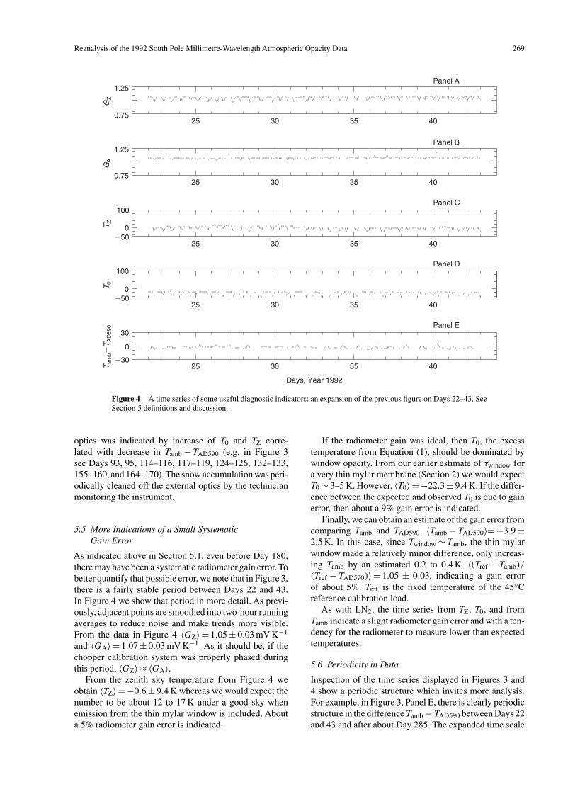
Figure 4 A time series of some useful diagnostic indicators: an expansion of the previous figure on Days 22–43. SeeSection 5 definitions and discussion.

optics was indicated by increase of T0 and TZ corre-lated with decrease in Tamb− TAD590 (e.g. in Figure 3see Days 93, 95, 114–116, 117–119, 124–126, 132–133,155–160, and 164–170). The snow accumulation was peri-odically cleaned off the external optics by the technicianmonitoring the instrument.

5.5 More Indications of a Small SystematicGain Error

As indicated above in Section 5.1, even before Day 180,there may have been a systematic radiometer gain error. Tobetter quantify that possible error, we note that in Figure 3,there is a fairly stable period between Days 22 and 43.In Figure 4 we show that period in more detail. As previ-ously, adjacent points are smoothed into two-hour runningaverages to reduce noise and make trends more visible.From the data in Figure 4 〈GZ〉= 1.05± 0.03 mV K−1

and 〈GA〉= 1.07± 0.03 mV K−1. As it should be, if thechopper calibration system was properly phased duringthis period, 〈GZ〉≈ 〈GA〉.

From the zenith sky temperature from Figure 4 weobtain 〈TZ〉=−0.6± 9.4 K whereas we would expect thenumber to be about 12 to 17 K under a good sky whenemission from the thin mylar window is included. Abouta 5% radiometer gain error is indicated.

If the radiometer gain was ideal, then T0, the excesstemperature from Equation (1), should be dominated bywindow opacity. From our earlier estimate of τwindow fora very thin mylar membrane (Section 2) we would expectT0∼ 3–5 K. However, 〈T0〉=−22.3± 9.4 K. If the differ-ence between the expected and observed T0 is due to gainerror, then about a 9% gain error is indicated.

Finally, we can obtain an estimate of the gain error fromcomparing Tamb and TAD590. 〈Tamb− TAD590〉=−3.9±2.5 K. In this case, since Twindow∼ Tamb, the thin mylarwindow made a relatively minor difference, only increas-ing Tamb by an estimated 0.2 to 0.4 K. 〈(Tref − Tamb)/

(Tref − TAD590)〉= 1.05 ± 0.03, indicating a gain errorof about 5%. Tref is the fixed temperature of the 45◦Creference calibration load.

As with LN2, the time series from TZ, T0, and fromTamb indicate a slight radiometer gain error and with a ten-dency for the radiometer to measure lower than expectedtemperatures.

5.6 Periodicity in Data

Inspection of the time series displayed in Figures 3 and4 show a periodic structure which invites more analysis.For example, in Figure 3, Panel E, there is clearly periodicstructure in the differenceTamb− TAD590 between Days 22and 43 and after about Day 285. The expanded time scale


in Figure 4 is useful for seeing the periodicity in moredetail. Fourier analysis on the time series ofTamb− TAD590

between Days 22 and 43 shows strong peaks in the powerspectrum at exactly 1, 2, and 3 dy−1 corresponding to thediurnal cycle and its harmonics. The diurnal characteris-tic Tamb− TAD590 occurred during a period when the sunwas up and so can likely be attributed to differential heat-ing of the radiometer load and the AD590 temperaturetransducer.

In the expanded time scale of Figure 4, Panel A, wecan also clearly see periodic structureGZ and correspond-ing structure in GA (Panel B) but with lower amplitude.This correspondence in periodicity, but differing ampli-tude between GZ and GA may suggest periods of poorchopper phasing, but we do not know how this effectcould come about periodically, and then recover on itsown. Fourier analysis on the time series of GZ showsa dominant peak at 1.82 dy−1, that is, a periodicity of13.2 h. This periodicity is not conveniently linked to thediurnal cycle and we do not know what caused it. GZ

was used to calibrate the sky signal so it not surpris-ing that corresponding structure appears in TZ, Panel C.However, it also appears in the derived quantity T0 sug-gesting it may be a component introduced into the τ timeseries.

Fourier analysis of the τ time series derived using Equa-tion (1) showed strong peaks in the power spectrum at 1.0,1.8, and 3.0 dy−1 as well as other structure. It seems likelythe peak at 1.8 dy−1 was due gain variations in the instru-ment itself, rather than actual variations in the atmosphere.The peaks at 1.0 and 3.0 dy−1 which are not evident inthe GZ power spectrum, may have been due to diurnalvariation in the atmosphere or surface temperature.

6 Reanalysis

In Sections 3 and 4 we have seen that skydip data reductionmay have been slightly biased toward lower values bythe implicit assumption in Equation (1), that η≡ 1.0, andslightly biased toward higher values by use of Tsur insteadof Tatm in Equation (1). We estimated the net effect ofusing Equation (1) instead of Equation (2) was to bias thereported opacity about 10% toward lower values in thebest weather.

In addition, in Section 5.3 we used previously unre-ported indications from the data stream to show that thedata may be corrupted after about Day 180 due to loss ofphase in the chopper calibration system. Prior to Day 43,during a stable period suitable for establishing instrumentperformance, we also inferred from TZ, Tamb, and T0 thatthe radiometer gain was somewhat in error, approximately6%, and biased toward measuring lower than true valuesfor Tsky.

6.1 Correction of Gain Error

If before Day 180 the radiometer gain error was approx-imately constant at 6%, then we could apply a simple,constant gain correction and reanalyse the data. We

did so and found the new results that between Days22–43, 〈TZ〉= 18.5± 7.0 K, 〈T0〉=−1.18± 6.9 K, and〈Tamb− TAD590〉= 0.8± 1.7 K. The constant 6% correc-tion also gave 〈GZ〉= 1.12± 0.03 mV K−1, and 〈GA〉=1.14± 0.02 mV K−1. These corrected results for TZ, T0,and Tamb are all more physically realistic.

With the gain correction applied, after the windowreplacement on Day 90 and before Day 180 we found〈T0〉= 69.2± 13.1 K, but this average was biased towarda higher value because it includes days when snow wascollected on the enclosure window.

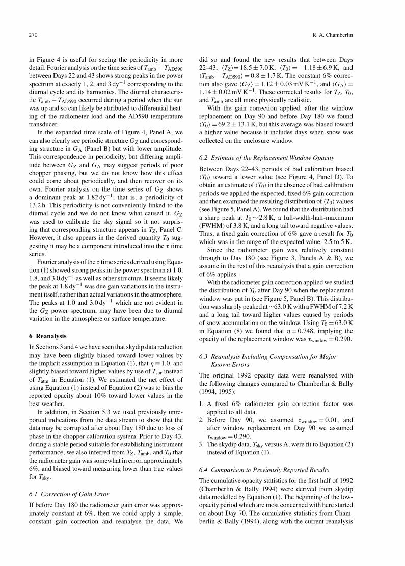
6.2 Estimate of the Replacement Window Opacity

Between Days 22–43, periods of bad calibration biased〈T0〉 toward a lower value (see Figure 4, Panel D). Toobtain an estimate of 〈T0〉 in the absence of bad calibrationperiods we applied the expected, fixed 6% gain correctionand then examined the resulting distribution of 〈T0〉 values(see Figure 5, Panel A). We found that the distribution hada sharp peak at T0∼ 2.8 K, a full-width-half-maximum(FWHM) of 3.8 K, and a long tail toward negative values.Thus, a fixed gain correction of 6% gave a result for T0

which was in the range of the expected value: 2.5 to 5 K.Since the radiometer gain was relatively constant

through to Day 180 (see Figure 3, Panels A & B), weassume in the rest of this reanalysis that a gain correctionof 6% applies.

With the radiometer gain correction applied we studiedthe distribution of T0 after Day 90 when the replacementwindow was put in (see Figure 5, Panel B). This distribu-tion was sharply peaked at∼63.0 K with a FWHM of 7.2 Kand a long tail toward higher values caused by periodsof snow accumulation on the window. Using T0= 63.0 Kin Equation (8) we found that η= 0.748, implying theopacity of the replacement window was τwindow= 0.290.

6.3 Reanalysis Including Compensation for MajorKnown Errors

The original 1992 opacity data were reanalysed withthe following changes compared to Chamberlin & Bally(1994, 1995):

1. A fixed 6% radiometer gain correction factor wasapplied to all data.

2. Before Day 90, we assumed τwindow= 0.01, andafter window replacement on Day 90 we assumedτwindow= 0.290.

3. The skydip data, Tsky versus A, were fit to Equation (2)instead of Equation (1).

6.4 Comparison to Previously Reported Results

The cumulative opacity statistics for the first half of 1992(Chamberlin & Bally 1994) were derived from skydipdata modelled by Equation (1). The beginning of the low-opacity period which are most concerned with here startedon about Day 70. The cumulative statistics from Cham-berlin & Bally (1994), along with the current reanalysis


�10�20�30�40 0 100

20

40

60

80

100Panel A

20 40 60 80 1000

50

100

150

200

250

T0, Days 90 –180T0, Days 22 – 43

Panel B

Fre

quen

cy o

f occ

urre

nce

Fre

quen

cy o

f occ

urre

nce

Figure 5 The distribution of T0 values for Days 22–43 and Days 90–180. T0 is in units of K and is a free parameterderived from the fit of Equation (1) or (2) to skydip data: Tsky versus A. For data in this figure, prior to fitting todetermine T0, a 6% gain correction was applied to the radiometer gain, see Section 6.1. If T0 was dominated bywindow emission, then η, the radiometer loss efficiency due to window opacity, can be determined from Equation(8). The amplitude of the plots, ‘frequency of occurrence’, is related to the total number of points in the sample andthe resolution in T0. These plot parameters are different in Panels A and B.

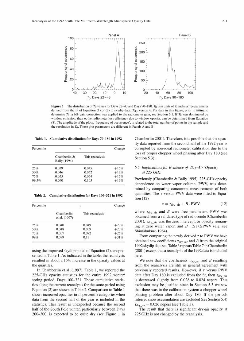
Table 1. Cumulative distribution for Days 70–180 in 1992

Percentile τ Change

Chamberlin & This reanalysisBally (1994)

25% 0.039 0.045 +15%50% 0.046 0.052 +13%75% 0.055 0.064 +16%99.5% 0.090 0.105 +16%

Table 2. Cumulative distribution for Days 100–321 in 1992

Percentile τ Change

Chamberlin This reanalysiset al. (1997)

25% 0.040 0.049 +23%50% 0.048 0.059 +23%75% 0.057 0.072 +26%99% 0.099 0.13 +31%

using the improved skydip model of Equation (2), are pre-sented in Table 1. As indicated in the table, the reanalysisresulted in about a 15% increase in the opacity values atthe quartiles.

In Chamberlin et al. (1997), Table 1, we reported the225-GHz opacity statistics for the entire 1992 winter/spring period, Days 100–321. Those cumulative statis-tics along the current reanalysis for the same period usingEquation (2) are shown in Table 2. Comparison to Table 1shows increased opacities in all percentile categories whendata from the second half of the year is included in thestatistics. This result is unexpected because the secondhalf of the South Pole winter, particularly between Days200–300, is expected to be quite dry (see Figure 1 in

Chamberlin 2001). Therefore, it is possible that the opac-ity data reported from the second half of the 1992 year iscorrupted by non-ideal radiometer calibration due to theloss of proper chopper wheel phasing after Day 180 (seeSection 5.3).

6.5 Implications for Evidence of ‘Dry-Air’ Opacityat 225 GHz

Previously (Chamberlin & Bally 1995), 225-GHz opacitydependence on water vapor column, PWV, was deter-mined by comparing concurrent measurements of bothquantities. The τ versus PWV data were fitted to Equa-tion (12)

τ = τdry_air + B · PWV (12)

where τdry_air and B were free parameters. PWV wasobtained from a validated type of radiosonde (Chamberlin2001), τdry_air was the zero intercept, or opacity remain-ing at zero water vapor, and B=�τ/�PWV (e.g. seeShimabukuro 1964).

From comparing the newly derived τ to PWV we haveobtained new coefficients τdry_air and B from the original1992 skydip data set. Table 3 repeatsTable 7 in Chamberlin(2001) except that a reanalysis of the 1992 data is includedhere.

We note that the coefficients τdry_air and B resultingfrom the reanalysis are still in general agreement withpreviously reported results. However, if τ versus PWVdata after Day 180 is excluded from the fit, then τdry_air

is decreased slightly from 0.028 to 0.024 nepers. Thisexclusion may be justified since in Section 5.3 we sawthat there was in the calibration system a chopper wheelphasing problem after about Day 180. If the periodsinferred snow accumulation are excluded (see Section 5.4)τdry_air = 0.026 nepers (see Table 3).

The result that there is significant dry-air opacity at225 GHz is not changed by the reanalysis.


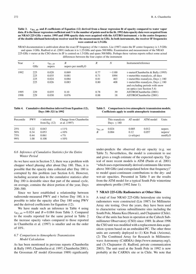
Table 3. τdry_air and B coefficients of Equation (12) derived from a linear regression fit of opacity compared to water vapordata. R is the linear regression coefficient and N is the number of points used in the fit. 1992 data opacity data were acquired froman NRAO 225-GHz τ -meter. 1995 and 1998 opacity data were acquired with the AST/RO instrument. ν is the centre frequencyof the double sideband heterodyne receiver used for the measurements in GHz. In both instruments, the receiver IF frequencies

were centred on 1.5 GHz

NRAO documentation is ambivalent about the exact IF frequency of the τ-meters. Liu (1987) states the IF centre frequency is 1.5 GHzand spans 1 GHz. Radford et al. (2001) indicate it is 1.25 GHz and spans 500 MHz. Examination and measurement of the NRAO

225-GHz τ-meter at the CSO shows its IF is centred on 1.5 GHz and spans 500 MHz. Perhaps these various reports reflect some actualdifferences between the four copies of the instrument

Year ν τdry_air B R N Instrument/referenceGHz nepers nepers per mmH2O

1992 225 0.028 0.069 0.77 ∼1100 τ-meter/Chamberlin & Bally (1995)225 0.035 0.081 0.71 1094 τ-meter/this reanalysis, all days225 0.024 0.084 0.81 463 τ-meter/this reanalysis, Days≤ 180225 0.026 0.083 0.80 408 τ-meter/this reanalysis, Days≤ 180

and excluding periods with snowon optics (see Section 5.4)

1995 229 0.035 0.10 0.78 39 AST/RO/Chamberlin (2001)1998 229 0.030 0.076 0.88 18 AST/RO/Chamberlin (2001)

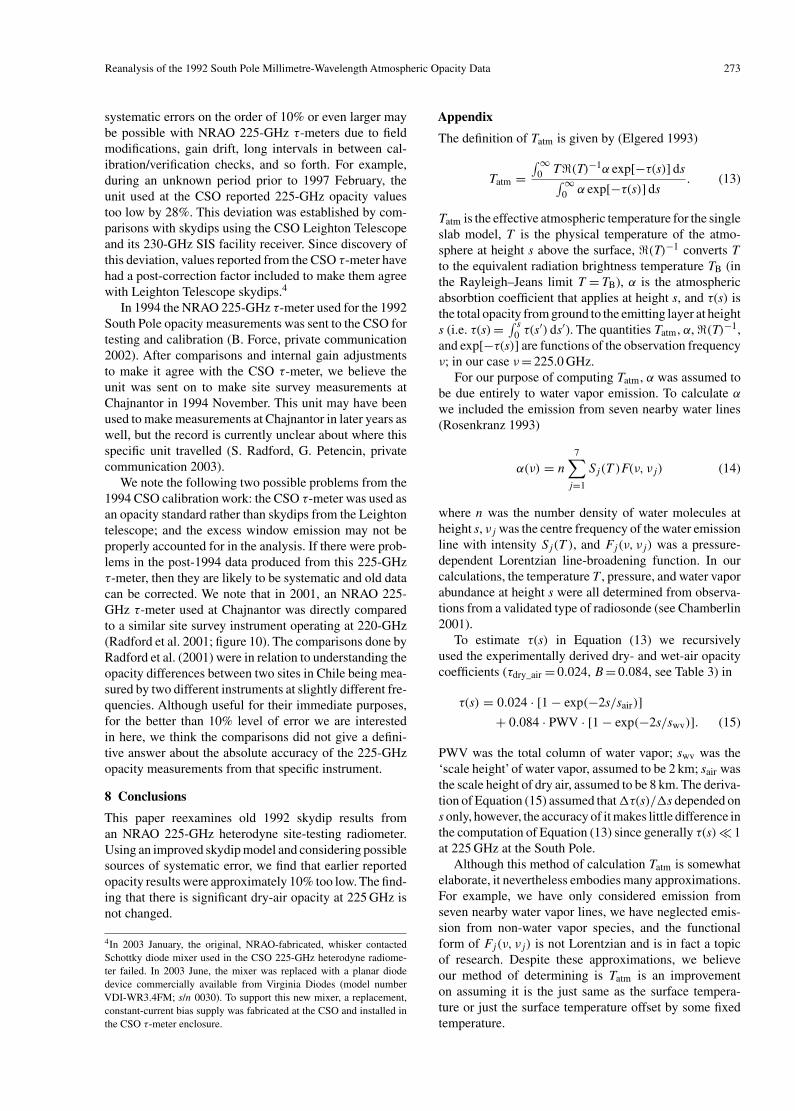
Table 4. Cumulative distribution inferred from Equation (12),Days 100–321 in 1992

Percentile PWV τ inferred Change from Chamberlinfrom Eq. (12) et al. (1997)

25% 0.22 0.043 +11%50% 0.34 0.053 +10%75% 0.44 0.061 +7%99% 1.00 0.108 +10%

6.6 Inference of Cumulative Statistics for the EntireWinter Period

As we have seen in Section 5.3, there was a problem withchopper wheel phasing after about Day 180. Thus, it ispossible that the opacity data collected after Day 180 iscorrupted by this problem (see Section 6.4). However,including accurate data in the cumulative statistics afterDay 180 is desirable since that part of the annual cycle,on average, contains the driest portion of the year, Days200–300.

Since we have established a relationship betweenradiosonde-measured PWV and τ before Day 180, it ispossible to infer the opacity after Day 180 using PWVand the derived coefficients for Equation (12).

We have made such an inference in Table 4 usingτdry_air = 0.024 and B= 0.084 from Table 3. Comparedto the results reported for the same period in Table 2the increase opacity values compared to those reportedin Chamberlin et al. (1997) is smaller and on the orderof 10%.

6.7 Comparison to Atmospheric TransmissionModel Calculation

As has been mentioned in previous reports (Chamberlin& Bally 1995; Chamberlin et al. 1997; Chamberlin 2001),the Grossman AT model (Grossman 1989) significantly

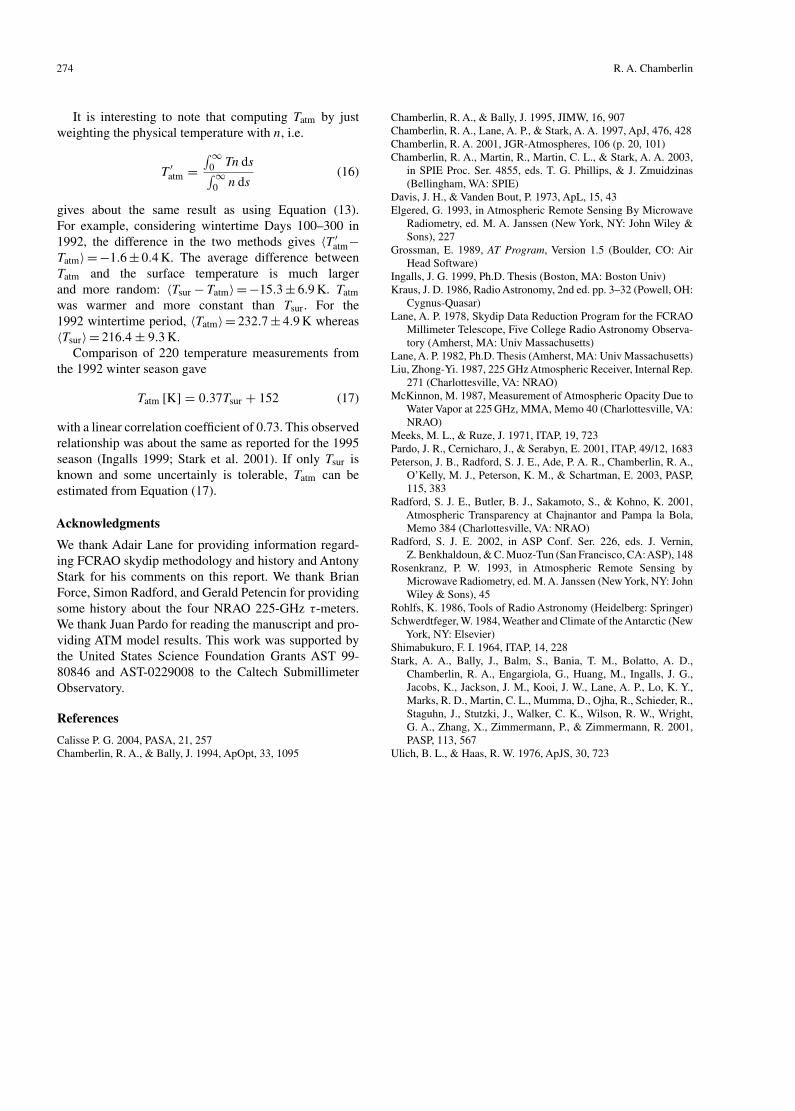
Table 5. Comparison to two atmospheric transmission models.Coefficients apply to zenith atmospheric transmission

This reanalysis AT model ATM model UnitsDays ≤ 180

τdry_air 0.024 0.005 0.012 nepersB 0.084 0.12 0.057 nepers/

(z-n/typo) mmH2O

under-predicts the observed dry-air opacity (e.g. seeTable 5). Nevertheless, the model is convenient to useand gives a rough estimate of the expected opacity. Typ-ical of more recent models is ATM (Pardo et al. 2001)“which uses experimentally derived continuum-like termsabove 300 GHz (and extrapolated below that frequency)”to model quasi-continuum contributions to the dry- andwet-air opacities. Presented in Table 5 are the resultsfrom the ATM model for a typical South Pole wintertimeatmospheric profile (1992 June 1).

7 NRAO 225-GHz Radiometers at Other Sites

A total of four NRAO 225-GHz heterodyne site testingradiometers were constructed (Liu 1987) for MillimetreArray site testing. Over the years, they have been usedto characterise various submillimetre sites including theSouth Pole, Mauna Kea (Hawaii), and Chajnantor (Chile).One of the units has been in operation at the Caltech Sub-millimeter Observatory (CSO) since 1989. In about 1996the CSO unit was modified with a replacement data acqui-sition system based on an embedded PC. The other threeunits are currently deployed to (1) Kitt Peak (Arizona),(2) The Combined Array for Research in Millimetre-wave Astronomy (CARMA) (http://www.mmarray.org/),and (3) Chajnantor (S. Radford, private communication2003). The unit used at the South Pole in 1992 is nowprobably at the CARMA site or in Chile. We note that


systematic errors on the order of 10% or even larger maybe possible with NRAO 225-GHz τ-meters due to fieldmodifications, gain drift, long intervals in between cal-ibration/verification checks, and so forth. For example,during an unknown period prior to 1997 February, theunit used at the CSO reported 225-GHz opacity valuestoo low by 28%. This deviation was established by com-parisons with skydips using the CSO Leighton Telescopeand its 230-GHz SIS facility receiver. Since discovery ofthis deviation, values reported from the CSO τ-meter havehad a post-correction factor included to make them agreewith Leighton Telescope skydips.4

In 1994 the NRAO 225-GHz τ-meter used for the 1992South Pole opacity measurements was sent to the CSO fortesting and calibration (B. Force, private communication2002). After comparisons and internal gain adjustmentsto make it agree with the CSO τ-meter, we believe theunit was sent on to make site survey measurements atChajnantor in 1994 November. This unit may have beenused to make measurements at Chajnantor in later years aswell, but the record is currently unclear about where thisspecific unit travelled (S. Radford, G. Petencin, privatecommunication 2003).

We note the following two possible problems from the1994 CSO calibration work: the CSO τ-meter was used asan opacity standard rather than skydips from the Leightontelescope; and the excess window emission may not beproperly accounted for in the analysis. If there were prob-lems in the post-1994 data produced from this 225-GHzτ-meter, then they are likely to be systematic and old datacan be corrected. We note that in 2001, an NRAO 225-GHz τ-meter used at Chajnantor was directly comparedto a similar site survey instrument operating at 220-GHz(Radford et al. 2001; figure 10). The comparisons done byRadford et al. (2001) were in relation to understanding theopacity differences between two sites in Chile being mea-sured by two different instruments at slightly different fre-quencies. Although useful for their immediate purposes,for the better than 10% level of error we are interestedin here, we think the comparisons did not give a defini-tive answer about the absolute accuracy of the 225-GHzopacity measurements from that specific instrument.

8 Conclusions

This paper reexamines old 1992 skydip results froman NRAO 225-GHz heterodyne site-testing radiometer.Using an improved skydip model and considering possiblesources of systematic error, we find that earlier reportedopacity results were approximately 10% too low. The find-ing that there is significant dry-air opacity at 225 GHz isnot changed.

4In 2003 January, the original, NRAO-fabricated, whisker contactedSchottky diode mixer used in the CSO 225-GHz heterodyne radiome-ter failed. In 2003 June, the mixer was replaced with a planar diodedevice commercially available from Virginia Diodes (model numberVDI-WR3.4FM; s/n 0030). To support this new mixer, a replacement,constant-current bias supply was fabricated at the CSO and installed inthe CSO τ-meter enclosure.

Appendix

The definition of Tatm is given by (Elgered 1993)

Tatm =∫∞

0 T�(T)−1α exp[−τ(s)] ds∫∞

0 α exp[−τ(s)] ds . (13)

Tatm is the effective atmospheric temperature for the singleslab model, T is the physical temperature of the atmo-sphere at height s above the surface, �(T)−1 converts Tto the equivalent radiation brightness temperature TB (inthe Rayleigh–Jeans limit T = TB), α is the atmosphericabsorbtion coefficient that applies at height s, and τ(s) isthe total opacity from ground to the emitting layer at heights (i.e. τ(s)= ∫ s0 τ(s′) ds′). The quantities Tatm, α, �(T)−1,and exp[−τ(s)] are functions of the observation frequencyν; in our case ν= 225.0 GHz.

For our purpose of computing Tatm, α was assumed tobe due entirely to water vapor emission. To calculate αwe included the emission from seven nearby water lines(Rosenkranz 1993)

α(ν) = n7∑

j=1

Sj(T )F(ν, νj) (14)

where n was the number density of water molecules atheight s, νj was the centre frequency of the water emissionline with intensity Sj(T ), and Fj(ν, νj) was a pressure-dependent Lorentzian line-broadening function. In ourcalculations, the temperature T , pressure, and water vaporabundance at height s were all determined from observa-tions from a validated type of radiosonde (see Chamberlin2001).

To estimate τ(s) in Equation (13) we recursivelyused the experimentally derived dry- and wet-air opacitycoefficients (τdry_air = 0.024, B= 0.084, see Table 3) in

τ(s) = 0.024 · [1− exp(−2s/sair)]+ 0.084 · PWV · [1− exp(−2s/swv)]. (15)

PWV was the total column of water vapor; swv was the‘scale height’ of water vapor, assumed to be 2 km; sair wasthe scale height of dry air, assumed to be 8 km. The deriva-tion of Equation (15) assumed that�τ(s)/�s depended ons only, however, the accuracy of it makes little difference inthe computation of Equation (13) since generally τ(s) 1at 225 GHz at the South Pole.

Although this method of calculation Tatm is somewhatelaborate, it nevertheless embodies many approximations.For example, we have only considered emission fromseven nearby water vapor lines, we have neglected emis-sion from non-water vapor species, and the functionalform of Fj(ν, νj) is not Lorentzian and is in fact a topicof research. Despite these approximations, we believeour method of determining is Tatm is an improvementon assuming it is the just same as the surface tempera-ture or just the surface temperature offset by some fixedtemperature.


It is interesting to note that computing Tatm by justweighting the physical temperature with n, i.e.

T ′atm =∫∞

0 Tn ds∫∞

0 n ds(16)

gives about the same result as using Equation (13).For example, considering wintertime Days 100–300 in1992, the difference in the two methods gives 〈T ′atm−Tatm〉=−1.6± 0.4 K. The average difference betweenTatm and the surface temperature is much largerand more random: 〈Tsur − Tatm〉=−15.3± 6.9 K. Tatm

was warmer and more constant than Tsur. For the1992 wintertime period, 〈Tatm〉= 232.7± 4.9 K whereas〈Tsur〉= 216.4± 9.3 K.

Comparison of 220 temperature measurements fromthe 1992 winter season gave

Tatm [K] = 0.37Tsur + 152 (17)

with a linear correlation coefficient of 0.73. This observedrelationship was about the same as reported for the 1995season (Ingalls 1999; Stark et al. 2001). If only Tsur isknown and some uncertainly is tolerable, Tatm can beestimated from Equation (17).

Acknowledgments

We thank Adair Lane for providing information regard-ing FCRAO skydip methodology and history and AntonyStark for his comments on this report. We thank BrianForce, Simon Radford, and Gerald Petencin for providingsome history about the four NRAO 225-GHz τ-meters.We thank Juan Pardo for reading the manuscript and pro-viding ATM model results. This work was supported bythe United States Science Foundation Grants AST 99-80846 and AST-0229008 to the Caltech SubmillimeterObservatory.

References

Calisse P. G. 2004, PASA, 21, 257Chamberlin, R. A., & Bally, J. 1994, ApOpt, 33, 1095

Chamberlin, R. A., & Bally, J. 1995, JIMW, 16, 907Chamberlin, R. A., Lane, A. P., & Stark, A. A. 1997, ApJ, 476, 428Chamberlin, R. A. 2001, JGR-Atmospheres, 106 (p. 20, 101)Chamberlin, R. A., Martin, R., Martin, C. L., & Stark, A. A. 2003,

in SPIE Proc. Ser. 4855, eds. T. G. Phillips, & J. Zmuidzinas(Bellingham, WA: SPIE)

Davis, J. H., & Vanden Bout, P. 1973, ApL, 15, 43Elgered, G. 1993, in Atmospheric Remote Sensing By Microwave

Radiometry, ed. M. A. Janssen (New York, NY: John Wiley &Sons), 227

Grossman, E. 1989, AT Program, Version 1.5 (Boulder, CO: AirHead Software)

Ingalls, J. G. 1999, Ph.D. Thesis (Boston, MA: Boston Univ)Kraus, J. D. 1986, Radio Astronomy, 2nd ed. pp. 3–32 (Powell, OH:

Cygnus-Quasar)Lane, A. P. 1978, Skydip Data Reduction Program for the FCRAO

Millimeter Telescope, Five College Radio Astronomy Observa-tory (Amherst, MA: Univ Massachusetts)

Lane, A. P. 1982, Ph.D. Thesis (Amherst, MA: Univ Massachusetts)Liu, Zhong-Yi. 1987, 225 GHz Atmospheric Receiver, Internal Rep.

271 (Charlottesville, VA: NRAO)McKinnon, M. 1987, Measurement of Atmospheric Opacity Due to

Water Vapor at 225 GHz, MMA, Memo 40 (Charlottesville, VA:NRAO)

Meeks, M. L., & Ruze, J. 1971, ITAP, 19, 723Pardo, J. R., Cernicharo, J., & Serabyn, E. 2001, ITAP, 49/12, 1683Peterson, J. B., Radford, S. J. E., Ade, P. A. R., Chamberlin, R. A.,

O’Kelly, M. J., Peterson, K. M., & Schartman, E. 2003, PASP,115, 383

Radford, S. J. E., Butler, B. J., Sakamoto, S., & Kohno, K. 2001,Atmospheric Transparency at Chajnantor and Pampa la Bola,Memo 384 (Charlottesville, VA: NRAO)

Radford, S. J. E. 2002, in ASP Conf. Ser. 226, eds. J. Vernin,Z. Benkhaldoun, & C. Muoz-Tun (San Francisco, CA:ASP), 148

Rosenkranz, P. W. 1993, in Atmospheric Remote Sensing byMicrowave Radiometry, ed. M. A. Janssen (NewYork, NY: JohnWiley & Sons), 45

Rohlfs, K. 1986, Tools of Radio Astronomy (Heidelberg: Springer)Schwerdtfeger, W. 1984, Weather and Climate of the Antarctic (New

York, NY: Elsevier)Shimabukuro, F. I. 1964, ITAP, 14, 228Stark, A. A., Bally, J., Balm, S., Bania, T. M., Bolatto, A. D.,

Chamberlin, R. A., Engargiola, G., Huang, M., Ingalls, J. G.,Jacobs, K., Jackson, J. M., Kooi, J. W., Lane, A. P., Lo, K. Y.,Marks, R. D., Martin, C. L., Mumma, D., Ojha, R., Schieder, R.,Staguhn, J., Stutzki, J., Walker, C. K., Wilson, R. W., Wright,G. A., Zhang, X., Zimmermann, P., & Zimmermann, R. 2001,PASP, 113, 567

Ulich, B. L., & Haas, R. W. 1976, ApJS, 30, 723

reanalysis of the 1992 south pole millimetre-wavelength atmospheric opacity data

Documents