real-time sensor anomaly detection and recovery in ... - arxiv

ACCEPTED TO BE PUBLISHED IN: IEEE TRANSACTIONS ON INTELLIGENT TRANSPORTATION SYSTEMS 1

Real-Time Sensor Anomaly Detection and Recoveryin Connected Automated Vehicle Sensors

Yiyang Wang, Neda Masoud, Anahita Khojandi, Member, IEEE

Abstract—In this paper we propose a novel observer-basedmethod to improve the safety and security of connected andautomated vehicle (CAV) transportation. The proposed methodcombines model-based signal filtering and anomaly detectionmethods. Specifically, we use adaptive extended Kalman filter(AEKF) to smooth sensor readings of a CAV based on a nonlinearcar-following motion model. Under the assumption of a car-following model, the subject vehicle utilizes its leading vehicle’sinformation to detect sensor anomalies by employing previously-trained One Class Support Vector Machine (OCSVM) models.This approach allows the AEKF to estimate the state of a vehiclenot only based on the vehicle’s location and speed, but alsoby taking into account the state of the surrounding traffic.A communication time delay factor is considered in the car-following model to make it more suitable for real-world appli-cations. Our experiments show that compared with the AEKFwith a traditional χ2-detector, our proposed method achieves abetter anomaly detection performance. We also demonstrate thata larger time delay factor has a negative impact on the overalldetection performance.

Index Terms—Cyber-physical systems, Fault diagnosis, Intel-ligent vehicles, Car-following model, Vehicle safety, Anomalydetection, Signal filtering

I. INTRODUCTION

Numerous studies within the past decade have focused onconnected and automated vehicle (CAV) technology, which isconsidered to be an integral part of the future of the intelligenttransportation system (ITS) field [1]. CAVs have the potentialto transform the ITS field by introducing numerous safety,mobility, and environmental sustainability benefits [2]–[5]. ACAV system combines connected vehicle (CV) and automatedvehicle (AV) technologies, creating a synergistic impact thatgoes well beyond the benefits that each of these technologiescan offer in isolation. It is envisioned that CAVs, with diversedegrees of connectivity and automation, will lead the pathtoward the next generation of transportation systems, whichis more intelligent, efficient, and sustainable [6], [7].

CAVs use wireless technologies to enable communicationand cooperation not only among vehicles but also between ve-hicles and the transportation infrastructure. By using dedicated

©2020 IEEE. Personal use of this material is permitted. Permission fromIEEE must be obtained for all other uses, in any current or future media,including reprinting/republishing this material for advertising or promotionalpurposes, creating new collective works, for resale or redistribution to serversor lists, or reuse of any copyrighted component of this work in other works.doi: 10.1109/TITS.2020.2970295.Yiyang Wang and Neda Masoud are with the University of Michigan, AnnArbor, MI 48109, USA (e-mail: [email protected], [email protected]).Anahita Khojandi is with the University of Tennessee at Knoxville, TN 37996,USA (email:[email protected]).

short-range communication (DSRC) [8], or other types of com-munication technologies, vehicles and roadside units (RSUs)are able to continuously transmit and receive information suchas speed, position, acceleration, braking status, traffic signalstatus, etc., through what is called a Basic Safety Message(BSM). These communication messages have a range of about400 meters and can detect high-risk situations that may notbe observable otherwise due to traffic, terrain, or weather [8].The CAV technology extends and enhances currently availablecrash avoidance systems that use radars and cameras to detectcollision threats by enabling CAVs to warn their surroundingvehicles of collisions and potentially hazardous circumstances.In addition, they provide mobility and sustainability benefitsby enabling platoon formation, which can increase road ca-pacity and reduce fuel consumption. However, as vehicles andinfrastructures become more interconnected and automated,the vulnerability of their components to faults and/or deliberatemalicious attacks increases. This vulnerability is exacerbatedby the increase in vehicle-to-vehicle (V2V) and vehicle-to-infrastructure (V2I) communications, which increase a vehi-cle’s external connection interfaces. At the system level, CAVsand the infrastructure can be viewed as individual nodes ina large interconnected network, where a single anomaly ormalicious attack can easily propagate through this network, af-fecting other network components (e.g., other vehicles, trafficcontrol devices, etc.). Therefore, there is an increasing demandfor cyber security solutions, e.g., anomaly detection methods,in CAV sensor systems to enhance safety and reliability ofCAVs and the entire network.

Anomaly detection in CAV sensors is an important but alsochallenging task. A traveling CAV could use the most recenthistory of data to detect anomalies. Presence of an anomalyin the pattern of data collected from a CAV sensor systemcan imply (i) a subset of sensors are faulty, or (ii) there hasbeen a malicious attack. In both cases, it is vital to detect theanomalies and exclude the anomalous data from the decisionmaking process.

An anomaly detection scheme introduces two types of errors– false negatives and false positives. It is easy to see that afalse negative error can allow falsified data to affect trajectoryplanning, which could lead to fatal consequences. Althoughless apparent, a false positive error can have consequences thatare just as severe. Consider a situation where an actual event inthe network (e.g., an unexpected braking from a downstreamvehicle) has led to an abrupt change in the pattern of observeddata. If the vehicle falsely detects such an unexpected changeas a fault/attack and discards the information, it may lead tothe CAV not reacting to such abrupt changes in the network

arX

iv:1

911.

0153

1v2

[ee

ss.S

P] 2

5 Fe

b 20

21


appropriately and in a timely manner, creating dangerous, andpotentially fatal, scenarios. In order to prevent this type offalse positive error, it is necessary for vehicles to incorporatenetwork-level information in their anomaly detection scheme.

In addition to distinguishing between real changes in net-work conditions and anomalies, the anomaly detection meth-ods should be able to identify the noise introduced by sensorsand the communication channel, exacerbated by potentialcommunication delay, as well as the missing values in thecollected data. Moreover, due to resource constraints for eachvehicle, the anomaly detection techniques in CAVs need to belightweight, and implementable in real-time.

Anomalous sensor behavior could manifest itself in variousforms and representations. Several faulty sensor behaviors arediscussed in [9]. Petit et al. [10] summarize the taxonomy ofintrusions or attacks on automated vehicles, among which thefalse injection attack is considered to be the most dangerousattack. In this paper, we consider five types of the anomaloussensor behavior resulting from both sensor faults and falseinjection attacks. We base this paper on the sensor failureand/or attack taxonomy provided by Sharma et al. [9] andVan et al. [11]:

1) Short: A single, sharp and abrupt change in the observeddata between two successive sensor readings.

2) Noise: An increase in the variance of the sensor read-ings. Different from Short, the Noise anomaly typeoccurs across multiple successive sensor readings.

3) Bias: A temporarily constant offset from the sensorreadings.

4) Gradual drift: A small and gradual drift in observed dataduring a time period. Over time, a gradual drift can resultin a large discrepancy between the observed and the truestate of the system.

5) Miss: Lack of available data during a time period.In this paper, we do not explicitly account for ‘miss,’ which

can result from DoS attacks preventing the exchange of infor-mation. However, note that ‘miss,’ depending on its duration,can be viewed as ‘short’ or ‘bias’, where the sensor reading isnon-existent instead of showing a wrong value. Hence, it canpartially be addressed using the same methods for detecting‘short’ or ‘bias’. For examples of specific scenarios that couldlead to these anomalies, refer to [12].

In order to successfully detect different types of anomalies,avoid falsely identifying unexpected changes in the network asanomalies, and mitigate the impact of random noise/missingvalues, we develop a novel and comprehensive framework thatcombines the adaptive extended Kalman Filter (AEKF) with acar following motion model, and employs a data-driven faultdetector. Our framework is capable of accounting for delay inobserving the environment, introduced by a congested commu-nication channel and/or delayed sensor observation. Specifi-cally, we use a car-following model to govern the motion of thevehicle in order to capture the interaction between the subjectvehicle and its immediate leading vehicle. We demonstrate thatthe time delay incorporated in the motion model renders thetraditional χ2 fault detector [13] not appropriate for anomalydetection, and propose and implement a One Class SupportVector Machine (OCSVM) model for anomaly detection [14]

together with AEKF instead. We demonstrate the power of theproposed framework in detecting various types of anomalies.

Our main objective in this study is to detect sensor anoma-lies and to recover the corrupt signals by utilizing the sur-rounding vehicles’ information. To this end, the followingassumptions are made:

1) Vehicles move according to a car-following model (i.e.,under adaptive cruise control mode), have access tolocation and velocity of their leader (either throughBSMs or using their on-board sensors), and are able tocontrol over their own acceleration rates.

2) A known time delay (e.g., communication, sensing,and/or reaction delay) is applied to the input vector ofthe car-following model.

The rest of the paper is organized as follows: Section IIprovides a brief review of the existing related work in thefield of anomaly detection in CAVs. Section III introduces theformulation of the problem and our method. In section IV weconduct a case study based on a well-known car-followingmodel. Finally, in section V, we conclude this paper.

II. RELATED WORK

Anomaly detection research has generated a substantialvolume of literature over the past few years, as it is animportant and challenging problem in many disciplines in-cluding but not limited to automotive systems [15], [16],wireless networks [17], and environmental engineering [18],[19]. Anomaly detection methods are used in a variety ofapplications including fault diagnosis, intrusion detection, andmonitoring applications. In some cases if the source of ananomaly can be quickly identified, appropriate reconfigurationcontrol actions can be made in order to avoid or minimizepotential loss.

In the past few years, a variety of methods have beendeveloped to detect anomalous behavior, and/or identify thesource of anomaly [20], [21]. Examples of anomaly detectionmethods include observer-based methods [22], [23], parityrelation methods [24], [25], and parameter estimation methods[26], etc. Among them, observer-based (quantitative model-based) fault detection is a common fault detection approach,as discussed in [21]. Observer-based fault detection is basedon the residual (or innovation) sequence obtained from using amathematical model and (adaptive) thresholding. In this paperwe study anomaly detection in CAVs using observer-basedanomaly detection.

Anomalous sensor behavior in CAVs could result from bothsensor failures or malicious cyber attacks. Sensor readings maybe influenced by a variety of factors, leading to collectionof faulty information [27]–[29]. For example, environmentalperturbations and sensor age may result in higher probabilitiesof failure. A short circuit, loose wire connection, or low batterysupply are among other reasons that may cause inaccurate datareporting, including an unexpectedly high variation of sensorreading, or noise [12].

Additionally, malicious attacks may cause anomaly in sen-sor readings. CAVs have several internal and external cyberattack surfaces through which they can be accessed and


compromised by ill-intended actors [10], [27], [30]–[32]. Petitand Shladover [10] showed that false injection of informationand map database poisoning are two of the most dangerouspotential attacks on CAVs. For example, the infrastructure (i.e.,RSU) or a neighboring vehicles can transmit fake messages(e.g., WAVE Service Advertisement, BSM), which may inturn generate wrong, and potentially harmful, reactions (e.g.,spurious braking), placing CAV occupants and other roadusers in life-threatening situations. There are several existingstudies that illustrate the vulnerability of CAV sensors, e.g.,speed, acceleration and location sensors, to cyber attacks orfaults. For in-vehicle speed and acceleration sensors, a falseinjection attack mentioned in [10] through the CAN bus or theon-board diagnostics (OBD) system could induce any of thefour types of anomalies considered in this paper. As anotherexample, Trippel et al. demonstrates that an acoustic injectionattack could lead to anomalous sensor values for the in-vehicleacceleration sensor [33]. Lastly, for the location measurementfrom the GPS, both the operating environment of the vehicleand GPS spoofing/jamming attacks may result in anomaloussensor values [34]. Note that in this study we only considerfalse injection attacks whose manifestations can be describedby four types of anomaly defined in Section I. As such, thestudy leaves out any types of attacks that do not impact sensorreadings.

Despite the severe consequences of failing to detect sensoranomalies in CAVs, there is a scarcity of anomaly detectiontechniques in the ITS literature. Only a limited number ofstudies have focused on cyber security in CAVs, or moregenerally in ITS. In [35], Park et al. use graph theory basedon a transient fault model to detect transient faults in CAVs.Christiansen et al. [36] combine background subtraction andconvolutional neural networks to detect anomalies/obstacles.Muter et al. [15] and Marchetti et al. [37] use entropy-basedmethods to detect anomalies (attacks) in in-vehicle networks.Faughnan et al. measure the discrepancy between redundantsensor readings to detect hijacking in unmanned aerialvehicles [34]. van Wyk et al. [11] use a CNN - Kalman Filter- χ2-detector hybrid method to detect and identify sensoranomaly in a CAV system.

In this paper, we focus on detection of anomalous sensorreadings and recovery of the corrupt signals. We propose anobserver-based anomaly detection method, which combinesa well-known filtering technique, namely, AEKF, to smooththe CAV sensor values, and a machine learning method, i.e.,OCSVM, to learn the normal vehicle behavior, with the objec-tive of detecting anomalous behavior. Specifically, we utilizea car following model to take into account the informationfrom the leading vehicle, so as to better detect anomalies byreducing the false positive error rate. Additionally, to makeour methodology robust to practical network conditions andimprove its anomaly detection performance, we account fortime delay in perceiving the environment, which could arisefrom communication delay or sensor observation delay.

One of the major differences of this paper with our pastwork is that in [11] we examine multiple sensor readings foreach type of sensor at the same time by feeding multiple sensorreadings into a CNN network. However, in this paper, for each

type of sensor we rely on readings from a single sensor onlyand propose a novel anomaly filtering and detection techniqueaccordingly. Another major difference is that this work takesinto account the state of the leading vehicle when conductinganomaly detection for the subject vehicle. These two majordifferences make the two frameworks fundamentally different,and applicable to different scenarios. Finally, in this paper wehave replaced the traditional χ2-detector, which was used in[11], with a OCSVM model. Our experiments show that bycooperating leading vehicle’s information and using OCSVM,we achieve a better detection performance compared to thetraditional χ2-detector. To the best of our knowledge, this isthe first study that detects CAV sensor anomaly by utilizingleading vehicle’s information, i.e., by incorporating a car-following model into a continuous state-space model with timedelay. Additionally, given the fact (demonstrated in the paper)that the model noise does not follow a Gaussian distribution,rendering the traditional χ2 test inapplicable, we propose anOCSVM model in order to deal with the bias and abnormaldistribution of innovation caused by time delay.

III. METHODS

In this section, we first discuss how a car-following modelwith time delay can be used to describe the motion (alsoknown as state-transition) model in AEKF. Next, we formulatea new continuous nonlinear state-space model with discretemeasurement based on a car-following motion model. Thecontinuous state-transition model represents the intrinsic na-ture of a vehicle’s response to the actions of its immediatedownstream traffic, and the discrete measurement model rep-resents the mechanics of sensor sampling, as is the case inpractice. Based on the proposed state-space model, we proposean anomaly detection method, which combines AEKF andOCSVM. Also a traditional χ2-detector is discussed and itsperformance is compared with that of OCSVM.

A. Car-Following Model with Time Delay

Consider the car-following model in [38]:

dn(t) = xn−1(t)− xn(t)

dn(t) = vn−1(t)− vn(t)

vn(t) = f(vn(t− τ), dn(t− τ), dn(t− τ))

(1)

where vn(t), vn(t), xn(t) are respectively the acceleration,speed, and location of the nth vehicle, to which we refer as the‘subject vehicle’, and dn(t) and dn(t) are the distance gap andthe speed difference between the subject vehicle and its leadingvehicle, the (n−1)th vehicle, respectively. Parameter τ denotestime delay, also known as the ‘perception-reaction time’, i.e.,the period of time lapsed from the moment the leading vehicleperforms an action, to the moment the subject vehicle executesan action in response. Function f is the stimulus function.vn(t) in Equation (1) can be recast in the following form:

vn(t) = q (xn(t− τ), vn(t− τ), xn−1(t− τ), vn−1(t− τ))(2)


where q produces the same output as f , given a different setof inputs.

We define a state vector in continuous time as:

sn(t) = [xn(t), vn(t)]T ∈ R2, (3)

where xn(k) ∈ R and vn(k) ∈ R. Note that, without loss ofgenerality, x and v can be extended to vector form to allowfor incorporating historical location and speed observations,respectively, into the state-space model, when desired.

Recasting equation (2) as a function of sn(t) produces a carfollowing model that maps the state into an actionable decisionfor the subject vehicle:

vn(t) :=fvc (sn(t− τ), un(t− τ)) (4)

where un(t) = [xn−1(t), vn−1(t)]T is the input vector con-taining information received from the leading vehicle, andfvc denotes the stimulus function describing velocity in acontinuous sate space.

B. Continuous State-Discrete Measurement State-SpaceModel

We now define a state-space model with a continuous state-transition model and discrete measurements. Using previousdefinition of the state vector sn(t), the state-transition modelsatisfies the following differential equation:

sn(t) =

[xn(t)vn(t)

]=

[eT2 sn(t)

fvc(sn(t− τ), un(t− τ))

].

(5)

where e2 = [0, 1]T .When τ = 0, the state-space model in equation (5) satisfies

the Markovian property, allowing for applying AEKF. How-ever, in practice, a variety of factors including time requiredfor data processing and computations as well as delays in thecommunication network can cause τ to be non-zero. As such,in practice AEKF cannot be applied to equation (5), sincethe derivative of the state vector is determined by multipleprevious state vectors.

In order to apply AEKF, we approximate equation (5) in thefollowing way: We assume the acceleration of each vehicleis bounded within the interval [amin, amax], where amin ≤0 and amax > 0 indicate the magnitude of the maximumdeceleration and acceleration rates, respectively. Based on theassumption of bounded acceleration, we can obtain lower andupper bounds on the approximation of vn(t):

eT2 sn(t− τ) + aminτ ≤ vn(t) ≤ eT2 sn(t− τ) + amaxτ.

Then a delay differential equation (DDE), describing thedelayed state-transition model, can be used to approximateequation (5):

sn(t) =

[xn(t)vn(t)

]=

[eT2 sn(t− τ) +

´ tt−τ an(r)dr

fvc(sn(t− τ), un(t− τ))

]≈[

eT2 sn(t− τ)fvc(sn(t− τ), un(t− τ))

]= gsc(sn(t− τ), un(t− τ))

(6)

where an(t) is the acceleration of the nth vehicle at time t,and gsc denotes the derivative of the continuous-time statespace. Finally, we obtain a continuous-time state-transitionmodel with discrete-time measurement as the following:

sn(t) = gsc(sn(t− τ), un(t− τ)) + θ(t)

zn(tk) = h(sn(tk)) + η(tk), k ∈ {0 ∪ Z+}(7)

where h(·) is the measurement function, zn(·) denotes sensorreading of the nth vehicle, θ(t) and η(tk) are the process noiseand the observation noise, respectively, which are assumed tobe mutually independent, tk+1 = tk + ∆t, k ∈ {0∪Z+}, and∆t is the sampling time interval for sensors. Note that θ(t)accounts for the error introduced by the approximation stepsin equation (6).

C. Adaptive Extended Kalman Filter with Fault Detector

Extended Kalman Filter (EKF) is a well-established methodused for timely and accurate estimation of the dynamic stateof a non-linear system [39]. One important issue that needs tobe addressed in EKF is how to properly set up the covariancematrices of process noise (i.e., Q) and measurement noise (i.e.,R). The performance of EKF is highly affected by propertuning of Q and R [40], while in practice these parametersare usually unknown a priori. Therefore, we apply an adaptiveextended Kalman filter (AEKF) to approximate these matrices.

An EKF is used to estimate state vector sn(tk) from sensorreading zn(tk). Let s(k|k−1) and P (tk|tk−1) denote the stateprediction and state covariance prediction at time tk, giventhe estimate at time tk−1, respectively. Note that for ease ofnotation, we omit subscript n. Hence, considering the state-space model in equation (7), the EKF consists of the following3 steps:

Step 0 - Initialize: To initialize EKF, the mean values andcovariance matrix of the states are set up at k = 0 as thefollowing:

sk|k−1 = E[s(t0)]

Pk|k−1 = Var[s(t0)].(8)

Step 1 - Predict: The state and its covariance matrix at tk−1

are projected one step forward in order to obtain the a prioriestimates at time tk,


Solve

{˙s(t) = gsc(s(t− τ), u(t− τ)),

P (t) = F (t− τ)P (t− τ) + P (t− τ)F (t− τ)T +Q(t)

with

{s(tk−1) = sk−1|k−1

P (tk−1) = Pk−1|k−1

⇒

{sk|k−1 = s(tk)

Pk|k−1 = P (tk)(9)

where F (t− τ) = ∂gsc∂s |s(t−τ),u(t−τ) is the first-order approx-

imation of the Jacobian matrix of function gsc(·).Step 2 - Update:

νk = z(tk)− h(sk|k−1)

Sk = H(tk)Pk|k−1H(tk)T +Rk

Kk = Pk|k−1H(tk)TS−1k

sk|k = sk|k−1 +Kkνk

Pk|k = Pk|k−1 −KkH(tk)Pk|k−1

(10)

where H(tk) = ∂h∂s |sk|k−1

, Q(t) is the covariance matrix of theprocess noise at time t, Rk = R(tk) is the covariance matrixof the measurement noise at time tk, and νk is innovation (i.e.,the difference between the measurement and the prediction) attime tk.

Since in practice Q and R are usually unknown, based onthe work in [41] with slight modifications, we apply an AEKFto estimate these two matrices by using a moving estimationwindow of size M , as follows:

µk = z(tk)− h(sk|k)

Rk =

M∑i=1

λi(µk−i+1 µ

Tk−i+1

+H(tk−i+1)Pk−i+1|k−i+1H(tk−i+1)T)

Qk =

M∑i=1

λiKk−i+1νk−i+1νTk−i+1Kk−i+1

(11)

where µk is the residual at time tk, which is the differencebetween actual measurement and its estimated value usingthe information available at time tk, {λi, i = 1, 2, ...,M} areforgetting factors, and

∑Mi=1 λi = 1. Note that using a moving

window, as we place more weight on previous estimates, lessfluctuation of Rk and Qk will incur, and it takes longer forthe model to capture changes in the system. Additionally, notethat we replace Q(t) in equation (9) with Qk during the timeinterval [tk−1, tk].

One of the traditional fault detectors used in conjunctionwith Kalman filter is the χ2-detector [13], [42], [43]. SinceAEKF is a special type of Kalman filter, the χ2-detector can beseamlessly applied to AEKF as well. Specifically, it constructsχ2 test statistics to determine whether the new measurementfalls into the gate region with the probability determined bythe gate threshold σ, as shown in the following:

Vγ(k) = {z :(z − zk|k−1)TS−1k (z − zk|k−1) ≤ σ}. (12)

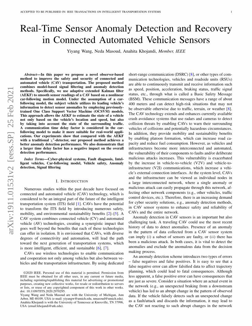
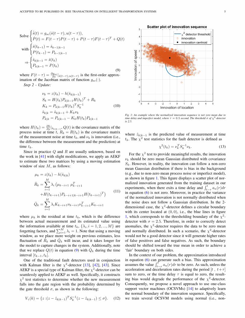
Fig. 1: An example where the normalized innovation sequence is not zero mean due totime delay and imperfect model, where τ = 0.5 second. The threshold σ of χ2-detectoris 2.5.

where zk|k−1 is the predicted value of measurement at timetk. The χ2 test statistics for the fault detector is defined as

χ2(tk) = νTk S−1k νk. (13)

For the χ2 test to provide meaningful results, the innovationνk should be zero mean Gaussian distributed with covarianceSk. However, in reality, the innovation can follow a non-zeromean Gaussian distribution if there is bias in the background(e.g., due to non-zero mean process noise or imperfect model),as shown in figure 1. This figure displays a scatter plot of nor-malized innovation generated from the training dataset in ourexperiments, when there exits a time delay and

´ tt−τ an(r)dr

in equation (6) is not zero. Moreover, in practice the varianceof the normalized innovation is not normally distributed whenthe noise does not follow a Gaussian distribution. In the 2-dimensional case, the χ2-detector defines a circular boundarywith its center located at (0, 0), i.e., the blue lines in figure1, which corresponds to the thresholding boundary of the χ2-detector with σ = 2.5. Therefore, in order to correctly detectanomalies, the χ2-detector requires the data to be zero meanand normally distributed. In such a scenario, the χ2-detectorwould not be a good detector since it will generate higher ratesof false positives and false negatives. As such, the boundaryshould be shifted toward the true mean in order to achieve a‘fair’ boundary on both sides.

In the context of our problem, the approximation introducedin equation (6) can generate such a bias. This approximationassumes the value

´ tt−τ an(r)dr to be zero. As such, unless the

acceleration and deceleration rates during the period [t , t+τ ]sum to zero, or the time delay τ is equal to zero, the result-ing bias would degrade the performance of the χ2-detector.Consequently, we propose a novel approach to use one-classsupport vector machines (OCSVMs) [14] to adaptively learnthe normal boundary of the innovation sequence. Specifically,we train several OCSVM models using normal (i.e., non-


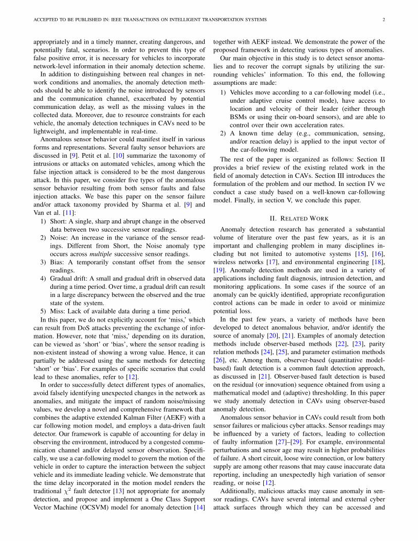
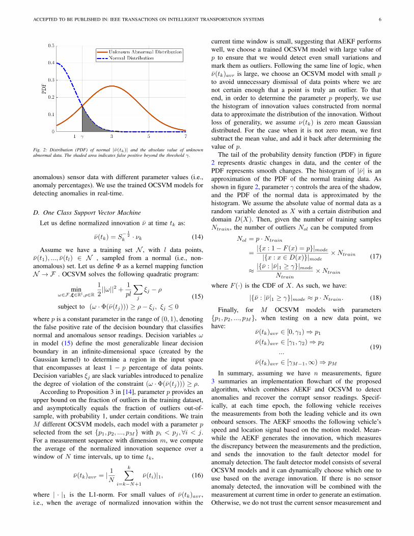
Fig. 2: Distribution (PDF) of normal |ν(tk)| and the absolute value of unknownabnormal data. The shaded area indicates false positive beyond the threshold γ.

anomalous) sensor data with different parameter values (i.e.,anomaly percentages). We use the trained OCSVM models fordetecting anomalies in real-time.

D. One Class Support Vector Machine

Let us define normalized innovation ν at time tk as:

ν(tk) = S− 1

2

k · νk (14)

Assume we have a training set N , with l data points,ν(t1), ..., ν(tl) ∈ N , sampled from a normal (i.e., non-anomalous) set. Let us define Φ as a kernel mapping functionN → F . OCSVM solves the following quadratic program:

minω∈F,ξ∈Rl,ρ∈R

1

2||ω||2 +

1

pl

∑j

ξj − ρ

subject to (ω · Φ(ν(tj))) ≥ ρ− ξj , ξj ≤ 0

(15)

where p is a constant parameter in the range of (0, 1), denotingthe false positive rate of the decision boundary that classifiesnormal and anomalous sensor readings. Decision variables ωin model (15) define the most generalizable linear decisionboundary in an infinite-dimensional space (created by theGaussian kernel) to determine a region in the input spacethat encompasses at least 1 − p percentage of data points.Decision variables ξj are slack variables introduced to penalizethe degree of violation of the constraint (ω · Φ(ν(tj))) ≥ ρ.

According to Proposition 3 in [14], parameter p provides anupper bound on the fraction of outliers in the training dataset,and asymptotically equals the fraction of outliers out-of-sample, with probability 1, under certain conditions. We trainM different OCSVM models, each model with a parameter pselected from the set {p1, p2, ..., pM} with pi < pj ,∀i < j.For a measurement sequence with dimension m, we computethe average of the normalized innovation sequence over awindow of N time intervals, up to time tk,

ν(tk)avr = | 1

N

k∑i=k−N+1

ν(ti)|1, (16)

where | · |1 is the L1-norm. For small values of ν(tk)avr,i.e., when the average of normalized innovation within the

current time window is small, suggesting that AEKF performswell, we choose a trained OCSVM model with large value ofp to ensure that we would detect even small variations andmark them as outliers. Following the same line of logic, whenν(tk)avr is large, we choose an OCSVM model with small pto avoid unnecessary dismissal of data points where we arenot certain enough that a point is truly an outlier. To thatend, in order to determine the parameter p properly, we usethe histogram of innovation values constructed from normaldata to approximate the distribution of the innovation. Withoutloss of generality, we assume ν(tk) is zero mean Gaussiandistributed. For the case when it is not zero mean, we firstsubtract the mean value, and add it back after determining thevalue of p.

The tail of the probability density function (PDF) in figure2 represents drastic changes in data, and the center of thePDF represents smooth changes. The histogram of |ν| is anapproximation of the PDF of the normal training data. Asshown in figure 2, parameter γ controls the area of the shadow,and the PDF of the normal data is approximated by thehistogram. We assume the absolute value of normal data as arandom variable denoted as X with a certain distribution anddomain D(X). Then, given the number of training samplesNtrain, the number of outliers Nol can be computed from

Nol = p ·Ntrain

=|{x : 1− F (x) = p}|mode|{x : x ∈ D(x)}|mode

×Ntrain

≈ |{ν : |ν|1 ≥ γ}|modeNtrain

×Ntrain

(17)

where F (·) is the CDF of X . As such, we have:

|{ν : |ν|1 ≥ γ}|mode ≈ p ·Ntrain. (18)

Finally, for M OCSVM models with parameters{p1, p2, ..., pM}, when testing on a new data point, wehave:

ν(tk)avr ∈ [0, γ1)⇒ p1

ν(tk)avr ∈ [γ1, γ2)⇒ p2

...

ν(tk)avr ∈ [γM−1,∞)⇒ pM

(19)

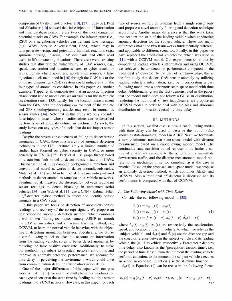
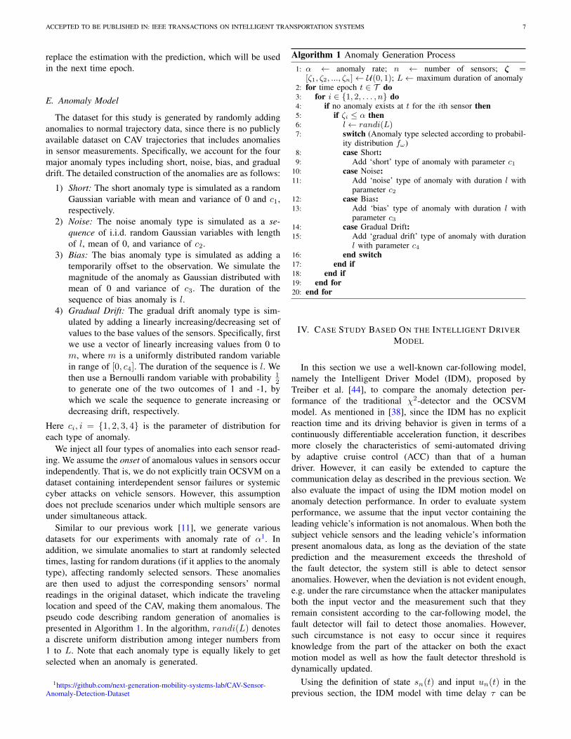
In summary, assuming we have n measurements, figure3 summaries an implementation flowchart of the proposedalgorithm, which combines AEKF and OCSVM to detectanomalies and recover the corrupt sensor readings. Specif-ically, at each time epoch, the following vehicle receivesthe measurements from both the leading vehicle and its ownonboard sensors. The AEKF smooths the following vehicle’sspeed and location signal based on the motion model. Mean-while the AEKF generates the innovation, which measuresthe discrepancy between the measurements and the prediction,and sends the innovation to the fault detector model foranomaly detection. The fault detector model consists of severalOCSVM models and it can dynamically choose which one touse based on the average innovation. If there is no sensoranomaly detected, the innovation will be combined with themeasurement at current time in order to generate an estimation.Otherwise, we do not trust the current sensor measurement and


replace the estimation with the prediction, which will be usedin the next time epoch.

E. Anomaly Model

The dataset for this study is generated by randomly addinganomalies to normal trajectory data, since there is no publiclyavailable dataset on CAV trajectories that includes anomaliesin sensor measurements. Specifically, we account for the fourmajor anomaly types including short, noise, bias, and gradualdrift. The detailed construction of the anomalies are as follows:

1) Short: The short anomaly type is simulated as a randomGaussian variable with mean and variance of 0 and c1,respectively.

2) Noise: The noise anomaly type is simulated as a se-quence of i.i.d. random Gaussian variables with lengthof l, mean of 0, and variance of c2.

3) Bias: The bias anomaly type is simulated as adding atemporarily offset to the observation. We simulate themagnitude of the anomaly as Gaussian distributed withmean of 0 and variance of c3. The duration of thesequence of bias anomaly is l.

4) Gradual Drift: The gradual drift anomaly type is sim-ulated by adding a linearly increasing/decreasing set ofvalues to the base values of the sensors. Specifically, firstwe use a vector of linearly increasing values from 0 tom, where m is a uniformly distributed random variablein range of [0, c4]. The duration of the sequence is l. Wethen use a Bernoulli random variable with probability 1

2to generate one of the two outcomes of 1 and -1, bywhich we scale the sequence to generate increasing ordecreasing drift, respectively.

Here ci, i = {1, 2, 3, 4} is the parameter of distribution foreach type of anomaly.

We inject all four types of anomalies into each sensor read-ing. We assume the onset of anomalous values in sensors occurindependently. That is, we do not explicitly train OCSVM on adataset containing interdependent sensor failures or systemiccyber attacks on vehicle sensors. However, this assumptiondoes not preclude scenarios under which multiple sensors areunder simultaneous attack.

Similar to our previous work [11], we generate variousdatasets for our experiments with anomaly rate of α1. Inaddition, we simulate anomalies to start at randomly selectedtimes, lasting for random durations (if it applies to the anomalytype), affecting randomly selected sensors. These anomaliesare then used to adjust the corresponding sensors’ normalreadings in the original dataset, which indicate the travelinglocation and speed of the CAV, making them anomalous. Thepseudo code describing random generation of anomalies ispresented in Algorithm 1. In the algorithm, randi(L) denotesa discrete uniform distribution among integer numbers from1 to L. Note that each anomaly type is equally likely to getselected when an anomaly is generated.

1https://github.com/next-generation-mobility-systems-lab/CAV-Sensor-Anomaly-Detection-Dataset

Algorithm 1 Anomaly Generation Process1: α ← anomaly rate; n ← number of sensors; ζ =

[ζ1, ζ2, ..., ζn]← U(0, 1); L← maximum duration of anomaly2: for time epoch t ∈ T do3: for i ∈ {1, 2, . . . , n} do4: if no anomaly exists at t for the ith sensor then5: if ζi ≤ α then6: l← randi(L)7: switch (Anomaly type selected according to probabil-

ity distribution fω)8: case Short:9: Add ‘short’ type of anomaly with parameter c1

10: case Noise:11: Add ‘noise’ type of anomaly with duration l with

parameter c212: case Bias:13: Add ‘bias’ type of anomaly with duration l with

parameter c314: case Gradual Drift:15: Add ‘gradual drift’ type of anomaly with duration

l with parameter c416: end switch17: end if18: end if19: end for20: end for

IV. CASE STUDY BASED ON THE INTELLIGENT DRIVERMODEL

In this section we use a well-known car-following model,namely the Intelligent Driver Model (IDM), proposed byTreiber et al. [44], to compare the anomaly detection per-formance of the traditional χ2-detector and the OCSVMmodel. As mentioned in [38], since the IDM has no explicitreaction time and its driving behavior is given in terms of acontinuously differentiable acceleration function, it describesmore closely the characteristics of semi-automated drivingby adaptive cruise control (ACC) than that of a humandriver. However, it can easily be extended to capture thecommunication delay as described in the previous section. Wealso evaluate the impact of using the IDM motion model onanomaly detection performance. In order to evaluate systemperformance, we assume that the input vector containing theleading vehicle’s information is not anomalous. When both thesubject vehicle sensors and the leading vehicle’s informationpresent anomalous data, as long as the deviation of the stateprediction and the measurement exceeds the threshold ofthe fault detector, the system still is able to detect sensoranomalies. However, when the deviation is not evident enough,e.g. under the rare circumstance when the attacker manipulatesboth the input vector and the measurement such that theyremain consistent according to the car-following model, thefault detector will fail to detect those anomalies. However,such circumstance is not easy to occur since it requiresknowledge from the part of the attacker on both the exactmotion model as well as how the fault detector threshold isdynamically updated.

Using the definition of state sn(t) and input un(t) in theprevious section, the IDM model with time delay τ can be

https://github.com/next-generation-mobility-systems-lab/CAV-Sensor-Anomaly-Detection-Dataset

https://github.com/next-generation-mobility-systems-lab/CAV-Sensor-Anomaly-Detection-Dataset


Fig. 3: Implementation flowchart of the proposed algorithm.

described as the following:

xn(t) = vn(t)

vn(t) = fvc(sn(t− τ), un(t− τ))

= a

(1−

(vn(t− τ)

v0

)δ−(s∗(vn(t− τ), vn(t− τ)− vn−1(t− τ))

xn−1(t− τ)− xn(t− τ)− ln

)2)

withs∗(vn,∆vn) = s0 + vnT +

vn∆vn

2√ab

where a, b, δ, v0, s0, T and ln are model parameters. The statevector sn and the input vector un both have dimension of 2.For detailed information on IDM refer to [44]. Following thetypical parameter values of city traffic used in [38], we setthe parameter values in our study as follows: a = 1.0, b =1.5, δ = 4, v0 = 33.75, s0 = 2, T = 1.0, ln = 5, and definethe measurement function h(·) as:

h(s) = H · s =

[1, 00, 1

]· s.

The data for this study is obtained from the research dataexchange (RDE) database constructed as part of the SafetyPilot Model Deployment (SPMD) program [45] funded by theUS department of Transportation, and collected in Michigan.This program was conducted with the primary objective ofdemonstrating CAVs, with the emphasis on implementing andtesting V2V and V2I communications technologies in real-world conditions. The program recorded detailed and high-frequency (10 Hz) data for more than 2,500 vehicles overa period of two years. The data features extracted from theSPMD dataset used in this study include the in-vehicle speed

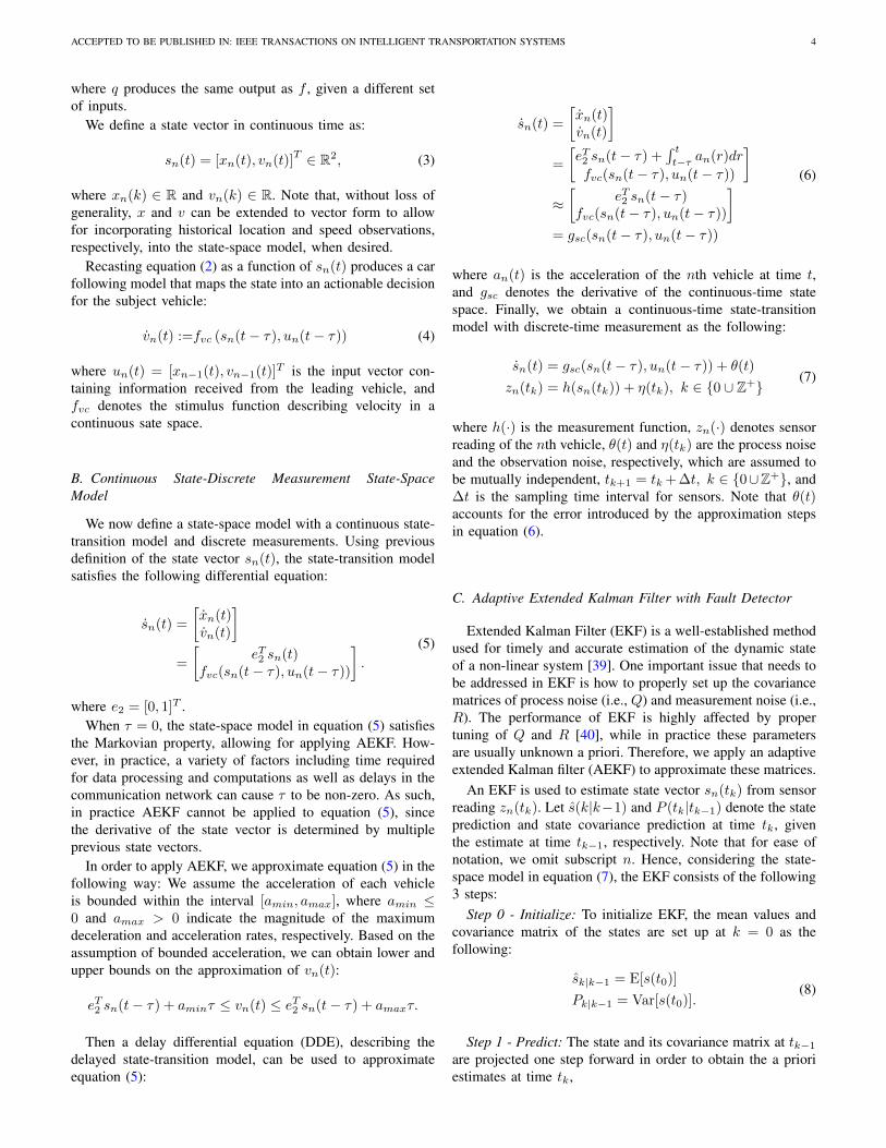
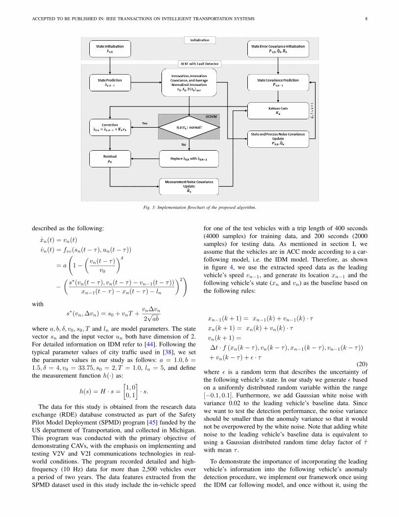
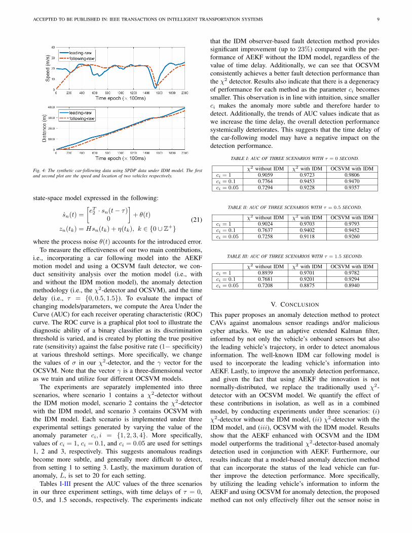
for one of the test vehicles with a trip length of 400 seconds(4000 samples) for training data, and 200 seconds (2000samples) for testing data. As mentioned in section I, weassume that the vehicles are in ACC mode according to a car-following model, i.e. the IDM model. Therefore, as shownin figure 4, we use the extracted speed data as the leadingvehicle’s speed vn−1, and generate its location xn−1 and thefollowing vehicle’s state (xn and vn) as the baseline based onthe following rules:

xn−1(k + 1) = xn−1(k) + vn−1(k) · τxn(k + 1) = xn(k) + vn(k) · τvn(k + 1) =

∆t · f (xn(k − τ), vn(k − τ), xn−1(k − τ), vn−1(k − τ))

+ vn(k − τ) + ε · τ(20)

where ε is a random term that describes the uncertainty ofthe following vehicle’s state. In our study we generate ε basedon a uniformly distributed random variable within the range[−0.1, 0.1]. Furthermore, we add Gaussian white noise withvariance 0.02 to the leading vehicle’s baseline data. Sincewe want to test the detection performance, the noise varianceshould be smaller than the anomaly variance so that it wouldnot be overpowered by the white noise. Note that adding whitenoise to the leading vehicle’s baseline data is equivalent tousing a Gaussian distributed random time delay factor of τwith mean τ .

To demonstrate the importance of incorporating the leadingvehicle’s information into the following vehicle’s anomalydetection procedure, we implement our framework once usingthe IDM car following model, and once without it, using the


Fig. 4: The synthetic car-following data using SPDP data under IDM model. The firstand second plot are the speed and location of two vehicles respectively.

state-space model expressed in the following:

sn(t) =

[eT2 · sn(t− τ)

0

]+ θ(t)

zn(tk) = Hsn(tk) + η(tk), k ∈ {0 ∪ Z+}(21)

where the process noise θ(t) accounts for the introduced error.To measure the effectiveness of our two main contributions,

i.e., incorporating a car following model into the AEKFmotion model and using a OCSVM fault detector, we con-duct sensitivity analysis over the motion model (i.e., withand without the IDM motion model), the anomaly detectionmethodology (i.e., the χ2-detector and OCSVM), and the timedelay (i.e., τ = {0, 0.5, 1.5}). To evaluate the impact ofchanging models/parameters, we compute the Area Under theCurve (AUC) for each receiver operating characteristic (ROC)curve. The ROC curve is a graphical plot tool to illustrate thediagnostic ability of a binary classifier as its discriminationthreshold is varied, and is created by plotting the true positiverate (sensitivity) against the false positive rate (1− specificity)at various threshold settings. More specifically, we changethe values of σ in our χ2-detector, and the γ vector for theOCSVM. Note that the vector γ is a three-dimensional vectoras we train and utilize four different OCSVM models.

The experiments are separately implemented into threescenarios, where scenario 1 contains a χ2-detector withoutthe IDM motion model, scenario 2 contains the χ2-detectorwith the IDM model, and scenario 3 contains OCSVM withthe IDM model. Each scenario is implemented under threeexperimental settings generated by varying the value of theanomaly parameter ci, i = {1, 2, 3, 4}. More specifically,values of ci = 1, ci = 0.1, and ci = 0.05 are used for settings1, 2 and 3, respectively. This suggests anomalous readingsbecome more subtle, and generally more difficult to detect,from setting 1 to setting 3. Lastly, the maximum duration ofanomaly, L, is set to 20 for each setting.

Tables I-III present the AUC values of the three scenariosin our three experiment settings, with time delays of τ = 0,0.5, and 1.5 seconds, respectively. The experiments indicate

that the IDM observer-based fault detection method providessignificant improvement (up to 23%) compared with the per-formance of AEKF without the IDM model, regardless of thevalue of time delay. Additionally, we can see that OCSVMconsistently achieves a better fault detection performance thanthe χ2 detector. Results also indicate that there is a degeneracyof performance for each method as the parameter ci becomessmaller. This observation is in line with intuition, since smallerci makes the anomaly more subtle and therefore harder todetect. Additionally, the trends of AUC values indicate that aswe increase the time delay, the overall detection performancesystemically deteriorates. This suggests that the time delay ofthe car-following model may have a negative impact on thedetection performance.

TABLE I: AUC OF THREE SCENARIOS WITH τ = 0 SECOND.

χ2 without IDM χ2 with IDM OCSVM with IDMci = 1 0.9059 0.9723 0.9806ci = 0.1 0.7764 0.9453 0.9470ci = 0.05 0.7294 0.9228 0.9357

TABLE II: AUC OF THREE SCENARIOS WITH τ = 0.5 SECOND.


TABLE III: AUC OF THREE SCENARIOS WITH τ = 1.5 SECOND.


V. CONCLUSION

This paper proposes an anomaly detection method to protectCAVs against anomalous sensor readings and/or maliciouscyber attacks. We use an adaptive extended Kalman filter,informed by not only the vehicle’s onboard sensors but alsothe leading vehicle’s trajectory, in order to detect anomalousinformation. The well-known IDM car following model isused to incorporate the leading vehicle’s information intoAEKF. Lastly, to improve the anomaly detection performance,and given the fact that using AEKF the innovation is notnormally-distributed, we replace the traditionally used χ2-detector with an OCSVM model. We quantify the effect ofthese contributions in isolation, as well as in a combinedmodel, by conducting experiments under three scenarios: (i)χ2-detector without the IDM model, (ii) χ2-detector with theIDM model, and (iii), OCSVM with the IDM model. Resultsshow that the AEKF enhanced with OCSVM and the IDMmodel outperforms the traditional χ2-detector-based anomalydetection used in conjunction with AEKF. Furthermore, ourresults indicate that a model-based anomaly detection methodthat can incorporate the status of the lead vehicle can fur-ther improve the detection performance. More specifically,by utilizing the leading vehicle’s information to inform theAEKF and using OCSVM for anomaly detection, the proposedmethod can not only effectively filter out the sensor noise in


CAVs, but also detect the anomalous sensor values in real-timewith better performance than that without utilizing leadingvehicle’s information. This high performance is showcased byhigh AUC values in our experiments. Moreover, we study thegeneral relationship between the delay in receiving informationand the performance of anomaly detection. We show that as thetime delay of signal transmission (i.e., communication channeldelay or sensor delay) becomes larger, the overall detectionperformance deteriorates.

The current study can be improved/expanded in multipleways. First, the following vehicle’s state and anomalous sensorvalues used in section IV are simulated, due to the paucity ofACC datasets with anomalies for CAVs. There exist multi-ple car-following datasets, but most of them were collectedfrom human drivers. Although our study mainly focuses onthe detection performance of our proposed method, it maybe beneficial to directly collect ACC data from CAVs andcalibrate the car-following model based on a real dataset,since the potential discrepancy between the car followingmodel and the true traveling behaviour of the vehicle mayintroduce new challenges. Second, in section IV, we assumethe input vector containing leading vehicle’s information isnot anomalous. However, our proposed method can still detectanomalies without such an assumption, i.e., as long as thediscrepancy between input vector and measurement are largeenough. Note that we also assume that anomalous input vectorare caused either by sensor failures or false injection attacksthat can be described by four types of anomaly. Third, inthis study for each vehicle we only utilize a single leadingvehicle’s information, whereas a connected vehicle can benefitfrom information shared by any number of connected vehicleswithin its communication range as well as the infrastructure. Inour future work, we plan to study the impact of incorporatingmultiple sources of information (e.g., multiple vehicles orRSUs) on the overall anomaly detection performance. Fur-thermore, we plan to expand our work to identify the sourceof anomaly after detection.

REFERENCES

[1] S. E. Shladover, “Connected and automated vehicle systems: Intro-duction and overview,” Journal of Intelligent Transportation Systems,vol. 22, no. 3, pp. 190–200, 2018.

[2] M. Abdolmaleki, M. Shahabi, Y. Yin, and N. Masoud, “Itineraryplanning for cooperative truck platooning,” Available at SSRN 3481598,2019.

[3] F. van Wyk, A. Khojandi, and N. Masoud, “A path towards understand-ing factors affecting crash severity in autonomous vehicles using currentnaturalistic driving data,” in Proceedings of SAI Intelligent SystemsConference. Springer, Cham, 2019, pp. 106–120.

[4] M. Abdolmaleki, N. Masoud, and Y. Yin, “Vehicle-to-vehicle wirelesspower transfer: Paving the way toward an electrified transportationsystem,” Transportation Research Part C: Emerging Technologies, vol.103, pp. 261–280, 2019.

[5] N. Masoud and R. Jayakrishnan, “Autonomous or driver-less vehicles:Implementation strategies and operational concerns,” Transportationresearch part E: logistics and transportation review, vol. 108, pp. 179–194, 2017.

[6] G. Meyer and S. Beiker, Road Vehicle Automation. Springer, 2014.[7] T. Litman, Autonomous vehicle implementation predictions. Victoria

Transport Policy Institute Victoria, Canada, 2017.[8] J. B. Kenney, “Dedicated short-range communications (dsrc) standards

in the united states,” Proceedings of the IEEE, vol. 99, no. 7, pp. 1162–1182, 2011.

[9] A. B. Sharma, L. Golubchik, and R. Govindan, “Sensor faults: Detectionmethods and prevalence in real-world datasets,” ACM Transactions onSensor Networks (TOSN), vol. 6, no. 3, p. 23, 2010.

[10] J. Petit and S. E. Shladover, “Potential cyberattacks on automatedvehicles.” IEEE Trans. Intelligent Transportation Systems, vol. 16, no. 2,pp. 546–556, 2015.

[11] F. van Wyk, Y. Wang, A. Khojandi, and N. Masoud, “Real-time sensoranomaly detection and identification in automated vehicles,” IEEETransactions on Intelligent Transportation Systems, 2019.

[12] K. Ni, N. Ramanathan, M. N. H. Chehade, L. Balzano, S. Nair,S. Zahedi, E. Kohler, G. Pottie, M. Hansen, and M. Srivastava, “Sensornetwork data fault types,” ACM Transactions on Sensor Networks(TOSN), vol. 5, no. 3, p. 25, 2009.

[13] B. Brumback and M. Srinath, “A chi-square test for fault-detection inkalman filters,” IEEE Transactions on Automatic Control, vol. 32, no. 6,pp. 552–554, 1987.

[14] B. Scholkopf, J. C. Platt, J. Shawe-Taylor, A. J. Smola, and R. C.Williamson, “Estimating the support of a high-dimensional distribution,”Neural computation, vol. 13, no. 7, pp. 1443–1471, 2001.

[15] M. Muter and N. Asaj, “Entropy-based anomaly detection for in-vehiclenetworks,” in Intelligent Vehicles Symposium (IV), 2011 IEEE. IEEE,2011, pp. 1110–1115.

[16] M. Muter, A. Groll, and F. C. Freiling, “A structured approach toanomaly detection for in-vehicle networks,” in Information Assuranceand Security (IAS), 2010 Sixth International Conference on. IEEE,2010, pp. 92–98.

[17] S. Rajasegarar, C. Leckie, and M. Palaniswami, “Anomaly detectionin wireless sensor networks,” IEEE Wireless Communications, vol. 15,no. 4, 2008.

[18] D. J. Hill, B. S. Minsker, and E. Amir, “Real-time bayesian anomaly de-tection for environmental sensor data,” in Proceedings of the Congress-International Association for Hydraulic Research, vol. 32, no. 2. Cite-seer, 2007, p. 503.

[19] D. J. Hill and B. S. Minsker, “Anomaly detection in streaming environ-mental sensor data: A data-driven modeling approach,” EnvironmentalModelling & Software, vol. 25, no. 9, pp. 1014–1022, 2010.

[20] R. Isermann, “Process fault detection based on modeling and estimationmethods—a survey,” automatica, vol. 20, no. 4, pp. 387–404, 1984.

[21] I. Hwang, S. Kim, Y. Kim, and C. E. Seah, “A survey of fault detection,isolation, and reconfiguration methods,” IEEE transactions on controlsystems technology, vol. 18, no. 3, pp. 636–653, 2010.

[22] R. N. Clark, D. C. Fosth, and V. M. Walton, “Detecting instrumentmalfunctions in control systems,” IEEE Transactions on Aerospace andElectronic Systems, no. 4, pp. 465–473, 1975.

[23] J. Wunnenberg and P. Frank, “Sensor fault detection via robust ob-servers,” in System fault diagnostics, reliability and related knowledge-based approaches. Springer, 1987, pp. 147–160.

[24] J. Deckert, M. Desai, J. Deyst, and A. Willsky, “F-8 dfbw sensorfailure identification using analytic redundancy,” IEEE Transactions onAutomatic Control, vol. 22, no. 5, pp. 795–803, 1977.

[25] J. Gertler, “Fault detection and isolation using parity relations,” Controlengineering practice, vol. 5, no. 5, pp. 653–661, 1997.

[26] C. Baskiotis, J. Raymond, and A. Rault, “Parameter identification anddiscriminant analysis for jet engine machanical state diagnosis,” inDecision and Control including the Symposium on Adaptive Processes,1979 18th IEEE Conference on, vol. 2. IEEE, 1979, pp. 648–650.

[27] S. Checkoway, D. McCoy, B. Kantor, D. Anderson, H. Shacham,S. Savage, K. Koscher, A. Czeskis, F. Roesner, T. Kohno et al.,“Comprehensive experimental analyses of automotive attack surfaces.”in USENIX Security Symposium. San Francisco, 2011, pp. 77–92.

[28] M. Realpe, B. Vintimilla, and L. Vlacic, “Sensor fault detection anddiagnosis for autonomous vehicles,” in MATEC Web of Conferences,vol. 30. EDP Sciences, 2015, p. 04003.

[29] N. Pous, D. Gingras, and D. Gruyer, “Intelligent vehicle embeddedsensors fault detection and isolation using analytical redundancy andnonlinear transformations,” Journal of Control Science and Engineering,vol. 2017, 2017.

[30] K. Koscher, A. Czeskis, F. Roesner, S. Patel, T. Kohno, S. Checkoway,D. McCoy, B. Kantor, D. Anderson, H. Shacham et al., “Experimentalsecurity analysis of a modern automobile,” in Security and Privacy (SP),2010 IEEE Symposium on. IEEE, 2010, pp. 447–462.

[31] A. Weimerskirch and R. Gaynier, “An overview of automotive cyberse-curity: Challenges and solution approaches.” in TrustED@ CCS, 2015,p. 53.

[32] C. Yan, W. Xu, and J. Liu, “Can you trust autonomous vehicles:Contactless attacks against sensors of self-driving vehicle,” DEF CON,vol. 24, 2016.


[33] T. Trippel, O. Weisse, W. Xu, P. Honeyman, and K. Fu, “Walnut: Wagingdoubt on the integrity of mems accelerometers with acoustic injectionattacks,” in Security and Privacy (EuroS&P), 2017 IEEE EuropeanSymposium on. IEEE, 2017, pp. 3–18.

[34] M. S. Faughnan, B. J. Hourican, G. C. MacDonald, M. Srivastava, J.-P. A. Wright, Y. Y. Haimes, E. Andrijcic, Z. Guo, and J. C. White,“Risk analysis of unmanned aerial vehicle hijacking and methods of itsdetection,” in Systems and Information Engineering Design Symposium(SIEDS), 2013 IEEE. IEEE, 2013, pp. 145–150.

[35] J. Park, R. Ivanov, J. Weimer, M. Pajic, and I. Lee, “Sensor attackdetection in the presence of transient faults,” in Proceedings of theACM/IEEE Sixth International Conference on Cyber-Physical Systems.ACM, 2015, pp. 1–10.

[36] P. Christiansen, L. N. Nielsen, K. A. Steen, R. N. Jørgensen, andH. Karstoft, “Deepanomaly: Combining background subtraction anddeep learning for detecting obstacles and anomalies in an agriculturalfield,” Sensors, vol. 16, no. 11, p. 1904, 2016.

[37] M. Marchetti, D. Stabili, A. Guido, and M. Colajanni, “Evaluation ofanomaly detection for in-vehicle networks through information-theoreticalgorithms,” in Research and Technologies for Society and IndustryLeveraging a better tomorrow (RTSI), 2016 IEEE 2nd InternationalForum on. IEEE, 2016, pp. 1–6.

[38] M. Treiber and A. Kesting, “Traffic flow dynamics: data, models andsimulation,” Physics Today, vol. 67, no. 3, p. 54, 2014.

[39] E. Wan, “Sigma-point filters: An overview with applications to integratednavigation and vision assisted control,” in Nonlinear Statistical SignalProcessing Workshop, 2006 IEEE. IEEE, 2006, pp. 201–202.

[40] A. Mohamed and K. Schwarz, “Adaptive kalman filtering for ins/gps,”Journal of geodesy, vol. 73, no. 4, pp. 193–203, 1999.

[41] S. Akhlaghi, N. Zhou, and Z. Huang, “Adaptive adjustment of noisecovariance in kalman filter for dynamic state estimation,” in Power &Energy Society General Meeting, 2017 IEEE. IEEE, 2017, pp. 1–5.

[42] Y. Bar-Shalom and X.-R. Li, Multitarget-multisensor tracking: princi-ples and techniques. YBs Storrs, CT, 1995, vol. 19.

[43] Y. Geng and J. Wang, “Adaptive estimation of multiple fading factors inkalman filter for navigation applications,” Gps Solutions, vol. 12, no. 4,pp. 273–279, 2008.

[44] M. Treiber, A. Hennecke, and D. Helbing, “Congested traffic states inempirical observations and microscopic simulations,” Physical review E,vol. 62, no. 2, p. 1805, 2000.

[45] D. Bezzina and J. Sayer, “Safety pilot model deployment: Test conductorteam report,” Report No. DOT HS, vol. 812, p. 171, 2014.

real-time sensor anomaly detection and recovery in ... - arxiv

Documents