rapid, accurate, precise and reproducible binding affinity
TRANSCRIPT
Rapid, Accurate, Precise andReproducible Binding Affinity
Calculations using Ensembles ofMolecular Dynamics
Simulations
Agastya Prakash Bhati
A dissertation submitted in partial fulfillment
of the requirements for the degree of
Doctor of Philosophy
of
University College London.
Department of Chemistry
University College London
April 30, 2018


I, Agastya Prakash Bhati, confirm that the work presented in this thesis
is my own. Where information has been derived from other sources, I confirm
that this has been indicated in the thesis.
i

Bhagwad Gita - Chapter 2, verse 47
(You have the right to work only but never to its fruits. Let not the fruits of
action be your motive, nor let your attachment be to inaction.)
Dedication
I dedicate this thesis to my parents Dr. Om Prakash and Dr. Praveena
Bhati. This is another milestone in the journey. With your blessings,
I hope to continue making progress in life.
iii

Abstract
The accurate prediction of the binding affinities of ligands to proteins is a
major goal in drug discovery and personalised medicine. The use of in silico
methods to predict binding affinities has been largely confined to academic
research until recently, primarily due to the lack of their reproducibility, as
well as unaffordably longer time to solution. In this thesis, I mainly describe
the ensemble based molecular dynamics approaches, ESMACS and TIES, that
provide a route to reliable predictions of free energies meeting the require-
ments of speed, accuracy, precision and reliability. The performance of both
these methods when applied to a diverse set of protein targets and ligands
is reported. The results are in very good agreement with experimental data
while the methods are repeatable by construction. Statistical uncertainties of
the order of 0.5 kcal/mol or less are achieved. These methods have been fur-
ther extended to incorporate enhanced sampling techniques based on replica
exchange (also known as parallel tempering) to handle situations where con-
formational sampling is difficult using standard molecular dynamics. A critical
assessment of free energy estimators like MBAR has been made for their appli-
cation in binding affinity prediction. The methodologies described are shown
to have a positive impact in the drug design process in the pharmaceutical
domain as well as in personalised medicine, with concomitant potential major
industrial and societal impact. Finally, our automated workflow, comprising
the Binding Affinity Calculator (BAC) together with the FabSim are described.
These tools and services help us complete the entire execution in 8 hours or
less, depending on the high performance architecture and hardware available.


Impact Statement
Classical molecular dynamics (MD) simulations have been in use to simulate
proteins for about 4 decades now. Over the last couple of decades, there has
been a lot of advancement in the development of techniques based on classical
MD simulations to calculate free energy, which is a thermodynamic property,
of biomolecular systems. In spite of such tremendous progress, such techniques
suffer from the issue of non-reproducible results, due to the practice of per-
forming only a single insufficiently long simulation, making them unreliable.
It has been well acknowledged in the literature that the predicted free energies
yielded by such techniques vary by non-negligible values on simply repeating
the calculation. In this work, I have recognised the underlying cause of this
problem and developed protocols to overcome it. I have introduced the concept
of “ensemble simulation” and developed two new methods namely, “thermody-
namic integration with enhanced sampling (TIES)” and “enhanced sampling
of molecular dynamics with approximation of continuum solvent (ESMACS)”,
based on it. In this thesis, I have provided sufficient evidence to show that TIES
and ESMACS yield accurate, precise and reproducible free energies rapidly for
a variety of biomolecular systems. In this way, I have successfully addressed
a fundamental issue in the field of MD-based free energy calculations. This
has attracted great attention from my peers (as of now, my research article
introducing TIES has been cited 16 times in the short time of 16 months).
The aforementioned methods have direct applications in important areas like
drug design and precision medicine as highlighted below.
Impact Statement
I have shown in my work that even the improved MD-based free energy meth-
ods, that accelerate the convergence of results using better sampling techniques
and statistically optimal free energy estimators, exhibit a similar variation in
their results on repeating the calculations. This observation will be of great
interest to all the researchers working in the field of free energy calculations.
TIES and ESMACS constitute complex computational workflows and imple-
menting them manually is quite tedious and error-prone. Therefore, in order
to make them easily usable, I developed an automation toolkit comprising of
the “Binding Affinity Calculator (BAC)” and “FabSim”. It provides an error-
proof way of implementing these workflows and helps perform the calculations
rapidly, which further enhances their applicability as explained in the following
paragraph.
There is a huge scope for the pharmaceutical companies to employ MD-based
free energy methods in the initial stages of drug discovery, which would help
them cut down both the cost and time required to develop new drugs. In
the case of precision medicine, these methods can be used as a tool to predict
the effect of clinically observed mutations on the affinity of drugs (a common
cause of the development of drug resistance). However, the lack of reliability
and the long time-to-solution of free energy methods had been limiting their
application in both these areas. TIES and ESMACS are not constrained by
such limitations and have been successfully employed in my collaborations with
two pharmaceutical companies, GlaxoSmithKline and Pfizer.
viii
Acknowledgements
The long journey of my PhD could have not been possible without the sup-
port, motivation and help from several people. I would like to express my
thankfulness to all these people.
First of all, I would like to thank my supervisor Professor Peter V. Coveney,
whose guidance always kept me going in the right direction. He granted enough
room for my own ideas but also advised me whenever needed, which led me
to accomplish my research work. He always motivated me and it has been fun
working under his supervision. I would also like to extend my sincere gratitute
to Shunzhou and Dave for all the useful scientific discussions, which helped me
progress quickly with my research. I learnt several technicalities from them,
without which my progress would have been much slower. I am thankful to
Derek for his support and advice in the development of FabBioMD, which
provided momentum to my work.
I take this opportunity to thank all my present and past colleagues at CCS (in
no particular order: James, Robin, Hugh, Emily, Ulf, Stefan, Sebastian, Alex,
Fouad, Maxime, Kristoff, Charlotte, Laura), who made my working hours
joyful and provided a healthy working atmosphere. A special thanks to Serge
and Robbie for being great PhD fellows and friends.
I cannot forget to thank all my friends Anuj, Aditya, Shiv Charan, Zulkifli,
Tiago and Harshvardhan, who have been my companions in good and bad
times for the last few years and have always been there in the hour of need. A
special mention of Priyal is necessary to express my gratitude for her being a
great company throughout.
Acknowledgements
Nothing is possible without financial resources. I would like to acknowledge
UCL and Inlaks Shivdasani Foundation for providing me scholarships. I am
thankful to the department of Chemistry at UCL for providing me infrastruc-
ture. I acknowledge the use of ARCHER, UK’s national High Performance
Computing Service, HPC facilities of the STFC's Hartree Centre and those of
the Leibniz Research Centre for all the work presented in this thesis.
No acknowledgement would ever adequately express my gratitude to my fam-
ily. I would like to specially mention Dr. Om Prakash, Dr. Praveena and
Aditya Bhati for always believing in me. Their moral support has always
boosted my confidence and their teachings have always enabled me to progress
in life.
x

Publications
The following publications and presentations have arisen from this thesis.
Publications
• D. Groen, A. P. Bhati, J. Suter, J. Hetherington, S. Zasada, and P. V.
Coveney. “FabSim: facilitating computational research through automa-
tion on large-scale and distributed e-infrastructures.” Computer Physics
Communications, 207, 375385 (2016), DOI:10.1016/j.cpc.2016.05.020.
• A. P. Bhati, S. Wan, D. Wright, P. V. Coveney. “Rapid, accurate, pre-
cise and reliable relative free energy prediction using ensemble based
thermodynamic integration.” Journal of Chemical Theory and Compu-
tation, 13(1), 210-222 (2017), DOI: 10.1021/acs.jctc.6b00979.
• S. Wan, A. P. Bhati, S. J. Zasada, I. Wall, D. Green, P. Bamborough, P.
V. Coveney. “Rapid and Reliable Binding Affinity Prediction of Bromod-
omain Inhibitors: a Computational Study.” Journal of Chemical Theory
Computation, 13(2), 784-795 (2017), DOI: 10.1021/acs.jctc.6b00794.
• S. Wan, A. P. Bhati, S. Skerratt, K. Omoto, V. Shanmugasundaram, S.
Bagal, P. V. Coveney. “Evaluation and Characterization of Trk Kinase
Inhibitors for the Treatment of Pain: Reliable Binding Affinity Predic-
tions from Theory and Computation.”, Journal of Chemical Information
and Modelling, 57(4), 897-909 (2017), DOI: 10.1021/acs.jcim.6b00780.
• A. P. Bhati, S. Wan, Y. Hu, B. Sherborne, P. V. Coveney. “Uncer-
tainty Quantification in Alchemical Free Energy Methods.”, Journal of
Publications
Chemical Theory Computation, Just Accepted Manuscript (2018), DOI:
10.1021/acs.jctc.7b01143.
Oral Presentations
• “Rapid, accurate, precise and reliable relative free energy prediction us-
ing ensemble based thermodynamic integration”, 11th European Con-
ference on Theoretical and Computational Chemistry (11EuCOTCC),
September 2017, Institute for Catalan Studies, Barcelona, Spain.
• “Rapid, accurate, precise and reliable relative free energy prediction us-
ing ensemble based thermodynamic integration”, 4th Scientific and In-
dustrial Conference by PRACE - PRACEDays17, May 2017, Polytechnic
University of Catalonia, Barcelona, Spain.
• “Rapid, precise and reproducible binding affinity calculations for drug-
protein interactions”, 15th European Conference on Computational Bi-
ology (ECCB 2016), September 2016, World Forum Convention Centre,
The Hague, Netherlands.
• “Computing ligand-protein free energies using multiscale methods”,
Solvay workshop on “Bridging the gap at the PCB interface”, April 2016,
Universite libre de Bruxelles, Brussels, Belgium.
• “Rapid, precise and reproducible binding affinity calculations for drug-
protein interactions”, 2nd workshop on High Throughput Molecular Dy-
namics, November 2015, Barcelona Biomedical Research Park (PRBB),
Barcelona, Spain.
Poster Presentations
• “Rapid, accurate, precise and reliable relative free energy prediction us-
ing ensemble based thermodynamic integration”, Computational Molecu-
lar Science 2017 conference, March 2017, University of Warwick, United
Kingdom.
xii

Publications
• “Rapid, Accurate and Reproducible Binding Affinity Calculations for
Drug-Protein Interactions”, CCP5 Summer School 2015, July 2015, Uni-
versity of Manchester, United Kingdom.
• “Rapid, Accurate and Reproducible Binding Affinity Calculations for
Drug-Protein Interactions”, Exascale Applications and Software Confer-
ence (EASC) 2015, April 2015, University of Edinburgh, United King-
dom.
xiii

Contents
1 Introduction 1
2 Binding Affinity Prediction with Classical Molecular Dynam-
ics 9
2.1 Binding Affinity . . . . . . . . . . . . . . . . . . . . . . . . . . . 10
2.1.1 Experimental Determination . . . . . . . . . . . . . . . . 12
2.1.2 Determination Using Computational Methods . . . . . . 13
2.2 Molecular Dynamics . . . . . . . . . . . . . . . . . . . . . . . . 16
2.2.1 Implementation of Molecular Dynamics . . . . . . . . . . 16
2.2.2 Force Fields . . . . . . . . . . . . . . . . . . . . . . . . . 17
2.2.3 Thermostats and Barostats . . . . . . . . . . . . . . . . 18
2.2.4 Improving Computational Efficiency . . . . . . . . . . . 19
2.3 Methods for In Silico Determination of Binding Affinity . . . . . 21
2.3.1 End-point Methods . . . . . . . . . . . . . . . . . . . . . 22
2.3.2 Alchemical Methods . . . . . . . . . . . . . . . . . . . . 27
2.3.3 Relative and Absolute Binding Affinity Calculation . . . 33
2.3.4 Accelerated Sampling Techniques . . . . . . . . . . . . . 34
2.4 Ensemble Averaging to Determine Thermodynamic Properties . 43
2.5 Ensemble Averaging and Repeatability of In Silico Binding
Affinity Predictions . . . . . . . . . . . . . . . . . . . . . . . . . 44
3 Thermodynamic Integration with Enhanced Sampling 47
3.1 Ensemble Simulation Based Thermodynamic Integration . . . . 48
Contents
3.2 Ligand-Protein Systems Studied . . . . . . . . . . . . . . . . . . 49
3.3 Method . . . . . . . . . . . . . . . . . . . . . . . . . . . . . . . 50
3.3.1 Initial Structures and Simulation Protocol . . . . . . . . 51
3.3.2 Hybrid Ligand Structure and Parameters . . . . . . . . . 53
3.3.3 Protocol for Free Energy Calculation . . . . . . . . . . . 53
3.3.4 Stochastic Integration and Error Propagation . . . . . . 56
3.4 Binding Affinity Predictions . . . . . . . . . . . . . . . . . . . . 57
3.4.1 Comparison with Experimental Data . . . . . . . . . . . 58
3.4.2 Repeatability and Reproducibility of the TIES Protocol . 63
3.4.3 Variation with Extended Simulation Duration . . . . . . 66
3.4.4 Size of the Alchemical Transformations . . . . . . . . . . 67
3.4.5 Comparison with Another In Silico Method . . . . . . . 68
3.5 Dynamics of the Water Molecule in the Binding Pocket . . . . . 69
3.6 Charged Groups in Alchemical Transformations . . . . . . . . . 70
3.7 Effect of Ligand Flexibility on Accuracy . . . . . . . . . . . . . 72
3.8 Conclusions . . . . . . . . . . . . . . . . . . . . . . . . . . . . . 73
4 Hamiltonian-Replica Exchange Methods and Uncertainty
Quantification 75
4.1 Protein Targets and Ligands . . . . . . . . . . . . . . . . . . . . 77
4.2 Methods . . . . . . . . . . . . . . . . . . . . . . . . . . . . . . . 77
4.2.1 Free Energy Schemes . . . . . . . . . . . . . . . . . . . . 79
4.2.2 Definition of the “Hot” Region . . . . . . . . . . . . . . 81
4.2.3 Initial Structures and Simulation Setup . . . . . . . . . . 81
4.2.4 Computational Cost . . . . . . . . . . . . . . . . . . . . 82
4.2.5 Uncertainty Quantification . . . . . . . . . . . . . . . . . 83
4.3 Binding Affinity Predictions . . . . . . . . . . . . . . . . . . . . 83
4.3.1 Variability in Different Free Energy Schemes . . . . . . . 83
4.3.2 Comparison of Different Free Energy Schemes . . . . . . 84
4.3.3 Comparison with Experimental Data . . . . . . . . . . . 86
4.3.4 Dependence on the Duration of Simulation . . . . . . . . 87
xvi
Contents
4.4 Conclusions . . . . . . . . . . . . . . . . . . . . . . . . . . . . . 88
5 Enhanced Sampling of Molecular Dynamics with Approxima-
tion of Continuum Solvent 91
5.1 Ensemble Simulation Based Approach . . . . . . . . . . . . . . . 93
5.2 Protein Targets and Ligands Studied . . . . . . . . . . . . . . . 94
5.3 Method . . . . . . . . . . . . . . . . . . . . . . . . . . . . . . . 96
5.3.1 Initial Structures and Simulation Setup . . . . . . . . . . 96
5.3.2 Free Energy Workflow . . . . . . . . . . . . . . . . . . . 98
5.3.3 Uncertainty Quantification . . . . . . . . . . . . . . . . . 99
5.3.4 Repeatability of Predicted Binding Affinities . . . . . . . 99
5.4 Case Studies . . . . . . . . . . . . . . . . . . . . . . . . . . . . . 101
5.4.1 Bcr-Abl Kinase . . . . . . . . . . . . . . . . . . . . . . . 101
5.4.2 BRD4 and TRKA . . . . . . . . . . . . . . . . . . . . . . 104
5.4.3 HIV-1 Protease . . . . . . . . . . . . . . . . . . . . . . . 107
5.5 Conclusions . . . . . . . . . . . . . . . . . . . . . . . . . . . . . 109
6 Automation toolkit 111
6.1 Binding Affinity Calculator . . . . . . . . . . . . . . . . . . . . . 111
6.2 FabSim . . . . . . . . . . . . . . . . . . . . . . . . . . . . . . . . 113
7 Conclusions 117
Appendix 121
Bibliography 129
xvii

List of Figures
2.1 Thermodynamic cycles for calculation of binding affinities using
alchemical methods. . . . . . . . . . . . . . . . . . . . . . . . . 34
3.1 Normalized frequency distribution of ensembles of ∂E/∂λ values
for 4 different intermediate alchemical states (λ=0.2, 0.4, 0.8,
0.9), fitted to Gaussian distributions for the transformation from
ligand L1Q to ligand LI9 binding to CDK2. . . . . . . . . . . . 49
3.2 Structures of all the seven target proteins (ribbon representa-
tion) studied using TIES in each case shown bound to a ligand. 51
3.3 TIES protocol requiring 5 replica simulations at each λ window.
For a single alchemical transmutation, 13 λ-windows are used
amounting to 65 molecular dynamics simulations in total. . . . . 54
3.4 (a) Variation of error (calculated using equation 3.2) with en-
semble size per λ window and (b) the variation of ∆Gboundalch with
simulation length for the transformation of ligand L1Q to ligand
LI9 bound to CDK2. . . . . . . . . . . . . . . . . . . . . . . . . 55
3.5 Variation of 〈∂E/∂λ〉 with the simulation length (including both
equilibration and production phases) for all five replicas at four
different λ windows in the case of the transformation from ligand
L1 to L4 binding to thrombin. . . . . . . . . . . . . . . . . . . . 57
3.6 (a) Correlation between TIES-predicted relative binding affini-
ties and experimental data for all seven protein targets studied.
(b) An alternative representation of the same data such that all
the experimental values are negative. . . . . . . . . . . . . . . . 60
List of Figures
3.7 Correlation between TIES-predicted binding affinities and the
experimental data for each biomolecular system shown separately. 62
3.8 Repeatability of TIES using CDK2 ligand transformations. . . . 64
3.9 Correlation plots for the TIES results from two different sources
when compared with the experimental data as well as with
each other. Relative binding affinities: (a) from the original
TIES study compared with the experimental data, (b) using
pmemdGTI software employing GPUs compared with the ex-
perimental data, (c) from the two calculations compared with
each other. Pearson’s correlation coefficients (rp) are shown for
each plot to quantify the degree of agreement in each case. . . . 66
3.10 The replica-wise variation of ∆Gboundalch with simulation length for
the transformation L1Q-LI9 bound to CDK2. The variation of
the absolute difference between the values corresponding to two
farthest replicas is shown in the inset. . . . . . . . . . . . . . . . 67
3.11 A comparison between the 18 ligand transformations which are
common between the ones studied here and those studied by
Wang et al. using FEP/REST[196]. . . . . . . . . . . . . . . . . 69
3.12 Cross sections of the S1 pocket of thrombin for the two end λ-
windows of an alchemical transformation involving mutation of
m-chloro benzylamide to benzamidine. (a) No water molecule
bound in the S1 pocket in the presence of chlorine at λ = 0; (b)
Water molecule enters the S1 pocket through channels C1 and
C2 on fully transforming Cl to H at λ = 1. . . . . . . . . . . . . 71
3.13 Two different conformations of the flexible carboxylate group of
ligand L14 inside the binding pocket of PTP1B taken from the
same molecular dynamics simulation. . . . . . . . . . . . . . . . 72
3.14 The generic structure of MCL1 ligands with the four membered
linker joining the two ends of the ligand containing different
functional groups. . . . . . . . . . . . . . . . . . . . . . . . . . . 73
xx
List of Figures
4.1 Structures of all the target proteins studied using the four
REST2 based schemes, in each case shown bound to a ligand. . 78
4.2 Comparison of the relative binding affinities for all complexes
using (a) scheme III and (b) the original TIES scheme with
normal MD simulations without REST2. . . . . . . . . . . . . . 85
4.3 Variation of cumulative ∆Gcomplexalch with simulation length for
five replicas of relative free energy calculations and their com-
bined TIES analysis result for all 4 schemes. . . . . . . . . . . . 87
5.1 Normalized frequency distributions of ∆G values for a set of
ligands bound to Abl T315I mutant kinase fitted to Gaussian
distributions. . . . . . . . . . . . . . . . . . . . . . . . . . . . . 93
5.2 Chemical structures of the proteins and inhibitors studied using
ESMACS. . . . . . . . . . . . . . . . . . . . . . . . . . . . . . . 95
5.3 ESMACS protocol requiring 25 replica MD simulations followed
by MMPBSA+NMODE calculation. . . . . . . . . . . . . . . . 97
5.5 Comparison of the calculated binding affinities from two inde-
pendent studies of the BRD4 system performed on BlueWonder2
and ARCHER. . . . . . . . . . . . . . . . . . . . . . . . . . . . 100
5.6 (a) to (e):Correlation plots (along with the best fit lines) of all
ligands bound to each variant of the Abl kinase. (f): Distri-
bution of the absolute free energies of receptor (Greceptor) from
1-trajectory calculations for all mutants of Abl kinase bound to
different inhibitors. . . . . . . . . . . . . . . . . . . . . . . . . . 103
5.7 Spearman ranking correlations of the calculated binding free
energies and the experimental data for BRD4 complexes from 1-
traj (left panel), 1-traj-avgrec (center), and 2-traj-avgrec (right
panel) ESMACS approaches. . . . . . . . . . . . . . . . . . . . . 105
xxi

List of Figures
5.8 Spearman ranking correlations of the calculated binding free
energies and the experimental data for TRKA complexes from 1-
traj (left panel), 1-traj-avgrec (center), and 2-traj-avgrec (right
panel) ESMACS approaches. . . . . . . . . . . . . . . . . . . . . 106
A.1 Chemical structures of BRD4 ligands. . . . . . . . . . . . . . . . 125
xxii

List of Tables
3.1 Summary of TIES results for the seven different target pro-
teins studied. The number of alchemical transformations, crys-
tal structures used, original publications reporting the experi-
mental binding affinities and the experimental method used to
determine the binding affinities are provided. . . . . . . . . . . . 59
3.2 A summary of the level of accuracy obtained for the total set
of TIES predictions. The number of predictions found to be
accurate for a specified absolute error range (left) and the num-
ber of predictions found to be in directional agreement with the
increasing absolute values of experimental results (right). . . . . 61
3.3 Hysteresis in the TIES predictions for the closed cycles formed
by the ligand transformations studied. . . . . . . . . . . . . . . 63
3.4 Comparison of different parameters used in this study with those
used in the study at Merck for the TIES calculations using the
pmemdGTI software package. . . . . . . . . . . . . . . . . . . . 65
4.1 A comparison of computational costs for different free en-
ergy calculations using L1-L9 ligand alchemical transformation
bound to thrombin (∼60k atoms). . . . . . . . . . . . . . . . . . 82
4.2 Relative binding affinity predictions for all complexes using the
four schemes (I to IV). . . . . . . . . . . . . . . . . . . . . . . . 84
List of Tables
5.1 Binding affinities of all 20 complexes of Abl kinase calculated
using the 1-trajectory approach of ESMACS (∆Gcalc) and their
comparison with the experimental values (∆Gexp. . . . . . . . . 102
5.2 Comparison of the Pearson correlation coefficient from 1-
trajectory and 3-trajectory results for all ligands bound to each
mutant of Abl kinase. . . . . . . . . . . . . . . . . . . . . . . . . 104
5.3 Binding Affinities of the wildtype HIV-1 protease bound to
three different inhibitors using ESMACS 1-trajectory and 3-
trajectory approaches along with corresponding experimental
binding affinities. . . . . . . . . . . . . . . . . . . . . . . . . . . 108
5.4 Binding Affinities (relative to LPV) of the wildtype HIV-1 pro-
tease bound to three different inhibitors using ESMACS 1-
trajectory and 3-trajectory approaches along with correspond-
ing experimental binding affinities. . . . . . . . . . . . . . . . . 108
5.5 Comparison of Greceptor and Gligand in 1-trajectory and 3-
trajectory studies of the HIV-1 protease. . . . . . . . . . . . . . 108
A.1 Chemical structures and experimental binding affinities of
CDK2 ligands. No error bars are available on the values used
in this study. . . . . . . . . . . . . . . . . . . . . . . . . . . . . 121
A.2 Chemical structures and experimental binding affinities of
TYK2 ligands. No error bars are available on the values used
in this study. . . . . . . . . . . . . . . . . . . . . . . . . . . . . 121
A.3 Chemical structures and experimental binding affinities of
thrombin ligands. No error bars are available on the values
used in this study. . . . . . . . . . . . . . . . . . . . . . . . . . . 122
A.4 Chemical structures and experimental binding affinities of
MCL1 ligands. No error bars are available on the values used
in this study. . . . . . . . . . . . . . . . . . . . . . . . . . . . . 123
xxiv
List of Tables
A.5 Chemical structures and experimental binding affinities of
PTP1B ligands. No error bars are available on the values used
in this study. . . . . . . . . . . . . . . . . . . . . . . . . . . . . 124
A.6 Chemical structures of TRKA ligands. All ligands have the
same net neutral charges. The experimental TRKA inhibitory
values (IC50) and the binding free energies derived from them
are shown. . . . . . . . . . . . . . . . . . . . . . . . . . . . . . . 126
A.7 Graphical display of all the ligand transformations studied using
TIES. . . . . . . . . . . . . . . . . . . . . . . . . . . . . . . . . 127
A.8 Free energy predictions for all complexes studied using 5 replicas
for the four schemes (I to IV). . . . . . . . . . . . . . . . . . . . 128
xxv

Chapter 1
Introduction
Reproducibility is an intrinsic characteristic of any scientific result, whether
experimental or computational. A method cannot be reliable if it does not
yield the same result when performed by others. However, the lack of repro-
ducible results in the published literature is a rising concern in the scientific
community[1]. This is true for all fields of research and for both computational
and experimental methods. It was recently revealed through a survey by Na-
ture that more than 70% of researchers failed to reproduce another researcher’s
results, while more than half were unable to reproduce their own[2]. In the
case of experiments, non-reproducible results can be an artifact of factors rang-
ing from mixed up chemicals, through confirmational bias[3, 4], fluctuations
in the environment to variations in the experimental setup[5, 6]. In the case
of computer-based methods, the reasons may lie in the theory or the model
used, convergence of the calculations, reliability of the software, and so on[7].
The use of computer models and simulations to understand natural systems
has become widespread, encompassing many diverse disciplines in academia as
well as industry. The systems studied can be as small as sub-atomic particles
and as large as the universe itself. The biggest advantage of computational
modelling is that it provides insight into the underlying mechanisms of the pro-
cesses studied, which are often inaccessible experimentally, within the limits of
the approximations in the model and the theory concerned. Computer simu-
lations can be performed under conditions at which it is impossible to conduct

Chapter 1. Introduction
experiments, for instance, at very high pressures and temperatures. In addi-
tion, one can argue that computational techniques may cut down both time
and cost as well as help the environment by reducing chemical waste in pro-
cesses like drug design. Due to such advantages, computer-based techniques
are becoming increasingly popular among researchers from all backgrounds,
and are being adopted as routine techniques by a large section of the scien-
tific community. The relentless improvement in performance of computers is
another contributor to the increasing adoption of computer-based methods in
sciences during the last few decades.
Given the growing popularity of computational techniques, it is all the more
necessary to ensure that the results and conclusions from these techniques
are reproducible. Only when the results from a computational technique are
repeatable irrespective of its user, time and place, can it be relied upon for
taking actionable decisions and become a standard technique applicable in
a scientific research, industrial or clinical context. The terms “reproducibil-
ity” and “repeatability” in the context of this thesis refer to the ability of a
technique to yield the same results within the expected uncertainty on repeat-
ing the calculation with and without any variation in its implementation, the
software and/or the hardware employed, respectively. This work is dedicated
to improving the precision of free energy methods such that the results from
two independent calculations are the same within the reported uncertainties
making such methods more reliable.
In this thesis, I confine my studies to the field of free energy calculation meth-
ods based on classical molecular dynamics (MD) simulations and biomolecular
systems. A systematic account of the variation in the results of in silico free
energy calculations from independent short simulations and an explanation for
its occurrence is provided. A solution to this problem is provided including sub-
stantial evidence of its ability to control the uncertainties in results. It should
be noted that observations made regarding the variation in results through
the work presented here are general and applicable to all methods based on
2
classical MD simulations when running a single short simulation. Before dis-
cussing more about the free energy calculation methods, below I mention their
important applications and current shortcomings which I overcome using the
methods presented in this thesis.
Applications of In Silico Free Energy Prediction
A ligand is any substance that binds reversibly and specifically to a biomolecule
(a protein in the context of this thesis) and alters its activity. It is often a
compound with low molecular weight and these are the ligands we consider
here. Binding affinity is the change in the free energy associated with the
binding event. The magnitude of the binding affinity is a measure of how
strong the interaction is between the ligand and the protein, and hence it is
often directly related to the potency of the ligand (in the case which the ligand
is a drug).
The measurement of ligand-protein binding affinity is of importance in the
fields of drug design and personalised medicine. It can be used as a virtual
screening tool in drug design or as a clinical tool to tailor a patient’s medication
based on his/her genetic makeup. Computer-aided drug design (CADD) is an
extremely active field of research[8]. In addition, rapid and accurate binding
affinity predictions can be useful in health-related applications like design of
medicines with reduced side-effects and drug resistance. Thus, the use of in
silico techniques to predict binding affinities has grown immensely in the last
few decades[9]. However, it should be noted that these applications of in
silico binding affinity prediction are subject to their short time to solution and
reliable predictions. The time needed to make a prediction should be shorter
than that required by the experimentalists in industrial and clinical settings in
order to influence decision making while, it is needless to say, the predictions
should be reliable. Presently, both of these factors restrict the application of
in silico methods in real-world scenarios.
3

Chapter 1. Introduction
Origin of the Variation in Results of Classical MD Based
Methods
As mentioned earlier, several factors can lead to the variation in results be-
tween independent calculations in the case of methods based on short molecular
simulation. For the classical MD based methods, such a variation in results
from two independent short runs exists even on getting rid of all other sources
of variation like the differences in force field parameters, MD engine, and so
on. As we will discuss in detail in chapter 2, the prediction of macroscopic
properties such as the Gibbs free energy using MD simulations requires ensem-
ble averaging over microscopic states as dictated by the theory of statistical
mechanics. Given the sensitivity of Newtonian dynamics to initial conditions,
the trajectories from two different MD simulations diverge rapidly over time
no matter how close their initial conditions[10]. This is true for essentially
all MD simulations of complex systems. It is worth mentioning here that the
equivalence of time average and the ensemble average via the ergodic theorem,
which is a key assumption in all current classical MD based methods, holds
in the limit of Poincare recurrence time, which is extremely long and unap-
proachable on compute resources available today[10]. Thus, short trajectories
may not be able to visit all relevant conformations and hence may lead to
unconverged thermodynamic averages. This is also known as the “time-scale”
problem.
Proposed Solution to Overcome the Variation in Results
of Free Energy Methods
A possible solution to the problems mentioned above is to perform ensemble
simulation as proposed in this thesis, breaking away from the traditional prac-
tice of performing a one-off simulation. Ensemble simulation in this context
means performing multiple replicas of MD simulations, where each replica is
an independent calculation initiated from a random initial condition. The re-
sults from ensemble simulations are accurate, precise and repeatable as will be
4
evident in the following chapters. It should be noted that the term “accuracy”
in this thesis refers to the closeness of the results to the corresponding experi-
mental values and it has been achieved within the limitations of the force field
employed. Importantly, ensemble simulations provide a route to quantify the
statistical uncertainties associated with the results. In addition, given the large
size of modern high performance computing resources, all of the replicas can
be run in parallel and hence the ensemble simulation can be run in the same
wall-clock time as needed for running a single replica. This leads to a rapid
outcome which is essential for improved applicability of free energy methods.
The appropriate number of replicas and the duration of simulation for each
replica are adjustable parameters which are dependent on the choice of system
studied and the level of precision desired.
Considerable effort has been invested into the development of new sampling
protocols in order to accelerate phase space sampling[11–16]. Among these,
the most popular in the case of biomolecular simulations is the Hamiltonian-
replica exchange (H-REMD)[17] and its variants - replica exchange with solute
tempering (REST2)[18] and FEP/REST[19] - which have all been discussed
in detail in Chapter 2. In addition, a free energy estimator called multistate
Bennett acceptance ratio (MBAR)[20] is also becoming increasingly popular.
Sometimes it is argued that the implementation of the “best” accelerated sam-
pling protocol and the “best” free energy estimator, such as the ones mentioned
here, may overcome the problem of the variation in results between indepen-
dent short runs. In this work, the credibility of such claims has been evaluated
by performing ensemble simulations using these so-called best practices (re-
fer to chapter 4). Unsurprisingly, it is observed that, even in such cases, a
single replica generates large variation and so the results obtained are non-
repeatable. Moreover, I have demonstrated that running a single replica for
extended duration (such that its total simulation time is equal to that of the
ensemble of short simulations) also does not help and cannot be an alternative
to ensemble simulation.
5
Chapter 1. Introduction
Brief Outline of the Thesis
The focus of the research presented in this thesis is to develop methods to
calculate rapid and reliable free energies based on classical MD simulations
which will overcome the problems of variation in results between independent
short runs and long time to solution, and enhance the applicability of such
methods in the context of drug design and personalised medicine. Chapter 2
provides the theoretical basis for calculating free energy computationally and
an overview of the popular methods available for the same. It also describes the
ensemble averaging approach employed in this work and how it leads to repeat-
able binding affinity predictions. Chapter 3 describes an approach based on
alchemical free energy methods using ensemble simulations called thermody-
namic integration with enhanced sampling (TIES)[21]. As the name suggests,
TIES is based on the free energy method called thermodynamic integration
(described in Chapter 2) and involves performing ensemble simulations at sev-
eral intermediate points along the alchemical path followed by the stochastic
integration of the potential energy derivative along that path to calculate the
free energy and associated uncertainty. The successful application of TIES
to a range of biomolecular systems has been demonstrated. The results are
accurate and repeatable, and the method is able to capture important chem-
ical properties of the systems studied. I have also provided a comparison of
TIES results for the same biomolecular system from two different sources using
different software and hardware along with some other variations in the calcu-
lations. They agree quite well indicating that TIES approach is reproducible
too. Chapter 4 provides an account on the application of the TIES approach
to the accelerated sampling methods, REST2[18] and FEP/REST[19], along
with the employment of the free energy estimator MBAR[20] (all detailed in
Chapter 2). The replicawise variation in results from short trajectories has
been shown to exist irrespective of the sampling method and the free energy
estimator employed. Evidence is provided to show that a single extended
simulation (such that its total simulation time is equal to that of the ensem-
6
ble of short simulations) cannot be an alternate to the ensemble simulation.
Chapter 5 describes another approach based on ensemble simulation called
enhanced sampling of molecular dynamics with approximation of continuum
solvent (ESMACS), which involves approximations while calculating the dif-
ferent components of free energy unlike TIES. The ESMACS approach is based
on a free energy method called MMPBSA (described in detail in Chapter 2)
and also involves calculating the entropic component using the normal mode
analysis (detailed in Chapter 2). Different versions of ESMACS, namely 1-,
2- and 3-trajectory, have been employed and their results compared for dif-
ferent biomolecular systems. Chapter 6 contains the details of the software
toolkit employed to automate the complex computational workflows of TIES
and ESMACS. Chapter 7 provides conclusions for all the work presented and
an outlook on the future directions of research based upon it.
TIES and ESMACS methodologies have been employed in our collabora-
tive studies with two pharmaceutical companies, GlaxoSmithKline and Pfizer,
yielding accurate and precise binding affinities. The results from both these
studies have been published[22, 23], which exhibits the suitability of these ap-
proaches in drug design context as a reliable virtual screening tool. These
results have been discussed in this thesis; TIES related discussion has been
included in Chapter 3, while ESMACS related discussion in Chapter 5.
7

Chapter 2
Binding Affinity Prediction with
Classical Molecular Dynamics
Proteins are complex macromolecules which constitute a substantial portion
of human body mass and play an important role in the functioning and regu-
lation of our cells and tissues. They are classified based on the functions they
perform. An enzyme is a protein that acts as a catalyst in a chemical reaction
taking place in the cell, while a receptor is one which receives a specific chem-
ical signal (by selectively binding to the signalling molecule specific to it) to
initiate a cellular or tissue response. The signalling molecule that binds to a
receptor is termed ligand. It can be a protein, a peptide or any small organic
molecule, for example a pharmaceutical drug, for which the receptor has high
specific affinity. A ligand is called an agonist if it activates the receptor on
binding resulting in a biological response, while it is called an antagonist if it
does not activate the receptor on binding but blocks the binding site for any
agonist, thereby inhibiting the latter’s biological response. A cell’s functions
are encapsulated by the chemical reactions it carries out, which in turn, are
controlled by regulating protein activity through the binding of agonists and
antagonists. Thus, the phenomenon of molecules binding to proteins has great
importance in our metabolism. Most drug molecules are antagonists which
inhibit the biological response triggered by a disease’s causative agent.
Chapter 2. Binding Affinity Prediction with Classical Molecular Dynamics
Binding affinity is a property used to quantify the extent of binding between a
ligand and a protein. Section 2.1 describes binding affinity, a few experimental
methods for its determination and the theory from statistical mechanics which
forms the basis for its determination using computational methods. Section
2.2 briefly describes the theory and the implementation of classical molecular
dynamics. Section 2.3 provides an overview of the available in silico meth-
ods based on classical MD simulations for determination of binding affinity,
detailing the ones relevant for this thesis. Section 2.4 introduces the concept
of ensemble simulation employed throughout this thesis to perform ensemble
averaging and Section 2.5 provides its relationship to the repeatability of free
energy predictions made using the in silico methods described in this chapter.
2.1 Binding Affinity
Binding affinity is a measure of the strength of interaction between a protein
and a ligand. A stronger interaction leads to better binding. The binding
affinity can be determined either experimentally or theoretically and there are
several methods available in each category as described below. Each method
quantifies the binding affinity in terms of different physical or physico-chemical
quantities. Before describing a few popular methods, the underlying theory is
discussed.
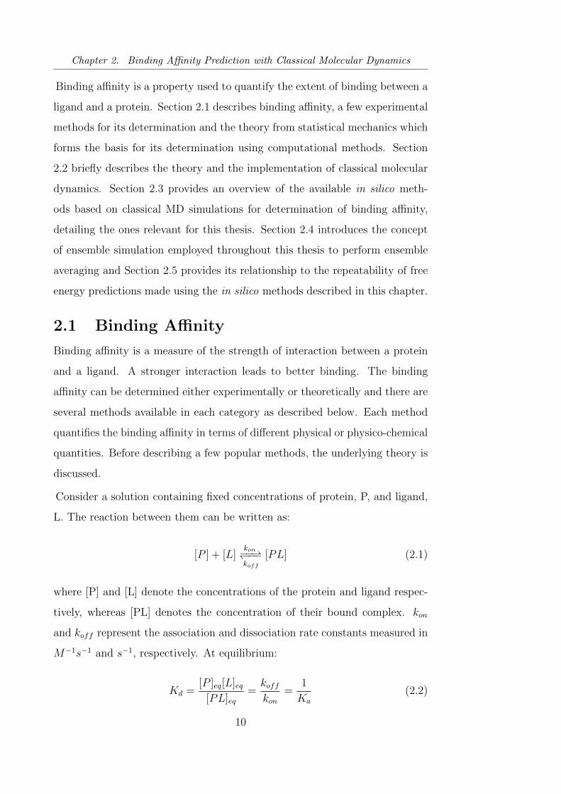
Consider a solution containing fixed concentrations of protein, P, and ligand,
L. The reaction between them can be written as:
[P ] + [L]kon−−⇀↽−−koff
[PL] (2.1)
where [P] and [L] denote the concentrations of the protein and ligand respec-
tively, whereas [PL] denotes the concentration of their bound complex. kon
and koff represent the association and dissociation rate constants measured in
M−1s−1 and s−1, respectively. At equilibrium:
Kd =[P ]eq[L]eq
[PL]eq=koffkon
=1
Ka
(2.2)
10
2.1. Binding Affinity
where [..]eq denotes the equilibrium concentration; Kd and Ka are the dissoci-
ation and association constants respectively. If [P ]i is the initial concentration
of protein, then [P ]eq = [P ]i − [PL]eq =⇒ [P ]i = [P ]eq + [PL]eq. It can be
seen from Equation 2.2 that when Kd = [L]eq, [P ]eq = [PL]eq = [P ]i/2. Thus,
the dissociation constant is the concentration of ligand at which half of the
total available binding sites of protein are occupied by ligand at equilibrium.
Therefore, the lower the value of Kd, the smaller concentration of ligand is
sufficient to occupy the available binding sites, which in turn, can be related
to higher level of attraction between the ligand and the protein. Consequently,
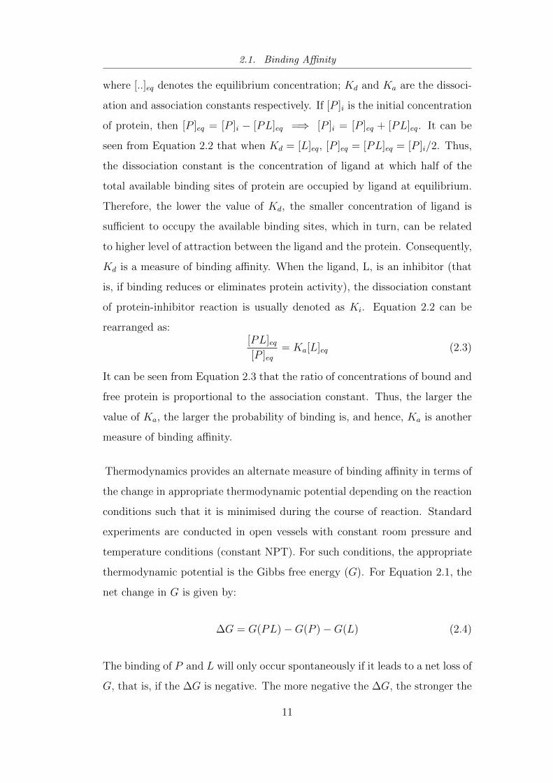
Kd is a measure of binding affinity. When the ligand, L, is an inhibitor (that
is, if binding reduces or eliminates protein activity), the dissociation constant
of protein-inhibitor reaction is usually denoted as Ki. Equation 2.2 can be
rearranged as:[PL]eq[P ]eq
= Ka[L]eq (2.3)
It can be seen from Equation 2.3 that the ratio of concentrations of bound and
free protein is proportional to the association constant. Thus, the larger the
value of Ka, the larger the probability of binding is, and hence, Ka is another
measure of binding affinity.
Thermodynamics provides an alternate measure of binding affinity in terms of
the change in appropriate thermodynamic potential depending on the reaction
conditions such that it is minimised during the course of reaction. Standard
experiments are conducted in open vessels with constant room pressure and
temperature conditions (constant NPT). For such conditions, the appropriate
thermodynamic potential is the Gibbs free energy (G). For Equation 2.1, the
net change in G is given by:
∆G = G(PL)−G(P )−G(L) (2.4)
The binding of P and L will only occur spontaneously if it leads to a net loss of
G, that is, if the ∆G is negative. The more negative the ∆G, the stronger the
11
Chapter 2. Binding Affinity Prediction with Classical Molecular Dynamics
binding. Therefore, ∆G provides another measure of the binding affinity. It
can also be related to the association constant, Ka, by the van’t Hoff equation:
∆G = −RT lnKa = RT lnKd (2.5)
where R and T are the universal gas constant and the temperature, respec-
tively, and ∆G is the standard binding affinity.
2.1.1 Experimental Determination
Experimentally, quantitative in vitro analysis of the binding reaction is un-
dertaken to determine the binding affinity. For this, a number of methods
have been developed which detect and monitor the concentration of ligand
and/or protein, including NMR spectroscopy, dynamic light scattering, fluores-
cence cross-correlation spectroscopy, affinity capillary electrophoresis, isother-
mal titration calorimetry, surface plasmon resonance and many more[24, 25].
In some experiments, the association and dissociation rate constants, kon and
koff respectively, of the protein-ligand reaction (as shown in Equation 2.1) are
measured based on which they report the binding affinity in terms of Kd (or Ki,
when the ligand is an inhibitor). Isothermal titration calorimetry (ITC)[26] is
a calorimetric approach which measures the heat loss or gain during the course
of the reaction between protein and ligand based on which ∆G is reported. In
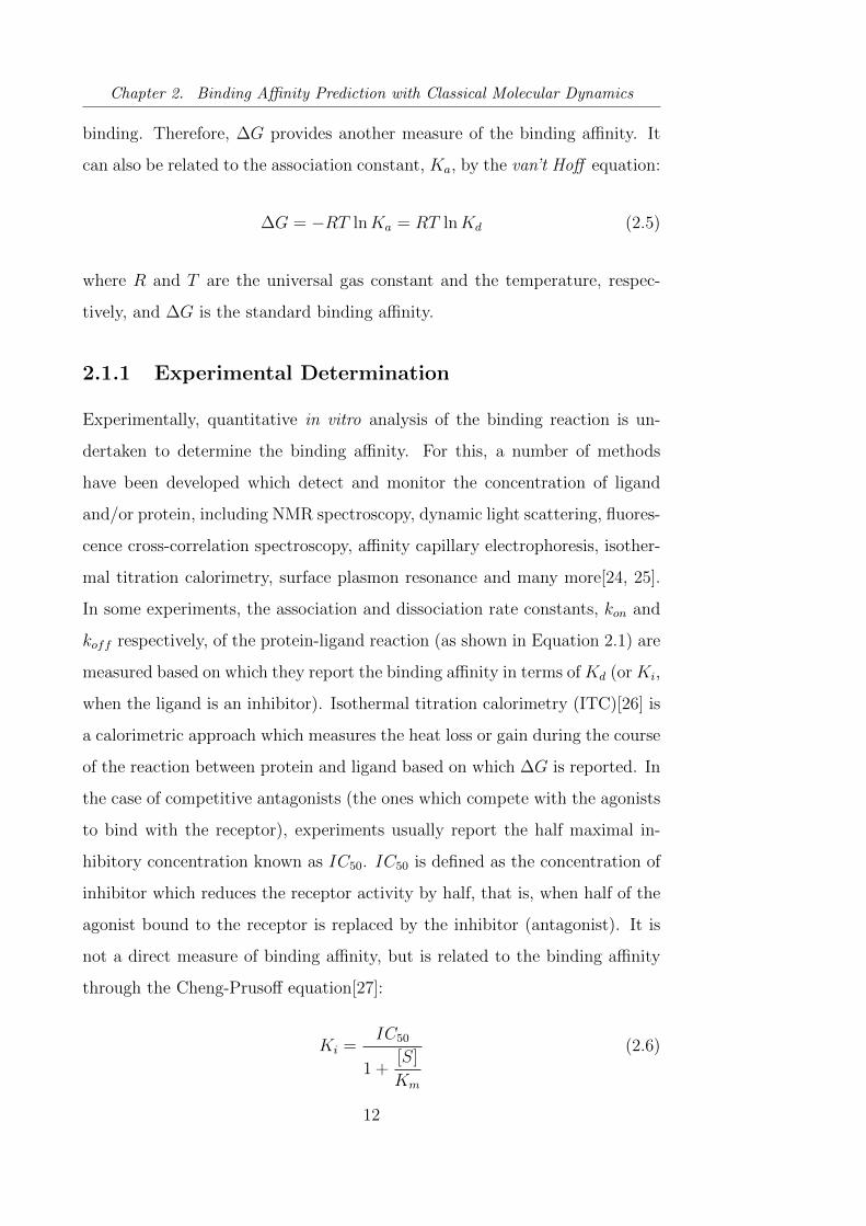
the case of competitive antagonists (the ones which compete with the agonists
to bind with the receptor), experiments usually report the half maximal in-
hibitory concentration known as IC50. IC50 is defined as the concentration of
inhibitor which reduces the receptor activity by half, that is, when half of the
agonist bound to the receptor is replaced by the inhibitor (antagonist). It is
not a direct measure of binding affinity, but is related to the binding affinity
through the Cheng-Prusoff equation[27]:
Ki =IC50
1 +[S]
Km
(2.6)
12
2.1. Binding Affinity
where Ki and Km are the dissociation constants of inhibitor and agonist for
the receptor respectively, [S] is the agonist concentration. The dependence
of IC50 on [S] and Km implies that it can only be used to compare different
inhibitors binding to the same receptor, but not same inhibitor binding to
different receptors. When [S] is low, IC50 can be approximated as Ki, and
Equations 2.5 and 2.6 give:
∆G ≈ RT ln(IC50) (2.7)
Due to this approximation ∆G values derived from IC50 values are considered
to be less accurate than those from more direct sources such as ITC.
2.1.2 Determination Using Computational Methods
Computational methods usually take the thermodynamic route to measure
binding affinity in terms of ∆G. They are commonly based on molecular level
simulations, where a single molecule of protein-ligand complex is simulated
to yield ∆G, which is macroscopic thermodynamic property. Statistical me-
chanics provides the link between microscopic simulations and macroscopic
properties estimated. This section is dedicated to a brief discussion of some
important concepts from statistical mechanics relevant for the determination
of binding affinity using computer-based methods. For more details, refer to
standard texts[28].
In classical statistical mechanics, the canonical partition function (Q) for a
system of N indistinguishable molecules is defined as:
Q =1
N !h3N
∫ ∫exp
(−E(p,r)
kBT
)drdp (2.8)
where kB is Boltzmann’s constant, T is absolute temperature, h is the Planck
constant and E(p,r) is the total energy of the system which depends on its
coordinates (r) and momenta (p). The total energy of the system can be taken
to be the sum of its kinetic and potential energies and the partition function
13
Chapter 2. Binding Affinity Prediction with Classical Molecular Dynamics
can be rewritten as:
E(p,r) =3N∑i=1
p2i
2m+ U(r)
Q =1
N !h3N
[∫. . .
∫exp
(−∑p2i
2mkBT
)dp1 . . . dp3N
] [∫exp
(−U(r)
kBT
)dr
]
=Z
N !h3N
+∞∫−∞
exp
(−p2
2mkBT
)dp
3N
=Z
N !
(2πmkBT
h2
)3N/2
Z =
∫exp(−U(r)
kBT)dr
(2.9)
where, U(r) is the potential energy of the system, m is the molecular mass
and Z is the configurational integral. The partition function can be used to
calculate the measurable properties of a system, and hence, provides a link
between its microscopic states and macroscopic variables. For example, the
Helmholtz free energy (A) of a system with partition function (Q) is given by:
A = −kBT lnQ (2.10)
As mentioned earlier, the binding reaction is driven by the need of minimising
an appropriate thermodynamic potential depending on the conditions of the
reaction. In case of constant number of particles (N), volume (V ) and tem-
perature (T ), also known as canonical ensemble, the appropriate potential is
Helmholtz free energy (A), while in case of constant NPT (P is the pressure),
also known as isothermal-isobaric ensemble, the Gibbs free energy (G) is the
appropriate quantity. These two state functions are related as follows:
G = A+ PV (2.11)
where, P and V are pressure and volume. For condensed phase system, such
as biomolecules in aqueous solutions, the contribution to free energy from
14
2.1. Binding Affinity
change in volume in isothermal-isobaric ensemble is negligible, and hence can
be neglected. On doing this, G ≡ A, and hence, a unified notation (G) will be
used for free energy henceforth.
If we want to calculate the free energy difference between two well-defined
states 1 and 2, it can be expressed in terms of a ratio of the two partition
functions corresponding to each state. LetQ1 andQ2 be the partition functions
for states 1 and 2 respectively, the difference in their free energies is given by:
∆G = G2 −G1 = −kBT ln
(Q2
Q1
)(2.12)
The ratio of partition functions can be simplified as:
Q2
Q1
=
⟨exp
(−(E2 − E1)
kBT
)⟩1
(2.13)
where 〈〉1 denotes that the average of the enclosed quantity is evaluated from
a thermodynamic ensemble for state 1, which essentially means that the term
exp(−(E2−E1)/kBT ) for a particular configuration is weighed directly propor-
tional to the probability of occurrence of that configuration in the ensemble of
configurations of state 1. Thus, the free energy difference between two states
can be computed from an ensemble average of the energy difference between
a reference state and a perturbed state, as follows:
∆G = G2 −G1 = −kBT ln
⟨exp
(−(E2 − E1)
kBT
)⟩1
(2.14)
It is worth mentioning here that, theoretically, E in Equation 2.14 is the total
energy of the system. However, as shown in Equation 2.9, the kinetic energy
component factorises out as the product of Gaussian integrals over momenta.
Therefore, the momentum contribution to the free energy difference is zero.
All the methods for in silico binding affinity determination as described in the
following sections will be derived from the above theory, more specifically from
Equations 2.10 and 2.14. The key point to be noted here is that to calculate ∆G
15
Chapter 2. Binding Affinity Prediction with Classical Molecular Dynamics
in silico, one needs to compute the ensemble average of microscopic properties.
Thus, the basic requirement for determining binding affinity is the generation of
an ensemble of conformations for the microscopic system. Molecular dynamics
is the method most commonly used to generate an ensemble of conformations
as discussed in the next section.
2.2 Molecular Dynamics
Molecular dynamics (MD) provides a way of modelling the complex motion of
biomolecules governed by their chemical interactions. Classical MD is based
on classical mechanics and is popularly used for modelling protein dynamics
given the large number of atoms in proteins. It should be noted here that
classical MD is only a tool to study the temporal evolution of the simulated
system. However, as discussed in the previous section, ensemble averaging
over microstates needs to be performed in order to compute the macroscopic
properties of a system like the Gibbs free energy. According to the ergodic
theorem, the ensemble average is equal to the time average only in the limit
of “long” time. Thus, a single short simulation cannot be used to compute
ensemble averages. Nonetheless, the practice has been so. The reliability of
such a practice is discussed in Section 2.4 and in the later chapters of this thesis.
In the remainder of this section, classical MD is described briefly. The details
on it can be found in standard texts like Leach[29], Frenkel and Smith[30] or
Allen and Tildesley[31].
2.2.1 Implementation of Molecular Dynamics
In MD simulations, the smallest unit of the molecule is taken to be atom.
Therefore, no sub-atomic level description of the system studied is possible
using MD. All atoms are considered to be point masses with a given partial
charge. The interactions between atoms are modelled using force field parame-
ters as described in Section 2.2.2. All atoms in a system of interest are assigned
initial positions and velocities and its trajectory is determined by numerically
solving the Newton’s equation of motion using an integrator. An important
16
2.2. Molecular Dynamics
criterion which an integrator should satisfy is energy conservation. There are
several integrators available but the most commonly used ones are the Verlet-
style algorithms like Verlet method[32], velocity Verlet method[31]. The latter
is employed by the NAMD code used for all simulations in this work.
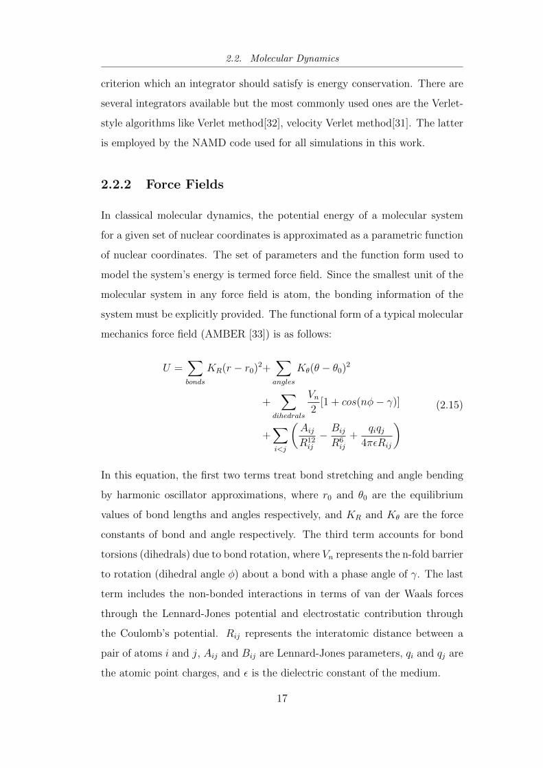
2.2.2 Force Fields
In classical molecular dynamics, the potential energy of a molecular system
for a given set of nuclear coordinates is approximated as a parametric function
of nuclear coordinates. The set of parameters and the function form used to
model the system’s energy is termed force field. Since the smallest unit of the
molecular system in any force field is atom, the bonding information of the
system must be explicitly provided. The functional form of a typical molecular
mechanics force field (AMBER [33]) is as follows:
U =∑bonds
KR(r − r0)2+∑angles
Kθ(θ − θ0)2
+∑
dihedrals
Vn2
[1 + cos(nφ− γ)]
+∑i<j
(AijR12ij
− Bij
R6ij
+qiqj
4πεRij
) (2.15)
In this equation, the first two terms treat bond stretching and angle bending
by harmonic oscillator approximations, where r0 and θ0 are the equilibrium
values of bond lengths and angles respectively, and KR and Kθ are the force
constants of bond and angle respectively. The third term accounts for bond
torsions (dihedrals) due to bond rotation, where Vn represents the n-fold barrier
to rotation (dihedral angle φ) about a bond with a phase angle of γ. The last
term includes the non-bonded interactions in terms of van der Waals forces
through the Lennard-Jones potential and electrostatic contribution through
the Coulomb’s potential. Rij represents the interatomic distance between a
pair of atoms i and j, Aij and Bij are Lennard-Jones parameters, qi and qj are
the atomic point charges, and ε is the dielectric constant of the medium.
17
Chapter 2. Binding Affinity Prediction with Classical Molecular Dynamics
It is clear from Equation 2.15 that force field potential function contains
many parameters such as force constants, equilibrium geometric parameters,
Lennard-Jones parameters, atomic charges and so on. These parameters are
obtained by fitting its potential function to experimental data or high-level
quantum calculations and hence the potential energy calculated using force
fields is said to be empirical. Some common force fields are AMBER [33],
CHARMM[34], MMFF[35], GROMOS[36], OPLS[37], CEDAR[38], MM2[39]
and MM3[40]. It should be noted that the force field functional form as well
as parameters may differ depending on the physical conditions used for their
parameterisation. AMBER employed in all the simulations performed for this
thesis is parameterised to be suitable for studying proteins.
The force field formalism involves several assumptions. The functional form
used to calculate the potential energy is itself an approximation. Another
important one is transferability, that is, assuming that the parameters fitted
for a relatively small set of molecules will remain valid for any molecule. For
instance, it is generally assumed in all force fields that the equilibrium bond
length and the harmonic force constant for the carbon-carbon single bond is
the same for all molecules. An important limitation of force fields is that the
number of atom combinations used for parameterisation is limited. Therefore,
although the atom combinations in all amino acids have been parameterised,
this may not be true for all molecules of interest. The General AMBER force
field[41] has been developed to extend parameterisation to nearly all known
atom combinations in organic molecules and has been used for ligand molecules
in all simulations for this thesis.
2.2.3 Thermostats and Barostats
Experiments are generally performed at constant pressure and temperature
conditions. Therefore, it is often desirable to perform simulations sampling
conformations from isothermal-isobaric ensemble. A method which maintains
the temperature of the system at a pre-defined value is known as thermo-
stat, while one which maintains the pressure of the system at a fixed value a
18
2.2. Molecular Dynamics
barostat. There are a variety of thermostats and barostats available for MD
simulations. Below we discuss the Langevin thermostat[42, 43] and Berendsen
barostat[44] which have been employed in all simulations performed for this
thesis.
The Langevin theromstat is analogous to the system of interest being embed-
ded in a sea of small fictional particles. These smaller fictional particles create
a damping force to the momenta of real atoms and give random kicks to the
atoms by virtue of their motion. The equations of motion for MD simula-
tions are replaced by the Langevin equation[42] which includes two additional
terms corresponding to the damping force and the randomly fluctuating force
which are related to each other such that the desired ensemble with constant
temperature is recovered.
The Berendsen barostat involves coupling the simulating system with an ex-
ternal pressure bath. The extent of coupling is determined by a coupling
parameter. Pressure is maintained by scaling the coordinates of the atoms
and hence adjusting the volume of the system at each time step. The scaling
factor is derived from the difference between the instantaneous pressure of the
system and that of the external bath, the isothermal compressibility of the
system and the coupling parameter.
2.2.4 Improving Computational Efficiency
There are several techniques employed in MD simulations to improve the com-
putational efficiency of simulations while enhancing the simulation model’s
resemblance to real experimental system. A few of them are mentioned below.
MD simulations are usually performed using just a single molecule of the sys-
tem of interest contained in a solvent buffer of a few tens of angstroms. In
order for it to mimic the real experimental system and yield the bulk properties
of the system, periodic boundary conditions are employed which increase the
effective size of the system. The idea is to have an infinite array of replicates,
called images, of the simulation box in all directions. The number of parti-
cles in the simulation box are conserved by allowing any particle leaving the
19
Chapter 2. Binding Affinity Prediction with Classical Molecular Dynamics
simulation box from one side be replaced by its image entering the box from
the opposite side. The employment of periodic boundary conditions enables
getting bulk properties by simulating a relatively small number of atoms.
The calculation of non-bonded energy terms is computationally much more
expensive than that of the bonded energy terms as, unlike non-bonded in-
teractions, the bonded interactions are limited to a few neighbouring atoms.
A common strategy to reduce the computational cost for calculation of non-
bonded energies is to introduce a cut-off distance beyond which all non-bonded
energies are set to zero[29, 45]. Conventionally, the cut-off distance for peri-
odic systems is set to a value smaller than half the length of the shortest edge
of the simulation box so that each atom just interacts with only one image
of any other atom. However, this scheme is effective only for the short range
Lennard-Jones potential which tails off quickly with distance. Electrostatic
interactions are long range and have considerable values even at long distances
and hence this scheme is inaccurate for them.
In the case of periodic systems, the electrostatic potential can be evalu-
ated more efficiently using the Ewald summation[46] or its improved vari-
ant particle-mesh Ewald (PME)[47]. These schemes assume that the periodic
boundary conditions have been employed and compute the electrostatic po-
tential energy as the sum of short range and long range terms. The short
range terms are calculated using the standard Coulomb formula in real space
while the long range terms are computed using Fourier transforms in reciprocal
space. PME employs Fast Fourier Transform to compute the long range terms
and hence is more efficient computationally. To further reduce the computa-
tional cost, the long-range electrostatic potential is sometimes not computed
at every time step in the simulation but less frequently. Such an approach is
referred to as a multiple time stepping algorithm[48].
The vibrational motion of hydrogen atoms bound to heavy atoms is usually
the fastest motion in the simulated system, necessitating the use of a timestep
of 1 fs. However, there are cases when these vibrations do not contribute sig-
20
2.3. Methods for In Silico Determination of Binding Affinity
nificantly to the overall dynamics of the system. In such cases, the lengths of
these bonds can be constrained which in turn allows using a larger timestep
(typically 2 fs in protein simulations). Several constraint algorithms are avail-
able for this purpose: SHAKE[49], RATTLE[50], SETTLE[51], M-SHAKE[52]
and so on.
2.3 Methods for In Silico Determination of
Binding Affinity
As detailed in the previous section, MD provides a tool to collect microstates
of the biomolecule of interest. Thereafter, the theory of statistical mechanics
can be applied to get the macroscopic thermodynamic properties G or ∆G
from the ensemble of microstates. The statistical framework for macromolec-
ular free energy calculations was first described by Zwanzig [53], Kirkwood
[54], and Valleau and Torrie [55], but it could not be actually implemented
until the advent of fast computers in the early 1980s. The first macromolec-
ular free energy calculations were performed about three decades ago [56–59].
The methods so developed were used to calculate relative free energies for
the binding of several ligands to a common receptor [59] and also to compute
the binding affinity for a single ligand and receptor [60]. Later that decade,
free energy studies started yielding exciting results and became very popular.
Several excellent reviews in this field are available [61–79]. Today, there exist
several methods to calculate the binding affinity based on non-biased MD sim-
ulations. Some of the popular ones, in order of decreasing speed and increasing
accuracy, are:
• Empirical scoring methods, based on simplified energy functions repre-
senting different contributions to binding affinity [80–83].
• Linear interaction energy (LIE) method, where electrostatic part of the
binding affinity is estimated using the linear response approximation,
while the non-electrostatic contributions are derived using empirical
21
Chapter 2. Binding Affinity Prediction with Classical Molecular Dynamics
parameters[84].
• Molecular mechanics Poisson-Boltzmann surface area (MMPBSA)
method, a semi-empirical method, where the solvent is approximated to
be a continuum [85].
• Free energy perturbation (FEP)[53] and thermodynamic integration
(TI)[86, 87].
Broadly, methods to calculate free energies can be classified into three classes
based on the part of phase space sampled: (i) end-point methods, which sam-
ple just the bound and unbound states of protein-ligand complex, (ii) meth-
ods based on sampling along an alchemical thermodynamic pathway, and (iii)
methods based on calculating free energy along a reaction coordinate, known
as the potential of mean force (PMF). Another classification of free energy
methods could be: “exact” and “approximate”. The former are based directly
on equations from statistical mechanics, while the latter start with statistical
mechanics, but then incorporate some assumptions and approximations into
those equations. One can logically conclude that the former are more accu-
rate than latter. But there exists a trade-off between accuracy and speed,
therefore, the former are computationally more expensive and time consuming
than latter. In the rest of this section, the methods relevant to this thesis are
described in more detail.
2.3.1 End-point Methods
End-point methods consider only the end states of the system, for example
bound and unbound states of the protein-ligand complex, and calculate their
absolute binding affinities. Methods like linear interaction energy (LIE)[84],
linear response approximation (LRA)[88], molecular mechanics/Poisson-
Boltzmann surface area (MM/PBSA)[85] and molecular mechanics/generalised
Born surface area (MM/GBSA)[89]. Here, we describe the latter two.
MMPBSA is often considered to be the best compromise between the speed
and accuracy of calculations. It is the most accurate among the approximate
22
2.3. Methods for In Silico Determination of Binding Affinity
methods and relatively less computationally expensive than exact methods.
Being an end-point method, MMPBSA considers only the two end states of
interest, that is, the protein and ligand in free and bound states and calculates
their absolute free energies. The binding affinity is subsequently calculated as
the difference of absolute free energies as shown below:
∆G = 〈Gcomplex,aq〉 − 〈Greceptor,aq〉 − 〈Gligand,aq〉 (2.16)
However, in solvated systems the majority of contributions to free energy come
from solvent-solvent interactions, resulting in large fluctuations. Therefore,
each of the above absolute free energies is decomposed into several components
as shown below[90–92]:
〈Gaq〉 = 〈Gvac〉+ 〈Gsol〉 (2.17a)
〈Gvac〉 = 〈UMM〉 − T 〈SMM〉 (2.17b)
〈Gsol〉 = 〈Gpolar〉+ 〈Gnp〉 (2.17c)
where, 〈...〉 denotes averaging over an ensemble of conformations, 〈Gaq〉 is free
energy in solvated state, 〈Gvac〉 is free energy in vacuum, 〈Gsol〉 is free energy
of solvation, which is the free energy change associated with taking a molecule
from vacuum into solvent. 〈UMM〉 represents the mean enthalpic energy of the
solute and 〈SMM〉 the mean solute entropy. 〈Gpolar〉 is the polar solvation free
energy and 〈Gnp〉 the non-polar solvation free energy. It is worth mentioning
here that the terms 〈Gpolar〉 and 〈Gnp〉 include both energetic and entropic com-
ponents of solvent free energy and hence 〈SMM〉 is the configurational entropy
associated with solute motion only. In practice, a MD simulation is performed
using explicit solvent and counter ions to get an ensemble of conformations
for each state in Equation 2.16 and the different energy components are then
calculated in the post processing step. The remainder of this section briefly
describes the method of evaluating all the components of MMPBSA.
23
Chapter 2. Binding Affinity Prediction with Classical Molecular Dynamics
2.3.1.A Calculation of the Solute Enthalpic Contribution
The solute enthalpic term 〈UMM〉 is calculated as the ensemble average of the
molecular mechanical force field terms for the solute. It consists of
UMM = U elec + U vdW + U int, (2.18)
where U elec is the electrostatic energy, U vdW is the van der Waals energy and
U int is the internal energy of the solute molecule. Uint can generally be de-
composed into bond, angle and dihedral terms of the force field.
2.3.1.B Calculation of the Solvation Free Energy
In order to calculate the solvation free energy, 〈Gsol〉, the explicit solvent
molecules and counter ions are removed from the MD trajectories and replaced
by a continuum solvent. As mentioned above, 〈Gsol〉 has two components, one
due to electrostatic interactions (〈Gpolar〉) and another due to non-polar inter-
actions (〈Gnp〉).
The polar solvation free energy 〈Gpolar〉 measures the energy corresponding to
the presence of the solute’s charge distribution in the continuum dielectric. It
is calculated either by numerical solution of the linearised Poisson-Boltzmann
(PB) equation[85, 93] or generalized-Born (GB) analysis [89, 94], which is a
faster approximation to full PB model, for the snapshots from the MD trajec-
tory. For typical biomolecules, the dielectric constants of solute and water are
commonly chosen to be 1.0 and 80.0 respectively for PB calculations.
The non-polar contribution 〈Gnp〉 accounts for the hydrophobic effect which
promotes the association of non-polar surfaces of the receptor and ligand [95].
It is determined using an equation involving solvent accessible surface area
(A)[96] and empirically derived parameters γ and b as shown in the equation
below[97].
〈Gnp〉 = γA+ b (2.19)
The coefficient γ is taken to be positive which leads to higher (unfavourable)
energy for conformations with more surface area (as it displaces more solvent
24

2.3. Methods for In Silico Determination of Binding Affinity
and hence needs more energy), and hence, it favours the binding which reduces
surface area. The method has been named MMPBSA due to contributions
from molecular mechanics (MM), Poisson-Boltzmann (PB) and surface area
(SA) terms. It is called MMGBSA if the generalized-Born solvation energy is
used instead of Poisson-Boltzmann.
It is important to mention here that MMPB(GB)SA involves taking the differ-
ence of large numbers (the absolute free energies are of the order of hundreds
to thousands of kcal/mol) to determine relatively small binding affinity (of the
order of tens of kcal/mol). Thus, it is important that the average absolute
free energies converge to values invariant of simulation length and also have
relatively low variances.
2.3.1.C Calculation of Configurational Entropy
The configurational entropy term 〈SMM〉 can be calculated using quasi-
harmonic analysis[98], normal-modes analysis [90] or restraint release
approach[99]. However, due to complications involved in its calculation, it
is often neglected for convenience. Here, we describe one of the most popular
methods for calculating configurational entropy - normal mode analysis.
Normal mode analysis method is based on the assumption that translational,
rotational and vibrational motions are independent from each other [100], and
also that the potential energy for the 3N-6 mutually orthogonal vibrational
degrees of freedom are harmonic with frequencies ωi. The total entropy can
then be calculated using the standard statistical mechanics formulae [28] as
follows:
Svib = kB
[3N−6∑i=1
αiexp(αi)− 1
− ln(1− exp(−αi))
]
Srot = kB ln
[√π
σ
(T 3
ΘAΘBΘC
)1/2
e3/2
]
Strans = kB ln
[(2πmkBT
h2
)3/2V
Ne5/2
] (2.20)
25
Chapter 2. Binding Affinity Prediction with Classical Molecular Dynamics
where αi = hωi/kBT , Θi = h2/2IikB is the rotational temperature, Ii is one of
the 3 principal moment of inertia IA, IB, IC and σ is the symmetry number.
Now, the problem of calculating conformational entropy of the molecule is
essentially reduced to determining its harmonic vibrational frequencies. This
can be done by diagonalizing the Hessian matrix H (a square matrix of order
3N with elements Hij) of the system’s potential energy (U) defined as follows:
Hij =
(∂2U
∂xi∂xj
)(2.21)
where xi and xj are the ith and jth component of the 3N dimensional configu-
ration of the system. In a normal mode analysis, the elements of the Hessian
matrix are constructed from a single conformation of the solute molecule. To
get the correct normal modes, the system needs to be at the minimum poten-
tial energy, that is, ∂U/∂xi = 0 and ∂2U/∂xi∂xj > 0 for each i and j [101–103].
Thus, first of all an energy minimization is performed in the normal mode anal-
ysis, followed by construction of the Hessian matrix and its diagonalization to
get the normal mode frequencies. Finally, Equation 2.20 is applied to get the
entropy. In practice, this procedure is applied on a selection of conformations
from the MD trajectories to get an ensemble of SMM and their average is the
final solute configurational entropy 〈SMM〉.
Swanson et al. [104] proposed the notion of free energy of association (re-
ferred to as ∆GAssoc hereafter) to improve the validity of the binding affinity
calculated using MMPB(GB)SA method. It accounts for the fact that a free
molecule at standard concentration of 1-M has translational freedom of 1660
A3 and rotational freedom of 8π2. On binding, the solute molecule loses these
freedoms while solvent molecules gain an equivalent freedom. ∆GAssoc can be
seen as alternate way to compute the ∆Strans and ∆Srot. We use it in the
following way to get the final binding affinity:
∆G = 〈UMM〉+ ∆GAssoc − T 〈SMM,vib〉+ 〈Gsolv〉+ 〈Gnp〉 (2.22)
26
2.3. Methods for In Silico Determination of Binding Affinity
∆GAssoc is evaluated using quasiharmonic model from Equation 2.23. For more
details about the method, refer to the literature [104, 105].
∆GAssoc = −RT ln
(C0ztransligandz
rotligand
8π2
)(2.23)
where C0 is the standard concentration 1 M, ztransligand and zrotligand are ligand
translational and rotational configurational integrals, respectively.
2.3.1.D Single and Multiple Trajectory Approaches
As per Equation 2.16, in order to get the binding affinity, we need to calcu-
late Gcomplex,aq, Greceptor,aq and Gligand,aq. The conformations of the complex,
receptor and ligand can be extracted either from separate MD trajectories for
each species, or all from a single MD trajectory of the protein/ligand complex,
leading to multiple and single trajectory versions of MMPB(GB)SA. More pre-
cisely, the former is 3-trajectory, while the latter is 1-trajectory approach. The
1-trajectory approach has an advantage that contributions from parts of the
system that do not affect binding exactly cancel as the same coordinates are
used for the components both as part of the complex and separated. If sepa-
rate trajectories are used then this exact cancellation of errors does not occur
as each trajectory is free to explore different conformations, and hence, con-
vergence of free energy might be difficult. On the other hand, the 1 trajectory
approach is unable to account for alterations in the conformations available
to the protein or ligand induced during binding and consequently may ignore
important contributions to the overall binding affinity.
2.3.2 Alchemical Methods
A range of methods are based on calculating the free energy along a non-
physical thermodynamic pathway, usually referred to as alchemical pathway,
to yield free energy difference between its two end points. Such methods are
termed as alchemical methods. The alchemical pathway usually corresponds
to transformation of one chemical species at one end into a different chemical
species at the other end of the pathway. In practice, this transformation is
27
Chapter 2. Binding Affinity Prediction with Classical Molecular Dynamics
defined as the function of a coupling parameter, λ, ranging between 0 (corre-
sponding to the initial state) and 1 (corresponding to the final state). In the
intermediate λ-states, the force field parameters are transformed from those of
the initial state to those of the final state in a smooth fashion, if not linearly.
The Hamiltonian of the system is defined in terms of λ such that it satisfies
the above mentioned properties. For example, one commonly used function is:
E(λ,p,r) = (1− λ)E1(p,r) + λE2(p,r) (2.24)
where E1 and E2 are the Hamiltonians of the initial and final states of the
alchemical transformation respectively. At each intermediate λ-state, a MD
simulation is performed to sample the conformations available to the system.
After this, there are several ways to calculate the free energy difference between
the two end states of the alchemical transformation. In the remaining of this
section, some important methods to do so are described.
2.3.2.A Thermodynamic Integration
Using Equations 2.8 and 2.10, we can derive the following:
∂G
∂λ=∂(−kBT lnQ)
∂λ
=−kBTQ
∂Q
∂λ
=−kBTQ
1
N !h3N
∫ ∫−1
kBTexp
(−E(λ,p,r)
kBT
)∂E(λ,p,r)
∂λdrdp
=
⟨∂E
∂λ
⟩λ
(2.25)
where 〈...〉λ denotes ensemble average over state λ. If λ is taken to be the
coupling parameter ranging from 0 to 1, the free energy difference between the
two end points is given by:
∆G0→1 =
1∫0
∂G
∂λ=
1∫0
⟨∂E
∂λ
⟩λ
(2.26)
28

2.3. Methods for In Silico Determination of Binding Affinity
Computing free energy difference using Equation 2.26 is termed as Thermody-
namic Integration (TI). In practice, the ensemble average of ∂E/∂λ is taken
at a few discrete values of λ and the free energy difference is calculated by nu-
merical integration of the integrand using standard methods like trapezoidal
rule.[106] The appropriate number of λ points depends on the curvature of
the 〈∂E/∂λ〉 function. For smooth and monotonic curves of 〈∂E/∂λ〉, TI is
expected to be quite accurate even using a small number of points.
2.3.2.B Free Energy Perturbation
Free energy perturbation (FEP) is one of the oldest methods to calculate the
free energy difference between two states. It was first proposed by Zwanzig[53]
and is described by Equation 2.14. It is also known by some other names
in the literature, such as, exponential averaging (EXP) and Zwanzig relation.
Equation 2.14 is precise only when the potential energy difference between the
two states is less than 2kBT which is often not the case. If the two states do
not have much phase-space overlap, the convergence of results is difficult using
FEP. In such cases, a series of non-physical intermediate states are defined in
terms of the coupling parameter, λ, and the free energy difference between the
end states is given by the sum of free energy differences between consecutive
intermediate λ-points as follows:
∆Gλ(i−1)→λ(i) = −kBT ln
⟨exp
(−[E(λ(i),p,r)− E(λ(i− 1),p,r)]
kBT
)⟩λ(i−1)
∆G =∑i
∆Gλ(i−1)→λ(i)
(2.27)
where λ(i) refers to the ith point in the series of λ values chosen, starting from
λ = 0 and ending at λ = 1. The number of intermediate λ-points depends on
the type of alchemical transformation. For significant chemical changes during
the transformation, a larger number of intermediate points are required.
29
Chapter 2. Binding Affinity Prediction with Classical Molecular Dynamics
2.3.2.C Bennett Acceptance Ratio
Bennett proposed an acceptance ratio estimator to calculate the free energy dif-
ference between two ensembles sampled using two different Hamiltonians[107].
His original formulation was based on the following form of free energy differ-
ence:
∆G1→2 = kBT lnZ1
Z2
= kBT ln〈α(r)exp[−βU1(r)]〉2〈α(r)exp[−βU2(r)]〉1
(2.28)
where 〈...〉i denote ensemble average over state i with potential energy Ui and
configurational integral Zi, β = (kBT )−1 is the inverse temperature, α(r) is
an arbitrary weight function which is finite for all coordinates r. Equation
2.28 is valid for any function α(r). Thereafter, variational calculus is applied
to find α(r) such that the variance of the free energy is minimized. This
gives an implicit function of ∆G1→2 which can be solved numerically. This
method of calculating free energy difference is called the Bennett acceptance
ratio (BAR). BAR has been shown to have lower bias and smaller variance
than EXP. [108, 109]
2.3.2.D Weighted Histogram Analysis Method
Histogram weighing techniques first introduced by Ferrenberg and Swendsen[110]
provide a route to calculate the entropy or free energy as a function of a
macroscopic parameter (X) at any desired value of X’s conjugate (Y) using
the probability distribution of X. Multiple distributions of X from ensembles
at different values of Y can also be combined to get statistically optimal esti-
mate of free energy. For example, Helmholtz/Gibb’s free energy as a function
of internal energy/enthalpy can be derived given multiple probability distri-
butions of internal energy/enthalpy from independent simulations at different
temperatures. The weighted histogram analysis method (WHAM) is an exten-
sion of these histogram weighing techniques which allows computation of free
energy differences or potential of mean force (PMF) using data from multiple
simulations with varying temperatures and/or potentials, usually controlled
by a parameter λ[111]. In addition, it allows one to calculate the expecta-
tion of any observable at the desired state for the system. WHAM has been
30
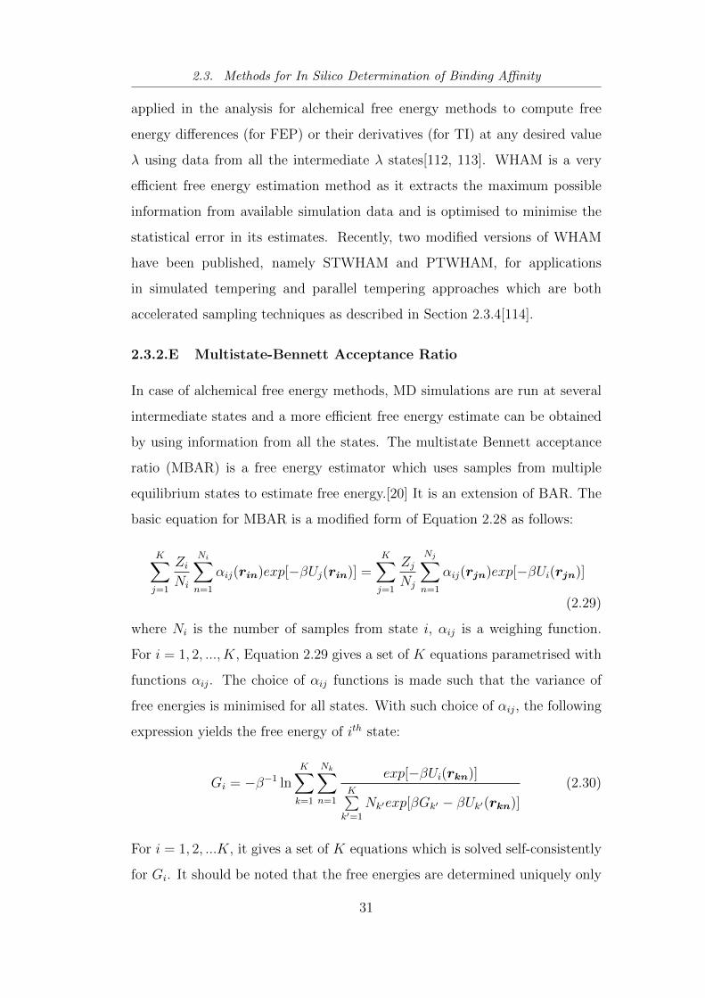
2.3. Methods for In Silico Determination of Binding Affinity
applied in the analysis for alchemical free energy methods to compute free
energy differences (for FEP) or their derivatives (for TI) at any desired value
λ using data from all the intermediate λ states[112, 113]. WHAM is a very
efficient free energy estimation method as it extracts the maximum possible
information from available simulation data and is optimised to minimise the
statistical error in its estimates. Recently, two modified versions of WHAM
have been published, namely STWHAM and PTWHAM, for applications
in simulated tempering and parallel tempering approaches which are both
accelerated sampling techniques as described in Section 2.3.4[114].
2.3.2.E Multistate-Bennett Acceptance Ratio
In case of alchemical free energy methods, MD simulations are run at several
intermediate states and a more efficient free energy estimate can be obtained
by using information from all the states. The multistate Bennett acceptance
ratio (MBAR) is a free energy estimator which uses samples from multiple
equilibrium states to estimate free energy.[20] It is an extension of BAR. The
basic equation for MBAR is a modified form of Equation 2.28 as follows:
K∑j=1
ZiNi
Ni∑n=1
αij(rin)exp[−βUj(rin)] =K∑j=1
ZjNj
Nj∑n=1
αij(rjn)exp[−βUi(rjn)]
(2.29)
where Ni is the number of samples from state i, αij is a weighing function.
For i = 1, 2, ..., K, Equation 2.29 gives a set of K equations parametrised with
functions αij. The choice of αij functions is made such that the variance of
free energies is minimised for all states. With such choice of αij, the following
expression yields the free energy of ith state:
Gi = −β−1 lnK∑k=1
Nk∑n=1
exp[−βUi(rkn)]K∑k′=1
Nk′exp[βGk′ − βUk′(rkn)]
(2.30)
For i = 1, 2, ...K, it gives a set of K equations which is solved self-consistently
for Gi. It should be noted that the free energies are determined uniquely only
31
Chapter 2. Binding Affinity Prediction with Classical Molecular Dynamics
up to an additive constant and hence only their differences are meaningful.
The above MBAR formulation can also be used to determine the equilibrium
expectation of an observable, for instance ∂G/∂λ, at any desired state. MBAR
is considered to be the lowest variance estimator.[20] It is noteworthy that
MBAR (Equation 2.30) is equivalent to WHAM in the limit of histograms
comprised of zero width bins.
2.3.2.F End-point Catastrophes
In cases where atoms are created or annihilated during an alchemical trans-
formation, points of singularities in ∂E/∂λ or numerical instability may occur
close to the end-points using classical force fields. This can happen when the
suddenly appearing atom overlaps or is very close to an existing atom leading
to 0 or very small interatomic distance between the two atoms. The Lennard-
Jones (LJ) and Coulomb terms used in classical force fields to describe the
non-bonded interactions will tend to infinity, or very large repulsive forces in
such situation. The former leads to singularities while the latter is the reason
of numerical instability during the simulation, which collectively may be re-
ferred to as end-point catastrophes. To avoid them, a soft-core potential is used
which scales and shifts the non-bonded interaction such that the repulsion be-
tween two atoms approaches a finite value at very short distances.[115–117] A
softcore potential can be used either just for van der Waals interaction[115] or
for both van der Waals and electrostatic interactions.[116] In the former case,
the coupling of non-softcore electrostatic interactions can be deferred until the
softcore van der Waals interactions have got rid of all unwanted overlaps, after
which its safe to couple the electrostatic interactions too. A new version of the
softcore potential has recently been proposed[117].
2.3.3 Relative and Absolute Binding Affinity Calcula-
tion
All the alchemical methods described in the previous section yield ∆G between
the two end-points of the alchemical transformation. However, the quantity of
32
2.3. Methods for In Silico Determination of Binding Affinity
real interest is the free energy difference between free and bound states of the
protein-ligand system, that is, their binding affinity. To calculate binding affin-
ity using alchemical methods, a thermodynamic cycle approach is employed
as shown in Figure 2.1. It can be used to calculate absolute (Figure 2.1(a)) or
relative (Figure 2.1(b)) binding affinity. Two calculations are required in such
approaches. The first calculation corresponds to the alchemical transformation
of ligand 1 to 2 in aqueous phase, whose free energy change is ∆Galch1, while
the second calculation corresponds to the same alchemical transformation in a
protein environment with accompanying free energy change as ∆Galch2. In the
case of absolute binding affinity calculation, the end-point, λ = 1, corresponds
to fully decoupled ligand 1, while in case of relative binding affinity calculation,
it corresponds to full decoupled ligand 1 and fully coupled ligand 2. Therefore,
in the former case, ∆G2 = 0 as can be seen in Figure 2.1(a). The following
equations give the corresponding binding affinities:
∆∆G = ∆G1 −∆G2 = ∆Galch1 −∆Galch2
∆G1 = ∆Galch1 −∆Galch2 (when ∆G2 = 0)(2.31)
This approach can be employed to calculate the relative binding affinities be-
tween two ligands associating with a protein or between two different proteins
bound to the same ligand.
The approach shown in Figure 2.1(a) to calculate the absolute binding affinity
of a ligand-protein interaction is termed as the double annihilation method
(DAM)[118]. However, this approach when applied directly has the problems
of ignoring the standard state dependence and slow convergence due to large
amount of sampling required, both of which can be overcome by the double
decoupling method (DDM), where the decoupled ligand is restrained to the
binding position[119]. Subsequently, several potentials restraining different
degrees of freedom and strategies to calculate absolute binding affinity have
been developed[120–122].
33
Chapter 2. Binding Affinity Prediction with Classical Molecular Dynamics
Figure 2.1: Thermodynamic cycles for calculation of binding affinities using al-chemical methods. Protein is shown in magenta; ligand 1 is shown in green andwhite while interacting and not interacting with the environment respectively; lig-and 2 is shown in red. (a) Calculation of absolute binding affinity of ligand 1 (∆G1),(b) calculation of relative binding affinity of ligands 1 and 2 (∆∆G).
2.3.4 Accelerated Sampling Techniques
One thing which is common to all the methods to calculate free energy of
biomolecular systems is the need for proper conformational sampling which is
important for robust results. The motion of biomolecular systems is governed
by a rugged energy landscape with several local minima connected by high
energy barriers[123]. It is not uncommon to have situations where the ligand
and/or protein are flexible and have interconvertible conformations (corre-
sponding to two local minima) through an energy barrier which is significantly
higher than the kinetic energy of molecules at room temperature (kBT ). Some-
times, large conformational changes are important for protein activity, for ex-
ample during catalysis or membrane transport. In such cases, conventional MD
simulations may take up to as long as a few microseconds to swap between
the two minima[124] or they might even get trapped into one of the local min-
ima indefinitely[13, 125] leading to their inability to sample the conformational
space of the protein-ligand system appropriately. Such trapping of molecules
34
2.3. Methods for In Silico Determination of Binding Affinity
in local minima slows down the conformational sampling of the molecule. To
overcome such problems, several accelerated sampling techniques have been
proposed. These include umbrella sampling[126], metadynamics[127], tem-
pering approaches[12, 14], steered molecular dynamics[128, 129], blue moon
sampling[130], adaptive biasing force algorithm[131], slow growth[132], fast
growth[133] and Gaussian accelerated MD[134] to name a few. A lot of good
reviews are available in the literature on different popular approaches[11–
16, 135]. Broadly, these techniques can be divided into two categories: tem-
pering approaches and those based on biasing potential. In the remainder of
this section, a few popular methods taken from these categories are discussed.
2.3.4.A Biasing Potential Based Approaches
Such approaches involve adding biasing terms to the Hamiltonian in order
to smooth out the energy landscape so as to facilitate the sampling of oth-
erwise unapproachable areas of the phase-space. The most popular method
in this category is umbrella sampling (US)[126]. It involves adding harmonic
constraints to the original potential centered at different fixed values of a pre-
defined reaction coordinate. An example of such a reaction coordinate is the
binding (or unbinding) pathway of a ligand to protein. This allows the sam-
pling of higher energy configurations relevant for the process of binding which
would otherwise remain unsampled. The complete potential of mean force
(PMF) along the reaction coordinate is calculated using weighted histogram
analysis method (WHAM)[111]. WHAM uses the biased probability distribu-
tions of reaction coordinates from individual US simulations to yield the op-
timal estimate of the unbiased probability distribution function which allows
the calculation of the potential of mean force (PMF). The total unbiased prob-
ability function is taken to be the weighted mean of the individual unbiased
probability functions from each simulation, where the weights are evaluated so
as to minimise the statistical error in the total probability function. Souaille
and Roux[136] demonstrated that US in combination with FEP could be ad-
vantageous compared to the standard FEP or TI through the judicious use of
35
Chapter 2. Binding Affinity Prediction with Classical Molecular Dynamics
a biasing potential.
Another biasing potential method, popularly known as metadynamics, is
where the biasing potential is adaptively built by periodic addition of per-
turbing terms with time in order to flatten the potential energy surface of the
system along the reaction coordinate[127]. The biasing potential in this case
is history-dependent, disfavouring configurations already visited in the space
of reaction coordinate. This allows efficient exploration and determination of
the energy surface with respect to the reaction coordinate. Many examples of
its application to study ligand binding are available in the literature[137–140].
2.3.4.B Tempering Based Approaches
Tempering methods involve increasing the temperature of the MD simula-
tion so as to facilitate crossing of energy barriers inaccessible at room tem-
perature. These methods form a subset of a class of methods which involve
performing a simulation in the generalised ensemble based on artificial, non-
Boltzmann probability distribution allowing a random walk in the potential
energy space[141, 142]. There are two types of tempering methods based on
the way higher temperature is introduced into the system. First is simulated
tempering (ST), also referred to as the method of expanded ensemble, where
a single MD simulation accesses different temperatures by performing a free
1D random walk in the temperature space[143, 144]. ST, like some other
methods based on the generalised ensemble simulation, uses non-Boltzmann
weight factors which are not known a priori and need to be determined by
short trial simulations. This task is tedious for biomolecular systems with
multiple minima. A solution to this problem is given by the second type
of tempering method called parallel tempering, also popularly known as the
replica-exchange method[145]. Replica exchange is discussed in more detail in
the following sections as it forms the basis of Chapter 4 in this thesis.
2.3.4.C Replica Exchange Molecular Dynamics
The replica exchange simulation method was first used by Swendsen and
Wang[146] as a replica Monte Carlo method in 1986. Thereafter, further de-
36
2.3. Methods for In Silico Determination of Binding Affinity
velopment and application of this approach by several people[147–149] led to
its current implementation in MD proposed by Okamoto and Sugita[145] in
1999. The basic idea of replica exchange molecular dynamics (REMD) is to
simulate M independent replicas of the system in the canonical ensemble with
each replica at a different temperature, some at low and others at high temper-
atures. The high temperature replicas are able to span much larger volumes
of the phase space and frequent exchanges of configurations between differ-
ent replicas allows better sampling of the phase space. The low temperature
replicas may be able to access several local minima, separated by high energy
barriers, due to such exchanges of configurations with high temperature repli-
cas. Since all the M replicas are simulated in canonical ensemble, they are
based on Boltzmann probability function, and hence, the problem of unknown
weight factors associated with other generalised ensemble methods, does not
exist in case of REMD. While the exchanges are attempted regularly with
neighbouring replicas, their acceptance probability is determined by the stan-
dard Metropolis criterion[150] which ensures the satisfaction of the detailed
balance condition[151] and convergence to an equilibrium distribution[145].
The implementation of REMD requires one to decide the optimal number of
replicas, temperature range and the highest temperature. The aim is to get
the best possible sampling done with minimum possible computational ex-
pense. The maximum temperature should be high enough to cross the energy
barriers one is concerned with so as to avoid trapping of any replica in local
minima. For a given maximum temperature, the number of replicas and tem-
perature spacing between neighbouring replicas need to be tuned such that
each replica spends equal amounts of time at each temperature[152]. This
means that the temperature of each replica has to be chosen such that the
temperature spacing between adjacent replicas allows a reasonable acceptance
ratio and this ratio should be equal for all adjacent pairs of replicas. Since
the acceptance probability decreases exponentially with the energy difference
as well as the temperature difference[145], the temperature spacing of neigh-
37
Chapter 2. Binding Affinity Prediction with Classical Molecular Dynamics
bouring replicas should allow overlap in corresponding energies[153]. Several
schemes for optimal temperature distribution over replicas have been suggested
in the literature[17, 152, 154–156]. One way is to impose the condition that
the energy fluctuation of a replica should be of the same order as the differ-
ence between the mean energy of that replica and that of its neighbouring
replica, which results in an exponential rule for the temperature distribution
over replicas[17]. It has also been shown that in some cases, minimisation of
the round trip time between the lowest and the highest temperatures is a bet-
ter estimate of mixing between states than the acceptance ratio[157]. Various
studies have arrived at different numbers as the optimal acceptance ratio for
the most efficient performance of REMD[152, 154, 158]. However, it turns out
that there is no strict rule and anything between 0.20-0.50 is deemed good
enough.
2.3.4.D Generalised Replica Exchange Methods
In the previous section, the original replica exchange method was introduced
where all the independent replicas differ only in their temperatures and the
rest of the properties of the system are identical for all replicas. However, the
replica exchange technique need not be confined to a random walk in temper-
ature space alone. Several generalisations have been reported in the litera-
ture. The first ever application of parallel tempering with multiple swapping
variables was reported by Yan and Pablo[159, 160]. Thereafter, a multidi-
mensional replica exchange method (MREM) was introduced soon after the
original REMD where, along with temperatures, the Hamiltonians of the repli-
cas were also modified[161]. In MREM, a one-to-one correspondence is defined
between replica m and its corresponding parameter set, Λm ≡ (Tm, λm) where
Tm is the temperature and λm is another parameter on which the Hamiltonian
depends for replica m. MREM provides a framework to combine REMD with
umbrella sampling[126] and FEP[53], in which λm can be used as the biasing
potential parameter in the former and the alchemical coupling parameter in
the latter case. It is to be noted that, in MREM, the temperature may or may
38
2.3. Methods for In Silico Determination of Binding Affinity
not be varied across replicas; that is, one can also have Λm ≡ λm with same T
for all replicas. Replica exchange umbrella sampling (REUS), a combination
of REMD and US where λ is varied between different replicas of US with and
without temperature exchanges, has been reported as an example[161, 162]
and has been shown to improve sampling in free energy calculations. FEP/λ-
REMD, a combination of FEP and REMD where λ is exchanged between
replicas, was reported by Jiang et al. as a scheme to calculate the abso-
lute hydration energy and binding affinity with improved convergence of their
results[163]. Multicanonical versions of replica exchange have also been re-
ported by adding some features of other generalised ensemble methods to the
original REMD with improved performance[141, 164–169]. There are a lot of
other improved versions of the original REMD available in literature[170–175].
In the light of these developments, the original REMD is also referred to as
T-REMD, as temperature is the only swapping parameter in that case.
As shown by Fukunishi et al., the optimal number of replicas required in
REMD for a given temperature range is proportional to√f , where f is the
total number of degrees of freedom of the system[17]. This imposes a severe
restriction on the applicability of such methods to solvated biomoleculear sys-
tem with large number of degrees of freedom as the number of replicas required
would be very high for them. Since most of the total degrees of freedom of
such systems are from the solvent, a large number of exchanges using REMD
would be uninteresting and waste CPU time. The solution to this problem
was proposed by Fukunishi et al. in the form of Hamiltonian replica exchange
method (H-REMD)[17]. In this approach, each replica differs in its interac-
tions, that is Hamiltonian, rather than temperature. It should be noted that
even MREM allows the use of different Hamiltonians at the same tempera-
tures across replicas like H-REMD. However, the advantage of H-REMD over
MREM is that the former allows one to modify the Hamiltonian only for a few
selected degrees of freedom which we are interested in across replicas. This
reduces the required number of total replicas thereby reducing the computa-
39

Chapter 2. Binding Affinity Prediction with Classical Molecular Dynamics
tional cost of the calculation. In terms of thermodynamics, potential scaling
is equivalent to scaling of the inverse temperature β, and hence, T-REMD is
a special case of H-REMD. However, from a practical point of view, H-REMD
has several advantages over T-REMD. First of all, since it allows scaling/mod-
ifying a part of the Hamiltonian, it is possible to avoid the wastage of CPU
time by excluding all uninteresting degrees of freedom from the scaled part of
the Hamiltonian. This substantially reduces the required number of replicas.
In addition, since all the replicas are run at the same temperature, there is no
need to reinitialise velocities after every successful exchange of configurations
like in T-REMD. The acceptance probability (A) between replicas i and j in
H-REMD is given by:
A = min{1, exp[−β([Ui(r′) + Uj(r)]− [Ui(r) + Uj(r
′)])]} (2.32)
where Ui and Uj are the potential energies of replica i and j, r and r′ are the
configurations of replicas i and j, respectively, prior to the exchange attempt.
The advent of H-REMD widely expanded the realm of application of
replica exchange methods. Thereafter, several variants of H-REMD have
been developed[176–181]. Jiang et al. proposed a method called FEP/H-
REMD[182], which is an extension to their previous method FEP/λ-
REMD[163], to calculate absolute ligand binding affinity. In this method,
H-REMD is implemented along two orthogonal axes, along one of which the
alchemical parameter λ varies, while along the other the boosting parameter
controlling the boosting potential set to accelerate sampling varies.
An important variant of H-REMD is called replica exchange with solute tem-
pering (REST)[183] where the total potential energy is divided into solute-
solute (SS), solute-solvent (SW) and solvent-solvent (WW) interactions and
the latter two are scaled by some factor along the replica ladder. It should be
noted that although a different system temperature is used for each replica,
like in T-REMD, scaling part of the Hamiltonian makes it equivalent to in-
creasing the temperature of solute only (the molecule of interest) while keeping
40
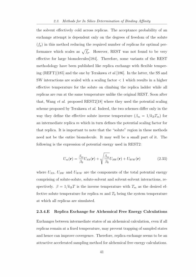
2.3. Methods for In Silico Determination of Binding Affinity
the solvent effectively cold across replicas. The acceptance probability of an
exchange attempt is dependent only on the degrees of freedom of the solute
(fp) in this method reducing the required number of replicas for optimal per-
formance which scales as√fp. However, REST was not found to be very
effective for large biomolecules[184]. Therefore, some variants of the REST
methodology have been published like replica exchange with flexible temper-
ing (REFT)[185] and the one by Terakawa et al.[186]. In the latter, the SS and
SW interactions are scaled with a scaling factor < 1 which results in a higher
effective temperature for the solute on climbing the replica ladder while all
replicas are run at the same temperature unlike the original REST. Soon after
that, Wang et al. proposed REST2[18] where they used the potential scaling
scheme proposed by Terakawa et al. Indeed, the two schemes differ only in the
way they define the effective solute inverse temperature (βm = 1/kBTm) for
an intermediate replica m which in turn defines the potential scaling factor for
that replica. It is important to note that the “solute” region in these methods
need not be the entire biomolecule. It may well be a small part of it. The
following is the expression of potential energy used in REST2:
Um(r) =βmβ0
USS(r) +
√βmβ0
USW (r) + UWW (r) (2.33)
where USS, USW and UWW are the components of the total potential energy
comprising of solute-solute, solute-solvent and solvent-solvent interactions, re-
spectively. β = 1/kBT is the inverse temperature with Tm as the desired ef-
fective solute temperature for replica m and T0 being the system temperature
at which all replicas are simulated.
2.3.4.E Replica Exchange for Alchemical Free Energy Calculations
Exchanges between intermediate states of an alchemical calculation, even if all
replicas remain at a fixed temperature, may prevent trapping of sampled states
and hence can improve covergence. Therefore, replica exchange seems to be an
attractive accelerated sampling method for alchemical free energy calculations.
41
Chapter 2. Binding Affinity Prediction with Classical Molecular Dynamics
The original idea of using replica exchange with FEP was proposed (although
not implemented) by Sugita et al. as a special case of MREM[161]. Later,
Woods et al. reported an improvement in the performance with the H-REMD
versions of both FEP and TI, called REFEP and RETI, respectively[112, 187],
where the usual simulations at the intermediate states for these calculations
were run accompanied with exchange of configurations between neighbour-
ing simulations. This was followed by several other similar reports of quicker
convergence and improved sampling when alchemical methods were combined
with H-REMD[188–192]. In all these applications, none of the replicas were
heated. Rick demonstrated the implementation of T-REMD with TI and re-
ported better convergence[113]. Jiang et al. reported FEP/λ-REMD[163] to
calculate absolute hydration and binding affinity using a combination of FEP
and REMD. They extended this method to propose a 2-dimensional replica
exchange scheme for absolute ligand binding affinity calculation based on H-
REMD, called FEP/H-REMD[182], where there is a two-dimensional grid of
simulations with the alchemical parameter varying in one direction while the
boosting potential parameter varying in the other and the exchanges are at-
tempted in both directions. Replica exchange has also been employed for
absolute binding affinity calculation[193, 194].
All the methods described above either introduce exchanges in the alchemical
space alone, or if they involve exchanging in the temperature or Hamiltonian
space, it is orthogonal to the exchanges in alchemical space. However, Wang et
al. recently proposed a method, called FEP/REST[19], combining the ideas of
MREM[161] and REST2[18]. It is basically a two dimensional H-REMD† where
both REST2 potential scaling factor, β, as well as the alchemical coupling
parameter, λ, vary and are exchanged across replicas such that the effective
temperatures of the end-point replicas corresponding to λ = 0 or 1 are set to
the room temperature, while it gradually increases for the intermediate λ values
attaining a maximum in the middle. This scheme provides the advantages
†Two-dimensional only in the sense that two parameters vary across replicas. It does notneed a two-dimensional grid of simulations like FEP/H-REMD.
42

2.4. Ensemble Averaging to Determine Thermodynamic Properties
of both tempering as well as exchanging in the alchemical space and also
is computationally less expensive as compared to its conceptually equivalent
method, FEP/H-REMD[182]. This method has been implemented to calculate
the free energies for a large number of biomolecular systems[195, 196].
2.4 Ensemble Averaging to Determine Ther-
modynamic Properties
As noted earlier in this chapter, statistical mechanics provides the formalism
to evaluate macroscopic thermodynamic properties like the Gibbs free energy
from the molecular simulations via ensemble averaging over microscopic sam-
ples (see Equation 2.14). However, it is a common practice to replace ensemble
average with time average performed in a single simulation relying on the er-
godic theorem. Time averaging self-evidently makes no sense when studying
non-equilibrium systems. It should be noted that the ergodic theorem holds
only in the limit of Poincare recurrence time, which is usually extremely long
for ligand binding[10]. Moreover, the Newtonian dynamics are very sensitive to
the initial conditions and hence two different MD trajectories diverge rapidly
over time no matter how close their initial conditions[10]. The key point is
that, for systems which exhibit an equilibrium thermodynamic state, the mi-
croscopic dynamics must be at least mixing in the language of ergodic theory,
hence chaotic[10]. Therefore, the practice of performing a short one-off MD
simulation to calculate free energy of a system should be replaced with en-
semble simulation. An ensemble simulation in this context means performing
multiple replicas of MD simulations, where each replica is an independent cal-
culation initiated from a randomly selected initial condition. Several different
approaches to vary the initial conditions of replicas have been reported includ-
ing varying only the initial velocities[21, 105, 197–204] or the initial velocities
in combination with other properties like the intial structures, the protonation
states, the solvation boxes, the intial conformations, the ligand charges, and
so on.[203, 205–209] In this thesis, all the replicas have identical initial con-
43
Chapter 2. Binding Affinity Prediction with Classical Molecular Dynamics
figurations while their initial velocities are randomly drawn from a Maxwell-
Boltzmann distribution. Ensemble averages can be computed by running a
sufficiently large number of replicas, an approach applicable for systems in as
well as out of equilibrium. The appropriate number of replicas in an ensemble
simulation is determined by the control of the error in the free energy predic-
tions that ensue. There is no general theory to determine this number which
needs to be assessed for each case under investigation[10]. In this thesis, it is
determined through the rule that the addition of one further replica to a set
N of replicas does not have a significant effect on the prediction. In practice,
there is a trade-off between the desired level of precision and the associated
computational cost. The number of replicas required may vary with the size
and the flexibility of the biomolecule studied as well as the free energy method
employed. For instance, in this thesis, I have used 5 replicas for all the relative
binding affinity calculations, but 25 replicas for all the absolute binding affinity
calculations (these choices have been justified in the following chapters). En-
semble simulation also provides a route to quantify the statistical uncertainty
associated with the calculated free energy.
2.5 Ensemble Averaging and Repeatability of
In Silico Binding Affinity Predictions
A reliable prediction of binding affinity has several important applications as
mentioned in Chapter 1. Drug design and personalised medicine are two im-
portant areas where such predictions can have a great deal of positive impact.
However, a prediction method can be relied upon only if one can confidently
get the same answer for a given system on repeating the process. A major
drawback of the methods described in the previous section (when running
only a single short MD simulation) is the variability in results on repeating
the calculation. This means that the studies reported by one group (which
might yield results in good agreement with experiment) do not yield the same
results when repeated by others[1, 2]. This lack of repeatability in the free
44
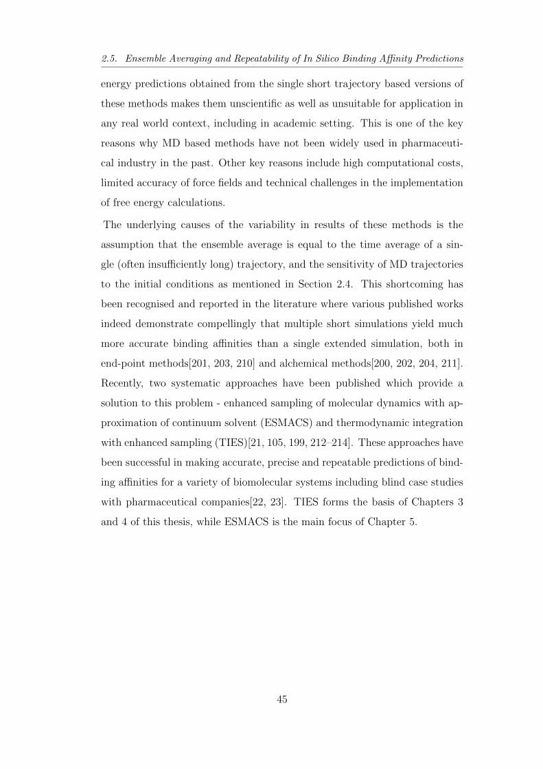
2.5. Ensemble Averaging and Repeatability of In Silico Binding Affinity Predictions
energy predictions obtained from the single short trajectory based versions of
these methods makes them unscientific as well as unsuitable for application in
any real world context, including in academic setting. This is one of the key
reasons why MD based methods have not been widely used in pharmaceuti-
cal industry in the past. Other key reasons include high computational costs,
limited accuracy of force fields and technical challenges in the implementation
of free energy calculations.
The underlying causes of the variability in results of these methods is the
assumption that the ensemble average is equal to the time average of a sin-
gle (often insufficiently long) trajectory, and the sensitivity of MD trajectories
to the initial conditions as mentioned in Section 2.4. This shortcoming has
been recognised and reported in the literature where various published works
indeed demonstrate compellingly that multiple short simulations yield much
more accurate binding affinities than a single extended simulation, both in
end-point methods[201, 203, 210] and alchemical methods[200, 202, 204, 211].
Recently, two systematic approaches have been published which provide a
solution to this problem - enhanced sampling of molecular dynamics with ap-
proximation of continuum solvent (ESMACS) and thermodynamic integration
with enhanced sampling (TIES)[21, 105, 199, 212–214]. These approaches have
been successful in making accurate, precise and repeatable predictions of bind-
ing affinities for a variety of biomolecular systems including blind case studies
with pharmaceutical companies[22, 23]. TIES forms the basis of Chapters 3
and 4 of this thesis, while ESMACS is the main focus of Chapter 5.
45

Chapter 3
Thermodynamic Integration
with Enhanced Sampling
In Chapter 2, several methods available for in silico binding affinity predictions
were mentioned. The importance of the ability to make reliable predictions of
binding affinities for ligand-protein complexes in real-world was mentioned in
Chapter 1. However, as noted in Chapter 2, the free energy methods based on
classical MD simulations suffer from the problem of variability in results when
running a single short simulation by virtue of the sensitivity of MD trajecto-
ries to the initial conditions. Ensemble simulation can be used to overcome
this problem. In this chapter, a new method called thermodynamic integra-
tion with enhanced sampling (TIES) is described, which utilises the idea of
ensemble simulation to yield accurate, precise and repeatable relative binding
affinities. TIES is based on one of the “exact” free energy methods, ther-
modynamic integration (TI), described in Chapter 2. Based on calculating
ensemble averages, it allows quantification of statistical uncertainties associ-
ated with the results. TIES has been shown to perform well for a wide range
of target proteins and ligands.
As has been emphasised in Chapter 1, reliable binding affinity predictions need
to be made on time scales comparable to, if not shorter than, the experimental
ones in order to have any impact in drug design. In the case of personalised
medicine, in silico methods should be able to make reliable predictions in a
Chapter 3. Thermodynamic Integration with Enhanced Sampling
few hours to be useful in clinical context. Therefore, the time to solution is an-
other important factor influencing the applicability of computational methods
in real-world. Currently, the wall-clock time requirements for predictions by
TIES (∼6-8 hours; reduced by a factor of 3-5 with GPUs) fulfil these require-
ments given the availability of sufficient computer resources. In fact, the TIES
approach has been employed in collaborative studies with two pharmaceuti-
cal companies (GlaxoSmithKline and Pfizer), yielding accurate and precise
relative binding affinity predictions[22, 23].
A method called independent trajectory TI (IT-TI)[204] has been reported
in the literature, and attempts to use multiple independent trajectories to
improve the accuracy of calculated free energies. Genheden et al. have also
shown that performing several independent trajectories yields better estimates
of free energies[215]. However, TIES involves a systematic application of the
concept of ensemble simulation for “exact” free energy calculations which is
different from the act of merely repeating the calculation a small number of
times as will be shown later in this chapter. The TIES methodology and most
of the results included in this chapter have been published and some figures
and tables have been reproduced from the published articles[21–23].
3.1 Ensemble Simulation Based Thermody-
namic Integration
TIES is based on the “exact” free energy method TI which was described in
Section 2.3.2. TI involves numerically integrating the potential energy deriva-
tive with respect to λ (∂E/∂λ), where λ is the alchemical coupling parameter
(see Equation 2.26). Therefore, to get a reliable free energy change ∂E/∂λ
values should be accurate, precise and repeatable which is not achievable us-
ing a single short MD simulation at each λ-window. TIES involves running
an ensemble simulation at each λ-window. All replica simulations of the en-
semble have identical initial conditions except their initial velocities, which
48
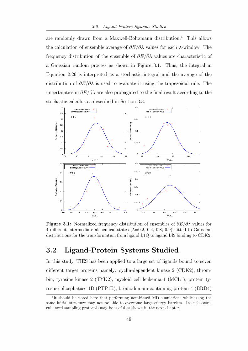
3.2. Ligand-Protein Systems Studied
are randomly drawn from a Maxwell-Boltzmann distribution.∗ This allows
the calculation of ensemble average of ∂E/∂λ values for each λ-window. The
frequency distribution of the ensemble of ∂E/∂λ values are characteristic of
a Gaussian random process as shown in Figure 3.1. Thus, the integral in
Equation 2.26 is interpreted as a stochastic integral and the average of the
distribution of ∂E/∂λ is used to evaluate it using the trapezoidal rule. The
uncertainties in ∂E/∂λ are also propagated to the final result according to the
stochastic calculus as described in Section 3.3.
Figure 3.1: Normalized frequency distribution of ensembles of ∂E/∂λ values for4 different intermediate alchemical states (λ=0.2, 0.4, 0.8, 0.9), fitted to Gaussiandistributions for the transformation from ligand L1Q to ligand LI9 binding to CDK2.
3.2 Ligand-Protein Systems Studied
In this study, TIES has been applied to a large set of ligands bound to seven
different target proteins namely: cyclin-dependent kinase 2 (CDK2), throm-
bin, tyrosine kinase 2 (TYK2), myeloid cell leukemia 1 (MCL1), protein ty-
rosine phosphatase 1B (PTP1B), bromodomain-containing protein 4 (BRD4)
∗It should be noted here that performing non-biased MD simulations while using thesame initial structure may not be able to overcome large energy barriers. In such cases,enhanced sampling protocols may be useful as shown in the next chapter.
49
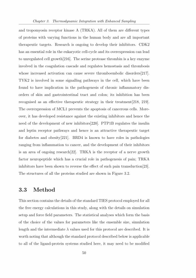
Chapter 3. Thermodynamic Integration with Enhanced Sampling
and tropomyosin receptor kinase A (TRKA). All of them are different types
of proteins with varying functions in the human body and are all important
therapeutic targets. Research is ongoing to develop their inhibitors. CDK2
has an essential role in the eukaryotic cell-cycle and its overexpression can lead
to unregulated cell growth[216]. The serine protease thrombin is a key enzyme
involved in the coagulation cascade and regulates hemostasis and thrombosis
whose increased activation can cause severe thromboembolic disorders[217].
TYK2 is involved in some signalling pathways in the cell, which have been
found to have implication in the pathogenesis of chronic inflammatory dis-
orders of skin and gastrointestinal tract and colon; its inhibition has been
recognised as an effective therapeutic strategy in their treatment[218, 219].
The overexpression of MCL1 prevents the apoptosis of cancerous cells. More-
over, it has developed resistance against the existing inhibitors and hence the
need of the development of new inhibitors[220]. PTP1B regulates the insulin
and leptin receptor pathways and hence is an attractive therapeutic target
for diabetes and obesity[221]. BRD4 is known to have roles in pathologies
ranging from inflammation to cancer, and the development of their inhibitors
is an area of ongoing research[22]. TRKA is the receptor of a nerve growth
factor neuropeptide which has a crucial role in pathogenesis of pain; TRKA
inhibitors have been shown to reverse the effect of such pain transduction[23].
The structures of all the proteins studied are shown in Figure 3.2.
3.3 Method
This section contains the details of the standard TIES protocol employed for all
the free energy calculations in this study, along with the details on simulation
setup and force field parameters. The statistical analyses which form the basis
of the choice of the values for parameters like the ensemble size, simulation
length and the intermediate λ values used for this protocol are described. It is
worth noting that although the standard protocol described below is applicable
to all of the ligand-protein systems studied here, it may need to be modified
50
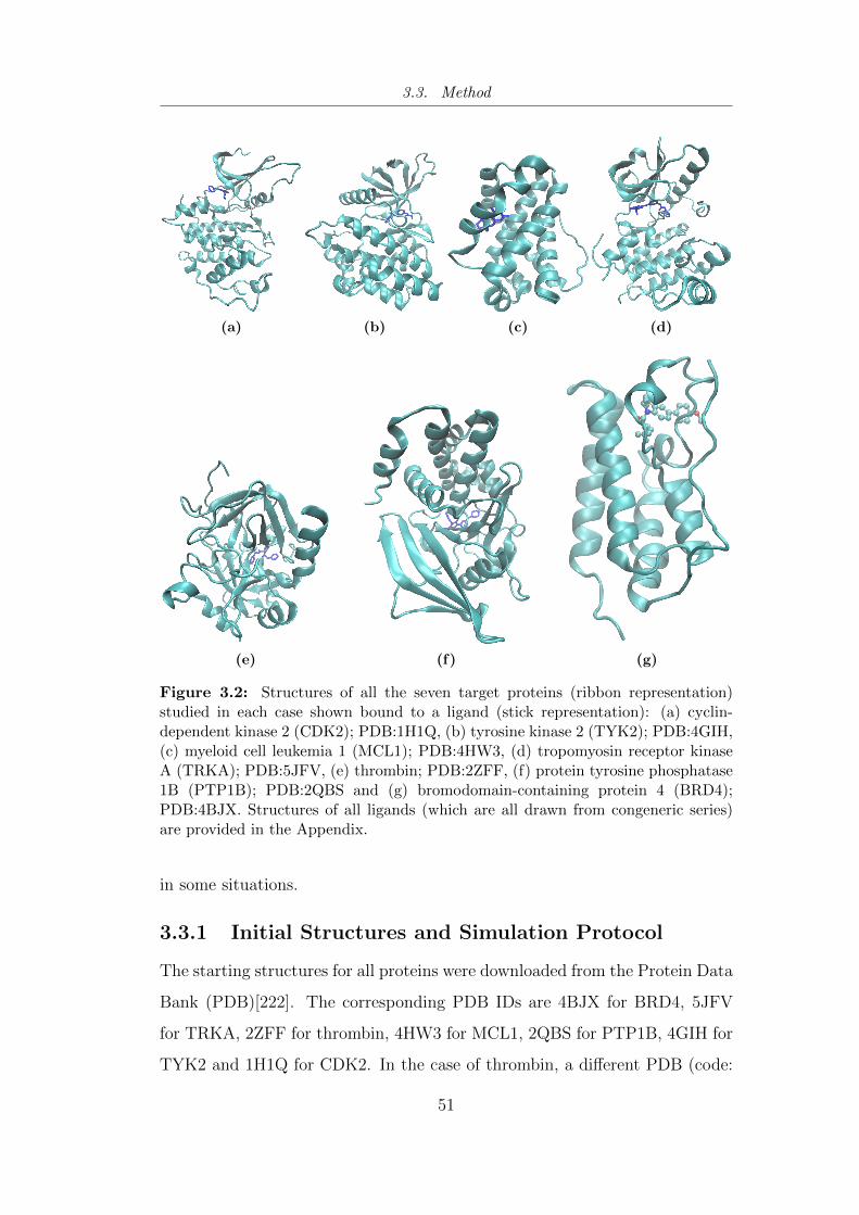
3.3. Method
(a) (b) (c) (d)
(e) (f) (g)
Figure 3.2: Structures of all the seven target proteins (ribbon representation)studied in each case shown bound to a ligand (stick representation): (a) cyclin-dependent kinase 2 (CDK2); PDB:1H1Q, (b) tyrosine kinase 2 (TYK2); PDB:4GIH,(c) myeloid cell leukemia 1 (MCL1); PDB:4HW3, (d) tropomyosin receptor kinaseA (TRKA); PDB:5JFV, (e) thrombin; PDB:2ZFF, (f) protein tyrosine phosphatase1B (PTP1B); PDB:2QBS and (g) bromodomain-containing protein 4 (BRD4);PDB:4BJX. Structures of all ligands (which are all drawn from congeneric series)are provided in the Appendix.
in some situations.
3.3.1 Initial Structures and Simulation Protocol
The starting structures for all proteins were downloaded from the Protein Data
Bank (PDB)[222]. The corresponding PDB IDs are 4BJX for BRD4, 5JFV
for TRKA, 2ZFF for thrombin, 4HW3 for MCL1, 2QBS for PTP1B, 4GIH for
TYK2 and 1H1Q for CDK2. In the case of thrombin, a different PDB (code:
51
Chapter 3. Thermodynamic Integration with Enhanced Sampling
2ZC9) was used as the starting structure while studying the transformation
of unsubstituted benzylamine to meta-substituted benzylamide as the water
molecule initially present in the S1 pocket of the protein get displaced by the
appearing substituent at the meta position (see Section 3.5 for details). The
ligand structures in case of CDK2, TYK2, MCL1, PTP1B and thrombin were
downloaded from the Supporting Information of an open access article[196].
The ligand structures for BRD4 and TRKA were provided by our experimental
collaborators at the pharmaceutical companies GSK and Pfizer respectively.
All the protein-ligand complexes were simulated in an orthorhombic water
box with a buffer width of 14 A. The net charge of the system was neu-
tralised by addition of counterions. The AMBER ff99SB-ILDN force field[223]
was used for protein parameters and general AMBER force field (GAFF)[41]
was employed for ligands. TIP3P model [224] was used for water molecules.
Standard protonation states were assigned to all titratable residues at pH 7,
with histidines protonated on the ε position (HIE). The partial atomic charges
for ligand atoms were calculated using the restrained electrostatic potential
(RESP) method after geometry optimisation by Gaussian03 package using the
Hartree-Fock method and 6-31G** basis set. RESP calculations were per-
formed using Antechamber (AmberTools 12). All simulations were performed
using the package NAMD 2.9[45] with three-dimensional periodic boundary
conditions. A cut-off of 12 A was used for non-bonded interactions and long
range Coulomb interactions were calculated using Particle Mesh Ewald (PME)
method.
The simulations were performed in an isothermal-isobaric ensemble at tem-
perature 300 K and pressure 1 bar. Langevin thermostat (with a damping
coefficient of 5 ps−1) and Berendsen barostat (compressibility of 4.57 × 10⁻⁵
bar−1 and a relaxation time of 100 fs) were used to maintain the temperature
and the pressure at these values. Constrained dynamics with a time step of 2 fs
were performed employing RATTLE algorithm. A soft core van der Waals po-
tential was used to avoid the problem of end point catastrophes as described in
52
3.3. Method
the previous chapter. The electrostatic interactions of the disappearing atoms
were decoupled linearly between λ = 0 and 0.55, and do not interact at all
beyond that; for appearing atoms they were linearly coupled between λ = 0.45
and 1, and do not interact otherwise.
3.3.2 Hybrid Ligand Structure and Parameters
In this study, alchemical transformations of ligands have been studied using
dual topology scheme[225]. A hybrid ligand contains a common region to
which both the disappearing part (belonging exclusively to the initial state)
and the appearing part (belonging exclusively to the final state) are bonded.
The latter two do not interact with each other at all. The initial structure of
the hybrid ligand for an alchemical transformation from ligand L1 to ligand L2
is generated by simply appending the coordinates of the set of appearing atoms
from L2 to the structure file of L1 after aligning the coordinates of all atoms in
their common region. The last atom of the common region in the hybrid ligand
is connected to the first atom of both the disappearing as well as the appearing
regions. In order to ensure that the common region is chemically similar in
both the ligands, it is chosen such that the overall charge of all the atoms as
well as the charge on each atom in the common region do not vary by more
than 0.1 e in individual ligands. However, this threshold limit of 0.1 e may
need to be relaxed in the cases of highly charged or polar ligands. The partial
atomic charges need to be recalculated for the hybrid ligand so as to have
unique charges for the atoms in the common region. This is done by setting
the latter’s charges in the hybrid ligand to the average of their charges in
the individual ligands. Thereafter, the charges on disappearing and appearing
parts are adapted accordingly by reparametrising the individual ligands after
constraining the charges on the common part to their newly derived values.
3.3.3 Protocol for Free Energy Calculation
Figure 3.3 shows a schematic of the protocol used to calculate all the free
energies in this study. A total of 13 values for the alchemical coupling param-
53
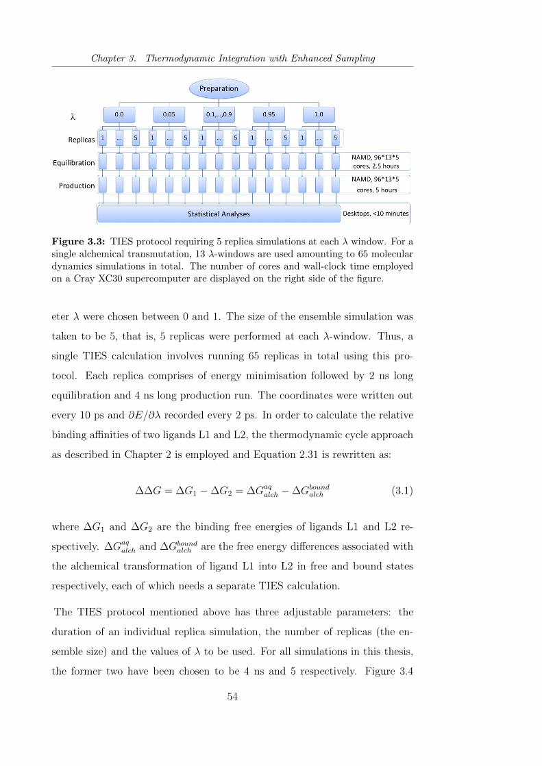
Chapter 3. Thermodynamic Integration with Enhanced Sampling
Figure 3.3: TIES protocol requiring 5 replica simulations at each λ window. For asingle alchemical transmutation, 13 λ-windows are used amounting to 65 moleculardynamics simulations in total. The number of cores and wall-clock time employedon a Cray XC30 supercomputer are displayed on the right side of the figure.
eter λ were chosen between 0 and 1. The size of the ensemble simulation was
taken to be 5, that is, 5 replicas were performed at each λ-window. Thus, a
single TIES calculation involves running 65 replicas in total using this pro-
tocol. Each replica comprises of energy minimisation followed by 2 ns long
equilibration and 4 ns long production run. The coordinates were written out
every 10 ps and ∂E/∂λ recorded every 2 ps. In order to calculate the relative
binding affinities of two ligands L1 and L2, the thermodynamic cycle approach
as described in Chapter 2 is employed and Equation 2.31 is rewritten as:
∆∆G = ∆G1 −∆G2 = ∆Gaqalch −∆Gbound
alch (3.1)
where ∆G1 and ∆G2 are the binding free energies of ligands L1 and L2 re-
spectively. ∆Gaqalch and ∆Gbound
alch are the free energy differences associated with
the alchemical transformation of ligand L1 into L2 in free and bound states
respectively, each of which needs a separate TIES calculation.
The TIES protocol mentioned above has three adjustable parameters: the
duration of an individual replica simulation, the number of replicas (the en-
semble size) and the values of λ to be used. For all simulations in this thesis,
the former two have been chosen to be 4 ns and 5 respectively. Figure 3.4
54
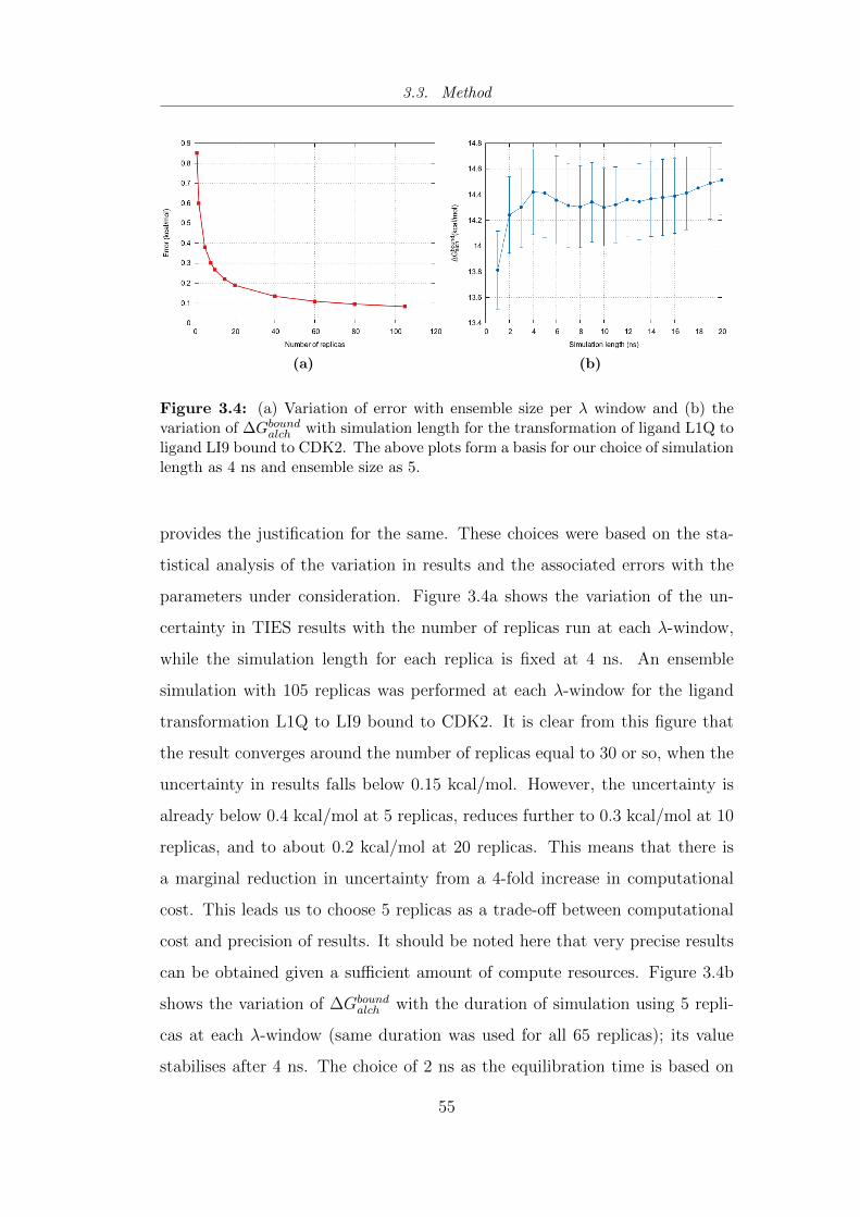
3.3. Method
(a) (b)
Figure 3.4: (a) Variation of error with ensemble size per λ window and (b) thevariation of ∆Gboundalch with simulation length for the transformation of ligand L1Q toligand LI9 bound to CDK2. The above plots form a basis for our choice of simulationlength as 4 ns and ensemble size as 5.
provides the justification for the same. These choices were based on the sta-
tistical analysis of the variation in results and the associated errors with the
parameters under consideration. Figure 3.4a shows the variation of the un-
certainty in TIES results with the number of replicas run at each λ-window,
while the simulation length for each replica is fixed at 4 ns. An ensemble
simulation with 105 replicas was performed at each λ-window for the ligand
transformation L1Q to LI9 bound to CDK2. It is clear from this figure that
the result converges around the number of replicas equal to 30 or so, when the
uncertainty in results falls below 0.15 kcal/mol. However, the uncertainty is
already below 0.4 kcal/mol at 5 replicas, reduces further to 0.3 kcal/mol at 10
replicas, and to about 0.2 kcal/mol at 20 replicas. This means that there is
a marginal reduction in uncertainty from a 4-fold increase in computational
cost. This leads us to choose 5 replicas as a trade-off between computational
cost and precision of results. It should be noted here that very precise results
can be obtained given a sufficient amount of compute resources. Figure 3.4b
shows the variation of ∆Gboundalch with the duration of simulation using 5 repli-
cas at each λ-window (same duration was used for all 65 replicas); its value
stabilises after 4 ns. The choice of 2 ns as the equilibration time is based on
55
Chapter 3. Thermodynamic Integration with Enhanced Sampling
the observation that the cumulative averages of ∂E/∂λ converge within this
duration, as shown in Figure 3.5. Several previous studies from my group have
reported a similar convergence behaviour for a large variety of ligand-protein
systems[214, 226]. It should be noted that we used CDK2 as a representative
system to establish a standard protocol for all systems in this study. This
holds true in the current scenario as all systems investigated here have rela-
tively rigid ligands and small globular protein. However, if the system being
studied has a flexible ligand or larger protein, it may be necessary to increase
the ensemble size and/or simulation duration to improve sampling and the
precision of results.
Figure 3.3 indicates the number of cores and wall-clock time required for a
typical TIES calculation. It is possible to finish the entire calculation using
the protocol mentioned above in ∼6-8 hours given sufficient computational
resources. This is of course dependent on the size of the system studied and
the number of cores used (GPUs may further reduce the time). The important
thing is that the TIES workflow is perfectly scalable and it is possible to
perform multiple calculations concurrently by increasing the allocated cores
keeping the wall clock time same as that for a single calculation.
3.3.4 Stochastic Integration and Error Propagation
As mentioned in Section 3.1, ∂E/∂λ has the characteristic of Gaussian ran-
dom variable (Figure 3.1). Therefore, in TIES, the integral in Equation 2.26 is
interpreted in terms of stochastic calculus. Each point of the integrand is the
ensemble average of ∂E/∂λ at that λ-window, which is taken to be the average
of its values from all five replicas such that the value from each replica is itself
the average over the whole simulation length. The integral is then calculated
numerically using the values of the integrand so obtained. The error in the
value of integrand at window λ (σλ) is taken to be the bootstrapped standard
error of the mean of potential derivatives from all replicas. In stochastic cal-
culus, the integral of a Gaussian random process is itself a Gaussian random
process and the variance on the resultant integral is the convolution of the
56
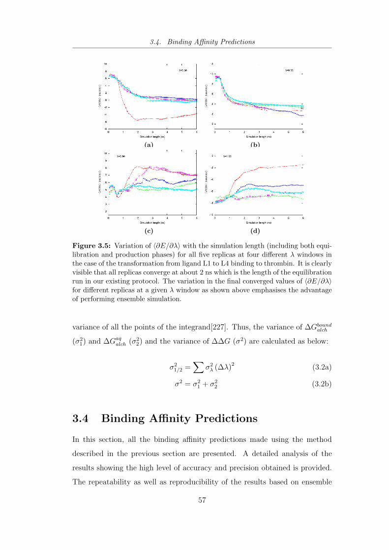
3.4. Binding Affinity Predictions
(a) (b)
(c) (d)
Figure 3.5: Variation of 〈∂E/∂λ〉 with the simulation length (including both equi-libration and production phases) for all five replicas at four different λ windows inthe case of the transformation from ligand L1 to L4 binding to thrombin. It is clearlyvisible that all replicas converge at about 2 ns which is the length of the equilibrationrun in our existing protocol. The variation in the final converged values of 〈∂E/∂λ〉for different replicas at a given λ window as shown above emphasises the advantageof performing ensemble simulation.
variance of all the points of the integrand[227]. Thus, the variance of ∆Gboundalch
(σ21) and ∆Gaq
alch (σ22) and the variance of ∆∆G (σ2) are calculated as below:
σ21/2 =
∑σ2λ (∆λ)2 (3.2a)
σ2 = σ21 + σ2
2 (3.2b)
3.4 Binding Affinity Predictions
In this section, all the binding affinity predictions made using the method
described in the previous section are presented. A detailed analysis of the
results showing the high level of accuracy and precision obtained is provided.
The repeatability as well as reproducibility of the results based on ensemble
57
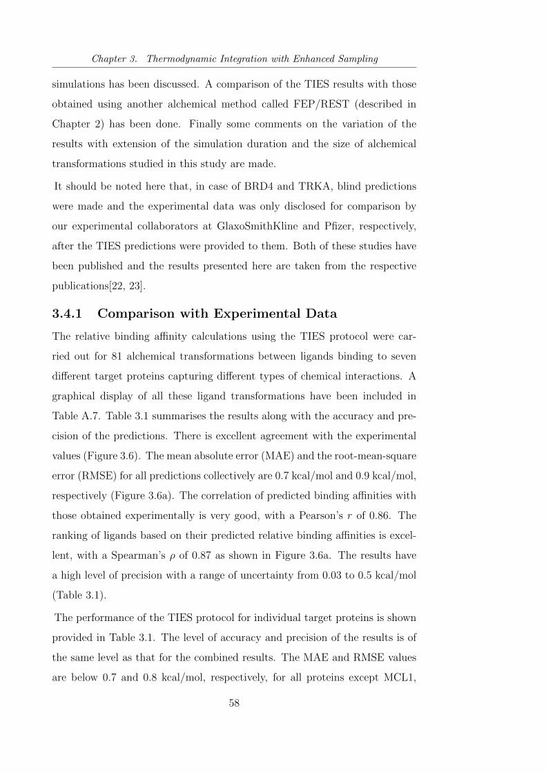
Chapter 3. Thermodynamic Integration with Enhanced Sampling
simulations has been discussed. A comparison of the TIES results with those
obtained using another alchemical method called FEP/REST (described in
Chapter 2) has been done. Finally some comments on the variation of the
results with extension of the simulation duration and the size of alchemical
transformations studied in this study are made.
It should be noted here that, in case of BRD4 and TRKA, blind predictions
were made and the experimental data was only disclosed for comparison by
our experimental collaborators at GlaxoSmithKline and Pfizer, respectively,
after the TIES predictions were provided to them. Both of these studies have
been published and the results presented here are taken from the respective
publications[22, 23].
3.4.1 Comparison with Experimental Data
The relative binding affinity calculations using the TIES protocol were car-
ried out for 81 alchemical transformations between ligands binding to seven
different target proteins capturing different types of chemical interactions. A
graphical display of all these ligand transformations have been included in
Table A.7. Table 3.1 summarises the results along with the accuracy and pre-
cision of the predictions. There is excellent agreement with the experimental
values (Figure 3.6). The mean absolute error (MAE) and the root-mean-square
error (RMSE) for all predictions collectively are 0.7 kcal/mol and 0.9 kcal/mol,
respectively (Figure 3.6a). The correlation of predicted binding affinities with
those obtained experimentally is very good, with a Pearson’s r of 0.86. The
ranking of ligands based on their predicted relative binding affinities is excel-
lent, with a Spearman’s ρ of 0.87 as shown in Figure 3.6a. The results have
a high level of precision with a range of uncertainty from 0.03 to 0.5 kcal/mol
(Table 3.1).
The performance of the TIES protocol for individual target proteins is shown
provided in Table 3.1. The level of accuracy and precision of the results is of
the same level as that for the combined results. The MAE and RMSE values
are below 0.7 and 0.8 kcal/mol, respectively, for all proteins except MCL1,
58
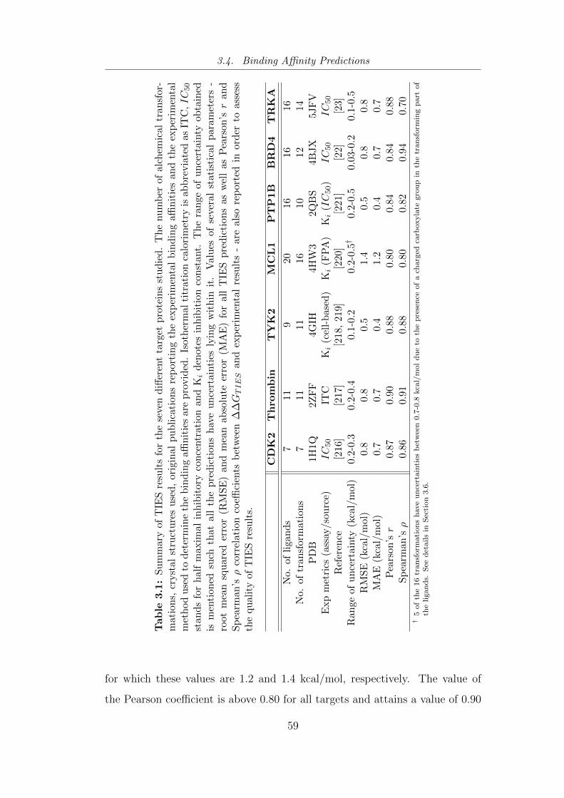
3.4. Binding Affinity Predictions
Tab
le3.1
:S
um
mary
ofT
IES
resu
lts
for
the
seve
nd
iffer
ent
targ
etp
rote
ins
stu
die
d.
Th
enu
mb
erof
alch
emic
altr
ansf
or-
mati
on
s,cr
yst
al
stru
ctu
res
use
d,
orig
inal
pu
bli
cati
ons
rep
orti
ng
the
exp
erim
enta
lb
ind
ing
affin
itie
san
dth
eex
per
imen
tal
met
hod
use
dto
det
erm
ine
the
bin
din
gaffi
nit
ies
are
pro
vid
ed.
Isot
her
mal
titr
atio
nca
lori
met
ryis
abb
revia
ted
asIT
C,IC
50
stan
ds
for
half
maxim
alin
hib
itory
con
centr
atio
nan
dKi
den
otes
inh
ibit
ion
con
stan
t.T
he
ran
geof
un
cert
ainty
obta
ined
ism
enti
on
edsu
chth
at
all
the
pre
dic
tion
sh
ave
un
cert
ainti
esly
ing
wit
hin
it.
Val
ues
ofse
ver
alst
atis
tica
lp
aram
eter
s-
root
mea
nsq
uare
der
ror
(RM
SE
)an
dm
ean
abso
lute
erro
r(M
AE
)fo
ral
lT
IES
pre
dic
tion
sas
wel
las
Pea
rson
’sr
and
Sp
earm
an’sρ
corr
elat
ion
coeffi
cien
tsb
etw
een
∆∆GTIES
and
exp
erim
enta
lre
sult
s-
are
also
rep
orte
din
ord
erto
asse
ssth
equ
ali
tyof
TIE
Sre
sult
s.
CD
K2
Th
rom
bin
TY
K2
MC
L1
PT
P1B
BR
D4
TR
KA
No.
of
liga
nd
s7
119
2016
1616
No.
of
tran
sform
atio
ns
711
1116
1012
14P
DB
1H
1Q2Z
FF
4GIH
4HW
32Q
BS
4BJX
5JF
VE
xp
met
rics
(ass
ay/so
urc
e)IC
50
ITC
Ki
(cel
l-b
ased
)Ki
(FP
A)
Ki
(IC
50)
IC
50
IC
50
Ref
eren
ce[2
16]
[217
][2
18,
219]
[220
][2
21]
[22]
[23]
Ran
geof
un
cert
ain
ty(k
cal/
mol)
0.2
-0.3
0.2-
0.4
0.1-
0.2
0.2-
0.5†
0.2-
0.5
0.03
-0.2
0.1-
0.5
RM
SE
(kca
l/m
ol)
0.8
0.8
0.5
1.4
0.5
0.8
0.8
MA
E(k
cal/
mol)
0.7
0.7
0.4
1.2
0.4
0.7
0.7
Pea
rson
’sr
0.8
70.
900.
880.
800.
840.
840.
88S
pea
rman
’sρ
0.8
60.
910.
880.
800.
820.
940.
70†
5of
the
16
tran
sform
ati
ons
have
un
cert
ain
ties
bet
wee
n0.7
-0.8
kca
l/m
ol
du
eto
the
pre
sen
ceof
ach
arg
edca
rboxyla
tegro
up
inth
etr
an
sform
ing
part
of
the
ligan
ds.
See
det
ails
inS
ecti
on
3.6
.
for which these values are 1.2 and 1.4 kcal/mol, respectively. The value of
the Pearson coefficient is above 0.80 for all targets and attains a value of 0.90
59
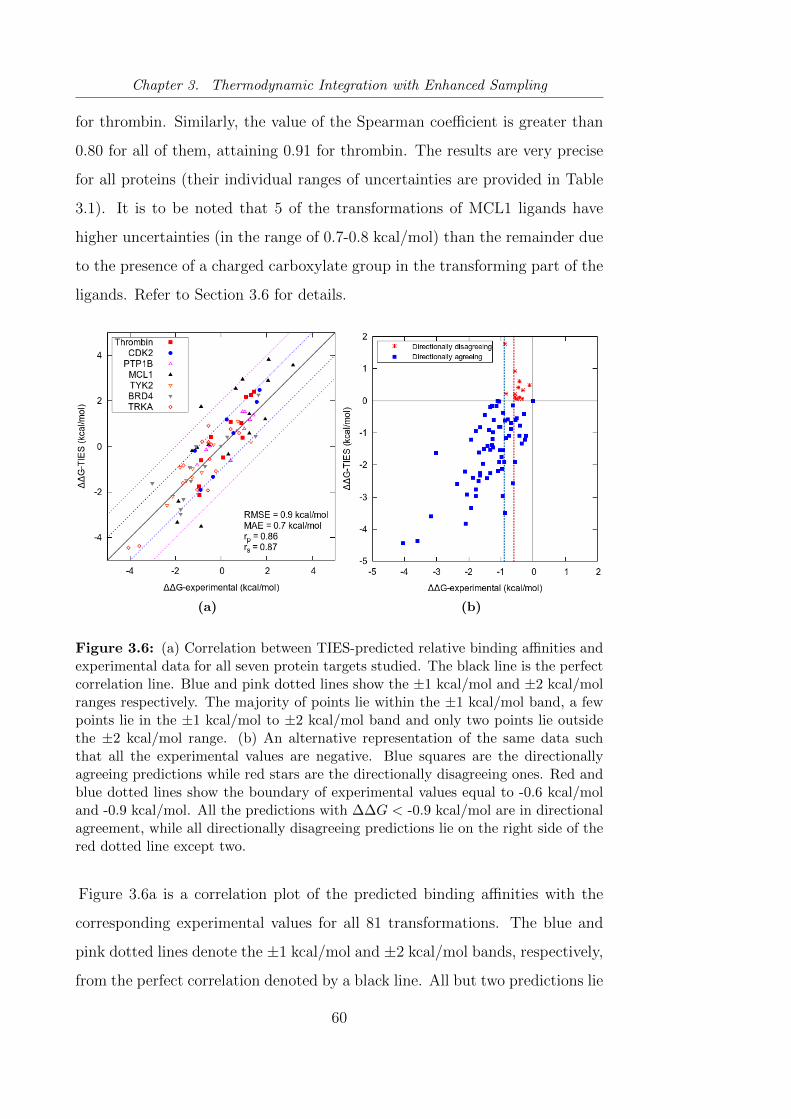
Chapter 3. Thermodynamic Integration with Enhanced Sampling
for thrombin. Similarly, the value of the Spearman coefficient is greater than
0.80 for all of them, attaining 0.91 for thrombin. The results are very precise
for all proteins (their individual ranges of uncertainties are provided in Table
3.1). It is to be noted that 5 of the transformations of MCL1 ligands have
higher uncertainties (in the range of 0.7-0.8 kcal/mol) than the remainder due
to the presence of a charged carboxylate group in the transforming part of the
ligands. Refer to Section 3.6 for details.
(a) (b)
Figure 3.6: (a) Correlation between TIES-predicted relative binding affinities andexperimental data for all seven protein targets studied. The black line is the perfectcorrelation line. Blue and pink dotted lines show the ±1 kcal/mol and ±2 kcal/molranges respectively. The majority of points lie within the ±1 kcal/mol band, a fewpoints lie in the ±1 kcal/mol to ±2 kcal/mol band and only two points lie outsidethe ±2 kcal/mol range. (b) An alternative representation of the same data suchthat all the experimental values are negative. Blue squares are the directionallyagreeing predictions while red stars are the directionally disagreeing ones. Red andblue dotted lines show the boundary of experimental values equal to -0.6 kcal/moland -0.9 kcal/mol. All the predictions with ∆∆G < -0.9 kcal/mol are in directionalagreement, while all directionally disagreeing predictions lie on the right side of thered dotted line except two.
Figure 3.6a is a correlation plot of the predicted binding affinities with the
corresponding experimental values for all 81 transformations. The blue and
pink dotted lines denote the ±1 kcal/mol and ±2 kcal/mol bands, respectively,
from the perfect correlation denoted by a black line. All but two predictions lie
60
3.4. Binding Affinity Predictions
within the pink lines, while a few of them lie between the blue and pink lines.
The high level of accuracy can be noted by the fact that the majority of points
lie within the blue lines. 61 predictions (75.31%) deviate from the experimental
binding affinities by less than 1.0 kcal/mol, while 79 predictions (97.53%) do
so by less than 2 kcal/mol (Table 3.2 (left)). It is worth mentioning here that
experimental binding affinities have significant uncertainties[228, 229]. The
experimental error for relative binding affinities between two compounds has
been reported to be in the range of 0.4-0.7 kcal/mol for high-quality binding
affinity measurements[196]. However, for CDK2, TYK2, MCL1, PTP1B and
thrombin, the error bars on experimental binding affinities are unavailable.
Figure 3.7 shows the correlation for each protein separately along with the
uncertainties in the results shown as error bars.
Table 3.2: A summary of the level of accuracy obtained for the total set of TIESpredictions. The number of predictions found to be accurate for a specified absoluteerror range (left) and the number of predictions found to be in directional agreementwith the increasing absolute values of experimental results (right). The lack ofexperimental errors means that the entire discrepancy is assigned to the theoreticalpredictions.
MAE < No. of predictions0.4 270.6 360.8 491.0 611.2 721.4 74
|∆∆Gexp| > No. of directionallydisagreeing predictions
0.0 130.3 120.4 100.5 60.6 20.9 0
Figure 3.6b represents the results differently. When a prediction has the same
sign as that of the corresponding experimental value it is said to be direction-
ally agreeing with experiments, and otherwise it is taken to be directionally
disagreeing. In Figure 3.6b the data-points from Figure 3.6a are rearranged
such that all the experimental ∆∆G values are negative. This was done by
flipping the signs of all the sets of ∆∆GTIES and ∆∆Gexp for which the latter
was positive originally. This representation of the results helps to see if the
predictions follow the same trend as the experimental values. In Figure 3.6b,
61
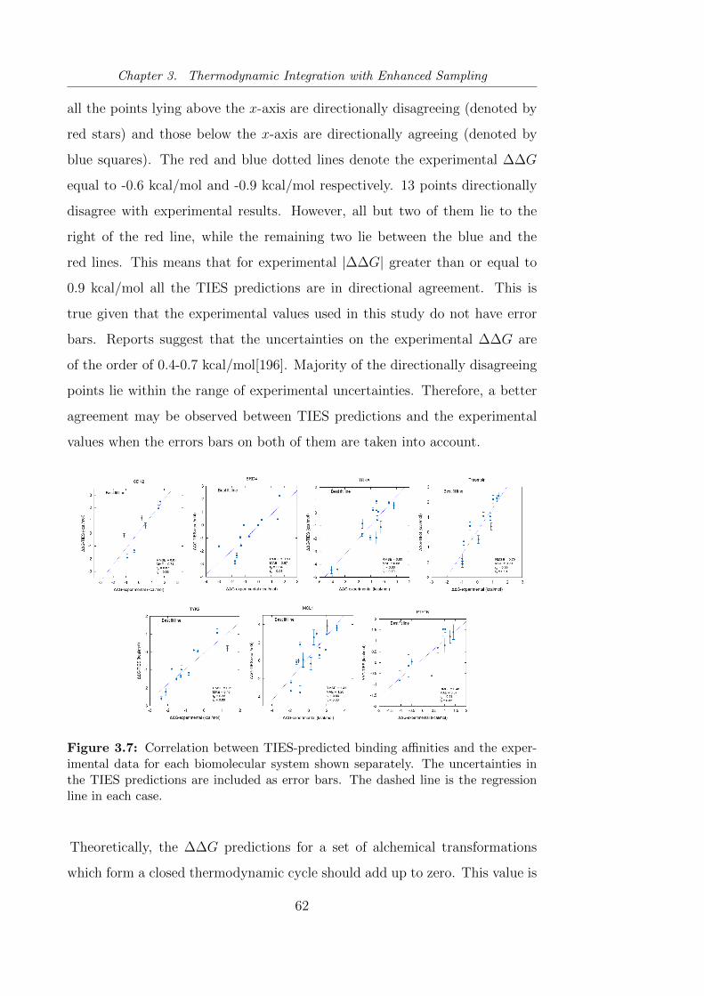
Chapter 3. Thermodynamic Integration with Enhanced Sampling
all the points lying above the x-axis are directionally disagreeing (denoted by
red stars) and those below the x-axis are directionally agreeing (denoted by
blue squares). The red and blue dotted lines denote the experimental ∆∆G
equal to -0.6 kcal/mol and -0.9 kcal/mol respectively. 13 points directionally
disagree with experimental results. However, all but two of them lie to the
right of the red line, while the remaining two lie between the blue and the
red lines. This means that for experimental |∆∆G| greater than or equal to
0.9 kcal/mol all the TIES predictions are in directional agreement. This is
true given that the experimental values used in this study do not have error
bars. Reports suggest that the uncertainties on the experimental ∆∆G are
of the order of 0.4-0.7 kcal/mol[196]. Majority of the directionally disagreeing
points lie within the range of experimental uncertainties. Therefore, a better
agreement may be observed between TIES predictions and the experimental
values when the errors bars on both of them are taken into account.
Figure 3.7: Correlation between TIES-predicted binding affinities and the exper-imental data for each biomolecular system shown separately. The uncertainties inthe TIES predictions are included as error bars. The dashed line is the regressionline in each case.
Theoretically, the ∆∆G predictions for a set of alchemical transformations
which form a closed thermodynamic cycle should add up to zero. This value is
62
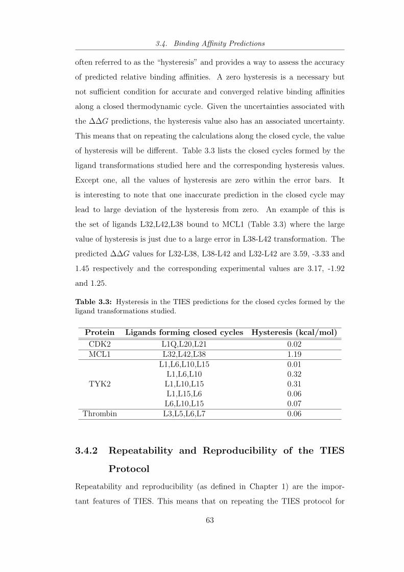
3.4. Binding Affinity Predictions
often referred to as the “hysteresis” and provides a way to assess the accuracy
of predicted relative binding affinities. A zero hysteresis is a necessary but
not sufficient condition for accurate and converged relative binding affinities
along a closed thermodynamic cycle. Given the uncertainties associated with
the ∆∆G predictions, the hysteresis value also has an associated uncertainty.
This means that on repeating the calculations along the closed cycle, the value
of hysteresis will be different. Table 3.3 lists the closed cycles formed by the
ligand transformations studied here and the corresponding hysteresis values.
Except one, all the values of hysteresis are zero within the error bars. It
is interesting to note that one inaccurate prediction in the closed cycle may
lead to large deviation of the hysteresis from zero. An example of this is
the set of ligands L32,L42,L38 bound to MCL1 (Table 3.3) where the large
value of hysteresis is just due to a large error in L38-L42 transformation. The
predicted ∆∆G values for L32-L38, L38-L42 and L32-L42 are 3.59, -3.33 and
1.45 respectively and the corresponding experimental values are 3.17, -1.92
and 1.25.
Table 3.3: Hysteresis in the TIES predictions for the closed cycles formed by theligand transformations studied.
Protein Ligands forming closed cycles Hysteresis (kcal/mol)
CDK2 L1Q,L20,L21 0.02MCL1 L32,L42,L38 1.19
TYK2
L1,L6,L10,L15 0.01L1,L6,L10 0.32L1,L10,L15 0.31L1,L15,L6 0.06L6,L10,L15 0.07
Thrombin L3,L5,L6,L7 0.06
3.4.2 Repeatability and Reproducibility of the TIES
Protocol
Repeatability and reproducibility (as defined in Chapter 1) are the impor-
tant features of TIES. This means that on repeating the TIES protocol for
63
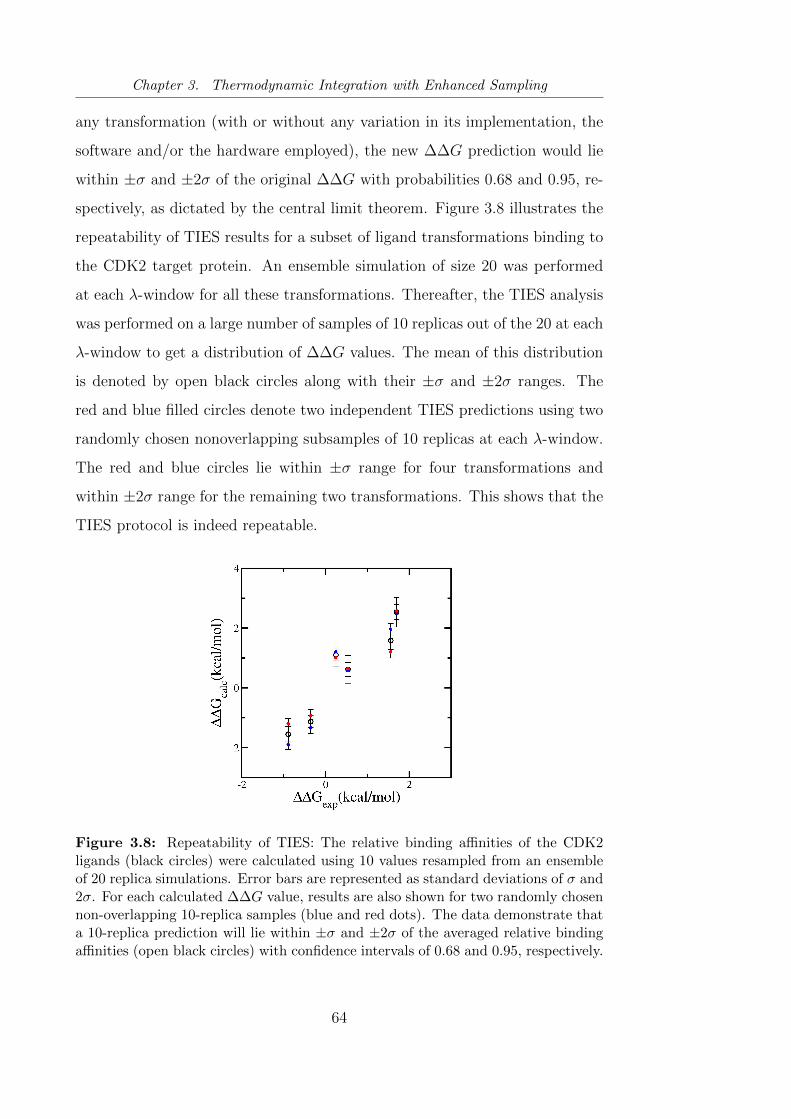
Chapter 3. Thermodynamic Integration with Enhanced Sampling
any transformation (with or without any variation in its implementation, the
software and/or the hardware employed), the new ∆∆G prediction would lie
within ±σ and ±2σ of the original ∆∆G with probabilities 0.68 and 0.95, re-
spectively, as dictated by the central limit theorem. Figure 3.8 illustrates the
repeatability of TIES results for a subset of ligand transformations binding to
the CDK2 target protein. An ensemble simulation of size 20 was performed
at each λ-window for all these transformations. Thereafter, the TIES analysis
was performed on a large number of samples of 10 replicas out of the 20 at each
λ-window to get a distribution of ∆∆G values. The mean of this distribution
is denoted by open black circles along with their ±σ and ±2σ ranges. The
red and blue filled circles denote two independent TIES predictions using two
randomly chosen nonoverlapping subsamples of 10 replicas at each λ-window.
The red and blue circles lie within ±σ range for four transformations and
within ±2σ range for the remaining two transformations. This shows that the
TIES protocol is indeed repeatable.
Figure 3.8: Repeatability of TIES: The relative binding affinities of the CDK2ligands (black circles) were calculated using 10 values resampled from an ensembleof 20 replica simulations. Error bars are represented as standard deviations of σ and2σ. For each calculated ∆∆G value, results are also shown for two randomly chosennon-overlapping 10-replica samples (blue and red dots). The data demonstrate thata 10-replica prediction will lie within ±σ and ±2σ of the averaged relative bindingaffinities (open black circles) with confidence intervals of 0.68 and 0.95, respectively.
64
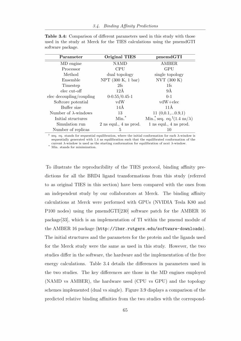
3.4. Binding Affinity Predictions
Table 3.4: Comparison of different parameters used in this study with thoseused in the study at Merck for the TIES calculations using the pmemdGTIsoftware package.
Parameter Original TIES pmemdGTI
MD engine NAMD AMBERProcessor CPU GPUMethod dual topology single topology
Ensemble NPT (300 K, 1 bar) NVT (300 K)Timestep 2fs 1fs
elec cut-off 12A 9Aelec decoupling/coupling 0-0.55/0.45-1 0-1
Softcore potential vdW vdW+elecBuffer size 14A 11A
Number of λ-windows 13 11 (0,0.1,...0.9,1)
Initial structures Min.* Min.*, seq. eq.†(1.4 ns/λ)Simulation run 2 ns equl., 4 ns prod. 1 ns equl., 4 ns prod.
Number of replicas 5 10† seq. eq. stands for sequential equilibration, where the initial conformation for each λ-window is
sequentially generated with 1.4 ns equilibration such that the equilibrated conformation of thecurrent λ-window is used as the starting conformation for equilibration of next λ-window.
* Min. stands for minimization.
To illustrate the reproducibility of the TIES protocol, binding affinity pre-
dictions for all the BRD4 ligand transformations from this study (referred
to as original TIES in this section) have been compared with the ones from
an independent study by our collaborators at Merck. The binding affinity
calculations at Merck were performed with GPUs (NVIDIA Tesla K80 and
P100 nodes) using the pmemdGTI[230] software patch for the AMBER 16
package[33], which is an implementation of TI within the pmemd module of
the AMBER 16 package (http://lbsr.rutgers.edu/software-downloads).
The initial structures and the parameters for the protein and the ligands used
for the Merck study were the same as used in this study. However, the two
studies differ in the software, the hardware and the implementation of the free
energy calculations. Table 3.4 details the differences in parameters used in
the two studies. The key differences are those in the MD engines employed
(NAMD vs AMBER), the hardware used (CPU vs GPU) and the topology
schemes implemented (dual vs single). Figure 3.9 displays a comparison of the
predicted relative binding affinities from the two studies with the correspond-
65
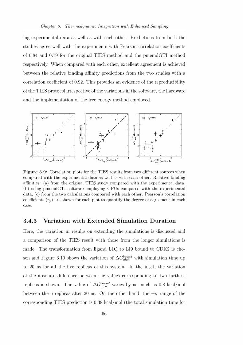
Chapter 3. Thermodynamic Integration with Enhanced Sampling
ing experimental data as well as with each other. Predictions from both the
studies agree well with the experiments with Pearson correlation coefficients
of 0.84 and 0.79 for the original TIES method and the pmemdGTI method
respectively. When compared with each other, excellent agreement is achieved
between the relative binding affinity predictions from the two studies with a
correlation coefficient of 0.92. This provides an evidence of the reproducibility
of the TIES protocol irrespective of the variations in the software, the hardware
and the implementation of the free energy method employed.
Figure 3.9: Correlation plots for the TIES results from two different sources whencompared with the experimental data as well as with each other. Relative bindingaffinities: (a) from the original TIES study compared with the experimental data,(b) using pmemdGTI software employing GPUs compared with the experimentaldata, (c) from the two calculations compared with each other. Pearson’s correlationcoefficients (rp) are shown for each plot to quantify the degree of agreement in eachcase.
3.4.3 Variation with Extended Simulation Duration
Here, the variation in results on extending the simulations is discussed and
a comparison of the TIES result with those from the longer simulations is
made. The transformation from ligand L1Q to LI9 bound to CDK2 is cho-
sen and Figure 3.10 shows the variation of ∆Gboundalch with simulation time up
to 20 ns for all the five replicas of this system. In the inset, the variation
of the absolute difference between the values corresponding to two farthest
replicas is shown. The value of ∆Gboundalch varies by as much as 0.8 kcal/mol
between the 5 replicas after 20 ns. On the other hand, the ±σ range of the
corresponding TIES prediction is 0.38 kcal/mol (the total simulation time for
66
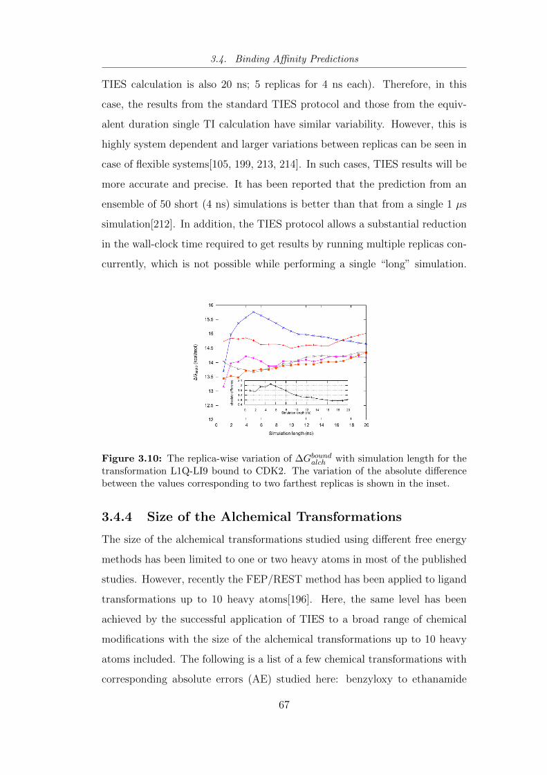
3.4. Binding Affinity Predictions
TIES calculation is also 20 ns; 5 replicas for 4 ns each). Therefore, in this
case, the results from the standard TIES protocol and those from the equiv-
alent duration single TI calculation have similar variability. However, this is
highly system dependent and larger variations between replicas can be seen in
case of flexible systems[105, 199, 213, 214]. In such cases, TIES results will be
more accurate and precise. It has been reported that the prediction from an
ensemble of 50 short (4 ns) simulations is better than that from a single 1 µs
simulation[212]. In addition, the TIES protocol allows a substantial reduction
in the wall-clock time required to get results by running multiple replicas con-
currently, which is not possible while performing a single “long” simulation.
Figure 3.10: The replica-wise variation of ∆Gboundalch with simulation length for thetransformation L1Q-LI9 bound to CDK2. The variation of the absolute differencebetween the values corresponding to two farthest replicas is shown in the inset.
3.4.4 Size of the Alchemical Transformations
The size of the alchemical transformations studied using different free energy
methods has been limited to one or two heavy atoms in most of the published
studies. However, recently the FEP/REST method has been applied to ligand
transformations up to 10 heavy atoms[196]. Here, the same level has been
achieved by the successful application of TIES to a broad range of chemical
modifications with the size of the alchemical transformations up to 10 heavy
atoms included. The following is a list of a few chemical transformations with
corresponding absolute errors (AE) studied here: benzyloxy to ethanamide
67

Chapter 3. Thermodynamic Integration with Enhanced Sampling
(AE = 0.5 kcal/mol), cyclohexyl to phenyl (AE = 0.5 kcal/mol), cyclopentyl
to cycloheptyl (AE = 0.0 kcal/mol), indole to indane (AE = 2.1 kcal/mol),
cyclohexyl methyl to 2,2,4,4-tetramethylcyclohexyl (AE = 0.2 kcal/mol), ben-
zamide to p-fluorobenzenesulfonamide (AE = 0.6 kcal/mol) and hydrogen to
methyl cyclohexane (AE = 0.1 kcal/mol).
3.4.5 Comparison with Another In Silico Method
FEP/REST (described in Chapter 2) has recently attracted a lot of attention
by pharmaceutical companies as a reliable tool to be applicable in their virtual
screening of ligands. It should be noted that FEP/REST, as published by
Wang et al.[196], relies on a single MD simulation at each λ-window. In this
study, five of the target proteins (CDK2, TYK2, MCL1, PTP1B and thrombin)
and corresponding ligands used are the same as those used by Wang et al.,
and hence a direct comparison of TIES predictions is made with theirs. The
RMSE and MAE for each protein target using TIES (Table 3.1) are smaller
than those reported by Wang et al., except for MCL1, for which they are
the same in both cases. The correlation coefficients obtained using TIES are
better than those from FEP/REST in the case of CDK2 (0.87 versus 0.48)
and thrombin (0.90 versus 0.71), while almost the same for the other proteins.
81.82% and 96.36% of TIES predictions are accurate within MAE range of 1.0
and 2.0 kcal/mol (these percentages are just considering the transformations
corresponding to the five proteins which are in common with FEP/REST),
respectively, while these values from Wang et al.’s report are 63.3% and 92.4%,
respectively. Eighteen of the transformations studied here are in common with
those studied by Wang et al. using their FEP/REST method[196]. Figure
3.11 shows a direct comparison of these 18 predictions from both the studies.
The results from TIES are marginally better with slightly larger correlation
coefficients and smaller RMSE and MAE. The number of transformations with
MAE larger than 1 kcal/mol is only one in the case of TIES while three in
the case of FEP/REST. The number of directionally disagreeing predictions in
the case of TIES and FEP/REST are 1 and 2, respectively. It is important to
68
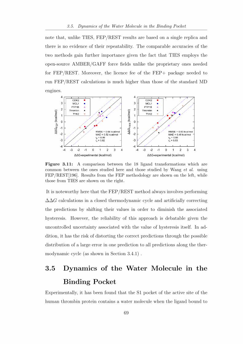
3.5. Dynamics of the Water Molecule in the Binding Pocket
note that, unlike TIES, FEP/REST results are based on a single replica and
there is no evidence of their repeatability. The comparable accuracies of the
two methods gain further importance given the fact that TIES employs the
open-source AMBER/GAFF force fields unlike the proprietary ones needed
for FEP/REST. Moreover, the licence fee of the FEP+ package needed to
run FEP/REST calculations is much higher than those of the standard MD
engines.
Figure 3.11: A comparison between the 18 ligand transformations which arecommon between the ones studied here and those studied by Wang et al. usingFEP/REST[196]. Results from the FEP methodology are shown on the left, whilethose from TIES are shown on the right.
It is noteworthy here that the FEP/REST method always involves performing
∆∆G calculations in a closed thermodynamic cycle and artificially correcting
the predictions by shifting their values in order to diminish the associated
hysteresis. However, the reliability of this approach is debatable given the
uncontrolled uncertainty associated with the value of hysteresis itself. In ad-
dition, it has the risk of distorting the correct predictions through the possible
distribution of a large error in one prediction to all predictions along the ther-
modynamic cycle (as shown in Section 3.4.1) .
3.5 Dynamics of the Water Molecule in the
Binding Pocket
Experimentally, it has been found that the S1 pocket of the active site of the
human thrombin protein contains a water molecule when the ligand bound to
69

Chapter 3. Thermodynamic Integration with Enhanced Sampling
it has no substituent on the benzylamine ring[217]. This water molecule plays
an important role in the ligand binding by mediating the hydrogen bonding
between the amidino group of the ligand and the protein. However, if the
benzylamide ring of the ligand has a substituent at the meta-position, the wa-
ter molecule is absent. In this study, TIES methodology has been applied to
study the transformation from meta-substituted benzylamide to benzylamine
(denoted as A) and the reverse of this transformation (denoted as B); the
predictions are in excellent agreement with those from experiments. TIES
predicted ∆∆G values for the transformations A and B are 0.6 ± 0.2 kcal/mol
and 1.0 ± 0.2 kcal/mol, respectively; the corresponding values from experi-
ments are -0.9 and 0.9 kcal/mol, respectively. In addition, TIES successfully
captures the dynamics of the water being pushed into the S1 pocket (in the case
of transformation A) and pushed out from there (in the case of transformation
B). The presence of water molecule in the S1 pocket has been quantified by
calculating the probability of the occurrence of a water molecule in a cubic box
(volume 1000 A3) centered around the S1 pocket over all conformations from
the five replicas after aligning them to the initial structure. The probability
goes from 0 at λ = 0 to 0.7 at λ = 1 for transformation A and from 0.6 at λ = 0
to 0.3 at λ = 1 for transformation B. The two end points (λ = 0, 1) of trans-
formation A have been displayed in Figure 3.12 along with a representation of
the occurrence of water molecule in the S1 pocket. The red frames represent
the regions where the number density of water oxygen atoms is greater than or
equal to that in bulk water. It is evident that the presence of water molecules
is confined to channels C1 and C2 in the presence of a chlorine atom on the
meta-position of the ligand ring but water molecules enter the pocket through
C1 and C2 when the chlorine transforms into hydrogen.
70
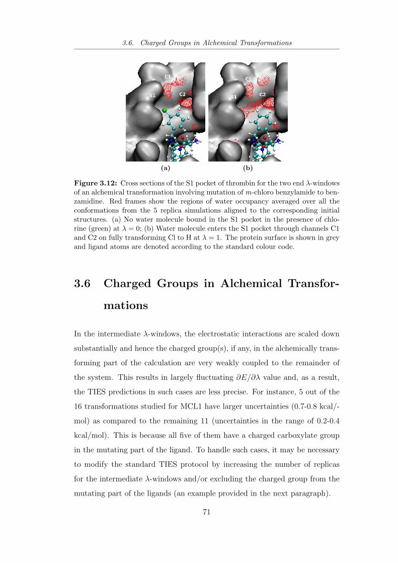
3.6. Charged Groups in Alchemical Transformations
(a) (b)
Figure 3.12: Cross sections of the S1 pocket of thrombin for the two end λ-windowsof an alchemical transformation involving mutation of m-chloro benzylamide to ben-zamidine. Red frames show the regions of water occupancy averaged over all theconformations from the 5 replica simulations aligned to the corresponding initialstructures. (a) No water molecule bound in the S1 pocket in the presence of chlo-rine (green) at λ = 0; (b) Water molecule enters the S1 pocket through channels C1and C2 on fully transforming Cl to H at λ = 1. The protein surface is shown in greyand ligand atoms are denoted according to the standard colour code.
3.6 Charged Groups in Alchemical Transfor-
mations
In the intermediate λ-windows, the electrostatic interactions are scaled down
substantially and hence the charged group(s), if any, in the alchemically trans-
forming part of the calculation are very weakly coupled to the remainder of
the system. This results in largely fluctuating ∂E/∂λ value and, as a result,
the TIES predictions in such cases are less precise. For instance, 5 out of the
16 transformations studied for MCL1 have larger uncertainties (0.7-0.8 kcal/-
mol) as compared to the remaining 11 (uncertainties in the range of 0.2-0.4
kcal/mol). This is because all five of them have a charged carboxylate group
in the mutating part of the ligand. To handle such cases, it may be necessary
to modify the standard TIES protocol by increasing the number of replicas
for the intermediate λ-windows and/or excluding the charged group from the
mutating part of the ligands (an example provided in the next paragraph).
71
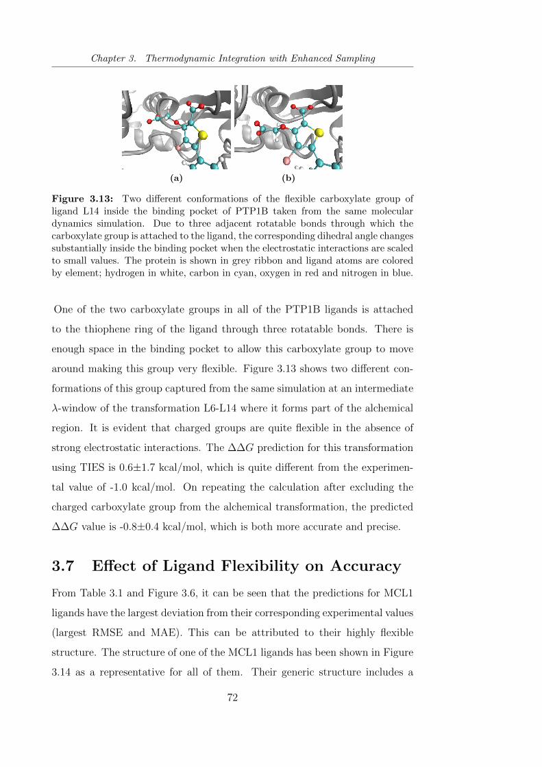
Chapter 3. Thermodynamic Integration with Enhanced Sampling
(a) (b)
Figure 3.13: Two different conformations of the flexible carboxylate group ofligand L14 inside the binding pocket of PTP1B taken from the same moleculardynamics simulation. Due to three adjacent rotatable bonds through which thecarboxylate group is attached to the ligand, the corresponding dihedral angle changessubstantially inside the binding pocket when the electrostatic interactions are scaledto small values. The protein is shown in grey ribbon and ligand atoms are coloredby element; hydrogen in white, carbon in cyan, oxygen in red and nitrogen in blue.
One of the two carboxylate groups in all of the PTP1B ligands is attached
to the thiophene ring of the ligand through three rotatable bonds. There is
enough space in the binding pocket to allow this carboxylate group to move
around making this group very flexible. Figure 3.13 shows two different con-
formations of this group captured from the same simulation at an intermediate
λ-window of the transformation L6-L14 where it forms part of the alchemical
region. It is evident that charged groups are quite flexible in the absence of
strong electrostatic interactions. The ∆∆G prediction for this transformation
using TIES is 0.6±1.7 kcal/mol, which is quite different from the experimen-
tal value of -1.0 kcal/mol. On repeating the calculation after excluding the
charged carboxylate group from the alchemical transformation, the predicted
∆∆G value is -0.8±0.4 kcal/mol, which is both more accurate and precise.
3.7 Effect of Ligand Flexibility on Accuracy
From Table 3.1 and Figure 3.6, it can be seen that the predictions for MCL1
ligands have the largest deviation from their corresponding experimental values
(largest RMSE and MAE). This can be attributed to their highly flexible
structure. The structure of one of the MCL1 ligands has been shown in Figure
3.14 as a representative for all of them. Their generic structure includes a
72
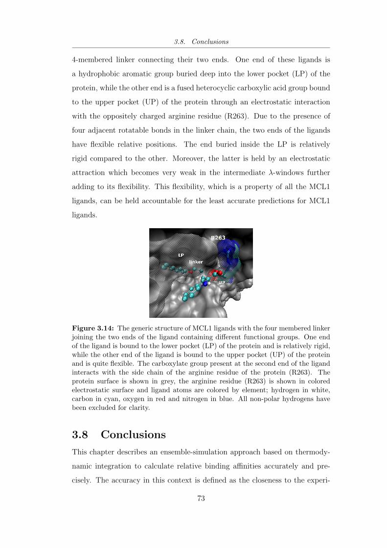
3.8. Conclusions
4-membered linker connecting their two ends. One end of these ligands is
a hydrophobic aromatic group buried deep into the lower pocket (LP) of the
protein, while the other end is a fused heterocyclic carboxylic acid group bound
to the upper pocket (UP) of the protein through an electrostatic interaction
with the oppositely charged arginine residue (R263). Due to the presence of
four adjacent rotatable bonds in the linker chain, the two ends of the ligands
have flexible relative positions. The end buried inside the LP is relatively
rigid compared to the other. Moreover, the latter is held by an electrostatic
attraction which becomes very weak in the intermediate λ-windows further
adding to its flexibility. This flexibility, which is a property of all the MCL1
ligands, can be held accountable for the least accurate predictions for MCL1
ligands.
Figure 3.14: The generic structure of MCL1 ligands with the four membered linkerjoining the two ends of the ligand containing different functional groups. One endof the ligand is bound to the lower pocket (LP) of the protein and is relatively rigid,while the other end of the ligand is bound to the upper pocket (UP) of the proteinand is quite flexible. The carboxylate group present at the second end of the ligandinteracts with the side chain of the arginine residue of the protein (R263). Theprotein surface is shown in grey, the arginine residue (R263) is shown in coloredelectrostatic surface and ligand atoms are colored by element; hydrogen in white,carbon in cyan, oxygen in red and nitrogen in blue. All non-polar hydrogens havebeen excluded for clarity.
3.8 Conclusions
This chapter describes an ensemble-simulation approach based on thermody-
namic integration to calculate relative binding affinities accurately and pre-
cisely. The accuracy in this context is defined as the closeness to the experi-
73
Chapter 3. Thermodynamic Integration with Enhanced Sampling
mental values and is achieved within the limitations of the force field employed.
It has been shown to yield repeatable predictions with and without the varia-
tion in parameters like the MD code, the hardware and the topology scheme.
Its excellent scalability allows one to perform multiple calculations concur-
rently. The protocol used is flexible and the parameters like ensemble size and
simulation length can be adjusted to achieve the desired level of precision. The
results provided in this chapter have very high accuracy for a diverse set of
ligands bound to seven different protein targets showing the wide applicability
of this approach. The alchemical transformations studied cover several types
of chemical group modifications (up to 10 heavy atoms).
All MD simulations for this chapter were performed using the standard force
fields which are known to be reliable for the systems studied. However, this
may not always hold true and it is necessary to choose the potential parametri-
sations carefully as the accuracy of results is dependent on them. The version
of TIES described here is unable to handle the situations where the alchemical
transformation involves a change in the net charge. However, it can handle
situations where the mutating part of the ligand is charged; although this may
sometimes need a modification in the standard TIES protocol.
Given the features of rapidity, high accuracy, high precision, repeatability and
reproducibility in the TIES predictions, this approach has the potential to be
routinely applicable in drug design and personalised medicine. In fact, TIES
calculations for BRD4 and TRKA included in this chapter were conducted
as blind studies in collaboration with two major pharmaceutical companies,
Glaxo Simth Kline and Pfizer, respectively. The experimental binding affini-
ties in both these cases were only disclosed after the predictions using TIES
were made available to the experimental collaborators. Both of these studies
have been published and the results are in excellent agreement with the ex-
perimental data[22, 23]. This exhibits the suitability of ensemble simulation
based approaches for their application as a virtual screening tool in the process
of drug design.
74
Chapter 4
Hamiltonian-Replica Exchange
Methods and Uncertainty
Quantification
In the previous chapter, an ensemble simulation based approach (TIES) was
described as a reliable way to predict relative binding affinities for ligand-
protein complexes. It was shown that the free energy predictions from TIES
are accurate and precise. TIES provides a control on the errors associated
with the predictions made using the free energy methods based on classical
MD simulations and its results are repeatable as well as reproducible. Thus,
TIES can be useful in several important applications relying on the reliable
prediction of ligand-protein binding affinities as mentioned in Chapter 1.
A large number of in silico methods based on one of the many accelerated
sampling protocols are available to calculate free energy as described in Chap-
ter 2. These methods seem to be useful in cases where the system studied has
multiple local minima separated by large energy barriers. Among them, the
Hamiltonian-replica exchange (H-REMD)[17] has proved to be very useful in
the case of large solvated biomolecules. As discussed in Chapter 2, REST2[18]
is an important variant of H-REMD, based on which, Wang et al. recently
proposed a method called FEP/REST[19]. FEP/REST has been referred to
as λ-REST2 in this thesis. In addition, free energy estimators like multistate
Chapter 4. Hamiltonian-Replica Exchange Methods and Uncertainty Quantification
Bennett acceptance ratio (MBAR)[20] have been proposed which claim to get
better estimates of free energy by utilising the maximum amount of informa-
tion from the simulation data. It is sometimes claimed that the problem of
the variability in results from independent short simulation based calculations
as mentioned in Chapter 1 can be overcome by using such enhanced sam-
pling methods and improved free energy estimators. However, a systematic
investigation of their repeatability has not yet been done.
In this chapter, the idea of ensemble simulation from the previous chapter has
been applied to the above mentioned accelerated sampling methods, REST2
and λ-REST2, and the free energy estimator, MBAR. An account of the vari-
ability in their free energy predictions, when performing a single short replica∗,
is provided. It has been found that the sensitivity of the classical MD simula-
tions to their initial conditions and the resultant variation in the macroscopic
properties calculated from short simulations (as discussed in Section 2.4) holds
irrespective of the sampling protocol used or the free energy estimator em-
ployed. It is found necessary to perform ensemble simulation even when such
improved sampling protocols and free energy estimators are employed in order
to get a proper control on the statistical uncertainties associated with the free
energy predictions. Extending the simulation duration (up to the cumulative
duration of the ensemble simulation) does not help get over this variation and
cannot be an alternative to ensemble simulation, an observation similar to the
one made in Chapter 3 for non-biased MD simulations. In this chapter, REST2
and λ-REST2 are chosen as the representatives for all other accelerated sam-
pling methods based on the replica-exchange technique. It should be noted
that the work presented in this chapter has been published and some figures
and tables have been reproduced from the published article[231]. Importantly,
although this chapter focusses on a selected few free energy methods, the ob-
∗The term “replica” means an independent MD simulation initiated from a random initialcondition in the context of ensemble simulation. It should not be confused with the term“replica” within the context of replica-exchange simulation. To avoid such confusion in thischapter, the term “replica” has always been used to refer to the former, while the latter hasbeen denoted as a “REST2 replica”.
76
4.1. Protein Targets and Ligands
servations made are general and applicable to other free energy methods based
on classical MD simulations.
4.1 Protein Targets and Ligands
Three different classes of proteins are chosen here to exhibit the wide appli-
cability of the below described methods. Two of them, namely thrombin and
bromodomain-containing protein 4 (BRD4), are the ones also used for the TIES
study in Chapter 3. The third is fibroblast growth factor receptor 1 (FGFR1).
The structure of all proteins and ligands studied are shown in Figure 4.1. It
is known that the activation of FGFR1 is related to the pathogenesis of sev-
eral human malignancies including various types of cancers[214]. Therefore,
efforts are ongoing to develop FGFR1 inhibitors as anticancer treatment. Most
inhibitors bind to the kinase domain (KD) of the FGFR1 protein.
It is well known that mutations in the FGFR1 KD can alter inhibitor binding
rendering some drugs ineffective[214]. In this study, alchemical methods are
applied to study the transformation of FGFR1 wildtype to V561M mutant
when bound to two inhibitors, namely PD173074 and TKI258 (Dovitinib).
V561M is the gatekeeper mutation. It occurs frequently and often leads to the
development of resistance against several drugs.
4.2 Methods
In this section, the free energy schemes employed in the study have been
described and the details about their implementation provided. The simulation
protocol used and parameters employed for the same have been described. The
parameters specific to REST2 and λ-REST2 have also been provided. The
post simulation analysis method has been described and an estimate of the
computational cost of the different free energy methods has been provided
along with their comparison with that for TIES (as described in Chapter 3).
77
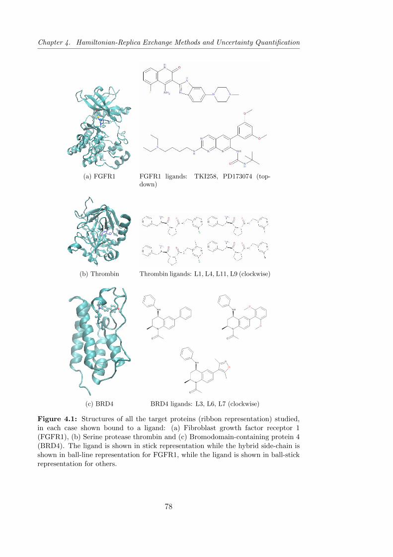
Chapter 4. Hamiltonian-Replica Exchange Methods and Uncertainty Quantification
(a) FGFR1 FGFR1 ligands: TKI258, PD173074 (top-down)
(b) Thrombin Thrombin ligands: L1, L4, L11, L9 (clockwise)
(c) BRD4 BRD4 ligands: L3, L6, L7 (clockwise)
Figure 4.1: Structures of all the target proteins (ribbon representation) studied,in each case shown bound to a ligand: (a) Fibroblast growth factor receptor 1(FGFR1), (b) Serine protease thrombin and (c) Bromodomain-containing protein 4(BRD4). The ligand is shown in stick representation while the hybrid side-chain isshown in ball-line representation for FGFR1, while the ligand is shown in ball-stickrepresentation for others.
78
4.2. Methods
4.2.1 Free Energy Schemes
In this chapter, the method employed to calculate the relative free energy
is identical to the TIES method as described in the previous chapter except
the sampling protocol used to generate the ensemble of conformations which
is different in the two. Unlike in the previous chapter, enhanced sampling
protocols based on replica-exchange methods, REST2 and λ-REST2, have been
used here. 〈∂E/∂λ〉 (Equation 2.26) is determined by performing an ensemble
simulation at each λ window. Since the integrand in Equation 2.26 comprises
points which are Gaussian random processes, stochastic calculus is employed
to calculate ∆Galch and the associated error as prescribed for TIES in the
previous chapter. The following sampling schemes are used in this study to
calculate the relative binding affinities:
I. TIES-REST2: In this scheme, the number of λ-windows and the cor-
responding values of λ are pre-defined and an ensemble of REST2 simu-
lations is performed at each window. Each REST2 simulation amounts
to running a set number of REST2 replicas in parallel which vary only
in their solute potential scaling factors (or equivalently their effective
temperatures, Teff ) and exchange of configurations are attempted reg-
ularly between the neighbouring REST2 replicas. TIES analysis is per-
formed using ∂E/∂λ values of samples only from the REST2 replicas at
Teff = 300 K to get the ∆Galch and associated uncertainty.
II. TIES-REST2-M: This scheme involves just re-analysing the simula-
tion data from scheme I and does not require any additional simulations.
It employs MBAR as a reweighing technique to calculate ∂E/∂λ using
samples from REST2 replicas at all Teff values from scheme I at each
λ-window for each REST2 simulation followed by the standard TIES
analysis. This scheme is expected to yield free energy predictions more
precise than those from scheme I as the entire simulation data generated
by the REST2 simulations is utilised unlike scheme I where a majority of
it is discarded.
79
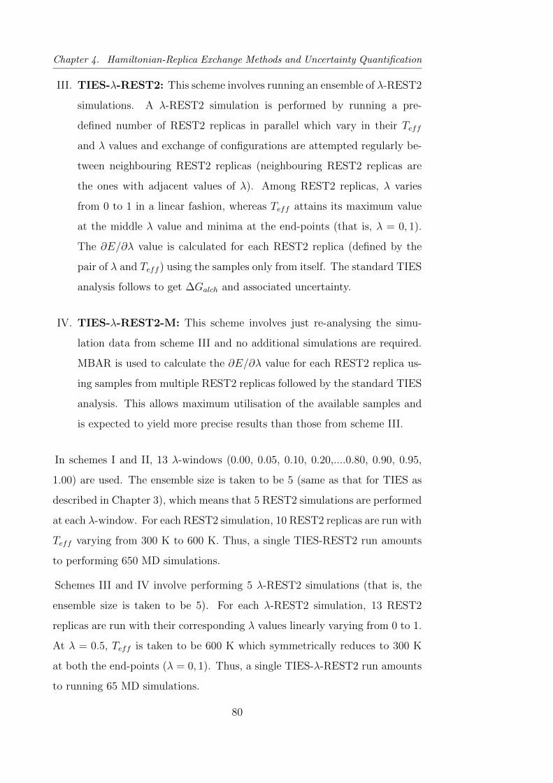
Chapter 4. Hamiltonian-Replica Exchange Methods and Uncertainty Quantification
III. TIES-λ-REST2: This scheme involves running an ensemble of λ-REST2
simulations. A λ-REST2 simulation is performed by running a pre-
defined number of REST2 replicas in parallel which vary in their Teff
and λ values and exchange of configurations are attempted regularly be-
tween neighbouring REST2 replicas (neighbouring REST2 replicas are
the ones with adjacent values of λ). Among REST2 replicas, λ varies
from 0 to 1 in a linear fashion, whereas Teff attains its maximum value
at the middle λ value and minima at the end-points (that is, λ = 0, 1).
The ∂E/∂λ value is calculated for each REST2 replica (defined by the
pair of λ and Teff ) using the samples only from itself. The standard TIES
analysis follows to get ∆Galch and associated uncertainty.
IV. TIES-λ-REST2-M: This scheme involves just re-analysing the simu-
lation data from scheme III and no additional simulations are required.
MBAR is used to calculate the ∂E/∂λ value for each REST2 replica us-
ing samples from multiple REST2 replicas followed by the standard TIES
analysis. This allows maximum utilisation of the available samples and
is expected to yield more precise results than those from scheme III.
In schemes I and II, 13 λ-windows (0.00, 0.05, 0.10, 0.20,....0.80, 0.90, 0.95,
1.00) are used. The ensemble size is taken to be 5 (same as that for TIES as
described in Chapter 3), which means that 5 REST2 simulations are performed
at each λ-window. For each REST2 simulation, 10 REST2 replicas are run with
Teff varying from 300 K to 600 K. Thus, a single TIES-REST2 run amounts
to performing 650 MD simulations.
Schemes III and IV involve performing 5 λ-REST2 simulations (that is, the
ensemble size is taken to be 5). For each λ-REST2 simulation, 13 REST2
replicas are run with their corresponding λ values linearly varying from 0 to 1.
At λ = 0.5, Teff is taken to be 600 K which symmetrically reduces to 300 K
at both the end-points (λ = 0, 1). Thus, a single TIES-λ-REST2 run amounts
to running 65 MD simulations.
80
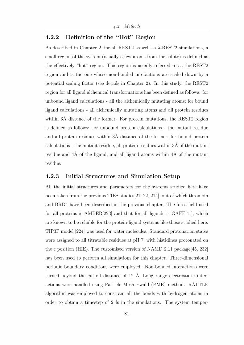
4.2. Methods
4.2.2 Definition of the “Hot” Region
As described in Chapter 2, for all REST2 as well as λ-REST2 simulations, a
small region of the system (usually a few atoms from the solute) is defined as
the effectively “hot” region. This region is usually referred to as the REST2
region and is the one whose non-bonded interactions are scaled down by a
potential scaling factor (see details in Chapter 2). In this study, the REST2
region for all ligand alchemical transformations has been defined as follows: for
unbound ligand calculations - all the alchemically mutating atoms; for bound
ligand calculations - all alchemically mutating atoms and all protein residues
within 3A distance of the former. For protein mutations, the REST2 region
is defined as follows: for unbound protein calculations - the mutant residue
and all protein residues within 3A distance of the former; for bound protein
calculations - the mutant residue, all protein residues within 3A of the mutant
residue and 4A of the ligand, and all ligand atoms within 4A of the mutant
residue.
4.2.3 Initial Structures and Simulation Setup
All the initial structures and parameters for the systems studied here have
been taken from the previous TIES studies[21, 22, 214], out of which thrombin
and BRD4 have been described in the previous chapter. The force field used
for all proteins is AMBER[223] and that for all ligands is GAFF[41], which
are known to be reliable for the protein-ligand systems like those studied here.
TIP3P model [224] was used for water molecules. Standard protonation states
were assigned to all titratable residues at pH 7, with histidines protonated on
the ε position (HIE). The customised version of NAMD 2.11 package[45, 232]
has been used to perform all simulations for this chapter. Three-dimensional
periodic boundary conditions were employed. Non-bonded interactions were
turned beyond the cut-off distance of 12 A. Long range electrostatic inter-
actions were handled using Particle Mesh Ewald (PME) method. RATTLE
algorithm was employed to constrain all the bonds with hydrogen atoms in
order to obtain a timestep of 2 fs in the simulations. The system temper-
81
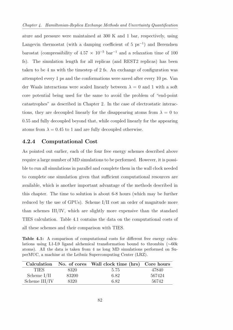
Chapter 4. Hamiltonian-Replica Exchange Methods and Uncertainty Quantification
ature and pressure were maintained at 300 K and 1 bar, respectively, using
Langevin thermostat (with a damping coefficient of 5 ps−1) and Berendsen
barostat (compressibility of 4.57 × 10⁻⁵ bar−1 and a relaxation time of 100
fs). The simulation length for all replicas (and REST2 replicas) has been
taken to be 4 ns with the timestep of 2 fs. An exchange of configuration was
attempted every 1 ps and the conformations were saved after every 10 ps. Van
der Waals interactions were scaled linearly between λ = 0 and 1 with a soft
core potential being used for the same to avoid the problem of “end-point
catastrophes” as described in Chapter 2. In the case of electrostatic interac-
tions, they are decoupled linearly for the disappearing atoms from λ = 0 to
0.55 and fully decoupled beyond that, while coupled linearly for the appearing
atoms from λ = 0.45 to 1 and are fully decoupled otherwise.
4.2.4 Computational Cost
As pointed out earlier, each of the four free energy schemes described above
require a large number of MD simulations to be performed. However, it is possi-
ble to run all simulations in parallel and complete them in the wall clock needed
to complete one simulation given that sufficient computational resources are
available, which is another important advantage of the methods described in
this chapter. The time to solution is about 6-8 hours (which may be further
reduced by the use of GPUs). Scheme I/II cost an order of magnitude more
than schemes III/IV, which are slightly more expensive than the standard
TIES calculation. Table 4.1 contains the data on the computational costs of
all these schemes and their comparison with TIES.
Table 4.1: A comparison of computational costs for different free energy calcu-lations using L1-L9 ligand alchemical transformation bound to thrombin (∼60katoms). All the data is taken from 4 ns long MD simulations performed on Su-perMUC, a machine at the Leibniz Supercomputing Center (LRZ).
Calculation No. of cores Wall clock time (hrs) Core hoursTIES 8320 5.75 47840
Scheme I/II 83200 6.82 567424Scheme III/IV 8320 6.82 56742
82
4.3. Binding Affinity Predictions
4.2.5 Uncertainty Quantification
As mentioned earlier, the simulation output of all the methods described in this
chapter has been analysed using the TIES methodology to yield the free energy
predictions and associated uncertainties. It is worth mentioning here that
TIES analysis is different from merely running the conventional TI calculation
five times followed by computing five integrals and assessing the error. TIES
involves performing stochastic integration recognising that each point of the
integrand is a Gaussian random process and the uncertainty in the final integral
is given by the convolution of the uncertainties in individual points of the
integrand. The error bars so obtained furnish an estimate of the repeatability
of the results and hence this approach provides a reliable way of uncertainty
quantification.
4.3 Binding Affinity Predictions
In this section, the results obtained from all four free energy schemes have
been described. The replica-wise variation of results has been provided and
discussed. A comparison of the results from all four schemes with each other as
well as with the experimental data has been done. The effect of the duration
of simulations on the accuracy and precision of the results for each scheme has
been provided.
4.3.1 Variability in Different Free Energy Schemes
The relative binding affinity predictions for all protein-ligand complexes using
all 4 schemes have been provided in Table 4.2. The notation of “forward” and
“reverse” transformations have been borrowed from the previous FGFR1 TIES
study[214]. Here, “forward” means V → M transformation while “reverse”
means M → V transformation; their initial structures were prepared from
different PDB files. The hysteresis, which is the residual ∆∆G over a closed
thermodynamic cycle, can be eliminated here by calculating ∆∆G in both
directions. An account of the replica-wise variation of results for all schemes
is provided in Table 4.2. This variation is 0.8-1.3 kcal/mol for FGFR1 and
83
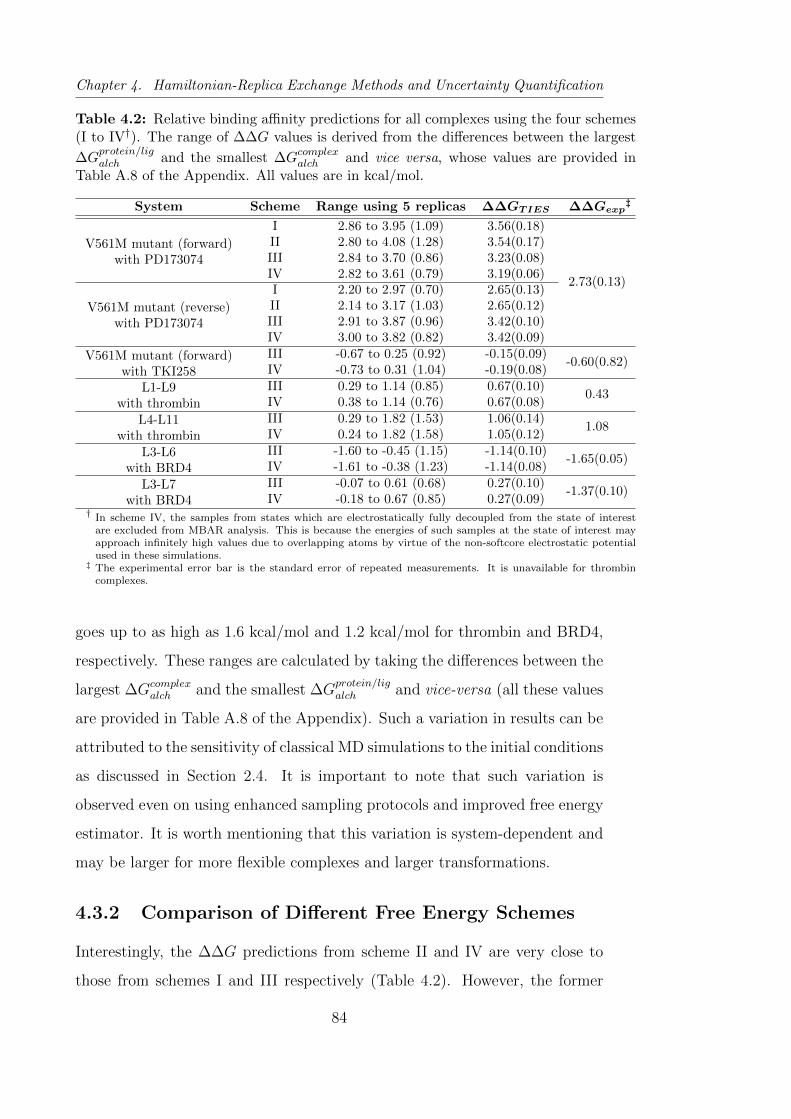
Chapter 4. Hamiltonian-Replica Exchange Methods and Uncertainty Quantification
Table 4.2: Relative binding affinity predictions for all complexes using the four schemes(I to IV†). The range of ∆∆G values is derived from the differences between the largest
∆Gprotein/ligalch and the smallest ∆Gcomplexalch and vice versa, whose values are provided in
Table A.8 of the Appendix. All values are in kcal/mol.
System Scheme Range using 5 replicas ∆∆GTIES ∆∆Gexp‡
V561M mutant (forward)with PD173074
I 2.86 to 3.95 (1.09) 3.56(0.18)
2.73(0.13)
II 2.80 to 4.08 (1.28) 3.54(0.17)III 2.84 to 3.70 (0.86) 3.23(0.08)IV 2.82 to 3.61 (0.79) 3.19(0.06)
V561M mutant (reverse)with PD173074
I 2.20 to 2.97 (0.70) 2.65(0.13)II 2.14 to 3.17 (1.03) 2.65(0.12)III 2.91 to 3.87 (0.96) 3.42(0.10)IV 3.00 to 3.82 (0.82) 3.42(0.09)
V561M mutant (forward)with TKI258
III -0.67 to 0.25 (0.92) -0.15(0.09)-0.60(0.82)
IV -0.73 to 0.31 (1.04) -0.19(0.08)
L1-L9with thrombin
III 0.29 to 1.14 (0.85) 0.67(0.10)0.43
IV 0.38 to 1.14 (0.76) 0.67(0.08)
L4-L11with thrombin
III 0.29 to 1.82 (1.53) 1.06(0.14)1.08
IV 0.24 to 1.82 (1.58) 1.05(0.12)
L3-L6with BRD4
III -1.60 to -0.45 (1.15) -1.14(0.10)-1.65(0.05)
IV -1.61 to -0.38 (1.23) -1.14(0.08)
L3-L7with BRD4
III -0.07 to 0.61 (0.68) 0.27(0.10)-1.37(0.10)
IV -0.18 to 0.67 (0.85) 0.27(0.09)† In scheme IV, the samples from states which are electrostatically fully decoupled from the state of interest
are excluded from MBAR analysis. This is because the energies of such samples at the state of interest mayapproach infinitely high values due to overlapping atoms by virtue of the non-softcore electrostatic potentialused in these simulations.
‡ The experimental error bar is the standard error of repeated measurements. It is unavailable for thrombincomplexes.
goes up to as high as 1.6 kcal/mol and 1.2 kcal/mol for thrombin and BRD4,
respectively. These ranges are calculated by taking the differences between the
largest ∆Gcomplexalch and the smallest ∆G
protein/ligalch and vice-versa (all these values
are provided in Table A.8 of the Appendix). Such a variation in results can be
attributed to the sensitivity of classical MD simulations to the initial conditions
as discussed in Section 2.4. It is important to note that such variation is
observed even on using enhanced sampling protocols and improved free energy
estimator. It is worth mentioning that this variation is system-dependent and
may be larger for more flexible complexes and larger transformations.
4.3.2 Comparison of Different Free Energy Schemes
Interestingly, the ∆∆G predictions from scheme II and IV are very close to
those from schemes I and III respectively (Table 4.2). However, the former
84
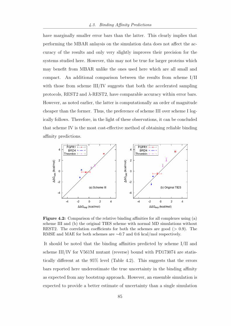
4.3. Binding Affinity Predictions
have marginally smaller error bars than the latter. This clearly implies that
performing the MBAR anlaysis on the simulation data does not affect the ac-
curacy of the results and only very slightly improves their precision for the
systems studied here. However, this may not be true for larger proteins which
may benefit from MBAR unlike the ones used here which are all small and
compact. An additional comparison between the results from scheme I/II
with those from scheme III/IV suggests that both the accelerated sampling
protocols, REST2 and λ-REST2, have comparable accuracy within error bars.
However, as noted earlier, the latter is computationally an order of magnitude
cheaper than the former. Thus, the preference of scheme III over scheme I log-
ically follows. Therefore, in the light of these observations, it can be concluded
that scheme IV is the most cost-effective method of obtaining reliable binding
affinity predictions.
Figure 4.2: Comparison of the relative binding affinities for all complexes using (a)scheme III and (b) the original TIES scheme with normal MD simulations withoutREST2. The correlation coefficients for both the schemes are good (> 0.9). TheRMSE and MAE for both schemes are ∼0.7 and 0.6 kcal/mol respectively.
It should be noted that the binding affinities predicted by scheme I/II and
scheme III/IV for V561M mutant (reverse) bound with PD173074 are statis-
tically different at the 95% level (Table 4.2). This suggests that the errors
bars reported here underestimate the true uncertainty in the binding affinity
as expected from any bootstrap approach. However, an ensemble simulation is
expected to provide a better estimate of uncertainty than a single simulation
85
Chapter 4. Hamiltonian-Replica Exchange Methods and Uncertainty Quantification
as the latter may suffer from the presence of correlated samples unlike the
former.
4.3.3 Comparison with Experimental Data
As noted above, scheme IV appears to be the best of all the schemes used in
this study. However, its results are almost identical to those from scheme III.
Therefore, the results from the latter have been compared with the experimen-
tal values. They are very accurate with their differences from the correspond-
ing experimental values lying in the range of 0.02-0.69 kcal/mol for all but
one transformation. The excellent agreement of the ∆∆G predictions from
scheme III with those reported from experiments is shown in Figure 4.2(a). It
is noteworthy that the hysteresis in the predicted ∆∆G for FGFR1 V561M
bound to PD173074 has diminished to zero in this study (0.19 kcal/mol for
scheme III which can be considered zero within the reported error bars) from
0.83 kcal/mol as reported in the previous TIES study (reference [214] using 5
replicas; may reduce further on increasing the number of replicas). In case of
the ligand transformation L4-L11 bound to thrombin, the difference between
the predicted ∆∆G with that from experiment has come down to 0.02 kcal/-
mol (in case of scheme III) from 1.10 kcal/mol as reported in the previous
TIES study (reference [21]). This suggests that Hamiltonian replica-exchange,
in combination with the TIES protocol, improves the accuracy of predictions
by accelerating the convergence of results from different initial structures.
A comparison of the ∆∆G predictions for all ligand-protein complexes from
scheme III and from the original TIES (without REST2) is made in Figure
4.2. Both of them are quite accurate with correlation coefficients greater than
0.9 and root mean square error (RMSE) and mean absolute error (MAE) of
around 0.7 and 0.6 kcal/mol, respectively. Not surprisingly, Scheme III pre-
dictions have smaller uncertainties. It is clear from Figure 4.2 that λ-REST2
improves the accuracy of relative binding affinity predictions for thrombin over
the straightforward TIES scheme. For other proteins, there is no observable
change except the L3-L7 transformation bound with BRD4 where the results
86

4.3. Binding Affinity Predictions
from scheme III are less accurate. This suggests that thrombin, unlike the
other two, has multiple local minima separated by energy barriers.
It should be noted that, although the methods used in this study are based
on thermodynamic integration, the conclusions made here are general and
applicable to other alchemical free energy methods like the recently published
FEP/REST[196].
Figure 4.3: Variation of cumulative ∆Gcomplexalch with simulation length for fivereplicas of relative free energy calculations (shown in different colours) and theircombined TIES analysis result (shown in black with error bars) for all 4 schemes.The simulations were extended up to 10 ns for schemes I and II and up to 20 ns forschemes III and IV. Some of the replicas are highlighted (thick lines) to show howa single replica may fluctuate substantially or become trapped in a local potentialminimum while the ensemble average overcomes such problems.
4.3.4 Dependence on the Duration of Simulation
The variation of the predicted free energies with the duration of simulation is
shown in Figure 4.3. The top panel displays results from schemes I and II up to
10 ns while the bottom panel displays those from scheme III and IV up to 20 ns.
The cumulative ∆Gcomplexalch from individual replicas (coloured plots) and their
ensemble averages calculated using TIES protocol (black plots with error bars)
87
Chapter 4. Hamiltonian-Replica Exchange Methods and Uncertainty Quantification
are both included. There is negligible variation in results beyond 4 ns. It can
be seen from Figure 4.3 that the differences between the values corresponding
to the black line at 4 ns and 10 ns is less than 0.2 kcal/mol for schemes I and
II and less than 0.1 kcal/mol for schemes III and IV. The contraction of error
bars is also marginal beyond 4 ns for all schemes. It is worth mentioning here
that such a behaviour is system-dependent; it may be necessary to increase
the ensemble size and/or simulation duration to achieve a similar precision for
larger alchemical transformations or more flexible proteins.
The variation of the results from individual replicas with the duration of simu-
lation should be noted in Figure 4.3 (coloured plots fluctuate much more than
the black plots). This indicates that a single replica consistently generates
larger variation in predictions. Some of the coloured lines are highlighted in
Figure 4.3 which correspond to the replicas which either fluctuate considerably
or get trapped within a region of conformation space. For instance, in the top
panel of Figure 4.3, the blue lines never get closer to the black ones. The
ensemble average gets over such issues. Although the variation in results from
a single replica is small for the complex shown in Figure 4.3, it may be larger
for other protein-ligand complexes and hence performing a single replica is not
reliable.
4.4 Conclusions
This chapter describes four different relative binding affinity calculation meth-
ods, namely TIES-REST2, TIES-REST2-M, TIES-λ-REST2, and TIES-λ-
REST2-M, based on thermodynamic integration. They all employ the concept
of ensemble simulation (that used for TIES as described in Chapter 3) in combi-
nation with the different versions of the Hamiltonian replica exchange method.
The results are found to be accurate and precise for a range of ligand-protein
complexes and the schemes have a built-in mechanism to control errors. An
account of the replica-wise variation in results has been provided to emphasise
the importance of ensemble simulation and the inability of a single replica to
88
4.4. Conclusions
properly assess statistical uncertainties. TIES-λ-REST2 is found to be equally
accurate as TIES-REST2 for an order of magnitude less computational cost.
MBAR[20] is shown to have to no effect on the accuracy and only marginally
improve the precision of the results and hence is found to be not necessary
for the biomolecular systems studied. In the case of thrombin complexes,
the Hamiltonian replica-exchange methods are shown to yield more accurate
results as compared to the ones from non-biased MD simulations. It is estab-
lished that ensemble simulations provide a systematic means of uncertainty
quantification for all methods based on classical MD simulations and hence
are required irrespective of the sampling protocol, the free energy estimator
and the duration of the simulation.
89

Chapter 5
Enhanced Sampling of
Molecular Dynamics with
Approximation of Continuum
Solvent
Chapter 2 provides an overview of the in silico free energy methods available,
categorised into alchemical and end-point methods. Two further points were
also made. Firstly, that all the methods based on classical MD simulations are
sensitive to the initial conditions. Secondly, that ensemble averages should not
be replaced with time averages given that both are equal only in the limit of the
Poincare recurrence time, which is inaccessible. In Chapters 3 and 4, ensem-
ble simulation based approaches based on an alchemical free energy method,
thermodynamic integration, have been described and successfully applied to
calculate accurate, precise and repeatable relative binding affinities for a large
number of target proteins and ligands.
Most of the alchemical methods yield relative binding affinities and hence
are of restricted validity as the relative change must be “small”. However,
this problem does not persist on calculating absolute binding affinities. As
discussed in Section 2.3.3, a few alchemical methods can be used to calculate
the absolute binding affinity. However, running a single (insufficiently long)
Chapter 5. ESMACS
replica version of these methods has the similar issue of variability in results, as
discussed in the previous chapters for other methods. The TIES approach (as
described in Chapter 3) has led one of my colleagues to develop an ensemble
simulation based approach to calculate the absolute binding affinity based on
an alchemical method[231]. The variation in charge between the two end-
points in alchemical methods also causes problems. However, corrections for
electrostatic finite-size effects[233, 234] were used to tackle this issue in the
case of charged ligands in our recently published work on absolute binding
affinity calculations[231].
In some situations, it is preferred to compromise on the accuracy of the pre-
dictions in order to reduce the cost of the calculations. In such situations
the end-point methods are employed to predict the absolute binding affini-
ties. They do not have the problem of restricted validity and do not require
additional correction terms for charged ligands, which are their additional ad-
vantages over alchemical methods. One of the most popular end-point method
is MMPB(GB)SA as described in Chapter 2. In this chapter, a new approach
called enhanced sampling of molecular dynamics with approximation of con-
tinuum solvent (ESMACS) to calculate absolute binding affinities based on
the MMPBSA method has been described. It utilises ensemble simulation to
yield precise and repeatable predictions with a proper control on statistical
uncertainties.
The term “MMPBSA” has many different meanings in literature. Some
authors use it to refer to the free energy calculation based on docked
structures[196]. Generally, it refers to free energy calculation based on a single
MD simulation, which may or may not include the configuration entropies.
On the other hand, the ESMACS approach always involves an ensemble sim-
ulation to calculate converged binding affinities including the configuration
entropy and the free energy of association. It may be performed using sin-
gle or multiple trajectory approaches. The size of the ensemble simulations
is determined systematically to obtain a desired level of precision. The time
92
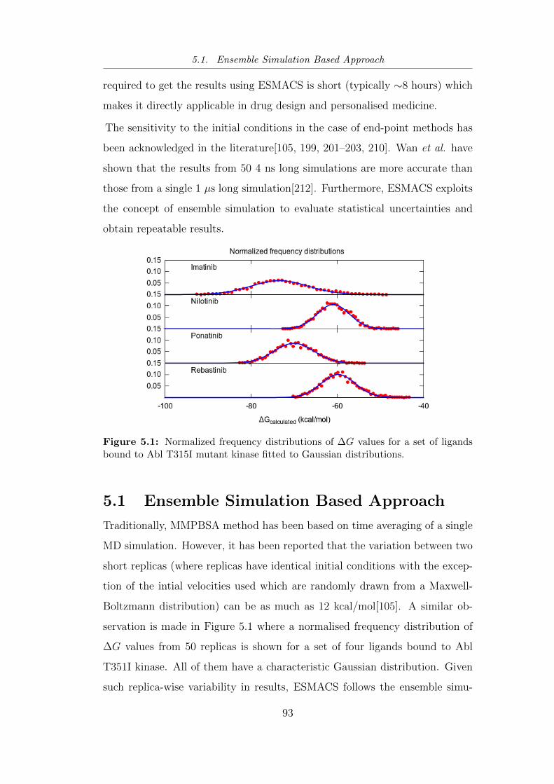
5.1. Ensemble Simulation Based Approach
required to get the results using ESMACS is short (typically ∼8 hours) which
makes it directly applicable in drug design and personalised medicine.
The sensitivity to the initial conditions in the case of end-point methods has
been acknowledged in the literature[105, 199, 201–203, 210]. Wan et al. have
shown that the results from 50 4 ns long simulations are more accurate than
those from a single 1 µs long simulation[212]. Furthermore, ESMACS exploits
the concept of ensemble simulation to evaluate statistical uncertainties and
obtain repeatable results.
Figure 5.1: Normalized frequency distributions of ∆G values for a set of ligandsbound to Abl T315I mutant kinase fitted to Gaussian distributions.
5.1 Ensemble Simulation Based Approach
Traditionally, MMPBSA method has been based on time averaging of a single
MD simulation. However, it has been reported that the variation between two
short replicas (where replicas have identical initial conditions with the excep-
tion of the intial velocities used which are randomly drawn from a Maxwell-
Boltzmann distribution) can be as much as 12 kcal/mol[105]. A similar ob-
servation is made in Figure 5.1 where a normalised frequency distribution of
∆G values from 50 replicas is shown for a set of four ligands bound to Abl
T351I kinase. All of them have a characteristic Gaussian distribution. Given
such replica-wise variability in results, ESMACS follows the ensemble simu-
93
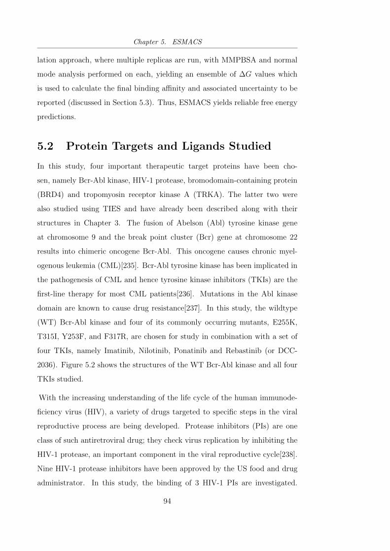
Chapter 5. ESMACS
lation approach, where multiple replicas are run, with MMPBSA and normal
mode analysis performed on each, yielding an ensemble of ∆G values which
is used to calculate the final binding affinity and associated uncertainty to be
reported (discussed in Section 5.3). Thus, ESMACS yields reliable free energy
predictions.
5.2 Protein Targets and Ligands Studied
In this study, four important therapeutic target proteins have been cho-
sen, namely Bcr-Abl kinase, HIV-1 protease, bromodomain-containing protein
(BRD4) and tropomyosin receptor kinase A (TRKA). The latter two were
also studied using TIES and have already been described along with their
structures in Chapter 3. The fusion of Abelson (Abl) tyrosine kinase gene
at chromosome 9 and the break point cluster (Bcr) gene at chromosome 22
results into chimeric oncogene Bcr-Abl. This oncogene causes chronic myel-
ogenous leukemia (CML)[235]. Bcr-Abl tyrosine kinase has been implicated in
the pathogenesis of CML and hence tyrosine kinase inhibitors (TKIs) are the
first-line therapy for most CML patients[236]. Mutations in the Abl kinase
domain are known to cause drug resistance[237]. In this study, the wildtype
(WT) Bcr-Abl kinase and four of its commonly occurring mutants, E255K,
T315I, Y253F, and F317R, are chosen for study in combination with a set of
four TKIs, namely Imatinib, Nilotinib, Ponatinib and Rebastinib (or DCC-
2036). Figure 5.2 shows the structures of the WT Bcr-Abl kinase and all four
TKIs studied.
With the increasing understanding of the life cycle of the human immunode-
ficiency virus (HIV), a variety of drugs targeted to specific steps in the viral
reproductive process are being developed. Protease inhibitors (PIs) are one
class of such antiretroviral drug; they check virus replication by inhibiting the
HIV-1 protease, an important component in the viral reproductive cycle[238].
Nine HIV-1 protease inhibitors have been approved by the US food and drug
administrator. In this study, the binding of 3 HIV-1 PIs are investigated.
94
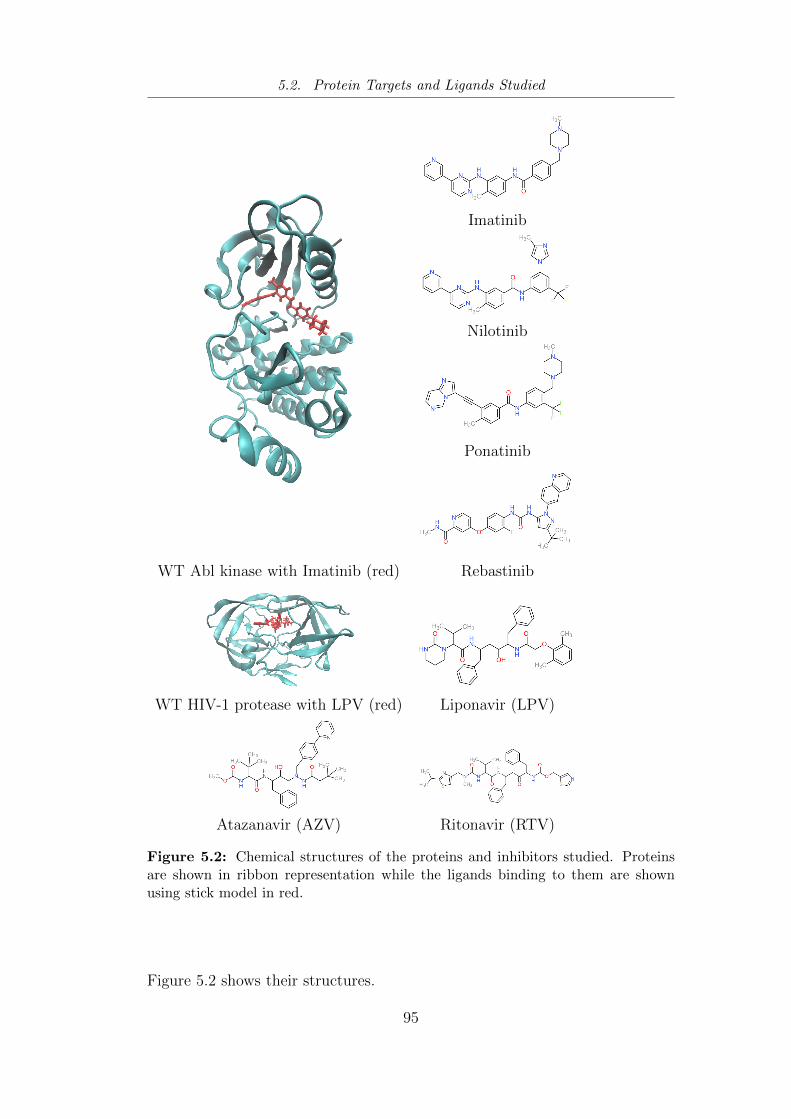
5.2. Protein Targets and Ligands Studied
Imatinib
Nilotinib
Ponatinib
WT Abl kinase with Imatinib (red) Rebastinib
WT HIV-1 protease with LPV (red) Liponavir (LPV)
Atazanavir (AZV) Ritonavir (RTV)
Figure 5.2: Chemical structures of the proteins and inhibitors studied. Proteinsare shown in ribbon representation while the ligands binding to them are shownusing stick model in red.
Figure 5.2 shows their structures.
95
Chapter 5. ESMACS
5.3 Method
This section details the simulation setup and the ESMACS free energy work-
flow employed to calculate all the binding affinities reported in this chapter.
A description of the evaluation of uncertainties in ESMACS results is also
provided. In addition, the repeatability of ESMACS results is discussed.
5.3.1 Initial Structures and Simulation Setup
The starting structures for Abl kinase complexes were taken from 4 differ-
ent PDBs: 1IEP for Imatinib complexes, 3CS9 for Nilotinib complexes, 3IK3
for Ponatinib complexes and 3QRI for Rebastinib complexes. Each PDB was
bound to one of the 5 mutants of the protein. The other mutants were pre-
pared by introducing the appropriate mutation into the original sequence using
the binding affinity calculator (BAC)[239]. In the case of HIV-1 protease, the
starting structures of the protein as well as all drugs were taken from a pre-
vious ESMACS study[105]. For BRD4 and TRKA, the initial structures were
prepared as described in Chapter 3.
All the protein-ligand complexes were simulated in an orthorhombic water box
with buffer width of 14 A. The net charge of the system was neutralised by ad-
dition of counterions. The AMBER ff99SB-ILDN force field[223] was used for
protein parameters and general AMBER force field (GAFF)[41] was employed
for ligands. TIP3P model [224] was used for water molecules. Standard pro-
tonation states were assigned to all titratable residues at pH 7, with histidines
protonated on the ε position (HIE). The partial atomic charges for ligand
atoms were calculated using restrained electrostatic potential (RESP) method
after geometry optimisation by Gaussian03 package using Hartree Fock method
and 6-31G** basis set. RESP calculations were performed using Antechamber
(available within AmberTools 12). All simulations were performed using the
package NAMD 2.9[45] with three-dimensional periodic boundary conditions.
A cut-off of 12 A was used for Lennard-Jones interactions and Particle Mesh
Ewald (PME) method employed for long range electrostatic interactions. The
simulations were performed in an isothermal-isobaric ensemble at temperature
96
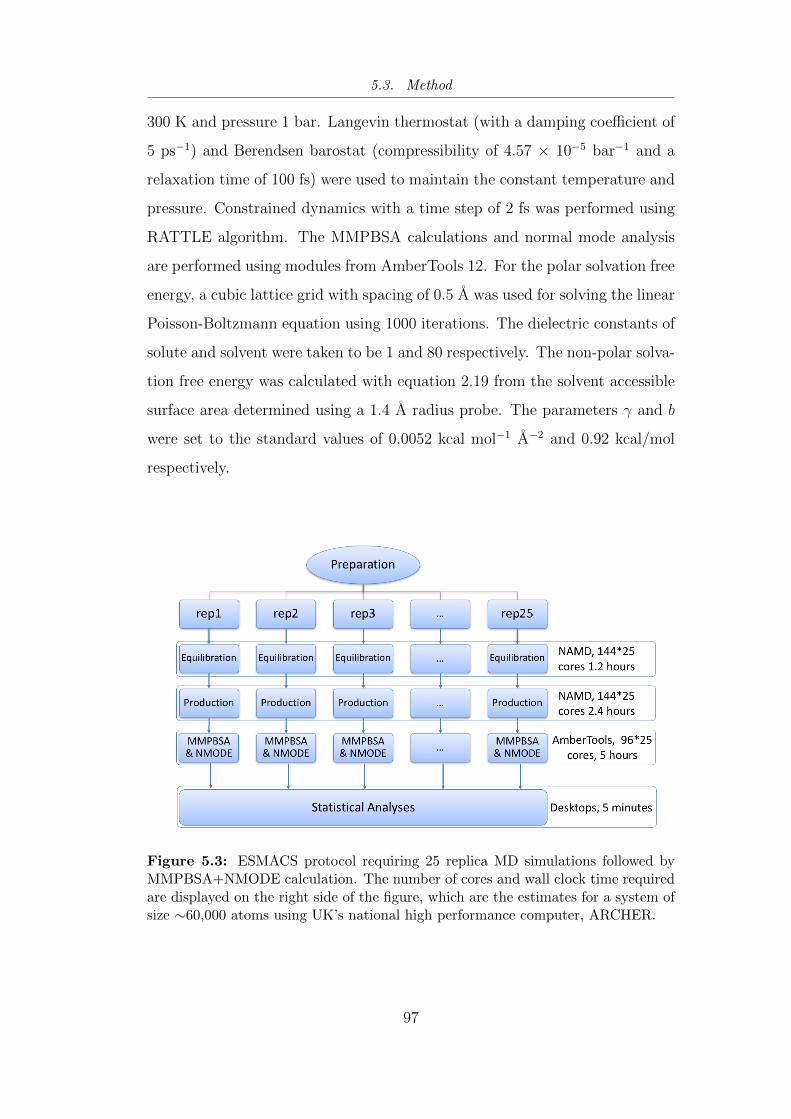
5.3. Method
300 K and pressure 1 bar. Langevin thermostat (with a damping coefficient of
5 ps−1) and Berendsen barostat (compressibility of 4.57 × 10⁻⁵ bar−1 and a
relaxation time of 100 fs) were used to maintain the constant temperature and
pressure. Constrained dynamics with a time step of 2 fs was performed using
RATTLE algorithm. The MMPBSA calculations and normal mode analysis
are performed using modules from AmberTools 12. For the polar solvation free
energy, a cubic lattice grid with spacing of 0.5 A was used for solving the linear
Poisson-Boltzmann equation using 1000 iterations. The dielectric constants of
solute and solvent were taken to be 1 and 80 respectively. The non-polar solva-
tion free energy was calculated with equation 2.19 from the solvent accessible
surface area determined using a 1.4 A radius probe. The parameters γ and b
were set to the standard values of 0.0052 kcal mol−1 A−2 and 0.92 kcal/mol
respectively.
Figure 5.3: ESMACS protocol requiring 25 replica MD simulations followed byMMPBSA+NMODE calculation. The number of cores and wall clock time requiredare displayed on the right side of the figure, which are the estimates for a system ofsize ∼60,000 atoms using UK’s national high performance computer, ARCHER.
97
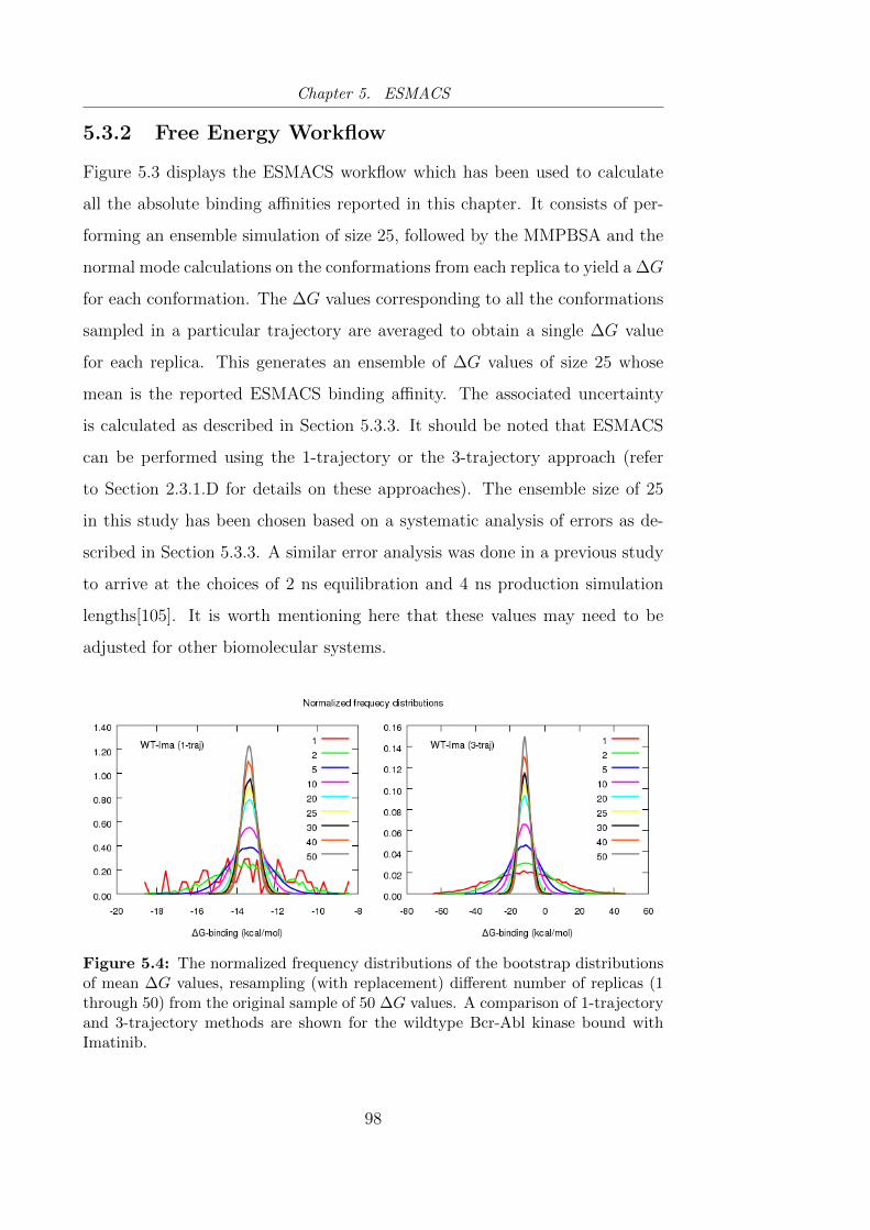
Chapter 5. ESMACS
5.3.2 Free Energy Workflow
Figure 5.3 displays the ESMACS workflow which has been used to calculate
all the absolute binding affinities reported in this chapter. It consists of per-
forming an ensemble simulation of size 25, followed by the MMPBSA and the
normal mode calculations on the conformations from each replica to yield a ∆G
for each conformation. The ∆G values corresponding to all the conformations
sampled in a particular trajectory are averaged to obtain a single ∆G value
for each replica. This generates an ensemble of ∆G values of size 25 whose
mean is the reported ESMACS binding affinity. The associated uncertainty
is calculated as described in Section 5.3.3. It should be noted that ESMACS
can be performed using the 1-trajectory or the 3-trajectory approach (refer
to Section 2.3.1.D for details on these approaches). The ensemble size of 25
in this study has been chosen based on a systematic analysis of errors as de-
scribed in Section 5.3.3. A similar error analysis was done in a previous study
to arrive at the choices of 2 ns equilibration and 4 ns production simulation
lengths[105]. It is worth mentioning here that these values may need to be
adjusted for other biomolecular systems.
Figure 5.4: The normalized frequency distributions of the bootstrap distributionsof mean ∆G values, resampling (with replacement) different number of replicas (1through 50) from the original sample of 50 ∆G values. A comparison of 1-trajectoryand 3-trajectory methods are shown for the wildtype Bcr-Abl kinase bound withImatinib.
98
5.3. Method
5.3.3 Uncertainty Quantification
As discussed above, ESMACS generates an ensemble of ∆G values (one ∆G
value corresponding to each replica) and its mean is the predicted binding
affinity. In order to get an estimate of the associated statistical uncertainty
in this prediction, a bootstrap distribution of mean ∆G values is generated.
This is done by resampling (with replacement) 25 (or the ensemble size in
a general case) ∆G values from the original ensemble of 25 ∆G values to
obtain a bootstrap resample. On repeating this step a large number of times
(100,000 times in this study), many bootstrap resamples are generated. A
frequency distribution of their means gives the bootstrap distribution of mean
∆G values. The standard deviation of this distribution provides an estimate
of the uncertainty in the predicted value and is reported as an error bar on
the predicted ∆G. In the case of the 3-trajectory approach, the bootstrap
distribution of mean ∆G values is given by the differences of the bootstrap
distributions of mean G values (for complex, receptor and ligand).
Figure 5.4 shows the plots of bootstrap distribution of mean ∆G values gener-
ated by bootstrap resamples of different sizes drawn from the original ensemble
of 50 ∆G values (or 50G values for complex, receptor and ligand each, in case of
3-trajectory approach). It can be seen that, on increasing the size of the boot-
strap resamples, the distribution becomes narrower; however, beyond 25 the
decrease in the distribution width is marginal. This suggests that an ensemble
size of 25 is a good balance between the precision of results and computational
costs. Thus, an ensemble size of 25 has been chosen for all calculations in this
chapter.
5.3.4 Repeatability of Predicted Binding Affinities
The bootstrap distribution of mean ∆G values as discussed above provides an
estimate of the repeatability of the predicted binding affinity from ESMACS.
The broader the distribution is, the different any two estimates of ∆G can be.
As can be seen in Figure 5.4, the width of the bootstrap distribution of mean
∆G values is much larger for ensemble size 1 as compared to that of 25. This
99

Chapter 5. ESMACS
Figure 5.5: Correlation and repeatability of the calculated binding affinities fromtwo independent studies of the BRD4 system performed on BlueWonder2 andARCHER. (a) Correlation of the predictions from 1-traj calculations performedon BlueWonder2 (BW2, horizontal axis) and ARCHER (vertical axis). Solid line,regression of the data using the calculated free energies; dotted line, 1:1 ideal re-gression. (b) the ESMACS predictions along with error bars from the two separatecalculations.
suggests that an estimate of binding affinity from a single replica would have
large variation; however, that from an ensemble of 25 would be repeatable
within a small error bar. The ESMACS error bars using ensemble size 25
are typically 0.5 kcal/mol for 1-trajectory approach, and about 2.5 kcal/mol
for 3-trajectory approach. Figure 5.5 shows a comparison of the two sets of
ESMACS predictions for BRD4 based on simulations performed independently
on two different supercomputers, namely BlueWonder2 and ARCHER; the
former is an IBM NextScale Cluster (8640 cores) located at the Science and
Technology Facilities Council's (STFC's) Hartree Centre and the latter is a
Cray XC30 supercomputer (equipped with ∼ 118000 cores), the UKs National
High Performance Computing Service located in Edinburgh. The results are
compared by linear regression. Results exhibit excellent repeatability with
a correlation coefficient of 0.98±0.01. The calculated regression line has a
slope of 1 and an intercept of 0 within the limits of error bars. Only 3 out
of 16 predictions do not overlap within the error bars. Only the results from
BlueWonder2 are reported in the following section. Figure 5.6 displays the
100
5.4. Case Studies
excellent repeatability of ESMACS predictions for Abl kinase complexes as
discussed later in the chapter.
5.4 Case Studies
In this section, case studies employing the ESMACS methodology on four
different target proteins are described. The binding affinity predictions us-
ing both single and multiple trajectory approaches have been provided and
compared.
5.4.1 Bcr-Abl Kinase
As described earlier, 5 mutants of the Abl kinase and 4 of their tyrosine ki-
nase inhibitors (TKIs) are chosen for this study amounting to a total of 20
complexes. Table 5.1 contains the ESMACS predictions and the correspond-
ing experimental binding affinities for all 20 complexes. The experimental
binding affinities are derived from the IC50 values[240] using Equation 2.7.
Typical experimental noise for high quality binding affinity measurements is
of the order of 0.5 kcal/mol[196]. However, experimental uncertainties are not
available in this case. Spearman rank coefficient (rs) and Pearson correlation
coefficient (r) are provided as statistical measures of the rank ordering and
the level of linear correlation, respectively, between the ESMACS predictions
and the corresponding experimental values. The high values of correlation co-
efficients mean that the ESMACS predictions are in good agreement with the
experimental data. It should be noted in Table 5.1 that ESMACS does not
yield the actual binding affinities. This is because it is based on the MMPBSA
method which involves several approximations (refer to Chapter 2). However,
ESMACS does a good job at ranking the ligands based on their binding affini-
ties with a given target protein, which is of greater interest than the actual
values of binding affinities in most cases.
Figures 5.6 (a) to (e) display the correlation plots of the predicted and exper-
imental ∆G values for all ligands bound to each variant of the Abl kinase for
better visual comparison of the two. The error bars on the predicted values
101
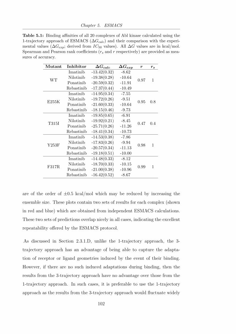
Chapter 5. ESMACS
Table 5.1: Binding affinities of all 20 complexes of Abl kinase calculated using the1-trajectory approach of ESMACS (∆Gcalc) and their comparison with the experi-mental values (∆Gexp; derived from IC50 values). All ∆G values are in kcal/mol.Spearman and Pearson rank coefficients (rs and r respectively) are provided as mea-sures of accuracy.
Mutant Inhibitor ∆Gcalc ∆Gexp r rs
WT
Imatinib -13.42(0.32) -8.62
0.97 1Nilotinib -19.38(0.28) -10.64Ponatinib -20.59(0.32) -11.91Rebastinib -17.37(0.44) -10.49
E255K
Imatinib -14.95(0.34) -7.55
0.95 0.8Nilotinib -19.72(0.26) -9.51Ponatinib -21.60(0.33) -10.64Rebastinib -18.15(0.46) -9.73
T315I
Imatinib -19.85(0.65) -6.91
0.47 0.4Nilotinib -19.92(0.21) -8.45Ponatinib -25.71(0.26) -11.26Rebastinib -18.41(0.34) -10.73
Y253F
Imatinib -14.53(0.38) -7.86
0.98 1Nilotinib -17.83(0.26) -9.94Ponatinib -20.57(0.34) -11.13Rebastinib -19.18(0.51) -10.00
F317R
Imatinib -14.48(0.33) -8.12
0.99 1Nilotinib -18.70(0.33) -10.15Ponatinib -21.00(0.38) -10.96Rebastinib -16.42(0.52) -8.67
are of the order of ±0.5 kcal/mol which may be reduced by increasing the
ensemble size. These plots contain two sets of results for each complex (shown
in red and blue) which are obtained from independent ESMACS calculations.
These two sets of predictions overlap nicely in all cases, indicating the excellent
repeatability offered by the ESMACS protocol.
As discussed in Section 2.3.1.D, unlike the 1-trajectory approach, the 3-
trajectory approach has an advantage of being able to capture the adapta-
tion of receptor or ligand geometries induced by the event of their binding.
However, if there are no such induced adaptations during binding, then the
results from the 3-trajectory approach have no advantage over those from the
1-trajectory approach. In such cases, it is preferable to use the 1-trajectory
approach as the results from the 3-trajectory approach would fluctuate widely
102
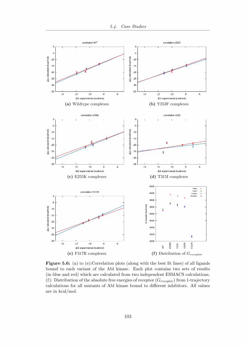
5.4. Case Studies
(a) Wildtype complexes (b) Y253F complexes
(c) E255K complexes (d) T315I complexes
(e) F317R complexes (f) Distribution of Greceptor
Figure 5.6: (a) to (e):Correlation plots (along with the best fit lines) of all ligandsbound to each variant of the Abl kinase. Each plot contains two sets of results(in blue and red) which are calculated from two independent ESMACS calculations.(f): Distribution of the absolute free energies of receptor (Greceptor) from 1-trajectorycalculations for all mutants of Abl kinase bound to different inhibitors. All valuesare in kcal/mol.
103
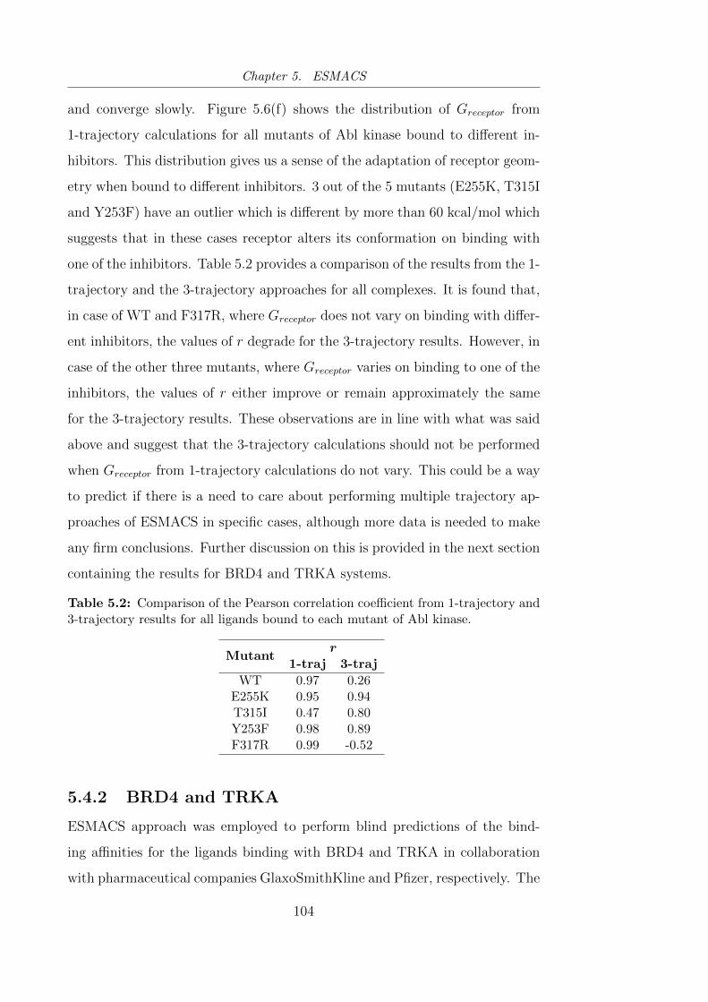
Chapter 5. ESMACS
and converge slowly. Figure 5.6(f) shows the distribution of Greceptor from
1-trajectory calculations for all mutants of Abl kinase bound to different in-
hibitors. This distribution gives us a sense of the adaptation of receptor geom-
etry when bound to different inhibitors. 3 out of the 5 mutants (E255K, T315I
and Y253F) have an outlier which is different by more than 60 kcal/mol which
suggests that in these cases receptor alters its conformation on binding with
one of the inhibitors. Table 5.2 provides a comparison of the results from the 1-
trajectory and the 3-trajectory approaches for all complexes. It is found that,
in case of WT and F317R, where Greceptor does not vary on binding with differ-
ent inhibitors, the values of r degrade for the 3-trajectory results. However, in
case of the other three mutants, where Greceptor varies on binding to one of the
inhibitors, the values of r either improve or remain approximately the same
for the 3-trajectory results. These observations are in line with what was said
above and suggest that the 3-trajectory calculations should not be performed
when Greceptor from 1-trajectory calculations do not vary. This could be a way
to predict if there is a need to care about performing multiple trajectory ap-
proaches of ESMACS in specific cases, although more data is needed to make
any firm conclusions. Further discussion on this is provided in the next section
containing the results for BRD4 and TRKA systems.
Table 5.2: Comparison of the Pearson correlation coefficient from 1-trajectory and3-trajectory results for all ligands bound to each mutant of Abl kinase.
Mutantr
1-traj 3-traj
WT 0.97 0.26E255K 0.95 0.94T315I 0.47 0.80Y253F 0.98 0.89F317R 0.99 -0.52
5.4.2 BRD4 and TRKA
ESMACS approach was employed to perform blind predictions of the bind-
ing affinities for the ligands binding with BRD4 and TRKA in collaboration
with pharmaceutical companies GlaxoSmithKline and Pfizer, respectively. The
104
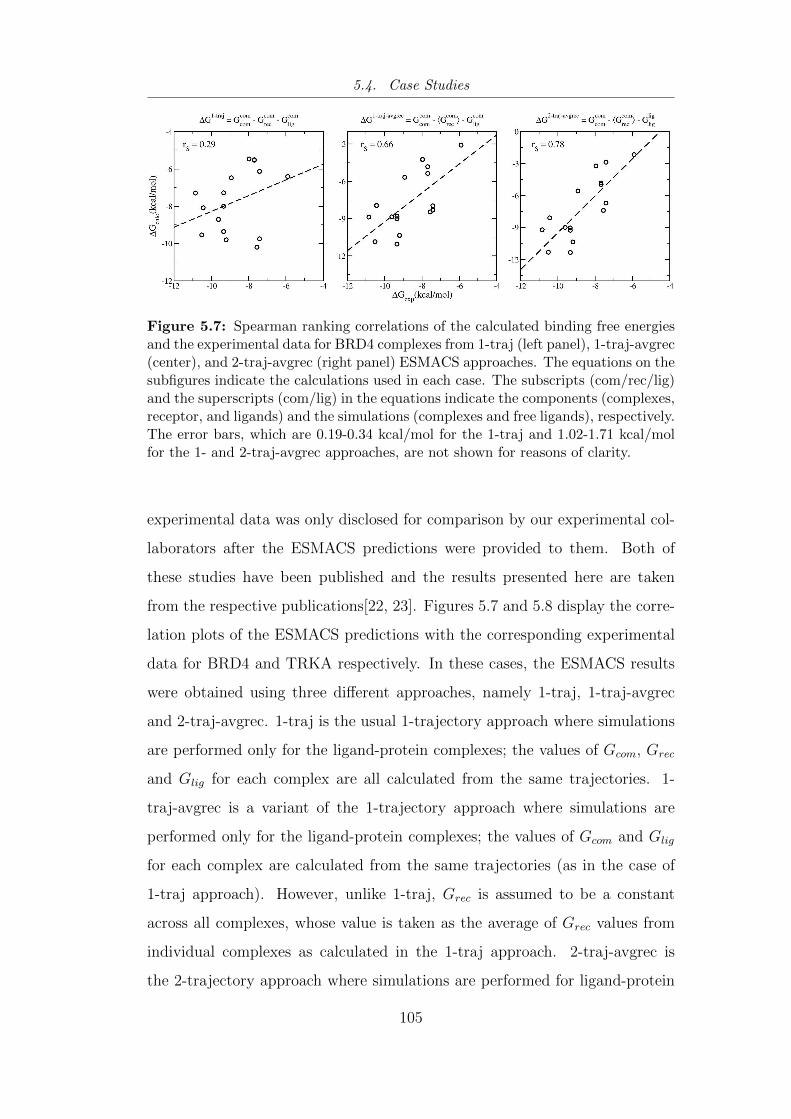
5.4. Case Studies
Figure 5.7: Spearman ranking correlations of the calculated binding free energiesand the experimental data for BRD4 complexes from 1-traj (left panel), 1-traj-avgrec(center), and 2-traj-avgrec (right panel) ESMACS approaches. The equations on thesubfigures indicate the calculations used in each case. The subscripts (com/rec/lig)and the superscripts (com/lig) in the equations indicate the components (complexes,receptor, and ligands) and the simulations (complexes and free ligands), respectively.The error bars, which are 0.19-0.34 kcal/mol for the 1-traj and 1.02-1.71 kcal/molfor the 1- and 2-traj-avgrec approaches, are not shown for reasons of clarity.
experimental data was only disclosed for comparison by our experimental col-
laborators after the ESMACS predictions were provided to them. Both of
these studies have been published and the results presented here are taken
from the respective publications[22, 23]. Figures 5.7 and 5.8 display the corre-
lation plots of the ESMACS predictions with the corresponding experimental
data for BRD4 and TRKA respectively. In these cases, the ESMACS results
were obtained using three different approaches, namely 1-traj, 1-traj-avgrec
and 2-traj-avgrec. 1-traj is the usual 1-trajectory approach where simulations
are performed only for the ligand-protein complexes; the values of Gcom, Grec
and Glig for each complex are all calculated from the same trajectories. 1-
traj-avgrec is a variant of the 1-trajectory approach where simulations are
performed only for the ligand-protein complexes; the values of Gcom and Glig
for each complex are calculated from the same trajectories (as in the case of
1-traj approach). However, unlike 1-traj, Grec is assumed to be a constant
across all complexes, whose value is taken as the average of Grec values from
individual complexes as calculated in the 1-traj approach. 2-traj-avgrec is
the 2-trajectory approach where simulations are performed for ligand-protein
105
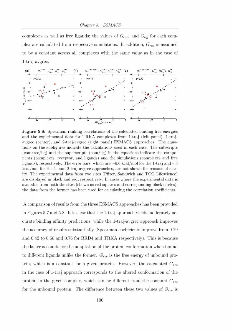
Chapter 5. ESMACS
complexes as well as free ligands; the values of Gcom and Glig for each com-
plex are calculated from respective simulations. In addition, Grec is assumed
to be a constant across all complexes with the same value as in the case of
1-traj-avgrec.
Figure 5.8: Spearman ranking correlations of the calculated binding free energiesand the experimental data for TRKA complexes from 1-traj (left panel), 1-traj-avgrec (center), and 2-traj-avgrec (right panel) ESMACS approaches. The equa-tions on the subfigures indicate the calculations used in each case. The subscripts(com/rec/lig) and the superscripts (com/lig) in the equations indicate the compo-nents (complexes, receptor, and ligands) and the simulations (complexes and freeligands), respectively. The error bars, which are ∼0.6 kcal/mol for the 1-traj and ∼3kcal/mol for the 1- and 2-traj-avgrec approaches, are not shown for reasons of clar-ity. The experimental data from two sites (Pfizer, Sandwich and TCG Lifescience)are displayed in black and red, respectively. In cases where the experimental data isavailable from both the sites (shown as red squares and corresponding black circles),the data from the former has been used for calculating the correlation coefficients.
A comparison of results from the three ESMACS approaches has been provided
in Figures 5.7 and 5.8. It is clear that the 1-traj approach yields moderately ac-
curate binding affinity predictions, while the 1-traj-avgrec approach improves
the accuracy of results substantially (Spearman coefficients improve from 0.29
and 0.42 to 0.66 and 0.76 for BRD4 and TRKA respectively). This is because
the latter accounts for the adaptation of the protein conformation when bound
to different ligands unlike the former. Grec is the free energy of unbound pro-
tein, which is a constant for a given protein. However, the calculated Grec
in the case of 1-traj approach corresponds to the altered conformation of the
protein in the given complex, which can be different from the constant Grec
for the unbound protein. The difference between these two values of Grec is
106
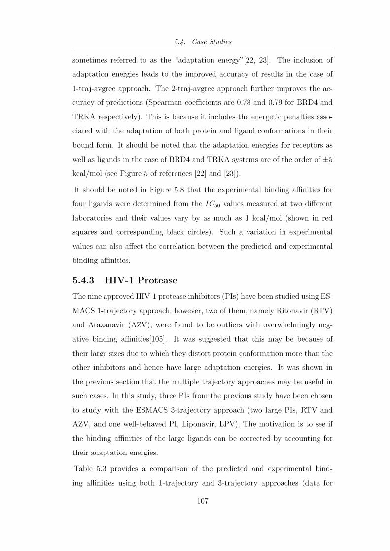
5.4. Case Studies
sometimes referred to as the “adaptation energy”[22, 23]. The inclusion of
adaptation energies leads to the improved accuracy of results in the case of
1-traj-avgrec approach. The 2-traj-avgrec approach further improves the ac-
curacy of predictions (Spearman coefficients are 0.78 and 0.79 for BRD4 and
TRKA respectively). This is because it includes the energetic penalties asso-
ciated with the adaptation of both protein and ligand conformations in their
bound form. It should be noted that the adaptation energies for receptors as
well as ligands in the case of BRD4 and TRKA systems are of the order of ±5
kcal/mol (see Figure 5 of references [22] and [23]).
It should be noted in Figure 5.8 that the experimental binding affinities for
four ligands were determined from the IC50 values measured at two different
laboratories and their values vary by as much as 1 kcal/mol (shown in red
squares and corresponding black circles). Such a variation in experimental
values can also affect the correlation between the predicted and experimental
binding affinities.
5.4.3 HIV-1 Protease
The nine approved HIV-1 protease inhibitors (PIs) have been studied using ES-
MACS 1-trajectory approach; however, two of them, namely Ritonavir (RTV)
and Atazanavir (AZV), were found to be outliers with overwhelmingly neg-
ative binding affinities[105]. It was suggested that this may be because of
their large sizes due to which they distort protein conformation more than the
other inhibitors and hence have large adaptation energies. It was shown in
the previous section that the multiple trajectory approaches may be useful in
such cases. In this study, three PIs from the previous study have been chosen
to study with the ESMACS 3-trajectory approach (two large PIs, RTV and
AZV, and one well-behaved PI, Liponavir, LPV). The motivation is to see if
the binding affinities of the large ligands can be corrected by accounting for
their adaptation energies.
Table 5.3 provides a comparison of the predicted and experimental bind-
ing affinities using both 1-trajectory and 3-trajectory approaches (data for
107
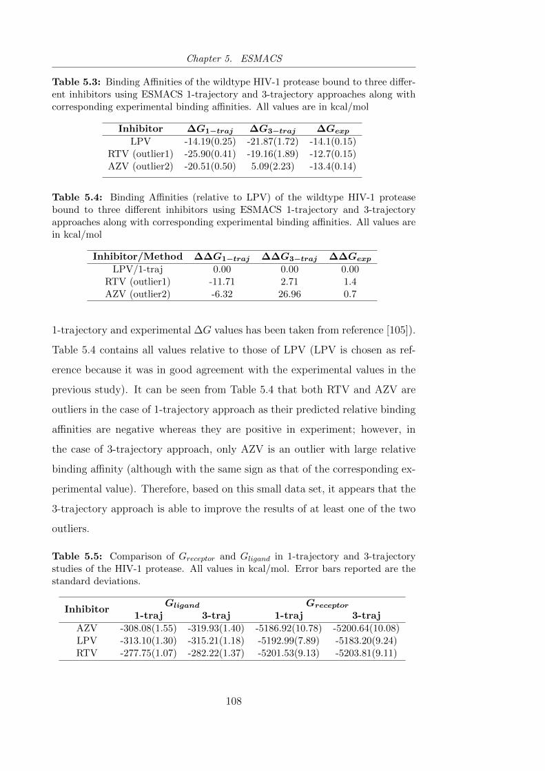
Chapter 5. ESMACS
Table 5.3: Binding Affinities of the wildtype HIV-1 protease bound to three differ-ent inhibitors using ESMACS 1-trajectory and 3-trajectory approaches along withcorresponding experimental binding affinities. All values are in kcal/mol
Inhibitor ∆G1−traj ∆G3−traj ∆Gexp
LPV -14.19(0.25) -21.87(1.72) -14.1(0.15)RTV (outlier1) -25.90(0.41) -19.16(1.89) -12.7(0.15)AZV (outlier2) -20.51(0.50) 5.09(2.23) -13.4(0.14)
Table 5.4: Binding Affinities (relative to LPV) of the wildtype HIV-1 proteasebound to three different inhibitors using ESMACS 1-trajectory and 3-trajectoryapproaches along with corresponding experimental binding affinities. All values arein kcal/mol
Inhibitor/Method ∆∆G1−traj ∆∆G3−traj ∆∆Gexp
LPV/1-traj 0.00 0.00 0.00RTV (outlier1) -11.71 2.71 1.4AZV (outlier2) -6.32 26.96 0.7
1-trajectory and experimental ∆G values has been taken from reference [105]).
Table 5.4 contains all values relative to those of LPV (LPV is chosen as ref-
erence because it was in good agreement with the experimental values in the
previous study). It can be seen from Table 5.4 that both RTV and AZV are
outliers in the case of 1-trajectory approach as their predicted relative binding
affinities are negative whereas they are positive in experiment; however, in
the case of 3-trajectory approach, only AZV is an outlier with large relative
binding affinity (although with the same sign as that of the corresponding ex-
perimental value). Therefore, based on this small data set, it appears that the
3-trajectory approach is able to improve the results of at least one of the two
outliers.
Table 5.5: Comparison of Greceptor and Gligand in 1-trajectory and 3-trajectorystudies of the HIV-1 protease. All values in kcal/mol. Error bars reported are thestandard deviations.
InhibitorGligand Greceptor
1-traj 3-traj 1-traj 3-traj
AZV -308.08(1.55) -319.93(1.40) -5186.92(10.78) -5200.64(10.08)LPV -313.10(1.30) -315.21(1.18) -5192.99(7.89) -5183.20(9.24)RTV -277.75(1.07) -282.22(1.37) -5201.53(9.13) -5203.81(9.11)
108
5.5. Conclusions
In order to further understand the behaviour of AZV whose predicted bind-
ing affinity changes from overwhelmingly negative in the case of 1-trajectory
approach to overwhelmingly positive in the case of 3-trajectory approach, a
comparison of Greceptor and Gligand for all inhibitors in both the cases has been
reported in Table 5.5. It should be noted that the Gligand changes by almost
12 kcal/mol between 1 and 3 trajectory results in the case of AZV. However,
the data presented is insufficient to draw any firm conclusion and further in-
vestigations are needed.
5.5 Conclusions
This chapter describes a new approach, called ESMACS, based on MMPBSA
to calculate precise and repeatable absolute binding affinities. It is not as accu-
rate as TIES (described in Chapter 3). However, ESMACS is computationally
cheaper than the absolute binding affinity approach based on alchemical meth-
ods as described earlier[231]. The ESMACS protocol is flexible, with parame-
ters like simulation duration and ensemble size adjusted to obtain the desired
level of precision. Another important feature of ESMACS is its scalability,
which reduces the wall-clock time required to make predictions by running
multiple replicas concurrently on a supercomputer. ESMACS has been shown
to rank the inhibitors bound to 5 different variants of Abl kinase, BRD4 and
TRKA well.
It should be noted that the accuracy of potential parametrisation has a great
influence on the predicted binding affinities and care must be taken while
choosing the parameters. In the HIV-1 protease case study, there is a need of
further investigation to understand the behaviour of the inhibitors, Ritonavir
and Atazanavir.
The discussion on the single and multiple trajectory versions of ESMACS and
their applicability in different scenarios highlights the strength of the method
and its potential applicability in real life context. Both TIES and ESMACS
approaches were employed in two recent collaborative studies with pharmaceu-
109

Chapter 5. ESMACS
tical companies, GlaxoSmithKline and Pfizer, where the blind binding affinity
predictions were found to rank a large set of ligands bound to the target
protein correctly when later compared with the corresponding experimental
values[22, 23]. This exhibits the immense potential of ensemble simulation
based approaches in the drug design process.
110
Chapter 6
Automation toolkit
In the previous chapters, several different approaches based on ensemble simu-
lation are described to calculate accurate, precise and repeatable binding free
energies. It has been shown that these approaches yield binding free energy
predictions in good agreement with the experimental values and hence have
the potential to be applicable in drug design and patient specific medicine.
However, in order to have a positive impact in industrial or clinical settings,
the predictions need to be made at the time scales which can compete with
the experimental determination of binding affinities. The important feature of
scalability of both TIES and ESMACS workflows (described in the previous
chapters) allows us to reduce the time required to make predictions by running
multiple replicas concurrently. However, these complex computational work-
flows are very tedious to perform manually and very error-prone. Automating
the execution of these workflows further reduces the time to solution. In this
chapter, the software tools developed in my group, namely the Binding Affin-
ity Calculator (BAC)[239] and FabSim[241, 242], are described. I extended
both of them to automate the implementation of the workflows described in
previous chapters.
6.1 Binding Affinity Calculator
BAC is a tool which automates the end-to-end execution of the TIES and the
ESMACS workflows (refer to Figures 3.3 and 5.3). It helps in managing the
Chapter 6. Automation toolkit
large volume of simulation and free energy calculation data from all replicas,
which have identical input but different output, in an error-proof manner.
Broadly, both these workflows can be divided into three phases: preparation
phase, production phase and analysis phase. Different components of BAC
have been developed to handle different phases.
BAC-Builder is the component of BAC which executes the preparation phase.
This phase involves preparing the simulation-ready solvated initial structure
of the biomolecular system to be studied from its raw starting structure (usu-
ally in the form of a crystal structure in PDB format) and the appropriate
potential parameters. BAC-Builder is a set of modules implemented in the
Perl language. It takes the raw PDB file and ligand parameter files as input
along with the specification of the desired force field as well as MD engine and
generates the structure and parameter files to be used for simulations in the
production phase. It also generates the input configuration files compatible
with the specified MD engine for the execution of the stepwise equilibration
and production simulations as described in detail in reference [239].
I extended the original BAC-builder by developing a new module to handle
the preparation phase of the TIES method. As described in Chapter 3, unlike
ESMACS, TIES requires hybrid structure and parameter files as raw input,
which need to be prepared using a tedious protocol. The automation of this
protocol substantially reduced the time and effort required in their preparation
and was a major advancement towards the implementation of TIES on a large
number of biomolecular systems.
In the production phase, before the simulations are performed, all the input
data generated during the preparation phase need to be rearranged in a di-
rectory structure appropriate to perform ensemble simulations such that the
common input is centrally accessible by all replicas and the distinct output is
saved in different sub-directories. Such an arrangement is essential for handling
the large amounts of data associated with ensemble simulations and makes it
convenient to perform the post-production statistical analysis. This step has
112
6.2. FabSim
been automated using the BAC-Builder and FabSim. After this rearrange-
ment, FabSim automates the tasks of staging the data and submitting the
job to run the ensemble simulation on a remote supercomputer. FabSim is
described in the next section.
After the successful execution of the production phase, the final step is to
perform the statistical analysis on the output generated (the analysis phase).
I developed the BAC-Analysis tool to automate this phase for both the ES-
MACS and the TIES workflows. In the case of TIES, this can be performed on
the local computer within a few minutes with a combination of bash, awk and
R scripts. In the case of ESMACS, the post-production analysis consists of
two parts: MMPBSA+NMODE calculations and the ESMACS binding affinity
calculation (see Chapter 5). The former need to be performed on a supercom-
puter with the help of modules of AmberTools 12, while the latter can be
performed on a local computer within a few minutes using the BAC-Analysis
tool.
Cloud computing is increasingly becoming popular. The users are allowed to
purchase access to appropriate number of CPUs on cloud resources for desired
duration of time as and when needed. Given the growing popularity of cloud
computing, BAC is now being deployed by my colleagues on commercial clouds
like Amazon web services, Microsoft Azure and DNANexus. A user friendly
interface of BAC, called UF-BAC, has been developed in order to make it
available to widest range of users possible.
6.2 FabSim
FabSim is a toolkit scripted in the Python language to simplify a broad range of
computational tasks for researchers in diverse disciplines[241, 242]. Its strength
lies in the fact that it is highly customisable and hence can be adapted to
a wide range of tasks. In addition, it provides a systematic route to auto-
mate the utilisation of HPC and distributed resources. FabSim has been em-
ployed in several diverse research domains including simulating cerebrovascular
113

Chapter 6. Automation toolkit
bloodflow, modelling multiscale clay-polymer nanocomposites, and predicting
ligand-protein binding affinities. Three application-specific modules of Fab-
Sim, namely FabHemeLB, FabMD and FabBioMD, have been developed for
the three applications mentioned above respectively[241]. A fourth module,
FabFlee, aimed towards migration modelling, is under development.
I developed the entire FabBioMD module of FabSim, which is relevant in
the production phases of both the TIES and the ESMACS workflows. In
order to effectively handle the large volume of data from these workflows, it is
desirable to have a well-defined method of data curation, which also enhances
data transferability between users. FabBioMD is configured to arrange all the
data in a comprehensible directory structure, to automatically stage the data
and submit the job to perform equilibration, simulation (for both ESMACS
and TIES) and MMPBSA calculations (for ESMACS) on the desired remote
supercomputer using one-line command. The command syntax is as follows:
fab <hostname> <command>:<conf igurat ion name >,
<parameter1=x1> , ( . . . ) , < parameterN=xn>
where, hostname is the remote machine to be used for the job, command is
the pre-defined function to be executed, configuration name is the location of
the input configuration, and the user has the option to specify values of the
parameters. In case no parameters are defined in the command, their pre-
defined default values are taken. An example function of FabBioMD module
with its usage is as follows:
fab archer b a c t i e s a r c h e r l i k e : myhomedirectory ,
c o r e s =1000 , wa l l t ime =06:00 :00 , r e p l i c a s =5
The above command when executed on the command line of my desktop calls
the FabBioMD function “bac ties archerlike”. It copies all the data from the
directory named “myhomedirectory” to a pre-configured remote location on
the supercomputer ARCHER, creates a submission script for a TIES job (using
1000 cores, 6 hours wall-clock time and 5 replicas per λ-window; the pre-defined
114
6.2. FabSim
default values of λ are used) and submits the job to the queue on ARCHER; all
with a single command. There is a long list of functions in FabBioMD module
of FabSim, which I developed to perform different steps of both ESMACS and
TIES workflows and to execute these workflows on a variety of supercomputers
with different architectures[241, 242].
One of the major advantages of FabSim is that it subsumes the underlying
complexities related to the submission of jobs on different HPC architectures
by allowing the user to easily submit jobs on different supercomputers. All that
needs to be done is a one-time configuration of each HPC resource and creation
of templates for job submission scripts which can be accessed while executing
the relevant function of the FabBioMD module. I have configured several ma-
jor supercomputers of different HPC centres including the UKs National High
Performance Computing Service (ARCHER; www.archer.ac.uk), the Science
and Technology Facilities Council's (STFC's) Hartree Centre ( BlueJoule and
BlueWonder; www.hartree.stfc.ac.uk) and Leibniz Supercomputing Cen-
tre (SuperMUC; www.lrz.de). These supercomputers were used to perform
almost all of the simulations related to this thesis.
It is possible for the users to define customised functions to suit their needs
if the available functions are not sufficient for their purpose. Any new remote
HPC resource can easily be configured and added to the known resources of
the FabSim database by the user.
It is worth mentioning here that the level of automation achieved using BAC
and FabSim made it possible for us to successfully perform hundreds of TIES
and ESMACS calculations for a large number of ligand-protein complexes in
a short period of 37 hours by occupying the whole SuperMUC (∼250,000
cores)[243]. It was achieved by the swift execution of the different phases
of these workflows through our automation toolkit. The successful execution
of this unprecedented “giant workflow” has realised that these workflows have
the ability to make useful binding affinity predictions within the span of a
few hours, which can be exploited for clinical decision making to personalise
115

Chapter 6. Automation toolkit
medicines for patients.
116
Chapter 7
Conclusions
This thesis addresses the issue of variability in results of the free energy meth-
ods based on classical molecular dynamics simulations when based on a single
short simulation and establishes a route to reliable binding affinity predictions.
It discusses the important property of sensitivity of classical MD simulations
to their initial conditions[10], which leads to the large variation in the free
energies predicted using a single short trajectory on repeating the calculation.
In addition, it has been noted that the ensemble average can be considered
equal to the time average via the ergodic theorem only in the limit of Poincare
recurrence time, which is usually extremely long for ligand binding and typi-
cally unapproachable on compute resources available today[10]. Moreover, for
a non-equilibrium system, time averaging is meaningless, since the observables
in that case are time dependent. With this in mind, ensemble simulations have
been proposed as a way to calculate macroscopic thermodynamic properties
like the Gibbs free energy through ensemble averaging over microstates instead
of performing time averages over a single insufficiently long simulation. It has
been shown that the employment of ensemble simulation based approaches
yields precise and repeatable free energy predictions within a short span of
time (∼6-8 hours, which can be further reduced using GPUs). The results are
found to be accurate within the limitations of the force fields used. Given the
reliability of predictions from the ensemble simulation based approaches, they
promise to make a positive impact in the fields of drug design and personalised
Chapter 7. Conclusions
medicine.
Thermodynamic integration with enhanced sampling (TIES) is a free energy
prediction method based on one of the alchemical methods, thermodynamic
integration, and employs the concept of ensemble simulation. The associated
parameters like ensemble size and simulation length were chosen based on a
proper assessment of statistical uncertainties. TIES has been shown to yield
relative binding affinity predictions with high accuracy and precision for a
large number of ligands bound to a variety of target proteins. TIES results
are shown to be repeatable with and without the variation in the software, the
hardware and the implementation of the free energy calculation. It has been
shown that an ensemble of short simulations does a better job than a single
simulation when the total simulation duration in both cases is the same. TIES
is able to capture important dynamical properties of the system correctly.
TIES methodology has also been employed to several accelerated sampling
protocols based on Hamiltonian replica-exchange technique and an improved
free energy estimator. It has been shown that the variability in results from in-
dependent short MD simulations exists even when employing better sampling
protocols and/or free energy estimators, and that ensemble simulation is nec-
essary in order to properly handle the statistical uncertainties associated with
the predicted free energies irrespective of such advancements in the free energy
method used. In addition, such variability in results from these advanced free
energy methods persists even on extending the simulations to durations up to
the cumulative duration of the ensemble simulation.
The ensemble simulation approach has been applied to the end-point free
energy method, MMPBSA, leading to a method called enhanced sampling
of molecular dynamics with approximation of continuum solvent (ESMACS).
The ensemble size was chosen based on the statistical assessment of errors
with the note that it is system-dependent. The single and multiple trajectory
approaches of ESMACS have been applied on several different protein systems
and their results compared. ESMACS is highly precise but inaccurate in the
118
sense that it is unable to predict the actual values of binding affinities but it
has been shown to rank the ligands well based on their binding affinities with
a given target protein.
TIES and ESMACS have complementary domain of applicabilities. TIES is
very accurate but its application is restricted to structurally similar compounds
when calculating the relative binding affinities. On the other hand, ESMACS
is not accurate given its underlying approximations but can be used to calcu-
late binding affinities of a diverse set of molecules. It is important to note that,
for these methods to yield reliable binding affinity predictions, it is necessary
to employ reliable force fields and potential parametrisations during the sim-
ulations as the accuracy of predictions is dependent on them. It should also
be noted that an ensemble of short non-biased MD simulations is suitable for
determining free energy when the initial structure of the system studied is at
equilibrium. However, it is unable to capture the dynamics of rare events such
as, protein folding or DFG flip, which would require long simulation duration
and/or biased potential employed for each replica of the ensemble[244].
The different free energy schemes described in this thesis comprise of complex
workflows. Therefore, a fair amount of effort was put into the development
of an automation toolkit, which made the execution of all workflows easier,
quicker and error-free. The automation of workflow execution also helps in
better management of the large volume of data generated by the free en-
ergy calculations based on ensemble simulations. Binding Affinity Calculator
(BAC) and FabSim are the tools developed for this purpose and have been
briefly described in Chapter 6.
All the methods described in this thesis along with the automation toolkit
provide a solution to the issue of variability of results from independent short
simulations in the field of in silico binding affinity calculations and provide a
route to their reliable predictions. The ability to make accurate, precise and
repeatable predictions using computational methods increases their scientific
value as well as reliability in industrial and clinical context. This along with the
119
Chapter 7. Conclusions
short time to solution makes it possible to apply these methods directly as tools
in the process of drug design and clinical decision making. The applicability of
TIES and ESMACS in pharmaceutical industry is evident from the published
works co-authored by myself in collaboration with GlaxoSmithKline[22] and
Pfizer[23] which were conducted as blind studies.
The work presented in this thesis has led to the development of another al-
chemical free energy method developed by one of my colleagues[231]. It applies
the TIES methodology to an alchemical method based on double annihilation
technique[245, 246] to reliably predict absolute binding affinities for a range of
biomolecular systems.
The future directions of research based upon this thesis include applying the
ensemble simulation based methods to study point mutations in proteins as
well as the estimation of reaction rate parameters. Protein side-chain muta-
tions occur naturally and sometimes may alter the ability of drug/ligand to
bind with the protein. This is the most common way in which the target
proteins develop drug resistance. Therefore, studying the effect of protein mu-
tations on the binding affinity is important. I am currently working on the
development of an alchemical method called TIES-PM which would employ
the TIES methodology to yield rapid, accurate, precise and repeatable relative
binding affinity corresponding to the mutation in a protein when bound with a
ligand. In future, the ensemble simulation based methods described here could
be used to develop reliable methods for the estimation of kinetic parameters
involved in binding process, which are quite challenging given the long time
scale of their occurrence.
120
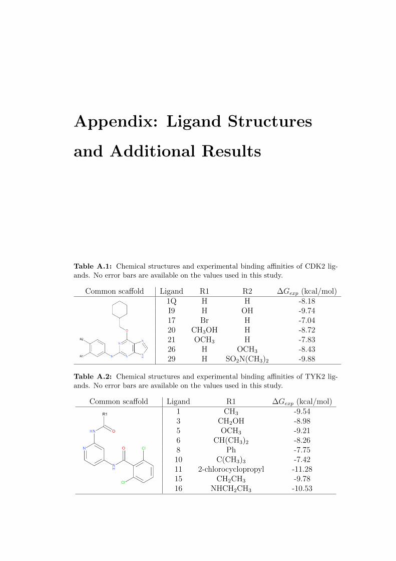
Appendix: Ligand Structures
and Additional Results
Table A.1: Chemical structures and experimental binding affinities of CDK2 lig-ands. No error bars are available on the values used in this study.
Common scaffold Ligand R1 R2 ∆Gexp (kcal/mol)1Q H H -8.18I9 H OH -9.7417 Br H -7.0420 CH3OH H -8.7221 OCH3 H -7.8326 H OCH3 -8.4329 H SO2N(CH3)2 -9.88
Table A.2: Chemical structures and experimental binding affinities of TYK2 lig-ands. No error bars are available on the values used in this study.
Common scaffold Ligand R1 ∆Gexp (kcal/mol)1 CH3 -9.543 CH2OH -8.985 OCH3 -9.216 CH(CH3)2 -8.268 Ph -7.7510 C(CH3)3 -7.4211 2-chlorocyclopropyl -11.2815 CH2CH3 -9.7816 NHCH2CH3 -10.53
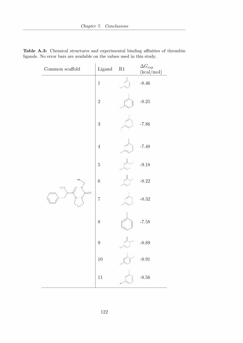
Chapter 7. Conclusions
Table A.3: Chemical structures and experimental binding affinities of thrombinligands. No error bars are available on the values used in this study.
Common scaffold Ligand R1∆Gexp
(kcal/mol)
1 -8.46
2 -8.25
3 -7.86
4 -7.48
5 -9.18
6 -8.22
7 -8.32
8 -7.58
9 -8.89
10 -8.91
11 -8.56
122
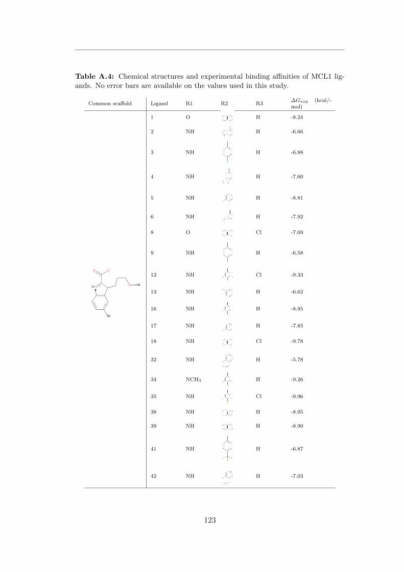
Table A.4: Chemical structures and experimental binding affinities of MCL1 lig-ands. No error bars are available on the values used in this study.
Common scaffold Ligand R1 R2 R3∆Gexp (kcal/-mol)
1 O H -8.24
2 NH H -6.66
3 NH H -6.88
4 NH H -7.60
5 NH H -8.81
6 NH H -7.92
8 O Cl -7.69
9 NH H -6.58
12 NH Cl -9.33
13 NH H -6.62
16 NH H -8.95
17 NH H -7.85
18 NH Cl -9.78
32 NH H -5.78
34 NCH3 H -9.26
35 NH Cl -9.96
38 NH H -8.95
39 NH H -8.90
41 NH H -6.87
42 NH H -7.03
123
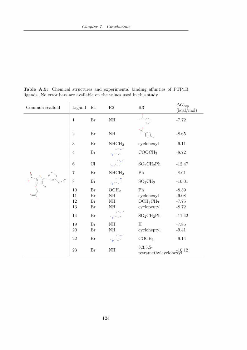
Chapter 7. Conclusions
Table A.5: Chemical structures and experimental binding affinities of PTP1Bligands. No error bars are available on the values used in this study.
Common scaffold Ligand R1 R2 R3∆Gexp(kcal/mol)
1 Br NH -7.72
2 Br NH -8.65
3 Br NHCH2 cyclohexyl -9.11
4 Br COOCH3 -8.72
6 Cl SO2CH2Ph -12.47
7 Br NHCH2 Ph -8.61
8 Br SO2CH3 -10.01
10 Br OCH2 Ph -8.3911 Br NH cyclohexyl -9.0812 Br NH OCH2CH3 -7.7513 Br NH cyclopentyl -8.72
14 Br SO2CH2Ph -11.42
19 Br NH H -7.8520 Br NH cycloheptyl -9.41
22 Br COCH3 -9.14
23 Br NH3,3,5,5-tetramethylcyclohexyl
-10.12
124
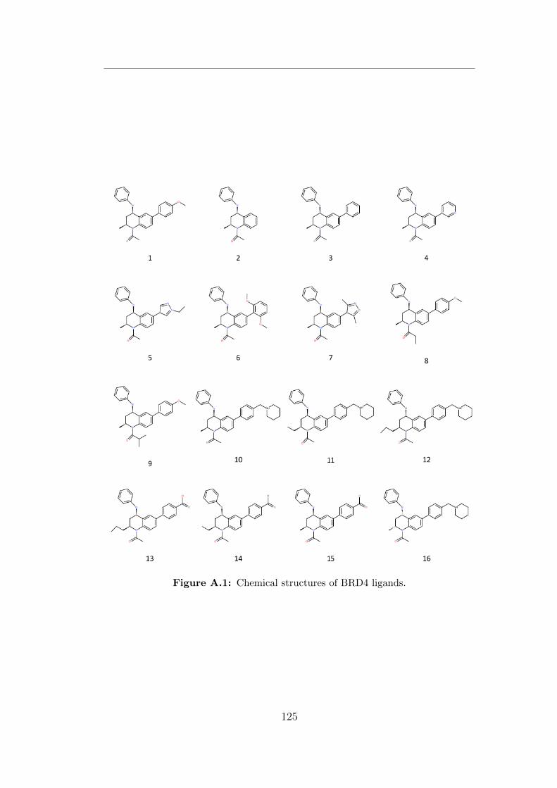
Figure A.1: Chemical structures of BRD4 ligands.
125
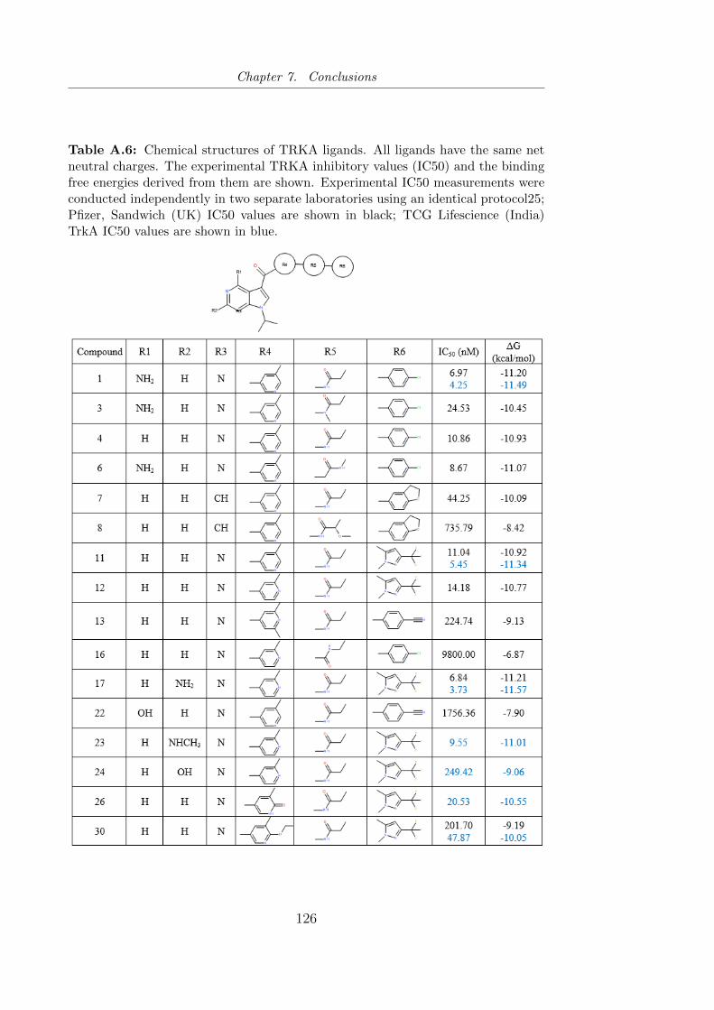
Chapter 7. Conclusions
Table A.6: Chemical structures of TRKA ligands. All ligands have the same netneutral charges. The experimental TRKA inhibitory values (IC50) and the bindingfree energies derived from them are shown. Experimental IC50 measurements wereconducted independently in two separate laboratories using an identical protocol25;Pfizer, Sandwich (UK) IC50 values are shown in black; TCG Lifescience (India)TrkA IC50 values are shown in blue.
126
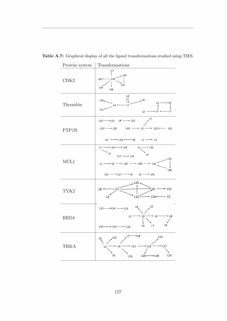
Table A.7: Graphical display of all the ligand transformations studied using TIES.
Protein system Transformations
CDK2
Thrombin
PTP1B
MCL1
TYK2
BRD4
TRKA
127
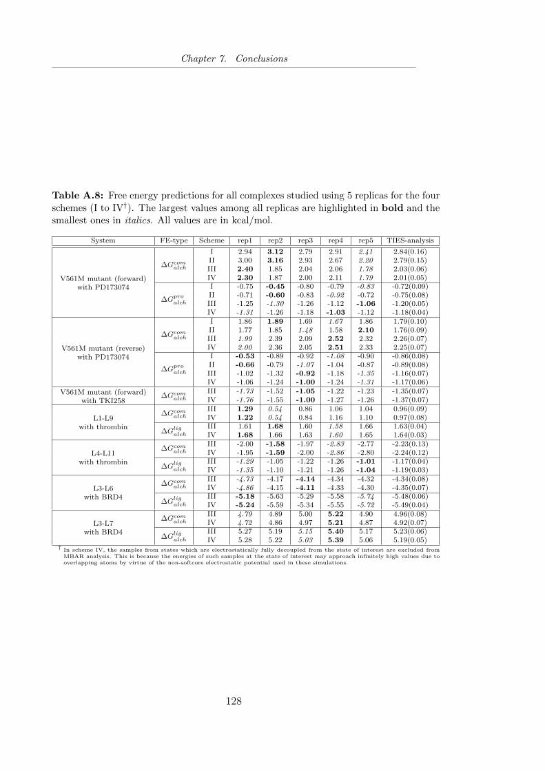
Chapter 7. Conclusions
Table A.8: Free energy predictions for all complexes studied using 5 replicas for the fourschemes (I to IV†). The largest values among all replicas are highlighted in bold and thesmallest ones in italics. All values are in kcal/mol.
System FE-type Scheme rep1 rep2 rep3 rep4 rep5 TIES-analysis
V561M mutant (forward)with PD173074
∆Gcomalch
I 2.94 3.12 2.79 2.91 2.41 2.84(0.16)II 3.00 3.16 2.93 2.67 2.20 2.79(0.15)III 2.40 1.85 2.04 2.06 1.78 2.03(0.06)IV 2.30 1.87 2.00 2.11 1.79 2.01(0.05)
∆Gproalch
I -0.75 -0.45 -0.80 -0.79 -0.83 -0.72(0.09)II -0.71 -0.60 -0.83 -0.92 -0.72 -0.75(0.08)III -1.25 -1.30 -1.26 -1.12 -1.06 -1.20(0.05)IV -1.31 -1.26 -1.18 -1.03 -1.12 -1.18(0.04)
V561M mutant (reverse)with PD173074
∆Gcomalch
I 1.86 1.89 1.69 1.67 1.86 1.79(0.10)II 1.77 1.85 1.48 1.58 2.10 1.76(0.09)III 1.99 2.39 2.09 2.52 2.32 2.26(0.07)IV 2.00 2.36 2.05 2.51 2.33 2.25(0.07)
∆Gproalch
I -0.53 -0.89 -0.92 -1.08 -0.90 -0.86(0.08)II -0.66 -0.79 -1.07 -1.04 -0.87 -0.89(0.08)III -1.02 -1.32 -0.92 -1.18 -1.35 -1.16(0.07)IV -1.06 -1.24 -1.00 -1.24 -1.31 -1.17(0.06)
V561M mutant (forward)with TKI258
∆Gcomalch
III -1.73 -1.52 -1.05 -1.22 -1.23 -1.35(0.07)IV -1.76 -1.55 -1.00 -1.27 -1.26 -1.37(0.07)
L1-L9with thrombin
∆Gcomalch
III 1.29 0.54 0.86 1.06 1.04 0.96(0.09)IV 1.22 0.54 0.84 1.16 1.10 0.97(0.08)
∆Gligalch
III 1.61 1.68 1.60 1.58 1.66 1.63(0.04)IV 1.68 1.66 1.63 1.60 1.65 1.64(0.03)
L4-L11with thrombin
∆Gcomalch
III -2.00 -1.58 -1.97 -2.83 -2.77 -2.23(0.13)IV -1.95 -1.59 -2.00 -2.86 -2.80 -2.24(0.12)
∆Gligalch
III -1.29 -1.05 -1.22 -1.26 -1.01 -1.17(0.04)IV -1.35 -1.10 -1.21 -1.26 -1.04 -1.19(0.03)
L3-L6with BRD4
∆Gcomalch
III -4.73 -4.17 -4.14 -4.34 -4.32 -4.34(0.08)IV -4.86 -4.15 -4.11 -4.33 -4.30 -4.35(0.07)
∆Gligalch
III -5.18 -5.63 -5.29 -5.58 -5.74 -5.48(0.06)IV -5.24 -5.59 -5.34 -5.55 -5.72 -5.49(0.04)
L3-L7with BRD4
∆Gcomalch
III 4.79 4.89 5.00 5.22 4.90 4.96(0.08)IV 4.72 4.86 4.97 5.21 4.87 4.92(0.07)
∆Gligalch
III 5.27 5.19 5.15 5.40 5.17 5.23(0.06)IV 5.28 5.22 5.03 5.39 5.06 5.19(0.05)
† In scheme IV, the samples from states which are electrostatically fully decoupled from the state of interest are excluded fromMBAR analysis. This is because the energies of such samples at the state of interest may approach infinitely high values due tooverlapping atoms by virtue of the non-softcore electrostatic potential used in these simulations.
128
Bibliography
[1] Nature special. http://www.nature.com/news/reproducibility-1.
17552. Accessed: 2017-09-26.
[2] M. Baker. 1,500 scientists lift the lid on reproducibility. Nature, 533:452–
454, 2016.
[3] J. P. A. Ioannidis. Why most published research findings are false. PLOS
Medicine, 2(8):e124, 08 2005.
[4] P. V. Coveney, E. R. Dougherty, and R. R. Highfield. Big data need big
theory too. Philosophical Transactions of the Royal Society of London
A: Mathematical, Physical and Engineering Sciences, 374(2080), 2016.
ArticleID: 20160153.
[5] M. Baker. Reproducibility: Check your chemistry. Nature, 548:485–488,
2017.
[6] G. J. Lithgow, M. Driscoll, and P. Phillips. A long journey to repro-
ducible results. Nature, 548:387–388, 2017.
[7] W. F. vanGunsteren, X. Daura, N. Hansen, A. E. Mark, C. Oostenbrink,
S. Riniker, and L. J. Smith. Validation of molecular simulation: An
overview of issues. Angewandte Chemie International Edition, 57(4):884–
902, 2018.
[8] G. Sliwoski, S. Kothiwale, J. Meiler, and E. W. Lowe. Computational
methods in drug discovery. Pharmacological Reviews, 66(1):334–395,
2014.
BIBLIOGRAPHY
[9] D. L. Mobley and M. K. Gilson. Predicting binding free energies: Fron-
tiers and benchmarks. Annual Review of Biophysics, 46(1):531–558,
2017.
[10] P. V. Coveney and S. Wan. On the calculation of equilibrium thermody-
namic properties from molecular dynamics. Physical Chemistry Chemical
Physics, 18:30236–30240, 2016.
[11] C. Abrams and G. Bussi. Enhanced sampling in molecular dynamics us-
ing metadynamics, replica-exchange, and temperature-acceleration. En-
tropy, 16(1):163–199, 2014.
[12] R. C. Bernardi, M. C. Melo, and K. Schulten. Enhanced sampling tech-
niques in molecular dynamics simulations of biological systems. Biochim-
ica et Biophysica Acta (BBA) - General Subjects, 1850(5):872–877, 2015.
Recent developments of molecular dynamics.
[13] S. Marsili, G. F. Signorini, R. Chelli, M. Marchi, and P. Procacci. ORAC:
A molecular dynamics simulation program to explore free energy surfaces
in biomolecular systems at the atomistic level. Journal of Computational
Chemistry, 31(5):1106–1116, 2010.
[14] D. J. Earl and M. W. Deem. Parallel tempering: Theory, applications,
and new perspectives. Physical Chemistry Chemical Physics, 7:3910–
3916, 2005.
[15] J. Kstner. Umbrella sampling. Wiley Interdisciplinary Reviews: Com-
putational Molecular Science, 1(6):932–942, 2011.
[16] K. Ostermeir and M. Zacharias. Advanced replica-exchange sampling to
study the flexibility and plasticity of peptides and proteins. Biochimica
et Biophysica Acta (BBA) - Proteins and Proteomics, 1834(5):847–853,
2013. The emerging dynamic view of proteins:Protein plasticity in al-
lostery,evolution and self-assembly.
130
BIBLIOGRAPHY
[17] H. Fukunishi, O. Watanabe, and S. Takada. On the Hamiltonian replica
exchange method for efficient sampling of biomolecular systems: Appli-
cation to protein structure prediction. The Journal of Chemical Physics,
116(20):9058–9067, 2002.
[18] L. Wang, R. A. Friesner, and B. J. Berne. Replica exchange with solute
scaling: A more efficient version of replica exchange with solute temper-
ing (REST2). The Journal of Physical Chemistry B, 115(30):9431–9438,
2011.
[19] L. Wang, B. J. Berne, and R. A. Friesner. On achieving high accuracy
and reliability in the calculation of relative proteinligand binding affini-
ties. Proceedings of the National Academy of Sciences, 109(6):1937–1942,
2012.
[20] M. R. Shirts and J. D. Chodera. Statistically optimal analysis of sam-
ples from multiple equilibrium states. The Journal of Chemical Physics,
129(12):124105, 2008.
[21] A. P. Bhati, S. Wan, D. W. Wright, and P. V. Coveney. Rapid, accurate,
precise, and reliable relative free energy prediction using ensemble based
thermodynamic integration. Journal of Chemical Theory and Computa-
tion, 13(1):210–222, 2017.
[22] S. Wan, A. P. Bhati, S. J. Zasada, I. Wall, D. Green, P. Bamborough,
and P. V. Coveney. Rapid and reliable binding affinity prediction of
bromodomain inhibitors: A computational study. Journal of Chemical
Theory and Computation, 13(2):784–795, 2017.
[23] S. Wan, A. P. Bhati, S. Skerratt, K. Omoto, V. Shanmugasundaram,
S. K. Bagal, and P. V. Coveney. Evaluation and characterization of trk
kinase inhibitors for the treatment of pain: Reliable binding affinity pre-
dictions from theory and computation. Journal of Chemical Information
and Modeling, 57(4):897–909, 2017.
131
BIBLIOGRAPHY
[24] J. Piehler. New methodologies for measuring protein interactions in vivo
and in vitro. Current Opinion in Structural Biology, 15(1):4–14, 2005.
Folding and binding / Protein-nucleic acid interactions.
[25] B. A. Shoemaker and A. R. Panchenko. Deciphering protein-protein in-
teractions. Part I. Experimental techniques and databases. PLOS Com-
putational Biology, 3(3):1–8, 03 2007.
[26] J. E. Ladbury and B. Z. Chowdhry. Sensing the heat: the application of
isothermal titration calorimetry to thermodynamic studies of biomolec-
ular interactions. Chemistry & Biology, 3(10):791–801, 1996.
[27] C. Yung-Chi and W. H. Prusoff. Relationship between the inhibition
constant (Ki) and the concentration of inhibitor which causes 50 per cent
inhibition (I50) of an enzymatic reaction. Biochemical Pharmacology,
22(23):3099–3108, 1973.
[28] D. A. McQuarrie. Statistical Mechanics. University Science Books, 2000.
[29] A. R. Leach. Molecular modelling: Principles and applications. Pearson
education, 2001.
[30] D. Frenkel and B. Smit. Understanding molecular simulation: From
algorithms to applications, volume 1. Academic press, 2001.
[31] M. P. Allen and D. J. Tildesley. Computer simulation of liquids. Oxford
university press, 2017.
[32] L. Verlet. Computer “experiments” on classical fluids. I. Thermodynam-
ical properties of Lennard-Jones molecules. Physical Review, 159:98–103,
Jul 1967.
[33] D. A. Case, T. E. Cheatham, T. Darden, H. Gohlke, R. Luo, K. M.
Merz, A. Onufriev, C. Simmerling, B. Wang, and R. J. Woods. The
AMBER biomolecular simulation programs. Journal of Computational
Chemistry, 26(16):1668–1688, 2005.
132
BIBLIOGRAPHY
[34] L. Nilsson and M. Karplus. Empirical energy functions for energy mini-
mization and dynamics of nucleic acids. Journal of Computational Chem-
istry, 7(5):591–616, 1986.
[35] T. A. Halgren. Merck molecular force field. I. Basis, form, scope, param-
eterization, and performance of MMFF94. Journal of Computational
Chemistry, 17(5-6):490–519, 1996.
[36] J. Koehler, W. Saenger, and W. Van Gunsteren. A molecular dynam-
ics simulation of crystalline α-cyclodextrin hexahydrate. European Bio-
physics Journal, 15(4):197–210, 1987.
[37] W. L. Jorgensen and J. Tirado-Rives. The OPLS [optimized potentials
for liquid simulations] potential functions for proteins, energy minimiza-
tions for crystals of cyclic peptides and crambin. Journal of the American
Chemical Society, 110(6):1657–1666, 1988.
[38] J. Hermans, H. J. Berendsen, W. F. Van Gunsteren, and J. P. Postma.
A consistent empirical potential for water-protein interactions. Biopoly-
mers, 23(8):1513–1518, 1984.
[39] N. L. Allinger. Conformational analysis. 130, MM2, a hydrocarbon force
field utilizing V1 and V2 torsional terms. Journal of the American Chem-
ical Society, 99:8127, 1977.
[40] N. L. Allinger, Y. H. Yuh, and J.-H. Lii. Molecular mechanics: The
MM3 force field for hydrocarbons. 1. Journal of the American Chemical
Society, 11(8551), 1989.
[41] J. Wang, R. M. Wolf, J. W. Caldwell, P. A. Kollman, and D. A. Case.
Development and testing of a general AMBER force field. Journal of
Computational Chemistry, 25(9):1157–1174, 2004.
[42] S. A. Adelman and J. D. Doll. Generalized Langevin equation approach
for atom/solidsurface scattering: General formulation for classical scat-
133
BIBLIOGRAPHY
tering off harmonic solids. The Journal of Chemical Physics, 64(6):2375–
2388, 1976.
[43] S. A. Adelman. Generalized Langevin theory for manybody problems
in chemical dynamics: General formulation and the equivalent harmonic
chain representation. The Journal of Chemical Physics, 71(11):4471–
4486, 1979.
[44] H. J. C. Berendsen, J. P. M. Postma, W. F. van Gunsteren, A. DiNola,
and J. R. Haak. Molecular dynamics with coupling to an external bath.
The Journal of Chemical Physics, 81(8):3684–3690, 1984.
[45] J. C. Phillips, R. Braun, W. Wang, J. Gumbart, E. Tajkhorshid, E. Villa,
C. Chipot, R. D. Skeel, L. Kale, and K. Schulten. Scalable molecular dy-
namics with NAMD. Journal of Computational Chemistry, 26(16):1781–
1802, 2005.
[46] P. P. Ewald. Die Berechnung optischer und elektrostatischer Gitterpo-
tentiale. Annalen der Physik, 369(3):253–287, 1921.
[47] T. Darden, D. York, and L. Pedersen. Particle Mesh Ewald: An N.log(N)
method for Ewald sums in large systems. The Journal of Chemical
Physics, 98(12):10089–10092, 1993.
[48] H. Grubmuller, H. Heller, A. Windemuth, and K. Schulten. Generalized
verlet algorithm for efficient molecular dynamics simulations with long-
range interactions. Molecular Simulation, 6(1-3):121–142, 1991.
[49] J.-P. Ryckaert, G. Ciccotti, and H. J. Berendsen. Numerical integra-
tion of the Cartesian equations of motion of a system with constraints:
molecular dynamics of n-alkanes. Journal of Computational Physics,
23(3):327–341, 1977.
[50] H. C. Andersen. Rattle: A “velocity” version of the shake algorithm
134
BIBLIOGRAPHY
for molecular dynamics calculations. Journal of Computational Physics,
52(1):24–34, 1983.
[51] S. Miyamoto and P. A. Kollman. Settle: An analytical version of the
SHAKE and RATTLE algorithm for rigid water models. Journal of
Computational Chemistry, 13(8):952–962, 1992.
[52] V. Krautler, W. F. van Gunsteren, and P. H. Hunenberger. A fast
SHAKE algorithm to solve distance constraint equations for small
molecules in molecular dynamics simulations. Journal of Computational
Chemistry, 22(5):501–508, 2001.
[53] R. W. Zwanzig. High-temperature equation of state by a perturbation
method. I. nonpolar gases. The Journal of Chemical Physics, 22(8):1420–
1426, 1954.
[54] J. G. Kirkwood. Statistical mechanics of fluid mixtures. The Journal of
Chemical Physics, 3(5):300–313, 1935.
[55] J. Valleau and G. Torrie. Modern theoretical chemistry. A Guide to
Monte Carlo for Statistical Mechanics, 2:169–194, 1977.
[56] S. H. Northrup, M. R. Pear, C. Y. Lee, J. A. McCammon, and
M. Karplus. Dynamical theory of activated processes in globular pro-
teins. Proceedings of the National Academy of Sciences, 79(13):4035–
4039, 1982.
[57] B. L. Tembe and J. A. McCammon. Ligand-receptor interactions. Com-
puters & Chemistry, 8(4):281–283, 1984.
[58] W. L. Jorgensen and C. Ravimohan. Monte Carlo simulation of differ-
ences in free energies of hydration. The Journal of Chemical Physics,
83(6):3050–3054, 1985.
[59] K. M. Merz and P. A. Kollman. Free energy perturbation simulations of
the inhibition of thermolysin: prediction of the free energy of binding of a
135
BIBLIOGRAPHY
new inhibitor. Journal of the American Chemical Society, 111(15):5649–
5658, 1989.
[60] W. L. Jorgensen, J. K. Buckner, S. Boudon, and J. Tirado-Rives. Effi-
cient computation of absolute free energies of binding by computer sim-
ulations. Application to the methane dimer in water. The Journal of
Chemical Physics, 89(6):3742–3746, 1988.
[61] D. A. Pearlman and B. G. Rao. Free energy calculations: methods and
applications. Encyclopedia of Computational Chemistry, 1998.
[62] M. R. Reddy, M. D. Erion, and A. Agarwal. Free energy calculations:
use and limitations in predicting ligand binding affinities. Reviews in
Computational Chemistry, 16:217–304, 2000.
[63] C. F. Wong and J. A. McCammon. Dynamics and design of enzymes
and inhibitors. Journal of the American Chemical Society, 108(13):3830–
3832, 1986.
[64] P. A. Bash, U. C. Singh, R. Langridge, and P. A. Kollman. Free energy
calculations by computer simulation. Science, 236:564, 1987.
[65] D. L. Beveridge and F. DiCapua. Free energy via molecular simulation:
Applications to chemical and biomolecular systems. Annual Review of
Biophysics and Biophysical Chemistry, 18(1):431–492, 1989.
[66] T. P. Lybrand. Computer simulation of biomolecular systems using
molecular dynamics and free energy perturbation methods. Reviews in
Computational Chemistry, Volume 1, pages 295–320, 1990.
[67] T. Straatsma and J. McCammon. Computational alchemy. Annual Re-
view of Physical Chemistry, 43(1):407–435, 1992.
[68] P. Kollman. Free energy calculations: applications to chemical and bio-
chemical phenomena. Chemical Reviews, 93(7):2395–2417, 1993.
136
BIBLIOGRAPHY
[69] A. Warshel, H. Tao, M. Fothergill, and Z.-T. Chu. Effective methods
for estimation of binding energies in computer-aided drug design. Israel
Journal of Chemistry, 34(2):253–256, 1994.
[70] T. J. Marrone, J. M. Briggs, and, and J. A. McCammon. Structure-based
drug design: computational advances. Annual Review of Pharmacology
and Toxicology, 37(1):71–90, 1997.
[71] T. Steinbrecher and A. Labahn. Towards accurate free energy calcu-
lations in ligand protein-binding studies. Current medicinal chemistry,
17(8):767–785, 2010.
[72] Z. Cournia, B. Allen, and W. Sherman. Relative binding free energy
calculations in drug discovery: Recent advances and practical considera-
tions. Journal of Chemical Information and Modeling, 57(12):2911–2937,
2017.
[73] K. M. Merz. Limits of free energy computation for proteinligand inter-
actions. Journal of Chemical Theory and Computation, 6(5):1769–1776,
2010.
[74] D. L. Mobley and K. A. Dill. Binding of small-molecule ligands to pro-
teins: what you see is not always what you get. Structure, 17(4):489 –
498, 2009.
[75] C. D. Christ, A. E. Mark, and W. F. van Gunsteren. Basic ingredients of
free energy calculations: A review. Journal of Computational Chemistry,
31(8):1569–1582, 2010.
[76] B. J. Williams-Noonan, E. Yuriev, and D. K. Chalmers. Free energy
methods in drug design: Prospects of alchemical perturbation in medic-
inal chemistry. Journal of Medicinal Chemistry, 61(3):638–649, 2018.
[77] R. Abel, L. Wang, D. L. Mobley, and R. A. Friesner. A critical review of
validation, blind testing, and real- world use of alchemical protein-ligand
137
BIBLIOGRAPHY
binding free energy calculations. Current Topics in Medicinal Chemistry,
17(23):2577–2585, 2017.
[78] D. L. Mobley and M. K. Gilson. Predicting binding free energies: Fron-
tiers and benchmarks. Annual Review of Biophysics, 46(1):531–558,
2017.
[79] N. Hansen and W. F. van Gunsteren. Practical aspects of free-energy
calculations: A review. Journal of Chemical Theory and Computation,
10(7):2632–2647, 2014.
[80] H.-J. Bohm. The development of a simple empirical scoring function
to estimate the binding constant for a protein-ligand complex of known
three-dimensional structure. Journal of Computer-Aided Molecular De-
sign, 8(3):243–256, 1994.
[81] A. N. Jain. Scoring noncovalent protein-ligand interactions: a continuous
differentiable function tuned to compute binding affinities. Journal of
Computer-Aided Molecular Design, 10(5):427–440, 1996.
[82] M. D. Eldridge, C. W. Murray, T. R. Auton, G. V. Paolini, and R. P.
Mee. Empirical scoring functions: I. the development of a fast empirical
scoring function to estimate the binding affinity of ligands in receptor
complexes. Journal of Computer-Aided Molecular Design, 11(5):425–445,
1997.
[83] T. Debroise, E. I. Shakhnovich, and N. Chron. A hybrid knowledge-based
and empirical scoring function for proteinligand interaction: Smog2016.
Journal of Chemical Information and Modeling, 57(3):584–593, 2017.
[84] J. Aqvist, C. Medina, and J.-E. Samuelsson. A new method for predicting
binding affinity in computer-aided drug design. Protein Engineering,
Design and Selection, 7(3):385–391, 1994.
138
BIBLIOGRAPHY
[85] P. A. Kollman, I. Massova, C. Reyes, B. Kuhn, S. Huo, L. Chong, M. Lee,
T. Lee, Y. Duan, W. Wang, et al. Calculating structures and free energies
of complex molecules: combining molecular mechanics and continuum
models. Accounts of Chemical Research, 33(12):889–897, 2000.
[86] T. P. Straatsma, H. J. C. Berendsen, and J. P. M. Postma. Free energy
of hydrophobic hydration: A molecular dynamics study of noble gases
in water. The Journal of Chemical Physics, 85(11):6720–6727, 1986.
[87] T. P. Straatsma and H. J. C. Berendsen. Free energy of ionic hydra-
tion: Analysis of a thermodynamic integration technique to evaluate
free energy differences by molecular dynamics simulations. The Journal
of Chemical Physics, 89(9):5876–5886, 1988.
[88] N. Makri. The linear response approximation and its lowest order correc-
tions: An influence functional approach. The Journal of Physical Chem-
istry B, 103(15):2823–2829, 1999.
[89] H. Gohlke, C. Kiel, and D. A. Case. Insights into protein-protein binding
by binding free energy calculation and free energy decomposition for
the Ras-Raf and Ras-RalGDS complexes. Journal of Molecular Biology,
330(4):891–913, 2003.
[90] J. Srinivasan, T. E. Cheatham, P. Cieplak, P. A. Kollman, and D. A.
Case. Continuum solvent studies of the stability of DNA, RNA, and
phosphoramidate-DNA helices. Journal of the American Chemical Soci-
ety, 120(37):9401–9409, 1998.
[91] Y. N. Vorobjev, J. C. Almagro, and J. Hermans. Discrimination between
native and intentionally misfolded conformations of proteins: ES/IS, a
new method for calculating conformational free energy that uses both
dynamics simulations with an explicit solvent and an implicit solvent
continuum model. Proteins: Structure, Function, and Bioinformatics,
32(4):399–413, 1998.
139
BIBLIOGRAPHY
[92] B. Jayaram, D. Sprous, M. Young, and D. Beveridge. Free energy anal-
ysis of the conformational preferences of A and B forms of DNA in solu-
tion. Journal of the American Chemical Society, 120(41):10629–10633,
1998.
[93] M. K. Gilson and B. Honig. Calculation of the total electrostatic energy
of a macromolecular system: solvation energies, binding energies, and
conformational analysis. Proteins: Structure, Function, and Bioinfor-
matics, 4(1):7–18, 1988.
[94] W. C. Still, A. Tempczyk, R. C. Hawley, and T. Hendrickson. Semian-
alytical treatment of solvation for molecular mechanics and dynamics.
Journal of the American Chemical Society, 112(16):6127–6129, 1990.
[95] W. Kauzmann. Some factors in the interpretation of protein denatura-
tion. Advances in Protein Chemistry, 14:1–63, 1959.
[96] F. M. Richards. Areas, volumes, packing, and protein structure. Annual
Review of Biophysics and Bioengineering, 6(1):151–176, 1977.
[97] D. Sitkoff, K. A. Sharp, and B. Honig. Accurate calculation of hydration
free energies using macroscopic solvent models. The Journal of Physical
Chemistry, 98(7):1978–1988, 1994.
[98] M. M. Teeter and D. A. Case. Harmonic and quasiharmonic descriptions
of crambin. The Journal of Physical Chemistry, 94(21):8091–8097, 1990.
[99] N. Singh and A. Warshel. A comprehensive examination of the contri-
butions to the binding entropy of proteinligand complexes. Proteins:
Structure, Function, and Bioinformatics, 78(7):1724–1735, 2010.
[100] R. M. Levy, M. Karplus, J. Kushick, and D. Perahia. Evaluation of the
configurational entropy for proteins: application to molecular dynamics
simulations of an α-helix. Macromolecules, 17(7):1370–1374, 1984.
140
BIBLIOGRAPHY
[101] B. Brooks and M. Karplus. Harmonic dynamics of proteins: normal
modes and fluctuations in bovine pancreatic trypsin inhibitor. Proceed-
ings of the National Academy of Sciences, 80(21):6571–6575, 1983.
[102] B. R. Brooks, D. Janezic, and M. Karplus. Harmonic analysis of
large systems. I. Methodology. Journal of Computational Chemistry,
16(12):1522–1542, 1995.
[103] E. B. Wilson, J. C. Decius, and P. C. Cross. Molecular vibrations.
McGraw-Hill, New York, 1955.
[104] J. M. Swanson, R. H. Henchman, and J. A. McCammon. Revisiting free
energy calculations: a theoretical connection to MM/PBSA and direct
calculation of the association free energy. Biophysical Journal, 86(1):67–
74, 2004.
[105] D. W. Wright, B. A. Hall, O. A. Kenway, S. Jha, and P. V. Coveney.
Computing clinically relevant binding free energies of HIV-1 protease
inhibitors. Journal of Chemical Theory and Computation, 10(3):1228–
1241, 2014.
[106] W. H. Press, B. P. Flannery, S. A. Teukolsky, W. T. Vetterling, et al.
Numerical recipes, volume 3. Cambridge University Press, Cambridge,
1989.
[107] C. H. Bennett. Efficient estimation of free energy differences from Monte
Carlo data. Journal of Computational Physics, 22:245–268, October
1976.
[108] M. R. Shirts and V. S. Pande. Comparison of efficiency and bias of
free energies computed by exponential averaging, the Bennett acceptance
ratio, and thermodynamic integration. The Journal of Chemical Physics,
122(14):144107, April 2005.
141
BIBLIOGRAPHY
[109] N. D. Lu, J. K. Singh, and D. A. Kofke. Appropriate methods to com-
bine forward and reverse free-energy perturbation averages. Journal of
Chemical Physics, 118(7), 2003.
[110] A. M. Ferrenberg and R. H. Swendsen. Optimized Monte Carlo data
analysis. Physical Review Letters, 63(12):1195–1198, September 1989.
[111] S. Kumar, J. M. Rosenberg, D. Bouzida, R. H. Swendsen, and P. A.
Kollman. The weighted histogram analysis method for free-energy cal-
culations on biomolecules. I. The method. Journal of Computational
Chemistry, 13(8):1011–1021, October 1992.
[112] C. J. Woods, J. W. Essex, and M. A. King. Enhanced configurational
sampling in binding free-energy calculations. The Journal of Physical
Chemistry B, 107(49):13711–13718, 2003.
[113] S. W. Rick. Increasing the efficiency of free energy calculations using par-
allel tempering and histogram reweighting. Journal of Chemical Theory
and Computation, 2(4):939–946, 2006.
[114] J. D. Chodera, W. C. Swope, J. W. Pitera, C. Seok, and K. A. Dill. Use
of the weighted histogram analysis method for the analysis of simulated
and parallel tempering simulations. Journal of Chemical Theory and
Computation, 3(1):26–41, 2007.
[115] M. Zacharias, T. P. Straatsma, and J. A. McCammon. Separation-shifted
scaling, a new scaling method for Lennard-Jones interactions in thermo-
dynamic integration. The Journal of Chemical Physics, 100(12):9025–
9031, 1994.
[116] T. C. Beutler, A. E. Mark, R. C. van Schaik, P. R. Gerber, and W. F.
van Gunsteren. Avoiding singularities and numerical instabilities in free
energy calculations based on molecular simulations. Chemical Physics
Letters, 222(6):529–539, 1994.
142
BIBLIOGRAPHY
[117] V. Gapsys, D. Seeliger, and B. L. de Groot. New soft-core potential func-
tion for molecular dynamics based alchemical free energy calculations.
Journal of Chemical Theory and Computation, 8(7):2373–2382, 2012.
[118] W. L. Jorgensen, J. K. Buckner, S. Boudon, and J. TiradoRives. Effi-
cient computation of absolute free energies of binding by computer sim-
ulations. Application to the methane dimer in water. The Journal of
Chemical Physics, 89(6):3742–3746, 1988.
[119] M. Gilson, J. Given, B. Bush, and J. McCammon. The statistical-
thermodynamic basis for computation of binding affinities: a critical
review. Biophysical Journal, 72(3):1047–1069, 1997.
[120] S. Boresch, F. Tettinger, M. Leitgeb, and M. Karplus. Absolute binding
free energies: A quantitative approach for their calculation. The Journal
of Physical Chemistry B, 107(35):9535–9551, 2003.
[121] Y. Deng and B. Roux. Computations of standard binding free energies
with molecular dynamics simulations. The Journal of Physical Chemistry
B, 113(8):2234–2246, 2009.
[122] J. Wang, Y. Deng, and B. Roux. Absolute binding free energy calcula-
tions using molecular dynamics simulations with restraining potentials.
Biophysical Journal, 91(8):2798–2814, 2006.
[123] J. N. Onuchic, Z. Luthey-Schulten, and P. G. Wolynes. Theory of protein
folding: The energy landscape perspective. Annual Review of Physical
Chemistry, 48(1):545–600, 1997.
[124] Y. Duan and P. A. Kollman. Pathways to a protein folding intermediate
observed in a 1-microsecond simulation in aqueous solution. Science,
282(5389):740–744, 1998.
[125] C. Bergonzo, N. M. Henriksen, D. R. Roe, J. M. Swails, A. E. Roitberg,
and T. E. Cheatham. Multidimensional replica exchange molecular dy-
143
BIBLIOGRAPHY
namics yields a converged ensemble of an RNA tetranucleotide. Journal
of Chemical Theory and Computation, 10(1):492–499, 2014.
[126] G. Torrie and J. Valleau. Nonphysical sampling distributions in Monte
Carlo free-energy estimation: Umbrella sampling. Journal of Computa-
tional Physics, 23(2):187–199, 1977.
[127] A. Laio and M. Parrinello. Escaping free-energy minima. Proceedings of
the National Academy of Sciences, 99(20):12562–12566, 2002.
[128] S. Izrailev, S. Stepaniants, B. Isralewitz, D. Kosztin, H. Lu, F. Molnar,
W. Wriggers, and K. Schulten. Steered molecular dynamics. Computa-
tional Molecular Dynamics: Challenges, Methods, Ideas, 4:39–65, 1999.
[129] B. Isralewitz, M. Gao, and K. Schulten. Steered molecular dynamics and
mechanical functions of proteins. Current Opinion in Structural Biology,
11(2):224–230, 2001.
[130] E. Carter, G. Ciccotti, J. T. Hynes, and R. Kapral. Constrained reaction
coordinate dynamics for the simulation of rare events. Chemical Physics
Letters, 156(5):472–477, 1989.
[131] E. Darve, D. Rodrguez-Gmez, and A. Pohorille. Adaptive biasing force
method for scalar and vector free energy calculations. The Journal of
Chemical Physics, 128(14):144120, 2008.
[132] J. Hermans. Simple analysis of noise and hysteresis in (slow-growth) free
energy simulations. The Journal of Physical Chemistry, 95(23):9029–
9032, 1991.
[133] D. A. Hendrix and C. Jarzynski. A fast growth method of computing free
energy differences. The Journal of Chemical Physics, 114(14):5974–5981,
2001.
[134] Y. Miao, V. A. Feher, and J. A. McCammon. Gaussian accelerated
molecular dynamics: Unconstrained enhanced sampling and free energy
144

BIBLIOGRAPHY
calculation. Journal of Chemical Theory and Computation, 11(8):3584–
3595, 2015.
[135] H. Xiong, A. Crespo, M. Marti, D. Estrin, and A. E. Roitberg. Free
energy calculations with non-equilibrium methods: Applications of the
Jarzynski relationship. Theoretical Chemistry Accounts, 116(1):338–346,
Aug 2006.
[136] M. Souaille and B. Roux. Extension to the weighted histogram analysis
method: Combining umbrella sampling with free energy calculations.
Computer Physics Communications, 135(1):40–57, 2001.
[137] A. Cavalli, A. Spitaleri, G. Saladino, and F. L. Gervasio. In-
vestigating drugtarget association and dissociation mechanisms us-
ing metadynamics-based algorithms. Accounts of Chemical Research,
48(2):277–285, 2015.
[138] Y. Sakai, A. Kawaguchi, K. Nagata, and T. Hirokawa. Analysis by meta-
dynamics simulation of binding pathway of influenza virus m2 channel
blockers. Microbiology and Immunology, 62(1):34–43, 2018.
[139] N. Saleh, P. Ibrahim, G. Saladino, F. L. Gervasio, and T. Clark. An effi-
cient metadynamics-based protocol to model the binding affinity and the
transition state ensemble of g-protein-coupled receptor ligands. Journal
of Chemical Information and Modeling, 57(5):1210–1217, 2017.
[140] V. Limongelli, M. Bonomi, and M. Parrinello. Funnel metadynamics
as accurate binding free-energy method. Proceedings of the National
Academy of Sciences, 110(16):6358–6363, 2013.
[141] Y. Okamoto. Generalized-ensemble algorithms: enhanced sampling tech-
niques for Monte Carlo and molecular dynamics simulations. Journal of
Molecular Graphics and Modelling, 22(5):425–439, 2004. Conformational
Sampling.
145
BIBLIOGRAPHY
[142] U. H. E. Hansmann and Y. Okamoto. Generalized-ensemble Monte Carlo
method for systems with rough energy landscape. Physics Review E,
56:2228–2233, Aug 1997.
[143] E. Marinari and G. Parisi. Simulated tempering: A new Monte Carlo
scheme. Europhysics Letters, 19(6):451, 1992.
[144] A. P. Lyubartsev, A. A. Martsinovski, S. V. Shevkunov, and P. N.
VorontsovVelyaminov. New approach to Monte Carlo calculation of the
free energy: Method of expanded ensembles. The Journal of Chemical
Physics, 96(3):1776–1783, 1992.
[145] Y. Sugita and Y. Okamoto. Replica-exchange molecular dynamics
method for protein folding. Chemical Physics Letters, 314(1):141–151,
1999.
[146] R. H. Swendsen and J.-S. Wang. Replica Monte Carlo simulation of
spin-glasses. Physical Review Letters, 57:2607–2609, Nov 1986.
[147] C. Geyer. Computing science and statistics proceedings of the 23 sym-
posium on the interface; American Statistical Association: New York,
1991; p 156.
[148] U. H. Hansmann. Parallel tempering algorithm for conformational stud-
ies of biological molecules. Chemical Physics Letters, 281(1):140–150,
1997.
[149] M. Falcioni and M. W. Deem. A biased Monte Carlo scheme for zeolite
structure solution. The Journal of Chemical Physics, 110(3):1754–1766,
1999.
[150] N. Metropolis, A. W. Rosenbluth, M. N. Rosenbluth, A. H. Teller, and
E. Teller. Equation of state calculations by fast computing machines.
The Journal of Chemical Physics, 21(6):1087–1092, 1953.
146
BIBLIOGRAPHY
[151] V. I. Manousiouthakis and M. W. Deem. Strict detailed balance is un-
necessary in Monte Carlo simulation. The Journal of Chemical Physics,
110(6):2753–2756, 1999.
[152] N. Rathore, M. Chopra, and J. J. de Pablo. Optimal allocation of replicas
in parallel tempering simulations. The Journal of Chemical Physics,
122(2):024111, 2005.
[153] M. Cecchini, F. Rao, M. Seeber, and A. Caflisch. Replica exchange
molecular dynamics simulations of amyloid peptide aggregation. The
Journal of Chemical Physics, 121(21):10748–10756, 2004.
[154] A. Kone and D. A. Kofke. Selection of temperature intervals for
parallel-tempering simulations. The Journal of Chemical Physics,
122(20):206101, 2005.
[155] D. A. Kofke. On the acceptance probability of replica-exchange Monte
Carlo trials. The Journal of Chemical Physics, 117(15):6911–6914, 2002.
[156] A. Patriksson and D. van der Spoel. A temperature predictor for parallel
tempering simulations. Physical Chemistry Chemical Physics, 10:2073–
2077, 2008.
[157] H. G. Katzgraber, S. Trebst, D. A. Huse, and M. Troyer. Feedback-
optimized parallel tempering Monte Carlo. Journal of Statistical Me-
chanics: Theory and Experiment, 2006(03):P03018, 2006.
[158] C. Predescu, M. Predescu, and C. V. Ciobanu. On the efficiency of
exchange in parallel tempering Monte Carlo simulations. The Journal of
Physical Chemistry B, 109(9):4189–4196, 2005.
[159] Q. Yan and J. J. de Pablo. Hyper-parallel tempering Monte Carlo: Ap-
plication to the Lennard-Jones fluid and the restricted primitive model.
The Journal of Chemical Physics, 111(21):9509–9516, 1999.
147
BIBLIOGRAPHY
[160] Q. Yan and J. J. de Pablo. Hyperparallel tempering Monte Carlo
simulation of polymeric systems. The Journal of Chemical Physics,
113(3):1276–1282, 2000.
[161] Y. Sugita, A. Kitao, and Y. Okamoto. Multidimensional replica-exchange
method for free-energy calculations. The Journal of Chemical Physics,
113(15):6042–6051, 2000.
[162] K. Murata, Y. Sugita, and Y. Okamoto. Free energy calculations for
DNA base stacking by replica-exchange umbrella sampling. Chemical
Physics Letters, 385(1):1–7, 2004.
[163] W. Jiang, M. Hodoscek, and B. Roux. Computation of absolute hydra-
tion and binding free energy with free energy perturbation distributed
replica-exchange molecular dynamics. Journal of Chemical Theory and
Computation, 5(10):2583–2588, 2009.
[164] A. Mitsutake and Y. Okamoto. Replica-exchange simulated tempering
method for simulations of frustrated systems. Chemical Physics Letters,
332(1):131–138, 2000.
[165] Y. Sugita and Y. Okamoto. Replica-exchange multicanonical algorithm
and multicanonical replica-exchange method for simulating systems with
rough energy landscape. Chemical Physics Letters, 329(3):261–270, 2000.
[166] A. Mitsutake, Y. Sugita, and Y. Okamoto. Generalized-ensemble al-
gorithms for molecular simulations of biopolymers. Peptide Science,
60(2):96–123, 2001.
[167] R. Faller, Q. Yan, and J. J. de Pablo. Multicanonical parallel tempering.
The Journal of Chemical Physics, 116(13):5419–5423, 2002.
[168] A. Mitsutake, Y. Sugita, and Y. Okamoto. Replica-exchange multi-
canonical and multicanonical replica-exchange Monte Carlo simulations
148
BIBLIOGRAPHY
of peptides. I. Formulation and benchmark test. The Journal of Chemical
Physics, 118(14):6664–6675, 2003.
[169] A. Mitsutake, Y. Sugita, and Y. Okamoto. Replica-exchange multicanon-
ical and multicanonical replica-exchange Monte Carlo simulations of pep-
tides. II. Application to a more complex system. The Journal of Chemical
Physics, 118(14):6676–6688, 2003.
[170] C. Chen, Y. Xiao, and Y. Huang. Improving the replica-exchange
molecular-dynamics method for efficient sampling in the temperature
space. Physical Review E, 91:052708, May 2015.
[171] C. Chen and Y. Huang. Walking freely in the energy and tempera-
ture space by the modified replica exchange molecular dynamics method.
Journal of Computational Chemistry, 37(17):1565–1575, 2016.
[172] J. Kim, J. E. Straub, and T. Keyes. Replica exchange statistical temper-
ature molecular dynamics algorithm. The Journal of Physical Chemistry
B, 116(29):8646–8653, 2012.
[173] R. Urano and Y. Okamoto. New implementations of replica-exchange
method for simulations of complex systems: Designed-walk and deter-
ministic replica-exchange methods. Physics Procedia, 68:100–104, 2015.
Proceedings of the 28th Workshop on Computer Simulation Studies in
Condensed Matter Physics (CSP2015).
[174] M. Kouza and U. H. E. Hansmann. Velocity scaling for optimizing
replica exchange molecular dynamics. The Journal of Chemical Physics,
134(4):044124, 2011.
[175] X. Cheng, G. Cui, V. Hornak, and C. Simmerling. Modified replica
exchange simulation methods for local structure refinement. The Journal
of Physical Chemistry B, 109(16):8220–8230, 2005.
149
BIBLIOGRAPHY
[176] J. Hritz and C. Oostenbrink. Hamiltonian replica exchange molecular
dynamics using soft-core interactions. The Journal of Chemical Physics,
128(14):144121, 2008.
[177] R. Affentranger, I. Tavernelli, and E. E. Di Iorio. A novel Hamiltonian
replica exchange MD protocol to enhance protein conformational space
sampling. Journal of Chemical Theory and Computation, 2(2):217–228,
2006.
[178] S. Jang, S. Shin, and Y. Pak. Replica-exchange method using the gener-
alized effective potential. Physics Review Letters, 91:058305, Aug 2003.
[179] S. G. Itoh, H. Okumura, and Y. Okamoto. Replica-exchange method
in van der Waals radius space: Overcoming steric restrictions for
biomolecules. The Journal of Chemical Physics, 132(13):134105, 2010.
[180] M. Fajer, D. Hamelberg, and J. A. McCammon. Replica-exchange ac-
celerated molecular dynamics (REXAMD) applied to thermodynamic
integration. Journal of Chemical Theory and Computation, 4(10):1565–
1569, 2008.
[181] D. R. Roe, C. Bergonzo, and T. E. Cheatham. Evaluation of enhanced
sampling provided by accelerated molecular dynamics with Hamilto-
nian replica exchange methods. The Journal of Physical Chemistry B,
118(13):3543–3552, 2014.
[182] W. Jiang and B. Roux. Free energy perturbation Hamiltonian replica-
exchange molecular dynamics (FEP/H-REMD) for absolute ligand bind-
ing free energy calculations. Journal of Chemical Theory and Computa-
tion, 6(9):2559–2565, 2010.
[183] P. Liu, B. Kim, R. A. Friesner, and B. J. Berne. Replica exchange with
solute tempering: A method for sampling biological systems in explicit
water. Proceedings of the National Academy of Sciences of the United
States of America, 102(39):13749–13754, 2005.
150
BIBLIOGRAPHY
[184] X. Huang, M. Hagen, B. Kim, R. A. Friesner, R. Zhou, and B. J. Berne.
Replica exchange with solute tempering: Efficiency in large scale systems.
The Journal of Physical Chemistry B, 111(19):5405–5410, 2007.
[185] S. L. C. Moors, S. Michielssens, and A. Ceulemans. Improved replica
exchange method for native-state protein sampling. Journal of Chemical
Theory and Computation, 7(1):231–237, 2011.
[186] T. Terakawa, T. Kameda, and S. Takada. On easy implementation of
a variant of the replica exchange with solute tempering in GROMACS.
Journal of Computational Chemistry, 32(7):1228–1234, 2011.
[187] C. J. Woods, J. W. Essex, and M. A. King. The development of replica-
exchange-based free-energy methods. The Journal of Physical Chemistry
B, 107(49):13703–13710, 2003.
[188] I. V. Khavrutskii and A. Wallqvist. Improved binding free energy predic-
tions from single-reference thermodynamic integration augmented with
Hamiltonian replica exchange. Journal of Chemical Theory and Compu-
tation, 7(9):3001–3011, 2011.
[189] D. K. Shenfeld, H. Xu, M. P. Eastwood, R. O. Dror, and D. E. Shaw.
Minimizing thermodynamic length to select intermediate states for free-
energy calculations and replica-exchange simulations. Physics Review E,
80:046705, Oct 2009.
[190] M. P. Luitz and M. Zacharias. Role of tyrosine hot-spot residues at the
interface of colicin E9 and immunity protein 9: A comparative free energy
simulation study. Proteins: Structure, Function, and Bioinformatics,
81(3):461–468, 2013.
[191] Y. Meng, D. Sabri Dashti, and A. E. Roitberg. Computing alchemi-
cal free energy differences with Hamiltonian replica exchange molecu-
lar dynamics (H-REMD) simulations. Journal of Chemical Theory and
Computation, 7(9):2721–2727, 2011.
151
BIBLIOGRAPHY
[192] D. Min, H. Li, G. Li, R. Bitetti-Putzer, and W. Yang. Synergistic ap-
proach to improve “alchemical” free energy calculation in rugged energy
surface. The Journal of Chemical Physics, 126(14):144109, 2007.
[193] T. Rodinger, P. L. Howell, and R. Poms. Calculation of absolute protein-
ligand binding free energy using distributed replica sampling. The Jour-
nal of Chemical Physics, 129(15):155102, 2008.
[194] M. Lapelosa, E. Gallicchio, and R. M. Levy. Conformational transitions
and convergence of absolute binding free energy calculations. Journal of
Chemical Theory and Computation, 8(1):47–60, 2012.
[195] L. Wang, Y. Deng, J. L. Knight, Y. Wu, B. Kim, W. Sherman, J. C. Shel-
ley, T. Lin, and R. Abel. Modeling local structural rearrangements using
FEP/REST: Application to relative binding affinity predictions of CDK2
inhibitors. Journal of Chemical Theory and Computation, 9(2):1282–
1293, 2013.
[196] L. Wang, Y. Wu, Y. Deng, B. Kim, L. Pierce, G. Krilov, D. Lupyan,
S. Robinson, M. K. Dahlgren, J. Greenwood, D. L. Romero, C. Masse,
J. L. Knight, T. Steinbrecher, T. Beuming, W. Damm, E. Harder,
W. Sherman, M. Brewer, R. Wester, M. Murcko, L. Frye, R. Farid,
T. Lin, D. L. Mobley, W. L. Jorgensen, B. J. Berne, R. A. Friesner,
and R. Abel. Accurate and reliable prediction of relative ligand binding
potency in prospective drug discovery by way of a modern free-energy
calculation protocol and force field. Journal of the American Chemical
Society, 137(7):2695–2703, 2015.
[197] A. Elofsson and L. Nilsson. How consistent are molecular dynamics sim-
ulations?: Comparing structure and dynamics in reduced and oxidized
escherichia coli thioredoxin. Journal of Molecular Biology, 233(4):766 –
780, 1993.
[198] L. S. D. Caves, J. D. Evanseck, and M. Karplus. Locally accessible
152

BIBLIOGRAPHY
conformations of proteins: Multiple molecular dynamics simulations of
crambin. Protein Science, 7(3):649–666, 1998.
[199] S. K. Sadiq, D. W. Wright, O. A. Kenway, and P. V. Coveney. Accurate
ensemble molecular dynamics binding free energy ranking of multidrug-
resistant HIV-1 proteases. Journal of Chemical Information and Model-
ing, 50(5):890–905, 2010.
[200] H. Fujitani, Y. Tanida, M. Ito, G. Jayachandran, C. D. Snow, M. R.
Shirts, E. J. Sorin, and V. S. Pande. Direct calculation of the bind-
ing free energies of fkbp ligands. The Journal of Chemical Physics,
123(8):084108, 2005.
[201] S. Genheden and U. Ryde. How to obtain statistically converged MM/G-
BSA results. Journal of Computational Chemistry, 31(4):837–846, 2010.
[202] B. Zagrovic and W. F. van Gunsteren. Computational analysis of the
mechanism and thermodynamics of inhibition of phosphodiesterase 5A
by synthetic ligands. Journal of Chemical Theory and Computation,
3(1):301–311, 2007.
[203] S. Genheden and U. Ryde. A comparison of different initialization proto-
cols to obtain statistically independent molecular dynamics simulations.
Journal of Computational Chemistry, 32(2):187–195, 2011.
[204] M. Lawrenz, R. Baron, and J. A. McCammon. Independent-trajectories
thermodynamic-integration free-energy changes for biomolecular sys-
tems: Determinants of H5N1 avian influenza virus neuraminidase in-
hibition by peramivir. Journal of Chemical Theory and Computation,
5(4):1106–1116, 2009.
[205] A. A. Gorfe, P. Ferrara, A. Caflisch, D. N. Marti, H. R. Bosshard, and
I. Jelesarov. Calculation of protein ionization equilibria with confor-
mational sampling: pka of a model leucine zipper, gcn4 and barnase.
Proteins: Structure, Function, and Bioinformatics, 46(1):41–60.
153
BIBLIOGRAPHY
[206] E. C. Sherer and C. J. Cramer. Internal loophelix coupling in the dy-
namics of the rna duplex (gc*c*aguucgcuggc)2. The Journal of Physical
Chemistry B, 106(19):5075–5085, 2002.
[207] A. E. Loccisano, O. Acevedo, J. DeChancie, B. G. Schulze, and J. D.
Evanseck. Enhanced sampling by multiple molecular dynamics trajec-
tories: carbonmonoxy myoglobin 10 µs a0 a13 transition from ten 400
picosecond simulations. Journal of Molecular Graphics and Modelling,
22(5):369 – 376, 2004. Conformational Sampling.
[208] A. N. Koller, H. Schwalbe, and H. Gohlke. Starting structure dependence
of nmr order parameters derived from md simulations: Implications for
judging force-field quality. Biophysical Journal, 95(1):L04 – L06, 2008.
[209] F. Manzoni and U. Ryde. Assessing the stability of free-energy pertur-
bation calculations by performing variations in the method. Journal of
Computer-Aided Molecular Design, 32(4):529–536, Apr 2018.
[210] P. Auffinger, S. Louise-May, and E. Westhof. Multiple molecular dy-
namics simulations of the anticodon loop of tRNAAsp in aqueous so-
lution with counterions. Journal of the American Chemical Society,
117(25):6720–6726, 1995.
[211] M. Lawrenz, R. Baron, Y. Wang, and J. A. McCammon. Independent-
Trajectory Thermodynamic Integration: A Practical Guide to Protein-
Drug Binding Free Energy Calculations Using Distributed Computing,
pages 469–486. Springer New York, New York, NY, 2012.
[212] S. Wan, B. Knapp, D. W. Wright, C. M. Deane, and P. V. Coveney.
Rapid, precise, and reproducible prediction of peptide-MHC binding
affinities from molecular dynamics that correlate well with experiment.
Journal of Chemical Theory and Computation, 11(7):3346–3356, 2015.
[213] S. Wan and P. V. Coveney. Rapid and accurate ranking of binding
affinities of epidermal growth factor receptor sequences with selected
154
BIBLIOGRAPHY
lung cancer drugs. Journal of the Royal Society Interface, 8(61):1114–
1127, 2011.
[214] T. D. Bunney, S. Wan, N. Thiyagarajan, L. Sutto, S. V. Williams,
P. Ashford, H. Koss, M. A. Knowles, F. L. Gervasio, P. V. Coveney,
and M. Katan. The effect of mutations on drug sensitivity and kinase
activity of fibroblast growth factor receptors: a combined experimental
and theoretical study. EBioMedicine, 2(3):194–204, 2015.
[215] S. Genheden, I. Nilsson, and U. Ryde. Binding affinities of factor xa
inhibitors estimated by thermodynamic integration and mm/gbsa. Jour-
nal of Chemical Information and Modeling, 51(4):947–958, 2011. PMID:
21417269.
[216] I. R. Hardcastle, C. E. Arris, J. Bentley, F. T. Boyle, Y. Chen, N. J.
Curtin, J. A. Endicott, A. E. Gibson, B. T. Golding, R. J. Griffin,
P. Jewsbury, J. Menyerol, V. Mesguiche, D. R. Newell, M. E. M. No-
ble, D. J. Pratt, L.-Z. Wang, and H. J. Whitfield. N2-substituted
O6-cyclohexylmethylguanine derivatives: Potent inhibitors of cyclin-
dependent kinases 1 and 2. Journal of Medicinal Chemistry, 47(15):3710–
3722, 2004.
[217] T. Steinmetzer and J. Sturzebecher. Progress in the development of syn-
thetic thrombin inhibitors as new orally active anticoagulants. Current
Medicinal Chemistry, 11(17):2297–2321, 2004.
[218] J. Liang, V. Tsui, A. V. Abbema, L. Bao, K. Barrett, M. Beresini,
L. Berezhkovskiy, W. S. Blair, C. Chang, J. Driscoll, C. Eigenbrot,
N. Ghilardi, P. Gibbons, J. Halladay, A. Johnson, P. B. Kohli, Y. Lai,
M. Liimatta, P. Mantik, K. Menghrajani, J. Murray, A. Sambrone,
Y. Xiao, S. Shia, Y. Shin, J. Smith, S. Sohn, M. Stanley, M. Ultsch,
B. Zhang, L. C. Wu, and S. Magnuson. Lead identification of novel and
155
BIBLIOGRAPHY
selective TYK2 inhibitors. European Journal of Medicinal Chemistry,
67:175–187, 2013.
[219] J. Liang, A. van Abbema, M. Balazs, K. Barrett, L. Berezhkovsky,
W. Blair, C. Chang, D. Delarosa, J. DeVoss, J. Driscoll, C. Eigen-
brot, N. Ghilardi, P. Gibbons, J. Halladay, A. Johnson, P. B. Kohli,
Y. Lai, Y. Liu, J. Lyssikatos, P. Mantik, K. Menghrajani, J. Murray,
I. Peng, A. Sambrone, S. Shia, Y. Shin, J. Smith, S. Sohn, V. Tsui,
M. Ultsch, L. C. Wu, Y. Xiao, W. Yang, J. Young, B. Zhang, B.-y.
Zhu, and S. Magnuson. Lead optimization of a 4-aminopyridine benza-
mide scaffold to identify potent, selective, and orally bioavailable TYK2
inhibitors. Journal of Medicinal Chemistry, 56(11):4521–4536, 2013.
[220] A. Friberg, D. Vigil, B. Zhao, R. N. Daniels, J. P. Burke, P. M. Garcia-
Barrantes, D. Camper, B. A. Chauder, T. Lee, E. T. Olejniczak, and
S. W. Fesik. Discovery of potent myeloid cell leukemia 1 (mcl-1) in-
hibitors using fragment-based methods and structure-based design. Jour-
nal of Medicinal Chemistry, 56(1):15–30, 2013.
[221] D. P. Wilson, Z.-K. Wan, W.-X. Xu, S. J. Kirincich, B. C. Follows,
D. Joseph-McCarthy, K. Foreman, A. Moretto, J. Wu, M. Zhu, E. Bin-
nun, Y.-L. Zhang, M. Tam, D. V. Erbe, J. Tobin, X. Xu, L. Leung,
A. Shilling, S. Y. Tam, T. S. Mansour, and J. Lee. Structure-based opti-
mization of protein tyrosine phosphatase 1B inhibitors: From the active
site to the second phosphotyrosine binding site. Journal of Medicinal
Chemistry, 50(19):4681–4698, 2007.
[222] H. M. Berman, J. Westbrook, Z. Feng, G. Gilliland, T. N. Bhat, H. Weis-
sig, I. N. Shindyalov, and P. E. Bourne. The protein data bank. Nucleic
Acids Research, 28:235242, 2000.
[223] K. Lindorff-Larsen, S. Piana, K. Palmo, P. Maragakis, J. L. Klepeis,
R. O. Dror, and D. E. Shaw. Improved side-chain torsion potentials for
156

BIBLIOGRAPHY
the AMBER ff99SB protein force field. Proteins: Structure, Function,
and Bioinformatics, 78(8):1950–1958, 2010.
[224] W. L. Jorgensen, J. Chandrasekhar, J. D. Madura, R. W. Impey, and
M. L. Klein. Comparison of simple potential functions for simulating
liquid water. The Journal of Chemical Physics, 79(2):926–935, 1983.
[225] D. A. Pearlman. A comparison of alternative approaches to free energy
calculations. The Journal of Physical Chemistry, 98(5):1487–1493, 1994.
[226] S. Wan, P. V. Coveney, and D. R. Flower. Molecular basis of peptide
recognition by the TCR: Affinity differences calculated using large scale
computing. The Journal of Immunology, 175(3):1715–1723, 2005.
[227] B. K. Øksendal. Stochastic differential equations : An introduction with
applications. Universitext. Springer, Berlin, Heidelberg, New York, 1998.
Corrected second printing 2000.
[228] C. Kramer, G. Dahl, C. Tyrchan, and J. Ulander. A comprehensive
company database analysis of biological assay variability. Drug Discovery
Today, 21(8):1213–1221, 2016.
[229] J. D. Chodera and D. L. Mobley. Entropy-enthalpy compensation: Role
and ramifications in biomolecular ligand recognition and design. Annual
Review of Biophysics, 42(1):121–142, 2013.
[230] T.-S. Lee, Y. Hu, B. Sherborne, Z. Guo, and D. M. York. Toward fast
and accurate binding affinity prediction with pmemdgti: An efficient
implementation of gpu-accelerated thermodynamic integration. Journal
of Chemical Theory and Computation, 13(7):3077–3084, 2017.
[231] A. P. Bhati, S. Wan, Y. Hu, B. Sherborne, and P. V. Coveney. Un-
certainty quantification in alchemical free energy methods. Journal of
Chemical Theory and Computation, 2018. Just Accepted Manuscript.
157
BIBLIOGRAPHY
[232] S. Jo and W. Jiang. A generic implementation of replica exchange with
solute tempering (REST2) algorithm in NAMD for complex biophys-
ical simulations. Computer Physics Communications, 197(Supplement
C):304–311, 2015.
[233] G. J. Rocklin, D. L. Mobley, K. A. Dill, and P. H. Hunenberger. Cal-
culating the binding free energies of charged species based on explicit-
solvent simulations employing lattice-sum methods: An accurate correc-
tion scheme for electrostatic finite-size effects. The Journal of Chemical
Physics, 139(18):184103, 2013.
[234] M. A. Olsson, A. T. Garcıa-Sosa, and U. Ryde. Binding affinities of the
farnesoid X receptor in the D3R grand challenge 2 estimated by free-
energy perturbation and docking. Journal of Computer-Aided Molecu-
lar Design, pages https://doi.org/10.1007/s10822–017–0056–z, Sep 2017.
online article.
[235] C. Lozzio and B. Lozzio. Human chronic myelogenous leukemia cell-line
with positive Philadelphia chromosome. Blood, 45(3):321–334, 1975.
[236] J. Zhang, P. L. Yang, and N. S. Gray. Targeting cancer with small
molecule kinase inhibitors. Nature Reviews Cancer, 9(1):28–39, 2009.
[237] T. O’Hare, C. A. Eide, and M. W. Deininger. Bcr-Abl kinase domain
mutations, drug resistance, and the road to a cure for chronic myeloid
leukemia. Blood, 110(7):2242–2249, 2007.
[238] S. G. Deeks, M. Smith, M. Holodniy, and J. O. Kahn. HIV-1 protease
inhibitors: A review for clinicians. JAMA, 277(2):145–153, 1997.
[239] S. K. Sadiq, D. Wright, S. J. Watson, S. J. Zasada, I. Stoica, and P. V.
Coveney. Automated molecular simulation based binding affinity calcula-
tor for ligand-bound HIV-1 proteases. Journal of Chemical Information
and Modeling, 48(9):1909–1919, 2008.
158
BIBLIOGRAPHY
[240] S. Redaelli, L. Mologni, R. Rostagno, R. Piazza, V. Magistroni, M. Cec-
con, M. Viltadi, D. Flynn, and C. Gambacorti-Passerini. Three novel
patient-derived BCR/ABL mutants show different sensitivity to second
and third generation tyrosine kinase inhibitors. American Journal of
Hematology, 87(11), 2012.
[241] D. Groen, A. P. Bhati, J. Suter, J. Hetherington, S. J. Zasada, and
P. V. Coveney. Fabsim: Facilitating computational research through
automation on large-scale and distributed e-infrastructures. Computer
Physics Communications, 207(Supplement C):375–385, 2016.
[242] https://github.com/djgroen/FabSim.
[243] https://blog.sciencemuseum.org.uk/supercomputer-bid-to-create-the-
first-truly-personalised-medicine.
[244] S. Lovera, L. Sutto, R. Boubeva, L. Scapozza, N. Dlker, and F. L. Ger-
vasio. The different flexibility of c-src and c-abl kinases regulates the
accessibility of a druggable inactive conformation. Journal of the Amer-
ican Chemical Society, 134(5):2496–2499, 2012.
[245] W. L. Jorgensen, J. K. Buckner, S. Boudon, and J. T. Rives. Effi-
cient computation of absolute free energies of binding by computer sim-
ulations. Application to the methane dimer in water. The Journal of
Chemical Physics, 89(6):3742–3746, 1988.
[246] M. Aldeghi, A. Heifetz, M. J. Bodkin, S. Knapp, and P. C. Biggin. Accu-
rate calculation of the absolute free energy of binding for drug molecules.
Chemical Science, 7:207–218, 2016.
159