a method for generating reproducible evidence in fmri studies

www.elsevier.com/locate/ynimg

NeuroImage 29 (2006) 383 – 395

A method for generating reproducible evidence in fMRI studies

Michelle Liou,a,b Hong-Ren Su,a Juin-Der Lee,a John A.D. Aston,a,*

Arthur C. Tsai,a and Philip E. Cheng a

aInstitute of Statistical Science, Academia Sinica, Taipei 115, TaiwanbGraduate Institute of Psychology, Fo Guang University, Taiwan

Received 6 December 2004; revised 1 July 2005; accepted 1 August 2005

Available online 14 October 2005

Insights into cognitive neuroscience from neuroimaging techniques are

now required to go beyond the localisation of well-known cognitive

functions. Fundamental to this is the notion of reproducibility of

experimental outcomes. This paper addresses the central issue that

functional magnetic resonance imaging (fMRI) experiments will

produce more desirable information if researchers begin to search

for reproducible evidence rather than only p value significance. The

study proposes a methodology for investigating reproducible evidence

without conducting separate fMRI experiments. The reproducible

evidence is gathered from the separate runs within the study. The

associated empirical Bayes and ROC extensions of the linear model

provide parameter estimates to determine reproducibility. Empirical

applications of the methodology suggest that reproducible evidence is

robust to small sample sizes and sensitive to both the magnitude and

persistency of brain activation. It is demonstrated that research

findings in fMRI studies would be more compelling with supporting

reproducible evidence in addition to standard hypothesis testing

evidence.

D 2005 Elsevier Inc. All rights reserved.

Introduction

In functional magnetic resonance imaging (fMRI) studies, brain

activation maps are soft synonyms for statistical parametric maps

(SPMs). These are reported by showing anatomy in the background,

with coloured overlays indicating those voxels with a level of

significance exceeding a p value threshold (e.g., p < 0.05). Those

supra-thresholded voxels are, presumably, brain regions that are

most responsive to the experimental stimuli. There has been a

general tendency amongst researchers to assume that p value

significance alone is indicative of the robustness of the experimental

effect. Success in achieving small p values could be accounted for by

a variety of confounding effects such as attention, baseline

1053-8119/$ - see front matter D 2005 Elsevier Inc. All rights reserved.

doi:10.1016/j.neuroimage.2005.08.015

* Corresponding author.

E-mail address: [email protected] (J.A.D. Aston).

Available online on ScienceDirect (www.sciencedirect.com).

correction, imaging techniques, and large sample sizes. Adequate

control over confounding errors will not make statistical maps more

compelling if the predicted outcome is simply a nonzero response on

average. In the literature, there has been demand for more insights

into cognitive neuroscience than just the localisation of well-known

cognitive functions (Savoy, 2001). Here, the central issue is that

functional MR experiments will produce more informative out-

comes if researchers begin to search for reproducible evidence rather

than just p value significance (Carver, 1993; Branch, 1999;

Nickerson, 2000; Smith et al., 2000).

In fMRI studies, reproducibility requires that the same local

activation maps are likely to be observed in an experimental

replication. A successful replication is certainly not the ultimate

proof; it is a modest, yet important, contribution to scientific

certainty. In the literature, there have been quite a few examples

directly addressing the reproducibility of research findings across

experimental sites. For example, Casey et al. (1998) studied the

reproducibility of fMRI results across four institutes using spatial

working memory tasks. Fernandez et al. (2003) evaluated the utility

of fMRI for presurgical lateralisation through a study on within-

subject reproducibility. Other studies either compared different

methods of statistical analysis on the basis of reproducing the same

SPMs or proposed tools for examining consistency between similar

studies (Noll et al., 1997; Genovese et al., 1997; Salli et al., 2001;

Strother et al., 2004). Researchers also suggested interpreting SPMs

in conjunction with evidence of reproducibility in fMRI studies

(Liou et al., 2003; van Horn et al., 2004).

Functional MRI experiments are usually performed over a period

of time and divided into smaller experimental runs to allow subjects

to rest. Image data are pooled across runs and multiple subjects to

accumulate enough statistical power. The final SPMs are constructed

by applying a general linear model or other methods to the pooled

data (Constable et al., 1995; Skudlarski et al., 1999). In the statistical

analysis, the (1 � p) value measures the likelihood that the average

(or weighted average) response in the pooled data follows a

theoretical response function. The smaller the p value, the greater

is the likelihood. However, the average may conceal more than it

reveals. For example, a face-specific region could be more

responsive to another visual stimuli one time out of three in an

http://www.sciencedirect.com

M. Liou et al. / NeuroImage 29 (2006) 383–395384

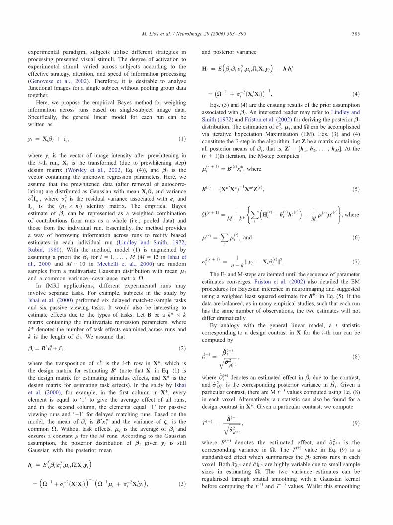
experiment and yet its average response to faces still gives a small

enough p value to pass a threshold test (see Fig. 1 as an example).

There is no reason to limit scientific inference to an average response

and leave out other more comprehensive information. The SPMs,

either constructed by the general linear model or by other methods,

provide a summary of responses, which is one of many sources of

evidence. Other supporting information could lead to new insights

into underlying cognitive functions that are not available from the

average response.

This study is designed to investigate reproducible evidence

without conducting separate fMRI experiments. Statistical methods

for analysing fMRI data have to be sensitive to small signal changes

(typically <1%) and robust to mild violation of distributional

assumptions. The study outlines a methodology for assessing

reproducible effects, including the empirical Bayes and receiver–

operator characteristic (ROC) curve methods. The general linear

model has been commonly used for analysing fMRI data in

experiments involving multiple types of stimuli and tasks (Friston

et al., 1995). The empirical Bayes method augments the general

linear model by assuming that the model parameters in individual

runs are random samples from a known distribution. The augmented

model provides a way of borrowing information across runs to

improve parameter estimates in each individual run. In other words,

the empirical Bayes method is more sensitive to reproducible effects

than the general linear model. In fMRI studies, experimental runs

may involve different tasks. The augmented model also introduces

an intuitive approach for examining task effects.

The general linear model or the empirical Bayes method always

generates voxel-wise statistics, for instance, t values. Individual

voxels are assigned to an active/inactive status according to a

threshold on the statistics. It has been frequently observed that,

even with the same scanner and experimental paradigm, subjects

can vary in the degree of activation (Genovese et al., 2002).

Research has also found that the pooled data across subjects

negatively affect reproducibility of brain activation maps (Swallow

et al., 2003). Therefore, different thresholds are appropriate for

different subjects. This study suggests selecting a threshold by

maximising the overall reproducibility of active/inactive outcomes

for all voxels associated with each subject. Reproducibility defined

in this study is simply the number of runs in which a particular

voxel is consistently classified as active. Both the empirical Bayes

Fig. 1. Averaged HRFs of 12/8/4 runs in the middle occipital gyrus of a subject in

respectively. The first graph is that of the average over the 12 experimental runs sh

eight of the experimental runs classified as reproducible, also showing stronger ac

experimental runs, showing stronger activation to houses. This figure results from

moderate reproducibility.

method and the ROC approach are optimal choices for assessing

the overall reproducibility. An experimental outcome must at least

satisfy this criterion if it is indeed reproducible.

The proposed methodology was implemented using data from

the studies by Ishai et al. (2000) and Mechelli et al. (2000), which

are part of the general collection of the fMRI Data Center. These

data sets were used to investigate the reproducibility of fMRI

findings in different settings and to make comparisons between

conventional SPM approaches and the reproducible evidence. We

will show that reproducible evidence is more robust to small

sample sizes than the p value approach. In the next section, we

discuss the methodology for assessing reproducibility of brain

activation maps. In the Empirical applications section, we present

the reproducible evidence supported by the fMRI data in the two

studies. Finally, we discuss research directions that use reprodu-

cible evidence in fMRI studies.

Methods

Statistical analysis

In constructing SPMswith the general linear model, observations

in each voxel are normally pooled over runs and experimental

subjects before estimating model parameters. Statistical analyses

using pooled data make a strong assumption that all observations in

individual runs and subjects are interchangeable. Empirical studies

have suggested that between-run variations make the interchange-

able assumption less tenable in fMRI experiments. For example,

subjects may become less attentive to stimuli due to fatigue or

drowsiness, and stimulus sequence may have unexpected order

effects upon responses. It is well known that functional images may

be contaminated by a global change in intensity between runs. These

unexpected errors can add bias to parameter estimates in the general

linear model. It was suggested that if experimental runs differed in

order of stimulus presentation as well as task performance,

individual regression parameters should be obtained from each run

separately (Constable et al., 1995; Skudlarski et al., 1999). This

procedure is effective because statistics within each run are not

affected by any substantial variations between runs. Empirical

studies also discovered that even with the same scanner and

the Ishai et al. (2000) study. The boxcar represents houses, faces, and chairs,

owing stronger activation to the face stimuli. The second is the average over

tivation to the face stimuli. The last is over the other four nonreproducible

examining areas which show significant activation ( p value thresh) but only

M. Liou et al. / NeuroImage 29 (2006) 383–395 385

experimental paradigm, subjects utilise different strategies in

processing presented visual stimuli. The degree of activation to

experimental stimuli varied across subjects according to the

effective strategy, attention, and speed of information processing

(Genovese et al., 2002). Therefore, it is desirable to analyse

functional images for a single subject without pooling group data

together.

Here, we propose the empirical Bayes method for weighing

information across runs based on single-subject image data.

Specifically, the general linear model for each run can be

written as

yi ¼ Xibi þ ei; ð1Þ

where yi is the vector of image intensity after prewhitening in

the i-th run, Xi is the transformed (due to prewhitening step)

design matrix (Worsley et al., 2002, Eq. (4)), and bi is the

vector containing the unknown regression parameters. Here, we

assume that the prewhitened data (after removal of autocorre-

lation) are distributed as Gaussian with mean Xibi and variance

ri2Ini

, where ri2 is the residual variance associated with ei and

Iniis the (ni � ni) identity matrix. The empirical Bayes

estimate of bi can be represented as a weighted combination

of contributions from runs as a whole (i.e., pooled data) and

those from the individual run. Essentially, the method provides

a way of borrowing information across runs to rectify biased

estimates in each individual run (Lindley and Smith, 1972;

Rubin, 1980). With the method, model (1) is augmented by

assuming a priori the bi for i = 1, . . . , M (M = 12 in Ishai et

al., 2000 and M = 10 in Mechelli et al., 2000) are random

samples from a multivariate Gaussian distribution with mean m i

and a common variance–covariance matrix 6.

In fMRI applications, different experimental runs may

involve separate tasks. For example, subjects in the study by

Ishai et al. (2000) performed six delayed match-to-sample tasks

and six passive viewing tasks. It would also be interesting to

estimate effects due to the types of tasks. Let B be a k* � k

matrix containing the multivariate regression parameters, where

k* denotes the number of task effects examined across runs and

k is the length of bi. We assume that

bi ¼ B0xi*þ f i; ð2Þ

where the transposition of xi* is the i-th row in X*, which is

the design matrix for estimating BV (note that Xi in Eq. (1) is

the design matrix for estimating stimulus effects, and X* is the

design matrix for estimating task effects). In the study by Ishai

et al. (2000), for example, in the first column in X*, every

element is equal to F1_ to give the average effect of all runs,

and in the second column, the elements equal F1_ for passive

viewing runs and F�1_ for delayed matching runs. Based on the

model, the mean of bi is BVxi* and the variance of z i is the

common 6. Without task effects, mi is the average of bi and

ensures a constant l for the M runs. According to the Gaussian

assumption, the posterior distribution of bi given yi is still

Gaussian with the posterior mean

hi u Eðbikr2i ;mi;V;Xi;yiÞ

¼ ðV�1 þ r�2i Xi

0Xið ÞÞ�1ðV�1mi þ r�2i Xi

0yiÞ; ð3Þ

and posterior variance

Hi u Eðbibi0kr2

i ;mi;V;Xi;yiÞ � hihi0

¼ V�1 þ r�2i Xi

0Xið Þ� ��1

; ð4Þ

Eqs. (3) and (4) are the ensuing results of the prior assumption

associated with bi. An interested reader may refer to Lindley and

Smith (1972) and Friston et al. (2002) for deriving the posterior bi

distribution. The estimation of ri2, mi, and 6 can be accomplished

via iterative Expectation Maximisation (EM). Eqs. (3) and (4)

constitute the E-step in the algorithm. Let Z be a matrix containing

all posterior means of bi, that is, ZV = [h1, h2, . . . , hM]. At the

(r + 1)th iteration, the M-step computes

m r þ 1ð Þi ¼ B0 rð Þ

xi4; where

B rð Þ ¼ X40X4ð Þ�1X40Z rð Þ; ð5Þ

V r þ 1ð Þ ¼ 1

M � k4

Xi

Hrð Þi þ h

rð Þi hi

0 rð Þ� �

� 1

Mm rð Þm0 rð Þ

)(; where

m rð Þ ¼Xi

m rð Þi ; and ð6Þ

r2 r þ 1ð Þi ¼ 1

n� kkk yi � Xib

rð Þi kk2: ð7Þ

The E- and M-steps are iterated until the sequence of parameter

estimates converges. Friston et al. (2002) also detailed the EM

procedures for Bayesian inference in neuroimaging and suggested

using a weighted least squared estimate for B(r) in Eq. (5). If the

data are balanced, as in many empirical studies, such that each run

has the same number of observations, the two estimates will not

differ dramatically.

By analogy with the general linear model, a t statistic

corresponding to a design contrast in X for the i-th run can be

computed by

tþð Þi ¼ bb þð Þ

iffiffiffiffiffiffiffiffiffiffiss2

b þð Þi

q ; ð8Þ

where b i(+) denotes an estimated effect in bi due to the contrast,

and s2b i

(+) is the corresponding posterior variance in Hi. Given a

particular contrast, there are M t(+) values computed using Eq. (8)

in each voxel. Alternatively, a t statistic can also be found for a

design contrast in X*. Given a particular contrast, we compute

T þð Þ ¼ BB þð Þffiffiffiffiffiffiffiffiffiffirr2B þð Þ

q ; ð9Þ

where B (+) denotes the estimated effect, and r2B (+) is the

corresponding variance in 6. The T(+) value in Eq. (9) is a

standardised effect which summarises the bi across runs in each

voxel. Both r2b i

(+) and r2B (+) are highly variable due to small sample

sizes in estimating 6. The two variance estimates can be

regularised through spatial smoothing with a Gaussian kernel

before computing the t(+) and T (+) values. Whilst this smoothing


does introduce slight bias into the variance estimate, it primarily

regularises the estimates as only a small width kernel for the

smoothing is used.

Reproducibility analysis

The t(+) values in Eq. (8) derived from the statistical analysis are

used to differentiate the truly active voxels from the truly inactive

voxels. Sensitivity is defined as the proportion of truly active

voxels that are classified as active. This proportion is also the

power of a statistical test in rejecting a false hypothesis. False

alarm rate, on the other hand, is the proportion of truly inactive

voxels that are classified as active, and contribute to the Type I

error made in rejecting a true hypothesis. Sensitivity can always be

increased by choosing a lower threshold for classifying the voxel

status, a situation in which the ensuing false alarm rate is inflated.

In fMRI studies, the true status of each voxel is unknown but the

two proportions can be estimated using the image data.

As previously mentioned, each voxel has M t(+) values

computed using Eq. (8). When selecting K distinct thresholds in

increasing order of magnitude, these t(+) values can be arranged into

(K + 1) classes. We denote the number of observations in each

group as rk with ~0K rk = M. A combination of rk can be con-

sidered a random sample from a mixed multinomial distribution:

C M ; r0; r1; N ; rKð Þ k kK

k ¼ 0

PrkAk

þ 1� kð Þ kK

k ¼ 0

PrkIk

�; ð10Þ

where C is the number of possible choices of rk for k = 0, . . . ,

K, and k is the proportion of truly active voxels. The PAkvalue

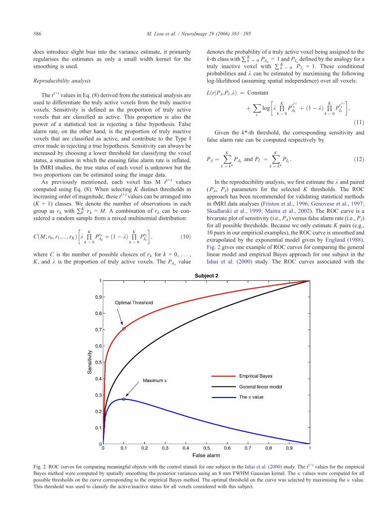
Fig. 2. ROC curves for comparing meaningful objects with the control stimuli for

Bayes method were computed by spatially smoothing the posterior variances usin

possible thresholds on the curve corresponding to the empirical Bayes method. T

This threshold was used to classify the active/inactive status for all voxels consid

denotes the probability of a truly active voxel being assigned to the

k-th class with ~ k = 0K PAk

= 1 and PIkdefined by the analogy for a

truly inactive voxel with ~ k = 0K PIk

= 1. These conditional

probabilities and k can be estimated by maximising the following

log-likelihood (assuming spatial independence) over all voxels:

L rkPA;PI ;kð Þ ¼ Constant

þXv

log k kK

k ¼ 0

Prvð Þk

Akþ 1� kð Þ k

K

k ¼ 0

Prvð Þk

Ik

�;

ð11ÞGiven the k*-th threshold, the corresponding sensitivity and

false alarm rate can be computed respectively by

PA ¼XK

k ¼ k4

PAkand PI ¼

XKk ¼ k4

PIk : ð12Þ

In the reproducibility analysis, we first estimate the k and paired

(PA, PI) parameters for the selected K thresholds. The ROC

approach has been recommended for validating statistical methods

in fMRI data analyses (Friston et al., 1996; Genovese et al., 1997;

Skudlarski et al., 1999; Maitra et al., 2002). The ROC curve is a

bivariate plot of sensitivity (i.e., PA) versus false alarm rate (i.e., PI)

for all possible thresholds. Because we only estimate K pairs (e.g.,

10 pairs in our empirical examples), the ROC curve is smoothed and

extrapolated by the exponential model given by England (1988).

Fig. 2 gives one example of ROC curves for comparing the general

linear model and empirical Bayes approach for one subject in the

Ishai et al. (2000) study. The ROC curves associated with the

one subject in the Ishai et al. (2000) study. The t(+) values for the empirical

g an 8 mm FWHM Gaussian kernel. The j values were computed for all

he optimal threshold on the curve was selected by maximising the j value.

ered with this subject.


empirical Bayes approach always lie above those from the general

linear model. Here, to combine voxels into one image-wide ROC

curve, independence was assumed. It has been shown that whilst

absolute values of the ROC curve may be affected by this

assumption, the relaxation of this assumption in preference of a

Markov random field assumption, did not give rise to large changes

in the relative magnitudes for comparing the different methods

(Maitra et al., 2002). Incorporation of suitable correlation models

into the ROC analysis is a subject of on-going research.

In fMRI experiments, it is important to understand the extent to

which replicates made under the same conditions give the same

results. The true active/inactive status and the decision outcomes

using an image-wide operating threshold generate a 2 by 2 table. The

proportion of agreement in the table is the sum of true positive and

true negative events; that is, pO = kPA +(1 � k)(1 � PI). The

expected chance proportion of each event can be found by the

product of the marginal row and column proportions corresponding

to the event cell in the table. We denote the agreement expected by

chance as pC = ks + (1 � k)(1 � s) where s = kPA + (1 �k)PI. Using the ROC model along with the estimated conditional

probabilities, the proportion of agreement corrected for chance is

j ¼ pO � pC

1 � pCð13Þ

which is the well-known Kappa index due to Cohen (1960). The

optimal operating point on the ROC curve can be selected by

maximising the j value. In the example of Fig. 2, the maximum jvalue is reached at the optimal threshold on the ROC curve

corresponding to the empirical Bayes approach.

The reproducibility of a voxel is defined as the degree to which

the active status of the voxel, in responding to stimuli, remains the

same across replicates implemented under the same conditions.

The minimum and maximum number of times that a voxel can be

classified as active are zero and M, respectively. This study

categorises voxels according to reproducibility; a voxel is strongly

reproducible if its active status remains the same in at least 90% of

the runs, moderately reproducible in 70–90% of the runs, weakly

reproducible in 50–70% of the runs, and otherwise not reprodu-

cible. It should be noted here that reproducibility only applies to

active voxels; inactive voxels are nonreproducible by definition as

they are not associated with the task. Given an optimal threshold,

the truly active voxels must be strongly reproducible. Some truly

active voxels may exhibit moderate reproducibility due to errors in

estimating t(+) values. We suggest not only selecting strongly

reproducible voxels to construct the brain activation maps, but also

including voxels that are moderately reproducible and spatially

proximal (a nearest neighbour) to the strongly reproducible voxels.

Interpretation of reproducibility plots

Reproducibility plots have previously been used in Liou et al.

(2003), but to aid interpretation for this paper, a short summary of

the plot is detailed here.

The horizontal axis in the bivariate plot refers to the number of

runs where a voxel was classified as active according to the contrast

under investigation (and this is defined as the number of repro-

ducible runs). The vertical axis refers to the overall T (+) task effect

having combined runs at that voxel. The colour scale gives a rep-

resentation of the conditional frequency of T (+) values in the range

occurring for the prescribed reproducibility. The 0 column contains

all the voxels which were never classified as active for any run.

Empirical applications

Experimental data

We studied reproducible evidence in two empirical examples.

The data sets were supported by the US National fMRI Data

Center. The first example investigated the representation of objects

in the human occipital and temporal cortex with two experiments

(Ishai et al., 2000). In Experiment 1, six subjects were presented

with gray-scale photographs of houses, faces, and chairs. Each

subject went through 12 experimental runs which were subdivided

into two tasks. In the delayed match-to-sample task, a target

stimulus was followed, after a 0.5 s delay, by a pair of choice

stimuli presented at a rate of 2 s. Subjects indicated which choice

of stimulus matched the target by pressing a button with the right

or left thumb. In the passive viewing task, stimuli (houses, faces

and chairs) were presented at a rate of 2 s and subjects simply

responded to the stimuli without recording a target or making a

decision on choice stimuli. In Experiment 2, the other six subjects

performed the delayed match-to-sample tasks with photographs (as

in Experiment 1) and with line drawings of houses, faces, and

chairs. In the two experiments, the control condition involved

phased, scrambled pictures presented at the same rate as the

experimental stimuli. In the original reports by Ishai et al. (1999)

and Ishai et al. (2000), three orthogonal contrasts were examined in

the two experiments: meaningful objects (faces, houses, and chairs)

versus control stimuli (phased, scrambled pictures), faces versus

houses/chairs, and houses versus chairs. As an illustration, we only

focus on the contrast comparing meaningful objects (i.e., faces,

houses, and chairs) with control stimuli (i.e., phased, scrambled

pictures), but all three contrasts were inserted in the design matrix

in the analysis. Each subject in the study went through 12

experimental runs with 91 functional volumes of MR images

scanned in each run.

The second example investigated the effects of presentation rate

on the occipital and parietal regions during word and pseudoword

reading (Mechelli et al., 2000). The experiment involved two

stimulus types (words and pseudowords) and three presentation

rates (20, 40, and 60 wpm) alternated with a resting condition. The

task involved silent reading of words and pseudowords as soon as

they appeared on the screen. The resting condition involved

fixating on a cross in the middle of the screen. The experimental

conditions were distributed into a single run and consistently

presented in a counterbalanced order across six subjects. The

available data for each subject were 360 functional volumes of MR

images scanned in the run with different combinations of

experimental conditions. There were also three orthogonal con-

trasts examined in the experiment: reading at all rates (20, 40, and

60 wpm) versus rest, a linear rate-dependent effect, and a quadratic

rate-dependent effect. In this study, we focused on the comparison

between silent reading and rest. The final analysis also eliminated

one female subject whose functional images were contaminated by

unknown irregularities. The available data for each subject were

randomly grouped into 10 ad hoc runs of five word reading and

five pseudoword reading. This was done to produce ‘‘runs’’ in the

data. The size of available data in each run in the second example

is much smaller than that in the first example (36 versus 91). We

will use this to show that reproducible evidence is also robust to

small sample sizes.

All image data were collected using either 1.5-T or 2-T scanners

and already preprocessed with correction for motion artifacts and

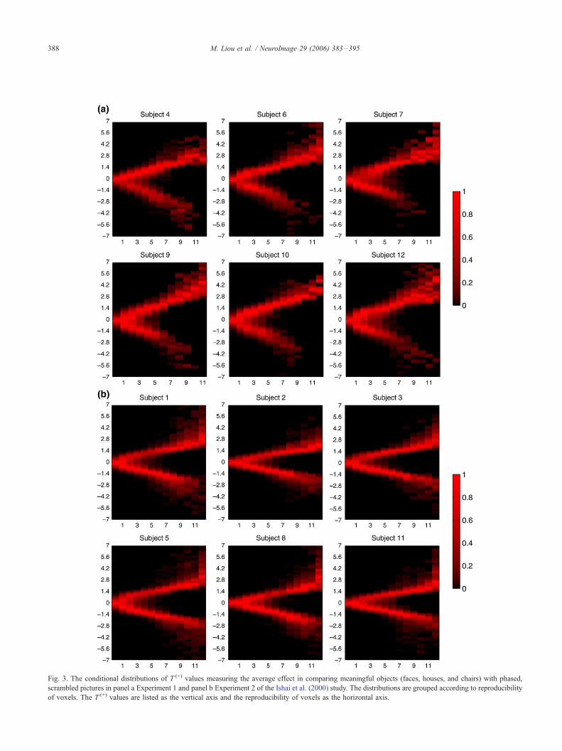
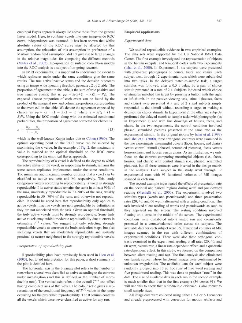
Fig. 3. The conditional distributions of T (+) values measuring the average effect in comparing meaningful objects (faces, houses, and chairs) with phased,

scrambled pictures in panel a Experiment 1 and panel b Experiment 2 of the Ishai et al. (2000) study. The distributions are grouped according to reproducibility

of voxels. The T (+) values are listed as the vertical axis and the reproducibility of voxels as the horizontal axis.



normalisation to a standard atlas. These preprocessed data were

analysed in this study. The data were additionally prewhitened by

correction for autocorrelation using the method by Worsley et al.

(2002). This involved correcting the preprocessed data for spatially

varying autocorrelated errors before statistical and ROC analyses.

In the design matrix of the statistical analysis, we simply used the

boxcar function without a convolution with any theoretical

haemodynamic response functions (HRF).

Empirical results

The optimal thresholds selected for counting reproducible runs

were distinct for individual subjects. Given an optimal threshold,

T(+) values and the number of reproducible runs were computed for

all in-brain voxels corresponding to each subject. There are two

standardised effects measuring the contrast of meaningful objects

versus control stimuli in the Ishai et al. (2000) study; one is the

average effect across the 12 runs and the other is the differential

effect comparing between tasks (e.g., passive viewing versus

delayed matching). As was seen in Fig. 1, care must be taken in

assigning significance as some regions may be more responsive to

one particular stimulus on average, but show greater response to

competing stimuli regularly (one time out of three in this case).

This region was identified by looking at differences in the

reproducibility plots and the traditional p value analysis.

The T (+) values are grouped according to reproducibility of

voxels and their density distributions are plotted in Figs. 3a and b

for the average effect and Figs. 4a and b for the differential effect.

Each plot in the figures can be interpreted within a vertical column

against the reproducibility axis. In each plot, for example, there is a

great portion of brain voxels consistently classified as inactive and

having almost zero T (+) values; their distribution exhibits high

density centering at zero on the vertical axis and is located on the

very left-hand side along the horizontal axis. The plots in Fig. 3

clearly show that conditional T (+) values are distributed with

positive and negative peaks that are separated more widely apart

when the reproducibility of voxels increases. This implies that a

T (+) value that is larger in absolute value also tends to be more

reproducible. In Fig. 3a, the negative peaks slightly lose their

continuity after 6 or 7 consecutive runs (i.e., there is no voxel that

routinely shows decreased activity across the 12 runs). However, it

has been observed that reproducible voxels with negative T (+)

values in this experiment are highly related to the delayed

matching task in Experiment 1. Voxels of negative T (+) values in

the experiment are only strongly reproducible across the delayed

matching runs. The decreased activity becomes more revealing

when we discuss plots in Fig. 4 later.

The other six subjects in Fig. 3b were involved in 12 delayed

matching runs of either photographs or line drawings, and show

negative peaks throughout the range of reproducibility. Relative to

passive viewing, the delayed matching task could require more

attention (Ishai et al., 1999), and this difference in attention

demand is reflected by increased responses and introduces

between-run variability. Therefore, T (+) values in Fig. 3a are more

scattered and have a smaller j value on average than those in Fig.

3b. Likewise, the plots in Figs. 4a and b clearly exhibit different

patterns. Five out of six subjects in Fig. 4a clearly show interaction

effects between object-related responses and experimental tasks.

For those subjects, there are some voxels activated consistently by

both tasks, and also voxels activated strictly by the delayed

matching task. Responses common to both tasks are positively

correlated with the stimulus presentation except for a greater

amplitude in the delayed matching task. Because we assigned F1_to the passive viewing runs and F�1_ to the delayed matching runs

in the design matrix, reproducible voxels show negative differential

effects in Fig. 4a. On the other hand, responses specific to the

delayed matching task are negatively correlated with the stimulus

presentation. Because of the codes used in the design matrix, the

ensuing differential effects are all positive in Fig. 4a.

By combining evidence in Figs. 3a and 4a, we conclude that the

delayed matching task engages additional brain regions which

show decreased activities following the stimulus presentation.

According to reproducibility plots in Fig. 4b, there is no strong

evidence suggesting functional dependence of voxel responses on

the spatial frequency differences in the stimuli (photographs versus

line drawings). The reproducible evidence also concurs with the

SPMs in the Ishai et al. (2000) study. Similar to strongly

reproducible voxels, voxels consistently classified inactive (i.e.,

zero reproducibility) have less scattered T(+) values. Therefore,

plots of T(+) values located at the very right- and left-hand sides of

the horizontal axis are less contaminated by noise than those

located in the middle of the axis.

As a comparison, the brain maps along with the corresponding

HRFs are given in Fig. 5 for Subjects 10 and 11 in the two

experiments. In constructing these maps, three-dimensional render-

ing was performed with mri3dX software (http://mrrc11.mrrc.

liv.ac.uk/mri3dX). The coloured voxels in these maps are strongly

reproducible, but their neighbourhood may have voxels that are

moderately reproducible. The maps suggest that a major portion of

reproducible voxels is distributed in the temporal and occipital

regions which concur with the SPMs in the Ishai et al. (2000)

study. The maps also show that the two subjects also engaged

regions in the bilateral cuneus, precuneus, and posterior cingulate.

In these regions, a decreased activity is followed by the delayed

matching task. Other subjects in the two experiments also have

similarly decreased responses in these regions. It is interesting to

note that the same type of decreased responses is found in the

lingual gyrus for both passive viewing and delayed matching tasks.

The decreased responses in this region have been observed for five

out of six subjects in Experiment 1 and for all subjects in

Experiment 2. Neuroimaging research has recently suggested that

there are few default human brain areas tonically active in a resting

state and deactive when subjects are engaged in a wide variety of

cognitive tasks (Raichle et al., 2001; Shulman et al., 2002). These

regions showing decreased responses in Fig. 5 are closely related to

the default areas discussed in this literature, but specific to the

delayed matching task in the Ishai et al. (2000) study. We

additionally found that subjects in the two experiments show

increased activity in the bilaterial precuneus and cuneus when

performing the delayed matching tasks. Therefore, there is a

portion of voxels located in the middle of the horizontal axis in Fig.

4a which have negative differential effects and are specific to the

delayed matching task. The plots of the differential effect for

Subject 4 in Fig. 4a deviate from those of other subjects in the

same experiment. The deviation could suggest an example of noisy

image data and smaller j value. However, we found that the

pattern of decreased activity of this subject is closer to that of

Subject 11 rather than Subject 10 in Fig. 5; that is, this subject

engages the default areas in both passive viewing and delayed

matching tasks.

For the study on word/pseudoword reading, the T(+) values of

average effects for comparing silent reading with the resting

http:\\www.mrrc11.mrrc.liv.ac.uk\mri3dX

Fig. 4. The conditional distributions of T (+) values measuring the differential effect in comparing meaningful objects with phased, scrambled pictures in panel a

Experiment 1 and panel b Experiment 2 of the Ishai et al. (2000) study.


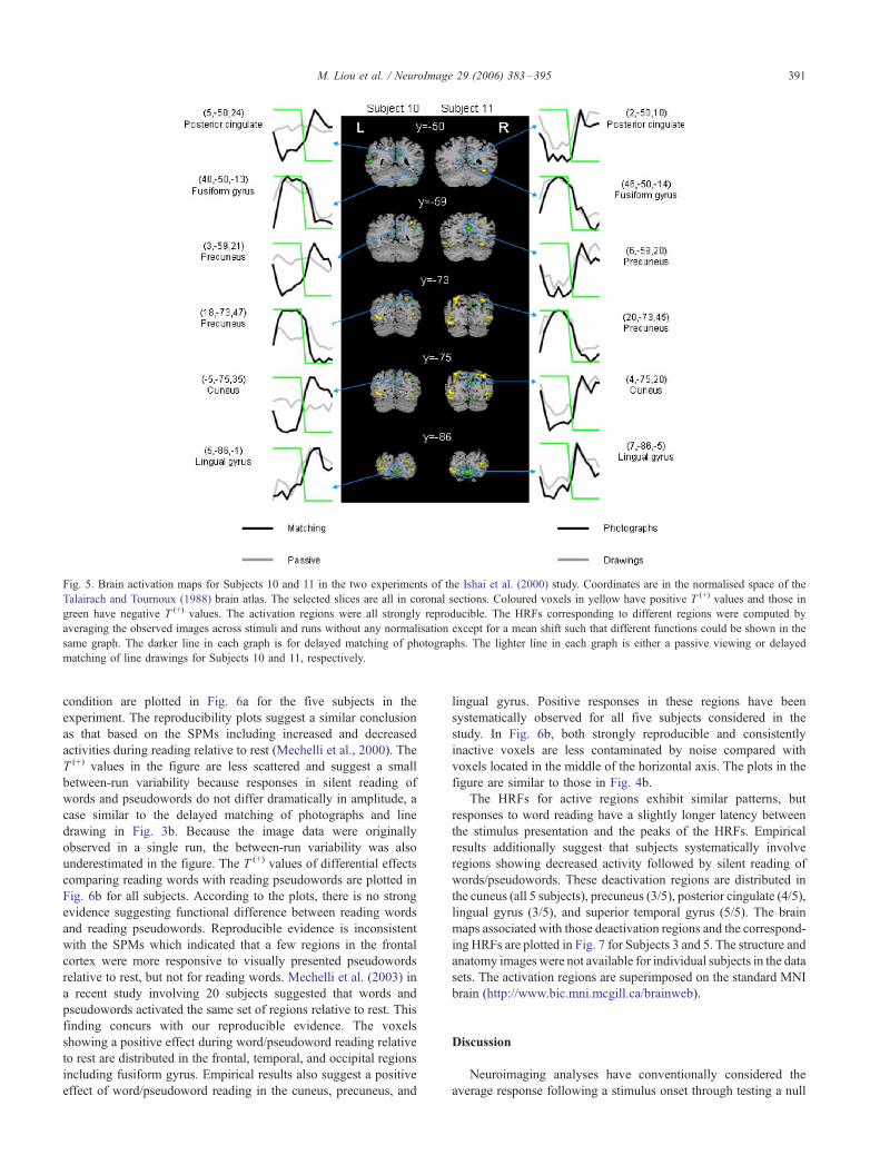
Fig. 5. Brain activation maps for Subjects 10 and 11 in the two experiments of the Ishai et al. (2000) study. Coordinates are in the normalised space of the

Talairach and Tournoux (1988) brain atlas. The selected slices are all in coronal sections. Coloured voxels in yellow have positive T (+) values and those in

green have negative T (+) values. The activation regions were all strongly reproducible. The HRFs corresponding to different regions were computed by

averaging the observed images across stimuli and runs without any normalisation except for a mean shift such that different functions could be shown in the

same graph. The darker line in each graph is for delayed matching of photographs. The lighter line in each graph is either a passive viewing or delayed

matching of line drawings for Subjects 10 and 11, respectively.


condition are plotted in Fig. 6a for the five subjects in the

experiment. The reproducibility plots suggest a similar conclusion

as that based on the SPMs including increased and decreased

activities during reading relative to rest (Mechelli et al., 2000). The

T (+) values in the figure are less scattered and suggest a small

between-run variability because responses in silent reading of

words and pseudowords do not differ dramatically in amplitude, a

case similar to the delayed matching of photographs and line

drawing in Fig. 3b. Because the image data were originally

observed in a single run, the between-run variability was also

underestimated in the figure. The T (+) values of differential effects

comparing reading words with reading pseudowords are plotted in

Fig. 6b for all subjects. According to the plots, there is no strong

evidence suggesting functional difference between reading words

and reading pseudowords. Reproducible evidence is inconsistent

with the SPMs which indicated that a few regions in the frontal

cortex were more responsive to visually presented pseudowords

relative to rest, but not for reading words. Mechelli et al. (2003) in

a recent study involving 20 subjects suggested that words and

pseudowords activated the same set of regions relative to rest. This

finding concurs with our reproducible evidence. The voxels

showing a positive effect during word/pseudoword reading relative

to rest are distributed in the frontal, temporal, and occipital regions

including fusiform gyrus. Empirical results also suggest a positive

effect of word/pseudoword reading in the cuneus, precuneus, and

lingual gyrus. Positive responses in these regions have been

systematically observed for all five subjects considered in the

study. In Fig. 6b, both strongly reproducible and consistently

inactive voxels are less contaminated by noise compared with

voxels located in the middle of the horizontal axis. The plots in the

figure are similar to those in Fig. 4b.

The HRFs for active regions exhibit similar patterns, but

responses to word reading have a slightly longer latency between

the stimulus presentation and the peaks of the HRFs. Empirical

results additionally suggest that subjects systematically involve

regions showing decreased activity followed by silent reading of

words/pseudowords. These deactivation regions are distributed in

the cuneus (all 5 subjects), precuneus (3/5), posterior cingulate (4/5),

lingual gyrus (3/5), and superior temporal gyrus (5/5). The brain

maps associated with those deactivation regions and the correspond-

ing HRFs are plotted in Fig. 7 for Subjects 3 and 5. The structure and

anatomy images were not available for individual subjects in the data

sets. The activation regions are superimposed on the standard MNI

brain (http://www.bic.mni.mcgill.ca/brainweb).

Discussion

Neuroimaging analyses have conventionally considered the

average response following a stimulus onset through testing a null

http:\\www.bic.mni.mcgill.ca\brainweb

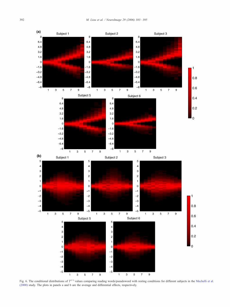
Fig. 6. The conditional distributions of T (+) values comparing reading words/pseudoword with resting conditions for different subjects in the Mechelli et al.

(2000) study. The plots in panels a and b are the average and differential effects, respectively.


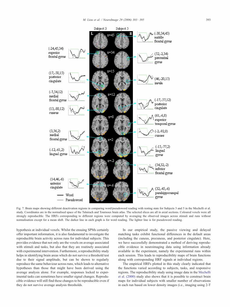
Fig. 7. Brain maps showing different deactivation regions in comparing word/pseudoword reading with resting state for Subjects 3 and 5 in the Mechelli et al.

study. Coordinates are in the normalised space of the Talairach and Tournoux brain atlas. The selected slices are all in axial sections. Coloured voxels were all

strongly reproducible. The HRFs corresponding to different regions were computed by averaging the observed images across stimuli and runs without

normalisation except for a mean shift. The darker line in each graph is for word reading. The lighter line is for pseudoword reading.


hypothesis at individual voxels. Whilst the ensuing SPMs certainly

offer important information, it is also fundamental to investigate the

reproducible brain activity across runs for individual subjects. This

provides evidence that not only are the voxels on average associated

with stimuli and tasks, but also that they are routinely associated

with experimental intervention. Furthermore, a reproducibility study

helps in identifying brain areas which do not survive a threshold test

due to their signal amplitude, but can be shown to regularly

reproduce the same behaviour across runs, which leads to alternative

hypotheses than those that might have been derived using the

average analysis alone. For example, responses locked to exper-

imental tasks can sometimes have smaller signal changes. Reprodu-

cible evidence will still find these changes to be reproducible even if

they do not survive average analysis thresholds.

In our empirical study, the passive viewing and delayed

matching tasks exhibit functional differences in the default areas

(including the cuneus, precuneus, and posterior cingulate). Here,

we have successfully demonstrated a method of deriving reprodu-

cible evidence in neuroimaging data using information already

available in the experiment, namely the experimental runs within

each session. This leads to reproducibility maps of brain functions

along with corresponding HRF signals at individual regions.

The empirical HRFs plotted in this study clearly indicated that

the functions varied according to subjects, tasks, and responsive

regions. The reproducibility study using image data in the Mechelli

et al. (2000) study also shows that it is possible to construct brain

maps for individual subjects with smaller number of observations

in each run based on lower density images (i.e., imaging using 2-T


scanners). By comparing plots in Fig. 4a with those in Fig. 4b,

passive viewing and delayed matching would appear to be

functionally different. In the same figures, the plot associated with

Subject 4 also suggests that the tasks were performed in a slightly

different way compared with the rest of the subjects in the same

experiment. Reproducible evidence indicates that the subject had

decreased responses in the default areas when performing passive

viewing and delayed matching tasks. In general, a decreased

activity in the default areas was followed by tasks demanding

focused attention (e.g., delayed matching and silent reading). This

information is a direct result of studying reproducible evidence. In

the Mechelli et al. (2000) study, although words and pseudowords

activated the same brain regions, processing meaningful words had

slightly longer latencies in HRFs. Subjects in this experiment also

systematically showed increased and decreased responses in the

cuneus, precuneus, lingual gyrus, and superior temporal gyrus.

Subjects performing the delayed matching tasks only showed

parallel processes in the precuneus and cuneus. Research findings

in our empirical studies in some ways confirm the SPM analysis

and in others refute it. This shows an obvious advantage in

considering reproducible evidence; that is, it can confirm or cast

doubt on an average result.

It must of course be recognised that reproducibility of

experimental outcomes does not determine if the analysis model

under consideration is valid or not. It simply allows the assessment

of whether the results from that model are reproducible across

experimental runs. By analogy, the ROC curve analysis does not

take into account any modeling bias generated by the model. In

addition to the design of the analysis model, there is a problem if

the design of the experiment did not include runs. As in the second

example, an ad hoc method of splitting the data is needed, and

further work is necessary to determine the optimal method of

splitting such experiments. However, in many cases, runs are a part

of the experimental design, and in cases where they are not, whilst

not optimal, ad hoc methods do allow some measure of

reproducibility to be found.

The methodology proposed in this study is conceptually simple

and is generalisable beyond the on–off paradigm. However,

interpretation of reproducible evidence is restricted by the design

of experiment. For the study on words/pseudoword reading, for

example, the decreased activity in Fig. 7 cannot be generalised to

studies with multiple runs because the between-run variability was

underestimated by using the ad hoc runs. The two empirical

examples did suggest that the reproducibility criterion is robust to a

major portion of image artifacts. This provides support for the

methodology proposed in this study. Of course, the true active/

inactive status was unknown and estimated using a statistical

model along with the EM procedure. The model could be biased

against a particular piece of scientific evidence. We also found that

the reproducibility maps in Figs. 5 and 7 are reasonably robust to

the selected thresholds; that is, the maps remained unchanged by

slightly shifting the thresholds to upper or lower bounds. We would

expect that thresholds found by other statistical models would not

alter the maps excessively.

The design of experiments in the Ishai et al. (2000) study has

optimised the between-stimuli, -tasks, -experimental runs, and

-subjects interactions which would serve as bench marks for the

future design of reproducibility studies. Both reproducible and

nonreproducible evidences are valuable for accumulating insight

into the design and methodology appropriate for fMRI studies. We

finally conclude that research findings in fMRI studies cannot be

completely compelling until reproducible evidence has been

considered.

Acknowledgments

The authors are indebted to the fMRIDC at Dartmouth College

for supporting the data sets analysed in this study. This research

was supported by grant NSC92-2413-H-001-007 from the National

Science Council (Taiwan).

References

Branch, M.N., 1999. Statistical inference in behavior analysis: some

things significance testing does and does not do. Behav. Anal. 22,

87–92.

Carver, R.P., 1993. The case against statistical significance testing,

revisited. J. Exp. Educ. 61, 287–292.

Casey, B.J., Cohen, J.D., O’Craven, K., Davidson, R.J., Irwin, W., Nelson,

C.A., Noll, D.C., Hu, X., Lowe, M.J., Rosen, B.R., Truwitt, C.L.,

Turski, P.A., 1998. Reproducibility of fMRI results across four institutes

using a spatial working memory task. NeuroImage 8, 249–261.

Cohen, J., 1960. A coefficient of agreement for nominal scales. Educ.

Psychol. Meas. 20, 37–46.

Constable, R.T., Skudlarski, P., Gore, J.C., 1995. An ROC approach for

evaluating functional brain MR imaging and postprocessing protocols.

Magn. Reson. Med. 34, 57–64.

England, W.L., 1988. An exponential model used for optimal threshold

selection on ROC curves. Med. Decis. Mak. 8, 120–131.

Fernandez, G., Specht, K., Weis, S., Tendolkar, I., Reuber, M., Fell, J.,

Klaver, P., Ruhlmann, J., Reul, J., Elger, C.E., 2003. Intrasubject

reproducibility of presurgical language lateralization and mapping using

fMRI. Neurology 60, 969–975.

Friston, K.J., Holmes, A., Worsley, K.J., Poline, J.B., Frith, C.D.,

Frackowiak, R.S.J., 1995. Statistical parametric maps in functional

imaging: a general linear approach. Hum. Brain Mapp. 2, 189–210.

Friston, K.J., Holmes, A., Poline, J.B., Price, C.J., Frith, C.D., 1996.

Detecting activations in PET and fMRI: levels of inference and power.

NeuroImage 4, 223–235.

Friston, K.J., Penny, W., Phillips, C., Kiebel, S., Hinton, G., Ashburner, J.,

2002. Classical and Bayesian inference in neuroimaging: theory.


Genovese, C.R., Noll, D.C., Eddy, W.F., 1997. Estimating test– retest

reliability in functional MR imaging: I. Statistical methodology. Magn.

Reson. Med. 38, 497–507.

Genovese, C.R., Lazar, N.A., Nichols, T., 2002. Thresholding of statistical

maps in functional neuroimaging using the false discovery rate.


Ishai, A., Ungerleider, L.G., Martin, A., Shouten, J.L., Haxby, J.V., 1999.

Distributed representation of objects in the human ventral visual

pathway. Proc. Natl. Acad. Sci. U. S. A. 96, 9379–9384.

Ishai, A., Ungerleider, L.G., Martin, A., Haxby, J.V., 2000. The representa-

tion of objects in the human occipital and temporal cortex. J. Cogn.

Neurosci. 12 (S2), 35–51.

Lindley, D.V., Smith, A.F.M., 1972. Bayes estimates for the linear model.

J. R. Stat. Soc., B 34, 1–41.

Liou, M., Su, H.R., Lee, J.D., Cheng, P.E., Huang, C.C., Tsai, C.H., 2003.

Bridging functional MR images and scientific inference: reproducibility

maps. J. Cogn. Neurosci. 15, 935–945.

Maitra, R., Roys, S.R., Gullapalli, R.P., 2002. Test– retest reliability

estimation of functional MRI data. Magn. Reson. Med. 48, 62–70.

Mechelli, A., Friston, K.J., Price, C.J., 2000. The effects of presentation rate

during word and pseudoword reading: a comparison of PET and fMRI.

J. Cogn. Neurosci. 12 (S2), 145–156.


Mechelli, A., Gorno-Tempini, M.L., Price, C.J., 2003. Neuroimaging

studies of word and pseudoword reading: consistencies, inconsistencies,

and limitations. J. Cogn. Neurosci. 15, 260–271.

Nickerson, R.S., 2000. Null hypothesis significance testing: a review of an

old and continuing controversy. Psychol. Methods 5, 241–301.

Noll, D.C., Genovese, C.R., Nystrom, L.E., Vazquez, A.L., Forman, S.D.,

Eddy, W.F., Cohen, J.D., 1997. Estimating test – retest reliability in

functional MR imaging: II. Application to motor and cognitive

activation studies. Magn. Reson. Med. 38, 508–517.

Raichle, M.E., MacLeod, A.M., Snyder, A.Z., Powers, W.J., Gusnard, D.A.,

Shulman, G.L., 2001. A default mode of brain function. Proc. Natl.

Acad. Sci. U. S. A. 98, 676–682.

Rubin, D.B., 1980. Using empirical Bayes techniques in the law school

validity studies. J. Am. Stat. Assoc. 75, 801–827.

Salli, E., Korvenoja, A., Visa, A., Katila, T., Aronen, H.J., 2001.

Reproducibility of fMRI: effect of the use of contextual information.


Savoy, R.L., 2001. History and future directions of human brain mapping

and functional neuroimaging. Acta Psychol. 107, 9–42.

Shulman, A., Yacoub, E., Pfeuffer, J., Van de Moortele, P.F., Adriany, G.,

Hu, X., Ugurbil, K., 2002. Sustained negative BOLD, blood flow and

oxygen consumption response and its coupling to the positive response

in the human brain. Neuron 36, 1195–1210.

Skudlarski, P., Constable, R.T., Gore, J.C., 1999. ROC analysis of statistical

methods used in functional MRI: individual subjects. NeuroImage 9,

311–329.

Smith, L.D., Best, L.A., Cylke, V.A., Stubbs, D.A., 2000. Psychology

without p values. Am. Psychol. 55, 260–263.

Strother, S., La Conte, S., Hansen, L.K., Anderson, J., Zhang, J., Pulapura,

S., Rottenberg, D., 2004. Optimizing the fMRI data-processing pipeline

using prediction and reproducibility performance metrics: I. A prelimi-

nary group analysis. NeuroImage 23 (S1), 196–207.

Swallow, K.M., Braver, T.S., Snyder, A.Z., Speer, N.K., Zacks, J.M., 2003.

Reliability of functional localization using fMRI. NeuroImage 20,

1561–1577.

Talairach, J., Tournoux, P., 1988. A Co-planar Stereotaxic Atlas of a Human

Brain, Thieme Medical Verlag, New York.

van Horn, J.D., Grafton, S.T., Rockmore, D., Gazzaniga, M.S., 2004.

Sharing neuroimaging studies of human cognition. Nat. Neurosci. 7,

473–481.

Worsley, K.J., Liao, C., Aston, J.A.D., Petre, V., Duncan, G., Evans, A.C.,

2002. A general statistical analysis for fMRI data. NeuroImage 15, 1–15.

a method for generating reproducible evidence in fmri studies

Documents