arX

iv:h

ep-t

h/06

0323

2v1

29

Mar

200

6

hep-th/0603232ITP–UH–07/06

HWM–06–6EMPG–06–03

Rank Two Quiver Gauge Theory, Graded Connections

and Noncommutative Vortices

Olaf Lechtenfeld1, Alexander D. Popov1,2 and Richard J. Szabo3

1Institut fur Theoretische Physik, Universitat Hannover

Appelstraße 2, 30167 Hannover, Germany

2Bogoliubov Laboratory of Theoretical Physics, JINR

141980 Dubna, Moscow Region, Russia

3Department of Mathematics and Maxwell Institute for Mathematical Sciences

Heriot-Watt University, Colin Maclaurin Building, Riccarton, Edinburgh EH14 4AS, U.K.

Email: lechtenf, popov @itp.uni-hannover.de , R.J.Szabo@ma.hw.ac.uk

Abstract

We consider equivariant dimensional reduction of Yang-Mills theory on Kahler manifolds of theform M×CP 1×CP 1. This induces a rank two quiver gauge theory on M which can be for-mulated as a Yang-Mills theory of graded connections on M . The reduction of the Yang-Millsequations on M×CP 1×CP 1 induces quiver gauge theory equations on M and quiver vortexequations in the BPS sector. When M is the noncommutative space R2n

θboth BPS and non-

BPS solutions are obtained, and interpreted as states of D-branes. Using the graded connectionformalism, we assign D0-brane charges in equivariant K-theory to the quiver vortex configu-rations. Some categorical properties of these quiver brane configurations are also described interms of the corresponding quiver representations.

1 Introduction and summary

It has become clear in recent years that a proper description of the nonperturbative vacuum instring theory will require detailed understanding of the properties of systems of both BPS and non-BPS brane configurations (see [1] for a recent review). The basic non-BPS system is the unstablebrane-antibrane configuration which corresponds to a pair of vector bundles with a tachyon fieldmapping between them. The dynamics of this system can be cast as a Yang-Mills theory ofsuperconnections [2]. In some instances the branes can be realized as instantons of gauge theoryin the appropriate dimensionality [3]. Important examples of this are noncommutative solitonsand instantons which find their most natural physical interpretations in terms of D-branes [4].This is related [5] to the fact that the charges of D-branes are classified by K-theory [6]. Reviewson noncommutative solitons and D-branes can be found in [7], while applications of BPS solitonsolutions in noncommutative (supersymmetric) Yang-Mills theory to D-brane dynamics are givene.g. in [8].

One way to generate both stable and unstable states of D-branes is by placing them at singular-ities of orbifolds [9, 10]. Regular representation D-branes then decay into irreducible representationfractional branes under the action of the discrete orbifold group. The low-energy dynamics of theD-brane decay is succinctly described by a quiver gauge theory. Resolving orbifold singularities bynon-contractible cycles blows up the fractional D-branes into higher dimensional branes wrappingthe cycles. Another way of obtaining quiver gauge theories on a q-dimensional manifold M is toconsider k coincident D(q+r)-branes wrapping the worldvolume manifold X = M×G/H whereG/H is an r-dimensional homogeneous space for a Lie group G with a closed subgroup H. In thestandard interpretation this system of D-branes corresponds to a rank k hermitean vector bun-dle E over X with a connection whose dynamics are governed by Yang-Mills gauge theory. ForKahler manifolds X the stability of such bundles (BPS conditions) is controlled by the Donaldson-Uhlenbeck-Yau (DUY) equations [11]. For G-equivariant bundles E → X one finds that Yang-Millstheory on X reduces to a quiver gauge theory on M [12]–[15].

In this paper we will focus on some of these issues in quiver gauge theories on Kahler manifoldsM which arise via a quotient by the natural action of the Lie group SU(2)×SU(2) on equivari-ant Chan-Paton bundles over M×CP 1×CP 1. Our analysis generalizes previous work on brane-antibrane systems from reduction on M×CP 1 [12, 16, 17], and on the generalization to chains ofbranes and antibranes arising from SU(2)-equivariant dimensional reduction onM×CP 1 [13, 18]. Inparticular, we will expand on the formalism introduced in [18] which merged the low-energy dynam-ics of brane-antibrane chains with quiver gauge theory into a Yang-Mills gauge theory of new objectson M termed “graded connections”, which generalize the usual superconnections on the worldvol-umes of coincident brane-antibrane pairs. This formalism is particularly well-suited to describesuch physical instances and their novel effects, such as the equivalence between non-abelian quivervortices on M and symmetric multi-instantons on the higher-dimensional space M×CP 1×CP 1.Moreover, when M is the noncommutative space R

2nθ , it enables one to interpret noncommutative

quiver solitons in the present case as states of D-branes in a straightforward manner, whilst pro-viding a categorical approach to D-branes which characterizes their moduli beyond their K-theorycharges. These quiver brane configurations require a more complex description than just that interms of branes and antibranes, and we construct a category of D-branes which incorporates boththeir locations and their bindings to abelian magnetic monopoles.

The essential new ingredients of the present paper are that our quivers are of rank two, asopposed to the rank one quivers considered in [18], and the necessity of imposing relations on thequiver. The resulting quiver D-brane configuration is new, and comprises a two-dimensional latticeof branes and antibranes coupled to U(1)×U(1) Dirac monopole fields with interesting dynamicsformulated through a higher-rank gauge theory of graded connections. We will also elaborate

1

further on some of the constructions introduced in [18].

The outline of this paper is as follows. In Section 2 we describe general features of theSU(2)×SU(2)-equivariant reduction of gauge theories on M×CP 1×CP 1 to an arbitrary Kahlermanifold M , including the special case of the noncommutative euclidean space M = R

2nθ . In

Section 3 we describe various features of the induced quiver gauge theory on M and develop the as-sociated formalism of graded connections in this case. In Section 4 we analyse the general structureof quiver gauge theory on M and the quiver vortex equations which describe the BPS sector. Wethen construct both BPS and non-BPS solutions of the Yang-Mills equations on the noncommuta-tive space R

2nθ ×CP 1×CP 1, describe their induced quiver representations, and analyse in detail the

structure of the moduli space of noncommutative instantons. Finally, in Section 5 we realize ournoncommutative instantons as configurations of D-branes by computing their topological charges,by computing their K-theory charges through a noncommutative equivariant version of the ABSconstruction, and by realizing them as objects in the category of quiver representations using sometechniques of homological algebra.

2 Equivariant gauge theory

In this section we will analyse some aspects of SU(2)×SU(2)-equivariant gauge theory on spacesof the form M×CP 1×CP 1, where M is a Kahler manifold. After some preliminary definitions, wedescribe the equivariant decomposition of generic gauge bundles over M×CP 1×CP 1, and of theirconnections and curvatures. We then write down the corresponding Yang-Mills action functionaland explain the generalization to noncommutative gauge theory. Equivariant dimensional reductionis described in general in [14], while general aspects of noncommutative field theories are reviewedin [19].

2.1 The Kahler manifold M×CP 1×CP 1

Let M be a Kahler manifold of real dimension 2n with local real coordinates x = (xµ) ∈ R2n,

where the indices µ, ν, . . . run through 1, . . . , 2n. Let S2(ℓ)

∼= CP 1(ℓ), ℓ = 1, 2, be two copies of

the standard two-sphere of constant radii Rℓ with coordinates ϑℓ ∈ [0, π] and ϕℓ ∈ [0, 2π]. Weshall consider the product M×CP 1

(1)×CP 1(2) which is also a Kahler manifold with local complex

coordinates (z1, . . . , zn, y1, y2) ∈ Cn+2 and their complex conjugates, where

za = x2a−1 − i x2a and za = x2a−1 + i x2a with a = 1, . . . , n (2.1)

while

yℓ =sinϑℓ

1 + cos ϑℓexp (− iϕℓ) and yℓ =

sinϑℓ

1 + cos ϑℓexp ( iϕℓ) with ℓ = 1, 2 . (2.2)

In these coordinates the riemannian metric

ds2 = gµν dxµ dxν (2.3)

on M×CP 1(1)×CP 1

(2) takes the form

ds2 = gµν dxµ dxν +R21

(dϑ2

1 + sin2 ϑ1 dϕ21

)+R2

2

(dϑ2

2 + sin2 ϑ2 dϕ22

)

= 2 gab dza dzb +4R2

1

(1 + y1y1)2 dy1 dy1 +

4R22

(1 + y2y2)2 dy2 dy2 , (2.4)

2

where hatted indices µ, ν, . . . run over 1, . . . , 2n + 4. The Kahler two-form Ω is given by

Ω = 12 ωµν dxµ ∧ dxν +R2

1 sinϑ1 dϑ1 ∧ dϕ1 +R22 sinϑ2 dϑ2 ∧ dϕ2

= −2 i gab dza ∧ dzb − 4 iR21

(1 + y1y1)2 dy1 ∧ dy1 −

4 iR22

(1 + y2y2)2 dy2 ∧ dy2 . (2.5)

2.2 Equivariant vector bundles

Let E →M×CP 1(1)×CP 1

(2) be a hermitean vector bundle of rank k. We wish to impose the condition

of G-equivariance on this bundle with the group G := SU(2)×SU(2) of rank 2 acting trivially onM and in the standard way on the homogeneous space CP 1×CP 1 ∼= G/H, where H := U(1)×U(1)is a maximal torus of G. This means that we should look for representations of the group G insidethe U(k) structure group of the bundle E , i.e. for k-dimensional unitary representations of G. Forevery pair of positive integers ki and kα, up to isomorphism there are unique irreducible SU(2)-modules V ki

and V kαof dimensions ki and kα, respectively, and consequently a unique irreducible

representation V kiα:= V ki

⊗V kαof G with dimension kiα := ki kα. Thus, for each pair of positive

integers m1 and m2, the module

V =

m1⊕

i=0

m2⊕

α=0

V kiαwith V kiα

∼= Ckiα and

m1∑

i=0

m2∑

α=0

kiα = k (2.6)

gives a representation of SU(2)×SU(2) inside U(k). The structure group of the bundle E is corre-spondingly broken as

U(k) −→m1∏

i=0

m2∏

α=0

U(kiα) . (2.7)

As a result, we must construct bundles E → M×CP 1(1)×CP 1

(2) whose typical fibres V are complex

vector spaces with a direct sum decomposition as in (2.6). We will now describe how this is doneexplicitly.

There are natural equivalence functors between the categories of G-equivariant vector bundlesover M×G/H and H-equivariant bundles over M , where H acts trivially on M [14]. If E →M isan H-equivariant bundle, then it defines a G-equivariant bundle E →M×CP 1×CP 1 by inductionas

E = G×HE , (2.8)

where the H-action on G×E is given by h · (g, e) = (g h−1, h · e) for h ∈ H, g ∈ G and e ∈ E.We therefore focus our attention on the structure of H-equivariant bundles E →M . For this, it ismore convenient to work in a holomorphic setting by passing to the universal complexification Gc :=G ⊗ C = SL(2,C)×SL(2,C) of the Lie group G. If E → M×CP 1×CP 1 is a G-equivariant vectorbundle, then the G-action can be extended to an action of Gc. Let K = P×P be the Borel subgroupof Gc with P the group of lower triangular matrices in SL(2,C). Its Levi decomposition is given byK = U ⋉Hc, where Hc := H ⊗C = C

××C×. A representation V of K is irreducible if and only if

the action of U on V is trivial and the restriction V |Hc is irreducible. It follows that there is a one-to-one correspondence between irreducible representations of K and irreducible representations ofthe Cartan subgroup Hc ⊂ Gc. The natural map CP 1×CP 1 = G/H → Gc/K is a diffeomorphismof projective varieties. The categorical equivalence above can then be reformulated as a one-to-onecorrespondence between Gc-equivariant bundles E → M×CP 1×CP 1 and K-equivariant bundlesover M , with K acting trivially on M .

3

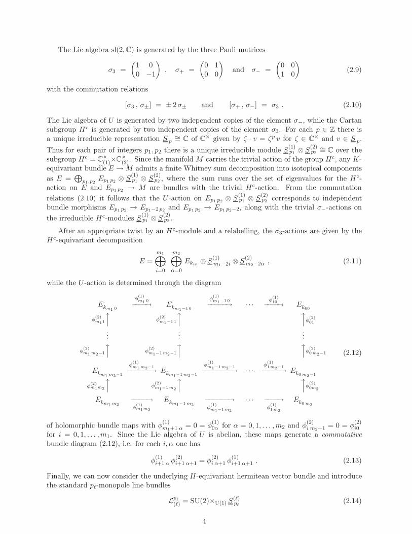
The Lie algebra sl(2,C) is generated by the three Pauli matrices

σ3 =

(1 00 −1

), σ+ =

(0 10 0

)and σ− =

(0 01 0

)(2.9)

with the commutation relations

[σ3 , σ±] = ± 2σ± and [σ+ , σ−] = σ3 . (2.10)

The Lie algebra of U is generated by two independent copies of the element σ−, while the Cartansubgroup Hc is generated by two independent copies of the element σ3. For each p ∈ Z there isa unique irreducible representation S p

∼= C of C× given by ζ · v = ζp v for ζ ∈ C

× and v ∈ S p.

Thus for each pair of integers p1, p2 there is a unique irreducible module S(1)p1 ⊗ S

(2)p2

∼= C over thesubgroup Hc = C

×(1)×C

×(2). Since the manifold M carries the trivial action of the group Hc, any K-

equivariant bundle E →M admits a finite Whitney sum decomposition into isotopical components

as E =⊕

p1,p2Ep1 p2 ⊗ S

(1)p1 ⊗ S

(2)p2 , where the sum runs over the set of eigenvalues for the Hc-

action on E and Ep1 p2 → M are bundles with the trivial Hc-action. From the commutation

relations (2.10) it follows that the U -action on Ep1 p2 ⊗ S(1)p1 ⊗ S

(2)p2 corresponds to independent

bundle morphisms Ep1 p2 → Ep1−2 p2 and Ep1 p2 → Ep1 p2−2, along with the trivial σ−-actions on

the irreducible Hc-modules S(1)p1 ⊗ S

(2)p2 .

After an appropriate twist by an Hc-module and a relabelling, the σ3-actions are given by theHc-equivariant decomposition

E =

m1⊕

i=0

m2⊕

α=0

Ekiα⊗ S

(1)m1−2i ⊗ S

(2)m2−2α , (2.11)

while the U -action is determined through the diagram

Ekm1 0

φ(1)m1 0−−−−→ Ekm1−1 0

φ(1)m1−1 0−−−−−→ · · · φ

(1)10−−−−→ Ek00

φ(2)m11

x φ(2)m1−1 1

xxφ

(2)01

......

...

φ(2)m1 m2−1

x φ(2)m1−1 m2−1

xxφ

(2)0 m2−1

Ekm1 m2−1

φ(1)m1 m2−1−−−−−−→ Ekm1−1 m2−1

φ(1)m1−1 m2−1−−−−−−−−→ · · ·

φ(1)1 m2−1−−−−−→ Ek0 m2−1

φ(2)m1m2

x φ(2)m1−1 m2

xxφ

(2)0m2

Ekm1 m2−−−−→φ

(1)m1m2

Ekm1−1 m2−−−−−−→φ

(1)m1−1 m2

· · · −−−−→φ

(1)1 m2

Ek0 m2

(2.12)

of holomorphic bundle maps with φ(1)m1+1 α = 0 = φ

(1)0α for α = 0, 1, . . . ,m2 and φ

(2)i m2+1 = 0 = φ

(2)i0

for i = 0, 1, . . . ,m1. Since the Lie algebra of U is abelian, these maps generate a commutative

bundle diagram (2.12), i.e. for each i, α one has

φ(1)i+1 α φ

(2)i+1 α+1 = φ

(2)i α+1 φ

(1)i+1 α+1 . (2.13)

Finally, we can now consider the underlying H-equivariant hermitean vector bundle and introducethe standard pℓ-monopole line bundles

Lpℓ

(ℓ) = SU(2)×U(1) S(ℓ)pℓ

(2.14)

4

over the homogeneous spaces CP 1(ℓ) for ℓ = 1, 2. Then the original rank k hermitean vector bundle

(2.8) over M×CP 1(1)×CP 1

(2) admits an equivariant decomposition

E =

m1⊕

i=0

m2⊕

α=0

Eiα with Eiα = Ekiα⊗ Lm1−2i

(1) ⊗ Lm2−2α(2) , (2.15)

where Ekiα→ M is a hermitean vector bundle of rank kiα with typical fibre the module V kiα

in(2.6), and Eiα →M×CP 1

(1)×CP 1(2) is the bundle with fibres

(Eiα

)(x, y1, y1, y2, y2)

=(Ekiα

)x⊗(Lm1−2i

(1)

)(y1,y1)

⊗(Lm2−2α

(2)

)(y2, y2)

. (2.16)

2.3 Equivariant gauge fields

Let A be a connection on the hermitean vector bundle E → M×CP 1(1)×CP 1

(2) having the form

A = Aµ dxµ in local coordinates (xµ) and taking values in the Lie algebra u(k). We will nowdescribe the G-equivariant reduction of A on M×CP 1

(1)×CP 2(2). The spherical dependences are

completely determined by the unique SU(2)-invariant connections a(ℓ)pℓ

, ℓ = 1, 2, on the monopoleline bundles (2.14) having, in local complex coordinates on CP 1

(ℓ), the forms

a(ℓ)pℓ

=pℓ

2 (1 + yℓyℓ)(yℓ dyℓ − yℓ dyℓ) . (2.17)

The curvatures of these connections are

f (ℓ)pℓ

= da(ℓ)pℓ

= − pℓ

(1 + yℓyℓ)2 dyℓ ∧ dyℓ , (2.18)

and their topological charges are given by the degrees of the complex line bundles Lpℓ

(ℓ) → CP 1(ℓ) as

deg Lpℓ

(ℓ) =i

2π

∫

CP 1(ℓ)

f (ℓ)pℓ

= pℓ . (2.19)

In the spherical coordinates (ϑℓ, ϕℓ) ∈ S2(ℓ) the monopole fields can be written as

a(ℓ)pℓ

= − i pℓ

2(1 − cos ϑℓ) dϕℓ and f (ℓ)

pℓ= da(ℓ)

pℓ= − i pℓ

2sinϑℓ dϑℓ ∧ dϕℓ . (2.20)

Related to the monopole fields are the unique, covariantly constant SU(2)-invariant forms of types(1, 0) and (0, 1) on CP 1

(ℓ) given respectively by

βℓ =dyℓ

1 + yℓyℓand βℓ =

dyℓ

1 + yℓyℓ. (2.21)

They take values respectively in the components L2(ℓ) and L−2

(ℓ) of the complexified cotangent bundle

T ∗CP 1

(ℓ) ⊗ C = L2(ℓ) ⊕L−2

(ℓ) over CP 1(ℓ). Note that there is no summation over the index ℓ in (2.17)–

(2.21).

With respect to the isotopical decomposition (2.15), the twisted u(k)-valued gauge potential Athus splits into kiα×kjβ blocks as

A =(Aiα, jβ

)with Aiα, jβ ∈ Hom

(V kjβ

, V kiα

), (2.22)

5

where

Aiα, iα = Aiα(x) ⊗ 1 ⊗ 1 + 1kiα⊗(a

(1)m1−2i(y1) ⊗ 1 + 1 ⊗ a

(2)m2−2α(y2)

), (2.23)

Aiα, i+1 α =: Φ(1)i+1 α = φ

(1)i+1 α(x) ⊗ β1(y1) ⊗ 1 , (2.24)

Ai+1 α, iα = −(Aiα, i+1 α

)†= −

(φ

(1)i+1 α(x)

)† ⊗ β1(y1) ⊗ 1 , (2.25)

Aiα, i α+1 =: Φ(2)i α+1 = φ

(2)i α+1(x) ⊗ 1 ⊗ β2(y2) , (2.26)

Ai α+1, iα = −(Aiα, i α+1

)†= −

(φ

(2)i α+1(x)

)† ⊗ 1 ⊗ β2(y2) . (2.27)

All other components Aiα, jβ vanish, while the bundle morphisms Φ(1)i+1α ∈ Hom(Ei+1 α, Eiα) and

Φ(2)i α+1 ∈ Hom(Ei α+1, Eiα) obey Φ

(1)m1+1 α = 0 = Φ

(1)0α for α = 0, 1, . . . ,m2 and Φ

(2)i m2+1 = 0 = Φ

(2)i0 for

i = 0, 1, . . . ,m1. The gauge potentials Aiα ∈ u(kiα) are connections on the hermitean vector bundles

Ekiα→M , while the bi-fundamental scalar fields φ

(1)i+1 α and φ

(2)i α+1 transform in the representations

V kiα⊗V ∨

ki+1 αand V kiα

⊗V ∨ki α+1

of the subgroups U(kiα)×U(ki+1 α) and U(kiα)×U(ki α+1) of theoriginal U(k) gauge group.

The curvature two-form F = dA + A ∧ A of the connection A has components Fµν = ∂µAν −∂νAµ +[Aµ,Aν ] in local coordinates (xµ), where ∂µ := ∂/∂xµ. It also take values in the Lie algebrau(k), and in local coordinates on M×CP 1

(1)×CP 1(2) it can be written as

F = 12 Fµν dxµ ∧ dxν + Fµy1 dxµ ∧ dy1 + Fµy1 dxµ ∧ dy1 + Fµy2 dxµ ∧ dy2

+Fµy2 dxµ ∧ dy2 + Fy1y1 dy1 ∧ dy1 + Fy2y2 dy2 ∧ dy2 + Fy1y2 dy1 ∧ dy2

+Fy1y2 dy1 ∧ dy2 + Fy1y2 dy1 ∧ dy2 + Fy1y2 dy1 ∧ dy2 . (2.28)

The calculation of the curvature (2.28) for A of the form (2.22)–(2.27) yields

F =(F iα, jβ

)with F iα, jβ = dAiα, jβ +

m1∑

l=0

m2∑

γ=0

Aiα, lγ ∧ Alγ, jβ , (2.29)

where

F iα, iα = F iα + f(1)m1−2i + f

(2)m2−2α

+(φ

(1)i+1 α

(φ

(1)i+1 α

)† −(φ

(1)iα

)†φ

(1)iα

) (β1 ∧ β1

)

+(φ

(2)i α+1

(φ

(2)i α+1

)† −(φ

(2)iα

)†φ

(2)iα

) (β2 ∧ β2

), (2.30)

F iα, i+1 α = Dφ(1)i+1 α ∧ β1 , (2.31)

F i+1 α, iα = −(F iα, i+1 α

)†= −

(Dφ

(1)i+1 α

)† ∧ β1 , (2.32)

F iα, i α+1 = Dφ(2)i α+1 ∧ β2 , (2.33)

F i α+1, iα = −(F iα, i α+1

)†= −

(Dφ

(2)i α+1

)† ∧ β2 , (2.34)

F iα, i+1 α+1 =(φ

(1)i+1 α φ

(2)i+1 α+1 − φ

(2)i α+1 φ

(1)i+1 α+1

)β1 ∧ β2 , (2.35)

F i+1 α+1, i α = −(F iα, i+1α+1

)†= −

(φ

(1)i+1 α φ

(2)i+1 α+1 − φ

(2)i α+1 φ

(1)i+1 α+1

)†β1 ∧ β2 , (2.36)

F i α+1, i+1 α =((φ

(2)i α+1

)†φ

(1)i+1 α − φ

(1)i+1 α+1

(φ

(2)i+1 α+1

)†)β1 ∧ β2 , (2.37)

F i+1 α, i α+1 = −(F i α+1, i+1 α

)†=((φ

(1)i+1 α

)†φ

(2)i α+1 − φ

(2)i+1 α+1

(φ

(1)i+1 α+1

)†)β2 ∧ β1 (2.38)

6

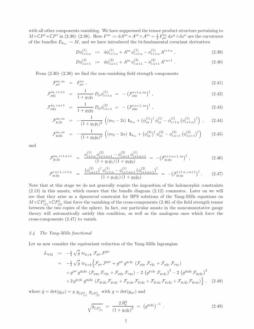
with all other components vanishing. We have suppressed the tensor product structure pertaining toM×CP 1×CP 1 in (2.30)–(2.38). Here F iα := dAiα+Aiα∧Aiα = 1

2 Fiαµν dxµ∧dxν are the curvatures

of the bundles Ekiα→M , and we have introduced the bi-fundamental covariant derivatives

Dφ(1)i+1α := dφ

(1)i+1 α +Aiα φ

(1)i+1 α − φ

(1)i+1 αA

i+1 α , (2.39)

Dφ(2)i α+1 := dφ

(2)i α+1 +Aiα φ

(2)i α+1 − φ

(2)i α+1A

i α+1 . (2.40)

From (2.30)–(2.38) we find the non-vanishing field strength components

F iα, iαµν = F iα

µν , (2.41)

F iα, i+1 αµy1

=1

1 + y1y1Dµφ

(1)i+1 α = −

(F i+1 α, iα

µy1

)†, (2.42)

F iα, i α+1µy2

=1

1 + y2y2Dµφ

(2)i α+1 = −

(F i α+1, iα

µy2

)†, (2.43)

F iα, iαy1y1

= − 1

(1 + y1y1)2

((m1 − 2i) 1kiα

+(φ

(1)iα

)†φ

(1)iα − φ

(1)i+1 α

(φ

(1)i+1 α

)†), (2.44)

F iα, iαy2y2

= − 1

(1 + y2y2)2

((m2 − 2α) 1kiα

+(φ

(2)iα

)†φ

(2)iα − φ

(2)i α+1

(φ

(2)i α+1

)†)(2.45)

and

F iα, i+1 α+1y1y2

=φ

(1)i+1 α φ

(2)i+1 α+1 − φ

(2)i α+1 φ

(1)i+1 α+1

(1 + y1y1) (1 + y2y2)= −

(F i+1 α+1, iα

y1y2

)†, (2.46)

F i α+1, i+1 αy1y2

=

(φ

(2)i α+1

)†φ

(1)i+1 α − φ

(1)i+1 α+1

(φ

(2)i+1 α+1

)†

(1 + y1y1) (1 + y2y2)= −

(F i+1 α, i α+1

y1y2

)†. (2.47)

Note that at this stage we do not generally require the imposition of the holomorphic constraints(2.13) in this ansatz, which ensure that the bundle diagram (2.12) commutes. Later on we willsee that they arise as a dynamical constraint for BPS solutions of the Yang-Mills equations onM×CP 1

(1)×CP 1(2) that force the vanishing of the cross-components (2.46) of the field strength tensor

between the two copies of the sphere. In fact, our particular ansatz in the noncommutative gaugetheory will automatically satisfy this condition, as well as the analogous ones which force thecross-components (2.47) to vanish.

2.4 The Yang-Mills functional

Let us now consider the equivariant reduction of the Yang-Mills lagrangian

LYM := −14

√g trk×k Fµν F µν

= −14

√g trk×k

Fµν Fµν + gµν gy1 y1 (Fµy1 Fνy1 + Fµy1 Fνy1)

+ gµν gy2y2 (Fµy2 Fνy2 + Fµy2 Fνy2) − 2(gy1y1 Fy1y1

)2 − 2(gy2y2 Fy2y2

)2

+ 2 gy1 y1 gy2y2 (Fy1y2 Fy1y2 + Fy1y2 Fy1y2 + Fy1y2 Fy1y2 + Fy1y2 Fy1y2), (2.48)

where g = det(gµν) = g gCP 1

(1)

gCP 1

(2)

with g = det(gµν) and

√g

CP 1(ℓ)

=2R2

ℓ

(1 + yℓyℓ)2 =

(gyℓyℓ

)−1. (2.49)

7

For the ansatz of the Section 2.3 above we substitute (2.41)–(2.47). After integration over thespherical factors CP 1

(1)×CP 1(2), the dimensional reduction of the corresponding Yang-Mills action

functional is given by

SYM :=

∫

M×CP 1(1)

×CP 1(2)

d2n+4x LYM

= π R21R

22

∫

Md2nx

√g

m1∑

i=0

m2∑

α=0

trkiα×kiα

[(F iα

µν

)†F iα µν (2.50)

+1

R21

(Dµφ

(1)i+1 α

) (Dµφ

(1)i+1 α

)†+

1

R21

(Dµφ

(1)iα

)† (Dµφ

(1)iα

)

+1

R22

(Dµφ

(2)i α+1

) (Dµφ

(2)i α+1

)†+

1

R22

(Dµφ

(2)iα

)† (Dµφ

(2)iα

)

+1

2R41

((m1 − 2i) 1kiα

+(φ

(1)iα

)†φ

(1)iα − φ

(1)i+1 α

(φ

(1)i+1 α

)†)2

+1

2R42

((m2 − 2α) 1kiα

+(φ

(2)iα

)†φ

(2)iα − φ

(2)i α+1

(φ

(2)i α+1

)†)2

+1

2R21 R

22

(φ

(1)i+1 α φ

(2)i+1 α+1 − φ

(2)i α+1 φ

(1)i+1 α+1

) (φ

(1)i+1 α φ

(2)i+1 α+1 − φ

(2)i α+1 φ

(1)i+1 α+1

)†

+1

2R21 R

22

(φ

(1)i α−1 φ

(2)iα − φ

(2)i−1 α φ

(1)iα

)† (φ

(1)i α−1 φ

(2)iα − φ

(2)i−1 α φ

(1)iα

)

+1

2R21 R

22

((φ

(2)iα

)†φ

(1)i+1 α−1 − φ

(1)i+1 α

(φ

(2)i+1 α

)†) ((φ

(2)iα

)†φ

(1)i+1 α−1 − φ

(1)i+1 α

(φ

(2)i+1 α

)†)†

+1

2R21 R

22

((φ

(2)i−1 α+1

)†φ

(1)iα − φ

(1)i α+1

(φ

(2)i α+1

)†)† ((φ

(2)i−1 α+1

)†φ

(1)iα − φ

(1)i α+1

(φ

(2)i α+1

)†) ].

All individual terms in (2.50) are kiα×kiα matrices. Recall that φ(1)i+1 α are kiα×ki+1 α matrices,

φ(2)i α+1 are kiα×ki α+1 matrices and Aiα

µ are kiα×kiα matrices. The action (2.50) is non-negative,and it can be regarded as an energy functional for static fields on R

0,1×M in the temporal gauge.

2.5 Noncommutative gauge theory

When we come to construct explicit solutions of the Yang-Mills equations we will specialize to theKahler manifold M = R

2n with metric tensor gµν = δµν and pass to a noncommutative deformationR

2n → R2nθ . The spherical factors CP 1

(ℓ), ℓ = 1, 2, will always remain commutative spaces. The

noncommutative space R2nθ is defined by declaring its coordinate functions x1, . . . , x2n to obey the

Heisenberg algebra relations[xµ , xν ] = i θµν (2.51)

with a constant real antisymmetric tensor θµν of maximal rank n. Via an orthogonal transformationof the coordinates, the matrix θ = (θµν) can be rotated into its canonical block-diagonal form withnon-vanishing components

θ2a−1 2a = −θ2a 2a−1 =: θa (2.52)

for a = 1, . . . , n. We will assume for definiteness that all θa > 0. The noncommutative version ofthe complex coordinates (2.1) has the non-vanishing commutators

[za , ˆzb

]= −2 δab θa =: θab = −θba < 0 . (2.53)

8

Taking the product of R2nθ with the commutative spheres CP 1

(1)×CP 1(2) means extending the non-

commutativity matrix θ by vanishing entries along the four new directions.

The algebra (2.51) can be represented on the Fock space H which may be realized as the linearspan

H =

∞⊕

r1,...,rn=0

C|r1, . . . , rn〉 , (2.54)

where the orthonormal basis states

|r1, . . . , rn〉 =n∏

a=1

(2 θa ra!)−1/2 (za)ra |0, . . . , 0〉 (2.55)

are connected by the action of creation and annihilation operators subject to the commutationrelations [ ˆzb

√2 θb

,za

√2 θa

]= δab . (2.56)

In the Weyl operator realization f 7→ f which maps Schwartz functions f on R2n into compact

operators f on H, coordinate derivatives are given by inner derivations of the noncommutativealgebra according to

∂zaf = θab

[ˆzb , f

]=: ∂za f and ∂zaf = θab

[zb , f

]=: ∂ˆz a f , (2.57)

where θab is defined via θbc θca = δa

b so that θab = −θba =δab

2 θa . On the other hand, integrals aregiven by traces over the Fock space H as

∫

R2n

d2nx f(x) = Pf(2π θ) TrH f . (2.58)

Vector bundles E → R2n whose typical fibres are complex vector spaces V are replaced by the

corresponding (trivial) projective modules V ⊗ H over R2nθ . The field strength components along

R2nθ in (2.28) read Fµν = ∂xµAν − ∂xν Aµ + [Aµ, Aν ], where Aµ are simultaneously valued in u(k)

and in End(H). To avoid a cluttered notation, we will omit the hats over operators, so that allequations will have the same form as previously but considered as equations in End(V ⊗H). Themain advantage of this prescription will arise from the fact that, unlike R

2n, the noncommutativespace R

2nθ has a non-trivial K-theory which allows for gauge field configurations of non-trivial

topological charge while retaining the simple geometry of flat contractible space.

3 Quiver gauge theory and graded connections

In this section we will exploit the fact that the G-equivariant reduction carried out in the previoussection has a natural interpretation as the representation of a particular class of quivers in thecategory of vector bundles over the Kahler manifold M , i.e. as a quiver bundle over M [14, 15, 20].The most natural notion of gauge field on a quiver bundle is provided by that of a graded connection

as introduced in [18]. After describing some general aspects of the quivers related to our analysis,we will rewrite the equivariant decomposition of the gauge fields of the previous section in terms ofgraded connections on the pertinent quivers. Besides its mathematical elegance, the main advantageof this representation is that it will make the physical interpretations of our field configurationscompletely transparent later on. Treatments of the theory of quivers can be found in [21].

9

3.1 The Am1+1 ⊕ Am2+1 quiver and its representations

A quiver is an oriented graph, i.e. a set of vertices together with a set of arrows between thevertices. For a given pair of positive integersm1,m2, it is clear that the bundle diagram (2.12) can benaturally associated to a quiver Q(m1,m2). The nodes of this quiver are labelled by monopole charges

giving the vertex set Q(0)(m1,m2)

= (v(1)i , v

(2)α ) = (m1 − 2i,m2 − 2α) | 0 ≤ i ≤ m1 , 0 ≤ α ≤ m2.

The arrow set is given by Q(1)(m1,m2) = ζ(ℓ)

iα | ℓ = 1, 2 , 0 ≤ i ≤ m1 , 0 ≤ α ≤ m2 with ζ(1)i+1 α :

(v(1)i+1, v

(2)α ) 7→ (v

(1)i , v

(2)α ) and ζ

(2)i α+1 : (v

(1)i , v

(2)α+1) 7→ (v

(1)i , v

(2)α ). A path in Q(m1,m2) is a sequence of

arrows in Q(1)(m1,m2) which compose. If the head of ζ

(ℓ)iα is the same node as the tail of ζ

(ℓ′ )i′α′ , then we

may produce a path ζ(ℓ′ )i′α′ ζ

(ℓ)iα consisting of ζ

(ℓ)iα followed by ζ

(ℓ′ )i′α′ . To each vertex (m1 − 2i,m2 − 2α)

we associate the trivial path eiα of length 0. Each arrow ζ(ℓ)iα itself may be associated to a path

of length 1. A relation r of the quiver is a formal finite sum of paths. From (2.13) it follows

that the set R(m1,m2) of relations of Q(m1,m2) are given by riα = ζ(1)i+1 α ζ

(2)i+1 α+1 − ζ

(2)i α+1 ζ

(1)i+1 α+1 for

0 ≤ i ≤ m1, 0 ≤ α ≤ m2.

If we set M = point in the construction of Section 2.2, then we obtain a representation V of thequiver Q(m1,m2) obtained by placing the G-modules V kiα

in (2.6) at the vertices (m1−2i,m2−2α).Recalling that the nodes of the quiver arose as the set of weights for the action of the Borelsubgroup K on the bundle E →M , we obtain natural equivalence functors between the categoriesof holomorphic representations ofK and indecomposable representations of the quiver with relations(Q(m1,m2) , R(m1,m2)), and also with the category of holomorphic homogeneous vector bundles overCP 1×CP 1 ∼= Gc/K. In particular, there is a one-to-one correspondence between G-equivariantvector bundles over CP 1×CP 1 and commutative diagrams on the quiver Q(m1,m2). In the caseof a generic Kahler manifold M , any G-equivariant bundle over M×CP 1×CP 1 defines a quiverrepresentation obtained by placing the vector bundles Ekiα

→ M at the vertices (m1 − 2i,m2 −2α), as in (2.12). It follows that there is a one-to-one correspondence between such bundles andindecomposable (Q(m1,m2) , R(m1,m2))-bundles over M . Neither the holomorphicity of the quiverrepresentation nor the relations need generically hold for the decomposition of gauge fields given inSection 2.3, but instead will arise as a dynamical effect from a specific choice of ansatz. Note thatwhen one passes to the corresponding noncommutative gauge theory, one is faced with infinite-dimensional quiver representations V ⊗ H, and one of the goals of our later constructions will beto find appropriate truncations to finite-dimensional modules over Q(m1,m2).

To aid in the construction of quiver representations, one defines the path algebra A(m1,m2) ofQ(m1,m2) to be the vector space over C generated by all paths, together with the multiplicationgiven by concatenation of paths. If two paths do not compose then their product is defined tobe 0. The trivial paths are idempotents, e2iα = eiα, and thereby define a collection of projectorson the finite-dimensional free algebra A(m1,m2). Imposing relations on the quiver then amounts totaking the quotient of A(m1,m2) by the ideal generated by the riα. Given a representation V of the

algebra A(m1,m2), we can form the vector spaces V kiα= V · eiα ∼= C

kiα . The elements of A(m1,m2)

corresponding to arrows in Q(m1,m2) yield linear maps between the V kiαwhich have to satisfy

the relations riα = 0. It follows that representations of the path algebra A(m1,m2)/R(m1,m2) areequivalent to quiver representations of (Q(m1,m2) , R(m1,m2)) [21]. Such a representation is specified

by giving the ordered collection of positive integers ~k = ~kV := (kiα)0≤i≤m1,0≤α≤m2 , called thedimension vector of the quiver representation, at the vertices of Q(m1,m2).

A useful set of quiver representations P iα is defined for each vertex of Q(m1,m2) by P iα :=eiα · A(m1,m2), which is the subspace of A(m1,m2) generated by all paths starting at the node (m1 −2i,m2 − 2α). Multiplying on the right by elements of the path algebra A(m1,m2) makes P iα intoa right A(m1,m2)-module and hence a quiver representation. This path algebra representation has

10

many special properties. The collection of all modules P iα, 0 ≤ i ≤ m1, 0 ≤ α ≤ m2 are exactlythe set of all indecomposable projective representations of the quiver Q(m1,m2), with the naturalisomorphism

A(m1,m2) =

m1⊕

i=0

m2⊕

α=0

P iα (3.1)

as right A(m1,m2)-modules. Furthermore, for any quiver representation (2.6) there is a naturalisomorphism

Hom(P iα , V

)= V kiα

, (3.2)

and in particularHom

(P jβ , P iα

)=(P iα

)jβ

= eiα · A(m1,m2) · ejβ (3.3)

is the vector space spanned by all paths from vertex (v(1)i , v

(2)α ) to vertex (v

(1)j , v

(2)β ). Imposing

the relations riα identifies all such paths and one has (P iα)jβ ∼= C for the corresponding quiverrepresentation of (Q(m1,m2) , R(m1,m2)).

A morphism f : V → V ′ of two quiver representations is given by linear maps fiα : V kiα→ V ′

k′iα

for each vertex such that φ′ (1)i+1 α fiα = fi+1α φ

(1)i+1 α and φ

′ (2)i α+1 fiα = fi α+1 φ

(2)i α+1. This notion defines

the abelian category of quiver representations (or equivalently of right A(m1,m2)-modules). If alllinear maps fiα are invertible, then f is called an isomorphism of quiver representations. Any two

isomorphic representations necessarily have the same dimension vector ~k. This provides a naturalnotion of gauge symmetry in quiver gauge theory. We will return to the issue of equivalence ofrepresentations of the quiver Q(m1,m2) in Section 4.5.

3.2 Matrix presentation of equivariant gauge fields

A convenient way of combining the reductions of equivariant gauge fields is through the formal-ism of graded connections introduced in [18]. The first step in this procedure is to rewrite thedecompositions of Section 2.3 in a particular matrix form that reflects the representations of thepath algebra given in (3.1)–(3.3). The basic idea is that, given the isomorphisms (P iα)jβ ∼= C, onecan identify (3.1) with an algebra of upper triangular complex matrices. For this, let us write therank k equivariant bundle E →M in the Zm1+1×Zm2+1-graded form

E :=

m1⊕

i=0

m2⊕

α=0

Ekiα=

m2⊕

α=0

E(m1)α with E(m1)α :=

m1⊕

i=0

Ekiα. (3.4)

The algebra Ω♯(M,E) of differential forms on the manifold M with values in the bundle E has atotal Zm1+1×Zm2+1 grading defined by combining the grading in (3.4) with the Z-grading by formdegree. Similarly, the Zm1+1×Zm2+1 grading of the endomorphism bundle

End(E) =

m1⊕

i,j=0

m2⊕

α,β=0

Hom(Ekiα, Ekjβ

) =

m2⊕

α=0

End(E(m1)α) ⊕m2⊕

α,β=0α6=β

Hom(E(m1)α, E(m1)β) (3.5)

induces a total Zm1+1×Zm2+1 grading on the endomorphism algebra Ω♯(M,End E).

A graded connection on E is a derivation on Ω♯(M,E) which shifts the total Zm1+1×Zm2+1

grading by 1, and is thus an element of the degree 1 subspace of Ω♯(M,End E). For a given module(2.6) over the quiver Q(m1,m2), the zero-form components in this subspace represent the arrowsof Q(m1,m2) and are defined by appropriately assembling the Higgs fields of the equivariant gauge

11

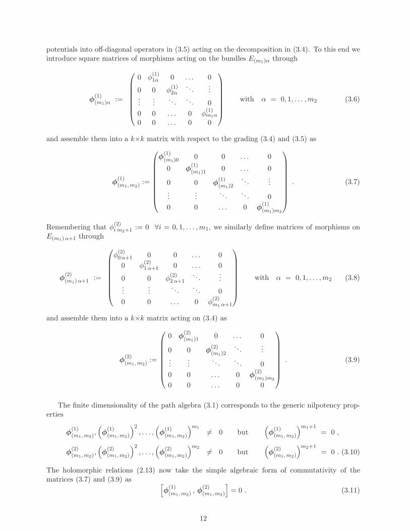
potentials into off-diagonal operators in (3.5) acting on the decomposition in (3.4). To this end weintroduce square matrices of morphisms acting on the bundles E(m1)α through

φ(1)(m1)α :=

0 φ(1)1α 0 . . . 0

0 0 φ(1)2α

. . ....

......

. . .. . . 0

0 0 . . . 0 φ(1)m1α

0 0 . . . 0 0

with α = 0, 1, . . . ,m2 (3.6)

and assemble them into a k×k matrix with respect to the grading (3.4) and (3.5) as

φ(1)(m1, m2) :=

φ(1)(m1)0 0 0 . . . 0

0 φ(1)(m1)1 0 . . . 0

0 0 φ(1)(m1)2

. . ....

......

. . .. . . 0

0 0 . . . 0 φ(1)(m1)m2

. (3.7)

Remembering that φ(2)i m2+1 := 0 ∀i = 0, 1, . . . ,m1, we similarly define matrices of morphisms on

E(m1) α+1 through

φ(2)(m1) α+1 :=

φ(2)0 α+1 0 0 . . . 0

0 φ(2)1 α+1 0 . . . 0

0 0 φ(2)2 α+1

. . ....

......

. . .. . . 0

0 0 . . . 0 φ(2)m1 α+1

with α = 0, 1, . . . ,m2 (3.8)

and assemble them into a k×k matrix acting on (3.4) as

φ(2)(m1, m2) :=

0 φ(2)(m1)1 0 . . . 0

0 0 φ(2)(m1)2

. . ....

......

. . .. . . 0

0 0 . . . 0 φ(2)(m1)m2

0 0 . . . 0 0

. (3.9)

The finite dimensionality of the path algebra (3.1) corresponds to the generic nilpotency prop-erties

φ(1)(m1, m2),

(φ

(1)(m1, m2)

)2, . . . ,

(φ

(1)(m1, m2)

)m1 6= 0 but(φ

(1)(m1, m2)

)m1+1= 0 ,

φ(2)(m1, m2),

(φ

(2)(m1, m2)

)2, . . . ,

(φ

(2)(m1, m2)

)m2 6= 0 but(φ

(2)(m1, m2)

)m2+1= 0 . (3.10)

The holomorphic relations (2.13) now take the simple algebraic form of commutativity of thematrices (3.7) and (3.9) as [

φ(1)(m1, m2) , φ

(2)(m1, m2)

]= 0 . (3.11)

12

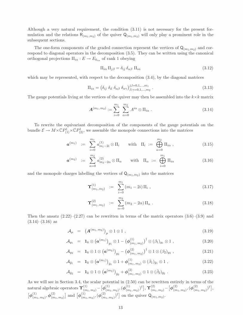
Although a very natural requirement, the condition (3.11) is not necessary for the present for-mulation and the relations R(m1,m2) of the quiver Q(m1,m2) will only play a prominent role in thesubsequent sections.

The one-form components of the graded connection represent the vertices of Q(m1,m2) and cor-respond to diagonal operators in the decomposition (3.5). They can be written using the canonicalorthogonal projections Πiα : E → Ekiα

of rank 1 obeying

Πiα Πjβ = δij δαβ Πiα (3.12)

which may be represented, with respect to the decomposition (3.4), by the diagonal matrices

Πiα =(δij δil δαβ δαγ

)j,l=0,1,...,m1

β,γ=0,1,...,m2. (3.13)

The gauge potentials living at the vertices of the quiver may then be assembled into the k×k matrix

A(m1, m2) :=

m1∑

i=0

m2∑

α=0

Aiα ⊗ Πiα . (3.14)

To rewrite the equivariant decomposition of the components of the gauge potentials on thebundle E →M×CP 1

(1)×CP 1(2), we assemble the monopole connections into the matrices

a(m1) :=

m1∑

i=0

a(1)m1−2i ⊗ Πi with Πi :=

m2⊕

α=0

Πiα , (3.15)

a(m2) :=

m2∑

α=0

a(2)m2−2α ⊗ Πα with Πα :=

m1⊕

i=0

Πiα (3.16)

and the monopole charges labelling the vertices of Q(m1,m2) into the matrices

Υ(1)(m1, m2) :=

m1∑

i=0

(m1 − 2i)Πi , (3.17)

Υ(2)(m1, m2) :=

m2∑

α=0

(m2 − 2α)Πα . (3.18)

Then the ansatz (2.22)–(2.27) can be rewritten in terms of the matrix operators (3.6)–(3.9) and(3.14)–(3.16) as

Aµ =(A(m1, m2)

)µ⊗ 1 ⊗ 1 , (3.19)

Ay1 = 1k ⊗(a(m1)

)y1

⊗ 1 −(φ

(1)(m1, m2)

)† ⊗ (β1)y1 ⊗ 1 , (3.20)

Ay2 = 1k ⊗ 1 ⊗(a(m2)

)y2

−(φ

(2)(m1, m2)

)† ⊗ 1 ⊗ (β2)y2 , (3.21)

Ay1 = 1k ⊗(a(m1)

)y1

⊗ 1 + φ(1)(m1, m2) ⊗ (β1)y1 ⊗ 1 , (3.22)

Ay2 = 1k ⊗ 1 ⊗(a(m2)

)y2

+ φ(2)(m1, m2) ⊗ 1 ⊗ (β2)y2 . (3.23)

As we will see in Section 3.4, the scalar potential in (2.50) can be rewritten entirely in terms of the

natural algebraic operators Υ(1)(m1, m2)

−[φ

(1)(m1, m2)

, (φ(1)(m1, m2)

)†], Υ

(2)(m1, m2)

−[φ

(2)(m1, m2)

, (φ(2)(m1, m2)

)†],

[φ

(1)(m1, m2),φ

(2)(m1, m2)

]and

[φ

(1)(m1, m2), (φ

(2)(m1, m2))

†]

on the quiver Q(m1,m2).

13

3.3 Examples

To help understand the forms of the matrix presentations introduced above, it is instructive to lookat some explicit examples of (Q(m1,m2) , R(m1,m2))-bundles over M before proceeding further withmore of the general formalism.

(m1, m2) = (m, 0). In this case the vertical arrows ζ(2)iα of the quiver Q(m,0) are all 0 and the

quiver bundle (2.12) collapses to the holomorphic chain [13]

Ekm 0

φ(1)m 0−−−−→ Ekm−1 0

φ(1)m−1 0−−−−→ · · · φ

(1)10−−−−→ Ek00

(3.24)

considered in [18]. The quiver Q(m,0) is called the Am+1-quiver. The set of relations R(m,0) is emptyand the non-vanishing Higgs fields are assembled into the zero-form graded connection component

φ(1)(m,0) = φ

(1)(m)0 =

0 φ(1)10 0 . . . 0

0 0 φ(1)20

. . ....

......

. . .. . . 0

0 0 . . . 0 φ(1)m0

0 0 . . . 0 0

on E = E(m)0 =

m⊕

i=0

Eki0. (3.25)

The simplest case m = 1 gives a holomorphic triple [12] and corresponds to the more standard

superconnections, having (φ(1)(1,0)

)2 = 0, which characterize the low-energy field content on brane-

antibrane systems with the tachyon field φ(1)10 between the branes and antibranes [2, 17]. A com-

pletely analogous characterization holds for the charge configuration (m1,m2) = (0,m). As we willdiscuss further in the subsequent sections, for generic m1,m2 the set of relations R(m1,m2), makingthe vector space (P iα)jβ one-dimensional, implies that the quiver Q(m1,m2) can always be naturallymapped (e.g. via a lexicographic ordering) onto an Am+1-quiver. This will become evident fromthe other examples considered below, and will have important physical ramifications later on.

(m1, m2) = (1, 1). In this case the quiver bundle truncates to a square

Ek10

φ(1)10−−−−→ Ek00

φ(2)11

xxφ

(2)01

Ek11−−−−→

φ(1)11

Ek01

(3.26)

and uniqueness of the bundle morphism on Ek11 → Ek00 (or of the corresponding path in the pathalgebra A(1,1)) yields the single holomorphic relation

φ(2)01 φ

(1)11 = φ

(1)10 φ

(2)11 . (3.27)

The equivariant graded connection admits the matrix presentation

A =

A00,00 φ(1)10 φ

(2)01 0

−(φ

(1)10

)† A10,10 0 φ(2)11

−(φ

(2)11

)†0 A01,01 φ

(1)11

0 −(φ

(2)11

)† −(φ

(1)11

)† A11,11

. (3.28)

14

(m1, m2) = (2, 1). The quiver bundle over M associated to Q(2,1) is given by

Ek20

φ(1)20−−−−→ Ek10

φ(1)10−−−−→ Ek00

φ(2)21

x φ(2)11

xxφ

(2)01

Ek21−−−−→

φ(1)21

Ek11−−−−→

φ(1)11

Ek01

(3.29)

with the pair of holomorphic relations

φ(2)11 φ

(1)21 = φ

(1)20 φ

(2)21 and φ

(2)01 φ

(1)11 = φ

(1)10 φ

(2)11 . (3.30)

The graded connection zero-form components

φ(1)(2,1) :=

0 φ(1)10 0 0 0 0

0 0 φ(1)20 0 0 0

0 0 0 0 0 0

0 0 0 0 φ(1)11 0

0 0 0 0 0 φ(1)21

0 0 0 0 0 0

and φ(2)(2,1) :=

0 0 0 φ(2)01 0 0

0 0 0 0 φ(2)11 0

0 0 0 0 0 φ(2)21

0 0 0 0 0 00 0 0 0 0 00 0 0 0 0 0

(3.31)satisfy the nilpotent relations

(φ

(1)(2,1)

)2 6= 0 ,(φ

(1)(2,1)

)3= 0 and

(φ

(2)(2,1)

)2= 0 . (3.32)

It is straightforward to check that the holomorphic relations (3.30) follow from the commutativitycondition (3.11) in this case.

(m1, m2) = (2, 2). Finally, the (Q(2,2) , R(2,2))-bundle is given by

Ek20

φ(1)20−−−−→ Ek10

φ(1)10−−−−→ Ek00

φ(2)21

x φ(2)11

xxφ

(2)01

Ek21−−−−→

φ(1)21

Ek11−−−−→

φ(1)11

Ek01

φ(2)22

x φ(2)12

xxφ

(2)02

Ek22−−−−→

φ(1)22

Ek12−−−−→

φ(1)12

Ek02

(3.33)

with

φ(1)(2,2) ⊕ φ

(2)(2,2) =

0 φ(1)10 0 φ

(2)01 0 0 0 0 0

0 0 φ(1)20 0 φ

(2)11 0 0 0 0

0 0 0 0 0 φ(2)21 0 0 0

0 0 0 0 φ(1)11 0 φ

(2)02 0 0

0 0 0 0 0 φ(1)21 0 φ

(2)12 0

0 0 0 0 0 0 0 0 φ(2)22

0 0 0 0 0 0 0 φ(1)12 0

0 0 0 0 0 0 0 0 φ(1)22

0 0 0 0 0 0 0 0 0

(3.34)

satisfying (φ

(ℓ)(2,2)

)2 6= 0 and(φ

(ℓ)(2,2)

)3= 0 for ℓ = 1, 2 . (3.35)

15

3.4 Graded connections on Q(m1,m2)

We would now like to write the graded connections as intrinsic objects to the quiver bundle (2.12)over M , without explicit reference to their origin as connections on the equivariant gauge bundleE →M×CP 1

(1)×CP 1(2). For this, we will introduce a more direct dimensional reduction of the gauge

potential A. The construction exploits the usual canonical isomorphism between the complexifiedexterior algebra bundle over M×CP 1

(1)×CP 1(2) and the corresponding graded Clifford algebra bun-

dle, which sends the exterior product into completely antisymmetrized Clifford multiplication andthe local cotangent basis dxµ onto the Clifford algebra generators Γµ obeying the anticommutationrelations

Γµ Γν + Γν Γµ = −2 gµν 12n+2 with µ, ν = 1, . . . , 2n+ 4 . (3.36)

The gamma-matrices in (3.36) may be decomposed asΓµ

=Γµ, Γy1, Γy1 , Γy2 , Γy2

(3.37)

whereΓµ = γµ ⊗ 12 ⊗ 12 , (3.38)

and γµ = −(γµ)† are the 2n×2n matrices which locally generate the Clifford algebra bundle overM and which obey the anticommutation relations

γµ γν + γν γµ = −2 gµν 12n with µ, ν = 1, . . . , 2n . (3.39)

The spherical components are given by

Γy1 = γ ⊗ γy1 ⊗ 12 , Γy1 = γ ⊗ γy1 ⊗ 12 , (3.40)

Γy2 = γ ⊗ σ3 ⊗ γy2 , Γy2 = γ ⊗ σ3 ⊗ γy2 , (3.41)

where

γyℓ = − 1

Rℓ(1 + yℓyℓ) σ+ and γyℓ =

1

Rℓ(1 + yℓyℓ) σ− (3.42)

are the Clifford algebra generators over CP 1(ℓ) for ℓ = 1, 2, with the constant sl(2,C) generators

given by (2.9,2.10). The chirality operator over M is

γ =i n

(2n)!√gǫµ1···µ2n

γµ1 · · · γµ2n with (γ)2 = 12n and γ γµ = −γµ γ . (3.43)

With this set-up we may now write the equivariant gauge potential given by (2.22)–(2.27) asthe graded connection

A := Γµ Aµ = Γµ Aµ + Γy1 Ay1 + Γy1 Ay1 + Γy2 Ay2 + Γy2 Ay2

= γµ(A(m1, m2)

)µ⊗ 12 ⊗ 12 +

1

R1

(φ

(1)(m1, m2)

)γ ⊗ σ− ⊗ 12 +

1

R1

(φ

(1)(m1, m2)

)†γ ⊗ σ+ ⊗ 12

+1

R2

(φ

(2)(m1, m2)

)γ ⊗ σ3 ⊗ σ− +

1

R2

(φ

(2)(m1, m2)

)†γ ⊗ σ3 ⊗ σ+

+ γ ⊗(γy1(a(m1)

)y1

+ γy1(a(m1)

)y1

)⊗ 12 + γ ⊗ σ3 ⊗

(γy2(a(m2)

)y2

+ γy2(a(m2)

)y2

),

(3.44)

where

γyℓ(a(mℓ)

)yℓ

+ γyℓ(a(mℓ)

)yℓ

=1

Rℓ(1 + yℓyℓ)

((a(mℓ)

)yℓσ− −

(a(mℓ)

)yℓσ+

)for ℓ = 1, 2 .

(3.45)

16

As desired, the zero-form components in (3.44) involving φ(ℓ)(m1,m2) are independent of the coor-

dinates (yℓ, yℓ) ∈ CP 1(ℓ) and they anticommute with the one-form components involving A(m1,m2)

due to their couplings with the chirality operator (3.43). From (2.41)–(2.47) the curvature of thegraded connection (3.44) is found to be

F := 14

[Γµ , Γν

]Fµν

= 14

[γµ , γν

] (F (m1, m2)

)µν

⊗ 12 ⊗ 12

− 1

R1γ(γµDµφ

(1)(m1, m2)

)⊗ σ− ⊗ 12 +

1

R1γ(γµDµφ

(1)(m1, m2)

)† ⊗ σ+ ⊗ 12

− 1

R2γ(γµDµφ

(2)(m1, m2)

)⊗ σ3 ⊗ σ− +

1

R2γ(γµDµφ

(2)(m1, m2)

)† ⊗ σ3 ⊗ σ+

+1

2R21

(Υ

(1)(m1, m2) −

[φ

(1)(m1, m2) ,

(φ

(1)(m1, m2)

)†])12n ⊗ σ3 ⊗ 12

+1

2R22

(Υ

(2)(m1, m2)

−[φ

(2)(m1, m2)

,(φ

(2)(m1, m2)

)†])12n ⊗ 12 ⊗ σ3

+1

R1R2

[φ

(1)(m1,m2) , φ

(2)(m1, m2)

]12n ⊗ σ− ⊗ σ−

+1

R1R2

[φ

(1)(m1, m2) , φ

(2)(m1, m2)

]†12n ⊗ σ+ ⊗ σ+

+1

R1R2

[φ

(1)(m1, m2) ,

(φ

(2)(m1, m2)

)†]12n ⊗ σ− ⊗ σ+

+1

R1R2

[φ

(1)(m1, m2) ,

(φ

(2)(m1, m2)

)†]†12n ⊗ σ+ ⊗ σ− (3.46)

where F (m1, m2) := dA(m1, m2) + A(m1, m2) ∧ A(m1, m2) = 12

(F (m1, m2)

)µν

dxµ ∧ dxν.

The graded curvature (3.46) is completely independent of the spherical coordinates. Using(3.46) and standard gamma-matrix trace formulas [18], it is possible to recast the dimensionallyreduced Yang-Mills action functional (2.50) in the compact form

SYM =π2R2

1R22

2n

∫

Md2nx

√g trk×k Tr

C2n+2 F2 , (3.47)

where the trace TrC2n+2 is taken over the representation space of (3.36) and may be thought of as an

“integral” over the Clifford algebra. Thus the entire equivariant gauge theory on M×CP 1(1)×CP 1

(2)may be elegantly rewritten as an ordinary Yang-Mills gauge theory of graded connections on thecorresponding quiver bundle over M .

4 Noncommutative instantons and quiver vortices

We will now proceed to the construction of explicit equivariant instanton solutions. We will buildboth BPS and non-BPS configurations of the Yang-Mills equations on the noncommutative spaceR

2nθ ×CP 1×CP 1. We then describe some general properties of the moduli space of noncommutative

instantons in this instance.

4.1 BPS equations

The equations of motion which follow from varying the Yang-Mills lagrangian (2.48) on the Kahlermanifold M×CP 1×CP 1 are given by

1√g∂µ

(√g F µν

)+[Aµ , F µν

]= 0 . (4.1)

17

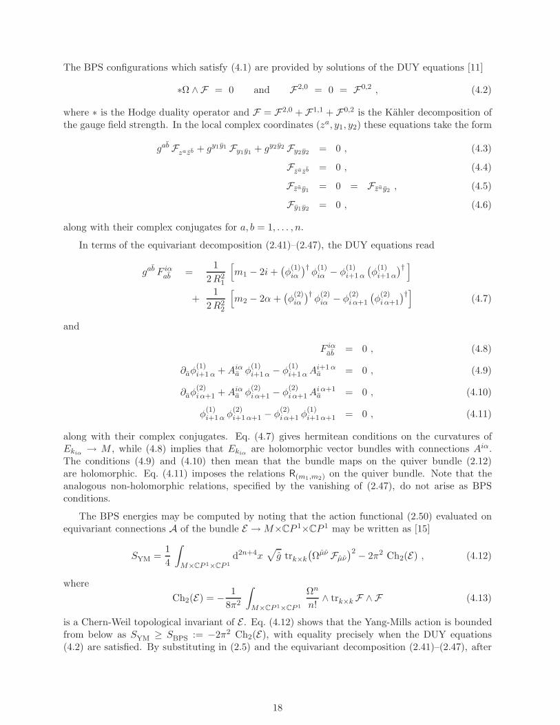
The BPS configurations which satisfy (4.1) are provided by solutions of the DUY equations [11]

∗Ω ∧ F = 0 and F2,0 = 0 = F0,2 , (4.2)

where ∗ is the Hodge duality operator and F = F2,0 + F1,1 + F0,2 is the Kahler decomposition ofthe gauge field strength. In the local complex coordinates (za, y1, y2) these equations take the form

gab Fzazb + gy1y1 Fy1y1 + gy2y2 Fy2y2 = 0 , (4.3)

Fzazb = 0 , (4.4)

Fzay1= 0 = Fzay2

, (4.5)

Fy1y2 = 0 , (4.6)

along with their complex conjugates for a, b = 1, . . . , n.

In terms of the equivariant decomposition (2.41)–(2.47), the DUY equations read

gab F iαab =

1

2R21

[m1 − 2i+

(φ

(1)iα

)†φ

(1)iα − φ

(1)i+1 α

(φ

(1)i+1 α

)† ]

+1

2R22

[m2 − 2α +

(φ

(2)iα

)†φ

(2)iα − φ

(2)i α+1

(φ

(2)i α+1

)†](4.7)

and

F iαab = 0 , (4.8)

∂aφ(1)i+1 α +Aiα

a φ(1)i+1 α − φ

(1)i+1 αA

i+1 αa = 0 , (4.9)

∂aφ(2)i α+1 +Aiα

a φ(2)i α+1 − φ

(2)i α+1A

i α+1a = 0 , (4.10)

φ(1)i+1 α φ

(2)i+1 α+1 − φ

(2)i α+1 φ

(1)i+1 α+1 = 0 , (4.11)

along with their complex conjugates. Eq. (4.7) gives hermitean conditions on the curvatures ofEkiα

→ M , while (4.8) implies that Ekiαare holomorphic vector bundles with connections Aiα.

The conditions (4.9) and (4.10) then mean that the bundle maps on the quiver bundle (2.12)are holomorphic. Eq. (4.11) imposes the relations R(m1,m2) on the quiver bundle. Note that theanalogous non-holomorphic relations, specified by the vanishing of (2.47), do not arise as BPSconditions.

The BPS energies may be computed by noting that the action functional (2.50) evaluated onequivariant connections A of the bundle E →M×CP 1×CP 1 may be written as [15]

SYM =1

4

∫

M×CP 1×CP 1

d2n+4x√g trk×k

(Ωµν Fµν

)2 − 2π2 Ch2(E) , (4.12)

where

Ch2(E) = − 1

8π2

∫

M×CP 1×CP 1

Ωn

n!∧ trk×k F ∧ F (4.13)

is a Chern-Weil topological invariant of E . Eq. (4.12) shows that the Yang-Mills action is boundedfrom below as SYM ≥ SBPS := −2π2 Ch2(E), with equality precisely when the DUY equations(4.2) are satisfied. By substituting in (2.5) and the equivariant decomposition (2.41)–(2.47), after

18

integration over CP 1×CP 1 one finds

SBPS = 2π2m1∑

i=0

m2∑

α=0

volM

[(m1 − 2i) (m2 − 2α) kiα

+4(R2

2 (m1 − 2i) +R21 (m2 − 2α)

)deg Ekiα

]− 64π2R2

1R22 Ch2(Ekiα

)

+

∫

Md2nx

√g trkiα×kiα

[(φ

(1)i+1 α+1

)† (φ

(2)i α+1

)†φ

(1)i+1 α φ

(2)i+1 α+1 −

(φ

(1)iα

)†φ

(1)iα

(φ

(2)i α+1

)†φ

(2)i α+1

+(φ

(1)i+1 α

)†φ

(1)i+1 α+1

(φ

(2)i+1 α+1

)†φ

(2)i α+1 − φ

(1)i+1 α

(φ

(1)i+1 α

)† (φ

(2)iα

)†φ

(2)iα

], (4.14)

where volM =∫M ωn/n! is the volume of the Kahler manifold M and

deg Ekiα=

i

volM

∫

M

ωn−1

(n− 1)!∧ trkiα×kiα

F iα (4.15)

is the degree of the rank kiα bundle Ekiα→M .

To cast these equations on the noncommutative space M = R2nθ , we introduce the operators

Xiαa := Aiα

a + θab zb and Xiα

a := Aiαa + θab z

b . (4.16)

In terms of these operators the antiholomorphic bi-fundamental covariant derivatives take the form

Daφ(1)i+1 α = Xiα

a φ(1)i+1 α−φ

(1)i+1 αX

i+1 αa and Daφ

(2)i α+1 = Xiα

a φ(2)i α+1−φ

(2)i α+1X

i α+1a , (4.17)

while the components of the field strength tensor become

F iαab =

[Xiα

a , Xiαb

]+ θab , F iα

ab =[Xiα

a , Xiαb

]and F iα

ab =[Xiα

a , Xiαb

]. (4.18)

The noncommutative DUY equations (without the complex conjugates) then read

δab([Xiα

a , Xiαb

]+ θab

)=

1

2R21

[m1 − 2i+

(φ

(1)iα

)†φ

(1)iα − φ

(1)i+1 α

(φ

(1)i+1 α

)† ](4.19)

+1

2R22

[m2 − 2α+

(φ

(2)iα

)†φ

(2)iα − φ

(2)i α+1

(φ

(2)i α+1

)†],

[Xiα

a , Xiαb

]= 0 , (4.20)

Xiαa φ

(1)i+1 α − φ

(1)i+1 αX

i+1 αa = 0 , (4.21)

Xiαa φ

(2)i α+1 − φ

(2)i α+1X

i α+1a = 0 , (4.22)

φ(1)i+1 α φ

(2)i+1 α+1 − φ

(2)i α+1 φ

(1)i+1 α+1 = 0 . (4.23)

4.2 Examples

Before proceeding with a more general analysis, we will provide some illustration of the meaningof the quiver vortex equations (4.7)–(4.11) through special cases and limiting solutions.

Chain vortex equations. Consider a holomorphic chain (3.24) with (m1,m2) = (m, 0). Its

equations, obtainable from (4.7)–(4.11) by taking φ(2)i α+1 = 0 in the ansatz for A and F , read

gab F iab =

1

2R2(m− 2i+ φ†i φi − φi+1 φ

†i+1) , F i

ab = 0 , (4.24)

∂aφi+1 + Aia φi+1 − φi+1A

i+1a = 0 for i = 0, 1, . . . ,m , (4.25)

19

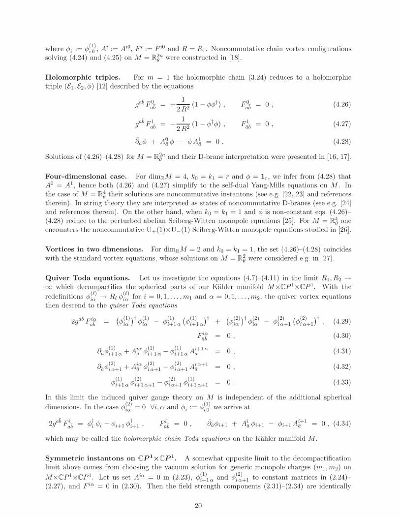
where φi := φ(1)i 0 , Ai := Ai0, F i := F i0 and R = R1. Noncommutative chain vortex configurations

solving (4.24) and (4.25) on M = R2nθ were constructed in [18].

Holomorphic triples. For m = 1 the holomorphic chain (3.24) reduces to a holomorphictriple (E1, E2, φ) [12] described by the equations

gab F 0ab = +

1

2R2(1 − φφ†) , F 0

ab = 0 , (4.26)

gab F 1ab = − 1

2R2(1 − φ†φ) , F 1

ab = 0 , (4.27)

∂aφ + A0a φ − φA1

a = 0 . (4.28)

Solutions of (4.26)–(4.28) for M = R2nθ and their D-brane interpretation were presented in [16, 17].

Four-dimensional case. For dimRM = 4, k0 = k1 = r and φ = 1r, we infer from (4.28) thatA0 = A1, hence both (4.26) and (4.27) simplify to the self-dual Yang-Mills equations on M . Inthe case of M = R

4θ their solutions are noncommutative instantons (see e.g. [22, 23] and references

therein). In string theory they are interpreted as states of noncommutative D-branes (see e.g. [24]and references therein). On the other hand, when k0 = k1 = 1 and φ is non-constant eqs. (4.26)–(4.28) reduce to the perturbed abelian Seiberg-Witten monopole equations [25]. For M = R

4θ one

encounters the noncommutative U+(1)×U−(1) Seiberg-Witten monopole equations studied in [26].

Vortices in two dimensions. For dimRM = 2 and k0 = k1 = 1, the set (4.26)–(4.28) coincideswith the standard vortex equations, whose solutions on M = R

2θ were considered e.g. in [27].

Quiver Toda equations. Let us investigate the equations (4.7)–(4.11) in the limit R1, R2 →∞ which decompactifies the spherical parts of our Kahler manifold M×CP 1×CP 1. With the

redefinitions φ(ℓ)iα → Rℓ φ

(ℓ)iα for i = 0, 1, . . . ,m1 and α = 0, 1, . . . ,m2, the quiver vortex equations

then descend to the quiver Toda equations

2gab F iαab =

(φ

(1)iα

)†φ

(1)iα − φ

(1)i+1 α

(φ

(1)i+1 α

)†+(φ

(2)iα

)†φ

(2)iα − φ

(2)i α+1

(φ

(2)i α+1

)†, (4.29)

F iαab = 0 , (4.30)

∂aφ(1)i+1 α +Aiα

a φ(1)i+1 α − φ

(1)i+1 αA

i+1 αa = 0 , (4.31)

∂aφ(2)i α+1 +Aiα

a φ(2)i α+1 − φ

(2)i α+1A

i α+1a = 0 , (4.32)

φ(1)i+1 α φ

(2)i+1 α+1 − φ

(2)i α+1 φ

(1)i+1 α+1 = 0 . (4.33)

In this limit the induced quiver gauge theory on M is independent of the additional spherical

dimensions. In the case φ(2)iα = 0 ∀i, α and φi := φ

(1)i 0 we arrive at

2gab F iab = φ†i φi − φi+1 φ

†i+1 , F i

ab = 0 , ∂aφi+1 + Aia φi+1 − φi+1A

i+1a = 0 , (4.34)

which may be called the holomorphic chain Toda equations on the Kahler manifold M .

Symmetric instantons on CP 1×CP 1. A somewhat opposite limit to the decompactificationlimit above comes from choosing the vacuum solution for generic monopole charges (m1,m2) on

M×CP 1×CP 1. Let us set Aiα = 0 in (2.23), φ(1)i+1 α and φ

(2)i α+1 to constant matrices in (2.24)–

(2.27), and F iα = 0 in (2.30). Then the field strength components (2.31)–(2.34) are identically

20

zero, but (2.35)–(2.38) are generically non-vanishing. The components (2.41)–(2.43) vanish, while(2.44)–(2.47) are non-vanishing and give the components of the gauge fields on CP 1×CP 1. TheBPS equations (4.8)–(4.10) are identically satisfied in this case, while eqs. (4.7) and (4.11) should be

solved with constant matrices φ(ℓ)iα . The simplest choice is square matrices with (m1,m2) = (1, 1).

The BPS equations (4.7) and (4.11) are respectively equivalent in this case to the equations

F iα,iαy1y1

+ F iα,iαy2y2

= 0 ,

F i+1 α+1,iαy1y2

= 0 = F iα,i+1 α+1y1y2

. (4.35)

Furthermore, F i α+1,i+1 αy1y2

is given by (2.47). The equations (4.35) give SU(2)×SU(2)-equivariantsolutions of the self-dual Yang-Mills equations on CP 1×CP 1 which are vacuum BPS solutions ofthe original DUY equations. These solutions have non-zero energy, and the entire structure of thesenon-abelian instantons on CP 1×CP 1 is reduced to equations for finite-dimensional matrices fromour equivariant fields.

4.3 Finite energy solutions

Let us fix monopole charges m1,m2 > 0 and an arbitrary integer 0 < r ≤ k. Consider the ansatz

Xiαa = θab TNiα

zb T †Niα

and Xiαa = θab TNiα

zb T †Niα

, (4.36)

φ(1)i+1 α = λ

(1)i+1 α TNiα

T †Ni+1 α

and(φ

(1)i+1 α

)†= λ

(1)i+1 α TNi+1 α

T †Niα

, (4.37)

φ(2)i α+1 = λ

(2)i α+1 TNiα

T †Ni α+1

and(φ

(2)i α+1

)†= λ

(2)i α+1 TNi α+1

T †Niα

, (4.38)

where λ(1)iα , λ

(2)iα ∈ C are some constants with λ

(1)0α = 0 = λ

(1)m1+1 α and λ

(2)i0 = 0 = λ

(2)i m2+1 for

i = 0, 1, . . . ,m1, α = 0, 1, . . . ,m2. Denoting by H the n-oscillator Fock space as before, theToeplitz operators

TNiα: C

r ⊗H −→ V kiα⊗H (4.39)

are partial isometries described by rectangular kiα×r matrices (with values in End H) possessingthe properties

T †Niα

TNiα= 1r while TNiα

T †Niα

= 1kiα− PNiα

, (4.40)

where PNiαis a hermitean projector of finite rank Niα on the Fock space V kiα

⊗H so that

P 2Niα

= PNiα= P †

Niαand TrV kiα

⊗H PNiα= Niα . (4.41)

It follows thatker TNiα

= 0 but kerT †Niα

= imPNiα∼= C

Niα . (4.42)

For the ansatz (4.36)–(4.38) the equations (4.20)–(4.23) are satisfied along with the non-holomorphic relations (

φ(2)iα

)†φ

(1)i+1 α−1 − φ

(1)i+1 α

(φ

(2)i+1 α

)†= 0 , (4.43)

or equivalently in terms of graded connections one has the commutativity condition[φ

(1)(m1, m2)

,(φ

(2)(m1, m2)

)†]= 0 . (4.44)

The non-vanishing gauge field strength components are given by

F iαab = θab PNiα

=1

2 θaδab PNiα

. (4.45)

21

It follows that our ansatz determines a finite-dimensional representation of the quiver with relations(Q(m1,m2) , R(m1,m2)). The projectors PNiα

give representations of the trivial path idempotents eiαand project the infinite-dimensional Fock module V ⊗ H over the path algebra A(m1,m2), given by

the noncommutative quiver bundle, onto finite-dimensional vector spaces PNiα·(V⊗H) = ker T †

Niα.

This module will be denoted as

T :=

m1⊕

i=0

m2⊕

α=0

ker T †Niα

(4.46)

with dimension vector~N := ~kT =

(Niα

)i=0,1,...,m1

α=0,1,...,m2. (4.47)

These dimensions correspond to the degrees of the corresponding noncommutative sub-bundlesdetermined by (4.45).

The noncommutative Yang-Mills action for the ansatz (4.36)–(4.38) can be evaluated by using(2.50), (2.58), (4.23), (4.40), (4.43) and (4.45) to get

SYM = −π R21R

22 Pf(2π θ)

m1∑

i=0

m2∑

α=0

TrV kiα⊗H

tr2n×2n

(θ−2)PNiα

− 1

2R41

[(m1 − 2i)1kiα

+(∣∣λ(1)

iα

∣∣2 −∣∣λ(1)

i+1 α

∣∣2) (

1kiα− PNiα

)]2

− 1

2R42

[(m2 − 2α)1kiα

+(∣∣λ(2)

iα

∣∣2 −∣∣λ(2)

i α+1

∣∣2) (

1kiα− PNiα

)]2 . (4.48)

Requiring that SYM < ∞ yields a pair of equations determining the moduli of the complex coef-

ficients λ(1)iα and λ

(2)iα respectively. Up to a phase they are thus uniquely fixed, by demanding that

the ansatz (4.36)–(4.38) be a finite energy field configuration, as

∣∣λ(1)iα

∣∣2 = i (m1 − i+ 1) and∣∣λ(2)

iα

∣∣2 = α (m2 − α+ 1) . (4.49)

The corresponding finite action (4.48) then reads

SYM = π R21R

22 Pf(2π θ)

⌊m12

⌋∑

i=0

⌊m22

⌋∑

α=0

(Niα +Nm1−i m2−α +Nm1−i α +Ni m2−α

)

×[

(m1 − 2i)2

2R41

+(m2 − 2α)2

2R42

− tr2n×2n

(θ−2) ]

, (4.50)

where we have split the sum over nodes of the quiver Q(m1,m2) into contributions from Diracmonopoles and antimonopoles which each have the same Yang-Mills energies on the spheres CP 1

(1)

and CP 1(2). This splitting will be the crux later on for the physical interpretation of our instanton

solutions.

Finally, let us check that the Yang-Mills equations on R2nθ ×CP 1

(1)×CP 1(2) are indeed satisfied by

our choice of ansatz. We have

Aa − θab zb =

m1∑

i=0

m2∑

α=0

Xiαa ⊗ Πiα = θab

m1∑

i=0

m2∑

α=0

TNiαzb T †

Niα⊗ Πiα , (4.51)

Aa − θab zb =

m1∑

i=0

m2∑

α=0

Xiαa ⊗ Πiα = θab

m1∑

i=0

m2∑

α=0

TNiαzb T †

Niα⊗ Πiα , (4.52)

22

while Ay1, Ay2, Ay1 and Ay2 are given by (3.20)–(3.23). For our ansatz the field strength tensorhas components

Fab = θab

m1∑

i=0

m2∑

α=0

PNiα⊗ Πiα , (4.53)

Fy1y1 =1

(1 + y1y1)2

m1∑

i=0

m2∑

α=0

(m1 − 2i) PNiα⊗ Πiα , (4.54)

Fy2y2 =1

(1 + y2y2)2

m1∑

i=0

m2∑

α=0

(m2 − 2α) PNiα⊗ Πiα , (4.55)

where we have imposed the finite energy conditions (4.49). One can now easily check in the sameway as in [18] that the Yang-Mills equations (4.1) are satisfied.

4.4 BPS solutions

The configurations described above are generically non-BPS solutions of the Yang-Mills equationson R

2nθ ×CP 1

(1)×CP 1(2). Let us now describe the structure of the BPS states. Substituting (4.37),

(4.38) and (4.45) into the remaining DUY equations (4.19) and using the finite energy constraints(4.49), one finds the BPS conditions

n∑

a=1

1

θa=m1 − 2i

2R21

+m2 − 2α

2R22

(4.56)

for all i, α withNiα > 0. Generically, these conditions are incompatible with one another unless onlyone of the degrees, say N00 for definiteness, is non-zero. Then the solution (4.36)–(4.38) is truncatedby setting TNiα

= 1r for all (i, α) 6= (0, 0) which correspond to vacuum gauge potentials Aiα = 0

with trivial bundle maps φ(ℓ)iα acting as multiplication by the complex numbers λ

(ℓ)iα satisfying

(4.49). The BPS solutions are also restricted to the special class of quiver representations (2.6)having dimension vectors ~k with kiα = r ∀(i, α) 6= (0, 0) and k00 + m1m2 r = k. As we will seein Section 4.5, these quiver representations are essentially generic and hence BPS solutions alwaysexist. The corresponding BPS energy (4.50) is proportional to the degree N00 and correspondsto the topological invariants displayed in (4.14), with the remaining terms vanishing due to thenon-holomorphic relations (4.43).

Notice that there are special points in the quiver vortex moduli space where the generic BPSgauge symmetry U(k00)×U(r)m1 m2 is enhanced. For example, if R1 = R2 and p is any fixed integerwith 0 ≤ p ≤ min(m1,m2), then a BPS solution with Ni p−i > 0 for i = 0, 1, . . . , p is possible. Thissolution corresponds to a holomorphic chain along the diagonal vertices (i, α) of the quiver Q(m1,m2)

with i+α = p. The corresponding BPS energies depend on p and are minimized precisely at p = 0.

The BPS solution having Niα > 0 may be characterized in quiver gauge theory as Niα copiesof the simple Schur representation L iα for each i = 0, 1, . . . ,m1, α = 0, 1, . . . ,m2. This is theQ(m1,m2)-module given by a one-dimensional vector space at vertex (m1−2i,m2−2α) with all maps

equal to 0, i.e. the A(m1,m2)-module with (L iα)jβ = δij δαβ C and dimension vector (~kL iα)jβ =

δij δαβ . The generic non-BPS configurations give modules T which are extensions of the BPSmodules (L iα)⊕Niα [18] describing noncommutative quiver vortex configurations.

23

4.5 Instanton moduli space

We will now describe the moduli space of the generic (non-BPS) solutions that we have obtained.The equations of motion are fixed first of all by the positive integers n and k. The condition ofG-equivariance then specifies a quiver representation (2.6) with dimension vector ~k. The Yang-Mills action (4.50) is independent of ~k, and later on we will find that in fact no physical quantitiesdepend on the particular choice of quiver representation. As we now proceed to demonstrate, thisindependence is due to the triviality of the moduli space of Q(m1,m2)-modules.

Let us fix a dimension vector ~k. Then with the identifications V kiα

∼= Ckiα we can regard the

module (2.6) as an element in the space of quiver representations into V given by

Rep(Q(m1,m2) , ~k

):=

m1⊕

i=0

m2⊕

α=0

(Hom

(C

ki+1 α , Ckiα)⊕ Hom

(C

ki α+1 , Ckiα))

(4.57)

with km1+1 α := 0 =: ki m2+1. This is the space of representations with fixed dimension vector ~k.The set of representations of Q(m1,m2) into V satisfying the relations R(m1,m2) is an affine varietyinside the space (4.57).

The gauge group of the corresponding quiver gauge theory is given by (2.7). As in Section 2.2,it is useful to work instead with the complexified gauge group

G(~k ) =

m1∏

i=0

m2∏

α=0

GL(kiα,C) . (4.58)

Suppose that V , V ′ ∈ Rep(Q(m1,m2), ~k ) and f : V → V ′ is an isomorphism of quiver representa-tions. Then f can be naturally regarded as an element of the gauge group (4.58). Conversely,

any element f = fiα ∈ GL(kiα,C)0≤i≤m1,0≤α≤m2 ∈ G(~k ) acts on V ∈ Rep(Q(m1,m2), ~k ) in

the same fashion. It follows that the gauge group G(~k ) acts on Rep(Q(m1,m2),~k ) and two quiver

representations are isomorphic if and only if they lie in the same orbit of G(~k ). Thus there isa one-to-one correspondence between G(~k )-orbits in Rep(Q(m1,m2), ~k ) and isomorphism classes of

Q(m1,m2)-modules with dimension vector ~k.

This set defines the moduli space M(Q(m1,m2), ~k ) of quiver representations. It has virtualdimension [28]

dim[M(Q(m1,m2) , ~k

)]vir= 1 + dim Rep

(Q(m1,m2) ,

~k)− dim G

(~k)

= 1 −m1∑

i=0

m2∑

α=0

kiα

(kiα − ki+1 α − ki α+1

). (4.59)

Restricting to representations which satisfy the relations R(m1,m2) lowers (4.59) by∑

i,α kiα ki+1 α+1.Representations with moduli space dimension greater than the virtual dimension can arise due toadditional unbroken gauge symmetry, as described in Section 4.4. Schur representations, describinggeneric BPS states, are those modules for which the stable dimension equals the virtual dimension.Rigid representations carry no moduli and have vanishing virtual dimension. As we now show, itis these latter Q(m1,m2)-modules that parametrize our noncommutative quiver vortices.

The scalar subgroup C× ⊂ G(~k ) acts trivially on Rep(Q(m1,m2), ~k ), and we are left with a free

action of the projective gauge group PG(~k ) := G(~k )/C×. Since PG(~k ) is not compact, we must usegeometric invariant theory to obtain a quotient which is well-defined as a projective variety [29].

24

The representation space X = Rep(Q(m1,m2),~k ) is an affine variety. Let C[X] denote the ring of

polynomial functions on X. The PG(~k )-action on X induces a PG(~k )-action on C[X] in the usual

way by pull-back. Let C[X]PG(~k ) ⊂ C[X] be the subalgebra of PG(~k )-invariant polynomials. Since

the gauge group (4.58) is reductive, the graded ring C[X]PG(~k ) is finitely generated and by theGel’fand-Naimark theorem it can be regarded as the polynomial ring of a complex projective affinevariety X //PG(~k ). This defines the desired moduli space

M(Q(m1,m2) ,

~k)

:= Rep(Q(m1,m2) ,

~k)//PG(~k ) = Proj C

[Rep

(Q(m1,m2) ,

~k)]PG(~k )

. (4.60)

Now since the quiver Q(m1,m2) has no oriented cycles, we may lexicographically order its vertex

set as Q(0)(m1,m2) = 1, 2, . . . , (m1 + 1) (m2 + 1) and assume that the integer label of the tail node

of each arrow is smaller than that of the head node. For ζ ∈ C× we define f ζ ∈ G(~k ) by

( f ζ)i = ζi 1ki∈ GL(ki,C) for each i ∈ Q

(0)(m1,m2)

. Then by considering the action of f ζ on

X = Rep(Q(m1,m2),~k ) and on C[X]PG(~k ), one easily deduces that C[X]PG(~k ) ∼= C. This means that

the moduli space (4.60) is trivial,

M(Q(m1,m2) , ~k

)= point , (4.61)

and all quiver representations are gauge equivalent.

Thus the only moduli of our solutions arise from the moduli space of noncommutative soli-tons [30]. They are parametrized by the pair of monopole charges (m1,m2) and by the dimen-sion vector ~N of the quiver representation (4.46). The above argument again shows that thereare no extra moduli associated with the Q(m1,m2)-modules T . For each i, α we let bliα = (baliα),liα = 1, . . . , Niα be the holomorphic components of fixed points in Cn, and let |bliα〉 be the corre-sponding coherent states in the n-oscillator Fock space H. For the projector PNiα

in the solutionof Section 4.3 we may take the orthogonal projection of H onto the linear span

⊕Niα

liα=1 C|bliα〉.Modulo the standard action of the noncommutative gauge group U(H) ∼= U(∞), the moduli spaceof these projectors can be described as an ideal I of the ring of polynomials C[z1, . . . , zn] in thenoncommutative coordinates acting on the vacuum state |0, . . . , 0〉. The zero set of I gives thelocations of the instantons in C

n and the codimension of I in C[z1, . . . , zn] is the number Niα ofinstantons. The moduli space of partial isometries TNiα

thereby coincides with the Hilbert scheme

HilbNiα(Cn) of Niα points in Cn [30], and thus the total moduli space of the solutions constructed

in Section 4.3 is

Mn(m1,m2)(

~N ) =

m1∏

i=0

m2∏

α=0

HilbNiα(Cn) . (4.62)

The quiver representation (4.46) thereby specifies the supports of the noncommutative quiver vor-tices in R

2n. Explicit forms for the Toeplitz operators TNiαcorresponding to specific points in

(4.62) may be constructed exactly as in [18] by using the noncommutative ABS construction. Wewill return to this point in the next section.

5 D-brane realizations

In this final section we will elucidate the physical interpretation of our solutions as particularconfigurations of branes and antibranes in Type IIA superstring theory. We will first compute,in the original gauge theory on R

2nθ ×CP 1×CP 1, the topological charges of the multi-instanton

solutions constructed in Section 4.3. This will make clear the D-brane interpretation which wedescribe in detail. We then present two independent checks of the proposed identification. Firstly,

25

we work out the K-theory charges associated to the noncommutative quiver vortices. Secondly, wecompute the topological charge in the quiver gauge theory arising after dimensional reduction toR

2nθ . While formally similar to the construction of [18] in the case of holomorphic chains, the new

feature of the higher rank quiver is that all of these computations of D-brane charges agree only

when one imposes the appropriate relations derived earlier. The ensuing calculations thereby alsoprovide a nice physical realization of the quiver with relations (Q(m1,m2) , R(m1,m2)). Details of thehomological algebra techniques used in this section may be found in [21, 31].

5.1 Topological charges

Let us compute the topological charge of the configurations (4.36)–(4.41). The non-vanishingcomponents of the field strength tensor along R

2nθ are given by

F2a−1 2a = 2 i Faa = − i

θa

m1∑

i=0

m2∑

α=0

PNiα⊗ Πiα , (5.1)

while the non-vanishing spherical components can be written in terms of angular coordinates onS2

(1)×S2(2) as

Fϑ1ϕ1= − i

sinϑ1

2

m1∑

i=0

m2∑

α=0

(m1 − 2i) PNiα⊗ Πiα , (5.2)

Fϑ2ϕ2= − i

sinϑ2

2

m1∑

i=0

m2∑

α=0

(m2 − 2α) PNiα⊗ Πiα . (5.3)

This gives

F12 F34 · · · F2n−1 2n Fϑ1ϕ1Fϑ2ϕ2

= (− i )nsinϑ1 sinϑ2

4 Pf(θ)

( m1∑

i=0

m2∑

α=0

PNiα⊗ Πiα

)n

×( m1∑

j1=0

m2∑

γ1=0

(m1 − 2j1) PNj1γ1⊗ Πj1γ1

)( m1∑

j2=0

m2∑

γ2=0

(m2 − 2j2) PNj2γ2⊗ Πj2γ2

)

= (− i )nsinϑ1 sinϑ2

4 Pf(θ)

m1∑

i=0

m2∑

α=0

(m1 − 2i) (m2 − 2α) PNiα⊗ Πiα . (5.4)

The instanton charge is then given by the (n+ 2)-th Chern number

Q :=1

(n+ 2)!

( i

2π

)n+2Pf(2π θ)

∫

S2(1)

×S2(2)

TrV⊗H F ∧ · · · ∧ F︸ ︷︷ ︸n+2

. (5.5)

The calculation now proceeds exactly as in [18] and one finds

Q =

m1∑

i=0

m2∑

α=0

(m1 − 2i) (m2 − 2α)Niα . (5.6)

For the BPS configurations described in Section 4.4 the energy functional (4.50) is proportional tothe topological charge (5.6), as expected for a BPS instanton solution.

26

As we did in (4.50), let us rewrite (5.6) in the form

Q =

⌊m12

⌋∑

i=0

⌊m22

⌋∑

α=0

(m1 − 2i) (m2 − 2α)[(Ni α +Nm1−im2−α

)−(Nm1−i α +Ni m2−α

)]. (5.7)

This formula suggests that one should regard the nodes of the quiver bundle (2.12) which live in theupper right and lower left quadrants as branes (with positive charges), and those in the upper leftand lower right quadrants as antibranes (with negative charges). The branes and antibranes arerealized as a quiver vortex configuration on R

2nθ of D0-branes in a system of k =

∑i,α kiα D(2n)-

branes. The twisting of the Chan-Paton bundles by the Dirac multi-monopole bundles over theCP 1 factors is crucial in this construction. This system is equivalent to a configuration of sphericalD2-branes, wrapping CP 1

(ℓ) for ℓ = 1, 2, inside a system of D(2n+ 4)-branes on R2nθ ×CP 1

(1)×CP 1(2).

The monopole flux through each CP 1 factor stabilizes the D2-branes. After equivariant dimensionalreduction, the D(2n)-branes which carry negative magnetic flux on their worldvolume have oppositeorientation with respect to those which carry positive magnetic flux, and are thus antibranes. The

bi-fundamental scalar fields φ(ℓ)iα correspond to massless open string excitations between nearest

neighbour D-branes on the quiver Q(m1,m2). The relations R(m1,m2) of the quiver, given by (2.13),imply that there is a unique Higgs excitation marginally binding any given pair of D-branes. Aswill become apparent in Section 5.3, only those brane-antibrane pairs whose total monopole chargevanishes are actually unstable and possess tachyonic excitations causing them to annihilate to thevacuum. Other pairs are stabilized by the non-trivial monopole bundles over the two CP 1 factorswhich act as a source of flux stabilization. This interpretation is consistent with the form of theenergy (4.50) of our solutions, and the stability of the brane configuration is consistent with thestructure of BPS solutions found in Section 4.4. In the remainder of this section we will justify andexpand on these statements.

5.2 Symmetric spinors

The standard explicit realization of the basic partial isometry operators TNiαdescribing the non-

commutative multi-instanton solutions is provided by a G-equivariant version of the (noncommu-tative) Atiyah-Bott-Shapiro (ABS) construction of tachyon field configurations [18], where G =SU(2)×SU(2). Let us now describe some general aspects of this construction. We begin withthe equivariant excision theorem [32] which computes the G-equivariant K-theory of the spaceM×CP 1

(1)×CP 1(2) through the isomorphism

KG

(M×CP 1

(1)×CP 1(2)

)= KG(G×HM) = KH(M) . (5.8)

Since the closed subgroup H = U(1)×U(1) ⊂ G acts trivially on M , from the Kunneth theoremwe arrive at

KG

(M×CP 1

(1)×CP 1(2)

)= K(M) ⊗ R

(1)U(1) ⊗ R

(2)U(1) , (5.9)

where RU(1) is the representation ring of the group U(1). Setting M = point in this isomorphismand using (2.14), we may describe this representation ring as the formal Laurent polynomial ringRH = KG(CP 1

(1)×CP 1(2)) = Z[L(1),L∨

(1)] ⊗ Z[L(2),L∨(2)]. Then (5.9) is just the generalization of the

isomorphism described in Section 2.2 to the case of virtual bundles.

In the case of main interest, M = R2n, we can make the above isomorphism very explicit.

Let RSpinH(2n) be the Grothendieck group of isomorphism classes of finite-dimensional Z2-gradedH×Cℓ2n-modules, where Cℓ2n := Cℓ(R2n) denotes the Clifford algebra of the vector space R

2n

with the canonical inner product δµν . Extending the standard ABS construction [33], we may then

27

compute the H-equivariant K-theory KH(R2n) with H acting trivially on R2n and commuting with

the Clifford action. Any such H×Cℓ2n-module is a direct sum of products of an H-module and aspinor module, and hence

RSpinH(2n) = RSpin(2n) ⊗ R(1)U(1) ⊗ R

(2)U(1) . (5.10)

The first factor can be treated by the standard ABS construction and yields the ordinary K-theorygroup K(R2n). Therefore, our equivariant K-theory group reduces to

KH

(R

2n)

= K(R

2n)⊗ R

(1)U(1) ⊗ R

(2)U(1) . (5.11)

In the present context of the equivariant ABS construction, this isomorphism may be described interms of the isotopical decomposition of the spinor module

∆ 2n := ∆(R

2n)

=

m1⊕

i=0

m2⊕

α=0

∆iα ⊗ S(1)m1−2i ⊗ S

(2)m2−2α (5.12)

obtained by restricting ∆ 2n to representations of U(1)×U(1) ⊂ Spin(2n) ⊂ Cℓ2n. Let ι : H → Gbe the inclusion map. It induces a restriction map from representations of G to representations ofH, and hence a homomorphism of representation rings

ι∗ : RG −→ RH . (5.13)

The ∆iα’s in (5.12) are then the corresponding multiplicity spaces

∆iα = HomH

(ι∗∆ 2n , S

(1)m1−2i ⊗ S

(2)m2−2α

). (5.14)

To compute the spaces (5.14) explicitly, consider the homomorphism of representation rings

ι∗ : RH −→ RG (5.15)

induced by the induction map from representations of H to representations of G. On generators itis given by the space of sections

ι∗(S(1)

p1⊗ S(2)

p2

)= Γ

(Lp1

(1) ⊗ Lp2

(2)

)(5.16)

of the homogeneous line bundle Lp1

(1) ⊗ Lp2

(2) = G×H

(S

(1)p1 ⊗ S

(2)p2

)over the base space G/H ∼=

CP 1(1)×CP 1

(2), with G-action induced by the standard action on the base. By Frobenius reciprocity

we have dim HomG(V , ι∗W ) = dim HomH(ι∗V , W ) for V a representation of G and W a repre-sentation of H. As a consequence we can identify the multiplicity spaces (5.14) as

∆iα = HomG

(∆ 2n , Γ

(Lm1−2i

(1) ⊗ Lm2−2α(2)

)). (5.17)

We may now calculate the isotopical decomposition (5.12) by using (5.17) to construct theSU(2)×SU(2)-invariant dimensional reduction of spinors from R

2n×CP 1×CP 1 to R2n. To this

end, we introduce the twisted Dirac operator on R2n×CP 1×CP 1 using the graded connection

formalism of Section 3.4 to write the Zm1+1×Zm2+1-graded Clifford connection

D/ := ΓµDµ = γµDµ ⊗ 12 ⊗ 12 +(φ

(1)(m1, m2)

)γ ⊗ γy1 βy1 ⊗ 12 −

(φ

(1)(m1, m2)

)†γ ⊗ γy1 βy1 ⊗ 12

+(φ

(2)(m1, m2)

)γ ⊗ 12 ⊗ γy2 βy2 −

(φ

(2)(m1, m2)

)†γ ⊗ 12 ⊗ γy2 βy2

+ γ ⊗D/(1)CP 1 ⊗ 12 + γ ⊗ 12 ⊗D/

(2)CP 1 (5.18)

28

whereD/

(ℓ)CP 1 := γyℓ

(∂yℓ

+ ωyℓ+(a(mℓ)

)yℓ

)+ γyℓ

(∂yℓ

+ ωyℓ+(a(mℓ)

)yℓ

)(5.19)

with ℓ = 1, 2, and ωy, ωy are the components of the Levi-Civita spin connection on the tangentbundle of CP 1. The operator (5.18) acts on sections Ψ of the twisted spinor bundle

S/ =

m1⊕

i=0

m2⊕

α=0

(Ekiα⊗ ∆ 2n) ⊗

(Lm1−2i+1

(1)

Lm1−2i−1(1)

)⊗(Lm2−2α+1

(2)

Lm2−2α−1(2)

)(5.20)

over R2n×CP 1×CP 1, where Lp+1 ⊕Lp−1 are the twisted spinor bundles of rank 2 over the sphere

CP 1. We are therefore interested in the product of the spinor module ∆ 2n ⊗ ∆ (CP 1) ⊗ ∆ (CP 1)with the fundamental representation (2.6) of the gauge group U(k) broken as in (2.7).

The symmetric fermions on R2n that we are interested in correspond to SU(2)×SU(2)-invariant

spinors on R2n×CP 1×CP 1. They belong to the kernels ker(D/

(1)CP 1) ⊗ ker(D/

(2)CP 1) of the two Dirac

operators (5.19) on CP 1. By using (3.15), (3.16) and (3.42) one can write chiral decompositions ofthe Dirac operators (5.19) acting on (5.20) in the form

D/(1)CP 1 =

m1⊕

i=0

(0 D/

(1) +m1−2i

D/(1)−m1−2i 0

)and D/

(2)CP 1 =

m2⊕

α=0

(0 D/

(2) +m2−2α

D/(2)−m2−2α 0

), (5.21)

where

D/(1) +m1−2i = − 1

R21

[(R2

1 + y1y1) ∂y1 + 12 (m1 − 2i+ 1) y1

], (5.22)

D/(1)−m1−2i =

1

R21

[(R2

1 + y1y1) ∂y1 − 12 (m1 − 2i+ 1) y1

](5.23)

and analogously for D/(2)±m2−2α. The non-trivial kernels are naturally isomorphic to irreducible SU(2)-

modules [18] given by

kerD/ (ℓ)+p = 0 and kerD/ (ℓ)−

p = V |p| for p < 0 ,

kerD/ (ℓ) +p = V p and kerD/ (ℓ)−

p = 0 for p > 0 , (5.24)

with p = m1 − 2i for ℓ = 1 and p = m2 − 2α for ℓ = 2. Thus the chirality gradings are by the signsof the corresponding magnetic charges.

It follows that the SU(2)×SU(2)-equivariant reduction of the twisted spinor representation ofCℓ(R2n×CP 1×CP 1) decomposes as a Z2×Z2-graded bundle giving

∆VSU(2)×SU(2) = ∆ 2n ⊗

(∆++

V ⊕ ∆+−V ⊕ ∆−+

V ⊕ ∆−−V

), (5.25)

where

∆++V =

m−

1⊕

i=0

m−

2⊕

α=0

∆ iα and ∆+−V =

m−

1⊕

i=0

m2⊕

α=m+2

∆ iα ,

∆−+V =

m1⊕

i=m+1

m−

2⊕

α=0

∆ iα and ∆−−V =

m1⊕

i=m+1

m2⊕

α=m+2

∆ iα

(5.26)

with∆ iα = V kiα

⊗ V |m1−2i| ⊗ V |m2−2α| and m±ℓ =

⌊mℓ±12

⌋. (5.27)

29

The reduction (5.25) is valid for m1m2 odd, which we henceforth assume for brevity. When m1m2

is even, one should also couple eigenspaces of spinor harmonics in the appropriate manner [18].

The chirality bi-grading in (5.25) is by the signs of the magnetic charges. The multiplicativeZ2-grading induced by this Z2×Z2-grading coincides with the grading into brane-antibrane pairsinfered from (5.7). The corresponding actions of the two Clifford multiplications

µ(1)V : ∆−•

V −→ ∆+ •V and µ

(2)V : ∆•−

V −→ ∆•+V (5.28)

are uniquely fixed on isotopical components in the same manner as in [18]. They give the tachyonfields which are maps between branes of equal and opposite charge.

The equivalence between D-brane charges on M×CP 1×CP 1 and on M asserted by the iso-morphism (5.9) can now be understood heuristically through equivariant dimensional reduction

as follows. The graded Clifford connection (5.18) defines a class [D/ ] in the analytic K-homology

group Ka(M×CP 1×CP 1). Corresponding to [D/ ], we may define a fermionic action functional onthe space of sections Ψ of the bundle (5.20) by

SD :=

∫

M×CP 1×CP 1

d2n+4x√g Ψ† D/Ψ . (5.29)

Let us evaluate (5.29) on symmetric spinors given by

Ψ =

m1⊕

i=0

m2⊕

α=0

Ψiα with Ψiα =

(ψ

(1) +(m1−2i)

ψ(1)−(m1−2i)

)⊗(ψ

(2) +(m2−2α)

ψ(2)−(m2−2α)

)(5.30)

with respect to the decomposition (5.20), where ψ(ℓ)±(p) are sections of Lp±1 and Ψiα takes values in

∆ 2n⊗V kiαwith coefficient functions on M . After integration over CP 1×CP 1, one easily computes

analogously to [18] that the action functional (5.29) on symmetric spinors becomes

SD = 16π2R21 R

22

∫

Md2nx (5.31)

×[ m−

1∑

i=0

m−

2∑

α=0

m1−2i−1∑

k1=0

m2−2α−1∑

k2=0

(ψ

(1)−(m1−2i) k1

ψ(2)−(m2−2α) k2

)†D/(ψ

(1)−(m1−2i) k1

ψ(2)−(m2−2α) k2

)

+

m−

1∑

i=0

m2∑

α=m+2

m1−2i−1∑

k1=0

|m2−2α|−1∑

k2=0

(ψ

(1)−(m1−2i) k1

ψ(2) +(m2−2α) k2

)†D/(ψ

(1)−(m1−2i) k1

ψ(2) +(m2−2α) k2

)

+

m1∑

i=m+1

m−

2∑

α=0

|m1−2i|−1∑

k1=0

m2−2α−1∑

k2=0

(ψ

(1) +(m1−2i) k1

ψ(2)−(m2−2α) k2

)†D/(ψ

(1) +(m1−2i) k1

ψ(2)−(m2−2α) k2

)

+

m1∑

i=m+1

m2∑

α=m+2

|m1−2i|−1∑

k1=0

|m2−2α|−1∑

k2=0

(ψ

(1) +(m1−2i) k1

ψ(2) +(m2−2α) k2

)†D/(ψ

(1) +(m1−2i) k1

ψ(2) +(m2−2α) k2

)],

where D/ := γµDµ and the component functions ψ(ℓ)±(p) k (x) on M with k = 0, 1, . . . , |p| − 1 form

the irreducible representation V |p|∼= C

|p| of the group SU(2). The action functional (5.31) corre-sponds to a K-homology class [D/ ] in Ka(M) twisted by appropriate monopole contributions andSU(2)×SU(2)-modules. We shall now proceed to describe this class more precisely.

30

5.3 K-theory charges

Consider a holomorphic chain as in (3.24) and suppose that it is a complex at the same time. Letus set E+ =

⊕i even Eki0

and E− =⊕

i odd Eki0, and define

Φ :=[φ

(1)(m,0) +

(φ

(1)(m,0)

)†]∣∣∣E−

. (5.32)

With respect to this grading, the graded connection (5.32) is an odd map Φ : E− → E+. Hence,the triple

[E−, E+; Φ

]represents the K-theory class of a brane-antibrane system with tachyon

field Φ [34]. The same construction would carry through for a higher-rank quiver bundle of theform (2.12) if the latter was also a bi-complex, i.e. if both the horizontal and vertical arrowsdefined complexes. In this case the commutativity conditions (3.11) and (4.44) would allow us tolexicographically map the lattice onto a chain, and hence make contact with the above well-knownK-theory construction.

However, for generic monopole numbers m1 and m2 the quiver bundle (2.12) does not have therequisite feature of a bi-complex due to the nilpotency properties (3.10). Following the interpreta-tion of Section 5.1 above, we need to fold the holomorphic lattice into maps between branes andantibranes [18, 34]. This accomplished by decomposing the quiver module (2.6) with respect tothe multiplicative Z2-grading induced by the Z2×Z2-grading defined by the signs of the monopolecharges m1 − 2i and m2 − 2α at each vertex of Q(m1,m2). As a Z2-graded vector space we have

V = V + ⊕ V − with V + = V ++ ⊕ V −− and V − = V −+ ⊕ V +− , (5.33)

where the bi-graded components are given analogously to (5.26) as

V ++ =

m−

1⊕

i=0

m−

2⊕

α=0

V kiαand V −− =

m1⊕

i=m+1

m2⊕

α=m+2

V kiα,

V +− =

m−

1⊕

i=0

m2⊕

α=m+2

V kiαand V −+ =

m1⊕

i=m+1

m−

2⊕

α=0

V kiα.

(5.34)

Using (3.6)–(3.11), we now introduce the operators

µ(1)(m1,m2) :=

(φ

(1)(m1,m2)

)m−

1and µ

(2)(m1,m2) :=

(φ

(2)(m1,m2)

)m−

2(5.35)

constructed from the finite-energy Yang-Mills solutions of Section 4.3. With respect to the Z2×Z2-grading in (5.33), they are odd maps

µ(1)(m1,m2)

: V −• ⊗H −→ V + • ⊗H with(µ

(1)(m1,m2)

)2= 0 ,

µ(2)(m1,m2)

: V •− ⊗H −→ V •+ ⊗H with(µ

(2)(m1,m2)

)2= 0 (5.36)

which together form the requisite bi-complex of noncommutative tachyon fields between branes andantibranes.

Let µ(1)(m1,m2)iα

and µ(2)(m1,m2)iα

denote the restrictions of the operators (5.35) to the isotopicalcomponent V kiα

. These operators can be written in terms of bundle morphisms as

µ(1)(m1,m2)iα = φ

(1)

i−m−

1 α· · ·φ(1)

iα and µ(2)(m1,m2)iα = φ

(2)

i α−m−

2

· · ·φ(2)iα , (5.37)

31

where it is understood that φ(1)iα = 0 = φ

(2)iα if i < 0 or α < 0. From (4.37) and (4.38) it follows that

the pair of operators (5.37) are respectively proportional to the Toeplitz operators

T(1)iα := TN

i−m−

1−1 α

T †Niα

and T(2)iα := TN

i α−m−

2−1T †

Niα. (5.38)

The tachyon fields (5.35) are thus holomorphic maps between branes of equal and opposite magneticcharges,

µ(1)(m1,m2)iα : V kiα

⊗H −→ V ki−m

−1 −1 α

⊗H ,

µ(2)(m1,m2)iα : V kiα

⊗H −→ V ki α−m

−

2−1

⊗H , (5.39)

with the implicit understanding that V kiα= 0 when i < 0 or α < 0. Furthermore, from (4.42) it

follows that when the operators (5.37) are non-vanishing their kernels and cokernels are the finitedimensional vector spaces given by

ker(µ

(1)(m1,m2)iα

)= imPNiα

and ker(µ

(1)(m1,m2)iα

)†= imPN

i−m−

1−1 α

,

ker(µ

(2)(m1,m2)iα

)= imPNiα

and ker(µ

(2)(m1,m2)iα

)†= imPN

i α−m−

2−1

(5.40)

with Niα := 0 for i < 0 or α < 0.

The operators µ(1)(m1,m2)

and µ(2)(m1,m2)

are k×k matrices whose sum can be written as

µ(1)(m1,m2) ⊕ µ

(2)(m1,m2)

=

0 µ(1)(m1,m2)−+ µ

(2)(m1,m2)+− 0

0 0 0 µ(2)(m1,m2)−−

0 0 0 µ(1)(m1,m2)−−

0 0 0 0

(5.41)

on V ⊗ H with V = V ++ ⊕ V −+ ⊕ V +− ⊕ V −−, where µ(1)(m1,m2)−± := µ

(1)(m1,m2)

|V −±⊗H and

µ(2)(m1,m2)±− := µ

(2)(m1,m2)

|V ±−⊗H. This matrix presentation corresponds to the bundle diagram

V −+ ⊗Hµ

(1)(m1,m2)−+−−−−−−−−→ V ++ ⊗H

µ(2)(m1,m2)−−

xxµ

(2)(m1,m2)+−

V −− ⊗H −−−−−−−−→µ

(1)(m1,m2)−−

V +− ⊗H .

(5.42)

Via an appropriate change of basis of the Hilbert space V ⊗ H, from (5.42) it follows that theoperator (5.41) can be rewritten as

T (m1,m2):=

0 0 µ(1)(m1,m2)−+ µ

(2)(m1,m2)+−

0 0(µ

(2)(m1,m2)−−

)† (µ

(1)(m1,m2)−−

)†

0 0 0 00 0 0 0

(5.43)

on V ⊗H with V = V ++ ⊕ V −− ⊕ V −+ ⊕ V +−.

32

The important ingredients in this construction are the holomorphic relations R(m1,m2) of thequiver Q(m1,m2) which enable us to commute the graded connections as in (3.11), along with thenon-holomorphic relations (4.44). Together they imply that, with respect to the Z2-grading in(5.33), the operator (5.43) is an odd map

T (m1,m2) : V − ⊗H −→ V + ⊗H with(T (m1,m2)

)2= 0 (5.44)

and hence it produces the appropriate two-term complex representing the brane-antibrane systemwith noncommutative tachyon field (5.43). Again, when acting on isotopical components the op-erator T (m1,m2)iα

relates a given brane to the two possible antibranes of equal but opposite chargeas

T (m1,m2)iα

∣∣∣V −+

: V kiα⊗H −→

(V k

i−m−1 −1 α

⊗H)

⊕(V k

i α+m−2 +1

⊗H),

T (m1,m2)iα

∣∣∣V +−

: V kiα⊗H −→

(V k

i α−m−

2−1

⊗H)

⊕(V k

i+m−

1+1 α

⊗H). (5.45)

From (5.40) it then follows that the operators (5.45) have kernels and cokernels of finite dimensionsgiven by

dim ker(T (m1,m2)iα

)†∣∣∣V ++

= dim[ker(µ

(1)(m1,m2)iα

)∩ ker

(µ

(2)(m1,m2)iα

)†]= Ni−m−

1 −1 α−m−

2 −1 ,

dimker(T (m1,m2)iα

)†∣∣∣V −−

= dim[ker(µ

(1)(m1,m2)iα

)†∩ ker

(µ

(2)(m1,m2)iα

)]= Niα ,

dimker(T (m1,m2)iα

)∣∣∣V −+

= dim[ker(µ

(1)(m1,m2)iα

)†∩ ker

(µ

(2)(m1,m2)iα

)†]= Ni α−m−

2 −1 ,

dimker(T (m1,m2)iα

)∣∣∣V +−

= dim[ker(µ

(1)(m1,m2)iα

)∩ ker

(µ

(2)(m1,m2)iα

)]= Ni−m−

1 −1α . (5.46)

To incorporate the twistings by the magnetic monopole bundles, we use the ABS constructionof Section 5.2 above to modify the tachyon field (5.43) to the operator

T (m1,m2):= T (m1,m2)

⊗ 1 : ∆−V ⊗H −→ ∆+

V ⊗H (5.47)

where ∆+V := ∆++

V ⊕ ∆−−V and ∆−

V := ∆−+V ⊕ ∆+−

V . The corresponding tachyon operators (5.35)then define noncommutative versions of the Clifford multiplications (5.28). Since dimV |p| = |p|,from (5.26), (5.27) and (5.46) it follows that the index of the tachyon field (5.47) is given by

index(T (m1,m2)

)= dimker

(T (m1,m2)

)− dimker

(T (m1,m2)

)†

=

m1∑

i=m+1

m2∑

α=m+2

|m1 − 2i| |m2 − 2α|

×[(Ni α−m−

2 −1 +Ni−m−

1 −1α

)−(Ni−m−

1 −1 α−m−

2 −1 +Niα

)]

= −Q . (5.48)

The virtual Euler class generated by the cohomology of the complex (5.44) is the analytic K-homology class in Ka(R2n) of the configuration of D-branes represented by the quiver bundle(2.12). The formula (5.48) then asserts that the K-theory charge of the noncommutative quivervortex configuration constructed in Section 4.3, i.e. the virtual dimension of this index class,coincides with the Yang-Mills instanton charge (5.5)–(5.7) on R

2nθ ×S2×S2. The corresponding

geometric worldvolume description in terms of topological K-cycles may now also be worked out inexactly the same way as in [18]. It relies crucially on the equivariant excision theorem (5.9) whichasserts the equivalence of the brane configurations on M×CP 1×CP 1 and on M .

33

5.4 D-brane categories

The K-theory construction in Section 5.3 above of the brane configuration corresponding to thequiver bundle (2.12) is somewhat primitive in that it only builds the system at the level of topo-logical charges. In particular, it relies crucially on the equivariant excision theorem (5.9). We canget a more detailed picture of the dynamics of these D-branes, and in particular how the originalconfiguration folds itself into branes and antibranes, by modelling our instanton solutions in thecategory of quiver representations of (Q(m1,m2) , R(m1,m2)). The ensuing homological algebra of thiscategory will then exemplify the roles of the SU(2)×SU(2)-modules and of the relations of thequiver in computing the equivariant charges. Our previous approach based on intersection pairingsat the K-theory level misses certain quantitative aspects of the brane configurations correspondingto the quiver bundle (2.12), while the category of quiver representations provides a rigorous andcomplete framework for understanding these systems [10].

Let us fix a vertex (m1 − 2i,m2 − 2α) ∈ Q(0)(m1,m2)

of the quiver and consider the distinguishedrepresentations P iα and L iα introduced in Sections 3.1 and 4.4 respectively. Then one has acanonical projective resolution given by the exact sequence [21]

0 −→ P i−1 α−1 −→ P i−1 α ⊕ P i α−1 −→ P iα −→ L iα −→ 0 . (5.49)

The first term corresponds to the independent relations of the quiver which are indexed by (i, α)with paths starting at (i, α) and ending at (i−1, α−1). The second sum corresponds to the arrowswhich start at node (i, α). Since there are no “relations among the relations”, there are no furthernon-trivial modules to the far left of the exact sequence (5.49).

Consider now the module (4.46) generated by a fixed noncommutative instanton solution. FromSection 4.5 it follows that this quiver representation specifies the loci of the D-branes in R

2n, andsince all the moduli of our solutions come from the noncommutative quiver solitons it will suffice torecover the appropriate topological charge. Taking the tensor product of (5.49) with the components

ker T †Niα

of T and summing over all nodes (i, α) of the quiver Q(m1,m2) gives the projective Ringelresolution of T as

0 −→m1⊕

i=0

m2⊕

α=0

P i−1 α−1 ⊗ ker T †Niα

−→m1⊕

i=0

m2⊕

α=0

(P i−1 α ⊕ P i α−1

)⊗ kerT †

Niα−→

−→m1⊕

i=0

m2⊕

α=0

P iα ⊗ kerT †Niα

−→ T −→ 0 . (5.50)

Let

W =

m1⊕

i=0

m2⊕

α=0

W iα with ~kW =(wiα

)i=0,1,...,m1

α=0,1,...,m2(5.51)

be any other representation of (Q(m1,m2) , R(m1,m2)). It will be fixed below to correctly incorporatethe monopole fields at the vertices of the quiver. Applying the contravariant functor Hom(− , W )to the projective resolution (5.50) using (3.2) then induces the complex

0 −→ Hom(T , W

)−→

m1⊕

i=0

m2⊕

α=0

Hom(ker T †

Niα, W iα

)−→

−→m1⊕

i=0

m2⊕

α=0

(Hom

(kerT †

Niα, W i−1 α

)⊕ Hom

(ker T †

Niα, W i α−1

))−→

−→m1⊕

i=0

m2⊕

α=0

Hom(kerT †

Niα, W i−1 α−1

)−→ Ext2

(T , W

)−→ 0 . (5.52)

34

The group Extp(T , W ) is defined to be the cohomology of the complex (5.52) in the p-th po-sition. One has Ext0(T , W ) = Hom(T , W ) corresponding to the vertices of the quiver Q(m1,m2).This group classifies morphisms f : T → W of quiver representations as in Section 3.1 and repre-sents the partial gauge symmetries of the combined system of D-branes and magnetic monopoles.The group Ext1(T , W ) = Ext(T , W ) corresponds to the arrows of the quiver and classifies theQ(m1,m2)-modules U which can be defined by short exact sequences

0 −→ Tf

−→ Ug

−→ W −→ 0 . (5.53)

We may regard the module U as a deformation of T ⊕W which simulates the attaching of magneticmonopoles to the D-branes to form a bound state U . The arrows of (5.53) are given by morphismsf ∈ Hom(T , U ) and g ∈ Hom(U , W ), reflecting the fact that T and W are constituents of Uarising from partial gauge symmetries. Finally, the non-trivial Ext2 group accounts for the relationsR(m1,m2), while Extp = 0 for all p ≥ 3 since there are no relations among our relations.

We now define the charge of the given configuration of noncommutative instantons relative tothe (Q(m1,m2) , R(m1,m2))-module (5.51) through the relative Euler character

χ(T , W

):=∑

p≥0

(−1)p dim Extp(T , W

). (5.54)

This coincides with the Ringel form on the representation ring RA(m1,m2)of the quiver Q(m1,m2).

Using (5.52) we may compute the Euler form as

χ(T , W

)= dim Hom

(T , W

)+ dim Ext2

(T , W

)− dim Ext

(T , W

)

=

m1∑

i=0

m2∑

α=0

dim Hom(ker T †

Niα, W iα

)+

m1∑

i=0

m2∑

α=0

dim Hom(ker T †

Niα, W i−1α−1

)

−m1∑

i=0

m2∑

α=0

(dim Hom

(ker T †

Niα, W i−1α

)+ dim Hom

(kerT †

Niα, W i α−1

))

=

m1∑

i=0

m2∑

α=0

Niα

(wiα + wi−1 α−1 − wi−1 α − wi α−1

). (5.55)

Following [18], we choose the coupling representation (5.51) to the brane configuration of thequiver bundle (2.12) to correctly incorporate the magnetic monopole charges through the appropri-ate folding of SU(2)×SU(2)-representations appearing in the ABS construction (5.25)–(5.27). Wedefine a non-decreasing sequence W iα ⊆ W jβ, i ≤ j, α ≤ β of representations as we move alongthe quiver of constituent D-branes such that the SU(2)×SU(2)-module W iα gives an extension ofthe monopole fields carried by the elementary brane state at node (i, α). Thus we take

W iα =

i−1⊕

j=0

α−1⊕

β=0

V |m1−2j| ⊗ V |m2−2β| . (5.56)

As an element of the representation ring RA(m1,m2)of the quiver Q(m1,m2), we view the module

(5.56) as a graded sum of representations with respect to the signs of the monopole charges suchthat its virtual dimension is given by

wiα = dim[W iα

]vir

=

i−1∑

j=0

α−1∑

β=0

(m1 − 2j) (m2 − 2β) = i α (m1 − i+ 1) (m2 − α+ 1) . (5.57)

35

One easily checks that the integers (5.57) obey the inhomogeneous recursion relation

wiα + wi−1 α−1 −wi−1 α − wi α−1 = (m1 − 2i) (m2 − 2α) . (5.58)

Consequently, the Euler-Ringel form (5.55) in this case becomes

χ(T , W

)=

m1∑

i=0

m2∑

α=0

Niα (m1 − 2i) (m2 − 2α) = Q , (5.59)

reproducing again the instanton charge (5.5). The equivalence between the Euler characteristic(5.54) and the K-theory charge of Section 5.3 above is a consequence of the index theorem appliedto the complex generating the cohomology groups Hp(R2n

θ ,T ⊗W∨ ⊗H).

Acknowledgments

This work was supported in part by the Deutsche Forschungsgemeinschaft (DFG). The work ofR.J.S. was supported in part by PPARC Grant PPA/G/S/2002/00478 and by the EU-RTN NetworkGrant MRTN-CT-2004-005104.

References

[1] A. Sen, “Tachyon dynamics in open string theory,”Int. J. Mod. Phys. A 20 (2005) 5513 [hep-th/0410103].

[2] M. Alishahiha, H. Ita and Y. Oz, “On superconnections and the tachyon effective action,”Phys. Lett. B 503 (2001) 181 [hep-th/0012222];R.J. Szabo, “Superconnections, anomalies and non-BPS brane charges,”J. Geom. Phys. 43 (2002) 241 [hep-th/0108043].

[3] M.R. Douglas, “Branes within branes,” in: Cargese 1997: Strings, branes and dualities

(Kluwer, Dordrecht, 1999), p. 267 [hep-th/9512077].

[4] K. Dasgupta, S. Mukhi and G. Rajesh, “Noncommutative tachyons,”JHEP 0006 (2000) 022 [hep-th/0005006];J.A. Harvey, P. Kraus, F. Larsen and E.J. Martinec, “D-branes and strings as noncommutativesolitons,” JHEP 0007 (2000) 042 [hep-th/0005031];M. Aganagic, R. Gopakumar, S. Minwalla and A. Strominger, “Unstable solitons in noncom-mutative gauge theory,” JHEP 0104 (2001) 001 [hep-th/0009142];J.A. Harvey, P. Kraus and F. Larsen, “Exact noncommutative solitons,”JHEP 0012 (2000) 024 [hep-th/0010060];D.J. Gross and N.A. Nekrasov, “Solitons in noncommutative gauge theory,”JHEP 0103 (2001) 044 [hep-th/0010090].

[5] Y. Matsuo, “Topological charges of noncommutative soliton,”Phys. Lett. B 499 (2001) 223 [hep-th/0009002];J.A. Harvey and G.W. Moore, “Noncommutative tachyons and K-theory,”J. Math. Phys. 42 (2001) 2765 [hep-th/0009030].

[6] R. Minasian and G.W. Moore, “K-theory and Ramond-Ramond charge,”JHEP 9711 (1997) 002 [hep-th/9710230];E. Witten, “D-branes and K-theory,” JHEP 9812 (1998) 019 [hep-th/9810188];

36

P. Horava, “Type IIA D-branes, K-theory and matrix theory,”Adv. Theor. Math. Phys. 2 (1998) 1373 [hep-th/9812135];K. Olsen and R.J. Szabo, “Constructing D-branes from K-theory,”Adv. Theor. Math. Phys. 3 (1999) 889 [hep-th/9907140];E. Witten, “Overview of K-theory applied to strings,”Int. J. Mod. Phys. A 16 (2001) 693 [hep-th/0007175];T. Asakawa, S. Sugimoto and S. Terashima, “D-branes, matrix theory and K-homology,”JHEP 0203 (2002) 034 [hep-th/0108085];R.J. Szabo, “D-branes, tachyons and K-homology,”Mod. Phys. Lett. A 17 (2002) 2297 [hep-th/0209210];J.J. Manjarın, “Topics on D-brane charges with B-fields,”Int. J. Geom. Meth. Mod. Phys. 1 (2004) 545 [hep-th/0405074].

[7] J.A. Harvey, “Komaba lectures on noncommutative solitons and D-branes,” hep-th/0102076;M. Hamanaka, “Noncommutative solitons and D-branes,” hep-th/0303256;R.J. Szabo, “D-branes in noncommutative field theory,” hep-th/0512054.

[8] D.J. Gross and N.A. Nekrasov, “Dynamics of strings in noncommutative gauge theory,”JHEP 0010 (2000) 021 [hep-th/0007204];L. Hadasz, U. Lindstrom, M. Rocek and R. von Unge, “Noncommutative multisolitons:Moduli spaces, quantization, finite θ effects and stability,”JHEP 0106 (2001) 040 [hep-th/0104017];O. Lechtenfeld and A.D. Popov, “Noncommutative multi-solitons in 2+1 dimensions,”JHEP 0111 (2001) 040 [hep-th/0106213]; “Scattering of noncommutative solitons in 2+1 di-mensions,” Phys. Lett. B 523 (2001) 178 [hep-th/0108118];M. Hamanaka, Y. Imaizumi and N. Ohta, “Moduli space and scattering of D0-branes in non-commutative super Yang-Mills theory,” Phys. Lett. B 529 (2002) 163 [hep-th/0112050];K. Furuta, T. Inami, H. Nakajima and M. Yamamoto, “Low-energy dynamics of noncommu-tative CP 1 solitons in 2+1 dimensions,” Phys. Lett. B 537 (2002) 165 [hep-th/0203125];M. Wolf, “Soliton-antisoliton scattering configurations in a noncommutative sigma model in2+1 dimensions,” JHEP 0206 (2002) 055 [hep-th/0204185];M. Ihl and S. Uhlmann, “Noncommutative extended waves and soliton-like configurations inN=2 string theory,” Int. J. Mod. Phys. A 18 (2003) 4889 [hep-th/0211263].

[9] M.R. Douglas and G.W. Moore, “D-branes, quivers and ALE instantons,” hep-th/9603167;C.V. Johnson and R.C. Myers, “Aspects of Type IIB theory on ALE spaces,”Phys. Rev. D 55 (1997) 6382 [hep-th/9610140];M.R. Douglas, B. Fiol and C. Romelsberger, “The spectrum of BPS branes on a noncompactCalabi-Yau,” JHEP 0509 (2005) 057 [hep-th/0003263].

[10] M.R. Douglas, “D-branes, categories and N=1 supersymmetry,”J. Math. Phys. 42 (2001) 2818 [hep-th/0011017];D. Berenstein and M.R. Douglas, “Seiberg duality for quiver gauge theories,” hep-th/0207027;P.S. Aspinwall and I.V. Melnikov, “D-branes on vanishing del Pezzo surfaces,”JHEP 0412 (2004) 042 [hep-th/0405134].

[11] S.K. Donaldson, “Anti-self-dual Yang-Mills connections on a complex algebraic surface andstable vector bundles,” Proc. Lond. Math. Soc. 50 (1985) 1; “Infinite determinants, stablebundles and curvature,” Duke Math. J. 54 (1987) 231;K.K. Uhlenbeck and S.-T. Yau, “On the existence of hermitian Yang-Mills connections onstable bundles over compact Kahler manifolds,” Commun. Pure Appl. Math. 39 (1986) 257;“A note on our previous paper,” ibid. 42 (1989) 703.

37

[12] O. Garcıa-Prada, “Invariant connections and vortices,”Commun. Math. Phys. 156 (1993) 527; “Dimensional reduction of stable bundles, vortices andstable pairs,” Int. J. Math. 5 (1994) 1.

[13] L. Alvarez-Consul and O. Garcıa-Prada, “Dimensional reduction, SL(2,C)-equivariant bundlesand stable holomorphic chains,” Int. J. Math. 12 (2001) 159.

[14] L. Alvarez-Consul and O. Garcıa-Prada, “Dimensional reduction and quiver bundles,”J. Reine Angew. Math. 556 (2003) 1 [math.DG/0112160].

[15] L. Alvarez-Consul and O. Garcıa-Prada, “Hitchin-Kobayashi correspondence, quivers and vor-tices,” Commun. Math. Phys. 238 (2003) 1 [math.DG/0112161].

[16] T.A. Ivanova and O. Lechtenfeld, “Noncommutative multi-instantons on R2n×S2,”

Phys. Lett. B 567 (2003) 107 [hep-th/0305195].

[17] O. Lechtenfeld, A.D. Popov and R.J. Szabo, “Noncommutative instantons in higher dimen-sions, vortices and topological K-cycles,” JHEP 0312 (2003) 022 [hep-th/0310267].

[18] A.D. Popov and R.J. Szabo, “Quiver gauge theory of nonabelian vortices and noncommutativeinstantons in higher dimensions,” J. Math. Phys. 47 (2006) 012306 [hep-th/0504025].

[19] A. Konechny and A.S. Schwarz, “Introduction to matrix theory and noncommutative geome-try,” Phys. Rept. 360 (2002) 353 [hep-th/0012145]; [hep-th/0107251];M.R. Douglas and N.A. Nekrasov, “Noncommutative field theory,”Rev. Mod. Phys. 73 (2002) 977 [hep-th/0106048];R.J. Szabo, “Quantum field theory on noncommutative spaces,”Phys. Rept. 378 (2003) 207 [hep-th/0109162].

[20] P.B. Gothen and A.D. King, “Homological algebra of twisted quiver bundles,”J. London Math. Soc. 71 (2005) 85 [math.AG/0202033].

[21] M. Auslander, I. Reiten and S.O. Smalø, Representation theory of Artin algebras

(Cambridge University Press, 1995);D.J. Benson, Representations and cohomology (Cambridge University Press, 1998).

[22] N.A. Nekrasov and A.S. Schwarz, “Instantons on noncommutative R4 and (2,0) superconformal

six dimensional theory,” Commun. Math. Phys. 198 (1998) 689 [hep-th/9802068];N.A. Nekrasov, “Noncommutative instantons revisited,”Commun. Math. Phys. 241 (2003) 143 [hep-th/0010017];C.-S. Chu, V.V. Khoze and G. Travaglini, “Notes on noncommutative instantons,”Nucl. Phys. B 621 (2002) 101 [hep-th/0108007];M. Hamanaka, “ADHM/Nahm construction of localized solitons in noncommutative gaugetheories,” Phys. Rev. D 65 (2002) 085022 [hep-th/0109070].

[23] O. Lechtenfeld and A.D. Popov, “Noncommutative ’t Hooft instantons,”JHEP 0203 (2002) 040 [hep-th/0109209];Y. Tian and C.-J. Zhu, “Comments on noncommutative ADHM construction,”Phys. Rev. D 67 (2003) 045016 [hep-th/0210163];Z. Horvath, O. Lechtenfeld and M. Wolf, “Noncommutative instantons via dressing and split-ting approaches,” JHEP 0212 (2002) 060 [hep-th/0211041];T.A. Ivanova, O. Lechtenfeld and H. Muller-Ebhardt, “Noncommutative moduli for multi-instantons,” Mod. Phys. Lett. A 19 (2004) 2419 [hep-th/0404127].

38

[24] N. Dorey, T.J. Hollowood, V.V. Khoze and M.P. Mattis, “The calculus of many instantons,”Phys. Rept. 371 (2002) 231 [hep-th/0206063];R. Wimmer, “D0–D4 brane tachyon condensation to a BPS state and its excitation spectrumin noncommutative super Yang-Mills theory,” JHEP 0505 (2005) 022 [hep-th/0502158];M. Billo, M. Frau, S. Sciuto, G. Vallone and A. Lerda, “Noncommutative (D-)instantons,”hep-th/0511036;O. Lechtenfeld and C. Samann, “Matrix models and D-branes in twistor string theory,”JHEP 0603 (2006) 002 [hep-th/0511130].

[25] E. Witten, “Monopoles and four-manifolds,” Math. Res. Lett. 1 (1994) 769 [hep-th/9411102].

[26] A.D. Popov, A.G. Sergeev and M. Wolf, “Seiberg-Witten monopole equations on noncommu-tative R

4,” J. Math. Phys. 44 (2003) 4527 [hep-th/0304263];A. Sako and T. Suzuki, “Dimensional reduction of Seiberg-Witten monopole equations, N=2noncommutative supersymmetric field theory and Young diagram,” hep-th/0511085.

[27] A.P. Polychronakos, “Flux tube solutions in noncommutative gauge theories,”Phys. Lett. B 495 (2000) 407 [hep-th/0007043];D.P. Jatkar, G. Mandal and S.R. Wadia, “Nielsen-Olesen vortices in noncommutative AbelianHiggs model,” JHEP 0009 (2000) 018 [hep-th/0007078];D. Bak, “Exact multi-vortex solutions in noncommutative Abelian-Higgs theory,”Phys. Lett. B 495 (2000) 251 [hep-th/0008204];D. Bak, K.M. Lee and J.H. Park, “Noncommutative vortex solitons,”Phys. Rev. D 63 (2001) 125010 [hep-th/0011099].

[28] V.G. Kac, “Infinite root systems, representations of graphs and invariant theory,”Invent. Math. 56 (1980) 57.

[29] D. Mumford, J. Fogarty and F. Kirwan, Geometric invariant theory

(Springer-Verlag, Berlin, 1994).

[30] R. Gopakumar, M. Headrick and M. Spradlin, “On noncommutative multi-solitons,”Commun. Math. Phys. 233 (2003) 355 [hep-th/0103256];T. Amdeberhan and A. Ayyer, “Towards the moduli space of extended partial isometries,”hep-th/0508014.

[31] Yu.A. Drozd and V.V. Kirichenko, Finite dimensional algebras (Springer, Berlin, 1994);C.A. Weibel, Introduction to homological algebra, Cambridge Studies Adv. Math. 38(Cambridge University Press, 1995).

[32] G.B. Segal, “The representation ring of a compact Lie group,”Publ. Math. IHES (Paris) 34 (1968) 113; “Equivariant K-theory,” ibid. 34 (1968) 129.

[33] M.F. Atiyah, R. Bott and A. Shapiro, “Clifford modules,” Topology 3 (1964) 3.

[34] E. Sharpe, “D-branes, derived categories, and Grothendieck groups,”Nucl. Phys. B 561 (1999) 433 [hep-th/9902116];Y. Oz, T. Pantev and D. Waldram, “Brane-antibrane systems on Calabi-Yau spaces,”JHEP 0102 (2001) 045 [hep-th/0009112].

39