random number generation using human gameplay
TRANSCRIPT
University of Calgary
PRISM: University of Calgary's Digital Repository
Graduate Studies The Vault: Electronic Theses and Dissertations
2016
Random Number Generation using Human Gameplay
Sharifian, Setareh
Sharifian, S. (2016). Random Number Generation using Human Gameplay (Unpublished master's
thesis). University of Calgary, Calgary, AB. doi:10.11575/PRISM/27524
http://hdl.handle.net/11023/3008
master thesis
University of Calgary graduate students retain copyright ownership and moral rights for their
thesis. You may use this material in any way that is permitted by the Copyright Act or through
licensing that has been assigned to the document. For uses that are not allowable under
copyright legislation or licensing, you are required to seek permission.
Downloaded from PRISM: https://prism.ucalgary.ca
UNIVERSITY OF CALGARY
Random Number Generation using Human Gameplay
by
Setareh Sharifian
A THESIS
SUBMITTED TO THE FACULTY OF GRADUATE STUDIES
IN PARTIAL FULFILLMENT OF THE REQUIREMENTS FOR THE
DEGREE OF MASTER OF SCIENCE
GRADUATE PROGRAM IN COMPUTER SCIENCE
CALGARY, ALBERTA
April, 2016
c� Setareh Sharifian 2016
Abstract
Randomness is one of the most important research areas in computer science and in
particular, in cryptography. Security of almost all cryptosystems relies on random
keys. Unfortunately, perfect sources of randomness are not easily accessible. However,
True Random Number Generators (TRNGs) generate almost random strings, using
non-perfect random sequences. A TRNG algorithm consists of an entropy source and
an extractor. In this thesis, a TRNG is proposed in which a human player’s input
in a two-player game is used as the entropy source and the random seed required
by the extractor. This means that the proposed TRNG is only dependent on user’s
inputs. The thesis contains the theoretical foundation of the approach, the design,
and implementation of the corresponding game. To validate theories, we designed
and implemented a game, and performed some user studies. The results of our exper-
iments support the e↵ectiveness of the proposed method in generating high-quality
randomness.
ii

Acknowledgements
First of all, I would like to thank my senior supervisor, Dr. Reihaneh Safavi-Naini
for her extensive support, patience and guidance during my studies, and for the
opportunity to work in her exceptional research group.
I would especially like to thank Mohsen Alimomeni for all his guidance, conceiving
and leading the project which was used as a part of this thesis. My sincere thanks
also go to Morshedul Islam, for his help in conducting experiments and analysis of
experimental results, since this work would not be possible without their help.
I would like to thank the fellows of the ISPIA lab who I had the great pleasure
of working with them. I am also thankful to my friends Syed Zain Rizvi, Paniz
Adibpour, Majid Tabkhpaz, Hamid Kaviani and all those who were my best friends
and companions on this journey.
Last but not the least, I am thankful to my wonderful family for their unlimited
support during my studies. I especially owe a great debt to my brother, mother, and
father without whom none of this would be possible.
iii
Table of Contents
Abstract . . . . . . . . . . . . . . . . . . . . . . . . . . . . . . . . . . . . iiAcknowledgements . . . . . . . . . . . . . . . . . . . . . . . . . . . . . . iiiTable of Contents . . . . . . . . . . . . . . . . . . . . . . . . . . . . . . . . ivList of Tables . . . . . . . . . . . . . . . . . . . . . . . . . . . . . . . . . . viList of Figures . . . . . . . . . . . . . . . . . . . . . . . . . . . . . . . . . . viiList of Symbols . . . . . . . . . . . . . . . . . . . . . . . . . . . . . . . . . viii1 Introduction . . . . . . . . . . . . . . . . . . . . . . . . . . . . . . . . 11.1 Randomness . . . . . . . . . . . . . . . . . . . . . . . . . . . . . . . . 2
1.1.1 Randomness Generation . . . . . . . . . . . . . . . . . . . . . 31.1.2 Evaluating RNGs . . . . . . . . . . . . . . . . . . . . . . . . . 4
1.2 Human as a source of randomness . . . . . . . . . . . . . . . . . . . . 41.3 The Contributions . . . . . . . . . . . . . . . . . . . . . . . . . . . . 6
1.3.1 Game theory based TRNG . . . . . . . . . . . . . . . . . . . . 71.3.2 Game Design for Applicable TRNG from Human Gameplay . 9
1.4 Thesis Structure . . . . . . . . . . . . . . . . . . . . . . . . . . . . . . 111.4.1 Theorems and proofs . . . . . . . . . . . . . . . . . . . . . . . 11
2 Preliminaries and Background . . . . . . . . . . . . . . . . . . . . . . 122.1 Linear Algebra . . . . . . . . . . . . . . . . . . . . . . . . . . . . . . 122.2 Probability Theory . . . . . . . . . . . . . . . . . . . . . . . . . . . . 132.3 Measures of Randomness . . . . . . . . . . . . . . . . . . . . . . . . . 15
2.3.1 Information Theoretic Measures of Randomness . . . . . . . . 152.3.2 Entropy Estimation . . . . . . . . . . . . . . . . . . . . . . . . 17
2.4 Graph Theory . . . . . . . . . . . . . . . . . . . . . . . . . . . . . . . 202.5 Game Theory . . . . . . . . . . . . . . . . . . . . . . . . . . . . . . . 20
2.5.1 Strategic Games . . . . . . . . . . . . . . . . . . . . . . . . . . 212.5.2 Mixed Strategy Equilibrium . . . . . . . . . . . . . . . . . . . 232.5.3 Repeated Games . . . . . . . . . . . . . . . . . . . . . . . . . 25
2.6 Related Works . . . . . . . . . . . . . . . . . . . . . . . . . . . . . . . 263 Randomness Generation . . . . . . . . . . . . . . . . . . . . . . . . . 303.1 Randomness Importance . . . . . . . . . . . . . . . . . . . . . . . . . 30
3.1.1 Random Number Generators . . . . . . . . . . . . . . . . . . 313.2 Statistical Tests . . . . . . . . . . . . . . . . . . . . . . . . . . . . . . 343.3 Human Psychology for Generating Randomness . . . . . . . . . . . . 34
3.3.1 Explanation by Trait for Humans’ Random Behaviour . . . . . 353.3.2 Explanation by Skill for Humans’ Random Behaviour . . . . 35
3.4 Randomness Extraction . . . . . . . . . . . . . . . . . . . . . . . . . 373.4.1 Deterministic extractors . . . . . . . . . . . . . . . . . . . . . 383.4.2 Seeded Extractors . . . . . . . . . . . . . . . . . . . . . . . . . 39
3.5 Expander Graphs for Randomness Extraction . . . . . . . . . . . . . 403.5.1 Measures of expansion . . . . . . . . . . . . . . . . . . . . . . 413.5.2 Expander Graphs as Extractors . . . . . . . . . . . . . . . . . 44
4 True Random Number Generator from Human Gameplay . . . . . . . 46
iv
4.1 Introduction . . . . . . . . . . . . . . . . . . . . . . . . . . . . . . . . 464.2 The Contribution: True Random Number Generator from Human
Gameplay . . . . . . . . . . . . . . . . . . . . . . . . . . . . . . . . . 474.2.1 Applications . . . . . . . . . . . . . . . . . . . . . . . . . . . . 474.2.2 The TRNG’s Structure . . . . . . . . . . . . . . . . . . . . . . 484.2.3 Game Design . . . . . . . . . . . . . . . . . . . . . . . . . . . 52
4.3 Simulating one of the Players by Computer . . . . . . . . . . . . . . . 554.3.1 Algorithm “A”: PRNG on the Computer Side . . . . . . . . . 554.3.2 Algorithm “B”: Predictor Algorithm on the Computer Side . 57
4.4 Enlarging Choices of the Human Player . . . . . . . . . . . . . . . . . 594.5 Comparison to Halprin et al. approach . . . . . . . . . . . . . . . . . 625 Experiments and Results . . . . . . . . . . . . . . . . . . . . . . . . . 655.1 Introduction . . . . . . . . . . . . . . . . . . . . . . . . . . . . . . . . 655.2 Game Design and Experiment Set-up . . . . . . . . . . . . . . . . . . 66
5.2.1 First Game: “Wolf and Sheep” . . . . . . . . . . . . . . . . . 675.2.2 Second Game: “C-Roshambo” . . . . . . . . . . . . . . . . . . 68
5.3 Entropy Estimation . . . . . . . . . . . . . . . . . . . . . . . . . . . . 695.3.1 Entropy Estimation in the Initial Stage-Game . . . . . . . . . 705.3.2 Entropy Estimation of Random Walks . . . . . . . . . . . . . 72
5.4 Measuring Statistical Property of the Output . . . . . . . . . . . . . 745.4.1 Evaluating the Output of the “Wolf and Sheep” Game . . . . 745.4.2 Evaluating the Output of the “C-Roshambo” Game . . . . . . 76
5.5 Conclusion . . . . . . . . . . . . . . . . . . . . . . . . . . . . . . . . . 776 Conclusion and Future Works . . . . . . . . . . . . . . . . . . . . . . 796.1 Concluding Remarks . . . . . . . . . . . . . . . . . . . . . . . . . . . 79
6.1.1 Advantages of the Proposed TRNG . . . . . . . . . . . . . . . 806.2 Future Works . . . . . . . . . . . . . . . . . . . . . . . . . . . . . . . 81References . . . . . . . . . . . . . . . . . . . . . . . . . . . . . . . . . . . . 837 Bibliography . . . . . . . . . . . . . . . . . . . . . . . . . . . . . . . . 83A Copyright Permission . . . . . . . . . . . . . . . . . . . . . . . . . . . 91
v
List of Tables
2.1 Prisoner’s Dilemma payo↵s . . . . . . . . . . . . . . . . . . . . . . . . 222.2 Matching Pennies payo↵s . . . . . . . . . . . . . . . . . . . . . . . . . 24
4.1 Number of required random walks (`) for di↵erent choices of d . . . . 534.2 Payo↵ table of a general two-player game . . . . . . . . . . . . . . . . 614.3 Payo↵ table for color picking game . . . . . . . . . . . . . . . . . . . 624.4 Mapping human choices to binary strings . . . . . . . . . . . . . . . . 624.5 Parameters setting in Halprin et al.’s design . . . . . . . . . . . . . . 634.6 Parameter setting in our design . . . . . . . . . . . . . . . . . . . . . 64
5.1 Min-entropy of users’ input in the first stage-game of Wolf and Sheepgame . . . . . . . . . . . . . . . . . . . . . . . . . . . . . . . . . . . . 71
5.2 Min-entropy of users’ inputs in first stage-game of C-Roshambo game 715.3 Min-entropy of users’ inputs in walk stage-games in “Wolf and Sheep” 735.4 Min-entropy of users in walk stage-games in “C-Roshambo” . . . . . 735.5 Statistical tests for the “Wolf and Sheep” game . . . . . . . . . . . . 755.6 Min-entropy comparison of user 1’s input and output . . . . . . . . . 765.7 Statistical tests for “C-Roshambo” game . . . . . . . . . . . . . . . . 77
vi
List of Figures
2.1 Two stage prisoner’s dilemma extensive form ([BS08]) . . . . . . . . . 252.2 Robust PRNG with human provided entropy . . . . . . . . . . . . . . 29
3.1 An 8-bit LFSR . . . . . . . . . . . . . . . . . . . . . . . . . . . . . . 33
4.1 The graph representation of ith stage-game . . . . . . . . . . . . . . . 51
5.1 Wolf and Sheep game . . . . . . . . . . . . . . . . . . . . . . . . . . . 685.2 C-Roshambo Game . . . . . . . . . . . . . . . . . . . . . . . . . . . . 69
vii

List of Symbols, Abbreviations and Nomenclature
Symbol Definition
ACC Anterior Cingulate Cortex
AES Advanced Encryption Standard
CH Cerebellar Hemispheres
CPU Central Processing Unit
CSPRNG Cryptographic Secure Random Number Generator
DES Data Encryption Standard
DLPFC Dorsolateral Prefrontal Cortex
GnuPG Gnu Privacy Guard
IID Independent Identically Distributed
LCG Linear Congruential Generator
LFSR Linear Feedback Shift Register
NIST National Institute of Standards and Technology
NPRNG Normal Pseudo Random Number Generator
OS Operating System
PC Personal Computer
PDA Personal Digital Assistant
PGP Pretty Good Privacy
PRNG Pseudo Random Number Generator
RAM Random Access Memory
RIFC Right Inferior Frontal Cortex
RNG Random Number Generator
SPC Superior Parietal Cortex
SSH Secure Shell
viii
SSL Secure Socket Layer
TDCS Transcranial Direct Current Stimulation
TLS Transport Layer Security
TRNG True Random Number Generator
UHF Universal Hash Function
U of C University of Calgary
ix
Chapter 1
Introduction
Randomness has been one of the most important research areas in computer science
over the past few decades. The applications of random numbers range from random-
ized algorithms to routing algorithms in networks, and finally cryptography. In the
world of information security, randomness is required for cryptosystems for purposes
such as key generation, data padding or challenge bits in challenge-response proto-
cols. Many security systems have been broken because they used poor sources of
randomness or weak random number generators for key generation. Attacks on the
Netscape implementation of the Secure Sockets Layer (SSL) protocol [GW96] and
Kerberos V4 [DLS97] are well-known examples of system breakdowns due to using
weak randomness sources and/or random number generation algorithms. More re-
cent studies show that the output of the /dev/urandom interface of the Linux Random
Number Generator (RNG) becomes deterministic under low entropy conditions, re-
sulting in insecurity of the Transport Layer Security (TLS) and Secure Shell (SSH)
keys [HDWH12]. Poorly generated randomness by the Linux Random Number Gen-
erator (RNG) also resulted in collisions among private and public keys, generated by
individuals around the world [LHA+12].
The examples of system breakdowns due to exploiting weak randomness, on one
hand, highlight the importance of randomness for security purposes, and on the other
hand confirms that generating true randomness is not an easy task especially in a de-
terministic device, such as a computer. Any random number generator ultimately
needs a physical entropy source. An entropy source uses a physical quantity such
as noise in electronic circuits, or “unpredictable” software processes to output a se-
1
quence over an alphabet that is highly “unpredictable”. However, the underlying
distribution of this sequence is not necessarily uniform or even close to uniform.
Thus, a postprocessing step is usually applied to the output of an entropy source
to make it follow a uniform distribution. Randomness extractors are deterministic
or probabilistic functions that are used for this purpose. A True Random Number
Generator (TRNG) exploits randomness extractors to generate a random sequence
from an entropy source.
In this thesis, a new user-based TRNG is proposed. This TRNG uses a human
player’s inputs in a two-player competitive zero-sum game as the main entropy source
in its structure. The human player’s input also provides the required randomness
for the functionality of the randomness extractor. Therefore, the dependency of the
TRNG on sources other than its user is minimized. As a proof of concept, a two-player
game, and accordingly a TRNG is designed and implemented based on the proposed
approach, and the output of the TRNG is evaluated using appropriate randomness
tests.
1.1 Randomness
In spite of common sense on the concept of randomness, it is hard to define it math-
ematically. Nevertheless, for the limited purposes of creating random sequences of
numbers or symbols on a computer, only some simple properties of random sequences
require understanding. A sequence of symbols is considered random if it does not fol-
low any specific order or pattern. Therefore, in a random sequence, it is not possible
to predict an upcoming symbol from the previous symbols and from any given part of
the sequence one cannot determine the previous symbols. Moreover, the symbols in
a random sequence have no dependency on each other; that is, each symbol is gener-
ated independently from other symbols. In terms of probability theory, a sequence of
2
symbols is perfectly random if and only if it is sampled from a uniform distribution.
Thus, all symbols in a random sequence are generated with the same probability. A
random sequence of bits can be viewed as the results of repeatedly flipping an un-
biased coin where one side corresponds to 0 and the other side to 1. Each outcome
happens with the probability of exactly 12 . Moreover, the flips are independent of
each other which means that the result of any previous coin flip will not influence
future coin flips.
In this thesis, the term “randomness” is used to specify the described properties
in a sequence of symbols.
1.1.1 Randomness Generation
Any resource that outputs an unpredictable value is considered as a “randomness
source” in this thesis. It is unclear whether the real world’s physical sources output
perfectly random sequences or not. However, some sources seem to have some unpre-
dictability, such as the low order bits of a system clock or thermal noise, nevertheless,
these sources generally have biases and correlations.
Random sequences are generated by “random number generators”. In a computer
system, there are two main categories of random number generators: True Random
Number Generators (TRNGs) and Pseudo Random Number Generators (PRNGs).
TRNGs exploit randomness from a physical source such as thermal noise or from
non-deterministic user based interactions such as mouse positions or times between
keystrokes. PRNGs, on the other hand, take an initial random value, named the
“initial seed”, to run an e�cient deterministic algorithm for producing a sequence
that “looks random” [RSN+01]. If a PRNG does not use an external source of ran-
domness, its output is deterministically determined by the initial seed, which means
compromising the seed will result in compromise of the whole system.
3
1.1.2 Evaluating RNGs
It is impossible to prove definitively whether a given sequence of numbers is random
simply because it is essentially impossible to prove a given sequence is sampled from
a uniform distribution. The practical approach for systematic evaluation of RNGs is
to take many sequences of random numbers from a given generator and subject them
to a battery of statistical tests that are introduced for this purpose. If the sequences
pass most of the tests, the confidence in the randomness of the numbers increases and
so does the confidence in the generator.
The National Institute of Standards and Technology (NIST) has developed a pack-
age of 15 statistical tests to evaluate the randomness of a sequence. We use some
tests from this package for the final evaluation of our designed TRNG.
1.2 Human as a source of randomness
Computers are fundamentally deterministic; therefore, they can not do anything un-
predictable, especially randomness generation unless they use an input from a physical
randomness source. Most randomness sources, such as thermal noise, are not easily
available and an extra piece of hardware is required for exploiting their random-
ness. Therefore, in many systems, user based random number generation methods
are preferable due to the availability of the user on demand. Moreover, user based
RNGs add an extra level of assurance about the randomness source because users
know their input will eventually be used for generating randomness in the system.
Random number generation by humans is related to specific functions of the brain
such as updating and monitoring information and inhibition of automatic responses.
Psychological experiments show that humans do a poor job when asked to choose
random numbers [Wag72]. However, some studies demonstrate that humans become
better at generating randomness by practice [Neu86, CCR+14]. This confirms that
4
humans, if led properly, can be considered as a relatively strong source of randomness
in user based random number generators. In [RB92], Rapoport et al. used game
theory to argue that the optimal strategy for rational players in some competitive
zero-sum games is to select actions from a uniform distribution. They conducted a
series of experiments to monitor human players’ actions in a specific zero-sum game
called “matching pennies”. In this game, each player makes a choice between heads
or tails; the first player wins if both players choose the same side or the second player
wins otherwise. The game theoretic argument implies that the optimal strategy for
winning the game is a uniform selection between heads and tails in each round of
the game. The experimental results supported the theoretic expectation of the user’s
selected strategy: they almost followed uniform strategy for selecting their action
in each round. This confirms that human can be considered as a good source of
randomness if engaged in a strategic game and randomness generation is an indirect
result of their actions.
In [HN09], Halprin et al. extended the previous experiment by enlarging players’
actions into distinct positions on a two-dimensional screen. The purpose was to gen-
erate more random bits in each round so that they can use the generated randomness
for practical applications such as cryptographic keys. However, their experimental
results endorse that their proposed approach for enlarging the action space decreases
the randomness level of generated sequence by users as they tend to avoid selecting
corner points. Thus, the users’ inputs are only considered as an entropy source. A
seeded extractor is then applied to extract randomness from this source, and the out-
put is fed to a robust PRNG for refreshing its states. Therefore, in this approach, the
entire random number generator is very dependent on randomness sources not pro-
vided by the user. The main reason is that a relatively long, truly random sequence
is required to provide a random seed for the operation of the seeded extractor that
5
is in charge of extracting randomness from the users’ inputs. Moreover, as the game
is played against a computer player, a PRNG is required for selecting the computer
player’s actions. Respectively, the quality of the generated randomness by the hu-
man player in the game is a↵ected by the quality of the PRNG that determines the
computer player’s actions; a weak PRNG leads the human player toward weak ran-
domness generation. This puts the e�ciency of the proposed approach under serious
doubt.
1.3 The Contributions
In this thesis, a TRNG that uses human gameplay against the computer as the main
source of randomness is proposed. The dependency of the proposed TRNG on other
randomness sources or generators is minimized. This work can be viewed as an
extension of the work of Halprin et al. [HN09], but having better functionality and
e�ciency. The rate of randomness generation is kept high and at the same time, the
human player’s actions are limited to a few choices (e.g. 3 choices). It is explained how
the designed game is e�ciently applicable for generating a long sequence of random
bits. This is a two-player game, but when only one human player is available it can be
played against a computer player. Two algorithms for simulating one of the players by
a computer program are discussed, and a game along with an interface for collecting
data from sample human players who play the game against each of the introduced
algorithms is implemented. Following this approach, the human player’s input in this
game corresponds to a sequence of bits which are supposed to be random. The quality
of the final generated random sequence is evaluated using appropriate randomness
tests. Finally, the randomness quality of the generated sequences according to each
of the simulating algorithms are compared, and the results are justified. Part of this
work is published in GameSec’13 [ASNS13].
6
When uniform selection among possible actions is the optimal strategy for win-
ning the game in a two-player game, one can simulate the optimal computer player by
choosing its actions using a PRNG. In this case, the proposed approach of using the
human player’s randomness will eventually generate a random sequence with better
random properties than the one used on the computer player’s side. An alternate ap-
proach for generating more random bits than what is used by a computer is proposed.
This approach, in fact, improves the e�ciency of the whole TRNG in the sense of the
randomness generation rate. This is basically done by providing more actions for the
human player than the computer player at each round of the game. The details of
this approach are discussed in Section 4.4.
1.3.1 Game theory based TRNG
The proposed TRNG algorithm is a seeded extractor that is constructed from an
expander graph. Expander graphs are well-connected d-regular graphs where each
vertex is connected to d neighbors. Random walks on an expander graph are used
to extract randomness from an initial distribution on a graph’s vertices [AB09]. One
can view the vertices as states of a process. Suppose there is an arbitrary distribution
on the vertices of the graph, which means there is a probability distribution on the
states. For doing a random walk on the graph, a uniform distribution on outgoing
edges from each vertex is required. This distribution determines the probability of
transition to corresponding neighbouring states. After one step of the random walk,
each state will transit to one of the corresponding d neighboring states with the same
probability. Thus, each step of the random walk results in a new distribution over the
vertices (states). This distribution is closer to a uniform distribution than the initial
one. By taking enough random walks, the obtained distribution becomes as close to
a uniform distribution as required.
In the proposed approach, the human player’s actions in the designed game are
7
used for providing the initial distribution as well as the uniform distribution for
each step of the random walk process in the above framework. The game consists
of a sequence of stages. Each stage is a simple two-player zero-sum game such as
Roshambo (Rock-Paper-Scissors). At each stage the human player makes a choice
among some alternatives. The game and the corresponding scores in each stage are
designed so that selecting actions uniformly randomly is the best strategy for winning
the game against a rational player. The first stage generates an input entropy for the
TRNG, and subsequent stages provide the random seed for the extractor algorithm.
At the first stage, the user is presented with the graph and asked to randomly
choose a vertex. The human player’s choice at this stage is e↵ectively a symbol of
an entropy source that is generated according to some unknown distribution. The
number of available actions at the first stage is relatively large and equals the number
of the graph’s vertices, thus, due to the experimental results mentioned in [HN09],
the human player’s choices are not uniformly distributed. However, the unknown
distribution has some entropy. The random walks of length ` over the graph will be
used to generate an output symbol for the TRNG with a close to uniform randomness
guarantee. Subsequent intermediate stages function as the required random walk. At
each intermediate stage, the player is presented with d possible actions to play a
zero-sum strictly competitive game while the optimal strategy for winning the game
is to select an action uniformly from the action space. Each of the d possible actions
corresponds to one neighbor vertex. Since the number of possible actions at each
stage is small (3, 5 or 7), the human player’s input would correspond to uniform
selection (based on the experiments in [RB92]) and consequently one random step on
the graph.
For an estimated min-entropy of the initial vertex selection, one can determine the
number of required random steps so that the output of the TRNG has the required
8
randomness guarantee.
Note that in the above, although the human player’s actions in the intermedi-
ate game stages are e↵ectively assumed uniformly distributed, in practice the human
player’s input will be close to uniform and so the proposed extraction process can be
seen as approximating the random walk by a high min-entropy walk. The experimen-
tal results confirm the feasibility of this approximate approach. From a theoretical
view, it is interesting to analyze the quality of the output in an expander graph ex-
tractor when the uniform random walk is replaced with a close to uniform random
walk.
1.3.2 Game Design for Applicable TRNG from Human Gameplay
Two games are designed and implemented to validate the proposed TRNG. The first
game is based on a 3-regular expander graph with 10 vertices. The game consists of a
sequence of stages. At each stage the human and the computer make a choice from a
set of vertices. If the choices coincide, the computer wins; otherwise, the human wins.
In the implementation, the computer’s choice is shown after the player picks his/her
action, even though this choice is independent of the player’s previous actions. At
the first stage, the user makes a choice among 10 vertices of the whole graph. In all
the subsequent stages, the player is asked to make a selection among only 3 neighbors
of the previously chosen vertex.
Some experiments are performed to support the theoretical approach for designing
the TRNG. The above game is implemented, and then experimented with nine human
users playing the game. For the precise design of the game, the min-entropy of human
choices in the initial stage is required, that is when the human player is an entropy
source. For this purpose, another game is designed, which requires users to choose a
vertex of the same graph and they win if their choice does not match the computer’s
choice. NIST [RSN+01] tests for estimating the min-entropy of the human player’s
9
choices in this initial game are used. The number of required random walks was
then determined with regards to this min-entropy. Moreover, the min-entropy of
the human player’s input at subsequent stages is measured and used to emulate the
random walk. The estimations show that the player’s choices at these stages are not
exactly uniform. However, they have high min-entropy, and thus the final output of
the TRNG passes the randomness tests. This confirms that the theoretical design of
the TRNG is applicable in practice.
The second game is designed to generate long random sequences (e.g. 40 bits)
for real world applications such as cryptographic keys. In this game, the human
player initially makes a choice on a circle. The selected location is mapped to an
8-bit value. The subsequent stages are a normal Roshambo game. The expander
graph is never presented to the player. Instead, random walks are tracked through
the indices of neighboring vertices. The output of the TRNG is a vertex on the
graph that is obtained by tracking random walks. The designed game requires two
players. However, we simulate one of the players actions by a computer. Two di↵erent
algorithms are used for simulating the second player’s actions. In the first one, the
output symbols of a very weak PRNG are mapped to the computer’s actions and then
the computer’s actions are selected based on the PRNG’s outputs and independent of
the user’s previous actions. The other algorithm is a predictor algorithm that keeps
a history of the human player’s actions over the previous rounds of the game and
decides on the computer’s action with respect to this history. This minimizes the
computer’s dependency on an outside PRNG and at the same time helps the player
to modify his/her actions if they are not su�ciently random and are predictable
by the computer. The details of the algorithm are explained in Section 4.3.2. The
output of the proposed TRNG is compared in these two cases that verifies using a
predictor algorithm for simulating one of the player’s actions causes better randomness
10
generation by the proposed TRNG. The initial min-entropy of the player’s actions is
estimated similar to the previous game: a separate game is designed in which players
are asked to pick a location on a circle, and they will win the game if their choice
does not match the computer’s. The player’s min-entropy in this game is estimated
using the NIST tests.
Statistical tests in a battery of tests called Rabbit [LS07] are used to evaluate the
output of the proposed TRNG. The details of the experiments are given in Chapter
5.
1.4 Thesis Structure
This thesis is divided into six chapters. Chapter 1 gives an overview of the stud-
ied problem, which is randomness generation, and addresses the contributions for
generating randomness from human gameplay. Chapter 2 is the definitions and the
related background knowledge. In Chapter 3 randomness measures and methods for
generating randomness are elaborated and the psychological studies on randomness
generation by human beings are briefly reviewed. Chapter 4 contains the main contri-
butions and methodology for constructing a TRNG from human gameplay. Chapter
5 explains the experimental set-up for evaluating the proposed TRNG and contains
the results and analysis of the experiments. Finally, the conclusion and future work
are in Chapter 6.
1.4.1 Theorems and proofs
In this thesis, whenever a theorem or lemma is used from other works, the original
reference proving it is cited. If a theorem or lemma is not cited, the proof is from
this work.
11
Chapter 2
Preliminaries and Background
In this chapter, some of the concepts and backgrounds which are extensively used in
this work are recalled. For definitions in probability theory section [S+02] is used,
and for the graph theory part [Gra95] is used. Information theoretic concepts are
mainly from [CT12]. For describing entropy estimation methods [BK12] is used. The
game theory concepts and definitions are from [Osb04] and [OR94] and the repeated
games part is mainly from [BS08].
2.1 Linear Algebra
For two vectors u,v 2 Rn, the inner product is defined as hu,vi =P
n
i=1 ui
,vi
. These
two vectors are orthogonal when hu,vi = 0.
L2-norm for a vector u 2 Rn is denoted by kuk2 and is defined asp
hu,ui =pP
n
i=1 u2i
. For L2-norm of the sum of two vectors we have ku+ vk2 kuk2 + kvk2,
where equality happens only when two vectors are orthogonal. The L1-norm of u
is denoted by |u|1, and is defined asP
n
i=1 |ui
|. The following lemma shows the
relationship between L1 and L2 norms:
Lemma 2.1.1 [AB09] For every vector u 2 Rn, we have:
|u|1pn
kuk2 |u|1
In this thesis, bold lower-case letters such as u are used to denote vectors, and bold
upper-case letters such as U are used to denote matrices. For row representation of
a column vector ut is used and the transpose of a matrix U is denoted by Ut.
12
2.2 Probability Theory
A probability space is a triple (⌦,F , P ) where ⌦ is a set of “outcomes”, F is a set of
“events”, and P : F ! [0, 1] is a function that assigns probabilities to events so that
the sum of probabilities over the whole sample space becomes 1 where the sample
space is the collection of all possible outcomes. A real-valued function defined on
the outcome of a probability experiment is called a “random variable”. A random
variable whose set of possible values is either finite or countably infinite is called
discrete.
Upper-case letters are used to denote discrete random variables, and lower-case
letters are used to denote a random variable’s realizations. By Pr(X = x) we mean
the assigned probability to the realization of random variable X when it equals x.
The calligraphic letters X are used to show sets and subsets of elements. In this
thesis, |X | is used to denote the number of elements in a set and X 2 X means the
random variable’s distribution is over X , and x 2 X means the realization of the
random variable is one of the elements of X .
PX
denotes the distribution of the random variable X. Since any random vari-
able corresponds to a distribution, the terms “random variable” and “distribution”
are used interchangeably, unless for emphasising their di↵erence. For two random
variables X 2 X and Y 2 Y , PXY
denotes their joint distribution, and PX|Y denotes
their conditional distribution. The conditional probability of a random variable X
given that Y takes a value y 2 Y with PY
(y) > 0, is denoted by PX|Y (x|y) and is
given by:
PX|Y (x|y) =
PXY
(x, y)
pY
(y)for x 2 X .
The expected value of a random variable X with probability distribution PX
is de-
13
noted by E[X] and is given by:
E(X) =X
x2X
xPr(X = x).
Theorem 2.2.1 (A Cherno↵ Bound)[Hoe63] Suppose X1, X2, ..., Xn
are indepen-
dent random variables taking values in the interval [0, 1]. Then for X =Pn
i=1 Xi
t
, we
have:
Pr[|X � E(X)| � ✏] 2exp(�t✏2
4).
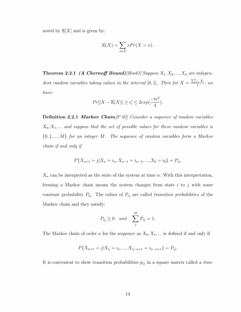
Definition 2.2.1 Markov Chain[S+02] Consider a sequence of random variables
X0, X1, ... and suppose that the set of possible values for these random variables is
{0, 1, ...,M} for an integer M . The sequence of random variables form a Markov
chain if and only if
P{Xn+1 = j|X
n
= in
, Xn�1 = i
n�1, ..., X0 = i0} = Pij
.
Xn
can be interpreted as the state of the system at time n. With this interpretation,
forming a Markov chain means the system changes from state i to j with some
constant probability Pij
. The values of Pij
are called transition probabilities of the
Markov chain and they satisfy:
Pij
� 0 andMX
j
Pij
= 1.
The Markov chain of order for the sequence as X0, X1, ... is defined if and only if
P{Xn+1 = j|X
n
= in
, ..., Xn�+1 = i
n�+1} = Pij
.
It is convenient to show transition probabilities pij
in a square matrix called a tran-
14
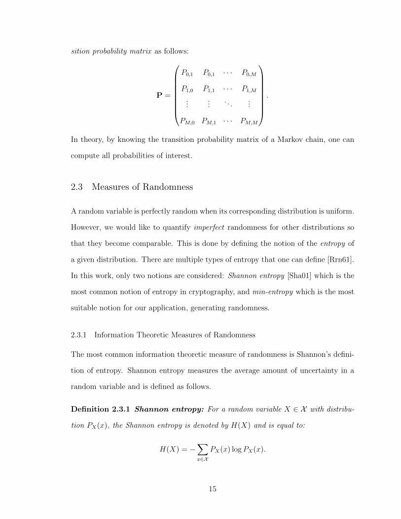
sition probability matrix as follows:
P =
0
BBBBBBB@
P0,1 P0,1 · · · P0,M
P1,0 P1,1 · · · P1,M
......
. . ....
PM,0 P
M,1 · · · PM,M
1
CCCCCCCA
.
In theory, by knowing the transition probability matrix of a Markov chain, one can
compute all probabilities of interest.
2.3 Measures of Randomness
A random variable is perfectly random when its corresponding distribution is uniform.
However, we would like to quantify imperfect randomness for other distributions so
that they become comparable. This is done by defining the notion of the entropy of
a given distribution. There are multiple types of entropy that one can define [Rrn61].
In this work, only two notions are considered: Shannon entropy [Sha01] which is the
most common notion of entropy in cryptography, and min-entropy which is the most
suitable notion for our application, generating randomness.
2.3.1 Information Theoretic Measures of Randomness
The most common information theoretic measure of randomness is Shannon’s defini-
tion of entropy. Shannon entropy measures the average amount of uncertainty in a
random variable and is defined as follows.
Definition 2.3.1 Shannon entropy: For a random variable X 2 X with distribu-
tion PX
(x), the Shannon entropy is denoted by H(X) and is equal to:
H(X) = �X
x2X
PX
(x) logPX
(x).
15
For X 2 X , Shannon entropy is maximized when we have uniform distribution over
X . In this case H(X) = � log |X | and any other distribution on this set will have
smaller Shannon entropy. One can view Shannon entropy as a measure of exist-
ing randomness in a random variable. The bigger Shannon entropy represents more
randomness. Nevertheless, this claim is not precise since it is possible to define patho-
logical distributions that have high Shannon entropy but are useless for randomness
extraction. To see why this is a problem, consider X 2 {0, 1}n with the following
distribution:
Pr[X = 0n] = 1� 1
2100.
and for a 2 {0, 1}n \ 0n:
Pr[X = a] =1
2100(
1
2n � 1) ⇠ 1
2n+100.
Consequently the Shannon entropy for a random variable X is:
H(X) = (1� 1
2100) log
1
1� 12100
+X
a 6=0n
1
2100(
1
2n � 1) log
1
12100 (
1
2n � 1)⇠ n+ 100
2100.
Although the amount of Shannon entropy in the above example is linear in n, we
cannot extract bits that are close to uniform by sampling X since it is a constant
value (0n) most of the time.
Min-entropy is an alternative entropy notion which is more useful for random-
ness extraction applications. The min-entropy measures the minimum information
contained in a random variable.
Definition 2.3.2 Min-entropy: For a random variable X 2 X with distribution
PX
(x), min-entropy is denoted by H1(X) and is :
H1(X) = � log(maxx2X
(PX
(x))).
16
In the mentioned example, H1(X) = �log(1 � 1
2100), which is quite a small num-
ber and matches our intuition about the amount of randomness in the described
distribution.
An alternative approach to evaluate the randomness of a distribution is to compare
it with the uniform distribution. The statistical distance of two distributions is a
measure of their di↵erence and is defined as follows.
Definition 2.3.3 Statistical distance: For two distributions X and Y defined over
the set U , the statistical distance between X and Y is defined as:
SD(X;Y ) , 1
2
X
u2U
|Pr(X = u)� Pr(Y = u)| = 1
2|X � Y |.
When SD(X;Y ) ✏ we say the distribution X is ✏-close to distribution Y .
2.3.2 Entropy Estimation
Finding the entropy of a source requires knowledge of the exact source distribution.
However, when the source distribution is unknown, one can still estimate the source
entropy by sampling (as much as required) from the source. Apparently the existence
of certain structures in the source simplifies entropy estimation. In particular, esti-
mating the min-entropy of an independently and identically distributed (IID) source
is straightforward. Since the samples are not correlated in such a source, the most
common value among the samples is more likely to be the most probable one. The
upper and lower bounds for the min-entropy is calculated based on this observation.
Details of finding the upper bound and lower bound for the min-entropy of an IID
source are explained in [BK12].
The testing method introduced in the NIST draft [BK12] initially, checks whether
the source can be considered an IID. NIST suggests the following set of tests for
checking if a source is IID: shu✏ing tests and statistical tests. The source output is
17
considered IID if the dataset passes all the tests. Then, based on the number of the
observations of the most common output value, the min-entropy is estimated.
In the shu✏ing tests the following scores are calculated for the shu✏ed datasets:
Compression score, Runs score, Excursion score, Directional Runs score, Covariance
score and Collision score. For the samples following an IID distribution, the shu✏ed
datasets would follow the same distribution as the original dataset and therefore, the
derived scores for the original dataset and shu✏ed datasets are expected to be similar.
But, if the samples do not follow an IID distribution, then some test scores may be
very di↵erent for the original and shu✏ed datasets.
NIST only introduces one statistical test to check if a source is IID. The test
is called Chi-square test and consists of two di↵erent types of test: a test for in-
dependence, and a test for goodness of fit. The independence test is aimed to find
dependencies in the existing samples of the dataset. The goodness of fit test checks
whether ten data subsets produced from the main dataset follow the same distribu-
tion.
A failure of any of the shu✏ing or statistical tests stops IID testing, and a number
of tests are used to estimate the min-entropy, assuming the source is non-IID. For
a non-IID source, the dependencies in time or state may result in entropy overesti-
mation. However, in [BK12], five tests are suggested to minimize the possibility of
overestimating the source entropy. Each of these tests is designed to measure spe-
cific statistics of the samples to capture the structure of the distribution. These five
tests are collision, collection, compression, Markov, and frequency tests. Each test
outputs a value as the estimation of the min-entropy. The final min-entropy will be
the minimum over all of these estimated values.
18
2.3.2.1 Collision Test
The collision test is designed to estimate the probability of the most-likely state in
a dataset. For this purpose it measures the mean time to the first collision in the
dataset. To avoid entropy overestimation in non-IID sources, this test selects the
minimum entropy estimation of all the tests as the expected entropy of the source
[BK12, p. 62].
2.3.2.2 Partial Collection Test
The partial collection test computes the entropy of a dataset with regards to the
number of distinct values in the output space. If the output dataset contains a small
number of distinct values, the test estimates low entropy and if the dataset has high
variation, high entropy is estimated [BK12, p. 65].
2.3.2.3 Markov Test
A Markov model in Definition 2.2.1 is used as a template for describing sources with
dependencies. The Markov tests estimate min-entropy by measuring the dependency
between successive outputs of the source. In the Markov tests, instead of single
samples, chains of samples are considered. By the careful estimation of the transition
probability matrix, the Markov model is used for entropy estimation. An accurate
estimation of this matrix requires a large dataset. Nevertheless, in practice, a large
data requirement is avoided by overestimating the low transition probabilities [BK12,
p. 67].
2.3.2.4 Compression Test
The comparison test is designed based on the Maurer Universal Statistic [Mau92].
The test does not have any assumption of independence. The entropy rate of the
dataset is calculated based on the compression rate of the dataset. The test initially
generates a dictionary of values, and then computes the average number of samples
19
required to write an output with respect to the dictionary [BK12, p. 69].
2.3.2.5 Frequency Test
In the frequency test, min-entropy is estimated based on the rate of occurrence of the
most probable sample value. Similar to the Markov test, an accurate estimation of
min-entropy requires a large dataset. When only a small dataset is available, this test
ignores unlikely sample values and therefore underestimates the min-entropy [BK12,
p. 71].
2.4 Graph Theory
A graph G consists of a non-empty set V (G) of elements, called vertices or nodes,
and a set E(G) of elements called edges, together with a relation of incidence that
associates each edge with two vertices, called its ends. An edge with identical ends
is a loop and one with distinct ends is a link. A multigraph is one with no loops. A
simple graph is one with neither loops nor multiple edges. A directed graph (digraph)
D is a graph in which a direction is assigned to each edge.
The degree of a vertex v in a graph G is the number of edges of G incident with
v. A graph is d-regular if each vertex has degree d.
The adjacency matrix A(G) is the matrix whose rows and columns are indexed
by the vertices of G and the element auv
is the number of edges of G joining vertices
u and v.
2.5 Game Theory
Game theory is the study of strategic decision making. Decision makers are consid-
ered the players of the game. There is a set of available actions for each player and a
specification of payo↵s for each combination of actions which models the interaction
20
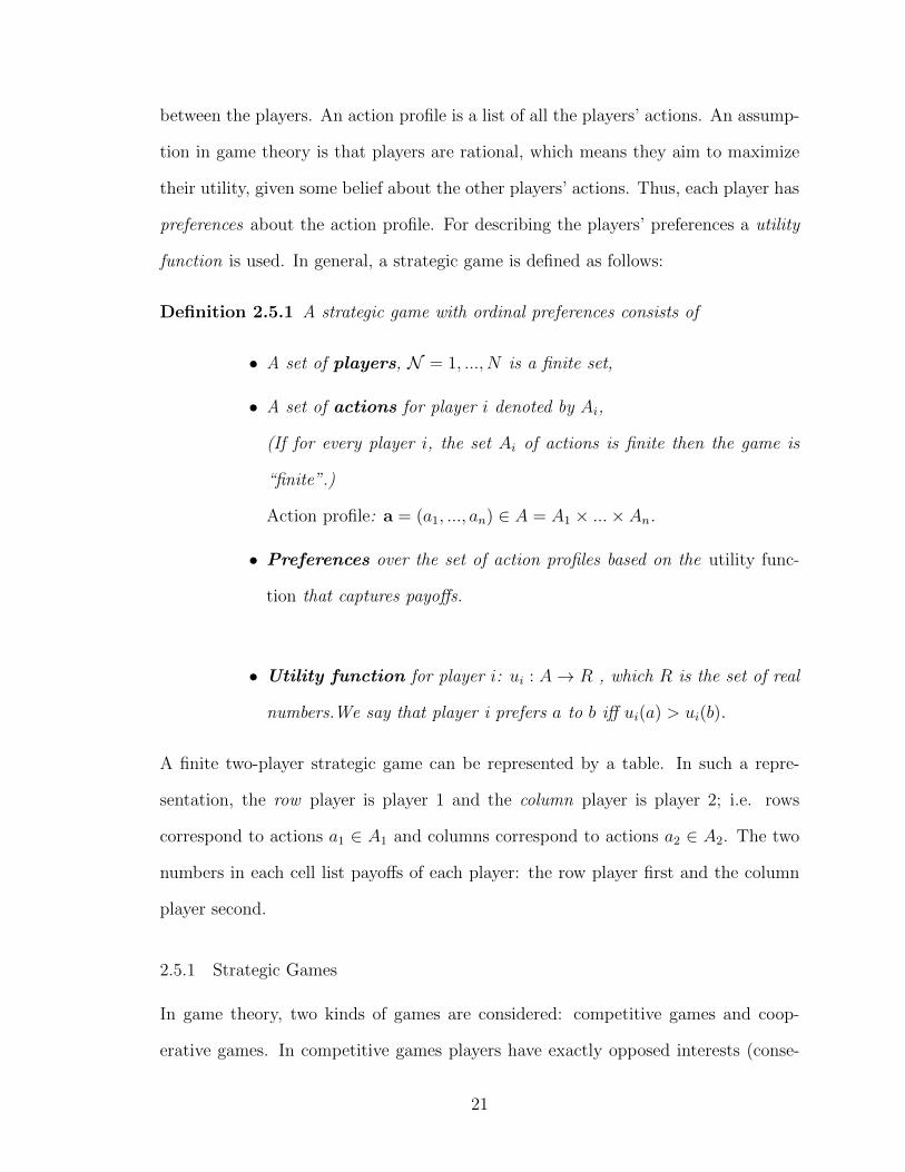
between the players. An action profile is a list of all the players’ actions. An assump-
tion in game theory is that players are rational, which means they aim to maximize
their utility, given some belief about the other players’ actions. Thus, each player has
preferences about the action profile. For describing the players’ preferences a utility
function is used. In general, a strategic game is defined as follows:
Definition 2.5.1 A strategic game with ordinal preferences consists of
• A set of players, N = 1, ..., N is a finite set,
• A set of actions for player i denoted by Ai
,
(If for every player i, the set Ai
of actions is finite then the game is
“finite”.)
Action profile: a = (a1, ..., an) 2 A = A1 ⇥ ...⇥ An
.
• Preferences over the set of action profiles based on the utility func-
tion that captures payo↵s.
• Utility function for player i: ui
: A ! R , which R is the set of real
numbers.We say that player i prefers a to b i↵ ui
(a) > ui
(b).
A finite two-player strategic game can be represented by a table. In such a repre-
sentation, the row player is player 1 and the column player is player 2; i.e. rows
correspond to actions a1 2 A1 and columns correspond to actions a2 2 A2. The two
numbers in each cell list payo↵s of each player: the row player first and the column
player second.
2.5.1 Strategic Games
In game theory, two kinds of games are considered: competitive games and coop-
erative games. In competitive games players have exactly opposed interests (conse-
21
quently the number of players is always 2), while in games of cooperation players
have the same interest.
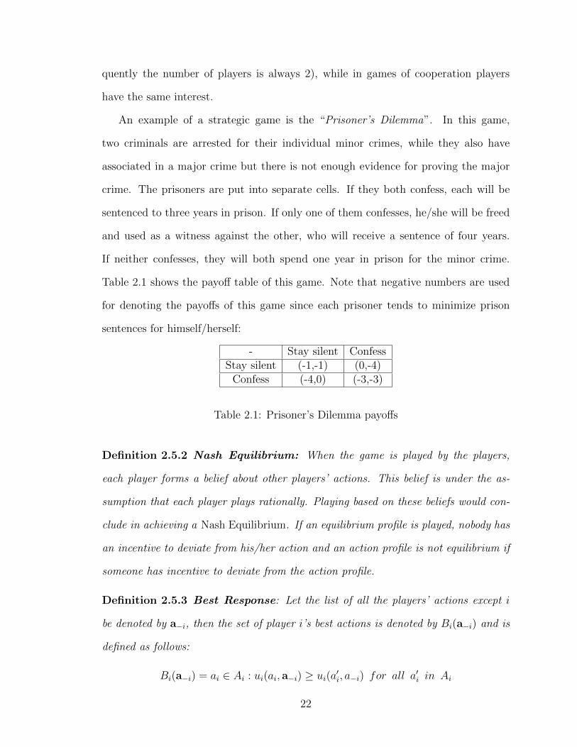
An example of a strategic game is the “Prisoner’s Dilemma”. In this game,
two criminals are arrested for their individual minor crimes, while they also have
associated in a major crime but there is not enough evidence for proving the major
crime. The prisoners are put into separate cells. If they both confess, each will be
sentenced to three years in prison. If only one of them confesses, he/she will be freed
and used as a witness against the other, who will receive a sentence of four years.
If neither confesses, they will both spend one year in prison for the minor crime.
Table 2.1 shows the payo↵ table of this game. Note that negative numbers are used
for denoting the payo↵s of this game since each prisoner tends to minimize prison
sentences for himself/herself:
- Stay silent ConfessStay silent (-1,-1) (0,-4)Confess (-4,0) (-3,-3)
Table 2.1: Prisoner’s Dilemma payo↵s
Definition 2.5.2 Nash Equilibrium: When the game is played by the players,
each player forms a belief about other players’ actions. This belief is under the as-
sumption that each player plays rationally. Playing based on these beliefs would con-
clude in achieving a Nash Equilibrium. If an equilibrium profile is played, nobody has
an incentive to deviate from his/her action and an action profile is not equilibrium if
someone has incentive to deviate from the action profile.
Definition 2.5.3 Best Response: Let the list of all the players’ actions except i
be denoted by a�i
, then the set of player i’s best actions is denoted by Bi
(a�i
) and is
defined as follows:
Bi
(a�i
) = ai
2 Ai
: ui
(ai
, a�i
) � ui
(a0i
, a�i
) for all a0i
in Ai
22
We say that a⇤i
2 BR(ai
) i↵ 8ai
2 Ai
: ui
(a⇤i
, a�i
) � ui
(ai
, a�i
), where a�i
=
(a1, ..., ai�1, ai+1, ..., an) and n is the number of the players.
The minmax value for player i is defined as vi
= mina�i2A�i
maxai2Ai
ui
(a�i
, ai
). We say that
players of the game are playing with pure strategy when they play only one action
with positive probability. Now we can define the pure strategy Nash equilibrium.
Definition 2.5.4 Pure strategy Nash equilibrium: a = (a1, ..., an) is a pure
strategy Nash equilibrium i↵ 8i, ai
2 BR(a�i
)
In the prisoner’s dilemma example the best response for each of the players regardless
of the other player’s action is to “confess”. Thus, the pure strategy Nash equilibrium
of this game is (Confess, Confess).
2.5.2 Mixed Strategy Equilibrium
There are many games that do not have a pure strategy Nash equilibrium. Another
kind of equilibrium, called a mixed strategy Nash Equilibrium, is defined for these
games. A mixed strategy of a player in a strategic game means that more than
one action is played with positive probability by the player. The set of actions with
non-zero probability form the support of a mixed strategy.
Suppose the set of all strategies for i is Si
, and the set of all strategy profiles is
S = S1 ⇥S2 ⇥ ...⇥Sn
. If all players follow a mixed strategy s 2 S, then their payo↵s
are:
ui
(s) =X
a2A
ui
(a)Pr(a|s)
And
Pr(a|s) =Y
j2N
sj
(aj
)
Definition 2.5.5 Mixed strategy Nash equilibrium: Suppose s is the action
profile of n players playing mixed strategies in a strategic game. s = (s1, s2, ..., sn) is
a Nash Equilibrium if 8i, si
2 BR(s�i)
23
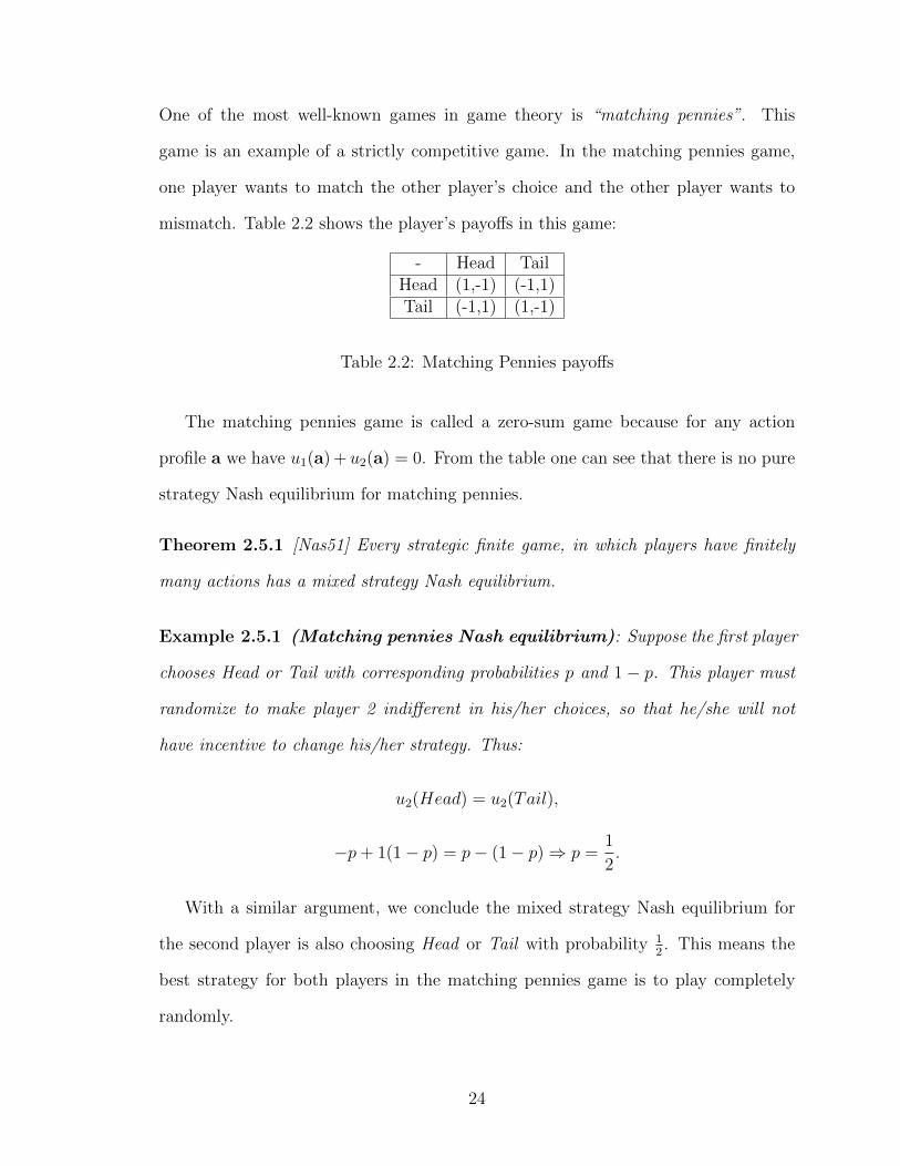
One of the most well-known games in game theory is “matching pennies”. This
game is an example of a strictly competitive game. In the matching pennies game,
one player wants to match the other player’s choice and the other player wants to
mismatch. Table 2.2 shows the player’s payo↵s in this game:
- Head TailHead (1,-1) (-1,1)Tail (-1,1) (1,-1)
Table 2.2: Matching Pennies payo↵s
The matching pennies game is called a zero-sum game because for any action
profile a we have u1(a) + u2(a) = 0. From the table one can see that there is no pure
strategy Nash equilibrium for matching pennies.
Theorem 2.5.1 [Nas51] Every strategic finite game, in which players have finitely
many actions has a mixed strategy Nash equilibrium.
Example 2.5.1 (Matching pennies Nash equilibrium): Suppose the first player
chooses Head or Tail with corresponding probabilities p and 1 � p. This player must
randomize to make player 2 indi↵erent in his/her choices, so that he/she will not
have incentive to change his/her strategy. Thus:
u2(Head) = u2(Tail),
�p+ 1(1� p) = p� (1� p) ) p =1
2.
With a similar argument, we conclude the mixed strategy Nash equilibrium for
the second player is also choosing Head or Tail with probability 12 . This means the
best strategy for both players in the matching pennies game is to play completely
randomly.
24
2.5.3 Repeated Games
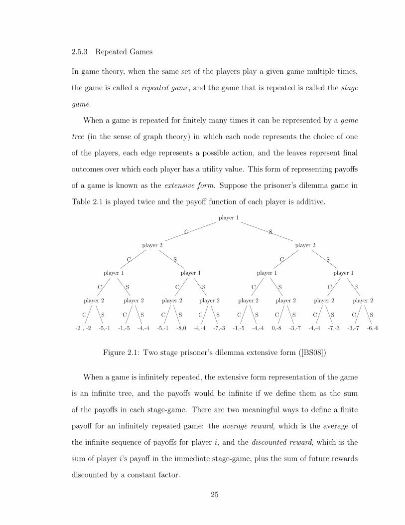
In game theory, when the same set of the players play a given game multiple times,
the game is called a repeated game, and the game that is repeated is called the stage
game.
When a game is repeated for finitely many times it can be represented by a game
tree (in the sense of graph theory) in which each node represents the choice of one
of the players, each edge represents a possible action, and the leaves represent final
outcomes over which each player has a utility value. This form of representing payo↵s
of a game is known as the extensive form. Suppose the prisoner’s dilemma game in
Table 2.1 is played twice and the payo↵ function of each player is additive.
player 1
player 2
player 1
player 2
-2 , -2 -5,-1
player 2
-1,-5 -4,-4
player 1
player 2
-5,-1 -8,0
player 2
-4,-4 -7,-3
player 2
player 1
player 2
-1,-5 -4,-4
player 2
0,-8 -3,-7
player 1
player 2
-4,-4 -7,-3
player 2
-3,-7 -6,-6
C
C
C
C S
S
C S
S
C
C S
S
C S
S
C
C
C S
S
C S
S
C
C S
S
C S
Figure 2.1: Two stage prisoner’s dilemma extensive form ([BS08])
When a game is infinitely repeated, the extensive form representation of the game
is an infinite tree, and the payo↵s would be infinite if we define them as the sum
of the payo↵s in each stage-game. There are two meaningful ways to define a finite
payo↵ for an infinitely repeated game: the average reward, which is the average of
the infinite sequence of payo↵s for player i, and the discounted reward, which is the
sum of player i’s payo↵ in the immediate stage-game, plus the sum of future rewards
discounted by a constant factor.
25
A payo↵ profile r = (r1, r2, ..., rn) in an n-player game is enforceable when each
player’s payo↵ is bigger or equal to its corresponding minmax value, and is feasible if
it is a convex, rational combination of the outcomes in the game.
Folk theorems are a family of theorems about possible Nash equilibrium payo↵
profiles in a repeated game. An instance of a folk theorem family for an infinitely
repeated game with an average reward is as follows:
Theorem 2.5.2 Folk Theorem[BS08] Consider an n-player infinitely repeated game
with average reward payo↵ profile r = (r1, r2, ..., rn).
1. If r is the payo↵ profile for any Nash equilibriums of the game, then for
each player i, ri
is enforceable.
2. If r is both feasible and enforceable, then r is the payo↵ profile for some
Nash equilibrium of the game.
2.6 Related Works
User inputs are widely used to provide background entropy for random number gener-
ators in computer systems. For example, in Linux based systems the operating system
continuously runs a background process to collect entropy from users’ inputs [GPR06].
However, due to repetitive patterns of mouse movements or keystrokes, these entropy
sources, in general, provide lower entropy level when used for on-demand collection
of entropy.
Psychological studies show that humans are neither capable of generating random-
ness nor recognizing it [Bru97, Wag72]. Nevertheless, some psychological experiments
confirm that humans’ random behaviour will improve by trial and error. In other
words, a human asked to continuously generate random sequences will do better by
receiving feedback on the randomness of previously generated sequences [Neu86].
26
Some competitive two-player games are capable of leading a human toward more
random behaviours. In such games, the opponent would exploit non-random be-
haviour of the human player to win the game. Thus, each of the players tries to play
as randomly as possible to win. Fortunately, such games are very well studied in the
“game theory” context. In particular, it has been shown that in some competitive
zero-sum games the best strategy for winning is to play uniformly randomly. The idea
of using such games for leading a human toward random behaviour and consequently
generate randomness was initially proposed by Rapoport and Budescu [RB92]. Their
experimental results showed that it is possible to generate a sequence with relatively
good randomness properties from a series of human actions in a two-player competi-
tive zero-sum game with uniform choices as the best strategy of players. They used
thematching pennies game as an example of the desired game in their study. In the
matching pennies game, each of the players makes a choice between “head” and “tail”.
One of the players wins the game in case of matching choices while the other one wins
if the choices mismatch. Due to the game theory, the optimal strategy for players in
this game is to choose uniformly randomly (with probability 12) between head and tail.
The experimental results in [RB92] showed that players almost followed a uniform
random strategy for playing the game. This result confirms that humans engaged in
a strategic game can be a good source of entropy and entropy generation could be
an indirect result of their actions. Indeed, one can view the two-player competitive
game as an approach to provide feedback for players on their previous actions. In
this sense, the later experimental results confirm the psychological experiments that
emphasise the role of feedback in training human for randomness generation.
Although the approach for generating randomness from human gameplay in [RB92]
is important from a theoretical point of view, it can not be considered as a practi-
cal framework since in each stage of the game the players have two possible choices
27
which means in each stage they can at most generate one random bit. Considering
that modern cryptographic keys are relatively long, e.g. at least 128 bits for AES
key, by using the above approach one needs to play the matching pennies game at
least 128 times in order to generate an appropriate key for a cryptographic purpose.
Playing the game so many times on one hand is boring for the player and on the
other hand is not e�cient since the randomness generation process is very slow.
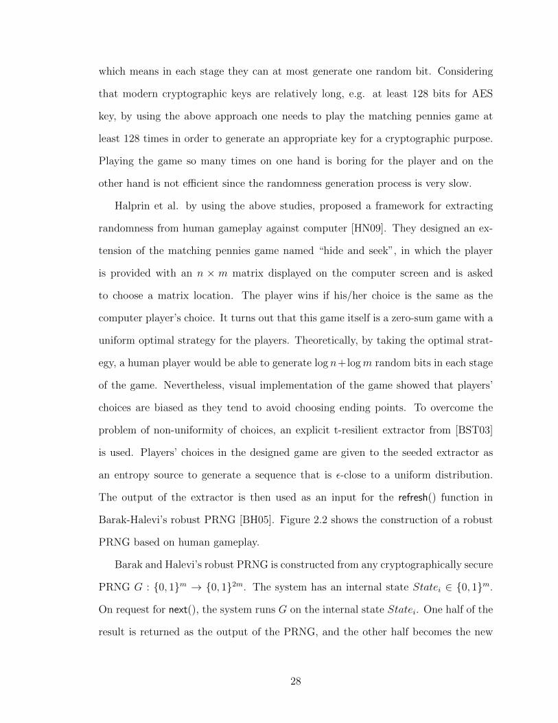
Halprin et al. by using the above studies, proposed a framework for extracting
randomness from human gameplay against computer [HN09]. They designed an ex-
tension of the matching pennies game named “hide and seek”, in which the player
is provided with an n ⇥ m matrix displayed on the computer screen and is asked
to choose a matrix location. The player wins if his/her choice is the same as the
computer player’s choice. It turns out that this game itself is a zero-sum game with a
uniform optimal strategy for the players. Theoretically, by taking the optimal strat-
egy, a human player would be able to generate log n+logm random bits in each stage
of the game. Nevertheless, visual implementation of the game showed that players’
choices are biased as they tend to avoid choosing ending points. To overcome the
problem of non-uniformity of choices, an explicit t-resilient extractor from [BST03]
is used. Players’ choices in the designed game are given to the seeded extractor as
an entropy source to generate a sequence that is ✏-close to a uniform distribution.
The output of the extractor is then used as an input for the refresh() function in
Barak-Halevi’s robust PRNG [BH05]. Figure 2.2 shows the construction of a robust
PRNG based on human gameplay.
Barak and Halevi’s robust PRNG is constructed from any cryptographically secure
PRNG G : {0, 1}m ! {0, 1}2m. The system has an internal state Statei
2 {0, 1}m.
On request for next(), the system runs G on the internal state Statei
. One half of the
result is returned as the output of the PRNG, and the other half becomes the new
28
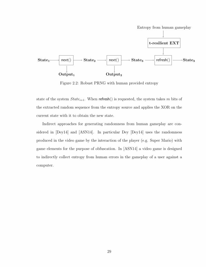
State1
Output1
next() State2 next()
Output2
State3 refresh() State3
t-resilient EXT
Entropy from human gameplay
Figure 2.2: Robust PRNG with human provided entropy
state of the system Statei+1. When refresh() is requested, the system takes m bits of
the extracted random sequence from the entropy source and applies the XOR on the
current state with it to obtain the new state.
Indirect approaches for generating randomness from human gameplay are con-
sidered in [Dey14] and [ASN14]. In particular Dey [Dey14] uses the randomness
produced in the video game by the interaction of the player (e.g. Super Mario) with
game elements for the purpose of obfuscation. In [ASN14] a video game is designed
to indirectly collect entropy from human errors in the gameplay of a user against a
computer.
29
Chapter 3
Randomness Generation
In this chapter, the di↵erent methods for randomness generation are introduced. Ran-
dom number generators (RNGs) are classified and an overview of practical RNGs as
well as theoretical functions and their explicit constructions that can extract random-
ness from an entropy source is conducted. To answer the question, “Is a human able
to generate randomness?”, a brief survey on human psychology is provided, and some
hypotheses and experiments that aim to explain the random behaviour of a human
are mentioned.
3.1 Randomness Importance
Randomness plays an important role in computer science, in particular in cryptog-
raphy and information security. The security of any cryptographic algorithm and
protocol directly depends on the randomness of the key. Indeed, it is impossible to
have a deterministic fixed secret. Randomness can be exploited for generating the
required cryptographic keys in encryption or challenge-response protocols (e.g. the
key in SSH or SSL/TLS connections), or for randomizing cryptographic algorithms
to achieve a desirable level of security. The unpredictability of a random sequence
is its pivotal property that makes it suitable for the mentioned applications. Using
weak randomness in security systems may result in a security breakdown of the whole
system.
A weak random number generator exposes the system to a variety of attacks.
Several attacks on Netscape browser Version 1.1 are addressed in [GW96]. These
attacks exploit weakness in the system’s RNG to guess the secret key, and break the
30
security of the system. Kerberos 4 session keys, generated for a DES block cipher, are
shown to have much smaller entropy than what is required for their security [DLS97].
This means that the brute force attack can break the security of the system with
much fewer trials than what is expected (in particular when time and the host-id of
Kerberos server are known, the number of possible keys is only 220, while DES o↵ers
256 possible keys for providing the security of the encrypted block). More recent
studies observed weak-key-generation vulnerability in the Debian Linux version of
OpenSSL [YRS+09] and a level of predictability in RSA public keys [LHA+12] due
to a bug in the random number generation algorithm.
The importance of having a good random number generator is well recognized
from the above examples. Indeed, a huge part of a system’s security depends on the
quality of randomness, and thus improving the random number generators as well
as introducing appropriate applicable entropy sources is of crucial importance for
enhancing the security level of cryptographic systems.
3.1.1 Random Number Generators
An RNG is an algorithm that could be implemented by a computer program, and is
intended to have an output with desirable randomness properties. There are mainly
two di↵erent types of RNGs: True Random Number Generators (TRNGs) and Pseudo
Random Number Generators (PRNGs).
3.1.1.1 True Random Number Generators
A TRNG (also referred to as an entropy harvester in the literature [VM03]) applies
a processing function to an entropy source to generate (extract) randomness. The
entropy source is obtained from a non-deterministic physical quantity such as noise
in an electrical circuit or mouse positions during a user’s specific interactions with
a computer program. Although TRNGs are presumably secure under most circum-
31
stances, their speed is limited by the speed of the physical phenomenon, and thus
they are usually slow. For increasing the throughput of random number generation,
the output of a TRNG might be fed into a PRNG.
Quantum TRNGs, on the other hand, are very fast, but using them requires
special hardware and resources. This limits their application to very restricted and
critical security purposes.
3.1.1.2 Pseudo Random Number Generators
A PRNG is an e�cient deterministic algorithm that expands a short perfectly random
(or almost perfectly random) seed to a much longer sequence that “looks random”
in a meaningful and well-defined way [Gol10, RSN+01]. This usually means that no
e�cient algorithm can distinguish the output of the CSPRNG (Cryptographic Secure
Pseudo Random Number Generator) from a perfectly random sequence.
There are two kinds of PRNGs: Normal Pseudo Random Number Generators
(NPRNGs) and Cryptographic Secure Pseudo Random Number Generators (CSPRNGs).
An NPRNG deterministically produces a sequence of values depending only on
the initial seed (also known as initial internal state). Since there are only a limited
number of states, the output of an NPRNG eventually repeats itself and becomes
periodic. If the initial seed is an n-bit vector, the maximum period for the NPRNG
is 2n [VGLS12], however some NPRNGs such as a Linear Feedback Shift Register
(LFSR) might have an even smaller period. Nevertheless, with a long enough period
the output random sequence could be appropriate for practical applications.
A simple example of an NPRNG is the Linear Congruential Generator (LCG)
[PM88]. The generator function of a LCG is:
Xn+1 = a.X
n
+ b mod m
Where a, b, and m are chosen constant integers and a, b < m. X0 is the initial seed
and the sequence of (Xn
)n�1s is the generated pseudo random sequence.
32
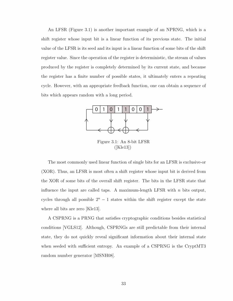
An LFSR (Figure 3.1) is another important example of an NPRNG, which is a
shift register whose input bit is a linear function of its previous state. The initial
value of the LFSR is its seed and its input is a linear function of some bits of the shift
register value. Since the operation of the register is deterministic, the stream of values
produced by the register is completely determined by its current state, and because
the register has a finite number of possible states, it ultimately enters a repeating
cycle. However, with an appropriate feedback function, one can obtain a sequence of
bits which appears random with a long period.
0 1001101
Figure 3.1: An 8-bit LFSR([Kle13])
The most commonly used linear function of single bits for an LFSR is exclusive-or
(XOR). Thus, an LFSR is most often a shift register whose input bit is derived from
the XOR of some bits of the overall shift register. The bits in the LFSR state that
influence the input are called taps. A maximum-length LFSR with n bits output,
cycles through all possible 2n � 1 states within the shift register except the state
where all bits are zero [Kle13].
A CSPRNG is a PRNG that satisfies cryptographic conditions besides statistical
conditions [VGLS12]. Although, CSPRNGs are still predictable from their internal
state, they do not quickly reveal significant information about their internal state
when seeded with su�cient entropy. An example of a CSPRNG is the CryptMT3
random number generator [MSNH08].
33
3.2 Statistical Tests
Generally, the quality of produced random numbers is evaluated by statistical tests;
this means that for making any statement about the quality of an RNG, we should
specify the tests this statement is based on. NIST has developed a package of 15
statistical tests to evaluate the randomness of (arbitrarily long) binary sequences.
Di↵erent types of predictability in a random sequence are considered in the NIST
statistical package [RSN+01]. The 15 tests included in the NIST statistical test suite
are: The Frequency Test, Frequency Test within a Block, The Runs Test, Tests for
the Longest-Run-of-Ones in a Block, The Binary Matrix Rank Test, The Discrete
Fourier Transform (Spectral) Test, The Non-overlapping Template Matching Test,
The Overlapping Template Matching Test, Maurer’s “Universal Statistical” Test,
The Linear Complexity Test, The Serial Test, The Approximate Entropy Test, The
Cumulative Sums (Cusums) Test, The Random Excursions Test, and The Random
Excursions Variant Test.
Note that some desirable properties for random numbers can only be checked by
non-polynomial-time tests, such as the spectral test. Thus, it is not su�cient to limit
the definition of PRNGs to those RNGs whose output could not be distinguished
from uniform sequences [Roc05] using polynomial-time algorithms.
3.3 Human Psychology for Generating Randomness
Random number generation by human subjects is a procedurally-simple task which is
related to specific executive functions in the brain such as updating and monitoring
of information and inhibition of automatic responses. There is a relatively large
body of literature on human random number generation in psychology. The failure of
human subjects to behave randomly is a robust finding (for reviews see [Wag72] and
[Bru97]). The experiments for evaluating human random behaviour vary from calling
34
out digits, letters of the alphabet, or nonsense syllables, to writing these same symbols
on paper, pressing push-buttons, touching metal disks with a stylus, or drawing lines
on a paper. The e↵ect of di↵erent experimental conditions such as required speed of
responses, age, mathematical sophistication of subjects, and competing attentional
demands have systematically been extensively studied and various statistical tests
have been used for evaluating the generated randomness [TN98].
There are two di↵erent explanations for human randomness generation ability in
the psychology community: explanation by trait and explanation by skill.
3.3.1 Explanation by Trait for Humans’ Random Behaviour
In a random sequence, each symbol is approximately equally repeated over a long
run. An explanation by trait claims that humans are incapable of generating random
sequences due to their inherent limitations. According to one hypothesis, humans fail
in generating randomness because their memory is not able to keep track of all the
generated symbols [Bad66]. According to another hypothesis, attentional processes do
not permit subjects to completely ignore their previous responses while it is essential
for random behaviour [Wei64]. The third hypothesis highlights humans’ di�culty
in distinguishing randomness (when presented with two series of numbers, subjects
usually cannot discriminate random from non-random series) as the trait limitation
that prevents randomness generation by a human [Wag70].
3.3.2 Explanation by Skill for Humans’ Random Behaviour
Due to this explanation, “Randomlike behaviours are learned and controlled by en-
vironmental feedback, as are other highly skilled activities” [Neu86]. If so, random
behaviour skill should be trained and practiced to be improved. Indeed, humans can
learn how to generate randomness during a process. The role of feedback in improving
generated randomness by humans is considered in [Neu86], and the result confirms
35
that humans generates better random sequences when feedback on their previous
actions is provided.
More recent studies showed that random number generation involves several men-
tal processes. In fact, it requires adopting the correct strategy, based on instructions
and the subject’s concept of randomness, monitoring the output, and eventually mod-
ifying the strategy of randomness generation. Generating random numbers requires
the activation of di↵erent brain regions consisting of the Left Dorsolateral Prefrontal
Cortex (DLPFC), the Anterior Cingulate Cortex (ACC), the Superior Parietal Cor-
tex (SPC), the Right Inferior Frontal Cortex (RIFC) and the Cerebellar Hemispheres
(CH) [CCR+14]. The functionality of each part is briefly explained below [MC07].
-The Left Dorsolateral Prefrontal Cortex (DLPFC) is an area in the prefrontal cor-
tex of the human brain that is “known to be involved in classical executive functions,
includng working memory, set shifting, sequencing, planing, inhibition and abstract
reasoning” [MC07, P. 355].
-The Anterior Cingulate Cortex (ACC) plays an important role as an integrative
center in lots of the body’s autonomic functions as well as controlling emotions. It
is also involved in cognitive behavioural tasks, such as reward anticipation, decision-
making and attention motivation.
-The Superior Parietal Cortex (SPC) is involved with divided attention and re-
ceives a great deal of visual input as well as sensory input from one’s hands.
-The Right Inferior Frontal Cortex (RIFC) mediates response inhibition. It is
typically implicated in go/no-go tasks.
-The Cerebellar Hemispheres (CH) play a significant role in some of the motor
and perceptual tasks like spatial attention, verbal working memory, and language
processing and in regulating fear and pleasure responses.
Transcranial Direct Current Stimulation (TDCS) is a safe and reliable technique
36
that can produce transient behavioural changes and influence cognitive functions. In
this method, a weak current is applied constantly over time to increase (anodal stimu-
lation) or decrease (cathodal stimulation) the excitability of the neuronal populations
underlying the active electrode.
TDCS can produce transient behavioural changes and influence cognitive func-
tions. When TDCS is combined with cognitive training protocols, seemingly it can
enhance the protocol e↵ects [LMF12].
The experiments in [CCR+14] demonstrate that practice consistently induces
training plasticity and influences specific features of humans’ performance in random-
ness generation. The experiments also suggest that TDCS could transiently modify
the random behaviour of a human.
3.4 Randomness Extraction
Any function that extracts almost uniform bits from an entropy source is called a
randomness extractor. Randomness extractors require a guarantee on the random-
ness property such as min-entropy of their input entropy source in order to guarantee
randomness level of the output. A TRNG thus can be built from a randomness
extractor together with an entropy source. There are two di↵erent types of extrac-
tors: deterministic extractors and seeded extractors. Deterministic extractors, like
TRNGs, use a source of imperfect randomness for generating randomness, but do not
require a random seed. On the other hand, seeded extractors and PRNGs are similar
due to using a random seed for randomness generation. Nevertheless, extractors and
PRNGs are totally di↵erent objects. The output of the extractor is statistically close
to uniform distribution, while the output of a PRNG is computationally indistin-
guishable from a uniform distribution. Moreover, a source of imperfect randomness is
not a required input for a PRNG, while it is necessary for randomness extractors. It
37
turns out that PRNG constructions of a certain kind are extractors. The connection
between extractors and PRNGs is demonstrated in [Tre01].
3.4.1 Deterministic extractors
Deterministic extractors are ideal extractors that extract randomness from an entropy
source without investing any extra randomness. However, it turns out that having
a deterministic extractor as a general imperfect randomness source is impossible.
Respectively, the challenge in constructing an optimal extractor is to minimize the
amount of required extra randomness known as the seed.
Definition 3.4.1 (Deterministic Extractors) For a class of distributions C over
{0, 1}n, the function Ext : {0, 1}n ! {0, 1}m is (n, ✏)-extractor if for any X 2 C,
Ext(X) is ✏-close to Um
, where Um
is the uniform distribution over {0, 1}m.
A well-known example of a deterministic extractors are the von Neumann extractor
[von63] that extracts perfectly uniform bits from a source generated by a finite-state
Markov chain. Suppose X1, X2, ..., Xn
is an identical independent distributed binary
sequence with bias � so that Pr[Xi
= 1] = �. A Von Neumann extractor breaks all
the variables in pairs and for each non-identical pair (01 or 10) outputs the first bit
and skips otherwise. With this extractor, after processing 12�(1��) pairs, on average,
we will have an unbiased random bit sequence.
The Definition 3.4.1 follows the observation that an extractor is a single function
that works for all sources in a class. For determining the class of a source, we do
not need the exact distribution of each source since only having special properties
is su�cient for our purpose. Some examples of specific class of distributions are as
follows:
• Bit fixing source: A block of n bits consisting of k random and inde-
pendent bits together with n� k fixed bits.
38
• Adaptive bit-fixing sources: A block of n bits consisting of k indepen-
dent and random bits and n � k bits that are dependent on the k
independent bits.
• Flat k-source: Uniform distribution on a subset S 2 {0, 1}n of size 2k.
The min-entropy of sources is a general measure that can be used to classify sources.
Definition 3.4.2 (k-source) A random variable X is a k-source if H1(X) � k, i.e.
if Pr[X = x] 2�k.
All the above examples of sources are considered k-sources. An appropriate determin-
istic extractor should work for a wide class of random sources. But it turns out that
it is impossible to construct a deterministic extractor that extracts even one random
bit from a general k-source. Further studies on deterministic extractors can be found
in [SV86].
3.4.2 Seeded Extractors
Although deterministic extractors do not exist for general k-sources, any randomly
chosen function is a good extractor for all flat k-sources (and therefore for all k-sources
because any k-source is a convex combination of flat k-sources [CG88]) with high
probability. One can show this by allowing the extractor to depend on the source and
then apply the Cherno↵ bound (Theorem 2.2.1) to bound the failure probability of the
extractor. By allowing extractors to use an additional random input called a seed,
extraction from general k-sources becomes possible. The additional random input
indeed randomizes over the choice of extracting function from a family of extractors.
As a result, the seeded extractor is able to extract almost all entropy from all k-sources
with high probability.
39
Definition 3.4.3 seeded extractors [NZ96]: A function Ext : {0, 1}n⇥{0, 1}d !
{0, 1}m is a (n, k, ✏)-extractor if for every k-source X on {0, 1}n, Ext(X,Ud
) is ✏-close
to Um
. An extractor is explicit if it is polynomial time computable.
Note that in seeded extractors, since output length is bigger than the seed length, the
overall generated randomness is more than the amount of randomness we invest as
the seed. The goal of seeded extractors is to produce as many output bits as possible
while minimizing the number of random bits used for the seed. The existence of
an optimal (n, k, ✏)-extractor with seed length d = log(n � k) + 2 log(1✏
) + O(1) and
output length k+ d� 2 log(1✏
)�O(1) has been shown by using probabilistic methods
[RTS00].
Despite an existence proof of extractors, using extractors for randomness gen-
eration requires an explicit construction of the extractor. These constructions are
mentioned in [Sha04]. One example of the explicit construction of extractors is ob-
tained by using pairwise independent hash functions [HILL99]. The other explicit
construction uses expander graphs for obtaining extractors. This type of construction
will be elaborated in the next section.
Definition 3.4.4 [BST03] A seeded extractor is called a t-resilient extractor if its
output is "-close to uniform for 2t pre-determined source distributions with the prob-
ability of at least 1� ", when the seed is chosen uniformly random.
Explicit constructions of t-resilient extractors from `-wise independent Universal Hash
Function (UHF) are given in [BST03].
3.5 Expander Graphs for Randomness Extraction
Expander graphs are a family of well-connected graphs with a broad range of applica-
tions in theoretical computer science as well as computer networks. They have been
40
used for designing algorithms, error correcting codes, pseudo random generators and
robust computer networks. In particular, they can be used as seeded extractors for
randomness extraction from an entropy source.
3.5.1 Measures of expansion
For a formal definition of an “expander graph”, we require a quantitative invariant
for measuring connectedness of the graph. Minimum number of neighbor vertices for
all sub-graphs or minimum number of edges leaving any sub-graphs are two classic
measures for well-connectedness [HLW06].
3.5.1.1 Vertex Expansion
This measure requires that every “not-too-large” set of vertices has “many” neighbors:
Definition 3.5.1 (Vertex Expander)A graph G is a (K,A) vertex expander if for
all sets S of at most K vertices, the neighborhood N(S)def
= {u| 9v 2 S| (u, v) 2 E}
is of size at least A⇥ |S|.
For an ideal d-regular expander graph, A is as close to d as possible. d = O(1) and
K = ⌦(n), where n is the number of vertices. In the above definition, if instead of
N(S) we use the number of edges leaving S, we will have edge expansion.
3.5.1.2 Random Walks and Spectral Expansion
Suppose X = i and i = 1, 2, ..., n is an outcome of a random experience, and vector
pt = (p1, p2, ..., pn) indicates the corresponding probabilities for each of the outcomes
such that Pr(X = i) = pi
. An undirected d-regular graph G with n vertices labelled
from 1 to n, depicts the outcomes of the random experience. Consequently, the
probability of picking vertex i is pi
. The edge between vertices i and j is denoted by
eij
. Suppose there is probability distribution on d connected edges to each vertex. The
41
corresponding probability for eij
is depicted by pij
. The corresponding probability
for eij
is regardless of starting and ending vertices order that is pij
= pji
. An edge
is selected due to the outcome of another independent random experience. Starting
from vertex i and picking the edge eij
will conclude in reaching to vertex j. This is
called one random walk on the graph G.
LetA be the normalized adjacency matrix of graphG. ObviouslyA is a symmetric
matrix and the sum of the entries on each row or column is exactly one. The product
of A and p, i.e. q = Ap, gives a vector qt = [q1, q2, ..., qn], which is actually the new
probability distribution on the vertices of graph G after one random walk. Elements
of q are obtained from the inner product of each row of A with vector p. Thus we
have:
qi
=nX
j=1
aij
pj
Since each element of q has a non-negative value andnP
i=1qi
= 1 (becausenP
j=1aij
= 1
andnP
j=1pj
= 1), we conclude that the vector qt = [q1, q2, ..., qn] is a probability
distribution vector.
Intuitively, well-connectedness of the graph implies that random walks on graph
would converge quickly to uniform distribution. The convergence rate of random
walks is captured by the second largest eigenvalue of the graph’s adjacency matrix.
This value is denoted by � from now on. Spectral expansion is the random walk based
measure of well-connectedness for the expander graph.
Definition 3.5.2 For � 2 [0, 1], a regular graph G has spectral expansion � if �
1� �.
The following lemma shows the exact relation between the convergence rate of random
walks and the second largest eigenvalue of the normalized adjacency matrix in an
expander graph:
42
Lemma 3.5.1 [AB09, Lemma 21.3] Let G be an n-vertex regular graph and p the
initial distribution on the nodes of the graph and u the vector of uniform distribution.
Then we have:
||Alp� u|| �l
Note that since A is a stationary matrix, all of its eigenvalues would be less than
or equal to 1 [AB09, p. 424]. Lemma 3.5.1 shows that good expander graphs have
smaller �, since with smaller �, one needs a smaller number of random walks to get
close to a uniform distribution.
The relation between spectral expansion, vertex expansion, and edge expansion
has been studied in [Tan84], [AM84] and [Che70]. These studies show that any of the
expansion measures implies others.
3.5.1.3 Explicit Expander Graphs
Due to the enormous number of applications of expander graphs in computer science,
having an explicit construction for them is essential. One simple construction for
an expander graph is d-regular graphs. The following theorem shows that d-regular
graphs have small � and consequently are good expanders.
Theorem 3.5.1 [AB09, Section 21.2.1] For every constant d 2 N any d-regular n-
vertex graph G satisfies � � 2pd� 1
d� o(1)where the o(1) term vanishes as n ! 1 and d
is constant.
Ramanujan graphs are the representation of an explicit construction for expander
graphs such that � <2pd� 1
d, which means for Ramanujan graphs as n ! 1 we
would have � =2pd� 1
d.
For a fixed d and large n , the d-regular n-vertex Ramanujan graph minimizes
�. Thus Ramanujan graphs are the best expanders. The explicit construction for
Ramanujan graphs is given in [LPS86] that uses deep mathematical results to prove
43
that the construction is a Ramanujan graph. There are other simple explicit construc-
tions of good expander graphs that can be e�ciently generated. That is, there exists a
polynomial-time algorithm that for vertices indexed by i 2 I, generates the indexes of
each vertex’s neighbors. In Chapter 4, a game is designed based on expander graphs.
The explicit construction of expander graphs is very critical for realizing the designed
game. Here we bring two examples of simple explicit constructions for 5-regular and
3-regular expander graphs. The designed game is realized based on these two graphs
in Chapter 4.
Construction 3.5.1 (discrete torus expanders) [GG81] Let G be a graph with
vertex set V = ZM
⇥ZM
and edges from each node (x, y) to the nodes (x, y), (x+1, y),
(x, y + 1), (x, x + y) and (�y, x) where all arithmetic is modulo M . This graph is a
good 5-regular graph.
Construction 3.5.2 (p-cycle with inverse chords) [Lub10] For a prime number
p, let V = Zp
be the set of vertices in graph G. The vertices are labelled by x 2
{0, p�1}. Neighbor vertices have indexes x�1, x+1 and x�1 where all arithmetic is
mod p and 0�1 is defined to be 0. This is a construction of a good 3-regular expander
graph.
Other explicit constructions of expander graphs use graph product techniques such
as the Zig-Zag product and replacement product [RVW00].
3.5.2 Expander Graphs as Extractors
Lemma 3.5.1 yields that a random walk on an expander graph can be interpreted as
an extractor. In particular we have the following extractor construction from random
walks on an expander graph.
Lemma 3.5.2 [AB09, lemma 21.27] For 0 < ✏ 1 and every n and k n, there
exists an explicit (k, ✏)-extractor Ext : {0, 1}n ⇥ {0, 1}t ! {0, 1}n where t = O(n �
44
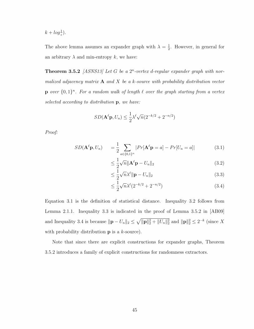
k + log 1✏
).
The above lemma assumes an expander graph with � = 12 . However, in general for
an arbitrary � and min-entropy k, we have:
Theorem 3.5.2 [ASNS13] Let G be a 2n-vertex d-regular expander graph with nor-
malized adjacency matrix A and X be a k-source with probability distribution vector
p over {0, 1}n. For a random walk of length ` over the graph starting from a vertex
selected according to distribution p, we have:
SD(A`p, Un
) 1
2�`
pn(2�k/2 + 2�n/2)
Proof:
SD(A`p, Un
) =1
2
X
a2{0,1}n|Pr[A`p = a]� Pr[U
n
= a]| (3.1)
1
2
pnkA`p� U
n
k2 (3.2)
1
2
pn�`kp� U
n
k2 (3.3)
1
2
pn�`(2�k/2 + 2�n/2) (3.4)
Equation 3.1 is the definition of statistical distance. Inequality 3.2 follows from
Lemma 2.1.1. Inequality 3.3 is indicated in the proof of Lemma 3.5.2 in [AB09]
and Inequality 3.4 is because kp� Un
k2 p
kpk22 + kUn
k22 and kpk22 2�k (since X
with probability distribution p is a k-source).
Note that since there are explicit constructions for expander graphs, Theorem
3.5.2 introduces a family of explicit constructions for randomness extractors.
45
Chapter 4
True Random Number Generator from Human
Gameplay
In this chapter, an integrated approach for true randomness generation from human
gameplay is proposed. Game theory is used for designing the game. We show that the
game design is adjustable to several popular existing games, such as Roshambo. The
proposed TRNG is compared with previous existing RNGs that use human gameplay,
and the advantages of the proposed approach are described.
4.1 Introduction
Every RNG (even PRNG) needs at least one source of randomness to produce random
numbers. The challenge is where to find randomness in a deterministic device, such as
a computer. The commonly applicable entropy sources in a computing device include
noise in electrical circuits, the current system time or user input (such as mouse
movements or time intervals between keystrokes). Any of these sources has their
advantages and drawbacks. System time is probably the worst source of randomness
among the above mentioned sources. This is because, if the execution time of the
RNG is almost known, the time as a source of randomness will only contain a few
bits of entropy [RSN+01]. This was the biggest problem in the implementation of
the Netscape browser v1.1 [GW96] and Kerberos V4 [DLS97]. Gathering entropy
from system-based noise sources often requires extra hardware. Moreover, such noise
sources are not always available. User based entropy sources, on the other hand, are
an attractive alternative entropy source, which is easily available while requiring no
46
extra hardware for exploiting their entropy.
Using the input of a computer game is a tempting idea for providing a user based
entropy source. The user willingly plays the game as much as required, while pro-
ducing entropy for a random number generator. Note that not just any game is
appropriate for this purpose. The desired game should lead the human player to
generate as much randomness as possible while staying interesting for the user.
4.2 The Contribution: True Random Number Generator from Human
Gameplay
A TRNG that uses human gameplay against a computer as the only source of random-
ness is proposed. This TRNG is a randomness extractor that uses human input as the
initial entropy source and the random seed. The user can improve the randomness of
the output at any time and to any level of closeness to a uniform distribution, simply
by playing the game for more rounds. Thus, the final results have a guaranteed and
adjustable level of randomness.
In comparison, in the construction of Halprin et al. [HN09], (i) although the en-
tropy source is based on human input, a second external source of perfect randomness
is required to provide a seed for the extractor, and (ii) the size and quality of the
final output depends on the extractor that is used after obtaining the output of the
entropy source. Therefore, changing the quality of the final output requires replacing
the extractor and performing the calculations from the beginning.
4.2.1 Applications
As mentioned before, RNGs are essential components for security systems. User-
based TRNGs add an extra level of assurance about the randomness source since
the TRNGs exploit randomness from the user’s input. An example application of
47
this approach is generating random cryptographic keys for software such as PGP,
OpenSSL, and GnuPG. These applications rely on the random number generation of
the OS, which collects its required entropy from a physical entropy source. However,
enough entropy for randomness extraction may not be available at the time of the
request. In this case, the proposed approach can be used to generate the required
randomness from users by asking them to play a simple game. According to the
conducted experiments in this thesis, for generating a 64 bit key that is 2�18-close to
uniform distribution, the user should choose 8 locations on a presented circle (with
256 distinct points) and then play Roshambo for 15 times against the computer.
Another application of the proposed approach can be in virtual environments in
which multiple users share some hardware such as CPU and RAM. In such environ-
ments using the shared hardware as an entropy source for the system’s RNG is risky
due to the dependence between entropy pools of di↵erent users, especially if the RNG
is used for generating a cryptographic key of a security protocol. In these scenarios us-
ing a human player’s gameplay for generating randomness is much more reliable, since
the generated randomness would be independent of the underlying shared hardware
and the other users’ randomness.
4.2.2 The TRNG’s Structure
The proposed TRNG, similar to any other TRNGs, consists of two main modules:
(i) An entropy source that uses a physical process to generate a sequence of symbols
with a lower bound on its min-entropy and (ii) a seeded randomness extractor that
transforms the entropy source into an almost perfect random sequence using the extra
randomness provided by the seed.
In the proposed approach, the gameplay between a human player and a computer
player is used to realize the two modules of a TRNG. The required entropy for the
proposed construction is provided by the user’s initial choices among the vertices of
48
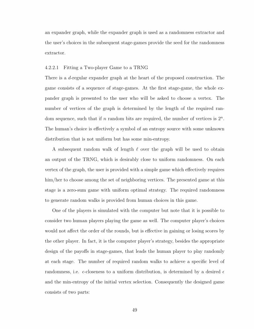
an expander graph, while the expander graph is used as a randomness extractor and
the user’s choices in the subsequent stage-games provide the seed for the randomness
extractor.
4.2.2.1 Fitting a Two-player Game to a TRNG
There is a d-regular expander graph at the heart of the proposed construction. The
game consists of a sequence of stage-games. At the first stage-game, the whole ex-
pander graph is presented to the user who will be asked to choose a vertex. The
number of vertices of the graph is determined by the length of the required ran-
dom sequence, such that if n random bits are required, the number of vertices is 2n.
The human’s choice is e↵ectively a symbol of an entropy source with some unknown
distribution that is not uniform but has some min-entropy.
A subsequent random walk of length ` over the graph will be used to obtain
an output of the TRNG, which is desirably close to uniform randomness. On each
vertex of the graph, the user is provided with a simple game which e↵ectively requires
him/her to choose among the set of neighboring vertices. The presented game at this
stage is a zero-sum game with uniform optimal strategy. The required randomness
to generate random walks is provided from human choices in this game.
One of the players is simulated with the computer but note that it is possible to
consider two human players playing the game as well. The computer player’s choices
would not a↵ect the order of the rounds, but is e↵ective in gaining or losing scores by
the other player. In fact, it is the computer player’s strategy, besides the appropriate
design of the payo↵s in stage-games, that leads the human player to play randomly
at each stage. The number of required random walks to achieve a specific level of
randomness, i.e. ✏-closeness to a uniform distribution, is determined by a desired ✏
and the min-entropy of the initial vertex selection. Consequently the designed game
consists of two parts:
49
1. Initial stage-game:
The initial stage-game is an extension of the matching pennies game.
The user chooses a vertex from the set of 2n possible vertices in the
graph, and wins if the computer cannot “guess” his/her choice.
2. Walk stage-games:
Each subsequent stage-game corresponds to a single step of the random
walk. At vertex V , the player is presented with a zero-sum game with
d possible actions. The game payo↵s are designed in such a way that a
uniform choice between the presented actions is the optimal strategy,
and so the user’s input would correspond to uniform selection among
the possible actions. Each of the d actions corresponds to one of the
neighbouring vertices of V . Thus, the user’s random choice in the zero-
sum game is used to generate a random walk on the expander graph.
Using a d-regular graph ensures that the number of choices at every
vertex is the same.
The main di↵erence between the initial and the subsequent stage-games is the
number of choices available to the user and the way these choices are used.
Suppose ni
represents the corresponding vertex of a player’s choice at the ith walk
stage-game and c1 to cd
represent the neighbouring vertices of ni
. Figure 4.1 shows
how player choices in walk stage-games are mapped to a random walk.
4.2.2.2 Choosing the expander graph
The initial step toward constructing the proposed TRNG is to choose an appropriate
d-regular expander graph. The number of vertices is determined by the length of the
required random string. An expander graph with 2n vertices outputs n bits that are
50
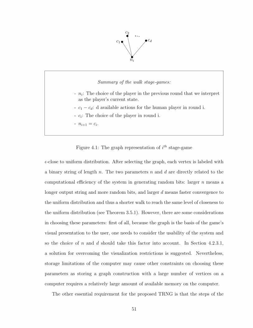
ni
c1
c2
cd
Summary of the walk stage-games:
- ni
: The choice of the player in the previous round that we interpretas the player’s current state.
- c1 � cd
: d available actions for the human player in round i.
- ci
: The choice of the player in round i.
- ni+1 = c
i
.
Figure 4.1: The graph representation of ith stage-game
✏-close to uniform distribution. After selecting the graph, each vertex is labeled with
a binary string of length n. The two parameters n and d are directly related to the
computational e�ciency of the system in generating random bits: larger n means a
longer output string and more random bits, and larger d means faster convergence to
the uniform distribution and thus a shorter walk to reach the same level of closeness to
the uniform distribution (see Theorem 3.5.1). However, there are some considerations
in choosing these parameters: first of all, because the graph is the basis of the game’s
visual presentation to the user, one needs to consider the usability of the system and
so the choice of n and d should take this factor into account. In Section 4.2.3.1,
a solution for overcoming the visualization restrictions is suggested. Nevertheless,
storage limitations of the computer may cause other constraints on choosing these
parameters as storing a graph construction with a large number of vertices on a
computer requires a relatively large amount of available memory on the computer.
The other essential requirement for the proposed TRNG is that the steps of the
51
random walk must correspond to an independent and uniformly distributed random
variable. Experimental results in [HN09, Wag72] show that bias will increase in the
human player’s choices for larger sets of possible choices as human beings naturally
tend to avoid picking end points. This implies a restriction on choosing relatively
large values for d.
Example 4.2.1 Suppose a sequence of 64 random bits that is 2�18-close to a uniform
sequence is required for a real world application (e.g. to construct a cryptographic
key). Using the proposed TRNG requires constructing a d-regular expander graph
with 264 vertices. According to Theorem 3.5.1, there exists an explicit construction
for expander graphs named Ramanujan graphs that, for large amounts of N (number
of vertices), have a second largest eigenvalue, that is approximately equal to � ⇡2pd� 1
d. To find the required number of random walks for obtaining the desirable
random sequence, we need an estimate for the min-entropy of the user’s initial choices.
Assume the amount of existing min-entropy is 0.6 per bit (38 bits in 64 bits) that is the
estimated min-entropy of human players in [HN09]. For the choice of d = 3, � ⇡ 0.92.
In this case, for obtaining 64 bits that are 2�18-close to uniform distribution:
2�19 1
20.92`
p64(2�19.2 + 2�32)
) ` � 14.3 ) ` = 15
Table 4.1 lists the number of required random walks for di↵erent amounts of d to
get 64 random bits that are 2�18 close to uniform distribution. As the table shows,
the number of required rounds significantly decreases as d grows.
4.2.3 Game Design
A two-player game based on the described approach is designed. For the game design,
a Petersen graph is used, which is a 3-regular graph with n vertices. The second
52
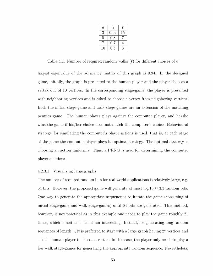
d � `3 0.92 155 0.8 77 0.7 410 0.6 3
Table 4.1: Number of required random walks (`) for di↵erent choices of d
largest eigenvalue of the adjacency matrix of this graph is 0.94. In the designed
game, initially, the graph is presented to the human player and the player chooses a
vertex out of 10 vertices. In the corresponding stage-game, the player is presented
with neighboring vertices and is asked to choose a vertex from neighboring vertices.
Both the initial stage-game and walk stage-games are an extension of the matching
pennies game. The human player plays against the computer player, and he/she
wins the game if his/her choice does not match the computer’s choice. Behavioural
strategy for simulating the computer’s player actions is used, that is, at each stage
of the game the computer player plays its optimal strategy. The optimal strategy is
choosing an action uniformly. Thus, a PRNG is used for determining the computer
player’s actions.
4.2.3.1 Visualizing large graphs
The number of required random bits for real world applications is relatively large, e.g.
64 bits. However, the proposed game will generate at most log 10 ⇡ 3.3 random bits.
One way to generate the appropriate sequence is to iterate the game (consisting of
initial stage-game and walk stage-games) until 64 bits are generated. This method,
however, is not practical as in this example one needs to play the game roughly 21
times, which is neither e�cient nor interesting. Instead, for generating long random
sequences of length n, it is preferred to start with a large graph having 2n vertices and
ask the human player to choose a vertex. In this case, the player only needs to play a
few walk stage-games for generating the appropriate random sequence. Nevertheless,
53
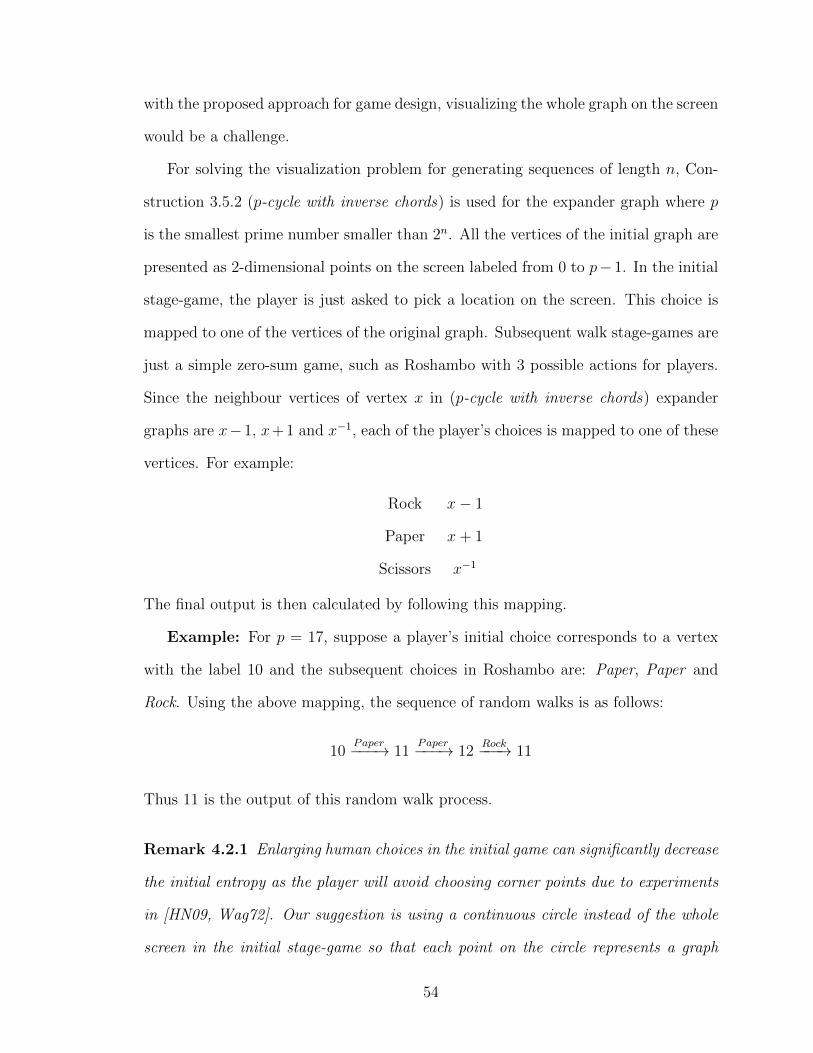
with the proposed approach for game design, visualizing the whole graph on the screen
would be a challenge.
For solving the visualization problem for generating sequences of length n, Con-
struction 3.5.2 (p-cycle with inverse chords) is used for the expander graph where p
is the smallest prime number smaller than 2n. All the vertices of the initial graph are
presented as 2-dimensional points on the screen labeled from 0 to p� 1. In the initial
stage-game, the player is just asked to pick a location on the screen. This choice is
mapped to one of the vertices of the original graph. Subsequent walk stage-games are
just a simple zero-sum game, such as Roshambo with 3 possible actions for players.
Since the neighbour vertices of vertex x in (p-cycle with inverse chords) expander
graphs are x�1, x+1 and x�1, each of the player’s choices is mapped to one of these
vertices. For example:
Rock x� 1
Paper x+ 1
Scissors x�1
The final output is then calculated by following this mapping.
Example: For p = 17, suppose a player’s initial choice corresponds to a vertex
with the label 10 and the subsequent choices in Roshambo are: Paper, Paper and
Rock. Using the above mapping, the sequence of random walks is as follows:
10Paper���! 11
Paper���! 12Rock���! 11
Thus 11 is the output of this random walk process.
Remark 4.2.1 Enlarging human choices in the initial game can significantly decrease
the initial entropy as the player will avoid choosing corner points due to experiments
in [HN09, Wag72]. Our suggestion is using a continuous circle instead of the whole
screen in the initial stage-game so that each point on the circle represents a graph
54
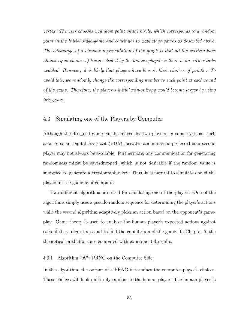
vertex. The user chooses a random point on the circle, which corresponds to a random
point in the initial stage-game and continues to walk stage-games as described above.
The advantage of a circular representation of the graph is that all the vertices have
almost equal chance of being selected by the human player as there is no corner to be
avoided. However, it is likely that players have bias in their choices of points . To
avoid this, we randomly change the corresponding number to each point at each round
of the game. Therefore, the player’s initial min-entropy would become larger by using
this game.
4.3 Simulating one of the Players by Computer
Although the designed game can be played by two players, in some systems, such
as a Personal Digital Assistant (PDA), private randomness is preferred as a second
player may not always be available. Furthermore, any communication for generating
randomness might be eavesdropped, which is not desirable if the random value is
supposed to generate a cryptographic key. Thus, it is natural to simulate one of the
players in the game by a computer.
Two di↵erent algorithms are used for simulating one of the players. One of the
algorithms simply uses a pseudo random sequence for determining the player’s actions
while the second algorithm adaptively picks an action based on the opponent’s game-
play. Game theory is used to analyze the human player’s expected actions against
each of these algorithms and to find the equilibrium of the game. In Chapter 5, the
theoretical predictions are compared with experimental results.
4.3.1 Algorithm “A”: PRNG on the Computer Side
In this algorithm, the output of a PRNG determines the computer player’s choices.
These choices will look uniformly random to the human player. The human player is
55
not able to remember long sequences. Thus, there is no need to use a cryptographic
PRNG for this application, as the output of even weak PRNGs looks uniformly ran-
dom to human players. In this case, the game is analyzed as an imperfect information
game with behavioural strategy.
In an extensive form game, which is obtained from a finitely repeated game, some-
times players do not know all the actions of the other player or cannot recall all their
past actions. In this case, some nodes in the game tree (Section 2.5.3) are indis-
tinguishable to the player simply because (i) the player does not have the sequence
of previous actions and (ii) the available actions in the indistinguishable nodes are
identical. These types of games are called imperfect information games. Each group
of indistinguishable nodes forms an information set. Behavioural strategies in the ex-
tensive form game are the strategies in which each agent’s (potentially probabilistic)
choice at each node is made independently of his/her choices at other nodes.
This algorithm does not use any history of previous actions. Thus, the game is
an imperfect information game and the computer player’s information set consists
of all the nodes that require its action. Since the action at each node is made inde-
pendent of other nodes, the computer’s strategy is considered a behavioural strategy.
Repeating a Nash strategy in each stage-game will be an equilibrium in behavioural
strategies simply because a Nash strategy is the optimal strategy at each node. The
human player may remember the previous 1 or 2 actions nevertheless, because of
the symmetry of the game and the computer player’s random strategy, this will not
change his/her optimal strategy which is playing uniformly randomly.
Note that one can view the game with a PRNG on the computer side as a non-
repetitive game: at each stage the computer’s choices are independent of previous
actions, and the human player does not need to remember previous actions (because
this will not change his/her optimal strategy).
56
4.3.2 Algorithm “B”: Predictor Algorithm on the Computer Side
For two-player zero-sum repeated games, the folk theorem (Theorem 2.5.2) is still true
[OR94, Proposition 156.1], but it becomes vacuous. Suppose we iterate a two-player
zero-sum game G with payo↵s U and �U . If each of the players uses a minimax
strategy against the opponent, the maximum payo↵ is U . Thus in the iterated game,
the only Nash-equilibrium payo↵ profile is (U, –U) and the only way to get this is
if each player always plays his/her minimax strategy, which is randomizing over the
possible actions with uniform distribution. Thus, a Nash equilibrium strategy is
optimal if the other players also use the Nash equilibrium strategies. In reality,
however, players will not use Nash equilibrium strategies simply because they may
be trying to predict the opponent’s actions. In this case, the player who can predict
better and plays more unpredictably wins the game.
The attempt to predict the opponent’s action naturally appears when a human is
involved in playing the game. This makes the game more competitive and thus more
interesting.
To have a more realistic simulation of the human player, a predictor algorithm
named “Iocaine Powder” [Egn00] by Dan Egnor is used. This algorithm took the
first place in the “First International Roshambo Programming Competition”. This
algorithm uses a heuristically designed compilation of strategies and attempts to
predict what the opponent will do. Thus, the optimal strategy or metastrategy is
chosen based on past performance. The main strategies that are employed in this
algorithm are random guessing, frequency analysis, and history matching:
• Random guess
The algorithm may choose a move by random selection. This algorithm
can be called a hedge. If somebody predicts and defeats this algorithm,
it means that he/she is able to predict the output of the PRNG, which
57
is assumed to be impossible. At that point, the meta-strategy will
make sure that the program “eliminates its losses” then starts playing
randomly to avoid a destructive loss.
• Frequency analysis
The frequency analyzer looks at the players’ past actions to find the
move they have made most frequently to predict their future moves.
However, it is not very useful against complex opponents. It can be
used to defeat other competitors who use it as a predictive method.
• History matching
This is the strongest predictor in the Iocaine Powder algorithm, and
several forms of this technique are used in other strong entries. This
algorithm looks for an order in the history similar to the last few moves.
For instance, if in the last four moves, the player played paper against
rock, scissors against scissors, rock against paper, and scissors against
rock, the algorithm will look for sequences in the history when the same
four moves happened. In fact, a sequence of the last 30 moves by the
opponent is considered superior to the last four moves. When such a
sequence is found, the history matcher assesses the opponent’s move
after that sequence and assumes they will make the same move in the
future.
Once the history is created, this predictor can easily defeat a broad
range of weak contestants. The use of meta-strategy allows this algo-
rithm to defeat other strong opponents.
This algorithm is used in the second experiment in Chapter 5, where the human
player plays Roshambo against the computer repeatedly and then the final output of
58
the TRNG is calculated based on the user’s choices.
4.4 Enlarging Choices of the Human Player
So far, we have considered the game in which the number of actions for both players
is equal and the optimal strategy for both players is to play uniformly randomly.
When the game is played against a computer, this e↵ectively means that the com-
puter should make a random choice for any random move of the human player. The
computer’s random choice is provided by a PRNG. When the number of actions for
both players is equal, any generated randomness by the human requires an equivalent
amount of randomness from the computer. This puts the e�ciency of such a human
based RNG into serious doubt.
Note that in the proposed TRNG, the equality of the actions for both players
will not disturb the e�ciency of the TRNG, as truly random bits are obtained from
human choices even if we spend some pseudo random bits for the computer player’s
choices. In other words, the quality of generated randomness is improved by the
proposed game design. Moreover, by using algorithm “B” (Section 4.3.2) the amount
of required pseudo random bits is much less than the generated bits.
Halprin et al. [HN09] use the two dimensional extension of the matching pennies
game (named Hide and Seek) to enlarge the choices of the players and subsequently
increase the number of generated random bits in one round of the game. Since in
this approach, the number of available actions for both of the players is equal, the
game is not an e�cient way of generating randomness from human gameplay. In
other words, this approach cannot produce more random bits than what is spent on
the computer player’s side. For example, assume there are 2n locations on a two
dimensional screen and each player is asked to choose one of the locations. The
computer player wins if the choices match and the human player wins otherwise.
59
The computer player’s actions are determined by a PRNG. Suppose the PRNG on
the computer side generates 2n�1 instead of 2n outputs. As a result, the computer
player only chooses half of the locations on the screen. For example, the computer
player chooses locations on the right half of the screen. The human player after a
while figures this out and chooses locations on the left half of the screen to avoid
matching the choices. Therefore, the generated random bits by the human player,
corresponding to his/her choices in the game, would at most be n� 1 bits.
In a two-player computer game, if we provide the human player with more choices
than the computer player, he/she can generate more random bits than a computer
player. For this purpose, we suggest using a non-cooperative game in which the
number of available actions for one of the players (the human player) is more than
the other player (the computer player). The important issue in designing such a game
is setting the payo↵s so that randomly choosing among possible actions becomes the
human player’s best strategy.
For setting the payo↵s in the desired game, let’s assume the computer’s strategy is
pre-determined (i.e. we know the probability distribution over the computer player’s
available actions). The payo↵s are set such that they lead the human player to play
uniformly randomly over the available actions.
Suppose the size of action profile (Definition 2.5.1) for the human player is n and
for the computer player is m, with m < n. We assume aij
is the payo↵ for the first
player resulting from picking the ith action by the first player and jth action by the
second player, and bij
is the corresponding payo↵ for the second player. Table 4.2
shows the payo↵ table of a general two-player game between the human player and
the computer player.
Assume that the computer player picks action Xi
with probability of pi
, thus we
havenP
i=1pi
= 1.
60
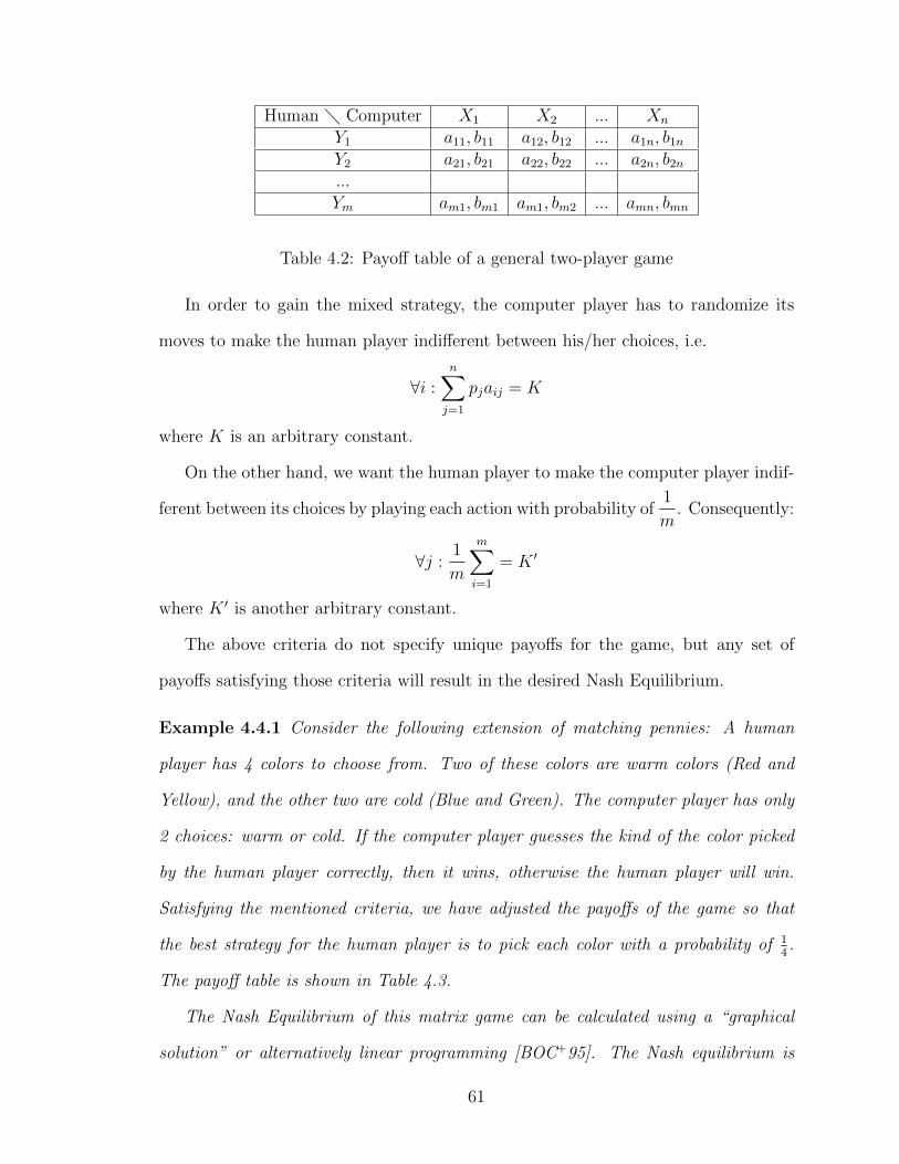
Human � Computer X1 X2 ... Xn
Y1 a11, b11 a12, b12 ... a1n, b1nY2 a21, b21 a22, b22 ... a2n, b2n...Ym
am1, bm1 a
m1, bm2 ... amn
, bmn
Table 4.2: Payo↵ table of a general two-player game
In order to gain the mixed strategy, the computer player has to randomize its
moves to make the human player indi↵erent between his/her choices, i.e.
8i :nX
j=1
pj
aij
= K
where K is an arbitrary constant.
On the other hand, we want the human player to make the computer player indif-
ferent between its choices by playing each action with probability of1
m. Consequently:
8j : 1
m
mX
i=1
= K 0
where K 0 is another arbitrary constant.
The above criteria do not specify unique payo↵s for the game, but any set of
payo↵s satisfying those criteria will result in the desired Nash Equilibrium.
Example 4.4.1 Consider the following extension of matching pennies: A human
player has 4 colors to choose from. Two of these colors are warm colors (Red and
Yellow), and the other two are cold (Blue and Green). The computer player has only
2 choices: warm or cold. If the computer player guesses the kind of the color picked
by the human player correctly, then it wins, otherwise the human player will win.
Satisfying the mentioned criteria, we have adjusted the payo↵s of the game so that
the best strategy for the human player is to pick each color with a probability of 14 .
The payo↵ table is shown in Table 4.3.
The Nash Equilibrium of this matrix game can be calculated using a “graphical
solution” or alternatively linear programming [BOC+95]. The Nash equilibrium is
61
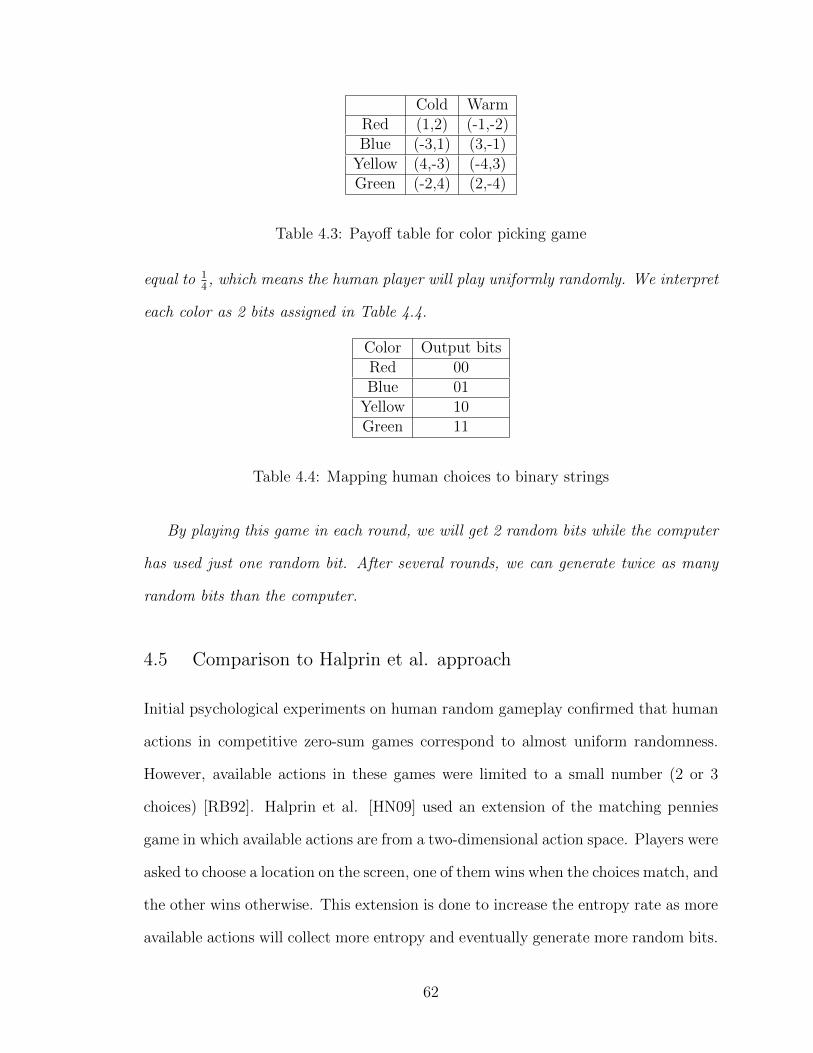
Cold WarmRed (1,2) (-1,-2)Blue (-3,1) (3,-1)Yellow (4,-3) (-4,3)Green (-2,4) (2,-4)
Table 4.3: Payo↵ table for color picking game
equal to 14 , which means the human player will play uniformly randomly. We interpret
each color as 2 bits assigned in Table 4.4.
Color Output bitsRed 00Blue 01Yellow 10Green 11
Table 4.4: Mapping human choices to binary strings
By playing this game in each round, we will get 2 random bits while the computer
has used just one random bit. After several rounds, we can generate twice as many
random bits than the computer.
4.5 Comparison to Halprin et al. approach
Initial psychological experiments on human random gameplay confirmed that human
actions in competitive zero-sum games correspond to almost uniform randomness.
However, available actions in these games were limited to a small number (2 or 3
choices) [RB92]. Halprin et al. [HN09] used an extension of the matching pennies
game in which available actions are from a two-dimensional action space. Players were
asked to choose a location on the screen, one of them wins when the choices match, and
the other wins otherwise. This extension is done to increase the entropy rate as more
available actions will collect more entropy and eventually generate more random bits.
62
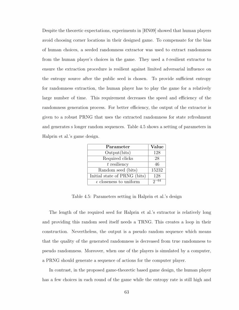
Despite the theoretic expectations, experiments in [HN09] showed that human players
avoid choosing corner locations in their designed game. To compensate for the bias
of human choices, a seeded randomness extractor was used to extract randomness
from the human player’s choices in the game. They used a t-resilient extractor to
ensure the extraction procedure is resilient against limited adversarial influence on
the entropy source after the public seed is chosen. To provide su�cient entropy
for randomness extraction, the human player has to play the game for a relatively
large number of time. This requirement decreases the speed and e�ciency of the
randomness generation process. For better e�ciency, the output of the extractor is
given to a robust PRNG that uses the extracted randomness for state refreshment
and generates s longer random sequences. Table 4.5 shows a setting of parameters in
Halprin et al.’s game design.
Parameter ValueOutput(bits) 128Required clicks 28t resiliency 46
Random seed (bits) 15232Initial state of PRNG (bits) 128
✏ closeness to uniform 2�64
Table 4.5: Parameters setting in Halprin et al.’s design
The length of the required seed for Halprin et al.’s extractor is relatively long
and providing this random seed itself needs a TRNG. This creates a loop in their
construction. Nevertheless, the output is a pseudo random sequence which means
that the quality of the generated randomness is decreased from true randomness to
pseudo randomness. Moreover, when one of the players is simulated by a computer,
a PRNG should generate a sequence of actions for the computer player.
In contrast, in the proposed game-theoretic based game design, the human player
has a few choices in each round of the game while the entropy rate is still high and
63
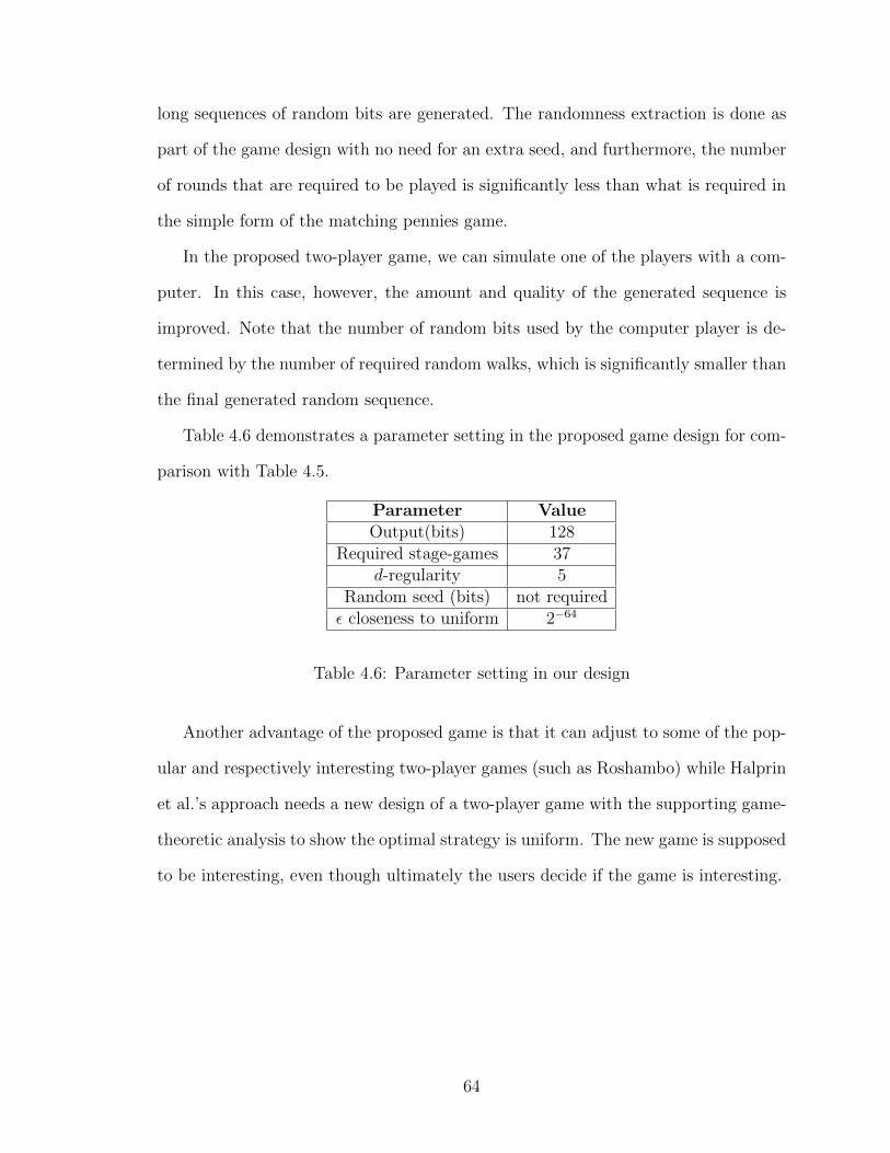
long sequences of random bits are generated. The randomness extraction is done as
part of the game design with no need for an extra seed, and furthermore, the number
of rounds that are required to be played is significantly less than what is required in
the simple form of the matching pennies game.
In the proposed two-player game, we can simulate one of the players with a com-
puter. In this case, however, the amount and quality of the generated sequence is
improved. Note that the number of random bits used by the computer player is de-
termined by the number of required random walks, which is significantly smaller than
the final generated random sequence.
Table 4.6 demonstrates a parameter setting in the proposed game design for com-
parison with Table 4.5.
Parameter ValueOutput(bits) 128
Required stage-games 37d-regularity 5
Random seed (bits) not required✏ closeness to uniform 2�64
Table 4.6: Parameter setting in our design
Another advantage of the proposed game is that it can adjust to some of the pop-
ular and respectively interesting two-player games (such as Roshambo) while Halprin
et al.’s approach needs a new design of a two-player game with the supporting game-
theoretic analysis to show the optimal strategy is uniform. The new game is supposed
to be interesting, even though ultimately the users decide if the game is interesting.
64
Chapter 5
Experiments and Results
5.1 Introduction
As mentioned in Section 4.2.2, a TRNG consists of two modules: (i) an entropy source
that generates a sequence of symbols and (ii) a randomness extractor module that
transforms the input from an entropy source into an almost uniformly distributed
sequence. The parameters of the extractor module directly depend on the minimum
available min-entropy in the entropy source. By conservatively estimating the min-
entropy, one can guarantee a reliable design of the extractor module. The output of
the TRNG is finally evaluated using statistical tests to ensure appropriate function-
ality of the designed TRNG.
In this chapter, the output of the proposed TRNG is assessed. Two di↵erent
games with the same structures are designed for this purpose. One is a graphical
game, named Wolf and Sheep, in which the human player is initially asked to choose
a vertex on a Petersen (10 vertex, 3-regular) graph. In the subsequent walk stage-
games, the player chooses a vertex from 3 neighbors of the previously selected vertex.
In each stage-game, the player wins the game in case of a mismatch. The other game
is called C-Roshambo, which is choosing a location on a circle followed by the regular
Roshambo game for a number of rounds 1. The theoretical approach, proposed in
this thesis, enables us to generate random sequences from human gameplay in these
two games. The details of the game design and the final evaluation of the output are
explained in this chapter.
1The University of Calgary Conjoint Faculties Research Ethics Board has approved this research
study
65
5.2 Game Design and Experiment Set-up
In this chapter, two di↵erent simple games are designed to examine the proposed
TRNG: Wolf and Sheep and C-Roshambo. Each game is played between a human
and a computer player. For estimating the min-entropy of human choices in the initial
stage-game, a separate sub-game is designed for each of the main games. The potential
players were contacted, and the willing players participated in the experiment. The
set of players who participate in the first game (Wolf and Sheep) is di↵erent from
those who participate in the second game (C-Roshambo). Nine players played the
first and seven players played the second game. All of them were graduate computer
science students at the University of Calgary. The instructions of the game were
explained to the players. Each player was asked to play each game for at least 1000
rounds, trying his/her best to win the game. This is su�cient to run the required
min-entropy and statistical tests. The objectives of the experiments are as follows:
1. Estimate the min-entropy of human choices in the initial stage-game,
which is required for an appropriate design of the extraction module
for the TRNG. With regards to Theorem 3.5.2, the number of required
random walks on the expander graph, and consequently the number of
walk stage-games is only determined if the min-entropy of the input is
lower-bounded.
2. Examine the statistical properties (e.g. min-entropy) of the user’s ran-
dom walks to verify whether they are a good approximation of uniform
random walks.
3. Examine the statistical properties of the final output.
4. Compare the output’s statistical properties with that of a pseudo ran-
dom sequence generated by the computer to show the generated random
66
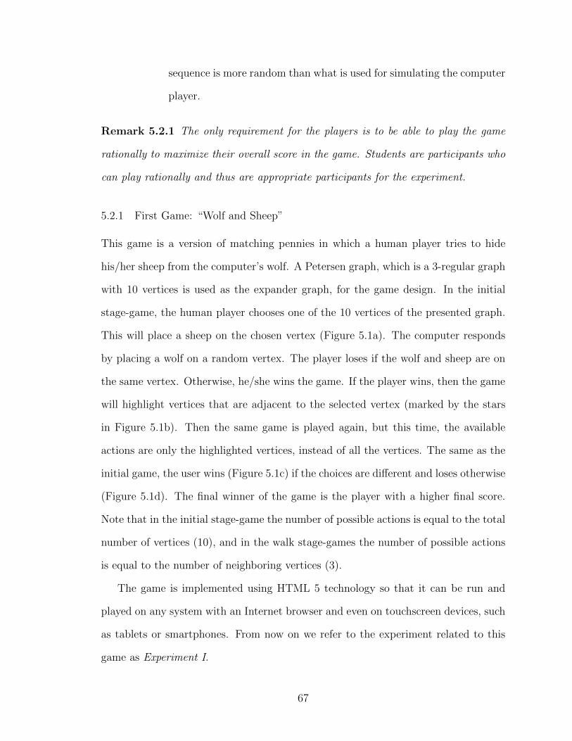
sequence is more random than what is used for simulating the computer
player.
Remark 5.2.1 The only requirement for the players is to be able to play the game
rationally to maximize their overall score in the game. Students are participants who
can play rationally and thus are appropriate participants for the experiment.
5.2.1 First Game: “Wolf and Sheep”
This game is a version of matching pennies in which a human player tries to hide
his/her sheep from the computer’s wolf. A Petersen graph, which is a 3-regular graph
with 10 vertices is used as the expander graph, for the game design. In the initial
stage-game, the human player chooses one of the 10 vertices of the presented graph.
This will place a sheep on the chosen vertex (Figure 5.1a). The computer responds
by placing a wolf on a random vertex. The player loses if the wolf and sheep are on
the same vertex. Otherwise, he/she wins the game. If the player wins, then the game
will highlight vertices that are adjacent to the selected vertex (marked by the stars
in Figure 5.1b). Then the same game is played again, but this time, the available
actions are only the highlighted vertices, instead of all the vertices. The same as the
initial game, the user wins (Figure 5.1c) if the choices are di↵erent and loses otherwise
(Figure 5.1d). The final winner of the game is the player with a higher final score.
Note that in the initial stage-game the number of possible actions is equal to the total
number of vertices (10), and in the walk stage-games the number of possible actions
is equal to the number of neighboring vertices (3).
The game is implemented using HTML 5 technology so that it can be run and
played on any system with an Internet browser and even on touchscreen devices, such
as tablets or smartphones. From now on we refer to the experiment related to this
game as Experiment I.
67
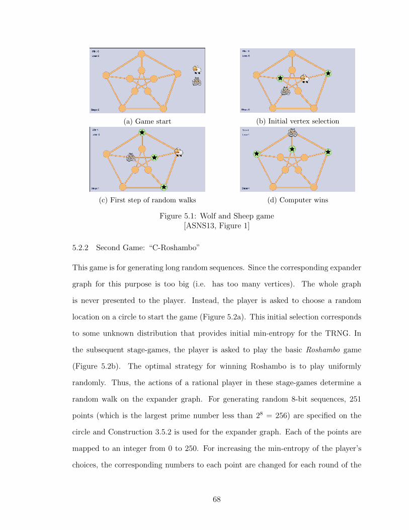
(a) Game start
(b) Initial vertex selection
(c) First step of random walks (d) Computer wins
Figure 5.1: Wolf and Sheep game[ASNS13, Figure 1]
5.2.2 Second Game: “C-Roshambo”
This game is for generating long random sequences. Since the corresponding expander
graph for this purpose is too big (i.e. has too many vertices). The whole graph
is never presented to the player. Instead, the player is asked to choose a random
location on a circle to start the game (Figure 5.2a). This initial selection corresponds
to some unknown distribution that provides initial min-entropy for the TRNG. In
the subsequent stage-games, the player is asked to play the basic Roshambo game
(Figure 5.2b). The optimal strategy for winning Roshambo is to play uniformly
randomly. Thus, the actions of a rational player in these stage-games determine a
random walk on the expander graph. For generating random 8-bit sequences, 251
points (which is the largest prime number less than 28 = 256) are specified on the
circle and Construction 3.5.2 is used for the expander graph. Each of the points are
mapped to an integer from 0 to 250. For increasing the min-entropy of the player’s
choices, the corresponding numbers to each point are changed for each round of the
68
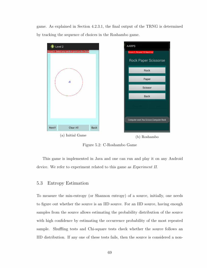
game. As explained in Section 4.2.3.1, the final output of the TRNG is determined
by tracking the sequence of choices in the Roshambo game.
(a) Initial Game
(b) Roshambo
Figure 5.2: C-Roshambo Game
This game is implemented in Java and one can run and play it on any Android
device. We refer to experiment related to this game as Experiment II.
5.3 Entropy Estimation
To measure the min-entropy (or Shannon entropy) of a source, initially, one needs
to figure out whether the source is an IID source. For an IID source, having enough
samples from the source allows estimating the probability distribution of the source
with high confidence by estimating the occurrence probability of the most repeated
sample. Shu✏ing tests and Chi-square tests check whether the source follows an
IID distribution. If any one of these tests fails, then the source is considered a non-
69
IID source, and the min-entropy is estimated through the corresponding tests for a
non-IID source (Section 2.3.2).
Any anomaly in the source should be detected before applying IID and non-IID
tests. Otherwise, the min-entropy would be over- or underestimated. NIST defines a
set of sanity checks to prevent this. The sanity checks contain two tests: a compression
test and a collision test. No estimation will be given if the sanity checks fail.
For the experiments in this thesis, an uno�cial version of the NIST tests for
entropy estimation are obtained (the code is not released yet) and used to estimate
the min-entropy of the user’s inputs. It is admitted in [BK12, Section 9.3.1] that
the approximation from the NIST tests are very much dependent on the number of
samples given to the tests (which is quite intuitive and acceptable). In our case, the
subset of users and consequently the sample size is relatively small which implies a
very conservative estimate of min-entropy for our experiment.
5.3.1 Entropy Estimation in the Initial Stage-Game
To measure the min-entropy of the initial stage-game, an independent sub-game is
designed for both of the experiments. The players are asked to play this initial game
for at least 1000 times that is su�cient for estimating the min-entropy of player’s
choices in the initial stag-game.
5.3.1.1 Entropy Estimation of Initial Stage-Game in the “Wolf and Sheep” Game
In Experiment I, players are asked to initially play the designed separate sub-game.
The min-entropy of player’s choices in this game is indeed, the min-entropy of the
player’s initial selection of a vertex on the graph in the main game. At each round of
this game, the player is asked to choose a vertex out of 10 existing vertices and wins
if his/her choice does not match the computer’s. Table 5.1 shows the estimated min-
entropy of 9 users who played the described game for some rounds. NIST tests showed
70
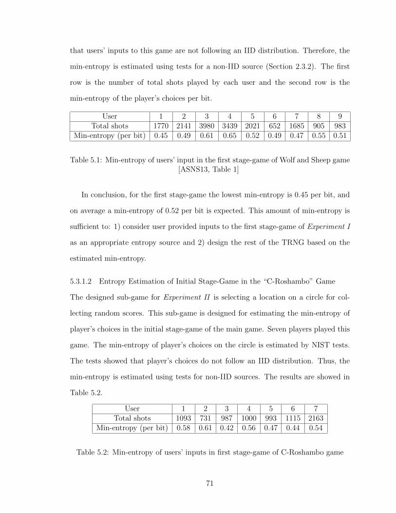
that users’ inputs to this game are not following an IID distribution. Therefore, the
min-entropy is estimated using tests for a non-IID source (Section 2.3.2). The first
row is the number of total shots played by each user and the second row is the
min-entropy of the player’s choices per bit.
User 1 2 3 4 5 6 7 8 9Total shots 1770 2141 3980 3439 2021 652 1685 905 983
Min-entropy (per bit) 0.45 0.49 0.61 0.65 0.52 0.49 0.47 0.55 0.51
Table 5.1: Min-entropy of users’ input in the first stage-game of Wolf and Sheep game[ASNS13, Table 1]
In conclusion, for the first stage-game the lowest min-entropy is 0.45 per bit, and
on average a min-entropy of 0.52 per bit is expected. This amount of min-entropy is
su�cient to: 1) consider user provided inputs to the first stage-game of Experiment I
as an appropriate entropy source and 2) design the rest of the TRNG based on the
estimated min-entropy.
5.3.1.2 Entropy Estimation of Initial Stage-Game in the “C-Roshambo” Game
The designed sub-game for Experiment II is selecting a location on a circle for col-
lecting random scores. This sub-game is designed for estimating the min-entropy of
player’s choices in the initial stage-game of the main game. Seven players played this
game. The min-entropy of player’s choices on the circle is estimated by NIST tests.
The tests showed that player’s choices do not follow an IID distribution. Thus, the
min-entropy is estimated using tests for non-IID sources. The results are showed in
Table 5.2.
User 1 2 3 4 5 6 7Total shots 1093 731 987 1000 993 1115 2163
Min-entropy (per bit) 0.58 0.61 0.42 0.56 0.47 0.44 0.54
Table 5.2: Min-entropy of users’ inputs in first stage-game of C-Roshambo game
71
The lowest min-entropy is 0.42 per bit and on average we expect 0.52 per bit
entropy. This amount of min-entropy is su�cient to: 1) consider user provided inputs
to the first stage-game of Experiment II as an appropriate entropy source and 2)
design the rest of the TRNG based on the estimated min-entropy.
5.3.2 Entropy Estimation of Random Walks
To use an expander graph as an extractor for randomness extraction, random walks
should follow a uniform distribution (Section 3.5.1). In both of the designed games,
the human player’s random choices in walk stage-games are used for doing a random
walk. In spite of theoretical expectation, the human player’s choices in these stage-
games are not uniformly random. However, because of the particular design of the
games (in which playing uniformly random is the optimal strategy), the sequence
of the human player’s choices is very close to uniform randomness. The result of
experiments in this section verifies that the sequence of the human player’s random
walks in both designed games has high min-entropy and thus is appropriate for using
as random walks to extract entropy from the initial game.
The players are asked to play the walk stage-game for at least 1000 rounds. Data
from game play of participants is collected, and the corresponding min-entropy for
both games is estimated.
5.3.2.1 Entropy Estimation of Walk Stage-games in Wolf and Sheep Game
In this experiment, NIST tests for IID sources are passed for player’s inputs in walk
stage-games. Therefore, the tests for IID sources are used for estimating the min-
entropy of the data. Table 5.3 shows the estimated min-entropy for each player during
the walk stage-game in Experiment I.
From the above table, the average expected min-entropy in walk stage-games for
Experiment I is 0.68 per bit. One can compare the average expected min-entropy
72
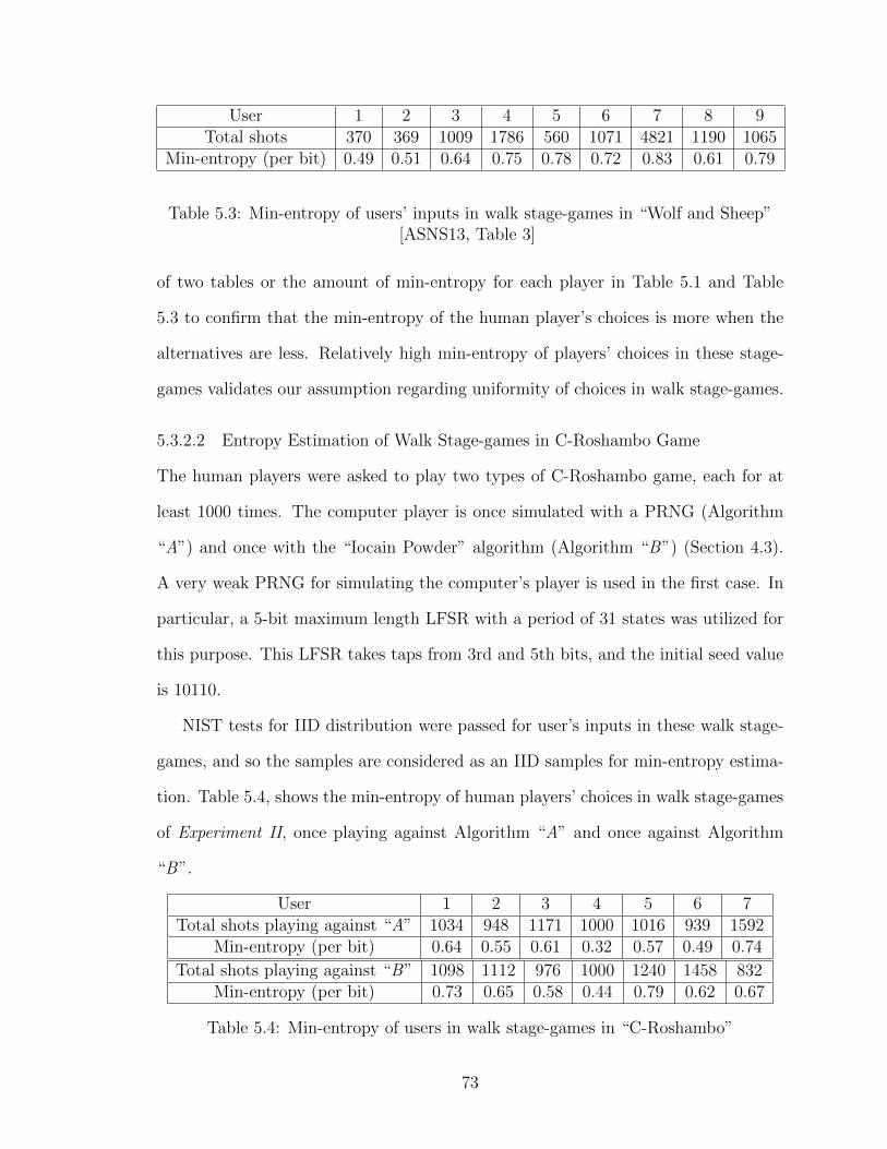
User 1 2 3 4 5 6 7 8 9Total shots 370 369 1009 1786 560 1071 4821 1190 1065
Min-entropy (per bit) 0.49 0.51 0.64 0.75 0.78 0.72 0.83 0.61 0.79
Table 5.3: Min-entropy of users’ inputs in walk stage-games in “Wolf and Sheep”[ASNS13, Table 3]
of two tables or the amount of min-entropy for each player in Table 5.1 and Table
5.3 to confirm that the min-entropy of the human player’s choices is more when the
alternatives are less. Relatively high min-entropy of players’ choices in these stage-
games validates our assumption regarding uniformity of choices in walk stage-games.
5.3.2.2 Entropy Estimation of Walk Stage-games in C-Roshambo Game
The human players were asked to play two types of C-Roshambo game, each for at
least 1000 times. The computer player is once simulated with a PRNG (Algorithm
“A”) and once with the “Iocain Powder” algorithm (Algorithm “B”) (Section 4.3).
A very weak PRNG for simulating the computer’s player is used in the first case. In
particular, a 5-bit maximum length LFSR with a period of 31 states was utilized for
this purpose. This LFSR takes taps from 3rd and 5th bits, and the initial seed value
is 10110.
NIST tests for IID distribution were passed for user’s inputs in these walk stage-
games, and so the samples are considered as an IID samples for min-entropy estima-
tion. Table 5.4, shows the min-entropy of human players’ choices in walk stage-games
of Experiment II, once playing against Algorithm “A” and once against Algorithm
“B”.
User 1 2 3 4 5 6 7Total shots playing against “A” 1034 948 1171 1000 1016 939 1592
Min-entropy (per bit) 0.64 0.55 0.61 0.32 0.57 0.49 0.74
Total shots playing against “B” 1098 1112 976 1000 1240 1458 832Min-entropy (per bit) 0.73 0.65 0.58 0.44 0.79 0.62 0.67
Table 5.4: Min-entropy of users in walk stage-games in “C-Roshambo”
73
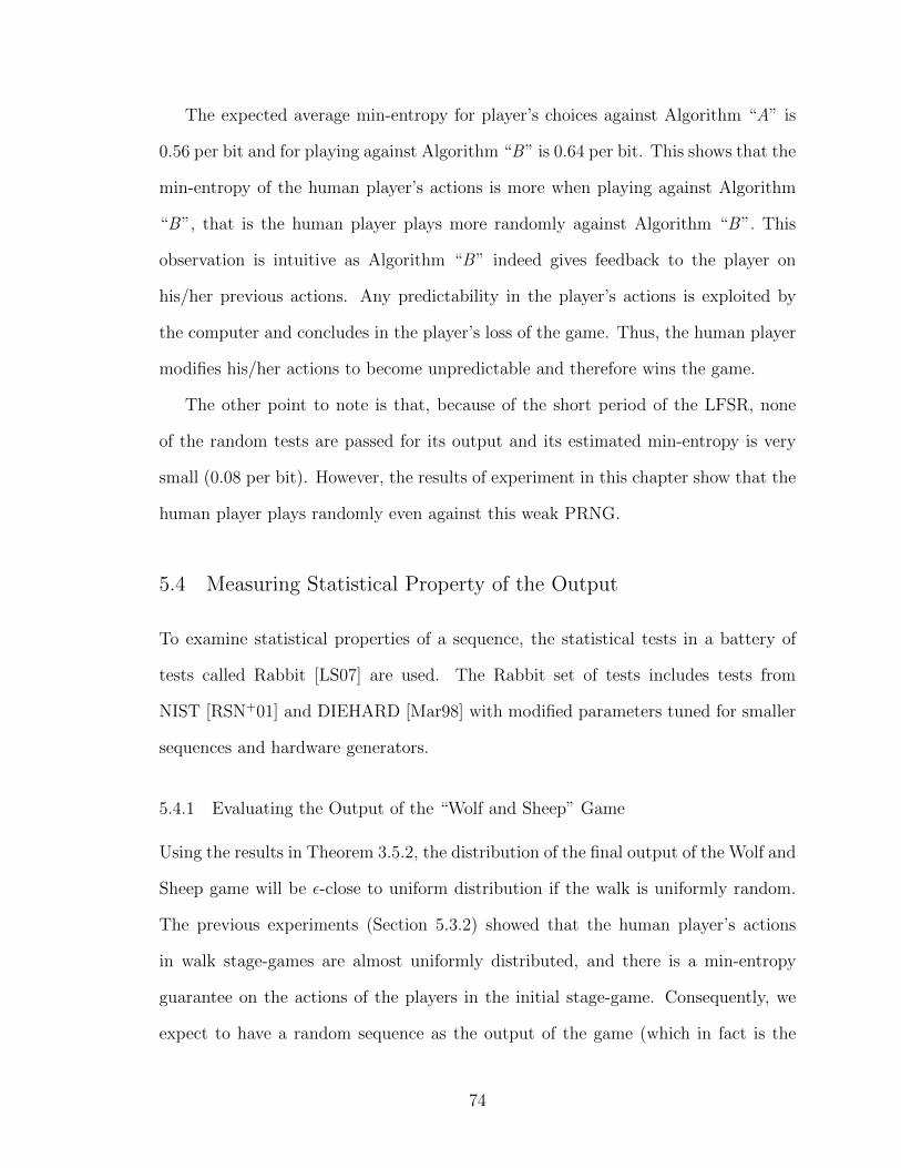
The expected average min-entropy for player’s choices against Algorithm “A” is
0.56 per bit and for playing against Algorithm “B” is 0.64 per bit. This shows that the
min-entropy of the human player’s actions is more when playing against Algorithm
“B”, that is the human player plays more randomly against Algorithm “B”. This
observation is intuitive as Algorithm “B” indeed gives feedback to the player on
his/her previous actions. Any predictability in the player’s actions is exploited by
the computer and concludes in the player’s loss of the game. Thus, the human player
modifies his/her actions to become unpredictable and therefore wins the game.
The other point to note is that, because of the short period of the LFSR, none
of the random tests are passed for its output and its estimated min-entropy is very
small (0.08 per bit). However, the results of experiment in this chapter show that the
human player plays randomly even against this weak PRNG.
5.4 Measuring Statistical Property of the Output
To examine statistical properties of a sequence, the statistical tests in a battery of
tests called Rabbit [LS07] are used. The Rabbit set of tests includes tests from
NIST [RSN+01] and DIEHARD [Mar98] with modified parameters tuned for smaller
sequences and hardware generators.
5.4.1 Evaluating the Output of the “Wolf and Sheep” Game
Using the results in Theorem 3.5.2, the distribution of the final output of the Wolf and
Sheep game will be ✏-close to uniform distribution if the walk is uniformly random.
The previous experiments (Section 5.3.2) showed that the human player’s actions
in walk stage-games are almost uniformly distributed, and there is a min-entropy
guarantee on the actions of the players in the initial stage-game. Consequently, we
expect to have a random sequence as the output of the game (which in fact is the
74
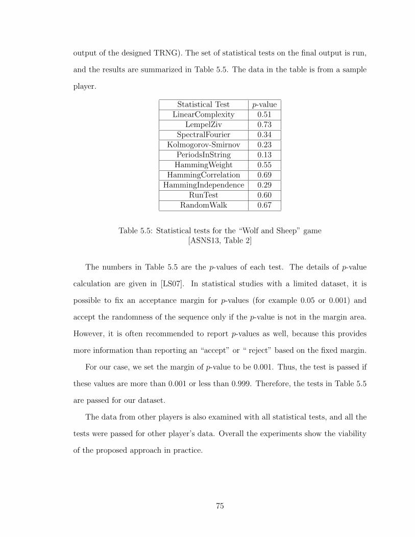
output of the designed TRNG). The set of statistical tests on the final output is run,
and the results are summarized in Table 5.5. The data in the table is from a sample
player.
Statistical Test p-valueLinearComplexity 0.51
LempelZiv 0.73SpectralFourier 0.34
Kolmogorov-Smirnov 0.23PeriodsInString 0.13HammingWeight 0.55
HammingCorrelation 0.69HammingIndependence 0.29
RunTest 0.60RandomWalk 0.67
Table 5.5: Statistical tests for the “Wolf and Sheep” game[ASNS13, Table 2]
The numbers in Table 5.5 are the p-values of each test. The details of p-value
calculation are given in [LS07]. In statistical studies with a limited dataset, it is
possible to fix an acceptance margin for p-values (for example 0.05 or 0.001) and
accept the randomness of the sequence only if the p-value is not in the margin area.
However, it is often recommended to report p-values as well, because this provides
more information than reporting an “accept” or “ reject” based on the fixed margin.
For our case, we set the margin of p-value to be 0.001. Thus, the test is passed if
these values are more than 0.001 or less than 0.999. Therefore, the tests in Table 5.5
are passed for our dataset.
The data from other players is also examined with all statistical tests, and all the
tests were passed for other player’s data. Overall the experiments show the viability
of the proposed approach in practice.
75
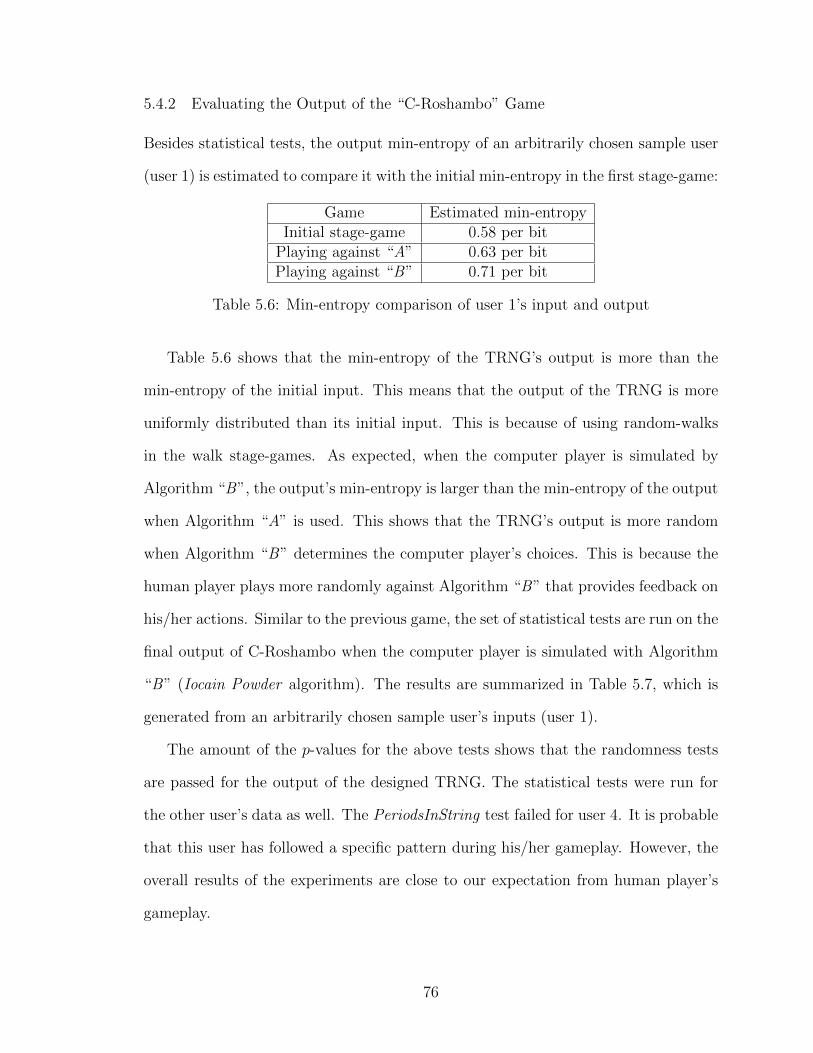
5.4.2 Evaluating the Output of the “C-Roshambo” Game
Besides statistical tests, the output min-entropy of an arbitrarily chosen sample user
(user 1) is estimated to compare it with the initial min-entropy in the first stage-game:
Game Estimated min-entropyInitial stage-game 0.58 per bitPlaying against “A” 0.63 per bitPlaying against “B” 0.71 per bit
Table 5.6: Min-entropy comparison of user 1’s input and output
Table 5.6 shows that the min-entropy of the TRNG’s output is more than the
min-entropy of the initial input. This means that the output of the TRNG is more
uniformly distributed than its initial input. This is because of using random-walks
in the walk stage-games. As expected, when the computer player is simulated by
Algorithm “B”, the output’s min-entropy is larger than the min-entropy of the output
when Algorithm “A” is used. This shows that the TRNG’s output is more random
when Algorithm “B” determines the computer player’s choices. This is because the
human player plays more randomly against Algorithm “B” that provides feedback on
his/her actions. Similar to the previous game, the set of statistical tests are run on the
final output of C-Roshambo when the computer player is simulated with Algorithm
“B” (Iocain Powder algorithm). The results are summarized in Table 5.7, which is
generated from an arbitrarily chosen sample user’s inputs (user 1).
The amount of the p-values for the above tests shows that the randomness tests
are passed for the output of the designed TRNG. The statistical tests were run for
the other user’s data as well. The PeriodsInString test failed for user 4. It is probable
that this user has followed a specific pattern during his/her gameplay. However, the
overall results of the experiments are close to our expectation from human player’s
gameplay.
76
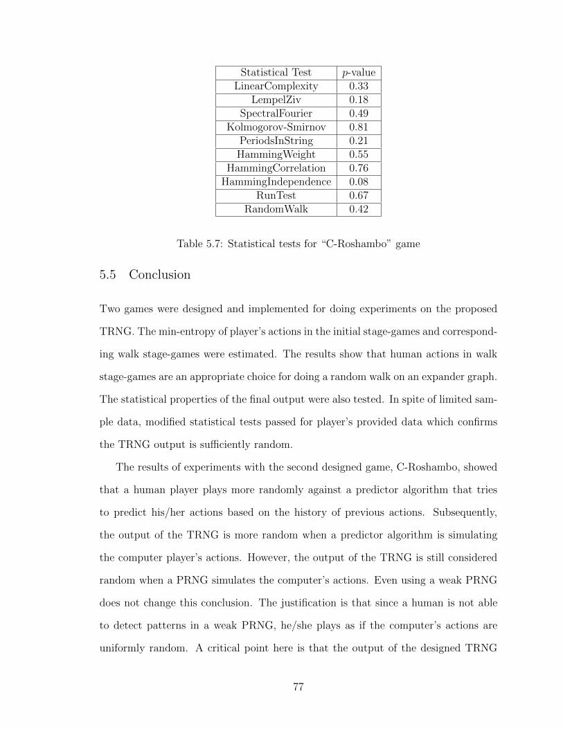
Statistical Test p-valueLinearComplexity 0.33
LempelZiv 0.18SpectralFourier 0.49
Kolmogorov-Smirnov 0.81PeriodsInString 0.21HammingWeight 0.55
HammingCorrelation 0.76HammingIndependence 0.08
RunTest 0.67RandomWalk 0.42
Table 5.7: Statistical tests for “C-Roshambo” game
5.5 Conclusion
Two games were designed and implemented for doing experiments on the proposed
TRNG. The min-entropy of player’s actions in the initial stage-games and correspond-
ing walk stage-games were estimated. The results show that human actions in walk
stage-games are an appropriate choice for doing a random walk on an expander graph.
The statistical properties of the final output were also tested. In spite of limited sam-
ple data, modified statistical tests passed for player’s provided data which confirms
the TRNG output is su�ciently random.
The results of experiments with the second designed game, C-Roshambo, showed
that a human player plays more randomly against a predictor algorithm that tries
to predict his/her actions based on the history of previous actions. Subsequently,
the output of the TRNG is more random when a predictor algorithm is simulating
the computer player’s actions. However, the output of the TRNG is still considered
random when a PRNG simulates the computer’s actions. Even using a weak PRNG
does not change this conclusion. The justification is that since a human is not able
to detect patterns in a weak PRNG, he/she plays as if the computer’s actions are
uniformly random. A critical point here is that the output of the designed TRNG
77

(generated by human gameplay) is much more random than the initial PRNG.
78
Chapter 6
Conclusion and Future Works
The main contribution in this thesis was proposing a new TRNG that is capable of
using the human player’s input as the only source of randomness. This TRNG is
mainly a two-player game that takes human gameplay as the input and generates
a sequence of random bits. We designed and implemented two games as a proof of
concept for the proposed TRNG. The results of statistical tests on the output of the
TRNG confirm its e�ciency and applicability.
6.1 Concluding Remarks
Random number generators are an important part of any security system. Good ran-
domness guarantees the security of cryptographic protocols. User based randomness
generation is preferable to other ways of randomness generation especially in shared
environments like cloud services. In such environments other traditional sources of
entropy (e.g. hardware consisting of CPU and RAM) are shared among users and
consequently user based random generation is the only way that ensures generation
of non-correlated randomness. Moreover, randomness generation from users doesn’t
need any extra hardware for entropy collection which eases its application for various
systems with limited resources, especially hardware.
This work opens a new direction for independent randomness generation in shared
environments without any requirement for extra computational capability or random-
ness generation subsystems.
79
6.1.1 Advantages of the Proposed TRNG
The proposed TRNG uses human gameplay, from interesting games, for generating
randomness which is interesting to users. The structure of this TRNG is very flexible
and can be fit to several popular games such as Roshambo. The only condition for
the game is that the optimal strategy requires the players to play uniformly randomly
for winning the game. The basic game of TRNG e↵ectively asks players to choose an
action among a group of alternatives. Although the proposed TRNG can generate
long random sequences, it always provides players with a few alternatives, except in
the initial stage-game. This feature causes human players to play more randomly
since they behave more predictably when choosing among many alternatives.
The game is capable of being played by two users. In this case, the generated
random sequence is completely independent from the computer. However, the game
can be played against a computer player as well. For this purpose, we require a
PRNG to simulate the computer player’s actions. The experimental results showed
that even very weak PRNGs are suitable for being used on the computer player’s
side because the human mind is unable to memorize relatively long patterns and thus
cannot distinguish between truly random sequences and pseudo random ones. In
other words, the experiments show that human players follow their optimal strategy,
which is playing uniformly randomly against a computer even if the computer uses a
weak PRNG for selecting its actions. One can also use a predictor algorithm on the
computer’s side for predicting the human player’s actions. In this case, the human
would play more randomly since the predictor algorithm indeed gives feedback to
the players on their previous actions. To summarize, we can say that dependency of
the proposed TRNG on computer randomness is minimized through an appropriate
game design. This feature is ideal for shared environments in which users require an
independent source of randomness for critical security applications.
80
6.2 Future Works
There are a number of extensions and directions for future work. On a theoretical
side, characterizing a randomness extractor with guaranteed min-entropy on its seed
is an interesting open problem. In particular it is challenging to analyze non-uniform
random walks on an expander graph based extractor.
On the implementation and experimental side, for generating large strings, for
example 64 or 80 bit strings, we need to collect as much entropy as possible in the
initial round. Here one needs to find ways for enabling the user to make the initial
selection of the random value with “high” initial min-entropy. In this work, Roshambo
is used as a zero-sum game with 3 choices in walk stage-games. Other interesting
zero-sum games with a greater number of available actions will conclude in faster
randomness generation of the whole game. Creating an interesting game and interface
to encourage random selection will improve the e�ciency of the approach. The strings
generated by sample users were analyzed. Wider user studies are required to measure
min-entropy and statistical properties of strings at di↵erent stages (entropy source,
random walk and final output) as well as usability of the system.
A predictor algorithm such as Iocain Powder used in this experiment improved
human random behaviour by giving indirect feedback of the player’s actions. Better
predictor algorithms for simulating human players in zero-sum games will lead the
player to generate better unpredictable sequences.
Hardware faults or malicious tampering with entropy sources may result in biases
in the randomness source that are not easily detectable. Using human input protects
a system against such faults or malicious tampering. Providing a secure interface
for playing the game by two users allows randomness generation independent of the
computer and improves trustworthiness of the generated randomness.
This work is the first construction of a full TRNG that uses human gameplay as
81

the entropy source and the seed for the extractor. Using human users to construct
TRNGs with a higher rate of randomness generation is an interesting direction for
future work.
82
Chapter 7
Bibliography
[AB09] Sanjeev Arora and Boaz Barak. Computational complexity: a modern
approach. Cambridge University Press, 2009.
[AM84] Noga Alon and Vitali D Milman. Eigenvalues, expanders and supercon-
centrators. Combinatorica 6, pages 83–96, 1984.
[ASN14] Mohsen Alimomeni and Reihaneh Safavi-Naini. Human assisted random-
ness generation using video games. IACR Cryptology ePrint Archive,
2014:45, 2014.
[ASNS13] Mohsen Alimomeni, Reihaneh Safavi-Naini, and Setareh Sharifian. A
true random generator using human gameplay. In Decision and Game
Theory for Security, pages 10–28. Springer, 2013.
[Bad66] Alan D Baddeley. The capacity for generating information by randomiza-
tion. The Quarterly Journal of Experimental Psychology, 18(2):119–129,
1966.
[BH05] Boaz Barak and Shai Halevi. A model and architecture for pseudo-
random generation with applications to /dev/random. In Proceedings of
the 12th ACM Conference on Computer and Communications Security,
pages 203–212. ACM, 2005.
[BK12] Elaine Barker and John Kelsey. Recommendation for the entropy sources
used for random bit generation. Draft NIST Special Publication, 2012.
83
[BOC+95] Tamer Basar, Geert Jan Olsder, GJ Clsder, T Basar, T Baser, and
Geert Jan Olsder. Dynamic noncooperative game theory, volume 200.
SIAM, 1995.
[Bru97] Peter Brugger. Variables that influence the generation of random se-
quences: An update. Perceptual and Motor Skills, 84(2):627–661, 1997.
[BS08] KL Brown and Y Shoham. Essentials of Game Theory. Morgan and
Claypool Publishers, 2008.
[BST03] Boaz Barak, Ronen Shaltiel, and Eran Tromer. True random number
generators secure in a changing environment. In Cryptographic Hardware
and Embedded Systems-CHES 2003, pages 166–180. Springer, 2003.
[CCR+14] Fioravante Capone, Gianluca Capone, Federico Ranieri, Giovanni
Di Pino, Gianluca Oricchio, and Vincenzo Di Lazzaro. The e↵ect of
practice on random number generation task: a transcranial direct cur-
rent stimulation study. Neurobiology of Learning and Memory, 114:51–57,
2014.
[CG88] Benny Chor and Oded Goldreich. Unbiased bits from sources of weak
randomness and probabilistic communication complexity. SIAM Journal
on Computing, 17(2):230–261, 1988.
[Che70] Je↵ Cheeger. A lower bound for the smallest eigenvalue of the Laplacian.
Problems in Analysis, 625:195–199, 1970.
[CT12] Thomas M Cover and Joy A Thomas. Elements of information theory.
John Wiley & Sons, 2012.
[Dey14] Sutapa Dey. Towards code obfuscation through video game crowd sourc-
ing. Master’s thesis, University of Calgary, 2014.
84
[DLS97] Bryn Dole, Steve Lodi, and Eugene Spa↵ord. Misplaced trust: Kerberos
4 session keys. In Proceedings of the 1997 Symposium on Network and
Distributed System Security, pages 60–70. IEEE, 1997.
[Egn00] Dan Egnor. Iocaine powder. ICGA Journal, 23(1):33–35, 2000.
[GG81] Ofer Gabber and Zvi Galil. Explicit constructions of linear-sized super-
concentrators. Journal of Computer and System Sciences, 22(3):407–420,
1981.
[Gol10] Oded Goldreich. A primer on pseudorandom generators, volume 55 of
University Lecture Series. American Mathematical Society, Providence,
RI, 2010.
[GPR06] Zvi Gutterman, Benny Pinkas, and Tzachy Reinman. Analysis of the
Linux random number generator. In IEEE Symposium on Security and
Privac, pages 371–385. IEEE, 2006.
[Gra95] Ronald L Graham. Handbook of combinatorics, volume 1. Elsevier, 1995.
[GW96] Ian Goldberg and David Wagner. Randomness and the Netscape browser.
Dr Dobb’s Journal-Software Tools for the Professional Programmer,
21(1):66–71, 1996.
[HDWH12] Nadia Heninger, Zakir Durumeric, Eric Wustrow, and J Alex Halderman.
Mining your ps and qs: Detection of widespread weak keys in network
devices. In USENIX Security Symposium, pages 205–220, 2012.
[HILL99] Johan Hastad, Russell Impagliazzo, Leonid A Levin, and Michael Luby.
A pseudorandom generator from any one-way function. SIAM Journal
on Computing, 28(4):1364–1396, 1999.
85
[HLW06] Shlomo Hoory, Nathan Linial, and Avi Wigderson. Expander graphs
and their applications. Bulletin of the American Mathematical Society,
43(4):439–561, 2006.
[HN09] Ran Halprin and Moni Naor. Games for extracting randomness. In Pro-
ceedings of the 5th Symposium on Usable Privacy and Security, page 12.
ACM, 2009.
[Hoe63] Wassily Hoe↵ding. Probability inequalities for sums of bounded random
variables. Journal of the American Statistical Association, 58(301):13–30,
1963.
[Kle13] Andreas Klein. Linear feedback shift registers. In Stream Ciphers, pages
17–58. Springer, 2013.
[LHA+12] Arjen Lenstra, James P Hughes, Maxime Augier, Joppe Willem Bos,
Thorsten Kleinjung, and Christophe Wachter. Ron was wrong, Whit is
right. Technical report, IACR, 2012.
[LMF12] Jean Levasseur-Moreau and Shirley Fecteau. Translational application
of neuromodulation of decision-making. Brain Stimulation, 5(2):77–83,
2012.
[LPS86] Alexander Lubotzky, Ralph Phillips, and Peter Sarnak. Explicit ex-
panders and the Ramanujan conjectures. In Proceedings of the Eighteenth
Annual ACM Symposium on Theory of Computing, pages 240–246. ACM,
1986.
[LS07] Pierre L’Ecuyer and Richard Simard. Testu01: AC library for empirical
testing of random number generators. ACM Transactions on Mathemat-
ical Software (TOMS), 33(4):22, 2007.
86
[Lub10] Alex Lubotzky. Discrete groups, expanding graphs and invariant mea-
sures. Springer Science & Business Media, 2010.
[Mar98] Georges Marsaglia. Diehard test suite. Online:
http://www.stat.fsu.edu/pub/diehard/, 8(01):2014, 1998.
[Mau92] Ueli M Maurer. A universal statistical test for random bit generators.
Journal of Cryptology, 5(2):89–105, 1992.
[MC07] Bruce L Miller and Je↵rey L Cummings. The human frontal lobes: Func-
tions and disorders. Guilford Press, 2007.
[MSNH08] Makoto Matsumoto, Mutsuo Saito, Takuji Nishimura, and Mariko
Hagita. Cryptmt3 stream cipher. In New Stream Cipher Designs, pages
7–19. Springer, 2008.
[Nas51] John Nash. Non-cooperative games. Annals of Mathematics, pages 286–
295, 1951.
[Neu86] Allen Neuringer. Can people behave “randomly?”: The role of feedback.
Journal of Experimental Psychology: General, 115(1):62, 1986.
[NZ96] Noam Nisan and David Zuckerman. Randomness is linear in space. Jour-
nal of Computer and System Sciences, 52(1):43–52, 1996.
[OR94] Martin J Osborne and Ariel Rubinstein. A course in game theory. MIT
Press, 1994.
[Osb04] Martin J Osborne. An introduction to game theory, volume 3. Oxford
University Press New York, 2004.
87
[PM88] Stephen K. Park and Keith W. Miller. Random number generators: good
ones are hard to find. Communications of the ACM, 31(10):1192–1201,
1988.
[RB92] Amnon Rapoport and David V Budescu. Generation of random series in
two-person strictly competitive games. Journal of Experimental Psychol-
ogy: General, 121(3):352, 1992.
[Roc05] Andrea Rock. Pseudorandom number generators for cryptographic appli-
cations. NA, 2005.
[Rrn61] Alfrped Rrnyi. On measures of entropy and information. In Fourth Berke-
ley Symposium on Mathematical Statistics and Probability, volume 1,
pages 547–561, 1961.
[RSN+01] Andrew Rukhin, Juan Soto, James Nechvatal, Miles Smid, and Elaine
Barker. A statistical test suite for random and pseudorandom number
generators for cryptographic applications. Technical report, DTIC Doc-
ument, 2001.
[RTS00] Jaikumar Radhakrishnan and Amnon Ta-Shma. Bounds for dispersers,
extractors, and depth-two superconcentrators. SIAM Journal on Discrete
Mathematics, 13(1):2–24, 2000.
[RVW00] Omer Reingold, Salil Vadhan, and Avi Wigderson. Entropy waves, the
zig-zag graph product, and new constant-degree expanders and extrac-
tors. In Proceedings of 41st Annual Symposium onFoundations of Com-
puter Science, pages 3–13. IEEE, 2000.
[S+02] Ross Sheldon et al. A first course in probability. Pearson Education India,
2002.
88
[Sha01] Claude Elwood Shannon. A mathematical theory of communication.
ACM SIGMOBILE Mobile Computing and Communications Review,
5(1):3–55, 2001.
[Sha04] Ronen Shaltiel. Recent developments in explicit constructions of extrac-
tors. Current and Trends in Theoretical Computer Science: The Chal-
lenge of the New Century, 1:189–228, 2004.
[SV86] Miklos Santha and Umesh V. Vazirani. Generating quasirandom se-
quences from semirandom sources. 25th Annual Symposium on Foun-
dations of Computer Science, Journal of Computer and System Sciences,
33(1):75–87, 1986.
[Tan84] R Michael Tanner. Explicit concentrators from generalized n-gons. SIAM
Journal on Algebraic Discrete Methods, 5(3):287–293, 1984.
[TN98] John N Towse and Derek Neil. Analyzing human random generation be-
havior: A review of methods used and a computer program for describing
performance. Behavior Research Methods, Instruments, & Computers,
30(4):583–591, 1998.
[Tre01] Luca Trevisan. Extractors and pseudorandom generators. Journal of the
ACM, 48(4):860–879, 2001.
[VGLS12] Thibaut Vuillemin, Francois Goichon, Cedric Lauradoux, and Guillaume
Salagnac. Entropy transfers in the Linux random number generator.
Technical report, INRIA, 09 2012.
[VM03] John Viega and Matt Messier. Secure Programming Cookbook for C
and C++: Recipes for Cryptography, Authentication, Input Validation
& More. “O’Reilly Media, Inc”, 2003.
89
[von63] John von Neumann. Various techniques used in conjunction with ran-
dom digits. In Collected works. Vol. V: Design of computers, theory of
automata and numerical analysis. The Macmillan Co., New York, 1963.
[Wag70] Willem Wagenaar. Appreciation of conditional probabilities in binary
sequences. Acta Psychologica, 34:348–356, 1970.
[Wag72] Willem AWagenaar. Generation of random sequences by human subjects:
A critical survey of literature. Psychological Bulletin, 77(1):65, 1972.
[Wei64] Robert L Weiss. On producing random responses. Psychological Reports,
14(3):931–941, 1964.
[YRS+09] Scott Yilek, Eric Rescorla, Hovav Shacham, Brandon Enright, and Ste-
fan Savage. When private keys are public: results from the 2008 Debian
OpenSSL vulnerability. In Proceedings of the 9th ACM SIGCOMM Con-
ference on Internet Measurement, pages 15–27. ACM, 2009.
90

Appendix A
Copyright Permission
91


May 11, 2016
This Agreement between setareh sharifian ("You") and Springer ("Springer") consists of your license details and the termsand conditions provided by Springer and Copyright Clearance Center.
License Number 3835060606298
License date Mar 23, 2016
Licensed ContentPublisher
Springer
Licensed ContentPublication
Springer eBook
Licensed Content Title A True Random Generator Using Human Gameplay
Licensed ContentAuthor
Mohsen Alimomeni
Licensed Content Date Jan 1, 2013
Type of Use Thesis/Dissertation
Portion Figures/tables/illustrations
Number of figures/tables/illustrations
5
Author of this Springerarticle
Yes and you are a contributor of the new work
Order reference number None
Original figure numbers Fig. 1 and Table 1,2,3,4
Title of your thesis /dissertation
Random Number Generation using Human Gameplay
Expected completiondate
Mar 2016
Estimated size(pages) 90
Requestor Location setareh sharifian#1903- 505 6st SWNoneNoneCalgary, AB t2s 1x5CanadaAttn: setareh sharifian
Billing Type Invoice
Billing Address setareh sharifian#1903- 505 6st SWNoneNoneCalgary, AB t2s 1x5CanadaAttn: setareh sharifian
Total 0.00 CADTotal 0.00 CAD
RightsLink - Your Account https://s100.copyright.com/MyAccount/viewPrint...
1 of 3 16-05-10 11:19 PM

Terms and Conditions
IntroductionThe publisher for this copyrighted material is Springer. By clicking "accept" in connection with completing this licensingtransaction, you agree that the following terms and conditions apply to this transaction (along with the Billing andPayment terms and conditions established by Copyright Clearance Center, Inc. ("CCC"), at the time that you openedyour Rightslink account and that are available at any time at http://myaccount.copyright.com).Limited LicenseWith reference to your request to reuse material on which Springer controls the copyright, permission is granted for theuse indicated in your enquiry under the following conditions:- Licenses are for one-time use only with a maximum distribution equal to the number stated in your request.- Springer material represents original material which does not carry references to other sources. If the material inquestion appears with a credit to another source, this permission is not valid and authorization has to be obtained fromthe original copyright holder.- This permission• is non-exclusive• is only valid if no personal rights, trademarks, or competitive products are infringed.• explicitly excludes the right for derivatives.- Springer does not supply original artwork or content.- According to the format which you have selected, the following conditions apply accordingly:• Print and Electronic: This License include use in electronic form provided it is password protected, on intranet, orCD-Rom/DVD or E-book/E-journal. It may not be republished in electronic open access.• Print: This License excludes use in electronic form.• Electronic: This License only pertains to use in electronic form provided it is password protected, on intranet, orCD-Rom/DVD or E-book/E-journal. It may not be republished in electronic open access.For any electronic use not mentioned, please contact Springer at [email protected] Although Springer controls the copyright to the material and is entitled to negotiate on rights, this license is only validsubject to courtesy information to the author (address is given in the article/chapter).- If you are an STM Signatory or your work will be published by an STM Signatory and you are requesting to reusefigures/tables/illustrations or single text extracts, permission is granted according to STM Permissions Guidelines:http://www.stm-assoc.org/permissions-guidelines/For any electronic use not mentioned in the Guidelines, please contact Springer at [email protected]. If you request to reuse more content than stipulated in the STM Permissions Guidelines, you will be chargeda permission fee for the excess content.Permission is valid upon payment of the fee as indicated in the licensing process. If permission is granted free of chargeon this occasion, that does not prejudice any rights we might have to charge for reproduction of our copyrighted materialin the future.-If your request is for reuse in a Thesis, permission is granted free of charge under the following conditions:This license is valid for one-time use only for the purpose of defending your thesis and with a maximum of 100 extracopies in paper. If the thesis is going to be published, permission needs to be reobtained.- includes use in an electronic form, provided it is an author-created version of the thesis on his/her own website andhis/her university’s repository, including UMI (according to the definition on the Sherpa website: http://www.sherpa.ac.uk/romeo/);- is subject to courtesy information to the co-author or corresponding author.Geographic Rights: ScopeLicenses may be exercised anywhere in the world.Altering/Modifying Material: Not PermittedFigures, tables, and illustrations may be altered minimally to serve your work. You may not alter or modify text in anymanner. Abbreviations, additions, deletions and/or any other alterations shall be made only with prior writtenauthorization of the author(s).Reservation of RightsSpringer reserves all rights not specifically granted in the combination of (i) the license details provided by you andaccepted in the course of this licensing transaction and (ii) these terms and conditions and (iii) CCC's Billing andPayment terms and conditions.
RightsLink - Your Account https://s100.copyright.com/MyAccount/viewPrint...
2 of 3 16-05-10 11:19 PM

License Contingent on PaymentWhile you may exercise the rights licensed immediately upon issuance of the license at the end of the licensing processfor the transaction, provided that you have disclosed complete and accurate details of your proposed use, no license isfinally effective unless and until full payment is received from you (either by Springer or by CCC) as provided in CCC'sBilling and Payment terms and conditions. If full payment is not received by the date due, then any license preliminarilygranted shall be deemed automatically revoked and shall be void as if never granted. Further, in the event that youbreach any of these terms and conditions or any of CCC's Billing and Payment terms and conditions, the license isautomatically revoked and shall be void as if never granted. Use of materials as described in a revoked license, as wellas any use of the materials beyond the scope of an unrevoked license, may constitute copyright infringement andSpringer reserves the right to take any and all action to protect its copyright in the materials.Copyright Notice: DisclaimerYou must include the following copyright and permission notice in connection with any reproduction of the licensedmaterial:"Springer book/journal title, chapter/article title, volume, year of publication, page, name(s) of author(s), (originalcopyright notice as given in the publication in which the material was originally published) "With permission of Springer"In case of use of a graph or illustration, the caption of the graph or illustration must be included, as it is indicated in theoriginal publication.Warranties: NoneSpringer makes no representations or warranties with respect to the licensed material and adopts on its own behalf thelimitations and disclaimers established by CCC on its behalf in its Billing and Payment terms and conditions for thislicensing transaction.IndemnityYou hereby indemnify and agree to hold harmless Springer and CCC, and their respective officers, directors, employeesand agents, from and against any and all claims arising out of your use of the licensed material other than as specificallyauthorized pursuant to this license.No Transfer of LicenseThis license is personal to you and may not be sublicensed, assigned, or transferred by you without Springer's writtenpermission.No Amendment Except in WritingThis license may not be amended except in a writing signed by both parties (or, in the case of Springer, by CCC onSpringer's behalf).Objection to Contrary TermsSpringer hereby objects to any terms contained in any purchase order, acknowledgment, check endorsement or otherwriting prepared by you, which terms are inconsistent with these terms and conditions or CCC's Billing and Paymentterms and conditions. These terms and conditions, together with CCC's Billing and Payment terms and conditions (whichare incorporated herein), comprise the entire agreement between you and Springer (and CCC) concerning this licensingtransaction. In the event of any conflict between your obligations established by these terms and conditions and thoseestablished by CCC's Billing and Payment terms and conditions, these terms and conditions shall control.JurisdictionAll disputes that may arise in connection with this present License, or the breach thereof, shall be settled exclusively byarbitration, to be held in the Federal Republic of Germany, in accordance with German law.Other conditions:V 12AUG2015
Questions? [email protected] or +1-855-239-3415 (toll free in the US) or +1-978-646-2777.
RightsLink - Your Account https://s100.copyright.com/MyAccount/viewPrint...
3 of 3 16-05-10 11:19 PM