Radiation of an electric charge in the field of amagnetic monopole

Michael Lublinskya,b, Claudia Rattia,c, Edward Shuryakaa Department of Physics & Astronomy, State University of New York

Stony Brook NY 11794-3800, USAb Physics Department, Ben-Gurion University, Beer Sheva 84105, Israel

c Department of Theoretical Physics, University of Wuppertal,

Wuppertal 42119, Germany

October 6, 2009

AbstractWe consider the radiation of photons from quarks scattering on color-

magnetic monopoles in the Quark-Gluon Plasma. We consider a temperatureregime T ∼> 2Tc, where monopoles can be considered as static, rare objectsembedded into matter consisting mostly of the usual “electric” quasiparti-cles, quarks and gluons. The calculation is performed in the classical, non-relativistic approximation and results are compared to photon emission fromCoulomb scattering of quarks, known to provide a significant contribution tothe photon emission rates from QGP. The present study is a first step towardsunderstanding whether this scattering process can give a sizeable contributionto dilepton production in heavy-ion collisions. Our results are encouraging:by comparing the magnitudes of the photon emission rate for the two pro-cesses, we find a dominance in the case of quark-monopole scattering. Ourresults display strong sensitivity to finite densities of quarks and monopoles.

1 Introduction

Creating and studying Quark-Gluon Plasma, the deconfined phase of QCD, in thelaboratory has been the goal of experiments at CERN SPS and at the RelativisticHeavy Ion Collider (RHIC) facility in Brookhaven National Laboratory, soon to becontinued by the ALICE (and, to a smaller extent, by the two other collaborations)at the Large Hadron Collider (LHC). Dileptons and photons are a particularly in-teresting observable from heavy ion collisions, since electromagnetic probes do not

1

arX

iv:0

910.

1067

v1 [

hep-

ph]

6 O

ct 2

009

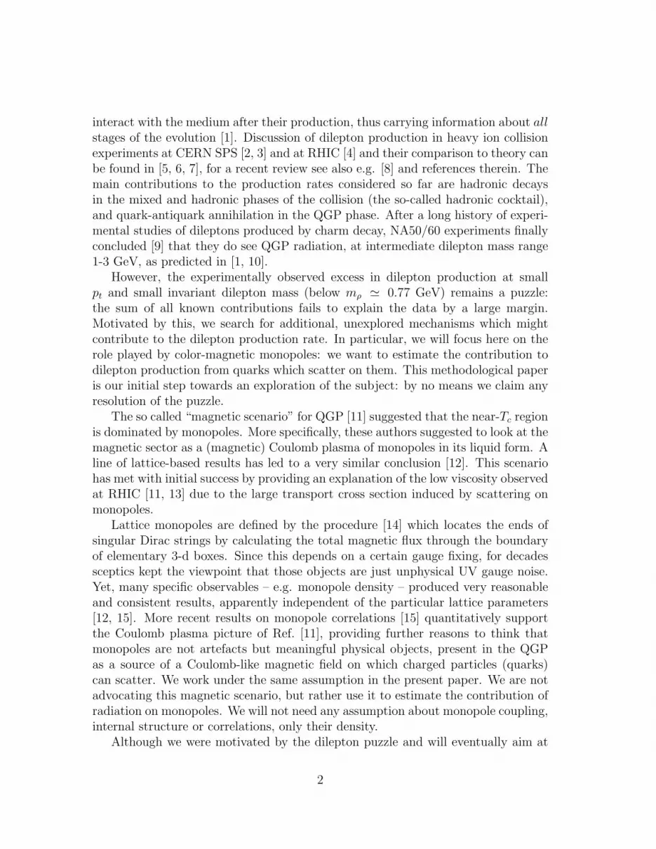
interact with the medium after their production, thus carrying information about allstages of the evolution [1]. Discussion of dilepton production in heavy ion collisionexperiments at CERN SPS [2, 3] and at RHIC [4] and their comparison to theory canbe found in [5, 6, 7], for a recent review see also e.g. [8] and references therein. Themain contributions to the production rates considered so far are hadronic decaysin the mixed and hadronic phases of the collision (the so-called hadronic cocktail),and quark-antiquark annihilation in the QGP phase. After a long history of experi-mental studies of dileptons produced by charm decay, NA50/60 experiments finallyconcluded [9] that they do see QGP radiation, at intermediate dilepton mass range1-3 GeV, as predicted in [1, 10].

However, the experimentally observed excess in dilepton production at smallpt and small invariant dilepton mass (below mρ ' 0.77 GeV) remains a puzzle:the sum of all known contributions fails to explain the data by a large margin.Motivated by this, we search for additional, unexplored mechanisms which mightcontribute to the dilepton production rate. In particular, we will focus here on therole played by color-magnetic monopoles: we want to estimate the contribution todilepton production from quarks which scatter on them. This methodological paperis our initial step towards an exploration of the subject: by no means we claim anyresolution of the puzzle.

The so called “magnetic scenario” for QGP [11] suggested that the near-Tc regionis dominated by monopoles. More specifically, these authors suggested to look at themagnetic sector as a (magnetic) Coulomb plasma of monopoles in its liquid form. Aline of lattice-based results has led to a very similar conclusion [12]. This scenariohas met with initial success by providing an explanation of the low viscosity observedat RHIC [11, 13] due to the large transport cross section induced by scattering onmonopoles.

Lattice monopoles are defined by the procedure [14] which locates the ends ofsingular Dirac strings by calculating the total magnetic flux through the boundaryof elementary 3-d boxes. Since this depends on a certain gauge fixing, for decadessceptics kept the viewpoint that those objects are just unphysical UV gauge noise.Yet, many specific observables – e.g. monopole density – produced very reasonableand consistent results, apparently independent of the particular lattice parameters[12, 15]. More recent results on monopole correlations [15] quantitatively supportthe Coulomb plasma picture of Ref. [11], providing further reasons to think thatmonopoles are not artefacts but meaningful physical objects, present in the QGPas a source of a Coulomb-like magnetic field on which charged particles (quarks)can scatter. We work under the same assumption in the present paper. We are notadvocating this magnetic scenario, but rather use it to estimate the contribution ofradiation on monopoles. We will not need any assumption about monopole coupling,internal structure or correlations, only their density.

Although we were motivated by the dilepton puzzle and will eventually aim at

2

solving it as a final goal, we start from the simpler problem of soft photon radiationduring the collision process. The emission of real photons is a process which is closelyrelated to dilepton production: the latter takes place through the emission of avirtual photon. In the QGP phase, the leading perturbative diagram is the Compton-like process (qg → qγ and the crossing diagram qq → γg), while perturbativelysubleading bremsstrahlung diagrams (qq → qqγ) and LPM-type resummed effectsare in fact equally important [16].

The classical trajectory of a particle with electric charge1 e in the field of aninfinitely heavy monopole with magnetic charge g takes place on the surface of acone. The static monopole approximation is valid for a regime of temperaturesT ∼> 2Tc, where they can be considered heavy, rare objects embedded into matterconsisting mostly of the usual electric quasiparticles, quarks and gluons. The Lorentzforce acting on the electric charge is proportional to the product of both couplings(eg). Thanks to the Dirac charge quantization condition, eg = 1 and thus it is nota small parameter and it is T -independent.

As a first step towards the solution of the problem, in the present paper wecompute the radiation from a non-relativistic electrically charged particle movingin the field of a monopole along the classical trajectory, ignoring back reaction. Afull quantum and relativistic study is postponed for future investigation. Below wewill discuss the applicability limits of our approximation. Therefore, our presentcalculation cannot address the actual phenomenological questions yet, but we canget an insight into how sizeable the effect of monopoles can be. To this purpose, wewill compare our results with the parallel computation of photon emission rate inthe process of Coulomb scattering of quarks, in the same approximations, regardingthe Coulomb problem as a benchmark for comparison.

Let us start with a “naive estimate” for the ratio of emission rates of quark-monopole vs Coulomb scattering of quarks:

IqM

Iqq∼ (eg)2v2

e4

µ

m

nMnq. (1)

First, the emission amplitude from monopoles is suppressed by the velocity v of theincoming electric particle, because the underlying scattering happens due to Lorentzrather than Coulomb force. Second, it obviously contains the density of monopolesnM ∼ T 3/ ln3(T ), which is smaller than the quark density nq ∼ T 3.

On the other hand, this rate is enhanced by the ratio of coupling constants.The numerator includes the product of the electric gauge coupling constant e andthe magnetic one g: in the units we are using, the Dirac quantization condition

1Here and below we call e the strong interaction coupling constant, using QED-like field normal-ization of the fields and 4π for consistency with the textbook material we use: note that e2 = αs.The name g is reserved to color-magnetic coupling, while the electromagnetic coupling will bedenoted as eem, again with e2em = αem.

3

implies eg = 1 (actually ~), while the electric Coulomb scattering is proportionalto e2 = αs ∼ 1/ ln(T ) 1. The ln2(T ) in the numerator to a significant extentcompensates the smallness of the monopole density nM ∼ 1/ ln3(T ). Althoughformally still decreasing at large T , as is the corresponding ratio of the contributionsto viscosity [13], large angle and even backward scattering induced by monopolesmay make this ratio numerically enhanced. The reduced mass µ = m/2 enters theCoulomb scattering problem whereas, in the limit of infinite monopole mass, thequark mass m appears in Newton law. There is an additional relative enhancementin favour of monopoles, which is due to the Casimirs of the qq and qq potentials.We will work out these factors in the following; they roughly bring a factor 1/4compared to the q −M scattering. For typical (thermal) velocity of 0.7, αs = 0.8,and the ratio of densities 0.2 we end up with a relative effect of order 1/2. Thisis obviously a good start, suggesting it is worth to examine the problem in moredetails.

We will see below that the above crude estimate is indeed correct when the veloc-ity of quarks is sufficiently close to one (we will still be using the non-relativistic ap-proximation); it is also correct in the ultrarelativistic limit. There is, however, a veryimportant effect, which noticeably enhances the relative contribution of monopoles.The above estimate holds for a fixed impact parameter. For soft radiation, only emis-sion from large impact parameters is relevant (and this is the only region where ourapproximations are in fact valid). However, finite densities of quarks and monopolesin the plasma provide natural cutoffs for maximal impact parameters. Moreover,since the density of monopoles in our temperature regime is much smaller thanthe density of quarks, the relevant upper cutoff on the impact parameter for theCoulomb problem is much smaller and it leads to a significant suppression of theCoulomb-induced emission rate relatively to the rate due to scattering on monopoles.

Our final results are very encouraging. We find that the soft photon emission ratefrom quark-monopole scattering could be as large as the mechanisms previously ac-counted for. Therefore, the problem calls for further and more detailed investigationat the full quantum level, which will be our next step in this project.

The paper is organized as follows. In Section 2 we provide a brief overviewof the classical motion of an electric charge in a Coulomb magnetic field: even ifthese results are well-known, a short summary is useful, since we will make largeuse of them in the following. In Section 3 we compute the photon radiation ratefor an electric particle moving in the field of a static monopole. This section canbe regarded as an extra chapter for Ref. [17], in which radiation rates for severaltrajectories were computed. In Section 4 we present an estimate of our effect inthe case of quarks scattering on monopoles in the QGP: we use parameter estimateswhich are typical of the QGP produced at RHIC. We compare our results with thoseobtained in the Coulomb problem, and discuss the validity of our approximations.We draw our conclusions in the last Section (5), where we also indicate future

4

improvements. Appendix A supplements Section 3 by providing details of analyticalcomputations for the emission rate. Appendix B presents a calculation of the quarkdensity in the PNJL model, a result which is needed when we apply our calculationsto QGP.

2 Classical quark-monopole scattering

We consider the classical, non-relativistic motion of a charge in an external field[18, 19, 20]. A pointlike magnetic charge g is the source of a Coulomb-like magneticfield

~B = g~r

r3. (2)

The equation of motion of an electrically charged particle e in such a field is

md2~r

dt2= e~v × ~B =

eg

r3

d~r

dt× ~r; (3)

the static monopole is located at the origin and the vector ~r defines the position ofthe electric charge (see Fig. 1). In the following, we set c = 1 for simplicity. Wealso use the convention e2 = α, and therefore eg = 1.

In this process, the kinetic energy of the electric charge is a constant:

E =mv2

2= const., (4)

as is the absolute value of the velocity vector v. There is no closed orbit in thecharge-monopole system: the electric charge is falling down from infinitely far away

4 1 Magnetic Monopole in Classical Theory

v

r

-egg!

L

z

re

!

L

Fig. 1.1. Motion of an electric charge in the monopole field

One could obtain the corresponding integrals of motion just by makinguse of (1.2). Scalar multiplication of (1.2) by a vector of velocity v gives:

12

d

dt

!mv2

"= 0 , (1.3)

so that the kinetic energy of an electric charge in a monopole field is a con-stant:

E =mv2

2= const. , (1.4)

as is the absolute value v of the velocity vector.On the other hand, the scalar product of the equation of motion (1.2) and

the radius vector r gives:

r · d2rdt2

! 12

d2

dt2r2 " v2 = 0 .

Taking into account the conservation of energy (1.3), one can write

r =#

v2t2 + b2 , (1.5)

and therefore r · (dr/dt) = r · v = v2t. Thus, there is no closed orbit in thecharge-monopole system: the electric charge is falling down from infinitelyfar away onto the monopole, approaching a minimal distance b and reflectedback to infinity (so-called “magnetic mirror” e!ect).

A very special feature of such a motion is that the conserved angularmomentum is di!erent from the ordinary case. Indeed, one can see that theabsolute value of the vector of ordinary angular momentum

Figure 1: The motion of an electric charge in the field of a magnetic monopole.

5

onto the monopole, approaching a minimal distance b and being reflected back toinfinity. This is evident from the trajectory

r =√v2t2 + b2. (5)

A special feature of such a motion is that the conserved angular momentum is differ-ent from the ordinary case: the absolute value of the ordinary angular momentumis conserved, but its direction is not constant. The generalized angular momentum

~J = [~r ×m~v]− eg~rr

(6)

is an integral of motion. The trajectory of the electric charge does not lie in theplane of scattering orthogonal to the angular momentum; the angle between thevectors ~J and ~r is a constant and the electric charge is moving on the surface of acone whose axis is directed along − ~J with the cone angle θ defined as:

sin θ =mvb√

(mvb)2 + (eg)2, cos θ =

eg√(mvb)2 + (eg)2

. (7)

The velocity of the electrically charged particle is

~v =d~r

dt=

1

mr2

[~J × ~r

]+v2t

rr =

1

mr2

[~J × ~r

]+

v√1 + (b/vt)2

r = ~vϕ × ~r + vrr (8)

where the angular and radial components of the velocity vector are

~vϕ =~J

mr2, vr =

v√1 + (b/vt)2

; (9)

asymptotically we have

vϕ

∣∣∣t=±∞

= 0, vr

∣∣∣t=±∞

= v, (10)

while at the turning point of the path we have

vϕ

∣∣∣t=0

=

√(mvb)2 + (eg)2

mb2, vr

∣∣∣t=0

= 0. (11)

The azimuthal angle ϕ as a function of time can be obtained by integrating theangular velocity:

ϕ =1

sin θarctan

vt

b. (12)

6

!3 !2 !1 0 1 2 30

5

10

15

20

x !GeV!1"

z!GeV

!1 "

(a)

!3 !2 !1 0 1 2 30

5

10

15

20

y !GeV!1"

z!GeV

!1 "

(b)

!2 0 2x !GeV!1"

!20

2y !GeV!1"0

5

10

15

20

z !GeV!1"

(c)

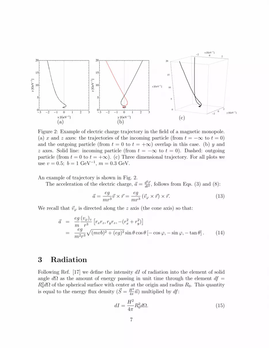
Figure 2: Example of electric charge trajectory in the field of a magnetic monopole.(a) x and z axes: the trajectories of the incoming particle (from t = −∞ to t = 0)and the outgoing particle (from t = 0 to t = +∞) overlap in this case. (b) y andz axes. Solid line: incoming particle (from t = −∞ to t = 0). Dashed: outgoingparticle (from t = 0 to t = +∞). (c) Three dimensional trajectory. For all plots weuse v = 0.5; b = 1 GeV−1, m = 0.3 GeV.

An example of trajectory is shown in Fig. 2.The acceleration of the electric charge, ~a = d2~r

dt2, follows from Eqs. (3) and (8):

~a =eg

mr3~v × ~r =

eg

mr3(~vϕ × ~r)× ~r. (13)

We recall that ~vϕ is directed along the z axis (the cone axis) so that:

~a =eg

m

(vϕ)zr3

[rxrz, ryrz,−(r2

x + r2y)]

=eg

m2r3

√(mvb)2 + (eg)2 sin θ cos θ [− cosϕ,− sinϕ,− tan θ] . (14)

3 Radiation

Following Ref. [17] we define the intensity dI of radiation into the element of solidangle dΩ as the amount of energy passing in unit time through the element df =R2

0dΩ of the spherical surface with center at the origin and radius R0. This quantity

is equal to the energy flux density (~S = H2

4π~n) multiplied by df :

dI =H2

4πR2

0dΩ. (15)

7

The energy dE~nω, radiated into the element of solid angle dΩ in the form of waveswith frequencies in the interval dω/2π is obtained from Eq. (15) by replacing thesquare of the field by the square modulus of its Fourier components and multiplyingby 2:

dE~nω =| ~Hω|2

2πR2

0dΩdω

2π(16)

where~Hω = i~k × ~Aω (17)

and

~Aω =eikR0

R0

∫ +∞

−∞eem~v(t)ei(ωt−

~k·~r(t))dt. (18)

We work in the dipole approximation, namely we neglect retardation effects.This approximation is valid provided that v c. In this case, the field can beconsidered as a plane wave, and therefore in determining the field it is sufficient tocalculate the vector potential. The intensity of the dipole radiation is:

dI =(eem~a)2

4πsin2 θdΩ, (19)

where ~a is the acceleration of the electric charge. Replacing dΩ = 2π sin θdθ andintegrating over θ from 0 to π, we find the total radiation:

I =2

3(eem~a)2. (20)

The quantity dEω of energy radiated throughout the time of the collision in theform of waves with frequencies in the interval dω/2π is obtained from Eq. (20) byreplacing ~a by its Fourier component ~aω and multiplying by 2:

dEω =4

3(eem~aω)2 dω

2π. (21)

In a standard planar collision, the total radiation dκω in a given frequency intervaldω can be obtained by multiplying the radiation dEω from a single particle (withgiven impact parameter ρ) by the measure 2πρdρ and integrating over ρ from ρminto ρmax. In our case, the motion of the electric particle takes place on the surfaceof a cone, therefore we have to find the corresponding measure for our process.

If we project the conical motion of the electric particle on a plane orthogonal to~J , it is possible to define the standard impact parameter ρ for the planar motion[20]. We can define a position vector ~R:

~R =J × (~r × J)

cos θ=

1

cos θ

[~r − J

(~r · J

)], (22)

8

which is the projection of ~r onto the plane perpendicular to ~J , times a factor 1/ cos θ

chosen so that ~R and ~r have the same length. At t = −∞ we have:

~R−∞ =1

cos θ

[~v − J

(~v · J

)]. (23)

The mechanical angular momentum of the projected motion is the same as theconserved total angular momentum of the motion in the monopole field:

~J = m~R× ~R; | ~J | = mρ| ~R−∞|. (24)

From the above Equation we get:

ρ =

√(mvb)2 + (eg)2

mv(25)

from which it is easy to obtain that ρdρ = bdb: the measure over which we needto integrate dEω turns out to be equal to bdb for the conical motion. Therefore, wecan identify b as the real impact parameter for the process that we are considering(b is actually the minimal distance between the electric particle and the monopole,which is reached at t = 0):

dκωdω

=

∫ bmax

bmin

2πbdbdEωdω

. (26)

The limits of integration for b are related to the specific scattering process we aredealing with. For example, if we consider a single quark scattering on a singlemonopole, we have bmax → ∞, while bmin can be identified with the size of themonopole core. In the problem we are considering, in which there is a finite densityof monopoles, bmax turns out to be finite, as we will see in the next Section.

We start by calculating the total radiation throughout the time of the collisionfollowing Eq. (20):

I =

∫ ∞

−∞I(t)dt =

2

3αem

∫ ∞

−∞|~a(t)|2dt; (27)

the acceleration components in the coordinate space are given in Eq. (14). Weobtain:

I(t) =2

3αem

(eg)2v2b2

m2r(t)6=

2

3αem

(eg)2v2b2

m2(v2t2 + b2)3(28)

so that:

I =2

3αem

(eg)2v

m2b3

∫ ∞

−∞

dτ

(τ 2 + 1)3=π

4αem

(eg)2v

m2b3; (29)

9

the total radiation can be obtained in the following way:

κ =

∫ bmax

bmin

2πbdbI =π2

2αem

(eg)2v

m2

(1

bmin− 1

bmax

). (30)

We now proceed by calculating the Fourier transform of the acceleration ~a in thecase of quark-monopole scattering:

(ax)ω = − (eg)2

m2b2vξ

∫ ∞

−∞dt

exp [iωt] cos [ξarctant]

(t2 + 1)3/2(31)

(ay)ω = − (eg)2

m2b2vξ

∫ ∞

−∞dt

exp [iωt] sin [ξarctant]

(t2 + 1)3/2(32)

(az)ω = −(eg)2

mbξ

∫ ∞

−∞dt

exp [iωt]

(t2 + 1)3/2(33)

where

ξ =

√(mvb)2 + (eg)2

mvb, ω = ω

b

v. (34)

For positive ω we obtain (see Appendix A):

(ax)ω =(eg)2

m2b2vξ

exp (−ω) cos

(πξ

2

)[1

4Γ

(1

2(ξ − 1)

)U

(1

2(ξ − 1) ,−1, 2ω

)

+4p!Γ

(−p+ ξ+3

2

)

ξ2 − 1

p∑

k=0

(−ω)k

k! (p− k)!Γ(ξ−3

2− p+ k + 1

) × (35)

× 2k−2Γ

(p− ξ + 1

2

)U

(p− ξ + 1

2, k − 1, 2ω

)]

(ay)ω = − (eg)2

m2b2vξ

i exp (−ω) cos

(πξ

2

)[1

4Γ

(1

2(ξ − 1)

)U

(1

2(ξ − 1) ,−1, 2ω

)

− 4p!Γ(−p+ ξ+3

2

)

ξ2 − 1

p∑

k=0

(−ω)k

k! (p− k)!Γ(ξ−3

2− p+ k + 1

) × (36)

× 2k−2Γ

(p− ξ + 1

2

)U

(p− ξ + 1

2, k − 1, 2ω

)]

(az)ω = −2egω

mbξK1 (ω) , (37)

10

where p is the smallest integer number larger than (ξ + 3)/2. p − 2 is the numberof full rotations around z axis. U(a, b, z) is the confluent hypergeometric functionwith integral representation:

U(a, b, z) =1

Γ(a)

∫ ∞

0

e−ztta−1(1 + t)b−a−1dt (38)

and Kn(z) is the modified Bessel function of the second kind:

Kn(z) =Γ(n+ 1

2)(2z)n√π

∫ ∞

0

cos t dt

(t2 + z2)n+1/2. (39)

Equations (35)-(36) are strictly valid for ω ≥ 0 and for any value of ξ, except odd,integer numbers. When ξ is an odd integer number, the above formulas vanishidentically, and the integral is given by Eq. (65) (see Appendix A). The behavior of(ax)ω, (ay)ω and (az)ω as functions of ω and b is shown in the two panels of Fig. 3.The component (ay)ω is purely imaginary and vanishes at ω = 0. The values of theacceleration components at ω = 0 are:

(ax)ω=0 =2v

ξcos

[πξ

2

]; (ay)ω=0 = 0 ; (az)ω=0 = − (eg)

mbξ. (40)

The subleading small ω asymptotic behavior can be found in Appendix A. Thephoton emission rate is finite as ω → 0. It is of course how it should be: thecorresponding number of photons dNω = dIω/~ω would show standard logarithmicIR divergence.

4 Application to QGP

In this Section we give a rough estimate of the effect that we are describing, inthe case in which the electric charge is a quark q (or an antiquark q), scatteringon a color-magnetic monopole in a deconfined medium. The medium contains afinite density of quarks and monopoles. We will compare our result to the radiationproduced from Coulomb scattering of qq, qq and qq pairs. We consider a regime oftemperatures ∼> 2 Tc where, according to the magnetic scenario proposed in [11],monopoles can be considered as heavy, static particles.

A quark moving in a deconfined medium acquires a thermal mass due to itsinteraction with the other particles of the medium. Lattice results for this quantityare available for three values of the temperature [21, 22]. At T = 1.5Tc and T = 3Tcthey find m = 0.8T , while at T = 1.25Tc they obtain m = 0.77T . At T = 2Tcwe therefore assume a value of m ' 0.8T , namely m ' 0.3 GeV. For temperaturesT ' 2Tc, we can assume that quarks move with an average velocity v ∼ 0.5− 0.7.

11

!ax"!"!#!ay"!$!az"!

0 1 2 3 4 5 6#3

#2

#1

0

1

! #GeV$

a

(a)

!ax"!"!#!ay"!$!az"!

0.0 0.5 1.0 1.5 2.0#1.5

#1.0

#0.5

0.0

0.5

b #GeV#1$a

(b)

Figure 3: (a): Fourier components of the acceleration as functions of ω, for m = 0.3GeV, b = 1 GeV−1, v = 0.7. (b): Fourier components of the acceleration as functionsof b, for m = 0.3 GeV, ω = 0.1 GeV, v = 0.7.

0 2 4

b @GeV-1D

0.0

0.2

0.4

Ω @GeVD

0.00

0.02

0.04

0.06

2Π b dEΩ dΩ @GeV-1D

Figure 4: Integrand 2πbdEω/dω as a function of ω and b. In this figure, m = 0.3GeV and v = 0.7.

12

a

Figure 5: A charge scattering on a 2-dimensional array of correlated monopoles(open points) and antimonopoles (closed points). The dotted circle indicates aregion of impact parameters for which scattering on a single monopole is a reasonableapproximation.

In Figure 4 we show the integrand for the total radiation in a given frequencyinterval, namely 2πbdEω/dω, as a function of ω and b. We need to integrate thisquantity over the impact parameter. There is no upper limit on b in the case ofscattering of one quark on one monopole. However, in matter there is a finitedensity of monopoles, so the scattering issue should be reconsidered. A sketch ofthe setting, assuming strong correlation of monopoles into a crystal-like structure,is shown in Fig. 5. A “sphere of influence of one monopole”(the dotted circle) givesthe maximal impact parameter to be used

bmax = n−1/3M /2. (41)

The same is true for the quark-quark and quark-antiquark Coulomb scatteringto which we will compare our results. The monopole density as a function of thetemperature for SU(2) gauge theory has been evaluated on the lattice [15]. In orderto account for the transition from SU(2) to SU(3) gauge group, we scale theseresults by a factor 2: in SU(2) there is in fact one monopole species while in SU(3)there are two, identified by two different U(1) subgroups. The monopole density atT ' 2Tc is nM ' 0.02 GeV3, which gives bmax ' 1.8 GeV−1. The lattice also givesus information about the monopole size [23]: they turn out to be very small objects,having a radius rM ' 0.15 fm=0.78 GeV−1. This is the bmin that we will use in ourintegration.

We therefore obtain, for the total energy radiated in unit volume throughout thetime of the collision in a given frequency interval:

dΣ

dω=

2

9

dκωdω

nqnM =2

9nqnM

2

3παem2π

∫ bmax

bmin

b|~aω|2db (42)

13

where the factor 29

= 13(4

9+ 1

9+ 1

9) comes from the different electric charges fur u, d

and s quarks (the density of quarks nq is the sum of the densities of u, d and squarks).

4.1 Comparison with Coulomb scattering

In this Section we give an estimate of the radiation produced in the scattering ofqq, qq and qq pairs in the plasma. In the case of an attractive interaction betweenparticles (namely in the singlet channel for the qq scattering and the antitripletchannel for the qq and qq scatterings), the formula for dEω/dω reads [17]:

dEωdω

=2πα2ω2

3v4

((eem)1

m1

− (eem)2

m2

)2[H

(1)′iν (iνε)

]2

+ε2 − 1

ε2

∣∣∣H(1)iν (iνε)

∣∣∣2

(43)

where:

ν =ωα

µv3, ε =

√1 +

µ2b2v4

α2, µ =

m1m2

m1 +m2

(44)

and H(1)iν (iνε) is the Hankel function of the first kind:

H(1)n (z) = Jn(z) + iYn(z). (45)

In Eq. (43), (eem)1, m1 and (eem)2, m2 are the electric charge and mass of the twocolliding particles, while α = CR αs is the strong coupling constant multiplied bythe corresponding Casimir factor CR for the channel under study:

C8 = 4/3 ; C1 = 1/6 ; C6 = 2/3 ; C 3 = 1/3 .

When the interaction is repulsive (namely in the octet channel for the qq scattering,and in the sextet channel for the qq and qq scatterings), Eq. (43) gets modified asfollows:

dEωdω

=2πα2ω2

3v4

((eem)1

m1

− (eem)2

m2

)2[H

(1)′iν (iνε)

]2

+ε2−1

ε2

∣∣∣H(1)iν (iνε)

∣∣∣2

exp [−2πν] . (46)

We consider quark matter with three equal mass light flavors, namely m1 = m2 =m; µ = m/2. The total density of quarks and antiquarks can be obtained forexample from the PNJL model (see Appendix B).

nq ' 2.8T 3 ' 0.12 GeV3.

14

The total energy radiated in unit volume throughout the time of the collision in thecase of Coulomb scattering can be obtained from the following formula:

dΣ

dω=

4π2αemω2

3v4

n2q

182

4

m2

∫ bmax

0

[(4

3αs

)2

f

(4

3αs

)+ 8

(1

6αs

)2

f

(1

6αs

)exp[−2πναs/6]

+ 3

(2

3αs

)2

f

(2

3αs

)+ 6

(1

3αs

)2

f

(1

3αs

)exp[−2πναs/3]

]bdb, (47)

where

f(α) =[H

(1)′iν (iνε)

]2

+ε2 − 1

ε2

∣∣∣H(1)iν (iνε)

∣∣∣2

. (48)

Eq. (47) is the total radiated energy, it takes into account all possible color chan-nels for qq, qq and qq scatterings, and all possible flavor combinations. bmax canbe estimated directly from the quark density: in our temperature regime, it turnsout that bmax ' 1 GeV−1. Our results for the ratio of the total energy radiatedthroughout the collision time in the case of quark-quark and quark-monopole scat-tering are shown in Figs. 6. The left panels show this ratio for bmax → ∞, whilein the right panels bmax is finite and fixed by the corresponding densities. This isuseful to understand how strongly a finite bmax influences our results: it turns outthat the cutoff dependence of dΣ/dω is dramatic. Without cutoff, this quantity ismuch larger in the case of a Coulomb scattering, while the opposite is true in thecase of a finite bmax. This effect is qualitatively true for all values of v that we haveconsidered, but obviously the relative magnitude for qq and qM scatterings dependson the specific value of v that we choose.

4.2 Validity of our approximations

Our results are obtained through a series of approximations:

• non-relativistic approximation: this is obviously valid if the velocity v of quarksis not too large compared to the speed of light, namely v 1;

• dipole approximation vs retarded emission. It is valid if the radiation wave-length is large. The retardation effects can be neglected in cases where thedistribution of charge changes little during the time a/c, where a is the orderof magnitude of the dimensions of the system. This is true if v 1, whichcoincides with the condition for the non-relativistic approximation;

• classical trajectory is used, without back reaction of radiation: in all our for-mulas, we assume that the particle moves along a trajectory which is thesolution of the classical equations of motion. This means that the energy lostby the particle through the radiation process is negligible. This approximationis valid in the limit ω m/e2;

15

0.00 0.05 0.10 0.150

10

20

30

40

50

60

70

! !GeV"

#d"$d!% qq$#d

"$d!%qM

(a)

0.00 0.05 0.10 0.150.0

0.5

1.0

1.5

2.0

2.5

3.0

! !GeV"

#d"$d!% qq$#d

"$d!%qM

(b)

0.00 0.05 0.10 0.150

5

10

15

20

! !GeV"

#d"$d!% qq$#d

"$d!%qM

(c)

0.00 0.05 0.10 0.150.0

0.2

0.4

0.6

0.8

1.0

! !GeV"

#d"$d!% qq$#d

"$d!%qM

(d)

0.00 0.05 0.10 0.150

1

2

3

4

5

6

! !GeV"

#d"$d!% qq$#d

"$d!%qM

(e)

0.00 0.05 0.10 0.150.0

0.2

0.4

0.6

0.8

1.0

! !GeV"

#d"$d!% qq$#d

"$d!%qM

(f)

Figure 6: Left column: ratio of dΣ/dω for Coulomb and quark-monopole scattering.In both cases, the integral over b is taken up to ∞. For these plots we use αs =0.8, m = 0.3 GeV and: (a) v = 0.3, (c) v = 0.5, (e) v = 0.7. Right column: sameas in the left column, but the integral over b is taken up to the corresponding bmax.For these plots we use αs = 0.8, m = 0.3 GeV and: (b) v = 0.3, (d) v = 0.5, (f)v = 0.7.

16

• classical approximation: naively, the emission of soft photons can be describedclassically for

~ω Ek = µ v2/2 = mv2/4.

Within the same approximation we can ignore the recoil effect (energy-momentumconservation).

The full quantum treatment of the radiation should include the back reactionof the radiation, one has to evaluate the nondiagonal matrix element of thedipole moment between the initial and final scattering states, with differentenergies. Such quantum states for quark-monopole problem were found in[24] and recently for gluon-monopole problem in [13]. However, the matrixelements have not been computed yet. Since it was done for quantum Coulombscattering, by A.Sommerfield in 1931, we can use those results in order to haveat least some qualitative estimate for the accuracy of classical description.

We compare the total radiation dκω in a given frequency interval dω, in thecase of scattering on a single particle, namely we integrate over the impactparameter b from 0 to ∞. In the classical case we have:

dκωdω

=32π2ωαemα

3s

3m3v5

∣∣∣H(1)iν (iν)

∣∣∣H(1)′iν (iν) (49)

which is to be compared to the quantum expression [25]:

d κ(ω)

dω= αem α

2s

64 π2

3

p′

p

1

(p − p′)2

1

(1 − e−2π β′) (e2π β − 1)

(− d

dξ|F (ξ)|2

)

(50)

where

β =αsv

β′ =αsv′

mv = 2 p mv′ = 2 p′ p′ =√p2 − mω

and

F (ξ) ≡ 2F1(i β′, i β; 1; ξ) ξ = − 4 p p′

(p − p′)2

2F1(a, b; c; d) is the Hypergeometric function. The two curves corresponding toclassical and quantum scatterings are shown in Fig. 7. It is thus evident thatwithin the energy region plotted the classical result is a very good approxima-tion of the quantum one. Note that there is a maximum ω, which is equal tothe energy of the incoming particle beyond which due to energy conservationthe quantum formula are not applicable.

17

classic

quantum

0.00 0.01 0.02 0.03 0.04

5

10

15

20

25

30

! !GeV"

d"!#d!!G

eV#2 "

Figure 7: Comparison between classic and quantum result for dκω/dω as a functionof ω, with αs = 0.8, v = 0.7, m = 0.3 GeV.

• two body vs many body scattering. So far, we have limited our analysis to two-body scattering, while mimicking the effects of multiple interactions by finitequark and monopole densities and the maximal impact parameter. The strongdependence on the maximal impact parameter cutoff observed in our results,reflects additional shortcomings of our approach. The origin of this problem isobvious: on the one hand soft radiation is emitted from large distances; on theother hand, too large distances are precisely governed by multiple scattering.

5 Conclusions and outlook

The present paper is the first step towards understanding whether the contributionof the quark-monopole scattering process in QGP is or is not important for photonand dilepton production. Our purpose at present was pretty modest: we wantedto evaluate the magnitude of soft photon radiation from this process and compareit to the one produced in Coulomb quark-quark scattering. A qualitative estimateoutlined in the Introduction, said that while the monopole density is small at high T ,nm ∼ (1/ ln(T ))3, the square of αs in the electric scattering cross section compensatestwo out of three such logarithms. So, parametrically, the process we consider issubleading at very large ln(T ). On the other hand, the charge-monopole scatteringat large angles and small impact parameter tends to be much larger than the charge-

18

charge one: we found that this enhances radiation, similarly to how it worked fortransport processes [13]. This represents an encouraging starting point for futurework.

We have calculated the photon radiation rate for quarks scattering on monopolesin a thermal medium which contains a finite density of both particles. We workedin the classic, non-relativistic approximation and neglected retardation effects andback reaction. Therefore, our calculation has a rather methodological status, itcannot address the actual phenomenological questions, such as the experimentallyobserved excess in dilepton production at small pt and invariant mass below mρ. Weneed to improve the present paper in many directions: first of all, a full quantumand relativistic calculation will be performed, also taking into account back reactionof the radiation. This can in principle be done using non-diagonal matrix elements,calculated between quantum scattering states such as those which were found in[13, 24].

Then we need to take into account the fireball evolution, in order to be able toquantitatively compare our results to the experimental data. Dramatic expansionof the fireball and long duration of the near-Tc phase leads to the conclusion thatsoft dileptons currently constituting the puzzle come from the end of the evolutionof QGP, T ∼ 1Tc, rather than the beginning of it, in the temperature regime wediscussed above. Unfortunately, the near-Tc region is very complicated and quitechallenging theoretically. In this region monopoles become lighter and thus dynam-ical and relativistic, matter is no longer an electric near-perturbative plasma withat least well-defined counting rules, but a strongly coupled liquid made of all kindof quasiparticles. We hope to address those issues elsewhere in our future work.

Acknowledgments

This work is partially supported by the DOE grants DE-FG02-88ER40388 and DE-FG03-97ER4014 and by the DFG grant SFB-TR/55.

Appendix A

In this Appendix we explicitly calculate the Fourier transform of the ~a components.We start from (ax):

(ax)ω = − (eg)2

m2b2vξ

∫ ∞

−∞

exp [iωt] cos [ξarctant]

(t2 + 1)3/2dt. (51)

If we set t = i+ iτ , dt = idτ . Both the square root and the arctan have branch cutsingularities from τ = 0 to τ =∞ and from τ = −∞ to τ = −2. This is clear if we

19

t

!

"

!

"

#!1

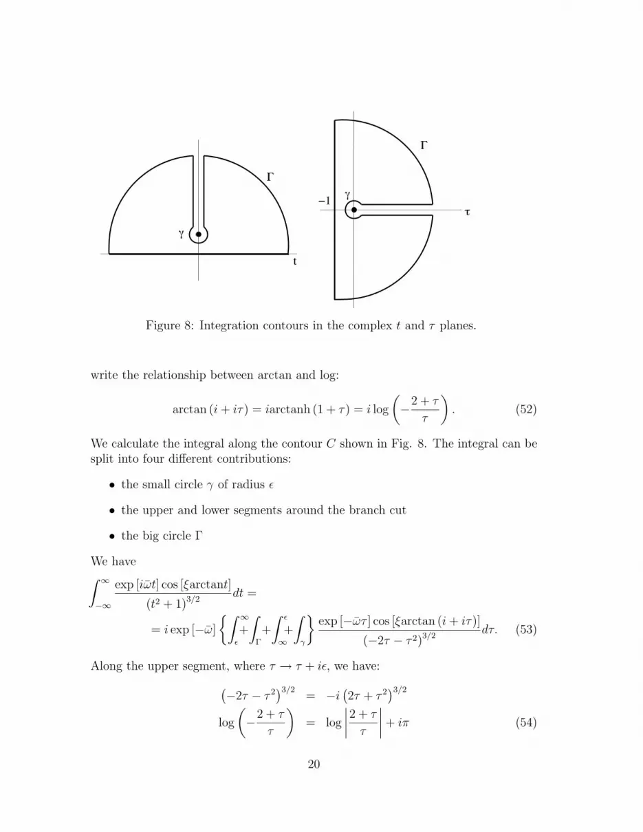
Figure 8: Integration contours in the complex t and τ planes.

write the relationship between arctan and log:

arctan (i+ iτ) = iarctanh (1 + τ) = i log

(−2 + τ

τ

). (52)

We calculate the integral along the contour C shown in Fig. 8. The integral can besplit into four different contributions:

• the small circle γ of radius ε

• the upper and lower segments around the branch cut

• the big circle Γ

We have∫ ∞

−∞

exp [iωt] cos [ξarctant]

(t2 + 1)3/2dt =

= i exp [−ω]

∫ ∞

ε

+

∫

Γ

+

∫ ε

∞+

∫

γ

exp [−ωτ ] cos [ξarctan (i+ iτ)]

(−2τ − τ 2)3/2dτ. (53)

Along the upper segment, where τ → τ + iε, we have:

(−2τ − τ 2

)3/2= −i

(2τ + τ 2

)3/2

log

(−2 + τ

τ

)= log

∣∣∣∣2 + τ

τ

∣∣∣∣+ iπ (54)

20

while along the lower one we have

(−2τ − τ 2

)3/2= i

(2τ + τ 2

)3/2

log

(−2 + τ

τ

)= log

∣∣∣∣2 + τ

τ

∣∣∣∣− iπ. (55)

Therefore we can write:∫ ∞

ε

+

∫ ε

∞

exp [−ωτ ] cos [ξarctan (i+ iτ)]

(−2τ − τ 2)3/2dτ = (56)

∫ ∞

ε

exp [−ωτ ] cos[iξ2

(log∣∣2+ττ

∣∣+ iπ)]

−i (2τ + τ 2)3/2dτ +

∫ ε

∞

exp [−ωτ ] cos[iξ2

(log∣∣2+ττ

∣∣− iπ)]

i (2τ + τ 2)3/2dτ

= 2i cos

(ξπ

2

)∫ ∞

ε

exp [−ωτ ] cos[iξ2

log∣∣2+ττ

∣∣]

(2τ + τ 2)3/2dτ

where we used the relationship

cosα + cos β = 2 cosα + β

2cos

α− β2

. (57)

We therefore have:∫ ∞

ε

+

∫ ε

∞

exp [−ωτ ] cos [ξarctan (i+ iτ)]

(−2τ − τ 2)3/2dτ = (58)

= i cos

(ξπ

2

)∫ ∞

ε

exp [−ωτ ]

(2τ + τ 2)3/2

[(2 + τ

τ

)−ξ/2+

(2 + τ

τ

)ξ/2]dτ.

The above integral contains two terms. The first one gives (in the limit ε→ 0):

i cos

(ξπ

2

)∫ ∞

0

exp [−ωτ ]

(2τ + τ 2)3/2

(2 + τ

τ

)−ξ/2dτ =

= i cos

(ξπ

2

)1

4Γ

[1

2(ξ − 1)

]U

(1

2(ξ − 1) ,−1, 2ω

). (59)

The second term needs to be integrated by parts p times, where p is the smallestinteger number > ξ+3

2. All boundary terms are either divergent or vanishing as

ε → 0. The divergent ones are exactly cancelled by corresponding divergent terms

21

coming from the integral over the small circle γ. The finite part is:

∫ ∞

ε

exp (−ωτ) (2 + τ)(ξ−3)/2

τ (ξ+3)/2dτ =

4Γ(ξ+3

2− p)p!

ξ2 − 1

p∑

k=0

(−ω)k

k!(p− k)!Γ( ξ−32− p+ k + 1)

×

×∫ ∞

0

exp (−ωτ) [2 + τ ](ξ−3)/2−(p−k) τ p−(ξ+3)/2dτ = (60)

=4Γ(ξ+3

2− p)p!

ξ2 − 1

p∑

k=0

(−ω)k

k!(p− k)!Γ( ξ−32− p+ k + 1)

×

× 2k−2Γ

(p− ξ + 1

2

)U

(p− ξ + 1

2, k − 1, 2ω

).

The above contribution vanishes for odd, integer values of ξ. The contributioncoming from Γ vanishes identically, while we get a nonvanishing contribution fromthe integral over the small circle γ. This contribution is divergent for nonintegeror even ξ, exactly cancelling the divergent contribution coming from the segmentsalong the branch cut. When ξ is an odd integer number we get a finite contribution.We redefine t = i+ iε exp(iθ), dt = −ε exp(iθ)dθ and get:

∫

γ

exp [−ωτ ] cos [ξarctan (i+ iτ)]

(−2τ − τ 2)3/2dτ

= −εe−ω∫ 2π

0

eiθe−εωeiθ

cos [ξarctan (i+ iε exp(iθ))]

(−2ε exp(iθ)− ε2 exp(2iθ))3/2dθ

= −εe−ω∫ 2π

0

eiθe−εωeiθ

(−2ε exp(iθ)− ε2 exp(2iθ))3/2cos

[ξ

2ilog

(− εeiθ

2 + εeiθ

)]dθ

=e−ω

2(−ε)1/2

∫ 2π

0

e−iθ/2e−εωeiθ

(2 + ε exp(iθ))3/2

[(− εeiθ

2 + εeiθ

)ξ/2+

(− εeiθ

2 + εeiθ

)−ξ/2]dθ

(61)

For ε→ 0, the first term in the parenthesis gives a finite contribution only for ξ = 1,a value which is never reached in practical cases, as we will see. For ξ > 1 its

22

contribution vanishes identically. The second term gives

e−ω

2(−ε)1/2

∫ 2π

0

e−iθ/2e−εωeiθ

(2 + εeiθ)3/2

(− εeiθ

2 + εeiθ

)−ξ/2dθ =

=e−ω

2

∫ 2π

0

e−2iθe−εωeiθ (

2e−iθ + ε)(ξ−3)/2

(−ε)(ξ+1)/2dθ =

=e−ω

2(−ε)(ξ+1)/2

∫ 2π

0

dθe−2iθ

∞∑

n=0

ωn(−ε)neinθn!

(ξ−3)/2∑

k=0

(2e−iθ)kε(ξ−3)/2−k( ξ−32

)!

k!( ξ−32− k)!

=

=e−ω

2

∫ 2π

0

dθe−2iθ

(ξ−3)/2∑

k=0

ωk+2

(k + 2)!

(−1)k−(ξ−3)/22ke2iθ( ξ−32

)!

k!( ξ−32− k)!

=

=e−ω

22π

(ξ−3)/2∑

k=0

ωk+2

(k + 2)!

(−1)k−(ξ−3)/22k( ξ−32

)!

k!( ξ−32− k)!

(62)

where we have taken into account the fact that the finite contribution from the sumover n comes from n = k + 2. The final result for (ax)ω is therefore

(ax)ω =(eg)2

m2b2vξ

exp (−ω) cos

(πξ

2

)[1

4Γ

(1

2(ξ − 1)

)U

(1

2(ξ − 1) ,−1, 2ω

)

+4p!Γ

(−p+ ξ+3

2

)

ξ2 − 1

p∑

k=0

(−ω)k

k! (p− k)!Γ(ξ−3

2− p+ k + 1

) × (63)

× 2k−2Γ

(p− ξ + 1

2

)U

(p− ξ + 1

2, k − 1, 2ω

)]

(64)

for any value of ξ other than odd-integer, and

(ax)ω =(eg)2

m2b2vξ

e−ω

22π

(ξ−3)/2∑

k=0

ωk+2

(k + 2)!

(−1)k−(ξ−3)/22k( ξ−32

)!

k!( ξ−32− k)!

. (65)

for odd-integer ξ.The component (ay)ω slightly differs from (ax)ω: the sin integration gives a purely

imaginary contribution. The second term in Eq. (63) has a minus sign.

23

The first terms of the components expansion around ω = 0 have the followingassymptotic behavior:

(ax)ω→0 '2v

ξcos

[πξ

2

]+ ω2 b

2(ξ2 − 1)

vξcos

[πξ

2

]− 1

ξ2 − 1

+1

2

[−Harmonicnumber

(p− ξ + 3

2

)− Harmonicnumber

(ξ + 1

2

)(66)

+1

ξ2 − 1

(−3− 2p2 − 2p(ξ − 2)− 2γ

(ξ2 − 1

)+ ξ (4− ξ (−3 + ln 4))

+ ln 4− 2(ξ2 − 1

)lnb

vω

)]+ θ (p− 3)

4p!Γ[−p+ ξ+3

2

]

ξ2 − 1

p∑

k=3

(−1)k(k − 3)!

k!(p− k)!Γ[ξ−3

2− p+ k + 1

]

(ay)ω→0 ' 2ib cos

[πξ

2

]ω

(az)ω→0 ' −(eg)v√

(eg)2 + (mvb)2− ω2

[b2eg

(−1 + 2γ + 2 lnω + 2 ln

(b

2v

))

2v√

(eg)2 + (mvb)2

]

where Harmonicnumber(z) = Ψ(z + 1) + γ and γ is the Euler’s constant and Ψ(z)is the logarithmic derivative of Γ-function.

Appendix B

In this appendix we briefly recall some aspects of the PNJL model [26], which we willthen use to calculate the density of quarks in the medium. This model successfullydescribes QCD thermodynamics in the temperature regime we are interested in, bycoupling quarks to the chiral condensate and to a temporal background gauge fieldrelated to the Polyakov loop. The Euclidean action of the three-flavor PNJL modelis

SE(ψ, ψ†, φ) =

∫ β=1/T

0

dτ

∫

V

d3x[ψ† ∂τ ψ +H(ψ, ψ†, φ)

]− V

TU(φ, T ). (67)

Here H is the fermionic Hamiltonian density given by:

H = −iψ† (~α · ~∇+ γ4m0 − φ)ψ + V(ψ, ψ†) , (68)

where ψ is the Nf = 3 quark field, ~α = γ0 ~γ and γ4 = iγ0 in terms of the standardDirac γ matrices and m0 = diag(m0u,m0d,m0s) is the current quark mass matrix.

24

V(ψ, ψ†) contains two parts: a four-fermion interaction acting in the pseudoscalar-isovector/scalar-isoscalar quark-antiquark channel, and a six-fermion interactionwhich breaks UA(1) symmetry explicitly:

V(ψ, ψ†

)= − G

2

∑

f=u,d,s

[(ψfψf

)2+(ψf iγ5~τ ψf

)2]

+K

2

[deti,j

(ψi (1 + γ5)ψj

)+ det

i,j

(ψi (1− γ5)ψj

)](69)

Quarks move in a background color gauge field φ ≡ A4 = iA0, where A0 =δµ0 gAµa ta with the SU(3)c gauge fields Aµa and the generators ta = λa/2. Thematrix valued, constant field φ relates to the (traced) Polyakov loop as follows:

Φ =1

Nc

Tr

[P exp

(i

∫ β

0

dτA4

)]=

1

3Tr eiφ/T . (70)

The thermodynamic potential of the system is:

Ω (T, µ) = U (Φ, T ) +σ2u,d

2G+σ2s

4G− K

4G3σ2u,dσs (71)

−2∑

f

T

∫d3p

(2π)3

ln[1 + Φe−(Ep,f−µf)/T + Φe−2(Ep,f−µf)/T + e−3(Ep,f−µf)/T

]

+ ln[1 + Φe−(Ep,f−µf)/T + Φe−2(Ep,f−µf)/T + e−3(Ep,f−µf)/T

]+ 3

Ep,fT

θ(Λ2 − ~p 2

).

where

σi = 2G〈ψiψi〉, µf = −µf , Ep,f =√~p 2 +m2

f , mi = m0i−σi−K

4G2σjσk.

(72)By minimizing the thermodynamic potential one can obtain the behavior of thechiral condensates σi and of the Polyakov loop Φ as functions of the temperatureand chemical potential. After this procedure, one is able to evaluate many thermo-dynamic quantities. For example, the quark density we are interested in is the sumof the densities of quarks and antiquarks and can be obtained through the followingformula:

nq =∂Ω

∂µf+∂Ω

∂µf(73)

25

0.0 0.1 0.2 0.3 0.40.0

0.5

1.0

1.5

2.0

2.5

T !GeV"

n q#T3

Figure 9: Total quark density as a function of the temperature (PNJL model result).

and it has the following explicit form:

nq=Nf

π2T 3

∫ [3 exp[µ/T ] (exp[2µ/T ] + Φ exp[2Ep/T ] + 2Φ exp[(Ep + µ)/T ])

exp[3Ep/T ] + exp[3µ/T ] + 3Φ exp[(2Ep + µ)/T ] + 3Φ exp[(Ep + 2µ)/T ]

+3 (1 + Φ exp[2(Ep + µ)/T ] + 2Φ exp[(Ep + µ)/T ])

1 + exp[3(Ep + µ)/T ] + 3Φ exp[2(Ep + µ)/T ] + 3Φ exp[(Ep + µ)/T ]

]p2dp (74)

We show the behavior of quark density in Fig. 9, for typical PNJL model parameterstaken from the last paper of Ref. [26].

References

[1] E. V. Shuryak, Phys. Lett. B 78, 150 (1978) [Sov. J. Nucl. Phys. 28, 408.1978YAFIA,28,796 (1978 YAFIA,28,796-808.1978)].

[2] G. Agakichiev et al. [CERES Collaboration], Eur. Phys. J. C 41, 475 (2005)[arXiv:nucl-ex/0506002].

[3] G. Usai et al. [NA60 Collaboration], Eur. Phys. J. C 43, 415 (2005).

[4] S. Afanasiev et al. [PHENIX Collaboration], arXiv:0706.3034 [nucl-ex];A. Adare et al. [PHENIX Collaboration], arXiv:0804.4168 [nucl-ex].

[5] K. Dusling and I. Zahed, Nucl. Phys. A 825, 212 (2009) [arXiv:0712.1982[nucl-th]].K. Dusling, arXiv:0901.2027 [nucl-th].

26

[6] S. Turbide, C. Gale, E. Frodermann and U. Heinz, Phys. Rev. C 77, 024909(2008) [arXiv:0712.0732 [hep-ph]].

[7] R. Rapp, J. Wambach and H. van Hees, arXiv:0901.3289 [hep-ph].H. van Hees and R. Rapp, Nucl. Phys. A 827, 341C (2009) [arXiv:0901.2316[nucl-th]].

[8] K. O. Lapidus and V. M. Emelyanov, Phys. Part. Nucl. 40, 29 (2009).

[9] R. Arnaldi et al. [NA60 Collaboration], Eur. Phys. J. C 59, 607 (2009)[arXiv:0810.3204 [nucl-ex]].

[10] R. Rapp and E. V. Shuryak, Phys. Lett. B 473, 13 (2000) [arXiv:hep-ph/9909348].

[11] J. Liao and E. Shuryak, Phys. Rev. C 75, 054907 (2007) [arXiv:hep-ph/0611131].

[12] M. N. Chernodub and V. I. Zakharov, Phys. Rev. Lett. 98, 082002 (2007)[arXiv:hep-ph/0611228].

[13] C. Ratti and E. Shuryak, Phys. Rev. D 80, 034004 (2009) [arXiv:0811.4174[hep-ph]]. C. Ratti, arXiv:0907.4353 [hep-ph].

[14] T. A. De Grand, D. Toussaint, Phys, Rev. D 22, 2478 (1980).

[15] A. D’Alessandro and M. D’Elia, Nucl. Phys. B 799, 241 (2008)[arXiv:0711.1266 [hep-lat]].

[16] P. Aurenche, F. Gelis, R. Kobes and H. Zaraket, Phys. Rev. D 58, 085003(1998) [arXiv:hep-ph/9804224]; F. Gelis, Nucl. Phys. A 698, 436 (2002)[arXiv:hep-ph/0104067]; P. Aurenche, F. Gelis, G. D. Moore and H. Zaraket,JHEP 0212, 006 (2002) [arXiv:hep-ph/0211036].

[17] L. D. Landau, E. M. Lifshitz “TEXTBOOK ON THEORETICAL PHYSICS.VOL. 2: CLASSICAL FIELD THEORY.

[18] Y. M. Shnir, Berlin, Germany: Springer (2005) 532 p

[19] K. A. Milton, Rept. Prog. Phys. 69, 1637 (2006) [arXiv:hep-ex/0602040].

[20] D. G. Boulware, L. S. Brown, R. N. Cahn, S. D. Ellis and C. k. Lee, Phys.Rev. D 14, 2708 (1976).

[21] F. Karsch and M. Kitazawa, Phys. Lett. B 658, 45 (2007) [arXiv:0708.0299[hep-lat]].

27

[22] F. Karsch and M. Kitazawa, arXiv:0906.3941 [hep-lat].

[23] E. M. Ilgenfritz, K. Koller, Y. Koma, G. Schierholz, T. Streuer, V. Weinbergand M. Quandt, PoS LAT2007, 311 (2007) [arXiv:0710.2607 [hep-lat]].

[24] Y. Kazama, C. N. Yang and A. S. Goldhaber, Phys. Rev. D 15, 2287 (1977).

[25] B Berestetskii, L. P. Pitaevskii, and E.M. Lifshitz, “TEXTBOOK ON THE-ORETICAL PHYSICS. VOL. 4: Quantum Electrodynamics”

[26] P. N. Meisinger, T. R. Miller, and M. C. Ogilvie, Phys. Rev. D 65, 034009(2002); P. N. Meisinger, M. C. Ogilvie and T. R. Miller, Phys. Lett. B 585,149 (2004); K. Fukushima, Phys. Lett. B 591, 277 (2004); C. Ratti, M. A.Thaler and W. Weise, Phys. Rev. D73, 014019 (2006); S. Roessner, C. Rattiand W. Weise, Phys. Rev. D75, 034007 (2007).

28