radiant ignition of new zealand upholstered furniture

ISSN 1173-5996

Radiant Ignition of New Zealand Upholstered Furniture Composites

by

Flora F Chen

Supervised by

Dr Charley Fleischmann

Fire Engineering Research Report 01/2

March 2001

This report was presented as a project report as part of the M.E. (Fire) degree at the University of Canterbury

School of Engineering University of Canterbury

Private Bag 4800 Christchurch, New Zealand

Phone 643 364-2250 Fax 643 364-2758

www.civil.canterbury.ac.nz

ABSTRACT

This experimental research evaluates the radiant ignitability of New Zealand

upholstered furniture composites using the ISO Ignitability Test (IS05657). It is a

part of a larger research project on the combustion of domestic upholstered furniture

at the University of Canterbury.

The project aims to predict the ignition time of New Zealand upholstered furniture

composites. Fourteen fabrics, one of which was fire retardant cotton, were chosen for

testing according to their compositions and content. They represented the most

common used fabrics in the manufacture of upholstered furniture in New Zealand.

One foam was chosen as it is the most commonly used foam for domestic and

commercial furniture. In total, the study tested fourteen types of fabric-foam

combination composites, of which there were 750 specimens in this project.

The time-to-ignition data are presented in a statistical way with mean, maximum,

minimum, standard deviation and included the ratio of standard deviation to mean.

The Flux Time Product concept and linearized thermal ignition model were applied

to predict the time-to-ignition, the critical heat flux for ignition and the ignition

temperature for the fabric foam composites. Predicting the ignition of upholstery

composites by applying the thermally thin theory obtains a reasonably good

comparison to the measured ignition data. Therefore, it is applicable to apply the

thermally thin theory in engineering calculations and design. The prediction by the

thermally thick theory is not as accurate as that by the thermally thin theory.

In this research, it was found that Flux Time Product index is smaller than 1.0 for

melting fabrics and greater than 1.0 for charring fabrics, when the best-fit linear

correlation is achieved. There needs to be further research to justify these values for

the FTP index for the fabric-foam composites.

11 Abstract

The ignition data obtained by the ISO Ignitability Apparatus in this study was

compared with that obtained from previous research in the Cone Calorimeter. The

comparison shows that the two test methods have a good agreement.

ACKNOWLEDGEMENTS

I would like to sincerely show appreciation to the following persons who have helped

me during this project.

Firstly, I am extremely grateful to my supervisor Dr. Charles Fleischmann for his

continued support and direction. His friendly encouragement and technical guidance

at all stages have been a driving force of the progress throughout this research. His

direction challenged my mind in analysis that it is demanding and educational and it

will benefit me in my future career.

Thanks to Dr. Andrew Buchanan for his time management and reporting advice.

Sincere gratitude to my lecturer Mr. Michael Spearpoint for his time and advice all

the way through both technique in fire engineering and computer skills.

Thanks to Grant Dunlop, Colin Bliss, Frank Greenslade and Ian Sheppard, for their

assistance, while conducting the ignitability tests.

Appreciation to the New Zealand Fire Service comm1ss10n for their financial

contribution.

Appreciation to the staff of the Engineering Library, in particular Christine Mckee,

for their friendly assistance in information searching.

Thanks to Mr. Barry Rea for his grammar and proofreading correction to my report

writing.

Lastly, I would like to thank my husband and my two lovely children for their

understanding, which make all this possible.

TABLE OF CONTENTS

ABSTRACT ................................................................................................................. i

ACKNOWLEDGEMENTS ..................................................................................... iii

TABLE OF CONTENTS ........................................................................................... v

LIST OF FIGURES ................................................................................................ viii

LIST OFT ABLES ................................................................................................... .. xi

NOMENCLATURE ............................................................................................... xiii

Chapter One

INTRODUCTION ...................................................................................................... 1

1.1 IMPETUS FOR THIS RESEARCH ........................................................................... 1

1.2 THE OBJECTIVES OF THIS PROJECT .................................................................... 2

1.3 OUTLINE OF THIS REPORT"" ........ "" ................ " .......... " .................. "."." ......... 2

Chapter Two

LITERATURE SURVEY .......................................................................................... 4

2.1 BACKGROUND OF IGNITABILITY MEASUREMENT ............................................. .4

2.2 THE ISO IGNITABILITY TEST VERSUS THE CONE CALORIMETER ...................... 6

2. 2.1 Test apparatus .......................................................................................... 6

2.2.2 Test method ............................................................................................... 8

2.2. 3 Comparison of measurement results ........................................................ 9

2.3 SIMPLE THERMAL THEORY ............................................................................. 12

2.3.1 Assumption of the theory ........................................................................ 12

2. 3. 2 Thermal thickness .................................................................................. . 12

2.3.3 The critical irradiance ( q;) and the ignition temperature (Tig) ............ 13

2.3.4 Correlating ignition data using the Flux Time Product (FTP) .............. 13

2.3.5 Correlating ignition data by Mikkola and Wichman method ................. 14

2. 3. 5 .1 General integral model ....................................................................... 15

2.3.5.2 Linearized thermal ignition model ..................................................... 16

VI Table of Contents

Chapter Three

MATERIALS AND EXPERIMENTS ................................................................... 18

3.1 THE ISO IGNITABILITY APPARATUS .............................................................. 18

3.2 MATERIALS ................................................................................................... 19

3.2.1 Criteria ofmaterial selection ................................................................. 19

3.2.2 Foams ..................................................................................................... 20

3.2.3 Fabrics ................................................................................................... 20

3.3 SPECIMEN CONSTRUCTION AND PREPARATION ............................................... 21

3.4 TEST PROCEDURE ........................................................................................... 27

Chapter Four

ANALYSIS AND RESULTS ................................................................................... 30

4.1 CHARACTERISTIC OF FABRICS ........................................................................ 30

4.2 TIME TO IGNITION RESULTS ............................................................................ 32

4.2.1 General observations ............................................................................. 33

4. 2. 2 Observations for individual type of composite ....................................... 3 7

4.3 CORRELATIONS OF TIME-TO-IGNITION DATA .................................................. 37

4.4 PREDICTING TIME-TO-IGNITION AND THE CRITICAL HEAT FLUX ..................... 40

4.4.1 Analysis time-to-ignition using the Flux Time Product (FTP) ............... 40

4.4.2 Analysis time-to-ignition using the linearized

thermal ignition model ........................................................................... 41

4.4.2.1 The thermally thin model.. ................................................................. 41

4.4.2.2 The thermally thick model ................................................................. 43

4. 4. 3 Prediction results for time-to-ignition ................................................... 44

4.4. 4 Prediction results for the critical heat flux ............................................ 48

4.5 PREDICTING THE EFFECTIVE IGNITION TEMPERATURE .................................... 51

Chapter Five

DISCUSSION ........................................................................................................... 56

5.1 CHARACTERISTICS OF FABRICS ...................................................................... 56

5.2 IGNITION MODES ............................................................................................ 56

5.3 TIME TO IGNITION .......................................................................................... 57

5.3.1 Time to ignition versus incident irradiance ........................................... 57

5.3.2 Influence offabric .................................................................................. 58

Table of Contents Vll

5.3.3 Influence of air flow ................................................................................ 59

5.4 APPLICABILITY OF SIMPLE THERMAL THEORY ................................................ 59

5.5 THE CRITICAL HEAT FLUX, q;,. ....................................................................... 63

5.5.1 The critical heat flux q;,. and the minimum heat flux q~un .................... 63

5. 5. 2 Comparison with the Cone Calorimeter results ..................................... 64

5.5.3 The critical heat flux q;,. versus material properties pL0 c .................... 66

5.6 THE EFFECTIVE IGNITION TEMPERATURE ........................................................ 67

5.7 ENGINEERING APPLICATION ........................................................................... 69

5.8 EFFECT OF SPECIMEN ORIENTATION ............................................................... 70

5.9 UNCERTAINTY OF THE TEST ............................ , ................ , .............................. 71

Chapter Six

CONCLUSIONS ...................................... , ................................................................ 72

Chapter Seven

RECOMMENDATIONS FOR FURTHER WORK ............................................. 75

REFERENCES ......................................................................................................... 7 6

APPENDICES ........................................................................................................... 79

APPENDIX A

APPENDIXB

APPENDIXC

APPENDIXD

FOURTEEN FABRICS SAMPLE ................................................ 79

THE IS 0 IGNIT ABILITY TEST RESULTS ................................ 81

CORRELATION OF TIME TO IGNITION DATA ......................... 96

PREDICTION RESULTS FOR TIME-TO-IGNITION .................... 111

LIST OF FIGURES

FIGURE 2-1 GENERAL VIEW OF THE ISO APPARATUS ............................................. 6

FIGURE2-2 GENERAL VIEW OF THE CONE CALORIMETER (HORIZONTAL) .............. 7

FIGURE 2-3 RADIATOR CONE OF ISO APPARATUS .................................................. 8

FIGURE2-4 RADIATOR CONE OF THE CONE CALORIMETER .................................... 8

FIGURE 3-1 THE ISO IGNITABILITY TEST ............................................................. 19

FIGURE3-2 FOAM BLOCK ..................................................................................... 22

FIGURE 3-3 FABRIC CUTTING SHAPE .................................................................... 23

FIGURE3-4 A FABRIC SHELL/ASSEMBLED SPECIMEN ........................................... 25

FIGURE 3-5 A WRAPPING FOIL .............................................................................. 26

FIGURE3-6 WRAPPING SPECIMEN AND BASEBOARD ............................................ 26

FIGURE 3-7 A WRAPPED SPECIMEN ...................................................................... 27

FIGURE 3-8 SETTING UP OF THE ISO IGNITABILITY TEST ...................................... 28

FIGURE4-1 THE REMAINS OF CHARRING FABRIC AND FOAM COMPOSITE ............. 31

FIGURE4-2 THE REMAINS OF MELTING FABRIC AND FOAM COMPOSITE ................ 31

FIGURE4-3 THE REMAINS OF IGNITED COMPOSITE (FABRIC 31/FOAM)

WITH THE INCIDENT HEAT FLUX OF 8 KW/M2 ..................................... 34

FIGURE 4-4 THE REMAINS OF NON-IGNITED COMPOSITE (FABRIC 31/FOAM)

WITHTHEINCIDENTHEATFLUXOF8 KW/M2 ..................................... 35

FIGURE 4-5 LINEAR CORRELATION FOR FABRIC 23 .............................................. 3 9

FIGURE 4-6 COMPARATIVE PLOT OF THE MEASURED TIME TO IGNITION

VERSUS THE PREDICTED FOR FABRIC 23/FOAM COMPOSITES ............. 45

FIGURE 4-7A PREDICTED TIME-TO-IGNITION VERSUS

MEASURED TIME-TO-IGNITION (1) ..................................................... 46

FIGURE 4-7B PREDICTED TIME-TO-IGNITION VERSUS

MEASURED TIME-TO-IGNITION (2) ..................................................... 47

FIGURE 4-8 DISTRIBUTION OF THE MINIMUM HEAT FLUX ..................................... 49

FIGURE 4-9 CUMULATIVE DISTRIBUTION OF THE MINIMUM HEAT FLUX ............... 49

FIGURE 4-10 EQUILIBRIUM SURFACE TEMPERATURES AS A FUNCTION OF

EXTERNAL RADIANT HEATING IN THE TEST APPARATUS .................... 52

List of Figures lX

FIGURE 5-1 lGNITABILITY CURVE FOR VARIOUS FABRIC/FOAM ASSEMBLIES ......... 64

APPENDICES:

FIGURE C - 1 LINEAR CORRELATION FOR FABRIC 23 ............................................... 97

FIGURE C- 2 LINEAR CORRELATION FOR FABRIC 24 ............................................... 98

FIGURE C - 3 LINEAR CORRELATION FOR FABRIC 25 ............................................... 99

FIGURE C- 4 LINEAR CORRELATION FOR FABRIC 26 ............................................. 100


FIGURE C - 6 LINEAR CORRELATION FOR FABRIC 28 ............................................. 1 02








FIGURE C -14 LINEAR CORRELATION FOR FABRIC 36 ............................................. 110

FIGURE D - 1 COMPARATIVE PLOT OF THE MEASURED TIME TO

IGNITION VERSUS THE PREDICTED FOR FABRIC 23 ............................ 112



FIGURED - 3 COMPARATIVE PLOT OF THE MEASURED TIME TO












X List ofFigures


IGNITION VERSUS THE PREDICTED FOR FABRIC 31 ........................... 120





FIGURED -12 COMPARATIVE PLOT OF THE MEASURED TIME TO


FIGURED- 13 COMPARATIVE PLOT OF THE MEASURED TIME TO


FIGURED- 14 COMPARATIVE PLOT OF THE MEASURED TIME TO


TABLE 2-1

TABLE2-2

TABLE 3-1

TABLE3-2

TABLE3-3

TABLE 4-1

TABLE 4-2

TABLE4-3

TABLE4-4

TABLE4-5

TABLE4-6

TABLE4-7

TABLE4-8

TABLE4-9

LIST OF TABLES

COMPARISON OF MEAN TIMES-TO-IGNITION FOR MATERIALS IN

NORMAL ORIENTATION (HORIZONTAL) (C= CONE, I=IS0) ................ 10

RESULTS FOR 12 MM THICK BIRCH PLYWOOD .................................... 11

FOAM CODING IDENTIFICATION AND SPECIFICATION .......................... 20

FABRIC CODING IDENTIFICATION AND SPECIFICATION ....................... 21

CONE TEMPERATURE VERSUS HEAT FLUX .......................................... 29

CHARACTERISTICS OF FABRICS .......................................................... 31

SUMMARY OF TIME-TO-IGNITION ....................................................... 32

STATISTICS RESULTS OF IGNITION TIME FOR FABRIC 23 ..................... 33

TEST RESULTS FOR THE COMPOSITES OF FABRIC 33/FOAM ................. 34

INFLUENCE OF AIRFLOW ON TIME-TO-IGNITION ................................. 36

INFLUENCE OF SPARI<. LENGTH ON TIME-TO-IGNITION ........................ 36

SUMMARIES OF R2 AND N FOR LINEAR CORRELATION ........................ 3 8

THE PRODUCT OF pL0 C AND MASS PER UNIT AREA OF FABRICS .......... 42

VARIATION BETWEEN PREDICTED AND

MEASURED TIME-TO-IGNITION ........................................................... 47

TABLE 4-10 THE CRITICAL HEAT FLUX AND THE MINIMUM HEAT FLUX ................ .48

TABLE 4-11 MEAN AND STANDARD DEVIATION OF THE CRITICAL HEAT FLUX ....... 50

TABLE 4-12 PREDICTED THE EFFECTIVE IGNITION TEMPERATURES ....................... 54

TABLE 4-13 MEAN AND STANDARD DEVIATION OF IGNITION TEMPERATURE ......... 55

TABLE 5-1 COMPARATIVE IGNIT ABILITY FOR THE RESULTS WITH THE

ISO APPARATUS AND WITH THE CONE CALORIMETER ...................... 65

APPENDICES:

TABLE B - 1 TEST DATA FOR FABRIC 23/FOAM COMPOSITES ................................. 82



TABLE B- 4 TEST DATA FOR FABRIC 26/FOAMCOMPOSITES ................................. 85

TABLE B- 5 TEST DATA FOR FABRIC 27/FOAM COMPOSITES ................................. 86

xu List of Tables






TABLE B -11 . TEST DATA FOR FABRIC 33/FOAM COMPOSITES ................................. 92


TABLE B -13 TEST DATA FOR FABRIC 35/FOAM COMPOSITES ................................. 94


NOMENCLATURE

a Slope of the straight line of the linear correlation

b Intercept of the straight line of the linear correlation

n The flux time product index

ij" Heat flux (kW/m2)

t Time (seconds)

T Temperature (K or °C)

To Ambient temperature (K)

Tig Ignition temperature (K)

c Specific heat, (kJ/kg K)

k Thermal conductivity of the solid (kW/m K)

L0 The thickness of the fuel (m)

he Convective heat transfer coefficient (kW/m2 K)

Greek symbols

a Thermal diffusivity (k/pc) (m2/s)

p Density (kg/m3)

8 Emissivity

cr Stefan-Boltzmann Constant (5.67xl0-11 kW/m2 K4)

Subscripts

1g Ignition

cr Critical

e External

Superscripts

Signifies rate of change as in q

Single prime (Signifies 'per unit width') II Double prime (Signifies 'per unit area')

XlV

List of abbreviations

ISO International Organisation for Standardisation

FTP The Flux Time Product

NI No ignition

SD Standard deviation

Nomenclature

Chapter One

INTRODUCTION

1.1 Impetus for this research

The fire behaviour of modem upholstered furniture and bed-assemblies has received

considerable attention over the past 10-15 years. It is because a significant

proportion of modem upholstered furniture and bed-assemblies are considered to be

relatively easy to ignite with small sources and then to bum rapidly. It produces

large quantities of heat, smoke and toxic gases, which form the main real-life fire

hazards. Fires may pass through several stages: ignition, growth to flashover,

spreading to adjacent rooms and buildings. It is the first stage which are of major

importance when considering upholstered furniture fire, because without ignition

there can be no fire. The ignitability of an upholstery composite determines the

likelihood of its igniting in a given environment. In other words, ignitability affects

the probability of a fire occurring, though it does not necessarily affect the severity

or the life hazard of the resultant fire (Paul, 1986). Due to the above consideration,

ignitability tests of upholstered furniture are required to determine the fire

performance of upholstered composites.

In some overseas countries such as the United Kingdom, and in the State of

California in the United States, there are some flammability regulations that

upholstered furniture must adhere to (Babraukas and Krasny, 1991). In New Zealand

the manufactures of upholstery fabrics, foams and the furniture makers are free to

use any composition and combination of materials when making furniture for

consumers. It is an effective approach to reduce fire hazards, if furniture

manufacturers are recommended to improve the fire performance of their products,

by giving top priority to ignition resistance to small sources.

2 Chapter One: Introduction

1.2 The objectives of this project .

This Research Project is a part of a larger research project on the combustion of

domestic upholstered furniture. It evaluates the ignitability of New Zealand

furniture. The emphasis in this project is focusing on predicting time to ignition of

New Zealand upholstered furniture by applying the ISO Ignitability Test according

to the description of BS467: Part 13: 1987. This part of BS 467 had been prepared

under the direction of the Fire Standards Committee. It is identical with ISO 5657 -

1986 'Fire tests - Reaction to fire - lgnitability of building products', published by

the International Organisation for Standardisation.

Attempts were made to make sure that chosen materials are commonly used in real

life situation in New Zealand upholstered furniture. To examine the most common

fabrics that the furniture manufacturers use, a wide survey was conducted in a major

upholstered furniture retailer in Christchurch. About 350 fabric samples of various

designs from a range of suppliers were found, excluding colour difference. Fourteen

fabrics were selected for testing for their representative compositions and content.

The selection of polyurethane foams that were analysed was chosen as a continuation

of Denize's research (Denize, 2000). Due to the time limitation, only one type of

foam was tested, which was the most commonly used for domestic and commercial

furniture. In total, fourteen types of upholstered furniture composite combinations

(fourteen fabrics, one foam), were subjeCted to 750 tests and completed in this

research.

This project applied mathematical models - the Flux Time Product method and

Mikkola & Wichman's linearized thermal ignition model, to predict the

critical/minimum heat flux and ignition temperature for New Zealand upholstered

furniture composites.

1.3 Outline of this report

This project report consists of six parts as from Chapter Two to Chapter Seven.

Chapter One: Introduction 3

Chapter Two, investigates the background and development of ignitability

measurement. The ignitability tests with the ISO Ignitability Apparatus and the Cone

Calorimeter are compared in their physical mechanisms of the apparatuses, and the

test protocols. Some measurement results from previous research are presented. This

part also introduces the fundamental theory applied to ignitability prediction and the

correlating methods for ignition data in previous research.

Chapter Three, describes the ISO Ignitability Apparatus used in this research, the

criteria of foam and fabric selection, and these products details. The construction of

test specimens and its preparation detail are also demonstrated in this chapter. This is

followed by a detailed description of the experimental set up and the test procedure.

It also explores the items tested and details of the experimental runs.

Chapter Four, presents phenomenon observed during the experiments and explores

the findings obtained from the experiments. It includes the correlation of the ignition

data, predicting the time-to-ignition, the critical ignition heat flux and the effective

ignition temperature for the fabric and foam composites.

Chapter Five, discusses the findings from the experiments with the ISO Ignitability

Apparatus, and examines the applicability of the thermally simple theory in the

prediction, factors effecting the ignitability of the upholstery composites and

uncertainties of the tests. This part also compares the test results with those from

previous research with the Cone Calorimeter.

Chapter Six, which outlines conclusions drawn from the discussion and is followed

by Chapter Seven, Recommendation, which suggests further research.

Chapter Two

LITERATURE SURVEY

2.1 Background of ignitability measurement

Early ignitability testing was generally based on a furnace exposure to a small

specimen, which was assumed to be of nearly uniform temperature. It was widely

used in the late 1940s. The test procedure consisted of determining the furnace

temperature at which ignition was first observed. Such a test could not be used to

study composite materials, nor to compare specimens of varying thickness

(Babraukas and Parker, 1987).

It was found to be more useful in assessing the performance of materials and

products if substantially larger specimens were used and the correlation between the

time to ignition and the given heating flux could be determined. Consequently,

ignitability apparatuses were designed where the heating source was primarily

radiant heat, convective heat and heating from direct flame impingement,

respectively. As the heating from direct flame impingement was non-uniform, its

analysis became mathematically difficult. The convective heating was less important

in room fires and had practical difficulties. Thus, radiant heating was considered to

be the preferred form for an ignitability test (Babraukas and Parker, 1987).

• The radiant heater

The radiant heater is the most important feature of the ignitability test. The heater

should be able to achieve adequately high irradiances, have a relatively small

convective heating component, and present a highly uniform irradiance over the

entire exposed face of the specimen. It should not change its irradiance when the

main voltage varies, when heater element ageing occurs, or when the apparatus

retains some residual heat from the exposure given to a prior specimen.

Chapter Two: Literature Survey 5

In larger fires, where the fires reach a hazardous condition, the radiant from the soot

tends to dominate. It results in an approximation to a grey body radiation. Electrical

heaters tend to have a near-grey body characteristic and a high emissivity (Babraukas

and Parker, 1987).

The geometry of the conical heater in the ISO Apparatus and m the Cone

Calorimeter appears to be ideal for the use.

• Means of ignition

The ignition source should not impose any additional localised heating flux on the

specimen. The igniter should reliably ignite a combustible gas mixture in its vicinity.

This means that pilot flames should be optically thin and their emissivity is low. The

igniter should be designed so as not to be extinguished by fire retardant compounds

coming from the specimen nor by airflow within the test apparatus. Initial experience

at NBS with electrical spark ignition was successful (Babraukas and Parker, 1987).

The location of the igniter should be at the place where the lower flammable limit is

expected to first be reached when the specimen begins its pyrolysis. It should,

however, not be close to the specimen surface that minor swelling of the specimen

would interfere with the ignition source. In the Cone Calorimeter, the igniter

locations were chosen so that the spark plug gap is located 13mm above the centre of

the specimen when testing in the horizontal orientation (Babraukas and Parker,

1987).

• Specimen size and thickness

The area effect on ignition is smaller when irradiances are high than when they are

low (Simms, 1960). For specimens of area 0.01 m2 or larger, the increase in ignition

time is typically only 10% or so over what would be seen with a specimen of infinite

area.

The ignition times of larger specimens 200 mm by 200 mm were compared against

100 mm by 100 mm ones in the Cone Calorimeter. It shows that quadrupling the

specimen area decreases the ignition time by about 20% (Babraukas and Parker,

1987).

6 Chapter Two: Literature Survey

For a thermally thick specimen, further increases in thickness are not expected to

change ignitability results. For a thermally thin specimen, there can be expected to be

a thickness effect, and the backing or substrate material's thermophysical properties

are of importance (Babraukas and Parker, 1987). The specimen thickness should be

the thickness of the finished product, as much as possible.

2.2 The ISO lgnitability Test versus the Cone Calorimeter

2.2.1 Test apparatus

The ISO Ignitability Apparatus represented the first widely used apparatus

specifically designed for testing radiant ignitability. Its thermal radiation source was

designed to be in the form of a truncated cone. It eliminates that the specimen centre

is heated more than the edges. The heat flux, provided up to 50 kW/m2 by the cone,

is constant and highly uniform. A general view of the ISO Ignitability Apparatus is

shown as Figure 2-1.

PilOt 11\lme appUcallon mechDOiSO'I

Ua$Et pl~to lOt f automated pfloi flame ~ applkatlon ~Mol$m

//

-- Aadiatotcona

Figure 2-1 General view of the ISO apparatus (BS 476 Part 13: 1987)


Based on the design of the ISO Ignitability Apparatus, the Cone Calorimeter was

developed to be able to make ignitability, heat release, mass loss and smoke

measurement. The constant heat flux provided by the conical electrical heater is up to

100 kW/m2 with uniformity.

The Cone Calorimeter was designed to test specimen in both horizontal and vertical

orientation. Figure 2-2 shows the general view of the Cone Calorimeter (horizontal).

LASER EXTINCTION BEAM INCLUDING TEMPERATURE MEASUREMENT

- TEMPERATURE AND DIFFERENTIAL ..--~---- PRESSURE MEASUREMENTS TAKEN HERE

SOOT SAMPLE TUBE LOCATION

EXHAUST BLOWER

SOOT COLLECTION FILTER

VERTICAL ORIENTATION

EXHAUST HOOD

SAMPLE

LOAD CELL

Figure 2-2 General view of the Cone Calorimeter (horizontal) (SFPE Handbook, 1995)

Figure 2-3 and Figure 2-4 shows the radiator cone of the ISO Ignitability Apparatus

and the Cone Calorimeter, respectively.

8

¢66

Chapter Two: Literature Survey

DlmeMions In mllllmetrel

Ceramie fibre Insulation 10

Shade ¢200

~---------¢_2_2_4 ____ ~----J \

Heating element

Figure 2-3 Radiator cone of ISO apparatus (BS 476 Part 13: 1987)

OUTER SHELL

++----160* rnm---~

SPACER BLOCK HEATING ELEMENT

*Indicates a critical dimension

CERAMIC FIBER PACKING

CONE HINGE AND MOUNT BRACKET

Figure 2-4 Radiator cone of the Cone Calorimeter (SFPE Handbook, 1995)

2.2.2 Test method

The main differences in measuring ignitability between the Cone Calorimeter Test

and the ISO Ignitability Test are in the size and wrapping of the specimen, the

backing material, the type of ignition source, and ventilation near the specimen

(Mikkola, 1991).


The specimen size of the ISO ignitability test is 165 mm x 165 mm. Specially

prepared aluminium foil (nominal thickness 0.02mm), having a 140 mm diameter

circular hole cut from its centre, is wrapped around both sample and backing board.

This arrangement exposes a constant area of the sample to heat flux. An automatic

mechanism brings a pilot flame above the centre of the specimen once every forth

second to ignite the volatiles. The pilot flame remains near the specimen surface for

one second. Sustained ignition is defined as inception of flame on the surface of the

specimen, which is still present at the next application of the pilot flame. The test

arrangements and the operation were according to ISO 5657.

The specimen size of the Cone Calorimeter test is 100 mm x 100 mm, which is

exposed to heat flux when no retainer frame is used. An electrical spark is used to

ignite the pyrolyzates. The sustained ignition is defined as the existence of flames for

periods of over 10 seconds. The operation and test arrangements were according to

ISO DIS 5660.

2.2.3 Comparison of measurement results

Shields, Mikkola and Babrauskas compared the ignitability difference for wood

based materials between the ISO ignitability test and the Cone Calorimeter, and

influence of ignition mode. They are demonstrated respectively as follow.

• Shields, Silcock and Murray

The study (Shields et al, 1993) investigated the times to ignition obtained using the

Cone Calorimeter and the ISO Apparatus for pilot flame, spark igniter and

spontaneous ignition modes. It compares the test results for chipboard (15mm),

plywood (12mm) and softwood (20mm) with the incident heat flux from 20 kW/m2

to 70 kW/m2, as listed in Table 2-1.

It can be seen from Table 2-1 that:

- The times to ignition in the Cone Calorimeter are typically shorter. Allowing

for error associated with the periodic delay time of the ISO Ignitability

Apparatus, the time to ignition obtained by the Cone Calorimeter and the ISO


Apparatus for gas flame pilot mode of ignition is similar over the range of

imposed incident fluxes (40 to 70 kW/m2).

- By the Cone Calorimeter the ignition time for a spark mode is longer than

that for gas flame pilot mode.

- When incident flux levels are greater than 50 kW/m2, the mode of ignition

does not significantly influence the time to ignition.

Table 2-1 Comparison of mean times-to-ignition for materials in normal orientation (horizontal) (C= Cone, I=ISO) (Shields et al., 1993)

Incident flux (kW/m2)

Material Ignition 20 30 40 50 60 70

mode c I c I c I c I c I c I (s) (~) (s) fs} (s) (s) _(~) _(~}_ __ (~ (s) (s) (s)

Gas flame 163 132 51 57 27 28 17 20 13 16 10 11

Chipboard , ___

Spark 169 54 32 20 14 10 (15mm) ··-·-·· ······-·--·- ······-·······-········

Spontaneous NI 2 123 70 61 38 27 25 i 19 19 14 15 ··-··· ··--·---·-····---·

Gas flame 120 228 48 71 32 40 19 25 15 22 9 15 --------

Plywood Spark 135 53 32 22 15 11 (12mm) :--------- !----------- ·---- ---- ·----

Spontaneous NI NI 585 607 11 72 80 29 42 20 29 15

Gas flame 316 47 85 25 40 i 11 22 8 11 5 7 Softwood

Spark 3 53 25 17 8 7 (20mm)

I Spontaneous r-~i-. 730 '

NI 154 74 82 1 25 j_ 28 17 12 9 10

• Babrauskas and Parker

The study (Babraukas and Parker, 1987) indicated that ignition times, as measured in

the Cone Calorimeter, are in most cases shorter than that measured in the ISO

Apparatus. This is coincident to the results of presented previously (Shields et al.,

1993).

• Mikkola

Table 2-2 compares the test ignition times for 12 mm plywood with the Cone

Calorimeter and the ISO Ignition Apparatus.


Table 2-2 Results for 12 mm thick birch plywood (Mikkola, 1991)

i : Heat flux Time to Standard Time to Standard

Number ignition deviation ignition deviation ··-···· of test ··'·-··-----· -~· .. ... ... !---~--· .. -·-· ...

(kW/m2) (s) i (s) (%) (s) (s) ! (%) i

\ t

12mm thick ISO 5657 Cone Calorimeter ··-~--

... ·- . ~- ~ "-----···

20 10 251 i 22 9 379 117 31

25 3 110 13 12 146 5 3 ----~-------~-~-·-- ----------·-- ·-~ . .. .. --------- -----------··- ,____ _____ -· ...

30 5 61 2 3 80 7 9 i

40 i

5 32 1.7 5 : 38 205 7 - --· ··-·----- -- .. ··-·-- -- ----··

15 i

21.9 1.6 7 2305 200 8 50 !········· -·-····· __ .. ___ ,_ -······ . ----------------- ·'· ----------.

5 2008 1 1.3 6 26oe 2o3 9 0 0

Spark 1gmtwn 2 Retainer frames used

Mikkola provided a simple approximate relation between the results of time to

ignition in the Cone Calorimeter and in the ISO Apparatus as Equation 2-1:

(ti,CC I )-II = Oo86

jti,ISO Equation 2-1

Where n is 1, 2/3, or 112 for thermally thin, intermediate or thick cases, respectively.

Variation in the factor 0.86 is the order of 6%. These show that ignition times in the

Cone Calorimeter test are slightly higher than in the ISO ignitability test (Mikkola,

1991).

This conclusion indicates a reverse trend presented by Shields (Shields et al, 1993),

where ignition time is slightly higher in the ISO Test.

Comparing the test result for 12 mm plywood in Table 2-1 and Table 2-2, it was

noticed that with the ISO Ignition Apparatus, time-to-ignition is higher in Table 2-1,

while with the Cone Calorimeter, the ignition time is higher in Table 2-2. This may

cause from the uncertainty of the test between labs and the different properties of the

tested plywood.


2.3 Simple thermal theory

2.3.1 Assumption of the theory

Ignition is assumed to occur when the surface reaches a material dependent

temperature. This is defined as the ignition temperature. The material is assumed to

be homogenous, opaque and chemically inert. These assumptions simplify the

problem to the radiant heating of a one-dimensional solid. The chemistry and mass

transfer are ignored. In addition, an exact solution is available when the exposing

radiation and thermal properties are assumed constant and the boundary conditions

are linearized (SFPE, 2001).

2.3.2 Thermal thickness

The heat wave penetration must be less than the physical depth so that increasing in

the physical thickness of the specimen will not influence the time-to-ignition for a

give set of conditions. Such specimen is considered to be a thermally thick sample.

For thinner specimens a thickness effect can be expected and the specimen's backing

or substrate can become an important factor (Shields, et al, 1994).

Drysdale (Drysdale, 1999) recommended that the characteristic thermal conduction

length (rat) could be used as an indicator of the depth of the heated layer of a thick

material, where a is the thermal diffusivity of the material and t is exposure time.

Heat losses from the rear face of a material would be negligible if L0>4x rat, which

indicates "semi-infinite behaviour"- thermally thick. L0 is the physical thickness of

the specimen. A thermally thin material could be defined as one with Lo<rat.

"Thermally thickness" increases with ..fi , and for a sufficiently long exposure time,

a physically thick material will no longer behave as a semi-infinite solid, and begin

to show behaviour that is neither "thick" nor "thin".


2.3.3 The critical irradiance ( 4;r) and the ignition temperature (Ti9)

The critical irradiance q;r is a theoretical lower limit on the flux necessary for

ignition. It is equal to the heat loss from the surface at ignition because below this

irradiance level the surface temperature can never reach the ignition temperature, Tig,

which has been defined in Section 2.3.1. The relationship between the critical

irradiance and the ignition temperature can be expressed by the equation of energy

balance (Equation 2-2). It is assumed that there is no conduction into the solid, and

all of the heat striking the surface must be lost from the surface either by radiation or

convection.

Where,

Convective heat transfer coefficient (kW/m2 K)

Emissivity

Equation 2-2

Stefan-Boltzmann Constant (5.67x10-11 kW/m2 k4)

Ambient temperature (K)

2.3.4 Correlating ignition data using the Flux Time Product (FTP)

A considerable amount of data has been gathered on "the time to ignition" as a

function of the incident heat flux in the Cone Calorimeter, in the ISO Ignitability

Test and in other experimental apparatus (Drysdale, 1999).

Smith and Green originally developed the Flux Time Product (FTP) method within a

thermally closed system, i.e., OSU apparatus (Toal et al, 1989). Taal, Silcock, and

Shields recommended this method be extended for use on data from the Cone

Calorimeter and the ISO Ignitability Test (Toal et al, 1989).

The relationship between the time-to-ignition, tig, for a sample under the impact of an

effective flux ( q"- q;r) is expressed as follow (Equation 2-3) (Shields et al, 1994):


FTP = t. (q'" -q·" )" 1g e cr Equation 2-3

Where,

FTP The Flux Time Product

n The Flux Time Product index, an empirical constant, which for

an open systems such as a the Cone Calorimeter and the ISO

Ignitability Apparatus, typically 1 ~ n ~ 2 .

tig The time-to-ignition (s)

q; The external heat flux (kW/m2)

q;r The critical irradiance (kW/m2)

By rearranging Equation 2-3, a linear relationship can be obtained for the incident

flux and the reciprocal ofn1h power of the time-to-ignition (Equation 2-4):

q.,=(FTP)%1

" +q'" e J;; cr

tig Equation 2-4

A material can thus be characterised in terms of its time-to-ignition by FTP 11n, q;r,

and n (an empirical constant).

2.3.5 Correlating ignition data by Mikkola and Wichman method

Mikkola and Wichman solved the differential form of the heat transfer equation and

provided a functional relationship between the ignition time and the incident heat

flux, which can be systematically used to correlate experimental data with a

theoretical foundation. Two ignition models were examined as described below:

• General integral model

• Linearized thermal ignition model


2.3.5.1 General integral model

This model (Mikkola and Wichman, 1989) provides the approximate solutions of the

integral equations for the general non-linear problem for the thermally thick, thin and

intermediate cases.

When the material is thermally thin, the equation is given as Equation 2-5:

Where,

p

c

.,, ., qin -qout

The time to ignition (s)

Density of the material (kg/m3)

Specific heat of the material (kJ/kg K)

The thickness of the solid (m)

Ambient temperature (K)

Ignition temperature (K)

Net heat flux (kW/m2)

When the material is thermally thick, it yields as Equation 2-6:

where,

I';g -T ( J

2

t ig ~ p ck • II - • II

qin qout

k Thermal conductivity of the solid (kW/m K)

Equation 2-5

Equation 2-6

For the thermally intermediate case, the equation appears to be (Equation 2-7):

16

f kL rg 0

( T. -T, )%

;g rx:. P c~ '" _ '" qin qout

Chapter Two: Literature Survey

Equation 2-7

This model is not sensitive and produces only the proper functional relationships,

since multiplicative constant factors cannot be deduced.

2.3.5.2 Linearized thermal ignition model

This model (Mikkola and Wichman, 1989) provides the exact solution of a linearized

heat-transfer problem for the surface temperature for both the thermally thick and

thin cases.

Thermally thin

For the thermally thin case the characteristic thermal conduction length is much

greater than the sample thickness. The method for thermally thin fuel is derived from

the solution of the one-dimension inert heat transfer equation called the lumped heat

capacity equation. It assumes a uniform temperature across the sample thickness. The

time to ignition, tig, can be approximated using the following equation (Equation

2-8):

Equation 2-8

Where,

An overall heat flux including surface heat losses and identical

t ., ., . E . 2 o q;, -qout m quat10n -5.

This relationship (Equation 2-8) applies to thin materials only. Although precise

limits are not defined, Mikkola and Wichman (Mikkola and Wichman, 1989) felt that


the thermally thin usually means a sample thickness less than 1-2 mm. It is (SFPE

2001) suggested that a sample could be considered to be thermally thin if

Equation 2-9

This (Equation 2-9) is a more conservative suggestion when compared with

Drysdale's recommendation (Drysdale, 1999), which was described in the previous

section.

Thermally thick

For thermally thick materials, the sample thickness is much greater than the

characteristic them1al conduction length. An approximate solution for the time to

ignition is derived using the first term of the series expansion and submitting in the

ignition temperature for the surface temperature. The equation for the time to ignition

1s:

Equation 2-10

The above relationship (Equation 2-10) applies to thick fuels. Usually, thermally

thick means more than 15-20 mm. Again, although a precise limit is not defined, a

sample is suggested to be thermally thick (SFPE, 2001) if

Equation 2-11

This suggestion (Equation 2-11) is coincident to the recommendation by Drysdale,

which was presented in the previous section (Drysdale, 1999)

Chapter Three

MATERIALS AND EXPERIMENTS

3.1 The ISO lgnitability Apparatus

A general view of the test apparatus was shown previously (Figure 2-1 ). It was made

according to the description BS467: Part 13: 1987 (This part of BS 467 had been

prepared under the direction of the Fire Standards Committee. It was identical with

ISO 5657 - 1986 'Fire tests- Reaction to fire- Ignitability of building products',

published by the International Organisation for Standardisation).

It consisted of a support framework, which clamped the test specimen horizontally

between a pressing plate and a masking plate. The defined area of the upper surface

of the specimen was exposed to a constant radiative flux, which was provided by the

radiator cone (Figure 3-1 ). The intensity of the radiation was measured using a

radiometer, which was removed prior to the sample being inserted.

• Radiator cone

The radiator cone con~isted of a heating element, contained within a stainless steel

tube, coiled into the shape of a truncated cone and fitted into a shade. The shade

consisted of two layers of 1mm thick stainless steel with a 10 mm thickness of

ceramic fibre insulation of nominal density 100 kg/m3 sandwiched between them

(Figure 2-3). The radiator cone was capable of providing irradiance in the range 0 to

50 kW/m2 at the centre of aperture in the masking plate and in a reference plane

coinciding with the underside of the masking plate. The temperature of the cone was

controlled by reference to the reading of a thermocouple.

Chapter Three: Materials and Experiments

~

Movable pilot tlomt _/ \

Stationary pilot flame I Radiation panel

Movable somole -" support

_ _,..._-.,;..;.,.-...:...

Figure 3-1 The ISO ignitability test (BS 476 Part 13: 1987)

• Spark ignition application

19

There were two igniters fitted in this particular apparatus - a flame igniter and a

spark igniter. In this test, the electrical spark was used to ignite the out-coming

volatiles. The spark was located 13 mm above the specimen surface.

• Specimen screening plate

A specimen plate was applied to slide over the top of the masking plate during the

period of insertion of the specimen, thus shielding the specimen from radiation until

commencement of the test. The plate was made from 2 mm thick polished stainless

steel.

3.2 Materials

3.2.1 Criteria of material selection

Attempts were made to make sure that chosen materials were close to the

compositions that are commonly used in New Zealand upholstered furniture. The

selection of polyurethane foams and fabrics coverings was important.

20 Chapter Three: Materials and Experiments

Polyurethane foam samples were chosen based on the following criteria:

• Commonly used as seating foam in upholstered furniture.

• Main foam supplier.

• Grade of foam and special application.

This was coincident to Denize's research (Denize, 2000).

Fabric samples were chosen on the following criteria:

• Commonly used as a covering fabric for upholstered furniture

• Composition of the fabrics.

• Availability.

3.2.2 Foams

As this project was a part of a larger research project on the combustion of domestic

upholstered furniture at the University of Canterbury, the foams were chosen as a

continuation of Denize's research (Denize, 2000), where the above criteria had been

considered. The coding, colour, density and manufacturer's designed applications of

the foams are listed in Table 3-1.

Table 3-1 Foam coding identification and specification

Code Colour Density

Application (kg/m3

)

f··············

K Green 27-29 Domestic and commercial furniture seat backs, seat-cushion and arms.

;

3.2.3 Fabrics

It was typical for a furniture designer to use a common fabric for its products. To

examine the most common fabrics that the furniture manufacturers use, a wide

survey was conducted in a major upholstered furniture retailer in Christchurch.

About 350 fabric samples of various designs from a range of suppliers were found,

Chapter Three: Materials and Experiments 21

excluding colour difference. According to the criteria described, fourteen fabrics

were selected for testing.

To distinguish the fabrics from one another, each fabric was coded with a number

from 23 to 36, which were consistent with other research coding in the University of

Canterbury. They are listed in Table 3-2, where coding, colour and composition of

the fabrics are detailed.

Table 3-2 Fabric coding identification and specification

Fabric Compsition (%) ·-·-·----··-····--·-· --. ·-·· ··········

I ~

= ~

= ~ code color c:l.. :... ·a 0 ~

:... .... C) ~

"' ~ = "' = c:l.. ~ 0 = 0 0 -; ..Q ..Q t t:= C) >. ~ "' .... 0 0 C) 0 0 ·;:; z 0 c:l.. : c:l.. C':l C) .... 23 pacific 100 100

24 cement 100 100

25 saffron 100 100

26 azure t

100 ... :.

100

27 , gold J .. ~ 100 i 100

28* j darkred 100 100 1--· ... ,. ... __ ;_ ·-- ~ . .... t······ ~t~icio -29 1 cadet 42 58

.. L 30 blue 51 49 i 100

31 sage 50 50 100 ·-····

32 navy 51 49 100

33 60 40 100

34 31 21 48 100

35 spring 43 . 41 16 100

36 . taupe 39 ' 40 l 1 21 i 100 .l * Fabric 28 is a fabric treated with fire retardant additive.

3.3 Specimen construction and preparation

• Forming blocks

The blocks were made of median density fibreboard in dimensions of 162 x 162 x 50

mm. All surfaces of the blocks were cut straight, true and smooth. The edges were

not rounded, but the comers were slightly rounded.


• Cutting of foam blocks

The thickness of the foam block was 50mm, which resulted in a total specimen

thickness of approximately 50.9 mm. Each foam block (Figure 3-2) was cut square,

with 90° comers and face dimensions of 167±0.5 mm by 167±0.5 mm. This size

ensured that the foam would be compressed during composite assembly, leading to

tight, well-formed specimens. Foams were cut with a band saw and a foam-cutting

blade was used.

Figure 3-2 Foam block

• Weighing and accepting foam blocks

For the purpose that the results were repeatable, foam specimens that had been

prepared were checked for mass. No foam was acceptable if it had a mass of more

than 105% of the mean of the five, nor any less than 95%. The preparation of

composites could not start until five foam blocks had been obtained which

conformed to the above 5% deviation limit.

• Cutting and weighing of fabrics

A square fabric of 265 mm by 265mm was cut and made sure it was not cut on the

bias. When the fabric weave was such that the threads in the two directions did not


lie at 90° to each other, it was not allow to cut the sample along threads in both

direction. The fabric piece was checked to be skew free. For the results to be

repeatable, fabric for the different replicates was cut in a uniform way. Fabric

material closer than 25 em to the selvage was not used.

When five replicate pieces had been cut, they were weighed to verify the uniformity

of specimens. No piece of fabric was acceptable if it had a mass of more than 105%

of the mean of the five, nor any less than 95%.

~ gluing o.reo.

To be cui; off o. f-ter gluing

Figure 3-3 Fabric cutting shape

Each specimen was cut to the shape indicated in Figure 3-3. The 159 mm and

166 mm dimensions were checked both before and after cutting. When a fabric

having thick thread was cut, the dimension was not allowed to be smaller than 168

mm.


• Preparing the fabric shell

The fabric was placed topside down on the table. Then the forming block was placed

on the top of the fabric, making sure that it was well centred. The short sides were

bent up and taped on to the top of the forming block in the centre of the top edge.

Masking tape was applied. Then, the long sides were bent up and also taped to the

top of the block. Four comers of the top face were checked to make sure that the

fabric did not slip sideways on the block.

A 10 mm gluing area as marked with a stripe in Figure 3-3 on each comer flap,

which belonged to the "long" side, was glued down onto its mating short-side surface

by flocking glue. The adhesive was applied to both the underneath surface of the flap

and to the surface against which it joined and then pressed down immediately. A 7 to

8 mm wide brush was used to ensure that the glued area was approximately 10 mm

wide. After the first two comers were glued up, the block was turned so as to rest on

the just-glued short side and glued up the two other comers.

A masking tape piece was applied on top to hold the joint in place and wrap the

block while it was drying for 24 hours with facing down. The specimens were not' ,

allowed to be stacked. After drying, the two flaps were trimmed off down to the

indicated offset mark, so that only the 10 mm glued-down portion was left.

• Assembling the foam and the fabric shell

After 24 hours, all pieces of masking tape were removed. Any fabric protruding

below the bottom edge of the forming block was trimmed off with scissors. Then, the

forming block was removed from the fabric shell.

The selected foam block was inserted into the fabric shell by compressing the four

comers of the block slightly with the fingers. The specimen was inspected to make

sure the foam block was inserted straight and the comers of the block lined up

exactly at the comers of the fabric shell. The top face of the specimen was checked to

see the foam block was inserted fully into the shell with appropriate gaps. The


bottom of the foam block was check to be neatly lined up with the bottom edge of the

fabric.

An assembled specimen is shown as Figure 3-4. It was checked to be square, with

sides measuring 165~5 mm. Before the test, each specimen was conditioned for at

least 48 hours at a temperature of 23 ± 2°C and a relative humidity of 50± 5%.

Figure 3-4 A fabric shelVassembled specimen

• Baseboards

One baseboard was required for each test specimen. The baseboard was square with

sides measuring 165~5 mm. The nominal thickness was 6mm. It was made of Firelite

insulation board with density complying to the standard.

Before test, the baseboards were conditioned for at least 24 hours at a temperature of

23 ± 2°C and a relative humidity of 50± 5%, with free access of air to both sides. The

baseboard was checked as clean and not contaminated.

• Wrapping of specimen

A conditioned specimen was placed on a treated baseboard. The combination was

wrapped in one piece of aluminium foil, from which a circle 140 mm diameter had


been cut (Figure 3-5). The nominal thickness of the foil was 0.02 mm. The circular

cutout zone was centrally positioned over the upper surface of the specimen. The

wrapping of specimen and baseboard and a wrapped specimen are shown in Figure

3-6 and Figure 3-7. The specimen-baseboard combination was returned to the

conditioning atmosphere until required for test.

Figure 3-5 A wrapping foil

Aluminium foil

I

t Specimen

~.-+---- 165 X 165

--- Baseboard

Figure 3-6 Wrapping specimen and baseboard


Figure 3-7 A wrapped specimen

3.4 Test procedure

Test set-up and procedures were performed according to the strict specification of the

protocol of ISO Ignitability Test, which was described in BS467: Part 13: 1987. It

was identical with ISO 5657 - 1986. Test environment is suggested in Clause 8,

BS476: Part 13:1987.

The test shall be carried out in an environment essentially free of air

currents and protected, where necessary, by a screen. The air velocity

close to the test apparatus should be not more than 0.2 m/s. The

operator should be protected from any products of combustion

generated by the specimen. The effluent gases shall be extracted

without causing forced ventilation over the apparatus.


To make sure the test environment reached this requirement, a special mask was

made for the apparatus, as shown in Figure 3-8.

Test Specimen

Radiator Cone

Sliding Counterweigh

Figure 3-8 Setting up of the ISO ignitability test

Five specimens were tested at each level of irradiance selected and for each different

fabric surface as consideration of uncertainty.

For each fabric, a minimum of six heat levels of incident iradiance were applied ( 40,

35, 30, 25, 20, 15 kW/m2). Depending on the individual fabric, some further tests

were undertaken at lower incident heat fluxes.


In this particular apparatus, heat fluxes corresponding to cone temperature and

voltage readings are listed in Table 3-3.

Table 3-3 Cone temperature versus heat flux

Target heat Target Cone Target heat l Target ! Cone flux voltage Temperature

(kW/m2)

J (mV) (OC)

flux voltage i Temperature (kW/m2

) (mV) (OC) i

6 1.12 380 17 3.18 573 ;----·- -·-··----·--····---·-··· -·---------·-·-- ----

7 1.31 408 18 3.37 587 ·-----·--~-

8 1.50 431 20 3.74 605

9 1.68 448 25 4.67 650 ----·---------~---- f--··-------~-------~---·--·- ···-·~----~~-----·--··--····

10 1.87 465 30 5.61 690

11 2.06 482 35 I 6.54 727 -·············-········

15 2.81 547 40 l 7.48 757

In this study, a test was terminated in 15 minutes if no sustained surface ignition

occurred and deemed that the specimen had not ignited.

Chapter Four

ANALYSIS AND RESULTS

4.1 Characteristic of fabrics

This study investigated the ignition performance of 14 upholstered furniture

composites with 1 type foam. About 750 specimens were tested. Characterising the

fabrics' heating processes, two categories of fabric were observed. One is the fabric

that ignites with charring. Another is the fabric that melts at first and ignites after

melting.

The response of igniting (charring) fabrics to heating, proceeds in four partially

overlapping stages:

• Inert heating of the fabrics.

• Thermal decomposition, drying, change in shape, splitting, accompanied by

the evolution of combustible and non-combustible gases.

• Ignition, which the spark ignites the yolatiles.

• Combustion with char formation.

The response of melting fabrics to heating proceeds in four partially overlapping

stages as well. They are:

• Inert heating of the fabrics.

• Melting proceeded and accompanied by change in shape, shrinking, splitting,

drying and evolution of volatiles.

• Disintegration, shrinking away, falling off, followed by ignition.

• Burning or charring the formation.

Characteristic behaviours of 14 types of composites are listed in Table 4-1. The

composite remains of charring fabric- and melting fabric-foam are shown in Figure

4-1 and Figure 4-2, respectively. Fabric 35 presented to be a melting fabric when the

Chapter Four: Analysis and Results 31

incidence of irradiation was high. When the heat flux was lower (::;10 kW/m2), part

of fabric was staying in place after ignition.

Table 4-1 Characteristics of fabrics

Fabric Ignition behaviour Fabric Ignition behaviour

23 Melting 30 Charring

24 Melting 31 Melting -- - ------- .. - -- ··-·· ·


26 Melting 33 Melting

27 Charring 34 Charring

28 Charring 35 Melting/charring


Figure 4-1 The remains of charring fabric and foam composite

Figure 4-2 The remains of melting fabric and foam composite

32 Chapter Four: Analysis and Results

4.2 Time to ignition results

The times to ignition for 14 types of fabric-foam composites (14 fabrics and 1 foam)

are summarised in Table 4-2.

Table 4-2 Summary of time-to-ignition

Irradiance Time to ignition t1g (s)

qe (kW/m2) Fabric 23 Fabric 24 Fabric 25 Fabric 26 Fabric 27 F~b-~l~-28 -F~b;l~z9-

1·······-···-······-····-··-·····-·······-·····-+·······················-············-···-···1··-·-···-····-···-····-·····--+-·····-··-··········--····-···-···-·+·····-·····-·······-··-················!1·····-··········-········-·-········-·+·········-···············-·········-·· ······-······-···-··-···· 40 35 30 25 20 18 17

8 10 10 9 13 15 10 9 12 12 10 17 17 11 12 15 16 13 21 22 14

--·-······--··-··--15 i 19 20 14 30 28 17

l 20 24 28 17 i 54 36 22

70 J NI

··-·t-··-·······- ·····-+· ····--····i-------------... -------------· ··-------~--------------... ·--------·-····--··-+ ····-···-····-··---·-·-··-····-·· ··············. ·······-·-· ···············t······-···------·-······· ···-- ..... .

15 31 I 38 I 39 28 i NI 56 36

~~-r- · _2!~ti~~Hf __ ----_ -~--+~--~~~:_:_~-~~--~-----_--·-··--+1--:-~••-~-~-~::_:.~~--~-~:~~---------~--t-~-=--------j-~-_:---_····-_----~-~-~= Irradiance Time to ignition t1g (s) qe (k W 1m2) r-F--a·-··b--n···-. c--3--·0··--,--F·--a-b __ r ___ i_c ___ 3··--1·-.-F-··-a·b--r--i-c---3--2---,·-F·-·-a-b·-···r-i.-c .. -3·--3 .,-F . .:....a_b_r--ic·-·-3--4·-.------·····-··3-5_1_F ___ a ___ b_r--i·c··--3-6·--u

40 10 . 8 11 i 9 9 12 i 11 D· -·-----''··-····----~- - -····-···"'------············· -:·------·-+·---·······-+·························----'----

- _____ ?~ --+- 12 10 j 10_·--·-······'··-··-··--···1·····2··-··-·- 12 30 17 13 12 l 17 16

···-·········-···················+·······-············ • 25 20 15 18 21 21

·--·-···· ---·---+---- ...... , ....... -. . .... -· ... ···-- ·- ····---------·-·i--·-··-····· ;·--- -----·. 20 29 20 21 28 30

u----····--··--·1···-5··-·····-··· ---·+···-·-··-···-···-··-··-··-·· --+·-···-·-··-······-······-·-+:··-···-·······6·····0·-· --········ ·+----··--···3··-·-1·-·--·······-.if-----····3 -6-- -·······--···4····-4·---··-·----+-··--·--··-4··--9···-··-··-·--ll

10 182 84 159 113 177 8 512 179 219 695 413 7 NI NI NI NI NI

The statistics results for composites of Fabric 23 and foam, such as mean, maximum,

minimum and standard deviation of ignition time and the ratio of standard deviation

to mean, are listed in Table 4-3. The ratio of standard deviation to mean reflects the

uncertainty of the experiment. The higher the ratio is, the more uncertainty the

experiment has. The statistics results for other types of composites can be found in

Appendix B.

Composites with Fabric 27 (nylon pile) and Fabric 28 (cotton with fire retardant

addition) had a relatively longer time to ignition than other fabrics did. Fabric 27 had


the highest minimum heat flux among all the fabrics, 17 kW/m2. Fabric 28 had the

lowest minimum heat flux, 6 kW/m2.

Table 4-3 Statistics results of ignition time for Fabric 23

Irradiance tig

Mean (s) Max (s) Min (s) SD (s) Ration of

40 8 9 7 0.5 0.06 35 9 10 8 0.7 0.07 30 0.07 25 15 16 0.03 20 20 21 0.09 15 31 35 0.07

··-·-; ...

10 88 72 13.4 0.15 -----~··- -·-- -----··-··

8 189 189 7 NI

Notice: NI =No Ignition;

4.2.1 General observations

• The standard deviation of the ignition time ~ata shows that the scatter increases

with decreasing incidence of irradiation, but the ratio of the standard deviation to

the mean presents another trend. Generally, the smallest ratio of the standard

deviation to the mean happens when the incident heat flux is between 20 to 30

kW/m2. It increases when the incident heat flux is getting lower or higher.

• For a melting fabric, no ignition was observed after 190s (less than 4 minutes),

irrespective of incident heat flux. Under a relatively low incident heat flux,

q; s 10 kW/m2, a melting fabric was ignited at close its mean time-to-ignition. In

other words, the standard deviation of the ignition time is small. If time elapsed

one minute longer than the expected average value and ignition did not occur,

then ignition would never happen. But for a charring fabric, ignition at 778s (13

minutes) was observed. This is further described as follows.

Table 4-4 demonstrates an example of such phenomenon. This is a part of test data

for the composites of Fabric 33 and foam. With 10 kW/m2 incident heat flux, the

average time to ignition is 84s. Most samples ignited at close this value, except that

non-ignition happened in Test 4. It could be inferred from the general observations

that under this condition, the ignition would unlikely happen if this type of specimen


is not ignited by 144s (84s+60s=144s). In the same way, with 8 kW/m2 of incident

heat flux, the ignition would unlikely occur after 239s (179s+60s=239s).

Table 4-4 Test results for the composites of Fabric 33/foam

Heat flux (kW/m2) 10 8

- I .-

Test 1 83 184 . -· --·--- ----- --

I

Test 2 82 174

Measured I -- ------- --·-·----

Test 3 73 NI time to

ignition (s) Test4 NI ---· -------------·-. ··-···-··----- ----------

Test 5 NI

Average 84 179

Figure 4-3 The remains of ignited composite (Fabric 31/foam) with the incident heat flux of 8 kW/m2


• The composite was charring deeply when the ignition did not happen. The

remains shown in Figure 4-3 and Figure 4-4 are the identical type of composite

(Fabric 31/foam) with the incident heat flux 8 kW/m2. Figure 4-3 shows the

exposure surface and cross-section of the sample that did ignite and its charring

formation is relatively thin. Figure 4-4 shows the exposure surface and cross

section of the sample that did not ignite and it was charred deeply.

Figure 4-4 The remains of non-ignited composite (Fabric 31 /foam) with the incident heat flux of 8 kW/m2

• When the incident heat flux was lower, the ignition time was longer, and

consequently the char depth was deeper. In other words, the charring depth of

foam increases with decreasing incidence of heat flux when ignition occurs.


• Influence of airflow in the test environment was observed to be significant. Table

4-5 shows an example set of test data for Fabric 23/foam composites under 10

kW/m2 incident heat flux with different air velocities (higher than 0.5 m/s and

lower than 0.2 m/s, respectively) in test environment. It is found that under the

same conditions, a higher air velocity may delay ignition or result in no ignition.

Table 4-5 Influence of airflow on time-to-ignition

Fabric 23/foam ·················

Vair(rnls) >0.5 <0.2

Time to ignition (s)

NI 84

NI NI qe =10 ;----

(kW/m2)

NI 72

NI 104

127 92

• Influence of the electrical spark length was observed to be significant in the tests.

The length of electrical spark was determined to be the distance of the two poles

that generated the spark. Table 4-6 shows an example set of test data for Fabric

35/foam composites under the identical incident heat flux, 30 kW/m2. With the

spark length of approximate 7 to 8 mm, the highest ignition time was 21 s, while

with the spark length of approximate 3 to 4 mm, the ignition time of 48s was

observed. This shows that increasing of the spark length will result in decreasing

of the time to ignition.

Table 4-6 Influence of spark length on time-to-ignition

Fabric 35/foam

Spark length (mm) ; 7-8 3-4 ·······-·-~---·-··················~·-·········~·-············'- -·-·······························--L. •.•.....•..........................•..... g

Time to ignition (s) ·····-······· .......... ···-···· ···········--····-····;.····· ····················-····-··--···-····-·······

16 26

21 21

14 24

18 41 ·················-·······i···················································

17 48


4.2.2 Observations for individual type of composite

Under a high incident heat flux, q; :2: 30 kW/m2, Fabric 26 was observed to peel

from the composite when it was exposed to the heat source. The peeled fabric

wrapped the spark igniter. This might exaggerate the uncertainty of the tests and lead

to higher ratio of standard deviation to mean.

In the heating process leading up to ignition, the composites of Fabric 27 and foam

were observed that flashes occurred prior to the flame becoming sustained.

Before ignition, relatively less pyrolyzate was observed for the composites of Fabric

28 and foam. Ignition started in a small area around the centre of exposure area.

After ignition, the flame spread very quickly and black smoke was released.

Fabric 34 was noted to have relative high ratio of standard deviation to mean. In the

heating process, the fabric split in certain location, which was fairly dependent on the

pattern orientation, and exposed the foam to the heat. When the splitting area was

closer to the spark, the composite ignited sooner.

4.3 Correlations of time-to-ignition data

Previous research described in Chapter Two indicated that the time-to-ignition is a

function of incident irradiance. Rearranging Equation 2-3 gives Equation 4-1.

Equation 4-1

Correlating tig-l/n versus q; with a straight line, n is determined when the best-fidine

is achieved. In this study, the data is also linearly correlated as tig-1 versus q; and

tig-112 versus q; ' where the samples are assumed to be thermally thin and/or thermally

thick, respectively.

Notice should be taken when correlating the ignition data. According to the ISO

Ignitability Test protocol, a specimen is considered to have no ignition if no

sustained surface ignition occurs within 15 minutes. When correlating the data for a


non-ignition specimen, tig is described as infinite and tig-1, tig-112 and tig- 11

" are

determined as zero. The mean, maximum and minimum ignition times are plotted on

t -1 t -112 d t -11" • " h . F' 4 5 fi h F b . ig , ig an ig versus q e grap s m 1gure - or t e a nc 23/foam

composites. The correlation for all fabrics can be found in Appendix C.

Table 4-7 Summaries of R2 and n for linear correlation

Fabric code 23 24 25 26 27 ........ -...... -... -... ·····-',1······-···-··-······-················-···-···1 .......•..•. ·- - -·-

1--b~-~tfii·-··--· ------·--;-- ------ - - ~-- ·· - ~

FTP I I 0.99 I 0.94 1.03 i 0.82 ! 0.79 . va ue , ! 1 Index( n) ···-········-··-······-··-··-········-···-··· ·······-···-········-···-···········-·······-t············-··--·-···-·-·-·····-······-···· f···-··········-··-···········-····-··-··-··r---··-····-··-····-··-······················+·-··········-·-··-····-··-············· ! range (0.98-1.01) I (0.94-0.95) (1.02-1.05) 1 (0.81-0.84) i (0.78-0.80)

-- --·---~--"~-t;;~-1-fit- ----o:9993---r·--o~99s~f ___ i --o-~99s3·--·T·--o~9-s76·---~---o:9926 ___ _ R2 :-----· n=l i 0.9993 0.9946 0.9951 0.9818 I 0.9811

1·········-··-···-···-··············--··-···-····l····-···-····-···-··-···-·-·---- l--···-····-··-······-·-······-·········-····-··l··- ·········-···-··-············-·······

Fabri~~h;;;~1:~sti~)--;~ti~1· ··j···· ~~~!:~--- ---;:ifi~:::·_: 1~ii~--··r· -·~1!l~g--;;;bfc~~~:iit-1- _z;s---1- ~::~- --1- ,3:3 - r -~;- -~-·~~;~ -

index (n) f---Y-~!!~ __ l_ ___ ------i--------------!···-----·--------J--------------1----------i range (0.96-1.01) 1 1 (1.02-1.04) 1 (0.89-0.91) l (1.15-1.18)

·· r :~:~~~~:~!:: -.~:~§.2.2:-~:~~]:~: 9~~-~?.:~·r::~§.?~L~I~:r·-~:~§.2.~~~~:--:~J~:::§~?~~~::::::: F;:k.~~.~~;~-.=~-r-!:!t~l-~wi~t-~~-~1~

Fabric code I 33 1 34 35 , 36 -------- -- .. - --- ---------~------------....!..._ __ ------------ --- -- - --------- ---------~----------~--------------

best fit 1 ' ;

FTP value i 0.9 i 1.02 1

1.02 i 1.08 index (n) :···--··-······-···-··-····--··---------r---·-··--··--··-·---··-------····i····-·-··--····------···----·····-··t·····--·-······---··-··--······---····---···-····-······-····-·-·---··--·····--i-····---------···-------------·

i range f (0.9-0.91) 1 (1.00-1.03) l (1.02-1.03) 1 (1.07-1.10)

- --·r-~~~~~tflt_~1 ·- -o.9_9.s3·---r-~~-~~~?J~~-- ~I~=~~-~-~-:=~~~?93~~~-~:~=-:~~~~-::r=Q:~~i~=~:: R2

: n=l · 0.9968 0.9939 0.9892 0.9963 i············-··-·······-··-···········-··-····-·· ········-··-···-···-···-·····-···--· ·····-··-·········-·-················-··+··············-·······-··········-······-···-··-··-·······-·······-····-··········-········ ··-··-··-··········-··-······-··-·········-·

1 n=2 o.9122 --··1-- o.9349 1 o.9235 o.9473 ···············--··-.. ··:····--·-····'···--·····-··--······--·--·-··:··--···:·····-- ··-····---·-··---··----~---·-··-·····- ···-----·~---------·-.--------·----··1······-···--··-······-·-···--··--·-·:·--·-···-·-·······-·-·--···~-----··-----··-···- i -······-···-····--:-·····--···-··-·

Fabnc charactenstic 1 meltmg charrmg i meltmg/charrmg 1 charrmg

Table 4-7 summanses square of correlation coefficient values, ~' of the linear

correlation and empirical constant n values when the best-fit line is achieved.

Generally, the linear correlation with n=l fits much better than that with n=2. The R2

value is quite close to the best-fit line when n=l. The composites of the foam-fabric

show a quasi-thermally thin property. Further study of the ignition data of the 14

fabrics, indicates that the FTP index, n, of composites with melting fabrics and with

charring fabric can be divided into two zones, when their linear correlation is best fit.

The linear correlation achieves best fit with a range of 1.16znzl.O for composites

with charring fabrics, and with 0.82.s;n.s;l.O for composites with melting fabrics.

Chapter Four: Analysis and Results

Fabric 23

0.16 .-------=-;...;...,..;.~~...::....L.--------.

0.14 0.12

f 0.10 .!E., 0.08 .E '7 en 0.06 +oi-

0.04 0.02

y = 0.0037x- 0.0251 R2 = 0.9993

+ mean --a-max ~min

-Linear (mean)

0.00 +---F.......,.-------,----,...-----,------1

0

0.16 -

0.14

0.12

- 0.10 "';' t/)

0.08 -.... 'en +oi- 0.06

0.04

0.02

0.00 0

10 20

n=1

y = 0.0037x- 0.0253 R2 = 0.9993

10 20 qe (kW/m 2)

30 40 50

+ mean --a-max -1:::--min -Linear (mean)

30 40 50

n=2 0.45 -r------------------, 0.40 0.35

~ 0.30 .... JE, 0.25 ~ 0.20-.... ~21 0.15

0.10 0.05

y = 0.0096x- 0.0016 R2 = 0.9285

+ mean -a-max -l!r-min -Linear (mean)

0.00 +-----,...----....,.---.,--====;=====~

0 10 40 50

Figure 4-5 Linear correlation for Fabric 23

39


4.4 Predicting time-to-ignition and the critical heat flux

4.4.1 Analysis time-to-ignition using the Flux Time Product (FTP)

Rearranging Equation 4-1 gives the following form:

r:lln = pyp-lln ·II_ pyp-lln • 11 = ·II b lg qe qcr aqe + Equation 4-2

Where,

a the slope of the straight line of the linear correlation in the plot of ti~lln

versus q;.

b the intercept of the straight line of the linear correlation in the plot of

t;1'n versus q;.

a= pyp-1/n Equation 4-3

b = -FTP-t'nq·" cr Equation 4-4

From the plot of t;"n versus q;, the slope and the intercept are known. It is easy to

obtain:

FTP =a-n

Substituting Equation 4-5 into Equation 4-4, it gives Equation 4-6:

•II b qcr = -

a

Equation 4-5

Equation 4-6


Equation 4-6 implicates that the critical heat flux is the intercept on the x-axis at

tig = oo, which is the heat flux required to cause ignition after an infinite length of

time.

The time to ignition can be predicted by Equation 4-7.

FTP t. =----

zg ( •II •II )II qe -qcr Equation 4-7

4.4.2 Analysis time-to-ignition using the linearized thermal ignition

model

4.4.2.1 The thermally thin model

This study applied the linearized thermal ignition model for both thermally thin and

thermally thick materials to predict the time to ignition. The results were compared

with the measurement data.

The linearized thermally thin ignition model described in Section 2.3.5.2, gives a

solution for predicting time-to-ignition as below (Equation 2-8):

The density p and the specimen thickness L0 are considered to be independent but it

is difficult to measure them separately. In the process of heating up, the material's

temperature rises, coupled with evolution of pyrolyzates. This chemical process

results in the change of its physical properties. Some materials char while other

materials shrink away and melt. Therefore, the density p and the specimen thickness

Lo are changing with time. The specific heat is a function of the temperature. It is

therefore easier that the product of pLoc is calculated from the plot oft;' versus q; by applying the following relationship (Equation 4-8) (SFPE, 2001):


Equation 4-8

Table 4-8 lists the product of pL0 c of composites and masses per unit area of the 14

fabrics.

Table 4-8 The product of pL0 c and mass per unit area of fabrics

mass per unit area pL0 c Fabric No. of fabric (PLo) fabric

(kg/m2)

(kW/m2 K)

23 0.23 1.09

24 0.32 1.20

25 0.32 1.29

26 0.20 1.23

27 0.26 0.89 1~~-

28 0.36 2.17

29 0.27 1.28

30 0.25 1.30

31 0.21 1.21

32 0.33 1.29

33 0.27 1.24

34 0.23 1.13 -·-----------~~- ···------ -------- -----------~ .. ~-----------~-

35 0.36 1.49

36 0.33 1.38

mean 0.28 1.30 11~-~

standard deviation (SD) 0.06 0.29

SD/mean (%) 19.79 22.03

Notice should be taken that mass per unit area of fabric is a measurement value

(equal to the ratio of mass/area of the fabric) for fabric only. The product of pLoc is a

calculated value obtained from the model and is an effective property of the

composite.

The values of pL0 c for most fabrics is a range from 1.10-1.50 kW/m2 K. Fabric 27

(nylon pile)/foam composite obtains the lowest value of pL0 c, 2.17 kW/m2 K. Fabric

28 (fire retardant cotton)/foam composite obtains the highest value of pLoc, 0.89

kW/m2 K.


The product of pL0 c value for the fabric foam composites can be expressed as:

p L 0 c = 1.30 ± 0.29 (kW/m2 K) Equation 4-9

The critical heat flux q;,. can be calculated by the following relationship (Equation

4-10), which is exactly the same as Equation 4-6:

'II qcr = intercept

= slope

b Equation 4-10

a

By submitting Equation 4-8 and Equation 4-10 into Equation 2-8, the time to ignition

can be predicted.

4.4.2.2 The thermally thick model

The linearized thermally thick ignition model described in Section 2.3.5.2 g1ves

another solution for predicting time-to-ignition as Equation 2-10:

Similarly, the product of kpc can be calculated by the following relationship:

( J2

4 1 kpc-

- 1r slope(T;g - T0 )

Equation 4-11

The critical heat flux q;,. can be calculated by Equation 4-10. By submitting

Equation 4-10 and Equation 4-11 into Equation 2-10, the time to ignition can be

predicted.


Fire Engineering Guide (SFPE, 2001) summarised the methods for predicting time to

ignition and pointed out that when n=1, Equation 4-7 is the same form as thermally

thin result in Equation 2-8, where,

Equation 4-12

When n=2, Equation 4-7 IS equivalent to the thermally thick solution given in

Equation 2-10, where,

Equation 4-13

4.4.3 Prediction results for time-to-ignition

In this study, the predicted times to ignition were calculated by n =best fit, 1, 2.

Predicting time-to-ignition by FTP is coincident with the linearized thermal ignition

model when n is equal to 1 and 2. Figure 4-6 shows the comparative plots of the

measured time to ignition versus the predicted time to ignition for Fabric 23/foam

composites. Predicted time-to-ignition results for each type of fabrics/foam

composites can be found in Appendix D. There are two plots for each type of fabric

composites, to present the case with relatively high heat flux levels and over a wider

range.

Figure 4-7a is a plot of the predicted time-to-ignition versus measured time-to

ignition for the 14 types of composites. It can be seen that, with n =best fit and 1, the

calculated results predict the time to ignition well, while they fit the measured results

poorly with n=2.


-(/) -s:: 0 :e s:: C)

0 +' Cl)

E

-(/) -s:: 0 :e s:: C) ·-0 +' Cl)

E ~ "'C .e 0 ·-"'C ~ a.

Fabric 23 Predicted time versus measured time

(15<=qe<=40 kW/m2)

100-.----,----,-----~--~----~

80 -~~i----

¢best fit

20 -+--~~r~-----+---+-----1 X n=1

b. n=2

0 20 40 60 80

Measured time to ignition (s)

100

300

250 7 200

150

100

50

0

~ 1/ 0

b. v / ¢best fit

A

X n=1 f---; b. n=2

0 50 100 150 200 250 300


Figure 4-6 Comparative plot of the measured time to ignition versus the predicted for Fabric 23/foam composites

45

46

0


Predicted time versus measured time

(15<=qe<=40 kW/m2)

20 40 60

Measured time (s)

80

~ bestf~

X n=1

l:>.n=2

100

Figure 4-7a Predicted time-to-ignition versus measured time-to-ignition (1)

Table 4-9 lists the percentage of variation between the predicted and measured time

to-ignition when the FTP index is equal to 1, 2 or the value when the best fit

correlation achieved, respectively. These values were obtained when external heat

flux is 15 ~ q_; ~ 40 kW/m2, except for the Fabric 27/foam composites, where the

values were obtained with 20 ~ q_; ~ 40 kW/m2• The percentage variation is

calculated by Equation 4-14.

t. d' d - t. d ~ o/o = 1g,pre 1cte 1g,measure XI OOo/o

t lg ,measured

Equation 4-14

It shows in Table 4-9 that the percentage of variation is smaller than 20% when the

FTP index, n, is the value with best fit or 1. With n=2, the variation is greater than

20%, and a variation of 60% is observed.


Table 4-9 Variation between predicted and measured time-to-ignition

A% Fabric Code : n =best fit n=l n=2

23 -2.4~2.9 -2.2~3.5 -19.9~42.0 --·-----~-~~---··· -~ i

24 -5.5~9.8 -4.1~12.9 -19.5~60.9

25 -4.3~16.1 -5.3~14.2 -16.0~56.4

26 -11.6~10.9 1---

-10.2~19.4 -40.3~27.8

27* -2.8~5.9 -3.1~14.5 -24.2~51.7

28 -1.6~4.6 -1.6~4.6 -29.6~40.3 - . -~ - -·· ..... 29 -3.8~3.1 -2.8~8.4 -21.5~44.8

30 -6.8~8.9 .. .L -7.1~6.8 -25.3~48.8

31 -4.9~7.7 -4.1-12.2 -24.5~43.8 -------------·------------

32 -8.5~5.6 -17.3~6.3 -21.3~36.5 ······-····-···-·····-·-··

33 -4.4~2.0 -3.6~6.1 -29.3~45.5 ---------34 -9.4~6.8 -9.9~5.1 -30.9~33.3

--------··------------------··-·· 35 -5.8~10.1 -6.1~10.2 -25.9~46.1

36 -2.8~5.4 i -3.9~5.9 -23.0~40.1

* The value of il% was obtained when 20 ~ q; ~ 40 kW/m2


(6<=qe<=40 kW/m2)

300~------~----~------~------~-----,,------n

en --Cl)

E +l 'C Cl)

t) :a Cl) ... a..

250

200

4> 150

b.

100

X 0

b.

~

o best fit

xn=1

b.,n=2

0~----~~-----+------~------+-----~------~

0 50 100 150 200 250 300

Measured time (s)

47

Figure 4-7b Predicted time-to-ignition versus measured time-to-ignition (2)


Figure 4-7b is the same plot as Figure 4-7a, but it presents the case over a wider

range. It can be seen that, it generally has a good comparison at high heat fluxes, but

poor comparison when approaching the minimum heat flux.

4.4.4 Prediction results for the critical heat flux

In the bench scale test, the heat flux below which ignition cannot occur is defined as

the minimum heat flux for ignition, q~Jin • Typically the minimum heat flux values are

determined by exposing the horizontal sample to various external heat flux values

until a value is found at which there is no ignition for about 15 minutes (Tewarson,

1995). Table 4-10 compares the calculated theoretical critical heat flux and the

minimum heat flux determined from bench scale tests based on the above definition.

The minimum incident irradiances ranged from 6 to 17 kW/m2. Actually, the

minimum heat flux can be some value between the maximum non-ignition heat flux

and the minimum ignition heat flux. Table 4-10 also lists bracket values of the

minimum heat flux, which were inferred from the test results.

Table 4-10 The critical heat flux and the minimum heat flux

Fabric code. Inferred

n=best fit (bracket value)

23 6.8 7 ~:::<Jc:r::::8 _Q:~)__ 24 8.~- __ " _____ 7 :? _ 9 9<:qcr<:!9J~.5) 25 7.3 7.5 0.6 8 8<gcr:::9_J§_:_?) . --. "l ________ --·- -----·----; .. --------'~----- ..

26 ___ _?:_~ _ -· ---~:L -1.1 8_ , _8<:9sr.::~ (§_.?L __ 27 16.1 14.6 ~---l:? _______ ~- 17 i 17<qcr<18 (17.5)

-.~-.~- ~! :-:-: --~-: j:i~-- _t_ ~ {~J -_- -: :~ ~ -~~; : _: -:::=~~f==:::E=f.~~:~~~~-~~~~:=~ 30 l 7.3 j 7.5 I 2.0 ! 7 ! 7<qcr<8 (7.5) 3i- .. ---·r- ---6:9---·T·--· 6T.. -r -~i·o -·J:·:~ =z::~:~:r: :?.:~q~;~~<?.~~2~--Jz...t·--7~o-- r-·-7§---r·· '2.3--.J___ 7 ! 7<qcr<8 (7.5)

33 ·::~J::::I.§::~::.[ =·::~I~-- I: _:2:?.__ .J.... _ __I~ ~-.~I ~::?.;g:~;~?.:.c?.:$.2:······ . ····---~:'!. _ , ___ 1.1 __ ; ___ _?.:~- _1 _ }_:!. _L ... _7 ___ L_?.<:q£r.::::§_Q:?.t.

35 6.8 7.0 1.0 7 7<q£r.::::§_Q:?.) 36 7.0 7.5 7

Again, with n =best fit and 1, the calculated critical heat flux is reasonably close to

the measured minimum heat flux. With n=2, the calculated values are further away

from the measured values. Some values are smaller than zero, which is physically

impossible within the limits of the assumption for the thermal model.


Figure 4-8 plots the distribution of the minimum heat fluxes for 14 fabrics. It shows

that 65% fabrics/foam composites' minimum heat fluxes happen at around 7 kW/m2•

Fabric 27 has the highest minimum heat flux among all the fabrics, 17 kW/m2. Fabric

28, which had been treated with fire retardant additive, has the lower minimum heat

flux than any other fabrics do, 6 kW/m2•

Distribution of the minim urn heat flux

0.70

0.60

~ 0.50

.c 0.40 l'tl

0.30 .c 0 II..

0.20 a. 0.10

~

- I \

-H I \

~ .:.;o.. T "' 0.00

6 8 10 12 14 16 18 20

Minimum heat flux (kW/m 2)

Figure 4-8 Distribution of the minimum heat flux

Figure 4-9 shows the cumulative distribution of the minimum heat flux for 14 type of

composites. It was found that the minimum heat flux of 95% fabric/foam composites . 2

ranges from 6 to 10 kW/m.

~ 1.00

:c

Cumulative distribution of the minim urn heat flux

~~ 0.80 ns .c

0 0.60 ... f c. C1)

0.40 > +i ~ 0.20 ::s

I 11

E 0.00 ::s

(.) '

6 8 10 12 14 16

Minimum heat flux (kW/m 2)

....

18

Figure 4-9 Cumulative distribution of the minimum heat flux


Table 4-11 presents the mean and standard deviation of the calculated critical heat

flux to ignition, for the composites made up of the 14 types of fabrics and the most

commonly used foam in New Zealand, when the FTP index n =best fit and 1. The

two sets of results are so close and the critical heat flux can be estimated from the

average of q;., = 7.8 kW/m2 with a range of values from 6.1 to 16.1 kW/m2, as

shown in Table 4-10. It can be expressed as form of Equation 4-15:

Equation 4-15

Table 4-11 Mean and standard deviation of the critical heat flux

q;, (kW/m2)

! i •II 2

: qmin (kW/m) n= best fit n=l

mean (kW/m2) 7.8 7.5 8.0 (8.5*)

SD (kW/m2) 2.4 2.1 2.7

* The mean of bracket value

As expected, the critical heat flux is smaller than the minimum heat flux. With n

=best fit, the minimum heat flux to ignition is 3% ~ 8% ((8.0-7.8)/8.0=3%, (8.5-

7.8)/8.5=8%) higher than the calculated critical heat flux to ignition. With n=l, the

minimum heat flux to ignition is 6% ~ 12% ((8.0-7.5)/8.0=6%, (8.5-7.5)/8.5=12%)

higher than the calculated critical value. Generally, the relationship between the

critical heat flux and the minimum heat flux can be simplified as Equation 4-16 .

. , -11 * ., qmin - ' qcr Equation 4-16


4.5 Predicting the effective ignition temperature Ti9

The ignition temperature was estimated by assuming a steady state energy balance at

the surface. The relationship between the critical irradiance and the ignition

temperature was presented in Equation 2-2 as:

The fourth power of temperature makes this equation non-linear and reqmres

iterative solution to solve for Tig· However, it is easy to obtain the results by

numerical means.

As the value of the ignition temperature, Tig, is not a measured value by tests, it is a

calculated result from the thermal model. Therefore, it is actually an effective value.

he, convective heat transfer coefficient (kW/m2 K)

Surface temperature is a function of external radiant flux as shown in Figure 4-10 for

several materials (Quintiere and Harkleroad, 1985). The idealised material represents

the conductive heat loss into the solid due to its finite thickness is zero and 8=1. The

theoretical curve is based on 8=1 and hc=15 W/m2 K, characteristic of the natural

convection condition in the test apparatus. It is assumed to be applicable to the test

apparatus, and can be used to infer the surface temperature for a material under

extended time heating conditions. From Equation 4-15, which was determined from

the analysis of the ignition data, the mean critical heat flux for the 14 types of fabric

foam composite is 7.8 kW/m2• Corresponding to this value in Figure 4-10, the

ignition temperature would be 260 °C. The data in this figure suggests that the true

surface temperature can be as much as 50 °C below the inferred idealised

temperature. This implicates that the true surface temperature of sample may be

down to 210 °C. Based on above suggestion, the surface temperature of sample could

be somewhere between 210 °C - 260 °C.


I

. . I : -:·--~-r-···H·

--.. --~-·-···l · ~ 1· -1 I

-r boar.d, black surface, heat flux ,. ---t7A~ I Tdi!arLetFma.J.er.ranJa.IOiiim iH.Ioite

; . j corrected for conducUon lou) · . - tt- Alr.craft panel (2.54 em) --r-~-1

j0 Douglas fir particle board (1.28 om Theoretical result, he:: Hi W/m2•K

------- ..,... .. ""!'""''"'""";---····--- ---··-·--- -·------ -----

0.5 1.0 1.5 2.0 2.5 3.0 3.~ 4.0 4.5 5.0

INCIDENT HEAT FLUX (W/cm2)

Figure 4-10 Equilibrium surface temperatures as a function of external radiant heating in the test apparatus (Quintiere and Harkleroad, 1985)

The free convective heat transfer coefficient is calculated as the case of horizontal

plates (with hot surface up), where formulas derived from first principle are used.

The following formulas are used in the calculation (SFPE Handbook, 1995).

NuL= 0.16Rat (RaL::; 2xl08)

' (with constant heat flux)

RaL = gf3 (Ts - To)L3 ua

Where,

NuL Nusselt number

Ra L Rayleigh number

L Characteristic length (m)

L=A p

A Area of exposure area (m2)

Equation 4-17

Equation 4-18


P Perimeter of exposure area (m)

Ts Surface temperature (K)

To Ambient temperature (K)

g Accelerate due to gravity, 9.8 m/s2

~ The coefficient of volumetric thermal expansion

u Viscosity of air (m2/s)

a Thermal diffusivity of air (m2/s)

The convective heat transfer coefficient is 8.8 W/m2 and 9.3 W/m2 for the surface

temperature of 210 °C and 260 °C, respectively. It is reasonable to use hc=lO W/m2

in this study.

Emissivity, E

Typically, the emissivity of the surface of the material is assumed to be c= 1.

Literature reports that the radiant heat source temperature has a significant effect on

the material heating over the range of source temperature utilised (700K-1050K)

(Thomson and Drysdale, 1988). In this study, the temperatures used by the cone

heater were in this range (653K-1030K) as listed in Table 3-3. On the other hand, the

surface emissivity is usually greater than 0.8 for common combustibles under

infrared conditions (Quintiere and Harkleroad, 1985). So, the effective ignition

temperature were also calculated with c=0.9 and 0.8. The results are shown in Table

4-12. It was found the effective ignition temperature decreases with the decreasing

emissivity of the material. Its variation is less than 14 °C when the emissivity

decreased by 20%. The ignition temperatures predicted by the thermal thick model

(n=2) were found to be lower than 150 °C, which is not applicable in a practical

sense.

Most fabric-foam composites were found to ignite between 250 °C to 300 °C. Fabric

27 (nylon pile)/foam composite obtains the highest ignition temperature, around

400 °C. Fabric 28/foam composite (1 00% cotton with fire retardant addition) 1s

ignited at a lower temperature than any other fabrics, which is under 250 °C.


Table 4-12 Predicted the effective ignition temperatures

Tlg

8 I n= best fit n=1 n=2 i i n= best fit n=1 n=2

Fabric 23 ! Fabric 24

1 266 1 294 269 63

0.9 261 0.9 288 278 60 --o:8 ____ 1 253 0.8 281 271 58

Fabric 25 Fabric 26 ------

1 276 i 1 i 283 251 -894

0.9 270 0.9 277 245 -916

0.8 262 280 51 0.8 269 237 -942

Fabric 27 Fabric 28

1 414 395 1 255 255 44

0.9 409 389 297 0.9 249 249 42

0.8 402 383 289 0.8 242 242 41 1·--- -- ----~-

Fabric 29 Fabric 30 "

1 285 265 2 1 J 276 280 121 1·-··· : ........

0.9 279 259 3 0.9 i 270 274 117

0.8 272 252 4 0.8 I 263 267 112

Fabric 31 Fabric 32

1 267 249 -53 1 270 289 136

0.9 261 243 -47 0.9 264 283 131 1----

0.8 254 236 -41 0.8 i 257 276 125

Fabric 33 Fabric 34 i

1 270 253 -18 I 1 271 274 82 ..........

0.9 264 247 -15 0.9 265 ' 268 79

0.8 257 240 -12 0.8 : 258 : 261 75

Fabric 35 j

Fabric 36 .......

-··

1 266 269 78 1 : 271 281 109

0.9 j

261 263 75 0.9 i

265 275 105 . ····-··

0.8 253 256 72 0.8 258 j 268 100

Table 4-13 shows the mean and standard deviation of the effective ignition

temperature versus the variation of emissivity (s=l.O to 0.8) with n= best-fit value

and 1.0, respectively.


Table 4-13 Mean and standard deviation of ignition temperature

. e n= best fit n=l

1.0 283 277

meaneC) 0.9 277 272

0.8 270 266

1.0 39 36 Standard """ ------

deviation (0C) 0.9 39 36

""-""""""""""""""""""·· ------0.8 39 37

Overall the above result shows that the ignition temperature of fabric/foam

composites can be determined as Equation 4-19.

Equation 4-19

The convective heat transfer coefficient was checked again as 9.7 W/m2 when the

surface temperature is 320 °C. In this study, that 10 W/m2 is applied in the

calculation is reasonable.

Chapter Five

DISCUSSION

5.1 Characteristics of fabrics

Characterising the heating processes of fabrics, two categories of fabric were

observed. One is the fabric that ignites with charring. Another is the fabric that melts

at first and ignites after melting. The characteristics of fabrics are mainly dependent

on their compositions and content. Polyester is the most common composition

existing in fabrics used in upholstered furniture in New Zealand. A cellulosic

material, which contains cotton and/or viscose in fabrics, behaves as charring and

then ignites when exposed to a heating source. A thermoplastic material, which

contains nylon, polyester, polyolefin, polypropylene and/or acrylic, behaves as

melting and then igniting when heated up.

Though described by the manufacturer as consists of 100% nylon, Fabric 27 is

actually a sort of nylon pile with cotton backing. In this configuration, nylon melts

and sticks on the backing. It does not shrink away from the heat source. The melted

nylon evolves volatities and becomes charring before ignition. Firstly, nylon is a

melting fabric. It explains why its correlated FTP index, n=0.79 (best-fit value), is

smaller than 1.0, and it behaves like other melting fabrics. Its ignition behaviour is

actually a combination of melting and charring process.

5.2 Ignition modes

A traditional ISO Ignitability Apparatus applied an automatic mechanism which

brings a pilot flame above the centre of the specimen once every forth seconds to

ignite the pyrolyzates. In this study, two igniters were fitted in this particular test

apparatus. One of them is an identical pilot flame igniter to that in the traditional

apparatus. Another is an electric spark, which is the same as that in the Cone

Chapter Five: Discussion 57

Calorimeter. The electric spark igniter was employed for the tests. It was located 13

mm above the surface of the specimen. This may take the advantage of the ISO

Apparatus in that test results have slightly smaller standard deviation value as an

average (Mikkola, 1991), and the advantages of spark igniter, whi~h provides a

reliable ignition source and less uncertainty to the measurement of ignition time. The

ignition data obtained in this study would be compatible and comparable to the

results with the Cone Calorimeter.

5.3 Time to ignition

5.3.1 Time to ignition versus incident irradiance

The standard deviation of the ignition time data shows that the scatter increases with

the decreasing of incident irradiance. This is to be expected since the rate of

temperature rise as the surface temperature reaches the ignition temperature is

reduced by decreasing the incident heat flux. Any random influences, which affect

the heating of the material, will have an exaggerated effect on ignition times at the

low heat flux. Therefore, the ratio of standard deviation to mean, which reflects the

uncertainty of experiments, is increasing when the incident heat flux is decreasing.

On the other hand, when the heat flux increases, the time to ignition decreases. The

fabric/foam composite ignites in a few seconds. Because the time to ignition is so

short, it is sensitive to measuring errors and any random influences that affect the

heating process of the material. Though their standard deviation is relatively small

compared to the standard deviation under a lower heat flux, the ratio could be higher

because the mean value is so small. This explains why the ratio of the standard

deviation to mean is lowest with a certain mid level of incident intensity.

A specimen is supposed to be ignited as long as the incident heat flux is higher than

the minimum heat flux in a bench scale test. However, it was observed that if time

elapsed longer than 4 minutes for a melting fabric foam composite and ignition did

not occur, then ignition would never happen. This time limit for a charring

fabric/foam composite can be as long as 13 minutes. This can be explained as

follows.

58 Chapter Five: Discussion

The time to ignition depends upon three factors: (1) the degradative thermal response

of the solid to yield the combustible gases - pyrolyzate, which is dependent upon the

local instantaneous density and temperature. This is a chemical process, (2) the

mixing of the gases with the air; (3) the induction of the temperature-dependent and

composition-dependent rate of the combustion reaction to a sufficiently high level to

be self-supporting (SFPE Handbook, 1995). This means that an external heat flux

should be high enough to cause sufficiently high temperature and sufficient level of

the evolution of flammable pyrolysis gases. The mixture of the pyrolyzates with air

reaches the lowest flammability limit and is ignited by an electrical spark.

When the ignition does not occur on the fabric/foam composites for some reason, the

ignitable condition becomes worse. Firstly, under a certain incident irradiance, the

composite evolves pyrolyzates at certain rate and it consumes the fabric and/or foam.

The exposure surface of the composite shrinks backward. The distance between the

heating source and exposure surface is increasing with time. It results in decreasing

the intensity of the incident heat flux and the temperature of pyrolysis zone. This

causes less pyrolyzate to be generated. Secondly, melted fabric/foam forms an

insulating layer, preventing heat transfer to the pyrolysis zone, and a barrier to the

volatile passing through. It decreases the flow of volatile. The concentration of

combustible gas is becoming lower by that time and never reaches the lower

flammability limit.

5.3.2 Influence of fabric

Fabric 28 was described as a fire retardant fabric by the manufacturer. Its composite

has a longer ignition time under the same incident irradiance compared with the other

types of composites. It was reported (Eggestad and Johnsen 1987) that the cover

fabric seems to make the greatest contribution to the ignitability of upholstered

furniture. It is known that most of the fire retardant is accomplished by modification

of the molecular structure during pyrolysis to produce a reduction in the fraction of

flammable gases and tars (Alvares, 1976). It is probable that fire retardant chemicals

will inhibit ignition in a similar manner.


Composite of Fabric 27 and foam has a longer ignition time under the same external

heat flux. Fabric 27 is made of nylon face with cotton backing. Melted nylon charred

and formed a barrier formation. It retarded the ignition time.

Matching Table 4-2 and Table 4-8, it was noted that the time to ignition of

fabric/foam composite is related to mass per unit area of fabrics. The heavier fabrics

require the longer ignition time. This is consistent with the previous research. It was

also found that fabric composition, construction, colour and pattern significantly

influence the ignitability of the composites.

5.3.3 Influence of air flow

The time to ignition is influenced by velocity of airflow in the test environment, as

shown in Table 4-5. The convective heat transfer loss increases with the increasing

of the air velocity around the surface. It decreases the rate of surface temperature

rise. Additionally, the airflow velocity determines the concentration of oxygen and

combustible volatities in the ignition boundary layer. The ignition time increases

with the increasing of airflow velocity. A high velocity of airflow will delay the

ignition or result in no ignition. It is obviously important that the air velocity of the

test environment needs to be controlled properly as required by the standard.

5.4 Applicability of simple thermal theory

In this study, it was found that with the flux time product index, n=l, prediction of

time-to-ignition shows a reasonably good comparison with the measured data, except

when approaching the minimum heat flux. With n=2, the predictions are not as

accurate as those are when n=l, as discussed in Section 4.4.3 and Section 4.4.4. This

demonstrates that the thermally thin theory is applicable to predict the ignition time

of the fabric-foam composites. It is expected and can be explained as follows.

It is assumed that ignition occurs when the surface reaches a material dependent

temperature. This is commonly referred to as the critical surface temperature, as

described previously. Several researchers have successfully correlated their data


using this technique. It is clear that this critical value is not only dependent on the

material property, but also influenced by the heat transfer boundary conditions

associated with the configuration of the sample. Usually, thermally thin means a

sample thickness less than 1-2 mm (Mikkola and Wichman, 1989). The thickness of

a fabric cover falls into this range. As the density of fabric is much higher than that

of foam, the thermal conductivity of foam is much lower than that of a fabric. This

produces a stratified material with a high - conductivity fabric at the surface and a

low conductivity region inside. The foam inside behaves like an insulator for the thin

fabric. Therefore, the composite material is ignited as thermally thin.

There are two alternatives to correlate and interpret data.

• There is a fundamental theory from which correlation formulas can be

deduced.

• There is no presently fundamental theory from which correlation formulas

can be deduced, so it is best to fit the data to an empirical formula.

For the first category, a fundamental formula is usually derived from a mathematical

model, based on certain assumptions. Therefore, a theoretical formula has its

limitation. When the limitations imposed by the theory are violated, the correlation

will fail. For the second category, formulas may take advantage of some fundamental

theory and need some modifications, but may go beyond the limitation. In this study,

both of the methods were applied to correlate the ignition data. Prediction by using

the linearized thermal ignition model falls into the first category. When the linear

correlation achieves the highest R2 value, the index n= best fit is obtained. This n

value is an empirical constant. Predicting the ignition time by using the Flux Time

Product theory falls into the second category. Fortunately, it is identical for the two

methods when FTP index n=1, 2, as where the sample is expected to be thermally

thin or thermally thick, respectively.

As we know, the typical value for FTP index is 1sns2. Some researchers have

theoretically derived it. In this study, it was interesting to find that the linear

correlation achieves best fit with 0.82snsl.O for melting fabrics' composites. Then


value is beyond its typical range. It is because the theoretical models for l.:s;n.:s;2 has

its limitations as follows.

• The mathematical models applied here, are only simple heat transfer models.

They assume that heat flow in the solid is one-dimensional, i.e., perpendicular

to the exposed surface. This is not a realistic situation. Heat transfer also occurs

in the parallel direction to the exposed surface.

• Chemical effects pnor to ignition are negligible. It assumes the solid is

homogenous and chemically inert. It means that the gas and solid phase

pr~blems are greatly idealised. Gas phase complication, such as the interaction

of incident radiance with volatile gases leaving the surface and the influences of

gas motion along the surface, are ignored. Solid phase complication, such as

variable radiant absorption thickness, variable thermal physical and thermal

chemical properties, heat transfer and mass transfer in the decomposing solid,

are ignored. An upholstered furniture composite consists of fabric cover and

fo<:J,m padding. It is not a homogenous solid. With a melting fabric, the fabric

shrinks away from the heating source and exposes the foam to the incident

irradiance. The exposure material changes from a fabric to foam. It follows that

the thermal physical and thermal chemical properties of the material totally

change. This would have significant influences on the heating process toward

ignition.

• Convective heat transfer between the volatile gases and the solid is ignored.

• The material is opaque. It means all incident irradiance is absorbed by the

exposure surface. Actually at the larger wavelengths, wave transparency

occupies relatively high proportion of the irradiation and should not be ignored.

It was reported that only about 20% of the incident radiant heat flux is absorbed

by the fabric tested before charring begins, but up to 40% after charring (Zuber

eta!, 1973).

• The material is assumed to be grey body and Kirchoff's law is valid, ie, a=s.

The material is idealised in the mathematical models.


• The value of a and E are assumed to be constant between the start of exposure

and the ignition. Actually, generated smoke obscures the incident irradiance. In

depth· radiation effects and ambiguities resulting from the emission spectral

characteristics of the material and the heat flux are not taken into account in the

models. The value of a and E are variable.

• The heat loss from the surface is assumed to consist of radiation, and

convection with a constant convective heat transfer coefficient. This is not true.

As the sample is exposed under a heat source, the surface temperature is

changing as time passes, and the convective heat transfer coefficient is not a

constant.

• For a thermally thin sample, the lumped heat capacity equation is applied,

which assumes a uniform temperature across the sample thickness. Heat loss

from the rear face and the effect of back material is ignored. For a thermally

thick sample, it is assumed to behave as a semi-infinite solid, which means that

there is not heat loss from the unexposed surface of the sample, and back

material has no effect on the heat transfer of the sample. A pervious study

shows that reducing heat losses from the rear of the sample will cause reducing

ignition time (Thomson and Drysdale, 1988).

Based on the thermally thin theory and correlation data analysis in this study, it is

reasonable to suggest that by applying n=0.9 (an average value of best-fit data for 7

melting fabrics) instead of n=l.O when correlating the ignition data for the

composites with a melting fabric. Use n=1.05 (an average value of best-fit data for 7

charring fabrics) as the flux time product index when correlating the ignition data of

a charring fabric. As it is known that correlation of experimental data must have a

firm theoretical foundation if they are to be useful. Therefore, this needs further

verification by studying more fabrics.

No matter that the FTP index is 0.9 for melting fabric-foam composites and 1.05 for

charring fabric-foam composites, both are reasonably close to 1.0. It is reasonable to

approximate it as n=l.O in a general engineering prediction of upholstered furniture.

Therefore, it is suitable to simplify the sample as a thermally thin issue.


5.5 The critical heat flux, 4;,.

5.5.1 The critical heat flux 4;,. and the minimum heat flux 4~un

As demonstrated previously, the heat flux required to cause ignition after an infinite

length of time is defined as the critical heat flux. This is an idealised value for the

minimum heat flux. The critical heat flux is a theoretical value derived from a

correlation of experimental data. It is obvious that a different calculating method will

yield different values of the critical heat flux with large and unreported margins of

errors. The minimum heat flux obtained from the bench scale test has allowance for

the uncertainty in the test. The critical heat flux from a good data correlation should

be smaller than, but close to the minimum heat flux for the same material.

In this study, the critical heat flux obtained from correlation of the ignition data, has

a relatively good agreement with the measured minimum heat flux as shown in Table

4-10 and Table 4-11, where the FTP index is equal to 1 or best fit, and satisfies the

expectation of q;,. < q~lin . As indicated by Equation 4-16, the calculated critical value

q;,. is about 90% of the minimum heat flux q~un . Literature (Drysdale, 1999)

reported that for a wood product, a linear extrapolation of the plot oftig-112 versus q; is likely to give a critical heat flux which is 70% of the true value - the minimum

heat flux. This difference between the two results would be subject to the physical

characteristic of the fuel and the test environment.

As shown in Table 4-10, calculation with n =best fit has a better prediction of critical

heat flux than with n=1 in some degree. It is suggested, that n=0.9 be applied in a

correlation for melting fabric-foam composites, and n=l.OS for charring fabric-foam

composites if the characteristic is known beforehand. As these values are concluded

from the tests of only 14 types of fabric/foam combinations in this study, further

research is needed to verify this point, as demonstrated previously (Section 5.4).

Predicting ignition by using the thermally thin theory, where n=l.O is suitable for

engineering use. The predicted critical heat flux fits the measured minimum heat flux

reasonably well. The main reason is the fabric cover is basically a thin material. The

critical heat flux predicted by the thermally thick theory, where n=2, is again further


away from the measured value. It confirms that the fabrics are not thermally thick

fuels.

5.5.2 Comparison with the Cone Calorimeter results

Some researchers have compared the ignitability with the ISO Ignitability Test and

that with the Cone Calorimeter. One researcher (Mikkola, 1990) concluded that

though ignition times in the Cone Calorimeter test are slightly higher than in the ISO

Ignitability test, both tests can be used to measure ignitability. Another study

(Ostman and Taantaridis, 1990) found that for most materials the ISO Ignitability has

greater slope of the linear correlation than the Cone Calorimeter. This means that the

times to ignition are longer in the Cone Calorimeter. However, ignition data seem to

agree fairly well or at least rank the different materials in approximately the same

order. A good agreement was obtained from different researchers.

1000 TT ___ 1 I

tr) • AV ll l II

liMIT IRRADlANCES ).6 6.0 8.1 13 14.5

~ •\ ~ ~TYPICAL SlOPE

·~ ~ ·15

100 r- \\, -

~ f.

z \ \~ 0 0~ j::.

·~ % 5::2 \ ~0\ 0 ..... ·~ w \. "'\'o :e ~ •\ j::. • ~ "0

\ \ ?, 10 \. • ~J 0 D. . \ 'V,

'• ?

c•

• COTTON,POLYURETHAHE. 17 kg-'ml !NfR) v

A POLYOLEFIN!POLYURETHAN(. 17 kg mJ IHfRI

o COTTON/POLYURETHANE. 21 kg;m1 trR}

A POLVOlEFIH.tPOLYURETHAHE. 21 kg/ml}fRI

v WOOL/NEOPRENE. 115 kgJml

1.0 I I

1.0 10 100

IRRAOIANCE lkW/m 2 l

Figure 5-1 lgnitability curve for various fabric/foam assemblies (Babrauskas and Krasny, 1985)


The minimum heat fluxes obtained in this research for the 14 types of fabric-foam

composites ranged from 6 to 17 kW/m2, with 65% at 7 kW/m2

• Babrauskas

conducted extensive investigation with the Cone Calorimeter in fabric/foam

composites, which represented specimens taken from upholstered furniture in the

U.S. (Babrauskas and Krasny, 1985). The irradiance, at which ignition occurred,

ranged from 5.6 to 14.5 kW/m2 as shown in Figure 5-1.

Comparative ignitability for the results with the ISO Apparatus and with the Cone

Calorimeter is shown in Table 5-1. The two results are in a good agreement. This

difference between the two results can be subject to the following factors.

Table 5-1 Comparative ignitability for the results with the ISO Apparatus and with the Cone Calorimeter

j The ISO lgnitability The Cone

........................................................ i ................... -~PP.l:!!:ll:.!~~---·------······ .. i ....................... ~a.:.!.~_t.:i_~~!~_t.: ____ _ Comparison 1 .............. c~~p~~it~ ·-· -·····r-·· -c~ti~~(F~b~i~·2851F~~;-··-··r·-- .. ·-·-·-c;ti;~~~;-- ---· ................................................ , .................................... .;.. ................. _ ................................................... _________ , ____ t ___________________________________________ ,,,,, ...................... ..

!_ _ _!_abri5:. _ __l __ .~-----S:otton (F!9 ____ L Cotton ______ _ composition I ! Polyurethane i Polyurethane

a------~ Foam _______ fZ!::29 ~__g/m3) I (17 kg/m3l_ _________ _

·-·~;~.~--~~~~~2?............ .... --· ........ --· .... ~:~ ~~_.~:L ................... L....................... --· -~:~-----···· ······· ·--······ .... .

................................................. ~~~P.~E~~~~-~-- ...................................... __________ .. Composite j Polyolefin (Fabric 26) /Foam l Polyolefm!Foam

--------------~-~------[--~~!~--I~------=~~?i~~i~~~-(!~~o/~)~~~=-=-=r==~-=~~r~i~i~~-=~-~-~~- · --composltlon 1 1 Polyurethane 1 Polyurethane

u---q-~--n-(k~/;;.~a"'__+____(2~:~~S;~-) ___ : ( 17 :~m3L _________ _

* Bracket value of the test results

• Due to the limited time for testing, very detailed tests have not been done in this

study. For example, tests for composites of Fabric 28 and foam were done under

these external heat fluxes: 40, 35, 30, 25, 20, 15, 10, 8, 7, 6 kW/m2• Under 7

kW/m2, the composites were ignited. Then the testing heat flux went to the next

heat flux level, 6 kW/m2, at which no ignition happened. No more detail test was

carried on the heat level between 6 to 7 kW/m2• The minimum heat flux was

determined as 6 kW/m2• Actually, the minimum heat flux should be somewhere

between 6 to 7 kW/m2, and 6.5 kW/m2 is a bracket value for this type of

composite. So, the minimum heat flux for composite of Fabric 26 and foam is

some value between 8 to 9 kW/m2 with the bracket value of8.5 kW/m2•


• The density of polyurethane foam used in this study was 27 to 29 kg/m3• The

density of foam Babrauska used was 17 kg/m3• Readers should keep in mind that

density of the foam material could be a factor in determining its ignitability.

• This difference is subject to different test protocols. Specimens used in the ISO

Ignitability Apparatus have a larger exposed surface area and larger thermal mass

than the specimens used in the Cone Calorimeter.

• Physical properties of specimens used in the test, such as fabric weave,

construction, colour and pattern, are different from lab to lab, though the

composition of the fabric could be the same.

• The density of the backing insulation board used in the ISO Ignitability

Apparatus was 825 kg/m3, while the density of the fibre blanket used in the Cone

Calorimeter was 65kg/m3•

• The way of aluminium wrapping is different in the ISO Ignitability Test and the

Cone Calorimeter. It could affect the ignitability of the samples.

5.5.3 The critical heat flux q;r versus material properties ploc

The prediction of the ignition is highly dependent upon the material properties,

especially the product of density, thickness, and specific heat (pLac). In the matching

of Table 4-8 and Table 4-10, it was found that the composite with Fabric 27 has the

smallest value of pL0 c, but it has the highest critical/minimum heat flux. The

composite with Fabric 28 has the biggest value of pL0 c, but it has the lowest

critical/minimum heat flux.

The product of pL0 c is a property of the composite of fabric and foam, which is

considered as one fuel. Let us consider this item separately. The product of pLo

[kg/m2] is mass per unit area of the composite. (Notice should be taken here that this

value is distinguished from the one in Table 4-8, which is mass per unit area of fabric

only.). The product of pL0 c (kJ/m2 K] is actually the heat needed for a unit area of

the material to rise one degree (K or °C) of its temperature. A smaller pLac implies


that the material needs less heat for the same temperature rise. With the same

incidence of heat flux, the temperature of the material rises higher. Consequently, the

surface temperature of the material is higher. It results in more heat loss by both of

radiative and convective heat transfer, of which the critical heat flux consists. This

explains why the composite of Fabric 27 and foam, whose pL0 c value is the lowest,

has the highest critical heat flux and ignition temperature. The same explanation is

suitable for the composite of Fabric 28 and foam has the lowest heat flux and the

ignition temperature.

5.6 The effective ignition temperature Tig

Analysis methods used in this study are based on the same fundamental assumption,

that is, ignition occurs when the surface reaches a critical temperature. This critical

temperature is the ignition temperature. Literature (Delichatsios eta!, 1991) reported

that the time to ignition for a fixed horizontal geometry corresponds very closely to

the time at which the surface temperature reaches the pyrolysis temperature, which

can be measured by a surface thermocouple. The ignition temperature can be

understood as the lowest temperature of air passing around the fuel surface and

causing it to produce combustible volatities at a rate, which is sufficiently high for

ignition by a small electrical spark (Zuber et a!, 1973). Ignition temperature has

proved to be a useful ignition criterion for engineering purposes.

It was found that the 14 types of fabric/foam composites ignited between 250 °C and

300 °C (Table 4-12). It is lower compared with previous report (Zuber eta!, 1973),

where pilot ignition temperatures for fabric are considered to be between 300 °C to

390 °C. This difference may be subject to the following factors.

• Firstly, in this study the ignition temperatures between 250 °C and 300 °C are not

measured values. They were calculated from the critical incident irradiance q;r

by Equation 2-2, in which it is assumed the critical heat flux is the surface loss by

radiative and convective heat transfer. It is an effective ignition temperature,

which is subject to the error of the mathematical model in the correlation of

ignition data. The reported ignition temperature 300 °C to 390 °C was a measured

value, which is subject to uncertainty in the experiment.


• Secondly, this effective ignition temperature is not for the fabric cover only. It is

a result of the fabric and foam composite. The interactions of fabrics and foams

control the ignition, although the ignitability of the composites might be actually

determined by the fabric alone, the foam initially acting as an insulating

substitute. It might be argued that the above case is suitable for a composite with

a charring fabric. For a composite with melting fabric cover, the fabric shrinks

away and exposes the foam to the heat source. The ignitability of the composite

may be more determined by the foam. Anyway, both agree on the combination

result of fabric and foam.

• Thirdly, the reported ignition temperature 300 °C to 390 °C was obtained for

fabric only from the Setchkin Furnace, where a fabric was heated convectively

(Zuber et al, 1973). The composites in this study were heated up radiatively by a

conical radiator.

The ignition of composite with Fabric 27 always occurred after flame flashes. This

can be explained by the analogy with combustible liquids of the flash point and the

fire point. The flash point is its temperature (presumed to be uniform) at which the

volatile and air mixture lying just above its surface is capable of marginally

supporting a momentarily flashing propagation of a flame when prompted by a pilot

spark. The fire point is very similar to the flash point, except that the flame does not

merely flash and cease, but must also be marginally self-sustained so as to continue

burning (SFPE Handbook, 1995). Obviously the flash point is lower that the fire

point. For Fabric 27, the difference of the flash point and the fire point would have

been greater than that of other fabrics. It takes a longer time for the temperature to

rise from its flash point to the fire point. The time difference is long enough for it to

be observed visually.

Fabric 27 consists of nylon face and cotton backing. It has the highest ignition

temperature. One factor is that it has the lowest pL0 c value. It was explained in

Section 5.5.3. Another factor is that it has high ratio of cotton. The pile fabrics'

ignition time appeared to be longer at higher rayon/cotton ratios (Hilado and Brauer,

1979).


The composite with Fabric 28, which is nominated as a fire retardant fabric by

manufacturer, has the lowest ignition temperature. It can be explained that fire

retardant addition reduces the decomposition temperature of cotton and the amount

of retardant was insufficient to provide self-extinguishing properties. Sufficient

retardant has to be added to make the fabric self extinguishing (Reeves and

Smitherman, 1978). The reduced decomposition temperature makes the fuel generate

a sufficient amount of pyrolyzates to cause ignition at a lower temperature than

would have been available without the retardant.

The effective ignition temperature is a derived temperature from an approximate

model. As long as the piloting conditions and models of ignition are consistent with

an inert solid, it is probably a good general value to use. As the ignition temperature

is a surrogate condition for a gas-phase flammable limit, it is probably dependent on

sample size, orientation and oxygen concentration (Quintiere and Harkleroad, 1985).

Though the ignition temperature is a useful criterion for engineering purposes, it is

necessary to keep in mind that there are circumstances when the use of this criterion

will predict ignition, but in fact ignition will not occur. As the case described in

Section 5.3.1, a specimen was exposed for a prolonged period of time to a flux

approaching to the minimum heat flux for piloted ignition and no ignition occurs.

The solid fuel will become fully exhausted and develop a thick layer of char. A

subsequent increase in the incidence of heat flux might cause the surface temperature

to rise above the critical value, but ignition may occur.

5.7 Engineering application

The objective of this project 1s to evaluate the ignitability of New Zealand

upholstered furniture. It aims to predict the time to ignition of the furniture. In

practice, it is difficult to estimate the ignition of furniture for various designs and

various compositions. It would be significant to have a general prediction of the time

to ignition in the engineering design.

As demonstrated in Sections 4.4.2, the time-to-ignition is given by Equation 2-8 as:

70

Equation 4-9,Equation 4-15 and Equation 4-19 give as:

q;r = 7.8 (kW/m2)

(6.1::;q;r ::;16.1 kW/m2)

Chapter Five: Discussion

By substituting these mean values into Equation 2-8, assuming T0=20°C, it gives

Equation 5-1, which estimates the ignitability of a fabric-foam composite.

338 t;g = (q; -7.8) (s) Equation 5-l

When applying Equation 5-1, it should be noticed that the values of ignition

temperature Tig, the critical heat flux q;r and the property of composites pL0 c are

mean values with variations. Large uncertainties in the calculation are included. It is

suggested to be used when sufficient information is unavailable. However, it is

suitable in engineering application.

5.8 Effect of specimen orientation

In this particular study, the ignition of the specimen using the ISO Ignitability

Apparatus was only in a horizontal orientation (the exposure surface facing up).

Previous research (Shields et al, 1993) indicated that for wood based specimens in a

ceiling orientation (the exposure surface facing down) or vertical orientation, the

mean times to ignition have significantly greater than those obtained for specimens

in the horizontal orientation. This effect would be valid for fabric/foam composite.

Fortunately, the results from this study, which is in the horizontal orientation, are on

the conservative side.


5.9 Uncertainty of the test

It was noticed that, some researchers reported that the times to ignition in the Cone

Calorimeter are shorter (Shields et al, 1993, Babraukas and Parker, 1987), while

some others demonstrated that the ignition times in the Cone Calorimeter test are

slightly higher than in the ISO ignitability test (Mikkola, 1991). This indicates that

the two test methods are subject to some uncertainty and it can not be concluded by

some simple comparisons.

In pursuing a general comparison of the times-to-ignition obtained with the ISO

Apparatus or a Cone Calorimeter, some external physical factors which may generate

uncertainties of the tests must be considered:

• Test environment. This includes ambient temperature and relative humidity, and

airflow velocity. This may be different from one lab to another.

• The material properties of the backing boards. Conductivity of the board, which

will affect heat transfer in the specimen, is dependent on the density of the

material. So, the density of backing material in service needs proper control.

• Operation protocol of tests should be strictly followed.

• The caliJ:>ration of the ignition apparatus has influence on the ignition result. It

is important to allow the apparatus to heat up to equilibrium. When the heater

attained a specified temperature, it was found that the reading of the millivolt

measuring device exhibited a cycle variation. It is suggested that calibration

period be long enough to eliminate the effect of these cycles.

• As each ISO Ignitability Apparatus is constructed individually, its elements and

wiring of electrical and control circuit would change from lab to another.

• Uncertainty might be caused from operation of different individuals, electrical

interference, size of spark and so on.

Chapter Six

CONCLUSIONS

• Characterising the heating process leading up to ignition, fabrics can be mainly

divided into two categories - charring and melting. This characteristic of a fabric

is dependent on its composition and content. A fabric containing cotton and/or

viscose behaves as a charring material. A fabric consisting of nylon, polyester,

polyolefin, polypropylene and/or acrylic behaves as a melting material.

• It is applicable to use the thermally thin theory to predict the ignition time of the

fabric/foam composites in the engineering calculation. The foam behaves like an

insulating substrate for the thin fabric. Before sufficient research are carried out,

the use of the thermally thin theory is recommended to predict the ignitability of

upholstered furniture for engineering design. The thermally thick theory is not

suitable in predicting the ignitability of the composites of upholstered furniture.

• Plotting tig-I/n versus q;, the best fit to ignition data is achieved when the Flux

Time Product index is 0.82~1.0 for melting fabric/foam composites and

1.16;:::n;:::l.O for composites with charring fabrics, respectively. In general, the

best fit is achieved when n=0.9 for melting fabrics/foam composites correlation,

and n=1.05 for charring fabrics/foam composites correlation.

• The calculated critical value q;r from mathematical models is approximately

90% of the minimum heat flux q~lin from bench scale tests. Their relationship

can simplified as:

., -11 * •II qmin - · qc,.

Chapter Six: Conclusions 73

• The minimum heat fluxes for upholstered furniture composite range from 6

kW/m2

to 17 kW/m2. The minimum heat fluxes of over 65% of composites were

7 kW/m2• With 95% confidence, the critical heat flux for the composites of New

Zealand upholstered furniture can be predicted as:

•II 7 8 qC/' = '

• Most ignition temperatures of the composites are predicted to be between 250 °C

to 300 °C. Composites of fire retardant fabric and foam obtained a relative lower

ignition temperature than those without treatments. The predicted ignition

temperature for the composites of New Zealand upholstered furniture is:

• When insufficient information is available, the following relationship can be used

as an estimation of ignitability of fabric/foam composites.

t. =----lg Cit: -7.8)

338 (s)

• With an incident heat flux approaching to the minimum heat flux, ignition is

expected in less than 4 minutes for the composites with a melting fabric. With a

charring fabric, ignition of composites is expected in a much longer time. It is

dependent upon the physical and chemical properties of the materials. Ignition

time of 13 minutes was observed.

• Test results with the ISO Ignitabiliy Apparatus have slightly smaller standard

deviation value as an average. It is recommended the ISO Apparatus with

electrical spark be used in an ignitability test. The test results in this study are

comparable to those with the Cone Calorimeter. It shows a good comparison

between the two methods.

7 4 Chapter Six: Conclusions

• The airflow velocity of the test environment has significant influence on the

ignitability of fabric-foam composites. Even low velocity airflow will delay

ignition or results in no ignition.

Chapter Seven

RECOMMENDATIONS FOR FURTHER WORK

• More tests are recommended as a part of this project, including testing the

ignitability of the foam block without fabric cover by using the ISO Ignitability

Apparatus for comparison with the results in this study.

• In this research, only one type of polyurethane foam is investigated. The

influences of the density and the fire retardant addition of the foam on the

ignitability of upholstered furniture composite need to be further studied.

• More tests are recommended as another part of this project. Test the ignitability

of the composites of the fabric and an insulating material backing, by using the

ISO Ignitability Test. A study could then be carried out as to whether the foam

performs the same as an insulating material.

REFERENCES

Alvares, N.J. (1976), Ignition Inhibitors for Cellulosic Materials, University of

California.

Atreya, A. (1995), 'Convective heat transfer'. In SFPE Handbook of Fire Protection

Engineering. 2nd Ed., National Fire Protection Association, Massachusetts. pp 1-39-

64.

Babraukas, V, and Parker, W.J. (1987) Ignitability Measurements with the Cone

Calorimeter, Fire and Materials, Vol. 11, 31-43.

Babraukas, V. and Krasny, J.F. (1991) 'Upholstered Furniture and Mattresses'. In:

Fire Protection Handbook. 1 ih Edition. Ed: A.E. Cote. The National Fire Protection

Association. pp 3/123-132.

Babrauskas, V. and Krasny, J.F. (1985), Fire Behaviour of Upholstered Furniture,

NBS Monograph 173 (U.S.), National Bureau of Standards.

British Standard BS 476; Part 13: 1987. Method of Measuring the Ignitability of

Products Subjected to Thermal Irradiance, Fire Tests on Building Materials and

Structures.

BS 476: Part 13:1987, Method of Measuring the Ignitability of Products subjected to

Thermal irradiance, Fire Tests on Building Materials and Structures. British

Standard.

Delichatsios, M.A., Panagiotou, T. and Kiley, F. (1991), The Use of Time to Ignition

Data for Characterising the Thermal Inertial and the Minimum (Critical) Heat Flux

for Ignition or Pyrolysis, Combustion and Flame, Vol. 84, 323-332.

Reference 77

Denize, H.R. (2000) The Combustion Behaviour of Upholstered Furniture Materials

in New Zealand, ME thesis, The University of Canterbury.

Drysdale, D. (1999), An Introduction to Fire Dynamics. Second edition. John Wiley

and Sons Ltd, Chichester, pp 212-222.

Effestad, J. and Johnsen, A.C. (1987), Effects of Interliners on the Ignitability of

Upholstered Furniture, Journal of Fire Science, Vol. 5, 152-161.

Hilado, C.J. and Brauer, D.P. (1979), Ignitability of Furniture Upholstery Fabrics:

Effects of Fibre Composition, Fabric Construction, and Backcoating, Journal of

CoatedFabrics, Vol. 8, 205-225.

Janssens, M. (1991), A Thermal Model for Piloted Ignition of Wood Including

Variable Thermophysical Properties, Fire Safety Science 3, 167-176.

Mikkola, E. (1991) Ignitability Comparison between the ISO Ignitability Test and the

Cone Calorimeter, Journal ofFire Science, Vol. 9, July/August, 276-284.

Mikkola, E. and Wichman, I.S. (1989) On the Thermal Ignition of Combustible

Materials, Fire and Materials, Vol. 14, 87-96.

Ostman, B.A.L. and Taantaridis, L.D. (1990), Ignitability in the Cone Calorimeter

and the ISO Ignitability Test, Interjlame '90, Swedish Institute for Wood Technology

Research, Sweden.

Paul, K.T. (1986) Fire and Upholstered Furniture, Fire and Materials, Vol10, 29-39.

Quintiere, J.G. and Harkleroad, M.T. (1985), New Concepts for Measuring Flame

Spread Properties, Fire Safety: Science and Engineering, ASTM STP882, T.Z.

Harmathy, Ed., American Society or Testing and Materials, Philadelphia, 239-267.

78 Reference

Reeves, W.A. and Smitherman, J.E. (1978), Ignition Characteristics of Fire Retardant

Cotton and Polyester/Cotton Fabrics, American Dyestuff Reporter, Vol. 67, No. 9,

64-85.

SFPE, Fire Engineering Guide: Piloted Ignition of Solid Materials Under Radiant

Exposure, Society of Fire Protection Engineers, 2001.

Shields, T.J., Silcock, G.W. and Murray, J.J. (1993) The Effects of Geometry and

Ignition Mode on Ignition Times Obtained Using a Cone Calorimeter and ISO

Ignitability Apparatus, Fire and Materials, Vol. 17, 25-32.

Shields, T.J., Silcock, G.W. and Murray, J.J. (1994) Evaluating Ignition Data Using

the Flux Time Product, Fire and Materials, Vol. 18, 243-254.

Simms, D.L. (1960) Ignition of cellulosic materials by radiation, Comb. and Flame,

Vol. 4, 293-300.

Tewarson, A. (1995), ' Generation of Heat and Chemical Compounds in Fires'. In

SFPE Handbook of Fire Protection Engineering. 2nd Ed, National Fire Protection

Association, Massachusetts. Pp 3-53-124.

Thomson, H.E. and Drysdale, D.D. (1988), An Experimental Evaluation of Critical

Surface Temperature as a Criterion for Piloted Ignition of Solid Fuels, Fire Safety

Journal, Vol. 13, 185-196.

Toal, B.R., Silcock, G.H. and Shields, T.J. (1989) An Examination of Piloted

Ignition Characteristics of Cellulosic Materials Using the ISO lgnitability Test, Fire

and Materials, Vol. 14, 97-106.

APPENDICES

Appendix A Fourteen Fabric Samples

Fabric 23 Fabric 24

Fabric 25 Fabric 26

Fabric 27 Fabric 28

80

' . ' . . . .. . . . ::::::: ~ ~ :-:.~:: ~ :·: ~~=-=-=: ~:; :::-: i , ........... .......................... . ... . -~~~;:: :;~:: ... ·- ·: .. ~;:.:-:: ..

;_;·;:~~;:~·~:~: ·; ::: .. ~·· ..... '" I o ' o ' • ~ r ' f • • ' • • • -> o " • " .. • •

.. • • I • • ; ! ,' ~ ; ; ; ~ or ; : ; ~ ~ ~ • ; . ~ _: : :. : ~ ; ; • • ..

.,, .:::;~::;:::~?::~;': :.:::;::_:~: :. ::· J ... ' • ~ ~ ; ~ .: ; : ~:;;: _:: ::; ~ :: :;:: :: : ••

10 II ~ I" # o II •• " o • •-• I• ' '• ' • ' • ... , ... - ....... 4 • ~ •· •• ~ .. .. .. k ' •••

' 10 0 I ~ .,. ~ 10 • 0 • • ' ' ' I t> II " • q • I l o ol • • ..... J , ",. d. ,. ..... ' - ... - .. ~ ., .. - ...... . . . .. . . . ~ " ' '.. . . ~ .. ' .... .... .

. .. • .. • . • v ., • t .. • " ... ~ , " •• .... ...... . ............. ...... . -~ ;: .• : ~ : 7. : :: :. ~:::;:: ~: . ! : ..

.. ·A · ·· · '···¥·

~ • ' t ,. • • o " I t II 0' ll , • a -• • • ~ of ' I · • II o ' "~ • • ~ ,. t • ' ~ a

Fabric 29

Fabric 31

Fabric 33

Fabric 35

Appendices

Fabric 30

Fabric32

Fabric 34

Fabric 36

Appendices

AppendixB

Note:

The ISO Ignitability Test Results

(Composites weights and the times to ignition)

• Data with shadow were not used in the calculation in this study. The reason is:

a The airflow velocity was higher that 0.2 m/s.

b The test were repeated.

• SD = standard deviation

81

82 Appendices

Table B - 1 Test data for Fabric 23/foam composites

Incident Sample Specimen time to mass time to jgnition irradiance No. mass Ignition (me~n) (SO) (mean) (max) (min) SO ratio of

qe m tlg m tlg,mean tlg,max tlg,mln SO/mean (kW/m

2) (g) (s) (g) (g) (s) (s) (s) (s)

40

35

30

25

20

15

10

8

7

11 12 13 14 15 16 17 18 19 20 21 22 23 24 25 26 27 28 29 30 31 32 33 34 35 36 37 38 39 40 41 42 43 44 45 46 47 48 49 50 51 52 53 54 55

55.71 55.68 54.96 55.12 55.65 56.33 56.34 56.06 56.37 55.86 55.78 54.53 54.62 55.32 54.83 56.12 54.42 55.02 56.02 55.08 55.37 54.93 56.64 55.03 54.36 54.89 55.11 56.18 55.23 55.23 54.87 55.15 55.55 55.38 55.25 55.55 55.37 56.27 55.96 55.42 56.49 56.41 55.84 54.96 55.04

8.2 8

7.3 55.42 0.36 8.1 8.5 7.3 0.5 0.06 8.4 8.5 9.6 9.2 9.6 56.19 0.22 9.32 10 8.2 0.7 0.07 8.2 10

12.2 10.7 11.7 55.02 0.53 11.68 12.8 10.7 0.9 0.07 12.8 11

15.6 15

14.7 55.33 0.72 15 15.6 14.4 0.5 0.03 14.4 15.3 18.6 21.4 17.1 55.27 0.85 19.7 21.4 17.1 1.8 0.09 21

20.4 31.5 31.8 34.6 55.33 0.50 31.42 34.6 28 2.3 0.07 28

31.2 84.4

Nl 71.9 55.24 0.26 88.08 103.6 71.9 13.4 0.15

103.6 92.4

Nl Nl Nl 55.71 0.39 189 189 189

189 Nl Nl Nl Nl Nl Nl

55.75 0.73 Nl

Appendices 83


Incident Sample Specimen time to mass time to ignition irradiance No. mass ignition (me~n) (SD) (mean) (max) (min) SD ratio of

qe m tlg m tlg,mean tlg,max tlg,mln SO/mean (kW/m2

) (g) (s) (g) (g) (s) (s) (s) (s) ~' ~ 1 1 ,60..48 155 I I ~ 2 . ~~~• 6Ct26 ·~~ Nl li . I ~ ~.

1Qa ,c3 . ~ ~ .•. 6o;42 Nl. 60.46 0.14 j55\ I 't55: . - -, ... "it_.~.- . 60.65 Nl h_c / •. ·:: >·~r•.~ ~ .

6o:sr .,

Nl . -~-. 1••:•·< -.

. : ·< . < I~ · ... . ~' ~ I . ~:~ · ..

I 6 ·~ c6Q.78 11.T ·_ ~ ~ ... - I/•' - .··· ~ ~ ~ .. ~/

t·. 'I . -6Q.53• 11 ;3 ~ ' c I· .·. •.c_, . .~~ ·:. . ~ ~ ' ... . ·~·

40b : 8 60.05. 10,8' 6.0.45 . 0.3.0 11.2 . . 11.7· '10:8 0.4 0.03 9 60.24 10.9 ~

10 60.65 11.1 11 60.08 10.4 12 60.48 9

40 13 60 9.8 60.21 0.26 9.7 10.4 9.0 0.6 0.06 14 60.5 9.2 15 60 10 16 60.16 12.2 17 60.92 10.8

35 18 60.66 10.9 60.58 0.28 11.5 12.2 10.8 0.7 0.06 19 60.66 11.6 20 60.51 12.1 21 59.57 14.9 22 60.19 14.9

30 23 60.11 15 59.98 0.33 14.7 15 14.1 0.4 0.03 24 59.71 14.1 25 60.33 14.5 26 60.06 18.2 27 60.46 18.6

25 28 60.59 18.7 60.32 0.26 19.0 20.6 18.2 0.9 0.05 29 60.48 20.6 30 60.03 19 31 60 23.9 32 60.23 23.7

20 33 59.96 23.8 60.36 0.46 23.9 25.1 23.2 0.7 0.03 34 61.07 25.1 35 60.56 23.2 36 61.01 37.3 37 60.18 36.8

15 38 60.92 39 60.75 0.35 38.3 39.4 36.8 1.1 0.03 39 60.99 38.8 40 60.66 39.4 41 60.18 104.8 42 59.52 Nl

10 43 60.17 121.7 60.27 0.51 109.0 121.7 104.7 8.5 0.08 44 60.67 104.7 45 60.82 104.8 46 60.92 Nl 47 60.46 Nl

9 48 60.38 Nl 60.43 0.30 Nl - - - -49 60.13 Nl 50 60.24 Nl

84 Appendices


Incident Sample Specimen time to mass time to ignition irradiance No. mass ignition (me~n) (SO) (mean) (max) (min) so ratio of

q. m tlg m tlg,mean tlg,max tlg,mln SO/mean (kW/m

2) (g) (s) (g) (g) (s) (s) (s) (s)

1 o' .. ••· . j ..... ··•·· J~!!t! ~)~t i;eo;s9 ' · o.1s ns : : .. •. " ;;~ ••. ) 11~;~·~;;:•.. ~;: 6 61.07 10.5 7 60.81 10.3

40 8 59.93 9.9 60.35 0.62 10.3 10.5 9.9 0.2 0.02

35

30

25

20

15

10

9

8

9 60.4 10.3 10 59.56 10.4 11 12 13 14 15 16 17 18 19 20 21 22 23 24 25 26 27 28 29 30 31 32 33 34 35 36 37 38 39 40 41 42 43 44 45 46 47 48 49 50

60.33 60.39 60.51 60.34 61.73 60.53 60.61 60.48

60 60.39 59.95 60.36 60.4

60.56 60.45 60.66 60.9 59.77 60.72 59.89 60.55 60.79 60.54 61.06 60.88 61.16 60.1

60.85 60.68 61.08 60.79 60.55 60.56 61.15 60.98 60.44 60.09 60.86 61.22 61.13

11.2 11.7 11.8 60.66 0.60 11.7 11.9 11.2 0.3 11.9 11.8 14.8 15

17.7 60.40 0.24 15.6 17.7 13.9 1.5 13.9 16.7 19.3 23.5 19.9 60.34 0.23 20.1 23.5 18.5 2.0 19.4 18.5 35.4 27.6 26.2 60.39 0.52 28.3 35.4 24.6 4.2 24.6 27.8 38.6 37.9 38.2 60.76 0.22 39.1 42.2 37.9 1.8 38.6 42.2 123.5 170.8 125.6 60.77 0.42 133.75 170.8 115.1 25.1

Nl 115.1

Nl 165.3

Nl 60.81 0.26 156 165.3 146.7 13.2 146.7

Nl Nl Nl Nl Nl Nl

60.75 0.48 Nl

0.02

0.10

0.10

0.15

0.04

0.19

0.08

Appendices 85



qe m tlg m tlg,mean tlg,max tlg,mln SO!mean (kWim 2

) (g) (s) (g) (g) (s) (s) (s) (s) 1 52.1 150 c'•. . .. •.

,,· 2 53.61 129 . 109

· I

53.09 0.58 138:25 155···.· 17.1 3 53;35 119 119 0;12 4 53.27 . 155

.. :

. ~: .. ·6 53.1A Nl ' ', · ...•.. : . : 6. 53.09 10;J I . ' . :· .···,·

7 l)3.05 9.5 ·~· ...

40b ~ '53.02 12.5 52.94 0.28· 13.2:. 19.1'. .··.•9.5 c 4.1 0.31 9 52A5 19.7

1···· ...

.. '· ··. -. -_

. 10 53,j 14,3 . · ..

',

11 52.17 9.1 12 52.68 12

40 13 52.2 6 52.23 0.26 8.5 12.0 6.0 2.2 0.26 14 52 7.6 15 52.09 7.8 16 53 8.4 17 51.65 8.9

35 18 52 8.8 52.44 0.71 9.8 12 8.4 1.6 0.16 19 52.19 12 20 53.36 11 21 52.15 16.1 22 52.66 10.7

30 23 52.48 14.1 52.33 0.23 13.3 16.1 10.4 2.6 0.20 24 52.15 10.4 25 52.21 15.1 26 51.76 13.4 27 52.42 14.2

25 28 52.3 14.5 52.43 0.46 14.1 16 12.3 1.4 0.10 29 53.01 16 30 52.65 12.3 31 52.8 21.4 32 52.75 15.9

20 33 52.1 17 52.45 0.34 17.2 21.4 14.7 2.5 0.15 34 52.11 17 35 52.47 14.7 36 53.57 25 37 53.32 25

15 38 53.09 25.1 53.24 0.26 27.8 36.5 25 5.0 0.18 39 53.34 27.4 40 52.88 36.5 41 52.36 Nl 42 52.24 78.5

10 43 52.56 74.9 52.38 0.27 80.65 85.9 74.9 4.9 0.06 44 52.72 83.3 45 52.04 85.9 46 53.01 132 47 52.85 113.9

9 48 52.76 Nl 52.82 0.12 121.5 132 113.9 9.4 0.08 49 52.68 118.7 50 52.79 Nl 51 53 Nl 52 52.6 Nl

8 53 52.34 Nl 52.59 0.25 Nl - - - -54 52.43 Nl 55 52.6 Nl

86 Appendices

Table B- 5 Test data for Fabric 27/foam composites

Incident Sample Specimen time to mass time to ignition irradlance No. mass Ignition (me~n) (SD) (mean) (max) (min) SD ratio of

qa m t,g m t1g,maan t1g,max t1g,mln SO/mean (kW/m

2) (g) (s) (g) (g) (s) (s) (s) (s)

11 56.81 12.2 12 57.14 11

40 13 56.84 13.9 56.9 0.15 13.2 15.1 11 1.6 0.12 14 56.75 13.7 15 56.96 15.1 16 57.62 17 17 56.71 19.3

35 18 56.96 16 56.988 0.37 16.9 19.3 15.8 1.4 0.09 19 56.73 16.2 20 56.92 15.8 21 56.63 20 22 56.96 21.5

30 23 56.97 19.8 56.99 0.30 21.1 22.8 19.8 1.2 0.06 24 56.93 21.2 25 57.46 22.8 26 57.64 32.1 27 57.25 30.5

25 28 57.28 31.6 57.346 0.28 30.4 32.1 28.7 1.5 0.05 29 57.6 29.3 30 56.96 28.7 31 56.77 50.9 32 57.62 55.1

20 33 57.39 57.4 57.23 0.32 53.9 57.4 50.9 2.8 0.05 34 57.23 51.3 35 57.14 54.8 36 57.7 67.1 37 57.38 Nl

18 38 56.9 Nl 57.32 0.30 69.9 73.6 67.1 3.3 0.05 39 57.42 69 40 57.2 73.6 41 57.73 Nl 42 57.65 Nl

17 43 57.98 Nl 57.672 0.24 Nl 44 57.7 Nl 45 57.3 Nl 46 57.19 Nl 47 57.65 Nl

15 48 57.53 Nl 57.434 0.22 Nl 49 57.21 Nl 50 57.59 Nl

Appendices 87


Incident Sample Specimen time to mass time to i{lnition irradiance No. mass ignition (me~n) (SD) (mean) (max) (min) so ratio of

q. m t,g m tlg,mean tlg,max tlg,mln SD!mean (kWtm2

) (g) (s) (g) (g) (s) (s) (s) (s) 1 . 63.78· 220 .... 2 . 63.81 202 -

I.· . o.ci6 108 3 63.66 231 63.27 0.73 223;8' I ·236 ; 402 13.5

4. 62.98 230 5 62.11 236 6 62.92 13.4 7 62.98 14.4

40 8 62.67 16 63.06 0.48 15.4 18.0 13.4 1.7 0.11 9 62.86 18

10 63.89 15.1 11 63.37 17.6 12 63.69 18.4

35 13 63.6 17.8 63.51 0.20 17.44 18.4 15.5 1.1 0.06 14 63.65 17.9 15 63.24 15.5 16 63.7 21.4 17 63.58 23.2

30 18 63.01 19.9 63.39 0.33 21.96 23.5 19.9 1.5 0.07 19 63.6 23.5 20 63.06 21.8 21 63.74 29.3 22 62.53 26.9

25 23 63.03 28 63.31 0.61 27.54 29.3 25.6 1.4 0.05 24 64.09 27.9 25 63.14 25.6 26 63.22 35.6 27 63.22 34.6

20 28 63.32 41.5 63.38 0.20 36 41.5 32 3.5 0.10 29 63.43 36.3 30 63.7 32 31 63.04 65.4 32 64.1 46

15 33 63.36 66.4 63.58 0.41 56.46 66.4 46 9.0 0.16 34 63.82 51.2 35 63.58 53.3 36 64.03 205.2 37 63.57 178.7

10 38 64.11 198.8 64.03 0.35 180.2 205.2 149.2 22.7 0.13 39 64.54 149.2 40 63.92 169.1 41 62.81 350 42 63.01 364

8 43 63.9 355 63.20 0.42 360 373 350 8.9 0.02 44 63.22 358 45 63.04 373 46 63 Nl 47 63.61 Nl

7 48 64.05 Nl 63.45 0.51 736 736 736 - -49 63.75 Nl 50 62.84 736 51 62.8 Nl 52 - -

6 53 - - 62.80 - Nl - - - -54 - -55 - -

88 Appendices


Incident Sample Specimen time to mass time to Ignition lrradlance No. mass Ignition (me~n) (SO) (mean) (max) (min) so ratio of

q. m tlg m tlg,mean tlg,max tlg,mln SO/mean (kW/m2

) (g) (s) (g) (g) (s) (s) (s) (s) ; i 1 ·57;96.<7 c,:;;:;f\jJ') .•. ·'•" " I .•.. : 1?'- ... 1:~ . .

. . ~ '. .··. :.· v-.•-

1;":> ·.: ···. I

. 2 .. ·· .• 57:65.;\

~~1~~~ ... ' ' -~'" · ..•.

~Oa a;- .. ·. 57;68::; ;;~f<•6 ;0,.17_ Nl •·•-· ·.·.·· .• .

I· "· -- ~

. '·I· :;.~~:~·~.>:; .

;,4,·< . · li •· .. _- . ... - ... ·. .... ;· ·: •. ··:< .. 5 •'. _o-' . ,_

• ' . > !12 6 57.86 10 7 57.88 9.8

40 8 58.1 10.3 57.83 0.18 9.7 10.3 9.1 0.5 0.05 9 57.71 9.5 10 57.62 9.1 11 57.16 10.9 12 57.34 11.1

35 13 58.19 10.9 57.87 0.57 10.9 11.1 10.7 0.2 0.02 14 58.36 11.1 15 58.3 10.7 16 57.33 13.5 17 57.58 14.8

30 18 57.73 15.2 57.42 0.22 14.0 15.2 12.4 1.1 0.08 19 57.25 13.9 20 57.23 12.4 21 57.6 17.3 22 57 17.3

25 23 57.49 17.2 57.41 0.27 16.76 17.3 15.8 0.7 0.04 24 57.3 16.2 25 57.67 15.8 26 57.36 22 27 56.66 22.8

20 28 56.78 20.9 57.11 0.43 22 22.8 20.9 0.7 0.03 29 57.03 22.2 30 57.72 22.1 31 58.16 35.5 32 57.99 36.6

15 33 57.92 34.1 57.88 0.22 36.3 38.8 34.1 1.7 0.05 34 57.6 36.5 35 57.74 38.8 36 57.05 97.6 37 58 Nl

10 38 56.79 103 57.60 0.63 103.8 112.6 97.6 6.3 0.06 39 58.03 101.9 40 58.14 112.6 41 58.1 Nl 42 58.31 135.3

9 43 58.7 Nl 58.22 0.32 133.6 135.3 131.5 1.9 0.01 44 58.13 134 45 57.84 131.5 46 58.03 Nl 47 57.67 Nl

8 48 57.37 Nl 57.38 0.49 Nl - - - -49 56.81 Nl 50 57.02 Nl

Appendices 89


Incident Sample Specimen time to mass time to ianition irradiance No. mass ignition (me~n) (SO) (mean) (max) (min) so ratio of

qe m t,g m tlg,mean tlg,max tlg,mln SO! mean (kWfm2

) (g) (s) (g) (g) (s) (s) (s) (s) 1 56.18 300 - -.- -' _,_

2 - 55.21 Nl I 1--

108: 3 55.59_ N! 55.68 0.36- 399.6'7 ·AM'- -~00 . $6.6 0.22

4 55.85- 456 - 1----- ~-

5 55.55 443 _, -

-- -_--_·

6 56.28 9.1 7 56.75 11.6

40 8 56.6 10.1 56.06 0.69 10.2 11.6 9.1 0.9 0.09 9 55.13 10.2 10 55.56 10.2 11 55.58 11.6 12 55.23 11.9

35 13 55.42 11.5 55.66 0.51 12.06 13.2 11.5 0.7 0.06 14 56.53 13.2 15 55.54 12.1 16 56.58 17.3 17 56.17 16

30 18 55.64 14.2 55.95 0.41 16.14 17.9 14.2 1.5 0.09 19 55.7 17.9 20 55.66 15.3 21 56.15 20.8 22 55.78 18.7

25 23 55.79 19.3 56.06 0.38 19.26 20.8 17.5 1.3 0.07 24 56.69 17.5 25 55.88 20 26 56.26 23.9 27 55.31 27

20 28 55.91 28.9 55.87 0.41 25.98 28.9 23.3 2.3 0.09 29 56.25 23.3 30 55.64 26.8 31 56.34 40.8 32 56.59 40.1

15 33 56.23 39.6 56.34 0.15 42.06 49.6 39.6 4.2 0.10 34 56.32 40.2 35 56.24 49.6 36 55.81 274.1 37 56.11 150.3

10 38 55.31 155.9 55.74 0.40 210.34 274.1 150.3 55.2 0.26 39 56.14 247 40 55.33 224.4 41 55.94 517 42 56.01 580

8 43 56 622 56.04 0.23 553.4 622 495 50.4 0.09 44 56.43 553 45 55.81 495 46 55.62 Nl 47 55.71 Nl

7 48 56.32 Nl 56.09 0.40 Nl - - - -49 56.32 Nl 50 56.49 Nl

90 Appendices


Incident Sample Specimen time to mass time to _ignition irradiance No. mass ignition (mean) . (50) (mean) (max) (min) 50 ratio of

qo m ~g m ~g. mean ~g,rnax ~g,nin 50/mean (kW/m2

) (g) (s) (g) (g) (s) (s) (s) (s) 1 53:0{>.· >NI········ ·.• ·. 1·: .

.. · .

2 53:47;; :'Nf·· ..• I . I ·'·

. ''53.&f . ..

108 ·. 3 I '5~.5f< •. .. f\ll .. < '0;27. 157 157 157 •..• - -4 53:()7 •.. Nr ··

·I·., J5: . 1. 53.:7:1> . ·.,157···:' I> . .

I .,

6 53.85 8.1 7 53.77 7.8

40 8 52.73 8 53.49 0.75 8.3 9.2 7.8 0.6 0.07 9 54.41 8.5 10 52.71 9.2 11 54.56 9.8 12 53.39 9.4

35 13 53.55 8.8 53.86 0.47 9.44 10.9 8.3 1.0 0.11 14 53.68 10.9 15 54.11 8.3 16 53.78 11.5 17 53.73 12.8

30 18 53.28 12.7 53.42 0.34 12.08 12.8 11.3 0.7 0.06 19 52.96 12.1 20 53.37 11.3 21 53.43 16 22 52.82 13.9

25 23 52.81 13.7 53.15 0.35 14.34 16 13.7 0.9 O.Q7 24 53.58 13.9 25 53.12 14.2 26 53.54 17.4 27 53.56 18.6

20 28 53.74 17.3 53.57 0.21 17.76 18.6 16.9 0.8 0.04 29 53.78 18.6 30 53.24 16.9 31 53.87 30.7 32 54.55 27.8

15 33 54.14 29.9 54.07 0.33 30.18 31.7 27.8 1.5 0.05 34 54.14 30.8 35 53.67 31.7 36 53.61 84.1 37 53.37 92.8

10 38 53.08 84.3 53.43 0.22 88.86 94.7 84.1 4.8 0.05 39 53.49 94.7 40 53.59 88.4 41 53.57 Nl 42 54.16 190

8 43 53.95 81 53.69 0.35 117 190 81 49.4 0.42 44 53.5 98 45 53.29 99 46 53.04 Nl 47 53.87 Nl

7 48 53.29 Nl 53.28 0.37 Nl - - - -49 52.91 Nl 50 53.3 Nl

Appendices 91


Incident Sample Specimen time to mass time to ignition irradiance No. mass ignition (me~n) (SD) (mean) (max) (min) SD ratio of


) (g) (s) (g) (g) (s) (s) (s) (s) 1 61.79 325 .<I··· ' ,, 2 61.34 291

29$ '' ·.1> '. ··•·· . 10~ .··. ·,,.3· .6t31 273 62.04 -1.05 $25· . 273. 21;6 1 '0,07 .· __ - .. :.

- .•. ~ I- Nl I ·_ 61.88 - -

63.86 I 295, . - .

·-·-

--< . - .. -·-·-·· l'•:c:, -_ -I.

_---.. -.'- 6 I 61.14 .----. 59 ~-.· ~' I" > -':_ •,_c_:> .,•

I' . '·· .. 1;. 7~ -.• -•• _13?.03 75 .. ·• ···-- .- -- _·. -.:·

1~;7~·9~ Lse;o·' .. _ .1{)a · .... 1: -8 . 61;3~-- 65 61;52. 0.~4 ·- 68~6 . 7~1 0.10 .. I ~· ._ .• · :·. - . -

1-··._· 9 -61Az .. · 76 : 10 61;61 68 ;'!·•· .

11 61.38 11.2 12 61.71 10.4

40 13 61.46 10.1 61.58 0.15 10.76 11.6 10.1 0.6 0.06 14 61.68 11.6 15 61.65 10.5 16 61.68 12 17 61.4 12.4

35 18 61.74 13 61.49 0.22 12.12 13 11.5 0.6 0.05 19 61.21 11.5 20 61.41 11.7 21 61.1 15.5 22 61.7 19

30 23 60.52 17.2 61.19 0.45 17.36 19 15.5 1.5 0.09 24 61.14. 18.8 25 61.47 16.3 26 61.11 20.7 27 61.5 21.8

25 28' 61.12 21 61.37 0.28 20.48 21.8 19.4 1.0 0.05 29 61.37 19.5 30 61.77 19.4 31 61.48 30.4 32 61.51 28.2

20 33 60.99 29 61.26 0.23 29.48 30.4 28.2 0.9 0.03 34 61.12 30.1 35 61.18 29.7 36 61.94 62.8 37 61.72 60.6

15 38 60.43 64 61.45 0.66 59.74 64 54.9 4.0 0.07 39 62 54.9 40 61.17 56.4 41 60.87 204.6 42 61.75 177.9

10 43 62.12 174.5 61.62 0.46 181.7 204.6 167.1 14.2 0.08 44 61.78 167.1 45 61.6 184.4 46 60.97 463 47 61.27 576

8 48 61.17 509.3 61.16 0.13 512.12 576 460 52.0 0.10 49 61.11 460 50 61.27 552.3 51 61.62 Nl 52 60.55 Nl

7 53 61.29 Nl 61.14 0.42 Nl - - - -54 61.33 Nl 55 60.89 Nl

92 Appendices


Incident Sample Specimen time to mass time to ignition irradlance No. mass Ignition (me~n) (SO) (mean) (max) (min) SO ratio of

q. (kW/m2

)

40

35

30

25

20

15

10

8

7

m t,0 m t,0,mean t10,max t,0,mln SO/mean (g) (s) (g) (g) (s) (s) (s) (s)

11 57.48 10.3 12 56.75 8.9 13 57.51 8.2 57.43 0.42 8. 78 10.3 8.2 0.9 0.10 14 57.49 8.2 15 57.91 8.3 16 17 18 19 20 21 22 23 24 25 26 27 28 29 30 31 32 33 34 35 36 37 38 39 40 41 42 43 44 45 46 47 48 49 50 51 52 53 54 55

57.2 57.66 57.46 58.01 57.83 57.95 58.01 57.82 58.11 57.38 57.94 57.67 57.79 56.45 57.66 57.41 58.11 57.88 57.66 58.15 56.81 58.05 57.16 57.19 57.67 57.92 57.18 57.32 57.8

57.01 57.69 57.79 57.76 58.22 57.37 57.44 57.45 57.98 58.33 58.1

9.2 11.2 9.7 10 9.6 16

11.2

10.8 12.7 15.9 14.4 14.1 14.9 14.8 22.7 20.4 18.4 19.9 18 30 34

31.5 30.7 30.2 83.4 82

73.2 Ni

97.6 184 174 Nl Nl Nl Nl Nl Nl Nl Nl

57.63 0.32 9.94 11.2 9.2 0.8 0.08

57.85 0.29 12.675 16 10.8 2.4 0.19

57.50 0.60 14.82 15.9 14.1 0.7 0.05

57.84 0.31 19.88 22.7 18 1.9 0.09

57.38 0.49 31.28 34 30 1.6 0.05

57.45 0.40 84.05 97.6 73.2 10.1 0.12

57.77 0.30 179 184 174 7.1 0.04

57.86 0.40 Nl

Appendices 93



q. m tlg m tlg,mean tlg,max tlg,mln SO/mean (kW/m2

) (g) (s) (g) (g) (s) (s) (s) (s) :1 54.75 239 I·· _-··· .·_ ... ..... .2 54.52 Nl

10~ 3 54.57 Nl 54.69 0.17 278. _317 __ · 239· 55;2 0.20 4 54.68 Nl 5 .·. ~---54.94 317

. -•. / .. .

6 54.77 10.7 7 55.31 8

40 8 55.19 7.4 55.13 0.21 8.8 10.7 7.4 1.4 0.16 9 55.26 9.8 10 55.13 8.2 11 54.31 9.3 12 54.26 11

35 13 54.01 11.8 54.58 o:57 10.44 11.8 9.3 1.1 0.11 14 55.43 9.3 15 54.89 10.8 16 54.97 10 17 55.83 13.9

30 18 55.36 12.3 55.20 0.45 11.84 13.9 10 1.7 0.15 19 55.23 12.9 20 54.62 10.1 21 54.34 18.6 22 54.47 18.5

25 23 54.77 19.2 54.70 0.35 17.94 19.2 15.4 1.5 0.08 24 54.67 18 25 55.26 15.4 26 55 27.3 27 54.89 18.4

20 28 55.67 15.7 55.29 0.33 21.4 27.8 15.7 5.7 0.27 29 55.45 27.8 30 55.45 17.8 31 55.06 28.4 32 54.94 39.3

15 33 54.88 43.4 54.96 0.23 35.68 43.4 27.3 7.3 0.21 34 55.26 27.3 35 54.65 40 36 54.8 198 37 55.42 113.3

10 38 54.83 136.3 54.90 0.37 158.9 198 113.3 36.5 0.23 39 55.06 193.3 40 54.4 153.6 41 54.54 167 42 54.4 210

8 43 54.8 299 54.71 0.25 219 299 167 50.3 0.23 44 55.03 190 45 54.8 229 46 54.43 Nl 47 55.2 Nl

7 48 54.48 Nl 54.74 0.36 Nl - - - -49 54.53 Nl 50 55.05 Nl

94 Appendices


Incident Sample Specimen time to mass time to ignition irradlance No. mass Ignition (mean) . (SD) (mean) (max) (min) SD ratio of


) (g) (s) (g) (g) (s) (s) (s) (s) 1. . 'fl2~0~\"· .. ··

~r~ . .. I' .. ,- <;-, I' ··; ;

•C; !; '; .63.3& 1~<2/~~. ,;io.6t.~ ~·3~2.~· "0s I;Sea} ~:2u3;a! ..

103 62.53 ," '6.61 ;:: ·'

. ;· · £n.9s l;'·i~1~', '

' ': .. ...

;;' ···\s;.< - I·· _··• -h> :-- ...... :.·

~·····_. '. :c· ·H>3~~Ji'> .·.:-•-.···.--·.;· 1.·~/. ; 1'/ ..••.. a~>: {~ JCC,J;,< •... ·;·.·;.;

. ;,~· . · ..• :.~g:g~'':1; s,~~r~ 1"'~~;7'

~:','. --. - . - I•' :. -·,·: ' ·.'

,,,,•·:,,. :·,· .. ,; <Y>. ·:·

'. •,. '> .<.• 11 '·.· .. ··~ > I .·. ,6.2 •. 28 ••. '

'o:34·· 153 -· .8 . 62.12·'i ,,56.6 .6LQ . ~46:o> l! I < ·;.

- 9 .

••··•. ~~::~·;'1.' ,· 4~t~ . .• . ,·10 .. ·~ .. · •. ·· ';

- ... .. · .. ·. ··.·

11 63.29 11.2 12 63.24 10.8

40 13 62.77 12.6 62.71 0.64 11.74 12.7 10.8 0.9 0.07 14 62.52 11.4 15 61.71 12.7 16 62.7 11.7 17 63.58 12.1

35 18 62.4 12.7 62.74 0.48 12 12.7 11.3 0.5 0.04 19 62.47 12.2 20 62.56 11.3 21 62.45 16.2 22 63.18 21

30 23 63.06 13.9 62.72 0.71 17.14 21 13.9 2.6 0.15 24 63.31 17.8 25 61.59 16.8 26 63.6 20.7 27 64.09 19.4

25 28 63.96 20.7 63.66 0.37 20.96 22.7 19.4 1.2 0.06 29 63.42 22.7 30 63.21 21.3 31 63.59 23.6 32 63.61 30.9

20 33 63.49 29 63.47 0.15 28 30.9 23.6 2.7 0.10 34 63.41 28 35 63.23 28.5 36 62.96 50.1 37 63.08 43.1

15 38 62.87 41.4 63.18 0.30 44.18 50.1 41.4 3.4 0.08 39 63.47 42.6 40 63.52 43.7 41 62.62 109.4 42 63.2 106

10 43 63.05 108.4 62.85 0.28 112.88 120.9 106 6.9 0.06 44 62.84 119.7 45 62.54 120.9 46 63.97 Nl 47 62.98 652.6

8 48 63.11 777.8 63.45 0.40 695.0 777.8 652.6 56.9 0.08 49 63.62 685.6 50 63.59 663.8 51 62.83 Nl 52 63.15 Nl

7 53 63.06 Nl 62.73 0.52 Nl 54 62.75 Nl 55 61.85 Nl

Appendices 95



qe m t,g m tlg,mean tlg,max ~g,mln SO/mean (kW/m2

) (g) (s) (g) (g) (s) (s) (s) (s) ~. ~. 1 60.54 ~~ 388 .

I ·-~~

. ~ . -

2 60.63 . 286 . .-- ~~

-- - -~ : I 103 3 61.25 220 I~- 61.00 0.40 ·318.4. 418 220 82.1 0.26

4 61.13 418 5 61..45 280 6 61.58 74 7 6.1.5 63

153 8 62.86 74 61.83 0.58 68.8 74:0 62.0 5.9 0,09 9 61.55 62 10 I 61.66 71 ~. . -

11 61.37 10.8 12 60.69 10.7

40 13 61.95 12.1 61.40 0.49 11.24 12.1 10.7 0.6 0.05 14 61.22 11.4 15 61.75 11.2 16 60.97 11.8 17 60.98 13

35 18 61.84 12 61.22 0.40 12.38 13 11.8 0.6 0.05 19 60.9 13 20 61.4 12.1 21 61.22 16 22 61.38 17.5

30 23 60.84 15.8 61.23 0.26 16.36 17.5 15.8 0.7 0.04 24 61.17 16 25 61.53 16.5 26 62.23 19.4 '

27 61.36 21.8 25 28 61.52 21.4 61.69 0.35 21.46 22.6 19.4 1.2 0.06

29 61.85 22.6 30 61.47 22.1 31 62.46 32.7 32 60.83 26.8

20 33 61.42 32.5 61.84 0.69 30 32.7 26.8 2.6 0.09 34 62.26 30 35 62.23 28 36 60.69 44 37 60.24 54.9

15 38 60.25 40.8 60.52 0.26 48.96 55 40.8 6.4 0.13 39 60.61 50.1 40 60.82 55 41 60.99 173.3 42 61.4 177.8

10 43 61.16 163 61._24 0.37 177.24 202.3 163 15.0 0.08 44 60.87 202.3 45 61.8 169.8 46 61.01 440 47 62.4 420.8

8 48 61.4 447 61.68 0.53 413.16 447 314 56.4 0.14 49 61.65 314 50 61.92 444 51 61.24 Nl 52 61.41 Nl

7 53 61.35 Nl 61.28 0.15 Nl - - - -54 61.03 Nl 55 61.36 Nl

96 Appendices

Appendix C

Correlation of Time to Ignition Data

Appendices

Fabric 23

0.16 ,-------;...l,..;,..;;..:,....:._,__ _____ ---,

-0.14 0.12

~ 0.10 !E.- 0.08 -E ";" Cl 0.06 ,.:.-

0.04 0.02

y = 0.0037x - 0.0251 R2 = 0.9993

+ mean --a--max -tr-min -Linear (mean)

0.00 i---tF--r-----r-------r-----,-----1

0

0.16

0.14

0.12 - 0.10 .... I

1/) 0.08 -....

'm ..,:.- 0.06

0.04

0.02

0.00

0

0.45 0.40 0.35 - 0.30 £::!

";' 0.25 II) -£::! 0.20

";"

,.:.'il' 0.15 0.10 0.05 0.00

0

10 20

n=1

y = 0.0037x - 0.0253 R2 = 0.9993

10 20 qe (kW/m 2)

n=2

y = 0.0096x- 0.0016 R2 = 0.9285

10 20

30

30

30

40

+ mean --a-max --1:s:.- min

50

-Linear (mean)

40 50

+ mean -a-max -tr--min -Linear (mean)

40 50

Figure C - 1 Linear correlation for Fabric 23

97

98 Appendices

Fabric 24

n=best fit {0.94)

0.12 -r------------------,

0.1 0 y = 0.0028x - 0.0225

r o.oa R2 = o.9954 ";'

~ 0.06-.E

~ 0.04 + mean -a--max

0.02 ~min -Linear (mean)

0. 00 -l----4r;:_---r-----r--:.::::::~::;;:;:::::::::~::..j

-";' 1/) -";'

Cl ,.:.-

0

0.12

0.10

0.08

0.06-

0.04

0.02

0.00

0

10

n=1

y = 0.0032x - 0.0244 R2 = 0.9946

10 20 30

40

+ ·mean -a-max -A-min -Linear (mean)

40

50

50

n=2 0.40 .-------------------. 0.35 0.30

y= 0.0088x- 0.0064

R2 = 0.8894 -~ 0.25 ~ 0.20 ~

: 21 0.15 1\ + mean J 0.10 - , -a-max

:-A-min 0.05 [-Linear (meail) 0.00 -4-----J.r---..,------,--~==::;:::=~~

0 10 40 50


Appendices

Fabric 25

n=best fit (1.03) 0.12 .-------------------.,

0.10

g' 0.08 .., !!J., 0.06 .!:: :21 0.04 -

y = 0.0032x- 0.0231 R2 = 0.9953

+ mean --a-max

0.02 ---.!r-min -Linear (mean)

0.00 -·~-~:::---..,..----~=====:¢::::====~ 0

0.12

0.10

- 0.08 .... I

t/) 0.06 -..,

Cl ,._j- 0.04

0.02

0.00-0

0.40 0.35

0.30 -~ 0.25 .... I

t/) 0.20 -~ .., Cl 0.15 ,._j-

0.10 0.05 0.00

0

10

n=1

y = 0.003x - 0.0223 R2 = 0.9951

10

n=2

y = 0.0085x - 0.005 R2 = 0.9236

10 20 30 qe (kW/m 2)

40

+ mean --a-max ---.!r-min -Linear (mean)

40

+ mean -a-max -tr-min

50

50

-Linear(mean)

40 50


99

100 Appendices

Fabric 26

n=best fit (0.82) 0.12 -..------------....:.--------.

y = 0.0022x - 0.0169 0.1 O R2 = 0.9876

~ 0.08 '";'

..!!t 0.06 ..e :.!;!! 0.04

0.02

+ mean -a-max --h:-min -Linear (mean)

0.00 -t----tii"LT-------,------r------r------1

0 10 20 30 40 50

n=1 0.18 -r---------,-------------,

-0.16 0.14 0.12

'";' ..!!t 0.10 '";'C) 0.08 ...... - 0.06

y = 0.0035x - 0.0216 R2 = 0.9818

+ mean 0.04 -a-max

--h:-min 0.02 -Linear (mean) 0.00 +--~~---,------,---~==:::;::::::=::::==~

0 10 20 30 40 50 qe (kW/m 2

)

n=2 0.45 -.--------------------, 0.40 y = 0.0091x + 0.0101 0.35 R2 = 0.8755

~ 0.30 .... (, 0.25 -~ 0.20

:.!;!! 0.15 + mean -a-max

0.10 -h:--min 0.05 -Linear (mean) 0.00 ~-4-..,.------r----~=====;====::=:.J

0 10 20 30 40 50


Appendices 101


102

0.08 0.07

0.06 - 0.05 ..e ";'

.!!!.. 0.04 ..e ";' Cl0.03 ...:.-

0.02 0.01 0.00

0

Fabric 28

n=best fit (1.0)

y = 0.002x - 0.0124 R2 = 0.9985

10

Appendices

+ mean -a--max -h::--min -Linear (mean)

40 . 50

n=1 0.08 -r-------------------. 0.07

0.06

:; 0.05

~ 0.04 ..... ~~ 0.03

y = 0.002x- 0.0124 R2 = 0.9985

+ mean 0.02 -a-max

-tr-min 0.01 -Linear (mean) 0.00 -f--4fl!:.:;:_ _ ___, __ --r~====::;:~===~

0 10 20 30 40 50

n=2 0.30 ··...-------____..:.-----------...,

0.25

G"' 0.20 ";'

~ 0.15 !::! ";'

.. ~ 0.10

0.05

y = 0.0071x- 0.0027 R2 = 0.9413

+ mean -a-max -h:-min

1-Linear(mean) ·-----··--0.00 +--...____,_ ___ ..,.._ __ __,.... ___ ...,..--__ --l

0 10 20 30 40 50 qe (kW/m 2)


Appendices

Fabric 29

n=2 0.40 ,.--------------------.

-0.35 0.30

~ 0.25 ~ 0.20 ~ ";"C)0.15 ~- 0.10

y = 0.0087x + 0.0025 ~=0.9024

+ mean -a--max -tr--min

0.05 -Linear (mean) 0.00 t--+,-----,-----,......::====~==::::::...j

0 10 40 50


103

104 Appendices

Fabric 30

n=best fd (1.03) 0.14 -,------------------.

0.12

- 0.10-..E ..... (, 0.08 -~ 0.06

I Cl ~- 0.04

0.02

y = 0.0032x- 0.0231 ~=0.9963

+ mean -a-max -tr-min -Linear (mean)

0.00 +--__.~---...-----,...---...-----!

0 10 20 30 40 50

n=1 0.12 -r------------------....., 0.10

-0.08 ";"

!E.. 0.06 ";" Cl ~- 0.04

0.02

y = 0.003x - 0.0221 ~=0.9961

+ mean -a-max -tr-min -Linear(mean)

0.00 +--~~---r-----r-....:::====~=====~

0 10 20 30 40 50

n=2 0.40 -r------------------, 0.35 y = 0.0089x- 0.0176

- 0.30 - ~ = 0.939 ~ 0.25-!E.. 0.20 -~ ";'Cl0.15 ~- 0.10

0.05

+ mean

I -a-max -tr-min )-Linear (mean)

0.00 +--_...--.-----r------r----,.------;

0 10 40 50


Appendices 105

Figure C- 9 Linear correlation for Fabric 31

106 Appendices

Fabric 32

n=best fit ( 1.16) 0.16 --r---------=--~-=--..l.-..--------.

-0.14

0.12

~ 0.10 ~ 0.08 -E "7.!21 0.06 .....

0.04

0.02

y = 0.004x - 0.0278 R2 = 0.9954

+ mean -a-max --h.--min -Linear (mean)

0.00 +---fF-1!....;----..,.------,----r------1

-.... I

tn -.... I

Cl ..,:.-

0

0.12

0.10

0.08

0.06

0.04

0.02

0.00-

0

10 20 30 40 50 qe (kW/m 2)

n=1

y = 0.0029x - 0.0228 R2 = 0.9918

10

n=2

+ mean -a-max --h.--min -Linear (mean)

40 50

0.35 --r--------------------, 0.30

- 0.25

y = 0.0088x - 0.0205 R2 =0.9569

~ .... (, 0.20--~ 0.15

...:.fJJ 0.10 + mea:~J -a-max 0.05 -h:- min

-Linear(mean) 0.00 +--4---.,-----,..------,----=====:;::====::::::::J

0 10 20 30 40 50

Figure C- 10 Linear correlation for Fabric 32

Appendices 107

Fabric 33

0.12 n=best fit (0.90)

0.10 y = 0.0027x - 0.0191 R2 = 0.9983 - 0.08

.E ";" 1/) 0.06 -.E ....

'...:.'!) 0.04- ~-~ • mean

0.02 -a-max -&-min

0.00 -Linear (mean)

0 10 20 30 40 50 qe (kW/m 2 )

n=1 0.14

0.12 y = 0.0034x - 0.0216

0.10 R2 = 0.9968 -"';" 0.08 en -"';" Cl 0.06 .,..:.- • mean

0.04 --a-max

0.02 --tr-min -Linear (mean)

0.00

0 10 20 30 40 50 qe (kW/m 2)

n=2 0.40

0.35 y = 0.0091x + 0.0051 0.30 R2 = 0.9122 -!::! 0.25 "';"

en 0.20 -!::! "';".!21 0.15 - • mean

0.10 --a-max

0 .. 05 --tr-min -Linear (mean)

0.00

0 10 20 30 40 50 qe (kW/m 2)


108 Appendices

Fabric 34

n=best fit (1.02) 0.16 .----------....;...._...;;........ _______ _,

0.14 y = 0.0036x- 0.0256 0.12 R2 =0.9939

f 0.10 .!!!. 0.08 .E ";' .21 0.06 ~ + moon

0.04 -a-max

0.02 ---.!.-min -Linear (mean)

0.00 +--4~---...,..-----,----===::::;:::::::::::::=~ 0

0.16

0.14

0.12

- 0.10 ";' 1/)

0.08 -.... '_.:.2~ 0.06

0.04

0.02

0.00

0

10 20 30 40 50 q

8 (kW/m 2)

n=1

y = 0.0035x - 0.025 R2 = 0.9939

10

n=2

+ mean -a--max -h:--min -Linear (mean)

40 50

0.40 ..--------------------,

-0.35 0.30

~ 0.25 !E... 0.20 ~

y = 0.0095x - 0.0104 R2 = 0.9349

'<;'Cl 0.15 ~ + m~ I

0.10 -a--max i -h:--min

0.05 1 -Linear (mean) [ ~------------·__j 0.00 +------r---..,.------,.---------l

0 10 40 50


Appendices 109

Fabric 35

0.12 n=best fit (1.02)

0.10 - y = 0.0028x- 0.0194

- R2 = 0.9893 ~ ";' 0.08 Ill -~ 0.06 ";'

0> ....,;-

0.04 • mean

0.02 --a-max --&-min

0.00 -Linear(mean)

0 10 20 30 40 50 qe (kW/m2)

n=1 0.10

0.08 y = 0.0027x - 0.0188

R2 = 0.9892

- 0.06 ";" (/) -T"

'...:.g) 0.04 • mean

0.02 --a-max --i.r-min -Linear (mean)

0.00 0 10 20 30 40 50

qe (kW/m 2)

n=2 0.35

0.30 y = 0.0084x - 0.0086

- 0.25 R2 = 0.9235 ~ T"

I

(/) 0.20 -~ 0.15 T"

'm ~- • mean 0.10

--e-m ax 0.05 --i.r-min

0.00 -Linear (mean)

0 10 20 30 40 50 qe (kW/m 2)


110 Appendices

Fabric 36

n=best fit (1.08) 0.12 ,...--------------------.

y = 0.0033x - 0.0234 0.10

~ 0.08 -... 0

.!!1 0.06 .E ... 'Cl .._:.- 0.04

0.02

~=0.9973

+ mean o max

-&-min -Linear(mean)

0.00 +--#-.:;:.._--..,---~====:;::::::======-!

0 10 40 50

n=1 0.10 ,...-------------------"1

0.08

:; 0.06 ~

:21 0.04

0.02

y = 0.0028x - 0.021 R2 = 0.9963

+ mean -a--max ··--A.-- min -Linear (mean)

0.00 +---IIIL-r----,.....----,-------r------1

-!::! ":" II) -!::!

":" Cl ..,.;-

0

0.35

0.30

0.25

0.20

0.15

0.10 -

0.05

0.00 0

10 20 30 qe (kW/m 2)

n=2

y = 0.0086x- 0.0144 R2 = 0.9473

40 50

+ mean -a--max

1 -tr-min I -Linear (mean)

10 20 30 40 50 qe (kW/m 2)


Appendices 111

AppendixD

Prediction Results for Time-to-ignition

112

-t/1 -c 0 E c C)

0 .... <1.1

E +:; "'0

<1.1

~ "'0 ~ a.


(15<=q9 <=40 kW/m2)

100

80

60

40

20

0

Fabric 23

0 20 40 60 80 100


¢best fit

X n=1

A n=2

Appendices


{6<=q9 <=40 kW/m2)

l I

Fabric 23

150 +---+-----

I

100 +---~---k---+-1 --r-·+--1

0 50 100 150 200 250 300


l -- ··-·····--------··--·--·-····-····

! ¢best fit~ X n=1 1

A n=2 ____ [

Figure D - 1 Comparative plot of the measured time to ignition versus the predicted for fabric 23

I I

Appendices

U) -s::: 0 E s:::

.!2> 0 ..... Cl> E

:;:::; 'C

Cl> ..... . ~ 'C

Cl> ... a..

-tJ) -c 0 E c

.!2> 0 ..... Cl> E

+::i 'C .$ .2 "C e a.

Predicted time versus measured time (15<=qe<=40 kW/m2)

Fabic 24

100.----r--~----~--~--~

80

60

40

20

0 -·IL----+-----+----+----+-----1

0 20 40 60 80 100


¢best fit

X n=1

A.n=2


(6<=qe<=40 kW/m2)

300

250

200

150

100

50

0

Fabric 24

L /

/ ~

A / IF 0 50 100 150 200 250 300


¢best fit

x n=1

A n=2


113

114

-1/) -s:: 0

:;::; '2 .!2' 0 +' Q)

E :;::; "C

~ "C Q) ... a.

-

Predicted time versus measured time (15<=q9<=40 kW/m2)

Fabric 25

100

80

60 ~best fit

X n=1 40 D. n=2

20 I ' --+-------+---'

0 20 40 60 80 1 00



(6<=qe<=40 kW/m2)

Fabric 25

~ 250+---~--~~---+--~--~ 0 E s:: .!2' .s Q)

E :;::; "C

~ "C 2:! a.

100 i -+---~--··

0-F--+---t----+--+---t---l

0 50 1 00 150 200 250 300


~best fit

X n=1

!D. n=2


Appendices

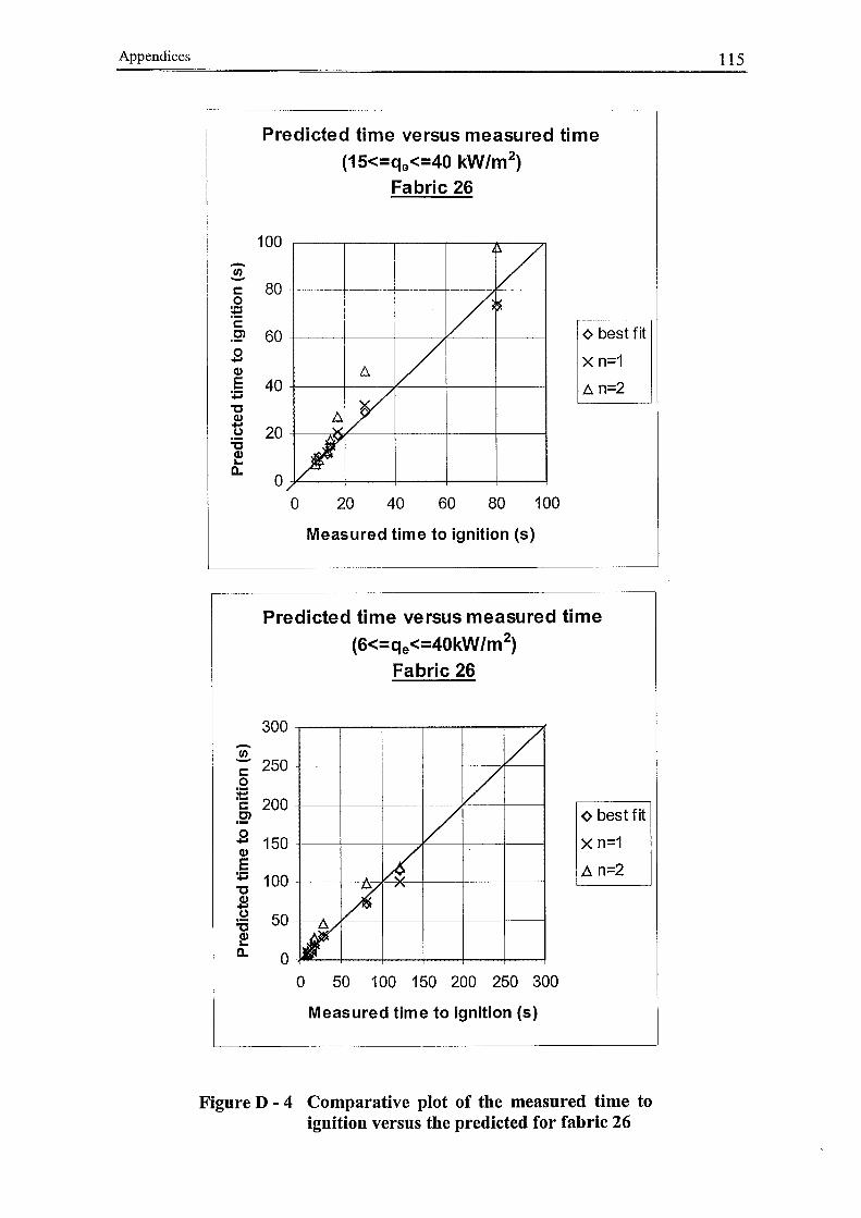
Appendices

-1/) -c 0 E c

.2> 0 +"' Q)

E +=i "0 Q)

t) :a ~ a.


(15<=qe<=40 kW/m2)

Fabric 26

0 20 40 60 80 100


¢best fit

X n=1

1:. n=2


(6<=qe<=40kW /m2)

300

250

200

150

100

50

0

Fabric 26

v 1/ v

lA 17

,

1£ '

0 50 100 150 200 250 300


¢best fit

X n=1

An=2


115

116

-.£?.

-Ill -c 0 :ij

'2 ,gl 0 -Q)

E :ij

"C $ .~ "C Q) .... c.


(18<=qe<=40 kW/m2)

Fabric 27

0 -¥----t---+---+--+---1

0 20 40 60 80 100

measured time to ignition (s)

¢best fit

X n=1

A n=2


(15<=qe<=40 kW/m2)

300

250

200

150

100

50

0

Fabric 27

v v v A v .A. v , I

I 0 50 100 150 200 250 300

measured time to ignition (s)

¢best fit

X n=1

l:ln=2

Appendices


Appendices

,------------------


(15<=qe<=40 kW /m2)

Fabric 28

100 .---....,----,---.,--..,..---..,., -U) -g 80 --1---J---~--------t---------;-IF------l :E c .~ 60 -t-----+-----+--~L__--t------1 .s

C1)

E 40+--4-~~--+-~-~ +i 'C

~ 20 --1--~-----+--1----+------l 'C ~ a. 0 -¥---+---+--1-----1---l

0 20 40 60 80 100


¢best fit

X n=1

A n=2


(6<=qe<=40kW /m2)

900 -U) - 750 c 0 +i ·c: 600 .!2' 0 .... 450 C1)

E +i 300 'C

C1)

£ 150 'C C1) a.. a.

0

Fabric 28

lS v v v A

~ ~

¥ [;/ ~

-

0 150 300 450 600 750 900


<>best fit

X n=1

An=2


117

118

-~ c 0 E c


(15<=q9 <=40 kW/m2)

Fabric 29

100~--~--~--~--~--~

.~ 60 +---+----::+--

.9 6. ¢best fit

x n=1 Q)

E ;:; "C

~ "C e a.

6. n=2

0-tG-----+----+----+---f----f 0 20 40 60 80 100



(6<=q9<=40 kW/m 2)

Fabric 29

0-+----f----1---+---+--+----l 0 50 1 00 150 200 250 300


¢best fit

X n=1

1::. n=2

Appendices

I J


Appendices

Predicted time versus measured time (15<=qe<=40 kW/m 2

)

Fabric 30

1 00 -,---,.---,---,------;-------;rt

0 20 40 60 80 100

Measured time to ignition(s)

¢best fit

X n=1

t:. n=2


(6<=qe<=40kW /m 2)

900

-(/) - 750 c 0 :2

600 c .!2' .s 450 Q)

E +::l 300 "0

~ 150 :a

~ a. 0

Fabric 30

v X I/

/ I .VI ll

/ ~

~

0 150 300 450 600 750 900

Measured time to ignition(s)

¢best fit

x n=1

A n=2


119

120

-1/) -

"'0


(15<=qe<=40 kW/m2)

Fabric 31

¢best fit

X n=1

.JJ. n=2

Appendices

~ 20 --~------~---+--+-------+---1 "'0 ~ ~ 0 ~---r----+----+----r--~

-

0 20 40 60 80 100



(6<=q9 <=40 kW/m 2)

Fabric 31

.!!!. c 250-t---+---~--r---r-~~~ 0 E c C)

0 ..... Q)

E +=i "'0 Q)

0 "'0 ~ ~ 0+-'--+---1---1----!1----f----l

0 50 100 150 200 250 300


¢best fit

X n=1

2 n=2 __ j


Appendices

-t/j -c 0 :;; ·c: .!2> 0 +' Q)

E :;; "C Q)

t) :a Q) ... ll.


(15<=qe<=40 kW/m2)

Fabric 32

0 20 40 60 80 100


o best fit

X n=1

t:.. n=2


{6<=qe<=40kW/m2)

900

750

600

450

300

150

0

Fabric 32

v 0 1/

1/ / !::..

¥ v 0 150 300 450 600 750 900


o best fit

X n=1

t:.. n=2

FigureD -10 Comparative plot of the measured time to ignition versus the predicted for fabric 32

121

122

-


(15<=qe<=40 kW /m2)

Fabric 33

Appendices

¢best fit

X n=1

l:l. n=2

0 20 40 60 80 100



(6<=qe<=40 kW /m 2)

Fabric 33

300~--~--~~--~--~--~

~ 250+---+---+---4---+---~~ c 0

:.p '2 .!2>

.s Q)

E :.p "C

~ "C ~ D. 0

0 50 100 150 200 250 300


¢best fit

x n=1

b n=2 L--


Appendices

-tl) -c 0 E c C)

0 ... (1)

E :;::; "'C (1) ... 0

"'C (1) ...

D..

-tl) -c 0 E c .~

.s (1)

E :;::; "'C (1)

~ "'C ~ D.


{15<=qe<=40 kW/m2)

Fabric 34

100

80

60

40

20

0 20 40 60 80 100



{7<=qe<=40 kW/m 2)

600

500

400

300

200

100

0

Fabric 34

/ v ~ / /

~ ~

0 100 200 300 400 500 600


~best fit

X n=1

A n=2


123

124

-~

-1/) -c 0

+:3 '2 ,g'l

.s Q)

E +:3 'C .s 0 =s Q) .... a.


(15<=q9 <=40 kW/m2)

Fabric 35

0 +---1----l-----1~-+---l

0 20 40 60 80 100


¢best fit

X n=1

A n=2


(6<=q9<=40 kW /m 2)

900

750

600

450

300

150

0

Fabric 35

I I I / ' I /I I

~ 1/ 0

~ u

A v i I I i

0 150 300 450 600 750 900


¢best fit

X n=1

A n=2

Appendices


Appendices

-Ill -

-


(15<=qe<=40 kW/m2)

Fabric 36

0+---+-----t--+---t-----1 0 20 40 60 80 100


¢best fit

X n=1

A n=2


(7<=qe<=40 kW/m 2)

Fabric 36

900

~ 750 1: 0

X / / ':t:l

'2 .!2>

.s C1l E

600

450

; 300

~ "C e D..

150

0

¢ / A

/ ¥

0 150 300 450 600 750 900


¢best fit

x n=1

b.n=2

FigureD- 14 Comparative plot of the measured time to ignition versus the predicted for fabric 36

125

FIRE ENGINEERING RESEARCH REPORTS

95/1 Full Residential Scale Backdraft I B Bolliger

95/2 A Study of Full Scale Room Fire Experiments P AEnright

95/3 Design of Load-bearing Light Steel Frame Walls for J T Gerlich Fire Resistance

95/4 Full Scale Limited Ventilation Fire Experiments D JMillar

95/5 An Analysis of Domestic Sprinkler Systems for Use in FRahmanian New Zealand

96/1 The Influence of Non-Uniform Electric Fields on MABelsham Combustion Processes

96/2 Mixing in Fire Induced Doorway Flows J M Clements

96/3 Fire Design of Single Storey Industrial Buildings B W Cosgrove

96/4 Modelling Smoke Flow Using Computational Fluid T NKardos Dynamics

96/5 Under-Ventilated Compartment Fires - A Precursor to ARParkes Smoke Explosions

96/6 An Investigation of the Effects of Sprinklers on MWRadford Compartment Fires

97/1 Sprinkler Trade Off Clauses in the Approved Documents GJBarnes

97/2 Risk Ranking of Buildings for Life Safety JWBoyes

97/3 Improving the Waking Effectiveness of Fire Alarms in T Grace Residential Areas

97/4 Study of Evacuation Movement through Different Building PHolmberg Components

97/5 Domestic Fire Hazard in New Zealand KDJirwin

97/6 An Appraisal of Existing Room-Corner Fire Models D C Robertson

97/7 Fire Resistance of Light Timber Framed Walls and Floors GCThomas

97/8 Uncertainty Analysis of Zone Fire Models AM Walker

97/9 New Zealand Building Regulations Five Years Later T M Pastore

98/1 The Impact of Post-Earthquake Fire on the Built Urban RBotting Environment

98/2 Full Scale Testing of Fire Suppression Agents on Unshielded MJDunn Fires

98/3 Full Scale Testing of Fire Suppression Agents on Shielded N Gravestock Fires

98/4 Predicting Ignition Time Under Transient Heat Flux Using A Henderson Results from Constant Flux Experiments

98/5 Comparison Studies of Zone and CFD Fire Simulations A Lovatt

98/6 Bench Scale Testing of Light Timber Frame Walls P Olsson

98/7 Exploratory Salt Water Experiments of Balcony Spill Plume E YYii Using Laser Induced Fluorescence Technique

99/1 Fire Safety and Security in Schools RACarter

99/2 A Review of the Building Separation Requirements of the JM Clarke New Zealand Building Code Acceptable Solutions

99/3 Effect of Safety Factors in Timed Human Egress Simulations KMCrawford

99/4 Fire Response ofHVAC Systems in Multistorey Buildings: MDixon An Examination of the NZBC Acceptable Solutions

99/5 The Effectiveness of the Domestic Smoke Alarm Signal C Duncan

99/6 Post-flashover Design Fires RFeasey

9917 An Analysis of Furniture Heat Release Rates by the Nordtest J Firestone

99/8 Design for Escape from Fire I J Garrett

99/9 Class A Foam Water Sprinkler Systems DB Hipkins

99/10 Review of the New Zealand Standard for Concrete Structures MJinwood (NZS 3101) for High Strength and Lightweight Concrete Exposed to Fire

99/12 An Analytical Model for Vertical Flame Spread on Solids: GANorth An Initial Investigation

99/13 Should Bedroom Doors be Open or Closed While People are D L Palmer Sleeping? - A Probabilistic Risk Assessment

99/14 Peoples Awareness of Fire S J Rusbridge

99/15 Smoke Explosions B J Sutherland

99/16 Reliability of Structural Fire Design JKSWong

99/17 Heat Release from New Zealand Upholstered Furniture T Enright

00/1 Fire Spread on Exterior Walls FNPBong

00/2 Fire Resistance of Lightweight Framed Construction PCR Collier

00/3 Fire Fighting Water: A Review of Fire Fighting Water S Davis Requirements (A New Zealand Perspective)

00/4 The Combustion Behaviour of Upholstered Furniture H Denize Materials in New Zealand

00/5 Full-Scale Compartment Fire Experiments on Upholstered N Girgis Furniture

00/6 Fire Rated Seismic Joints MJames

00/7 Fire Design of Steel Members KRLewis

00/8 Stability of Precast Concrete Tilt Panels in Fire LLim

00/9 Heat Transfer Program for the Design of Structures Exposed JMason to Fire

00/10 An Analysis of Pre-Flashover Fire Experiments with Field C Nielsen Modelling Comparisons

00/11 Fire Engineering Design Problems at Building Consent Stage PTeo

00/12 A Comparison of Data Reduction Techniques for Zone Model S Weaver Validation

00/13 Effect of Surface Area and Thickness on Fire Loads HWYii

00/14 Home Fire Safety Strategies P Byrne

00/15 Accounting for Sprinkler Effectiveness in Performance MFeeney Based Design of Steel Buildings in Fire

00/16

01/1

01/2

01/3

01/4

01/5

01/6

01/7

01/8

01/9

01/10

A Guideline for the Fire Design of Shopping Centres

Flammability of Upholstered Furniture Using the Cone Calorimeter

Radiant Ignition of New Zealand Upholstered Furniture Composites

Statistical Analysis of Hospitality Industry Fire Experience

Performance of Gypsum Plasterboard Assemblies Exposed to Real Building Fires

Ignition Properties of New Zealand Timber

Effect of Support Conditions on Steel Beams Exposed of Fire

Validation of an Evacuation Model Currently Under Development

2-D Analysis of Composite Steel- Concrete Beams in Fire

Contribution of Upholstered Furniture to Residential Fire Fatalities in New Zealand

The Fire Safety Design of Apartment Buildings

School of Engineering

University of Canterbury

Private Bag 4800, Christchurch, New Zealand

Phone 643 364-2250

Fax 643 364-2758

JMMcMillan

A Coles

FChen

TY A Chen

B HJones

CKNgu

J Seputro

A Teo

R Welsh

CRWong

SWu