quasiconformal maps in metric spaces with controlled geometry

Acta Math., 181 (1998), 1-61 (~) 1998 by Institut Mittag-Leffier. All rights reserved

Quasiconformal maps in metric spaces with controlled geometry

JUHA HEINONEN

University of Michigan Ann Arbor, MI, U.S.A.

b y

and P E K K A KOSKELA

University of Jyviiskylii Jyvliskylll, Finland

C o n t e n t s

1. Introduction 2. Modulus and capacity in a metric space 3. Loewner spaces 4. Quasiconformality vs. quasisymmetry 5. Poincar@ inequalities and the Loewner condition 6. Examples of Loewner spaces 7. Absolute continuity of quasisymmetric maps 8. Quasisymmetric invariance of Loewner spaces 9. Quasiconformal maps and Sobolev spaces

1. I n t r o d u c t i o n

This pape r develops the founda t ions of the t heo ry of quas iconformal maps in met r i c

spaces t h a t sa t i s fy ce r ta in bounds on the i r mass and geometry . T h e pr inc ipa l message is

t h a t such a t heo ry is b o t h re levant and viable.

The first ma in issue is the p rob l e m of defini t ion, which we next descr ibe. Quasi-

conformal m a p s are commonly u n d e r s t o o d as h o m e o m o r p h i s m s t h a t d i s to r t the shape

of inf in i tes imal bal ls by a un i fo rmly b o u n d e d amount . Th is r equ i rement makes sense

in every met r ic space. Given a h o m e o m o r p h i s m f f rom a met r i c space X to a met r i c

space Y, then for x c X and r > 0 set

Hi (x , r ) = s u p { J f ( x ) - f(Y)l : Ix -y[ ~ r} (I . I)

Here and hereaf te r we use the d i s t ance n o t a t i o n I x - y l in any met r i c space.

Both authors were supported in part by the NSF and the Academy of Finland. The first author is a Sloan Fellow.

J. H E I N O N E N A N D P. K O S K E L A

Definition 1.2. A homeomorphism f : X-~ Y is called quasiconformal if there is a

constant H < c~ so that

lim sup Hi(x, r) <~ H (1.3) r--*0

for all x ~ X.

This definition is easy to state, but not easy to use. It does follow easily from the

definition and classical theorems in real analysis that quasiconformal homeomorphisms

in Euclidean spaces are almost everywhere differentiable. But it is not clear whether,

for instance, the inverse of a given quasiconformal map is quasiconformal; nor is it easy

to ascertain desired stronger properties such as H61der continuity or the compactness of

a suitably normalized family of quasiconformal homeomorphisms. The difficulties stem

from the fact that (1.3) is a local, infinitesimal condition.

Let us look at a stronger, global requirement.

Definition 1.4. A homeomorphism f : X-~ Y is called quasisymmetric if there is a

constant H < c ~ so that

Hi(x, r) ~< H (1.5)

for all x E X and all r >0.

It is not difficult to demonstrate starting from the definition that quasisymmet-

tic homeomorphisms between reasonable spaces enjoy many strong properties: they are

HSlder continuous, inverse maps are quasisymmetric as well, normal families are common

and quasisymmetry carries over to limit homeomorphisms. In fact, much of the classical

quasiconformal theory can be done by directly exploiting condition (1.5), or its local ver-

sions. Quasisymmetric maps made their first official appearance in the 1956 paper [BA]

by Beurling and Ahlfors, who were concerned about maps of the real line, and quasi-

conformal extensions thereof. The concept was later promoted by Tukia and V~is~l/i, who

introduced and studied quasisymmetric maps between arbitrary metric spaces in [TV].

Recently V~iis/il/i IV5], IV6] has developed a "dimension-free" theory of quasiconformal

maps in infinite-dimensional Banach spaces based on the idea of quasisymmetry. See

also IV2].

It is a fundamental fact that quasiconformal homeomorphisms between Euclidean

spaces of dimension at least two are quasisymmetric; that is, (1.3) implies (1.5) for a

homeomorphism f : Rn--*R n if n ~2 . (The value of the constant H in (1.5) may differ,

but it only depends on the constant appearing in (1.3) and possibly--this is an open

problem--on the dimension n.) If we assume that f is a diffeomorphism, then this fact

is not overly difficult to establish, albeit still nontrivial. That global bounds can be

obtained without any a priori regularity assumptions is a deep result that reflects certain

QUASICONFORMAL MAPS IN METRIC SPACES WITH CONTROLLED GEOMETRY 3

special properties of Euclidean space, worth seeking elsewhere. This result was first

proved by Gehring in [G1] for R 2, with a method that extends to higher dimensions;

see iV1] for a full account. For n - - l , the statement is false; consider, for example,

f ( x ) =x+e x.

The problem whether (1.3) and (1.5) are equivalent for a given self-homeomorphism

of a space can be phrased in more intrinsic terms as follows. Let X be a space with

metric d, which we regard as the fixed "conformal" structure on X. Suppose then that

we are given an infinitesimal quasiconformal structure on X. By this we mean a new

metric on X whose balls, at the limit when the radius goes to zero, are not too differ-

ent in shape from the bails in the metric d. Is it then true that these two structures

are globally quasisymmetrically equivalent? In other words, can we recapture the global

quasisymmetric structure of a space from a local or infinitesimal quasiconformal struc-

ture? This question comes up naturally in the quasiisometry classification of negatively

curved spaces. It is known that the quasiisometry type of a negatively curved space

(in the sense of Gromov [GH]) is in many cases determined by the quasisymmetric type

of its boundary; thus we would like to know whether it is already determined by the

infinitesimal quasiconformal type. See the survey article by Gromov and Pansu [GP] for

an excellent discussion. (See also [P3] and [Paul.)

For a long time it was not clear whether this infinitesimal-to-global principle was

valid in spaces that are sufficiently distinct from R n. In fact, examples of relatively nice

spaces were found where it fails; for instance, one can take X to be R 2 and Y to be a

certain smooth hypersurface in R 3, cf. [HK1, Example 4.71 or iV2, w As a consequence

of the recent work of IViostow [Mo2], Pansu [PI], [P2], and others, it followed that (1.3)

implies (1.5) for homeomorphisms between the spaces that occur as conformal boundaries

of rank-one symmetric spaces. In particular, Kor~nyi and Reimann [KR1], [KR2] have

conducted a thorough study of the quasiconformal maps on the Heisenberg group, and

a careful treatment of various definitions for quasiconformal maps on the Heisenberg

group is given in [KR2]. The authors showed in [HK1] that (1.3) implies (1.5) in an

arbitrary Carnot group (see w below), or more generally in the case where X is a

Carnot group and Y is a metric space with similar homogeneity and local connectivity

properties to X. Recently, Margulis and Mostow [MM] established important absolute

continuity properties of quasiconformal maps on general Carnot Carath6odory spaces.

Their results can be used to derive (semi-)global distortion properties of quasiconformal

maps on those spaces. See also [VG].

One of the main goals of the present paper is to show that the two concepts, quasi-

conformality and quasisymmetry, are quantitatively equivalent in a large class of metric

spaces, which includes all the previously known examples and more. Such spaces are

4 J. H E I N O N E N AND P. K O S K E L A

discussed next.

The most important tool in the quasiconformal theory is the conformal modulus, or

capacity. This is a global conformal invariant that attaches a real number to each pair

of disjoint continua in a given space. (By a continuum we mean a compact, connected

set.) The crucial property of this invariant in R ~ is that it has a uniform lower bound,

which depends only on the dimension n and on the relative position of the two continua.

In the case n=2, this fact was known already to GrStzsch and Teichmiiller. For n~>3

it was first observed by Loewner ILl in 1959; he used this property of modulus to show

that one cannot map R n quasiconformally onto a proper subset. In w we shall define

a Loewner space to be a space where a similar lower bound for the modulus holds.

Then, in w we shall show that a quasiconformal map from a Loewner space X into a

space Y is quasisymmetric, if the Hausdorff measures of X and Y are both Ahlfors-David

regular of the same dimension larger than one, and if Y satisfies a (necessary) linear local

connectivity condition.

Let us recall the definition of an Ahlfors-David regular space.

Definition 1.6. A metric space X is said to be AhlforsDavid regular of dimension

Q > 0 if there is a constant C~>I so that

C - J R Q ~ ~LQ(BR) ~ CR Q (1.7)

for all balls BR in X of radius R < d i a m X . Here, and hereafter, ?-/Q denotes the Q-

Hausdorff measure in the metric space X. We often call X simply Q-regular, or just

regular, if the dimension is not important to the discussion.

It is easy to see that X satisfies (1.7) if it satisfies a similar condition for some Borel-

regular measure #; only the constant C may change slightly. David and Semmes [DS2],

[DS3] have conducted an extensive study of regular spaces, usually furnished with some

additional properties. Regular spaces are particular examples of spaces of homogeneous

type in the sense of Coifman and Weiss [CW]. Although a lot of harmonic analysis can

be done in homogeneous spaces, they are usually too general for the kind of questions

we want to address in this paper; for us, it is important that the spaces have good

connectivity properties. (This is not to say that many of our results, especially in w

would not hold in more generality, or when differently interpreted; there are interesting

questions left open in this respect. Our techniques fail if the spaces admit few or no

rectifiable curves.)

The main new point introduced in [HK1] was that one can use modulus estimates

to study maps even without a differentiable structure of any kind in the underlying

space. The usual analytic change of variables procedure was replaced there by a discrete,


combinatorial argument. In the end, all one needs is a lower bound for the modulus.

This idea is pursued further here, and the main question is: what spaces admit such a

lower bound for the modulus? Equivalently, in our present terminology, what spaces are

Loewner spaces? The answer will be given in terms of a Poincard inequality.

Recall that the usual Poincard inequality in R n implies, by way of Hhlder's inequality,

that

inf [ lu-a]dx<~C(n)(diamB)n(; IVupdx) 1In (1.8) a e R J B

for any bounded smooth or Lipschitz function u in a ball B (see [GT, p. 164]). We shall

formulate a version of (1.8) in a general, rectifiably connected metric space. We then

show (see w that if X is a proper and regular space that in addition satisfies a local

quasiconvexity condition, then X is a Loewner space if and only if X admits a Poincard

inequality. (A proper space is one whose closed balls are compact; for the quasiconvexity

condition, see w

The search for Poincard-type inequalities in various situations has been intensive

in recent years. Spaces that admit the kind of Poincard inequality we are looking for

include Riemannian manifolds of nonnegative Ricci curvature and Euclidean volume

growth, as well as various Carnot-type geometries. See [Bu], [DS1], [Gr], [J], [MSC],

[SC], [VSC]. Semmes [$4] has shown recently that any n-regular, complete metric space,

that is also an oriented (homology) n-manifold satisfying a linear local contractibility

condition, admits a Poincard inequality. (Added in December 1997: For an interesting

new geometry which admits a Poincard inequality, see the recent paper by Bourdon and

Pajot [BP].) We shall show in this paper that any connected, finite simplicial complex

admits a Poincard inequality if it is of pure dimension n > 1 and if it has the (obviously

necessary) property that the link of every vertex is connected (i.e. a removal of a point

does not locally disconnect the space).

Consequently, in all these spaces we can go from an infinitesimal quasiconformal

structure to a global one. Note that in the case of a Riemannian manifold, quasiconformal

maps are always quasisymmetric in small coordinate charts by Gehring's theorem (if the

dimension is larger than one), but in general there need not be any control over the global

distortion. Our result says that we can control the global distortion in the presence of

appropriate volume bounds and a Poincard inequality. Recall that certain Sobolev

Poincard inequalities carry information about the isoperimetric profile of a space, which

is closely connected with the quasiconformal theory [GLP]. The inequalities we need in

this paper are weaker than those related to isoperimetric inequalities.

There are many important cases where the existence of a Poincard inequality is

not known. If /~ is the universal cover of a negatively curved compact Riemannian

J. H E I N O N E N AND P. KOSKti;LA

n-manifold M, then the ideal boundary 0 ~ r of M is topologically a sphere of dimen-

sion n - 1. One would like to understand the metrics on 0-~ where the fundamental group

7c1(M) acts uniformly quasiconformally. (Note that such metrics always exist [GH].)

A particularly interesting case is related to the problem of recognizing the fundamental

groups of compact hyperbolic three-manifolds. A long standing conjecture is that every

negatively curved or Gromov hyperbolic group whose boundary is a two-sphere is such

a group. Cannon, Floyd, Parry, and Swenson [C], [CFP], [CS] have showed that this

conjecture can be solved affirmatively if a certain combinatorial modulus on the bound-

ary two-sphere has roughly Euclidean behavior. This is a Loewner-type requirement.

In [HK1], the authors employed a discrete modulus similar to that of Cannon et al.,

but in the present paper the concepts are defined in continuous terms. Many arguments

below, however, can be seen as combinatorial.

It remains an open problem precisely under what circumstances the Loewner con-

dition is a quasisymmetric invariant. We conjecture that the Loewner property is a

quasisymmetric invariant of a locally compact Q-regular space for Q > 1. In w we prove

this under an additional hypothesis. (After this paper was submitted, Tyson [Ty] verified

the conjecture; see Remark 8.7 (a).)

After this study of definitions, we come to the second main issue of the paper, which

is the actual theory of quasiconformal maps between spaces with appropriate control on

mass and geometry. A regular metric space X that admits a Poincar6-type inequality

appears to be an amenable environment where the quasiconformal theory works much

in the same way it does in Euclidean space. We shall show that a quasiconformal map

between two such spaces is not only absolutely continuous in that it preserves sets of

measure zero, but it induces an A~-weight in the sense of Muckenhoupt. Moreover,

under similar assumptions, quasiconformal maps are absolutely continuous on Q-modulus

almost every curve. The assumptions are general enough to encompass the results of

Pansu [P2], and Margulis and Mostow [MM] on absolute continuity on lines. We also

show that a quasiconformal map between such spaces belongs to a Sobolev space of

higher degree than a priori is expected. These results extend the celebrated theorems of

Bojarski [Bo] in R 2 and Gehring [G3] in R n. By a Sobolev space, we mean a space as

defined either by Hajtasz [Ha], or by Korevaar and Schoen [KS].

Finally, we should warn the reader that what we call quasisymmetry in Definition 1.4

is called weak quasisymmetry by Tukia and V~iis/il~i in [TV]; they demand that quasisym-

metric maps satisfy a stronger distortion condition, valid for points in all locations. See

(4.5) for the precise definition. We chose to ignore this difference in this introduction,

for we shall deal only with metric spaces where these two definitions of quasisymmetry

are quantitatively equivalent. This point is clarified later in w Also, in the case of


compact or bounded spaces, the concept of a quasi-MSbius map as defined by V~is~l~

in IV3] would appear more natural than that of a quasisymmetric map. (Recall that

the conformal automorphism group of the unit disk is not uniformly quasisymmetric in

the Euclidean metric.) However, for simplicity of exposition we have decided not to deal

with quasi-M5bius maps in this paper.

Some of the results of this paper were announced in [HK2].

Acknowledgement. We wish to express our grati tude to Fred Gehring for his con-

tinuous advice, encouragement and interest in our work, past and present. We dedicate

this paper to him with admirat ion and appreciation.

We would also like to thank Stephen Semmes for numerous useful discussions related

to the topics of this paper, Jussi Vs163 for helpful information about continua in metric

spaces, and Toni Hukkanen, Juha Kinnunen, Paul MacManus and Hervd Pajot for their

comments on the manuscript.

Special thanks go to the referee, whose extremely careful reading of the manuscript

led to many clarifications and improvements in the text.

2. M o d u l u s and c a p a c i t y in a m e t r i c s p a c e

In this section, we first recall the definition for the modulus of a curve family in a metric

measure space (X, p). Then we introduce the concept of capacity between two continua

in X. The latter requires an appropriate substi tute for the gradient of a smooth or

Lipschitz function. This done, we proceed to show that the two notions are equal in

certain important situations. Just as in R n, the modulus is more general and flexible in

use, while it is easier to give estimates for the more concrete capacity.

2.1. Definitions and conventions. All metric spaces in this paper are assumed to be

rectifiably connected and all measures are assumed to be locally finite and Borel regular

with dense support. A metric space is called rectifiably connected if every pair of two

points in it can be joined by a rectifiable curve (see w below). We shall denote by

(X, p) such a metric measure space. We do not assume in general that X be locally

compact or complete.

Open balls are writ ten as B(x, r), and if B = B ( x , r), then C B = B ( x , Cr) for C > 0 .

The closure of a set A is denoted A.

2.2. Curves and line integrals in a metric space. We recall the basic concepts of

rectifiability and line integration in a metric space. Let X be a metric space as in w

By a curve we mean either a continuous map ~/of an interval I c R into X, or the

image ~/(I) of such a map. We usually abuse notation by writing ~/=~/(I). If I = [a, b] is

J. H E I N O N E N A N D P. K O S K E L A

a closed interval, then the length of a curve 7: I ~ X is

l ( 7 ) = l e n g t h ( v ) = s u p i = 1

where the s u p r e m u m is over all finite sequences a=tl<.t2<....~tn<~tn+l=b. I f I is not

closed, then we set

I(7) = s u p l ( T l J ) ,

where the s u p r e m u m is t aken over all closed subintervals J of I . We call a curve 7

rectifiable if its length is a finite number . Similarly, a curve 7: I--*X is locally rectifiable if its restr ic t ion to each closed subinterval of I is rectifiable.

Any rectifiable curve 7: I - ~ X has a unique extension ~ to the closure [ of I ; we

ignore the fact t h a t the values of ~ at the endpoin ts of I m a y not lie in X but ra ther

in the comple t ion of X . If I is unbounded , the extension is unders tood in a general ized

sense. From now on, if 7 is rectifiable, we au tomat i ca l ly consider its extension ~' and do

not dist inguish these two curves in notat ion. For any rectifiable 7 there are its associa ted

length function s-y: I---*[0, l('),)] and a unique 1-Lipschitz cont inuous m a p %: [0, I (7)]--~X

such tha t 7 = % o s ~ . T h e curve % is the arc length parametrization of 7.

If 7 is a rectifiable curve in X , the line integral over 7 of each nonnegat ive Borel

funct ion 0: X--*[0, c~] is

pds= / P~ dt. J0

If -y is only locally rectifiable, we set

~ pds = sup j r , 0 ds,

where the s u p r e m u m is t aken over all rectifiable subcurves 7 ' of 7- If 7 is not locally

rectifiable, no line integrals are defined.

A detai led t r e a t m e n t of line integrals in the case X = R n can be found in [V1,

Chap te r 1]. The general case is only ostensibly different, cf. [Fe, 2.5.16]. The length of

a curve 7 as defined above agrees wi th its 1-Hausdorff measure in X provided the m a p

7: I--*X is injective [Fe, 2.10.13].

2.3. Modulus of a curve family. Suppose t ha t (X, #) is a metr ic measure space as

in w Let F be a family of curves in X and let p~>l be a real number . T h e p-modulus of F is defined as

F = inf / F ~ d/z, modp Jx

Q U A S I C O N F O R M A L M A P S IN M E T R I C S P A C E S W I T H C O N T R O L L E D G E O M E T R Y 9

where the infimum is taken over all nonnegative Borel functions 6: X--*[0, cx~] satisfying

~ Qds ~> 1 (2.4)

for all locally rectifiable curves ~CF. Functions Q satisfying (2.4) are called admissible (metrics) for F. Note that by definition the modulus of all curves in X that are not

locally rectifiable is zero. We observe that

modp(o) = 0, (2.5)

modp F1 ~< modp F2, (2.6)

if FICF2, and

modp Fi ~ ~ i=1 modpr i . (2.7) i -

Moreover, if Fo and F are two curve families such that each curve ~ c F has a subcurve

~oCF0, then

modp F ~< modp F0. (2.8)

These properties of modulus are easily proven, cf. [Fu], IV1, pp. 16-17]. They will be

used repeatedly, and usually without extra fanfare, throughout this paper.

Often one would like to restrict the pool of admissible metrics to, say, continuous

or bounded functions 6. Such a reduction generally leads to a different concept. For

instance, the n-modulus of the family of all (nonconstant) curves in R '* that pass through

a given point is zero, but there are no admissible bounded metrics for this family. The

only concession that can be made is to consider lower semicontinuous functions, for it

follows from the Vitali-Carath6odory theorem in real analysis that every function f in

LP(X) can be approximated in LP(X) by a lower semicontinuous function g with g>~f. This requires X to be locally compact; see [Ru, p. 57].

The triple (E, F; U) will denote the family of all curves in an open subset U of X

joining two disjoint closed subsets E and F of U, cf. w For brevity, (E, F; X)= ( E , F ) .

2.9. Very weak gradients. Let U be an open set in X and let u be an arbitrary real-

valued function in U. We say that a Borel function Q: U--*[0, ce] is a very weak gradient of u in U if

lu(x)-u(y)l <~ ]~ Qds (2.10)

whenever ~'xy is a rectifiable curve joining two points x and y in U. Clearly, a very weak

gradient is not unique, and O--(x~ is always a very weak gradient. As an example, if X is

10 J. H E I N O N E N A N D P. K O S K E L A

a Riemannian manifold, for instance R n with its standard metric, and if u is a smooth

function on X, then Q=IVul is a very weak gradient of u. It is also not difficult to see

that if Q is any very weak gradient of a smooth function u in R n, then IVuI~Q almost

everywhere.

Recall that a mapping u between metric spaces is Lipschitz if there is a constant

C>~1 so that

lu (x ) -u (y ) l ~< C I x - y I

for all points x and y in the domain of u; moreover, u is locally Lipschitz if every point

in the domain has a neighborhood where u is Lipschitz. If u is a Lipschitz function on

a Riemannian manifold X, it is differentiable almost everywhere, and the function IVul

can be redefined everywhere on X so that it becomes a very weak gradient of u. And,

as in the case of a smooth function, IVul is almost everywhere less than or equal to any

given very weak gradient of u.

If X is a Carnot group, then IV0ul, the length of the horizontal differential of a

smooth function u, serves as a very weak gradient of u (see w and the references there

for the terminology). Conversely, if ~ is any very weak gradient of such a function u,

then IV0ul ~<Q almost everywhere, cf. [HK1, proof of Proposition 2.4].

2.11. Capacity. Suppose that E and F are closed subsets of an open set U in X.

The triple (E, F; U) is called a condenser and its p-capacity for l~<p<:cx~ is defined as

F; U) = i n f / u Qp d#, (2.12) capp(E,

where the infimum is taken over all very weak gradients of all functions u in U such that

ulE>~l and ulF~O. Such a function u is called admissible for the condenser (E, F; U).

If U=X, we write (E, F; X)=(E, F) as in the case of modulus.

Remark 2.13. Observe that no a priori regularity of admissible functions is assumed

above. In practice, of course, the existence of a very weak gradient in L p imposes restric-

tions. We use the notation capp(E, F; U) and capL(E, F; U) for the quantity in (2.12)

if the infimum is taken over all continuous or locally Lipschitz admissible functions,

respectively. We trivially have

capp(E, F; U) ~< cap~ (E, F; U) ~< capL(E, F; U). (2.14)

In R n, if E and F are compact subsets of an open set U, then equality holds in (2.14);

see [He]. We do not know in what generality there is equality in (2.14).

We shall next prove the equality between modulus and capacity, plus an important

inequality (2.19) for condensers of certain type. This result is well known in the Euclidean


case, and the proof below is distilled from various works, most notably from [Z]. The

generality of the situation forces us to present a detailed argument. First we require

some definitions.

2.15. Quasiconvex and proper spaces. We say that X is quasiconvex if there is a

constant C > 0 so that every pair of two points x and y in X can be joined by a curve

V whose length satisfies l(v)<~CIx-y I. Moreover, X is locally quasiconvex if every point

in X has a neighborhood that is quasiconvex.

More generally, X is said to be V-convex if there is a cover of X by open sets {Us}

together with homeomorphisms { ~ : [0, co)--~[0, c~)} such that any pair of two points x

and y in Us can be joined by a curve in X whose length does not exceed ~a(Ix-yl ) .

We shall not be using the concept of V-convexity in any serious way in this paper:

the functions { ~ } will have no quantitative bearing on our discussion. Most of the

spaces considered below will be (globally) quasiconvex, but to prove this, something like

~-convexity needs to be assumed first.

We call X proper if its closed balls are compact.

Remark 2.16. There is a neat connection between quasiconvexity and very weak

gradients of Lipschitz functions. Namely, it is easy to see that a space X is quasiconvex

if and only if every function with bounded very weak gradient on X is Lipschitz.

PROPOSITION 2.17. We always have

Capp(E, F; U) = modp(E, F; U). (2.18)

Next suppose that X is V-convex, that E and F are two disjoint closed sets in X with

compact boundaries, and that X is proper. Then

Capp(ENB, F n B ; B) <~ modp(E, F ) (2.19)

for each ball B in X . If, moreover, X is locally quasiconvex, (2.19) holds with cap L on

the left-hand side.

Proof. To prove the inequality modp(E, F; U)~capp(E, F; U), take a function u in

U such that ulE>~l and u I F ~ 0 , and take any very weak gradient ~ of u. Then

~ Q ds ~> 1 (2.20)

for all rectifiable curves V joining E and F in U, so that

modp(E, F; U) ~</u oVd#"

12 J. H E I N O N E N A N D P, K O S K E L A

Because u and Q were arbitrary, the inequality follows.

To prove the reverse inequality capp(E,F;U)<~modp(E,F;U), fix a function Q:

U---*[O, oc] satisfying (2.20). Define

u(x)=inf f~ ods (2.21)

for xEU, where the infimum is taken over all rectifiable paths 7~ in U joining x to F; if

no such 7~ exists, set u(x)=l. Then u[F=O and ulE>~l. Moreover, we have that

]u (x ) -u (y ) l <~ ~ ods

for any rectifiable curve 7~y joining x and y in U. Thus u is admissible and Q is a very

weak gradient of u, whence

F; U) <<. Iv oV d~" capp(E,

Because Q was arbitrary, we conclude the proof of equality (2.18).

Now we turn to the second assertion of the proposition. Fix a ball B in X and fix an

admissible metric p for (E, F) . We may clearly assume tha t B is large enough so tha t the

boundaries OE and OF are both contained in B. We would like to build an appropriate

admissible continuous function u in B using Q, under the proviso that X is Q-convex.

The definition in (2.21) may not work as t~ need not be bounded, and to circumvent this

possibility an approximation argument is needed.

By the remark made in w we may assume that 0 is lower semicontinuous, and

clearly we may assume that t~lF=0. By considering the functions x~-~max{t~(x), 1/m} if xC2B, and x~o(x) if xq~2B, r e = l , 2 , ..., we may further assume that t~[2B is lower

semicontinuous and that oI2B\F is bounded away from zero: t~>~ in 2B\F, where ~>0

is a positive constant (use Lebesgue's monotone convergence theorem). Fix a positive

integer k and consider the function 0k=min{0, k}. Then 0k is bounded and lower semi-

continuous in 2B, 0k~>~ in 2B\F (for we may clearly assume that ~<1) , and vanishes

in F. Define

uk(x) = inf / Ok ds (2.22) J " f z

for xcB, where the infimum is taken over all rectifiable paths 7~ joining x to F in B; if

no such pa th exists, we set u k ( x ) = l . As above, we find tha t uklFNB=O and that 0k is a

very weak gradient of uk. Next, it is not difficult to see tha t u is continuous in B. Indeed,

pick a point in B and let x and y be points in some small open ~ - c o n v e x neighborhood


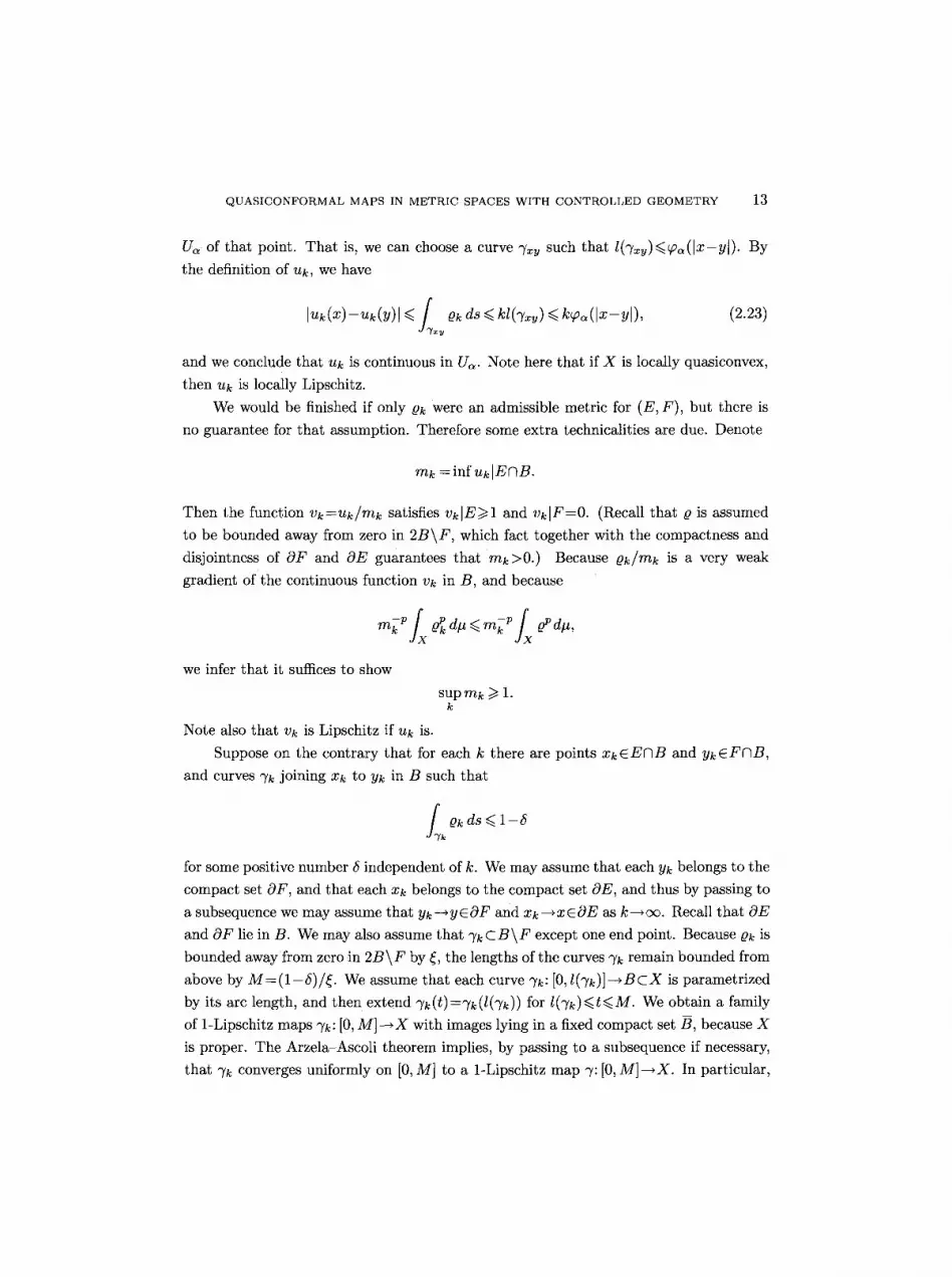
Us of that point. Tha t is, we can choose a curve 7xy such that l(%y)<.~(lx-y[). By

the definition of Uk, we have

luk(x)-uk(Y)[ <~ f Ok ds <~ kl(~/~y) <<. kqp~(lx-y[), (2.23) J~ w y

and we conclude that uk is continuous in Us. Note here that if X is locally quasiconvex,

then Uk is locally Lipschitz.

We would be finished if only Pk were an admissible metric for (E, F) , but there is

no guarantee for that assumption. Therefore some extra technicalities are due. Denote

mk = inf Uk IENB.

Then the function Vk=Uk/mk satisfies VklE>/1 and vklF=O. (Recall that p is assumed

to be bounded away from zero in 2B\F, which fact together with the compactness and

disjointness of OF and OE guarantees that ink>0.) Because Ok~ink is a very weak

gradient of the continuous function Vk in B, and because

we infer that it suffices to show

Note also that Vk is Lipschitz if uk is.

sup mk >/1. k

Suppose on the contrary that for each k there are points xkEENB and ykEFNB, and curves 0'k joining xk to Yk in B such tha t

f~k Pk ds <<. 1-

for some positive number 5 independent of k. We may assume that each Yk belongs to the

compact set OF, and that each xk belongs to the compact set OE, and thus by passing to

a subsequence we may assume that yk--*ycOF and Xk--+xcaE as k---+oo. Recall that OE and OF lie in B. We may also assume tha t ~/k C B \ F except one end point. Because Pk is

bounded away from zero in 2B\F by ~, the lengths of the curves 7k remain bounded from

above by M = ( 1 - 5 ) / ~ . We assume that each curve ~/k: [0, l(~/k)]-~BcX is parametrized

by its arc length, and then extend ")'k(t)=~/k(l(~/k)) for l(~/k)<.t<.M. We obtain a family

of 1-Lipschitz maps 0'k: [0, M]--*X with images lying in a fixed compact set B, because X

is proper. The Arzela Ascoli theorem implies, by passing to a subsequence if necessary,

that ")'k converges uniformly on [0, M] to a 1-Lipschitz map "),: [0, M]-*X. In particular,

14 J. HEINONEN AND P. KOSKELA

"y is a rectifiable curve in X joining the points xEOE and yEOF. We may also assume

at this point that l(~k)---+M. Hence, for a fixed positive integer k0, we have that

f fz(~k) lim inf Pko ds -- lim inf pko OTk ( t ) dt k c~ J'Tk k---+oo J0

7> lim inf fM-~okoO~/k(t) dt >1 jofM--~likm~f Ok~176 dt k--,oo Jo

~oM-eokoO"y( t ) dt,

where e>0 is arbitrary. Note that the lower semicontinuity of Qk0]2B was needed here.

Thus

/ /? i lim inf Qko ds ~ QkoOT( t ) dt >~ Qko ds. k ---+ oo k

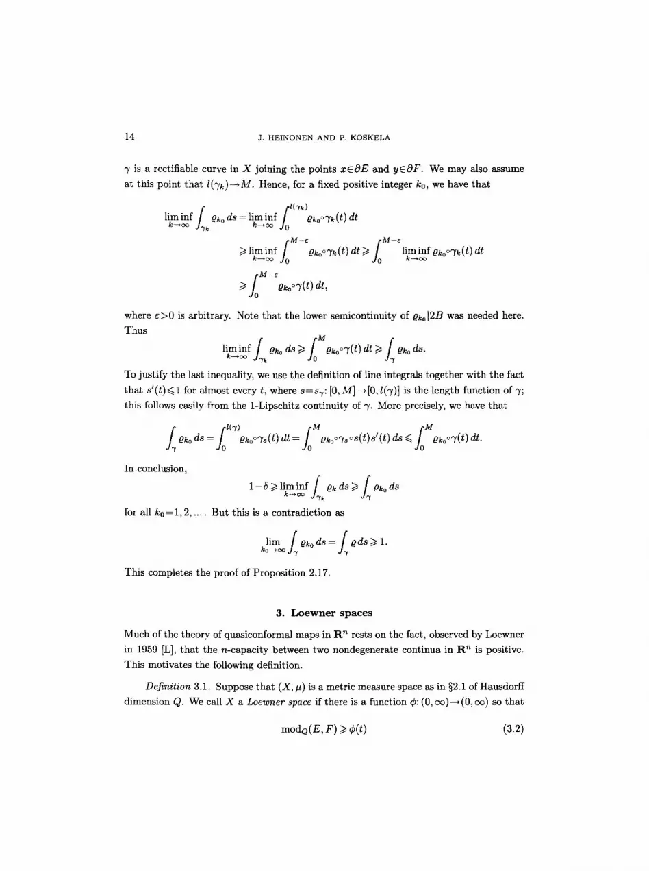
To justify the last inequality, we use the definition of line integrals together with the fact

that s'(t)~< 1 for almost every t, where s=s~: [0, M]--+ [0,/(~,)] is the length function of %

this follows easily from the 1-Lipschitz continuity of ~,. More precisely, we have that

f l ( ' 7 ) o M M

/OkodS:Jo Oko %(t)dt=fo OkoO%~ L Oko~ dt.

In conclusion, P

1 - 6/> lim inf I Qk ds >~ I Pko ds k- .*oo J T k A

for all ko--1, 2, .... But this is a contradiction as

[ es = [ o es 1. koli~mccx~ J~/ Jr

This completes the proof of Proposition 2.17.

3. L o e w n e r s p a c e s

Much of the theory of quasiconformal maps in R '~ rests on the fact, observed by Loewner

in 1959 ILl, that the n-capacity between two nondegenerate continua in R '~ is positive.

This motivates the following definition.

Definition 3.1. Suppose that (X, #) is a metric measure space as in w of Hausdorff

dimension Q. We call X a Loewner space if there is a function r (0, cx~)--+(0, c~) so that

modQ(E, F) ~> r (3.2)


whenever E and F are two disjoint, nondegenerate continua in X and

dist(E, F ) (3.3) t/> A(E, F) = min{diam E, diam F}"

Note that the Loewner condition (3.2) depends both on the underlying metric and

on the measure p, which a priori need not be related to each other.

Euclidean space R n with its usual metric is a Loewner space, and further examples

will be presented in w In the present section, we analyze the Loewner condition in some

detail.

Remark and convention 3.4. Recall from the introduction that a space (X, #) is

Q-regular if there is a constant C>~1 so that

C-1R Q <~ #(BR) <~ C R Q (3.5)

for all balls BR in X of radius R < d i a m X . In Definition 1.6, we defined the regularity

of a space in terms of its Hausdorff measure ~Q. If (3.5) holds, then X has Hausdorff

dimension Q and (3.5) holds for T/Q as well, possibly with different constant C. Moreover,

if X is locally compact and if # is a Borel measure on X satisfying (3.5), then # and T/Q

are comparable measures on X. See [$4, Appendix C] for a careful discussion on these

matters.

From now on, if a space (X, #) is called Q-regular, we understand that (3.5) holds;

if no measure is being specified, we understand that (1.7) holds.

THEOREM 3.6. Let (X, #) be a Loewner space of Hausdorff dimension Q > I . Then

there is a constant C1>~1 such that

C~IR Q < p(BR) (3.7)

for all balls BR in X of radius R < d i a m X . If there is a constant C2>~1 so that

(BR) Q

for all balls BR in X of radius R < d i a m X , then (X,#)

decreasing homeomorphism r (0, oo)--* (0, co) such that

modQ (E, F ) ~> ~b(A(E, F)) .

Moreover, we can select r so as to satisfy

1 r log y

(3.8)

is Q-regular and there is a

(3.9)

(3.10)


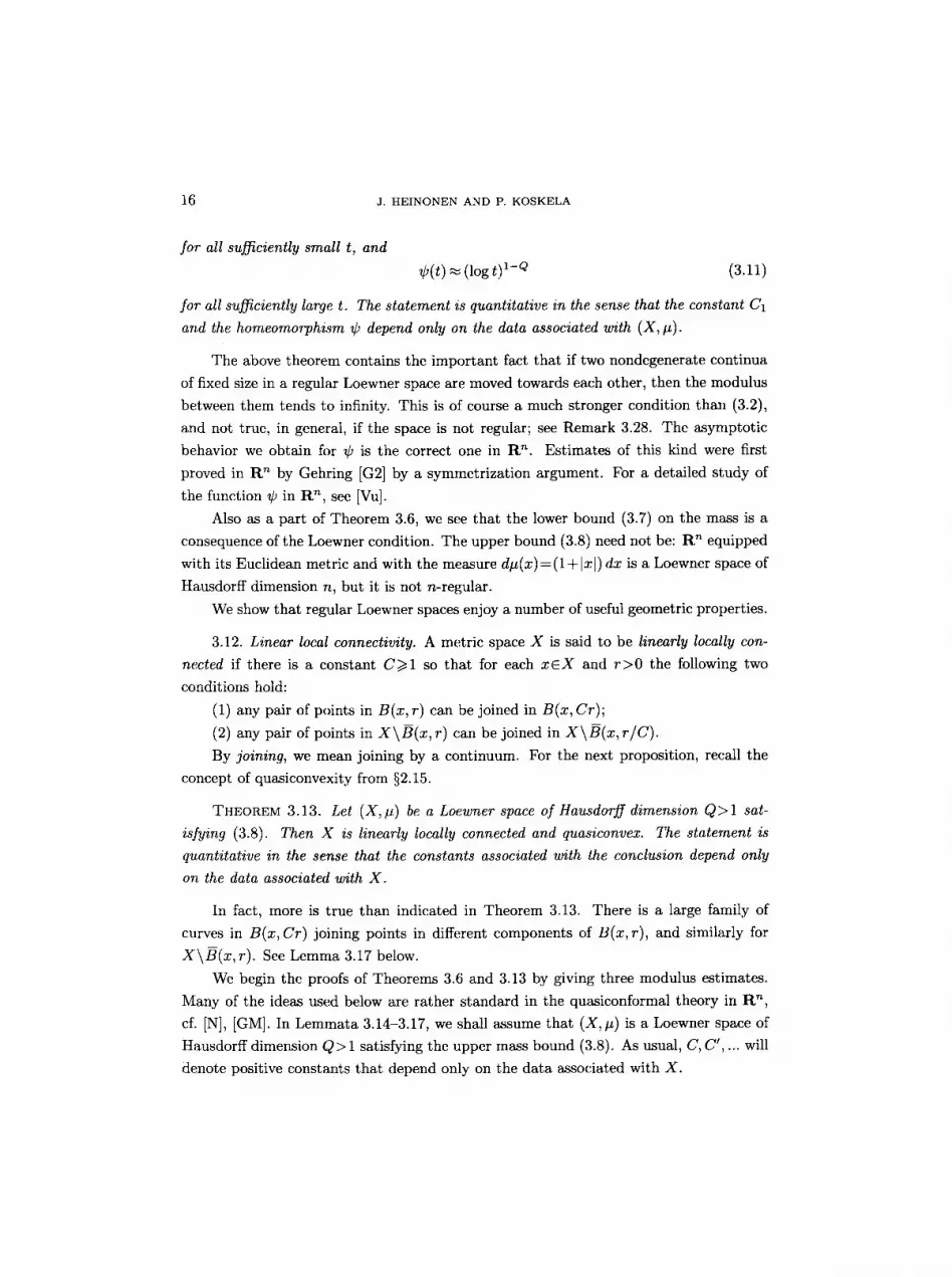
for all sufficiently small t, and

~(t) ~ (log t) 1-Q (3.11)

for all sufficiently large t. The statement is quantitative in the sense that the constant C1

and the homeomorphism ~ depend only on the data associated with (X, #).

The above theorem contains the important fact that if two nondegenerate continua

of fixed size in a regular Loewner space are moved towards each other, then the modulus

between them tends to infinity. This is of course a much stronger condition than (3.2),

and not true, in general, if the space is not regular; see Remark 3.28. The asymptot ic

behavior we obtain for ~ is the correct one in R n. Est imates of this kind were first

proved in R n by Gehring [G2] by a symmetr izat ion argument. For a detailed s tudy of

the function r in R n, see [Vu].

Also as a part of Theorem 3.6, we see that the lower bound (3.7) on the mass is a

consequence of the Loewner condition. The upper bound (3.8) need not be: R n equipped

with its Euclidean metric and with the measure d#(x)--(1 + Ixl) dx is a Loewner space of

Hausdorff dimension n, but it is not n-regular.

We show tha t regular Loewner spaces enjoy a number of useful geometric properties.

3.12. Linear local connectivity. A metric space X is said to be linearly locally con-

nected if there is a constant C~>I so that for each x E X and r > 0 the following two

conditions hold:

(1) any pair of points in B(x, r) can be joined in B(x, Cr);

(2) any pair of points in X \ B ( x , r) can be joined in X \ B ( x , r /C).

By joining, we mean joining by a continuum. For the next proposition, recall the

concept of quasiconvexity from w

THEOREM 3.13. Let (X,#) be a Loewner space of Hausdorff dimension Q> I sat-

isfying (3.8). Then X is linearly locally connected and quasiconvex. The statement is

quantitative in the sense that the constants associated with the conclusion depend only

on the data associated with X .

In fact, more is true than indicated in Theorem 3.13. There is a large family of

curves in B(x, Cr) joining points in different components of B(x,r) , and similarly for

X \ B ( x , r ) . See Lemma 3.17 below.

We begin the proofs of Theorems 3.6 and 3.13 by giving three modulus estimates.

Many of the ideas used below are rather s tandard in the quasiconformal theory in R n,

el. [N], [GM]. In Lemmata 3.14-3.17, we shall assume that (X ,# ) is a Loewner space of

Hausdorff dimension Q > 1 satisfying the upper mass bound (3.8). As usual, C, C' .... will

denote positive constants that depend only on the da ta associated with X.


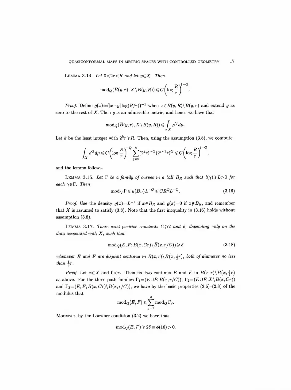
LEMMA 3.14. Let 0 < 2 r < R and let yEX. Then

mOdQ( B(y, r), X \ B(y, R) ) ~ C (log R ) 1-Q.

Proof. Define ~(x)=(Ix-yl log(R/r)) -1 when xcB(y, R)\B(y,r) and extend t) as

zero to the rest of X. Then t) is an admissible metric, and hence we have that

(B(y, r), X \ B(y, R)) ~< f x oq d#. modQ

Let k be the least integer with 2kr~R. Then, using the assumption (3.8), we compute

and the lemma follows.

E(2Jr)-Q(2J+lr) Q <~ C (log j=0

LEMMA 3.15. Let F be a family of curves in a ball BR such that I(7)~>L>0 for each "yEF. Then

modQ F ~< #(BR)L -Q <. CRQL -Q. (3.16)

Proof. Use the density Q(x)=L -~ if xCBR and g(x)=O if X~BR, and remember

that X is assumed to satisfy (3.8). Note that the first inequality in (3.16) holds without

assumption (3.8).

LEMMA 3.17. There exist positive constants C>/2 and 6, depending only on the data associated with X, such that

modQ(E, F; B(x, Cr)\B(x, r /C)) ~> 6 (3.18)

whenever E and F are disjoint continua in B(x,r) \B(x, 1 ~r), both of diameter no less 1 than ~r.

Proof. Let x e X and 0<r. Then fix two continua E and F in B(x,r) \B(x, �89 as above. For the three path families rl=(EUF, ~(x,r/C)), r2=(EuF, X \B(x , Cr)) and r3=(E, F; B(x, Cr)\~(x, r/C)), w e have by the basic properties (2.6) (2.8) of the

modulus that 3

modQ(E, F) ~< E mOdQ Fj. j = l

Moreover, by the Loewner condition (3.2) we have that

modQ (E, F) ~> 25 ~ r > 0.


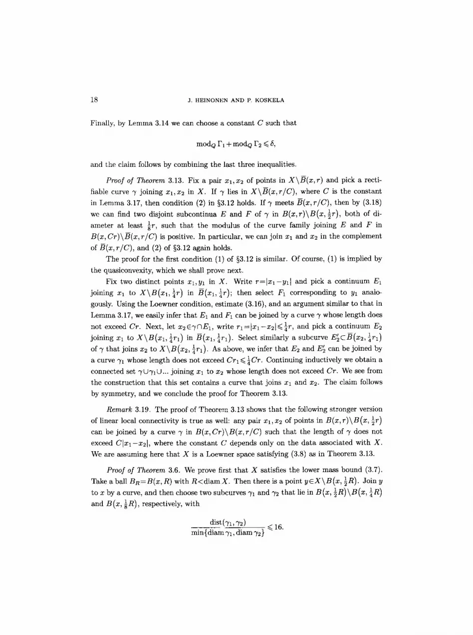
Finally, by Lemma 3.14 we can choose a constant C such that

modQ F1 + modQ F2 ~/5,

and the claim follows by combining the last three inequalities.

Proof of Theorem 3.13. Fix a pair xl,x2 of points in X\B(x,r) and pick a recti-

fiable curve V joining xl,x2 in X. If 3' lies in X\B(x,r/C), where C is the constant

in Lemma 3.17, then condition (2) in w holds. If "I, meets B(x,r/C), then by (3.18)

we can find two disjoint subcontinua E and F of 3' in B(x,r)\B(x, �89 both of di-

ameter at least 1 ~r, such that the modulus of the curve family joining E and F in

B(x, Cr)\B(x, r/C) is positive. In particular, we can join xl and x2 in the complement

of B(x, r/C), and (2) of w again holds.

The proof for the first condition (1) of w is similar. Of course, (1) is implied by

the quasiconvexity, which we shall prove next.

Fix two distinct points xl,yl in X. Write r=[xl-yll and pick a continuum E1 1 . joining xl to X\B(Xl, �88 in B(x l , ~r), then select F1 corresponding to Yl analo-

gously. Using the Loewner condition, estimate (3.16), and an argument similar to that in

Lemma 3.17, we easily infer that E1 and F1 can be joined by a curve 3' whose length does

not exceed Cr. Next, let x2C')'CIE1, write r l : lX l - -X2 1 ~ 1 ~r, and pick a continuum E2

~r l ) 1 ~ ( X l , 1 joining xl to X\B(Xl, ~rl) in g r l ) . Select similarly a subcurve E ~ c B ( x 2 , 1 1 of 'y tha t joins x2 to X\B(x2, ~rl). As above, we infer tha t E2 and E~ can be joined by

a curve ~1 whose length does not exceed Crl 1 <. ~ Cr. Continuing inductively we obtain a

connected set "rU~'IU... joining Xl to x2 whose length does not exceed Cr. We see from

the construction that this set contains a curve that joins xl and x2. The claim follows

by symmetry, and we conclude the proof for Theorem 3.13.

Remark 3.19. The proof of Theorem 3.13 shows that the following stronger version

of linear local connectivity is true as well: any pair x l , x2 of points in B(x, r)\B(x, �89 can be joined by a curve "y in B(x, Cr)\B(x, r/C) such tha t the length of 3' does not

exceed C[xl-x2[, where the constant C depends only on the da ta associated with X.

We are assuming here tha t X is a Loewner space satisfying (3.8) as in Theorem 3.13.

Proof of Theorem 3.6. We prove first that X satisfies the lower mass bound (3.7).

Take a ball BR=B(x, R) with R < d i a m X . Then there is a point yEX\B(x, �89 Join y

to x by a curve, and then choose two subcurves 3'1 and ")'2 that lie in B(x, �89 B(x, 1R) and B(x,-~R), respectively, with

dist (~,1,72) ~< 16. min{diam-rl , diam ~2}


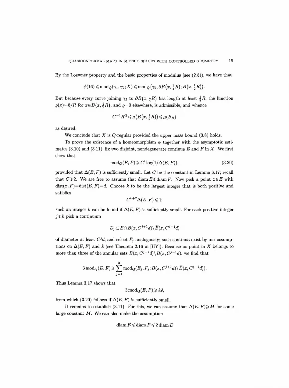
By the Loewner property and the basic properties of modulus (see (2.8)), we have that

1 . r ~< mOdQ (~/1, ~'2; X) ~< modp (~2, OB(x, -~ R), B(x, �89 R))

But because every curve joining 72 to OB (x, �88 R) has length at least 1 gR, the function

Q(x)=8/R for xeB(x, 1R ), and 6=0 elsewhere, is admissible, and whence

C-1R Q <~ #(B(x, �89 <<. #(BR)

as desired.

We conclude that X is Q-regular provided the upper mass bound (3.8) holds.

To prove the existence of a homeomorphism r together with the asymptotic esti-

mates (3.10) and (3.11), fix two disjoint, nondegenerate continua E and F in X. We first

show that

modQ (E, F) >/C' log(1/A(E, F)), (3.20)

provided that A(E, F) is sufficiently small. Let C be the constant in Lemma 3.17; recall

that C~>2. We are free to assume that diamE~<diamF. Now pick a point xEE with

dist(x, F ) = d i s t ( E , F ) = d . Choose k to be the largest integer that is both positive and

satisfies

Ck+2A(E, F) ~< 1;

such an integer k can be found if A(E, F) is sufficiently small. For each positive integer

j ~< k pick a continuum

Ej c EnB(x, CJ+ld)\~(x, C~-ld)

of diameter at least CJd, and select Fj analogously; such continua exist by our assump-

tions on A(E, F) and k (see Theorem 2.16 in [HY]). Because no point in X belongs to

more than three of the annular sets B(x, CJ+ld)\B(x, CJ-ld), we find that

k

3 mOdQ(E, F) i> ~ modQ (Ej, Fj; B(x, CJ+ld)\B(x, cJ - ld ) ) . 5=1

Thus Lemma 3.17 shows that

3 modp (E, F) ) k6,

from which (3.20) follows if A(E, F) is sufficiently small.

It remains to establish (3.11). For this, we can assume that A(E, F)>>.M for some

large constant M. We can also make the assumption

diam E ~< diam F ~< 2 diam E


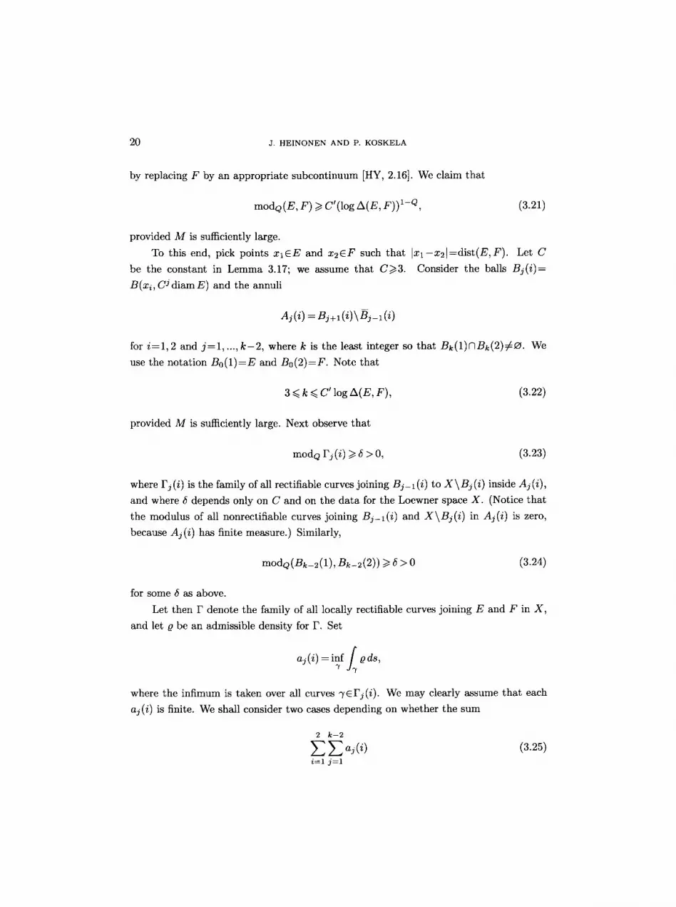
by replacing F by an appropriate subcontinuum [HY, 2.16]. We claim that

mOdQ(E, F) ~> C( log A(E, F)) l-Q, (3.21)

provided M is sufficiently large.

To this end, pick points xlEE and x2CF such that ]xl-x21=dist(E,F). Let C

be the constant in Lemma 3.17; we assume that C~>3. Consider the balls Bj(i)= B(xi, C j diam E) and the annuli

Aj (i) = Bj+I ( i ) \Bj -1 (i)

for i=1, 2 and j = l , ..., k - 2 , where k is the least integer so that Bk(1)NBk(2)~O. We

use the notation Bo(1)=E and B0(2)=F. Note that

3 ~< k <~ C' log A(E, F), (3.22)

provided M is sufficiently large. Next observe that

modQ rj(i)/> 5 > 0, (3.23)

where Fj (i) is the family of all rectifiable curves joining Bj-1 (i) to X \ B i (i) inside Aj (i),

and where 5 depends only on C and on the data for the Loewner space X. (Notice that

the modulus of all nonrectifiable curves joining Bj-l(i) and X\Bj(i) in Aj(i) is zero,

because Aj(i) has finite measure.) Similarly,

modQ(Bk_2(1), Bk-2(2))/> 5 > 0 (3.24)

for some 5 as above.

Let then F denote the family of all locally rectifiable curves joining E and F in X,

and let Q be an admissible density for F. Set

f aj (i) ---- inf J ~ ds,

where the infimum is taken over all curves q, CFj(i). We may clearly assume that each

aj (i) is finite. We shall consider two cases depending on whether the sum

2 k--2

Z a (i) i ~ 1 j ~ l

(3.25)

Q U A S I C O N F O R M A L M A P S IN M E T R I C SPACES W I T H C O N T R O L L E D G E O M E T R Y 21

1 is less than i or not. Assume first that it is no less than ~.1 If aj(i)>0, then the function

o/aj(i) restricted to Aj(i) is an admissible density for Fj(i) , and so by (3.23),

2 k--2 . 2 k--2

3ix.Qd#~ E E]i .Qd#>ISEE aj(i)Q" i=l jzl Aj(i) i =1 j=l

Since 2 k--2

a.(i)Q C'k'-Q i = 1 j = l

by H61der's inequality, (3.21) follows from (3.22) in the case when the sum (3.25) is at 1 least ~.

1 We can find rectifiable curves Suppose then that the sum (3.25) is less than ~.

~/j (i) C Fj (i) so that

. pds<. g. i=1 j = l J"/j(i)

Furthermore, we can assume that there is a rectifiable curve "~k-1 joining Bk-2(1) and

Bk_2(2) such that

ds <. 1 (3.27) Q g, k - - 1

for otherwise we easily conclude from (3.24) that (3.21) holds for M sufficiently large.

Set

bj (i) = inf ] 0 ds, "yj.y

where the infimum here is over all rectifiable curves ~, joining "yj(i) and 7j+~(i) in

Aj(i)UAj+I(i), and where we define "/k_l(i)=~/k_ , and Ak-l( i)=Ak-2(i) . Because O

is an admissible metric for the curve family joining E and F, we infer from (3.26) and

from (3.27) that 2 k--1

1

i=1 j = l

Now the argument of the preceding paragraph applies with obvious modifications; simply

replace estimate (3.23) with Lemma 3.17. Hence (3.21) follows in this case as well.

Finally, we choose an appropriate homeomorphism r of the positive real axis such

that r162 for t>0 , and such that (3.10) and (3.11) hold. This completes the proof

of Theorem 3.6.

Remark 3.28. We already pointed out after the statement of Theorem 3.6 that Q-

regularity is not a consequence of the Loewner condition although the lower mass bound

22 J. H E I N O N E N A N D P K O S K E L A

(3.7) is. On the other hand, the upper mass bound (3.8) is necessary if we are to obtain

the conclusions of Theorems 3.6 and 3.13. This is seen by the following example.

Let X be the plane domain {x=(xl,x2):lxl[<lx21+l}. Let # be the measure

dtt(x)=P(Ixl) dx given by some positive increasing weight function P. If P(t) grows

sufficiently fast as t-~c~, then (X, #) satisfies the Loewner condition (3.2); note that the

metric in X is the Euclidean metric. On the other hand, it is not difficult to check that one

cannot choose r so as to satisfy the estimates in Theorem 3.6. In fact, modQ(E, F ) will

not necessarily tend to infinity as A(E, F) tends to zero. (Consider JEt = { x l = 0 , 1~x2 ~<t}

and Ft={xl=O,-t~x2~<-l}, and let t--~cx~.) Moreover, X fails to be linearly locally

connected.

4. Q u a s i e o n f o r m a l i t y vs. quasisymmetry

In this section, we study the fundamental question when quasiconformal maps are quasi-

symmetric. The main theorems are Theorem 4,7 and Theorem 4.9. They imply, for

instance, that quasiconformal maps between Q-regular Loewner spaces are quasisym-

metric if Q is bigger than one. This extends the main result of [HK1], where one of the

spaces was assumed to be a Carnot group. The crucial idea needed for the proofs of

Theorems 4.7 and 4.9 can already be found in [HK1] (see Main Lemma 4.12 below).

To set up some notation, we recall that a homeomorphism f : X--*Y between metric

spaces X and Y is said to be quasiconformal if there is a constant H < c ~ so that

Li(z, r) l imsup - - <~ H (4.1)

r - 0 t s ( z , r )

for all xEX, where

Lf(x,r)= sup If(x)-f(Y)l (4.2) Ix-yl~<r

and

ls(x, r)= l inf>~r If(x)- f(y)l. (4.3)

Recall also that a homeomorphism f : X---,Y as above is said to be quasisymmetric

if there is a constant H < c ~ so that

Ix-al • Ix-hi implies I f ( x ) - f ( a ) l ~< H[f(x)- f(b)l (4.4)

for each triple x, a, b of points in X. This requirement is the same as (1.5) in the in-

troduction. The slightly different formulation used here can easily be turned into the


following stronger quasisymmetry condition. A homeomorphism f: X - - * Y is called 7/-

quasisymmetric if there is a homeomorphism r/: [0, oo) --* [0, oc) so that

Ix-al<~ t l x - b l implies I f ( x ) - f ( a ) [ ~ u ( t ) l f ( x ) - f ( b ) l (4.5)

for each t > 0 and for each triple x, a, b of points in X. Obviously, (4.5) implies quasisym-

metry as defined in (4.4), and in general these two notions are not equivalent. However,

we have the following lemma due to V~is~l~ IV4, 2.9]:

LEMMA 4.6. Suppose that X and Y are pathwise connected doubling metric spaces

(defined in w Then each homeomorphism f from X onto Y that satisfies (4.4) also

satisfies (4.5). The statement is quantitative in that the function ~ will only depend on

H in (4.4) and on the data associated with X and Y .

Our standing assumption in w entails that all metric spaces be pathwise connected.

Moreover, in connection with quasisymmetric maps, we only consider doubling spaces in

this paper. Thus the two notions of quasisymmetry can and will be used interchangeably

in what follows.

For the following discussion, recall the standing assumptions from w and also the

definitions in Definition 3.1, (3.5) and w

THEOREM 4.7. Suppose that X and Y are Q-regular metric spaces with Q > I ,

that X is a Loewner space, and that Y is linearly locally connected. I f f is a quasi-

eonformal map from X onto Y as defined in (4.1), then each point x in X has a neigh-

borhood U where f is ~l-quasisymmetric as defined in (4.5). We can take U = B ( x , r) if

Y \ B ( f ( x ) , 2Ll (x , 2r ) ) r This statement is quantitative in that the function ~ depends

only on H in (4.1) and on the data associated with X and Y .

The proof of Theorem 4.7 will show that the linear local connectivity of Y could be

replaced by a weaker condition that only requires "local linear local connectivity". We

leave such generalizations to the reader. Remember also that X as a Loewner space is

linearly locally connected (Theorem 3.13).

COROLLARY 4.8. Suppose that X and Y are unbounded Q-regular metric spaces

with Q > I , that X is a Loewner space, and that Y is linearly locally connected. I f f is

a quasiconformal map from X onto Y that maps bounded sets to bounded sets, then f is

quasisymmetric. This statement is quantitative in the same sense as in Theorem 4.7.

Theorem 4.7 does not directly apply for bounded spaces, which need to be handled

with a separate argument.


THEOREM 4.9. Suppose that X and Y are bounded Q-regular metric spaces with

Q > I , that X is a Loewner space, and that Y is linearly locally connected. If f is a

quasiconformal map from X onto Y, then f is quasisymmetric.

Theorem 4.9 cannot be made quantitative, for there need not be a bound for the

quasisymmetry constant in terms of the data of X and Y even if f is conformal. (Think

of the group of conformal transformations on the n-sphere.) Similarly, conformal or

quasiconformal maps need not map bounded spaces onto bounded spaces, and so there

is no counterpart to Theorem 4.9 in the case when only one of the spaces is bounded

(the quasisymmetric image of a bounded space is always bounded).

Combining Corollary 4.8, Theorem 4.9 and the simple observation that linear local

connectivity is preserved under quasisymmetric maps, we arrive at the following corollary.

COROLLARY 4.10. Suppose that X and Y are Q-regular metric spaces with Q > I

and that X is a Loewner space. Assume that X and Y are simultaneously bounded

or unbounded. Then a quasiconformal map f from X onto Y that maps bounded sets

to bounded sets is quasisymmetric if and only if Y is linearly locally connected. This

statement is quantitative if X and Y are both unbounded, but not so if they are both

bounded.

There is one immediate important application of the above results. Even in R '~, n/> 2,

it is difficult to verify directly from the definition (4.1) that the inverse of a quasiconformal

map is quasiconformal; standard proofs of this fact use rather deep analytic properties

of quasiconformal maps. In contrast, the inverse of an ~-quasisymmetric map is easily

seen to be quasisymmetric, hence quasiconformal, and therefore we obtain the following

corollary to Theorem 4.7.

COROLLARY 4.11. Suppose that X and Y are Q-regular metric spaces with Q > I ,

that X is a Loewner space, and that Y is linearly locally connected. Then the inverse of a

quasiconformal map f from X onto Y is quasiconformal. The statement is quantitative

in the sense that the constant for f -1 depends only on the constant of f and on the data

associated with X and Y.

The proofs rely on the following crucial lemma.

MAIN LEMMA 4.12. Suppose that X and Y are Q-regular metric spaces with Q > I

and that f is a quasiconformal map from X onto Y as defined in (4.1). If E and F

are two continua in Z such that yC f ( E ) c B ( y , r) and such that f ( F ) c Y \ B ( y , R) for

some y c Y and for some R>2r, then

IodQ( E, F; X) <~. C (log R ) 1-Q. (4.13)


The constant C>~1 only depends on H from (4.1) and on the data associated with X and Y.

Proof. The proof of the lemma is essentially contained in the proof of Theorem 1.7

in [HK1]. In that paper, we assumed that X is a Carnot group, but the only property

of a Carnot group that was used in the argument there was Q-regularity. We shall not

repeat the somewhat lengthy details here. However, because the assertion (4.13) is not

directly stated in [HK1], to ease the reader's task, we outline the main steps in the proof.

First, the quasiconformality condition (4.1) guarantees that the images of all suffi-

ciently small balls about each point in X have a uniformly roundish shape. We cover the

complement of the sets E and F in X by countably many such small balls Bj, j - - l , 2, ...,

and~obtain in this way a cover for the image of X\(EUF) in Y by fairly round ob-

jects f(Bj). The selection of the balls Bj is relatively simple if X is R n, because we can

use the Besicovitch covering theorem. In the general case, we have to resort to weaker

covering theorems and the selection becomes more delicate. The process is explained in

detail in [HK1, pp. 70-71].

Next, one shows that with the given choice of the balls By, the function

O(x) =C log _ d iamBj "dis t(f(B~),y)

is an admissible metric for the condenser (E, F; X); the constant C ) I depends only on

the data. See [HK1, p. 67 and p. 72, in particular formula (2.10) and w thereJ.

Finally, the indicated bound (4.13) for the modulus follows by estimating the inte-

gral of 0 Q from above by using the Q-regularity of X and Y, and a maximal function

argument. See [HK1, p. 73 and p. 67, and especially formula (2.11)] for this. We thus

conclude our discussion of the Main Lemma.

Proof of Theorem 4.7. Fix xEX and let r > 0 be such that Y\B( f (x ) , 2Lf(x, 2r))

is not empty. Notice that such an r can be found since f is a homeornorphism. Suppose

then that w, a, b are points in B(x, r) such that

and such that

[w-a I <~ Iw-bl (4.14)

s = I f ( w ) - f (a) l > Mlf(w ) - f ( b ) l . (4.15)

We shall show that M cannot be too large in (4.15). This suffices in light of Lemma 4.6.

To this end, notice that f(b)EB(f(w), s/M), that f(a)~B(f(w), s) and that there

is a point z in X\B(x , 2r) with

f(z) ~ B ( f ( w ) , �89 (4.16)


To prove the last statement (4.16), note first that

s= [f(w)- f(a)[ <~ If(w)- f(x)l+lf(x)- f(a)l ~ 2LI (x, 2r)

and that there is z'=f(z) with If(z)-f(x)l>2Lf(x,2r), so that zCX\B(x, 2r). We

obtain

2Lf(x, 2r) < If(z)- f(w)[+lf(w)- f(x)[ <~ If(z)- f(w)l§ Ly(x, 2r),

and so [f(z)-f(w)l>Ly(x,2r)~�89 This proves (4.16).

Since Y is linearly locally connected, we can join f(w) to f(b) in B(f(w), Cs/M) by

a continuum E' , and we can join f(a) to f(z) in Y\B(f(w), s/C) by a continuum F ' .

Write E=f-I(E ') and F=f-I(F'). Then E joins w to b and F joins a to z. We find

from (4.14) that

A(E, F) = dist(E, F) min{diam E, diam F}

Because X is a Loewner space, we conclude that

w - a I 42. min{Iw-bl,r}

mOdQ(E, F; X) ~> r > 0.

On the other hand, for M > 2 C 2, we have

IodQ( E, F; X) ~ C (log ~-~ ) 1-Q

by Main Lemma 4.12. A bound for M follows from these last two estimates as desired,

and the theorem is proved.

Proof of Theorem 4.9. The proof in this case is basically the same as above, only

slightly more awkward because we have to observe the behavior of f near a fixed "base

point". This extra complication reflects the fact that there is no quantitative version of

the theorem. Thus, fix a point xoCX. By Theorem 4.7 we can pick a ball Bo=B(xo,ro) such that f is quasisymmetric in 4/3o. Then let x, a, b be a triple of points in X such

that

Ix-al <~ Ix-bl . (4.17)

We need to show that

If(x)- f (a) l ~ nl f (x ) - f(b)l

for some constant H independent of the points x, a and b.


We shall consider two cases depending on whether x is in/30 or not. Assume first

that xEBo. If b is in 2B0, then a is in 4B0, and the desired quasisymmetry estimate

follows. If b is not contained in 2/30, then the quasisymmetry of f in 4B0 shows that

diam f(Bo) <<. e l f ( x ) - f(b)l. (4.18)

To see this, assume that

MIf(x)-f(b)l <~ I f ( x ) - f(w)l (4.19)

for some wCBo and for some large M. Because Y is linearly locally connected, we can

join f(x) to f(b) in B(f(x), C[f(x)-f(b)l); in particular, there is a point zEO2Bo such

that l/(x)-f(z)[<<.Clf(x)-/(b)l. Because f is quasisymmetric in 4Bo, we infer from

(4.19) that

MIf(x)- f(b)l <<. If(x)- f(w)l <~ CIf(x)- f(z)l <~ CIf(x)- f(b)l.

Thus M in (4.19) cannot be too large, and (4.18) follows. It follows from (4.18) that

If(x)- f(a) l ~< diam Y ~< C diam Y(diam f(B0))-i pf(x)-f(b)r <. C If(x)-f(b)l.

We have thus verified the quasisymmetry in the case when x lies in/30.

Suppose now that x is not contained in B0. Notice that if

I f ( x ) - f(x0)l ~< MIf(x)- f(b) h (4.2o)

then by reasoning as in the above paragraph we conclude that (4.18) holds, and hence

that the desired quasisymmetry estimate holds; in this case the constant will depend on

M from (4.20). Thus we assume that

If(x)-f(xo)l/> MIf(z)-f(b)l (4.21)

for some large M whose value will be determined momentarily. Suppose that

If(x)- f(a)l >1 MI/(x)-/(b)l (4.22)

for the same value of M as in (4.21). By the linear local connectivity of Y we may

join f(x) to f(b) by a continuum E in B(f(x), CIf(x)-f(b)l ) and f(a) to f(xo) by a

continuum F in Y\B(f(x) , MIf(x)-f(b)l/C ). We again separate two cases, this time depending on the location of a. Suppose first

that a~SBo, where 0 < 5 < 1 is a constant such that X is 1/25-linearly locally connected.

Notice that such a constant exists because X is Loewner (Theorem 3.13). Then by (4.17),

min{diam f - l ( F ) , diam f - l ( E ) } ~> min{Sr0, Ix-bl}/> min{Sro, Ix -a l}

/> min{Sro, dist (/-1 (F), f-1 (E))} (4.23) ~> 5r0 dist ( f - 1 (F), f - 1 (E))

diam X


Because X is a Loewner space, we obtain from (4.23) and from Main Lemma 4.12 that

M)I- Q O<C<.modQ(f-l(E),f-l(F);X)<.C log~-- 5 ,

provided M > 2C 2. Consequently, a bound for M follows and the proof is complete in

the case aq~6Bo. Assume finally that a lies in 6B0, while (4.21) holds. Let F ' be a continuum in 1 ~B0

which joins a and Xo and has diameter at least 6ro; such a continuum exists by the choice

of 6. Let F=f(F'). We claim that

d-- dist ( f (x) , F) >~ C -1 diam f(Bo), (4.24)

where C~> 1 depends only on the linear local connectivity constant of Y and on the quasi-

symmetry constant of f in 4B0. To prove (4.24), let weF be such that [ f ( x ) - f ( w ) [ = d .

Then we can join f(x) and f(w) in B(f(x), Cd) by a continuum; in particular, because

x ~ B0, we can find points Zl and z2 in X such that

X 0 - - Z l I z 1 ~ro, [Xo-Z2[:r 0 and f(zi)eB(f(x),Cd)

for i--1, 2. Because f is 7]-quasisymmetric in 4B0, we have, for any yCBo, that

I f (Y) - f(xo)l ~ Clf(z2)-f(xo)[ ~ Clf(zx)- f(xo)l < C[f(zl)- f(z2)l ~ Cd.

This gives (4.24). Next, (4.22) implies that

If(x)-f(b)l <~ M -1 I f ( z ) - f(a)[ ~< M -1 diam X,

and hence we can find a continuum E joining f(x) to f(b) in B(f(x), C diam X/M). Thus

an upper bound for M follows as in the above paragraph upon observing that (4.23) holds

for the present continua E and F as well. This completes the proof of Theorem 4.9.

Remark 4.25. (a) An inspection of the proof of Theorem 4.9 gives that the quasi-

symmetry constant of f will depend, in addition to the usual data, on the quantities

r0 diam f(Bo) diam X ' diam Y '

and nothing else. These are natural parameteres that necessarily show up (and would

disappear if quasi-Mhbius maps [V3] were used instead of quasisymmetric maps).

(b) In the proof of Main Lemma 4.12 one only needs a local lower bound on the mass

in Y; that is, the bound (3.7) is only required to hold for R sufficiently small (depending


on the center of the ball). Thus in the case where X and Y are domains (i.e. open

connected subsets) in R n, n~>2, Theorems 4.7 and 4.9 directly generalize some results

proved by Gehring and Martio [GM], V~iss163 [V4] and the first author [H1]. For those

who are familiar with the lingo, we recall that it was proved in [GM] that quasiconformal

maps from QED-domains onto linearly locally connected domains are quasisymmetric

(see also [V3]); similar results were proved in [V4], [H1] with respect to the internal

metrics of the domains in question.

(c) If the space X in Main Lemma 4.12 satisfies a stronger, Besicovitch-type cover-

ing theorem, where every cover of a set by balls admits a countable subcover with finite

(depending on X) amount of overlap, then one can replace "lim sup" in the definition

of quasiconformality (4.1) by "liminf"; the conclusion remains the same. In particular,

under the stronger covering hypothesis in each of the results of this section this weaker

notion of quasiconformality is sufficient to imply quasisymmetry. This follows from the

proof of Theorem 1.7 in [HK1], where comments in the case X = R n have been made.

Besides R n, many other "Riemannian-type" spaces have this covering property, for ex-

ample compact polyhedra (cf. Theorem 6.13). See [Fe, 2.8] for a thorough discussion of

covering theorems.

5. P o i n c a r ~ inequal i t ies and the Loewner condi t ion

Suppose throughout this section that (X,#) is a metric measure space as in w We

shall show that the validity of a Poincar@-type inequality in X is tantamount to X being

a Loewner space as defined in Definition 3.1, provided X is proper, regular and V-convex.

5.1. Poincard inequalities. Let p~> 1 be a real number. We say that X admits a weak (1, p)-Poincar~ inequality if

/B 'U-UB' d# ~ Cp(diam B) ( /Cos~P d#) 1/p (5.2)

whenever u is a bounded continuous function in a ball CoB and Q is its very weak gradient

there. The constants Cp ~> 1 and Co ~> 1 should be independent of B and u. We use the

standard notation

UA : /AUd# = 1 [ JA u d# #(A)

for the mean value of a function u in a measurable set A of positive measure.

Inequality (5.2) is termed "weak" because we allow a larger ball on the right-hand

side than on the left. In many cases, because of the uniformity of (5.2) (constants are

independent of B), this weak estimate can be used to iterate so as to yield an inequality


with the same ball on both sides [J], [HaK]. Moreover, if the measure it satisfies the

doubling condition (5.4) below, then a weak (1, p)-Poincar6 inequality (5.2) (for all balls)

implies the a priori stronger inequality where one replaces (for all balls) the averaged

Ll-norm on the left by the averaged Lq-norm for some q>p [HaK]. This explains the

terminology; we could speak about a (q,p)-Poincar6 inequality. The weak inequality

(5.2) is sufficient for our purposes in this paper.

Notice that if X admits a weak (1,p)-Poincar6 inequality, then it admits a weak

(1,p')-Poincar6 inequality for p '>p by Hhlder's inequality. The converse is not true in

general; see Remark 6.19.

We emphasize that inequality (5.2) should hold for all balls B in X. It may well

happen that something like (5.2) is true for B = X , but X may still not admit a weak

Poincar6 inequality in the above sense.

5.3. Doubling space. A metric measure space (X, it) is said to be doubling if there is

a constant C~>I so that

#(B2R) <. C#(B~) (5.4)

for all balls BR in X of radius 0 < R < d i a m X . If there is no measure specified on X, we

can define X to be doubling if there is a constant C~>I so that every ball in X can be

covered by at most C balls with half the radius. It is easy to see (by Covering Lemma 5.5)

that X is doubling in this latter sense if there is a measure it on X such that (5.4) holds.

Clearly, if X is regular, it is also doubling, but the converse need not be true. For

instance, the space (R n, ( l + l x l ) d x ) is a doubling space with lower mass bound (3.7)

(with Q=n) , but it is not regular. Similarly, any complete Riemannian n-manifold with

nonnegative Ricci curvature is doubling with upper mass bound (3.8) (with Q = n ) , but

it need not be regular.

Next we record a basic but most useful covering lemma (see [Ma, 2.1] or [Stl, p. 9]).

COVERING LEMMA 5.5. Suppose that X is a metric space and suppose that A is

a bounded subset of X . I f for each x C A we are given a radius r~>0 and a ball B x =

B(x , rx), then we can pick a countable, pairwise disjoint collection {Bi=B~.: i=1 , 2, ...}

of balls of this given form such that either

A c U 5B~ (5.6) i

or (ri) is an infinite sequence that does not converge to zero as i--+oc.

Typically, the spaces X in this paper are such that the second alternative in Covering

Lemma 5.5 is ruled out, and hence (5.6) holds. This happens for instance if X is doubling.


We begin with the following theorem, which gives a sufficient condition for a space

to be Loewner. Recall that a proper space is one where closed balls are compact; recall

also the definition for p-convexity from w

THEOREM 5.7. Suppose that (X, #) is a proper, doubling and ~-convex space where

the lower mass bound (3.7) holds for some Q>~I. I f X admits a weak (1,Q)-Poincard

inequality, then X is a Loewner space. The statement is quantitative in that the function

r in Definition 3.1 only depends on the data associated with X (of which the p-convexity

is not part).

We do not know to what extent the assumptions "proper, doubling and ~-convex"

in Theorem 5.7 are necessary.

Theorem 5.7 follows from the more general Theorem 5.9 below. The latter will be

needed later in w We record the following corollary to Theorems 5.7 and 3.13. The

statement is quantitative, and the p-convexity plays no role in the conclusion.

COROLLARY 5.8. Suppose that X is a proper, Q-regular and ~-convex space that

admits a weak (1,Q)-Poincarg inequality for some Q > I . Then X is linearly locally

connected and quasiconvex.

A smooth submanifold of Euclidean space provides a standard example of a space

that is proper and locally quasiconvex. Corollary 5.8 provides a sufficient condition for

such a submanifold to be quasiconvex. Related but different sufficient conditions for

quasiconvexity of metric manifolds can be found in [$4].

Recall that the Hausdorff s-content of a set E in a metric space is the number

~ 7 (E) = inf ~ r~, i

where the infimum is taken over all countable covers of the set E by balls Bi of radius ri.

Thus the s-content of E is less than, or equal to, the Hausdorff s-measure of E, and it

is never infinite for E bounded. However, the s-content of a set is zero if and only if its

Hausdorff s-measure is zero.

THEOREM 5.9. Suppose that (X, #) is a doubling space where the lower mass bound

(3.7) holds for some Q>~I. Suppose further that X admits a weak (1,p)-Poincarg in-

equality for some l ~ p ~ Q . Let E and F be two compact subsets of a ball BR in X and

assume that, for some Q>~s>Q-p and I~>A>0, we have

min{7-/7 (E), 7-/7 (F) } ~ ARS-Q#(BR) . (5.10)

Then there is a constant C>~I, depending only on s and on the data associated with X ,

so that

BcR gp d# >~ C-1)~#( B R ) R -p (5.11)


whenever u is a continuous function in the ball BCR with ulE<~O and ulF>~l, and Q is

a very weak gradient of u in Bcl~.

The reason why (5.11) is not being formulated in terms of capacity, but rather for

an individual function, is that we have defined capacity by using arbitrary test functions,

whereas a Poincar~ inequality is required for continuous functions only, cf. Remark 2.13.

Let us check how Theorem 5.7 follows from Theorem 5.9.

Proof of Theorem 5.7. Let E and F be two disjoint continua in X. Write d=

dist(E, F) and assume without loss of generality that

= diam E = min{diam E, diam F}.

Fix dist(E, F) d

t t> A(E, F) = min{diam E, diam F} = ~"

Choose a point x E E such that the closed ball B(x, d) meets F. Then consider the ball

B = B(x, d+25).

The compact sets E and F ' = F N B ( x , d+5) both lie in B and have Hausdorff 1-content

at least ~(d-t-2~) Q-I (d+26)l-Q#(B).

= , ( B )

We use this fact and Theorem 5.9 to estimate the modulus between E and F. Because X

is assumed to be proper and Q-convex, we can use inequality (2.19) in Proposition 2.17.

(This is the only place where the concept of Q-convexity is used in this paper. Moreover,

we only use it so that test functions can be taken to be continuous, whence there is no

quantitative dependence on Q-convexity.) In conclusion, by (5.10) and (5.11) with p=Q

and s = l ,

modq (E, F) /> cap~(E, F; CB) >1 C -1 ~(d+2~i)Q-1 #(B)(d+2~i)_ Q t> C - 1 min{1, 1/t},

and thereby Theorem 5.7 follows.

Proof of Theorem 5.9. Let u be a continuous function in the ball B C R , where

C=10C0, and Co is the constant appearing in (5.2). Assume that ulE<.O and ulF>~l ,

and let L) be a very weak gradient of u in BCR.

The proof splits into two cases depending on whether or not there are points x in E

and y in F so that neither

Q U A S I C O N F O R M A L M A P S I N M E T R I C S P A C E S W I T H C O N T R O L L E D G E O M E T R Y 33

nor

1 If such points can be found, then exceeds ~.

l--lU U l--i 1<~ lu(x)-u(y)l <~ ~-rl B(~,R)-- B(y,5R)l-r~,

o r

I ~ C /B(y,5R)IU--UB(y,5R)Id#~ CR( /BcR~P d#) 1/p,

from which (5.11) follows. Note that B(x, R)cB(y, 5R)CBcR by the choices.

The second alternative, by symmetry, is tha t for all points x in E we have that

1 <<. lu(x)--uB(x,R)I.

Therefore, because u is continuous,

oo

1 <CEluBj(x)--uBj+I(x)I<C E /B,(z)lU--UBj(x)]d# j = 0 j = 0 "

c e j=0 \ cos~(~)

where Bj(x)-~2-JB(x, R). Therefore~ if

c ~P d# <~ cRQ-'-P(2-JR/-Q#(By (x)) o B~ (x)

for a fixed E>O and for each j=O, 1, 2, . . . , we have that

oo

1 ~ CE 1/p E(2-J) (p+s-Q)/p ~ Cs 1/p j = 0

because s>Q-p. It follows that there is an index j~ such tha t

~Pd#>~c~ o Bjx (x)

for some ~0>0 depending only on the data. In particular, using Covering Lemma 5.5

and the fact that X is doubling, we find a pairwise disjoint collection of balls of the form

Bk=B(xk, rkR) such that

E c U 5 B k k


and such that

Hence

#(Bk)(rkR) ~-Q <~ CRS+P-Q f ~Pd#. J B k

)~RS-Q#(BR) <. 7-l~(E) <~ E ( 5 r k R ) S <. C E(rkR)~-Q(rkR)Q k k

C E ( r k R ) S - Q # ( B k ) < CRS+P-Q/ ~Pd#, k B c R

as desired. This completes the proof of Theorem 5.9.

Next theorem gives a converse to Theorem 5.7.

THEOREM 5.12. Suppose that X is a locally compact, Q-regular Loewner space.

Then X admits a weak (1, Q)-Poincard inequality. The statement is quantitative in that

(5.2) will hold with constants CQ >~ 1 and Co >11 that depend only on the data associated with X .

Before we go into the proof of this theorem, it is worthwhile to summarize the

equivalence of the Loewner condition and Poincar~ inequality in the following corollary.

COROLLARY 5.13. Suppose that X is proper, Q-regular and ~-convex. Then X is

a Loewner space if and only if X admits a weak (1, Q)-Poincard inequality.

The statement of the above corollary is quantitative, but remember that the ~-

convexity assumption has no bearing on the constants. It would be interesting to find

analogues of Corollary 5.13 for l<.p<Q.

The proof of Theorem 5.12 consists of two lemmata. The first lemma probably

belongs to folklore, but we have no reference to give. In it, an alternative characterization

of a Poincar~ inequality is given in terms of the maximal function

MRg(x) = r<Rsup J B~(~,r)g d#. (5.14)

For a future reference, a general p-version is proved.

LEMMA 5.15. Suppose that (X,#) is a locally compact doubling space. Then X

admits a weak (1,p)-Poincard inequality if and only if there is a constant C>~I so that

lu(x) - u(Y)l < C I x - Yl (MR ~(x ) +MR QP(y) )1/p (5.16)

whenever u is a continuous function in a ball Bn, x, yEC-1BR, and Q is a very weak

gradient of u in BR. The statement is quantitative in the usual sense.


LEMMA 5.17. Suppose that X is a Q-regular Loewner space. Then the pointwise estimate (5.16) holds for p=Q, quantitatively.

Proof of Lemma 5.15. First we prove the sufficiency. Let u be a continuous function

in a ball BR and let 0 be a very weak gradient of u there. Denote by B the ball C-1BR, where C is as in (5.16). Pick t such that #({xEB:u~t})>~ 1 ~#(B) and #({xcB:u>~t})>~ I # ( B ) . We shall in fact prove a weak (p, p)-Poincar~ inequality with UB replaced by t;

tha t is, we shall prove (5.2) with the averaged LP-norm of u - t on the left-hand side. By

replacing u with u- t , we may further assume tha t t=0 .

We estimate the integral of lul over B; by symmet ry it suffices to estimate the

integral over the set where u>0 . Thus we can assume that u is nonnegative in B. Let

s>0 . We claim tha t

#({x E B:u ) s}) ~ Cs-PR p / QPd# (5.18) J B R

for some C ) 1 independent of s.

To this end, let x be a point in B such that u(x))s. Then pick yEB with u(y)~O. By assumption (5.16), there is a radius O<r<Clx-y I so that

<.cIx-yl'8-'[ oPd#, (5.19) J B ( w , r )

where w--x or w=y. Notice tha t B(w,r)CBR. If (5.19) holds with w=y for each choice

of y, we apply Covering Lemma 5.5 and conclude that the set in B where u vanishes can

be covered by a countable collection of balls of the form 5B(wi, ri) such tha t the balls

B(wi, ri) are pairwise disjoint and satisfy (5.19). Thus

< 2#({y e B: u(y) = 0}) 2 Z r,)) i

<~ CEt t (B(wi ' r i ) ) < C[x-Y[Ps-P fB QPd# i R

so tha t inequality (5.18) follows. Otherwise, given x with u(x)>~s, there is always some

y such that (5.19) holds for w=x. Then we use a covering argument just as above to

obtain inequality (5.18) (in this case we really estimate the measure of the set where u>~s and not just #(B)) .

Inequality (5.18) is a weak-type inequality which does not in general lead to the

strong-type inequality we are looking for. However, the fact that it holds for a function

and its gradient, even if a very weak one, allows one to use a t runcation argument which

leads to the desired estimate

,.f lul" d, c , , , , [ f (5.20)


This is done, for instance, in [$4, Appendix C]. For convenience, we sketch the argument.

Suppose that j is an integer and consider the set Lj={xEBR: 2J~u~<2J+l}. Sub-

t ract 2J from u and truncate u to obtain a function v such that v = 0 when u~2 j and

v=2J when u>~2 j+l . If U is any open set containing Lj then the function h defined

as the restriction of Q in U, and zero elsewere, is a very weak gradient of v in BR (see

Lemma C.19 in [$4]). If we now apply the argument above and especially the weak

estimate (5.18) to v, we conclude by letting U tend to Lj that

~L~+lnB'U'P d# ~ CRP ~L~ Qp d#"

(It is in this approximation by open sets that the local compactness of X is needed.)

The claim (5.20) follows by summing over j . The sufficiency part of the lemma is thus

proved.

To prove the necessity, let u be a continuous function in a ball BR in X, and let

Q be its very weak gradient there. Pick xEIBR. Then denote B~=B(x, ~o R) and

Bi=2-~Bx, and est imate

lu(x)--uB~l <<. lUB,--UB,§ <<. C~--~ lU--UB, I i=0 i=O i

<~ CR ~ ~P d#]/p <~ CR(MR gP (x)) 1 / p

i=0 i

1 R ) , w e h a v e Similarly, for yC I~BR and Bu=B(y ,

lu(y)--UB~ I ~ CR(MR~(Y)) 1/p.

In conclusion, because B~ C B u and because #(By) ~ C#(B~),

lu(x)-u(y)l <~ lu(x)-uB~ I+~ ( lu-uB~ I dtL§ pu(y)--US~ I J B x

<. lU(X)--UB~ I + C f_ lu-us~ I d# + lu(y) ~ U B ~

J IJ y

<~ CR( Mt~ ~P(x) § QP(y) ) 1/p

as desired. This completes the proof of Lemma 5.15.

Proof of Lemma 5.17. Let u be a continuous function in a ball B in X and let • be

a very weak gradient of u in B. We pick two points x and y from B~=Cr-IB for some

large C r, depending only on the data; the value of C ~ will be determined in the course


of the proof. We need to show that inequality (5.16) holds. As customary, we let below

C, C1,6'2, ... denote various constants depending only on the data.

Because X is assumed to be Q-regular and Loewner, it is quasiconvex by Theo-

rem 3.13. Pick a curve 3 ̀joining x and y with length not exceeding Cllx-yl; we may

assume that 9, lies in B by making C' sufficiently large. We may also assume that

lu(x)-u(y)l=l, because estimate (5.16) has the correct homogeneity properties. Con-

sider the annuli

Aj = B(x, C23J d) \ B(x, c23j-2d)

for j = 0 , 1,2,..., where C2~>2 is a constant that will be determined momentarily and

where d is chosen so that the boundary of the ball B(x, d) meets the midpoint of 3 .̀

Note that d<~CllX-yl. We choose C' so large that the ball B(x, C2d) is still in B; in

particular, the annuli Aj all lie in B. Next, let 3 j̀ in ii j be a part of 3' joining the

boundaries of the two balls that define Aj. Then we infer from Lemma 3.15 and from

(the proof of) Lemma 3.17 that, by choosing 6'2 sufficiently large, the estimate

mOdQ Fj ) C -1 > 0 (5.21)

holds, where Fj consists of all those curves in the family (3`j, 3`j+1; B j) whose length does

not exceed C3C~3Jd, where Bj=B(x, C23j+1d).

Next, write

aj = inf f 0 ds, (5.22) ay~ where the infimum is taken over all curves a in Fj. By (5.21), we have that

and hence that

Bj OQ d# ) C- la?,

B~ QQ d# ~ C- l a? C3JQ d -Q.

Therefore the desired estimate

l u ( x ) - u ( y ) l = 1 .< d ( / , 0 Q d.)l/q .< CIx-yl(M~I~-yJOQ(x)) 1/Q

holds provided that there is an index j with

aQ,.~3jQ 6-1

for some C~>I depending only on the data; recall that d<~CllX-y]. Thus we may assume

that

aj <~ ~C23j (5.23)


for some small r > 0 and for all j .

Assuming (5.23), we connect each pair of curves 3g and 3'j+1 by a curve -yjIcFj

inside the ball Bj such that

j f eds <~ 2 E 6 2 3 j . (5.24) j r

By the definition of Fj, the length of 3,j I does not exceed 63623Jd. These continua ~/jl

are so located that we can repeat the above argument by using ~j' instead of ~yj. Notice

however that in this case the continua 3,j ~ and 7j+1 ~ need not be disjoint. If they are

disjoint, we obtain that the modulus of the family of all those curves that join 3,j ~ and

~/j+l ~ in some appropriate ball roughly of size 623Jd, and whose length does not exceed

64623Jd, has a positive lower bound depending only on the data.

Now we define numbers bj analogously to (5.22); if the continua 3'j' and ~/j+l ~ meet,

we set bj =0. It then follows as above that the required pointwise estimate holds unless

bj ~< eC~ -3j

for some small e > 0 and for all j . This means that there are curves 3'y" joining ~// and

3,j+1 ~ with length not exceeding C4C23Jd such that

~j g ds <~ 2eC23j. (5.25) M

Note that ~/j" may be a constant curve. By using the curves 7 / and 3'j", we obtain a

curve ~x joining x to some point in 3'0. The curve 3'~ has finite length, as follows by

summing up the lengths of 3'j' and %-"; moreover, by (5.24) and (5.25) we have that

j / 2e 1 yds<<. 1-C2- 3 < 3' (5.26)

provided E is small enough, depending only on the data.

Next we repeat the argument for the point y. We find a curve 3'y starting from y

such that [ 1 0 ds < - (5.27) .j ,-y.~ 3

and dist {3,~, ~'~} ~< C. (5.28)

A (7~, ~y) = min{diam 3'~, diam ~fy }

By using (5.28) and the Loewner property as above one more time, we find that either

the desired estimate (5.16) holds or there is a curve ~ joining ~/~ and % in B such that

j ( 1 (5.29) eds< ~.

Q U A S I C O N F O R M A L M A P S IN M E T R I C S P A C E S W I T H C O N T R O L L E D G E O M E T R Y

By combining (5.26)-(5.29), we arrive at the contradictory inequality

1 = lu(x)-u(y) l <<. f ods < 1. Jz ~Uq~yU~/

The proof of Lemma 5.17 is complete.

39

6. E x a m p l e s o f L o e w n e r spaces

In this section, we collect examples, old and new, of spaces that satisfy the Loewner

condition as defined in Definition 3.1. In particular, we give examples of situations where

the local-to-global phenomenon in the quasiconformal mapping theory occurs, cf. w

6.1. Euclidean space and compact manifolds. Euclidean n-space R n is a Loewner

space for each n~>l. This is trivial for n=l , easy for n=2, and due to Loewner ILl for

n~>3. The quickest proof of this fact uses the scale invariance of the Loewner condition

and the Sobolev embedding theorem on codimension-one spheres in R n. The argument

using the Poincar~ inequality in w of course applies here as well, but insofar as one does

not care about sharp estimates for the function r there are other simple proofs available,

cf. IV1, 10.12]. Modelled by R n, a compact Riemannian manifold is a Loewner space because a

weak Poincar5 inequality trivially holds. In fact, one only needs Lipschitz charts so that

by Sullivan's theorem [Su] every compact topological manifold outside dimension four

admits a metric that makes it a Loewner space. See also w below.

6.2. Carnot groups. Carnot Carathdodory spaces provide examples of regular Loew-

net spaces whose Hausdorff dimension exceeds the topological dimension. Roughly, these

are spaces that are locally modelled by a Carnot group. It was in the setting of Carnot

groups where quasiconformal maps beyond Riemannian spaces first appeared. Namely,

the boundaries of rank-one symmetric spaces can be identified as certain Carnot groups

of step two, and Mostow [Mol] had to develop the basic quasiconformal theory in these

groups in order to reach his celebrated rigidity results.

A Carnot group admits a (1, p)-Poincar5 inequality for all p~> 1 by a result of Jeri-

son [J], and hence is a Loewner space. The Loewner property of a Carnot group was

known before; see [Re] and [H2]. More information about Carnot spaces, Poincar~ in-

equalities and quasiconformal maps can be found in [Cr], [HK1], [KR1], [KR2], [MM],

[P1], [P2], [VG], [VSC].

6.3. Riemannian manifolds of nonnegative Ricci curvature. Let M be a complete,

noncompact Riemannian n-manifold, n~>2, whose Ricci curvature is nonnegative. Then


M is a Loewner space if and only if M is n-regular; the latter is equivalent to the existence

of a constant C~>I such that

C-1R n <~ #(BR), (6.4)

where BR is any metric ball of radius R and # is the Riemannian volume. Recall that

the classical comparison theorem of Bishop implies that we always have the inequality

, (BR) < anR n (6.5)

for balls BR as above, where ~n is the volume of the unit ball in Rn; see e.g. [Ch, p. 123].

Thus M is n-regular if it has Euclidean volume growth.

The claim follows from Theorem 5.7 and from the fact that M admits a Poincar~

inequality; the necessity of (6.4) follows from Theorem 3.6. The validity of a (1, 2)-

Poincar~ inequality under the above assumptions was proved by Buser [Bu]. There are

several works by several people in this area; see [Ch], [MSC], [SC], and the references

there. (See also [CSC].)

Recently, significant advances have been made in understanding the structure of a

tangent cone M ~ of a manifold M as above (in particular, assume that M has Euclidean

volume growth). See [CC]. Because quasiconformal maps are insensitive to scaling, and

because they easily form compact families, one is led to wonder whether quasiconformal

maps can be used to resolve some issues in the study of the tangent cones. One can show

without much difficulty that if M and N are two manifolds of nonnegative Ricci curvature

and Euclidean volume growth, and if f : M--*N is quasiconformal, then the tangent cones

at infinity of M and N are pairwise (quasisymmetrically) homeomorphic in the following

sense: for each tangent cone M ~ , there is a tangent cone N ~ and a quasisymmetric

homeomorphism M~- -~N~. This discussion is very general and well known, and it has

nothing to do with Ricci curvature, or even manifolds per se, cf. [GLP]. The perhaps new

observation made here is that if f is a quasiconformal map (in the infinitesimal sense)

between two manifolds M and N as above, then f is globally quasisymmetric, and hence

can be scaled and pushed to a quasisymmetric homeomorphism between appropriate

tangent cones.

6.6. Strong A~-geometry. The concept of a strong A~-geometry is due to David

and Semmes [DS1], [S1], [$2]. Intuitively, such a geometry results when one changes

the standard metric in R ~ by a conformal factor. The main difference is that we do

not assume this change to be smooth, or even continuous, but rather to hold on to the

minimal requirements that prevent the associated distance function from degenerating.

Assume that # is a doubling measure in R n given by a locally integrable density w.

That is, dp(x)=w(x) dx, where dx is Lebesgue measure in R n. (Recall the definition for


doubling measure from w We assume here n~>2. To each such density, or weight, we

associate the distance function

dw(x,y) = tt(Bxy)l/n= (/B~yW(x) dx)l/n, (6.7)

where B~y is the smallest closed Euclidean ball containing x and y. The function d~:

R ~ • R~--~R does not generally define a metric in R ~, nor is it even comparable to one.

If there is a metric Dw in R n and a constant C>~I so that

C-ida(x, y) < D~(x, y) ~ Cd~(x, y) (6.8)

for all x and y in R n, then w is Called a strong Ao~-weight. The name derives from the

fact that every strong Am-weight is an Am-weight in the sense of Muckenhoupt, while

not every Am-weight is a strong one. See [DS1], IS]I, [$2] for a thorough discussion of

strong Am-weights.

Let w be a strong Am-weight and let Dw be a metric satisfying (6.8). Then the

metric space (R n, Dw) with measure d#=w dx is n-regular and every two points in it

can be joined by a rectifiable curve [$1].

THEOREM 6.9. The n-regular metric space X = ( R n , D ~ ) associated to a strong

Ac~-weight w as above is a Loewner space. The statement is quantitative in that the function r only depends on n and on the constants associated with w.

Because X admits the appropriate Poincar5 inequalities and is quasiconvex (see

[DS1], [S1], [$4], [$5]), Theorem 6.9 follows from Theorem 5.7.

The space (R n, D~) can be quite different from the standard R ~. Semmes [$2] has

given examples of strong Am-weights w in R 3 such that the associated space (R 3, D~) is

not bi-Lipschitz equivalent to the standard R 3. Moreover, there is, in some R ~, a strong

Am-weight w such that the associated space does not admit a bi-Lipschitz embedding

into any Euclidean space. On the other hand, the identity map from (R ~, D~) to the

standard R n is always quasisymmetric, and this implies, among other things, quantitative

bounds for the contractibility function of the space (cf. [$3], [$4]).

Semmes [$2] has further shown that every doubling metric space X admits a bi-

Lipschitz embedding into some (R ~, D~), where w is a strong Am-weight. Semmes uses

partly a theorem of Assouad [A]. From the point of view of quasiconformal mapping

theory, a bi-Lipschitz change of coordinates is a harmless procedure. Therefore, in light

of the Assouad-Semmes theorem, we could think of all the metric spaces in this paper

as subspaces of (R n, D~) for some n and for some strong Am-weight w in R'L


6.10. Unifo~nly contractible, regular topological manifolds. In an interesting and

massive recent paper [$4], Semmes has verified Poincar4-type inequalities for a large

class of metric spaces.

Let X be a connected and complete n-regular metric space that is also an orientable

topological n-manifold, n~>2. Assume that X satisfies the following local linear con-

tractibility condition: there is C>~I so that, for each x E X and R < C - i d i a m X , the ball

B(x, R) can be contracted to a point inside B(x, CR).

THEOREM 6.11. Under the above assumptions, X admits a (1,p)-Poincard inequal-

ity for all p>~l. In particular, X is a Loewner space. These statements are quantitative

in the usual sense.

The first part of Theorem 6.11 is contained in [$4, Theorem B.10]. The second part

follows from Theorem 5.7. (Note that under these assumptions, X is quasiconvex by [$4,

Theorem B.6].)

Theorem 6.11 covers a wide variety of spaces, including the strong A~-geometries.

Moreover, the assumption that X be a topological manifold can be relaxed: it suffices to

assume that X is an orientable homology n-manifold, cf. [$4, A.35]. Every finite polyhe-

dron (i.e. a finite simplicial complex) that is an orientable homology n-manifold satisfies

the above assumptions (see [$3, Proposition 1.11]) and hence is a Loewner space. These

and other examples are discussed in the many papers by Semmes [$2], [$3], [$4], [$5].

We reiterate that there are spaces, even finite polyhedra, that satisfy the assumptions of

Theorem 6.11 and are homeomorphic to some Euclidean space, but do not admit even

local bi-Lipschitz or quasisymmetric coordinates.

6.12. Simplicial complexes. It follows from Theorem 6.11 that every finite simplicial

complex that is also a manifold is a Loewner space. In fact, a more general result is true.

THEOREM 6.13. Suppose that X is a connected, finite simplicial complex of pure

dimension Q > I such that the link of each vertex is connected. Then X admits a (1, Q)-

Poincard inequality. In particular, X is a Q-regular Loewner space.

In the above theorem, we can use in X either the barycentric metric or the metric

X inherits by sitting inside some R N. Simple examples show that as stated this theorem

cannot be made quantitative. Similarly, the assumption on links is necessary.

Theorem 6.13 follows from a yet more general result which will be described in the

next subsection.

6.14. Glueing spaces together. The Loewner condition, or more generally a weak

(1,p)-Poincar4 inequality, rather easily survives under unions.


Suppose that X and Y are two locally compact Q-regular metric measure spaces.

Suppose also tha t A is a closed subset of X that has an isometric copy inside Y, i.e. there

is an isometric embedding i: A--~Y. In the following, we understand this embedding as

fixed and think of A as a closed subset of both X and Y. Then form a space

X U A Y

which is the disjoint union of X and Y with points in the two copies of A identified.

This space has a natural metric which extends the metrics from X and Y: the distance

between x C X U A Y and y E X U A Y is

inf ] x - a i + l a - y ]. aEA

Furthermore, the measures on X and Y add to a measure # on X U A Y that is evidently

Q-regular. (Note that if X and Y were only doubling spaces, the new space X U A Y is

not necessarily doubling.)

THEOREM 6.15. Let X , Y and A be as above. Suppose that there are numbers

Q ~ s > Q - p and C>~I so that

TI~(ANBR) ~ C-1R 8 (6.16)

for all balls BR either in X or in Y that are centered at A with radius 0 < R <

min{diamX, d iamY}. If both X and Y admit a weak (1,p)-Poincard inequality, then

XUA Y admits a weak (1,p)-Poincard inequality as well. The statement is quantitative

in the usual sense.

Proof. The proof is based on Theorem 5.9 and Lemma 5.15. Fix a ball B=BRo in

XUAY, a continuous function u in B, and a very weak gradient Q of u in B. We may

assume that B is centered at a point in A, as is easily seen. By Lemma 5.15 it suffices

to show that

]u (x ) -u (y ) l < CIx--yI(MR o QP(x)+MRo ~(y)) l /p (6.17)

for all x, y c C - 1 B for some C~>I depending only on the data.

To this end, observe that (6.17) has the correct homogeneity properties so that there

is no loss of generality in assuming that

m a x u - - 1 and min u - - 0 . C 1B C-1B

We assume here for simplicity that the above extreme values are taken at points x and y,

so that u(x)- -1 and u (y)=0 . We may clearly assume tha t x C X and y c Y , for if both


points belong to either space, then there is nothing to prove by assumption and by the

necessity part of Lemma 5.15. Next, take a ball B I in XUAY that is centered at A, has

radius R comparable to ]x -y ] , and such that the points x and y are contained in �88 I.

Such a ball B ~ clearly exists and can be assumed to lie in B by simply choosing the

constant C above sufficiently large.

Now if either ]u(x)--UBx ] or lu(y)--UBy] exceeds 1 ~, where Bx=B(x, Ix-yl) is a

ball in X and By=B(y, ]x -y ] ) is a ball in Y, then clearly (6.17) holds by (the proof of)

Lemma 5.15. Thus we assume that

lUB,]<~ and ] l -uBx]<~ 1

It then follows that the sets

Ax={wCBx:u(w)> 3} and Ay={wEBy:u(w)< �88

both have measure at least ~ of the measure of Bx and By, respectively. But the

measures of these two balls are comparable to R O by the regularity assumption. Therefore

we find tha t

min{7-l~ (mxnB'), 7"L~(Ay NB')} ~ C-1R Q,

and hence that

min{7-lT(AxnB'), ?-I•(AyNB')} >~ C-1R ~. (6.18)

(We leave this latter deduction to the reader to verify.) Note that AxUAy belongs to 1 i B t because x and y belong to ~ B .

Next, consider the sets

1 AI={wEANB':u(w)<~}, A2=(ANB')\A1.

By assumption, one of these two sets has to have s-content at least C-1R s both as a

subset of X and as a subset of Y. Say A1 does. (The opposite case is similar.) The

function v = 4 ( u - 1 ) satisfies v~>l on Ax and v<~0 on A1, and it has 4Q as its very weak

gradient in B. We combine this observation with (6.18) and deduce from Theorem 5.9

that

1 < CR p-P Is ~p d# < CRPMRo ~(x) <~ C]x--ylPMRo QP(x),

as desired. Note tha t we may assume R~<R0. This completes the proof of Theorem 6.15.

Remark 6.19. (a) Theorem 6.15 can be used to produce a variety of examples of

spaces that admit a Poincar~ inequality. Some of these are quite amusing. Take, for

instance, X to be R a with its s tandard metric and Y to be the first Heisenberg group


H1 with its Carnot metric. Then both spaces are 4-regular. Glue them along a geodesic,

i.e. along an isometric copy of R. The resulting space X U R Y admits a (1,p)-Poincar~

inequality for all p>3. (It does not admit a weak (1, 3)-Poincar~ inequality, cf. (b) below.)

It is a Loewner space, too. Notice that locally the topological dimension of X U R Y is

different at different places.

(b) One can use Theorem 6.15 to show that the spaces that admit a weak (1,p)-

Poincar~ inequality are strictly ordered by p. In fact, given l<~q<p~n, there is an

n-regular Riemannian n-manifold M that admits a weak (1,p)-Poincard inequality but

does not admit a weak (1, q)-Poincard inequality.

We sketch the proof for this claim. Let l<.q<p~n. Take a suitable closed Cantor-

type set A in R n such that A has zero Hausdorff (n -q) -measure but the estimate

:H~(AnBR) >1 C-1R ~

holds for all balls BR centered at A, for some n - q > s > n - p . Then glue two copies of

R n along A. The resulting space admits a (1,p)-Poincar~ inequality by Theorem 6.15.

However, it is well known that 7-/~_q(A)=0 implies that A has zero q-capacity in R ~ (see

e.g. [HKM, Chapter 3]). In particular, there are continuous functions r in the Sobolev

class w I ' q ( R n) with arbitrarily small wl ,q-norm such that r By extending such

a function r to be identically 1 in the second copy of R n, we see that no (1, q)-Poincar~

inequality is possible in RnUAR n.

We leave it to the reader to modify this example so that X can be taken to be a

smooth manifold.

One can furthermore show that there are spaces that satisfy, for a given p > l , a

(1, p)-Poincar~ inequality, but do not satisfy a (1, q)-Poincar~ inequality for any q<p [K].

(c) In w we show that under certain additional assumptions on a Q-regular space,

the validity of a (1, Q)-Poincar~ inequality is a quasisymmetric invariant. The example

in (b) shows that the same statement is not true for p<n. Simply take a quasiconformal

map of R n that transforms one self-similar Cantor set of dimension s to another self-

similar Cantor set of dimension q, where l<~q<s<n.

7. A b s o l u t e c o n t i n u i t y o f q u a s i s y m m e t r i c m a p s

In this section, we show that a quasisymmetric map f : X---~Y between two locally com-

pact Q-regular metric spaces induces a measure in X that is A~-related to the Hausdorff

Q-measure in X, provided that Q > I and that X admits a (1,p)-Poincar~ inequality for

some p<Q. This generalizes Gehring's well-known result [G3]. For earlier extensions of

Gehring's theorem, see [DS1], IS1] and [KR2].


Notice that by the results of the previous sections, with some (mild) additional as-

sumptions added on X and Y, we could equivalently assume that f is only quasiconformal

in the sense of Definition 1.2. We prefer to assume quasisymmetry at the outset here.

7.1. A~-weights. Let (X, #) be a metric measure space as in w and assume that

# is a doubling measure (Definition 5.3). Assume also that X is locally compact. Let a

be another doubling Borel measure in X. Then a is said to be A~-related to # if for

each e > 0 there is 5>0 such that

tt(E) < 5 # ( B ) implies a(E) <~a(B)

whenever E is a measurable subset of a ball B. Clearly a is absolutely continuous with

respect to # if a is A~-rela ted to #, so that da=w d# for some nonnegative locally

#-integrable weight function w. It turns out that if a is Am-related to #, then # is

A~-rela ted to a, and that this symmetric relationship between two doubling measures

can be expressed in various equivalent ways [ST], [St2]. Consider the following reverse HSlder inequality:

There is a locally #-integrable function w in X together with constants C~>I and

p > l so that da=wd# and

( /B wP d#)I/P <~ C /B W d# (7.2)

whenever B is a ball in X.

It is well known that a doubling measure a is A~-rela ted to # if and only if (7.2) is

satisfied. This is a quantitative statement. See e.g. [CF] or [ST, Chapter I].

Condition (7.2) has the following important self-improving character.

GEHRING'S LEMMA 7.3. If a weight w satisfies (7.2), then there is c>0 such that

( /BwP+e d#)I/(P+E) ~ C /Bwd# (7.4)

whenever B is a ball in X. The constants ~ and C depend only on the constants appearing in (7.2) and on the doubling constant of it.

The original proof due to Gehring [G3] in R n can be extended to this more general

setting; see e.g. [ST, p. 6].

7.5. Volume derivative of a quasisymmetric map. Let X and Y be two Q-regular

metric measure spaces as in w Denote the Hausdorff Q-measure in both spaces by T/Q,

and to keep the notation simple, we write

IA]~-7-IQ(A), dx=dT-lQ(x).


Suppose now that f : X ~ Y is an y-quasisymmetric homeomorphism between X and Y

as defined in (4.5). By the Lebesgue-Radon-Nikodym theorem, the volume derivative

[f(B(x,r))[ (7.6) # i (x ) = lim r~o IB(x,r) l

exists and is finite for almost every x in X; it is locally integrable and satisfies

EPI(X dx ~ If(E)[ (7.7)

for every measurable subset E of X, with equality if and only if f is absolutely continuous.

The paramount reference to the basic measure theory is [Fe].

7.8. Maximum derivative of a quasisymmetric map. Next we introduce another func-

tion, which describes the local stretching of f . The situation is assumed to be as in w

For x E X write

nf(x) = lim sup nf(x, r), (7.9) r---*0 r

where Li(x , r) is defined in (4.2). It is not difficult to see that L I is a Borel-measurable

function in X. Moreover, by the Q-regularity of X and Y, and by the quasisymmetry

of f , we find that

(Lf~x,r) ; ~c[f(B(x'r))'[B(x,r),

for O < r < d i a m X . Therefore

Lf(x)Q~C#f(x) (7.10)

for almost every x in X, where C depends only on the quasisymmetry function ~1 of f

and on the constants associated with the Q-regularity of X and Y. With an obvious

abuse of language, we call the function Lf the maximum derivative of a quasisymmetric

map f .

THEOREM 7.11. Suppose that X and Y are locally compact Q-regular spaces for

some Q> I and that X admits a weak (1,p)-Poincard inequality for some p<Q. Let f be a quasisymmetric map from X onto Y. Then the pull-back measure af ,

~f(E)=]f(E)[, E C X ,

is A~-related to the Hausdorff Q-measure 7tQ in X. Moreover,

dcrf= #f dx


with # : (x )>O for TlQ-almost every x in X, and there is ~>0 such that

f \1/(1+~)

for all balls B in X. The statement is quantitative in that all the constants involved

in the conclusion depend only on the quasisymmetry constant of f , on the constants

associated with the Q-regularity o/ X and Y, and on the constant appearing in the

Poincard inequality.

COROLLARY 7.13. Under the assumptions of Theorem 7.11,

IEI = 0 if and only i/ [ f ( E ) l = 0

for E c X . In other words, both f and its inverse are absolutely continuous.

Because, in the situation of Theorem 7.11, L? and the volume derivative are c o m -

p a r a b l e for quasisymmetric maps, we also have the following reverse H51der inequality

for the maximum derivative as well.

COROLLARY 7.14. Under the assumptions of Theorem 7.11, there is q>Q such that

f q \ l lq

for all balls B in X . The statement is quantitative similarly to Theorem 7.11.

We do not know whether Theorem 7.11 remains true if X satisfies a weak (1, Q)-

Poincar5 inequality only, cf. Remark 8.7.

To prove Theorem 7.11, we shall show that the reverse HSlder inequality (7.12) holds

for the volume derivative. This suffices in view of the discussion in w In the following,

let f : X---~Y be an 7/-quasisymmetric map between two Q-regular metric spaces with

Q > 1. For e > 0 define

L ~ ( x ) = sup L:(x ,r) (7.15) 0 < r ~ s r

Clearly L~ (x) decreases as ~ decreases, and

l imL~(x )=Lf (x ) , ~--*0, E---*O

for each x C X by the definition of Lf. Fix a ball B=B(xo, R) in X with R < d i a m X .


LEMMA 7.16. There is a constant C=C0?)~>I such that, for each e>0, the function CL~ is a very weak gradient of the function u (x )= l f ( x ) - f(xo)] in B.

Proof. Fix e>0 and let 3' be a rectifiable curve joining two points x and y in B.

Suppose first that d=diam3',.<e. Then for each zE3' we have

L/(z, d) >1 C_ 1Ll(x , d) L~(z) >~ d d

by quasisymmetry. Thus

f L~ ds >1 C -1L/ (x , d) 1(3") >. C-1L/(x , d) >1 C-1 l f ( x ) - f ( y ) l d

6-11 ] f (x ) - f ( x o ) l - l f ( y ) - f(xo)I ]= C-11u(x)-u(y)].

If d=d iam 3'>e, then pick successive points Xo, ..., XN from 3' such that Xo=X, XN =y, and such that the diameter of 3"i, the portion of 3' between xi-1 and xi, is less than e for

i=1 , ..., N. As above,

N N

" z z 1 3'~ i = 1

C - ~ l f ( x ) - f(y)l ~ C-1lu(x)-u(y)l .

The lemma follows.

Remark 7.17. Note that the above proof gives

I f ( x ) - f(y)l <~ C(~) f~ L~I ds (7.18)

for all points x and y in X and all rectifiable curves 3' joining these points. It is important

to notice that (7.18) is not necessarily true when L~ is replaced with L/, for f need not be

absolutely continuous on rectifiable curves. In other words, it may well happen that L~

is not integrable on such a curve. The next lemma tells us however that L~ is integrable

against the volume measure.

LEMMA 7.19. The function L~ belongs to the space weak-LQ(B) with norm independent of ~, provided ~ is small enough. More precisely, for e< I R and t > 0 we have that

]{x c B : i~ (x ) > t}] ~< c t -QI f (B) I, (7.20)


where C>~I depends only on ?7 and the data of X and Y. A fortiori, the function Lf belongs to weak-LQ(B) with norm depending only on the data.

Proof. Denote by Et the set of points x in B where L~(x)>t. Then by Covering

Lemma 5.5, we can find a countable collection of disjoint balls Bi=B(xi, ri) such that

Lf(xi,ri) >t ri

and

E, C [.J 5Bi c 2B.

Thus, by quasisymmetry and Q-regularity,

[Et[ ~ C ~'~ r Q < Ct-Q Z LI(xi,ri)Q

<. Ct-Q ~ II(B~)I <. Ct-QIf(2S)l <~ Ct-QIf(B)I,

as desired. Finally, because L I ~<L~, the lemma follows.

COROLLARY 7.21. For l~s<Q and 0 < c < ~ R , the function L~ is in LS(B) with

IlL) [Is < C[B[(Q-s)/Qs [f(B)[1/Q, (7.22)

where C>~I depends only on s, ?7 and the data of X and Y. A similar statement is true for L s.

Proof of Theorem 7.11. We shall show that L I satisfies the reverse HSlder inequality

where p<Q is as in the assumptions. The claim follows from this and Corollary 7.21 via

Gehring's Lemma 7.3, because the Qth power of the maximum derivative is comparable

to the volume derivative by quasisymmetry (see (7.10)). Remember that we have fixed

a ball B=B(xo, R ) c X with R < d i a m X . The constant C~>I in (7.23) does not depend

on B.

Because X is assumed to admit a weak (1, p)-Poincar6 inequality and because CL~ I is a very weak gradient of the function u(x)=lf(x ) - f ( x 0 ) l in B by Lemma 7.16, we have

that

/B [U(X)- UB" dx <~ C diam B ( /B L)P dx) 1/p,

where B~=ColB, cf. (5.2). Therefore, in fact,

f f ~l/p /B , [u(x) -uB,[dx~CdiamB~J BLpldx ) , (7.24)


by (7.22) and the Lebesgue Convergence Theorem. On the other hand,

uB,= /B,[f(x)--f(xo)[dx>/ ~B~ /B,\�89 ]f(x)-f(x~

>~ c-1nf(xo, R) IB'\ �89 >1 C~lLy(xo, R) IBI

because

Lf(xo, R) ~ Clf(x )- f(xo)l

for xCB'\ �89 by quasisymmetry. For sufficiently small 5>0, we similarly have that

u(x) = I f (x) - f (x0) l ~ ~?(5)Lf(xo, R) <~ (2C1)-lLf(xo, R)

for xCSB', where CI>O isas above, and so

I~t(X)--UB, ]>1 (2C1)-l Lf(xo, R)

for x in ~B'. Consequently,

fB' lU(X) --UB, I dx >1 ~ lu(x)--UB, I dx >1 C-1Lf (Xo, R)IB], B ~

where C~>I depends only on ~ and the data associated with X. Combining this with

(7.24) gives

Lf(xo,R) / f ,~l/p

Finally, we invoke the Lebesgue inequality (7.7) which together with (7.10) and (7.25)

implies

(7.26) ~cLf(xo, R) ( r .,1/p

R ~ C ]B LPfdx) "

This is (7.23), and the proof of Theorem 7.11 is complete as soon as we can show that

there is an equality in (7.7); that is, we need to show that f is absolutely continuous.

Notice that the A~-theory does guarantee that #f is positive almost everywhere, cf. [CF].

The absolute continuity of f follows basically from the second line in formula (7.26);

it implies by quasisymmetry and by H61der's inequality that

(diam f(B)) Q <~ C L L? dx (7.27)


for all balls B in X. Because L f is locally in L Q, (7.27) implies the claim by standard

arguments. Indeed, for bounded open sets U, a covering argument and quasisymmetry

together with (7.27) give

If(u)l < C /v L Q dx,

from which the claim follows as every set of measure zero in X is contained in an open

set of arbitrarily small measure IF, 2.2.2].

This completes the proof of Theorem 7.11.

Remark 7.28. Stephen Semmes pointed out to us that Theorem 7.11 admits a gen-

eralization as follows. Suppose that (X, #) is a locally compact Q-regular space for some

Q :> 1 and suppose that X admits a weak (1, p)-Poincar~ inequality for some p < Q. Sup-

pose next that a is a metric doubling measure in X; this means that a is doubling and

that there is a metric Do in X such that Do(x, y) is comparable to a(B(x, Ix-yl)) 1/Q (equivalently, to a(B(y, Iz-yl)) 1/Q) with constants independent of x and y, cf. the dis-

cussion in w

The conclusion then is that there is a locally #-integrable density w in X such that

da=w d# and that w satisfies the reverse Hblder inequality (7.2). Moreover, the space

(X,a,D~) is a Q-regular space admit t ing a weak (1,q)-Poincar~ inequality for some

p<~q<Q. This assertion for X = R n was proved in [DS1]; see also [S1], [$5]. Note that it extends

Gehring's theorem to the case where no maps are present; Theorem 7.11 follows by

substituting r above. The main point is to change the function u(x)=lf(x)-f(xo)l to Do(x, xo) in the proof of Theorem 7.11. There is also the issue of "smoothing",

cf. (7.15); the arguments in [S1] are helpful here.

It is interesting to note tha t when X = R n, then one can have p = q = l in the above

conclusion, so there is no loss in the exponent after the deformation of metric [DS1]. In

general, one has to allow for values q>p, as follows from Remark 6.19 (c). It would be

interesting to find general conditions under which q=p is an admissible choice.

8. Q u a s i s y m m e t r i c i n v a r i a n c e o f L o e w n e r spaces

We do not know whether the Loewner condition is a quasisymmetric invariant of an

Ahlfors-David regular metric space. Basically, the lack of Fuglede's theorem prevents

us from drawing this conclusion. Recall that in R n, Fuglede's theorem says that W I'p- Sobolev maps are absolutely continuous on p-modulus a.e. curve [Fu]. Pansu [Pl], [P2]

proved that quasisymmetric maps enjoy the same property in spaces that can be foliated

by curves in a suitable way. See also [MM].


We shall show next that Fuglede's theorem holds for quasisymmetric maps between

Q-regular spaces where an appropriate Poincard inequality holds. The quasisymmetric

invariance of the Loewner condition then follows under these assumptions. The situation

here is similar to that in the previous section.

As in w we use the notation IEI=7-IQ(E) and dx=dT-lQ.

THEOREM 8.1. Suppose that f is a quasisymmetric map between two Q-regular, locally compact metric spaces X and Y, where Q > 1. Suppose furthermore that X admits a (1,p)-Poincarg inequality for some p<Q. Then f is absolutely continuous on Q-almost every curve in X.

The conclusion of Theorem 8.1 means that the curve family

F0 = {3": I --~ X : fo3': I ~ Y is not absolutely continuous} (8.2)

has zero Q-modulus in X. Recall that a rectifiable curve 3': I ~ X is absolutely continuous

if 7-/l(E)=0 implies 7-/1(3'(E))=0 for ECI; this is equivalent to saying that s~>0 a.e.

on I, where s~: I---~[0, l(7)] is the reparametrization of 3' as explained in w

Proof of Theorem 8.1. The issue is obviously local, so fix a small ball B in X. It

follows from Theorem 7.11 that the maximum derivative Lf of f is in Lq(B) for some

q>Q. We claim that for ~ < ~ d i am B the function L) is in LS(B) for all s<q, where

L) is defined in (7.15). In fact, the covering argument in Lemma 7.19 together with

Corollary 7.14 gives that

I{x c B : L~f(x) >t}l < C E rQ

~ct-qErQL(Xi'ri)qq r i

<" ct-q E rQ ( If(B')I ~q/O

= c t - q E r ? ( / B P f d x ) q / Q ~ c t - q E r ? / B L q f d x

Ct-q /B L} dx.

It follows that n~ is in weak-Lq(B), and hence in ns(B) for all s<q. Fix E as above, and pick a curve 3' from F0, where F0 is defined in (8.2). We can

assume that all curves from F0 lie in B and are locally rectifiable. Then

f n~ ds = c~, (8.3)

for otherwise

I f (x)- f (y) l ~ C [ L• ds < cc (8.4) J ~/xy


for any subcurve 7*y of 7 joining two points x and y (cf. Remark 7.17). In particular,

(8.4) implies that f is absolutely continuous on 7, which is a contradiction. Thus (8.3)

holds. It follows that AL~ is an admissible function for Fo for any A>0. Because L~ is

in LQ(B), we conclude that modQ F0=0, and the proof of Theorem 8.1 is complete.

THEOREM 8.5. Suppose that f is a quasisymmetric map between two Q-regular, locally compact metric spaces X and Y, where Q > I . Suppose furthermore that X is a Loewner space that admits a (1,p)-Poincard inequality for some p<Q. Then Y is a Loewner space. In particular, Y satisfies a weak (1, Q)-Poincard inequality.

Proof. By quasisymmetry, it suffices to show that

modQ (E, F; X) ~ C modQ(f( E), f (F ) ; Y) (8.6)

whenever E and F are two disjoint continua in X. Indeed, it then follows from (3.2)

that Y is a Loewner space, and the second assertion comes from Theorem 5.12.

To this end, let 6' be an admissible function for (f(E), f (F ) ; Y). Let 7 be a rectifiable

path joining E and F in X, parametrized by the arc length. We may assume that f is

absolutely continuous on 7 by Theorem 8.1. Write

6(x) = 6'of(x)Lf(x).

Standard arguments using the absolute continuity then give that

r" /, ods = p'of(7(s))Lf(7(s)) ds ) p'ds >~ 1. J O o2(

Thus 6 is admissible for (E, F; X), and hence

mOdQ(E, F; X) <~ /x6(X)Q dx <. C / x6 '~ f(x)Q #f(x) d x = C /y6 ' (Y)Q dY.

Here the middle inequality follows because Lf(x) Q ~C#f (x) almost everywhere, and the

last, by standard arguments, because f is absolutely continuous (cf. (7.7)). Because 6'

was arbitrary, and because C~> 1 only depends on the data, the theorem follows.

Remark 8.7. (a) We conjecture that the Loewner condition is preserved under quasi-

symmetric maps between locally compact Q-regular spaces, Q > 1. It is possible that the

validity of a weak (1, Q)-Poincar~ inequality is similarly preserved, cf. Remark 6.19 (c).

(Added in July 1997: Tyson [Ty] has recently verified this conjecture. It also follows

from his work and from Theorems 5.7 and 5.12 that a weak (1, Q)-Poincar5 inequality is

preserved if the spaces in question are proper and ~-convex.)


(b) Theorem 8.5 can be strengthened. MacManus and the second author [KM] have

recently established that, under the assumptions of Theorem 8.5, the space Y admits

a (1, q)-Poincard inequality for some p4q<Q. This also follows from the remark made

by Semmes in Remark 7.28. Moreover, Koskela and MacManus have shown that (1,p)-

Poincard inequalities for p>Q are not quasisymmetric invariants in the following sense:

given p > 2 there is a compact geodesic 2-regular space X that admits a (1,p)-Poincard

inequality and there is a quasisymmetric map f from X onto another 2-regular space

Y that does not admit a (1, q)-Poincard inequality for any q>2; moreover, the pullback

measure under f is A~-related to the Hausdorff 2-measure on X.

9. Q u a s i c o n f o r m a l m a p s a n d S o b o l e v spaces

The Sobolev space theory occupies a central role in the quasiconformal analysis in R n,

and it is natural to ask how the maps considered in this paper fit in to more general

Sobolev space theories. In this last section, we consider two generalizations of classical

Sobolev spaces. One is due to Hajtasz [Ha], and the other to Korevaar and Schoen [KS].

The results here are basically corollaries of the results in the previous sections.

9.1. Sobolev spaces of Hajtasz. In [Ha] Hajtasz defined, for any metric measure space

(X,#) of finite diameter, the Sobolev space WI'P(X) for l < p < c ~ to be the set of all

real-valued measurable functions u in LP(X) such that there is an LP(X)-function g with

the property that

lu(x)-u(y)l <~ Ix-yl (g(x)+g(y) ) (9.2)

whenever x and y lie outside some set of measure zero. If X is a smoothly bounded

domain in some Euclidean space, then WI,P(X) as defined above identifies with the

standard Sobolev space; a natural choice for g in this case is an appropriate maximal

function of [Vu I. See [Ha] for a more complete discussion.

THEOREM 9.3. Suppose that X and Y are locally compact, Q-regular metric spaces

for some Q> I, and suppose that X admits a (1,p)-Poincard inequality for some p<Q.

If f is a quasisymmetrie map from X onto Y, then there is q>Q such that the func-

tion u (x )=] f ( x ) - f(xo)l belongs to the Sobolev space wl ,q(u) of Hajtasz whenever B=-

B(Xo, R) is a ball in X .

The statement is quantitative in that q depends only on the quasisymmetry constant

of f and the data associated with X .

Remark 9.4. Under mild additional assumptions on X and Y, we could have stated

Theorem 9.3 for quasiconformal maps in the sense of (1.3), cf. w


Proof. By the proof of Theorem 7.11, we have the following weak Poincarfi inequality

/ B , u ( x ) _ u B , d # < C d i a m B ( / c B L P f \l/p d#) , (9.5)

where L f is the maximum derivative of f as defined in (7.9), and where p<Q is as in the

assumptions. Although Lf need not be a very weak gradient of u, we still obtain from

(9.5), by using a chaining argument as in the proof of Lemma 5.15, that the estimate

]u(x)-u(y)] <~ C ] x - y I (McR LPf(x)+ McR LPf(y) ) 1/p

holds for all pair of points x, y in C - l B . Here MCR is the restricted maximal function

defined in (5.14). Because Men maps LS(B) to LS(B) for s > l (see [St, Chapter 1]), and

because Lf belongs to Lq(B) for some q>Q by Theorem 7.11, we conclude that u lies in

the Sobolev space W<q(C-1B). Because B was an arbitrary ball in X, the factor C -1

can be ignored. Theorem 9.3 follows.

9.6. Sobolev spaces of Korevaar and Schoen. In [KS] Korevaar and Schoen considered

Sobolev spaces WI,P(~;X) of maps u from a Riemannian domain ~ into a complete

metric space X.

THEOREM 9.7. Suppose that ~ is a connected, open subset of a Riemannian n-

manifold M such that its metric completion ~ is a compact subset of M. Suppose that n > l and that f is a quasiconformal map of ~ onto a linearly locally connected (Definition 3.12) n-regular metric space X . Then there is q>n such that f Ewl'q(~; X), where wl,q(~; X) is the Sobolev space of Korevaar and Sehoen.

The statement is quantitative in that q depends only on H in Definition 1.2 and on the data associated with X.

Let us quickly recall the definition for WI'P(~; X) as given in [KS]. For a map u

from ~ into X, for points x and y in ~, and for e>0, write

e (x, y; lu(x)- (Y)l e

Then for l ( p < c ~ the (nonnormalized) averaged e-approximate density function is

eP(x; u) =/B(~,~)eP(x, y) dy,

where dy denotes the Riemannian measure on f~. We also require that dist(x, O~)>e.

Next, for each compactly supported function ~ on ~t, write

EP(~; u) : ~ ~(x) eP(x; u) dx


whenever e is positive and small enough. The map u is said to be in the Sobolev space

WI'P(~t;X) if there is a constant E ( u ) < c o so that

lim sup EP(~; u) ~ max I~1E(u) (9.8) ~--~0

for all compactly supported continuous real-valued functions ~ in ~.

Proof of Theorem 9.7. Because ~ is compact in M, we may assume that ~ is small

enough so that a (1, 1)-Poincar~ inequality holds there. It then follows, because X is

assumed to be linearly locally connected, that f is quasisymmetric in 12 (w167 4 and 5).

Let q>n be an exponent such that the volume derivative #f , defined in (7.6), belongs to

Lq/n(~t) (see Theorem 7.11). We shall show that this choice of q will do here.

To this end, we estimate the average e~(x; f)q by using the quasisymmetry of f as

follows:

eq(x) =/B If(x)--f(Y) Iq dy <~ ~-qLf(x, ~)q (x,~) ~q

.~q/n ~q/n ~c~-q(/;(x,E)~fdY fl ~C(/B(x,~)~fdY fl ~CM~tf( x)q/n,

where M#f is the Hardy-Lit t lewood maximal function of the volume derivative #f .

(Recall the definition for L I (x, ~) from (4.2).) Because the volume derivative belongs to

iq/'~(f~), where q/n> 1, the maximal function belongs to iq/n(f~) as well (note that ~ is

a compact subset of a Riemannian manifold so that the maximal function operator maps

L p to L p for p > l ) . In conclusion,

fa ~(x)eq(x; f) dx <~ C ~ qo(x) Mpf(x) q/n dx

for any compactly supported continuous function ~ in f~. Because the right-hand side is

dominated by

C max I~1 ~ Mls dx,

we arrive at the desired conclusion (9.8). The theorem follows.


[A]

[BA]

[So]

[BP]

[Bu]

[C]

[CC]

[CF]

[CFP]

[Ch]

[cs]

[csc]

[cw]

[DS1]

[DS2]

[DS3]

[Eel

[~1

[G1]

[G2] [G3]

[CH]

[GLP]

R e f e r e n c e s

ASSOUAD, P., Plongements lipschitziens dans R n. Bull. Soc. Math. France, 111 (1983), 429 448.

BEURLING, A. ~; AHLFORS, L. V., The boundary correspondence under quasiconformal mappings. Acta Math., 96 (1956), 125-142.

BOJARSKI, B., Homeomorphic solutions of Beltrami systems. Dokl. Akad. Nauk SSSR, 102 (1955), 661-664 (Russian).

BOURDON, M. ~z PAJOT, H., Poincar6 inequalities and quasiconformal structure on the boundary of some hyperbolic buildings. To appear in Proc. Amer. Math. Soc.

BUSER, P., A note on the isoperimetric constant. Ann. Sci. t~cole Norm. Sup. (~), 15 (1982), 213-230.

CANNON, J. W., The combinatorial Riemann mapping theorem. Acta Math., 173 (1994), 155-234.

CHEEGER, J. ~= COLDING, T. H., Almost rigidity of warped products and the structure of spaces with Ricci curvature bounded below. C. R. Acad. Sci. Paris Sdr. I Math., 320 (1995), 353-357.

COIFMAN, R. ~= FEFFERMAN, C., Weighted norm inequalities for maximal functions and singular integrals. Studia Math., 51 (1974), 241-250.

CANNON, J .W., FLOYD, W.J . • PARRY, W.R., Squaring rectangles: The finite Rie- mann mapping theorem. Contemp. Math., 169 (1994), 133-212.

CHAVEL, I., Riemannian Geometry--A Modern Introduction. Cambridge Tracts in Math., 108. Cambridge Univ. Press, Cambridge, 1993.

CANNON, J .W. ~ SWENSON, E.L., Recognizing constant curvature discrete groups in dimension 3. Trans. Amer. Math. Soc., 350 (1998), 809-849.

COULHON, T. & SALOFF-COSTE, L., Vari&~s riemanniennes isom&riques s l'infini. Rev. Mat. Iberoamericana, 11 (1995), 687-726.

COIFMAN, R. ~g WEISS, g., Analyse harmonique non-commutative sur certains espaces homog~nes. Lecture Notes in Math., 242. Springer-Verlag, Berlin-NewYork, 1971.

DAVID, G. ~: SEMMES, S., Strong Aoo-weights, Sobolev inequalities and quasiconformal mappings, in Analysis and Partial Differential Equations, pp. 101-111. Lecture Notes in Pure and Appl. Math., 122. Dekker, NewYork, 1990.

- - Singular Integrals and Rectifiable Sets in Rn: Au-deld des graphes lipschitziens. Ast~risque, 193. Soc. Math. France, Paris, 1991.

- - Analysis of and on Uniformly Rectifiable Sets. Math. Surveys Monogr., 38. Amer. Math. Soc., Providence, RI, 1993.

FEDERER, n., Geometric Measure Theory. Grundlehren Math. Wiss., 153. Springer- Verlag, NewYork, 1969.

FUGLEDE, B., Extremal length and functional completion. Acta Math., 98 (1957), 171-219.

GEHRING, F.W., The definitions and exceptional sets for quasiconformal mappings. Ann. Acad. Sci. Fenn. Math., 281 (1960), 1-28.

- - Symmetrization of rings in space. Trans. Amer. Math. Soc., 101 (1961), 499-519. The LP-integrability of the partial derivatives of a quasiconformal mapping. Acta Math., 130 (1973), 265-277.

GHYS, E. & HARPE, P. DE LA, Sur les groupes hyperboliques d'apr~s Mikhael Gromov. Progr. Math., 83. Birkh/iuser, Boston, MA, 1990.

GROMOV, M., Structures mdtriques pour les varidtds riemanniennes. Edited by J. La- fontaine and P. Pansu. Textes Math6matiques, 1. CEDIC, Paris, 1981.


[GM] GEHRING, F.W. & MARTIO, 0., Quasiextremal distance domains and extension of quasiconformal mappings. J. Analyse Math., 45 (1985), 181 206.

[GP] G ROMOV, M. ~= PANSU, P., Rigidity of lattices: An introduction, in Geometric Topol- ogy: Recent Developments. Lecture Notes in Math., 1504. Springer-Verlag, Berlin- New York, 1991.

[Gr] GROMOV, M., Carnot-Carath6odory spaces seen from within, in Sub-Riemannian Ge- ometry, pp. 79-323. Progr. Math., 144. Birkh~iuser, Basel, 1996.

[GT] GILBARG, D. • TRUDINGER, N. S., Elliptic Partial Differential Equations of Second Or- der, 2nd edition. Grundlehren Math. Wiss., 224. Springer-Verlag, Berlin-NewYork, 1983.

[H1] HEINONEN, J., Quasiconformai mappings onto John domains. Rev. Mat. Iberoamericana, 5 (1989), 97-123.

[H2] - - A capacity estimate on Carnot groups. Bull. Sci. Math., 119 (1995), 475-484. [Ha] HAJLASZ, P., Sobolev spaces on an arbitrary metric space. Potential Anal., 5 (1996),

403-415. [HaK] HAJLASZ, P. & KOSKELA, P., Sobolev meets Poincar6. C. R. Aead. Sci. Paris Sdr. I

Math., 320 (1995), 1211-1215. [He] HESSE, J., A p-extremal length and p-capacity equality. Ark. Mat., 13 (1975), 131-144. [HK1] HEINONEN, J. & KOSKELA, P., Definitions of quasiconformality. Invent. Math., 120

(1995), 61 79. [HK2] - - From local to global in quasiconformal structures. Proc. Nat. Aead. Sci. U.S.A., 93

(1996), 554-556. [HKM] HEINONEN, J., KILPELAINEN, T. & MARTIO, O., Nonlinear Potential Theory of De-

generate Elliptic Equations. Oxford Univ. Press, New York, 1993. [HY] HOCKING, J. G. & YOUNG, G.S., Topology. Academic Press, Reading, MA, 1959. [J] JERISON, D., The Poincar6 inequality for vector fields satisfying HSrmander's condition.

Duke Math. J., 53 (1986), 503-523. [K] KOSKELA, P., Removable sets for Sobolev spaces. To appear in Ark. Mat. [KM] KOSKELA, P. ~z MACMANUS, P., Quasiconformal mappings and Sobolev spaces. Studia

Math., 131 (1998), 1-17. [KR1] KORANYI, A. ~ REIMANN, n. M., Quasiconformal mappings on the Heisenberg group.

Invent. Math., 80 (1985), 309-338. [KR2] - - Foundations for the theory of quasiconformal mappings on the Heisenberg group.

Adv. in Math., 111 (1995), 1-87. [KS] KOREVAAR, J.N. ~ SCHOEN, R.M., Sobolev spaces and harmonic maps for metric

space targets. Comm. Anal. Geom., 1 (1993), 561-659. [L] LOEWNER, C., On the conformal capacity in space. J. Math. Mech., 8 (1959), 411 414. [Ma] MATTILA, P., Geometry of Sets and Measures in Euclidean Spaces. Cambridge Stud.

Adv. Math., 44. Cambridge Univ. Press, Cambridge, 1995. [MM] MARGULIS, G.A. ~z MOSTOW, G.D., The differential of a quasiconformal mapping of

a Carnot-Carath6odory space. Geom. Funct. Anal., 5 (1995), 402-433. [Mol] MOSTOW, G.D., Strong Rigidity of Locally Symmetric Spaces. Princeton Univ. Press,

Princeton, N J, 1973. [Mo2] - - A remark on quasiconformal mappings on Carnot groups. Michigan Math. J., 41

(1994), 31-37. [MSC] MAHEUX, P. & SALOFF-COSTE, L., Analyse sur les boules d'un op6rateur sous-

elliptique. Math. Ann., 303 (1995), 713-740. IN] N~.KKI, R., Extension of Loewner's capacity theorem. Trans. Amer. Math. Sou., 180

(1973), 229 236.


[P1]

[ P 2 ]

[ P 3 ]

[ P a u ]

[ R e ]

[ R u ]

[S1]

[s2]

[s3]

[S4]

[s5]

[sc]

[ S t l ]

[ S t 2 ]

[ST]

[Su]

[TV]

[Ty]

[Vl]

[V2]

IV3] [V4] [V5]

IV6]

[VG]

PANSU, P., Quasiisom~tries des vari~t~s ~ courbure n~gative. Thesis, Universit~ Paris VII, 1987. M~triques de Carnot-Carath~odory et quasiisom~tries des espaces sym~triques de rang un. Ann. of Math., 129 (1989), 1-60.

- - Dimension conforme et sphere ~ l'infini des vari~t6s ~ courbure n~gative. Ann. Acad. Sci. Fenn. Math., 14 (1989), 177-212.

PAULIN, P., Un groupe hyperbolique est d~termin6 par son bord. J. London Math. Soc., 54 (1996), 50-74.

REIMANN, H. M., An estimate for pseudoconformal capacities on the sphere. Ann. Acad. Sci. Fenn. Math., 14 (1989), 315-324.

RUDIN, W., Real and Complex Analysis, 2nd edition. McGraw-Hill, NewYor~Diisse l - dorf-Johannesburg, 1974.

SEMMES, S., Bilipschitz mappings and strong Ao~-weights. Ann. Acad. Sci. Fenn. Math., 18 (1993), 211-248.

- - On the nonexistence of bilipschitz parameterizations and geometric problems about Ao~-weights. Rev. Mat. Iberoamerieana, 12 (1996), 33~410.

- - Good metric spaces without good parameterizations. Rev. Mat. Iberoamericana, 12 (1996), 187-275.

- - Finding curves on general spaces through quanti tat ive topology with applications to Sobolev and Poincar~ inequalities. Selecta Math. (N.S.), 2 (1996), 155-295.

- - Some remarks about metric spaces, spherical mappings, functions and their derivatives. Publ. Mat., 40 (1996), 411-430.

SALOFF-COSTE, L., Uniformly elliptic operators on Riemannian manifolds. J. Differen- tial Geom., 36 (1992), 417-450.

STEIN, E. M., Singular Integrals and Differentiability Properties of Functions. Princeton Univ. Press, Princeton, N J, 1970. Harmonic Analysis: Real-Variable Methods, Orthogonality and Oscillatory Integrals. Princeton Univ. Press, Princeton, N J, 1993.

STROMBERG, J . D . & TORCHINSKY, A., Weighted Hardy Spaces. Lecture Notes in Math., 1381. Springer-Verlag, Berlin-NewYork, 1989.

SULLIVAN, D.P., Hyperbolic geometry and homeomorphisms, in Geometric Topology (Athens, GA, 1977), pp. 543-555. Academic Press, NewYork-London, 1979.

TUKIA, P. • VAIS~.L.~, J., Quasisymmetric embeddings of metric spaces. Ann. Acad. Sci. Fenn. Math., 5 (1980), 97-114.

TYSON, J., Quasiconformality and quasisymmetry in metric measure spaces. To appear in Ann. Acad. Sci. Fenn. Math.

V)~IS~.LA, J., Lectures on n-Dimensional Quasiconformal Mappings. Lecture Notes in Math., 229. Springer-Verlag, Berlin-NewYork, 1971.

- - Quasisymmetric embeddings in Euclidean spaces. Trans. Amer. Math. Soc., 264 (1981), 191-204.

- - QuasimSbius maps. J. Analyse Math., 44 (1984/85), 218-234. Quasiconformal maps of cylindrical domains. Acta Math., 162 (1989), 201-225.

- - Free quasiconformality in Banach spaces, I. Ann. Aead. Sci. Fenn. Math., 15 (1990), 355-379. Free quasiconformality in Banach spaces, II. Ann. Acad. Sci. Fenn. Math., 16 (1991), 255-310.

VODOP'YANOV, S. K. ~ GRESHNOV, A. V., Analytic properties of quasiconformal mappings on Carnot groups. Siberian Math. J., 36 (1995), 1142-1151.


[VSCl

[Vu]

[z]

VAROPOULOS, N. TH., SALOFF-COSTE, L. & COULHON, T., Analysis and Geometry on Groups. Cambridge Tracts in Math., 100. Cambridge Univ. Press, Cambridge, 1992.

VUORINEN, M., Conformal Geometry and Quasiregular Mappings. Lecture Notes in Math., 1319. Springer-Verlag, NewYork, 1988.

ZIEMER, W. P., Extremal length and p-capacity. Michigan Math. J., 16 (1969), 43-51.

JUHA HEINONEN Department of Mathematics University of Michigan Ann Arbor, MI 48109 U.S.A. [email protected]

PEKKA KOSKELA Department of Mathematics University of Jyviiskylii P.O. Box 35 FIN-40351 Jyv/iskyl/i Finland [email protected]

Received June 24, 1996

quasiconformal maps in metric spaces with controlled geometry

Documents