lable at ScienceDirect

Food Control 63 (2016) 83e92

Contents lists avai

Food Control

journal homepage: www.elsevier .com/locate/ foodcont

Quantity-based microbiological sampling plans and quality afterinspection

Edgar SantoseFern�andez*, K. Govindaraju, Geoff JonesInstitute of Fundamental Sciences Massey University, Private Bag 11222, Palmerston North, 4442, New Zealand

a r t i c l e i n f o

Article history:Received 5 August 2015Received in revised form9 November 2015Accepted 19 November 2015Available online 30 November 2015

Keywords:Analytical unit amountComposite samplesHeterogeneityPoisson-lognormalQuality after inspectionSafety sampling plan

* Corresponding author.E-mail addresses: edgar.santosfdez@gmail.com, e

nz (E. SantoseFern�andez), k.govindaraju@massey.ac.nmassey.ac.nz (G. Jones).

http://dx.doi.org/10.1016/j.foodcont.2015.11.0280956-7135/© 2015 Elsevier Ltd. All rights reserved.

a b s t r a c t

Sampling inspection plans are principally used to determine whether a batch of food is contaminated ornot. In this theoretical research, we study the effect of increasing the analytical unit amount on theperformance of microbiological sampling plans, and on the resulting quality after inspection. We discussseveral scenarios of homogeneous and inhomogeneous contamination for assessing the consumer's risk.Several statistical approaches to describe the effect of an increase in analytical amount are studied. Weprovided a procedure for designing of the sampling plan for a given consumer's risk and according todifferent dispersion parameters and contamination levels.

© 2015 Elsevier Ltd. All rights reserved.

1. Introduction

Sampling inspection plans for microbiological characteristicsseldom allow the acceptance of a batch when test samples fail on asafety parameter. Even for sanitary characteristics, only one or twotest samples are allowed to fail. The performance of microbiologicalinspection plans largely depends on the number of test samples (n).The adequacy of n can be assessed using the Operating Character-istic (OC) curve of the plan to ensure that batches of unsafe orlimiting concentration levels are mostly rejected. In addition toensuring the rejection of unsafe/poor quality batches, focus mustalso be placed on the (outgoing) concentration levels in acceptedbatches. The amount of material to be tested, called the analyticalunit amount (w) in FAO/WHO (2014) and expressed in weight/volume/area, is an important factor that affects the operatingcharacteristics of the plan and hence the concentration levels in aseries of accepted batches.

When sampling plans are used by regulatory authorities, theydeal with many suppliers whose submitted quality can vary frombatch to batch. Regulatory risk assessment cannot ignore possible

.santosfernandez@massey.ac.z (K. Govindaraju), g.jones@

batch to batch variation in microbiological concentration levels.Because of sampling inspection, the overall quality in the acceptedbatches is expected to be improved because poor quality batchesare mostly rejected. Moderate quality batches may still be acceptedand hence the concentration levels in a series of accepted batchesare of interest, for example for evaluating the expected number ofindividuals contracting food poisoning.

The analytical unit amount w is an important leverage factorwhen a higher level of protection is desired without increasing thenumber of tests. Even though the size of w is restricted by the ca-pacity of the analytical method, a small wmay lead to a misleadingconclusion regarding the distribution of cells, see thewarning givenby Jarvis (2008, pp.63). It is reasonable to assume that the sampledmaterialw is sufficient to capture the local distribution of cells. Thatis, the size of the cluster of microorganisms is generally smallerthan w.

In this paper, we mainly study the effect of increasing w on theprobability of detection and batch acceptance under a samplingplan. Protection against a poor quality individual batch as well asthe overall concentration level in a series of batches are important.An individual or isolated batch needs not necessarily be homoge-neous which will also affect the protection to the consumer. Hencewe discuss the following four cases:

E. SantoseFern�andez et al. / Food Control 63 (2016) 83e9284

� Case 1: Contaminationwithin a batch is homogenous (i.e. case ofan individual but homogeneous batch).

� Case 2: Contamination within a batch is inhomogeneous (i.e.case of an individual but inhomogeneous batch).

� Case 3: Contamination in a series of batches which are ho-mogenous within the batch but the concentration level fluctu-ates from batch to batch.

� Case 4: Contamination in a series of batches which are inho-mogeneous within as well as the concentration level fluctuatesfrom batch to batch.

Throughout this paper, C is the observed concentration of mi-croorganisms per gram. The random variable X represents thenumber of microorganisms inw. The notations E[X], Var[X] and S[X]are used to refer to the within batch mean concentration (or ex-pected value), the variance and standard deviation of the concen-tration respectively. Notations of m and s are specifically used forthe parameters of the lognormal distribution on the base 10 loga-rithmic (log10) scale. The log notation without a subscript refers tothe natural logarithm (loge or ln). A summary of the symbols used ispresented in the Appendix A.

The paper is structured in the following way. We start the dis-cussion with concentration-based sampling plans in section 2.Cases 1 and 2 are studied in subsection 2.1 focusing on the qualityassurance of on every batch intended for individual buyers andimporters (who in turn represent the ultimate consumers). Thesampling plan design issues are discussed in subsection 2.1.5. Insubsection 2.2, we consider Cases 3 and 4 which are important forregulatory purposes wherein the focus is on a broader populationdealing with issues such as the rate of cases of food-borne disease.Finally, a variables version of the inspection plan is studied insection 3.

2. Concentration-based sampling plan

2.1. Single batch microbial risk assessment

In this section we focus the analysis on presenceeabsence testsand particularly for safety characteristics. Safety inspection is car-ried out when microorganisms pose a significant risk for humanhealth even when these are unknowingly consumed in minutequantity. Ideally all accepted batches must be free of pathogens.Safety inspection results are often qualitative because the batchdisposition is based on whether the target microorganism is pre-sent in any of analytical samples or not.

2.1.1. Inspection of a homogeneous batch (Case 1)In a homogeneous batch, the concentration of pathogenwill not

differ within it. In other words, if the batch is split into sublots, nosublot is expected to contain either high or low concentrationwhencompared to any other sublot. Homogeneity is often assumed inwell-mixed bulk materials. The Poisson distribution is commonlyused to model the count (X) of pathogens found in random samplesdrawn from a homogeneous batch. For the Poisson distribution, E[X] and Var[X] are equal to l, the underlying concentration rate in afixed amount (mass) such as w ¼ 5 g of material. The Poissonfunction

PðxjlÞ ¼ lxe�l

x!(1)

gives the probability of obtaining x cells for a given l. While theconcentration C gives the actual contamination level, l is a measureof the risk of contamination. The parameter lmust be defined for afixed constant mass or amount, and without loss of generality l can

be assumed to be associated with smallest amount that can betested (such as 5 g). Suppose that the analytical method is alsocapable of analysing an amount larger than the unit amount ofmaterial, say wy ¼ 25 g. Let m ¼ wy/w. Let the random variable Yrepresents the number of microorganisms in wy. The rate param-eter ly for the larger amount wy will then be ly ¼ lwy/w ¼ lm. Inpresenceeabsence tests, an analytical sample is declared as positivewhen at least one target microorganism is found. Hence theprobability of detection Pd(ljw) in a single analytical sample is givenby P(x > 0)¼ 1� P(x¼ 0)¼ 1� e�l for the sizew. The probability ofdetection is greater for the analytical sample of size wy becausePðy>0Þ ¼ 1� e�ly ¼ 1� e�lwy=w. This means that an increase inthe analytical amount will always lead to a higher the probability ofdetection. We assume that the analytical test has perfect sensitivityand specificity and thereby avoid the complications of false posi-tives and/or false negatives.

Let n be the number of analytical samples tested. For the in-spection of a homogeneous batch, FAO/WHO (2014) provided setsof amount w and n fixing the total T ¼ nw. For a zero acceptancenumber (c¼ 0) plan, the OC function giving the batch probability ofacceptance is Paðljn;wÞ ¼ ð1� PdÞn ¼ ðe�lÞn which is the proba-bility of n analytical samples failing to detect any pathogen. For ahomogeneous batch, Pa ¼ e�Tl depends on the underlying rateparameter l, and the total amount tested T (because T ¼ nw), seeFAO/WHO (2014). For example, for a fixed total amount of materialof 50 g, testing 10 samples of 5 g is similar to testing 2 samples of25 g each. In this case, the second alternative is preferable since itwould involve less testing.

2.1.2. Inspection of an inhomogeneous batch (Case 2)Microorganisms grow in colonies, clusters or clumps resulting in

batch inhomogeneity for the cell counts. It is well established infood control literature that the Poisson law fails to apply whenpathogen counts are over dispersed (Var[X] > E[X]). The family ofPoisson mixture distributions, which combines the Poisson distri-bution with another continuous distribution to account for varyingl, is adopted for modelling over-dispersed cell counts. Consider-

Pðl; xÞ ¼Z∞0

lxe�l

x!f ðlÞdl (2)

where f(l) is the mixing distribution. Popular Poisson mixturedistributions are the Poisson-gamma (Anscombe, 1950) and thePoisson-lognormal (Bulmer, 1974). Both models have been usedextensively in the food safety literature, e.g. Toft, Innocent, Mellor,and Reid (2006), Teunis, Ogden, and Strachan (2008), Jarvis (2008),Van Schothorst, Zwietering, Ross, Buchanan, and Cole (2009),Zwietering (2009), Gonzales-Barron and Butler (2011a,b),Jongenburger, Bassett, Jackson, Zwietering, and Jewell (2012a),Jongenburger, Reij, Boer, Zwietering, and Gorris (2012b), Williamsand Ebel (2012), Gonzales-Barron, Zwietering, and Butler (2013),Mussida, Gonzales-Barron, and Butler (2013a) and Haas, Rose, andGerba (2014).

We particularly focus on the Poisson-lognormal (PLN) distri-bution because it is common to study the effect of the amount wusing this mixture distribution. The PLN arises as a Poisson processin which the rate parameter l is lognormally distributed (withparameters m and s) with probability density function:

Pðxj _m; _sÞ ¼Z∞0

lxe�l

x!1

l _sffiffiffiffiffiffi2p

p e

�ðlnðlÞ� _mÞ2

2 _s2

!dl (3)

−4 −3 −2 −1 0

0.0

0.2

0.4

0.6

0.8

1.0

Pro

b. o

f acc

epta

nce

Case 1Case 2

0.00055 0.00546 0.05455 0.54554 5.45541

μ

mean concentration (cfu/g)

Fig. 2. Effect of batch inhomogeneity on the OC curve (n ¼ 10, c ¼ 0). Cases 1 and 2refer to homogenous and inhomogeneous contamination respectively.

E. SantoseFern�andez et al. / Food Control 63 (2016) 83e92 85

The above integral has no analytical solution. Hence the prob-ability of detection is also evaluated numerically. Notice that thenotations _m and _s in Eq. (3) are specifically used to assert that theseare on the natural logarithmic scale (loge) and obtained from thelog10 base parameters as _m ¼ lnð10Þm and _s ¼ lnð10Þs.

Consider the zero acceptance number plans with n ¼ 10 and 30for the underlying PLN distribution with unknown parameters mand s and a unit amount w. Ideally, the performance of these plansmust be assessed using the OC or Pa contours for given (m s) pairs.The traditional two dimensional OC curve of Pa vs l is suitable forthe Poisson case but not for the PLN case because it involves twoparameters for a fixed amount w. The PLN distribution approachesthe Poisson distribution for s < 0.10, and only in such cases can thetwo-dimensional OC curve plotting Pa against m be useful. Fig. 1gives the OC contour plot of the plans (n ¼ 10 and 30, c ¼ 0)which shows the Pa contours against m and s (both in log10 scale).This plot clearly shows that the higher the inhomogeneity within abatch, the smaller the batch probability of acceptance will be.

In order to compare the sampling plans based on the Poissonand PLN models, Pa can be plotted against the respective expecta-tions E[X] for a fixed s (Fig. 2). E[X] is referred to as the arithmeticmean of the discrete cell counts in food control literature, but itshould be noted that E½X� ¼ l ¼ 10mþlogð10Þs2=2 is not computedusing sample data but rather is an unknown population value.Under a heterogeneous spatial distribution of cells, the probabilityof detecting contamination is smaller. The higher the dispersion ofcells, the smaller the chances of detecting contamination.

2.1.3. Using composite samplesComposite sampling aims to provide more representative

samples with a reduced variability in the test results. Therefore, thistechnique might lower the risk while keeping the analytical costs.See e.g. ICMSF (2002). Compositing is a natural averaging process inwhich nI primary units or increments of size w are physicallycombined forming n composite or pooled samples. The compositesamples are then well mixed and a subsample of size w is obtainedfrom each one for testing purposes. In this section, we show howcomposite sampling is another important strategy to take into ac-count in the design of microbiological sampling plans.

There are several recommendations on how compositing should

Fig. 1. OC contour plots of two-class concentration-based sampling plans with n ¼ 10 adistribution.

be used. For example, Jarvis (2007) discussed three methods ofcompositing. For the purpose of this paper we only analyse thecomposite that was formed before the laboratory test so thatcompositing does not conflict with the test procedure. The case inwhich the samples are firstly incubated as in Jarvis (2007) thirdalternative, would yield better probability of detection. We need tomention that the number of increments to be used depends on thespecific test protocol. For the purpose of this discussion we usenI ¼ 4 increments. Moreover, the efficiency of this technique de-pends on the quality of the mixing of the primary units. Perfectcomposite means that every individual sample will equallycontribute to the final subsample. However, this is rarely achievablein practice. For the development of the theory, we assume perfectmixing and our results are expected to hold as long as the mixing isnot too imperfect. Various scenarios of imperfect mixing have beendiscussed by Nauta (2005) and Santos-Fern�andez, Govindaraju, andJones (2015).

In Fig. 3 we compare sampling plans using composite samplesand using the primary samples directly (without pooling primarysamples). Compositing has little effect when microorganisms are

nd 30. The batch probability of acceptance is obtained from the Poisson-lognormal

−4 −3 −2 −1 0

0.0

0.2

0.4

0.6

0.8

1.0

Pro

b. o

f acc

epta

nce

0.00055 0.00546 0.05455 0.54554 5.45541

μ

mean concentration (cfu/g)

Case 1Case 2Case 1 , nI = 4Case 2 , nI = 4

Fig. 3. Effect of using composite samples with nI ¼ 4 increments using the plan(n ¼ 10, c ¼ 0) for the cases of homogeneity and inhomogeneity.

E. SantoseFern�andez et al. / Food Control 63 (2016) 83e9286

homogenously distributed, which is given by the difference be-tween the black and grey solid lines (Case 1 vs. Case 1, nI ¼ 4).However, for heterogeneous contamination the use of compositesamples provides higher stringency and lower consumer's risk.Notice the difference between the dashed black and dashed greylines (Case 2 vs. Case 2, nI ¼ 4). Since the spatial distribution of cellsis commonly unknown, it seems to be convenient to test pooledsamples. Compositing can reduce the risk difference associatedwith both homogenous and inhomogeneous distributions of mi-croorganisms. In subsequent sections we are not using compositesamples.

Table 1Detection probability according to different methods for s ¼ 0.8.

E(X) V(X) m m Case 2a Case 2b Case 2c

0.055 0.37 �2 2 0.08 0.07 0.040.055 0.37 �2 5 0.18 0.14 0.040.055 0.37 �2 10 0.32 0.21 0.040.546 3.01 �1 2 0.35 0.31 0.220.546 3.01 �1 5 0.62 0.47 0.220.546 3.01 �1 10 0.83 0.59 0.22

2.1.4. Effect of increasing the analytical amountIn this section we examine the risk when the analytical amount

is increased m-fold using three methods (designated as a, b and c),corresponding to three different spatial levels of inhomogeneity.

In the first approach (a), the effect of wy is incorporated via theparameters of the population of the bigger unit (my and sy). Thedistribution parameters are obtained using the arithmetic mo-ments E(Y) ¼ mE(X) and V(Y) ¼ mV(X). The expected number ofmicroorganisms in the bigger unit is m times the expected numberin the small unit. The same is true for the arithmetic variance. Theserelationships are based on the assumption that there is no spatialcorrelation in the (contamination) rate. Using this method,Mussida, Vose, and Butler (2013b) recently demonstrated how anincrease inw leads to a reduction in the risks. This approach, knownas convolution, is briefed in Appendix B.

The second method (b) is obtained using the probability massfunction given by Haas et al. (2014, pp.193) for a given m value.

Pðxj _m; _s;mÞ ¼Z∞0

ðlmÞxe�lm

x!1

l _sffiffiffiffiffiffi2p

p e

��ðlnðlÞ� _mÞ2

2 _s2

�dl (4)

This method assumes that l is locally constant, equivalently thatthere is a high spatial correlation locally. That is, adjacent smallunits in the batch are assumed to have similar numbers of cells.Since Eq. (4) depends onm, this form of the distribution is differentfrom the usual two-parameter PLN distribution based on a fixed w.This equation clearly shows that m affects the probability ofdetection Pd¼ P(0jm,s,m) and hence batch probability of acceptancePaðm; sjmÞ ¼ ð1� PdÞn for the c ¼ 0 plan. For fixed m and s, an in-crease in w will decrease Pa.

The degree of spatial correlation in the contamination is

commonly unknown. Our third method (c) represents the scenarioin which the contamination is most likely to be present in onecluster. The Pd in this alternative is obtained via Monte Carlo sim-ulations using the following algorithm:

� Step 0. Define the parameters mx, sx in the small analytical unit Xof size wx.

� Step 1. Set the increased analytical unit wy and obtain m.� Step 2. Set the number of iterations I. Using I ¼ 50,000 gives agood estimate.

� Step 3. Generate the number of microorganisms in wx usingrandom numbers from the PLN(m, s), creating a two dimen-sional grid Nij with I rows and m columns.

� Step 4. Sort (ascending) Nij so that the contaminated small unitsform a unique cluster in one extreme of the grid.

� Step 5. Sum by rows (Pm

j¼1Nij) to obtain the number of micro-organisms in the bigger unit Y.

� Step 6. Obtain the Pd as the proportion of Y units with one ormore microorganisms.

This contamination is likely to occur when a highly contami-nated external source enters to the stream of product. ICMSF (2002,pp.193) describes this type of contamination as “comet like”. Otherexamples of this type contamination can be found in the literature.See for example the study of the contamination of beef withEscherichia coli O157 by Kiermeier, Mellor, Barlow, and Jenson(2011). This case is also described by Jongenburger, Reij, Boer,Gorris, and Zwietering (2011) as localized contamination.

In Table 1 we compare the detection probabilities for Case 2using the three types of clustering described above. The scaleparameter is fixed (s ¼ 0.8) and different values of m and w areconsidered.

Case 2a of no clustering gives the highest probability of detec-tion being therefore the most optimistic scenario. The most con-servative approach is Case 2c because it gives the lowest Pd. This isthe worst case scenario increasing the consumer's risk becausethere is a high correlation between the contaminated units, andhence the contaminated units form a large cluster with the rest ofthe batch cluster free of pathogens. Hence, it may be appropriate todesign microbial sampling plans based on this conservative sup-position for some product types relying on the empirical knowl-edge on the frequency of large contaminated clusters to improveconsumer protection. This, however, will undoubtedly requirehigher sample effort involving additional testing costs.

2.1.5. Sampling plan designIn this sectionwe provide the required sample size for a given m,

s, Pd and w for Cases 2a and 2b. We consider that the typical unitamount tested is lognormally distributed with s ¼ 0.8. FromTable 2, it should be noted that for small m, say�3 log10 cfu/g, usinga small unit amount of 5 g is simply not viable since it requires anenormous sample size. Testing 107 samples of 10 g provides thesame level of protection as 43 samples of 25 g each for Case 2a. Case2b requires higher sample sizes because this alternative lowers the

Table 2Number of analytical samples (n) to be tested when the contamination is modelled by the Poisson-lognormal distribution for a desired probability of detection given m, s andanalytical portion (in g).

Case 2a Case 2b Case 2c

s ¼ 0.8 s ¼ 0.8 s ¼ 0.8m w Pd m ¼ �3 m ¼ �2 m ¼ �1 m ¼ �3 m ¼ �2 m ¼ �1 m ¼ �3 m ¼ �2 m ¼ �11 5 0.67 213 27 5 213 27 5 213 27 51 5 0.90 446 55 10 446 55 10 446 55 101 5 0.95 580 72 13 580 72 13 580 72 131 5 0.99 891 110 20 891 110 20 891 110 20

s ¼ 0.5 s ¼ 0.5 s ¼ 0.5m ¼ �1.56 m ¼ �0.56 m ¼ 0.44 m ¼ �1.56 m ¼ �0.56 m ¼ 0.44 m ¼ �1.56 m ¼ �0.56 m ¼ 0.44

2 10 0.67 107 14 3 111 15 3 213 27 52 10 0.90 224 29 6 231 32 7 446 55 102 10 0.95 291 37 7 301 41 9 580 72 132 10 0.99 447 57 11 462 63 13 891 110 20

s ¼ 0.38 s ¼ 0.38 s ¼ 0.38m ¼ �1.03 m ¼ �0.03 m ¼ 0.97 m ¼ �1.03 m ¼ �0.03 m ¼ 0.97 m ¼ �1.03 m ¼ �0.03 m ¼ 0.97

5 25 0.67 43 6 2 48 8 2 213 27 55 25 0.90 90 12 3 101 16 4 446 55 105 25 0.95 117 16 4 131 21 5 580 72 135 25 0.99 180 24 5 201 31 8 891 110 20

E. SantoseFern�andez et al. / Food Control 63 (2016) 83e92 87

probability of detection.

2.2. Average quality in accepted batches

Highly contaminated batches are most likely rejected by theinspection process. Similarly good quality batches are likely to beaccepted and cleared to the consumers. As a result, the overallquality in the population (or series) of accepted batches is expectedto be superior when compared to the quality in the submitted oruninspected batches. This property is clearly established in theliterature for physically discrete units, mainly when screening fordefective units and correcting them are possible. In bulk materials,the quality after inspection is more complex to derive compared tothe traditional inspection of units in parts manufacturing. In themicrobial risk assessment context, several authors have shown theneed for models accounting for variability from batch-to-batch. Seee.g. Paoli and Hartnett (2006), Zwietering (2009), Gonzales-Barronet al. (2013), Mussida, Vose, et al. (2013b).

The impact of pathogenic microorganisms in public health isoften assessed for a single batch. Given that the probability ofillness is a function of the intake dose (number of microorganisms),the computation of metrics like the expected annual number ofillnesses is a function of the quality of the accepted batches. Forexample, FAO/WHO (2007) provides a web-based tool for riskassessment for Enterobacter sakazakii in powdered infant formula.This tool gives the quality after inspection for a given log concen-tration. It considers within batch heterogeneity as well as betweenbatch variability. The main limitation of this tool is that it requiresknowledge of the incoming log concentration, which is generallyunknown. Moreover, the computation of the risk for increasing theanalytical amount is obtained from Eq. (4) (Haas et al., 2014).Mussida, Vose, et al. (2013b) instead used the convolution approachthat gives the most optimistic scenario. However, both methodsunderestimate the risk when the contamination is localized in aspecific part of a batch (Case 4c).

In the next subsection, we discuss the measurement of a limitfor the average quality after inspection. This limit gives the peakaverage level of contamination in accepted batches and portraysrealistic picture of the quality received by the consumer. We alsodiscuss the scenario of a series of homogenous batches with vari-ation in the contamination rate from batch to batch.

2.2.1. Simulation algorithmWe opted for Monte Carlo simulation in this section since the

analytical solution is intractable when batch to batch variability isadditionally involved. The following algorithm allows the compu-tation of the outgoing concentration levels in accepted batches forCases 3 and 4:

� Step 0. Set a sample size (n) and an analytical unit amount (w),e.g. n ¼ 10 and w ¼ 5.

� Step 1. Homogeneity within the batch is modelled with thePoisson distributionwith rate l. We first assumed that the batchis homogenous, but allow the contamination rate to vary frombatch to batch. The inhomogeneous case is then modelled withthe Poisson-lognormal distribution with parameters m andwithin batch standard deviation sw. Similarly, m changes frombatch to batch.

For a given contamination level, the parameters under batchhomogeneity and inhomogeneity are matched using the mean ofthe original counts E½X� ¼ l ¼ 10mþlogð10Þs2=2. Notice that if we usethe mean log concentration, the risk is underestimated. Define thewithin and between batch standard deviations, say sw¼ 0.8 (Legan,Vandeven, Dahms,& Cole, 2001) and sb ¼ 0.8 (Mussida, Vose, et al.,2013b).

� Step 2. Set the number of batches N to be simulated. Forinstance, N ¼ 50,000 gives a good estimate.

� Step 3. Suppose that mi changes from batch to batch and that thenormal distribution with standard deviation (sb) is suitable todescribe it. Generate N values mi with mean m and standarddeviation sb. Compute the corresponding li ¼ 10miþlogð10Þs2=2.

� Step 4. For each mi (inhomogeneous case) and the matching li(homogenous case), obtain the probability of detectingcontamination and batch probability of acceptance Pa.

� Step 5. Determine the concentration of microorganisms afterinspection as theweighted arithmetic mean of li using the batchPa as weights.

� Step 6. For the incoming and accepted batches, estimate thepopulation prevalence (p) for the homogeneous and inhomoge-neous scenarios. The prevalence p is the proportion of analytical

−4 −3 −2 −1 0

0.0

0.2

0.4

0.6

0.8

1.0

(a) w = 5 , n = 10 , σw = 0.8 , σb = 0.8

μ

cfu/

g

incoming concentrationconc. after insp. (Case 3)conc. after insp. (Case 4)

−4 −3 −2 −1 0

0.0

0.2

0.4

0.6

0.8

1.0

(b) w = 5 , n = 10 , σw = 0.8 , σb = 0.8

μ

p

incoming prevalence (Case 1)incoming prevalence (Case 2)prev. after inspection (Case 3)prev. after inspection (Case 4)

−4 −3 −2 −1 0

0.0

0.2

0.4

0.6

0.8

1.0

(c) w = 5 , n = 10 , σw = 0.8 , σb = 0.8

Pro

b. o

f acc

epta

nce

Case 1Case 2Case 3Case 4

0.00055 0.00546 0.05455 0.54554 5.45541

μ

mean concentration

Fig. 4. (a) Incoming concentration (l) is represented by the solid line. The meanconcentration after the inspection for Cases 3 and 4 are shown as dashed and dot-dashed lines. (b) Estimates of prevalence in the incoming and in the accepted batches.(c) Probability of acceptance for the homogeneous and inhomogeneous batches, beforeand after inspection.

E. SantoseFern�andez et al. / Food Control 63 (2016) 83e9288

units in the population with at least one microorganism. The

prevalence before inspection is p ¼PNi¼1Pdi

=N. For accepted

batches, it becomes p ¼PNi¼1Pdi

� Pai=PN

i¼1Pai .

� Step 7. Compute the proportion of accepted batches out of N.� Step 8. Repeat Steps 1e7 for various m in the interval �7 � m� 0.The bigger the m value, the lower the proportion of acceptedbatches would be.

We considered that every batch is inspected only once and noresampling is carried out when a nonconforming batch is found.The concentration of microorganisms and the associated preva-lence are treated as measures of quality for the incoming andaccepted batches and calculated in the above steps.

2.2.2. ResultsFig. 4 compares several metrics for the submitted as well as the

accepted batches using the sampling plan n ¼ 10, c ¼ 0, w ¼ 5 g,sw ¼ sb ¼ 0.8. In Fig. 4(a), we compare the contamination levels ofthe incoming batches with those in accepted batches. The averageconcentration is substantially lower in the accepted batches whencompared to the concentration before inspection. The concentra-tion in Case 4 is higher when compared with Case 3, since batcheswith high and localized contamination are more difficult to detect.

Fig. 4(b) shows the prevalence before and after inspection.Notice that Case 2 presents a lower prevalence than Case 1 for thesame concentration rate. However, the prevalence is similar inaccepted batches irrespective of whether the submitted batches arehomogeneous or not. For the range of m we studied, the prevalencewas found to be monotonically increasing with m. The prevalenceafter inspection does not decrease (see the right-hand part of thisgraph) because a contaminated batch cannot be replaced with abatch guaranteed to be completely free of contamination (whichcan occur in screening a batch of discrete units with non-destructive testing). A newly produced batch is subjected to in-spection and upon acceptance; it can take the place of a rejectedbatch to form part of the series of batches released to the con-sumers. Fig. 4 (a) represents the contamination for hygiene char-acteristics, where the conformance depends on the level of thecontamination. While (b) is more relevant for safety characteristics,where non-conformance as well as noncompliance is caused by thepresence of a single cell or more in the sample.

In Fig. 4(c) we show the proportion of accepted batches in oursimulation for Cases 3 and 4 along with the batch probability ofacceptance for Cases 1 and 2. An increase in m means a highercontamination and higher probability of detection in the incomingbatches. Notice that the risk is higher when considering betweenbatch variation because the OC curve for Cases 3 and 4 is lesssteeper when compared with Cases 1 and 2. Consider the samplingplan (n¼ 10,c¼ 0) with more than 50% free of contamination in thesubmitted batches. The mean contamination in the batchesreceived by the consumers is 0.07 cfu/5 g. An increase in n is neededto lower down the mean contamination in the accepted batches.

2.2.2.1. Effect of increasing the analytical amount. Assume that theanalytical amount w is increased five-fold (from 5 to 25 g). Theprobability of detection for the heterogeneous case in Step 4 isobtained using the three methods described in the last section. Thesimulation results shown in Fig. 5 reveal the following:

1. the concentration after inspection in the bigger analytical unit ismore than the concentration in the smaller unit (E[Y] > E[X]).However, the relative concentration (at the same w) is smallerfor the bigger analytical unit because E[Y] < E[X] � w.

Consequently, the overall contamination is reduced in theaccepted batches when using a bigger w.

2. the prevalence in the bigger analytical unit increases, since theprobability of observing at least one cell is increased. However,the relative prevalence (at the same w) is smaller sincepy < px � w.

3. the proportion of accepted batches is reduced because of theincreased probability of detection for the analytical sample.

4. as expected the Case 4 becomes closer to Case 3 with increasedanalytical unit amount.

−4 −3 −2 −1 0

0.0

0.5

1.0

1.5

2.0

(a) w = 25 , n = 10 , σw = 0.8 , σb = 0.8

μ

cfu/

g

incoming conc.conc. after insp. (Case 3)conc. after insp. (Case 4a)conc. after insp. (Case 4b)conc. after insp. (Case 4c)

−4 −3 −2 −1 0

0.0

0.2

0.4

0.6

0.8

1.0

(b) w = 25 , n = 10 , σw = 0.8 , σb = 0.8

μ

p

incoming prevalence (Case 1)incoming prevalence (Case 2)prev. after insp. (Case 3)prev. after insp. (Case 4a)prev. after insp. (Case 4b)prev. after insp. (Case 4c)

−4 −3 −2 −1 0

0.0

0.2

0.4

0.6

0.8

1.0

(c) w = 25 , n = 10 , σw = 0.8 , σb = 0.8

Pro

b. o

f acc

epta

nce

Case 1Case 2Case 3Case 4aCase 4bCase 4c

0.00055 0.00546 0.05455 0.54554 5.45541

μ

mean concentration

Fig. 5. Increased analytical unit amount w ¼ 25 g. (a) Incoming concentration (l) isrepresented by the solid line. The mean concentrations after inspection for Cases 3 and4 are shown as dashed and dotdashed lines. (b) Estimate of the prevalence of thecontamination in the incoming and in the accepted batches. (c) Probability of accep-tance for the homogeneous and inhomogeneous batches, before and after inspection.

−0.5 0.0 0.5 1.0 1.5 2.0

0.0

0.2

0.4

0.6

0.8

1.0

n = 10 , σw = 0.8

Pro

b. o

f acc

epta

nce

w = 5w = 25

μ

1.73 5.46 17.25 54.55 172.52 545.54mean concentration

Fig. 6. OC curve of the variables plan with n ¼ 10 and sw ¼ 0.8 for w ¼ 5 and 25 g. This

E. SantoseFern�andez et al. / Food Control 63 (2016) 83e92 89

3. Variables sampling plan

Variables plan are mainly employed for hygienic indicatorswhere the background concentration level is low but not neces-sarily absent, e.g. Enterobacteriaceae in meat. The lognormal dis-tribution is the de facto model for estimating the risk in this case.

This distribution is easily transformed to normal after applyinglog10 and the traditional variables plan is then used. Let V¼ log10(X)and mv ¼ log10(m). The batch is accepted if vþ ksv ⩽mv, otherwiserejected, where v ¼Pn

i¼1vi=n is the mean of the log10-transformedcount, sv is the known standard deviation of V and k is the criticaldistance. If the left part in the acceptance criterion (vþ ksv) is large,the prevalence is higher than expected and hence the batch shouldbe rejected.

3.1. Effect of increasing the analytical amount

In this plan, increasing the analytical amount also increases thechances of finding contamination and therefore it also increases theprobability of rejecting poor quality. The effect of w on the perfor-mance of the variables plan is not reported in the literature.Consider the following example. Suppose that the contamination inthe small analytical unit X of 5 g is lognormally distributed withsw ¼ 0.8, X~LN(m,sw ¼ 0.8). Consider a microbiological limitm¼ 2.5log10 cfu/5 g. Consider that the analytical method is also capable ofanalysing a greater amount, wy ¼ 25 g. In order to obtain the pa-rameters of the bigger unit (my and sy), we used the convolutionapproach previously described. In Fig. 6 we show the OC curve ofthe plan n ¼ 10 for w ¼ 5 & 25. We notice the substantial reductionin the limiting quality level when increasing w.

3.2. Sampling plan design

In Table 3 we show the required sample size for given values ofw, m, sw for the case of an individual batch. From this table, it can benoted that the sample size is significantly reduced with a higheranalytical amount. For example, using 30 samples of 5 g each isequivalent in terms of consumers protection to using 11 samples of25 g each.

3.3. Average quality in accepted batches using variables plan

In this section, we explore the microbiological quality inaccepted batches when the inspection is based on a variables plan.In the population of accepted batches, the distributional parame-ters of the contamination cannot be obtained analytically. Weresorted to the simulation procedure previously discussed to obtainthe probability of acceptance.

In Fig. 7 (a), we compare the concentration in the submitted as

figure shows that an increased analytical unit amount reduces the consumer's risk.

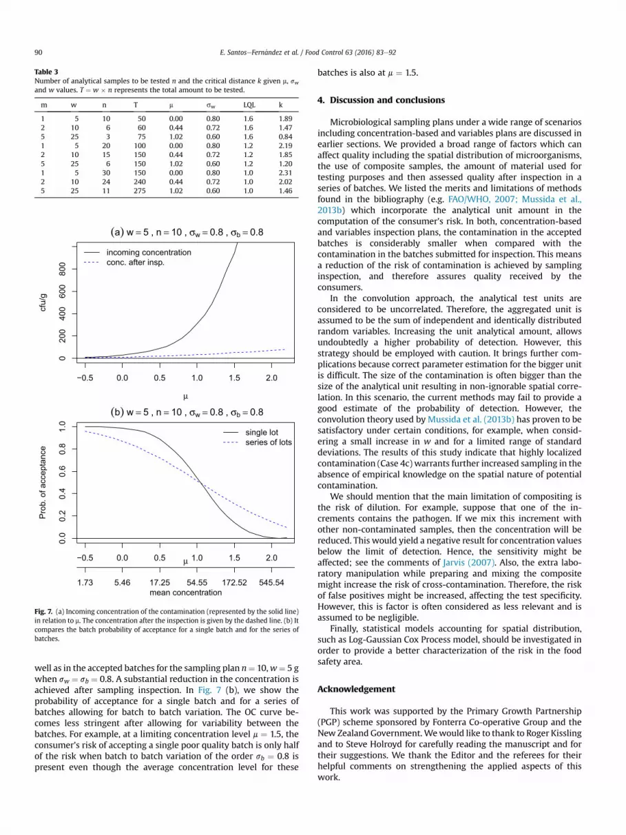
Table 3Number of analytical samples to be tested n and the critical distance k given m, swand w values. T ¼ w � n represents the total amount to be tested.

m w n T m sw LQL k

1 5 10 50 0.00 0.80 1.6 1.892 10 6 60 0.44 0.72 1.6 1.475 25 3 75 1.02 0.60 1.6 0.841 5 20 100 0.00 0.80 1.2 2.192 10 15 150 0.44 0.72 1.2 1.855 25 6 150 1.02 0.60 1.2 1.201 5 30 150 0.00 0.80 1.0 2.312 10 24 240 0.44 0.72 1.0 2.025 25 11 275 1.02 0.60 1.0 1.46

−0.5 0.0 0.5 1.0 1.5 2.0

020

040

060

080

0

(a) w = 5 , n = 10 , σw = 0.8 , σb = 0.8

μ

cfu/

g

incoming concentrationconc. after insp.

−0.5 0.0 0.5 1.0 1.5 2.0

0.0

0.2

0.4

0.6

0.8

1.0

(b) w = 5 , n = 10 , σw = 0.8 , σb = 0.8

Pro

b. o

f acc

epta

nce

single lotseries of lots

1.73 5.46 17.25 54.55 172.52 545.54

μ

mean concentration

Fig. 7. (a) Incoming concentration of the contamination (represented by the solid line)in relation to m. The concentration after the inspection is given by the dashed line. (b) Itcompares the batch probability of acceptance for a single batch and for the series ofbatches.

E. SantoseFern�andez et al. / Food Control 63 (2016) 83e9290

well as in the accepted batches for the sampling plan n¼ 10,w¼ 5 gwhen sw ¼ sb ¼ 0.8. A substantial reduction in the concentration isachieved after sampling inspection. In Fig. 7 (b), we show theprobability of acceptance for a single batch and for a series ofbatches allowing for batch to batch variation. The OC curve be-comes less stringent after allowing for variability between thebatches. For example, at a limiting concentration level m ¼ 1.5, theconsumer's risk of accepting a single poor quality batch is only halfof the risk when batch to batch variation of the order sb ¼ 0.8 ispresent even though the average concentration level for these

batches is also at m ¼ 1.5.

4. Discussion and conclusions

Microbiological sampling plans under a wide range of scenariosincluding concentration-based and variables plans are discussed inearlier sections. We provided a broad range of factors which canaffect quality including the spatial distribution of microorganisms,the use of composite samples, the amount of material used fortesting purposes and then assessed quality after inspection in aseries of batches. We listed the merits and limitations of methodsfound in the bibliography (e.g. FAO/WHO, 2007; Mussida et al.,2013b) which incorporate the analytical unit amount in thecomputation of the consumer's risk. In both, concentration-basedand variables inspection plans, the contamination in the acceptedbatches is considerably smaller when compared with thecontamination in the batches submitted for inspection. This meansa reduction of the risk of contamination is achieved by samplinginspection, and therefore assures quality received by theconsumers.

In the convolution approach, the analytical test units areconsidered to be uncorrelated. Therefore, the aggregated unit isassumed to be the sum of independent and identically distributedrandom variables. Increasing the unit analytical amount, allowsundoubtedly a higher probability of detection. However, thisstrategy should be employed with caution. It brings further com-plications because correct parameter estimation for the bigger unitis difficult. The size of the contamination is often bigger than thesize of the analytical unit resulting in non-ignorable spatial corre-lation. In this scenario, the current methods may fail to provide agood estimate of the probability of detection. However, theconvolution theory used by Mussida et al. (2013b) has proven to besatisfactory under certain conditions, for example, when consid-ering a small increase in w and for a limited range of standarddeviations. The results of this study indicate that highly localizedcontamination (Case 4c) warrants further increased sampling in theabsence of empirical knowledge on the spatial nature of potentialcontamination.

We should mention that the main limitation of compositing isthe risk of dilution. For example, suppose that one of the in-crements contains the pathogen. If we mix this increment withother non-contaminated samples, then the concentration will bereduced. This would yield a negative result for concentration valuesbelow the limit of detection. Hence, the sensitivity might beaffected; see the comments of Jarvis (2007). Also, the extra labo-ratory manipulation while preparing and mixing the compositemight increase the risk of cross-contamination. Therefore, the riskof false positives might be increased, affecting the test specificity.However, this is factor is often considered as less relevant and isassumed to be negligible.

Finally, statistical models accounting for spatial distribution,such as Log-Gaussian Cox Process model, should be investigated inorder to provide a better characterization of the risk in the foodsafety area.

Acknowledgement

This work was supported by the Primary Growth Partnership(PGP) scheme sponsored by Fonterra Co-operative Group and theNew Zealand Government.Wewould like to thank to Roger Kisslingand to Steve Holroyd for carefully reading the manuscript and fortheir suggestions. We thank the Editor and the referees for theirhelpful comments on strengthening the applied aspects of thiswork.

E. SantoseFern�andez et al. / Food Control 63 (2016) 83e92 91

Appendix A. Table of symbols

n Sample size or the number of analytical samples testedw analytical unit amountC concentration of microorganismsl rate parameter in the Poisson distributionPa probability of acceptancePd probability of detectionp prevalencenI number of primary samples or increments that are combined to form a composite sampleLN lognormal distributionPLN Poisson-lognormal distributionm location parameter (mean log) of the LN and PLN distributions on the log10 scalesw within-batch scale (standard deviation) of the LN and PLN distributions on the log10 scalesb between batches scale (standard deviation) on the log10 scaleLQL Limiting Quality Levelb consumer's riskX number of microorganisms in the small unitY ¼ SX number of microorganisms in the bigger unitE[X] expected valueVar[X] variance in the arithmetic scaleS[X] standard deviation in the arithmetic scaleCase 1 individual but homogeneous batchCase 2 individual but heterogeneous batchCase 3 series of homogenous batchesCase 4 series of heterogeneous batchesa convolution methodb Haas et al. (2014) Eq. (4) methodc simulation method for the case of one cluster

Appendix B. The convolution theory

If the cell cluster size is expected to be small compared toanalytical unit amount for low contamination levels, the spatialcorrelation between the analytical units can be considered negli-gible. In other words, the analytical amounts can be treated as in-dependent. Suppose that the analytical method is also capable ofanalysing a greater amount of material. For the bigger amount, theprocess of aggregation of the small analytical samples can betreated as the convolution or sum operation done on random var-iables. The sum of independent log-normally distributed randomvariables does not have a closed-form solution, but it can beapproximated by another lognormal distribution under certainconditions, (Johnson, Kotz,& Balakrishnan,1994, p. 217). That is, if Ybe the sum of independent and identically distributed (i.i.d.)lognormal random variables X, then the approximate distributionof Y is LN(my,sy) where E(Y) ¼ mE(X) and V(Y) ¼ mV(X). The meanand variance for the larger amount is obviously biggerwhen severalsmall amounts are aggregated. This approach of approximating thesum of lognormals is known as the Fenton-Wilkinson (Fenton,1960) method. In the log10 scale, the parameters my and sy of thepopulation using a bigger unit Y become

my ¼ log10ðE½Y �Þ � logð10Þs2y.2 (B.1)

sy ¼ffiffiffiffiffiffiffiffiffiffiffiffiffiffiffiffiffiffiffiffiffiffiffiffiffiffiffiffiffiffiffiffiffiffiffiffiffiffiffiffiffiffiffiffiffiffiffiffiffiffiffiffiffiffiffiffiffiffiffiffiffiffiffiffiffiffiffiffiffiffiffiffiffiffiffiffiffilog10

1þ Var½Y � � E½Y �

ðE½Y �Þ2!,

logð10Þvuut (B.2)

References

Anscombe, F. J. (1950). Sampling theory of the negative binomial and logarithmicseries distributions. Biometrika, 37, 358e382.

Bulmer, M. (1974). On fitting the Poisson lognormal distribution to species-abundance data. Biometrics, 101e110.

FAO/WHO. (2007). Risk assessment for Enterobacter sakazakii in powdered infantformula. http://www.mramodels.org/esakmodel/ESAKRAModelWizard.aspx(Accessed 01.11.15.).

FAO/WHO. (2014). Risk manager's guide to the statistical aspects of microbiologicalcriteria related to foods (Accessed 19.11.14.).

Fenton, L. (1960). The sum of log-normal probability distributions in scattertransmission systems. IRE Transactions on Communications Systems, 8, 57e67.

Gonzales-Barron, U., & Butler, F. (2011a). Characterisation of within-batch andbetween-batch variability in microbial counts in foods using Poisson-gammaand Poisson-lognormal regression models. Food Control, 22, 1268e1278.

Gonzales-Barron, U., & Butler, F. (2011b). A comparison between the discretePoisson-gamma and Poisson-lognormal distributions to characterise microbialcounts in foods. Food Control, 22, 1279e1286.

Gonzales-Barron, U., Zwietering, M. H., & Butler, F. (2013). A novel derivation of awithin-batch sampling plan based on a Poisson-gamma model characterisinglow microbial counts in foods. International Journal of Food Microbiology, 161,84e96.

Haas, C. N., Rose, J. B., & Gerba, C. P. (2014). Quantitative microbial risk assessment.New York, NY: John Wiley & Sons.

ICMSF. (2002). Microorganisms in foods 7. Microbiological testing in food safetymanagement. International commission on microbiological specifications for foods.Blackwell Scientific Publications.

Jarvis, B. (2007). On the compositing of samples for qualitative microbiologicaltesting. Letters in Applied Microbiology, 45, 592e598.

Jarvis, B. (2008). Statistical aspects of the microbiological examination of foods. Aca-demic Press. Elsevier/Academic Press.

Johnson, N. L., Kotz, S., & Balakrishnan, N. (1994). Continuous univariate distributions(Vol. 1). New York, NY: John Wiley & Sons.

Jongenburger, I., Bassett, J., Jackson, T., Zwietering, M., & Jewell, K. (2012a). Impact ofmicrobial distributions on food safety I. Factors influencing microbial distri-butions and modelling aspects. Food Control, 26, 601e609.

Jongenburger, I., Reij, M., Boer, E., Gorris, L., & Zwietering, M. (2011). Random orsystematic sampling to detect a localised microbial contamination within abatch of food. Food Control, 22, 1448e1455.

Jongenburger, I., Reij, M., Boer, E., Zwietering, M., & Gorris, L. (2012b). Modellinghomogeneous and heterogeneous microbial contaminations in a powderedfood product. International Journal of Food Microbiology, 157, 35e44.

E. SantoseFern�andez et al. / Food Control 63 (2016) 83e9292

Kiermeier, A., Mellor, G., Barlow, R., & Jenson, I. (2011). Assumptions of acceptancesampling and the implications for lot contamination: Escherichia coli O157 inlots of Australian manufacturing beef. Journal of Food Protection, 74, 539e544.

Legan, J., Vandeven, M. H., Dahms, S., & Cole, M. B. (2001). Determining the con-centration of microorganisms controlled by attributes sampling plans. FoodControl, 12, 137e147.

Mussida, A., Gonzales-Barron, U., & Butler, F. (2013a). Effectiveness of samplingplans by attributes based on mixture distributions characterising microbialclustering in food. Food Control, 34, 50e60.

Mussida, A., Vose, D., & Butler, F. (2013b). Efficiency of the sampling plan for Cro-nobacter spp. assuming a Poisson lognormal distribution of the bacteria inpowder infant formula and the implications of assuming a fixed within andbetween-lot variability. Food Control, 33, 174e185.

Nauta, M. J. (2005). Microbiological risk assessment models for partitioning andmixing during food handling. International Journal of Food Microbiology, 100,311e322 (The Fourth International Conference on Predictive Modelling inFoods).

Paoli, M. G., & Hartnett, E. (2006). Overview of a risk assessment model for Enter-obacter sakazakii in powdered infant formula. Available from The Food and

Agriculture Organization of the United Nations and the World HealthOrganization.

Santos-Fern�andez, E., Govindaraju, K., & Jones, G. (2015). Variables sampling plansusing composite samples for food quality assurance. Food Control, 50, 530e538.

Teunis, P., Ogden, I., & Strachan, N. (2008). Hierarchical dose response of E. coliO157: H7 from human outbreaks incorporating heterogeneity in exposure.Epidemiology and Infection, 136, 761e770.

Toft, N., Innocent, G. T., Mellor, D. J., & Reid, S. W. (2006). The gamma-Poisson modelas a statistical method to determine if micro-organisms are randomly distrib-uted in a food matrix. Food microbiology, 23, 90e94.

Van Schothorst, M., Zwietering, M., Ross, T., Buchanan, R., & Cole, M. (2009).Relating microbiological criteria to food safety objectives and performanceobjectives. Food Control, 20, 967e979.

Williams, M. S., & Ebel, E. D. (2012). Methods for fitting the Poisson-lognormaldistribution to microbial testing data. Food Control, 27, 73e80.

Zwietering, M. H. (2009). Quantitative risk assessment: is more complex alwaysbetter?: simple is not stupid and complex is not always more correct. Inter-national Journal of Food Microbiology, 134, 57e62.