quantitative simulation of errors in correlation analysis

Quantitative simulation of errors in correlation analysis

Anthony E. Smart, Robert V. Edwards, and William V. Meyer

Bounding the errors of measurements derived from correlation functions of light scattered from somephysical systems is typically complicated by the ill conditioning of the data inversion. Parameter valuesare estimated from fitting well-chosen models to measurements taken for long enough to look acceptable,or at least to yield convergence to some reasonable result. We show some simple numerical simulationsthat indicate the possibility of substantial and unanticipated errors even in comparatively simple ex-periments. We further show quantitative evidence for the effectiveness of a number of ad hoc aspectsof the art of performing good light-scattering experiments and recovering useful measurements fromthem. Separating data-inversion properties from experimental inconsistencies may lead to a betterunderstanding and better bounding of some errors, giving new ways to improve overall experimentalaccuracy. © 2001 Optical Society of America

OCIS code: 290.0290.

1. Introduction

The extraction of accurate information from the cor-relation functions of light scattered from a number ofphysical systems is typically an ill-conditionedprocess.1–4 The extent to which ill conditioning is alimiting factor on the useful precision of recoveredinformation has been analyzed.5 There was exten-sive research by Pike and Jakeman6 in the 1970s onestimating the error in the decay constant of a singleexponential in a photon-counting experiment. Thetreatment was approximate mainly because present-day computing power was not available to the au-thors. They were able to derive approximatealgebraic expressions to estimate the errors, but theydid no simulations. However, the critical parame-ters affecting accuracy and orders of magnitude forthe errors were identified, and the orders of magni-tude of the errors were estimated.

This paper presents simple numerical simulationsof correlation measurements constructed to emulatean idealized experiment with Gaussian statistics, to-

A. E. Smart [email protected]! is at 2857 Europa Drive, CostaMesa, California 92626-3525. R. V. Edwards [email protected]!is with Case Western Reserve University, 127 A. W. Smith Building,10900 Euclid Avenue, Cleveland, Ohio 44106-7217. W. V. [email protected]! is with the NASA Glenn ResearchCenter, National Center for Microgravity Research, M.S. 110-3,21000 Brookpark Road, Cleveland, Ohio 44135-3191.

Received 14 November 2000; revised manuscript received 20April 2001.

0003-6935y01y244064-15$15.00y0© 2001 Optical Society of America

4064 APPLIED OPTICS y Vol. 40, No. 24 y 20 August 2001

gether with accurate estimations of the errors in themeasured coefficients. In essence, we are simulat-ing experiments with ideal experimental equipmentand an infinite photon rate. The results of thisstudy thus represent the best possible accuracy thatcan be achieved in any real experiment. For in-stance, decreasing the photon rate to the point atwhich photon-detection statistics dominate the mea-surement cannot possibly give better accuracy.Here, we derive and use a precise form of the corre-lation between points in a measured autocorrelation.One conclusion from the analysis of these simulateddata sets is that apparently excellent data from evenideal experiments may yield measurements that aredisconcertingly in error. That data should appearsmooth is not sufficient, nor is it even necessary, forthe extraction of correct measurements. We alsoshow that a poorly chosen model, even though it ap-pears to fit the data well, can give rise to large errorsin the interpreted values of the physical parametersthat we wish to measure.

2. Simulated Functions

The experimental correlation function of a given pro-cess converges on an analytic model of that processonly after a perfect experiment has been conductedfor an infinitely long time. For example, the single-exponential decay, which theoretically is assumed torepresent closely the autocorrelation function of lightscattered from a stable coherent source by monodis-perse spheres in an almost transparent colloidal sus-pension in equilibrium, even supposing such an idealcase were possible, is approached only after an infi-

tmlottbuic

emriebctsas

nite observation time. Errors are inevitable in finiteexperiments. Brilliant experimental technique mayreduce many physical sources of error, such as elec-trical noise, system drift from optical and thermalinstabilities, and limitations of the apparatus or thesample itself. At least two noise sources, however,are intrinsic and may not be reduced. These areshot noise in the correlogram, which appears as un-correlated grassy channel-to-channel fluctuation,and what often proves to be the more serious effect,correlation of noise in the signal over nearby chan-nels in the correlation function, leading to a lumpyappearance. In both cases increasing the length ofthe experiment improves the accuracy. In this pa-per, we perform numerical simulations to quantifyand confirm the accuracy that might be availablefrom finite experiments performed on real systems.

A proper simulation requires the generation of asequence of estimates of a one-dimensional process,which may be autocorrelated to produce a functionsuch as is familiarly derived from a real experiment.Each of many such independent sequences is numer-ically autocorrelated, yielding functions whose vari-ability depends on only random effects and whosestatistics are stationary. The analysis of suchknown and standardized data sets with different as-sumptions, fitting models, and techniques proves in-formative.

The program can currently synthesize a signalthat, after correlation, simulates the sum of one ormore decaying exponentials with different constantbaseline, amplitude~s!, decay rate~s!, and modula-ion. An exponentially decaying form with one orore rate constants is typical of scattering from col-

oids, and an exponentially damped cosine is typicalf underdamped surface light scattering, i.e., a scat-ering sample when a local oscillator is present. Inhe four initial simulation types discussed here, theaseline was simulated as zero, but although this is aseful simplification, it is neither necessary nor need

t compromise generality of the method or the derivedonclusions.

3. Simulation

The simulation of a time series, for example, of suc-cessive measurements of optical intensity, that islong enough to represent a typical experimentallyderived correlogram would require an array of sev-eral million elements. Fortunately, we can avoidthis computational demand by noting that we onlyrequire sufficient channels of the correlation functionto indicate that the function has decayed to what webelieve to be insignificance. We can therefore in-voke the same method used in physical experimentsby discarding samples of the time series after theyhave been used over the displayed abscissa of thecorrelogram. The computation for generating theseries may be reduced by the simulation of each newpoint in the series based on the correct memory ofwhat went before and the multiplication of this sim-ulation by each member of the series shifted back byone time tick ~see below!. At each time tick every

lement of the correlation function is thus incre-ented appropriately. For avoiding end errors cor-

elation is started only after typically 20 decay timesnto the simulated process. In the case of a single-xponential decay the method of extending the seriesy each new point exploits the self-similarity of theorrelation function and applies a forgetting constanto the previous point before adding it to the succes-ive points. This computational economy in gener-ting the exponentially decaying function wasuggested by D. Cannell7 of the University of Califor-

nia, Santa Barbara, California. A. Lomakin8 of theMassachusetts Institute of Technology, Cambridge,Massachusetts, extended the method to the case ofcosine modulation by allowing the forgetting functionto be complex. We wish to acknowledge both contri-butions. The newest point is generated from aGaussian random variable with a variance of unitycentered on zero by the application of the Box–Mullertransform to the uniform random-number generatorthat is so capably built into most current program-ming languages. This method is adequate despitethe sensitivity of correlation to nonrandom effects.Functions comprising more than one exponential de-cay may be constructed by the application of indepen-dent processes to the next point of each differentsequence, with summation of the resultant series be-fore correlation. Two separate exponentials thustake twice as long to generate, but several separatesizes or a narrow distribution of sizes, more repre-sentative of polydispersity, would require proportion-ally more time. The damped cosine is elegantlygenerated from a series of Gaussian random realnumbers created from the product of a complex vectorwith each member of a series generated in the sameway as before. The constraint of a zero mean for theelements of the time series is equivalent to ac-coupling the signal, and, although it yields a correlo-gram that converges to zero from an interceptbetween one and zero rather than converging onunity from an intercept between one and two, it in noway compromises the following discussion.

For example, successive elements of a time serieswhose correlation function is a single exponentialmay be represented as

xt21 5 xt c 1 rt,

where c 5 exp~2g! and r is a Gaussian random vari-able centered on zero. After this process has beeniterated for a sufficiently long time and we note thatt increases as we go backwards from the present, thecurrent value of xt becomes

xt 5 rt 1 crt11 1 c2rt12 1 c3rt13 1 . . .

5limit

N3 ` (k50

N

ckrt1k,

which has a value related to its adjacent values in therequired manner and a zero mean because r is un-

20 August 2001 y Vol. 40, No. 24 y APPLIED OPTICS 4065

Z

ttndiwo

pitts

it

Table 1. Formulas and Parameter Values for Data Synthesis

4

correlated between successive estimates. It is easyto show that

^xt xt1M& 5cM

1 2 c2 ^x2& 5exp~2gM!

1 2 c2 ^x2&.

A random series with the desired exponential auto-correlation function is generated. This algorithmhas been extensively checked both theoretically andexperimentally. It accurately mimics a Gaussianrandom variable with a zero mean and an exponen-tial autocorrelation.

For more than one exponential decay time values ofx are generated independently by use of the aboverule with different values of g and summed sequen-tially. The more challenging function of a dampedcosine, again centered on zero, may be generated byone’s allowing c to become complex of the form c 5exp~2g 1 iv! and generating, from similar but inde-pendent values of r and a now complex x, a series ofreal numbers yt from the relation yt 5 Re~Zx!, where

5 ~1 2 c!1y2 and is also complex.These two methods permit the generation of data

sequences that may be correlated to give functionssuitable for model fitting and statistical examination.Although idealized, they approximate those se-quences typical of real experiments in which the in-evitable physical limitations have been optimallycontrolled. The four initial data series were eachused to construct correlation functions with the prop-erties described in Table 1. Common attributes arethat each correlogram is 200 channels long ~0hrough 199!, all baselines B are nominally zero, andhe amplitude A has a mean value of zero and aominal variance of unity. Each of the shortest in-ependent basic experiments is run for 4000 timentervals, or 160 decay times of the slower process,hen there is more than one. All units are in terms

f time ticks, permitting scalable derived properties.In terms of an actual quasi-elastic light-scattering ex-

eriment, we are generating the electric field and not thentensity that is usually measured. There is no scien-ific reason for which we could not have done that, but wehought the results would be cleaner and more under-tandable if we did not square the generated series.

For specified values of A the intercept scaling factors given by the summation of individual contributionso the zero channel as the infinite sum

I 5 @B 1 A0 exp~2gt0!#2 1 @B 1 A1 exp~2gt1!#

2

1 @B 1 A2 exp~2gt2!#2 1 . . .

5 (n50

`

@B 1 An exp~2ngtn!#2.

Type of Function Formula

Single exponential B 1 A exp~2gt!Double exponential B 1 A1 exp~2g1t! 1 A2 exp~2gDecaying cosine B 1 A exp~2gt!cos~vt!


Because we have currently chosen B 5 0, we mayscale by A or, equivalently, without a loss of gener-ality set ^An

2&1y2 5 1, as described above, to obtain

I 5 (n50

`

exp~22ng! 51

1 2 exp~22ng!.

Thus the numerical value of the intercept at the zerochannel becomes I multiplied by the experimentlength. For the double exponential described abovein which the decay rates differ by a factor of 2, we canwrite the scaling as

I 51

1 2 exp~22g!1

11 2 exp~24g!

,

which is simply evaluated. For an intercept that isnormalized to unity and the values given in Table 1the relative intercept contributions of the slower andthe faster decay rates are 0.657899 and 0.342101,respectively. For the cosine-modulated correlationwaveforms the normalizing summation is more com-plicated, becoming

I 51

2@1 2 exp~22g!#

11

2@1 2 2 exp~22g!cos~2v! 1 exp~24g!#1y2 .

A sequence of 8192 ~conveniently, 213! correlogramsof each type was generated and accumulated into afamily of files, each of which contains entries com-posed of the sum of two records in the previouslyranked file. Thus the first file contains all 8192 cor-relograms simulated as independent experiments;the second file contains 4096 entries, each of which isthe sum of two adjacent entries in the previous file,and so on down to one file that represents a singleexperiment that is 32,768,000 time ticks or 1,310,720decay times long. We emphasize here that the pur-pose of this exercise is to simulate an ideal correlationfunction to test the properties of data-processing andinformation-retrieval methods, separated from themany real physical limitations, and that this reset toan independent measurement every 160 decay timesis not typical of real correlators. The method may beextended to include presently unexamined effectssuch as quantization, experimental consequences ofphoton counting, or even the extreme case of hardclipping. Other real empirical effects such as drifts,

Decay Rate g Frequency v

0.04 NA0.04, 0.08 NA0.04 v 5 0.06 3 2p ~oscillatory!,

v 5 g ~critically damped!

2t!

otsaovftssodWtmbeidvcfp

sbtcsie

instabilities, or even changing experimental condi-tions, which can limit accuracy in practice, are lesseasy to simulate usefully. Although the shortestcorrelograms are truly independent, the conclusiondrawn from successive sums thereof is not, and thislack of independence may be overcome only by one’staking even longer than the current tens of hoursnecessary to synthesize each data set by use of cur-rent Pentium-based computers running at a few hun-dred megahertz.

Each of these simulated correlograms was ana-lyzed initially by an unweighted Levenberg–Marquardt nonlinear fitting routine with the knowninput parameter values as the starting estimates.Although this approach is not typically possible inreal experiments, here it shows the best that can bedone by such procedures and predicts that claims ofaccuracy greater than those obtained under theseconditions are likely to be suspect.

For most correlograms with sufficient accumula-tion time the fitting procedure converges to valuesslightly different from the ideal and with a quantifi-able standard deviation. As the correlograms arebased on fewer data, the errors increase, and somefits no longer converge, typically failing in one of twodifferent ways. The first cause of failure appears tobe exceeding the numerical dynamic range ~106;300!f the fitting routine in the incremental matrix. Al-hough the parameter values at this point may stillometimes appear plausible after such a failure, theyre disregarded in the statistical analyses. The sec-nd reason to disregard results of the process is if thealue of any fitted parameter is negative because,rom the model, all are known to be positive. Wherehe baseline is also fitted, this is excluded from theecond rejection criterion because it may take eitherign. In the case of the single-exponential and thescillatory cosine data examined here all fits to dataerived from longer than 160 decay times converged.ith the critically damped cosine, and more so with

he double exponential, failure to converge becomesore frequent as the simulated experiment time

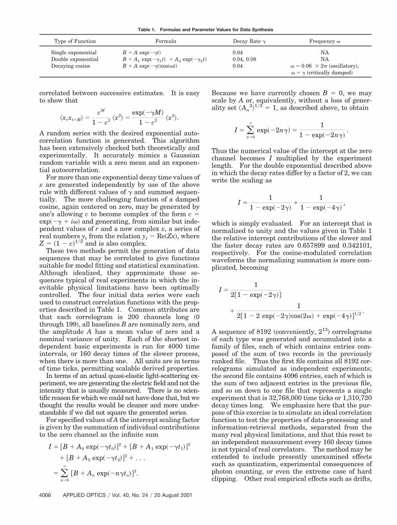
ecomes shorter. For the independent double-xponential correlation functions in which the exper-mental duration was only 160 times the exp~21!ecay time of the slower process, .14% failed to con-erge when the baseline was forced to zero and ex-luded from the fitting parameter set, and .16%ailed when the baseline was included as a fittingarameter with a starting estimate of zero.Figure 1 shows analytic representations of the four

imulated functions with the properties given in Ta-le 1 for which the abscissa is 8 times the relaxationime, that is, exp~21! of the slower exponentially de-aying process, suggesting that, by the end of theimulated function, the residual baseline, asymptot-cally approaching zero, has fallen to approximatelyxp~28! or ,0.034% of the value of the zero channel.

Although in many real experiments the zero-channelvalue may be independently accessible, the accurateinference from it of a baseline value to be exploited inthe fit is subject to experimental corruptions, such as

noise, dead time, and afterpulsing. The trade-off be-tween the length of the recorded correlation functionand the separation of the channels, the product ofwhich is limited by traditional hardware, has led tosuggestions of nonlinear channel spacing, but thispossibility is neither simulated nor examined here.

Figure 2 shows three single-exponential functionsthat illustrate the comparative appearances of ananalytic function without noise ~continuous curve!,the properly synthesized lumpy correlation function~open circles!, and the grassy function ~filled circles!in which a statistically constant amount of noise wasadded to each channel. For the particular exampleshown in Fig. 2 an unweighted least-squares fit of acorrect model, with or without allowing the baselineto float as a variable, yields decay-rate and interceptrms errors of between 2% and 3%. Here the addeduncorrelated noise has a rms level of approximately3% of the value in the zero channel, and for the cor-rectly simulated correlogram the signal is a Gaussianrandom variable with a superimposed decay constantaccumulated for approximately 5000 decay times.We note that the grassy scatter for uncorrelated er-

Fig. 1. Analytic representations of single-exponential decay ~h!,double-exponential decay ~E!, oscillatory decaying cosine ~{!, andcritically damped decaying cosine ~‚!.

Fig. 2. Analytic single exponential without noise ~solid curves!,synthesized correlation function with channel-to-channel correla-tion ~E!, and function with uncorrelated shot noise ~F!. The lasttwo function yield similar errors ~approximately 3%!.


tt

pttptTu

w

w

D

4

rors appears to be very large compared with thelumpiness for comparable accuracy, indicating thatthe appearance of smoothness in an accumulatingcorrelogram is not a sufficient test for acceptabledata.

This channel-to-channel correlation of noise meansthat the number of channels in the correlogram istypically far larger than the number of independentmeasurements available.9

4. Theory of Error Estimates

The correlograms computed here, and all measuredcorrelograms, show that the correlation of noise be-tween nearby channels makes the correlationsmoother than it would appear if the noise were un-correlated ~Fig. 2!. We show below how to estimatehe errors in the measured parameters, while takinghis correlation into account.

Let gn~a! be the fitting function for a least-squaresrocedure designed to find the value of the parame-ers a. In practice, every new set of data ~realiza-ion! will result in a different estimate for thearameters. We approximate the change in the fit-ing function as a function of the parameter set by aaylor series in the variation in the parameter val-es, that is,

gn~a! 5 gn~a0! 1 (k

]gn

]ak~ak 2 a0k!,

here a0 is the true value of the parameter vector.When we set up the least-squares objective e2, we

get

e2 5 (n

Fdn 2 gn~a0! 2 (k

]gn

]akDakG2

,

here dn are the measurements and the fitting func-tion gn is evaluated at the true values for a. Thus

ak represents the variation in the estimate for theparameters from the ‘true’ value for a given datarealization.

Note that this approach is applicable only when thechanges in the estimated parameters are smallenough for the linear approximation to be valid.However, other problems become serious long beforethis linear approximation ceases to be useful, as wesee below with the double exponential.

We attempt to minimize the above expression bygenerating a series of equations

(n

Fdn 2 gn~a0! 2 (k

]gn

]akDakG ]gn

]aj5 0

or

(n

@dn 2 gn~a0!#]gn

]aj5 (

n(

k

]gn

]aj

]gn

]akDak.


Define

Bjk 5 (n

]gn

]aj

]gn

]ak(1)

and rewrite it as

(n

@dn 2 gn~a0!#]gn

]aj5 (

kBjkDak.

Now we can write

(n

@dn 2 gn~a0!# (j

Blj21 ]gn

]aj5 (

j(

kBlj

21BjkDak

5 Da1,

which is what we want. The above equation showsthat the least-squares procedure should be unbiasedin that the expected value of the extracted parame-ters should be unbiased. To confirm this, we takethe expected value of both sides of the previous equa-tion. Because the expected error of the left-handside of the equation is zero, it follows that the ex-pected error on the right-hand side must also equalzero.

Squaring this quantity and taking the expectedvalue, we obtain

(m

(n

@dn 2 gn~a0!#@dm 2 gm~a0!#

3 (j

Blj21(

kBpk

21 ]gn

]aj

]gm

]ak5 DapDal.

Define

Lnm 5 ^@dn 2 gn~a0!#@dm 2 gm~a0!#&,

where the angle brackets denote the expected value.Then

(m

(n

Lnm (j

Blj21 (

kBpk

21 ]gn

]aj

]gm

]ak

5 DapDal 5 Cpl. (2)

C is the desired parameter, the covariance matrix.An explicit numerical theory for the variation in theparameter estimates requires the computation of thecovariance matrix Lnm, which is expanded in Appen-dix A for the three functions of interest here.

Define the expected autocorrelation of the time se-ries f ~k! as

R0~m! ; ^ f ~k! f ~k 1 m!&S1 2umuN D .

The measured correlation function is

R~m! ;1N (

k50

N2m

f ~k! f ~k 1 m!,

Ipcd

mfi

o

o

IGif

Sf

Fb

evd

dutN

watscss

eb

where N is the total number of points used to calcu-late the measured correlation function

^R~m!& ; R0~m!.

f N is large enough the difference between the ex-ected and the measured correlograms should be-ome negligible because here all the correlogramsecay exponentially to a nominally zero baseline.The expected covariance of the errors between theeasured and the expected correlograms may be de-

ned as

Lmn 5 ^@R~m! 2 R0~m!#@R~n! 2 R0~n!#&,

r

Lmn 5 ^R~m!R~n!& 2 R0~m! R0~n!,

Lmn 5 K 1N 2 (

k50

N2m

f ~k! f ~m 1 k! (k950

N2n

f ~k9! f ~n 1 k9!L2 R0~m! R0~n!,

r

Lmn 51

N 2 (k50

N2m

(k9

N2n

^ f ~k! f ~m 1 k! f ~k9! f ~n 1 k9!&

2 R0~m! R0~n!.

n this paper, the statistics for f are known to beaussian and zero mean and we assume the system

s stationary, so we may use the well-known identityrom Saleh10

^ f ~k! f ~n 1 k! f ~k9! f ~m 1 k9!&

5 R0~n! R0~m! 1 R0~k9 2 k! R0~m 2 n 1 k9 2 k!

1 R0~m 1 k9 2 k! R0~k9 2 k 2 n!.

ubstituting this equation back into the expressionsor the covariance, we find

Lmn 51

N 2 (k50

N2m

(k950

N2n

@R0~k9 2 k! R0~k9 2 k 1 m 2 n!

1 R0~m 1 k9 2 k! R0~k9 2 k 2 n!#.

Summing first over k and then over k9 2 k allows thisdouble sum to be rewritten in the useful form

Lmn 51N (

p52`

p5` S1 2umuN D@R0~ p! R0~ p 1 m 2 n!

1 R0~ p 1 m! R0~ p 2 n!#.

or N sufficiently large, we can approximate the sumy the integral

Lmn 51N *

2`

`

@R0~ p! R0~ p 1 m 2 n!

1 R0~ p 1 m! R0~ p 2 n!#dp.

This is the form of the covariance estimate that weuse in this paper.

The explicit forms for the covariance of each func-tion are given in Appendix A.1, and Mathematicanotebooks were written for their evaluation under thespecific conditions chosen for synthesis here. Notethat, in all cases, the number of independent datapoints always appears to the first power in the de-nominator of the expression for covariance. FromEq. ~1!, we can see that the variance in the parameterstimates is proportional to the magnitude of the co-ariance. From this and the above theory, we mayeduce our first two predictions:

~1! The variance in the estimate of any parameterecreases as the number of independent data pointssed to estimate the parameter. This means that allhe fractional standard deviations should decay as

D1y2, where ND is the number of decay times. This

behavior is clear in all the plots except those for thedouble exponential, which we discuss below.

~2! The fluctuations in the measured correlogramsshould scale as the square root of the covariance.From the formulae for the covariance, one can seethat the rms fluctuation in the first point of the cor-relogram should scale as the expected size of the firstpoint and inversely as the square root of the numberof points used to calculate the correlogram. Thusplots versus the number of points are equivalent toplots versus the first point divided by the fluctuationintensity. One is proportional to the inverse of theother.

Each of the measured standard deviations ~S.D.s!,hich are plotted here throughout instead of the vari-nce, involved averaging all independent estimates ofhe measured parameters. The estimated S.D. istill a random variable, but we can estimate howlose the estimate is to some true value. It can behown that the measured variances follow a chi-quared distribution. If s2 is an estimated variance

with N data points it can be further shown11 that thexpected variance in the measured variance is giveny

Var~s2! 52~s2!2

N 2 1,

where s2 is the expected variance, here the diagonalelements of the C matrix. So the relation of themeasured variance to the theoretical variance shouldbe given by

S.D.~s2!

s2 5 S 2N 2 1D

1y2

.

For our exemplary data in the condition for which allfits converge N 5 8192, so the measured S.D.s andthe actual S.D. should agree to within approximately1.5%.

5. Comparisons with Theory

Interesting observations are available from theselarge numbers of well-characterized data and their


vc

nlwe

~

Table 2. Relative S.D.s for the Single Exponential

4

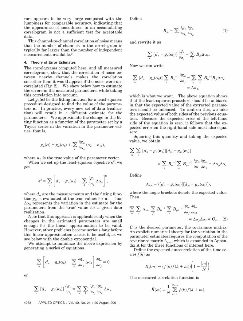
statistical summaries. We emphasize here the rea-sonable correspondence of the theoretical predictionwith the numbers derived from the numerical exper-iments described in Section 2 for all but the doubleexponential, which we discuss below. Tables 2through 5 show values of the S.D. of errors calculatedfrom first principles and measured from each of thesynthesized data sets with fixed and fitted baselines.Figure 3 and Figs. 10–12 show the rms differences ofunweighted fitted parameter values from the knowngenerating values for the various multiparameter fitsto the different data types and sets. The plottedS.D.s are the difference in the reciprocal decay timenormalized by the decay rate, the difference from thenormalized value of unity for the intercept, and theunnormalized baseline. Parametric fits with a fixedzero baseline are generally plotted with open sym-bols, and those including the baseline as a floatingvariable are shown with filled symbols. The solidcurves represent theoretical values derived from theabove analyses and where not separately identifiedare sufficiently close to the symbols to which eachcorresponds to eliminate ambiguity.

A. Single Exponential

Figure 3 represents the simulation of a single-exponential function as defined in Fig. 1, as this issupposed to be a common situation for optical scat-tering from monodisperse colloids. The correspon-dence with theory is remarkably good, particularly atshort experiment times for which, in general, theerrors are much larger ~typically so large as to berelatively uninteresting for most physical experi-ments but excellent for examining the theoretical be-havior!. Table 2 shows that, although the actualalues predicted for all parameters differ slightly ac-ording to whether the baseline is fixed or fitted, the

Fig. 3. S.D.s of the fits for a single exponential: decay rate ~h!and intercept ~‚! for a fixed zero baseline; decay rate ~■!, interceptŒ!, and baseline ~F! for a fitted baseline; decay, intercept, and

baseline ~solid curves! from theory.


correspondence between theory and numerical exper-iment is excellent in both cases. For real experi-ments, we do not in general have the luxury of aknown baseline, but some experimental systemsmake available an estimate from an independentmeasurement of the total signal. It can be shownthat the effect of fitting the baseline on the errors inthe estimation of the other parameters is negligiblefor correlograms such as these that are accumulatedfor sufficient time and for which the computed delaytime is at least 8 times the decay time of the slowestprocess. This is borne out by our synthetic measure-ments, as we see below. As the experiment becomeslonger, the experimental errors for the decay ratebecome slightly greater than theory, and those for theintercept become a little less. Although the dispar-ity does not cause immediate alarm, the presence ofwhat must appear as superresolution for long exper-iments suggests that the fitting routine may not be astrustworthy as one might suppose or wish, especiallywhen the correspondence of synthetic ~experimentaldata! and analytic functions becomes close. The in-creasing scatter toward the longer experiment timesarises from small-number statistics—the number ofindependent experiments contributing to each esti-mate is the abscissa divided by 8192 3 160, except forthose for which some fits do not converge, which re-duces the first number. Thus only one experimentalsequence contributes to the last point.

In Tables 2 through 5 the relative error is definedas the S.D. of the measurement error divided by theexpected value of the parameter. For example, avalue of 0.10 represents a 10% relative error.

1. Uncorrelated ErrorsTo gain additional insight into the effects of corre-lated versus uncorrelated noise, we generated newsingle-exponential data sets without simulating fullcorrelation. Here a Gaussian random number isadded to each channel of the analytic representationof the single exponentially decaying correlogram.The added value has a zero mean and S.D. of a givenfraction of the zero-channel content, or normalizedintercept, and is denoted by a reciprocal noise factor.We generated 256 such pseudo-correlograms for re-ciprocal noise factors between unity, where the S.D.was equal to the intercept ~giving an unreasonablyragged appearance!, and 1048576 ~220!, where almost

o noise was apparent. Each correlogram was ana-yzed by the fitting of a single-exponential functionith fixed and floating baselines, as above. Hereach random data set was generated and analyzed

Parameter

Zero Fixed Baseline Fitted Baseline

Prediction Measurement Prediction Measurement

Decay 0.2685 0.2668 0.2813 0.2784Intercept 0.1335 0.1372 0.1353 0.1351Baseline NA NA 0.0638 0.0660

sequentially, avoiding the need to store large arrays,and, although the use of different data for each com-parative analysis with and without baseline fittingintroduces variability, it does not affect the conclu-sions drawn from the statistically stationary behav-ior. Not surprisingly, fits of data sets withuncorrelated errors are much better than those cor-rectly synthesized with correlated errors.

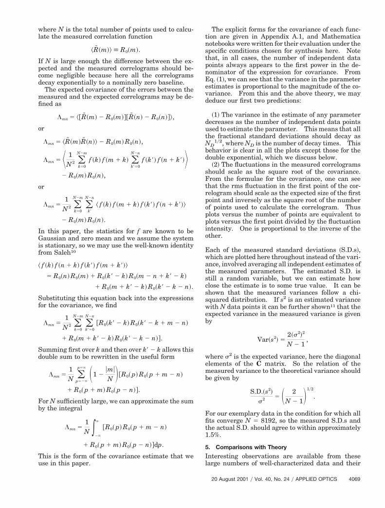
Figure 4 shows the results of this simulation. Theabscissa is the reciprocal noise factor defined above,and the ordinate is the normalized rms error for thedecay time and the intercept for a fixed zero baseline,repeated to include a baseline value where this isfitted. The uncorrelated errors reduce linearly withdecreasing additive noise. Although we did not ex-plicitly test the results from more correlograms orlonger accumulation times, we believe that in allcases the effects of correlated noise remain substan-tially worse than those of uncorrelated noise. Thespurious values for which noise is large indicate apoor fit to the data whose appearance is so raggedthat its parameter values are suspect, even though afit converges.

Adding uncorrelated shot noise to the correlogramis an unrealistic assumption but indicates a usefulpoint. For example, allowing for correlated noise,we find that an accumulation over 160 decay timesgives an approximately 30% rms error, the sameamount as would be found from additive uncorrelatednoise of approximately 50% of the zero intercept.Adding uncorrelated noise of 5% reduces this rmserror by a factor of ten to approximately 3%. Anequivalent improvement for which realistic corre-lated noise is present requires an increase in theobservation time of a factor of 100. This value is inaccord with experimental experience; real correlo-grams improve only as the square root of the obser-vation time, and after the accumulation time is long

Fig. 4. Errors from shot noise for a single exponential: decayrate ~h! and intercept ~‚! for a fixed zero baseline; decay rate ~■!,intercept ~Œ!, and baseline ~F! for a fitted baseline.

enough to be useful uncorrelated channel-to-channelvariation, typically arising from shot noise, is usuallynegligible. Hence channel-to-channel correlationbecomes the limiting factor on accuracy in an other-wise ideal experiment.

One potentially useful conclusion from this ap-proach is that we can mitigate some serious experi-mental limitations by cross-correlating the outputsfrom two similar detectors that observe nominally thesame optical intensity signals. Although thecorrelated-noise effects remain the same, the uncor-related effects from shot noise, dead time, afterpuls-ing, or other detector limitations rapidly becomeinsignificant, resulting in improved measurements.

One further interpretation of this approach, as wealready affirmed above, is that the adjacent channelsin a real correlogram do not necessarily representindependent measurements and the optimization ofthe number of channels and their spacing for a givenexperiment may be subtle.

2. Frequency-Domain AnalysisFor surface light scattering the application of a sur-face response function is desirable for optimizing theinformation recoverable from the measured data, andthis function is known only in the frequency domainbecause a branch cut in the complex plane preventsFourier transformation to a function that is applica-ble in the time domain. With this constraint, weneed to know how many decay times are required inthe correlation data to obtain a good Fourier trans-form before frequency-domain analysis. We may ex-amine estimates obtained in both the time and thefrequency domains from an analytic form of the sin-gle exponential compared with a synthesized form,which includes channel-to-channel correlations.This type of analysis give a best-case test of the Fou-rier transform process by the exclusion of uncon-trolled variables that are encountered in realexperiments, such as zero-channel corruptions fromdead time, afterpulsing, and noise, possible problemswith high-frequency aliasing, and other potentiallyunknown empirical imperfections. With syntheticdata, we can find the best accuracy of obtaining fre-quency data from correlation data that are acquiredover different numbers of decay times. This distinc-tion is typically not possible with real experimentaldata because they are constrained by the limitationsof real analog, or even digital, correlators, for exam-ple, intentional or implicit low-pass filtering.

To obtain the power spectrum, we first fold thecorrelation function before applying a prime-number-decomposition fast Fourier transform ~FFT!. Thisform of FFT does not assume 2n data points, where nis an integer; hence it does not require padding,which may bias our analysis. Because a FFT as-sumes that the pattern being transformed covers allfrequencies ~infinite bandwidth! and that it is a pat-tern that repeats forever, we fold the data beforetransforming to avoid introducing a step that wouldotherwise add spurious high-frequency componentsto the power spectrum. Because we intend to work


wa5rfsvtc

tdgasaIfFsr~

lebat

tmtva

so

cesttssOttdpfieta

rnrobs

4

with correlation functions that decay to a relativelyflat baseline, this approach avoids the need to applya windowing function or roll-off filter to suppress theeffects of the step, possibly biasing the results. It iswell known that folding the correlation function re-quires some care to ensure that the fold, particularlyat the zero end, does not introduce spurious phaseeffects. A value at zero time delay is necessary,which for real experiments can be extrapolated withminimum impact. Note that, if we start, for exam-ple, with 257 data points ~including the zero channel!,

e will find 512 data points in the Fourier transformfter folding, but half of these are redundant. The12 points in the transform result from dropping theedundant data points from the unfolded and theolded data sets before they are concatenated. Twoimple criteria for successful folding are that thealue and its gradient should both be continuous athe ends of the input data and that establishing thisondition should not introduce spurious phase effects.

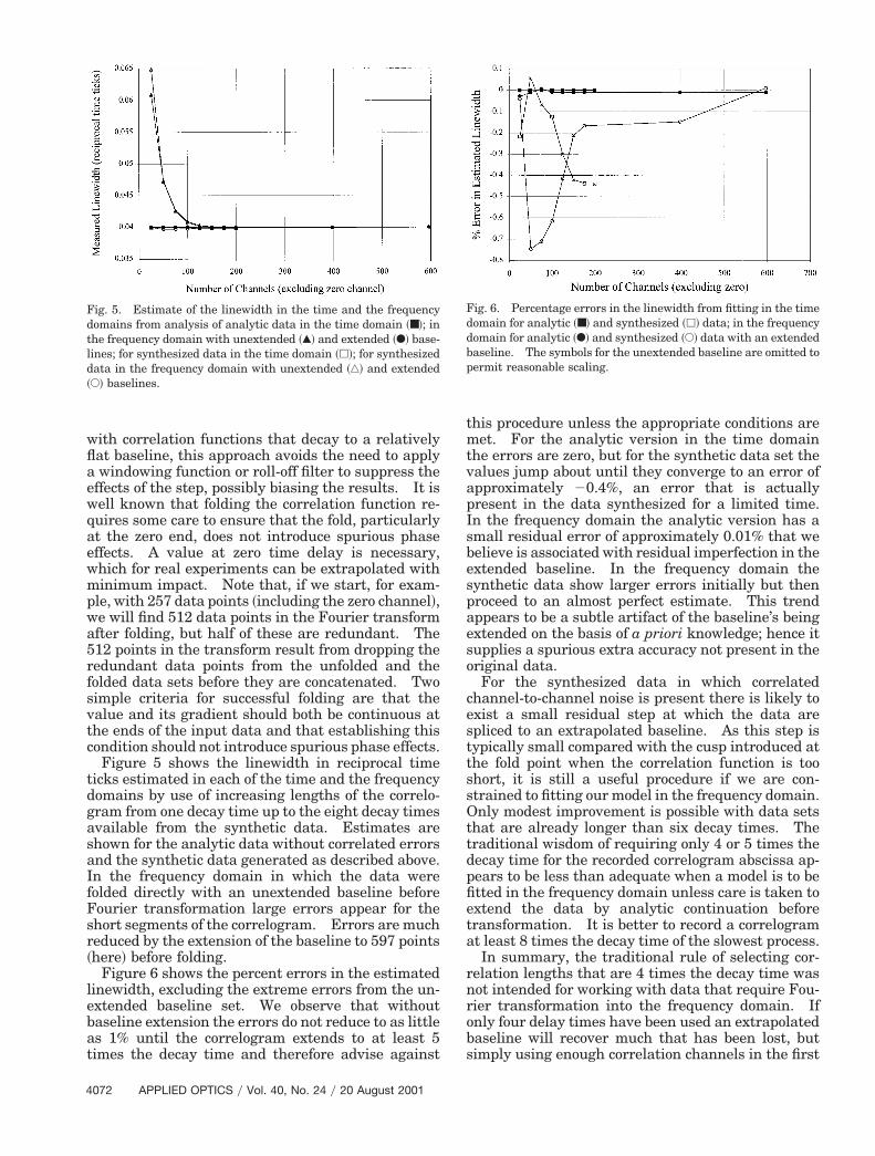
Figure 5 shows the linewidth in reciprocal timeicks estimated in each of the time and the frequencyomains by use of increasing lengths of the correlo-ram from one decay time up to the eight decay timesvailable from the synthetic data. Estimates arehown for the analytic data without correlated errorsnd the synthetic data generated as described above.n the frequency domain in which the data wereolded directly with an unextended baseline beforeourier transformation large errors appear for thehort segments of the correlogram. Errors are mucheduced by the extension of the baseline to 597 pointshere! before folding.

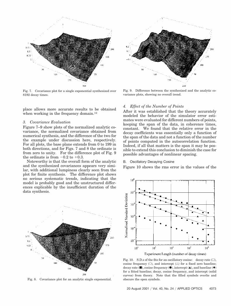
Figure 6 shows the percent errors in the estimatedinewidth, excluding the extreme errors from the un-xtended baseline set. We observe that withoutaseline extension the errors do not reduce to as littles 1% until the correlogram extends to at least 5imes the decay time and therefore advise against

Fig. 5. Estimate of the linewidth in the time and the frequencydomains from analysis of analytic data in the time domain ~■!; inthe frequency domain with unextended ~Œ! and extended ~F! base-lines; for synthesized data in the time domain ~h!; for synthesizeddata in the frequency domain with unextended ~‚! and extended~E! baselines.


his procedure unless the appropriate conditions areet. For the analytic version in the time domain

he errors are zero, but for the synthetic data set thealues jump about until they converge to an error ofpproximately 20.4%, an error that is actually

present in the data synthesized for a limited time.In the frequency domain the analytic version has asmall residual error of approximately 0.01% that webelieve is associated with residual imperfection in theextended baseline. In the frequency domain thesynthetic data show larger errors initially but thenproceed to an almost perfect estimate. This trendappears to be a subtle artifact of the baseline’s beingextended on the basis of a priori knowledge; hence itupplies a spurious extra accuracy not present in theriginal data.For the synthesized data in which correlated

hannel-to-channel noise is present there is likely toxist a small residual step at which the data arepliced to an extrapolated baseline. As this step isypically small compared with the cusp introduced athe fold point when the correlation function is toohort, it is still a useful procedure if we are con-trained to fitting our model in the frequency domain.nly modest improvement is possible with data sets

hat are already longer than six decay times. Theraditional wisdom of requiring only 4 or 5 times theecay time for the recorded correlogram abscissa ap-ears to be less than adequate when a model is to betted in the frequency domain unless care is taken toxtend the data by analytic continuation beforeransformation. It is better to record a correlogramt least 8 times the decay time of the slowest process.In summary, the traditional rule of selecting cor-

elation lengths that are 4 times the decay time wasot intended for working with data that require Fou-ier transformation into the frequency domain. Ifnly four delay times have been used an extrapolatedaseline will recover much that has been lost, butimply using enough correlation channels in the first

Fig. 6. Percentage errors in the linewidth from fitting in the timedomain for analytic ~■! and synthesized ~h! data; in the frequencydomain for analytic ~F! and synthesized ~E! data with an extendedbaseline. The symbols for the unextended baseline are omitted topermit reasonable scaling.

place allows more accurate results to be obtainedwhen working in the frequency domain.12

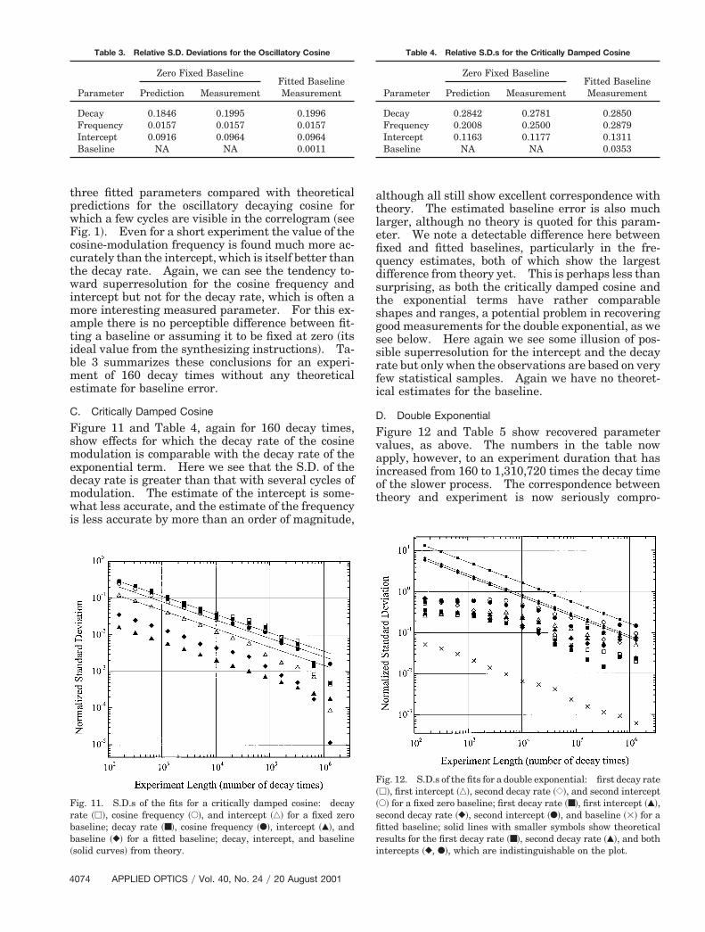
3. Covariance EvaluationFigure 7–9 show plots of the normalized analytic co-variance, the normalized covariance obtained fromnumerical synthesis, and the difference of the two forthe example under discussion here, respectively.For all plots, the base plane extends from 0 to 199 inboth directions, and for Figs. 7 and 8 the ordinate isfrom zero to unity. For the difference plot of Fig. 9the ordinate is from 20.2 to 10.3.

Noteworthy is that the overall form of the analyticand the synthesized covariances appears very simi-lar, with additional lumpiness clearly seen from theplot for finite synthesis. The difference plot showsno serious systematic trends, indicating that themodel is probably good and the unstructured differ-ences explicable by the insufficient duration of thedata synthesis.

Fig. 7. Covariance plot for a single exponential synthesized over8192 decay times.

Fig. 8. Covariance plot for an analytic single exponential.

4. Effect of the Number of PointsAfter it was established that the theory accuratelymodeled the behavior of the simulator error esti-mates were evaluated for different numbers of points,keeping the span of the data, in coherence times,constant. We found that the relative error in thedecay coefficients was essentially only a function ofthe span of the data and not a function of the numberof points computed in the autocorrelation function.Indeed, if all that matters is the span it may be pos-sible to extend this conclusion to diminish the case forpossible advantages of nonlinear spacing.

B. Oscillatory Decaying Cosine

Figure 10 shows the rms error in the values of the

Fig. 9. Difference between the synthesized and the analytic co-variance plots, showing no overall trend.

Fig. 10. S.D.s of the fits for an oscillatory cosine: decay rate ~h!,cosine frequency ~E!, and intercept ~‚! for a fixed zero baseline;decay rate ~■!, cosine frequency ~F!, intercept ~Œ!, and baseline ~}!for a fitted baseline; decay, cosine frequency, and intercept ~solidcurves! from theory. Note that the filled symbols overlie andobscure the open symbols.


Fcctwimatibme

Table 3. Relative S.D. Deviations for the Oscillatory Cosine Table 4. Relative S.D.s for the Critically Damped Cosine

4

three fitted parameters compared with theoreticalpredictions for the oscillatory decaying cosine forwhich a few cycles are visible in the correlogram ~see

ig. 1!. Even for a short experiment the value of theosine-modulation frequency is found much more ac-urately than the intercept, which is itself better thanhe decay rate. Again, we can see the tendency to-ard superresolution for the cosine frequency and

ntercept but not for the decay rate, which is often aore interesting measured parameter. For this ex-

mple there is no perceptible difference between fit-ing a baseline or assuming it to be fixed at zero ~itsdeal value from the synthesizing instructions!. Ta-le 3 summarizes these conclusions for an experi-ent of 160 decay times without any theoretical

stimate for baseline error.

C. Critically Damped Cosine

Figure 11 and Table 4, again for 160 decay times,show effects for which the decay rate of the cosinemodulation is comparable with the decay rate of theexponential term. Here we see that the S.D. of thedecay rate is greater than that with several cycles ofmodulation. The estimate of the intercept is some-what less accurate, and the estimate of the frequencyis less accurate by more than an order of magnitude,

Fig. 11. S.D.s of the fits for a critically damped cosine: decayrate ~h!, cosine frequency ~E!, and intercept ~‚! for a fixed zerobaseline; decay rate ~■!, cosine frequency ~F!, intercept ~Œ!, andbaseline ~}! for a fitted baseline; decay, intercept, and baseline~solid curves! from theory.

Parameter

Zero Fixed BaselineFitted BaselineMeasurementPrediction Measurement

Decay 0.1846 0.1995 0.1996Frequency 0.0157 0.0157 0.0157Intercept 0.0916 0.0964 0.0964Baseline NA NA 0.0011


although all still show excellent correspondence withtheory. The estimated baseline error is also muchlarger, although no theory is quoted for this param-eter. We note a detectable difference here betweenfixed and fitted baselines, particularly in the fre-quency estimates, both of which show the largestdifference from theory yet. This is perhaps less thansurprising, as both the critically damped cosine andthe exponential terms have rather comparableshapes and ranges, a potential problem in recoveringgood measurements for the double exponential, as wesee below. Here again we see some illusion of pos-sible superresolution for the intercept and the decayrate but only when the observations are based on veryfew statistical samples. Again we have no theoret-ical estimates for the baseline.

D. Double Exponential

Figure 12 and Table 5 show recovered parametervalues, as above. The numbers in the table nowapply, however, to an experiment duration that hasincreased from 160 to 1,310,720 times the decay timeof the slower process. The correspondence betweentheory and experiment is now seriously compro-

Fig. 12. S.D.s of the fits for a double exponential: first decay rate~h!, first intercept ~‚!, second decay rate ~{!, and second intercept~E! for a fixed zero baseline; first decay rate ~■!, first intercept ~Œ!,second decay rate ~}!, second intercept ~F!, and baseline ~3! for afitted baseline; solid lines with smaller symbols show theoreticalresults for the first decay rate ~■!, second decay rate ~Œ!, and bothintercepts ~}, F!, which are indistinguishable on the plot.

Parameter


Decay 0.2842 0.2781 0.2850Frequency 0.2008 0.2500 0.2879Intercept 0.1163 0.1177 0.1311Baseline NA NA 0.0353

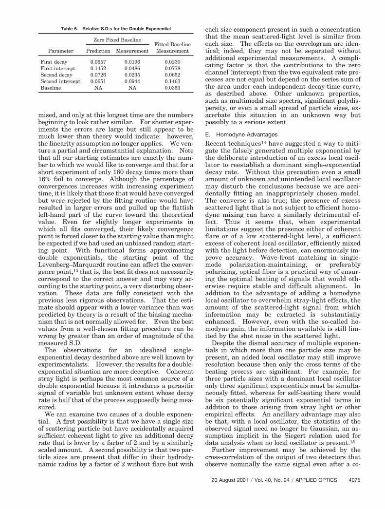
Table 5. Relative S.D.s for the Double Exponential

mised, and only at this longest time are the numbersbeginning to look rather similar. For shorter exper-iments the errors are large but still appear to bemuch lower than theory would indicate: however,the linearity assumption no longer applies. We ven-ture a partial and circumstantial explanation. Notethat all our starting estimates are exactly the num-ber to which we would like to converge and that for ashort experiment of only 160 decay times more than16% fail to converge. Although the percentage ofconvergences increases with increasing experimenttime, it is likely that those that would have convergedbut were rejected by the fitting routine would haveresulted in larger errors and pulled up the flattishleft-hand part of the curve toward the theoreticalvalue. Even for slightly longer experiments inwhich all fits converged, their likely convergencepoint is forced closer to the starting value than mightbe expected if we had used an unbiased random start-ing point. With functional forms approximatingdouble exponentials, the starting point of theLevenberg–Marquardt routine can affect the conver-gence point,13 that is, the best fit does not necessarilycorrespond to the correct answer and may vary ac-cording to the starting point, a very disturbing obser-vation. These data are fully consistent with theprevious less rigorous observations. That the esti-mate should appear with a lower variance than waspredicted by theory is a result of the biasing mecha-nism that is not normally allowed for. Even the bestvalues from a well-chosen fitting procedure can bewrong by greater than an order of magnitude of themeasured S.D.

The observations for an idealized single-exponential decay described above are well known byexperimentalists. However, the results for a double-exponential situation are more deceptive. Coherentstray light is perhaps the most common source of adouble exponential because it introduces a parasiticsignal of variable but unknown extent whose decayrate is half that of the process supposedly being mea-sured.

We can examine two causes of a double exponen-tial. A first possibility is that we have a single sizeof scattering particle but have accidentally acquiredsufficient coherent light to give an additional decayrate that is lower by a factor of 2 and by a similarlyscaled amount. A second possibility is that two par-ticle sizes are present that differ in their hydrody-namic radius by a factor of 2 without flare but with

Parameter


First decay 0.0657 0.0196 0.0230First intercept 0.1452 0.0486 0.0778Second decay 0.0726 0.0235 0.0652Second intercept 0.0651 0.0944 0.1463Baseline NA NA 0.0353

each size component present in such a concentrationthat the mean scattered-light level is similar fromeach size. The effects on the correlogram are iden-tical; indeed, they may not be separated withoutadditional experimental measurements. A compli-cating factor is that the contributions to the zerochannel ~intercept! from the two equivalent rate pro-cesses are not equal but depend on the series sum ofthe area under each independent decay-time curve,as described above. Other unknown properties,such as multimodal size spectra, significant polydis-persity, or even a small spread of particle sizes, ex-acerbate this situation in an unknown way butpossibly to a serious extent.

E. Homodyne Advantages

Recent techniques14 have suggested a way to miti-gate the falsely generated multiple exponential bythe deliberate introduction of an excess local oscil-lator to reestablish a dominant single-exponentialdecay rate. Without this precaution even a smallamount of unknown and unintended local oscillatormay disturb the conclusions because we are acci-dentally fitting an inappropriately chosen model.The converse is also true; the presence of excessscattered light that is not subject to efficient homo-dyne mixing can have a similarly detrimental ef-fect. Thus it seems that, when experimentallimitations suggest the presence either of coherentflare or of a low scattered-light level, a sufficientexcess of coherent local oscillator, efficiently mixedwith the light before detection, can enormously im-prove accuracy. Wave-front matching in single-mode polarization-maintaining, or preferablypolarizing, optical fiber is a practical way of ensur-ing the optimal beating of signals that would oth-erwise require stable and difficult alignment. Inaddition to the advantage of adding a homodynelocal oscillator to overwhelm stray-light effects, theamount of the scattered-light signal from whichinformation may be extracted is substantiallyenhanced. However, even with the so-called ho-modyne gain, the information available is still lim-ited by the shot noise in the scattered light.

Despite the dismal accuracy of multiple exponen-tials in which more than one particle size may bepresent, an added local oscillator may still improveresolution because then only the cross terms of thebeating process are significant. For example, forthree particle sizes with a dominant local oscillatoronly three significant exponentials must be simulta-neously fitted, whereas for self-beating there wouldbe six potentially significant exponential terms inaddition to those arising from stray light or otherempirical effects. An ancillary advantage may alsobe that, with a local oscillator, the statistics of theobserved signal need no longer be Gaussian, an as-sumption implicit in the Siegert relation used fordata analysis when no local oscillator is present.15

Further improvement may be achieved by thecross-correlation of the output of two detectors thatobserve nominally the same signal even after a co-


gr

c~pi

bckiocpncmnoftploOptpacfrr

oweeoutetA

4

herent homodyne field is imposed. Continuing withthis line of reasoning, one can see that single-photondetection is no longer favored even for weak signals,and a linear analog detector with a large dynamicrange and sufficient numbers and spacing of correla-tor channels will accommodate the homodyne gainfactor without penalty.

A limitation of the foregoing discussions is that weconfined the analysis to Gaussian statistics, whereasin real life this condition may not always be met,particularly for individual photon detections in whichPoisson statistics significantly complicate the situa-tion. No attempt has yet been made to venture intothese areas, but we have shown the validity of thedata-synthesis technique for predicting errors cor-rectly in simple well-understood situations. Thisvalidation suggests that it may be useful to exploitthis computationally complete technique for investi-gating the performance of systems for which it ispossible to synthesize data with all the necessaryproperties and limitations of real physical experi-ments but for which it is impossible to derive a suf-ficiently comprehensive theoretical model from whichto predict the accuracy that it might be reasonable toanticipate.

6. Opportunities for Investigation

Further application of the numerical modeling dis-cussed above may significantly extend the presentbrief observations. Regardless of how the data areobtained, the choice of model, assumptions, and pro-cessing methods can yield different errors and indeeddifferent mean values for parameters that are beingfitted to data. The foregoing material provides anoutline of potential methods whereby these may bequantified as a practical extension of much earliertheoretical study.

A. Simple Questions

A few simple questions that may be answerable bythese techniques include ~1! How long should theexperiment time be? ~2! How long a correlogram de-lay time should be computed? ~3! What should thechannel time separation~s! be? ~4! How many chan-nels are necessary or desirable? ~5! Should the base-line be fitted or independently measured? ~6! Whatfunction best approximates the experimental data?~7! What, if any, weighting functions should be ap-plied?

B. More Difficult Questions

We can extend these ideas into other areas that mayperhaps begin to address problems of greater diffi-culty with less ambiguous answers. These includebut are certainly not limited to ~1! How significant iscorrelated noise to the accuracy of fitted values? ~2!How significant is correlated noise on the variance offitted values? ~3! When and how does correlated noiseive rise to systematic errors? ~4! How are these er-ors to be assessed and compensated? ~5! Is baseline

drift worse than random noise and if so by how much?~6! Is filtering followed by analog correlation better


than photon counting? ~7! How many quantizationlevels are necessary or optimum? ~8! Does photonounting introduce systematic errors or noise effects?9! How serious are the errors from fitting an inap-ropriate model? ~10! Can nonuniform channel spac-ng give increased accuracy or range? ~11! What

experimental conditions reduce the dependence onassumptions? ~12! Is it better to analyze data in thetime or the frequency domain? ~13! When and whereare homodyne techniques useful, desirable, or neces-sary? ~14! How much advantage can homodyne tech-niques offer?

7. Conclusions

The limited numerical experiments performed sofar quantitatively support much of the existing artof retrieving good measurements from the analysisof correlation functions that are derived from opti-cal scattering by a range of physical phenomena.These numerical models also suggest areas inwhich common assumptions may not be so well sup-ported; hence they merit further consideration.Six observations are supported by the above study:~1! When the purity of a single exponential cannot

e guaranteed, fitting even an appropriate modelan yield significant errors. ~2! One cannot alwaysnow the appropriate model unless coherent andncoherent scatter are eliminated, well controlled,r independently assessed. ~3! Shot noise in theorrelogram itself is relatively insignificant com-ared with the diffusion of correlated errors toearby channels that arise from the nature of theorrelation process and yield far fewer independenteasurements than might be supposed from theumber and spacing of the channels and the lengthf the experiment. This noise results in errorsrom slight lumpiness being much more serioushan the worse-looking grass. ~4! It is almost im-ossible to tell by visual observation of the accumu-ating correlogram when sufficient data have beenbtained to generate a given desired accuracy. ~5!ther factors remaining constant, accuracy de-ends roughly on the square root of the experimentime except when more than one exponential isresent, in full agreement with current knowledgend experience. ~6! For surface scattering moreycles in the cosine modulation yield much greaterrequency accuracy, significantly improved decay-ate accuracy, and some improvement in the accu-acy of the intercept and the baseline.With its close correspondence to newly derived the-

ry the suggested method of numerical simulationhereby correlograms are correctly constructed fromxactly known data and subsequently analyzed byxisting or innovative techniques allows the accuracyf properties that are intrinsic to the analysis to benderstood and bounded. This trend contrasts withhe physical constraints of the experiment, whoserrors and variability may now be separated fromhose arising from the choice of processing technique.pplication of the present simulation technique may

icad

pzdswItpoia

qasmsoFtaitBned

tldopt

T

Hat

T

T

permit many currently unanswered questions to beunequivocally resolved.

The application to practical techniques could of-fer a number of possibilities. A large improvementin accuracy may be gained from homodyne tech-niques, the deliberate coherent mixing of a suffi-cient excess of local oscillator to swamp effects thatmight otherwise lead to the presence of a doubleexponential, or more complex phenomenology, intwo conditions: ~1! when the scattered-light levels low, or ~2! when there is even a small amount ofoherent stray light. Some improvements maylso be found in situations in which there is poly-ispersity or more than one discrete particle size

resent. Because, so far, we have simulated onlyero baselines, we have found little evidence to in-icate that accuracy might be improved by use ofupplementary information to estimate a baseline,hich is then excluded from the fitted parameters.

n some cases, however, for weak signals fitting allhe parameters, including the baseline, might im-rove accuracy. For surface scattering an intrinsicffset frequency that gives several oscillatory cyclesn the decaying correlogram improves the recoveryccuracy of all four parameters: decay time, fre-

uency, intercept, and baseline. For volume ~bulk!nd overdamped surface light scattering without aignificant implicit oscillatory term, such a termay be introduced by the addition of a frequency-

hifted local oscillator, simultaneously accruing thether potential advantages of homodyning. Theourier-transformed correlogram is not subject tohe channel-to-channel error correlation; hencenalysis in the frequency domain may be preferredf a suitable analytic model is available. The ini-ial transformation, however, requires some care.ecause shot noise and disparities between chan-els are so much less significant than correlatedrrors, great advantage including immunity frometector defects may be gained by use of two detec-

Lexp 5A2@exp~2gun 1 mu!~1 1 gun 1

Lcos 5A2

2N Hexp~2lun 2 mu!F~2l2 1 v2!cos~vunl

1vun 2 mucos~vun 2 mu! 1 sin~vun 2 m

v

3 F~2l2 1 v2!cos~vun 1 mu! 2 lv sin~vunl~l2 1 v2!

ors for observing nominally the same signal, fol-owed by cross correlation. The associatedeterioration of the signal-to-noise ratio by a factorf 4 is a random effect that may be more than com-ensated by the reduction of systematic experimen-al limitations.

Appendix A: Derivation of Covariance Matrices

1. Single Exponential

The single-exponential function is given by

f ~n! 5 B 1 A exp~2lunu!.he covariance is given by

ere n and m are the indices of the covariance matrixnd N is the total number of points used to computehe autocorrelation function of interest.

2. Damped Cosine

The damped-cosine function is given by

f ~n! 5 B 1 A exp~2lunu!cos~vn!.

he covariance is given by

3. Double Exponential

The double-exponential function is given by

f ~n! 5 B 1 A1 exp~2l1unu! 1 A2 exp~2l2unu!.

he covariance is given by

Ldoub 51

2N Fexp~2l1un 2 mu!SA12

l12

2 A1 A2

l1 2 l2

12 A1 A2

l1 1 l21 A1

2un 2 muD 1 exp~2l2un 2 mu!

3 SA22

l21

2 A1 A2

l1 2 l21

2 A1 A2

l1 1 l21 A2

2un 2 muD

1 exp~2gun 2 mu!~1 1 gun 2 mu!#N

.

u! 2 lv sin~vun 2 mu!v2!

exp~2lun 1 mu!

u!1

vun 1 mucos~vun 1 mu! 1 sin~vun 1 mu!v GJ .

mu!g

2 m~l2 1

u!G 1

1 m


2 7. D. S. Cannell, Department of Physics, University of California

4

1 exp~2l1un 1 mu!SA1

l12

2 A1 A2

l1 2 l21

2 A1 A2

l1 1 l2

1 A12un 1 muD 1 exp~2l2un 1 mu!

3 SA22

l21

2 A1 A2

l1 2 l21

2 A1 A2

l1 1 l21 A2

2un 1 muDG .

References1. V. Degiorgio and J. B. Lastovka, “Intensity-correlation spec-

troscopy,” Phys. Rev. A 4, 2033–2050 ~1971!.2. E. Jakeman, E. R. Pike, and S. Swain, “Statistical accuracy in

the digital autocorrelation of photon counting fluctuations,” J.Phys. A 4, 517–534 ~1971!.

3. J. Hughes, E. Jakeman, C. J. Oliver, and E. R. Pike, “Photon-correlation spectroscopy: dependence of linewidth error onnormalization, clip level, detector area, sample time and countrate,” J. Phys. A 6, 1327–1336 ~1973!.

4. K. Schatzel, “Noise in photon correlation and photon structurefunctions,” Opt. Acta 30, 155–166 ~1983!.

5. M. Bertero, P. Boccacci, and E. R. Pike, “On the recovery andresolution of exponential relaxation rates from experimentaldata: a singular-value analysis of the Laplace transform in-version in the presence of noise,” Proc. R. Soc. London Ser. A383, 15–29 ~1982!.

6. E. R. Pike and E. Jakeman, “Photon statistics and photon-correlation spectroscopy,” Adv. Quantum Electron. 2, 1 ~1974!.


Santa Barbara, Santa Barbara, Calif. 93106 ~private commu-nication, 15 March 2000!.

8. A. V. Lomakin, Massachusetts Institute of Technology, Cam-bridge, Mass. 02139 ~private communications, 10 January2000 and 1 May 2000!.

9. A. V. Lomakin, “Fitting the correlation function,” Appl. Opt.40, 4079–4086 ~2001!.

10. B. Saleh, Photoelectron Statistics with Applications to Spec-troscopy and Optical Communication, Springer Series in Op-tical Sciences ~Springer-Verlag, New York, 1978!, p. 18.

11. D. C. Montgomery and G. C. Runger, Applied Statistics andProbability for Engineers ~Wiley, New York, 1994!.

12. W. V. Meyer, G. H. Wegdam, D. Feinstein, and J. A. Mann, Jr.,“Advances in surface-light-scattering instrumentation andanalysis: noninvasive measuring of surface tension, viscos-ity, and other interfacial parameters,” Appl. Opt. 40, 4113–4133 ~2001!.

13. W. V. Meyer, A. E. Smart, D. S. Cannell, R. G. W. Brown, J. A.Lock, and T. W. Taylor, “Laser light scattering: multiple scat-tering suppression with cross correlation, and flare rejectionwith fiber optic homodyning,” in Proceedings of the Thirty-Seventh AIAA Aerospace Science Meeting and Exhibit ~Amer-ican Institute of Aeronautics and Astronautics, New York,1999!, paper AIAA 99-0962.

14. R. G. W. Brown, “Homodyne optical fiber dynamic light scat-tering,” Appl. Opt. 40, 4004–4010 ~2001!.

15. B. Chu, Laser Light Scattering ~Academic, New York, 1974!, p.104.

quantitative simulation of errors in correlation analysis

Documents