Journal of

Marine Science and Engineering

Article

Quantifying Variable Importance in PredictingCritical Span Length and Scour Depth for Failure ofOnshore River Crossing Pipelines Using ANN

Adithyaa Karthikeyan 1,* , Saadat Mirza 1, Byul Hur 2, Gregory Pearlstein 3 andRonald Ledbetter 1

1 Department of Multidisciplinary Engineering, Texas A&M University, College Station, TX 77843, USA;smirza@tamu.edu (S.M.); wrl_69@tamu.edu (R.L.)

2 Department of Engineering Technology and Industrial Distribution, Texas A&M University, College Station,TX 77843, USA; byulmail@tamu.edu

3 Department of Mathematics, Texas A&M University, College Station, TX 77843, USA;gpearl@math.tamu.edu

* Correspondence: adithyaa1996@tamu.edu

Received: 24 September 2020; Accepted: 16 October 2020; Published: 26 October 2020�����������������

Abstract: Onshore oil and gas pipelines are often buried beneath the river bed and channel banks.One of the primary reasons for the exposure of buried pipelines is the scouring mechanism thatoccurs when shear stress induced on riverbed by flowing water exceeds the resistance of channelbed material. Depending on the free spanning length and watercourse flow velocity, the vortexshedding phenomena may cause interactions resulting in a catastrophic pipeline failure. Accurateestimation of parameters that influence critical span length and scour depth become extremelyimportant to maintain the integrity of the pipeline system and optimize its effective service life.This study is aimed at quantifying the relative importance of input variables used in predictingcritical span length and scour depth based on the weights obtained from an Artificial Neural Network(ANN). The Artificial Neural Network model is developed by collecting pipeline accident reportsfrom Pipeline and Hazardous Material Safety Administration (PHMSA) database for accidents thatoccurred due to Vortex Induced Vibration (VIV) loading during flooding in the last 35 years. It isseen that factors such as internal fluid pressure, dynamic lateral and vertical soil stiffness, reducedvelocity and age of pipeline have a significant contribution in terms of model weights and help inaccurately assessing the pipeline’s vulnerability to failure.

Keywords: river crossing pipelines; vortex induced vibrations; Artificial Neural Networks;critical span length; scour depth; pipeline integrity management; predicitve analysis

1. Introduction

Pipeline Integrity Management is one of the most extensively carried out programs across theworld that focuses on safety and environmental hazards associated with liquid and natural gaspipelines. In the United States, the transmission pipeline infrastructure is estimated to have more than100,000 km of pipeline crossings in rivers, streams, lakes or flood plains. Accidents at river crossingsaccount for less than one percent of the total number of pipeline accidents. However the environmentalconsequence of a release of hydrocarbons into water can be severe. The impact of these spills on theenvironment have been analysed in terms of cost, rate of contamination of soil, average volume ofrelease, annual ratio of water type contamination, and effects on fish, birds and terrestrial wildlifebetween 2010 and 2017 based on the information from the Pipeline and Hazardous Material SafetyAdministration (PHMSA) database by Chiara Belvederesi, Megan S. Thompson and Petr E. Komers [1].

J. Mar. Sci. Eng. 2020, 8, 840; doi:10.3390/jmse8110840 www.mdpi.com/journal/jmse

J. Mar. Sci. Eng. 2020, 8, 840 2 of 18

Among the many different failure modes of pipeline in river crossings, the predominant ones have beencaused by Vortex Induced Vibration (VIV) loading due to the exposure of unsupported free spanningpipelines over flowing water, as documented in Reference [2]. Their study focused on developinga flood monitoring program to quantify threshold flood levels that would result in exposure andfailure of pipeline water crossings. The flood monitoring program is in turn aimed at establishing anaction plan based on the assessment of the flood scenario to reduce the consequences of a pipelinewatercourse crossing failure.

Free-span management of pipelines transporting liquid and natural gas starts from the earlyproject phases including pre-engineering survey, design and construction, and continues throughoutthe whole operating life. The design phase is the core of free span integrity management.Hence determination of Maximum Allowable Free Span Length (MAFSL) or Critical Span Length(CSL) plays a crucial role in the design of pipelines and in trouble shooting existing pipelines in rivercrossings. In addition, an accurate measure of scour depth potentially identifies a feasible Depthof Cover (DoC) for the pipelines to be buried during the initial laying phase. Over many years,various research papers, design codes and industry publications have come up with different analysisand methods to determine critical span length for pipelines. The combined analysis method prescribesvarious static and dynamic analysis methods, addressing different loading conditions on the pipe spanwhich are listed below as follows [3]:

(1) Static Analysis of free spans induced by low depressions.(2) Static Analysis of free spans using simple beam relations based on ASME B31.8 codes.(3) Static Analysis of free spans induced by elevated obstructions.(4) General Dynamic VIV Analysis.(5) Analysis of Cross-flow VIV based on DNV Guidelines.

The output from all of these methods are compared and the most conservative or minimum valueis chosen as the critical span length. There is no single approach that entirely captures the physicsof the problem. Hence, difficulties exist in the mathematical modelling of scenario considering allphysical and environmental parameters associated with pipelines using the traditional deterministicapproach. Artificial Neural Networks play a key role in mathematical modelling of such a system.A part of this research in this paper was presented in author Adithyaa Karthikeyan’s thesis for hisMaster’s degree.

2. Background

Prediction of fatigue life-cycles of onshore pipelines that become exposed at river crossingsdue to riverbed erosion were modelled using DNV GL’s FATFREE software based on S-N curvesapproach [4]. Studies have been carried out to assess and model VIV loading for free spanning pipelinesfor estimating MAFSL for both offshore and onshore water crossing pipelines [5,6]. Rhett Dotson andLawrence Matta discussed the analytical assessments for MAFSL by ensuring that total longitudinalstresses fall below the elastic code limits. They also carried out finite element assessment based onelastic and elastic-plastic modelling of pipelines for three different scenarios posed by operators [7].The influence of soil characteristics on pipeline supports in free span was analysed in determiningthe natural frequency of pipeline vibrations [8]. Recommendations and guidelines have beenprescribed by DNV [9] to evaluate the dynamic response of a free spanning pipeline based on pipe-soilinteractions [10]. Determining the combination of loads that act on the pipeline is crucial for modellingand analysis of MAFSL. Variation in factors such as line geometry or end restraints can greatly affectthe nature of results. These results are based on deterministic approach.

The oil and gas industry has vast amounts of data captured by instruments and generatedby simulations. We are in a period ideally positioned to combine traditional methodologies withcomputational intelligence characterized by data driven models. With the availability of real timegeometrical survey data, the implementation of Artificial Neural Networks (ANN) to model nonlinear

J. Mar. Sci. Eng. 2020, 8, 840 3 of 18

functions with several variables is increasingly finding its advantages in the industry. Performance ofMultivariate Adaptive Regression Splines (MARS) was compared with multilayer perceptron neuralnetwork model in the prediction of scour depth beneath pipelines based on data available in literaturewritten by Haghiabi [11]. The MARS model was found to have high precision for modelling scourdepth and gave clear information regarding internal processes carried out in the model developmentdue to its linear nature. However the model had less accuracy in prediction when compared to theneural network model. In relation to the above article, Barati (2009) developed new models for scourdepth estimation using regression optimization based on power functions [12]. Numerical modelingusing CFD techniques were carried out for flow and local scour around pipelines in steady currents andresults were compared to published laboratory measurements [13]. Failure prediction of undergroundpipeline in non-uniform soil settlement was modelled using artificial neural networks with axial stressas the output vector and buried depth, wall thickness, pipe diameter, precipitation level, soil modulusof elasticity, and soil density as six input vectors [14].

2.1. Influence of Internal Fluid Pressure on Critical Span Length

A number of authors have suggested that critical span length can be influenced by internal fluidpressure. Olav Fyriliev and Leif Collberg explained how both buoyancy (external pressure) andweight of internal fluid (internal pressure) have an indirect effect on the effective axial force which ismathematically modelled into a differential equation using hoop stress and poisson effect [15]. This onthe contrary defers from the results showed by Galgoul et al. (2004) where internal pressure willincrease the natural frequency [16]. Though DNV-RP-F105 provides some guidance on the criticalbuckling load and natural frequency of vibration of pipeline based on internal and external pressure,the non-linear effects due to gradual pipeline deflection are not exactly modelled and expressionsbased on linear beam theory shall not be valid for all cases.

2.2. Influence of Soil Stiffness on Critical Span Length

In order to understand the effects of soil characteristics on the natural frequency of vibration,literature studies were carried out by simulating pipe-soil interactions using vertical and horizontalsprings that would prevent pipe oscillations in the cross-flow and in-line directions respectively [8].The results showed that dense sand with pinned-pinned boundary condition had maximum influenceon the natural frequency of vibration and soft clay soil with fixed-fixed end condition had minimalinfluence on the natural frequency. A pinned boundary condition allows the structural member torotate, but not to translate in any direction, whereas in fixed support both translation and rotationaldegrees of freedom are constrained.

In the United States, pipeline operators are required to abide by regulations put forth by thefederal Pipeline and Hazardous Materials Safety Administration (PHMSA). With a large number ofhistorical data available from PHMSA database, the United States Geographical Survey (USGS) andthe National Oceanic and Atmospheric Administration (NOAA), we have set up an ANN model topredict critical span length and scour depth and understand the non-linear variation of 12 input factorssuch as river flow rate, river depth, reduced velocity due to inline and crossflow oscillations, lateraland vertical dynamic soil stiffness coefficients, pipeline outer diameter, wall thickness, yield strength,age and incident fluid pressure.

3. Materials and Methods

3.1. Data Preparation

The factors that govern scour depth and critical span length of river crossing pipelines aremulti-fold in nature. The exact relationships between them have not been identified completelyand hence we resort to ANN to develop a robust prediction model. The selection of relevantparameters is based on engineering judgement and experience about the vibration behaviour of

J. Mar. Sci. Eng. 2020, 8, 840 4 of 18

the pipelines. This section highlights the process of gathering data for features from various datasources available online.

3.1.1. PHMSA Database

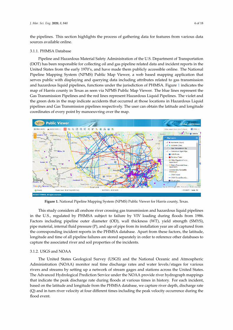
Pipeline and Hazardous Material Safety Administration of the U.S. Department of Transportation(DOT) has been responsible for collecting oil and gas pipeline related data and incident reports in theUnited States from the early 1970’s, and have made them publicly accessible online. The NationalPipeline Mapping System (NPMS) Public Map Viewer, a web based mapping application thatserves public with displaying and querying data including attributes related to gas transmissionand hazardous liquid pipelines, functions under the jurisdiction of PHMSA. Figure 1 indicates themap of Harris county in Texas as seen via NPMS Public Map Viewer. The blue lines represent theGas Transmission Pipelines and the red lines represent Hazardous Liquid Pipelines. The violet andthe green dots in the map indicate accidents that occurred at those locations in Hazardous Liquidpipelines and Gas Transmission pipelines respectively. The user can obtain the latitude and longitudecoordinates of every point by manoeuvring over the map.

Figure 1. National Pipeline Mapping System (NPMS) Public Viewer for Harris county, Texas.

This study considers all onshore river crossing gas transmission and hazardous liquid pipelinesin the U.S., regulated by PHMSA subject to failure by VIV loading during floods from 1986.Factors including pipeline outer diameter (OD), wall thickness (WT), yield strength (SMYS),pipe material, internal fluid pressure (P), and age of pipe from its installation year are all captured fromthe corresponding incident reports in the PHMSA database. Apart from these factors, the latitude,longitude and time of all pipeline failures are stored separately in order to reference other databases tocapture the associated river and soil properties of the incidents.

3.1.2. USGS and NOAA

The United States Geological Survey (USGS) and the National Oceanic and AtmosphericAdministration (NOAA) monitor real time discharge rates and water levels/stages for variousrivers and streams by setting up a network of stream gages and stations across the United States.The Advanced Hydrological Prediction Service under the NOAA provide river hydrograph mappingsthat indicate the peak discharge rate during floods at various times in history. For each incident,based on the latitude and longitude from the PHMSA database, we capture river depth, discharge rate(Q) and in turn river velocity at four different times including the peak velocity occurrence during theflood event.

J. Mar. Sci. Eng. 2020, 8, 840 5 of 18

3.1.3. Estimation of Reduced Velocity for Inline and Cross-Flow Oscillations

Interactions between pipeline and external fluid flow (in this case, river water) in a directionperpendicular to the axis of the pipeline reduces the flow around the pipe and in turn inducesoscillations due to the formation of vortices. This unsteady phenomenon occurs at specific flowvelocities governed by the length and shape of the exposed pipeline and is an important sourceof fatigue damage for both onshore and offshore free spanning pipelines. The onset of vortexshedding-induced oscillations for both in-line and cross-flow motions is determined by reducedvelocity Vr and is defined as,

Vr =V

fnD, (1)

where fn is the natural frequency of vibration of pipe, V is the actual velocity of river water and D isthe outer diameter of the pipe.

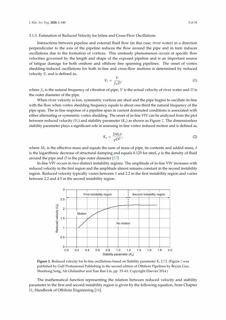
When river velocity is low, symmetric vortices are shed and the pipe begins to oscillate in-linewith the flow when vortex shedding frequency equals to about one-third the natural frequency of thepipe span. The in-line response of a pipeline span in current dominated conditions is associated witheither alternating or symmetric vortex shedding. The onset of in-line VIV can be analyzed from the plotbetween reduced velocity (Vr) and stability parameter (Ks) as shown as Figure 2. The dimensionlessstability parameter plays a significant role in assessing in-line vortex induced motion and is defined as,

Ks =2Meδ

ρD2 , (2)

where Me is the effective mass and equals the sum of mass of pipe, its contents and added mass, δ

is the logarithmic decrease of structural damping and equals 0.125 for steel, ρ is the density of fluidaround the pipe and D is the pipe outer diameter [17]

In-line VIV occurs in two distinct instability regions. The amplitude of in-line VIV increases withreduced velocity in the first region and the amplitude almost remains constant in the second instabilityregion. Reduced velocity typically varies between 1 and 2.2 in the first instability region and variesbetween 2.2 and 4.5 in the second instability region.

Figure 2. Reduced velocity for In-line oscillations based on Stability parameter Ks [17]. (Figure 2 waspublished by Gulf Professional Publishing in the second edition of Offshore Pipelines by Boyun Guo,Shanhong Song, Ali Ghalambor and Tian Ran Lin, pp. 53–63. Copyright Elsevier 2014.)

The mathematical function representing the relation between reduced velocity and stabilityparameter in the first and second instability region is given by the following equation, from Chapter11, Handbook of Offshore Engineering [18].

J. Mar. Sci. Eng. 2020, 8, 840 6 of 18

Vr =

1 , if Ks ≤ 0.25

0.188 + 3.6Ks − 1.6K2s , if 0.25 < Ks ≤ 1.2

2.2 , if Ks > 1.2

(3)

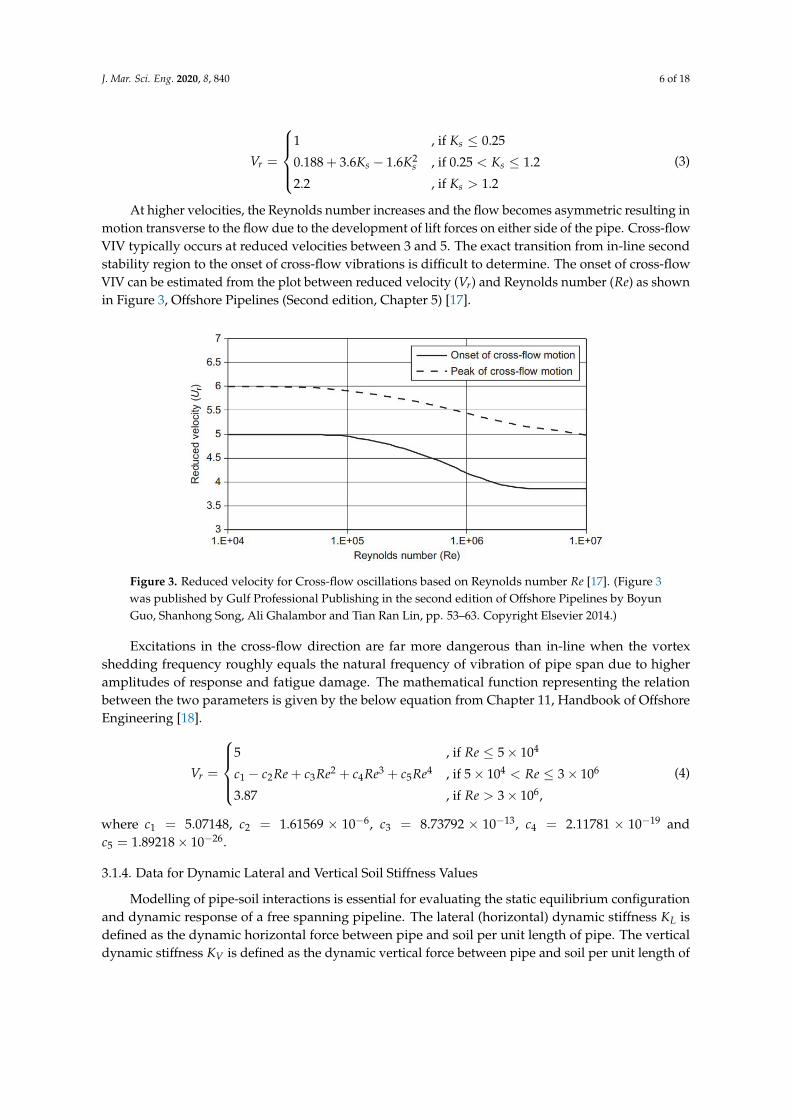
At higher velocities, the Reynolds number increases and the flow becomes asymmetric resulting inmotion transverse to the flow due to the development of lift forces on either side of the pipe. Cross-flowVIV typically occurs at reduced velocities between 3 and 5. The exact transition from in-line secondstability region to the onset of cross-flow vibrations is difficult to determine. The onset of cross-flowVIV can be estimated from the plot between reduced velocity (Vr) and Reynolds number (Re) as shownin Figure 3, Offshore Pipelines (Second edition, Chapter 5) [17].

Figure 3. Reduced velocity for Cross-flow oscillations based on Reynolds number Re [17]. (Figure 3was published by Gulf Professional Publishing in the second edition of Offshore Pipelines by BoyunGuo, Shanhong Song, Ali Ghalambor and Tian Ran Lin, pp. 53–63. Copyright Elsevier 2014.)

Excitations in the cross-flow direction are far more dangerous than in-line when the vortexshedding frequency roughly equals the natural frequency of vibration of pipe span due to higheramplitudes of response and fatigue damage. The mathematical function representing the relationbetween the two parameters is given by the below equation from Chapter 11, Handbook of OffshoreEngineering [18].

Vr =

5 , if Re ≤ 5× 104

c1 − c2Re + c3Re2 + c4Re3 + c5Re4 , if 5× 104 < Re ≤ 3× 106

3.87 , if Re > 3× 106,

(4)

where c1 = 5.07148, c2 = 1.61569 × 10−6, c3 = 8.73792 × 10−13, c4 = 2.11781 × 10−19 andc5 = 1.89218× 10−26.

3.1.4. Data for Dynamic Lateral and Vertical Soil Stiffness Values

Modelling of pipe-soil interactions is essential for evaluating the static equilibrium configurationand dynamic response of a free spanning pipeline. The lateral (horizontal) dynamic stiffness KL isdefined as the dynamic horizontal force between pipe and soil per unit length of pipe. The verticaldynamic stiffness KV is defined as the dynamic vertical force between pipe and soil per unit length of

J. Mar. Sci. Eng. 2020, 8, 840 7 of 18

pipe. The two parameters KL and KV for non-stratified and homogeneous soil are determined basedon the DNV Recommended Practice for Free Spanning Pipelines [9] as follows,

KV =CV

1− ν(

2ρs

3ρ+

13)√

D (5)

KL = CL(1 + ν)(2ρs

3ρ+

13)√

D, (6)

where CL and CV are coefficients selected based on Table 1, ν is the Poisson’s ratio and equals 0.5 forundrained conditions, ρs/ρ represents the specific mass ratio between pipe mass and displaced waterand D is the pipe outer diameter in meters. Density of steel equals 7861 kg/m3. Density of fluid insidethe pipeline is taken as 870 kg/m3 for light crude oil and 0.8 kg/m3 for natural gas. The above stiffnessparameters KL and KV play a crucial role in modelling pipe-soil interactions to determine the naturalfrequency of vibration of the pipe. The soil type is identified by the value of its friction angle, which isa characteristic parameter of the soil. Typical friction angles and stiffness values for different types ofsand are given in Table 1.

Table 1. Friction angles and stiffness values for pipe-soil interaction in sand. Adaptedfrom Reference [9].

Soil Type ψs CV (kN/m(5/2)) CL (kN/m(5/2)) KV ,S (kN/m/m)

Loose sand 28–30◦ 10,500 9000 250

Medium sand 30–36◦ 14,500 12,500 530

Dense sand 36–41◦ 21,000 18,000 1350

The Natural Resources Conservation Service (NRCS) under the United States Department ofAgriculture provides soil maps and data surveyed throughout the United States as a web basedapplication to the public. Based on the river, the latitude and longitude of the pipeline incident,contents of sand on the pipeline shoulders are identified to determine its friction angle and in turn thecoefficient values. Using this method, lateral and vertical dynamic soil stiffness values are determinedat all pipeline incidents.

3.1.5. River Bed Scour

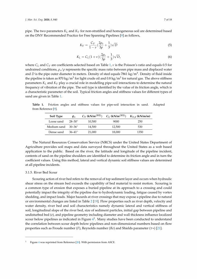
Scouring action of river bed refers to the removal of top sediment layer and occurs when hydraulicshear stress on the stream bed exceeds the capability of bed material to resist motion. Scouring isa common type of erosion that exposes a buried pipeline at its approach to a crossing and couldpotentially impact the integrity of the pipeline due to hydrodynamic loading, fatigue caused by vortexshedding, and impact loads. Major hazards at river crossings that may expose a pipeline due to naturalor environmental changes are listed in Table 2 [19]. Flow properties such as river depth, velocity andwater density, river bed and soil characteristics namely dynamic lateral and vertical stiffness ofsoil, longitudinal slope of the river bed, size of sediment particles, initial gap between pipeline andundisturbed bed (e), and pipeline geometry including diameter and wall thickness influence localizedscour below pipelines as indicated in Figure 41. Many studies have been conducted to understandthe correlation between scour depth below pipelines and non-dimensional numbers based on flowproperties such as Froude number (F), Reynolds number (Re) and Shields parameter (τ∗) [21].

1 Figure 4 was reprinted from Reference [20]. With permission from ASCE.

J. Mar. Sci. Eng. 2020, 8, 840 8 of 18

Table 2. Classification of river bed erosion phenomenon.

S.No Hazard Category Sub Hazard Type

1 Episodic exposureLocal scour and river bed degradationcausing vertical channel movements

2 Progressive erosionBank erosion, encroachment and gullying

causing lateral channel movements

3 Channel AvulsionMeandering river, debris jams, sediment

accumulation and extreme flooding resulting in thedevelopment of a new conveyance route

Here we restrict our study on exposed pipelines due to the onset of scour in riverbeds thatexperience vortex induced vibrations due to the flowing water. Moncada and Aguirre-Pe (1999)presented the following relationship for estimating localized scour depth under pipelines [22],

ds

D= 0.9 ∗ tanh (1.4F) + 0.55, (7)

where ds is the scour depth, F = V√gy is the Froude number, V is the velocity of river, y is the water

depth, g is gravitational acceleration and D is the pipeline outer diameter. They have concluded thatparameters such as river bed slope and e

D ratio have very minimal effect on scour depth and have beenneglected in our prediction model.

Figure 4. Localized scouring phenomenon below river crossing pipelines.

3.2. Artificial Neural Network Model

Forty five incidents were captured from the PHMSA database pertaining to failure of gastransmission and hazardous liquid pipelines as a result of VIV loading due to floods in the last35 years. For each of the forty five incident cases, river velocity, discharge rate and river stage werecaptured at four different times resulting in a total of 180 analyzed data sets. Table 3 indicates the 12input features and its correlation with the 3 output parameters used in modelling the neural network.Scour depth parameters were evaluated for the entire dataset using the Froude Number approach asprescribed by Moncada and Aguirre-Pe [22]. First general formulations of DNV on calculations ofcritical span lengths due to inline and cross flow oscillations were carried out for all cases. The criticalspan length calculations for all incidents were validated based on the approach prescribed by MineralsManagement Service under United States Department of the Interior [3].

Feature scaling was performed to selective attributes such as yield strength, internal fluid pressure,discharge rate and dynamic lateral and vertical soil stiffness values to ensure all input attributes had

J. Mar. Sci. Eng. 2020, 8, 840 9 of 18

values in a similar range. Feature scaling involves dividing the input values of one or more attributesby the maximum value of that particular attribute, resulting in a new range between 0 and 1. The errordecreases rapidly after every iteration and the model converges quickly when the input features arere-scaled. Feature scaling prevents weight matrices from oscillating inefficiently when the variablesare uneven and have large ranges. Unlike normalization, feature scaling does not alter the distributionof the data and only re-scales the data to the desired range.

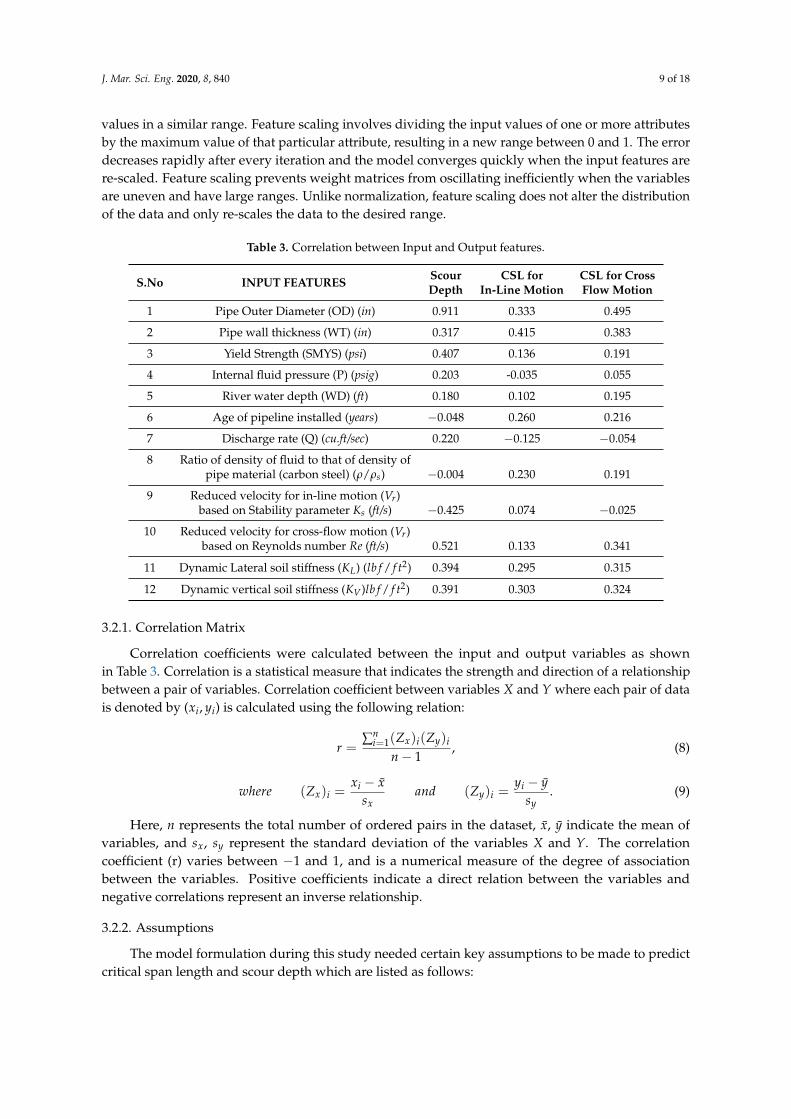
Table 3. Correlation between Input and Output features.

S.No INPUT FEATURES Scour CSL for CSL for CrossDepth In-Line Motion Flow Motion

1 Pipe Outer Diameter (OD) (in) 0.911 0.333 0.495

2 Pipe wall thickness (WT) (in) 0.317 0.415 0.383

3 Yield Strength (SMYS) (psi) 0.407 0.136 0.191

4 Internal fluid pressure (P) (psig) 0.203 -0.035 0.055

5 River water depth (WD) (ft) 0.180 0.102 0.195

6 Age of pipeline installed (years) −0.048 0.260 0.216

7 Discharge rate (Q) (cu.ft/sec) 0.220 −0.125 −0.054

8 Ratio of density of fluid to that of density ofpipe material (carbon steel) (ρ/ρs) −0.004 0.230 0.191

9 Reduced velocity for in-line motion (Vr)based on Stability parameter Ks (ft/s) −0.425 0.074 −0.025

10 Reduced velocity for cross-flow motion (Vr)based on Reynolds number Re (ft/s) 0.521 0.133 0.341

11 Dynamic Lateral soil stiffness (KL) (lb f / f t2) 0.394 0.295 0.315

12 Dynamic vertical soil stiffness (KV)lb f / f t2) 0.391 0.303 0.324

3.2.1. Correlation Matrix

Correlation coefficients were calculated between the input and output variables as shownin Table 3. Correlation is a statistical measure that indicates the strength and direction of a relationshipbetween a pair of variables. Correlation coefficient between variables X and Y where each pair of datais denoted by (xi, yi) is calculated using the following relation:

r =∑n

i=1(Zx)i(Zy)i

n− 1, (8)

where (Zx)i =xi − x

sxand (Zy)i =

yi − ysy

. (9)

Here, n represents the total number of ordered pairs in the dataset, x, y indicate the mean ofvariables, and sx, sy represent the standard deviation of the variables X and Y. The correlationcoefficient (r) varies between −1 and 1, and is a numerical measure of the degree of associationbetween the variables. Positive coefficients indicate a direct relation between the variables andnegative correlations represent an inverse relationship.

3.2.2. Assumptions

The model formulation during this study needed certain key assumptions to be made to predictcritical span length and scour depth which are listed as follows:

J. Mar. Sci. Eng. 2020, 8, 840 10 of 18

• The pipelines are situated perpendicular to the flow, where maximum hydrodynamic loads andvortex induced vibrations would be expected.

• The pipeline under study is on the river bed and hence scouring will expose the pipeline andinduce VIV, when flooding occurs.

• The soil on the pipe shoulder is assumed to be non-stratified and homogeneous in all the casesfor calculating lateral and vertical dynamic soil stiffness as there are no standard prescriptions forcomputing stiffness values for heterogeneous soils.

• The free span end fixity constant is 1.57 for pinned-pinned ends and 3.54 for fixed-fixed ends.In this study, we have considered the value to be 2.52 for all cases because in reality, pipes areneither completely pinned nor clamped on the ends.

• The cross sectional area of the river is taken as the product of width and depth, and the riverwater is assumed to flow at mean velocity when it comes in contact with the pipe neglecting thevariation of velocity with depth.

4. Results

4.1. Best Fit Neural Network Architecture

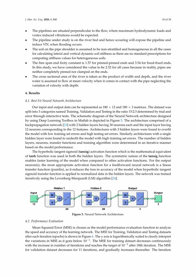
Our input and output data can be represented as 180 × 12 and 180 × 3 matrices. The dataset wassplit into 3 categories named Training, Validation and Testing in the ratio 15:2:3 determined by trial anderror through interactive tests. The schematic diagram of the Neural Network architecture designedby using Deep Learning Toolbox in Matlab is depicted in Figure 5. The architecture comprised of abackpropagation network [23] with 2 hidden layers having 30 neurons each and the input layer having12 neurons corresponding to the 12 features. Architectures with 3 hidden layers were found to overfitthe model with low training set errors and high testing set errors. Similarly architectures with a singlehidden layer were found to underfit the model with high training set errors. The number of hiddenlayers, neurons, transfer functions and training algorithm were determined in an iterative mannerbased on the model performance.

The hyperbolic tangent sigmoid (tansig) activation function which is the mathematical equivalentof tanh function was used in both the hidden layers. The symmetric nature of the tansig functionenables faster learning of the model when compared to other activation functions. For the outputneuron(s), the most appropriate activation function for a feedforward neural network is a lineartransfer function (purelin), as it reduces the loss in accuracy of the model when hyperbolic tangentsigmoid transfer function is applied to normalized data in the hidden layers. The network was trainediteratively using the Levenberg-Marquardt (LM) algorithm [24].

Figure 5. Neural Network Architecture.

4.2. Performance Evaluation

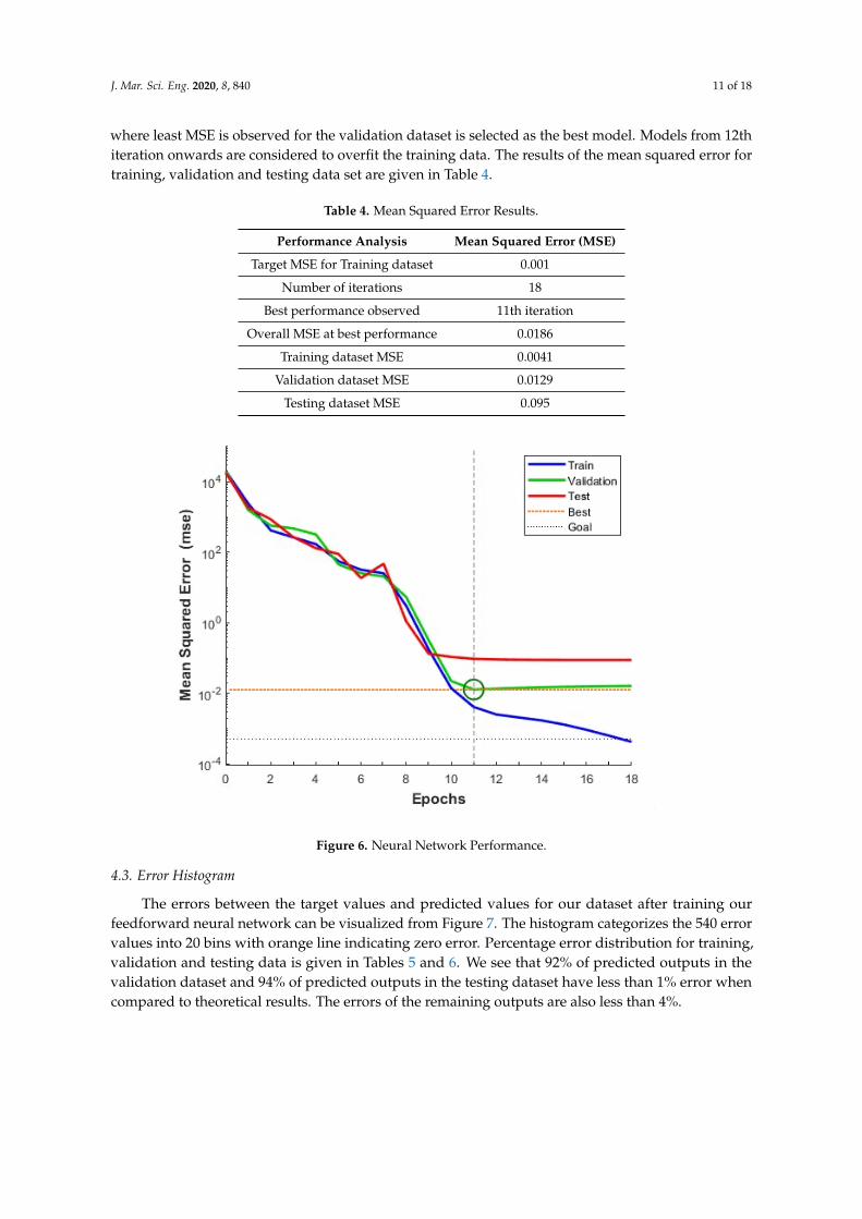
Mean Squared Error (MSE) is chosen as the model performance evaluation function to analyzethe speed and accuracy of the learning network. The MSE for Training, Validation and Testing datasetsafter each iteration (epochs) is shown in Figure 6. The y axis is logarithmically scaled to clearly interpretthe variations in MSE as it goes below 10−1. The MSE for training dataset decreases continuouslywith the increase in number of iterations and reaches the target of 10−3 after 18th iteration. The MSEfor validation dataset decreases for 11 iterations, and gradually increases thereafter. The iteration

J. Mar. Sci. Eng. 2020, 8, 840 11 of 18

where least MSE is observed for the validation dataset is selected as the best model. Models from 12thiteration onwards are considered to overfit the training data. The results of the mean squared error fortraining, validation and testing data set are given in Table 4.

Table 4. Mean Squared Error Results.

Performance Analysis Mean Squared Error (MSE)

Target MSE for Training dataset 0.001

Number of iterations 18

Best performance observed 11th iteration

Overall MSE at best performance 0.0186

Training dataset MSE 0.0041

Validation dataset MSE 0.0129

Testing dataset MSE 0.095

Figure 6. Neural Network Performance.

4.3. Error Histogram

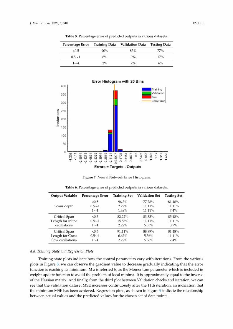
The errors between the target values and predicted values for our dataset after training ourfeedforward neural network can be visualized from Figure 7. The histogram categorizes the 540 errorvalues into 20 bins with orange line indicating zero error. Percentage error distribution for training,validation and testing data is given in Tables 5 and 6. We see that 92% of predicted outputs in thevalidation dataset and 94% of predicted outputs in the testing dataset have less than 1% error whencompared to theoretical results. The errors of the remaining outputs are also less than 4%.

J. Mar. Sci. Eng. 2020, 8, 840 12 of 18

Table 5. Percentage error of predicted outputs in various datasets.

Percentage Error Training Data Validation Data Testing Data

<0.5 90% 83% 77%

0.5∼1 8% 9% 17%

1∼4 2% 7% 6%

Figure 7. Neural Network Error Histogram.

Table 6. Percentage error of predicted outputs in various datasets.

Output Variable Percentage Error Training Set Validation Set Testing Set

Scour depth<0.5 96.3% 77.78% 81.48%

0.5∼1 2.22% 11.11% 11.11%1∼4 1.48% 11.11% 7.4%

Critical Span <0.5 82.22% 83.33% 85.18%Length for Inline 0.5∼1 15.56% 11.11% 11.11%

oscillations 1∼4 2.22% 5.55% 3.7%

Critical Span <0.5 91.11% 88.89% 81.48%Length for Cross 0.5∼1 6.67% 5.56% 11.11%flow oscillations 1∼4 2.22% 5.56% 7.4%

4.4. Training State and Regression Plots

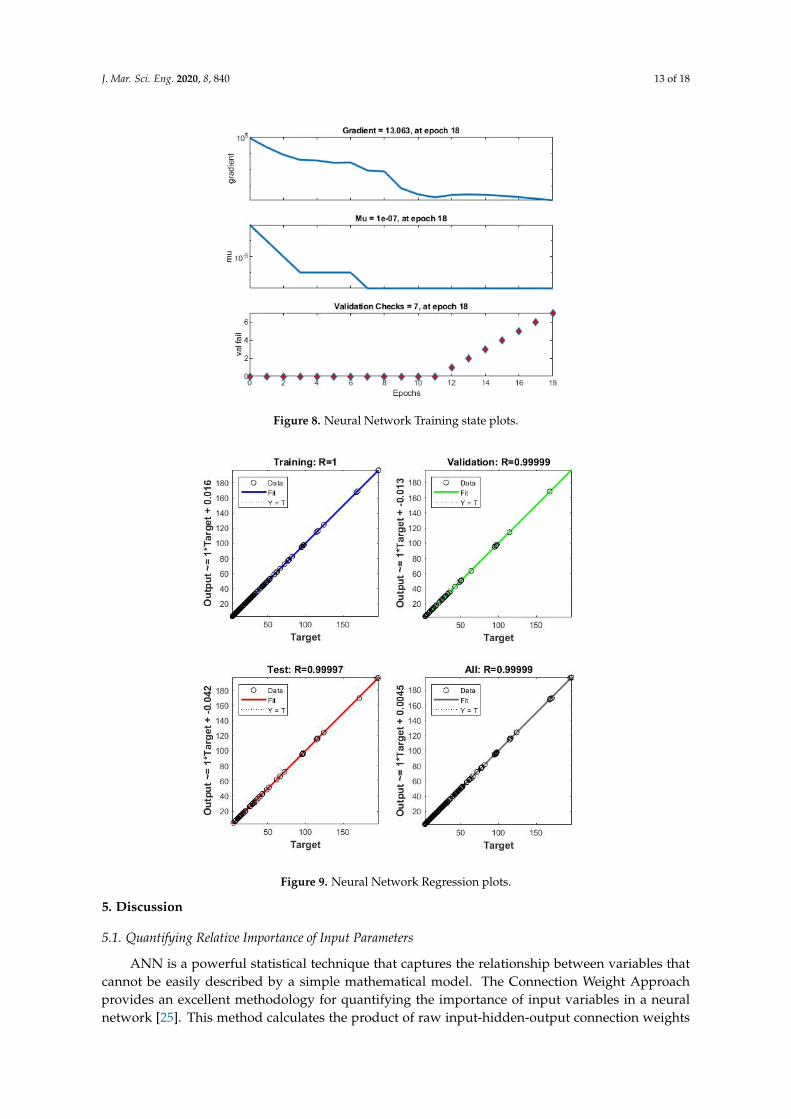
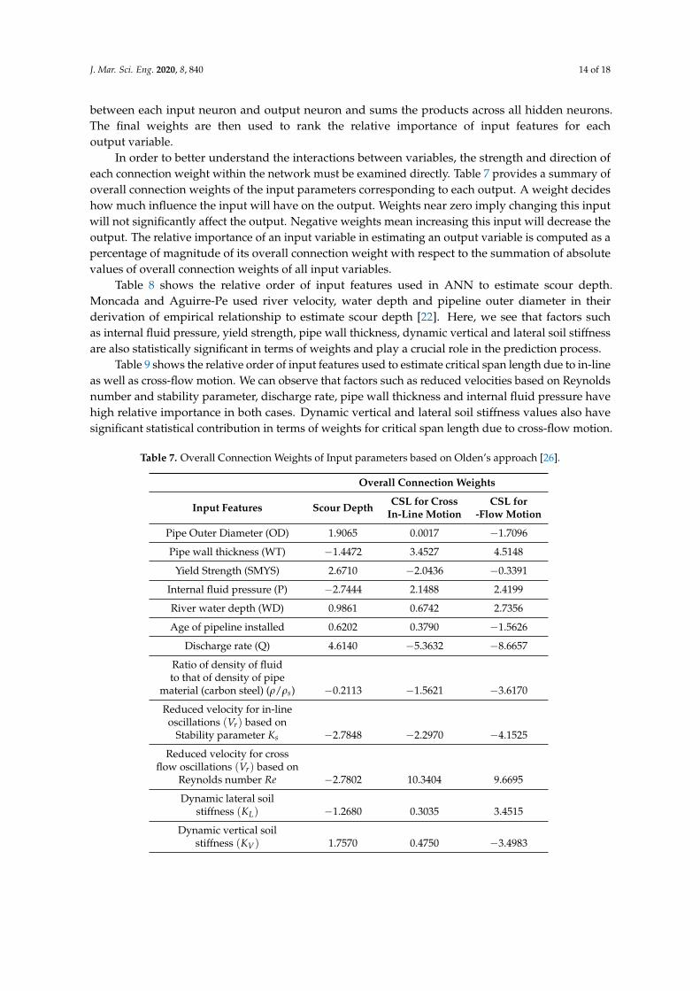
Training state plots indicate how the control parameters vary with iterations. From the variousplots in Figure 8, we can observe the gradient value to decrease gradually indicating that the errorfunction is reaching its minimum. Mu is referred to as the Momentum parameter which is included inweight update function to avoid the problem of local minima. It is approximately equal to the inverseof the Hessian matrix. And finally, from the third plot between Validation checks and iteration, we cansee that the validation dataset MSE increases continuously after the 11th iteration, an indication thatthe minimum MSE has been achieved. Regression plots, as shown in Figure 9 indicate the relationshipbetween actual values and the predicted values for the chosen set of data points.

J. Mar. Sci. Eng. 2020, 8, 840 13 of 18

Figure 8. Neural Network Training state plots.

Figure 9. Neural Network Regression plots.

5. Discussion

5.1. Quantifying Relative Importance of Input Parameters

ANN is a powerful statistical technique that captures the relationship between variables thatcannot be easily described by a simple mathematical model. The Connection Weight Approachprovides an excellent methodology for quantifying the importance of input variables in a neuralnetwork [25]. This method calculates the product of raw input-hidden-output connection weights

J. Mar. Sci. Eng. 2020, 8, 840 14 of 18

between each input neuron and output neuron and sums the products across all hidden neurons.The final weights are then used to rank the relative importance of input features for eachoutput variable.

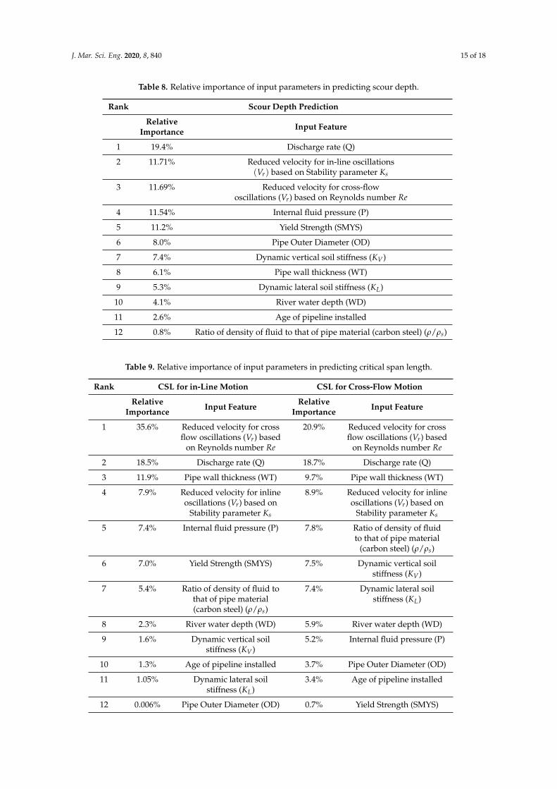
In order to better understand the interactions between variables, the strength and direction ofeach connection weight within the network must be examined directly. Table 7 provides a summary ofoverall connection weights of the input parameters corresponding to each output. A weight decideshow much influence the input will have on the output. Weights near zero imply changing this inputwill not significantly affect the output. Negative weights mean increasing this input will decrease theoutput. The relative importance of an input variable in estimating an output variable is computed as apercentage of magnitude of its overall connection weight with respect to the summation of absolutevalues of overall connection weights of all input variables.

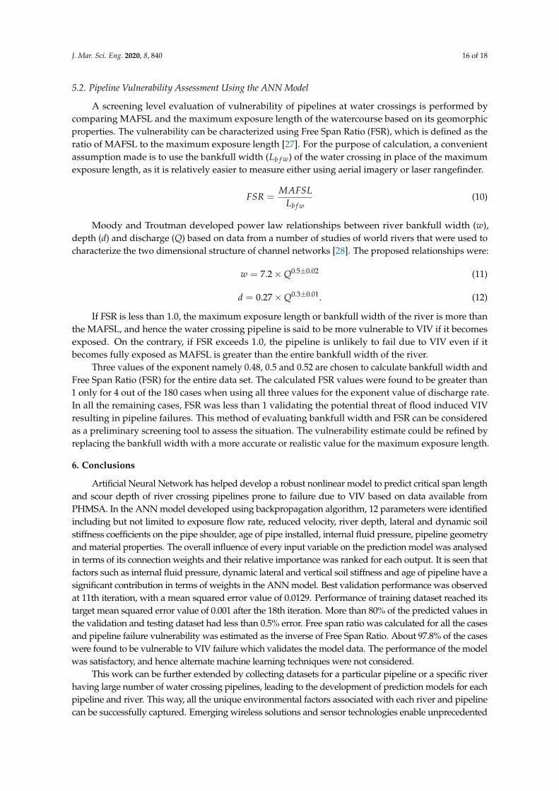
Table 8 shows the relative order of input features used in ANN to estimate scour depth.Moncada and Aguirre-Pe used river velocity, water depth and pipeline outer diameter in theirderivation of empirical relationship to estimate scour depth [22]. Here, we see that factors suchas internal fluid pressure, yield strength, pipe wall thickness, dynamic vertical and lateral soil stiffnessare also statistically significant in terms of weights and play a crucial role in the prediction process.

Table 9 shows the relative order of input features used to estimate critical span length due to in-lineas well as cross-flow motion. We can observe that factors such as reduced velocities based on Reynoldsnumber and stability parameter, discharge rate, pipe wall thickness and internal fluid pressure havehigh relative importance in both cases. Dynamic vertical and lateral soil stiffness values also havesignificant statistical contribution in terms of weights for critical span length due to cross-flow motion.

Table 7. Overall Connection Weights of Input parameters based on Olden’s approach [26].

Overall Connection Weights

Input Features Scour Depth CSL for Cross CSL forIn-Line Motion -Flow Motion

Pipe Outer Diameter (OD) 1.9065 0.0017 −1.7096

Pipe wall thickness (WT) −1.4472 3.4527 4.5148

Yield Strength (SMYS) 2.6710 −2.0436 −0.3391

Internal fluid pressure (P) −2.7444 2.1488 2.4199

River water depth (WD) 0.9861 0.6742 2.7356

Age of pipeline installed 0.6202 0.3790 −1.5626

Discharge rate (Q) 4.6140 −5.3632 −8.6657

Ratio of density of fluidto that of density of pipe

material (carbon steel) (ρ/ρs) −0.2113 −1.5621 −3.6170

Reduced velocity for in-lineoscillations (Vr) based on

Stability parameter Ks −2.7848 −2.2970 −4.1525

Reduced velocity for crossflow oscillations (Vr) based on

Reynolds number Re −2.7802 10.3404 9.6695

Dynamic lateral soilstiffness (KL) −1.2680 0.3035 3.4515

Dynamic vertical soilstiffness (KV) 1.7570 0.4750 −3.4983

J. Mar. Sci. Eng. 2020, 8, 840 15 of 18

Table 8. Relative importance of input parameters in predicting scour depth.

Rank Scour Depth Prediction

RelativeImportance Input Feature

1 19.4% Discharge rate (Q)

2 11.71% Reduced velocity for in-line oscillations(Vr) based on Stability parameter Ks

3 11.69% Reduced velocity for cross-flowoscillations (Vr) based on Reynolds number Re

4 11.54% Internal fluid pressure (P)

5 11.2% Yield Strength (SMYS)

6 8.0% Pipe Outer Diameter (OD)

7 7.4% Dynamic vertical soil stiffness (KV)

8 6.1% Pipe wall thickness (WT)

9 5.3% Dynamic lateral soil stiffness (KL)

10 4.1% River water depth (WD)

11 2.6% Age of pipeline installed

12 0.8% Ratio of density of fluid to that of pipe material (carbon steel) (ρ/ρs)

Table 9. Relative importance of input parameters in predicting critical span length.

Rank CSL for in-Line Motion CSL for Cross-Flow Motion

Relative Input Feature Relative Input FeatureImportance Importance

1 35.6% Reduced velocity for cross 20.9% Reduced velocity for crossflow oscillations (Vr) based flow oscillations (Vr) based

on Reynolds number Re on Reynolds number Re

2 18.5% Discharge rate (Q) 18.7% Discharge rate (Q)

3 11.9% Pipe wall thickness (WT) 9.7% Pipe wall thickness (WT)

4 7.9% Reduced velocity for inline 8.9% Reduced velocity for inlineoscillations (Vr) based on oscillations (Vr) based on

Stability parameter Ks Stability parameter Ks

5 7.4% Internal fluid pressure (P) 7.8% Ratio of density of fluidto that of pipe material

(carbon steel) (ρ/ρs)

6 7.0% Yield Strength (SMYS) 7.5% Dynamic vertical soilstiffness (KV)

7 5.4% Ratio of density of fluid to 7.4% Dynamic lateral soilthat of pipe material stiffness (KL)(carbon steel) (ρ/ρs)

8 2.3% River water depth (WD) 5.9% River water depth (WD)

9 1.6% Dynamic vertical soil 5.2% Internal fluid pressure (P)stiffness (KV)

10 1.3% Age of pipeline installed 3.7% Pipe Outer Diameter (OD)

11 1.05% Dynamic lateral soil 3.4% Age of pipeline installedstiffness (KL)

12 0.006% Pipe Outer Diameter (OD) 0.7% Yield Strength (SMYS)

J. Mar. Sci. Eng. 2020, 8, 840 16 of 18

5.2. Pipeline Vulnerability Assessment Using the ANN Model

A screening level evaluation of vulnerability of pipelines at water crossings is performed bycomparing MAFSL and the maximum exposure length of the watercourse based on its geomorphicproperties. The vulnerability can be characterized using Free Span Ratio (FSR), which is defined as theratio of MAFSL to the maximum exposure length [27]. For the purpose of calculation, a convenientassumption made is to use the bankfull width (Lb f w) of the water crossing in place of the maximumexposure length, as it is relatively easier to measure either using aerial imagery or laser rangefinder.

FSR =MAFSL

Lb f w(10)

Moody and Troutman developed power law relationships between river bankfull width (w),depth (d) and discharge (Q) based on data from a number of studies of world rivers that were used tocharacterize the two dimensional structure of channel networks [28]. The proposed relationships were:

w = 7.2×Q0.5±0.02 (11)

d = 0.27×Q0.3±0.01. (12)

If FSR is less than 1.0, the maximum exposure length or bankfull width of the river is more thanthe MAFSL, and hence the water crossing pipeline is said to be more vulnerable to VIV if it becomesexposed. On the contrary, if FSR exceeds 1.0, the pipeline is unlikely to fail due to VIV even if itbecomes fully exposed as MAFSL is greater than the entire bankfull width of the river.

Three values of the exponent namely 0.48, 0.5 and 0.52 are chosen to calculate bankfull width andFree Span Ratio (FSR) for the entire data set. The calculated FSR values were found to be greater than1 only for 4 out of the 180 cases when using all three values for the exponent value of discharge rate.In all the remaining cases, FSR was less than 1 validating the potential threat of flood induced VIVresulting in pipeline failures. This method of evaluating bankfull width and FSR can be consideredas a preliminary screening tool to assess the situation. The vulnerability estimate could be refined byreplacing the bankfull width with a more accurate or realistic value for the maximum exposure length.

6. Conclusions

Artificial Neural Network has helped develop a robust nonlinear model to predict critical span lengthand scour depth of river crossing pipelines prone to failure due to VIV based on data available fromPHMSA. In the ANN model developed using backpropagation algorithm, 12 parameters were identifiedincluding but not limited to exposure flow rate, reduced velocity, river depth, lateral and dynamic soilstiffness coefficients on the pipe shoulder, age of pipe installed, internal fluid pressure, pipeline geometryand material properties. The overall influence of every input variable on the prediction model was analysedin terms of its connection weights and their relative importance was ranked for each output. It is seen thatfactors such as internal fluid pressure, dynamic lateral and vertical soil stiffness and age of pipeline have asignificant contribution in terms of weights in the ANN model. Best validation performance was observedat 11th iteration, with a mean squared error value of 0.0129. Performance of training dataset reached itstarget mean squared error value of 0.001 after the 18th iteration. More than 80% of the predicted values inthe validation and testing dataset had less than 0.5% error. Free span ratio was calculated for all the casesand pipeline failure vulnerability was estimated as the inverse of Free Span Ratio. About 97.8% of the caseswere found to be vulnerable to VIV failure which validates the model data. The performance of the modelwas satisfactory, and hence alternate machine learning techniques were not considered.

This work can be further extended by collecting datasets for a particular pipeline or a specific riverhaving large number of water crossing pipelines, leading to the development of prediction models for eachpipeline and river. This way, all the unique environmental factors associated with each river and pipelinecan be successfully captured. Emerging wireless solutions and sensor technologies enable unprecedented

J. Mar. Sci. Eng. 2020, 8, 840 17 of 18

asset visibility and help understand pipeline behaviours under different conditions including structuralloads, deflection, weather changes, soil characteristics, moisture and pH levels. This real time data fromIoT based sensors play an important role to develop reliable prediction models and optimize the effectiveservice life of a pipeline.

Author Contributions: Conceptualization, A.K. and S.M.; Data curation, A.K. and S.M.; Formal analysis, A.K.and S.M.; Investigation, A.K., S.M. and R.L.; Methodology, A.K., S.M. and B.H.; Project administration, S.M.and B.H.; Resources, S.M.; Software, A.K.; Supervision, B.H., G.P. and R.L.; Validation, S.M., B.H. and G.P.;Visualization, A.K.; Writing—original draft, A.K.; Writing—review & editing, S.M., B.H., G.P. and R.L. All authorshave read and agreed to the published version of the manuscript.

Funding: The open access publishing fees for this article have been covered by the Texas A&M University OpenAccess to Knowledge Fund (OAKFund), supported by the University Libraries.

Acknowledgments: We would like to thank Timothy Jacobs and Julie Ingram for their valuable insights andguidance during the course of this research.

Conflicts of Interest: The authors declare no conflict of interest. There was no role played by funders in thedesign of the study; in the collection, analyses, or interpretation of data; in the writing of the manuscript, or in thedecision to publish the results.

Abbreviations

The following abbreviations are used in this manuscript:

ANN Artificial Neural NetworksCFD Computational Fluid DynamicsCSL Critical Span Length, (also) Maximum Allowable Free Span LengthDNV Det Norske VeritasFSR Free Span RatioIoT Internet of ThingsLM Levenberg-Marqaurdt Training algorithmMAFSL Maximum Allowable Free Span Length, (also) Critical Span LengthMARS Multivariate Adaptive Regression SplinesMSE Mean Square ErrorNOAA National Oceanic and Atmospheric AdministrationNPMS National Pipeline Mapping SystemPHMSA Pipeline and Hazardous Materials Safety AdministrationVIV Vortex Induced VibrationsUSGS United States Geological Survey

References

1. Belvederesi, C.; Thompson, M.; Komers, P. Statistical Analysis of Environmental Consequences of HazardousLiquid Pipeline Accidents. Heliyon 2018, 4, e00901. [CrossRef] [PubMed]

2. Ferris, G.; Newton, S.; Ho, M.; Eichhorn, G.; Bear, D. Flood Monitoring for Buried PipelineWatercourse Crossing. In Proceedings of the Rio Pipeline Conference & Exposition, Rio de Janiro, Brazil,24–25 September 2015.

3. Analysis and Assessment of Unsupported Subsea Pipeline Spans; United States Department of the Interior,Minerals Management Service: Washington, DC, USA, 1997; pp. 1–42.

4. Heggen, H.O.; Fletcher, R.; Ferris, G.; Ho, M. Fatigue of Pipelines Subjected to Vortex-Induced Vibrationsat River Crossings. In Proceedings of the Rio Oil & Gas Expo and Conference, Rio de Janeiro, Brazil,15–18 September 2014.

5. Xu, J.; Li, G.; Horrillo, J.; Rongmin, Y.; Cao, L. Calculation of Maximum Allowable Free Span Length andSafety Assessment of the DF1-1 Submarine Pipeline. J. Ocean. Univ. China 2010, 9, 1–10. [CrossRef]

6. Koushan, K. Vortex Induced Vibrations of Free Span Pipelines. Ph.D. Thesis, Norwegian University ofScience and Technology, Trondheim, Norway, 2009.

7. Matta, L.; Dotson, R. Key considerations in the assessment of pipeline spans. In Proceedings of the PipelinePigging Integrity Management Conference, Houston, TX, USA, 9–12 February 2015.

J. Mar. Sci. Eng. 2020, 8, 840 18 of 18

8. Yaghoobi, M.; Mazaheri, S.; Jabbari, E. Determining Natural Frequency of Free Spanning Offshore Pipelinesby Considering the Seabed Soil Characteristics. J. Persian Gulf 2012, 3, 25–34.

9. DNV Recommended Practice DNV-RP-F105—Free Spanning Pipelines. February 2006. Available online:https://www.academia.edu/34034147/ (accessed on 26 October 2020).

10. Fyrileiv, O.; MÃrk, K.; Ronold, K. Free Span Design according to the DNV-RP-F105 for Free Spanning Pipelines.In Proceedings of the Offshore Pipeline Technology Conference, Amsterdam, The Netherlands, 1 January 2002.

11. Haghiabi, A.H. Prediction of River Pipeline Scour Depth using Multivariate Adaptive Regression Splines.J. Pipeline Syst. Eng. Pract. 2016, 8, 04016015. [CrossRef]

12. Barati, R. Discussion of Prediction of River Pipeline Scour Depth using Multivariate Adaptive RegressionSplines by Amir Hamzeh Haghiabi. J. Pipeline Syst. Eng. Pract. 2019, 10, 07019001. [CrossRef]

13. Yan, X.; Mohammadian, A.; Rennie, C.D. Numerical Modeling of Flow and Local Scour around Pipeline inSteady Currents using moving mesh with masked elements. J. Hydraul. Eng. 2020, 146, 06020005. [CrossRef]

14. Ychen, Y.H.; Li, J.N.; Kai, L.; Zhu, Q.J.; Liu, Y.L. Failure Prediction of Underground Pipeline Based onArtificial Neural Network. Destech Trans. Comput. Sci. Eng. 2017. [CrossRef]

15. Fyrileiv, O.; Collberg, L. Influence of Pressure in Pipeline Design—Effective Axial Force. In Proceedings of the24th International Conference on Offshore Mechanics and Arctic Engineering, Halkidiki, Greece, 12–17 June 2005.

16. Nelson, G.; Andre, M.; Cláudia, C. A Discussion on How Internal Pressure is Treated in Offshore PipelineDesign. In Proceedings of the IPC 2004, International Pipeline Conference, Calgary, AB, Canada, 4–8 October2004. [CrossRef]

17. Guo, B.; Song, S.; Ghalambor, A.; Lin, T.R. Chapter 5–Pipeline Span. In Offshore Pipelines, 2nd, ed.;Gulf Professional Publishing: Houston, TX, USA, 2014; pp. 53–63.

18. Nogueira, A.C.; Mckeehan, D.S. Chapter 11–Design and Construction of Offshore Pipelines. In Handbook ofOffshore Engineering; Chakrabarti, S.K., Ed.; Elsevier: London, UK, 2005; pp. 891–937.

19. Sawatsky, L.F.; Bender, M.J.; Long, D. Pipeline Exposure at River Crossings: Causes and Cures. In Proceedingsof the International Pipeline Conference, Calgary, AB, Canada, 7–11 June 1998; American Society ofMechanical Engineers: New York, NY, USA, 1998; Volume 1, pp. 159–163.

20. Azamathulla, M.H.; Ghani, A.A. Genetic programming to predict river pipeline scour. J. Pipeline Syst.Eng. Pract. 2010, 1, 127–132. [CrossRef]

21. Chiew, Y.M. Prediction of maximum scour depth at submarine pipelines. J. Hydraul. Eng. 1991, 117, 452–466.[CrossRef]

22. Moncada-M.A.; Aguirre-Pe, J. Scour below pipeline in river crossings. J. Hydraul. Eng. 1999, 125, 953–958.[CrossRef]

23. Skorpil, V.; Stastny, J. Neural Networks and Back Propagation Algorithm. In Proceedings of theELECTRONICS’ 2006, Sozopol, Bulgaria, 20–22 September 2006.

24. Gavin, H.P. The Levenberg-Marquardt Algorithm for Nonlinear Least Squares Curve-Fitting Problems;Department of Civil and Environmental Engineering, Duke University: Durham, NC, USA, 2019.

25. Olden, J.D.; Joy, M.K.; Death, R.G. An accurate comparison of methods for quantifying variable importancein artificial neural networks using simulated data. Ecol. Model. 2004, 178, 389–397. [CrossRef]

26. Olden, J.; Jackson, D. Illuminating the “black box”: A randomization approach for under-standing variablecontributions in artificial neural networks. Ecol. Model. 2002, 154, 135–150. [CrossRef]

27. Dooley, C.; Prestie, Z.; Ferris, G.; Fitch, M.; Zhang, H. Approaches for evaluating the vulnerability ofpipelines at water crossings. In Proceedings of the Biennial International Pipeline Conference, IPC, Calgary,AB, Canada, 29 September–3 October 2014; Volume 2.

28. Moody, J.A.; Troutman, B.M. Characterization of the spatial variability of channel morphology. Earth Surf.Process. Landf. 2002, 27, 1251–1266. [CrossRef]

Publisher’s Note: MDPI stays neutral with regard to jurisdictional claims in published maps and institutionalaffiliations.

c© 2020 by the authors. Licensee MDPI, Basel, Switzerland. This article is an open accessarticle distributed under the terms and conditions of the Creative Commons Attribution(CC BY) license (http://creativecommons.org/licenses/by/4.0/).