Seediscussions,stats,andauthorprofilesforthispublicationat:https://www.researchgate.net/publication/246955786

Quantificationof1HNMRspectraofhumancerebrospinalfluid:Aprotocolbasedonconstrainedtotal-line-shapeanalysis

ARTICLEinMETABOLOMICS·JUNE2008

ImpactFactor:3.86·DOI:10.1007/s11306-008-0106-6

CITATIONS

18

READS

50

10AUTHORS,INCLUDING:

NikoMikaelJukarainen

UniversityofEasternFinland

5PUBLICATIONS65CITATIONS

SEEPROFILE

MikkoPLaakso

NiuvanniemiHospital

94PUBLICATIONS7,308CITATIONS

SEEPROFILE

MinnaAKorolainen

Janssen-Cilag,Finland

14PUBLICATIONS416CITATIONS

SEEPROFILE

JoukoVepsäläinen

UniversityofEasternFinland

282PUBLICATIONS3,046CITATIONS

SEEPROFILE

Allin-textreferencesunderlinedinbluearelinkedtopublicationsonResearchGate,

lettingyouaccessandreadthemimmediately.

Availablefrom:MikkoPLaakso

Retrievedon:04February2016

ORIGINAL ARTICLE

Quantification of 1H NMR spectra of human cerebrospinal fluid:a protocol based on constrained total-line-shape analysis

Niko M. Jukarainen Æ Samuli-Petrus Korhonen Æ Mikko P. Laakso ÆMinna A. Korolainen Æ Matthias Niemitz Æ Pasi P. Soininen Æ Kari Tuppurainen ÆJouko Vepsalainen Æ Tuula Pirttila Æ Reino Laatikainen

Received: 11 July 2007 / Accepted: 22 January 2008 / Published online: 10 February 2008

� Springer Science+Business Media, LLC 2008

Abstract A protocol for quantitative 1H NMR analysis

of human cerebrospinal fluid (hCSF) was built up and

assessed as based on Constrained Total-Line-Shape

(CTLS) fitting. In this method, linear constraints were

applied to spectral structures. The 1H NMR spectra of 45

human CSF samples were measured and quantified using

the CTLS method. The quantification strategies based on

total-line-shape fitting are discussed. The metabolic model

for CTLS includes 31 metabolites covering 85% of the

total spectral intensity, excluding the protein contribution.

Prior to data analysis, the data was divided into patients

with no Alzheimer’s disease (AD), but with a normal AD

marker profile (the peptide b-amyloid42 and tau protein)

present in CSF, and into controls that do not have an AD

marker profile in CSF. Unexpectedly large variations in

metabolite concentrations within the two patient groups

were detected, but an analysis of variance revealed a

significant (P = 0.027) difference only in the concentra-

tion of creatinine which was higher in patients that had a

normal AD marker profile. Multivariate classification tools

such as self-organizing maps (SOM) failed in separation of

the two classes.

Keywords Nuclear magnetic resonance � Metabolomics �Quantification � Total-line-shape � Cerebrospinal fluid �Creatinine

1 Introduction

The composition of biofluids carries invaluable informa-

tion about the biochemical status of a living organism.

Modern 1H NMR spectroscopy provides an efficient tool

with which to analyze biofluids and nowadays this tech-

nique is commonly used in profiling of biofluids such as

urine and blood plasma (Bollard et al. 2005; Lindon et al.

2007; Vanderhoeven et al. 2006; Wang et al. 2006). The

advantages of NMR methods are that measurements can be

done with minimal sample preparation and instrument

calibration. Moreover, recent technical and software

developments have reduced the cost of an NMR analysis

making it a versatile option for biomarker analysis

(Anderson et al. 2006; Nicholson 2006). Current NMR

applications include assessments of differences in diverse

neurological disorders such as Alzheimer’s disease (AD)

and subjective cognitive impairment (Weiss et al. 2003).

Cerebrospinal fluid (CSF) indirectly reflects the bio-

chemical processes occurring in the brain. Therefore its

N. M. Jukarainen (&) � S.-P. Korhonen �P. P. Soininen � K. Tuppurainen � J. Vepsalainen �R. Laatikainen

Laboratory of Chemistry, Department of Biosciences,

University of Kuopio, P.O. Box 1627, 70211 Kuopio, Finland

e-mail: Niko.Jukarainen@uku.fi

M. P. Laakso � T. Pirttila

Department of Neurology, Kuopio University Hospital,

Kuopio, Finland

M. P. Laakso

Department of Clinical Radiology, Kuopio University Hospital,

Kuopio, Finland

M. A. Korolainen

Department of Neuroscience and Neurology,

University of Kuopio, Kuopio, Finland

M. A. Korolainen � T. Pirttila

Brain Research Unit, Clinical Research Centre/Mediteknia,

University of Kuopio, Kuopio, Finland

M. Niemitz

PERCH Solutions Ltd, Kuopio, Finland

123

Metabolomics (2008) 4:150–160

DOI 10.1007/s11306-008-0106-6

composition can be anticipated to provide information

about states of normal or pathological metabolism of the

brain. The biochemical composition of CSF resembles that

of ultrafiltered blood plasma, but it also contains metabo-

lites which are secreted by the central nervous system

(Lindon et al. 2000; Maillet et al. 1998). Although CSF

samples are more difficult to obtain than blood samples, for

an NMR analysis, CSF possesses clear advantages due to

the relatively low protein and lipid content and the low

viscosity of the medium. Additionally, signal overlap in

CSF is not as serious as in urine or whole blood, because of

the fewer metabolites present (Lindon et al. 2000). It is

therefore not surprising that several NMR studies on CSF

have been reported (Ghauri et al. 1993; Holmes et al.

2006; Koschorek et al. 1993; Maillet et al. 1998) and that

some changes in NMR observable metabolites in the brain

associated with AD have been reported (Hancu et al.

2005). These include an increase in the myo-inositol con-

centration and its ratio to creatinine, as well as a decrease

in N-acetyl-aspartate and its ratio to creatinine and myo-

inositol. The trend in NMR analysis of CSF seems to be

toward in vivo methods due to medical, technical, and

ethical constraints and the lack of specific information on

metabolic perturbations which are truly characteristic of

central nervous system disorders (Hancu et al. 2005;

Pfeuffer et al. 1999). A major problem in a human meta-

bolomic model seems to be the physiological variation,

attributable to several intrinsic and extrinsic factors such as

genetics, ageing, gender, dietary variation, smoking, stress

and physical exercise (Bollard et al. 2005). Also animal

models offer potential tools for drug metabonomics: we

have recently shown that characteristic differences between

AD and controls rats exists, and is detectable in NMR

spectra (Malm et al. 2006).

The existing NMR analytical protocols do not utilize the

spectral information to its full potential. In principle, the

information content of biofluid 1H NMR spectra is high,

but the transformation of this information into concentra-

tions of individual metabolites, essential to many

applications, is not straightforward. Each metabolite may

contribute up to tens of individual signals in the spectrum

and the signals may seriously overlap with each other.

Several approaches for solving problems such as signal

shifts and peak overlap and other problems have been

presented. These strategies include a ‘curve-fitting method’

based on pre-fitted model signals of components

(Crockford et al. 2005; Weljie et al. 2006), the automatic

alignment of spectral peak-regions (Stoyanova et al. 2004),

spectral editing via relaxation and diffusion (Wang et al.

2003), peak alignment using reduced set mapping (Torgrip

et al. 2006), and a method for stepwise selection of peaks

in NMR spectra from multiple groups (Ammann and

Merritt 2007). Several methods and the validity of their

results have also been assessed (Forshed et al. 2005). It has

also been suggested that curve-fitting methods may intro-

duce bias to the data (Viles et al. 2001). In this work,

we used a Constrained Total-Line-Shape (CTLS) method

(Laatikainen et al. 1996a) to alleviate the aforesaid prob-

lems. The objective of this study was to build up and assess

approaches for using quantitative 1H NMR analysis of CSF

and to evaluate their applicability for metabolic profiling of

neurological patients.

2 Materials and methods

2.1 CSF samples of neurological controls

The patient group of 45 neurological controls aged 45–82

consisted of individuals examined for various neuropsy-

chiatric symptoms such as depression or headache but who

had no signs of dementia and no chronic neurological

disease. These patients were further divided into two

groups: patients with a normal AD marker (the peptide

b-amyloid42 and tau protein) profile present in CSF (patient

class abbreviation: C_ADP) and controls that do not have

an AD marker profile in CSF (patient class abbreviation:

C_NRM). The C_ADP group consisted of 10 patients of

whom 7 were female (females aged 57–79 years; males

aged 57–66 years), the C_NRM group consisted of 34

patients of whom 19 were female (females aged 52–

81 years; males aged 45–78 years). No other confounding

disease states were associated with these patients. Lumbar

CSF samples were obtained using a standardized protocol.

All samples were placed in a cold gel pack immediately

after sample acquirement and frozen within 2 h. The study

was approved by the local ethics committee of the Uni-

versity of Kuopio and Kuopio University Hospital, and

informed consent for participation in the study was

obtained from all subjects.

2.2 Sample preparation

The samples were prepared according to the protocol

described by Maillet (Maillet et al. 1998). First, 1,800 ll of

each sample was subjected to an identical lyophilization

protocol for 40 h. The freeze-dried samples were then

stored at -20�C in sealed vials until analysis. Prior to the

NMR measurements, the samples were reconstituted in

600 ll of D2O (99.98%-D, Merck) and 450 ll of this liquid

was transferred to a separate vial followed by addition of

50 ll of 21.5 mM TSP-d4 in D2O to be used as an internal

standard of known concentration. The pH of the samples

was not adjusted, being typically around 7.00 ± 0.05. This

pH can be defined as pH*, which is the reading of the pH

Constrained total-line-shape quantification protocol of CSF 151

123

meter as measured with a standard pH electrode. The pD

value is ca. 0.4 units higher than pH*.

2.3 NMR spectroscopy

The metabolic profiling was based on a standard 1D 1H

NMR spectrum. All spectra were measured by using a

Bruker AVANCE DRX 500 instrument operating at

500.13 MHz (Bruker-Biospin GmbH, Karlsruhe, Ger-

many), equipped with a quadronuclear probe. The Bruker

XWIN-NMR software version 3.5pl5 running on a standard

PC was used for acquisition of all spectra. The relevant

parameters used in the 1D experiments, were calibrated and

used as follows: recycling delay 45 s, acquisition time

6.5 s, number of scans 128, and a sweep width of 9.5 ppm.

A calibrated 90� pulse was used for all spectra and all

acquisitions were performed on non-spinning samples. To

assess the use of relaxation editing in spectral simplifica-

tion, T2 edited 1D NMR spectra were measured. For the

three spectra (not edited, minimally and heavily edited)

measured, a standard 1D Carr–Purcell–Meiboom–Gill

(CPMG) pulse sequence with a 40 ms or 320 ms (for

minimally edited and fully edited, respectively) T2-filter

using a fixed echo delay of 400 ls that eliminates diffusion

and J-modulation effects was used.

2.4 Identification of metabolites

The assignments of the spectral signals were done

according to available chemical shift and coupling constant

information in the literature (Fan 1996; Govindaraju et al.

2000; Maillet et al. 1998; Nicholson et al. 1995). Some

metabolites and signals were verified by using 2D NMR

spectroscopy and by performing 1D spiking experiments.

2.5 Metabolic concentration analysis and classification

Metabolite concentrations and ratio relations were ana-

lyzed in the hopes of finding patterns within the control

patient group. Concentrations were assessed by using one

way ANOVA as implemented in SPSS v14.0. Separation of

the two patient classes was explored by using the Self-

Organizing Map algorithm (Kohonen et al. 1996) (SOM)

which uses competitive learning to create a two-dimen-

sional map of the original data in such a manner that it

conserves the maximum amount of the structure present in

the original data. The actual analysis was performed by

using the SOM_PAK software, version 3.1, freely

available.

2.6 Quantification analysis

All spectral processing prior to the model creation was done

using the PERCH NMR Software version 2005/1 (PERCH

Solutions Ltd., Kuopio, Finland). The total-line-shape

(TLS) fitting tool of PERCH NMR Software version 2007.2

was used in the quantification analyses. The local baseline

option was added to the software during these analyses.

2.7 Magnesium and calcium concentrations

Ca2+ and Mg2+ concentrations were measured by a Perkin

Elmer PE 460 AAS and a Perkin Elmer PE 5100 AAS

instrument, respectively, using a multi-element hollow

cathode lamp and an air-acetylene flame.

3 Results and discussion

3.1 Quantification: CTLS fitting

The positions of the signal frequencies of some metabolites

(e.g. citrate and glutamine c-CH2) vary significantly (up to

10 Hz) from one spectrum to another, likely reflecting

variations in ionic strength and Ca2+ and Mg2+ concen-

trations. This means that the traditional methods based on

integrals (buckets) would not perform well and, therefore,

the analysis was performed using the CTLS method.

The 1H NMR spectrum I(v) is sum of the numerous

individual lines Ln(v)

IðvÞ ¼X

LnðvÞ ð1Þ

A single compound may produce tens or more lines that

may overlap with lines of other metabolites. The concen-

tration of the compound is fairly strictly proportional to the

area of the lines arising from the compound. TLS fitting, or

deconvolution, is an efficient way and in fact the only way

when dealing with 1H NMR spectra, to integrate the area of

overlapping multiplets of different protons. However,

overlap or closeness of very large signals, leads to prob-

lems in estimation of the line areas (Soininen et al. 2005).

In this work, a CTLS fitting strategy, utilizing constraints

derived from spectral structures, was applied. As previ-

ously shown (Laatikainen et al. 1996a), constraints

describing spectral structures improve the statistics of

concentrations obtained by TLS analysis. In this work, 20

constraints were written to define doublets, triplets, quar-

tets and quintets of the most intensive signals arising from

the major metabolites. This helps in quantification of the

signals close to the major components, such as glucose and

lactate (see below), and also reduces the number of

152 N. M. Jukarainen et al.

123

parameters to be fitted. For example, a triplet can be

described by 4 parameters (position, intensity, line-width

and splitting) instead of the 9 needed for three separate

lines. Because the number of the parameters is presently

limited to 500, the spectrum must usually be fitted in parts.

Some parameters are also needed to describe the line-shape

and the baseline.

The TLS fitting is a nonlinear problem that can be

solved only iteratively. A special problem is formed by the

baseline arising from instrumental artifacts and broad

signals of macromolecules. Another problem, related to

weak signals close to strong signals, is that the real line-

shape cannot be completely described by the theoretical

Lorenzian line-shape. This has been discussed in detail

before (Soininen et al. 2005).

The concentration of a metabolite is proportional to the

area of the sum of the signals arising from it. The standard

deviation of the area, and thus that of concentration, can be

computed from the normal equation (variance–covariance)

matrix formed in the iterative protocol, which has been

described before (Laatikainen et al. 1996a). The protocol

also gives estimates of standard deviations of the popula-

tions and it is notable that the standard deviations must be

computed taking the correlations of the individual signal

parameters into account.

The estimate of standard deviation (s) for single line and

multiplet area are obtained from the equation

sðnÞ ¼ rrms �ffiffiffiffiffiffiffiffiffiffiffiffiffiffiffiffiffiffiffiffiffiffiffiffiffiffiffiffiffiffiffiffiffiffiffiffiffiffiffiffiffiffiffiffiffiffiffiffiAnnI2 þ AkkW2 þ 2AnkW

pð2Þ

where In = the intensity of the line, Wn = the half-height

width of the line, normalized so that the area = I * W, Akk,

Ann and Ank are elements of the inverse matrix of

correlation-covariance matrix D, corresponding to I and

W. The matrix D element Dnk can be approximated by the

equation

Dnk ¼XI

i

oIiðvÞoIn� oIiðvÞ

oWkð3Þ

where the derivatives qIi(v)/qIn and qIi(v)/qWk are com-

puted for the iterative algorithm. Rrms is the residual root

mean square.

For the standard deviation estimate of a sum of areas

also the correlations of the contributing lines need to be

taken into account:

where n and m refer to the lines belonging to the structure,

k, l, i, j are the indices relating the line-widths and inten-

sities, respectively, to the A matrix. The second sum term is

normally negative, which means that s2(sum) \ Rs2(n),

which would be the standard deviation of the sum of

independent terms. This also means that the integration

based on deconvolution, while ignoring the correlations

and spectral structures, may give poor statistics for the

quantified area. To illustrate the effects of the constraints

and the correlations equations we took an example. For

example, if the doublet at 2.44 ppm (marked by an arrow in

Fig. 2) is devonvoluted asuming two independent lines,

their total area is 0.400 ± 0.077 (area ± rms, as reported

by TLS). If the standard deviation was calculated by

assuming s2(sum) = Rs2(n), the result would be 0.088,

reflecting the effect of the correlations to the error

parameters. If however the lines are defined to form a 1:1

doublet, the total area is 0.408 ± 0.028. Similar effects are

obtained for many other lines, some of which are marked

by arrows in Fig. 2.

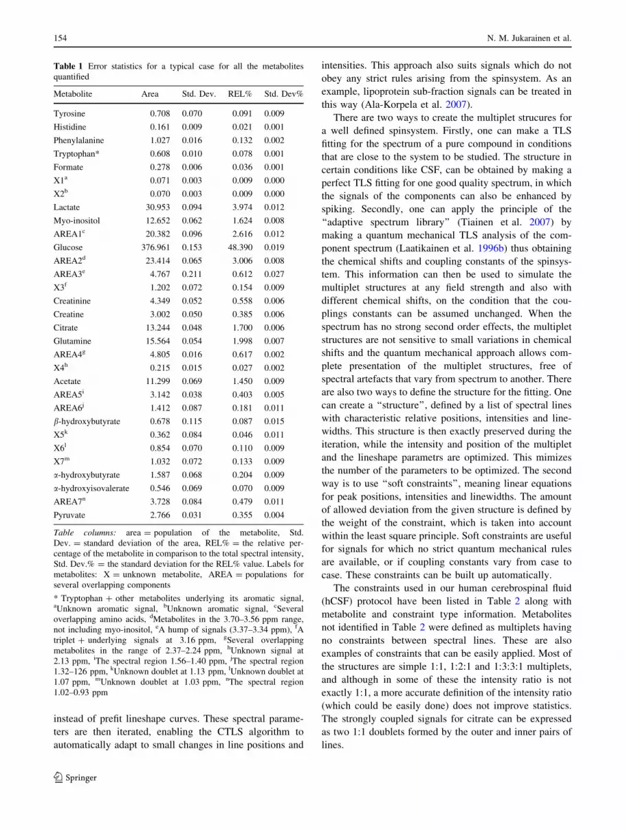
Error statistics produced by the CTLS algorithm for a

typical CSF case are shown in Table 1. Although the

estimated standard deviations based on the variance–

covariance matrix are usually systematically slightly too

small, they can be assumed to give a fair picture about the

relative reliability of the compound populations, if the

fitting is done with a similar protocol for each case.

Expectedly, the accuracy of major components is better

than that of minor ones. This may also depend more on the

protocol, especially on the number of baseline terms and

how the spectrum is divided into fitting segments.

3.2 Prior knowledge

In the CTLS approach, practically any prior knowledge

about spectral structures can be easily incorporated into the

fitting algorithm. The multiplet structure (the relative

positions and intensities of the lines), can be obtained by

measuring a component spectrum and performing the TLS

fitting on pure component multiplets, much like described

elsewhere (Crockford et al. 2005; Weljie et al. 2006).

However, in CTLS fitting the structures are defined for the

program as line positions and intensities or constraints

sðsumÞ ¼ rrms �

ffiffiffiffiffiffiffiffiffiffiffiffiffiffiffiffiffiffiffiffiffiffiffiffiffiffiffiffiffiffiffiffiffiffiffiffiffiffiffiffiffiffiffiffiffiffiffiffiffiffiffiffiffiffiffiffiffiffiffiffiffiffiffiffiffiffiffiffiffiffiffiffiffiffiffiffiffiffiffiffiffiffiffiffiffiffiffiffiffiffiffiffiffiffiffiffiffiffiffiffiffiffiffiffiffiffiffiffiffiffiffiffiffiffiffiffiffiffiffiffiffiffiffiffiffiXN

n

s2ðnÞ þ 2XN

n

XM

m

ðAklInIm þ AijWnWm þ AliImWn þ AkjInWmÞ

vuut ð4Þ

Constrained total-line-shape quantification protocol of CSF 153

123

instead of prefit lineshape curves. These spectral parame-

ters are then iterated, enabling the CTLS algorithm to

automatically adapt to small changes in line positions and

intensities. This approach also suits signals which do not

obey any strict rules arising from the spinsystem. As an

example, lipoprotein sub-fraction signals can be treated in

this way (Ala-Korpela et al. 2007).

There are two ways to create the multiplet strucures for

a well defined spinsystem. Firstly, one can make a TLS

fitting for the spectrum of a pure compound in conditions

that are close to the system to be studied. The structure in

certain conditions like CSF, can be obtained by making a

perfect TLS fitting for one good quality spectrum, in which

the signals of the components can also be enhanced by

spiking. Secondly, one can apply the principle of the

‘‘adaptive spectrum library’’ (Tiainen et al. 2007) by

making a quantum mechanical TLS analysis of the com-

ponent spectrum (Laatikainen et al. 1996b) thus obtaining

the chemical shifts and coupling constants of the spinsys-

tem. This information can then be used to simulate the

multiplet structures at any field strength and also with

different chemical shifts, on the condition that the cou-

plings constants can be assumed unchanged. When the

spectrum has no strong second order effects, the multiplet

structures are not sensitive to small variations in chemical

shifts and the quantum mechanical approach allows com-

plete presentation of the multiplet structures, free of

spectral artefacts that vary from spectrum to another. There

are also two ways to define the structure for the fitting. One

can create a ‘‘structure’’, defined by a list of spectral lines

with characteristic relative positions, intensities and line-

widths. This structure is then exactly preserved during the

iteration, while the intensity and position of the multiplet

and the lineshape parametrs are optimized. This mimizes

the number of the parameters to be optimized. The second

way is to use ‘‘soft constraints’’, meaning linear equations

for peak positions, intensities and linewidths. The amount

of allowed deviation from the given structure is defined by

the weight of the constraint, which is taken into account

within the least square principle. Soft constraints are useful

for signals for which no strict quantum mechanical rules

are available, or if coupling constants vary from case to

case. These constraints can be built up automatically.

The constraints used in our human cerebrospinal fluid

(hCSF) protocol have been listed in Table 2 along with

metabolite and constraint type information. Metabolites

not identified in Table 2 were defined as multiplets having

no constraints between spectral lines. These are also

examples of constraints that can be easily applied. Most of

the structures are simple 1:1, 1:2:1 and 1:3:3:1 multiplets,

and although in some of these the intensity ratio is not

exactly 1:1, a more accurate definition of the intensity ratio

(which could be easily done) does not improve statistics.

The strongly coupled signals for citrate can be expressed

as two 1:1 doublets formed by the outer and inner pairs of

lines.

Table 1 Error statistics for a typical case for all the metabolites

quantified

Metabolite Area Std. Dev. REL% Std. Dev%

Tyrosine 0.708 0.070 0.091 0.009

Histidine 0.161 0.009 0.021 0.001

Phenylalanine 1.027 0.016 0.132 0.002

Tryptophan* 0.608 0.010 0.078 0.001

Formate 0.278 0.006 0.036 0.001

X1a 0.071 0.003 0.009 0.000

X2b 0.070 0.003 0.009 0.000

Lactate 30.953 0.094 3.974 0.012

Myo-inositol 12.652 0.062 1.624 0.008

AREA1c 20.382 0.096 2.616 0.012

Glucose 376.961 0.153 48.390 0.019

AREA2d 23.414 0.065 3.006 0.008

AREA3e 4.767 0.211 0.612 0.027

X3f 1.202 0.072 0.154 0.009

Creatinine 4.349 0.052 0.558 0.006

Creatine 3.002 0.050 0.385 0.006

Citrate 13.244 0.048 1.700 0.006

Glutamine 15.564 0.054 1.998 0.007

AREA4g 4.805 0.016 0.617 0.002

X4h 0.215 0.015 0.027 0.002

Acetate 11.299 0.069 1.450 0.009

AREA5i 3.142 0.038 0.403 0.005

AREA6j 1.412 0.087 0.181 0.011

b-hydroxybutyrate 0.678 0.115 0.087 0.015

X5k 0.362 0.084 0.046 0.011

X6l 0.854 0.070 0.110 0.009

X7m 1.032 0.072 0.133 0.009

a-hydroxybutyrate 1.587 0.068 0.204 0.009

a-hydroxyisovalerate 0.546 0.069 0.070 0.009

AREA7n 3.728 0.084 0.479 0.011

Pyruvate 2.766 0.031 0.355 0.004

Table columns: area = population of the metabolite, Std.

Dev. = standard deviation of the area, REL% = the relative per-

centage of the metabolite in comparison to the total spectral intensity,

Std. Dev.% = the standard deviation for the REL% value. Labels for

metabolites: X = unknown metabolite, AREA = populations for

several overlapping components

* Tryptophan + other metabolites underlying its aromatic signal,aUnknown aromatic signal, bUnknown aromatic signal, cSeveral

overlapping amino acids, dMetabolites in the 3.70–3.56 ppm range,

not including myo-inositol, eA hump of signals (3.37–3.34 ppm), fA

triplet + underlying signals at 3.16 ppm, gSeveral overlapping

metabolites in the range of 2.37–2.24 ppm, hUnknown signal at

2.13 ppm, iThe spectral region 1.56–1.40 ppm, jThe spectral region

1.32–126 ppm, kUnknown doublet at 1.13 ppm, lUnknown doublet at

1.07 ppm, mUnknown doublet at 1.03 ppm, nThe spectral region

1.02–0.93 ppm

154 N. M. Jukarainen et al.

123

The glutamine c-CH2 signal at ca. 2.42 ppm forms a

special problem. In its very tightly coupled system, even

very small changes in the chemical shifts change the

relative positions and intensity ratios of the lines of the

multiplet, so that it is not possible to build up a good

general structure for the signal. In principle, the only way

to do the fitting would be to use an iterative quantum

mechanical TLS fitting which properly accounts for the

second order effects.

3.3 Quantification: fitting protocol

Although the protein concentration of CSF is low, and in

the spectral ranges of 6.5–8.5 ppm and 0.7–1.3 ppm, it

corresponds to great part of the total spectral integral. The

protein baseline can be described with global Fourier

expansion (Laatikainen et al. 1996a)

bðvÞ ¼XN

n

Bn sinðnv=DvÞ þ b0 þ slope ð5Þ

where Dv = the width of the fitting range or, as in this

work, using an n term local Fourier-type function

bðvÞ ¼XN

n

Bn sin2 x ð6Þ

where x = [(v - vn)/k], with k = dv/(N - 1), for vi +

k[ x [ vi - k, otherwise sin2x is set to 0. Although both

of the functions give practically the same result with the

same number of terms, the local function is easier to

visualize, store (in form of constants B), and to make

continuous when the spectrum is fitted in parts. Because a

straight line can be constructed by using equal sin2-terms,

the b0 and slope terms should not be used in local func-

tions. Figure 1 illustrates how the aromatic region hump

can be fully described by a 14 terms expansion.

In this region the signals are clearly separated from the

baseline and the hump can be removed by subtracting the

baseline contribution before the TLS fitting. On the other

hand, the high field (0.7–4.5 ppm) hump is not so well-

defined, because almost the whole range is covered by

some signals. Therefore the baseline must be optimized

simultaneously with the TLS fitting.

After the baseline correction, the spectrum is fitted in

parts as follows (see Fig. 2). An essential question is the

number of the baseline terms. When the spectral intensity

is formed in large extent by the baseline hump, the number

of the terms and also the fitting protocol becomes impor-

tant: a numerically reasonable fit can be obtained in many

ways. The number of baseline terms usually influences the

obtained populations; however, when using the same fitting

protocol and number of terms for all samples, the bias can

be minimized. The following protocol was found to be the

most robust:

• Add as many lines as clearly visible to the model.

• Set the number of local Fourier baseline terms to 2–20

(depending on the fitting range but 10 is a good guess)

and perform the fitting using an option where every line

has same line-width. It is essential that the trial line-

width is set to a reasonable value, on the basis of some

well-defined typical signal in the range. This should

lead to a fairly good fit in this case. If not and there

exists clear observed minus calculated differences,

additional lines can be added to the model or the

number of the baseline terms can be changed.

Table 2 The constraints used in the fitting protocol along with cor-

responding metabolites

Constraint chemical

shift (ppm)

Constraint type Metabolite

0.84 Doublet a-hydroxyisovalerate

0.90 Triplet a-hydroxybutyrate

1.03 Doublet Unknown

1.07 Doublet Unknown

1.13 Doublet Unknown

1.20 Doublet b-hydroxybutyrate

1.33 Doublet Lactate

1.46 Doublet Alanine

2.54 + 2.70 Slanted doublets Citrate

3.24 + 3.26 Doublets Glucose

3.29 Triplet Myo-inositol

3.53 + 3.55 Doublets Glucose

3.63 Triplet Myo-inositol

3.89 + 3.91 Doublets Glucose

4.07 Triplet Myo-inositol

4.12 Quartet Lactate

6.87 + 7.18 AB-quartets Tyrosine

8.40 8.20 8.00 7.80 7.60 7.40 7.20 7.00 6.80 6.60 6.40

Fig. 1 A representation of the local Fourier baseline functions

applied for the baseline fit of the aromatic hump. The separate Fourier

functions and their sum (the baseline) have been separately indicated

Constrained total-line-shape quantification protocol of CSF 155

123

• Refine the fit using an option that allows different line-

widths for lines. If two lines are defined to form, for

example, a 1:1 doublet, the line-widths are kept the

same; this strongly guides both the baseline function

iteration and iteration of overlapping signals to the

correct direction. If the baseline is not well-defined, one

can use a weighting parameter that forces Fourier terms

toward zero.

• Known metabolites are assigned and only clearly

resolved signals (if available) are used for quantifica-

tion. For example, when fitting glutamine, the multiplet

at 2.42 ppm was used but the signals at 2.05 ppm

ignored.

• Signals that cannot be assigned to any known metab-

olite can be taken into account by grouping them into

well-defined packages that can be treated in the

statistical analysis in the same way as the identified

compounds. In our data those integrals are marked with

Xi (unknown metabolites) and Ai (areas with multiple

signals).

The spectral range of 0.70–1.3 ppm forms a good

example of the fitting strategies when determining how

to fix the fitting parameters. Within this range, the three

rightmost lines are broad and poorly defined. If the

number of baseline terms is too small, the intensity of

those lines may become zero or even negative. It is

obvious that the intensity of these lines remains somewhat

inaccurate, although fair relative values can be obtained

when the number of baseline terms is set with same

criteria for every spectrum. To test the robustness of the

fitting, we performed the fitting with 10, 20 and 30

baseline terms and the obtained populations remained

nearly identical with each number of terms. In some cases

however, where very small populations were quantified,

30 baseline terms led to erroneous populations for the

metabolites. A typical error range was ±20% when

compared to populations obtained by using 10–20 base-

line terms and typical metabolites with low concentrations

were b-hydroxybutyrate, a-hydroxybutyrate and a-hydrox-

yisovalerate. This is because of overfitting: the baseline

function tries to fit the smallest signals in the spectrum as

a part of the baseline.

Anyhow, consideration of the above aspects evidently

leads to the conclusion that each CTLS application

demands its own validated protocol; our protocol for hCSF

is described in detail below. In our final fitting protocol the

spectrum was divided into 7 parts, for each of which the

fitting was performed independently. An essential point is

to perform the fitting for the lines with strong intensities

first (e.g. like lactate at 1.33 ppm), so that its contribution

to the signals close to its root can be interpolated in the

fitting. This led to the following total fitting protocol:

la

ahi

ahbbh x5 x6 x7

1.40 1.20 1.00 0.80

A5 A6 A7

e acpy

ci ci

2.60 2.40 2.20 2.00

x4A4

la

crecrn

glcglc glc

glc

glc

mi

mi+A2mi

A1

4.00 3.80 3.60 3.40 3.20

A3 x3h

fw+o y y

x1

fm

8.40 8.20 8.00 7.80 7.60 7.40 7.20 7.00

x2

b

(a)

(c) (d)

(b)

Fig. 2 A presentation of a 1H NMR spectrum of hCSF at 500 MHz.

(a) Higher field aliphatic region, with metabolite markings as follows:

la = lactate, ahi = a-hydroxyisovalerate, ahb = a-hydroxybutyrate,

bhb = b-hydroxybutyrate, A5 through A7 = metabolite areas 5–7,

x5 through x7 = unknown metabolites. (b) Lower field aliphatic

region: e = glutamate, ac = acetate, py = pyruvate, ci = citrate,

A4 = several overlapping metabolites, x4 = unknown metabolite.

(c) Middle region: la = lactate, cre = creatine, crn = creatinine,

glc = glucose (a protons not shown), mi = myo-inositol, A1 through

A3 = metabolite areas 1–3, x3 = unknown metabolite. (d) Aromatic

region: h = histidine, f = phenylalanine, w = tryptophan, y = tyro-

sine, fm = formate, o = others, x1 & x2 = unknown aromatic

metabolites. For details on the metabolite areas, see Table 1

156 N. M. Jukarainen et al.

123

1. Fit the TSP signal (-0.10–0.10 ppm) with 3-4 lines

and 5 baseline terms. Scale the spectrum so that the

area of these signals together is 100.

2. Fit the lactate signal (1.30–1.40 ppm), with 5 baseline

terms.

3. Fit spectral region 0.6–1.75 ppm with 10–20 baseline

terms.

4. Fit spectral region 1.75–2.8 ppm with 10–20 baseline

terms.

5. Fit spectral region 2.9–4.2 ppm with 10–20 baseline

terms.

6. Fit spectral region 3.57–4.3 ppm with 10–20 baseline

terms.

7. Fit the aromatic range using 10 baseline terms.

8. The protein concentration was estimated by quantify-

ing the protein hump for the spectral region 0.7–

4.5 ppm. The hump area was obtained by integrating

the optimized baseline function.

Figure 2 shows the assigned spectrum of hCSF with

assignment of the metabolite signals.

For each single line, the frequency, line-width and

intensity were optimized during the fitting. For multiplets,

the widths of each line were kept equal. The same line-

shape (Laatikainen et al. 1996a) was used for every line.

The use of macros for the quantification and processing of

spectra is highly beneficial in the creation of automatic

protocols, thus ensuring that all the analyses are performed

in an identical way. All calculations were performed on a

standard PC (AMD Athlon MP 2800+, dual CPU). Phase

correction was done manually and the baseline was

described as shown above. While the above constraints and

those defining the structures of multiplets are absolute,

further ‘soft’ least-square constraints on frequencies (to

prevent signals moving far from their original positions),

line-widths (to force widths into a similar range and to

prevent the formation of broad signals to imitate the

baseline) and intensities (to level the weights of very high

and low intensity lines in the least-squares process) were

also applied. For the range 0.7–3.0 ppm a weak constraint

was applied to force Fourier terms toward zero. For the

glutamine c-CH2-signal and citrate, it was sometimes

necessary to manually adjust the trial positions of lines

prior to iteration. Otherwise the program tolerates a few Hz

differences between the trial and final positions. The

spectral processing and fitting takes less than 2 min per

spectrum.

3.4 Comparison with T2 editing

The macromolecular baseline can be avoided by T2 editing

(Tang et al. 2004). However, this method is complicated by

J-coupling evolution, diffusion, and selective signal loss

due to different T2 relaxation times (de Graaf and Behar

2003; Tang et al. 2004). This suggests that while T2 editing

is a valuable tool in detecting small components when

creating a metabolomic model, it is not necessarily the best

option when absolute quantitative results are desired. In

order to assess the performance of CTLS and T2 editing,

the three measured T2 spectra (not edited, minimally and

heavily edited) were fitted in the identical way by using the

same metabolite template. When the spectrum was mea-

sured so that some protein baseline was still clearly visible

(demanding nonlinear baseline), a good correlation of

R2 = 0.989 was obtained between the normal 1D and T2

edited spectra (using y = ax + b type regression equa-

tion). Although the good overall correlation is evidence for

the robustness of the baseline correction, up to 25% bias

between some concentrations were seen and when the

protein signal was fully removed with a 320 ms T2-filter,

the bias in those concentrations increased, while the cor-

relation decreased to R2 = 0.859. For example, the T2

edited lactate signal was 70% too large while that of glu-

cose was 35% too small. Because the protein concentration

shows huge variations (Table 4) and because the T2 arti-

facts to the intensities can be supposed to be sensitive to

them, due to viscosity and metabolite-protein interactions,

use of T2 editing is not ideal in quantification of CSF

metabolites.

3.5 Chemical shift dependence on Ca2+ and Mg2+

concentrations

The positions of signal frequencies of some metabolites

(e.g. citrate, glutamine and glucose) varied significantly (up

to 10 Hz) from one spectrum to another. The good corre-

lation (R = 0.96) between the glutamine c-CH2 proton

shift and Ca2+ concentration suggests that this shift varia-

tion arises mainly from Ca2+ concentration (see Table 3).

The correlation with Mg2+ was nearly insignificant. The

results also propose that the glutamine c-CH2 chemical

shift can be used as a Ca2+ concentration indicator: a high

Table 3 Ca2+ and Mg2+ concentration (mg/ml) vs. glutamine c-CH2

signal shift (ppm and Hz) at 500 MHz

Ca2+

concentration

(mg/l)

Mg2+

concentration

(mg/l)

Glutamine c-CH2

chemical shift

in ppm (in Hz)

31.2 16.6 2.3752 (1187.90)

32.6 19.6 2.3846 (1192.60)

34.0 18.8 2.3876 (1194.10)

37.2 26.6 2.3946 (1197.60)

39.6 15.2 2.4022 (1201.40)

Constrained total-line-shape quantification protocol of CSF 157

123

chemical shift indicates a high Ca2+ concentration.

Assuming the chemical shift pH dependence zero, the

correlation follows the equation, d(c-CH2) = 1.4562

[Ca2+] + 1143.9, where the shift is given in Hz at

500.13 MHz.

3.6 Metabolite concentrations and relevance

The average populations, their standard deviations and

ranges of the metabolites are reported in Tables 4 and 5.

The concentrations for metabolites are reported as mM

concentrations, and in the case of areas, as signal areas

relative to the 2.15 mM TSP in the samples (the TSP signal

was scaled to 100), the latter having no specific unit. A

single anomalous myo-inositol concentration was observed

(56.5 vs. mean 11.4). The data was first subjected to the

Grubb’s outlier test and the anomalous value was detected

as an outlier at probability level P \ 0.0001 and thus

excluded. No further outliers were detected.

Tables 4 and 5 reveal the large variation of the con-

centrations within the groups. ANOVA results did not

indicate average concentration differences between single

metabolites (when comparing C_ADP patients and

C_NRM patients), with the exception of creatinine

(P = 0.027). Creatinine concentrations were higher in

patients that had a normal AD marker profile in CSF. This

may indicate differences in cerebral energy metabolism, as

previously investigated (Agren et al. 1988). Additionally,

as previously reported to have significance in AD, the

concentration of myo-inositol and its ratio to creatinine was

also assessed with ANOVA and found to be nearly sig-

nificant (P = 0.053 for the ratio). Interestingly, while

increased in AD (Hancu et al. 2005), the ratio was now

lower in the group having a normal AD marker profile.

Metabolite concentration correlations and their two-

tailed significance were analyzed by using Pearson corre-

lation. The most notable of the correlations detected (all

with a significance level \0.0005) were: tyrosine–phenyl-

alanine (0.809), citrate–lactate (0.744), glucose–citrate

(0.751), citrate–glutamine (0.679) and x6–x7 (0.788). The

full data used in these analyses is available, upon request,

from the corresponding author.

In general, surprisingly large variations in metabolite

concentrations can be seen. In over half of the metabolites

quantified, the concentration variances were larger than

30%, in some cases even over 60% (x1, x2, x4, acetate and

area6 in C_ADP patients and x3, x4, acetate and a-hy-

droxyisovalerate in C_NRM patients). The overall protein

concentration of the samples was also estimated, yielding a

very large variability of the concentrations (mean = 1,435,

range = 260–5,140). 4. In Table 4 also the relative con-

centrations of the metabolites are given: the total

concentration of the metabolites was set 100%, which more

Table 4 Metabolite concentrations (mM) measured from NMR samples in neurological control patients

Metabolite Absolute concentrations Normalized concentrations

Concentration in

C_ADP patients

Range Concentration in

C_NRM patients

Range Concentration in

C_ADP patients

Concentration in

C_NRM patients

Tyrosine 0.015 ± 0.008 0.114 0.014 ± 0.005 0.105 0.003 ± 0.001 0.003 ± 0.001

Histidine 0.005 ± 0.001 0.007 0.005 ± 0.001 0.018 0.001 ± 0.000 0.001 ± 0.000

Phenylalanine 0.018 ± 0.010 0.176 0.015 ± 0.005 0.113 0.004 ± 0.002 0.003 ± 0.001

Tryptophan* 0.008 ± 0.003 0.066 0.007 ± 0.002 0.031 0.002 ± 0.001 0.002 ± 0.000

Formate 0.022 ± 0.010 0.036 0.024 ± 0.010 0.040 0.005 ± 0.002 0.005 ± 0.002

Lactate 1.642 ± 0.281 1.041 1.688 ± 0.376 1.295 0.359 ± 0.044 0.355 ± 0.042

Myo-inositol 0.156 ± 0.056 0.840 0.164 ± 0.038 3.372 0.034 ± 0.011 0.035 ± 0.007

Glucose 3.542 ± 0.649 13.995 3.732 ± 0.699 18.639 0.767 ± 0.029 0.785 ± 0.027

Creatinine 0.263 ± 0.052 0.198 0.226 ± 0.042 0.169 0.057 ± 0.008 0.048 ± 0.008

Creatine 0.163 ± 0.035 0.120 0.172 ± 0.038 0.155 0.036 ± 0.007 0.036 ± 0.005

Citrate 0.532 ± 0.158 0.783 0.552 ± 0.141 0.964 0.114 ± 0.020 0.116 ± 0.018

Glutamine 0.409 ± 0.085 0.639 0.388 ± 0.079 0.718 0.089 ± 0.012 0.082 ± 0.013

Acetate 0.191 ± 0.194 1.610 0.179 ± 0.257 3.550 0.038 ± 0.035 0.034 ± 0.045

b-hydroxybutyrate 0.020 ± 0.009 0.090 0.019 ± 0.011 0.183 0.004 ± 0.002 0.004 ± 0.002

a-hydroxybutyrate 0.045 ± 0.017 0.161 0.041 ± 0.014 0.214 0.010 ± 0.003 0.009 ± 0.003

a-hydroxyisovalerate 0.005 ± 0.003 0.049 0.004 ± 0.003 0.082 0.001 ± 0.001 0.001 ± 0.001

Pyruvate 0.046 ± 0.016 0.167 0.042 ± 0.021 0.222 0.010 ± 0.003 0.009 ± 0.004

Standard deviations and concentration ranges for metabolite are also presented. The range is the calculated difference of the maximum and

minimum concentration. Metabolite details as in Table 1

158 N. M. Jukarainen et al.

123

efficiently reflects the relative variations of the metabolites.

Analyses performed on this normalized data resulted in the

same conclusions as the analyses done on the relative

concentration data.

The principal component analysis revealed that 87% of

variance is explained by the first 10 components and that

there are several components that explain *2% of vari-

ance. This result suggests that significant correlations exist

between the metabolites. On the other hand, the ca. 10

independent concentrations variables offer a potential

mirror for watching CSF in metabolomic applications.

In order to examine whether the two patient groups can

be classified on the basis of the metabolite concentrations,

we performed a SOM analysis including age and sex into

the multivariate model. The SOM results clearly indicate

that the SOM does not adequately separate the groups. We

conclude that the two groups do not differ enough to be

separated on the basis of the metabolite concentrations.

4 Concluding remarks

In this work a protocol for quantification of a 1H NMR

spectrum of hCSF as based on CTLS fitting, was devel-

oped. The CTLS approach helps to minimize problems

arising from signal overlap, chemical shift variations and

spectral artifacts, including protein background. In this

approach, almost any the spectral regularities can be

conveniently incorporated into the spectral model. The

inclusion of prior knowledge significantly improves the

metabolite population statistics.

Up to 85% of the non-protein signal area could be

explained by 17 metabolites. The rest of the area was

grouped into 7 integrals. Although large variations were

observed between individual patients, the only difference

(P = 0.027) between control patients and patients with a

normal AD marker profile, was the higher creatinine level

in the latter group. SOM analysis failed in classification of

the patient groups. The large variations, with ca. 10 inde-

pendent principal components, help to profile patient neural

metabolomics on the basis of CSF NMR analysis. On the

other hand, although it is obvious that CSF reflects the

neural metabolomics, the large variations lead us to wonder

whether the composition of hCSF, with the exception of

creatinine with a relative low variation, is essential in

neural functions.

Acknowledgements This work was supported by the National

Technology Agency of Finland (TEKES), EVO grant of Kuopio

University Hospital (5772720), Sigrid Juselius Foundation, Maire

Taponen Foundation and the Culture Fund of Finland.

References

Agren, H., & Niklasson, F. (1988). Creatinine and creatine in CSF—

Indexes of brain energy-metabolism in depression. Journal ofNeural Transmission, 74, 55–59.

Ala-Korpela, M., Lankinen, N., Salminen, A., et al. (2007).

The inherent accuracy of 1H NMR spectroscopy to quantify

Table 5 Metabolite areas relative to 2.15 mM TSP when TSP scaled to 100

Metabolite Area relative to TSP Normalized areas

Areas in C_ADP

patients

Range Areas in

C_NRM patients

Range Areas in

C_ADP patients

Areas in C_NRM

patients

X1a 0.042 ± 0.032 0.097 0.051 ± 0.030 0.122 0.009 ± 0.007 0.011 ± 0.007

X2b 0.060 ± 0.040 0.127 0.069 ± 0.039 0.149 0.014 ± 0.010 0.014 ± 0.008

AREA1c 11.604 ± 2.576 8.753 11.257 ± 2.583 10.642 2.546 ± 0.525 2.386 ± 0.444

AREA2d 10.937 ± 4.001 12.287 10.454 ± 3.413 12.769 2.396 ± 0.842 2.235 ± 0.665

AREA3e 3.057 ± 0.810 2.615 3.212 ± 1.231 5.595 0.671 ± 0.163 0.678 ± 0.239

X3f 0.622 ± 0.329 1.123 0.566 ± 0.506 2.377 0.140 ± 0.069 0.121 ± 0.105

AREA4g 5.248 ± 1.970 5.713 4.995 ± 1.617 6.434 1.118 ± 0.322 1.040 ± 0.253

X4h 0.790 ± 1.207 4.556 0.824 ± 0.807 3.172 0.174 ± 0.228 0.177 ± 0.155

AREA5i 1.785 ± 0.721 2.685 1.919 ± 0.667 2.615 0.394 ± 0.141 0.399 ± 0.102

AREA6j 2.470 ± 2.369 9.068 1.574 ± 0.847 3.855 0.593 ± 0.686 0.345 ± 0.202

X5k 0.396 ± 0.153 0.639 0.330 ± 0.130 0.639 0.090 ± 0.039 0.072 ± 0.029

X6l 0.981 ± 0.350 1.334 0.916 ± 0.234 1.068 0.212 ± 0.058 0.193 ± 0.040

X7m 1.127 ± 0.625 2.503 0.956 ± 0.291 1.165 0.244 ± 0.111 0.201 ± 0.053

AREA7n 3.902 ± 1.809 6.870 3.191 ± 0.948 3.659 0.852 ± 0.326 0.668 ± 0.154

Protein 1370.262 ± 1237.306 4721.600 1480.900 ± 1197.683 4814.400 7.692 ± 6.946 8.313 ± 6.723

Standard deviations and concentration ranges for areas are also presented. The range is the calculated difference of the maximum and minimum.

Metabolite area details as in Table 1

Constrained total-line-shape quantification protocol of CSF 159

123

plasma lipoproteins is subclass dependent. Atherosclerosis, 190,

353–358.

Ammann, L., & Merritt, M. (2007). StePSIM—A method for stepwise

peak selection and identification of metabolites in 1H NMR

spectra. Metabolomics, 3, 1–11.

Anderson, J. E., Hansen, L. L., Mooren, F. C., et al. (2006). Methods

and biomarkers for the diagnosis and prognosis of cancer and

other diseases: Towards personalized medicine. Drug ResistanceUpdates, 9, 198–210.

Bollard, M. E., Stanley, E. G., Lindon, J. C., Nicholson, J. K., &

Holmes, E. (2005). NMR-based metabonomic approaches for

evaluating physiological influences on biofluid composition.

NMR in Biomedicine, 18, 143–162.

Crockford, D. J., Keun, H., Smith, L. M., Holmes, E., & Nicholson, J.

K. (2005). Curve-fitting method for direct quantification of

compounds in complex biological mixtures using 1H NMR:

Application in metabonomic toxicology studies. AnalyticalChemistry, 77, 4556–4562.

de Graaf, R. A., & Behar, K. L. (2003). Quantitative 1H NMR

spectroscopy of blood plasma metabolites. Analytical Chemistry,75, 2100–2104.

Fan, T. W. M. (1996). Metabolite profiling by one- and two-

dimensional NMR analysis of complex mixtures. Progress inNuclear Magnetic Resonance Spectroscopy, 28, 161–219.

Forshed, J., Torgrip, R. J. O., Aberg, K. M., et al. (2005). A

comparison of methods for alignment of NMR peaks in the

context of cluster analysis. Journal of Pharmaceutical andBiomedical Analysis, 38, 824–832.

Ghauri, F. Y., Nicholson, J. K., Sweatman, B. C., et al. (1993). NMR

spectroscopy of human post mortem cerebrospinal fluid: distinc-

tion of Alzheimer’s disease from control using pattern

recognition and statistics. NMR in Biomedicine, 6, 163–167.

Govindaraju, V., Young, K., & Maudsley, A. (2000). Proton NMR

chemical shifts and coupling constants for brain metabolites.

NMR in Biomedicine, 13, 129–153.

Hancu, I., Zimmermann, E. A., Sailasuta, N., & Hurd, R. E. (2005). 1H

MR spectroscopy using TE averaged PRESS: A more sensitive

technique to detect neurodegeneration associated with alzhei-

mer’s disease. Magnetic Resonance in Medicine, 53, 777–782.

Holmes, E., Tsang, T. M., Huang, J. T. J., et al. (2006). Metabolic

profiling of CSF: Evidence that early intervention may impact on

disease progression and outcome in schizophrenia. PLoS Med-icine, 3, 1420–1428.

Kohonen, T., Hynninen, J., Kangas, J., & Laaksonen, J. (1996).

SOM_PAK: The self-organizing map program package.

http://www.cis.hut.fi/research/som_pak/

Koschorek, F., Offermann, W., Stelten, J., et al. (1993). High-

resolution 1H NMR spectroscopy of cerebrospinal fluid in spinal

diseases. Neurosurgical Review, 16, 307–315.

Laatikainen, R., Niemitz, M., Malaisse, W. J., Biesemans, M., &

Willem, R. (1996a). A computational strategy for the deconvo-

lution of NMR spectra with multiplet structures and constraints:

Analysis of overlapping 13C-2H multiplets of 13C enriched

metabolites from cell suspensions incubated in deuterated media.

Magnetic Resonance in Medicine, 36, 359–365.

Laatikainen, R., Niemitz, M., Weber, U., et al. (1996b). General

strategies for total-lineshape-type spectral analysis of NMR

spectra using integral-transform iterator. Journal of MagneticResonance Series A, 120, 1–10.

Lindon, J. C., Holmes, E., & Nicholson, J. K. (2007). Metabonomics

in pharmaceutical R & D. The FEBS Journal, 274, 1140–1151.

Lindon, J. C., Nicholson, J. K., Holmes, E., & Everett, J. R. (2000).

Metabonomics: Metabolic processes studied by NMR spectros-

copy of biofluids. Concepts in Magnetic Resonance, 12, 289–320.

Maillet, S., Vion-Dury, J., Confort-Gouny, S., et al. (1998). Exper-

imental protocol for clinical analysis of cerebrospinal fluid by

high resolution proton magnetic resonance spectroscopy. BrainResearch. Brain Research Protocols, 3, 123–134.

Malm, T., Ort, M., Tahtivaara, L., et al. (2006). Intraventricular

infusion of b-amyloid results in delayed and age-dependent

learning deficits without involvement of inflammation or b-

amyloid deposits. Proceedings of the National Academy ofSciences of the United States of America, 103, 8852–8857.

Nicholson, J. K. (2006). Global systems biology and statistical

spectroscopic approaches to biomarker discovery. ChemicalResearch in Toxicology, 19, 1681.

Nicholson, J. K., Foxall, P. J., Spraul, M., Farrant, R. D., & Lindon, J.

C. (1995). 750 MHz 1H and 1H-13C NMR spectroscopy of

human blood plasma. Analytical Chemistry, 67, 793–811.

Pfeuffer, J., Tkac, I., Provencher, S. W., & Gruetter, R. (1999).

Towards an in vivo neurochemical profile: quantification of 18

metabolites in short-echo-time 1H NMR spectra of the rat brain.

Journal of Magnetic Resonance, 141, 104–120.

Soininen, P., Haarala, J., Vepsalainen, J., Niemitz, M., & Laatikainen,

R. (2005). Strategies for organic impurity quantification by1H NMR spectroscopy: Constrained total-line-shape fitting.

Analytica Chimica Acta, 542, 178–185.

Stoyanova, R., Nicholls, A. W., Nicholson, J. K., Lindon, J. C., &

Brown, T. M. (2004). Automatic alignment of individual peaks

in large high-resolution spectral data sets. Journal of MagneticResonance, 170, 329–335.

Tang, H. R., Wang, Y. L., Nicholson, J. K., & Lindon, J. C. (2004).

Use of relaxation-edited one-dimensional and two dimensional

nuclear magnetic resonance spectroscopy to improve detection

of small metabolites in blood plasma. Analytical Biochemistry,325, 260–272.

Tiainen, M., Maaheimo, H., Niemitz, M., Soininen P., & Laatikainen

R. (2007). Spectral analysis of 1H coupled 13C spectra of the

amino acids: Adaptive spectral library of amino acid 13C

isotopomers and positional fractional 13C enrichments. Mag-netic Resonance in Chemistry, 46, 125–137.

Torgrip, R. J. O., Lindberg, J., Linder, M., et al. (2006). New modes

of data partitioning based on PARS peak alignment for improved

multivariate biomarker/biopattern detection in 1H-NMR spec-

troscopic metabolic profiling of urine. Metabolomics, 2, 1–19.

Vanderhoeven, S. J., Lindon, J. C., Troke, J., Nicholson, J. K., &

Wilson, I. D. (2006). NMR spectroscopic studies of the

transacylation reactivity of ibuprofen 1-beta-O-acyl glucuro-

nide. Journal of Pharmaceutical and Biomedical Analysis, 41,

1002–1006.

Viles, J. H., Duggan, B. M., Zaborowski, E., et al. (2001). Potential

bias in NMR relaxation data introduced by peak intensity

analysis and curve fitting methods. Journal of BiomolecularNMR, 21, 1–9.

Wang, Y., Bollard, M. E., Keun, H., et al. (2003). Spectral editing and

pattern recognition methods applied to high-resolution magic-

angle spinning 1H nuclear magnetic resonance spectroscopy of

liver tissues. Analytical Biochemistry, 323, 26–32.

Wang, Y. L., Holmes, E., Tang, H. R., et al. (2006). Experimental

metabonomic model of dietary variation and stress interactions.

Journal of Proteome Research, 5, 1535–1542.

Weiss, U., Bacher, R., Vonbank, H., et al. (2003). Cognitive

impairment: Assessment with brain magnetic resonance imaging

and proton magnetic resonance spectroscopy. The Journal ofClinical Psychiatry, 64, 235–242.

Weljie, A. M., Newton, J., Mercler, P., Carlson, E., & Slupsky, C. M.

(2006). Targeted profiling: Quantitative analysis of 1H NMR

metabolomics data. Analytical Chemistry, 78, 4430–4442.

160 N. M. Jukarainen et al.

123