proportional contact representations of planar graphs

Journal of Graph Algorithms and Applicationshttp://jgaa.info/ vol. 16, no. 3, pp. 701–728 (2012)DOI: 10.7155/jgaa.00276

Proportional Contact Representations of Planar

Graphs

Md. Jawaherul Alam 1 Therese Biedl 2 Stefan Felsner 3

Michael Kaufmann 4 Stephen G. Kobourov 1

1Department of Computer Science, University of Arizona2David R. Cheriton School of Computer Science, University of Waterloo

3Institut fur Mathematik, Technische Universitat Berlin4Institut fur Informatik, Universitat Tubingen

Abstract

We study contact representations for planar graphs, with vertices rep-resented by simple polygons and adjacencies represented by point-contactsor side-contacts between the corresponding polygons. Specifically, weconsider proportional contact representations, where pre-specified vertexweights must be represented by the areas of the corresponding polygons.Natural optimization goals for such representations include minimizingthe complexity of the polygons, and the unused area. We describe al-gorithms for proportional contact representations with optimal polygonalcomplexity for general planar graphs and planar 2-segment graphs, whichinclude maximal outer-planar graphs and partial 2-trees.

Submitted:November 2011

Reviewed:April 2012

Revised:May 2012

Reviewed:July 2012

Revised:August 2012

Accepted:August 2012

Final:September 2012

Published:September 2012

Article type:Regular paper

Communicated by:M. van Kreveld and B. Speckmann

Research funded in part by EUROGIGA project GraDR, DFG Fe 340/7-2NSF, NSERC, and

NSF grants CCF-0545743 and CCF-1115971.

E-mail addresses: [email protected] (Md. Jawaherul Alam) [email protected] (Therese Biedl)

[email protected] (Stefan Felsner) [email protected] (Michael Kaufmann)

[email protected] (Stephen G. Kobourov)

http://dx.doi.org/10.7155/jgaa.00276

mailto:[email protected]





702 Alam et al. Proportional Contact Representations of Planar Graphs

1 Introduction

For both theoretical and practical reasons, there is a large body of work aboutrepresenting planar graphs as contact graphs, where vertices are represented bygeometrical objects with edges corresponding to two objects touching in somefashion. Typical classes of objects might be curves, line segments, or polygons.

In this paper we consider contact graphs with vertices represented by simplepolygons in the plane with disjoint interiors, and adjacencies represented bypoint-contacts or side-contacts between corresponding polygons; see Fig. 1. Inthe weighted version of the problem, the input is not only a planar graph G =(V,E) but also a weight function w : V (G) → R+ that assigns a weight to eachvertex. A graph G admits a proportional contact representation with the weightfunction w if there exists a contact representation of G, where the area of thepolygon for each vertex v of G is proportional to w(v). Such representationshave practical applications in cartography, VLSI Layout, and floor-planning.

Using adjacency of regions to represent edges in a graph can lead to a morecompelling visualization than drawing a straight edge between two points [6].In such representations of planar graphs it is desirable, for aesthetic, practicaland cognitive reasons, to limit how complicated the polygons are. In practicalareas such as VLSI layout, it is also desirable to minimize the unused area inthe representation. With these considerations in mind, we study the problemof constructing proportional point-contact and side-contact representations ofplanar graphs with respect to the following parameters, partially taken from thecartography-oriented literature, e.g. [22, 31] :

• complexity: maximum number of sides in a polygon representing a vertex;

• cartographic error: maxv∈V |A(v) − w(v)|/w(v), where A(v) is v’s area,w(v) its weight;

• holes: total area of the representation that is not used by a polygon andnot adjacent to the unbounded face.

1.1 Related Work

Koebe’s theorem [25] is an early example of point-contact representation andshows that a planar graph can be represented by touching circles. Any planargraph also has a contact representation, where all the vertices are representedby triangles [11] and with cubes in 3D [16]. Badent et al. [4] show that par-tial planar 3-trees and some series-parallel graphs also have contact represen-tations with homothetic triangles. Recently, Goncalves et al. [18] proved thatany 3-connected planar graph and its dual can be simultaneously representedby touching triangles, and pointed out that 4-connected planar graphs also havecontact representations with homothetic triangles.

While the above results deal with point-contacts, there is also related workon the problem of constructing side-contact representations. Gansner et al. [14]

JGAA, 16(3) 701–728 (2012) 703

(a) (b) (c)

(h)

(d) (e) (f)

(i)(g)

1 2

3

4

56

7

8

1 2

3

4

5

6

7

8

7

5

3

61

2

4

8

1 25

34

7

66

71

2

5

3

4

1

2

3

4

5

6

7

1 2

45

6

7

3

24

5

7

6

13

1

2

3

4

5

6

7

Figure 1: A general planar graph (a), its proportional point-contact represen-tation with 4-sided non-convex polygons (b), and with its proportional side-contact representation with 7-sided polygons (c). A 2-tree (d), its proportionalpoint-contact representation with triangles (e), and its proportional side-contactrepresentation with trapezoids (f). A maximal outer-planar graph (g), its hole-free proportional side-contact representations with triangles (h), and with 4-sided convex polygons (i).


show that any planar graph G has a side-contact representation with convexhexagons. Moreover, they show that 6 sides are necessary if convexity is re-quired. For maximal planar graphs, the representation obtained by the algo-rithm in [14] is hole-free. Buchsbaum et al. [6] give an overview on the stateof the art concerning rectangle contact graphs. The characterization of graphsadmitting a hole-free side-contact representation with rectangles was obtainedby Kozminski and Kinnen [26] or in the dual setting by Ungar [30]. Thereis a also a simple linear time algorithm for constructing triangle side-contactrepresentations for outer-planar graphs [17].

Note that in all the contact representation results mentioned above, theareas of the circles or polygons are not considered. That is, these results dealwith the unweighted version of the problem. Furthermore, previous works onside-contact representations rarely focused on the presence or absence of holes,or the actual area taken by such holes. In our work we take both the areaof regions and the presence of holes into account. For example, we show thatrepresentations by triangles or any convex shapes are not possible for certainplanar graphs with pre-specified weights.

Motivated by the application in VLSI layouts, contact representations ofplanar graphs with rectilinear polygons and no holes have also been studied.For example, Rahman et al. give an algorithm for hole-free proportional con-tact representation with 8-sided rectilinear polygons for a special class of planegraphs [28]. Another application of proportional contact representations canbe found in cartograms, or value-by-area maps. Here, the goal is to redrawan existing geographic map so that a given weight function (e.g., population)is represented by the area of each country. Algorithms by van Kreveld andSpeckmann [31] and Heilmann et al. [22] can realize graphs obtained from ge-ographic maps with rectangular polygons and with zero or small cartographicerrors, but occasionally compromising either the number of sides or the adja-cencies. De Berg et al. describe an algorithm for hole-free proportional contactrepresentation with at most 40 sides for an internally triangulated plane graphG (and only 20 sides when G has four vertices on the exterior face and containsno separating triangles) [8]. This was later improved to 34 sides [24], then to12 sides [5], and then to 10 sides [1]. It is known that 8 sides are sometimesnecessary and always sufficient for the rectilinear unweighted case [32] and itwas recently shown that 8 sides are also sufficient for the rectilinear weightedcase [3].

1.2 Our Results

In this paper we study the problem of proportional contact representation ofplanar graphs, with the goal to minimize the complexity of the polygons andthe cartographic error. The main results in our paper are optimal (with respectto polygon complexity) algorithms for proportional contact representations forgeneral planar graphs, and 2-segment graphs1. (G is a 2-segment graph if it

1The conference version of this paper [2] only had a construction with cartographic errorfor this class.

JGAA, 16(3) 701–728 (2012) 705

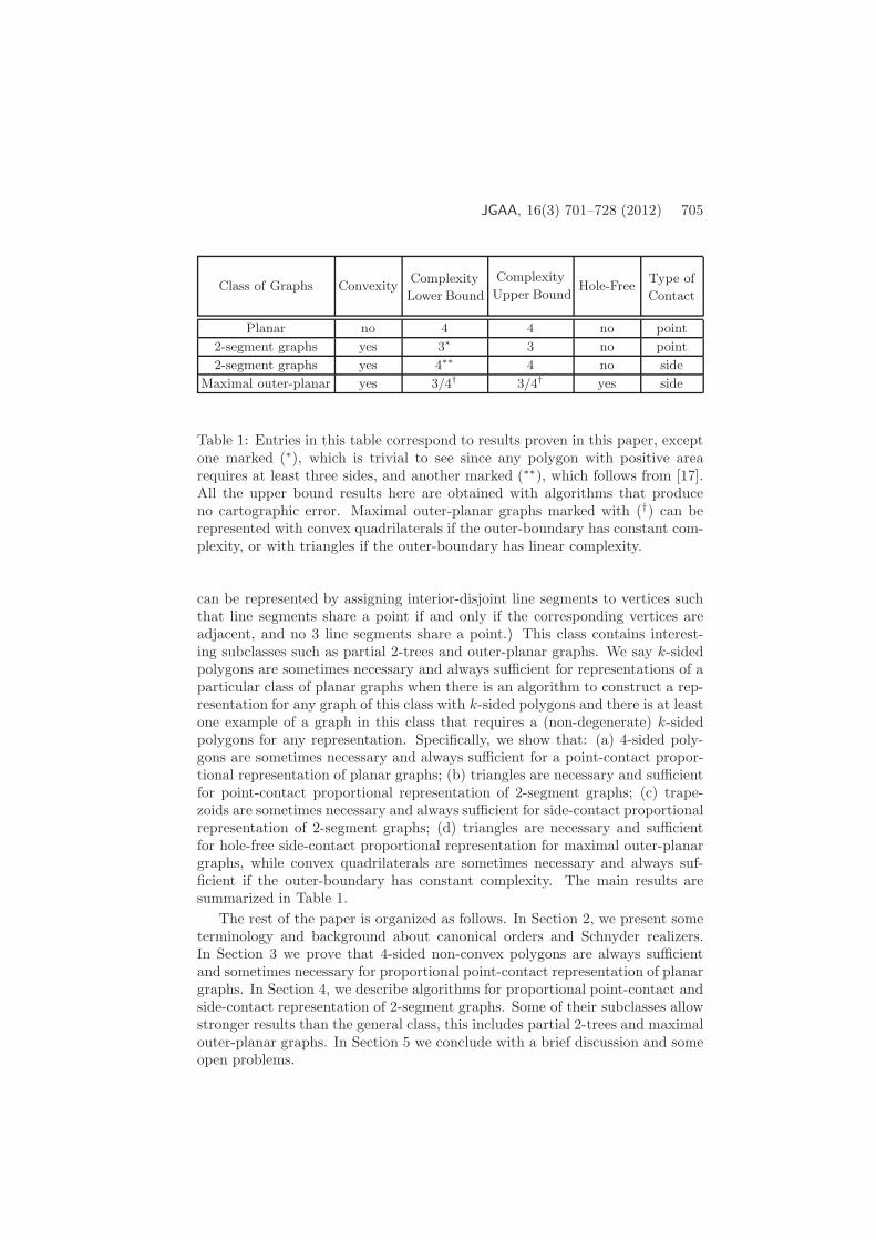
Class of Graphs ConvexityComplexity

Lower Bound

Complexity

Upper BoundHole-Free

Type of

Contact

Planar no 4 4 no point

2-segment graphs yes 3∗ 3 no point

2-segment graphs yes 4∗∗ 4 no side

Maximal outer-planar yes 3/4† 3/4† yes side

Table 1: Entries in this table correspond to results proven in this paper, exceptone marked (∗), which is trivial to see since any polygon with positive arearequires at least three sides, and another marked (∗∗), which follows from [17].All the upper bound results here are obtained with algorithms that produceno cartographic error. Maximal outer-planar graphs marked with (†) can berepresented with convex quadrilaterals if the outer-boundary has constant com-plexity, or with triangles if the outer-boundary has linear complexity.

can be represented by assigning interior-disjoint line segments to vertices suchthat line segments share a point if and only if the corresponding vertices areadjacent, and no 3 line segments share a point.) This class contains interest-ing subclasses such as partial 2-trees and outer-planar graphs. We say k-sidedpolygons are sometimes necessary and always sufficient for representations of aparticular class of planar graphs when there is an algorithm to construct a rep-resentation for any graph of this class with k-sided polygons and there is at leastone example of a graph in this class that requires a (non-degenerate) k-sidedpolygons for any representation. Specifically, we show that: (a) 4-sided poly-gons are sometimes necessary and always sufficient for a point-contact propor-tional representation of planar graphs; (b) triangles are necessary and sufficientfor point-contact proportional representation of 2-segment graphs; (c) trape-zoids are sometimes necessary and always sufficient for side-contact proportionalrepresentation of 2-segment graphs; (d) triangles are necessary and sufficientfor hole-free side-contact proportional representation for maximal outer-planargraphs, while convex quadrilaterals are sometimes necessary and always suf-ficient if the outer-boundary has constant complexity. The main results aresummarized in Table 1.

The rest of the paper is organized as follows. In Section 2, we present someterminology and background about canonical orders and Schnyder realizers.In Section 3 we prove that 4-sided non-convex polygons are always sufficientand sometimes necessary for proportional point-contact representation of planargraphs. In Section 4, we describe algorithms for proportional point-contact andside-contact representation of 2-segment graphs. Some of their subclasses allowstronger results than the general class, this includes partial 2-trees and maximalouter-planar graphs. In Section 5 we conclude with a brief discussion and someopen problems.


2 Preliminaries

In a point-contact representation of a planar graph G = (V,E), we constructa set P of closed simple interior-disjoint polygons with an isomorphism P :V → P , where for any two vertices u, v ∈ V , the boundaries of P(u) and P(v)touch through at least one contact point if and only if (u, v) is an edge. A side-contact representation of a planar graph is defined analogously, where insteadof a contact point, we have a contact side between P(u) and P(v), which is anon-degenerate line segment in the boundary of both. A hole of such a contactrepresentation is a non-empty region that does not belong to any P (v) and isnot part of the infinite region.

Let Γ be a contact (point-contact or side-contact) representation of G. Wecan then place a point pv inside each P (v) and for any edge (v, w) connect pvand pw via the contact point of P (v) and P (w). This gives a planar drawingof G. In this drawing, any face f of G contains inside either a point where allpolygons of vertices on f meet, or one (or more) holes.

In the weighted version of the problem, the input also includes a weightfunction w : V (G) → R+ that assigns a positive weight to each vertex of G.We say that G admits a proportional contact representation with the weightfunction w if there exists a contact representation of G such that the area ofthe polygon for each vertex v of G is proportional to its weight w(v). We definethe complexity of a polygon as the number of sides it has. In this paper, we alsoconsider a polygon with less than k sides to be a (degenerate) k-sided polygonfor convenience.

A plane graph is a planar graph with a fixed embedding. A plane graphis fully triangulated or maximally planar if all its faces, including the outer-face, are triangles. Both the concept of “canonical order” [12] and “Schnyderrealizer” [29] are defined for fully triangulated plane graphs in the context ofstraight-line drawings of planar graphs on an integer grid. We briefly reviewthe two concepts below:

Let G = (V,E) be a fully triangulated plane graph with outer-face u, v, win clockwise order. Then G has a canonical order of the vertices v1 = u, v2 = v,v3, . . ., vn = w, |V | = n, which satisfies for every 4 ≤ i ≤ n:

• The subgraph Gi−1 ⊆ G induced by v1, v2, . . ., vi−1 is biconnected, andthe boundary of its outer-face is a cycle Ci−1 containing the edge (u, v).

• The vertex vi is in the exterior face of Gi−1, and its neighbors in Gi−1

form an (at least 2-element) subinterval of the path Ci−1 − (u, v).

A Schnyder realizer of a fully triangulated graph G is a partition of theinterior edges of G into three sets T1, T2 and T3 of directed edges such that foreach interior vertex v, the following conditions hold:

• v has out-degree exactly one in each of T1, T2 and T3,

• the counterclockwise order of the edges incident to v is: entering T1, leav-ing T2, entering T3, leaving T1, entering T2, leaving T3.

JGAA, 16(3) 701–728 (2012) 707

The first condition implies that each Ti, i = 1, 2, 3 defines a tree rooted atexactly one exterior vertex and containing all the interior vertices such thatthe edges are directed towards the root. The following by now classical lemmashows a profound connection between canonical orders and Schnyder realizers.

Lemma 1 Let G be a fully triangulated plane graph. Then a canonical order ofthe vertices of G defines a Schnyder realizer of G, where the outgoing edges of avertex v are to its first and last predecessor (where “first” is w.r.t. the clockwiseorder around v), and to its highest-numbered successor.

3 Proportional Point-Contact Representations

Recall that any planar graph can be represented by touching triangles. Fromthis, it is easy to create proportional point-contact representations: Scale therepresentation such that the triangle T (v) of vertex v has area at least w(v),and then “carve away” a triangular part H of T (v) near a corner to achieve thecorrect area. Now the new polygon has six corners with two of them overlappingwith each other. This can be avoided by moving these two overlapped cornersa small distance away from each other and changing the area of H accordingly.So we can easily achieve 6-sided representations.

In this section, we create point-contact representations with the optimalnumber of sides. Indeed, we show that 4-sided non-convex polygons alwayssufficient for a proportional contact representation of a planar graph. This isquite easy to do for 2-segment graphs (essentially by adding a small triangle atone end of the segment), but we show this here for all planar graphs.

We first describe an algorithm to obtain proportional point-contact repre-sentations of planar graphs using 4-sided non-convex polygons. We then showthat there exists a planar graph with a given weight function that does notadmit a proportional point-contact representation with convex polygons, thusmaking our 4-sided construction optimal.

Theorem 1 Let G = (V,E) be a planar graph and let w : V → R+ be aweight function. Then G admits a proportional point-contact representationwith respect to w in which each vertex of V is represented by a 4-sided polygon.It can be found in linear time.2

Proof: We first take a planar embedding of G and assume that it is fullytriangulated, for if it is not, we can add dummy vertices (and edges to thesevertices) to make it so, and later remove those dummy vertices from the obtainedproportional contact representation.

Assume (after some scaling) that w(v) ≤ 1/n2 for all v ∈ V and fix an arbi-trary outer-face. We construct the drawing incrementally, following a canonical

2 In this paper, we assume the real RAM model, i.e., any arithmetic operation, even involv-ing arbitrarily small coordinates, can be done in constant time. Of course this is unrealistic.It would be of interest whether the size of coordinates can be bounded polynomially, but thisremains open.


333

31

1

3

3

3

11 2

2

2

21

n

1 2

j

n

21

S(2)

S(n)

S(1)

(b)(a)

Figure 2: (a) The canonical order and Ti (marked by labels); (b) the placementof 1,2,n.

ordering v1, . . . , vn. We prescribe what the polygon assigned to j looks like be-fore even placing it (here and in the rest of the paper we use j as a shorthand forvj). So let T1, T2, T3 be the Schnyder realizer defined by the canonical ordering,where T1 is rooted at 1, T2 is rooted at 2 and T3 is rooted at n; see Fig. 2. LetΦi(j) be the parent of j in tree Ti.

It is easy to show that T−12 ∪T1 is an acyclic graph on the vertex set V −n,

where T−12 is the tree T2 with the direction of all its edges reversed. For every

vertex j 6= n, let π(j) be the index of j in a topological order of this graph. Thenn ≥ π(Φ1(j)) > π(j) > π(Φ2(j)) ≥ 1. Now for every vertex j 6= 1, 2, n, we definethe spike S(j) to be a 4-sided polygon with one reflex vertex. One segment (thebase) is horizontal with y-coordinate j. Its length will be determined later, butit will always be at least 2/n2 ≥ 2w(j). From the left endpoint of the base, thespike continues with the upward segment, which has slope π(j) and up to its tipwhich has y-coordinate y = Φ3(j). Next comes the downward segment until thereflex vertex, and from there to the right endpoint of the base; see Fig. 3(a).The placement of the reflex vertex is arbitrary, as long as the resulting shape hasarea w(j) and the down-segment has positive slope. Note that since the basehas length ≥ 2w(j) and y-coordinate j, the reflex vertex will have y-coordinateat most j + 1. We first place 1, 2, n, and then add 3, . . . , n− 1 (in this order):

• Vertex 1 is represented by a triangle S(1) whose base has length 2w(1)/(n−1), placed arbitrarily with y-coordinate 1. The tip of S(1) has y-coordinaten.

• Vertex 2 is represented by a triangle S(2) whose base has length 2w(2)/(n−2), placed at y-coordinate 2 and with its left endpoint abutting S(1). Thetip of S(2) has y-coordinate n.

• Vertex n is represented by a triangle whose base is at y-coordinate n and

JGAA, 16(3) 701–728 (2012) 709

Φ3(j)

j

j + 1

j

j + 1down-s

egm

ent:slo

pe

>π(j)

base

base

slo

pe

t

slope≤

t−

1

slo

pe

≥t+

1

up-segm

ent:

slo

pe

π(j

)

tip

S(Φ2(j))

S(Φ1(j)) sℓ sr

prj − 1

pℓ

p

S(j)

(a) (b)

Figure 3: (a) Adding j; (b) computing the width of the base.

long enough to cover the tips of S(1) and S(2). We choose the height ofS(n) such that the area is correct.

We maintain the following invariant: For j ≥ 2, after vertex j has beenplaced, the horizontal line with y-coordinate j + 1 intersects only the spikes ofthe vertices on the outer-face of Gj , and in the order in which they occur onthe outer-face.

To place j ≥ 3, we place the base of S(j) with y-coordinate j, and extend itfrom the down-segment of Φ1(j) to the up-segment of Φ2(j). Recall that Φ2(j)and Φ1(j) are exactly the first and last predecessor of j, and j = Φ3(i) for allother predecessors i 6= j. Hence S(j) touches S(Φ1(j)) and S(Φ2(j)) at theends of the base, and all other predecessors i of j have their tips at the base.Note that this creates a contact between j and all its predecessors, as desired.The rest of S(j) is then as described above. It is easy to verify the invariant,and therefore S(j) does not intersect any other spikes.

To see that the base of S(j) has length ≥ 2/n2 as required, let pℓ and prbe its left and right endpoints, and sℓ and sr be the other segments containingthem. Imagine that we extend sℓ and sr until they meet in a point p. Since srcontains a point with y-coordinate ≤ j − 1 (at the base of S(Φ2(j)) ), triangle∆p, pℓ, pr has height h ≥ 1; see Fig. 3.

Let t = π(vj) be the slope of the up-segment of S(vj). Since π(Φ2(vj)) <π(vj) = t, we have that sr has slope at most t− 1 and x(pr) ≥ x(p) + h

t−1 . Onthe other hand, the slope of sℓ is positive by construction, and must exceed theslope of the up-segment of Φ1(vj), which has slope π(Φ1(vj)) > π(vj) = t. Sosℓ has slope ≥ t+ 1 and x(pℓ) ≤ x(p) + h

t+1 . Therefore,

x(pr)− x(pℓ) ≥h

t− 1−

h

t+ 1=

h((t+ 1)− (t− 1))

t2 − 1≥

2h

t2≥

2

n2

as desired. Therefore the base of S(j) is wide enough, which shows the correct-ness of our construction.


It remains to analyze the run-time of the algorithm implicit in our construc-tive proof. Computing the Schnyder decomposition can be done in linear time.We claim that processing vertex j also takes constant time; the claim then fol-lows. Note that the base of S(j) is already fixed when handling j, since Φ1(j)and Φ2(j) are placed already, and we only need to compute the intersection oftheir polygons with the horizontal line with y-coordinate j. This also fixes thetip of S(j). All that remains to do is hence to find an appropriate point r forthe reflex vertex. Let ℓ be the line from the tip to the right end of the base ofS(j), and let C be the convex hull of S(j) (i.e., the triangle defined by the tipand the base of S(j).) If C has area A, then r must have height 2(A−w(v))/||ℓ||over ℓ. Draw the line ℓ′ parallel to ℓ at that distance. Also draw the verticalline ℓ′′ through the tip of S(j). Any point that is on ℓ′, to the left of ℓ′′ andinside C is suitable for r, and such a point exists by the above discussion ofcorrectness. Hence finding r takes a constant number of arithmetic operations,and the algorithm to find the contact representation takes linear time.

Our construction used non-convex shapes. Lemma 2 shows that this is some-times required.

Lemma 2 There exists a planar graph and a weight function such that thegraph does not admit a proportional point-contact representation, with respectto the weight function, with convex shapes for all vertices.

Proof: We aim to show that the graph in Fig. 4(a) has no proportional rep-resentation with convex polygons if the small vertices (a0, a1, a2, b) have weightδ and the larger vertices (c0, c1, c2, d) have weight D > 3δ. Assume for contra-diction that we had such a representation. Note that this graph is 3-connectedand all faces of this graph are isomorphic (even when taking vertex weights intoaccount), so all planar embeddings of it are equivalent. We may assume there-fore that d is incident to the outer-face. We will focus now on the sub-graphdefined by a0, a1, a2 and its interior. Fig. 4(b) and (c) illustrate the notationfor the following argument.

For i = 0, 1, 2, let pi be a contact point between P(ai) and P(ai+1). (Alladditions and subtractions in this proof are modulo 3.) Let T0 = ∆p0, p1, p2be the triangle spanned by p0, p1 and p2. Further, let qi be a point of contactbetween P(ai) and P(b). Let Li be the line parallel to pi−1pi that passes throughqi, and let Hi be the half-space supported by Li that contains pi−1pi. The linesL0, L1, L2 define a triangle T1 with corners p′0, p

′1, p

′2 where p′i is the corner of

T1 corresponding to the corner pi of T0.Observe that triangle ∆p0, p1, q1 is a subset of P(a1) by convexity, so it

has area at most δ. The trapezoid T0 ∩ H1 has less than twice the area of∆p0, p1, q1, so it has area at most 2δ. Since the triangle ∆p1, q2, q1 has toaccommodate P(c0) it has area at least D > 3δ. This implies that q2 6∈ T0∩H1.Analogous arguments show that for any i 6= j, qi is not inside T0 ∩Hj . Hence,qi is on Li between p′i and p′i−1. The generic situation is illustrated in Fig. 4(c).

Now consider the triangle ∆p1, p′1, q1: it has the same height and a base

that is no larger than that of ∆p0, p1, q1, so the area of ∆p1, p′1, q1 is at

JGAA, 16(3) 701–728 (2012) 711

b

c1 c0

c2

d

a1a0

a2

(b)

q2

p2

q1

p0

P(a

1 )

P(a2)

T0

q0

P(b)

L1

(c)

q2

p2

p0

p1

q0

p′2

p′0

p′1

q1

H1

p1

T2

T1

T0

P(a

0)

(a)

Figure 4: A graph G that does not have a proportional contact-representationwith convex shapes.


most δ. Similarly, one can show that triangle ∆p1, q2, p′1 has area at most δ.

Since the triangle ∆p1, q2, q1 contains P(c0) it has area at least D. There-fore triangle ∆p′1, q2, q1 = ∆p1, q2, q1−∆p1, q2, p

′1−∆p1, p

′1, q1 has area

at leastD−δ−δ > δ (by choice ofD > 3δ.) Similarly, one can show that triangle∆p′2, q0, q2 and triangle ∆p′0, q1, q0 have area strictly greater than δ.

Define T2 to be the triangle ∆q0, q1, q2, and observe that T2 ⊆ P(b), andhence T2 has area at most δ. But now we have a triangle T2 of area at most δthat is circumscribed by a triangle T1 such that the three triangles of T1−T2 eachhave area strictly greater than δ. This is impossible due to a classic geometricresult, which states that when a triangle T2 is inscribed in another triangle T1,then the area of T2 is at least as much as the minimum of the areas of the threetriangles in T1 − T2. For details, see e.g. [13].

Lemma 2 implies that 3-sided polygons are not always sufficient for propor-tional contact representations of planar graphs. On the other hand, Theorem1 implies that any planar graph has a proportional contact representation withany given weight function on the vertices so that each of the vertices is rep-resented by a non-convex 4-sided polygon. Summarizing these two results wehave the following theorem.

Theorem 2 4-sided non-convex polygons are always sufficient and sometimesnecessary for proportional point-contact representation of a planar graph with agiven weight function on the vertices.

4 Subclasses of Planar Graphs with Convex Rep-

resentations

In this section we address the problem of proportional contact representationswith convex polygons of low complexity. The lower bound in Lemma 2 showsthat for some planar triangulations, the complexity in any proportional contactrepresentation must be at least 4 and the polygons must be non-convex. Wehence focus on planar graphs with fewer edges.

We first give some constructions for so-called 2-segment graphs and then dis-cuss what these graphs are and which well-known subclasses of planar graphs(such as series-parallel graphs and triangle-free planar graphs) fall into them. Fi-nally we give an entirely different construction for maximal outer-planar graphs,which (as opposed to all previous constructions) gives hole-free representations.

4.1 2-segment graphs

Call a planar graph a 2-segment graph if it can be represented by assigninginterior-disjoint line segments to vertices such that two line segments sharea point if and only if the corresponding vertices are adjacent, and no 3 linesegments share a point; see Fig. 5(a)–(b).

Given a 2-segment representation Γ of a graph G, we can easily constructa side-contact representation for G by giving an arbitrary thickness to each

JGAA, 16(3) 701–728 (2012) 713

segment of Γ. This is a side-contact representation and uses convex shapes. Italso seems intuitive that we can choose the thickness suitable so that weightsof vertices are respected. However, choosing the thickness is non-trivial for tworeasons: we must be careful not to make segments too thick (and hence createdunwanted adjacencies), and thickened segments may overlap, and removing suchoverlap might create error unless we are very careful about how we thicken thesegments.

Let Γ be a 2-segment representation of G, with vertex v represented by linesegment ℓ(v). After possible rotation, we may assume that Γ has no horizontalline segment, hence every line segment has a well-defined left and right side andtop and bottom endpoint. After lengthening segments, if necessary, we may alsoassume that no two line segments end at the same point. So that if two linesegments share a point, then one of them ends on either the right or the leftside of the other.

Lemma 3 There exists an order v1, . . . , vn of the vertices in G such that forany i, the right side of ℓ(vi) contains only ends of neighbors vj with j > i.

Proof: It is enough to show that there is an “unobstructed” segment ℓ, i.e.,a segment for which no other segment ends on the right side. We then set vnto be the vertex belonging to ℓ, and obtain the complete ordering by inductionafter removing ℓ.

To find an unobstructed segment look at the scene from (∞, 0) and orderthe visible ends of segments by increasing y-coordinate. This yields a sequenceof top and bottom ends of segments. The first point in the sequence is a bottomendpoint and the last one is a top endpoint. Hence there are two consecutiveendpoints p1, p2 for which p1 is a bottom endpoint and p2 a top endpoint. Sincethe segments in Γ do not cross, this pair of points is the pair of endpoints of anunobstructed segment.

Theorem 3 Let G = (V,E) be a 2-segment graph and let w : V → R+ bea weight function. Then G admits a proportional point-contact representationwith respect to w in which each vertex of V is represented by a trapezoid. Givena 2-segment representation of G, such a contact representation can be found inO(n logn) time.

Proof: As before we presume that no line segment is horizontal and no twoline segments end in a point. Let δ > 0 be the minimum feature size of thissegment representation, i.e., the smallest distance between a line segment ℓ andan endpoint of another line segment that does not end at ℓ. Next, let α be thesmallest angle between two line segments where one ends at the other. Scalethe entire drawing, if needed, such that δ > 2 and ||ℓ(v)|| ≥ w(v) + 2

sinα + 1tanα

for all vertices v.Compute the sequence v1, . . . , vn of vertices such that the right side of ℓ(vi)

contains only endpoints of ℓ(vj) for j > i. We thicken vertices in order v1, . . . , vn.

2A point is visible from (∞, 0) when the line segment between these two points does notcross any segments.


6 6

11

22

3

3

44

5

577

8

8

T (vi)

(a) (b) (c)

≤ 1/ sinα

ℓ(vi)ℓ(vj)

Figure 5: (a) A 2-segment graph; (b) a representation with line segments; thenumbers indicate a suitable vertex order; (c) converting ℓ(vi) into a trapezoidT (vi) and clipping ℓ(vj). The indicated angles are all at least α, hence theoff-set is at most 1, and at most 1

sinα is cut off ℓ(vj).

At the time of handling vi, we have a contact representation where each vh, h < iis represented as a trapezoid T (vh) of area w(vh), while each vj , j ≥ i is repre-sented as a line segment that is a part of ℓ(vj) (but may have been shorteneda bit). We will guarantee in the following that ℓ(vj) has been shortened by atmost 1

sinα at each end, so that it still has length at least w(vj) +1

tanα .

To thicken vi, off-set ℓ(vi) by moving a copy of it to the right in parallel whileshortening/lengthening it so that it still touches the same segments/trapezoidsas it did before. We choose the distance d for off-setting such that the trapezoidT (vi) between the off-set line and ℓ(vi) has area w(vi). In particular, observethat T (vi) has a base of length ||ℓ(vi)|| ≥ w(vi) +

1tanα and the angles at the

base are at least α. Then the length of the segment parallel to ℓ(vi) is at least(||ℓ(vi)|| − 2 d

tanα ) and the area of the newly formed trapezoid is d(||ℓ(vi)|| −d

tanα ) ≥ d(w(vi) +1

tanα − dtanα ). Therefore, the required off-set d is at most

1 < δ/2, which implies that in the final representation no trapezoids intersectunless their line segments touched.

This yields the desired contact representation, except that a line segmentℓ(vj) that ended on the right side of ℓ(vi) now intersect T (vi). By the chosenvertex order, j > i, ℓ(vj) has not been thickened into a trapezoid yet. We clipℓ(vj) so that it now ends on the right side of T (vi). Since T (vi) had heightat most 1, and ℓ(vj) attaches to ℓ(vi) with angle at least α, this clips at most

1sinα off ℓ(vj) as desired. No segments can attach at ℓ(vj) in the clipped-offpart, since it is all within distance 1 < δ/2 of ℓ(vi). So we obtain the contactedrepresentation with v1, . . . , vi thickened, and the entire proportional contactrepresentation can be built by induction.

All operations used to compute this contact representation take constanttime per vertex, except for the computation of δ. It is easy to find the two closestcontacts of a 2-segment representation in linear time. In general, however, thefeature size may be determined by the distance from the end of one segmentto an interior point of another segment. Determining these distances in caseswhere we have non-convex faces in the representation is more intricate can be

JGAA, 16(3) 701–728 (2012) 715

done with a sweep-line algorithm in O(n log n) time.3

Theorem 4 4-sided convex polygons are always sufficient and sometimes nec-essary for proportional side-contact representation of a 2-segment graph with agiven weight function on the vertices. Given a 2-segment representation of G,such a contact representation can be found in O(n log n) time.

Proof: The sufficiency and the running time for the algorithm (assuming thata 2-segment representation is given) have been discussed before.

To establish necessity, consider the graph K2,5. This is a 2-segment graph.In this graph two vertices have five common neighbors, but as was proved in [17],in any side-contact representation with triangles, any pair of vertices has at mostfour common neighbors. Hence this graph has no side-contact representationwith triangles, let alone one that respects the weights. Another, smaller, ex-ample consists of the graph obtained from K2,4 by adding an edge between thevertices v1, v2 of the partition of size two. This graph is a 2-segment graph.The two vertices v1, v2 have four common neighbors, but as was proved in [17],in any side-contact representation with triangles, any pair of adjacent verticeshas at most three common neighbors. So again this graph has no side-contactrepresentation with triangles.

If we switch from side-contact representations to point-contact representa-tions, however, we can reduce the complexity of the regions from four to three.Specifically, we can replace line-segments by triangles.

The construction of the triangle P (v) of a vertex v can be done very muchlike the construction of the trapezoids in the previous proof. Instead of takinga parallel shift of the segment ℓ(v) we now fix the lower endpoint and rotate acopy of ℓ(v) clockwise, lengthening/shortening it as needed to maintain contactwith the neighbor, until the area of the triangle between the two copies of ℓ(v)is w(v). Then clip neighbors that ended on the right side of ℓ(v) as before. Notethat this construction guarantees that at least one half of the edges of G arerealized by side contacts.

Theorem 5 Triangles are always sufficient (and of course necessary) for a pro-portional point-contact representation of a 2-segment graph with a given weightfunction on the vertices. Given a 2-segment representation of G, such a contactrepresentation can be found in O(n log n) time.

4.1.1 Constructing 2-segment representations

The constructions for Theorem 4 and 5 are based on a 2-segment representa-tion. In this subsection we review the characterization of 2-segment graphs anddiscuss issues of constructing such a representation.

3A lower bound δ′ for the minimum feature size can be computed in linear time usingChazelle’s triangulation algorithm for polygons [7]. Since Chazelle’s algorithm is rather com-plex and the resulting δ′ can be arbitrarily smaller than the true δ we stick to the O(n logn)time bound.


Thomassen presented the characterization (Theorem 6) of 2-segment graphsat Graph Drawing 1993 but never published his proof. A proof of the theoremis part of [10].

The characterization theorem together with results by Lee and Streinu implythat one can test in quadratic time whether a given graph is a 2-segment graph.In contrast, Hlineny [23] showed that the recognition of general contact graphsof segments is NP-complete.

Theorem 6 [10] A planar graph G = (V,E) is a 2-segment graph if and onlyif it is (2, 3)-sparse, i.e., for any W ⊆ V the set E[W ] of edges induced by Wmust satisfy |E[W ]| ≤ 2|W | − 3.

The necessity is quite straightforward to see. Let S be the set of segmentsof a 2-segment representation of G. For W ⊂ V let XW be the set of end-pointsof segments in S corresponding to vertices of W . Since we have a 2-segmentrepresentation we may assume that |XW | = 2|W |. There is an injection φ fromedges in E[W ] to points in XW , but points belonging to the convex hull of XW

cannot be in the image of φ. Since the convex hull contains at least three pointswe get |E[W ]| ≤ |XW | − 3 = 2|W | − 3. So if G is a 2-segment graph, then it is(2, 3)-sparse.

Below we give a new proof of the sufficiency, which has three advantages:(a) It is shorter and more direct than the proof in [10], (b) it uses an interestingdetour into rigidity theory to prove the result, and most importantly (c) it isconstructive and allows us to construct a 2-segment representation in quadratictime.

Theorem 7 Given a planar graph G, we can test in quadratic time whether itis a 2-segment graph, and if so, construct a 2-segment representation.

Proof: We will give an algorithm that either detects that G is not (2, 3)-sparse (which by Theorem 6 means it is not a 2-segment graph), or constructa 2-segment representation of G in quadratic time. This implies that every(2, 3)-sparse graph is a 2-segment graph, i.e., the sufficiency for Theorem 6.

We need some prerequisites. A Laman graph (also called a (2, 3)-tight graph)is a (2, 3)-sparse graph with the maximum number (2n − 3) of edges. Lamangraphs are of interest in rigidity-theory, see e.g. [15, 19]. Laman graphs admita Henneberg construction, i.e., an ordering v1, . . . , vn of the vertices such that ifGi is the graph induced by the vertices v1, . . . , vi then G3 is a triangle and Gi

is obtained from Gi−1 by one of the following two operations:

(H1) Choose two vertices x, y from Gi−1 and add vi together with the edges(vi, x) and (vi, y).

(H2) Choose an edge (x, y) and a third vertex z from Gi−1, remove (x, y) andadd vi together with the three edges (vi, x), (vi, y), and (vi, z).

In [20] it is shown that planar Laman graphs admit a planar Hennebergconstruction, in the sense that the graph is constructed together with a plane

JGAA, 16(3) 701–728 (2012) 717

straight-line embedding and vertices stay at their position once they have beeninserted.

Now let G be a planar graph. First apply the algorithm by Lee and Streinu[27] to test in quadratic time whether G is a (2, 3)-sparse graph. If not, then weare done, so presume in the following that G is (2, 3)-sparse.

Claim: We can add edges to G such that the resulting graph G′ is a planarLaman graph. Proof of Claim: Find the components of G, which are themaximal subgraphs that are (2, 3)-tight. From [27], it is known that componentsare a partition of the edges and two components share at most one vertex. If Ghas only one component, then G is a Laman graph and we are done. Otherwise,find a face f with three consecutive vertices v1, v2, v3 such that edges (v1, v2)and (v2, v3) belong to different components C1 and C2. Then no component Ccontains both v1 and v3, otherwise C ∪v2 would be an even bigger (2, 3)-tightgraph, contradicting the definition of component. Therefore, the pair (v1, v3)is not an edge of the graph. Add edge (v1, v3); this maintains planarity. Also,the resulting graph is again (2, 3)-sparse since the endpoints of the new edgedid not reside within one component. Finally, the components of the resultinggraph are the same as before, except that (as a simple counting-argument shows)C1 ∪C2 ∪ (v1, v3) becomes one new component. Hence the new graph has fewercomponents and the claim follows by induction.

Observe that the edges in the above claim can be found in quadratic time:We once compute components with the algorithm of [27], and then spend at mostO(n) time per added edge to find the edge to add and to update components.

So in the following we will create a 2-segment representation of the planarsupergraph G′ that is a Laman-graph; we can obtain one for G from it byretracting segments at the added edges. Since G′ is a Laman-graph, it has aHenneberg sequence G3, . . . , Gn (which we can find with the algorithm of Leeand Streinu in quadratic time.) We build the 2-segment representation followingthis sequence. Starting from three pairwise touching segments representing G3,we add segments one by one. For the induction we need the invariant that afteradding the ith segment si we have a 2-segment representation of Gi for whichall cells (connected components that are not on the infinite face) are convex.Moreover, there is a correspondence between the cells and the interior faces ofGi which preserves edges, i.e., if (x, y) is an edge of the face, then one of thecorners of the corresponding cell is a contact between sx and sy. Fig. 6 indicateshow to add segment si in the cases where vi is added by H1, resp. H2. It iseasy to see that the invariant for the induction is maintained.

Directly from the construction it should be clear that we can find the 2-segment representation (given the Henneberg sequence) in linear time. So therunning time is dominated by making the graph into a planar Laman graph andfinding the Henneberg sequence, which takes O(n2) time.


H1

x

z

H2

z

x

y

xsi

y

yx

y

si

Figure 6: The addition of segment si.

4.1.2 Subclasses of 2-segment graphs

Planar and triangle-free

Let G be planar and triangle-free. Then m ≤ 2n − 4 by the usual counting-argument using Euler’s formula and since every face has at least 4 edges on it.By Theorem 6, hence G is a 2-segment graph. (This was already known by adirect construction that uses only three slopes, see [9].)

Planar bipartite

Planar bipartite graphs are a subclass of planar triangle-free graphs, in partic-ular they are 2-segment graphs. In fact, the segments can be restricted to behorizontal or vertical [21], and the segments can be found in linear time and haveminimum feature size 1. Hence for planar bipartite graphs, we can construct inlinear time proportional side-contact representations with trapezoids. In fact,the trapezoids used in such a representation are rectangles. On the other hand,side-contact representations with triangles are not possible since K2,5 does nothave one, as discussed in Theorem 4.

Planar 4-connected 3-colorable

Any 4-connected 3-colorable planar graph is also a 2-segment graph [10]. ByTheorem 7 we can find such a 2-segment representation, and hence the propor-tional contact representations in quadratic time.

Planar 2-shellable

A graph G is 2-shellable if G has a vertex order v1, . . . , vn such that for i ≥3 vertex vi has at most two neighbors in v1, . . . , vi−1. (Other names in theliterature for such graphs include 2-degenerate graphs, 2-strippable graphs, and2-regular acyclic orientable graphs.). From the definition it follows that a 2-shellable graph has at most 2n− 3 edges. Since the property is hereditary, theclass is (2, 3)-sparse. By Theorem 7 we can find a 2-segment representation,and hence the proportional contact representations of 2-shellable planar graphsin quadratic time.

JGAA, 16(3) 701–728 (2012) 719

Partial 2-trees

A 2-tree is defined as follows: It is either an edge or a graph G with a vertexv of degree two in G such that G − v is a 2-tree and the neighbors of v areadjacent. A partial 2-tree is a subgraph of a 2-tree. Every partial 2-tree isplanar. Partial 2-trees are the same as series-parallel graphs and include allouter-planar graphs.

Partial 2-trees are 2-shellable, hence 2-segment graphs. However, we canconstruct the 2-segment representation for them more efficiently.

Let G be a partial 2-tree. It is well-known that we can find in linear time asupergraph G′ of G that is a 2-tree, and with it an elimination order v1, . . . , vn,where for any i ≥ 3, vertex vi has exactly two earlier neighbors and they areadjacent. In the following we review the very simple construction of a 2-segmentrepresentation of G′.

Lemma 4 Let G′ be a 2-tree with vertex elimination order v1, . . . , vn. Then G′

has a 2-segment representation with convex interior faces and positive featuresize. Moreover, for any i line segment ℓ(vi) ends at the line segments of thepredecessors of vi. It can be found in linear time.

Proof: Vertices v1, v2, v3 form a triangle and it is easy to find three linesegments for them that satisfy the claim. See Fig. 7. Now consider vi, i ≥ 4and presume we found line segments for v1, . . . , vi−1 already. Let vh, vj be thepredecessors of vi, h < j. By definition of a 2-tree edge (vj , vh) exists, and byour invariant ℓ(vj) ends at ℓ(vh). Cut off a small triangle near the contact pointof ℓ(vj) and ℓ(vh) and assign the segment to vi; this satisfies all requirements.

So for every partial 2-tree G, we can find a supergraph that is a 2-tree, findits 2-segment representation in linear time, retract segments to obtain one forG (and at the same time compute the minimum feature size), and then applythe above constructions. So every partial 2-tree has a proportional side-contactrepresentation with trapezoids and a proportional point-contact representationwith triangles, and they can be found in linear time.

On the other hand, side-contact representations with triangles are not possi-ble sinceK2,4 with an added edges is a 2-tree, but does not have one as discussedin Theorem 4.

4.2 Maximal Outer-planar Graphs

In this section, we study maximal outer-planar graphs, i.e., planar graphs whoseouter-face is a cycle and all interior faces are triangles. These are 2-trees, sothe results from the previous subsection apply, but with a different constructionwe can generate hole-free side-contact representations. First we show how togenerate hole-free proportional side-contact representations using quadrilateralsso that the entire representation fits inside a triangle, that is, the outer-boundaryhas constant complexity. At the cost of an outer-boundary of high complexity,


vh

v2

v3 vi

vj vj

vh

v1

Figure 7: The 2-segment representation for 2-trees.

we can construct hole-free proportional side-contact representations using onlytriangles. We also show that the use of triangles might also require a boundaryof linear complexity in the size of the graph.

Let G be a maximal outer-planar graph. For any two vertices u, v, denoteby G(u, v) the graph induced by the vertices that are between u to v (endsexcluded) while walking along the outer-face in counterclockwise order, and letw(G(u, v)) be the sum of the weights of all these vertices; see Fig. 8. Definean aligned triangle to be one with horizontal base and tip below the base. Thisnaturally defines a left and right side of the triangle. The next lemma showsthat an outer-planar graph can be represented inside any aligned triangle ofsuitable area.

Lemma 5 Let G = (V,E) be a maximal outer-planar graph and let w : V → R+

be a weight-function. Then for any aligned triangle T of area w(G(v, u)), thereexists a hole-free proportional side-contact representation of G(v, u) inside Tsuch that the left [right] side of T contains segments of the neighbors of u [v]and of no other vertices. It can be found in linear time.

Proof: We proceed by induction on the number of vertices in G. In the basecase, G is a 3-cycle u, v, x. Use T itself to represent x; this satisfies allconditions.

In the inductive step, let x be the unique common neighbor of u and v.Divide T with a segment s from the tip to the base such that the region Tℓ

left of s has area w(G(x, u)) + 12w(x), and the region Tr right of ℓ has area

w(G(v, x)) + 12w(x). Cut off triangles of area 1

2w(x) each from the tips of Tℓ

and Tr; the combination of these two triangles forms a convex quadrilateral ofarea w(x) which we use for x; see Fig. 8. Recursively place G(x, u) and G(v, x)(if non-empty) in the remaining triangles of T ; it is easy to verify that thesehave the correct area, which yields the desired side-contact representation.

As for the linear time, this can be achieved with a 2-pass approach. In thefirst pass, split G(u, v) into graph G(v, x) and G(x, u), and so on recursivelyuntil all graphs are triangles. While returning from the recursing, we can hencecompute w(G(y, z)) for all those subgraphs G(y, z) where it will be needed later(which is exactly those subgraphs where (y, z) is an edge not on the outer-face,hence O(m) many.) This takes linear time in total. With these values readily

JGAA, 16(3) 701–728 (2012) 721

s

P(x)

P(v)

P(u)

G(v

,x)

G(x

,u)

(a) (b)

Tr

vu

x

(c)

Tℓ

T

Figure 8: The construction for maximal outer-planar graphs: (a) the graph; (b)splitting triangle T suitably; (c) adding u and v in the outer-most recursion.

available, computing the positions of corners of P (x) involves only elementaryarithmetic operations and takes constant time, hence the algorithm has linearrun-time overall.

Apply this lemma for an arbitrary edge (u, v) on the outer-face of a maximalouter-planar graph G and an arbitrary triangle T with area w(G(v, u)). We canthen add triangles for u and v to it to complete the drawing into a contactrepresentation of G; see Fig. 8(c). So we obtain:

Corollary 8 Let G = (V,E) be a maximal outer-planar graph and let w : V →R+ be a weight function. Then G admits a hole-free proportional side-contactrepresentation where vertices are represented by triangles or convex quadrilater-als and the outer boundary is a triangle. It can be found in linear time.

Next, we restrict ourselves to representations with triangles.

Lemma 6 Let G = (V,E) be a maximal outer-planar graph and (u, v) an edgeon the outer-face of G, with u before v in counterclockwise order. Let w : V →R+ be a weight-function. Then there exists a hole-free proportional side-contactrepresentation of G(v, u) with triangles that can be placed inside an an axis-aligned rectangle R such that:

(i) From the bottom left corner of R upward, we encounter boundaries of allneighbors of u (in order), followed by unused space.

(ii) From the bottom left corner of R rightward, we encounter boundaries ofall neighbors of v (in order), followed by unused space.

It can be found in linear time.

Proof: The idea for the construction is illustrated in Fig. 9. We proceedby induction on the number of vertices in G. In the base case, G is a 3-cycleu, v, x. Represent x as a cut-off corner (of appropriate area) of an axis-alignedrectangle; this satisfies both conditions of the lemma; see Fig. 9(b).


R

(b)

x

(c)

Tx

R′v (rotated & sheared)Ru

G(u, v)

(a)

neigh

bors

ofv

neighborsofu

neighbors of v

neighborsofu

Figure 9: The construction for maximal outer-planar graphs: (a) requirementson drawing; (b) the base case; (c) combining the drawings.

In the inductive step, let x be the unique common neighbor of u and v.Recursively draw G(x, u) and G(v, x) inside axis-aligned rectangles Ru and Rv.Rotate the drawing inside Rv such that the neighbors of x are now on thebottom side of Rv, while the neighbors of v are on the right side of v.

The crucial operation to apply now is a shear. A horizontal shear maps apoint (x, y) to point (x+k ·y, y) for some constant k. A shear preserves straightlines and areas (but it changes angles.)

We apply a horizontal shear to Rv for some positive k, turning Rv into aparallelogram R′

v whose slope depends on k. We chose k such that the area of xis correct in the resulting drawing. Specifically, consider the triangle Tx formedby the extension of the left side of Ru, the bottom sides of Ru and R′

v (placednext to each other) and the extension of the right side of R′

v; see Fig. 9(c).If we choose k = 0 (i.e., no shear has been applied), then Tx has infinite

area. If we choose k = ∞ (i.e., Rv is flattened into horizontal ray), then Tx

has zero area. By the intermediate value theorem, there exists some horizontalshear such that the area of Tx is exactly the weight of x, and we use this shear.(In fact, the correct value can easily be computed; it needs to be such that theslanted edge has slope s = 2A(x)/b, where b is the length of the base of Tx.)Then use Tx to represent vertex x.

Consider the two rays that emanate from the tip of Tx. Along the verticalray, we encounter (in order) first the boundary of x, then all other neighbors ofu (which were on Ru), and finally free space. Hence we encounter all neighborsof u in order. Similarly we encounter all neighbors of v in order along the otherray. The drawing then satisfies all conditions, except that it is contained insidea triangle, rather than a rectangle. But this is easily fixed with a vertical shearthat maps (x, y) to (x, y − s · x), where s = 2A(x)/b is the slope of the slantededge of the triangle. The drawing is then contained in a rectangle as desired.

To achieve linear run-time, we use a 2-pass approach. In the first pass,we break each graph G(u, v) into subgraphs G(x, u) and G(v, x) and recurse.When returning from the recursion, each subgraph reports the enclosing rect-angle that can be achieved, but does not actually have final coordinates yet.Instead, G(u, v) stores what translations and shares need to be applied to thetwo subgraphs G(x, u) and G(v, x), which in turn store which translations and

JGAA, 16(3) 701–728 (2012) 723

shears must be applied inside, and so on.On the second pass, we compute final coordinates, by combining all the

translations and shears to be applied in the subgraph into one affine transfor-mation, applying it for x to compute the final coordinates of P (x), and recursingin the subgraphs. This computes all final coordinates in linear time.

Let G be a maximal outer-planar graph. Apply Lemma 6 for an arbitraryedge (u, v) on the outer-face of G. We can then add triangles for u and v to itto complete the drawing into a contact representation of G. We thus obtain thefollowing result.

Corollary 9 Let G = (V,E) be a maximal outer-planar graph and let w : V →R+ be a weight function. Then G admits a hole-free proportional side-contactrepresentation where vertices are represented by triangles.

Note that in this construction, even though each vertex is represented by atriangle, the outer-face may have complexity Ω(n). Moreover, in some cases thishigh complexity is unavoidable, even for unweighted contact representations, asshown in the following lemma.

Lemma 7 There exists a maximal outer-planar graph with n vertices for whichany hole-free side-contact representation with triangles requires Ω(n) sides onthe outer-face.

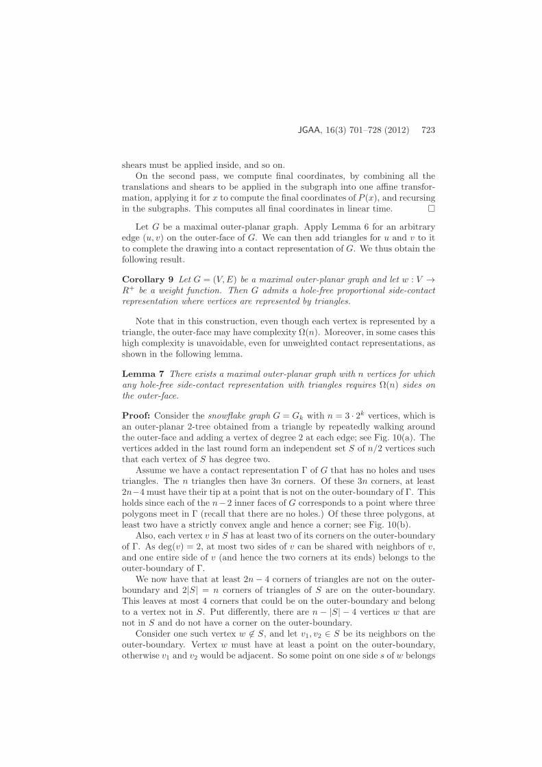
Proof: Consider the snowflake graph G = Gk with n = 3 · 2k vertices, which isan outer-planar 2-tree obtained from a triangle by repeatedly walking aroundthe outer-face and adding a vertex of degree 2 at each edge; see Fig. 10(a). Thevertices added in the last round form an independent set S of n/2 vertices suchthat each vertex of S has degree two.

Assume we have a contact representation Γ of G that has no holes and usestriangles. The n triangles then have 3n corners. Of these 3n corners, at least2n−4 must have their tip at a point that is not on the outer-boundary of Γ. Thisholds since each of the n−2 inner faces of G corresponds to a point where threepolygons meet in Γ (recall that there are no holes.) Of these three polygons, atleast two have a strictly convex angle and hence a corner; see Fig. 10(b).

Also, each vertex v in S has at least two of its corners on the outer-boundaryof Γ. As deg(v) = 2, at most two sides of v can be shared with neighbors of v,and one entire side of v (and hence the two corners at its ends) belongs to theouter-boundary of Γ.

We now have that at least 2n− 4 corners of triangles are not on the outer-boundary and 2|S| = n corners of triangles of S are on the outer-boundary.This leaves at most 4 corners that could be on the outer-boundary and belongto a vertex not in S. Put differently, there are n − |S| − 4 vertices w that arenot in S and do not have a corner on the outer-boundary.

Consider one such vertex w 6∈ S, and let v1, v2 ∈ S be its neighbors on theouter-boundary. Vertex w must have at least a point on the outer-boundary,otherwise v1 and v2 would be adjacent. So some point on one side s of w belongs


to the outer-boundary, but the corners at the ends of s do not belong to theouter-boundary; see Fig. 10(c). Therefore the outer-boundary must touch andthen leave s, which means it has a reflex vertex somewhere along s.

As a result, the outer-face has at least n− |S| − 4 ≥ n/2− 4 reflex vertices,which completes the claim.

triangle of w

outer−faces

(b)

(c)(a)

Figure 10: (a) The snowflake graph G3; (b)–(c) illustration for the proof ofLemma 7.

Lemma 7 shows that proportional side-contact representations with trianglesrequires the outer-boundary to have linear complexity for some maximal outer-planar graphs. Corollary 8 shows that we can also have a triangle as the outer-boundary, but at the cost of using convex quadrilaterals for vertices. Theseresults are summarized in the last theorem.

Theorem 10 Convex quadrilaterals are always sufficient and sometimes nec-essary for hole-free proportional side-contact representations of maximal outer-planar graphs when an outer-boundary of constant complexity is required. Hole-free proportional contact representation with triangles can also be computed butat the expense of linear complexity of the outer boundary. Both types of contactrepresentations can be computed in linear time.

5 Conclusion and Open Problems

We described algorithms for proportional point-contact and side-contact repre-sentations of planar graphs, 2-segment graphs, outer-planar graphs, and 2-trees.We focused on the complexity of the polygons representing vertices, and pro-vided bounds on this complexity that are tight, for a variety of graph classesand drawing models.

However, many problems still remain open. What is the complexity of side-contact proportional representations of maximal planar graphs? We can achieve7-sided polygons easily (essentially by cutting the convex corners of the 4-sidedspikes), but can we do better? Likewise, what is the complexity for hole-freeproportional representations of maximal planar graphs? Here, a bound of 8 isknown (and the polygons are orthogonal) [3], but can we do better if polygonsneed not be orthogonal?

JGAA, 16(3) 701–728 (2012) 725

Acknowledgment. This work was initiated at the Dagstuhl Seminar 10461on Schematization. A preliminary version of this paper was presented at GraphDrawing 2011 [2]. We thank Marcus Krug, Ignaz Rutter, Henk Meijer, EmilioDi Giacomo, and Andreas Gerasch and several anonymous referees for usefuldiscussions and suggestions.


References

[1] M. J. Alam, T. C. Biedl, S. Felsner, A. Gerasch, M. Kaufmann, and S. G.Kobourov. Linear-time algorithms for hole-free rectilinear proportional con-tact graph representations. In International Symposium on Algorithms andComputation(ISAAC’11), volume 7074 of Lecture Notes in Computer Sci-ence, pages 281–291. Springer, 2011.

[2] M. J. Alam, T. C. Biedl, S. Felsner, M. Kaufmann, and S. G. Kobourov.Proportional contact representations of planar graphs. In Graph Drawing(GD’11), volume 7034 of Lecture Notes in Computer Science, pages 26–38.Springer, 2012.

[3] M. J. Alam, T. C. Biedl, S. Felsner, M. Kaufmann, S. G. Kobourov, andT. Ueckerdt. Computing cartograms with optimal complexity. In Sympo-sium on Computational Geometry (SoCG’12), 2012 (to appear).

[4] M. Badent, C. Binucci, E. Di Giacomo, W. Didimo, S. Felsner, F. Giordano,J. Kratochvıl, P. Palladino, M. Patrignani, and F. Trotta. Homothetictriangle contact representations of planar graphs. In Canadian Conferenceon Computational Geometry (CCCG’07), pages 233–236, 2007.

[5] T. C. Biedl and L. E. R. Velazquez. Orthogonal cartograms with few cornersper face. In Workshop on Algorithms and Data Structures (WADS’11),volume 6844 of Lecture Notes in Computer Science, pages 98–109. Springer,2011.

[6] A. L. Buchsbaum, E. R. Gansner, C. M. Procopiuc, and S. Venkatasubra-manian. Rectangular layouts and contact graphs. ACM Transactions onAlgorithms, 4(1), 2008.

[7] B. Chazelle. Triangulating a simple polygon in linear time. Discrete &Computational Geometry, 6:485–524, 1991.

[8] M. de Berg, E. Mumford, and B. Speckmann. On rectilinear duals forvertex-weighted plane graphs. Discrete Mathematics, 309(7):1794–1812,2009.

[9] N. de Castro, F. J. Cobos, J. C. Dana, A. Marquez, and M. Noy. Triangle-free planar graphs and segment intersection graphs. Journal of Graph Al-gorithms and Applications, 6(1):7–26, 2002.

[10] H. de Fraysseix and P. O. de Mendez. Representations by contact andintersection of segments. Algorithmica, 47(4):453–463, 2007.

[11] H. de Fraysseix, P. O. de Mendez, and P. Rosenstiehl. On triangle contactgraphs. Combinatorics, Probability and Computing, 3:233–246, 1994.

[12] H. de Fraysseix, J. Pach, and R. Pollack. How to draw a planar graph ona grid. Combinatorica, 10(1):41–51, 1990.

JGAA, 16(3) 701–728 (2012) 727

[13] H. Debrunner. Aufgabe 260. Elemente der Mathematik, 12, 1957.

[14] C. A. Duncan, E. R. Gansner, Y. F. Hu, M. Kaufmann, and S. G.Kobourov. Optimal polygonal representation of planar graphs. Algorith-mica, 63(3):672–691, 2012.

[15] S. Felsner. Geometric Graphs and Arrangements. Advanced Lectures inMathematics. Vieweg Verlag, 2004.

[16] S. Felsner and M. C. Francis. Contact representations of planar graphswith cubes. In Symposium on Computational Geometry (SoCG’11), pages315–320, 2011.

[17] E. R. Gansner, Y. Hu, and S. G. Kobourov. On touching triangle graphs.In Graph Drawing (GD’10), volume 6502 of Lecture Notes in ComputerScience, pages 250–261. Springer, 2010.

[18] D. Goncalves, B. Leveque, and A. Pinlou. Triangle contact representationsand duality. In Graph Drawing (GD’10), volume 6502 of Lecture Notes inComputer Science, pages 238–249. Springer, 2010.

[19] J. Graver, B. Servatius, and H. Servatius. Combinatorial Rigidity. GraduateStudies in Mathematics. American Mathematical Society, 1993.

[20] R. Haas, D. Orden, G. Rote, F. Santos, B. Servatius, H. Servatius, D. L.Souvaine, I. Streinu, and W. Whiteley. Planar minimally rigid graphs andpseudo-triangulations. Computational Geometry, 31(1-2):31–61, 2005.

[21] I. Hartman, I. Newman, and R. Ziv. On grid intersection graphs. DiscreteMathematics, 97:41–52, 1991.

[22] R. Heilmann, D. A. Keim, C. Panse, and M. Sips. Recmap: Rectangularmap approximations. In IEEE Symposium on Information Visualization(INFOVIS’04), pages 33–40, 2004.

[23] P. Hlineny. Contact graphs of line segments are NP-complete. DiscreteMathematics, 235(1–3):95–106, 2001.

[24] A. Kawaguchi and H. Nagamochi. Orthogonal drawings for plane graphswith specified face areas. In International Conf. Theory and Applicationsof Models of Computation (TAMC’07), volume 4484 of Lecture Notes inComputer Science, pages 584–594, 2007.

[25] P. Koebe. Kontaktprobleme der konformen Abbildung. Berichte uber dieVerhandlungen der Sachsischen Akademie der Wissenschaften zu Leipzig.Math.-Phys. Klasse, 88:141–164, 1936.

[26] K. Kozminski and E. Kinnen. Rectangular duals of planar graphs. Net-works, 15:145–157, 1985.


[27] A. Lee and I. Streinu. Pebble game algorithms and sparse graphs. DiscreteMathematics, 308(8):1425–1437, 2008.

[28] M. S. Rahman, K. Miura, and T. Nishizeki. Octagonal drawings of planegraphs with prescribed face areas. Computational Geometry, 42(3):214–230, 2009.

[29] W. Schnyder. Embedding planar graphs on the grid. In Symposium onDiscrete Algorithms (SODA’90), pages 138–148, 1990.

[30] P. Ungar. On diagrams representing graphs. Journal of London Mathe-matical Society, 28:336–342, 1953.

[31] M. J. van Kreveld and B. Speckmann. On rectangular cartograms. Com-putational Geometry, 37(3):175–187, 2007.

[32] K.-H. Yeap and M. Sarrafzadeh. Floor-planning by graph dualization: 2-concave rectilinear modules. SIAM Journal on Computing, 22:500–526,1993.

proportional contact representations of planar graphs

Documents