proceedings of the 12th australian space science
TRANSCRIPT
Proceedings of the 12th Australian Space Science Conference, 2012 Page i
Proceedings of the 12th Australian Space Science Conference
Melbourne 24 - 26 September, 2012
Australian Space Science Conference Series1st Edition
Published in Australia in 2013 byNational Space Society of Australia Ltd
GPO Box 7048Sydney NSW 2001
Fax: 61 (02) 9988-0262email: [email protected]
website: http://www.nssa.com.au
Copyright © 2013 National Space Society of Australia Ltd
All rights reserved. No part of this publication may be reproduced, stored in a retrieval system or transmitted in any form or by any means, electronic, mechanical, photocopying, recording or otherwise, without prior permission from the publisher.
ISBN 13: 978-0-9775740-6-3
Editors: Wayne Short and Iver Cairns
Distributed on DVD

Proceedings of the 12th Australian Space Science Conference, 2012 Page iii
Preface to the Proceedings
A large number of the presenters at the conference later submitted completed written papers which form the basis of this Conference Proceedings.
All papers published in these proceedings have been subject to a peer review process whereby a scholarly judgement by at least two suitable individuals endorsed by the Program Committee determined if the paper was suitable to be published. All papers not rejected were revised until deemed suitable. Responsibility for the content of each paper lies with its author(s). The publisher retains copyright over the text. Papers appear in the Conference Proceedings with the permission of the authors. The Editors would like to give special thanks to the Program Committee and those scholars who participated in the peer review process: Elais Aboutanios , Brett Addison, Brad Alexander, John Auld, Jeremy Bailey, Daniel Bayliss, James Bennett,
Rod Boswell, Brad Carter, Iain Cartright, Jon Clarke, Daniel Cotton, Andrew Dempster, Graham Dorrington,
Paul Francis, Brian Fraser, Yue Gao, Illiana Genkova, Eamon Glennon, Ali Goktagon, Felipe Gonzalez, Jose
Guivant, Duane Hamacher, Jason Held, Jonathan Horner, David Hudson, Michael Ireland, Trevor Ireland,
Adrian James, Xiuping Jia, Shuanggen Jin, John Kennewell, Joe Khachen, Elliot Koch, Trevor Lafleur,
David Lingard, John O’Byrne, Dennis Odijk, John Olsen, Barnaby Osborne, Murray Parkinson, John Page,
Gordon Pike, Lily Qiao, Peter Rayner, Chris Rizos, Stuart Ryder, Richard Samuel, Jizhang Sang, Nagaraj C.
Shivaramaiah, Leon Stepan, Tanya Vladimirova, Martin Westwell, Rob Wittenmeyer, Malcolm Walter, Falin
Wu, Suquin Wu, Xaoifeng Wu, Kegen Yu and Kefei Zhang.
Finally we would like to thank our sponsors (the Space Policy Unit of DIISR, RMIT University and the RMIT SPACE Research Centre) for their support in funding student participation and the Organising Committee, Program Comittee and colleagues Brett Carter, Sarah Gordon and Kefei Zhang for giving generously of their time and efforts.
We trust that you will find the 2012 Conference Proceedings enjoyable and informative.
Wayne Short and Iver Cairns Editors, 12ASSC Conference Proceedings, May 2013
Page iv Proceedings of the 12th Australian Space Science Conference, 2012
Conference Background
The Australian Space Science Conference (ASSC) is the focus of scientific cooperation and discussion in Australia on research relating to space. It is a peer reviewed forum for space scientists, engineers, educators, and workers in Industry and Government.
The conference is of relevance to a very broad cross section of the space community, and therefore generates an enlightening and timely exchange of ideas and perspectives. The scope of the conference covers fundamental and applied research that that can be done from space and space-based platforms, and includes the following:
• Space science, including space and atmospheric physics, remote sensing from space, planetary sciences, astrobiology and life sciences, and space-based astronomy and astrophysics
• Space engineering, including communications, navigation, space operations, propulsion and spacecraft design, testing, and implmentation
• Space industry• Space archeology• Government, International relations and law• Education and outreach The 12th ASSC was held at RMIT University in Melbourne from September 24 to 26, 2012. The Conference was opened by Deputy Vice-Chancellor for Research and Innovation of RMIT University, Professor Daine Alcorn.
The conference included a comprehensive program of plenary talks and special sessions on the national context for space (including papers on the new Roadmap for the National Research Infrastructure, the new Australian Space Industry Association, and the status and implementation of the 2010 Decadal Plan for Australian Space Science), the foci and programs of Australian Government units with interests in space, and detailed descriptions and progress reports of research funded by the Australian Space Research Program. In addition, the program contained a special student session, with a strong preponderance of projects involving the Australian Space Research Institute. The program also ontained multiple sessions of invited and contributed presentations, both oral and poster, on Propulsion, Planetary Science, Remote Sensing and Geodesy, Space Capabilities, Hazard Monitoring, Space Physics, Space Technology, Space Archeology and Education and Outreach.
Appendix A has a copy of all abstracts accepted for presentation at the conference.

Proceedings of the 12th Australian Space Science Conference, 2012 Page v
The 12th ASSC was organised by the National Space Society of Australia (NSSA), the Academy of Sciences National Committee for Space Science (NCSS) and RMIT University. The Australian Space Research Institute (ASRI) also helped significantly with organising abstract submissions.
A call for papers was issued in March 2012 and researchers were invited to submit abstracts for presentation at the conference. Following the conference itself, a call for written papers was issued in October 2012: this invited presenters to submit a formal written paper for this Proceedings that covered their abstracts.
Page vi Proceedings of the 12th Australian Space Science Conference, 2012
Table of Contents
Preface to Proceedings page iii
Conference Background page iv
List of Proceedings Papers page vii
Welcome to the 12th Australian Space Science Conference page x
About the NSSA page xii
About the NCSS page xiii
2012 Program Committee page xv
2012 Organising Committee page xvi
Conference Plenary Speakers page xvii
Program page xix
Proceedings of the 12th Australian Space Science Conference, 2012 Page vii
List of Proceedings PapersAuthors Paper Title
Carol Oliver, Kerrie Dougherty, Jennifer Fergusson Pathways to Space: A first year report card pages 1 - 8
Bernanda Telalovic`, Roanna Chan, Jordan Epstein, Laurie Mac, Jeff Stanger, Jie Zhou
A Case for Hydrothermal Systems in Firsoff Crater pages 9 -18
Jeremy Bailey Mariner 2 and its Legacy: 50 Years On pages 19- 28
Paul ten Boom The Pioneer Anomaly: An inconvenient reality or NASA’s 12 year misconception? pages 29 - 40
Kimberly Bott, Lucyna Kedziora-Chudczer and Jeremy Bailey
VSTAR Modelling of the Infrared Spectrum of Uranus pages 41- 52
Lucyna Kedziora-Chudczer, Jeremy Bailey and Jonathan Horner
Observations of the D/H ratio in Methane in the atmosphere of Saturn’s moon, Titan - where did the Saturnian system form?
pages 53 - 64
Graham E. Dorrington and Colin F. Wilson
Possible Architectures for Near-Future Venus Atmosphere in situ Missions pages 65 - 76
Amanda Goldfarb Discovering Ancient Astronomy pages 77 - 90
Jonathan Horner, F. Elliott Koch, and Patryk Sofia Lykawka
Capturing Trojans and Irregular Satellites - the key required to unlock planetary migration pages 91 - 102
Jonathan Horner, Robert A. Wittenmyer, Chris G. Tinney, Paul Robertson , Tobias C. Hinse, and Jonathan P. Marshall
Dynamical Constraints on Multi-Planet Exoplanetary Systems pages 103 - 116
Champlain Kenyi, Daniel V. Cotton and Jeremy Bailey
Retrieval Software for Total Column Greenhouse Gas Measurements from Ground and Space pages 117 - 128
Iain J. R. Cartwright, Leon B. Stepan and David M. Lingard
Satisfying Australia’s Future Need for Multi-Spectral Imagery using a Cubesat Solution pages 129 - 140
Owen Giersch, John Kennewell Solar Radio Interference to the GNSS pages 141 - 150
Jeremy Bailey, Steven Tsitas, Daniel Bayliss, Tim Bedding
A CubeSat Mission for Exoplanet Transit Detection and Asteroseismology
pages 151 - 162
M. Fabiao Dionizio, D. V. Cotton , J. Bailey
Preliminary Parameters for an Experimental Payload forTropospheric CO2 Measurement Using a Space-borne Lidar 6U Cubesat Platform
pages 163- 174
Nima Alam, Kegen Yu, Andrew G. Dempster
On the Achievable Accuracy for Estimating the Ocean Surface Roughness using Multi-GPS Bistatic Radar pages 175- 190
Page viii Proceedings of the 12th Australian Space Science Conference, 2012
List of Proceedings PapersAuthors Paper Title
James C. Bennett, Jizhang Sang, Kefei Zhang and Craig Smith
A re-analysis of the 2009 Iridium-Cosmos predicted miss distance using two-line element derived orbits pages 191 - 200
Tzi-Chieh Chi, Haoyang Cheng, John Page and John Olsen
Debris Avoidance through Autonomous Spacecraft Scattering pages 201 -210
Ahmad S. Mohd Harithuddin, Pavel M. Trivailo and Reza N. Jazar
Qualitative Analysis of the Kinematics of a Torque-free Gyro using Multiple Coordinate Frames
pages 211 - 222
Mohd Faisal Ibrahim and Bradley Alexander
Designing a Navigational Control System of an Autonomous Robot for Multi-requirements Planetary Navigation using Evolutionary Algorithms Approaches
pages 223 - 234
Gourav Mahapatra, Pallavi Reddy, Soumitro Datta , Adheesh Boratkar , Rodney Gracian D’Souza , and Bharat Ramanathan
Thermal Imaging and Electrodynamic Tether Payloads for a Nano Satellite pages 235 - 248
Li Qiao, Chris Rizos, Andrew G. Dempster Analysis and Comparison of CubeSat Lifetime pages 249 - 260
Li Qiao, Chris Rizos, Andrew G Dempster Satellites Orbit Design for the Australian Garada Project pages 261 - 272
Steven R. Tsitas and George Constantinos
Garada SAR Formation Flying requirements, space system baseline and spacecraft structural design pages 273 - 284
Mazher Choudhury, Jinghui Wu, Nagaraj C. Shivaramaiah and Andrew G Dempster
Development of a Software GNSS/RNSS Receiver with Carrier-Phase Output pages 285 - 294
Mazher Choudhury, Eamonn Glennon, Andrew G Dempster and Peter Mumford
Characterization of the Namuru V3.2 Spaceborne GPS Receiver pages 295 -306
Peter J Mumford, Nagaraj Shivaramaiah, Eamonn Glennon, Kevin Parkinson
The Namuru V3.2A Space GNSS receiver pages 307 - 314
Suchet Bargoti, Aditya Mahajan and Ali Haydar G¨oktoˇgan
Fourier-Mellin Transform Based Visual Odometry for an Experimental Mars Rover on Rough Terrain pages 315 - 326
Joo Wui Kho and L Thompson
The Design of a Concurrent Design Facility (CDF) for a Space Launch Vehicle pages 327 - 338
C. A. Barry Stoute, Brendan Quine, Stephen Brown, Shervin Khazarie
RF Electrothermal Propulsion Testing Using N2-He Gas Mixture in Low-Temperature Plasma pages 339 - 350
Lachlan Thompson Space Engineering in Australia pages 351 - 362
APPENDIX A 12ASSC: List of Presentations & Posters pages a - j

Proceedings of the 12th Australian Space Science Conference, 2012 Page ix
Page x Proceedings of the 12th Australian Space Science Conference, 2012
Welcome to the 12th Australian Space Science Conference
and to Storey Hall, RMIT University! This will be the sixth ASSC jointly sponsored and organised by the National Committee for Space Science (NCSS) and the National Space Society of Australia (NSSA). The ASSC is intended to be the primary annual meeting for Australian research relating to space science. It welcomes space scientists, engineers, educators, and workers in Industry and Government.
The conference was opened by Professor Daine Alcorn, Deputy Vice-Chancellor for Research and Innovation at RMIT University.
The 12th ASSC has over 120 accepted abstracts across Australian space research, academia, education, industry, and government.
We would like thank Space Policy Unit and RMIT University for their sponsorship. Special thanks also go to the RMIT University Space Research Centre, Australian Space Research Institute (ASRI), Engineers Australia and Mars Society Australia (MSA) for their support.
We look forward to an excellent meeting!
Iver Cairns Wayne ShortCo Chair ASSC 2012 Co Chair ASSC 2012University of Sydney President, NSSA

Proceedings of the 12th Australian Space Science Conference, 2012 Page xi
Page xii Proceedings of the 12th Australian Space Science Conference, 2012
The National Space Society of Australia is the coming together of like-minded space enthusiasts who share a vision for the future in which there is an ambitious and vigorous space program leading to eventual space settlement.
To this end the National Space Society (worldwide) promotes interest in space exploration, research, development and habitation through events such as science and business conferences, speaking to the press, public outreach events, speaking engagements with community groups and schools, and other pro-active events. We do this to stimulate advancement and development of space and related applications and technologies and by bringing together people from government, industry and all walks of life for the free exchange of information.
As a non-profit organisation, the National Space Society of Australia draws its strength from an enthusiastic membership who contributes their time and effort to assist the Society in pursuit of its goals.
For more information, and to become a member:
http://www.nssa.com.au
Ad Astra!Wayne ShortNSSA President
Proceedings of the 12th Australian Space Science Conference, 2012 Page xiii
The National Committee for Space Science (NCSS) is chartered by the Australian Academy of Science to foster space science, to link Australian space scientists together and to their international colleagues, and to advise the Academy’s Council on policy for science in general and space science in particular. The associated web page can be reached at http://www.science.org.au/natcoms/nc-space.html . Accessible resources include the 2004-2006 Report on Australian Space Research.
NCSS believes that ASSC meetings provide a natural venue to link Australian space scientists and foster the associated science, two of its core goals. As well as ASSC, it is also sponsoring the VSSEC – NASA Australian Space Prize.
This is the second ASSC meeting following the launch of the first Decadal Plan for Australian Space Science in 2010. NCSS encourages people to work together to accomplish the Plan’s vision: “Build Australia a long term, productive presence in Space via world-leading innovative space science and technology, strong education and outreach, and international Collaborations.” The Plan can be downloaded from the Academy website or obtained from Iver Cairns. Wishing you an excellent meeting,
Russell Boyce (UQ, Chair), Iver Cairns (U. Sydney, observer), Graziella Caprarelli (UTS, Deputy Chair), Alex Held (CSIRO, COSSA., observer), Fred Menk (U. Newcastle), David Neudegg (IPS Radio & Space Services, Bureau of Meteorology), Iain Reid (University of Adelaide) and Malcolm Walter (UNSW).

Page xiv Proceedings of the 12th Australian Space Science Conference, 2012
Proceedings of the 12th Australian Space Science Conference, 2012 Page xv
2012 ASSC Program Committee
Mark Blair (Australian Space Research Institute)
Iver Cairns (Chair, University of Sydney)
Graziella Caprarelli (University of Technology Sydney)
Eamon Glennon (University of NSW)
Alice Gorman (Finders University)
Trevor Harris (Defence Science Technology Organisation)
Alex Held (Commonwealth Scientific and Industrial Research Organisation)
Trevor Ireland (Australian National University)
Charlie Lineweaver (Australian National University)
Naomi Mathers (Engineers Australia, VSSEC)
Fred Menk (University of Newcastle)
Carol Oliver (University of NSW)
Richard Samuel (Australian Space Research Institute)
Daniel Shaddock (Australian National University)
Nagaraj Channarayapatna Shivaramaiah (University of NSW)
Murray Sciffer (University of Newcastle)
Liam Waldron (Engineers Australia)
Kefei Zhang (RMIT University)
Page xvi Proceedings of the 12th Australian Space Science Conference, 2012
2012 ASSC Organising Committee
Iver CairnsCo Chair ASSC 2012University of Sydney
Graziella Caprarelli University of Technolgy, Sydney
Brett CarterRMIT University
Aditya ChopraAustralian National University
Sarah GordonRMIT University
Eloise MathesonNSSA
Daniel ShaddockAustralian National University
Wayne ShortCo Chair ASSC 2012
President, NSSA
Liam WaldronEngineers Australia, Committee for Space Engineering
Kefei ZhangRMIT University
Proceedings of the 12th Australian Space Science Conference, 2012 Page xvii
Conference Plenary Speakers
Dr Jeremy BaileyUniversity of NSW
“Mariner 2 and its Legacy: 50 Years on”
Professor Paul CallyMonash University
“Exploring the Sun through its Oscillations”
Dr Graziella CaprarelliUniversity of Technology, Sydney
“Australian Planetary Science and the Broad International Context”
Dr Tom KennanCentre for Australian Weather and Climate Research
“Earth observation from Space: A meteorological perspective”
Page xviii Proceedings of the 12th Australian Space Science Conference, 2012
Conference Plenary Speakers
Professor Gottfried KirchengatUniversity of Graz, Austria
“Benchmark monitoring of greenhouse gases and climate change from space and opportunities for Australian science and industry”
Dr Francois RigautAustralian National University
“Recent Advances in Adaptive Optics and Applications to Space Sciences”
Professor Lachlan Thompson RMIT University
“Space Engineering in Australia”
Dr Peter WoodgateCooperative Research Centre for Spatial Information
“CRCSI: The next wave of spatial science research in Australia and New Zealand”

Proceedings from 12th Australian Space Science Conference, 2012 Page xix
12th ASSC Conference ProgramSeptember 24 - 26

Page xx Proceedings from 12th Australian Space Science Conference, 2012
Proceedings from 12th Australian Space Science Conference, 2012 Page 1
Pathways to Space and student outcome: Does a day on ‘Mars’ make a difference?
Carol Oliver1, Jennifer Fergusson1, Kerrie Dougherty2
1. Australian Centre for Astrobiology, School of Biotechnology and Biomolecular Sciences, University of New South Wales, Kensington, NSW 2052, Australia
2. Powerhouse Museum, P.O. Box K346, Haymarket NSW123, Australia
Summary: Pathways to Space is an education and research project designed to encourage students in Years 10-12 to consider university studies and careers in science and engineering, by exposing them to real robotics and astrobiology research undertaken in a simulated Martian landscape. It was the first education project funded under the Australian Space Research Program. In this paper, we report on the progress of the project through the end of its first year of operation (July 2012), presenting the high school education outcomes to date, as well as the tertiary education and research outcomes. The paper also looks at the project’s public interaction with visitors to the Powerhouse Museum and the prospects for its long-term sustainability beyond the cessation of ASRP funding and includes a discussion of the significance of the high school education outcomes. Keywords: science education, science communication, space education
Introduction Pathways to Space was the first education project funded under the Australian Space Research Program (ASRP), which is an initiative of the Department of Industry, Innovation, Science, Research, and Tertiary Education. It is a collaboration between four partners: the Australian Centre for Astrobiology (University of New South Wales), the Australian Centre for Field Robotics (University of Sydney), the Powerhouse Museum (Sydney) and Cisco Systems. Pathways is an education and research project designed to encourage students in Years 10-12 to consider university studies and careers in science and engineering, by exposing them to real robotics and astrobiology research undertaken in a simulated Martian landscape. The project is physically based at the Powerhouse Museum, where the ASRP funding enabled the construction of a scientifically accurate 140 square metre Mars Yard and associated robotics lab. This facility is the largest Martian surface simulation in a public space worldwide. During their one-day Mars focussed learning experience, high school students participating in Pathways to Space utilise the Powerhouse’s Thinkspace digital learning studio to plan and execute a Mars exploration mission, which is carried out in the Mars Yard using a robotic roving vehicle. Students also have the opportunity to use a Powerhouse-contributed Virtual Mars Yard (a digital replica of the physical facility) to undertake science and engineering missions. (A simpler version of this program is also available to the general public as part of the museum visit experience). In addition, the high school students participate in other activities such as rock and mineral identification, a visit to the museum’s Space exhibition, and - more recently - some Arduino programming of simple electronics as a brief taste of programming a Mars rover. Arduino is
Page 2 Proceedings from 12th Australian Space Science Conference, 2012
an open source programming language that provides pathways for students to continue to explore at home and at school. As the project aims to bring high school students into contact with actual research, the Mars Yard is utilised by the Australian Centre for Astrobiology and the Australian Centre for Field Robotics for research and tertiary level education (from undergraduate to doctoral level). The objective in exposing students to real science and engineering research is the hope that it will encourage them to consider space-related courses at university and careers in the space sector: Australia already has 400 companies undertaking space-related work and the country has strategic and economic needs to exploit niche capabilities in the space area. Pathways to Space commenced development in 2010 and saw its first students in mid-2011. It will continue to be funded under the ASRP until mid-2013. The project has already met - and in some cases exceeded - all its milestones, many months ahead of the end of funding. Results have been achieved at all levels in the education area from high school through to, and including, doctoral level. Research in both science and robotics has been undertaken in the Mars Yard and ‘Virtual Mars Yard’ terminals have been installed to enable museum visitors to gain an understanding of the activities being undertaken on the simulated Martian surface.
Basis for the Project Pathways to Space was based on the evidence available in the literature relating to the best approaches to science outreach, though no data were available on the effectiveness of similar science outreach projects.
• An Australian government research report (Ainley et.al., 2008) [1] confirmed a 30-year decline in participation in senior secondary school science. For example, in 1979 almost 30% of Year 12 students studied physics. By 2007, less than 15% did so. An Australian Academy of Science report (2011) [2] reveals that 30 years ago 94% of students enrolled for senior science. Today only 51% choose to do so.
• The disengagement with science is underscored by Thomson and DeBortoli (2008) [3] who demonstrated that 15-year-old Australian students score lower than the Organisation of Economic Cooperation and Development average on general interest in science learning, enjoyment of science learning, the importance of doing well in science, and future motivations to study or work in science.
• Lyons and Quinn (2010) [4] demonstrated with a survey of almost 4,000 high school students that student interest in science is about the same as it was 30 years ago. Of those choosing not to undertake senior science, 66% could not picture themselves as scientists.
• Lyons (2006) [5] showed that Australian students believe science is not associated with creativity, the real world, technology, or the future.
• Other studies support the conclusion that students in general have a negative view of Australian school science (Raison, 2006; Tytler, 2007) [6,7].
• Australian high school students are able to end their formal science education in Year 10. When Year 10 students are tested using the same measures as for scientific literacy they score well below any country that measures adult scientific literacy (Oliver, 2008). [8]

Proceedings from 12th Australian Space Science Conference, 2012 Page 3
The evidence from the literature accords with the results of a small outreach project undertaken in 2004, that brought 24 Year 10 students from ten high schools together to undertake real science by designing and carrying out their own experiment alongside scientists (Oliver et.al., 2004) [9]. As a result of this experience, three of the group changed their minds about dropping science in Year 11 and two thirds of the group said that it had made them rethink their choices of science subjects for Years 11 and 12. The common theme in verbal and written evaluations was that ‘real’ science was very different from school science. Against this background of declining interest in science studies at school, Australia faces a significant challenge: although it does not have a space agency, there are already some 400 companies in Australia undertaking some form of space-related activity. If Australia is to grow its niche areas of technical expertise in the space arena it will need a workforce in the future – a workforce that is likely still to be at high school right now. Hence, the objective of Pathways to Space in encouraging students to consider space-related courses at university and subsequent careers in space-related areas.
Project Outcomes to Date High School Education Outcomes At the Years 7-12 level, approximately 1,000 high school students have participated in Pathways to Space. While the majority have been Year 9 and 10 students, there have been classes of both younger and older students. The achievements of this part of the project include:
• A significant increase in student understanding that science is a creative enterprise (Fergusson et. al., 2012) [10]
• 26% of the students self-identified between pre and post surveys (taken, on average, a month apart) that they were now interested in space related courses and careers as a result of the Pathways to Space experience
• A group of 13 self-identifying Pathways to Space students from four Sydney schools, who participated in the Mars Student Imaging Program (see below), presented their results in the Planetary Science session of the Australian Space Science Conference (Chan et. al., Australian Space Science Conference, Melbourne, 2012) [11]
• Five of the students participating in the Mars Student Imaging Project achieved a refereed conference proceedings paper on this project (Telalovic et. al., 2012) [12]
• A class of 24 16-year-old students and three teachers came from Singapore to participate in the project
Mars Student Imaging Project An agreement was reached with the Mars Education Program at Arizona State University for Pathways to Space participants who self-identified as being interested in further space-related activities to participate in a NASA student research program, Mars Student Imaging Program (MSIP). Pathways to Space students worked in collaboration with students from Evergreen Middle School in Cottonwood, California, to undertake Mars research as scientists. The project involved:
Page 4 Proceedings from 12th Australian Space Science Conference, 2012
• Identification of an area of Mars to look for specific features and to present a hypothesis using previous detailed pictures of the Martian surface provided to the students
• Presentation of a defined research question to a scientific panel, as a pitch for the right to have the THEMIS camera on board the Mars Odyssey spacecraft (currently in orbit around Mars) provide an image of their chosen area in relation to the research question. Once the picture was taken, it was processed and sent back to the students for research
• Students reporting their findings to the Mars Education team and NASA scientists • Students subsequently offering an abstract on findings to a science conference • Students undertaking the writing of a refereed conference proceedings paper
Students involved in the MSIP project came to the Powerhouse Museum for a special session every Saturday morning over a period of almost eight months. They attributed their dedication to this project to the fact that they found that doing science this way was “fun”. All the students reported that they had not imagined that scientific research was actually done this way and said that they had gained an understanding that science is done in teams and across borders. Several of the MSIP students were so inspired by the work that they have indicated an interest in further NASA student projects. It is also notable that teachers of the students involved in MSIP project report that the students have gained greater confidence and maturity in their understanding of science compared to non-participating classmates. Tertiary Education Outcomes At the tertiary level Pathways to Space has, to date, achieved the following:
• A total of almost 50 undergraduate engineering and astrobiology students hosted in the Mars Yard, many of them undertaking short research projects
• Three Honours theses completed • Five Masters theses completed • Five doctoral programs under way, one of which will complete in March, 2013 in the
education research area. The remaining four doctoral candidates are all engineers The Mars Yard facilities have been incorporated into a fourth level course on ‘guidance, navigation and control’ at the University of Sydney, which has been redesigned to focus on the rovers in the Mars Yard. Additionally, a third level astrobiology course at the University of New South Wales now includes a research project entitled “Mission to Mars” that includes a visit to the Mars Yard. Research Aims The university-level research in the Mars Yard research is focussed on demonstrating the ability of a robotic rover to search and find a rock of astrobiological significance. Starting from anywhere within the Mars Yard, without any prior knowledge of its initial location, the rover has to navigate around obstacles autonomously in search of a rock that has significance. It has to be able to classify rocks in order to distinguish between them. After finding the rock of interest the rover needs to geo-locate and return to its starting position. Areas of research include visual terrain mapping, obstacle avoidance and path planning, low level multi-actuated control, and visual classification – in particular defining differences between
Proceedings from 12th Australian Space Science Conference, 2012 Page 5
sedimentary rock and ancient stromatolites (fossilised microbial mats that mediate through sediment to create a layered effect in the rock). The objective of the education research is to understand how an informal space science education project results in an uptake of space-related courses and eventually space-related careers as a result of the project. Research Outcomes to Date Research conducted in the Mars Yard has already borne fruit to the extent of 12 conference presentations and one refereed publication (Fergusson et.al., 2012) [10]
Post-ASRP Sustainability Solution There is considerable potential for the Pathways to Space project to continue well beyond the cessation of ASRP funding. However, without additional funding, Pathways to Space will revert to the normal programming of the Powerhouse Museum’s Thinkspace digital learning studio, which means a charge will need to be levied to pay for teaching time. The Powerhouse intends to retain the Mars Yard as a publicly accessible research space within the museum for the foreseeable future and the University of Sydney is likely to continue to use the Mars Yard as part of its research projects: it is committed to maintaining the rovers. Opportunities exist for Pathways to Space to be delivered to schools thorough NSW via the “Connected Classrooms” network. Utilising the Telepresence system that was funded by the ASRP grant, it is also possible to extend the Pathways program to schools and museums in other states and even internationally. Consequently, three of the original four partners (University of NSW, University of Sydney and the Powerhouse) have sought and won a new grant of $2.9m that will extend the use of the Mars Yard and Telepresence through the provision of two new tele-operable rovers, a multicast studio and a rich multi-media database. This new project will utilise the capabilities of the National Broadband Network to enable a transformation in teaching in classrooms from a transmissive mode (teacher lectures, students take notes) to a partnership in learning between teachers and students, and is more aligned to the discovery nature of science. Five schools from Tasmania, South Australia, NSW, and the Northern Territories will be testing the program before it is offered Australia-wide in 2015. The grant is provided by the NBN-Enabled Education and Skills Services program, which is an initiative of the Department of Education, Employment, and Workplace Relations.
Public interactions and visitors Due to the location of the Mars Yard within the public space of the Powerhouse Museum, a key aspect of the Pathways project is for it to function as a ‘living laboratory’ accessible to museum visitors and affording them the opportunity to see scientific research in action. Museum visitors can not only observe students and researchers using the Mars Yard, they can also ‘interact’ with the facility via three iPads that have been installed outside the perimeter. Loaded with a virtual replica of the Mars Yard and a virtual rover that can search out and
Page 6 Proceedings from 12th Australian Space Science Conference, 2012
identify virtual rocks, these iPads enable museum visitors to undertake their own simulated Mars research and thus gain an insight into the work being carried out in front of them. Even when researchers and students are not using the Mars Yard, public interaction with the space is still possible through the iPad terminals. The Mars Yard has been a focus for events during Powerhouse public programs, such as National Science Week (2011), the Ultimo Science Festival (2011, 1012) and the museum’s special event for the landing on Mars of NASA’s car-sized rover, the Mars Science Laboratory Curiosity. It is expected that the Yard will continue to act as a focus for space-related special events in coming years. The unique nature of the Pathways to Space program has attracted professional visits from national and international colleagues. The most high profile visitors have included: Microsoft founder Bill Gates and his son; NASA Administrator and four-time astronaut Charles Bolden; the heads of NASA Astrobiology teams at MIT and Arizona State University. Visitors have also come from the University of Connecticut, and in Australia from Curtin and Flinders Universities.
Discussion: the Significance of the High School Education Outcomes One of the biggest issues in undertaking any science outreach is in understanding the effectiveness of that outreach. To do that requires purposeful objectives that can be tested, analysed and published so that other researchers may benefit from the experiences of previous outreach efforts. In the view of the authors, outreach with more general aims such as increasing interest in, or awareness of, science is good as far as it goes, but the chances of learning any more than the number of people attracted to the outreach are slim. Without the benefit of research on which to base outreach it is difficult to work with any more than what seems like a good idea. Pathways to Space found little data internationally to indicate which techniques and programs are the most effective in science outreach. However, as noted in the remarks in the “basis for the project” section above, we did our best to understand the circumstances in which we proposed the project. These circumstances include the critical understanding that disinterest in science was unlikely to be the reason for declining enrolments in senior science. Therefore we made no assumption that the students had to have their interest in science stimulated by the experience. This approach was reinforced after the project began with the publication of the extensive “Choosing science” study by Lyons and Quinn (2010) [4], which confirmed that high school students are no less interested in science today than they were three decades ago. The problems of declining enrolments in senior science are multiple, including whole research areas in themselves such as the training of science teachers, content-driven curricula, the lack of authenticity in school science, and the impact of one or more of these on student learning outcomes. These are outside the scope of Pathways to Space. However, Pathways to Space has highlighted several important aspects worthy of further research to understand and quantify the drivers. One is that even our best and brightest high school students – the typical students undertaking Pathways to Space - are failing to see science as creative. This is a finding increasingly supported in the literature as detailed by Fergusson et. al., (2012) [10]. A surprising outcome of Pathways to Space was that even a very short exposure to real science increases the understanding of the role of creativity in the scientific enterprise. Another aspect seen clearly by Pathways to Space was that, again, just a
Proceedings from 12th Australian Space Science Conference, 2012 Page 7
short exposure to potential science careers (albeit in a rather high profile way) results in increased interest in a science career in that particular area. Lastly, it has been plain throughout the project that today’s students are very different learners from the learners we were a decade or more ago, as is widely reported in the literature. It suggests to us that change in the classroom may soon be driven by the learners themselves, backed by an increasingly information rich world, and that those designing and researching science outreach should take note of this change. The experience of the Pathways to Space project itself bears this out. The original program for students was written with the best expertise available: at the beginning we were recording more than 19% of students self-identifying between pre and post surveys as now being interested in space-related courses and careers. After we listened to student comments and modified the program, this number jumped to 26%. While it is dangerous to say that this demonstrates cause and effect (particularly as the results are still being analysed), the adjacency to the two events is worth reporting for those constructing future outreach. Additionally, it is worth noting that because of the wealth of information available, museums may soon find themselves in the virtual-space role of assisting individual interpretation of an increasingly complex information-based world that requires a scientifically literate public.
Conclusion The key objective of Pathways to Space has far exceeded expectations with 26% of participants self-identifying as being interested in space-related courses and careers as a result of the Pathways to Space experience. In addition, both the research and the tertiary education outcomes have exceeded predictions made in the application for funding. Assured sustainability of the Mars Yard for at least the next five years, together with new funding to take the resources in a new direction, also provides a sustainability solution for the Pathways to Space project. We look forward to continuing to welcome schools to the project in 2013 and beyond.
Acknowledgements We would like to acknowledge almost $1m in funding over three years (2010-2013) from the Australian Space Research Program, an initiative of the Department of Industry, Innovation, Science, Research, and Tertiary Education. We would also like to thank the many engineers, scientists, and other experts who have given their time freely to the project to help make it a success. Our thanks, too, to Jeff Stanger, the Head Science Teacher at St George Girls High School who kindly facilitated the MSIP Powerhouse group.
References 1. Ainley, J., Kos, J. and Nicholas, M. (2008) Participation in science, mathematics, and technology in Australian education, ACER Research Monograph 63, http://www.acer.edu.au/research_reports/monographs.html 2. Australian Academy of Science (2011) High school students turn backs on science, ABC news report, http://www.abc.net.au/news/2011-12-21/australian-students-shun-science/3741316
Page 8 Proceedings from 12th Australian Space Science Conference, 2012
3. Thomson, S. and DeBortoli, L. (2008) Exploring scientific literacy: How Australia measures up, ACER, http://www.acer.edu.au/ozpisa/reports.html 4. Lyons, T., and Quinn, F. (2010) Choosing science: Understanding the decline in senior high school science enrolments, Research report to the Australian Science Teachers’ Association, University of New England, Australia 5. Lyons, T. (2006) Different countries, same science classes: Students’ experiences of school science in their own words, International Journal of Science Education 28(6):591-613 6. Raison, M. (2006) Macquarie University Science, Engineering and Technology Study, http://www.pr.mq.edu.au/SET/MQ-SET-Study.pdf 7. Tytler, R. (2007) Re-imagining science education: Engaging students in science for Australia’s future, Australian Education Review No 51, http://research.acer.edu.au/aer/3/ 8. Oliver, C.A. (2008) communicating astrobiology in public: A study of scientific literacy (PhD thesis) Faculty of Science. http://www.unsw.edu.au/search/unsw?kw=communicating%20astrobiology%20in%20public 9. Oliver, C.A., Fergusson, J., Ryde, S., Anitori, R., Walter, M. and DeVore, E. (2004) Education Project provides interesting results, International Bioastronomy Conference, Iceland. 10. Fergusson, J., Oliver, C.A., and Walter, M. (2012) Astrobiology and the nature of science: the role of creativity, Astrobiology 12 (12) published online ahead of print http://online.liebertpub.com/doi/abs/10.1089/ast.2012.0873 11. Chan, R., Baloch, A., Chen, J., Epstein, J., Gleeson, S., Mac, L., McKinlay, W., Smith, W., Telalovic, B., Tran, S., Zhou, J., Stanger, J., Oliver, C.A., and Fergusson, J. (2012) Are ancient hydrothermal systems present in some types of Martian crater?, Australian Space Science Conference, Melbourne, Victoria. 12. Telalovic, B., Chan, R., Epstein, J. Mac, L., Zhou, J. (2012) A case for hydrothermal systems in Firsoff crater, Australian Space Science Conference proceedings, 2012.
Proceedings from 12th Australian Space Science Conference, 2012 Page 9
A Case for Hydrothermal Systems in Firsoff Crater
Bernanda Telalovic`1, Roanna Chan2, Jordan Epstein3, Laurie Mac4, Jeff Stanger5, Jie Zhou6 Mars Student Imaging Program, Sydney Powerhouse Museum, NSW, Australia
1 Student, Casula High School; [email protected]
2 Student, St. George Girls High School, [email protected] 3 Student, Cranbrook School, [email protected]
4 Student, St. George Girls High School, [email protected] 5Head Teacher Science, St. George Girls High School, [email protected]
6 Student, St. George Girls High School, [email protected] Summary: Life on Earth is thought to possibly have originated from ancient hydrothermal systems, some of which are associated with impact craters. This analogue was used to investigate the potential circumstances for past hydrothermal systems on Mars. Candidate craters are those with diameters >50km and evidence of phyllosilicates. All dust-covered and eroded craters were eliminated to avoid spectral data errors. Features found using HiRISE were found to be morphologically similar to hydrothermal systems on Earth. An analysis of the intersection of the crater depth profile with the Martian steady-state ground ice shows the intersection of the two, further supporting the existence of impact-induced hydrothermal phenomena. Firsoff Crater was imaged by THEMIS after comparing spectral and morphological data and analysed with respect to these criteria. Keywords: Hydrothermal, Mars, Craters, Firsoff, Cryolithosphere
Introduction and Methods
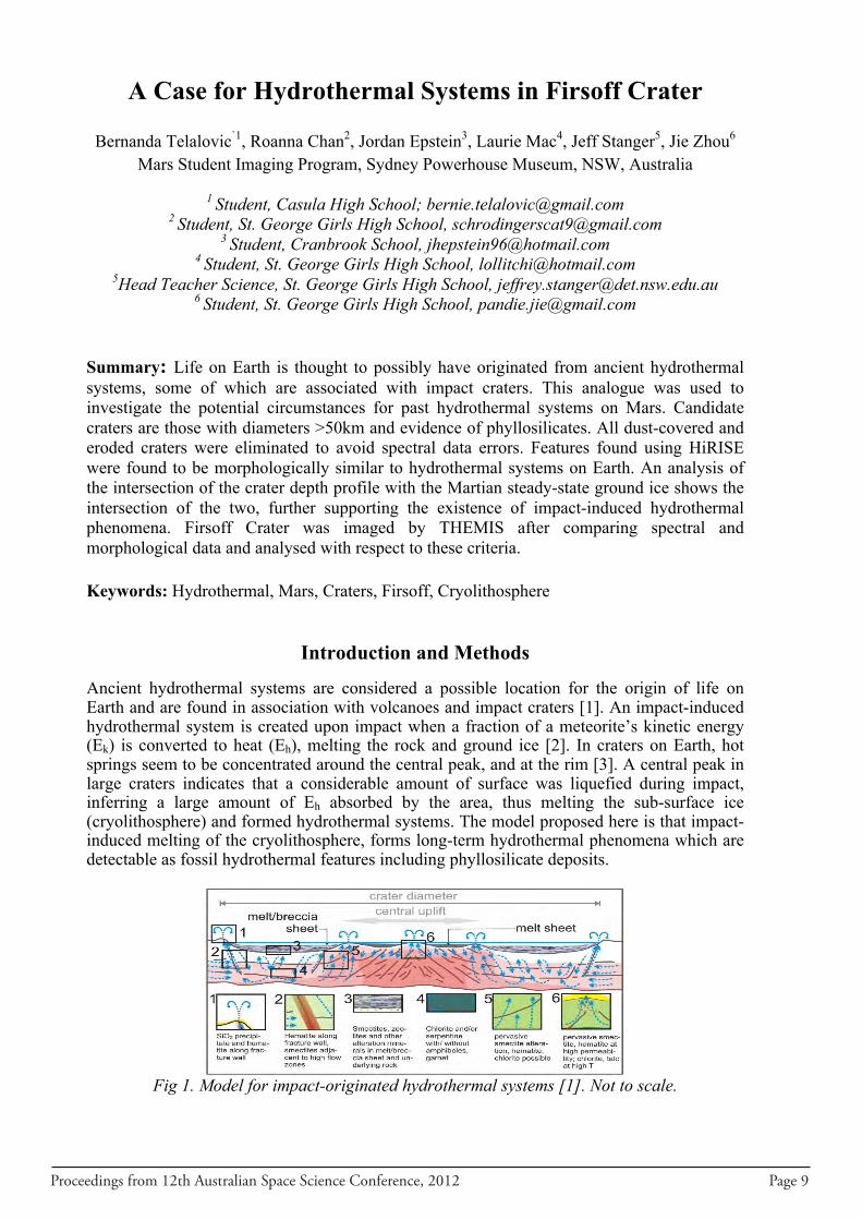
Ancient hydrothermal systems are considered a possible location for the origin of life on Earth and are found in association with volcanoes and impact craters [1]. An impact-induced hydrothermal system is created upon impact when a fraction of a meteorite’s kinetic energy (Ek) is converted to heat (Eh), melting the rock and ground ice [2]. In craters on Earth, hot springs seem to be concentrated around the central peak, and at the rim [3]. A central peak in large craters indicates that a considerable amount of surface was liquefied during impact, inferring a large amount of Eh absorbed by the area, thus melting the sub-surface ice (cryolithosphere) and formed hydrothermal systems. The model proposed here is that impact-induced melting of the cryolithosphere, forms long-term hydrothermal phenomena which are detectable as fossil hydrothermal features including phyllosilicate deposits.
Fig 1. Model for impact-originated hydrothermal systems [1]. Not to scale.
Page 10 Proceedings from 12th Australian Space Science Conference, 2012
Martian craters with diameters larger than 50 km [2] were examined for a sizeable impact-related heating effect and to better suit the resolution of the Thermal Emission Imaging System (THEMIS) camera (18 m2/pixel) on-board the Mars Odyssey orbiter [4]. Candidate craters associated with evidence of phyllosilicates were of particular interest since these are often associated with hydrothermal activity [5]. The existence of phyllosilicates was investigated using data from the Compact Reconnaissance Imaging Spectrometer (CRISM) on the Mars Reconnaissance Orbiter (MRO) [6]. CRISM images were studied in the ir_phy band (infrared hydroxylated silicates (including phyllosilicates) reflectance band) and ir_hyd band (infrared bound water reflectance band). The ir_phy browse products visualise spectral data as red (Fe/Mg phyllosilicates), green (Al phyllosilicates or hydrated silica) and blue (hydrated minerals). The ir_hyd browse products visualise spectral data as red (bound water or ice), green (monohydrated sulfates) and blue (bound water). Ir_phy images with localised detections of hydrated clays (seen in blue) along with ir_hyd images containing an abundance of bound water (seen in red) were taken as indicative of a possible hydrothermal occurrence (Fig. 3) which is undermined by the unreliability of the CRISM instrument due to the dust cover in the area. Features that corresponded to Earth-established hydrothermal systems were observed using images from the High Resolution Imaging Science Experiment (HiRISE) [7] and compared to existing THEMIS images. The sizes of the features were measured using the Java Mission-planning and Analysis for Remote Sensing program (JMARS) [8]. To study the effect the impact would have had on the cryolithosphere; existing models outlined in references 9 and 10 were used to estimate the depth of the cryolithosphere. The theoretical initial depth of Firsoff was estimated to 3.3 km maximum, according to relationships proposed by Garvin et al. [11]. Superimposing the two shows the impact carried sufficient energy to melt the cryolithosphere, thus forming hydrothermal systems (see Fig 9).
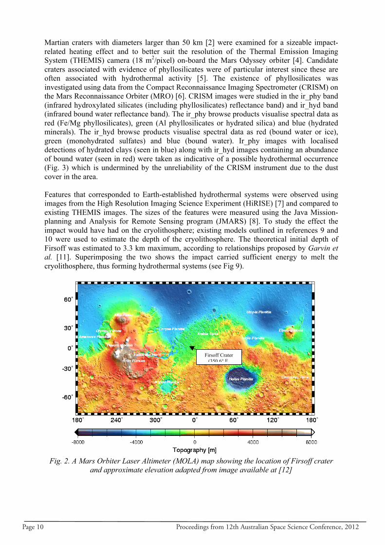
Fig. 2. A Mars Orbiter Laser Altimeter (MOLA) map showing the location of Firsoff crater and approximate elevation adapted from image available at [12]
Firsoff Crater (350.6° E, 2.73°)
Firsoff Crater (350.6° E,
2.73°)
Proceedings from 12th Australian Space Science Conference, 2012 Page 11
C1 image no. 00017697
C3 image no. 0000C384
C2 image no. 000170B5
C4 image no. 000172F1
Data and Analysis
Firsoff crater is located at coordinates 350.6° E, 2.73° N in the Meridiani Planum which has been dated to approximately the upper Noachian age [13], however further research needs to be done to narrow this down to a specific timeframe. The crater is at current depth of approximately 3.06 km in depth and 79 km diameter (see Fig 8). It was selected as it was the best match for the set search criteria (e.g. >50km in diameter with evidence of phyllosilicates in the area and a large central peak). Morphologically, Firsoff is akin to the Curiosity landing site Gale crater, with a similar layered central peak raised to the level of the crater rim. Figure 2 gives a context of the crater’s location. Mineralogical Analysis of CRISM Data Firsoff’s location places it in a mild dust region as observed by the Thermal Emission Spectrometer (TES) [14] (see also Fig 4). The CRISM spectroscopic analysis is only reliable in low dust zones, since dust can affect the accuracy of detections. It is for this reason that the infrequent CRISM data could not be taken as reliable evidence for the sediment composition of the area. CRISM images of the crater and surrounding area have been analysed nonetheless to get an estimate as to there being any significant variations.
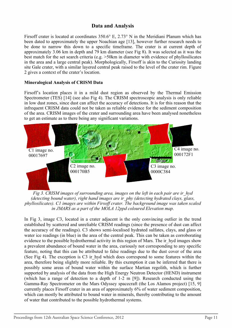
Fig 3. CRISM images of surrounding area, images on the left in each pair are ir_hyd (detecting bound water), right hand images are ir_phy (detecting hydrated clays, glass,
phyllosilicates). C1 images are within Firsoff crater. The background image was taken scaled in JMARS as a part of the MOLA 12ppd coloured Elevation map.
In Fig 3, image C3, located in a crater adjacent is the only convincing outlier in the trend established by scattered and unreliable CRISM readings (since the presence of dust can affect the accuracy of the readings). C3 shows semi-localised hydrated sulfates, clays, and glass or water ice readings (in blue) in the area of the central peak. This can be taken as corroborating evidence to the possible hydrothermal activity in this region of Mars. The ir_hyd images show a prevalent abundance of bound water in the area, curiously not corresponding to any specific feature, noting that this can be attributed to false readings due to the dust cover of the area (See Fig 4). The exception is C3 ir_hyd which does correspond to some features within the area, therefore being slightly more reliable. By this exemption it can be inferred that there is possibly some areas of bound water within the surface Martian regolith, which is further supported by analysis of the data from the High Energy Neutron Detector (HEND) instrument (which has a range of detection to a depth of 1-2 m [9]). Research conducted using the Gamma-Ray Spectrometer on the Mars Odyssey spacecraft (the Los Alamos project) [15, 9] currently places Firsoff crater in an area of approximately 6% of water sediment composition, which can mostly be attributed to bound water in minerals, thereby contributing to the amount of water that contributed to the possible hydrothermal systems.
Page 12 Proceedings from 12th Australian Space Science Conference, 2012
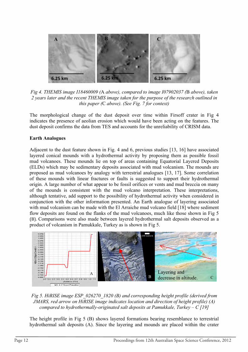
Fig 4. THEMIS image I18460009 (A above), compared to image I07902037 (B above), taken 2 years later and the recent THEMIS image taken for the purpose of the research outlined in
this paper (C above). (See Fig. 7 for context) The morphological change of the dust deposit over time within Firsoff crater in Fig 4 indicates the presence of aeolian erosion which would have been acting on the features. The dust deposit confirms the data from TES and accounts for the unreliability of CRISM data. Earth Analogues Adjacent to the dust feature shown in Fig. 4 and 6, previous studies [13, 16] have associated layered conical mounds with a hydrothermal activity by proposing them as possible fossil mud volcanoes. These mounds lie on top of areas containing Equatorial Layered Deposits (ELDs) which may be sedimentary deposits associated with mud volcanism. The mounds are proposed as mud volcanoes by analogy with terrestrial analogues [13, 17]. Some correlation of these mounds with linear fractures or faults is suggested to support their hydrothermal origin. A large number of what appear to be fossil orifices or vents and mud breccia on many of the mounds is consistent with the mud volcano interpretation. These interpretations, although tentative, add support to the possibility of hydrothermal activity when considered in conjunction with the other information presented. An Earth analogue of layering associated with mud volcanism can be made with the El Arraiche mud volcano field [18] where sediment flow deposits are found on the flanks of the mud volcanoes, much like those shown in Fig 5 (B). Comparisons were also made between layered hydrothermal salt deposits observed as a product of volcanism in Pamukkale, Turkey as is shown in Fig 5.
Fig 5. HiRISE image ESP_026270_1820 (B) and corresponding height profile (derived from JMARS, red arrow on HiRISE image indicates location and direction of height profile) (A)
compared to hydrothermally-originated salt deposits at Pamukkale, Turkey – C [19] The height profile in Fig 5 (B) shows layered formations bearing resemblance to terrestrial hydrothermal salt deposits (A). Since the layering and mounds are placed within the crater
Layering and decrease in altitude. C B
A
C
6.25 km
A
6.25 km
B
6.25 km
Proceedings from 12th Australian Space Science Conference, 2012 Page 13
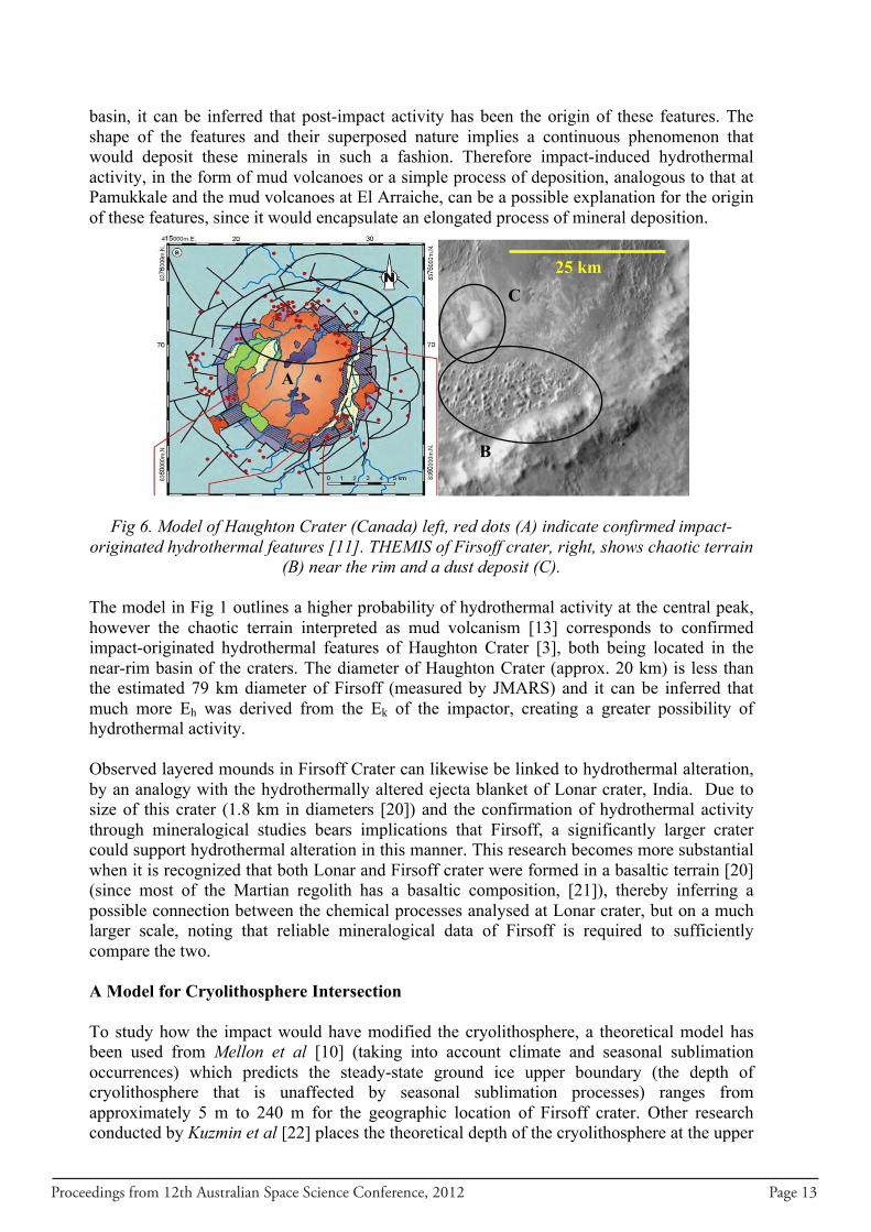
basin, it can be inferred that post-impact activity has been the origin of these features. The shape of the features and their superposed nature implies a continuous phenomenon that would deposit these minerals in such a fashion. Therefore impact-induced hydrothermal activity, in the form of mud volcanoes or a simple process of deposition, analogous to that at Pamukkale and the mud volcanoes at El Arraiche, can be a possible explanation for the origin of these features, since it would encapsulate an elongated process of mineral deposition.
Fig 6. Model of Haughton Crater (Canada) left, red dots (A) indicate confirmed impact-
originated hydrothermal features [11]. THEMIS of Firsoff crater, right, shows chaotic terrain (B) near the rim and a dust deposit (C).
The model in Fig 1 outlines a higher probability of hydrothermal activity at the central peak, however the chaotic terrain interpreted as mud volcanism [13] corresponds to confirmed impact-originated hydrothermal features of Haughton Crater [3], both being located in the near-rim basin of the craters. The diameter of Haughton Crater (approx. 20 km) is less than the estimated 79 km diameter of Firsoff (measured by JMARS) and it can be inferred that much more Eh was derived from the Ek of the impactor, creating a greater possibility of hydrothermal activity. Observed layered mounds in Firsoff Crater can likewise be linked to hydrothermal alteration, by an analogy with the hydrothermally altered ejecta blanket of Lonar crater, India. Due to size of this crater (1.8 km in diameters [20]) and the confirmation of hydrothermal activity through mineralogical studies bears implications that Firsoff, a significantly larger crater could support hydrothermal alteration in this manner. This research becomes more substantial when it is recognized that both Lonar and Firsoff crater were formed in a basaltic terrain [20] (since most of the Martian regolith has a basaltic composition, [21]), thereby inferring a possible connection between the chemical processes analysed at Lonar crater, but on a much larger scale, noting that reliable mineralogical data of Firsoff is required to sufficiently compare the two. A Model for Cryolithosphere Intersection To study how the impact would have modified the cryolithosphere, a theoretical model has been used from Mellon et al [10] (taking into account climate and seasonal sublimation occurrences) which predicts the steady-state ground ice upper boundary (the depth of cryolithosphere that is unaffected by seasonal sublimation processes) ranges from approximately 5 m to 240 m for the geographic location of Firsoff crater. Other research conducted by Kuzmin et al [22] places the theoretical depth of the cryolithosphere at the upper
25 km
A
B
C
Page 14 Proceedings from 12th Australian Space Science Conference, 2012
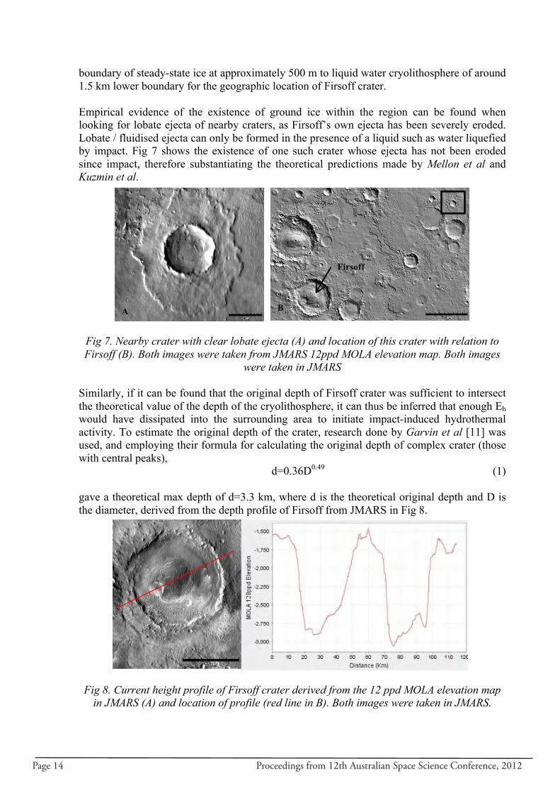
boundary of steady-state ice at approximately 500 m to liquid water cryolithosphere of around 1.5 km lower boundary for the geographic location of Firsoff crater. Empirical evidence of the existence of ground ice within the region can be found when looking for lobate ejecta of nearby craters, as Firsoff’s own ejecta has been severely eroded. Lobate / fluidised ejecta can only be formed in the presence of a liquid such as water liquefied by impact. Fig 7 shows the existence of one such crater whose ejecta has not been eroded since impact, therefore substantiating the theoretical predictions made by Mellon et al and Kuzmin et al.
Fig 7. Nearby crater with clear lobate ejecta (A) and location of this crater with relation to Firsoff (B). Both images were taken from JMARS 12ppd MOLA elevation map. Both images
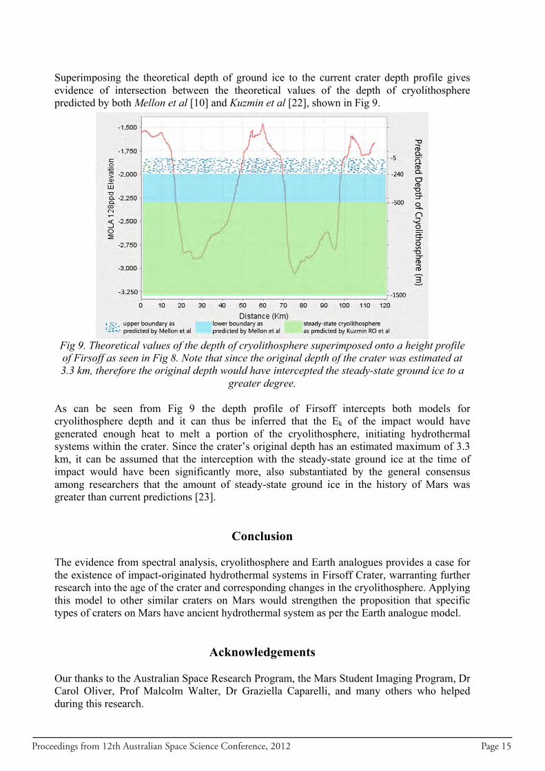
were taken in JMARS Similarly, if it can be found that the original depth of Firsoff crater was sufficient to intersect the theoretical value of the depth of the cryolithosphere, it can thus be inferred that enough Eh would have dissipated into the surrounding area to initiate impact-induced hydrothermal activity. To estimate the original depth of the crater, research done by Garvin et al [11] was used, and employing their formula for calculating the original depth of complex crater (those with central peaks), d=0.36D0.49 (1)
gave a theoretical max depth of d=3.3 km, where d is the theoretical original depth and D is the diameter, derived from the depth profile of Firsoff from JMARS in Fig 8.
Fig 8. Current height profile of Firsoff crater derived from the 12 ppd MOLA elevation map
in JMARS (A) and location of profile (red line in B). Both images were taken in JMARS.
A B
Firsoff
A
B
Proceedings from 12th Australian Space Science Conference, 2012 Page 15
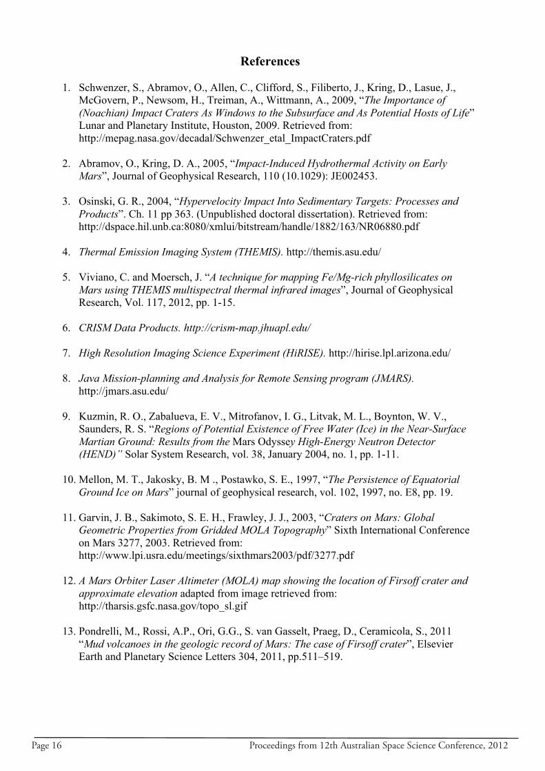
Superimposing the theoretical depth of ground ice to the current crater depth profile gives evidence of intersection between the theoretical values of the depth of cryolithosphere predicted by both Mellon et al [10] and Kuzmin et al [22], shown in Fig 9.
Fig 9. Theoretical values of the depth of cryolithosphere superimposed onto a height profile of Firsoff as seen in Fig 8. Note that since the original depth of the crater was estimated at 3.3 km, therefore the original depth would have intercepted the steady-state ground ice to a
greater degree. As can be seen from Fig 9 the depth profile of Firsoff intercepts both models for cryolithosphere depth and it can thus be inferred that the Ek of the impact would have generated enough heat to melt a portion of the cryolithosphere, initiating hydrothermal systems within the crater. Since the crater’s original depth has an estimated maximum of 3.3 km, it can be assumed that the interception with the steady-state ground ice at the time of impact would have been significantly more, also substantiated by the general consensus among researchers that the amount of steady-state ground ice in the history of Mars was greater than current predictions [23].
Conclusion The evidence from spectral analysis, cryolithosphere and Earth analogues provides a case for the existence of impact-originated hydrothermal systems in Firsoff Crater, warranting further research into the age of the crater and corresponding changes in the cryolithosphere. Applying this model to other similar craters on Mars would strengthen the proposition that specific types of craters on Mars have ancient hydrothermal system as per the Earth analogue model.
Acknowledgements Our thanks to the Australian Space Research Program, the Mars Student Imaging Program, Dr Carol Oliver, Prof Malcolm Walter, Dr Graziella Caparelli, and many others who helped during this research.
Page 16 Proceedings from 12th Australian Space Science Conference, 2012
References 1. Schwenzer, S., Abramov, O., Allen, C., Clifford, S., Filiberto, J., Kring, D., Lasue, J.,
McGovern, P., Newsom, H., Treiman, A., Wittmann, A., 2009, “The Importance of (Noachian) Impact Craters As Windows to the Subsurface and As Potential Hosts of Life” Lunar and Planetary Institute, Houston, 2009. Retrieved from: http://mepag.nasa.gov/decadal/Schwenzer_etal_ImpactCraters.pdf
2. Abramov, O., Kring, D. A., 2005, “Impact-Induced Hydrothermal Activity on Early
Mars”, Journal of Geophysical Research, 110 (10.1029): JE002453. 3. Osinski, G. R., 2004, “Hypervelocity Impact Into Sedimentary Targets: Processes and
Products”. Ch. 11 pp 363. (Unpublished doctoral dissertation). Retrieved from: http://dspace.hil.unb.ca:8080/xmlui/bitstream/handle/1882/163/NR06880.pdf
4. Thermal Emission Imaging System (THEMIS). http://themis.asu.edu/ 5. Viviano, C. and Moersch, J. “A technique for mapping Fe/Mg-rich phyllosilicates on
Mars using THEMIS multispectral thermal infrared images”, Journal of Geophysical Research, Vol. 117, 2012, pp. 1-15.
6. CRISM Data Products. http://crism-map.jhuapl.edu/ 7. High Resolution Imaging Science Experiment (HiRISE). http://hirise.lpl.arizona.edu/ 8. Java Mission-planning and Analysis for Remote Sensing program (JMARS).
http://jmars.asu.edu/ 9. Kuzmin, R. O., Zabalueva, E. V., Mitrofanov, I. G., Litvak, M. L., Boynton, W. V.,
Saunders, R. S. “Regions of Potential Existence of Free Water (Ice) in the Near-Surface Martian Ground: Results from the Mars Odyssey High-Energy Neutron Detector (HEND)” Solar System Research, vol. 38, January 2004, no. 1, pp. 1-11.
10. Mellon, M. T., Jakosky, B. M ., Postawko, S. E., 1997, “The Persistence of Equatorial
Ground Ice on Mars” journal of geophysical research, vol. 102, 1997, no. E8, pp. 19. 11. Garvin, J. B., Sakimoto, S. E. H., Frawley, J. J., 2003, “Craters on Mars: Global
Geometric Properties from Gridded MOLA Topography” Sixth International Conference on Mars 3277, 2003. Retrieved from: http://www.lpi.usra.edu/meetings/sixthmars2003/pdf/3277.pdf
12. A Mars Orbiter Laser Altimeter (MOLA) map showing the location of Firsoff crater and
approximate elevation adapted from image retrieved from: http://tharsis.gsfc.nasa.gov/topo_sl.gif
13. Pondrelli, M., Rossi, A.P., Ori, G.G., S. van Gasselt, Praeg, D., Ceramicola, S., 2011
“Mud volcanoes in the geologic record of Mars: The case of Firsoff crater”, Elsevier Earth and Planetary Science Letters 304, 2011, pp.511–519.
Proceedings from 12th Australian Space Science Conference, 2012 Page 17
14. Ruff, S., Christensen, P. “Bright and dark regions on Mars: Particle size and mineralogical characteristics based on Thermal Emission Spectrometer data”. Journal of Geophysical Research, Vol. 107, 2002.
15. “Los Alamos Releases New Maps of Mars Water”. July 24, 2003. Retrieved from:
http://mars.jpl.nasa.gov/odyssey/newsroom/pressreleases/20030724a.html 16. Franchi, F., Rossi, A., Pondrelli, M. and Barbieri1, R. “Ancient Fluid Escape and Conical
Mound Fields in Firsoff Crater, Arabia Terra (MARS)”, 2012. 43rd Lunar and Planetary Science Conference. Retrieved from: http://www.lpi.usra.edu/meetings/lpsc2011/pdf/1062.pdf
17. Franchi, Cavalazzi, B., Rossi A. P., Pondrelli, M., Barbieri, R., 2012 “Kess Kess
Hydrothermal Mounds In Morocco: A Unique Analog For Exploring Possible Fossil Or Extant Life On Mars.” 43rd Lunar and Planetary Science Conference (2012). Retrieved from: http://www.lpi.usra.edu/meetings/lpsc2012/pdf/2245.pdf
18. Rensbergen, P. V., Depreiter, D., Pannemans, B., Henriet, J-P. “Seafloor expression of
sediment extrusion and intrusion at the El Arraiche mud volcano field, Gulf of Cadiz” Journal of Geophysical Research, 2005, vol. 110, F02010, doi:10.1029/2004JF000165.
19. Özgüler, M.E., Turgay, M.I., Şahin, H., 1984, “Geophysical Investigations in Denizli
Geothermal Fields, Turkey” Retrieved from: http://www.mta.gov.tr/v2.0/eng/dergi_pdf/99-100/7.pdf
20. Newsom, H. E., Nelson, M. J., Shearer, C. K., Misra, S.,
Narasimham, V., 2005, “Hydrothermal Alteration at Lonar Crater, India and Elemental Variations in Impact Crater Clays” Lunar and Planetary Science, 205, 36: 1143.
21. Taylor, G. J., 2009, “Mars Crust: Made of Basalt” Retrieved
from: http://www.psrd.hawaii.edu/May09/Mars.Basaltic.Crust.html 22. Kuzmin, R.O., Zabalueva, E.V., 1998, “On Salt Solution of the Martian Cryolithosphere”
Solar Syst. Res., 1998, 32, pp. 187-197. 23. Baker, V. R., 2006 “Water and the Evolutionary Geological History of Mars”. Retrieved
from: http://www.lpi.usra.edu/meetings/earlymars2012/reprintLibrary/Baker_2006.pdf

Page 18 Proceedings from 12th Australian Space Science Conference, 2012
Proceedings from 12th Australian Space Science Conference, 2012 Page 19
Mariner 2 and its Legacy: 50 Years On
Jeremy Bailey
School of Physics, University of New South Wales, NSW, 2052, Australia
Summary: 50 years ago NASA’s Jet Propulsion Laboratory (JPL) built and flew the first successful spacecraft to another planet — Mariner 2 to Venus. This paper discusses the context of this mission at a crucial phase in the space race between the USA and the USSR and its results and legacy. As its first major success, Mariner 2, helped to cement JPL’s position as a centre for robotic planetary exploration. Mariner 2 successfully solved the scientific problem of the high temperature observed for Venus by ground-based radio telescopes. It also pioneered new techniques for observing the atmosphere of a planet from space, which were subsequently developed into the microwave sounding and infrared sounding techniques for observing the Earth atmosphere. Today these techniques provide some of the most important data for constraining weather forecasting models, as well as a key series of data on the Earth’s changing climate. Keywords: Venus, remote sensing, infrared sounding, microwave sounding, weather forecasting, climate
Introduction
On August 27th 1962, the Mariner 2 spacecraft built by NASA’s Jet Propulsion Laboratory (JPL) was successfully launched on its way to Venus. On December 14th 1962 it passed within 35,000 km of Venus and observed the planet with its onboard instruments and returned the resulting data to Earth [1]. It was the first successful spacecraft to another planet. The Mariner 2 mission came at the height of the space race between the USA and USSR, and at a time when the USSR was making all the running. The Soviet Union had shocked the world with the launch of Sputnik 1 in 1957. The launch was made possible by the development of the world’s first Intercontinental Ballistic Missile (ICBM), the R-7, by the team led by Sergei Korolev in Moscow. A month after the first successful test flight of the R-7 it was used to put Sputnik 1 in orbit [2]. By 1959 Korolev had added an additional upper stage to his R-7 to make the 8K72 launch vehicle used to launch a series of spacecraft to the Moon. Luna 1 flew past the Moon in January 1959. Luna 2 impacted on the Moon’s surface in September 1959, and Luna 3 flew round the Moon and photographed its far side in October 1959 [3]. The same launch vehicle was used to launch the 4.7 tonne Vostok manned spacecraft that carried Yuri Gagarin into orbit in April 1961 [4]. Over the same period the USA was playing catch up. Early US space launches, such as the Explorer and Vanguard satellites, and Pioneer lunar and interplanetary spacecraft were smaller spacecraft launched by smaller rockets, and the US was repeatedly beaten by the Soviet Union to key space “firsts”. In this context the achievement of the first successful planetary mission with Mariner 2 in 1962 came as something of a surprise. By 1960 Korolev’s team had added two upper stages to the R-7 to make the 8K78 (later known as the Molniya) and was using this to attempt launches to the planets. Two Mars launch attempts were made in October 1960 but both were lost when the third stage of the launch vehicle failed to ignite [5]. Then two Venus launches were attempted in February
Page 20 Proceedings from 12th Australian Space Science Conference, 2012
1961. The first failed to leave Earth orbit, but the second (later designated Venera 1) was successfully placed on its path to Venus. It did not last long. After a few days the spacecraft’s attitude stabilization and thermal control failed and radio contact was lost. Venera 1 did fly within 100,000 km of Venus, but attempts to receive signals from it (even using the powerful radio telescope at Jodrell Bank in England) were unsuccessful [6].
JPL and Mariner The Jet Propulsion Laboratory grew out of the work of a group of rocket enthusiasts at CalTech who began experimenting with rocket engines in 1936. During World War II the group developed JATO units, rockets used to assist aircraft take-off. JPL was formally established in 1944 [7]. After the war JPL worked on the development of missiles including the liquid fuelled Corporal [8] and solid fuelled Sergeant [9]. In 1954, William Pickering became director of JPL and remained in the role until 1976. [10] The first satellite launched by the US, Explorer 1, was the result of collaboration between JPL and the Army Ballistic Missile Agency (ABMA). The launch vehicle was based on ABMA’s Redstone missile developed by Wernher von Braun. The upper stages and the satellite were built by JPL, with the upper stages being made from clusters of miniature versions of the Sergeant missile’s solid fuel engine [11]. The satellite carried a radiation detector built by Iowa State University’s James Van Allen, and the measurements from this and subsequent Explorer missions led to the discovery of the Van Allen radiation belts [12]. Following the success of Explorer, JPL became part of the new National Aeronautics and Space Administration (NASA) formed in 1958 to coordinate the USA’s civilian space program. By the end of 1959 the role of JPL was determined to be the development of unmanned spacecraft to the Moon and planets. The lunar missions would be known as Rangers, and spacecraft to Mars and Venus would be given the name Mariner [13]. A major issue for the US lunar and planetary missions was to find a suitable launch vehicle. While the USSR used the R-7 ICBM and derivatives for all space launches, most early US launch attempts were based on smaller rockets. America’s own ICBM, the Atlas, went through test flights in 1958 and 1959 [14], but Atlas was smaller than the R-7 and needed additional upper stages for lunar and planetary launches. The first configuration tried was the Atlas-Able, which added the upper stages of the Vanguard launch vehicle to the Atlas. Four Pioneer launch attempts with this launch vehicle in 1959 and 1960 all resulted in failure [15]. JPL and NASA had a proposal for a new vehicle called the Atlas-Vega, but this project was dropped when it was realized that the Air Force’s Agena B could be used as an Atlas upper stage to provide similar performance [16]. The other project under development was the Centaur [17], a high performance liquid hydrogen fuelled upper stage designed specifically for use with the Atlas. The Atlas-Centaur combination was the most powerful available, and JPL designed its first Mariner spacecraft concept named Mariner-A for an Atlas-Centaur launch to Venus in the 1962 launch window. Mariner A would have been a spacecraft of around 500 kg [18]. By August 1961 it became clear that the Centaur would not be ready for the planned 1962 launches. Instead a concept for a spacecraft called Mariner-R, based partly on the Ranger spacecraft being designed for lunar missions, was rapidly developed. This would have a mass of only ~200 kg allowing it to be launched with the smaller Atlas-Agena-B. According to Mariner project manager Jack James, “In a three week period from 8 August 1961 to 1 September 1961, a conceptual design was completed” [19]. That left just nine months for the
Proceedings from 12th Australian Space Science Conference, 2012 Page 21
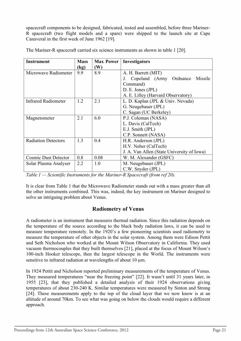
spacecraft components to be designed, fabricated, tested and assembled, before three Mariner-R spacecraft (two flight models and a spare) were shipped to the launch site at Cape Canaveral in the first week of June 1962 [19]. The Mariner-R spacecraft carried six science instruments as shown in table 1 [20]. Instrument Mass
(kg) Max Power (W)
Investigators
Microwave Radiometer 9.9 8.9 A. H. Barrett (MIT) J. Copeland (Army Ordnance Missile Command) D. E. Jones (JPL) A. E. Lilley (Harvard Observatory)
Infrared Radiometer 1.2 2.1 L. D. Kaplan (JPL & Univ. Nevada) G. Neugebauer (JPL) C. Sagan (UC Berkeley)
Magnetometer 2.1 6.0 P.J. Coleman (NASA) L. Davis (CalTech) E.J. Smith (JPL) C.P. Sonnett (NASA)
Radiation Detectors 1.3 0.4 H.R. Anderson (JPL) H.V. Neher (CalTech) J. A. Van Allen (State University of Iowa)
Cosmic Dust Detector 0.8 0.08 W. M. Alexander (GSFC) Solar Plasma Analyser 2.2 1.0 M. Neugebauer (JPL)
C.W. Snyder (JPL) Table 1 — Scientific Instruments for the Mariner-R Spacecraft (from ref 20). It is clear from Table 1 that the Microwave Radiometer stands out with a mass greater than all the other instruments combined. This was, indeed, the key instrument on Mariner designed to solve an intriguing problem about Venus.
Radiometry of Venus A radiometer is an instrument that measures thermal radiation. Since this radiation depends on the temperature of the source according to the black body radiation laws, it can be used to measure temperature remotely. In the 1920’s a few pioneering scientists used radiometry to measure the temperature of other objects in the solar system. Among them were Edison Pettit and Seth Nicholson who worked at the Mount Wilson Observatory in California. They used vacuum thermocouples that they built themselves [21], placed at the focus of Mount Wilson’s 100-inch Hooker telescope, then the largest telescope in the World. The instruments were sensitive to infrared radiation at wavelengths of about 10 µm. In 1924 Pettit and Nicholson reported preliminary measurements of the temperature of Venus. They measured temperatures “near the freezing point” [22]. It wasn’t until 31 years later, in 1955 [23], that they published a detailed analysis of their 1924 observations giving temperatures of about 230-240 K. Similar temperatures were measured by Sinton and Strong [24]. These measurements apply to the top of the cloud layer that we now know is at an altitude of around 70km. To see what was going on below the clouds would require a different approach.
Page 22 Proceedings from 12th Australian Space Science Conference, 2012
The microwave radiometer was invented in 1942, and was a by-product of World War 2 radar research. Microwave radar had been made possible by the British invention of the cavity magnetron [25]. This secret development was shared with the USA and led to the establishment of the MIT Radiation Laboratory (RadLab) to further develop microwave radar [26]. It was here that Robert Dicke built the first microwave radiometer, a radio receiver sensitive enough to be able to detect thermal radiation [27]. After the war many of the scientists who had worked on wartime radar began to explore the new field of radio astronomy. While much of the early work on radio astronomy involved observations at metre wavelengths a few researchers explored the shorter microwave wavelengths. At the Naval Research Laboratory in Washington DC, Cornell Mayer and Fred Haddock built a 50-foot microwave telescope mounted on a gun mount on the roof of one of the NRL buildings [28]. Using this telescope, in 1956, Mayer made measurements of the temperature of Venus using a Dicke type radiometer working at a wavelength of 3.15 cm. He obtained temperatures ranging from 560 to 620 K [29]. Other observations soon followed and confirmed the high temperatures [30]. But what was being measured? According to Carl Sagan [31] the high temperatures measured by the microwave instruments were thermal emission from the surface or lower atmosphere heated by a very efficient greenhouse effect. The key difference between the microwave and infrared measurements is that microwave radiation is unaffected by the clouds and so can measure the true surface temperature, whereas infrared radiation cannot see through the clouds and measures only the cloud tops. However, many scientists were reluctant to accept that the greenhouse effect was sufficient to heat the surface of Venus to such extreme temperatures. Other mechanisms were suggested in which the microwave radiation originated in the ionosphere of Venus [31]. The microwave radiometer on Mariner 2 was designed to carry out observations that would clearly distinguish these two models. By scanning across the disk of Venus it would determine if the microwave radiation increased or decreased at the limb of the planet. Limb darkening would indicate that Sagan’s greenhouse model was correct because radiation coming from the surface would suffer more absorption on the way out. Limb brightening would favour the ionosphere model since a greater path length of the ionosphere would be observed near the limb. This test could not be carried out using earth-based radio telescopes as their spatial resolution, at that time, was far too small.
Voyage to Venus
Mariner 1, the first of the Mariner-R spacecraft was launched on July 21 1962. Five minutes into the flight the Atlas-Agena had to be destroyed after a guidance system failure. Mariner 1 continued to transmit until it hit the Atlantic ocean 357 seconds after lift-off [16]. For JPL it was all too familiar. The first four of their Ranger spacecraft to the Moon had resulted in failure. Another Atlas-Agena was readied to launch Mariner 2. After some delays the launch finally occurred on August 27 1962. This time the Atlas-Agena was successful. The Agena-Mariner combination was placed in a parking orbit and then the Agena fired again to launch Mariner 2 on its way to Venus. The heart of Mariner 2 was a system called the “Central Computer and Sequencer” (CC&S). This was not a computer as we would understand the term today. The CC&S was basically a timer that counted the time since launch and initiated operations and manoeuvres at the appropriate times [32]. Following launch the CC&S instructed the spacecraft to deploy its
Proceedings from 12th Australian Space Science Conference, 2012 Page 23
solar panels and turn on its attitude control system, which pointed the spacecraft towards the Sun and the high-gain antenna at the Earth. On September 4 the CC&S carried out the mid-course manoeuvre, which involved a motor-burn to adjust the spacecraft’s velocity to put it on course for its encounter with Venus. The required burn duration and direction parameters were provided by ground command, based on analysis of the spacecraft’s orbit to that point. Back on Earth the Soviet team were still trying to launch their planetary spacecraft. Three Venus launches in the same launch window as Mariner 2 all failed. However, on November 1st 1962 Mars 1 was successfully launched on a trajectory to Mars [33]. Should Mariner 2 fail, the Soviet Union could still achieve the first successful flight to another planet. And all was not well with Mariner 2. A short circuit occurred in one of the two solar panels, the fault fixed itself a few days later and then recurred. Fortunately as Mariner was approaching the Sun the power from a single solar panel would be sufficient, although the scientific instruments had to be turned off for 8 days to conserve power [16]. As well as the solar panel problem, Mariner 2 was overheating. The thermal control system designed to keep the spacecraft at a safe operating temperature was not working well enough. On November 16 one temperature sensor reached its limit [34] and temperatures were generally 40 degrees Farenheit higher than expected [16]. Several of the spacecraft systems were operating at or above their maximum temperatures, including the crucial earth-sensor that kept Mariner 2 correctly oriented, with its antenna pointed at Earth. Failures could be expected at any time. According to project manager Jack James, “Now we could only wait and hope” [16]. On December 9, just 5 days before encounter, four of the spacecraft telemetry measurements that were regularly returned to Earth failed. On December 12 the CC&S failed to issue a regular update pulse that should occur every 1000 minutes [34]. This indicated that the CC&S might fail to initiate the encounter activities and so a ground command was sent to initiate the encounter sequence with Venus. On December 14 the overheated Mariner 2 flew past Venus at a distance of 35,000 km with 7 of its 18 temperature sensors now at their limit [34]. However, everything worked as expected. The radiometers performed their scans across the disk of Venus and returned the crucial data on the planet’s temperature. All the science instruments functioned properly. The spacecraft continued to operate until January 3 1963.
Results The Mariner 2 microwave radiometer experiment confirmed the high temperatures observed in ground-based observations. Results from three scans across the disk showed limb darkening and thus showed conclusively that the surface of Venus was hot [16, 35, 36] as has been suggested by Sagan, and ruled out the ionosphere model. The results would lead to the runaway greenhouse model for the evolution of the Venus atmosphere [37]. Mariner 2’s infrared radiometer confirmed the cold cloud top temperatures (220-230 K) obtained by the ground-based measurements and showed no evidence of breaks in the cloud coverage that could see deeper into the atmosphere [38].
Page 24 Proceedings from 12th Australian Space Science Conference, 2012
Mariner 2’s other instruments such as the magnetometer and radiation detectors made valuable studies of the magnetic field and radiation environment in interplanetary space [1]. During the encounter with Venus, however, no change was detected in the magnetic field and radiation levels. This indicated that Venus was very different to Earth with a much weaker magnetic field and hence no extended magnetosphere. From precise tracking of Mariner’s orbit as it passed Venus it was possible to derive a much improved value for the mass of Venus [16].
From Radiometers to Sounders
If microwave and infrared radiometers could make valuable observations of the temperature structure in the Venus atmosphere, then could the same techniques play a role in studying the Earth’s weather and climate? This was what several of the Mariner scientists began to investigate in the years following Mariner 2’s mission. Alan Barrett, a radio astronomer at MIT, and an investigator on the Mariner 2 microwave radiometer experiment, began to develop the concept for a microwave “sounder” that would observe the temperature structure of the atmosphere from space. The way to make a sounder was to make use of an absorption band, in this case one due to oxygen at around 60 GHz. By using microwave radiometers at different frequencies within this band, with different amounts of absorption, temperatures could be measured at different heights in the atmosphere. Barrett had a number of his graduate students work on the concept. One of these, William B. Lenoir (who would go on to be a NASA astronaut) tested the concept using a balloon-borne radiometer [39]. Others used ground and airborne instruments, but the real aim was to put an instrument on a satellite that could look down on Earth and make global 3D maps of the temperature distribution in the atmosphere. The opportunity came in 1972 with the Nimbus 5 satellite and an instrument called NEMS (Nimbus-E Microwave Spectrometer). Another former Barrett student, David Staelin, now on the MIT faulty, was the principal investigator for the instrument, with Barrett as a co-investigator. The instrument successfully demonstrated the concept of microwave temperature sounding from space [40]. The follow up to this experimental instrument was the microwave sounding unit (MSU), a four channel microwave sounder [41] that was installed as standard on a series of meteorological satellites starting with TIROS-N in 1978 and ending with NOAA-14 in 1994. It was then superseded by an improved instrument, the Advanced Microwave Sounding Unit (AMSU), with 15 channels. AMSU is currently installed on a number of NOAA satellites, on NASA’s Aqua and on the European MetOp satellites. In parallel with the microwave development, Lewis Kaplan, a member of the Mariner 2 infrared radiometer team was making similar proposals for an infrared sounder. In fact even before Mariner he had proposed atmospheric temperature sounding using a CO2 band at 15 µm [42]. The first satellite instrument to use this technique was the Nimbus 3 Satellite Infrared Spectrometer (SIRS) launched in 1969. The present versions of such instruments are the Atmospheric Infrared Sounder (AIRS) on the NASA Aqua satellite and the Infrared Atmospheric Sounding Interferometer (IASI) on the European MetOp satellites. Weather forecasting today is based on sophisticated computer models that “assimilate” data from a wide variety of sources including ground weather stations and remote sensing data
Proceedings from 12th Australian Space Science Conference, 2012 Page 25
from satellites. It is possible to analyse these systems to determine which observations contribute most to the accuracy of the forecast. Such an analysis carried out at the European Centre for Medium-Range Weather Forecasting (ECWMF) [43] shows that the instruments at the top of the list are AMSU, AIRS and IASI, the very instruments that can trace their heritage to Mariner 2. The more than 30 year record of data from microwave sounding using MSU and AMSU also provides an important dataset on the earth’s warming atmosphere [44], showing the trend in temperature rise, as well as the geographical distribution, with global warming being greatest in the arctic region.
Conclusions Mariner 2 is an important mission not just because of the obvious milestone of being the first successful spacecraft to another planet. Its success in 1962 marks the beginning of the turnaround of fortunes in the space race. As JPL’s first successful lunar or planetary mission it helped to secure JPL’s future and was the forerunner of a long record of success in planetary exploration. It also did important science establishing the reality of the extreme greenhouse effect in the atmosphere of Venus. And the radiometers that flew on it are the predecessors of the infrared and microwave sounders that circle the earth today and are major contributors to the accuracy of the weather forecasts we use every day.
References 1. Sonnett, C.P., “A Summary Review of the Scientific Findings of the Mariner Venus
Mission”, Space Science Reviews, Vol. 2, 1963, pp. 751-777.
2. Siddiqi, A., Sputnik and the Soviet Space Challenge, Univ. Press Florida, Gainesville, 2003, pp. 102-170.
3. Gallentine, J., Ambassadors from Earth, Univ. of Nebraska Press, Lincoln, 2009, pp. 135-
154.
4. Siddiqi, A., 2003, op. cit., pp. 276-282. 5. Gallentine, J., 2009, op. cit., pp. 177-178. 6. Gallentine, J., 2009, op. cit., pp. 181-183. 7. Koppes, C.R., JPL and the American Space Program, Yale University Press, New Haven,
1982, pp. 1-20. 8. Hunley, J.D., Prelude to U.S. Space-Launch Vehicle Technology, Univ. Press Florida,
Gainesville, 2008, pp. 105-121. 9. Hunley, J.D., 2008, op. cit., pp. 161-164. 10. Koppes, C.R., 1982, op. cit., p 65.
Page 26 Proceedings from 12th Australian Space Science Conference, 2012
11. Burrows, W.E , This New Ocean, The Modern Library, New York, 1999, pp. 206-208. 12. Van Allen, J.A., Ludwig, G.H., Ray, E.C., McIlwain, C.E., “Observation of High Intensity
Radiation by Satellites 1958 Alpha and Gamma”, J. Jet Propulsion, Vol. 28, 1958, pp. 588-592.
13. Koppes, C.R., 1982, op. cit., pp. 105-107. 14. Hunley, J.D., 2008, op. cit., pp. 229-232. 15. Walker, C., Powell, J , Atlas, The Ultimate Weapon, Apogee Books, Burlington, Ontario,
2005, p. 230. 16. James, J. N., “The Voyage of Mariner II”, Scientific American, Vol. 209, No 1, 1963, pp.
70-84. 17. Dawson, V.P., Bowles, M.D., Taming Liquid Hydrogen: The Centaur Upper Stage Rocket
1958-2002, NASA SP-4230, 2004, pp. 1-29. 18. NASA JPL, Mariner Venus 1962 – Final Project Report, NASA SP-59, 1965, p 11. 19. James, J.N., Mariner II, NASA CR-52376, 1963, p. 3. 20. Wyckoff, R.C., 1962, “Scientific Experiments For Mariner R-1 and R-2”, JPL Technical
Report No 32-315, 1962. 21. Pettit, E., Nicholson, S.B., “The Application of Vacuum Thermocouples to Problems in
Astrophysics”, Astrophys. J., Vol. 56, 1922, pp. 295-317. 22. Pettit, E., Nicholson, S.B., “Radiation from the dark hemisphere of Venus”, Popular
Astronomy, Vol. 32, 1924, p. 614. 23. Pettit, E., Nicholson, S.B., “Temperatures of the Bright and Dark Sides of Venus”, Publ.
Astron. Soc. Pacific, Vol. 67, 1955, pp. 293-303. 24. Sinton, W. M., Strong, J., “Radiometric Observations of Venus”, Astrophys. J., Vol. 131,
1960, pp. 470-491. 25. Megaw, E.C.S., “The High-Power Pulsed Magnetron: A Review of Early Developments”,
Journal of the Institution of Electrical Engineers, Part IIIA, Radiolocation, Vol. 93, 1946, pp. 977-984.
26. Buderi, R., The Invention that Changed the World, Simon & Shuster, 1996. 27. Dicke, R., “The Measurement of Thermal Radiation at Microwave Frequencies”, Rev.
Scientific Instr., Vol. 17, 1946, pp. 268-275. 28. Radhakrishnan, V., “Obituary: Cornell H. Mayer”, 1921-2005, Bull. Amer. Astron. Soc.,
Vol. 38, 2006, pp. 1279-1280. 29. Mayer, C.H., McCullough, T.P., Sloanaker, R.M., “Observations of Venus at 3.15 cm
Wavelength”, Astrophys. J., Vol. 127, 1956, pp. 1-10.
Proceedings from 12th Australian Space Science Conference, 2012 Page 27
30. Barrett, A.H., “Microwave Absorption and Emission in the Atmosphere of Venus”,
Astrophys. J., Vol. 133, 1961, pp. 281-293. 31. Sagan, C., “The Planet Venus”, Science, Vol. 133, 1961, pp. 849-858. 32. NASA JPL, Mariner Venus 1962 – Final Project Report, NASA SP-59, 1965, pp. 171-
182. 33. Gallantine, J., 2009, op. cit., pp. 236-237. 34. NASA JPL, Mariner Venus 1962 – Final Project Report, NASA SP-59, 1965, pp. 115-
117. 35. Barath, F.T., Barrett, A.H., Copeland, J., Jones, D.E., Lilley, A.E., “Microwave
Radiometers”, Science, Vol. 139, 1963, pp. 908-909. 36. Pollack, J. & Sagan, C., “An Analysis of the Mariner 2 Microwave Observations of
Venus”, Astrophys. J., Vol. 150, 1967, pp. 327-333. 37. Ingersoll, A.P., “The Runaway Greenhouse: A History of Water on Venus”, J. Atmos. Sci.,
Vol. 26, 1969, pp. 1191-1198. 38. Chase, S.C., Kaplan, L.D., Neugebauer, G., “The Mariner 2 Infrared Radiometer
Experiment”, J. Geophys. Res., Vol. 68, 1963, pp. 6157-6169. 39. Lenoir, W.B. “Remote Sounding of the Upper Atmosphere by Microwave
Measurements”, PhD Thesis, Massachussets Institute of Technology, 1965. 40. Staelin, D. H., Barrett, A.H., Waters, J.W., Barath, F.T., Johnson, E.J., Rosenkranz, P.W.,
Gaut, N.E., Lenoir, W.B., “Microwave Spectrometer on the Nimbus 5 Satellite: Meteorological and Geophysical Data”, Science, Vol. 182, 1973, pp. 1339-1341.
41. Swanson, P.N., Harris, W.M., Johnston, E.J., Soltis, F.S., “The TIROS-N Microwave
Sounder Unit”, MTT-S International Microwave Symposium Digest, vol 80., 1980, pp. 123-125.
42. Kaplan, L., “Inference of Atmospheric Structure from Remote Radiation Measurements”,
Journal of the Optical Society of America, Vol 49, 1959, pp. 1004-1007. 43. Cardinali, C. and Prates, F., “Performance measurement with advanced diagnostic tools of
all-sky microwave imager radiances in 4D-Var”, Quarterly Journal Royal Meteorological Society, Vol. 137, 2011, pp. 2038-2046.
44. Mears, C.A., Wentz, F.J., “Construction of the RSS V3.2 lower tropospheric dataset from
the MSU and AMSU microwave sounders”, Journal of Atmospheric and Oceanic Technology, Vol. 26, 2009, pp. 1493-1509.

Page 28 Proceedings from 12th Australian Space Science Conference, 2012
Proceedings from 12th Australian Space Science Conference, 2012 Page 29
The Pioneer Anomaly: an inconvenient reality or NASA‟s 12 year misconception?
Paul ten Boom 1
1 School of Physics, University of New South Wales, Sydney, NSW, 2052, Australia
Summary: This paper discusses the likelihood of whether the Pioneer anomaly is due to „mundane‟ systematic errors/effects or indicative of new or unappreciated physics. The main aim of this paper is to argue that recent publications suggesting that the anomaly is previously overlooked thermal recoil forces, which is in stark contrast to the earlier consensus (1998-2010), are open to questioning. Both direct and circumstantial evidence are examined, and the uncertainty or inaccuracy associated with observations of such a small magnitude effect is recognised. Whilst a non-systematic based anomaly appears to be very unlikely, by way of the awkwardness of the observational characteristics that would need to be modelled, the existence of other peripheral anomalous phenomena makes an outright dismissal of the anomaly unwise. Issues from the philosophy of science (and physics) are also tabled. In the interests of having a contingency plan, should future experiments provide support for a Pioneer-like anomaly, the type of unappreciated physics that could conceivably satisfy the awkward observational evidence is alluded to, albeit in a non-rigorous and cursory manner. Keywords: Pioneer anomaly; spacecraft navigation; gravitation; Earth flyby anomaly; fundamental physics
Introduction The Pioneer 10 and 11 spacecraft, launched in 1972 and 1973 respectively, represent an ideal system to perform precision celestial mechanics experiments [1]. The radiometric Doppler tracking data of these spacecraft (in the outer solar system and beyond) indicated the presence of a small, anomalous, frequency blue-shift (relative to expectations) of 96 10 Hz/s. This unmodelled Doppler „drift‟, which is applicable to both spacecraft, has been interpreted as an anomalous deceleration – as compared to a clock (or time) acceleration effect [2]. The average value of this anomalous (Pioneer) deceleration ( Pa ) is 10 2(8.74 1.33) 10 m/s . Note
that this value is inclusive of a 10 20.90 10 m/s bias due to various systematics (see Table II in Ref. 1), particularly the radio beam reaction force and the negative/inward contribution of onboard heat reflected off the spacecraft. The anomalous deceleration is an offset relative to predictions, with these predictions involving great complexity. Its direction is imprecisely determined, equally favoured are: Sun-pointing, Earth-pointing, and spin-axis directed. A path or velocity vector direction has also been considered consistent with the observations [1]. The spin stabilisation of these spacecraft, as compared to the three-axis stabilisation of the Voyager (1 and 2) spacecraft, makes them navigationally superior to the Voyagers. The only other spacecraft to have travelled beyond 20 AU, where the effect of solar radiation pressure has decreased to less than 10 24 10 m/s [3], is the New Horizons mission which is en route to encounter Pluto in July 2015. Somewhat surprisingly, the Pioneer 10/11 based data represents the „cutting edge‟ of navigational precision and accuracy in the solar system. A future space mission dedicated to improving upon this level of navigational precision and accuracy is
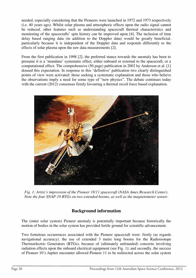
Page 30 Proceedings from 12th Australian Space Science Conference, 2012
needed, especially considering that the Pioneers were launched in 1972 and 1973 respectively (i.e. 40 years ago). Whilst solar plasma and atmospheric effects upon the radio signal cannot be reduced, other features such as understanding spacecraft thermal characteristics and monitoring of the spacecrafts‟ spin history can be improved upon [4]. The inclusion of time delay based ranging data (in addition to the Doppler data) would be greatly beneficial, particularly because it is independent of the Doppler data and responds differently to the effects of solar plasma upon the raw data measurements [2]. From the first publication in 1998 [2], the preferred stance towards the anomaly has been to presume it is a „mundane‟ systematic effect, either onboard or external to the spacecraft, or a computational effect. The comprehensive (50 page) publication in 2002 by Anderson et al. [1] doused this expectation. In response to this „definitive‟ publication two clearly distinguished points of view were activated: those seeking a systematic explanation and those who believe the observations imply a need for some type of “new physics”. The debate continues today with the current (2012) consensus firmly favouring a thermal recoil force based explanation.
Fig. 1: Artist’s impression of the Pioneer 10/11 spacecraft (NASA Ames Research Center). Note the four SNAP-19 RTGs on two extended booms, as well as the magnetometer sensor.
Background information
The (outer solar system) Pioneer anomaly is potentially important because historically the motion of bodies in the solar system has provided fertile ground for scientific advancement. Two fortuitous occurrences associated with the Pioneer spacecraft were: firstly (as regards navigational accuracy), the use of extended 3 metre long booms for the Radioisotope Thermoelectric Generators (RTGs), because of (ultimately unfounded) concerns involving radiation effects upon the onboard electrical equipment (see Fig. 1); and secondly, the success of Pioneer 10‟s Jupiter encounter allowed Pioneer 11 to be redirected across the solar system
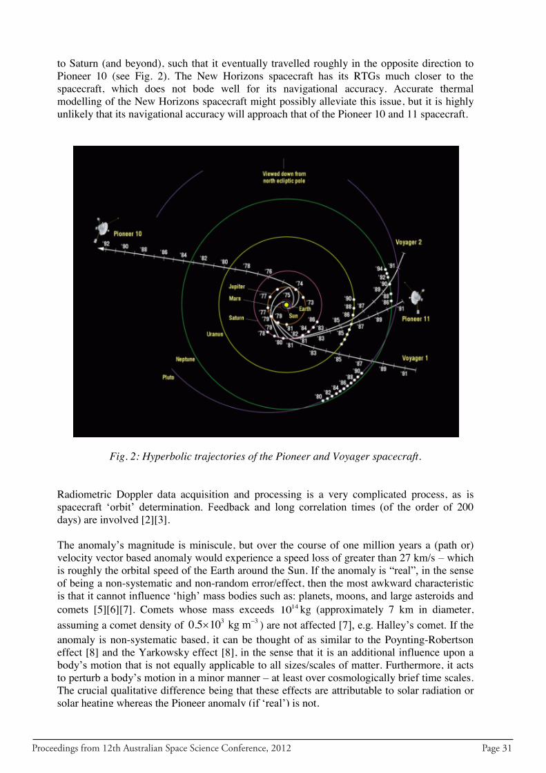
Proceedings from 12th Australian Space Science Conference, 2012 Page 31
to Saturn (and beyond), such that it eventually travelled roughly in the opposite direction to Pioneer 10 (see Fig. 2). The New Horizons spacecraft has its RTGs much closer to the spacecraft, which does not bode well for its navigational accuracy. Accurate thermal modelling of the New Horizons spacecraft might possibly alleviate this issue, but it is highly unlikely that its navigational accuracy will approach that of the Pioneer 10 and 11 spacecraft.
Fig. 2: Hyperbolic trajectories of the Pioneer and Voyager spacecraft. Radiometric Doppler data acquisition and processing is a very complicated process, as is spacecraft „orbit‟ determination. Feedback and long correlation times (of the order of 200 days) are involved [2][3]. The anomaly‟s magnitude is miniscule, but over the course of one million years a (path or) velocity vector based anomaly would experience a speed loss of greater than 27 km/s – which is roughly the orbital speed of the Earth around the Sun. If the anomaly is “real”, in the sense of being a non-systematic and non-random error/effect, then the most awkward characteristic is that it cannot influence „high‟ mass bodies such as: planets, moons, and large asteroids and comets [5][6][7]. Comets whose mass exceeds 1410 kg (approximately 7 km in diameter, assuming a comet density of 3 30.5 10 kg m ) are not affected [7], e.g. Halley‟s comet. If the anomaly is non-systematic based, it can be thought of as similar to the Poynting-Robertson effect [8] and the Yarkowsky effect [8], in the sense that it is an additional influence upon a body‟s motion that is not equally applicable to all sizes/scales of matter. Furthermore, it acts to perturb a body‟s motion in a minor manner – at least over cosmologically brief time scales. The crucial qualitative difference being that these effects are attributable to solar radiation or solar heating whereas the Pioneer anomaly (if „real‟) is not.
Page 32 Proceedings from 12th Australian Space Science Conference, 2012
Evolution of the anomaly‟s interpretation between 1998 and 2012
1998 to 2010: A plethora of hypotheses found wanting NASA was very cautious in not publishing until 18 years after the anomaly was first noticed in 1980, and four years after Michael M. Nieto (Los Alamos) and John D. Anderson (JPL, NASA) spoke in 1994 regarding the corroboration of deep space navigation with general relativity. Between 1998 and 2010, by way of a linear increase in the Doppler residual (cf. predictions/expectations), a (mean) constant anomaly was implied by the observations and analyses. This constancy was prominent in the first publication [1] and again in the definitive 2002 article [2], which featured an independent analysis from The Aerospace Corporation. Between late 1998 and early 2010, all conceivable systematic based explanations, other than asymmetric thermal (radiation pressure) effects, were (able to be) ruled out. Furthermore, the awkward observational constraints ensured that all attempts at “new physics” were ultimately unsuccessful. Subsequently, the anomaly remained unresolved, unexplained and underdetermined. The existence of a thermal (or heat) based explanation was argued for very early on [9], even though decay of the RTGs as well as reduction in the power supplied is inconsistent with a constant anomaly. The thermal recoil force hypothesis gained a firmer foothold in 2002 with Craig Markwardt‟s independent analysis [10] indicating that the timescale of his investigations could not preclude a jerk term (i.e. rate of change of acceleration). Note that he used a truncated data set (spanning 1987-1994) cf. the Anderson et al. „extended‟ (highest quality) data set spanning 3 January 1987 to 22 July 1998 [1] – i.e. spanning roughly one solar cycle. Interestingly, the original comprehensive analysis [1] had concluded that heat based effects (although present) were not significant. Indeed one French team‟s analysis of the 1987-1998 data set found the best fit to the data could only be a (mean) constant anomaly [11]. All other analyses (spanning 1998-2010) without exception confirmed the (mean) constancy of the anomaly, e.g. [10][12][13]. It was the noise/errors in the data that had permitted the postulation of a decaying anomaly, although an increasing anomaly could just as easily been entertained. Two very different schools of thought and the failure of “new physics” During these twelve years or so (1998-2010) the polarisation of the two points of view, and their interpretations of the data and peripheral evidence, became further entrenched. The anomaly‟s constancy was the thorn in the side of those who sought to explain the anomaly away, whereas the restriction to „low‟ mass bodies thwarted the new physics contingent. Today, the anomaly‟s interpretation is black and white, it is either heat based or it is not. The time for “I think the Pioneer anomaly might be due to …” is largely over. A non-heat based approach is unconventional, and (to date) its supporters have failed to deliver a fully viable and/or well-received hypothesis. Essentially, by way of default (and possibly impatience), the thermal recoil force hypothesis has evolved to become the strongly preferred stance/option. The earlier less rigorously examined data (see Fig. 7 in Ref. 1) suggested a mild decline in the anomaly between 1980 and 1986, in support of a heat systematic. Awkwardly, this earlier analysis also implied that Pioneer 11 en route to Saturn across the solar system (see Fig. 2) could have experienced a much smaller anomaly – about half the „headline‟ magnitude.
Proceedings from 12th Australian Space Science Conference, 2012 Page 33
Factors weighing upon the anomaly‟s interpretation Over the years circumstantial „evidence‟ such as: the anomaly‟s inconsistency with standard gravitational theory; the failure of new physics models; scepticism from galactic physicists and cosmologists; and the numerous successes of general relativity; has indirectly supported a (mundane) systematic cause of the anomaly, notwithstanding the observational evidence. It seems somewhat odd that nearly all galactic physicists, who have entertained the unfulfilled notion of dark matter for roughly 35 years, would not be more interested in a possible supplementation (rather than an extension) of standard gravitation. The extension of solar system based Newtonian Mechanics (with its dominant central sun) to galactic systems, with their approximately 100 billion stars, may not be a seamless extrapolation. It is sensible to be conservative in science rather than outlandish, this is inarguable, but ultimately, hard won observational evidence should be a physicist‟s first priority. Compromising this point of view is the fact that the raw observations required significant processing. Simply citing general relativity‟s success fails to appreciate the uniqueness of the Pioneer experiment, i.e. a very small effect upon a body‟s motion over many years. 2006 to 2012: The inclusion of older (post-1979 and pre-1987) data Between 2006 and 2012, with financial assistance from the Planetary Society, older pre-1987 data were retrieved and processed. This was a formidable task. Understandably, the initial expectation was that the extension of the data set would resolve the anomaly. Published results derived from this data [14][15] suggest a decaying anomaly (directed towards the Sun or Earth) in support of a heat based hypothesis. Concurring with this approach/agenda were two other teams: a Portuguese team [16] and a team at the Center of Applied Space technology and microgravity (ZARM) in Germany [17]. That a meager 65 watts or 3% asymmetry in total thermal radiation pressure is sufficient to attain the anomaly‟s magnitude [3] makes a thermal recoil force model very appealing. The main contributors are waste heat from (both) the RTGs and the electrical equipment inside the spacecraft‟s compartments. Today, the Pioneer anomaly would appear to have become a non-issue were it not for the following mitigating circumstances. Firstly, John D. Anderson, the team leader of the original investigation [2], is not convinced. In a recent interview he argued that the new analysis has mis-modelled the solar radiation pressure [18]. By way of a process of elimination, John Anderson continues to pursue a non-heat or non-thermal recoil based approach [19][20]. Secondly, due to the greater number of maneouvres, and greater solar radiation pressure closer to the Sun, these new results (spanning 1980-1986) are necessarily of a lower quality than those comprising the 1987 to 1998 data set. Thirdly, the decades old data required translation into a common modern useable format. Not all of this data was recoverable. Spacecraft navigation is a complex process, requiring data feedback and long correlation times. The qualitative distinction of the new extended data set, as compared to the „original‟ highest quality data set, is cause for concern. The tiny magnitude of the Pioneer anomaly means that there is uncertainty in both the accuracy of the observations and the modelling thereof. Remarks within Turyshev, S.G. et al. [15] give lose support to this uncertainty: “... the addition of earlier data arcs, with greater occurrences of [spin axis orientation] maneuvers, did not help as much as desired (p.4) [15].” Further, “The gradually decreasing linear and exponential decay models [and the stochastic model] yield [only] marginally [italics added] improved fits when compared to the [steadily] constant acceleration model; … (pp. 3-4) [15].”
Page 34 Proceedings from 12th Australian Space Science Conference, 2012
Appraising and responding to the inclusion of the supplementary (1980-1986) data set It is not in the usual methodology of scientific enquiry to overturn a long established result by way of lesser quality older data, nor is it appropriate to disregard the opinion of a leading figure in the field. The appropriate response, in this author‟s opinion, would be to maintain both points of view and to deem the Pioneer Anomaly an “open issue”. The new evidence is by no means decisive or conclusive, and a detailed account of the methods and results has (to date) not been published. On a lesser note, no direct physical (corroborative) testing has been done on the Pioneer H spacecraft, which was to be Pioneer 12 had NASA approved its out-of-the-ecliptic mission (1974 launch). It sits quietly in Washington D. C. at the National Air and Space Museum, albeit without its (radioisotope based) power supply. The new/current consensus, i.e. the thermal recoil force explanation, is comforting in that it removes the theoretical conundrum that the original investigation raised. Of concern is the need for extensive parametrisation in establishing each of the three thermal models [14][16][17] – especially considering that the „original‟ thermal modelling of the spacecraft was significantly different. Furthermore, the post-anomaly thermal modelling has the luxury of knowing the „correct‟ (or sought) answer before setting the values of different parameters.
Examining the case for a „real‟ non-systematic based Pioneer anomaly In the interests of comprehensiveness, and possibly scientific progress, it is worth examining the awkward theoretical constraints a non-systematic explanation would have to circumvent. Characteristics of a non-systematic based (or „real‟) Pioneer anomaly One of the challenges confronting any non-systematic based model is the need to establish the characteristics that require modelling. A sound scientific methodology is to respect the hard won best quality observational evidence and then work backwards to a model from these observations, even though the peripheral theoretical circumstances are discouraging. The primary characteristics of a Pioneer anomaly (1998-2010) that is not based upon systematic or random errors/effects are:
1. Only „low mass‟ bodies are affected (i.e. 1410 kg [7]). This implies a violation of the (weak) principle of equivalence if the anomaly is of a „standard‟ gravitational nature.
2. Beyond 20 AU, where the effects of solar radiation are minimal, the mean value of the anomaly is constant.
3. There is temporal structure around the anomaly‟s mean constant value that exceeds the measurement error [21]. Furthermore, the „annual‟ variation of the anomaly, i.e. the annual residual, has an amplitude that has proved difficult to account for [1][2], and a not quite annual period of approximately 355 days (or 0.0177 rad/day) [1][2][22][23].
The following (fourth) characteristic is more tenuous, it refines characteristics 2 and 3.
4. There is possibly a much lower value of the Pioneer anomaly for Pioneer 11 when it was between Jupiter and Saturn during its pre-1980 journey to Saturn across the solar system [1] (recall Fig. 2). The notion of a discontinuous onset of the Pioneer anomaly, activated around the time of Saturn encounter – possibly by way of a drag effect [24] – is unsupported by other aspects of the observational evidence.
Proceedings from 12th Australian Space Science Conference, 2012 Page 35
Response to these observational characteristics and theoretical constraints At first glance, the observational evidence would appear to defy any prospective model, including a conventional heat-based hypothesis. Some encouragement for the viability of a non-systematic based model can be found in the existence of the unresolved Earth flyby anomaly [25][26], and the empirical formula established regarding six of these Earth flybys [25]. Note that these flybys involve Earth based observations of Earth based gravitational assist events. Similar to the Pioneer anomaly there are two schools of thought on this issue, as there are regarding galactic flat rotation curves, with Occam‟s razor favouring conservatism. Importantly, one should appreciate that (herein) General Relativity (GR) is not being considered wrong in any way, nor is GR in need of modification. This line of argument is inconsistent with the observational evidence/characteristics. A more appropriate response is to question the scope of general relativity, i.e. to examine whether all conceivable sources and means to non-Euclidean geometry or spacetime curvature are encompassed in the theory. The source type of the non-Euclidean geometry would need to be supplementary to and distinct from the standard sources of curved spacetime – as expressed in GR‟s stress-energy tensor. As regards the solar system, a process of elimination leaves a quantum mechanical (systemic) energy source as the only viable option. On first gloss, this implication sounds preposterous, but it may be in the interests of physicists to not disregard this unlikely and ambiguous option. To entertain a supplementary form of non-Euclidean geometry, or „gravitation‟ in the widest sense of the word, is tantamount to indirectly questioning the viability of the reductive agenda currently favoured by physicists. This agenda assumes a unification of the standard model‟s three forces and general relativity is the next big step in theoretical physics. Subsequently, physical reality may have two largely distinct domains/realms that interface and interact in a different manner. The relationship of the microscopic „world‟ to the macroscopic world, especially regarding: quantum decoherence [27], quantum entanglement and non-locality, and kinematic based geometric phase offsets [28], remains open to interpretation. The external effect of analogue curved spacetime upon atomic or molecular quantum systems (in motion), particularly when it is below a minimum „internal‟ energy level, would need reassessment. It is not in the make-up of everyday physics that one needs to revisit the foundational aspects of gravitation, but in the case of a non-heat based Pioneer anomaly it seems unavoidable and appropriate. To “cast one‟s net” solely within accepted present-day physics, or by way of conventional „modifications‟, will inevitably deny a non-systematic based Pioneer anomaly. Appreciating issues in the philosophy of science and the philosophy of physics The Pioneer anomaly could possibly be necessitating a deep rethink of fundamental concepts such as: space, time, mass, gravitation, and energy interactions. Discussions within the philosophy of science and philosophy of physics provide the deepest questioning of aspects of general relativity and its associated concepts. Although an enquiry of this type was signaled in the comprehensive 2002 analysis [1], from 1998 to 2012 there has been little or no philosophical based discussion in the literature pertaining to the Pioneer anomaly. It is worth noting that on the road to a general theory of relativity, Einstein failed in his original objective of rendering acceleration relative (so as to „satisfy‟ Mach‟s Principle). Related to this, both proper acceleration and rotation are notable in that they are inherently non-relative [29]. Furthermore, the physical (and ontological) status of the principle of general covariance and spacetime continue to be active topics of debate within the philosophy of science [30][31]. It is undeniable that spacetime is theoretically and (hence) observationally
Page 36 Proceedings from 12th Australian Space Science Conference, 2012
fundamental, but it may not be ontologically fundamental. The issues of (systemic) quantum entanglement and quantum non-locality are not necessarily independent of these concerns, in particular their apparent inconsistency with the special theory of relativity (SR) [32]. By way of these issues, it is conceivable that a solely local and relativistic approach to gravitation, in the sense of a metric based non-Euclidean geometry, is possibly an incomplete rendering of „gravitation‟, in the widest possible sense of the world. One would need to be sympathetic to Vladimir Fock‟s preference for viewing SR as a “Theory of Invariance” and GR as a “Relativistic Theory of Gravitation” [33] in order to loosen the grip of GR, with its implicit assumption of reductionism to exclusively local causal effects. If physicists were able to define dark matter, characterise dark energy, and establish a „progressive‟ (four force) unified field theory then this vague possibility of incompleteness would be totally inappropriate. Until such time, there is no harm done in exploring alternative options. The solar system‟s curious relationship to two unresolved issues in astrophysics The significance of fully understanding the motion of bodies in the solar system is undeniable. In the interests of thoroughness it appears prudent to mention two effects that (somewhat intriguing) may indicate that the solar system may be associated with additional field effects. In both cases – noting that the later scenario is predominantly attributed to dark energy – the existence of a solar system based „contaminating‟ foreground effect has been muted as a (low probability) possible explanation. Two distinct foreground effects should not be ruled out. Firstly, there is the anomalous alignment of the cosmic microwave background (CMB) radiation anisotropy with respect to both the orientation of the solar system and its motion through space [34]. Secondly, the transition redshift from a decelerating expansion of the universe to an accelerating expansion of 0.43 0.07tz [35] implies a lookback time (to transition) of 4.5 0.5 billion years, for 0 71H (km/s)/Mpc, 0.27M and assuming a flat universe [see either Edward (Ned) Wright‟s (http://www.astro.ucla.edu/~wright/CosmoCalc.html) or Siobhan Morgan‟s (http://www.uni.edu/morgans/ajjar/) “Cosmic Calculators”]. This lookback time is remarkably consistent with the solar system‟s epoch of formation and early establishment, including when the largest moons of the solar system achieved spin-orbit resonance with respect to their host planets. Two qualifying remarks It is worth noting that the existence of the graviton particle and the extension of general relativity to the universe as a whole are actually provisional assumptions rather than assured reality. As such, observations implying a “flat” universe do not necessarily imply that dark matter and dark energy must exist. Their undeniably high likelihood relies on the assumption that physical reality and its theorisation, as currently understood, is largely finalised/complete. The primary intention of this section‟s discussions has not been to outline a model for a non-systematic based Pioneer anomaly. It was merely to delineate aspects of the theoretical and observation „landscape‟ surrounding the anomaly, particularly assumptions that might be obscuring alternative ideas. Resolute and final clarification of the Pioneer anomaly will conceivably occur years into the future. Until the issues discussed throughout this section are resolved it may be prudent to not entirely disregard the solar system based Pioneer anomaly.

Proceedings from 12th Australian Space Science Conference, 2012 Page 37
Conclusion
In support of John D. Anderson – team leader of the original Pioneer anomaly investigation –who is strongly sceptical of the thermal recoil force hypothesis [18], this paper has argued that a heat-based explanation does not constitute a watertight „solution‟. Although the (new) heat-based explanation overcomes the under-determinism that ensued from the comprehensive 2002 analysis, and is more likely and more scientific than all (to date) new physics based explanations, it too has its deficiencies. The major deficiency is its reliance upon an inferior quality extension (spanning 1980-86) of the highest quality data set (1987-98) to overturn the consensus view (1998-2010) of a (mean) constant anomaly. Having examined evidence that is both central and peripheral to the Pioneer anomaly, it is concluded that the anomaly should remain an open issue. Subsequently, the anomaly is neither an inconvenient truth, nor NASA‟s 12 year misconception. The ability of a dedicated space mission to significantly improve upon the navigational accuracy of the (40 year old) Pioneer spacecraft, and hence confirm or deny the veracity of the anomaly, was promoted.
References
1. Anderson, J.D., Laing, P.A., Lau, E.L., Liu, A.S., Nieto, M.M. and Turyshev, S.G.,
“Study of the anomalous acceleration of Pioneer 10 and 11”, Physical Review D, Vol. 65, No.8, 2002, id. 082004
2. Anderson, J.D., Laing, P.A., Lau, E.L., Liu, A.S., Nieto, M.M. and Turyshev, S.G., “Indication, from Pioneer 10/11, Galileo, and Ulysses Data, of an Apparent Anomalous, Weak, Long-Range Acceleration”, Physical Review Letters, Vol. 81, No. 14, 1998, pp. 2858-2861
3. Turyshev, S.G. and Toth, T., “The Pioneer Anomaly”, Living Reviews in Relativity, Vol. 13, No. 4, 2010, pp. 1-175
4. Mashhoon, B., “Modification of the Doppler effect due to the helicity-rotation coupling”, Physics Letters A, Vol. 306, No. 2-3, 2003, pp. 66-72
5. Iorio, L., “Can the Pioneer Anomaly be Induced by Velocity-Dependent Forces? Tests in the Outer Regions of the Solar System with Planetary Dynamics”, International Journal of Modern Physics D, Vol. 18, No. 6, 2009, pp. 947-958
6. Iorio, L., “Jupiter, Saturn and the Pioneer anomaly: a planetary-based independent test”, Journal of Gravitational Physics, Vol. 1, No.1, 2007, pp. 5-8
7. Whitmire, D.P. and Matese, J.L., “The Pioneer 10 anomalous acceleration and Oort cloud comets”, Icarus, Vol. 165, No. 1, 2003, pp. 219-222
8. de Pater, I. and Lissauer, J.J., Planetary Sciences, Cambridge University Press, Cambridge, 2010
9. Katz, J.I., “Comment on „Indication, from Pioneer 10/11, Galileo, and Ulysses Data, of an Apparent Anomalous, Weak, Long-Range Acceleration‟ ”, Physical Review Letters, Vol. 83, No. 9, 1999, pp. 1892-1892
10. Markwardt, C.B., “Independent Confirmation of the Pioneer 10 Anomalous Acceleration”, arXiv e-print [gr-qc/0208046], 2002, pp. 1-21
11. Levy, A.; Christophe, B.; Bério, P.; Métris, G.; Courty, J.M.; and Reynaud, S., “Pioneer 10 Doppler data analysis: Disentangling periodic and secular anomalies”, Advances in Space Research, Vol. 43, No. 10, 2009, pp. 1538-1544
Page 38 Proceedings from 12th Australian Space Science Conference, 2012
12. Olsen, Ø., “The constancy of the Pioneer anomalous acceleration”, Astronomy and Astrophysics, Vol. 463, No. 1, 2007, pp. 393-397
13. Turyshev, S.G., Toth, V.T., Kellogg, L.R., Lau, E.L. and Lee, K.J., “A Study of the Pioneer Anomaly: New Data and Objectives for New Investigation”, International Journal of Modern Physics D, Vol. 15, No. 1, 2006, pp. 1-55
14. Turyshev, S.G., Toth, V.T., Kinsella, G., Lee, S.C., Lok, S.M. and Ellis, J., “Support for the Thermal Origin of the Pioneer Anomaly”, Physical Review Letters, Vol. 108, No. 24, 2012, id. 241101
15. Turyshev, S.G., Toth, V.T., Ellis, J. and Markwardt, C.B. “Support for Temporally Varying Behavior of the Pioneer Anomaly from the Extended Pioneer 10 and 11 Doppler Data Sets”, Physical Review Letters, Vol. 107, No. 8, 2011, id. 081103
16. Francisco, F., Bertolami, O., Gil, P.J.S. and Páramos, J., “Modelling the reflective thermal contribution to the acceleration of the Pioneer spacecraft”, Physics Letters B, Vol. 711, No. 5, 2012, pp. 337-346
17. Rievers, B. and Lämmerzahl, C., “High precision thermal modeling of complex systems with application to the flyby and Pioneer anomaly”, Annalen der Physik, Vol. 523, No. 6, 2011, pp. 439-449
18. Kerr, R.A., “Mystery Pioneer Anomaly Is Real But Still a Mystery”, Science, Vol. 333, No. 6047, 2011, p. 1208
19. Anderson, J.D. and Morris, J.R., “Brans-Dicke theory and the Pioneer anomaly”, Physical Review D, Vol. 86, No. 6, 2012, id. 064023
20. Anderson, J. D. and Morris, J.R., “Chameleon effect and the Pioneer anomaly”, Physical Review D, Vol. 85, No. 8, 2012, id. 084017
21. Levy, A., Christophe, B., Métris, G., Bério, P., Courty, J. and Reynaud, S., “ODYSSEY, Orbit Determination Software for the Pioneer Data Analysis”, Space Science Reviews, Vol. 151, No. 1-3, 2010, pp. 105-121
22. Scherer, K., Fichter, H., Anderson, J.D. and Lau, E.L., “A Pulsar, the Heliosphere, and Pioneer 10: Probable Mimicking of a Planet of PSR B1257+12 by Solar Rotation”, Science, Vol. 278, No. 5345, 1997, pp. 1919-1921
23. ten Boom, P.G., “A beacon of new physics: the Pioneer anomaly modelled as a path based speed loss driven by the externalisation of aggregate non-inertial QM energy”, e-print arXiv:1205.3312 [gr-qc], 2012, pp. 1-144
24. Nieto, M.M., “New Horizons and the onset of the Pioneer anomaly”, Physics Letters B, Vol. 659, No 3, 2008, pp. 483-485
25. Anderson, J.D., Campbell, J.K., Ekelund, J.E., Ellis, J. and Jordon, J.F., “Anomalous Orbital-Energy Changes Observed during Spacecraft Flybys of Earth”, Physical Review Letters, Vol. 100, No. 9, 2008, id. 091102
26. Antreasian, P.G. and Guinn, J.R., “Investigations into the unexpected delta-v increases during the Earth Gravity Assists of GALILEO and NEAR”, American Institute of Aeronautics and Astronautics (AIAA), Paper No. 98-4287, 1998, pp. 1-12
27. Vedral, V., “Living in a Quantum World”, Scientific American, Vol. 304, 2011, pp. 38-43
28. Anandan, J. and Aharonov, Y., “Geometric quantum phases and angles”, Physical Review D (Particles and Fields), Vol. 38, No. 6, 1988, pp. 1963-1970
Proceedings from 12th Australian Space Science Conference, 2012 Page 39
29. Sklar, L., Space, time and spacetime, University of California Press, Berkeley, 1974
30. Earman, J., World Enough and Spacetime: Absolute vs. Relational Theories of Space and Time, MIT Press, Cambridge MA, 1989
31. Norton, J.D., “General covariance and the foundations of general relativity: eight decades of dispute”, Rep. Prog. Phys., Vol. 56, No. 791, 1993, pp. 791-858
32. Albert, D Z. and Galchen, R., “A Quantum Threat to Special Relativity”, Scientific American, Vol. 300, 2009, pp. 32-39
33. Fock, V., The Theory of Space, Time, and Gravitation, Pergamon Press, London, 1959
34. Copi, C.J., Huterer, D., Schwarz, D.J. and Starkman, G.D., “Large-Angle Anomalies in the CMB”, Advances in Astronomy, Vol. 2010, 2010, id. 847541
35. Riess, A.G., Strolger, L., Casertano, S., Ferguson, H.C., Mobasher, B., Gold, B., Challis, P.J., Filippenko, A.V., Jha, S., et al., “New Hubble Space Telescope Discoveries of Type Ia Supernovae at z >= 1”, The Astrophysical Journal, Vol. 659, No. 1, 2007, pp. 98-121

Page 40 Proceedings from 12th Australian Space Science Conference, 2012
Proceedings from 12th Australian Space Science Conference, 2012 Page 41
VSTAR Modelling of the Infrared Spectrum of Uranus
Kimberly Bott∗, Lucyna Kedziora-Chudczer∗ and Jeremy Bailey∗
∗ School of Physics, University New South Wales, NSW, Australia, 2052
Summary: We modelled the H-band spectrum obtained with the Infrared Imaging Spec-trograph (IRIS2) at the Anglo-Australian Telescope in order to infer the cloud structure andcomposition of the atmosphere of the planet between 0.1 and 11 bar. Such modelling can beused to derive the D/H ratio in the atmosphere of Uranus, which is an important diagnosticof the conditions in early history of the planetary formation. We describe here our modellingtechnique based on the Versatile Software for Transfer of Atmospheric Radiation (VSTAR)[3]. Since the infrared spectrum of Uranus is dominated by absorption from methane, theaccuracy of the models is limited largely by the quality of the low temperature, CH4 linedatabases used. Our modelling includes the latest laboratory line data for methane describedin Bailey 2011 [4]. The parameters of this model will be applied in the future to model ourobservations of GNIRS high resolution spectra of Uranus and derive the D/H ratio in the1.58µm window based on absorption in the CH3D band in this region.
Keywords: Uranus, modelling, spectroscopy, atmospheres, cloud structure
Introduction
The gas giant Uranus, with its 98◦ spin-axis inclination [1] has the largest variation in theamount of solar radiation received of any planet as one pole pointing nearly to the sun at apoint in the orbit, becomes the pole pointing nearly away from the sun at the opposite pointin the orbit. However the lack of an internal heat source combined with the long radiativetime constant is the most likely reason that its atmosphere appears rather devoid of the band-like features characteristic for Jupiter or Saturn [2]. The aquamarine colour of the planet isattributed to methane absorption in visible light.
After the flyby of Voyager 2 in 1986 [5], detailed imaging and spectroscopy measurementsconfirmed that molecular hydrogen and helium (0.152 molar fraction) are the main constituentsof the planet’s atmosphere. The next most abundant component is methane with a mixingratio of about 2%, followed by traces of ammonia, water and hydrogen sulphide. The radiooccultation measurements suggested the existence of a thick methane cloud layer in thetroposphere at 1.2 bar. Methane freezes out in the higher levels of the atmosphere andits mixing ratio drops below 5 × 10⁻³ at pressures lower than 500mb. A haze of complexhydrocarbons in the stratosphere (at pressures below 20 mbar) was suggested by SpitzerTelescope 20 µm observations [6] and occultation measurements with the UV spectrometeron Voyager 2 [7]. Clouds of water, ammonia and hydrogen sulphide are expected to form inthe lower troposphere at pressures above 3 bar. The top of the highest deck of ammonia orhydrogen sulphide clouds was derived based on the optical spectrum in Irwin 2010 [8].
Discrete clouds were first imaged by Voyager 2 [9] and later by Keck and Hubble Spacetelescopes [10] in the near-infrared range. The highest clouds at 200 mbar were visible in
Page 42 Proceedings from 12th Australian Space Science Conference, 2012
the K-band, while imaging and J and H band spectroscopy showed cloud features at 2 to5 bar in so-called ”methane windows”, where the atmosphere is transparent to almost 10bar. Observations of discrete clouds allow measurement of the atmospheric circulation andzonal wind speeds at different heights. Seasonal and longitudinal variations in albedo dueto inhomogeneity of aerosols over the disk of Uranus have been detected and discussed inKostogryz 2007 [11].
Karkoshka and Tomasko 2009 [12] analysed a number of spatially resolved spectra ofUranus obtained with the STIS Hubble spectrograph in a range between 0.3 and 1 µm andfound evidence of changes in the mixing ratio of methane at different latitudes, with highermixing ratios at lower latitudes. This is consistent with the suggestion of a meridional flowwith descending gas at high latitudes [13]. Irwin 2010 [14] used the latest methane line data(available from Campargue 2012 [15]) to model the near-infrared spectra from Gemini NorthNIFS data to better constrain methane abundance, the height of the top of the main cloudand the CH3D/CH4 ratio. Their results suggest that the thickness and the height of the maincloud varies as a function of latitude. The cloud deck appears highest at around 45◦ Northand South of equator and it thickens towards the equator.
In this paper we describe our collection and reduction methods in the ”Observations”section. We then describe the Fortran code, VSTAR, used to model a comparison spectrumand describe the considerations that went into setting the model up such as the methane mixingratio and why it is important, other sources of absorption, scattering sources and the structureof the clouds. We then discuss the deuterium abundance and its importance before concludingwith comments on the abilities of VSTAR, the importance of deuterium measurement andthe possibility of better confining the deuterium amounts with new, higher resolution spectra.
Observations
On the 31st of July 2010 we acquired long-slit (7.7 arcmin) spectra of Uranus with theInfraRed Imaging Spectrograph (IRIS2) at the Anglo-Australian Telescope. The observationswere taken with a resolving power of R∼2400 over the J, H and K bands, which covers thewavelength region between 1.09 to 2.4µm. For the H band, of which this paper is primarilyconcerned the signal to noise ratio was sufficiently high that it did not affect the quality ofthe fits. The 1 arcsec wide slit was oriented north-south on the sky, but the axis of Uranusis at a position angle of 254◦ (measured E from N), so our slit crosses mostly equatorialregions of the planet. The width of the slit is equivalent to 2.2 pixels on the detector. Ourobserving strategy was to take a sequence of four exposures (A, B, B, A) where A and Bdenote frames with the planet offset to two different positions on the slit. Observations weretaken in 16 cycles of 1.5s x 41 exposures giving us a total exposure time of 960 seconds.
The spectra were extracted using the standard data reduction package FIGARO [16]. Wecarried out flat-field correction of the 2D spectra in order to remove the non-uniform responseof the detector. Wavelength calibration was achieved with a xenon line source. Sky subtractionwas performed by subtracting two corresponding frames with offset spectra (A and B) fromeach other. We also corrected for spectral curvature by resampling the frames using the spectraof standard stars taken for each band. In addition we removed bad pixels due to cosmic raysand known imperfections of the detector by interpolating between their neighbours. Oursun-like, G-type, standard stars used for flux calibration and removal of telluric absorption
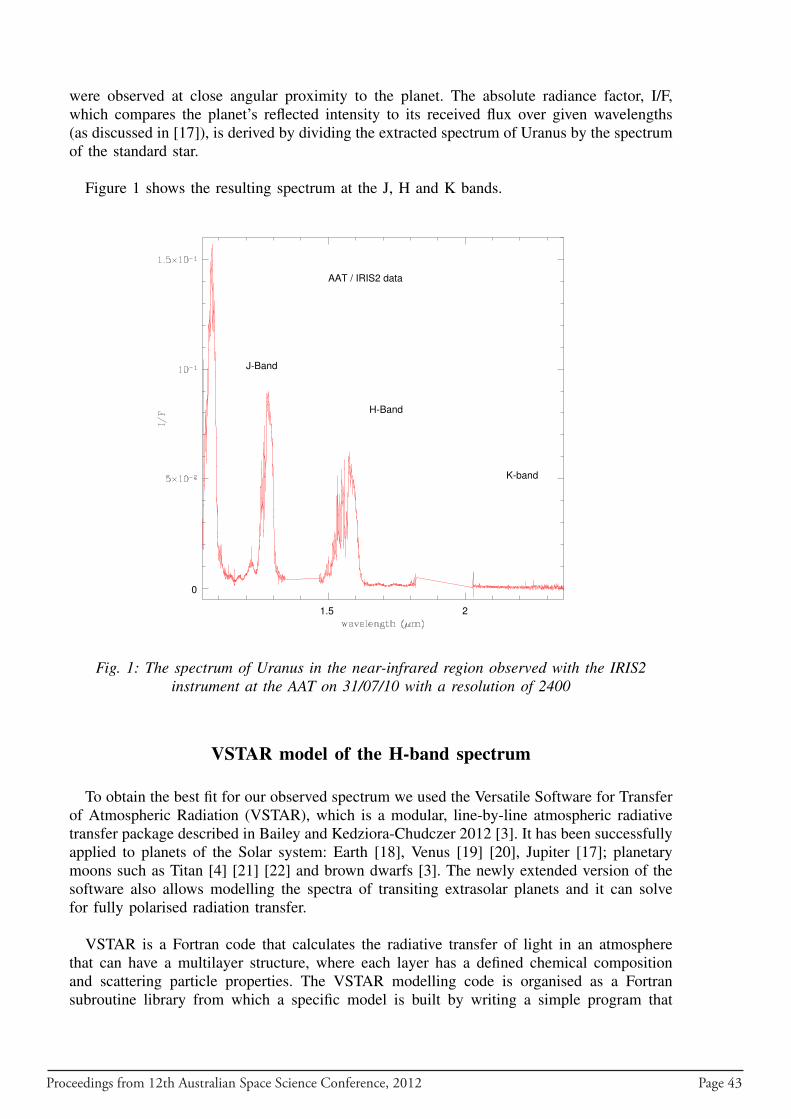
Proceedings from 12th Australian Space Science Conference, 2012 Page 43
were observed at close angular proximity to the planet. The absolute radiance factor, I/F,which compares the planet’s reflected intensity to its received flux over given wavelengths(as discussed in [17]), is derived by dividing the extracted spectrum of Uranus by the spectrumof the standard star.
Figure 1 shows the resulting spectrum at the J, H and K bands.
1.5 2
0
J-Band
H-Band
K-band
AAT / IRIS2 data
Fig. 1: The spectrum of Uranus in the near-infrared region observed with the IRIS2instrument at the AAT on 31/07/10 with a resolution of 2400
VSTAR model of the H-band spectrum
To obtain the best fit for our observed spectrum we used the Versatile Software for Transferof Atmospheric Radiation (VSTAR), which is a modular, line-by-line atmospheric radiativetransfer package described in Bailey and Kedziora-Chudczer 2012 [3]. It has been successfullyapplied to planets of the Solar system: Earth [18], Venus [19] [20], Jupiter [17]; planetarymoons such as Titan [4] [21] [22] and brown dwarfs [3]. The newly extended version of thesoftware also allows modelling the spectra of transiting extrasolar planets and it can solvefor fully polarised radiation transfer.
VSTAR is a Fortran code that calculates the radiative transfer of light in an atmospherethat can have a multilayer structure, where each layer has a defined chemical compositionand scattering particle properties. The VSTAR modelling code is organised as a Fortransubroutine library from which a specific model is built by writing a simple program that
Page 44 Proceedings from 12th Australian Space Science Conference, 2012
calls appropriate routines. The MOD package defines a two dimensional grid of parametersfor each atmospheric layer as a function of wavelength or a wave number. The parametersof the atmosphere such as pressure and temperature for every layer are either known fromdirect measurements or can be solved for in a similar way as described in Hubeny 1995 [23].The LIN package is used to read spectral lines from line databases [4] and the RAY packagederives optical depth due to Rayleigh scattering due to molecules. The PART module is usednext to derive scattering properties of the aerosols and clouds. In this module, one specifiessize distributions and refractive indices and optical depths for all particles present in differentlayers of the atmosphere and the scattering properties are calculated using Lorenz-Mie theory.The major component of the VSTAR package is the RT module, which contains a selectionof radiative transfer solvers including DISORT adapted from Stanmes 1988 [24]. VSTARwas recently upgraded to allow a full four Stokes treatment of the polarized radiative transferproblem [25].
The spectrum of Uranus was modelled by dividing the atmosphere into 58 layers rangingfrom 0 to 136.5 km (or 11285 to 101 mbar) with the temperature-pressure (P-T) profile derivedfrom radio occultations measured with Voyager 2 [26]. For this model we concentrated onthe window surrounding 1.6µm because the K band for Uranus is low flux and databases formethane lines at the temperature of Uranus are not yet well developed for the J band.
Methane Mixing Ratio Profile and Absorption
The distribution of methane over these altitudes is not uniform and the profile of themethane mixing ratio almost certainly depends on the observed latitudes as well. The new,refined profile derived from Irwin et al. 2010 [27] (Figure 2) gave the best fit to our data.The CH4 mixing ratio at the deepest levels of the atmosphere is 4%, which is higher than the1.6% estimated from observations at polar latitudes at pressures higher than 1 bar [28]. Thishigher 4% mixing ratio is consistent with the P-T profile containing warmer lower layers ofthe atmosphere from occultation data [26], as can be seen in the left panel of Fig. 7 of Irwin2010 [27]. Our slit, positioned at the centre of the planetary disk, covers a only a limitedrange of latitudes around the equator. Therefore the single methane profile from Irwin 2010[27] is expected to account for the observed absorption features visible in our data.
Methane is the dominant absorbing species in the atmosphere of Uranus in the near infraredregion. The CH4 molecule has a complex absorption spectrum, which arises due to fourvibrational modes interacting with each other, forming so-called polyads. Although there hasbeen continuing progress in determination of the methane spectrum (see [21]), the high-orderpolyads, which form absorption lines in the near infrared (1 – 2 µm) are not well understood.The HITRAN database at these wavelengths is largely based on empirical measurementsat room temperature, but because their lower-state energies and quantum identifications aremissing, it is difficult to model such lines for different temperatures.
A recent major breakthrough has been a set of deep laboratory measurements of methanelines at room temperature and cryogenic temperatures by the Grenoble group ([29], [30])which provide an excellent line list over the range 1.26 – 1.71 µm. These line data have beenshown to give good models for the spectra of Titan ([4], [21], [31]). We use a line list basedon this new data, as well as other sources at longer wavelengths, as described in Bailey 2012[21].
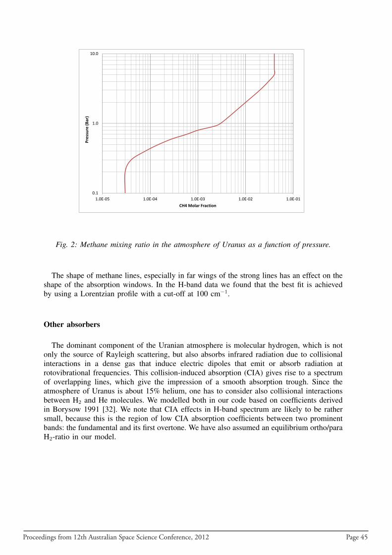
Proceedings from 12th Australian Space Science Conference, 2012 Page 45
0.1
1.0
10.0
1.0E-05 1.0E-04 1.0E-03 1.0E-02 1.0E-01
Pres
sure
(Bar
)
CH4 Molar Fraction
Fig. 2: Methane mixing ratio in the atmosphere of Uranus as a function of pressure.
The shape of methane lines, especially in far wings of the strong lines has an effect on theshape of the absorption windows. In the H-band data we found that the best fit is achievedby using a Lorentzian profile with a cut-off at 100 cm−1.
Other absorbers
The dominant component of the Uranian atmosphere is molecular hydrogen, which is notonly the source of Rayleigh scattering, but also absorbs infrared radiation due to collisionalinteractions in a dense gas that induce electric dipoles that emit or absorb radiation atrotovibrational frequencies. This collision-induced absorption (CIA) gives rise to a spectrumof overlapping lines, which give the impression of a smooth absorption trough. Since theatmosphere of Uranus is about 15% helium, one has to consider also collisional interactionsbetween H2 and He molecules. We modelled both in our code based on coefficients derivedin Borysow 1991 [32]. We note that CIA effects in H-band spectrum are likely to be rathersmall, because this is the region of low CIA absorption coefficients between two prominentbands: the fundamental and its first overtone. We have also assumed an equilibrium ortho/paraH2-ratio in our model.
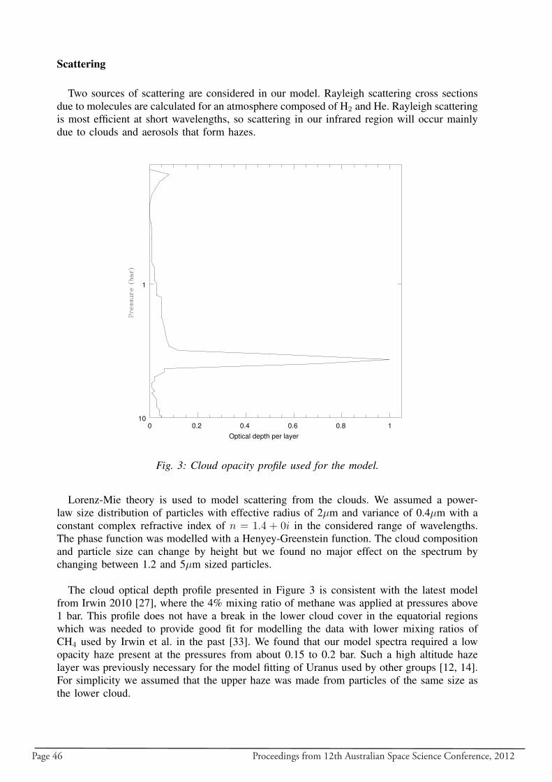
Page 46 Proceedings from 12th Australian Space Science Conference, 2012
Scattering
Two sources of scattering are considered in our model. Rayleigh scattering cross sectionsdue to molecules are calculated for an atmosphere composed of H2 and He. Rayleigh scatteringis most efficient at short wavelengths, so scattering in our infrared region will occur mainlydue to clouds and aerosols that form hazes.
0 0.2 0.4 0.6 0.8 110
1
Optical depth per layer
Fig. 3: Cloud opacity profile used for the model.
Lorenz-Mie theory is used to model scattering from the clouds. We assumed a power-law size distribution of particles with effective radius of 2µm and variance of 0.4µm with aconstant complex refractive index of n = 1.4 + 0i in the considered range of wavelengths.The phase function was modelled with a Henyey-Greenstein function. The cloud compositionand particle size can change by height but we found no major effect on the spectrum bychanging between 1.2 and 5µm sized particles.
The cloud optical depth profile presented in Figure 3 is consistent with the latest modelfrom Irwin 2010 [27], where the 4% mixing ratio of methane was applied at pressures above1 bar. This profile does not have a break in the lower cloud cover in the equatorial regionswhich was needed to provide good fit for modelling the data with lower mixing ratios ofCH4 used by Irwin et al. in the past [33]. We found that our model spectra required a lowopacity haze present at the pressures from about 0.15 to 0.2 bar. Such a high altitude hazelayer was previously necessary for the model fitting of Uranus used by other groups [12, 14].For simplicity we assumed that the upper haze was made from particles of the same size asthe lower cloud.
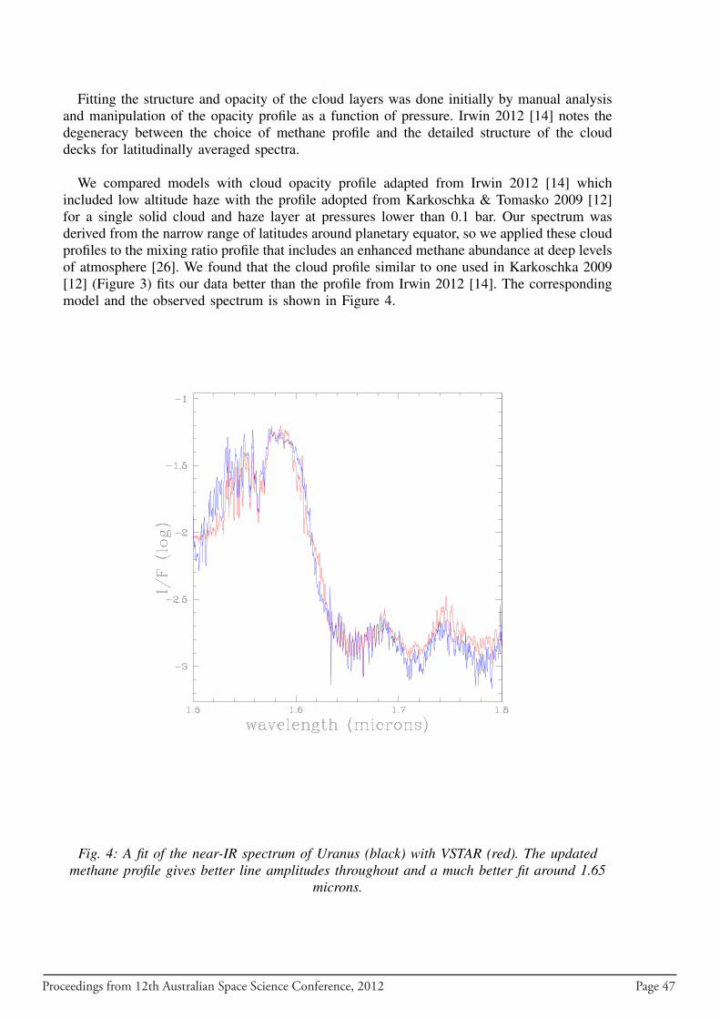
Proceedings from 12th Australian Space Science Conference, 2012 Page 47
Fitting the structure and opacity of the cloud layers was done initially by manual analysisand manipulation of the opacity profile as a function of pressure. Irwin 2012 [14] notes thedegeneracy between the choice of methane profile and the detailed structure of the clouddecks for latitudinally averaged spectra.
We compared models with cloud opacity profile adapted from Irwin 2012 [14] whichincluded low altitude haze with the profile adopted from Karkoschka & Tomasko 2009 [12]for a single solid cloud and haze layer at pressures lower than 0.1 bar. Our spectrum wasderived from the narrow range of latitudes around planetary equator, so we applied these cloudprofiles to the mixing ratio profile that includes an enhanced methane abundance at deep levelsof atmosphere [26]. We found that the cloud profile similar to one used in Karkoschka 2009[12] (Figure 3) fits our data better than the profile from Irwin 2012 [14]. The correspondingmodel and the observed spectrum is shown in Figure 4.
Fig. 4: A fit of the near-IR spectrum of Uranus (black) with VSTAR (red). The updatedmethane profile gives better line amplitudes throughout and a much better fit around 1.65
microns.

Page 48 Proceedings from 12th Australian Space Science Conference, 2012
Deuterium Abundances
The H-band region of the Uranus spectrum can be used to model the ratio of deuterium tohydrogen (D/H). This ratio is an important diagnostic, helping us to understand the process ofSolar System formation. The D/H ratio combined with a solar nebula model provides insightinto the formation of the giant planets, namely where they formed and through what meanstheir deuterium is likely to have been trapped. [34] [35]
The new line data from Wang 2011 [29] provide identification of the CH3D 3ν2 band inthe 1.56 µm window. The most recent modelling of this band from the Gemini North NIFSdata in Irwin 2012 [14] provided a D/H ratio in methane of 9.2 × 10⁻⁵ as compared withthe D/H of the Vienna Standard Mean Ocean Water (V-SMOW) of 1.56 × 10⁻⁴. Deuteriumabundances decrease as we move away from the sun in the current Solar System formationmodel, therefore a vastly different D/H ratio could suggest that Uranus formed far fromits current orbital distance. Uranus’ spin-axial tilt, it has been suggested, could be due tocollisions with large bodies [36], so it would not be entirely surprising if it did form at adifferent distance from where it currently sits and moved die to interactions with large bodies.
The preliminary model in Figure 4 was derived with a D/H of 7.5× 10⁻⁵ notably furtherremoved from the Earth abundance than the value of 9.2× 10⁻⁵ from Irwin 2012 [14]. Thiswas used because it provided us with an apparent best fit for the deuterium-sensitive H-bandwindow, however this resolution of spectra is not sufficient to distinguish this value frompreviously estimated values. We are currently analysing high resolution data (R ∼ 18000)of this region from Gemini North GNIRS from which we should be able to better confinethe best fit for the D/H ratio. The model parameters from the IRIS2 data presented herewill be used as starting parameters for the more detailed and refined model needed to fitthe GNIRS spectrum. For icy objects this ratio is determined by the formation temperatureand hence the orbital radius in the Solar System at which ice formed [37]. Hence, accuratemeasurements can provide information on the formation and early history of the ice giantplanets, and in particular their possible orbital migration [22]. Our GNIRS data should enableimproved determination of the D/H ratio due to its higher spectral resolution compared to theAAT IRIS2 data. The GNIRS observations were also obtained in good seeing conditions, andso have better spatial resolution, which will allow to apply more targeted model parametersfor different ranges of latitudes.
Discussion and Conclusions
Our results show that a much improved model of the spectrum of Uranus in the H-bandregion can be achieved using the new methane spectral line data now available. Because thisline data is not available at wavelengths shorter than 1.26 µm, it is not currently possible tomodel the J-band data using these line-by-line techniques.
This type of model will be a valuable starting point for modelling the much higher resolutionGemini GNIRS data on Uranus that we have taken recently. These higher resolution spectrashould enable much more accurate determinations of the D/H ratio and will also allowsearching for other trace species that might be present in the atmosphere.
Uranus now joins a growing list of Solar System atmospheres that have been successfully
Proceedings from 12th Australian Space Science Conference, 2012 Page 49
modelled with VSTAR and shows the versatility of the methods employed by the software.VSTAR allows the modelling of exoplanetary spectra, such as those that are now beingobtained from transits and secondary eclipses. As has been shown in the modelling of theSolar System giant planets, the quality of the spectral line data is important in achievingsuccessful results. While the methane line data are now good enough for accurate modellingof low temperature objects like Uranus, the line lists are still not sufficiently complete for hightemperature objects such as hot Jupiters, where hot bands of methane become important. Thedesign of VSTAR allows the easy inclusion of updated line lists as they become available,meaning that once these lists are developed, VSTAR will be ready to move on to exoticexoplanets.
We’ve produced a good fit to the observed spectrum with two cloud layers, the upperone of which being a thin haze-like layer, and an adopted mixing ratio. Further analysis isneeded for the deuterium abundance to be well determined and any firm conclusions drawnabout it. GNIRS observations already acquired will be analysed to pin down the deuteriumabundance, although the IRIS2 data we’ve considered here has given us a firmer understandingof the structure and composition of the atmosphere, allowing us to more confidently fine tunethe deuterium abundance. The implications of these findings however are of interest as thedeuterium abundance can give us clues about where a planet has formed and under whatconditions. [4] [14] [17] [22] [37]
Acknowledgments
We acknowledge the support of the Australian Astronomical Observatory in scheduling theobservations presented here in the IRIS2 observing programme.
References
[1] Seidelmann, K., Archinal, B.A., A’Hearn, M.F, et al. “Report of the IAU/IAG WorkingGroup on cartographic coordinates and rotational elements: 2006” Celestial Mechanicsand Dynamical Astronomy, Vol. 98, Issue 3, 2007, 155- 180.
[2] Sromovsky, L.A. and Fry, P.M. ”Dynamics of cloud features on Uranus” Icarus, Vol. 179,Issue 2, 2005, 459- 484.
[3] Bailey J. and Kedziora-Chudczer, L., “Modelling the spectra of planets, brown dwarfsand stars using VSTAR”, MNRAS, Vol. 419, 2012, 1913-1929
[4] Bailey, J., Ahlsved, L. and Meadows, V. S., “The near-IR spectrum of Titan modeledwith an improved methane line list”, Icarus, Vol. 213, 2011, 218 -232
[5] Lindal, G.F., Lyons, J.R., Sweetnam, D.N., Eshleman, V.R., Hinson, D.P., “The atmo-sphere of Uranus - Results of radio occultation measurements with Voyager 2”, Journalof Geophysical Research, Vol. 92, 1987, pp. 14987-15001.
[6] Burgdorf, M., Orton, G., van Cleve, J., Meadows, V., & Houck, J. 2006, “Detectionof new hydrocarbons in Uranus’ atmosphere by infrared spectroscopy”, Icarus, Vol.184,2006, 634-637
[7] Bishop, J., Atreya, S. K., Herbert, F., & Romani, P. 1990, “Reanalysis of Voyager 2 UVSoccultations at Uranus - Hydrocarbon mixing ratios in the equatorial stratosphere”, Icarus,Vol. 88, 1990, 448-464
Page 50 Proceedings from 12th Australian Space Science Conference, 2012
[8] Irwin, P.G.J., Teanby, N.A., Davis, G.R., ”Revised vertical cloud structure of Uranus fromUKIRT/UIST observations and changes seen during Uranus’ Northern Spring Equinoxfrom 2006 to 2008: Application of new methane absorption data and comparison withNeptune” Icarus, Vol. 208, 2010, pp. 913-926.
[9] Smith, B. A., Soderblom, L. A., Beebe, R., Bliss, D., Brown, R. H., Collins, S. A., Boyce,J. M., Briggs, G. A., Brahic, A., Cuzzi, J. N. & Morrison, D. “Voyager 2 in the UranianSystem: Imaging Science Results” Science, Vol. 233, 1986, 43
[10] Sromovsky, L. A., Fry, P. M., Hammel, H. B., et al. “Uranus at equinox: Cloudmorphology and dynamics” Icarus, Vol. 203, 2009, 265-286
[11] Kostogryz, N. M. “Study of the Reasons for the Geometric Albedo Variations of Uranus”Proceedings of the 14th Young Scientists Conference on Astronomy and Space Physics,44-48
[12] Karkoschka, E., Tomasko, M. “The haze and methane distributions on Uranus fromHST-STIS spectroscopy.” Icarus Vol. 202, 2009, 287309.
[13] Sromovsky, L. A., Fry, P. M. and J. H. Kim “High-latitude depletion of methane onUranus” EPSC-DPS Joint Meeting 2011, EPSC Abstracts Vol. 6, 2011
[14] Irwin, P. G. J., de Bergh, C., Courtin, R., et al. “The application of new methane lineabsorption data to Gemini-N/NIFS and KPNO/FTS observations of Uranus near-infraredspectrum” Icarus, Vol. 220, 2012, 369–382
[15] Campargue, A., Wang, L., Mondelain, D., Kassi, S. et al., “An empirical line listfor methane in the 1.26-1.71 µm region for planetary investigations (T = 80-300 K).Application to Titan”, Icarus, Vol. 219, 2012, 110-128
[16] Shortridge K., Meatheringham S. J., Carter B. D. & Ashley M. C. B. “Making theFIGARO Data Reduction System Portable” PASA, Vol.12, 1995, 244
[17] Kedziora-Chudczer, L. and Bailey, J. “Modelling the near-IR spectra of Jupiter usingline-by-line methods” MNRAS, vol.414, 2011,1483-1492
[18] Hough, J.H., et al. “PlanetPol: A Very High Sensitivity Polarimeter” Mon. Not. R. Astr.Soc., Vol. 118, 2006, 1302-1318.
[19] Bailey, J., Meadows, V.S., Chamberlain, S., Crisp, D., “The temperature of the Venusmesosphere from O2(a1∆g) airglow observations,” Icarus 197, 247-259.
[20] Bailey, J. “A comparison of water vapor line parameters for modeling the Venus deepatmosphere. ” Icarus Vol. 201, 2009, 444-453.
[21] Bailey, J., “Methane and Deuterium in Titan’s Atmosphere”, Proceedings of the 11thAustralian Space Science Conference, 2012, Vol. 55, 64 - 76
[22] Kedziora-Chudczer, L., Bailey, J. & Horner, J. “Observations of the D/H ratio in Methanein the atmosphere of Saturn’s moon, Titan - where did the Saturnian system form?”Proceedings of the 12th Australian Space Science Conference, Submitted
[23] Hubeny, I., & Lanz, T. , “Non-LTE line-blanketed model atmospheres of hot stars. 1:Hybrid complete linearization/accelerated lambda iteration method”, ApJ, Vol. 439, 1995,875
[24] Stanmes, K., Tsay, C. S., Wiscombe, W. & Jayaweera, K. “A numerically stablealgorithm for discrete-ordinate-method radiative transfer in multiple scattering and emittinglayers media” Appl. Opt, Vol. 27.1988, Issue 12, 2502.
[25] Kedziora-Chudczer, L., Bailey, J., ”Application of the VSTAR Code for Modeling ofSpectra and Polarization Curves of Hot Jupiters”, AAS/Division for Extreme Solar SystemsAbstracts, Vol. 2, 2011, p. 4012.
[26] Lindal, G. F., Lyons, J. R., Sweetnam, D. N., Eshleman, V. R., Hinson, D. P. “Theatomsphere of Uranus – Results of radio occultation measurements with Voyager 2.” J.Geophys. Res. Vol.92 (11), 1087, 14987-15001
Proceedings from 12th Australian Space Science Conference, 2012 Page 51
[27] Irwin, P.G J., Teanby, N. A. and Davis, G. R. “Revised vertical cloud structure ofUranus from UKIRT/UIST observations and changes seen during Uranus’ Northern SpringEquinox from 2006 to 2008: Application of new methane absorption data and comparisonwith Neptune” Icarus, Vol. 208, 2010, 913-926
[28] Karkoschka, E., Tomasko, M. “Methane absorption coefficients for the jovian planetsfrom laboratory, Huygens, and HST data” Icarus Vol. 205, 2010, 674-694.
[29] Wang, L., Kassi, S., Liu, A.W., Hu, S.M., Campargue, A., “The 1.58 µm transparencywindow of methane (6165-6750 cm-1): Empirical line list and temperature dependencebetween 80 and 296 K” J. Quant. Spectrosc. Radiat. Trans., Vol. 112, 2011, 937-951.
[30] Campargue, A., Wang, L., Kassi, S, Masat, M.,, Votava, O., “Empirical line parametersof methane in the 1.63-1.48 µm transparency window by high sensitivity Cavity RingDown Spectroscopy” Chemical Physics, vol. 373, 2010, 2034-210.
[31] De Bergh, C. et al., “Application of a new set of methane line parameters to the modelingof Titan’s spectrum in the 1.58 µm window”. Plan. Space Sci, Vol. 61, 2012, pp 85-98.
[32] Borysow, A. . “Modeling of collision-induced infrared absorption spectra of H2- H2pairs in the fundamental band at temperatures from 20 to 300 K. Icarus, Vol. 92, 1991,273- 279.
[33] Irwin, P.G J., Teanby, N. A. and Davis, G. R. “Latitudinal variations in Uranus’vertical cloud structure from UKIRT UIST observations” The Astrophysical Journal, Vol.665,2007, L71-L74
[34] Hersant, F., Gautier, D., and Hure, J-M. ”A two-dimensional model for the primordialnebula constrained by D/H measurements in the solar system: Implications for theformation of giant planets.” Astrophysical Journal, Vol. 554, 2001, 391-407.
[35] Horner, J., Mousis, O., Aliber, Y., Lunine, J., Blanc, M. ”Constraints from deuteriumon the formation of icy bodies in the Jovian system and beyond.” Planetary and SpaceScience, Vol. 56, Issue 12., 2008, 1585-1595.
[36] Korycansky, D.G., Bodenheimer, P., Cassen, P., Pollack, J.B. ”One-dimentional calcula-tions of a large impact on Uranus.” Icarus, Vol. 84, Issue 2, 1990, 528-541.
[37] Horner, J., Mousis, O. and Hersant, F. ”Constraints on the Formation Regions of Cometsfrom their D:H ratios” Earth, Moon and Planets, Vol. 100, Issue 1-2, 2007, pp. 43 - 56

Page 52 Proceedings from 12th Australian Space Science Conference, 2012
Proceedings from 12th Australian Space Science Conference, 2012 Page 53
Observations of the D/H ratio in Methane in the atmosphere ofSaturn’s moon, Titan - where did the Saturnian system form?
Lucyna Kedziora-Chudczer ∗, Jeremy Bailey ∗ and Jonathan Horner∗
∗ Department of Astrophysics, School of Physics, The University of New South Wales,Sydney, Australia 2052
Summary: The details of the Solar system’s formation are still heavily debated. Questionsremain about the formation locations of the giant planets, and the degree to which volatilematerial was mixed throughout the proto-planetary system. One diagnostic which offers greatpromise in helping to unravel the history of planet formation is the study of the level ofdeuteration in various Solar system bodies. For example, the D/H ratio of methane in theatmosphere of Titan can be used as a diagnostic of the initial conditions of the solar nebulawithin the region of giant planet formation, and can help us to determine where Titan (and, byextension, the Saturnian system) accreted its volatile material. The level of Titanian deuterationalso has implications for both the sources and long term evolution of Titan’s atmosphericcomposition. We present the results of observations taken in the 1.58 µm window using theNIFS spectrometer on the Gemini telescope, and model our data using the VSTAR line–by–line transfer model, which yields a D/H ratio for Titan’s atmosphere of (143 ± 16) × 10−6
[1]. We are currently in the process of modeling the Gemini high resolution GNIRS spectrausing new sets of line parameters derived for methane in the region between 1.2-1.7 µm [2].
Keywords: Titan, methane, spectroscopy, radiative transfer, deuterium, planetary formation
Introduction
Over the years, our understanding of the formation of our Solar system has evolveddramatically. For a long time, it was believed that our planetary system was formed by achance encounter between the Sun and another star, which passed sufficiently close to theSun to draw a lengthy tongue of material from it which then coalesced to form the planets(e.g. [3, 4]). In recent decades, it has become widely accepted that our planetary systeminstead formed from a dynamically cold disk1 of dust and gas around the proto-Sun. By theearly 1990s, it was thought that the process of planetary formation was essentially a leisurely,gentle process that occurred at a fixed location within the proto-planetary disk (e.g. [5]).
It was soon realised that the planet formation process must be somewhat more compli-cated, involving proto-planets and planets migrating over many astronomical units from theirformation location to their current locations. This sea-change in our understanding of planet
1Objects moving on dynamically cold orbits have very low orbital eccentricity and inclination. Therefore a dynamically colddisk is rather flattened and consists of the protoplanetary material in orbits of very low eccentricity. Objects in dynamicallycold orbits typically only experience collisions at very low relative velocities. Such collisions tend to be constructive ratherthan destructive.
Page 54 Proceedings from 12th Australian Space Science Conference, 2012
formation came about, in part, as a result of the discovery of the first planets found aroundSun-like stars (e.g. [6]), which were found moving on totally unexpected orbits (Jupiter-sizeplanets orbiting far closer to their host stars than Mercury to our Sun). Within our own Solarsystem, planet formation models featuring migration were found to be necessary in order toexplain various aspects of the distribution of small bodies in the outer Solar system includingthe orbits of Pluto and the Plutinos (e.g. [7, 8]), the proposed Late Heavy Bombardment ofthe inner Solar system (e.g. [9]) and the populations of Jovian and Neptunian Trojans (e.g.[10, 11]).
Although it is now widely accepted that the giant planets migrated significant distancesbefore reaching their current locations, the nature, range, and pace of that migration are stillheavily debated. Some models suggest a relatively sedate migration for the giant planets (e.g.[12]), whilst others suggest highly chaotic migration featuring significant mutual scatteringbetween the giant planets (e.g. [13]). Whilst it is likely that dynamical studies of the smallbody populations in the outer Solar system may help to resolve the unanswered questionof the nature of planetary migration (e.g. [14, 15]), the observation of isotopic abundancesin the ices and atmospheres of objects in the outer Solar system will provide an importantindependent test of their formation locations (e.g. [16, 17]). In particular, the study of thedeuterium-to-hydrogen (D/H) ratio in the icy and gaseous material in the outer Solar systemmay well provide a signpost to the formation location of the bodies in question.
In this work, we present the first results of an observational program targeted at determiningthe D/H ratio within methane in the atmosphere of Saturn’s largest satellite, Titan. In the nextsection, we describe in more detail the current state of play in our understanding of theway in which the D/H ratio varied through the proto-planetary disk, before briefly discussingthe origin of methane in Titan’s atmosphere in the following section. Next we detail ourobservations of Titan and describe our modelling of the Titanian spectrum. Finally, we presentour conclusions and discuss future work.
Deuterium and the formation of the Solar system
Protium (1H) and deuterium (2H or D) are the only two stable isotopes of hydrogen.The largest mass difference between two isotopes of any element leads to rather distinctproperties of hydrogen isotopologues (for example HDO and H2O). Differences in boilingpoint, vapour pressure and reactivity of compounds with different isotopes will result in theirhaving unique natural abundances. Once formed, a process of isotopic fractionation (resultingfrom the different physical properties of the two isotopes) can lead to the physical separationof isotopologues through evaporation, condensation, melting or diffusion. The D/H ratio hastherefore long been considered to be a useful diagnostic of the geological history of rockformations, bodies of fluid and organic materials.
Deuterium formed during the Big Bang is subsequently destroyed in stars, and therefore itsabundance in the interstellar medium decreases with time. Currently, the D/H ratio in the localinterstellar medium is of the order of 15×10−6 [18], while the initial value, immediately afterthe big bang, may well have been as high as 30×10−6 [19]. The D/H ratio in the protostellarsolar nebula has been estimated using measurements of D/H in the atmospheres of Jupiterand Saturn, because HD does not fractionate during the transition from the molecular tometallic form. Observations from the Galileo probe mass spectrometer provide a D/H value
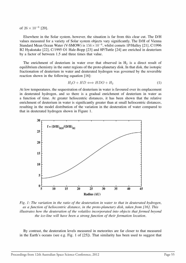
Proceedings from 12th Australian Space Science Conference, 2012 Page 55
of 26 × 10−6 [20].
Elsewhere in the Solar system, however, the situation is far from this clear cut. The D/Hvalues measured for a variety of Solar system objects vary significantly. The D/H of ViennaStandard Mean Ocean Water (V-SMOW) is 156×10−6, whilst comets 1P/Halley [21], C/1996B2 Hyakutake [22], C/1995 O1 Hale-Bopp [23] and 8P/Tuttle [24] are enriched in deuteriumby a factor of between 1.5 and three times that value.
The enrichment of deuterium in water over that observed in H2 is a direct result ofequilibrium chemistry in the outer regions of the proto-planetary disk. In that disk, the isotopicfractionation of deuterium in water and deuterated hydrogen was governed by the reversiblereaction shown in the following equation [16]:
H2O + HD ⇐⇒ HDO + H2 (1)
At low temperatures, the sequestration of deuterium in water is favoured over its emplacementin deuterated hydrogen, and so there is a gradual enrichment of deuterium in water asa function of time. At greater heliocentric distances, it has been shown that the relativeenrichment of deuterium in water is significantly greater than at small heliocentric distances,resulting in the model distribution of the variation in the deuteration of water compared tothat in deuterated hydrogen shown in Figure 1.
Fig. 1: The variation in the ratio of the deuteration in water to that in deuterated hydrogen,as a function of heliocentric distance, in the proto-planetary disk, taken from [16]. This
illustrates how the deuteration of the volatiles incorporated into objects that formed beyondthe ice-line will have been a strong function of their formation location.
By contrast, the deuteration levels measured in meteorites are far closer to that measuredin the Earth’s oceans (see e.g. Fig. 1 of [25]). That similarity has been used to suggest that
Page 56 Proceedings from 12th Australian Space Science Conference, 2012
the bulk of the Earth’s water was delivered by asteroidal, rather than cometary bodies2 - with[26] suggesting that, if the carbonaceous chondrites were the main source of oceanic water,another suggested source (the comets) could have contributed only a small fraction (less than10%). Following this logic, it has often been assumed that the initial volatile budget of all theterrestrial planets would have been identical to that of the Earth, although [27] showed thatthe terrestrial planets would have experienced significantly different contributions of volatilesfrom cometary and asteroidal bodies.
A number of studies (e.g. [25, 28, 16]) have suggested that the D/H ratio within icesaccreted in the outer Solar system should vary significantly as a function of heliocentricdistance within the Solar nebula. The lowest D/H ratios would be found in objects whichaccreted near the ice-line, the innermost location where water could condense as a solid, andthe largest D/H ratios would be found in volatiles that condensed beyond the current orbit ofNeptune. Figure 1 shows the predicted enrichment in D/H for water over that in deuteratedhydrogen as a function of heliocentric distance in the outer Solar system. It is clear that objectsthat formed at different heliocentric distances would have incorporated volatiles containingvastly different amounts of deuterium. The less stirred the disk, the more pronounced thevariation in D/H as a function of heliocentric distance would be between one body and the next(since increased stirring would doubtless bring icy bodies with high deuteration to the innerreaches of the nebula). It is highly likely that the bulk of volatile material accreted by a givenobject would be sourced from its immediate surroundings, however, and so measurements ofthe deuteration of objects in the outer Solar system give us a tool by which their formationlocation can be constrained.
Origin of CH4 in the atmosphere of Titan
In 1981, Prinn and Fegley [30] assumed that, in the primordial solar nebula, carbonand nitrogen were entirely sequestered in CO and N2. During the early stages of Saturn’sformation, a dense and warm sub-nebula developed, which enabled the conversion of CO toCH4 and N2 into NH3. This methane and ammonia was accreted to form icy planetisimals,the building blocks of Titan. By contrast, Mousis et al. [31] argued that such conversion ofCO and N2 into methane and ammonia is unlikely to occur in conditions that would havebeen prevalent in the Saturn sub-nebula, and that therefore CH4 would have to be present inthe primary solar nebula in order to explains its accretion onto Titan.
According to the first model, methane becomes enriched in deuterium gradually whenCH3D in vapour phase exchanges deuterium with hydrogen. After the temperature drops below200K, this process stops, but isotopic fractionation can continue through solar photolysis andoutgassing processes.
The model put forward by Mousis et al. instead assumed that vaporisation of CH4 hap-pened during the infall of icy planetisimals onto the protoplanetary disk, which allowed theexchange of deuterium with hydrogen from the solar nebula. Methane was later releasedfrom the subsurface layers to the atmosphere of Titan. The D/H ratio predicted from thismodel is in good agreement with measurements without requiring additional fractionation
2The origin of the Earth’s water has long been debated, with most modern theories favouring an exogeneous source ofour planet’s oceans. We direct the interested reader to section 4, ”Planetary Features” of [29], and references therein, for adetailed discussion of the origin of Earth’s water.
Proceedings from 12th Australian Space Science Conference, 2012 Page 57
to have occurred. Since methane undergoes solar photolysis by breaking into hydrocarbons,cryovolcanism was proposed as its replenishment mechanism.
More recently Atreya et al. [32] have suggested that so-called “serpentinization” reactions(i.e. hydrothermal reactions between silicates and water) in the interior of Titan could generateCH4. However, Mousis et al. [33] point out that this is unlikely because it would imply arelatively low value for the D/H of the water involved (similar to the V-SMOW value). Theyargue that water ice delivered to Titan should have a higher D/H, similar to that measured incomets, and in the Enceladus plume [34] and that a primordial origin for Titan’s methane ismore likely.
D/H ratio measurements in Titan’s atmosphere
Two methods were used to determine the D/H ratio in Titan’s atmosphere. In-situ measure-ments were taken by the Cassini-Huygens probe [35], and used the abundance of molecularand deuterated hydrogen measured by the gas chromatograph mass spectrometer carried on-board, yielding a D/H ratio of (135 ± 30) × 10−6 for the satellite’s atmosphere.
Measurements of the D/H ratio can also be obtained using remote sensing observationsof the spectrum of Titan from the Cassini spacecraft and ground-based telescopes. Theseobservations are analysed using radiative transfer models, such as the VSTAR model describedin [36]. Along with molecular nitrogen, which is the most abundant gas in Titans atmosphere,methane is a major component, comprising a few percent of the atmosphere, as measuredby mole fraction. The spectrum of methane has four vibrational modes forming overlappingabsorption bands in the infrared region, which become increasingly complex towards higherenergies. Measurements of Titan’s D/H ratio from observations in the thermal infrared withthe Cassini CIRS instrument give a value of (159 ± 33) × 10−6 [37]
New, improved laboratory measurements of methane lines in the near infrared at temper-atures relevant to cold regions of the Solar system are now becoming available for use inradiative transfer models [2]. These line lists can be used to model spectra of Titan observedwith near infrared spectrometers on ground-based telescopes. The model shown in Figure 2yields a D/H ratio of (143 ± 16) × 10−6 [1] for the atmosphere of Titan. De Bergh et al.[38] used a different set of data from KPNO/FTS with the improved list of methane linesfrom [39], and obtained a rather different result (113± 25)× 10−6. It is becoming clear thata number of different datasets have to be analysed and modelled to resolve the differencesbetween estimates obtained from different methods.
Modelling of the 1.58 µm window of Titan’s atmosphere
We obtained spectra of Titan in the J, H and K bands (1.1 to 2.4 µm) with the Near-InfraredIntegral Field Spectrometer (NIFS) on the Gemini North 8m telescope. The NIFS spectrum inthe 1.53 to 1.59 µm region and its VSTAR model are reproduced from [1] in Figure 2, wheredata and model are shown in the top panel. In the second panel from the top, the residualsare plotted between the data and the model, which includes only CH4 features. In the panelbelow, the absorption from the CH3D are added, while in the bottom panel the addition ofCO 3-0 lines based on a mixing ratio of 50 ppmv completes the removal of unaccounted
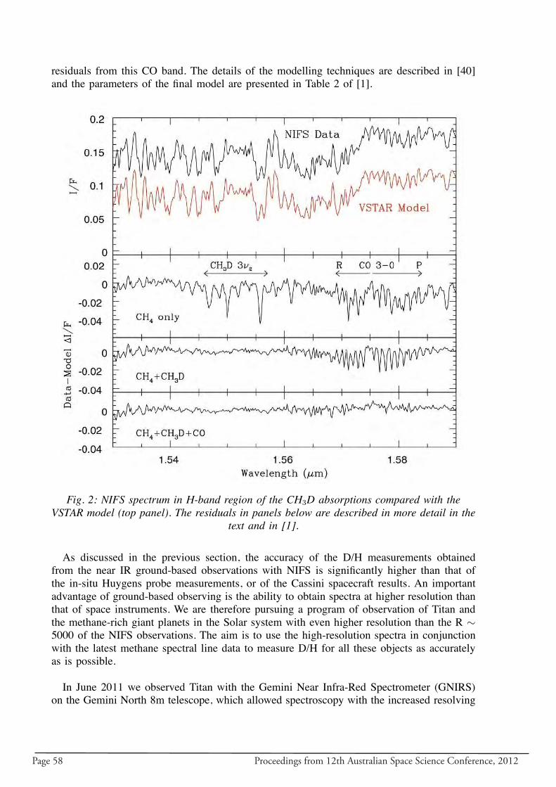
Page 58 Proceedings from 12th Australian Space Science Conference, 2012
residuals from this CO band. The details of the modelling techniques are described in [40]and the parameters of the final model are presented in Table 2 of [1].
Fig. 2: NIFS spectrum in H-band region of the CH3D absorptions compared with theVSTAR model (top panel). The residuals in panels below are described in more detail in the
text and in [1].
As discussed in the previous section, the accuracy of the D/H measurements obtainedfrom the near IR ground-based observations with NIFS is significantly higher than that ofthe in-situ Huygens probe measurements, or of the Cassini spacecraft results. An importantadvantage of ground-based observing is the ability to obtain spectra at higher resolution thanthat of space instruments. We are therefore pursuing a program of observation of Titan andthe methane-rich giant planets in the Solar system with even higher resolution than the R ∼
5000 of the NIFS observations. The aim is to use the high-resolution spectra in conjunctionwith the latest methane spectral line data to measure D/H for all these objects as accuratelyas is possible.
In June 2011 we observed Titan with the Gemini Near Infra-Red Spectrometer (GNIRS)on the Gemini North 8m telescope, which allowed spectroscopy with the increased resolving
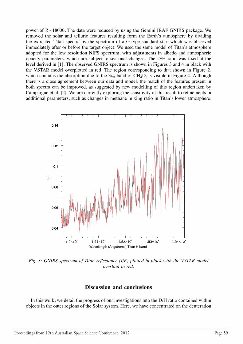
Proceedings from 12th Australian Space Science Conference, 2012 Page 59
power of R∼18000. The data were reduced by using the Gemini IRAF GNIRS package. Weremoved the solar and telluric features resulting form the Earth’s atmosphere by dividingthe extracted Titan spectra by the spectrum of a G-type standard star, which was observedimmediately after or before the target object. We used the same model of Titan’s atmosphereadopted for the low resolution NIFS spectrum, with adjustments in albedo and atmosphericopacity parameters, which are subject to seasonal changes. The D/H ratio was fixed at thelevel derived in [1]. The observed GNIRS spectrum is shown in Figures 3 and 4 in black withthe VSTAR model overplotted in red. The region corresponding to that shown in Figure 2,which contains the absorption due to the 3ν2 band of CH3D, is visible in Figure 4. Althoughthere is a close agreement between our data and model, the match of the features present inboth spectra can be improved, as suggested by new modelling of this region undertaken byCampargue et al. [2]. We are currently exploring the sensitivity of this result to refinements inadditional parameters, such as changes in methane mixing ratio in Titan’s lower atmosphere.
0.04
0.06
0.08
0.1
0.12
0.14
0.04
0.06
0.08
0.1
0.12
0.14
0.04
0.06
0.08
0.1
0.12
0.14
Wavelength (Angstroms) Titan H band
0.04
0.06
0.08
0.1
0.12
0.14
Fig. 3: GNIRS spectrum of Titan reflectance (I/F) plotted in black with the VSTAR modeloverlaid in red.
Discussion and conclusions
In this work, we detail the progress of our investigations into the D/H ratio contained withinobjects in the outer regions of the Solar system. Here, we have concentrated on the deuteration
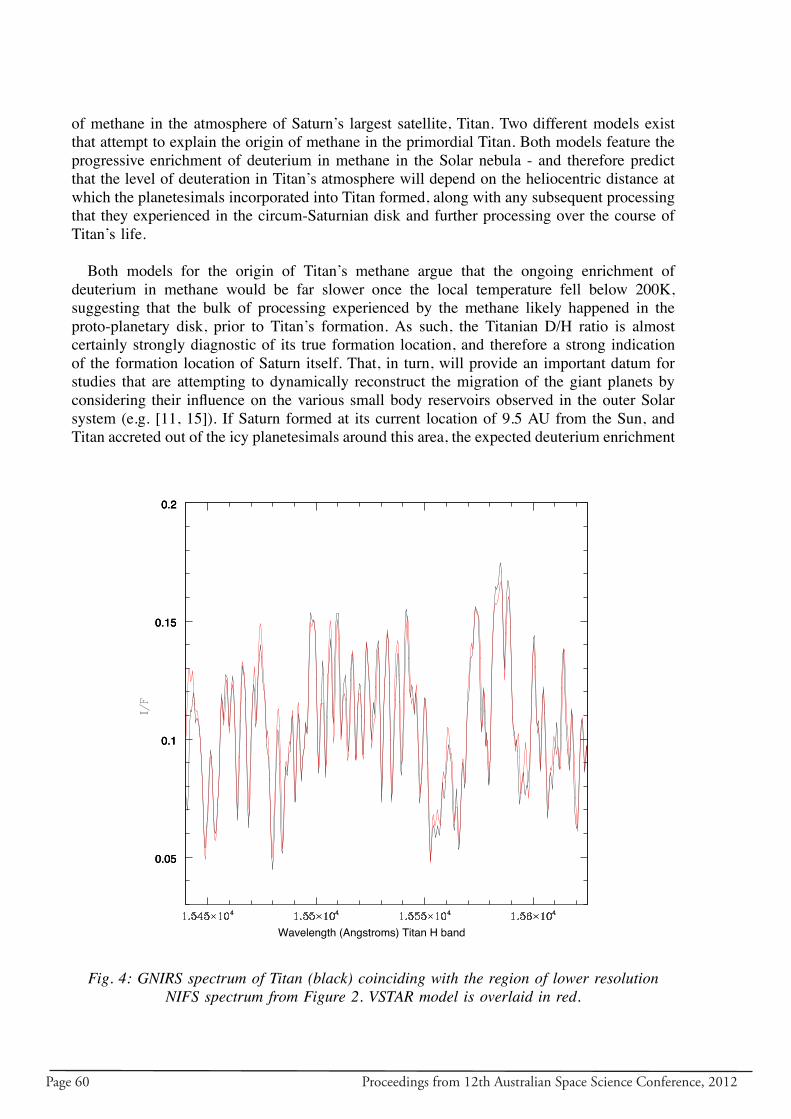
Page 60 Proceedings from 12th Australian Space Science Conference, 2012
of methane in the atmosphere of Saturn’s largest satellite, Titan. Two different models existthat attempt to explain the origin of methane in the primordial Titan. Both models feature theprogressive enrichment of deuterium in methane in the Solar nebula - and therefore predictthat the level of deuteration in Titan’s atmosphere will depend on the heliocentric distance atwhich the planetesimals incorporated into Titan formed, along with any subsequent processingthat they experienced in the circum-Saturnian disk and further processing over the course ofTitan’s life.
Both models for the origin of Titan’s methane argue that the ongoing enrichment ofdeuterium in methane would be far slower once the local temperature fell below 200K,suggesting that the bulk of processing experienced by the methane likely happened in theproto-planetary disk, prior to Titan’s formation. As such, the Titanian D/H ratio is almostcertainly strongly diagnostic of its true formation location, and therefore a strong indicationof the formation location of Saturn itself. That, in turn, will provide an important datum forstudies that are attempting to dynamically reconstruct the migration of the giant planets byconsidering their influence on the various small body reservoirs observed in the outer Solarsystem (e.g. [11, 15]). If Saturn formed at its current location of 9.5 AU from the Sun, andTitan accreted out of the icy planetesimals around this area, the expected deuterium enrichment
0.05
0.1
0.15
0.2
0.05
0.1
0.15
0.2
0.05
0.1
0.15
0.2
Wavelength (Angstroms) Titan H band
0.05
0.1
0.15
0.2
Fig. 4: GNIRS spectrum of Titan (black) coinciding with the region of lower resolutionNIFS spectrum from Figure 2. VSTAR model is overlaid in red.
Proceedings from 12th Australian Space Science Conference, 2012 Page 61
factor in Titan f would be of the order of 5 times the initial proto-solar value (see figure 1).If the value of 26 × 10−6 obtained for Jupiter [20] is representative of the protosolar valuewe predict ∼ 130× 10−6 for an object formed at this location. The value (143± 16)× 10−6
obtained from the NIFS data [1] is consistent with this scenario. However, more accuratemeasurements would help to further constrain the formation location and mechanism.
We are currently in the process of analysing data obtained using higher resolution GNIRSfor the four giant planets (Jupiter, Saturn, Uranus and Neptune) in the H and K bands. Weintend to apply a similar modelling technique as presented in this work to derive accurateD/H values for each of those planets in turn. We will also use our GNIRS observations for theK-band 2µm regions to measure the D/H ratio from the CH3D absorption due to the ν5 +3ν6
and 2ν3 + 2ν6 bands, which were detected in Titan’s NIFS spectrum (as presented in [40]).However the detailed modelling of this region is dependent on availability of intensities inthese bands, which still await laboratory measurement.
It seems likely that the D/H ratio in the atmospheres of Jupiter and Saturn will be stronglyinfluenced by their accretion of hydrogen and deuterated hydrogen directly from the proto-planetary nebula, and therefore they might be expected to display values similar to the Solarvalue (since only a small fraction of their hydrogen will have been accreted in the formof solid volatile material such as water and methane). By contrast, the hydrogen/deuteriumbudget of Uranus and Neptune was most likely primarily accreted in the form of solids - suchas water, methane and ammonia. The deuteration of these planets, then, will likely stronglyreflect the accretion location of their volatile budgets - and therefore, the location at whichthose planets accreted the bulk of their mass. The situation is perhaps even more clear cut forthe regular satellites of the giant planets (such as Titan), whose volatile budget will have beenaccreted entirely in the form of solid planetesimals. However, it is possible that the volatilesaccreted to these bodies underwent further processing in circum-planetary disks around theirhost planet prior to accreting to form the satellites we observe today.
Our future studies of deuteration in the outer Solar system will help to answer a varietyof outstanding questions on the formation and evolution of our Solar system, and, taken inconcert with independent dynamical tests of planetary migration, should allow us to finallydetermine the true architecture of our Solar system prior to the migration of its giant planets.
Acknowledgments
Based on observations obtained at the Gemini Observatory, which is operated by the Associ-ation of Universities for Research in Astronomy, Inc., under a cooperative agreement with theNSF on behalf of the Gemini partnership: the National Science Foundation (United States),the Science and Technology Facilities Council (United Kingdom), the National ResearchCouncil (Canada), CONICYT (Chile), the Australian Research Council (Australia), Ministerioda Ciencia, Tecnologia e Inovacao (Brazil) and Ministerio de Ciencia, Tecnologıa e InnovacionProductiva (Argentina). The observations were obtained under the program GN-2011A-Q-36.
Page 62 Proceedings from 12th Australian Space Science Conference, 2012
References
[1] Bailey, J., “Methane and Deuterium in Titan’s Atmosphere”, Proceedings of the 11thAustralian Space Science Conference, 2012, Vol. 55, 64 - 76
[2] Campargue, A., Wang, L., Mondelain, D., Kassi, S. et al., “An empirical line listfor methane in the 1.26-1.71 µm region for planetary investigations (T = 80-300 K).Application to Titan”, Icarus, Vol. 219, 2012, 110
[3] Lyttleton, R. A., ”The Origin of the Solar System” Monthly Notices of the RoyalAstronomical Society Vol. 9 , 1936, 559
[4] Woolfson, M. M. ”A Capture Theory of the Origin of the Solar System” Proceedings ofthe Royal Society of London. Series A, Mathematical and Physical Sciences, Volume 282,Issue 1391, 1964, pp. 485-507
[5] Lissauer, J. J. ”Planet formation” Annual Review of Astronomy and Astrophysics Vol. 31,1993, pp. 129 - 174
[6] Mayor, M. and Queloz, D. ”A Jupiter-mass companion to a solar-type star” Nature Vol.378, 1995, pp. 355 - 359
[7] Malhotra, R. ”The origin of Pluto’s peculiar orbit” Nature Vol. 365, Issue 6449, 1993,pp. 819 - 821
[8] Malhotra, R. ”The Origin of Pluto’s Orbit: Implications for the Solar System BeyondNeptune” Astronomical Journal Vol. 110, 1995, p. 420
[9] Gomes, R., Levison, H. F., Tsiganis, K. and Morbidelli, A. ”Origin of the cataclysmicLate Heavy Bombardment period of the terrestrial planets” Nature, Vol. 435, Issue 7041,2005, pp. 466-469
[10] Morbidelli, A., Levison, H. F., Tsiganis, K. and Gomes, R. ”Chaotic capture of Jupiter’sTrojan asteroids in the early Solar system” Nature, Vol. 435, Issue 7041, 2005, pp. 462 -465
[11] Lykawka, P. S., Horner, J., Jones, B. W. and Mukai, T. ”Origin and dynamical evolutionof Neptune Trojans - I. Formation and planetary migration” Monthly Notices of the RoyalAstronomical Society Vol. 398, 2009, pp. 1715 - 1729
[12] Lykawka, P. S., Horner, J., Jones, B. W. and Mukai, T. ”Formation and dynamicalevolution of the Neptune Trojans - the influence of the initial Solar system architecture”Monthly Notices of the Royal Astronomical Society Vol.. 404, Issue 3, 2010, pp. 1272-1280
[13] Thommes, E. W., Duncan, M. J. and Levison, H. F. ”The Formation of Uranus andNeptune among Jupiter and Saturn” The Astronomical Journal Vol 123, Issue 5, 2002, pp.2862 - 2883
[14] Lykawka, P. S. and Horner, J. ”The capture of Trojan asteroids by the giant planetsduring planetary migration” Monthly Notices of the Royal Astronomical Society Vol. 405,Issue 2, 2010, pp. 1375 - 1383
[15] Horner, J., Koch, F. E. and Lykawka, P. S. ”Capturing Trojans and Irregular Satellites -the key required to unlock planetary migration” Proceedings of the 12th Annual AustralianSpace Science Conference, 2013, submitted
[16] Horner, J., Mousis, O. and Hersant, F. ”Constraints on the Formation Regions of Cometsfrom their D:H ratios” Earth, Moon and Planets, Vol. 100, Issue 1-2, 2007, pp. 43 - 56
[17] Horner, J., Mousis, O., Alibert, Y., Lunine, J. I. and Blanc, M. ”Constraints fromdeuterium on the formation of icy bodies in the Jovian system and beyond” Planetaryand Space Science, Vol. 56, Issue 2, 2008, pp. 1585 - 1595
[18] McCullough, P., “The interstellar deuterium-to-hydrogen ratio - A reevaluation of Lymanabsorption-line measurements”, ApJ Vol. 390, 1992, 213-218
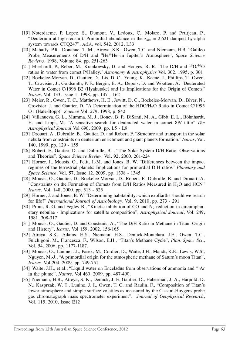
Proceedings from 12th Australian Space Science Conference, 2012 Page 63
[19] Noterdaeme, P. Lopez, S., Dumont, V., Ledoux, C., Molaro, P. and Petitjean, P.,“Deuterium at high-redshift: Primordial abundance in the zabs = 2.621 damped Ly-alphasystem towards CTQ247”, A&A, vol. 542, 2012, L33
[20] Mahaffy, P.R., Donahue, T. M., Atreya, S.K., Owen, T.C. and Niemann, H.B. “GalileoProbe Measurements of D/H and 3He/4He in Jupiter’s Atmosphere”, Space ScienceReviews, 1998, Volume 84, pp. 251-263
[21] Eberhardt, P., Reber, M., Krankowsky, D. and Hodges, R. R. ”The D/H and 18O/16Oratios in water from comet P/Halley.” Astronomy & Astrophysics Vol. 302, 1995, p. 301
[22] Bockelee-Morvan, D., Gautier, D., Lis, D. C., Young, K., Keene, J., Phillips, T., Owen,T., Crovisier, J., Goldsmith, P. F., Bergin, E. A., Depois, D. and Wootten, A. ”DeuteratedWater in Comet C/1996 B2 (Hyakutake) and Its Implications for the Origin of Comets”Icarus, Vol. 133, Issue 1, 1998, pp. 147 - 162
[23] Meier, R., Owen, T. C., Matthews, H. E., Jewitt, D. C., Bockelee-Morvan, D., Biver, N.,Crovisier, J. and Gautier, D. ”A Determination of the HDO/H2O Ratio in Comet C/1995O1 (Hale-Bopp)” Science Vol. 279, 1998, p. 842
[24] Villanueva, G. L., Mumma, M. J., Bonev, B. P., DiSanti, M. A., Gibb, E. L., Bohnhardt,H. and Lippi, M. ”A sensitive search for deuterated water in comet 8P/Tuttle” TheAstrophysical Journal Vol 690, 2009, pp. L5 - L9
[25] Drouart, A., Dubrulle, B., Gautier, D. and Robert, F. ”Structure and transport in the solarnebula from constraints on deuterium enrichment and giant planets formation.” Icarus, Vol.140, 1999, pp. 129 - 155
[26] Robert, F., Gautier, D. and Dubrulle, B. , “The Solar System D/H Ratio: Observationsand Theories”, Space Science Review Vol. 92, 2000, 201-224
[27] Horner, J., Mousis, O., Petit, J.-M. and Jones, B. W. ”Differences between the impactregimes of the terrestrial planets: Implications for primordial D:H ratios” Planetary andSpace Science, Vol. 57, Issue 12, 2009, pp. 1338 - 1345
[28] Mousis, O., Gautier, D., Bockelee-Morvan, D., Robert, F., Dubrulle, B. and Drouart, A.”Constraints on the Formation of Comets from D/H Ratios Measured in H2O and HCN”Icarus, Vol. 148, 2000, pp. 513 - 525
[29] Horner, J. and Jones, B. W. ”Determining habitability: which exoEarths should we searchfor life?” International Journal of Astrobiology, Vol. 9, 2010, pp. 273 - 291
[30] Prinn, R. G. and Fegley B., “Kinetic inhibition of CO and N2 reduction in circumplan-etary nebulae - Implications for satellite composition”, Astrophysical Journal, Vol. 249,1981, 308-317
[31] Mousis, O., Gautier, D. and Coustenis, A., “The D/H Ratio in Methane in Titan: Originand History”, Icarus, Vol 159, 2002, 156-165
[32] Atreya, S.K., Adams, E.Y., Niemann, H.S., Demick-Montelara, J.E., Owen, T.C.,Fulchigoni, M., Francesca, F., Wilson, E.H., “Titan’s Methane Cycle”, Plan. Space Sci.,Vol. 54, 2006, pp. 1177-1187.
[33] Mousis, O., Lunine, J.I., Pasek, M., Cordier, D., Waite, J.H., Mandt, K.E., Lewis, W.S.,Nguyen, M.-J., “A primordial origin for the atmospheric methane of Saturn’s moon Titan”,Icarus, Vol 204, 2009, pp. 749-751.
[34] Waite, J.H., et al., “Liquid water on Enceladus from observations of ammonia and 40Arin the plume”, Nature, Vol 460, 2009, pp. 487-490.
[35] Niemann, H.B., Atreya, S. K., Demick, J. E, Gautier, D., Haberman, J. A., Harpold, D.N., Kasprzak, W. T., Lunine, J. I., Owen, T. C. and Raulin, F., “Composition of Titan’slower atmosphere and simple surface volatiles as measured by the Cassini-Huygens probegas chromatograph mass spectrometer experiment”, Journal of Geophysical Research,Vol. 115, 2010, Issue E12

Page 64 Proceedings from 12th Australian Space Science Conference, 2012
[36] Bailey J. and Kedziora-Chudczer, L., “Modelling the spectra of planets, brown dwarfsand stars using VSTAR”, MNRAS, Vol. 419, 2012, 1913-1929
[37] Nixon, C.A. et al., “Isotopic Ratios in Titan’s Methane: Measurements and Modeling”,Astrophysical Journal, Vol. 749, 2012, 159.
[38] de Bergh, C., Courtin, R., Bzard, B., Coustenis, A. et al., “Applications of a new set ofmethane line parameters to the modeling of Titan’s spectrum in the 1.58 µm window”,Planetary and Space Science Vol. 61, 2012, 85-98
[39] Wang L, Kassi S, Liu A. W., Hu S.M. and Campargue A. , “The 1.58 µm transparencywindow of methane (6165-6750 cm−1): Empirical line list and temperature dependencebetween 80 and 296 K”, Journal of Quantitative Spectroscopy & Radiative Transfer, Vol.112, 2011, 937-951
[40] Bailey, J., Ahlsved, L. and Meadows, V. S., “The near-IR spectrum of Titan modeledwith an improved methane line list”, Icarus, Vol. 213, 2011, 218 -232
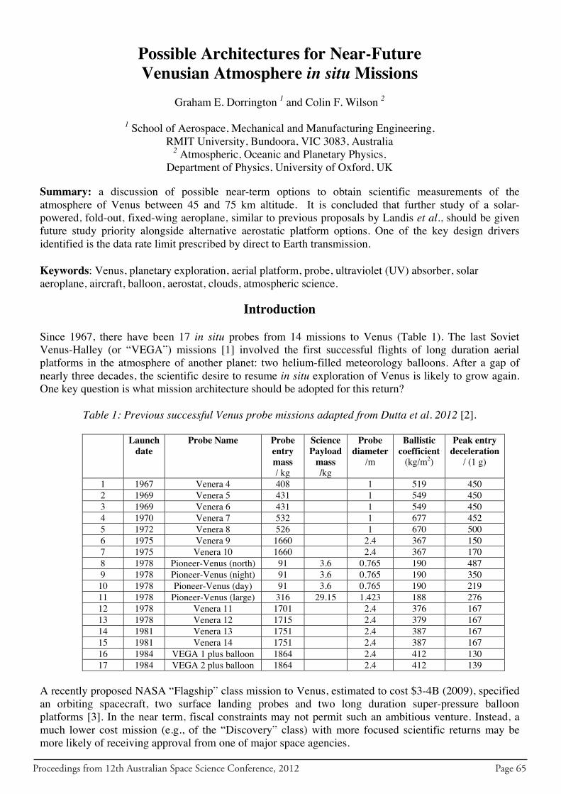
Proceedings from 12th Australian Space Science Conference, 2012 Page 65
Possible Architectures for Near-FutureVenusian Atmosphere in situ Missions
Graham E. Dorrington 1 and Colin F. Wilson 2
1 School of Aerospace, Mechanical and Manufacturing Engineering, RMIT University, Bundoora, VIC 3083, Australia
2 Atmospheric, Oceanic and Planetary Physics, Department of Physics, University of Oxford, UK
Summary: a discussion of possible near-term options to obtain scientific measurements of the atmosphere of Venus between 45 and 75 km altitude. It is concluded that further study of a solar-powered, fold-out, fixed-wing aeroplane, similar to previous proposals by Landis et al., should be given future study priority alongside alternative aerostatic platform options. One of the key design drivers identified is the data rate limit prescribed by direct to Earth transmission.
Keywords: Venus, planetary exploration, aerial platform, probe, ultraviolet (UV) absorber, solar aeroplane, aircraft, balloon, aerostat, clouds, atmospheric science.
Introduction
Since 1967, there have been 17 in situ probes from 14 missions to Venus (Table 1). The last Soviet Venus-Halley (or “VEGA”) missions [1] involved the first successful flights of long duration aerial platforms in the atmosphere of another planet: two helium-filled meteorology balloons. After a gap of nearly three decades, the scientific desire to resume in situ exploration of Venus is likely to grow again. One key question is what mission architecture should be adopted for this return?
Table 1: Previous successful Venus probe missions adapted from Dutta et al. 2012 [2].
Launch date
Probe Name Probe entry mass/ kg
SciencePayload
mass/kg
Probe diameter
/m
Ballistic coefficient
(kg/m2)
Peak entry deceleration
/ (1 g)
1 1967 Venera 4 408 1 519 450 2 1969 Venera 5 431 1 549 450 3 1969 Venera 6 431 1 549 450 4 1970 Venera 7 532 1 677 452 5 1972 Venera 8 526 1 670 500 6 1975 Venera 9 1660 2.4 367 150 7 1975 Venera 10 1660 2.4 367 170 8 1978 Pioneer-Venus (north) 91 3.6 0.765 190 487 9 1978 Pioneer-Venus (night) 91 3.6 0.765 190 350
10 1978 Pioneer-Venus (day) 91 3.6 0.765 190 219 11 1978 Pioneer-Venus (large) 316 29.15 1.423 188 276 12 1978 Venera 11 1701 2.4 376 167 13 1978 Venera 12 1715 2.4 379 167 14 1981 Venera 13 1751 2.4 387 167 15 1981 Venera 14 1751 2.4 387 167 16 1984 VEGA 1 plus balloon 1864 2.4 412 130 17 1984 VEGA 2 plus balloon 1864 2.4 412 139
A recently proposed NASA “Flagship” class mission to Venus, estimated to cost $3-4B (2009), specified an orbiting spacecraft, two surface landing probes and two long duration super-pressure balloon platforms [3]. In the near term, fiscal constraints may not permit such an ambitious venture. Instead, a much lower cost mission (e.g., of the “Discovery” class) with more focused scientific returns may be more likely of receiving approval from one of major space agencies.
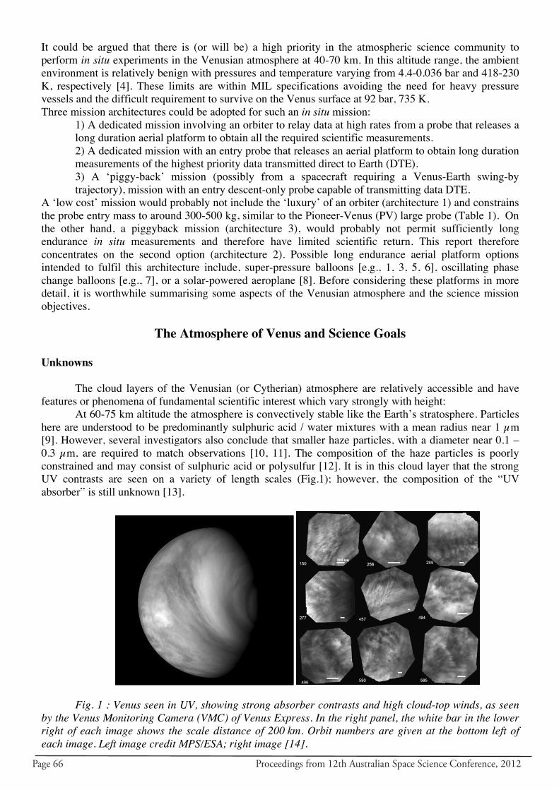
Page 66 Proceedings from 12th Australian Space Science Conference, 2012
It could be argued that there is (or will be) a high priority in the atmospheric science community to perform in situ experiments in the Venusian atmosphere at 40-70 km. In this altitude range, the ambient environment is relatively benign with pressures and temperature varying from 4.4-0.036 bar and 418-230 K, respectively [4]. These limits are within MIL specifications avoiding the need for heavy pressure vessels and the difficult requirement to survive on the Venus surface at 92 bar, 735 K. Three mission architectures could be adopted for such an in situ mission:
1) A dedicated mission involving an orbiter to relay data at high rates from a probe that releases a long duration aerial platform to obtain all the required scientific measurements. 2) A dedicated mission with an entry probe that releases an aerial platform to obtain long duration measurements of the highest priority data transmitted direct to Earth (DTE). 3) A ‘piggy-back’ mission (possibly from a spacecraft requiring a Venus-Earth swing-by trajectory), mission with an entry descent-only probe capable of transmitting data DTE.
A ‘low cost’ mission would probably not include the ‘luxury’ of an orbiter (architecture 1) and constrains the probe entry mass to around 300-500 kg, similar to the Pioneer-Venus (PV) large probe (Table 1). On the other hand, a piggyback mission (architecture 3), would probably not permit sufficiently long endurance in situ measurements and therefore have limited scientific return. This report therefore concentrates on the second option (architecture 2). Possible long endurance aerial platform options intended to fulfil this architecture include, super-pressure balloons [e.g., 1, 3, 5, 6], oscillating phase change balloons [e.g., 7], or a solar-powered aeroplane [8]. Before considering these platforms in more detail, it is worthwhile summarising some aspects of the Venusian atmosphere and the science mission objectives.
The Atmosphere of Venus and Science Goals
Unknowns
The cloud layers of the Venusian (or Cytherian) atmosphere are relatively accessible and have features or phenomena of fundamental scientific interest which vary strongly with height:
At 60-75 km altitude the atmosphere is convectively stable like the Earth’s stratosphere. Particles here are understood to be predominantly sulphuric acid / water mixtures with a mean radius near 1 µm [9]. However, several investigators also conclude that smaller haze particles, with a diameter near 0.1 – 0.3 µm, are required to match observations [10, 11]. The composition of the haze particles is poorly constrained and may consist of sulphuric acid or polysulfur [12]. It is in this cloud layer that the strong UV contrasts are seen on a variety of length scales (Fig.1); however, the composition of the “UV absorber” is still unknown [13].
Fig. 1 : Venus seen in UV, showing strong absorber contrasts and high cloud-top winds, as seen by the Venus Monitoring Camera (VMC) of Venus Express. In the right panel, the white bar in the lower right of each image shows the scale distance of 200 km. Orbit numbers are given at the bottom left of each image. Left image credit MPS/ESA; right image [14].
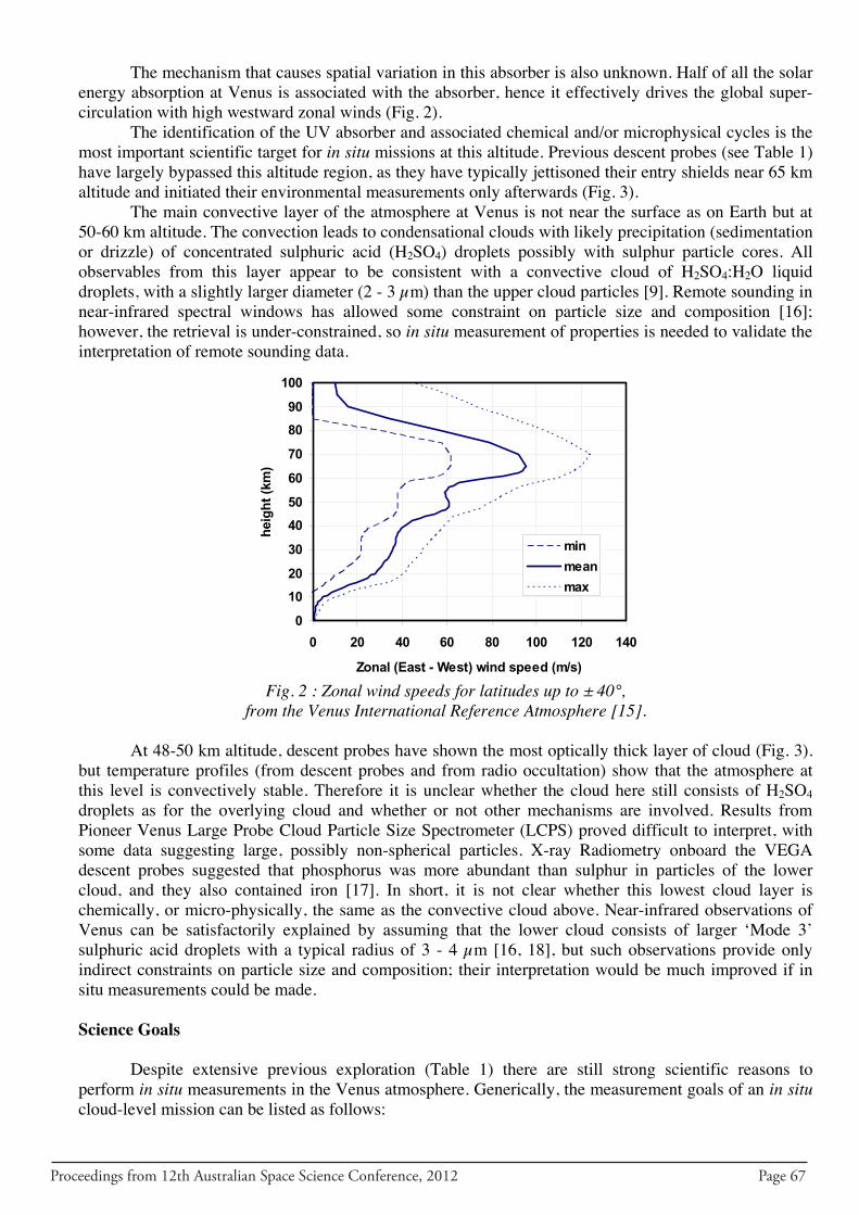
Proceedings from 12th Australian Space Science Conference, 2012 Page 67
The mechanism that causes spatial variation in this absorber is also unknown. Half of all the solar energy absorption at Venus is associated with the absorber, hence it effectively drives the global super-circulation with high westward zonal winds (Fig. 2).
The identification of the UV absorber and associated chemical and/or microphysical cycles is the most important scientific target for in situ missions at this altitude. Previous descent probes (see Table 1) have largely bypassed this altitude region, as they have typically jettisoned their entry shields near 65 km altitude and initiated their environmental measurements only afterwards (Fig. 3).
The main convective layer of the atmosphere at Venus is not near the surface as on Earth but at 50-60 km altitude. The convection leads to condensational clouds with likely precipitation (sedimentation or drizzle) of concentrated sulphuric acid (H2SO4) droplets possibly with sulphur particle cores. All observables from this layer appear to be consistent with a convective cloud of H2SO4:H2O liquid droplets, with a slightly larger diameter (2 - 3 µm) than the upper cloud particles [9]. Remote sounding in near-infrared spectral windows has allowed some constraint on particle size and composition [16]; however, the retrieval is under-constrained, so in situ measurement of properties is needed to validate the interpretation of remote sounding data.
0
1020
30
4050
60
70
8090
100
0 20 40 60 80 100 120 140
Zonal (East - West) wind speed (m/s)
heig
ht (k
m)
minmeanmax
Fig. 2 : Zonal wind speeds for latitudes up to ± 40°,from the Venus International Reference Atmosphere [15].
At 48-50 km altitude, descent probes have shown the most optically thick layer of cloud (Fig. 3). but temperature profiles (from descent probes and from radio occultation) show that the atmosphere at this level is convectively stable. Therefore it is unclear whether the cloud here still consists of H2SO4droplets as for the overlying cloud and whether or not other mechanisms are involved. Results from Pioneer Venus Large Probe Cloud Particle Size Spectrometer (LCPS) proved difficult to interpret, with some data suggesting large, possibly non-spherical particles. X-ray Radiometry onboard the VEGA descent probes suggested that phosphorus was more abundant than sulphur in particles of the lower cloud, and they also contained iron [17]. In short, it is not clear whether this lowest cloud layer is chemically, or micro-physically, the same as the convective cloud above. Near-infrared observations of Venus can be satisfactorily explained by assuming that the lower cloud consists of larger ‘Mode 3’ sulphuric acid droplets with a typical radius of 3 - 4 µm [16, 18], but such observations provide only indirect constraints on particle size and composition; their interpretation would be much improved if in situ measurements could be made.
Science Goals
Despite extensive previous exploration (Table 1) there are still strong scientific reasons to perform in situ measurements in the Venus atmosphere. Generically, the measurement goals of an in situcloud-level mission can be listed as follows:
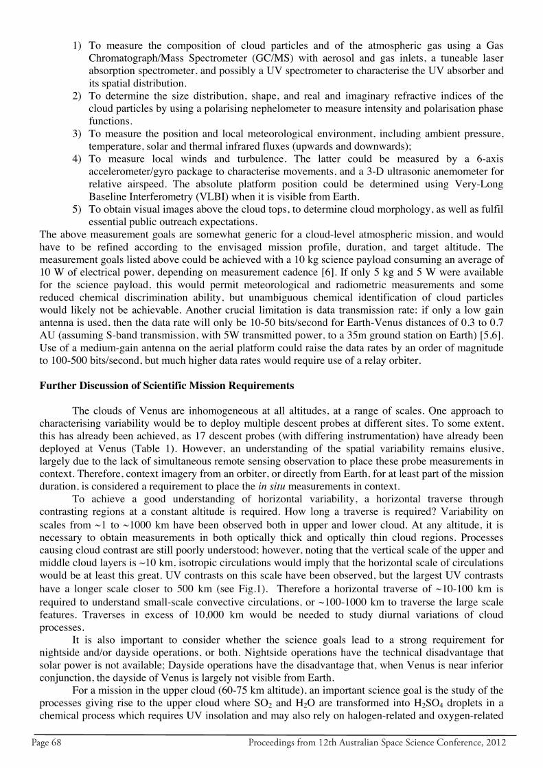
Page 68 Proceedings from 12th Australian Space Science Conference, 2012
1) To measure the composition of cloud particles and of the atmospheric gas using a Gas Chromatograph/Mass Spectrometer (GC/MS) with aerosol and gas inlets, a tuneable laser absorption spectrometer, and possibly a UV spectrometer to characterise the UV absorber and its spatial distribution.
2) To determine the size distribution, shape, and real and imaginary refractive indices of the cloud particles by using a polarising nephelometer to measure intensity and polarisation phase functions.
3) To measure the position and local meteorological environment, including ambient pressure, temperature, solar and thermal infrared fluxes (upwards and downwards);
4) To measure local winds and turbulence. The latter could be measured by a 6-axis accelerometer/gyro package to characterise movements, and a 3-D ultrasonic anemometer for relative airspeed. The absolute platform position could be determined using Very-Long Baseline Interferometry (VLBI) when it is visible from Earth.
5) To obtain visual images above the cloud tops, to determine cloud morphology, as well as fulfil essential public outreach expectations.
The above measurement goals are somewhat generic for a cloud-level atmospheric mission, and would have to be refined according to the envisaged mission profile, duration, and target altitude. The measurement goals listed above could be achieved with a 10 kg science payload consuming an average of 10 W of electrical power, depending on measurement cadence [6]. If only 5 kg and 5 W were available for the science payload, this would permit meteorological and radiometric measurements and some reduced chemical discrimination ability, but unambiguous chemical identification of cloud particles would likely not be achievable. Another crucial limitation is data transmission rate: if only a low gain antenna is used, then the data rate will only be 10-50 bits/second for Earth-Venus distances of 0.3 to 0.7 AU (assuming S-band transmission, with 5W transmitted power, to a 35m ground station on Earth) [5,6]. Use of a medium-gain antenna on the aerial platform could raise the data rates by an order of magnitude to 100-500 bits/second, but much higher data rates would require use of a relay orbiter.
Further Discussion of Scientific Mission Requirements
The clouds of Venus are inhomogeneous at all altitudes, at a range of scales. One approach to characterising variability would be to deploy multiple descent probes at different sites. To some extent, this has already been achieved, as 17 descent probes (with differing instrumentation) have already been deployed at Venus (Table 1). However, an understanding of the spatial variability remains elusive, largely due to the lack of simultaneous remote sensing observation to place these probe measurements in context. Therefore, context imagery from an orbiter, or directly from Earth, for at least part of the mission duration, is considered a requirement to place the in situ measurements in context.
To achieve a good understanding of horizontal variability, a horizontal traverse through contrasting regions at a constant altitude is required. How long a traverse is required? Variability on scales from ∼1 to ∼1000 km have been observed both in upper and lower cloud. At any altitude, it is necessary to obtain measurements in both optically thick and optically thin cloud regions. Processes causing cloud contrast are still poorly understood; however, noting that the vertical scale of the upper and middle cloud layers is ~10 km, isotropic circulations would imply that the horizontal scale of circulations would be at least this great. UV contrasts on this scale have been observed, but the largest UV contrasts have a longer scale closer to 500 km (see Fig.1). Therefore a horizontal traverse of ∼10-100 km is required to understand small-scale convective circulations, or ∼100-1000 km to traverse the large scale features. Traverses in excess of 10,000 km would be needed to study diurnal variations of cloud processes.
It is also important to consider whether the science goals lead to a strong requirement for nightside and/or dayside operations, or both. Nightside operations have the technical disadvantage that solar power is not available; Dayside operations have the disadvantage that, when Venus is near inferior conjunction, the dayside of Venus is largely not visible from Earth.
For a mission in the upper cloud (60-75 km altitude), an important science goal is the study of the processes giving rise to the upper cloud where SO2 and H2O are transformed into H2SO4 droplets in a chemical process which requires UV insolation and may also rely on halogen-related and oxygen-related
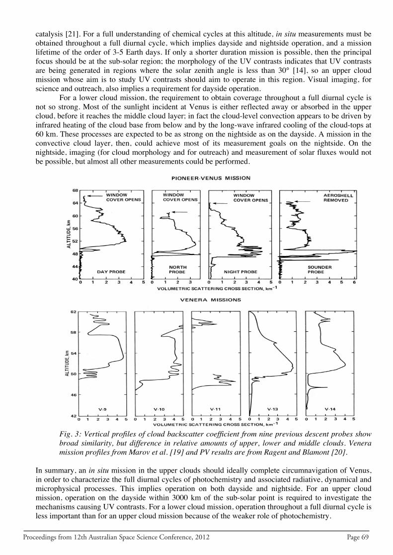
Proceedings from 12th Australian Space Science Conference, 2012 Page 69
catalysis [21]. For a full understanding of chemical cycles at this altitude, in situ measurements must be obtained throughout a full diurnal cycle, which implies dayside and nightside operation, and a mission lifetime of the order of 3-5 Earth days. If only a shorter duration mission is possible, then the principal focus should be at the sub-solar region; the morphology of the UV contrasts indicates that UV contrasts are being generated in regions where the solar zenith angle is less than 30° [14], so an upper cloud mission whose aim is to study UV contrasts should aim to operate in this region. Visual imaging, for science and outreach, also implies a requirement for dayside operation.
For a lower cloud mission, the requirement to obtain coverage throughout a full diurnal cycle is not so strong. Most of the sunlight incident at Venus is either reflected away or absorbed in the upper cloud, before it reaches the middle cloud layer; in fact the cloud-level convection appears to be driven by infrared heating of the cloud base from below and by the long-wave infrared cooling of the cloud-tops at 60 km. These processes are expected to be as strong on the nightside as on the dayside. A mission in the convective cloud layer, then, could achieve most of its measurement goals on the nightside. On the nightside, imaging (for cloud morphology and for outreach) and measurement of solar fluxes would not be possible, but almost all other measurements could be performed.
Fig. 3: Vertical profiles of cloud backscatter coefficient from nine previous descent probes show broad similarity, but difference in relative amounts of upper, lower and middle clouds. Venera mission profiles from Marov et al. [19] and PV results are from Ragent and Blamont [20].
In summary, an in situ mission in the upper clouds should ideally complete circumnavigation of Venus, in order to characterize the full diurnal cycles of photochemistry and associated radiative, dynamical and microphysical processes. This implies operation on both dayside and nightside. For an upper cloud mission, operation on the dayside within 3000 km of the sub-solar point is required to investigate the mechanisms causing UV contrasts. For a lower cloud mission, operation throughout a full diurnal cycle is less important than for an upper cloud mission because of the weaker role of photochemistry.
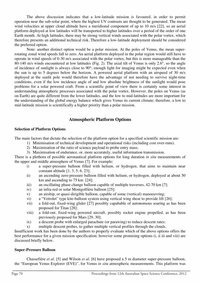
Page 70 Proceedings from 12th Australian Space Science Conference, 2012
The above discussion indicates that a low-latitude mission is favoured, in order to permit operation near the sub-solar point, where the highest UV contrasts are thought to be generated. The mean wind velocities at upper cloud altitude have a meridional component of up to 10 m/s [22], so an aerial platform deployed at low latitudes will be transported to higher latitudes over a period of the order of one Earth month. At high latitudes, there may be strong vertical winds associated with the polar vortex, which therefore presents an additional technical risk. Therefore a low-latitude deployment should be considered the preferred option.
Note: another distinct option would be a polar mission. At the poles of Venus, the mean super-rotating zonal wind speeds fall to zero. An aerial platform deployed in the polar region would still have to operate in wind speeds of 0-30 m/s associated with the polar vortex, but this is more manageable than the 80-140 m/s winds encountered at low latitudes (Fig. 2). The axial tilt of Venus is only 2.6°, so the angle of incidence of sunlight is always close to 90°; enough light for imaging might be expected even when the sun is up to 5 degrees below the horizon. A powered aerial platform with an airspeed of 30 m/s deployed at the sunlit pole would therefore have the advantage of not needing to survive night-time conditions, even if the low incidence angle of and low absolute brightness of the sunlight would pose problems for a solar powered craft. From a scientific point of view there is certainly some interest in understanding atmospheric processes associated with the polar vortex. However, the poles on Venus (as on Earth) are quite different from the lower latitudes, and the low to mid-latitudes are more important for the understanding of the global energy balance which gives Venus its current climate; therefore, a low to mid-latitude mission is scientifically a higher priority than a polar mission.
Atmospheric Platform Options
Selection of Platform Options
The main factors that dictate the selection of the platform option for a specified scientific mission are: 1) Minimisation of technical development and operational risks (including cost over-runs).2) Maximisation of the ratio of science payload to probe entry mass. 3) Maximisation of endurance, or, more accurately, useful information transmission.
There is a plethora of possible aeronautical platform options for long duration in situ measurements of the upper and middle atmosphere of Venus [7]. For example:
i) a super-pressure balloon filled with helium, or hydrogen, that aims to maintain near constant altitude [1, 3, 5, 6, 23];
ii) an ascending zero-pressure balloon filled with helium, or hydrogen, deployed at about 50 km and ascending to 75 km [24];
iii) an oscillating phase change balloon capable of multiple traverses, 42-70 km [7]; iv) an infra-red or solar Montgolfière balloon [25]; v) an airship, or quasi-dirigible balloon, capable of some (vertical) manoeuvring; vi) a “Vetrolet” type kite-balloon system using vertical wing shear to provide lift [26]; vii) a fold-out, fixed-wing glider [27] possibly capabable of autonomous soaring as has been
proposed for Titan [28];viii) a fold-out, fixed-wing powered aircraft, possibly rocket engine propelled, as has been
previously proposed for Mars [29, 30]; ix) a descent probe with enlarged parachute (or parawing) to reduce descent rates; x) multiple descent probes, to gather multiple vertical profiles through the clouds.
Insufficient work has been done by the authors to properly evaluate which of the above options offers the best performance for a given mission specification; however some promising options (i, ii iii and viii) are discussed briefly below.
Super-Pressure Balloon
Chassefière et al. [5] and Wilson et al. [6] have proposed a 5 m diameter super-pressure balloon, the “European Venus Explorer (EVE)”, for Venus in situ atmospheric measurements. This platform was
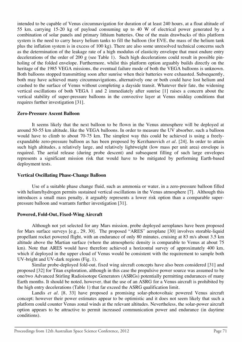
Proceedings from 12th Australian Space Science Conference, 2012 Page 71
intended to be capable of Venus circumnavigation for duration of at least 240 hours, at a float altitude of 55 km, carrying 15-20 kg of payload consuming up to 40 W of electrical power generated by a combination of solar panels and primary lithium batteries. One of the main drawbacks of this platform system is the need to carry heavy helium tanks to fill the balloon (for EVE, the mass of the helium tank plus the inflation system is in excess of 100 kg). There are also some unresolved technical concerns such as the determination of the leakage rate of a high modulus of elasticity envelope that must endure entry decelerations of the order of 200 g (see Table 1). Such high decelerations could result in possible pin-holing of the folded envelope. Furthermore, whilst this platform option arguably builds directly on the heritage of the 1985 VEGA missions, the eventual failure mode of both the VEGA balloons is unknown. Both balloons stopped transmitting soon after sunrise when their batteries were exhausted. Subsequently, both may have achieved many circumnavigations, alternatively one or both could have lost helium and crashed to the surface of Venus without completing a dayside transit. Whatever their fate, the widening vertical oscillations of both VEGA 1 and 2 immediately after sunrise [1] raises a concern about the vertical stability of super-pressure balloons in the convective layer at Venus midday conditions that requires further investigation [31].
Zero-Pressure Ascent Balloon
It seems likely that the next balloon to be flown in the Venus atmosphere will be deployed at around 50-55 km altitude, like the VEGA balloons. In order to measure the UV absorber, such a balloon would have to climb to about 70-75 km. The simplest way this could be achieved is using a freely-expandable zero-pressure balloon as has been proposed by Kerzhanovich et al. [24]. In order to attain such high altitudes, a relatively large, and relatively lightweight (low mass per unit area) envelope is required. The aerial release (during probe descent) and subsequent filling of such large envelopes represents a significant mission risk that would have to be mitigated by performing Earth-based deployment tests.
Vertical Oscillating Phase-Change Balloon
Use of a suitable phase change fluid, such as ammonia or water, in a zero-pressure balloon filled with helium/hydrogen permits sustained vertical oscillations in the Venus atmosphere [7]. Although this introduces a small mass penalty, it arguably represents a lower risk option than a comparable super-pressure balloon and warrants further investigation [31].
Powered, Fold-Out, Fixed-Wing Aircraft
Although not yet selected for any Mars mission, probe deployed aeroplanes have been proposed for Mars surface surveys [e.g., 29, 30]. The proposed “ARES” aeroplane [30] involves storable-liquid propellant rocket powered flight, with an endurance of only 80 minutes, cruising at 83 m/s about 3.5 km altitude above the Martian surface (where the atmospheric density is comparable to Venus at about 75 km). Note that ARES would have therefore achieved a horizontal survey of approximately 400 km, which if deployed in the upper cloud of Venus would be consistent with the requirement to sample both UV-bright and UV-dark regions (Fig. 1).
Similar probe-deployed fold-out, fixed wing aircraft concepts have also been considered [31] and proposed [32] for Titan exploration, although in this case the propulsive power source was assumed to be one/two Advanced Stirling Radioisotope Generators (ASRGs) potentially permitting endurances of many Earth months. It should be noted, however, that the use of an ASRG for a Venus aircraft is prohibited by the high entry decelerations (Table 1) that far exceed the ASRG qualification limit.
Landis et al. [8, 33] have proposed a promising solar-photovoltaic powered Venus aircraft concept; however their power estimates appear to be optimistic and it does not seem likely that such a platform could counter Venus zonal winds at the relevant altitudes. Nevertheless, the solar-power aircraft option appears to be attractive to permit increased communication power and endurance (in daytime conditions).
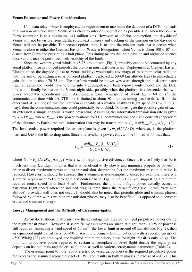
Page 72 Proceedings from 12th Australian Space Science Conference, 2012
Venus Encounter and Power Considerations
If no data relay orbiter is employed, the requirement to maximize the data rate of a DTE link leads to a mission insertion when Venus is as close to inferior conjunction as possible (i.e. when the Venus-Earth separation is at a minimum, ∼41 million km). However, at inferior conjunction, the dayside of Venus will not be visible from Earth, so context imagery and tracking of the mission on the dayside of Venus will not be possible. The second option, then, is to time the mission such that it occurs when Venus is close to either the Greatest Eastern or Western Elongations, when Venus is about 100 × 106 km distant from Earth and presenting a half phase. This timing means that both dayside and nightside science observations may be performed with visibility of the Earth.
Since the western zonal winds at 45-75 km altitude (Fig. 3) probably cannot be countered by any aerial platform for prolonged periods, the platform must drift westward. Deployment at Greatest Eastern Elongation on the dayside (close to Venus midday) would take advantage of maximum solar radiation with the aim of permitting a solar powered platform deployed at 50-60 km altitude (say) to immediately gain altitude to about 70-75 km. The platform would be blown westward through the dusk terminator (then an aeroplane would have to enter into a gliding-descent battery-power-only mode) and the DTE link would finally be lost on the Venus night side, possibly when the platform has descended below a lower acceptable operational limit. Assuming a zonal windspeed of about Uw = 60 m s-1, the communication time with the DTE link is limited to about 80 hours assuming passive drift. If, on the otherhand, it is supposed that the platform is capable of a relative eastward flight speed of U = 30 m s-1
(say), then the communication time could potentially be doubled. To investigate the possible gain of such an extension a simple analysis is worth presenting. Assuming the information transmission rate is given by commskPI = where commsP is the power available for DTE communication and k is a constant (dependent of the distance to Earth), the total information that may be transmitted is )/( UURkPI wVenuscommtot −≅ π . The level cruise power required for an aeroplane is given by )//( DLgUmp where mp is the platform mass and L/D is the lift-to-drag ratio. Since total available power, Ptot , will be limited, it follows that,
( ))/1(/1
ww
PtotVenustot UUU
UUPkRI
−−
≅π
(1)
where )/()/( gmDLPU pptotP η= where ηp is the propulsive efficiency. Since it is also likely that UP is much less than Uw, Eqn 1 implies that it is beneficial to fly slowly and minimise propulsive power, in order to divert maximum power to data transmission, despite the fact the maximum mission duration is reduced. However, it should be stressed this statement is over-simplistic since, for example, there is a scientific requirement to fly through a UV contrast band (Fig. 1), i.e. ∼1000 km, suggesting a minimum required cruise speed of at least 4 m/s. Furthermore, the minimum flight power actually occurs at particular flight speed when the induced drag is three times the zero-lift drag (i.e., it will vary with altitude), provided stall does not occur. It should also be noted that periodic glide and transmit phases, followed by climb with zero data transmission phases, may also be beneficial, as opposed to a constant cruise and transmit strategy.
Energy Management and the Difficulty of Circumnavigation
Aerostatic (balloon) platforms have the advantage that they do not need propulsive power during the night transit phase. However, if scientific measurements are made at night, then ∼10 W or power is still required. Assuming a wind speed of 60 ms-1 (the lower limit at around 60 km altitude, Fig. 2), then an equatorial night transit lasts for ∼90 h. Assuming primary lithium batteries with a specific energy of ∼590 Wh/kg [23] are employed, the required minimum battery mass for night transit is only ∼2 kg. The minimum propulsive power required to sustain an aeroplane in level flight during the night phase depends on its total mass and the cruise altitude, as well as various aerodynamic parameters (Table 2).
The essential point to note (about electric powered aeroplanes) is the required propulsive power far exceeds the assumed science budget (10 W), and results in battery masses in excess of ∼20 kg. This
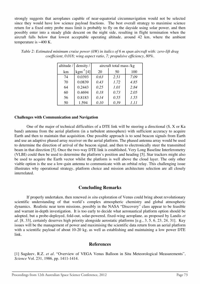
Proceedings from 12th Australian Space Science Conference, 2012 Page 73
strongly suggests that aeroplanes capable of near-equatorial circumnavigation would not be selected since they would have low science payload fractions. The best overall strategy to maximise science return for a fixed entry probe mass limit is probably to fly on the dayside using solar power, and then possibly enter into a steady glide descent on the night side, resulting in flight termination when the aircraft falls below that lowest acceptable operating altitude, around 42 km, where the ambient temperature is ∼400 K.
Table 2: Estimated minimum cruise power (kW) in italics of 6 m span aircraft with: zero-lift drag coefficient, 0.018; wing aspect ratio, 7; propulsive efficiency, 80%.
altitude / density / aircraft total mass /kgkm kgm-3 [4] 20 50 10074 0.0393 0.63 2.51 7.0970 0.0839 0.43 1.72 4.8564 0.2443 0.25 1.01 2.8460 0.4694 0.18 0.73 2.0556 0.8183 0.14 0.55 1.5550 1.594 0.10 0.39 1.11
Challenges with Communication and Navigation
One of the major of technical difficulties of a DTE link will be steering a directional (S, X or Ka band) antenna from the aerial platform (in a turbulent atmosphere) with sufficient accuracy to acquire Earth and then to maintain that acquisition. One possible approach is to send beacon signals from Earth and use an adaptive phased array receiver on the aerial platform. The phased antenna array would be used to determine the direction of arrival of the beacon signal, and then to electronically steer the transmitted beam in that direction [5]. Once the two-way DTE link is established, Very Long Baseline Interferometry (VLBI) could then be used to determine the platform’s position and heading [5]. Star trackers might also be used to acquire the Earth vector whilst the platform is well above the cloud layer. The only other viable option is the use a low-gain antenna to communicate with an orbital relay. This challenging issue illustrates why operational strategy, platform choice and mission architecture selection are all closely interrelated.
Concluding Remarks
If properly undertaken, then renewed in situ exploration of Venus could bring about revolutionary scientific understanding of that world’s complex atmospheric chemistry and global atmospheric dynamics. Realistic near term missions, possibly in the NASA “Discovery” class appear to be feasible and warrant in-depth investigation. It is too early to decide what aeronautical platform option should be adopted, but a probe-deployed, fold-out, solar-powered, fixed-wing aeroplane, as proposed by Landis etal. [8, 33], certainly deserves high priority alongside aerostatic platforms [e.g., 3, 5, 6, 23, 24, 31]. Key issues will be the management of power and maximising the scientific data return from an aerial platform with a scientific payload of about 10-20 kg, as well as establishing and maintaining a low power DTE link.
References
[1] Sagdeev, R.Z. et al. “Overview of VEGA Venus Balloon in Situ Meteorological Measurements”,Science Vol. 231, 1986, pp. 1411-1414.
Page 74 Proceedings from 12th Australian Space Science Conference, 2012
[2] Dutta, S., Smith, B., Prabhu, D., Venkatapathy, E., “Mission Sizing and Trade Studies for Low Ballisitic Coefficient Entry Systems to Venus”, IEEE Aerospace Conf., Big Sky, MT., USA, 3-10 March 2012, DOI: 10.1109/AERO.2012.6187002
[3] Hall, J. L., Bullock, M. A., Senske, D. A., Cutts, J. A., Grammier, R. Venus Flagship Mission Study, Final Report of the Venus Science and Technology Definition Team, http://vfm.jpl.nasa.gov/library2/2009 accessed July 7, 2012.
[4] Seiff, A. Schofield, J.T., Kliore, A.J., et al. “Models of the Structure of the Atmosphere of Venus from the Surface to 100 km Altitude”. Advances in Space Research. Vol. 5, No. 11, 1985, pp. 3–58.
[5] Chassefière E. et al., “European Venus Explorer (EVE) – An in-situ Mission to Venus. Experimental Astronomy”, Vol. 23, Issue 3, 2009, pp. 741-760.
[6] Wilson C. F. et al. “The 2010 European Venus Explorer (EVE) Mission Proposal”, ExperimentalAstronomy, Vol. 33, 2012, pp. 305–335, doi:10.1007/s10686-011-9259-9.
[7] Dorrington, G. E. “Venus Atmospheric Platform Options Revisited”, Advances in Space Research,vol. 46, 2010, pp. 310–326.
[8] Landis, G. A., LaMarre, C., Colozza, A. “Venus Atmospheric Exploration by Solar Aircraft”, Acta Astronautica, vol. 56, 2005, pp. 750-755. See also: Landis, G. A., LaMarre, C., Colozza, “Atmospheric Flight on Venus”, AIAA-2002-0819, 40th Aerospace Science Meeting & Exhibit, Reno, Nevada, 14-17 January, 2002.
[9] Carlson, R. W. et al. “Variations in Venus Cloud Particle Properties: A New View of Venus’s Cloud Morphology as Observed by the Galileo Near-Infrared Mapping Spectrometer” Planetary and Space Science Vol. 41, 1993, pp. 471-486.
[10] Braak, C. J. et al. “Spatial and Temporal Variations of Venus Haze Properties Obtained from Pioneer Venus Orbiter Polarimetry”. J. Geophysical Research. Vol. 107 (E5), 2002, p. 5029.
[11] Wilquet, V. et al. “Preliminary Characterization of the Upper Haze by SPICAV/SOIR Solar Occultation in UV to mid-IR onboard Venus Express”. J. Geophysical Research Vol. 114, 2009, E00B42.
[12] Zhang, X. et al. “Sulfur Chemistry in the Middle Atmosphere of Venus”, Icarus Vol. 217, 2012, pp 714-739.
[13] Krasnopolsky, V.A. “Chemical Composition of Venus Atmosphere and Clouds: Some Unsolved Problems”, Planetary and Space Science, Vol. 54, Issues 13–14, pp. 1352–1359, 2006.
[14] Titov D.V. et al. “Morphology of the Cloud Tops as Observed by the Venus Express Monitoring Camera”, Icarus, Vol.217, Issue 2, 2012, pp. 682–701.
[15] Kerzhanovich, V.V. et al. “Circulation of the Atmosphere from the Surface to 100 km”, Advances in Space Research Vol. 5, No. 11, 1985, pp 59-83.
[16] Barstow, J.K. et al. “Models of the Global Cloud Structure on Venus Derived from Venus Express Observations”, Icarus, Vol. 217, 2012, pp. 542-560.
[17] Andreichikov, B.M., Akhmetsin, I.K., Korchuganov, B.N., et al. “VEGA 1 and 2 X-Ray Radiometer Analysis of the Venus Cloud Aerosol”. Kosmicheskie Issledonvaniia. Vol. 25, 1987, pp. 721.
Proceedings from 12th Australian Space Science Conference, 2012 Page 75
[18] Cotton, D. V., Bailey, J., Crisp, D., and Meadows, V. S.“The Distribution of Carbon Monoxide in the Lower Atmosphere of Venus”. Icarus Vol. 217 (2), 2012, pp. 570–584.
[19] Marov, M. Ia. et al. “Investigation of the Structure of the Venus Clouds Using the Nephelometers on the Venera-13 and Venera-14 Probes”. Kosmicheskie Issledovaniia. Vol. 21, 1983, pp. 269-278.
[20] Ragent, B., Blamont, J. “The Structure of the Clouds of Venus - Results of the Pioneer Venus Nephelometer Experiment”, Journal of Geophysical Research, Vol. 85, 1980, pp 8089-8105.
[21] Mills, F.P., Allen, M.A. “Review of Selected Issues Concerning the Chemistry in Venus’ Middle Atmosphere”, Planetary and Space Science, Vol. 55, Issue 12, 2007, pp. 1729–1740.
[22] Sánchez-Lavega, A. et al. Variable Winds on Venus Mapped in Three Dimensions, GeophysicalResearch Letters, Vol. 35, L13204, 2008. DOI:10.1029/2008GL033817
[23] Phipps et al. “Venus Orbiter and Entry Probe: An ESA Technology Reference Study”, Proceedings of the 8th ESA Workshop on Advanced Space Technologies for Robotics and Automation, ASTRA 2004, ESTEC, Noordwijk, The Netherlands, Nov. 2-4, 2004.
[24] Kerzhanonvich, V.V., Crisp, D., Preston, R.A., et al. “Venus Stratospheric Sounder” Acta Astron.Vol. 52, 2003, pp. 159–164.
[25] Jones, J.A., Heun, M.K. Montgolfiere Balloon Aerobots for Planetary Atmospheres, AIAA-97-1445, 12th Lighter-Than-Systems Tech. Conf. San Francisco, CA, June 3–5, 1997.
[26] Vorontsov, V.A. et al. Prospective Spacecraft for Venus Research: Venera-D Research, SpaceSystem Research, Vol. 45, no. 7, 2011, pp. 710-744.
[27] Miralles, C., MacCready, P. B. “Gliders for Atmospheric and Surface Science, Mission concepts Utilizing Gliders for Atmospheric and Surface Science”, Poster No. 1506, Lunar and Planetary Science Conf., Houston, March 15–19, 1999.
[28] Lawrence, N., Sukkarieh, R. J. “Autonomous Soaring for Atmospheric Exploration of Titan”, Proc.10th Australian Space Conference, Brisbane, Sept. 27-30, 2010.
[29] Calvin, W.M., Miralles, B. C., Wilson, G.R. “Mars Science with Small Aircraft”, Workshop on Concepts and Approaches for Mars Exploration, LPI-contrib-1062-Pt-1, JPL, Pasadena, 2000.
[30] Braun, R. D. et al. “Design of the ARES Mars Airplane and Mission Architecture”, J. Spacecraft and Rockets, Vol. 43, No. 5, Sept.-Oct. 2006, pp. 1026-1034.
[31] Dorrington, G.E. “Venus Aerial Platform Options Reconsidered”, 9th International Planetary Probe Workshop, Toulouse, France, 16-22 June 2012.
[32] Barnes, J. W. et al. “AVIATR – Aerial Vehicle for In-situ and Airborne Titan Reconnaissance”, Exp. Astron. Vol. 33 (1), 2012, pp. 55-127.
[33] Colozza, A., Landis, G., Lyons, V. “Overview of Innovative Aircraft Power and Propulsion Systems and Their Applications for Planetary Exploration”, NASA/TM-2003-212459, Int. Air and Space Symp. & Exposition, NASA/AIAA, Dayton, Ohio, July 14-17, 2003.

Page 76 Proceedings from 12th Australian Space Science Conference, 2012
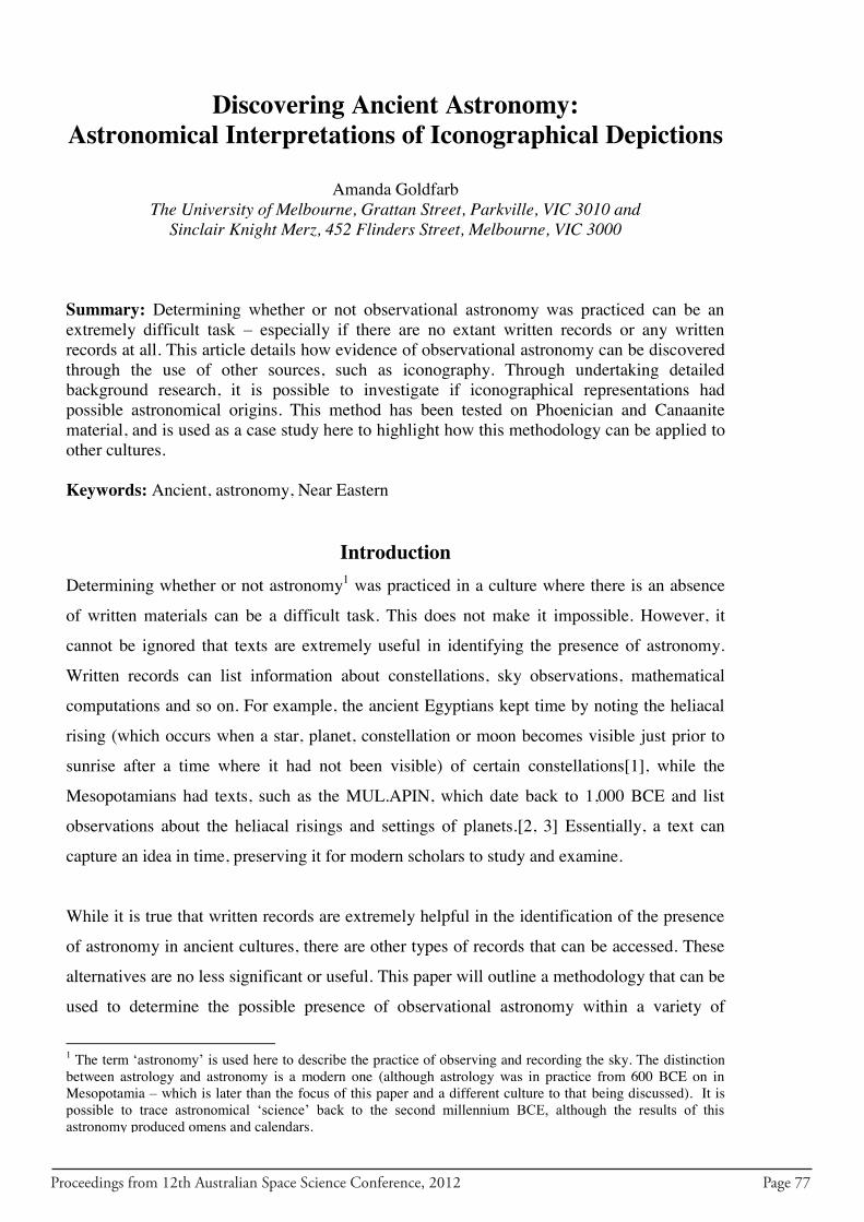
Proceedings from 12th Australian Space Science Conference, 2012 Page 77
Discovering Ancient Astronomy: Astronomical Interpretations of Iconographical Depictions
Amanda Goldfarb
The University of Melbourne, Grattan Street, Parkville, VIC 3010 and Sinclair Knight Merz, 452 Flinders Street, Melbourne, VIC 3000
Summary: Determining whether or not observational astronomy was practiced can be an extremely difficult task – especially if there are no extant written records or any written records at all. This article details how evidence of observational astronomy can be discovered through the use of other sources, such as iconography. Through undertaking detailed background research, it is possible to investigate if iconographical representations had possible astronomical origins. This method has been tested on Phoenician and Canaanite material, and is used as a case study here to highlight how this methodology can be applied to other cultures. Keywords: Ancient, astronomy, Near Eastern
Introduction Determining whether or not astronomy1 was practiced in a culture where there is an absence
of written materials can be a difficult task. This does not make it impossible. However, it
cannot be ignored that texts are extremely useful in identifying the presence of astronomy.
Written records can list information about constellations, sky observations, mathematical
computations and so on. For example, the ancient Egyptians kept time by noting the heliacal
rising (which occurs when a star, planet, constellation or moon becomes visible just prior to
sunrise after a time where it had not been visible) of certain constellations[1], while the
Mesopotamians had texts, such as the MUL.APIN, which date back to 1,000 BCE and list
observations about the heliacal risings and settings of planets.[2, 3] Essentially, a text can
capture an idea in time, preserving it for modern scholars to study and examine.
While it is true that written records are extremely helpful in the identification of the presence
of astronomy in ancient cultures, there are other types of records that can be accessed. These
alternatives are no less significant or useful. This paper will outline a methodology that can be
used to determine the possible presence of observational astronomy within a variety of
1 The term „astronomy‟ is used here to describe the practice of observing and recording the sky. The distinction between astrology and astronomy is a modern one (although astrology was in practice from 600 BCE on in Mesopotamia – which is later than the focus of this paper and a different culture to that being discussed). It is possible to trace astronomical „science‟ back to the second millennium BCE, although the results of this astronomy produced omens and calendars.
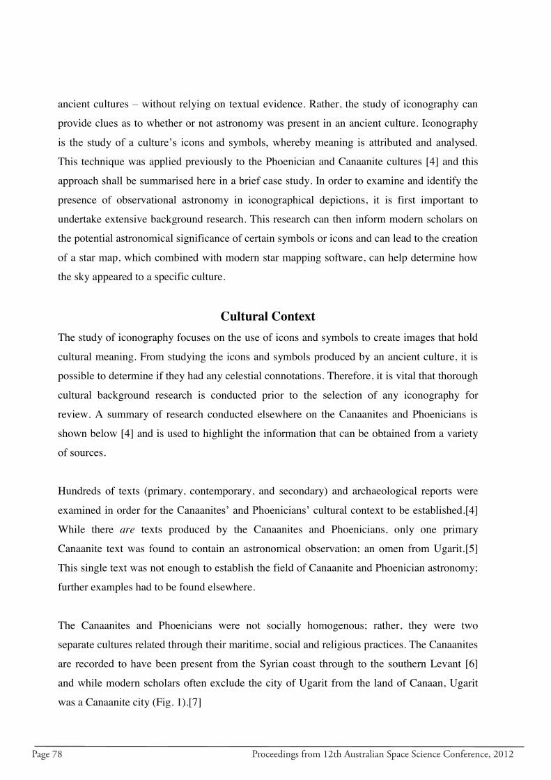
Page 78 Proceedings from 12th Australian Space Science Conference, 2012
ancient cultures – without relying on textual evidence. Rather, the study of iconography can
provide clues as to whether or not astronomy was present in an ancient culture. Iconography
is the study of a culture‟s icons and symbols, whereby meaning is attributed and analysed.
This technique was applied previously to the Phoenician and Canaanite cultures [4] and this
approach shall be summarised here in a brief case study. In order to examine and identify the
presence of observational astronomy in iconographical depictions, it is first important to
undertake extensive background research. This research can then inform modern scholars on
the potential astronomical significance of certain symbols or icons and can lead to the creation
of a star map, which combined with modern star mapping software, can help determine how
the sky appeared to a specific culture.
Cultural Context The study of iconography focuses on the use of icons and symbols to create images that hold
cultural meaning. From studying the icons and symbols produced by an ancient culture, it is
possible to determine if they had any celestial connotations. Therefore, it is vital that thorough
cultural background research is conducted prior to the selection of any iconography for
review. A summary of research conducted elsewhere on the Canaanites and Phoenicians is
shown below [4] and is used to highlight the information that can be obtained from a variety
of sources.
Hundreds of texts (primary, contemporary, and secondary) and archaeological reports were
examined in order for the Canaanites‟ and Phoenicians‟ cultural context to be established.[4]
While there are texts produced by the Canaanites and Phoenicians, only one primary
Canaanite text was found to contain an astronomical observation; an omen from Ugarit.[5]
This single text was not enough to establish the field of Canaanite and Phoenician astronomy;
further examples had to be found elsewhere.
The Canaanites and Phoenicians were not socially homogenous; rather, they were two
separate cultures related through their maritime, social and religious practices. The Canaanites
are recorded to have been present from the Syrian coast through to the southern Levant [6]
and while modern scholars often exclude the city of Ugarit from the land of Canaan, Ugarit
was a Canaanite city (Fig. 1).[7]
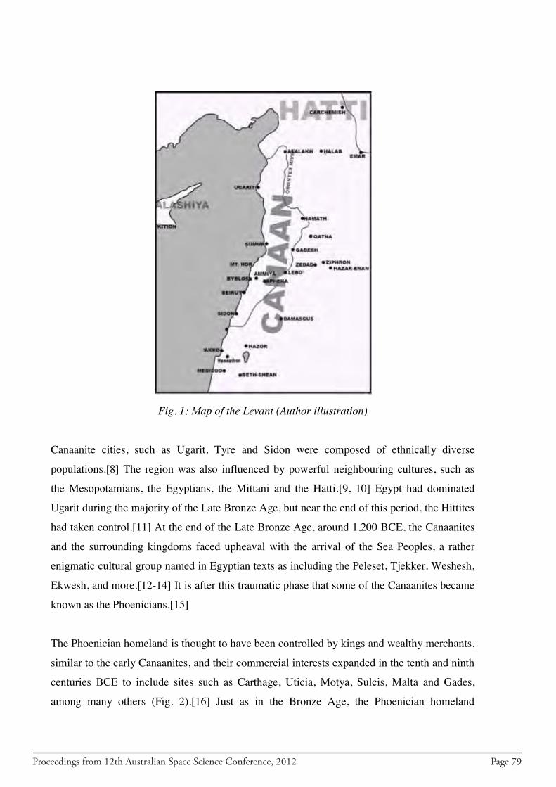
Proceedings from 12th Australian Space Science Conference, 2012 Page 79
Fig. 1: Map of the Levant (Author illustration)
Canaanite cities, such as Ugarit, Tyre and Sidon were composed of ethnically diverse
populations.[8] The region was also influenced by powerful neighbouring cultures, such as
the Mesopotamians, the Egyptians, the Mittani and the Hatti.[9, 10] Egypt had dominated
Ugarit during the majority of the Late Bronze Age, but near the end of this period, the Hittites
had taken control.[11] At the end of the Late Bronze Age, around 1,200 BCE, the Canaanites
and the surrounding kingdoms faced upheaval with the arrival of the Sea Peoples, a rather
enigmatic cultural group named in Egyptian texts as including the Peleset, Tjekker, Weshesh,
Ekwesh, and more.[12-14] It is after this traumatic phase that some of the Canaanites became
known as the Phoenicians.[15]
The Phoenician homeland is thought to have been controlled by kings and wealthy merchants,
similar to the early Canaanites, and their commercial interests expanded in the tenth and ninth
centuries BCE to include sites such as Carthage, Uticia, Motya, Sulcis, Malta and Gades,
among many others (Fig. 2).[16] Just as in the Bronze Age, the Phoenician homeland
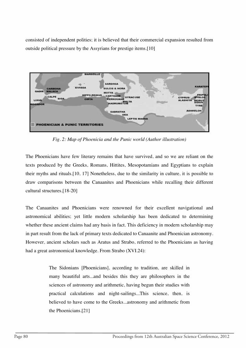
Page 80 Proceedings from 12th Australian Space Science Conference, 2012
consisted of independent polities; it is believed that their commercial expansion resulted from
outside political pressure by the Assyrians for prestige items.[10]
Fig. 2: Map of Phoenicia and the Punic world (Author illustration)
The Phoenicians have few literary remains that have survived, and so we are reliant on the
texts produced by the Greeks, Romans, Hittites, Mesopotamians and Egyptians to explain
their myths and rituals.[10, 17] Nonetheless, due to the similarity in culture, it is possible to
draw comparisons between the Canaanites and Phoenicians while recalling their different
cultural structures.[18-20]
The Canaanites and Phoenicians were renowned for their excellent navigational and
astronomical abilities; yet little modern scholarship has been dedicated to determining
whether these ancient claims had any basis in fact. This deficiency in modern scholarship may
in part result from the lack of primary texts dedicated to Canaanite and Phoenician astronomy.
However, ancient scholars such as Aratus and Strabo, referred to the Phoenicians as having
had a great astronomical knowledge. From Strabo (XVI.24):
The Sidonians [Phoenicians], according to tradition, are skilled in
many beautiful arts...and besides this they are philosophers in the
sciences of astronomy and arithmetic, having begun their studies with
practical calculations and night-sailings...This science, then, is
believed to have come to the Greeks...astronomy and arithmetic from
the Phoenicians.[21]
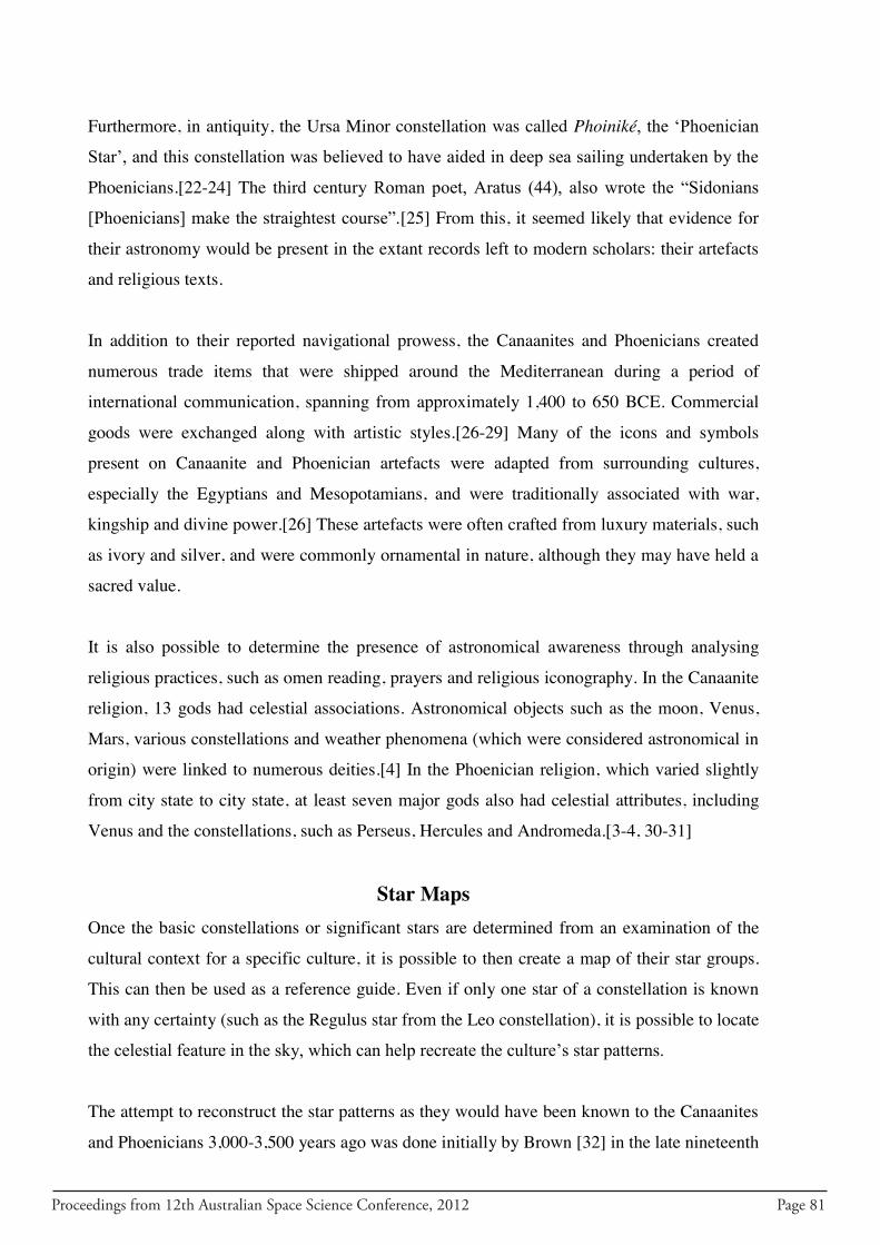
Proceedings from 12th Australian Space Science Conference, 2012 Page 81
Furthermore, in antiquity, the Ursa Minor constellation was called Phoiniké, the „Phoenician
Star‟, and this constellation was believed to have aided in deep sea sailing undertaken by the
Phoenicians.[22-24] The third century Roman poet, Aratus (44), also wrote the “Sidonians
[Phoenicians] make the straightest course”.[25] From this, it seemed likely that evidence for
their astronomy would be present in the extant records left to modern scholars: their artefacts
and religious texts.
In addition to their reported navigational prowess, the Canaanites and Phoenicians created
numerous trade items that were shipped around the Mediterranean during a period of
international communication, spanning from approximately 1,400 to 650 BCE. Commercial
goods were exchanged along with artistic styles.[26-29] Many of the icons and symbols
present on Canaanite and Phoenician artefacts were adapted from surrounding cultures,
especially the Egyptians and Mesopotamians, and were traditionally associated with war,
kingship and divine power.[26] These artefacts were often crafted from luxury materials, such
as ivory and silver, and were commonly ornamental in nature, although they may have held a
sacred value.
It is also possible to determine the presence of astronomical awareness through analysing
religious practices, such as omen reading, prayers and religious iconography. In the Canaanite
religion, 13 gods had celestial associations. Astronomical objects such as the moon, Venus,
Mars, various constellations and weather phenomena (which were considered astronomical in
origin) were linked to numerous deities.[4] In the Phoenician religion, which varied slightly
from city state to city state, at least seven major gods also had celestial attributes, including
Venus and the constellations, such as Perseus, Hercules and Andromeda.[3-4, 30-31]
Star Maps Once the basic constellations or significant stars are determined from an examination of the
cultural context for a specific culture, it is possible to then create a map of their star groups.
This can then be used as a reference guide. Even if only one star of a constellation is known
with any certainty (such as the Regulus star from the Leo constellation), it is possible to locate
the celestial feature in the sky, which can help recreate the culture‟s star patterns.
The attempt to reconstruct the star patterns as they would have been known to the Canaanites
and Phoenicians 3,000-3,500 years ago was done initially by Brown [32] in the late nineteenth
Page 82 Proceedings from 12th Australian Space Science Conference, 2012
century CE. Brown compiled a star map using the texts of other cultures and artefacts, such as
coins.[32] This map was later updated by the author and refined using further analysis, aided
by texts that were unavailable at the time of Brown‟s work.[4] This star map shows that while
the constellation patterns differ in shape to those of modern constellations, they were
positioned in the same locations (Fig. 3).
Fig. 3: Constellation map, location Tyre, Lebanon, 1,200 BCE (Author illustration)
There is debate as to when the modern star groups appeared in the historical record.
Cornell[33] claims that some of our modern constellations may have dated back to 3,300
BCE, but this date is quite early. Aveni[34] also argues that it is third millennium BCE Sumer
(Mesopotamia) from whence our constellations originate, but that the constellation names
were not recorded until the seventh century BCE. As a result of this long history, the
Proceedings from 12th Australian Space Science Conference, 2012 Page 83
constellations shown in Fig. 3 should also be somewhat familiar. Taurus (the Bull), Leo (the
Lion), Hydra (the Water Snake) and Orion (the Hunter) are all present.
While the boundaries of these ancient constellations are different to those of modern star
groups (constellations are, after all, arbitrary), it is still possible to place them in the celestial
sphere. This is because many of the same stars were included in the ancient constellations,
despite the differing shapes. Due to their similar celestial locations, it is possible to use star
mapping software to view the movement of these star groups at a specific time in the past
from a specific geographical location. It is important to use star mapping programs, as they
automatically correct for precession (the rotation of the earth‟s axis) and stellar proper motion
(its angular change in position over time). Furthermore, Fig. 3 can also be used in the study of
Canaanite and Phoenician iconography, in order to determine if there was any apparent link
between the icons portrayed and the known celestial features.
Iconographical Evidence Iconographical evidence of astronomical observations can be found across the world on a
range of artefacts and sites: on portable objects, such as coins, bowls and pendants, and on
more permanent sites, such as stelae, rock art and so forth. This paper shall focus only on one
example belonging to the Phoenicians and Canaanites. It is not the purpose of this analysis to
provide new and exclusive interpretations for the iconography reviewed; rather, it is to add to
the current understanding of well-known Near Eastern motifs and to highlight that this
process can indicate the presence of astronomy in iconography that has otherwise been
associated with other cultural narratives.
When reviewing iconography, it is important to discuss the concept of multivalency. It is easy
to think that an icon or symbol has a fixed meaning; but interpretation is often not that simple.
Icons can have similarities to their „object‟, while symbols may have only arbitrary
associations with theirs.[35] The „meaning‟ of an image is also dependent on a variety of
factors: the context, the intention of the artist/admirer, the expectations of the viewer and the
greater cultural, or social, knowledge.[35]
From the previous study conducted for the Canaanites and Phoenicians,[4] it became apparent
that certain deities had astronomical associations and that their iconographical depictions may
also carry these connotations. Furthermore, certain motifs held similar meanings throughout
Page 84 Proceedings from 12th Australian Space Science Conference, 2012
the Near East: for example, the Horus-falcon was commonly known to be a representation of
the sun, and it is reasonable to assume that depictions of the Horus-falcon in Canaanite and
Phoenician art were intended to portray the sun.
In order to archaeologically determine whether or not astronomy was associated with a
specific site or object, it is vital to collate as much information about the object or site as
possible. In some cultures, this can be a difficult task, as artefacts may have been removed
from a site without maintenance of the provenance, or it can be problematic to determine
accurate dating. In order to conclude whether or not an artefact may hold astronomical
meaning, it is important to know its approximate date of creation, the culture that made it (this
may be different to culture that owned it, as was the case with portable trade items) and the
cultural histories associated with the iconography. If any of this information is unknown, the
analysis may be incomplete.
It is also important to choose a piece of iconography that appears to have celestial links; there
is little point selecting an artefact or site that has no associations with any known
constellations, stars or planets. When undertaking iconographical analysis, it should also be
noted that it is imperative to incorporate all of the icons and symbols present on the piece of
art, both as individual features and as parts of a greater whole. This approach allows for the
layering of iconography ― its multivalency ― to become apparent. The icons and symbols
chosen in the use of art were not solely “an inventory of the natural world, but a selection
taken from it”.[36] These designs were used to evoke the imagination in certain, culturally
specific ways.[36, 37]
In order to demonstrate how background research and star maps can aid in the identification
of astronomical features, a golden Canaanite pendant from the Bronze Age city of Ugarit
(Minet el Beida) shall be examined below (Fig. 4).
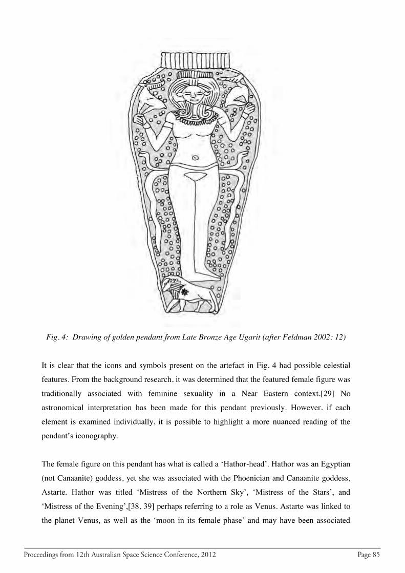
Proceedings from 12th Australian Space Science Conference, 2012 Page 85
Fig. 4: Drawing of golden pendant from Late Bronze Age Ugarit (after Feldman 2002: 12)
It is clear that the icons and symbols present on the artefact in Fig. 4 had possible celestial
features. From the background research, it was determined that the featured female figure was
traditionally associated with feminine sexuality in a Near Eastern context.[29] No
astronomical interpretation has been made for this pendant previously. However, if each
element is examined individually, it is possible to highlight a more nuanced reading of the
pendant‟s iconography.
The female figure on this pendant has what is called a „Hathor-head‟. Hathor was an Egyptian
(not Canaanite) goddess, yet she was associated with the Phoenician and Canaanite goddess,
Astarte. Hathor was titled „Mistress of the Northern Sky‟, „Mistress of the Stars‟, and
„Mistress of the Evening‟,[38, 39] perhaps referring to a role as Venus. Astarte was linked to
the planet Venus, as well as the „moon in its female phase‟ and may have been associated
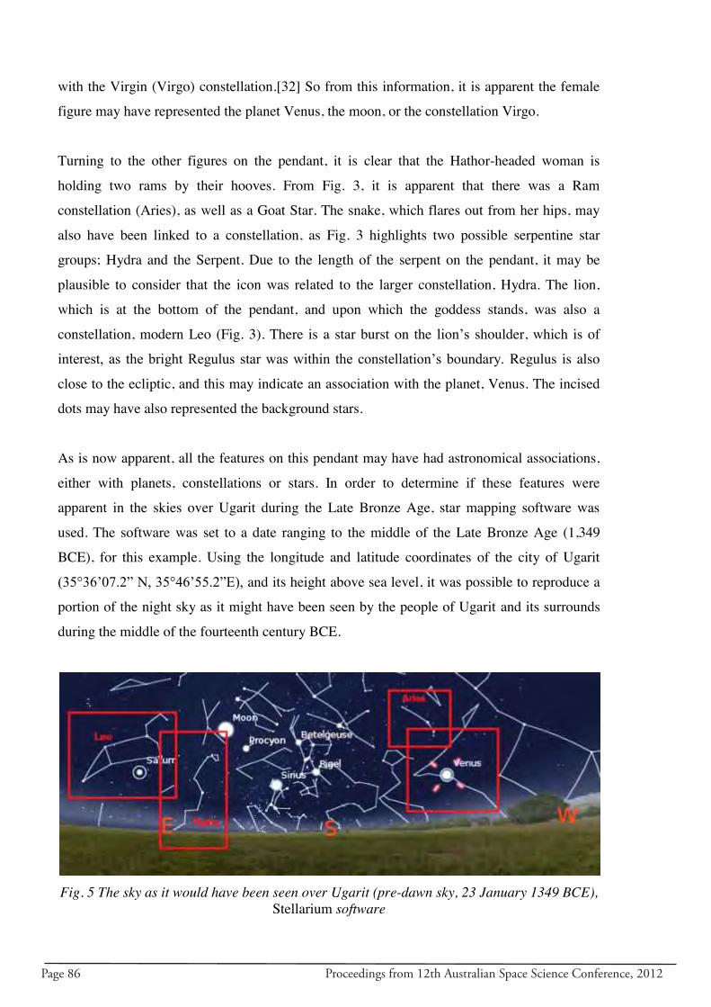
Page 86 Proceedings from 12th Australian Space Science Conference, 2012
with the Virgin (Virgo) constellation.[32] So from this information, it is apparent the female
figure may have represented the planet Venus, the moon, or the constellation Virgo.
Turning to the other figures on the pendant, it is clear that the Hathor-headed woman is
holding two rams by their hooves. From Fig. 3, it is apparent that there was a Ram
constellation (Aries), as well as a Goat Star. The snake, which flares out from her hips, may
also have been linked to a constellation, as Fig. 3 highlights two possible serpentine star
groups; Hydra and the Serpent. Due to the length of the serpent on the pendant, it may be
plausible to consider that the icon was related to the larger constellation, Hydra. The lion,
which is at the bottom of the pendant, and upon which the goddess stands, was also a
constellation, modern Leo (Fig. 3). There is a star burst on the lion‟s shoulder, which is of
interest, as the bright Regulus star was within the constellation‟s boundary. Regulus is also
close to the ecliptic, and this may indicate an association with the planet, Venus. The incised
dots may have also represented the background stars.
As is now apparent, all the features on this pendant may have had astronomical associations,
either with planets, constellations or stars. In order to determine if these features were
apparent in the skies over Ugarit during the Late Bronze Age, star mapping software was
used. The software was set to a date ranging to the middle of the Late Bronze Age (1,349
BCE), for this example. Using the longitude and latitude coordinates of the city of Ugarit
(35°36‟07.2” N, 35°46‟55.2”E), and its height above sea level, it was possible to reproduce a
portion of the night sky as it might have been seen by the people of Ugarit and its surrounds
during the middle of the fourteenth century BCE.
Fig. 5 The sky as it would have been seen over Ugarit (pre-dawn sky, 23 January 1349 BCE),
Stellarium software
Proceedings from 12th Australian Space Science Conference, 2012 Page 87
From Fig. 4, it is apparent that precession (the rotation of the axial tilt of the earth every
26,000 years) would not have had a large enough affect to have altered the portion of the sky
that was viewable to the people of Ugarit during the Late Bronze Age – that it would have
been similar to what is viewable today. This makes it possible to show that all of the
pendant‟s features (Venus, Aries, Hydra and Leo) were apparent at one time during the year
to the population of Ugarit. This information can provide additional meaning to the pendant‟s
iconography. Rather than just highlighting female sexuality, the pendant could also feature
astronomical imagery as well; perhaps indicating a time of the year, or a combination of
celestial features that held some unknown cultural significance.
Conclusions The above discussion highlights how it is possible to determine previously unknown or
disregarded astronomical associations in cultures that have a lack of primary astronomical
texts. Through extensive background research, it is possible to catalogue potential celestial
associations with deities (or other important supernatural beings) and to determine which stars
may have held significance to a particular culture. Star mapping can then provide an easy-to-
view reference chart and can be used in combination with background research to analyse
iconographical depictions. Despite only one example being examined above, it is important to
complete a series of analyses in order to determine if there are any patterns apparent in the
iconography. For the Canaanites and Phoenicians, this was done elsewhere.[4] Once a series
of systematic studies are completed, star mapping software can then be used to reproduce
portions of the night sky to view the location of star patterns to determine if the iconography
had an association with astronomy. This methodology is not only applicable to the Canaanite
and Phoenician cultures, but has the potential to be applied to other cultures where there is
also an absence of primary textual material.
Page 88 Proceedings from 12th Australian Space Science Conference, 2012
References
1. Neugebauer, O., A History of Ancient Mathematical Astronomy, Volume 2, Springer-Verlag Berlin, New York, 1975.
2. Evans, J., The History and Practice of Ancient Astronomy, Oxford University Press, New York, 1998.
3. Rochberg, F., The Heavenly Writing: Divination, Horoscopy, and Astronomy in Mesopotamian Culture, Cambridge University Press, Cambridge, New York, 2004.
4. Goldfarb, A.N, Canaanite and Phoenician Astronomy: From the Late Bronze Age to the Early Iron Age, Unpublished Masters Thesis, The University of Melbourne, Melbourne, 2012.
5. Olmo Lete, G.D., Canaanite Religion: According to the Liturigical Texts of Ugarit, Watson, W.G.E., Trans., Eisenbrauns, Winona Lake, 2004.
6. Cohen, S.L., Canaanites, Chronologies and Connections: The Relationship of Middle Bronze Age IIA Canaan to Middle Kingdom Egypt, Eisenbrauns, Winona Lake, 2002.
7. Gibson, J.C.L., Canaanite Myths and Legends, T. and T. Clark Ltd, Edinburgh, 1978.
8. Dalley, S., „Near Eastern Myths and Legends‟, in The Biblical World, Volume 1, Barton, J., Ed., Routledge, London, 2002, pp. 41-64.
9. Azize, J., The Phoenician Solar Theology, Gorgias Press, Piscataway, 2005.
10. Niemeyer, H.G., „The Phoenicians in the Mediterranean. Between Expansion and Colonisation: A Non-Greek Model of Overseas Settlement and Presence‟, in Greek Colonisation: An Account of Greek Colonies and Other Settlements Overseas, Handbook, Volume 1, Tsetskhladze, G., Ed., Brill, Leiden, 2006, pp. 143-168.
11. Parker, S.B., Ugaritic Narrative Poetry, Smith, M.S., Trans., Scholars Press, Atlanta, 1997.
12. Leonard A.Jr., „Archaeological Sources for the History of Palestine: The Late Bronze Age‟, in Biblical Archaeologist, 52: 1, 1989, pp. 4-39.
13. Negbi, O., „Early Phoenician Presence in the Mediterranean Islands: A Reappraisal‟, in American Journal of Archaeology, 96: 4, 1992, pp. 599-615.
14. Preziosi, D. and Hitchcock, L.A., Aegean Art and Architecture, Oxford University Press, Oxford, 1999.
15. Hamblin, D.J., „The Trade and Treasure of Phoenicia Come Alive in a Venetian Palazzo‟, in Smithsonian, 19: 5, 1988, pp. 62-75.
16. O‟Brien, K.T., Rethinking the ‘Orientalizing’ Phenomenon: A Localized Study of Colonialism and Colonization in the Southern Iberian Peninsula (Andalucía) from the Eighth Century B.C.E., Bachelor of Arts, Unpublished Honours Thesis, The University of Melbourne, Melbourne, 2005.
Proceedings from 12th Australian Space Science Conference, 2012 Page 89
17. Goodspeed, G.S., „A Sketch of Canaanitish History to about the Year 1,000 BC‟, in The Biblical World, 7: 6, 1896, pp. 459-471.
18. Bonnet, C. and Xella, P., „La Religion‟, in La Civilisation Phénicienne et Punique, Krings, V., Ed., E.J. Brill, Leiden, New York, 1995, pp. 316-321.
19. Clifford, R.J., „Phoenician Religion‟, in BASOR, 279, 1990, pp. 55-64.
20. Ribichini, S., „Beliefs and Religious Life‟, in The Phoenicians: Under the Scientific Direction of Sabatino Moscati, Moscati, S., Ed., Abbeville Press, New York, 1988, pp. 104-125.
21. Strabo, Geography, Jones, H.L, Harvard University Press and W. Heinemann, London, Cambridge, Ma, 1917-1944.
22. Bartoloni, P., „Ships and Navigation‟, in The Phoenicians: Under the Scientific Direction of Sabatino Moscati, Moscati, S. Ed, Abbeville Press, New York, 1988, pp. 72-77.
23. Moscati, S., The Phoenicians: Under the Scientific Direction of Sabatino Moscati, Moscati, S. Ed, Abbeville Press, New York, 1988.
24. Aubet, M.E., The Phoenicians and the West: Politics, Colonies, and Trade, Turton, M., Trans., Cambridge, Cambridge University Press, New York, 1993.
25. Aratus, Phaenomena, Kidd, D., Ed & Trans., Cambridge University Press, Cambridge, New York, 1997.
26. Markoe, G.E., „The Emergence of Phoenician Art‟, in Bulletin of the American Schools of Oriental Research, 279, 1990, pp. 13-26.
27. Cornelius, I., The Iconography of the Canaanite Gods Reshef and Ba‘al: Late Bronze Age and Iron Age I Periods (ca. 1,500-1,000 BCE), Universitätsverlag, Fribourg, 1994.
28. Pittman, H., „Constructing Context: The Gebel el-Arak Knife‟, in The Study of the Ancient Near East in the Twenty-First Century: the William Foxwell Albright Centennial Conference, Cooper, J.S. and Schwartz, G.M. Eds., Eisenbrauns, Winona Lake, 1996, pp. 9-32.
29. Feldman, M.H., „Luxurious Forms: Redefining a Mediterranean “International Style”', 1,400-1,200 BCE‟, in The Art Bulletin, 84: 1, 2002, pp. 6-29.
30. Reiner, E., „Babylonian Celestial Divination‟, in Ancient Astronomy and Celestial Divination, Swerdlow, N.M., Ed., MIT Press, Cambridge, Ma, London, 1999, pp. 21-37.
31. Swerdlow, N.M., „Introduction‟, in Ancient Astronomy and Celestial Divination, Swerdlow, N.M., Ed., MIT Press, London, Cambridge, Ma, 1999, pp 1-21.
32. Brown, R.B., Researches into the Origin of the Primitive Constellations of the Greeks, Phoenicians and Babylonians, Vols. 1 and 2, Williams and Norgate, London, 1899-1900.
33. Cornell, J., The First Stargazers: An Introduction to the Origins of Astronomy, Althone Press, London, 1981.
Page 90 Proceedings from 12th Australian Space Science Conference, 2012
34. Aveni, A.F., People and the Sky: Our Ancestors and the Cosmos, Thames and Hudson, New York, 2008.
35. McGowan, E., Cryptic glyptic: A Rhizomatic Exploration of Ambiguity in Selected Minoan Neopalatial Glyptic Images, Unpublished Masters Thesis, The University of Melbourne, Melbourne, 2010.
36. Morgan, L., „Idea, Idiom and Iconography‟, in „L‟Iconographie Minoenne‟, in Bulletin de Correspondance Héllenique, Suppl. 11, 1985, pp. 5-19.
37. Goodison, L., Death, Women, and the Sun: Symbolism of Regeneration in Early Aegean Religion, University of London, Institute of Classical Studies, London, 1989.
38. Pinch, G., Handbook of Egyptian Mythology, ABC-CLIO, Santa Barbara, 2002.
39. Bleeker, C.J., Hathor and Thoth: Two Key Figures of the Ancient Egyptian Religion, Brill, Leiden, 1973.
Proceedings from 12th Australian Space Science Conference, 2012 Page 91
Capturing Trojans and Irregular Satellites - the key required to unlock planetary migration
Jonathan Horner 1, F. Elliott Koch 1, and Patryk Sofia Lykawka 2
1 Department of Astrophysics and Optics, School of Physics, University of New South Wales,
Sydney, NSW, 2052, Australia 2 Astronomy Group, Faculty of Social and Natural Sciences, Kinki University,
Shinkamikosaka 228-3, Higashiosaka-shi, Osaka 577-0813, Japan
Summary: It is now widely accepted that the Solar system’s youth was a remarkably dynamic and chaotic time. The giant planets are understood to have migrated significant distances to reach their current locations, and evidence of that migration’s chaotic influence on the Solar system abounds. The pace of that migration, and the precise distance over which it occurred, is still heavily debated. Some models of planetary migration feature systems in which the giant planets were initially in an extremely compact configuration, in which Uranus and Neptune are chaotically scattered into the outer solar system. Other models feature architectures that were initially more relaxed, and smoother, more sedate migration. To determine which of these scenarios best represents the formation of our Solar system, we must turn to the structure of the system’s small body populations, in which the scars of that migration are still clearly visible. We present the first results of a program investigating the effect of giant planet migration on the reservoirs of small bodies that existed at that time. As the planets migrate, they stir these reservoirs, scattering vast numbers of small bodies onto dynamically unstable orbits in the outer Solar system. The great majority of those bodies are rapidly removed from the system – through collisions and ejections, but a small number become captured as planetary Trojans or irregular satellites, with others being driven by the migration, leading to a significant sculpting of the asteroid belt and trans-Neptunian region. The capture and retention efficiencies to these stable reservoirs are, to a large extent, dependent on the particular migration scenario used. Advocates of chaotic migration from an initially compact scenario argue that smoother, more sedate migration cannot explain the observed populations of Trojans and irregular satellites. Our results draw a strikingly different picture, revealing that such smooth migration is perfectly capable of reproducing the observed populations. Keywords: Asteroids, trans-Neptunian objects, planetary formation, Solar system dynamics, Jupiter Trojans, Neptune Trojans, Irregular satellites
Introduction Evidence abounds within our Solar system that the giant planets migrated over significant distances during the final stages of their formation (e.g. [1][2][3]). Such migration is required to explain the highly excited orbits1 of the Jovian Trojans (e.g. [4][5][6][7]), Neptunian
1 Objects moving on highly excited orbits have orbits with high eccentricities and/or inclinations. Such orbits stand in stark contrast to the relatively unexcited orbits of the planets in the Solar system. In this work, we use the terms “dynamically hot” and “dynamically cold”,
Page 92 Proceedings from 12th Australian Space Science Conference, 2012
Trojans (e.g. [8][9][10][11]), the fine structure of the asteroid belt (e.g. [12][13][14][15]), the distribution of objects in the trans-Neptunian region (e.g. [16][17][18]), and even the origin of the myriad irregular satellites of the giant planets (e.g. [19][20][21][22]). The most obvious evidence for planetary migration in our own Solar system is the population of objects known as the Plutinos, after the first discovered, the dwarf planet Pluto2 ([23]). These objects, trapped in 2:3 mean-motion resonance (MMR)3 with Neptune, move on highly excited orbits ([24]), with many members, like Pluto, crossing Neptune’s orbit at perihelion. Given that the Solar system formed from a dynamically cold disk of material, featuring dust and gas on orbits with very low eccentricities and inclinations (e.g. [25][26][27]), the most likely way the Plutino population can be understood is that Neptune migrated outwards after its formation (e.g. [1][3][28]). As Neptune moved outward, it was preceded by its web of MMRs, which swept before it, trapping planetesimals and carrying them outward. Once caught in Neptune’s web, the orbital inclinations and eccentricities of these objects were pumped up and they were forced ever further from the Sun, resulting in the highly excited population we observe today. The Plutinos are not the only Solar system population that still bears the scars of planetary migration. In fact, the more objects we discover and study in our Solar system (e.g. [13][29][30][31][32]), the more evidence we find that the formation of our planetary system was a chaotic process, and that the giant planets migrated over significant distances before coming to rest at their current locations (e.g. [3][9][28]). Despite the fact that the evidence for giant planet migration is now well accepted, the nature of that migration remains the subject of much debate. Was the migration fast or slow? Smooth or jumpy? Did the planets migrate at the same rate, or form and move at different times?4 The answer to all these questions may lie in the evidence left behind by that migration – the distribution of the Solar system’s small bodies. In this work, we present the first preliminary results of a new dynamical study of the influence of planetary migration on the structure of the Solar system’s small body reservoirs. In section two, we describe the set-up of our model, and discuss the various migration scenarios we will consider. In section three, we present preliminary results for the first of those migration scenarios. Finally, we draw our first tentative conclusions, and discuss our future work.
Modelling Migration and Primordial Small Body Populations
together with talking about “excited orbits”, when discussing the orbital properties of the Solar system’s small body populations. A dynamically hot population is composed of objects moving on excited orbits, whilst a dynamically cold population is one in which the members move on orbits with negligible eccentricity (i.e. on near-circular orbits) and with very low inclinations (i.e. essentially within the plane of the Solar system). 2 Following its reclassification as a dwarf planet, Pluto was added to the list of minor planets, and given the minor planet number 134340. Therefore, technically, it should be referred to as minor planet 134340 Pluto. 3 For brevity, we hereafter use the abbreviation “MMR” for mean-motion resonance. Since the Plutinos are trapped in 2:3 MMR with Neptune, this means, on average, they complete two orbits in the time it takes the giant planet to complete three full orbits of the Sun. 4 For examples of the many different types of migration that have been proposed to date, we direct the interested reader to e.g. [2] [7][14].
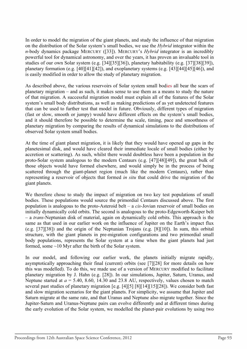
Proceedings from 12th Australian Space Science Conference, 2012 Page 93
In order to model the migration of the giant planets, and study the influence of that migration on the distribution of the Solar system’s small bodies, we use the Hybrid integrator within the n-body dynamics package MERCURY ([33]). MERCURY’s Hybrid integrator is an incredibly powerful tool for dynamical astronomy, and over the years, it has proven an invaluable tool in studies of our own Solar system (e.g. [34][35][36]), planetary habitability (e.g. [37][38][39]), planetary formation (e.g. [40][41][42]), and exoplanetary systems (e.g. [43][44][45][46]), and is easily modified in order to allow the study of planetary migration. As described above, the various reservoirs of Solar system small bodies all bear the scars of planetary migration – and as such, it makes sense to use them as a means to study the nature of that migration. A successful migration model must explain all of the features of the Solar system’s small body distributions, as well as making predictions of as yet undetected features that can be used to further test that model in future. Obviously, different types of migration (fast or slow, smooth or jumpy) would have different effects on the system’s small bodies, and it should therefore be possible to determine the scale, timing, pace and smoothness of planetary migration by comparing the results of dynamical simulations to the distributions of observed Solar system small bodies. At the time of giant planet migration, it is likely that they would have opened up gaps in the planetesimal disk, and would have cleared their immediate locale of small bodies (either by accretion or scattering). As such, whilst there would doubtless have been a population in the proto-Solar system analogous to the modern Centaurs (e.g. [47][48][49]), the great bulk of those objects would have formed elsewhere, and would simply be in the process of being scattered through the giant-planet region (much like the modern Centaurs), rather than representing a reservoir of objects that formed in situ that could drive the migration of the giant planets. We therefore chose to study the impact of migration on two key test populations of small bodies. These populations would source the primordial Centaurs discussed above. The first population is analogous to the proto-Asteroid belt – a cis-Jovian reservoir of small bodies on initially dynamically cold orbits. The second is analogous to the proto-Edgeworth-Kuiper belt – a trans-Neptunian disk of material, again on dynamically cold orbits. This approach is the same as that used in our earlier work on the influence of Jupiter on the Earth’s impact flux (e.g. [37][38]) and the origin of the Neptunian Trojans (e.g. [8][10]). In sum, this orbital structure, with the giant planets in pre-migration configurations and two primordial small body populations, represents the Solar system at a time when the giant planets had just formed, some ~10 Myr after the birth of the Solar system. In our model, and following our earlier work, the planets initially migrate rapidly, asymptotically approaching their final (current) orbits (see [7][28] for more details on how this was modelled). To do this, we made use of a version of MERCURY modified to facilitate planetary migration by J. Hahn (e.g. [28]). In our simulations, Jupiter, Saturn, Uranus, and Neptune started at a = 5.40, 8.60, 14.30 and 23.8 AU, respectively, values chosen to match several past studies of planetary migration [e.g. [4][5] [8][14][15][28]). We consider both fast and slow migration scenarios for the giant planets. For simplicity, we assume that Jupiter and Saturn migrate at the same rate, and that Uranus and Neptune also migrate together. Since the Jupiter-Saturn and Uranus-Neptune pairs can evolve differently and at different times during the early evolution of the Solar system, we modelled the planet-pair evolutions by using two
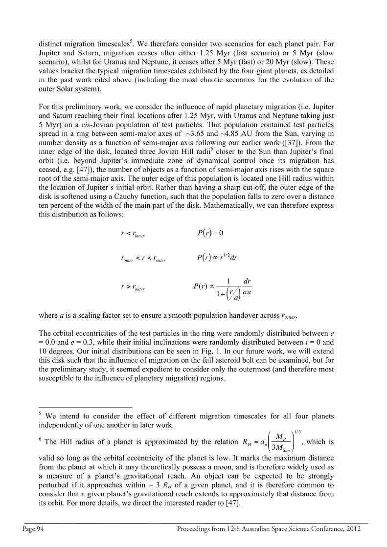
Page 94 Proceedings from 12th Australian Space Science Conference, 2012
distinct migration timescales5. We therefore consider two scenarios for each planet pair. For Jupiter and Saturn, migration ceases after either 1.25 Myr (fast scenario) or 5 Myr (slow scenario), whilst for Uranus and Neptune, it ceases after 5 Myr (fast) or 20 Myr (slow). These values bracket the typical migration timescales exhibited by the four giant planets, as detailed in the past work cited above (including the most chaotic scenarios for the evolution of the outer Solar system). For this preliminary work, we consider the influence of rapid planetary migration (i.e. Jupiter and Saturn reaching their final locations after 1.25 Myr, with Uranus and Neptune taking just 5 Myr) on a cis-Jovian population of test particles. That population contained test particles spread in a ring between semi-major axes of ~3.65 and ~4.85 AU from the Sun, varying in number density as a function of semi-major axis following our earlier work ([37]). From the inner edge of the disk, located three Jovian Hill radii6 closer to the Sun than Jupiter’s final orbit (i.e. beyond Jupiter’s immediate zone of dynamical control once its migration has ceased, e.g. [47]), the number of objects as a function of semi-major axis rises with the square root of the semi-major axis. The outer edge of this population is located one Hill radius within the location of Jupiter’s initial orbit. Rather than having a sharp cut-off, the outer edge of the disk is softened using a Cauchy function, such that the population falls to zero over a distance ten percent of the width of the main part of the disk. Mathematically, we can therefore express this distribution as follows:
€
r < rinner P r( ) = 0
rinner < r < router P r( )∝ r1/ 2dr
r > router P(r)∝ 11+ r
a( )draπ
where a is a scaling factor set to ensure a smooth population handover across router. The orbital eccentricities of the test particles in the ring were randomly distributed between e = 0.0 and e = 0.3, while their initial inclinations were randomly distributed between i = 0 and 10 degrees. Our initial distributions can be seen in Fig. 1. In our future work, we will extend this disk such that the influence of migration on the full asteroid belt can be examined, but for the preliminary study, it seemed expedient to consider only the outermost (and therefore most susceptible to the influence of planetary migration) regions. 5 We intend to consider the effect of different migration timescales for all four planets independently of one another in later work.
6 The Hill radius of a planet is approximated by the relation
€
RH = apMP
3MSun
"
# $
%
& '
1/ 3
, which is
valid so long as the orbital eccentricity of the planet is low. It marks the maximum distance from the planet at which it may theoretically possess a moon, and is therefore widely used as a measure of a planet’s gravitational reach. An object can be expected to be strongly perturbed if it approaches within ~ 3 RH of a given planet, and it is therefore common to consider that a given planet’s gravitational reach extends to approximately that distance from its orbit. For more details, we direct the interested reader to [47].
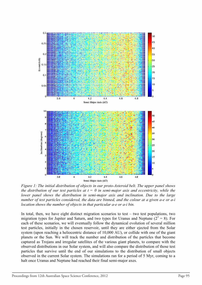
Proceedings from 12th Australian Space Science Conference, 2012 Page 95
Figure 1: The initial distribution of objects in our proto-Asteroid belt. The upper panel shows the distribution of our test particles at t = 0 in semi-major axis and eccentricity, while the lower panel shows the distribution in semi-major axis and inclination. Due to the large number of test particles considered, the data are binned, and the colour at a given a-e or a-i location shows the number of objects in that particular a-e or a-i bin. In total, then, we have eight distinct migration scenarios to test – two test populations, two migration types for Jupiter and Saturn, and two types for Uranus and Neptune (23 = 8). For each of these scenarios, we will eventually follow the dynamical evolution of several million test particles, initially in the chosen reservoir, until they are either ejected from the Solar system (upon reaching a heliocentric distance of 10,000 AU), or collide with one of the giant planets or the Sun. We will track the number and distribution of the particles that become captured as Trojans and irregular satellites of the various giant planets, to compare with the observed distributions in our Solar system, and will also compare the distribution of those test particles that survive until the end of our simulations to the distribution of small objects observed in the current Solar system. The simulations ran for a period of 5 Myr, coming to a halt once Uranus and Neptune had reached their final semi-major axes.
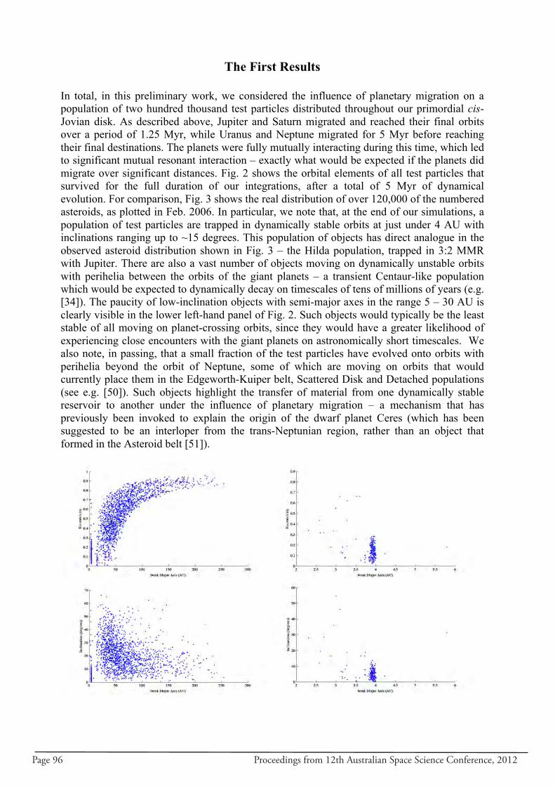
Page 96 Proceedings from 12th Australian Space Science Conference, 2012
The First Results
In total, in this preliminary work, we considered the influence of planetary migration on a population of two hundred thousand test particles distributed throughout our primordial cis-Jovian disk. As described above, Jupiter and Saturn migrated and reached their final orbits over a period of 1.25 Myr, while Uranus and Neptune migrated for 5 Myr before reaching their final destinations. The planets were fully mutually interacting during this time, which led to significant mutual resonant interaction – exactly what would be expected if the planets did migrate over significant distances. Fig. 2 shows the orbital elements of all test particles that survived for the full duration of our integrations, after a total of 5 Myr of dynamical evolution. For comparison, Fig. 3 shows the real distribution of over 120,000 of the numbered asteroids, as plotted in Feb. 2006. In particular, we note that, at the end of our simulations, a population of test particles are trapped in dynamically stable orbits at just under 4 AU with inclinations ranging up to ~15 degrees. This population of objects has direct analogue in the observed asteroid distribution shown in Fig. 3 – the Hilda population, trapped in 3:2 MMR with Jupiter. There are also a vast number of objects moving on dynamically unstable orbits with perihelia between the orbits of the giant planets – a transient Centaur-like population which would be expected to dynamically decay on timescales of tens of millions of years (e.g. [34]). The paucity of low-inclination objects with semi-major axes in the range 5 – 30 AU is clearly visible in the lower left-hand panel of Fig. 2. Such objects would typically be the least stable of all moving on planet-crossing orbits, since they would have a greater likelihood of experiencing close encounters with the giant planets on astronomically short timescales. We also note, in passing, that a small fraction of the test particles have evolved onto orbits with perihelia beyond the orbit of Neptune, some of which are moving on orbits that would currently place them in the Edgeworth-Kuiper belt, Scattered Disk and Detached populations (see e.g. [50]). Such objects highlight the transfer of material from one dynamically stable reservoir to another under the influence of planetary migration – a mechanism that has previously been invoked to explain the origin of the dwarf planet Ceres (which has been suggested to be an interloper from the trans-Neptunian region, rather than an object that formed in the Asteroid belt [51]).
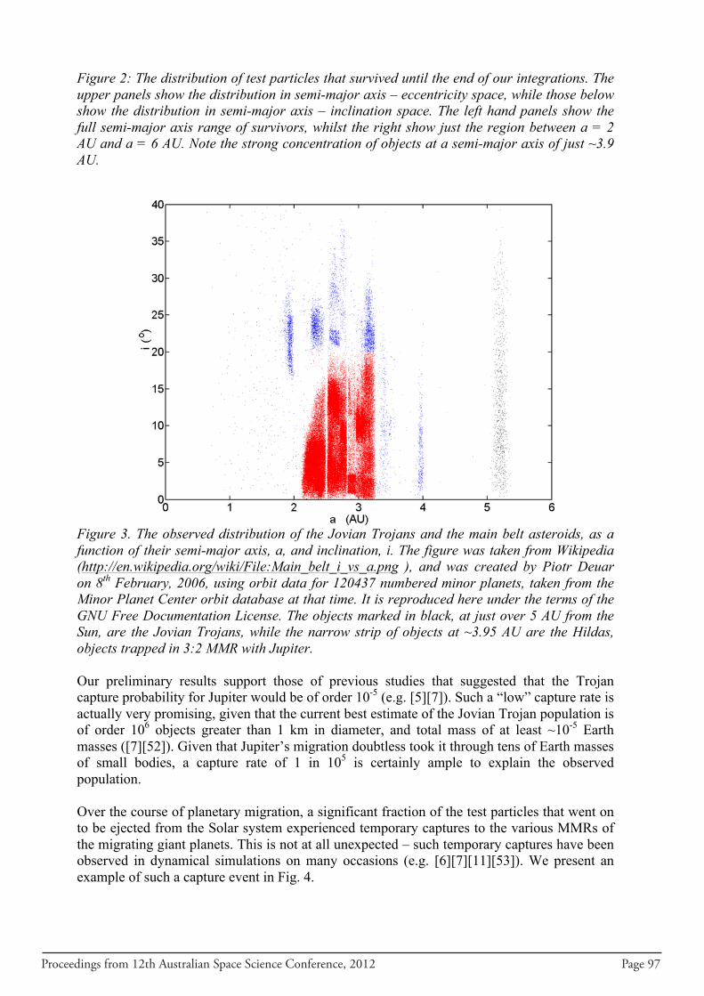
Proceedings from 12th Australian Space Science Conference, 2012 Page 97
Figure 2: The distribution of test particles that survived until the end of our integrations. The upper panels show the distribution in semi-major axis – eccentricity space, while those below show the distribution in semi-major axis – inclination space. The left hand panels show the full semi-major axis range of survivors, whilst the right show just the region between a = 2 AU and a = 6 AU. Note the strong concentration of objects at a semi-major axis of just ~3.9 AU.
Figure 3. The observed distribution of the Jovian Trojans and the main belt asteroids, as a function of their semi-major axis, a, and inclination, i. The figure was taken from Wikipedia (http://en.wikipedia.org/wiki/File:Main_belt_i_vs_a.png ), and was created by Piotr Deuar on 8th February, 2006, using orbit data for 120437 numbered minor planets, taken from the Minor Planet Center orbit database at that time. It is reproduced here under the terms of the GNU Free Documentation License. The objects marked in black, at just over 5 AU from the Sun, are the Jovian Trojans, while the narrow strip of objects at ~3.95 AU are the Hildas, objects trapped in 3:2 MMR with Jupiter. Our preliminary results support those of previous studies that suggested that the Trojan capture probability for Jupiter would be of order 10-5 (e.g. [5][7]). Such a “low” capture rate is actually very promising, given that the current best estimate of the Jovian Trojan population is of order 106 objects greater than 1 km in diameter, and total mass of at least ~10-5 Earth masses ([7][52]). Given that Jupiter’s migration doubtless took it through tens of Earth masses of small bodies, a capture rate of 1 in 105 is certainly ample to explain the observed population. Over the course of planetary migration, a significant fraction of the test particles that went on to be ejected from the Solar system experienced temporary captures to the various MMRs of the migrating giant planets. This is not at all unexpected – such temporary captures have been observed in dynamical simulations on many occasions (e.g. [6][7][11][53]). We present an example of such a capture event in Fig. 4.
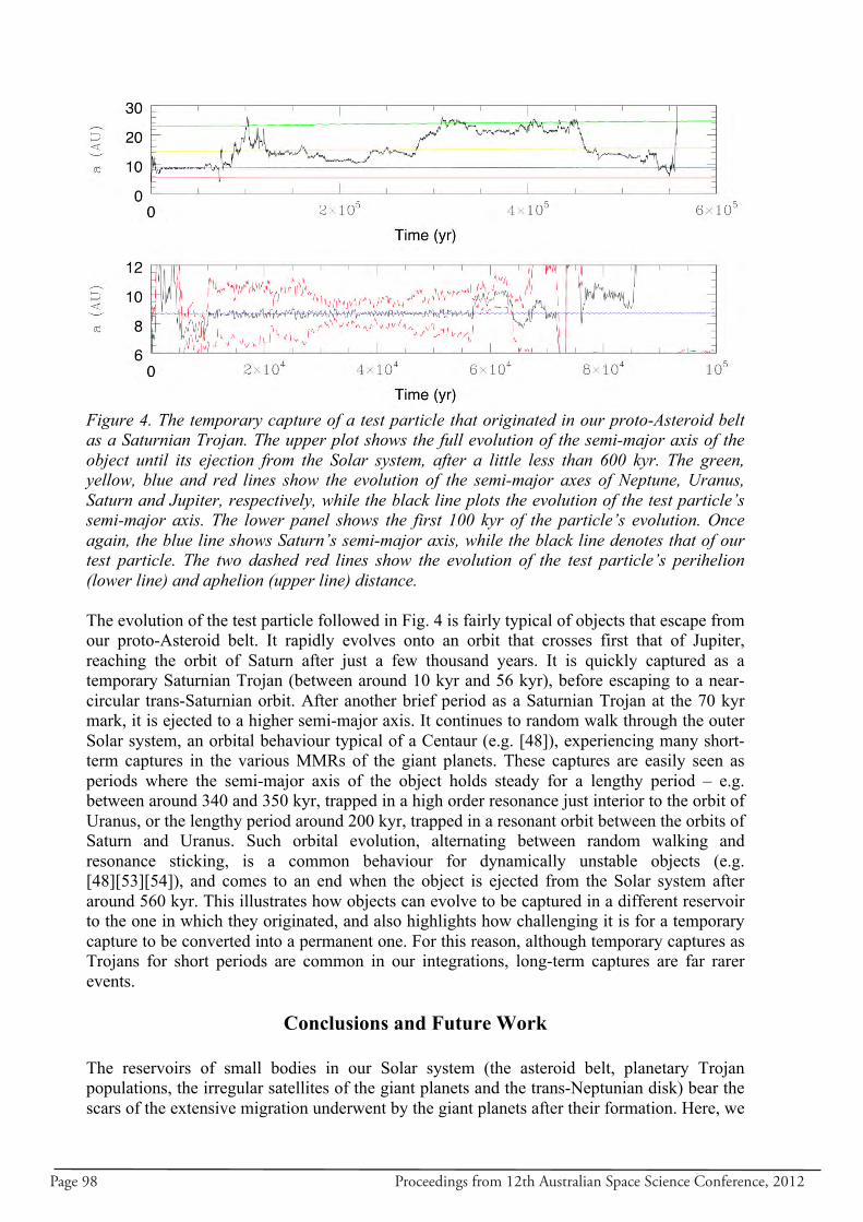
Page 98 Proceedings from 12th Australian Space Science Conference, 2012
Figure 4. The temporary capture of a test particle that originated in our proto-Asteroid belt as a Saturnian Trojan. The upper plot shows the full evolution of the semi-major axis of the object until its ejection from the Solar system, after a little less than 600 kyr. The green, yellow, blue and red lines show the evolution of the semi-major axes of Neptune, Uranus, Saturn and Jupiter, respectively, while the black line plots the evolution of the test particle’s semi-major axis. The lower panel shows the first 100 kyr of the particle’s evolution. Once again, the blue line shows Saturn’s semi-major axis, while the black line denotes that of our test particle. The two dashed red lines show the evolution of the test particle’s perihelion (lower line) and aphelion (upper line) distance. The evolution of the test particle followed in Fig. 4 is fairly typical of objects that escape from our proto-Asteroid belt. It rapidly evolves onto an orbit that crosses first that of Jupiter, reaching the orbit of Saturn after just a few thousand years. It is quickly captured as a temporary Saturnian Trojan (between around 10 kyr and 56 kyr), before escaping to a near-circular trans-Saturnian orbit. After another brief period as a Saturnian Trojan at the 70 kyr mark, it is ejected to a higher semi-major axis. It continues to random walk through the outer Solar system, an orbital behaviour typical of a Centaur (e.g. [48]), experiencing many short-term captures in the various MMRs of the giant planets. These captures are easily seen as periods where the semi-major axis of the object holds steady for a lengthy period – e.g. between around 340 and 350 kyr, trapped in a high order resonance just interior to the orbit of Uranus, or the lengthy period around 200 kyr, trapped in a resonant orbit between the orbits of Saturn and Uranus. Such orbital evolution, alternating between random walking and resonance sticking, is a common behaviour for dynamically unstable objects (e.g. [48][53][54]), and comes to an end when the object is ejected from the Solar system after around 560 kyr. This illustrates how objects can evolve to be captured in a different reservoir to the one in which they originated, and also highlights how challenging it is for a temporary capture to be converted into a permanent one. For this reason, although temporary captures as Trojans for short periods are common in our integrations, long-term captures are far rarer events.
Conclusions and Future Work
The reservoirs of small bodies in our Solar system (the asteroid belt, planetary Trojan populations, the irregular satellites of the giant planets and the trans-Neptunian disk) bear the scars of the extensive migration underwent by the giant planets after their formation. Here, we
Proceedings from 12th Australian Space Science Conference, 2012 Page 99
present the results of a dynamical investigation of the effect of giant planet migration on objects in a proto-asteroid belt. We model the migration of the giant planets as starting rapidly, then slowing as they approach their final destinations. We followed the dynamical evolution of twenty thousand test particles distributed through the outer reaches of a proto-asteroid belt, which stretched from an inner edge at around 3.7 AU to an outer edge just beyond 4.8 AU. We found that the great majority of the objects in our proto-asteroid belt were scattered and ejected from the Solar system. However, a significant number remained, trapped in mutual 3:2 mean-motion resonance with Jupiter. The distribution of these test particles in semi-major axis – inclination space was essentially identical to that of the Hilda population observed today. The test particles that escaped from the proto-asteroid belt typically moved onto Jupiter-crossing orbits, and then evolved as typical Centaurs for tens or hundreds of thousands of years until a close encounter with one of the giant planets flung them out of the Solar system forever. A significant fraction of the test particles collided with the giant planets – a result that is not unsurprising, since it is reasonable to expect that the giant planets would still be accreting large amounts of material as they migrate. The majority of the test particles experienced repeated short-term captures in the many MMRs of the giant planets. Such captures were generally short, however, with only a tiny fraction of those objects experiencing long-term capture. Our results support earlier work, finding that the long-term capture probability as a Jovian Trojan is of order 10-5. Although such a capture probability sounds punishingly low, it is actually more than ample to explain the currently observed Jovian Trojan population, since Jupiter’s migration would have caused it to encounter tens of Earth masses of small bodies before it reached its final destination. In the future, we will continue our studies by performing seven further simulations, each examining either a different migration scenario for the giant planets, or a different source reservoir for the small bodies involved (a proto-Edgeworth-Kuiper belt). By the end of our work, we should be able to better constrain the true nature and pace of planetary migration, using the known populations of small bodies in our Solar system today as a guide to disentangle the events that occurred over four billion years ago.
Acknowledgements
The authors wish to thank J. Hahn, who made available the version of MERCURY, modified to enable planetary migration, used in this work. The authors also wish to thank the two referees of this paper, Dr. Paul Francis and Dr. Rob Wittenmyer, for their comments, which helped to improve the flow and clarity of our article.
References 1. Malhotra, R., “The origin of Pluto’s peculiar orbit”, Nature, Vol. 365, 1993, pp. 819 -
821
2. Tsiganis, K., Gomes, R., Morbidelli, A., and Levison, H. F., “Origin of the orbital architecture of the giant planets of the Solar System”, Nature, Vol. 435, 2005, pp. 459-461
3. Levison, H. F., Morbidelli, A., Van Laerhoven. C., Gomes, R. and Tsiganis, K., “Origin of the Structure of the Kuiper Belt during a Dynamical Instability in the Orbits of Uranus and Neptune”, Icarus, Vol. 196, 2008, pp. 258 - 273
Page 100 Proceedings from 12th Australian Space Science Conference, 2012
4. Fleming, H. J. and Hamilton, D. P., “On the Origin of the Trojan Asteroids: Effects of Jupiter’s Mass Accretion and Radial Migration”, Icarus, Vol. 148, pp. 479 - 493
5. Morbidelli A., Levison, H. F., Tsiganis, K. & Gomes, R., “Chaotic capture of Jupiter’s Trojan asteroids in the early Solar System”, Nature, Vol. 435, 2005, pp. 462-465.
6. Horner, J. and Wyn Evans, N., “The capture of Centaurs as Trojans”, Monthly Notices of the Royal Astronomical Society: Letters, Vol. 367, 2006, pp. L20 – L23
7. Lykawka, P. S. and Horner, J., “The capture of Trojan asteroids by the giant planets during planetary migration”, Monthly Notices of the Royal Astronomical Society, Vol. 405, 2010, pp. 1375-1383.
8. Lykawka, P. S., Horner, J., Jones, B. W. and Mukai, T., “Origin and dynamical evolution of Neptune Trojans – I. Formation and planetary migration”, Monthly Notices of the Royal Astronomical Society, Vol. 398, 2009, pp. 1715 -1729.
9. Lykawka, P. S., Horner, J., Jones, B. W. and Mukai, T., “Formation and dynamical evolution of the Neptune Trojans – the influence of the initial Solar system architecture”, Monthly Notices of the Royal Astronomical Society, Vol. 404, 2010, pp. 1272 -1280.
10. Lykawka, P. S., Horner, J., Jones, B. W. and Mukai, T., “Origin and dynamical evolution of Neptune Trojans – II. Long -term evolution”, Monthly Notices of the Royal Astronomical Society, Vol. 412, 2011, pp. 537-550.
11. Nesvorný, D., V., Vokrouhlicky, D., “Chaotic Capture of Neptune Trojans” , Astronomical Journal, Vol. 137, 2009, pp. 5003-5011.
12. Gomes, R. S., “Dynamical Effects of Planetary Migration on the Primordial Asteroid Belt”, Astronomical Journal, Vol. 114, 1997, pp. 396 – 401
13. Minton, D. A. and Malhotra, R., “A record of planet migration in the main asteroid belt”, Nature, Vol. 457, 2009, pp. 1109 - 1111
14. Minton, D. A. and Malhotra, R., “Secular resonance sweeping of the main asteroid belt during planet migration”, The Astrophysical Journal, Vol. 732, 2011, article id. 53
15. Morbidelli, A., Brasser, R., Gomes, R., Levison, H. F. and Tsiganis, K, “Evidence from the Asteroid Belt for a Violent Past Evolution of Jupiter's Orbit”, The Astronomical Journal, Vol. 140, 2010, pp. 1391-1401
16. Gomes, R. S., Morbidelli, A. and Levison, H. D., “Planetary migration in a planetesimal disk: why did Neptune stop at 30 AU?”, Icarus, Vol. 170, 2004, pp. 492-507
17. Emel’Yanenko, V. V., “Kuiper Belt structure as a reflection of the migration process of a planet”, Solar System Research, Vol. 44, 2010, pp. 281 - 289
18. Lykawka, P. S. and Mukai, T., “An Outer Planet Beyond Pluto and the Origin of the Trans-Neptunian Belt Architecture”, The Astronomical Journal, Vol. 135, 2008, pp. 1161-1200
19. Jewitt, D. and Haghighipour, N., “Irregular Satellites of the Planets: Products of Capture in the Early Solar System”, Annual Review of Astronomy & Astrophyiscs, Vol. 45, 2007, pp. 261 - 295
20. Koch, F. E. and Hansen, B. M. S., “On collisional capture rates of irregular satellites around the gas -giant planets and the minimum mass of the solar nebula”, Monthly Notices of the Royal Astronomical Society, Vol. 416, 2011, pp. 1274 -1283.
Proceedings from 12th Australian Space Science Conference, 2012 Page 101
21. Quillen, A. C., Hasan, I. and Moore, A., “Capture of irregular satellites via binary planetesimal exchange reactions in migrating planetary systems”, Monthly Notices of the Royal Astronomical Society, Vol. 425, 2012, pp. 2507 – 2518
22. Vokrouhlický, D., Nesvorný, D. and Levison, H. F., Irregular Satellite Capture by Exchange Reactions, The Astronomical Journal, Vol. 136, 2008, pp. 1463-1476
23. Malhotra, R., “The Origin of Pluto’s Orbit: Implications for the Solar System Beyond Neptune”, The Astronomical Journal, Vol. 110, 1995, pp. 420
24. Yu, Q. and Tremaine, S., “The Dynamics of Plutinos”, The Astronomical Journal, Vol. 118, 1999, pp. 1873 - 1881
25. Lissauer, J. J., “Timescales for planetary accretion and the structure of the protoplanetary disk”, Icarus, Vol. 69, 1987, pp. 249 - 265
26. Pollack, J. B., Hubickyj, O., Bodenheimer, P., Lissauer, J. J., Podolak, M. and Greenzweig, Y., “Formation of the Giant Planets by Concurrent Accretion of Solids and Gas”, Icarus, Vol. 124, 1996, pp. 62 - 85
27. Ida, S. and Lin, D. N. C., “Toward a Deterministic Model of Planetary Formation. I. A Desert in the Mass and Semimajor Axis Distributions of Extrasolar Planets”, Astrophysical Journal, Vol. 604, 2004, pp. 388 - 413
28. Hahn, J. M. and Malhotra, R., “Neptune's Migration into a Stirred-Up Kuiper Belt: A Detailed Comparison of Simulations to Observations”, The Astronomical Journal, Vol. 130, 2005, 2392-2414.
29. Horner, J. and Lykawka, P. S., “2001 QR322: a dynamically unstable Neptune Trojan?”, Monthly Notices of the Royal Astronomical Society, Vol. 405, 2010, pp. 49 – 56
30. Horner, J., Lykawka, P. S., Bannister, M. T. and Francis, P., “2008 LC18: a potentially unstable Neptune Trojan”, Monthly Notices of the Royal Astronomical Society, Vol. 422, 2012, pp. 2145 – 2151
31. Horner, J., Müller, T. G. and Lykawka, P. S., “(1173) Anchises – Thermophysical and dynamical studies of a dynamically unstable Jovian Trojan”, Monthly Notices of the Royal Astronomical Society, Vol. 423, 2012, pp. 2587 – 2596
32. Lykawka, P. S. and Mukai, T., “Origin of scattered disk resonant TNOs: Evidence for an ancient excited Kuiper belt of 50 AU radius”, Icarus, Vol. 186, 2007, pp. 331 – 341
33. Chambers, J., “A hybrid symplectic integrator that permits close encounters between massive bodies”, Monthly Notices of the Royal Astronomical Society, Vol. 304, 1999, pp. 793 – 799.
34. Horner, J., Evans, N. W. and Bailey, M. E., “Simulations of the population of Centaurs – I. The bulk statistics”, Monthly Notices of the Royal Astronomical Society, Vol. 354, 2004, pp. 798 – 810
35. Jewitt, D., Yang, B. and Haghighipour, N., “Main-Belt Comet P/2008 R1 (Garradd)”, The Astronomical Journal, Vol. 137, Issue 5., 2009, pp. 4313 – 4321
36. Asher, D. J. and Emel’Yanenko, V. V., “The origin of the June Bootid outburst in 1998 and determination of cometary ejection velocities”, Monthly Notices of the Royal Astronomical Society, Vol. 331., Issue 1, 2002, pp. 126 – 132
37. Horner, J. and Jones, B. W., “Jupiter friend or foe? I: The asteroids”, International Journal of Astrobiology, Vol. 7, 2008, pp. 251 - 261
Page 102 Proceedings from 12th Australian Space Science Conference, 2012
38. Horner, J. and Jones, B. W., “Jupiter – friend or foe? II: the Centaurs”, International Journal of Astrobiology, Vol. 8, 2009, pp. 75 - 80
39. Jones, B. W., Sleep, P. N. and Chambers, J. E., “The stability of the orbits of terrestrial planets in the habitable zones of known exoplanetary systems”, Astronomy and Astrophysics, Vol. 366, 2001, pp. 254 – 262
40. Raymond, S. N., Mandell, A. M. and Sigurdsson, Steinn, “Exotic Earths: Forming Habitable Worlds with Giant Planet Migration”, Science, Vol. 313, Issue 5792, 2006, pp. 1413 – 1416
41. Fogg, M. and Nelson, R. P., “Oligarchic and giant impact growth of terrestrial planets in the presence of gas giant planet migration”, Astronomy and Astrophysics, Vol. 441, Issue 2, 2005, pp.791-806
42. Kennedy, G. M. and Kenyon, S. J., “Planet formation around stars of various masses: Hot Super-Earths”, The Astrophysical Journal, Vol. 682, Issue 2, 2008, pp. 1264-1276
43. Ford, E. B., Lystad, V. and Rasio, F. A., “Planet-planet scattering in the upsilon Andromedae system”, Nature, Vol. 434, 2005, pp. 873 - 876
44. Marshall, J., Horner, J. and Carter, A., “Dynamical simulations of the HR8799 planetary system”, International Journal of Astrobiology, Vol. 9, 2010, pp. 259 - 264
45. Horner, J., Marshall, J. P., Wittenmyer, R. A. and Tinney, C. G., “A dynamical analysis of the proposed HU Aquarii planetary system”, Monthly Notices of the Royal Astronomical Society: Letters, Vol. 416, 2011, pp. 11 – 15
46. Wittenmyer, R. A., Horner, J., Marshall, J. P., Butters, O. W. and Tinney, C. G., “Revisiting the proposed planetary system orbiting the eclipsing polar HU Aquarii”, Monthly Notices of the Royal Astronomical Society, Vol. 419, 2012, pp. 3258 – 3267
47. Horner, J., Evans, N. W., Bailey, M. E. and Asher, D. J., “The populations of comet-like bodies in the Solar system”, Monthly Notices of the Royal Astronomical Society, Vol. 343, 2003, pp. 1057 - 1066
48. Horner, J., Evans, N. W. and Bailey, M. E., “Simulations of the population of Centaurs – II. Individual objects”, Monthly Notices of the Royal Astronomical Society, Vol. 355, 2004, pp. 321 - 329
49. di Sisto, R. P. and Brunini, A., “The origin and distribution of the Centaur population”, Icarus, Vol. 190, 2007, p. 224-235
50. Lykawka, P. S. and Mukai, T., "Dynamical classification of trans-neptunian objects: Probing their origin, evolution, and interrelation”, Icarus, Vol. 189, 2007, pp. 213 – 232
51. McKinnon, W. B. “Where Did Ceres Accrete?”, Asteroids, Comets, Meteors 2012, Proceedings of the conference held May 16-20, 2012, in Niigata, Japan, LIP Contribution No. 1667, 2012, id. 6475
52. Yoshida, F. and Nakamura, T., “Size distribution of faint L4 Trojan asteroids”, The Astronomical Journal, Vol. 130, 2005, pp. 2900-2911
53. Lykawka, P. S. and Mukai, T., “Resonance sticking in the scattered disk”, Icarus, Vol. 192, 2007, pp. 238 - 247
54. Bailey, B. L. and Malhotra, R., “Two dynamical classes of Centaurs”, Icarus, Vol. 203, 2009, pp. 155 – 163
Proceedings from 12th Australian Space Science Conference, 2012 Page 103
Dynamical Constraints on Multi-Planet Exoplanetary Systems
Jonathan Horner 1, Robert A. Wittenmyer 1, Chris G. Tinney 1, Paul Robertson 2, Tobias C.
Hinse 3, 4 and Jonathan P. Marshall 5
1 Department of Astrophysics and Optics, School of Physics, University of New South Wales, Sydney, NSW, 2052, Australia
2 Department of Astronomy and McDonald Observatory, University of Texas at Austin, Austin, TX 78712, USA
3 Korea Astronomy and Space Science Institute, 776 Daedeokdae-ro Yuseong-gu 305-348 Daejeon, Korea
4 Armagh Observatory, College Hill, Armagh, BT61 9DG 5 Departmento Física Teórica, Facultad de Ciencias, Universidad Autónoma de Madrid,
Cantoblanco, 28049 Madrid, Spain
Summary: As a direct result of ongoing efforts to detect more exoplanetary systems, an ever-increasing number of multiple-planet systems are being announced. But how many of these systems are truly what they seem? In many cases, such systems are announced solely on the basis of orbital fits to observational data, and no attempt is made to see whether the proposed orbits are actually dynamically feasible. As a result, it is certain that planetary systems are being announced that involve planets moving on orbits that would be dynamically unstable on timescales of just a few hundred years. Here, we present the results of dynamical simulations that investigate the orbital stability and evolution of a number of recently discovered exoplanetary systems. These simulations have enabled us to create highly detailed dynamical maps of those systems, allowing us to better constrain the orbits of the planets contained therein. In some cases, our results have even led to the very existence of the planets themselves being called into question. Keywords: Planetary systems, Numerical methods: N body simulation, Planetary systems: dynamical evolution and stability, Exoplanets, Circumbinary companions
Introduction The question of whether we are alone in the universe is one that has been pondered since humanity first looked up at the night sky. Until the latter part of the twentieth century, such speculation remained firmly entrenched in science fiction, as the tools necessary to search for planets around other stars were beyond us. In the late 1980s and early 1990s, that changed, and astronomers began to search for planets around other stars. The first planetary system detected beyond our own Solar system was that around the pulsar PSR B1257 +12 (discovered in 1992) [1][2], a discovery which was quickly followed (in 1995) by the detection of the first planet orbiting a sun-like star, 51 Pegasi b [3]. Since those first discoveries, a vast number of exoplanets have been detected1, at an ever-accelerating rate. Planets have been found moving on extreme orbits, and around a diverse sample of stars (e.g. [4][5][6][[7][8][9]), and the announcement of new planets has essentially become routine. 1 As of 2nd November, 2012, the Extrasolar Planets Encyclopaedia, http://exoplanet.eu/, lists a total of 843 planets, whilst the stricter Exoplanet Data Explorer (http://exoplanets.org) lists a total of 632 planets as having been confirmed to date.
Page 104 Proceedings from 12th Australian Space Science Conference, 2012
When the first planets were found around other stars, the discovery process followed the maxim “extraordinary claims require extraordinary evidence” and, as such, every other possible explanation for the observed “planetary” signal was examined in detail, prior to the researchers feeling confident in announcing the planetary discovery. In recent years, as the presence of planets around a wide variety of stars has been confirmed, the rigour with which such claims are examined prior to announcement has, in some cases, diminished. The detection of stars with multiple planets provides the opportunity for us to apply tools initially developed to study the behaviour of objects in our own Solar system to test whether proposed planetary systems are truly feasible. It is worth noting that the process of detecting multiple planet systems is often far more involved than the discovery of single planets. Such discoveries typically require observations to be carried out over multiple-year baselines before the presence of additional planets can be detected in a given system (e.g. [13][14]). As such, studying the dynamics of multiple-planet systems is an even younger science than the study of exoplanets themselves, which might explain why dynamical studies are often overlooked in papers announcing new multiple planet systems. In this work, we present the results of dynamical studies of a wide variety of proposed multiple-planet systems in order to show how such dynamical tests can be used to form a critical component of the exoplanetary discovery process. In some cases, our results reveal that the planetary system, as proposed in the discovery work, is simply not dynamically feasible, and that there must be some other explanation for the observed signal. In others, our results can be used to obtain better constraints on the true nature of a detected planetary system. In section 2, we describe the methodology used in our dynamical studies, before providing examples of how dynamical studies can force a significant rethink of the nature of proposed planetary systems in section 3. In section 4, we show how dynamical studies of other systems have helped to constrain their orbital architecture, cases where observational and theoretical work go hand in hand. Finally, in section 5, we present our conclusions.
Dynamically Testing Exoplanetary Systems In order to test the dynamical stability of multiple-planetary systems, we use the Hybrid integrator within the n-body dynamics package MERCURY [10]. It allows long-term dynamical integrations of a given exoplanetary system to be carried relatively quickly, whilst accurately integrating the effects of close encounters between any objects in the integration. This latter point is vital, if one is to determine the true dynamical stability of a given planetary system. For each system we study, we follow a now well-established routine. We place the planet with the best-determined orbit on the best-fit orbit detailed in the relevant literature. We then create a suite of dynamical simulations in which the second planet in the system starts on a wide variety of initial orbits, distributed in even steps across the full ±3σ error ellipse for a number of the planet’s orbital elements. The precise number of integrations we carry out for a given exoplanetary system has changed since our first work, as we have gained access to more powerful supercomputing systems. In our earliest work, studying the proposed planets around HR8799 [11] and the cataclysmic variable HU Aquarii [12], we were only able to study of the order of ten thousand potential architectures at any given time. More recently, we have be able to expand our work so that we now consider approximately ten times as many trial systems, allowing a greater resolution across the orbital parameter space we consider.
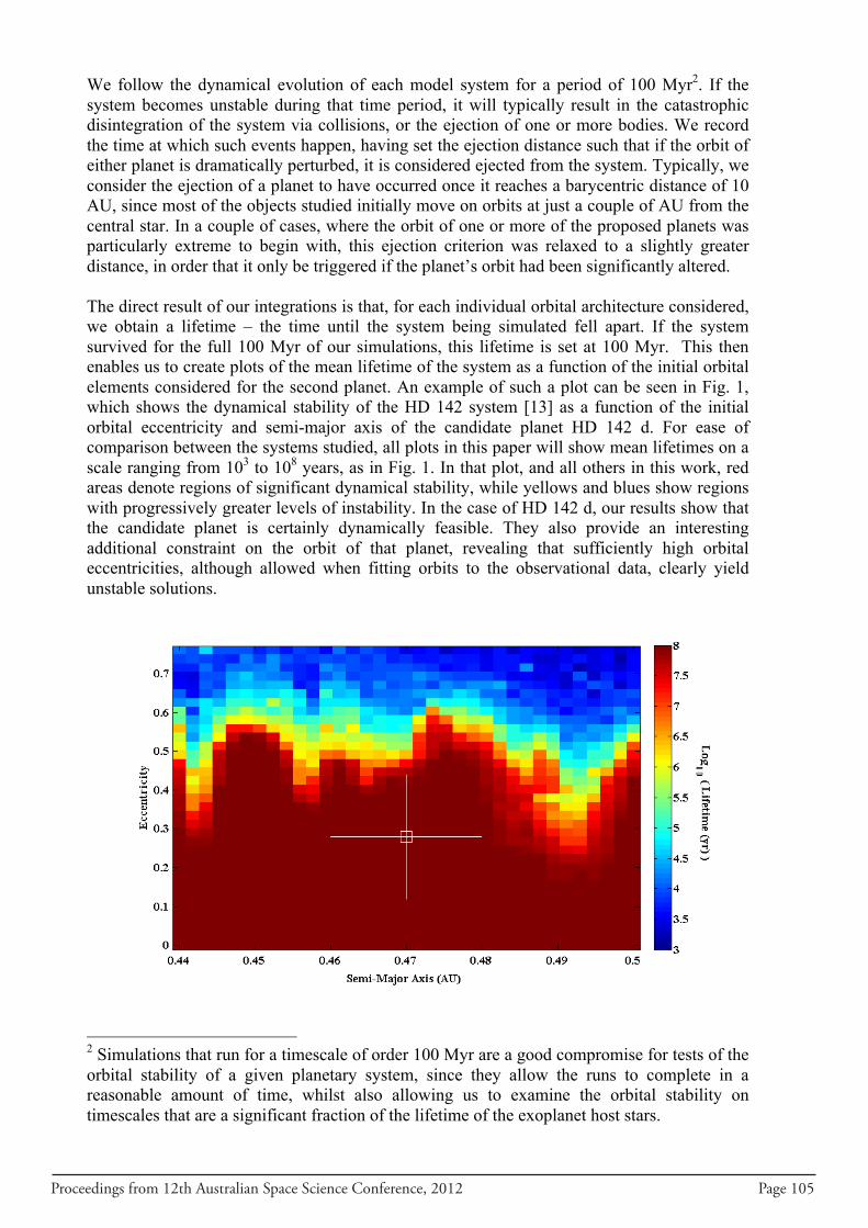
Proceedings from 12th Australian Space Science Conference, 2012 Page 105
We follow the dynamical evolution of each model system for a period of 100 Myr2. If the system becomes unstable during that time period, it will typically result in the catastrophic disintegration of the system via collisions, or the ejection of one or more bodies. We record the time at which such events happen, having set the ejection distance such that if the orbit of either planet is dramatically perturbed, it is considered ejected from the system. Typically, we consider the ejection of a planet to have occurred once it reaches a barycentric distance of 10 AU, since most of the objects studied initially move on orbits at just a couple of AU from the central star. In a couple of cases, where the orbit of one or more of the proposed planets was particularly extreme to begin with, this ejection criterion was relaxed to a slightly greater distance, in order that it only be triggered if the planet’s orbit had been significantly altered. The direct result of our integrations is that, for each individual orbital architecture considered, we obtain a lifetime – the time until the system being simulated fell apart. If the system survived for the full 100 Myr of our simulations, this lifetime is set at 100 Myr. This then enables us to create plots of the mean lifetime of the system as a function of the initial orbital elements considered for the second planet. An example of such a plot can be seen in Fig. 1, which shows the dynamical stability of the HD 142 system [13] as a function of the initial orbital eccentricity and semi-major axis of the candidate planet HD 142 d. For ease of comparison between the systems studied, all plots in this paper will show mean lifetimes on a scale ranging from 103 to 108 years, as in Fig. 1. In that plot, and all others in this work, red areas denote regions of significant dynamical stability, while yellows and blues show regions with progressively greater levels of instability. In the case of HD 142 d, our results show that the candidate planet is certainly dynamically feasible. They also provide an interesting additional constraint on the orbit of that planet, revealing that sufficiently high orbital eccentricities, although allowed when fitting orbits to the observational data, clearly yield unstable solutions.
2 Simulations that run for a timescale of order 100 Myr are a good compromise for tests of the orbital stability of a given planetary system, since they allow the runs to complete in a reasonable amount of time, whilst also allowing us to examine the orbital stability on timescales that are a significant fraction of the lifetime of the exoplanet host stars.

Page 106 Proceedings from 12th Australian Space Science Conference, 2012
Fig. 1: The dynamical stability of the HD142 planetary system, as a function of the initial semi-major axis and eccentricity of the orbit of HD142 d, a candidate planet of mass 0.3 times that of Jupiter. Each grid point shows the mean lifetime of 25 independent simulations carried out at that particular combination of initial semi-major axis and eccentricity, on a logarithmic scale. The box in the centre of the plot shows the nominal best-fit orbit for HD142 d, while the arms radiating from that point show the 1σ errors on that orbital solution. As can be seen, in this case, the nominal best-fit orbit for the planet lies in a region of extreme stability (mean lifetimes of 100 Myr, the maximum duration of our integrations). However, a broad region of extreme instability can also be seen, towards higher orbital eccentricities.
Dynamically Unfeasible Planetary Systems – the Circumbinary Planets
Perhaps the most important role played by dynamical simulations of newly announced exoplanetary systems is to test whether those systems are actually dynamically feasible. Although it might appear obvious that dynamical tests of any proposed system should form an integral part of the planet discovery process, many groups sadly neglect this aspect, choosing instead to publish proposed planetary systems on best-fit orbits that are often dynamically unrealistic. Discoveries of planets in one particular area have historically proven particularly prone to this mistake – the announcement of planets orbiting evolved binary star systems, such as HU Aquarii (e.g. [12][15][16][17]) and HW Virginis (e.g. [18][19]), discoveries based on variations in the timings of eclipses between the two binary components. In both discovery works, the proposed planets moved on best-fit orbits that were mutually crossing, and yet were not mutually resonant. The results of our dynamical simulations of these systems are shown in Fig. 2.
Fig. 2: The dynamical stability of the proposed HU Aquarii (left) and HW Virginis (right) planetary systems. In both cases, the best-fit orbits lie in regions of extreme instability, with the systems being disrupted on timescales of hundreds or thousands of years. For both HU Aquarii and HW Virginis, we find that the planetary systems, as proposed in the discovery works ([15] and [18], respectively), are simply not dynamically feasible. In both cases, the proposed systems are dynamically unstable on timescales of hundreds or thousands of years – a result that calls into question the existence of planets in those systems, and most likely reveals that the observed eclipse timing variations are the result of a physical process other than planetary perturbations. The recently proposed planetary system in the evolved eclipsing binary star system NSVS 14256825 ([20]) is another interesting case in point. In that work, the authors present observations of the eclipsing binary system taken over a period of several years, and showed that the timing of the eclipses between the two stars therein was deviating from the predicted times in a systematic fashion. Following the hypothesis that the variation was the result of perturbations from unseen giant planets in the system, they found that the variation could be
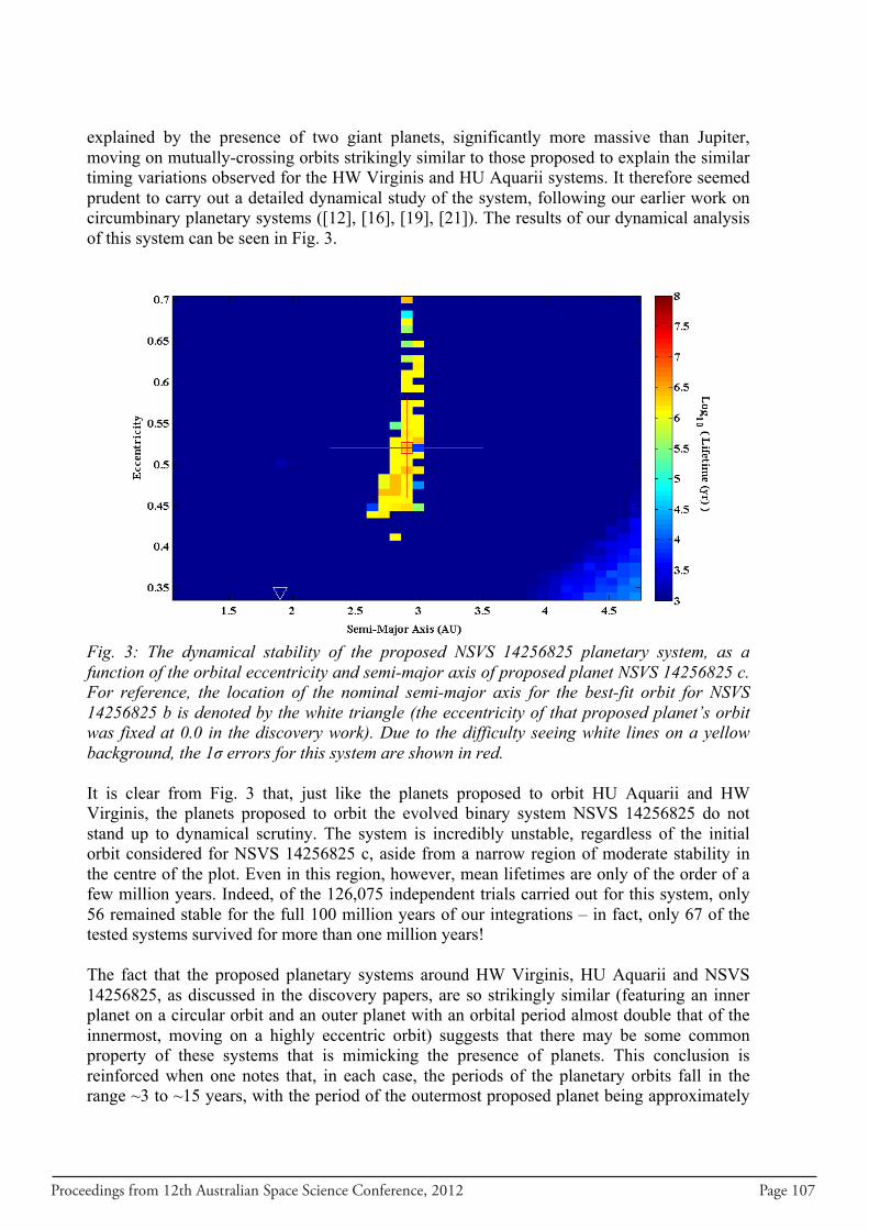
Proceedings from 12th Australian Space Science Conference, 2012 Page 107
explained by the presence of two giant planets, significantly more massive than Jupiter, moving on mutually-crossing orbits strikingly similar to those proposed to explain the similar timing variations observed for the HW Virginis and HU Aquarii systems. It therefore seemed prudent to carry out a detailed dynamical study of the system, following our earlier work on circumbinary planetary systems ([12], [16], [19], [21]). The results of our dynamical analysis of this system can be seen in Fig. 3.
Fig. 3: The dynamical stability of the proposed NSVS 14256825 planetary system, as a function of the orbital eccentricity and semi-major axis of proposed planet NSVS 14256825 c. For reference, the location of the nominal semi-major axis for the best-fit orbit for NSVS 14256825 b is denoted by the white triangle (the eccentricity of that proposed planet’s orbit was fixed at 0.0 in the discovery work). Due to the difficulty seeing white lines on a yellow background, the 1σ errors for this system are shown in red. It is clear from Fig. 3 that, just like the planets proposed to orbit HU Aquarii and HW Virginis, the planets proposed to orbit the evolved binary system NSVS 14256825 do not stand up to dynamical scrutiny. The system is incredibly unstable, regardless of the initial orbit considered for NSVS 14256825 c, aside from a narrow region of moderate stability in the centre of the plot. Even in this region, however, mean lifetimes are only of the order of a few million years. Indeed, of the 126,075 independent trials carried out for this system, only 56 remained stable for the full 100 million years of our integrations – in fact, only 67 of the tested systems survived for more than one million years! The fact that the proposed planetary systems around HW Virginis, HU Aquarii and NSVS 14256825, as discussed in the discovery papers, are so strikingly similar (featuring an inner planet on a circular orbit and an outer planet with an orbital period almost double that of the innermost, moving on a highly eccentric orbit) suggests that there may be some common property of these systems that is mimicking the presence of planets. This conclusion is reinforced when one notes that, in each case, the periods of the planetary orbits fall in the range ~3 to ~15 years, with the period of the outermost proposed planet being approximately
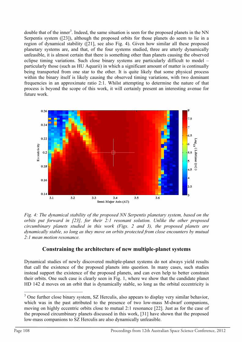
Page 108 Proceedings from 12th Australian Space Science Conference, 2012
double that of the inner3. Indeed, the same situation is seen for the proposed planets in the NN Serpentis system ([23]), although the proposed orbits for those planets do seem to lie in a region of dynamical stability ([21], see also Fig. 4). Given how similar all these proposed planetary systems are, and that, of the four systems studied, three are utterly dynamically unfeasible, it is almost certain that there is something other than planets causing the observed eclipse timing variations. Such close binary systems are particularly difficult to model – particularly those (such as HU Aquarii) in which a significant amount of matter is continually being transported from one star to the other. It is quite likely that some physical process within the binary itself is likely causing the observed timing variations, with two dominant frequencies in an approximate ratio 2:1. Whilst attempting to determine the nature of that process is beyond the scope of this work, it will certainly present an interesting avenue for future work.
Fig. 4: The dynamical stability of the proposed NN Serpentis planetary system, based on the orbits put forward in [23], for their 2:1 resonant solution. Unlike the other proposed circumbinary planets studied in this work (Figs. 2 and 3), the proposed planets are dynamically stable, so long as they move on orbits protected from close encounters by mutual 2:1 mean motion resonance.
Constraining the architecture of new multiple-planet systems
Dynamical studies of newly discovered multiple-planet systems do not always yield results that call the existence of the proposed planets into question. In many cases, such studies instead support the existence of the proposed planets, and can even help to better constrain their orbits. One such case is clearly seen in Fig. 1, where we show that the candidate planet HD 142 d moves on an orbit that is dynamically stable, so long as the orbital eccentricity is 3 One further close binary system, SZ Herculis, also appears to display very similar behavior, which was in the past attributed to the presence of two low-mass M-dwarf companions, moving on highly eccentric orbits close to mutual 2:1 resonance [22]. Just as for the case of the proposed circumbinary planets discussed in this work, [31] have shown that the proposed low-mass companions to SZ Herculis are also dynamically unfeasible.
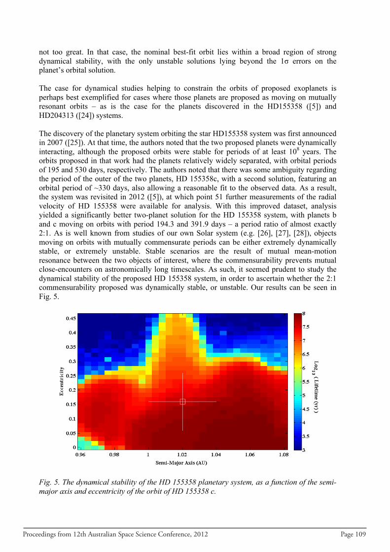
Proceedings from 12th Australian Space Science Conference, 2012 Page 109
not too great. In that case, the nominal best-fit orbit lies within a broad region of strong dynamical stability, with the only unstable solutions lying beyond the 1σ errors on the planet’s orbital solution. The case for dynamical studies helping to constrain the orbits of proposed exoplanets is perhaps best exemplified for cases where those planets are proposed as moving on mutually resonant orbits – as is the case for the planets discovered in the HD155358 ([5]) and HD204313 ([24]) systems. The discovery of the planetary system orbiting the star HD155358 system was first announced in 2007 ([25]). At that time, the authors noted that the two proposed planets were dynamically interacting, although the proposed orbits were stable for periods of at least 108 years. The orbits proposed in that work had the planets relatively widely separated, with orbital periods of 195 and 530 days, respectively. The authors noted that there was some ambiguity regarding the period of the outer of the two planets, HD 155358c, with a second solution, featuring an orbital period of ~330 days, also allowing a reasonable fit to the observed data. As a result, the system was revisited in 2012 ([5]), at which point 51 further measurements of the radial velocity of HD 155358 were available for analysis. With this improved dataset, analysis yielded a significantly better two-planet solution for the HD 155358 system, with planets b and c moving on orbits with period 194.3 and 391.9 days – a period ratio of almost exactly 2:1. As is well known from studies of our own Solar system (e.g. [26], [27], [28]), objects moving on orbits with mutually commensurate periods can be either extremely dynamically stable, or extremely unstable. Stable scenarios are the result of mutual mean-motion resonance between the two objects of interest, where the commensurability prevents mutual close-encounters on astronomically long timescales. As such, it seemed prudent to study the dynamical stability of the proposed HD 155358 system, in order to ascertain whether the 2:1 commensurability proposed was dynamically stable, or unstable. Our results can be seen in Fig. 5.
Fig. 5. The dynamical stability of the HD 155358 planetary system, as a function of the semi-major axis and eccentricity of the orbit of HD 155358 c.
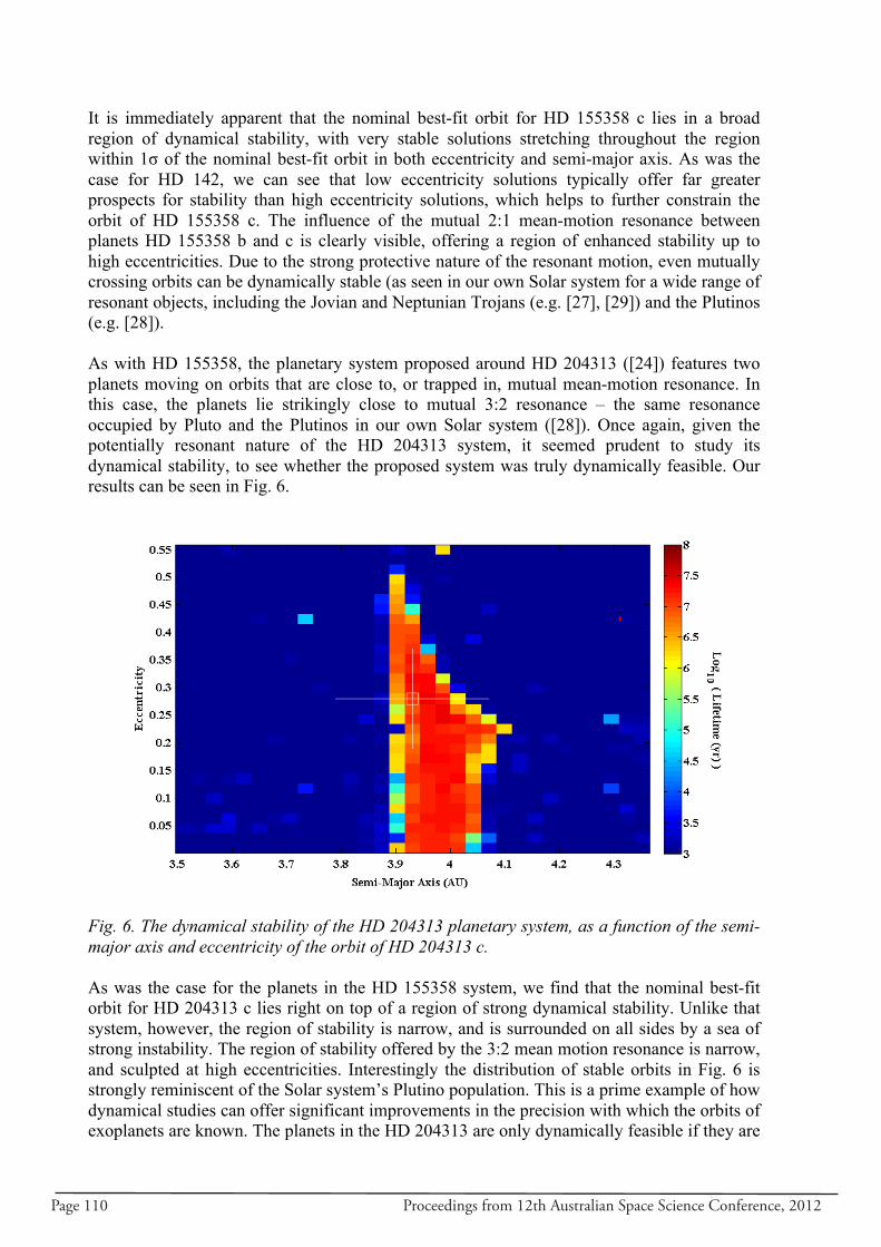
Page 110 Proceedings from 12th Australian Space Science Conference, 2012
It is immediately apparent that the nominal best-fit orbit for HD 155358 c lies in a broad region of dynamical stability, with very stable solutions stretching throughout the region within 1σ of the nominal best-fit orbit in both eccentricity and semi-major axis. As was the case for HD 142, we can see that low eccentricity solutions typically offer far greater prospects for stability than high eccentricity solutions, which helps to further constrain the orbit of HD 155358 c. The influence of the mutual 2:1 mean-motion resonance between planets HD 155358 b and c is clearly visible, offering a region of enhanced stability up to high eccentricities. Due to the strong protective nature of the resonant motion, even mutually crossing orbits can be dynamically stable (as seen in our own Solar system for a wide range of resonant objects, including the Jovian and Neptunian Trojans (e.g. [27], [29]) and the Plutinos (e.g. [28]). As with HD 155358, the planetary system proposed around HD 204313 ([24]) features two planets moving on orbits that are close to, or trapped in, mutual mean-motion resonance. In this case, the planets lie strikingly close to mutual 3:2 resonance – the same resonance occupied by Pluto and the Plutinos in our own Solar system ([28]). Once again, given the potentially resonant nature of the HD 204313 system, it seemed prudent to study its dynamical stability, to see whether the proposed system was truly dynamically feasible. Our results can be seen in Fig. 6.
Fig. 6. The dynamical stability of the HD 204313 planetary system, as a function of the semi-major axis and eccentricity of the orbit of HD 204313 c. As was the case for the planets in the HD 155358 system, we find that the nominal best-fit orbit for HD 204313 c lies right on top of a region of strong dynamical stability. Unlike that system, however, the region of stability is narrow, and is surrounded on all sides by a sea of strong instability. The region of stability offered by the 3:2 mean motion resonance is narrow, and sculpted at high eccentricities. Interestingly the distribution of stable orbits in Fig. 6 is strongly reminiscent of the Solar system’s Plutino population. This is a prime example of how dynamical studies can offer significant improvements in the precision with which the orbits of exoplanets are known. The planets in the HD 204313 are only dynamically feasible if they are
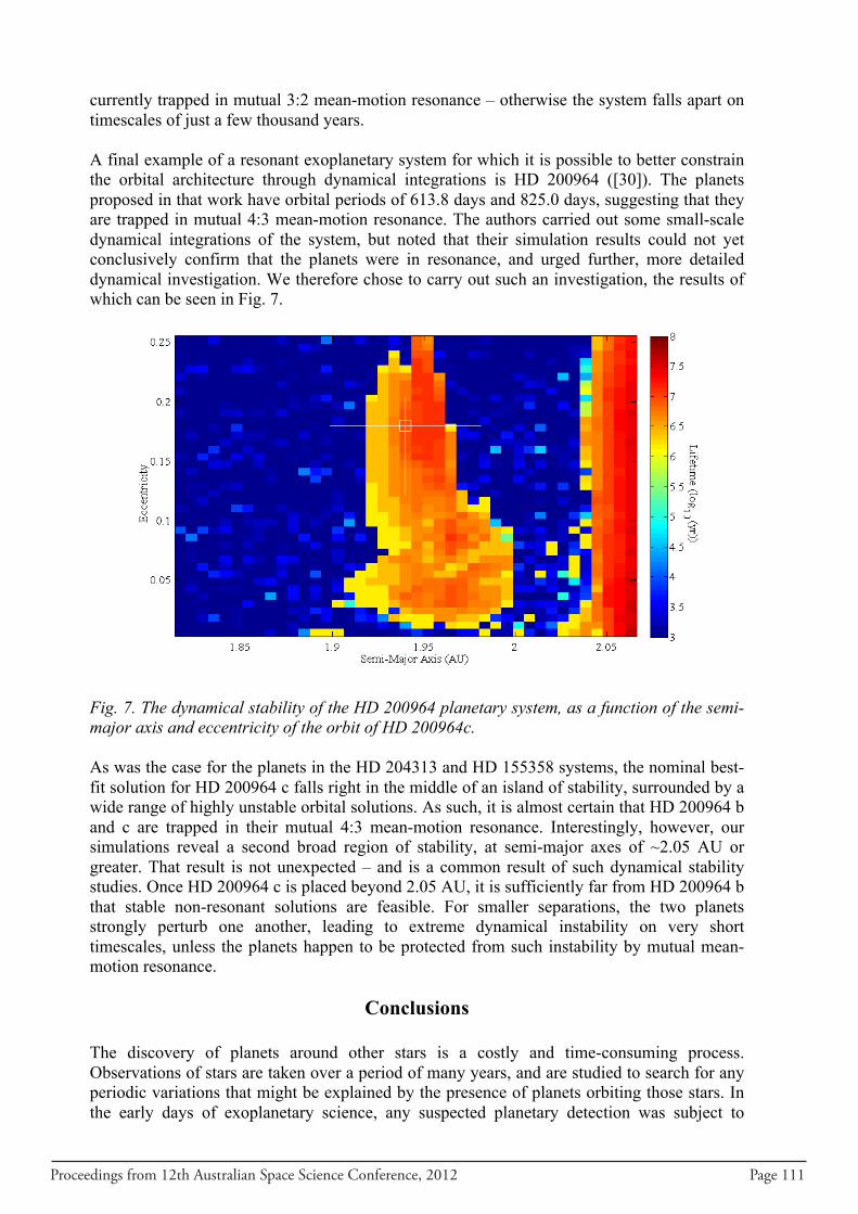
Proceedings from 12th Australian Space Science Conference, 2012 Page 111
currently trapped in mutual 3:2 mean-motion resonance – otherwise the system falls apart on timescales of just a few thousand years. A final example of a resonant exoplanetary system for which it is possible to better constrain the orbital architecture through dynamical integrations is HD 200964 ([30]). The planets proposed in that work have orbital periods of 613.8 days and 825.0 days, suggesting that they are trapped in mutual 4:3 mean-motion resonance. The authors carried out some small-scale dynamical integrations of the system, but noted that their simulation results could not yet conclusively confirm that the planets were in resonance, and urged further, more detailed dynamical investigation. We therefore chose to carry out such an investigation, the results of which can be seen in Fig. 7.
Fig. 7. The dynamical stability of the HD 200964 planetary system, as a function of the semi-major axis and eccentricity of the orbit of HD 200964c. As was the case for the planets in the HD 204313 and HD 155358 systems, the nominal best-fit solution for HD 200964 c falls right in the middle of an island of stability, surrounded by a wide range of highly unstable orbital solutions. As such, it is almost certain that HD 200964 b and c are trapped in their mutual 4:3 mean-motion resonance. Interestingly, however, our simulations reveal a second broad region of stability, at semi-major axes of ~2.05 AU or greater. That result is not unexpected – and is a common result of such dynamical stability studies. Once HD 200964 c is placed beyond 2.05 AU, it is sufficiently far from HD 200964 b that stable non-resonant solutions are feasible. For smaller separations, the two planets strongly perturb one another, leading to extreme dynamical instability on very short timescales, unless the planets happen to be protected from such instability by mutual mean-motion resonance.
Conclusions
The discovery of planets around other stars is a costly and time-consuming process. Observations of stars are taken over a period of many years, and are studied to search for any periodic variations that might be explained by the presence of planets orbiting those stars. In the early days of exoplanetary science, any suspected planetary detection was subject to
Page 112 Proceedings from 12th Australian Space Science Conference, 2012
rigorous investigation, prior to being announced. In recent years, however, as the detection of exoplanets have moved from the extraordinary to the mundane, a bewildering diversity of exoplanets are being announced orbiting an extremely diverse sample of stars. It is now the case that the presence of planets is regularly invoked to explain periodic variations observed in distant stars. In this work, we show how detailed dynamical simulations can be used to examine proposed exoplanetary systems, and determine whether those systems are truly dynamically feasible. In many cases, we find that the proposed planets simply do not work, moving on orbits that are unstable on timescales of just hundreds or thousands of years – far shorter than the billion-year lifetimes of their host stars. In these cases, we suggest that another explanation is needed for the observed periodic variations in the host star or stars. If there are exoplanets orbiting those stars, they must move on drastically different orbits to those proposed in the discovery works – although it seems more likely that some other physical process is creating the observed variations. We also show how dynamical studies can help astronomers to refine and better constrain the orbital architecture of proposed multiple-planetary systems. In the case of the planets discovered in the HD 155358, HD 204313 and HD 200964 systems, for example, our results reveal that the proposed planets are only dynamically stable if they move on mutually resonant orbits, and that a wide range of the observationally allowed orbital solutions are not dynamically feasible. In each of these cases, it is reassuring that the nominal best-fit orbital solutions for the planets in question lie in the middle of islands of stability, a case where detailed dynamical studies add further evidence for the presence of planets in those systems. In the future, such dynamical studies will form a crucial part of the exoplanet discovery and announcement process. In principle any new multiple-planetary system should be studied dynamically to see whether the proposed planets truly make sense. We are now routinely carrying out such dynamical studies, as part of the Anglo-Australian Planet Search, where any suspected multiple-exoplanet systems detected are dynamically investigated prior to being announced.
Acknowledgements
The work was supported by iVEC through the use of advanced computing resources located at the Murdoch University, in Western Australia. This research has made use of NASA’s Astrophysics Data System (ADS), and the SIMBAD database, operated at CDS, Strasbourg, France. This research has also made use of the Exoplanet Orbit Database and the Exoplanet Data Explorer at exoplanets.org. The authors also wish to thank the two referees of this paper, Dr. Elliott Koch and Brett Addison, for their comments, which helped to improve the flow and clarity of our article.
References 1. Wolszczan, A. and Frail, D. A., “A planetary system around the millisecond pulsar
PSR1257 +12”, Nature, Vol. 355, 1992, pp. 145-147 2. Wolszczan, A., “Confirmation of Earth-Mass Planets Orbiting the Millisecond Pulsar
PSR B1257 +12”, Science, Vol. 264, Issue 5158, 1994, pp. 538-542
Proceedings from 12th Australian Space Science Conference, 2012 Page 113
3. Mayor, M. and Queloz, D., “A Jupiter-mass companion to a solar-type star”, Nature, Vol. 378, Issue 6555, 1995, pp. 355-359
4. Tinney, C. G., Wittenmyer, R. A., Butler, R. P., Jones, H. R. A., O’Toole, S. J.,
Bailey, J. A., Carter, B. D. and Horner, J., “The Anglo-Australian Planet Search. XXI. A Gas-giant Planet in a One Year Orbit and the Habitability of Gas-giant Satellites”, The Astrophysical Journal, Vol. 732., Issue 1, 2011, article 1
5. Robertson, P., Endl, M., Cochran, W. D., MacQueen, P. J., Wittenmyer, R. A.,
Horner, J., Brugamyer, E. J., Simon, A. E., Barnes, S. I. and Caldwell, C., “The McDonald Observatory Planet Search: New Long-period Giant Planets and Two Interacting Jupiters in the HD155358 System”, The Astrophysical Journal, Vol. 749, Issue 1, 2012, article 1.
6. Sato, B., Omiya, M., Wittenmyer, R. A., Harakawa, H., Nagasawa, M., Izumiura, H.,
Kambe, E., Takeda, Y., Yoshida, M., Itoh, Y., Ando, H., Kokubo, E. and Ida, S., “A Double Planetary System around the Evolved Intermediate-Mass Star HD 4732”, The Astrophysical Journal, in press, 2012
7. Wittenmyer, R. A., Endl, M., Wang, L., Johnson, J. A., Tinney, C. G. and O’Toole, S.
J., “The Pan-Pacific Planet Search. I. A Giant Planet Orbiting 7 CMa”, The Astrophysical Journal, Vol. 743, Issue 2, 2011, article id. 184
8. Naef, D., Latham, D. W., Mayor, M., Mazeh, T., Beuzit, J. L., Drukier, G. A., Perrier-
Bellet, C., Queloz, D., Sivan, J. P., Torres, G., Udry, S. and Zucker, S., “HD 80606 b, a planet on an extremely elongated orbit”, Astronomy and Astrophysics, Vol. 375, 2001, pp. L27–L30
9. Jones, H. R. A., Butler, R. P., Tinney, C. G., O’Toole, S., Wittenmyer, R., Henry, G.
W., Meschiari, S., Vogt, S., Rivera, E., Laughlin, G., Carter, B. D., Bailey, J. and Jenkins, J. S., “A long-period planet orbiting a nearby Sun-like star”, Monthly Notices of the Royal Astronomical Society, Vol. 403, Issue 4, 2010, pp. 1703-1713
10. Chambers, J. E., “A hybrid symplectic integrator that permits close encounters
between massive bodies”, Monthly Notices of the Royal Astronomical Society, Vol. 304, 1999, pp. 793-799
11. Marshall, J. P., Horner, J. and Carter, A., “Dynamical simulations of the HR8799
planetary system”, The International Journal of Astrobiology, Vol. 9, 2010, pp. 259-264
12. Horner, J., Marshall, J. P., Wittenmyer, R. A. and Tinney, C. G., “A dynamical
analysis of the proposed HU Aquarii planetary system”, Monthly Notices of the Royal Astronomical Society: Letters, Vol. 416, 2011, pp. 11 – 15
13. Wittenmyer, R. A., Horner, J., Tuomi, M., Salter, G. S., Tinney, C. G., Butler, R. P.,
Jones, H. R. A., O’Toole, S. J., Bailey, J., Carter, B. D., Jenkins, J. S., Zhang, Z., Vogt, S. S. and Rivera, E. J., “The Anglo-Australian Planet Search. XXII. Two New Multi-Planet Systems”, The Astrophysical Journal, Vol. 753, 2012, article 169
Page 114 Proceedings from 12th Australian Space Science Conference, 2012
14. Vogt, S., Butler, R. P. and Haghighipour, N., “GJ 581 update: Additional evidence for a Super-Earth in the habitable zone”, Astronomische Nachrichten, Vol. 333, Issue 7, 2012, pp. 561
15. Qian, S.-B, Liu, L., Liao, W.-P., Li, L.-J., Zhu, L.-Y., Dai, Z.-B., He, J.-J., Zhao, E.-
G., Zhang, J, and Li, K., “Detection of a planetary system orbiting the eclipsing polar HU Aqr”, Monthly Notices of the Royal Astronomical Society: Letters, Vol. 414, Issue 1, 2010, pp. 16-20
16. Wittenmyer, R. A., Horner, J., Marshall, J. P., Butters, O. W. and Tinney, C. G.,
“Revisiting the proposed planetary system orbiting the eclipsing polar HU Aquarii”, Monthly Notices of the Royal Astronomical Society, Vol. 419, Issue 4, 2012, pp. 3258-3267
17. Hinse, T. C., Lee, J. W., Goździewski, K., Haghighipour, N., Lee, C.-U. and Scullion,
E. M., “New light-travel time models and orbital stability study of the proposed planetary system HU Aquarii”, Monthly Notices of the Royal Astronomical Society, Vol. 420, Issue 4, 2012, pp. 3609-3620.
18. Lee, J. W., Kim, S.-L., Kim, C.-H., Koch, R. H., Lee, C.-U., Kim, H,-I and Park, J.-H.,
“The sdB+M Eclipsing System HW Virginis and its Circumbinary Planets”, The Astronomical Journal, Vol. 137, Issue 2., 2009, pp. 3181-3190
19. Horner, J., Hinse, T. C., Wittenmyer, R. A., Marshall, J. P. and Tinney, C. G., “A
Dynamical Analysis of the Proposed Circumbinary HW Virginis Planetary System”, Monthly Notices of the Royal Astronomical Society, in press, arXiv:1209.0608, 2012
20. Almeida, L. A., Jablonski, F. and Rodrigues, C. V., “Two circumbinary planets in the
eclipsing post-common envelope system NSVS 14256825”, arXiv:1210.3055v1, 2012 21. Horner, J., Wittenmyer, R. A., Hinse, T. C. and Tinney, C. G., “A detailed
investigation of the proposed NN Serpentis planetary system”, Monthly Notices of the Royal Astronomical Society, Vol. 425, Issue 1, 2012, pp. 749-756
22. Lee, J. W., Lee, C.-U., Kim, S.-L., Kim, H.-I. and Park, J.-H., “The Algol System SZ
Herculis: Physical Nature and Orbital Behavior”, The Astronomical Journal, Vol. 143, Issue 2, 2012, article id. 34
23. Beuermann, K., Hessman, F. V., Dreizler, S., Marsh, T. R., Parsons, S. G,, Winget, D.
E., Miller, G. F., Schreiber, M. R., Kley, W., Dhillon, V. S., Littlefair, S. P., Copperwheat, C. M. and Hermes, J. J., “Two planets orbiting the recently formed post-common envelope binary NN Serpentis”, Astronomy & Astrophysics, Vol. 521, 2010, id L60
24. Robertson, P., Horner, J. Wittenmyer, R. A., Endl, M., Cochran, W. D., MacQueen, P.
J., Brugamyer, E. J., Simon, A. E., Barnes. S. I. and Caldwell, C., “A Second Giant Planet in 3:2 Mean-motion Resonance in the HD 204313 system”, The Astrophysical Journal, Vol. 754, Issue 1, 2012, article id. 50
25. Cochran, W. D., Endl, M., Wittenmyer, R. A. and Bean, J. L., “A Planetary System
around HD 155358: The Lowest Metallicity Planet Host Star”, The Astrophysical Journal, Vol. 665, Issue 2, pp. 1407-1412
Proceedings from 12th Australian Space Science Conference, 2012 Page 115
26. Horner, J. and Lykawka, P. S., “2001 QR322: a dynamically unstable Neptune
Trojan?”, Monthly Notices of the Royal Astronomcial Society, Vol. 405, Issue 1, 2010, pp. 49 – 56
27. Horner, J., Lykawka, P. S., Bannister, M. T. and Francis, P., “2008 LC18: a potentially
unstable Neptune Trojan”, Monthly Notices of the Royal Astronomical Society, Vol. 422, Issue 3, 2012, pp. 2145 - 2151
28: Malhotra, R., “The Origin of Pluto’s Orbit: Implications for the Solar System Beyond
Neptune”, Astronomical Journal, Vol. 110, 1995, pp. 420 29. Horner, J., Müller, T. G. and Lykawka, P. S., “(1173) Anchises - thermophysical and
dynamical studies of a dynamically unstable Jovian Trojan”, Monthly Notices of the Royal Astronomical Society, Vol. 423, Issue 3, 2012, pp. 2587 - 2596
30. Johnson, J. A., Payne, M., Howard, A. W., Clubb, K. I., Ford, E. B., Bowler, B. P.,
Henry, G. W., Fischer, D. A., Marcy, G. W., Brewer, J. M., Schwab, C., Reffert, S. and Lowe, T. B., “Retired A Stars and Their Companions. VI. A Pair of Interacting Exoplanets Around the Subgiants 24 Sextanis and HD 200964”, The Astronomical Journal, Vol. 141, Issue 1, 2011, article id. 16
31. Hinse, T. C., Goździewski, K, Lee, J. W., Haghighipour, N. and Lee, C.-U., “The
Proposed Quadruple System SZ Herculis: Revised LITE Model and Orbital Stability Study”, The Astronomical Journal, Vol. 144, Issue 2, 2012, article id. 34

Page 116 Proceedings from 12th Australian Space Science Conference, 2012
Proceedings from 12th Australian Space Science Conference, 2012 Page 117
Retrieval Software for Total Column Greenhouse Gas Measurements from Ground and Space
Champlain Kenyi, Daniel V. Cotton and Jeremy Bailey
School of Physics, The University of New South Wales, NSW 2052, Australia
Summary: Accurate measurements of atmospheric greenhouse gases are important in order to better understand the carbon cycle, and to provide a check on the carbon accounting methods that are the basis of carbon pricing schemes and emission control agreements. Both space- and ground-based techniques are under development, but all existing measuring instruments have limitations. Space-based instruments (such as GOSAT and SCIAMACHY) provide wider coverage, but are not yet accurate enough to detect small changes contributed by human activities over the large background. Ground-based methods can provide higher accuracy but the networks are too sparse for detailed mapping. We have built a compact and portable up-looking, ground-based, greenhouse gas-monitoring instrument. Here we describe work on developing retrieval methods for deriving CO2 abundances. The software used for modelling is based on the VSTAR (Versatile Software for Transfer of Atmospheric Radiation) package. As an input solar spectrum for the model we use a spectrum derived by combining the Kitt Peak Solar Atlas with the model-based Kurucz flux distribution. We compared the quality of our VSTAR model spectrum with a highly accurate FTIR ground-based spectrum. The spectra are in excellent agreement.
Keywords: Earth atmosphere, carbon dioxide, methane, greenhouse gas-monitoring,
spectroscopy, modelling.
Introduction
Greenhouse Gas Monitoring
Carbon dioxide (CO2) and methane (CH4) are the two most important anthropogenic greenhouse gases in the Earth atmosphere that largely account for recent climate change. The concentration of these gases has increased over the last 250 years probably due to human activities [1, 2]. However our knowledge of the carbon cycle is still inadequate owing to limited spatial and temporal observations of CO2 and CH4 over the globe, leading to large uncertainties in climate change prediction [2]. Satellites hold substantial promise for long-term space monitoring of these gases by providing the spatial coverage (especially over the oceans and tropical land) and sampling density [3] needed to resolve CO2 and CH4 weather, but the retrievals are contaminated by aerosols and clouds. Additionally, the aerosol models used are often over simplified, yielding large biases. As such space-based observations are validated by highly accurate observations from surface-based networks (e.g. TCCON -Total Carbon Column Observing Network).
Page 118 Proceedings from 12th Australian Space Science Conference, 2012
Accurate monitoring of CO2 and CH4 is required to improve our understanding of their sources and sinks and the processes governing the carbon cycle. This will resolve the linkage between global warming and human perturbations on the environment, allowing policy makers to better manage and control the Earth energy budget. However retrieval of these long-lived and well-mixed gases is challenging as only small changes over the large background yield information on their sources and sinks [4]. To date information on the atmospheric column abundances of CO2 and CH4 is mainly relied on in-situ measurements (which sample air at the surface), as well as sporadic observations from aircrafts in the lower atmosphere and from tall towers [5]. As pointed out by Petri et al., using surface data in inverse models requires assumptions on the vertical mixing of the air masses; this causes biases in the retrievals. To minimise the perturbing effects of these assumptions, total column measurements are used since they are less affected by vertical mixing [6], i.e. they reduce the uncertainties in the spatial distribution and temporal variability of the sources and sinks of these greenhouse gases [7]. There have been two types of satellites for observing atmospheric CO2 and CH4 in use over the past decade [2]. The first type makes thermal infrared (TIR) observations, typical example of which is the Atmospheric Infrared Sounder (AIRS) onboard the Aqua satellite [8]. The second type, represented by the SCanning Imaging Absorption spectroMeter for Atmospheric CHartographY (SCIAMACHY) onboard the Envisat satellite [2, 4, and the references therein] makes short-wavelength infrared (SWIR) observations. In the TIR type, the sensors measure thermally emitted radiation in the infrared portion of the electromagnetic spectrum; measurements pursued in the nadir geometry are found sensitive in the middle and upper troposphere but not near the surface where the local sources/sinks are largest [9]. Unlike the TIR type, SWIR sensing exploits reflected (back backscattered) sunlight to space from the Earth’s surface and the atmosphere and measures the greenhouse gas abundances with higher near-surface sensitivity [2, 10]; and so is more suitable from the view-point of carbon flux estimation [11].
Sources and sinks of CO2 and CH4
Carbon dioxide (CO2) is a common, chemically-unreactive, trace gas found in the Earth-Ocean-atmosphere system with a lifetime of approximately a century; its primary sources and sinks are located within the planetary boundary layer [12]. The gas originates from both natural emission sources (e.g. volcanoes, forest fires and biological processes say breathing) as well as from anthropogenic sources. Materials such as coal, oil, natural gas and wood are mostly carbon [13, 14] which on combustion release CO2 into the atmosphere. Carbon dioxide naturally cycles rapidly through the atmosphere, ocean and land; and is removed at the surface and to a lesser extent in the atmosphere by photolysis [15]. Because of limiting processes to the uptake rate of the gas, removal of the anthropogenic CO2 perturbation takes longer. Uptake by the ocean is due to its high solubility, but limited by finite speed of vertical mixing. On the other hand, the terrestrial ecosystem can sequester anthropogenic CO2 content through land management, CO2 fertilization to enhance plant growth, and increasing anthropogenic inputs of nitrogen. This uptake (by both oceans and the land), however, is expected to decrease with increasing CO2 concentration [16]. Methane emissions can be due to human induced causes such as leaks during coal mining and transportation of natural gas, agriculture and livestock production, biomass burning and paddy fields in addition to the natural sources [17] (e.g. wetlands, termites, oceans, lakes and
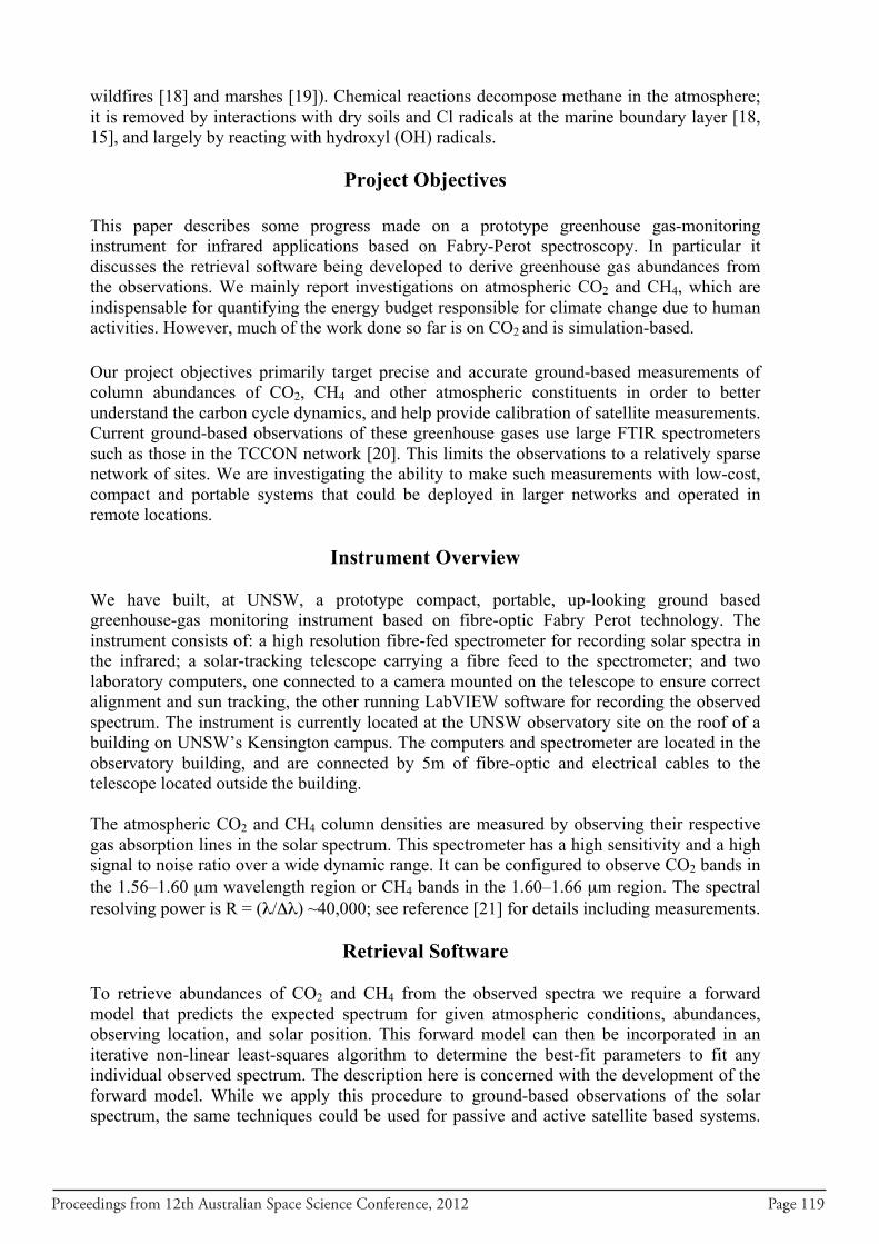
Proceedings from 12th Australian Space Science Conference, 2012 Page 119
wildfires [18] and marshes [19]). Chemical reactions decompose methane in the atmosphere; it is removed by interactions with dry soils and Cl radicals at the marine boundary layer [18, 15], and largely by reacting with hydroxyl (OH) radicals.
Project Objectives
This paper describes some progress made on a prototype greenhouse gas-monitoring instrument for infrared applications based on Fabry-Perot spectroscopy. In particular it discusses the retrieval software being developed to derive greenhouse gas abundances from the observations. We mainly report investigations on atmospheric CO2 and CH4, which are indispensable for quantifying the energy budget responsible for climate change due to human activities. However, much of the work done so far is on CO2 and is simulation-based.
Our project objectives primarily target precise and accurate ground-based measurements of column abundances of CO2, CH4 and other atmospheric constituents in order to better understand the carbon cycle dynamics, and help provide calibration of satellite measurements. Current ground-based observations of these greenhouse gases use large FTIR spectrometers such as those in the TCCON network [20]. This limits the observations to a relatively sparse network of sites. We are investigating the ability to make such measurements with low-cost, compact and portable systems that could be deployed in larger networks and operated in remote locations.
Instrument Overview
We have built, at UNSW, a prototype compact, portable, up-looking ground based greenhouse-gas monitoring instrument based on fibre-optic Fabry Perot technology. The instrument consists of: a high resolution fibre-fed spectrometer for recording solar spectra in the infrared; a solar-tracking telescope carrying a fibre feed to the spectrometer; and two laboratory computers, one connected to a camera mounted on the telescope to ensure correct alignment and sun tracking, the other running LabVIEW software for recording the observed spectrum. The instrument is currently located at the UNSW observatory site on the roof of a building on UNSW’s Kensington campus. The computers and spectrometer are located in the observatory building, and are connected by 5m of fibre-optic and electrical cables to the telescope located outside the building. The atmospheric CO2 and CH4 column densities are measured by observing their respective gas absorption lines in the solar spectrum. This spectrometer has a high sensitivity and a high signal to noise ratio over a wide dynamic range. It can be configured to observe CO2 bands in the 1.56–1.60 µm wavelength region or CH4 bands in the 1.60–1.66 µm region. The spectral resolving power is R = (λ/Δλ) ~40,000; see reference [21] for details including measurements.
Retrieval Software To retrieve abundances of CO2 and CH4 from the observed spectra we require a forward model that predicts the expected spectrum for given atmospheric conditions, abundances, observing location, and solar position. This forward model can then be incorporated in an iterative non-linear least-squares algorithm to determine the best-fit parameters to fit any individual observed spectrum. The description here is concerned with the development of the forward model. While we apply this procedure to ground-based observations of the solar spectrum, the same techniques could be used for passive and active satellite based systems.
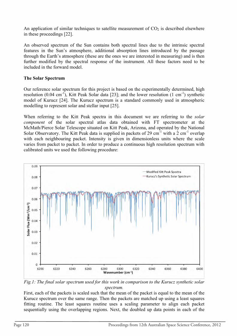
Page 120 Proceedings from 12th Australian Space Science Conference, 2012
An application of similar techniques to satellite measurement of CO2 is described elsewhere in these proceedings [22]. An observed spectrum of the Sun contains both spectral lines due to the intrinsic spectral features in the Sun’s atmosphere, additional absorption lines introduced by the passage through the Earth’s atmosphere (these are the ones we are interested in measuring) and is then further modified by the spectral response of the instrument. All these factors need to be included in the forward model. The Solar Spectrum Our reference solar spectrum for this project is based on the experimentally determined, high resolution (0.04 cm-1), Kitt Peak Solar data [23]; and the lower resolution (1 cm-1) synthetic model of Kurucz [24]. The Kurucz spectrum is a standard commonly used in atmospheric modelling to represent solar and stellar input [25]. When referring to the Kitt Peak spectra in this document we are referring to the solar component of the solar spectral atlas data obtained with FT spectrometer at the McMath/Pierce Solar Telescope situated on Kitt Peak, Arizona, and operated by the National Solar Observatory. The Kitt Peak data is supplied in packets of 29 cm-1 with a 2 cm-1 overlap with each neighbouring packet. Intensity is given in dimensionless units where the scale varies from packet to packet. In order to produce a continuous high resolution spectrum with calibrated units we used the following procedure:
Fig.1: The final solar spectrum used for this work in comparison to the Kurucz synthetic solar
spectrum. First, each of the packets is scaled such that the mean of the packet is equal to the mean of the Kurucz spectrum over the same range. Then the packets are matched up using a least squares fitting routine. The least squares routine uses a scaling parameter to align each packet sequentially using the overlapping regions. Next, the doubled up data points in each of the
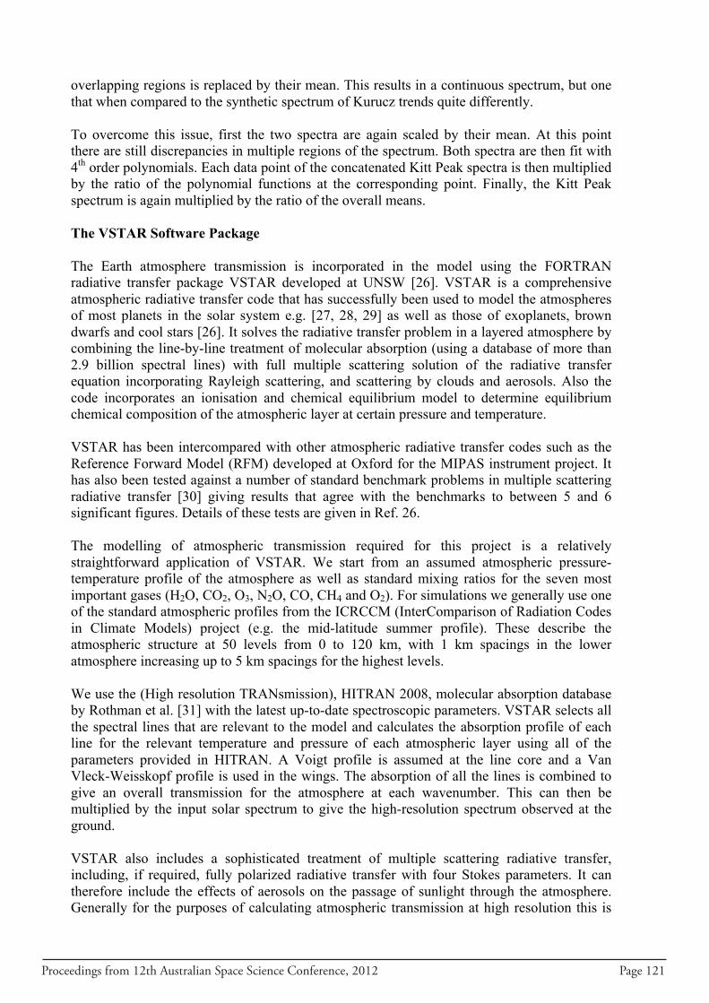
Proceedings from 12th Australian Space Science Conference, 2012 Page 121
overlapping regions is replaced by their mean. This results in a continuous spectrum, but one that when compared to the synthetic spectrum of Kurucz trends quite differently. To overcome this issue, first the two spectra are again scaled by their mean. At this point there are still discrepancies in multiple regions of the spectrum. Both spectra are then fit with 4th order polynomials. Each data point of the concatenated Kitt Peak spectra is then multiplied by the ratio of the polynomial functions at the corresponding point. Finally, the Kitt Peak spectrum is again multiplied by the ratio of the overall means. The VSTAR Software Package The Earth atmosphere transmission is incorporated in the model using the FORTRAN radiative transfer package VSTAR developed at UNSW [26]. VSTAR is a comprehensive atmospheric radiative transfer code that has successfully been used to model the atmospheres of most planets in the solar system e.g. [27, 28, 29] as well as those of exoplanets, brown dwarfs and cool stars [26]. It solves the radiative transfer problem in a layered atmosphere by combining the line-by-line treatment of molecular absorption (using a database of more than 2.9 billion spectral lines) with full multiple scattering solution of the radiative transfer equation incorporating Rayleigh scattering, and scattering by clouds and aerosols. Also the code incorporates an ionisation and chemical equilibrium model to determine equilibrium chemical composition of the atmospheric layer at certain pressure and temperature. VSTAR has been intercompared with other atmospheric radiative transfer codes such as the Reference Forward Model (RFM) developed at Oxford for the MIPAS instrument project. It has also been tested against a number of standard benchmark problems in multiple scattering radiative transfer [30] giving results that agree with the benchmarks to between 5 and 6 significant figures. Details of these tests are given in Ref. 26. The modelling of atmospheric transmission required for this project is a relatively straightforward application of VSTAR. We start from an assumed atmospheric pressure-temperature profile of the atmosphere as well as standard mixing ratios for the seven most important gases (H2O, CO2, O3, N2O, CO, CH4 and O2). For simulations we generally use one of the standard atmospheric profiles from the ICRCCM (InterComparison of Radiation Codes in Climate Models) project (e.g. the mid-latitude summer profile). These describe the atmospheric structure at 50 levels from 0 to 120 km, with 1 km spacings in the lower atmosphere increasing up to 5 km spacings for the highest levels. We use the (High resolution TRANsmission), HITRAN 2008, molecular absorption database by Rothman et al. [31] with the latest up-to-date spectroscopic parameters. VSTAR selects all the spectral lines that are relevant to the model and calculates the absorption profile of each line for the relevant temperature and pressure of each atmospheric layer using all of the parameters provided in HITRAN. A Voigt profile is assumed at the line core and a Van Vleck-Weisskopf profile is used in the wings. The absorption of all the lines is combined to give an overall transmission for the atmosphere at each wavenumber. This can then be multiplied by the input solar spectrum to give the high-resolution spectrum observed at the ground. VSTAR also includes a sophisticated treatment of multiple scattering radiative transfer, including, if required, fully polarized radiative transfer with four Stokes parameters. It can therefore include the effects of aerosols on the passage of sunlight through the atmosphere. Generally for the purposes of calculating atmospheric transmission at high resolution this is
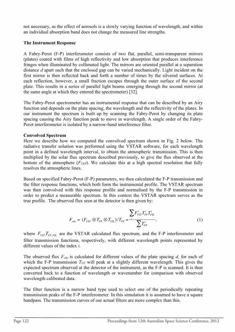
Page 122 Proceedings from 12th Australian Space Science Conference, 2012
not necessary, as the effect of aerosols is a slowly varying function of wavelength, and within an individual absorption band does not change the measured line strengths. The Instrument Response A Fabry-Perot (F-P) interferometer consists of two flat, parallel, semi-transparent mirrors (plates) coated with films of high reflectivity and low absorption that produces interference fringes when illuminated by collimated light. The mirrors are oriented parallel at a separation distance d apart such that the enclosed gap can be varied mechanically. Light incident on the first mirror is then reflected back and forth a number of times by the silvered surfaces. At each reflection, however, a small fraction escapes through the outer surface of the second plate. This results in a series of parallel light beams emerging through the second mirror (at the same angle at which they entered the spectrometer) [32]. The Fabry-Perot spectrometer has an instrumental response that can be described by an Airy function and depends on the plate spacing, the wavelength and the reflectivity of the plates. In our instrument the spectrum is built up by scanning the Fabry-Perot by changing its plate spacing causing the Airy function peak to move in wavelength. A single order of the Fabry-Perot interferometer is isolated by a narrow-band interference filter. Convolved Spectrum Here we describe how we computed the convolved spectrum shown in Fig. 2 below. The radiative transfer solution was performed using the VSTAR software, for each wavelength point in a defined wavelength interval, to obtain the atmospheric transmission. This is then multiplied by the solar flux spectrum described previously, to give the flux observed at the bottom of the atmosphere (FVST). We calculate this at a high spectral resolution that fully resolves the atmospheric lines. Based on specified Fabry-Perot (F-P) parameters, we then calculated the F-P transmission and the filter response functions, which both form the instrumental profile. The VSTAR spectrum was then convolved with this response profile and normalised by the F-P transmission in order to predict a measurable spectrum. In this context the VSTAR spectrum serves as the true profile. The observed flux seen at the detector is then given by:
(1)
where are the VSTAR calculated flux spectrum, and the F-P interferometer and filter transmission functions, respectively, with different wavelength points represented by different values of the index i. The observed flux Fobs is calculated for different values of the plate spacing d, for each of which the F-P transmission TFP will peak at a slightly different wavelength. This gives the expected spectrum observed at the detector of the instrument, as the F-P is scanned. It is then converted back to a function of wavelength or wavenumber for comparison with observed wavelength calibrated data. The filter function is a narrow band type used to select one of the periodically repeating transmission peaks of the F-P interferometer. In this simulation it is assumed to have a square bandpass. The transmission curves of our actual filters are more complex than this.
€
Fobs = (FVST ⊗TFP ⊗TFIL ) /TFP =
FVSTi TFP
i TFILi
i∑
TFPi
i∑
,
€
FVST ,TFP ,FIL
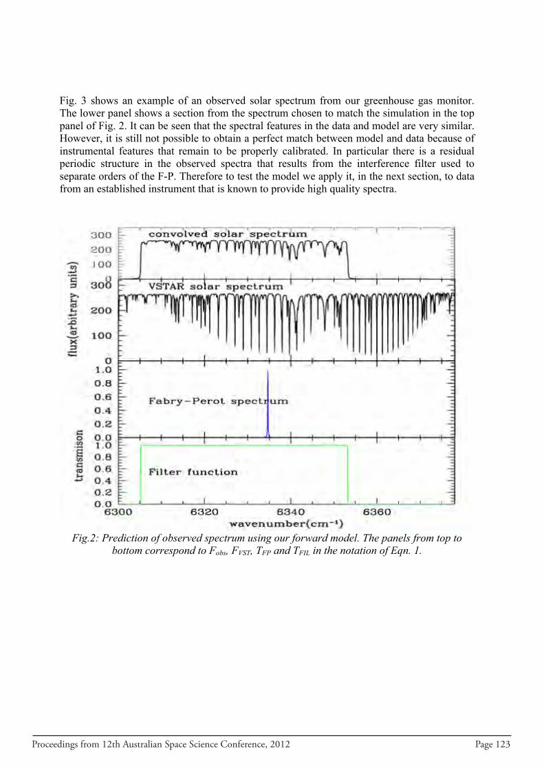
Proceedings from 12th Australian Space Science Conference, 2012 Page 123
Fig. 3 shows an example of an observed solar spectrum from our greenhouse gas monitor. The lower panel shows a section from the spectrum chosen to match the simulation in the top panel of Fig. 2. It can be seen that the spectral features in the data and model are very similar. However, it is still not possible to obtain a perfect match between model and data because of instrumental features that remain to be properly calibrated. In particular there is a residual periodic structure in the observed spectra that results from the interference filter used to separate orders of the F-P. Therefore to test the model we apply it, in the next section, to data from an established instrument that is known to provide high quality spectra.
Fig.2: Prediction of observed spectrum using our forward model. The panels from top to
bottom correspond to Fobs, FVST, TFP and TFIL in the notation of Eqn. 1.
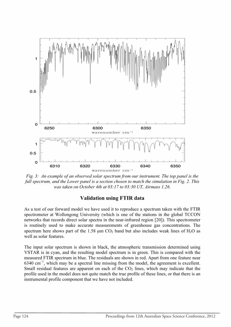
Page 124 Proceedings from 12th Australian Space Science Conference, 2012
Fig. 3: An example of an observed solar spectrum from our instrument. The top panel is the full spectrum, and the Lower panel is a section chosen to match the simulation in Fig. 2. This
was taken on October 4th at 03:17 to 03:30 UT, Airmass 1.26.
Validation using FTIR data As a test of our forward model we have used it to reproduce a spectrum taken with the FTIR spectrometer at Wollongong University (which is one of the stations in the global TCCON networks that records direct solar spectra in the near-infrared region [20]). This spectrometer is routinely used to make accurate measurements of greenhouse gas concentrations. The spectrum here shows part of the 1.58 µm CO2 band but also includes weak lines of H2O as well as solar features. The input solar spectrum is shown in black, the atmospheric transmission determined using VSTAR is in cyan, and the resulting model spectrum is in green. This is compared with the measured FTIR spectrum in blue. The residuals are shown in red. Apart from one feature near 6340 cm–1, which may be a spectral line missing from the model, the agreement is excellent. Small residual features are apparent on each of the CO2 lines, which may indicate that the profile used in the model does not quite match the true profile of these lines, or that there is an instrumental profile component that we have not included.
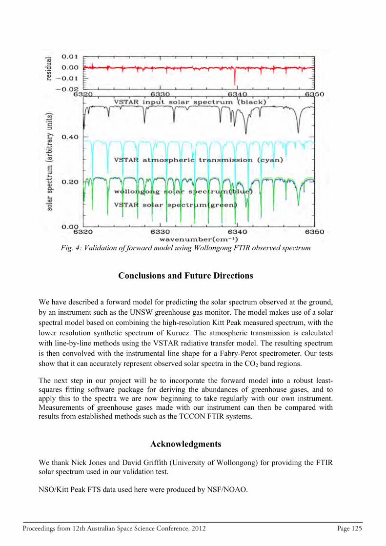
Proceedings from 12th Australian Space Science Conference, 2012 Page 125
Fig. 4: Validation of forward model using Wollongong FTIR observed spectrum
Conclusions and Future Directions
We have described a forward model for predicting the solar spectrum observed at the ground, by an instrument such as the UNSW greenhouse gas monitor. The model makes use of a solar spectral model based on combining the high-resolution Kitt Peak measured spectrum, with the lower resolution synthetic spectrum of Kurucz. The atmospheric transmission is calculated with line-by-line methods using the VSTAR radiative transfer model. The resulting spectrum is then convolved with the instrumental line shape for a Fabry-Perot spectrometer. Our tests show that it can accurately represent observed solar spectra in the CO2 band regions.
The next step in our project will be to incorporate the forward model into a robust least-squares fitting software package for deriving the abundances of greenhouse gases, and to apply this to the spectra we are now beginning to take regularly with our own instrument. Measurements of greenhouse gases made with our instrument can then be compared with results from established methods such as the TCCON FTIR systems.
Acknowledgments We thank Nick Jones and David Griffith (University of Wollongong) for providing the FTIR solar spectrum used in our validation test. NSO/Kitt Peak FTS data used here were produced by NSF/NOAO.
Page 126 Proceedings from 12th Australian Space Science Conference, 2012
References
1. IPCC (Intergovernmental Panel on Climate Change), “Climate Change 2007: The
Physical Science Basis”, Contribution of Working Group I to the Fourth Assessment Report of the Intergovernmental Panel on Climate Change, edited by: Solomon, S., Qin, D., Manning, M., Chen, Z., Marquis, M., Averyt, K.B., Tignor, M. and Miller, H.L., Cambridge University Press, Cambridge, United Kingdom and New York, USA, 2007.
2. Yoshida, Y., Ota, Y., Eguchi, N., Kikuchi, N., Nobuta, K., Tran, H., Morino, L. and
Yokota, T., “Retrieval algorithm for CO2 and CH4 column abundances from short- wavelength infrared spectral observations by the Greenhouse gases observing satellite”, Atmospheric Measurement Techniques, Vol. 4, No. 4, 2011, pp. 717–734.
3. Crisp, D., “Space-Based Measurements for Long-Term Global Monitoring of Atmospheric CO2”, 2009 ESRL Global Monitoring Annual Conference, May 13, 2009.
4. Schneising, O, Buchwitz, M, Burrows, J.P., Bovensmann, H., Reuter, M., Notholt, J., Macatangay, R. and Warneke, T., “Three years of greenhouse gas column-averaged dry air mole fractions retrieved from satellite – Part 1: Carbon dioxide”, Atmospheric Chemistry and Physics, Vol. 8, No. 14, 2008, pp. 3827–3853.
5. Petri, C., Warneke, T, Jones, N., Ridder, T., Messerschmidt, J, Weinzierl, T., Geibel, M. and Notholt, J., “Remote sensing of CO2 and CH4 using solar absorption spectrometry with low resolution spectrometer”, Atmospheric Measurement Techniques, Vol.5, No.7, pp., 2012, 1627–1635.
6. Yang, Z.H., Washenfelder, R.A., Keppel-Aleks, G., Krakauer, N.Y., Randerson, J.T., Tans, P.P., Sweeney, C. and Wennberg, P.O., “New constraints on northern hemisphere growing season net flux”, Geophysical Research Letter, Vol. 34, L12807 pp. 1-6, doi: 10.1029/2007GL029742.2007.
7. Rayner, P. and O’Brien, D., “The utility of remotely sensed CO2 concentration data in surface source inversions”, Geophysical Research Letters, Vol. 28, No. 1, 2001, pp. 175–178.
8. Crevoisier, C., Heilliette, S., Ch´edin, A., Serrar, S., Armante, R. and Scott, N.A.,
“Midtropospheric CO2 concentration retrieval from AIRS observations in the tropics”, Geophysical Research Letter., Vol. 31, L17106, doi: 10.1029/2004GL020141, 2004 pp. 1-4.
9. Bovensmann, H. Buchwitz, M., Burrows, J.P., Reuter, M., Krings, T., Gerilowski, K.,
Schneising, O., Heymann, J. Tretner, A. and Erzinger, J., “A remote sensing technique for global monitoring of power plant CO2 emissions from space and related applications, Atmospheric Measurement Techniques, Vol. 3, No. 4, 2010, pp.781–811.
10. ASCENDS (Active Sensing of CO2 Emissions over Nights, Days, and Seasons
Mission), “NASA Science Definition and Planning Workshop Report” University of Michigan in Ann Arbor, Michigan, USA, July 23-25, 2008, pp. 1-78.
Proceedings from 12th Australian Space Science Conference, 2012 Page 127
11. Chevallier, F., Maksyutov, S., Bousquet, P., Br´eon, F.-M., Saito, R., Yoshida, Y., and Yokota, T., “On the accuracy of the CO2 surface fluxes to be estimated from the GOSAT observations”, Geophysical Research Letter, Vol. 36, L19807, doi: 10.1029/2009GL040108, 2009, pp.1-5.
12. Predoi-Cross, A., Unni, A.V., Liu, W., Schofield, I., Holladay, C., McKellar, A.R.W.,
and Hurtmans, D., “Line shape parameters measurement and computations for self-broadened carbon dioxide transitions in the 30012 ‹- 00001 and 30013 ‹- 00001 bands, line mixing, and speed dependence”, Journal of Molecular Spectroscopy, Vol. 245, Issue 1, 2007 pp. 34–51.
13. WMO-GAW (World Meteorological Organisation-Global Atmospheric Watch), “No.
143 Global Atmospheric Watch Measurements Guide”, WMO TD No. 1073, July 2001, pp. 1-84.
14. Sundquist, E., Burruss, R., Faulkner, S., Gleason, R., Harden, J., Kharaka, Y., Tieszen,
L. and Waldrop, M., “Carbon Sequestration to Mitigate Climate Change, USGS science for changing world, Fact Sheet 2008-3097, 2008, pp.1-4.
15. Worsy, S. C., McConnell, J.C. and McElroy, M.B., “Atmospheric CO2, CO and CH4”,
Journal of Geophysical Research, Vol. 77, No. 24, 1972, pp. 4477-4493.
16. IPCC (Intergovernmental Panel on Climate Change), “Climate Change 2001-The Scientific Basis”, Contribution of Working Group I to the Third Assessment Report of the Intergovernmental Panel on Climate Change, Cambridge University Press, Cambridge, UK, 2001.
17. NIES GOSAT Project newsletter, Issue No. 14, Feb 2011, viewed Aug. 2011
(http://www.gosat.nies.go.jp).
18. Khalil, M.A.K., “Non-CO2 Greenhouse Gases in the atmosphere”, Annual Reviews of Energy and The Environment, Vol. 24, 1999, pp.645-661, doi: 10.1146/annurev.energy.24.1.645.
19. Vardavas, I.M. and Taylor, F.W., Radiation and Climate, Oxford University Press
Inc., New York, USA, 2007.
20. Wunch, D., Toon, G. C., Blavier, J. -F. L., Washenfelder, R. A., Notholt, J., Connor, J. B., Griffith, D. W. T., Sherlock, V., and Wennberg, P. O., “The Total Carbon Column Observing Network”, Philosophical Transactions The Royal Society A, (in press),Vol. 369, 2011, pp. 2087-2112, doi: 10.1098/rsta.2010.0240.
21. Bailey, J., “A low-cost portable fibre-optic spectrometer for atmospheric absorption
studies”, Atmospheric Measurement Techniques Discussions, Vol. 6, 1067-1092, 2013.
22. Dionizio, M.F., Cotton, V. D. and Bailey, J. “Preliminary Parameters for an
Experimental Payload for Tropospheric CO2 Measurement Using a Space-borne Lidar 6C Cubesat Platform” The 12th Australian Space Science Conference (ASSC), Melbourne, September 24-26, 2012.
Page 128 Proceedings from 12th Australian Space Science Conference, 2012
23. Livingston, W. and Wallace, L. “An Atlas of the Solar Spectrum in the Infrared from 1850 to 9000 cm-1 (1.1 to 5.4 microns)'' N.S.O. Technical Report No. 91-001, July 1991.
24. Kurucz, R. L., “The solar irradiance by computation,” http://kurucz.harvard.edu/papers/irradiance/solarirr.tab obtained online 12th of January 2009.
25. Clough, S.A., Shephard, M.W., Mlawer, E.J., Delamere, J.S., Iacomo, M.J., Cady-Pereira, K., Boukabara, S. and Brown, P.D., “Atmospheric radiative transfer modelling: a summary of the AER codes”, Journal of Quantitative Spectroscopy and Radiative Transfer, Vol. 91, Issue 2, 2005, pp. 233-244.
26. Bailey, J., and Kedziora-Chudczer, L., “Modelling the Spectra of Planets, Brown
Dwarfs and Stars using VSTAR”, Monthly Notices of the Royal Astronomical Society, Vol.,419, Issue 3, 2012, pp. 1913-1929.
27. Kedziora-Chudczer., L., and Bailey, J., “Modelling the near-IR spectra of Jupiter
using line-by-line methods”, Monthly Notices of the Royal Astronomical Society, Vol. 414, 2011, pp. 1483-1492.
28. Bailey, J., Ahlsved, L. and Meadows, V.S., “The near-IR spectrum of Titan modeled
with an improved methane line list”, Icarus, Vol. 213, Issue 1, 2011, p. 218-232.
29. Cotton, D.V., Bailey, J. Crisp, D. and Meadows, V.S., “The distribution of carbon monoxide in the lower atmosphere of Venus”, Icarus, Vol. 217, Issue 2, 2012, pp. 570-584.
30. Garcia, R.D.M. and Siewert, C.E., “Benchmark Results in Radiative Transfer,”
Transport Theory and Statistical Physics, Vol. 14, No. 4, 1985, pp. 437-483.
31. Rothman L.S. L.S., Gordon I.E., Barbe A., Benner D.C., Bernath P.F., Birk M., Boudon, V., Brown L.R., Campargue A., Champion J.-P., Chance K., Coudert L.H., Dana V., Devi, V.M., Fally, S., Flaud J.-M., Gamache R.R., Goldman A., Jacquemart D., Kleiner, I., Lacome, N., Lafferty W., Mandin J.-Y., Massie S.T., Mikhailenko, S.N., Miller C.E., Moazzen-Ahmadi, N., Naumenko, O.V., Nikitin A.V., Orphal J., Perevalov, V.I., Perrin, A., Predoi-Cross A., Rinsland C.P., Rotger, M., Simeckova, M., Smith M.A.H., Sung K., Tashkun, S.A., Tennyson J., Toth R.A., Vandaele A.C. and Vander Auwera J., 2009: “The HITRAN 2008 molecular spectroscopic database”, Journal of Quantitative Spectroscopy and Radiative Transfer , Vol. 110, 2009, pp. 533-572.
32. Mulligan, J.F., “Who were Fabry and Perot?”, American Journal of Physics, Vol. 66,
No. 9, 1998, pp.797-802.
Proceedings from 12th Australian Space Science Conference, 2012 Page 129
Satisfying Australia’s Future Need for Multi-Spectral
Imagery using a Cubesat Solution
Iain J. R. Cartwright, Leon B. Stepan and David M. Lingard
Defence Science and Technology Organisation, Intelligence Surveillance and Reconnaissance
Division, PO Box 1500, Edinburgh, South Australia, Australia
Email: [email protected]
Summary: In 2011 Geosciences Australia released a document titled “Continuity of Earth
Observation Data for Australia - Operational Requirements to 2015 for Lands, Coasts and
Oceans” [1]. This forecasts a need for medium resolution multi-spectral coverage of the
entire Australian landmass every day. This paper estimates the amount of imagery that future
public good systems could potentially provide to meet this requirement. It then describes a
modification of the cubesat system proposed by Tsitas and Kingston in [2] that could
supplement the public good systems, and models the collection capabilities of various
constellations of these cubesats. The analysis shows that public good systems will only
provide ~40% of the stated requirement, but that another 40% could be provided by a
constellation containing as little as eight cubesats, provided adequate supporting investment is
also made in ground infrastructure. Thus a relatively small investment in cubesats might meet
a significant portion of Australia’s future space imagery requirements. In doing so the
investment would also provide assured access to imagery from space, transform Australia into
an ‘active’ rather than a ‘passive’ user of Earth observations from space and increase
Australia’s international leverage.
Keywords: Earth observation from space, nano-satellites, 6U cubesat, multi-spectral
imaging, collection planning, ground station network.
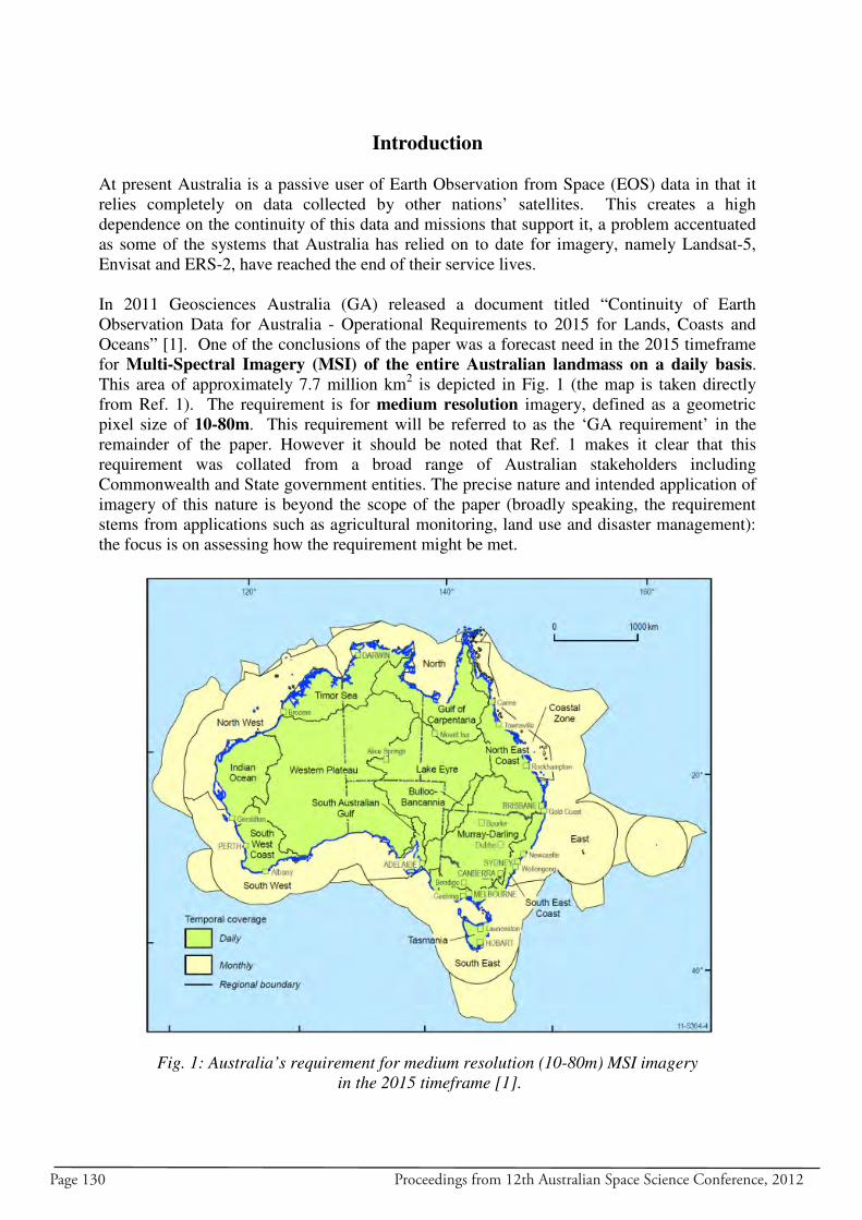
Page 130 Proceedings from 12th Australian Space Science Conference, 2012
Introduction
At present Australia is a passive user of Earth Observation from Space (EOS) data in that it
relies completely on data collected by other nations’ satellites. This creates a high
dependence on the continuity of this data and missions that support it, a problem accentuated
as some of the systems that Australia has relied on to date for imagery, namely Landsat-5,
Envisat and ERS-2, have reached the end of their service lives.
In 2011 Geosciences Australia (GA) released a document titled “Continuity of Earth
Observation Data for Australia - Operational Requirements to 2015 for Lands, Coasts and
Oceans” [1]. One of the conclusions of the paper was a forecast need in the 2015 timeframe
for Multi-Spectral Imagery (MSI) of the entire Australian landmass on a daily basis.
This area of approximately 7.7 million km2 is depicted in Fig. 1 (the map is taken directly
from Ref. 1). The requirement is for medium resolution imagery, defined as a geometric
pixel size of 10-80m. This requirement will be referred to as the ‘GA requirement’ in the
remainder of the paper. However it should be noted that Ref. 1 makes it clear that this
requirement was collated from a broad range of Australian stakeholders including
Commonwealth and State government entities. The precise nature and intended application of
imagery of this nature is beyond the scope of the paper (broadly speaking, the requirement
stems from applications such as agricultural monitoring, land use and disaster management):
the focus is on assessing how the requirement might be met.
Fig. 1: Australia’s requirement for medium resolution (10-80m) MSI imagery
in the 2015 timeframe [1].
Proceedings from 12th Australian Space Science Conference, 2012 Page 131
To date Australia has relied on publicly available data collected by earth observation systems
run by other national or international agencies. Advances in satellite technology have made it
possible to collect medium resolution imagery using quite small, low cost systems: one such
cubesat design is described by Tsitas and Kingston in Ref. 2. Such systems will only be
deployed, however, if a convincing case can be made for their use. The present authors have
therefore explored how the GA requirement may be met through a combination of the public
good EOS systems, and constellations of small satellites similar to those described in Ref. 2.
The results indicate that almost all the requirement could be met for a relatively small cost
through utilisation of publicly available EOS data supplemented by investment in a
constellation of Australian owned and operated small satellites.
The paper is structured as follows. The next section briefly describes the modelling and
simulation tools used to carry out the subsequently presented analysis. These tools are then
used to model the data that existing and future public good MSI systems are likely to be able
to collect in 2015. The following section briefly describes the cubesat design in Ref. 2 along
with a proposed modification that would improve its performance in the GA mission. The
next three sections describe the various constellations considered, the nature and extent of the
coverage they provide, and options for the ground stations needed to download the data they
collect. The last three sections describe the overall results of the modelling, the conclusions
drawn, and options for further work.
In summary, the modelling shows that the public good systems can be expected to only meet
about ~40% of GA’s 2015 requirements for medium resolution MSI. Current cubesat designs
are also capable of collecting the desired imagery. In particular an appropriately placed
constellation of eight cubesats and associated ground stations would increase the daily collect
to ~80% of GA’s requirement: 100% coverage, however, would require more than twelve
satellites. Australian investment in such a constellation would have the additional advantages
of providing assured access to space, establishing Australia as an active contributor to the
international EOS system, and so improve Australia’s negotiating position in future EOS
initiatives.
Modelling and Simulation Approach
The analysis presented in this paper was conducted using two modelling and simulation tools:
Satellite Tool Kit (STK) by Analytical Graphics Incorporated; and the Collection Planning &
Analysis Workstation (CPAW) by Orbit Logic Incorporated. STK allows users to propagate
satellite orbits and conduct access calculations to areas of interest and ground facilities. STK
was used to identify the area collected by the future public good systems.
CPAW couples high fidelity spacecraft modelling, including satellite agility, with multiple
advanced scheduling algorithms to generate optimised collection plans for one or more
remote sensing satellites. CPAW also tracks satellite consumables such as hard drive and
battery capacity to ensure that the planned collections can be satisfied within the satellite’s
resource constraints. Thus, given the quantity of imagery that the public good systems could
potentially provide, CPAW was used to task a number of 6U cubesats in a constellation to
best fill the associated gap in imagery on a typical day. This methodology allows accurate
determination of how well a 6U cubesat constellation could supplement the public good
systems.
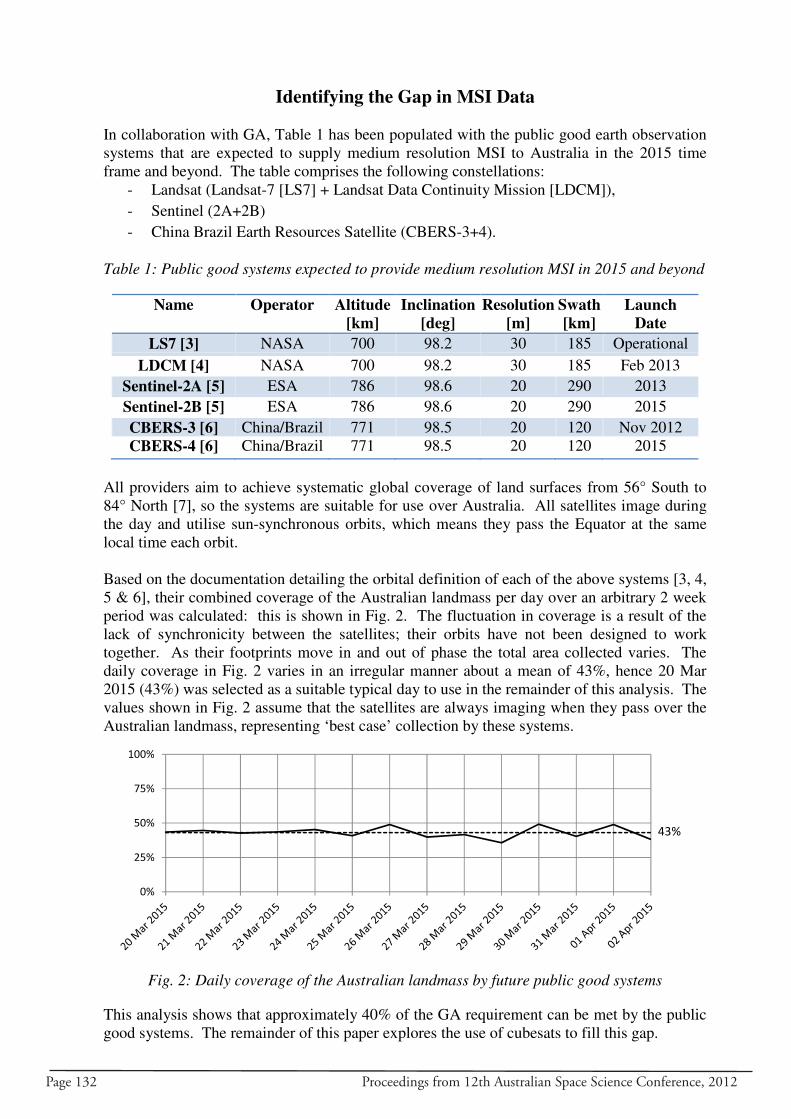
Page 132 Proceedings from 12th Australian Space Science Conference, 2012
Identifying the Gap in MSI Data
In collaboration with GA, Table 1 has been populated with the public good earth observation
systems that are expected to supply medium resolution MSI to Australia in the 2015 time
frame and beyond. The table comprises the following constellations:
- Landsat (Landsat-7 [LS7] + Landsat Data Continuity Mission [LDCM]),
- Sentinel (2A+2B)
- China Brazil Earth Resources Satellite (CBERS-3+4).
Table 1: Public good systems expected to provide medium resolution MSI in 2015 and beyond
Name Operator Altitude
[km]
Inclination
[deg]
Resolution
[m]
Swath
[km]
Launch
Date
LS7 [3] NASA 700 98.2 30 185 Operational
LDCM [4] NASA 700 98.2 30 185 Feb 2013
Sentinel-2A [5] ESA 786 98.6 20 290 2013
Sentinel-2B [5] ESA 786 98.6 20 290 2015
CBERS-3 [6] China/Brazil 771 98.5 20 120 Nov 2012
CBERS-4 [6] China/Brazil 771 98.5 20 120 2015
All providers aim to achieve systematic global coverage of land surfaces from 56° South to
84° North [7], so the systems are suitable for use over Australia. All satellites image during
the day and utilise sun-synchronous orbits, which means they pass the Equator at the same
local time each orbit.
Based on the documentation detailing the orbital definition of each of the above systems [3, 4,
5 & 6], their combined coverage of the Australian landmass per day over an arbitrary 2 week
period was calculated: this is shown in Fig. 2. The fluctuation in coverage is a result of the
lack of synchronicity between the satellites; their orbits have not been designed to work
together. As their footprints move in and out of phase the total area collected varies. The
daily coverage in Fig. 2 varies in an irregular manner about a mean of 43%, hence 20 Mar
2015 (43%) was selected as a suitable typical day to use in the remainder of this analysis. The
values shown in Fig. 2 assume that the satellites are always imaging when they pass over the
Australian landmass, representing ‘best case’ collection by these systems.
Fig. 2: Daily coverage of the Australian landmass by future public good systems
This analysis shows that approximately 40% of the GA requirement can be met by the public
good systems. The remainder of this paper explores the use of cubesats to fill this gap.
0%
25%
50%
75%
100%
43%
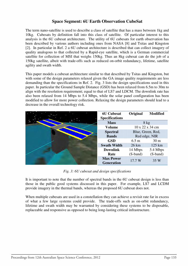
Proceedings from 12th Australian Space Science Conference, 2012 Page 133
Space Segment: 6U Earth Observation CubeSat
The term nano-satellite is used to describe a class of satellite that has a mass between 1kg and
10kg. Cubesats by definition fall into this class of satellite. Of particular interest to this
analysis is the 6U cubesat architecture. The utility of 6U cubesats for earth observation has
been described by various authors including ones from NASA [8] and Tsitas and Kingston
[2]. In particular in Ref. 2 a 6U cubesat architecture is described that can collect imagery of
quality analogous to that collected by a Rapid-eye satellite, which is a German commercial
satellite for collection of MSI that weighs 150kg. Thus an 8kg cubesat can do the job of a
150kg satellite, albeit with trade-offs such as reduced on-orbit redundancy, lifetime, satellite
agility and swath width.
This paper models a cubesat architecture similar to that described by Tsitas and Kingston, but
with some of the design parameters relaxed given the GA image quality requirements are less
demanding than the specifications in Ref. 2. Fig. 3 lists the design specifications used in this
paper. In particular the Ground Sample Distance (GSD) has been relaxed from 6.5m to 30m to
align with the resolution requirement; equal to that of LS7 and LDCM. The downlink rate has
also been relaxed from 14 Mbps to 5.4 Mbps, while the solar panel configuration has been
modified to allow for more power collection. Relaxing the design parameters should lead to a
decrease in the overall technology risk.
6U Cubesat
Specifications
Original Modified
Mass 8 kg
Volume 10 x 22 x 34 cm
Spectral
Bands
Blue, Green, Red,
Red edge, NIR
GSD 6.5 m 30 m
Swath Width 26 km 125 km
Downlink
Rate
14 Mbps
(S-band)
5.4 Mbps
(S-band)
Max Power
Generation 17.7 W 35 W
Fig. 3: 6U cubesat and design specifications
It is important to note that the number of spectral bands in the 6U cubesat design is less than
those in the public good systems discussed in this paper. For example, LS7 and LCDM
provide imagery in the thermal bands, whereas the proposed 6U cubesat does not.
When multiple cubesats are used in a constellation they can achieve a revisit rate far in excess
of what a few large systems could provide. The trade-offs such as on-orbit redundancy,
lifetime and swath width may be warranted by considering these systems to be disposable,
replaceable and responsive as opposed to being long-lasting critical infrastructure.
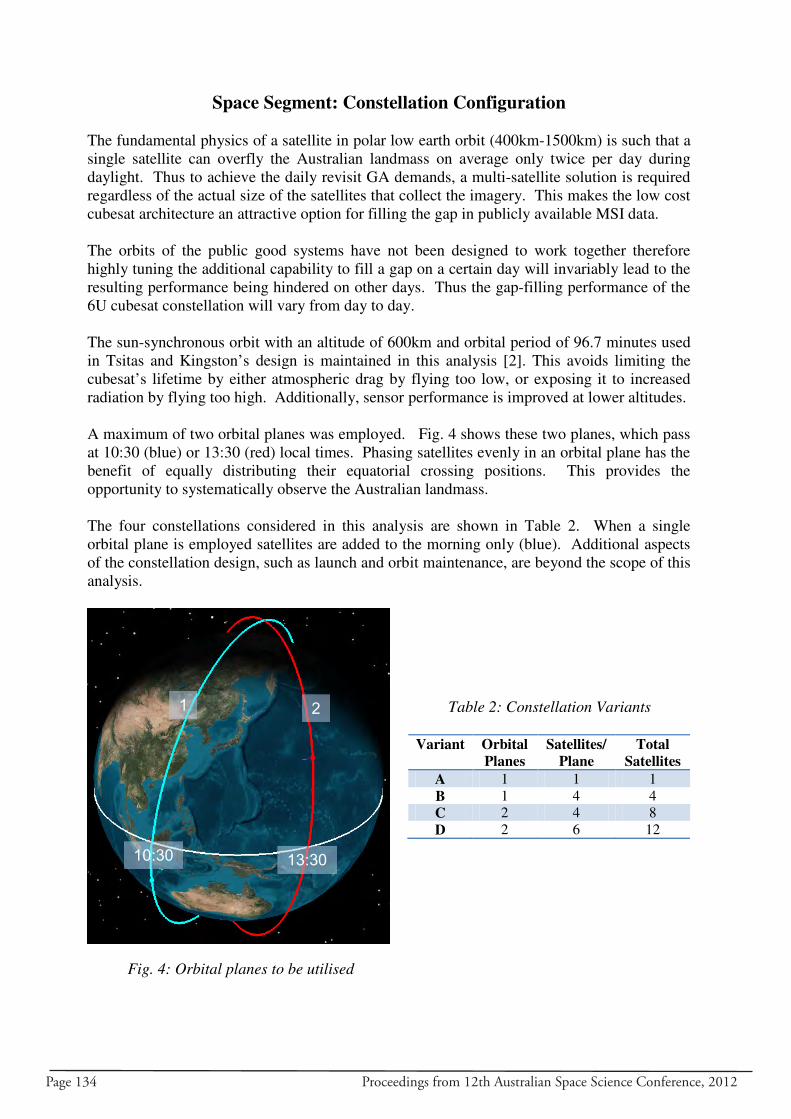
Page 134 Proceedings from 12th Australian Space Science Conference, 2012
Space Segment: Constellation Configuration
The fundamental physics of a satellite in polar low earth orbit (400km-1500km) is such that a
single satellite can overfly the Australian landmass on average only twice per day during
daylight. Thus to achieve the daily revisit GA demands, a multi-satellite solution is required
regardless of the actual size of the satellites that collect the imagery. This makes the low cost
cubesat architecture an attractive option for filling the gap in publicly available MSI data.
The orbits of the public good systems have not been designed to work together therefore
highly tuning the additional capability to fill a gap on a certain day will invariably lead to the
resulting performance being hindered on other days. Thus the gap-filling performance of the
6U cubesat constellation will vary from day to day.
The sun-synchronous orbit with an altitude of 600km and orbital period of 96.7 minutes used
in Tsitas and Kingston’s design is maintained in this analysis [2]. This avoids limiting the
cubesat’s lifetime by either atmospheric drag by flying too low, or exposing it to increased
radiation by flying too high. Additionally, sensor performance is improved at lower altitudes.
A maximum of two orbital planes was employed. Fig. 4 shows these two planes, which pass
at 10:30 (blue) or 13:30 (red) local times. Phasing satellites evenly in an orbital plane has the
benefit of equally distributing their equatorial crossing positions. This provides the
opportunity to systematically observe the Australian landmass.
The four constellations considered in this analysis are shown in Table 2. When a single
orbital plane is employed satellites are added to the morning only (blue). Additional aspects
of the constellation design, such as launch and orbit maintenance, are beyond the scope of this
analysis.
Fig. 4: Orbital planes to be utilised
Table 2: Constellation Variants
Variant Orbital
Planes
Satellites/
Plane
Total
Satellites
A 1 1 1
B 1 4 4
C 2 4 8
D 2 6 12
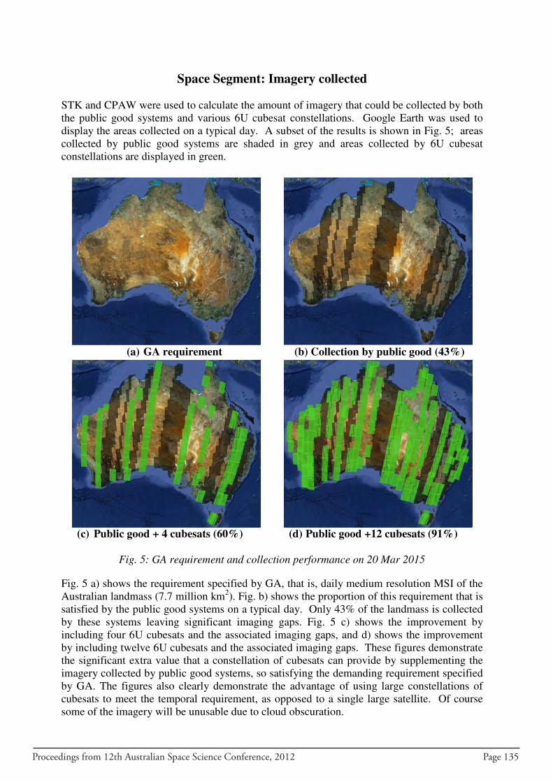
Proceedings from 12th Australian Space Science Conference, 2012 Page 135
Space Segment: Imagery collected
STK and CPAW were used to calculate the amount of imagery that could be collected by both
the public good systems and various 6U cubesat constellations. Google Earth was used to
display the areas collected on a typical day. A subset of the results is shown in Fig. 5; areas
collected by public good systems are shaded in grey and areas collected by 6U cubesat
constellations are displayed in green.
(a) GA requirement
(b) Collection by public good (43%)
(c) Public good + 4 cubesats (60%)
(d) Public good +12 cubesats (91%)
Fig. 5: GA requirement and collection performance on 20 Mar 2015
Fig. 5 a) shows the requirement specified by GA, that is, daily medium resolution MSI of the
Australian landmass (7.7 million km2). Fig. b) shows the proportion of this requirement that is
satisfied by the public good systems on a typical day. Only 43% of the landmass is collected
by these systems leaving significant imaging gaps. Fig. 5 c) shows the improvement by
including four 6U cubesats and the associated imaging gaps, and d) shows the improvement
by including twelve 6U cubesats and the associated imaging gaps. These figures demonstrate
the significant extra value that a constellation of cubesats can provide by supplementing the
imagery collected by public good systems, so satisfying the demanding requirement specified
by GA. The figures also clearly demonstrate the advantage of using large constellations of
cubesats to meet the temporal requirement, as opposed to a single large satellite. Of course
some of the imagery will be unusable due to cloud obscuration.
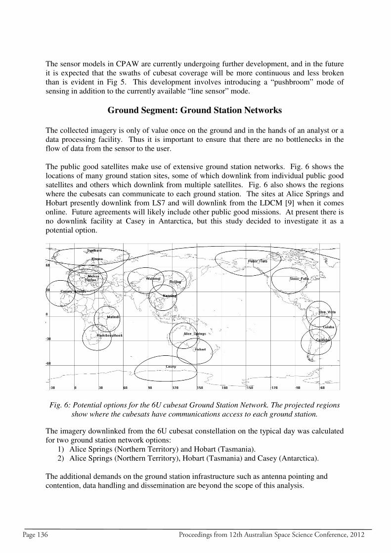
Page 136 Proceedings from 12th Australian Space Science Conference, 2012
The sensor models in CPAW are currently undergoing further development, and in the future
it is expected that the swaths of cubesat coverage will be more continuous and less broken
than is evident in Fig 5. This development involves introducing a “pushbroom” mode of
sensing in addition to the currently available “line sensor” mode.
Ground Segment: Ground Station Networks
The collected imagery is only of value once on the ground and in the hands of an analyst or a
data processing facility. Thus it is important to ensure that there are no bottlenecks in the
flow of data from the sensor to the user.
The public good satellites make use of extensive ground station networks. Fig. 6 shows the
locations of many ground station sites, some of which downlink from individual public good
satellites and others which downlink from multiple satellites. Fig. 6 also shows the regions
where the cubesats can communicate to each ground station. The sites at Alice Springs and
Hobart presently downlink from LS7 and will downlink from the LDCM [9] when it comes
online. Future agreements will likely include other public good missions. At present there is
no downlink facility at Casey in Antarctica, but this study decided to investigate it as a
potential option.
Fig. 6: Potential options for the 6U cubesat Ground Station Network. The projected regions
show where the cubesats have communications access to each ground station.
The imagery downlinked from the 6U cubesat constellation on the typical day was calculated
for two ground station network options:
1) Alice Springs (Northern Territory) and Hobart (Tasmania).
2) Alice Springs (Northern Territory), Hobart (Tasmania) and Casey (Antarctica).
The additional demands on the ground station infrastructure such as antenna pointing and
contention, data handling and dissemination are beyond the scope of this analysis.
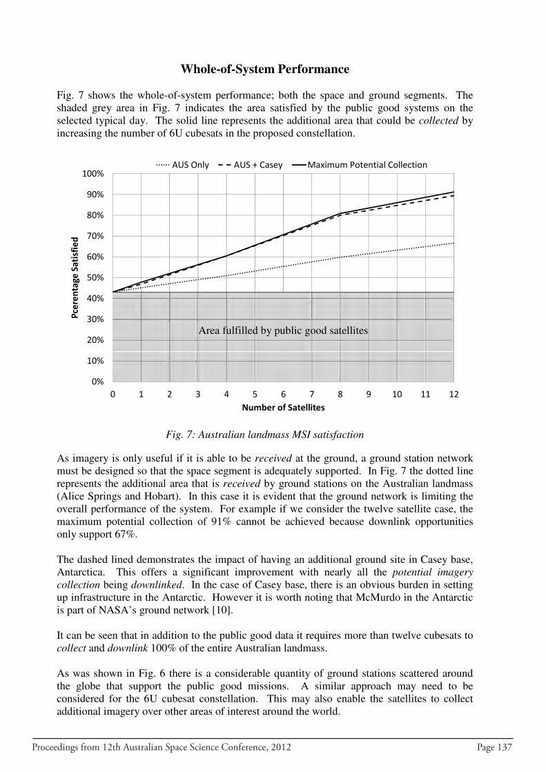
Proceedings from 12th Australian Space Science Conference, 2012 Page 137
Whole-of-System Performance
Fig. 7 shows the whole-of-system performance; both the space and ground segments. The
shaded grey area in Fig. 7 indicates the area satisfied by the public good systems on the
selected typical day. The solid line represents the additional area that could be collected by
increasing the number of 6U cubesats in the proposed constellation.
Fig. 7: Australian landmass MSI satisfaction
As imagery is only useful if it is able to be received at the ground, a ground station network
must be designed so that the space segment is adequately supported. In Fig. 7 the dotted line
represents the additional area that is received by ground stations on the Australian landmass
(Alice Springs and Hobart). In this case it is evident that the ground network is limiting the
overall performance of the system. For example if we consider the twelve satellite case, the
maximum potential collection of 91% cannot be achieved because downlink opportunities
only support 67%.
The dashed lined demonstrates the impact of having an additional ground site in Casey base,
Antarctica. This offers a significant improvement with nearly all the potential imagery
collection being downlinked. In the case of Casey base, there is an obvious burden in setting
up infrastructure in the Antarctic. However it is worth noting that McMurdo in the Antarctic
is part of NASA’s ground network [10].
It can be seen that in addition to the public good data it requires more than twelve cubesats to
collect and downlink 100% of the entire Australian landmass.
As was shown in Fig. 6 there is a considerable quantity of ground stations scattered around
the globe that support the public good missions. A similar approach may need to be
considered for the 6U cubesat constellation. This may also enable the satellites to collect
additional imagery over other areas of interest around the world.
0%
10%
20%
30%
40%
50%
60%
70%
80%
90%
100%
0 1 2 3 4 5 6 7 8 9 10 11 12
Pcer
enta
ge S
atis
fied
Number of Satellites
AUS Only AUS + Casey Maximum Potential Collection
Area fulfilled by public good satellites
Page 138 Proceedings from 12th Australian Space Science Conference, 2012
Conclusions
Through taking a ‘whole-of-system’ approach to addressing the problem described by GA the
following conclusions were reached:
- Proposed future public good systems will only be able to satisfy less than half the
anticipated daily requirement for medium resolution MSI data in the 2015 timeframe.
- Cubesats can provide a credible supplementary capability that would fill the coverage
gaps left by the larger public good systems.
- The temporal aspect of GA’s requirement can only be satisfied through the use of
multiple satellites, making the 8kg 6U cubesat satellite option attractive.
- More than twelve cubesats are required to fulfil the GA requirement of complete daily
MSI coverage of the Australian landmass, although ~80% coverage can be provided
by as few as eight.
- The analysis identified ground station location and availability as a key determinant of
overall system performance. A sophisticated space segment must be appropriately
supported by a distributed ground segment to ensure all imagery collected is
downlinked and processed.
- With the addition of a ground station at Casey Antarctica, the majority of the potential
imagery collection would be supported with downlink opportunities. Alternatively,
other nations could collaborate by offering additional ground sites to fully utilise the
space segment.
In summary a relatively small investment in cubesats and ground infrastructure supplementing
public good systems could meet Australia’s requirements for medium resolution MSI. Such
an investment would transform Australia from a ‘passive’ into an ‘active’ user of EOS data,
leaving the Australian user community less vulnerable and providing it with greater
international leverage.
Further work
This paper has considered a constellation to undertake the mission of imaging the Australian
landmass daily. If an event created a priority to image a few specific areas urgently such as in
the case of a disaster, the constellation could have tactical utility, a utility that would increase
with the size of the constellation.
The paper has also described a modelling and simulation environment, along with a
methodology to make use of this environment. This could be used to analyse the collection
performance of alternative options for space systems on quite fine scales, e.g. considering
different options for sub-system components such as the attitude control and determination
system. Additionally, CPAW allows users to insert dynamic cloud layers into collection
planning simulations. This would reveal the impact of cloud cover on collection performance
over the Australian landmass. Furthermore other topics not considered in the present analysis
could be investigated within this framework, including launch, orbit maintenance and ground
infrastructure aspects such as antenna pointing, contention, data handling and dissemination.
Proceedings from 12th Australian Space Science Conference, 2012 Page 139
Finally one way to baseline the costs of the 6U cubesat constellations proposed here would be
to compare the costs of the constellations with the cost of purchasing the commercial imagery
that would be required to fill the gaps left by public good systems.
References
1. Hudson, D., Harrison, B., Piotrowicz, L., Lewis, A., Browne, S., Drozda, A. “Continuity
of Earth Observation Data for Australia - Operational Requirements to 2015 for Lands,
Coasts and Oceans”, Geosciences Australia, 2011.
2. Tsitas, S. R. and Kingston, J., “6U CubeSat design for Earth observation with 6.5m GSD,
five spectral bands and 14Mbps downlink”, The Aeronautical Journal, November 2010,
Vol. 114, No 1161, pp 689-697.
3. NASA, “Landsat Science Data Users Handbook”, http://landsathandbook.gsfc.nasa.gov/
pdfs/Landsat7_Handbook.pdf
4. Markham, B., “LDCM On-Orbit Cal/Val Considerations”, NASA, 1 March 2011
http://landsat.usgs.gov/documents/LDCM_Cal_Val_Considerations.pptx.
5. EADS Astrium, “Sentinel 2 Data Sheet”, ESA, 2010. http://www.astrium.eads.net/
media/document/sentinel_2_data_sheet.pdf.
6. INPE - National Institute For Space Research, “CBERS 3 and 4 Cameras”,
http://www.cbers.inpe.br/ingles/satellites/cameras_cbers3_4.php.
7. Meygret, A., Baillarin, S., Gascon, F., Hillairet, E., Dechoz, C., Lacherade, S., Martimort,
P., Spoto, F., Henry, P., Duca, R., “SENTINEL-2 Image Quality and Level 1 Processing”,
CNES, 2009. http://144.206.159.178/ft/CONF/16436695/16436706.pdf
8. Agasid, E., Rademacher, A., McCullar, M., Gilstrap, R., “Study to Determine the
Feasibility of an Earth Observing Telescope Payload for a 6U Nano Satellite”, National
Aeronautics and Space Administration, October 2010. http://www.nsbe-
hsc.org/CDST_Feasability_Report.pdf
9. Gatt, E. “Australia Signs Historic Partnership Deal for Satellite Access”, media release by
the Minister for Resources and Energy, Australian Government, 12 July 2012,
http://minister.ret.gov.au/MediaCentre/MediaReleases/Pages/AustraliaPartnershipSatellite
Access.aspx
10. Antarctic Meteorological Research Center (AMRC) and Automatic Weather Station
(AWS), “The McMurdo Ground Station (MGS)”, http://amrc.ssec.wisc.edu/
meetings/MGS/history.html

Page 140 Proceedings from 12th Australian Space Science Conference, 2012
Proceedings from 12th Australian Space Science Conference, 2012 Page 141
Solar Radio Interference to the GNSS
Owen Giersch1,2, John Kennewell2,3
1IPS Radio and Space Services, PO Box 1386, Haymarket, NSW, 1240, Australia
2Curtin University of Technology, Department of Imaging and Applied Physics, GPO Box U1987, Perth, Western Australia, 6845, Australia
3Australian Space Academy, PO Box 3, Meckering, Western Australia, 6405, Australia Summary: Space weather impacts on the Global Navigation Satellite System (GNSS) are generally discussed in terms of ionospheric scintillation. However this is most significant around the equatorial anomaly (about 15 degrees north and south of the equator), and to a lesser extent in the polar regions. It is much less significant at mid latitudes which include a majority of the world’s technical population. There is, however, another space weather impact that can affect the GNSS worldwide, and that effect is direct radio interference from the sun. We shall discuss the effect that large solar radio events can have on the GNSS. We have investigated the sunspot group and magnetic features responsible for the extremely intense December 2006 L-band radio bursts to determine if any significant features were present. We could find no features that were unique to the regions originating these bursts, thus making them inherently unpredictable. Finally, using a statistical analysis we have estimated that 1.4 solar radio bursts per decade could interfere with Global Positioning System (GPS) lock and 0.2 bursts per decade would make GPS unusable. Keywords: GNSS, GPS, Solar Radio Bursts, Interference, Sunspot Regions
Background Ionospheric scintillation is a known problem for Global Navigation Satellite Systems (GNSS) in equatorial regions [11]. Fig. 1 shows the scintillation intensity at 2300 local time (when scintillation is likely to be highest). The colours represent the S4 scintillation index [12]. The orange and red regions are areas of high scintillation and primarily occur at equatorial latitudes or the poles. At mid-latitudes, scintillation is not significant (the white regions on Fig 1). However, at mid-latitudes, solar radio bursts have affected the Global Positioning System (GPS) in the past [5]. In order to describe these effects, a brief review of GPS is required [13], [14]. GPS uses spread-spectrum modulation which spreads the signal over a wide frequency band. At any one frequency the signal lies well below the external noise level. Demodulation of the signal is accomplished by correlating the incoming signal with a copy of the digital pseudo-random noise code that was used to modulate the signal. This increases the signal to noise ratio (S/N) by a factor of around 30 dB (effectively by concentrating the signal in a much smaller bandwidth). Fig. 2 shows a sample GPS signal [1]. On the right vertical axis, we have added spectral flux density in terms of Solar Flux Units (SFU) where 1 SFU = 10-22 W m-2 Hz-1. It is interesting to note that the background sun around 1400 MHz near sunspot maximum is about 100 SFU. This is the peak level of the GPS spread signal. Receiver demodulation effectively raises this signal by 30 dB (a thousand-fold increase), giving an equivalent solar flux density of 105
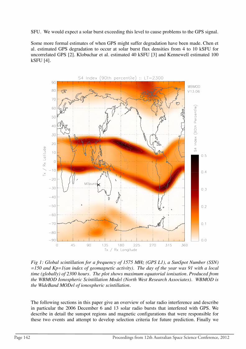
Page 142 Proceedings from 12th Australian Space Science Conference, 2012
SFU. We would expect a solar burst exceeding this level to cause problems to the GPS signal. Some more formal estimates of when GPS might suffer degradation have been made. Chen et al. estimated GPS degradation to occur at solar burst flux densities from 4 to 10 kSFU for uncorrelated GPS [2]. Klobuchar et al. estimated 40 kSFU [3] and Kennewell estimated 100 kSFU [4].
Fig 1: Global scintillation for a frequency of 1575 MHz (GPS L1), a SunSpot Number (SSN) =150 and Kp=1(an index of geomagnetic activity). The day of the year was 91 with a local time (globally) of 2300 hours. The plot shows maximum equatorial ionisation. Produced from the WBMOD Ionospheric Scintillation Model (North West Research Associates). WBMOD is the WideBand MODel of ionospheric scintillation. The following sections in this paper give an overview of solar radio interference and describe in particular the 2006 December 6 and 13 solar radio bursts that interfered with GPS. We describe in detail the sunspot regions and magnetic configurations that were responsible for these two events and attempt to develop selection criteria for future prediction. Finally we
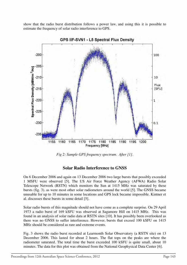
Proceedings from 12th Australian Space Science Conference, 2012 Page 143
show that the radio burst distribution follows a power law, and using this it is possible to estimate the frequency of solar radio interference to GPS.
Fig 2: Sample GPS frequency spectrum. After [1].
Solar Radio Interference to GNSS On 6 December 2006 and again on 13 December 2006 two large bursts that possibly exceeded 1 MSFU were observed [5]. The US Air Force Weather Agency (AFWA) Radio Solar Telescope Network (RSTN) which monitors the Sun at 1415 MHz was saturated by these bursts (fig. 3), as were most other solar radiometers around the world [5]. The GNSS became unusable for up to 10 minutes in some locations and GPS lock became impossible. Kintner et al. discusses these bursts in some detail [5]. Solar radio bursts of this magnitude should not have come as a complete surprise. On 29 April 1973 a radio burst of 169 kSFU was observed at Sagamore Hill on 1415 MHz. This was found in an analysis of solar radio data at RSTN sites [10]. It has possibly been overlooked as there was no GNSS to suffer interference. However, bursts that exceed 100 kSFU on 1415 MHz should be considered as rare and extreme events. Fig. 3 shows the radio burst recorded at Learmonth Solar Observatory (a RSTN site) on 13 December 2006. This lasted for about 2 hours. The flat tops on the peaks are where the radiometer saturated. The total time the burst exceeded 100 kSFU is quite small, about 10 minutes. The data for this plot was obtained from the National Geophysical Data Center [6].
SFU. We would expect a solar burst exceeding this level to cause problems to the GPS signal. Some more formal estimates of when GPS might suffer degradation have been made. Chen et al. estimated GPS degradation to occur at solar burst flux densities from 4 to 10 kSFU for uncorrelated GPS [2]. Klobuchar et al. estimated 40 kSFU [3] and Kennewell estimated 100 kSFU [4].
Fig 1: Global scintillation for a frequency of 1575 MHz (GPS L1), a SunSpot Number (SSN) =150 and Kp=1(an index of geomagnetic activity). The day of the year was 91 with a local time (globally) of 2300 hours. The plot shows maximum equatorial ionisation. Produced from the WBMOD Ionospheric Scintillation Model (North West Research Associates). WBMOD is the WideBand MODel of ionospheric scintillation. The following sections in this paper give an overview of solar radio interference and describe in particular the 2006 December 6 and 13 solar radio bursts that interfered with GPS. We describe in detail the sunspot regions and magnetic configurations that were responsible for these two events and attempt to develop selection criteria for future prediction. Finally we
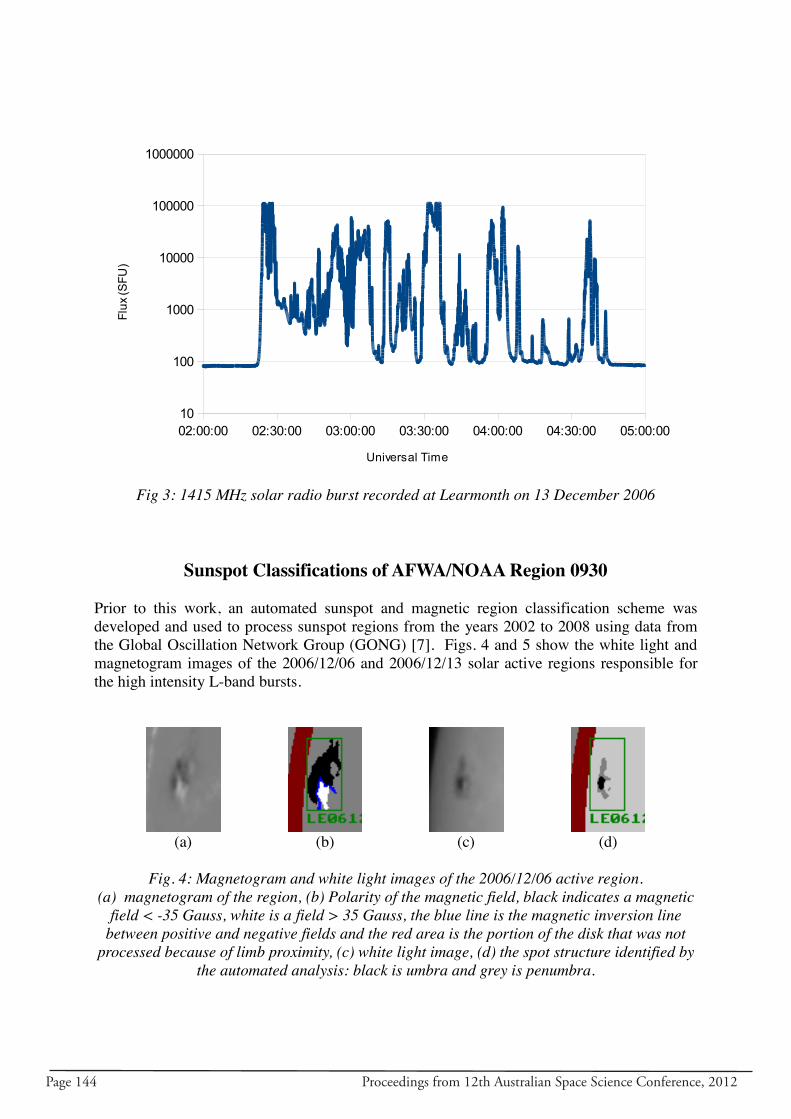
Page 144 Proceedings from 12th Australian Space Science Conference, 2012
(a) (b) (c) (d)
Fig 5: Magnetogram and white light images of the 2006/12/13 active region.
(a) magnetogram of the region, (b) Polarity of the magnetic field, black indicates a magnetic field < -35 Gauss, white is a field > 35 Gauss, the blue line is the magnetic inversion line
between positive and negative fields and the red area is the portion of the disk that was not processed due to limb proximity, (c) white light image, (d) the spot structure identified by the
automated analysis: black is umbra and grey is penumbra.
Region Date Location Area ZPC Length # Spots Mag 0930 2006/12/06 S06E72 390 DKO 4 5 β 0930 2006/12/13 S06W21 680 DKI 8 17
Table 1: AFWA/NOAA Sunspot Classification Table 1 shows the AFWA/NOAA classifications for these two regions. Here the area is the total sunspot area (millionths of the solar hemisphere), ZPC is the McIntosh sunspot classification (Zurich Sunspot class, Penumbral Class, and Compactness Class) [8], Length is the extent of the region (degrees). The #Spots is the number of sunspots visible in white light, and Mag is the Magnetic Classification. These are the only sunspot parameters reported by the AFWA/NOAA. The Automated GONG Sunspot Classification Program produced Tables 2 and 3 Region Date Loc Area Largest
Spot Area Ln #
Spots P Ratio
Cpct G ratio
ZPC Mag
0930 06/12/13 S06E70 494 483 4 2 .77 126 0.38 CKI r 0930 06/12/13 S05W21 608 605 6 3 0.68 94 0.52 DKI r
Table 2: Automated GONG Sunspot Classification Region Date Min
Gauss Location Max
Gauss Location Grad Grad
Dir ILL ILC
0930 2006/12/06 -411 S07E70 +311 S05E70 24 86 11.9 2.786 0930 2006/12/13 -1048 S07W19 +1452 S05W20 85 76 15.2 3.54
Table 3: Automated GONG Magnetic Classification In Table 2, most of the parameters are the same as for the AFWA/NOAA classifications. However there are some additional parameters. The largest spot area is the area of the largest spot in the group in micro-hemispheres. The P-ratio is the East – West extent divided by the North – South extent of largest spot. The closer this value is to one the more symmetric the sunspot. The Compactness is a measure of how densely packed the region is with spots. It is the total area of sunspots divided by the extent of the region. The G-ratio is the amount of spatial overlap between the positive and negative fields (this indicates polarity mixing). Table 3 shows the region magnetic parameters. Min Gauss and Max Gauss are the minimum
02:00:00 02:30:00 03:00:00 03:30:00 04:00:00 04:30:00 05:00:0010
100
1000
10000
100000
1000000
Universal Time
Flux
(SFU
)
Fig 3: 1415 MHz solar radio burst recorded at Learmonth on 13 December 2006
Sunspot Classifications of AFWA/NOAA Region 0930
Prior to this work, an automated sunspot and magnetic region classification scheme was developed and used to process sunspot regions from the years 2002 to 2008 using data from the Global Oscillation Network Group (GONG) [7]. Figs. 4 and 5 show the white light and magnetogram images of the 2006/12/06 and 2006/12/13 solar active regions responsible for the high intensity L-band bursts.
(a) (b) (c) (d)
Fig. 4: Magnetogram and white light images of the 2006/12/06 active region.
(a) magnetogram of the region, (b) Polarity of the magnetic field, black indicates a magnetic field < -35 Gauss, white is a field > 35 Gauss, the blue line is the magnetic inversion line
between positive and negative fields and the red area is the portion of the disk that was not processed because of limb proximity, (c) white light image, (d) the spot structure identified by
the automated analysis: black is umbra and grey is penumbra.
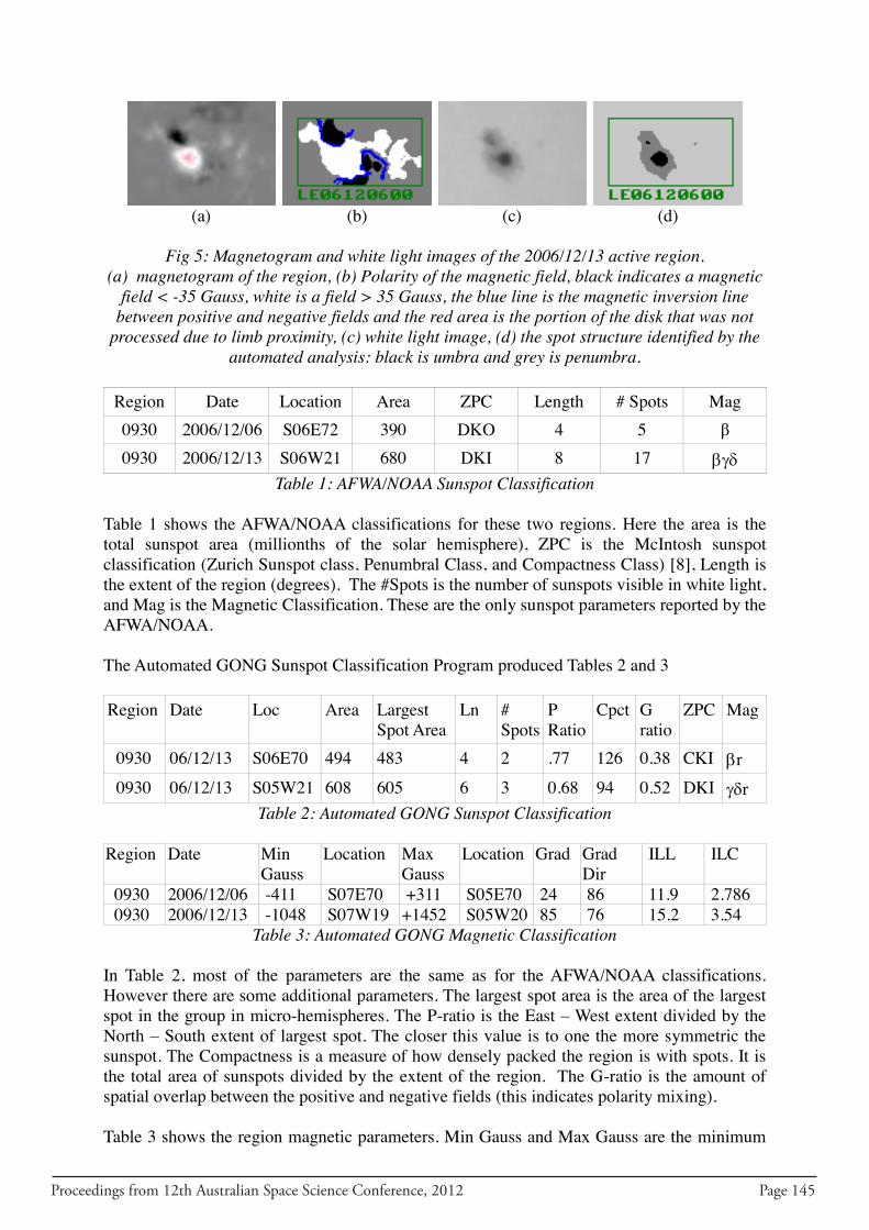
Proceedings from 12th Australian Space Science Conference, 2012 Page 145
(a) (b) (c) (d)
Fig 5: Magnetogram and white light images of the 2006/12/13 active region.
(a) magnetogram of the region, (b) Polarity of the magnetic field, black indicates a magnetic field < -35 Gauss, white is a field > 35 Gauss, the blue line is the magnetic inversion line
between positive and negative fields and the red area is the portion of the disk that was not processed due to limb proximity, (c) white light image, (d) the spot structure identified by the
automated analysis: black is umbra and grey is penumbra.
Region Date Location Area ZPC Length # Spots Mag 0930 2006/12/06 S06E72 390 DKO 4 5 β 0930 2006/12/13 S06W21 680 DKI 8 17
Table 1: AFWA/NOAA Sunspot Classification Table 1 shows the AFWA/NOAA classifications for these two regions. Here the area is the total sunspot area (millionths of the solar hemisphere), ZPC is the McIntosh sunspot classification (Zurich Sunspot class, Penumbral Class, and Compactness Class) [8], Length is the extent of the region (degrees). The #Spots is the number of sunspots visible in white light, and Mag is the Magnetic Classification. These are the only sunspot parameters reported by the AFWA/NOAA. The Automated GONG Sunspot Classification Program produced Tables 2 and 3 Region Date Loc Area Largest
Spot Area Ln #
Spots P Ratio
Cpct G ratio
ZPC Mag
0930 06/12/13 S06E70 494 483 4 2 .77 126 0.38 CKI r 0930 06/12/13 S05W21 608 605 6 3 0.68 94 0.52 DKI r
Table 2: Automated GONG Sunspot Classification Region Date Min
Gauss Location Max
Gauss Location Grad Grad
Dir ILL ILC
0930 2006/12/06 -411 S07E70 +311 S05E70 24 86 11.9 2.786 0930 2006/12/13 -1048 S07W19 +1452 S05W20 85 76 15.2 3.54
Table 3: Automated GONG Magnetic Classification In Table 2, most of the parameters are the same as for the AFWA/NOAA classifications. However there are some additional parameters. The largest spot area is the area of the largest spot in the group in micro-hemispheres. The P-ratio is the East – West extent divided by the North – South extent of largest spot. The closer this value is to one the more symmetric the sunspot. The Compactness is a measure of how densely packed the region is with spots. It is the total area of sunspots divided by the extent of the region. The G-ratio is the amount of spatial overlap between the positive and negative fields (this indicates polarity mixing). Table 3 shows the region magnetic parameters. Min Gauss and Max Gauss are the minimum
02:00:00 02:30:00 03:00:00 03:30:00 04:00:00 04:30:00 05:00:0010
100
1000
10000
100000
1000000
Universal Time
Flux
(SFU
)
Fig 3: 1415 MHz solar radio burst recorded at Learmonth on 13 December 2006
Sunspot Classifications of AFWA/NOAA Region 0930
Prior to this work, an automated sunspot and magnetic region classification scheme was developed and used to process sunspot regions from the years 2002 to 2008 using data from the Global Oscillation Network Group (GONG) [7]. Figs. 4 and 5 show the white light and magnetogram images of the 2006/12/06 and 2006/12/13 solar active regions responsible for the high intensity L-band bursts.
(a) (b) (c) (d)
Fig. 4: Magnetogram and white light images of the 2006/12/06 active region.
(a) magnetogram of the region, (b) Polarity of the magnetic field, black indicates a magnetic field < -35 Gauss, white is a field > 35 Gauss, the blue line is the magnetic inversion line
between positive and negative fields and the red area is the portion of the disk that was not processed because of limb proximity, (c) white light image, (d) the spot structure identified by
the automated analysis: black is umbra and grey is penumbra.
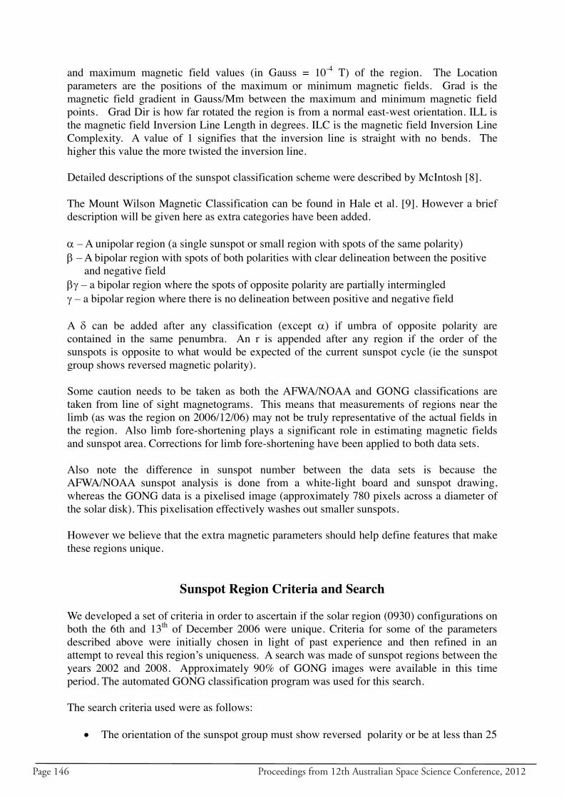
Page 146 Proceedings from 12th Australian Space Science Conference, 2012
and maximum magnetic field values (in Gauss = 10-4 T) of the region. The Location parameters are the positions of the maximum or minimum magnetic fields. Grad is the magnetic field gradient in Gauss/Mm between the maximum and minimum magnetic field points. Grad Dir is how far rotated the region is from a normal east-west orientation. ILL is the magnetic field Inversion Line Length in degrees. ILC is the magnetic field Inversion Line Complexity. A value of 1 signifies that the inversion line is straight with no bends. The higher this value the more twisted the inversion line. Detailed descriptions of the sunspot classification scheme were described by McIntosh [8]. The Mount Wilson Magnetic Classification can be found in Hale et al. [9]. However a brief description will be given here as extra categories have been added. – A unipolar region (a single sunspot or small region with spots of the same polarity) – A bipolar region with spots of both polarities with clear delineation between the positive and negative field – a bipolar region where the spots of opposite polarity are partially intermingled – a bipolar region where there is no delineation between positive and negative field A can be added after any classification (except ) if umbra of opposite polarity are contained in the same penumbra. An r is appended after any region if the order of the sunspots is opposite to what would be expected of the current sunspot cycle (ie the sunspot group shows reversed magnetic polarity). Some caution needs to be taken as both the AFWA/NOAA and GONG classifications are taken from line of sight magnetograms. This means that measurements of regions near the limb (as was the region on 2006/12/06) may not be truly representative of the actual fields in the region. Also limb fore-shortening plays a significant role in estimating magnetic fields and sunspot area. Corrections for limb fore-shortening have been applied to both data sets. Also note the difference in sunspot number between the data sets is because the AFWA/NOAA sunspot analysis is done from a white-light board and sunspot drawing, whereas the GONG data is a pixelised image (approximately 780 pixels across a diameter of the solar disk). This pixelisation effectively washes out smaller sunspots. However we believe that the extra magnetic parameters should help define features that make these regions unique.
Sunspot Region Criteria and Search We developed a set of criteria in order to ascertain if the solar region (0930) configurations on both the 6th and 13th of December 2006 were unique. Criteria for some of the parameters described above were initially chosen in light of past experience and then refined in an attempt to reveal this region’s uniqueness. A search was made of sunspot regions between the years 2002 and 2008. Approximately 90% of GONG images were available in this time period. The automated GONG classification program was used for this search. The search criteria used were as follows:
The orientation of the sunspot group must show reversed polarity or be at less than 25

Proceedings from 12th Australian Space Science Conference, 2012 Page 147
degrees from north-south orientation The area of the largest sunspot must be greater than 250 millionths of the solar
hemisphere The magnetic field gradient must be greater than 90 G/Mm The inversion line complexity must be greater than 2.5 The largest spot must have an asymmetric penumbra The compactness ratio must be greater than 90
Twenty-nine regions were found that matched these criteria. Three of these regions were AFWA/NOAA region 0930 (on different days). We therefore conclude that we have not yet identified any outstanding features of the regions that produced the December 2006 bursts. This will make future forecasting of such events difficult. We should bear in mind that region 0930 on 6 December 2006 had observed magnetic parameters that were highly affected by the extreme longitude of the region. In particular the magnetic field intensity and gradient distortions make these values unreliable.
Solar Radio Burst Statistics and Frequency A search of the National Geophysical Data Center (NGDC) database was made to compile a list of solar radio bursts on 1415 MHz from 1966 to 2010. The burst data can be found at the NGDC ftp site [10]. The sites used are Learmonth, San Vito, Sagamore Hill and Palehua which make up RSTN. The database contains all of the burst reports transmitted, including preliminary real time reports, final reports and corrections. We note that minimum reported burst thresholds have increased from 10 SFU to 100 SFU during the 44 years of observation (Sagamore Hill started observation in 1966). In order to manage these details, the following criteria were used:
any burst of less than 100 SFU was rejected any preliminary report was rejected any noise storm was rejected if there was a correction to a burst, then the correction was used if there were two or more corrections to a burst then the higher burst value was used
As there may be more than one site observing the sun at the same time, if a burst was observed at multiple sites, then the higher reported value was used. We also need to make an estimate of the total observing time. Each site operates while the sun has an elevation of more than 3 degrees. Unfortunately, there is no record kept of down time for each site, so we have assumed complete patrol. Whilst this is unrealistic, we believe it will affect the statistics by less than a factor of two (from personal knowledge of network performance). Fig. 6 shows the burst distribution for 1415 MHz. This distribution follows a power law with a lower cutoff of 100 SFU. The number of observing days was estimated to be 14,214. Bursts that exceeded 100 kSFU have been excluded in this fit because it is unknown exactly how large they were (due to radio telescope saturation), and therefore impossible to window in a histogram.
and maximum magnetic field values (in Gauss = 10-4 T) of the region. The Location parameters are the positions of the maximum or minimum magnetic fields. Grad is the magnetic field gradient in Gauss/Mm between the maximum and minimum magnetic field points. Grad Dir is how far rotated the region is from a normal east-west orientation. ILL is the magnetic field Inversion Line Length in degrees. ILC is the magnetic field Inversion Line Complexity. A value of 1 signifies that the inversion line is straight with no bends. The higher this value the more twisted the inversion line. Detailed descriptions of the sunspot classification scheme were described by McIntosh [8]. The Mount Wilson Magnetic Classification can be found in Hale et al. [9]. However a brief description will be given here as extra categories have been added. – A unipolar region (a single sunspot or small region with spots of the same polarity) – A bipolar region with spots of both polarities with clear delineation between the positive and negative field – a bipolar region where the spots of opposite polarity are partially intermingled – a bipolar region where there is no delineation between positive and negative field A can be added after any classification (except ) if umbra of opposite polarity are contained in the same penumbra. An r is appended after any region if the order of the sunspots is opposite to what would be expected of the current sunspot cycle (ie the sunspot group shows reversed magnetic polarity). Some caution needs to be taken as both the AFWA/NOAA and GONG classifications are taken from line of sight magnetograms. This means that measurements of regions near the limb (as was the region on 2006/12/06) may not be truly representative of the actual fields in the region. Also limb fore-shortening plays a significant role in estimating magnetic fields and sunspot area. Corrections for limb fore-shortening have been applied to both data sets. Also note the difference in sunspot number between the data sets is because the AFWA/NOAA sunspot analysis is done from a white-light board and sunspot drawing, whereas the GONG data is a pixelised image (approximately 780 pixels across a diameter of the solar disk). This pixelisation effectively washes out smaller sunspots. However we believe that the extra magnetic parameters should help define features that make these regions unique.
Sunspot Region Criteria and Search We developed a set of criteria in order to ascertain if the solar region (0930) configurations on both the 6th and 13th of December 2006 were unique. Criteria for some of the parameters described above were initially chosen in light of past experience and then refined in an attempt to reveal this region’s uniqueness. A search was made of sunspot regions between the years 2002 and 2008. Approximately 90% of GONG images were available in this time period. The automated GONG classification program was used for this search. The search criteria used were as follows:
The orientation of the sunspot group must show reversed polarity or be at less than 25
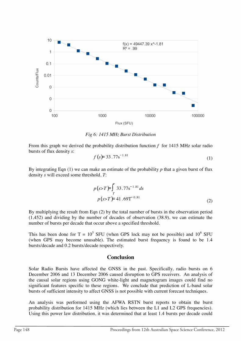
Page 148 Proceedings from 12th Australian Space Science Conference, 2012
100 1000 10000 1000000
0
0
0.01
0.1
1
10f(x) = 49447.39 x^-1.81R² = .99
Flux (SFU)
Cou
nts/
Flux
Fig 6: 1415 MHz Burst Distribution
From this graph we derived the probability distribution function f for 1415 MHz solar radio bursts of flux density s:
f (s)= 33 .77s− 1.81 (1)
By integrating Eqn (1) we can make an estimate of the probability p that a given burst of flux density s will exceed some threshold, T:
p (s>T )=∫T
∞33.77s− 1 .81 ds
p (s>T )= 41 .69T− 0.81 (2)
By multiplying the result from Eqn (2) by the total number of bursts in the observation period (1,452) and dividing by the number of decades of observation (38.9), we can estimate the number of bursts per decade that occur above a specified threshold. This has been done for T = 105 SFU (when GPS lock may not be possible) and 106 SFU (when GPS may become unusable). The estimated burst frequency is found to be 1.4 bursts/decade and 0.2 bursts/decade respectively.
Conclusion Solar Radio Bursts have affected the GNSS in the past. Specifically, radio bursts on 6 December 2006 and 13 December 2006 caused disruption to GPS receivers. An analysis of the causal solar regions using GONG white-light and magnetogram images could find no significant features specific to these regions. We conclude that prediction of L-band solar bursts of sufficient intensity to affect GNSS is not possible with current forecast techniques. An analysis was performed using the AFWA RSTN burst reports to obtain the burst probability distribution for 1415 MHz (which lies between the L1 and L2 GPS frequencies). Using this power law distribution, it was determined that at least 1.4 bursts per decade could
Proceedings from 12th Australian Space Science Conference, 2012 Page 149
interfere with GPS lock and 0.2 bursts per decade could make GPS unusable. These numbers may be on the low side because we have assumed interference thresholds at the high end of published speculation. Some GNSS systems may well be affected by lower levels of solar radio emission.
References 1. “Inside GNSS News”, 17 June 2010, http://www.insidegnss.com/node/2138 2. Zhiyu Chen, Yang Gao, Zhizhao Liu, “Evaluation of Solar Radio Bursts’ Effect on GPS Receiver Signal Tracking within International GPS Service Network”, Radio Science, Vol 40, 2005, RS3012 [doi:10.1029/2004RS003066] 3. J.A. Klobuchar, J.M. Kunches, and A.J. Van Dierendonck, “Eye on the Ionosphere: Potential Solar Radio Burst Effects on GPS Signal to Noise”, GPS Solutions, Vol 3(2), pp 69-71, 1999 4. J. Kennewell, “Interference to GPS Signals by Solar Radio Bursts”, http://www.ips.gov.au/Educational/1/3/10 5. P.M. Kintner Jr, B. O'Hanlon, D.E. Gary, and P.M.S. Kintner, “Global Positioning System and Solar Radio Burst Forensics”, Radio Science, Vol 44, 2009, RS0A08 [doi:10.1029/2008RS004039] 6. ftp://ftp.ngdc.noaa.gov/STP/SOLAR_DATA/SOLAR_RADIO/RSTN_1sec/Learmonth/ 2006/12/13DEC06.APL.gz 7. http://gong2.nso.edu/dsds 8. P.S. McIntosh, “The Classification of Sunspot Groups”, Solar Physics, Vol 125, pp 251-267, 1990 9. George E. Hale, Ferdinand Ellerman, S. B. Nicholson, A. H. Joy, “The Magnetic Polarity of Sunspots”, Astrophysical Journal, Vol 40, pp 153-185, 1919 10. ftp://ftp.ngdc.noaa.gov/STP/SOLAR_DATA/SOLAR_RADIO/BURSTS/fixed/ 11. L. Wanninger, “Effects of Equatorial Ionosphere on GPS”, GPS World, Vol 4, pp 48-54, 1993 12. http://www.ips.gov.au/Satellite/6/3 13. Tom Logsdon, The Navstar Global Positioning System, Van Nostrand Reinhold, 1992. 14. Philip Mattos, “GPS”, Electronics World, December 1992, pp 982-987, “GPS 2: Receiver Architecture”, Electronics World, January 1993, pp 29 – 32, “GPS 3: The GPS Message on the Hardware Platform”, Electronics World, February 1993, pp 146 – 151, “GPS 4: Radio Architecture”, Electronics World, March 1993, pp 210 – 216, “GPS 5: The Software Engine”, Electronics World, April 1993, pp 296 – 304. Note: All web references were current as of 31 January 2013.
100 1000 10000 1000000
0
0
0.01
0.1
1
10f(x) = 49447.39 x^-1.81R² = .99
Flux (SFU)
Cou
nts/
Flux
Fig 6: 1415 MHz Burst Distribution
From this graph we derived the probability distribution function f for 1415 MHz solar radio bursts of flux density s:
f (s)= 33 .77s− 1.81 (1)
By integrating Eqn (1) we can make an estimate of the probability p that a given burst of flux density s will exceed some threshold, T:
p (s>T )=∫T
∞33.77s− 1 .81 ds
p (s>T )= 41 .69T− 0.81 (2)
By multiplying the result from Eqn (2) by the total number of bursts in the observation period (1,452) and dividing by the number of decades of observation (38.9), we can estimate the number of bursts per decade that occur above a specified threshold. This has been done for T = 105 SFU (when GPS lock may not be possible) and 106 SFU (when GPS may become unusable). The estimated burst frequency is found to be 1.4 bursts/decade and 0.2 bursts/decade respectively.
Conclusion Solar Radio Bursts have affected the GNSS in the past. Specifically, radio bursts on 6 December 2006 and 13 December 2006 caused disruption to GPS receivers. An analysis of the causal solar regions using GONG white-light and magnetogram images could find no significant features specific to these regions. We conclude that prediction of L-band solar bursts of sufficient intensity to affect GNSS is not possible with current forecast techniques. An analysis was performed using the AFWA RSTN burst reports to obtain the burst probability distribution for 1415 MHz (which lies between the L1 and L2 GPS frequencies). Using this power law distribution, it was determined that at least 1.4 bursts per decade could

Page 150 Proceedings from 12th Australian Space Science Conference, 2012
Proceedings from 12th Australian Space Science Conference, 2012 Page 151
A CubeSat Mission for Exoplanet Transit Detection and Asteroseismology
Jeremy Bailey1, Steven Tsitas2, Daniel Bayliss3, Tim Bedding4
1School of Physics, University of New South Wales, NSW, 2052, Australia
2Australian Centre for Space Engineering Research, University of New South Wales, NSW, 2052, Australia
3Research School of Astronomy and Astrophysics, Australian National University, Mt Stromlo Observatory, Cotter Road, Weston Creek, ACT 2611, Australia
4Sydney Institute for Astronomy (SIfA), School of Physics, University of Sydney, NSW 2006, Australia
Summary: We describe a satellite concept that incorporates a small wide-field telescope for precision photometry in a 6U CubeSat format. The science goals of the mission are exoplanet detection through transits and the study of stellar pulsations (asteroseismology). The NASA Kepler mission has demonstrated the value of a wide-field space telescope for detecting transitting planets too small to be detectable from the ground. However, most of the planet candidates found by Kepler are orbiting stars too faint for follow-up with radial-velocity studies or atmospheric characterization by spectroscopy. By using a much smaller telescope with a wider field, we can find similar candidates around much brighter stars that are much more suitable for follow-up. Keywords: exoplanets, asteroseismology, cubesats, satellites, photometry
Introduction
The NASA Kepler mission [1] has revolutionized exoplanet science by using precision photometry from space to detect large numbers of exoplanet candidates by transit. More than 2300 planet candidates have now been reported from the first 16 months of Kepler data [2]. 105 of the Kepler candidates have been confirmed as planets1 and many interesting systems have been found, including the habitable zone planet Kepler-22b [3], the six planet system Kepler-11 [4], and the circumbinary planetary systems Kepler-16 [5] and Kepler-47 [6]. However, the Kepler telescope is relatively large (0.95m aperture) and the Kepler exoplanet candidate stars are mostly in the magnitude range 12-16. This makes most of them too faint for follow-up observations, such as radial velocity studies that would be needed to confirm the planets and determine their mass. Many of the detected signals are therefore likely to remain as unconfirmed planet candidates. This also means that the Kepler transiting planets will, in most cases, not be suitable for the spectroscopic studies that can be used for atmospheric characterization. Such observations have been successfully applied to transiting planets found by ground-based telescopes, orbiting bright stars, such as HD189733b and HD209458b. By observing the primary transit, absorption features can be detected in the atmosphere of the planet [7, 8], whilst differencing spectra in and out of secondary eclipse allows the emission spectrum of the planet’s dayside to be observed [9].
1 http://kepler.nasa.gov
Page 152 Proceedings from 12th Australian Space Science Conference, 2012
Exoplanet transit detection is a field in which, unlike most of astronomy, there can be significant advantages in using a smaller telescope. For a given detector area, a smaller telescope covers a larger area of sky to a smaller depth than a larger telescope of similar focal ratio. This means the smaller telescope sees about the same number of stars, but on average these are brighter and more suitable for the necessary follow-up observations. This has been recognized in recent ground-based transit detection projects that use relatively small telescopes with large area detectors, as in the SuperWasp [10] and HATSouth [11,12] projects. Even more extreme examples are the KELT (Kilodegree Extremely Little Telescope) North [13] and South [14] telescopes, which use 85mm focal-length camera lenses. These ground-based projects can discover transiting planets around bright stars, but the limited accuracy of photometry achievable from the ground means they can only discover relatively large planets. A similar system in space using a small wide-field telescope will be able to obtain much more accurate photometry, permitting the detection of smaller planets like those found by Kepler, but around much brighter stars. The planets found by such a mission are likely to be good candidates for follow up spectroscopy using instruments such as the Veloce instrument proposed for the Anglo-Australian Telescope [15] and the GHOST instrument proposed for the Gemini observatory [16]. Some of the planets found by such a system can be expected to be ideal cases for detailed studies such as atmospheric characterization. The value of very small space telescopes has been recognized in other proposed missions such as Brite-Constellation [17] and ExoplanetSat [18]. Brite-Constellation uses an even smaller telescope (30 mm aperture) than we propose for asteroseismology of very bright stars. ExoplanetSat is a 3U CubeSat for exoplanet transit detection, but targets only a single bright star at any one time. The accurate photometric data obtained will also be ideal for asteroseismology, the study of stellar pulsations. These pulsations can reveal detailed information about the internal structure and properties of stars that cannot be obtained in any other way. While such studies are also being made with other space missions such as Kepler [19], the ability of our system to point over much of the sky and to observe very bright stars will provide some unique capabilities. It will provide data on many bright stars that have well determined properties. It will also be possible to observe fields containing clusters, such as the open clusters IC2602 and M67, allowing the detailed investigation of a set of stars with similar age.
The 6U CubeSat Format The CubeSat standard [20] was originally developed at California Polytechnic State University in 1999 and specifies a standard design for small satellites built up from 10cm cube units. CubeSats can be deployed from a launch vehicle using a standard deployment system called a PPOD (Poly Picosatellite Orbital Deployer). The CubeSat format has become popular and widely used, particularly for low-cost satellite development by educational organizations. Many standard CubeSat components are available and on-line CubeSat shops have been set up by companies such as ClydeSpace and ISIS. The original Cal Poly CubeSat standard [20] specified satellites from 1U (a single 10cm cube) to 3U (three such cubes stacked together). However, the NASA CubeSat launch initiative [21] also allows for 6U CubeSats (2U × 3U) that have dimensions of 33 x 22 x 10 cm. Tsitas and Kingston [22] have described a design for an Earth Observation satellite implemented in a 6U
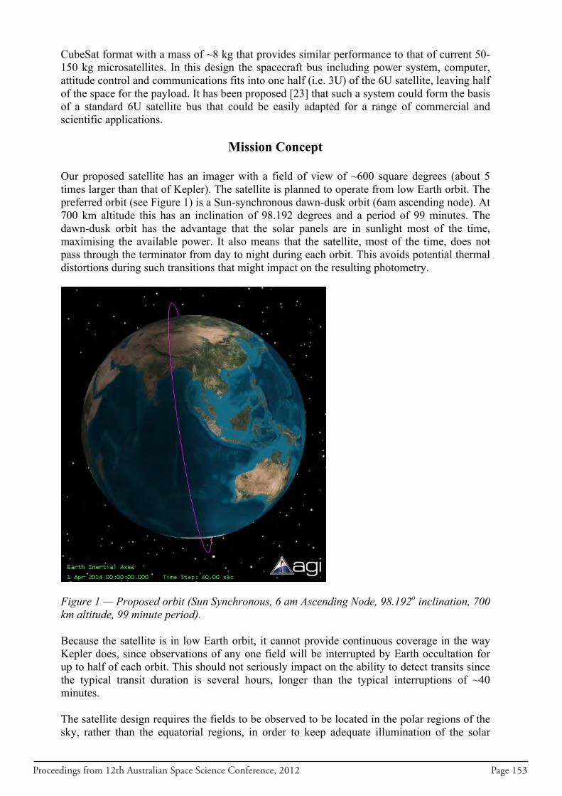
Proceedings from 12th Australian Space Science Conference, 2012 Page 153
CubeSat format with a mass of ~8 kg that provides similar performance to that of current 50-150 kg microsatellites. In this design the spacecraft bus including power system, computer, attitude control and communications fits into one half (i.e. 3U) of the 6U satellite, leaving half of the space for the payload. It has been proposed [23] that such a system could form the basis of a standard 6U satellite bus that could be easily adapted for a range of commercial and scientific applications.
Mission Concept
Our proposed satellite has an imager with a field of view of ~600 square degrees (about 5 times larger than that of Kepler). The satellite is planned to operate from low Earth orbit. The preferred orbit (see Figure 1) is a Sun-synchronous dawn-dusk orbit (6am ascending node). At 700 km altitude this has an inclination of 98.192 degrees and a period of 99 minutes. The dawn-dusk orbit has the advantage that the solar panels are in sunlight most of the time, maximising the available power. It also means that the satellite, most of the time, does not pass through the terminator from day to night during each orbit. This avoids potential thermal distortions during such transitions that might impact on the resulting photometry.
Figure 1 — Proposed orbit (Sun Synchronous, 6 am Ascending Node, 98.192o inclination, 700 km altitude, 99 minute period). Because the satellite is in low Earth orbit, it cannot provide continuous coverage in the way Kepler does, since observations of any one field will be interrupted by Earth occultation for up to half of each orbit. This should not seriously impact on the ability to detect transits since the typical transit duration is several hours, longer than the typical interruptions of ~40 minutes. The satellite design requires the fields to be observed to be located in the polar regions of the sky, rather than the equatorial regions, in order to keep adequate illumination of the solar
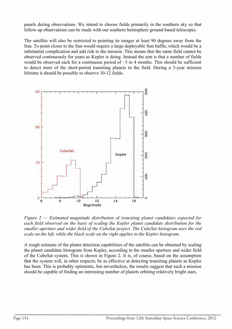
Page 154 Proceedings from 12th Australian Space Science Conference, 2012
panels during observations. We intend to choose fields primarily in the southern sky so that follow up observations can be made with our southern hemisphere ground-based telescopes. The satellite will also be restricted to pointing its imager at least 90 degrees away from the Sun. To point closer to the Sun would require a large deployable Sun baffle, which would be a substantial complication and add risk to the mission. This means that the same field cannot be observed continuously for years as Kepler is doing. Instead the aim is that a number of fields would be observed each for a continuous period of ~3 to 4 months. This should be sufficient to detect most of the short-period transiting planets in the field. During a 3-year mission lifetime it should be possible to observe 10-12 fields.
Figure 2 — Estimated magnitude distribution of transiting planet candidates expected for each field observed on the basis of scaling the Kepler planet candidate distribution for the smaller aperture and wider field of the CubeSat project. The CubeSat histogram uses the red scale on the left, while the black scale on the right applies to the Kepler histogram. A rough estimate of the planet detection capabilities of the satellite can be obtained by scaling the planet candidate histogram from Kepler, according to the smaller aperture and wider field of the CubeSat system. This is shown in Figure 2. It is, of course, based on the assumption that the system will, in other respects, be as effective at detecting transiting planets as Kepler has been. This is probably optimistic, but nevertheless, the results suggest that such a mission should be capable of finding an interesting number of planets orbiting relatively bright stars.
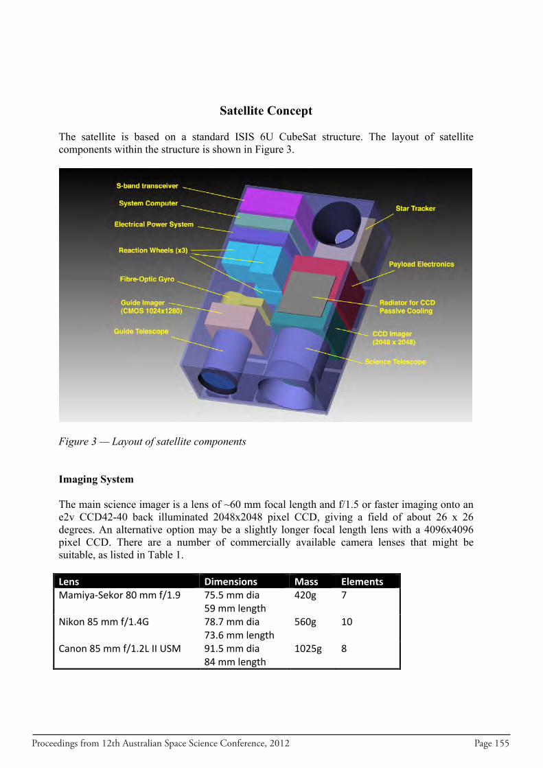
Proceedings from 12th Australian Space Science Conference, 2012 Page 155
Satellite Concept The satellite is based on a standard ISIS 6U CubeSat structure. The layout of satellite components within the structure is shown in Figure 3.
Figure 3 — Layout of satellite components Imaging System The main science imager is a lens of ~60 mm focal length and f/1.5 or faster imaging onto an e2v CCD42-40 back illuminated 2048x2048 pixel CCD, giving a field of about 26 x 26 degrees. An alternative option may be a slightly longer focal length lens with a 4096x4096 pixel CCD. There are a number of commercially available camera lenses that might be suitable, as listed in Table 1. Lens Dimensions Mass Elements Mamiya-‐Sekor 80 mm f/1.9 75.5 mm dia
59 mm length 420g 7
Nikon 85 mm f/1.4G 78.7 mm dia 73.6 mm length
560g 10
Canon 85 mm f/1.2L II USM 91.5 mm dia 84 mm length
1025g 8
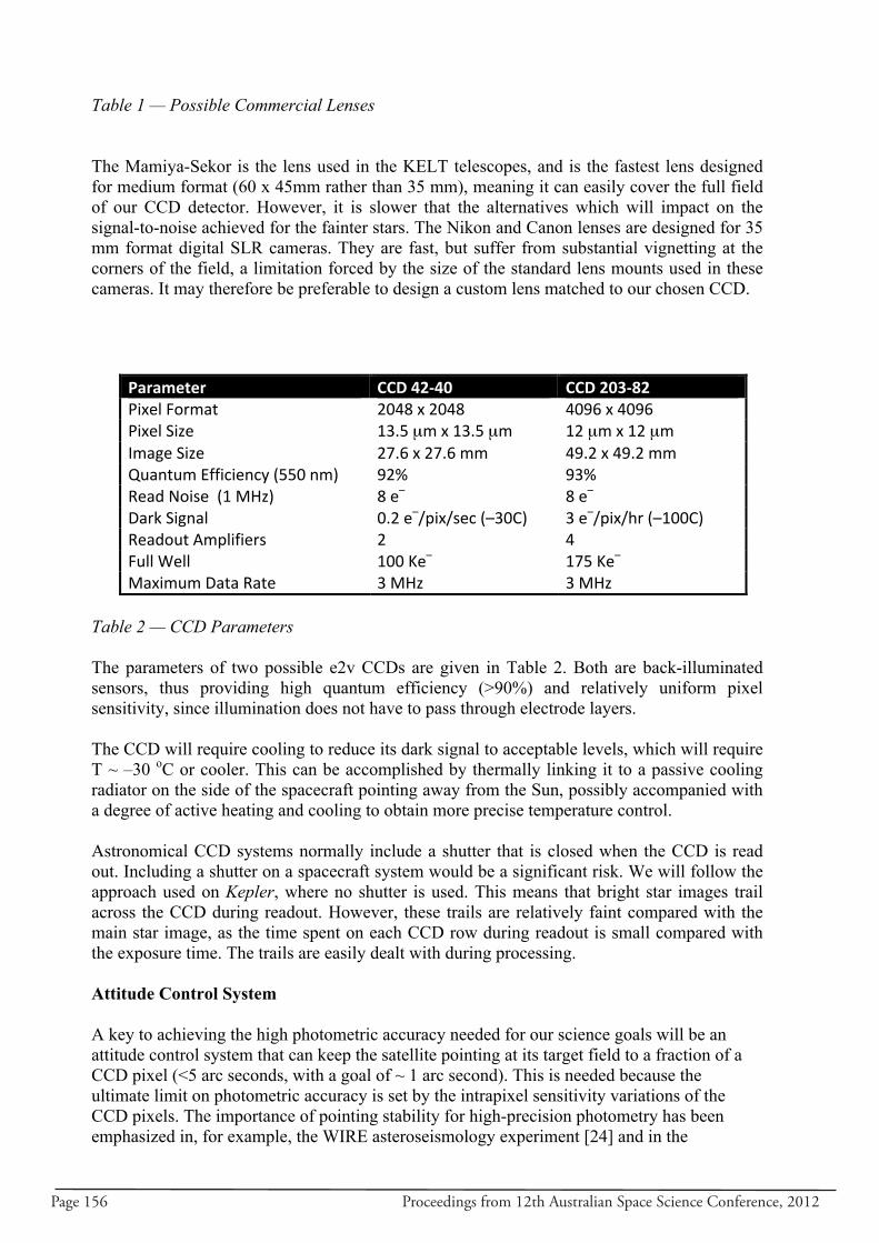
Page 156 Proceedings from 12th Australian Space Science Conference, 2012
Table 1 — Possible Commercial Lenses The Mamiya-Sekor is the lens used in the KELT telescopes, and is the fastest lens designed for medium format (60 x 45mm rather than 35 mm), meaning it can easily cover the full field of our CCD detector. However, it is slower that the alternatives which will impact on the signal-to-noise achieved for the fainter stars. The Nikon and Canon lenses are designed for 35 mm format digital SLR cameras. They are fast, but suffer from substantial vignetting at the corners of the field, a limitation forced by the size of the standard lens mounts used in these cameras. It may therefore be preferable to design a custom lens matched to our chosen CCD.
Table 2 — CCD Parameters The parameters of two possible e2v CCDs are given in Table 2. Both are back-illuminated sensors, thus providing high quantum efficiency (>90%) and relatively uniform pixel sensitivity, since illumination does not have to pass through electrode layers. The CCD will require cooling to reduce its dark signal to acceptable levels, which will require T ~ –30 oC or cooler. This can be accomplished by thermally linking it to a passive cooling radiator on the side of the spacecraft pointing away from the Sun, possibly accompanied with a degree of active heating and cooling to obtain more precise temperature control. Astronomical CCD systems normally include a shutter that is closed when the CCD is read out. Including a shutter on a spacecraft system would be a significant risk. We will follow the approach used on Kepler, where no shutter is used. This means that bright star images trail across the CCD during readout. However, these trails are relatively faint compared with the main star image, as the time spent on each CCD row during readout is small compared with the exposure time. The trails are easily dealt with during processing. Attitude Control System A key to achieving the high photometric accuracy needed for our science goals will be an attitude control system that can keep the satellite pointing at its target field to a fraction of a CCD pixel (<5 arc seconds, with a goal of ~ 1 arc second). This is needed because the ultimate limit on photometric accuracy is set by the intrapixel sensitivity variations of the CCD pixels. The importance of pointing stability for high-precision photometry has been emphasized in, for example, the WIRE asteroseismology experiment [24] and in the
Parameter CCD 42-‐40 CCD 203-‐82 Pixel Format 2048 x 2048 4096 x 4096 Pixel Size 13.5 µm x 13.5 µm 12 µm x 12 µm Image Size 27.6 x 27.6 mm 49.2 x 49.2 mm Quantum Efficiency (550 nm) 92% 93% Read Noise (1 MHz) 8 e– 8 e– Dark Signal 0.2 e–/pix/sec (–30C) 3 e–/pix/hr (–100C) Readout Amplifiers 2 4 Full Well 100 Ke– 175 Ke– Maximum Data Rate 3 MHz 3 MHz

Proceedings from 12th Australian Space Science Conference, 2012 Page 157
performance of the Canadian MOST microsatellite [25]. In the case of MOST, the performance of the direct-imaging photometry was substantially improved when the pointing accuracy of the satellite was improved from ~10 to ~1 arc second [26]. This arc-second pointing accuracy is well beyond anything that has yet been attempted for a CubeSat. The attitude control system will make use of three orthogonal reaction wheels (Sinclair Interplanetary RW-0.03-4), and a star tracker (Comtech AeroAstro Miniature Star Tracker). The star tracker will enable sensing of attitude to ~90 arc seconds, which will be sufficient for acquisition of fields. To achieve the arc second level pointing accuracy required during imaging we propose to include a long focal length telescope imaging onto a small CCD with a pixel scale of ~1 arcsec. We would choose each of our fields to be centered on a suitable bright star, which would be used as a guide star in this telescope. For this guide telescope a Maksutov design would be used to produce a compact optical system with 60-80 mm aperture and ~500mm focal length. The imager would use a standard CMOS sensor with 5.2 mm pixels giving around 2 arc seconds per pixel. A suitable imager would be the Miniature Imager from Comtech AeroAstro. The guide telescope would be used to maintain pointing to within ~ 1 arc sec, but it is also necessary to control the rotation about this pointing axis. The science camera can be used as a source of data for this, but its update rate will be relatively slow with typical exposure times of 30 seconds. Therefore, it will be used in combination with a fibre-optic gyro (KVH DSP-1750). This has high performance, with an angular random walk of 0.013o /√hr and bias stability of <0.05o/hr. Integrating the gyro output for the 30 seconds of an exposure will lead to an rms error of <4.2 arc seconds in rotation, which is less than 5% of the pixel size at the edge of the field. Component Performance Mass/Power Usage Comtech AeroAstro Miniature Star Tracker
90 arcsec in three axes 1 Hz update rate Lost-in-space capability
375 g / <2W Attitude sensing during field acquisition and when not observing
Guide Telescope with Comtech AeroAstro Miniature Imager
~1 arcsec in two axes frame rate up to 27 fps
375 g / 1W (not including telescope)
Pointing axis sensing during observing
Science Camera Rotation to ~10 arc second every 30 sec.
Rotation sensing during observing
Fibre-optic gyro KVH DSP-1750
Random walk <0.013o/√hr Drift < 0.05o/hr
90g / 3W Rotation sensing during observing
3 x Reaction Wheels, Sinclair Interplanetary RW-0.03-4
30 mNm-sec at 5600 rpm, 2 mNm torque
185g / 1.5W at full torque
Attitude control in three axes
3 x orthogonal magnetourquer coils mounted in three orthogonal face panels.
0.14 – 0.5 A/m2 Dumping excess angular momentum from reaction wheels
Table 3 — Attitude Control System Components
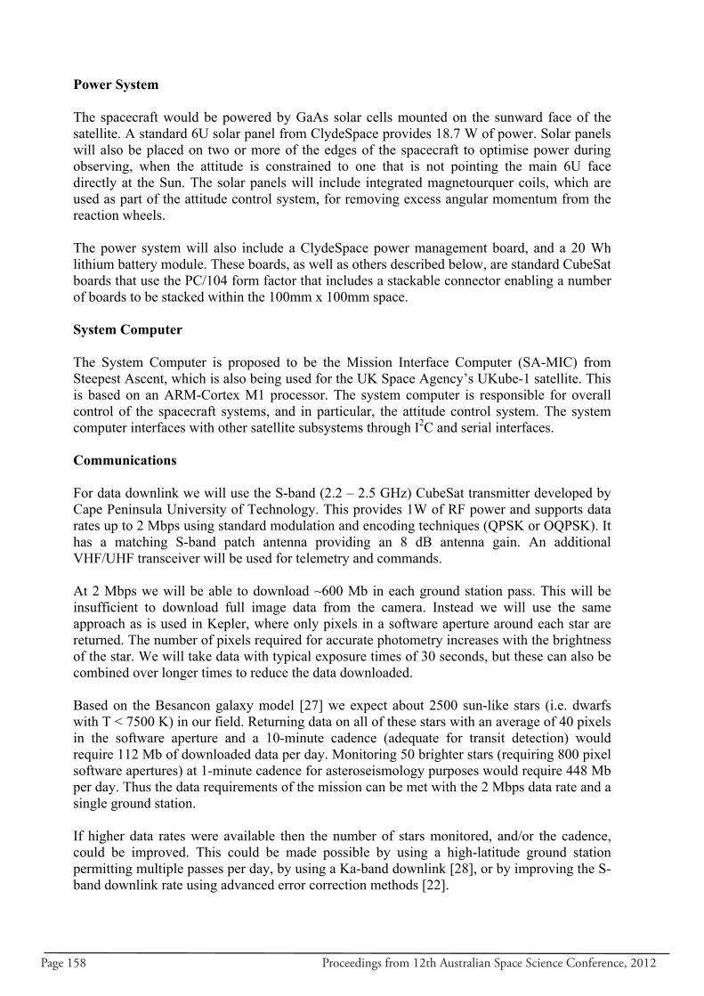
Page 158 Proceedings from 12th Australian Space Science Conference, 2012
Power System The spacecraft would be powered by GaAs solar cells mounted on the sunward face of the satellite. A standard 6U solar panel from ClydeSpace provides 18.7 W of power. Solar panels will also be placed on two or more of the edges of the spacecraft to optimise power during observing, when the attitude is constrained to one that is not pointing the main 6U face directly at the Sun. The solar panels will include integrated magnetourquer coils, which are used as part of the attitude control system, for removing excess angular momentum from the reaction wheels. The power system will also include a ClydeSpace power management board, and a 20 Wh lithium battery module. These boards, as well as others described below, are standard CubeSat boards that use the PC/104 form factor that includes a stackable connector enabling a number of boards to be stacked within the 100mm x 100mm space. System Computer The System Computer is proposed to be the Mission Interface Computer (SA-MIC) from Steepest Ascent, which is also being used for the UK Space Agency’s UKube-1 satellite. This is based on an ARM-Cortex M1 processor. The system computer is responsible for overall control of the spacecraft systems, and in particular, the attitude control system. The system computer interfaces with other satellite subsystems through I2C and serial interfaces. Communications For data downlink we will use the S-band (2.2 – 2.5 GHz) CubeSat transmitter developed by Cape Peninsula University of Technology. This provides 1W of RF power and supports data rates up to 2 Mbps using standard modulation and encoding techniques (QPSK or OQPSK). It has a matching S-band patch antenna providing an 8 dB antenna gain. An additional VHF/UHF transceiver will be used for telemetry and commands. At 2 Mbps we will be able to download ~600 Mb in each ground station pass. This will be insufficient to download full image data from the camera. Instead we will use the same approach as is used in Kepler, where only pixels in a software aperture around each star are returned. The number of pixels required for accurate photometry increases with the brightness of the star. We will take data with typical exposure times of 30 seconds, but these can also be combined over longer times to reduce the data downloaded. Based on the Besancon galaxy model [27] we expect about 2500 sun-like stars (i.e. dwarfs with T < 7500 K) in our field. Returning data on all of these stars with an average of 40 pixels in the software aperture and a 10-minute cadence (adequate for transit detection) would require 112 Mb of downloaded data per day. Monitoring 50 brighter stars (requiring 800 pixel software apertures) at 1-minute cadence for asteroseismology purposes would require 448 Mb per day. Thus the data requirements of the mission can be met with the 2 Mbps data rate and a single ground station. If higher data rates were available then the number of stars monitored, and/or the cadence, could be improved. This could be made possible by using a high-latitude ground station permitting multiple passes per day, by using a Ka-band downlink [28], or by improving the S-band downlink rate using advanced error correction methods [22].

Proceedings from 12th Australian Space Science Conference, 2012 Page 159
Payload Electronics It is necessary to provide a subsystem to read out the data from the CCD, store and process the images, and provide data to the S-band transmitter for downlink. This does not appear to be possible with a commercially available system. A number of standardised low-noise readout controllers for astronomical CCDs have been developed [29, 30] but these are not made to fit within the constraints of CubeSat volume and power limitations. A preliminary design for such a low-power CCD system has been developed. It uses an FPGA-based system to generate the clock waveforms that drive the CCD’s horizontal and vertical clocks, and a low-power video processing system that amplifies and digitizes the CCD output signals. The CCD system interfaces with a payload computer, which will be a second SA-MIC computer board, as used for the satellite’s system computer. The power requirements for the CCD system have been determined using methods described in ref. 31. For a 1 MHz readout rate, which will read a 2K x 2K CCD in 4 seconds, the power needed is 2.3 W, including the computer system. The SA-MIC computer can be configured with flash memory that can be used for storing data prior to downlink and will send its data to the S-band transmitter via an SPI bus interface.
Conclusions
We have outlined a concept for a 6U CubeSat that uses a wide-field telescope to obtain high-precision photometry of bright stars. The satellite is capable of discovering a significant number of transiting planets around stars bright enough for follow-up studies, including the characterization of their atmospheres. It will also be suitable for asteroseismology studies of bright stars. The satellite can be assembled largely from commercially available components that either have flight heritage, or are due to fly shortly. The most challenging aspect of the project is to provide an attitude control system capable of maintaining pointing at the arc second level. Further study will be needed to determine the feasibility of such a system. It will also be necessary to develop appropriate low-power CCD readout electronics and a cooling system for the CCD.
References 1. Borucki, W.J., et al., “Kepler Planet-Detection Mission: Introduction and First Results”,
Science, Vol. 327, 2010, pp. 977-980.
2. Batalha, N.M., et al., “Planetary Candidates Observed by Kepler, III. Analysis of the first 16 Months of Data”, Submitted to Astrophys. J. Supp., 2012, arXiv 1202.5825.
3. Borucki, W.J., et al., “Kepler-22b: A 2.4 Earth-radius Planet in the Habitable Zone of a
Sun-like Star”, Astrophys. J., Vol. 745, article id. 120, 2012. 4. Lissauer, J.J. et al., “A closely packed system of low-mass, low-density planets transiting
Kepler-11”, Nature, Vol. 470, 2011, pp. 53-58.
Page 160 Proceedings from 12th Australian Space Science Conference, 2012
5. Doyle, L.R., et al., “Kepler-16: A Transiting Circumbinary Planet”, Science, Vol. 333, 2011, pp. 1602-1606.
6. Orosz, J.A., et al., Kepler-47: “A Transiting Circumbinary Multiplanet System”, Science,
Vol. 337, 2012, pp. 1511-1514. 7. Swain, M.R., Vasicht, G., Tinetti, G., “The presence of methane in the atmosphere of an
extrasolar planet”, Nature, Vol 452, 2008, pp. 329-331. 8. Zhou, G. and Bayliss, D.D.R., “Detection of sodium absorption in WASP-17b with
Magellan”, Mon. Not. R. Astron. Soc., Vol. 426, 2012, 2483-2488. 9. Swain, M.R. et al., “Water, Methane and Carbon Dioxide Present in the Dayside Spectrum
of the Exoplanet HD 209458b”, Astrophys. J., Vol. 704, 2009, pp. 1616-1621. 10. Pollacco, D.L., et al., “The WASP project and the SuperWASP cameras”, Publ. Astr. Soc.
Pacific, Vol. 118, 2006, 1407-1418. 11. Bakos, G.A. et al., “HATSouth: a global network of fully automated identical wide-field
telescopes”, submitted to Publ. Astr. Soc. Pacific, 2012, arXiv 1206.1391. 12. Penev, K. et al., “HATS-1b: The First Transiting Planet Discovered by the HATSouth
Survey”, submitted to Astron. J., 2012, arXiv 1206.1524. 13. Siverd, R.J. et al., “KELT-1b: A Strongly Irradiated, Highly Inflated, Short Period, 27
Jupiter-mass Companion Transiting a mid-F Star”, submitted to Astrophys. J., 2012, arXiv 1206.1635.
14. Pepper, J., Kuhn, R., Siverd, R., James, D., Stassun, K., “The KELT-South Telescope”,
Publ. Astr. Soc. Pacific, Vol. 124, 2012, pp. 230-241. 15. Tinney, C.G., “Veloce Position Paper”, 2012,
http://www.phys.unsw.edu.au/~cgt/cgt/Veloce.html 16. Ireland, M. et al., “The AAO's Gemini High-resolution Optical SpecTrograph (GHOST)
concept”, in Ground-based and Airborne Instrumentation for Astronomy IV, Proc SPIE, Vol. 8446, 2012, doi:10.1117/12.925746.
17. Appourchaux, T., “Oscillation mode frequencies of 61 main-sequence and subgiant stars
observed by Kepler”, Astron. & Astrophys., Vol. 543, 2012, id. A54. 18. Kaiser, A., Kuschnig, R., Weiss, W.W. and the Brite-Constellation team, “Brite-
Constellation: A status report”, Astron. Nachr., Vol. 333, 2012, pp.1096-1098. 19. Smith, M.W. et al., “ExoplanetSat: Detecting transiting exoplanets using a low-cost
CubeSat platform”, in Space Telescopes and Instrumentation 2010: Optical, Infrared and Millimeter Wave, Proc Spie, Vol 7731, 2010, 773127,
20. CubeSat Design Specification Rev. 12, California Polytechnic State University, 2009,
http://www.cubesat.org/images/developers/cds_rev12.pdf
Proceedings from 12th Australian Space Science Conference, 2012 Page 161
21. NASA CubeSat Launch Initiative, http://www.nasa.gov/directorates/heo/home/CubeSats_initiative.html
22. Tsitas, S.R. and Kingston, J., “6U CubeSat design for Earth observation with 6.5m GSD,
five spectral bands and 14Mbps downlink”, The Aeroautical Journal, Vol. 114, 2010, pp. 689-697.
23. Tsitas, S.R. and Kingston, J., “6U CubeSat commercial applications”, The Aeroautical
Journal, Vol. 116, 2012, pp. 189-198. 24. Buzasi, D.L., “The performance of a high-precision photometry mission in space” in
Second Eddington Workshop: Stellar structure and habitable planet finding, ESA SP538, 2004, pp. 205-213.
25. Zee, R.E. and Stibrany, P., “Canada’s First Microsatellite – An Enabling Low-Cost
Technology for Future Space Science and Technology Missions”, Canadian Aeronautics & Space Journal, Vol. 48, 2002, pp. 1-11.
26. Rowe, J.F. et al., “Direct imaging photometry with the MOST satellite”, Mem. Soc.
Astron. It., Vol. 77, 2006, pp. 282-286. 27. Robin, A.C., Reyle, C., Derriere, S., Picaud, S., “A synthetic view on structure and
evolution of the Milky Way”, Astron & Astrophys., Vol. 409, 2003, pp. 523-540. 28. King, J.A., Ness, J., Bonin, G., Brett, M., Faber, D., “Nanosat Ka-band Communications
— A Paradigm Shift in Small Satellite Data Throughput”, Proceedings 26th Annual AIAA/USU Conference on Small Satellites, SSC12-VI-9, 2012, pp. 1-21.
29. Waller, L., Barton, J., Mayfield, D., Griesbach, J., “AAO2: a general purpose CCD
controller for the AAT”, in Optical and Infrared Detectors for Astronomy, Proc. SPIE Vol. 5499, 204, pp. 452-63.
30. Leach, B., and Low, F., 2000, “CCD and IR array controllers”, in Optical and IR
Telescope Instrumentation and Detectors, Proc. SPIE, Vol. 4008, 2000, pp. 337-343. 31. Jorden, P.R., Morris, D.G., Pool, P.J., “Technology of large focal planes of CCDs”, in
Focal Planes for Space Telescopes, Proc. SPIE, 5167, 2004, pp. 72-82.

Page 162 Proceedings from 12th Australian Space Science Conference, 2012
Proceedings from 12th Australian Space Science Conference, 2012 Page 163
Preliminary Parameters For An Experimental Payload For Tropospheric CO2 Measurement Using A Space-borne
Lidar 6U Cubesat Platform M. Fabiao Dionizio1, D. V. Cotton 2, J. Bailey 2
1 The University of New South Wales, Australian Centre for Space Engineering Research, Sydney, Australia
2 The University of New South Wales, School of Physics, Sydney, Australia
Summary: This paper investigates the implementation of a downward looking space-borne lidar system to map the concentration of Tropospheric CO2. Lidar has been used to measure greenhouse gases and a variety of trace species, profile winds, and producing high-resolution topographical maps. Sufficiently accurate CO2 mapping can locate and quantify sources and sinks of CO2, thus helping understand the carbon cycle, to verify the emissions accounting methods that are the basis of the developing carbon market, and to provide input for future climate predictions. The proposed payload consists of an Erbium doped fibre laser in a Master Oscillator Power Amplifier (MOPA) configuration. The laser system consists of a tunable narrow-line Continuous Wave (CW) laser of low power that produces the required narrow line shape switching between on-line and off-line wavelengths. A 10 cm aperture telescope is used as both a transmitter and receiver telescope. Preliminary results show that achieving both high spatial and temporal resolution is currently not feasible using a 6U Cubesat platform, due to power and telescope constraints.
Keywords: CO2 mapping, 6U cubesat, space-born lidar, DIAL.
Introduction
The issue of carbon accounting has far-reaching environmental and political ramifications. Accurate and complete accounting of CO2 sources and sinks is essential to helping maintain CO2 at sustainable levels. Current CO2 inventories are derived from a carbon accounting process based on proxy measurements and do not involve direct measurement of CO2 [1]. The National Oceanic & Atmospheric Administration (NOAA) has gathered weekly in-situ data since 1967 through its Cooperative Air Sampling Network, in which air samples are collected from various locations throughout the globe, but the network is far too sparse to detect sources and sinks at regional and local scales [2]. Passive satellite measurements of CO2 can be made by observing absorption in reflected sunlight with instruments such as TANSO-FTS on GOSAT [3], and NASA’s OCO-2 mission due to be launched in 2014 [4]. However, the accuracy of such measurements is limited by the poorly defined optical path resulting from scattering off clouds and aerosols. Also such instruments cannot operate at night and have poorer performance over oceans due to the reduced reflectivity. A space lidar system can potentially offer significant advantages. It provides a better-defined optical path and the pulse timing can be used to discriminate between surface reflection and clouds. It can operate at night and over oceans where it benefits from the enhanced glint reflection. The feasibility of lidar from space has been demonstrated by the NASA CALIPSO mission. CALIPSO’s main scientific payload provides scientific data on aerosol distribution and extinction coefficient. The payload consists of a differential absorption lidar that emits pulses at 532 nm and 1064 nm, an Imaging Radiometer and a wide field camera. These
Page 164 Proceedings from 12th Australian Space Science Conference, 2012
instruments measure aerosol vertical distribution and other crucial parameters such as aerosol absorption rate and cloud reflectance [5], [6]. In particular, the payload measures the convective boundary layer (CBL) with high spatial and temporal resolutions. This region is characterised by high aerosol and moisture loading. The aerosol and moisture content is generally lower in the free troposphere, while a sharp change in the aerosol and humidity profile occurs at the CBL top. The CBL top and its variability can be accurately measured with high spatial and temporal resolution [7]. Despite the success of such large-scale missions, the liberalisation of space has brought in private players, who are now in a position to become data providers. This has increased the drive for low-cost, smaller scale missions. Cubesats and microsatellites are an example of low-cost platforms, delivering payloads into orbit at a fraction of the cost of conventional larger scale missions. Lidar scanning determines range by measuring the time interval required for an emitted laser beam to travel to the target. The recorded waveform is a temporal representation of the returned energy profile of a single or group of scatterers. Lidar systems have a number of advantages over other types of remote-sensing methods, including better special resolution, smaller sensor size than radar applications and independence from natural light sources. Another advantage is the ability to measure the backscatter of aerosol particles with extreme accuracy. A precision accuracy of less than 1% is required for meaningful monitoring of CO2, currently not available in the standard CO2 molecular databases [8].
Several 6U configuration concepts have been proposed in the literature [9], [10], [11]. The 6U CubeSat structure is developed as a generic, modular satellite structure based upon the CubeSat standard (See Figure 1). The design allows for multiple mounting configurations, giving payload developers maximum flexibility in the design process. The stacks of Printed Circuit Boards (PCB) and other flight modules can be build up first in the secondary structure and integrated with the load carrying frames at the end of the process, ensuring accessibility of the flight avionics. In addition, the use of a load carrying frame and detachable shear panels allows for access to all parts of the spacecraft avionics, including after final integration by removing one or more of the shear panels. The modular structure allows up to six 1-Unit stacks of PCB, or other modules, to be mounted inside the structure in two rows of three [12]. The main purpose of this work is to investigate on the feasibility of a low-cost solution for tropospheric CO2 measurement. The payload has strict mass and sizing requirements and must adhere to the 6U Cubesat standards. Presented below is a summary of the main mission requirements:
Table 1: Mission functional requirements Scientific measurement requirements
Instrument functional requirements
Spacecraft and mission requirements
CO2 mixing ratio precision: 1 ppm
Laser: narrow bandwidth is required to efficiently target the CO2. Duty Cycle: 300 Hz Pulse Width: 1 µs. Orbit: 500-700 km, circular,
sun-synchronous Coverage: Global Resolution (vertical): PBB ~ 0-5 km Troposphere ~ 1 km
Swath width: determined by pulse beamwidth
Eight-day revisit time Minimum three-year mission life
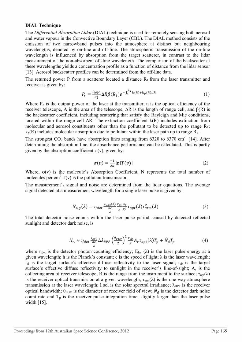
Proceedings from 12th Australian Space Science Conference, 2012 Page 165
DIAL Technique The Differential Absorption Lidar (DIAL) technique is used for remotely sensing both aerosol and water vapour in the Convective Boundary Layer (CBL). The DIAL method consists of the emission of two narrowband pulses into the atmosphere at distinct but neighbouring wavelengths, denoted by on-line and off-line. The atmospheric transmission of the on-line wavelength is influenced by absorption from the target scatterer, in contrast to the lidar measurement of the non-absorbent off-line wavelength. The comparison of the backscatter at these wavelengths yields a concentration profile as a function of distance from the lidar sensor [13]. Aerosol backscatter profiles can be determined from the off-line data. The returned power Pr from a scatterer located a distance R1 from the laser transmitter and receiver is given by:
!! =!!!"!!!
Δ!"(!!)!! ! ! !!! ! !"!!! (1)
Where Po is the output power of the laser at the transmitter, η is the optical efficiency of the receiver telescope, A is the area of the telescope, ΔR is the length of range cell, and β(R) is the backscatter coefficient, including scattering that satisfy the Rayleigh and Mie conditions, located within the range cell ΔR. The extinction coefficient k(R) includes extinction from molecular and aerosol constituents other than the pollutant to be detected up to range R1; kp(R) includes molecular absorption due to pollutant within the laser path up to range R1. The strongest CO2 bands have absorption lines ranging from 6320 to 6370 cm-1 [14]. After determining the absorption line, the absorbance performance can be calculated. This is partly given by the absorption coefficient σ(v), given by: ! ! = !!
!!ln !(!) (2)
Where, σ(v) is the molecule’s Absorption Coefficient, N represents the total number of molecules per cm2 T(v) is the pollutant transmission. The measurement’s signal and noise are determined from the lidar equations. The average signal detected at a measurement wavelength for a single laser pulse is given by:
!!"# ! = !!"#!!"# !
!!!
!!"!!!!!!!"#(!)!!"#! (!) (3)
The total detector noise counts within the laser pulse period, caused by detected reflected sunlight and detector dark noise, is
!! ≈ !!"#!!"#!!!
Δ!!"#!!"#!
! !!"!!!!!"# ! !! + !!!! (4)
where ηdet is the detector photon counting efficiency; Elas (λ) is the laser pulse energy at a given wavelength; h is the Planck’s constant; c is the speed of light; λ is the laser wavelength; rsl is the target surface’s effective diffuse reflectivity to the laser signal; rsb is the target surface’s effective diffuse reflectivity to sunlight in the receiver’s line-of-sight; Ar is the collecting area of receiver telescope; R is the range from the instrument to the surface; τopt(λ) is the receiver optical transmission at a given wavelength; τatm(λ) is the one-way atmosphere transmission at the laser wavelength; I sol is the solar spectral irradiance; λBPF is the receiver optical bandwidth; θFOV is the diameter of receiver field of view; !! is the detector dark noise count rate and Tp is the receiver pulse integration time, slightly larger than the laser pulse width [15].
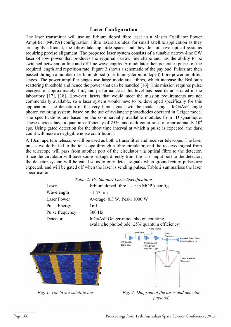
Page 166 Proceedings from 12th Australian Space Science Conference, 2012
Laser Configuration The laser transmitter will use an Erbium doped fibre laser in a Master Oscillator Power Amplifier (MOPA) configuration. Fibre lasers are ideal for small satellite application as they are highly efficient, the fibres take up little space, and they do not have optical systems requiring precise alignment. The proposed laser system consists of a tunable narrow-line CW laser of low power that produces the required narrow line shape and has the ability to be switched between on-line and off-line wavelengths. A modulator then generates pulses of the required length and repetition rate. Figure 3 shows a schematic of the payload. Pulses are then passed through a number of erbium doped (or erbium-ytterbium doped) fibre power amplifier stages. The power amplifier stages use large mode area fibres, which increase the Brillouin scattering threshold and hence the power that can be handled [16]. This mission requires pulse energies of approximately 1mJ, and performance at this level has been demonstrated in the laboratory [17], [18]. However, lasers that would meet the mission requirements are not commercially available, so a laser system would have to be developed specifically for this application. The detection of the very faint signals will be made using a InGaAsP single photon counting system, based on the use of avalanche photodiodes operated in Geiger mode. The specifications are based on the commercially available modules from ID Quantique. These devices have a quantum efficiency of 25%, and dark count rates of approximately 104 cps. Using gated detection for the short time interval at which a pulse is expected, the dark count will make a negligible noise contribution. A 10cm aperture telescope will be used as both a transmitter and receiver telescope. The laser pulses would be fed to the telescope through a fibre circulator, and the received signal from the telescope will pass from another port of the circulator via optical fibre to the detector. Since the circulator will have some leakage directly from the laser input port to the detector, the detector system will be gated so as to only detect signals when ground return pulses are expected, and will be gated off when the laser is sending pulses. Table 2 summarises the laser specifications.
Table 2: Preliminart Laser Specifications Laser Erbium doped fibre laser in MOPA config. Wavelength ~1.57 µm Laser Power Average: 0.3 W, Peak: 1000 W Pulse Energy 1mJ Pulse frequency 300 Hz Detector InGaAsP Geiger-mode photon counting
avalanche photodiode (25% quantum efficiency)
Fig. 1: The 6Unit satellite bus. Fig. 2: Diagram of the laser and detector
payload.
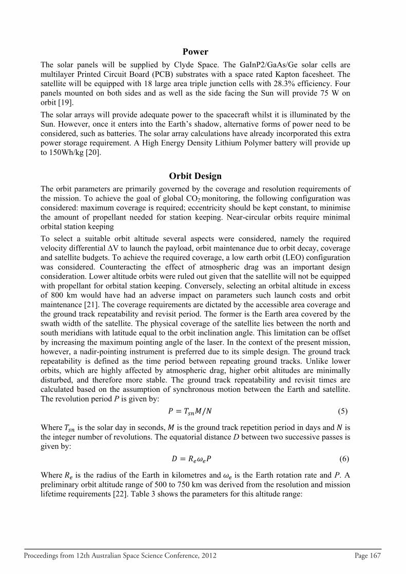
Proceedings from 12th Australian Space Science Conference, 2012 Page 167
Power The solar panels will be supplied by Clyde Space. The GaInP2/GaAs/Ge solar cells are multilayer Printed Circuit Board (PCB) substrates with a space rated Kapton facesheet. The satellite will be equipped with 18 large area triple junction cells with 28.3% efficiency. Four panels mounted on both sides and as well as the side facing the Sun will provide 75 W on orbit [19]. The solar arrays will provide adequate power to the spacecraft whilst it is illuminated by the Sun. However, once it enters into the Earth’s shadow, alternative forms of power need to be considered, such as batteries. The solar array calculations have already incorporated this extra power storage requirement. A High Energy Density Lithium Polymer battery will provide up to 150Wh/kg [20].
Orbit Design The orbit parameters are primarily governed by the coverage and resolution requirements of the mission. To achieve the goal of global CO2 monitoring, the following configuration was considered: maximum coverage is required; eccentricity should be kept constant, to minimise the amount of propellant needed for station keeping. Near-circular orbits require minimal orbital station keeping To select a suitable orbit altitude several aspects were considered, namely the required velocity differential ∆V to launch the payload, orbit maintenance due to orbit decay, coverage and satellite budgets. To achieve the required coverage, a low earth orbit (LEO) configuration was considered. Counteracting the effect of atmospheric drag was an important design consideration. Lower altitude orbits were ruled out given that the satellite will not be equipped with propellant for orbital station keeping. Conversely, selecting an orbital altitude in excess of 800 km would have had an adverse impact on parameters such launch costs and orbit maintenance [21]. The coverage requirements are dictated by the accessible area coverage and the ground track repeatability and revisit period. The former is the Earth area covered by the swath width of the satellite. The physical coverage of the satellite lies between the north and south meridians with latitude equal to the orbit inclination angle. This limitation can be offset by increasing the maximum pointing angle of the laser. In the context of the present mission, however, a nadir-pointing instrument is preferred due to its simple design. The ground track repeatability is defined as the time period between repeating ground tracks. Unlike lower orbits, which are highly affected by atmospheric drag, higher orbit altitudes are minimally disturbed, and therefore more stable. The ground track repeatability and revisit times are calculated based on the assumption of synchronous motion between the Earth and satellite. The revolution period P is given by: ! = !!"!/! (5)
Where !!" is the solar day in seconds, ! is the ground track repetition period in days and ! is the integer number of revolutions. The equatorial distance D between two successive passes is given by: ! = !!!!! (6)
Where !! is the radius of the Earth in kilometres and !! is the Earth rotation rate and P. A preliminary orbit altitude range of 500 to 750 km was derived from the resolution and mission lifetime requirements [22]. Table 3 shows the parameters for this altitude range:
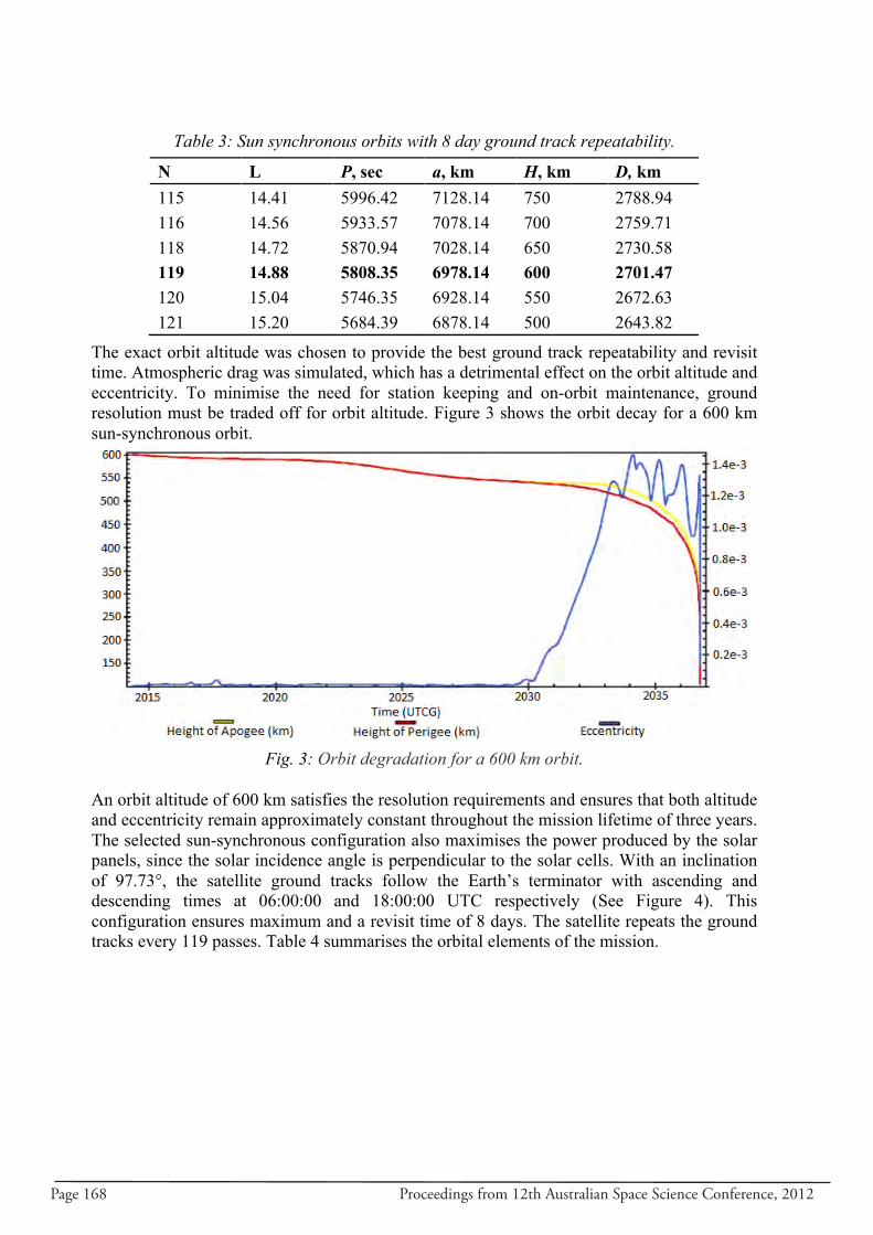
Page 168 Proceedings from 12th Australian Space Science Conference, 2012
Table 3: Sun synchronous orbits with 8 day ground track repeatability.
N L P, sec a, km H, km D, km 115 14.41 5996.42 7128.14 750 2788.94 116 14.56 5933.57 7078.14 700 2759.71 118 14.72 5870.94 7028.14 650 2730.58 119 14.88 5808.35 6978.14 600 2701.47 120 15.04 5746.35 6928.14 550 2672.63 121 15.20 5684.39 6878.14 500 2643.82
The exact orbit altitude was chosen to provide the best ground track repeatability and revisit time. Atmospheric drag was simulated, which has a detrimental effect on the orbit altitude and eccentricity. To minimise the need for station keeping and on-orbit maintenance, ground resolution must be traded off for orbit altitude. Figure 3 shows the orbit decay for a 600 km sun-synchronous orbit.
Fig. 3: Orbit degradation for a 600 km orbit.
An orbit altitude of 600 km satisfies the resolution requirements and ensures that both altitude and eccentricity remain approximately constant throughout the mission lifetime of three years. The selected sun-synchronous configuration also maximises the power produced by the solar panels, since the solar incidence angle is perpendicular to the solar cells. With an inclination of 97.73°, the satellite ground tracks follow the Earth’s terminator with ascending and descending times at 06:00:00 and 18:00:00 UTC respectively (See Figure 4). This configuration ensures maximum and a revisit time of 8 days. The satellite repeats the ground tracks every 119 passes. Table 4 summarises the orbital elements of the mission.
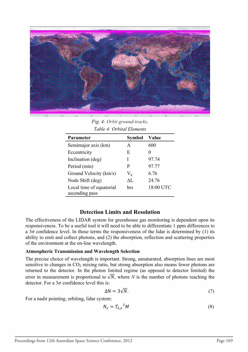
Proceedings from 12th Australian Space Science Conference, 2012 Page 169
Fig. 4: Orbit ground-tracks. Table 4: Orbital Elements
Parameter Symbol Value Semimajor axis (km) A 600 Eccentricity E 0 Inclination (deg) I 97.74 Period (min) P 97.77 Ground Velocity (km/s) Vg 6.76 Node Shift (deg) ΔL 24.76 Local time of equatorial ascending pass
hrs 18:00 UTC
Detection Limits and Resolution
The effectiveness of the LIDAR system for greenhouse gas monitoring is dependent upon its responsiveness. To be a useful tool it will need to be able to differentiate 1 ppm differences to a 3! confidence level. In those terms the responsiveness of the lidar is determined by (1) its ability to emit and collect photons, and (2) the absorption, reflection and scattering properties of the environment at the on-line wavelength. Atmospheric Transmission and Wavelength Selection The precise choice of wavelength is important. Strong, unsaturated, absorption lines are most sensitive to changes in CO2 mixing ratio, but strong absorption also means fewer photons are returned to the detector. In the photon limited regime (as opposed to detector limited) the error in measurement is proportional to !, where N is the number of photons reaching the detector. For a 3! confidence level this is: ΔN = 3 !. (7) For a nadir pointing, orbiting, lidar system: !! = !!,!!! (8)
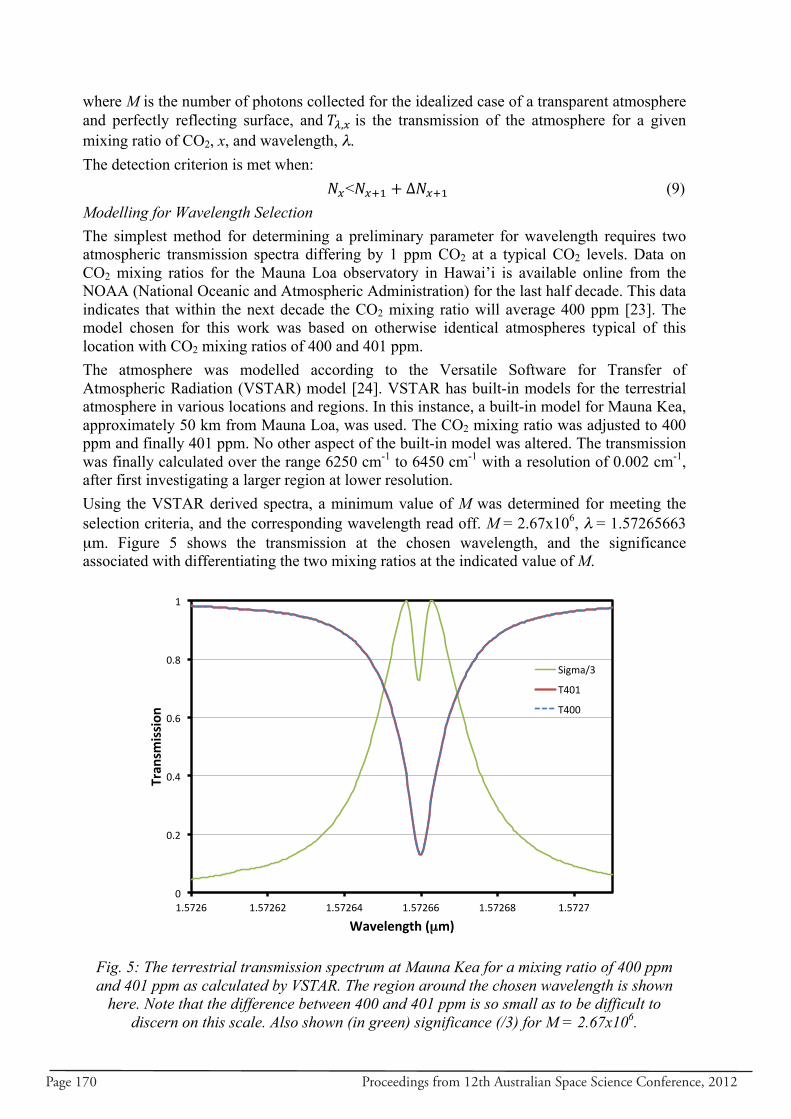
Page 170 Proceedings from 12th Australian Space Science Conference, 2012
where M is the number of photons collected for the idealized case of a transparent atmosphere and perfectly reflecting surface, and !!,! is the transmission of the atmosphere for a given mixing ratio of CO2, x, and wavelength, λ. The detection criterion is met when: !!<!!!! + Δ!!!! (9) Modelling for Wavelength Selection The simplest method for determining a preliminary parameter for wavelength requires two atmospheric transmission spectra differing by 1 ppm CO2 at a typical CO2 levels. Data on CO2 mixing ratios for the Mauna Loa observatory in Hawai’i is available online from the NOAA (National Oceanic and Atmospheric Administration) for the last half decade. This data indicates that within the next decade the CO2 mixing ratio will average 400 ppm [23]. The model chosen for this work was based on otherwise identical atmospheres typical of this location with CO2 mixing ratios of 400 and 401 ppm. The atmosphere was modelled according to the Versatile Software for Transfer of Atmospheric Radiation (VSTAR) model [24]. VSTAR has built-in models for the terrestrial atmosphere in various locations and regions. In this instance, a built-in model for Mauna Kea, approximately 50 km from Mauna Loa, was used. The CO2 mixing ratio was adjusted to 400 ppm and finally 401 ppm. No other aspect of the built-in model was altered. The transmission was finally calculated over the range 6250 cm-1 to 6450 cm-1 with a resolution of 0.002 cm-1, after first investigating a larger region at lower resolution. Using the VSTAR derived spectra, a minimum value of M was determined for meeting the selection criteria, and the corresponding wavelength read off. M = 2.67x10⁶, λ = 1.57265663 µm. Figure 5 shows the transmission at the chosen wavelength, and the significance associated with differentiating the two mixing ratios at the indicated value of M.
Fig. 5: The terrestrial transmission spectrum at Mauna Kea for a mixing ratio of 400 ppm and 401 ppm as calculated by VSTAR. The region around the chosen wavelength is shown
here. Note that the difference between 400 and 401 ppm is so small as to be difficult to discern on this scale. Also shown (in green) significance (/3) for M = 2.67x10⁶.
µ
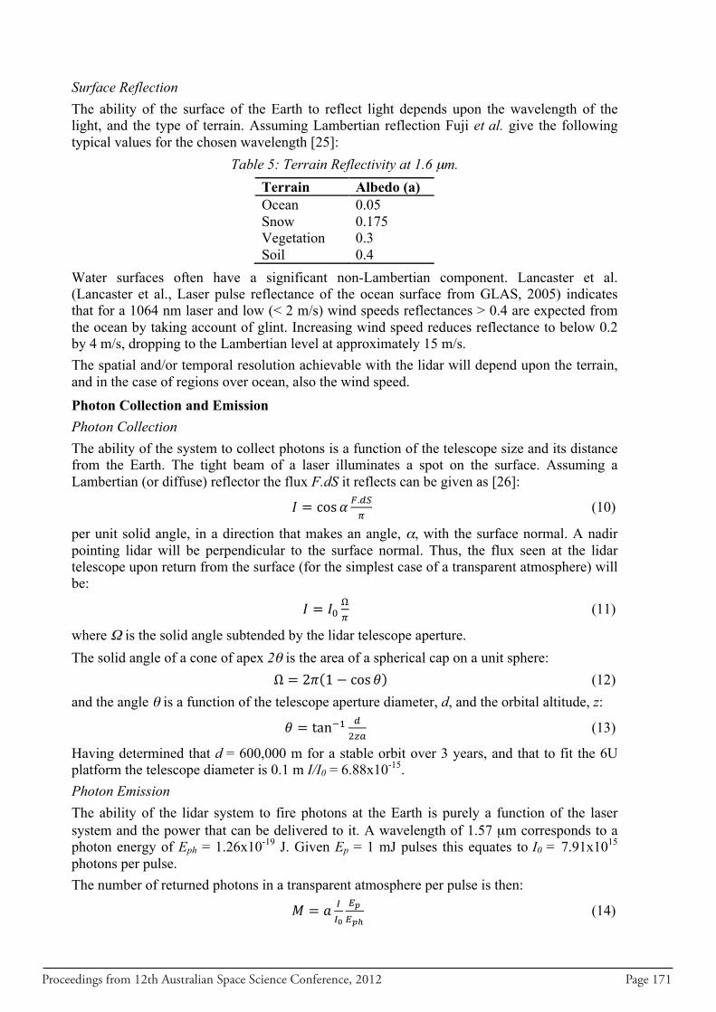
Proceedings from 12th Australian Space Science Conference, 2012 Page 171
Surface Reflection The ability of the surface of the Earth to reflect light depends upon the wavelength of the light, and the type of terrain. Assuming Lambertian reflection Fuji et al. give the following typical values for the chosen wavelength [25]:
Table 5: Terrain Reflectivity at 1.6 µm. Terrain Albedo (a) Ocean 0.05 Snow 0.175 Vegetation 0.3 Soil 0.4
Water surfaces often have a significant non-Lambertian component. Lancaster et al. (Lancaster et al., Laser pulse reflectance of the ocean surface from GLAS, 2005) indicates that for a 1064 nm laser and low (< 2 m/s) wind speeds reflectances > 0.4 are expected from the ocean by taking account of glint. Increasing wind speed reduces reflectance to below 0.2 by 4 m/s, dropping to the Lambertian level at approximately 15 m/s. The spatial and/or temporal resolution achievable with the lidar will depend upon the terrain, and in the case of regions over ocean, also the wind speed. Photon Collection and Emission Photon Collection The ability of the system to collect photons is a function of the telescope size and its distance from the Earth. The tight beam of a laser illuminates a spot on the surface. Assuming a Lambertian (or diffuse) reflector the flux F.dS it reflects can be given as [26]:
! = cos! !.!"!
(10)
per unit solid angle, in a direction that makes an angle, α, with the surface normal. A nadir pointing lidar will be perpendicular to the surface normal. Thus, the flux seen at the lidar telescope upon return from the surface (for the simplest case of a transparent atmosphere) will be:
! = !!!!
(11)
where Ω is the solid angle subtended by the lidar telescope aperture. The solid angle of a cone of apex 2θ is the area of a spherical cap on a unit sphere:
Ω = 2! 1− cos! (12) and the angle θ is a function of the telescope aperture diameter, d, and the orbital altitude, z:
! = tan!! !!!"
(13)
Having determined that d = 600,000 m for a stable orbit over 3 years, and that to fit the 6U platform the telescope diameter is 0.1 m I/I0 = 6.88x10⁻¹⁵. Photon Emission The ability of the lidar system to fire photons at the Earth is purely a function of the laser system and the power that can be delivered to it. A wavelength of 1.57 µm corresponds to a photon energy of Eph = 1.26x10⁻¹⁹ J. Given Ep = 1 mJ pulses this equates to I0 = 7.91x10¹⁵ photons per pulse. The number of returned photons in a transparent atmosphere per pulse is then:
! = ! !!!
!!!!!
(14)
Page 172 Proceedings from 12th Australian Space Science Conference, 2012
equal to 21.8 photons/pulse for soil or calm ocean, or 5.45 photons/pulse for choppy ocean. Therefore, to meet the detection criteria of 1 ppm significance at 400 ppm CO2, and with a detector efficiency of 25%, at minimum 489909 pulses are required over soil, or 1959636 pulses over ocean in the worst conditions, under a cloudless sky. Resolution At an altitude of 600 km, the round trip time for a photon is 12 ms, however the duty cycle of the laser corresponds to 33.3 ms. The pulse width is negligible on this scale. Every second pulse is an offline pulse with the DIAL technique, so the time between online pulses is 66.7 ms. This means the satellite must observe for between 32677 s to 130708 s to achieve the desired precision; this corresponds to between 5.626 orbits and 22.504 orbits, so achieving both high spatial and temporal resolution is not possible. The satellite will complete 16303 orbits in its 3 year life time, corresponding to 137 repeats of 119 distinct ground tracks. Combining all 3 years worth of data would therefore allow spatial resolution of between 17 and 68 degrees arc along the tracks depending upon the terrain. To aid in visualising the spatial resolution possible, consider the Earth’s surface is approximately 71% water and the remainder land. A simple calculation gives ~525 distinct spatial regions. On the average the size of one of these regions is ~3 degrees by ~47 degrees. For scale Australia is roughly 40 degrees in width between Cape Byron, NSW and Steep Point, WA. Since this scenario involves averaging all 3 years worth of data it isn’t necessary to keep to the tracks when considering the spatial resolution. If one considers a track as if it is representative of the width between it and the mid-way point to the adjacent track then the spatial resolution could instead be representative of a region of land ~6 degrees by ~9 degrees. This is too large to distinguish between countries in closely packed regions like Europe, but could distinguish between broad regions of continents, though it must be stressed that this calculation is for ideal weather conditions.
Conclusions This paper investigated the requirements for an experimental lidar payload for tropospheric CO2 detection. To achieve the desired coverage the satellite will be placed on a 97.74 degree Sun-synchronous orbit at 600 km with ascending node at 06:00:00 UTC. This orbit configuration maximises the solar output by maintaining a perpendicular angle between the solar incidence angle and the satellite’s GaInP2/GaAs/Ge cells. The solar panels produce 75 W during payload operation mode. The proposed payload consists of an Erbium doped fibre laser in a Master Oscillator Power Amplifier (MOPA) configuration. The laser system consists of a tunable narrow-line CW laser of low power that produces the required narrow line shape and has the ability to be switched between on-line and off-line wavelengths. With 1 mJ pulses, a 10 cm diameter telescope, a detector efficiency of 25%, and given typical reflectance values from terrestrial terrain, approximately 5 photons are expected to be returned per pulse beamed to the Earth for the off-line pulse. The preliminary results show that achieving high spatial or temporal resolution with the desired resolution in mixing ratio is not feasible using a 6U platform. Indeed, the best achievable spatial resolution is worse than 17 degrees or arc. The current power configuration does not allow for meaningful detection of scatterers. A higher power configuration coupled with larger optics is required. A larger satellite than the 6U system will therefore be required to partially satisfy the mission requirements.
Proceedings from 12th Australian Space Science Conference, 2012 Page 173
Acknowledgements This work was funded by the Australian Centre for Space Engineering Research at the University of New South Wales. The authors would also like to thank A/Prof Graham Town from the Australian Research Network for Advanced Material for his input on laser concepts.
References 1. Jae H. Park, "Atmospheric CO2 Monitoring From Space," Appl. Opt. 36, 1997, pp. 2701-
2712. 2. Cooperative Air Sampling Network, Pieter Tans, NOAA/ESRL,
http://www.esrl.noaa.gov/gmd/ccgg/flask.html, obtained online 13/11/2012. 3. Suto, H., Kuze, A., Shiomi, K., and Nakajima, M.: On Orbit Status Of TANSO-FTS On
GOSAT, Sensors, Systems, and Next Generation Satellites XIV, edited by: Meynart, R., Neeck, S. P., Shimoda, H., Proc. SPIE, 782604, 2010.
4. Crisp, D., The Orbiting Carbon Observatory: NASA’s First Dedicated Carbon Dioxide Mission, Sensors, Systems, and Next Generation Satellites XII, edited by: Meynart, R., Neeck, S. P., Shimoda, H., and Habib, S., Proc. SPIE, 710604, 2008.
5. Winker, D. M., Vaughan, M. A., Omar, A., Hu, Y., Powell, K. A., Liu, Z., Hunt, W. H., Young, S. A., “Overview Of The CALIPSO Mission And CALIOP Data Processing Algorithms” J. Atmos. Oceanic Technol., 26, 2009, pp. 2310–2323.
6. Winker, D. M., Pelon, J. R., Cormick, M. P., “The CALIPSO Mission: Spaceborn Lidar For Observation Of Aerosols and Clouds”, Proc. SPIE, 4893, 2003, pp. 1-11.
7. Melfi, S. H., J. D. Spinhire, S.-H. Chou, and S. P. Palm, “Lidar Observation Of Vertically Organized Convection In The Planetary Boundary Layer Over The Ocean”, J. Climate Appl. Meteor.,24, 1985, pp. 806–821.
8. Joly, L., Marnas, F., Gibert, F., Bruneau, D., Grouiez, B., Flamant, P.H., Durry, G., Dumelie, N., Parvitte, B., Zéninari, V., “Laser Diode Absorption Spectroscopy For Accurate CO2 Line Parameters At 2 µm: Consequences For Space-based DIAL Measurements And Potential Biases”, Applied Optics, 48 (29), 2009, pp. 5475-5483.
9. Tsitas, S. & Kingston, J., 2010. 6U, CubeSat Design For Earth Observation With 6.5 m GSD, 5 Spectral Bands and 14 Mbps downlink, The Aeronautical Journal, 114, 689-697.
10. Tsitas, S., 2011. Design & Commercial Applications of a 6U CubeSat. Royal Aeronautical Society Boscombe Down Branch, UK.
11. Bailey, J., Tsitas, S., Bayliss, D., Bedding, T., “A CubeSat Mission for Exoplanet Transit Detection and Astroseismology”, in these proceedings.
12. 6U Cubesat structure, Clyde Space, http://www.clyde-space.com/cubesat_shop/structures/6u_structures/313_6u-cubesat-structure, obtained online 12/11/2012.
13. Schotland, R.M. “Errors In The Lidar Measurement Of Atmospheric Gases By Differential Absorption”, Journal of Applied Meteorology, 13(1), 1974.
14. Snell, H. E., Hager, J. S., Zaccheo, T. S., Simulation Testbed for Atmospheric LiDAR Applications, Atmospheric and Environmental Research, Inc., Lexington, Massachusetts
15. Abshire, J. B., Riris, H., Allan, G. R., Weaver, C. J., Mao, J., Sun, X., Hasselbrack, W. E.,
Kawa, S. R. and Biraud, S., “Pulsed Airborne Lidar Measurements Of Atmospheric CO2 Column Absorption”, Tellus B, 62, 2010, pp. 770–783.

Page 174 Proceedings from 12th Australian Space Science Conference, 2012
16. Broderick, N.G., Offerhaus, H.L., Richardson, D.J., Sammut, R., Caplen, J., Dong, L., “Large Mode Area Fibres For High Power Applications”, Optical Fibre Technology, Col. 5, 1999, pp. 185-196.
17. Philippov, V., Sahu, J.K., Codemard, C., Clarkson, W.A., Jang, J.-N., Nilsson, J., Pearson, G.N., “All-fiber 1.15 mJ Pulsed Eye-safe Optical Source”, in Fibre Lasetrs, Technology, Systems and Applications, SPIE Proc., Vol. 5535, 2004, pp. 1-7.
18. Codemard, C., Farrell, C., Dupriez, P., Philippov, V., Sahu, J.K., Nilsson, J., “Millijoule, High-peak-power, Narrow-linewidth, Sub-hundred Nanosecond Pulsed Fibre Master-Oscillator Power-Amplifier at 1.55 µm”, Comptes Rendus – Physique, Vol. 7, 2006, pp. 170-176.
19. Small Satellite Solar Panels Datasheet, Clyde Space, http://www.clyde-space.com/documents/2625, obtained online 10/11/2012
20. Cubesat Standalone Battery datasheet, Clyde Space, http://www.clyde-space.com/documents/2381, obtained online 12/11/2012
21. Wertz, J. R., Larson, W. J., Space Mission Analysis And Design. 3rd ed. Torrance, CA: Kluwer Academic, 1999, pp. 268-270.
22. Bar-Lev, M., Shcherbina, L., Levin, V. “EROS System – Satellite Orbit And Constellation Design”. 22nd Asian Conference on Remote Sensing, 5-9 November 2011.
23. Trends in Atmoshpheric Carbon Dioxide, Pieter Tans, NOAA/ESRL and Ralph Keeling, Scripps Institution of Oceanography, www.esrl.noaa.gov/gmd/ccgg/trends/co2_data_mlo.html, obtained online 15/11/2012
24. Bailey J. and Kedziora-Chudczer, L., “Modelling The Spectra Of Planets, Brown Dwarfs And Stars Using VSTAR”, MNRAS, Vol. 419, 2012, pp 1913-1929.
25. Fujii, Y., Kawahara, H., Suto, Y., Taruya, A., Fukuda, S., Nakajima, T. & Turner, E. L., "Colors Of A Second Earth: Estimating The Fractional Areas Of Ocean, Land, And Vegetation Of Earth-like Exoplanets," The Astrophysical Journal, 715, pp. 866-880.
26. H.C. van der Hulst, Light Scattering: By Small Particles, Courier Dover Publications, 1957, p. 112.

Proceedings from 12th Australian Space Science Conference, 2012 Page 175
Cramer-Rao Lower Bound for Ocean Surface Roughness Estimation Using Multi-GPS Bistatic Radar
Nima Alam, Kegen Yu, Andrew G. Dempster
Australian Centre for Space Engineering Research (ACSER) University of New South Wales, Sydney, Australia
Summary: The Global Positioning System (GPS) signals reflected from the ocean surface have been considered for estimating geophysical parameters including ocean near-surface wind speed and wave height. A variety of models, methods, and experimental campaigns have verified the level of viability and reliability of the bistatic GPS radars. In this article, we analyse the ocean roughness information inherent in the reflected GPS signals in terms of the ocean state, the number of visible satellites and the altitude of the receiver. Through this theoretical analysis the Cramer-Rao lower bound (CRLB) can be derived to benchmark the performance of surface roughness estimation. In the analysis the impact of different surface wind speeds and surface roughness on the sea state estimation error is studied. Real position data of observed satellites are used to calculate the CRLB in a certain area over 24 hours. The applicability of the theoretical results to airborne and spaceborne receivers is also discussed. Keywords: Bistatic GPS radar, Cramer-Rao Lower Bound, Ocean Roughness.
Introduction Global Positioning System (GPS) signals have been utilized for scientific applications beyond timing, navigation and positioning. GPS-based Earth observation and remote sensing are among those applications which have been proposed to take further advantage of GPS signals. Earth polar motion, temperature and vapour profiling, and ionosphere density monitoring are some examples of scientific applications based on the GPS [1]. These applications fuse data received directly from GPS satellites. Another category of applications has been identified using GPS signals which are scattered from the ocean surface and can be received by an airborne or spaceborne receiver [2]. This approach, which implies a bistatic radar architecture using GPS satellites as transmitters, has been employed to estimate the wind and wave behaviour of the ocean surface and ocean surface height [3]. The GPS signals scattered from the ocean surface are modelled in [4] with a focus on ocean surface remote sensing applications. The model presented in this work is detailed and can be considered as a base to drive other relevant researches. In [5] and [6], models for the ocean surface wind estimation are proposed and experimental results verified the applicability of the models. In [7], the basic theories of GPS bistatic radars are explained and different applications including deriving the mean sea height, ocean surface wind, and Significant Wave Height (SWH) are explained. Some fundamental issues for signal processing of the scattered signals are investigated in [8]. It is concluded that conventional GPS receivers at airborne altitude can track the reflected signals for remote sensing purposes. However, for spaceborne receivers, some modifications are needed due to the larger scattering area compared with that for airborne receivers. In [9], a novel model for scattered signals from the ocean surface is presented. The authors propose an improved Geometrical Optics (GO) method to replace the conventional Kirchhoff model to reduce the computational burden and maintain the same performance. The results of an experimental campaign for estimating the roughness of the ocean surface is presented in [10]. The surface was almost smooth and the logged data in an
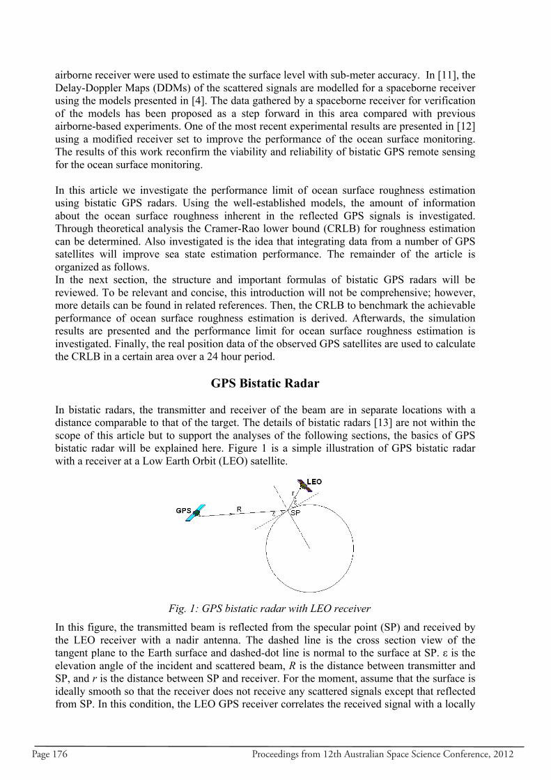
Page 176 Proceedings from 12th Australian Space Science Conference, 2012
airborne receiver were used to estimate the surface level with sub-meter accuracy. In [11], the Delay-Doppler Maps (DDMs) of the scattered signals are modelled for a spaceborne receiver using the models presented in [4]. The data gathered by a spaceborne receiver for verification of the models has been proposed as a step forward in this area compared with previous airborne-based experiments. One of the most recent experimental results are presented in [12] using a modified receiver set to improve the performance of the ocean surface monitoring. The results of this work reconfirm the viability and reliability of bistatic GPS remote sensing for the ocean surface monitoring. In this article we investigate the performance limit of ocean surface roughness estimation using bistatic GPS radars. Using the well-established models, the amount of information about the ocean surface roughness inherent in the reflected GPS signals is investigated. Through theoretical analysis the Cramer-Rao lower bound (CRLB) for roughness estimation can be determined. Also investigated is the idea that integrating data from a number of GPS satellites will improve sea state estimation performance. The remainder of the article is organized as follows. In the next section, the structure and important formulas of bistatic GPS radars will be reviewed. To be relevant and concise, this introduction will not be comprehensive; however, more details can be found in related references. Then, the CRLB to benchmark the achievable performance of ocean surface roughness estimation is derived. Afterwards, the simulation results are presented and the performance limit for ocean surface roughness estimation is investigated. Finally, the real position data of the observed GPS satellites are used to calculate the CRLB in a certain area over a 24 hour period.
GPS Bistatic Radar In bistatic radars, the transmitter and receiver of the beam are in separate locations with a distance comparable to that of the target. The details of bistatic radars [13] are not within the scope of this article but to support the analyses of the following sections, the basics of GPS bistatic radar will be explained here. Figure 1 is a simple illustration of GPS bistatic radar with a receiver at a Low Earth Orbit (LEO) satellite. In this figure, the transmitted beam is reflected from the specular point (SP) and received by the LEO receiver with a nadir antenna. The dashed line is the cross section view of the tangent plane to the Earth surface and dashed-dot line is normal to the surface at SP. ε is the elevation angle of the incident and scattered beam, R is the distance between transmitter and SP, and r is the distance between SP and receiver. For the moment, assume that the surface is ideally smooth so that the receiver does not receive any scattered signals except that reflected from SP. In this condition, the LEO GPS receiver correlates the received signal with a locally
Fig. 1: GPS bistatic radar with LEO receiver
Proceedings from 12th Australian Space Science Conference, 2012 Page 177
generated replica signal to lock and track the GPS signal [14]. Avoiding the details, the ideal output of the correlation is
⎪⎩
⎪⎨
⎧≤−
−−
=Λ
otherwise
TT
,0
,1)( 00 ττττ
τ (1)
where τ0=(R+r)/c is the travel time of the signal form the transmitter to receiver, and T is the duration of a GPS code chip. Equation 1 represents an isosceles triangle with unity maximum at τ0 and base length of 2T. This equation is for ideal condition that ocean surface is absolutely smooth and the signal bandwidth is unlimited. However, in scenarios where the sea surface is not perfectly smooth, in addition to SP reflection, scattered beams are received from an area on the surface. This is due to roughness of the surface and leads to the following formulation for the correlation output:
∑∞
=
− −Λ=Λ0
)( )()(k
kj
kPkea τττ ϕϕ (2)
where ak and φk are the amplitude and phase of the reflected beam k respectively, φ is the phase of the locally generated signal, and k=0 corresponds to the beam reflected from SP. The power of kth signal is
223
2
64 kk
kkrkttk rR
AGGPPπ
ρλ= (3)
where Pt is the transmit power, Gt is the gain of transmitter’s antenna, Grk is the gain of receiver’s antenna for kth scattering element, λ is the signal’s wavelength, Ak is the area and ρk is the scattering cross-section coefficient of kth scattering element, and Rk and rk are the distances of kth scattering element to the transmitter and receiver respectively. Considering Equations 2 and 3, we have:
∫∫∑ −Λ=−Λ=ΛΛ
∞
=
dxdyrRGGP
rRAGGP
yxrtt
kk
kk
kkrkttPP )(
64)(
64 ,2
223
2
0
2223
2* ττ
ρπλ
ττρ
πλ (4)
where ρ is the corresponding scattering cross-section coefficient at point (x,y) on the ocean surface, and R and r are the distances from this point to the transmitter and receiver respectively. Considering a tangent plane to surface at SP, here it is assumed that the SP is at the origin of a coordinate system with X and Y axes in the tangent plane and axis Z the normal vector of that the plane. In deriving Equation 4, it is assumed that the scattering is incoherent. In [4], the effect of the Doppler shift of the scattered signals on the received power is added:
∫∫ −Λ=ΛΛ dxdyfSrRGGP
yxrtt
PP )()(64 ,
22223
2* ττδ
ρπλ (5)
where δf is the Doppler shift of the signal scattered from (x,y). As indicated in [7], the integral in Equation 5 will be performed over an ellipsoid footprint with a and b as the semi-major and semi-minor axis
Page 178 Proceedings from 12th Australian Space Science Conference, 2012
rRRrTb
rRRrTa
+=
+=
)sin(1ε
(6)
According to [4], the parameters in Equation 5 are defined as follows.
)exp()sin()( i
i
i fTjfTfTfS πδ
πδπδ
δ −= (7)
where Ti is the integration time and Doppler shift is
λδ
1⎟⎟⎠
⎞⎜⎜⎝
⎛ ⋅+
⋅−=
rrV
RRVf rt
(8)
where tV
is the velocity vector of the transmitter, rV
is the velocity vector of the receiver,
R
is the relative position vector between the SP and transmitter, and r is the relative position vector between the SP and receiver. The scattering cross-section for each scattering point can be calculated using
)(),( 4
42
zs
z qqf
yx ⊥−ℜ
=π
ρ (9)
where ℜ is the polarization sensitive reflection coefficient and
)(2rr
RRq
+=
λπ (10)
In Equation 9, qz represents the element of q perpendicular to the tangent plane at SP and
⊥q is the projection of q on this surface. Also, fs is the Probability Density Function (PDF) of
surface wave slopes:
⎥⎥⎦
⎤
⎢⎢⎣
⎡
⎟⎟⎠
⎞⎜⎜⎝
⎛+−
−−
−= 2
2
2
2
222
)1(21exp
121),(
sysysxxy
sxxyxysysx
syxybx
bbyxf
σσσσσπσ (11)
More details about σsx , σsy , and bxy can be found in [4]. These parameters depend on the surface wind. To estimate the PDF of the ocean wave height and corresponding SWH using Equation 5, the effect of the PDF of the height of scattering points, fz, is required. Calling the left side of the correlation function in Equation 5 “CF” , in [7], Λ is replaced with the one convolved with fz to incorporate the effect of the PDF of the surface height. This reformulates CF to
∫∫ −Λ= dxdyfSrRGGPCF yxRrtt )()(
64 ,22
223
2
ττδρ
πλ (12)
where
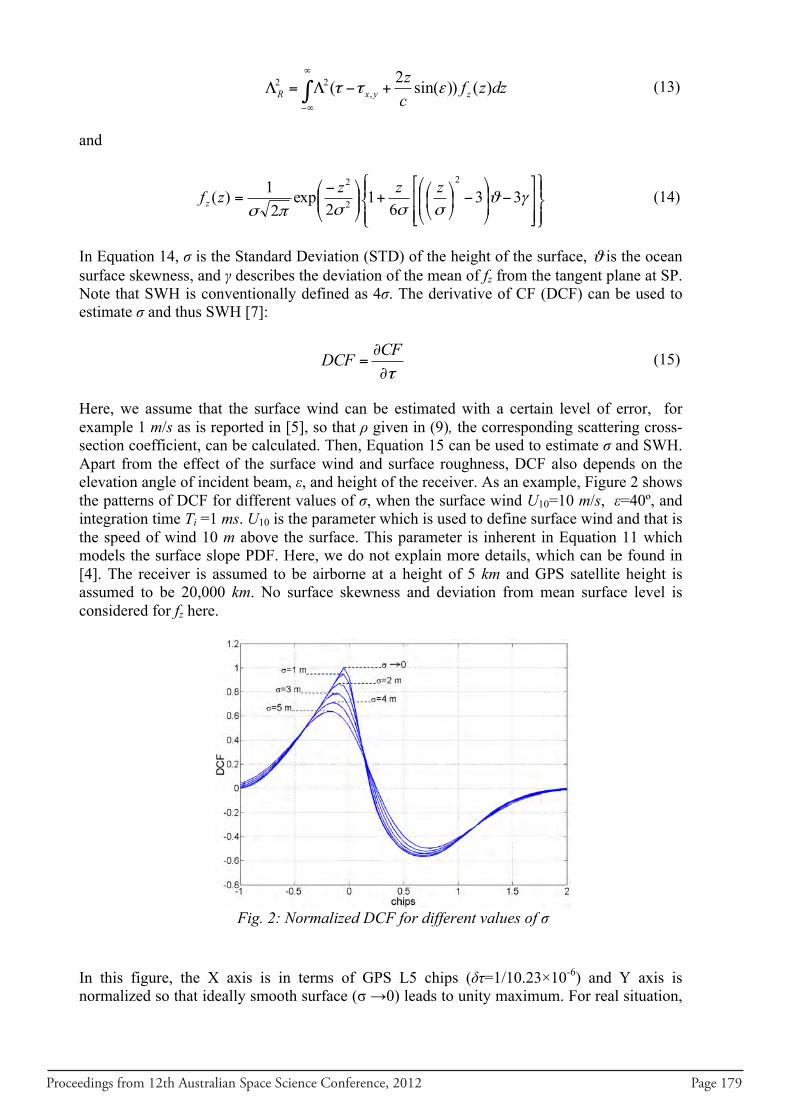
Proceedings from 12th Australian Space Science Conference, 2012 Page 179
∫∞
∞−
+−Λ=Λ dzzfcz
zyxR )())sin(2( ,22 εττ (13)
and
⎪⎭
⎪⎬⎫
⎪⎩
⎪⎨⎧
⎥⎥⎦
⎤
⎢⎢⎣
⎡−⎟
⎟⎠
⎞⎜⎜⎝
⎛−⎟
⎠
⎞⎜⎝
⎛+⎟⎟⎠
⎞⎜⎜⎝
⎛ −= γϑ
σσσπσ33
61
2exp
21)(
2
2
2 zzzzfz (14)
In Equation 14, σ is the Standard Deviation (STD) of the height of the surface, ϑ is the ocean surface skewness, and γ describes the deviation of the mean of fz from the tangent plane at SP. Note that SWH is conventionally defined as 4σ. The derivative of CF (DCF) can be used to estimate σ and thus SWH [7]:
τ∂∂
=CFDCF (15)
Here, we assume that the surface wind can be estimated with a certain level of error, for example 1 m/s as is reported in [5], so that ρ given in (9), the corresponding scattering cross-section coefficient, can be calculated. Then, Equation 15 can be used to estimate σ and SWH. Apart from the effect of the surface wind and surface roughness, DCF also depends on the elevation angle of incident beam, ε, and height of the receiver. As an example, Figure 2 shows the patterns of DCF for different values of σ, when the surface wind U10=10 m/s, ε=40º, and integration time Ti =1 ms. U10 is the parameter which is used to define surface wind and that is the speed of wind 10 m above the surface. This parameter is inherent in Equation 11 which models the surface slope PDF. Here, we do not explain more details, which can be found in [4]. The receiver is assumed to be airborne at a height of 5 km and GPS satellite height is assumed to be 20,000 km. No surface skewness and deviation from mean surface level is considered for fz here. In this figure, the X axis is in terms of GPS L5 chips (δτ=1/10.23×10-6) and Y axis is normalized so that ideally smooth surface (σ →0) leads to unity maximum. For real situation,
Fig. 2: Normalized DCF for different values of σ
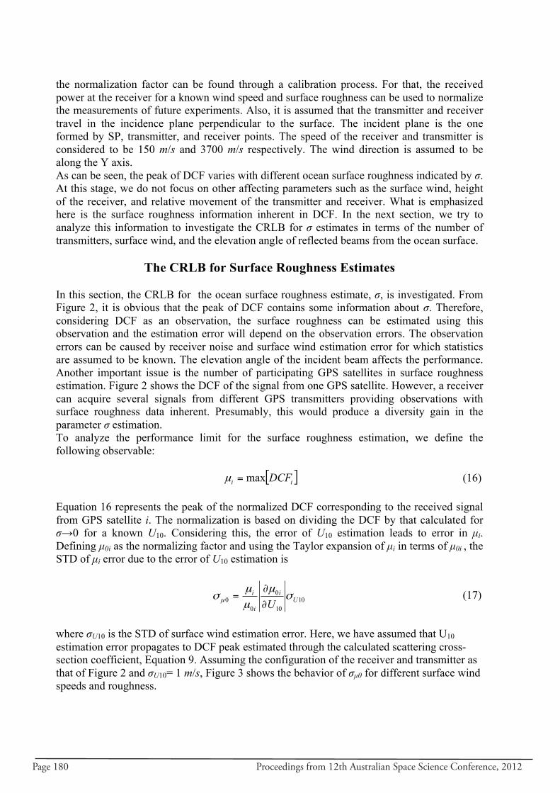
Page 180 Proceedings from 12th Australian Space Science Conference, 2012
the normalization factor can be found through a calibration process. For that, the received power at the receiver for a known wind speed and surface roughness can be used to normalize the measurements of future experiments. Also, it is assumed that the transmitter and receiver travel in the incidence plane perpendicular to the surface. The incident plane is the one formed by SP, transmitter, and receiver points. The speed of the receiver and transmitter is considered to be 150 m/s and 3700 m/s respectively. The wind direction is assumed to be along the Y axis. As can be seen, the peak of DCF varies with different ocean surface roughness indicated by σ. At this stage, we do not focus on other affecting parameters such as the surface wind, height of the receiver, and relative movement of the transmitter and receiver. What is emphasized here is the surface roughness information inherent in DCF. In the next section, we try to analyze this information to investigate the CRLB for σ estimates in terms of the number of transmitters, surface wind, and the elevation angle of reflected beams from the ocean surface.
The CRLB for Surface Roughness Estimates In this section, the CRLB for the ocean surface roughness estimate, σ, is investigated. From Figure 2, it is obvious that the peak of DCF contains some information about σ. Therefore, considering DCF as an observation, the surface roughness can be estimated using this observation and the estimation error will depend on the observation errors. The observation errors can be caused by receiver noise and surface wind estimation error for which statistics are assumed to be known. The elevation angle of the incident beam affects the performance. Another important issue is the number of participating GPS satellites in surface roughness estimation. Figure 2 shows the DCF of the signal from one GPS satellite. However, a receiver can acquire several signals from different GPS transmitters providing observations with surface roughness data inherent. Presumably, this would produce a diversity gain in the parameter σ estimation. To analyze the performance limit for the surface roughness estimation, we define the following observable:
[ ]ii DCFmax=µ (16) Equation 16 represents the peak of the normalized DCF corresponding to the received signal from GPS satellite i. The normalization is based on dividing the DCF by that calculated for σ→0 for a known U10. Considering this, the error of U10 estimation leads to error in µi. Defining µ0i as the normalizing factor and using the Taylor expansion of µi in terms of µ0i , the STD of µi error due to the error of U10 estimation is
10
10
0
00 U
i
i
i
Uσ
µµµ
σ µ ∂∂
= (17)
where σU10 is the STD of surface wind estimation error. Here, we have assumed that U10 estimation error propagates to DCF peak estimated through the calculated scattering cross-section coefficient, Equation 9. Assuming the configuration of the receiver and transmitter as that of Figure 2 and σU10= 1 m/s, Figure 3 shows the behavior of σµ0 for different surface wind speeds and roughness.
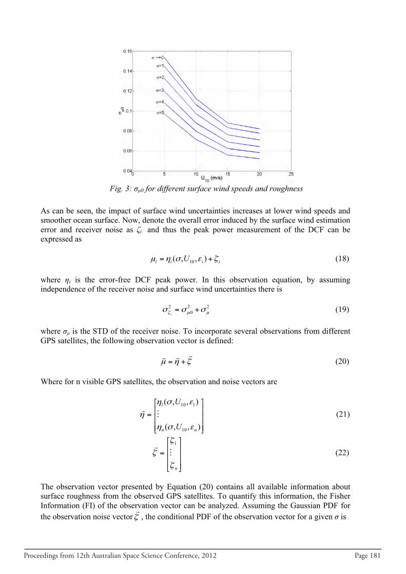
Proceedings from 12th Australian Space Science Conference, 2012 Page 181
As can be seen, the impact of surface wind uncertainties increases at lower wind speeds and smoother ocean surface. Now, denote the overall error induced by the surface wind estimation error and receiver noise as ζi and thus the peak power measurement of the DCF can be expressed as
iiii U ζεσηµ += ),,( 10 (18) where ηi is the error-free DCF peak power. In this observation equation, by assuming independence of the receiver noise and surface wind uncertainties there is
22
02
µµζ σσσ +=i
(19) where σµ is the STD of the receiver noise. To incorporate several observations from different GPS satellites, the following observation vector is defined:
ζηµ
+= (20) Where for n visible GPS satellites, the observation and noise vectors are
⎥⎥⎥
⎦
⎤
⎢⎢⎢
⎣
⎡
=
),,(
),,(
10
1101
nn U
U
εση
εση
η (21)
⎥⎥⎥
⎦
⎤
⎢⎢⎢
⎣
⎡
=
nζ
ζ
ζ 1
(22)
The observation vector presented by Equation (20) contains all available information about surface roughness from the observed GPS satellites. To quantify this information, the Fisher Information (FI) of the observation vector can be analyzed. Assuming the Gaussian PDF for the observation noise vectorζ
, the conditional PDF of the observation vector for a given σ is
Fig. 3: σµ0 for different surface wind speeds and roughness
Page 182 Proceedings from 12th Australian Space Science Conference, 2012
( ) [ ] [ ]
⎭⎬⎫
⎩⎨⎧ −Σ−−
Σ= − ηµηµ
πσµ ζ
ζ
1
21exp
)det(21 Tf
(23)
where Σζ is the covariance of the observation error, a diagonal matrix with 2
iζσ as the ith
diagonal element. The FI can be calculated using Equation 24 [15]:
( )( ) ( )( )⎪⎭
⎪⎬⎫
⎪⎩
⎪⎨⎧
⎥⎦
⎤⎢⎣
⎡
∂
∂⎥⎦
⎤⎢⎣
⎡
∂
∂=
σ
σµ
σ
σµσµ
ffEI
Tlnln
)(
(24)
where E is the expected value operator. Replacing Equation 23 in 24 leads to FI of the observation vector
⎥⎦
⎤⎢⎣
⎡∂∂
Σ⎥⎦
⎤⎢⎣
⎡∂∂
= −
ση
ση
σ ζµ
1)(
T
I (25)
For bistatic GPS observations, there is not any analytical solution for Equation 25. Thus, the FI will be evaluated numerically. That is, the vector η will first be evaluated for different surface wind speeds, ocean roughness, and elevation angles of the incident beams at SP. Then the required derivatives for Equation 25 will be computed. Once the FI is calculated, the performance limit, i.e. the CRLB, for estimation of surface roughness, σ, can be determined [15]:
)()( 1 σσ µµ−= IC (26)
Using Equation 26, it will be possible to determine the CRLB for the estimation of ocean surface roughness or STD of surface height, in terms of the number of visible GPS satellites, the real condition of the surface roughness, the speed of surface wind, and the elevation angle of incident beams.
Simulation Results for CRLB
In this section, the effect of the number of visible satellites and elevation angle of the corresponding incident beams is investigated. Note that when we consider a number of satellites, the SP for each of them is in a different location on the ocean surface. We assume that the ocean surface roughness has the same behavior around these SPs which are in vicinity of each other. Therefore, the received signals can be considered as separate observations of a common unknown parameter. The vicinity of SPs for different numbers of satellites is investigated in the next section using real GPS satellite position data. Here, the parameter setting is the same as that for Figure 2, unless any change is mentioned. An airborne receiver at a height of 5 km is assumed for the moment. The effect of elevation angle of the reflected beam, ε Here, we consider a single GPS satellite with different reflected beam elevation angles and calculate the CRLB, by Equation 26, for varying surface wind speed and roughness. In this section and the rest of article, the STD of surface wind estimation error is assumed to be σU10=
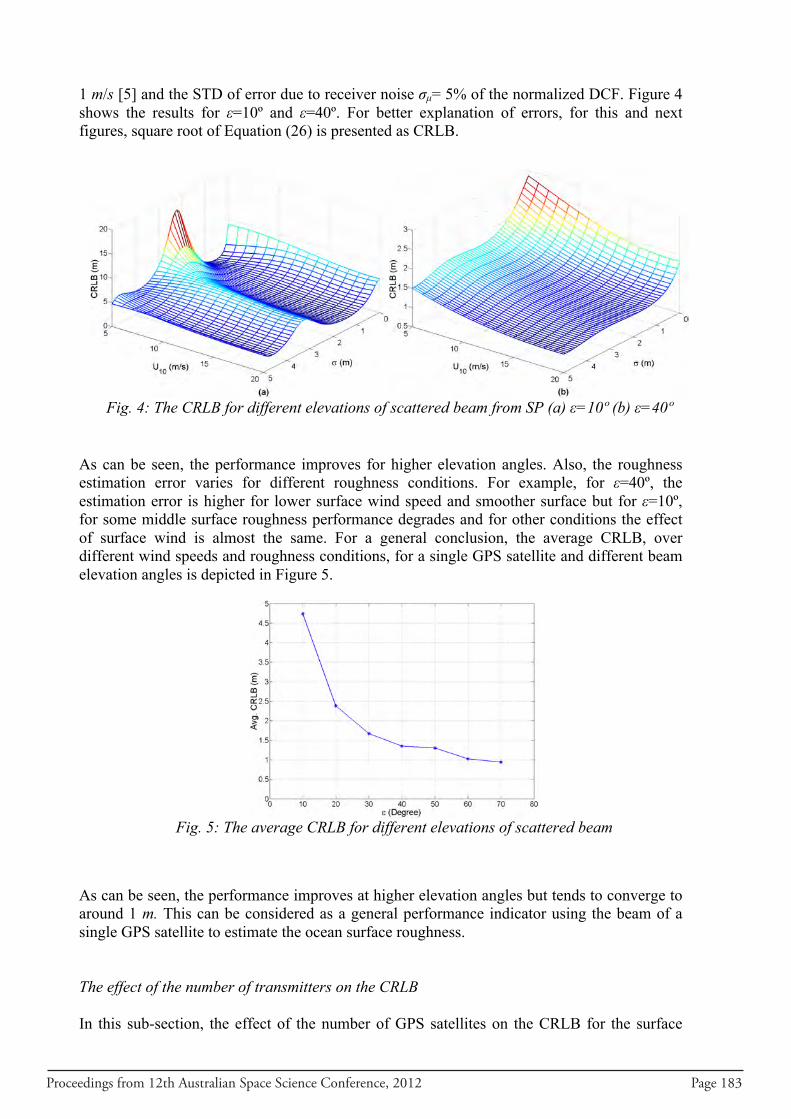
Proceedings from 12th Australian Space Science Conference, 2012 Page 183
1 m/s [5] and the STD of error due to receiver noise σµ= 5% of the normalized DCF. Figure 4 shows the results for ε=10º and ε=40º. For better explanation of errors, for this and next figures, square root of Equation (26) is presented as CRLB.
As can be seen, the performance improves for higher elevation angles. Also, the roughness estimation error varies for different roughness conditions. For example, for ε=40º, the estimation error is higher for lower surface wind speed and smoother surface but for ε=10º, for some middle surface roughness performance degrades and for other conditions the effect of surface wind is almost the same. For a general conclusion, the average CRLB, over different wind speeds and roughness conditions, for a single GPS satellite and different beam elevation angles is depicted in Figure 5.
As can be seen, the performance improves at higher elevation angles but tends to converge to around 1 m. This can be considered as a general performance indicator using the beam of a single GPS satellite to estimate the ocean surface roughness. The effect of the number of transmitters on the CRLB In this sub-section, the effect of the number of GPS satellites on the CRLB for the surface
Fig. 4: The CRLB for different elevations of scattered beam from SP (a) ε=10º (b) ε=40º
Fig. 5: The average CRLB for different elevations of scattered beam
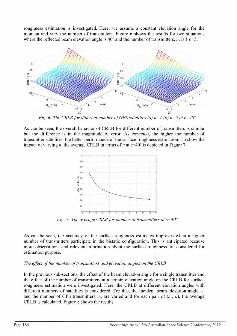
Page 184 Proceedings from 12th Australian Space Science Conference, 2012
roughness estimation is investigated. Here, we assume a constant elevation angle for the moment and vary the number of transmitters. Figure 6 shows the results for two situations where the reflected beam elevation angle is 40º and the number of transmitters, n, is 1 or 5.
As can be seen, the overall behavior of CRLB for different number of transmitters is similar but the difference is in the magnitude of error. As expected, the higher the number of transmitter satellites, the better performance of the surface roughness estimation. To show the impact of varying n, the average CRLB in terms of n at ε=40º is depicted in Figure 7.
As can be seen, the accuracy of the surface roughness estimates improves when a higher number of transmitters participate in the bistatic configuration. This is anticipated because more observations and relevant information about the surface roughness are considered for estimation purpose. The effect of the number of transmitters and elevation angles on the CRLB In the previous sub-sections, the effect of the beam elevation angle for a single transmitter and the effect of the number of transmitters at a certain elevation angle on the CRLB for surface roughness estimation were investigated. Here, the CRLB at different elevation angles with different numbers of satellites is considered. For this, the incident beam elevation angle, ε, and the number of GPS transmitters, n, are varied and for each pair of (ε , n), the average CRLB is calculated. Figure 8 shows the results.
Fig. 6: The CRLB for different number of GPS satellites (a) n=1 (b) n=5 at ε=40º
Fig. 7: The average CRLB for number of transmitters at ε=40º
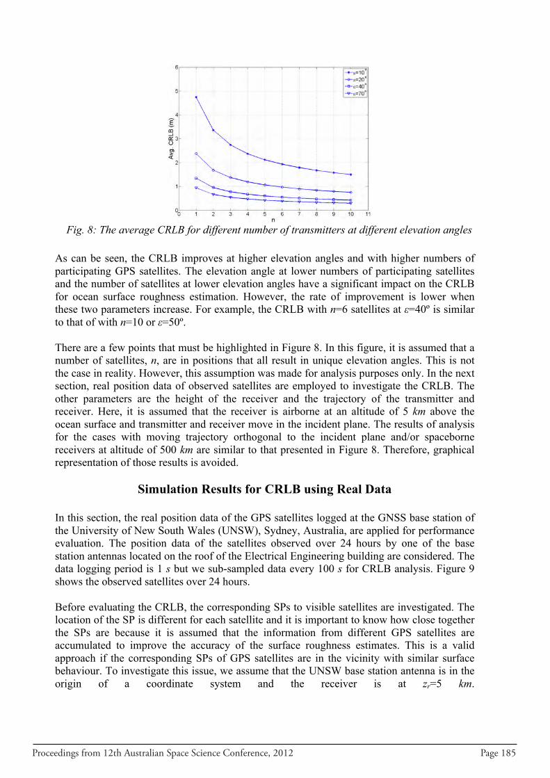
Proceedings from 12th Australian Space Science Conference, 2012 Page 185
As can be seen, the CRLB improves at higher elevation angles and with higher numbers of participating GPS satellites. The elevation angle at lower numbers of participating satellites and the number of satellites at lower elevation angles have a significant impact on the CRLB for ocean surface roughness estimation. However, the rate of improvement is lower when these two parameters increase. For example, the CRLB with n=6 satellites at ε=40º is similar to that of with n=10 or ε=50º. There are a few points that must be highlighted in Figure 8. In this figure, it is assumed that a number of satellites, n, are in positions that all result in unique elevation angles. This is not the case in reality. However, this assumption was made for analysis purposes only. In the next section, real position data of observed satellites are employed to investigate the CRLB. The other parameters are the height of the receiver and the trajectory of the transmitter and receiver. Here, it is assumed that the receiver is airborne at an altitude of 5 km above the ocean surface and transmitter and receiver move in the incident plane. The results of analysis for the cases with moving trajectory orthogonal to the incident plane and/or spaceborne receivers at altitude of 500 km are similar to that presented in Figure 8. Therefore, graphical representation of those results is avoided.
Simulation Results for CRLB using Real Data
In this section, the real position data of the GPS satellites logged at the GNSS base station of the University of New South Wales (UNSW), Sydney, Australia, are applied for performance evaluation. The position data of the satellites observed over 24 hours by one of the base station antennas located on the roof of the Electrical Engineering building are considered. The data logging period is 1 s but we sub-sampled data every 100 s for CRLB analysis. Figure 9 shows the observed satellites over 24 hours. Before evaluating the CRLB, the corresponding SPs to visible satellites are investigated. The location of the SP is different for each satellite and it is important to know how close together the SPs are because it is assumed that the information from different GPS satellites are accumulated to improve the accuracy of the surface roughness estimates. This is a valid approach if the corresponding SPs of GPS satellites are in the vicinity with similar surface behaviour. To investigate this issue, we assume that the UNSW base station antenna is in the origin of a coordinate system and the receiver is at zr=5 km.
Fig. 8: The average CRLB for different number of transmitters at different elevation angles
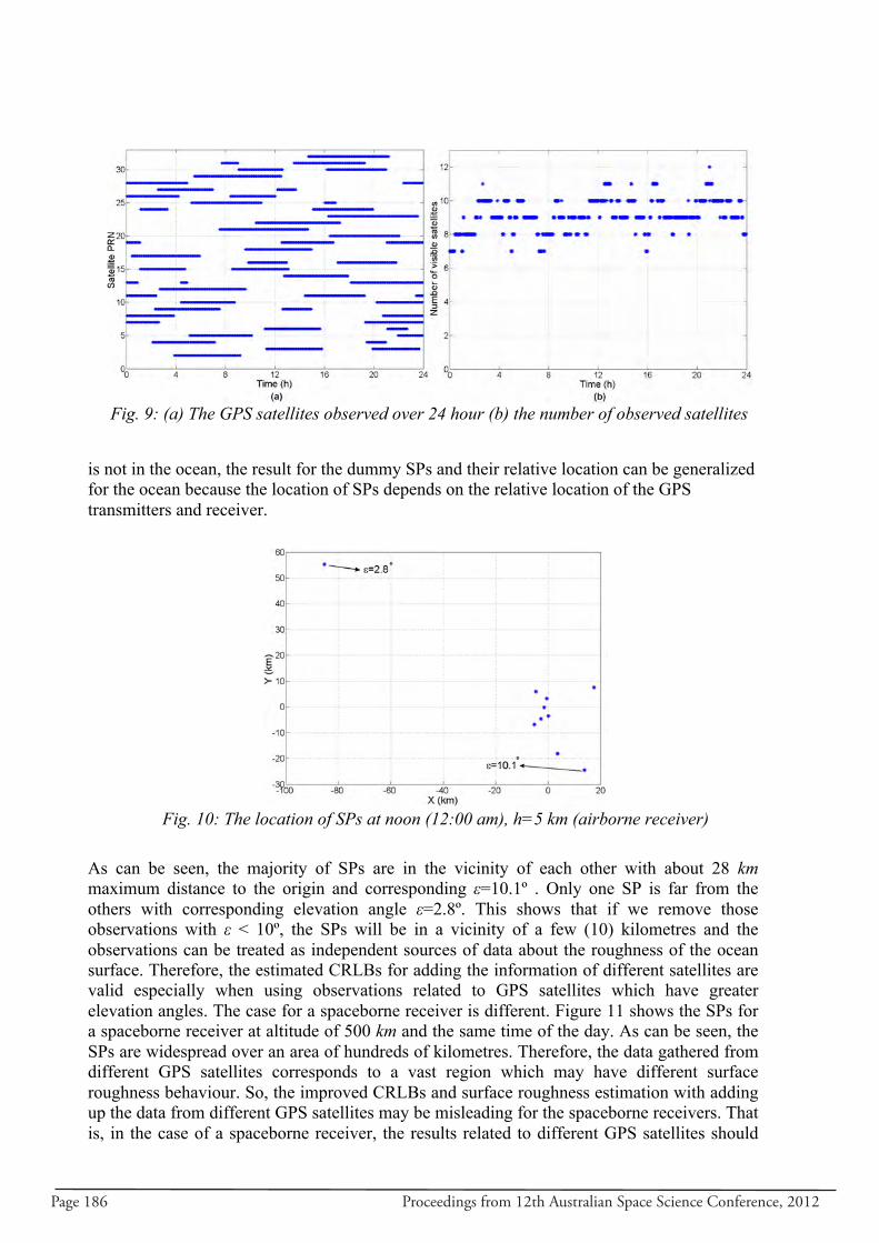
Page 186 Proceedings from 12th Australian Space Science Conference, 2012
Figure 10, shows the location of SPs at noon, 12:00 am. Although, the observing base station is not in the ocean, the result for the dummy SPs and their relative location can be generalized for the ocean because the location of SPs depends on the relative location of the GPS transmitters and receiver.
As can be seen, the majority of SPs are in the vicinity of each other with about 28 km maximum distance to the origin and corresponding ε=10.1º . Only one SP is far from the others with corresponding elevation angle ε=2.8º. This shows that if we remove those observations with ε < 10º, the SPs will be in a vicinity of a few (10) kilometres and the observations can be treated as independent sources of data about the roughness of the ocean surface. Therefore, the estimated CRLBs for adding the information of different satellites are valid especially when using observations related to GPS satellites which have greater elevation angles. The case for a spaceborne receiver is different. Figure 11 shows the SPs for a spaceborne receiver at altitude of 500 km and the same time of the day. As can be seen, the SPs are widespread over an area of hundreds of kilometres. Therefore, the data gathered from different GPS satellites corresponds to a vast region which may have different surface roughness behaviour. So, the improved CRLBs and surface roughness estimation with adding up the data from different GPS satellites may be misleading for the spaceborne receivers. That is, in the case of a spaceborne receiver, the results related to different GPS satellites should
Fig. 9: (a) The GPS satellites observed over 24 hour (b) the number of observed satellites
Fig. 10: The location of SPs at noon (12:00 am), h=5 km (airborne receiver)
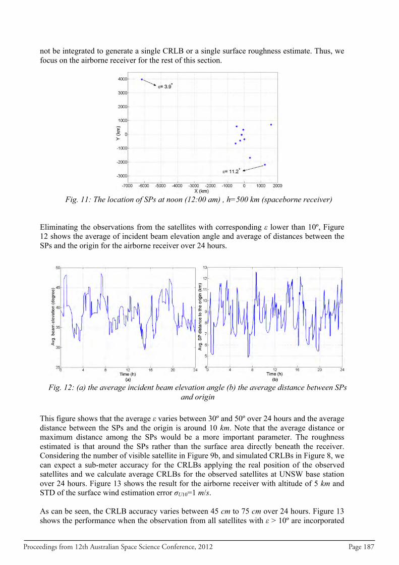
Proceedings from 12th Australian Space Science Conference, 2012 Page 187
not be integrated to generate a single CRLB or a single surface roughness estimate. Thus, we focus on the airborne receiver for the rest of this section. Eliminating the observations from the satellites with corresponding ε lower than 10º, Figure 12 shows the average of incident beam elevation angle and average of distances between the SPs and the origin for the airborne receiver over 24 hours. This figure shows that the average ε varies between 30º and 50º over 24 hours and the average distance between the SPs and the origin is around 10 km. Note that the average distance or maximum distance among the SPs would be a more important parameter. The roughness estimated is that around the SPs rather than the surface area directly beneath the receiver. Considering the number of visible satellite in Figure 9b, and simulated CRLBs in Figure 8, we can expect a sub-meter accuracy for the CRLBs applying the real position of the observed satellites and we calculate average CRLBs for the observed satellites at UNSW base station over 24 hours. Figure 13 shows the result for the airborne receiver with altitude of 5 km and STD of the surface wind estimation error σU10=1 m/s. As can be seen, the CRLB accuracy varies between 45 cm to 75 cm over 24 hours. Figure 13 shows the performance when the observation from all satellites with ε > 10º are incorporated
Fig. 11: The location of SPs at noon (12:00 am) , h=500 km (spaceborne receiver)
Fig. 12: (a) the average incident beam elevation angle (b) the average distance between SPs
and origin
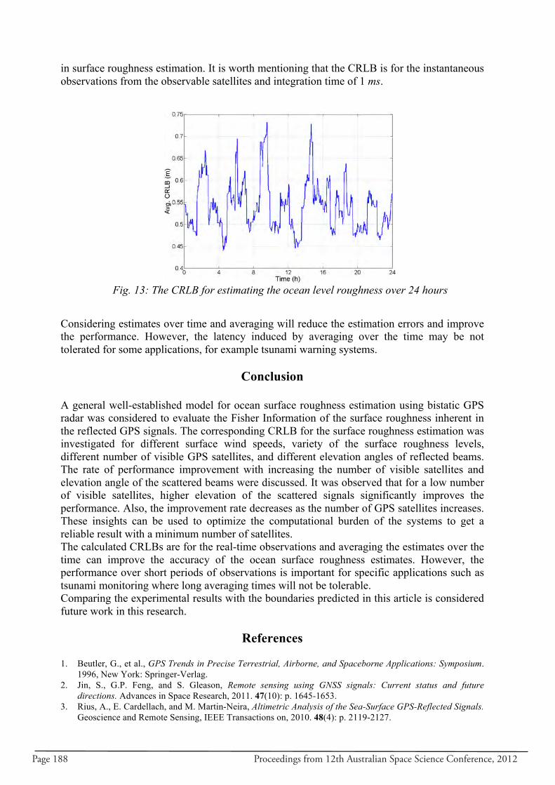
Page 188 Proceedings from 12th Australian Space Science Conference, 2012
in surface roughness estimation. It is worth mentioning that the CRLB is for the instantaneous observations from the observable satellites and integration time of 1 ms.
Considering estimates over time and averaging will reduce the estimation errors and improve the performance. However, the latency induced by averaging over the time may be not tolerated for some applications, for example tsunami warning systems.
Conclusion
A general well-established model for ocean surface roughness estimation using bistatic GPS radar was considered to evaluate the Fisher Information of the surface roughness inherent in the reflected GPS signals. The corresponding CRLB for the surface roughness estimation was investigated for different surface wind speeds, variety of the surface roughness levels, different number of visible GPS satellites, and different elevation angles of reflected beams. The rate of performance improvement with increasing the number of visible satellites and elevation angle of the scattered beams were discussed. It was observed that for a low number of visible satellites, higher elevation of the scattered signals significantly improves the performance. Also, the improvement rate decreases as the number of GPS satellites increases. These insights can be used to optimize the computational burden of the systems to get a reliable result with a minimum number of satellites. The calculated CRLBs are for the real-time observations and averaging the estimates over the time can improve the accuracy of the ocean surface roughness estimates. However, the performance over short periods of observations is important for specific applications such as tsunami monitoring where long averaging times will not be tolerable. Comparing the experimental results with the boundaries predicted in this article is considered future work in this research.
References 1. Beutler, G., et al., GPS Trends in Precise Terrestrial, Airborne, and Spaceborne Applications: Symposium.
1996, New York: Springer-Verlag. 2. Jin, S., G.P. Feng, and S. Gleason, Remote sensing using GNSS signals: Current status and future
directions. Advances in Space Research, 2011. 47(10): p. 1645-1653. 3. Rius, A., E. Cardellach, and M. Martin-Neira, Altimetric Analysis of the Sea-Surface GPS-Reflected Signals.
Geoscience and Remote Sensing, IEEE Transactions on, 2010. 48(4): p. 2119-2127.
Fig. 13: The CRLB for estimating the ocean level roughness over 24 hours

Proceedings from 12th Australian Space Science Conference, 2012 Page 189
4. Zavorotny, V.U. and A.G. Voronovich, Scattering of GPS signals from the ocean with wind remote sensing application. IEEE Transactions on Geoscience and Remote Sensing, 2000. 38(2).
5. Komjathy, A., et al., GPS Signal Scattering from Sea Surface:Wind Speed Retrieval Using Experimental Data and Theoretical Model. Remote Sensing of Environment, 2000. 73: p. 162-174.
6. Garrison, J.L., et al., Wind speed measurement using forward scattered GPS signals. IEEE Transactions on Geoscience and Remote Sensing, 2002. 40(1): p. 50-65.
7. Hajj, G.A. and C. Zuffada, Theoretical description of a bistatic system for ocean altimetry using the GPS signal. Radio Science 2003. 38(5).
8. Gleason, S., et al., Detection and processing of bistatically reflected GPS signals from low earth orbit for the purpose of ocean remote sensing. IEEE Transactions on Geoscience and Remote Sensing, 2005. 43(6): p. 1229-1241.
9. Thompson, D.R., T.M. Elfouhaily, and J.L. Garrison, An improved geometrical optics model for bistatic GPS scattering from the ocean surface. IEEE Transactions on Geoscience and Remote Sensing, 2005. 43(12): p. 2810-2820.
10. Wilmhoff, B., et al. GPS ocean altimetry from aircraft using the P(Y) code signal. 2007. Barcelona. 11. Clarizia, M.P., et al. Global navigation satellite system-reflectometry (GNSS-R) from the UK-DMC satellite
for remote sensing of the ocean surface. 2008. Boston, MA. 12. Rius, A., et al., Altimetry with GNSS-R interferometry: First proof of concept experiment. GPS Solutions,
2012. 16(2): p. 231-241. 13. Cherniakov, M., Bistatic Radar: Principles and Practice. 2007, Chichester,UK: John Wiley & Sons Ltd. 14. Kaplan, E.D. and C.J. Hegarty, Understanding GPS Principles and Applications. 2 ed. 2006, Norwood:
Artech House Inc. 15. Trees, H.L.V., Detection, Estimation, and Modulation Theory. 2003, New York: Wiley-IEEE.

Page 190 Proceedings from 12th Australian Space Science Conference, 2012
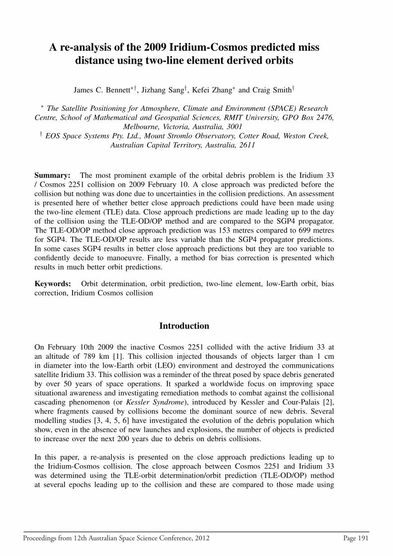
Proceedings from 12th Australian Space Science Conference, 2012 Page 191
A re-analysis of the 2009 Iridium-Cosmos predicted missdistance using two-line element derived orbits
James C. Bennett∗†, Jizhang Sang†, Kefei Zhang∗ and Craig Smith†
∗ The Satellite Positioning for Atmosphere, Climate and Environment (SPACE) ResearchCentre, School of Mathematical and Geospatial Sciences, RMIT University, GPO Box 2476,
Melbourne, Victoria, Australia, 3001† EOS Space Systems Pty. Ltd., Mount Stromlo Observatory, Cotter Road, Weston Creek,
Australian Capital Territory, Australia, 2611
Summary: The most prominent example of the orbital debris problem is the Iridium 33/ Cosmos 2251 collision on 2009 February 10. A close approach was predicted before thecollision but nothing was done due to uncertainties in the collision predictions. An assessmentis presented here of whether better close approach predictions could have been made usingthe two-line element (TLE) data. Close approach predictions are made leading up to the dayof the collision using the TLE-OD/OP method and are compared to the SGP4 propagator.The TLE-OD/OP method close approach prediction was 153 metres compared to 699 metresfor SGP4. The TLE-OD/OP results are less variable than the SGP4 propagator predictions.In some cases SGP4 results in better close approach predictions but they are too variable toconfidently decide to manoeuvre. Finally, a method for bias correction is presented whichresults in much better orbit predictions.
Keywords: Orbit determination, orbit prediction, two-line element, low-Earth orbit, biascorrection, Iridium Cosmos collision
Introduction
On February 10th 2009 the inactive Cosmos 2251 collided with the active Iridium 33 atan altitude of 789 km [1]. This collision injected thousands of objects larger than 1 cmin diameter into the low-Earth orbit (LEO) environment and destroyed the communicationssatellite Iridium 33. This collision was a reminder of the threat posed by space debris generatedby over 50 years of space operations. It sparked a worldwide focus on improving spacesituational awareness and investigating remediation methods to combat against the collisionalcascading phenomenon (or Kessler Syndrome), introduced by Kessler and Cour-Palais [2],where fragments caused by collisions become the dominant source of new debris. Severalmodelling studies [3, 4, 5, 6] have investigated the evolution of the debris population whichshow, even in the absence of new launches and explosions, the number of objects is predictedto increase over the next 200 years due to debris on debris collisions.
In this paper, a re-analysis is presented on the close approach predictions leading up tothe Iridium-Cosmos collision. The close approach between Cosmos 2251 and Iridium 33was determined using the TLE-orbit determination/orbit prediction (TLE-OD/OP) methodat several epochs leading up to the collision and these are compared to those made using

Page 192 Proceedings from 12th Australian Space Science Conference, 2012
Simplified General Perturbations 4 (SGP4) propagation – the method originally used to pro-vide conjunction assessments in Satellite Orbital Conjunction Reports Assessing ThreateningEncounters in Space (SOCRATES) [7].
In what follows, the TLE-OD/OP method is introduced along with results of an accuracystudy comparing it to standard SGP4 propagation. The method is then used to calculate thepredicted close approach between Iridium 33 and Cosmos 2251 leading up to the collision onFebruary 10. Then, the TLE-OD/OP method is used in tandem with a nonlinear bias correctionmethod resulting in drastic improvements in OP accuracy. The motivation for these methodsis the scenario that was faced with the Iridium-Cosmos collision. The TLE-OD/OP methodyields better orbit predictions than SGP4, which leads to better conjunction assessments. Ifobjects of interest are identified by the TLE-OD/OP method, the bias correction method canbe employed once a small amount of tracking data has been collected. The prediction thencontains information from two data sources and better conjunction assessments can be made.
The TLE-OD/OP method
The TLE-OD/OP method is based on the method introduced by [8] and uses multiple TLEs tocreate pseudo-observations for an OD process. Details may be found in [9]. All the TLEs thatfall within the OD period (fixed at 10 days) are downloaded from [10]. Pseudo-observationsare generated every 10 minutes using the SGP4 propagator by propagating backwards fromeach TLE, past the previous TLE epoch by an arbitrary period of 0.2 days. This is to ensuresufficient observations are generated for the OD process. The first and last TLEs are usedto create the observations up until the initial and final epochs of the OD window. Thesepropagated states are then used as observations and an orbit is determined, considering afull set of forces, using least squares. The determined orbit is then propagated forward usingnumerical integration to obtain the OP. For comparison, the standard SGP4 propagation startsfrom the latest TLE available in the OD window. A schematic of the observation generationprocess and the OD/OP time lines are shown in Fig. 1. To determine the accuracy of the
0 10Days
TLE-OD/OP OD TLE-OD/OP OP
SGP4 OP
TLE1 TLE2 TLEn−1 TLEn
Pseudo-observations generated every 10 minutes using SGP4
Fig. 1: Schematic of the pseudo-observation generation and the TLE-OD/OP time line. n isthe number of TLEs available in the OD window
predicted orbits from both methods, they are compared to highly accurate satellite laserranging (SLR) consolidated prediction format (CPF) data downloaded from [11].
Proceedings from 12th Australian Space Science Conference, 2012 Page 193
TLE-OD/OP accuracy study
The accuracy of the TLE-OD/OP method compared to standard SGP4 propagation wasdetermined from an extensive 200-run simulation study for four LEO satellites – Starlette,Stella, Grace A and Grace B. Starlette and Stella are spherical satellites whilst Grace A andB are non-spherical. The TLE-OD/OP process described above was repeated 200 times, witheach run starting from a random (unique) epoch. For comparison, standard SGP4 propagationwas also performed in each of the 200 runs for each satellite from the last TLE in the ODwindow. The accuracy of the resulting OPs made using the TLE-OD/OP method and standardSGP4 propagation was determined by comparing them to the highly accurate SLR CPF data.
The metric used to determine the accuracy of each method was the absolute maximum alongtrack bias after a 7 day OP. This is considered to be a worst case scenario measure. The resultsof this study are shown in Table 1. This shows the proportion of runs where the TLE-OD/OP
Table 1: Results from study comparing TLE-OD/OP method and standard SGP4propagation for a 7 day OP
Satellite TLE-OD/OP Ave max abs SGP4 Ave max abswin % along track bias win % along track bias
(all runs) (m) (all runs) (m)Starlette 93.4% 1,025 6.6% 2,812Stella 98.5% 1,349 1.5% 5,173Grace A 97.5% 2,967 2.5% 9,373Grace B 95.5% 2,921 4.5% 8,216
method resulted in a better 7 day OP compared to standard SGP4 propagation. If the absolutemaximum along track bias after a 7 day OP is lower it is considered more accurate. Table 1also shows the average absolute 7 day along track bias over all runs for the TLE-OD/OPmethod and standard SGP4 propagation. The results of this study show that the TLE-OD/OPvastly outperforms standard SGP4 propagation with it resulting in a smaller 7 day absolutemaximum along track bias over 90% of the time. The reduction in the average maximum 7day along track biases for Starlette, Stella, Grace A, and Grace B are 64%, 74%, 68%, and64%, respectively. A better win % would be achieved for the TLE-OD/OP method if eitherof the other biases were considered as the metric for accuracy. See the boxplots containedin [9] for details.
An example of the improvements in OPs obtained using the TLE-OD/OP method and theinaccuracies faced using standard SGP4 propagation for Starlette is shown in Fig. 2. Thisshows the position prediction bias in the along, cross track and radial directions. The TLE-OD/OP method results in a much more accurate position prediction over standard SGP4propagation. The improvements that may be achieved in prediction accuracy are especiallyprevalent in the along track direction (Fig. 2(a)). The TLE-OD/OP method also results insmaller biases in the cross track and radial directions (Figs. 2(b) and 2(c)). The TLE-OD/OPmethod results in biases that are simple sinusoidal variations, opposed to the SGP4 predictionswhich are less well-behaved.
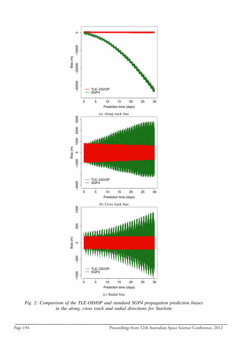
Page 194 Proceedings from 12th Australian Space Science Conference, 2012
0 5 10 15 20 25 30
−300
00−2
0000
−100
000
Prediction time (days)
Bias
(m)
TLE−OD/OPSGP4
(a) Along track bias
0 5 10 15 20 25 30
−300
0−1
000
010
0020
0030
00
Prediction time (days)
Bias
(m)
TLE−OD/OPSGP4
(b) Cross track bias
0 5 10 15 20 25 30
−100
0−5
000
500
1000
Prediction time (days)
Bias
(m)
TLE−OD/OPSGP4
(c) Radial bias
Fig. 2: Comparison of the TLE-OD/OP and standard SGP4 propagation prediction biasesin the along, cross track and radial directions for Starlette
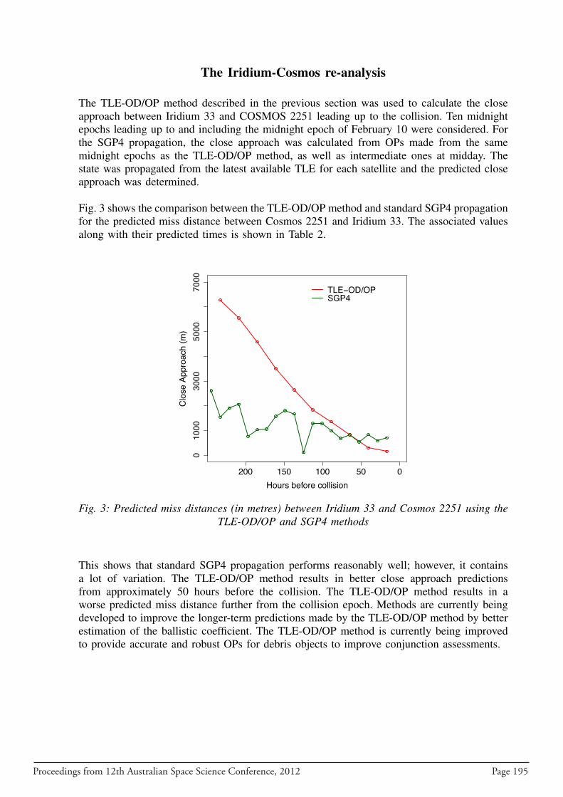
Proceedings from 12th Australian Space Science Conference, 2012 Page 195
The Iridium-Cosmos re-analysis
The TLE-OD/OP method described in the previous section was used to calculate the closeapproach between Iridium 33 and COSMOS 2251 leading up to the collision. Ten midnightepochs leading up to and including the midnight epoch of February 10 were considered. Forthe SGP4 propagation, the close approach was calculated from OPs made from the samemidnight epochs as the TLE-OD/OP method, as well as intermediate ones at midday. Thestate was propagated from the latest available TLE for each satellite and the predicted closeapproach was determined.
Fig. 3 shows the comparison between the TLE-OD/OP method and standard SGP4 propagationfor the predicted miss distance between Cosmos 2251 and Iridium 33. The associated valuesalong with their predicted times is shown in Table 2.
200 150 100 50 0
010
0030
0050
0070
00
Hours before collision
Clo
se A
ppro
ach
(m)
TLE−OD/OPSGP4
Fig. 3: Predicted miss distances (in metres) between Iridium 33 and Cosmos 2251 using theTLE-OD/OP and SGP4 methods
This shows that standard SGP4 propagation performs reasonably well; however, it containsa lot of variation. The TLE-OD/OP method results in better close approach predictionsfrom approximately 50 hours before the collision. The TLE-OD/OP method results in aworse predicted miss distance further from the collision epoch. Methods are currently beingdeveloped to improve the longer-term predictions made by the TLE-OD/OP method by betterestimation of the ballistic coefficient. The TLE-OD/OP method is currently being improvedto provide accurate and robust OPs for debris objects to improve conjunction assessments.
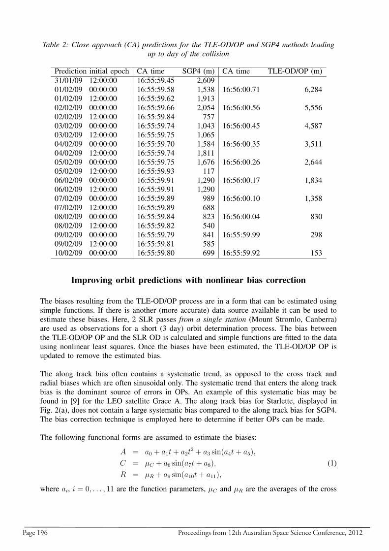
Page 196 Proceedings from 12th Australian Space Science Conference, 2012
Table 2: Close approach (CA) predictions for the TLE-OD/OP and SGP4 methods leadingup to day of the collision
Prediction initial epoch CA time SGP4 (m) CA time TLE-OD/OP (m)31/01/09 12:00:00 16:55:59.45 2,60901/02/09 00:00:00 16:55:59.58 1,538 16:56:00.71 6,28401/02/09 12:00:00 16:55:59.62 1,91302/02/09 00:00:00 16:55:59.66 2,054 16:56:00.56 5,55602/02/09 12:00:00 16:55:59.84 75703/02/09 00:00:00 16:55:59.74 1,043 16:56:00.45 4,58703/02/09 12:00:00 16:55:59.75 1,06504/02/09 00:00:00 16:55:59.70 1,584 16:56:00.35 3,51104/02/09 12:00:00 16:55:59.74 1,81105/02/09 00:00:00 16:55:59.75 1,676 16:56:00.26 2,64405/02/09 12:00:00 16:55:59.93 11706/02/09 00:00:00 16:55:59.91 1,290 16:56:00.17 1,83406/02/09 12:00:00 16:55:59.91 1,29007/02/09 00:00:00 16:55:59.89 989 16:56:00.10 1,35807/02/09 12:00:00 16:55:59.89 68808/02/09 00:00:00 16:55:59.84 823 16:56:00.04 83008/02/09 12:00:00 16:55:59.82 54009/02/09 00:00:00 16:55:59.79 841 16:55:59.99 29809/02/09 12:00:00 16:55:59.81 58510/02/09 00:00:00 16:55:59.80 699 16:55:59.92 153
Improving orbit predictions with nonlinear bias correction
The biases resulting from the TLE-OD/OP process are in a form that can be estimated usingsimple functions. If there is another (more accurate) data source available it can be used toestimate these biases. Here, 2 SLR passes from a single station (Mount Stromlo, Canberra)are used as observations for a short (3 day) orbit determination process. The bias betweenthe TLE-OD/OP OP and the SLR OD is calculated and simple functions are fitted to the datausing nonlinear least squares. Once the biases have been estimated, the TLE-OD/OP OP isupdated to remove the estimated bias.
The along track bias often contains a systematic trend, as opposed to the cross track andradial biases which are often sinusoidal only. The systematic trend that enters the along trackbias is the dominant source of errors in OPs. An example of this systematic bias may befound in [9] for the LEO satellite Grace A. The along track bias for Starlette, displayed inFig. 2(a), does not contain a large systematic bias compared to the along track bias for SGP4.The bias correction technique is employed here to determine if better OPs can be made.
The following functional forms are assumed to estimate the biases:
A = a0 + a1t+ a2t2 + a3 sin(a4t+ a5),
C = µC + a6 sin(a7t+ a8), (1)R = µR + a9 sin(a10t+ a11),
where ai, i = 0, . . . , 11 are the function parameters, µC and µR are the averages of the cross
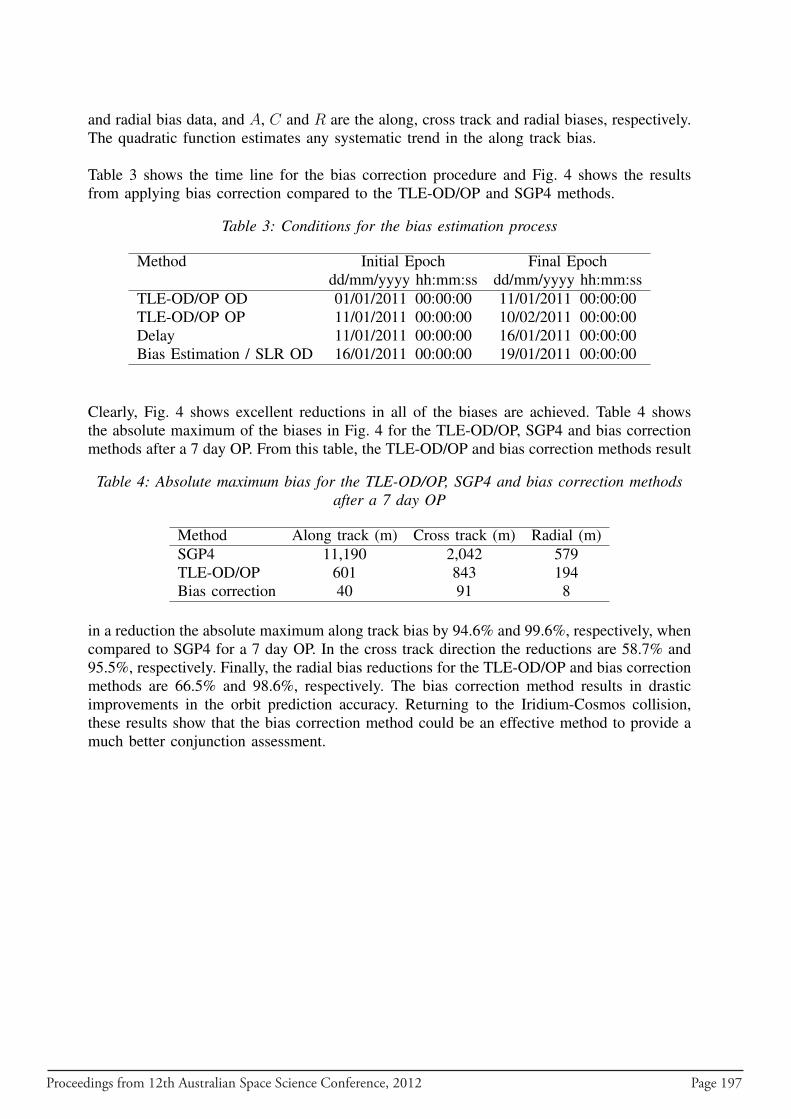
Proceedings from 12th Australian Space Science Conference, 2012 Page 197
and radial bias data, and A, C and R are the along, cross track and radial biases, respectively.The quadratic function estimates any systematic trend in the along track bias.
Table 3 shows the time line for the bias correction procedure and Fig. 4 shows the resultsfrom applying bias correction compared to the TLE-OD/OP and SGP4 methods.
Table 3: Conditions for the bias estimation process
Method Initial Epoch Final Epochdd/mm/yyyy hh:mm:ss dd/mm/yyyy hh:mm:ss
TLE-OD/OP OD 01/01/2011 00:00:00 11/01/2011 00:00:00TLE-OD/OP OP 11/01/2011 00:00:00 10/02/2011 00:00:00Delay 11/01/2011 00:00:00 16/01/2011 00:00:00Bias Estimation / SLR OD 16/01/2011 00:00:00 19/01/2011 00:00:00
Clearly, Fig. 4 shows excellent reductions in all of the biases are achieved. Table 4 showsthe absolute maximum of the biases in Fig. 4 for the TLE-OD/OP, SGP4 and bias correctionmethods after a 7 day OP. From this table, the TLE-OD/OP and bias correction methods result
Table 4: Absolute maximum bias for the TLE-OD/OP, SGP4 and bias correction methodsafter a 7 day OP
Method Along track (m) Cross track (m) Radial (m)SGP4 11,190 2,042 579TLE-OD/OP 601 843 194Bias correction 40 91 8
in a reduction the absolute maximum along track bias by 94.6% and 99.6%, respectively, whencompared to SGP4 for a 7 day OP. In the cross track direction the reductions are 58.7% and95.5%, respectively. Finally, the radial bias reductions for the TLE-OD/OP and bias correctionmethods are 66.5% and 98.6%, respectively. The bias correction method results in drasticimprovements in the orbit prediction accuracy. Returning to the Iridium-Cosmos collision,these results show that the bias correction method could be an effective method to provide amuch better conjunction assessment.
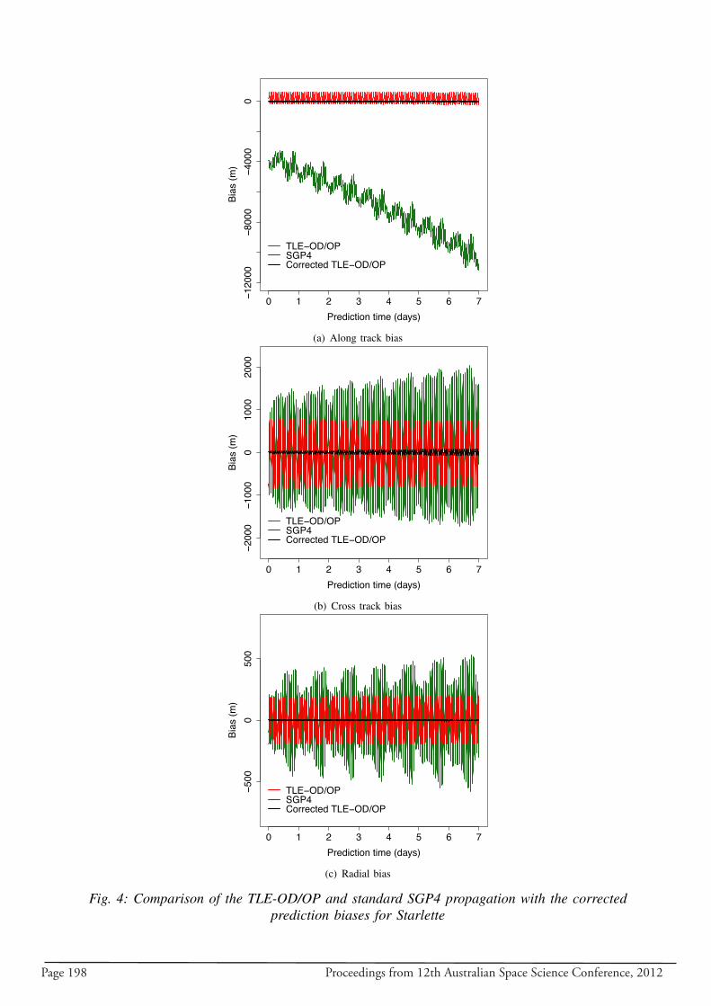
Page 198 Proceedings from 12th Australian Space Science Conference, 2012
0 1 2 3 4 5 6 7−120
00−8
000
−400
00
Prediction time (days)
Bias
(m)
TLE−OD/OPSGP4Corrected TLE−OD/OP
(a) Along track bias
0 1 2 3 4 5 6 7
−200
0−1
000
010
0020
00
Prediction time (days)
Bias
(m)
TLE−OD/OPSGP4Corrected TLE−OD/OP
(b) Cross track bias
0 1 2 3 4 5 6 7
−500
050
0
Prediction time (days)
Bias
(m)
TLE−OD/OPSGP4Corrected TLE−OD/OP
(c) Radial bias
Fig. 4: Comparison of the TLE-OD/OP and standard SGP4 propagation with the correctedprediction biases for Starlette
Proceedings from 12th Australian Space Science Conference, 2012 Page 199
Conclusion
Providing reliable conjunction assessments is an extremely important task for the safety ofspace operations. In this paper, two techniques to provide better OPs using TLE data werepresented. The TLE-OD/OP method uses only the freely-available TLE data. This methodprovided large improvements in accuracy over standard SGP4 propagation (Table 1). Thebias correction method resulted in drastic improvements in OPs with little supplementarydata required which is the case often faced when calculating debris OPs. The bias correctionmethod is an example of how data from multiple sources can be combined to provide thebest possible OPs.
The TLE-OD/OP method is being refined to improve debris OP. These changes are expected toprovide better close approach predictions further in advance for the Iridium-Cosmos examplepresented.
Acknowledgments
The authors would like to gratefully acknowledge the Australian government’s research grantsupport for this project through the Australian Space Research Program (ASRP) project“Platform Technologies for Space, Atmosphere and Climate”.
References
[1] Kelso, T. S., “Analysis of the Iridium 33-Cosmos 2251 collision”, Advances in theAstronautical Sciences, Vol. 135, Suppl. 2, AAS 09-368, 2009, pp. 1099-1112.
[2] Kessler, D.J. and Cour-Palais, B.G., Collision frequency of artificial satellites: The creationof a debris belt, Journal of Geophysical Research, Vol. 83, No. A6, 2637-2646, 1978.
[3] Liou, J.C. and Johnson N.L., Risks in space from orbiting debris, Science, Vol. 311, No.5759, 340-341, 2006.
[4] Liou, J.C. and Johnson N.L., Instability of the present LEO satellite populations, Advancesin Space Research, Vol. 41, No. 7, 1046-1053, 2008.
[5] Rossi, A., Anselmo, L., Pardini, C., Jehn, R. and Valsecchi, G.B., The new space debrismitigation (SDM 4.0) long term evolution code, in Proceedings of the Fifth EuropeanConference on Space Debris, ESA SP-672, Noordwijk, The Netherlands, 2009.
[6] Bennett, J. C. and Sang, J., Modelling the evolution of the low-Earth orbit debris popu-lation, Proceedings of the 11th Australian Space Science Confernece, 26–29 September,Canberra, Australia, ISBN 13: 978-0-9775740-5-6, 165–178, 2011.
[7] CelesTrak, Satellite Orbital Conjunction Reports Assessing Threatening Encounters inSpace, Online; accessed 21-February-2012, http://celestrak.com/.
[8] Levit, C. and Marshall, W., “Improved orbit predictions using two-line elements”,Advances in Space Research, Vol. 62, No. 7, 2011, pp. 1107-1115.
[9] Bennett, J.C., Sang, J., Smith, C. and Zhang, K., “Improving low-Earth orbit predictionsusing two-line element data with bias correction”, in Advanced Maui Optical and SpaceSurveillance Technologies Conference, 2012: Maui, Hawaii.
[10] Space-Track, Two Line Element (TLE) data, Online; accessed 21-February-2012, https://www.space-track.org/.

Page 200 Proceedings from 12th Australian Space Science Conference, 2012
[11] NASA Crustal Dynamics Data Information System, Consolidated Laser RangingPrediction Format, Online; accessed 21-February-2012, ftp://cddis.gsfc.nasa.gov/slr/cpfpredicts/.
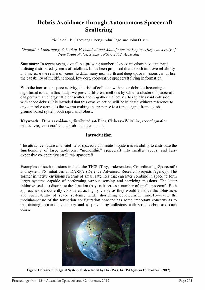
Proceedings from 12th Australian Space Science Conference, 2012 Page 201
Debris Avoidance through Autonomous Spacecraft Scattering
Tzi-Chieh Chi, Haoyang Cheng, John Page and John Olsen
Simulation Laboratory, School of Mechanical and Manufacturing Engineering, University of
New South Wales, Sydney, NSW, 2052, Australia
Summary: In recent years, a small but growing number of space missions have emerged utilising distributed systems of satellites. It has been proposed that to both improve reliability and increase the return of scientific data, many near Earth and deep space missions can utilise the capability of multifunctional, low cost, cooperative spacecraft flying in formation. With the increase in space activity, the risk of collision with space debris is becoming a significant issue. In this study, we present different methods by which a cluster of spacecraft can perform an energy efficient scatter and re-gather manoeuvre to rapidly avoid collision with space debris. It is intended that this evasive action will be initiated without reference to any control external to the swarm making the response to a threat signal from a global ground-based system both rapid and robust. Keywords: Debris avoidance, distributed satellites, Clohessy-Wiltshire, reconfiguration manoeuvre, spacecraft cluster, obstacle avoidance.
Introduction
The attractive nature of a satellite or spacecraft formation system is its ability to distribute the functionality of large traditional “monolithic” spacecraft into smaller, robust and less-expensive co-operative satellites/ spacecraft.
Examples of such missions include the TICS (Tiny, Independent, Co-ordinating Spacecraft) and system F6 initiatives at DARPA (Defence Advanced Research Projects Agency). The former initiative envisions swarms of small satellites that can later combine in space to form larger systems capable of performing various sensing and servicing missions. The latter initiative seeks to distribute the function (payload) across a number of small spacecraft. Both approaches are currently considered as highly viable as they would enhance the robustness and survivability of space systems, while shortening development time. However, the modular-nature of the formation configuration concept has some important concerns as to maintaining formation geometry and to preventing collisions with space debris and each other.
Figure 1 Program Image of System F6 developed by DARPA (DARPA System F5 Program, 2012)
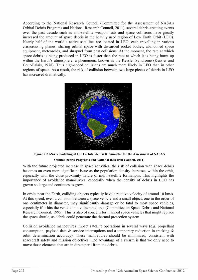
Page 202 Proceedings from 12th Australian Space Science Conference, 2012
According to the National Research Council (Committee for the Assessment of NASA's Orbital Debris Programs and National Research Council, 2011), several debris-creating events over the past decade such as anti-satellite weapon tests and space collisions have greatly increased the amount of space debris in the heavily used region of Low Earth Orbit (LEO). Nearly half of the world’s active satellites are located in LEO, each travelling in various crisscrossing planes, sharing orbital space with discarded rocket bodies, abandoned space equipment, meteoroids, and shrapnel from past collisions. At the moment, the rate at which space debris is being produced in LEO is faster than the rate at which it is being burnt up within the Earth’s atmosphere, a phenomena known as the Kessler Syndrome (Kessler and Cour-Palais, 1978). Thus high-speed collisions are much more likely in LEO than in other regions of space. As a result, the risk of collision between two large pieces of debris in LEO has increased dramatically.
With the future projected increase in space activities, the risk of collision with space debris becomes an even more significant issue as the population density increases within the orbit, especially with the close proximity nature of multi-satellite formations. This highlights the importance of avoidance manoeuvres, especially when the density of debris in LEO has grown so large and continues to grow. In orbits near the Earth, colliding objects typically have a relative velocity of around 10 km/s. At this speed, even a collision between a space vehicle and a small object, one in the order of one centimeter in diameter, may significantly damage or be fatal to most space vehicles, especially if it hits the vehicle in a vulnerable area (Committee on Space Debris and National Research Council, 1995). This is also of concern for manned space vehicles that might replace the space shuttle, as debris could penetrate the thermal protection system. Collision avoidance manoeuvres impact satellite operations in several ways (e.g. propellant consumption, payload data & service interruptions and a temporary reduction in tracking & orbit determination accuracy). These manoeuvres should be minimized, consistent with spacecraft safety and mission objectives. The advantage of a swarm is that we only need to move those elements that are in direct peril from the debris.
Figure 2 NASA’s modelling of LEO orbital debris (Committee for the Assessment of NASA's
Orbital Debris Programs and National Research Council, 2011)
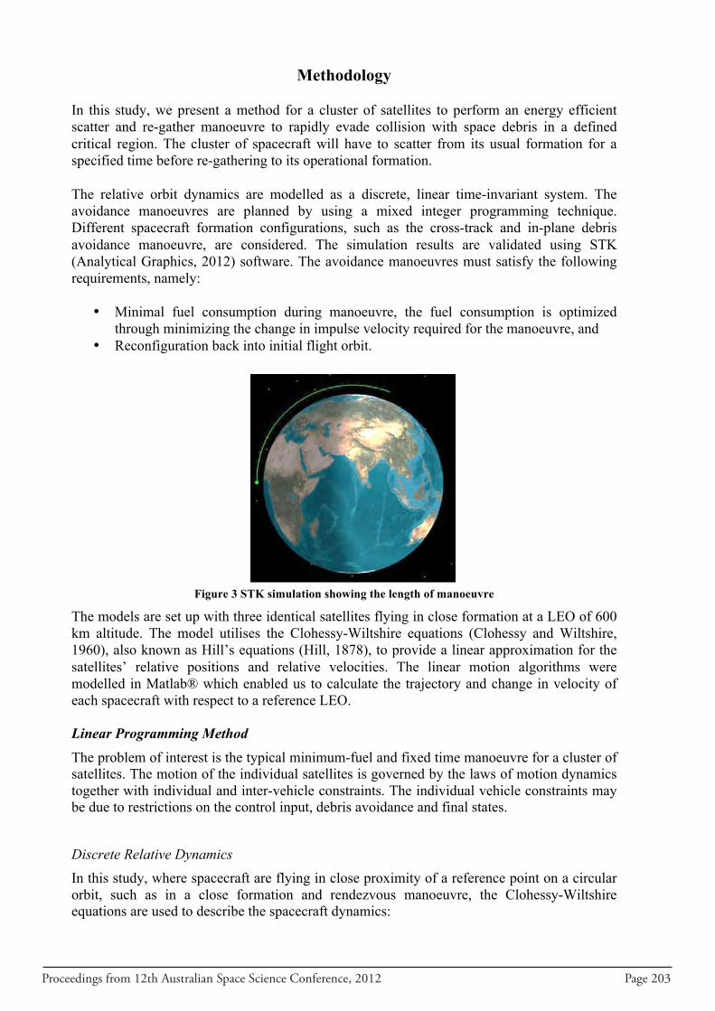
Proceedings from 12th Australian Space Science Conference, 2012 Page 203
Methodology In this study, we present a method for a cluster of satellites to perform an energy efficient scatter and re-gather manoeuvre to rapidly evade collision with space debris in a defined critical region. The cluster of spacecraft will have to scatter from its usual formation for a specified time before re-gathering to its operational formation. The relative orbit dynamics are modelled as a discrete, linear time-invariant system. The avoidance manoeuvres are planned by using a mixed integer programming technique. Different spacecraft formation configurations, such as the cross-track and in-plane debris avoidance manoeuvre, are considered. The simulation results are validated using STK (Analytical Graphics, 2012) software. The avoidance manoeuvres must satisfy the following requirements, namely:
• Minimal fuel consumption during manoeuvre, the fuel consumption is optimized through minimizing the change in impulse velocity required for the manoeuvre, and
• Reconfiguration back into initial flight orbit.
The models are set up with three identical satellites flying in close formation at a LEO of 600 km altitude. The model utilises the Clohessy-Wiltshire equations (Clohessy and Wiltshire, 1960), also known as Hill’s equations (Hill, 1878), to provide a linear approximation for the satellites’ relative positions and relative velocities. The linear motion algorithms were modelled in Matlab® which enabled us to calculate the trajectory and change in velocity of each spacecraft with respect to a reference LEO. Linear Programming Method
The problem of interest is the typical minimum-fuel and fixed time manoeuvre for a cluster of satellites. The motion of the individual satellites is governed by the laws of motion dynamics together with individual and inter-vehicle constraints. The individual vehicle constraints may be due to restrictions on the control input, debris avoidance and final states.
Discrete Relative Dynamics In this study, where spacecraft are flying in close proximity of a reference point on a circular orbit, such as in a close formation and rendezvous manoeuvre, the Clohessy-Wiltshire equations are used to describe the spacecraft dynamics:
Figure 3 STK simulation showing the length of manoeuvre
Page 204 Proceedings from 12th Australian Space Science Conference, 2012
(1a)
(1b)
(1c) Where is the angular velocity of the reference orbit and , and are the accelerations that are applied to the spacecraft by the rocket thrusters (assuming that the attitude of the spacecraft is maintained in such a way that three thrust components is available along the reference axes). The state variable of the spacecraft, namely , give the spacecraft relative position and velocity with respect to a reference point in the directions that are radial, “along-track” and normal to orbital plane (cross-track). The state space form of the spacecraft‘s relative motion in the local vertical/local horizontal frame are given by the linear time-invariant equation:
, (2) where
,
and
.
The continuous time system can be change to discrete form with a zero-order hold at a sampling time period, . The discrete equivalent state space equation is:
, (3) where
,
And
.
With the initial state and control sequence, , the final state can be written recursively as:
. (4)
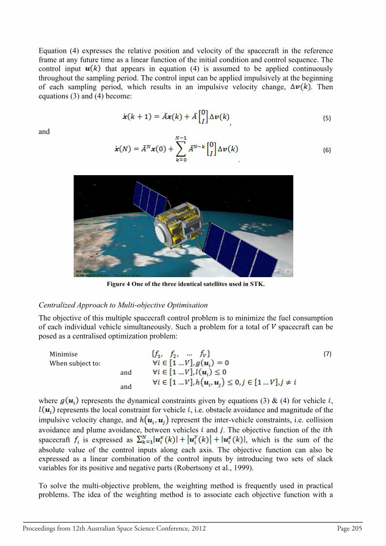
Proceedings from 12th Australian Space Science Conference, 2012 Page 205
Equation (4) expresses the relative position and velocity of the spacecraft in the reference frame at any future time as a linear function of the initial condition and control sequence. The control input that appears in equation (4) is assumed to be applied continuously throughout the sampling period. The control input can be applied impulsively at the beginning of each sampling period, which results in an impulsive velocity change, . Then equations (3) and (4) become:
, (5)
and
. (6)
Centralized Approach to Multi-objective Optimisation
The objective of this multiple spacecraft control problem is to minimize the fuel consumption of each individual vehicle simultaneously. Such a problem for a total of spacecraft can be posed as a centralised optimization problem: Minimise (7) When subject to: and
and
where represents the dynamical constraints given by equations (3) & (4) for vehicle , represents the local constraint for vehicle , i.e. obstacle avoidance and magnitude of the
impulsive velocity change, and represent the inter-vehicle constraints, i.e. collision avoidance and plume avoidance, between vehicles and . The objective function of the spacecraft is expressed as , which is the sum of the absolute value of the control inputs along each axis. The objective function can also be expressed as a linear combination of the control inputs by introducing two sets of slack variables for its positive and negative parts (Robertsony et al., 1999). To solve the multi-objective problem, the weighting method is frequently used in practical problems. The idea of the weighting method is to associate each objective function with a
Figure 4 One of the three identical satellites used in STK.
Page 206 Proceedings from 12th Australian Space Science Conference, 2012
weighting coefficient and minimize the weighted sum of the objectives. In this way, the multiple objective functions are transformed into a single objective function:
,
(8)
where for all and . It has been proved that the solution of this weighting problem is Pareto optimal (Miettinen, 1998).
Operational Constraints This is a preliminary study on this type of exercise. One of the major drawbacks of the centralized approach is that it scales poorly with the number of agents. The decision variables related to inter-vehicle constraints increase exponentially as the size of the formation increases. Such computational complexity could make the problem unsolvable with limited on-board computation resources. Alternatively, for the system in which a centralized controller is not desirable, a decentralized approach could be adopted to reach the global objectives while distributing the computational load.
Simulation Result The collision avoidance and formation re-acquisition manoeuvres in current synthetic aperture radar satellites is such a complex operation, that the planning process has to be performed manually by flight dynamics engineers less than 12 hours prior to execution (Kahle et al., 2012). This should be greatly improved as this simulation indicates. Identical satellites were used in both avoidance manoeuvers with the following arbitrary satellite configuration:
Table 1 Satellite Configuration used in both model
Satellite Configuration Dry Mass 500 kg Fuel Mass 500 kg Total Mass 1000 kg Area/Mass Ratio 2×10⁻² m2/kg Tank Pressure 5000 Pa Fuel Density 1000 kg/m3
The manoeuvers were carried out with constant rocket thrusts with the assumption that the changes in velocity were instantaneous.
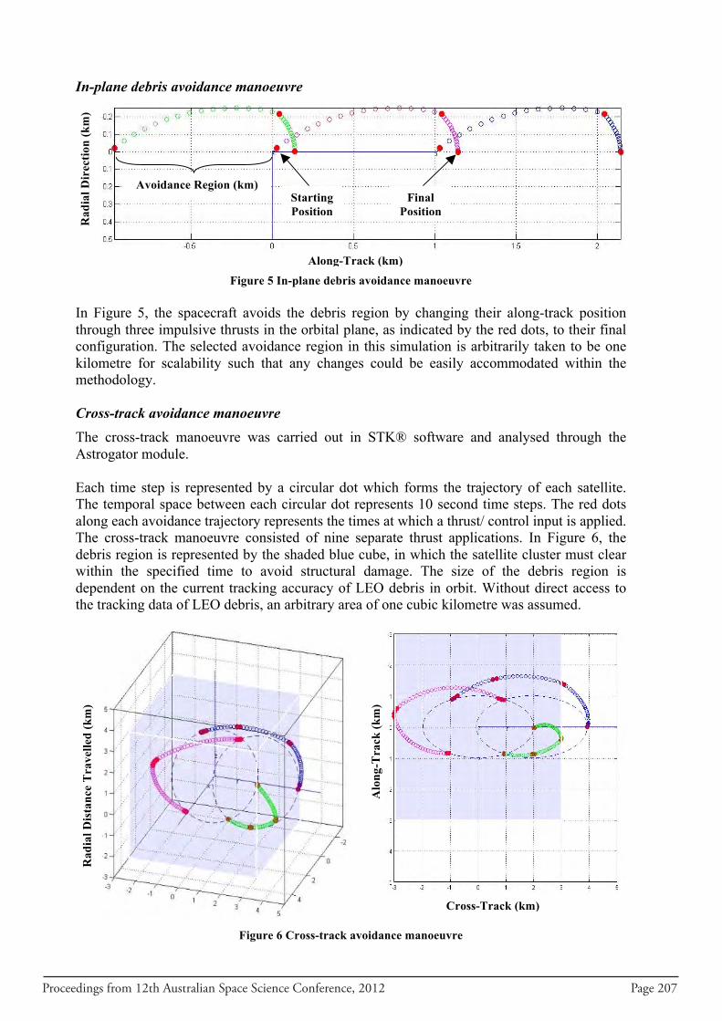
Proceedings from 12th Australian Space Science Conference, 2012 Page 207
Alo
ng-T
rack
(km
)
In-plane debris avoidance manoeuvre
Figure 5 In-plane debris avoidance manoeuvre In Figure 5, the spacecraft avoids the debris region by changing their along-track position through three impulsive thrusts in the orbital plane, as indicated by the red dots, to their final configuration. The selected avoidance region in this simulation is arbitrarily taken to be one kilometre for scalability such that any changes could be easily accommodated within the methodology. Cross-track avoidance manoeuvre The cross-track manoeuvre was carried out in STK® software and analysed through the Astrogator module. Each time step is represented by a circular dot which forms the trajectory of each satellite. The temporal space between each circular dot represents 10 second time steps. The red dots along each avoidance trajectory represents the times at which a thrust/ control input is applied. The cross-track manoeuvre consisted of nine separate thrust applications. In Figure 6, the debris region is represented by the shaded blue cube, in which the satellite cluster must clear within the specified time to avoid structural damage. The size of the debris region is dependent on the current tracking accuracy of LEO debris in orbit. Without direct access to the tracking data of LEO debris, an arbitrary area of one cubic kilometre was assumed.
Figure 6 Cross-track avoidance manoeuvre
Rad
ial D
irec
tion
(km
)
Along-Track (km)
Avoidance Region (km) Starting Position
Final Position
Rad
ial D
ista
nce
Tra
velle
d (k
m)
Cross-Track (km)
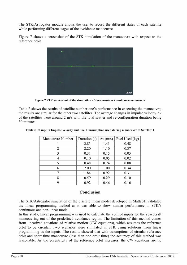
Page 208 Proceedings from 12th Australian Space Science Conference, 2012
The STK/Astrogator module allows the user to record the different states of each satellite while performing different stages of the avoidance manoeuvre.
Figure 7 shows a screenshot of the STK simulation of the manoeuvre with respect to the reference orbit.
Figure 7 STK screenshot of the simulation of the cross-track avoidance manoeuvre Table 2 shows the results of satellite number one’s performance in executing the manoeuvre; the results are similar for the other two satellites. The average changes in impulse velocity ∆ν of the satellites were around 2 m/s with the total scatter and re-configuration duration being 30 minutes.
Table 2 Change in Impulse velocity and Fuel Consumption used during manoeuvre of Satellite 1
Manoeuvre Number Duration (s) ∆ν (m/s) Fuel Used (kg) 1 2.83 1.41 0.48 2 2.20 1.10 0.37 3 0.31 0.15 0.05 4 0.10 0.05 0.02 5 0.48 0.24 0.08 6 2.00 1.00 0.34 7 1.84 0.92 0.31 8 0.59 0.29 0.10 9 0.92 0.46 0.16
Conclusion
The STK/Astrogator simulation of the discrete linear model developed in Matlab® validated the linear programming method as it was able to show similar performance in STK’s continuous and non-linear model. In this study, linear programming was used to calculate the control inputs for the spacecraft manoeuvring out of the predefined avoidance region. The limitation of this method comes from linearized equations of relative motion (CW equations), which assumes the reference orbit to be circular. Two scenarios were simulated in STK using solutions from linear programming as the inputs. The results showed that with assumptions of circular reference orbit and short time manoeuvre (less than one orbit time) the accuracy of this method was reasonable. As the eccentricity of the reference orbit increases, the CW equations are no
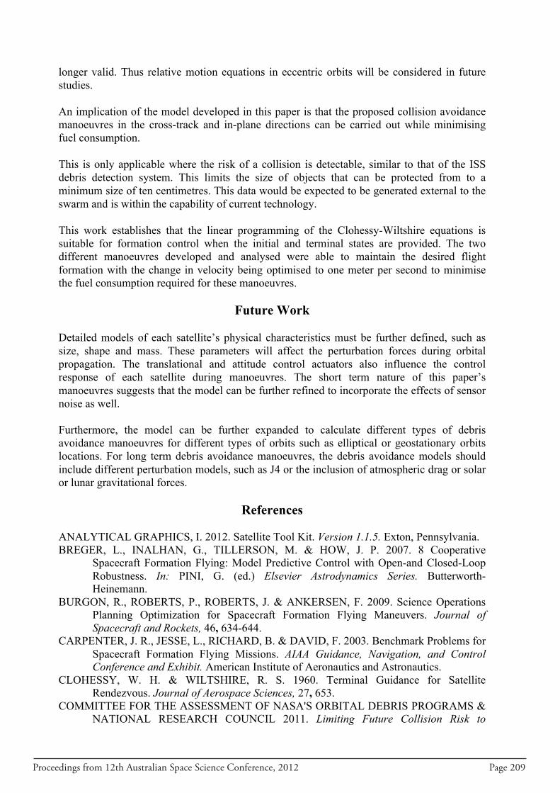
Proceedings from 12th Australian Space Science Conference, 2012 Page 209
longer valid. Thus relative motion equations in eccentric orbits will be considered in future studies. An implication of the model developed in this paper is that the proposed collision avoidance manoeuvres in the cross-track and in-plane directions can be carried out while minimising fuel consumption. This is only applicable where the risk of a collision is detectable, similar to that of the ISS debris detection system. This limits the size of objects that can be protected from to a minimum size of ten centimetres. This data would be expected to be generated external to the swarm and is within the capability of current technology. This work establishes that the linear programming of the Clohessy-Wiltshire equations is suitable for formation control when the initial and terminal states are provided. The two different manoeuvres developed and analysed were able to maintain the desired flight formation with the change in velocity being optimised to one meter per second to minimise the fuel consumption required for these manoeuvres.
Future Work Detailed models of each satellite’s physical characteristics must be further defined, such as size, shape and mass. These parameters will affect the perturbation forces during orbital propagation. The translational and attitude control actuators also influence the control response of each satellite during manoeuvres. The short term nature of this paper’s manoeuvres suggests that the model can be further refined to incorporate the effects of sensor noise as well. Furthermore, the model can be further expanded to calculate different types of debris avoidance manoeuvres for different types of orbits such as elliptical or geostationary orbits locations. For long term debris avoidance manoeuvres, the debris avoidance models should include different perturbation models, such as J4 or the inclusion of atmospheric drag or solar or lunar gravitational forces.
References ANALYTICAL GRAPHICS, I. 2012. Satellite Tool Kit. Version 1.1.5. Exton, Pennsylvania. BREGER, L., INALHAN, G., TILLERSON, M. & HOW, J. P. 2007. 8 Cooperative
Spacecraft Formation Flying: Model Predictive Control with Open-and Closed-Loop Robustness. In: PINI, G. (ed.) Elsevier Astrodynamics Series. Butterworth-Heinemann.
BURGON, R., ROBERTS, P., ROBERTS, J. & ANKERSEN, F. 2009. Science Operations Planning Optimization for Spacecraft Formation Flying Maneuvers. Journal of Spacecraft and Rockets, 46, 634-644.
CARPENTER, J. R., JESSE, L., RICHARD, B. & DAVID, F. 2003. Benchmark Problems for Spacecraft Formation Flying Missions. AIAA Guidance, Navigation, and Control Conference and Exhibit. American Institute of Aeronautics and Astronautics.
CLOHESSY, W. H. & WILTSHIRE, R. S. 1960. Terminal Guidance for Satellite Rendezvous. Journal of Aerospace Sciences, 27, 653.
COMMITTEE FOR THE ASSESSMENT OF NASA'S ORBITAL DEBRIS PROGRAMS & NATIONAL RESEARCH COUNCIL 2011. Limiting Future Collision Risk to
Page 210 Proceedings from 12th Australian Space Science Conference, 2012
Spacecraft:An Assessment of NASA's Meteoroid and Orbital Debris Programs, The National Academies Press.
COMMITTEE ON SPACE DEBRIS & NATIONAL RESEARCH COUNCIL 1995. Orbital Debris:A Technical Assessment, The National Academies Press.
DADKHAH, N., RODRIGUES, L. & AGHDAM, A. G. Satellite Formation Flying Controller Design Using an Optimal Decentralized Approach. American Control Conference, 2007. ACC '07, 9-13 July 2007 2007. 3162-3167.
DAN, M., FRED, H., LARS, B., DAVID, B., SOON-JO, C. & BEHCET, A. 2011. Swarm Keeping Strategies for Spacecraft under J2 and Atmospheric Drag Perturbations. AIAA Guidance, Navigation, and Control Conference. American Institute of Aeronautics and Astronautics.
DARPA SYSTEM F5 PROGRAM 2012. Program Images. In: F6_TOPGRAPHIC01_LANDSCAPE-1.JPG (ed.). DARPA Tactical Technology Office.
HILL, G. W. 1878. Researches in the Lunar Theory. American Journal of Mathematics 1, 5-26.
KAHLE, R., SCHLEPP, B., AIDA, S., KIRSCHNER, M. & WERMUTH, M. 2012. Flight Dynamics Operations of the TanDEM-X Formation. American Institute of Aeronautics and Astronautics.
KAPILAL, V., SPARKS, A. G., BUFFINGTON, J. M. & QIGUO, Y. Spacecraft formation flying: dynamics and control. American Control Conference, 1999. Proceedings of the 1999, 1999 1999. 4137-4141 vol.6.
KESSLER, D. J. & COUR-PALAIS, B. G. 1978. Collision frequency of artificial satellites: The creation of a debris belt. Journal of Geophysical Research: Space Physics, 83, 2637-2646.
MICHAEL, A., BARO, H., JOHN, C. & RICHARD, L. 2008. Deterministic Relative Attitude Determination of Formation Flying Spacecraft. AIAA/AAS Astrodynamics Specialist Conference and Exhibit. American Institute of Aeronautics and Astronautics.
MIETTINEN, K. 1998. Nonlinear Multiobjective Optimization, Springer. QUAN, H. & CHAO, H. 2008. Dynamics and Control of Satellite Formation Flying Based on
Relative Orbit Elements. AIAA Guidance, Navigation and Control Conference and Exhibit. American Institute of Aeronautics and Astronautics.
REX, D., BENDISCH, J., EICHLER, P. & ZHANG, J. 1991. Protecting and manoeuvring of spacecraft in space debris environment. Advances in Space Research, 11, 53-62.
ROBERTSONY, A., INALHANZ, G. & HOW, J. P. Spacecraft formation flying control design for the Orion mission AIAA Guidance, Navigation, and Control Conference and Exhibit, Aug. 9-11 1999 Portland, OR.
ROSSI, A. & VALSECCHI, G. 2006. Collision risk against space debris in Earth orbits. Celestial Mechanics and Dynamical Astronomy, 95, 345-356.
SABATINI, M. & PALMERINI, G. B. Linearized Formation-Flying Dynamics in a Perturbed Orbital Environment. Aerospace Conference, 2008 IEEE, 1-8 March 2008 2008. 1-13.
SÁNCHEZ-ORTIZ, N., BELLÓ-MORA, M. & KLINKRAD, H. 2006. Collision avoidance manoeuvres during spacecraft mission lifetime: Risk reduction and required ΔV. Advances in Space Research, 38, 2107-2116.
SLATER, G. L., BYRAM, S. M. & WILLIAMS, T. W. 2006. Collision avoidance for satellites in formation flight, Reston, VA, ETATS-UNIS, American Institute of Aeronautics and Astronautics.
TIN DUC, L., FURUSAWA, K. & HAYAKAWA, T. Orbital formation control of multiple spacecraft. American Control Conference (ACC), 2010, June 30 2010-July 2 2010 2010. 3636-3641.
Proceedings from 12th Australian Space Science Conference, 2012 Page 211
Qualitative Analysis of the Kinematics of a Torque-free Gyrousing Multiple Coordinate Frames
Ahmad S. Mohd Harithuddin∗†, Pavel M. Trivailo∗ and Reza N. Jazar∗
∗ School of Aerospace, Mechanical and Manufacturing Engineering RMIT University, VIC,Australia, 3083
† Department of Aerospace Engineering, Universiti Putra Malaysia, Serdang, Selangor,Malaysia, 43400
Summary: Spacecraft motion around a gravitational body often exhibits gyroscopic motion.The kinematical analysis of such motion presents problems in the calculation of displacementsand accelerations due to the interaction of the compound rotations. The inertia loading fromthe gyroscopic motion can cause oscillating forces that may contribute to overstressing andfatigue damage on bearings and mountings of structures e.g. tracking solar arrays, pointingantennas, and manipulators. It is, therefore, necessary to accurately evaluate the kinematicsto ensure the safety of the spacecraft’s structural design and components. In this paper, themodel of the spacecraft under consideration is that of a gyro upon which no external torque isacting. We use multiple coordinate frames to break down the complex gyroscopic motion intoseveral simpler rotations. We present the mathematical constructs used to represent the vectorderivatives for systems with multiple coordinate frames. The formulation is then applied toextract and evaluate the velocity and acceleration of an arbitrary point on the gyro. A numericalexample illustrates the methodology. The results from this paper give valuable insight onto theinternal factors that can affect spacecraft and gyro mechanisms, contribute to the stress-straindesign of their components, and ultimately enhance their characteristics.
Keywords: spacecraft structures, gyroscopic motion, precession, spin, inertia loading, Raziacceleration, vector derivative, coordinate frames.
I. Introduction
Moving structures and mechanisms are always subjected to inertia body forces whichresulted from body acceleration and rotational motion with respect to the inertial referenceframe. Among the common inertia forces in a fixed-axis rotation are caused by fictitiousor inertial accelerations such as centripetal and Coriolis accelerations. These forces maygenerate oscillatory forces causing unwanted loading on structures. In, compund/enclosedrotation motion where the axis rotation is not fixed - e.g. gyroscopic motion or precessionalmotion - the simple rotation analysis is not sufficient in calculating the inertia body forces asfictitious accelerations become more complex and not intuitive. A rigid body that is undergoingsuch motion is referred in this paper as a gyro.
Evaluating inertia forces acting on bodies under compound/enlcosed rotation is importantas such forces affects the displacements and stress-strain loading on the structures. Anderson[1] analyzed the kinematics of a nutating plate transmission to derive the inertial momentequations. However, most of the analysis is done using scalar variables which does not give
Page 212 Proceedings from 12th Australian Space Science Conference, 2012
a good intuition of the directions of the resulting acceleration and results in cumbersomekinematic equations. Barlow [2] stressed the significance of inertia loading on structures undercompound motion (multiple rotations) and included its calculation to improve the numericalanalysis of a turbo-fan blade loading. The study of the effects of inertial acceleration onvibration is also done by Gulyaev for conical shells [3] and twin-bladed rotors [4] in compoundmotion. His works, however, are more focused towards the vibrational qualities rather thanthe kinematics analysis.
The effects of inertial acceleration on space structures has also been considered, especiallyregarding the extendable appendages of the spacecraft. A boom may be deployed from aspacecraft while it is still rotating, which makes the boom structure subject to centrifugaland Coriolis acceleration. While the centrifugal force may help to speed up the deploymentprocess, it can cause excessive strain loading and over-extension to the boom [5]. The Coriolisforce, due to the combined translational and rotational motion of the deployed structure, causesbending-type loading. The Coriolis force has also been determined as one of the causes ofthe large deformation of deployed space tether [6]. No consideration has been made for theinertial acceleration caused by the Razi acceleration, which may exist in spacecraft undercompound/enclosed rotation.
Jazar [7] reviewed the inertial/fictitious acceleration concept using the derivative transforma-tion formula between two relatively moving coordinate frames (which is introduced by Euler[8]). Extending the formula for the case where three relatively rotating coordinate framesare used, Jazar found a new acceleration term that can exist in compound rotation motion,which is called the Razi acceleration. This inertial acceleration is analogous to centripetalacceleration (away from the center of rotation) but instead, it is acting to the out-of-planedirection of the rotation plane. This can be attributed to the ”wobbling” motion of a rigidbody in compound rotation motion.
In this present study, we want to apply the finding into practical application in spacecraftdynamics. An axisymmetrical gyro under compound rotation motion in space is consideredas a simple representation of a spacecraft. The motion under consideration is a torque-freemotion, which means there is no external torque acting on the gyro. The kinematics is analyzedusing three coordinate frames to decompose the complex motion: the body-frame which takesinto account the spin motion, the precession frame and the global frame. Under the compoundrotation motion, the Razi acceleration is calculated as to evaluate the characteristic of inertialoading acting on the structures of the spacecraft.
Section II of this paper shows the derivation and the characterisics of the Razi accelerationbased on the works by [7] with a demonstrative example. Section III is dedicated to findingthe relationship between the Razi acceleration and the rigid body motion of an axisymmetric,torque-free gyro. Section IV shows an illustrative example on how magnitude of the Raziacceleration depends on the gyro’s spin rate and its inertia properties. Section IV concludesthe paper.
II. Razi Acceleration
In classical mechanics, an inertial frame is a reference point-of-view where space andtime are homogeneous and isotropic. This frame is sometimes called global-fixed frame, to
Proceedings from 12th Australian Space Science Conference, 2012 Page 213
indicate that it is static and fixed with respect to a moving system. To describe a mechanicalsystem, it is simpler to represent its kinematics and dynamics in its own body-fixed framewhich is different from the inertial frame. The non-inertial reference frame can be translatingand rotating with respect to the inertial frame, resulting in extra terms in the equations thatdescribes the law of motion, which is called fictitious or inertial accelerations [7, 8].
Mixed Double Derivative
Consider three relatively rotating coordinate frames A(OxAyAzA), B(OxByBzB), and C(OxCyCzC),with all three sharing the same origin O. The A-frame is rotating with respect to the B-framewhile the B-frame is rotating inside the global-fixed frame C. For a general vector r expressedin frame A, the first-derivative expression of the vector in another frame, e.g. frame B, canbe written as,
Bd
dtAr =
Ad
dtAr+ A
BωA × Ar (1)
where ABωA is the angular velocity of the frame A with respect to B. This is the first-derivative
(velocity) of a point in A as seen from B. The second-derivative expression is the derivativeof Equation (1) from the frame B
Bd
dt
Bd
dtAr =
Ad
dt
Ad
dtAr+ A
BωA × Ar+ 2ABωA ×Ad
dtAr+ A
BωA ×(ABωA × Ar
)(2)
This is the double-derivative (acceleration) of a point in A as seen from B. Letting the genericvector r be a position vector, the terms on right-hand side of Equation (2) shows the absoluteacceleration of r in A, the angular acceleration, the Coriolis acceleration, and the centripetalacceleration respectively.
The mixed double acceleration is expressed when the second derivative of Equation (1)is taken from a different frame C. To obtain the mixed double acceleration, we differentiateEquation (1) with respect to the frame C
Cd
dt
Bd
dtAr =
Cd
dt
(Ad
dtAr
)+
Cd
dt
(ABωA × Ar
)
=Ad
dt
Ad
dtAr+ A
CωA ×Ad
dtAr+
(Ad
dtABωA + A
CωA × ABωA
)× Ar
+ ABωA ×
(Ad
dtAr+ A
CωA × Ar
)
=Ad
dt
Ad
dtAr+ A
BωA × Ar+ ACωA ×
Ad
dtAr+ A
BωA ×Ad
dtAr+ A
BωA ×(ACωA × Ar
)
+(ACωA × A
BωA
)× Ar
(3)
where ACωA is the angular velocity of the frame A with respect to C. According to the angular
velocity addition rule, this angular velocity can be equated as the sum of the angular velocityof the frame B with respect to C and the angular velocity of the frame A with respect to B.
ACωA = A
CωB + ABωA (4)
Equation (3) contains several familiar forms such as the absolute acceleration, the tangentialacceleration (a cross product of the angular acceleration vector and the position vector), the
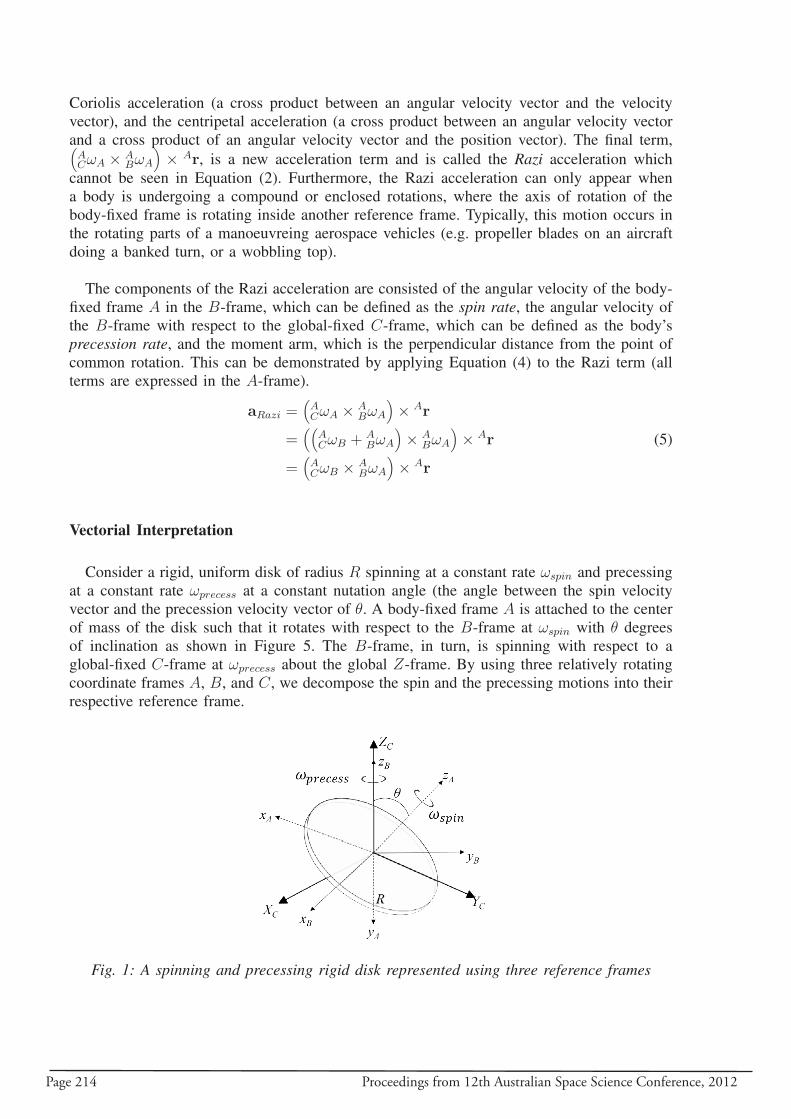
Page 214 Proceedings from 12th Australian Space Science Conference, 2012
Coriolis acceleration (a cross product between an angular velocity vector and the velocityvector), and the centripetal acceleration (a cross product between an angular velocity vectorand a cross product of an angular velocity vector and the position vector). The final term,(ACωA × A
BωA
)× Ar, is a new acceleration term and is called the Razi acceleration which
cannot be seen in Equation (2). Furthermore, the Razi acceleration can only appear whena body is undergoing a compound or enclosed rotations, where the axis of rotation of thebody-fixed frame is rotating inside another reference frame. Typically, this motion occurs inthe rotating parts of a manoeuvreing aerospace vehicles (e.g. propeller blades on an aircraftdoing a banked turn, or a wobbling top).
The components of the Razi acceleration are consisted of the angular velocity of the body-fixed frame A in the B-frame, which can be defined as the spin rate, the angular velocity ofthe B-frame with respect to the global-fixed C-frame, which can be defined as the body’sprecession rate, and the moment arm, which is the perpendicular distance from the point ofcommon rotation. This can be demonstrated by applying Equation (4) to the Razi term (allterms are expressed in the A-frame).
aRazi =(ACωA × A
BωA
)× Ar
=((
ACωB + A
BωA
)× A
BωA
)× Ar
=(ACωB × A
BωA
)× Ar
(5)
Vectorial Interpretation
Consider a rigid, uniform disk of radius R spinning at a constant rate ωspin and precessingat a constant rate ωprecess at a constant nutation angle (the angle between the spin velocityvector and the precession velocity vector of θ. A body-fixed frame A is attached to the centerof mass of the disk such that it rotates with respect to the B-frame at ωspin with θ degreesof inclination as shown in Figure 5. The B-frame, in turn, is spinning with respect to aglobal-fixed C-frame at ωprecess about the global Z-frame. By using three relatively rotatingcoordinate frames A, B, and C, we decompose the spin and the precessing motions into theirrespective reference frame.
Fig. 1: A spinning and precessing rigid disk represented using three reference frames
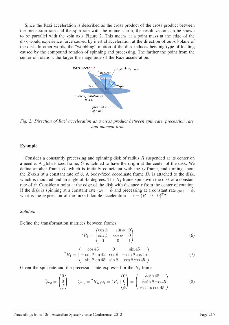
Proceedings from 12th Australian Space Science Conference, 2012 Page 215
Since the Razi acceleration is described as the cross product of the cross product betweenthe precession rate and the spin rate with the moment arm, the result vector can be shownto be parrallel with the spin axis Figure 2. This means at a point mass at the edge of thedisk would experience force caused by inertial acceleration at the direction of out-of-plane ofthe disk. In other words, the ”wobbling” motion of the disk induces bending type of loadingcaused by the compound rotation of spinning and precessing. The farther the point from thecenter of rotation, the larger the magnitude of the Razi acceleration.
Fig. 2: Direction of Razi acceleration as a cross product between spin rate, precession rate,and moment arm
Example
Consider a constantly precessing and spinning disk of radius R suspended at its center ona needle. A global-fixed frame, G is defined to have the origin at the center of the disk. Wedefine another frame B1 which is initially coincident with the G-frame, and turning aboutthe Z-axis at a constant rate of φ. A body-fixed coordinate frame B2 is attached to the disk,which is mounted and an angle of 45 degrees. The B2-frame spins with the disk at a constantrate of ψ. Consider a point at the edge of the disk with distance r from the center of rotation.If the disk is spinning at a constant rate 1ω2 = ψ and precessing at a constant rate Gω1 = φ,what is the expression of the mixed double acceleration at r = (R 0 0)T ?
Solution
Define the transformation matrices between frames
GR1 =
cosφ − sinφ 0sinφ cosφ 00 0 1
(6)
2R1 =
cos 45 0 sin 45− sin θ sin 45 cos θ − sin θ cos 45− sin θ sin 45 sin θ cos θ cos 45
(7)
Given the spin rate and the precession rate expressed in the B2-frame
21ω2 =
00
ψ
2
Gω1 =2R1
1Gω1 =
2R1
00
φ
=
φ sin 45
−φ sin θ cos 45
φ cos θ cos 45
(8)
Page 216 Proceedings from 12th Australian Space Science Conference, 2012
Using Equation (3), the mixed acceleration of a fixed body point as expressed in the B2
coordinate is
2amixed =Gd
dt
1d
dt2r = 2
1ω2 ×(2Gω2 × 2r
)+
(2Gω2 × 2
1ω2
)× 2r
=((
2Gω1 +
21ω2
)× 2
1ω2
)× 2r+ 2
1ω2 ×((
2Gω1 +
21ω2
))× 2r
=(2Gω1 × 2
1ω2
)× 2r+ 2
1ω2 ×((
2Gω1 +
21ω2
)× 2r
)
=
00
φψR sin 45
+
−ψR
(ψ + φ cos θ cos 45
)
00
(9)
From Equation (9), we could see that the Razi acceleration acts in the z2 direction, providingout-of-plane inertial loading to the disk structure. This type of inertial loading is also dis-cussed in [2, 3, 4]. The other acceleration in the x2-direction is called the mixed centripetalacceleration [7], which has no particular importance in this study.
III. Torque-Free Motion
In this section, we want to relate the inertial loading caused by the Razi acceleration tothe structures of an axisymmetric gyro in space. The motion is assumed to be free of anyexternal torque. At the end of this section, we look to find the relationship between the spinrate and the precession rate of this specific case, and use this information to find the Raziacceleration acting on the external structures of the spacecraft, e.g. boom, antenna, tether,which are extruded perpendicular to the body’s spin-axis (x-y direction).
Euler Rotational Equations of Motion
Consider a rigid body B(Oxyz) with its center of mass O fixed in a global coordinateframe G. The rotational equations of motion of such body can be expressed in the body-fixedframe as
BM = BJBGωB + B
GωB × BJBGωB (10)
where M is the 3-by-1 external moment vector. The distribution of mass of a rigid body inspace about a body-fixed frame with the point of origin O at its center of mass is denotedby a symmetric 3-by-3 matrix called the inertia matrix J
J =
Jxx Jxy JxzJyx Jyy JyzJzx Jzy Jzz
(11)
and the angular velocity vector of the rigid body with respect to the global-fixed frame isdenoted by
ω =
ωx
ωy
ωz
(12)
Proceedings from 12th Australian Space Science Conference, 2012 Page 217
Equation (10) can be expressed in scalar form, respective of the basis vectors (x, y, z) as
Jxωx − (Jy − Jz)ωyωz = Mx
Jyωy − (Jz − Jx)ωzωx = My
Jzωz − (Jx − Jy)ωxωy = Mz
(13)
The orientation and angular velocity of the rigid body B in the global frame G can berepresented by using three methods [7]: (1) A set of Euler angles and Euler frequencies (2)Euler parameters, which also cover the quaternion expressions, and (3) rotation about theCartesian body-fixed frame. The most commonly used expression for the motion for rigidbodies are the Euler frequencies. While Euler angles are directly measurable from gyroscopereadings (used in aerospace vehicles), the angles and their frequencies relation to the motionof a rigid body are not intuitive. Euler parameters, due to its computational efficiency, ismore used for computer graphics application than analytical kinematics of rigid bodies. Torelate the inertial acceleration acting on the spacecraft and to maintain the same conventionused in the derivation of the Razi acceleration, we use the third method. Using the rotationof the body-fixed frame provides more intuition of its relative motion with respect to theglobal-fixed frame. To make the method more efficient, we introduce three different framesas demonstrated in the previous section.
Spin and Precession Relation of a Torque-free Axisymmetric Body
For an axisymmetrical rigid body, the inertia matrix is presented as follows
J =
J 0 00 J 00 0 Jzz
(14)
where the z-axis of the body-fixed coordinate is the axis of symmetry (thus, Jxx = Jyy = J),and all the non-diagonal elements are zero. Since, in this present study, no external torque areapplied on the body, the external moment M is zero. Therefore, Euler’s rotational equationsof motion in Equation (13) become
Jωx − (J − Jz)ωyωz = 0
Jωy − (Jz − J)ωzωx = 0
Jzωz = 0
(15)
Considering a 3-1-3 Euler sequence with the rates of ψ (spin), φ (precession), and θ (nutation),the angular velocity of the body B with respect to the G-frame can be expressed in Eulerangles as
ω1
ω2
ω3
=
sin θ sinψ cosψ 0sin θ cosψ − sinψ 0
cos θ 0 1
φ
θ
ψ
(16)
Letting the nutation rate to be zero,ω1
ω2
ω3
=
φ sin θ sinψ
φ sin θ cosψ
φ cos θ + ψ
(17)
Page 218 Proceedings from 12th Australian Space Science Conference, 2012
The relation between the precession rate (φ) and the spin rate (ψ) is
φ =J3
J − J3 cos θψ (18)
We can relate the spin rate and precession rate expressions in Equation (18) with ABωA and
ACωB respectively.
ABωA =
00
ψ
(19)
ACωB =
00
φ
=
00
J3(J−J3) cos θ
ψ
(20)
Applying Equation (19) and Equation (20) into Equation (5), we obtain the scalar represen-tation of the Razi acceleration for an axisymmetric gyro
aRazi =J3
(J − J3) cos θψ2 sin θ (21)
To further reduce the amount of variables, we introduce the parameter called oblateness, f
f =J3 − J
J3(22)
Equation (21) becomes
aRazi = − 1
f cos θψ2 sin θ (23)
Note that at θ = 0, there is no precession thus the Razi acceleration does not exist accordingto Equation (5) and at θ = 90o, body spin does not occur for a torque-motion.
IV. Example and Result
The Razi effect on a gyro is demonstrated in the following example. An orbiting spacecraftcan experience compound rotation motion (spin and precession) before it is stabilized byits attitude control system. This example investigates the magnitude of the inertial loadingcaused by the Razi acceleration during this motion. As seen in the previous section, the Raziacceleration depends on the spin rate and the precession rate of the rigid body, as well as thenutation angle between the two angular rates. This example focuses on a simplified version ofa spacecraft with an axisymmetric body so that its precession rate can be related to the spinrate depending on its inertia properties (J and J3 in Equation (18)). Therefore, the magnitudeof the Razi acceleration acting on a point on the spacecraft (or its appendages) away fromthe center of rotation can be determined as a function of the spin rate, the inertia propertiesand the nutation angle.
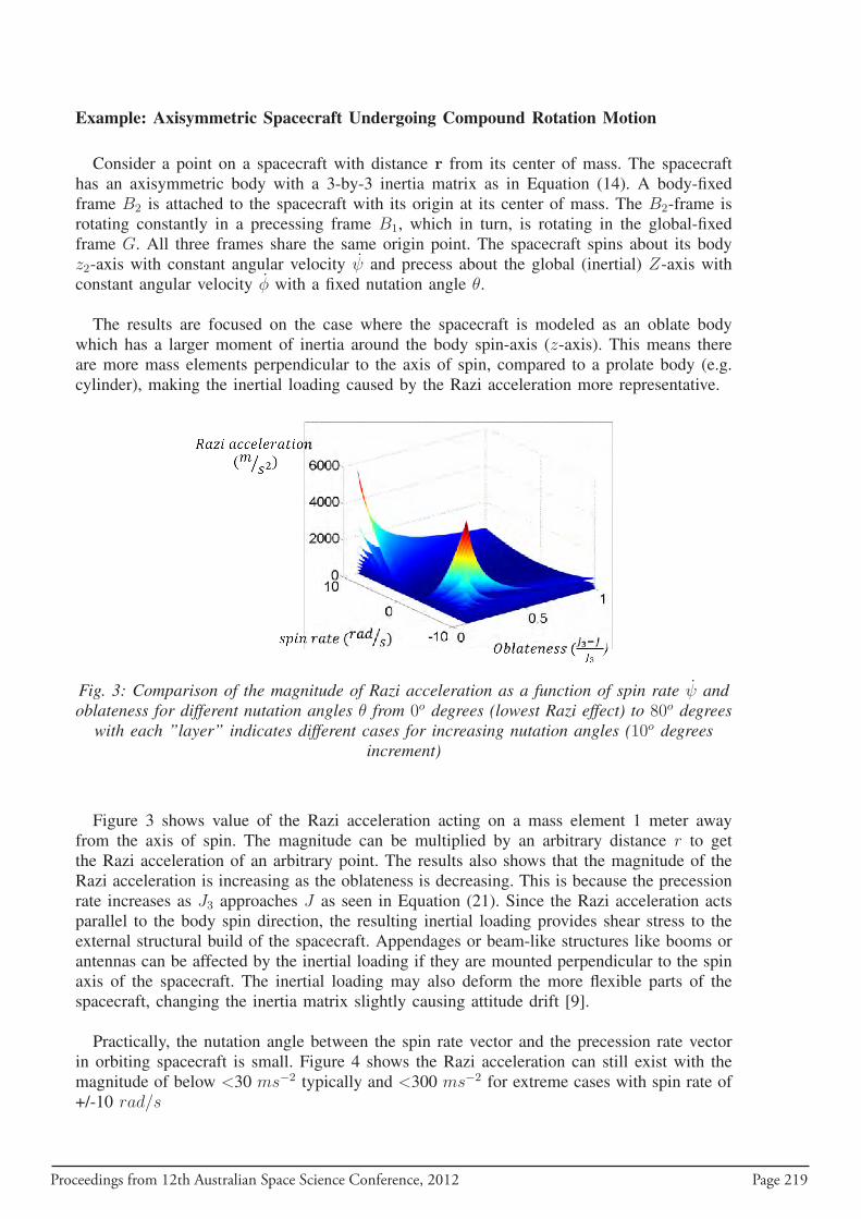
Proceedings from 12th Australian Space Science Conference, 2012 Page 219
Example: Axisymmetric Spacecraft Undergoing Compound Rotation Motion
Consider a point on a spacecraft with distance r from its center of mass. The spacecrafthas an axisymmetric body with a 3-by-3 inertia matrix as in Equation (14). A body-fixedframe B2 is attached to the spacecraft with its origin at its center of mass. The B2-frame isrotating constantly in a precessing frame B1, which in turn, is rotating in the global-fixedframe G. All three frames share the same origin point. The spacecraft spins about its bodyz2-axis with constant angular velocity ψ and precess about the global (inertial) Z-axis withconstant angular velocity φ with a fixed nutation angle θ.
The results are focused on the case where the spacecraft is modeled as an oblate bodywhich has a larger moment of inertia around the body spin-axis (z-axis). This means thereare more mass elements perpendicular to the axis of spin, compared to a prolate body (e.g.cylinder), making the inertial loading caused by the Razi acceleration more representative.
Fig. 3: Comparison of the magnitude of Razi acceleration as a function of spin rate ψ andoblateness for different nutation angles θ from 0o degrees (lowest Razi effect) to 80o degrees
with each ”layer” indicates different cases for increasing nutation angles (10o degreesincrement)
Figure 3 shows value of the Razi acceleration acting on a mass element 1 meter awayfrom the axis of spin. The magnitude can be multiplied by an arbitrary distance r to getthe Razi acceleration of an arbitrary point. The results also shows that the magnitude of theRazi acceleration is increasing as the oblateness is decreasing. This is because the precessionrate increases as J3 approaches J as seen in Equation (21). Since the Razi acceleration actsparallel to the body spin direction, the resulting inertial loading provides shear stress to theexternal structural build of the spacecraft. Appendages or beam-like structures like booms orantennas can be affected by the inertial loading if they are mounted perpendicular to the spinaxis of the spacecraft. The inertial loading may also deform the more flexible parts of thespacecraft, changing the inertia matrix slightly causing attitude drift [9].
Practically, the nutation angle between the spin rate vector and the precession rate vectorin orbiting spacecraft is small. Figure 4 shows the Razi acceleration can still exist with themagnitude of below <30 ms−2 typically and <300 ms−2 for extreme cases with spin rate of+/-10 rad/s
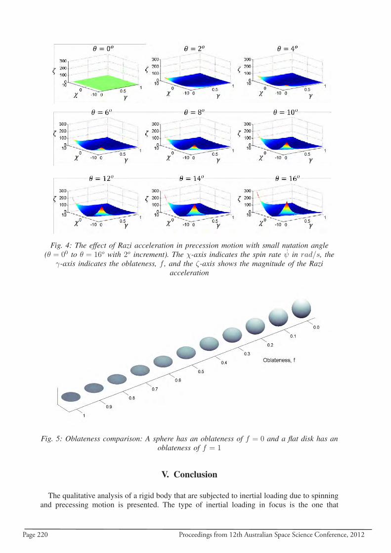
Page 220 Proceedings from 12th Australian Space Science Conference, 2012
Fig. 4: The effect of Razi acceleration in precession motion with small nutation angle(θ = 00 to θ = 16o with 2o increment). The χ-axis indicates the spin rate ψ in rad/s, the
γ-axis indicates the oblateness, f , and the ζ-axis shows the magnitude of the Raziacceleration
Fig. 5: Oblateness comparison: A sphere has an oblateness of f = 0 and a flat disk has anoblateness of f = 1
V. Conclusion
The qualitative analysis of a rigid body that are subjected to inertial loading due to spinningand precessing motion is presented. The type of inertial loading in focus is the one that
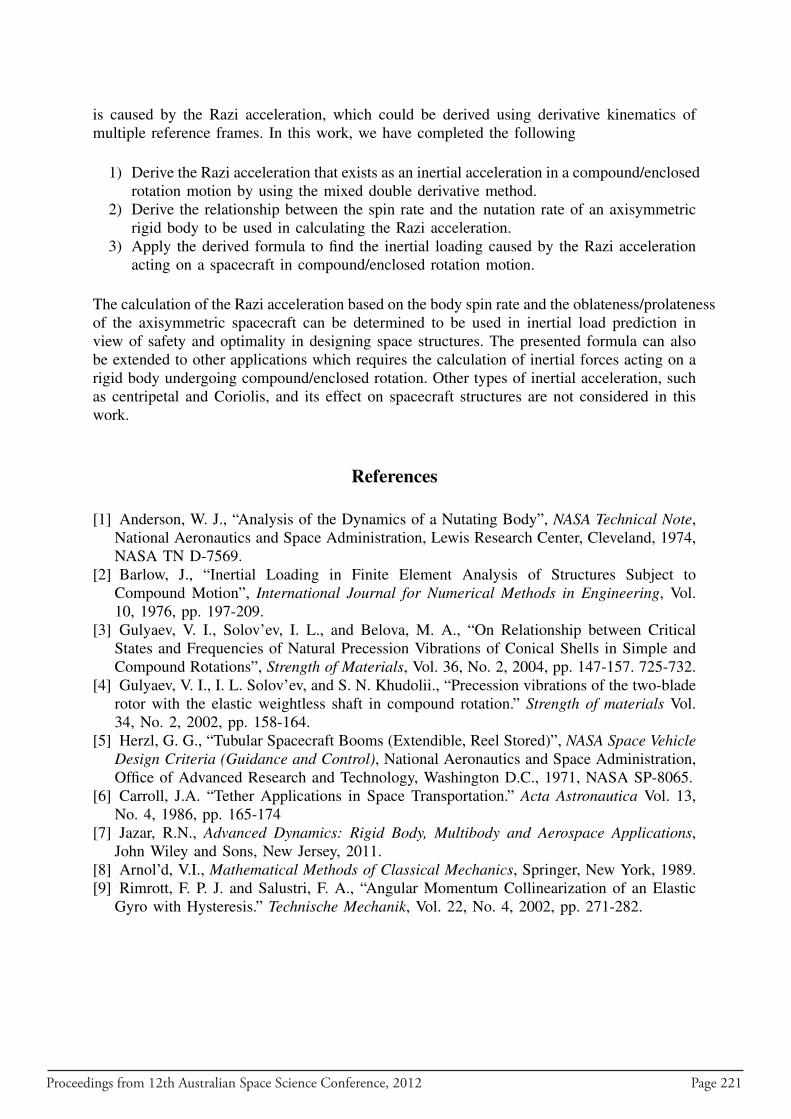
Proceedings from 12th Australian Space Science Conference, 2012 Page 221
is caused by the Razi acceleration, which could be derived using derivative kinematics ofmultiple reference frames. In this work, we have completed the following
1) Derive the Razi acceleration that exists as an inertial acceleration in a compound/enclosedrotation motion by using the mixed double derivative method.
2) Derive the relationship between the spin rate and the nutation rate of an axisymmetricrigid body to be used in calculating the Razi acceleration.
3) Apply the derived formula to find the inertial loading caused by the Razi accelerationacting on a spacecraft in compound/enclosed rotation motion.
The calculation of the Razi acceleration based on the body spin rate and the oblateness/prolatenessof the axisymmetric spacecraft can be determined to be used in inertial load prediction inview of safety and optimality in designing space structures. The presented formula can alsobe extended to other applications which requires the calculation of inertial forces acting on arigid body undergoing compound/enclosed rotation. Other types of inertial acceleration, suchas centripetal and Coriolis, and its effect on spacecraft structures are not considered in thiswork.
References
[1] Anderson, W. J., “Analysis of the Dynamics of a Nutating Body”, NASA Technical Note,National Aeronautics and Space Administration, Lewis Research Center, Cleveland, 1974,NASA TN D-7569.
[2] Barlow, J., “Inertial Loading in Finite Element Analysis of Structures Subject toCompound Motion”, International Journal for Numerical Methods in Engineering, Vol.10, 1976, pp. 197-209.
[3] Gulyaev, V. I., Solov’ev, I. L., and Belova, M. A., “On Relationship between CriticalStates and Frequencies of Natural Precession Vibrations of Conical Shells in Simple andCompound Rotations”, Strength of Materials, Vol. 36, No. 2, 2004, pp. 147-157. 725-732.
[4] Gulyaev, V. I., I. L. Solov’ev, and S. N. Khudolii., “Precession vibrations of the two-bladerotor with the elastic weightless shaft in compound rotation.” Strength of materials Vol.34, No. 2, 2002, pp. 158-164.
[5] Herzl, G. G., “Tubular Spacecraft Booms (Extendible, Reel Stored)”, NASA Space VehicleDesign Criteria (Guidance and Control), National Aeronautics and Space Administration,Office of Advanced Research and Technology, Washington D.C., 1971, NASA SP-8065.
[6] Carroll, J.A. “Tether Applications in Space Transportation.” Acta Astronautica Vol. 13,No. 4, 1986, pp. 165-174
[7] Jazar, R.N., Advanced Dynamics: Rigid Body, Multibody and Aerospace Applications,John Wiley and Sons, New Jersey, 2011.
[8] Arnol’d, V.I., Mathematical Methods of Classical Mechanics, Springer, New York, 1989.[9] Rimrott, F. P. J. and Salustri, F. A., “Angular Momentum Collinearization of an Elastic
Gyro with Hysteresis.” Technische Mechanik, Vol. 22, No. 4, 2002, pp. 271-282.

Page 222 Proceedings from 12th Australian Space Science Conference, 2012
Proceedings from 12th Australian Space Science Conference, 2012 Page 223
Designing a Navigational Control System of an AutonomousRobot for Multi-requirements Planetary Navigation using
Evolutionary Algorithms Approaches
Mohd Faisal Ibrahim and Bradley Alexander
School of Computer Science, The University of Adelaide, SA, Australia, 5005
Summary: As space missions become more complex, the need for autonomous behavior inplanetary rovers increases. Given a complex unknown environment and approximate sensorinformation, rovers must make their own navigational decisions to maximise exploration speedwhilst conserving power and preserving safety. Designing handwritten control to optimisethese factors from first principles is difficult. The alternative of using standard search algo-rithms for good control settings is made difficult by natural variability in the performanceof the system. A search method able to handle this variability is required. We present anevolutionary algorithm (EA) approach to the design of control system for an autonomous non-holomic robot. We show that our approach is able to produce control parameters that producegood results in terms of navigational speed, hazard avoidance and power consumption. Wedemonstrate that control evolved under two evolutionary frameworks outperforms carefullyrefined handwritten control. Our framework produces a population of good control settingswhich opens the prospect of real-time selection and adaptation of control in future.
Keywords: Robotic planetary navigation, motion planner, evolutionary algorithms, gram-matical evolution, co-variance matrix adaptation evolutionary strategies.
Introduction
Autonomous mobile robots have enormous potential for safe and cost-effective study ofplanetary terrains. As missions become larger and more demanding in scope, the need forsafe and fast autonomous navigation of unknown environments increases. In performingexploration, robotic explorers must cope with incomplete knowledge, noisy sensor data andlimited power budgets. In these circumstances the design of good adaptive navigationalcontrol algorithms from first principles becomes difficult. Moreover, the use of standardsearch algorithms to optimise control settings is infeasible due, in part, to variations in theperformance of the system.
In this paper we explore the use of evolutionary algorithms (EA’s) in optimising settings forthe motion planner for an autonomous robot exploring unknown terrain. The motion plannerguides highly adaptive navigation by using a ranking equation to choose the best of a setof short range movements. The ranking equation responds to a number of signals condensedfrom field information gathered from the robot’s sensors. In this work we evolve parametersfor this ranking equation according to the performance they yield in simulation.
The contribution of this paper is twofold:-
Page 224 Proceedings from 12th Australian Space Science Conference, 2012
1) we provide a methodology for the automatic design of a motion planner throughevolutionary search.
2) we provide a preliminary comparative study of performance of simulated robotic plan-etary navigation using handwritten control system design and EA-based control systemdesign. We measure performance for multiple navigational criteria: speed of exploration;power consumption; and, critically, safety.
The remainder of this paper is structured as follows, the next section surveys related work.We follow with a section describing our EA-based control system design framework. Then,the evolutionary process is introduced. Then we summarise our results and the final sectionconcludes and describes potential future work.
Related work
One essential question in planetary navigation is : Given what you know about the world,where should you move to gain as much new information as possible? [1]. This requires thatthe robot navigate to unexplored areas. In order to complete the task, the navigational controlsystems are typically composed of several layers of control modules. One of them is motionplanner.
The motion planner receives an allocated long-range target point from a higher level modulethat attracts the robot toward an unexplored area. This module then performs traversabilityanalysis to evaluate several candidate short-range waypoints. In order to choose the bestwaypoint, the motion planner has to consider multiple navigational requirements. Most currentmotion planner strategies are based on fixed assumptions which makes it difficult adequatelycater for these navigational requirements, especially in systems with noisy and oscillatoryproximity data [10]. Early approaches to motion planner design are based on handwrit-ten control. This “white box” approach usually embeds mathematical models that performtraversability analysis. These approaches include: potential fields [2], vector field histograms[3], nearness diagrams [4] and rapidly-exploring random trees [5]. Although these approacheswork well for a fixed set of navigational requirements, extending them to cope with additionalrequirements entails considerable additional work. Moreover, as the number of navigationalrequirements increases, the space of possible control models increases exponentially – makinghand-derivation of control difficult. The additional factors of environmental uncertainty andsensor noise make this problem even worse.
In constrast, machine-learning approaches derive control based on real or simulated robotperformance. [6] describes a fuzzy logic behaviour-based control to assess traversabilityaccording to terrain complexity whilst seeking navigational goals. A neuro-evolutionary ap-proach is used in [7] to design an adaptive navigation policy in noisy environment. Bothapproaches show impressive improvement on navigation performance over conventional ap-proaches. However, these “black box” approaches suffer from an opaque control structurewhich hampers further extension and post-design analysis. A “white-box” genetic program-ming approach was used in [8] to cater multi-robot system navigation by taking into accountcollaboration state among robots. This evolutionary approach shows that the motion plannerstructure can be optimised by using a compreshensible mathematical function with welldefined parameters. The strategy in this paper differs in that we implement an improvedstructure for our motion planner with different variables to cater for planetary navigational
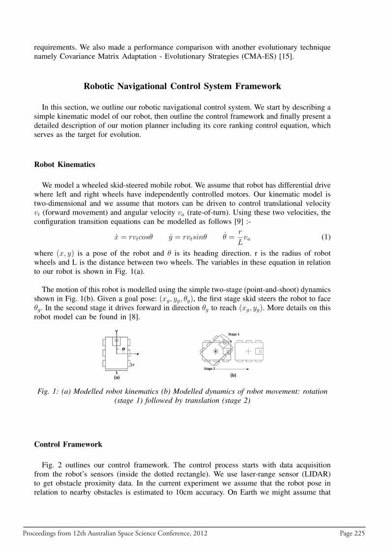
Proceedings from 12th Australian Space Science Conference, 2012 Page 225
requirements. We also made a performance comparison with another evolutionary techniquenamely Covariance Matrix Adaptation - Evolutionary Strategies (CMA-ES) [15].
Robotic Navigational Control System Framework
In this section, we outline our robotic navigational control system. We start by describing asimple kinematic model of our robot, then outline the control framework and finally present adetailed description of our motion planner including its core ranking control equation, whichserves as the target for evolution.
Robot Kinematics
We model a wheeled skid-steered mobile robot. We assume that robot has differential drivewhere left and right wheels have independently controlled motors. Our kinematic model istwo-dimensional and we assume that motors can be driven to control translational velocityvt (forward movement) and angular velocity va (rate-of-turn). Using these two velocities, theconfiguration transition equations can be modelled as follows [9] :-
x = rvtcosθ y = rvtsinθ θ =r
Lva (1)
where (x, y) is a pose of the robot and θ is its heading direction. r is the radius of robotwheels and L is the distance between two wheels. The variables in these equation in relationto our robot is shown in Fig. 1(a).
The motion of this robot is modelled using the simple two-stage (point-and-shoot) dynamicsshown in Fig. 1(b). Given a goal pose: (xg, yg, θg), the first stage skid steers the robot to faceθg. In the second stage it drives forward in direction θg to reach (xg, yg). More details on thisrobot model can be found in [8].
Fig. 1: (a) Modelled robot kinematics (b) Modelled dynamics of robot movement: rotation(stage 1) followed by translation (stage 2)
Control Framework
Fig. 2 outlines our control framework. The control process starts with data acquisitionfrom the robot’s sensors (inside the dotted rectangle). We use laser-range sensor (LIDAR)to get obstacle proximity data. In the current experiment we assume that the robot pose inrelation to nearby obstacles is estimated to 10cm accuracy. On Earth we might assume that
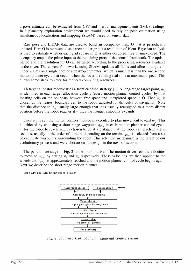
Page 226 Proceedings from 12th Australian Space Science Conference, 2012
a pose estimate can be extracted from GPS and inertial management unit (IMU) readings.In a planetary exploration environment we would need to rely on pose estimation usingsimultaneous localisation and mapping (SLAM) based on sensor data.
Raw pose and LIDAR data are used to build an occupancy map, O that is periodicallyupdated. Here O is represented as a rectangular grid at a resolution of 10cm. Bayesian analysisis used to estimate whether each grid square in O is either occupied, free or unexplored. Theoccupancy map is the prime input to the remaining parts of the control framework. The updateperiod and the resolution for O can be tuned according to the processing resources availableto the rover. The current framework, using SLAM, updates all fields and allocate targets inunder 200ms on a single core of a desktop computer1 which is much less than the one secondmotion planner cycle that occurs when the rover is running real-time at maximum speed. Thisallows some slack to cater for reduced computing resources.
Th target allocator module uses a frontier-based strategy [1]. A long-range target point, qtgis identified in each target allocation cycle g (every motion planner control cycles) by firstlocating cells on the boundary between free space and unexplored space in O. Then qtg ischosen as the nearest boundary cell to the robot, adjusted for difficulty of navigation. Notethat the distance to qtq usually large enough that it is usually reassigned to a more distantposition before the robot reaches it – thus the frontier smoothly expands.
Once qtg is set, the motion planner module is executed to plan movement toward qtg . Thisis achieved by choosing a short-range waypoint, qwm in each motion planner control cycle,m for the robot to reach. qwm is chosen to be at a distance that the robot can reach in a fewseconds, usually in the order of a metre depending on the terrain. qwm is selected from a setof candidate waypoints surrounding the robot. This selection mechanism is the target of ourevolutionary process and we elaborate on its design in the next subsection.
The penultimate stage in Fig. 2 is the motion driver. The motion driver sets the velocitiesto move to qwm by setting vt and va respectively. These velocities are then applied to thewheels until qwm is approximately reached and the motion planner control cycle begins again.Next we describe the short range motion planner.
1using GPS and IMU for navigation is faster
Fig. 2: Framework of robotic navigational control system
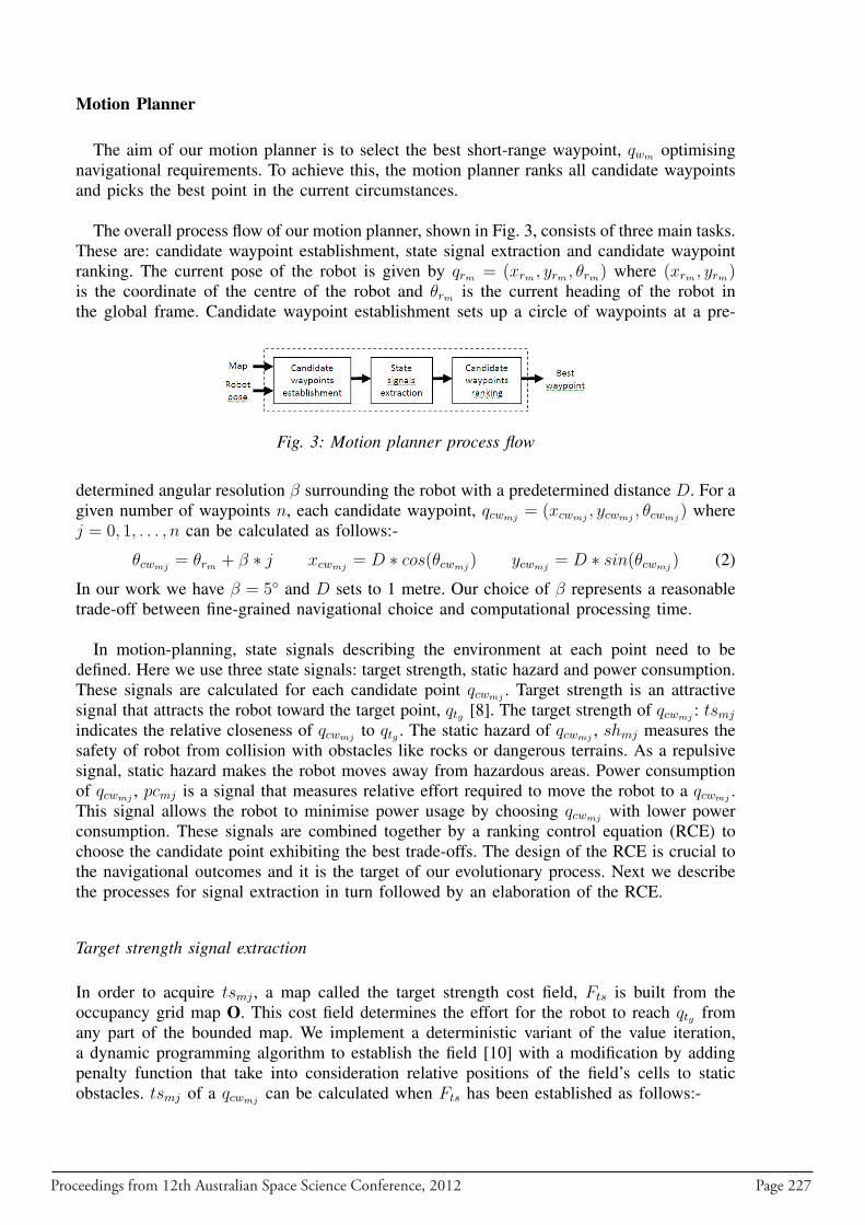
Proceedings from 12th Australian Space Science Conference, 2012 Page 227
Motion Planner
The aim of our motion planner is to select the best short-range waypoint, qwm optimisingnavigational requirements. To achieve this, the motion planner ranks all candidate waypointsand picks the best point in the current circumstances.
The overall process flow of our motion planner, shown in Fig. 3, consists of three main tasks.These are: candidate waypoint establishment, state signal extraction and candidate waypointranking. The current pose of the robot is given by qrm = (xrm , yrm , θrm) where (xrm , yrm)is the coordinate of the centre of the robot and θrm is the current heading of the robot inthe global frame. Candidate waypoint establishment sets up a circle of waypoints at a pre-
Fig. 3: Motion planner process flow
determined angular resolution β surrounding the robot with a predetermined distance D. For agiven number of waypoints n, each candidate waypoint, qcwmj
= (xcwmj, ycwmj
, θcwmj) where
j = 0, 1, . . . , n can be calculated as follows:-
θcwmj= θrm + β ∗ j xcwmj
= D ∗ cos(θcwmj) ycwmj
= D ∗ sin(θcwmj) (2)
In our work we have β = 5◦ and D sets to 1 metre. Our choice of β represents a reasonabletrade-off between fine-grained navigational choice and computational processing time.
In motion-planning, state signals describing the environment at each point need to bedefined. Here we use three state signals: target strength, static hazard and power consumption.These signals are calculated for each candidate point qcwmj
. Target strength is an attractivesignal that attracts the robot toward the target point, qtg [8]. The target strength of qcwmj
: tsmj
indicates the relative closeness of qcwmjto qtg . The static hazard of qcwmj
, shmj measures thesafety of robot from collision with obstacles like rocks or dangerous terrains. As a repulsivesignal, static hazard makes the robot moves away from hazardous areas. Power consumptionof qcwmj
, pcmj is a signal that measures relative effort required to move the robot to a qcwmj.
This signal allows the robot to minimise power usage by choosing qcwmjwith lower power
consumption. These signals are combined together by a ranking control equation (RCE) tochoose the candidate point exhibiting the best trade-offs. The design of the RCE is crucial tothe navigational outcomes and it is the target of our evolutionary process. Next we describethe processes for signal extraction in turn followed by an elaboration of the RCE.
Target strength signal extraction
In order to acquire tsmj , a map called the target strength cost field, Fts is built from theoccupancy grid map O. This cost field determines the effort for the robot to reach qtg fromany part of the bounded map. We implement a deterministic variant of the value iteration,a dynamic programming algorithm to establish the field [10] with a modification by addingpenalty function that take into consideration relative positions of the field’s cells to staticobstacles. tsmj of a qcwmj
can be calculated when Fts has been established as follows:-
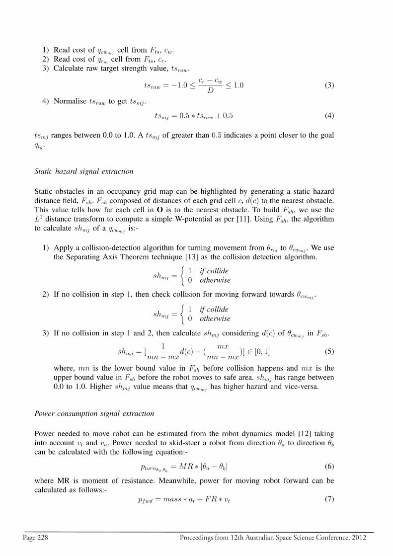
Page 228 Proceedings from 12th Australian Space Science Conference, 2012
1) Read cost of qcwmjcell from Fts, cw.
2) Read cost of qrm cell from Fts, cr.3) Calculate raw target strength value, tsraw.
tsraw = −1.0 ≤ cr − cwD
≤ 1.0 (3)
4) Normalise tsraw to get tsmj .
tsmj = 0.5 ∗ tsraw + 0.5 (4)
tsmj ranges between 0.0 to 1.0. A tsmj of greater than 0.5 indicates a point closer to the goalqtg .
Static hazard signal extraction
Static obstacles in an occupancy grid map can be highlighted by generating a static hazarddistance field, Fsh. Fsh composed of distances of each grid cell c, d(c) to the nearest obstacle.This value tells how far each cell in O is to the nearest obstacle. To build Fsh, we use theL1 distance transform to compute a simple W-potential as per [11]. Using Fsh, the algorithmto calculate shmj of a qcwmj
is:-
1) Apply a collision-detection algorithm for turning movement from θrm to θcwmj. We use
the Separating Axis Theorem technique [13] as the collision detection algorithm.
shmj =
{1 if collide0 otherwise
2) If no collision in step 1, then check collision for moving forward towards θcwmj.
shmj =
{1 if collide0 otherwise
3) If no collision in step 1 and 2, then calculate shmj considering d(c) of θcwmjin Fsh.
shmj = [1
mn−mxd(c)− (
mx
mn−mx)] ∈ [0, 1] (5)
where, mn is the lower bound value in Fsh before collision happens and mx is theupper bound value in Fsh before the robot moves to safe area. shmj has range between0.0 to 1.0. Higher shmj value means that qcwmj
has higher hazard and vice-versa.
Power consumption signal extraction
Power needed to move robot can be estimated from the robot dynamics model [12] takinginto account vt and va. Power needed to skid-steer a robot from direction θa to direction θbcan be calculated with the following equation:-
pturnθa,θb= MR ∗ |θa − θb| (6)
where MR is moment of resistance. Meanwhile, power for moving robot forward can becalculated as follows:-
pfwd = mass ∗ at + FR ∗ vt (7)
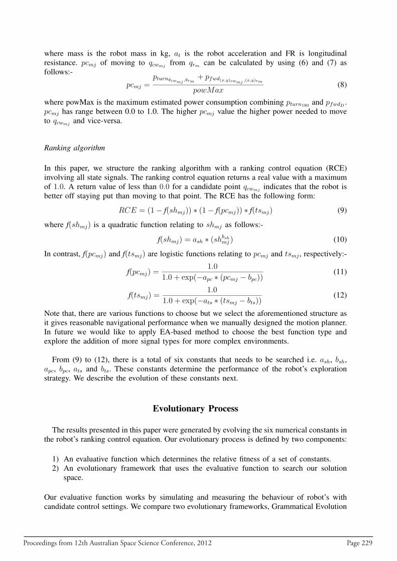
Proceedings from 12th Australian Space Science Conference, 2012 Page 229
where mass is the robot mass in kg, at is the robot acceleration and FR is longitudinalresistance. pcmj of moving to qcwmj
from qrm can be calculated by using (6) and (7) asfollows:-
pcmj =pturnθcwmj ,θrm
+ pfwd(x,y)cwmj ,(x,y)rm
powMax(8)
where powMax is the maximum estimated power consumption combining pturn180 and pfwdD .pcmj has range between 0.0 to 1.0. The higher pcmj value the higher power needed to moveto qcwmj
and vice-versa.
Ranking algorithm
In this paper, we structure the ranking algorithm with a ranking control equation (RCE)involving all state signals. The ranking control equation returns a real value with a maximumof 1.0. A return value of less than 0.0 for a candidate point qcwmj
indicates that the robot isbetter off staying put than moving to that point. The RCE has the following form:
RCE = (1− f(shmj)) ∗ (1− f(pcmj)) ∗ f(tsmj) (9)
where f(shmj) is a quadratic function relating to shmj as follows:-
f(shmj) = ash ∗ (shbshmj ) (10)
In contrast, f(pcmj) and f(tsmj) are logistic functions relating to pcmj and tsmj , respectively:-
f(pcmj) =1.0
1.0 + exp(−apc ∗ (pcmj − bpc))(11)
f(tsmj) =1.0
1.0 + exp(−ats ∗ (tsmj − bts))(12)
Note that, there are various functions to choose but we select the aforementioned structure asit gives reasonable navigational performance when we manually designed the motion planner.In future we would like to apply EA-based method to choose the best function type andexplore the addition of more signal types for more complex environments.
From (9) to (12), there is a total of six constants that needs to be searched i.e. ash, bsh,apc, bpc, ats and bts. These constants determine the performance of the robot’s explorationstrategy. We describe the evolution of these constants next.
Evolutionary Process
The results presented in this paper were generated by evolving the six numerical constants inthe robot’s ranking control equation. Our evolutionary process is defined by two components:
1) An evaluative function which determines the relative fitness of a set of constants.2) An evolutionary framework that uses the evaluative function to search our solution
space.
Our evaluative function works by simulating and measuring the behaviour of robot’s withcandidate control settings. We compare two evolutionary frameworks, Grammatical Evolution
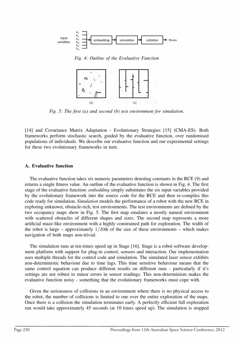
Page 230 Proceedings from 12th Australian Space Science Conference, 2012
!"#!$$%&'( )%"*+,-.&( /.++,-.&(
,0)(#0)(,)1(#)1(,2/(#2/(
30&!))(%&2*0(
4,5%,#+!)(
Fig. 4: Outline of the Evaluative Function
Fig. 5: The first (a) and second (b) test environment for simulation.
[14] and Covariance Matrix Adaptation - Evolutionary Strategies [15] (CMA-ES). Bothframeworks perform stochastic search, guided by the evaluative function, over randomisedpopulations of individuals. We describe our evaluative function and our experimental settingsfor these two evolutionary frameworks in turn.
A. Evaluative function
The evaluative function takes six numeric parameters denoting constants in the RCE (9) andreturns a single fitness value. An outline of the evaluative function is shown in Fig. 4. The firststage of the evaluative function: embedding simply substitutes the six input variables providedby the evolutionary framework into the source code for the RCE and then re-compiles thiscode ready for simulation. Simulation models the performance of a robot with the new RCE inexploring unknown, obstacle-rich, test environments. The test environments are defined by thetwo occupancy maps show in Fig. 5. The first map emulates a mostly natural environmentwith scattered obstacles of different shapes and sizes. The second map represents a moreartificial maze-like environment with a highly constrained path for exploration. The width ofthe robot is large – approximately 1/20th of the size of these environments – which makesnavigation of both maps non-trivial.
The simulation runs at ten-times speed up in Stage [16]. Stage is a robot software develop-ment platform with support for plug-in control, sensors and interaction. Our implementationuses multiple threads for the control code and simulation. The simulated laser sensor exhibitsnon-deterministic behaviour due to time lags. This time sensitive behaviour means that thesame control equation can produce different results on different runs - particularly if it’ssettings are not robust to minor errors in sensor readings. This non-determinism makes theevaluative function noisy - something that the evolutionary frameworks must cope with.
Given the seriousness of collisions in an environment where there is no physical access tothe robot, the number of collisions is limited to one over the entire exploration of the maps.Once there is a collision the simulation terminates early. A perfectly efficient full explorationrun would take approximately 45 seconds (at 10 times speed up). The simulation is stopped
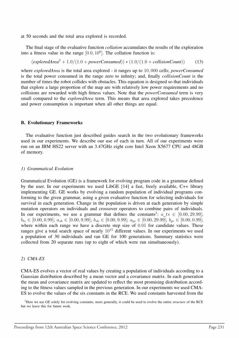
Proceedings from 12th Australian Space Science Conference, 2012 Page 231
at 50 seconds and the total area explored is recorded.
The final stage of the evaluative function collation accumulates the results of the explorationinto a fitness value in the range [0.0, 108]. The collation function is:
(exploredArea2 + 1.0/(1.0 + powerConsumed)) ∗ (1.0/(1.0 + collisionCount)) (13)
where exploredArea is the total area explored - it ranges up to 10, 000 cells; powerConsumedis the total power consumed in the range zero to infinity; and, finally collisionCount is thenumber of times the robot collides with obstacles. This equation is designed so that individualsthat explore a large proportion of the map are with relatively low power requirements and nocollisions are rewarded with high fitness values. Note that the powerConsumed term is verysmall compared to the exploredArea term. This means that area explored takes precedenceand power consumption is important when all other things are equal.
B. Evolutionary Frameworks
The evaluative function just described guides search in the two evolutionary frameworksused in our experiments. We describe our use of each in turn. All of our experiments wererun on an IBM HS22 server with an 3.47GHz eight core Intel Xeon X5677 CPU and 48GBof memory.
1) Grammatical Evolution
Grammatical Evolution (GE) is a framework for evolving program code in a grammar definedby the user. In our experiments we used LibGE [14] a fast, freely available, C++ libraryimplementing GE. GE works by evolving a random population of individual programs con-forming to the given grammar, using a given evaluative function for selecting individuals forsurvival in each generation. Change in the population is driven at each generation by simplemutation operators on individuals and crossover operators to combine pairs of individuals.In our experiments, we use a grammar that defines the constants2: a ts ∈ [0.00, 29.99];bts ∈ [0.00, 0.99]; ash ∈ [0.00, 9.99]; bsh ∈ [0.00, 9.99]; apc ∈ [0.00, 29.99]; bpc ∈ [0.00, 0.99];where within each range we have a discrete step size of 0.01 for candidate values. Theseranges give a total search space of nearly 1015 different values. In our experiments we useda population of 30 individuals and ran GE for 100 generations. Summary statistics werecollected from 20 separate runs (up to eight of which were run simultaneously).
2) CMA-ES
CMA-ES evolves a vector of real values by creating a population of individuals according to aGaussian distribution described by a mean vector and a covariance matrix. In each generationthe mean and covariance matrix are updated to reflect the most promising distribution accord-ing to the fitness values sampled in the previous generation. In our experiments we used CMA-ES to evolve the values of the six constants in the RCE. We used constants harvested from the
2Here we use GE solely for evolving constants, more generally, it could be used to evolve the entire structure of the RCEbut we leave this for future work.
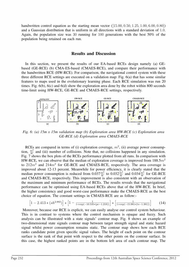
Page 232 Proceedings from 12th Australian Space Science Conference, 2012
handwritten control equation as the starting mean vector ([15.00, 0.50, 1.25, 1.00, 6.00, 0.80])and a Gaussian distribution that is uniform in all directions with a standard deviation of 1.0.Again, the population size was 30 running for 100 generations with the best 50% of thepopulation being retained on each run.
Results and Discussion
In this section, we present the results of our EA-based RCEs design namely (a) GE-based (GE-RCE) (b) CMA-ES-based (CMAES-RCE), and compare their performance withthe handwritten RCE (HW-RCE). For comparison, the navigational control system with thesethree different RCE settings are executed on a validation map: Fig. 6(a) that has some similarfeatures to maps used in the evolutionary learning phase. Each RCE simulation was run 20times. Fig. 6(b), 6(c) and 6(d) show the exploration area done by the robot within 800 secondstime-limit using HW-RCE, GE-RCE and CMAES-RCE settings, respectively.
Fig. 6: (a) 15m x 15m validation map (b) Exploration area HW-RCE (c) Exploration areaGE-RCE (d) Exploration area CMAES-RCE
RCEs are compared in terms of (i) exploration coverage, m2, (ii) average power consump-tion, m2
Wand (iii) number of collisions. Note that, no collisions happened in any simulation.
Fig. 7 shows the box plots of the RCEs performance plotted from all runs. In comparison withHW-RCE, we can observe that the median of exploration coverage is improved from 188.5m2
to 212m2 and 214m2 for GE-RCE and CMAES-RCE, respectively. The area coverage isimproved about 12-13 percent. Meanwhile for power efficiency, it is clearly stated that themedian power consumption is reduced from 0.037m2
Wto 0.032m2
Wand 0.034m2
Wfor GE-RCE
and CMAES-RCE, respectively. This improvement is also consistent with an observation ofthe maximum and minimum performance of RCEs. The results reveals that the navigationalperformance can be optimised using EA-based RCEs above that of the HW-RCE. In brief,the higher consistency and good worst-case performance make the CMAES-RCE as the bestchoice of equation. The constant settings in CMAES-RCE are as follow:-
[1− 2.413 ∗ (sh2.882)
]∗[1− 1
1+exp(−10.535∗(pc−1.218))
]∗[
11+exp(−15.981∗(ts−1.381))
](14)
Moreover, because our RCE is explicit, we can easily analyse our control system behaviour.This is in contrast to systems where the control mechanism is opaque and fuzzy. Suchanalysis can be illustrated with a state signals’ contour map. Fig. 8 shows an example oftwo-dimensional state signals contour map between target strength signal and static hazardsignal whilst power consumption remains static. The contour map shows how each RCEranks candidate point given specific signal values. The height of each point on the contoursurface is the rank of that point with respect to the other points on the contour surface. Inthis case, the highest ranked points are in the bottom left area of each contour map. The
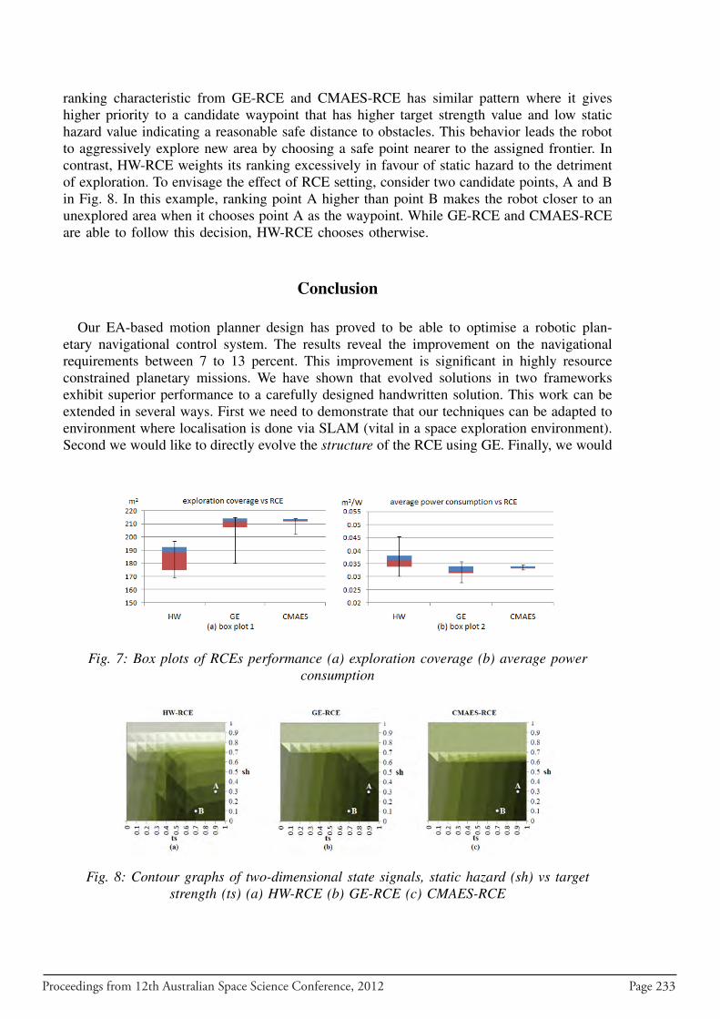
Proceedings from 12th Australian Space Science Conference, 2012 Page 233
ranking characteristic from GE-RCE and CMAES-RCE has similar pattern where it giveshigher priority to a candidate waypoint that has higher target strength value and low statichazard value indicating a reasonable safe distance to obstacles. This behavior leads the robotto aggressively explore new area by choosing a safe point nearer to the assigned frontier. Incontrast, HW-RCE weights its ranking excessively in favour of static hazard to the detrimentof exploration. To envisage the effect of RCE setting, consider two candidate points, A and Bin Fig. 8. In this example, ranking point A higher than point B makes the robot closer to anunexplored area when it chooses point A as the waypoint. While GE-RCE and CMAES-RCEare able to follow this decision, HW-RCE chooses otherwise.
Conclusion
Our EA-based motion planner design has proved to be able to optimise a robotic plan-etary navigational control system. The results reveal the improvement on the navigationalrequirements between 7 to 13 percent. This improvement is significant in highly resourceconstrained planetary missions. We have shown that evolved solutions in two frameworksexhibit superior performance to a carefully designed handwritten solution. This work can beextended in several ways. First we need to demonstrate that our techniques can be adapted toenvironment where localisation is done via SLAM (vital in a space exploration environment).Second we would like to directly evolve the structure of the RCE using GE. Finally, we would
Fig. 7: Box plots of RCEs performance (a) exploration coverage (b) average powerconsumption
Fig. 8: Contour graphs of two-dimensional state signals, static hazard (sh) vs targetstrength (ts) (a) HW-RCE (b) GE-RCE (c) CMAES-RCE
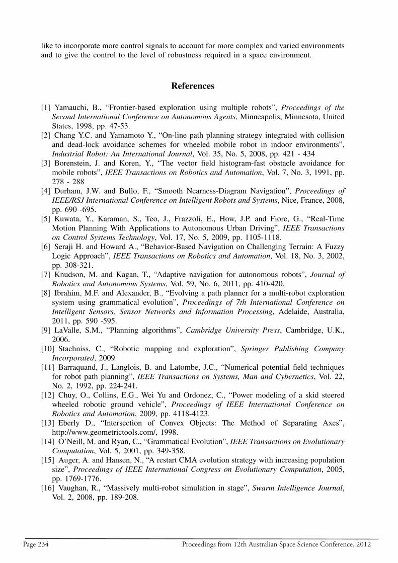
Page 234 Proceedings from 12th Australian Space Science Conference, 2012
like to incorporate more control signals to account for more complex and varied environmentsand to give the control to the level of robustness required in a space environment.
References
[1] Yamauchi, B., “Frontier-based exploration using multiple robots”, Proceedings of theSecond International Conference on Autonomous Agents, Minneapolis, Minnesota, UnitedStates, 1998, pp. 47-53.
[2] Chang Y.C. and Yamamoto Y., “On-line path planning strategy integrated with collisionand dead-lock avoidance schemes for wheeled mobile robot in indoor environments”,Industrial Robot: An International Journal, Vol. 35, No. 5, 2008, pp. 421 - 434
[3] Borenstein, J. and Koren, Y., “The vector field histogram-fast obstacle avoidance formobile robots”, IEEE Transactions on Robotics and Automation, Vol. 7, No. 3, 1991, pp.278 - 288
[4] Durham, J.W. and Bullo, F., “Smooth Nearness-Diagram Navigation”, Proceedings ofIEEE/RSJ International Conference on Intelligent Robots and Systems, Nice, France, 2008,pp. 690 -695.
[5] Kuwata, Y., Karaman, S., Teo, J., Frazzoli, E., How, J.P. and Fiore, G., “Real-TimeMotion Planning With Applications to Autonomous Urban Driving”, IEEE Transactionson Control Systems Technology, Vol. 17, No. 5, 2009, pp. 1105-1118.
[6] Seraji H. and Howard A., “Behavior-Based Navigation on Challenging Terrain: A FuzzyLogic Approach”, IEEE Transactions on Robotics and Automation, Vol. 18, No. 3, 2002,pp. 308-321.
[7] Knudson, M. and Kagan, T., “Adaptive navigation for autonomous robots”, Journal ofRobotics and Autonomous Systems, Vol. 59, No. 6, 2011, pp. 410-420.
[8] Ibrahim, M.F. and Alexander, B., “Evolving a path planner for a multi-robot explorationsystem using grammatical evolution”, Proceedings of 7th International Conference onIntelligent Sensors, Sensor Networks and Information Processing, Adelaide, Australia,2011, pp. 590 -595.
[9] LaValle, S.M., “Planning algorithms”, Cambridge University Press, Cambridge, U.K.,2006.
[10] Stachniss, C., “Robotic mapping and exploration”, Springer Publishing CompanyIncorporated, 2009.
[11] Barraquand, J., Langlois, B. and Latombe, J.C., “Numerical potential field techniquesfor robot path planning”, IEEE Transactions on Systems, Man and Cybernetics, Vol. 22,No. 2, 1992, pp. 224-241.
[12] Chuy, O., Collins, E.G., Wei Yu and Ordonez, C., “Power modeling of a skid steeredwheeled robotic ground vehicle”, Proceedings of IEEE International Conference onRobotics and Automation, 2009, pp. 4118-4123.
[13] Eberly D., “Intersection of Convex Objects: The Method of Separating Axes”,http://www.geometrictools.com/, 1998.
[14] O’Neill, M. and Ryan, C., “Grammatical Evolution”, IEEE Transactions on EvolutionaryComputation, Vol. 5, 2001, pp. 349-358.
[15] Auger, A. and Hansen, N., “A restart CMA evolution strategy with increasing populationsize”, Proceedings of IEEE International Congress on Evolutionary Computation, 2005,pp. 1769-1776.
[16] Vaughan, R., “Massively multi-robot simulation in stage”, Swarm Intelligence Journal,Vol. 2, 2008, pp. 189-208.
Proceedings from 12th Australian Space Science Conference, 2012 Page 235
Thermal Imaging and Electrodynamic Tether Payloads for a Nano Satellite
Gourav Mahapatra, Pallavi Reddy, Soumitro Datta , Adheesh Boratkar , Rodney Gracian D’Souza, and Bharat Ramanathan
Manipal Institute of Technology, Manipal University,
Manipal, Karnataka-576104, India
Summary: Parikshit is a Nano class satellite being engineered by a group of undergrad students from Manipal University, India. It consists of two major payloads which are terrestrial thermal imaging using a LWIR camera and de orbiting of the satellite using an electrodynamic tether. This paper gives a brief introduction to the two payloads. The thermal camera is a COTS device which will be suitably modified for use in space. It is capable of taking pictures of the Earth in the Long Wave Infrared Range and shall be used for mapping the temperature variations. An electro-dynamic tether consists of a conducting wire, dragged through a magnetic field. We intend to conduct a deorbiting experiment utilizing this technology. The tether deployment mechanism to be used is manufactured by Saber Astronautics and will be tested on board the satellite.
Keywords: thermal imaging, passive electrodynamic tether, student nano satellite, LWIR, deorbiting.
Introduction
The advent of Nano satellites has increased the scope of research and experimentation in a space environment. These satellites have proved to be more economical in terms of development and functioning. One such initiative has been started by a group of students of Manipal Institute of Technology, India. The payloads for our first satellite are Terrestrial thermal imaging which is the primary payload and Deorbiting of our satellite after its mission life using a passive Electrodynamic tether. The arrangement of these payloads in the satellite structure is illustrated in Fig. 1. Terrestrial thermal imaging is being conducted using an FLIR Camera which is active in the Long wave infrared region(LWIR) of the IR spectrum. The LWIR is the thermal imaging region, in which sensors can obtain a picture of the outside world based exclusively on thermal emissions and requires no external light or thermal source. We intend to monitor the cloud cover and ocean surface temperatures over the mission life as well as attempt to isolate urban areas based on their heat signatures.
Today an astounding number of more than 600,000 objects revolve around the earth out of which only 19000 are tracked. All these form space junk or debris, the removal of which is nearly impossible as of now. Electrodynamic tether can be used to avoid the accumulation of such debris in future and we plan to test this by conducting a deorbiting experiment on our satellite at the end of its mission life.
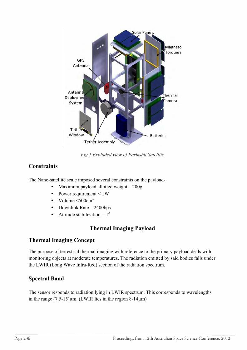
Page 236 Proceedings from 12th Australian Space Science Conference, 2012
Fig.1 Exploded view of Parikshit Satellite
Constraints
The Nano-satellite scale imposed several constraints on the payload- • Maximum payload allotted weight – 200g • Power requirement < 1W • Volume <500cm3 • Downlink Rate – 2400bps • Attitude stabilization - 1o
Thermal Imaging Payload
Thermal Imaging Concept
The purpose of terrestrial thermal imaging with reference to the primary payload deals with monitoring objects at moderate temperatures. The radiation emitted by said bodies falls under the LWIR (Long Wave Infra-Red) section of the radiation spectrum.
Spectral Band The sensor responds to radiation lying in LWIR spectrum. This corresponds to wavelengths in the range (7.5-15)µm. (LWIR lies in the region 8-14µm)
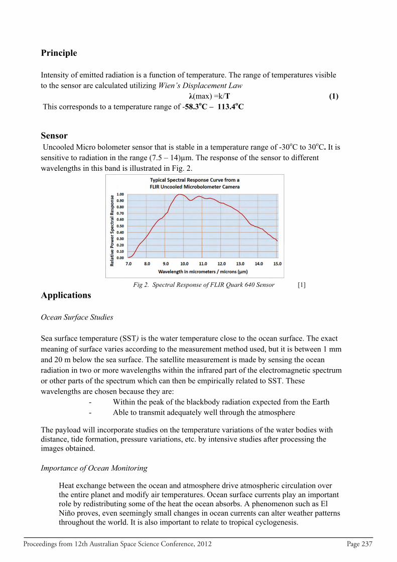
Proceedings from 12th Australian Space Science Conference, 2012 Page 237
Principle
Intensity of emitted radiation is a function of temperature. The range of temperatures visible to the sensor are calculated utilizing Wien’s Displacement Law
λ(max) =k/T (1) This corresponds to a temperature range of -58.3oC – 113.4oC
Sensor Uncooled Micro bolometer sensor that is stable in a temperature range of -30oC to 30oC. It is sensitive to radiation in the range (7.5 – 14)µm. The response of the sensor to different wavelengths in this band is illustrated in Fig. 2.
Fig 2. Spectral Response of FLIR Quark 640 Sensor [1]
Applications
Ocean Surface Studies
Sea surface temperature (SST) is the water temperature close to the ocean surface. The exact meaning of surface varies according to the measurement method used, but it is between 1 mm and 20 m below the sea surface. The satellite measurement is made by sensing the ocean radiation in two or more wavelengths within the infrared part of the electromagnetic spectrum or other parts of the spectrum which can then be empirically related to SST. These wavelengths are chosen because they are:
- Within the peak of the blackbody radiation expected from the Earth - Able to transmit adequately well through the atmosphere
The payload will incorporate studies on the temperature variations of the water bodies with distance, tide formation, pressure variations, etc. by intensive studies after processing the images obtained.
Importance of Ocean Monitoring
Heat exchange between the ocean and atmosphere drive atmospheric circulation over the entire planet and modify air temperatures. Ocean surface currents play an important role by redistributing some of the heat the ocean absorbs. A phenomenon such as El Niño proves, even seemingly small changes in ocean currents can alter weather patterns throughout the world. It is also important to relate to tropical cyclogenesis.
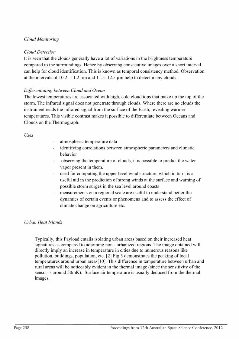
Page 238 Proceedings from 12th Australian Space Science Conference, 2012
Cloud Monitoring
Cloud Detection It is seen that the clouds generally have a lot of variations in the brightness temperature compared to the surroundings. Hence by observing consecutive images over a short interval can help for cloud identification. This is known as temporal consistency method. Observation at the intervals of 10.2– 11.2 µm and 11.5–12.5 µm help to detect many clouds. Differentiating between Cloud and Ocean The lowest temperatures are associated with high, cold cloud tops that make up the top of the storm. The infrared signal does not penetrate through clouds. Where there are no clouds the instrument reads the infrared signal from the surface of the Earth, revealing warmer temperatures. This visible contrast makes it possible to differentiate between Oceans and Clouds on the Thermograph.
Uses
- atmospheric temperature data - identifying correlations between atmospheric parameters and climatic
behavior - observing the temperature of clouds, it is possible to predict the water
vapor present in them. - used for computing the upper level wind structure, which in turn, is a
useful aid in the prediction of strong winds at the surface and warning of possible storm surges in the sea level around coasts
- measurements on a regional scale are useful to understand better the dynamics of certain events or phenomena and to assess the effect of climate change on agriculture etc.
Urban Heat Islands
Typically, this Payload entails isolating urban areas based on their increased heat signatures as compared to adjoining non - urbanized regions. The image obtained will directly imply an increase in temperature in cities due to numerous reasons like pollution, buildings, population, etc. [2] Fig 3 demonstrates the peaking of local temperatures around urban areas[10]. This difference in temperature between urban and rural areas will be noticeably evident in the thermal image (since the sensitivity of the sensor is around 50mK). Surface air temperature is usually deduced from the thermal images.
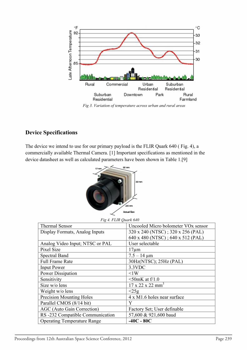
Proceedings from 12th Australian Space Science Conference, 2012 Page 239
Fig 3. Variation of temperature across urban and rural areas
Device Specifications
The device we intend to use for our primary payload is the FLIR Quark 640 ( Fig. 4), a commercially available Thermal Camera. [1] Important specifications as mentioned in the device datasheet as well as calculated parameters have been shown in Table 1.[9]
Fig 4. FLIR Quark 640 Thermal Sensor Uncooled Micro bolometer VOx sensor Display Formats, Analog Inputs 320 x 240 (NTSC) ; 320 x 256 (PAL)
640 x 480 (NTSC) ; 640 x 512 (PAL) Analog Video Input; NTSC or PAL User selectable Pixel Size 17µm Spectral Band 7.5 – 14 µm Full Frame Rate 30Hz(NTSC); 25Hz (PAL) Input Power 3.3VDC Power Dissipation <1W Sensitivity <50mK at f/1.0 Size w/o lens 17 x 22 x 22 mm3 Weight w/o lens <25g Precision Mounting Holes 4 x M1.6 holes near surface
Parallel CMOS (8/14 bit) Y AGC (Auto Gain Correction) Factory Set; User definable RS -232 Compatible Communication 57,600 & 921,600 baud Operating Temperature Range -40C - 80C
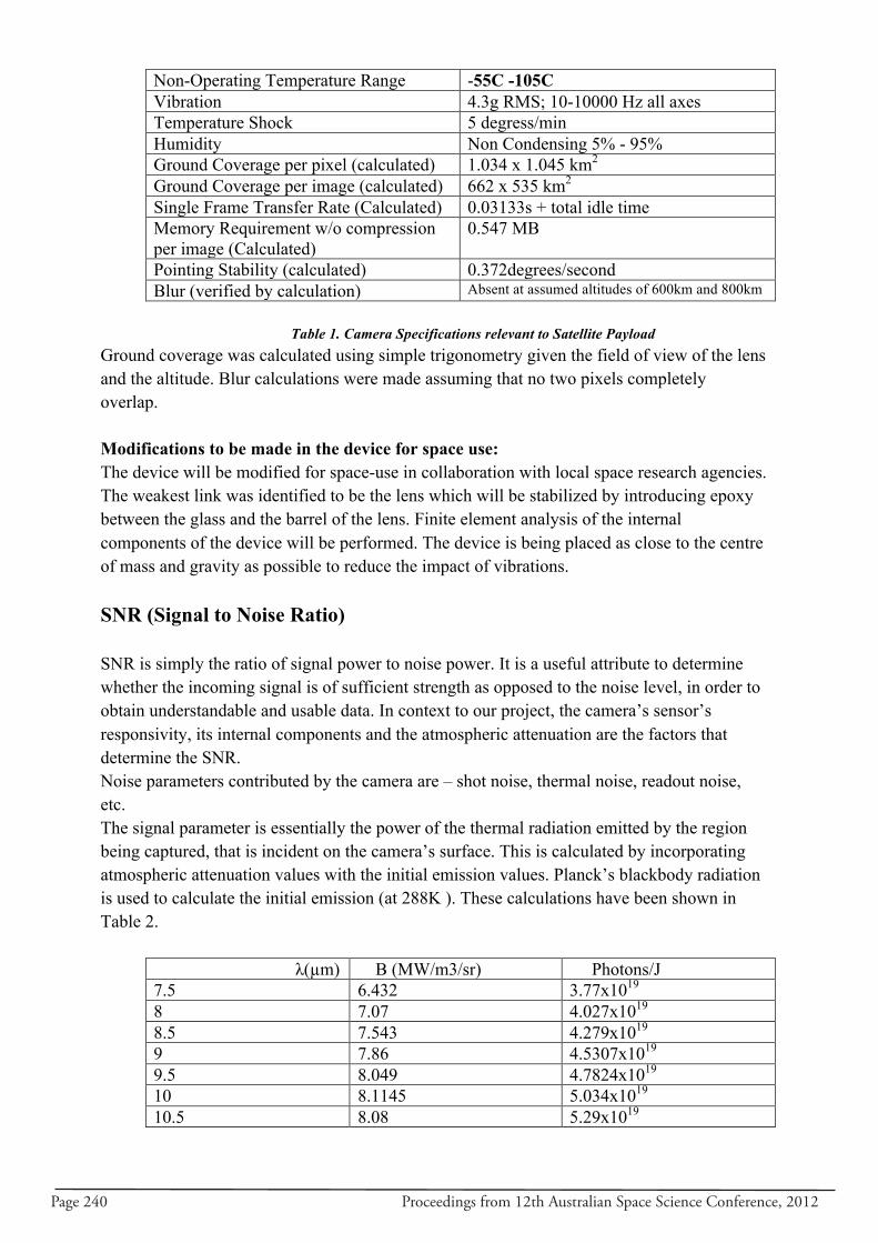
Page 240 Proceedings from 12th Australian Space Science Conference, 2012
Non-Operating Temperature Range -55C -105C Vibration 4.3g RMS; 10-10000 Hz all axes Temperature Shock 5 degress/min Humidity Non Condensing 5% - 95% Ground Coverage per pixel (calculated) 1.034 x 1.045 km2 Ground Coverage per image (calculated) 662 x 535 km2 Single Frame Transfer Rate (Calculated) 0.03133s + total idle time
Memory Requirement w/o compression per image (Calculated)
0.547 MB
Pointing Stability (calculated) 0.372degrees/second Blur (verified by calculation) Absent at assumed altitudes of 600km and 800km Table 1. Camera Specifications relevant to Satellite Payload
Ground coverage was calculated using simple trigonometry given the field of view of the lens and the altitude. Blur calculations were made assuming that no two pixels completely overlap. Modifications to be made in the device for space use: The device will be modified for space-use in collaboration with local space research agencies. The weakest link was identified to be the lens which will be stabilized by introducing epoxy between the glass and the barrel of the lens. Finite element analysis of the internal components of the device will be performed. The device is being placed as close to the centre of mass and gravity as possible to reduce the impact of vibrations. SNR (Signal to Noise Ratio)
SNR is simply the ratio of signal power to noise power. It is a useful attribute to determine whether the incoming signal is of sufficient strength as opposed to the noise level, in order to obtain understandable and usable data. In context to our project, the camera’s sensor’s responsivity, its internal components and the atmospheric attenuation are the factors that determine the SNR. Noise parameters contributed by the camera are – shot noise, thermal noise, readout noise, etc. The signal parameter is essentially the power of the thermal radiation emitted by the region being captured, that is incident on the camera’s surface. This is calculated by incorporating atmospheric attenuation values with the initial emission values. Planck’s blackbody radiation is used to calculate the initial emission (at 288K ). These calculations have been shown in Table 2.
λ(µm) B (MW/m3/sr) Photons/J 7.5 6.432 3.77x10¹⁹ 8 7.07 4.027x10¹⁹ 8.5 7.543 4.279x10¹⁹ 9 7.86 4.5307x10¹⁹ 9.5 8.049 4.7824x10¹⁹ 10 8.1145 5.034x10¹⁹ 10.5 8.08 5.29x10¹⁹
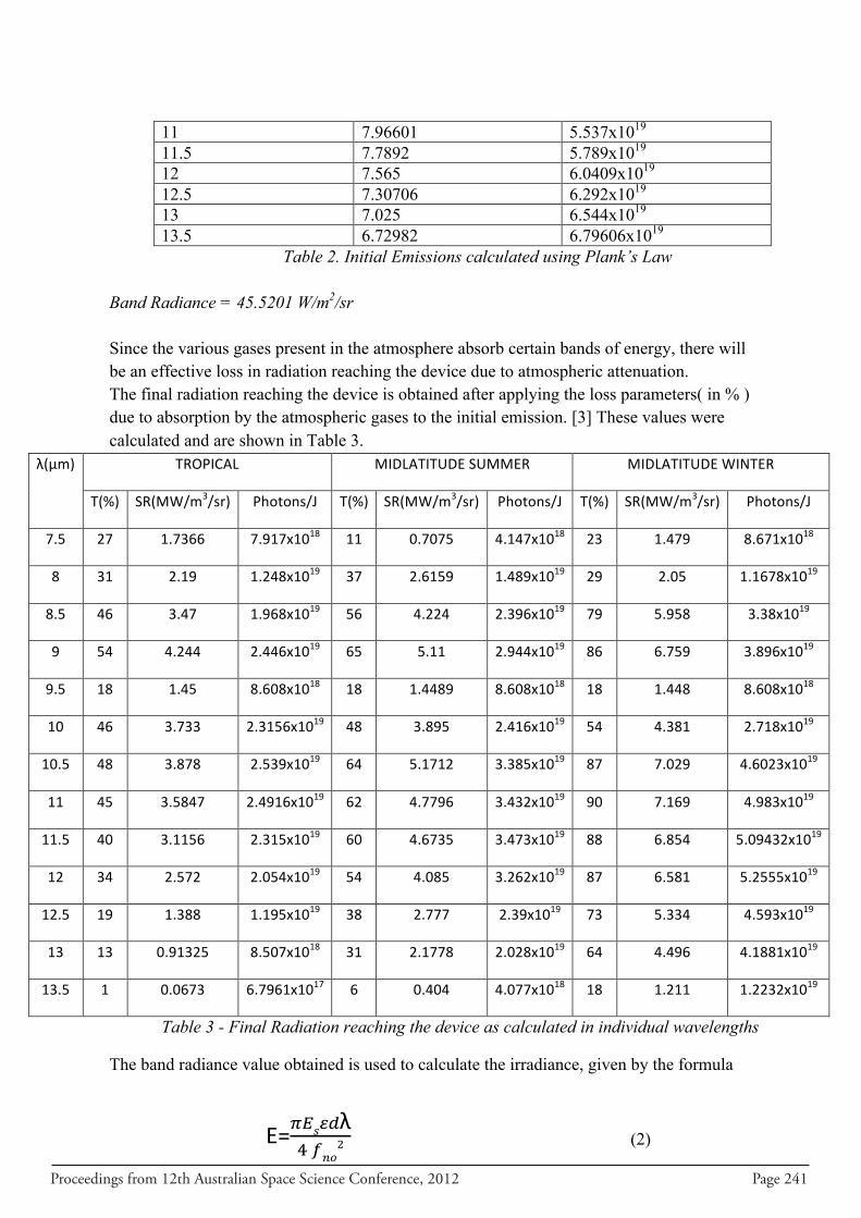
Proceedings from 12th Australian Space Science Conference, 2012 Page 241
11 7.96601 5.537x10¹⁹ 11.5 7.7892 5.789x10¹⁹ 12 7.565 6.0409x10¹⁹ 12.5 7.30706 6.292x10¹⁹ 13 7.025 6.544x10¹⁹ 13.5 6.72982 6.79606x10¹⁹ Table 2. Initial Emissions calculated using Plank’s Law
Band Radiance = 45.5201 W/m2/sr
Since the various gases present in the atmosphere absorb certain bands of energy, there will be an effective loss in radiation reaching the device due to atmospheric attenuation. The final radiation reaching the device is obtained after applying the loss parameters( in % ) due to absorption by the atmospheric gases to the initial emission. [3] These values were calculated and are shown in Table 3.
λ(µm) TROPICAL MIDLATITUDE SUMMER MIDLATITUDE WINTER
T(%) SR(MW/m3/sr) Photons/J T(%) SR(MW/m3/sr) Photons/J T(%) SR(MW/m3/sr) Photons/J
7.5 27 1.7366 7.917x10¹⁸ 11 0.7075 4.147x10¹⁸ 23 1.479 8.671x10¹⁸
8 31 2.19 1.248x10¹⁹ 37 2.6159 1.489x10¹⁹ 29 2.05 1.1678x10¹⁹
8.5 46 3.47 1.968x10¹⁹ 56 4.224 2.396x10¹⁹ 79 5.958 3.38x10¹⁹
9 54 4.244 2.446x10¹⁹ 65 5.11 2.944x10¹⁹ 86 6.759 3.896x10¹⁹
9.5 18 1.45 8.608x10¹⁸ 18 1.4489 8.608x10¹⁸ 18 1.448 8.608x10¹⁸
10 46 3.733 2.3156x10¹⁹ 48 3.895 2.416x10¹⁹ 54 4.381 2.718x10¹⁹
10.5 48 3.878 2.539x10¹⁹ 64 5.1712 3.385x10¹⁹ 87 7.029 4.6023x10¹⁹
11 45 3.5847 2.4916x10¹⁹ 62 4.7796 3.432x10¹⁹ 90 7.169 4.983x10¹⁹
11.5 40 3.1156 2.315x10¹⁹ 60 4.6735 3.473x10¹⁹ 88 6.854 5.09432x10¹⁹
12 34 2.572 2.054x10¹⁹ 54 4.085 3.262x10¹⁹ 87 6.581 5.2555x10¹⁹
12.5 19 1.388 1.195x10¹⁹ 38 2.777 2.39x10¹⁹ 73 5.334 4.593x10¹⁹
13 13 0.91325 8.507x10¹⁸ 31 2.1778 2.028x10¹⁹ 64 4.496 4.1881x10¹⁹
13.5 1 0.0673 6.7961x10¹⁷ 6 0.404 4.077x10¹⁸ 18 1.211 1.2232x10¹⁹
Table 3 - Final Radiation reaching the device as calculated in individual wavelengths
The band radiance value obtained is used to calculate the irradiance, given by the formula
(2) E=
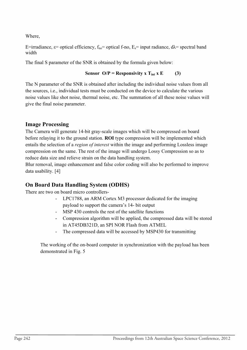
Page 242 Proceedings from 12th Australian Space Science Conference, 2012
Where,
E=irradiance, ε= optical efficiency, fno= optical f-no, Es= input radiance, dλ= spectral band width
The final S parameter of the SNR is obtained by the formula given below:
Sensor O/P = Responsivity x Tint x E (3)
The N parameter of the SNR is obtained after including the individual noise values from all the sources, i.e., individual tests must be conducted on the device to calculate the various noise values like shot noise, thermal noise, etc. The summation of all these noise values will give the final noise parameter. Image Processing The Camera will generate 14-bit gray-scale images which will be compressed on board before relaying it to the ground station. ROI type compression will be implemented which entails the selection of a region of interest within the image and performing Lossless image compression on the same. The rest of the image will undergo Lossy Compression so as to reduce data size and relieve strain on the data handling system. Blur removal, image enhancement and false color coding will also be performed to improve data usability. [4]
On Board Data Handling System (ODHS) There are two on board micro controllers-
- LPC1788, an ARM Cortex M3 processor dedicated for the imaging payload to support the camera’s 14- bit output
- MSP 430 controls the rest of the satellite functions - Compression algorithm will be applied, the compressed data will be stored
in AT45DB321D, an SPI NOR Flash from ATMEL - The compressed data will be accessed by MSP430 for transmitting
The working of the on-board computer in synchronization with the payload has been demonstrated in Fig. 5
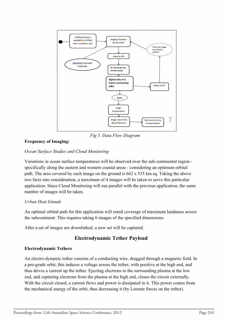
Proceedings from 12th Australian Space Science Conference, 2012 Page 243
Fig 5. Data Flow Diagram
Frequency of Imaging:
Ocean Surface Studies and Cloud Monitoring
Variations in ocean surface temperatures will be observed over the sub-continental region - specifically along the eastern and western coastal areas - considering an optimum orbital path. The area covered by each image on the ground is 662 x 535 km sq. Taking the above two facts into consideration, a maximum of 4 images will be taken to serve this particular application. Since Cloud Monitoring will run parallel with the previous application, the same number of images will be taken.
Urban Heat Islands
An optimal orbital path for this application will entail coverage of maximum landmass across the subcontinent. This requires taking 6 images of the specified dimensions.
After a set of images are downlinked, a new set will be captured.
Electrodynamic Tether Payload
Electrodynamic Tethers
An electro-dynamic tether consists of a conducting wire, dragged through a magnetic field. In a pro-grade orbit, this induces a voltage across the tether, with positive at the high end, and thus drives a current up the tether. Ejecting electrons to the surrounding plasma at the low end, and capturing electrons from the plasma at the high end, closes the circuit externally. With the circuit closed, a current flows and power is dissipated in it. This power comes from the mechanical energy of the orbit, thus decreasing it (by Lorentz forces on the tether).
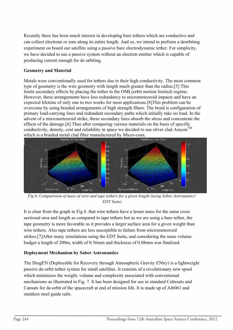
Page 244 Proceedings from 12th Australian Space Science Conference, 2012
Recently there has been much interest in developing bare tethers which are conductive and can collect electrons or ions along its entire length. And so, we intend to perform a deorbiting experiment on board our satellite using a passive bare electrodynamic tether. For simplicity, we have decided to use a passive system without an electron emitter which is capable of producing current enough for de orbiting.
Geometry and Material
Metals were conventionally used for tethers due to their high conductivity. The most common type of geometry is the wire geometry with length much greater than the radius.[5] This limits secondary effects by placing the tether in the OML(orbit motion limited) regime. However, these arrangements have less redundancy to micrometeoroid impacts and have an expected lifetime of only one to two weeks for most applications.[8]This problem can be overcome by using braided arrangements of high strength fibers. The braid is configuration of primary load-carrying lines and redundant secondary paths which initially take no load. In the advent of a micrometeoroid strike, these secondary lines absorb the stress and concentrate the effects of the damage.[6] Thus after comparing various materials on the basis of specific conductivity, density, cost and reliability in space we decided to use silver clad AraconTM which is a braided metal clad fiber manufactured by Micro-coax.
Fig 6. Comparision of mass of wire and tape tethers for a given length (using Saber Astronautics’
EDT Suite)
It is clear from the graph in Fig 6. that wire tethers have a lesser mass for the same cross sectional area and length as compared to tape tethers but as we are using a bare tether, the tape geometry is more favorable as it provides a larger surface area for a given weight than wire tethers. Also tape tethers are less susceptible to failure from micrometeoroid strikes.[7]After many simulations using the EDT Suite, and considering the mass volume budget a length of 200m, width of 0.56mm and thickness of 0.08mm was finalized.
Deployment Mechanism by Saber Astronautics
The DragEN (Deployable for Recovery through Atmospheric Gravity ENtry) is a lightweight passive de-orbit tether system for small satellites. It consists of a revolutionary new spool which minimizes the weight, volume and complexity associated with conventional mechanisms as illustrated in Fig. 7. It has been designed for use in standard Cubesats and Cansats for de-orbit of the spacecraft at end of mission life. It is made up of Al6061 and stainless steel guide rails.

Proceedings from 12th Australian Space Science Conference, 2012 Page 245
Fig7. Tether Deploy Mechanism in the stowed position
Dimensions :
• Width 50mm
• Height 16mm,
• Depth 13mm
Mass excluding springs: 94.53g
• Base: 19.23g
• Ballast: 46.63g
Estimated Total Volume with Aracon tether: 33351mm3
Interfacing with the satellite
The base plate is held in position on structure with the help of brackets fixed by screws on the H-brackets.
Fig 8. View from inside the satellite of the tether assembly Fig 9.View from outside with the tether window closed.
The base will be firmly attached to the satellite’s body via three arms as shown in Fig 8. The window will be forced to close by tying it to the satellite panel (Fig. 9) via a monofilament wire. The material for this wire has been finalized as dyneema due to its space heritage. The spool will be held tightly with the base with another monofilament wire passing through the center of the base. In order to eject the tether both these wires will have to be burned. This is a two tier safety feature adopted to prevent premature deployment.
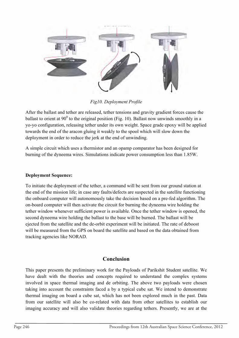
Page 246 Proceedings from 12th Australian Space Science Conference, 2012
Fig10. Deployment Profile
After the ballast and tether are released, tether tensions and gravity gradient forces cause the ballast to orient at 900 to the original position (Fig. 10). Ballast now unwinds smoothly in a yo-yo configuration, releasing tether under its own weight. Space grade epoxy will be applied towards the end of the aracon gluing it weakly to the spool which will slow down the deployment in order to reduce the jerk at the end of unwinding.
A simple circuit which uses a thermistor and an opamp comparator has been designed for burning of the dyneema wires. Simulations indicate power consumption less than 1.85W.
Deployment Sequence:
To initiate the deployment of the tether, a command will be sent from our ground station at the end of the mission life; in case any faults/defects are suspected in the satellite functioning the onboard computer will autonomously take the decision based on a pre-fed algorithm. The on-board computer will then activate the circuit for burning the dyneema wire holding the tether window whenever sufficient power is available. Once the tether window is opened, the second dyneema wire holding the ballast to the base will be burned. The ballast will be ejected from the satellite and the de-orbit experiment will be initiated. The rate of deboost will be measured from the GPS on board the satellite and based on the data obtained from tracking agencies like NORAD.
Conclusion
This paper presents the preliminary work for the Payloads of Parikshit Student satellite. We have dealt with the theories and concepts required to understand the complex systems involved in space thermal imaging and de orbiting. The above two payloads were chosen taking into account the constraints faced a by a typical cube sat. We intend to demonstrate thermal imaging on board a cube sat, which has not been explored much in the past. Data from our satellite will also be co-related with data from other satellites to establish our imaging accuracy and will also validate theories regarding tethers. Presently, we are at the
Proceedings from 12th Australian Space Science Conference, 2012 Page 247
components testing phase and are working on testing of the camera module and deployment of the tether under free fall conditions. The Parikshit satellite is expected to be launch ready by the end of 2013 and to be launched by the first half of 2014 after clearing the thermal tests, vacuum chamber tests and the launch vehicle vibration loads test.
References
1.FLIRSystems, http://www.flir.com/cvs/cores/view/?id=51266&collectionid=549&col=51276 ,last accessed December 2012 2. Urban heat island pdf, http://icecap.us/images/uploads/URBAN_HEAT_ISLAND.pdf ,last accessed December 2012 3. An Introduction to Solar System Astronomy, Prof. Richard Pogge http://www.astronomy.ohio-state.edu/~pogge/Ast161/Unit5/atmos.html, last accessed December 2012 4. Digital Image Processing, Gonzalez Woods 5. Richard Tøpholm “Electrodynamic Tether for DTUSat” http://dtusat.dtu.dk/files, last accessed December 2012 6. Daniel Lee John Bunker “Secondary Power Generation for Picosatellites
using the Ambient Space Plasma Environment: an electrodynamic tether approach decided and implemented”
7. Deux, J.M. and Martinez-Sanchez, M. (supervisor), Kinetic modeling of electrodynamic space tethers, AIAA, December 22, 2004
8. Tether Experiments in Space, http://www.delta-utec.com/deltautec_tethers.html last accessed December 2012. 9. Quark Product Specification http://www.flir.com/cvs/cores/view/?id=51266&collectionid=549&col=51276, last accesed December 2012. 10. http://www.climatechangefacts.info/Today-Global-Climate-Change-Status-and-Trends.html , last accessed December 2012.

Page 248 Proceedings from 12th Australian Space Science Conference, 2012
Proceedings from 12th Australian Space Science Conference, 2012 Page 249
Analysis and comparison of CubeSat lifetime Li Qiao, Chris Rizos, Andrew G. Dempster
Australian Centre for Space Engineering Research, School of Surveying and Geospatial
Engineering, University of New South Wales, Sydney, NSW, 2032, Australia
Summary: The decay of satellite orbits is of considerable interest to CubeSat missions. This study considers a range of typical CubeSat satellites, sorted by the form factors from 1U to 6U. The tool used for the calculation of orbital lifetimes is the STK/Lifetime Tool. A number of factors are considered in the STK analyses, including atmospheric density model, solar flux, orbit configurations, satellite mass, drag coefficient, and cross-sectional area. The results indicate that CubeSat lifetimes are mainly determined by the primary orbit altitude, and quite sensitive to the mass, cross-sectional area and atmospheric density model which affect the calculation of atmospheric drag, but insensitive to solar radiation pressure. The results have implications for the design of CubeSat missions at both low and high orbit altitudes. Equation Chapter 1 Section 1 Keywords: CubeSat satellite, lifetime, orbital decay, atmospheric drag.
Introduction The original CubeSat concept, now referred to as the 1U CubeSat, is a miniaturised satellite (10×10×10 cm3) weighing less than 1.33 kg [1], which makes it a very affordable satellite accessible for student projects as well as some traditional missions. Therefore, the CubeSat is of great interest to universities due to its tremendous educational benefits. The CubeSat satellites are favoured by universities for research missions in Low Earth Orbit (LEO) such as the project undertaken by California Polytechnic University and Stanford University [2] and the undergoing QB50 project [3]. Somewhat larger CubeSats, e.g. those in 2U, 3U and 6U formats, could provide many of the functions now achieved by much larger spacecraft. An incomplete list on Wikipedia shows 100 CubeSat missions that have been sent to space [4]. As a result, space debris imposed by CubeSats might be an issue. One one hand, the number of CubeSats will increase due to reduce costs coming from platform standardization. On the other hand, new space debris mitigation guidelines require satellites in LEO to de-orbit within 25 years after end of life. Therefore it is of interest to know CubeSat orbit lifetimes sorted by form factor from 1U to 6U at Low Earth Orbits, typically under 600 km. The simulations are performed using AGI’s STK lifetime tool.
Types of CubeSats The significant difference between CubeSats and normal satellites is that the CubeSat structure is based on a modular frame, and 10×10×10 cm3 is the typical size of a 1U CubeSat. Other types of CubeSats are available in 2U, 3U, 4U and 6U in length by module integration, as shown in Figure 1. The number corresponds to the numbers of modules of the integrated CubeSat. The width and depth are always 10 centimetres. Other sizes could be custom made.
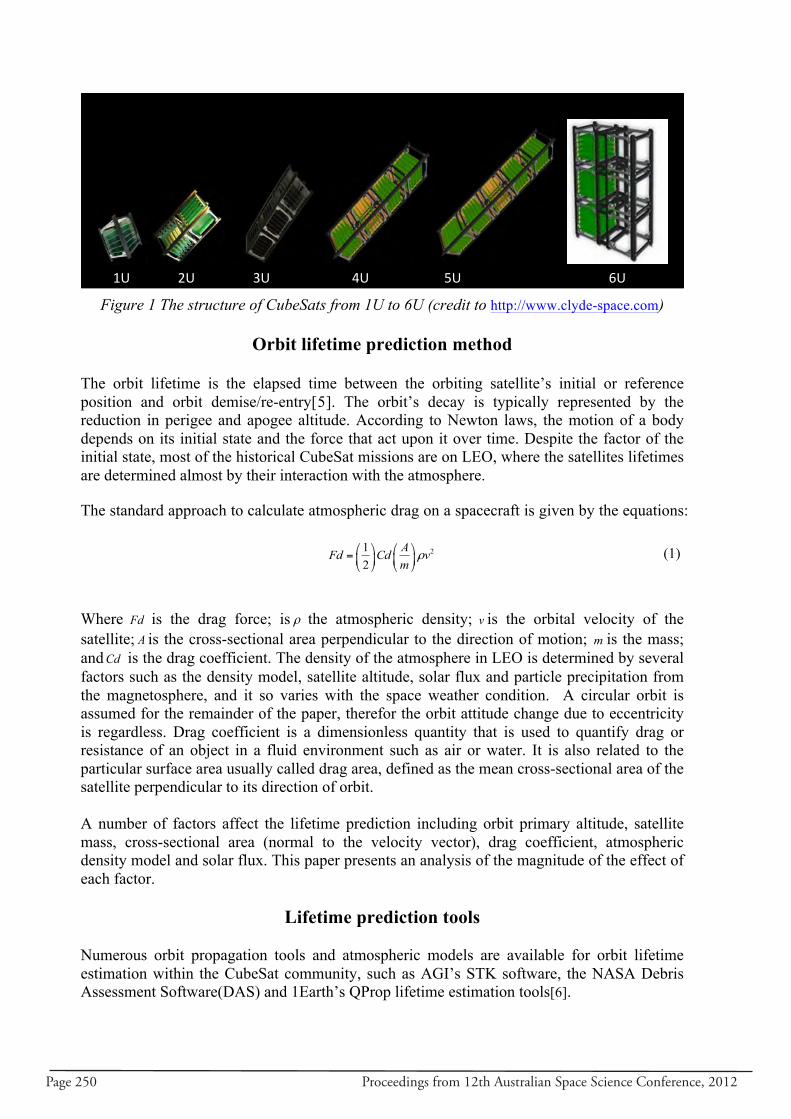
Page 250 Proceedings from 12th Australian Space Science Conference, 2012
Figure 1 The structure of CubeSats from 1U to 6U (credit to http://www.clyde-space.com)
Orbit lifetime prediction method
The orbit lifetime is the elapsed time between the orbiting satellite’s initial or reference position and orbit demise/re-entry[5]. The orbit’s decay is typically represented by the reduction in perigee and apogee altitude. According to Newton laws, the motion of a body depends on its initial state and the force that act upon it over time. Despite the factor of the initial state, most of the historical CubeSat missions are on LEO, where the satellites lifetimes are determined almost by their interaction with the atmosphere. The standard approach to calculate atmospheric drag on a spacecraft is given by the equations: 21
2AFd Cd vm
ρ⎛ ⎞ ⎛ ⎞= ⎜ ⎟ ⎜ ⎟⎝ ⎠ ⎝ ⎠
(1)
Where Fd is the drag force; is ρ the atmospheric density; v is the orbital velocity of the satellite; A is the cross-sectional area perpendicular to the direction of motion; m is the mass; andCd is the drag coefficient. The density of the atmosphere in LEO is determined by several factors such as the density model, satellite altitude, solar flux and particle precipitation from the magnetosphere, and it so varies with the space weather condition. A circular orbit is assumed for the remainder of the paper, therefor the orbit attitude change due to eccentricity is regardless. Drag coefficient is a dimensionless quantity that is used to quantify drag or resistance of an object in a fluid environment such as air or water. It is also related to the particular surface area usually called drag area, defined as the mean cross-sectional area of the satellite perpendicular to its direction of orbit. A number of factors affect the lifetime prediction including orbit primary altitude, satellite mass, cross-sectional area (normal to the velocity vector), drag coefficient, atmospheric density model and solar flux. This paper presents an analysis of the magnitude of the effect of each factor.
Lifetime prediction tools Numerous orbit propagation tools and atmospheric models are available for orbit lifetime estimation within the CubeSat community, such as AGI’s STK software, the NASA Debris Assessment Software(DAS) and 1Earth’s QProp lifetime estimation tools[6].
1U
1U 2U 3U 4U 5U 6U
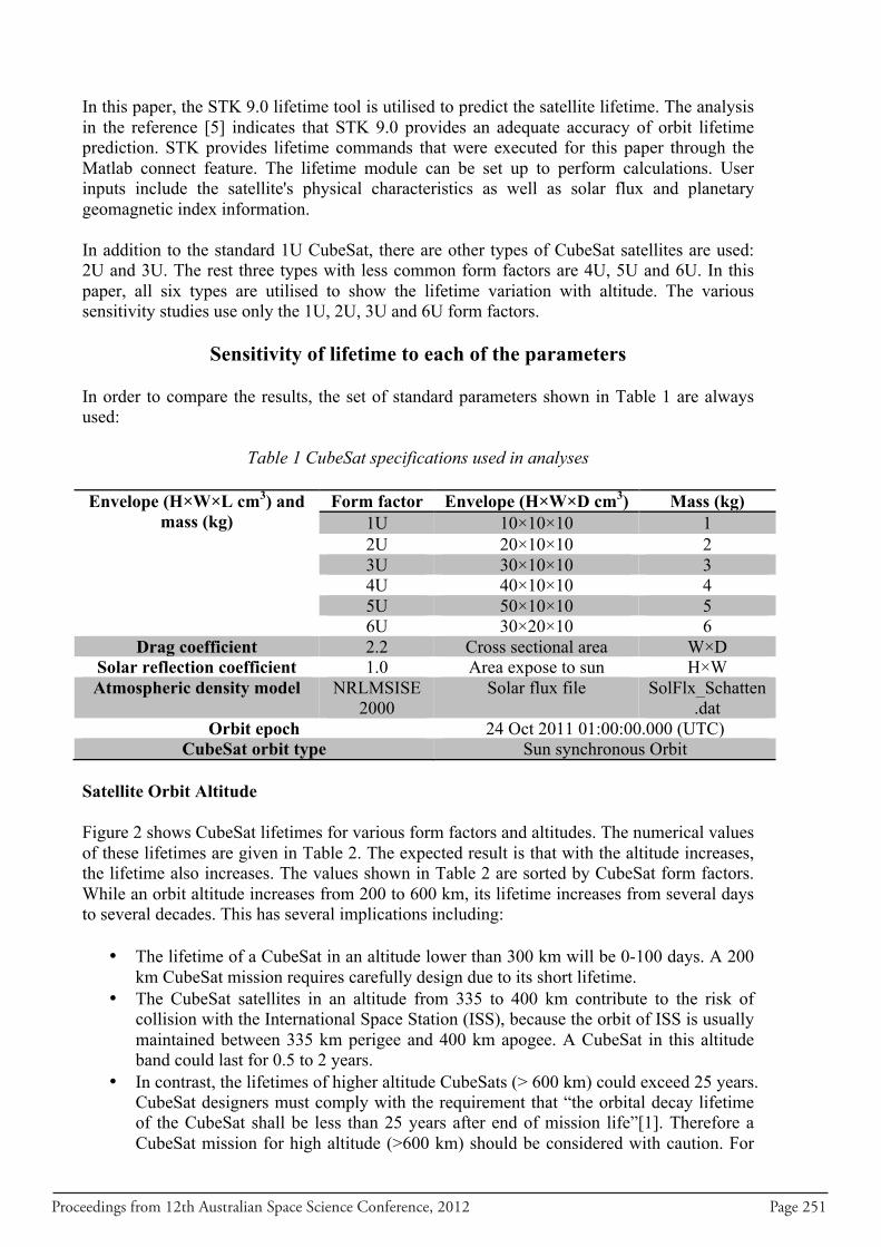
Proceedings from 12th Australian Space Science Conference, 2012 Page 251
In this paper, the STK 9.0 lifetime tool is utilised to predict the satellite lifetime. The analysis in the reference [5] indicates that STK 9.0 provides an adequate accuracy of orbit lifetime prediction. STK provides lifetime commands that were executed for this paper through the Matlab connect feature. The lifetime module can be set up to perform calculations. User inputs include the satellite's physical characteristics as well as solar flux and planetary geomagnetic index information. In addition to the standard 1U CubeSat, there are other types of CubeSat satellites are used: 2U and 3U. The rest three types with less common form factors are 4U, 5U and 6U. In this paper, all six types are utilised to show the lifetime variation with altitude. The various sensitivity studies use only the 1U, 2U, 3U and 6U form factors.
Sensitivity of lifetime to each of the parameters In order to compare the results, the set of standard parameters shown in Table 1 are always used:
Table 1 CubeSat specifications used in analyses Envelope (H×W×L cm3) and
mass (kg) Form factor Envelope (H×W×D cm3) Mass (kg)
1U 10×10×10 1 2U 20×10×10 2 3U 30×10×10 3 4U 40×10×10 4 5U 50×10×10 5 6U 30×20×10 6
Drag coefficient 2.2 Cross sectional area W×D Solar reflection coefficient 1.0 Area expose to sun H×W Atmospheric density model NRLMSISE
2000 Solar flux file SolFlx_Schatten
.dat Orbit epoch 24 Oct 2011 01:00:00.000 (UTC)
CubeSat orbit type Sun synchronous Orbit Satellite Orbit Altitude Figure 2 shows CubeSat lifetimes for various form factors and altitudes. The numerical values of these lifetimes are given in Table 2. The expected result is that with the altitude increases, the lifetime also increases. The values shown in Table 2 are sorted by CubeSat form factors. While an orbit altitude increases from 200 to 600 km, its lifetime increases from several days to several decades. This has several implications including:
• The lifetime of a CubeSat in an altitude lower than 300 km will be 0-100 days. A 200 km CubeSat mission requires carefully design due to its short lifetime.
• The CubeSat satellites in an altitude from 335 to 400 km contribute to the risk of collision with the International Space Station (ISS), because the orbit of ISS is usually maintained between 335 km perigee and 400 km apogee. A CubeSat in this altitude band could last for 0.5 to 2 years.
• In contrast, the lifetimes of higher altitude CubeSats (> 600 km) could exceed 25 years. CubeSat designers must comply with the requirement that “the orbital decay lifetime of the CubeSat shall be less than 25 years after end of mission life”[1]. Therefore a CubeSat mission for high altitude (>600 km) should be considered with caution. For
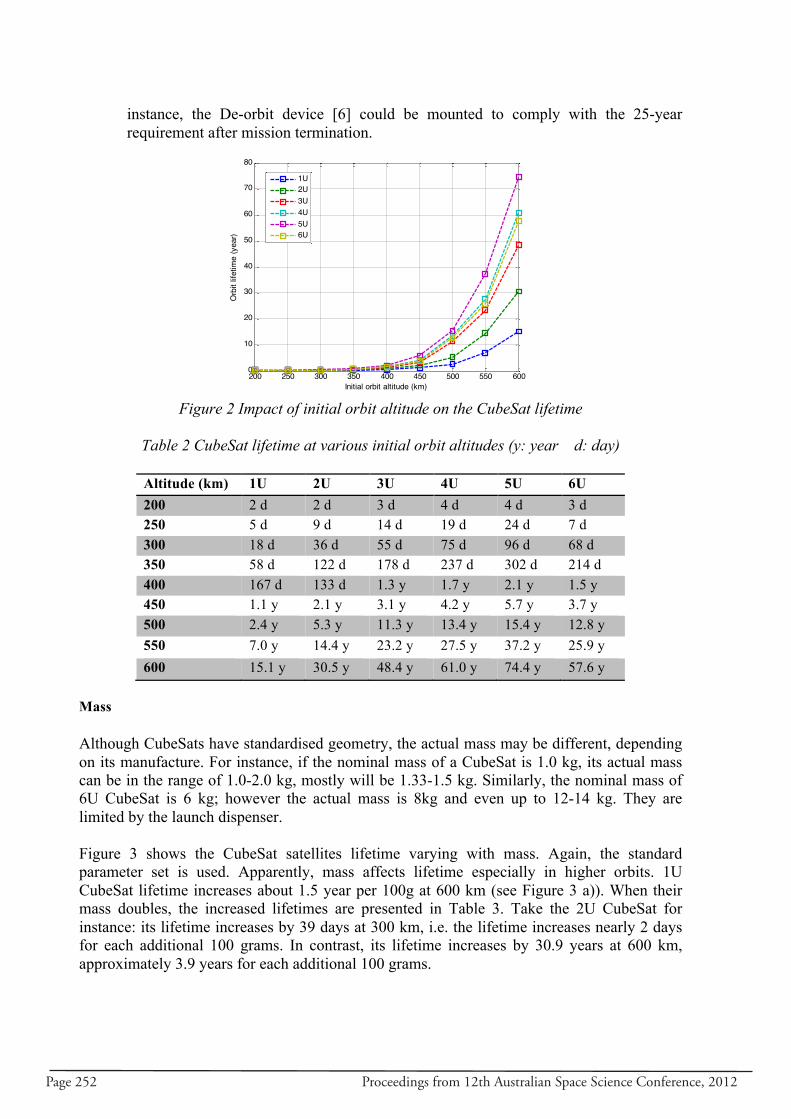
Page 252 Proceedings from 12th Australian Space Science Conference, 2012
instance, the De-orbit device [6] could be mounted to comply with the 25-year requirement after mission termination.
Figure 2 Impact of initial orbit altitude on the CubeSat lifetime
Table 2 CubeSat lifetime at various initial orbit altitudes (y: year d: day)
Altitude (km) 1U 2U 3U 4U 5U 6U 200 2 d 2 d 3 d 4 d 4 d 3 d 250 5 d 9 d 14 d 19 d 24 d 7 d 300 18 d 36 d 55 d 75 d 96 d 68 d 350 58 d 122 d 178 d 237 d 302 d 214 d 400 167 d 133 d 1.3 y 1.7 y 2.1 y 1.5 y 450 1.1 y 2.1 y 3.1 y 4.2 y 5.7 y 3.7 y 500 2.4 y 5.3 y 11.3 y 13.4 y 15.4 y 12.8 y 550 7.0 y 14.4 y 23.2 y 27.5 y 37.2 y 25.9 y 600 15.1 y 30.5 y 48.4 y 61.0 y 74.4 y 57.6 y
Mass Although CubeSats have standardised geometry, the actual mass may be different, depending on its manufacture. For instance, if the nominal mass of a CubeSat is 1.0 kg, its actual mass can be in the range of 1.0-2.0 kg, mostly will be 1.33-1.5 kg. Similarly, the nominal mass of 6U CubeSat is 6 kg; however the actual mass is 8kg and even up to 12-14 kg. They are limited by the launch dispenser. Figure 3 shows the CubeSat satellites lifetime varying with mass. Again, the standard parameter set is used. Apparently, mass affects lifetime especially in higher orbits. 1U CubeSat lifetime increases about 1.5 year per 100g at 600 km (see Figure 3 a)). When their mass doubles, the increased lifetimes are presented in Table 3. Take the 2U CubeSat for instance: its lifetime increases by 39 days at 300 km, i.e. the lifetime increases nearly 2 days for each additional 100 grams. In contrast, its lifetime increases by 30.9 years at 600 km, approximately 3.9 years for each additional 100 grams.
200 250 300 350 400 450 500 550 6000
10
20
30
40
50
60
70
80
Initial orbit altitude (km)
Orb
it lif
etim
e (y
ear)
Lifetime (years) vs. initial orbit altitude (km)
1U2U3U4U5U6U
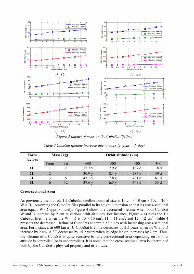
Proceedings from 12th Australian Space Science Conference, 2012 Page 253
a) 1U
b) 2U
c) 3U
d) 6U
Figure 3 Impact of mass on the CubeSat lifetime
Table 3 CubeSat lifetime increase due to mass (y: year d: day)
Form factors
Mass (kg) Orbit altitude (km)
From To 600 500 400 300 1U 1 2 15.7 y 2.9 y 167 d 18 d 2U 2 4 30.9 y 8.1 y 287 d 39 d 3U 3 6 43.1 y 7.8 y 401 d 61 d 6U 6 12 39.6 y 6.5 y 365 d 55 d
Cross-sectional Area As previously mentioned, 1U CubeSat satellite nominal size is 10 cm × 10 cm × 10cm (H × W × D). Assuming the CubeSat flies parallel to its height dimension so that its cross-sectional area equals W×D approximately. Figure 4 shows the decreased lifetime when both CubeSat W and D increase by 2 cm at various orbit altitudes. For instance, Figure 4 a) plots the 1U CubeSat lifetime when the W × D is 10 × 10 cm2, 11 × 11 cm2, and 12 ×12 cm2. Table 4 presents the decreased lifetime of CubeSats at certain altitudes with increasing cross-sectional area. For instance, at 600 km a 1U CubeSat lifetime decreases by 2.5 years when its W and D increase by 2 cm. A 3U decreases by 15.2 years when its edge length increases by 2 cm. Thus, the lifetime of a CubeSat is quite sensitive to its cross-sectional area depending on how its attitude is controlled (or is uncontrolled). It is noted that the cross-sectional area is determined both by the CubeSat’s physical property and its attitude.
1 1.1 1.2 1.3 1.4 1.5 1.6 1.7 1.8 1.9 20
10
20
30
40
50
Orb
it lif
etim
e(ye
ar)
1U CubeSat lifetime (years) vs. CubeSat mass (kg)
Altitude = 600kmAltitude = 500km
1 1.1 1.2 1.3 1.4 1.5 1.6 1.7 1.8 1.9 20
200
400
600
1U CubeSat Mass (kg)
Orb
it lif
etim
e(da
y)
Altitude = 400kmAltitude = 300km
2 2.2 2.4 2.6 2.8 3 3.2 3.4 3.6 3.8 40
20
40
60
80
Orb
it lif
etim
e(ye
ar)
2U CubeSat lifetime (years) vs. CubeSat mass (kg)
2 2.2 2.4 2.6 2.8 3 3.2 3.4 3.6 3.8 40
200
400
600
800
2U CubeSat Mass (kg)
Orb
it lif
etim
e(da
y)
Altitude = 600kmAltitude = 500km
Altitude = 400kmAltitude = 300km
3 3.5 4 4.5 5 5.5 60
20
40
60
80
100
Orb
it lif
etim
e(ye
ar)
3U CubeSat lifetime (years) vs. CubeSat mass (kg)
3 3.5 4 4.5 5 5.5 60
200
400
600
800
1000
3U CubeSat Mass (kg)
Orb
it lif
etim
e(da
y)
Altitude = 600kmAltitude = 500km
Altitude = 400kmAltitude = 300km
6 7 8 9 10 11 120
20
40
60
80
100
Orb
it lif
etim
e(ye
ar)
6U CubeSat lifetime (years) vs. CubeSat mass (kg)
6 7 8 9 10 11 120
200
400
600
800
1000
6U CubeSat Mass (kg)
Orb
it lif
etim
e(da
y)
Altitude = 600kmAltitude = 500km
Altitude = 400kmAltitude = 300km
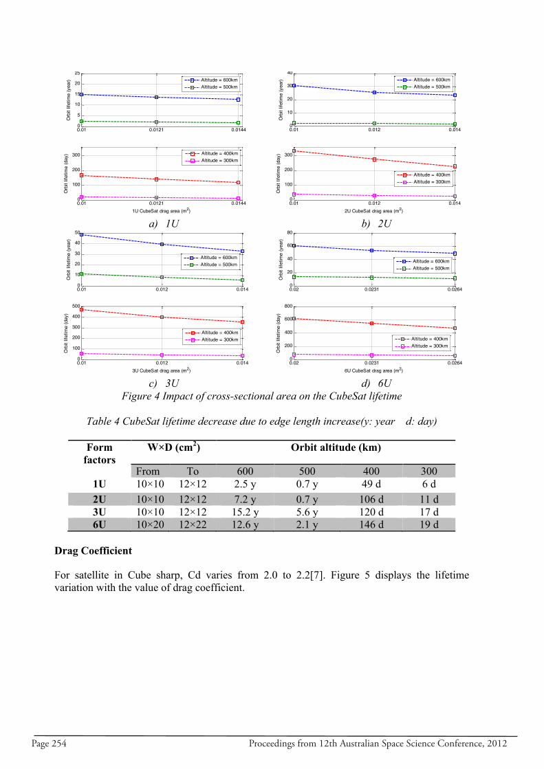
Page 254 Proceedings from 12th Australian Space Science Conference, 2012
a) 1U
b) 2U
c) 3U
d) 6U
Figure 4 Impact of cross-sectional area on the CubeSat lifetime
Table 4 CubeSat lifetime decrease due to edge length increase(y: year d: day)
Form factors
W×D (cm2) Orbit altitude (km)
From To 600 500 400 300 1U 10×10 12×12 2.5 y 0.7 y 49 d 6 d 2U 10×10 12×12 7.2 y 0.7 y 106 d 11 d 3U 10×10 12×12 15.2 y 5.6 y 120 d 17 d 6U 10×20 12×22 12.6 y 2.1 y 146 d 19 d
Drag Coefficient For satellite in Cube sharp, Cd varies from 2.0 to 2.2[7]. Figure 5 displays the lifetime variation with the value of drag coefficient.
0.01 0.0121 0.01440
5
10
15
20
25O
rbit
lifet
ime
(yea
r)1U CubeSat lifetime (years) vs. drag area (m2)
Altitude = 600kmAltitude = 500km
0.01 0.0121 0.01440
100
200
300
Orb
it lif
etim
e (d
ay)
1U CubeSat drag area (m2)
Altitude = 400kmAltitude = 300km
0.01 0.012 0.0140
10
20
30
40
Orb
it lif
etim
e (y
ear)
2U CubeSat lifetime (years) vs. drag area (m2)
0.01 0.012 0.0140
100
200
300
Orb
it lif
etim
e (d
ay)
2U CubeSat drag area (m2)
Altitude = 600kmAltitude = 500km
Altitude = 400kmAltitude = 300km
0.01 0.012 0.0140
10
20
30
40
50
Orb
it lif
etim
e (y
ear)
3U CubeSat lifetime (years) vs. drag area (m2)
0.01 0.012 0.0140
100
200
300
400
500
Orb
it lif
etim
e (d
ay)
3U CubeSat drag area (m2)
Altitude = 600kmAltitude = 500km
Altitude = 400kmAltitude = 300km
0.02 0.0231 0.02640
20
40
60
80
Orb
it lif
etim
e (y
ear)
6U CubeSat lifetime (years) vs. drag area (m2)
0.02 0.0231 0.02640
200
400
600
800
Orb
it lif
etim
e (d
ay)
6U CubeSat drag area (m2)
Altitude = 600kmAltitude = 500km
Altitude = 400kmAltitude = 300km
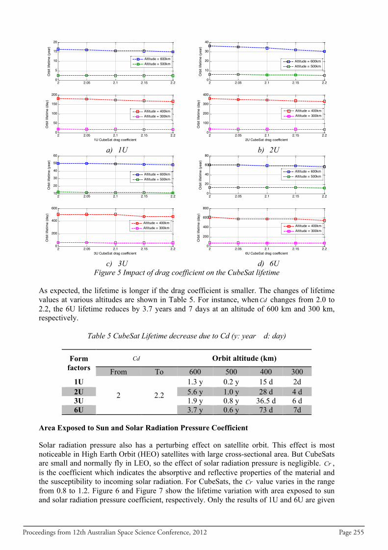
Proceedings from 12th Australian Space Science Conference, 2012 Page 255
a) 1U
b) 2U
c) 3U
d) 6U
Figure 5 Impact of drag coefficient on the CubeSat lifetime As expected, the lifetime is longer if the drag coefficient is smaller. The changes of lifetime values at various altitudes are shown in Table 5. For instance, whenCd changes from 2.0 to 2.2, the 6U lifetime reduces by 3.7 years and 7 days at an altitude of 600 km and 300 km, respectively.
Table 5 CubeSat Lifetime decrease due to Cd (y: year d: day)
Form factors
Cd Orbit altitude (km)
From To 600 500 400 300 1U
2 2.2
1.3 y 0.2 y 15 d 2d 2U 5.6 y 1.0 y 28 d 4 d 3U 1.9 y 0.8 y 36.5 d 6 d 6U 3.7 y 0.6 y 73 d 7d
Area Exposed to Sun and Solar Radiation Pressure Coefficient Solar radiation pressure also has a perturbing effect on satellite orbit. This effect is most noticeable in High Earth Orbit (HEO) satellites with large cross-sectional area. But CubeSats are small and normally fly in LEO, so the effect of solar radiation pressure is negligible. Cr , is the coefficient which indicates the absorptive and reflective properties of the material and the susceptibility to incoming solar radiation. For CubeSats, the Cr value varies in the range from 0.8 to 1.2. Figure 6 and Figure 7 show the lifetime variation with area exposed to sun and solar radiation pressure coefficient, respectively. Only the results of 1U and 6U are given
2 2.05 2.1 2.15 2.20
5
10
15
20O
rbit
lifet
ime
(yea
r)
1U CubeSat lifetime (years) vs. drag coefficient
Altitude = 600kmAltitude = 500km
2 2.05 2.1 2.15 2.20
50
100
150
200
Orb
it lif
etim
e (d
ay)
1U CubeSat drag coefficient
Altitude = 400kmAltitude = 300km
2 2.05 2.1 2.15 2.20
10
20
30
40
Orb
it lif
etim
e (y
ear)
2U CubeSat lifetime (years) vs. drag coefficient
2 2.05 2.1 2.15 2.20
100
200
300
400
Orb
it lif
etim
e (d
ay)
2U CubeSat drag coefficient
Altitude = 600kmAltitude = 500km
Altitude = 400kmAltitude = 300km
2 2.05 2.1 2.15 2.210
20
30
40
50
60
Orb
it lif
etim
e (y
ear)
3U CubeSat lifetime (years) vs. drag coefficient
2 2.05 2.1 2.15 2.20
200
400
600
Orb
it lif
etim
e (d
ay)
3U CubeSat drag coefficient
Altitude = 600kmAltitude = 500km
Altitude = 400kmAltitude = 300km
2 2.05 2.1 2.15 2.20
20
40
60
80
Orb
it lif
etim
e (y
ear)
6U CubeSat lifetime (years) vs. drag coefficient
2 2.05 2.1 2.15 2.20
200
400
600
800
Orb
it lif
etim
e (d
ay)
6U CubeSat drag coefficient
Altitude = 600kmAltitude = 500km
Altitude = 400kmAltitude = 300km
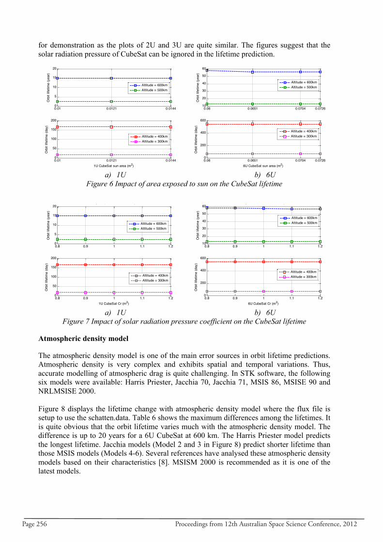
Page 256 Proceedings from 12th Australian Space Science Conference, 2012
for demonstration as the plots of 2U and 3U are quite similar. The figures suggest that the solar radiation pressure of CubeSat can be ignored in the lifetime prediction.
a) 1U
b) 6U
Figure 6 Impact of area exposed to sun on the CubeSat lifetime
a) 1U
b) 6U
Figure 7 Impact of solar radiation pressure coefficient on the CubeSat lifetime Atmospheric density model The atmospheric density model is one of the main error sources in orbit lifetime predictions. Atmospheric density is very complex and exhibits spatial and temporal variations. Thus, accurate modelling of atmospheric drag is quite challenging. In STK software, the following six models were available: Harris Priester, Jacchia 70, Jacchia 71, MSIS 86, MSISE 90 and NRLMSISE 2000. Figure 8 displays the lifetime change with atmospheric density model where the flux file is setup to use the schatten.data. Table 6 shows the maximum differences among the lifetimes. It is quite obvious that the orbit lifetime varies much with the atmospheric density model. The difference is up to 20 years for a 6U CubeSat at 600 km. The Harris Priester model predicts the longest lifetime. Jacchia models (Model 2 and 3 in Figure 8) predict shorter lifetime than those MSIS models (Models 4-6). Several references have analysed these atmospheric density models based on their characteristics [8]. MSISM 2000 is recommended as it is one of the latest models.
0.01 0.0121 0.01440
5
10
15
20
Orb
it lif
etim
e (y
ear)
1U CubeSat lifetime (years) vs. sun area(m2)
Altitude = 600kmAltitude = 500km
0.01 0.0121 0.01440
50
100
150
200
Orb
it lif
etim
e (d
ay)
1U CubeSat sun area (m2)
Altitude = 400kmAltitude = 300km
0.06 0.0651 0.0704 0.072610
20
30
40
50
60
Orb
it lif
etim
e (y
ear)
6U CubeSat lifetime (years) vs. sun area(m2)
Altitude = 600kmAltitude = 500km
0.06 0.0651 0.0704 0.07260
200
400
600
Orb
it lif
etim
e (d
ay)
6U CubeSat sun area (m2)
Altitude = 400kmAltitude = 300km
0.8 0.9 1 1.1 1.20
5
10
15
20
Orb
it lif
etim
e (y
ear)
1U CubeSat lifetime (years) vs. solar radiation pressure coefficient
Altitude = 600kmAltitude = 500km
0.8 0.9 1 1.1 1.20
50
100
150
200
Orb
it lif
etim
e (d
ay)
1U CubeSat Cr (m2)
Altitude = 400kmAltitude = 300km
0.8 0.9 1 1.1 1.210
20
30
40
50
60
Orb
it lif
etim
e (y
ear)
6U CubeSat lifetime (years) vs. solar radiation pressure coefficient
0.8 0.9 1 1.1 1.20
200
400
600
Orb
it lif
etim
e (d
ay)
6U CubeSat Cr (m2)
Altitude = 600kmAltitude = 500km
Altitude = 400kmAltitude = 300km
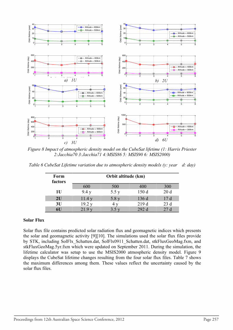
Proceedings from 12th Australian Space Science Conference, 2012 Page 257
a) 1U
b) 2U
c) 3U
d) 6U
Figure 8 Impact of atmospheric density model on the CubeSat lifetime (1: Harris Priester
2:Jacchia70 3:Jacchia71 4:MSIS86 5: MSIS90 6: MSIS2000)
Table 6 CubeSat Lifetime variation due to atmospheric density models (y: year d: day)
Form factors
Orbit altitude (km)
600 500 400 300 1U 9.4 y 5.5 y 150 d 20 d 2U 11.4 y 5.8 y 136 d 17 d 3U 19.2 y 4 y 219 d 23 d 6U 21.9 y 3.5 y 292 d 27 d
Solar Flux Solar flux file contains predicted solar radiation flux and geomagnetic indices which presents the solar and geomagnetic activity [9][10]. The simulations used the solar flux files provide by STK, including SolFlx_Schatten.dat, SolFlx0911_Schatten.dat, stkFluxGeoMag.fxm, and stkFluxGeoMag.5yr.fxm which were updated on September 2011. During the simulation, the lifetime calculator was setup to use the MSIS2000 atmospheric density model. Figure 9 displays the CubeSat lifetime changes resulting from the four solar flux files. Table 7 shows the maximum differences among them. These values reflect the uncertainty caused by the solar flux files.
1 2 3 4 5 60
10
20
30
40
Orb
it lif
etim
e (y
ear)
1U CubeSat lifetime (years) vs. Atmosphere Density
Altitude = 600kmAltitude = 500km
1 2 3 4 5 60
200
400
600
Orb
it lif
etim
e (d
ay)
Density model for 1U lifetime caculation1:Harris Priester 2:Jacchia70 3:Jacchia71
4:MSIS86 5:MSIS90 6:MSIS2000
Altitude = 400kmAltitude = 300km
1 2 3 4 5 60
10
20
30
40
Orb
it lif
etim
e (y
ear)
2U CubeSat lifetime (years) vs. Atmosphere Density
Altitude = 600kmAltitude = 500km
1 2 3 4 5 60
200
400
600
Orb
it lif
etim
e (d
ay)
Density model for 2U lifetime caculation1:Harris Priester 2:Jacchia70 3:Jacchia71
4:MSIS86 5:MSIS90 6:MSIS2000
Altitude = 400kmAltitude = 300km
1 2 3 4 5 60
20
40
60
Orb
it lif
etim
e (y
ear)
3U CubeSat lifetime (years) vs. Atmosphere Density
1 2 3 4 5 60
200
400
600
800
Orb
it lif
etim
e (d
ay)
Density model for 3U lifetime caculation1:Harris Priester 2:Jacchia70 3:Jacchia71
4:MSIS86 5:MSIS90 6:MSIS2000
Altitude = 600kmAltitude = 500km
Altitude = 400kmAltitude = 300km
1 2 3 4 5 60
20
40
60
80
Orb
it lif
etim
e (y
ear)
6U CubeSat lifetime (years) vs. Atmosphere Density
1 2 3 4 5 60
500
1000O
rbit
lifet
ime
(day
)
Density model for 6U lifetime caculation1:Harris Priester 2:Jacchia70 3:Jacchia71
4:MSIS86 5:MSIS90 6:MSIS2000
Altitude = 600kmAltitude = 500km
Altitude = 400kmAltitude = 300km
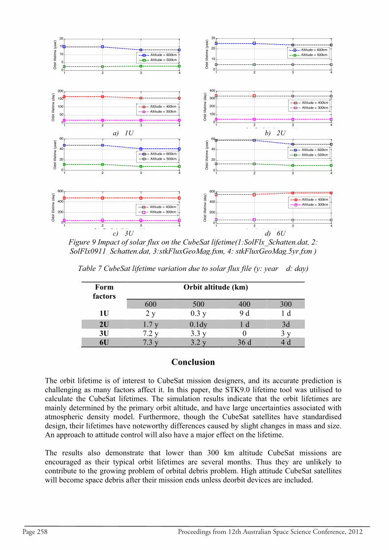
Page 258 Proceedings from 12th Australian Space Science Conference, 2012
a) 1U
b) 2U
c) 3U
d) 6U
Figure 9 Impact of solar flux on the CubeSat lifetime(1:SolFlx_Schatten.dat, 2: SolFlx0911_Schatten.dat, 3:stkFluxGeoMag.fxm, 4: stkFluxGeoMag.5yr.fxm )
Table 7 CubeSat lifetime variation due to solar flux file (y: year d: day)
Form
factors Orbit altitude (km)
600 500 400 300 1U 2 y 0.3 y 9 d 1 d 2U 1.7 y 0.1dy 1 d 3d 3U 7.2 y 3.3 y 0 3 y 6U 7.3 y 3.2 y 36 d 4 d
Conclusion
The orbit lifetime is of interest to CubeSat mission designers, and its accurate prediction is challenging as many factors affect it. In this paper, the STK9.0 lifetime tool was utilised to calculate the CubeSat lifetimes. The simulation results indicate that the orbit lifetimes are mainly determined by the primary orbit altitude, and have large uncertainties associated with atmospheric density model. Furthermore, though the CubeSat satellites have standardised design, their lifetimes have noteworthy differences caused by slight changes in mass and size. An approach to attitude control will also have a major effect on the lifetime. The results also demonstrate that lower than 300 km altitude CubeSat missions are encouraged as their typical orbit lifetimes are several months. Thus they are unlikely to contribute to the growing problem of orbital debris problem. High attitude CubeSat satellites will become space debris after their mission ends unless deorbit devices are included.
1 2 3 40
5
10
15
20
Orb
it lif
etim
e (y
ear)
1U CubeSat lifetime (years) vs. Solar flux file used for caculation
Altitude = 600kmAltitude = 500km
1 2 3 40
50
100
150
200
Orb
it lif
etim
e (d
ay)
Solar Flux file for lifetime caculation1:SolFlx Schatten.dat 2:SolFlx0911 Schatten.dat3:stkFluxGeoMag.fxm stkFluxGeoMag.5yr.fxm
Altitude = 400kmAltitude = 300km
1 2 3 40
10
20
30
Orb
it lif
etim
e (y
ear)
2U CubeSat lifetime (years) vs. Solar flux file used for caculation
Altitude = 600kmAltitude = 500km
1 2 3 40
100
200
300
400
Orb
it lif
etim
e (d
ay)
Solar Flux file for lifetime caculation1:SolFlx Schatten.dat 2:SolFlx0911 Schatten.dat3:stkFluxGeoMag.fxm stkFluxGeoMag.5yr.fxm
Altitude = 400kmAltitude = 300km
1 2 3 40
20
40
60
Orb
it lif
etim
e (y
ear)
3U CubeSat lifetime (years) vs. Solar flux file used for caculation
Altitude = 600kmAltitude = 500km
1 2 3 40
200
400
600
Orb
it lif
etim
e (d
ay)
Solar Flux file for lifetime caculation1:SolFlx Schatten.dat 2:SolFlx0911 Schatten.dat3:stkFluxGeoMag.fxm stkFluxGeoMag.5yr.fxm
Altitude = 400kmAltitude = 300km
1 2 3 40
20
40
60
Orb
it lif
etim
e (y
ear)
6U CubeSat lifetime (years) vs. Solar flux file used for caculation
1 2 3 40
200
400
600
Orb
it lif
etim
e (d
ay)
Solar Flux file for lifetime caculation1:SolFlx Schatten.dat 2:SolFlx0911 Schatten.dat3:stkFluxGeoMag.fxm stkFluxGeoMag.5yr.fxm
Altitude = 600kmAltitude = 500km
Altitude = 400kmAltitude = 300km
Proceedings from 12th Australian Space Science Conference, 2012 Page 259
As “The only thing certain is uncertainty”, the CubeSat mission designer should keep the uncertainties within a sustainable range to ensure the mission performs properly.
Acknowledgments This research project is funded by the Australian Space Research Program on "SAR Formation Flying". The authors acknowledge the support of the Australian Centre for Space Engineering Research. Special thanks to the first author’s colleague Gordon Roesler for his support for the work contribute for this paper.
References 1 . “CubeSat Design Specification Rev.12”, The CubeSat Program, California State
Polytechnic University. Retrieved Oct 16, 2010, pp.5-13.
2. AMSAT Cubesat Information. http://www.amsat.org/, assessed 4 Dec. 2012.
3. QB 5 project. https://www.qb50.eu/, assessed 4 Dec. 2012,
4. WIKIPEIDA List of CubeSat http://en.wikipedia.org/wiki/List_of_CubeSats
5. ISO Standard 27852, “Space Systems – Determining” . International Organization for Standardization. Geneva, Switzerland,2009
6. Oltrogge, D.L.,Leveque,K., “An Evaluation of CubeSat Orbital Decay”, Proceedings of the 25th Annual AIAA/USU Conference on Small Satellites, Logan,UT, USA, Aug 08-11,2011.
7. Reynerson, C., Aerodynamic Disturbance Force and Torque Estimation for Spacecraft and Simple Shapes Using Finite Plate Elements – Part I: Drag Coefficient,. Advances in Spacecraft Technologies, Dr Jason Hall (Ed.), ISBN: 978-953-307-551-8, InTech, 2011. pp.333-352
8. Picone, J.M., Hedin, A.E., Drob, D.P., and Aikin ,A.C., "NRL-MSISE-00 Empirical Model of the Atmosphere: Statistical Comparisons and Scientific Issues", Journal of Geophysical Research, Vol. 107,No. A14, 2003, pp.15
9. Nassiz, B.J., Berry, K. and Schatten, K., “Orbit Decay Prediction Sensitivity to Solar Flux Variations”, Proceedings of the AIAA/AAS Astrodynamics Specialists Conference”, Paper 07-264, Mackinac Island, MI, USA, August 2007.
10. Analytical Graphics, Inc.,”Lifetime Tool”,
http://www.agi.com/resources/help/online/stk/source/stk/importfiles-15.htm, accessed 4 December 2012

Page 260 Proceedings from 12th Australian Space Science Conference, 2012
Proceedings from 12th Australian Space Science Conference, 2012 Page 261
Satellites Orbit Design for the Australian Garada Project
Li Qiao, Chris Rizos, Andrew G Dempster
Australian Centre for Space Engineering Research(ACSER), School of Geospatial Engineering, University of New South Wales, Sydney 2052, Australia
Summary: Australia is presently investigating the design of an earth observation Synthetic Aperture Radar (SAR) satellite mission, known as “Garada”. It adopts an approach of several satellites flying in formation to optimise the capability of collecting SAR images over Australia’s huge land mass for a variety of applications. Mission objectives and satellite orbit design are briefly described in this paper. Requirements and considerations regarding the selection of satellite orbits are discussed as well. Generally, orbit design is mainly driven by the requirements of revisit, SAR imaging capability and solar power budget. Our preliminary results show that two identical satellites flying in the Sun-synchronous orbit at an altitude of 613 km could meet the user’s requirement of a 3-day revisit. Keywords: Orbit design, SAR satellite, Garada Equation Chapter 1 Section 1
INTRODUCTION
In late 2010 the Garada project funded by the Australian Space Research Program (ASRP), was launched at the Australian Centre for Space Engineering Research (ACSER). This collaborative project is aiming to develop the design, technologies and business case for an Earth observation Synthetic Aperture Radar (SAR) satellite mission, known as “Garada”. The objectives of the mission are to be able to continuously acquire images of the Earth in all weather for multi-applications such as soil moisture measurement, biomass estimation, and flood mapping. This paper summarises the analyses of determining orbit parameters for the proposed Garada satellite mission. It first analyses the mission objectives, payload and satellite design requirements. Then trade-off studies are performed in order to find a suitable orbit that satisfies the mission goals. Simulation results using the Satellite Tool Kit (STK) are presented.
MISSION REQUIREMENTS 1) Soil moisture monitoring of Murray Darling Basin(MDB) The key application that could be provided to deliver significant benefit to Australia is soil moisture monitoring over an agricultural area (predominantly the MDB (see Figure 1)). The payload requirements therefore relate primarily to soil moisture mapping. MDB is highlighted as a key area of interest as the area provides one third of Australia’s agricultural produce. A coverage revisit interval of 2-3 days would be required to satisfy the mission goal. The payload will revisit the target area at the same time of day on subsequent passes to determine the moisture content of the soil in the coverage area. Priority will be given to Australian target areas and Australian clients.
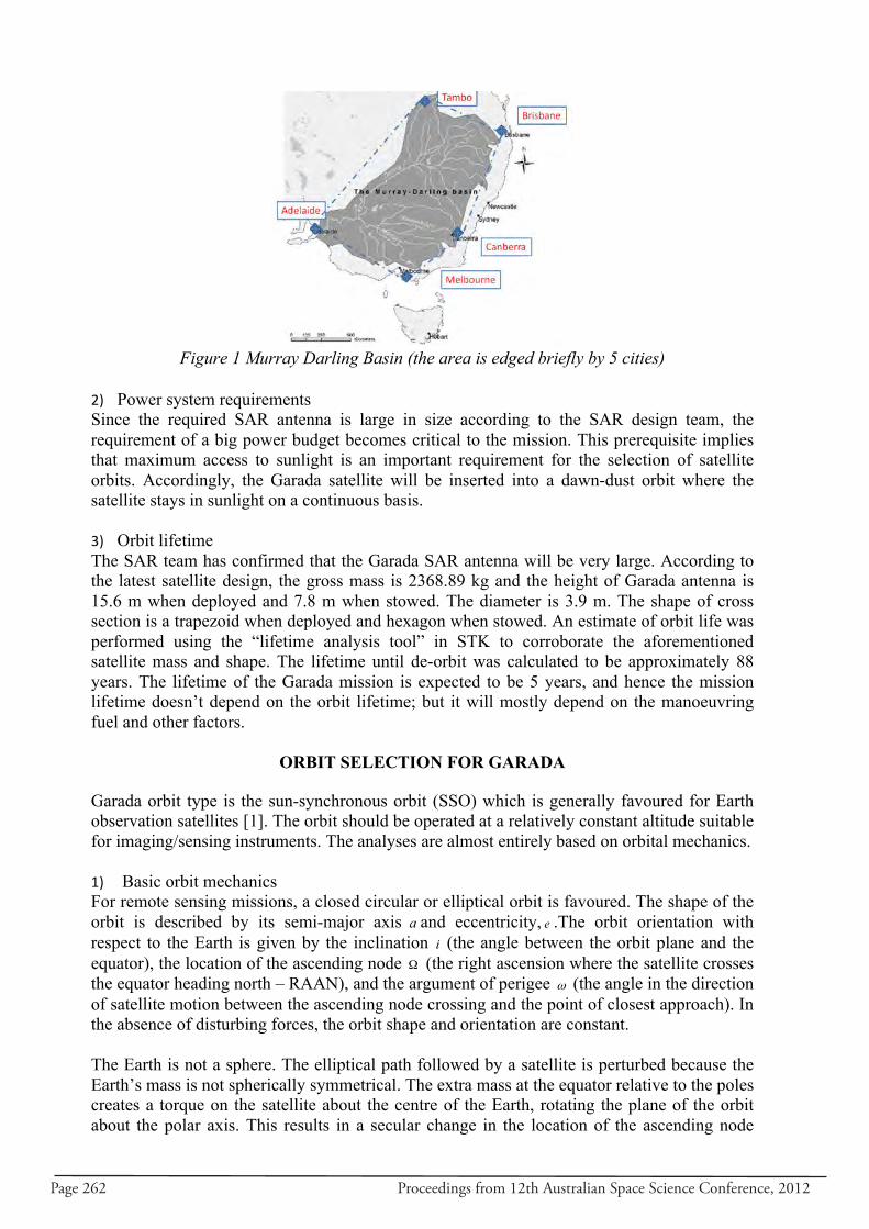
Page 262 Proceedings from 12th Australian Space Science Conference, 2012
Figure 1 Murray Darling Basin (the area is edged briefly by 5 cities)
2) Power system requirements Since the required SAR antenna is large in size according to the SAR design team, the requirement of a big power budget becomes critical to the mission. This prerequisite implies that maximum access to sunlight is an important requirement for the selection of satellite orbits. Accordingly, the Garada satellite will be inserted into a dawn-dust orbit where the satellite stays in sunlight on a continuous basis. 3) Orbit lifetime The SAR team has confirmed that the Garada SAR antenna will be very large. According to the latest satellite design, the gross mass is 2368.89 kg and the height of Garada antenna is 15.6 m when deployed and 7.8 m when stowed. The diameter is 3.9 m. The shape of cross section is a trapezoid when deployed and hexagon when stowed. An estimate of orbit life was performed using the “lifetime analysis tool” in STK to corroborate the aforementioned satellite mass and shape. The lifetime until de-orbit was calculated to be approximately 88 years. The lifetime of the Garada mission is expected to be 5 years, and hence the mission lifetime doesn’t depend on the orbit lifetime; but it will mostly depend on the manoeuvring fuel and other factors.
ORBIT SELECTION FOR GARADA Garada orbit type is the sun-synchronous orbit (SSO) which is generally favoured for Earth observation satellites [1]. The orbit should be operated at a relatively constant altitude suitable for imaging/sensing instruments. The analyses are almost entirely based on orbital mechanics. 1) Basic orbit mechanics For remote sensing missions, a closed circular or elliptical orbit is favoured. The shape of the orbit is described by its semi-major axis a and eccentricity, e .The orbit orientation with respect to the Earth is given by the inclination i (the angle between the orbit plane and the equator), the location of the ascending node Ω (the right ascension where the satellite crosses the equator heading north – RAAN), and the argument of perigee ω (the angle in the direction of satellite motion between the ascending node crossing and the point of closest approach). In the absence of disturbing forces, the orbit shape and orientation are constant. The Earth is not a sphere. The elliptical path followed by a satellite is perturbed because the Earth’s mass is not spherically symmetrical. The extra mass at the equator relative to the poles creates a torque on the satellite about the centre of the Earth, rotating the plane of the orbit about the polar axis. This results in a secular change in the location of the ascending node
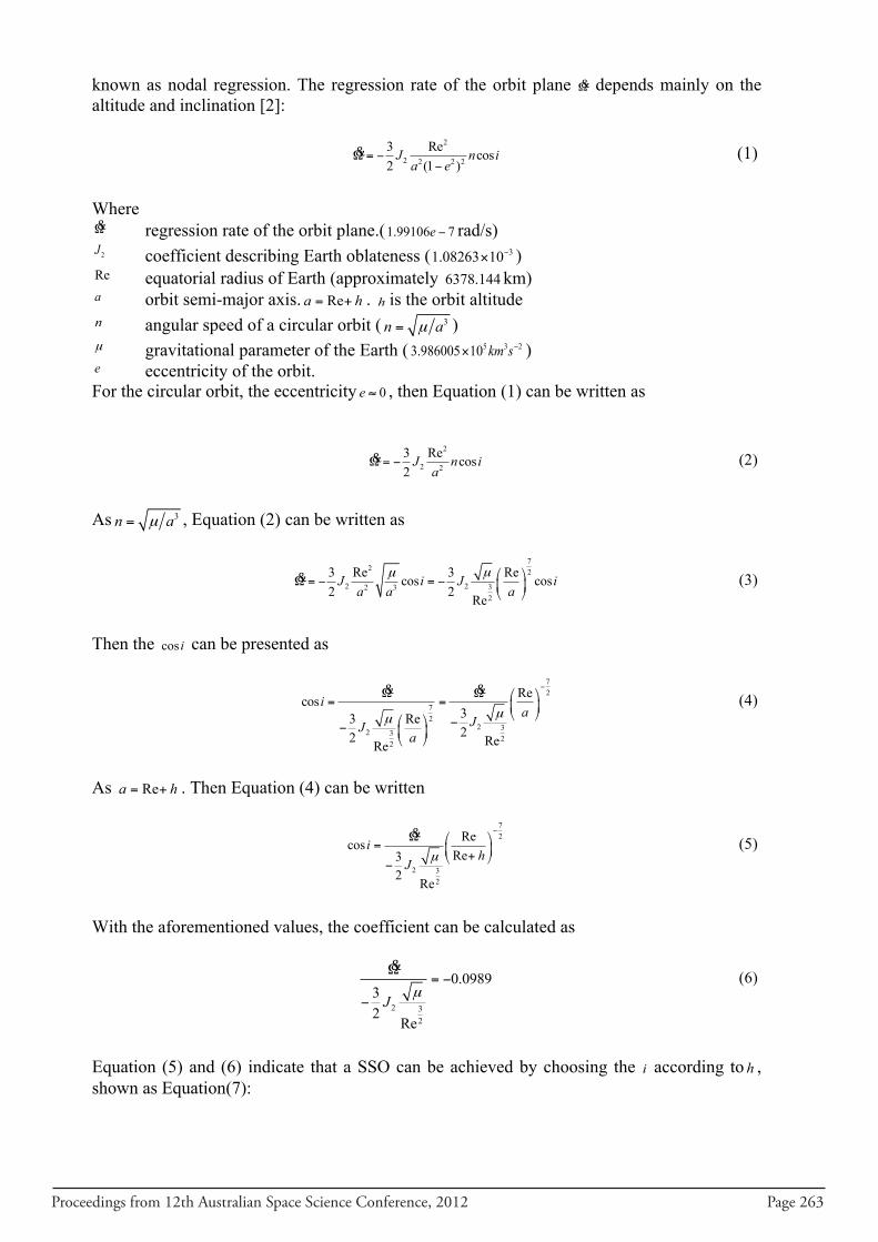
Proceedings from 12th Australian Space Science Conference, 2012 Page 263
known as nodal regression. The regression rate of the orbit plane Ω& depends mainly on the altitude and inclination [2]:
2
2 2 2 2
3 Re cos2 (1 )J n ia e
Ω = −−
& (1)
Where Ω& regression rate of the orbit plane.(1.99106 7e − rad/s) 2J coefficient describing Earth oblateness ( 31.08263 10−× ) Re equatorial radius of Earth (approximately 6378.144km) a orbit semi-major axis. Rea h= + . h is the orbit altitude n angular speed of a circular orbit ( 3n aµ= ) µ gravitational parameter of the Earth ( 5 3 23.986005 10 km s−× ) e eccentricity of the orbit. For the circular orbit, the eccentricity 0e ≈ , then Equation (1) can be written as
2
2 2
3 Re cos2J n ia
Ω = −& (2)
As 3n aµ= , Equation (2) can be written as
7
2 2
2 2 32 32
3 Re 3 Recos cos2 2 ReJ i J ia a a
µµ ⎛ ⎞Ω = − = − ⎜ ⎟⎝ ⎠
& (3)
Then the cos i can be presented as
72
72
2 32 32
2
Recos33 Re22 ReRe
ia
JJa
µµ
−Ω Ω ⎛ ⎞= = ⎜ ⎟
⎝ ⎠⎛ ⎞ −− ⎜ ⎟⎝ ⎠
& & (4)
As Rea h= + . Then Equation (4) can be written
72
2 32
RecosRe3
2 Re
ih
J µ
−Ω ⎛ ⎞= ⎜ ⎟+⎝ ⎠
−
& (5)
With the aforementioned values, the coefficient can be calculated as
2 32
0.098932
ReJ µ
Ω= −
−
& (6)
Equation (5) and (6) indicate that a SSO can be achieved by choosing the i according to h , shown as Equation(7):
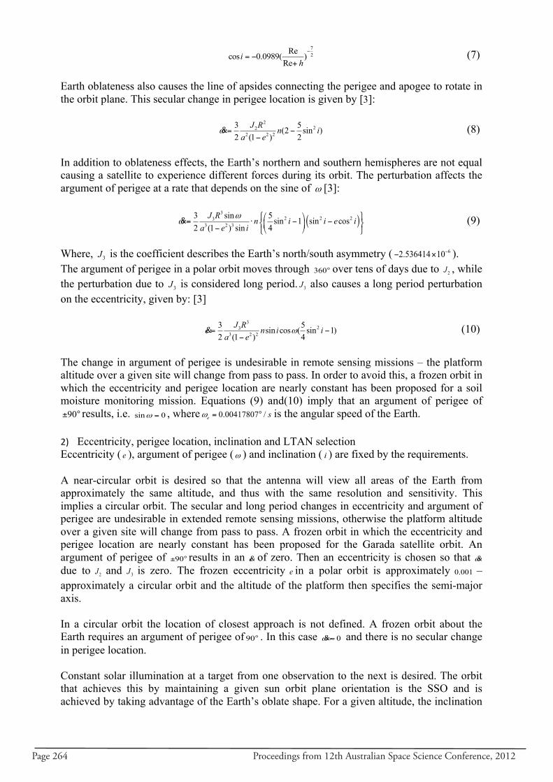
Page 264 Proceedings from 12th Australian Space Science Conference, 2012
72Recos 0.0989( )
Rei
h−
= −+
(7)
Earth oblateness also causes the line of apsides connecting the perigee and apogee to rotate in the orbit plane. This secular change in perigee location is given by [3]:
222
2 2 2
3 5(2 sin )2 (1 ) 2
J R n ia e
ω = −−
& (8)
In addition to oblateness effects, the Earth’s northern and southern hemispheres are not equal causing a satellite to experience different forces during its orbit. The perturbation affects the argument of perigee at a rate that depends on the sine of ω [3]:
( )3
2 2 233 2 3
3 sin 5 sin 1 sin cos2 (1 ) sin 4
J R n i i e ia e i
ωω
⎧ ⎫⎛ ⎞= ⋅ − −⎨ ⎬⎜ ⎟− ⎝ ⎠⎩ ⎭& (9)
Where, 3J is the coefficient describes the Earth’s north/south asymmetry ( 62.536414 10−− × ). The argument of perigee in a polar orbit moves through 360° over tens of days due to 2J , while the perturbation due to 3J is considered long period. 3J also causes a long period perturbation on the eccentricity, given by: [3]
323
3 2 2
3 5sin cos ( sin 1)2 (1 ) 4
J Re n i ia e
ω= −−
& (10)
The change in argument of perigee is undesirable in remote sensing missions – the platform altitude over a given site will change from pass to pass. In order to avoid this, a frozen orbit in which the eccentricity and perigee location are nearly constant has been proposed for a soil moisture monitoring mission. Equations (9) and(10) imply that an argument of perigee of 90± ° results, i.e. sin 0ω = , where 0.00417807 /e sω = ° is the angular speed of the Earth.
2) Eccentricity, perigee location, inclination and LTAN selection Eccentricity ( e ), argument of perigee (ω ) and inclination ( i ) are fixed by the requirements. A near-circular orbit is desired so that the antenna will view all areas of the Earth from approximately the same altitude, and thus with the same resolution and sensitivity. This implies a circular orbit. The secular and long period changes in eccentricity and argument of perigee are undesirable in extended remote sensing missions, otherwise the platform altitude over a given site will change from pass to pass. A frozen orbit in which the eccentricity and perigee location are nearly constant has been proposed for the Garada satellite orbit. An argument of perigee of 90± ° results in an e& of zero. Then an eccentricity is chosen so that ω& due to 2J and 3J is zero. The frozen eccentricity e in a polar orbit is approximately 0.001 – approximately a circular orbit and the altitude of the platform then specifies the semi-major axis. In a circular orbit the location of closest approach is not defined. A frozen orbit about the Earth requires an argument of perigee of 90° . In this case 0ω ≈& and there is no secular change in perigee location. Constant solar illumination at a target from one observation to the next is desired. The orbit that achieves this by maintaining a given sun orbit plane orientation is the SSO and is achieved by taking advantage of the Earth’s oblate shape. For a given altitude, the inclination
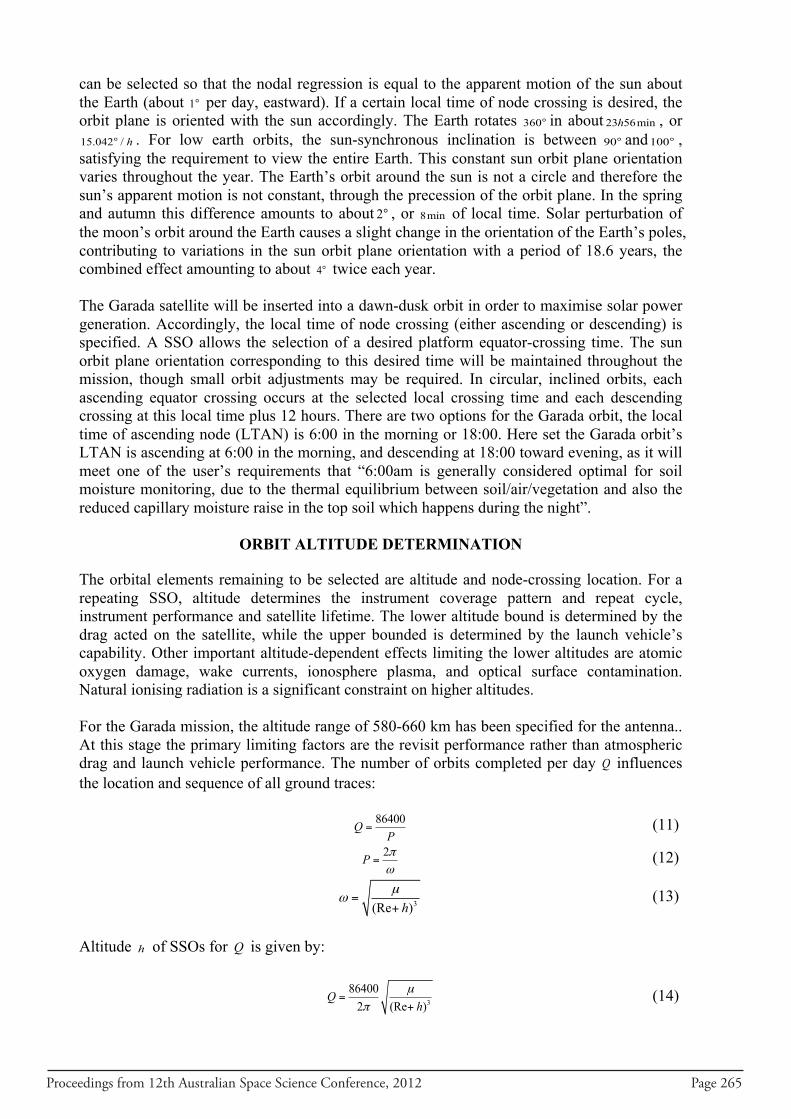
Proceedings from 12th Australian Space Science Conference, 2012 Page 265
can be selected so that the nodal regression is equal to the apparent motion of the sun about the Earth (about 1° per day, eastward). If a certain local time of node crossing is desired, the orbit plane is oriented with the sun accordingly. The Earth rotates 360° in about 23 56minh , or 15.042 / h° . For low earth orbits, the sun-synchronous inclination is between 90° and100° , satisfying the requirement to view the entire Earth. This constant sun orbit plane orientation varies throughout the year. The Earth’s orbit around the sun is not a circle and therefore the sun’s apparent motion is not constant, through the precession of the orbit plane. In the spring and autumn this difference amounts to about 2° , or 8min of local time. Solar perturbation of the moon’s orbit around the Earth causes a slight change in the orientation of the Earth’s poles, contributing to variations in the sun orbit plane orientation with a period of 18.6 years, the combined effect amounting to about 4° twice each year. The Garada satellite will be inserted into a dawn-dusk orbit in order to maximise solar power generation. Accordingly, the local time of node crossing (either ascending or descending) is specified. A SSO allows the selection of a desired platform equator-crossing time. The sun orbit plane orientation corresponding to this desired time will be maintained throughout the mission, though small orbit adjustments may be required. In circular, inclined orbits, each ascending equator crossing occurs at the selected local crossing time and each descending crossing at this local time plus 12 hours. There are two options for the Garada orbit, the local time of ascending node (LTAN) is 6:00 in the morning or 18:00. Here set the Garada orbit’s LTAN is ascending at 6:00 in the morning, and descending at 18:00 toward evening, as it will meet one of the user’s requirements that “6:00am is generally considered optimal for soil moisture monitoring, due to the thermal equilibrium between soil/air/vegetation and also the reduced capillary moisture raise in the top soil which happens during the night”.
ORBIT ALTITUDE DETERMINATION The orbital elements remaining to be selected are altitude and node-crossing location. For a repeating SSO, altitude determines the instrument coverage pattern and repeat cycle, instrument performance and satellite lifetime. The lower altitude bound is determined by the drag acted on the satellite, while the upper bounded is determined by the launch vehicle’s capability. Other important altitude-dependent effects limiting the lower altitudes are atomic oxygen damage, wake currents, ionosphere plasma, and optical surface contamination. Natural ionising radiation is a significant constraint on higher altitudes. For the Garada mission, the altitude range of 580-660 km has been specified for the antenna.. At this stage the primary limiting factors are the revisit performance rather than atmospheric drag and launch vehicle performance. The number of orbits completed per day Q influences the location and sequence of all ground traces: 86400Q
P= (11)
2P πω
= (12)
3(Re )hµ
ω =+
(13)
Altitude h of SSOs for Q is given by:
3
864002 (Re )
Qh
µπ
=+
(14)
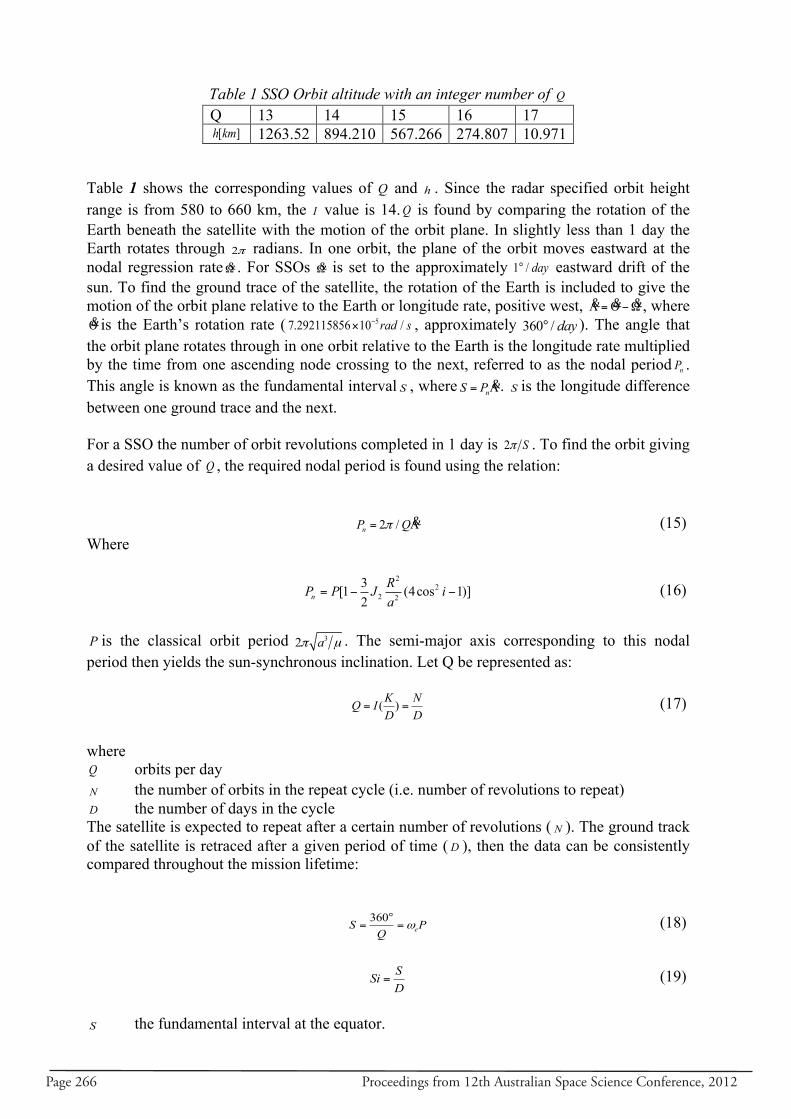
Page 266 Proceedings from 12th Australian Space Science Conference, 2012
Table 1 SSO Orbit altitude with an integer number of Q Q 13 14 15 16 17 [ ]h km 1263.52 894.210 567.266 274.807 10.971
Table 1 shows the corresponding values of Q and h . Since the radar specified orbit height range is from 580 to 660 km, the I value is 14.Q is found by comparing the rotation of the Earth beneath the satellite with the motion of the orbit plane. In slightly less than 1 day the Earth rotates through 2π radians. In one orbit, the plane of the orbit moves eastward at the nodal regression rateΩ& . For SSOs Ω& is set to the approximately 1 / day° eastward drift of the sun. To find the ground trace of the satellite, the rotation of the Earth is included to give the motion of the orbit plane relative to the Earth or longitude rate, positive west, Λ = Θ −Ω& & &, where Θ& is the Earth’s rotation rate ( 57.292115856 10 /rad s−× , approximately 360 / day° ). The angle that the orbit plane rotates through in one orbit relative to the Earth is the longitude rate multiplied by the time from one ascending node crossing to the next, referred to as the nodal period nP . This angle is known as the fundamental interval S , where nS P= Λ&. S is the longitude difference between one ground trace and the next. For a SSO the number of orbit revolutions completed in 1 day is 2 Sπ . To find the orbit giving a desired value of Q , the required nodal period is found using the relation: 2 /nP Qπ= Λ& (15) Where
2
22 2
3[1 (4cos 1)]2n
RP P J ia
= − − (16)
P is the classical orbit period 32 aπ µ . The semi-major axis corresponding to this nodal period then yields the sun-synchronous inclination. Let Q be represented as: ( )K NQ I
D D= = (17)
where Q orbits per day N the number of orbits in the repeat cycle (i.e. number of revolutions to repeat) D the number of days in the cycle The satellite is expected to repeat after a certain number of revolutions ( N ). The ground track of the satellite is retraced after a given period of time ( D ), then the data can be consistently compared throughout the mission lifetime: 360
eS PQ
ω°
= = (18)
SSi
D= (19)
S the fundamental interval at the equator.
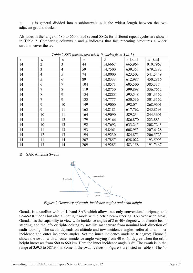
Proceedings from 12th Australian Space Science Conference, 2012 Page 267
Si S is general divided into D subintervals. Si is the widest length between the two adjacent ground tracks. Altitudes in the range of 580 to 660 km of several SSOs for different repeat cycles are shown in Table 2. Comparing columns D and Si indicates that fast repeating D requires a wider swath to cover the Si .
Table 2 SSO parameters when D varies from 3 to 14 I K D N Q h [km] Si [km] 14 2 3 44 14.6667 665.964 910.7968 14 3 4 59 14.7500 639.351 679.2382 14 4 5 74 14.8000 623.503 541.5449 14 5 6 89 14.8333 612.987 450.2816 14 6 7 104 14.8571 605.500 385.337 14 7 8 119 14.8750 599.898 336.7652 14 8 9 134 14.8888 595.548 301.3162 14 7 9 133 14.7777 630.536 301.3162 14 9 10 149 14.9000 592.074 268.9601 14 9 11 163 14.8181 617.762 245.8593 14 10 11 164 14.9090 589.234 244.3601 14 11 12 179 14.9166 586.870 223.883 14 10 13 192 14.7692 633.245 208.7243 14 11 13 193 14.8461 608.953 207.6428 14 12 13 194 14.9230 584.871 206.5725 14 11 14 207 14.7857 628.022 193.5993 14 13 14 209 14.9285 583.158 191.7467 1) SAR Antenna Swath
Figure 2 Geometry of swath, incidence angles and orbit height
Garada is a satellite with an L-band SAR which allows not only conventional stripmap and ScanSAR modes but also a Spotlight mode with electric beam steering. To cover wide areas, Garada has the capability to view wide incidence angles of 8 to 40+ degree with electric beam steering, and the left- or right-looking by satellite manoeuvre from nominal look direction of nadir-looking. The swath depends on altitude and tow incidence angles, referred to as inner incidence and outer incidence angles. Set the inner incidence angle to 8 degree; Figure 3 shows the swath with an outer incidence angle varying from 40 to 50 degree when the orbit height increases from 580 to 660 km. Here the inner incidence angle is 8°. The swath is in the range of 359.3 to 587.9 km. Some of the swath values in Figure 3 are listed in Table 3. The 40
Orbit height
Incidence Angle
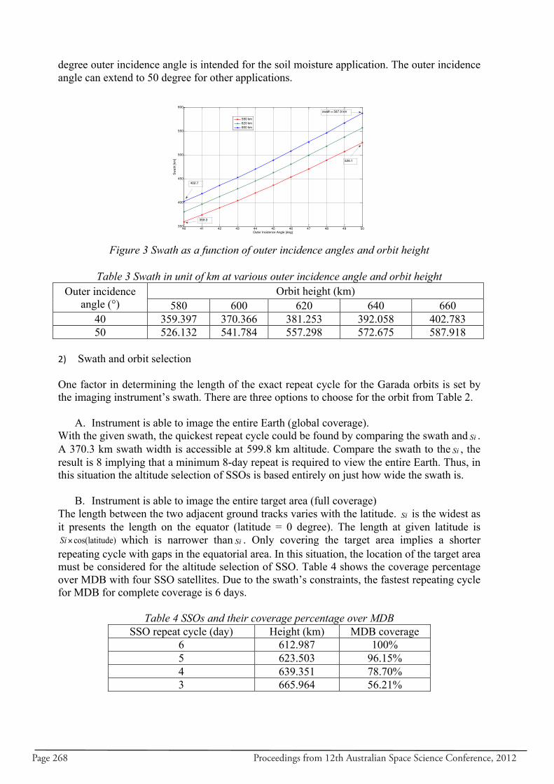
Page 268 Proceedings from 12th Australian Space Science Conference, 2012
degree outer incidence angle is intended for the soil moisture application. The outer incidence angle can extend to 50 degree for other applications.
Figure 3 Swath as a function of outer incidence angles and orbit height
Table 3 Swath in unit of km at various outer incidence angle and orbit height
Outer incidence angle (°)
Orbit height (km) 580 600 620 640 660
40 359.397 370.366 381.253 392.058 402.783 50 526.132 541.784 557.298 572.675 587.918
2) Swath and orbit selection One factor in determining the length of the exact repeat cycle for the Garada orbits is set by the imaging instrument’s swath. There are three options to choose for the orbit from Table 2.
A. Instrument is able to image the entire Earth (global coverage). With the given swath, the quickest repeat cycle could be found by comparing the swath and Si . A 370.3 km swath width is accessible at 599.8 km altitude. Compare the swath to the Si , the result is 8 implying that a minimum 8-day repeat is required to view the entire Earth. Thus, in this situation the altitude selection of SSOs is based entirely on just how wide the swath is.
B. Instrument is able to image the entire target area (full coverage) The length between the two adjacent ground tracks varies with the latitude. Si is the widest as it presents the length on the equator (latitude = 0 degree). The length at given latitude is
cos(latitude)Si× which is narrower than Si . Only covering the target area implies a shorter repeating cycle with gaps in the equatorial area. In this situation, the location of the target area must be considered for the altitude selection of SSO. Table 4 shows the coverage percentage over MDB with four SSO satellites. Due to the swath’s constraints, the fastest repeating cycle for MDB for complete coverage is 6 days.
Table 4 SSOs and their coverage percentage over MDB SSO repeat cycle (day) Height (km) MDB coverage
6 612.987 100% 5 623.503 96.15% 4 639.351 78.70% 3 665.964 56.21%
40 41 42 43 44 45 46 47 48 49 50350
400
450
500
550
600
Outer Incidence Angle [deg]
Swat
h [k
m]
580 km620 km660 km
swath = 587.9 km
359.3
402.7
526.1
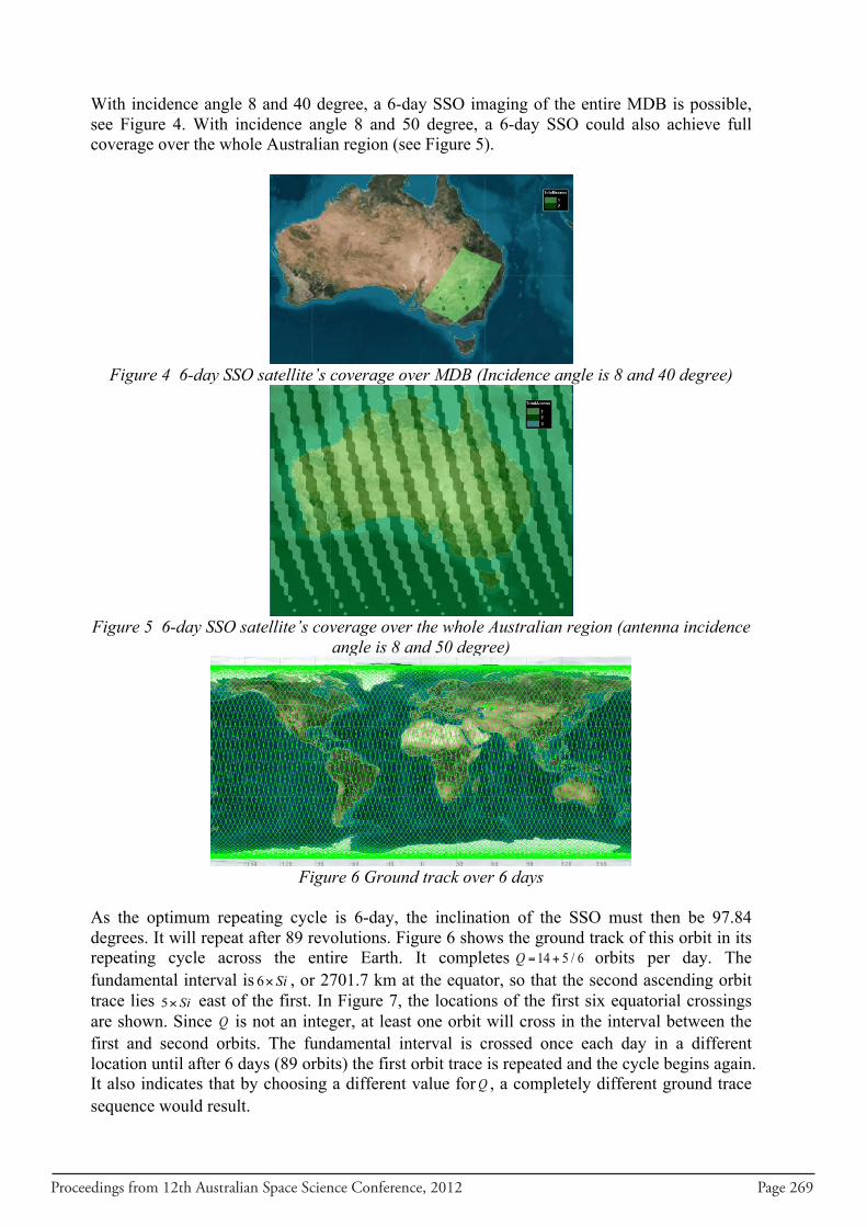
Proceedings from 12th Australian Space Science Conference, 2012 Page 269
With incidence angle 8 and 40 degree, a 6-day SSO imaging of the entire MDB is possible, see Figure 4. With incidence angle 8 and 50 degree, a 6-day SSO could also achieve full coverage over the whole Australian region (see Figure 5).
Figure 4 6-day SSO satellite’s coverage over MDB (Incidence angle is 8 and 40 degree)
Figure 5 6-day SSO satellite’s coverage over the whole Australian region (antenna incidence
angle is 8 and 50 degree)
Figure 6 Ground track over 6 days
As the optimum repeating cycle is 6-day, the inclination of the SSO must then be 97.84 degrees. It will repeat after 89 revolutions. Figure 6 shows the ground track of this orbit in its repeating cycle across the entire Earth. It completes 14 5 / 6Q = + orbits per day. The fundamental interval is 6 Si× , or 2701.7 km at the equator, so that the second ascending orbit trace lies 5 Si× east of the first. In Figure 7, the locations of the first six equatorial crossings are shown. Since Q is not an integer, at least one orbit will cross in the interval between the first and second orbits. The fundamental interval is crossed once each day in a different location until after 6 days (89 orbits) the first orbit trace is repeated and the cycle begins again. It also indicates that by choosing a different value forQ , a completely different ground trace sequence would result.
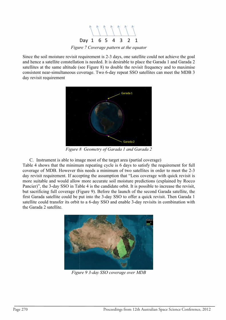
Page 270 Proceedings from 12th Australian Space Science Conference, 2012
Figure 7 Coverage pattern at the equator
Since the soil moisture revisit requirement is 2-3 days, one satellite could not achieve the goal and hence a satellite constellation is needed. It is desirable to place the Garada 1 and Garada 2 satellites at the same altitude (see Figure 8) to double the revisit frequency and to maximise consistent near-simultaneous coverage. Two 6-day repeat SSO satellites can meet the MDB 3 day revisit requirement
Figure 8 Geometry of Garada 1 and Garada 2
C. Instrument is able to image most of the target area (partial coverage)
Table 4 shows that the minimum repeating cycle is 6 days to satisfy the requirement for full coverage of MDB. However this needs a minimum of two satellites in order to meet the 2-3 day revisit requirement. If accepting the assumption that “Less coverage with quick revisit is more suitable and would allow more accurate soil moisture predictions (explained by Rocco Pancier)”, the 3-day SSO in Table 4 is the candidate orbit. It is possible to increase the revisit, but sacrificing full coverage (Figure 9). Before the launch of the second Garada satellite, the first Garada satellite could be put into the 3-day SSO to offer a quick revisit. Then Garada 1 satellite could transfer its orbit to a 6-day SSO and enable 3-day revisits in combination with the Garada 2 satellite.
Figure 9 3-day SSO coverage over MDB
Day 1 6 5 4 3 2 1
Garada1
Garada2
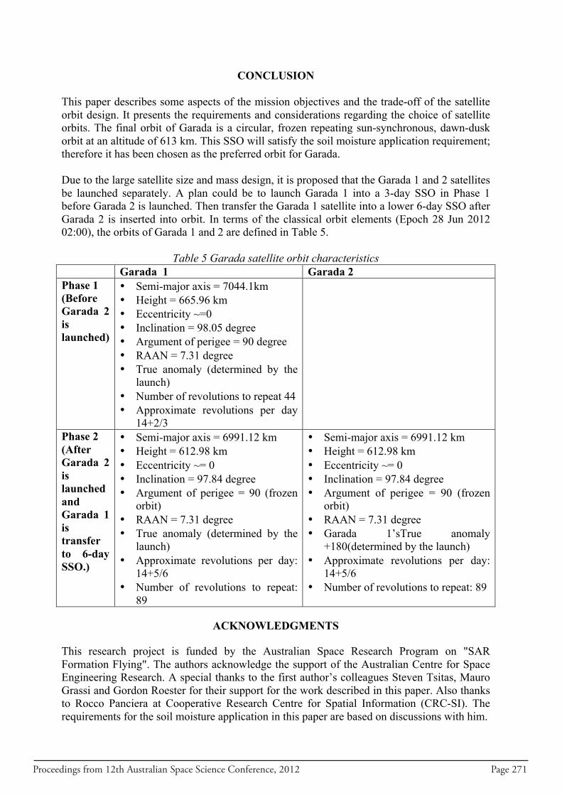
Proceedings from 12th Australian Space Science Conference, 2012 Page 271
CONCLUSION This paper describes some aspects of the mission objectives and the trade-off of the satellite orbit design. It presents the requirements and considerations regarding the choice of satellite orbits. The final orbit of Garada is a circular, frozen repeating sun-synchronous, dawn-dusk orbit at an altitude of 613 km. This SSO will satisfy the soil moisture application requirement; therefore it has been chosen as the preferred orbit for Garada. Due to the large satellite size and mass design, it is proposed that the Garada 1 and 2 satellites be launched separately. A plan could be to launch Garada 1 into a 3-day SSO in Phase 1 before Garada 2 is launched. Then transfer the Garada 1 satellite into a lower 6-day SSO after Garada 2 is inserted into orbit. In terms of the classical orbit elements (Epoch 28 Jun 2012 02:00), the orbits of Garada 1 and 2 are defined in Table 5.
Table 5 Garada satellite orbit characteristics Garada 1 Garada 2 Phase 1 (Before Garada 2 is launched)
• Semi-major axis = 7044.1km • Height = 665.96 km • Eccentricity ~=0 • Inclination = 98.05 degree • Argument of perigee = 90 degree • RAAN = 7.31 degree • True anomaly (determined by the
launch) • Number of revolutions to repeat 44 • Approximate revolutions per day
14+2/3
Phase 2 (After Garada 2 is launched and Garada 1 is transfer to 6-day SSO.)
• Semi-major axis = 6991.12 km • Height = 612.98 km • Eccentricity ~= 0 • Inclination = 97.84 degree • Argument of perigee = 90 (frozen
orbit) • RAAN = 7.31 degree • True anomaly (determined by the
launch) • Approximate revolutions per day:
14+5/6 • Number of revolutions to repeat:
89
• Semi-major axis = 6991.12 km • Height = 612.98 km • Eccentricity ~= 0 • Inclination = 97.84 degree • Argument of perigee = 90 (frozen
orbit) • RAAN = 7.31 degree • Garada 1’sTrue anomaly
+180(determined by the launch) • Approximate revolutions per day:
14+5/6 • Number of revolutions to repeat: 89
ACKNOWLEDGMENTS
This research project is funded by the Australian Space Research Program on "SAR Formation Flying". The authors acknowledge the support of the Australian Centre for Space Engineering Research. A special thanks to the first author’s colleagues Steven Tsitas, Mauro Grassi and Gordon Roester for their support for the work described in this paper. Also thanks to Rocco Panciera at Cooperative Research Centre for Spatial Information (CRC-SI). The requirements for the soil moisture application in this paper are based on discussions with him.

Page 272 Proceedings from 12th Australian Space Science Conference, 2012
REFERENCES 1. Casey, D., Way, J, “Orbit Selection for the EOS Mission and its Synergism Implications”, IEEE Transaction on Geoscience and Remote Sensing, Vol. 29, No.6, 1991, pp. 822-835.
2. Ronald, J. B.,” A-B-Cs of Sun-Synchronous Orbit Mission Design”, Proceedings of the 14th AAS/AIAA Space Flight Mechanics Conference, S.L.Coffey. Maui, Hawaii, USA, February 8-12, 2004, pp.85-104.
3. Vallado, D. A., McClain, W. D.,“Fundamentals of Astrodynamics and Applications”, Second Editon, Springer, New York, 2001.
Proceedings from 12th Australian Space Science Conference, 2012 Page 273
Garada SAR Formation Flying requirements, space system baseline and spacecraft structural design
Steven R. Tsitas 1 and George Constantinos 2
1 Australian Centre for Space Engineering Research (ACSER), University of New South
Wales, Sydney, NSW, 2052, Australia 2 University of New South Wales, Sydney, NSW, 2052, Australia
Summary: The mission baseline of the Australian Garada SAR Formation Flying mission is described, which is designed for operational soil moisture mapping of the Murray Darling Basin from space. An L-Band Synthetic Aperture Radar is described with an antenna size of 15.5m x 3.9m, packaged into a spacecraft bus design with a single fold in two symmetrical spacecraft halves. Space system requirements are specified and design decisions are shown to follow from requirements. The spacecraft structural design is presented along with the results of finite element analysis calculations verifying the structure. Keywords: Garada, ASRP, SAR, L-Band, soil moisture, bushfire, flood, forest, REDD, Australian, Antarctic, Territory, strategy, Broadband, Ground Station, Astrium, Snapdragon
Introduction The Garada SAR Formation Flying project is a Phase 0 design study at the Australian Centre for Space Engineering Research (ACSER) at UNSW and is funded by the Australian Space Research Program (ASRP). The Garada mission is being designed to support operational soil moisture mapping at high spatial resolution using Synthetic Aperture Radar (SAR) of the Murray Darling Basin (MDB) from space. The requirements and space system baseline for the mission are described in this paper, and the spacecraft structural design is presented. Design decisions are shown to flow from requirements. There is a programmatic requirement that the space system design involve formation flying. A formation of two SAR spacecraft flying in formation half an orbit out of phase is required to meet the requirements for revisit frequency for soil moisture mapping, thereby meeting the programmatic requirement for formation flying.
Applications
Soil moisture mapping
Measuring soil moisture is a way to determine how much water is present in the soil and therefore how much water to apply by irrigation, helping avoid over or under watering which can result in crop damage, poor yields and environmental damage [1]. One of the authors (ST) has suggested soil moisture monitoring of the MDB using spaceborne SAR as a potential “killer app” for an Australian spaceborne SAR. Top level user requirements (from Australian farmers and environmental authorities) are now the subject of investigation, but preliminary space system requirements have been defined with the help of soil moisture researcher input [2]. It should be noted that there are currently no operational methods for soil moisture mapping using SAR [3]; the development of such operational methods is in fact one of the goals of the upcoming Argentine L-Band SAR SAOCOM mission [4]. The Garada mission
Page 274 Proceedings from 12th Australian Space Science Conference, 2012
may be able to leverage the research that will be done with SAOCOM towards an operational method of soil moisture mapping using SAR from space. It is envisaged that further Australian research using ground and airborne SAR is required to develop an operational method of soil moisture mapping of the MDB using SAR.
This research should be completed before a Garada mission is implemented. However there is already sufficient knowledge to define requirements with enough detail for a Phase 0 design study of a spaceborne SAR. Improvement in knowledge of end user (farmers and environmental authorities) requirements and development of an operational method for soil moisture mapping using SAR should not change some of the design features (for example the need for quad polarisation) that existing research can already define.
Other applications supported by the Garada mission include forest change detection in support of REDD (Reducing Emissions from Deforestation and Forest Degradation) objectives and flood monitoring both for disaster support and hydrological applications in the MDB (Table 1).
Table 1: Applications supported by the Garada SAR Formation Flying mission
Application Currently an operational solution?
High spatial resolution soil moisture measurement from space using SAR
N
Forest change detection Y Flood monitoring (disaster support and hydrological monitoring in the MDB)
Y
Forest change detection is assigned operational status since detection of clear cut forest, the requirement stated by the Australian Department of Climate Change and Energy Efficiency [5], has been performed from spaceborne SAR imagery in the past [6]. Similarly flood monitoring would use the interferometric change detection method demonstrated by TerraSAR-X and TanDEM-X during floods in Pakistan [7].
Bush fire monitoring through cloud In the southern state of Victoria in Australia it is overcast approximately one third of the time over bush fires [8], so optical methods of remote monitoring of the fire front will not work. It is proposed here that a possible method for remotely monitoring bush fire fronts through cloud is with repeat SAR images taken from almost the same position (in space or from the air above the clouds). As the fire burns it will change the structure of the vegetation which might show up as decoherence when a subsequent image is taken from a position close enough to the original position that there is not significance spatial decoherence (“close enough” is calculated later in this paper using equation (1) to be less than approximately 10.5 km if imaged from space). In this case the fire front should show up as a decoherence front in the combined images (combined by looking at the phase difference between each pixel). For Garada the Earth’s rotation in the time it takes for the second Garada spacecraft (following half an orbit behind the leading spacecraft) to be in the same position as the first Garada spacecraft is approximately 1,000 km at the latitude of Victoria, which would spatially decohere the images acquired by the two spacecraft preventing application of this method. While not part of the mission baseline, a third receive only spacecraft following less than

Proceedings from 12th Australian Space Science Conference, 2012 Page 275
approximately 30 seconds behind the second spacecraft, which is itself half an orbit behind the first spacecraft, would be able to acquire images that have not significantly spatially decohered due to the Earth’s rotation. It is also proposed that this spacecraft could also be used for flood monitoring using interferometric change detection between the two spacecraft; in the short time between images the only features in a scene that will change are liquid (or perhaps solids burnt by fire), allowing water to be detected by its decorrelation signature. This was the method used from space by TerraSAR-X and TanDEM-X during floods in Pakistan [7].
Mission Baseline The requirements for soil moisture mapping of the MDB from space are described in Table 2. A survey of potential Australian applications relevant to a spaceborne SAR was carried out and the requirements for soil moisture mapping of the MDB were found to be the most descriptive in terms of allowing a flow down to mission design decisions. By designing the Garada mission baseline to the soil moisture mapping requirements described in Table 2 the spacecraft design is traceable to requirements in accordance with best space engineering practice. Support for other applications with less descriptive requirements such as flood mapping and forest change detection is not reduced as a result. In fact the SAR that results from meeting the soil moisture requirements is quad-polarisation and has the largest antenna of any L-Band SAR planned as described in the Summary below. This will make the spacecraft quite capable for other applications including flood mapping and forest change detection. Table 3 includes a description of two ways in which the design which results from meeting the soil moisture requirements improves the ability to support the flood monitoring and forest change detection applications.
Table 2: Garada SAR Formation Flying mission requirements
Mission parameter Requirement
Frequency band L-Band, to minimize the contributions of surface roughness and overlying vegetation to the radar echo
Polarisation Quad Polarisation, to allow the system to be used operationally for soil moisture measurement from space
Spatial resolution Stripmap – 250 m parcel with 25 x 25 multilooking (10 m native resolution). Sub-km multilooked parcel resolution in Stripmap
mode will provide a significant advancement over SMAP.
ScanSAR – 1 km after 25 x 25 multilooking. 1 km parcel resolution over wide area was formerly provided by Envisat
Radiometric resolution
Distinguish a 4% difference in reflectivity between two parcels of multilooked pixels
Incidence angle 6.7°- 40º. 10°- 40º is the range of incidence angles that soil moisture retrieval using SAR has been studied. The lower limit of 10° can be reduced assuming no SAR imaging issues to improve
revisit frequency.
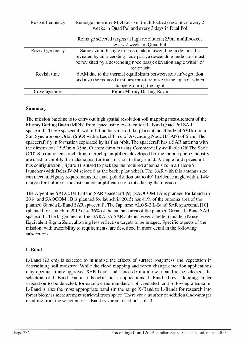
Page 276 Proceedings from 12th Australian Space Science Conference, 2012
Revisit frequency Reimage the entire MDB at 1km (multilooked) resolution every 2 weeks in Quad Pol and every 3 days in Dual Pol
Reimage selected targets at high resolution (250m multilooked) every 2 weeks in Quad Pol
Revisit geometry
Same azimuth angle (a pass made in ascending node must be revisited by an ascending node pass, a descending node pass must be revisited by a descending node pass); elevation angle within 5°
for revisit Revisit time
6 AM due to the thermal equilibirum between soil/air/vegetation and also the reduced capillary moisture raise in the top soil which
happens during the night Coverage area Entire Murray Darling Basin
Summary
The mission baseline is to carry out high spatial resolution soil mapping measurement of the Murray Darling Basin (MDB) from space using two identical L-Band Quad-Pol SAR spacecraft. These spacecraft will orbit in the same orbital plane at an altitude of 630 km in a Sun Synchronous Orbit (SSO) with a Local Time of Ascending Node (LTAN) of 6 am. The spacecraft fly in formation separated by half an orbit. The spacecraft has a SAR antenna with the dimensions 15.52m x 3.9m. Custom circuits using Commercially available Off The Shelf (COTS) components including microchip amplifiers developed for the mobile phone industry are used to amplify the radar signal for transmission to the ground. A single fold spacecraft bus configuration (Figure 1) is used to package the required antenna size in a Falcon 9 launcher (with Delta IV-M selected as the backup launcher). The SAR with this antenna size can meet ambiguity requirements for quad polarisation out to 40° incidence angle with a 14% margin for failure of the distributed amplification circuits during the mission.
The Argentine SAOCOM L-Band SAR spacecraft [9] (SAOCOM 1A is planned for launch in 2014 and SAOCOM 1B is planned for launch in 2015) has 41% of the antenna area of the planned Garada L-Band SAR spacecraft. The Japanese ALOS-2 L-Band SAR spacecraft [10] (planned for launch in 2013) has 36% of the antenna area of the planned Garada L-Band SAR spacecraft. The larger area of the GARADA SAR antenna gives a better (smaller) Noise Equivalent Sigma Zero, allowing less reflective targets to be imaged. Specific aspects of the mission, with traceability to requirements, are described in more detail in the following subsections.
L-Band
L-Band (23 cm) is selected to minimise the effects of surface roughness and vegetation in determining soil moisture. While the flood mapping and forest change detection applications may operate in any approved SAR band, and hence do not allow a band to be selected, the selection of L-Band can also benefit those applications. L-Band allows flooding under vegetation to be detected, for example the inundation of vegetated land following a tsunami. L-Band is also the most appropriate band (in the range X-Band to L-Band) for research into forest biomass measurement retrieval from space. There are a number of additional advantages resulting from the selection of L-Band as summarised in Table 3.
Proceedings from 12th Australian Space Science Conference, 2012 Page 277
Table 3: Additional advantages resulting from selection of L-Band
Advantage Explanation Market differentiation There are existing X-Band and C-Band SAR spacecraft but
currently no L-Band SAR spacecraft in orbit (SAOCOM [9] and ALOS-2 [10] are planned).
COTS microamplifiers L-Band is the same frequency band used by mobile phones, consequently Commercially available Off The Shelf (COTS) microamplifiers are available which can be used in an appropriate circuit design to amplify the RF signal for radiation to the ground. This approach is compatible with highly deployable membrane antennas which may significantly reduce the size and cost of an L-Band SAR spacecraft.
Low loss line feeds Transmitting the preamplifed signal from the bus to the circuit amplifiers is possible at L-Band using relatively low loss line feeds. At higher frequencies such as X-Band the losses become prohibitive, requiring waveguides or a space feed which add to complexity and packaging requirements.
Cheaper highly deployable antenna
Garada is a stepping stone towards smaller and potentially cheaper L-Band SAR spacecraft which utilise highly deployable membrane antennas. The antenna design is de-risked compared to a more highly deployable design which the Garada project lacks the resources to investigate. However, COTS microamplifiers are being investigated. These are an enabling technology for future highly deployable antenna designs. A highly deployable L-Band antenna is expected to be cheaper than an X-Band highly deployable antenna. While smaller the X-Band antenna requires that the two membrane layers (an active and a ground plane) be held much more closely apart than at L-Band. Maintaining this closer membrane separation at X-Band is expected to lead to a more expensive deployable structure than at L-Band.
More extensive flood mapping capability
Flooding can be detected under vegetation (for example the inundation of coastal areas after a tsunami)
More suitable band for biomass research
Biomass retrieval methods that rely on backscatter information are limited by saturation of the backscatter cross-section above a certain biomass areal density. L-Band saturates at higher biomass densities than shorter wavelengths. L-Band is also more suitable than shorter wavelengths for POLInSAR [11] based biomass measurement methods which rely on an appreciable echo from the ground. The longer wavelength of L-Band enhances penetration of the tree canopy compared to shorter wavelengths.
Quad-Polarisation
If the SAR is to be used operationally for soil moisture measurements then quad-polarisation is required [2]. Accordingly quad-polarisation is specified for the SAR which requires a larger antenna area to suppress ambiguities. This results in a significantly bigger spacecraft due to the direct relationship between antenna size and spacecraft size for a SAR spacecraft unless a highly deployable antenna is used. However quad-polarisation has the additional advantages
Page 278 Proceedings from 12th Australian Space Science Conference, 2012
of allowing Faraday Rotation to be compensated for and can be used for research into biomass measurements from space [11].
One remote sensing biomass measurement technique is POLInSAR which combines quad-polarisation and interferometry to determine the height of a forest [11]. The biomass areal density can then be estimated from the tree height. Tree height is determined by subtracting the height of the canopy from the height of the ground, with each height determined using across-track interferometry. Polarisation combinations are used which separate the echoes from the canopy and from the ground. This method relies on across-track interferometry where a baseline perpendicular to the line of sight is required to allow heights to be determined. However this baseline must be less than the critical baseline BC, which is given in equation (6-156) of Elachi and van Zyl [12]. The critical baseline may be written as
BC = |(R/c)Btan | (1) is the wavelength, R is the distance between the antenna and the point on the ground being illuminated, B is the signal bandwidth, is the incidence angle and c is the speed of light. Using =25° (the centre of the access region), =0.23 m, R=695 km (assuming an altitude of 630 km) and B=85 MHz the value of the critical baseline is BC =21 km.
This creates a requirement to determine whether the orbit propagation model predicts baselines less than this critical baseline for 3 day (two spacecraft) and 6 day repeat (same spacecraft) observations. If not then orbit control will be required to fly the spacecraft within a “tube” of less than approximately 10.5 km diameter if repeat pass interferometric observations are required for POLInSAR or other across track interferometry applications such as Digital Elevation Model (DEM) generation and earth movement detection due to subsidence and earthquakes.
Spatial resolution of 7-10 m stripmap, 60-100 m ScanSAR
There is a soil moisture research requirement (Table 2) to provide “high resolution” stripmap multilooked parcels that are less than or equal to 250 m x 250 m that are the product of 25 x 25 multilooks to meet radiometric resolution requirements. Lower resolution ScanSAR multilooked parcels are to be approximately 1 km in resolution to replace a capability lost with Envisat earlier this year. To meet these requirements 7-10 m spatial resolution in stripmap mode is specified for the SAR. Incidence angle range of 6.7°-40° for soil moisture, 6.7°-50° supported Soil moisture requirements originally specified a 20°-40° range for the incidence angles. This was modified to 6.7°-40° to increase the access width to improve revisit rate to meet the 3 day revisit requirements. The upper limit was not increased in response to researcher feedback that SAR soil moisture methods are limited to this upper limit in incidence angle. The lower limit was decreased in consultation with the researcher after assurances that the SAR design could cope with the issues associated with a steeper incidence angle (decreased range resolution is one problem).
Proceedings from 12th Australian Space Science Conference, 2012 Page 279
SAR antenna size 15.5m x 3.9m, “Snapdragon” spacecraft design and Falcon 9 launch (Delta IV-M backup) SAR soil moisture requirements specify a 3 day revisit time for the entire MDB in dual polarisation, with the requirement to also image selected targets within the MDB in stripmap mode in quad-polarisation. In order to image out to 40° incidence angle (the requirement for soil moisture observations, although the 40°-50° incidence angle range may also be of interest to soil moisture researchers) with quad-polarisation suppression of range ambiguities forces the antenna width (the dimension perpendicular to the direction of spacecraft travel) to be bigger than for dual polarisation.
CAD modeling by one of the authors (GC) indicates that the maximal antenna size that can be accommodated in the minimum of a Falcon 9 and Delta IV-M shroud (the Delta IV-M shroud is the smaller of the two) with a single fold antenna is 15.5m x 3.9m. To allow for the loss of some radiating elements (or more precisely the loss of the amplifier circuits providing power to the radiating elements) and still meet ambiguity suppression requirements during the mission the 15.52m x 3.9m antenna is specified for the Garada antenna design to provide a 14% margin against radiating element loss during the mission lifetime. Accordingly the 15.52m x 3.9m antenna design is selected to meet performance requirements at End of Life (EOL).
Both a primary and backup launcher are specified, with the cheaper Falcon 9 designated as the primary launcher. Although Falcon 9 has a bigger shroud the spacecraft must nonetheless be designed for the smaller shroud of the Delta IV-M for it to function as the backup launcher. The Falcon 9 launch cost is $54 M USD [13] while the Delta IV-M launch cost is $133 M USD in 2004 dollars [14].
A foldable or collapsible antenna design is required because there is no launcher with a shroud big enough to accommodate a 15.52m x 3.9m antenna. The Astrium “Snapdragon” [15] configuration has the features of only requiring one hinge which may improve reliability and does not cantilever the antenna. The antenna is instead integrated into the body (Figure 1) which reduces the difficulty of ensuring antenna planarity. Therefore a snapdragon configuration spacecraft sized to the minimum of the Falcon 9 (primary) and Delta IV-M (backup) shrouds with an antenna area of 15.52m x 3.9m is chosen to meet performance requirements at EOL.
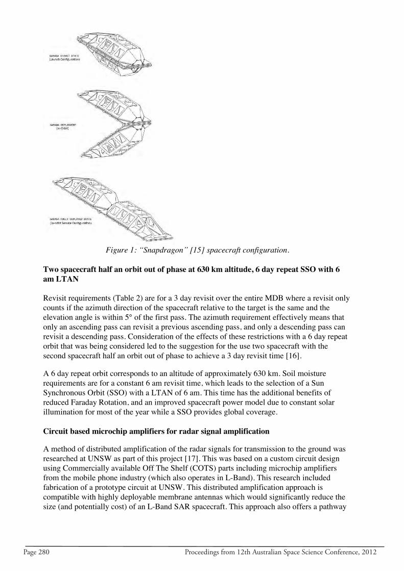
Page 280 Proceedings from 12th Australian Space Science Conference, 2012
Figure 1: “Snapdragon” [15] spacecraft configuration.
Two spacecraft half an orbit out of phase at 630 km altitude, 6 day repeat SSO with 6 am LTAN Revisit requirements (Table 2) are for a 3 day revisit over the entire MDB where a revisit only counts if the azimuth direction of the spacecraft relative to the target is the same and the elevation angle is within 5° of the first pass. The azimuth requirement effectively means that only an ascending pass can revisit a previous ascending pass, and only a descending pass can revisit a descending pass. Consideration of the effects of these restrictions with a 6 day repeat orbit that was being considered led to the suggestion for the use two spacecraft with the second spacecraft half an orbit out of phase to achieve a 3 day revisit time [16].
A 6 day repeat orbit corresponds to an altitude of approximately 630 km. Soil moisture requirements are for a constant 6 am revisit time, which leads to the selection of a Sun Synchronous Orbit (SSO) with a LTAN of 6 am. This time has the additional benefits of reduced Faraday Rotation, and an improved spacecraft power model due to constant solar illumination for most of the year while a SSO provides global coverage. Circuit based microchip amplifiers for radar signal amplification
A method of distributed amplification of the radar signals for transmission to the ground was researched at UNSW as part of this project [17]. This was based on a custom circuit design using Commercially available Off The Shelf (COTS) parts including microchip amplifiers from the mobile phone industry (which also operates in L-Band). This research included fabrication of a prototype circuit at UNSW. This distributed amplification approach is compatible with highly deployable membrane antennas which would significantly reduce the size (and potentially cost) of an L-Band SAR spacecraft. This approach also offers a pathway
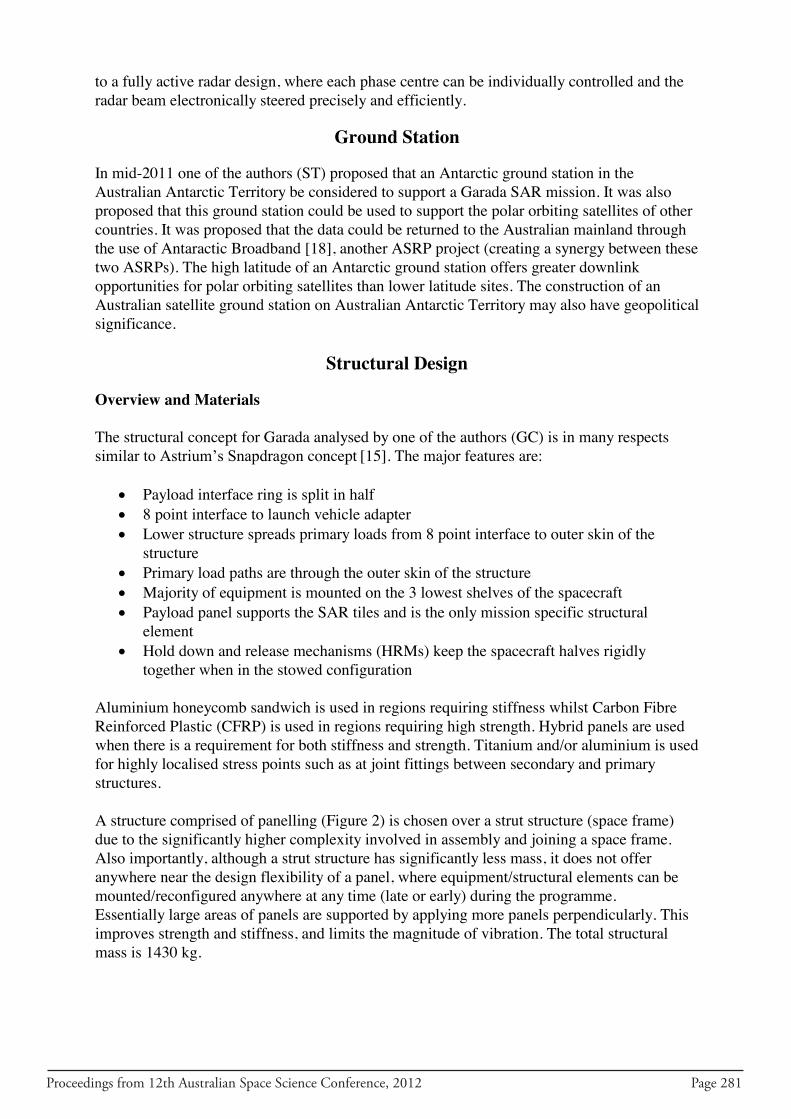
Proceedings from 12th Australian Space Science Conference, 2012 Page 281
to a fully active radar design, where each phase centre can be individually controlled and the radar beam electronically steered precisely and efficiently.
Ground Station
In mid-2011 one of the authors (ST) proposed that an Antarctic ground station in the Australian Antarctic Territory be considered to support a Garada SAR mission. It was also proposed that this ground station could be used to support the polar orbiting satellites of other countries. It was proposed that the data could be returned to the Australian mainland through the use of Antaractic Broadband [18], another ASRP project (creating a synergy between these two ASRPs). The high latitude of an Antarctic ground station offers greater downlink opportunities for polar orbiting satellites than lower latitude sites. The construction of an Australian satellite ground station on Australian Antarctic Territory may also have geopolitical significance.
Structural Design
Overview and Materials The structural concept for Garada analysed by one of the authors (GC) is in many respects similar to Astrium’s Snapdragon concept [15]. The major features are:
Payload interface ring is split in half 8 point interface to launch vehicle adapter Lower structure spreads primary loads from 8 point interface to outer skin of the
structure Primary load paths are through the outer skin of the structure Majority of equipment is mounted on the 3 lowest shelves of the spacecraft Payload panel supports the SAR tiles and is the only mission specific structural
element Hold down and release mechanisms (HRMs) keep the spacecraft halves rigidly
together when in the stowed configuration
Aluminium honeycomb sandwich is used in regions requiring stiffness whilst Carbon Fibre Reinforced Plastic (CFRP) is used in regions requiring high strength. Hybrid panels are used when there is a requirement for both stiffness and strength. Titanium and/or aluminium is used for highly localised stress points such as at joint fittings between secondary and primary structures. A structure comprised of panelling (Figure 2) is chosen over a strut structure (space frame) due to the significantly higher complexity involved in assembly and joining a space frame. Also importantly, although a strut structure has significantly less mass, it does not offer anywhere near the design flexibility of a panel, where equipment/structural elements can be mounted/reconfigured anywhere at any time (late or early) during the programme. Essentially large areas of panels are supported by applying more panels perpendicularly. This improves strength and stiffness, and limits the magnitude of vibration. The total structural mass is 1430 kg.
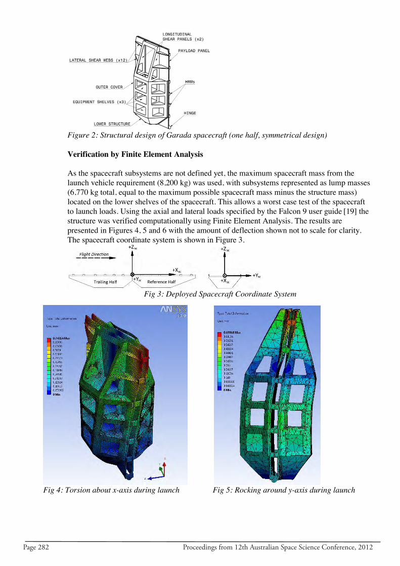
Page 282 Proceedings from 12th Australian Space Science Conference, 2012
Figure 2: Structural design of Garada spacecraft (one half, symmetrical design) Verification by Finite Element Analysis As the spacecraft subsystems are not defined yet, the maximum spacecraft mass from the launch vehicle requirement (8,200 kg) was used, with subsystems represented as lump masses (6,770 kg total, equal to the maximum possible spacecraft mass minus the structure mass) located on the lower shelves of the spacecraft. This allows a worst case test of the spacecraft to launch loads. Using the axial and lateral loads specified by the Falcon 9 user guide [19] the structure was verified computationally using Finite Element Analysis. The results are presented in Figures 4, 5 and 6 with the amount of deflection shown not to scale for clarity. The spacecraft coordinate system is shown in Figure 3.
Fig 3: Deployed Spacecraft Coordinate System
Fig 4: Torsion about x-axis during launch Fig 5: Rocking around y-axis during launch
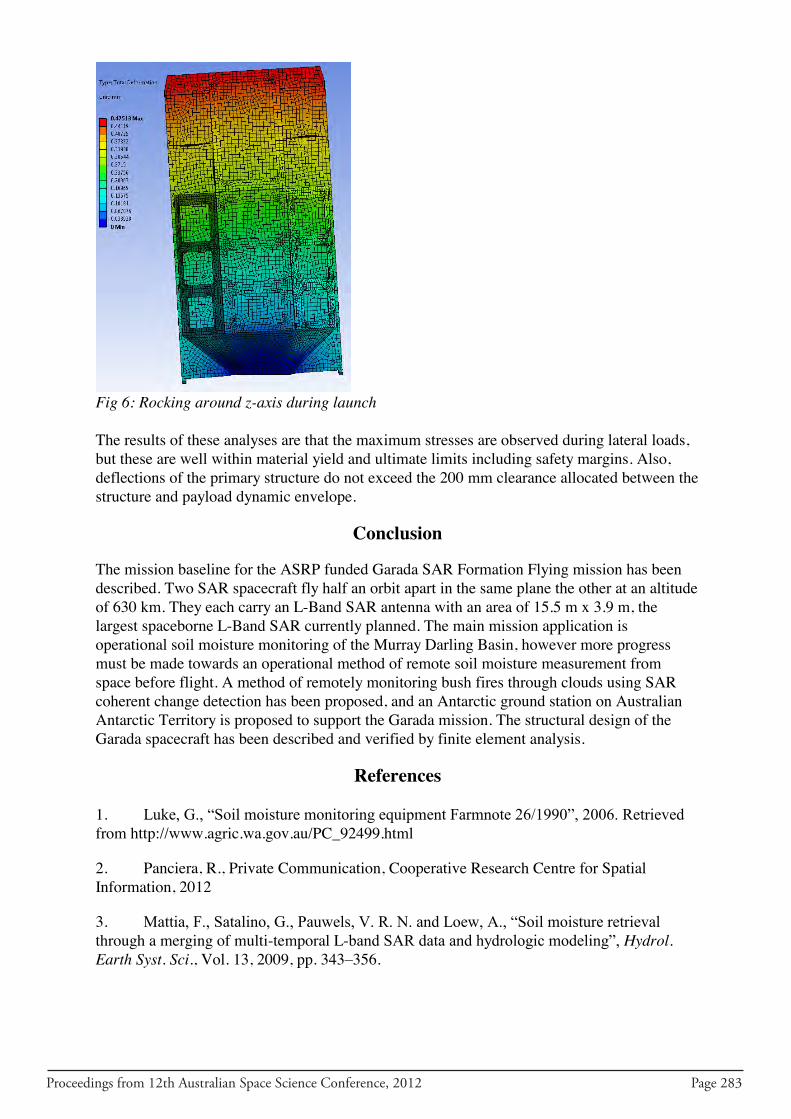
Proceedings from 12th Australian Space Science Conference, 2012 Page 283
Fig 6: Rocking around z-axis during launch The results of these analyses are that the maximum stresses are observed during lateral loads, but these are well within material yield and ultimate limits including safety margins. Also, deflections of the primary structure do not exceed the 200 mm clearance allocated between the structure and payload dynamic envelope.
Conclusion
The mission baseline for the ASRP funded Garada SAR Formation Flying mission has been described. Two SAR spacecraft fly half an orbit apart in the same plane the other at an altitude of 630 km. They each carry an L-Band SAR antenna with an area of 15.5 m x 3.9 m, the largest spaceborne L-Band SAR currently planned. The main mission application is operational soil moisture monitoring of the Murray Darling Basin, however more progress must be made towards an operational method of remote soil moisture measurement from space before flight. A method of remotely monitoring bush fires through clouds using SAR coherent change detection has been proposed, and an Antarctic ground station on Australian Antarctic Territory is proposed to support the Garada mission. The structural design of the Garada spacecraft has been described and verified by finite element analysis.
References 1. Luke, G., “Soil moisture monitoring equipment Farmnote 26/1990”, 2006. Retrieved from http://www.agric.wa.gov.au/PC_92499.html
2. Panciera, R., Private Communication, Cooperative Research Centre for Spatial Information, 2012
3. Mattia, F., Satalino, G., Pauwels, V. R. N. and Loew, A., “Soil moisture retrieval through a merging of multi-temporal L-band SAR data and hydrologic modeling”, Hydrol. Earth Syst. Sci., Vol. 13, 2009, pp. 343–356.
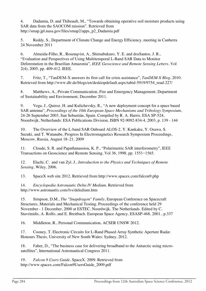
Page 284 Proceedings from 12th Australian Space Science Conference, 2012
4. Dadamia, D. and Thibeault, M., “Towards obtaining operative soil moisture products using SAR data from the SAOCOM mission”. Retrieved from http://smap.jpl.nasa.gov/files/smap2/apps_p2_Dadamia.pdf
5. Reddy, S., Department of Climate Change and Energy Efficiency, meeting in Canberra 24 November 2011
6. Almeida-Filho, R., Rosenqvist, A., Shimabukuro, Y. E. and dosSantos, J. R., “Evaluation and Perspectives of Using Multitemporal L-Band SAR Data to Monitor Deforestation in the Brazilian Amazonia”, IEEE Geoscience and Remote Sensing Letters, Vol 2(4), 2005, pp. 409-412, IEEE.
7. Fritz, T., “TanDEM-X answers its first call for crisis assistance”, TanDEM-X Blog, 2010. Retrieved from http://www.dlr.de/blogs/en/desktopdefault.aspx/tabid-5919/9754_read-227/
8. Matthews, A., Private Communication, Fire and Emergency Management, Department of Sustainability and Environment, December 2011.
9. Vega, J., Quiroz, H. and Kulichevsky, R., “A new deployment concept for a space based SAR antenna”, Proceedings of the 10th European Space Mechanisms and Tribology Symposium, 24-26 September 2003, San Sebastián, Spain. Compiled by R. A. Harris. ESA SP-524, Noordwijk, Netherlands: ESA Publications Division, ISBN 92-9092-834-4, 2003, p. 139 - 144
10. The Overview of the L-band SAR Onboard ALOS-2, Y. Kankaku, Y. Osawa, S. Suzuki, and T. Watanabe, Progress In Electromagnetics Research Symposium Proceedings, Moscow, Russia, August 18–21, 2009
11. Cloude, S. R. and Papathanassiou, K. P., “Polarimetric SAR interferometry”, IEEE Transactions on Geoscience and Remote Sensing, Vol 36, 1998, pp. 1551−1565.
12. Elachi, C. and van Zyl, J., Introduction to the Physics and Techniques of Remote Sensing, Wiley, 2006.
13. SpaceX web site 2012. Retrieved from http://www.spacex.com/falcon9.php
14. Encyclopedia Astronautic Delta IV Medium. Retrieved from http://www.astronautix.com/lvs/deledium.htm
15. Simpson, D.M., The "Snapdragon" Family, European Conference on Spacecraft Structures, Materials and Mechanical Testing, Proceedings of the conference held 29 November - 1 December, 2000 at ESTEC, Noordwijk, The Netherlands. Edited by C. Stavrinidis, A. Rolfo, and E. Breitbach. European Space Agency, ESASP-468, 2001., p.337
16. Middleton, R., Personal Communication, ACSER UNSW 2012.
17. Cooney, T. Electronic Circuits for L-Band Phased Array Synthetic Aperture Radar. Honours Thesis, University of New South Wales: Sydney, 2012.
18. Faber, D., “The business case for delivering broadband to the Antarctic using micro-satellites”, International Astronautical Congress 2011.
19. Falcon 9 Users Guide, SpaceX. 2009. Retrieved from http://www.spacex.com/Falcon9UsersGuide_2009.pdf
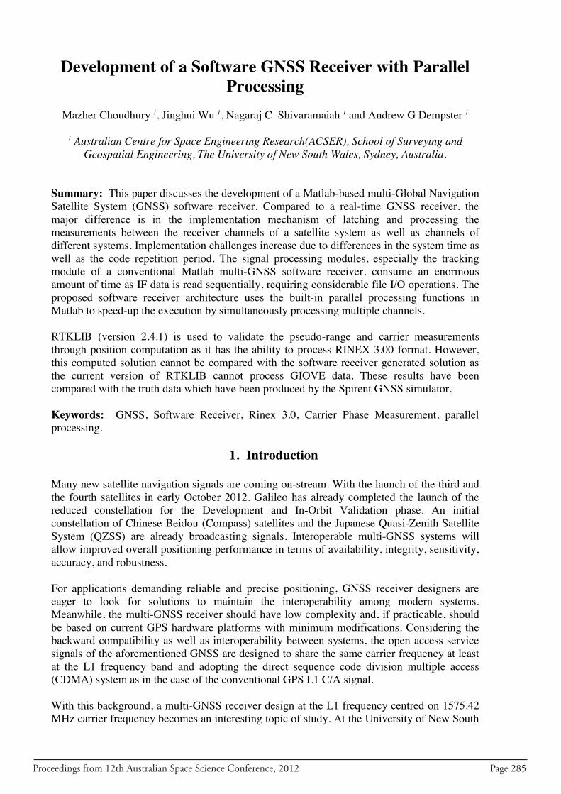
Proceedings from 12th Australian Space Science Conference, 2012 Page 285
Development of a Software GNSS Receiver with Parallel Processing
Mazher Choudhury 1, Jinghui Wu 1, Nagaraj C. Shivaramaiah 1 and Andrew G Dempster 1
1 Australian Centre for Space Engineering Research(ACSER), School of Surveying and
Geospatial Engineering, The University of New South Wales, Sydney, Australia.
Summary: This paper discusses the development of a Matlab-based multi-Global Navigation Satellite System (GNSS) software receiver. Compared to a real-time GNSS receiver, the major difference is in the implementation mechanism of latching and processing the measurements between the receiver channels of a satellite system as well as channels of different systems. Implementation challenges increase due to differences in the system time as well as the code repetition period. The signal processing modules, especially the tracking module of a conventional Matlab multi-GNSS software receiver, consume an enormous amount of time as IF data is read sequentially, requiring considerable file I/O operations. The proposed software receiver architecture uses the built-in parallel processing functions in Matlab to speed-up the execution by simultaneously processing multiple channels. RTKLIB (version 2.4.1) is used to validate the pseudo-range and carrier measurements through position computation as it has the ability to process RINEX 3.00 format. However, this computed solution cannot be compared with the software receiver generated solution as the current version of RTKLIB cannot process GIOVE data. These results have been compared with the truth data which have been produced by the Spirent GNSS simulator. Keywords: GNSS, Software Receiver, Rinex 3.0, Carrier Phase Measurement, parallel processing.
1. Introduction
Many new satellite navigation signals are coming on-stream. With the launch of the third and the fourth satellites in early October 2012, Galileo has already completed the launch of the reduced constellation for the Development and In-Orbit Validation phase. An initial constellation of Chinese Beidou (Compass) satellites and the Japanese Quasi-Zenith Satellite System (QZSS) are already broadcasting signals. Interoperable multi-GNSS systems will allow improved overall positioning performance in terms of availability, integrity, sensitivity, accuracy, and robustness. For applications demanding reliable and precise positioning, GNSS receiver designers are eager to look for solutions to maintain the interoperability among modern systems. Meanwhile, the multi-GNSS receiver should have low complexity and, if practicable, should be based on current GPS hardware platforms with minimum modifications. Considering the backward compatibility as well as interoperability between systems, the open access service signals of the aforementioned GNSS are designed to share the same carrier frequency at least at the L1 frequency band and adopting the direct sequence code division multiple access (CDMA) system as in the case of the conventional GPS L1 C/A signal. With this background, a multi-GNSS receiver design at the L1 frequency centred on 1575.42 MHz carrier frequency becomes an interesting topic of study. At the University of New South
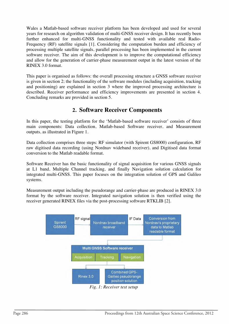
Page 286 Proceedings from 12th Australian Space Science Conference, 2012
Wales a Matlab-based software receiver platform has been developed and used for several years for research on algorithm validation of multi-GNSS receiver design. It has recently been further enhanced for multi-GNSS functionality and tested with available real Radio-Frequency (RF) satellite signals [1]. Considering the computation burden and efficiency of processing multiple satellite signals, parallel processing has been implemented in the current software receiver. The aim of this development is to improve the computational efficiency and allow for the generation of carrier-phase measurement output in the latest version of the RINEX 3.0 format. This paper is organised as follows: the overall processing structure a GNSS software receiver is given in section 2; the functionality of the software modules (including acquisition, tracking and positioning) are explained in section 3 where the improved processing architecture is described. Receiver performance and efficiency improvements are presented in section 4. Concluding remarks are provided in section 5.
2. Software Receiver Components
In this paper, the testing platform for the ‘Matlab-based software receiver’ consists of three main components: Data collection, Matlab-based Software receiver, and Measurement outputs, as illustrated in Figure 1. Data collection comprises three steps: RF simulator (with Spirent GS8000) configuration, RF raw digitised data recording (using Nordnav wideband receiver), and Digitised data format conversion to the Matlab readable format. Software Receiver has the basic functionality of signal acquisition for various GNSS signals at L1 band, Multiple Channel tracking, and finally Navigation solution calculation for integrated multi-GNSS. This paper focuses on the integration solution of GPS and Galileo systems. Measurement output including the pseudorange and carrier-phase are produced in RINEX 3.0 format by the software receiver. Integrated navigation solution is then verified using the receiver generated RINEX files via the post-processing software RTKLIB [2].
Fig. 1: Receiver test setup
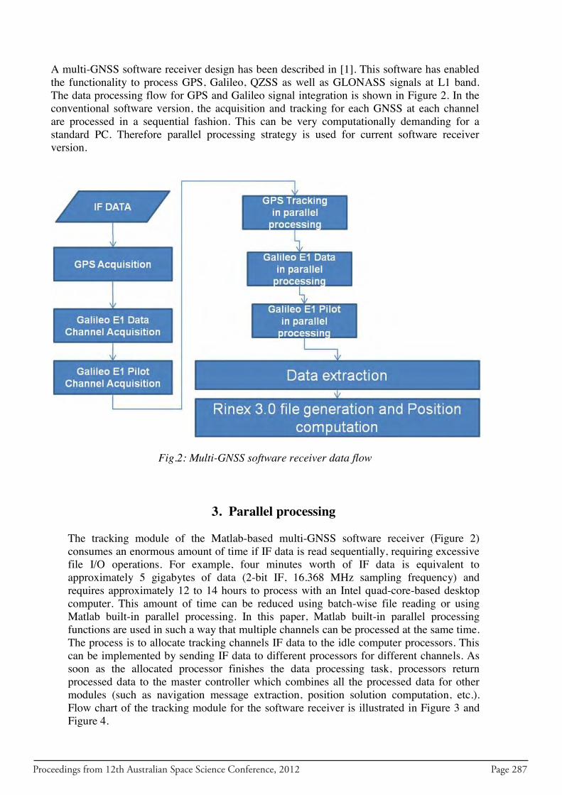
Proceedings from 12th Australian Space Science Conference, 2012 Page 287
A multi-GNSS software receiver design has been described in [1]. This software has enabled the functionality to process GPS, Galileo, QZSS as well as GLONASS signals at L1 band. The data processing flow for GPS and Galileo signal integration is shown in Figure 2. In the conventional software version, the acquisition and tracking for each GNSS at each channel are processed in a sequential fashion. This can be very computationally demanding for a standard PC. Therefore parallel processing strategy is used for current software receiver version.
Fig.2: Multi-GNSS software receiver data flow
3. Parallel processing The tracking module of the Matlab-based multi-GNSS software receiver (Figure 2) consumes an enormous amount of time if IF data is read sequentially, requiring excessive file I/O operations. For example, four minutes worth of IF data is equivalent to approximately 5 gigabytes of data (2-bit IF, 16.368 MHz sampling frequency) and requires approximately 12 to 14 hours to process with an Intel quad-core-based desktop computer. This amount of time can be reduced using batch-wise file reading or using Matlab built-in parallel processing. In this paper, Matlab built-in parallel processing functions are used in such a way that multiple channels can be processed at the same time. The process is to allocate tracking channels IF data to the idle computer processors. This can be implemented by sending IF data to different processors for different channels. As soon as the allocated processor finishes the data processing task, processors return processed data to the master controller which combines all the processed data for other modules (such as navigation message extraction, position solution computation, etc.). Flow chart of the tracking module for the software receiver is illustrated in Figure 3 and Figure 4.
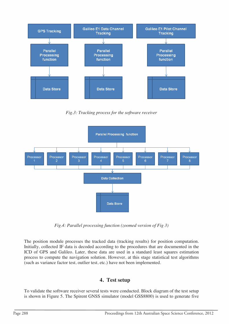
Page 288 Proceedings from 12th Australian Space Science Conference, 2012
Fig.3: Tracking process for the software receiver
Fig.4: Parallel processing function (zoomed version of Fig 3)
The position module processes the tracked data (tracking results) for position computation. Initially, collected IF data is decoded according to the procedures that are documented in the ICD of GPS and Galileo. Later, these data are used in a standard least squares estimation process to compute the navigation solution. However, at this stage statistical test algorithms (such as variance factor test, outlier test, etc.) have not been implemented.
4. Test setup To validate the software receiver several tests were conducted. Block diagram of the test setup is shown in Figure 5. The Spirent GNSS simulator (model GSS8800) is used to generate five
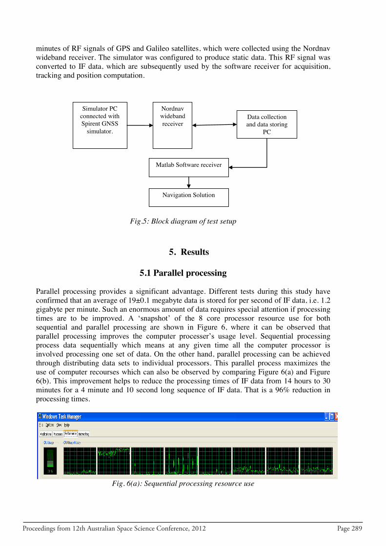
Proceedings from 12th Australian Space Science Conference, 2012 Page 289
minutes of RF signals of GPS and Galileo satellites, which were collected using the Nordnav wideband receiver. The simulator was configured to produce static data. This RF signal was converted to IF data, which are subsequently used by the software receiver for acquisition, tracking and position computation.
Fig.5: Block diagram of test setup
5. Results
5.1 Parallel processing Parallel processing provides a significant advantage. Different tests during this study have confirmed that an average of 19±0.1 megabyte data is stored for per second of IF data, i.e. 1.2 gigabyte per minute. Such an enormous amount of data requires special attention if processing times are to be improved. A ‘snapshot’ of the 8 core processor resource use for both sequential and parallel processing are shown in Figure 6, where it can be observed that parallel processing improves the computer processer’s usage level. Sequential processing process data sequentially which means at any given time all the computer processor is involved processing one set of data. On the other hand, parallel processing can be achieved through distributing data sets to individual processors. This parallel process maximizes the use of computer recourses which can also be observed by comparing Figure 6(a) and Figure 6(b). This improvement helps to reduce the processing times of IF data from 14 hours to 30 minutes for a 4 minute and 10 second long sequence of IF data. That is a 96% reduction in processing times.
Fig. 6(a): Sequential processing resource use
Nordnav wideband receiver
Simulator PC connected with Spirent GNSS
simulator.
Matlab Software receiver
Data collection and data storing
PC
Navigation Solution
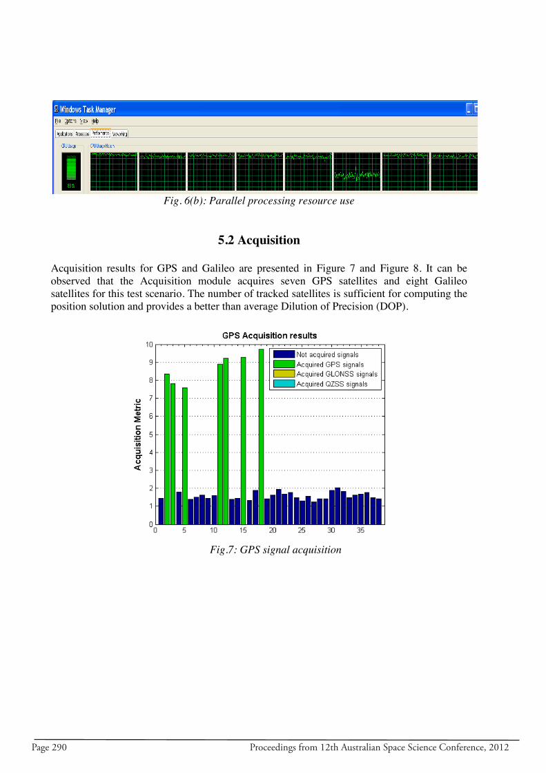
Page 290 Proceedings from 12th Australian Space Science Conference, 2012
Fig. 6(b): Parallel processing resource use
5.2 Acquisition
Acquisition results for GPS and Galileo are presented in Figure 7 and Figure 8. It can be observed that the Acquisition module acquires seven GPS satellites and eight Galileo satellites for this test scenario. The number of tracked satellites is sufficient for computing the position solution and provides a better than average Dilution of Precision (DOP).
Fig.7: GPS signal acquisition
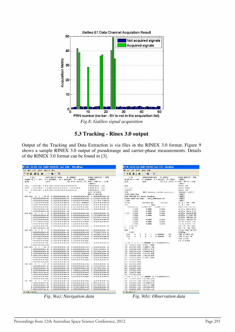
Proceedings from 12th Australian Space Science Conference, 2012 Page 291
Fig.8: Galileo signal acquisition
5.3 Tracking - Rinex 3.0 output
Output of the Tracking and Data Extraction is via files in the RINEX 3.0 format. Figure 9 shows a sample RINEX 3.0 output of pseudorange and carrier-phase measurements. Details of the RINEX 3.0 format can be found in [3].
Fig. 9(a): Navigation data Fig. 9(b): Observation data
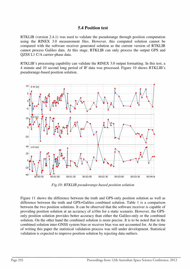
Page 292 Proceedings from 12th Australian Space Science Conference, 2012
5.4 Position test RTKLIB (version 2.4.1) was used to validate the pseudorange through position computation using the RINEX 3.0 measurement files. However, this computed solution cannot be compared with the software receiver generated solution as the current version of RTKLIB cannot process Galileo data. At this stage, RTKLIB can only process the output GPS and QZSS L1 C/A carrier-phase data. RTKLIB’s processing capability can validate the RINEX 3.0 output formatting. In this test, a 4 minute and 10 second long period of IF data was processed. Figure 10 shows RTKLIB’s pseudorange-based position solution.
Fig.10: RTKLIB pseudorange-based position solution Figure 11 shows the difference between the truth and GPS-only position solution as well as difference between the truth and GPS+Galileo combined solution. Table 1 is a comparison between the two position solutions. It can be observed that the software receiver is capable of providing position solution at an accuracy of ±10m for a static scenario. However, the GPS-only position solution provides better accuracy than either the Galileo-only or the combined solution. On the other hand the combined solution is more precise. It is to be noted that in the combined solution inter-GNSS system bias or receiver bias was not accounted for. At the time of writing this paper the statistical validation process was still under development. Statistical validation is expected to improve position solution by rejecting data outliers.
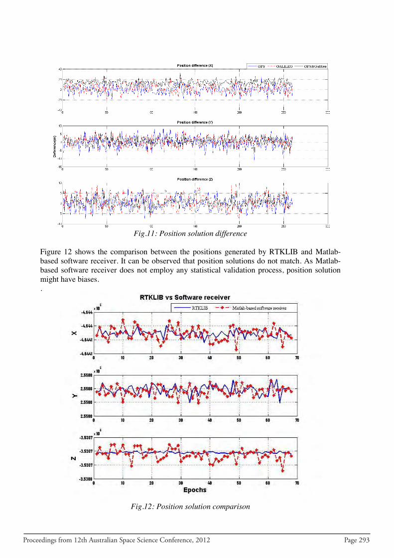
Proceedings from 12th Australian Space Science Conference, 2012 Page 293
Fig.11: Position solution difference
Figure 12 shows the comparison between the positions generated by RTKLIB and Matlab-based software receiver. It can be observed that position solutions do not match. As Matlab-based software receiver does not employ any statistical validation process, position solution might have biases. .
Fig.12: Position solution comparison
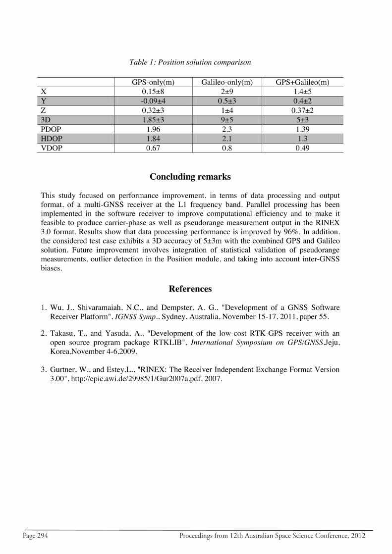
Page 294 Proceedings from 12th Australian Space Science Conference, 2012
Table 1: Position solution comparison
GPS-only(m) Galileo-only(m) GPS+Galileo(m) X 0.15±8 2±9 1.4±5 Y -0.09±4 0.5±3 0.4±2 Z 0.32±3 1±4 0.37±2 3D 1.85±3 9±5 5±3 PDOP 1.96 2.3 1.39 HDOP 1.84 2.1 1.3 VDOP 0.67 0.8 0.49
Concluding remarks This study focused on performance improvement, in terms of data processing and output format, of a multi-GNSS receiver at the L1 frequency band. Parallel processing has been implemented in the software receiver to improve computational efficiency and to make it feasible to produce carrier-phase as well as pseudorange measurement output in the RINEX 3.0 format. Results show that data processing performance is improved by 96%. In addition, the considered test case exhibits a 3D accuracy of 5±3m with the combined GPS and Galileo solution. Future improvement involves integration of statistical validation of pseudorange measurements, outlier detection in the Position module, and taking into account inter-GNSS biases.
References
1. Wu, J., Shivaramaiah, N.C., and Dempster, A. G., "Development of a GNSS Software
Receiver Platform", IGNSS Symp., Sydney, Australia, November 15-17, 2011, paper 55. 2. Takasu, T., and Yasuda, A., "Development of the low-cost RTK-GPS receiver with an
open source program package RTKLIB", International Symposium on GPS/GNSS,Jeju, Korea,November 4-6,2009.
3. Gurtner, W., and Estey,L., "RINEX: The Receiver Independent Exchange Format Version
3.00", http://epic.awi.de/29985/1/Gur2007a.pdf, 2007.
Proceedings from 12th Australian Space Science Conference, 2012 Page 295
Characterization of the Namuru V3.2 Spaceborne GPS Receiver
Mazher Choudhury 1, Eamonn Glennon 1, Andrew G Dempster 1 and Peter Mumford1
1 Australian Centre for Space Engineering Research (ACSER), School of Surveying and
Geospatial Engineering, The University of New South Wales, Sydney, Australia.
Summary: This paper describes test results used to qualify the performance of the Namuru V3.2 GPS receiver running the Aquarius GPS firmware, which has been developed specifically for use in space operations. The results include typical receiver performance characteristics such as time to first fix (TTFF) for cold, warm and hot start, as well as acquisition and reacquisition performance and receiver sensitivity. Testing for low earth orbit operation was performed using a Spirent GPS simulator that was used to generate scenarios. Many of the tests were performed multiple times (20 to 100 times) to ensure the results are statistically meaningful. As this receiver is designed to operate in space scenario, navigation performance as well as the baseline solution was also analysed. Keywords: Namuru, Spaceborne GPS Receiver, receiver performance, Cubesat.
Introduction
The development of the Namuru FPGA based GPS receiver is one of key research outputs of the School of Surveying and Geospatial Engineering at the University of New South Wales. Different versions of Namuru provide different capabilities in the GNSS environment, with the Namuru v3.2 having been developed specifically for spaceborne applications, such as Project Biarri [1] and “Synthetic Aperture Radar” (SAR) formation flying. [2], [3] and [4] provides the design concept and the hardware details of Namuru V3.2. [5] provides a detailed description of the Aquarius firmware that is used in Namuru V3.2. These publications also discuss some of the design requirements for the for space scenario. The navigation performance of the Namuru GPS receiver was described in performance studies undertaken by [6] and [7]. [6] has compared the raw measurement accuracy of the Namuru V2.4 receiver running firmware derived from the GPS Architect with the Phoenix GPS receiver, which is another spaceborne GPS receiver [8], along with the 3D position and velocity accuracy. This study reports position errors below 10m and velocity errors below 1m/s for a space scenario. [7] shows that carrier phase differential accuracy of 0.02m can be achieved in six different space scenarios using a Namuru V2.4 GPS receiver. Although the [5] study is based on the Namuru‟s previous generation design (i.e. V2.4), it provides a significant understanding of the navigation algorithm in the space scenario. However, Namuru V3.2‟s receiver‟s characteristics have not been reported. In this paper, Namuru V3.2‟s performance is characterised through tests in simulation environment. The following sections describe the test setups used to characterise time-to-first-fix (TTFF), acquisition sensitivity, tracking sensitivity and the navigation solutions.
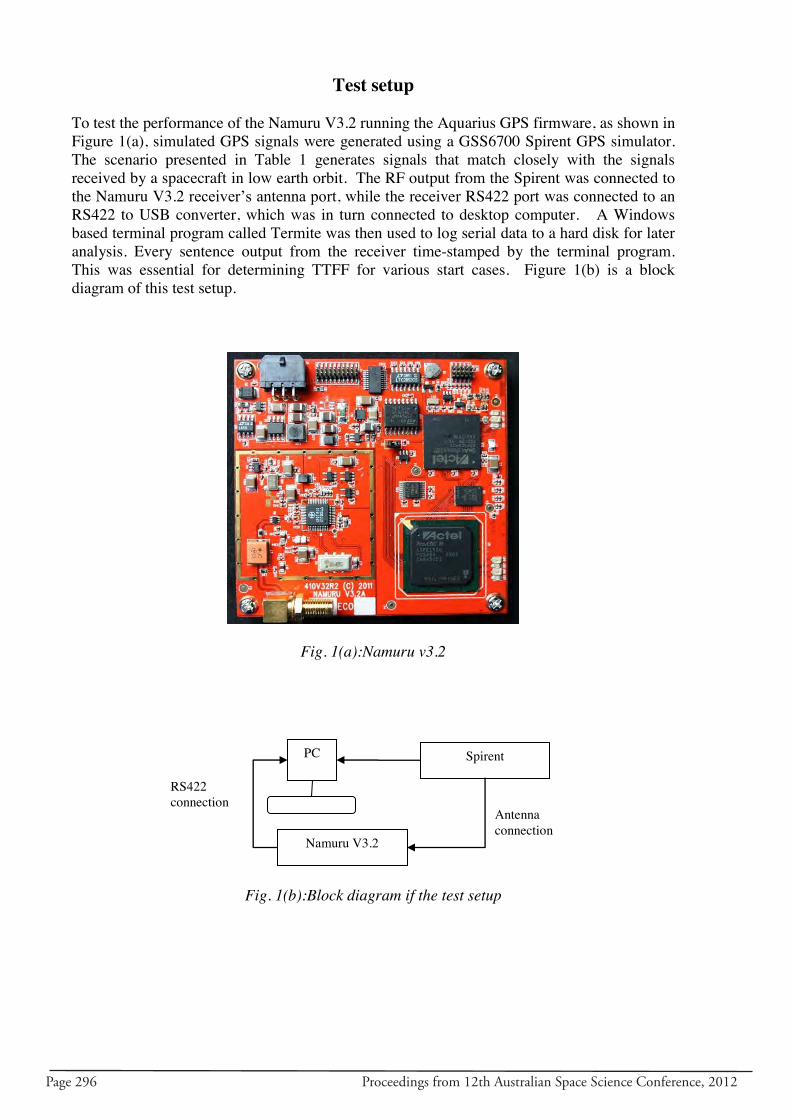
Page 296 Proceedings from 12th Australian Space Science Conference, 2012
Test setup To test the performance of the Namuru V3.2 running the Aquarius GPS firmware, as shown in Figure 1(a), simulated GPS signals were generated using a GSS6700 Spirent GPS simulator. The scenario presented in Table 1 generates signals that match closely with the signals received by a spacecraft in low earth orbit. The RF output from the Spirent was connected to the Namuru V3.2 receiver‟s antenna port, while the receiver RS422 port was connected to an RS422 to USB converter, which was in turn connected to desktop computer. A Windows based terminal program called Termite was then used to log serial data to a hard disk for later analysis. Every sentence output from the receiver time-stamped by the terminal program. This was essential for determining TTFF for various start cases. Figure 1(b) is a block diagram of this test setup.
Fig. 1(a):Namuru v3.2
Fig. 1(b):Block diagram if the test setup
PC
Namuru V3.2
Spirent
RS422 connection
Antenna connection
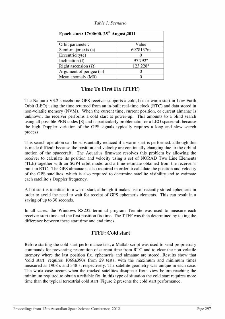
Proceedings from 12th Australian Space Science Conference, 2012 Page 297
Table 1: Scenario
Epoch start: 17:00:00, 25th August,2011 Orbit parameter: Value Semi-major axis (a) 6978137m Eccentricity(e) 0 Inclination (I) 97.792° Right ascension (Ω) 123.228° Argument of perigee (ω) 0 Mean anomaly (M0) 0
Time To First Fix (TTFF)
The Namuru V3.2 spaceborne GPS receiver supports a cold, hot or warm start in Low Earth Orbit (LEO) using the time returned from an in-built real-time clock (RTC) and data stored in non-volatile memory (NVM). When the current time, current position, or current almanac is unknown, the receiver performs a cold start at power-up. This amounts to a blind search using all possible PRN codes [8] and is particularly problematic for a LEO spacecraft because the high Doppler variation of the GPS signals typically requires a long and slow search process. This search operation can be substantially reduced if a warm start is performed, although this is made difficult because the position and velocity are continually changing due to the orbital motion of the spacecraft. The Aquarius firmware resolves this problem by allowing the receiver to calculate its position and velocity using a set of NORAD Two Line Elements (TLE) together with an SGP4 orbit model and a time-estimate obtained from the receiver‟s built-in RTC. The GPS almanac is also required in order to calculate the position and velocity of the GPS satellites, which is also required to determine satellite visibility and to estimate each satellite‟s Doppler frequency. A hot start is identical to a warm start, although it makes use of recently stored ephemeris in order to avoid the need to wait for receipt of GPS ephemeris elements. This can result in a saving of up to 30 seconds. In all cases, the Windows RS232 terminal program Termite was used to measure each receiver start time and the first position fix time. The TTFF was then determined by taking the difference between these start time and end times.
TTFF: Cold start
Before starting the cold start performance test, a Matlab script was used to send proprietrary commands for preventing restoration of current time from RTC and to clear the non-volatile memory where the last position fix, ephemeris and almanac are stored. Results show that „cold start‟ requires 1069±390s from 29 tests, with the maximum and minimum times measured as 1908 s and 348 s, respectively. The satellite geometry was unique in each case. The worst case occurs when the tracked satellites disappear from view before reaching the minimum required to obtain a reliable fix. In this type of situation the cold start requires more time than the typical terrestrial cold start. Figure 2 presents the cold start performance.
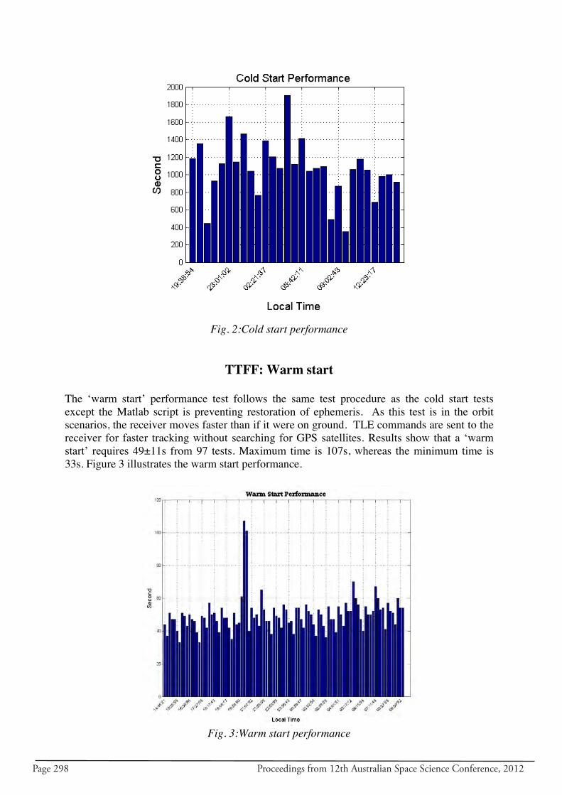
Page 298 Proceedings from 12th Australian Space Science Conference, 2012
Fig. 2:Cold start performance
TTFF: Warm start
The „warm start‟ performance test follows the same test procedure as the cold start tests except the Matlab script is preventing restoration of ephemeris. As this test is in the orbit scenarios, the receiver moves faster than if it were on ground. TLE commands are sent to the receiver for faster tracking without searching for GPS satellites. Results show that a „warm start‟ requires 49±11s from 97 tests. Maximum time is 107s, whereas the minimum time is 33s. Figure 3 illustrates the warm start performance.
Fig. 3:Warm start performance
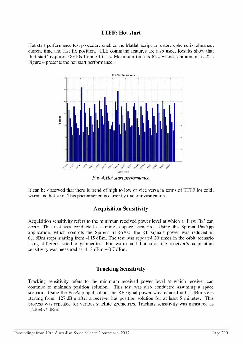
Proceedings from 12th Australian Space Science Conference, 2012 Page 299
TTFF: Hot start
Hot start performance test procedure enables the Matlab script to restore ephemeris, almanac, current time and last fix position. TLE command features are also used. Results show that „hot start‟ requires 38±10s from 84 tests. Maximum time is 62s, whereas minimum is 22s. Figure 4 presents the hot start performance.
Fig. 4:Hot start performance
It can be observed that there is trend of high to low or vice versa in terms of TTFF for cold, warm and hot start. This phenomenon is currently under investigation.
Acquisition Sensitivity
Acquisition sensitivity refers to the minimum received power level at which a „First Fix‟ can occur. This test was conducted assuming a space scenario. Using the Spirent PosApp application, which controls the Spirent STR6700, the RF signals power was reduced in 0.1 dBm steps starting from -115 dBm. The test was repeated 20 times in the orbit scenario using different satellite geometries. For warm and hot start the receiver‟s acquisition sensitivity was measured as -118 dBm ± 0.7 dBm.
Tracking Sensitivity
Tracking sensitivity refers to the minimum received power level at which receiver can continue to maintain position solution. This test was also conducted assuming a space scenario. Using the PosApp application, the RF signal power was reduced in 0.1 dBm steps starting from -127 dBm after a receiver has position solution for at least 5 minutes. This process was repeated for various satellite geometries. Tracking sensitivity was measured as -128 ±0.7 dBm.
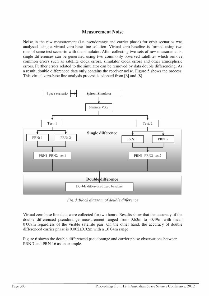
Page 300 Proceedings from 12th Australian Space Science Conference, 2012
Measurement Noise Noise in the raw measurement (i.e. pseudorange and carrier phase) for orbit scenarios was analysed using a virtual zero-base line solution. Virtual zero-baseline is formed using two runs of same test scenario with the simulator. After collecting two sets of raw measurements, single differences can be generated using two commonly observed satellites which remove common errors such as satellite clock errors, simulator clock errors and other atmospheric errors. Further errors related to the simulator can be removed by data double differencing. As a result, double differenced data only contains the receiver noise. Figure 5 shows the process. This virtual zero-base line analysis process is adopted from [6] and [8].
Fig. 5:Block diagram of double difference
Virtual zero base line data were collected for two hours. Results show that the accuracy of the double differenced pseudorange measurement ranged from 0.63m to -0.49m with mean 0.007m regardless of the visible satellite pair. On the other hand, the accuracy of double differenced carrier phase is 0.002±0.02m with a ±0.04m range. Figure 6 shows the double differenced pseudorange and carrier phase observations between PRN 7 and PRN 16 as an example.
Double difference
Single difference PRN: 2
Space scenario Spirent Simulator
Namuru V3.2
PRN: 1
PRN: 1
PRN: 2
Test: 2
Test: 1
PRN1_PRN2_test1
PRN1_PRN2_test2
Double differenced zero baseline
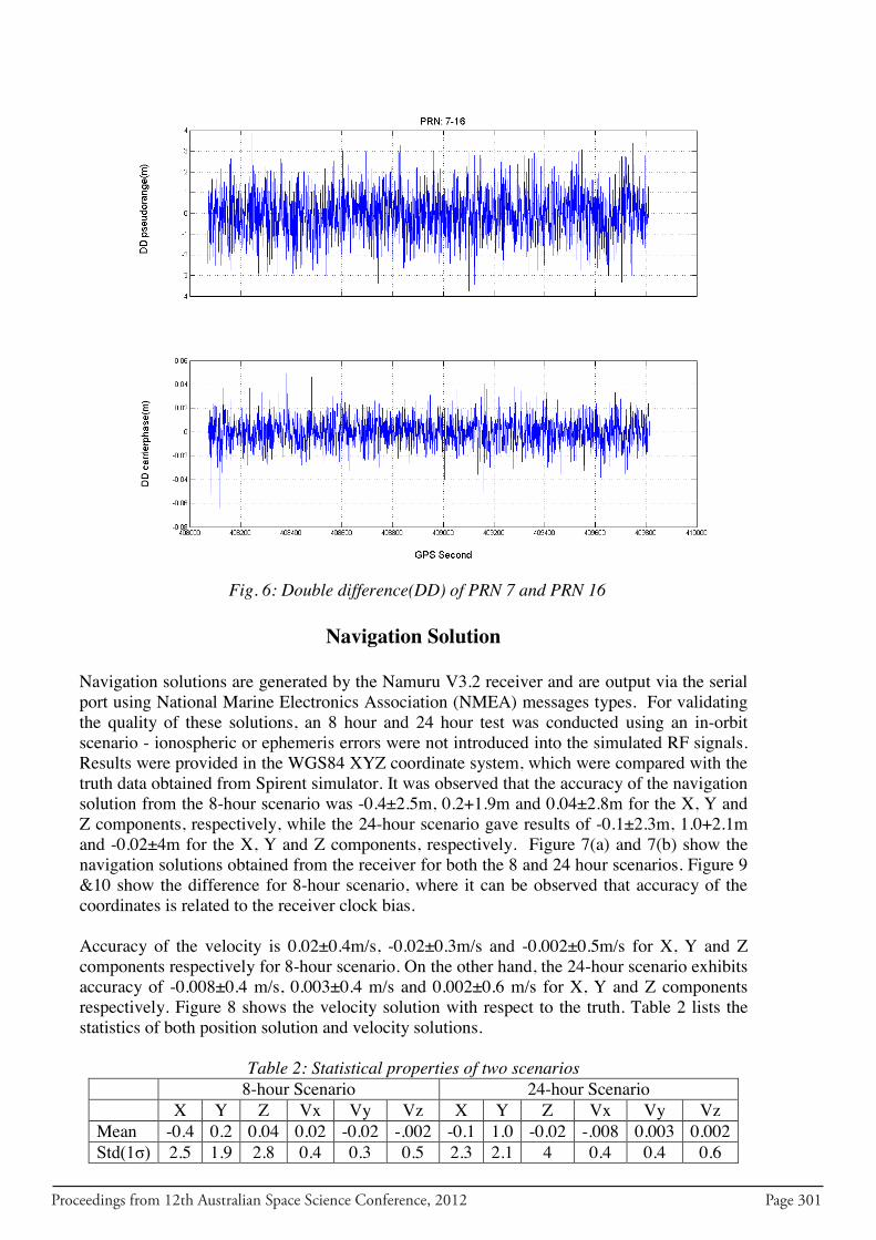
Proceedings from 12th Australian Space Science Conference, 2012 Page 301
Fig. 6: Double difference(DD) of PRN 7 and PRN 16
Navigation Solution
Navigation solutions are generated by the Namuru V3.2 receiver and are output via the serial port using National Marine Electronics Association (NMEA) messages types. For validating the quality of these solutions, an 8 hour and 24 hour test was conducted using an in-orbit scenario - ionospheric or ephemeris errors were not introduced into the simulated RF signals. Results were provided in the WGS84 XYZ coordinate system, which were compared with the truth data obtained from Spirent simulator. It was observed that the accuracy of the navigation solution from the 8-hour scenario was -0.4±2.5m, 0.2+1.9m and 0.04±2.8m for the X, Y and Z components, respectively, while the 24-hour scenario gave results of -0.1±2.3m, 1.0+2.1m and -0.02±4m for the X, Y and Z components, respectively. Figure 7(a) and 7(b) show the navigation solutions obtained from the receiver for both the 8 and 24 hour scenarios. Figure 9 &10 show the difference for 8-hour scenario, where it can be observed that accuracy of the coordinates is related to the receiver clock bias. Accuracy of the velocity is 0.02±0.4m/s, -0.02±0.3m/s and -0.002±0.5m/s for X, Y and Z components respectively for 8-hour scenario. On the other hand, the 24-hour scenario exhibits accuracy of -0.008±0.4 m/s, 0.003±0.4 m/s and 0.002±0.6 m/s for X, Y and Z components respectively. Figure 8 shows the velocity solution with respect to the truth. Table 2 lists the statistics of both position solution and velocity solutions.
Table 2: Statistical properties of two scenarios 8-hour Scenario 24-hour Scenario
X Y Z Vx Vy Vz X Y Z Vx Vy Vz Mean -0.4 0.2 0.04 0.02 -0.02 -.002 -0.1 1.0 -0.02 -.008 0.003 0.002 Std(1σ) 2.5 1.9 2.8 0.4 0.3 0.5 2.3 2.1 4 0.4 0.4 0.6
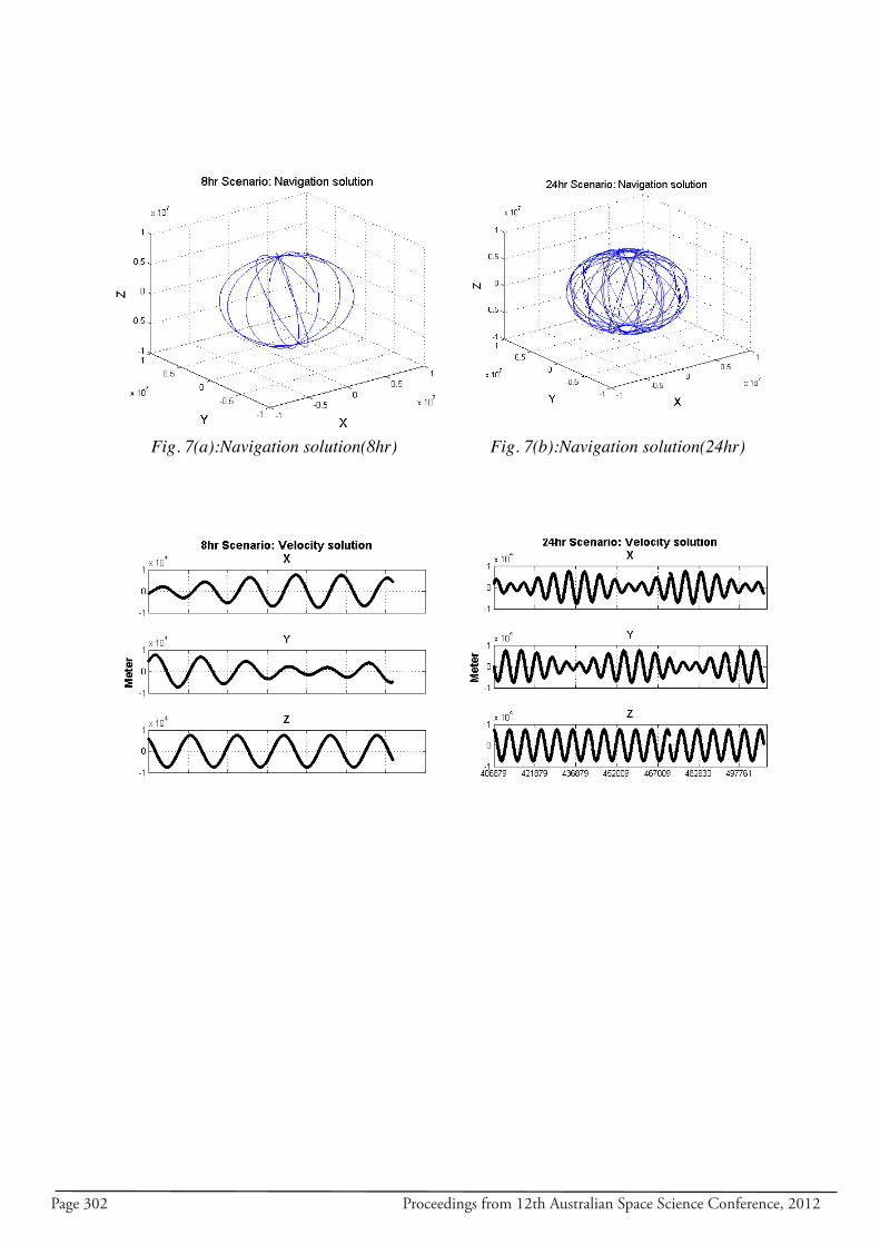
Page 302 Proceedings from 12th Australian Space Science Conference, 2012
Fig. 7(a):Navigation solution(8hr)
Fig. 7(b):Navigation solution(24hr)
Fig. 8(a):Velocity solution(8hr) Fig.8(b):Velocity solution(24hr)
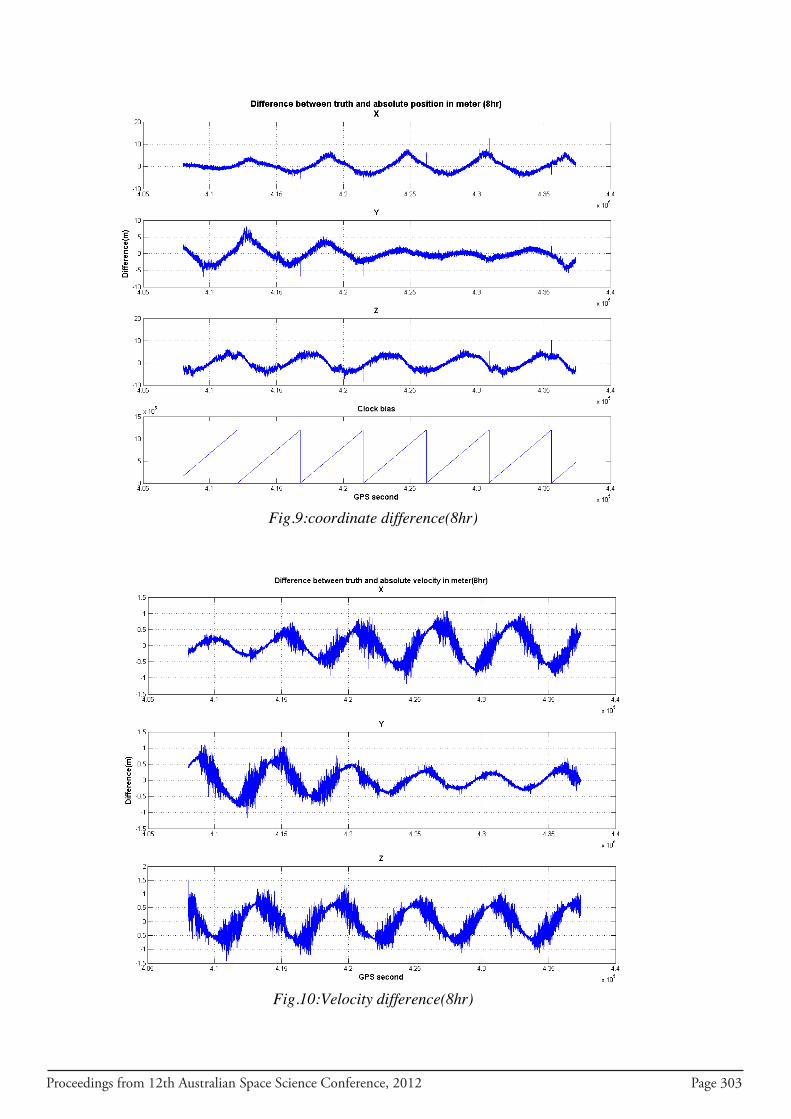
Proceedings from 12th Australian Space Science Conference, 2012 Page 303
Fig.9:coordinate difference(8hr)
Fig.10:Velocity difference(8hr)
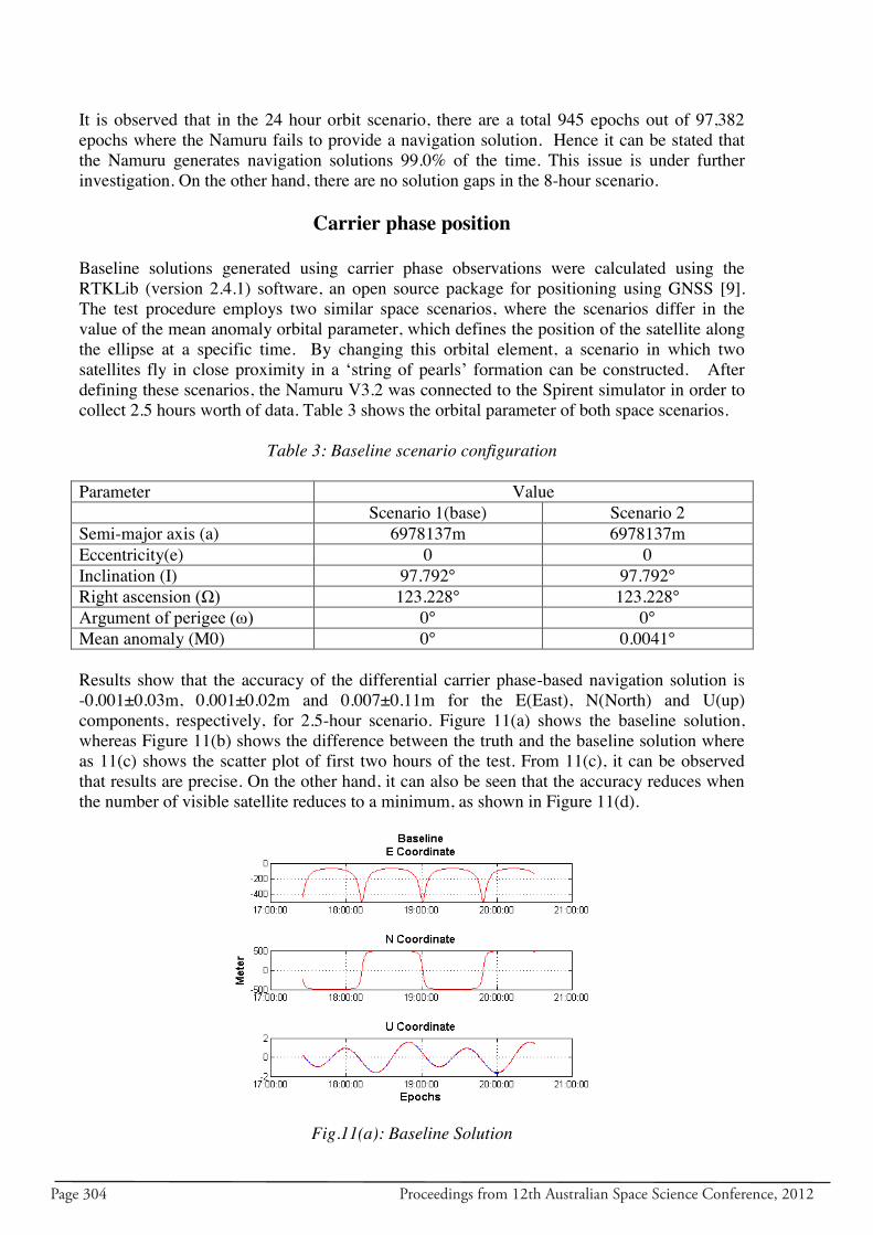
Page 304 Proceedings from 12th Australian Space Science Conference, 2012
It is observed that in the 24 hour orbit scenario, there are a total 945 epochs out of 97,382 epochs where the Namuru fails to provide a navigation solution. Hence it can be stated that the Namuru generates navigation solutions 99.0% of the time. This issue is under further investigation. On the other hand, there are no solution gaps in the 8-hour scenario.
Carrier phase position
Baseline solutions generated using carrier phase observations were calculated using the RTKLib (version 2.4.1) software, an open source package for positioning using GNSS [9]. The test procedure employs two similar space scenarios, where the scenarios differ in the value of the mean anomaly orbital parameter, which defines the position of the satellite along the ellipse at a specific time. By changing this orbital element, a scenario in which two satellites fly in close proximity in a „string of pearls‟ formation can be constructed. After defining these scenarios, the Namuru V3.2 was connected to the Spirent simulator in order to collect 2.5 hours worth of data. Table 3 shows the orbital parameter of both space scenarios.
Table 3: Baseline scenario configuration
Parameter Value Scenario 1(base) Scenario 2 Semi-major axis (a) 6978137m 6978137m Eccentricity(e) 0 0 Inclination (I) 97.792° 97.792° Right ascension (Ω) 123.228° 123.228° Argument of perigee (ω) 0° 0° Mean anomaly (M0) 0° 0.0041° Results show that the accuracy of the differential carrier phase-based navigation solution is -0.001±0.03m, 0.001±0.02m and 0.007±0.11m for the E(East), N(North) and U(up) components, respectively, for 2.5-hour scenario. Figure 11(a) shows the baseline solution, whereas Figure 11(b) shows the difference between the truth and the baseline solution where as 11(c) shows the scatter plot of first two hours of the test. From 11(c), it can be observed that results are precise. On the other hand, it can also be seen that the accuracy reduces when the number of visible satellite reduces to a minimum, as shown in Figure 11(d).
Fig.11(a): Baseline Solution
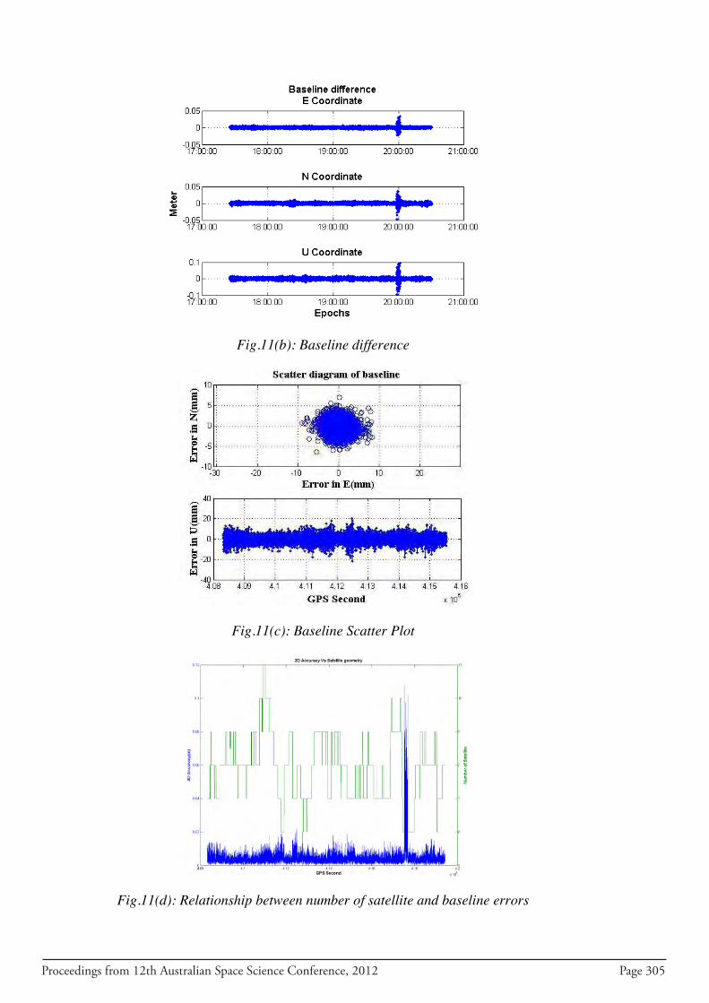
Proceedings from 12th Australian Space Science Conference, 2012 Page 305
Fig.11(b): Baseline difference
Fig.11(c): Baseline Scatter Plot
Fig.11(d): Relationship between number of satellite and baseline errors
Page 306 Proceedings from 12th Australian Space Science Conference, 2012
Concluding remarks
In this paper the Namuru V3.2 spaceborne receiver was tested in orbital scenarios. Cold, warm and hot start processes, as well as acquisition and tracking sensitivity were analysed. Navigation and velocity solutions were also assessed using two different orbital scenarios. Furthermore, the baseline solution was also assessed for validity and applicability of carrier phase measurement in the space scenario, where the receiver experiences high velocity as well as high signal dynamics. In future work, navigation solutions as well as baseline solutions will be further analysed to identify the presence of any systematic bias. Residuals from solutions also need to be analysed to ensure solution robustness, and high precision and accuracy.
Acknowledgment
The work was supported by the Australian Research Council and the Australian Space Research Program. This material is also based on research sponsored by the Defence Science and Technology Organisation (DSTO), Department of Defence, Australia. References
1. Newsam, G. and Gordon, N., “An Update on SSA in Australia”, 12th Annual Advanced Maui Optical and Space Technologies (AMOS) Conference, September 13-15, 2011, http:// www.amostech.com/TechnicalPapers/2011/Poster/GORDON.pdf
2. Parkinson, K.J., Mumford, P.J., Glennon, E.P., Shivaramaiah, N.C., Dempster, A.G., and Rizos, C., “A low cost Namuru V3 receiver for spacecraft operation” IGNSS Symp., Sydney, Australia, November 15-17,2011, paper 72.
3. Mumford, P., Shivaramaiah, N., Glennon., E.P., and Parkinson, K., “The Namuru V3.2A space GNSS receiver”, 12th Australian Space Science Conference, Melbourne, Australia, September 24-27,2012.
4. Glennon, E.P., Parkinson, K.J., Mumford, P., Shivaramaiah, N.C., Dempster, A.G., Li, Y., Li, R. and Jiao, Y., “A GPS Receiver Designed for Cubesat Operations”, 11th Australian Space Science Conference, Canberra, Australia, September 26-29, 2011.
5. Glennon, E.P., Mumford, P.J., and Parkinson, K.J., “ Aquarius firmware for UNSW Namuru GPS receivers”, IGNSS Symp., Sydney, Australia, November 15-17, 2011, paper 57.
6. Grillenberger, A., Rivas, R., Markgraf, M., Mumford, P., Parkinson, K., and Rizos, C., “The Namuru receiver as development platform for spaceborne GNSS applications”, 4th ESA Workshop on Satellite Navigation User Equipment Technologies, Noordwijk, The Netherlands, December 10-12, 2008 , Session 11, Paper 2.
7. Li, Y., Glennon, E.P., Li, R., Jiao, Y., and DEMPSTER, A.G., “Development of a spaceborne GPS receiver for precise relative navigation of formation flying small satellites”, Lecture Notes in Electrical Engineering, Vol 161, 2012, pp. 467-476.
8. Montenbruck,O., and Renaudie, C., "Phoenix-S/-XNS Performance Validation", DLR/GSOC GTN-TST-0120; Deutsches Zentrum für Luft- und Raumfahrt, Oberpfaffenhofen, April 5, 2007.
9. Takasu, T., and Yasuda, A.,"Development of the low-cost RTK-GPS receiver with an open source program package RTKLIB", International Symposium on GPS/GNSS,Jeju, Korea,November 4-6,2009.
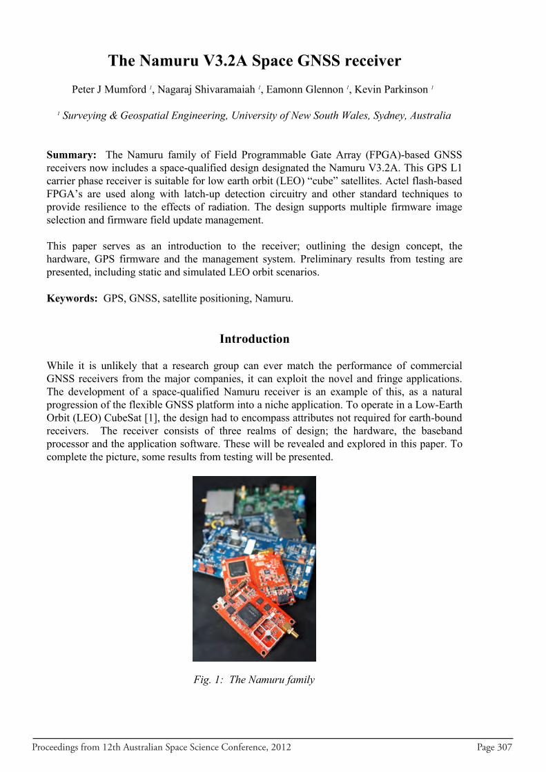
Proceedings from 12th Australian Space Science Conference, 2012 Page 307
The Namuru V3.2A Space GNSS receiver
Peter J Mumford 1, Nagaraj Shivaramaiah 1, Eamonn Glennon 1, Kevin Parkinson 1
1 Surveying & Geospatial Engineering, University of New South Wales, Sydney, Australia
Summary: The Namuru family of Field Programmable Gate Array (FPGA)-based GNSS
receivers now includes a space-qualified design designated the Namuru V3.2A. This GPS L1
carrier phase receiver is suitable for low earth orbit (LEO) “cube” satellites. Actel flash-based
FPGA’s are used along with latch-up detection circuitry and other standard techniques to
provide resilience to the effects of radiation. The design supports multiple firmware image
selection and firmware field update management.
This paper serves as an introduction to the receiver; outlining the design concept, the
hardware, GPS firmware and the management system. Preliminary results from testing are
presented, including static and simulated LEO orbit scenarios.
Keywords: GPS, GNSS, satellite positioning, Namuru.
Introduction
While it is unlikely that a research group can ever match the performance of commercial
GNSS receivers from the major companies, it can exploit the novel and fringe applications.
The development of a space-qualified Namuru receiver is an example of this, as a natural
progression of the flexible GNSS platform into a niche application. To operate in a Low-Earth
Orbit (LEO) CubeSat [1], the design had to encompass attributes not required for earth-bound
receivers. The receiver consists of three realms of design; the hardware, the baseband
processor and the application software. These will be revealed and explored in this paper. To
complete the picture, some results from testing will be presented.
Fig. 1: The Namuru family
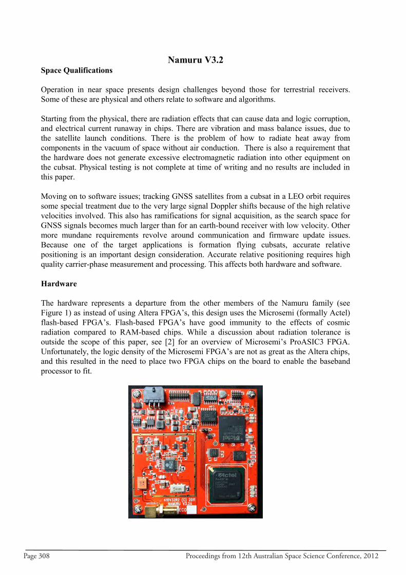
Page 308 Proceedings from 12th Australian Space Science Conference, 2012
Namuru V3.2Space Qualifications
Operation in near space presents design challenges beyond those for terrestrial receivers.
Some of these are physical and others relate to software and algorithms.
Starting from the physical, there are radiation effects that can cause data and logic corruption,
and electrical current runaway in chips. There are vibration and mass balance issues, due to
the satellite launch conditions. There is the problem of how to radiate heat away from
components in the vacuum of space without air conduction. There is also a requirement that
the hardware does not generate excessive electromagnetic radiation into other equipment on
the cubsat. Physical testing is not complete at time of writing and no results are included in
this paper.
Moving on to software issues; tracking GNSS satellites from a cubsat in a LEO orbit requires
some special treatment due to the very large signal Doppler shifts because of the high relative
velocities involved. This also has ramifications for signal acquisition, as the search space for
GNSS signals becomes much larger than for an earth-bound receiver with low velocity. Other
more mundane requirements revolve around communication and firmware update issues.
Because one of the target applications is formation flying cubsats, accurate relative
positioning is an important design consideration. Accurate relative positioning requires high
quality carrier-phase measurement and processing. This affects both hardware and software.
Hardware
The hardware represents a departure from the other members of the Namuru family (see
Figure 1) as instead of using Altera FPGA’s, this design uses the Microsemi (formally Actel)
flash-based FPGA’s. Flash-based FPGA’s have good immunity to the effects of cosmic
radiation compared to RAM-based chips. While a discussion about radiation tolerance is
outside the scope of this paper, see [2] for an overview of Microsemi’s ProASIC3 FPGA.
Unfortunately, the logic density of the Microsemi FPGA’s are not as great as the Altera chips,
and this resulted in the need to place two FPGA chips on the board to enable the baseband
processor to fit.
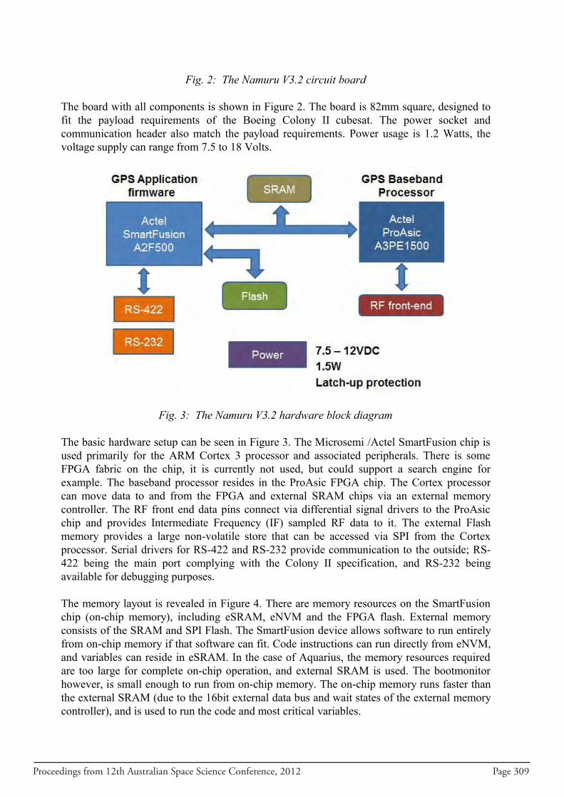
Proceedings from 12th Australian Space Science Conference, 2012 Page 309
Fig. 2: The Namuru V3.2 circuit board
The board with all components is shown in Figure 2. The board is 82mm square, designed to
fit the payload requirements of the Boeing Colony II cubesat. The power socket and
communication header also match the payload requirements. Power usage is 1.2 Watts, the
voltage supply can range from 7.5 to 18 Volts.
Fig. 3: The Namuru V3.2 hardware block diagram
The basic hardware setup can be seen in Figure 3. The Microsemi /Actel SmartFusion chip is
used primarily for the ARM Cortex 3 processor and associated peripherals. There is some
FPGA fabric on the chip, it is currently not used, but could support a search engine for
example. The baseband processor resides in the ProAsic FPGA chip. The Cortex processor
can move data to and from the FPGA and external SRAM chips via an external memory
controller. The RF front end data pins connect via differential signal drivers to the ProAsic
chip and provides Intermediate Frequency (IF) sampled RF data to it. The external Flash
memory provides a large non-volatile store that can be accessed via SPI from the Cortex
processor. Serial drivers for RS-422 and RS-232 provide communication to the outside; RS-
422 being the main port complying with the Colony II specification, and RS-232 being
available for debugging purposes.
The memory layout is revealed in Figure 4. There are memory resources on the SmartFusion
chip (on-chip memory), including eSRAM, eNVM and the FPGA flash. External memory
consists of the SRAM and SPI Flash. The SmartFusion device allows software to run entirely
from on-chip memory if that software can fit. Code instructions can run directly from eNVM,
and variables can reside in eSRAM. In the case of Aquarius, the memory resources required
are too large for complete on-chip operation, and external SRAM is used. The bootmonitor
however, is small enough to run from on-chip memory. The on-chip memory runs faster than
the external SRAM (due to the 16bit external data bus and wait states of the external memory
controller), and is used to run the code and most critical variables.
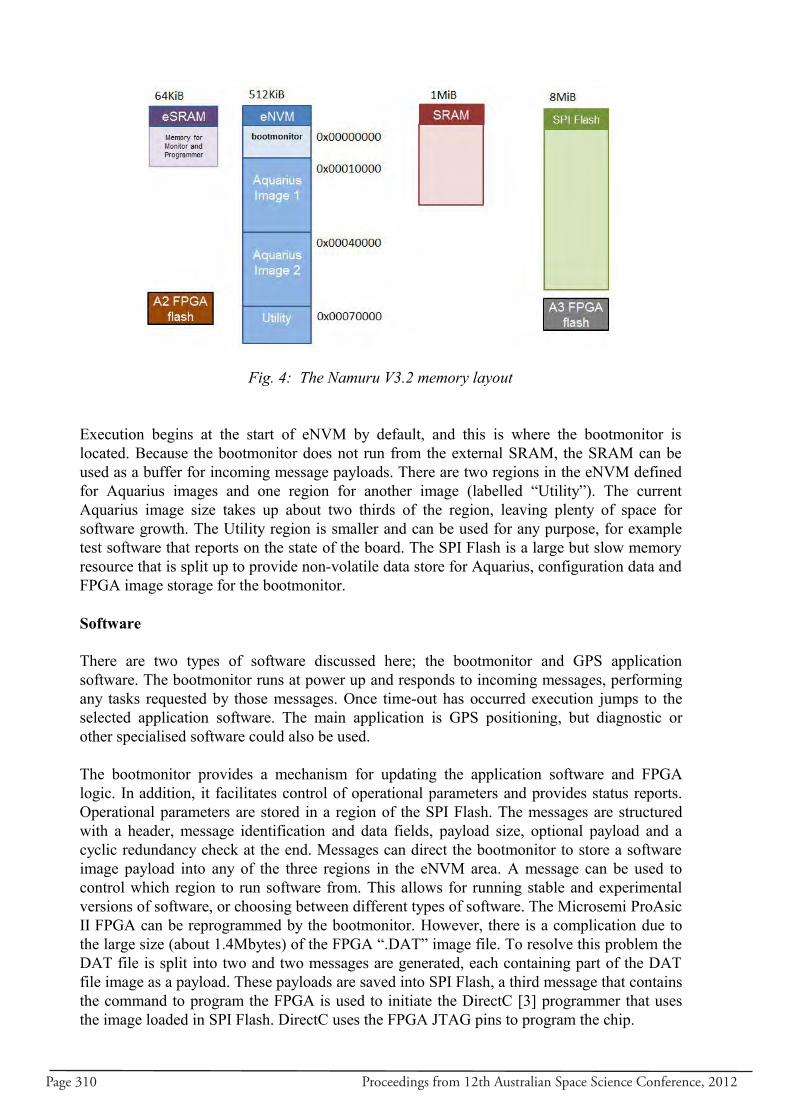
Page 310 Proceedings from 12th Australian Space Science Conference, 2012
Fig. 4: The Namuru V3.2 memory layout
Execution begins at the start of eNVM by default, and this is where the bootmonitor is
located. Because the bootmonitor does not run from the external SRAM, the SRAM can be
used as a buffer for incoming message payloads. There are two regions in the eNVM defined
for Aquarius images and one region for another image (labelled “Utility”). The current
Aquarius image size takes up about two thirds of the region, leaving plenty of space for
software growth. The Utility region is smaller and can be used for any purpose, for example
test software that reports on the state of the board. The SPI Flash is a large but slow memory
resource that is split up to provide non-volatile data store for Aquarius, configuration data and
FPGA image storage for the bootmonitor.
Software
There are two types of software discussed here; the bootmonitor and GPS application
software. The bootmonitor runs at power up and responds to incoming messages, performing
any tasks requested by those messages. Once time-out has occurred execution jumps to the
selected application software. The main application is GPS positioning, but diagnostic or
other specialised software could also be used.
The bootmonitor provides a mechanism for updating the application software and FPGA
logic. In addition, it facilitates control of operational parameters and provides status reports.
Operational parameters are stored in a region of the SPI Flash. The messages are structured
with a header, message identification and data fields, payload size, optional payload and a
cyclic redundancy check at the end. Messages can direct the bootmonitor to store a software
image payload into any of the three regions in the eNVM area. A message can be used to
control which region to run software from. This allows for running stable and experimental
versions of software, or choosing between different types of software. The Microsemi ProAsic
II FPGA can be reprogrammed by the bootmonitor. However, there is a complication due to
the large size (about 1.4Mbytes) of the FPGA “.DAT” image file. To resolve this problem the
DAT file is split into two and two messages are generated, each containing part of the DAT
file image as a payload. These payloads are saved into SPI Flash, a third message that contains
the command to program the FPGA is used to initiate the DirectC [3] programmer that uses
the image loaded in SPI Flash. DirectC uses the FPGA JTAG pins to program the chip.
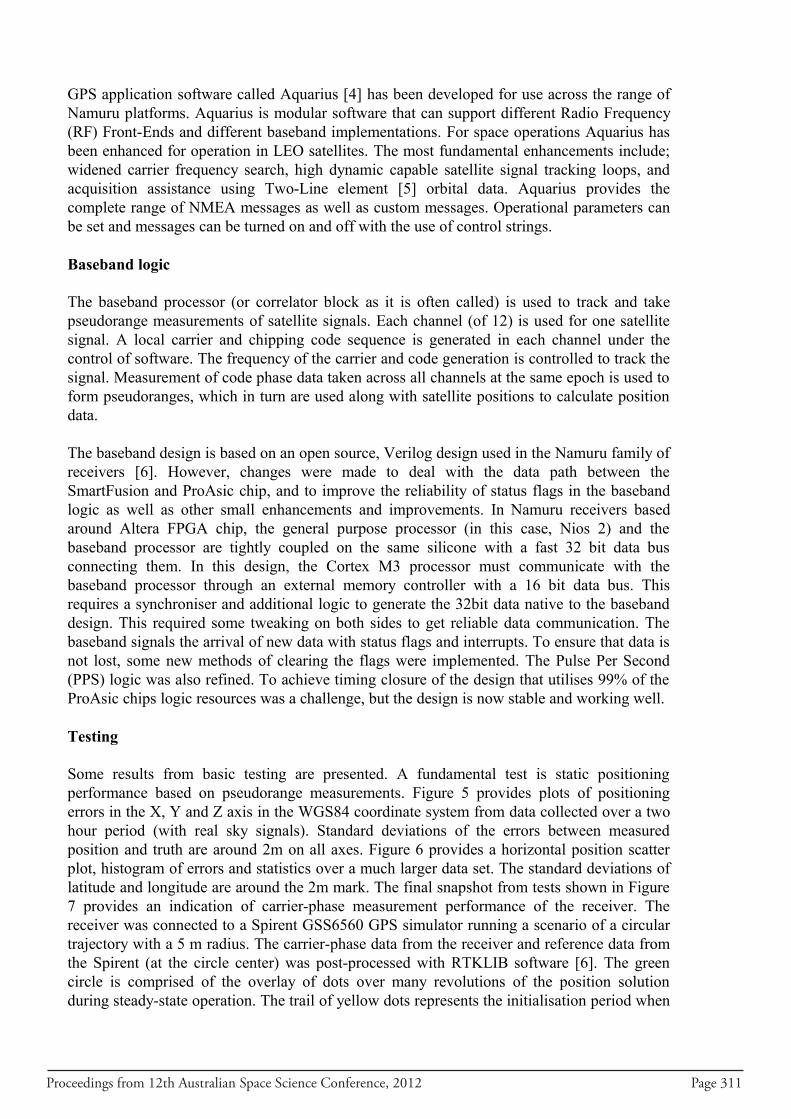
Proceedings from 12th Australian Space Science Conference, 2012 Page 311
GPS application software called Aquarius [4] has been developed for use across the range of
Namuru platforms. Aquarius is modular software that can support different Radio Frequency
(RF) Front-Ends and different baseband implementations. For space operations Aquarius has
been enhanced for operation in LEO satellites. The most fundamental enhancements include;
widened carrier frequency search, high dynamic capable satellite signal tracking loops, and
acquisition assistance using Two-Line element [5] orbital data. Aquarius provides the
complete range of NMEA messages as well as custom messages. Operational parameters can
be set and messages can be turned on and off with the use of control strings.
Baseband logic
The baseband processor (or correlator block as it is often called) is used to track and take
pseudorange measurements of satellite signals. Each channel (of 12) is used for one satellite
signal. A local carrier and chipping code sequence is generated in each channel under the
control of software. The frequency of the carrier and code generation is controlled to track the
signal. Measurement of code phase data taken across all channels at the same epoch is used to
form pseudoranges, which in turn are used along with satellite positions to calculate position
data.
The baseband design is based on an open source, Verilog design used in the Namuru family of
receivers [6]. However, changes were made to deal with the data path between the
SmartFusion and ProAsic chip, and to improve the reliability of status flags in the baseband
logic as well as other small enhancements and improvements. In Namuru receivers based
around Altera FPGA chip, the general purpose processor (in this case, Nios 2) and the
baseband processor are tightly coupled on the same silicone with a fast 32 bit data bus
connecting them. In this design, the Cortex M3 processor must communicate with the
baseband processor through an external memory controller with a 16 bit data bus. This
requires a synchroniser and additional logic to generate the 32bit data native to the baseband
design. This required some tweaking on both sides to get reliable data communication. The
baseband signals the arrival of new data with status flags and interrupts. To ensure that data is
not lost, some new methods of clearing the flags were implemented. The Pulse Per Second
(PPS) logic was also refined. To achieve timing closure of the design that utilises 99% of the
ProAsic chips logic resources was a challenge, but the design is now stable and working well.
Testing
Some results from basic testing are presented. A fundamental test is static positioning
performance based on pseudorange measurements. Figure 5 provides plots of positioning
errors in the X, Y and Z axis in the WGS84 coordinate system from data collected over a two
hour period (with real sky signals). Standard deviations of the errors between measured
position and truth are around 2m on all axes. Figure 6 provides a horizontal position scatter
plot, histogram of errors and statistics over a much larger data set. The standard deviations of
latitude and longitude are around the 2m mark. The final snapshot from tests shown in Figure
7 provides an indication of carrier-phase measurement performance of the receiver. The
receiver was connected to a Spirent GSS6560 GPS simulator running a scenario of a circular
trajectory with a 5 m radius. The carrier-phase data from the receiver and reference data from
the Spirent (at the circle center) was post-processed with RTKLIB software [6]. The green
circle is comprised of the overlay of dots over many revolutions of the position solution
during steady-state operation. The trail of yellow dots represents the initialisation period when
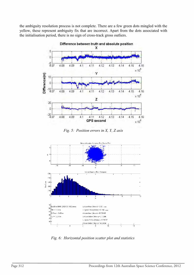
Page 312 Proceedings from 12th Australian Space Science Conference, 2012
the ambiguity resolution process is not complete. There are a few green dots mingled with the
yellow, these represent ambiguity fix that are incorrect. Apart from the dots associated with
the initialisation period, there is no sign of cross-track gross outliers.
Fig. 5: Position errors in X, Y, Z axis
Fig. 6: Horizontal position scatter plot and statistics
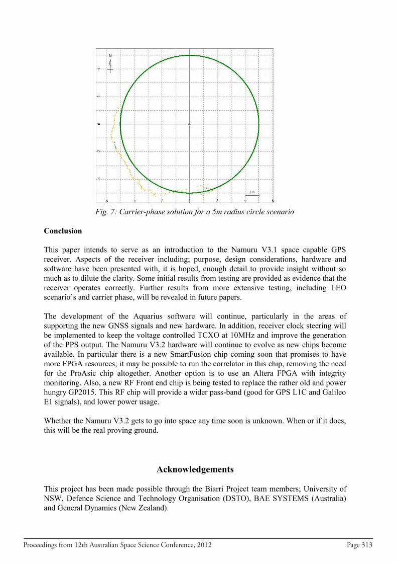
Proceedings from 12th Australian Space Science Conference, 2012 Page 313
Fig. 7: Carrier-phase solution for a 5m radius circle scenario
Conclusion
This paper intends to serve as an introduction to the Namuru V3.1 space capable GPS
receiver. Aspects of the receiver including; purpose, design considerations, hardware and
software have been presented with, it is hoped, enough detail to provide insight without so
much as to dilute the clarity. Some initial results from testing are provided as evidence that the
receiver operates correctly. Further results from more extensive testing, including LEO
scenario’s and carrier phase, will be revealed in future papers.
The development of the Aquarius software will continue, particularly in the areas of
supporting the new GNSS signals and new hardware. In addition, receiver clock steering will
be implemented to keep the voltage controlled TCXO at 10MHz and improve the generation
of the PPS output. The Namuru V3.2 hardware will continue to evolve as new chips become
available. In particular there is a new SmartFusion chip coming soon that promises to have
more FPGA resources; it may be possible to run the correlator in this chip, removing the need
for the ProAsic chip altogether. Another option is to use an Altera FPGA with integrity
monitoring. Also, a new RF Front end chip is being tested to replace the rather old and power
hungry GP2015. This RF chip will provide a wider pass-band (good for GPS L1C and Galileo
E1 signals), and lower power usage.
Whether the Namuru V3.2 gets to go into space any time soon is unknown. When or if it does,
this will be the real proving ground.
Acknowledgements
This project has been made possible through the Biarri Project team members; University of
NSW, Defence Science and Technology Organisation (DSTO), BAE SYSTEMS (Australia)
and General Dynamics (New Zealand).
Page 314 Proceedings from 12th Australian Space Science Conference, 2012
References
1. The CubSat Project, “CubeSat Design Specifications”, ds_rev12.pdf, cubesat.org website.
Accessed on-line 2012, www.cubesat.org
2. Microsemi / Actel, “Radiation-Tolerant ProASIC3 FPGAs Radiation Effects”,
RT3P_Rad_Rpt.pdf, Actel websit. Accessed On-line 2012, www.actel.com
3. Microsemi / Actel, “DirectC v2.7 User’s Guide”, directc_ug.pdf, Actel websit. Accessed
on-line 2012, www.actel.com
4. GLENNON, E.P., MUMFORD, P.J., & PARKINSON, K.J., 2011. “Aquarious firmware
for UNSW Namuru GPS receivers”, IGNSS Symposium., Sydney, Australia, 15-17
November, paper 57.
5. Celestrak “NORAD Two-Line Element Set”,
www.celestrak.com/NORAD/documentation/, accessed on-line 2012
6. MUMFORD, P.J., PARKINSON, K., & DEMPSTER, A.G., 2006. “Open GNSS receiver
platform”. IEEE/ION PLANS, San Diego, California, 25-27 April, 1108-1113.
7. RTKLIB “RTKLIB ver. 2.4.1 Manual”, www.rtklib.com, accessed on-line 2012
Proceedings from 12th Australian Space Science Conference, 2012 Page 315
Visual Odometry Based on the Fourier-Mellin Transform foran Experimental Mars Rover on Rough Terrain
Suchet Bargoti, Aditya Mahajan and Ali Haydar Goktogan
Australian Centre for Field Robotics, The University of Sydney, NSW, 2006, Australia
Summary: Egomotion estimation is a critical component of autonomous navigation systems,especially in unexplored and potentially hazardous environments. This paper explores a meansof visual odometry for an Experimental Mars Rover on rough terrain. A downward facingcamera attached in front of the rover captured images as the vehicle traversed through aMars Yard, a landscape simulating the Martian surface. Analysis of visual information wasconducted in the frequency domain using the Fourier-Mellin Transform (FMT) to obtainrotation, translation and scaling between consecutive images. These similarity transformswere calculated through phase correlation and used to update the rover position and headingestimates. The accuracy of the developed algorithm was quantitatively measured over a seriesof navigation experiments in varying terrain roughness. Results were compared with datafrom a similar analysis performed indoors on flat ground. Accurate instantaneous egomotionestimates were obtained regardless of terrain type. Due to the locally-planar ground assumptionimposed by the FMT, the algorithm is sensitive to terrain roughness and ground stability inthe long term. Odometry errors exhibited consistency on regolith but not on rough terrain.The most accurate odometry was obtained on regolith.
Keywords: Visual odometry, rough terrain, Fourier-Mellin transform, experimental Marsrover, ground-facing camera, monocular vision.
I. Introduction
Robotic exploration of unknown and hazardous environments has become increasinglyfeasible over the past decade. In the case of planetary rovers, continuous and real-timecommunication between the vehicle and the base station is not always possible. This maybe due to limitations in bandwidth, signal delay over large distances or other factors likeocclusions in line-of-sight. Such challenges dictate a high level of autonomy to achieve adiverse range of mission objectives. With increasing mission complexity comes the need forthese machines to be localised with little-to-none a priori information about the environment.
For a planetary rover, accurate localisation is critical for successful autonomous operation[1]. External infrastructure such as GPS satellites, predefined fiducials or signal emittingbeacons can provide accurate position information in a global frame but access to suchinfrastructure is not available in unexplored terrain like that of other planets. Infrastructure-independent accurate localisation can be achieved through wheel encoders (although wheelsare prone to slip [2]), Inertial Measurement Units (IMUs) [3] or infrared sensing [4]. Othermeans of achieving the same are possible with the use of consumer cameras [5]. This approach,dubbed Visual Odometry (VO), can potentially integrate with other sensor estimates to providemore precise results.
Page 316 Proceedings from 12th Australian Space Science Conference, 2012
This paper explores a frequency based approach towards VO using Fourier-Mellin Trans-forms (FMTs). An Experimental Mars Rover (EMR) equipped with a monocular downwardfacing camera is localised while traversing over fine and rough terrain with images capturedat varying resolutions.
The following section presents several means of VO and highlights our reasoning for select-ing the FMT based approach. Next, we outline the mathematical theory governing the Fourierand Mellin transforms, put into practice in Section III. The architecture is then implementedonto an EMR and its performance is tested under various traversability scenarios.
II. Background
Hardware approaches to VO can be classified according to the type of sensor data used toestimate the robot trajectory i.e. stereo or monocular vision [6]. Although low-level algorithmscan be applied to both setups, stereo vision allows for robust and error-tolerant motionestimation [7], describing the rover state in 6 Degrees of Freedom (DoF) [8] at the expenseof increased computational complexity. Whereas when depth perception is limited, as in thecase for monocular vision, a planar approximation is made for the local terrain.
The processing of visual data for egomotion estimation can be divided into three categories:feature-based methods, appearance-based methods, and hybrid methods [9].
Feature-based methods are based on salient and repeatable features that are tracked overseveral frames. Feature detection and classification operators such as Harris or Frostner cornerdetectors [7, 8], Shi-Tomasi feature selection [10] or Scale Invariant Feature Transforms(SIFT) [11, 1] are used to recognise points of interest in consecutive images. Through uniqueclassification and/or using motion estimates (e.g. from wheel encoders) the same features arematched in the next frame. Robust motion estimation is then done in two steps. Least-squaresestimates provides an inexpensive initial guess of any Rotation, Scale or Translation (RST)parameters whereas maximum-likelihood estimation provides more accurate retrieval of theseparameters. Cumulative storage/updates of unique features leads to Simultaneous LocalisationAnd Mapping (SLAM).
Appearance-based methods or hybrid approaches use the intensity information of all thepixels in the image or subregions of it. This paper looks at such an approach using the Fourier-Mellin Transform. The algorithm is used for registering images of the ground plane takenfrom the Mars rover. The advantages of using a frequency based approach are its simplicity,computational cost and the fact that it better exploits better the invariance against ground-planerotations [6]. The FMT approach applied here concerns the transformation of 2D data. Thisimposes an assumption that the terrain is locally planar. Due to the relatively slow speeds ofthe EMR (∼0.1m/s), a high frame rate and the limited size of any obstacles in the FoV, suchan assumption will not have a significant impact in the retrieval of the similarity transformparameters: rotation, scale and translation.
The algorithm is implemented on an EMR, which is also known as Mawson (named after thefamous Australian explorer Sir Douglas Mawson). The rover was developed at the AustralianCentre for Field Robotics (ACFR), the University of Sydney, Australia. The traversabilitytests have been performed in an indoor Mars Yard available at the PowerHouse Museum
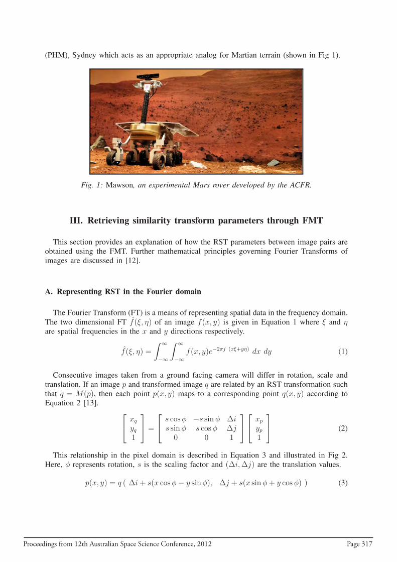
Proceedings from 12th Australian Space Science Conference, 2012 Page 317
(PHM), Sydney which acts as an appropriate analog for Martian terrain (shown in Fig 1).
Fig. 1: Mawson, an experimental Mars rover developed by the ACFR.
III. Retrieving similarity transform parameters through FMT
This section provides an explanation of how the RST parameters between image pairs areobtained using the FMT. Further mathematical principles governing Fourier Transforms ofimages are discussed in [12].
A. Representing RST in the Fourier domain
The Fourier Transform (FT) is a means of representing spatial data in the frequency domain.The two dimensional FT f(ξ, η) of an image f(x, y) is given in Equation 1 where ξ and ηare spatial frequencies in the x and y directions respectively.
f(ξ, η) =
∫ ∞
−∞
∫ ∞
−∞f(x, y)e−2πj (xξ+yη) dx dy (1)
Consecutive images taken from a ground facing camera will differ in rotation, scale andtranslation. If an image p and transformed image q are related by an RST transformation suchthat q = M(p), then each point p(x, y) maps to a corresponding point q(x, y) according toEquation 2 [13].
xq
yq1
=
s cosφ −s sinφ ∆is sinφ s cosφ ∆j
0 0 1
xp
yp1
(2)
This relationship in the pixel domain is described in Equation 3 and illustrated in Fig 2.Here, φ represents rotation, s is the scaling factor and (∆i,∆j) are the translation values.
p(x, y) = q ( ∆i+ s(x cosφ− y sinφ), ∆j + s(x sinφ+ y cosφ) ) (3)
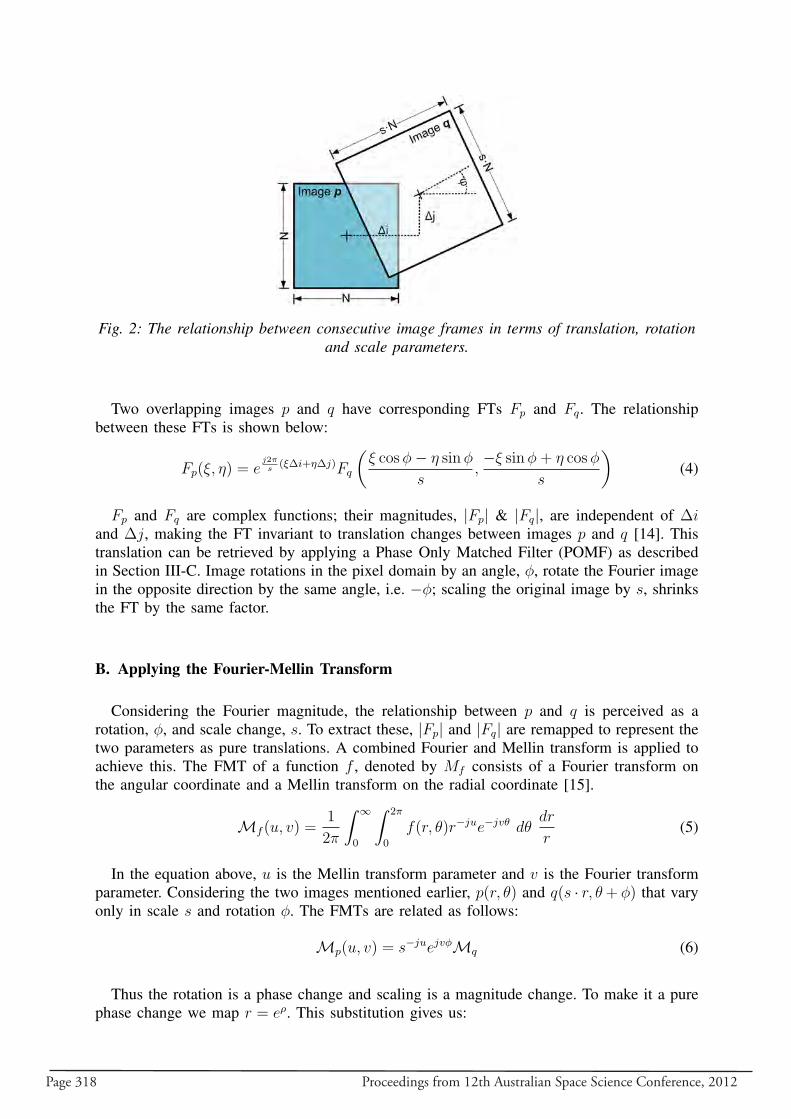
Page 318 Proceedings from 12th Australian Space Science Conference, 2012
Fig. 2: The relationship between consecutive image frames in terms of translation, rotationand scale parameters.
Two overlapping images p and q have corresponding FTs Fp and Fq. The relationshipbetween these FTs is shown below:
Fp(ξ, η) = ej2πs
(ξ∆i+η∆j)Fq
(ξ cosφ− η sinφ
s,−ξ sinφ+ η cosφ
s
)(4)
Fp and Fq are complex functions; their magnitudes, |Fp| & |Fq|, are independent of ∆iand ∆j, making the FT invariant to translation changes between images p and q [14]. Thistranslation can be retrieved by applying a Phase Only Matched Filter (POMF) as describedin Section III-C. Image rotations in the pixel domain by an angle, φ, rotate the Fourier imagein the opposite direction by the same angle, i.e. −φ; scaling the original image by s, shrinksthe FT by the same factor.
B. Applying the Fourier-Mellin Transform
Considering the Fourier magnitude, the relationship between p and q is perceived as arotation, φ, and scale change, s. To extract these, |Fp| and |Fq| are remapped to represent thetwo parameters as pure translations. A combined Fourier and Mellin transform is applied toachieve this. The FMT of a function f , denoted by Mf consists of a Fourier transform onthe angular coordinate and a Mellin transform on the radial coordinate [15].
Mf (u, v) =1
2π
∫ ∞
0
∫ 2π
0
f(r, θ)r−jue−jvθ dθdr
r(5)
In the equation above, u is the Mellin transform parameter and v is the Fourier transformparameter. Considering the two images mentioned earlier, p(r, θ) and q(s · r, θ+ φ) that varyonly in scale s and rotation φ. The FMTs are related as follows:
Mp(u, v) = s−juejvφMq (6)
Thus the rotation is a phase change and scaling is a magnitude change. To make it a purephase change we map r = eρ. This substitution gives us:
Proceedings from 12th Australian Space Science Conference, 2012 Page 319
Mf (u, v) =1
2π
∫ ∞
−∞
∫ 2π
0
f(eρ, θ)e−juρe−jvθ dθ dρ (7)
The above is equivalent to the 2D FT shown in Equation 1. Thus, by remapping the originalFourier transforms into log-polar coordinates, the images Fp and Fq differ only in translation.The horizontal and vertical axes of the log-polar images now represent rotation and scalingrespectively.
C. Translation recovery in the frequency domain
The Fourier Shift Theorem states that the Fourier Transfroms are translation invariant, i.e.they only differ by phase shift if its a pure translation (as shown in Equation 4) [14]. APOMF calculates the phase difference using the Cross Power Spectrum (CPS) between Fp
and Fq and looks at the Inverse Fourier Transform (IFT) to evaluate the translation values.The CPS is calculated as:
ej2π(ξ∆x+η∆y) =Fp(ξ, η) · Fq(ξ, η)
|Fp(ξ, η) · Fq(ξ, η)|(8)
The CPS is followed by taking the inverse of the phase difference:
R(i, j) =
∫ ∞
−∞
∫ ∞
−∞ej2π(ξ∆x+η∆y)ej2π(ξ+η)dξdη (9)
The phase difference R(i, j) contains a single peak (ideally a Dirac function) at R(∆i,∆j)with the peak height denoting the phase correlation value.
D. RST recovery
Starting with images p and q of size N×N , we calculate the Fourier Transform to obtainFp and Fq. The large DC-gain (zero frequency gain) and relatively high FT magnitudes atlow frequencies cause magnitude saturation in this region (seen in Fig 4d). To compensate, acosine shaped high-pass filter is applied prior to log-polar remapping [14]. The remapping isapplied where the η axis is transformed to θ ranging between 0◦ and 360◦; ξ is transformed toa logarithmic distribution of radius between 0 and N
2. Both axes have a resolution of N points,
resulting in N×N images. The resulting images are labelled LPp and LPq. Fig 4e illustratesthis transformation. The log-polar image pair are related by pure translation reflecting therotation and scaling parameters between the original images. The POMF compares the phasecomponents of the FTs of LPp and LPq, giving a phase correlation peak Rθs(∆i,∆j). Pixel-wise translation values for the log-polar images are converted into angular and scale valuesusing Equation 10.
θ = ∆jN
× 360◦, s = N2
(∆i−1N−1 ) (10)
Page 320 Proceedings from 12th Australian Space Science Conference, 2012
The second image q is rotated and scaled by the results obtained in Equation 10 suchthat p and q now only differ by pure translation. A second application of POMF results intranslation parameters.
An inherent property of calculating the Discrete Fourier Transform (DFT) of an image isthat it assumes the image is infinitely tiled. The recovered correlation peak at Rθs(∆i,∆j) canrepresent two possible translation matches. Regarding an N×N image, the true translationmay be ∆i or (∆i−N ). We assume that the image does not translate more than N
2such that
if ∆i is greater than N2
, the true translation is (∆i−N ). The same applies for ∆j.
This means that if ∆i in Equation 10 is greater than N2
, the scale factor is changed froms to 1
s. For the rotation, this ambiguity results in the angle being either θ or θ + 180◦. The
ambiguity is resolved by rotating copies of the second image by both angles and evaluatingtheir respective translations with the first image. The image pair with a higher translationcorrelation value (given by Rxy(∆i,∆j)) can be tracked back to the correct rotation angle.Furthermore, to reduce the risk of erroneous image matching, the algorithm tests θ valuescorresponding to the ten highest peaks of Rθs(∆i,∆j). This results in twenty possible valuesof θ which are filtered by implementing a saturation limit of 10◦ between each image pair.Of these, the value that produces the largest peak for Rxy(∆i,∆j) is used.
IV. Experimental setup
A few additional aspects of image processing (such as camera parameters, image distortion,and filtering) need to be assessed before experimental application of the FMT and POMF.The following sections address hardware and image pre-processing and how these factor intoour experimental setup. Following this, Section V-A explains several traversability scenariosthat evaluate the accuracy of the VO approach.
A. Hardware aspects
The GoPro HD Hero 2 camera was used as the image capture device for our experiments.The camera was mounted in front of the rover looking downwards, approximately 0.30 metresfrom the ground. The setup is illustrated in Fig 3. An external light source was used to providebetter illumination.
Operating at 2 Hz, the camera captured images at a resolution of 5 megapixels (2592×1944)covering a 127◦ Field of View (FoV) [16]. Keeping the rover speed minimal, the given framerate and the large FoV ensures an image overlap of ∼85%, much greater than the minimum50% required for successful registration [13]. To investigate the registration ability of theFMT at different resolutions, the sequences were downsampled to the following resolutions:480×480, 600×600, 800×800 and 1080×1080. To preserve the FoV, these resolutions wereobtained by downsampling the originals and recalculating camera parameters.
The camera intrinsic parameters were obtained using the MATLAB Camera CalibrationToolbox [17]. The camera matrix, K (shown in Equation 11) and distortion coefficients (radialand tangential) were obtained for each resolution. Due to the adjustable position of the cameramount, extrinsic calibration was performed prior to each sequence.
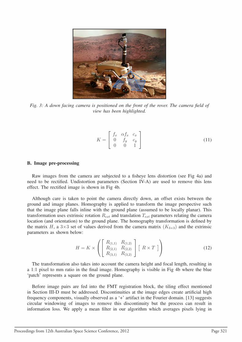
Proceedings from 12th Australian Space Science Conference, 2012 Page 321
Fig. 3: A down facing camera is positioned on the front of the rover. The camera field ofview has been highlighted.
K =
fx αfx cx0 fy cy0 0 1
(11)
B. Image pre-processing
Raw images from the camera are subjected to a fisheye lens distortion (see Fig 4a) andneed to be rectified. Undistortion parameters (Section IV-A) are used to remove this lenseffect. The rectified image is shown in Fig 4b.
Although care is taken to point the camera directly down, an offset exists between theground and image planes. Homography is applied to transform the image perspective suchthat the image plane falls inline with the ground plane (assumed to be locally planar). Thistransformation uses extrinsic rotation Rext and translation Text parameters relating the cameralocation (and orientation) to the ground plane. The homography transformation is defined bythe matrix H , a 3×3 set of values derived from the camera matrix (K3×3) and the extrinsicparameters as shown below:
H = K ×
R(1,1) R(1,2)
R(2,1) R(2,2)
R(3,1) R(3,2)
[
R× T] (12)
The transformation also takes into account the camera height and focal length, resulting ina 1:1 pixel to mm ratio in the final image. Homography is visible in Fig 4b where the blue‘patch’ represents a square on the ground plane.
Before image pairs are fed into the FMT registration block, the tiling effect mentionedin Section III-D must be addressed. Discontinuities at the image edges create artificial highfrequency components, visually observed as a ‘+’ artifact in the Fourier domain. [13] suggestscircular windowing of images to remove this discontinuity but the process can result ininformation loss. We apply a mean filter in our algorithm which averages pixels lying in
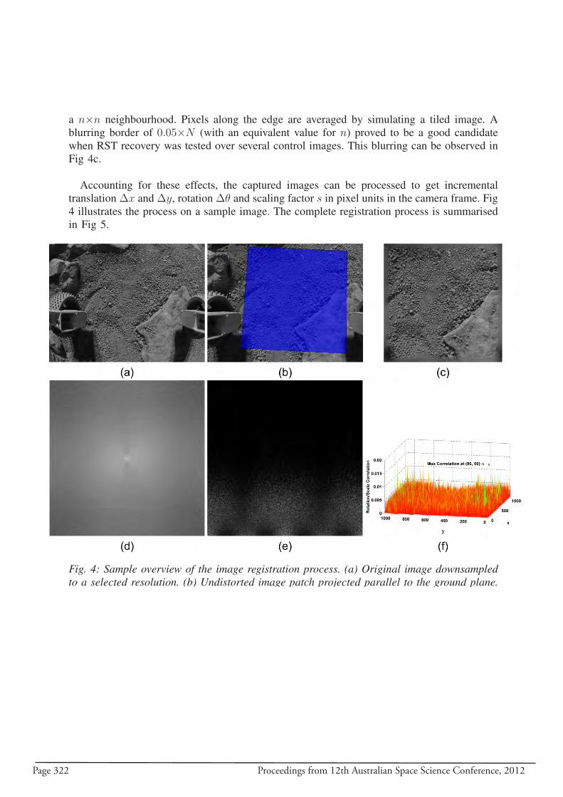
Page 322 Proceedings from 12th Australian Space Science Conference, 2012
a n×n neighbourhood. Pixels along the edge are averaged by simulating a tiled image. Ablurring border of 0.05×N (with an equivalent value for n) proved to be a good candidatewhen RST recovery was tested over several control images. This blurring can be observed inFig 4c.
Accounting for these effects, the captured images can be processed to get incrementaltranslation ∆x and ∆y, rotation ∆θ and scaling factor s in pixel units in the camera frame. Fig4 illustrates the process on a sample image. The complete registration process is summarisedin Fig 5.
Fig. 4: Sample overview of the image registration process. (a) Original image downsampledto a selected resolution. (b) Undistorted image patch projected parallel to the ground plane.(c) Edge blurring applied to minimise tiling effect. (d) FT of the image, displayed as the logof Fourier magnitude. (e) Log-polar transformation applied to the filtered FT magnitude. (f)
Phase correlation plot R(i, j) obtained by evaluating the CPS between image pairs.
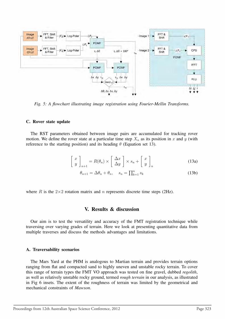
Proceedings from 12th Australian Space Science Conference, 2012 Page 323
Fig. 5: A flowchart illustrating image registration using Fourier-Mellin Transforms.
C. Rover state update
The RST parameters obtained between image pairs are accumulated for tracking rovermotion. We define the rover state at a particular time step Xn as its position in x and y (withreference to the starting position) and its heading θ (Equation set 13).
[xy
]
n+1
= R(θn)×[∆x∆y
]× sn +
[xy
]
n
(13a)
θn+1 = ∆θn + θn, sn =∏n
k=1 sk (13b)
where R is the 2×2 rotation matrix and n represents discrete time steps (2Hz).
V. Results & discussion
Our aim is to test the versatility and accuracy of the FMT registration technique whiletraversing over varying grades of terrain. Here we look at presenting quantitative data frommultiple traverses and discuss the methods advantages and limitations.
A. Traversability scenarios
The Mars Yard at the PHM is analogous to Martian terrain and provides terrain optionsranging from flat and compacted sand to highly uneven and unstable rocky terrain. To coverthis range of terrain types the FMT VO approach was tested on fine gravel, dubbed regolith,as well as relatively unstable rocky ground, termed rough terrain in our analysis, as illustratedin Fig 6 insets. The extent of the roughness of terrain was limited by the geometrical andmechanical constraints of Mawson.
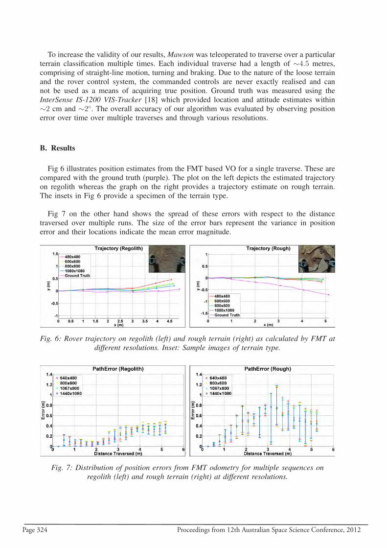
Page 324 Proceedings from 12th Australian Space Science Conference, 2012
To increase the validity of our results, Mawson was teleoperated to traverse over a particularterrain classification multiple times. Each individual traverse had a length of ∼4.5 metres,comprising of straight-line motion, turning and braking. Due to the nature of the loose terrainand the rover control system, the commanded controls are never exactly realised and cannot be used as a means of acquiring true position. Ground truth was measured using theInterSense IS-1200 VIS-Tracker [18] which provided location and attitude estimates within∼2 cm and ∼2◦. The overall accuracy of our algorithm was evaluated by observing positionerror over time over multiple traverses and through various resolutions.
B. Results
Fig 6 illustrates position estimates from the FMT based VO for a single traverse. These arecompared with the ground truth (purple). The plot on the left depicts the estimated trajectoryon regolith whereas the graph on the right provides a trajectory estimate on rough terrain.The insets in Fig 6 provide a specimen of the terrain type.
Fig 7 on the other hand shows the spread of these errors with respect to the distancetraversed over multiple runs. The size of the error bars represent the variance in positionerror and their locations indicate the mean error magnitude.
Fig. 6: Rover trajectory on regolith (left) and rough terrain (right) as calculated by FMT atdifferent resolutions. Inset: Sample images of terrain type.
Fig. 7: Distribution of position errors from FMT odometry for multiple sequences onregolith (left) and rough terrain (right) at different resolutions.
Proceedings from 12th Australian Space Science Conference, 2012 Page 325
C. Discussion
For both scenarios shown in Fig 6, FMT provides a very successful means of egomotionestimation over short distances. However, the dead-reckoning state estimates cause the pathto deviate from the ground truth if left unchecked.
Working with monocular vision, FMT imposes a locally planar assumption as imageregistration can only be performed in 2D. The assumption is violated when terrain featuresbearing significant heights enter the FoV. Relatively large objects are seen with varyingperspective as the vehicle traverses over them. This perceived change in shape contributed toerrors in the odometry estimate. Additionally, large outliers were observed when traversingover loose rocks where the image contents shifted as a result of rover-terrain interaction.The nature of FMT as an appearance-based method allowed for accurate image registrationprovided that the entire image experienced a common translation/rotation. If parts of the imagemoved with respect to each other, RST estimates deteriorated. On the other hand levelledand compact terrain like regolith yielded accurate egomotion estimates. The inconsistencyof rover-terrain interaction over several scenarios caused a large variance in position errors.This irregularity is seen in Fig 7 (right). The opposite was true for multiple traverses onregolith where the relative homogeneity of the terrain resulted in a fairly uniform distributionof position errors over the length of the traverse. The same is apparent in Fig 7 (left).
It was observed that the rover was prone to rapid changes in velocity (and hence imageoverlap), particularly when navigating over rocks or sloped ground. The consequent reductionin overlap leads to poorer odometry performance [13]. This can be seen in Fig 6 (right) wherea single heading error at ∼0.8 m caused a continuously divergent position estimate. Althoughnot implemented here, such a flaw may be mitigated through data fusion with other modalities(IMU or wheel encoders), as applied in [1].
Improvements in odometry were expected with increasing image resolution. This is evidentin Fig 6 where the high-resolution image sequence gives a more fitting estimate to the groundtruth. Interestingly, odometry improvements using high-resolution images were insignificantwhen operating on rough terrain. This is because of the inability of low-resolution analysis todetect the finer features on the regolith surface. Noting that these results only span the givenresolutions, we can infer that computational demands can be reduced by working with lowerresolutions on rough terrain. This can be achieved without without compromising accuracy.
VI. Conclusion & future work
We have successfully implemented the Fourier-Mellin Transform image registration tech-nique to perform odometry for a planetary rover on rough terrain. Similarity transformparameters were obtained by analysing image pairs from a down facing camera. Operatingon an analog of the Martian surface at the Powerhouse Museum, Sydney, the advantages andlimitations of this algorithm were brought to attention. Our experiments have indicated thatthis method provides highly accurate motion estimates in the short term. These estimates wereconsistent while operating on regolith.
The global nature of transformation to the frequency domain placed limitations on thealgorithm. External lighting was used to reduce shadowing and ameliorate image quality.
Page 326 Proceedings from 12th Australian Space Science Conference, 2012
Loose rocks in the FoV resulted in outliers during image registration, causing dead-reckoningerrors which accumulated over time. Additionally, the resolution analysis concluded that high-resolution images were more favourable over regolith than on rough terrain.
Image registration using the Fourier-Mellin Transform has potential for robust egomotionestimation. It has been proven to be more accurate than optical flow [15]. This warrantscomparison of FMT based VO with the more common feature-based techniques such asSIFT or Shi-Tomasi. These have the added benefit of incorporating SLAM. For future work,a multi-modal approach for slip estimation is planned on the EMR. Here, the VO analysisfrom the camera combined with IMU data will be compared to slip affected wheel odometry.
Acknowledgments
This work is supported by the Australian Space Research Program (ASRP) and funded bythe Australian Research Council (ARC) and the New South Wales State Government.
References
[1] S. Se, T. D. Barfoot, and P. Jasiobedzki, Eds., Visual Motion Estimation and Terrain Modelling for Planetary Rovers,2005.
[2] T. Hellstrom, O. Ringdahl, and I. Wasterlund, “Estimating wheel slip for a forest machine: Pre-Study Report,” 2008.[Online]. Available: http://www8.cs.umu.se/research/ifor/en/files/slip pre-study 1.pdf
[3] C. M. Gifford, “Low-Cost Mobile Robot Localization Using Only a Downward-Facing Webcam,” 2009. [Online].Available: https://www.cresis.ku.edu/∼cgifford/Papers/Gifford WebcamLocalization TechReport.pdf
[4] J. Zhou and L. Huang, “Experimental study on sensor fusion to improve real time indoor localization of a mobilerobot,” in 2011 IEEE 5th International Conference on Robotics, Automation and Mechatronics (RAM). IEEE, 2011,pp. 258–263.
[5] L. H. Matthies, M. W. Maimone, A. Johnson, Y. Cheng, R. Willson, C. Villalpando, S. Goldberg, A. Huertas, A. Stein,and A. Angelova, “Computer Vision on Mars,” International Journal of Computer Vision, vol. 75, no. 1, pp. 67–92,2007.
[6] D. Valiente Garcıa, L. Fernandez Rojo, A. Gil Aparicio, L. Paya Castello, and O. Reinoso Garcıa, “Visual Odometrythrough Appearance and Feature-Based Method with Omnidirectional Images,” Journal of Robotics, vol. 2012, pp.1–13, 2012.
[7] Y. Cheng, M. W. Maimone, and L. H. Matthies, “Visual odometry on the Mars exploration rovers - a tool to ensureaccurate driving and science imaging,” IEEE Robotics & Automation Magazine, vol. 13, no. 2, pp. 54–62, 2006.
[8] D. M. Helmick, S. I. Roumeliotis, Y. Cheng, D. S. Clouse, M. Bajracharya, and L. H. Matthies, “Slip compensationfor a Mars Rover,” in IEEE International Conference on Intelligent Robots and Systems, Edmonton and Canada, 2005.
[9] D. Scaramuzza and F. Fraundorfer, “Visual Odometry [Tutorial],” IEEE Robotics & Automation Magazine, vol. 18,no. 4, pp. 80–92, 2011.
[10] J. Shi and C. Tomasi, “Good features to track,” in Proceedings of IEEE Conference on Computer Vision and PatternRecognition CVPR-94. IEEE Comput. Soc. Press, 1994, pp. 593–600.
[11] Q. Lv, W. Zhou, and J. Liu, “Realization of Odometry System Using Monocular Vision,” in 2006 InternationalConference on Computational Intelligence and Security. IEEE, 2006, pp. 1841–1844.
[12] R. Fisher, S. Perkins, A. Walker, and E. Wolfart, “The Fourier Transform,” 2003. [Online]. Available:http://homepages.inf.ed.ac.uk/rbf/HIPR2/fourier.htm
[13] M. McGuire, “An image registration technique for recovering rotation, scale and translation parameters,” 1998.[14] B. Reddy and B. Chatterji, “An FFT-based technique for translation, rotation, and scale-invariant image registration,”
IEEE Transactions on Image Processing, vol. 5, no. 8, pp. 1266–1271, 1996.[15] T. Kazik and A. H. Goktogan, “Visual odometry based on the Fourier-Mellin transform for a rover using a monocular
ground-facing camera,” in 2011 IEEE International Conference on Mechatronics. IEEE, 2011, pp. 469–474.[16] GoPro, “GoPro Official Website: The World’s Most Versatile Camera,” 2006. [Online]. Available: http:
//gopro.com/cameras/hd-hero2-outdoor-edition/#specs[17] J.-Y. Bouguet, “Camera Calibration Toolbox for Matlab,” 2010. [Online]. Available: http://www.vision.caltech.edu/
bouguetj/calib doc/index.html#parameters[18] GENTEX, “InterSense, LLC - Precision Motion Tracking Solutions, IS-1200 System,” 2012. [Online]. Available:
http://www.intersense.com/pages/21/13
Proceedings from 12th Australian Space Science Conference, 2012 Page 327
The Design of a Concurrent Design Facility (CDF) for a Space Launch Vehicle
J W Kho1, L Thompson1
1RMIT University, GPO Box 2476V, Melbourne, Victoria, 3001, Australia
Summary: This study focuses on the feasibility of implementing the Concurrent Design Facility on a design of a Space Launch Vehicle. The Concurrent Engineering implemented on this study is a scaled down version of the European Space Agency (ESA)’s CDF and would be suitable for academic study and implementation. CDF is a design method that uses parallel input of the design constraints into a specific performance model which is capable of instantaneous evaluation and optimisation of the results. This method was initially coined by the European Space Agency (ESA) and is proven to significantly increase the performance of the project, the reliability of the design and substantially reduce the design and evaluation time. This paper will include the design methods implemented in this study and the integration methods of various design functions. The baseline model used in this study would be the AUSROC Nano.
Keywords: Concurrent Design Facility, Concurrent Engineering, Matlab, Catia, Ansys, GMAT, Design Interface Linking.
Introduction
This study covers a detailed study and design of a Concurrent Design Facility (CDF) for a Space Launch Vehicle. The CDF uses the Concurrent Engineering method which encourages parallel design and review instead of the traditional sequential method. The CDF idea was coined by the European Space Agency (ESA) in November 1998. Since their first successful study, the agency has been assisting universities and corporate companies in designing and reviewing space launch vehicles. With over 150 successful studies and reviewed conducted under ESA’s CDF, many other agencies and companies have already taken up this method and customise the method according to their requirement. The National Aeronautical and Space Administration (NASA) of United State of America have their own concurrent design known as the Project Design Centre (PDC).
The CDF concept can be explained as a network of different specialists specialising in different part of a design process collaborating together to optimise the design of a specific product. The specialists are assisted with personal computers that are linked in with one another as well as engineering design tools such as Design, Command Tool, Finite Element Analysis (FEA) and Computational Fluid Dynamics (CFD). All these essential engineering tools are linked with a master programming tool. Any changes and modifications in the value or design could be changed within the master programming tool and the master programming tool will trigger an automatic change of the changed value in the other linked design functions. By implementing this method, the chances of loss of communication or information between different disciplines could be reduced and discrepancies could be prevented. This method is also proven to provide efficient yet rapid optimisation, saving time and cost in the design process as well as increase reliability. All the design process will be conducted in parallel.
Page 328 Proceedings from 12th Australian Space Science Conference, 2012
The purpose of this study is to design a scaled down version of the CDF that is suitable for university academic use. Upon the finalising of the design process, all values are simultaneously input into a performance model for parallel evaluation and improvement. The AUSROC Nano rocket model would be used as a baseline for this study. All values are kept within a Microsoft Excel Spreadsheet file for reference.
Coding methodology
The methods and procedures required to interface the design functions are mentioned. Prior to the interfacing, initial procedures are required to be made to ensure the design functions responds to the scripts.
Initial Procedure
Prior to the initialisation of this study, it is highly suggested that all files are to be located within the same root folder and then create subfolders with respect to the specific design function. This way, it would prevent any errors made due to opening wrong files. Apart from that, when starting up Matlab, by default, it would be within a folder (usually within Documents) where Administrative Privileges is not needed. The command cd ‘C:\Folder’ where the path within the quotation marks refer to the path directory of the folders.
Microsoft Visual Studio is required alongside with Matlab to enable the Matlab Compiler to compile C or C++ libraries inside Matlab. Without the Visual Studio, Matlab would not be able to compile C or C++ libraries. For this study, Microsoft Visual Studio 2010 is being implemented. After the installation, an initial setup to link the Visual Studio with Matlab is required. This can be done by typing mbuild –setup inside the Matlab command window. Matlab will automatically search for Visual Studio directory within the computer and prompts the user to confirm the path. mex –setup will initialise the setup of Matlab executable (MEX) compiling to enable Matlab to create a dynamic link library (.dll) files.
With the addition of Visual Studio onto Matlab, Matlab would provide better flexibility such as support of other coding and scripts, deployment of other executable and linking of other programmes. By adding any corresponding C or C++ filenames behind the mcc commands, it will be passed directly to the Visual Studio for interpretation and compiling.
Ansys Configuration
Create an .ini file with all the commands for ANSYS 13. These commands can be obtained within the ANSYS 13 documentation. The calling commands will act as a matlab interface command for the function in running several design functions within the ANSYS. An .INI file is a configuration file format for Windows and it is usually in a form of plain text. To create a dynamic link library (.dll) for ansys, the definition files, ansys.liband cAnsInterface.h should be specified in the header files. These header files are found in the folders custom and customise located in the root directory, C:\ProgramFiles\Ansys Inc\V130\ANSYS\ [1]. With the dll file, matlab will be able to command Ansys by executing any of the API functions described in the link library. The command script is listed in Figure 1: Sample of the codes [1].
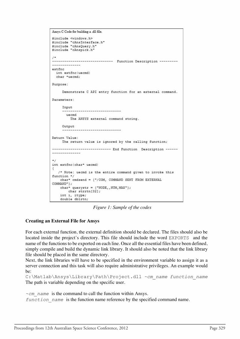
Proceedings from 12th Australian Space Science Conference, 2012 Page 329
Figure 1: Sample of the codes
Creating an External File for Ansys
For each external function, the external definition should be declared. The files should also be located inside the project’s directory. This file should include the word EXPORTS and the name of the functions to be exported on each line. Once all the essential files have been defined, simply compile and build the dynamic link library. It should also be noted that the link library file should be placed in the same directory. Next, the link libraries will have to be specified in the environment variable to assign it as a server connection and this task will also require administrative privileges. An example would be:C:\Matlab\Ansys\Library\Path\Project.dll ~cm_name function_name The path is variable depending on the specific user.
~cm_name is the command to call the function within Ansys.function_name is the function name reference by the specified command name.
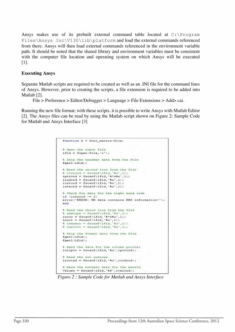
Page 330 Proceedings from 12th Australian Space Science Conference, 2012
Ansys makes use of its prebuilt external command table located at C:\ProgramFiles\Ansys Inc\V130\lib\platform and load the external commands referenced from there. Ansys will then load external commands referenced in the environment variable path. It should be noted that the shared library and environment variables must be consistent with the computer file location and operating system on which Ansys will be executed [1].
Executing Ansys
Separate Matlab scripts are required to be created as well as an .INI file for the command lines of Ansys. However, prior to creating the scripts, a file extension is required to be added into Matlab [2].
File > Preference > Editor/Debugger > Language > File Extensions > Add> cai.
Running the new file format; with these scripts, it is possible to write Ansys with Matlab Editor [2]. The Ansys files can be read by using the Matlab script shown on Figure 2: Sample Code for Matlab and Ansys Interface [3]
Figure 2 : Sample Code for Matlab and Ansys Interface
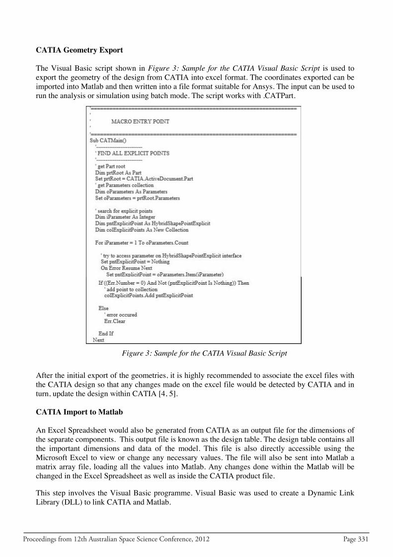
Proceedings from 12th Australian Space Science Conference, 2012 Page 331
CATIA Geometry Export
The Visual Basic script shown in Figure 3: Sample for the CATIA Visual Basic Script is used to export the geometry of the design from CATIA into excel format. The coordinates exported can be imported into Matlab and then written into a file format suitable for Ansys. The input can be used to run the analysis or simulation using batch mode. The script works with .CATPart.
Figure 3: Sample for the CATIA Visual Basic Script
After the initial export of the geometries, it is highly recommended to associate the excel files with the CATIA design so that any changes made on the excel file would be detected by CATIA and in turn, update the design within CATIA [4, 5].
CATIA Import to Matlab
An Excel Spreadsheet would also be generated from CATIA as an output file for the dimensions of the separate components. This output file is known as the design table. The design table contains all the important dimensions and data of the model. This file is also directly accessible using the Microsoft Excel to view or change any necessary values. The file will also be sent into Matlab a matrix array file, loading all the values into Matlab. Any changes done within the Matlab will be changed in the Excel Spreadsheet as well as inside the CATIA product file.
This step involves the Visual Basic programme. Visual Basic was used to create a Dynamic Link Library (DLL) to link CATIA and Matlab.
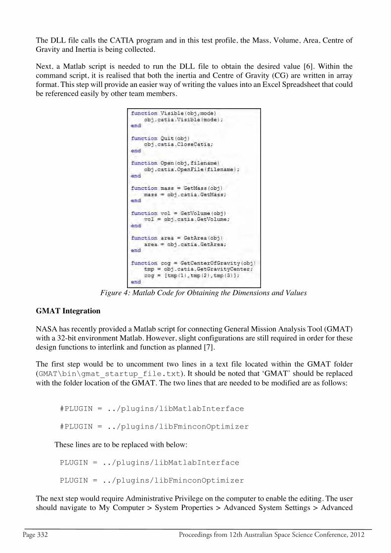
Page 332 Proceedings from 12th Australian Space Science Conference, 2012
The DLL file calls the CATIA program and in this test profile, the Mass, Volume, Area, Centre of Gravity and Inertia is being collected.
Next, a Matlab script is needed to run the DLL file to obtain the desired value [6]. Within the command script, it is realised that both the inertia and Centre of Gravity (CG) are written in array format. This step will provide an easier way of writing the values into an Excel Spreadsheet that could be referenced easily by other team members.
Figure 4: Matlab Code for Obtaining the Dimensions and Values
GMAT Integration
NASA has recently provided a Matlab script for connecting General Mission Analysis Tool (GMAT) with a 32-bit environment Matlab. However, slight configurations are still required in order for these design functions to interlink and function as planned [7].
The first step would be to uncomment two lines in a text file located within the GMAT folder (GMAT\bin\gmat_startup_file.txt). It should be noted that ‘GMAT’ should be replaced with the folder location of the GMAT. The two lines that are needed to be modified are as follows:
#PLUGIN = ../plugins/libMatlabInterface
#PLUGIN = ../plugins/libFminconOptimizer
These lines are to be replaced with below:
PLUGIN = ../plugins/libMatlabInterface
PLUGIN = ../plugins/libFminconOptimizer
The next step would require Administrative Privilege on the computer to enable the editing. The user should navigate to My Computer > System Properties > Advanced System Settings > Advanced
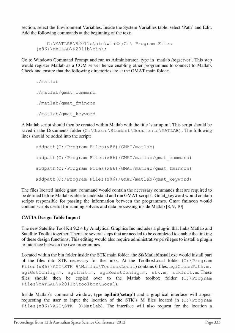
Proceedings from 12th Australian Space Science Conference, 2012 Page 333
section, select the Environment Variables. Inside the System Variables table, select ‘Path’ and Edit. Add the following commands at the beginning of the text:
C:\MATLAB\R2011b\bin\win32;C:\ Program Files (x86)\MATLAB\R2011b\bin\;
Go to Windows Command Prompt and run as Administrator, type in ‘matlab /regserver’. This step would register Matlab as a COM server hence enabling other programmes to connect to Matlab. Check and ensure that the following directories are at the GMAT main folder:
./matlab
./matlab/gmat_command
./matlab/gmat_fmincon
./matlab/gmat_keyword
A Matlab script should then be created within Matlab with the title ‘startup.m’. This script should be saved in the Documents folder (C:\Users\Student\Documents\MATLAB). The following lines should be added into the script:
addpath(C:/Program Files(x86)/GMAT/matlab)
addpath(C:/Program Files(x86)/GMAT/matlab/gmat_command)
addpath(C:/Program Files(x86)/GMAT/matlab/gmat_fmincon)
addpath(C:/Program Files(x86)/GMAT/matlab/gmat_keyword)
The files located inside gmat_command would contain the necessary commands that are required to be defined before Matlab is able to understand and run GMAT scripts. Gmat_keyword would contain scripts responsible for passing the information between the programmes. Gmat_fmincon would contain scripts useful for running solvers and data processing inside Matlab [8, 9, 10]
CATIA Design Table Import
The new Satellite Tool Kit 9.2.4 by Analytical Graphics Inc includes a plug-in that links Matlab and Satellite Toolkit together. There are several steps that are needed to be completed to enable the linking of these design functions. This editing would also require administrative privileges to install a plugin to interface between the two programmes.
Located within the bin folder inside the STK main folder, the StkMatlabInstall.exe would install part of the files into STK necessary for the links. At the ToolboxLocal folder (C:\ProgramFiles(x86)\AGI\STK 9\Matlab\ToolboxLocal) contains 6 files, agiCleanPath.m,agiGetConfig.m, agiInit.m, agiResetConfig.m, stk.m, stkInit.m. These files should then be copied over to the Matlab toolbox folder (C:\ProgramFiles\MATLAB\R2011b\toolbox\Local).
Inside Matlab’s command window, type agiInit(‘setup’) and a graphical interface will appear requesting the user to input the location of the STK’s M files located in (C:\ProgramFiles(x86)\AGI\STK 9\Matlab). The interface will also request for the location a
Page 334 Proceedings from 12th Australian Space Science Conference, 2012
mexConnect.mexw32 file in (C:\Program Files(x86)\AGI\bin). This STK connection interface is able to connect to another workstation within the same network. However, for this case study, the same workstation would be used hence, the hostname would be localhost:5001.
After launching both STK and Matlab, at the Matlab command window, type stkInit to start the connection. A socket connection is then required to be initiated by entering stkOpen and holding the socket number by entering conid = stkOpen. Creating a new STK scenario can be done using stkExec(conid,’New/Scenario CDF’) [11].
Figure 5: A Flow Diagram of a Conceptual CDF for Space Launch Vehicle
CONCLUSION
This paper reports that management of team structure and processes in engineering design teams is an important factor for decreasing the time required to design a space mission. In the conceptual design phase, a redesigned process featuring management of team dynamics has resulted in significant favourable changes in design time, cost and quality. A proposed change to the design scheme in implementation phase design has potential for similar improvements in time and quality.
Proceedings from 12th Australian Space Science Conference, 2012 Page 335
A simple design cycle model shows that if moderate improvements in team efficiency can be achieved, significant improvements in total design time will result [12].
It will see the input of the data into a performance model in DATCOM to simulate the theoretical performance of the model. The results from DATCOM will then be forwarded into GMAT and STK for further analysis and evaluation. All output from previous design functions will be evaluated concurrently through the performance model.
All interfacing of the design functions have been analysed and discussed. Upon the successful integration, the design will be finalising and put into the performance model for simulation. Rapid optimisation will be corrected during this phase.
ACKNOWLEDGEMENTS
The author would like to acknowledge the contributions made by many people throughout the course of this project. Firstly, the author would like to thank the project supervisor, Associate Professor Lachlan Thompson, whose technical knowledge and advice were invaluable to the authors. His continuous dedication to the project, countless hours spent in consultation and guidance contributed dramatically to the project.
The group is also in debt to the supervisor’s assistance and PhD student, Thomas Baum for his expertise in programming and design software, ideas and advices.
The author would also like to thank the other group members, Matthew Wisniewski, Chuntit Phetkhai, Winson Wu, Tao Lin and Pengcheng Gao for their assistance and opinion. Their assistance and expertise in their respective areas have contributed greatly to the project.
Finally, the author would like to deeply thank his friends and families. The successful results of the project are a reflection of their continuous support and understanding throughout the duration of the project.
FUTURE WORK
The CDF concept is still in an initial stage and hence, there are still many aspects of the design that is required to be improved and optimised. Some of the optimisations are but not limited to the below mentioned.
To ensure the optimum results and consistency, it is suggested to gain better access to the required software by making it readily available in the university’s workstations and off campus access for this study. Licenses of software not being immediately available should also be obtained to prevent discrepancies and further delay of the study.
As mentioned in the detailed study, it was necessary to obtain the administrative privileges on the workstations as certain scripts and codes are required to be located inside the root folder and failing to do so, will cause errors and prevent the scripts from running. Certain interface are also required to be installed as plugin to allow the interfacing of two design functions.
The implementation of AutoDesk is also suggested for future research. As AutoDesk has rolled out programmes covering CAD, Dynamic Simulation, CFD and FEA; it would mean better integration and interfacing across these different design functions. AutoDesk Inventor Professional for CAD, Dynamic Simulation and FEA whereas AutoDesk Simulation CFD focuses on CFD. AutoDesk
Page 336 Proceedings from 12th Australian Space Science Conference, 2012
Fusion will also serve as an additional tool capable of importing CAD drawings from different software ranging from CATIA to SpaceClaim, Siemens NX to SolidWorks hence, greatly improves the overall operability and capability.
Interfacing with Matlab’s Simulink could also help improve the productivity of the overall project. With Simulink, the user can map out the entire command interface, linkages and design functions on a matlab model, thereby providing a clear view of the entire project. Simulink contains a function known as S-function. The S-function is an easy way of embedding C code inside the Simulink model. The function acts as a caller to the C source code from Simulink, providing the required codes and commands for interfacing between both. Running the S-function builder, the builder will generate the necessary standard .c source code, the wrapper.c customised interfacing options, .tlc legacy file format to run accelerated and real time workshop and .dll dynamic link library to link the c code [13]. The S-function will be particularly useful when defining flow or boundary conditions within Ansys as defining those conditions would require mathematical equations. S-function with different conditions and instances can also be used at the same time within the same model.
REFERENCES[1] SAS IP, “Tasks in Creating an External Command,” 2010. [Online]. Available:
https://www.sharcnet.ca/Software/Fluent13/help/ans_prog/Hlp_P_UPFB_2.html. [Accessed 09 08 2012].
[2] Cai, “Use Matlab Editor to Write and Run ANSYS Program,” 2011. [Online]. Available: http://www.mathworks.com/matlabcentral/fileexchange/30887-use-matlab-editor-to-write-and-run-ansys-program. [Accessed 08 05 2012].
[3] C. Siewert, “Matlab Code,” Institute of Dynamics and Vibration Research, 2012. [4] Witchita State University, “Drafting,” National Institute for Aviation Research,
Kansas, 2005. [5] Anonymous, “CATIA Points and Excel,” 2008. [Online]. Available:
http://www.coe.org/p/fo/et/thread=16586. [Accessed 08 09 2012]. [6] Friedrich, “Link Catia to Matlab,” 2011. [Online]. Available:
http://www.mathworks.com/matlabcentral/answers/15228-link-catia-to-matlab. [Accessed 08 05 2012].
[7] National Aeronautics and Space Administration, “GMAT Plugins and Extensions,” 2012. [Online]. Available: http://gmatplugins.sourceforge.net/blog/. [Accessed 07 06 2012].
[8] National Aeronautics and Space Administration, “Configuring the MATLAB Interface,” 2012. [Online]. Available: http://gmat.ed-pages.com/wiki/Configuring+the+MATLAB+Interface. [Accessed 06 08 2012].
[9] National Aeronautics and Space Administration , “Data and Configuration,” 2012. [Online]. Available: http://gmat.sourceforge.net/docs/latest/html/DataAndConfiguration.html. [Accessed 08 08 2012].
[10] Anonymous, “Matlab GMAT Interface FAQ,” 2008. [Online]. Available: http://gmat.ed-pages.com/forum/viewtopic.php?f=14&t=65. [Accessed 09 09 2012].
[11] Analytical Graphics Inc, “STK/Matlab Configuration Guide,” 2012. [Online]. Available: http://www.agi.com/resources/faq-system/faq_details.cfm?FAQ_ID=10873. [Accessed 08 09 2012].
[12] S. D. Wall, “Use of Concurrent Engineering in Space Mission Design,” Jet Propulsion Laboratory NASA, California, 2012.
[13] F. Nagi, “What is S-Function,” Universiti Tenaga Nasional, Kuala Lumpur, 2012.

Proceedings from 12th Australian Space Science Conference, 2012 Page 337
[14] S. D. Wall, “Use of Concurrent Engineering in Space Mission Design,” Jet Propulsion Laboratory NASA, California, 2012.

Page 338 Proceedings from 12th Australian Space Science Conference, 2012
Proceedings from 12th Australian Space Science Conference, 2012 Page 339
RF Electrothermal Propulsion Testing Using N2-He Gas Mixture in Low-Temperature Plasma
C. A. Barry Stoute1, Brendan Quine1, Stephen Brown2, Shervin Khazarie
1Department of Earth and Space Science and Engineering, Faculty of Science and Engineering, York University, Toronto, Ontario, M3J1P3, Canada
2Centre for Research in Earth and Space Science, Faculty of Science and Engineering, York University, Toronto, Ontario, M3J1P3, Canada
Abstract
Electrothermal thruster is a low-cost electric engine which can be used for orbital manoeuvres and deep-space missions. These thrusters work well using light elements such as hydrogen and helium. The problem with these two elements is the large storage tank required to keep these propellants. Hydrazine (N2H4) is currently used in electrothermal thruster technology, but due to its volatility, high freezing point, and toxicity, special equipment must be used to preserve this fuel carefully. Therefore, a nitrogen-helium gas mixture has been researched to view the potential alternative to hydrazine. This research focus on low-temperature plasma since the limiting factor is the power input of the system, 20W and under. Thus, the improvement of the specific impulse from cold gas is minor. The mixed gases (nitrogen-helium) show the correlation between the gas mixtures and specific impulse. The range of the gas mixtures are 100% He, 90% He – 10 % N2, 80% He – 20% N2, 50% He – 50% N2, 100% N2. For the 0.90He-0.10N2, the specific impulse is 136.77s while the 0.50He-0.50N2 has the specific impulse of 96.27s. However, the 0.50He-0.50N2 shows the best improvement over cold gas in comparison to the rest of the gas mixtures.
Introduction
Electrothermal propulsion involves a low-cost electric engine which could be used in station keeping and attitude control. Electrothermal propulsion uses plasma as high temperature fuel and conventional nozzle techniques for propulsion. The technology is less complicated than electrostatic and electromagnetic propulsion systems. This technology yields the lowest specific impulse out of the electric engine technologies; however, it is the simplest electric engine to date [1].
Industrial electrothermal thrusters use ammonia (NH3) and hydrazine (N2H4) as their propellant because the availability of hydrogen. Hydrogen as a fuel alone is ideal for these thrusters because of its light atomic mass but due to its high volatility, it is not recommended to transport pure hydrogen in spacecraft; therefore, hydrazine is the ideal propellant for electrothermal propulsion [1]. The force of electrothermal thrusters depends on the overall mass flow rate and the exhaust velocity of the propellant. The exhaust velocity is inversely proportional to the molecular mass of the propellant. Therefore, the lighter elements yield the higher exhaust velocity [1]. Hydrazine is a type of fuel used for monopropellant rockets. It is a toxic, colorless liquid2 whose freezing point is at 274.3 K. Due to its high freezing point and low temperatures in celestial space, the piping system is heated to prevent freezing; in addition, it has a short ignition delay. Hydrazine reacts with many materials and only selected materials can be used in the piping system [1, 2]. This chemical is also very toxic for humans, at around four ppm, which may be a human carcinogen. In monopropellant engines, as well as in electrothermal engines, hydrazine is passed through a catalyst such as carbon fibers. This causes the hydrazine to decompose to ammonia, nitrogen and hydrogen, as shown in equation 1[2, 3].
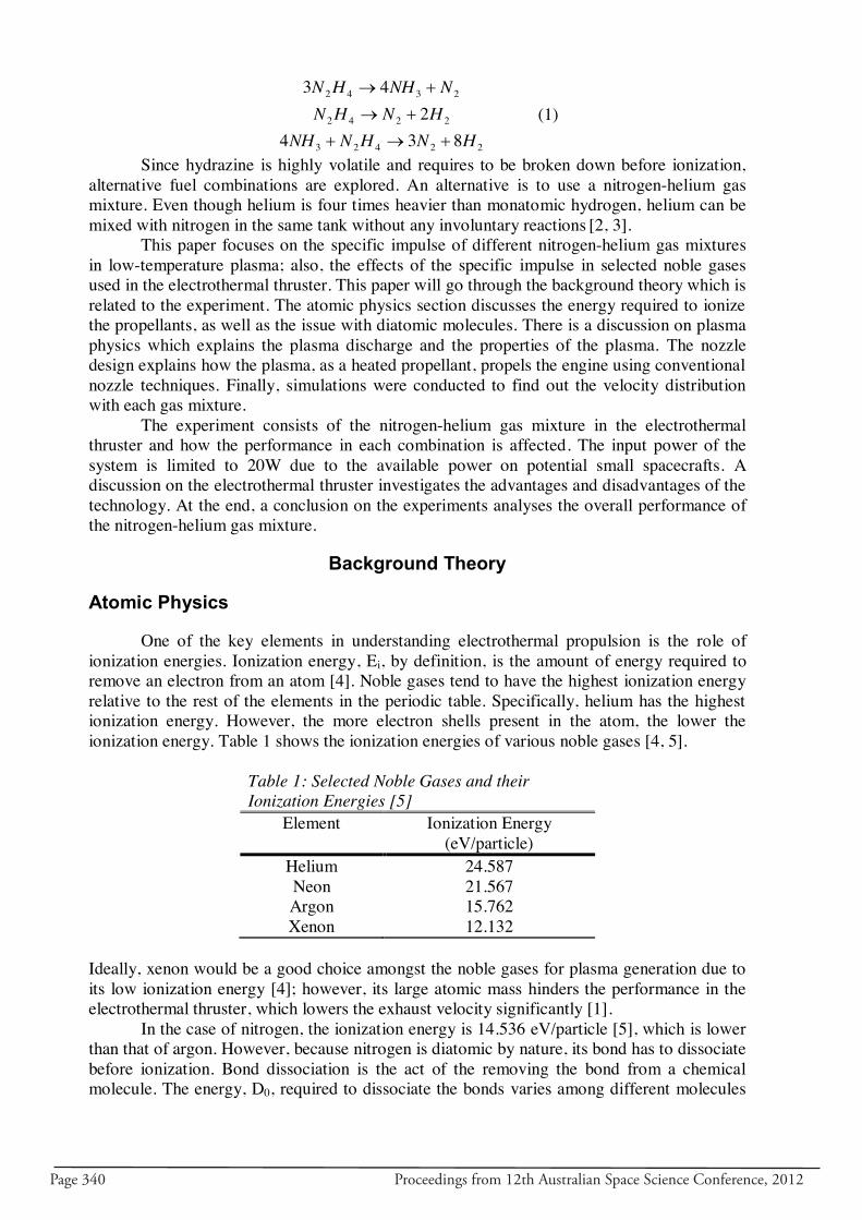
Page 340 Proceedings from 12th Australian Space Science Conference, 2012
22423
2242
2342
8342
43
HNHNNHHNHN
NNHHN
(1)
Since hydrazine is highly volatile and requires to be broken down before ionization, alternative fuel combinations are explored. An alternative is to use a nitrogen-helium gas mixture. Even though helium is four times heavier than monatomic hydrogen, helium can be mixed with nitrogen in the same tank without any involuntary reactions [2, 3].
This paper focuses on the specific impulse of different nitrogen-helium gas mixtures in low-temperature plasma; also, the effects of the specific impulse in selected noble gases used in the electrothermal thruster. This paper will go through the background theory which is related to the experiment. The atomic physics section discusses the energy required to ionize the propellants, as well as the issue with diatomic molecules. There is a discussion on plasma physics which explains the plasma discharge and the properties of the plasma. The nozzle design explains how the plasma, as a heated propellant, propels the engine using conventional nozzle techniques. Finally, simulations were conducted to find out the velocity distribution with each gas mixture. The experiment consists of the nitrogen-helium gas mixture in the electrothermal thruster and how the performance in each combination is affected. The input power of the system is limited to 20W due to the available power on potential small spacecrafts. A discussion on the electrothermal thruster investigates the advantages and disadvantages of the technology. At the end, a conclusion on the experiments analyses the overall performance of the nitrogen-helium gas mixture.
Background Theory
Atomic Physics
One of the key elements in understanding electrothermal propulsion is the role of ionization energies. Ionization energy, Ei, by definition, is the amount of energy required to remove an electron from an atom [4]. Noble gases tend to have the highest ionization energy relative to the rest of the elements in the periodic table. Specifically, helium has the highest ionization energy. However, the more electron shells present in the atom, the lower the ionization energy. Table 1 shows the ionization energies of various noble gases [4, 5].
Table 1: Selected Noble Gases and their Ionization Energies [5]
Element Ionization Energy (eV/particle)
Helium 24.587 Neon 21.567 Argon 15.762 Xenon 12.132
Ideally, xenon would be a good choice amongst the noble gases for plasma generation due to its low ionization energy [4]; however, its large atomic mass hinders the performance in the electrothermal thruster, which lowers the exhaust velocity significantly [1]. In the case of nitrogen, the ionization energy is 14.536 eV/particle [5], which is lower than that of argon. However, because nitrogen is diatomic by nature, its bond has to dissociate before ionization. Bond dissociation is the act of the removing the bond from a chemical molecule. The energy, D0, required to dissociate the bonds varies among different molecules
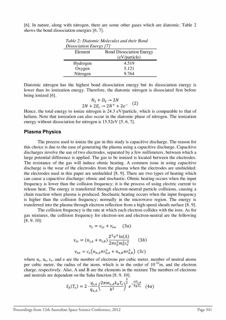
Proceedings from 12th Australian Space Science Conference, 2012 Page 341
[6]. In nature, along with nitrogen, there are some other gases which are diatomic. Table 2 shows the bond dissociation energies [6, 7].
Table 2: Diatomic Molecules and their Bond Dissociation Energy [7]
Element Bond Dissociation Energy (eV/particle)
Hydrogen 4.519 Oxygen 5.121 Nitrogen 9.764
Diatomic nitrogen has the highest bond dissociation energy but its dissociation energy is lower than its ionization energy. Therefore, the diatomic nitrogen is dissociated first before being ionized [6].
Hence, the total energy to ionize nitrogen is 24.3 eV/particle, which is comparable to that of helium. Note that ionization can also occur in the diatomic phase of nitrogen. The ionization energy without dissociation for nitrogen is 15.52eV [5, 6, 7].
Plasma Physics
The process used to ionize the gas in this study is capacitive discharge. The reason for this choice is due to the ease of generating the plasma using a capacitive discharge. Capacitive discharges involve the use of two electrodes, separated by a few millimeters, between which a large potential difference is applied. The gas to be ionized is located between the electrodes. The resistance of the gas will induce ohmic heating. A common issue in using capacitive discharge is the wear of the electrodes from the plasma when the electrodes are unshielded; the electrodes used in this paper are unshielded [8, 9]. There are two types of heating which can cause a capacitive discharge: ohmic and stochastic. Ohmic heating occurs when the input frequency is lower than the collision frequency; it is the process of using electric current to release heat. The energy is transferred through electron-neutral particle collisions, causing a chain reaction where plasma is produced. Stochastic heating occurs when the input frequency is higher than the collision frequency; normally in the microwave region. The energy is transferred into the plasma through electron reflection from a high-speed sheath surface [8, 9]. The collision frequency is the rate at which each electron collides with the ions. As for gas mixtures, the collision frequency for electron-ion and electron-neutral are the following [8, 9, 10]:
( ) where ne, nn, rn, and e are the number of electrons per cubic meter, number of neutral atoms per cubic meter, the radius of the atom, which is in the order of 10-10m, and the electron charge, respectively. Also, A and B are the elements in the mixture The numbers of electrons and neutrals are dependent on the Saha function [8, 9, 10].
( )
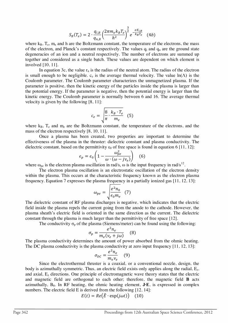
Page 342 Proceedings from 12th Australian Space Science Conference, 2012
( )
where kB, Te, me and h are the Boltzmann constant, the temperature of the electrons, the mass of the electron, and Planck’s constant respectively. The values qi and qn are the ground state degeneracies of an ion and a neutral respectively. The number of electrons are summed up together and considered as a single batch. These values are dependent on which element is involved [10, 11]. In equation 3c, the value rn is the radius of the neutral atom. The radius of the electron is small enough to be negligible. ce is the average thermal velocity. The value ln(Λ) is the Coulomb parameter. The Coulomb parameter characterizes the unmagnetized plasma. If the parameter is positive, then the kinetic energy of the particles inside the plasma is larger than the potential energy. If the parameter is negative, then the potential energy is larger than the kinetic energy. The Coulomb parameter is normally between 6 and 16. The average thermal velocity is given by the following [8, 11]:
√
where kB, Te and me are the Boltzmann constant, the temperature of the electrons, and the mass of the electron respectively [8, 10, 11]. Once a plasma has been created, two properties are important to determine the effectiveness of the plasma in the thruster: dielectric constant and plasma conductivity. The dielectric constant, based on the permittivity ε0 of free space is found in equation 6 [11, 12]:
(
)
where ωpe is the electron plasma oscillation in rad/s, ω is the input frequency in rad/s12. The electron plasma oscillation is an electrostatic oscillation of the electron density within the plasma. This occurs at the characteristic frequency known as the electron plasma frequency. Equation 7 expresses the plasma frequency in a partially ionized gas [11, 12, 13]:
√
The dielectric constant of RF plasma discharges is negative, which indicates that the electric field inside the plasma repels the current going from the anode to the cathode. However, the plasma sheath’s electric field is oriented in the same direction as the current. The dielectric constant through the plasma is much larger than the permittivity of free space [12]. The conductivity σp of the plasma (Siemens/meter) can be found using the following:
The plasma conductivity determines the amount of power absorbed from the ohmic heating. The DC plasma conductivity is the plasma conductivity at zero input frequency [11, 12, 13]:
Since the electrothermal thruster is a coaxial, or a conventional nozzle, design, the
body is azimuthally symmetric. Thus, an electric field exists only applies along the radial, Er, and axial, Ez directions. One principle of electromagnetic wave theory states that the electric and magnetic field are orthogonal to each other; therefore, the magnetic field B acts azimuthally, Bθ. In RF heating, the ohmic heating element, J∙E, is expressed in complex numbers. The electric field E is derived from the following [12, 14]:
( )
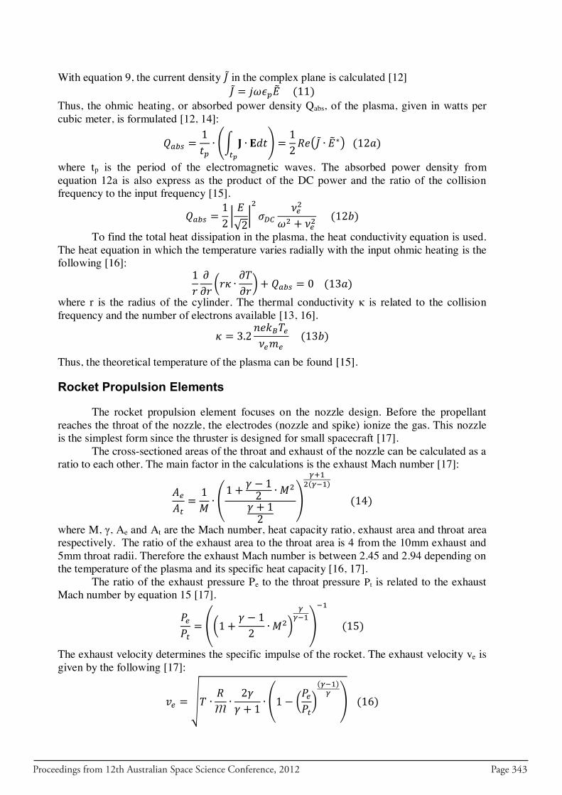
Proceedings from 12th Australian Space Science Conference, 2012 Page 343
With equation 9, the current density in the complex plane is calculated [12]
Thus, the ohmic heating, or absorbed power density Qabs, of the plasma, given in watts per cubic meter, is formulated [12, 14]:
(∫
) (
)
where tp is the period of the electromagnetic waves. The absorbed power density from equation 12a is also express as the product of the DC power and the ratio of the collision frequency to the input frequency [15].
| √ |
To find the total heat dissipation in the plasma, the heat conductivity equation is used. The heat equation in which the temperature varies radially with the input ohmic heating is the following [16]:
(
)
where r is the radius of the cylinder. The thermal conductivity κ is related to the collision frequency and the number of electrons available [13, 16].
Thus, the theoretical temperature of the plasma can be found [15].
Rocket Propulsion Elements
The rocket propulsion element focuses on the nozzle design. Before the propellant reaches the throat of the nozzle, the electrodes (nozzle and spike) ionize the gas. This nozzle is the simplest form since the thruster is designed for small spacecraft [17]. The cross-sectioned areas of the throat and exhaust of the nozzle can be calculated as a ratio to each other. The main factor in the calculations is the exhaust Mach number [17]:
(
)
where M, γ, Ae and At are the Mach number, heat capacity ratio, exhaust area and throat area respectively. The ratio of the exhaust area to the throat area is 4 from the 10mm exhaust and 5mm throat radii. Therefore the exhaust Mach number is between 2.45 and 2.94 depending on the temperature of the plasma and its specific heat capacity [16, 17]. The ratio of the exhaust pressure Pe to the throat pressure Pt is related to the exhaust Mach number by equation 15 [17].
(( )
)
The exhaust velocity determines the specific impulse of the rocket. The exhaust velocity ve is given by the following [17]:
√ ( (
) )
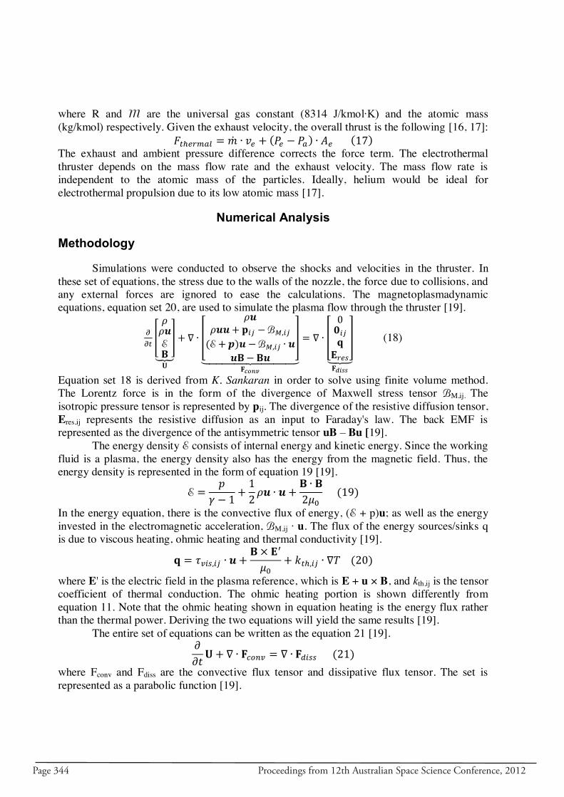
Page 344 Proceedings from 12th Australian Space Science Conference, 2012
where R and M are the universal gas constant (8314 J/kmol∙K) and the atomic mass (kg/kmol) respectively. Given the exhaust velocity, the overall thrust is the following [16, 17]:
The exhaust and ambient pressure difference corrects the force term. The electrothermal thruster depends on the mass flow rate and the exhaust velocity. The mass flow rate is independent to the atomic mass of the particles. Ideally, helium would be ideal for electrothermal propulsion due to its low atomic mass [17].
Numerical Analysis
Methodology
Simulations were conducted to observe the shocks and velocities in the thruster. In these set of equations, the stress due to the walls of the nozzle, the force due to collisions, and any external forces are ignored to ease the calculations. The magnetoplasmadynamic equations, equation set 20, are used to simulate the plasma flow through the thruster [19].
*
+
⏟
[
]
⏟
[
]⏟
(18)
Equation set 18 is derived from K. Sankaran in order to solve using finite volume method. The Lorentz force is in the form of the divergence of Maxwell stress tensor BM,ij. The isotropic pressure tensor is represented by pij. The divergence of the resistive diffusion tensor, Eres,ij represents the resistive diffusion as an input to Faraday's law. The back EMF is represented as the divergence of the antisymmetric tensor uB – Bu [19]. The energy density E consists of internal energy and kinetic energy. Since the working fluid is a plasma, the energy density also has the energy from the magnetic field. Thus, the energy density is represented in the form of equation 19 [19].
In the energy equation, there is the convective flux of energy, (E + p)u; as well as the energy invested in the electromagnetic acceleration, BM,ij ∙ u. The flux of the energy sources/sinks q is due to viscous heating, ohmic heating and thermal conductivity [19].
where E' is the electric field in the plasma reference, which is E + u × B, and kth,ij is the tensor coefficient of thermal conduction. The ohmic heating portion is shown differently from equation 11. Note that the ohmic heating shown in equation heating is the energy flux rather than the thermal power. Deriving the two equations will yield the same results [19]. The entire set of equations can be written as the equation 21 [19].
where Fconv and Fdiss are the convective flux tensor and dissipative flux tensor. The set is represented as a parabolic function [19].
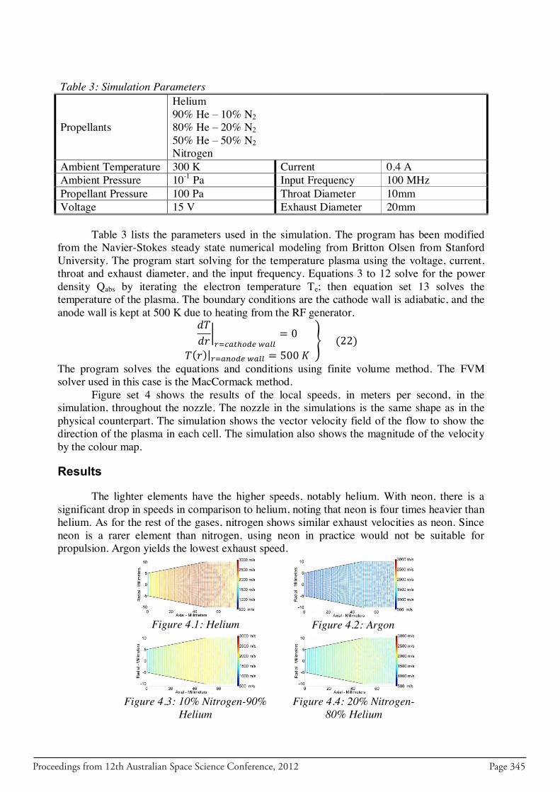
Proceedings from 12th Australian Space Science Conference, 2012 Page 345
Table 3: Simulation Parameters
Propellants
Helium 90% He – 10% N2 80% He – 20% N2 50% He – 50% N2 Nitrogen
Ambient Temperature 300 K Current 0.4 A Ambient Pressure 10-1 Pa Input Frequency 100 MHz Propellant Pressure 100 Pa Throat Diameter 10mm Voltage 15 V Exhaust Diameter 20mm Table 3 lists the parameters used in the simulation. The program has been modified from the Navier-Stokes steady state numerical modeling from Britton Olsen from Stanford University. The program start solving for the temperature plasma using the voltage, current, throat and exhaust diameter, and the input frequency. Equations 3 to 12 solve for the power density Qabs by iterating the electron temperature Te; then equation set 13 solves the temperature of the plasma. The boundary conditions are the cathode wall is adiabatic, and the anode wall is kept at 500 K due to heating from the RF generator.
|
|
}
The program solves the equations and conditions using finite volume method. The FVM solver used in this case is the MacCormack method.
Figure set 4 shows the results of the local speeds, in meters per second, in the simulation, throughout the nozzle. The nozzle in the simulations is the same shape as in the physical counterpart. The simulation shows the vector velocity field of the flow to show the direction of the plasma in each cell. The simulation also shows the magnitude of the velocity by the colour map.
Results
The lighter elements have the higher speeds, notably helium. With neon, there is a significant drop in speeds in comparison to helium, noting that neon is four times heavier than helium. As for the rest of the gases, nitrogen shows similar exhaust velocities as neon. Since neon is a rarer element than nitrogen, using neon in practice would not be suitable for propulsion. Argon yields the lowest exhaust speed.
Figure 4.1: Helium
Figure 4.2: Argon
Figure 4.3: 10% Nitrogen-90%
Helium
Figure 4.4: 20% Nitrogen-
80% Helium
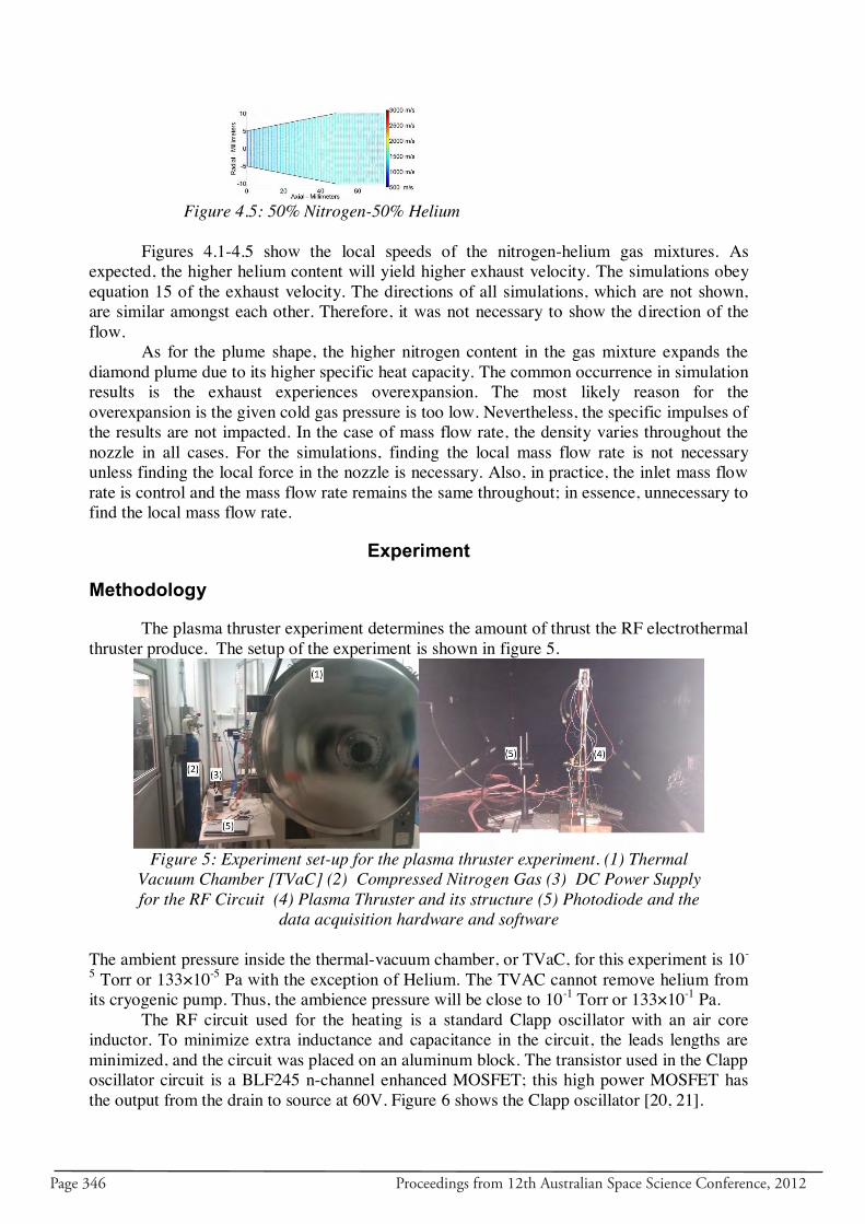
Page 346 Proceedings from 12th Australian Space Science Conference, 2012
Figure 4.5: 50% Nitrogen-50% Helium
Figures 4.1-4.5 show the local speeds of the nitrogen-helium gas mixtures. As
expected, the higher helium content will yield higher exhaust velocity. The simulations obey equation 15 of the exhaust velocity. The directions of all simulations, which are not shown, are similar amongst each other. Therefore, it was not necessary to show the direction of the flow. As for the plume shape, the higher nitrogen content in the gas mixture expands the diamond plume due to its higher specific heat capacity. The common occurrence in simulation results is the exhaust experiences overexpansion. The most likely reason for the overexpansion is the given cold gas pressure is too low. Nevertheless, the specific impulses of the results are not impacted. In the case of mass flow rate, the density varies throughout the nozzle in all cases. For the simulations, finding the local mass flow rate is not necessary unless finding the local force in the nozzle is necessary. Also, in practice, the inlet mass flow rate is control and the mass flow rate remains the same throughout; in essence, unnecessary to find the local mass flow rate.
Experiment
Methodology
The plasma thruster experiment determines the amount of thrust the RF electrothermal thruster produce. The setup of the experiment is shown in figure 5.
Figure 5: Experiment set-up for the plasma thruster experiment. (1) Thermal
Vacuum Chamber [TVaC] (2) Compressed Nitrogen Gas (3) DC Power Supply for the RF Circuit (4) Plasma Thruster and its structure (5) Photodiode and the
data acquisition hardware and software The ambient pressure inside the thermal-vacuum chamber, or TVaC, for this experiment is 10-
5 Torr or 133×10-5 Pa with the exception of Helium. The TVAC cannot remove helium from its cryogenic pump. Thus, the ambience pressure will be close to 10-1 Torr or 133×10-1 Pa. The RF circuit used for the heating is a standard Clapp oscillator with an air core inductor. To minimize extra inductance and capacitance in the circuit, the leads lengths are minimized, and the circuit was placed on an aluminum block. The transistor used in the Clapp oscillator circuit is a BLF245 n-channel enhanced MOSFET; this high power MOSFET has the output from the drain to source at 60V. Figure 6 shows the Clapp oscillator [20, 21].
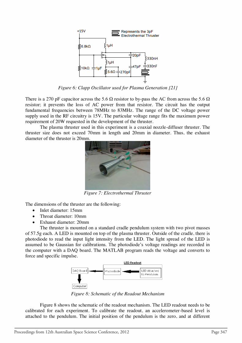
Proceedings from 12th Australian Space Science Conference, 2012 Page 347
Figure 6: Clapp Oscillator used for Plasma Generation [21]
There is a 270 pF capacitor across the 5.6 Ω resistor to by-pass the AC from across the 5.6 Ω resistor; it prevents the loss of AC power from that resistor. The circuit has the output fundamental frequencies between 78MHz to 83MHz. The range of the DC voltage power supply used in the RF circuitry is 15V. The particular voltage range fits the maximum power requirement of 20W requested in the development of the thruster. The plasma thruster used in this experiment is a coaxial nozzle-diffuser thruster. The thruster size does not exceed 70mm in length and 20mm in diameter. Thus, the exhaust diameter of the thruster is 20mm.
Figure 7: Electrothermal Thruster
The dimensions of the thruster are the following:
Inlet diameter: 15mm Throat diameter: 10mm Exhaust diameter: 20mm
The thruster is mounted on a standard cradle pendulum system with two pivot masses of 57.5g each. A LED is mounted on top of the plasma thruster. Outside of the cradle, there is photodiode to read the input light intensity from the LED. The light spread of the LED is assumed to be Gaussian for calibrations. The photodiode’s voltage readings are recorded in the computer with a DAQ board. The MATLAB program reads the voltage and converts to force and specific impulse.
Figure 8: Schematic of the Readout Mechanism
Figure 8 shows the schematic of the readout mechanism. The LED readout needs to be calibrated for each experiment. To calibrate the readout, an accelerometer-based level is attached to the pendulum. The initial position of the pendulum is the zero, and at different
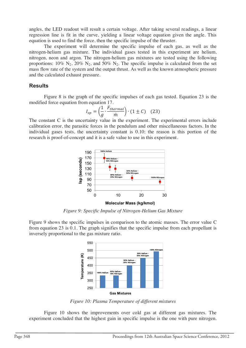
Page 348 Proceedings from 12th Australian Space Science Conference, 2012
angles, the LED readout will result a certain voltage. After taking several readings, a linear regression line is fit in the curve, yielding a linear voltage equation given the angle. This equation is used to find the force, then the specific impulse of the thruster.
The experiment will determine the specific impulse of each gas, as well as the nitrogen-helium gas mixture. The individual gases tested in this experiment are helium, nitrogen, neon and argon. The nitrogen-helium gas mixtures are tested using the following proportions: 10% N2, 20% N2, and 50% N2. The specific impulse is calculated from the set mass flow rate of the system and the output thrust. As well as the known atmospheric pressure and the calculated exhaust pressure.
Results
Figure 8 is the graph of the specific impulses of each gas tested. Equation 23 is the modified force equation from equation 17.
( )
The constant C is the uncertainty value in the experiment. The experimental errors include calibration error, the parasitic forces in the pendulum and other miscellaneous factors. In the individual gases tests, the uncertainty constant is 0.10; the reason is this portion of the research is proof-of-concept and it is a safe value to use in this experiment.
Figure 9: Specific Impulse of Nitrogen-Helium Gas Mixture
Figure 9 shows the specific impulses in comparison to the atomic masses. The error value C from equation 23 is 0.1. The graph signifies that the specific impulse from each propellant is inversely proportional to the gas mixture ratio.
Figure 10: Plasma Temperature of different mixtures
Figure 10 shows the improvements over cold gas at different gas mixtures. The
experiment concluded that the highest gain in specific impulse is the one with pure nitrogen.
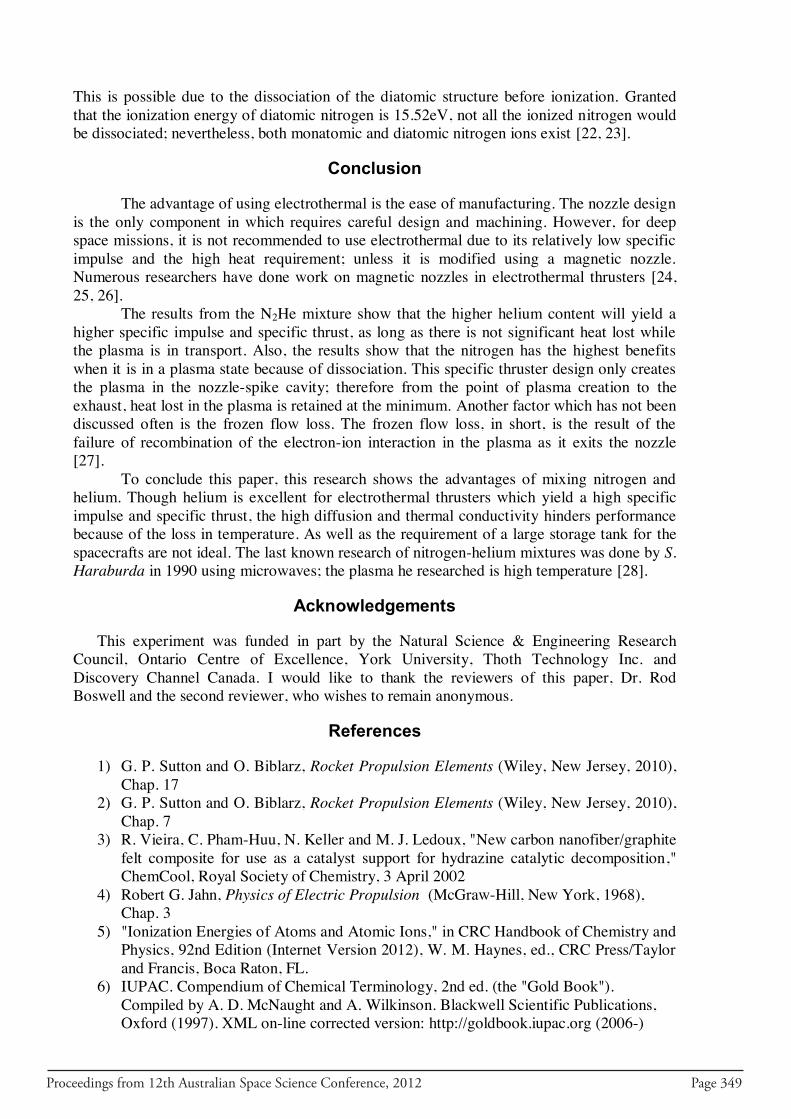
Proceedings from 12th Australian Space Science Conference, 2012 Page 349
This is possible due to the dissociation of the diatomic structure before ionization. Granted that the ionization energy of diatomic nitrogen is 15.52eV, not all the ionized nitrogen would be dissociated; nevertheless, both monatomic and diatomic nitrogen ions exist [22, 23].
Conclusion
The advantage of using electrothermal is the ease of manufacturing. The nozzle design is the only component in which requires careful design and machining. However, for deep space missions, it is not recommended to use electrothermal due to its relatively low specific impulse and the high heat requirement; unless it is modified using a magnetic nozzle. Numerous researchers have done work on magnetic nozzles in electrothermal thrusters [24, 25, 26]. The results from the N2He mixture show that the higher helium content will yield a higher specific impulse and specific thrust, as long as there is not significant heat lost while the plasma is in transport. Also, the results show that the nitrogen has the highest benefits when it is in a plasma state because of dissociation. This specific thruster design only creates the plasma in the nozzle-spike cavity; therefore from the point of plasma creation to the exhaust, heat lost in the plasma is retained at the minimum. Another factor which has not been discussed often is the frozen flow loss. The frozen flow loss, in short, is the result of the failure of recombination of the electron-ion interaction in the plasma as it exits the nozzle [27]. To conclude this paper, this research shows the advantages of mixing nitrogen and helium. Though helium is excellent for electrothermal thrusters which yield a high specific impulse and specific thrust, the high diffusion and thermal conductivity hinders performance because of the loss in temperature. As well as the requirement of a large storage tank for the spacecrafts are not ideal. The last known research of nitrogen-helium mixtures was done by S. Haraburda in 1990 using microwaves; the plasma he researched is high temperature [28].
Acknowledgements
This experiment was funded in part by the Natural Science & Engineering Research Council, Ontario Centre of Excellence, York University, Thoth Technology Inc. and Discovery Channel Canada. I would like to thank the reviewers of this paper, Dr. Rod Boswell and the second reviewer, who wishes to remain anonymous.
References
1) G. P. Sutton and O. Biblarz, Rocket Propulsion Elements (Wiley, New Jersey, 2010), Chap. 17
2) G. P. Sutton and O. Biblarz, Rocket Propulsion Elements (Wiley, New Jersey, 2010), Chap. 7
3) R. Vieira, C. Pham-Huu, N. Keller and M. J. Ledoux, "New carbon nanofiber/graphite felt composite for use as a catalyst support for hydrazine catalytic decomposition," ChemCool, Royal Society of Chemistry, 3 April 2002
4) Robert G. Jahn, Physics of Electric Propulsion (McGraw-Hill, New York, 1968), Chap. 3
5) "Ionization Energies of Atoms and Atomic Ions," in CRC Handbook of Chemistry and Physics, 92nd Edition (Internet Version 2012), W. M. Haynes, ed., CRC Press/Taylor and Francis, Boca Raton, FL.
6) IUPAC. Compendium of Chemical Terminology, 2nd ed. (the "Gold Book"). Compiled by A. D. McNaught and A. Wilkinson. Blackwell Scientific Publications, Oxford (1997). XML on-line corrected version: http://goldbook.iupac.org (2006-)
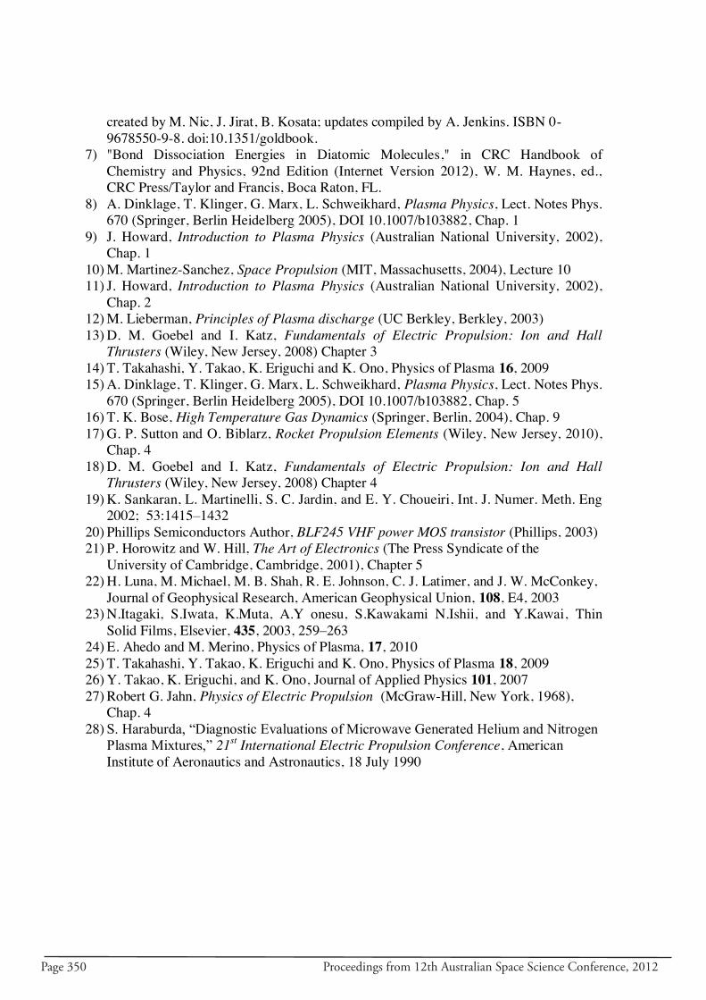
Page 350 Proceedings from 12th Australian Space Science Conference, 2012
created by M. Nic, J. Jirat, B. Kosata; updates compiled by A. Jenkins. ISBN 0-9678550-9-8. doi:10.1351/goldbook.
7) "Bond Dissociation Energies in Diatomic Molecules," in CRC Handbook of Chemistry and Physics, 92nd Edition (Internet Version 2012), W. M. Haynes, ed., CRC Press/Taylor and Francis, Boca Raton, FL.
8) A. Dinklage, T. Klinger, G. Marx, L. Schweikhard, Plasma Physics, Lect. Notes Phys. 670 (Springer, Berlin Heidelberg 2005), DOI 10.1007/b103882, Chap. 1
9) J. Howard, Introduction to Plasma Physics (Australian National University, 2002), Chap. 1
10) M. Martinez-Sanchez, Space Propulsion (MIT, Massachusetts, 2004), Lecture 10 11) J. Howard, Introduction to Plasma Physics (Australian National University, 2002),
Chap. 2 12) M. Lieberman, Principles of Plasma discharge (UC Berkley, Berkley, 2003) 13) D. M. Goebel and I. Katz, Fundamentals of Electric Propulsion: Ion and Hall
Thrusters (Wiley, New Jersey, 2008) Chapter 3 14) T. Takahashi, Y. Takao, K. Eriguchi and K. Ono, Physics of Plasma 16, 2009 15) A. Dinklage, T. Klinger, G. Marx, L. Schweikhard, Plasma Physics, Lect. Notes Phys.
670 (Springer, Berlin Heidelberg 2005), DOI 10.1007/b103882, Chap. 5 16) T. K. Bose, High Temperature Gas Dynamics (Springer, Berlin, 2004), Chap. 9 17) G. P. Sutton and O. Biblarz, Rocket Propulsion Elements (Wiley, New Jersey, 2010),
Chap. 4 18) D. M. Goebel and I. Katz, Fundamentals of Electric Propulsion: Ion and Hall
Thrusters (Wiley, New Jersey, 2008) Chapter 4 19) K. Sankaran, L. Martinelli, S. C. Jardin, and E. Y. Choueiri, Int. J. Numer. Meth. Eng
2002; 53:1415–1432 20) Phillips Semiconductors Author, BLF245 VHF power MOS transistor (Phillips, 2003) 21) P. Horowitz and W. Hill, The Art of Electronics (The Press Syndicate of the
University of Cambridge, Cambridge, 2001), Chapter 5 22) H. Luna, M. Michael, M. B. Shah, R. E. Johnson, C. J. Latimer, and J. W. McConkey,
Journal of Geophysical Research, American Geophysical Union, 108, E4, 2003 23) N.Itagaki, S.Iwata, K.Muta, A.Y onesu, S.Kawakami N.Ishii, and Y.Kawai, Thin
Solid Films, Elsevier, 435, 2003, 259–263 24) E. Ahedo and M. Merino, Physics of Plasma, 17, 2010 25) T. Takahashi, Y. Takao, K. Eriguchi and K. Ono, Physics of Plasma 18, 2009 26) Y. Takao, K. Eriguchi, and K. Ono, Journal of Applied Physics 101, 2007 27) Robert G. Jahn, Physics of Electric Propulsion (McGraw-Hill, New York, 1968),
Chap. 4 28) S. Haraburda, “Diagnostic Evaluations of Microwave Generated Helium and Nitrogen
Plasma Mixtures,” 21st International Electric Propulsion Conference, American Institute of Aeronautics and Astronautics, 18 July 1990
Proceedings from 12th Australian Space Science Conference, 2012 Page 351
Australian Engineering in Space
Plenary Presentation By Assoc. Prof Lachlan Thompson
RMIT University, [email protected] Abstract: Australia has had a rocky road in space engineering since the launch of WRESAT in 1967. With WRESAT Australia became the fourth nation to successfully design build and launch a functional satellite. Since then one could easily relate Australia’s work in this field followed the orbital decay of WRESAT, but this is far from the truth. Australian engineering expertise in space has through the application of space tracking played a role in the first landing on the moon in 1969 to the continuous communication and tracking of Voyager from launch in 1977 to 18 billion kilometres from our sun the very edge of our solar system this June (2012). Despite these achievements, Australian engineering in space has been diverse and sporadic. In 2008 the Australian Senate economic committee chartered a fresh direction for the nation with the Senate report1: “Lost in Space? Setting a new direction for Australia's space science and industry sector”. The report resulted in the Australian space research program grant scheme stimulus. But is it a matter of too little, too late? Is there sufficient infrastructure and expertise to allow Australian engineering to grow? The ASRP initiatives were wide sweeping from SCRAMJET research to the Australian Centre for Space Engineering Research. What avenues are available to Australia that would facilitate space engineering industry business growth? This paper presents options and examples of pathways for Australian engineering expertise to earn high export returns for modest investment. A Brief Chronology of Space Events Australia took its first engineering step into space2 in;
• 1961 with the Parkes Radio Telescope, a brilliant initiative by “Taffy” Bowen, then Chief of CSIRO Radio Physics Laboratory. Bowen used his connections to obtain funding from the Carnegie Corporation and the Rockefeller Foundation to pay half the cost of the telescope, the balance was eventually approved by then Prime Minister Sir Robert Menzies. It is inspiring to appreciate this great Australian Initiative, unintentionally played a key role in the first NASA Apollo Moon Landing. The Parkes radio telescope is now best known as “The Dish3”. “The Dish” has seen active participation in numerous space missions including Mariner 2, Mariner 4, Voyager, Giotto, Galileo, Cassini-Huygens, Mars Rover ‘Opportunity’ and current Curiosity rover. The Dish was superior to then NASA telescopes, NASA copied the CSIRO design for their Deep Space Network, for the 64 m dishes built at Tidbinbilla, Goldstone and Madrid.
• In 1967 DSTO borrowed a Redstone rocket from the US Army and launched WRESat into orbit from Woomera, this was Australia’s first and only satellite launched from Australian Territory. Two other satellites have been launched which were designed
1 Hurley A., (Chair), Lost in Space? Setting a new direction for Australia's space science and industry sector, Standing Committee on Economics, ISBN 978-‐0-‐642-‐71996-‐6, Commonwealth of Australia, 2008, p. 6 2 Woomera was established as a Weapons Test range in 1947 not a space facility see: Bil C., History of Australian Aviation, ICAS-‐2012, Brisbane September 2012, p. 11,. 3 Sitch R., The Dish, Working Dog Films Inc., Warner Bros. 2000
Page 352 Proceedings from 12th Australian Space Science Conference, 2012
and built in Australia. These are; Australis Oscar-54 an amateur satellite launched from the Vandenberg AFB complex USA on a Thor Delta in 1970 and in 2002, FedSat 1, on an H2A 202 from Tanegashima in Japan.
• The Canberra Deep Space Communication Complex (CDSCC) was established in 1965 by NASA JPL which includes Honey Suckle Creek (Apollo program), is assumed by many Australians as an Australian engineering venture, not so. It was not until February 2010 that CSIRO took over direct management of the site with the establishment of CSIRO Astronomy and Space Science, CASS.
• 1998 saw some glimmer of hope for a developing space industry with the funding of a Cooperative Research Centre for Satellite Systems (CRCSS). The CRCSS undertook communications, space science and computer technology research and the 50kg microsatellite FedSat launched from Japan, on 12 December, 2002. FedSat operated successfully in an 800km altitude Sun-synchronous polar orbit for approximately 3 years providing research data. Due to an inability to attract sufficient funding the CRCSS closed in 2005, and any expertise disbanded.
Significant Australian Space Political Initiatives • 1958 Australia a founding signatory UN Committee on the Peaceful Uses of Outer
Space, COPUOS • 1961 Robert Menzies completes funding for Parkes Radio Telescope • 1987 AusSat propose Cape York spaceport (scrapped 2001) • 1999 Chapman Report “Space Port Australia” • 2008 Hurley, Australian Senate Report “Lost in Space” • 2009 Australian Space Research Grants a Government injection of some $40 million
over three years. • 2011 the Australian Square Kilometre Array5 ASKA, as a contributor with South
Africa, The contracts offers little for spin off technologies that would stimulate Australian business.
The Australian Space Research Program Grants In 2009 acting on the outcomes of the 2008 Australian Senate report into Australian space activity the Australian Government initiated , The Australian Space Research Program6, which to date $40 million AUD, distributed over four years. The objective of the program was to develop Australia’s niche space capabilities by supporting space-related research, innovation and skills in areas of national significance or excellence. The scheme specifically excluded astronomy, astrophysics and cosmology. Projects funded were: Round 1: Pathways to Space: empowering the internet generation, U of NSW, $0.9 million; Platform technologies for space, atmosphere and climate, RMIT University, $2.8 million; Antarctic Broadband Definition and Capability Development, Aerospace Research Pty Ltd, $2.1 million; Scramjet-based access-to-space systems, U of Q, $5.0 million
4 Dunkerley Jr. W., Australis Oscar 5: The Launch Story, WA2INB, QST, April 1970, p. 61 5 Boyle B., Australian Industry Participation Plan for the Australian SKA Pathfinder and the Murchison Radio-‐astronomy Observatory, CSIRO Australia Telescope National Facility, Australia, 2011 6 Anon, Australian Space Research Program, Program Guidelines, Dept. Innovation, Industry, science and Research, Australian Government, October 2009, p. 2
Proceedings from 12th Australian Space Science Conference, 2012 Page 353
Round 2: Southern Hemisphere Summer Space Program, U of SA, $0.47 million; GRACE Follow-on Mission, ANU, $4.6 million; Automated Laser Tracking of Space Debris, EOS Space Systems Pty Ltd, $4.0 million; SAR Formation Flying, U of NSW, $4,6 million.
Round 3: Place and Space: Perspective in Earth Observations, Flinders U, $0.95 million, Space-based National Wireless Sensor Network, U of SA, $4.9 million, Unlocking the LANDSAT Archive for Future Challenges, Lockheed Martin Australia Pty Ltd, $3.4 million.
Round 4: A Comprehensive Tertiary Education Program in Satellite Systems Engineering, U of NSW, 0.67 million. The Australia Plasma Thruster Project, ANU, $3.1 million, Greenhouse Gas Monitor, Vipac Engineers & Scientists Ltd, $2.3 million. This initiative gave an important injection into Australian space activities in an attempt to retain some key skills and capability. However the grant scheme lacks mechanism or facility to engineer, the innovation of science into applied technologies which business can commercialise. Confusing Space Science with Space Engineering & Technology Australia invests each year on average sixty million dollars into astronomy7 research which compared to the ASSRP grants of approximately twelve million per annum. Whilst space science research provides the necessary foundation on which technological and engineering development is based. Australia has failed to articulate both funding and the research findings into engineering product to earn the nation a return on investment. Part of this problem is the priorities of the Australian Research Council (ARC) grants give priority to science and the grant evaluation methods both ARC and ASSRP do not prioritise leading to a commercial outcome as a success factor. These existing priorities must change radically if Australia is to grow a viable space industry. 2009 saw an even gloomier future to grow of space industry capability with the release of the National Committee for Space Science8 of the Australian Academy of Sciences Decadal Plan 2010-2019 charting our national future into space. Using a broad canvas this plan well defines the science Australia can pursue, its vision attempts to address technology but fails to close the loop to build a viable and sustainable industry. This lack of understanding of the national commercial benefits is evidenced by the absence of a mechanism to stimulate industry to develop space spinoff commercial technology. Unlike the European Space Agency which reaps financial rewards by making business incubation9 an integral part of its space science program which has returned hundreds of millions of Euros per annum to its membership. Civilian Space Active Companies Taking a quick look at some of the civilian space industry players active in Australia there are: Aerospace Concepts Pty Ltd., who provides systems analysis and consultancy, which
7 Boyal B., (ed), New Horizons 2006-‐2015; A Decadal plan for Australian Astronomy, National Committee for Astronomy of the Australian Academy of Science, Australia, November 2005 p. 9 8 Cains, I., (Chair), National Committee for Space Science of the Australian Academy of Sciences Decadal Plan 2010-‐2019, Australia, 2009. pp. 1-‐25 9 Salzgeber F. M., (ed), Impressions of the ESA TTPO participation, ESA, Hanover May 2012 pp. 1-‐52.

Page 354 Proceedings from 12th Australian Space Science Conference, 2012
include range safety, engineering management services, and the design of the management framework for Magellan10 telescope, in Chile. The Cooperative Research Centre for Spatial Information which provides special information research services for industry areas of agriculture, climate change, national security, urban planning development. Like all CRC’s the CRCSI must prioritise its research in line with the interests of its commercial industry partner(s). Silanna Semiconductor is interesting as it was formed as recently as 1996. Silanna delivers high performance integrated circuits into the global space, defense, medical and consumer markets. Devices manufactured in their Sydney facility have been used in many of the United States’ satellites that have been launched over the last few years, with the well renowned Mars Rovers Spirit and Opportunity using chips11 manufactured by Silanna. Well known communications operator Optus Satellite12 is not a manufacturer, however Optus does provide some input into the design of its digital communications satellites. All of the Optus fleet of satellites is manufactured external to Australia. The CSIRO, an Australian Government owned civilian research organization, the CSIRO Operates Parks Radio telescope, and manages for JPL the Canberra Deep Space Communications Complex at Tidbinbilla. The CSIRO has a diverse capability engaging in areas of research particular to Australian industry needs. The CSIRO has proven amazingly successful at taking research to commercial product, one invention that of using forward error correction, frequency-domain interleaving, and Multi Carrier Modulation to enhance Wi-Fi connection speed has earned CSIRO over $43013 million in patent royalties. Not so successful have been the Australian Research Grants and the ASRP Grants have no mechanism for spinoff. What is a Space Agency? Very few Australians understand what a space Agency is really like; the usual vision is a massive trillion dollar facility with giant rockets, satellites and geeky scientists and engineers using complex weird gadgets to go into space. Nothing could be further from the truth, this Disney World image is one that has been created over the years by NASA in its public justification for existence. It is an image that was necessary in the Cold War to intimidate the “Soviet Union”. It is an image long past its use by date and certainly irrelevant and misleading today. A private US Company Delaware North14 has operated the Kennedy Space Center Visitor Complex, since 1995, which has variety of exhibits, artifacts, displays and attractions on the history and future of human and robotic spaceflight. In France the Cite de l'espace15 is a venture owned by the City of Toulouse and is a Disney type theme park not ESA owned or operated.
10 Jenkins C., Australian Membership of the Giant Magellan Telescope Project, NCRIS Extremely Large Telescopes, CSIRO, 2007, p. 5 11 Bergmann K., ADIN, Examples of Successful SMEs, Silanna Semiconductor, Asia pacific Defence Reporter, July/August 2011, p. 31 12 Kotis J., Optus Satellite Network Designers Guide, Optus Satellite, May 2002, p. 7 13 Poole N., CSIRO wins legal battle over wi-‐fi patent. ABC News. 1 April 2012. http://www.abc.net.au/news/2012-‐04-‐01/csiro-‐receives-‐payment-‐for-‐wifi-‐technology/3925814. Retrieved 24 Sep 2012. 14 Jacobs J., (CEO), Delaware North Companies Retrospective, 95th year, DNC Inc., Annual General Report 2010, P. 52 15 Seroussi F., DOSSIER DE PRESSE 2012, Dossier Presse 21 Septembre 2012, City of Toulouse, 2012, p. 32
Proceedings from 12th Australian Space Science Conference, 2012 Page 355
The real space agencies NASA, ESA, JAXA, ISRO or CSA are all the same. They are a tiny office with an administrator and some bland offices with a number of administration staff whose job is to co-ordinate the space projects. No wiz bang laboratories, no astronauts running around in space suits, the staff in business suits. The agency operational budget is the size of a small home business. What this small business does is that it manages the space projects across the nation. The real space industry is the national industries and corporations, from the giant automotive manufacturers such as Ford Motor Company, who made the moon buggy for the Apollo missions to small business like the Fischer ink pen maker in Wisconsin, a company that employs 55 staff, so the astronaut can take notes (the Russians use pencils). A space agency negotiates with the space agencies of other nations to negotiate the rights for Australian small business and industry to bid for contracts in an otherwise closed (to non-space nations) market place. It has the responsibility of distributing projects to the nation’s business and university sectors, contracts for advanced versions of their product to be used on a space project. This in turn funds product improvement which the company otherwise could not afford. The national space industry is actually every university, business and industry across the nation. The famous Mars rovers Spirit and Opportunity were designed by team based at Cornell University with the rover parts being made by more than one thousand US companies and from a backyard video camera maker16 in Germany, who assembled the cameras on his kitchen table. Australia lacks a dedicated space agency to establish commercial bilateral agreements with other nations and to prioritize and coordinate our national civilian space commerce. Australia also confuses defence relationships with civilian business ventures. An example of the way forward is Canada who manages a profitable civilian space activity with China, India, South Africa, Japan, Europe and the USA. Importantly Canada relies on a strong defence partnership with the USA which it has found a means to grow without compromising development of local industry technologies and trade. Australian Space Research Program & Spin off Technology Australian space companies and Universities face a formidable problem in capitalising on their research. The first is there is only a small investment base in Australia and as such the IP will almost certainly license offshore. This does not create a total loss as CSIRO has shown. Australia has two major problems the first is that all space agencies around the world have laws prohibit non-national or non-member state entities from bidding to be a prime or frame contractor. The second is that a non-member company may be invited to collaborate but due to technology transfer regulations (ITR) they are unable to capitalize on the spin off technologies. This is evidenced by our recent agreement on space tracking operations17 in Australia by ESA. The agreement has no provision for joint development of technology or collaboration on capability development. Simply put the ESA treaty is a land rental agreement. 16 Squires S., Roving Mars: Spirit, Opportunity, and the Exploration of the Red Planet, ISBN 1-‐4013-‐0149-‐5, 2005, p. 177. 17 Anon, Agreement between the Government of Australia and the European Space Agency for a Co-‐operative Space Vehicle Tracking Program, AUSTRALIAN TREATY SERIES [2012] ATS 29, National Interest Analysis reference: [2011] ATNIA 30, Capetown, 5 October 2011.
Page 356 Proceedings from 12th Australian Space Science Conference, 2012
The ASRP grants have funded specialist areas they ignore the reality that the major benefit of space research has been the spin off technologies. Space agencies are aware of the gains of technology spin offs and these have earned billions of dollars in exports for their respective nations. These include NASA who ensures that all prime contractors are USA companies and therefore benefit from the technology spin offs. JAXA, ISRO and China Space Agencies all have similar policies. The European Space Agency goes one step further it requires all prime contractors to be from EU member states and it provides incubators to help grow spin off technologies. Does Australia Need a Space Agency? The answer to this question is YES! Australia needs a single organisation to coordinate and focus space related project, to find opportunities to our businesses and Universities to bid for contracts in international projects. We need a Space Agency to network the nation’s capability and manage spin in technologies; which are technologies that exist in noncore space industry into space applications, and spin off technologies which are new discoveries from solving space project problems that have application to advancing Australian industry capability. With the National Broadband Network (NBN) an Australian Space Agency now has the opportunity to affordably and effectively create profitable opportunities for our widely dispersed small business and manufacturing industry. Where are the Benefits from Space Research? The European Space Agency recognised that spinoff space technology was a key means of financial return to the member states. In 1990 Antonio Rodotà, the Director General of the European Space Agency wrote, “The success18 of the TTP, which has had the full support of Europe’s space industry, can be summarised by the following achievements: More than 200 space companies have participated in the programme; 400 space technologies have been actively marketed; More than 70 transfers of technology have resulted between space and non-space industry, many transnational; The direct commercial benefit to European industry already runs into hundreds of millions of Euro.” In the 2013 fiscal budget 19 the NASA Administrator James Bolden Jr., wrote, “…..NASA will continue to stimulate a U.S. economic powerhouse, the small business sector, through the competitive Small Business Innovative Research and Small Business Technology Transfer programs”. Space Technology Transfer To accelerate Space Technology Transfer ESA created Business Incubators this model appears to be the best for Australia. The ESA Business Incubation Centres are designed to create new business opportunities and jobs for non-space companies and broaden the market for space industry by translating space technologies, applications and services into viable business ideas in the non-space marketplace. The ESA Technology Transfer Programme Office coordinates space technology spin off throughout Europe, offering technical expertise as well as advice and support with business development. The ESA BIC was so successful that the project was expanded from the pilot centre at the European Space Research and Technology Centre ESTEC in Noordwijk, Netherlands to clones in Germany, UK and France.
18 Anon, Spin off Successes, Preparing for the Future, European Space Agency, BR152, June 1990, p. 3 19 Bolden C. Jr., NASA FY2013 Budget Request Executive Summary, Summary Budget, NASA, 2013, p. 6
Proceedings from 12th Australian Space Science Conference, 2012 Page 357
Since 2004, ESA’s Technology Transfer Programme Office, together with the Dutch Ministry of Economic Affairs, has been running a business incubation centre at ESTEC. More than 50 start ups companies have been supported, exploiting space based technology ranging from satellite application to hardware and software integration. Typical markets addressed are Location Based Services, ICT, Health Care and Life Sciences, Green Energy and Industrial applications. To further foster space to non-space start-up companies, ESA has taken the initiative to create an Open Sky Technologies Fund, managed by Triangle Venture Group. The investment focus of the fund is placed on seed capital investments, start-ups and early stage growth capital for companies using space related technologies or satellite applications in non-space fields. Providing a one-stop shop of coaches, business experts and services is offered. The service package offered includes:
• Cash incentive to fund product & IPR development by ESA & NSO • Pre-seed loan from Rabobank • Expert technical support from ESA • Hands-on business support from BViT • Office space and shared facilities at Reduced rates • Preferred supplier’s network and networking with entrepreneurs, businesses, potential clients and industry through the membership of the innovation network.
The Spirit and Opportunity video camera maker (built on the kitchen table) now has a million dollar business making cameras for the medical industry. What are the benefits? Space technology transfer20 and BIC’s have contributed hundreds of millions of Euro to ESA members since 2008. Since 1990 the TTP has earned for Europe new markets in advanced technology in automotive radar, tracking systems, airport security systems, earth observation applications, medicine and hundreds more. It has enabled Canada a corresponding member of ESA create a new industry in advanced robotics as evidenced by the Canada Arm on the Space Shuttle and ISS. Canada, which joined the ESA in the 1980s, is now earning21 128% per annum on its membership investment and has created new industries in advanced robotics, earth observation, communications and visualisation software. Australia has lost the opportunity to join ESA; we need to invest seriously in space to reap the benefits. A strong space industry should not be seen as an indulgence, but rather the backbone of a high-technology, 21st century economy.
A Suggested Way for Australia While space technology development is expensive, the financial rewards from spinoff technology to national industries are enormous. Australia currently has no mechanism to maximise the commercial return from our research and, on our own, we lack sufficient financial and capability mass to build a viable space industry. Establishing a southern hemisphere space agency – based on the highly successful European Space Agency model –
20 Anon, Spin off Successes, Preparing for the Future, European Space Agency, BR152, June 1990, p. 22 21 Triavilo P., Brumfitt A. & Thompson L.., Submission 39 to the Senate Standing Committee on Economics into Space, RMIT University, 2008, p. 3
Page 358 Proceedings from 12th Australian Space Science Conference, 2012
will enable us to stimulate new spinoff technology products, manufacturing technologies and export opportunities. This would allow sufficient funding and expertise base for a technology transfer program with a Business incubator component. Australia is well placed to join with countries like South Africa and Brazil using ESA as the model for a Southern Hemisphere Space Agency, with the purpose to jointly fund and develop member state space capability, spin off technologies and exploitation of those technologies. Southern Hemisphere Space Agency Brazil and South Africa are ideal founding partners with Australia; both have established space agencies, (unlike Australia who has not). Australia not having a Space Agency means that there is not an Agency to Agency level where the proposal for a Southern Hemisphere Space Agency can easily be explored. Brazil Brazil does however have significant similarities to Australia. Just as Australia relies on the USA for space technology, Brazil relied heavily on the USA and its good relationship with NASA for collaborative space industry. But continued frustration of dealing with the United States technology transfer restrictions eventually resulted in Brazil taking a more independent line. This independent action has not prevented Brazil being a significant partner with NASA, in the International Space Station. With an annual budget22 of $275 million USD, the AEB manages two launch sites; a spaceport at Alcântara and a rocket launch site at Barreira do Inferno. With its own design launch vehicle the VLS30 it has micro satellite launch capacity. In 2011 Brazil allocated $1 billion USD over ten years to develop a heavy lift launch capacity with its Epsilon series launcher. Brazil’s first astronaut went into space in 2006 successfully conducting experiments on the ISS. Brazil now has an open space policy, and a key player in the International Astronautics Federation, has collaborations with USA, China, India, Japan, Argentina, Russia and Ukraine. South Africa South Africa's government agency responsible for the development of aeronautics and aerospace space research is the South African National Space Agency (SANSA). South Africa has supported NASA in lunar and interplanetary missions of the 1950’s and 70’s from a tracking station at Hartebeesthoek. It was from this station that the first images of Mars were received from the Mariner IV spacecraft in the first successful flyby of the planet. South Africa launched its first satellite in 1999, SUNSAT from Vandenberg Air Force Base, followed by SumbandilaSat in 2009, which was launched from the Baikonur Cosmodrome. Technology transfer restrictions in collaborations with NASA had resulted in small discounted space specialist expertise. With the intent of consolidating space-related research, projects and research in South Africa a new space agency SANSA23 created in 2008 by acting
22 Anon, 2011 Federal Budget: Brazilian Space Agency (Agência Espacial Brasileira). Federal Government of Brazil, Ministry of Planning and Budget, 2011, p. 116 23 Anon, South African National Space Agency Act 2008, South African Government gazette, 31729, No. 36, 2008, p. 11
Proceedings from 12th Australian Space Science Conference, 2012 Page 359
President Kgalema Motlanthe. The 2012 SANSA budget24 was $170 million USD, excluding the MerKAT funding of $108 million USD, for the Square kilometre Array (SKA) bid. Australia already collaborates with South Africa on the Square Kilometre Array Radio Telescope.
Engineering our Space Future & Some Recommendations Australia will lose expertise if we continue to funding narrow specialisms as we have in the ASRP. Our Car industry is an excellent example of how not to do it, always lacking in sufficient critical mass and introspective to succeed. Australia has a narrow launch window of opportunity to establish an international partnership with Brazil and South Africa to initiate a Southern Hemisphere Space Agency (SHSA). The new agency should be based largely on the European Space Agency, with a membership subscription based on percentage of Gross National Product. The frame work can follow the rules of membership states similar to ESA. The subscription provides base funding capital and a mechanism to formulate and execute projects. The SHSA would not impinge on any pre-established relationships with NASA, ESA, JAXA, ISRO etc. For example Australia can still collaborate with NASA as would Brazil. The SHSA through government and the International Astronautical Federation establish working agreements for the new consortia. By using the Technology Transfer Program and business incubator models of ESA we can facilitate spin-off technologies to member states, at last getting a return on our hard-won science.
The space industry is you the Australian, the company you work for or own, we are all part of it and can through a Space Agency benefit directly from space technology. Space technology gives us the ability to improve our products, become more competitive with exported products, to grow to be a world business player, ensuring our nation’s economy for the future.
The NBN has created the opportunity for all Australian business to benefit from a National Space Agency. Our nation’s businesses are our space industry and space business is fundamental to developing the smart and clever technology industries that will take Australia financially secure into the 21st century and beyond.
REFERENCES
1. Hurley A., (Chair), Lost in Space? Setting a new direction for Australia's space science and industry sector, Standing Committee on Economics, ISBN 978-0-642-71996-6, Commonwealth of Australia, 2008, p. 6
2. Bil, C., History of Australian Aviation, ICAS-2012, Brisbane, Sept 2012, p. 11 3. Sitch R., The Dish, Working Dog Films Inc., Warner Bros. 2000
24 Anon, National Treasury Budget 2012, Estimates of National Expenditure, South African Government gazette, ISBN: 978-‐0-‐621-‐40578-‐1, No. 34, 2011, p. 10
Page 360 Proceedings from 12th Australian Space Science Conference, 2012
4. Dunkerley Jr. W., Australis Oscar 5: The Launch Story, WA2INB, QST, April 1970, p. 61
5. Boyle B., Australian Industry Participation Plan for the Australian SKA Pathfinder and the Murchison Radio-astronomy Observatory, CSIRO Australia Telescope National Facility, Australia, 2011
6. Anon, Australian Space Research Program, Program Guidelines, Dept. Innovation, Industry, science and Research, Australian Government, October 2009, p. 2
7. Boyal B., (ed), New Horizons 2006-2015; A Decadal plan for Australian Astronomy, National Committee for Astronomy of the Australian Academy of Science, Australia, November 2005 p. 9
8. Cains, I., (Chair), National Committee for Space Science of the Australian Academy of Sciences Decadal Plan 2010-2019, Australia, 2009. pp. 1-25
9. Salzgeber F. M., (ed), Impressions of the ESA TTPO participation, ESA, Hanover May 2012 pp. 1-52
10. Jenkins C., Australian Membership of the Giant Magellan Telescope Project, NCRIS Extremely Large Telescopes, CSIRO, 2007, p. 5
11. Bergmann K., ADIN, Examples of Successful SMEs, Silanna Semiconductor, Asia pacific Defence Reporter, July/August 2011, p. 31
12. Kotis J., Optus Satellite Network Designers Guide, Optus Satellite, May 2002, p. 7 13. Poole N., CSIRO wins legal battle over wi-fi patent. ABC News. 1 April 2012.
http://www.abc.net.au/news/2012-04-01/csiro-receives-payment-for-wifi-technology/3925814. Retrieved 24 Sep 2012.
14. Jacobs J., (CEO), Delaware North Companies Retrospective, 95th year, DNC Inc., Annual General Report 2010, P. 52
15. Seroussi F., DOSSIER DE PRESSE 2012, Dossier Presse 21 Septembre 2012, City of Toulouse, 2012, p. 32
16. Squires S., Roving Mars: Spirit, Opportunity, and the Exploration of the Red Planet, ISBN 1-4013-0149-5, 2005, p. 177.
17. Anon, Agreement between the Government of Australia and the European Space Agency for a Co-operative Space Vehicle Tracking Program, AUSTRALIAN TREATY SERIES [2012] ATS 29, National Interest Analysis reference: [2011] ATNIA 30, Capetown, 5 October 2011.
18. Anon, Spin off Successes, Preparing for the Future, European Space Agency, BR152, June 1990, p. 3
19. Bolden C. Jr., NASA FY2013 Budget Request Executive Summary, Summary Budget, NASA, 2013, p. 6
20. Anon, Spin off Successes, Preparing for the Future, European Space Agency, BR152, June 1990, p. 22
21. Triavilo P., Brumfitt A. & Thompson L.., Submission 39 to the Senate Standing Committee on Economics into Space, RMIT University, 2008, p. 3
22. Anon, 2011 Federal Budget: Brazilian Space Agency (Agência Espacial Brasileira). Federal Government of Brazil, Ministry of Planning and Budget, 2011, p. 116
23. Anon, South African National Space Agency Act 2008, South African Government gazette, 31729, No. 36, 2008, p. 11

Proceedings from 12th Australian Space Science Conference, 2012 Page 361
24. Anon, National Treasury Budget 2012, Estimates of National Expenditure, South African Government gazette, ISBN: 978-0-621-40578-1, No. 34, 2011, p. 10

Page 362 Proceedings from 12th Australian Space Science Conference, 2012

Proceedings from 12th Australian Space Science Conference, 2012 Page a
APPENDIX A
12ASSCList of Presentations &
Posters

Page b Proceedings from 12th Australian Space Science Conference, 2012
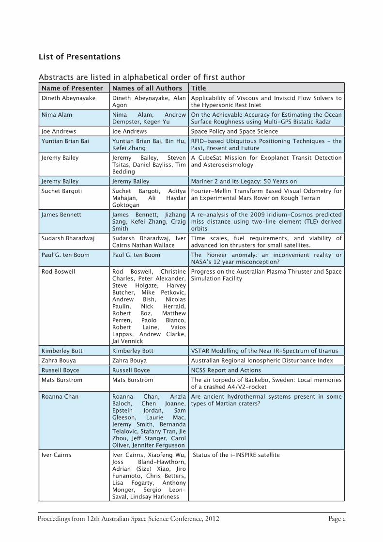
Proceedings from 12th Australian Space Science Conference, 2012 Page c
List of Presentations
Abstracts are listed in alphabetical order of first authorName of Presenter Names of all Authors TitleDineth Abeynayake Dineth Abeynayake, Alan
AgonApplicability of Viscous and Inviscid Flow Solvers to the Hypersonic Rest Inlet
Nima Alam Nima Alam, Andrew Dempster, Kegen Yu
On the Achievable Accuracy for Estimating the Ocean Surface Roughness using Multi-GPS Bistatic Radar
Joe Andrews Joe Andrews Space Policy and Space ScienceYuntian Brian Bai Yuntian Brian Bai, Bin Hu,
Kefei ZhangRFID-based Ubiquitous Positioning Techniques - the Past, Present and Future
Jeremy Bailey Jeremy Bailey, Steven Tsitas, Daniel Bayliss, Tim Bedding
A CubeSat Mission for Exoplanet Transit Detection and Asteroseismology
Jeremy Bailey Jeremy Bailey Mariner 2 and its Legacy: 50 Years onSuchet Bargoti Suchet Bargoti, Aditya
Mahajan, Ali Haydar Goktogan
Fourier-Mellin Transform Based Visual Odometry for an Experimental Mars Rover on Rough Terrain
James Bennett James Bennett, Jizhang Sang, Kefei Zhang, Craig Smith
A re-analysis of the 2009 Iridium-Cosmos predicted miss distance using two-line element (TLE) derived orbits
Sudarsh Bharadwaj Sudarsh Bharadwaj, Iver Cairns Nathan Wallace
Time scales, fuel requirements, and viability of advanced ion thrusters for small satellites.
Paul G. ten Boom Paul G. ten Boom The Pioneer anomaly: an inconvenient reality or NASA’s 12 year misconception?
Rod Boswell Rod Boswell, Christine Charles, Peter Alexander, Steve Holgate, Harvey Butcher, Mike Petkovic, Andrew Bish, Nicolas Paulin, Nick Herrald, Robert Boz, Matthew Perren, Paolo Bianco, Robert Laine, Vaios Lappas, Andrew Clarke, Jai Vennick
Progress on the Australian Plasma Thruster and Space Simulation Facility
Kimberley Bott Kimberley Bott VSTAR Modelling of the Near IR-Spectrum of UranusZahra Bouya Zahra Bouya Australian Regional Ionospheric Disturbance IndexRussell Boyce Russell Boyce NCSS Report and ActionsMats Burström Mats Burström The air torpedo of Bäckebo, Sweden: Local memories
of a crashed A4/V2-rocketRoanna Chan Roanna Chan, Anzla
Baloch, Chen Joanne, Epstein Jordan, Sam Gleeson, Laurie Mac, Jeremy Smith, Bernanda Telalovic, Stafany Tran, Jie Zhou, Jeff Stanger, Carol Oliver, Jennifer Fergusson
Are ancient hydrothermal systems present in some types of Martian craters?
Iver Cairns Iver Cairns, Xiaofeng Wu, Joss Bland-Hawthorn, Adrian (Size) Xiao, Jiro Funamoto, Chris Betters, Lisa Fogarty, Anthony Monger, Sergio Leon-Saval, Lindsay Harkness
Status of the i-INSPIRE satellite
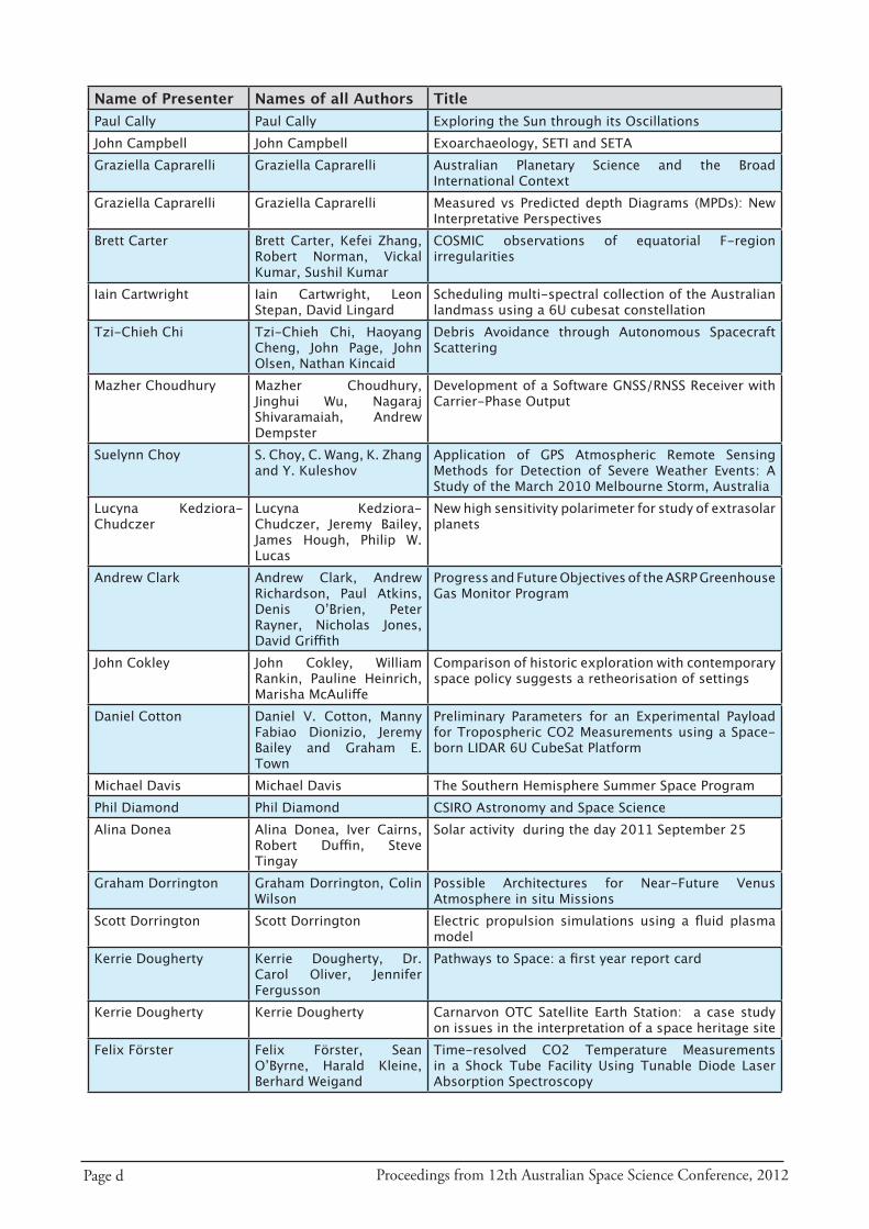
Page d Proceedings from 12th Australian Space Science Conference, 2012
Name of Presenter Names of all Authors TitlePaul Cally Paul Cally Exploring the Sun through its OscillationsJohn Campbell John Campbell Exoarchaeology, SETI and SETAGraziella Caprarelli Graziella Caprarelli Australian Planetary Science and the Broad
International ContextGraziella Caprarelli Graziella Caprarelli Measured vs Predicted depth Diagrams (MPDs): New
Interpretative PerspectivesBrett Carter Brett Carter, Kefei Zhang,
Robert Norman, Vickal Kumar, Sushil Kumar
COSMIC observations of equatorial F-region irregularities
Iain Cartwright Iain Cartwright, Leon Stepan, David Lingard
Scheduling multi-spectral collection of the Australian landmass using a 6U cubesat constellation
Tzi-Chieh Chi Tzi-Chieh Chi, Haoyang Cheng, John Page, John Olsen, Nathan Kincaid
Debris Avoidance through Autonomous Spacecraft Scattering
Mazher Choudhury Mazher Choudhury, Jinghui Wu, Nagaraj Shivaramaiah, Andrew Dempster
Development of a Software GNSS/RNSS Receiver with Carrier-Phase Output
Suelynn Choy S. Choy, C. Wang, K. Zhang and Y. Kuleshov
Application of GPS Atmospheric Remote Sensing Methods for Detection of Severe Weather Events: A Study of the March 2010 Melbourne Storm, Australia
Lucyna Kedziora-Chudczer
Lucyna Kedziora-Chudczer, Jeremy Bailey, James Hough, Philip W. Lucas
New high sensitivity polarimeter for study of extrasolar planets
Andrew Clark Andrew Clark, Andrew Richardson, Paul Atkins, Denis O’Brien, Peter Rayner, Nicholas Jones, David Griffith
Progress and Future Objectives of the ASRP Greenhouse Gas Monitor Program
John Cokley John Cokley, William Rankin, Pauline Heinrich, Marisha McAuliffe
Comparison of historic exploration with contemporary space policy suggests a retheorisation of settings
Daniel Cotton Daniel V. Cotton, Manny Fabiao Dionizio, Jeremy Bailey and Graham E. Town
Preliminary Parameters for an Experimental Payload for Tropospheric CO2 Measurements using a Space-born LIDAR 6U CubeSat Platform
Michael Davis Michael Davis The Southern Hemisphere Summer Space ProgramPhil Diamond Phil Diamond CSIRO Astronomy and Space ScienceAlina Donea Alina Donea, Iver Cairns,
Robert Duffin, Steve Tingay
Solar activity during the day 2011 September 25
Graham Dorrington Graham Dorrington, Colin Wilson
Possible Architectures for Near-Future Venus Atmosphere in situ Missions
Scott Dorrington Scott Dorrington Electric propulsion simulations using a fluid plasma model
Kerrie Dougherty Kerrie Dougherty, Dr. Carol Oliver, Jennifer Fergusson
Pathways to Space: a first year report card
Kerrie Dougherty Kerrie Dougherty Carnarvon OTC Satellite Earth Station: a case study on issues in the interpretation of a space heritage site
Felix Förster Felix Förster, Sean O’Byrne, Harald Kleine, Berhard Weigand
Time-resolved CO2 Temperature Measurements in a Shock Tube Facility Using Tunable Diode Laser Absorption Spectroscopy
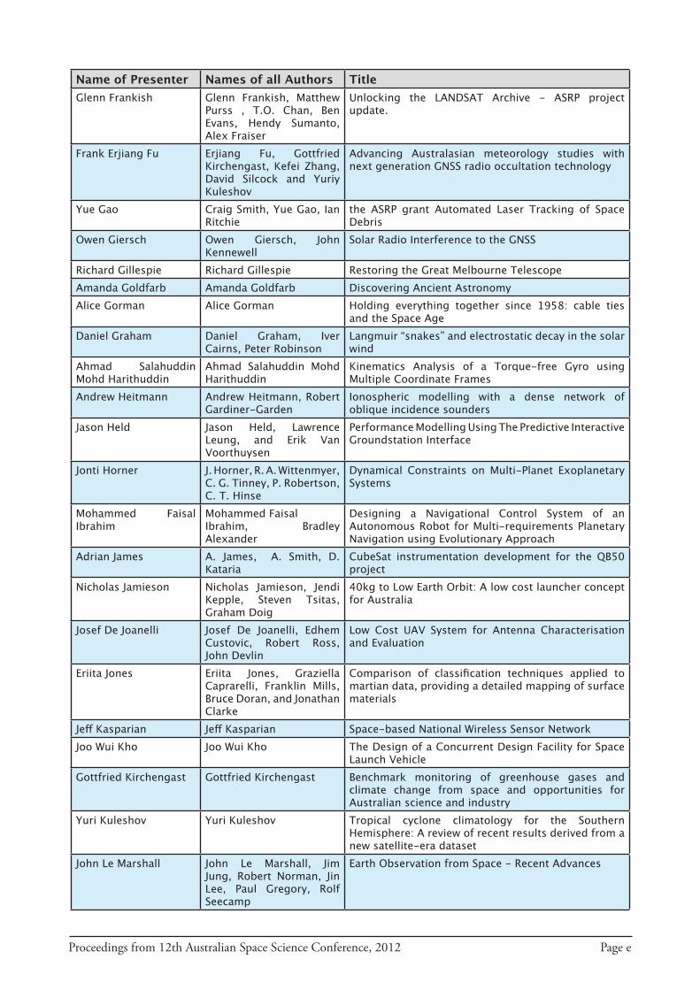
Proceedings from 12th Australian Space Science Conference, 2012 Page e
Name of Presenter Names of all Authors TitleGlenn Frankish Glenn Frankish, Matthew
Purss , T.O. Chan, Ben Evans, Hendy Sumanto, Alex Fraiser
Unlocking the LANDSAT Archive - ASRP project update.
Frank Erjiang Fu Erjiang Fu, Gottfried Kirchengast, Kefei Zhang, David Silcock and Yuriy Kuleshov
Advancing Australasian meteorology studies with next generation GNSS radio occultation technology
Yue Gao Craig Smith, Yue Gao, Ian Ritchie
the ASRP grant Automated Laser Tracking of Space Debris
Owen Giersch Owen Giersch, John Kennewell
Solar Radio Interference to the GNSS
Richard Gillespie Richard Gillespie Restoring the Great Melbourne TelescopeAmanda Goldfarb Amanda Goldfarb Discovering Ancient AstronomyAlice Gorman Alice Gorman Holding everything together since 1958: cable ties
and the Space AgeDaniel Graham Daniel Graham, Iver
Cairns, Peter RobinsonLangmuir “snakes” and electrostatic decay in the solar wind
Ahmad Salahuddin Mohd Harithuddin
Ahmad Salahuddin Mohd Harithuddin
Kinematics Analysis of a Torque-free Gyro using Multiple Coordinate Frames
Andrew Heitmann Andrew Heitmann, Robert Gardiner-Garden
Ionospheric modelling with a dense network of oblique incidence sounders
Jason Held Jason Held, Lawrence Leung, and Erik Van Voorthuysen
Performance Modelling Using The Predictive Interactive Groundstation Interface
Jonti Horner J. Horner, R. A. Wittenmyer, C. G. Tinney, P. Robertson, C. T. Hinse
Dynamical Constraints on Multi-Planet Exoplanetary Systems
Mohammed Faisal Ibrahim
Mohammed FaisalIbrahim, Bradley Alexander
Designing a Navigational Control System of an Autonomous Robot for Multi-requirements Planetary Navigation using Evolutionary Approach
Adrian James A. James, A. Smith, D. Kataria
CubeSat instrumentation development for the QB50 project
Nicholas Jamieson Nicholas Jamieson, Jendi Kepple, Steven Tsitas, Graham Doig
40kg to Low Earth Orbit: A low cost launcher concept for Australia
Josef De Joanelli Josef De Joanelli, Edhem Custovic, Robert Ross, John Devlin
Low Cost UAV System for Antenna Characterisation and Evaluation
Eriita Jones Eriita Jones, Graziella Caprarelli, Franklin Mills, Bruce Doran, and Jonathan Clarke
Comparison of classification techniques applied to martian data, providing a detailed mapping of surface materials
Jeff Kasparian Jeff Kasparian Space-based National Wireless Sensor NetworkJoo Wui Kho Joo Wui Kho The Design of a Concurrent Design Facility for Space
Launch VehicleGottfried Kirchengast Gottfried Kirchengast Benchmark monitoring of greenhouse gases and
climate change from space and opportunities for Australian science and industry
Yuri Kuleshov Yuri Kuleshov Tropical cyclone climatology for the Southern Hemisphere: A review of recent results derived from a new satellite-era dataset
John Le Marshall John Le Marshall, Jim Jung, Robert Norman, Jin Lee, Paul Gregory, Rolf Seecamp
Earth Observation from Space - Recent Advances
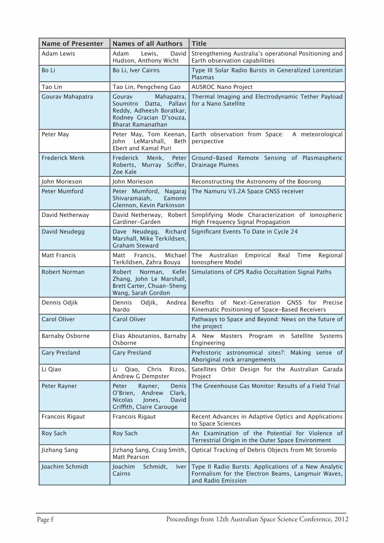
Page f Proceedings from 12th Australian Space Science Conference, 2012
Name of Presenter Names of all Authors TitleAdam Lewis Adam Lewis, David
Hudson, Anthony WichtStrengthening Australia’s operational Positioning and Earth observation capabilities
Bo Li Bo Li, Iver Cairns Type III Solar Radio Bursts in Generalized Lorentzian Plasmas
Tao Lin Tao Lin, Pengcheng Gao AUSROC Nano ProjectGourav Mahapatra Gourav Mahapatra,
Soumitro Datta, Pallavi Reddy, Adheesh Boratkar, Rodney Gracian D’souza, Bharat Ramanathan
Thermal Imaging and Electrodynamic Tether Payload for a Nano Satellite
Peter May Peter May, Tom Keenan, John LeMarshall, Beth Ebert and Kamal Puri
Earth observation from Space: A meteorological perspective
Frederick Menk Frederick Menk, Peter Roberts, Murray Sciffer, Zoe Kale
Ground-Based Remote Sensing of Plasmaspheric Drainage Plumes
John Morieson John Morieson Reconstructing the Astronomy of the BoorongPeter Mumford Peter Mumford, Nagaraj
Shivaramaiah, Eamonn Glennon, Kevin Parkinson
The Namuru V3.2A Space GNSS receiver
David Netherway David Netherway, Robert Gardiner-Garden
Simplifying Mode Characterization of Ionospheric High Frequency Signal Propagation
David Neudegg Dave Neudegg, Richard Marshall, Mike Terkildsen, Graham Steward
Significant Events To Date in Cycle 24
Matt Francis Matt Francis, Michael Terkildsen, Zahra Bouya
The Australian Empirical Real Time Regional Ionosphere Model
Robert Norman Robert Norman, Kefei Zhang, John Le Marshall, Brett Carter, Chuan-Sheng Wang, Sarah Gordon
Simulations of GPS Radio Occultation Signal Paths
Dennis Odjik Dennis Odjik, Andrea Nardo
Benefits of Next-Generation GNSS for Precise Kinematic Positioning of Space-Based Receivers
Carol Oliver Carol Oliver Pathways to Space and Beyond: News on the future of the project
Barnaby Osborne Elias Aboutanios, Barnaby Osborne
A New Masters Program in Satellite Systems Engineering
Gary Presland Gary Presland Prehistoric astronomical sites?: Making sense of Aboriginal rock arrangements
Li Qiao Li Qiao, Chris Rizos, Andrew G Dempster
Satellites Orbit Design for the Australian Garada Project
Peter Rayner Peter Rayner, Denis O’Brien, Andrew Clark, Nicolas Jones, David Griffith, Claire Carouge
The Greenhouse Gas Monitor: Results of a Field Trial
Francois Rigaut Francois Rigaut Recent Advances in Adaptive Optics and Applications to Space Sciences
Roy Sach Roy Sach An Examination of the Potential for Violence of Terrestrial Origin in the Outer Space Environment
Jizhang Sang Jizhang Sang, Craig Smith, Matt Pearson
Optical Tracking of Debris Objects from Mt Stromlo
Joachim Schmidt Joachim Schmidt, Iver Cairns
Type II Radio Bursts: Applications of a New Analytic Formalism for the Electron Beams, Langmuir Waves, and Radio Emission
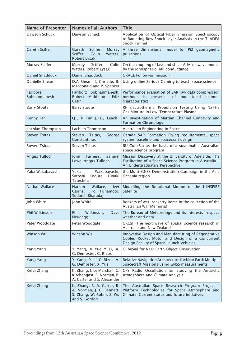
Proceedings from 12th Australian Space Science Conference, 2012 Page g
Name of Presenter Names of all Authors TitleDawson Schuck Dawson Schuck Application of Optical Fiber Emission Spectroscopy
to Radiating Bow Shock Layer Analysis in the T-ADFA Shock Tunnel
Gareth Sciffer Gareth Sciffer, Murray Sciffer, Colin Waters, Robert Lysak
A three dimensional model for Pi2 geomagnetic pulsations.
Murray Sciffer Murray Sciffer, Colin Waters, Robert Lysak
On the coupling of fast and shear Alfv´en wave modes by the ionospheric Hall conductance
Daniel Shaddock Daniel Shaddock GRACE Follow-on missionDanielle Shean D.A Shean, I. Christie, B.
Macdonald and P. SpencerUsing online Serious Gaming to teach space science
FariborzSobhanmanesh
Fariborz Sobhanmanesh, Robert Middleton, Ediz Cetin
Performance evaluation of SAR raw data compression methods in presence of non ideal channel characteristics
Barry Stoute Barry Stoute RF Electrothermal Propulsion Testing Using N2-He Gas Mixture in Low-Temperature Plasma
Kenny Tan Q. J. K. Tan, J. H. J. Leach An Investigation of Martian Channel Concavity and Formation Chronology.
Lachlan Thompson Lachlan Thompson Australian Engineering in SpaceSteven Tsitas Steven Tsitas, George
ConstantinosGarada SAR Formation Flying requirements, space system baseline and spacecraft design
Steven Tsitas Steven Tsitas 6U CubeSat as the basis of a sustainable Australian space science program
Angus Tulloch John Furness, Samuel Lowe, Angus Tulloch
Mission Discovery at the University of Adelaide: The Facilitation of a Space Science Program in Australia - An Undergraduate’s Perspective
Yaka Wakabayashi Yaka Wakabayashi, Satoshi Kogure, Hioaki Tateshita
the Multi-GNSS Demonstration Campaign in the Asia Oceania region
Nathan Wallace Nathan Wallace, Iver Cairns, Jiro Funamoto, Sudarsh Bharadaj
Modelling the Rotational Motion of the i-INSPIRE Satellite
John White John White Rockets of war: rocketry items in the collection of the Australian War Memorial
Phil Wilkinson Phil Wilkinson, Dave Neudegg
The Bureau of Meteorology and its interests in space weather and data
Peter Woodgate Peter Woodgate CRCSI: The next wave of spatial science research in Australia and New Zealand
Winson Wu Winson Wu Innovative Design and Manufacturing of Regenerative Cooled Rocket Motor and Design of a Concurrent Design Facility of Space Launch Vehicles
Yang Yang Y. Yang, X. Yue, Y. Li, A. G. Dempster, C. Rizos
CubeSail for Near Earth Object Observation
Yang Yang Y. Yang, Y. Li, C. Rizos, A. G. Dempster, X. Yue
Relative Navigation Architecture for Near Earth Multiple Spacecraft Missions using GNSS measurements
Kefei Zhang K. Zhang, J. Le Marshall, G. Kirchengast, R. Norman, B. A. Carter and S. Alexander
GPS Radio Occultation for studying the Antarctic Atmosphere and Climate Analysis
Kefei Zhang K. Zhang, B. A. Carter, R. A. Norman, J. C. Bennett, S. Zhang, W. Rohm, S. Wu and S. Gordon
The Australian Space Research Program Project - Platform Technologies for Space Atmosphere and Climate: Current status and future initiatives
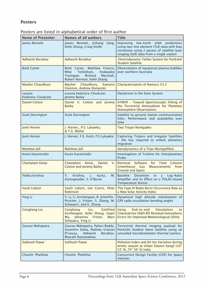
Page h Proceedings from 12th Australian Space Science Conference, 2012
Posters
Posters are listed in alphabetical order of first authorName of Presenter Names of all authors TitleJames Bennett James Bennett, Jizhang Sang,
Kefei Zhang, Craig SmithImproving low-Earth orbit predictions using two-line element (TLE) data with bias correction using 2 passes of satellite laser ranging (SLR) data from a single station
Adheesh Boratkar Adheesh Boratkar Electrodynamic Tether System for Parikshit Student Satellite
Brett Carter Brett Carter, Matthew Francis, Mike Terkildsen, Endawoke Yizengaw, Richard Marshall, Robert Norman, Kefei Zhang
Observations of equatorial plasma bubbles over northern Australia
Mazher Choudhury Mazher Choudhury, Eamonn Glennon, Andrew Dempster
Characterization of Namuru V3.2
Lucyna Kedziora-Chudczer
Lucyna Kedziora-Chudczer,Jeremy Bailey
Deuterium in the Solar System
Daniel Cotton Daniel V. Cotton and Jeremy Bailey
ATMOF – Toward Spectroscopic Fitting of the Terrestrial Atmosphere for Planetary Atmosphere Observations
Scott Dorrington Scott Dorrington Satellite to ground station communication links: Performance and availability over time
Jonti Horner J. Horner,. P.S. Lykawka, & T.G. Müller
Two Trojan Renegades
Jonti Horner J. Horner, F.E. Koch, P.S Lykawka Capturing Trojans and Irregular Satellites - the key required to unlock planetary migration
Matthew Joll Matthew Joll Aerodynamics of a Titan MontgolfièreKosta Kazantzidis Kosta Kazantzidis Investigation of Turbine for Interplanetary
ProbeChamplain Kenyi Champlain Kenyi, Daniel V.
Cotton and Jeremy BaileyRetrieval Software for Total Column Greenhouse Gas Measurements from Ground and Space
Yedhu Krishna Y. Krishna, J. Kurtz, M. Aizengendler, S. O’Byrne
Baseline Distortion in a Log-Ratio Amplifier and its Effect on a TDLAS-based Temperature Sensor
Vasili Lobzin Vasili Lobzin, Iver Cairns, Peter Robinson
The Type III Radio Burst Occurrence Rate as a New Solar Activity Index
Ying Li Y. Li, G. Kirchengast, B. Scherllin-Pirscher, J. Fritzer, S. Zhang, M. Schwaerz, and K. Zhang
Dynamical high altitude initialization of GPS radio occultation bending angles
Congliang Liu Congliang Liu, Gottfried Kirchengast, Kefei Zhang, Suqin Wu, Johannes Fritzer, Marc Schwaerz, Ying Li
Using End-to-end Simulations to Characterise GNSS RO Residual Ionospheric Errors for Improved Meteorological Utility
Gourav Mahapatra Gourav Mahapatra, Pallavi Reddy, Soumitro Datta, Rodney Gracian D’souza, Adheesh Boratkar, Bharath Ramanathan
Terrestrial thermal imaging payload for Parikshit Student Nano Satellite using an uncooled microbolometer thermal camera
Subhash Pawar Subhash Pawar Pollution Index and Air Ion Variation during winter season at Urban Station Sangli (16° 52’ N, 74° 36’ E) India
Chuntit Phetkhai Chuntit Phetkhai Concurrent Design Facility (CDF) for Space Vehicles
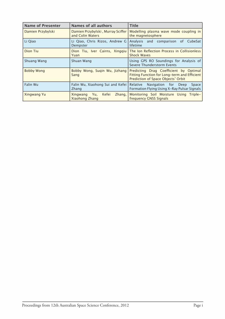
Proceedings from 12th Australian Space Science Conference, 2012 Page i
Name of Presenter Names of all authors TitleDamien Przybylski Damien Przybylski , Murray Sciffer
and Colin WatersModelling plasma wave mode coupling in the magnetosphere
Li Qiao Li Qiao, Chris Rizos, Andrew G Dempster
Analysis and comparison of CubeSat lifetime
Dion Tiu Dion Tiu, Iver Cairns, Xingqiu Yuan
The Ion Reflection Process in Collisionless Shock Waves
Shuang Wang Shuan Wang Using GPS RO Soundings for Analysis of Severe Thunderstorm Events
Bobby Wong Bobby Wong, Suqin Wu, Jizhang Sang
Predicting Drag Coefficient by Optimal Fitting Function for Long-term and Efficient Prediction of Space Objects’ Orbit
Falin Wu Falin Wu, Xiaohong Sui and Kefei Zhang
Relative Navigation for Deep Space Formation Flying Using X-Ray Pulsar Signals
Xingwang Yu Xingwang Yu, Kefei Zhang, Xiaohong Zhang
Monitoring Soil Moisture Using Triple-frequency GNSS Signals

Page j Proceedings from 12th Australian Space Science Conference, 2012