Prepared for submission to JHEP IP/BBSR/2021-06

Probing Lorentz Invariance Violation with

Atmospheric Neutrinos at INO-ICAL

Sadashiv Sahooa,b Anil Kumar,a,b,c Sanjib Kumar Agarwallaa,b,d

aInstitute of Physics, Sachivalaya Marg, Sainik School Post, Bhubaneswar 751005, IndiabHomi Bhabha National Institute, Anushakti Nagar, Mumbai 400094, IndiacApplied Nuclear Physics Division, Saha Institute of Nuclear Physics, Block AF, Sector 1, Bid-

hannagar, Kolkata 700064, IndiadInternational Centre for Theoretical Physics, Strada Costiera 11, 34151 Trieste, Italy

E-mail: sadashiv.sahoo@iopb.res.in (ORCID: 0000-0001-6719-7723),

anil.k@iopb.res.in (ORCID: 0000-0002-8367-8401), sanjib@iopb.res.in

(ORCID: 0000-0002-9714-8866)

Abstract: The possibility of Lorentz Invariance Violation (LIV) may appear in unified

theories, such as string theory, which allow the existence of a new space-time structure

at the Planck scale (Mp ∼ 1019 GeV). This effect can be observed at low energies with

a strength of ∼ 1/Mp using the perturbative approach. In the minimal Standard Model

extension (SME) framework, the neutrino mass-induced flavor oscillation gets modified in

the presence of LIV. The Iron Calorimeter (ICAL) detector at the proposed India-based

Neutrino Observatory (INO) offers a unique window to probe these LIV parameters by ob-

serving atmospheric neutrinos and antineutrinos separately over a wide range of baselines

in the multi-GeV energy range. In this paper, for the first time, we study in detail how

the CPT-violating LIV parameters (aµτ , aeµ, aeτ ) can alter muon survival probabilities and

expected µ− and µ+ event rates at ICAL. Using 500 kt·yr exposure of ICAL, we place

stringent bounds on these CPT-violating LIV parameters at 95% C.L., which are slightly

better than the present Super-Kamiokande limits. We demonstrate the advantage of in-

corporating hadron energy information and charge identification capability at ICAL while

constraining these LIV parameters. Further, the impact of the marginalization over the

oscillation parameters and choice of true values of sin2 θ23 on LIV constraints is described.

We also study the impact of these LIV parameters on mass ordering determination and

precision measurement of atmospheric oscillation parameters.

Keywords: LIV, Atmospheric Neutrinos, Oscillation, ICAL, INO

ArXiv ePrint: 2110.13207

arX

iv:2

110.

1320

7v2

[he

p-ph

] 2

0 Ju

n 20

22

Contents

1 Introduction and motivation 1

2 Lorentz and CPT violation in neutrino oscillations 3

3 A brief history of the search for LIV in neutrino oscillations 6

4 Effects of Lorentz Invariance Violation on oscillograms 8

5 Event generation at ICAL 13

5.1 Total event rates 14

5.2 Reconstructed event distributions 15

6 Simulation method 19

7 Results 20

7.1 Effective regions in (Erecµ , cos θrec

µ ) plane to constrain LIV parameters 20

7.2 Advantage of hadron energy information in constraining LIV parameters 21

7.3 Advantage of charge identification capability to constrain LIV parameters 23

7.4 Impact of marginalization on constraining LIV parameters 24

7.5 Impact of true values of sin2 θ23 on constraining LIV parameters 26

7.6 Impact of non-zero LIV parameters on mass ordering determination 27

7.7 Allowed regions in (|∆m232| – sin2 θ23) plane with non-zero LIV parameters 28

7.8 Correlation between off-diagonal LIV parameters 29

8 Summary and concluding remarks 30

A Some properties of gauge invariant LIV parameters 32

B Effect of aeµ and aeτ on appearance channel P (νe → νµ) 36

C Effective regions in (Erecµ , cos θrecµ ) plane to constrain aeµ and aeτ 38

1 Introduction and motivation

The Lorentz symmetry has been preserved in the fundamental theories of physics, such as

the general theory of relativity and the quantum field theory. However, this symmetry could

be challenged at the Planck scale physics (Mp ∼ 1019 GeV), where the unification of gravity

with the gauge fields of the Standard Model (SM) of particle physics is expected. Quantum

loop gravity [1–5] and String theory [6–11] attempt such unification by allowing small

perturbation of Lorentz symmetry breaking, so-called Lorentz Invariance Violation (LIV).

– 1 –

Even an introduction of non-commutativity in space-time structure at local fields [12, 13]

can give rise to a breaking of charge, parity, and time-reversal (CPT) symmetry, so-called

CPT violation, which is indeed a special case of LIV [14]. At the low energy observables,

the coupling strength of LIV is expected to be suppressed by an order of (1/Mp) [15, 16]. In

order to accommodate all possible LIV interactions with the presently known SM physics,

the suitable framework is the Standard Model extension (SME) [17–20], where the LIV

terms act as observer scalars to the SM fields. In principle, the presence of LIV can be

probed via three basic mechanisms like coherence, interference, and extreme effects. In

the interference category, the mass-induced neutrino flavor transition, so-called neutrino

oscillation [21], is a potential candidate to probe LIV [22–27].

The neutrino oscillations allow neutrinos to change their flavor while traveling. The

Super-Kamiokande (Super-K) experiment discovered the phenomenon of neutrino oscilla-

tion in their atmospheric neutrino data for the first time in 1998 [28]. The neutrino oscil-

lation is parameterized in terms of three mixing angles (θ12, θ13, θ23), two mass-squared

differences (∆m221, ∆m2

32), and one CP-violating phase (δCP). There has been significant

progress in the past two decades, and now, neutrino oscillation is a well-established model

which has entered into an era of precision measurement. In the standard three-flavor neu-

trino oscillation framework, only a few parameters have been left to be measured precisely,

such as CP-violating phase (δCP), atmospheric mixing angle (θ23), and neutrino mass or-

dering. This is also important to note that neutrino oscillations can only be explained if

neutrinos have non-zero degenerate masses. The non-zero neutrino masses provide one of

the strongest hints towards physics beyond the Standard Model (BSM). Thus, neutrino

oscillation is a legitimate area to look for hints towards BSM physics.

The atmospheric neutrinos provide an avenue to study neutrino oscillations in the

multi-GeV range of energies over a wide range of baselines starting from 10 km to 104 km.

The upward-going neutrinos travel deep inside the Earth and experience Earth’s matter

effect [29–38] due to the interactions with ambient electrons. Apart from providing crucial

information on standard three-flavor oscillation parameters, the atmospheric neutrinos can

also play an important role to probe various BSM scenarios like non-standard interactions

(NSI) [29, 39–56], sterile neutrinos [57–72], neutrino decay [73–75], LIV [22, 24–27], and

several other new physics models [76, 77]. The signature of LIV, which is the topic of this

paper, can be explored at several L/E values accessible in the case of atmospheric neutrinos.

An atmospheric neutrino detector having good resolutions in energy and direction will be

able to observe the possible modifications in standard three-flavor oscillations due to LIV.

The proposed 50 kt Iron Calorimeter (ICAL) detector at the India-based Neutrino

Observatory (INO) [78] aims to measure neutrino mass ordering by separately detecting

atmospheric neutrinos and antineutrinos in the multi-GeV range of energies over a wide

range of baselines. Harnessing the magnetic field of 1.5 T [79], the ICAL detector would

be able to identify µ− and µ+ events separately. The ICAL has an excellent muon energy

resolution of about 10 to 15% in the reconstructed muon energy range of 1 to 25 GeV [80].

As far as the muon direction is concerned, the ICAL detector is capable of providing muon

angular resolution of less than 1◦. Using this good detector response, the ICAL Collab-

oration has performed various analyses involving standard oscillations using atmospheric

– 2 –

neutrino [78, 81–90]. ICAL provides a unique avenue to probe a plethora of BSM scenar-

ios [49, 53, 91–98]. In the context of searching the signature of CPT violation at ICAL,

a dedicated work has been performed in Ref. [99] by introducing the new CPT-violating

parameters in the effective Hamiltonian as suggested by the authors in Ref. [100]. Since

ICAL can measure the atmospheric mass-squared differences using atmospheric neutrinos

and antineutrinos separately, any possible differences in their measurements would be a

smoking gun signature of the CPT-violation, which may also indicate the possible viola-

tion of Lorentz Invariance. This possibility has been explored by the INO Collaboration

in Refs. [101, 102]. In the present work, for the first time, we explore in detail the impact

of CPT-violating LIV parameters in the SME framework using the atmospheric neutrinos

at the ICAL detector. The sensitivity of ICAL towards the presence of CPT-violating LIV

parameters is estimated using the ICAL detector with 500 kt·yr exposure, and stringent

constraints are placed. We will also demonstrate the impact of the presence of LIV on the

measurement of neutrino mass ordering and oscillation parameters.

In section 2, we describe the theoretical background of LIV in the context of the neu-

trino oscillations. The experimental attempts to probe LIV are summarized in section 3.

The impacts of LIV on neutrino oscillograms are presented in section 4. In section 5, we

elaborate the method to simulate neutrino events at the ICAL detector and modifications

in the event distributions due to the presence of LIV. The method to perform the statistical

analysis is explained in section 6 which is followed by the results in section 7 where we

constrain the CPT-violating LIV parameters and show the impact of LIV on the measure-

ment of mass ordering and precision measurement. Finally, we summarize our findings and

conclude in section 8. In appendix A, we describe the properties of gauge invariant LIV

parameters. The effect of LIV parameters on the appearance channel is discussed in ap-

pendix B. The appendix C presents some additional plots identifying effective regions in the

plane of energy and direction of reconstructed muons while constraining LIV parameters.

2 Lorentz and CPT violation in neutrino oscillations

The study of atmospheric neutrinos provides an avenue to probe neutrino oscillations as

an interferometer with a length scale of the diameter of Earth, which may also get affected

by the presence of LIV. In order to understand the effect of LIV on neutrino oscillation

probabilities, we first look at the modified Hamiltonian in the presence of LIV keeping

only the terms which are gauge-invariant and renormalizable under the minimal SME

framework. In the ultra-relativistic limit, the effective Hamiltonian(Heff

)ij

describing the

propagation of left-handed neutrino in vacuum can be written in the following fashion:(Heff

)ij

= Eδij +m2ij

2E+

1

E

(aµLpµ − c

µνL pµpν

)ij, (2.1)

where, i and j are the neutrino flavor indices, whereas pµ and E are the four momenta

and energy of neutrino, respectively. In Eq. 2.1, the first two terms correspond to the

standard kinematics1, whereas the last two terms denote the LIV interactions governed

1Here, m2ij = U · diag(m2

1, m22, m

23) · U†, where U is the unitary neutrino mixing matrix known as the

Pontecorvo-Maki-Nakagawa-Sakata (PMNS) matrix [21, 103, 104].

– 3 –

by the parameters aµL (CPT-violating LIV parameters) and cµνL (CPT-conserving LIV pa-

rameters). While going from neutrino to antineutrino, the CPT-violating LIV parameters

change their sign, whereas the sign of the CPT-conserving parameters remain unchanged

(see the discussion in detail in appendix A).

So far, we consider the neutrino propagation in vacuum, but in reality, the neutrinos

propagate through Earth’s matter. The electron neutrinos undergo W -mediated charged-

current interactions with the ambient electrons. This coherent and forward-scattering of νewith matter electrons gives rise to the so-called “Wolfenstein matter potential” [29, 31, 105].

Note that the Wolfenstein matter potential doesn’t get affected by the presence of non-zero

LIV parameters. In the present work, we focus on the isotropic2 component (µ = 0, ν = 0)

of the LIV parameters and denote

a0L ≡ a, c00

L ≡ c, p0 ≡ E. (2.2)

Therefore, the effective Hamiltonian(Heff

)ij

for left handed neutrino boils down to

Heff =1

2EU

0 0 0

0 ∆m221 0

0 0 ∆m231

U † +

aee aeµ aeτa∗eµ aµµ aµτa∗eτ a

∗µτ aττ

− 4

3E

cee ceµ ceτc∗eµ cµµ cµτc∗eτ c

∗µτ cττ

+√

2GFNe

1 0 0

0 0 0

0 0 0

, (2.3)

here, U is the standard 3×3 neutrino mixing matrix called PMNS matrix, ∆m2ab (≡ m2

a −m2b) are the mass-squared splittings of the neutrino mass eigenstates, and

√2GFNe is

matter potential where GF is Fermi weak coupling constant, and Ne is the electron number

density inside the Earth’s matter. The contributions to Heff from LIV are given by the

terms containing CPT-violating parameters aαβ and CPT-conserving parameters3 cαβ.

Note that the effective Hamiltonian Heff in Eq. 2.3 is written for neutrino, if we go to

antineutrino then, U → U∗,√

2GFNe → −√

2GFNe, aαβ → −a∗αβ, and cαβ → c∗αβ, where

the negative sign for CPT-violating LIV parameter aαβ appears as a multiplicative factor

due to the construction of LIV formalism as discussed in appendix A. However, the sign

of CPT-conserving LIV parameter cαβ does not change when we go to antineutrino (see

appendix A).

In this work, we focus our attention on CPT-violating LIV parameters (aαβ), whereas

the CPT-conserving LIV parameters (cαβ) will be studied separately in another work. As

far as the CPT-violating LIV parameters are concerned, in the present work, we only focus

on the off-diagonal parameters: aµτ ≡ |aµτ |eiφµτ , aeµ ≡ |aeµ|eiφeµ , and aeτ ≡ |aeτ |eiφeτ .

Our analysis is mainly dominated by νµ → νµ and νµ → νµ disappearance oscillation

2One of the choices for the isotropic frame is the Sun-centered celestial-equatorial frame [106]. In this

frame, we ignore the anisotropy generated due to the Earth’s boost, which is suppressed by a factor of

∼ 10−4.3In Eq. 2.3, there is a multiplicative factor 4/3 in the terms containing cαβ . This factor arises due to

the choice of a frame which is rotational invariant. See Eq. A.25 and the related discussion in appendix A.

– 4 –

channels where the off-diagonal LIV parameter aµτ appears only in the form of |aµτ | cosφµτat the leading order (one can see a similar discussion in the context of NSI in Ref. [107]).

Therefore, a complex phase only modifies the effective value of aµτ to a real number between

−|aµτ | to |aµτ | at the leading order. We exploit this observation by considering only real

values of aµτ in the range of −|aµτ | to |aµτ | for the present work. From these arguments, we

can say that our method effectively covers the entire range of complex values of aµτ which

is equivalent to the variation of φµτ in the full range of −π to π. As far as the off-diagonal

LIV parameters aeµ and aeτ are concerned, they appear at the subleading order in νµ → νµsurvival channel and are always θ13-suppressed. The imaginary parts associated with the

phases are further suppressed in the survival channel compared to the real parts and have

a negligible impact (� 1%). Thus, the real values of aeµ and aeτ cover the entire complex

parameter space.

Note that the CPT-violating LIV parameters (aαβ) appear in an analogous fashion

to that of neutral-current (NC) NSI parameters (εαβ) in the effective Hamiltonian (see

Eq. 2.3). One can obtain the following relation between the NC-NSI and CPT-violating

LIV parameters [23, 27]

εαβ =aαβ√

2GFNe

. (2.4)

Here, we would like to mention that though these two new physics scenarios show a cor-

respondence as given in the above equation, their physics origins are completely different.

Further, the NC-NSI which appears during neutrino propagation is driven by the non-

standard matter effects and it does not exist in vacuum. On the other hand, the LIV is an

intrinsic effect that can be present even in vacuum. Note that for long-baseline experiments

such as DUNE [108], where a line-averaged constant Earth matter density may be a valid

approximation, this one-to-one correspondence between CPT-violating LIV and NC-NSI

parameters as shown in Eq. 2.4 may hold. But in the present paper, our focus is on at-

mospheric neutrino experiments where we deal with a wide range of baselines spanning

from 15 km to 12757 km. For each of these baselines, the scaling between CPT-violating

LIV and NC-NSI parameters is expected to be different. Moreover, for a large fraction of

these baselines (5721 km to 12757 km), neutrinos pass through the inner mantle or even

core, where the density changes significantly following the PREM [109] profile with a sharp

jump in the density at the core-mantle boundary. Therefore, for these trajectories, the

line-averaged constant Earth matter density approximation is no longer valid and a simple

scaling between CPT-violating LIV and NC-NSI parameters does not work.

While showing the approximate analytical expressions of neutrino oscillation probabil-

ities in the presence of non-zero CPT-violating LIV parameters aαβ, we use the existing

expressions in the literature for NC-NSI [53, 107] by replacing the NC-NSI parameters εαβwith the CPT-violating LIV parameters aαβ following Eq. 2.4. Note that to study the

impact of CPT-violating LIV parameters on the atmospheric neutrinos at INO-ICAL, we

indeed perform a full-fledged numerical simulation from scratch considering three-flavor

neutrino oscillation probabilities in the presence of the PREM profile of Earth and obtain

all the results that we show in the present paper.

– 5 –

In this work, we focus on the survival channel (νµ → νµ) and appearance channel (νe →νµ) because these two channels have significant contribution to the neutrino events at the

ICAL detector. The survival channel probability P (νµ → νµ) is dominantly affected by LIV

parameter aµτ whereas the effects of aeµ and aeτ are subdominant. Using approximations of

one mass scale dominance (OMSD) [∆m221L/(4E)� ∆m2

32L/(4E)] in the limit of θ13 → 0

with constant matter density, the survival probability for νµ can be expressed as [53, 110],

P (νµ → νµ) = 1− sin2 2θeff sin2

[ξ

∆m232Lν

4Eν

], (2.5)

where

sin2 2θeff =| sin 2θ23 + 2β ηµτ |2

ξ2, (2.6)

ξ =√| sin 2θ23 + 2β ηµτ |2 + cos2 2θ23 , (2.7)

and

ηµτ =2Eν ω aµτ|∆m2

32|, (2.8)

where, we have replaced εµτ with aµτ using Eq. 2.4. For a given value of CPT-violating

parameter aαβ, the parameter ω = +1 for neutrino and ω = −1 for antineutrino due to the

construction of LIV formalism as explained in appendix A. Here, β ≡ sgn(∆m232) which

is the sign of atmospheric mass-squared difference. We have β = +1 for normal ordering

(NO, m1 < m2 < m3) and β = −1 for inverted ordering (IO, m3 < m1 < m2). In the limit

of maximal mixing (θ23 = 45◦), the Eq. 2.5 boils down to [111],

P (νµ → νµ) = cos2

[Lν

(∆m2

32

4Eν+ ω aµτ

)]. (2.9)

As far as the effects of LIV parameters aeµ and aeτ on survival channel (νµ → νµ)

are concerned, it appears in subleading order terms and non-trivial to express analytically.

The effects of aeµ and aeτ with similar strengths become dominant in appearance channel

(νe → νµ) because it occurs at leading order terms. We provide the expression for P (νe →νµ) in the presence of both LIV parameters aeµ and aeτ at-a-time in appendix B. The

effect of LIV parameter aµτ on P (νe → νµ) is not significant, hence, it is not present in

Eq. B.4. Note that these approximate expressions for oscillation probabilities are just for

understanding purposes. However, in this work, we use numerically calculated full three-

flavor oscillation probabilities with LIV in the presence of Earth’s matter with the PREM

profile [109].

3 A brief history of the search for LIV in neutrino oscillations

In this section, we discuss how the search for LIV parameters in neutrino oscillations

progressed. In 2004, a general formalism for LIV and CPT-violation was developed in

the neutrino oscillation sector, where possible definitive signals are predicted in the light

of prevailing and proposed neutrino experiments [112]. After that, a few sample and

– 6 –

global models are proposed to illustrate the key physical effects of LIV by considering both

with and without neutrino mass, along that, a few generalized models with operators of

arbitrary dimension are discussed to accommodate the signals observed in various neutrino

experiments [113–122]. Now, we summarize the experimental attempts to probe the LIV:

• A proposal of possible LIV signal was made in the context of the results obtained

from the short-baseline experiments, and in 2005, the first experimental attempt

to probe Lorentz and CPT violation was made by the liquid scintillator neutrino

detector (LSND) experiment [123] to accommodate the oscillation excess. But null

results of LIV in LSND signal put bounds on (aL) and (E× cL) of the order of 10−19

GeV, which is in an expected scale of suppression.

• In 2008, a search for the sidereal modulation in the MINOS near detector neutrino

data was performed [124]. No significant evidence was found, resulting in the bounds

on the sidereal components of LIV parameters to the order of 10−20 GeV. Con-

sequently, in 2010, the same search was performed with the MINOS far detector

neutrino data (Run I, II, and III) [125]. No signature of sidereal effect was found,

and the bounds are further improved to the order of 10−23 GeV.

• In 2010, the IceCube experiment [126] had reported the results of the search for

a Lorentz-violating sidereal signal with the atmospheric neutrinos. No direction-

dependent variation was found, and the constraints improved by a factor of 3 for

(aL) and an order of 3 for (cL).

• In 2011, the result from the MiniBooNE Collaboration [127] was consistent with

MINOS near detector bounds.

• In 2012, the MINOS Collaboration searched the sidereal variation with muon type

antineutrino data at the near detector [128], and the result was consistent with their

earlier work with neutrino data [124].

• In the later part of 2012, the Double Chooz Collaboration [129] showed their results of

the search for LIV with reactor antineutrinos. Data indicated no sidereal variations,

so their work set the first limits on 14 LIV coefficients associated with e-τ sector and

set two competitive limits associated with e-µ sectors.

• The presence of LIV allows the neutrino and antineutrino mixings, hence to see such

a signal, in early 2013, MINOS has performed a search analysis [130]. There was no

evidence of such a signal, resulting in the limit of the appropriate 66 LIV coefficients

(H and g)4, which govern the neutrino-antineutrino mixing.

• Further search for neutrino-antineutrino mixing was performed using the disappear-

ance of reactor antineutrinos in the Double Chooz experiment [131] and set limits

4These two parameters are the elements of the off-diagonal block in the effective Hamiltonian, see

Refs. [112, 117].

– 7 –

on another 15 LIV coefficients (H and g). A similar study in the context of solar

neutrinos was performed by the authors in Ref. [132].

• In 2015, the Super-Kamiokande (Super-K) Collaboration published their result to

search Lorentz Invariance with atmospheric neutrinos with a large range of baselines

and wide range of energies [22]. No evidence of Lorentz violation was observed, so

limits were set on the renormalizable isotropic LIV coefficients in the e-µ, µ-τ , and

e-τ sectors, with an improvement of seven orders of magnitude.

• In 2017, the T2K Collaboration searched LIV using sidereal time dependence of

neutrino flavor transitions with the T2K on-axis near detector [133]. The results

were consistent with the limits put by other short-baseline experiments.

• In 2018, a simultaneous measurement of LIV coefficients was done using the Daya Bay

reactor antineutrino experiment [134]. The bounds on the appropriate parameters

were agreed to the suppression of the Planck mass scale (Mp).

• The IceCube experiment analyzed the LIV hypothesis using the high-energy part

of atmospheric neutrinos in the year 2018 [25]. They perform the analysis using a

perturbative approach in an effective two-flavor neutrino oscillation framework and

obtained the limits on individual LIV coefficients (aL and cL) with mass dimensions

ranging from 3 to 8. These are the most stringent limits on Lorentz violation (in the

µ-τ sector) set by any physical experiment.

The current constraints on all the relevant LIV/CPT-violating parameters are nicely

summarized in Ref. [106]. In a recent review [135], the authors have discussed the phe-

nomenological effects of CPT and Lorentz symmetry violations in the context of particle

and astroparticle physics.

4 Effects of Lorentz Invariance Violation on oscillograms

In this section, we describe how does the neutrino oscillation probabilities get affected due

to the presence of LIV. The atmospheric neutrinos are produced as a result of the interaction

of primary cosmic rays with the nuclei of the atmosphere and mostly consist of electron

and muon flavors. The atmospheric neutrinos with the multi-GeV energy range have access

to a wide range of baselines starting from about 15 km to 12757 km. The upward-going

neutrinos with longer baselines experience the Earth’s matter effect, which results in the

modification of oscillation probabilities. The effect of LIV on neutrino oscillations can be

explored at several L/E values available for atmospheric neutrinos.

In the present analysis, we numerically calculate the neutrino oscillation probability

in the three-flavor paradigm with Earth’s matter effect using the PREM profile [109]. We

use the benchmark values of oscillation parameters given in Table 1. The value of ∆m231

is obtained from the effective mass-squared difference5 ∆m2eff. To consider NO as mass

5The effective mass-squared difference is defined in terms of ∆m231 as follows [140, 141]:

∆m2eff = ∆m2

31 −∆m221(cos2 θ12 − cos δCP sin θ13 sin 2θ12 tan θ23). (4.1)

– 8 –

sin2 2θ12 sin2 θ23 sin2 2θ13 ∆m2eff (eV2) ∆m2

21 (eV2) δCP Mass Ordering

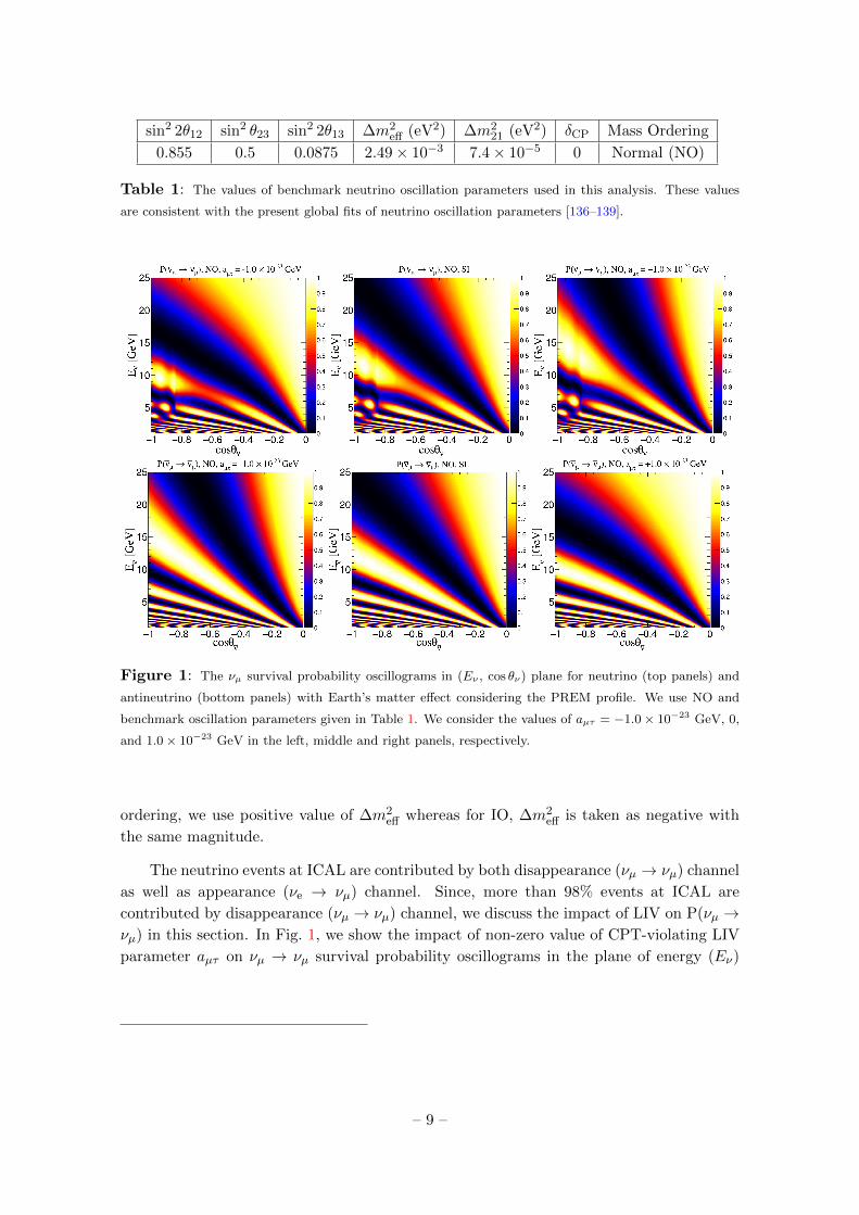
0.855 0.5 0.0875 2.49× 10−3 7.4× 10−5 0 Normal (NO)

Table 1: The values of benchmark neutrino oscillation parameters used in this analysis. These values

are consistent with the present global fits of neutrino oscillation parameters [136–139].

Figure 1: The νµ survival probability oscillograms in (Eν , cos θν) plane for neutrino (top panels) and

antineutrino (bottom panels) with Earth’s matter effect considering the PREM profile. We use NO and

benchmark oscillation parameters given in Table 1. We consider the values of aµτ = −1.0× 10−23 GeV, 0,

and 1.0× 10−23 GeV in the left, middle and right panels, respectively.

ordering, we use positive value of ∆m2eff whereas for IO, ∆m2

eff is taken as negative with

the same magnitude.

The neutrino events at ICAL are contributed by both disappearance (νµ → νµ) channel

as well as appearance (νe → νµ) channel. Since, more than 98% events at ICAL are

contributed by disappearance (νµ → νµ) channel, we discuss the impact of LIV on P(νµ →νµ) in this section. In Fig. 1, we show the impact of non-zero value of CPT-violating LIV

parameter aµτ on νµ → νµ survival probability oscillograms in the plane of energy (Eν)

– 9 –

and direction6 (cos θν) of neutrino. We consider three different choices of aµτ which are

−1.0× 10−23 GeV, 0, and 1.0× 10−23 GeV as shown in the left, middle and right columns,

respectively, in Fig. 1. The panels in top and bottom rows correspond to neutrinos and

antineutrinos, respectively.

In Fig. 1, the effect of LIV parameter aµτ can be observed at energies above 10 GeV

and baselines with cos θν < −0.6. This region is dominated by vacuum oscillations. The

dark blue diagonal band, which is termed as oscillation valley in Ref. [53, 89], bends in the

presence of LIV parameter aµτ . The direction of bending depends on the sign of aµτ . For

example, the oscillation valley for neutrino bends in the downward direction for negative

aµτ in the top left panel, whereas for positive aµτ , the bending is in the upward direction

in the top right panel. For a given value of aµτ , the oscillation valley curves in the opposite

directions for neutrinos and antineutrinos. In summary, we can infer that the bending

of oscillation valley for neutrino with positive aµτ (top right panel) is similar to that for

antineutrino with negative aµτ (bottom left panel) and vice versa.

We now discuss how the modification of the oscillation valley due to non-zero aµτ can be

understood analytically. The oscillation valley corresponds to the first oscillation minimum

in νµ survival probability in Eq. 2.9 which results in the following relation between Eν and

cos θν [53],

Eν |valley ≈|∆m2

32|(π/|R cos θν |) − 4β ω aµτ

. (4.3)

where, we assume Lν ≈ 2R| cos θν |. For the case of standard interactions (SI) with aµτ = 0,

Eq. 4.3 results in a linear relation between Eν and cos θν which is manifested as oscillation

valley with straight line for SI case in the middle panels of Fig. 1.

In the case of NO (β = +1), if aµτ is positive then for neutrino (ω = +1), Eν increases

compared to that for SI case for a given cos θν as observed in the top right panel of Fig. 1.

If we consider negative value of aµτ then for neutrino, Eν decreases as seen in the top left

panel of Fig. 1. As far as antineutrino is concerned, where ω = −1, positive (negative)

value of aµτ results in decrease (increase) in Eν as shown in the bottom right (left) panel

of Fig. 1. Since, β and ω appear as product, the effect of positive (negative) aµτ with

neutrino is same as that of negative (positive) aµτ with antineutrino. If we consider the

case of IO (β = −1), then all these effects are reversed with the opposite curvatures of

oscillation valley.

In Fig. 2, we present the impact of CPT-violating LIV parameter aeµ on νµ → νµsurvival probability oscillograms in the plane of neutrino energy (Eν) and direction (cos θν).

We assume three different values of aeµ which are −2.5 × 10−23 GeV, 0, and 2.5 × 10−23

GeV as shown in the left, middle and right columns, respectively, in Fig. 2. In the top

and bottom panels, we portray plots for neutrinos and antineutrinos, respectively. Unlike

6The relation between neutrino zenith angle θν and neutrino baseline Lν is given as

Lν =√

(R+ h)2 − (R− d)2 sin2 θν − (R− d) cos θν , (4.2)

where, R, h, and d represent the radius of Earth, the average production height for neutrinos, and the

depth of the detector, respectively. In the present study, we consider R = 6371 km, h = 15 km, and d = 0

km.

– 10 –

Figure 2: The νµ survival probability oscillograms in (Eν , cos θν) plane for neutrino (top panels) and

antineutrino (bottom panels) with Earth’s matter effect considering the PREM profile. We use NO and

benchmark oscillation parameters given in Table 1. We consider the values of aeµ = −2.5× 10−23 GeV, 0,

and 2.5× 10−23 GeV in the left, middle and right panels, respectively.

the case of aµτ , here, we do not observe any bending in the oscillation valley due to the

presence of non-zero aeµ. However, a distortion in the oscillation valley can be observed

due to aeµ. The regions with matter effect also get modified. For neutrino, the effect due

to positive aeµ is significantly more than that due to negative aeµ. We also observe that

the effect of aeµ for antineutrino is not significant.

We would like to highlight that the effect of aeµ appears at the subleading order in the

expression of P (νµ → νµ), which are non-trivial to express analytically. We can analyze

the same by studying the analytical expression for the appearance channel P (νe → νµ) as

given in Eq. B.4 in appendix B, where the effect of aeµ appears in the leading order terms.

The effect of aeµ is dominantly contributed by the fifth term in Eq. B.4, which has the

following form

+ 16ωaeµEν s13s323

1

∆m231 − aCC

sin2 (∆m231 − aCC)Lν

4Eν, (4.4)

where (∆m231 − aCC) factor in the denominator causes the matter-driven resonance effect

for the case of neutrino with NO. Since this term has positive sign for the case of neutrino

(ω = +1), the positive value of aeµ increases P (νe → νµ). This can be translated as the

decrease in P (νµ → νµ) around the region of matter effect as shown in the top right panel

– 11 –

Figure 3: The νµ survival probability oscillograms in (Eν , cos θν) plane for neutrino (top panels) and

antineutrino (bottom panels) with Earth’s matter effect considering the PREM profile. We use NO and

benchmark oscillation parameters given in Table 1. We consider the values of aeτ = −2.5× 10−23 GeV, 0,

and 2.5× 10−23 GeV in the left, middle and right panels, respectively.

of Fig. 2 because we have,

P (νµ → νµ) = 1− P (νµ → νe)− P (νµ → ντ ), (4.5)

where P (νµ → νe) = P (νe → νµ) for δCP = 0. Note that νµ → ντ oscillation channel

also gets affected due to matter effects in certain ranges of energies and baselines (see

Ref. [142]). But as far as the impact of LIV parameter aeµ is concerned, it appears only at

the subleading order in νµ → ντ oscillation channel. For negative value of aeµ, P (νe → νµ)

decreases and P (νµ → νµ) increases, hence we observe dilution of matter effect in the top

left panel of Fig. 2. We can see that the effect of aeµ is larger in the case of neutrino than

antineutrino. This happens because aCC becomes negative for antineutrino and matter-

driven resonance condition is not fulfilled for NO due to which the above-mentioned term

does not contribute significantly.

Similar to LIV parameter aeµ, now we depict the impact of aeτ on νµ → νµ survival

probability oscillograms in the plane of neutrino energy (Eν) and direction (cos θν) in Fig. 3.

We take three different values of aeτ which are −2.5×10−23 GeV, 0, and 2.5×10−23 GeV as

shown in the left, middle and right columns, respectively, in Fig. 3. The features present in

the oscillograms due to aeτ in Fig. 3 are analogous to that due to aeµ in Fig. 2. Here also,

we can observe the distortions in the oscillation valley as well as the matter effect regions.

The effect of aeτ is more for neutrinos than that for antineutrino. If we focus on neutrinos,

– 12 –

we see that the effect of positive aeτ (top right panel) is larger than that of negative aeτ(top left panel). Following the similar arguments as for aeµ in the previous paragraph, these

features can be explained using the seventh term in Eq. B.4. These asymmetric effects for

CPT-violating LIV parameter aeµ and aeτ can also be observed in our result section where

we constrain them using 500 kt·yr exposure at the ICAL detector.

Till now, we have described the impact of CPT-violating LIV parameters at the prob-

ability level, where we observe some interesting features. In the next section, we explain

the procedure to simulate neutrino events at the ICAL detector and explore how the event

distribution modifies in the presence of LIV.

5 Event generation at ICAL

The proposed ICAL detector at INO [78] consists of a 50 kt magnetized iron stack of

size 48 m × 16 m × 14.5 m which would be able to detect atmospheric neutrinos and

antineutrinos separately in the multi-GeV range of energies over a wide range of baselines.

The vertically stacked 151 layers of iron of thickness 5.6 cm act as the target material

for neutrino interactions. The charged-current interactions of neutrinos and antineutrinos

with iron nuclei produce charged muons, µ− and µ+ respectively. The 2 m × 2 m Resistive

Plate Chambers (RPCs) [143–145] sandwiched between iron layers act as active detector

elements. The charged particles deposit energies while passing through RPCs, which result

in the production of electronic signals. The perpendicularly arranged pickup strips of RPC

give the X and Y coordinates of the hit, whereas the Z coordinate is obtained from the

layer number of RPC.

The muons are minimum ionizing particles in the multi-GeV range of energies, and

hence, they pass through many layers producing hits in each of those layers in the form

of tracks. The ICAL can efficiently reconstruct muon energies and directions in the re-

constructed muon energy range of 1 to 25 GeV [80]. Thanks to the magnetic field of 1.5

Tesla [79], ICAL will be able to distinguish µ− and µ+ from the opposite curvatures of

their tracks. This charge identification (CID) capability of ICAL helps us to separately

identify neutrinos (νµ) and antineutrinos (νµ). Due to ns time resolution of RPCs [146–

148], ICAL can efficiently distinguish the upward-going and downward-going muon events.

The resonance scattering and deep-inelastic scattering of neutrinos with iron nuclei result

in the production of hadrons which produce showers inside the detector.

In the present work, the neutrino events are simulated using NUANCE Monte Carlo

(MC) neutrino event generator [149] using ICAL-geometry as a target. While simulating

data, we use atmospheric neutrino flux at the INO site [150, 151] in the Theni district of

Tamil Nadu, India, with a rock coverage of 1 km in all directions. Due to the rock coverage

of about 1 km (3800 m water equivalent), the downward-going cosmic muon background

gets reduced by ∼ 106 [152]. The application of fiducial volume cut further vetoes these

events. We incorporate the effect of solar modulation on atmospheric neutrinos flux by

considering solar maxima for half exposure and solar minima for another half. Since we

estimate the median sensitivities in our analysis, we simulate unoscillated neutrino events

at ICAL for a large exposure of 1000-year MC to minimize the statistical fluctuation. The

– 13 –

neutrino oscillation with LIV in the three-flavor framework in the presence of matter with

the PREM profile [109] is incorporated using reweighting algorithm following Refs. [82, 83,

85].

The detector response to muons and hadrons is simulated using GEANT4 simulations

of the ICAL detector as described in Refs [80, 153]. The track-like events associated with

muons are fitted with the Kalman filter technique to obtain information about the energy,

direction, and charge of the reconstructed muons [154]. Although, the configuration of

ICAL is mainly optimized to measure the four-momenta of muon, it can also measure the

hadron energy in each event. In the resonance and deep-inelastic scattering processes, a

significant fraction of neutrino energy is carried away by the hadrons and it is defined as

E′had = Eν − Eµ. The hadron energy deposited in a shower is estimated using the total

number of hits that are not part of the muon track. Since we can obtain information

on the hadron energy apart from precisely measuring the four-momenta of muon on an

event-by-event basis, we consider the binning in three separate observables: muon direc-

tion cos θµ, muon energy Eµ, and hadron energy E′had. The use of both Eµ and E′had as

separate observables, allows us to indirectly probe the incoming neutrino energy. Note that

if we add these two observables to reconstruct the neutrino energy, we may not be able to

take the advantage of precise measurement of muon energy. This additional information

on hadron energy is very important to improve the constraints on the LIV parameters,

as we show in our result section. The reconstructed µ− and µ+ events at ICAL detector

with observables cos θrecµ , Erec

µ , and E′rechad are obtained after folding with detector proper-

ties using the migration matrices [80, 153] provided by ICAL collaboration following the

procedure mentioned in Refs [82, 83, 85]. These reconstructed µ− and µ+ events at 50 kt

ICAL detector are scaled from 1000-yr MC to 10-yr MC for analysis. Now, we present the

reconstructed µ− and µ+ events expected for 500 kt·yr exposure at ICAL for the case of

SI and SI with LIV.

5.1 Total event rates

First of all, we would like to address the question: can we observe the signal of non-

zero CPT-violating LIV parameter (aµτ , aeµ, and aeτ ) in the total number of µ− and

µ+ events at 50 kt ICAL detector for 10-year exposure? To answer this question, we

estimate total reconstructed µ− and µ+ events at ICAL for 500 kt·yr exposure for the

cases of SI and SI with non-zero CPT-violating LIV parameters one at-a-time considering

aµτ = ± 1.0 × 10−23 GeV, aeµ = ± 2.5 × 10−23 GeV, and aeτ = ± 2.5 × 10−23 GeV.

We present these numbers in Table 2 assuming NO as true mass ordering while using

the values of benchmark oscillation parameters given in Table 1. While calculating total

number of events, we integrate over reconstructed muon energy Erecµ in the range 1 to 25

GeV, reconstructed muon direction cos θrecµ in the range -1 to 1, and reconstructed hadron

energy E′rechad in the range 0 to 25 GeV.

In Table 2, we present total µ− events along with the estimates of individual events

contributed from νµ → νµ disappearance channel and νe → νµ appearance channel. Simi-

larly, we also show total µ+ events originating from νµ → νµ disappearance and νe → νµappearance channels. Here, we observe that about 2% of total µ− events at ICAL for SI

– 14 –

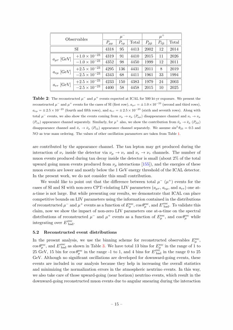
Observablesµ− µ+

Pµµ Peµ Total Pµµ Peµ Total

SI 4318 95 4413 2002 12 2014

aµτ [GeV]+1.0× 10−23 4319 91 4410 2015 11 2026

−1.0× 10−23 4352 98 4450 1999 12 2011

aeµ [GeV]+2.5× 10−23 4295 136 4431 2011 8 2019

−2.5× 10−23 4343 68 4411 1961 33 1994

aeτ [GeV]+2.5× 10−23 4233 150 4383 1979 24 2003

−2.5× 10−23 4400 58 4458 2015 10 2025

Table 2: The reconstructed µ− and µ+ events expected at ICAL for 500 kt·yr exposure. We present the

reconstructed µ− and µ+ events for the cases of SI (first row), aµτ = ± 1.0×10−23 (second and third rows),

aeµ = ± 2.5× 10−23 (fourth and fifth rows), and aeτ = ± 2.5× 10−23 (sixth and seventh rows). Along with

total µ− events, we also show the events coming from νµ → νµ (Pµµ) disappearance channel and νe → νµ

(Peµ) appearance channel separately. Similarly, for µ+ also, we show the contribution from νµ → νµ (Pµµ)

disappearance channel and νe → νµ (Peµ) appearance channel separately. We assume sin2 θ23 = 0.5 and

NO as true mass ordering. The values of other oscillation parameters are taken from Table 1.

are contributed by the appearance channel. The tau lepton may get produced during the

interaction of ντ inside the detector via νµ → ντ and νe → ντ channels. The number of

muon events produced during tau decay inside the detector is small (about 2% of the total

upward going muon events produced from νµ interactions [155]), and the energies of these

muon events are lower and mostly below the 1 GeV energy threshold of the ICAL detector.

In the present work, we do not consider this small contribution.

We would like to point out that the difference between total µ− (µ+) events for the

cases of SI and SI with non-zero CPT-violating LIV parameters (aµτ , aeµ, and aeτ ) one at-

a-time is not large. But while presenting our results, we demonstrate that ICAL can place

competitive bounds on LIV parameters using the information contained in the distributions

of reconstructed µ− and µ+ events as a function of Erecµ , cos θrec

µ , and E′rechad. To validate this

claim, now we show the impact of non-zero LIV parameters one at-a-time on the spectral

distributions of reconstructed µ− and µ+ events as a function of Erecµ , and cos θrec

µ while

integrating over E′rechad.

5.2 Reconstructed event distributions

In the present analysis, we use the binning scheme for reconstructed observables Erecµ ,

cos θrecµ , and E′rec

had as shown in Table 3. We have total 13 bins for Erecµ in the range of 1 to

25 GeV, 15 bin for cos θrecµ in the range -1 to 1, and 4 bins for E′rec

had in the range 0 to 25

GeV. Although no significant oscillations are developed for downward-going events, these

events are included in our analysis because they help in increasing the overall statistics

and minimizing the normalization errors in the atmospheric neutrino events. In this way,

we also take care of those upward-going (near horizon) neutrino events, which result in the

downward-going reconstructed muon events due to angular smearing during the interaction

– 15 –

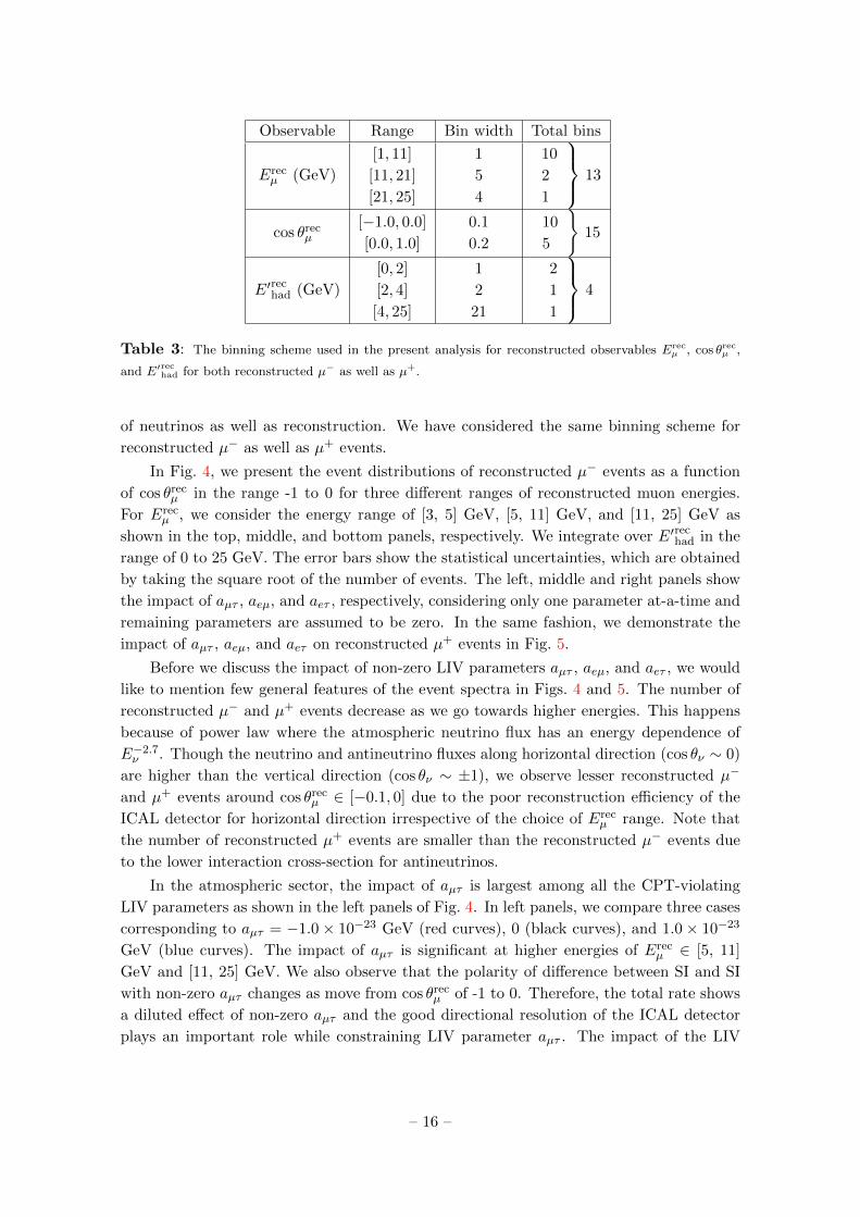
Observable Range Bin width Total bins

Erecµ (GeV)

[1, 11]

[11, 21]

[21, 25]

1

5

4

10

2

1

13

cos θrecµ

[−1.0, 0.0]

[0.0, 1.0]

0.1

0.2

10

5

}15

E′rechad (GeV)

[0, 2]

[2, 4]

[4, 25]

1

2

21

2

1

1

4

Table 3: The binning scheme used in the present analysis for reconstructed observables Erecµ , cos θrec

µ ,

and E′rechad for both reconstructed µ− as well as µ+.

of neutrinos as well as reconstruction. We have considered the same binning scheme for

reconstructed µ− as well as µ+ events.

In Fig. 4, we present the event distributions of reconstructed µ− events as a function

of cos θrecµ in the range -1 to 0 for three different ranges of reconstructed muon energies.

For Erecµ , we consider the energy range of [3, 5] GeV, [5, 11] GeV, and [11, 25] GeV as

shown in the top, middle, and bottom panels, respectively. We integrate over E′rechad in the

range of 0 to 25 GeV. The error bars show the statistical uncertainties, which are obtained

by taking the square root of the number of events. The left, middle and right panels show

the impact of aµτ , aeµ, and aeτ , respectively, considering only one parameter at-a-time and

remaining parameters are assumed to be zero. In the same fashion, we demonstrate the

impact of aµτ , aeµ, and aeτ on reconstructed µ+ events in Fig. 5.

Before we discuss the impact of non-zero LIV parameters aµτ , aeµ, and aeτ , we would

like to mention few general features of the event spectra in Figs. 4 and 5. The number of

reconstructed µ− and µ+ events decrease as we go towards higher energies. This happens

because of power law where the atmospheric neutrino flux has an energy dependence of

E−2.7ν . Though the neutrino and antineutrino fluxes along horizontal direction (cos θν ∼ 0)

are higher than the vertical direction (cos θν ∼ ±1), we observe lesser reconstructed µ−

and µ+ events around cos θrecµ ∈ [−0.1, 0] due to the poor reconstruction efficiency of the

ICAL detector for horizontal direction irrespective of the choice of Erecµ range. Note that

the number of reconstructed µ+ events are smaller than the reconstructed µ− events due

to the lower interaction cross-section for antineutrinos.

In the atmospheric sector, the impact of aµτ is largest among all the CPT-violating

LIV parameters as shown in the left panels of Fig. 4. In left panels, we compare three cases

corresponding to aµτ = −1.0× 10−23 GeV (red curves), 0 (black curves), and 1.0× 10−23

GeV (blue curves). The impact of aµτ is significant at higher energies of Erecµ ∈ [5, 11]

GeV and [11, 25] GeV. We also observe that the polarity of difference between SI and SI

with non-zero aµτ changes as move from cos θrecµ of -1 to 0. Therefore, the total rate shows

a diluted effect of non-zero aµτ and the good directional resolution of the ICAL detector

plays an important role while constraining LIV parameter aµτ . The impact of the LIV

– 16 –

1− 0.8− 0.6− 0.4− 0.2− 0-µ

recθcos0

10

20

30

40

- µ [3, 5] GeV∈ -µ

recE

SI GeV-23 10× = +1.0 τµa GeV-23 10× = -1.0 τµa

1− 0.8− 0.6− 0.4− 0.2− 0-µ

recθcos0

10

20

30

40

- µ

[3, 5] GeV∈ -µrecE

SI GeV-23 10× = +2.5 µea GeV-23 10× = -2.5 µea

1− 0.8− 0.6− 0.4− 0.2− 0-µ

recθcos0

10

20

30

40

- µ

[3, 5] GeV∈ -µrecE

SI GeV-23 10× = +2.5 τea GeV-23 10× = -2.5 τea

1− 0.8− 0.6− 0.4− 0.2− 0-µ

recθcos0

10

20

30

- µ

[5, 11] GeV∈ -µrecE

1− 0.8− 0.6− 0.4− 0.2− 0-µ

recθcos0

10

20

30

- µ [5, 11] GeV∈ -µ

recE

1− 0.8− 0.6− 0.4− 0.2− 0-µ

recθcos0

10

20

30

- µ

[5, 11] GeV∈ -µrecE

1− 0.8− 0.6− 0.4− 0.2− 0-µ

recθcos0

10

20

30

- µ

[11, 25] GeV∈ -µrecE

1− 0.8− 0.6− 0.4− 0.2− 0-µ

recθcos0

10

20

30

- µ

[11, 25] GeV∈ -µrecE

1− 0.8− 0.6− 0.4− 0.2− 0-µ

recθcos0

10

20

30

- µ

[11, 25] GeV∈ -µrecE

Figure 4: The distributions of reconstructed µ− events at the ICAL detector for 500 kt·yr exposure for

three different range of Erecµ : [3, 5] GeV (top panels), [5, 11] GeV (middle panels) and [11, 25] GeV (bottom

panels) where y-ranges are different among these rows. Here, error bars show the statistical uncertainties.

Note that, although the events are binned in (Erecµ , cos θrec

µ , E′rechad) binning scheme given in Table 3, the

reconstructed events in the hadron energy bins are integrated in the range 0 to 25 GeV in these plots. The

left, middle and right panels show the effect of aµτ , aeµ, and aeτ , respectively one parameter at-a-time. In

the left panels, the red, black, and blue curves represent aµτ = −1.0× 10−23 GeV, 0, and 1.0× 10−23 GeV,

respectively. In the middle panels, the red, black, and blue curves refer to aeµ = −2.5 × 10−23 GeV, 0,

and 2.5× 10−23 GeV, respectively. Similarly, in the right panels, the red, black, and blue curves stand for

aeτ = −2.5× 10−23 GeV, 0, and 2.5× 10−23 GeV, respectively. We assume sin2 θ23 = 0.5 and NO as true

mass ordering. The values of other oscillation parameters are taken from Table 1.

parameter aeµ is shown in the panels of the middle column where the red, black, and blue

curves refers to aeµ = −2.5 × 10−23 GeV, 0, and 2.5 × 10−23 GeV, respectively. We can

observe that the difference between SI and SI with non-zero aeµ is significant for Erecµ ∈ [5,

– 17 –

1− 0.8− 0.6− 0.4− 0.2− 0+µ

recθcos0

5

10

15

20+ µ

[3, 5] GeV∈ +µrecE

SI GeV-23 10× = +1.0 τµa GeV-23 10× = -1.0 τµa

1− 0.8− 0.6− 0.4− 0.2− 0+µ

recθcos0

5

10

15

20

+ µ

[3, 5] GeV∈ +µrecE

SI GeV-23 10× = +2.5 µea GeV-23 10× = -2.5 µea

1− 0.8− 0.6− 0.4− 0.2− 0+µ

recθcos0

5

10

15

20

+ µ

[3, 5] GeV∈ +µrecE

SI GeV-23 10× = +2.5 τea GeV-23 10× = -2.5 τea

1− 0.8− 0.6− 0.4− 0.2− 0+µ

recθcos0

5

10

15

20

+ µ

[5, 11] GeV∈ +µrecE

1− 0.8− 0.6− 0.4− 0.2− 0+µ

recθcos0

5

10

15

20+ µ

[5, 11] GeV∈ +µrecE

1− 0.8− 0.6− 0.4− 0.2− 0+µ

recθcos0

5

10

15

20

+ µ

[5, 11] GeV∈ +µrecE

1− 0.8− 0.6− 0.4− 0.2− 0+µ

recθcos0

5

10

15

+ µ

[11, 25] GeV∈ +µrecE

1− 0.8− 0.6− 0.4− 0.2− 0+µ

recθcos0

5

10

15

+ µ

[11, 25] GeV∈ +µrecE

1− 0.8− 0.6− 0.4− 0.2− 0+µ

recθcos0

5

10

15+ µ

[11, 25] GeV∈ +µrecE

Figure 5: The distributions of reconstructed µ+ events at the ICAL detector for 500 kt·yr exposure for

three different range of Erecµ : [3, 5] GeV (top panels), [5, 11] GeV (middle panels) and [11, 25] GeV (bottom

panels) where y-ranges are different among these rows. Here, error bars show the statistical uncertainties.

Note that, although the events are binned in (Erecµ , cos θrec

µ , E′rechad) binning scheme given in Table 3, the

reconstructed events in the hadron energy bins are integrated in the range 0 to 25 GeV in these plots. The

left, middle and right panels show the effect of aµτ , aeµ, and aeτ , respectively one parameter at-a-time. In

the left panels, the red, black, and blue curves represent aµτ = −1.0× 10−23 GeV, 0, and 1.0× 10−23 GeV,

respectively. In the middle panels, the red, black, and blue curves refer to aeµ = −2.5 × 10−23 GeV, 0,

and 2.5× 10−23 GeV, respectively. Similarly, in the right panels, the red, black, and blue curves stand for

aeτ = −2.5× 10−23 GeV, 0, and 2.5× 10−23 GeV, respectively. We assume sin2 θ23 = 0.5 and NO as true

mass ordering. The values of other oscillation parameters are taken from Table 1.

11] GeV. Similarly, we show the effect of non-zero aeτ on the distribution of reconstructed

µ− events in the right panels of Fig. 4 where the red, black, and blue curves stand for

aeτ = −2.5 × 10−23 GeV, 0, and 2.5 × 10−23 GeV, respectively. The difference between

– 18 –

SI and SI with non-zero aeτ is largest for Erecµ ∈ [5, 11] GeV, but we also see significant

difference for Erecµ ∈ [3, 5] GeV.

As far the case of µ+ is concerned, we observe that the impact of aµτ is significant in

the higher muon energy range of [5, 11] GeV and [11, 25] GeV as shown in the left panels

in Fig. 5. By comparing the left panels of Figs. 4 and 5, we observe that for a given value

of aµτ , the effect is in the opposite direction for reconstructed µ− and µ+ events. For

example, the reconstructed µ− events increase for the negative value of aµτ and the red

curve is higher than black curve in the bottom left panel of Fig. 4 for Erecµ ∈ [11, 25] GeV

whereas the corresponding curve is lower in the case of µ+ as shown in Fig. 5. The addition

of reconstructed µ− and µ+ events will dilute this feature. This observation indicates that

the charge identification efficiency of the ICAL detector will play an important role while

constraining LIV parameter aµτ . The effect of other LIV parameters aeµ and aeτ on the

event spectra of reconstructed µ+ events is significantly lower than that for the case of µ−.

This happens because the effect of aeµ and aeτ is driven by matter resonance term, which

occurs for the case of neutrino for NO but not antineutrino as explained in the section 4.

Next, we discuss the numerical method and analysis procedure that we use to obtain our

final results.

6 Simulation method

To obtain the median sensitivity of the ICAL atmospheric neutrino experiment in the

frequentist approach [156], we define the following Poissonian χ2− [157] for reconstructed

µ− events in Erecµ , cos θrec

µ , and E′rechad observables (the so-called “3D” analysis as considered

in [85]):

χ2−(3D) = min

ξl

NE′rechad∑

i=1

NErecµ∑

j=1

Ncos θrecµ∑

k=1

[2(N theory

ijk −Ndataijk )− 2Ndata

ijk ln

(N theoryijk

Ndataijk

)]+

5∑l=1

ξ2l

(6.1)

where,

N theoryijk = N0

ijk

(1 +

5∑l=1

πlijkξl

). (6.2)

In these equations, Ndataijk and N theory

ijk stand for the expected and observed number

of reconstructed µ− events in a given (Erecµ , cos θrec

µ , E′rechad) bin, respectively. We used the

binning scheme mentioned in Table 3 where NErecµ

= 13, Ncos θrecµ

= 15, and NE′rechad

= 4. In

Eq. 6.2, N0ijk corresponds to the number of expected events without considering systematic

uncertainties. In this analysis, we consider five systematic uncertainties following Refs. [82,

83, 158]: 20% error in flux normalization, 10% error in cross section, 5% energy dependent

tilt error in flux, 5% zenith angle dependent tilt error in flux, and 5% overall systematics.

We use the well-known method of pulls [110, 159, 160] to incorporate these systematic

uncertainties in our simulation. The pulls due to the systematic uncertainties are denoted

by ξl in Eqs. 6.1 and 6.2.

– 19 –

When we do not incorporate the hadron energy information E′rechad in our analysis and

use only Erecµ , and cos θrec

µ (the so-called “2D” analysis as considered in Ref. [82]), the

Poissonian χ2− for µ− events boils down to

χ2−(2D) = min

ξl

NErecµ∑

j=1

Ncos θrecµ∑

k=1

[2(N theory

ijk −Ndatajk )− 2Ndata

jk ln

(N theoryjk

Ndatajk

)]+

5∑l=1

ξ2l (6.3)

with,

N theoryjk = N0

jk

(1 +

5∑l=1

πljkξl

). (6.4)

In Eq. 6.3, Ndatajk and N theory

jk correspond to the observed and expected number of

reconstructed µ− events in a given (Erecµ , cos θrec

µ ) bin, respectively. The expected number

of events without systematic uncertainties are represented by N0jk in Eq. 6.4. In case of

binning scheme mentioned in Table 3, NErecµ

= 13, and Ncos θrecµ

= 15.

Following the same procedure, as described above, the χ2+ for reconstructed µ+ events

is determined for both the “2D” and “3D” analyses. The total χ2 is estimated by adding

the contribution from µ− and µ+:

χ2ICAL = χ2

− + χ2+. (6.5)

In this analysis, we simulate the prospective data using the benchmark values of os-

cillation parameters given in Table 1. We use Eq. 4.1 to estimate the value of ∆m231 from

∆m2eff where ∆m2

eff has the same magnitude for NO and IO with positive and negative

signs, respectively. To incorporate the systematic uncertainties, the χ2ICAL is minimized

with respect to pull parameters ξl in the fit. After that the marginalization is performed

over atmospheric mixing angle sin2 θ23 in the range (0.36, 0.66), atmospheric mass square

difference |∆m2eff| in the range (2.1, 2.6) ×10−3 eV2, and over both choices of mass ordering,

NO and IO, in the theory. We do not consider any priors for sin2 θ23 and |∆m2eff| in our

analysis. While performing fit, we keep the solar oscillation parameters sin2 2θ12 and ∆m221

fixed at their values as mentioned in Table 1. Since the reactor mixing angle is already

very well measured [136–139], we use a fixed value of sin2 2θ13 = 0.0875 both in data and

theory. Throughout our analysis, we take δCP = 0 both in data and theory.

7 Results

7.1 Effective regions in (Erecµ , cos θrecµ ) plane to constrain LIV parameters

For simulating the prospective data for statistical analysis, we assume the oscillations

with standard interactions only where LIV parameters are taken as zero. The statistical

significance of the analysis for constraining the LIV parameters (aµτ , aeµ, aeτ ) is quantified

in the following fashion:

∆χ2ICAL-LIV = χ2

ICAL (SI + aαβ)− χ2ICAL (SI). (7.1)

– 20 –

Here, χ2ICAL (SI) and χ2

ICAL (SI + aαβ) are calculated by fitting the prospective data

with only SI case (no LIV) and with SI in the presence of non-zero LIV parameter aαβ,

respectively. We consider only one LIV parameter at-a-time where aαβ can be aµτ , aeµ, or

aeτ . Since, the statistical fluctuations are suppressed to estimate the median sensitivity,

we have χ2ICAL (SI) ∼ 0.

As we will demonstrate in the later part of the result section that ICAL being an

atmospheric neutrino experiment dominated by νµ → νµ survival channel places tightest

constraint on aµτ among all the LIV parameters. Here, we discuss what regions in (Erecµ ,

cos θrecµ ) plane contribute significantly towards the sensitivity of ICAL for aµτ . A similar

discussion for other two off-diagonal LIV parameters aeµ and aeτ is provided in the ap-

pendix C. The sensitivity of ICAL towards the LIV parameter aµτ stems from both µ−

and µ+ events for both the choices of mass ordering. While considering aµτ = 1.0× 10−23

GeV (−1.0 × 10−23 GeV) in theory and aµτ = 0 in data, the contribution of µ− and µ+

towards fixed-parameter7 ∆χ2ICAL-LIV for 500 kt·yr exposure at ICAL for NO is 43.5 (43.9)

and 25.0 (23.8), respectively.

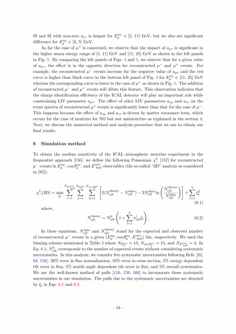
Before we present our final results, let us first identify the effective regions in (Erecµ ,

cos θrecµ ) plane which contribute significantly towards ∆χ2

ICAL-LIV. In Fig. 6, we show the

distribution of fixed-parameter ∆χ2− ( ∆χ2

+) without pull penalty term8 from reconstructed

µ− (µ+) events in (Erecµ , cos θrec

µ ) plane for 500 kt·yr exposure at ICAL assuming NO at

true mass ordering. For demonstration purpose, we have added the ∆χ2 contribution from

all E′rechad bins for each (Erec

µ , cos θrecµ ) bin while using binning scheme mentioned in Table 3.

In the top (bottom) panels in Fig. 6, we take non-zero LIV parameter aµτ = 1.0 × 10−23

GeV (−1.0 × 10−23 GeV) in theory while considering aµτ = 0 in the prospective data.

The left and the right panels show the distribution of ∆χ2− and ∆χ2

+, respectively. In all

the panels, we observe that a significant contribution is received from bins with 7 GeV <

Erecµ < 17 GeV and cos θrec

µ < −0.4. These are the regions around the oscillation valley as

observed in Fig. 1.

7.2 Advantage of hadron energy information in constraining LIV parameters

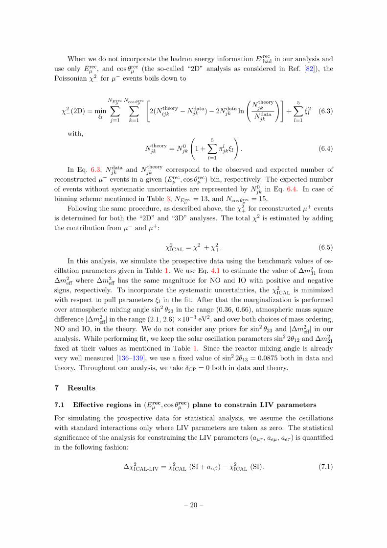
In Fig. 7, we constrain the LIV parameters aµτ , aeµ, and aeτ using 500 kt·yr exposure at the

ICAL detector and describe the advantage of incorporating the hadron energy information.

In the prospective data, we assume the case of SI where the values of all LIV parameters

are considered to be zero, whereas in theory, we consider SI + LIV case where the value

of the LIV parameters aµτ , aeµ, and aeτ are varied one-at-a-time. In the left, middle and

right panels, we constrain the LIV parameters aµτ , aeµ, and aeτ , respectively. In all the

panel, the red curves represent the 2D case where we use only Erecµ and cos θrec

µ variables

without considering any hadron energy information. For reconstructed variables of Erecµ

and cos θrecµ , we use binning scheme mentioned in Table 3, where the events are integrated

7Please note that in the fixed-parameter scenario, we minimize only over the systematic uncertainties,

but we keep the oscillation parameters fixed in both theory and data at their benchmark values as mentioned

in Table 1.8We do not include pull penalty term

∑5l=1 ξ

2l (see Eq. 6.1) while calculating ∆χ2

− and ∆χ2+ to explore

contributions from each bin in the plane of Erecµ and cos θrec

µ for µ− and µ+ events, respectively.

– 21 –

Figure 6: The distribution of fixed-parameter ∆χ2− (∆χ2

+) in the plane of (Erecµ , cos θrec

µ ) without pull

penalty term using 500 kt·yr exposure of the ICAL detector as shown in the left (right) panels. Note that

∆χ2− and ∆χ2

+ are presented in the units of GeV−1sr−1 where we have divided them by 2π × bin area.

In data, aµτ = 0 with NO (true) using the benchmark value of oscillation parameters given in Table 1. In

theory, aµτ = −1.0× 10−23 GeV and 1.0× 10−23 GeV in the top and bottom panels, respectively.

over E′rechad bins in the hadron energy range of 0 to 25 GeV. On the other hand, the black

curves represent the 3D case considering reconstructed variables of Erecµ , cos θrec

µ , and E′rechad

where we use the hadron energy information available at the ICAL detector. For 3D case,

we used the binning scheme given in Table 3 where E′rechad is divided into 4 bins in the

hadron energy range of 0 to 25 GeV.

We can observe in Fig. 7 that the incorporation of hadron energy information results

in the improved constraints for all three cases of LIV parameters aµτ , aeµ, and aeτ . The

ICAL detector places the tightest constraint on LIV parameter aµτ among all the three

off-diagonal LIV parameters. For the case of aeµ and aeτ , we observe that the bounds

are asymmetric with stronger constraints for the positive values than that for the negative

values. These observations are consistent with the effect of aeµ and aeτ on νµ survival

probability oscillograms in Figs. 2 and 3, respectively. In section 4, we use Eq. B.4 to

explain the reason behind stronger effects of aeµ and aeτ for positive values. In the next

– 22 –

0.3− 0.2− 0.1− 0 0.1 0.2 0.3 [GeV] (fit)23 10× τµa

0

1

2

3

4

52 χ∆

95% C.L.

500 kt.yr

(w/ CID)2χ∆

)µrecθ, cosµ

rec(E

)had'rec, Eµ

recθ, cosµrec(E

3− 2− 1− 0 1 2 [GeV] (fit)23 10× µea

0

1

2

3

4

5

2 χ∆

95% C.L.

5− 4− 3− 2− 1− 0 1 2

[GeV] (fit)23 10× τea

0

1

2

3

4

5

2 χ∆

95% C.L.

Figure 7: The sensitivities to constrain the LIV parameters aµτ , aeµ, and aeτ using 500 kt·yr exposure

at the ICAL detector as shown in the left, middle, and right panels, respectively. In each panel, the red

lines represent the 2D analysis using reconstructed observables (Erecµ , cos θrec

µ ) whereas the black lines refers

to the 3D analysis using reconstructed observables (Erecµ , cos θrec

µ , E′rechad). We have used the benchmark

value of oscillation parameters given in Table 1. In theory, we have marginalized over oscillation parameters

sin2 θ23, |∆m2eff|, and both choices of mass orderings.

0.6− 0.4− 0.2− 0 0.2 0.4 0.6 [GeV] (fit)23 10× τµa

0

1

2

3

4

5

2 χ∆

95% C.L.

500 kt.yr

)had'rec, Eµ

recθ, cosµrec (E2χ∆

w/ CIDw/o CID

4− 3− 2− 1− 0 1 2 3 [GeV] (fit)23 10× µea

0

1

2

3

4

5

2 χ∆

95% C.L.

4− 3− 2− 1− 0 1 2 3 4

[GeV] (fit)23 10× τea

0

1

2

3

4

5

2 χ∆

95% C.L.

Figure 8: The sensitivities to constrain the LIV parameters aµτ , aeµ, and aeτ using 500 kt·yr exposure at

the ICAL detector as shown in the left, middle, and right panels, respectively. In each panel, the black lines

represent the case when the charge identification capability of the ICAL detector is used while estimating

the sensitivities, whereas the red lines refer to the case when the charge identification capability of ICAL is

absent. We have used the benchmark value of oscillation parameters given in Table 1. In theory, we have

marginalized over oscillation parameters sin2 θ23, |∆m2eff|, and both choices of mass orderings.

section, we explore the impact of CID capability of the ICAL detector in constraining the

LIV parameters.

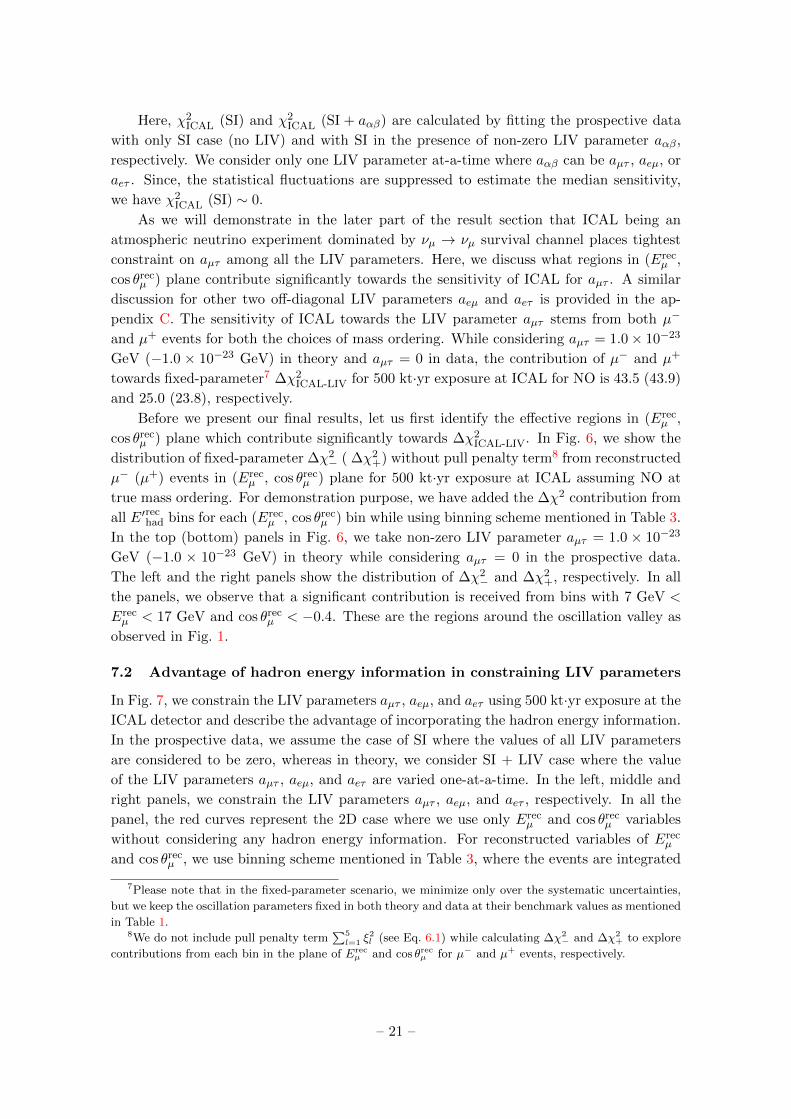
7.3 Advantage of charge identification capability to constrain LIV parameters

The presence of a 1.5 T magnetic field enables the ICAL detector to distinguish µ− and µ+

events, which leads to the capability of the ICAL detector to separately identify their parent

particles neutrinos and antineutrinos, respectively. In Fig. 8, we discuss the advantage of

charge identification capability of the ICAL detector while constraining the CPT-violating

LIV parameters aµτ , aeµ, and aeτ using 500 kt·yr exposure. In each panel of Fig. 8, black

– 23 –

curves show the sensitivity of the ICAL detector where CID capability is exploited, and

two separate sets of bins for reconstructed µ− and µ+ events are used. On the other hand,

the red curves represent the case where the CID capability of the ICAL detector is not

utilized, and a single set of combined bins for both reconstructed µ− and µ+ events is

considered.

We can observe in Fig. 8 that the incorporation of CID capability of the ICAL detector

significantly improves the sensitivity to constrain the LIV parameters aµτ , aeµ, and aeτ .

In section 4, we discussed that for a given value of aµτ , the oscillation valley bends in

the opposite directions for neutrinos and antineutrinos. The combined binning of both

reconstructed µ− and µ+ events in a single set of bins will lead to a dilution of these features,

which are caused due to the presence of non-zero LIV parameter. Thus, it is important

to separately identify reconstructed µ− and µ+ events to preserve the information about

LIV. All these observations validate the fact that the charge identification capability of the

ICAL detector will play a crucial role in constraining LIV parameters.

In the subsections 7.2 and 7.3, we discussed the advantage of incorporating hadron

energy information and presence of CID while constraining CPT-violating LIV parameters

aµτ , aeµ, and aeτ . Now, Table 4 nicely summarizes the findings from these two studies

in tabular form, and at the same time, we compare the performance of ICAL with other

experiments. In Table 4, we present the constraints on LIV parameters aµτ , aeµ, and aeτ at

95% C.L. using 500 kt·yr exposure at the ICAL detector. By comparing the results shown

in the second row with respect to that in the first row, we can infer that the incorporation

of hadron energy information improves the bounds on all of these LIV parameters. The

improvement due to the presence of CID capability can be observed by comparing the

second row with respect to the third row. While doing comparison with existing constraints,

we have mentioned the results from Super-K analysis [22] for LIV parameters aµτ , aeµ, and

aeτ at 95% C.L. with real and imaginary parts separately. The IceCube collaboration [25]

has performed analysis only for aµτ . We show constraints for the real and imaginary parts

of aµτ separately at 99% C.L. as provided by the IceCube collaboration.

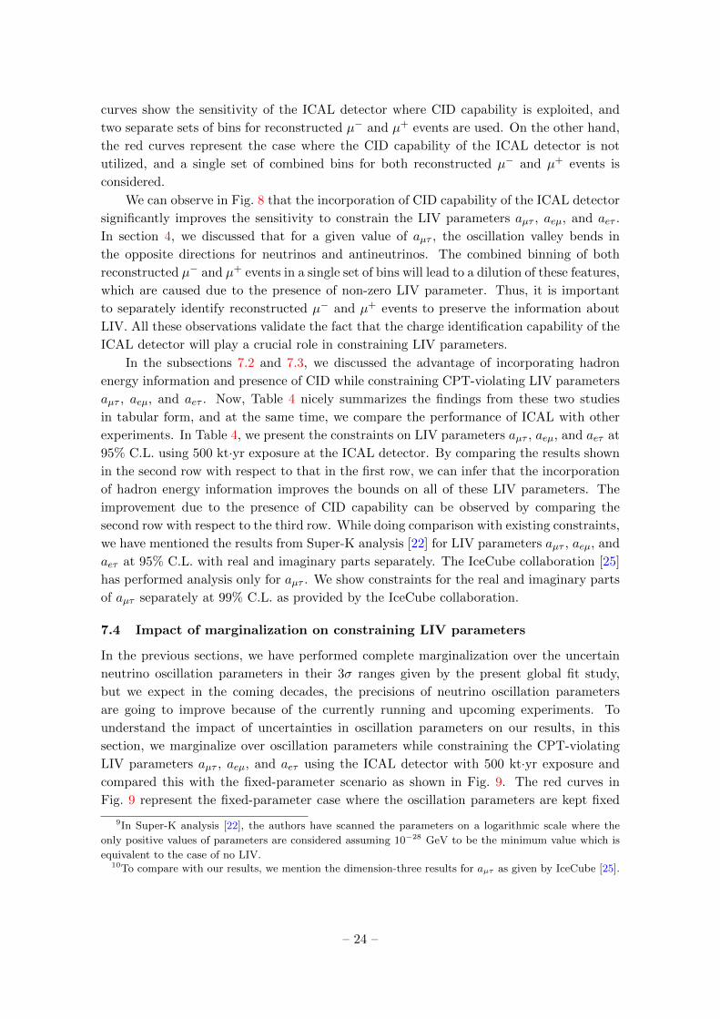
7.4 Impact of marginalization on constraining LIV parameters

In the previous sections, we have performed complete marginalization over the uncertain

neutrino oscillation parameters in their 3σ ranges given by the present global fit study,

but we expect in the coming decades, the precisions of neutrino oscillation parameters

are going to improve because of the currently running and upcoming experiments. To

understand the impact of uncertainties in oscillation parameters on our results, in this

section, we marginalize over oscillation parameters while constraining the CPT-violating

LIV parameters aµτ , aeµ, and aeτ using the ICAL detector with 500 kt·yr exposure and

compared this with the fixed-parameter scenario as shown in Fig. 9. The red curves in

Fig. 9 represent the fixed-parameter case where the oscillation parameters are kept fixed

9In Super-K analysis [22], the authors have scanned the parameters on a logarithmic scale where the

only positive values of parameters are considered assuming 10−28 GeV to be the minimum value which is

equivalent to the case of no LIV.10To compare with our results, we mention the dimension-three results for aµτ as given by IceCube [25].

– 24 –

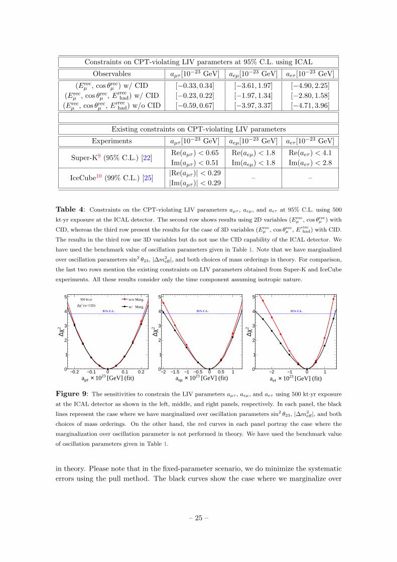
Constraints on CPT-violating LIV parameters at 95% C.L. using ICAL

Observables aµτ [10−23 GeV] aeµ[10−23 GeV] aeτ [10−23 GeV]

(Erecµ , cos θrec

µ ) w/ CID [−0.33, 0.34] [−3.61, 1.97] [−4.90, 2.25]

(Erecµ , cos θrec

µ , E′rechad) w/ CID [−0.23, 0.22] [−1.97, 1.34] [−2.80, 1.58]

(Erecµ , cos θrec

µ , E′rechad) w/o CID [−0.59, 0.67] [−3.97, 3.37] [−4.71, 3.96]

Existing constraints on CPT-violating LIV parameters

Experiments aµτ [10−23 GeV] aeµ[10−23 GeV] aeτ [10−23 GeV]

Super-K9 (95% C.L.) [22]Re(aµτ ) < 0.65 Re(aeµ) < 1.8 Re(aeτ ) < 4.1

Im(aµτ ) < 0.51 Im(aeµ) < 1.8 Im(aeτ ) < 2.8

IceCube10 (99% C.L.) [25]|Re(aµτ )| < 0.29

– –|Im(aµτ )| < 0.29

Table 4: Constraints on the CPT-violating LIV parameters aµτ , aeµ, and aeτ at 95% C.L. using 500

kt·yr exposure at the ICAL detector. The second row shows results using 2D variables (Erecµ , cos θrec

µ ) with

CID, whereas the third row present the results for the case of 3D variables (Erecµ , cos θrec

µ , E′rechad) with CID.

The results in the third row use 3D variables but do not use the CID capability of the ICAL detector. We

have used the benchmark value of oscillation parameters given in Table 1. Note that we have marginalized

over oscillation parameters sin2 θ23, |∆m2eff|, and both choices of mass orderings in theory. For comparison,

the last two rows mention the existing constraints on LIV parameters obtained from Super-K and IceCube

experiments. All these results consider only the time component assuming isotropic nature.

0.2− 0.1− 0 0.1 0.2 [GeV] (fit)23 10× τµa

0

1

2

3

4

5

2 χ∆

95% C.L.

500 kt.yr

(w/ CID)2χ∆

w/o Marg.

w/ Marg.

2− 1.5− 1− 0.5− 0 0.5 1 [GeV] (fit)23 10× µea

0

1

2

3

4

5

2 χ∆

95% C.L.

2− 1− 0 1

[GeV] (fit)23 10× τea

0

1

2

3

4

5

2 χ∆

95% C.L.

Figure 9: The sensitivities to constrain the LIV parameters aµτ , aeµ, and aeτ using 500 kt·yr exposure

at the ICAL detector as shown in the left, middle, and right panels, respectively. In each panel, the black

lines represent the case where we have marginalized over oscillation parameters sin2 θ23, |∆m2eff|, and both

choices of mass orderings. On the other hand, the red curves in each panel portray the case where the

marginalization over oscillation parameter is not performed in theory. We have used the benchmark value

of oscillation parameters given in Table 1.

in theory. Please note that in the fixed-parameter scenario, we do minimize the systematic

errors using the pull method. The black curves show the case where we marginalize over

– 25 –

0.2− 0.1− 0 0.1 0.2 [GeV] (fit)23 10× τµa

0

1

2

3

4

52 χ∆

95% C.L.

500 kt.yr, NO (true)

)had'rec, Eµ

recθ, cosµrec (E2χ∆

= 0.4 (true)23θ2sin

= 0.5 (true)23θ2sin

= 0.6 (true)23θ2sin

2− 1− 0 1 [GeV] (fit)23 10× µea

0

1

2

3

4

5

2 χ∆

95% C.L.

4− 3− 2− 1− 0 1

[GeV] (fit)23 10× τea

0

1

2

3

4

5

2 χ∆

95% C.L.

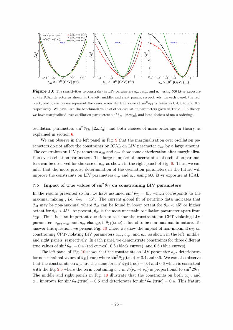
Figure 10: The sensitivities to constrain the LIV parameters aµτ , aeµ, and aeτ using 500 kt·yr exposure

at the ICAL detector as shown in the left, middle, and right panels, respectively. In each panel, the red,

black, and green curves represent the cases when the true value of sin2 θ23 is taken as 0.4, 0.5, and 0.6,

respectively. We have used the benchmark value of other oscillation parameters given in Table 1. In theory,

we have marginalized over oscillation parameters sin2 θ23, |∆m2eff|, and both choices of mass orderings.

oscillation parameters sin2 θ23, |∆m2eff|, and both choices of mass orderings in theory as

explained in section 6.

We can observe in the left panel in Fig. 9 that the marginalization over oscillation pa-

rameters do not affect the constraints by ICAL on LIV parameter aµτ by a large amount.

The constraints on LIV parameters aeµ and aeτ show some deterioration after marginaliza-

tion over oscillation parameters. The largest impact of uncertainties of oscillation parame-

ters can be observed for the case of aeτ as shown in the right panel of Fig. 9. Thus, we can

infer that the more precise determination of the oscillation parameters in the future will

improve the constraints on LIV parameters aeµ and aeτ using 500 kt·yr exposure at ICAL.

7.5 Impact of true values of sin2 θ23 on constraining LIV parameters

In the results presented so far, we have assumed sin2 θ23 = 0.5 which corresponds to the

maximal mixing , i.e. θ23 = 45◦. The current global fit of neutrino data indicates that

θ23 may be non-maximal where θ23 can be found in lower octant for θ23 < 45◦ or higher

octant for θ23 > 45◦. At present, θ23 is the most uncertain oscillation parameter apart from

δCP. Thus, it is an important question to ask how the constraints on CPT-violating LIV

parameters aµτ , aeµ, and aeτ change, if θ23(true) is found to be non-maximal in nature. To

answer this question, we present Fig. 10 where we show the impact of non-maximal θ23 on

constraining CPT-violating LIV parameters aµτ , aeµ, and aeτ as shown in the left, middle,

and right panels, respectively. In each panel, we demonstrate constraints for three different

true values of sin2 θ23 = 0.4 (red curves), 0.5 (black curves), and 0.6 (blue curves).

The left panel of Fig. 10 shows that the constraints on LIV parameter aµτ deteriorates

for non-maximal values of θ23(true) where sin2 θ23(true) = 0.4 and 0.6. We can also observe

that the constraints on aµτ are the same for sin2 θ23(true) = 0.4 and 0.6 which is consistent

with the Eq. 2.5 where the term containing aµτ in P (νµ → νµ) is proportional to sin2 2θ23.

The middle and right panels in Fig. 10 illustrate that the constraints on both aeµ, and

aeτ improves for sin2 θ23(true) = 0.6 and deteriorates for sin2 θ23(true) = 0.4. This feature

– 26 –

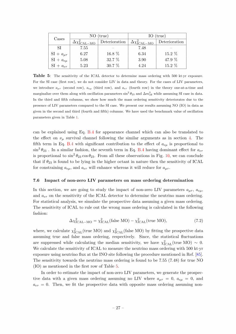
CasesNO (true) IO (true)

∆χ2ICAL−MO Deterioration ∆χ2

ICAL−MO Deterioration

SI 7.55 – 7.48 –

SI + aµτ 6.27 16.8 % 6.34 15.2 %

SI + aeµ 5.08 32.7 % 3.90 47.9 %

SI + aeτ 5.23 30.7 % 4.24 15.2 %

Table 5: The sensitivity of the ICAL detector to determine mass ordering with 500 kt·yr exposure.

For the SI case (first row), we do not consider LIV in data and theory. For the cases of LIV parameters,

we introduce aµτ (second row), aeµ (third row), and aeτ (fourth row) in the theory one-at-a-time and

marginalize over them along with oscillation parameters sin2 θ23 and ∆m2eff while assuming SI case in data.

In the third and fifth columns, we show how much the mass ordering sensitivity deteriorates due to the

presence of LIV parameters compared to the SI case. We present our results assuming NO (IO) in data as

given in the second and third (fourth and fifth) columns. We have used the benchmark value of oscillation

parameters given in Table 1.

can be explained using Eq. B.4 for appearance channel which can also be translated to

the effect on νµ survival channel following the similar arguments as in section 4. The

fifth term in Eq. B.4 with significant contribution to the effect of aeµ is proportional to

sin3 θ23 . In a similar fashion, the seventh term in Eq. B.4 having dominant effect for aeτis proportional to sin2 θ23 cos θ23. From all these observations in Fig. 10, we can conclude

that if θ23 is found to be lying in the higher octant in nature then the sensitivity of ICAL

for constraining aeµ, and aeτ will enhance whereas it will reduce for aµτ .

7.6 Impact of non-zero LIV parameters on mass ordering determination

In this section, we are going to study the impact of non-zero LIV parameters aµτ , aeµ,

and aeτ on the sensitivity of the ICAL detector to determine the neutrino mass ordering.

For statistical analysis, we simulate the prospective data assuming a given mass ordering.

The sensitivity of ICAL to rule out the wrong mass ordering is calculated in the following

fashion:

∆χ2ICAL−MO = χ2

ICAL(false MO)− χ2ICAL(true MO), (7.2)

where, we calculate χ2ICAL(true MO) and χ2

ICAL(false MO) by fitting the prospective data

assuming true and false mass ordering, respectively. Since, the statistical fluctuations

are suppressed while calculating the median sensitivity, we have χ2ICAL(true MO) ∼ 0.

We calculate the sensitivity of ICAL to measure the neutrino mass ordering with 500 kt·yr

exposure using neutrino flux at the INO site following the procedure mentioned in Ref. [85].

The sensitivity towards the neutrino mass ordering is found to be 7.55 (7.48) for true NO

(IO) as mentioned in the first row of Table 5.

In order to estimate the impact of non-zero LIV parameters, we generate the prospec-

tive data with a given mass ordering assuming no LIV where aµτ = 0, aeµ = 0, and

aeτ = 0. Then, we fit the prospective data with opposite mass ordering assuming non-

– 27 –

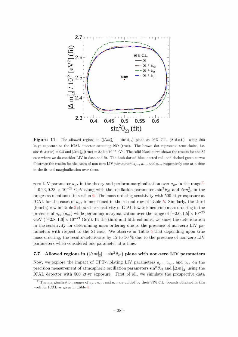
0.4 0.45 0.5 0.55 0.6

(fit)23θ2sin

2.3

2.4

2.5

2.6

2.7

] (f

it)2

[eV

-3| /

10

322 m∆|

95% C.L.

true

SI

µeSI + a

τeSI + a

τµSI + a

Figure 11: The allowed regions in (|∆m232| – sin2 θ23) plane at 95% C.L. (2 d.o.f.) using 500

kt·yr exposure at the ICAL detector assuming NO (true). The brown dot represents true choice, i.e.

sin2 θ23(true) = 0.5 and |∆m232|(true) = 2.46× 10−3 eV2. The solid black curve shows the results for the SI

case where we do consider LIV in data and fit. The dash-dotted blue, dotted red, and dashed green curves

illustrate the results for the cases of non-zero LIV parameters aµτ , aeµ, and aeτ , respectively one-at-a-time

in the fit and marginalization over them.

zero LIV parameter aµτ in the theory and perform marginalization over aµτ in the range11

[−0.23, 0.23]× 10−23 GeV along with the oscillation parameters sin2 θ23 and ∆m2eff in the

ranges as mentioned in section 6. The mass-ordering sensitivity with 500 kt·yr exposure at

ICAL for the cases of aµτ is mentioned in the second row of Table 5. Similarly, the third

(fourth) row in Table 5 shows the sensitivity of ICAL towards neutrino mass ordering in the

presence of aeµ (aeτ ) while perfoming marginalization over the range of [−2.0, 1.5]× 10−23

GeV ([−2.8, 1.6] × 10−23 GeV). In the third and fifth columns, we show the deterioration

in the sensitivity for determining mass ordering due to the presence of non-zero LIV pa-

rameters with respect to the SI case. We observe in Table 5 that depending upon true

mass ordering, the results deteriorate by 15 to 50 % due to the presence of non-zero LIV

parameters when considered one parameter at-a-time.

7.7 Allowed regions in (|∆m232| – sin2 θ23) plane with non-zero LIV parameters

Now, we explore the impact of CPT-violating LIV parameters aµτ , aeµ, and aeτ on the

precision measurement of atmospheric oscillation parameters sin2 θ23 and |∆m232| using the

ICAL detector with 500 kt·yr exposure. First of all, we simulate the prospective data

11The marginalization ranges of aµτ , aeµ, and aeτ are guided by their 95% C.L. bounds obtained in this

work for ICAL as given in Table 4.

– 28 –

assuming sin2 θ23 (true) = 0.5 and |∆m232|(true) = 2.46× 10−3 eV2 for case of SI with no

LIV. The statistical significance for this is quantified using the following expression:

∆χ2ICAL−PM(sin2 θ23, |∆m2

32|) = χ2ICAL(sin2 θ23, |∆m2

32|)− χ20, (7.3)

where, χ2ICAL(sin2 θ23, |∆m2

32|) is estimated by fitting the prospective data with theory for

a given value of sin2 θ23, and |∆m232|. χ2

0 is the minimum value of χ2ICAL(sin2 θ23, |∆m2

32|)in the allowed range of oscillation parameters sin2 θ23 and |∆m2

32|. Here, χ20 ∼ 0 because

the statistical fluctuations are suppressed. We estimate the allowed regions in (|∆m232| –

sin2 θ23) plane for the case of SI at 95% C.L. (2 d.o.f.) as shown by black line in Fig. 11.

Now, we discuss the impact of non-zero LIV parameters aµτ , aeµ, and aeτ one-at-a-

time on the precision measurement of atmospheric oscillation parameters. We simulate the

prospective data considering the true values of sin2 θ23 and |∆m232| as mentioned above

without LIV. Then, we estimate allowed regions in (|∆m232| – sin2 θ23) plane with non-zero

LIV parameters aµτ , aeµ, and aeτ one-at-a-time in the fit. Further, we marginalize over aµτin the range [−0.23, 0.23]×10−23 GeV, aeµ in the range [−2.0, 1.5]×10−23 GeV, and aeτ in

the range [−2.8, 1.6]×10−23 GeV one-at-a-time in the fit (see footnote 11). We show these

results for the cases of non-zero LIV parameters aµτ , aeµ, and aeτ at 95 % C.L. (2 d.o.f.)

using dotted red, dashed green, and dash-dotted blue lines, respectively, in Fig. 11. We do

not observe a significant change in the allowed regions at 95% C.L. when we introduce aµτin fit and marginalize over it. It indicates that the precision measurement of atmospheric

oscillation parameters using the ICAL detector is quite robust against the presence of aµτin the fit. However, the presence of non-zero LIV parameter aeµ in fit deteriorate the

allowed region in the direction of sin2 θ23. As far as the presence of LIV parameter aeτ in

fit is concerned, it deteriorates allowed region in the direction of |∆m232|.

7.8 Correlation between off-diagonal LIV parameters

So far, we have studied the neutrino oscillations in the presence of only one CPT-violating

LIV parameter at-a-time. In this section, we explore the correlation between different

CPT-violating LIV parameters. To begin with, we generate prospective data with 500

kt·yr exposure at the ICAL detector considering no LIV with NO as true mass ordering

and benchmark value of oscillation parameters mentioned in Table 1. While constraining

two LIV parameters at-a-time, we quantify the statistical significance using the following

expression:

∆χ2ICAL−LIV(aµτ , aeµ) = χ2

ICAL(SI + (aµτ , aeµ))− χ2ICAL(SI), (7.4)

where, χ2ICAL(SI) and χ2

ICAL(SI + (aµτ , aeµ)) are calculated by fitting the prospective data

with only SI case (no LIV) and with SI + LIV (aµτ , aeµ) case, respectively. Since, the

statistical fluctuations are suppressed, we have χ2ICAL(SI) ∼ 0. Then, we estimate the

allowed regions in the plane of CPT-violating LIV parameters (aµτ , aeµ) at 95% C.L. (2

d.o.f.) as shown in the left panel of Fig. 12. The true choices of LIV parameters aµτ = 0,

aeµ = 0, and aeτ = 0 in data are depicted as red dots in Fig. 12. In theory, we vary two

LIV parameters at-a-time with (without) marginalization over the oscillation parameters

– 29 –

5− 4− 3− 2− 1− 0 1 2 [GeV] (fit)23 10× µea

0.3−

0.2−

0.1−

0

0.1

0.2

0.3 [

GeV

] (f

it)23

10

× τµa

5− 4− 3− 2− 1− 0 1 2

[GeV] (fit)23 10× τea

0.3−

0.2−

0.1−

0

0.1

0.2

0.3

[G

eV]

(fit)

23 1

0× τµa

4− 3− 2− 1− 0 1 2 [GeV] (fit)23 10× µea

4−

2−

0

2

[G

eV]

(fit)

23 1

0× τea

NO (true)

true

Fix. 95% C.L. (2 d.o.f)

Marg. 95% C.L. (2 d.o.f)

Figure 12: The correlated constraints in the plane of CPT-violating LIV parameters (aµτ , aeµ) (left

panel), (aµτ , aeτ ) (middle panel), and (aeτ , aeµ) (right panel) at 95% C.L. (2 d.o.f.) with 500 kt·yr exposure

at the ICAL detector. We generate prospective data considering no LIV (red dots) with NO (true) and

benchmark value of oscillation parameters mentioned in Table 1. In theory, we vary two LIV parameters

at-a-time with marginalization over the oscillation parameters sin2 θ23, ∆m2eff , and both choices of mass

ordering as shown by black curves. The blue curves represent the fixed-parameter scenario where we do not

marginalize over any oscillation parameter in theory, but we do marginalize over systematic uncertainties.

sin2 θ23, ∆m2eff , and both choices of mass ordering as shown by black (blue) curve. Similarly,

we present the allowed regions in the plane of LIV parameters (aµτ , aeτ ) and (aeτ , aeµ) in

the middle and left panels, respectively, in Fig. 12.

8 Summary and concluding remarks

In this paper, for the first time, we explore the Lorentz Invariance Violation (LIV) through

the mass-induced flavor oscillations of atmospheric neutrino in the multi-GeV range of

energies over a wide range of baselines using the proposed ICAL detector at INO. In the

present analysis, we focus our attention on the isotropic CPT-violating LIV parameters

aµτ , aeµ, and aeτ where we consider their real values only with both positive and negative

signs.

We perform a detailed analysis by demonstrating the effect of non-zero CPT-violating

LIV parameters (aµτ , aeµ, and aeτ ) one-at-a-time on probability oscillograms of the disap-

pearance (νµ → νµ) channel, which has a dominant contribution (more than 98%) to the

reconstructed muon events at the ICAL detector. We observe that the vacuum oscillation

valley bends due to the presence of non-zero LIV parameter aµτ where the curvature of

valley depends on the sign of aµτ . For a given aµτ , the curvatures of bendings are opposite

for neutrino and antineutrino. This fact indicates that the charged identification capability

of the ICAL detector is a crucial property while probing LIV parameter aµτ . If we turn our

attention to the other off-diagonal LIV parameters aeµ and aeτ , we observe that they do

not result in any bending of oscillation valley, but they do disturb the vacuum oscillation

valley as well as matter effect regions.

Next, we present the impact of LIV on the reconstructed event distributions at the

ICAL detector for 500 kt·yr exposure. We observe that aµτ affects the event distributions

– 30 –

by the largest amount among all off-diagonal CPT-violating LIV parameters. Since the

effects of LIV parameters depend on energy and direction, the good energy and direction

resolution of the ICAL detector is going to play an important role.

After describing the modification in reconstructed event distributions due to LIV, we

calculate statistical significance for the presence of LIV using the ICAL detector at the χ2

level. In order to calculate ∆χ2, we simulate the prospective data at ICAL with 500 kt·yr

exposure for SI case with no LIV and perform fitting assuming SI+LIV case in theory where

we consider the CPT-violating LIV parameters aµτ , aeµ, and aeτ one-at-a-time. First of

all, we identify the energy and direction bins that contribute significantly to ∆χ2. Further,

we constrain the LIV parameters aµτ , aeµ, and aeτ at 95% C.L. using 500 kt·yr exposure

at the ICAL detector.

We show the advantage of incorporating hadron energy information and the CID ca-

pability of ICAL while constraining LIV parameters. We also demonstrate that the con-

straints on aµτ are robust against the uncertainties in oscillation parameters where the

estimated bounds on aeµ and aeτ are expected to improve with more precise determination

of oscillation parameters. As far as the non-maximal value of θ23 is concerned, it deterio-

rates the constraints on aµτ whereas constraints on aeµ and aeτ improve (worsen) if θ23 is

found to be lying in the higher (lower) octant.

The aim of the ICAL detector at INO is to determine the mass ordering and the

precise determination of atmospheric oscillation parameters θ23 and |∆m232|. In the present

analysis, we also explore how the sensitivity to measure mass ordering gets affected due

to the presence of non-zero LIV parameters considered one-at-a-time. We observe that

depending upon true mass ordering, the results get deteriorated by about 15 to 50% due to

the presence of LIV. If we look at the effect of LIV on precision measurement of atmospheric

oscillation parameters θ23 and |∆m232|, we find that the precision measurement is quite

robust against the marginalization over aµτ in the fit. However, the presence of aeµ (aeτ )

worsens the allowed region in the direction of sin2 θ23 (|∆m232|).

The above-mentioned analyses consider one LIV parameter at-a-time. In order to ex-

plore the correlation among various off-diagonal CPT-violating LIV parameters, we consid-

ered two LIV parameter at-a-time and constrain (2 d.o.f.) them using 500 kt·yr exposure at

the ICAL detector. We have obtained allowed regions in three different planes of (aµτ , aeµ),

(aµτ , aeτ ) and (aeτ , aeµ) while marginalizing over oscillation parameters.

Before we conclude, we would like to highlight the fact that the present analysis has

been performed in the multi-GeV range of energies which is complementary to energy ranges

used in the analyses of Super-K and IceCube. We would also like to emphasize that the

LIV bounds obtained in the present analysis using the ICAL detector are quite competitive

compared to the existing bounds from Super-K and IceCube due to the charge identification

capability of ICAL as well as the good resolutions in reconstructed muon energy and

direction. In the absence of CID, the constraints on LIV parameters deteriorate significantly

due to the dilution of LIV features while combining µ− and µ+ events. This unique

capability of CID enables ICAL to probe LIV separately in neutrino and antineutrino

modes which may not be possible at any other existing or planned neutrino detector based

on water, ice, or argon.

– 31 –

Acknowledgements

This work is performed by the members of the INO-ICAL collaboration to estimate the

constraints on the CPT-violating off-diagonal LIV parameters using 500 kt·yr exposure

of the ICAL-INO atmospheric neutrino detector. We thank M. Masud, S. Das, and A.

Khatun for useful communications. We thank A. Dighe, S. Goswami, J. F. Libby, A. K.

Nayak, A. M. Srivastava, V. A. Kostelecky, and J. S. Diaz for their useful suggestions and

constructive comments on our work. We sincerely thank the INO internal referees, M. V.

N. Murthy and S. Uma Sankar for their careful reading of the manuscript and for providing

useful suggestions. S. Sahoo would like to thank the organizers of the XXIV DAE-BRNS

High Energy Physics Online Symposium at NISER, Bhubaneswar, India, from 14th to 18th

December 2020, for providing him an opportunity to present a poster based on this work.

We get benefited from the valuable discussions during the Fourth IUCSS Summer School

and Workshop on the Lorentz and CPT-violating Standard-Model Extension during May-

2021. We acknowledge the support of the Department of Atomic Energy (DAE), Govt.

of India. S.K.A. is supported by the DST/INSPIRE Research Grant [IFA-PH-12] from

the Department of Science and Technology (DST), Govt. of India, and the Young Scien-

tist Project [INSA/SP/YSP/144/2017/1578] from the Indian National Science Academy

(INSA). S.K.A. acknowledges the financial support from the Swarnajayanti Fellowship Re-

search Grant (No. DST/SJF/PSA-05/2019-20) provided by the Department of Science and

Technology (DST), Govt. of India, and the Research Grant (File no. SB/SJF/2020-21/21)

provided by the Science and Engineering Research Board (SERB) under the Swarnajayanti

Fellowship by the DST, Govt. of India. We acknowledge CCHPC-19 and Sim01: High-

Performance Computing facilities at Tata Institute of Fundamental Research, Mumbai, and

SAMKHYA: High-Performance Computing facility at Institute of Physics, Bhubaneswar,

for performing the numerical simulations.

A Some properties of gauge invariant LIV parameters

In this section, we describe the properties of CPT-violating and conserving LIV parameters.

Let us consider a set of Dirac spinors representing the neutrino field, ψ = {νe, νµ, ντ} and

corresponding charge conjugated field, ψc = {νce , νcµ, νcτ}. Here, the charge conjugated field

transforms as ψc = CψT , and C is the charge conjugation operator. Now, lets define a

Langragian density L = Lo−L′, where Lo represents the weak interactions in the Standard

Model and L′ represents the new physics interactions induced due to the violation of

Lorentz symmetry. In order to address the new physics interactions, we are adopting the

spontaneous Lorentz violation mechanism that is proposed in the string theory. At the

Planck scale (Mp), spontaneous breaking of the Lorentz symmetry can be expected when

a tensor field of non-perturbative vacuum in the proposed model acquires the non-zero

vacuum expectation values (VEVs). These VEVs effectively can act as a fixed background

to a given observer’s frame of reference. The interactions induced due to this background

can have the boost dependency which breaks the Lorentz symmetry12.

12Note that there are also proposed models where Lorentz violation can occur via explicit breaking

mechanism.

– 32 –

At low energy, the induction strength of Lorentz violation is expected to be suppressed

by an order of 1/Mp [19, 20, 112, 161]. In the low-energy effective field theory, the LIV inter-

action can have many coupling coefficients which effectively maintain the power-counting

renormalizability as follows [9]:

L′ ⊇ λ

(Mp)k〈T 〉ψΓ (i∂)k ψ + h.c., (A.1)

where, λ stands for a dimensionless coupling constant, Mp denotes the Planck mass scale,

〈T 〉 are the non-zero tensor VEVs, Γ represent some gamma-matrix structure, and k is

an integer power where the dominant terms with k ≤ 1 are renormalizable. Considering

only the gauge-invariant terms, the CPT-violating and CPT-conserving parameters at low

energies are obtained by choosing the mass dimension to be zero and one, respectively. For

k = 0, 〈T 〉 ∼(m2

Mp

)and for k = 1, 〈T 〉 ∼ m, where m is the mass of fermionic field, ψ.

The CPT-violating and CPT-conserving terms appear in the following fashion [17]:

L′CPT−violating = aµψγµψ + bµψγ5γ

µψ + h.c. , (A.2)

L′CPT−conserving = icµνψγµ∂νψ + idµνψγ5γ

µ∂νψ + h.c. (A.3)

=1

4cµνψγ

µγν(i/∂)ψ +1

4dµνψγ5γ

µγν(i/∂)ψ + h.c. . (A.4)

Here, the quantities aµ, bµ, cµν , and dµν are real because of their mode of origin via spon-

taneous symmetry breaking mechanism followed by the hermitian nature of the underlying

theory [20]. Note that the running of these Lorentz-violating couplings between the Planck

scale and the low-energy scale is discussed in Ref. [162].

Now, by interchanging the space-time indices µ ↔ ν, we get for the CPT-conserving

parameters

L′CPT−conserving =1

4cνµψγ

νγµ(i/∂)ψ +1

4dνµψγ5γ

νγµ(i/∂)ψ + h.c. (A.5)

= −1

4cνµψγ

µγν(i/∂)ψ − 1

4dνµψγ5γ

µγν(i/∂)ψ + h.c. (for µ 6= ν) . (A.6)

Note, L′CPT−conserving must be invariant under the interchange of space-time indices (µ↔ν), which implies that cµν and dµν are the antisymmetric tensors, i.e.,

cµν = −cνµ = −cTµν , (A.7)

dµν = −dνµ = −dTµν . (A.8)

Thus, L′ is defined as [27, 121, 135],

L′ = L′CPT−violating + L′CPT−conserving (A.9)

=1

2

[aµψγ

µψ + bµψγ5γµψ − icµνψγµ∂νψ − idµνψγ5γ

µ∂νψ]

+ h.c. , (A.10)

where, aµ and bµ are the CPT-violating LIV parameters, whereas cµν and dµν are the

CPT-conserving LIV parameters. The 1/2 factor in Eq. A.10 appears due to the cannonical

renormalization of the neutrino field.

– 33 –

A single field χ consisting of the ψ and ψc fields can be defined as

χ =

[ψ

ψc

]and χc = Cχ, where C =

[0 1

1 0

]. (A.11)

The Lagrangian L is defined in terms of field χ as [112]

L =1

2χΓµ (i∂µ)χ− χMχ+ h.c. , (A.12)

where,

Γµ = γµ + cµνγν + dµνγ5γν , (A.13)

M = (m+ im5γ5) + aµγµ + bµγ5γµ . (A.14)

The hermiticity demands that Γµ = γ0Γ†µγ0, and M = γ0M†γ0. It is expected that at low

energies, the LIV observables don’t have the significant effects on the SM weak interactions.

Hence, the active neutrino can be treated as left-handed and the antineutrino as right-

handed. The structure of the equation of motion should remain unaltered under the charge

conjugation operation, which is denoted by the operator, C = iγ2γ0. Under the charge

conjugation operation, Γµ = -C(Γµ)TC−1 and M = CMTC−1, which further implies

aµγµ = C (aµγ

µ)TC−1, (A.15a)

bµγ5γµ = C

(bµγ

5γµ)TC−1, (A.15b)

cµνγµ = −C (cµνγ

µ)TC−1, (A.15c)

dµνγ5γµ = −C

(dµνγ

5γµ)TC−1. (A.15d)

Now, expanding A.15a,

aµγµ = C (aµγ

µ)TC−1 (A.16a)

= C (γµ)T aTµC−1 (A.16b)

= C (γµ)TC−1CaTµC−1 [using C−1C = I] (A.16c)

= −γµC aTµ C

−1 [using C (γµ)TC−1 = −γµ] (A.16d)

⇒ aµ = −C aTµ C

−1 . (A.16e)

Similarly, expanding A.15b,

bµγ5γµ = C

(bµγ

5γµ)TC−1 (A.17a)

= C(γ5γµ

)TbTµC

−1 (A.17b)

= C(γµ)TC−1C(γ5)TC−1CbTµC−1 [using C−1C = I] (A.17c)

= −γµγ5C bTµ C−1[using C (γµ)TC−1 = −γµ, C(γ5)TC−1 = γ5] (A.17d)

since, {γµ, γ5} = 0

= γ5γµC bTµ C−1 , (A.17e)

⇒ bµ = C bTµ C−1 . (A.17f)

– 34 –

Following the same procedure for A.15c and A.15d, we obtain,

cµν = C cTµν C

−1 , (A.18a)

dµν = −C dTµν C

−1 . (A.18b)

The experiments to probe LIV parameters can be categorized on the phenomena of i)

Coherent, ii) Interferometric, or iii) Extreme effects. For the mass-induced neutrino oscil-

lations, the LIV parameters have interference effects. Thus, the individual CPT-violating

parameters aµ and bµ, as well as the CPT-conserving parameters cµν and dµν , are not

the observable quantities. These interfering parameters can be redefined as the observ-

able quantities decomposed along with the polarization of active left-handed neutrinos and

right-handed antineutrinos. Therefore, we define

aL = (a+ b) , (A.19)

aR = (a− b) , (A.20)

cL = (c+ d) , (A.21)

cR = (c− d) , (A.22)

where, indices are supressed for simplicity. The relation between aL and aR can be evalu-

ated using A.16e and A.17f, respectively. The expectation value of 〈aL〉 is 〈χ|aL|χ〉. Hence,

we obtain

〈aL〉 = 〈χ|(C(aL)TC−1)|χ〉 (A.23a)

= 〈χ|(C aTC−1 + C bTC−1)|χ〉 (A.23b)

= 〈χ|(−a+ b)|χ〉 (A.23c)

= −〈χc|CaRC|χc〉, (A.23d)

since, C2 = I

⇒ 〈aL〉 = −〈aR〉 . (A.23e)

Similarly using A.18a and A.18b,

〈cL〉 = 〈χ|(C(cL)TC−1)|χ〉 (A.24a)

= 〈χ|(C cTC−1 + C dTC−1)|χ〉 (A.24b)

= 〈χ|(c− d)|χ〉 (A.24c)

= 〈χc|CcRC|χc〉, (A.24d)

since, C2 = I

⇒ 〈cL〉 = 〈cR〉 . (A.24e)

In simple terms, we can conclude that when we transform from neutrino to antineu-

trino, the CPT-violating parameters flip their signs, whereas CPT-conserving parameters

do not. This is an important property of LIV parameters for the case of neutrino oscilla-

tions.

– 35 –

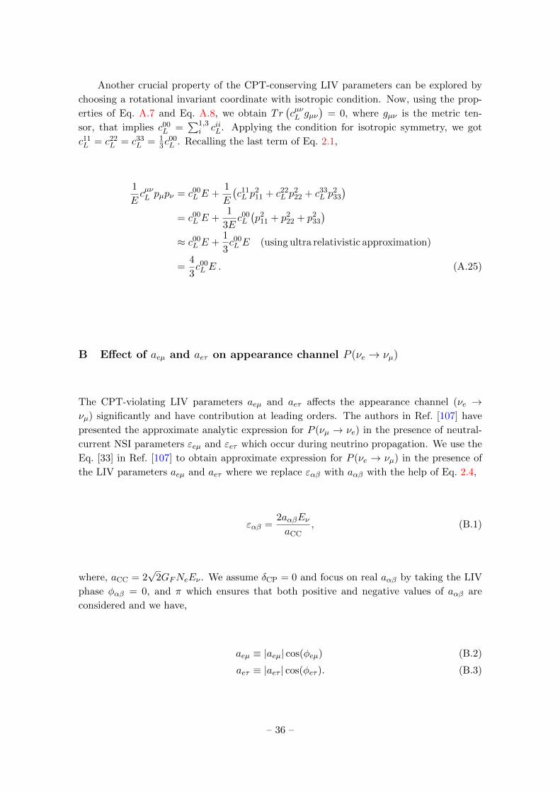
Another crucial property of the CPT-conserving LIV parameters can be explored by

choosing a rotational invariant coordinate with isotropic condition. Now, using the prop-

erties of Eq. A.7 and Eq. A.8, we obtain Tr(cµνL gµν

)= 0, where gµν is the metric ten-

sor, that implies c00L =

∑1,3i ciiL. Applying the condition for isotropic symmetry, we got

c11L = c22

L = c33L = 1

3c00L . Recalling the last term of Eq. 2.1,

1

EcµνL pµpν = c00

L E +1

E

(c11L p

211 + c22

L p222 + c33

L p233

)= c00

L E +1

3Ec00L

(p2

11 + p222 + p2

33

)≈ c00

L E +1

3c00L E (using ultra relativistic approximation)

=4

3c00L E . (A.25)

B Effect of aeµ and aeτ on appearance channel P (νe → νµ)

The CPT-violating LIV parameters aeµ and aeτ affects the appearance channel (νe →νµ) significantly and have contribution at leading orders. The authors in Ref. [107] have

presented the approximate analytic expression for P (νµ → νe) in the presence of neutral-

current NSI parameters εeµ and εeτ which occur during neutrino propagation. We use the

Eq. [33] in Ref. [107] to obtain approximate expression for P (νe → νµ) in the presence of

the LIV parameters aeµ and aeτ where we replace εαβ with aαβ with the help of Eq. 2.4,

εαβ =2aαβEνaCC

, (B.1)

where, aCC = 2√

2GFNeEν . We assume δCP = 0 and focus on real aαβ by taking the LIV

phase φαβ = 0, and π which ensures that both positive and negative values of aαβ are

considered and we have,

aeµ ≡ |aeµ| cos(φeµ) (B.2)

aeτ ≡ |aeτ | cos(φeτ ). (B.3)

– 36 –

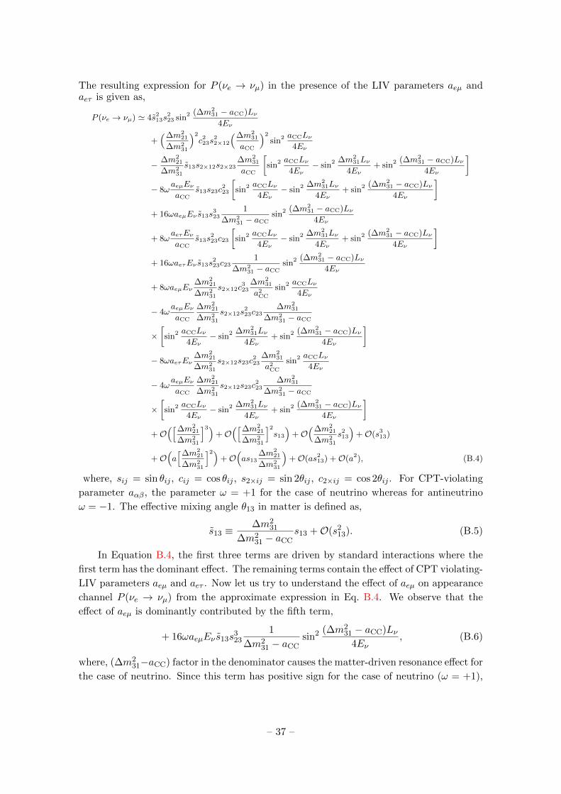
The resulting expression for P (νe → νµ) in the presence of the LIV parameters aeµ andaeτ is given as,

P (νe → νµ) ' 4s213s

223 sin2 (∆m2

31 − aCC)Lν4Eν

+(∆m2

21

∆m231

)2

c223s22×12

(∆m231

aCC

)2

sin2 aCCLν4Eν

− ∆m221

∆m231

s13s2×12s2×23∆m2

31

aCC

[sin2 aCCLν

4Eν− sin2 ∆m2

31Lν4Eν

+ sin2 (∆m231 − aCC)Lν

4Eν

]− 8ω

aeµEνaCC

s13s23c223

[sin2 aCCLν

4Eν− sin2 ∆m2

31Lν4Eν

+ sin2 (∆m231 − aCC)Lν

4Eν

]+ 16ωaeµEν s13s

323

1

∆m231 − aCC

sin2 (∆m231 − aCC)Lν

4Eν

+ 8ωaeτEνaCC

s13s223c23

[sin2 aCCLν

4Eν− sin2 ∆m2

31Lν4Eν

+ sin2 (∆m231 − aCC)Lν

4Eν

]+ 16ωaeτEν s13s

223c23

1

∆m231 − aCC

sin2 (∆m231 − aCC)Lν

4Eν

+ 8ωaeµEν∆m2

21

∆m231

s2×12c323

∆m231

a2CC

sin2 aCCLν4Eν

− 4ωaeµEνaCC

∆m221

∆m231

s2×12s223c23

∆m231

∆m231 − aCC

×[sin2 aCCLν

4Eν− sin2 ∆m2

31Lν4Eν

+ sin2 (∆m231 − aCC)Lν

4Eν

]− 8ωaeτEν

∆m221

∆m231

s2×12s23c223

∆m231

a2CC

sin2 aCCLν4Eν

− 4ωaeµEνaCC

∆m221

∆m231

s2×12s23c223

∆m231

∆m231 − aCC

×[sin2 aCCLν

4Eν− sin2 ∆m2

31Lν4Eν

+ sin2 (∆m231 − aCC)Lν

4Eν

]+O

([∆m221

∆m231

]3)+O

([∆m221

∆m231

]2s13

)+O

(∆m221

∆m231

s213

)+O(s3

13)

+O(a[∆m2

21

∆m231

]2)+O

(as13

∆m221

∆m231

)+O(as2

13) +O(a2), (B.4)

where, sij = sin θij , cij = cos θij , s2×ij = sin 2θij , c2×ij = cos 2θij . For CPT-violating

parameter aαβ, the parameter ω = +1 for the case of neutrino whereas for antineutrino

ω = −1. The effective mixing angle θ13 in matter is defined as,

s13 ≡∆m2

31

∆m231 − aCC

s13 +O(s213). (B.5)

In Equation B.4, the first three terms are driven by standard interactions where the

first term has the dominant effect. The remaining terms contain the effect of CPT violating-

LIV parameters aeµ and aeτ . Now let us try to understand the effect of aeµ on appearance

channel P (νe → νµ) from the approximate expression in Eq. B.4. We observe that the

effect of aeµ is dominantly contributed by the fifth term,

+ 16ωaeµEν s13s323

1

∆m231 − aCC

sin2 (∆m231 − aCC)Lν

4Eν, (B.6)

where, (∆m231−aCC) factor in the denominator causes the matter-driven resonance effect for

the case of neutrino. Since this term has positive sign for the case of neutrino (ω = +1),

– 37 –

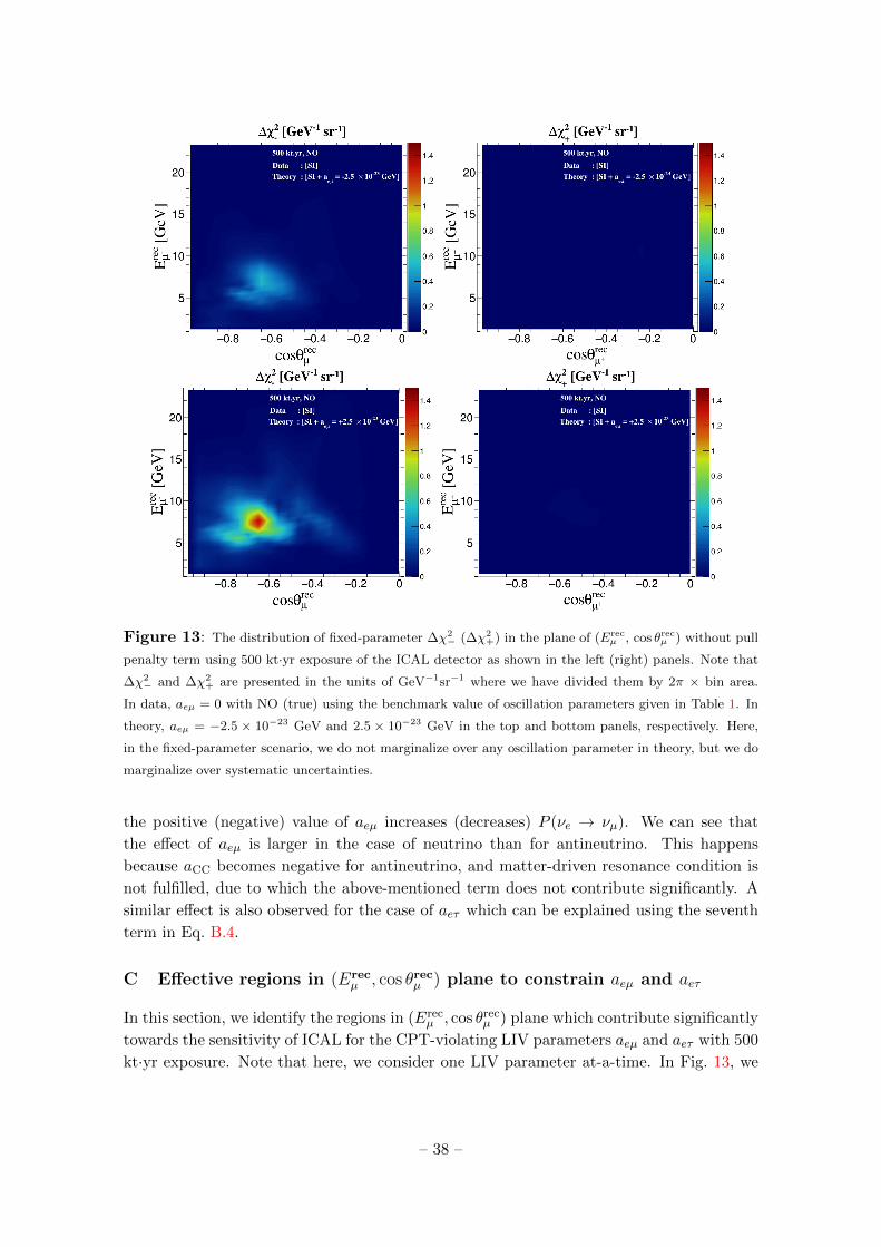
Figure 13: The distribution of fixed-parameter ∆χ2− (∆χ2

+) in the plane of (Erecµ , cos θrec

µ ) without pull

penalty term using 500 kt·yr exposure of the ICAL detector as shown in the left (right) panels. Note that

∆χ2− and ∆χ2

+ are presented in the units of GeV−1sr−1 where we have divided them by 2π × bin area.

In data, aeµ = 0 with NO (true) using the benchmark value of oscillation parameters given in Table 1. In

theory, aeµ = −2.5 × 10−23 GeV and 2.5 × 10−23 GeV in the top and bottom panels, respectively. Here,

in the fixed-parameter scenario, we do not marginalize over any oscillation parameter in theory, but we do

marginalize over systematic uncertainties.

the positive (negative) value of aeµ increases (decreases) P (νe → νµ). We can see that

the effect of aeµ is larger in the case of neutrino than for antineutrino. This happens

because aCC becomes negative for antineutrino, and matter-driven resonance condition is

not fulfilled, due to which the above-mentioned term does not contribute significantly. A

similar effect is also observed for the case of aeτ which can be explained using the seventh

term in Eq. B.4.

C Effective regions in (Erecµ , cos θrecµ ) plane to constrain aeµ and aeτ

In this section, we identify the regions in (Erecµ , cos θrec

µ ) plane which contribute significantly

towards the sensitivity of ICAL for the CPT-violating LIV parameters aeµ and aeτ with 500

kt·yr exposure. Note that here, we consider one LIV parameter at-a-time. In Fig. 13, we

– 38 –

Figure 14: The distribution of fixed-parameter ∆χ2− (∆χ2

+) in the plane of (Erecµ , cos θrec

µ ) without pull

penalty term using 500 kt·yr exposure of the ICAL detector as shown in the left (right) panels. Note that

∆χ2− and ∆χ2

+ are presented in the units of GeV−1sr−1 where we have divided them by 2π × bin area.

In data, aeτ = 0 with NO (true) using the benchmark value of oscillation parameters given in Table 1. In

theory, aeτ = −2.5 × 10−23 GeV and 2.5 × 10−23 GeV in the top and bottom panels, respectively. Here,

in the fixed-parameter scenario, we do not marginalize over any oscillation parameter in theory, but we do

marginalize over systematic uncertainties.

show the distribution of sensitivity of ICAL for aeµ in terms of fixed-parameter ∆χ2− (∆χ2

+)

without pull penalty term contributed from reconstructed µ− (µ+) events in (Erecµ , cos θrec

µ )

plane following the same procedure as described in section 7.1 for aµτ . While estimating

sensitivity of ICAL for aeµ in the top (bottom) panels in Fig. 13, we assume non-zero value

of aeµ = −2.5 × 10−23 GeV (+2.5 × 10−23 GeV) in theory while taking aeµ = 0 in data

for the case of SI. We keep the oscillation parameters fixed in theory and data at their

benchmark values as mentioned in Table 1. We consider 500 kt·yr exposure at ICAL with

NO as true mass ordering. We use the binning scheme mentioned in Table 3 where we

add contribution from all E′rechad bins for each (Erec

µ , cos θrecµ ) bins. The left and right panels

show the distribution of ∆χ2− and ∆χ2

+, respectively.

We can observe in Fig. 13 that the contribution towards the sensitivity of ICAL for aeµ

– 39 –

mainly stems from µ− as shown in left panels, whereas the contribution from µ+ is negligible

as shown in the right panels. This happens because the term with a significant contribution

of aeµ has a matter-driven resonance effect for the case of neutrino as described in section 4

while explaining the oscillograms in Fig. 2. We also observe in the left panels in Fig. 13 that

∆χ2− is significantly larger for the positive value (top left panel) of aeµ compared to that for

negative value (bottom left panel). This observation is also consistent with the asymmetric

effect of aeµ on νµ survival oscillograms shown in Fig. 2, and the reason behind this effect

is explained in detail in section 4. We would like to highlight the observation that the

sensitivity of ICAL for aeµ is significantly contributed by the reconstruction muon energy

and direction bins corresponding to the region of matter effect, which is not surprising

because the impact of aeµ is being driven by the resonance effect with the matter as

explained in section 4.

Similar to the case of aeµ, we present the distribution of sensitivity of ICAL for aeτin terms of fixed-parameter ∆χ2

− (∆χ2+) with contribution from reconstructed µ− (µ+)

events in (Erecµ , cos θrec

µ ) plane in Fig. 14. To estimate the sensitivity of ICAL for aeτ in

the top (bottom) panels in Fig. 14, we take non-zero value of aeτ = −2.5 × 10−23 GeV

(+2.5×10−23 GeV) in theory while keeping aeτ = 0 in data for the case of SI. Analogous to

the case of aeµ, we observe that the sensitivity for aeτ is more in the case of µ− (left panels)

than that for µ+ (right panels). The asymmetric effect of aeτ leads to higher sensitivity for

positive aeτ as shown in the bottom right panel of Fig. 14. These features can be explained

in the same fashion as we did for aeµ in the previous paragraph. The reasons behind these

effects of aeτ on νµ survival oscillograms are described in section 4.

References

[1] R. Gambini and J. Pullin, Nonstandard optics from quantum space-time, Phys. Rev. D 59

(1999) 124021, [gr-qc/9809038].

[2] J. Alfaro, H. A. Morales-Tecotl, and L. F. Urrutia, Quantum gravity and spin 1/2 particles

effective dynamics, Phys. Rev. D 66 (2002) 124006, [hep-th/0208192].

[3] D. Sudarsky, L. Urrutia, and H. Vucetich, New observational bounds to quantum gravity

signals, Phys. Rev. Lett. 89 (2002) 231301, [gr-qc/0204027].

[4] G. Amelino-Camelia, Quantum gravity phenomenology: Status and prospects, Mod. Phys.

Lett. A 17 (2002) 899–922, [gr-qc/0204051].

[5] Y. J. Ng, Selected topics in Planck scale physics, Mod. Phys. Lett. A 18 (2003) 1073–1098,

[gr-qc/0305019].

[6] A. M. Polyakov, Gauge Fields and Strings, vol. 3 of Contemporary concepts in physics.

Harwood Academic Publishers, 1987.

[7] V. A. Kostelecky and S. Samuel, Spontaneous Breaking of Lorentz Symmetry in String

Theory, Phys. Rev. D 39 (1989) 683.

[8] V. A. Kostelecky and R. Potting, CPT and strings, Nucl. Phys. B 359 (1991) 545–570.

[9] V. A. Kostelecky and R. Potting, Expectation values, Lorentz invariance, and CPT in the

open bosonic string, Phys. Lett. B 381 (1996) 89–96, [hep-th/9605088].

– 40 –

[10] V. A. Kostelecky and R. Potting, Analytical construction of a nonperturbative vacuum for

the open bosonic string, Phys. Rev. D 63 (2001) 046007, [hep-th/0008252].

[11] V. A. Kostelecky, M. Perry, and R. Potting, Off-shell structure of the string sigma model,

Phys. Rev. Lett. 84 (2000) 4541–4544, [hep-th/9912243].

[12] S. M. Carroll, J. A. Harvey, V. A. Kostelecky, C. D. Lane, and T. Okamoto,

Noncommutative field theory and Lorentz violation, Phys. Rev. Lett. 87 (2001) 141601,

[hep-th/0105082].

[13] I. Mocioiu, M. Pospelov, and R. Roiban, Breaking CPT by mixed noncommutativity, Phys.

Rev. D 65 (2002) 107702, [hep-ph/0108136].

[14] O. W. Greenberg, CPT violation implies violation of Lorentz invariance, Phys. Rev. Lett.

89 (2002) 231602, [hep-ph/0201258].

[15] R. C. Myers and M. Pospelov, Ultraviolet modifications of dispersion relations in effective

field theory, Phys. Rev. Lett. 90 (2003) 211601, [hep-ph/0301124].

[16] N. E. Mavromatos, Theoretical and phenomenological aspects of CPT violation, Nucl.

Instrum. Meth. B 214 (2004) 1–6, [hep-ph/0305215].

[17] D. Colladay and V. A. Kostelecky, Lorentz violating extension of the standard model, Phys.

Rev. D 58 (1998) 116002, [hep-ph/9809521].

[18] V. A. Kostelecky, Gravity, Lorentz violation, and the standard model, Phys. Rev. D 69

(2004) 105009, [hep-th/0312310].

[19] R. Bluhm, Overview of the SME: Implications and phenomenology of Lorentz violation,

Lect. Notes Phys. 702 (2006) 191–226, [hep-ph/0506054].

[20] D. Colladay and V. A. Kostelecky, CPT violation and the standard model, Phys. Rev. D 55

(1997) 6760–6774, [hep-ph/9703464].

[21] B. Pontecorvo, Neutrino Experiments and the Problem of Conservation of Leptonic Charge,

Zh. Eksp. Teor. Fiz. 53 (1967) 1717–1725.

[22] Super-Kamiokande Collaboration, K. Abe et al., Test of Lorentz invariance with

atmospheric neutrinos, Phys. Rev. D 91 (2015), no. 5 052003, [arXiv:1410.4267].

[23] J. S. Diaz, Correspondence between nonstandard interactions and CPT violation in neutrino

oscillations, arXiv:1506.01936.

[24] C. A. Arguelles, G. H. Collin, J. M. Conrad, T. Katori, and A. Kheirandish, Search for

Lorentz Violation in km3-Scale Neutrino Telescopes, in 7th Meeting on CPT and Lorentz

Symmetry, pp. 153–156, 2017. arXiv:1608.02946.

[25] IceCube Collaboration, M. G. Aartsen et al., Neutrino Interferometry for High-Precision

Tests of Lorentz Symmetry with IceCube, Nature Phys. 14 (2018), no. 9 961–966,

[arXiv:1709.03434].

[26] IceCube Collaboration, T. Katori, C. A. Arguelles, K. Farrag, and S. Mandalia, Test of

Lorentz Violation with Astrophysical Neutrino Flavor at IceCube, in 8th Meeting on CPT

and Lorentz Symmetry, pp. 166–169, 2020. arXiv:1906.09240.

[27] S. K. Agarwalla and M. Masud, Can Lorentz invariance violation affect the sensitivity of

deep underground neutrino experiment?, Eur. Phys. J. C 80 (2020), no. 8 716,

[arXiv:1912.13306].

– 41 –

[28] Super-Kamiokande Collaboration, Y. Fukuda et al., Evidence for oscillation of

atmospheric neutrinos, Phys. Rev. Lett. 81 (1998) 1562, [hep-ex/9807003].

[29] L. Wolfenstein, Neutrino Oscillations in Matter, Phys. Rev. D 17 (1978) 2369–2374.

[30] S. P. Mikheev and A. Y. Smirnov, Resonance enhancement of oscillations in matter and

solar neutrino spectroscopy, Sov. J. Nucl. Phys. 42 (1985) 913. [Yad.Fiz.42:1441-1448,1985].

[31] S. P. Mikheev and A. Y. Smirnov, Resonant amplification of neutrino oscillations in matter

and solar neutrino spectroscopy, Nuovo Cim. C 9 (1986) 17–26.

[32] S. Petcov, Diffractive - like (or parametric resonance - like?) enhancement of the earth (day

- night) effect for solar neutrinos crossing the earth core, Phys. Lett. B 434 (1998) 321,

[hep-ph/9805262].

[33] M. Chizhov, M. Maris, and S. T. Petcov, On the oscillation length resonance in the

transitions of solar and atmospheric neutrinos crossing the earth core, hep-ph/9810501.

[34] S. T. Petcov, New enhancement mechanism of the transitions in the earth of the solar and

atmospheric neutrinos crossing the earth core, Nucl. Phys. B Proc. Suppl. 77 (1999) 93–97,

[hep-ph/9809587].

[35] M. Chizhov and S. Petcov, New conditions for a total neutrino conversion in a medium,

Phys.Rev.Lett. 83 (1999) 1096–1099, [hep-ph/9903399].

[36] M. V. Chizhov and S. T. Petcov, Enhancing mechanisms of neutrino transitions in a

medium of nonperiodic constant density layers and in the earth, Phys. Rev. D 63 (2001)

073003, [hep-ph/9903424].

[37] E. K. Akhmedov, Parametric resonance of neutrino oscillations and passage of solar and

atmospheric neutrinos through the earth, Nucl. Phys. B538 (1999) 25, [hep-ph/9805272].

[38] E. K. Akhmedov, A. Dighe, P. Lipari, and A. Smirnov, Atmospheric neutrinos at

Super-Kamiokande and parametric resonance in neutrino oscillations, Nucl. Phys. B542

(1999) 3, [hep-ph/9808270].

[39] M. M. Guzzo, A. Masiero, and S. T. Petcov, On the MSW effect with massless neutrinos

and no mixing in the vacuum, Phys. Lett. B 260 (1991) 154–160.

[40] Super-Kamiokande Collaboration, G. Mitsuka et al., Study of Non-Standard Neutrino

Interactions with Atmospheric Neutrino Data in Super-Kamiokande I and II, Phys. Rev. D

84 (2011) 113008, [arXiv:1109.1889].

[41] T. Ohlsson, Status of non-standard neutrino interactions, Rept. Prog. Phys. 76 (2013)

044201, [arXiv:1209.2710].

[42] A. Esmaili and A. Y. Smirnov, Probing Non-Standard Interaction of Neutrinos with

IceCube and DeepCore, JHEP 06 (2013) 026, [arXiv:1304.1042].

[43] O. G. Miranda and H. Nunokawa, Non standard neutrino interactions: current status and

future prospects, New J. Phys. 17 (2015), no. 9 095002, [arXiv:1505.06254].

[44] J. Salvado, O. Mena, S. Palomares-Ruiz, and N. Rius, Non-standard interactions with

high-energy atmospheric neutrinos at IceCube, JHEP 01 (2017) 141, [arXiv:1609.03450].

[45] IceCube Collaboration, M. G. Aartsen et al., Search for Nonstandard Neutrino

Interactions with IceCube DeepCore, Phys. Rev. D 97 (2018), no. 7 072009,

[arXiv:1709.07079].

– 42 –

[46] Y. Farzan and M. Tortola, Neutrino oscillations and Non-Standard Interactions, Front.in

Phys. 6 (2018) 10, [arXiv:1710.09360].

[47] I. Esteban, M. C. Gonzalez-Garcia, M. Maltoni, I. Martinez-Soler, and J. Salvado, Updated

constraints on non-standard interactions from global analysis of oscillation data, JHEP 08

(2018) 180, [arXiv:1805.04530]. [Addendum: JHEP 12, 152 (2020)].

[48] P. S. Bhupal Dev et al., Neutrino Non-Standard Interactions: A Status Report, SciPost

Phys. Proc. (2019) 1, [arXiv:1907.00991].

[49] A. Khatun, S. S. Chatterjee, T. Thakore, and S. K. Agarwalla, Enhancing sensitivity to

non-standard neutrino interactions at INO combining muon and hadron information, Eur.

Phys. J. C 80 (2020), no. 6 533, [arXiv:1907.02027].

[50] C. A. Arguelles et al., New opportunities at the next-generation neutrino experiments I:

BSM neutrino physics and dark matter, Rept. Prog. Phys. 83 (2020), no. 12 124201,

[arXiv:1907.08311].

[51] KM3NeT Collaboration, N. Khan Chowdhury, T. Thakore, J. B. Coelho, J. Zornoza, and

S. Navas, Sensitivity to Non-Standard Interactions (NSI) with KM3NeT-ORCA, PoS

ICRC2019 (2020) 931.

[52] IceCube Collaboration, S. Blot, Probing Beyond Standard Model Physics via Oscillations

with IceCube DeepCore, J. Phys. Conf. Ser. 1468 (2020), no. 1 012168.

[53] A. Kumar, A. Khatun, S. K. Agarwalla, and A. Dighe, A New Approach to Probe

Non-Standard Interactions in Atmospheric Neutrino Experiments, JHEP 04 (2021) 159,

[arXiv:2101.02607].

[54] S. K. Agarwalla, S. Das, M. Masud, and P. Swain, Evolution of Neutrino Mass-Mixing

Parameters in Matter with Non-Standard Interactions, arXiv:2103.13431.

[55] IceCube Collaboration, R. Abbasi et al., All-flavor constraints on nonstandard neutrino

interactions and generalized matter potential with three years of IceCube DeepCore data,

arXiv:2106.07755.

[56] ANTARES, KM3NeT Collaboration, J. J. Hernandez Rey, N. R. Khan Chowdhury,

J. Manczak, S. Navas, and J. D. Zornoza, Search for neutrino non-standard interactions

with ANTARES and KM3NeT-ORCA, in 9th Very Large Volume Neutrino Telescopes

Workshop 2021, 7, 2021. arXiv:2107.14296.

[57] S. Razzaque and A. Yu. Smirnov, Searching for sterile neutrinos in ice, JHEP 07 (2011)

084, [arXiv:1104.1390].

[58] K. N. Abazajian et al., Light Sterile Neutrinos: A White Paper, arXiv:1204.5379.

[59] Super-Kamiokande Collaboration, K. Abe et al., Limits on sterile neutrino mixing using

atmospheric neutrinos in Super-Kamiokande, Phys. Rev. D 91 (2015) 052019,

[arXiv:1410.2008].

[60] IceCube Collaboration, M. G. Aartsen et al., Searches for Sterile Neutrinos with the

IceCube Detector, Phys. Rev. Lett. 117 (2016), no. 7 071801, [arXiv:1605.01990].

[61] IceCube Collaboration, M. G. Aartsen et al., Search for sterile neutrino mixing using three

years of IceCube DeepCore data, Phys. Rev. D 95 (2017), no. 11 112002,

[arXiv:1702.05160].

– 43 –

[62] M. Blennow, E. Fernandez-Martinez, J. Gehrlein, J. Hernandez-Garcia, and J. Salvado,

IceCube bounds on sterile neutrinos above 10 eV, Eur. Phys. J. C 78 (2018), no. 10 807,

[arXiv:1803.02362].

[63] P. B. Denton, Y. Farzan, and I. M. Shoemaker, Activating the fourth neutrino of the 3+1

scheme, Phys. Rev. D 99 (2019), no. 3 035003, [arXiv:1811.01310].

[64] L. S. Miranda and S. Razzaque, Revisiting constraints on 3 + 1 active-sterile neutrino

mixing using IceCube data, JHEP 03 (2019) 203, [arXiv:1812.00831].

[65] ANTARES Collaboration, A. Albert et al., Measuring the atmospheric neutrino

oscillation parameters and constraining the 3+1 neutrino model with ten years of

ANTARES data, JHEP 06 (2019) 113, [arXiv:1812.08650].

[66] M. H. Moulai, C. A. Arguelles, G. H. Collin, J. M. Conrad, A. Diaz, and M. H. Shaevitz,

Combining Sterile Neutrino Fits to Short Baseline Data with IceCube Data, Phys. Rev. D

101 (2020), no. 5 055020, [arXiv:1910.13456].

[67] KM3NeT Collaboration, N. R. Khan Chowdhury, Neutrino Oscillations and Non-standard

Interactions with KM3NeT-ORCA, in Prospects in Neutrino Physics, 4, 2020.

arXiv:2004.05004.

[68] IceCube Collaboration, M. G. Aartsen et al., eV-Scale Sterile Neutrino Search Using Eight

Years of Atmospheric Muon Neutrino Data from the IceCube Neutrino Observatory, Phys.

Rev. Lett. 125 (2020), no. 14 141801, [arXiv:2005.12942].

[69] IceCube Collaboration, M. G. Aartsen et al., Searching for eV-scale sterile neutrinos with

eight years of atmospheric neutrinos at the IceCube Neutrino Telescope, Phys. Rev. D 102

(2020), no. 5 052009, [arXiv:2005.12943].

[70] S. Razzaque and L. S. Miranda, Revisiting constraints on sterile neutrino mixing

parameters using IceCube atmospheric neutrino data, PoS ICRC2019 (2021) 987.

[71] A. Schneider, B. Skrzypek, C. A. Arguelles, and J. M. Conrad, Closing the Neutrino ”BSM

Gap”: Physics Potential of Atmospheric Through-Going Muons at DUNE,

arXiv:2106.01508.

[72] KM3NeT Collaboration, S. Aiello et al., Sensitivity to light sterile neutrino mixing

parameters with KM3NeT/ORCA, arXiv:2107.00344.

[73] Y. Chikashige, R. N. Mohapatra, and R. D. Peccei, Are There Real Goldstone Bosons

Associated with Broken Lepton Number?, Phys. Lett. B 98 (1981) 265–268.

[74] G. B. Gelmini and M. Roncadelli, Left-Handed Neutrino Mass Scale and Spontaneously

Broken Lepton Number, Phys. Lett. B 99 (1981) 411–415.

[75] G. B. Gelmini and J. W. F. Valle, Fast Invisible Neutrino Decays, Phys. Lett. B 142 (1984)

181–187.

[76] Super-Kamiokande Collaboration, K. Abe et al., Search for Differences in Oscillation

Parameters for Atmospheric Neutrinos and Antineutrinos at Super-Kamiokande, Phys.

Rev. Lett. 107 (2011) 241801, [arXiv:1109.1621].

[77] KM3NeT Collaboration, J. a. A. B. Coelho, Probing new physics with atmospheric

neutrinos at KM3NeT-ORCA, J. Phys. Conf. Ser. 888 (2017), no. 1 012115,

[arXiv:1702.04508].

– 44 –

[78] ICAL Collaboration, S. Ahmed et al., Physics Potential of the ICAL detector at the

India-based Neutrino Observatory (INO), Pramana 88 (2017), no. 5 79,

[arXiv:1505.07380].

[79] S. P. Behera, M. S. Bhatia, V. M. Datar, and A. K. Mohanty, Simulation Studies for

Electromagnetic Design of INO ICAL Magnet and its Response to Muons, IEEE Trans.

Magnetics 51 (2015) 4624, [arXiv:1406.3965].

[80] A. Chatterjee, K. Meghna, K. Rawat, T. Thakore, V. Bhatnagar, et al., A Simulations

Study of the Muon Response of the Iron Calorimeter Detector at the India-based Neutrino

Observatory, JINST 9 (2014) P07001, [arXiv:1405.7243].

[81] S. Goswami, Physics program of india based neutrino observatory, Nuclear Physics B -

Proceedings Supplements 188 (2009) 198–200. Proceedings of the Neutrino Oscillation

Workshop.

[82] A. Ghosh, T. Thakore, and S. Choubey, Determining the Neutrino Mass Hierarchy with

INO, T2K, NOvA and Reactor Experiments, JHEP 1304 (2013) 009, [arXiv:1212.1305].

[83] T. Thakore, A. Ghosh, S. Choubey, and A. Dighe, The Reach of INO for Atmospheric

Neutrino Oscillation Parameters, JHEP 1305 (2013) 058, [arXiv:1303.2534].

[84] A. Ghosh and S. Choubey, Measuring the Mass Hierarchy with Muon and Hadron Events in

Atmospheric Neutrino Experiments, JHEP 1310 (2013) 174, [arXiv:1306.1423].

[85] M. M. Devi, T. Thakore, S. K. Agarwalla, and A. Dighe, Enhancing sensitivity to neutrino

parameters at INO combining muon and hadron information, JHEP 10 (2014) 189,

[arXiv:1406.3689].

[86] L. S. Mohan and D. Indumathi, Pinning down neutrino oscillation parameters in the 2–3

sector with a magnetised atmospheric neutrino detector: a new study, Eur. Phys. J. C77

(2017), no. 1 54, [arXiv:1605.04185].

[87] K. R. Rebin, J. Libby, D. Indumathi, and L. S. Mohan, Study of neutrino oscillation

parameters at the INO-ICAL detector using event-by-event reconstruction, Eur. Phys. J. C

79 (2019), no. 4 295, [arXiv:1804.02138].

[88] J. Datta, M. Nizam, A. Ajmi, and S. U. Sankar, Matter vs vacuum oscillations in

atmospheric neutrinos, Nucl. Phys. B 961 (2020) 115251, [arXiv:1907.08966].

[89] A. Kumar, A. Khatun, S. K. Agarwalla, and A. Dighe, From oscillation dip to oscillation

valley in atmospheric neutrino experiments, Eur. Phys. J. C 81 (2021), no. 2 190,

[arXiv:2006.14529].

[90] A. Kumar and S. K. Agarwalla, Validating the Earth’s core using atmospheric neutrinos

with ICAL at INO, JHEP 08 (2021) 139, [arXiv:2104.11740].

[91] T. Thakore, M. M. Devi, S. K. Agarwalla, and A. Dighe, Active-sterile neutrino oscillations

at INO-ICAL over a wide mass-squared range, JHEP 08 (2018) 022, [arXiv:1804.09613].

[92] N. Dash, V. M. Datar, and G. Majumder, Sensitivity of the INO-ICAL detector to magnetic

monopoles, Astropart. Phys. 70 (2015) 33–38, [arXiv:1406.3938].

[93] S. P. Behera, A. Ghosh, S. Choubey, V. M. Datar, D. K. Mishra, and A. K. Mohanty,

Search for the sterile neutrino mixing with the ICAL detector at INO, Eur. Phys. J. C77

(2017), no. 5 307, [arXiv:1605.08607].

– 45 –

[94] A. Khatun, R. Laha, and S. K. Agarwalla, Indirect searches of Galactic diffuse dark matter

in INO-MagICAL detector, JHEP 06 (2017) 057, [arXiv:1703.10221].

[95] S. Choubey, S. Goswami, C. Gupta, S. M. Lakshmi, and T. Thakore, Sensitivity to neutrino

decay with atmospheric neutrinos at the INO-ICAL detector, Phys. Rev. D 97 (2018), no. 3

033005, [arXiv:1709.10376].

[96] A. Khatun, T. Thakore, and S. K. Agarwalla, Can INO be Sensitive to Flavor-Dependent

Long-Range Forces?, JHEP 04 (2018) 023, [arXiv:1801.00949].

[97] S. Choubey, A. Ghosh, and D. Tiwari, Prospects of Indirect Searches for Dark Matter at

INO, JCAP 05 (2018) 006, [arXiv:1711.02546].

[98] D. Tiwari, S. Choubey, and A. Ghosh, Prospects of indirect searches for dark matter

annihilations in the earth with ICAL@INO, JHEP 05 (2019) 039, [arXiv:1806.05058].

[99] A. Chatterjee, R. Gandhi, and J. Singh, Probing Lorentz and CPT Violation in a

Magnetized Iron Detector using Atmospheric Neutrinos, JHEP 1406 (2014) 045,

[arXiv:1402.6265].

[100] S. R. Coleman and S. L. Glashow, High-energy tests of Lorentz invariance, Phys. Rev. D 59

(1999) 116008, [hep-ph/9812418].

[101] D. Kaur, Z. A. Dar, S. Kumar, and M. Naimuddin, Search for the differences in

atmospheric neutrino and antineutrino oscillation parameters at the INO-ICAL experiment,

Phys. Rev. D 95 (2017), no. 9 093005, [arXiv:1703.06710].

[102] Z. A. Dar, D. Kaur, S. Kumar, and M. Naimuddin, Independent measurement of muon

neutrino and antineutrino oscillations at the INO–ICAL experiment, J. Phys. G 46 (2019),

no. 6 065001, [arXiv:2004.01127].

[103] B. Pontecorvo, Inverse beta processes and nonconservation of lepton charge, Zh. Eksp. Teor.

Fiz. 34 (1957) 247.

[104] Z. Maki, M. Nakagawa, and S. Sakata, Remarks on the unified model of elementary

particles, Prog. Theor. Phys. 28 (1962) 870–880.

[105] S. P. Mikheyev and A. Y. Smirnov, Resonance Amplification of Oscillations in Matter and

Spectroscopy of Solar Neutrinos, Sov. J. Nucl. Phys. 42 (1985) 913–917.

[106] V. A. Kostelecky and N. Russell, Data Tables for Lorentz and CPT Violation,

arXiv:0801.0287.

[107] J. Kopp, M. Lindner, T. Ota, and J. Sato, Non-standard neutrino interactions in reactor

and superbeam experiments, Phys. Rev. D 77 (2008) 013007, [arXiv:0708.0152].

[108] DUNE Collaboration, R. Acciarri et al., Long-Baseline Neutrino Facility (LBNF) and

Deep Underground Neutrino Experiment (DUNE): Conceptual Design Report, Volume 2:

The Physics Program for DUNE at LBNF, arXiv:1512.06148.

[109] A. Dziewonski and D. Anderson, Preliminary Reference Earth Model, Phys.Earth

Planet.Interiors 25 (1981) 297–356.

[110] M. C. Gonzalez-Garcia and M. Maltoni, Atmospheric neutrino oscillations and new physics,

Phys. Rev. D70 (2004) 033010, [hep-ph/0404085].

[111] I. Mocioiu and W. Wright, Non-standard neutrino interactions in the mu–tau sector,

Nucl.Phys. B893 (2015) 376–390, [arXiv:1410.6193].

– 46 –

[112] V. A. Kostelecky and M. Mewes, Lorentz and CPT violation in neutrinos, Phys. Rev. D 69

(2004) 016005, [hep-ph/0309025].

[113] V. A. Kostelecky and M. Mewes, Lorentz violation and short-baseline neutrino experiments,

Phys. Rev. D 70 (2004) 076002, [hep-ph/0406255].

[114] V. A. Kostelecky and M. Mewes, Lorentz and CPT violation in the neutrino sector, Phys.

Rev. D 70 (2004) 031902, [hep-ph/0308300].

[115] T. Katori, V. A. Kostelecky, and R. Tayloe, Global three-parameter model for neutrino

oscillations using Lorentz violation, Phys. Rev. D 74 (2006) 105009, [hep-ph/0606154].

[116] V. Barger, D. Marfatia, and K. Whisnant, Challenging Lorentz noninvariant neutrino

oscillations without neutrino masses, Phys. Lett. B 653 (2007) 267–277,

[arXiv:0706.1085].

[117] J. S. Diaz, V. A. Kostelecky, and M. Mewes, Perturbative Lorentz and CPT violation for

neutrino and antineutrino oscillations, Phys. Rev. D 80 (2009) 076007, [arXiv:0908.1401].

[118] J. S. Diaz, Overview of Lorentz Violation in Neutrinos, in Meeting of the APS Division of

Particles and Fields, 9, 2011. arXiv:1109.4620.

[119] V. Barger, J. Liao, D. Marfatia, and K. Whisnant, Lorentz noninvariant oscillations of

massless neutrinos are excluded, Phys. Rev. D 84 (2011) 056014, [arXiv:1106.6023].

[120] J. S. Diaz and V. A. Kostelecky, Three-parameter Lorentz-violating texture for neutrino

mixing, Phys. Lett. B 700 (2011) 25–28, [arXiv:1012.5985].

[121] A. Kostelecky and M. Mewes, Neutrinos with Lorentz-violating operators of arbitrary

dimension, Phys. Rev. D 85 (2012) 096005, [arXiv:1112.6395].

[122] J. S. Diaz and A. Kostelecky, Lorentz- and CPT-violating models for neutrino oscillations,

Phys. Rev. D 85 (2012) 016013, [arXiv:1108.1799].

[123] LSND Collaboration, L. B. Auerbach et al., Tests of Lorentz violation in anti-nu(mu) —>

anti-nu(e) oscillations, Phys. Rev. D 72 (2005) 076004, [hep-ex/0506067].

[124] MINOS Collaboration, P. Adamson et al., Testing Lorentz Invariance and CPT

Conservation with NuMI Neutrinos in the MINOS Near Detector, Phys. Rev. Lett. 101

(2008) 151601, [arXiv:0806.4945].

[125] MINOS Collaboration, P. Adamson et al., A Search for Lorentz Invariance and CPT

Violation with the MINOS Far Detector, Phys. Rev. Lett. 105 (2010) 151601,

[arXiv:1007.2791].

[126] IceCube Collaboration, R. Abbasi et al., Search for a Lorentz-violating sidereal signal with

atmospheric neutrinos in IceCube, Phys. Rev. D 82 (2010) 112003, [arXiv:1010.4096].

[127] MiniBooNE Collaboration, A. A. Aguilar-Arevalo et al., Test of Lorentz and CPT

violation with Short Baseline Neutrino Oscillation Excesses, Phys. Lett. B 718 (2013)

1303–1308, [arXiv:1109.3480].

[128] MINOS Collaboration, P. Adamson et al., Search for Lorentz invariance and CPT

violation with muon antineutrinos in the MINOS Near Detector, Phys. Rev. D 85 (2012)

031101, [arXiv:1201.2631].

[129] Double Chooz Collaboration, Y. Abe et al., First Test of Lorentz Violation with a

Reactor-based Antineutrino Experiment, Phys. Rev. D 86 (2012) 112009,

[arXiv:1209.5810].

– 47 –

[130] B. Rebel and S. Mufson, The Search for Neutrino-Antineutrino Mixing Resulting from

Lorentz Invariance Violation using neutrino interactions in MINOS, Astropart. Phys. 48

(2013) 78–81, [arXiv:1301.4684].

[131] J. S. Dıaz, T. Katori, J. Spitz, and J. M. Conrad, Search for neutrino-antineutrino

oscillations with a reactor experiment, Phys. Lett. B 727 (2013) 412–416,

[arXiv:1307.5789].

[132] J. S. Diaz and T. Schwetz, Limits on CPT violation from solar neutrinos, Phys. Rev. D 93

(2016), no. 9 093004, [arXiv:1603.04468].

[133] T2K Collaboration, K. Abe et al., Search for Lorentz and CPT violation using sidereal

time dependence of neutrino flavor transitions over a short baseline, Phys. Rev. D 95

(2017), no. 11 111101, [arXiv:1703.01361].

[134] Daya Bay Collaboration, D. Adey et al., Search for a time-varying electron antineutrino

signal at Daya Bay, Phys. Rev. D 98 (2018), no. 9 092013, [arXiv:1809.04660].

[135] V. Antonelli, L. Miramonti, and M. D. C. Torri, Phenomenological Effects of CPT and

Lorentz Invariance Violation in Particle and Astroparticle Physics, Symmetry 12 (2020),

no. 11 1821, [arXiv:2110.09185].

[136] A. Marrone, Phenomenology of Three Neutrino Oscillations, 2021. Talk given at the XIX

International Workshop on Neutrino Telescopes, 18th to 26th February, 2021, Padova, Italy,

https://agenda.infn.it/event/24250/overview.

[137] NuFIT 5.0 (2020), http://www.nu-fit.org/.

[138] I. Esteban, M. C. Gonzalez-Garcia, M. Maltoni, T. Schwetz, and A. Zhou, The fate of

hints: updated global analysis of three-flavor neutrino oscillations, JHEP 09 (2020) 178,

[arXiv:2007.14792].

[139] P. F. de Salas, D. V. Forero, S. Gariazzo, P. Martınez-Mirave, O. Mena, C. A. Ternes,

M. Tortola, and J. W. F. Valle, 2020 global reassessment of the neutrino oscillation picture,

JHEP 02 (2021) 071, [arXiv:2006.11237].

[140] A. de Gouvea, J. Jenkins, and B. Kayser, Neutrino mass hierarchy, vacuum oscillations,

and vanishing U(e3), Phys.Rev. D71 (2005) 113009, [hep-ph/0503079].

[141] H. Nunokawa, S. J. Parke, and R. Zukanovich Funchal, Another possible way to determine

the neutrino mass hierarchy, Phys.Rev. D72 (2005) 013009, [hep-ph/0503283].

[142] R. Gandhi, P. Ghoshal, S. Goswami, P. Mehta, and S. U. Sankar, Large matter effects in

nu(mu) to nu(tau) oscillations, Phys.Rev.Lett. 94 (2005) 051801, [hep-ph/0408361].

[143] R. Santonico and R. Cardarelli, Development of resistive plate counters, Nuclear

Instruments and Methods in Physics Research 187 (1981), no. 2 377 – 380.

[144] S. Bheesette, Design and Characterisation Studies of Resistive Plate Chambers. PhD thesis,

Indian Inst. Tech., Mumbai, 2009.

[145] M. Bhuyan et al., Development of 2m x 2m size glass RPCs for INO, Nucl. Instrum. Meth.

A 661 (2012) S64–S67.

[146] N. Dash, V. M. Datar, and G. Majumder, A Study on the time resolution of Glass RPC,

arXiv:1410.5532.

[147] A. D. Bhatt, V. M. Datar, G. Majumder, N. K. Mondal, Pathaleswar, and

– 48 –

B. Satyanarayana, Improvement of time measurement with the INO-ICAL resistive plate

chambers, JINST 11 (2016), no. 11 C11001.

[148] A. Gaur, A. Kumar, and M. Naimuddin, Study of timing response and charge spectra of

glass based Resistive Plate Chamber detectors for INO-ICAL experiment, JINST 12 (2017),

no. 03 C03081.

[149] D. Casper, The Nuance neutrino physics simulation, and the future, Nucl. Phys. Proc.

Suppl. 112 (2002) 161, [hep-ph/0208030].

[150] M. Sajjad Athar, M. Honda, T. Kajita, K. Kasahara, and S. Midorikawa, Atmospheric

neutrino flux at INO, South Pole and Pyhasalmi, Phys. Lett. B718 (2013) 1375,

[arXiv:1210.5154].

[151] M. Honda, M. Sajjad Athar, T. Kajita, K. Kasahara, and S. Midorikawa, Atmospheric

neutrino flux calculation using the NRLMSISE-00 atmospheric model, Phys. Rev. D 92

(2015), no. 2 023004, [arXiv:1502.03916].

[152] N. Dash, Feasibility studies for the detection of exotic particles using ICAL at INO. PhD

thesis, HBNI, Mumbai, 2015.

[153] M. M. Devi, A. Ghosh, D. Kaur, L. S. Mohan, S. Choubey, et al., Hadron energy response

of the Iron Calorimeter detector at the India-based Neutrino Observatory, JINST 8 (2013)

P11003, [arXiv:1304.5115].

[154] K. Bhattacharya, Event Reconstruction for ICAL Detector and Neutrino Mass Hierarchy

Sensitivity Analysis at India-based Neutrino Observatory (INO). PhD thesis, TIFR,

Mumbai, 2015.

[155] S. Pal, Development of the INO-ICAL detector and its physics potential. PhD thesis, HBNI,

Mumbai, 2014.

[156] M. Blennow, P. Coloma, P. Huber, and T. Schwetz, Quantifying the sensitivity of oscillation

experiments to the neutrino mass ordering, JHEP 1403 (2014) 028, [arXiv:1311.1822].

[157] S. Baker and R. D. Cousins, Clarification of the Use of Chi Square and Likelihood

Functions in Fits to Histograms, Nucl. Instrum. Meth. 221 (1984) 437–442.

[158] J. Kameda, Detailed studies of neutrino oscillations with atmospheric neutrinos of wide

energy range from 100 MeV to 1000 GeV in Super-Kamiokande. PhD thesis, Tokyo U.,

2002.

[159] P. Huber, M. Lindner, and W. Winter, Superbeams versus neutrino factories, Nucl. Phys.

B645 (2002) 3–48, [hep-ph/0204352].

[160] G. L. Fogli, E. Lisi, A. Marrone, D. Montanino, and A. Palazzo, Getting the most from the

statistical analysis of solar neutrino oscillations, Phys. Rev. D 66 (2002) 053010,

[hep-ph/0206162].

[161] V. A. Kostelecky and R. Lehnert, Stability, causality, and Lorentz and CPT violation, Phys.

Rev. D 63 (2001) 065008, [hep-th/0012060].

[162] V. A. Kostelecky, C. D. Lane, and A. G. M. Pickering, One loop renormalization of Lorentz

violating electrodynamics, Phys. Rev. D 65 (2002) 056006, [hep-th/0111123].

– 49 –