privacy-preserving data publishing for cluster analysis

Privacy-Preserving Data Publishing for

Cluster Analysis

Benjamin C. M. Fung ∗Concordia Institute for Information Systems Engineering

Concordia University, Montreal, QC, Canada H3G 1M8

Ke Wang

School of Computing Science

Simon Fraser University, BC, Canada V5A 1S6

Lingyu Wang

Concordia Institute for Information Systems Engineering

Concordia University, Montreal, QC, Canada H3G 1M8

Patrick C. K. Hung

Faculty of Business and Information Technology

University of Ontario Institute of Technology, Oshawa, ON, Canada L1H 7K4

Abstract

Releasing person-specific data could potentially reveal sensitive information aboutindividuals. k-anonymization is a promising privacy protection mechanism in datapublishing. Although substantial research has been conducted on k-anonymizationand its extensions in recent years, only a few prior works have considered releasingdata for some specific purpose of data analysis. This paper presents a practical datapublishing framework for generating a masked version of data that preserves bothindividual privacy and information usefulness for cluster analysis. Experiments onreal-life data suggest that by focusing on preserving cluster structure in the maskingprocess, the cluster quality is significantly better than the cluster quality of themasked data without such focus. The major challenge of masking data for clusteranalysis is the lack of class labels that could be used to guide the masking process.Our approach converts the problem into the counterpart problem for classificationanalysis, wherein class labels encode the cluster structure in the data, and presentsa framework to evaluate the cluster quality on the masked data.

Key words: privacy, knowledge discovery, anonymity, cluster analysis

Preprint submitted to Elsevier 6 December 2008

1 Introduction

Information sharing is a vital building block for today’s business world. In June2004, the Information Technology Advisory Committee released a report en-titled Revolutionizing Health Care Through Information Technology [31]. Akey point is the establishment of a nationwide system of electronic medicalrecords that encourages sharing medical knowledge through computer-assistedclinical decision support. The report states that “all information about a pa-tient from any source could be securely available to any health care providerwhen needed, while assuring patient control over privacy.” However, in manyreal-life data publishing scenarios, individual participants (e.g., the patients)do not even have the right to opt out from the sharing. For example, licensedhospitals in California are required to submit specific demographic data on ev-ery patient discharged from their facility [7]. Thus, the burden of data privacyprotection falls on the shoulder of the data holder (e.g., the hospital). Thispaper presents a technical response to the demand for simultaneous privacyprotection and information sharing, specifically for the task of cluster analysis.

In this paper, we define the data publishing scenario as follows. Consider aperson-specific data table T with patients’ information on Zip code, Birthplace,Gender, and Disease. The data holder wants to publish T to some recipientfor cluster analysis. However, if a set of attributes, called a Quasi-Identifieror a QID, on {Zip code, Birthplace, Gender} is so specific that few peoplematch it, publishing the table will lead to linking a unique or small numberof individuals with the sensitive information on Disease. Even if the currentlypublished table T does not contain sensitive information, individuals in Tcan be linked to the sensitive information in some (readily available) externalsource by a join on the common attributes [33][40]. The problem studied inthis paper is to generate a masked version of T that satisfies two requirements:the anonymity requirement and the clustering requirement.

Anonymity Requirement: To protect privacy, instead of publishing the rawtable T (QID, Sensitive attribute), the data holder publishes a masked table

∗ Corresponding author.Email addresses: [email protected] (Benjamin C. M. Fung),

[email protected] (Lingyu Wang), [email protected] (Patrick C.K. Hung).

URLs: www.ciise.concordia.ca/~fung (Benjamin C. M. Fung),www.cs.sfu.ca/~wangk (Ke Wang), www.ciise.concordia.ca/~wang (LingyuWang), www.hrl.uoit.ca/~ckphung (Patrick C. K. Hung).

2

T ∗, where QID is a set of quasi-identifying attributes masked to some generalconcept. For example, QID = {Zip code, Birthplace, Gender}. The data holdercould generalize the values in Birthplace from city level to region level so thatmore records will match the generalized description and, therefore, individu-als who match the description will become less identifiable. The anonymityrequirement is specified by k-anonymity [33][40]: A masked table T ∗ satisfiesk-anonymity if each record in T ∗ shares the same value on QID with at leastk − 1 other records, where k is an anonymity threshold specified by the dataholder. 1 All records in the same QID group are made indistinguishable and,therefore, it is difficult to determine whether a matched individual actuallyhas the disease from T ∗.

Clustering Requirement: The data holder wants to publish a masked tableT ∗ to a recipient for the purpose of cluster analysis, the goal of which is togroup similar objects into the same cluster and group dissimilar objects intodifferent clusters. We assume that the Sensitive attribute is important for thetask of cluster analysis; otherwise, it should be removed. The recipient mayor may not be known at the time of data publication.

We study the anonymity problem for cluster analysis : For a given anonymityrequirement and a raw data table T , a data holder wants to generate an anony-mous version of T , denoted by T ∗, that preserves as much of the informationas possible for cluster analysis, and then publish T ∗ to a data recipient. Thedata holder, for example, could be a hospital that wants to share its patients’information with a drug company for pharmaceutical research.

There are many possible masked versions of T ∗ that satisfy the anonymityrequirement. The challenge is how to identify the appropriate one for clusteranalysis. An inappropriately masked version could put originally dissimilarobjects into the same cluster, or put originally similar objects into differentclusters because other masked objects become more similar to each other.Therefore, a quality-guided masking process is crucial. Unlike the anonymityproblem for classification analysis [12], the anonymity problem for cluster anal-ysis does not have class labels to guide the masking. Another challenge is thatit is not even clear what “information for cluster analysis” means, nor how toevaluate the cluster quality of generalized data. In this paper, we define theanonymity problem for cluster analysis and present a solution framework toaddress the challenges in the problem. Our contributions to the literature canbe summarized by answering the following key questions:

(1) Can a masked table simultaneously satisfy both anonymity and cluster-ing requirements? Our insight is that the two requirements are indeeddealing with two types of information: The anonymity requirement aims

1 To avoid confusion with the number of clusters k in k-means clustering algorithmdiscussed later, we use h to denote anonymity threshold in the rest of this paper.

3

at masking identifying information that specifically describes individuals;the clustering requirement aims at extracting general structures that cap-ture patterns. If masking is carefully performed, identifying informationcan be masked while still preserving the patterns for cluster analysis. Ourexperimental results on real-life data support this insight.

(2) What information should be preserved for cluster analysis in the maskeddata? We present a framework to convert the anonymity problem forcluster analysis to the counterpart problem for classification analysis. Theidea is to extract the cluster structure from the raw data, encode it inthe form of class labels, and preserve such class labels while masking thedata. The framework also permits the data holder to evaluate the clusterquality of the anonymized data by comparing the cluster structures beforeand after the masking. This evaluation process is important for datapublishing in practice, but very limited study has been conducted in thecontext of privacy preservation and cluster analysis.

(3) Can cluster-quality guided anonymization improve the cluster quality inanonymous data? A naive solution to the studied privacy problem isto ignore the clustering requirement and employ some general purposeanonymization algorithms, e.g., [20], to mask data for cluster analysis.Extensive experiments suggest that by focusing on preserving clusterstructure in the masking process, the cluster quality outperforms thecluster quality on masked data without such focus. Our experiments alsodemonstrate there is a trade-off between privacy protection and clusterquality. In general, the cluster quality on the masked data degrades asthe anonymity threshold k increases.

(4) Can the specification of multiple quasi-identifiers improve the cluster qual-ity in anonymous data? The classic notion of k-anonymity assumes thata single united quasi-identifier QID contains all quasi-identifying at-tributes, but research shows that it often leads to substantial loss of dataquality as the QID size increases [1]. Our insight is that, in practice, anattacker is unlikely to know all identifying attributes of a target victim(the person being identified), so the data is over-protected by a singleQID. Our proposed method allows the specification of multiple QIDs,each of which has a smaller size, and therefore avoids over-masking andimproves the cluster quality.

Given that the clustering task is known in advance, why not publish the analy-sis result instead of the data records? Unlike classification trees and associationrules, publishing the cluster statistics (e.g., cluster centers, together with theirsize and radius) usually cannot fulfil the information needs for cluster analysis.Often, data recipients want to browse into the clustered records to gain moreknowledge. For example, a medical researcher may browse into some clustersof patients and examine their common characteristics. Publishing data recordsnot only fulfills the vital requirement for cluster analysis, but also increasesthe availability of information for the recipients.

4

The paper is organized as follows. We review related works in Section 2, definethe problem in Section 3, present the framework of our approach in Section 4,and evaluate it in Section 5. Then, we show the extensions of the framework toachieve other privacy notions in Section 6 and conclude the paper in Section 7.

2 Related Works

Recently, the research topic of privacy-preserving data publishing (PPDP) hasreceived a great deal of attention in the database and data mining researchcommunities. The literature in PPDP can be broadly categorized by linkageprevention models. A privacy violation occurs when a person is linked to arecord or to a value on Sensitive attribute; these violations are called recordlinkage and attribute linkage. In both types of violations, the attacker knowsthe QID of the victim and that the victim has a record in the released table.

In the attack of record linkage, some value qid on QID identifies a smallnumber of records in the released table T . If the victim’s QID matches thevalue qid, the victim is vulnerable to being linked to the small number ofrecords in the qid group. In this case, the attacker faces only a small number ofpossibilities for the victim’s record, and with the help of additional knowledge,there is a chance that the attacker could uniquely identify the victim’s recordfrom the group. The notion of k-anonymity [33][40] and its variations [21][27]are proposed to prevent record linkage through QID.

In the attack of attribute linkage, the attacker may not precisely identify therecord of the victim, but could infer his or her sensitive values from the pub-lished data T , based on the set of sensitive values associated with the groupthat the victim belongs to. If some sensitive values predominate in a qid group,a successful inference becomes relatively easy even if k-anonymity is satisfied.Alternative privacy notions, such as `-diversity [25] and confidence bound-ing [45][46], are proposed to prevent attribute linkage. The general idea isto de-associate the correlation between QID and Sensitive attribute so thateven if the attacker can identify the QID group of the victim, the attackercannot infer the victim’s sensitive information. The `-diversity requires everyqid group to contain at least ` “well-represented” sensitive values. Thus, a `-diverse table also satisfies k-anonymity with k = `. Yet, not all privacy notionsthat thwart attribute linkages can thwart record linkages. For example, con-fidence bounding [46] cannot prevent record linkages. [47] proposed a unifiednotion of k-anonymity and confidence bounding to prevent both linkages.

Many generalization methods [8][19][20][23][25][39][48][49] have been proposedto achieve the above mentioned privacy notions, but they use simple qual-ity measures to guide the masking process and do not consider data min-

5

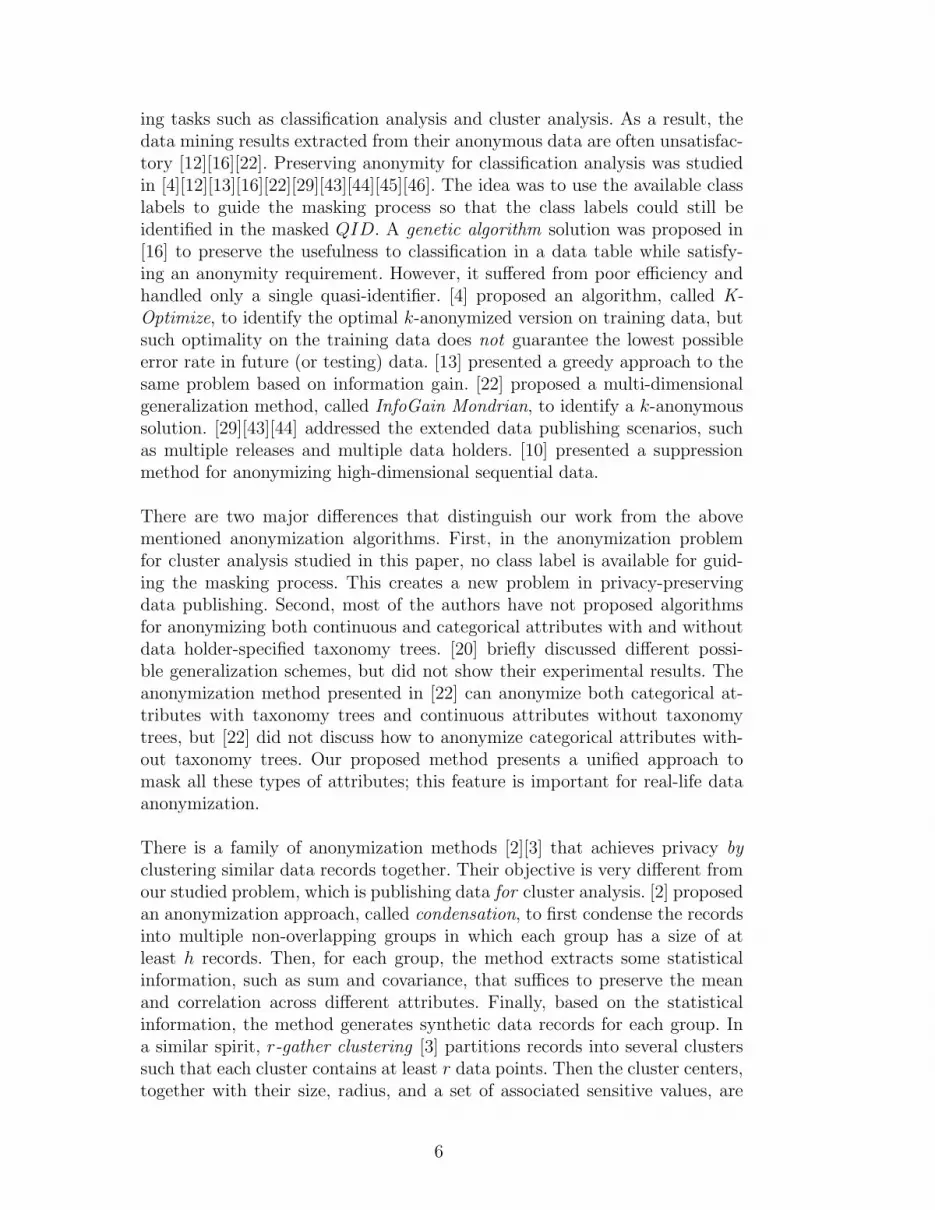
ing tasks such as classification analysis and cluster analysis. As a result, thedata mining results extracted from their anonymous data are often unsatisfac-tory [12][16][22]. Preserving anonymity for classification analysis was studiedin [4][12][13][16][22][29][43][44][45][46]. The idea was to use the available classlabels to guide the masking process so that the class labels could still beidentified in the masked QID. A genetic algorithm solution was proposed in[16] to preserve the usefulness to classification in a data table while satisfy-ing an anonymity requirement. However, it suffered from poor efficiency andhandled only a single quasi-identifier. [4] proposed an algorithm, called K-Optimize, to identify the optimal k-anonymized version on training data, butsuch optimality on the training data does not guarantee the lowest possibleerror rate in future (or testing) data. [13] presented a greedy approach to thesame problem based on information gain. [22] proposed a multi-dimensionalgeneralization method, called InfoGain Mondrian, to identify a k-anonymoussolution. [29][43][44] addressed the extended data publishing scenarios, suchas multiple releases and multiple data holders. [10] presented a suppressionmethod for anonymizing high-dimensional sequential data.

There are two major differences that distinguish our work from the abovementioned anonymization algorithms. First, in the anonymization problemfor cluster analysis studied in this paper, no class label is available for guid-ing the masking process. This creates a new problem in privacy-preservingdata publishing. Second, most of the authors have not proposed algorithmsfor anonymizing both continuous and categorical attributes with and withoutdata holder-specified taxonomy trees. [20] briefly discussed different possi-ble generalization schemes, but did not show their experimental results. Theanonymization method presented in [22] can anonymize both categorical at-tributes with taxonomy trees and continuous attributes without taxonomytrees, but [22] did not discuss how to anonymize categorical attributes with-out taxonomy trees. Our proposed method presents a unified approach tomask all these types of attributes; this feature is important for real-life dataanonymization.

There is a family of anonymization methods [2][3] that achieves privacy byclustering similar data records together. Their objective is very different fromour studied problem, which is publishing data for cluster analysis. [2] proposedan anonymization approach, called condensation, to first condense the recordsinto multiple non-overlapping groups in which each group has a size of atleast h records. Then, for each group, the method extracts some statisticalinformation, such as sum and covariance, that suffices to preserve the meanand correlation across different attributes. Finally, based on the statisticalinformation, the method generates synthetic data records for each group. Ina similar spirit, r-gather clustering [3] partitions records into several clusterssuch that each cluster contains at least r data points. Then the cluster centers,together with their size, radius, and a set of associated sensitive values, are

6

released. Compared to the masking approach, one limitation of the clusteringapproach is that the published records are “synthetic” in that they may notcorrespond to the real world entities represented by the raw data. As a result,the analysis result is difficult to justify if, for example, a police officer wants todetermine the common characteristics of some criminals from the data records.

Many secure protocols have been proposed for distributed computation amongmultiple parties. For example, [41] and [15] presented secure protocols to gen-erate a clustering solution from vertically and horizontally partitioned dataowned by multiple parties. In their model, accessing data held by other partiesis prohibited, and only the final cluster solution is shared among participatingparties. We consider a completely different problem, of which the goal is toshare data that is immunized against privacy attacks.

We highlight some recent development in cluster analysis. [5] presented amethod for clustering parallel data streams. [6] studied the problem of clus-tering spatial-temporal data. [28] presented a number of efficient clusteringstrategies for distributed database. [14] conducted an extensive empirical studyon different clustering methods.

3 Problem Statements

A labelled table has the form T (D1, . . . , Dm, Class) and contains a set ofrecords of the form 〈v1, . . . , vm, cls〉, where vj, for 1 ≤ j ≤ m, is a domainvalue of attribute Dj, and cls is a class label of the Class attribute. Each Dj

is either a categorical or a continuous attribute. An unlabelled table has thesame form as a labelled table but without the Class attribute.

Suppose that a data holder wants to publish a person-specific table T ∗, but alsowants to protect against linking an individual to sensitive information eitherinside or outside T ∗ through some sets of identifying attributes, called quasi-identifiers QID. A sensitive record linking occurs if some value on a quasi-identifier is shared by only a small number of records in T ∗. This requirementis formally defined below.

Definition 3.1 (Anonymity requirement) Consider p quasi-identifiers QID1,. . ., QIDp on T ∗, where QIDi ⊆ {D1, . . . , Dm} for 1 ≤ i ≤ p. a(qidi) de-notes the number of data records in T ∗ that share the value qidi on QIDi.The anonymity of QIDi, denoted by A(QIDi), is the minimum a(qidi) forany value qidi on QIDi. A table T ∗ satisfies the anonymity requirement{〈QID1, h1〉, . . . , 〈QIDp, hp〉} if A(QIDi) ≥ hi for 1 ≤ i ≤ p, where QIDi

and the anonymity thresholds hi are specified by the data holder.

7

Table 1The labelled table

Rec ID Education Gender Age ... Class Count

1-3 9th M 30 0C1 3C2 3

4-7 10th M 32 0C1 4C2 4

8-12 11th M 35 2C1 3C2 5

13-16 12th F 37 3C1 1C2 4

17-22 Bachelors F 42 4C1 2C2 6

23-26 Bachelors F 44 4C1 0C2 4

27-30 Masters M 44 4C1 0C2 4

31-33 Masters F 44 3C1 0C2 3

34 Doctorate F 44 1C1 0C2 1

Total: 21C1 13C2 34

Secondary University

Junior Sec.

11th

Bachelors

Masters

ANY

Senior Sec.

Doctorate

Grad School

Education

12th10th9th

ANY

Male Female

Gender

[1-35)

[1-99)

[1-37) [37-99)

[35-37)

Age

Fig. 1. Taxonomy trees

If some QIDj could be “covered” by another QIDi, then QIDj can be removedfrom the anonymity requirement. This observation is stated as follows:

Observation 3.1 (Cover) Suppose QIDj ⊆ QIDi and hj ≤ hi where j 6= i.If A(QIDi) ≥ hi, then A(QIDj) ≥ hj. We say that QIDj is covered by QIDi;therefore, QIDj is redundant and can be removed.

Example 3.1 Consider the data in Table 1 and taxonomy trees in Figure 1.Ignore the dashed line in Figure 1 for now. The table has 34 records, witheach row representing one or more raw records that agree on (Education,Gender, Age). The Class column stores a count for each class label. Theanonymity requirement 〈QID1 = {Education,Gender}, 4〉 states that everyexisting qid1 in the table must be shared by at least 4 records. Therefore,〈9th,M〉, 〈Masters,F〉, 〈Doctorate,F〉 violate this requirement. To make the“female doctor” less unique, we can generalize Masters and Doctorate to GradSchool. As a result, “she” becomes less identifiable by being one of the fourfemales who have a graduate degree in the masked table T ∗.

Definition 3.1 generalizes the classic notion of k-anonymity [34] by allowing

8

multiple QIDs with different anonymity thresholds. The specification of mul-tiple QIDs is based on an assumption that the data holder knows exactlywhat external information source is available for sensitive record linkage. Theassumption is realistic in some data publishing scenarios. Suppose that thedata holder wants to release a table T ∗(A,B, C, D, S), where A, B, C, D areidentifying attributes and S is a sensitive attribute, and knows that the recip-ient has access to previously released tables T1∗(A,B,X) and T2∗(C, D, Y ),where X and Y are attributes not in T . To prevent linking the records in Tto X or Y , the data holder only has to specify the anonymity requirementon QID1 = {A,B} and QID2 = {C, D}. In this case, enforcing anonymityon QID = {A,B, C, D} will distort the data more than is necessary. Mostprevious works suffer from this over-masking problem because they simply in-clude all potential identifying attributes into a single QID. The experimentalresults in Section 5 confirm that the specification of multiple QIDs can reducemasking and, therefore, improve the data quality.

Masking operations: To transform a table T to satisfy an anonymity re-quirement, we apply one of the following three types of masking operationson every attribute Dj in ∪QIDi: If Dj is a categorical attribute with pre-specified taxonomy tree, then we generalize Dj. Specifying taxonomy trees,however, requires expert knowledge of the data. In case the data holder lackssuch knowledge or, for any reason, does not specify a taxonomy tree for thecategorical attribute Dj, then we suppress Dj. If Dj is a continuous attributewithout a pre-discretized taxonomy tree, then we discretize Dj.

2 These threetypes of masking operations are formally described as follows:

(1) Generalize Dj if it is a categorical attribute with a taxonomy tree speci-fied by the data holder. Figure 1 shows the taxonomy trees for categoricalattributes Education and Gender. A leaf node represents a domain valueand a parent node represents a less specific value. A generalized Dj canbe viewed as a “cut” through its taxonomy tree. A cut of a tree is a sub-set of values in the tree, denoted Cutj, that contains exactly one valueon each root-to-leaf path. Figure 1 shows a cut on Education and Gen-der, indicated by the dash line. If a value v is generalized to its parent,all siblings of v must also be generalized to its parent. This propertyensures that a value and its ancestor values will not coexist in the gen-eralized table T ∗. This generalization scheme was previously employedin [4][11][12][16][43][44].

(2) Suppress Dj if it is a categorical attribute without a taxonomy tree.Suppressing a value on Dj means replacing all occurrences of the valuewith the special value ⊥j. All suppressed values on Dj are represented bythe same value ⊥j. We use Supj to denote the set of values suppressed

2 A continuous attribute with a pre-discretized taxonomy tree is equivalent to acategorical attribute with a pre-specified taxonomy tree.

9

by ⊥j. This type of suppression is performed at the value level, in thatSupj in general contains a subset of the values in the attribute Dj. Aclustering algorithm treats ⊥j as a new value. Suppression can be viewedas a special case of generalization by considering ⊥j to be the root of ataxonomy tree and child(⊥j) to contain all domain values of Dj. In thisspecial case of generalization (which we call it suppression), we couldselectively generalize (suppress) some values in child(⊥j) to ⊥j whilesome other values in child(⊥j) remain intact.

(3) Discretize Dj if it is a continuous attribute. Discretizing a value v onDj means replacing all occurrences of v with an interval containing thevalue. Our algorithm dynamically grows a taxonomy tree for intervals atruntime. Each node represents an interval. Each non-leaf node has twochild nodes representing some optimal binary split of the parent interval.Figure 1 shows such a dynamically grown taxonomy tree for Age, where[1−99) is split into [1−37) and [37−99). More details will be discussed inSection 4.2.1. A discretized Dj can be represented by the set of intervals,denoted Intj, corresponding to the leaf nodes in the dynamically growntaxonomy tree of Dj.

A masked table T can be represented by 〈∪Cutj,∪Supj,∪Intj〉, where Cutj,Supj, Intj are defined above. If the masked table T ∗ satisfies the anonymity re-quirement, then 〈∪Cutj,∪Supj,∪Intj〉 is called a solution set. Generalization,suppression, and discretization have their own merits and flexibility; therefore,our unified framework employs all of them.

What kind of information should be preserved for cluster analysis? Unlike clas-sification analysis, wherein the information utility of attributes can be mea-sured by their power of identifying class labels [4][12][16][22], no class labelsare available for cluster analysis. One natural approach is to preserve the clus-ter structure in the raw data. Any loss of structure due to the anonymizationis measured relative to such “raw cluster structure.” We define the anonymityproblem for cluster analysis as follows to reflect this natural choice of approach.

Definition 3.2 (Anonymity problem for cluster analysis) Given an un-labelled table T , an anonymity requirement {〈QID1, h1〉, . . . , 〈QIDp, hp〉},and an optional taxonomy tree for each categorical attribute in ∪QIDi, theanonymity problem for cluster analysis is to mask T on the attributes ∪QIDi

such that the masked table T ∗ satisfies the anonymity requirement and hasa cluster structure as similar as possible to the cluster structure in the rawtable T .

Intuitively, two cluster structures, before and after masking, are similar if thefollowing two conditions are generally satisfied:

(1) two objects that belong to the same cluster before masking remain in the

10

same cluster after masking, and(2) two objects that belong to different clusters before masking remain in

different clusters after masking.

A formal measure for the similarity of two structures will be discussed inSection 4.3.

4 Our Approach

In this section, we present an algorithmic framework to generate a maskedtable T ∗, represented by a solution set 〈∪Cutj,∪Supj,∪Intj〉 that satisfiesa given anonymity requirement and preserves as much as possible the rawcluster structure.

4.1 Overview of Solution Framework

Figure 2 provides an overview of our proposed framework. First, we gener-ate the cluster structure in the raw table T and label each record in T bya class label. This labelled table, denoted by Tl, has a Class attribute that

Raw Table T

Raw Labelled

Table Tl*

Masked Labelled

Table Tl*

Masked Table Tl*

Ste

p 5

Rele

ase

Ste

p 1

Clu

ste

rin

g &

Lab

ellin

g

Step 2

Masking

Ste

p 3

Clu

ste

ring &

La

bellin

g

Step 4

Comparing Cluster Structures

Data Holder Data Recipient

Fig. 2. The framework

11

contains a class label for each record. Essentially, preserving the raw clus-ter structure is to preserve the power of identifying such class labels duringmasking. Masking that diminishes the difference among records belonging todifferent clusters (classes) is penalized. As the requirement is the same asthe anonymity problem for classification analysis, theoretically we can applyexisting anonymization algorithms for classification analysis [4][12][16][22] toachieve the anonymity, although none of them in practice can perform all ofthe three types of masking operations discussed in Section 3. We explain eachstep in Figure 2 as follows.

(1) Convert T to a labelled table Tl. Apply a clustering algorithm to T toidentify the raw cluster structure, and label each record in T by its classlabel. The resulting labelled table Tl has a Class attribute containing thelabels.

(2) Mask the labelled table Tl. Employ an anonymization algorithm forclassification analysis to mask Tl. The masked T ∗

l satisfies the givenanonymity requirement.

(3) Clustering on the masked T ∗l . Remove the labels from the masked

T ∗l and then apply a clustering algorithm to the masked T ∗

l , where thenumber of clusters is the same as in Step 1. By default, the clusteringalgorithm in this step is the same as the clustering algorithm in Step1, but can be replaced with the recipient’s choice if this information isavailable. See more discussion below.

(4) Evaluate the masked T ∗l . Compute the similarity between the cluster

structure found in Step 3 and the raw cluster structure found in Step 1.The similarity measures the loss of cluster quality due to masking. If theevaluation is unsatisfactory, the data holder may repeat Steps 1-4 withdifferent specification of taxonomy trees, choice of clustering algorithms,masking operations, number of clusters, and anonymity thresholds if pos-sible. We study how these choices could influence the cluster quality inSection 5.

(5) Release the masked T ∗l . If the evaluation in Step 4 is satisfactory, the

data holder can release the masked T ∗l together with some optional sup-

plementary information: all the taxonomy trees (including those gener-ated at runtime for continuous attributes), the solution set, the similarityscore computed in Step 4, and the class labels generated in Step 1.

In some data publishing scenarios, the data holder does not even know whothe prospective recipients are and, therefore, does not know how the recipientswill cluster the published data. For example, when the Census Bureau releasesdata on the World Wide Web, how should the bureau set the parameters, suchas the number of clusters, for the clustering algorithm in Step 1? In this case,we suggest releasing one version for each reasonable cluster number so that therecipient can make the choice based on her desired number of clusters, but thiswill cause a potential privacy breach because an attacker can further narrow

12

down a victim’s record by comparing different releases. A remedy is to employthe privacy notion of BCF -anonymity [11], which guarantees k-anonymityeven in the presence of multiple releases. The general idea is to first computethe number of “cracked” records in each QID group by comparing multiplereleases, and then compute the “true” anonymity of a qid group by subtractingthe number of cracked records from the qid group size. Since BCF -anonymityis a generalized notion of k-anonymity, our privacy-preserving framework forcluster analysis can easily adopt BCF -anonymity to guarantee anonymizationover multiple releases.

4.2 Anonymization for Classification

The anonymity problem for classification has been studied in [4][12][16][22].However, none of these anonymization algorithms could perform all maskingoperations, namely generalization, suppression, and discretization, specifiedin Section 3. To effectively mask both categorical and continuous attributesin real-life data, we proposed and implemented an anonymization algorithmcalled top-down refinement (TDR) that can perform all three types of maskingoperations in a unified fashion. TDR shares a similar top-down specialization(TDS) approach in [12], but TDS cannot perform suppression and, therefore,cannot handle categorical attributes without taxonomy trees.

TDR takes a labelled table and an anonymity requirement as inputs. Themain idea of TDR is to perform maskings that preserve the information foridentifying the class labels. The next example illustrates this point.

Example 4.1 Suppose that the raw cluster structure produced by Step 1 hasthe class (cluster) labels given in the Class attribute in Table 1. In Example 3.1we generalize Masters and Doctorate into Grad School to make linking through(Education,Gender) more difficult. No information is lost in this generalizationbecause the class label C1 does not depend on the distinction of Mastersand Doctorate. However, further generalizing Bachelors and Grad School toUniversity makes it harder to separate the two class labels involved.

Instead of masking a labelled table T ∗l starting from the most specific do-

main values, TDR masked T ∗l by a sequence of refinements starting from the

most masked state in which each attribute is generalized to the topmost value,suppressed to the special value ⊥, or represented by a single interval. TDRiteratively refines a masked value selected from the current set of cuts, sup-pressed values, and intervals, and stops if any further refinement would violatethe anonymity requirement. A refinement is valid (with respect to T ∗

l ) if T ∗l

satisfies the anonymity requirement after the refinement.

We formally describe different types of refinements in Section 4.2.1, define a

13

selection criterion for a single refinement in Section 4.2.2, and provide theanonymization algorithm TDR in Section 4.2.3.

4.2.1 Refinement

Refinement for generalization. Consider a categorical attribute Dj witha pre-specified taxonomy tree. Let T ∗

l [v] denote the set of generalized recordsthat currently contains a generalized value v in the table T ∗

l . Let child(v) bethe set of child values of v in a pre-specified taxonomy tree of Dj. A refinement,denoted by v → child(v), replaces the parent value v in all records in T ∗

l [v]with the child value c ∈ child(v), where c is either a domain value d in theraw record or c is a generalized value of d. For example, a raw data record rcontains a value Masters and the value has been generalized to Universityin a masked table T ∗

l . A refinement University → {Bachelors, Grad School}replaces University in r by Grad School because Grad School is a generalizedvalue of Masters.

Refinement for suppression. For a categorical attribute Dj without a tax-onomy tree, a refinement ⊥j → {v,⊥j} refers to disclosing one value v fromthe set of suppressed values Supj. Let T ∗

l [⊥j] denote the set of suppressedrecords that currently contain ⊥j in the table T ∗

l . Disclosing v means replac-ing ⊥j with v in all records in T ∗

l [⊥j] that originally contain v.

Refinement for discretization. For a continuous attribute, refinement issimilar to that for generalization except that no prior taxonomy tree is givenand the taxonomy tree has to be grown dynamically in the process of refine-ment. Initially, the interval that covers the full range of the attribute formsthe root. The refinement on an interval v, written v → child(v), refers to theoptimal split of v into two child intervals child(v), which maximizes the in-formation gain. Suppose there are i distinct values in an interval. Then, thereare i − 1 number of possible splits. The optimal split can be efficiently iden-tified by computing the information gain of each possible split in one scan ofdata records containing such an interval of values. See Section 4.2.2 for thedefinition of information gain. Due to this extra step of identifying the opti-mal split of the parent interval, we treat continuous attributes separately fromcategorical attributes with taxonomy trees.

4.2.2 Selection Criterion

Each refinement increases information utility and decreases anonymity of thetable because records are more distinguishable by refined values. The key isselecting the best refinement at each step with both impacts considered. Ateach iteration, TDR greedily selects the refinement on value v that has thehighest score, in terms of the information gain (InfoGain(v)) per unit of

14

anonymity loss (AnonyLoss(v)):

Score(v) =InfoGain(v)

AnonyLoss(v) + 1. (1)

1 is added to AnonyLoss(v) to avoid division by zero. Each choice of InfoGain(v)and AnonyLoss(v) gives a trade-off between classification and anonymization.We borrow Shannon’s information theory to measure information gain [37].Consider a categorical attribute Dj with pre-specified taxonomy tree. Let T ∗[v]denote the set of records generalized to the value v and let T ∗[c] denote the setof records generalized to a child value c in child(v) after specializing v. Let |x|be the number of elements in a set x. |T ∗[v]| = ∑

c |T ∗[c]|, where c ∈ child(v).

InfoGain(v) = I(T ∗[v])−∑c

|T ∗[c]||T ∗[v]|I(T ∗[c]), (2)

where I(T ∗[x]) is the entropy of T ∗[x] [37]:

I(T ∗[x]) = −∑

cls

freq(T ∗[x], cls)

|T ∗[x]| × log2freq(T ∗[x], cls)

|T ∗[x]| . (3)

freq(T [x], cls) is the number of data records in T ∗[x] having the class cls.Intuitively, I(T ∗[x]) measures the entropy (or “impurity”) of classes in T [x].The more dominating the majority class in T ∗[x], the smaller I(T ∗[x]) is (i.e.,less entropy in T ∗[x]). Therefore, I(T ∗[x]) measures the error because non-majority classes are considered as errors. InfoGain(v) then measures thereduction of entropy after refining v. InfoGain(v) is non-negative. For moredetails on information gain and classification, see [32].

AnonyLoss(v) = avg{A(QIDi)− Av(QIDi)}, (4)

where A(QIDi) and Av(QIDi) represent the anonymity before and after re-fining v. avg{A(QIDi) − Av(QIDi)} is the average loss of anonymity for allQIDi that contain the attribute of v.

If Dj is a categorical attribute without taxonomy tree, the refinement ⊥j →{v,⊥j}means refining T ∗[⊥j] into T ∗[v] and T ∗′ [⊥j], where T ∗[⊥j] denotes theset of records containing ⊥j before the refinement, T ∗[v] and T ∗′ [⊥j] denotethe set of records containing v and ⊥j after the refinement, respectively. Weemploy the same Score(v) function to measure the goodness of the refinement⊥j → {v,⊥j}, except that InfoGain(v) is now defined as:

InfoGain(v) = I(T ∗[⊥j])− |T ∗[v]||T ∗[⊥j]|I(T ∗[v])− |T ∗′ [⊥j]|

|T ∗[⊥j]| I(T ∗′ [⊥j]). (5)

4.2.3 The Anonymization Algorithm (TDR)

15

Algorithm 1 Top-Down Refinement (TDR)1: Initialize every value of Dj to the topmost value or suppress every value of Dj

to ⊥j or include every continuous value of Dj into the full range interval, whereDj ∈ ∪QIDi.

2: Initialize Cutj of Dj to include the topmost value, Supj of Dj to include alldomain values of Dj , and Intj of Dj to include the full range interval, whereDj ∈ ∪QIDi.

3: while some candidate x in 〈∪Cutj ,∪Supj ,∪Intj〉 is valid do4: Find the Best refinement from 〈∪Cutj ,∪Supj ,∪Intj〉.5: Perform Best on T ∗l and update 〈∪Cutj ,∪Supj ,∪Intj〉.6: Update Score(x) and validity for x∈〈∪Cutj ,∪Supj ,∪Intj〉.7: end while8: return Masked T ∗l and 〈∪Cutj ,∪Supj ,∪Intj〉.

Algorithm 1 summarizes the conceptual algorithm. All attributes not in ∪QIDi

are removed from T ∗l , and duplicates are collapsed into a single row with the

Class column storing the count for each class label. Initially, Cutj containsonly the topmost value for a categorical attribute Dj with a taxonomy tree,Supj contains all domain values of a categorical attribute Dj without a taxon-omy tree, and Intj contains the full range interval for a continuous attributeDj. The valid refinements in 〈∪Cutj,∪Supj,∪Intj〉 form the set of candidates.At each iteration, we find the candidate of the highest Score, denoted Best(Line 4), apply Best to T ∗ and update 〈∪Cutj,∪Supj,∪Intj〉 (Line 5), and up-date Score and the validity of the candidates in 〈∪Cutj,∪Supj,∪Intj〉 (Line6). The algorithm terminates when there is no more candidate in 〈∪Cutj,∪Supj,∪Intj〉,in which case it returns the masked table together with the solution set〈∪Cutj,∪Supj,∪Intj〉.

The following example illustrates how to achieve a given anonymity require-ment by performing a sequence of refinements, starting from the most maskedtable.

Example 4.2 Consider the labelled table in Table 1, where Education andGender have pre-specified taxonomy trees and the anonymity requirement:

{〈QID1 = {Education,Gender}, 4〉, 〈QID2 = {Gender,Age}, 11〉}.

Initially, all data records are masked to

〈ANY Edu, ANY Gender, [1− 99)〉,

and

∪Cuti = {ANY Edu, ANY Gender, [1− 99)}.

To find the next refinement, we compute the Score for each of ANY Edu,ANY Gender, and [1-99). Table 2 shows the masked data after performing

16

the following refinements in order:

[1− 99) → {[1− 37), [37− 99)}ANY Edu → {Secondary, University}Secondary → {JuniorSec., Senior Sec.}Senior Sec. → {11th, 12th}University → {Bachelors, Grad School}.

The solution set ∪Cuti is:

{JuniorSec., 11th, 12th,Bachelors, GradSchool, ANY Gender, [1− 37), [37− 99)}.

4.3 Evaluation

This step compares the raw cluster structure found in Step 1 in Section 4.1,denoted by C, with the cluster structure found in the masked data in Step3, denoted by Cg. Both C and Cg are extracted from the same set of records,so we can evaluate their similarity by comparing their record groupings. Wepropose two evaluation methods: F-measure [42] and match point.

4.3.1 F-measure

F-measure [42] is a well-known evaluation method for cluster analysis withknown cluster labels. The idea is to treat each cluster in C as the relevant setof records for a query, and treat each cluster in Cg as the result of a query. Theclusters in C are called “natural clusters,” and those in Cg are called “queryclusters.”

For a natural cluster Ci in C and a query cluster Kj in Cg, let |Ci| and |Kj|Table 2The masked table for release, satisfying {〈QID1 ={Education,Gender}, 4〉, 〈QID2 = {Gender,Age}, 11〉}

Rec ID Education Gender Age · · · Count

1-7 Junior Sec. ANY [1-37) · · · 7

8-12 11th ANY [1-37) · · · 5

13-16 12th ANY [37-99) · · · 4

17-26 Bachelors ANY [37-99) · · · 10

27-34 Grad School ANY [37-99) · · · 8

Total: · · · 34

17

Table 3The masked labelled table for evaluation

Rec ID Education Gender Age · · · Class Count

1-7 Junior Sec. ANY [1-37) · · · K1 7

8-12 11th ANY [1-37) · · · K1 5

13-16 12th ANY [37-99) · · · K2 4

17-26 Bachelors ANY [37-99) · · · K2 10

27-34 Grad School ANY [37-99) · · · K2 8

Total: 34

denote the number of records in Ci and Kj respectively, let nij denote thenumber of records contained in both Ci and Kj, let |T | denote the total num-ber of records in T ∗. The recall, precision, and F-measure for Ci and Kj arecalculated as follows:

Recall(Ci, Kj) =nij

|Ci| (6)

read as the fraction of relevant records retrieved by the query.

Precision(Ci, Kj) =nij

|Kj| (7)

read as the fraction of relevant records among the records retrieved by thequery.

F (Ci, Kj) =2 ∗Recall(Ci, Kj) ∗ Precision(Ci, Kj)

Recall(Ci, Kj) + Precision(Ci, Kj)(8)

F (Ci, Kj) measures the quality of query cluster Kj in describing the naturalcluster Ci, by the harmonic mean of Recall and Precision.

The success of preserving a natural cluster Ci is measured by the “best” querycluster Kj for Ci, i.e., Kj maximizes F (Ci, Kj). We measure the quality of Cg

using the weighted sum of such maximum F-measures for all natural clusters.This measure is called the overall F-measure of Cg, denoted F (Cg):

F (Cg) =∑

Ci∈C

|Ci||T |maxKj∈Cg{F (Ci, Kj)} (9)

Note that F (Cg) is in the range [0,1]. A larger value indicates a higher simi-larity between the two cluster structures generated from the raw data and themasked data, i.e., better preserved cluster quality.

Example 4.3 Table 3 shows a cluster structure with k = 2 produced fromthe masked Table 2. The first 12 records are grouped into K1, and the restare grouped into K2. By comparing with the raw cluster structure in Table 1,

18

Table 4The similarity of two cluster structures

Clusters in Clusters in Table 3

Table 1 K2 K1

C1 19 2

C2 3 10Table 5The F-measure computed from Table 4

F (Ci,Kj) K2 K1

C1 0.88 0.12

C2 0.17 0.8

we can see that, among the 21 records in C1, 19 remain in the same clusterK2 and only 2 are sent to a different cluster. C2 has a similar pattern. Table 4shows the comparison between the clusters of the two structures, and Table 5shows the F-measure. The overall F-measure is:

F (Cg) = |C1||T | × F (C1, K2) + |C2|

|T | × F (C2, K1)

= 2134× 0.88 + 13

34× 0.8 = 0.85.

F-measure is an efficient evaluation method, but it considers only the bestquery cluster Kj for each natural cluster Ci; therefore, it does not capturethe quality of other query clusters and may not provide a full picture of thesimilarity between two cluster structures. Thus, we propose an alternative eval-uation method, called match point, to directly measure the preserved clusterstructure.

4.3.2 Match Point

Intuitively, two cluster structures C and Cg are similar if two objects that be-long to the same cluster in C remain in the same cluster in Cg, and if two objectsthat belong to different clusters in C remain in different clusters in Cg. To re-flect the intuition, we build two square matrices Matrix(C) and Matrix(Cg) torepresent the grouping of records in cluster structures C and Cg, respectively.The square matrices are |T |-by-|T |, where |T | is the total number of recordsin table T . The (i, j)th element in Matrix(C) (or Matrix(Cg)) has value 1 ifthe ith record and the jth record in the raw table T (or the masked table T ∗)are in the same cluster; 0 otherwise. Then, we define match point 3 to be the

3 We acknowledge the anonymous reviewer of DKE for suggesting this intuitiveevaluation method.

19

percentage of matched values between Matrix(C) and Matrix(Cg):

Match Point(Matrix(C),Matrix(Cg)) =

∑1≤i,j≤|T | Mij

|T |2 , (10)

where Mij is 1 if the (i, j)th element in Matrix(C) and Matrix(Cg) have thesame value; 0 otherwise. Note that match point is in the range of [0,1]. Alarger value indicates a higher similarity between the two cluster structuresgenerated from the raw data and the masked data, i.e., better preserved clusterquality.

Example 4.4 Continue from Example 4.3. Among the 5 records with RecIDs 8-12, 2 records are not in its original clusters in Cg. Among the 24 recordswith Rec IDs 13-34, 3 are not in its original clusters in Cg. The match pointis: 924

342 = 0.80.

4.4 Analytical Discussion

We discuss some open issues and possible improvements in our proposed pri-vacy framework for cluster analysis. Then, we present an analysis on the effi-ciency of the TDR algorithm.

4.4.1 Open Issues and Improvements

Refer to Figure 2. One open issue is the choice of clustering algorithms em-ployed by the data holder in Step 1. Each clustering algorithm has its ownsearch bias or preference. Experimental results in Section 5 suggest that if thesame clustering algorithm is employed in Step 1 and Step 3, then the clusterstructure from the masked data is very similar to the raw cluster structure;otherwise, the cluster structure in the masked data could not even be ex-tracted. We suggest two methods for choosing clustering algorithms.

Recipient oriented. This approach minimizes the difference generated if therecipient had applied her clustering algorithm to both the raw data and themasked data. It requires the clustering algorithm in Step 1 to be the same,or to use the same bias, as the recipient’s algorithm. We can implement thisapproach in a similar way as for determining the cluster number: either therecipient provides her clustering algorithm information, or the data holderreleases one version of masked data for each popular clustering algorithm,leaving the choice to the recipient. Refer to the earlier discussion in Section 4.1for handling potential privacy breaches caused by multiple releases.

20

Structure oriented. This approach focuses on preserving the “true” clusterstructure in the data instead of matching the recipient’s choice of algorithms.Indeed, if the recipient chooses a bad clustering algorithm, matching her choicemay minimize the difference but is not helpful for cluster analysis. This ap-proach aims at preserving the “truthful” cluster structure by employing arobust clustering algorithm in Step 1 and Step 3. Dave and Krishnapuram [9]specified a list of requirements in order for a clustering algorithm to be robust.The principle is that “the performance of a robust clustering algorithm shouldnot be affected significantly by small deviations from the assumed model andit should not deteriorate drastically due to noise and outliers.” If the recipientemploys a less robust clustering algorithm, it may not find the “true” clusterstructure. This approach is suitable for the case in which the recipient’s pref-erence is unknown at the time of data release, and the data holder wants topublish only one or a small number of versions. Optionally, the data holdermay release the class labels in Step 1 as a sample clustering solution. In therest of this section, we discuss the anonymization in Step 2 and the evaluationin Step 4.

Our study in TDR focuses mainly on single-dimensional global recoding, de-fined in Section 3. LeFevre et al. [20][21] presented alternative masking op-erations, such as local recoding and multidimensional recoding, for achievingk-anonymity and its extended privacy notions. For example, in Table 1 theBachelors with Rec ID# 17-22 can be generalized to University, while theBachelors with Rec ID# 23-26 can remain ungeneralized. Compared withglobal recoding, local recoding and multidimensional recoding are more flex-ible and result in less distortion; therefore, they may further improve thepreserved cluster quality in the anonymous data. Nonetheless, it is importantto note that local recoding and multidimensional recoding may cause a dataexploration problem: most standard data mining methods treat Bachelorsand University as two independent values; but, in fact, they are not. Build-ing a decision tree from such a generalized table may result in two branches,Bachelors → class1 and University → class2. It is unclear which branchshould be used to classify a new Bachelor. Though very important, this as-pect of data utility has been ignored by all works that employed the localrecoding and multidimensional recoding schemes. Data produced by globalgeneralization and global suppression does not suffer from this data explo-ration problem.

4.4.2 Efficiency of TDR

Let T ∗l [v] denote the set of records containing value v in a masked table T ∗

l .Each iteration in TDR involves two types of work. The first type accesses datarecords in T ∗

l [Best] or T ∗l [⊥] for updating the anonymity counts a[qidi] and

entropy. If Best is an interval, an extra step is required for determining the

21

optimal split for each child interval c in child(Best). This requires making ascan on records in T ∗

l [c], which is a subset of T ∗l [Best]. To determine a split,

T ∗l [c] has to be sorted, which can be an expensive operation. Fortunately,

resorting T ∗l [c] is unnecessary for each iteration because its superset T ∗

l [Best]is already sorted. Thus, this type of work involves one scan of the recordsbeing refined in each iteration. The second type of work computes Score(x)for the candidates x ∈ 〈∪Cutj,∪Intj,∪Intj〉 without accessing data records.For a table with m attributes and each taxonomy tree with at most p nodes,the number of such x is at most m × p. This computation makes use of themaintained counts and does not access data records. Let h be the maximumnumber of times that a value in a record will be refined. For an attribute witha taxonomy tree, h is bounded by the height of the taxonomy tree, and for anattribute without a taxonomy tree, h is bounded by 1 (that is, a suppressedvalue is refined at most once). In the whole computation, each record will berefined at most m × h times and, therefore, accessed at most m × h timesbecause only refined records are accessed. Since m × h is a small constant,independent of the table size, the TDR algorithm is linear in the table size.

Our current implementation assumes that the qid groups fit in memory. Often,this assumption is valid because the qid groups are much smaller than theoriginal table. If the qid groups do not fit in the memory, we can store someqid groups on disk in the process of TDR, if necessary. Favorably, the memoryis used to keep only qid groups that are smaller than the page size to avoidfragmentation of disk pages. A nice property of TDR is that the qid groups thatcannot be further refined (that is, on which there is no candidate refinement)can be discarded, and only some statistics for them need to be kept. Thislikely applies to small qid groups in memory; therefore, the memory demandis unlikely to build up.

5 Experimental Study

In this section, our objectives are to:

(1) study the loss of cluster quality for achieving various anonymity require-ments;

(2) verify that the cluster-quality in the masked data produced by our cluster-oriented anonymization method is better than the cluster quality in themasked data produced by some general purpose anonymization methodwithout a specific usage of data analysis;

(3) verify that the employment of multiple QIDs relaxes the anonymity re-quirement and, therefore, improves the cluster quality;

(4) study the effects on cluster quality when the data recipient and the dataholder use different clustering algorithms; and

22

(5) evaluate the efficiency and scalability on large data sets of the proposedanonymization method.

We employ the CLUTO-2.0 Clustering Toolkit [17], in particular, bisectingk-means [18] and basic k-means [26], to generate cluster structures in Step 1and Step 3 (refer to Section 4 and Figure 2). These two clustering algorithmsare chosen due to their popularity and wide applicability to different clusteringproblems [35][36][38]. We first give a brief description of both clustering algo-rithms. Basic k-means is a partitioning clustering algorithm. The general ideais to position k points in the space represented by the records. These k pointsrepresent the initial cluster centroid. Then, assign each record to the clusterthat has the closest centroid, recompute the centroid, and repeat the computa-tion of centroid and assignment of records until the centroid no longer moves.Bisecting k-means [18] is a divisive hierarchical clustering algorithm. It startswith a single cluster of all records and first selects a cluster (e.g., the largestcluster) to split. Then, it utilizes basic k-means to form two sub-clusters andrepeats until the desired number of clusters is reached.

A naive approach to the studied privacy problem is to ignore the cluster struc-ture and simply employ general purpose anonymization methods [20][33] toanonymize the data. So, one objective of the experiment is to compare thecluster quality, in terms of overall F-measure and match point, of our clusterquality-guided anonymization approach with the general purpose anonymiza-tion approach. To ensure a fair comparison, both approaches employ the samemodified TDR anonymization method but with different Score functions. Theoverall F-measure and match point produced by different Score functions arelabelled as follows:

• clusterFM and clusterMP denote the overall F-measure and match point,respectively, of the cluster structures before and after masking by our clusterstructure-guided anonymization approach, whereas the Score function isspecified in Equation 1.

• distortFM and distortMP denote the overall F-measure and match pointof the cluster structures before and after masking by the general purposeanonymization approach that aims at minimizing distortion [34]. The intu-ition is to charge one unit of distortion for each occurrence of value gen-eralized to its parent value or suppressed to ⊥. Following such intuition,at each iteration, the Score function biases to refine on a value v that re-sults in the maximum number of refined records in table T ∗

l . Specifically,Score(v) = |T ∗

l [v]|, where |T ∗l [v]| is number of records containing v in T ∗

l .Note, this Score function ignores the cluster structure.

Given the above objective measures, we can compare the two anonymizationapproaches in terms of cluster quality. clusterFM−distortFM

distortFMcalculates the benefit

in F-measure of our cluster quality-guided anonymization over the general

23

purpose anonymization. Similarly, clusterMP−distortMPdistortMP

calculates the benefit inmatch point of our cluster quality-guided benefit over the general purposebenefit. In this section, the term “benefit” refers to such ratios.

We are also interested in computing the loss in cluster quality due to masking.Both the overall F-measure and the match point equal to 1 if the two clusterstructures, before and after the masking, are identical; therefore, 1−clusterFM

1=

1 − clusterFM calculates the cost for achieving anonymity measured in F-measure. Similarly, 1− clusterMP calculates the cost for achieving anonymitymeasured in match point. In this section, the term “cost” refers to such dif-ferences.

All experiments were conducted on an Intel Pentium IV 2.6-GHz PC with1-Gbyte RAM. We adopted two publicly available real-life data sets, Adultand Japanese Credit Screen (a.k.a. CRX), from the University of California,Irvine (UCI) machine learning repository [30]. Extensive experimental resultsfor Adult and CRX are presented in Section 5.1 and Section 5.2, respectively.We summarize the results in Section 5.3.

5.1 The Adult Data Set

The Adult data set contains real-life census data. It is a de facto benchmark fortesting anonymization algorithms, previously used in [4][11][12][16][20][22][23][24][25][43][44][45][46]. After removing records with missing values, we have45,222 records. Every record represents an individual in the United States. Thedata set is intended for the purpose of classification analysis, so we droppedthe class attribute, but kept the 6 continuous attributes and 8 categoricalattributes; see Table 6 for their description. All 14 attributes are used in clusteranalysis. We used discretization and generalization to mask the continuousand categorical attributes. The taxonomy trees for categorical attributes areadopted from [12]. The continuous attributes are normalized as a standardpreprocessing step in many clustering algorithms. The taxonomy trees forcontinuous attributes are dynamically generated by our TDR algorithm.

In Section 5.1.1, we present the results for the scenario called homogeneousclustering, where the same clustering algorithm is applied in both Step 1 andStep 3. In Section 5.1.2, we present the results for the scenario called hetero-geneous clustering, where different clustering algorithms are applied in Step 1and Step 3. In Section 5.1.3, we evaluate the efficiency of the proposed method.

24

Table 6The attributes for Adult data set

Attribute Type Numerical Range

# of Leaves # of Levels

Age (Ag) continuous 17 - 90

Capital-gain (Cg) continuous 0 - 99999

Capital-loss (Cl) continuous 0 - 4356

Education-num (En) continuous 1 - 16

Final-weight (Fw) continuous 13492 - 1490400

Hours-per-week (Hw) continuous 1 - 99

Education (Ed) categorical 16 5

Marital-status (Ms) categorical 7 4

Native-country (Nc) categorical 40 5

Occupation (Oc) categorical 14 3

Race (Ra) categorical 5 3

Relationship (Re) categorical 6 3

Sex (Se) categorical 2 2

Work-class (Wc) categorical 8 5

5.1.1 Homogenous Clustering

Homogeneous clustering refers to the scenario in which the same clusteringalgorithm is applied in both Step 1 and Step 3. In the scenario it models, therecipient applies the same clustering algorithm as the one used by the dataholder. We first evaluate the cost and benefit, in terms of cluster quality, of em-ploying our proposed method for anonymity requirements with a single QID.Next, we study how the cluster quality is influenced by the anonymity thresh-old and QID size. Then, we study cluster quality for anonymity requirementwith multiple QIDs.

Single QID: Observation 3.1 implies that for the same anonymity threshold,a single QID is always more restrictive than breaking it into multiple QIDs.We first consider the case of a single QID. To ensure that the QID containsattributes that have an impact on clustering, we use the C4.5 classifier [32]to rank the attributes with respect to the raw cluster labels. The top rankattribute is the attribute at the top of the C4.5 decision tree. Then, we re-move the top attribute and repeat this process to determine the rank of otherattributes. In our experiments, Top9 denotes the anonymity requirement inwhich the QID contains the top 9 attributes. Note that these attributes de-

25

0

0.2

0.4

0.6

0.8

1

2 6 10

Number of Clusters (k)

Ov

era

ll F

-me

as

ure

clusterFM distortFM

(a) Basic k-means

0

0.2

0.4

0.6

0.8

1

2 6 10


Ov

era

ll F

-me

as

ure

clusterFM distortFM

(b) Bisecting k-means

0

0.2

0.4

0.6

0.8

1

5 15 25 35 45 55 65 75 85 95

Anonymity Threshold (h)

Ov

era

ll F

-me

as

ure

Basic KM (clusterFM) Bisecting KM (clusterFM)

Basic KM (distortFM) Bisecting KM (distortFM)

(c) k = 2

0

0.2

0.4

0.6

0.8

1

5 15 25 35 45 55 65 75 85 95


Ov

era

ll F

-me

as

ure



(d) k = 6

0

0.2

0.4

0.6

0.8

1

5 15 25 35 45 55 65 75 85 95


Ov

era

ll F

-me

as

ure



(e) k = 10

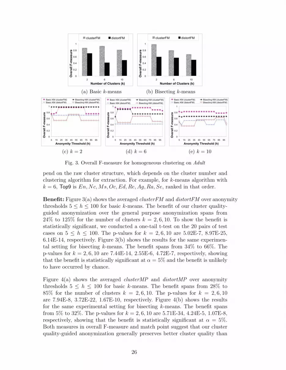
Fig. 3. Overall F-measure for homogeneous clustering on Adult

pend on the raw cluster structure, which depends on the cluster number andclustering algorithm for extraction. For example, for k-means algorithm withk = 6, Top9 is En, Nc,Ms,Oc,Ed,Re,Ag, Ra, Se, ranked in that order.

Benefit: Figure 3(a) shows the averaged clusterFM and distortFM over anonymitythresholds 5 ≤ h ≤ 100 for basic k-means. The benefit of our cluster quality-guided anonymization over the general purpose anonymization spans from24% to 125% for the number of clusters k = 2, 6, 10. To show the benefit isstatistically significant, we conducted a one-tail t-test on the 20 pairs of testcases on 5 ≤ h ≤ 100. The p-values for k = 2, 6, 10 are 5.02E-7, 8.97E-25,6.14E-14, respectively. Figure 3(b) shows the results for the same experimen-tal setting for bisecting k-means. The benefit spans from 34% to 66%. Thep-values for k = 2, 6, 10 are 7.44E-14, 2.55E-6, 4.72E-7, respectively, showingthat the benefit is statistically significant at α = 5% and the benefit is unlikelyto have occurred by chance.

Figure 4(a) shows the averaged clusterMP and distortMP over anonymitythresholds 5 ≤ h ≤ 100 for basic k-means. The benefit spans from 28% to85% for the number of clusters k = 2, 6, 10. The p-values for k = 2, 6, 10are 7.94E-8, 3.72E-22, 1.67E-10, respectively. Figure 4(b) shows the resultsfor the same experimental setting for bisecting k-means. The benefit spansfrom 5% to 32%. The p-values for k = 2, 6, 10 are 5.71E-34, 4.24E-5, 1.07E-8,respectively, showing that the benefit is statistically significant at α = 5%.Both measures in overall F-measure and match point suggest that our clusterquality-guided anonymization generally preserves better cluster quality than

26

0

0.2

0.4

0.6

0.8

1

2 6 10


Ma

tch

Po

int

clusterMP distortMP

(a) Basic k-means

0

0.2

0.4

0.6

0.8

1

2 6 10


Ma

tch

Po

int

clusterMP distortMP


0

0.2

0.4

0.6

0.8

1

5 15 25 35 45 55 65 75 85 95


Ma

tch

Po

int

Basic KM (clusterMP) Bisecting KM (clusterMP)

Basic KM (distortMP) Bisecting KM (distortMP)

(c) k = 2

0

0.2

0.4

0.6

0.8

1

5 15 25 35 45 55 65 75 85 95


Ma

tch

Po

int



(d) k = 6

0

0.2

0.4

0.6

0.8

1

5 15 25 35 45 55 65 75 85 95


Ma

tch

Po

int



(e) k = 10

Fig. 4. Match point for homogeneous clustering on Adult

the general purpose anonymization on the Adult data set.

Cost: Consider Figures 3(a)-3(b) and Figures 4(a)-4(b) again. The averagedcost, measured in overall F-measure, for achieving a given anonymity require-ment spans from 2% to 20% for basic k-means and bisecting k-means at clusternumbers k = 2 and k = 6. The averaged cost, measured in match point, spansfrom 9% to 23% for basic k-means and bisecting k-means at cluster num-bers k = 2, 6, 10. In general the loss of cluster quality is mild and the rawcluster structure has been preserved. There is an exception. For example, thecost increases to 33% in Figure 3(b) at k = 10, indicating that the numberof clusters k plays an important role in the preserved cluster quality. It alsostrengthens the importance of the evaluation phase (Step 3 and Step 4) in ourframework because it provides the data holder an opportunity to evaluate thecluster quality before releasing the data. If the loss is large, e.g., at k = 10,the data holder may consider releasing an alternative version with a differentnumber of clusters k, which usually is not a hard constraint. The problem ofdetermining the cluster number is part of cluster analysis, not a new issue inour anonymization problem.

Sensitivity to anonymity threshold h: Figures 3(c)-3(e) and Figures 4(c)-4(e) plot the clusterFM, distortFM, clusterMP, and distortMP of anonymitythresholds 5 ≤ h ≤ 100 at k = 2, 6, 10 for basic k-means and bisecting k-means. Each data point in the figures represent one test case. We made twoobservations from these figures.

27

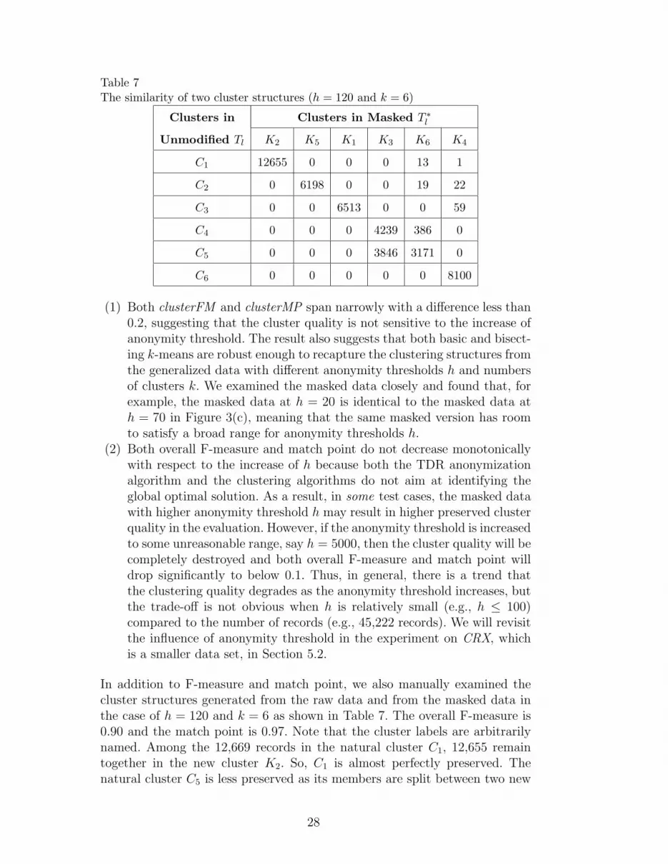
Table 7The similarity of two cluster structures (h = 120 and k = 6)

Clusters in Clusters in Masked T ∗l

Unmodified Tl K2 K5 K1 K3 K6 K4

C1 12655 0 0 0 13 1

C2 0 6198 0 0 19 22

C3 0 0 6513 0 0 59

C4 0 0 0 4239 386 0

C5 0 0 0 3846 3171 0

C6 0 0 0 0 0 8100

(1) Both clusterFM and clusterMP span narrowly with a difference less than0.2, suggesting that the cluster quality is not sensitive to the increase ofanonymity threshold. The result also suggests that both basic and bisect-ing k-means are robust enough to recapture the clustering structures fromthe generalized data with different anonymity thresholds h and numbersof clusters k. We examined the masked data closely and found that, forexample, the masked data at h = 20 is identical to the masked data ath = 70 in Figure 3(c), meaning that the same masked version has roomto satisfy a broad range for anonymity thresholds h.

(2) Both overall F-measure and match point do not decrease monotonicallywith respect to the increase of h because both the TDR anonymizationalgorithm and the clustering algorithms do not aim at identifying theglobal optimal solution. As a result, in some test cases, the masked datawith higher anonymity threshold h may result in higher preserved clusterquality in the evaluation. However, if the anonymity threshold is increasedto some unreasonable range, say h = 5000, then the cluster quality will becompletely destroyed and both overall F-measure and match point willdrop significantly to below 0.1. Thus, in general, there is a trend thatthe clustering quality degrades as the anonymity threshold increases, butthe trade-off is not obvious when h is relatively small (e.g., h ≤ 100)compared to the number of records (e.g., 45,222 records). We will revisitthe influence of anonymity threshold in the experiment on CRX, whichis a smaller data set, in Section 5.2.

In addition to F-measure and match point, we also manually examined thecluster structures generated from the raw data and from the masked data inthe case of h = 120 and k = 6 as shown in Table 7. The overall F-measure is0.90 and the match point is 0.97. Note that the cluster labels are arbitrarilynamed. Among the 12,669 records in the natural cluster C1, 12,655 remaintogether in the new cluster K2. So, C1 is almost perfectly preserved. Thenatural cluster C5 is less preserved as its members are split between two new

28

clusters.

A closer look at the masked data reveals that among the nine top rankedattributes, four are generalized to a different degree of granularity, and five,namely Nc (ranked 2nd), Oc (ranked 4th), Ed (ranked 5th), Re (ranked 6th),and Ra (ranked 8th), are generalized to the topmost value ANY. Even forthis drastic masking, the overall F-measure and match point remain at 0.90and 0.97, respectively. This suggests that there is much room for maskingwithin the constraint of preserving the cluster structure. Such room comesfrom the fact that some values are unnecessarily specific for cluster analysis,and masking them to less specific values does not affect the cluster structure.Our approach seizes the opportunity provided by this flexibility for maskingidentifying information.

We also conducted some experiments to study how the structure of a taxonomytree could influence the generalization on a categorical attribute and the over-all cluster quality. In general, a taller taxonomy tree increases the flexibility ofgeneralization because domain values have more opportunities to be general-ized into different granularity. As a result, masking is reduced and the overallcluster quality is improved. However, data could become hard to interpret if ataxonomy tree is unreasonably tall. For the dynamically generated taxonomytree in continuous attributes, we also examined the split points computed byinformation gain. Figure 5 shows the dynamically generated taxonomy tree forEducation-num (En). The split point at 13 (the years of education, not age)is very reasonable because it indicates whether a person has post-secondaryeducation.

ANY [1-20)

[1-13) [13-20)

Years of Education

Fig. 5. The generated taxonomy tree for Education-num

0

0.2

0.4

0.6

0.8

1

Top3

(Basic

KM)

Top6

(Basic

KM)

Top9

(Basic

KM)

Top3

(Bisecting

KM)

Top6

(Bisecting

KM)

Top9

(Bisecting

KM)

QID Size

Ov

era

ll F

-me

as

ure

clusterFM distortFM

(a) F-measure

0

0.2

0.4

0.6

0.8

1

Top3

(Basic

KM)

Top6

(Basic

KM)

Top9

(Basic

KM)

Top3

(Bisecting

KM)

Top6

(Bisecting

KM)

Top9

(Bisecting

KM)

QID Size

Ma

tch

Po

int

clusterMP distortMP

(b) Match point

Fig. 6. Increasing QID size for k = 6 on Adult

29

0

0.2

0.4

0.6

0.8

1

h=20

(Basic

KM)

h=50

(Basic

KM)

h=80

(Basic

KM)

h=20

(Bisecting

KM)

h=50

(Bisecting

KM)

h=80

(Bisecting

KM)


Ov

era

ll F

-me

as

ure

MultiQID SingleQID

(a) F-measure

0

0.2

0.4

0.6

0.8

1

h=20

(Basic

KM)

h=50

(Basic

KM)

h=80

(Basic

KM)

h=20

(Bisecting

KM)

h=50

(Bisecting

KM)

h=80

(Bisecting

KM)


Ma

tch

Po

int

MultiQID SingleQID

(b) Match point

Fig. 7. MultiQID vs. SingleQID for k = 6 on Adult

Sensitivity to QID size: Figure 6 studies the influence of QID size on thepreserved cluster quality. Figure 6(a) has two portions. The left and right por-tions, separated by a vertical dashed line, show the averaged overall F-measureover anonymity thresholds 5 ≤ h ≤ 100 for basic k-means and bisecting k-means, respectively, at k = 6 with QID size from 3 attributes (Top3) to 9attributes (Top9). Figure 6(b) shows the averaged match point for the sameexperimental setting. Both overall F-measure and match point exhibit a simi-lar pattern and suggest that as the QID increase, the preserved cluster qualitydecreases because more attributes are included for masking. It is interestingto note that as QID size decreases, the benefit of the cluster quality-guidedanonymization over the general purpose anonymization becomes smaller be-cause the non-QID attributes dominate the clustering effect and, therefore,diminish the difference between the two anonymization methods.

Multiple QIDs: To verify the claim that multi-QID anonymity requirementscan help reduce unnecessary masking, we compared the overall F-measure be-tween a multi-QID requirement and the corresponding single QID require-ment, where the QID is the union of the multiple QIDs. For example, arequirement of 3 length-2 QIDs is

{〈{Ag, En}, h〉, 〈{Ag, Re}, h〉, 〈{Se, Hw}, h〉},

and the corresponding single QID requirement is

{〈{Ag, En, Re, Se, Hw}, h〉}.

We randomly generated 30 multi-QID requirements as follows. For each re-quirement, we first determined the number of QIDs using the uniform prob-ability distribution U [3, 7] (i.e., randomly drew a number between 3 and 7where the probability of selecting each number was the same) and the lengthof QIDs using U [2, 9]. For simplicity, all QIDs in the same requirement hadthe same length and same threshold h. For each QID, we randomly selectedattributes according to the QID length from the 14 attributes. A repeatingQID was discarded.

30

Figure 7 studies the effect on the preserved cluster quality between multi-QID,denoted by MultiQID, and its corresponding single QID, denoted by SingleQID.Figure 7(a) has two portions. The left and right portions show the averagedoverall F-measure over the 30 randomly generated test cases described aboveat h = 20, 50, 80 for basic k-means and bisecting k-means, respectively, wherek = 6. To show the difference between MultiQID and SingleQID is statisticallysignificant, we conducted a one-tail t-test on the 30 pairs of test cases. Thep-values for basic k-means at h = 20, 50, 80 are 4.20E-6, 9.27E-6, 2.27E-5,respectively. The p-values for bisecting k-means at h = 20, 50, 80 are 2.05E-9,2.49E-9, 6.94E-8, respectively. The difference between MultiQID and SingleQIDis statistically significant at α = 5%. Figure 7(b) shows the averaged matchpoint for the same experimental setting and exhibits similar results, so we omitthe explanation. Figure 7 suggests that a multi-QID anonymity requirementgenerally results in higher cluster quality than its corresponding single QIDanonymity requirement.

5.1.2 Heterogeneous Clustering

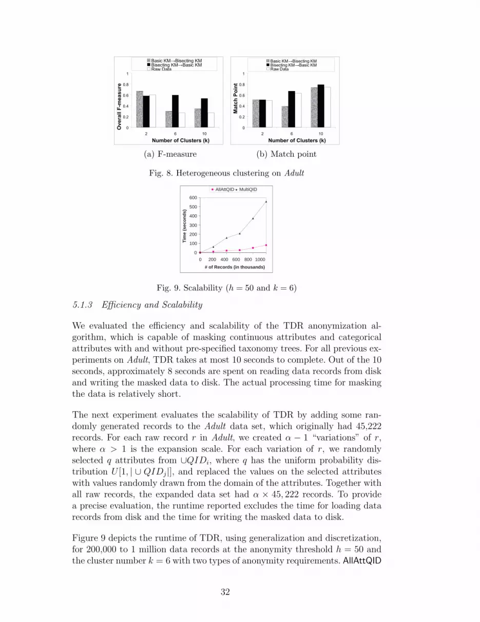
Heterogeneous clustering refers to the case that different clustering algorithmsare applied in Step 1 and Step 3. It models the scenario that the data recip-ient applies a clustering algorithm to the masked data that is different fromthe one used by the data holder for masking the data. We applied bisectingand basic k-means in Step 1 and Step 3 in two different orders, denoted by(Basic KM→Bisecting KM ) and (Bisecting KM→Basic KM ), respectively,in Figure 8. In both cases, compared to the homogenous clustering in Fig-ures 3-4, there is a very severe drop on clusterFM and clusterMP. The dropon clusterFM and clusterMP spans from 33% to 78%, and from 16% to 50%,respectively. To explain the drops, we encoded two raw cluster structures sep-arately using the two clustering methods (without any masking), and thenmeasured the overall F-measure and match point between the two raw clusterstructures, denoted by Raw Data in the figures. Because the drops on clus-terFM and clusterMP of Raw Data are also severe, we can conclude that thedrops on (Basic KM→Bisecting KM ) and (Bisecting KM→Basic KM ) arecaused by the nature of heterogeneous clustering, not by the masking.

The above studies suggest that if the data recipient applies the same cluster-ing algorithm as the one used by the data holder for masking the data, thecluster structure obtained will be more similar to the raw cluster structurebecause the second clustering could extract the embedded structure preservedin the masked data. In contrast, if different clustering algorithms are used,the structure preserved by masking may not be useful to the second clusteringdue to a different search bias. This explains the significant drops in overallF-measure and match point for heterogeneous clustering.

31

0

0.2

0.4

0.6

0.8

1

2 6 10


Ov

era

ll F

-me

as

ure

Basic KM→Bisecting KMBisecting KM→Basic KMRaw Data

(a) F-measure

0

0.2

0.4

0.6

0.8

1

2 6 10


Ma

tch

Po

int


(b) Match point

Fig. 8. Heterogeneous clustering on Adult

0

100

200

300

400

500

600

0 200 400 600 800 1000

# of Records (in thousands)

Tim

e (s

eco

nd

s)

AllAttQID MultiQID

Fig. 9. Scalability (h = 50 and k = 6)

5.1.3 Efficiency and Scalability

We evaluated the efficiency and scalability of the TDR anonymization al-gorithm, which is capable of masking continuous attributes and categoricalattributes with and without pre-specified taxonomy trees. For all previous ex-periments on Adult, TDR takes at most 10 seconds to complete. Out of the 10seconds, approximately 8 seconds are spent on reading data records from diskand writing the masked data to disk. The actual processing time for maskingthe data is relatively short.

The next experiment evaluates the scalability of TDR by adding some ran-domly generated records to the Adult data set, which originally had 45,222records. For each raw record r in Adult, we created α − 1 “variations” of r,where α > 1 is the expansion scale. For each variation of r, we randomlyselected q attributes from ∪QIDi, where q has the uniform probability dis-tribution U [1, | ∪ QIDj|], and replaced the values on the selected attributeswith values randomly drawn from the domain of the attributes. Together withall raw records, the expanded data set had α × 45, 222 records. To providea precise evaluation, the runtime reported excludes the time for loading datarecords from disk and the time for writing the masked data to disk.

Figure 9 depicts the runtime of TDR, using generalization and discretization,for 200,000 to 1 million data records at the anonymity threshold h = 50 andthe cluster number k = 6 with two types of anonymity requirements. AllAttQID

32

refers to the single QID having all 14 attributes. This is one of the most time-consuming settings because of the large number of candidate refinements toconsider at each iteration. For TDR, the small anonymity threshold of h = 50requires more iterations to reach a solution, hence more runtime, than a largerthreshold. TDR takes approximately 80 seconds to transform 1 million records.

In Figure 9, MultiQID refers to the average runtime over the 30 random multi-QID requirements generated as described in Section 5.1.1 with h = 50 andk = 6. Compared to AllAttQID, TDR becomes less efficient for handling multi-QID because an anonymity requirement on multi-QID is a less restrictive con-straint than the single QID anonymity requirement containing all attributes;therefore, TDR has to perform more refinements to reach a local optimal so-lution. The runtime of suppression on this expanded data set is roughly thesame as shown in Figure 9, so we omit the figure.

5.2 The Japanese Credit Screening (CRX) Data Set

The Japanese Credit Screening data set, also known as CRX, contains real-lifecredit card applications. It was previously used in [45][46]. With the binaryclass attribute removed, there are 6 continuous attributes and 9 categoricalattributes on 653 records. Every record represents a credit card applicationof an individual in Japan. In the UCI repository, all values and attributenames in CRX have been changed to meaningless symbols, e.g., A1 . . . A15.The continuous attributes are normalized as a standard preprocessing step inmany clustering algorithms. No taxonomy trees are given for the categoricalattributes, so we use discretization and suppression to mask the continuousand categorical attributes. All 15 attributes are used in cluster analysis.

Following the same experimental settings for Adult in Section 5.1, we presentthe result of CRX below. In general, the result exhibits patterns similar tothose shown in Section 5.1 The only difference is that the cluster quality inCRX is more sensitive to the increase of anonymity threshold h due to itssmaller data set size. We first present the results for the scenario of homoge-nous clustering, followed by heterogeneous clustering.

5.2.1 Homogenous Clustering

We first evaluate the cost and benefit, in terms of cluster quality, of employingour proposed method for anonymity requirements with single QID. Next, westudy how the cluster quality is influenced by the anonymity threshold andQID size. Then, we study cluster quality for anonymity requirement withmultiple QIDs.

33

0

0.2

0.4

0.6

0.8

1

2 6 10

Ove

rall

F-m

ea

su

re


clusterFM distortFM

(a) Basic k-means

0

0.2

0.4

0.6

0.8

1

2 6 10


Ov

era

ll F

-me

as

ure

clusterFM distortFM


0

0.2

0.4

0.6

0.8

1

5 15 25 35 45 55 65 75 85 95

Ove

rall

F-m

ea

su

re




(c) k = 2

0

0.2

0.4

0.6

0.8

1

5 15 25 35 45 55 65 75 85 95

Ov

era

ll F

-me

as

ure




(d) k = 6

0

0.2

0.4

0.6

0.8

1

5 15 25 35 45 55 65 75 85 95

Ove

rall

F-m

ea

su

re




(e) k = 10

Fig. 10. Overall F-measure for homogeneous clustering on CRX

Single QID: For each test case, we used the same method described in Sec-tion 5.1 to identify the top 9 most important attributes to form the anonymityrequirement, denoted by Top9.

Benefit: Figure 10(a) shows the averaged clusterFM and distortFM overanonymity thresholds 5 ≤ h ≤ 100 for basic k-means. The benefit of ourcluster quality-guided anonymization over the general purpose anonymizationspans from 40% to 155% for the number of clusters k = 2, 6, 10. To show thebenefit is statistically significant, we conducted a one-tail t-test on the 20 pairsof test cases from 5 ≤ h ≤ 100. The p-values for k = 2, 6, 10 are 2.24E-26,4.67E-17, 1.40E-10, respectively. Figure 10(b) shows the results for the sameexperimental setting for bisecting k-means. It is interesting to note that theraw cluster structure is perfectly preserved at k = 2 for both clusterFM anddistortFM in all 20 test cases of anonymity threshold 5 ≤ h ≤ 100, so thebenefit and the cost are 0. The benefit at k = 6 and k = 10 are 45% and 57%,respectively. The p-values for k = 10 and k = 10 are 4.25E-9 and 1.11E-10,respectively, showing that the benefit is statistically significant at α = 5%;the benefit is unlikely to have occurred by chance.

Figure 11(a) shows the averaged clusterMP and distortMP over anonymitythresholds 5 ≤ h ≤ 100 for basic k-means. The benefit spans from 9% to60% for the number of clusters k = 2, 6, 10. The p-values for k = 2, 6, 10are 1.67E-16, 8.50E-14, 1.81E-6, respectively. Figure 11(b) shows the resultsfor the same experimental setting for bisecting k-means. The benefit at k =6 and k = 10 are 13% and 8%, respectively. The p-values for k = 6 and

34

0

0.2

0.4

0.6

0.8

1

2 6 10

Ma

tch

Po

int


clusterFM distortFM

(a) Basic k-means

0

0.2

0.4

0.6

0.8

1

2 6 10

Ma

tch

Po

int


clusterFM distortFM


0

0.2

0.4

0.6

0.8

1

5 15 25 35 45 55 65 75 85 95

Ma

tch

Po

int




(c) k = 2

0

0.2

0.4

0.6

0.8

1

5 15 25 35 45 55 65 75 85 95

Ma

tch

Po

int




(d) k = 6

0

0.2

0.4

0.6

0.8

1

5 15 25 35 45 55 65 75 85 95

Ma

tch

Po

int




(e) k = 10

Fig. 11. Match point for homogeneous clustering on CRX

k = 10 are 1.04E-9 and 1.06E-11, respectively, showing that the benefit isstatistically significant at α = 5%. The results suggest that that our clusterquality-guided anonymization generally preserves better cluster quality thanthe general purpose anonymization on CRX.

Cost: Consider Figures 10(a)-10(b) and Figures 11(a)-11(b) again. The av-eraged cost, measured in overall F-measure, for achieving a given anonymityrequirement spans from 0% to 23% for basic k-means and bisecting k-meansat cluster numbers k = 2 and k = 6. The averaged cost, measured in matchpoint, spans from 0% to 20% for basic k-means and bisecting k-means atcluster numbers k = 2, 6, 10. The results suggest that the cost is mild andsupport the claim that the cluster structure can be preserved for restrictiveanonymity requirements. However, the cost increases to 30% when k = 10 inFigure 10(a). Thus, it strengthens our claim that it is important to evaluatethe cluster quality before releasing the data.

Sensitivity to anonymity threshold h: Figures 10(c)-10(e) and Figures 11(c)-11(e) plot the clusterFM, distortFM, clusterMP, and distortMP for basic k-means and bisecting k-means with anonymity thresholds 5 ≤ h ≤ 100 atk = 2, 6, 10. From the figures, we noted that at k = 6 and k = 10, both clus-terFM and clusterMP are more sensitive to the increase of anonymity thresh-old h, and the preserved cluster quality generally degrades as h increases. Thetrade-off between cluster quality and anonymity is more obvious in CRX thanin Adult because the data set size of CRX (653 records) is much smaller thanthe data set size of Adult (45,222 records); therefore, increasing the anonymity

35

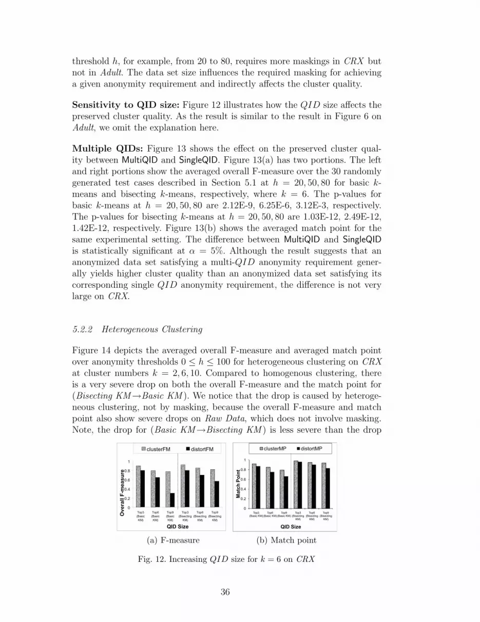
threshold h, for example, from 20 to 80, requires more maskings in CRX butnot in Adult. The data set size influences the required masking for achievinga given anonymity requirement and indirectly affects the cluster quality.

Sensitivity to QID size: Figure 12 illustrates how the QID size affects thepreserved cluster quality. As the result is similar to the result in Figure 6 onAdult, we omit the explanation here.

Multiple QIDs: Figure 13 shows the effect on the preserved cluster qual-ity between MultiQID and SingleQID. Figure 13(a) has two portions. The leftand right portions show the averaged overall F-measure over the 30 randomlygenerated test cases described in Section 5.1 at h = 20, 50, 80 for basic k-means and bisecting k-means, respectively, where k = 6. The p-values forbasic k-means at h = 20, 50, 80 are 2.12E-9, 6.25E-6, 3.12E-3, respectively.The p-values for bisecting k-means at h = 20, 50, 80 are 1.03E-12, 2.49E-12,1.42E-12, respectively. Figure 13(b) shows the averaged match point for thesame experimental setting. The difference between MultiQID and SingleQIDis statistically significant at α = 5%. Although the result suggests that ananonymized data set satisfying a multi-QID anonymity requirement gener-ally yields higher cluster quality than an anonymized data set satisfying itscorresponding single QID anonymity requirement, the difference is not verylarge on CRX.

5.2.2 Heterogeneous Clustering

Figure 14 depicts the averaged overall F-measure and averaged match pointover anonymity thresholds 0 ≤ h ≤ 100 for heterogeneous clustering on CRXat cluster numbers k = 2, 6, 10. Compared to homogenous clustering, thereis a very severe drop on both the overall F-measure and the match point for(Bisecting KM→Basic KM ). We notice that the drop is caused by heteroge-neous clustering, not by masking, because the overall F-measure and matchpoint also show severe drops on Raw Data, which does not involve masking.Note, the drop for (Basic KM→Bisecting KM ) is less severe than the drop

0

0.2

0.4

0.6

0.8

1

Top3

(Basic

KM)

Top6

(Basic

KM)

Top9

(Basic

KM)

Top3

(Bisecting

KM)

Top6

(Bisecting

KM)

Top9

(Bisecting

KM)

QID Size

Ov

era

ll F

-me

as

ure

clusterFM distortFM

(a) F-measure

0

0.2

0.4

0.6

0.8

1

Top3 (Basic KM)

Top6 (Basic KM)

Top9 (Basic KM)

Top3 (Bisecting

KM)

Top6 (Bisecting

KM)

Top9 (Bisecting

KM)

Ma

tch

Po

int

QID Size

clusterMP distortMP

(b) Match point

Fig. 12. Increasing QID size for k = 6 on CRX

36

0

0.2

0.4

0.6

0.8

1

h=20 (Basic KM)

h=50 (Basic KM)

h=80 (Basic KM)

h=20 (Bisecting

KM)

h=50 (Bisecting

KM)

h=80 (Bisecting

KM)

Ove

rall

F-m

ea

su

re


MultiQID SingleQID

(a) F-measure

0

0.2

0.4

0.6

0.8

1

h=20 (Basic KM)

h=50 (Basic KM)

h=80 (Basic KM)

h=20 (Bisecting

KM)

h=50 (Bisecting

KM)

h=80 (Bisecting

KM)

Ma

tch

Po

int


MultiQID SingleQID

(b) Match point

Fig. 13. MultiQID vs. SingleQID for k = 6 on CRX

0

0.2

0.4

0.6

0.8

1

2 6 10

Ove

rall

F-m

ea

su

re



(a) F-measure

0

0.2

0.4

0.6

0.8

1

2 6 10

Ma

tch

Po

int



(b) Match point

Fig. 14. Heterogeneous clustering on CRX

for (Bisecting KM→Basic KM ), implying that bisecting k-means can extractthe cluster structure encoded by basic k-means in the masked data. Interest-ingly, the overall F-measure for (Bisecting KM→Basic KM ) is even betterthan the overall F-measure on Raw Data because the masking removes someoverly specific information (i.e., noise) from the data.

5.3 Summary

These experiments verified the claim that the proposed approach of convertingthe anonymity problem for cluster analysis to the counterpart problem forclassification analysis is effective. This is demonstrated by the preservationof most of the cluster structure in the raw data after masking identifyinginformation for a broad range of anonymity requirements. The experimentalresults also suggest that our cluster quality-guided anonymization can preservebetter cluster structure than the general purpose anonymization.

The experiments demonstrated the cluster quality with respect to the variationof anonymity thresholds, QID size, and number of clusters. In general, thecluster quality degrades as the anonymity threshold increases. This trend ismore obvious if the data set size is small or if h is relatively large, e.g., h =5000. The cluster quality degrades as the QID size increases. The cluster

37

quality exhibits no obvious trend with respect to the number of clusters, asthe natural number of clusters is data dependent.

The experiments confirmed that the specification of the multi-QID anonymityrequirement helps avoid unnecessary masking and, therefore, preserves moreof the cluster structure. However, if the data recipient and the data holderemploy different clustering algorithms, then there is no guarantee that theencoded raw cluster structure can be extracted. Thus, in practice, it is impor-tant for the data holder to validate the cluster quality, using the evaluationmethods proposed in our framework, before releasing the data. Finally, exper-iments suggest that the proposed anonymization approach is highly efficientand scalable for single QID, but less efficient for multi-QID.

6 Extension: Beyond Anonymity

The above approach provides a flexible framework that makes use of existingsolutions as “plug-in” components. These include the cluster analysis in Steps1 and 3, the anonymization in Step 2, and the evaluation in Step 4. For ex-ample, instead of using the proposed TDR algorithm, the data holder has theoption to perform the anonymization by employing one of the genetic algo-rithms [16], top-down specialization [12], or InfoGain Mondrian [22]. None ofthem can perform all three types of masking operations discussed in Section 3,so some modification is necessary.

This paper focuses on preventing the privacy threats caused by sensitive recordlinkage, but the framework can also prevent sensitive attribute linkage byadopting different anonymization algorithms and achieving other privacy re-quirements, such as `-diversity [25] and confidence bounding [45][46], discussedin Section 2. The extension requires modification of the Score or cost functionsin these algorithms to bias on refinements or maskings that can distinguishclass labels. The framework can also adopt other evaluation methods, suchas entropy [37], or any ad-hoc methods defined by the data holder. For fu-ture work, we are interested in building a visualization tool to allow the dataholder to adjust the parameters, such as the number of clusters and anonymitythresholds, and visualize their influence on the clusters interactively.

7 Conclusions

We studied the problem of releasing person-specific data for cluster analy-sis while protecting privacy. The proposed solution is to mask unnecessarilyspecific information into a less specific but semantically consistent version,

38

so that person-specific identifying information is masked but essential clusterstructure remains. The major challenge is the lack of class labels that couldbe used to guide the masking process. Our main contribution is a generalframework for converting this problem into the counterpart problem for clas-sification analysis so that the masking process can be properly guided. Thekey idea is to encode the original cluster structure into the class label of datarecords and subsequently preserve the class labels for the corresponding clas-sification problem. The experimental results verified the effectiveness of thisapproach.

We also studied several practical issues arising from applying this approachin a real-life data publishing scenario. These include how the choices of clus-tering algorithms, number of clusters, anonymity threshold, and size and typeof quasi-identifiers can affect the effectiveness of this approach, and how toevaluate the effectiveness in terms of cluster quality. These studies lead to therecommendation of two strategies for choosing the clustering algorithm in themasking process, each having a different focus. The contribution in this paperprovides a useful framework of secure data sharing for the purpose of clusteranalysis.

8 Acknowledgements

The research is supported in part by the Discovery Grants (356065-2008) fromthe Natural Sciences and Engineering Research Council of Canada (NSERC),and the Faculty Start-up Funds from Concordia University.

References

[1] C. C. Aggarwal, On k-anonymity and the curse of dimensionality, in: Proc. ofthe 31st Very Large Data Bases (VLDB), Trondheim, Norway, 2005.

[2] C. C. Aggarwal, P. S. Yu, A condensation approach to privacy preserving datamining, in: Proc. of the 9th International Conference on Extending DatabaseTechnology (EDBT), 2004.

[3] G. Aggarwal, T. Feder, K. Kenthapadi, R. Motwani, R. Panigrahy, D. Thomas,A. Zhu, Achieving anonymity via clustering, in: Proc. of the 25th ACMSIGMOD-SIGACT-SIGART Principles of Database Systems (PODS), 2006.

[4] R. J. Bayardo, R. Agrawal, Data privacy through optimal k-anonymization, in:Proc. of the 21st IEEE International Conference on Data Engineering (ICDE),2005.

39

[5] J. Beringer, E. Hullermeier, Online clustering of parallel data streams, Data &Knowledge Engineering (DKE) 58 (2) (2006) 180–204.

[6] D. Birant, A. Kut, ST-DBSCAN: an algorithm for clustering spatial-temporaldata, Data & Knowledge Engineering (DKE) 60 (1) (2007) 208–221.

[7] D. M. Carlisle, M. L. Rodrian, C. L. Diamond, California inpatient datareporting manual, medical information reporting for california, 5th edition,Tech. rep., Office of Statewide Health Planning and Development (July 2007).

[8] R. Chaytor, Utility-preserving k-anonymity, Master’s thesis, MemorialUniversity of Newfoundland, Canada (2006).

[9] R. N. Dave, R. Krishnapuram, Robust clustering methods: a unified view, IEEETransactions on Fuzzy Systems 5 (2) (1997) 270–293.

[10] B. C. M. Fung, M. Cao, B. C. Desai, H. Xu, Privacy protection for RFID data,in: Proc. of the 24th ACM SIGAPP Symposium on Applied Computing (SAC)Special Track on Database Theory, Technology, and Applications (DTTA),ACM Press, Honolulu, HI, 2009.

[11] B. C. M. Fung, K. Wang, A. W. C. Fu, J. Pei, Anonymity for continuousdata publishing, in: Proc. of the 11th International Conference on ExtendingDatabase Technology (EDBT), ACM Press, Nantes, France, 2008.

[12] B. C. M. Fung, K. Wang, P. S. Yu, Top-down specialization for informationand privacy preservation, in: Proc. of the 21st IEEE International Conferenceon Data Engineering (ICDE), Tokyo, Japan, 2005.

[13] B. C. M. Fung, K. Wang, P. S. Yu, Anonymizing classification data for privacypreservation, IEEE Transactions on Knowledge and Data Engineering (TKDE)19 (5) (2007) 711–725.

[14] R. Gelbard, O. Goldman, I. Spiegler, Investigating diversity of clusteringmethods: An empirical comparison, Data & Knowledge Engineering (DKE)63 (1) (2007) 155–166.

[15] A. Inan, S. V. Kaya, Y. Saygin, E. Savas, A. A. Hintoglu, A. Levi, Privacypreserving clustering on horizontally partitioned data, Data & KnowledgeEngineering (DKE) 63 (3) (2007) 646–666.

[16] V. S. Iyengar, Transforming data to satisfy privacy constraints, in: Proc. of the8th ACM International Conference on Knowledge Discovery and Data Mining(SIGKDD), 2002.

[17] G. Karypis, Cluto - family of data clustering software tools,http://glaros.dtc.umn.edu/gkhome/views/cluto/ (October 2006).

[18] L. Kaufman, P. J. Rousseeuw, Finding Groups in Data: An Introduction toCluster Analysis, John Wiley and Sons, 1990.

[19] D. Kifer, J. Gehrke, Injecting utility into anonymized datasets, in: Proc. ofACM International Conference on Management of Data (SIGMOD), 2006.

40

[20] K. LeFevre, D. J. DeWitt, R. Ramakrishnan, Incognito: Efficient full-domaink-anonymity, in: Proc. of ACM International Conference on Management ofData (SIGMOD), 2005.

[21] K. LeFevre, D. J. DeWitt, R. Ramakrishnan, Mondrian multidimensional k-anonymity, in: Proc. of the 22nd IEEE International Conference on DataEngineering (ICDE), Atlanta, GA, 2006.

[22] K. LeFevre, D. J. DeWitt, R. Ramakrishnan, Workload-aware anonymization,in: Proc. of the 12th ACM SIGKDD International Conference on KnowledgeDiscovery and Data Mining, 2006.

[23] G. Loukides, J. Shao, Capturing data usefulness and privacy protection in k-anonymisation, in: Proc. of the 2007 SAC, 2007.

[24] G. Loukides, J. Shao, Data utility and privacy protection trade-off in k-anonymization, in: Proc. of the International Workshop on Privacy andAnonymity in the Information Society (PAIS), 2008.

[25] A. Machanavajjhala, D. Kifer, J. Gehrke, M. Venkitasubramaniam, `-diversity:Privacy beyond k-anonymity, ACM Transactions on Knowledge Discovery fromData (TKDD) 1 (1).

[26] J. B. MacQueen, Some methods for classification and analysis of multivariateobservations, in: Proc. of the 5th Berkeley Symposium on MathematicalStatistics and Probability, vol. 1, Atlanta, GA, 1967.

[27] B. Malin, k-unlinkability: A privacy protection model for distributed data, Data& Knowledge Engineering (DKE) 64 (1) (2008) 294–311.

[28] S. McClean, B. Scotney, P. Morrow, K. Greer, Knowledge discoveryby probabilistic clustering of distributed databases, Data & KnowledgeEngineering (DKE) 54 (2) (2005) 189–210.

[29] N. Mohammed, B. C. M. Fung, K. Wang, P. C. K. Hung, Privacy-preservingdata mashup, in: Proc. of the 12th International Conference on ExtendingDatabase Technology (EDBT), ACM Press, Saint-Petersburg, Russia, 2009.

[30] D. J. Newman, S. Hettich, C. L. Blake, C. J. Merz, UCI repository of machinelearning databases (1998).URL http://www.ics.uci.edu/∼mlearn/MLRepository.html

[31] President Information Technology Advisory Committee, Revolutionizing healthcare through information technology, Tech. rep., Executive Office of thePresident of the United States (June 2004).

[32] J. R. Quinlan, C4.5: Programs for Machine Learning, Morgan Kaufmann, 1993.

[33] P. Samarati, Protecting respondents’ identities in microdata release, IEEETransactions on Knowledge and Data Engineering (TKDE) 13 (6) (2001) 1010–1027.

41

[34] P. Samarati, L. Sweeney, Generalizing data to provide anonymity whendisclosing information, in: Proc. of the 17th ACM SIGACT-SIGMOD-SIGARTPrinciples of Database Systems (PODS), Seattle, WA, 1998.

[35] S. Savaresi, D. L. Boley, S. Bittanti, G. Gazzaniga, Cluster selection in divisiveclustering algorithms, in: 2nd SIAM International Conference on Data Mining(SDM), 2002.

[36] S. M. Savaresi, D. L. Boley, On the performance of bisecting k-means and pddp,in: 1st SIAM International Conference on Data Mining (SDM), 2001.

[37] C. E. Shannon, A mathematical theory of communication, Bell SystemTechnical Journal 27 (1948) 379–423 and 623–656.

[38] M. Steinbach, G. Karypis, V. Kumar, A comparison of document clusteringtechniques, in: Proc. of KDD Workshop on Text Mining, 2000.

[39] L. Sweeney, Achieving k-anonymity privacy protection using generalization andsuppression, International Journal on Uncertainty, Fuzziness, and Knowledge-based Systems 10 (5) (2002) 571–588.

[40] L. Sweeney, k-Anonymity: a model for protecting privacy, International Journalon Uncertainty, Fuzziness and Knowledge-based Systems 10 (5) (2002) 557–570.

[41] J. Vaidya, C. Clifton, Privacy-preserving k-means clustering over verticallypartitioned data, in: Proc. of ACM SIGMOD International Conference onManagement of Data, 2003.

[42] C. J. van Rijsbergen, Information Retrieval, 2nd edition, London, Butterworths,1979.

[43] K. Wang, B. C. M. Fung, Anonymizing sequential releases, in: Proc. of the 12thACM SIGKDD International Conference on Knowledge Discovery and DataMining, 2006.

[44] K. Wang, B. C. M. Fung, G. Dong, Integrating private databases for dataanalysis, in: Proc. of IEEE International Conference on Intelligence and SecurityInformatics (ISI), 2005.

[45] K. Wang, B. C. M. Fung, P. S. Yu, Template-based privacy preservation inclassification problems, in: Proc. of the 5th IEEE International Conference onData Mining (ICDM), Houston, TX, 2005.

[46] K. Wang, B. C. M. Fung, P. S. Yu, Handicapping attacker’s confidence:An alternative to k-anonymization, Knowledge and Information Systems: AnInternational Journal (KAIS) 11 (3) (2007) 345–368.

[47] R. C. W. Wong, J. Li., A. W. C. Fu, K. Wang, (α,k)-anonymity: An enhancedk-anonymity model for privacy preserving data publishing, in: Proc. of the 12thACM SIGKDD, Philadelphia, PA, 2006.

[48] L. Xiong, K. Rangachari, Towards application-oriented data anonymization, in:Proc. of the 4th SIAM Workshop on Practical Privacy-Preserving Data Mining,2008.

42

[49] J. Xu, W. Wang, J. Pei, X. Wang, B. Shi, A. W. C. Fu, Utility-basedanonymization using local recoding, in: Proc. of the 12th ACM InternationalConference on Knowledge Discovery and Data Mining (SIGKDD), 2006.

43

privacy-preserving data publishing for cluster analysis

Documents