Andreas Jørgensen Tveito

Price Coordination andConsumer BehaviorEvidence from Retail Fuel

2022

Thesis for the degree of Philosophiae Doctor (PhD)University of Bergen, Norway

at the University of Bergen

Avhandling for graden philosophiae doctor (ph.d )

ved Universitetet i Bergen

.

2017

Dato for disputas: 1111

Andreas Jørgensen Tveito

Price Coordination andConsumer Behavior

Evidence from Retail Fuel

Thesis for the degree of Philosophiae Doctor (PhD)

Date of defense: 08.04.2022

The material in this publication is covered by the provisions of the Copyright Act.

Print: Skipnes Kommunikasjon / University of Bergen

© Copyright Andreas Jørgensen Tveito

Name: Andreas Jørgensen Tveito

Title: Price Coordination and Consumer Behavior

Year: 2022

Acknowledgements

When I finished my master’s degree at the Department of Economics at the Universityof Bergen (UoB) in 2007 I did not consider starting a PhD. Instead, I wanted to applywhat I had learned in the "real world" and started working at the Norwegian CompetitionAuthority. After working there for almost a decade, I was very happy to get the opportu-nity to apply for funds for a "Public Sector PhD" from the Research Council of Norway.Immersing myself in research on topics I had become interested in at the competitionauthority was tempting, and suddenly I was back at UoB working on a PhD.

Many people have contributed to making my four years as a PhD student an enjoyableexperience and improving the quality of my thesis. My main supervisor, Bjørn OlavJohansen, has always been open to discuss ideas, give honest and constructive feedback,and to point me in the right direction when I hit a dead end. My co-supervisor, MortenSæthre, has been very helpful on various econometric problems I have encountered and hasalso provided great insights on how to improve the introductions in my research articles.I also want to thank both my supervisors for letting me explore my own ideas rather thanpushing me to pursue projects closer to their own research agendas.

I also want to thank the people at the Department of Economics at the UoB. Theclose integration of PhD students with the staff creates an inclusive and stimulatingenvironment. Thanks to all the PhD students and post-docs for making the time both inand out of the office a pleasure. Thanks to Hans K. Hvide for valuable comments on myresearch. A special thanks to my fellow industrial organization nerds and office mates TeisLunde Lømo and Håvard Mork Sandvik. Although they are mainly working on industrialorganization theory, they patiently listened to my rants about the retail fuel market andhave been great discussion partners. Teis even came up with the best possible title forone of my papers.

I also had a great stay at the University of California San Diego and wish to thankGordon Dahl, who arranged for my visit and gave very useful feedback on my research, andthe PhD students for a welcoming and stimulating research environment. A special thanksalso to Giacomo Rondina and Lodovica Guidarelli and family for the warm welcome andgood times at the beach and in the waves.

It has also been a pleasure to spend some time at the competition authority during thelast 4 years, and I am thankful for the comments from various people at the seminars I heldthere. Sigurd Birkeland has been a great discussion partner for various issues regardingretail fuel markets. Magnus Friis Reitan has provided insightful comments on my researchand been a great discussion partner. Kurt Richard Brekke and Mai Nguyen-Ones havealso provided valuable feedback on my papers.

Jonas Gade Christensen has also taken an interest in and provided great feedback onmy research. Katrine Vellesen Løken has kindly read drafts of all my papers, given greatfeedback, and has endured listening to my complaints about issues with the data, nastyfixed effects, and imperfect control groups, and given thoughtful responses.

My greatest thanks go to my family. I am lucky to have incredibly supportive parents—both in terms of supporting my choices and of babysitting my kids. Some may think thathaving kids is a burden when working on a PhD, but I rather find that Oskar, Sara, andrecently also Alfred have forced me to structure my work time and have been a mostwelcome distraction. Spending time with them and my wife, Katrine, has been the bestcure for the gloom after less successful days of research. Katrine has constantly encour-aged me, and has both been understanding in periods when I have worked long hours andurged me to relax in periods when I have been unnecessarily stressed.♥.

Bergen, October 2021Andreas Tveito

Abstract

This thesis consists of an introduction and three essays on price coordination andconsumer behavior in the retail fuel market. Each essay includes one of the researcharticles that compose the principle part of the thesis. The essays use microeconometricmethods and data from the Norwegian retail fuel market to investigate how firms useprice leadership to coordinate more frequent price increases, the costs and benefits of priceleadership, and long-run dynamics in consumers’ response to changes in the intertemporalprice pattern. The introduction summarizes the essays, discusses the merits of studyingfirm and consumer behavior in the retail fuel market, and elaborates on policy implicationsof the research in the thesis.

Price leadership—a practice involving sequential price changes whereby a leader changesprice first and rivals quickly follow—is commonly observed in many retail markets. Thefirst chapter use a unique dataset spanning 14 years with the exact timing of price changesfor most Norwegian gasoline stations to study price leadership and coordination in theNorwegian retail gasoline market. The market features asymmetric price cycles whereprices slowly fall for several days before being restored to a high level within a few hours.The main contribution is to show how large retail chains use price leadership to both agreeon and sustain a new equilibrium with more frequent price hikes. I argue that faster pricechanges due to a lack of price regulations in Norway can explain why the chains in Norwayend up coordinating on a different equilibrium than in other countries. By combining theprice data with data on volumes and costs, I estimate that the transition to more frequentprice hikes has a substantial positive effect on volume-weighted retail margins.

Price leadership can bring about higher prices for all firms in the market, but can alsobe costly for the leader because it loses volume to rivals in the interim period when it isthe sole firm with a high price. The second chapter of my thesis studies the costs andbenefits of price leadership in the Norwegian retail gasoline market. The dataset withhigh-frequency price and volume data coupled with a particular pricing pattern allowsthe estimation of the costs and benefits of leading price hikes. The main result is thatthe leader’s volume loss from being the sole firm to raise its price until the other firms

match that price increase is small compared with the large margin increases and profitgains resulting from the price jumps. Furthermore, I find that the leader is not worse offthan the non-leading firms. The results can assist in explaining why firms are willing toact as regular price leaders.

Many retail markets feature intertemporal price variation caused by promotional sales,short-run wholesale price variation, or price cycles where prices fall for several days beforequickly being restored to a high level. The third chapter uses 11 years of high-frequencyprices and volumes for Norwegian gas stations to study the short- and long-run consumerresponse to price cycles with a regular low-price period at the same time every week (thesale period). I show that diesel and gasoline consumers over time increasingly fill theirtanks during the sale period. Before the transition to the new price pattern, about 21%of the weekly gasoline and diesel volumes are sold in that part of the week. In the firstquarter after the transition, the sale-period volume shares increase by 1–2 percentagepoints. In the subsequent years, the sale-period rebates remain stable while the sale-period volume shares keep rising, to total increases of 6–9 percentage points five yearslater. The intertemporal price elasticity increases from about -2 immediately after thetransition to -6 five years later. These findings emphasize the importance of accounting fordynamics when studying consumer responses to intertemporal price variation and suggestthat non-volume-weighted prices may be a poor proxy for the prices consumers pay.

Contents

Chapter 1: Introduction 1

Chapter 2: Might as Well Jump! Coordinating More Frequent 27Price Hikes in a Retail Gasoline Market

Chapter 3: The Costs and Benefits of Price Leadership— 69Evidence from Retail Gasoline

Chapter 4: Long-Run Dynamics in Intertemporal Substitution— 129Evidence from Retail Fuel

Chapter 1

Introduction

Introduction∗

Markets connect buyers and sellers. In many markets, the sellers are organized in largefirms—often chains with multiple outlets—while buyers are individual consumers. In suchretail markets, the number of firms is often limited, and each individual customer is toosmall to exercise buyer power. This market structure can allow firms to exercise marketpower unilaterally. If the market is transparent and firms can easily monitor prices andquickly respond to competitors’ price changes, firms may also be able to exercise marketpower collectively by colluding with the other firms in the market. Market power canresult in higher prices and lower product quality, and leads to a dead-weight welfare lossfor society (Tirole, 1988). Surplus is also shifted from consumers to producers.

Colluding on higher-than-competitive prices demands both that the higher prices em-body a stable equilibrium, and that firms manage to agree on a common strategy—theymust for example agree on the timing and level of price increases. A large literatureconsiders the stability of collusive equilibria, while a much smaller literature investigateshow firms agree on a common strategy. The easiest way to agree on a common strategyis direct communication between representatives at the different firms. Because such ex-plicit communication between firms is unlawful, they may try to find other ways to agreeon a common strategy.

The first two papers of this thesis concern a commonly observed practice that canhelp firms agree on a common strategy to initiate price increases: price leadership—apractice involving sequential price changes whereby a leader changes price first and rivalsquickly follow. The price leader solves the problem of coordinating on a common strategyby deciding when and by how much prices should increase. The first article, “Mightas Well Jump—Coordinating More Frequent Price Hikes in a Retail Gasoline Market”,analyzes price leadership and price coordination in the Norwegian retail gasoline marketand shows how large retail chains use price leadership to coordinate on a margin-enhancingequilibrium. I refer to this chapter to as Tveito (2021c) in the following. The equilibrium

∗The views expressed in this introduction are those of the author and do not necessarily reflect theviews of the Norwegian Competition Authority.

1

transition involves a new way to increase margins: more frequent price increases. I arguethat faster price changes due to a lack of price regulation in Norway can explain whythe chains in Norway coordinate on a different margin-enhancing equilibrium than thatof other countries.

Price leadership can be costly for the leader because the leader loses volume to com-petitors in the interim period when it the sole firm with a high price. The second chapterof my thesis, “The Costs and Benefits of Price Leadership—Evidence from Retail Gaso-line”, studies the costs and benefits of price leadership in the retail gasoline market, andshows that the leader’s volume loss in the interim period is small compared with thelarge margin increases and profit gains that result from the price increases. I refer to thischapter to as Tveito (2021a) in the following.

The third paper, “Long-Run Dynamics in Intertemporal Substitution—Evidence fromRetail Fuel”, shifts the focus from the sellers’ behavior to the retail fuel buyers’ behavior.I refer to this chapter to as Tveito (2021b) in the following. During the sample period, theprice pattern in the studied market changes to a cycle with predictable intertemporal pricevariation with a low-price period at the same time every week. I study how consumersrespond to the new pricing pattern in the short and the long run and show that over time,gasoline and diesel consumers increasingly move purchases to the part of the week whenprices are low, and that the intertemporal elasticity of demand increases gradually overtime.

The remainder of this introduction is divided into two sections. First, I discuss themerits of studying firm and consumer behavior in the retail fuel market. Second, I discussvarious possible interventions in oligopoly markets characterized by fast price changes,price leadership, and possible tacit collusion.

1 Studying the Norwegian retail fuel market

Four years is a long time to dedicate to study a single market. Would it not be moreinteresting to use data across many industries to reach more general conclusions aboutmarket structure, institutions, and competition? A brief history of industrial organizationprovides some answers.

Industrial organization is concerned with the structure of industries in the economyand the behavior of firms and individuals in these industries. Historically, industrialorganization focused on how markets depart from idealized conditions with perfect com-petition (Einav & Levin, 2010). Modern industrial organization has mainly tried to tackletwo different challenges in the early literature. The first is a lack of theoretical modelsfor studying imperfect competition. This problem was largely reversed with the intro-duction of game theory and the subsequent flood of theoretical research on various formsof market imperfections such as entry barriers, information asymmetries, differentiation,

2

and collusion (Tirole, 1988).The second challenge concerned empirical evidence. Empirical industrial organiza-

tion was lacking good data and convincing empirical strategies for evaluating hypothe-ses about competition and industry structure (Einav & Levin, 2010). The most ac-tive strand of empirical industrial organization into the 1980s was cross-industry regres-sion analysis of market structure with various market outcomes—the so-called “struc-ture–conduct–performance” paradigm. The questions being investigated were important,but the literature was riddled with problems related to small datasets and imperfect prox-ies for the market outcomes. However, the most serious issue in the literature was that theoutcomes were “logically endogenous” and that most studies lacked convincing strategiesfor econometric identification of causal effects (Schmalensee, 1989).

The concerns about cross-industry regression models and the development of clearertheoretical foundations for analyzing imperfect competition set the stage for a dramaticshift in the 1980s toward what Bresnahan (1989) called the “New Empirical IndustrialOrganization.” Underlying this approach was the idea that individual industries are suffi-ciently distinct, and industry details sufficiently important, that cross-industry variationwas often going to be problematic as a source of identification (Einav & Levin, 2010). In-stead, the new wave of research set out to understand the institutional details of particularindustries and to use this knowledge to test specific hypotheses about consumer or firmbehavior. The current state of empirical industrial organization reflects this development.Emphasis has shifted from the cross-industry correlations toward more focused studies ofindividual industries.

Under this more focused approach, it is not unusual to spend an entire PhD thesisstudying a single industry. Studying the retail fuel market has a number of advantages.First, the homogeneous nature of the products makes retail fuel markets attractive forstudy (Eckert, 2013). As Barron et al. (2004) state, "gasoline markets appear to benearly ideal for testing the theories because the physical attributes of regular unleadedgasoline are essentially identical across spatially differentiated sellers." Second, the retailfuel market is a large industry with substantial regulatory and antitrust scrutiny. InNorway, the industry generated 44 billion NOK of revenue in 2019—1.2% of the GDP.1

The Norwegian retail fuel industry has also frequently been reviewed by regulators whohave conducted market studies, investigations of collusion, and merger reviews.2 Similarinvestigations are also common in other countries, prompting Eckert (2013) to note that"few industries have been subject to as much regulatory and antitrust scrutiny as gasolineretailing." The size of the industry and the intense scrutiny from regulators and policymakers makes research that leads to new policy recommendations valuable.

1Total revenue is calculated based on volume and price information from Drivkraft Norge, and GDPfrom Statistics Norway (2021).

2See e.g., Konkurransetilsynet (2010), Konkurransetilsynet (2014) Konkurransetilsynet (2015) andKonkurransetilsynet (2020).

3

The fast price changes and intricate pricing behavior seen in retail fuel markets alsomean that they can provide insights relevant to the introduction of high-frequency pricing,sometimes using pricing algorithms, and particularly in markets where prices are postedonline; see Assad et al. (2020) and Calvano et al. (2020).

A final and significant reason that I chose to study the Norwegian retail fuel marketwas data availability. As for many other retail fuel studies, I have a good proxy for thewholesale costs the retail chains are facing on a daily frequency. Many other studies havealso obtained and used gasoline price data. However, the price data is often aggregatedacross firms, areas, and time—making it difficult to, for example, identify price leadersand estimate short-run elasticities. The price data I had access to for my dissertation isboth completely disaggregated (exact time of price changes for individual gas stations) andspans a period of 14-years. However, the most unique feature of the data is that it includeshigh-frequency station-level sales volumes, giving me the opportunity to estimate volumeloss when leading price increases, consumers’ reactions to changes in the price cycles, andvolume-weight price–cost margins.

Some may question the relevance of these types of studies, and in the following sub-sections I consider three other issues relevant for assessing the contribution of my thesis.First, I consider how the demand for retail fuel will develop in the coming years. Second,I consider whether letting firms collude can be an effective way to decrease greenhouse gasemissions. Third, I consider the external validity of my results—how relevant the resultsare for other markets and other countries.

1.1 The demand for retail fossil fuel

New electric vehicles (EVs) are indeed being developed at a record pace, but high costs(mainly related to the large batteries) mean that EVs are still more expensive to producethan comparable fossil fuel vehicles. Norway has very high taxes on fossil fuel vehicles andno taxes (not even VAT) on EVs. EVs also obtain some benefits such as free or reducedprices for using toll roads, ferries, and parking. Retail gasoline and diesel is also heavilytaxed. Due to the tax benefits, Norway is the global leader in EV adoption. In 2020,54% of new cars sold in Norway were BEVs (pure battery electric cars, excluding hybrids)(Statistics Norway, Table 11823). Nevertheless, due to the large number of existing fossilfuel cars, BEVs only made up 12% of the total Norwegian car fleet. With the current paceof BEV adoption, the market share of BEVs will clearly increase in the coming years, butthe existing fossil fuel cars and the fact that a large share of new cars still have fossil fuelengines, mean that there will be demand for retail gasoline and diesel in Norway for yearsto come.

No other country is close to Norway when it comes to EV adoption. In 2019, the shareof EVs in Norway was almost 3 times higher than the next country’s figures (Iceland),

4

and only four other countries had a car fleet with more than a 1.5% share of electriccars (International Energy Agency, 2020). The USA in particular struggles to increasethe share of electric cars: in 2020, only 2% of new cars were BEVs (International EnergyAgency, 2021). Even with a predicted reduction in the cost of producing BEVs, theInternational Energy Agency estimates that only 17–36% of global new car sales and8–13% of the global car fleet will be electric in 2030.

Unfortunately, the demand for retail gasoline and diesel will continue to be strong formany years to come.

1.2 Collusion with a view to reducing greenhouse gas emissions

If demand for gasoline and diesel continues to be high and we wish to reduce greenhousegas emissions, why not let gas stations collude and set higher prices, and thus reducedemand?

In the classical economic approach, damaging side-effects of market interactions areseen as negative externalities (Schinkel & Treuren, 2021). The solution is to force marketparticipants to internalize these externalities. The social costs of greenhouse gas emissionsfrom retail fuel then become part of the production costs to be expressed in the product’sprices. Higher prices decrease demand and thereby environmental damage. Throughcompetition, an optimal allocation of production and consumption will take place, basedon a society’s preferences to favor the climate over consumption goods. The governmentshould ensure that the social costs of production are incorporated in the private costs ofsuppliers. This can be achieved through taxes or emission quotas. Governments have,however, frequently failed to achieve this goal, and several scholars have in fact pushed forrelaxing cartel laws as a way to fight climate change—so-called "green antitrust policy"(see, e.g., OECD (2020).)

Schinkel & Treuren (2021) warns against trying to remedy government failure to inter-nalize emission externalities by allowing firms to collude and gain market power. There isno reason for a green corporate cooperative to invest more of its extra revenue in sustain-ability than it is minimally required to do: the rest it can pocket as profit. Governments,though certainly imperfect, at least strive for optimal taxation and break-even publicgood provision. Companies with market power instead have an incentive to maximizetheir margin. In addition, green antitrust policy runs the risk of exacerbating governmentfailure. Governments’ failure to guarantee the public interest has many causes, includingpublic choice incentives ranging from regulatory laziness to outright corruption. Beingable to point to industry self-regulation, in the form of sustainability agreements on therestriction of competition, can be another excuse for governments not to take up theirregulatory responsibility.

Many countries, in particular Norway, have high carbon taxes on the sale of retail fuel.

5

Levying taxes on retail vehicle fuel seems easier than levying fuel taxes on internationaltransport industries such as the shipping and airline industries, because motorists mustbuy fuel for their vehicles locally. Ships and planes that are visiting multiple countriescan more easily fill the tank in the country with lower fuel taxes. Currently, the taxper liter of gasoline sold in Norway is 6.36 NOK + 25% VAT, representing more than 1US$ total taxes per liter. Most political parties are also in favor of increasing the taxfurther in the coming years. As mentioned, there are also high taxes on vehicles withfossil fuel engines, while EVs are exempted from taxes. Thus, the government seemsable to impose high taxes to internalize the social costs of greenhouse gases in the retailfuel market. Internalization through taxes is a better solution than allowing collusionbecause it produces tax revenue that can be used for sustainability projects (or otherwelfare-enhancing projects) that firms would be unlikely to initiate with the extra cartelprofit.

1.3 External validity

As Angrist & Pischke (2010) explains, empirical evidence on any given causal effect isalways local: it is derived from a particular time, place, and research design. Economictheory often suggests general principles, but extrapolation of causal effects to new set-tings is always speculative. Nevertheless, anyone who makes a living out of data analysisprobably believes that heterogeneity is limited enough that the well-understood past canbe informative about the future. External validity is the ability to generalize the relation-ships found in a study to other persons, times, and settings (Roe & Just, 2009). Externalvalidity depends on the relationship between the population for which internally validestimates have been obtained and another, different population (Bo & Galiani, 2020).

The extent to which results from a particular industry in a given time period and ina particular country can be generalized to other countries, industries, or time periods isalways open to debate. Markets differ greatly, and importing particular numbers acrossmarkets often does not seem compelling. Instead, if one hopes to generalize, it is oftenmore appealing to view empirical industrial organization as building up support for prin-ciples of strategic interaction or market functioning that are broadly applicable acrossindustries (Einav & Levin, 2010). Nevertheless, it seems likely that results are more likelyto have relevance in other settings if the institutions are similar, the agents are similar,and the events of interest are similar.

The first chapter of this thesis concerns price leadership and coordination on a higher-price equilibrium in the Norwegian retail gasoline market. The fact that the organizationof the Norwegian retail fuel market is similar to that of other countries (oligopoly with afew large chains that control prices of affiliated gas stations) and that the product soldis almost identical in different countries indicates that the results have relevance to retail

6

fuel markets in other countries. An additional benefit is that there is no special regulationof prices in Norway.

The asymmetric price cycles found in the Norwegian retail fuel market are indeed astrange phenomenon. However, the cycles are not at all exclusive to the Norwegian retailfuel market. Similar cycles are found in the retail fuel markets in the USA, Canada,Australia, and multiple European countries such as Sweden and Germany. The maincontribution of the paper is showing how price leadership can increase profit marginsby initiating the coordination of more frequent price jumps. Price leadership is also acommon practice in most retail fuel markets with price cycles, and Byrne & de Roos(2019) have shown another way in which firms use price leadership to coordinate on ahigh-price equilibrium in the retail gasoline market in Australia. Ultimately, externalvalidity is established by replication in other datasets (Angrist, 2004). My paper is notthe first to document that price leadership can be used to coordinate price increases, butby studying a different country with a different setting (especially one with a lack of priceregulation) and documenting a different mechanism for price increases, it strengthensthe evidence that large chains can use price leadership to coordinate price increases indifferent settings, particularly in retail fuel markets with price cycles. The results alsoguide regulators to be concerned with increases in the frequency of price jumps.

Asymmetric price cycles have recently also been observed in procurement auctions forpharmaceuticals (Hauschultz & Munk-Nielsen, 2017), bank deposit rates (Fung, 2018),equity markets (Hasbrouck, 2018), bidding for search-engine advertising (Zhang & Feng,2011), and supermarkets (Seaton & Waterson, 2013). Eibelshäuser & Wilhelm (2018)also argue that the recent introduction of digital price tags drastically reduces menucosts, while price comparison applications promote price transparency and increase thespeed at which retailers can react to price changes by their competitors. As a result, re-tailers in many different industries change their prices more and more frequently, possiblymaking price cycles more likely to occur in other retail markets in the near future. Myresult, showing that large firms can act as price leaders to initiate and preserve an equi-librium with more frequent price jumps, is also relevant to other retail fuel markets withasymmetric price cycles and other industries with price cycles. Although not as directly,these results contribute to general knowledge about price leadership, showing that largechains can act as price leaders to coordinate equilibria with higher prices.

Chapter 2 of the thesis concerns the costs and benefits of acting as a price leader. Asin the first chapter, the setting is the Norwegian retail gasoline market with its cyclingprices. The results in the second chapter are also clearly relevant to other retail fuelmarkets with price cycles. Some of the results are also informative for other industriesand retail fuel markets without price cycles—most notably the results that when pricetransparency is high, other firms can follow the leader within a very short period and leadto a very small loss of demand for the leader.

7

Chapter 3 of the thesis studies the development of consumers’ response to changes inthe intertemporal price pattern. The results are of course particularly relevant to otherretail fuel markets because the option to store fuel in the fuel tank is the same in allcountries and fuel consumers are probably quite similar between countries. I study theresponse to changes in the price cycle, and similar changes are common also in the retailfuel market in other countries. Examples include many different changes in Australiasuch as the recent change from price jumps on Wednesday to jumps on Tuesday in Perth(ACCC, 2020), the additional noon and afternoon price jumps in Germany (Eibelshäuser& Wilhelm, 2018), and a transition to a cycle with more frequent (daily) price jumps inmultiple Canadian states (Atkinson et al., 2014).

In other industries, consumers’ storage facilities may differ. Some grocery items will forexample perish quickly while others can be stored several months before consumption. Insome industries, like the residential electricity market, changing the consumption timingmay be more relevant than changing the purchase timing.3 The intertemporal pricevariation may also be more or less salient to consumers (sales may be pre-announced, orprice transparency may be low). Each item may also be purchased as part of a multi-product shopping basket, meaning that sales on individual products may be less likely totrigger a shopping trip. The study showing substantial dynamics in retail fuel customers’response to intertemporal price variation does, however, show that such dynamics canexist and should be explored in other markets as well.

Changes in the intertemporal price pattern have also recently taken place in the resi-dential electricity market in many countries and are expected to occur in more countriesin the coming years. The changes occur when smart meters are installed, and real-timepricing (RTP) is introduced. Before the transition to RTP, consumers typically pay asingle monthly price computed as the average monthly RTP price, adjusted according toa standard consumption profile. The transition from fixed prices through long periodsto hourly price variation in the residential electricity market is similar to the transitionfrom fixed prices to the cycling of retail fuel prices that I study. The existing evidence onthe introduction of RTP suggest that consumers do not adjust their consumption to theintertemporal price variation in the short run (Fabra et al., 2021). My results suggeststhat it is important to study the long-run response as well because consumers may needtime to learn about the new price pattern and to change their habits.

3Note, however, that it is possible to install household batteries like the Tesla Powerwall to storeelectricity. The introduction of EVs also makes it possible to purchase electricity when prices are low,store it in the car’s battery, and use it later either to power the EV or even to power the household inperiods when electricity prices are low.

8

2 Policy

The retail fuel market in both Norway and many other countries has been found to beconducive to, and subject to, tacit collusion. The public’s dissatisfaction with high fuelprices and large price fluctuations due to cyclical fuel prices have put considerable pressureon competition authorities and governments in many countries to implement measures todecrease retail fuel prices. In this section, I discuss different measures policy makerscould implement to lower the prices that consumers pay in retail markets with high-frequency pricing and possible tacit collusion. I focus on the retail fuel market, but thediscussion is also relevant to other markets with possible tacit collusion, high-frequencyprice changes, price cycles, price leadership, and slow consumer adaptation to changes inpricing patterns.

As in many other countries, the Norwegian market has seen multiple equilibrium tran-sitions over the last 20 years. This dissertation explores issues related to the transitionsfrom 2004 to 2009, documenting a gradual shift from price cycles with non-synchronizedprice hikes to a cycle with price hikes every Monday and later to price hikes every Mon-day and Thursday. Large chains share price leadership on the different days. The patternwith hikes every Monday and Thursday continued until November 2017, when price hikesagain began to increase on irregular weekdays (but never on Saturday or Sunday) and thetwo largest chains started to signal price hikes with changes in their online recommendedprices. The Norwegian Competition Authority issued a decision in October 2020, haltingsignaling with recommended prices. No study has explored the pricing pattern after theauthority’s decision, but personal observation indicates that prices are still following acycle with 2–3 weekly price hikes. Price hikes appear to also be carried out on Saturdaysand Sundays.

Volume-weighted price–cost margins in Norway increased after the transition from 1 to2 price hikes per week in 2009 (Tveito, 2021c), and Norwegian margins have been found tobe high compared with other countries (Konkurransetilsynet, 2014). As more consumerspurchase during the low-price part of the cycle over time (Tveito, 2021b), volume-weightedmargins could have been decreasing in the years before the transition to non-synchronizedcycles in November 2017. No studies have investigated margin development after Novem-ber 2017, but the transition to irregular timing of price hikes means that the strategyof purchasing on Sunday or Monday morning is no longer a good strategy to follow forcustomers wanting to fill up at low prices. Slow consumer adaptation to changes in theintertemporal price pattern (Tveito, 2021b) and the fact that the timing of the bottom ofthe cycle becomes harder to predict, may have increased the retailers’ volume-weightedmargins.

9

2.1 Merger control and market entry

European competition authorities can challenge mergers that they can plausibly arguewill "significantly impede effective competition." In practice, this means that competitionauthorities must prove that it is more likely than not that prices will increase, or consumerswill be harmed in some other way. The Europe Commission’s horizontal merger guidelinesalso state that prices can increase due to "the creation or the strengthening of a collectivedominant position because it increases the likelihood that firms are able to coordinatetheir behavior in this way and raise price."(European Commission, 2004). Basically, amerger can be prohibited if the competition authority can prove that it is likely to maketacit collusion possible, or because it makes an existing tacit collusive equilibrium morestable or allows coordination on higher prices.

According to economic theory, firm size asymmetries make tacit collusion easier tosustain (Motta & Fabra, 2013), and the European Commission’s merger guidelines pointto size symmetry as a factor that makes tacit collusion more likely. However, the resultsin Byrne & de Roos (2019) indicate that mergers that create a clear market leader, andthus increase size asymmetries, may make collusion easier to initiate because the marketleader acts as a price leader and facilitates agreement on focal points for collusion. Tveito(2021c) corroborates that the largest chain acts as a price leader, but may also suggestthat mergers creating a clear runner-up in terms of market share can bring about a newprice leader that initiates additional price increases at a different time than the largestfirm.4

Adding to this, a reduction in the number of firms will make collusion easier to initiateand sustain because it is easier to agree on a common strategy, easier to monitor fordeviations, and less tempting to deviate from the collusive agreement because the collusiveprofits are shared among fewer firms. Similarly, the Edgeworth pricing model predictsthat average prices are lower with more firms involved because attempts to lead pricejumps will fail more frequently (Noel, 2008).

The evidence suggests that competition authorities should have a strict merger policyin markets with price cycles and pay particular attention to the possibility that the mergedfirm can become a price leader and initiate more frequent price jumps.

While mergers reduce the number of firms, entry increases the number of firms. Muchin the same way as mergers make tacit collusion easier to initiate and sustain, low barriersof entry and new entrants make tacit collusion harder to initiate and sustain (Ivaldi et al.,2003). Policies that reduce entry barriers could thus increase welfare in markets conduciveto tacit collusion. In retail fuel markets, easing zoning restrictions on gas stations andforcing existing market players to grant entrants access to fuel depots are some entry-inducing options that can be explored.

4Similarly, mergers creating a new runner-up in markets with multi-product retailers may create anew price leader that can lead price increases in new product categories or in new areas.

10

2.2 Vertical relations

Large chains dominate both retail fuel markets and many other retail markets. The chainseither own the retail outlets in their network (vertically integrated outlets) or have variouskinds of franchising agreements and long-run vertical contracts with affiliated outlets thatare locally owned (vertically separated outlets). In Norway, about one third of gas stationsare vertically separated from the chains (Tveito, 2021a). Similar market structures havebeen observed in the retail fuel industry in many other countries and have been extensivelystudied in the academic literature.5

Foros & Steen (2013b) and Wang (2009) show that retail fuel chains use either de jureretail price maintenance (RPM), minimum RPM, or a combination of maximum RPMand wholesale prices to force vertically separated stations to set their pump prices at thelevels suggested by headquarters.

RPM can facilitate collusion among upstream firms (or in other ways induce higherretail prices) but can also solve a free-riding problem with regard to presale services byretailers, meaning that the effect of RPM on consumer welfare is ambiguous. When whole-sale prices are not easily observable, upstream firms may find it difficult to distinguishbetween changes in retail prices that are caused by local demand and cost fluctuationsfrom changes that are caused by cheating on the collusive arrangement. In contrast, RPMcan enhance stability by ensuring that retail prices are uniform, thereby making price cutseasier to detect and punish (Jullien & Rey, 2007). The prices that retail fuel chains chargeto affiliate stations are typically not observed by competing chains, meaning that de jureor de facto RPM can facilitate tacit collusion in retail fuel markets.

Lewis (2012) also argues that chains’ ability to control prices at many stations enablethem to carry out a chain-wide price jump at the same time for all affiliated stations andthus facilitate coordination on price jumps by sending a strong signal to competitors thata market-wide price restoration is being initiated.

RPM can facilitate collusion in retail markets both with and without price cycles.De jure or de facto RPM can breach antitrust laws, and both the Irish and Danishcompetition authorities have forced the headquarters of retail fuel chains not to use pricesupport arrangements that limit the control that independent retailers have over pricedecisions (Foros & Steen, 2013a). Competition authorities that are concerned about tacitcollusion in retail markets can consider taking legal action against de jure or de factoRPM. Enforcement action does, however, risk being rendered irrelevant if the chains canchange the contracts with retailers to so-called "agency agreements" (that are exceptedfrom antitrust laws) where the financial and commercial risk lies with the chain.6 Similar

5See Shepard (1993), Slade (1998), (Wang, 2009) and (Foros & Steen, 2013a).6The European Commission’s new draft guidelines for vertical relations should be commended for

providing clearer and stricter requirements for agreements to be considered agency agreements exemptedfrom the Treaty on the Functioning of the European Union TFEU 101 (European Commission, 2021).

11

issues arise if the chains are allowed to buy the independent retailers.

2.3 Recommended prices

Before November 2017, the price leader in the Norwegian retail fuel market would initiatechain-wide price jumps, and the other chains would follow 1–5 hours later. All stationswithin a chain would increase the price to the chain’s publicly available national recom-mended price (adjusted for transportation costs). Foros & Steen (2013b) argue that suchpublicly recommended prices are only targeted at competitors, can facilitate horizontalcollusion, and should be banned.

Because a price leader carried out price jumps first (Tveito, 2021c), the other chainscould observe the leader’s actual new price before changing their own price, diminishingthe information value of the publicly recommended prices. It is not clear why the publiclyavailable recommended prices in this situation should contribute to coordination betweenthe chains.7

On the other hand, the recommended prices have very limited informational valuefor customers and may in some cases, as in Konkurransetilsynet (2020), be used to signalupcoming price increases.8 Banning retail fuel chains from publishing recommended pricesis unlikely to have any negative effects and may in some cases make it harder for firmsto coordinate price increases. In Norway, the commitment decision of 2020 (See Section2.4) has already prevented the two largest retail fuel chains from publishing recommendedprices.

2.4 Outlawing price leadership

The legal framework to prevent collusion focuses on explicit communication and informa-tion exchange between firms as a means to reach a collusive agreement. Price leadershippresents an alternative to explicit communication to initiating collusive equilibria and willgenerally not be considered to breach antitrust laws.

Changing antitrust laws to ban price leadership may thus be tempting for policymakers. There are, however, several problems with this proposition. Firms must beallowed to change prices in response to, for example, cost changes, changes in demand, orchanges in the product space. The same firm may regularly be the first to change its pricewithout trying to initiate collusion. This can occur with barometric price leadership wheresome firms are better informed than others. Less informed firms delay their decisions until

7The competition authority’s 2020 commitment decision focused on the two largest chains’ use ofchanges in the recommended prices to signal the timing of price increases, not the presence of publiclyavailable recommended prices in themselves.

8Faber & Janssen (2019) also provide evidence indicating that publicly suggested prices have a hori-zontal coordinating effect in the Dutch retail gasoline market.

12

a better-informed firm moves, thereby providing a signal about market conditions; theleader thus acts as a "barometer" (Cooper, 1996).

Philips (1996) note that tacit collusion may be hard to distinguish from oligopolisticcompetition. Similarly, collusive price leadership may be difficult to separate from normalprice changes that are responses to changes in the marketplace. Even when the samefirm is frequently the first to implement price changes, this may be caused by innocuousreasons such as the firm being better informed than its competitors.9 Thus, a generalban on price leadership risks restricting market operators’ ability to compete and mayultimately resemble an instrument of price control.

There are, however, some activities related to price leadership that appear more suitedto regulation. First, firms may act as price leaders by announcing their intent to changefuture prices. Miller et al. (in press) provide evidence suggesting that a major beer brewerin the USA acts as a leader in price announcements to coordinate prices tacitly.10 Just aswith price leadership in actual prices, pre-announcing price increases can enable a priceleader to create focal points for price. However, pre-announcing price increases can helpthe leader avoid the demand loss that would otherwise be associated with being the firstfirm to raise prices because all firms can simultaneously implement the price increases(Harrington, 2017). In many cases, the pre-announcement of price changes also provideslittle or no informational value to consumers.

Signaling of future price jumps to avoid the cost of leading price jumps was indeedat the center of the Norwegian Competition Authority commitment decision on the retailfuel market in 2020 (Konkurransetilsynet, 2020).11 The two largest chains used pub-lic pre-announcements of changes in recommended prices to signal that chain-wide pricejumps would occur. The competition authority argued that this made it possible for thechains to carry out price jumps simultaneously and thus reduce the volume loss related toleading. The decision also considers the fact that the pre-announcements have little valuefor consumers, but mainly inform competing firms of future intentions. Furthermore, thefact that multiple firms pre-announce their price changes made it easier for the author-ity to argue that the chains’ behavior was a form of coordination between undertakingsrather than unilateral conduct. Andreoli-Versbach & Franck (2015) discuss an interestingproblem regarding unilateral pre-announcements. They argue that, given a concentratedmarket prone to tacit collusion and evidence on price increases, the market leader’s unilat-eral public commitment to a specific pricing strategy should also be considered a breach

9Gerlarc & Nguyen (2021) shows, in a theoretical model, how explicit cartels can use staggered priceincreases to reach optimal cartel prices without triggering suspicion from customers and competitionauthorities. Their results give some guidance to competition authorities in their assessment as to whethera given staggered price increase is potentially a sign of collusion or the outcome of normal competitivebehavior.

10Marshall et al. (2008) also argue that firms in an explicit cartel in the vitamins industry use priceannouncements to make buyers accept price increases.

11Foros & Ones (2021) describe in detail the transition that occurred.

13

of antitrust laws.Price leadership in actual prices can certainly facilitate price coordination, but a gen-

eral ban on this kind of conduct is neither feasible nor desirable. However, behavior thatreduces the cost of leading price increases, for example though pre-announcement of pricechanges or other kind of signaling of future intentions, can in some cases reasonably beprohibited

2.5 Price transparency

Gas stations in Norway post their prices on large electronic boards. Consumers canthus observe each station’s price when they pass by, but driving to different stationsinvolves time and fuel costs meaning the search is expensive for many customers. Similarly,retailers can monitor competitors’ prices, but monitoring is costly. Price comparisonservices where users report fuel prices to a webpage exist in many markets and can reducesearch costs, but as prices vary greatly between areas and through the week, the pricereports for individual stations are often out of date.

To better inform retail fuel customers, Australia, Chile, Germany, Austria, France,and South Korea have implemented information disclosure policies. The retail chains arerequired to report up-to-date prices for all stations to a government-run database, andeither the government or private firms present the price information to users throughwebpages or smartphone apps. Similar policies have also been introduced in severalother industries such as ready-mixed concrete, supermarkets, snack foods, and restaurants(Luco, 2019). In Norway, price disclosure policies have been implemented in the residentialelectricity market, dentists, markets for financial and telecom services, but not in the retailfuel market.

The information disclosure policies aim to intensify competition by reducing consumersearch cost. A major drawback of these policies is that they also allow firms to moni-tor their rivals’ actions, which could facilitate coordination among firms and decreasethe intensity of competition. In the end, whether information disclosure policies inten-sify competition or facilitate coordination crucially depends on whether the demand- orsupply-side response to disclosure dominates (Luco, 2019).

The evidence on the effect of the disclosure policies is mixed. Luco (2019) finds thatretail gasoline margins in Chile increased by 9% on average after the introduction of thedisclosure policy in 2012. The results show significant heterogeneity across the country,and an analysis based on data on locations of smartphone users when they searched forprices through a smartphone app suggests that in areas with low local search intensity,the supply-side response to disclosure (coordination) dominates and margins increase.However, when local search intensity is higher, the disclosure policy has the potential toovercome price coordination and increase competition. Montag & Winter (2020) analyzed

14

the introduction of a price disclosure policy in the German retail fuel market in 2013 andfound that the policy decreased retail margins by 13%. They also found that the effectwas greater in areas where local radio stations frequently broadcast local petrol prices.12

The studies in Chile and Germany only consider margin development over 1.5–2 yearsafter the introduction of the disclosure policies. Byrne & de Roos (2019) and Tveito(2021c) show that it takes several years to coordinate on a margin-enhancing new equi-librium. A new price disclosure policy can have positive short-run effects, as it makesconsumer search less costly, and the change in market conditions may trigger a break-down in an existing collusive equilibrium. However, the lower prices may not last. Firmsmay need time to initiate coordination (again) under the new market conditions. Even-tually, the increased transparency may facilitate tacit collusion in markets where it waspreviously not possible or could facilitate tacit collusion on higher prices than was previ-ously possible.

A recent working paper by Assad et al. (2020) shows a particularly worrying develop-ment in German retail gasoline markets several years after the price disclosure policy wasintroduced. The price disclosure policy allows the feeding of real-time prices to algorithmsthat can determine each station’s price. Such algorithmic pricing became widely availablein the German retail fuel market in mid-2017. The authors found that in local duopolymarkets where both stations adopt algorithmic prices, margins increase by 28%. The in-crease occurs gradually, starting about a year after adoption, suggesting that algorithmslearn tacitly collusive strategies over time. Feeding real-time price information into thealgorithm is unlikely to be possible without the price disclosure policy.

Prices in Germany follow a high-amplitude intra-day price cycle, and a change in theweekly cycle occurred (Eibelshäuser & Wilhelm, 2018) at about the same time as the pric-ing algorithms became widely available in mid-2017. The papers analyzing the Germanretail fuel market do not use volume-weighted prices. Tveito (2021b) shows that con-sumers’ long-run response to changes in the intertemporal price pattern is much strongerthan the short-run response, and that unweighted prices may give biased estimates ofchanges in the profits that firms actually earn and the prices consumers actually pay.

In Norway and many other countries in the year 2021, the smart phone penetrationrate is very high – much higher than it was in the areas of low penetration in Chile in2012. Thus, it is likely that a large proportion of consumers could utilize information frominternet-based price comparison services. In this situation, the evidence from Germanyand Chile suggest that Norwegian retail fuel prices would decrease in the short run if aprice disclosure policy is introduced. However, the evidence showing that it may take along time to initiate a new high-price equilibrium, and the evidence of algorithmic tacitcollusion, suggest that in the longer run, prices may increase again—possibly to a higher

12Ater & Rigbi (2019) similarly found that in Israel, grocery prices decreased after the introduction ofa price portal, and that newspapers played an important role in diffusing information to consumers.

15

level than without the price disclosure policy.An alternative could be to disclose non-perfect price information that can steer con-

sumers to purchase at low-price suppliers at the time of the week when prices are lowest,without disclosing detailed price information that could help suppliers facilitate tacit col-lusion. The most basic way to steer consumer to purchase at the bottom of the cycle isto inform them about the typical timing of the price cycles. With calendar-synchronizedprice cycles, this is as easy as diffusing information through webpages and traditional orsocial media about the time of the week when the bottom of the cycle occurs. If theprice cycles are non-synchronized and trough occurrence varies from week to week, as inNorway in 2021, policy makers could try to release information that could help consumerspredict when the next trough might occur. The Australian Competition and ConsumerCommission continuously collects price data and presents up-to-date buying tips for dif-ferent major cities three times a week (ACCC, 2021). The buying tips urge customersto either buy now or wait, depending on how prices are predicted to develop in the nearfuture.

Given that the price cycle does not change, such information policies can clearly helpconsumers save money by buying when prices are low. However, they can also enhancewelfare by lowering prices. de Roos & Smirnov (2020) present a theory of collusive in-tertemporal price dispersion In their model, price cycles can enable higher collusive profitsbecause they hamper consumer search and thus decrease deviation profits. Increasing theproportion of consumers who can predict and purchase when the trough of the cycle oc-curs means that suppliers must accelerate price cutting during the cycle and provide adeeper sale at the trough to prevent deviations from the collusive equilibrium. Policiesthat enable consumers to predict the future price path can thus reduce prices both at thebottom and other parts of the cycle.

Market-wide price hikes in markets with asymmetric price cycles occur at the bottomof the cycle. Tveito (2021a) shows that the leader’s volume loss is low, and argues thatthis may have contributed to the transition to an equilibrium with more frequent pricejumps and higher margins. Steering consumers to purchase at the bottom of the cyclecan increase the share of total volume that is sold in the period when the price leader isalone with a high price and thereby increase the cost of leading. A higher cost of leadingcan reduce the frequency of price jumps and thus increase the time spent at the low-pricepart of the price cycle.13

Policy makers can also amplify the loss of leading by providing information aboutwhen each firm typically increases prices to help consumers take advantage of the non-

13In Edgeworth pricing models based on the model in Maskin & Tirole (1988), the incentives toundercut in a given period depends both on current period profits and the discounted expected profit inthe following periods. If the cost of leading jumps increases and firms expect that the probability of pricejumps at a given price level decreases, a firm’s decision to undercut or not at different parts of the cycleand the size of price cuts may change.

16

leaders’ low prices in the period before they match the leader’s price jump. In marketswhere price jumps are not calendar-synchronized, policy makers can send notificationsthrough smart phone apps immediately after the leader carries out market-wide pricejumps. Motorists can then purchase at rival chains’ stations within the few hours beforerivals raise their prices. Johnson et al. (2021) propose similar demand steering using onlineplatforms: They simulate competing Q-learning algorithms in a market where productsare displayed on online platforms and show that that competition can be improved bygiving sellers that display behavior consistent with deviation from a collusive equilibriumadditional exposure for a long time, to prevent other firms from punishing the deviation.

2.6 Price regulation

Dissatisfaction with high retail fuel prices puts governments under pressure from the publicto act and find suitable measures to decrease prices. Several countries have respondedby implementing various price regulations to lower the prices. I focus on regulating thefrequency of price changes rather than regulating the price level directly.

Prices change very frequently—often multiple times per day—in both the Norwegianand other retail fuel markets. In Germany, where real-time prices are being fed to pricingalgorithms, prices change on average nine times per day (Assad et al., 2020). The fastprice changes cause two possible problems. First, consumers may find it expensive anddifficult to compare prices at different gas stations. For example, a consumer passingmultiple gas stations on the commute to and from work can check prices at all stationson her way to work. When prices change multiple times per day, she cannot, however,expect prices at the various stations to be the same on the commute home. This limitsthe value of the information she gathered on the way to work and likely makes it harderto choose the cheapest supplier and reduce competition even without tacit collusion. deRoos & Smirnov (2020) show that firms can use intertemporal price variation to obfuscateprices for consumers and in this way reduce the payoffs to deviation and make collusioneasier to sustain. de Roos & Smirnov (2021) consider a similar setting but with a fringecompetitor. Faced with a fringe competitor, the colluding firms have an additional moti-vation for obfuscation: to limit the ability of the fringe to undercut the collusive price andsteal market share. Pennerstorfer et al. (2020) found empirical evidence that a greaterproportion of informed consumers has a negative effect on retail fuel prices.

Second, the fast price changes mean that firms can respond very quickly to rivals’ priceincreases and decreases. Fast response to price decreases mean that the volume gains fromsubstantial price decreases will be small, discouraging deviation from possible collusiveequilibria. Both in models of tacit collusion supported by history-dependent strategiesand in Edgworth-pricing models with Markow strategies, decreasing the frequency of price

17

adjustments relative to the discount factor leads to lower prices.14. Fast response to priceincreases means that the cost of leading price increases is small, making price leadershipa cheap way to coordinate price increases Tveito (2021a).

The metropolitan area of Perth in Australia has implemented regulations restrictingthe frequency of retail fuel price changes. The regulation took effect in 2001. It requiresevery gas station to (1) notify the government of its next day’s retail prices by 14:00 eachday so that these prices can be published on a website, and (2) post the published priceson its price board at the start of the next day for a duration of at least 24 hours. Thelaw thus forces firms to set gasoline prices simultaneously (without knowing rivals’ prices)and at most once every 24 hours.

Wang (2009) finds that the pricing pattern in Australia changed after the law wasenacted. Before the law, gasoline prices followed an asymmetrical cycle. Just after thechange, the price cycles disappeared, but they returned 4 months later. Before the law, asingle chain acted as a regular price leader to restore prices to a high level from the bottomof the cycle, and the other chains followed within a few hours, which is very similar tothe way price jumps are carried out in Norway. After the change, the leader had to bealone with a high price for at least 24 hours and thus faced a higher demand loss. Whenthe cycles began to occur again, price leadership was shared among the chains, consistentwith no firm wanting to bear the higher cost of leading alone. The timing law lowered thePerth market average non-volume-weighted retail prices in the first 4 months of the lawwhen the price cycles disappeared (consistent with the fact that the timing law disruptedthe firms’ price coordination in the short run) but did not have a statistically significanteffect once the chains succeeded in re-establishing the price cycle equilibrium.

Some years after the law was enacted, the largest chain in Perth used price leadershipto coordinate higher prices at the top of the cycle over a three-year long equilibriumtransition (Byrne & de Roos, 2019). The chains eventually managed to coordinate onincreasing prices simultaneously once per week and fixed simultaneous 2-cent price cutsper day in the downward-sloping part of the cycle.

Austria implemented a similar regulation in 2009, allowing retailers to increase dailyfuel prices only once at the beginning of the day, but allowing them to carry out pricedecreases whenever they wanted. Obradovits (2014) argues, based on a theoretical model,that the law – specifically the option to lower prices at any time during the day, canincrease average prices, but Becker et al. (2021) found that Austrian retail gasoline marginsdecreased relative to other European countries in the first two years after the law wasimplemented.15

Summing up, restricting the frequency of price changes and forcing firms to set prices14See Ivaldi et al. (2003) and Noel (2008)15There were intra-day price cycles in Austria in 2014 (Boehnke, 2017), but price cycles are not discussed

by Becker et al. (2021).

18

simultaneously seems a promising way to lower prices in markets characterized by frequentprice changes, price leadership, intertemporal price variation, and tacit collusion. Suchregulations can improve consumer search, destabilize tacit collusion, and make it harderto use price leadership to coordinate a new high-price equilibrium. The evidence fromAustralia and Austria shows that such regulations can have a positive effect. However,the Australian experience, where price leadership is used to initiate coordination on ahigh-price equilibrium under the law, indicates that a restriction to one price per daymay not be sufficient in the retail fuel market. Less frequent price changes, perhaps onceper week, may be better.

A potential problem with restricting the frequency of price changes is that it makes themarket more transparent for firms. If prices can only change once per week, firms can moreeasily monitor their competitors. The well-known problem related to higher transparencyleading to swift punishment and low deviation profits for firms is not, however, relevantas long as firms have to set prices for the coming week simultaneously without knowingrivals’ prices: Even though firms can swiftly detect that a rival has set a low price, theyhave to wait until the next week to punish them for the deviation. Similarly, firms mustwait a week to follow a price leader’s price increase even though the increase is swiftlydetected.

Another possible problem is that the complexity of collusive equilibria can be reduced.The coordination on 2-cent daily price cuts that occurred in Perth would, for example,be harder to initiate in a market where prices can change multiple times per day. Thus,a regulation restricting price changes to a frequency of only once per week would make itvery expensive to use price leadership to initiate coordination but would also reduce thecomplexity of the coordination problem.

Policy makers should also be aware that the price cycles can disappear if each pricesticks for a week or longer, and if the cycles continue, the duration of each cycle will lastseveral weeks. This will eradicate the gains from intertemporal substitution, eliminatingthe time costs related to timing purchases to the bottom of the cycle ((Noel, 2012). Thereis, however, no guarantee that the fixed weekly prices will be equal to or lower than priceswould have been at the bottom of the cycle without the regulation.

A final problem is that wholesale costs in the retail fuel market are fairly volatile anda long fixed-price period can prevent firms from responding to cost shocks. Althoughwholesale costs vary greatly over time, the within-week variation is rarely more than onecent in the US dollar. A good wholesale price proxy is also readily available to both firmsand regulators, making it easy to include a safeguard that allows firms extra price changesif the wholesale price changes more than a given amount.

19

3 Concluding remarks

Strict merger control and an entry-friendly environment should be priorities in any oligopolymarket, and competition authorities should always consider whether vertical relations andsignaling of future intentions restrict competition. Price disclosure policies and regulationof the timing of price changes are more novel interventions, and the effects of these policiesare harder to predict. In dynamic games with sufficiently patient firms, a multitude ofdifferent equilibria are possible market outcomes (Fudenberg & Tirole, 1991). Even withextensive knowledge of a market it is difficult to predict which equilibrium will arise aftera policy change.

In general, the worse a market is performing (the closer it is to the monopoly outcome),the more likely it is that new policies will be welfare-enhancing. The Norwegian retailfuel market has historically been characterized by tacit collusion and increasing margins,but a thorough investigation of the situation today would be necessary before reforms canbe considered.

The goal of price disclosure policies and regulation of the timing of price changes isto 1) improve consumer search to enable consumers to purchase from a low-price retailerat a low-price time of the week, (2) make tacit collusion harder to sustain by increasingdeviation payoffs, and (3) make it harder to initiate new tacit collusive equilibria byincreasing the cost of leading price increases and lengthening the time it would takepricing algorithms to learn to collude.

In markets with frequent price changes, price leadership, and tacit collusion, regulatingthe timing and frequency of price changes is a promising intervention that speaks to allthe goals mentioned above. Furthermore, implementation costs are likely to be small, andthe regulation will be easy to reverse if it is not performing well. It is hard to know exante which frequency would be better suited, but evidence of the extensive use of priceleadership and successful coordination with a daily frequency in Perth suggests a longerperiod may be better—perhaps one price change per week. It is also very important toensure that prices for the upcoming week are set simultaneously without knowing rivals’future prices.

As consumers’ search costs decrease with longer price duration, the value for consumersof price disclosure policies like a webpage with real-time price information would be lowerif a restriction of the frequency of price changes also exists. However, as firms can easilymonitor rivals’ prices with a restriction of the frequency of price changes (but cannotrespond quickly to price changes), price disclosure policies are unlikely to do any harm(except for the cost of implementing the policy). If a timing regulation is not implemented,measures that give customers information to help predict when prices will be low and tryto steer customers to purchase from non-leaders before they match the leader’s price jumpmay be preferable to policies giving perfect real-time price information.

20

Tveito (2021b) shows that over time, consumers respond more strongly to intertem-poral price variation. When the cycle with a regular sale period every Sunday/Mondaymorning had been present for 5–10 years, a large share of customers timed their purchasesto the bottom of the cycle. The best time to implement regulation of the timing of pricechanges is soon after a change in the pricing pattern has occurred, when most consumershave yet to learn about the new pattern and change their habits accordingly.

New policies should be evaluated to see if they work and should be reversed if it isfound that they do not achieve their goals. Evaluations should take into considerationthat while firms may not be able to initiate a new collusive equilibrium in the short run,they may be able to do so in the long run. Furthermore, evaluations should also take intoconsideration that consumers may need time to respond to changes in the price patterncaused by the policy, and that unweighted average prices and margins are poor proxiesfor changes in the price consumers pay and the profit firms earn (Tveito, 2021b).

21

References

ACCC. (2020). Report on the Australian Petroleum Market - June Quarter2020. Retrieved 2021-05-12, from https://www.accc.gov.au/system/files/20-27RPT_Petrol%2520Quarterly%2520Report%2520-%2520June%25202020_FA.pdf

ACCC. (2021). Petrol Price Cycles. Retrieved 2021-08-06, from https://www.accc.gov.au/consumers/petrol-diesel-lpg/petrol-price-cycles#petrol-price-cycles-in-capital-cities/

Andreoli-Versbach, P., & Franck, J. (2015). Endogenous Price Commitment, Sticky andLeadership Pricing: Evidence from the Italian Petrol Market. International Journal ofIndustrial Organization, 40 , 32-48.

Angrist, J. D. (2004). Treatment Effect Heterogeneity in Theory and Practice. EconomicJournal, 114 (494), C52-C83.

Angrist, J. D., & Pischke, J.-S. (2010). The Credibility Revolution in Empirical Eco-nomics: How Better Research Design is Taking the Con out of Econometrics. Journalof Economic Perspectives, 24 (2), 3-30.

Assad, S., Clark, R., Ershov, D., & Xu, L. (2020). Algorithmic Pricing and Competition:Empirical Evidence from the German Retail Gasoline Market. Working Paper .

Ater, I., & Rigbi, O. (2019). Price Transparency, Media and Informative Advertising.Working Paper .

Atkinson, B., Eckert, A., & West, D. S. (2014). Daily Price Cycles and Constant Margins:Recent Events in Canadian Gasoline Retailing. Energy Journal, 35 (3), 47-69.

Barron, J. M., Taylor, B. A., & Umbeck, J. R. (2004). Number of Sellers, Average Pricesand Price Dispersion. International Journal of Industrial Organization(8-9), 1041-1066.

Becker, M., Pfifer, G., & Schweikert, K. (2021). Price Effects of the Austrian Fuel PriceFixing Act: A Synthetic Control Study. Energy Economics, 97 .

Bo, H., & Galiani, S. (2020). Assessing External Validity. Working Paper .

Boehnke, J. (2017). Pricing Strategies and Competition: Evidence from the Austrian andGerman Retail Gasoline Markets. Working Paper .

Bresnahan, T. F. (1989). Empirical Studies of Industries with Market Power. Handbookof Industrial Organization, vol. 2, ed. Richard Schmalensee and Robert D. Willig, 2 ,1011–57.

22

Byrne, D. P., & de Roos, N. (2019). Learning to Coordinate - A Study in Retail Gasoline.American Economic Review, 109 (2), 591-619.

Calvano, E., Calzolari, G., Denicolò, V., & Pastorello, S. (2020). Artificial Intelligence,Algorithmic Pricing, and Collusion. American Economic Review, 110 (10), 3267-3297.

Cooper, D. J. (1996). Barometric Price Leadership. International Journal of IndustrialOrganization, 15 , 301-325.

de Roos, N., & Smirnov, V. (2020). Collusion with Intertemporal Price Dispersion. RANDJournal of Economics, 51 (1), 158-188.

de Roos, N., & Smirnov, V. (2021). Collusion, Price Dispersion, and Fringe Competition.European Economic Review, 132 .

Eckert, A. (2013). Empirical Studies of Gasoline Retailing: A Guide to the Literature.Journal of Economic Surveys, 27 (1), 140-166.

Eibelshäuser, S., & Wilhelm, S. (2018). High-Frequency Price Fluctuations in Brick-and-Mortar Retailing. Working paper .

Einav, L., & Levin, J. (2010). Empirical Industrial Organization: A Progress Report.Journal of Economic Perspectives, 24 (2), 145–162.

European Commission. (2004). Guidelines on the Assessment of Horizontal Mergers underthe Council Regulation on the Control of Concentrations Between Undertakings.

European Commission. (2021). Draft Revised Guidelines on Vertical Restraints.

Faber, R. P., & Janssen, M. C. W. (2019). On the Effects of Suggested Prices in GasolineMarkets. Scandinavian Journal of Economics, 121 (2), 676-705.

Fabra, N., Rapson, D., Reguant, M., & Wang, J. (2021). Estimating the Elasticity toReal Time Pricing: Evidence from the Spanish Electricity Market. AEA – Papers andProceedings(111), 425-429.

Foros, Ø., & Ones, M. N. (2021). Coordinate to Obfuscate? The Role of Prior Announce-ments of Recommended Prices. Economics Letters, 198 .

Foros, Ø., & Steen, F. (2013a). Retail Pricing, Vertical Control and Competition in theSwedish Gasoline Market. Report for the Swedish Competition Authority.

Foros, Ø., & Steen, F. (2013b). Vertical Control and Price Cycles in Gasoline Retailing.Scandinavian Journal of Economics, 115 (3), 640-661.

Fudenberg, D., & Tirole, J. (1991). Game Theory. Cambridge, MIT Press.

23

Fung, M. K. (2018). Deposit Rate Asymmetry and Edgeworth Cycles after Hong Kong’sInterest Rate Deregulation, in (ed.) Banking and Finance Issues in Emerging Markets.International Symposia in Economic Theory and Econometrics, 25 , 105-121.

Gerlarc, H., & Nguyen, L. (2021). Price Staggering in Cartels. International Journal ofIndustrial Organization, 77 .

Harrington, J. E. (2017). A Theory of Collusion with Partial Mutual Understanding.Research in Economics, 71 , 140-158.

Hasbrouck, J. (2018). High-Frequency Quoting: Short-Term Volatility in Bids and Offers.Journal of Financial and Quantitative Analysis, 53 (2), 613-641.

Hauschultz, F. P., & Munk-Nielsen, A. (2017). Priscykler i Markedet for ReceptpligtigMedicin efter Patentudløb (Price Cycles in the Market for Prescription Medicin afterPatent Expiration). Konkurrence- og Forbrugerstyrelsen: Velfungerende Markeder .

International Energy Agency. (2020). Global EV Outlook.

International Energy Agency. (2021). Global EV Outlook.

Ivaldi, M., Jullien, B., Rey, P., Seabright, P., & Tirole, J. (2003). The Economics of TacitCollusion. Final Report for DG Competition, European Commission.

Johnson, J. P., Rhodes, A., & Wildenbeest, M. (2021). Platform Design When Selles UseAlgorithms. Working Paper .

Jullien, B., & Rey, P. (2007). Resale Price Maintenance and Collusion. RAND Journalof Economics, 38 (4), 983-1001.

Konkurransetilsynet. (2010). Det Norske Drivstoffmarkedet (The Norwegian Fuel Mar-ket).

Konkurransetilsynet. (2014). Drivstoff Markedet i Norge - Marginøkning og Ny Pristopp(The Norwegian Fuel Market – Margin increase and a New Price Peak).

Konkurransetilsynet. (2015). Vedtak V2015-29 - St1 Nordic OY - Smart Fuel AS -Konkurranseloven § 16 jf. § 20 - Inngrep mot Foretakssammenslutning (Decision V2015-29 - St1 Nordic OY - Smart Fuel AS - the Competition Act § 16 jf. § 20 - InterventionAgainst Merger).

Konkurransetilsynet. (2020). V2020-26 – Circle K Norge AS - Konkurranseloven § 12Tredje Ledd, Jf. § 10 og EØS-Avtalen Artikkel 53 (Decision V2020-26 - Circle K NorgeAS - the Competition act § 12 Third Paragraph Ref. Competition Act § 10 and EEA-Agreement Article 53).

24

Lewis, M. S. (2012). Price Leadership and Coordination in Retail Gasoline Markets withPrice Cycles. International Journal of Industrial Organization, 30 (4), 342–351.

Luco, F. (2019). Who Benefits from Information Disclosure? The Case of Retail Gasoline.American Economic Journal: Microeconomics, 11 (2), 277-305.

Marshall, R. C., Marx, L. M., & Raiff, M. E. (2008). Cartel Price Announcements: TheVitamins Industry. International Journal of Industrial Organization, 26 , 762-802.

Maskin, E., & Tirole, J. (1988). A Theory of Dynamic Oligopoly, II: Price Competition,Kinked Demand Curves, and Edgeworth Cycles. Econometrica, 56 (3), 571-599.

Miller, N. H., Sheu, G., & Weinberg, M. C. (in press). Oligopolistic Price Leadership andMergers: The United States Beer Industry. American Economic Review.

Montag, F., & Winter, C. (2020). Price Transparency against Market Power. WorkingPaper .

Motta, M., & Fabra, N. (2013). Coordinated Effects in Merger Cases. Report Commis-sioned by the World Bank.

Noel, M. D. (2008). Edgeworth Price Cycles and Focal Prices: Computational DynamicMarkov Equilibria. Journal of Economics and Managment Science, 17 (2), 345-377.

Noel, M. D. (2012). Edgeworth Price Cycles and Intertemporal Price Discrimination.Energy Economics, 34 (4), 942–954.

Obradovits, M. (2014). Austrian-Style Gasoline Price Regulation: How it May Backfire.International Journal of Industrial Organization, 32 , 33-45.

OECD. (2020). Sustainability and Competition.

Pennerstorfer, D., Schmidt-Dengler, P., Schutz, N., Weiss, C., & Yontcheva, B. (2020).Information and Price Dispersion: Theory and Evidence. International Economic Re-view, 61 (2), 871–899.

Philips, L. (1996). On the Detection of Collusion and Predation. European EconomicReview, 40 (3-5), 495-510.

Roe, B. E., & Just, D. R. (2009). Internal and External Validity in Economics Research:Tradeoffs between Experiments, Field Experiments, Natural Experiments, and FieldData. American Journal of Agricultural Economics, 91 (5), 1266-1271.

Schinkel, M. P., & Treuren, L. (2021). Green Antitrust: Friendly Fire in the Fight againstClimate Change. Working Paper .

25

Schmalensee, R. (1989). Inter Industry Studies of Structure and Performance. Handbookof Industrial Organization, vol. 2, ed. Richard Schmalensee and Robert D. Willig, 2 ,951–1010.

Seaton, J. S., & Waterson, M. (2013). Identifying and Characterising Price Leadershipin British Supermarkets. International Journal of Industrial Organization, 115 (31),392-403.

Shepard, A. (1993). Contractual Form, Retail Price, and Asset Characteristics in GasolineRetailing. RAND Journal of Economics, 24 (1), 58-77.

Slade, M. E. (1998). Strategic Motives for Vertical Separation: Evidence from RetailGasoline Markets. Journal of Law, Economics, and Organization, 14 (1), 84–113.

Statistics Norway. (2021). Nasjonalregnskap for 2020(National Accounts 2020).

Tirole, J. (1988). The Theory of Industrial Organization. The MIT Press.

Tveito, A. (2021a). The Costs and Benefits of Price Leadership – Evidence from RetailGasoline. Working Paper .

Tveito, A. (2021b). Dynamics in Intertemporal Substitution – Evidence from Retail Fuel.Working Paper .

Tveito, A. (2021c). Might as Well Jump! Coordinating More Frequent Price Hikes in aRetail Gasoline Market. Working Paper .

Wang, Z. (2009). (Mixed) Strategy in Oligopoly Pricing: Evidence from Gasoline PriceCycles Before and Under a Timing Regulation. Journal of Political Economy, 117 (61),987-1030.

Zhang, M., & Feng, J. (2011). Cyclical Bid Adjustments in Search-Engine Advertising.Management Science, 57 (9), 1703-1719.

26

Chapter 2

Might as Well Jump! Coordinating More Frequent Price Hikes ina Retail Gasoline Market

Might as Well Jump! Coordinating More FrequentPrice Hikes in a Retail Gasoline Market∗

Andreas Tveito†

October 7, 2021

Abstract

I use a unique dataset spanning 14 years with the exact timing of price changesfor most Norwegian gas stations to study price leadership and coordination in theretail gasoline market. The market features asymmetric price cycles where pricesslowly fall for several days before being restored to a high level within a few hours.The main contribution is to show how large retail chains use price leadership to bothagree on and sustain a new equilibrium with more frequent price hikes. I argue thatfaster price changes due to a lack of price regulations in Norway can explain whythe chains in Norway end up coordinating on a different equilibrium than in othercountries. By combining the price data with data on volumes and costs, I estimatethat the transition to more frequent price hikes has a substantial positive effect onvolume-weighted retail margins.

∗I would like to thank Sigurd Birkeland, Kurt Brekke, Shangrong Chen, Jonas Gade Christensen,Gordon Dahl, Joe Harrington, Bjørn Olav Johansen, Katrine V. Løken, Teis,Lunde Lømo, Ole-AndreasE. Næss, Mai N. Ones, Frode Steen, Morten Sæthre, Simen A. Ulsaker, and seminar participants atCRESSE, University of Bergen, and the Norwegian Competition Authority for helpful comments. Igratefully acknowledge financial support from the Research Council of Norway.†Department of Economics, University of Bergen and the Norwegian Competition Authority. The

views expressed in this paper are those of the author and do not necessarily reflect the views of theNorwegian Competition Authority.

27

1 Introduction

Collective price hikes can be difficult to implement because firms fail to initiate coordina-tion or because the high-price outcome is not a stable equilibrium (Harrington, 2017). Alarge body of theoretical literature investigates the stability of collusive equilibria, and agrowing body of empirical literature provides evidence of the pervasiveness of both tacitand explicit collusion.1 However, research on the initiation of tacit collusion is sparse. Ini-tiation demands that firms have mutual beliefs regarding the new strategy profile—theymust coordinate on focal points for the timing and level of price hikes.

Direct communication using natural language could help firms coordinate on a high-price strategy, but policy makers wanting low prices have outlawed such communication.2

Thus, firms may employ other instruments to agree on a strategy. Price leadership—apractice involving sequential price changes whereby a leader changes price first and rivalsquickly follow—provides a natural solution to the coordination problem (Markham, 1951).Byrne & de Roos (2019) show how a retail gasoline price leader in Perth, Australia, createsfocal points that facilitate price coordination and enhance profit margins.

I employ a unique dataset with the exact timing of retail gasoline price changes foralmost all Norwegian gas stations from 2004 to 2017 to show that large retail chains actas price leaders, and argue that price leadership enables the chains to both agree on andsustain a new margin-enhancing equilibrium. The equilibrium transition involves a newway to increase margins: more frequent price increases. I argue that faster price changesdue to a lack of price regulations in Norway can explain why the chains in Norway end upcoordinating on a different margin-enhancing equilibrium than the chains in Perth. Theprice data combined with data on costs and volume sold allow me to present evidencesuggesting that the transition to the new equilibrium increases volume-weighted price–cost margins. This paper also contributes to the literature on asymmetric price cycles byshowing that, contrary to predictions in the existing literature, the size of the price jumpsdoes not decrease when the amplitude increases.

The market is dominated by four national chains with a combined national marketshare of more than 90%. Unlike the market studied by (Byrne & de Roos, 2019), there areno price regulations in the Norwegian retail fuel market. During the start of the sampleperiod, prices follow a sawtooth-like pattern in which stations carry out a large pricejump once a week but on different weekdays in different weeks. Every week, one of thenational chains leads by increasing prices at most of its stations almost simultaneously,and the other chains follow a few hours later. Many small price cuts follow after the largeprice jump before another large jump occurs in the following week. Similar price patterns

1See Green et al. (2014) for a discussion of the theoretical literature on collusion and Byrne & de Roos(2019) for a short review of the empirical literature on collusion.

2Despite the illegality of such communication, explicit cartels are not uncommon, see Wang (2008)and Clark & Houde (2013) for examples of cartels in the retail gasoline market.

28

have been found in retail fuel markets in the United States, Canada, multiple Europeancountries, and Australia.3 The pricing pattern is often rationalized by Maskin & Tirole(1988)’s model of “Edgeworth cycles,” in which firms are restricted to Markov strategiesand undercut each other down to marginal cost, before playing a war of attrition gamefor several periods at the bottom of the cycle to decide who makes the next price jumpto restore prices.

How can firms in an equilibrium featuring asymmetric price cycles increase margins?They could try to coordinate at a fixed high price, but this may be unattainable dueto problems related to initiating or implementing this kind of equilibrium—see, e.g., deRoos & Smirnov (2020) who show that equilibria with cycling prices can sustain highercollusive profits than collusion with a fixed price. Firms could instead try to increase theprice at the top of the cycle or reduce the size of the price cuts: Byrne & de Roos (2019)show how a dominant chain uses price leadership and signaling to transition the retailfuel market in Perth to an equilibrium with price jumps every Thursday, a fixed price cutper day in the undercutting phase, and a gradual increase in margins at the peak of thecycle.

Margins can also be boosted by coordinating to shorten the time between price jumps.Wang (2008) shows how explicit communication among retail gasoline stations is used toresolve the war of attrition problem at the bottom of the cycle and thus shorten the timebetween price jumps. Lewis (2012) documents the price leadership that is prevalent inU.S. cities with retail gasoline price cycles and suggests that price leadership can be ameasure to avoid the war of attrition game. Foros & Steen (2013) argue that Norwegianretail gasoline chains de facto simultaneously decide to hike prices at the same timeevery Monday to stop the war of attrition phase and increase average margins. However,Noel (2019) argues that such “calendar synchronization” of price jumps is not necessarilyanticompetitive because consumers can use the more predictable price pattern to shiftpurchases to low-price days. He also argues that even a transition to more frequentprice jumps may not be anticompetitive because prices at the top of the cycle shouldcompetitively adjust downwards when the frequency of jumps increases.

I show how price leadership is used to first initiate calendar-synchronized price jumpsonce per week and then to increase the frequency of price jumps from 1 to 2 per week.The largest chain begins to initiate price jumps at the same time every Monday in April2004. From the very first week, the other chains match the Monday jumps within a fewhours. When the leader stops initiating price jumps in a short period in the fall of 2004,the other chains also stop hiking prices on Mondays. After the short break, the leader

3See Eckert (2013) for a review of the literature on price cycles in retail gasoline. Price cycles haverecently also been observed in procurement auctions for pharmaceuticals (Hauschultz & Munk-Nielsen,2017)), bank deposit rates (Fung, 2018), equity markets (Hasbrouck, 2018), bidding for search-engineadvertising (Zhang & Feng, 2011), and supermarkets (Seaton & Waterson, 2013).

29

starts to initiate Monday price jumps every week for the next 13 years.4 The Mondayjumps are stable even through periods with extreme wholesale price volatility when pricecycles have been shown to break down in other countries. Contrary to Foros & Steen(2013), I find that the calendar-synchronized price jumps occur sequentially rather thansimultaneously. The jumps are initiated by a regular price leader, and the other chainsswiftly follow the leader.

I find that the calendar synchronization of the cycles is unlikely to have caused animmediate increase in retail margins. The regular Monday jumps do, however, preparethe ground for more frequent price jumps. The largest chain tries to initiate Thursdayprice jumps as well in the first weeks when the Monday price jumps are initiated, butafter several failed attempts (one or more chains do not follow the Thursday price jump,and prices quickly revert to the pre-jump path), the Thursday jumps are abandoned.

In January 2005, Thursday, or (more rarely) Friday, price jumps begin to occur againin some weeks. As these are in addition to the Monday price jumps, I call them secondprice jumps. Over the next four years, second price jumps occur in 62% of the weeks, and43% of the attempts fail.

In August–December 2008, an acquisition transferring 90 stations between two of thenational chains increases one of the chains’ market share, creating a clear number twoin the market. A few months later, the period with irregular and often failed secondprice jumps comes to an end as the acquiring chain becomes a leader of regular Thursdayprice jumps. The chain begins to initiate price jumps every Thursday, and the rate offailure drops to zero as all other chains follow the second price jumps. Both Monday andThursday price jumps occur every week for the next eight years.

Using a difference-in-difference (diff-in-diff) approach in which I compare the devel-opment for cycling stations with non-cycling stations, I find that the transition fromirregular to regular Thursday jumps increases volume-weighted retail margins by at least0.10 Norwegian kroner (10%). The margin increase is driven by higher margins in thepart of the week after the Thursday jumps are carried out. The downward adjustment inprices at the top of the cycle that Noel (2019) predicts should occur when the frequencyof price jumps increases does not materialize. Coordinating an additional weekly pricejump allows the chains to avoid the trough of the cycle while still reaping the benefits ofhigh prices at the peak.

This paper contributes to the sparse literature on how collusive equilibria are initiated.Recent research investigates the emergence of collusion with explicit secret communication(Chilet, 2018), price-matching guarantees (Cabral et al., 2021), and public announcements(Foros & Ones, 2021). As in Byrne & de Roos (2019)’s study of the retail gasoline marketin Perth, I focus on price leadership in actual prices rather than secret communicationor publicly pre-announced prices. However, the events leading to price coordination in

4The only exception is that price jumps never occur on public holidays.

30

Norway differ from those in Perth. Margins in Perth increase due to transitioning toregular Thursday price jumps, increasing margins at the top of the cycle, and fixing sizeof the daily price cut. Margins in Norway increase due to a transition to more frequentprice jumps.

Different regulatory regimes provide a possible explanation for the chains in Perth andNorway ending up with different margin-enhancing equilibria. Regulation of the frequencyof price changes in Perth forces the price leader to be alone with a high price for a fullday, and a requirement for retailers to post prices online is likely to increase own-priceelasticities. Thus, this regulatory regime is likely to increase the volume loss related toraising prices first in Perth. However, this regime limits gas stations to one price changeper day and thus makes it easier to coordinate prices in the undercutting phase of thecycle. There are no price regulations in Norway, and I show in a companion paper thatthe volume loss related to leading second price jumps in Norway is low (Tveito, 2021a).The low cost of leading price jumps and high complexity related to coordinating pricesin the undercutting phase of the cycle make a transition to more frequent price jumps anattractive way to increase margins for Norwegian gasoline retailers.

The paper also contributes to our understanding of the connection between firm sizeand price leadership. Byrne & de Roos (2019) show that the largest chain in Perth actsas a regular price leader over a long period where prices only change once per day. High-frequency price changes and lower frequency data limit the robustness of the previousstudies on price leadership in the more typical case without price regulation, but Noel(2007), Atkinson (2009), and Lewis (2012) provide some cross-sectional evidence thatprice jumps in the USA and Canada are led by large retail gasoline chains. I provideevidence that size differences both between chain and within-chain changes over timesuggest that having a large network of gas stations is positively correlated with being aregular price leader. Price jumps are also more frequent and more often successful whenthe largest chains lead.

The paper is organized as follows. Section 2 presents institutional details and a de-scription of the data. Section 3 describes the transition to more frequent price jumps.Section 4 estimates the effect of the transitions. Section 5 discusses the results empha-sizing the role of price leadership in the transitions and the connection between firm sizeand price leadership. Section 6 concludes.

31

2 Institutional setting and data

2.1 Institutional setting

Four national chains with a combined market share of more than 90% dominate the retailgasoline market.5 Before 2012, the only other notable competitor is a regional chain activein the south-eastern part of Norway. Figure 1 plots the national market shares over timefor these five chains.6 Chain A is the largest chain, with 30–35% market share. ChainsB–D have about 20–25% market share each until August 2008. Between August andDecember 2008, Chain C begins to operate the 90 gas stations it gained control over afteran agreement with Chain D. By December 2008, Chain C’s market share has increased toalmost 30%, while Chain D’s share has fallen to less than 15%.7 Before 2012, independentstations and small local chains constitute only 1–4% of all stations in the market. After2012, some of the smaller chains expand, leading to a gradual increase in the share ofstations controlled by a non-major chain to almost 10% in 2017.

Figure 1: Market shares of major chains

5The same chains also sell diesel and dominate the retail diesel market. I focus on retail gasoline.However, retail diesel prices follow the same pattern as retail gasoline prices, with price jumps on thesame days and generally the same chains leading price jumps.

6Chain A’s market share also includes a small chain with stations located in rural areas. The smallchain’s stations are supplied by Chain A’s depots, accept Chain A’s loyalty cards, and seem to bebound by the same vertical restraints as the dealer-owned stations connected to Chain A (Neset, 2010).Independent stations and some small local chains are not included when market shares in the figure arecalculated.

7Four other mergers are proposed in the sample period. Three of these are vertical, and one horizontalmerger is solved with structural remedies (see Appendix B).

32

One major difference between the Norwegian retail gasoline market and other fre-quently studied gasoline markets is the lack of regulation. In Australia, Germany, andChile, gasoline stations are obliged to report prices to a price comparison web page, giv-ing almost perfectly transparent prices. In Australia and Austria, the frequency of pricechanges is also regulated, and in some regions of Canada price floor regulation is imple-mented. Norwegian gasoline stations can change prices as often as they like and are notobliged to report prices to any price comparison website.

The chains have a combination of vertically integrated (stations owned by the chains)and vertically separated retail outlets (owned by the local dealers). About two-thirdsof the gas stations are vertically integrated. The dealer-owned stations have exclusivelong-term contracts (usually for five years or more) with one of the major chains. Thechains use vertical restraints to transfer price control from the local dealers to the chainheadquarters, meaning that the chains control prices of both vertically integrated andvertically separated stations (Foros & Steen, 2013).

Each chain operates with a national “recommended price” (Foros & Steen, 2013). Thechains post their recommended price online or communicate it in newsletters. The rec-ommended prices closely trail the wholesale price of gasoline and can change multipletimes each week. Station-level prices are posted on large electronic boards next to eachstation, and the retail chains closely monitor each other’s prices at a local level (Konkur-ransetilsynet, 2015). The actual prices at a given chain’s affiliated stations are close tothe recommended price at the top of the price cycle, but otherwise prices at stationswithin the same chain vary between local markets with different competitive conditions(Section 3).

Gasoline is a homogeneous good, suppliers share the same input costs, and in mostretail gasoline markets, prices are controlled by a few chains. Together with high pricetransparency, this has led multiple academic studies and competition authorities to con-clude that the market for retail gasoline is conducive to tacit collusion (Borenstein &Shepard, 1996; Bundeskartellamt, 2011; Byrne & de Roos, 2019). The Norwegian Com-petition Authority has also concluded that the Norwegian retail gasoline market is subjectto tacit collusion (Konkurransetilsynet, 2015).

2.2 Data

Data on gasoline price and volume spells, station characteristics, and the cost of trans-porting gasoline are obtained from the Norwegian Competition Authority, which collectsthe data directly from the chains and has merged and prepared the data for analysis.8.

The data include price and volume periods spells for most of the gas stations in Norway8The data include unleaded 95-octane gasoline prices and volumes. No gas stations sold leaded gasoline

during the sample period. The share of non-95 octane gasoline was low during the period, starting at 8%of retail gasoline sales in 2004 and steadily falling to 2% in 2017 (Drivkraft Norge, 2021)

33

from January 2004 to November 2017.9 A price spell starts the minute a station changesits price and ends when the station next changes price. The price spells are on average15 hours long (Table 1). The panel with to-the-minute timing of price changes makes itpossible to identify price leaders even when stations change prices multiple times per day.The price spells also allow the construction of a data set with hourly prices that is usedin the Figures 2–5 in Section 3 to illustrate how prices develop through the week.

Volume spells show how many liters of gasoline a given station sold during a spell.The start and end times of the volume spells usually match the price spells, but some ofthe price spells are also split into multiple volume spells of shorter duration. For thesespells, the price is unchanged over a longer period, but volume is registered in two or moredifferent spells. For this reason, the average volume spell is only nine hours long (Table1). I use the high-frequency volume and price spells to create a panel with weekly station-level volume-weighted price–cost margins to estimate the effects of transitions betweendifferent market equilibria. For spells starting and ending in different weeks, I assumethat volume sold is equal in every minute of the spells, and split the spell volume betweenthe different weeks accordingly.

Similar to multiple other papers, I proxy wholesale prices with the reference wholesaleprice of gasoline from a price-reporting agency (see Tveito (2021a) for details). Thereference price on day t is based on trades that took place during day t and therefore notknown to the gasoline chains when they make pricing decisions on day t. Thus, I use thereference price on day t−1 as a proxy for the wholesale price on day t. The wholesale priceis by far the most important component of marginal costs in gasoline retailing, averaging3.37 NOK/liter (69% of the tax-excluded retail price) in the sample period (Table 1).

The second most important nontax marginal cost component is the cost of transport-ing gasoline to each individual station. Gasoline is transported by ship from refineries todepots along the Norwegian coast, and then by road to the gas stations. All the nationalchains own depots both separately and jointly. The chains calculate the cost of transport-ing gasoline to each individual station and use this information when setting retail pricesForos & Steen (2013). The average transportation cost is 0.15 NOK/liter (Table 1), andthe within-station variation from year to year is very small.

There are large VAT and environmental taxes on motor fuels. The VAT increases from24% to 25% in January 2005 and stays at 25% thereafter. The environmental taxes are

9There are a few periods with missing data. Spell data are missing for Chain A between January 2012and September 2013, but daily quantities, volume-weighted daily prices, and all posted prices during eachday (but not the exact time each price was posted) for each of Chain A’s stations during this period areavailable. Spell data for Chain C’s stations before November 2004 are missing, but daily volume soldand volume-weighted daily prices are available for most of Chain C’s stations during this period. Spelldata for Chain E are missing between November 2008 and June 2009. Spell volumes for Chain E aremissing before 2012, but daily volumes for the chain’s stations are available from 2004 to 2009. The dailyprices and volumes are used to construct weekly station-level panels (see below) when spell data are notavailable. Some individual stations are also missing price or volume data in parts of the sample period.

34

CPI-adjusted January 1 every year, leading to a steady increase from 4.72 NOK/liter in2004 to 6.23 NOK/liter in 2017.

I combine the reference wholesale price and transportation cost to make a proxy formarginal costs. I use the marginal cost proxy when calculating margins. Throughout thepaper, the volume-weighted margin per liter for station i in the time period t is definedas yit = pit −Wt − taxt − cit, where yit is the average volume-weighted margin/liter forstation i in time period t, pit is the average volume-weighted price/liter (the average pricethe consumer paid), Wt is the wholesale price proxy, taxt is VAT and other taxes, and cit

is the station-specific transportation cost.Price jumps never occur on weekends or any public holidays. The pricing pattern is

therefore different in weeks when any of the weekdays are public holidays. In periodswith regular price jumps on Monday and later also on Thursday, price jumps either takeplace the day before or after the holiday or not at all. A likely explanation for the lack ofweekend/holiday price jumps is that the chains’ head offices are closed and management ateach station may not be present, making it more difficult to initiate price jump attempts,decreasing the probability that competitors will quickly detect and respond to attempts.Because the paper focuses on transitions between different calendar synchronized pricecycles, while the price patterns in weeks with public holidays deviate from the regularpatterns, the 5–8 weeks each year when one or more weekdays are public holidays areexcluded from the analysis.

The sample restriction leaves us with 10.6 million price spells for 2245 individual sta-tions located in 395 different municipalities in the period from January 2004 to November2017. The panel with station-level average weekly margins consists of 931 000 observa-tions. Table 1 shows descriptive statistics for the sample.

Table 1: Descriptive statistics, January 2004 to November 2017

Mean Std. dev. Min. Max.Price excl tax/L 4.88 1.07 0.45 8.15Wholesale price/L 3.37 0.81 1.62 5.20Transportation costs/L 0.15 0.10 0.01 1.15Margin/L 1.36 0.48 -1.42 4.61Volume/Week 16674 12151 0 150071Price spell length in hours 14.6 29.6 0 12749Volume spell length in hours 9.2 11.9 0 720

Note: The upper five rows in the table show the mean, standard deviation, minimum, and maximum forvarious variables in the weekly panel. The bottom two rows show the same statistics for the length ofprice and volume spells.

35

3 Transition to more frequent price jumps

The market is characterized by asymmetric price cycles during the whole sample period.Prices slowly decrease over multiple days before all chains in quick succession initiatesudden large price jumps for most of their stations (Figure 2).

In this section, I study the transition from cycles with irregular price jump days, toregular Monday jumps, and finally to regular price jumps on both Monday and Thursday.To aid the analysis, I use the following definitions.

(a) Let pidt be the retail price at station i on day d and time of day t, pidz be a vectorof all prices at station i on day d before time t, and ∆pidt = pidt −min{pidz}. Astation price jump occurs at station i on day d and time t the first minute of theday when ∆pidt ≥ 0.25NOK (the first time during a given day when the price is atleast 0.25 NOK higher than the lowest previous price at the station that day).

(b) I split the stations into one group with price cycles and another group with almostconstant prices through the week. During most of 2004 and all years thereafter,all chains carry out Monday price jumps every week. Station i is a cycling stationin year y if the average difference between the maximum and minimum price onMondays when market-wide price jumps are carried out is > 0.05NOK, and anon-cycling station if the difference is ≤ 0.05NOK.10

(c) In the restoration phase of the cycle, each chain carries out price jumps for most ofits stations within a very short period of time (typically within 1 hour for the first75% of the stations that carry out station price jumps, see Tveito (2021a)). A chainprice jump for Chain C occurs on day d at time t the first minute of the day whenstation price jumps have occurred on at least 30% of Chain C’s cycling stations.

(d) A price jump attempt occurs on day d at time t, where t is the time of day of thefirst chain price jump on day d. A successful price jump occurs on day d at time twhen chain price jumps have been carried out by each of the five major chains.

The 0.25 NOK threshold strikes a balance between identifying chain-wide price jumpsand excluding more random smaller station-specific price increases (Tveito, 2021a). Themain results are robust to variations in the definitions of station and chain price jumps.

From 2004 to 2011, the share of non-cycling stations slowly decreases from 13% to8% (panel (a) in Appendix Figure A.1). After 2011, the share of non-cycling stationsdecreases further, and only 1% of the stations are non-cycling in 2017.

10Byrne & de Roos (2019) define station i as a cycling station in year y if station-level price jumps occurat least 15 times during year y. The amplitude-based definitions I employ are useful in the Norwegianmarket where cycle amplitude varies greatly between stations.

36

Competitive pressure and cycle amplitude are likely to be the main reasons that somestations are cycling, and some are not. Panel (b) in Figure A.1 reveals that stations withmultiple competitors are more likely to be cycling. Prices fall swiftly in the undercuttingphase in areas with strong local competition, while stations facing weak competition stayat or close to the recommended price for the whole week (Konkurransetilsynet, 2014).However, each chain increases prices to about the same level—the recommended price ad-justed for transportation costs—for affiliated stations when large chain-wide price jumpsare initiated (Foros & Steen, 2013). This means that price jumps are larger for stationsfacing strong local competition. Thus, the cycle amplitude (the difference between maxi-mum and minimum prices for each station during each cycle) is larger for stations facingstrong competition, leading to a higher probability of being a cycling station. Cycle am-plitude gradually increases, particularly after 2011, due to higher margins at the peak ofthe cycle, leading to more cycling stations.

3.1 Weekly price jumps on irregular weekdays

In the first 16 weeks of the sample period, successful price jumps occur once a week buton different weekdays—seven Tuesdays, four Wednesdays, and five Thursdays. The firstthree panels of Figure 2 depict price cycles for the last three of these weeks. There isno regular price leader—all national chains are leading price jumps in one or more weeks(Appendix Figure A.4).11

11Spell prices for Chain C are missing before October 26, 2004. Theoretically, Chain C could be leadingall price jumps before May 2004. This does, however, seem unlikely as Chain C rarely leads in the firstyears after October 26, 2004. Moreover, most price jump attempts in the first 16 weeks are initiatedearlier (between 9:00 and 10:00) or at the same time of day as price jump attempts after October 26,2004 (between 10:00 and 11:00), making an even earlier price jump by Chain C unlikely. Chain C is mostlikely participating in all the price jumps before April 26, 2004 (and all the Monday price jumps afterApril 26, 2004), because prices do not revert to the pre-jump path after the price jumps (Figure 2). Seealso footnote 14.

37

Figure 2: Price cycles, March 2004 to July 2004

Note: The figure plots average prices excluding taxes for each chain’s cycling stations during each hourof the week. The bottom grey line is the marginal cost proxy. Take note of the following.

1. Price jumps occur on different weekdays and only once each week before the week of April 26.2. Successful price jumps occur every Monday starting the week of April 26.3. Attempts at Thursday/Friday jumps start on the week of April 26. There are five such attempts

in the following weeks, and three of the attempts fail.

3.2 Regular Monday price jumps

The week of April 26, 2004, is the first week in the sample period with a Monday pricejump. The jump is initiated by Chain A (Figure 2 and Appendix Figure A.4).12 TheMonday price jump is successful, and Chain A continues to initiate successful Mondayprice jumps around 10:00 with the other chains following 1–4 hours later until September2004 (Figure A.4).

After four months of successful Monday price jumps, Chain A does not initiate a pricejump on the first Monday in September 2004 (Appendix Figure A.6). Only Chain Dcompletes a price jump this Monday. When Chain A refrains from initiating a price jumpthe following Monday as well, no other chains jump. In the next six weeks, price jumps

12Foros & Steen (2013) identify the change to regular Monday price jumps, but do not analyze priceleadership or how the change was initiated.

38

occur on irregular weekdays and different chains lead.In mid-October 2004, Chain A starts to initiate Monday price jumps again. For the

next 13 years, Chain A leads price jumps that are followed by all other chains everyMonday. The chain initiates price jumps at 10:00 until January 2005 and at 11:00 for theremainder of the sample period (Figure 3). The three other national chains follow 1–3hours later, and the smaller regional chain implements price jumps 4–5 hours after theleader.

Figure 3: Time of day of Monday chain price jumps, 2004–2017

Note: The figure depicts the time of Monday chain price jumps for each chain for all weeks fromOctober 2004 to November 2017. Each dot represents the time-of-day a given chain initiates a chainprice jump. Data are missing for Chain E from November 2008 to June 2009, and for Chain A fromJanuary 2012 to October 2013.

In late August 2005, hurricanes Katrina and Rita landed and caused large supplyshocks to the world oil market and extreme volatility in the wholesale price of gasolineuntil mid-October. A price cycle with weekly jumps in Perth, Australia, collapsed duringthe supply shocks. The cycle in Perth restarts in January–March 2006 when the largestchain begins to lead price jumps every second week (Byrne & de Roos, 2018). Price cyclesalso temporarily broke down in a range of U.S. cities in this period (Lewis, 2009). ChainA continues to lead Monday price jumps through this period in the Norwegian market

39

even though some of the Monday jumps are unsuccessful as one or more competitors failto follow (Appendix Figure A.7). By the end of October, all Monday jumps are successfulagain.

The cycle in Perth also collapsed in April 2008 during a period with large wholesaleprice variation caused by a global crude oil price shock. Chain A continues to initiateMonday price jumps during this turbulent period too, and the Monday jumps remainsuccessful (Appendix Figure A.8).

3.3 Transition from 1 to 2 price jumps per week

The week when Chain A introduces regular Monday price jumps is also the first weekwith two price jumps in the sample period. Chain A also leads a price jump on Thursdaythis week, but no competitors follow the Thursday jump (Figure 2). Multiple attemptsat second price jumps on Thursday or Friday follow the next weeks. However, the secondprice jumps are mostly unsuccessful (three of five fail) and quickly vanish. Beyond thesefirst attempts, there are no weeks with more than one jump until January 2005.

Starting in January 2005, a second price jump occurs in some weeks on Thursday orFriday. Over the next four years, such jumps happen in 62% of the weeks. 43% of thejumps fail as one or more chains do not follow the leader’s price jump. All four nationalchains lead second price jumps during these four years. Chain A leads most of the jumpsin a four-month period in 2005, and Chain B leads most of the jumps after June 2007.The price jumps occur more frequently and have a higher success rate in the periods whenChain A or Chain B provides price leadership regularly.13

Between August and December 2008, Chain C starts operating 90 gas stations itacquired from Chain D (see Appendix B), increasing Chain C’s national market sharefrom 23% to 29% (Figure 1) and creating a clear market share runner-up. A few monthslater in March 2009, the period with irregular and often unsuccessful second price jumpsends when Chain C begins to initiate Thursday price jumps every week.

Second price jumps occur in all weeks from the start of January until March 16, 2009,but these price jumps frequently fail (Figure 4). After the week of March 23, 2009, pricejumps occur every Thursday and are always successful. Figure 5 depicts how Chain Bleads most jumps until March 2009. Chain C leads two late (12:30–13:00) jumps in theweeks of March 9, 2009, and March 16, 2009, when no other chains initiate price jumpsearlier in the day. The two late jumps are not successful. The following week (March 23,2009), Chain C initiates a Thursday jump at 11:00 that is successful and continues to do

13The four-year period with irregular Thursday/Friday jumps is described in depth by Tveito (2021a).In the period without a regular leader from October 2005 to June 2007, second price jumps occur in 50%of the weeks, and 38% of the jumps are successful. Jump attempts occur every week in the four monthswhen Chain A leads second jumps in April–September 2005, and 88% of these jumps are successful.Second jumps occur in 71% of weeks when Chain B leads regularly after June 2007, and 58% of thesejumps are successful.

40

so in the following months.14

Figure 4: Price cycles, January–March 2009

Note: The figure plots average prices excluding taxes for each chain from January to March 2009. Thebottom grey line is the marginal cost proxy. Data are missing for Chain E. Weeks with nationalholidays are omitted. Take note of the following.

1. Thursday/Friday jump attempts fail in the weeks of 19Jan2009, 16Feb2009, 09March2009, and16March2009.

2. Starting the week of 23March2009, Thursday price jumps occur every week and are alwayssuccessful.

After March 2009, successful Monday and Thursday price jumps are initiated everyweek for more than eight years. The timing of price jumps is fairly stable once the new

14Data are missing for Chain E in this period. Figure 4 shows that prices quickly revert to the pre-jump path during the four weeks when one or more of the other chains do not carry out price jumps. Inweeks when all the other chains carry out price jumps, prices do not revert to the pre-jump path. Asprices normally quickly revert to the pre-jump path if one or more chains fail to initiate price jumps, thisobservation suggests that Chain E implements price jumps during all weeks when the other four chainsimplement price jumps. Chain E is almost always the last chain to initiate price jumps, making it veryunlikely that the chains should start to lead price jumps in the period with missing data

41

equilibrium is solidified (Appendix Figure A.5), with the most important change beingthat Chain D starts to lead the Thursday jumps in 2014 after having experienced a slowbut continuous growth in its market share since 2009 (Figure 1 and Figure A.5).

The price pattern changes in November 2017 when the largest chain publicly announcesa change in its pricing policy and stops leading Monday price jumps. After this, the marketimmediately transitions to a new equilibrium where the two largest chains signal futureprice jumps with changes in their recommended prices (Foros & Ones, 2021).

Figure 5: Time of day of second chain price jumps, first half of 2009

Note: The figure depicts the time of day of Thursday/Friday chain price jumps for each chain for allweeks in the first half of 2009. Each dot represents the time-of-day a given chain initiates a chain pricejump. The jumps in the week of 19Jan2009 occur on a Friday, and all other jumps occur on Thursday.Take note of the following.

1. Chain B leads Thursday price jumps at 10:30 in most weeks until the second week of March 2009.2. When Chain B abstains from initiating a Thursday price jump the week of March 9, Chain C

initiates a price jump at 12:30 (first black rectangle). Chains B and D follow, while Chain A doesnot. The following week is similar, but with Chain B being a lone non-follower.

3. In the week of March 23, Chain C initiates a price jump at 11:00, and all other chains follow(second black rectangle). In the following weeks, Chain C continues to initiate price jumpsaround 11:00, and all other chains follow.

42

4 The effect of the transitions on price–cost margins

4.1 Methods

The goal of this section is to estimate the effects of both the transition to regular Mondayprice jumps and the transition to the additional regular Thursday price jumps.

For each of the transitions, I first estimate fixed-effects models that simply calculatethe change in cycling stations’ margins from the period before to the period after thetransition. However, my main specification is a diff-in-diff model where I compare cyclingstations with non-cycling stations to account for trends affecting all stations. I followByrne & de Roos (2019) in aggregating to weekly time frequency to net out the within-week price variation. Contrary to Byrne & de Roos (2019) and most other studies of theretail fuel market, I have access to station-level high-frequency volume data that allow meto estimate the development in volume-weighted margins (the margins the firms actuallyearn) rather than unweighted margins.15

The fixed-effects model is run on a sample including all cycling stations and is givenby

yit = α + β1Postt + δit + βWt + γi + εit, (1)

where yit is the average volume-weighted margin of station i in week t as definedin Section 2.2. Postt identifies all weeks after (and including) the week the transitionoccurs. γi represents station fixed effects, and δit represents fixed effects for the numberof competing chains in the vicinity of station i in week t.16 Wt is a vector of variablesfor the reference wholesale price of gasoline in the current week and lags of the wholesaleprice in each of the four previous weeks as in Andreoli-Versbach & Franck (2015). β1 isthe coefficient of interest as it gives the change in cycling stations’ margins from beforeto after the transition.

The diff-in-diff model is given by

yit = α + β1Postt + β2Postt × Cyclei +Wt × Cyclei + δit + γi + τt + εit, (2)

Cyclei identifies cycling stations, and τt is week fixed effects. The interaction with Cyclei

allows the vector of current and lagged wholesale prices to have a different effect oncycling and non-cycling stations’ margins. β2 is the coefficient of interest as it estimatesthe change in cycling stations’ margins relative to non-cycling stations’ margins frombefore to after the transition.

15Tveito (2021b) shows that the development in unweighted margins can be a poor proxy for thedevelopment in volume-weighted margins in markets featuring intertemporal price variation.

16Station entry and exit gives some variation in how many competing chains are present in the vicinityof each station. δit is a vector of dummies indicating the number of chains present within 15 minutes’drive time of station i in week t.

43

4.2 Transition to regular Monday price jumps

The transition to regular Monday price jumps does not in itself increase the frequencyof price jumps. However, it does change which days’ prices are high and low. Beforethe transition, both the peak and the trough of the cycle occur at different times eachweek, but on average prices are highest on Thursday and Friday and lowest on Mondayand Tuesday morning (Figure A.2).17 After the transition, prices are always highest onMonday afternoon and the following days and lowest on Sunday and Monday morning.

Noel (2019) argues that calendar synchronization of price jumps can either increase ordecrease volume-weighted margins. On the one hand, firms can time the price jumps sothat the high-price days coincide with the days of the week when gasoline demand is high;on the other hand, the troughs and peaks of the cycle become easier to predict, makingit easier for consumers to plan ahead and fill up on low-price days.

An increase in margins after the transition to Monday jumps in Norway would besurprising as the new high-margin days are not days with particularly high sales volumes(Figure A.2). However, by comparing non-volume-weighted margins calculated based onan unbalanced sample of user-reported price observations 100 days before and after thetransition, Foros & Steen (2013) find a large increase in margins (about 0.11 NOK/13.5%)after the transition.18

In this paper, the sample period starts only four months before the transition to regularMonday price jumps in the week of April 26, 2004. I limit the post-period to the firsteight months after the transition to isolate the effect of the regular Monday jumps fromthe effect of additional Thursday/Friday price jumps that start to occur in January 2005.

Figure 6 plots average volume-weighted margins across all non-cycling and all cyclingstations and the difference between the two groups in four 4-week periods before and nine4-week periods after the transition to Monday jumps. Cycling stations’ margins increaserelative to non-cycling stations (the difference between the two groups decreases) in thelast 4-week period before the transition to Monday jumps. In the first 4-week periodwith Monday jumps (period 0), there are two successful second price jumps (Figure 2).Given the positive effect second price jumps have on retail margins (see Section 4.3), itis therefore unsurprising that cycling stations’ margins increase slightly relative to thenon-cycling stations in period 0. After period 0, both cycling and non-cycling stations’margins are mostly slightly higher than before the transition, but cycling stations’ marginsdo not increase relative to non-cycling stations.

17The figure only shows averages per day. On average, prices are lowest on Tuesday morning.18The authors also refer to fixed-effects models reported in a working paper. The fixed-effects models

are estimated with the same unbalanced sample of user-reported and non-volume-weighted prices butinclude observations one year before and after the transition. The authors also find a large positiveincrease in margins (about 23% increase in margins) using this approach. Note, however, that theseestimates are based on a sample that also includes observations for almost four months in 2005 whensuccessful Thursday price jumps occur in addition to the Monday jumps in about half of the weeks.

44

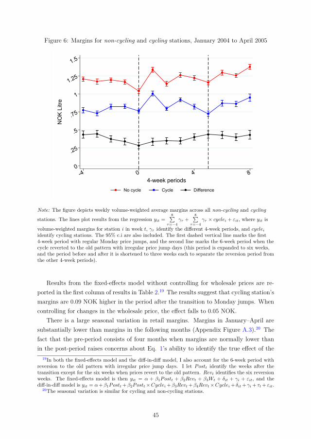
Figure 6: Margins for non-cycling and cycling stations, January 2004 to April 2005

0

.25

.5

.75

1

1.25

1.5N

OK

Litre

-4 0 4 84-week periods

No cycle Cycle Difference

Note: The figure depicts weekly volume-weighted average margins across all non-cycling and cycling

stations. The lines plot results from the regression yit =8∑

τ=−4γτ +

8∑τ=−4

γτ × cyclei + εit, where yit is

volume-weighted margins for station i in week t, γτ identify the different 4-week periods, and cycleiidentify cycling stations. The 95% c.i are also included. The first dashed vertical line marks the first4-week period with regular Monday price jumps, and the second line marks the 6-week period when thecycle reverted to the old pattern with irregular price jump days (this period is expanded to six weeks,and the period before and after it is shortened to three weeks each to separate the reversion period fromthe other 4-week periods).

Results from the fixed-effects model without controlling for wholesale prices are re-ported in the first column of results in Table 2.19 The results suggest that cycling station’smargins are 0.09 NOK higher in the period after the transition to Monday jumps. Whencontrolling for changes in the wholesale price, the effect falls to 0.05 NOK.

There is a large seasonal variation in retail margins. Margins in January–April aresubstantially lower than margins in the following months (Appendix Figure A.3).20 Thefact that the pre-period consists of four months when margins are normally lower thanin the post-period raises concerns about Eq. 1’s ability to identify the true effect of the

19In both the fixed-effects model and the diff-in-diff model, I also account for the 6-week period withreversion to the old pattern with irregular price jump days. I let Postt identify the weeks after thetransition except for the six weeks when prices revert to the old pattern. Revt identifies the six reversionweeks. The fixed-effects model is then yit = α + β1Postt + β2Revt + β3Wt + δit + γi + εit, and thediff-in-diff model is yit = α+β1Postt +β2Postt×Cyclei +β3Revt +β4Revt×Cyclei + δit + γi + τt + εit.

20The seasonal variation is similar for cycling and non-cycling stations.

45

transition to regular Monday price jumps. I account for seasonal variation by includingobservations from 2004 to 2017 and including month-of-year and year fixed effects inEq. 1.21 Controlling for seasonal variation in the fixed-effects model further reduces theestimate of the transition to −0.02 NOK (column 3 in Table 2. The diff-in-diff modelsalso give estimates close to zero (columns (4) and (5) in Table 2).

Table 2: Transition to regular Monday price jumps

(1) (2) (3) (4) (5)Post 0.09*** 0.05*** -0.02

(0.01) (0.01) (0.01)Post × Cycle 0.03 0.02

(0.02) (0.01)Constant 0.78*** 0.84*** 1.54*** 0.86*** 0.89***

(0.01) (0.06) (0.02) (0.01) (0.02)Week FE No No No Yes YesWholesale price+Lags No Yes Yes No YesAccount for seasonal variation No No Yes No NoAccount for reversion period Yes Yes Yes Yes YesStation FE Yes Yes Yes Yes YesCompetitors FE Yes Yes Yes Yes YesObservations 55376 52168 866149 63171 59534R2 0.53 0.59 0.69 0.70 0.71

Notes: The 1st column displays results from the fixed-effects model in Eq. 1 accounting for the reversionperiod. The model in the 2nd column also adjusts for changes in the wholesale price, and the 3rd columnalso accounts for seasonal variation. The 4th column shows results from the diff-in-diff model in Eq. 2,and the diff-in-diff model in the 5th column also adjusts for changes in the wholesale price. Standarderrors are clustered at the municipality level and are shown in parentheses. *p < 0.05, **p < 0.01,***p < 0.001.

The short pre- and post-periods limit the robustness of the results somewhat, butoverall the evidence suggests that the transition to regular Monday price jumps did nothave a substantial effect on retail margins. The difference in results in this study andForos & Steen (2013)’s study could be due to the fact that their analysis is based onan unbalanced and non-volume-weighted panel of user-reported prices, that they do notaccount for seasonal variation, or because the pre- and post-periods differ. When I do notaccount for seasonal variation, estimates in this study are closer to their results.

4.3 Transition to regular Thursday price jumps

I focus on the period from two years before to two years after the transition to regularThursday jumps.22 There are successful second price jumps in some of the weeks in the

21Postt still only identifies the weeks in the first eight months after the transition to regular Mondayjumps. The result that the transition to regular Monday jumps did not have a substantial effect on retailmargins is robust to changing how many years after 2004 are included in the model.

22The results in Table 3 are robust to decreasing the pre- and post-periods to one year before and afterthe transition or increasing the pre- and post-periods to three years. The estimates from the fixed-effects

46

pre-period. Thus, I estimate the effect of a transition from an equilibrium with regularMonday jumps and also Thursday/Friday price jumps in some weeks, to an equilibriumwith successful price jumps on Monday and Thursday every week. The development inmaximum margins on Monday and Thursday in Figure 8 illustrates this nicely—beforethe transition, maximum Thursday margins are lower than maximum Monday margins,but after the transition maximum margins on those two days are almost identical becauseprices are increased to the same level on both Monday and Thursday.

Given that the other characteristics of the cycle, such as the size of the jumps and howfast prices fall in the undercutting phase of the cycle, remain unchanged, it is natural toexpect that the more frequent price jumps increase the chains’ average margins. However,according to Noel (2019), more frequent price jumps need not be anticompetitive. Theauthor argues that price jumps should occur only when they are competitively necessary,even if the frequency of jumps increases. With more frequent price jumps, the size ofthe jumps should competitively adjust downwards to compensate for fewer rounds ofundercutting so that the bottom of the cycle is reached faster. Noel (2019)’s insightimplies that margins at the bottom of the cycle should be the same after the jumpfrequency increases, but the smaller price jump size should decrease margins at the topof the cycle, i.e., the maximum margin on Monday should decrease.

Figure 7 reveals that the Monday maximum margin does not decrease after thetransition—the mitigating effect related to decreasing margins at the top of the cyclethat Noel (2019) predicts does not materialize. The figure also shows that the minimummargin on Monday (the margin at the bottom of the cycle) increases substantially afterthe transition. Contrary to Noel (2019)’s predictions, Monday price jumps are carriedout as before the transition even though the pre-jump margins are higher.

Figure 8 shows that the trends in cycling and non-cycling stations’ margins are fairlysimilar in the pre-period, but with a small gradual increase in cycling stations’ marginsrelative to the non-cycling stations’ margins.23 Both the cycling and non-cycling stations’margins are higher in the post-period than in the pre-period. The cycling stations’ marginsalso increase relative to the non-cycling stations’ immediately after the transition (inperiod 0) and stay closer to the non-cycling stations’ margins through the next seven13-week periods, indicating that the transition to regular Thursday price jumps increasesthe cycling stations’ margins.

Table 3 shows a final set of results related to the transition to Thursday price jumpsbased on Eqs. 1 and 2.24 In line with the development in the cycling stations’ prices

model in column (1) change 60.04 NOK, and the diff-in-diff estimates in columns (2)–(4) change 60.02NOK.

23I exclude the few stations that change cycling status from non-cycling to cycling or vice versa in theyears 2007–2011 from the analysis. The results are robust to including the excluded stations as well.

24All specifications in Table 3 include controls for current and lagged wholesale prices. All results arevery similar (60.02 NOK difference) without the wholesale price controls.

47

Figure 7: Min. and max. margins

.5

.75

1

1.25

1.5

1.75N

OK/

Litre

-8 -4 0 4 713-week periods

Max margin Mon Max margin Thu Min margin Mon

Note: The figure depicts the development in cycling stations’ maximum margin on Monday, maximummargin on Thursday, and minimum margin on in the two years before and after the transition to

regular Thursday price jumps. The lines plot results from the regression yit =7∑

τ=−8γτ + εit, where yit is

maximum Monday margin, maximum Thursday margins, and minimum Monday margin for cyclingstation i in week t. γτ identify the different 13-week periods. The 95% c.i are also included. The dashedvertical line marks the first 13-week period with regular Thursday price jumps.

in Figure 8, the results from the fixed-effects model in the first column of the tableshow that average volume-weighted margins for cycling stations are 0.26 NOK higherin the two years following the transition than in the two years before the transition.This increase in volume-weighted margins does, however, include the general increase inmargins experienced by the control group consisting of non-cycling stations. The resultsfrom the diff-in-diff model in column (2) show that cycling stations’ margins increase by0.10 NOK after the transition relative to the non-cycling stations. As average margins inthe two years before the transition are 1.05 NOK, a 0.10 NOK increase equals an increaseof about 10%.

The non-cycling stations do not provide a perfect counterfactual. Tveito (2021b) showsthat the share of cycling stations’ volume that is sold on Sunday and Monday morning(the time of week when prices are lowest) increases slowly from 2004 to 2009 Q1. All elseequal, average weekly volume-weighted margins decrease when more consumers substitutepurchases to the low-price part of the cycle. The trend towards more volume sold in the

48

Figure 8: Margins, cycling and non-cycling stations

0

.25

.5

1

1.5

2N

OK

Litre

-8 -4 0 4 713-week periods

No cycle Cycle Difference

Note: The figure depicts the development in volume-weighted average margins across all non-cyclingand cycling stations in the two years before and after the transition to regular Thursday price jumps.The difference between cycling and non-cycling stations’ margins is also plotted. The lines plot results

from the regression yit =7∑

τ=−8γτ +

7∑τ=−8

γτ × Cyclei + εit, where yit is volume-weighted margins for

station i in week t, γτ identify the different 13-week periods, and Cyclei identify cycling stations. The95% c.i are also included. The dashed vertical line marks the first 13-week period with regularThursday price jumps.

low-price part of the cycle and lower average prices would probably have continued atthe cycling stations in a counterfactual without regular Thursday price jumps, but thestations in the control group do not take into account this trend. Thus, the cyclingstations’ volume-weighted margins would probably have decreased slightly relative to thenon-cycling stations without the introduction of regular Thursday jumps. This impliesthat results from a diff-in-diff model of cycling stations change over time in volume-weighted margins with non-cycling stations as a control group contains a slight downwardbias.

The Thursday jumps increase prices around noon on Thursday, and prices stay at ahigher path until around noon the next Monday. The main effect of the transition toregular Thursday jumps should thus be to increase prices on Thursday to Monday. Wetherefore expect the increase in average weekly margins to be driven by large marginincreases in this part of the week. If other characteristics of the cycle—such as how fastprices fall in the undercutting phase—do not change after the transition, we expect to

49

Table 3: Transition to regular Thursday price jumps

(1) (2) (3) (4)Post 0.26***

(0.01)Post × Cycle 0.10*** 0.01 0.13***

(0.01) (0.01) (0.01)Constant 1.07*** 1.15*** 1.30*** 1.11***

(0.02) (0.01) (0.01) (0.01)Week FE No Yes Yes YesWholesale price controls Yes Yes Yes YesCompetitors FE Yes Yes Yes YesStation FE Yes Yes Yes YesObservations 205892 219740 219739 219740R2 0.51 0.63 0.55 0.63F-value 775.94 20.98 11.62 25.38

Note: Column (1) displays results from Eq. 1. Column (2) displays results from Eq. 2. Column (3)displays results from a model similar to Eq. 2, where yit is the average volume-weighted margins overTue and Wed for station i in week t. Column (4) displays results from a model similar to Eq. 2, butwhere yit is the average volume-weighted margins over Monday, Thursday, Friday, Saturday, andSunday for station i in week t. Post identifies all weeks after March 23, 2009. The sample period isMarch 2007 to March 2011. *p < 0.05, **p < 0.01, ***p < 0.001.

see no change in cycling stations’ Tuesday and Wednesday margins (the two full daysafter the Monday jumps and before the Thursday jumps). Column (3) in Table 3 showsresults from Eq. 2 with average margins across Tuesday and Wednesday as the dependentvariable. Reassuringly, the cycling stations’ margins on these days do not increase relativeto non-cycling stations after the transition. The final column in the table shows resultsfrom Eq. 2 with average margins across Thursday–Monday as the dependent variable.As expected, cycling stations’ margins on these days increase more than average weeklymargins (0.13 vs 0.10 NOK).

Chain C acquired 90 stations from Chain D just prior to the transition to regularThursday jumps (see Appendix B). A final concern is that unilateral effects from themerger, rather than the transition to regular Thursday price jumps, are driving the in-crease in margins. If this is the case, an increase in margins for the stations subject to themerger relatively to stations in other areas should be observed. However, the NorwegianCompetition Authority has conducted an ex post evaluation of the merger and found,employing a diff-in-diff model, that the stations subject to the merger (and to a smallerextent, other stations in the same areas) experience a small (0–0.05 NOK) decrease inmargins after the merger relative to stations in other areas (OECD, 2013).

Summing up, Noel (2019)’s prediction of lower margins at the top of the cycle when thefrequency of price jumps increases does not materialize, and the evidence suggests that thetransition to regular Thursday jumps increases cycling stations’ volume-weighted marginsby at least 0.10 NOK (10%). The effect is driven by an increase in margins in the part

50

of the week after the Thursday jumps are initiated and before the next Monday jumps.Coordination of two weekly price jumps not only helps the chains to avoid the war ofattrition game at the very bottom of the cycle but also enables them to avoid large partsof cycle trough while still reaping the benefits of high prices at the peak of the cycle.

As shown in Section 3.3, there are successful Thursday price jumps in about 40% ofthe weeks in the two years before the transition to regular Thursday jumps. Thus, inthis section I estimate the effect of transitioning from a pattern with one price jump insome weeks and two price jumps in other weeks to a pattern with two price jumps everyweek. The total effect of transitioning from one to two price jumps per week is larger.Tveito (2021a) estimate that in the four years with irregular Thursday jumps, a Thursdayjump increases the average weekly margins in a given week by 25% compared with acounterfactual without Thursday jumps.

5 Discussion

We have seen that the market gradually transitioned from one price jump per week onirregular weekdays to a more profitable equilibrium with two price jumps per week onregular weekdays. The calendar synchronized price jumps are remarkably stable overtime. In this section, I argue that regular price leadership provided by the large retailchains played a key role in coordinating the transition to more frequent price jumps andensuring that the price jumps continue to occur at the same time over a very long periodof time. Furthermore, I highlight the connection between firms’ size and price leadership.

5.1 Price leadership and transition to more frequent price jumps

The Monday price jumps emerge when the largest chain begins to initiate price jumpsevery Monday. From the very start, the chain’s jumps are matched by all other chains.When the chain stops providing price leadership for six weeks, no other chains initiateMonday jumps, and prices revert to the old pattern with price jumps on irregular week-days. After the six weeks without Monday jumps, the largest chain initiates Mondayprice jumps every week for the next 13 years. The Monday price jumps remain successfulduring all these years, even through periods with large wholesale price volatility whenprice cycles in other countries have been shown to break down.

During the four years with irregular second price jumps, both the frequency and successrate of the jumps are higher in periods when one of the chains acts as a regular leaderof the second jumps. The transition to regular Thursday jumps occurs when the second-largest chain starts to lead Thursday jumps every week, and the jumps are immediatelysuccessful. The pattern with price jumps on both Monday and Thursday is stable for thenext eight years until the transition to a new equilibrium is once again initiated by the

51

largest chain.The evidence suggests that regular price leadership was instrumental to coordinate

the transition to more frequent price jumps and to keep the equilibrium with calendarsynchronized jumps stable over a very long time period.

Existing empirical evidence on how firms coordinate on collusive equilibria is sparse,but in a recent paper Byrne & de Roos (2019) offer a compelling analysis of how large retailgasoline chains in Perth, Australia, use price leadership to coordinate a transition to anequilibrium with higher profit margins. There are, however, some interesting differencesin the institutional settings and how the transitions occur in Norway and Perth. Perth’sFuelWatch program requires gasoline retailers to submit next-day station-level prices tothe government every day before 14:00, without knowing rivals’ next-day prices. Pricesare then posted on a webpage and are fixed at these levels the next day. Norwegian gasstations are not subject to any price regulation.

After three years of experimentation and price leadership, calendar synchronized Thurs-day price jumps are established as a focal point for price increases in Perth. Instead oftrying to initiate price jumps on other weekdays in addition to the Thursday jumps, theleader in Perth manages to transition the market to a pricing pattern with a fixed pricecut size per day in the undercutting phase of the cycle, and also greatly increases marginsat the top of the cycle. This way, price–cost margins increase on all weekdays. In theNorwegian market, margins at the top of the cycle increase gradually during the wholesample period, but I find no evidence of standardization of the size of price cuts.25 In-stead, the main margin-enhancing event in Norway is the transition from one to two pricejumps per week.

The different regulatory regimes provide a possible explanation of the different ways ofcoordinating margin-enhancing equilibria that chains in Perth and Norway ended up with.The firm providing price leadership is alone with a high price for some time until the otherfirms match the price increase. In this period, the leader loses volume to competitors. Thevolume loss related to leading imposes a cost on the leader and can thus limit incentives tolead price increases. Perth’s FuelWatch regulation forces the price leader to be alone witha high price for a full day before competitors can match the price increase. In Norway, theother chains match the leader’s price increase after only a few hours. The requirement inPerth to post prices online also increases price transparency, perhaps giving higher ownprice elasticities in Perth than in Norway. Tveito (2021a) shows that the volume lossrelated to leading the second price jumps in Norway is low, and that the leader does notlose profit relative to the followers. Due to the longer period alone with a high price andhigher price transparency in Perth, it seems much more costly to provide price leadership

25Margins at the top of the cycle increase at a fairly steady pace until 2012. After 2012, margins atthe top of the cycle increase at a faster pace. However, prices fall faster in the undercutting phase of thecycle after 2012, partly mitigating the effect of higher margins at the peak of the cycle.

52

for more frequent price jumps in Perth than in Norway.By contrast, coordinating prices in the undercutting phase of the cycle is less com-

plicated in Perth than in Norway. The chains in Perth only need to coordinate on thesize of the daily price decrease, while coordination of prices in the undercutting phase inNorway would require firms to agree on the number of price changes per day, the timingof the price changes, and the size of the price decreases.

Summing up, I find that large retail chains use price leadership to coordinate a tran-sition to more frequent price jumps and to sustain the new equilibrium. The absence ofregulation of the timing of price changes and lack of measures to increase price trans-parency decrease the cost of leading and increase the complexity of coordinating pricesin the undercutting phase of the cycle. In such an unregulated environment, a transitionto an equilibrium with more frequent price jumps is probably easier to coordinate thantransitions to other margin-enhancing equilibria that have been observed in markets withprice regulations.

5.2 Firm size

The results from Section 3 also contribute to our understanding of the connection betweenfirm size and price leadership—in particular for retail gasoline markets with price cycles.Price leadership is already comprehensibly studied in the retail gasoline market in Perth.Wang (2009) uses a combination of hourly and twice-a-day observations to show thatthe largest chain in this market was acting as a regular price leader in the six monthsbefore the regulation prohibiting more than one price change per day was introduced, andthat just after the regulation came into effect, multiple large chains were rotating priceleadership. Byrne & de Roos (2019) show that the largest chain in Perth is once againacting as a regular price leader several years later.

High-frequency price changes and data of lower frequency limit the robustness of theprevious studies of price leadership in the more typical case without price regulation. Noel(2007), Atkinson (2009), and Lewis (2012) provide some evidence that price jumps in theUSA and Canada are led by retail gasoline chains controlling a large number of stations,but not necessarily the largest chain. Noel (2007) and Lewis (2012)’s studies are based onobservations with 12 hours and daily data frequency, meaning that the results are onlya rough indicator of the retailers whose stations are most likely to jump early. Even inAtkinson (2009)’s study where prices are observed every two hours, the ability of stationsto respond quickly makes it fairly difficult to identify price leaders. In addition, Atkinson(2009)’s study is based on a sample of only 26 stations and over only 103 days. Lemus& Luco (2021) find that the largest chain is the most frequent price leader in the retailgasoline market in Chile where prices only change about once per week.

With the panel of to-the-minute information on price changes for almost all Norwegian

53

gas stations over a 14-year-long period, I provide several observations related to firm sizeand price leadership. First, the largest chain is the regular leader of Monday price jumpsfor 13 consecutive years. The chain initiates large price jumps within about an hour foraffiliated stations located in all parts of Norway, and the price jumps are always followedby the other chains.

Second, the second price jumps start to occur every week and achieve a 100% successrate when Chain C starts to lead every Thursday in March 2009. The transition occursjust a few months after a transaction that made Chain C a clear runner-up in terms ofnational market share. The 90 stations Chain C acquired were spread out in differentparts of Norway but were almost exclusively located in populous areas with other ChainC stations.26 The local overlap with existing Chain C stations led to an increase in averagelocal market share for Chain C’s stations of the same magnitude as the increase in thenational market share.27

A final observation is that Chain C continues to lead most Thursday price jumps untilChain D takes over as a Thursday price leader in 2014 after its market share increasedover several years.

Taken together, evidence of size differences of both between-chain and within-chainchanges in size shows that having a large network of gas stations is positively correlatedwith being a regular price leader. Price jumps are also more frequent and more oftensuccessful when the largest chains lead. The correlation between size and price leadershipis consistent with theoretical models of price leadership in markets with Edgeworth cycleswhere firms with a large share of retail outlets earn greater profits at high prices andtherefore have stronger incentives to lead price jumps (Eibelshäuser & Wilhelm, 2018;Eckert, 2003).

6 Concluding remarks

In this paper, I employ a unique data set of to-the-minute price data to show how retailgasoline chains use price leadership to both initiate and sustain a new equilibrium withprice jumps every Monday and Thursday. I argue that lack of price regulation makesit easier to enhance margins by the transition to more frequent price jumps rather thanby inflating margins on all days of the price cycle as in the regulated market studied byByrne & de Roos (2019).

Contrary to what Noel (2019) postulates, the transition to more frequent price jumps2693% of the stations were located within 15 minutes’ drive time of another Chain C station.27The average volume-based local market share of Chain C’s stations increased from 33% in January

2008 to 39% in January 2009. A local market is defined around each station and includes all stationswithin a 15-minute drive time. The market share of the center station is calculated by adding the volumeof the center station and all other stations from the same chain in the local market and dividing by thetotal volume of all stations in the local market.

54

leads to a substantial increase in average volume-weighted margins. The results suggestthat regulators should be concerned with increases in the frequency of price jumps.

What can regulators do to destabilize such high-margin equilibrium? Foros & Steen(2013) argue that the retail gasoline chains in Norway de facto simultaneously decide tohike prices to the recommended price. They suggest that the publication of recommendedprices increases transparency among competitors, facilitates horizontal coordination, andshould be banned. Due to my extremely high-frequency price data, I can show thatthe price hikes are sequential rather than simultaneous. A leader first hikes prices forits stations, and the other chains follow within a few hours. The non-leaders thereforeobserve the leader’s new price level before they hike prices. Thus, the leader can createa focal point for the new price level without the publication of recommended prices. Therecommended prices appear to be redundant for coordinating the price hikes.28

Other approaches for regulators can be to make it harder or more costly to act as aprice leader. Weakening the chain headquarters’ control over dealer-owned outlets’ priceswould make it harder to initiate chain-wide price jumps (Wang, 2009). Tveito (2021a)argues that policies that inform customers about when price jumps occur and which firmsact as leaders and followers can increase the cost of leading price jumps.

Finally, I find that price leadership is provided by large chains, and the jumps are moreoften successful when one of the largest chains leads. The results are consistent with Byrne& de Roos (2019)’s conclusion that firm asymmetries can facilitate collusion because adominant firm can act as a price leader and initiate price coordination. Furthermore, thesolidification of Thursday price jumps after a transaction that created a clear number twoin the market may indicate that mergers increasing the size of the runner-up can give riseto an additional price leader and equilibria with more frequent price increases.

28The publication of future changes in recommended prices can, however, help firms coordinate pricejumps (Foros & Ones, 2021).

55

References

Andreoli-Versbach, P., & Franck, J. (2015). Endogenous Price Commitment, Sticky andLeadership Pricing: Evidence from the Italian Petrol Market. International Journal ofIndustrial Organization, 40 , 32-48.

Atkinson, B. (2009). Retail Gasoline Price Cycles: Evidence from Guelph, Ontario UsingBi Hourly, Station-Specific Retail Price Data. Energy Journal, 30 (1), 85-109.

Borenstein, S., & Shepard, A. (1996). Dynamic Pricing in Retail Gasoline Markets.RAND Journal of Economics, 23 (3), 429-451.

Bundeskartellamt. (2011). Fuel Sector Inquiry.

Byrne, D. P., & de Roos, N. (2018). Online Appendix: Learning to Coordinate - A Studyin Retail Gasoline.

Byrne, D. P., & de Roos, N. (2019). Learning to Coordinate - A Study in Retail Gasoline.American Economic Review, 109 (2), 591-619.

Cabral, L., Duerr, N., Schober, D., & Voll, O. (2021). Price Matching Guarantees andCollusion: Theory and Evidence from Germany. Working Paper .

Chilet, J. A. (2018). Gradually Rebuilding a Relationship: The Emergence of Collusionin Retail Pharmacies in Chile. Working Paper .

Clark, R., & Houde, J. F. (2013). Collusion with Asymmetric Retailers: Evidence froma Gasoline Price-Fixing Case. American Economic Journal: Microeconomics, 5 (3),97-123.

de Roos, N., & Smirnov, V. (2020). Collusion with Intertemporal Price Dispersion. RANDJournal of Economics, 51 (1), 158-188.

Drivkraft Norge. (2021). Salg av Bransjens Hovedprodukter tilbake til 1952(Sale of the Industries Main Products back to 1952. Retrieved 2021-08-25, from https://www.drivkraftnorge.no/siteassets/dokumenter--filer/statistikk/salg/salg-tilbake-til-1952-til-hjemmesiden.xlsx

Eckert, A. (2003). Retail Price Cycles and the Presence of Small Firms. InternationalJournal of Industrial Organization, 21 (2), 151-170.

Eckert, A. (2013). Empirical Studies of Gasoline Retailing: A Guide to the Literature.Journal of Economic Surveys, 27 (1), 140-166.

Eibelshäuser, S., & Wilhelm, S. (2018). High-Frequency Price Fluctuations in Brick-and-Mortar Retailing. Working paper .

56

Foros, Ø., & Ones, M. N. (2021). Coordinate to Obfuscate? The Role of Prior Announce-ments of Recommended Prices. Economics Letters, 198 .

Foros, Ø., & Steen, F. (2013). Vertical Control and Price Cycles in Gasoline Retailing.Scandinavian Journal of Economics, 115 (3), 640-661.

Fung, M. K. (2018). Deposit Rate Asymmetry and Edgeworth Cycles after Hong Kong’sInterest Rate Deregulation, in (ed.) Banking and Finance Issues in Emerging Markets.International Symposia in Economic Theory and Econometrics, 25 , 105-121.

Green, E. J., Marshall, R. C., & Marx, L. M. (2014). Tacit Collusion in Oligopoly.The Oxford Handbook of International Antitrust Economics, Volume 2, Edited by R. D.Blair and D. D. Sokol.

Harrington, J. E. (2017). A Theory of Collusion with Partial Mutual Understanding.Research in Economics, 71 , 140-158.

Hasbrouck, J. (2018). High-Frequency Quoting: Short-Term Volatility in Bids and Offers.Journal of Financial and Quantitative Analysis, 53 (2), 613-641.

Hauschultz, F. P., & Munk-Nielsen, A. (2017). Priscykler i Markedet for ReceptpligtigMedicin efter Patentudløb (Price Cycles in the Market for Prescription Medicin afterPatent Expiration). Konkurrence- og Forbrugerstyrelsen: Velfungerende Markeder .

Konkurransetilsynet. (2014). Drivstoff Markedet i Norge - Marginøkning og Ny Pristopp(The Norwegian Fuel Market – Margin increase and a New Price Peak).

Konkurransetilsynet. (2015). Vedtak V2015-29 - St1 Nordic OY - Smart Fuel AS -Konkurranseloven § 16 jf. § 20 - Inngrep mot Foretakssammenslutning (Decision V2015-29 - St1 Nordic OY - Smart Fuel AS - the Competition Act § 16 jf. § 20 - InterventionAgainst Merger).

Lemus, J., & Luco, F. (2021). Price Leadership and Uncertainty about Future Costs.Journal of Industrial Economics, 69 (2), 305-337.

Lewis, M. S. (2009). Temporary Wholesale Gasoline Price Spikes Have Long-LastingRetail Effects: The Aftermath of Hurricane Rita. Journal of Law and Economics, 52 ,581–605.

Lewis, M. S. (2012). Price Leadership and Coordination in Retail Gasoline Markets withPrice Cycles. International Journal of Industrial Organization, 30 (4), 342–351.

Markham, J. W. (1951). The Nature and Significance of Price Leadership. AmericanEconomic Review, 41 (5), 891-905.

57

Maskin, E., & Tirole, J. (1988). A Theory of Dynamic Oligopoly, II: Price Competition,Kinked Demand Curves, and Edgeworth Cycles. Econometrica, 56 (3), 571-599.

Neset, G. P. (2010). Prisstøttesystemet i Bensinmarkedet (The Price Support System inthe Gasoline Market).

Noel, M. D. (2007). Edgeworth Price Cycles: Evidence from the Toronto Retail GasolineMarket. Journal of Industrial Economics, 66 (2), 69-92.

Noel, M. D. (2019). Calendar Synchronization of Gasoline Price Increases. Journal ofEconomics and Managment Science, 28 (2), 355-370.

OECD. (2013). Competition in Road Fuel.

Seaton, J. S., & Waterson, M. (2013). Identifying and Characterising Price Leadershipin British Supermarkets. International Journal of Industrial Organization, 115 (31),392-403.

Tveito, A. (2021a). The Costs and Benefits of Price Leadership – Evidence from RetailGasoline. Working Paper .

Tveito, A. (2021b). Dynamics in Intertemporal Substitution – Evidence from Retail Fuel.Working Paper .

Wang, Z. (2008). Collusive Communication and Pricing Coordination in a Retail GasolineMarket. Review of Industrial Organization, 32 (1), 32-52.

Wang, Z. (2009). (Mixed) Strategy in Oligopoly Pricing: Evidence from Gasoline PriceCycles Before and Under a Timing Regulation. Journal of Political Economy, 117 (61),987-1030.

Zhang, M., & Feng, J. (2011). Cyclical Bid Adjustments in Search-Engine Advertising.Management Science, 57 (9), 1703-1719.

58

Appendices

A Additional figures

Figure A.1: Cycle groups, shares and number of competitors

0

.25

.5

.75

1

Shar

e of

all

stat

ions

20042006

20082010

20122014

2016

Year

(a) Number of stations

0

.5

1

1.5

2

2.5

3

Avg

n co

mpe

ting

chai

ns

20042006

20082010

20122014

2016

Year

(b) Avg number of competitors

No Cycle Cycle

Note: Panel (a) plots the share of stations that are cycling and non-cycling each year. Panel (b) plotsaverage number of competing chains present within 15 min drive time of each station for the samegroups.

59

Figure A.2: Share of volume on different weekdays, Jan2004–Apr2004

2.6

2.8

3

3.2

Pric

e ex

cl ta

x in

NO

K/lit

re

0

.02

.04

.06

.08

.1

.12

.14

.16

.18

Shar

e of

tota

l wee

kly

volu

me

Monday Tuesday Wednesday Thursday Friday Saturday Sunday

Vol share, cycle Vol share, no cycleAvg price, cycle Avg price, no cycle

Note: The figure depicts average prices excl. taxes, and average share of weekly volume of gasoline soldon different weekdays before the regular Monday jumps are introduced. Results are split betweencycling stations (prices represented by the solid red line and volume shares by the dark blue bars) andnon-cycling stations (prices represented by the dashed red line and volume shares by the light blue bars).Note that both cycling and non-cycling stations experience relatively small variations in volumes ondifferent weekdays, but sell slightly higher volume on Friday than on other days.

60

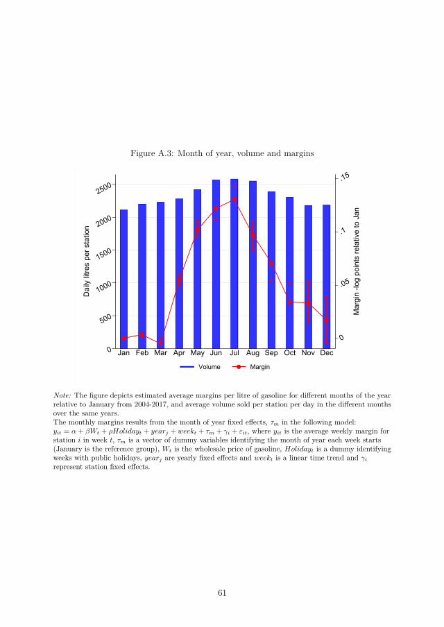
Figure A.3: Month of year, volume and margins

0

.05

.1

.15

Mar

gin

-log

poin

ts re

lativ

e to

Jan

0

500

1000

1500

2000

2500

Dai

ly li

tres

per s

tatio

n

Jan Feb Mar Apr May Jun Jul Aug Sep Oct Nov Dec

Volume Margin

Note: The figure depicts estimated average margins per litre of gasoline for different months of the yearrelative to January from 2004-2017, and average volume sold per station per day in the different monthsover the same years.The monthly margins results from the month of year fixed effects, τm in the following model:yit = α+ βWt + ρHolidayt + yearj + weekt + τm + γi + εit, where yit is the average weekly margin forstation i in week t, τm is a vector of dummy variables identifying the month of year each week starts(January is the reference group), Wt is the wholesale price of gasoline, Holidayt is a dummy identifyingweeks with public holidays, yearj are yearly fixed effects and weekt is a linear time trend and γirepresent station fixed effects.

61

Figure A.4: Time of day of chain price jumps, 2004

Note: The figure shows the time of chain price jumps for each chain for all weeks in 2004. Each dotrepresents the time of day a given chain initiates a chain price jump. Take note of the following:

1. Chain A (third black rectangle), Chain B (second black rectangle) and Chain D (first blackrectangle) all lead price jumps before the week of April 26 2004.

2. On April 26 2004 (first dashed vertical line), Chain A starts to initiate price jumps everyMonday. In the periods with regular Monday jumps (between the first and second dashed lineand after the third dashed line), Chain A leads price jumps around 10:00 almost all weeks. Theother chains follow in a fairly orderly fashion 1–4 hours later.

3. Different chains lead in the period when the pricing pattern reverts to price jumps on irregularweekdays (between the second and third dashed line).

*In the five weeks with second price jumps starting the week of April 26 2004 only the Monday pricejumps are depicted.**Data is missing for Chain C before the week of October 26 2004.

62

Figure A.5: Time of day of Thursday chain price jumps, 2009–2017

9

10

11

12

13

14

15

16

17

Tim

e of

day

Jan2009Jan2011

Jan2013Jan2015

Jan2017

Week

Chain A Chain B Chain C Chain D Chain E

Note: The figure depicts the time of Thursday chain price jumps for each chain for all weeks fromJanuary 2009–November 2017. Each dot represents the time of day a given chain initiates a chain pricejump. The vertical red line highlights the week of March 23 2009, when successful Thursday price jumpsare solidified. Take note of the following:

1. Chain C is first to initiate Thursday price jumps most weeks (between 11:00 and 11:30) from theweek Thursday price jumps are solidified until January 2014.

2. Chain B normally initiates price jumps 0.5–1 hour after Chain C, but in some weeks when ChainC initiates price jumps at 12:00 or even later, Chain B initiates price jumps about the same timeor before Chain C.

3. Chain A initiates price jumps 1-3 hours after the price leader.4. Chain E is the last chain to initiate price jumps 3–5 hours after the price leader.5. When Chain B and Chain C delay price jumps to 12:30-13:00 starting in 2014, Chain D is first to

initiate price jumps (at 12:00).

63

Figure A.6: Reversion to irregular jump days

Note: The figure plots average prices excluding taxes for each chain during each hour of the week ofAugust 30 2004 to the week of October 25 2004. The bottom grey line is the marginal cost proxy. Takenote of the following:

1. When Chain A suddenly stops initiating Monday price jumps the week of September 6, onlyChain D carries out a price jump. The next Monday, no chains implement a Monday price jump.

2. Price jumps take place on Tuesdays, Wednesdays, and Thursdays in the weeks when Chain Adoes not initiate Monday price jumps (September 6–October 11).

3. When Chain A re-initiates Monday price jumps, all other chains immediately follow.

64

Figure A.7: Price cycles during wholesale price turbulence

Note: The figure plots average prices excluding taxes for each chain during each hour of the week ofAugust 22 2005, to the week of November 7 2005. The bottom grey line is the marginal cost proxy.Take note of the following:

1. The marginal costs are very volatile from the week of August 29 to the week of October 17.2. Chain A continues to initiate Monday price jumps every week during these eight weeks, but in

some of the weeks the jumps fail because one or more of the other chains do not follow.3. In addition to the Monday jumps, jump attempts are also initiated on Tuesday, Wednesday,

Thursday, and Friday.4. When the marginal costs stabilizes after the week of October 17 2005, regular successful Monday

jumps continue to occur.

65

Figure A.8: Price cycles during the crude oil crisis

Note: The figure depicts average hourly prices excluding taxes cycling stations from April2008–February 2009 during a period with large wholesale price variation due to the 2008 crude oil crisis.The upper grey line is average list price, and the lower grey line is the marginal cost proxy. Note thatmarginal costs fall greatly during this period, but the price cycle remains stable.

66

B Notable events in the sample period

In August 2007, Chain C and Chain D agreed that Chain C would control the sale ofgasoline at 92 of Chain D’s manned stations in Norway for a period of 10 years. Thedeal was approved by the Norwegian Competition Authority in February 2008 after theparties agreed to exclude two stations from the deal. The merger was consummatedbetween August and December 2008, when Chain C gradually began operating the 90 gasstations.

Chain E was part of a Nordic chain until October 2008 when Chain A bought theNordic chain as part of a larger multinational merger. To remedy regulators’ concernsabout impediment to effective competition, Chain A sold Chain E to another Nordic fuelcompany with no prior activity in the Norwegian market in April 2009. In the interimperiod, Chain E was managed by a Hold Separate Manager under the supervision of aMonitoring Trustee.

Chain A was vertically integrated with a large oil company until April 2012, whenfuel retailing was fissioned out and sold to a large international retail chain with no prioractivity in Norway.

Chain C was vertically integrated with a large oil company until October 2015, whenfuel retailing was fissioned out and sold to the Nordic company controlling Chain E. Toremedy concerns about impediment to effective competition, the Nordic company had tosell its existing Norwegian fuel retail network (Chain E) to an independent buyer. Aftera lengthy process, Chain E was sold to a small Norwegian bio-fuel firm in July 2017.

67

68

Chapter 3

The Costs and Benefits of Price Leadership—Evidence fromRetail Gasoline

The Costs and Benefits of Price Leadership—Evidencefrom Retail Gasoline∗

Andreas Tveito†

October 7, 2021

Abstract

A trade-off between losing volume to rivals and gaining higher price–costs mar-gins is central to understanding why firms may choose to act as price leaders. Aunique dataset with high-frequency price, cost, and volume data allows the esti-mation of costs and benefits of leading price jumps in a retail gasoline market withasymmetric price cycles. The main result is that the leader’s volume loss from beingthe sole firm to raise its price until the other firms match that price increase is smallcompared with the large margin increases and profit gains resulting from the pricejumps. Furthermore, I find that the leader is not worse off than the non-leadingfirms. The results can assist in explaining why firms are willing to act as regularprice leaders.

∗I would like to thank Sigurd Birkeland, Kurt Brekke, Gordon Dahl, Øystein Foros, Joe Harrington,Hans K. Hvide, Bjørn Olav Johansen, Katrine V. Løken, Teis Lunde Lømo, Magnus Friis Reitan andMorten Sæthre for helpful comments. I gratefully acknowledge financial support from the ResearchCouncil of Norway.†Department of Economics, University of Bergen and the Norwegian Competition Authority. The

views expressed in this paper are those of the author and do not necessarily reflect the views of theNorwegian Competition Authority.

69

1 Introduction

Price leadership—a practice involving sequential price changes whereby a leader changesprice first and rivals quickly follow—is a common feature in retail markets.1 Price leader-ship has long been considered a possible instrument to coordinate on higher prices—theleader provides focal points for the timing and level of price changes that are neededto initiate price hikes (Markham, 1951). All firms benefit from higher margins after themarket-wide price hikes, but the leader suffers a cost in terms of volume transfers to rivalsin the interim period before the rivals match the high price. The firms following the leaderenjoy both higher demand in the interim period, and higher profits in the after period.Thus, leading price hikes is a public good from the firms’ point of view and a free-riderproblem regarding which firm should lead can delay the price hikes, , even if leading aprice hike is better than no hike (Maskin & Tirole, 1988). Small volume transfers in theinterim period and large profit increases in the after period all, make it more likely thata firm is willing to provide price leadership.

This paper uses a unique dataset of high-frequency price, cost, and volume data forNorwegian gas stations to study the costs and benefits of leading price hikes. The costsand benefits of price leadership are particularly relevant in this market because it featuresasymmetric price cycles with frequent market-wide price restorations led by large chains.The main results are that the leader’s profit increases greatly compared with a situationwithout price hikes, the volume transfers from the leader to the followers in the interimperiod are small, and the leader does not perform worse than the followers. The resultssuggest that the cost of leading and the free-rider problem are not significant for the firmsstudied, and can assist in explaining why firms are often willing to act as regular priceleaders to initiate more frequent price increases.

The Norwegian retail gasoline market is dominated by four national chains with in-dividual market shares of 20–30% and a combined market share of more than 90%. Thechains own most of their affiliated stations and control the prices of other stations throughstrong vertical restraints. Because each chain controls prices at all affiliated stations andcarries out synchronized price hikes for affiliated stations, I focus on the effects of leadingprice hikes at the chain level.

As in many other countries, the Norwegian retail gasoline market features asymmetricprice cycles.2 Prices slowly decrease over several days until a nationwide price restorationoccurs, with each chain quickly initiating large price jumps for affiliated stations (Figure1). The jumps are partly “calendar synchronized” in that they occur at particular timesof the week. Large chains act as “regular leaders”; the same chain leads all or most of

1In addition to retail gasoline markets, price leadership has been documented in grocery retailing(Seaton & Waterson, 2013), brewing (Miller et al., in press), book and CD retailing (Kauffman & Wood,2007), and passenger transport (Bergantino et al., 2018).

2Asymmetric price cycles have been found in retail gasoline markets in multiple European countries,as well as in Australia, Canada, and the USA. Calendar-synchronized price jumps have been found inretail gasoline markets in the USA, Canada, Germany, and Australia (Noel, 2019).

70

the jumps that take place at a particular time of the week over several months or years.3

The largest chain (Chain A) leads price jumps every Monday through the entire sampleperiod. The three other national chains (Chains B, C, and D) and a regional chain (ChainE) always match the Monday jumps. In the 4-year period on which the main part of thisanalysis is based, there are also jump attempts on Thursdays (or more rarely on Fridays)in 62% of weeks. The non-leaders match most of these “midweek jumps” within a fewhours. Which of the national chains leads the midweek jumps varies over time, but thereare long periods in which a single chain leads almost all the midweek jumps. Immediatelyafter the 4-year period, one of the national chains begins leading Thursday jumps everyweek, and both Monday and Thursday jumps take place every week for the next 8 years.

The asymmetric price cycles in retail gasoline markets are often rationalized by the“Edgeworth cycle” price commitment model first described by Edgeworth (1925), andlater formalized by Maskin & Tirole (1988). The gradual price decreases over several daysand the market-wide price jumps occuring within a few hours align well with the theoryof Edgeworth cycles. However, several characteristics are contrary to the Edgeworth-model—the regularity of the price jumps, the same chains leading the jumps, high pre-jump margins, and the fact that the followers do not undercut the leader’s price at thetop of the cycle. Firm behavior in the undercutting phase of the cycle adheres well to theEdgeworth model, but the large chains appear to be using price leadership to coordinateon more frequent price jumps to avoid the cycle trough.4

A regular leader can solve the free-rider problem regarding who should hike prices first,thus limiting the time for which prices remain near the trough of the cycle. However, theleader must be willing to incur the cost of losing volume to rivals. Noel (2008) shows thatin a price commitment model, increasing the cost of leading price jumps relative to thebenefits, lowers incentives to lead and reduces the frequency of price jumps.5

The interim volume loss and subsequent profit increases are important determinantsfor firms’ incentive to provide price leadership. Yet, the empirical evidence quantifyingthese costs and benefits is very limited. Wang (2009) argues that a new regulation inthe Perth retail gasoline market increased the cost of providing price leadership, and thuscaused a transition from a regular price leader to alternating price leadership. But thestudy does not document the actual cost of leading. Clark & Houde (2013) study a marketwith explicit collusion and infrequent price hikes and find large volume transfers from thecartel members who hike prices first to the members who hike prices a few hours later.However, the authors only have access to quarterly volume data, and their estimates arebased on strong assumptions.

3Lewis (2012) (USA), Wang (2009) (Australia), and Cabral et al. (2021) (Germany) show that largechain acts as regular price leaders in other countries as well.

4de Roos & Smirnov (2020) show that asymmetric price cycles can be the optimal equilibrium forfirms in a model with history-based strategies and tacit collusion.

5Both the trade-off between the cost of leading and the benefits of higher future prices, and the free-rider problem are present also in models of price leadership in repeated games with history-dependentstrategies and non-cycling prices (Harrington, 2017; Harrington & Zhao, 2012).

71

This study has the advantage of a unique dataset that includes the exact timing ofprice changes, daily volume data, and data on wholesale prices and transportation costs formost Norwegian gas stations. Furthermore, the price pattern with regular Monday jumpsand irregular midweek jumps provides a setting that is well suited to studying the costsand benefits of price leadership. Figure 1 provides examples of a week with a successfulmidweek jump and a week without a midweek jump, indicating that successful midweekjumps bring about higher prices until the next Monday jump.6 Due to the regular Mondayjumps and irregular midweek jumps, it is safe to assume that the chains anticipate that aMonday jump will occur regardless of whether a midweek occurs. Therefore, the benefitsof midweek jumps last until the next Monday morning. As the followers increase priceswithin a few hours of the leader, the leader’s immediate cost is incurred on the same daythat the jumps are carried out.

Figure 1: Price cycles—with and without a midweek jump

Note: The colored lines depict the average hourly price excluding taxes in Norwegian kroner/liter foreach chain for 2 weeks in November 2007. The gray line is a proxy for marginal cost, as defined in Section2.2.

The primary challenge in estimating the effect of the price jumps is to identify thecounterfactual—how the outcomes of interest would have developed if the jump had nottaken place. The development in the outcome through the week in those weeks withoutmidweek jumps provides a suitable counterfactual for weeks with midweek jumps. Mybaseline specification is a difference-in-difference (“diff-in-diff”) model where the first dif-ference is the development in the outcomes of interest (margins, volumes, and profits)through the week for (1) stations affiliated with the chain leading the Thursday jumpsand (2) stations affiliated with the chains following the leader. The second difference isthe development through the week for all stations in weeks without midweek jumps. The

6I focus on the Thursday jumps because 84% of the midweek jumps occur on Thursdays.

72

model removes biases resulting from shocks that have the same effect on the outcomeon all weekdays, and accounts for trends in the outcome through the week. Except forThursdays (the day that jumps take place), the outcomes for both the leader and thefollowers have a very similar development to the outcomes in weeks without midweekjumps, supporting the parallel trend assumption.

Leading a successful Thursday price jump is greatly profitable for the price leadercompared with a counterfactual with no midweek jump. Across the whole week, theleader gives up only 0.5% of its market share but gains from price—cost margins—that,on average, are 25% higher, leading to a 21% increase in average weekly profit. Theleader’s post-jump price–cost margins increases greatly—Friday–Sunday margins increaseabout 45%. The higher prices trigger a close to 10% volume reduction on Friday–Sunday,but it is likely that a significant share of the volume loss stems from consumers delayingpurchases, and that these losses are later recouped. Even assuming that none of the lostvolume is recouped, the margin increase greatly outweighs the loss of volume and theleader’s profit increases about 36% on Friday–Sunday.

As expected, the leader loses market shares only on the day of the price jumps—theleader’s volume decreases 4% more than the followers’ volumes on Thursday, whereas theleader and followers have similar volume losses on Friday–Sunday. However, the leader’shigher margins on Thursday counteract the higher volume loss, and the leader’s and thefollowers’ profits increase by close to 20% on Thursdays compared with a counterfactualwithout midweek jumps.

Several factors are likely to contribute to reducing the leader’s volume loss. First,the chains’ strict control of prices at affiliated stations enable them to carry out pricejumps very fast for all stations, reducing the delay before the followers match the highprice. Second, the jumps take place in the middle of the workday when road traffic isrelatively low. Third, the followers do not undercut the leader’s price at the top of thecycle, meaning the leader only loses demand in the period before its rivals hike prices andnot in the subsequent period. Thus, even under the extreme assumption that the priceleader does not sell anything until all nearby stations have hiked prices, I find that theleader would only lose about 3% of its weekly volume.

I investigate several factors that could increase the leader’s loss beyond the short-runloss on the day of the price jumps. I find no evidence of any negative spillovers to eitherthe leader’s convenience store revenue, or its gasoline volumes on days when price jumpsdo not occur. In addition, I examine whether the volume loss resulting from being aregular price leader increases over time. I study four different events where a single chainstarts to act as a regular leader of Thursday jumps, and find no evidence that the regularleader incurs a larger volume loss over time.

The large post-jump profit relative to the small prior volume loss related to providesa strong incentive to price leadership, while the lack of a profit loss for the leader relativeto the other chains indicates that the free-rider problem is not significant in this market.

73

Thus, the results may explain why the large chains accept the role as regular leaders.In markets with more than two firms, the free-rider problem at the bottom of the cyclecan become severe, making it less likely that the asymmetric price cycles materialize(Noel, 2008). However, with regular leaders the free-rider problem is mitigated, andprice restorations can occur frequently. This means that the low cost of leading mayalso contribute to the existence of asymmetric price cycles despite the fact that severalcompeting chains are active in the Norwegian market.

The presence of several large chains, the timing of price hikes to match low-trafficperiods, the short time span between the leader’s and the followers’ price hikes, and thefact that the followers do not undercut the leader, are features of retail gasoline marketsin other countries as well as in Norway (Lewis, 2012; Wang, 2008; Atkinson, 2009; Cabralet al., 2021). Thus, a low cost of leading may explain to the common observation of largechains acting as regular price leaders in markets featuring asymmetric price cycles, andthus contribute to explain the very existence of asymmetric price cycles in these markets.

The rest of this article is organized as follows. Section 2 outlines some key institutionalfeatures of the market, introduces the data, and describes the observed price pattern.Section 3 presents an analysis of the short-run costs and benefits of leading price jumps.Section 4 is devoted to the long-run effects of leading price jumps. The study concludesin Section 5 where I relate the empirical results to the development in the observed pricepattern with irregular midweek jumps for 4 years before the Thursday jumps start tooccur every week and argue that policies that increase price transparency for consumerscould decrease the frequency of price jumps.

2 Institutional setting, data and price pattern

2.1 Institutional setting

There are four national chains and one regional chain in the industry. The largest chainhas a market share of about 30% (Figure 2), and the other three national chains havemarket shares of 20%–25%.7. The share of independent stations not affiliated with any ofthe major chains is less than 5%. All the national chains have both staffed stations witha convenience store (on average 78% of stations) and unstaffed stations where customerscan only pay with credit/debit card at the pump (22% of stations), and they have stationslocated in all parts of Norway. The regional chain is only active in the southeastern partof Norway and has only unstaffed stations.

The chains have a combination of vertically integrated stations (owned by the chains)and vertically separated retail outlets (owned by the local dealers). About two-thirds ofthe stations are vertically integrated. The dealer-owned stations have exclusive long-term

7Chain A’s market share includes a small chain with stations located in rural areas. The small chain’sstations are supplied by Chain A’s depots, accept Chain A’s loyalty cards, and appear to be bound bythe same vertical restraints as the dealer-owned stations connected to Chain A (Neset, 2010)

74

contracts (usually for 5 years or more) with one of the major chains. Foros & Steen(2013) document that the chains use vertical restraints to transfer price control from thelocal dealers to the chain headquarters, meaning that the chains control prices of bothvertically integrated and vertically separated stations. The vertical restraints enable thechains to make vertically separated stations initiate price jumps at about the same timeas vertically integrated outlets (Table 3).

Figure 2: Market shares

0

.05

.1

.15

.2

.25

.3

.35

Shar

es o

f vol

ume

2005m12006m1

2007m12008m1

2008m11

Chain A Chain B Chain C Chain D Chain E

Norwegian gas stations can change prices as often as they want and are not obligated toreport prices to any price comparison website. Prices are posted on large electronic boardsnext to each station, and the retail chains closely monitor each other’s prices at a local level(Konkurransetilsynet, 2015b). Each chain operates with national “recommended prices”(Foros & Steen, 2013). Prices vary between local areas, and prices typically fall fasterin the undercutting phase of the price cycle in areas where multiple chains are present(Konkurransetilsynet, 2014), resulting in significant price dispersion between local areas.However, each chain increases prices to about the same level (the recommended price) foraffiliated stations when large chain-wide price jumps are initiated.8 Near-uniform pricesat the top of the cycle and significant price dispersion as prices fall have been observedin various other countries, see, e.g., Lewis (2012).

Both the market structure where a few large chains control prices for most outlets,and national or regional recommended prices are common in the retail gasoline industry(Foros & Steen, 2013).

8See Foros & Steen (2013). Prices are normally increased to the recommended price plus each station’stransportation costs. Unstaffed stations increase prices to 0.1–0.2 NOK below the recommended priceplus transportation costs.

75

2.2 Data

Data on gasoline price and volume spells, station characteristics, convenience store rev-enues, and the cost of transporting gasoline are obtained from the Norwegian CompetitionAuthority, which collects the data directly from the five major retail chains in variouscases. The data include the unleaded 95-octane gasoline price and volume information.No gas stations sold leaded gasoline during the sample period. The share of non-95 octanegasoline was low during the period, starting at 7% of retail gasoline sales in 2005, andfalling to 5% in 2008 (Drivkraft Norge, 2021). The data have been merged and cleanedby the competition authority and include price and volume spells for more than 90% ofNorwegian gas stations. Confidentiality restrictions preclude me from showing resultshighlighting volume-based information for individual chains; therefore, I pool results forall followers in Section 3 rather than show results for the first, second, third, and lastchains to follow the leader separately, and I cannot show results from each of the eventsin Section 4 separately.

I use data for the period January 2005 to the first week of November 2008 for the mainanalysis in the paper, but also utilize data in later years for an analysis of long-run effects.The key reason that the main analysis is carried out based on data for the selected periodis that irregular midweek price jumps only occur between January 2005 and March 2009.I end the sample period in November 2008 because data on price changes are missing forChain E from November 2008 to June 2009, and because convenience store revenue isonly available until November 2008.

The paper is concerned with price leadership and interaction between gas stations ata local level, meaning only stations with nearby competitors are of interest. Furthermore,I focus on price leadership in the restoration phase of asymmetric price cycles when largeprice jumps are carried out. Most stations located outside built-up areas or in built-upareas where only one chain is present have fixed rather than cycling prices. Therefore,I restrict the analysis to stations located in built-up areas where at least two differentchains are present. built-up areas are delineated by Statistics Norway and are areas withan average population of at least 200 people, and less than 50 m between houses. Thebuilt-up areas in the sample cover 9.5km2 and have an average population of 18,000.Stations located outside built-up areas or in built-up areas with only one chain presentconstitute 11% of total volume in the sample. I drop a few noncycling stations locatedin built-up areas with two or more chains present from the sample because these stationsare not affected by the chain-wide price jumps.9

A price spell commences the minute that a station changes its price and ends whenthe station makes a new price change. On average, the price spells in the main samplelast 19 hours (Table 1). The panel with to-the-minute timing of price changes makes it

9Station i is a noncycling station in year y if the average difference between maximum and minimumprice on Monday is < 0.05NOK. Noncycling stations located in built-up areas with at least two differentchains constitute 3% of the volume in the sample.

76

possible to identify price leaders even when stations change prices multiple times per day.Volume spells show how many liters of gasoline a given station sells during the duration

of the spell. The start and end times of the volume spells often match those of the pricespells, but some of the price spells are also split into volume spells of shorter duration.For these spells, the price is unchanged over a longer period, but volume is registered intwo or more different spells. For this reason, the average volume spell is only 10 hourslong (Table 1).

To analyze the changes in volume sold when the leader initiates price jumps, thevolume spells must be transformed to a panel with station-level volume sold in fixed timeperiods. Although the volume spells are highly frequent, I do not know the exact volumesold for each station in each hour of the sample. When transforming the data, I assumethat a station’s volume sold is equal in all minutes of a given spell. For spells that startand end in the same fixed period, there is no uncertainty in relation to the fixed periodin which the volume is actually sold. For spells that start and end in different fixedperiods, volume is split between the fixed periods according to the share of each spell’stotal minutes that took place in each of the fixed periods. For example, if a station sold2,000 liters of gasoline in a spell that started at 20:00 hours on July 1 and ended at 16:00hours on July 2 and the fixed periods span a calendar day, then 400 liters of the spellwould be credited to July 1 and 1,600 liters of the spell would be credited to July 2.

When aggregating the spell volumes to a fixed period panel, there is a trade-off betweenfrequency and accuracy of the volume observations. Long fixed periods may average outimportant intra-week volume variation but are more accurate because the share of aperiod’s volume that comes from spells spanning multiple periods is low. An hourly panelwould be ideal to investigate the leader’s loss in the few hours before other chains match itsprice increase. However, the multi-hour volume spells entail a panel with longer duration.I transform the volume spells to a panel with daily station-level volumes, meaning I canestimate, e.g., the leader’s volume loss on the day it is leading.10 The assumption ofequal sales per minute in each spell allows me to create a panel with daily station-levelvolume-weighted prices.

I conducted a robustness check where I reproduced all results in the paper with asample restricted to station-months combinations with an average of ≤ 24 hours betweeneach volume registration. This sample excludes station-months with less accurate volumeinformation, which reduces the size of the sample by 11% and reduces the average durationof the volume spells to 9.2 hours. The main results are very similar with this sample andall conclusions remain unchanged.

The data include station characteristics such as chain affiliation and location. Forthe period January 2005–November 2008, convenience store nonfuel revenue at the daily

10Daily volumes rather than spell volumes are available for some chains in part of the sample period(Tveito, 2021a). Working with a daily frequency allows me to include these observations. Some individualstations are missing price or volume data in parts of the sample period. I drop all station-weeks whereone or more minute of the week involves missing information about prices or volumes.

77

station level is available for the 75% of stations with on-site convenience stores.Following common practice in the existing literature, I proxy wholesale prices with

the reference wholesale price of gasoline from a price-reporting agency (Foros & Steen,2013). Norwegian retailers’ wholesale prices are based on the European reference pricefrom Platts (Konkurransetilsynet, 2015b)) which can be regarded as the opportunity costfor companies of selling their gasoline on the international wholesale market rather thanto gas stations (Andreoli-Versbach & Franck, 2015).11 The reference price on day t isbased on trades that took place during day t and is therefore not known to the gasolinechains when they make pricing decisions on day t. Thus, I use the reference price on dayt− 1 as a proxy for the wholesale price on day t. The wholesale price is by far the mostimportant component of marginal costs in gasoline retailing, averaging 3.02 NOK/liter(73% of the tax-excluded retail price) in the sample period (Table 1).

The second most important nontax marginal cost component is the cost of transport-ing gasoline to each individual station. Gasoline is transported by ship from refineries todepots along the Norwegian coast, and then by road to the gas stations. All the nationalchains own depots both separately and jointly. The chains calculate the cost of trans-porting gasoline to each individual station and use this information when setting retailprices (Foros & Steen, 2013). The data contain information about transport costs to eachindividual station. Transport costs could change over time, but for most stations only thetransport cost of November 2008 is available. I use each station’s transportation cost forNovember 2008 (or from a later date if transportation costs are not available for Novem-ber 2008) as a proxy for each station’s transportation costs in previous periods. For somestations where no transportation costs are available, I use the average transportation costsfor other stations within the same chain and same built-up area as a proxy. For the fewremaining stations without (proxy) transportation costs, I use the average transportationcosts of stations in the same built-up area but affiliated with other chains as a proxy. Theaverage transportation cost is 0.12 NOK/liter (Table 1).

There are large value-added taxes (VAT) and environmental taxes on motor fuels.The VAT is 25% during the sample period and the environmental tax is CPI-adjusted onJanuary 1 every year, leading to a steady increase from 4.81 NOK/liter in 2005 to 5.15NOK/liter in 2008.

I combine the reference wholesale price and transportation cost to make a proxy formarginal costs. I use the marginal cost proxy when calculating margins and profits.Throughout the paper, volume-weighted margin per liter for station i on day t is definedas yit = pit −Wt − taxt − cit, where yit is the average volume-weighted margin/liter forstation i on day t, pit is the average volume-weighted price/liter (the average price thatthe consumer paid), Wt is the wholesale price proxy, taxt is VAT and other taxes, and cit

11KT has used the same wholesale price proxy in multiple cases and has noted that the four nationalchains have similar costs (Konkurransetilsynet, 2015b). Platts is a global price-reporting agency thatpublishes bids and offers for oil products.

78

is the station-specific transportation cost.There is a 6-week period during September–October 2005 with extreme wholesale

price volatility caused by the hurricanes Katrina and Rita. I exclude this period from theanalysis due to a temporary disruption of the price pattern with successful Monday pricejumps (Tveito, 2021b). Finally, I exclude weeks with national holidays (6–8 weeks peryear) because the price pattern is different in holiday weeks (Tveito, 2021b).

The sample restrictions leave 1.1 million daily observations for 1,164 individual stationslocated in 196 different built-up areas in the period January 2005–November 2008. In thefollowing, I refer to this as “the main sample” and the “the sample period”. Table 1 showsdescriptive statistics for the main sample.12

Table 1: Descriptive statistics for the main sample, Jan 2005-Nov 2008

Mean Std. dev. Min. Max.Price excl. tax in NOK/liter 4.15 0.71 1.16 6.62Wholesale price in NOK/liter 3.02 0.60 1.60 4.63Transport costs in NOK/liter 0.12 0.07 0.02 0.57Margin in NOK/liter 1.01 0.36 -1.00 2.93Liters sold/day 3,489 2,305 0 29,753Price spell length in hours 18.6 23.2 0 1,783Volume spell length in hours 10.2 12.2 0 718

2.3 Price pattern

In April 2004, Chain A starts leading price jumps every Monday.13 The other chainsalways follow the Monday jumps and, for the next 13 years, market-wide Monday jumpshappen every week. Starting in January 2005, a second price jump occurs in some weekson Thursdays or Fridays. Over the next 4 years, midweek jumps occur in 62% of theweeks (Figure 3). Most of the midweek jumps occurs on Thursdays (84%). A total of43% of the midweek jumps fail, as one or more chains do not follow the leader’s pricejump. Just after the sample period, in March 2009, Chain C starts to lead Thursdayjumps every week and for the next 8 years, market-wide jumps occur on both Mondayand Thursday every week.

I use the to-the minute data on price changes for all stations to identify which chainleads price jumps in a given week. As each chain has many stations and each stationdoes not initiate price jumps at exactly the same time, I first find the time at which eachstation initiates a price jump and then define a chain as initiating a price jump when a

12On average, 1 USD is equivalent to 6.09 NOK and 1 EUR is equivalent to 8.07 NOK during thesample period, meaning that the average price exclusive of tax/liter in the sample period is 0.68 USDand 0.52 EUR.

13See Tveito (2021b) for a detailed description of the different price patterns and the transitions betweendifferent price patterns.

79

given share of its affiliated stations have initiated price jumps. The following definitionsaid the analysis:

(a) Let pidt be the retail price at station i on day d and at time t, pidz be a vector of allprices at station i on day d before time t, and ∆pidt = pidt −min{pidz}. Astationprice jump occurs at station i on day d and at time t, the first minute of the daywhen ∆pidt ≥ 0.25NOK (i.e., the first time during a given day when the price isat least 0.25 NOK higher than the lowest previous price at that station that day).The threshold is in 2005 NOK and is CPI-adjusted yearly.

(b) A chain price jump for chain c occurs on day d at time t when station price jumpshave occurred for at least 30% of chain c’s stations.

(c) The first chain to initiate a chain price jump on a given day is the price leaderthat day. Chains initiating chain price jumps the same day but after the leader arefollowers, and chains not initiating chain price jumps on days when one or moreother chains initiate chain price jumps are nonfollowers.

(d) A successful price jump occurs on days when all five major chains carry out chainprice jumps. A failed price jump occurs on days when one or more but not all fivechains carry out a chain price jump.

The 0.25 NOK threshold is similar to the threshold of 0.06 AUD/liter in Byrne &de Roos (2019) (0.06 AUD = 0.29 NOK) and about half of the average Thursday pricejump (0.47 NOK) and one quarter of the average retail margin (1.01 NOK). It strikes abalance between identifying chain-wide price jumps and excluding more random smallerstation-specific price increases. The main results are robust to variations in the definitionsof station price jumps and chain price jumps.

In the restoration phase of the cycle, each chain carries out price jumps for most ofits stations within a very short period. On average, it takes only 1.07 hours between thetime at which the first 10% of a chain’s stations have carried out midweek price jumpsto the time at which 75% of the chain’s stations have carried out price jumps (Table2). The variations in the within-chain timing of price jumps can largely be attributed todifferences between staffed and unstaffed stations; within the same chain (and within thesame chain and the same built-up area), unstaffed stations typically carry out price jumpsa few hours after staffed stations—they occur about 1.7 hours later for the chain that isleading and 0.9 hours later when including observations from chain-wide price jumps forboth the leader and the followers (Table 3). Consistent with strict vertical price control,the results show that within the same chain, chain-owned stations carry out price jumpsat about the same time as vertically separated stations.

Both the leader and the followers restore prices to the recommended price adjustedfor transportation costs, except for unstaffed stations, which restore prices to 0.1–0.2

80

NOK less than staffed stations (Section 2.1). See also Appendix Table A.1, which showsthat stations associated with the leader hike prices to about the same level as stationsassociated with the followers. This means that the followers typically do not undercutthe leader’s price at the top of the cycle.

Table 2: Within-chain timing of midweek price jumps, by chain

10% to 30% 10% to 50% 10% to 75%Chain A 0.13 0.30 0.96Chain B 0.12 0.22 0.46Chain C 0.28 0.36 0.64Chain D 0.19 0.46 1.40Chain E 0.78 1.31 2.01Mean of all chains 0.27 0.49 1.07

Note: The table shows the average time in hours from which the first 10% of each chain’s stations carriedout station price jumps until the times at which 30%, 50%, and 75% of the chain’s stations had carriedout station price jumps. The statistics in the table are based on observations from days with midweekchain price jumps in the main sample period.

Table 3: Within-chain timing of midweek price jumps, by characteristics

All All—Built-up FE Leader Leader—Built-up FEStaffed -0.89*** -0.90*** -1.56*** -1.75***

(0.08) (0.11) (0.23) (0.32)Chain-owned -0.04 0.02 -0.19*** -0.11

(0.04) (0.06) (0.05) (0.13)Constant 13.35*** 13.32*** 12.63*** 12.73***

(0.09) (0.12) (0.25) (0.35)Chain FE Yes Yes Yes YesWeek FE Yes Yes Yes YesBuilt-up FE No Yes No YesObservations 68030 68022 18505 18488R2 0.29 0.31 0.33 0.42

Note: The table shows the results from the regression model yiw = α+ β1Staffedi + β2COi + γi + θi +δw + εiw. yiw is the time of day that station i carried out a midweek price jump in week w. Staffedis a dummy identifying stations with a staffed convenience store. CO is a dummy identifying stationsthat are chain owned. θi represent chain fixed effects and δw represents week fixed effects. Results areshown both with and without built-up area fixed effects, γi. The first two columns of results include allstation-weeks where the chain with which station i is affiliated carries out a midweek chain price jump.The last two columns only include station-weeks where the chain with which station i is affiliated is aprice leader of a midweek jump. Observations in the main sample are included, except for 12% of stationsthat are missing information about whether they are chain-owned.

All four national chains lead midweek price jumps in multiple weeks in the sampleperiod (Figure 3). Chain A leads most of the jumps in a 4-month period in 2005, andChain B leads most of the jumps after June 2007.

Regardless of which chain is leading, the leader typically initiates price jumps between10:00 and 11:00. As we see in Table 4, the first follower carries out a chain price jump

81

Figure 3: Midweek price jumps, Jan 2005–Nov 2008

Note: The figure shows the prevalence and success of midweek price jumps in the sample period. Thecoloured symbols in the upper row indicate which chain (if any) leads the midweek jump attempt in agiven week. The connected gray dots indicate whether the jumps were successful.

about 1.5 hours after the leader. All chains except one have carried out price jumps within3 hours of the leader doing so, and all chains have carried out price jumps 5 hours afterthe leader. The regional chain with only around 40 gas stations is always the last chainto restore prices (Tveito, 2021b); thus, in most areas, all stations have carried out pricejumps within 3 hours of the leader doing so. The delay from the leader to the followers isfairly stable over time for the period 2005–2008 (Appendix Figure A.1).

Table 4: Between-chain timing of midweek price jumps, Jan 2005–Nov 2008

Hours after leader1. Follower 1.452. Follower 2.223. Follower 3.104. Follower 5.25Mean of all followers 3.01

Note: The table shows the average time in hours from the time that the leader carries out a midweekchain price jump until the other chains follow, from the first to the fourth chain following, for the weekswith successful midweek chain price jumps.

The leader carries out price jumps in the middle of the workday, and most rivalsincrease prices before the afternoon rush starts. Road traffic—which is likely to be agood proxy for fuel demand—is 17% lower in the period from 10:00 to 15:00 than in themorning rush period of 08:00–10:00, and 25% lower than in the afternoon rush from 15:00to 18:00 (see Appendix Figure A.2, which is based on 3 years of data of traffic countsfrom nine tracker stations). Travel demand is even lower during the night, but the lack ofpersonnel at head offices and gas stations would make it difficult to carry out price jumpsduring these hours. This may also explain why price jumps never occur on weekends orpublic holidays.

The asymmetric price cycles in retail gasoline markets are often rationalized by the

82

Edgeworth cycle price commitment model first described by Edgeworth (1925) and laterformalized by Maskin & Tirole (1988). The observed gradual price decreases over severaldays and the market-wide price jumps occurring within a few hours align well with theEdgeworth model. However, according to the Edgeworth model, the time between pricejumps should be stochastic and different firms should lead price jumps.14 This is not thecase in the sample market where price jumps occur at the same time every Monday and onsome Thursdays/Fridays, and the same firms repeatedly lead the price jumps. Accordingto the Edgeworth model, price jumps should only occur when margins approach marginalcosts. Lower midweek margins increase the chance of midweek price jumps (AppendixF), but the pre-midweek-jump margins are still far above marginal costs, and well abovethe pre-Monday jump margins.15 Finally, followers hike prices to the same level as theleader rather than undercutting the leader as (Maskin & Tirole, 1988)’s model predicts.Firm behavior in the undercutting phase of the cycle aligns with the Edgeworth model,but the large chains appear to use price leadership to coordinate on more frequent pricejumps to avoid the cyclical trough.16

3 Short-run costs and benefits of price leadership

In this section, I investigate the short-run effect of midweek price jumps on the leader’s andnonleaders’ margins, the volume of gasoline sold, the gasoline market share, conveniencestore revenue, and profits. I focus on Thursday jumps because they make up 84% of themidweek jumps. Friday jumps have very similar effects, as can be seen in Appendix C.

The period when the leader is in danger of losing volume to competitors starts whenit increases its prices and ends when all competitors have matched the price increases.17

We have seen that the leader of midweek jumps remains the sole competitor with a higherprice for only 1.5 hours before the first competitor follows, and it takes about 5 hoursbefore all competitors have followed suit. Therefore, the potential volume loss related toleading midweek jumps is limited to the same day that the price jumps are carried out.

The period when the benefits of price jumps are reaped is typically difficult to delineate14Noel (2008) extends Maskin & Tirole (1988)’s model to include firm asymmetries and shows that

asymmetries can lead to a situation where the same firm leads all jumps. However, this model cannotexplain the situation where one chain leads all Monday jumps while other firms act as regular leaders ofthe Thursday jumps.

15In weeks with Thursday jumps, the average pre-Monday-jump margins (average minimum marginson Monday) are NOK 0.72 and the average pre-Thursday margins are NOK 0.94.

16See also Tveito (2021b), who studies the transition to the equilibrium with two price jumps per week.An alternative explanation for the cycles is that they result from intertemporal price discrimination, asin Conlisk et al. (1984). However, Noel (2012) argues that expectations about falling prices come wellafter the cycle has been established and do not create the cycle in the first place, as is required in aprice discrimination story. He also argues that the low long-run elasticity of demand for retail gasolinemakes volume gains from intertemporal price discrimination small compared with the necessary slash inmargins. Foros & Steen (2013) also note that Norwegian gas stations without nearby competitors havefixed prices, which contrasts with the price discrimination explanation.

17I discuss possible spillover effects to other periods in Section 4.

83

because it is hard to say how long the higher prices last. The regular Monday jumps andirregular midweek jumps provide a suitable setting to overcome this problem. The chainsknow that a price jump will occur the next Monday morning regardless of whether amidweek jump is carried out. Thus, the benefits of a successful midweek jump last untilthe next Monday morning. The effect of the midweek jumps on the outcome of interestthe following Monday is difficult to separate from the effect of the Monday price jump thesame day (the chains increase prices at different times on Mondays). Therefore, I excludeMondays from most of the analysis.

3.1 Empirical strategy

The primary challenge in estimating the effect of the Thursday jumps is to identify thecorrect counterfactual; how would the outcome of interest have developed if no Thursdayjump attempt occurred? The jumps are not exogenous events, and it is not randomwhich weeks they take place in, nor which chain leads the jump. For example, margins onTuesdays and Wednesdays are lower in weeks with Thursday jumps than in weeks withoutThursday jumps. Therefore, simply comparing the outcome of interest in weeks withjumps to weeks without jumps can lead to biased estimates. Furthermore, there are cleartrends in both demand and prices/margins through the week, making a simple comparisonof the outcome of interest in the pre-jump days to the post-jump days infeasible.

Therefore, my baseline specification is a diff-in-diff model that accounts for differencesbetween the treatment and control groups in terms of both pre-period differences andtrends through the week. Consider a simplified setting in which only the effect of leadingsuccessful Thursday jumps on the leader’s outcome of interest is estimated. The treatmentgroup consists of the leader’s stations in weeks with successful Thursday jumps and thecontrol group of all chains’ stations in weeks without midweek jump attempts. The firstdifference is the change in the treatment group’s outcome from Wednesday to weekdayslater in the week, and the second difference is the same change in the control group’soutcome. Tuesdays are also included to see how the outcome changes from Tuesday toWednesday (“pre-trends”), whereas Mondays are dropped because another price jumptakes place this day. With both failed and successful jumps and with a leader, followers,and nonfollowers, there are five different treatment groups: “Leader in failed weeks”,“Followers in failed weeks”, “Nonfollowers in failed weeks”, “Leader in successful weeks”,and “Followers in successful weeks”. The five treatment groups are compared with thecontrol group consisting of all stations in weeks without midweek jumps.18

I estimate the effects of Thursday price jumps with the following model:

ln(yiwt) = α+β1Treatiw +β2Dt+β3Treatiw×Dt+ρWwt+θDiw +λwt+γw +δi+εiwt (1)18Weeks with Friday price jumps are removed from the sample when estimating the effects of Thursday

jumps to ensure that the baseline only includes weeks without price jumps.

84

where yiwt is the outcome of interest for station i in week w and on weekday t. Dt isa vector of day-of-week indicators with Wednesday as baseline. Treatiw is a vector ofindicators for the five treatment groups and weeks without midweek jumps as baseline.

The main specification includes various controls. Wwt is the European reference whole-sale price of gasoline, and θDiw is a vector of three sets of indicators interacted with day-of-week indicators. The first set of indicators is the chain affiliation. Stations affiliatedwith a given chain can change Treatiw-group from week to week depending on whetherprice jumps take place and whether the chain they are affiliated with is a leader, follower,or nonfollower in a given week. The Chain×D fixed effects control for differences in thedevelopment in the outcome variable through the week for different chains. The secondset is the number of chains present in week w in the built-up area where station i is lo-cated, and the third set identifies if a given station is staffed or unstaffed. The second andthird sets control for possible differences in the development in the outcome variable forstations located in areas with different numbers of competing chains and for differencesbetween staffed and unstaffed stations. λwt representsMonth×D fixed effects to accountfor changes in how the outcomes develop through the week over time. Week fixed effects,γw, are included to remove overall differences in the outcomes between different weeks. δirepresents station fixed effects and εiwt is an error term.

Standard errors are clustered at the built-up area level. Two-way clustering by built-up area and week increases standard errors slightly, but the main results hold (AppendixFigure A.4).

The diff-in-diff model removes bias resulting from unobserved shocks that have thesame effect on the outcome on all weekdays (such as demand shocks with the same effecton all weekdays) and accounts for trends through the week. The possible remainingbiases are related to unobservables correlated with both Thursday price jumps and thedevelopment of the outcome through the week. The identifying assumption is that, in theabsence of the Thursday jumps, the outcome of interest would have followed the sametrend through the week as in weeks without midweek jump attempts (conditional on thecontrol variables).19

Appendix Figures B.1–B.5 show trends through the weeks conditional on the controlvariables for the leader and followers in weeks with successful Thursday jumps and forall stations in weeks without midweek jumps (the counterfactual). Conditional on thecontrol variables, all the outcomes follow a very similar trend from Tuesday to Wednesdayin weeks with successful jumps as in weeks without price jumps. In the period aftersuccessful Thursday jumps are carried out (Friday–Sunday), the level of the outcomes isdifferent, but the day-to-day changes are similar to the counterfactual. It should be notedthat, except for Thursdays, the development through the week is almost identical for the

19The dependent variable is ln(outcome). Therefore, the identifying assumption is that in the absenceof the Thursday jump, the log-change in the outcome variable from Wednesday to other weekdays wouldhave been the same as in weeks without midweek jumps.

85

leader and the followers. The similar trends both before and after Thursday support theidentifying assumption.

However, without controlling for changes in the wholesale price and the Month ×Dfixed effects, the price–cost margins fall faster from Tuesday to Wednesday (panel (a)in Appendix Figure A.3).20 This is likely due to selection into Thursday price jumpswhen margins are low. As the wholesale price (and obviously the Month×D) indicatorsare plausibly exogenous (see Appendix D), and controlling for these removes the pre-period trend differences, I am less concerned that selection into Thursday jumps biasesthe results. Note also that the developments through the week for the leader and thefollowers are almost identical (except for Thursdays) without the control variables, andthat the main results are very similar with and without the controls (compare AppendixFigure A.3 with Figure 4).

Nevertheless, the common trend assumption in the diff-in-diff model could be violatedif the Thursday price jumps are correlated with unobserved variables that are also corre-lated with the development of the outcome variable through the week. For example, thediff-in-diff estimate of the effect of Thursday jumps on volume-weighted margins can bebiased if the chains can predict how fast margins will fall through the week and are morelikely to initiate Thursday jumps if they expect faster than normal margin reductionsfrom Thursday to Sunday. In this case, the counterfactual margin in the diff-in-diff modelis too high (margins would have fallen faster than in the control group consisting of weekswithout midweek price jumps) and the diff-in-diff estimate would be biased downwards.21

I estimate similar diff-in-diff models as Eq. 1 in Appendix D but use the WednesdayEuropean reference wholesale price as an instrument for Thursday jumps to account forpossible selection bias. The Wednesday reference wholesale price is a valid instrumentbecause it is strongly correlated with the probability of Thursday price jumps. Theexclusion restriction would be violated if the wholesale price is correlated with the outcomeof interest through other channels than the Thursday price jumps. I argue that theEuropean wholesale price is unlikely to be affected by shocks in the Norwegian gasolinemarket. In addition, I argue—based on out-of-sample testing—that the higher averageprices in weeks with high wholesale prices are unlikely to bias results through an increasein the intertemporal demand elasticity.

The diff-in-diff and the instrumental variable (IV) models assume the same counter-factual development through the week for both the leader and followers. However, thechains could be selecting into leading price jumps based on unobservables that are cor-

20θDiw, the three sets of indicators interacted with the day-of-week indicators are dropped in the modelestimated for Figure A.3. However, these indicators have a very small impact on the results.

21Similarly, the diff-in-diff estimate of the effect on the volume sold from Friday to Sunday can bebiased if the chains can both predict how demand will develop through the week and Thursday jumpsare more likely if they expect demand to be high in the period after all chains have carried out a pricejump (Friday–Sunday). The estimate of the counterfactual Friday–Sunday volume sold that I use in thediff-in-diff model would then be too low, giving an upward bias in the estimated effect that Thursdayjumps have on the Friday–Sunday volume.

86

related with the outcome of interest. Even if the models are well suited to estimatingthe average effect of Thursday jumps across both the leader and the followers, selectioninto leading may make it difficult to separate effects for the leader and the followers. Forexample, a chain with a lower own-price demand elasticity on midday Thursday relativeto other chains would have a lower cost of leading and therefore a greater incentive tolead. In this case, the loss of volume on Thursday for the leader relative to the followerswould be overestimated.

Even so, I argue that selection into leading is unlikely to bias the results. Recall firstthat both the diff-in-diff and the IV models remove bias caused by unobservable shocksthat have the same effect on all weekdays. Chain × D fixed effects also remove time-invariant chain-specific differences in ∆yiwt. Nevertheless, selection into leading could bea problem if ∆yiwt develops differently over time for different chains. Apart from spatialdifferentiation, retail gasoline is a very homogeneous product, and all four national chainshave stations in all parts of Norway and quite stable market shares, suggesting thatunobserved firm-specific factors that influence ∆yiwt are unlikely to exist.

3.2 Results—Successful price jumps

Figure 4 presents the main results from the diff-in-diff model. The red lines plot thedifference in the development through the week in the outcome of interest between stationsaffiliated with the leader in weeks with successful Thursday jumps and all stations inweeks without midweek jumps (counterfactual). The blue lines plot the same for stationsaffiliated with the followers. Figures with the development through the week for both thetreatment and control groups are presented in Appendix B. Appendix Table A.2 displaysall coefficients. Results from the IV model are presented in Tables D.3–D.7 in Appendix D.

87

Figure 4: Successful price jumps

01020304050

TueWed Thu Fri Sat

Sun

(a) Volume-weighted margins

-15

-10

-5

0

% c

hang

e fro

m c

ount

erfa

ctua

l

TueWed Thu Fri Sat

Sun

(b) Volume

0

10

20

30

40

TueWed Thu Fri Sat

Sun

(c) Profit

Leader Follower

Note: The figure plots results from Eq. 1 with volume-weighted margins, volume sold, and profit asoutcome of interest. The lines plot (exp(β3Treatiw ×Dt)− 1)× 100 over different weekdays for thetreatment groups “Leader in successful weeks” and “Followers in successful weeks”. The red lines plotthe difference in the outcome through the week between stations affiliated with the leader in weeks withsuccessful Thursday jumps and all stations in weeks without midweek jumps (counterfactual). The bluelines plot the same for stations affiliated with the followers. The 95% confidence intervals are shown.

88

3.2.1 Margins

Of course, the primary effect of the price jumps is to increase prices, and we expectsuccessful jumps to result in large increases in price–cost margins.

Panel (a) in Figure 4 plots the diff-in-diff estimates of the effect that successful Thurs-day price jumps have on the leader’s and followers’ volume-weighted margins. The leaderexperiences a larger increase in margins on Thursday than the followers do (35% vs 25%).The higher average margins for the leader result from the leader moving early rather thanthe leader having higher prices at the top of the cycle (Section 2.3). Margins stay at thehigher path through the rest of the week, and both the leader’s and the followers’ marginsare 44%–46% higher than the counterfactual on Friday–Sunday. Overall, in weeks withsuccessful Thursday jumps, the leader’s volume-weighted margins are 25% higher thanthey would have been in the counterfactual.22

The IV model also indicates large positive effects of the Thursday price jumps (Ap-pendix Table D.3). For Friday–Sunday, the IV model predicts margin increases abouttwice as large as those of the diff-in-diff model. The IV estimates are less accurate,making it difficult to identify differences between the leader and the followers.

3.2.2 Volume and market shares

Panel (b) in Figure 4 plots the results from the diff-in-diff model with liters of gasolinesold per day as the outcome of interest. As expected, volume sold falls after successfulprice jumps. Both the leader and followers sell 6%–9% less gasoline on the weekdays afterthe jump. On Thursday, the leader loses 10% of volume sold, whereas the followers loseonly 6%. Losing 4% more volume on Thursday corresponds to losing 0.5% more of totalweekly volume. The estimates from the IV model are similar to those from the diff-in-diffmodel (Appendix Table D.4).

The results suggest that in the very short run (1–4 days), the market demand elasticityis high and successful price jumps lead to a substantial volume loss for both the leaderand followers. However, Levin et al. (2017) find that although there is a large response inthe amount of gasoline purchased in the first days following a price change, the responseresults almost entirely from a temporary change in the probability of making a purchaserather than a change in gasoline usage. As in multiple other studies, Levin et al. (2017)find that the longer-run market demand elasticity is much lower than in the very shortrun. Consistent with this, I find that both the leader and followers experience a 3%increase in volume on Tuesdays and Wednesdays in the first week after a week featuringa successful midweek jump (Appendix E). The total effect that the price jumps have on

22The overall change in the weekly volume-weighted margin is the difference between the averagevolume-weighted margin across all weekdays in weeks with successful jumps, and the average volume-weighted margins across all weekdays in the counterfactual. I assume that 50% of the Monday volumeis sold before the regular Monday price jump is initiated, that the Monday margin prior to the Mondayprice jump is equal to the Sunday margin, and that the Monday margin after the Monday price jump isequal to the Tuesday margin.

89

gasoline demand is likely to be negative, but it is smaller than the decline in volumes seenon Thursday–Sunday in weeks with midweek jumps.

The leader’s volume falls by 4% more than the followers’ volume on the day of theprice jump. As the leader’s volume loss relative to the followers is central to the free-riderproblem related to leading price jumps, I also show results from models with market shareas the outcome of interest.23 Panel (a) in Appendix Figure A.5 shows that the leader loses3.4% market share on Thursday, whereas the followers gain 1.3%. Results from the IVmodel are similar (Appendix Table A.5). Losing 3.4% market share on Thursday reducesthe weekly market share by about 0.5%.

The results support Wang (2009)’s prediction of a small volume loss for the leaderwhen the delay between the leader and followers is short. The delay is comparably longin my study and Clark & Houde (2013)’s study of volume transfers between early and latemovers in a Canadian retail gasoline cartel, but my results imply much smaller volumetransfers from the early movers to the late movers than their estimate of an at least 2.5%loss of volume in restoration weeks for the early movers and at least 12.5% gains for thelate movers.24

The main reason for the diverging results is likely to be that the share of total weeklyvolume sold in the few hours when the leader stands alone with a high price in my studyis much smaller than the 14% of total weekly volume that Clark & Houde (2013) assume.Using the traffic flow data as a proxy for hourly fuel demand (Section 2.3), I estimate thattotal volume sold in the few hours from the time that the leader’s stations increase pricesuntil all other stations have increased prices is about 2.8% of total weekly volume.25

Clark & Houde (2013) base their assumption of a very high volume share in therestoration period on a stockpiling effect, whereby consumers time their purchases to therestoration period because prices are lowest during these hours. Stockpiling effects arecertainly present in the market that I study, but prices are lower on Sundays and on Mon-day mornings than in the Thursday restoration period. Consumers shift their purchasesto Sundays or Monday mornings rather than the Thursday restoration period (Tveito,2021a).26 Transforming the spell volumes to hourly volumes carries a risk of measure-

23The market share of station i is defined as the station’s share of total volume sold in the built-uparea where the station is located.

24Clark & Houde (2013) estimate that the late movers’ total volume increases about 5% comparedwith simultaneous price changes and that the early movers’ volume decreases about 1%. This includesboth transfers from price increases and price decreases, but the authors mention that the transfers occurmostly during price restorations. Price restorations occur in only 20% of weeks. Assuming that 50%of the volume transfers are related to price increases, the authors’ method provides an estimate of latemovers’ volume increase of 0.5× 0.05× (1/0.2) = 0.125 = 12.5% in weeks with price restorations and theearly movers’ weekly volume decrease of 0.5× (−0.01)× (1/0.2) = −0.025 = −2.5%.

25I assume that the leader increases prices at 11:00, that all stations affiliated with the followers haveincreased prices by 14:00 in built-up areas where the regional Chain E is not present (59% of stations),and that all stations have increased prices by 16:00 in built-up areas where Chain E is present (41% ofthe stations). Based on these assumptions, 2.8% of weekly traffic takes place during the hours before allother stations have increased their prices.

26Tveito (2021a) does not find evidence of a large share of volume sold in the Monday restorationperiod, estimating that the share of weekly volume sold on Mondays between 11:00 and 16:00 is about

90

ment error (Section 2.1); nevertheless, I find a similar Thursday restoration volume share(3.1% vs 2.8%) by converting the spell volumes to hourly data as I do with the trafficflow data.

I argue in Section 3.1 that selection into leading is unlikely to bias my results concern-ing the leader’s volume loss. However, I provide an estimate of an extreme lower boundof the leader’s loss. Even under the assumption of perfectly elastic demand, where theleader’s stations sell no gasoline before all other stations in the same built-up area havejumped prices, the low share of volume sold in the Thursday restoration period impliesthat the leader only suffers a modest volume loss relative to the followers: the leader’sweekly volume would fall 2.8%, and the followers’ volumes would rise by on average about0.7%. Various market imperfections imply that the own-price elasticity of demand is farfrom perfectly elastic. For example, Chandra & Tappata (2011) find that search costsdeter gasoline consumers from price shopping. MacKey & Remer (2021) find that 62%of gasoline consumers become affiliated to the brand from which they have previouslypurchased. These consumers have an average own-price (brand-level) elasticity of only–0.55 and the average own-price elasticity across all consumers is –3.4.

The timing of price restorations to midday, when many people are at work and demandis likely quite low, probably lowers the volume loss for the leader. Price restorationstypically occur around noon in retail gasoline markets with price cycles in Canada, theUSA, Australia, and Germany (Atkinson, 2009; Lewis, 2012; Wang, 2009; Cabral et al.,2021).

It is likely that several other factors contribute to reducing the leader’s loss of volumeto its rivals. First, the followers match the leader’s price increase very quickly, limitingthe period when the leader stands alone with a high price. A high share of chain-ownedstations and the headquarters’ strict control of vertically separated station prices (Section2.3) may contribute to the fast price jumps—the leader can increase prices at all affiliatedstation at about the same time and thus send a strong signal to rival chains that a market-wide price restoration has been initiated (Lewis, 2012), and the rivals can quickly matchthe price jump. Strong vertical price control is common in retail gasoline markets in othercountries as well, and price restorations typically occur within a few hours (Wang, 2009;Lewis, 2012; Atkinson, 2009).

Second, the followers do not undercut the leader’s price at the top of the cycle (Section2.3) as Maskin & Tirole (1988)’s theory of Edgeworth cycles predicts. Thus, the leaderonly loses demand in the period before rivals match the price increase, and not in thesubsequent period as it would if followers were undercutting the leader at the top of thecycle. Again, this result is not unique to the Norwegian retail fuel market—Atkinson(2009), Lewis (2012), and Wang (2009) show that the leader and the followers restoreprices to about the same level in Canada, the USA, and Australia, respectively.

4% for the period 2005–2009.

91

3.2.3 Convenience store revenue

Gasoline price jumps could also have spillover effects on the co-located convenience stores’revenue. However, the baseline diff-in-diff model does not point to any clear effect ofThursday price jumps on convenience store revenue. For both the leader and the followers,the development in convenience store revenue through weeks with successful Thursdayprice jumps is about the same as in weeks without midweek price jumps (AppendixFigure B.4). The lack of an effect on convenience store revenue can be explained by a lowshare of convenience store sales coming from customers who also purchase gasoline. In a2015 survey, the Norwegian Competition Authority found that only 14% of conveniencestore customers also purchased gasoline (Konkurransetilsynet, 2015a). Customers whoavoid purchasing gasoline due to high gasoline prices could be more price sensitive andless inclined to shop at convenience stores where prices are higher than in grocery stores.

The IV model points to no effect on convenience store revenue for both the leader andfollowers on Thursday, but an 11% increase for the leader on Friday–Sunday (AppendixTable A.6). However, if there were an effect on convenience store revenue, we wouldexpect it to be negative rather than positive in the period after the Thursday jumps werecarried out.

Overall, there is no indication that Thursday price jumps have a negative effect onconvenience store sales for the leader.

3.2.4 Profit

We have seen that successful Thursday price jumps bring about large increases in Thursday–Sunday margins and a lower volume sold for both the leader and the followers. As ex-pected, on Thursday, the leader has a higher margin than the followers but it loses volumerelative to the followers. In this section, I combine the margin and volume data to considerhow the jumps affect firm profits.

I define daily profit for station i on day t as Πit = mit×vit, wherem is volume-weightedmargin and v is volume sold. Then, I estimate the diff-in-diff model in Eq. 1 and the IVmodel in Eq. D.2 with Πit as the outcome of interest to determine how Thursday jumpsaffect profit.

In weeks with successful Thursday jumps, both the leader and the followers experiencea close to 20% increase in profit on Thursday relative to the counterfactual (panel (c) inFigure 4). On Friday–Sunday, profits are 33–38% higher than the counterfactual. Overall,in weeks with successful Thursday jumps, the leader’s profit increases 21% compared witha counterfactual without midweek jumps.27 The IV model gives lower estimates of theThursday profit increases than the diff-in-diff-model, and estimates that are more thantwice as the large profit increases for Friday–Sunday (Appendix Table D.7).

27The overall change in weekly volume-weighted profit is the difference between the average profitacross all weekdays (weighted by volume sold per weekday) in weeks with successful price jumps, andaverage profit across all weekdays in the counterfactual.

92

The results suggest that successful Thursday price jumps greatly increase the leader’sprofit. However, pre-jump margins are higher in weeks without a midweek jump thanin weeks with a successful midweek jump (Appendix F). Could this mean that leadingsuccessful Thursday jumps would not have been profitable in weeks when no midweekjump occurred because margins would be quite high even without midweek jumps? Iestimate a lower bound of the profitability of leading Thursday price jumps in no-midweek-jump weeks by assuming both that margins would increase to the same level and theleader’s volume loss would be the same as in weeks with successful Thursday jumps. Itis likely that this approach underestimates the profitability of price jumps because itboth assumes a smaller price increase than in weeks with successful jumps (the leader’smargin increases from a higher pre-jump level to the same post-jump level), and that theleader’s volume loss is equally large as in weeks with successful jumps. Even with theseconservative assumptions, I find that leading successful Thursday jumps in the weekswhen they do not occur would have increased the leader’s profit by 5% on Thursday andon average by 10% across Thursday–Sunday.

The results suggest that the leader does not lose profits relative to the followers—likelybecause the leader sells some volume during the short period before rivals match the highprice and the leader’s higher margins in this period counteracts the loss of volume torivals. Even in the extreme scenario where the leader sells no gasoline in the restorationperiod, the leader’s weekly profit only falls modestly by about 3%. If Thursday pricejumps are profitable for the leader, and the leader is unlikely to be worse off than thefollowers, why do the jumps not occur every week? In the first quarter of 2009, after 4years with irregular Thursday jumps, the jumps do in fact start to occur every week. Idiscuss the slow transition to regular Thursday jumps in Section 5.

3.3 Failed price jumps

A total of 43% of all midweek price jumps fail because one or more chains do not followthe leader’s price increase. Thursday jumps fail slightly less often (38%). Figure 5 showsthe margin development through the week for the leader, followers, nonfollowers, and thecounterfactual in weeks with failed Thursday jumps. The leader and followers experiencea large increase in margins as they increase prices on Thursdays, whereas the nonfollowersstay at the same path as the counterfactual. The leader and followers quickly decreaseprices again after observing that some chains do not follow, and margins converge downto about the same level as the nonfollowers’ level over Friday–Sunday.28

The leader loses 5% volume on Thursdays with failed price jumps, whereas the followerslose 4% and the nonfollowers gain 1% (panel (a) in Appendix Figure A.6). In terms ofThursday market share, the leader loses 3%, the followers lose 1%, and the nonfollowers

28Margins for all chains stay slightly above the counterfactual on Friday–Sunday. This is likely becausethe distinction between failed and successful price jumps is not perfect. In some weeks categorized asfailed price jumps, a small share of the stations keep prices high through the rest of the week.

93

Figure 5: Margins—Failed weeks

50

60

70

80

90

100

110

120

% re

lativ

e to

Wed

TueWed Thu Fri Sat

Sun

Leader Followers Non-followers Counterfactual

Note: The red line plots the development in volume-weighted margins through the week for stationsaffiliated with the leader in weeks with failed Thursday jumps. The blue line is for followers and theblack for nonfollowers. The dashed gray line plots the development through the week for all stations inweeks without midweek jumps. The lines plot (exp(β2Dt + β3Treatiw ×Dt)− 1)× 100 in Eq. 1 withvolume-weighted margins as the outcome of interest on different weekdays for the different treatmentgroups. The 95% confidence intervals are shown. Standard errors for the combined coefficients arecalculated using the delta method.

gain 3% (panel (b) in Appendix Figure A.6).The leader’s margins are slightly larger than the followers’ on Thursdays with failed

jumps (Figure 5). The higher margins offset the leader’s small market share loss, and theleader does not lose profit on Thursday relative to the other chains (panel (c) in AppendixFigure A.6).

4 Spillovers and long-run costs of price leadership

Consumer affiliation arising from search costs, habit formation, or brand loyalty maymake consumers more likely to repurchase from a retailer from which they have previouslypurchased.29 Such affiliations can result in negative spillover effects on the price leader’sdemand in the period after the followers have increased prices because loyal or poorlyinformed consumers are less likely to choose the leader after the price jumps when allfirm have similar prices. Furthermore, if the same firm provides price leadership over along period, the regular leader’s volume loss can increase over time as consumers becomebetter informed and change their habits to avoid buying from the leader when it stands

29See MacKey & Remer (2021) who find evidence of state dependence in the retail gasoline market.

94

alone with a high price.30

4.1 Spillovers

The presence of demand spillovers related to leading Thursday jumps should decrease theleader’s volume relative to the nonleaders on other weekdays. I consider such possiblespillovers in both the short run and the long run.

In the short run, spillovers would decrease the leader’s volume relative to the nonlead-ers’ on the days following the price jumps. As can be seen in panel (b) in Figure 4, thevolume change on Friday–Sunday after successful Thursday jumps is almost identical forthe leader and the followers, and market shares return to pre-jump levels (Appendix Fig-ure A.5). The leader and followers experience a very similar volume increase on Tuesdayand Wednesday in the week after successful price jumps (Appendix Table E.1).

There are multiple events where a chain starts to act as a regular leader of Thursdayprice jumps. Below, I exploit these events to examine how the regular leader’s volume onthe price jump day develops in the long run, but similar models can uncover spillovers.Spillovers to other weekdays could reduce the regular leader’s volume on no-jump daysover time. Column 4 in Appendix Table G.1 shows the volume development for the regularleader relative to the nonleaders on Wednesdays and column 4 shows the same for totalvolume over Tuesday, Friday, Saturday, and Sunday. There are no indications that theregular leaders lose volume relative to nonleaders on no-jump days in the period aftertaking up regular price leadership.

The short period in which the leader is the sole retailer with a high price and the smallvolume loss in this period suggest that relatively few customers notice that the leader hasa higher price than the nonleaders. In this light, the lack of spillover effects is perhapsunsurprising.

4.2 Long-run effects

Price leadership is often provided by a single firm that leads most price increases overa long period (Lewis, 2012), and there are multiple episodes where a single chain leadsalmost all Thursday jumps over a long time period in the sample market. A graduallydecreasing Thursday volume for the regular leader after it starts leading Thursday jumpswould suggest that the volume loss of leading increases over time. To investigate suchpossible long-run effects, I conduct an event study into how the Thursday volume soldfor stations affiliated with a chain acting as a regular leader of Thursday jumps developsin the weeks before (“pre-periods”) and after (“post-periods”) the chain starts to leadregularly.

30See e.g., Deryugina et al. (2020), who show that the residential price elasticity of electricity demandincreases over time.

95

There are only two events where a chain starts to regularly lead Thursday jumps in themain sample period—Chain A leads for 4 months in 2005 and Chain B leads for 1.5 yearsduring 2007–2009 (Figure 3). Therefore, I also include two events occurring later, whenThursday price jumps occur every week, when Chain C leads for 1.5 years in 2009–2010and Chain D leads for a little for than a year in 2014–2015; see Appendix Figure G.1 fora summary of the different events.

The treatment group consists of stations affiliated with the chain that takes up regularThursday price leadership in each event. To account for trends affecting both the regularleader and the other chains, the treatment group is compared with a control group ofstations affiliated with the other chains in the market.31 The control group is also affectedby the events—they follow the leader’s Thursday price jumps in the post-period.32 Thus,the estimated treatment effect is the effect of leading price jumps relative to following aleader’s jumps. Our main interest is not in the average treatment effect across all weeksin the post-period, but rather how the effect evolves over time in the post-period.

Unobserved shocks could affect the volume of the treatment and control groups dif-ferently and bias estimates. For example, an advertising campaign carried out by theregular price leader could increase demand on all weekdays for the leader’s stations rel-ative to other stations. To minimize the risk of bias, I use the change in volume fromWednesday to Thursday as the dependent variable. This essentially makes the analysisa triple diff-in-diff. The third difference is the change in the volume from Wednesday toThursday. The first difference is the change in the treatment group’s volume developmentfrom Wednesday to Thursday in the baseline period compared with other periods. Thesecond difference is the change in the control group’s volume development from Wednes-day to Thursday in the baseline period compared with the other periods. This approacheliminates bias caused by unobserved factors that have a differential effect on the overall

31Observations from stations affiliated with the chain that is a regular leader in the pre-period in eachevent are excluded from the control group. This means that Chain B is removed from Event 3, and ChainC is removed from Event 4. No chain is excluded from Event 1 or 2 as there were few Thursday jumpsand no regular Thursday leader in the pre-period in these events.

32Ideally, there would be no Thursday price jumps in the pre-period of the events and Thursday jumpsled by the regular leader in every week in the post-period. However, in the pre-period of the first threeevents, there are Thursday jumps in a little more than half of the weeks and different chains lead thejumps. This gives some week-to-week variation in the Thursday prices and volumes between the differentchains. Therefore, I only retain the weeks without Thursday jumps in the pre-periods of these threeevents. In the last event, Thursday jumps occur in all weeks in the pre-period and the same chainleads almost all these jumps. As Thursday jumps always occur and the same chain leads, there is littleweek-to-week variation in Thursday prices and volumes, and I keep all weeks in the pre-period in thisevent.In the post-periods, the regular leader leads Thursday jumps in 81% of weeks, there are no Thursday

jumps in 7% of weeks, and there are Thursday jumps led by a chain that is not a regular leader in 12% ofthe weeks. Almost all post-period weeks without Thursday jumps occur in Event 2. The results in thissection are robust to removing Event 2 from the sample. Almost all post-period Thursday jumps led bya chain that is not a regular leader occur over a few months in Event 3 when the regular leader delays itsprice jumps a few hours. The results in this section are robust to removing Event 3 from the sample. Ilimit the post-period sample to the 81% of weeks when the regular leader leads Thursday jumps becausethe Thursday price difference between the regular leader and the other chains is obviously different inweeks when the regular leader does not lead.

96

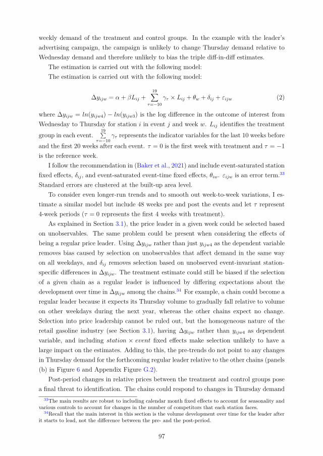
weekly demand of the treatment and control groups. In the example with the leader’sadvertising campaign, the campaign is unlikely to change Thursday demand relative toWednesday demand and therefore unlikely to bias the triple diff-in-diff estimates.

The estimation is carried out with the following model:The estimation is carried out with the following model:

∆yijw = α + βLij +19∑

τ=−10γτ × Lij + θw + δij + εijw (2)

where ∆yijw = ln(yijw4) − ln(yijw3) is the log difference in the outcome of interest fromWednesday to Thursday for station i in event j and week w. Lij identifies the treatmentgroup in each event.

19∑τ=−10

γτ represents the indicator variables for the last 10 weeks beforeand the first 20 weeks after each event. τ = 0 is the first week with treatment and τ = −1is the reference week.

I follow the recommendation in (Baker et al., 2021) and include event-saturated stationfixed effects, δij, and event-saturated event-time fixed effects, θiw. εijw is an error term.33

Standard errors are clustered at the built-up area level.To consider even longer-run trends and to smooth out week-to-week variations, I es-

timate a similar model but include 48 weeks pre and post the events and let τ represent4-week periods (τ = 0 represents the first 4 weeks with treatment).

As explained in Section 3.1), the price leader in a given week could be selected basedon unobservables. The same problem could be present when considering the effects ofbeing a regular price leader. Using ∆yijw rather than just yijw4 as the dependent variableremoves bias caused by selection on unobservables that affect demand in the same wayon all weekdays, and δij removes selection based on unobserved event-invariant station-specific differences in ∆yijw. The treatment estimate could still be biased if the selectionof a given chain as a regular leader is influenced by differing expectations about thedevelopment over time in ∆yijw among the chains.34 For example, a chain could become aregular leader because it expects its Thursday volume to gradually fall relative to volumeon other weekdays during the next year, whereas the other chains expect no change.Selection into price leadership cannot be ruled out, but the homogeneous nature of theretail gasoline industry (see Section 3.1), having ∆yijw rather than yijw4 as dependentvariable, and including station × event fixed effects make selection unlikely to have alarge impact on the estimates. Adding to this, the pre-trends do not point to any changesin Thursday demand for the forthcoming regular leader relative to the other chains (panels(b) in Figure 6 and Appendix Figure G.2).

Post-period changes in relative prices between the treatment and control groups posea final threat to identification. The chains could respond to changes in Thursday demand

33The main results are robust to including calendar month fixed effects to account for seasonality andvarious controls to account for changes in the number of competitors that each station faces.

34Recall that the main interest in this section is the volume development over time for the leader afterit starts to lead, not the difference between the pre- and the post-period.

97

Figure 6: Long-run event study - weekly

0

.01

.02

.03

Log

poin

ts

-10 0 10 19Week

(a) Price excl. tax

-.15

-.1

-.05

0

.05

-10 0 10 19Week

(b) Volume

Note: The figure shows results from Eq. 2. Panel (a) plots γτ from –10 to 19 with volume-weighteddaily gasoline prices as the outcome of interest. Panel (b) plots the same with daily volume gasoline asthe outcome of interest. The 95% confidence intervals are also included. The results in tabular form arepresented in Appendix Table G.1.

by changing Thursday prices. Thus, changes in the regular leader’s prices relative to theother chains’ prices over time in the post-period could be indicative of long-run demandeffects but would also complicate the analysis of long-run demand changes because theprice changes would impact the observed post-period volumes. Panels (a) in Figure 6 andAppendix Figure G.2 show that the only notable change occurs when the regular leader’s∆pijw (Thursday price minus Wednesday price) increases 1–2 log points relative to thatof the control group in period τ = 0. Otherwise, the difference in prices is fairly stable inboth the pre- and the post-period

Panel (b) in Figure 6 depicts results from Eq. 2 with volume as the outcome of interest.As expected, the regular leader experiences a downward shift in ∆vijw relative to thecontrol group in week τ = 0. The regular leader’s volume relative to the other chains’volumes vary somewhat over the next 20 weeks, but the volume difference does not increaseover time.35 Appendix Figure G.2 depicts results from a model similar to Eq. 2, but with τrepresenting 4-week periods and with 12 such periods before and after each event included.As can be seen in the figure, there is no evidence of increasing volume loss. The middaytiming of price restorations masking the timing of price restorations for many customersmight be part of the reason why the leader does not experience an increasing demand lossover time.

35The results are similar to the Thursday volume rather than to the difference from Wednesday toThursday as the dependent variable (Appendix Table G.1).

98

5 Concluding remarks

High-frequency price and volume data coupled with a particular price pattern have allowedme to estimate the costs and benefits of leading price jumps in a retail gasoline market.The evidence suggests that rivals follow the leader’s price jump within a few hours andthat the leader’s volume loss is low both in weeks when price jumps fail and in weeks whenthey succeed. Successful jumps bring about large margin and profit increases for boththe leader and followers. Regardless of whether price jumps succeed or fail, the leaderdoes not lose profit relative to the other chains, indicating that the free-rider problem isof little importance in this market.

Given the profitability of leading price jumps and the apparent unimportance of thefree-rider problem, it is perhaps surprising that Thursday jumps do not happen everyweek. However, Thursday jumps become a regular occurrence just after the sample pe-riod ends when one of the chains starts to lead Thursday jumps every week. SuccessfulThursday jumps are then carried out every week over the next 8 years. During the sampleperiod, each individual chain did not have access to the 4 years of price and volume datafrom all chains that I use in this paper. Uncertainty about the costs and benefits of lead-ing and following price jumps may have contributed to what appear, in retrospect, to besuboptimal strategies in the sample period. Slow equilibrium transitions are not unique tothe Norwegian retail fuel market—Byrne & de Roos (2019) show that Australian gasolineretailers took 3 years to coordinate on a collusive equilibrium.

Providing price leadership to coordinate price increases is not illegal per se. Changingthis would risk unduly restricting firms’ ability to compete. Policy makers wanting to de-crease average prices could instead implement regulations aimed at increasing the leader’svolume loss to make it less attractive to lead and thus possibly decrease the frequency ofprice jumps. Regulating how often firms can change their prices can increase the time forwhich the leader is the sole chain to implement a high price and thus increase the vol-ume loss (Wang, 2009), but such regulation risks limiting competition in the undercuttingphase (Byrne & de Roos, 2019). Regulations mandating that gas stations post prices ongovernment webpages can increase the leader’s volume loss by helping consumers timetheir purchases to the bottom of the cycle and take advantage of the nonleaders’ lowerprices. However, such measures can also facilitate collusion by helping firms monitor theirrivals’ actions and have been shown to increase retail gasoline margins (Luco, 2019).

In recent years, some policy makers have focused on enabling customers to time theirpurchases to the bottom of the price cycle. For example, both the Australian and theNorwegian Competition Authorities frequently collect price data from the retail chainsand issue updates online, in reports or press releases focusing on when prices are lowest(ACCC, 2021; Konkurransetilsynet, 2014). An additional benefit of these measures couldbe increasing the share of total volume that is sold in the period when the leader onlyhas a high price, thereby increasing the cost of leading. Policy makers could also iden-

99

tify the price leader and provide information about when each firm typically increasesprices to help consumers take advantage of the nonleaders’ low prices in the period be-fore they match the leader’s price jump. Such limited information disclosure measurescould increase the cost of being a price leader and thus possibly decrease the frequency ofprice jumps, but would not temper firms’ capacity to price freely and would largely avoidimproving firms’ ability to monitor their rivals’ actions.

100

References

ACCC. (2021). Petrol Price Cycles. Retrieved 2021-08-06, from https://www.accc.gov.au/consumers/petrol-diesel-lpg/petrol-price-cycles#petrol-price-cycles-in-capital-cities/

Andreoli-Versbach, P., & Franck, J. (2015). Endogenous Price Commitment, Sticky andLeadership Pricing: Evidence from the Italian Petrol Market. International Journal ofIndustrial Organization, 40 , 32-48.

Atkinson, B. (2009). Retail Gasoline Price Cycles: Evidence from Guelph, Ontario UsingBi Hourly, Station-Specific Retail Price Data. Energy Journal, 30 (1), 85-109.

Bachmeier, L. J., & Griffin, J. M. (2003). New Evidence on Asymmetric Gasoline PriceResponses. Review of Economics and Statistics, 85 (3), 772-776.

Baker, A., Larcker, D., & Wang, C. (2021). How Much Should We Trust StaggeredDifference-In-Differences Estimates? Working Paper .

Bergantino, A. S., Capozza, C., & Capurso, M. (2018). Follow the Leader: Price ChangeTiming in Internet-Based Selling. Managerial and Decision Economics, 50 (46), 4937-4953.

Byrne, D. P., & de Roos, N. (2019). Learning to Coordinate - A Study in Retail Gasoline.American Economic Review, 109 (2), 591-619.

Cabral, L., Duerr, N., Schober, D., & Voll, O. (2021). Price Matching Guarantees andCollusion: Theory and Evidence from Germany. Working Paper .

Chandra, A., & Tappata, M. (2011). Consumer search and dynamic price dispersion: anapplication to gasoline markets. RAND Journal of Economics, 42 (4), 681-7043.

Clark, R., & Houde, J. F. (2013). Collusion with Asymmetric Retailers: Evidence froma Gasoline Price-Fixing Case. American Economic Journal: Microeconomics, 5 (3),97-123.

Conlisk, J., Gerstner, E., & Sobel, J. (1984). Cyclic Pricing by a Durable Goods Monop-olist. Quarterly Journal of Economics, 38 (2), 291-313.

de Roos, N., & Smirnov, V. (2020). Collusion with Intertemporal Price Dispersion. RANDJournal of Economics, 51 (1), 158-188.

Deryugina, T., MacKay, A., & Reif, J. (2020). The Long-Run Dynamics of ElectricityDemand: Evidence from Municipal Aggregation. American Economic Journal: AppliedEconomics, 12 (1), 86-114.

101

Drivkraft Norge. (2021). Salg av Bransjens Hovedprodukter tilbake til 1952(Sale of the Industries Main Products back to 1952. Retrieved 2021-08-25, from https://www.drivkraftnorge.no/siteassets/dokumenter--filer/statistikk/salg/salg-tilbake-til-1952-til-hjemmesiden.xlsx

Edgeworth, F. Y. (1925). ’The Pure Theory Economy’ in Papers Relating to PoliticalEconomy, Volume 1. MacMillan.

Foros, Ø., & Steen, F. (2013). Vertical Control and Price Cycles in Gasoline Retailing.Scandinavian Journal of Economics, 115 (3), 640-661.

Harrington, J. E. (2017). A Theory of Collusion with Partial Mutual Understanding.Research in Economics, 71 , 140-158.

Harrington, J. E., & Zhao, W. (2012). Signaling and Tacit Collusion in an InfinitelyRepeated Prisoners’ Dilemma. Mathematical Social Sciences, 64 , 277-289.

Hastings, J. S., & Shapiro, J. M. (2013). Fungibility and Consumer Choice: Evidencefrom Commodity Price Shocks. Quarterly Journal of Economics, 128 (4), 1449-1498.

Kauffman, R. J., & Wood, C. A. (2007). Follow the Leader: Price Change Timing inInternet-Based Selling. Managerial and Decision Economics, 28 (7), 679-700.

Konkurransetilsynet. (2014). Drivstoff Markedet i Norge - Marginøkning og Ny Pristopp(The Norwegian Fuel Market – Margin increase and a New Price Peak).

Konkurransetilsynet. (2015a). Varsel - NorgesGruppen ASA - Tiger AS/Esso Norge AS- Konkurranseloven § 16 jf. § 20 - Inngrep mot Foretakssammenslutning (Statement ofObjection - Tiger AS/Esso Norge AS - the Competition act § 16 jf. § 20 - InterventionAgainst Merger).

Konkurransetilsynet. (2015b). Vedtak V2015-29 - St1 Nordic OY - Smart Fuel AS -Konkurranseloven § 16 jf. § 20 - Inngrep mot Foretakssammenslutning (Decision V2015-29 - St1 Nordic OY - Smart Fuel AS - the Competition Act § 16 jf. § 20 - InterventionAgainst Merger).

Levin, L., Lewis, M. S., & Wolak, F. A. (2017). High Frequency Evidence on the Demandfor Gasoline. American Economic Journal: Economic Policy, 9 (3), 314–347.

Lewis, M. S. (2012). Price Leadership and Coordination in Retail Gasoline Markets withPrice Cycles. International Journal of Industrial Organization, 30 (4), 342–351.

Liu, W. (2016). Estimating the Elasticities of Gasoline Demand: an Instrumental VariableApproach. Applied Economics Letters, 23 (16), 1153-1156.

102

Luco, F. (2019). Who Benefits from Information Disclosure? The Case of Retail Gasoline.American Economic Journal: Microeconomics, 11 (2), 277-305.

MacKey, A., & Remer, M. (2021). Consumer Inertia and Market Power. Working Paper .

Markham, J. W. (1951). The Nature and Significance of Price Leadership. AmericanEconomic Review, 41 (5), 891-905.

Maskin, E., & Tirole, J. (1988). A Theory of Dynamic Oligopoly, II: Price Competition,Kinked Demand Curves, and Edgeworth Cycles. Econometrica, 56 (3), 571-599.

Miller, N. H., Sheu, G., & Weinberg, M. C. (in press). Oligopolistic Price Leadership andMergers: The United States Beer Industry. American Economic Review.

Neset, G. P. (2010). Prisstøttesystemet i Bensinmarkedet (The Price Support System inthe Gasoline Market).

Noel, M. D. (2008). Edgeworth Price Cycles and Focal Prices: Computational DynamicMarkov Equilibria. Journal of Economics and Managment Science, 17 (2), 345-377.

Noel, M. D. (2012). Edgeworth Price Cycles and Intertemporal Price Discrimination.Energy Economics, 34 (4), 942–954.

Noel, M. D. (2019). Calendar Synchronization of Gasoline Price Increases. Journal ofEconomics and Managment Science, 28 (2), 355-370.

Sanderson, E., & Windmeijer, F. (2016). A Weak Instrument F-test in Linear IV modelswith Multiple Endogenous Variables. Journal of Econometrics, 190 (2), 212-221.

Seaton, J. S., & Waterson, M. (2013). Identifying and Characterising Price Leadershipin British Supermarkets. International Journal of Industrial Organization, 115 (31),392-403.

Tveito, A. (2021a). Dynamics in Intertemporal Substitution – Evidence from Retail Fuel.Working Paper .

Tveito, A. (2021b). Might as Well Jump! Coordinating More Frequent Price Hikes in aRetail Gasoline Market. Working Paper .

Wang, Z. (2008). Collusive Communication and Pricing Coordination in a Retail GasolineMarket. Review of Industrial Organization, 32 (1), 32-52.

Wang, Z. (2009). (Mixed) Strategy in Oligopoly Pricing: Evidence from Gasoline PriceCycles Before and Under a Timing Regulation. Journal of Political Economy, 117 (61),987-1030.

103

Appendices

A Additional figures and tables

Figure A.1: Follower delay after leader, Jan 2005–Nov 2008

1

2

3

4

5

6

Hou

rs a

fter l

eade

r

2005q12006q1

2007q12008q1

2009q1

Quarter

1. follower 2. follower3. follower 4. follower

Note: The figure depicts the quarterly development in average duration from the leader carried out achain price jump until the first to fourth follower carried out a chain price jump. The figure is based onsuccessful midweek price jumps.

104

Table A.1: Prices at the top of the cycle

Within Station Within Built-up AreaLeader 0.0002 0.0008**

(0.0004) (0.0003)Staffed 0.0122***

(0.0005)Constant 2.4668*** 2.4575***

(0.0001) (0.0004)Week FE Yes YesStation FE Yes NoBuilt-up area FE No YesObservations 95329 95270R2 0.98 0.97

Note: The first column shows results from the regression model ln(yiw) = β1Leaderiw + γi + δw + εiw.yiw is the maximum price of station i on the day the chain it is affiliated with carries out a Thursdayprice jump in week w. Leaderiw identifies stations affiliated with the chain that is leading the midweekprice jump in week w. δw represents week-fixed-effects and γi represents station-fixed-effects. The secondcolumn shows results from the regression ln(yiw) = β1Leaderiw + β2Staffedi + γi + δw + εiw, whereStaffed identifies stations with a staffed convenience store, and θi represent built-up area-fixed-effects.*p < 0.05, **p < 0.01, ***p < 0.001. Take note of the following:

1. The first column of results shows that a station’s maximum price on days with Thursday jumps is0.02% higher (and not significantly different from zero) in weeks when the chain they are associatedwith is leading a Thursday jumps than in weeks when the chain is following.

2. The second column of results shows that, after controlling for whether stations are staffed or not,stations in a given built-up area associated with the leader have 0.08% higher maximum prices ondays with Thursday jumps than station in the same built-up area associated with the followers.

3. Both models point to the leader and followers having very similar maximum prices on days withThursday jumps. In levels the difference is NOK 0.002–0.009. 0.01 NOK is the smallest possibleprice increment and the average size of price cuts in the sample is NOK 0.15.

Figure A.2: Hourly share of Thursday traffic counts

0.00

0.02

0.04

0.06

0.08

0.10

Shar

e of

dai

ly tr

affic

0 4 8 12 16 20Hour of day

Note: The figure shows the average hourly share of the total daily count of cars on Thursdays. Thesample consists of all cars passing tracker stations run by The Norwegian Public Roads Administrationat 9 roads in the county of Vestfold in Norway on Thursdays in the period March 2014–December 2017.Observations from vehicles longer than 7.5 meters, and observations in weeks with public holidays areexcluded. The dashed line marks the hour from 11:00 to 12:00.

105

Table A.2: Thursday price jumps

M V MS CSR ProWholesale price 0.34*** 0.97*** 1.00 0.95*** 0.32***

(0.01) (0.01) (0.00) (0.01) (0.01)Tue 1.14*** 0.88*** 0.96*** 0.99 1.00

(0.02) (0.01) (0.00) (0.01) (0.01)Thu 0.87*** 1.10*** 1.00 1.04*** 0.96***

(0.01) (0.01) (0.00) (0.01) (0.01)Fri 0.72*** 1.33*** 1.03** 1.23*** 0.96

(0.02) (0.03) (0.01) (0.02) (0.02)Sat 0.60*** 1.25*** 1.07*** 1.06 0.73***

(0.03) (0.04) (0.01) (0.04) (0.02)Sun 0.57*** 1.29*** 1.13*** 1.47*** 0.70***

(0.03) (0.06) (0.03) (0.10) (0.03)Fail - Leader 1.00 1.00 1.00 0.97*** 1.01

(0.00) (0.01) (0.00) (0.01) (0.01)Fail - Follower 0.99 0.99 1.00 0.98** 0.99*

(0.01) (0.00) (0.00) (0.01) (0.00)Success - Leader 1.01 0.99* 0.99** 1.00 1.00

(0.01) (0.00) (0.00) (0.01) (0.01)Tue × Fail - Leader 1.01** 0.99 1.01** 1.00 1.00

(0.00) (0.00) (0.00) (0.01) (0.00)Tue × Fail - Follower 1.01** 0.98*** 0.99*** 0.99** 0.99***

(0.00) (0.00) (0.00) (0.00) (0.00)Tue × Fail - Non-Follower 1.02*** 0.98*** 1.00 0.99* 1.00

(0.00) (0.00) (0.00) (0.00) (0.00)Tue × Success - Leader 1.01 0.99 1.00 1.00 1.01

(0.01) (0.00) (0.00) (0.00) (0.01)Tue × Success - Follower 1.02*** 0.99*** 1.00 0.99*** 1.01**

(0.00) (0.00) (0.00) (0.00) (0.00)Thu × Fail - Leader 1.17*** 0.95*** 0.97*** 1.01 1.11***

(0.01) (0.01) (0.00) (0.01) (0.01)Thu × Fail - Follower 1.14*** 0.96*** 0.99*** 1.01*** 1.10***

(0.01) (0.00) (0.00) (0.00) (0.01)Thu × Fail - Non-Follower 1.03*** 1.01** 1.03*** 1.00 1.04***

(0.00) (0.00) (0.00) (0.00) (0.01)Thu × Success - Leader 1.35*** 0.90*** 0.97*** 1.00 1.22***

(0.02) (0.01) (0.00) (0.00) (0.01)Thu × Success - Follower 1.25*** 0.94*** 1.01*** 1.00 1.18***

(0.01) (0.01) (0.00) (0.00) (0.01)Fri × Fail - Leader 1.07*** 1.00 1.02*** 1.01 1.07***

(0.01) (0.01) (0.00) (0.01) (0.01)Fri × Fail - Follower 1.10*** 0.97*** 0.99*** 0.99 1.06***

(0.01) (0.01) (0.00) (0.00) (0.01)Fri × Fail - Non-Follower 1.06*** 0.98*** 1.00 0.99* 1.04***

(0.01) (0.00) (0.00) (0.00) (0.01)Fri × Success - Leader 1.44*** 0.92*** 1.02*** 1.00 1.34***

(0.03) (0.01) (0.00) (0.00) (0.02)Fri × Success - Follower 1.46*** 0.91*** 1.00** 0.98*** 1.33***

(0.03) (0.01) (0.00) (0.00) (0.02)Sat × Fail - Leader 1.05*** 0.99* 1.00 1.01 1.04***

(0.01) (0.01) (0.00) (0.01) (0.01)Sat × Fail - Follower 1.06*** 0.98*** 1.00 1.01* 1.05***

(0.02) (0.00) (0.00) (0.00) (0.01)Sat × Fail - Non-Follower 1.04*** 0.98*** 1.00 1.01* 1.02**

(0.01) (0.00) (0.00) (0.01) (0.01)Sat × Success - Leader 1.44*** 0.93*** 1.00 1.03*** 1.36***

(0.04) (0.01) (0.00) (0.00) (0.03)Sat × Success - Follower 1.45*** 0.93*** 1.00 1.00 1.37***

(0.04) (0.01) (0.00) (0.00) (0.02)Sun × Fail - Leader 1.06** 1.00 1.01* 1.06*** 1.06**

(0.02) (0.01) (0.00) (0.01) (0.02)Sun × Fail - Follower 1.07** 0.98** 0.99** 1.01 1.05**

(0.02) (0.01) (0.00) (0.01) (0.02)Sun × Fail - Non-Follower 1.06*** 0.97*** 1.00 1.00 1.03*

(0.02) (0.00) (0.00) (0.00) (0.01)Sun × Success - Leader 1.44*** 0.94*** 1.00 1.02*** 1.38***

(0.04) (0.01) (0.00) (0.01) (0.03)Sun × Success - Follower 1.44*** 0.93*** 1.00 0.98*** 1.37***

(0.04) (0.01) (0.00) (0.00) (0.03)Week FE Yes Yes Yes Yes YesStation FE Yes Yes Yes Yes YesChain X DoW FE Yes Yes Yes Yes YesN Chain X DoW FE Yes Yes Yes Yes YesStaffed X DoW FE Yes Yes Yes Yes YesMonth X DoW FE Yes Yes Yes Yes YesObservations 836004 844277 844277 582597 836004R2 0.22 0.13 0.05 0.25 0.13

Note: The table shows the results from Eq. 1 for Thursday price jumps with the outcome of interestbeing volume-weighted retail gasoline margins, liters of gasoline sold per day, market shares based onvolume gasoline, convenience store revenue, and profits, respectively. The coefficients are exponentiated.*p < 0.05, **p < 0.01, ***p < 0.001.

106

Figure A.3: Successful price jumps, less controls

01020304050

TueWed Thu Fri Sat

Sun

(a) Volume-weighted margins

-15

-10

-5

0

% c

hang

e fro

m c

ount

erfa

ctua

l

TueWed Thu Fri Sat

Sun

(b) Volume

0

10

20

30

40

TueWed Thu Fri Sat

Sun

(c) Profit

Leader Follower

Note: The figure plots results from a model similar to Eq. 1, but with less control variables. ρWwt, θDiwand λwt are not included. Volume-weighted margins, volume sold, and profits are outcomes of interest.The lines plot (exp(β3Treatiw ×Dt)− 1)× 100 over different weekdays for the treatment groups“leader in successful weeks” and “followers in successful weeks”. 95% confidence intervals are shown.

107

Figure A.4: Successful price jumps, two-way clustering

01020304050

TueWed Thu Fri Sat

Sun

(a) Volume-weighted margins

-15

-10

-5

0

% c

hang

e fro

m c

ount

erfa

ctua

l

TueWed Thu Fri Sat

Sun

(b) Volume

0

10

20

30

40

TueWed Thu Fri Sat

Sun

(c) Profit

Leader Follower

Note: The figure plots results from Eq. 1, but with two-way clustering of standard errors on built-uparea and week. Volume-weighted margins, volume sold, and profits are outcomes of interest. The linesplot (exp(β3Treatiw ×Dt)− 1)× 100 over different weekdays for the treatment groups “leader insuccessful weeks” and “followers in successful weeks”. 95% confidence intervals are shown.

108

Figure A.5: Successful Thursday jumps, market share

-4

-3

-2

-1

0

1

2

% c

hang

e fro

m c

ount

erfa

ctua

l

TueWed Thu Fri Sat

Sun

Leader Follower

Note: The figure plots results from Eq. 1 with gasoline market share as outcome of interest. The linesplot (exp(β3Treatiw ×Dt)− 1)× 100 over different weekdays for the treatment groups “leader in failedweeks” and “followers in failed weeks”. 95% confidence intervals are shown.

109

Figure A.6: Failed Thursday price jumps

-5

0

5

TueWed Thu Fri Sat

Sun

(a) Volume

-3

0

3

% c

hang

e fro

m c

ount

erfa

ctua

l

TueWed Thu Fri Sat

Sun

(b) Market share

0

5

10

15

TueWed Thu Fri Sat

Sun

(c) Profit

Leader Follower Non-follower

Note: The figure plots results from Eq. 1 with volume-weighted margins, volume sold and profit asoutcome of interest. The lines plot (exp(β3Treatiw ×Dt)− 1)× 100 over different weekdays for thetreatment groups “leader in failed weeks”, “followers in failed weeks” and “non-followers in failedweeks”. 95% confidence intervals are shown.

110

B Trends through the week

Figure B.1: Margins trends, success

50

60

70

80

90

100

110

120%

rela

tive

to W

ed

TueWed Thu Fri Sat

Sun

Leader Followers Counterfactual

Note: The red line plots the development in volume-weighted margins through the week for stationsaffiliated with the price leader in weeks with successful Thursday jumps. The blue line for the followers.The dashed gray line plots the development through the week for all stations in weeks without midweekjumps. Take note of the following:

1. The leader’s and followers’ margins have a very similar development from Tuesday to Wednesdaycompared with weeks without midweek jumps.

2. After the Thursday jumps, the leader’s and followers’ margins stay at a higher level but have avery similar development compared with weeks without midweek jumps.

*The lines plot (exp(β2Dt + β3Treatiw ×Dt)− 1) ∗ 100 in Eq. 1 with volume-weighted margins asoutcome of interest over different weekdays for the treatment groups “leader in successful weeks”,“followers in successful weeks” and the counterfactual. 95% confidence intervals are shown. Standarderrors for the combined coefficients are calculated using the delta method.

111

Figure B.2: Price trends, success

85

90

95

100

105

% re

lativ

e to

Wed

TueWed Thu Fri Sat

Sun

Leader Followers Counterfactual

Note: The red line plots the development in volume-weighted prices through the week for stationsaffiliated with the price leader in weeks with successful Thursday jumps. The blue line for followers.The dashed gray line plots the development through the week for all stations in weeks without midweekjumps (the counterfactual). Take note of the following:

1. The leader’s and followers’ prices have a very similar development from Tuesday to Wednesdaycompared with weeks without midweek jumps.

2. After the Thursday jumps, both the leader’s and followers’ prices stay at a higher level but havea very similar development compared with weeks without midweek jumps.

*The lines plot (exp(β2Dt + β3Treatiw ×Dt)− 1) ∗ 100 in Eq. 1 with volume-weighted prices asoutcome of interest on different weekdays for the treatment groups “leader in successful weeks”,“followers in successful weeks” and the counterfactual. 95% confidence intervals are shown. Standarderrors for the combined coefficients are calculated using the delta method.

112

Figure B.3: Volume trends, success

80

100

120

140

% re

lativ

e to

Wed

TueWed Thu Fri Sat

Sun

Leader Followers Counterfactual

Note: The red line plots the development in volume gasoline sold through the week for stationsaffiliated with the price leader in weeks with successful Thursday jumps. The blue line for followers.The dashed gray line plots the development through the week for all stations in weeks without midweekjumps (the counterfactual). Take note of the following:

1. The leader’s and followers’ volume sold have a very similar development from Tuesday toWednesday compared with weeks without midweek jumps.

2. After the Thursday jumps, the leader’s and followers’ volume stay at a lower level but have avery similar development compared with weeks without midweek jumps.

*The lines plot (exp(β2Dt + β3Treatiw ×Dt)− 1) ∗ 100 in Eq. 1 with volume gasoline sold as outcomeof interest on different weekdays for the treatment groups “leader in successful weeks”, “followers insuccessful weeks” and the counterfactual. 95% confidence intervals are shown. Standard errors for thecombined coefficients are calculated using the delta method.

113

Figure B.4: Store revenue trends, success

100

120

140

160

180

% re

lativ

e to

Wed

TueWed Thu Fri Sat

Sun

Leader Followers Counterfactual

Note: The red line plots the development in store revenue through the week for stations affiliated withthe price leader in weeks with successful Thursday jumps. The blue line for followers. The dashed grayline plots the development through the week for all stations in weeks without midweek jumps (thecounterfactual). Take note of the following:

1. The leader’s and followers’ store revenue follow a similar development through the whole week asin weeks without midweek jumps.

*The lines plot (exp(β2Dt + β3Treatiw ×Dt)− 1) ∗ 100 in Eq. 1 with store revenue as outcome ofinterest on different weekdays for the treatment groups “leader in successful weeks”, “followers insuccessful weeks” and the counterfactual. 95% confidence intervals are shown. Standard errors for thecombined coefficients are calculated using the delta method.

114

Figure B.5: Profits trends, success

60

80

100

120

140

% re

lativ

e to

Wed

TueWed Thu Fri Sat

Sun

Leader Followers Counterfactual

Note: The red line plots the development in gasoline profits through the week for stations affiliated withthe price leader in weeks with successful Thursday jumps. The blue line for followers. The dashed grayline plots the development through the week for all stations in weeks without midweek jumps (thecounterfactual). Take note of the following:

1. The leader’s and followers’ profits have a similar development from Tuesday to Wednesdaycompared with weeks without midweek jumps.

2. After the Thursday jumps, the leader’s and followers’ profits have a very similar developmentcompared with weeks without midweek jumps.

*The lines plot (exp(β2Dt + β3Treatiw ×Dt)− 1) ∗ 100 in Eq. 1 with profit as outcome of interest ondifferent weekdays for the treatment groups “leader in successful weeks”, “followers in successful weeks”and the counterfactual. 95% confidence intervals are shown. Standard errors for the combinedcoefficients are calculated using the delta method.

115

C Friday price jumps

Table C.1: Friday price jumps

M V MSG CSR ProWholesale price 0.39*** 0.95* 1.00 0.99 0.37***

(0.02) (0.02) (0.01) (0.01) (0.02)Tue 1.17*** 0.88*** 0.97*** 0.99 1.03*

(0.02) (0.01) (0.00) (0.01) (0.01)Thu 0.84*** 1.10*** 1.02** 1.06*** 0.92***

(0.02) (0.01) (0.01) (0.01) (0.02)Fri 0.65*** 1.34*** 1.04*** 1.24*** 0.87**

(0.03) (0.03) (0.01) (0.02) (0.04)Sat 0.54*** 1.23*** 1.07*** 1.07 0.65***

(0.04) (0.04) (0.02) (0.04) (0.03)Sun 0.51*** 1.26*** 1.14*** 1.47*** 0.62***

(0.03) (0.07) (0.03) (0.11) (0.03)Fail - Leader 0.99 1.02** 1.02** 1.05*** 1.01

(0.01) (0.01) (0.01) (0.01) (0.01)Fail - Follower 1.01 0.98* 0.98* 1.04*** 0.99

(0.01) (0.01) (0.01) (0.01) (0.01)Success - Leader 0.99 1.03*** 1.03*** 1.02 1.02*

(0.01) (0.01) (0.01) (0.01) (0.01)Tue × Fail - Leader 1.00 0.95*** 0.97*** 1.02 0.95***

(0.01) (0.01) (0.01) (0.01) (0.01)Tue × Fail - Follower 0.99 0.98* 1.00 1.01 0.97*

(0.01) (0.01) (0.00) (0.01) (0.01)Tue × Fail - Non-Follower 1.01 0.99* 1.00 1.01 1.00

(0.01) (0.01) (0.00) (0.01) (0.01)Tue × Success - Leader 1.01 0.97*** 0.99* 0.96*** 0.98

(0.01) (0.01) (0.01) (0.01) (0.01)Tue × Success - Follower 1.01 0.99*** 1.00 0.98** 0.99

(0.01) (0.00) (0.00) (0.01) (0.01)Thu × Fail - Leader 0.99 0.94*** 0.98*** 0.97*** 0.93***

(0.01) (0.01) (0.00) (0.01) (0.01)Thu × Fail - Follower 0.99 0.95*** 1.00 0.97** 0.95***

(0.01) (0.01) (0.00) (0.01) (0.01)Thu × Fail - Non-Follower 0.99 0.95*** 0.99 0.97** 0.94***

(0.01) (0.01) (0.00) (0.01) (0.01)Thu × Success - Leader 1.01 0.97** 0.99* 1.00 0.99

(0.01) (0.01) (0.01) (0.01) (0.01)Thu × Success - Follower 1.01 0.99 1.01* 1.02* 1.00

(0.01) (0.01) (0.00) (0.01) (0.01)Fri × Fail - Leader 1.17*** 0.91*** 0.97*** 0.95*** 1.07***

(0.01) (0.01) (0.01) (0.01) (0.01)Fri × Fail - Follower 1.12*** 0.92*** 0.98** 0.96*** 1.03*

(0.01) (0.01) (0.01) (0.01) (0.01)Fri × Fail - Non-Follower 0.99 0.96*** 1.01* 0.97*** 0.95***

(0.02) (0.01) (0.01) (0.01) (0.01)Fri × Success - Leader 1.45*** 0.86*** 0.95*** 0.96*** 1.25***

(0.03) (0.01) (0.01) (0.01) (0.03)Fri × Success - Follower 1.33*** 0.92*** 1.01*** 1.00 1.23***

(0.02) (0.01) (0.00) (0.01) (0.02)Sat × Fail - Leader 1.03 0.91*** 0.98** 0.97*** 0.93**

(0.03) (0.01) (0.01) (0.01) (0.02)Sat × Fail - Follower 1.01 0.90*** 0.98** 0.92*** 0.91***

(0.02) (0.01) (0.01) (0.01) (0.02)Sat × Fail - Non-Follower 0.97 0.94*** 1.01 0.97*** 0.91***

(0.02) (0.01) (0.01) (0.01) (0.02)Sat × Success - Leader 1.48*** 0.89*** 0.99 0.98 1.33***

(0.04) (0.01) (0.01) (0.01) (0.03)Sat × Success - Follower 1.49*** 0.89*** 0.99 0.99 1.35***

(0.03) (0.01) (0.00) (0.01) (0.03)Sun × Fail - Leader 1.03 0.90*** 1.00 0.93*** 0.92**

(0.03) (0.01) (0.01) (0.01) (0.03)Sun × Fail - Follower 1.00 0.90*** 0.99 0.91*** 0.90***

(0.03) (0.01) (0.01) (0.01) (0.02)Sun × Fail - Non-Follower 0.98 0.90*** 0.99 0.95*** 0.89***

(0.04) (0.01) (0.01) (0.01) (0.03)Sun × Success - Leader 1.42*** 0.92*** 0.99 0.99 1.33***

(0.04) (0.01) (0.01) (0.01) (0.03)Sun × Success - Follower 1.45*** 0.92*** 1.00 0.99 1.36***

(0.03) (0.01) (0.00) (0.01) (0.02)Week FE Yes Yes Yes Yes YesStation FE Yes Yes Yes Yes YesChain X DoW FE Yes Yes Yes Yes YesN Chain X DoW FE Yes Yes Yes Yes YesStaffed X DoW FE Yes Yes Yes Yes YesMonth X DoW FE Yes Yes Yes Yes YesObservations 450032 455851 455851 314766 450032R2 0.25 0.15 0.04 0.24 0.14

Note: The table displays the results from Eq. 1 for Friday price jumps with the outcome of interest beingvolume-weighted retail gasoline margins, daily volume gasoline, market shares based on volume gasoline,convenience store revenue, and profits. The coefficients are exponentiated. *p < 0.05, **p < 0.01,***p < 0.001.

116

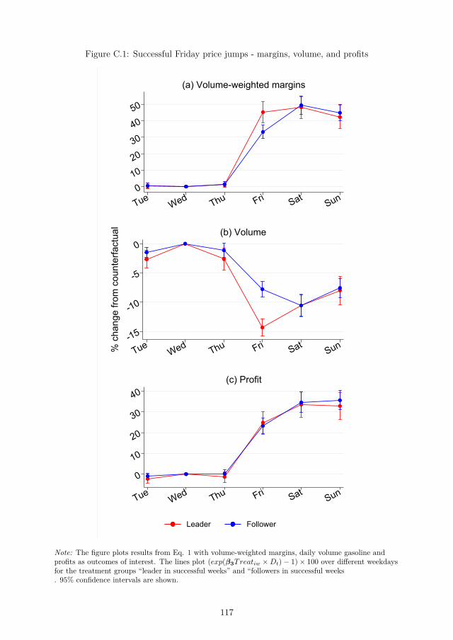
Figure C.1: Successful Friday price jumps - margins, volume, and profits

01020304050

TueWed Thu Fri Sat

Sun

(a) Volume-weighted margins

-15

-10

-5

0

% c

hang

e fro

m c

ount

erfa

ctua

l

TueWed Thu Fri Sat

Sun

(b) Volume

0

10

20

30

40

TueWed Thu Fri Sat

Sun

(c) Profit

Leader Follower

Note: The figure plots results from Eq. 1 with volume-weighted margins, daily volume gasoline andprofits as outcomes of interest. The lines plot (exp(β3Treatiw ×Dt)− 1)× 100 over different weekdaysfor the treatment groups “leader in successful weeks” and “followers in successful weeks. 95% confidence intervals are shown.

117

Figure C.2: Successful Friday jumps, market shares

-5-4-3-2-1012

% c

hang

e fro

m c

ount

erfa

ctua

l

TueWed Thu Fri Sat

Sun

Leader Follower

Note: The figure plots results from Eq. 1 with market shares as outcome of interest. The lines plot(exp(β3Treatiw ×Dt)− 1)× 100 over different weekdays for the treatment groups “leader in successfulweeks” and “followers in successful weeks”. 95% confidence intervals are shown.

D Diff-in-diff+IV

In this appendix, I estimate similar diff-in-diff models as Eq. 1, but use the WednesdayEuropean reference wholesale price, w, WW

w , as an instrument for Thursday jumps.36 Tobe a suitable instrument,WW

w must be strongly correlated with Thursday jumps (validity),but not influence the change in the outcome from Wednesday to later weekdays, ∆yiwt,aside from its effects on Thursday jumps (exclusion restriction).37 I first show that theinstrument is valid, and then discuss the exclusion restriction.

Figure D.1 reveals that there is a lot of variation in WWw . The average within-month

standard deviation of WWw , given by σ, is 0.13 NOK.38 The figure also shows a strong

correlation between WWw and the average Wednesday retail price. However, the short-run

pass-through of WWw is less than 100%; a σ increase in WW

w gives 6% lower Wednesdaymargins (Table D.1). The theory of Edgeworth Cycles predicts that price jumps should

36The leader initiates price jumps around 11:00 on Thursday and likely decides on implementation atleast a few hours earlier, meaning the Thursday wholesale price (an average through all hours on Thu)is not known when Thursday jumps are initiated. The Wednesday wholesale price is a proxy for thewholesale price at the time when the chains decide whether to carry out a price jump or not.

37The reference wholesale price of gasoline is strongly correlated with the European crude oil price(Figure D.1). The crude oil price has been used as an instrument to estimate price elasticities (Liu, 2016)and been assumed to be exogenous to retail gasoline prices in multiple studies estimating asymmetriccost pass-through in the gasoline industry (Bachmeier & Griffin, 2003). I instrument price jumps withthe reference wholesale price rather than the crude oil price because the reference wholesale price is amore relevant cost measure for gasoline retailers and hence a stronger instrument. Results are similar,but less precise, when instrumenting with the crude oil price.

38σ is defined as σ = 1/MM∑m=1

(σm), where σm is the standard deviation of WWw in month m.

118

occur more frequently when margins are low (Noel, 2008). In accordance with this, thefirst-stage regression of WW

w on the probability of successful Thursday jumps, revealsthat a σ increase in WW

w increases the probability of a successful price jump with 16%,indicating that the instrument has some bite. The F-statistic (calculated with the methodproposed by Sanderson & Windmeijer (2016)) is over 1500 for all IV-models, rejecting thehypothesis that the second-stage equation is weakly identified.

Figure D.1: Reference wholesale price, Brent crude oil and Wednesday margins

2.00

3.00

4.00

5.00

6.00

NO

K/Li

tre

Jan2005Jan2006

Jan2007Jan2008

Nov2008

WeekWholesale gasoline price Crude oil price Retail price ex tax

Note: The figure plots the weekly Wednesday reference price for wholesale gasoline (WWw ), the

Wednesday European Brent crude oil price, and the average Wednesday retail gasoline price exclusivetaxes across all stations in the main sample.

The exclusion restriction would be violated if WWw is correlated with the outcome of

interest through other channels than the Thursday price jumps. The Norwegian retailgasoline market is small compared with the rest of Europe, meaning that demand shocksspecific to Norway are unlikely to affect WW

w . But WWw could be correlated with demand

through seasonal demand variation or macro shocks that are transmitted to demand forretail gasoline. The monthly fixed effects eliminate the main channels through which suchcorrelation could emerge.

Even if WWw was correlated with overall demand, it would not necessarily be corre-

lated with the within-week development of demand, ∆yiwt. However, wholesale pricesare higher in weeks when WW

w is high, leading to higher average retail gasoline prices inthese weeks. This could increase consumers’ inter-temporal demand elasticity, therebyincreasing demand in periods of the week with low prices.39 This would violate the exclu-

39The inter-temporal demand elasticity could increase due to income effects, or category budgeting asin Hastings & Shapiro (2013).

119

Table D.1: Within-month pass-through of WWw

PT WEDWednesday wholesale price -0.42***

(0.03)Month FE YesStation FE YesObservations 139261R2 0.35F-value 200.56

Note: The within-month pass-through of WWw to Wednesday margins is estimated with the model

yiw = α+ β1WWw + θm + δi + εiw, where yiw is the volume-weighted margin of station i in week w, WW

w

is the reference wholesale price on Wednesday in week w. θm and δi signify month and station fixedeffects. The table shows that a 1 NOK increase in WW

w decreases the Wednesday margin with 0.42NOK. A σ increase in WW

w reduces the Wednesday margin by 0.42× 0.13 = 0.06 NOK.

sion restriction. Out-of-sample testing of this potential violation is possible in the periodwhen Thursday price jumps occur every week (after March 2009). Table D.2 shows howWWw affects the change in different outcomes through the week after March 2009. De-

pending on how many years after March 2009 is included, WWw can have a statistically

significant effect. However, the economic impact of a σ change in WWw is very small com-

pared with the effects of Thursday price jumps, suggesting that potential bias workingthrough changes in the inter-temporal elasticity is small—a σ change in WW

w never givemore than 1.3 % change in ∆yiwt with volume-weighted margins as outcome, and nevermore than 1.0% change in ∆yiwt with volume as outcome. These effects are very smallcompared with the diff-in-diff estimates in Section 3.2 and the IV estimates reported inthis appendix.

The IV-models are estimated by 2SLS. In the first stage (Eq. D.1), the possibly endoge-nous Thursday price jumps, Sw, are independently regressed on the excluded instrument,WWw , and the included instruments, θDiw, δi and γm. θDiw, γm, and δi are defined as in Eq. 1.

Siw = α1 + δWWw + θDiw + γm + δi + εiw (D.1)

The IV estimates are then obtained in the second stage by estimating a slightly alteredversion of the diff-in-diff model in Eq. 1 using the predicted instead of the observed valuesof the Thursday price jumps.40

∆yiwt = α2 + πSiw + θDiw + γm + δi + uiwt (D.2)

∆yiwt is given by ln(yiwt) − ln(yiw3); the difference between the outcome of interest40Note that in the diff-in-diff model yi = β0 + β1TREAT + β2POST + β3TREAT × POST + ei the

POST-period values are yi = β0 + β1TREAT + β2 + β3TREAT + ei, and the pre-period values areyi = β0 + β1TREAT + ei. Post minus Pre is then given by ∆yi = β2 + β3TREAT + ui.

120

Table D.2: Out of sample testing of the exclusion restriction

M_09_10 M_09_11 M_09_12 V_09_10 V_09_11 V_09_12Thu × platts_wed 1.07*** 1.00 1.01*** 1.00 0.99* 1.00

(0.01) (0.00) (0.00) (0.01) (0.01) (0.00)Fri × platts_wed 1.07*** 0.99 1.02** 1.07*** 1.01 1.00

(0.01) (0.01) (0.01) (0.01) (0.01) (0.01)Sat × platts_wed 1.09*** 0.94** 0.99 0.99 0.98* 1.00

(0.02) (0.02) (0.01) (0.01) (0.01) (0.01)Sun × platts_wed 1.09*** 0.90*** 0.94*** 0.92*** 1.03 1.08***

(0.02) (0.03) (0.01) (0.02) (0.03) (0.02)Observations 193355 400485 597224 193856 401126 598021R2 0.16 0.18 0.20 0.11 0.10 0.11

Note: The table shows results from the model ∆yiwt = α+ β1WWw ×D + θDiw + γm + δi + εiwt, where

∆yiwt = ln(yiwt)− ln(yiw3) is the log difference in the outcome of interest from Wednesday to the laterweekdays. θDiw, γm and δi are defined as in Eq. D.2. The first 3 columns show results withvolume-weighted margins as outcome and include observations from April 2009-March 2010, April2009-March 2011, and April 2009-March 2012. The last 3 columns show results with volume sold perday as outcome for the same periods.The results vary quite a bit depending on which years are included, but a 1 NOK change in WW

w nevergive more than 10% change in ∆yiwt for any weekdays with volume-weighted margins as outcome andnever more than 8% change in ∆yiwt with volume sold at outcome. This means a σ change in WW

w

never give more than 10%× 0.13 = 1.3% change in volume-weighed margins, and never more than8%× 0.13 = 1.0% change in volume sold.*The coefficients are exponentiated. *p < 0.05, **p < 0.01, ***p < 0.001.

on weekday t and the outcome of interest on Wednesday. The effect of Thursday pricejumps on the outcome of interest is given by π. I estimate the model separately for dif-ferent weekdays and separately for the leader and the followers. For example, to estimatethe effect of successful Thursday jumps on the leader’s Thursday margins, I keep onlyThursday observations so that ∆yiwt is given by the difference in the outcome betweenThursday and Wednesday, ln(yiw4)− ln(yiw3). Furthermore, I only keep observations forthe leader’s stations in weeks with successful Thursday jumps (treatment) and observa-tions for all stations in weeks without midweek jumps (control). Fridays, Saturdays, andSundays are pooled together to increase accuracy.

Tables D.3–D.7 show results from the IV model with different outcome variables.

121

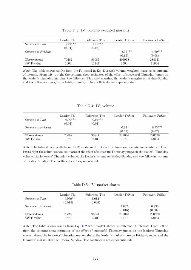
Table D.3: IV, volume-weighted margins

Leader Thu Followers Thu Leader FriSun Followers FriSunSuccess× Thu 1.19*** 1.19***

(0.04) (0.03)Success× FriSun 2.05*** 1.69***

(0.15) (0.08)Observations 70282 96087 207978 284641SW F-value 1609 13147 1593 11634

Note: The table shows results from the IV model in Eq. D.2 with volume-weighted margins as outcomeof interest. From left to right the columns show estimates of the effect of successful Thursday jumps onthe leader’s Thursday margins, the followers’ Thursday margins, the leader’s margins on Friday–Sundayand the followers’ margins on Friday–Sunday. The coefficients are exponentiated.

Table D.4: IV, volume

Leader Thu Followers Thu Leader FriSun Followers FriSunSuccess× Thu 0.90*** 0.94***

(0.02) (0.01)Success× FriSun 0.94 0.93***

(0.03) (0.02)Observations 70682 96841 212046 290520SW F-value 1579 13100 1579 13084

Note: The table shows results from the IV model in Eq. D.2 with volume sold as outcome of interest. Fromleft to right the columns show estimates of the effect of successful Thursday jumps on the leader’s Thursdayvolume, the followers’ Thursday volume, the leader’s volume on Friday–Sunday and the followers’ volumeon Friday–Sunday. The coefficients are exponentiated.

Table D.5: IV, market shares

Leader Thu Followers Thu Leader FriSun Followers FriSunSuccess× Thu 0.959** 1.012*

(0.014) (0.006)Success× FriSun 1.002 0.990

(0.016) (0.007)Observations 70682 96841 212046 290520SW F-value 1579 13100 1579 13084

Note: The table shows results from Eq. D.2 with market shares as outcome of interest. From left toright the columns show estimates of the effect of successful Thursday jumps on the leader’s Thursdaymarket share, the followers’ Thursday market share, the leader’s market share on Friday–Sunday and thefollowers’ market share on Friday–Sunday. The coefficients are exponentiated.

122

Table D.6: IV - convenience store revenue

Leader Thu Followers Thu Leader FriSun Followers FriSunSuccess× Thu 1.009 0.989

(0.030) (0.012)Success× FriSun 1.112*** 1.016

(0.033) (0.013)Observations 51361 65396 151372 192088SW F-value 1701 11426 1763 10873

Note: The table shows results from Eq. D.2 with convenience store revenue as outcome of interest. Fromleft to right the columns show estimates of the effect of successful Thursday jumps on the leader’s Thursdayconvenience store revenue, the followers’ Thursday convenience store revenue, the leader’s conveniencestore revenue on Friday–Sunday and the followers’ convenience store revenue on Friday–Sunday. Thecoefficients are exponentiated.

Table D.7: IV, profits

Leader Thu Followers Thu Leader FriSun Followers FriSunSuccess× Thu 1.07** 1.12***

(0.03) (0.02)Success× FriSun 1.94*** 1.58***

(0.12) (0.05)Observations 70282 96087 207978 284641SW F-value 1609 13147 1593 11634

Note: The table shows results from the IV model in Eq. D.2 with Πiwt as the outcome of interest.From left to right the columns show estimates of the effect of successful Thursday jumps on the leader’sThursday profits, the followers’ Thursday profits, the leader’s profits on Friday–Sunday and the followers’profits on Friday–Sunday. The coefficients are exponentiated.

123

E Delayed purchasing

I compare price and volume in week (t) following a week featuring a successful or failedmidweek price jump (t− 1) with weeks following weeks without midweek price jumps. Irestrict the sample to only Tuesdays and Wednesdays because Mondays are contaminateddue to the regular Monday jumps, and Thursdays–Sundays are contaminated by possiblemidweek jumps in week t. I separate results for the leader, the followers and the non-followers after failed and successful weeks using the following model:

ln(yiwt) = α + β2Priceiwt + β3Treati,t−1 + λt + θm + δi + εiwt (E.1)

where yiwt is volume sold for station i on day of week t in week w. λt represents day-of-week fixed effects and Priceiwt is the daily average price. Treatt−1 is a vector of dummyvariables identifying weeks following the five different treatments as described in Section3.1. The baseline is weeks when no midweek jump occurred. θm is month fixed effects, δiis station fixed effects and εiwt is an error term. Table E.1 presents the results.

Table E.1: Week after midweek jumps

Ln(v)Fail - Leader 0.008

(0.004)Fail - Follower 0.002

(0.005)Fail - Non-Follower -0.005

(0.004)Success - Leader 0.033***

(0.006)Success - Follower 0.032***

(0.005)Station FE YesMonth FE YesDay-of-week FE YesObservations 311003R2 0.83

Note The table displays results from Eq. E.1. Standard errors are clustered at built-up area level and areshown in parentheses. *p < 0.05, **p < 0.01, ***p < 0.001.

The leader’s and the followers’ volumes are is slightly more than 3% higher on Tuesdayand Wednesday in the first week after a week featuring a successful midweek price jumpscompared with the first week after a week without any midweek price jump. The leader’s,the followers’, and the non-followers’ volumes are about the same in the first week aftera week with failed midweek price jumps as in the first week after a week without anymidweek price. Effects sizes are almost identical for the leader and the followers.

124

F Pre-jump margins

I employ the following model to find the difference in pre-jump margins in weeks withoutmidweek jumps, failed midweek jumps and successful midweek jumps.

ln(yiw) = α + β1Attemptw + β2Successw + γm + δi + εiw (F.1)

where yiw is volume-weighted Wednesday margins for station i in week w, Attemptwis dummy variable identifying weeks with Thursday price jump jumps attempts andSuccessw is a dummy variable identifying weeks with successful price jump attempts.γm signify monthly fixed effects, δi signify station fixed effects and εiw is an error term.Table F.1 shows results.

Table F.1: Wednesday margins

Thu_JumpAttempt 0.95***

(0.00)Success 0.91***

(0.01)Month FE YesStation FE YesObservations 156289R2 0.03

Note: The table shows results from Eq. F.1. Take note of the following:1. In weeks with failed Thursday price jump attempts, Wednesday margins are 5% lower than in

weeks without midweek price jumps.2. In weeks with successful Thursday price jump, Wednesday margins are 9% lower than in weeks

with failed Thursday price jump and 14 % lower than in weeks without midweek price jumps.

The coefficients are exponentiated. Standard errors are clustered at built-up area level. *p < 0.05,**p < 0.01, ***p < 0.001.

G Long-run effects of regular price leadership - Ad-ditional figures and tables

125

Figure G.1: Overview of events

Figure G.2: Long-run event study, 4-week periods

0

.01

.02

Log

poin

ts

-10 -5 0 5 104-Week periods

(a) Price excl. tax

-.1

-.05

0

.05

-10 -5 0 5 104-Week periods

(b) Volume

Note: The figure shows results from a model similar to Eq. 2, but with τ representing 4-week periods.Panel (a) plots γτ from -12 to 11 with volume-weighted daily gasoline prices as the outcome of interest.Panel (b) plots the same for daily gasoline volumes. 95% confidence intervals are included.

126

Table G.1: Long-run event study

DD-P DD-V WED-V THU-V TFSS-Vγ−10 × L 0.001 -0.006 0.008 0.002 0.023

(0.002) (0.025) (0.022) (0.021) (0.018)γ−9 × L -0.001 0.002 -0.009 -0.006 -0.015

(0.003) (0.028) (0.029) (0.020) (0.014)γ−8 × L -0.003 -0.018 -0.016 -0.034 -0.019

(0.002) (0.031) (0.021) (0.021) (0.015)γ−7 × L -0.001 0.002 -0.002 -0.000 -0.009

(0.002) (0.028) (0.022) (0.017) (0.012)γ−6 × L -0.000 -0.034 0.026 -0.008 0.009

(0.002) (0.025) (0.019) (0.016) (0.013)γ−5 × L 0.000 -0.036 0.021 -0.015 0.012

(0.002) (0.024) (0.022) (0.017) (0.013)γ−4 × L -0.002 -0.023 0.019 -0.005 -0.013

(0.002) (0.023) (0.019) (0.014) (0.011)γ−3 × L 0.004 -0.061* 0.034 -0.026 0.009

(0.002) (0.023) (0.020) (0.017) (0.010)γ−2 × L 0.000 -0.019 0.020 0.001 0.016

(0.002) (0.024) (0.019) (0.016) (0.010)γ0 × L 0.026*** -0.095*** 0.020 -0.074*** 0.008

(0.003) (0.024) (0.021) (0.016) (0.011)γ1 × L 0.018*** -0.105*** 0.027 -0.078*** 0.034**

(0.002) (0.026) (0.018) (0.016) (0.012)γ2 × L 0.009** -0.095*** 0.064*** -0.031* 0.005

(0.003) (0.021) (0.018) (0.013) (0.012)γ3 × L 0.013** -0.127*** 0.051** -0.076*** 0.033**

(0.004) (0.023) (0.017) (0.017) (0.012)γ4 × L 0.009** -0.066** 0.036 -0.030 0.010

(0.003) (0.024) (0.018) (0.016) (0.014)γ5 × L 0.010** -0.087*** 0.038 -0.049*** 0.019

(0.003) (0.022) (0.021) (0.015) (0.014)γ6 × L 0.014*** -0.057* 0.018 -0.039* 0.036**

(0.004) (0.024) (0.017) (0.019) (0.013)γ7 × L 0.014*** -0.065* 0.019 -0.045* 0.016

(0.003) (0.025) (0.020) (0.020) (0.013)γ8 × L 0.017*** -0.106*** 0.035 -0.071*** 0.020

(0.004) (0.031) (0.024) (0.016) (0.014)γ9 × L 0.017*** -0.146*** 0.046 -0.101*** 0.018

(0.003) (0.023) (0.024) (0.019) (0.014)γ10 × L 0.021*** -0.140*** 0.049* -0.091*** 0.020

(0.003) (0.022) (0.022) (0.017) (0.014)γ11 × L 0.012* -0.109*** 0.013 -0.096*** 0.005

(0.005) (0.027) (0.025) (0.019) (0.016)γ12 × L 0.022*** -0.108*** 0.006 -0.102*** -0.003

(0.005) (0.019) (0.021) (0.018) (0.017)γ13 × L 0.006 -0.089*** -0.006 -0.095*** -0.005

(0.003) (0.025) (0.025) (0.020) (0.015)γ14 × L 0.017*** -0.026 0.007 -0.019 0.025

(0.005) (0.027) (0.020) (0.018) (0.013)γ15 × L 0.008* -0.091*** 0.023 -0.068** -0.005

(0.003) (0.026) (0.023) (0.023) (0.016)γ16 × L 0.007 -0.079*** -0.011 -0.090*** 0.004

(0.004) (0.023) (0.021) (0.023) (0.015)γ17 × L 0.009** -0.035 -0.029 -0.064** 0.003

(0.003) (0.028) (0.028) (0.022) (0.015)γ18 × L 0.018*** -0.087*** -0.002 -0.090*** -0.012

(0.003) (0.022) (0.029) (0.021) (0.014)γ19 × L 0.006 -0.068** -0.006 -0.074*** -0.019

(0.003) (0.025) (0.025) (0.021) (0.017)Observations 85916 85916 85918 85916 85918R2 0.44 0.13 0.85 0.87 0.94

Note: The table shows results from Eq. 2 and similar specifications. The 2nd column displays results from Eq. 2 with ∆vijw

(Thursday minus Wednesday volumes) as dependent variable. The 3rd column displays results from Eq. 2 with ∆pijw

(Thursday minus Wednesday price) as dependent variable. The 4th column displays results from a similar specificationas Eq. 2 but with Wednesday volume as dependent variable. The 5th column displays results with total volume acrossTuesday, Friday, Saturday, and Sunday (“TFSS”) as dependent variable. *p < 0.05, **p < 0.01, ***p < 0.001. Take noteof the following:

1. Results for the 1st and 3rd column are displayed in Figure 6.2. In the pre-period, the treatment group’s Thursday volumes are similar to the control group’s volumes. The treatment

group’s Thursday volumes are 0.04-0.10 log points lower in the post-period relative to the control group. Nodownward or upward trend is visible in the post-period.

3. In both the pre- and post-periods, the treatment groups Wednesday volume is fairly stable relative to the controlgroup’s Wednesday volume and there is no sign of a negative trend. The same is true for TFSS volume.

127

128

Chapter 4

Long-Run Dynamics in Intertemporal Substitution—Evidencefrom Retail Fuel

Long-Run Dynamics in IntertemporalSubstitution—Evidence from Retail Fuel∗

Andreas Tveito†

October 7, 2021

Abstract

Many retail markets feature intertemporal price variation caused by promotionalsales, wholesale price variation, or price cycles where prices fall for several daysbefore quickly being restored to a high level. I use 11 years of high-frequency pricesand volumes for Norwegian gas stations to study the short- and long-run consumerresponse to price cycles with a regular low-price period at the same time every week(the sale period). I show that diesel and gasoline consumers over time increasinglyfill their tanks during the sale period. Before the transition to the new price pattern,about 21% of the weekly gasoline and diesel volumes are sold in that part of the week.In the first quarter after the transition, the sale-period volume shares increase by 1–2 percentage points. In the subsequent years, the sale-period rebates remain stablewhile the sale-period volume shares keep rising, to total increases of 6–9 percentagepoints five years later. The intertemporal price elasticity increases from about -2immediately after the transition to -6 five years later. These findings emphasizethe importance of accounting for dynamics when studying consumer responses tointertemporal price variation and suggest that non-volume-weighted prices may bea poor proxy for the prices consumers pay.

∗I would like to thank Sigurd Birkeland, Kurt Brekke, Bjørn Olav Johansen, Katrine V. Løken, TeisLunde Lømo, Magnus Friis Reitan, Morten Sæthre, and seminar participants at CBE (NHH) for helpfulcomments. I gratefully acknowledge financial support from the Research Council of Norway.†Department of Economics, University of Bergen and the Norwegian Competition Authority. The

views expressed in this paper are those of the author and do not necessarily reflect the views of theNorwegian Competition Authority.

129

1 Introduction

Theoretical models and empirical studies both frequently assume that consumer responsesto price changes or changes in the product space are static. However, consumers may needtime to adjust to price changes because of learning, slow habit formation, or switchingcosts (e.g., from brand loyalty or consumer inertia). As a result, as consumers graduallylearn about the price or product changes and slowly change their habits, demand may bemore elastic in the long run. For example, Deryugina et al. (2020) provide evidence ofdynamics in the residential electricity demand to changes in the overall price level. Byexploiting lasting changes in the overall price level in an electricity market, they show thatdemand is some three times more elastic 2 years after the change. Similarly, Hortaçsu etal. (2017) find that an incumbent electricity provider’s brand advantage decreases overtime as consumers update their beliefs about the quality of entrants’ products, therebycontributing to a gradual substitution toward the entrants.

Prices can exhibit systematic intertemporal variation caused by the promotional salescommon to many retail markets (Hendel & Nevo, 2006), the intraday wholesale pricevariation often prevailing in residential electricity markets (Fabra et al., 2021), and theasymmetric price cycles frequently observed in retail fuel markets (Eckert, 2013). In-tertemporal price variation gives consumers the option to purchase at different times withdifferent prices, like a menu of products with different prices. Purchasing when prices arelow may involve time costs related to both predicting when prices are low and travellingto the retail location during the low-price period. Over time, consumers may becomebetter informed about when prices are low. They may also need time to update theirbeliefs about the costs and benefits of purchasing at different times and habit formationmay be slow. Thus, there can also be dynamics in consumers’ intertemporal substitutionpatterns because consumers over time increasingly purchase when prices are low.

This study uses 11 years of high-frequency retail fuel prices and volumes to investigatethe consumer response to intertemporal price variation caused by asymmetric price cy-cles. Exploiting changes in the price pattern that lead to a sale at Sundays and Mondaymornings every week, I show that diesel and gasoline consumers over time increasingly fillup their tanks during this sale period, even though the price rebates in the sale periodare quite stable. Before the regular sale, about 21% of the weekly gasoline and dieselvolumes are sold on Sundays/Monday mornings. The first quarter with the sale, the Sun-days/Monday morning volume shares increase 1–2 percentage points (pp) (6%–11% ofthe Sundays/Mondays morning volume share before the sale). Five years later, the totalincrease in the Sundays/Monday mornings volume shares are 6–9 pp (28%–43%). Theintertemporal price elasticity increases from about -2 immediately after the introductionof the regular sale to -6 five years later. These findings emphasize the importance ofaccounting for dynamics when studying consumer responses to intertemporal price vari-

130

ation and suggest that non-volume-weighted prices may be a poor proxy for the pricesconsumers pay.

The context for the analysis is the Norwegian retail fuel market. It features asym-metric price cycles where prices increase sharply and then slowly fall until another sharpincrease. In 2004, the price pattern changes from a sharp price hike at a different time eachweek (“irregular cycles”) to a cycle with a regular price trough on Sundays and Mondaymornings and sharp price hikes around noon on Monday (“regular cycles”). Both regularand irregular price cycles are frequently observed in retail fuel markets.1 Such cycles havebeen extensively studied using station-level prices, but as discussed by Eckert (2013), fewstudies employ high-frequency volume data to investigate the demand response to thecycles. The cycles are often rationalized by the Edgeworth price commitment model for-malized by (Maskin & Tirole, 1988), but recent work suggests they may also result from oftacit collusion (de Roos & Smirnov, 2020; Byrne & de Roos, 2019). In this analysis, I takeretailer behavior as given and consider only the consumer response to the intertemporalprice variation.

However, cycling prices are not universal in the Norwegian retail fuel market. In2004, 13% of gas stations (mostly near-monopoly stations) set fixed gasoline and dieselprices that only change occasionally, i.e., from wholesale price variation. At differenttimes, mainly between 2005 and 2008, most of these suddenly transition to a regular cyclewith Monday price hikes every week. When a station transitions to the regular cycle, ithikes prices every Monday around noon with its lowest prices on Sundays and Mondaymornings (the “sale period”) throughout the remainder of the sample period. The “sale-period rebates” (prices on Sundays and Monday mornings relative to the weekly averageprice) are fairly stable over time.

In terms of the consumer response, most consumers purchase fuel less frequently thanonce a week and thus have the option to fill their tank during the sale period and consumefuel already in the tank during the high-price part of the cycle. Filling 45 liters during thesale period then yields modest savings of about 18 Norwegian kroner (NOK) (about US$2.95) compared with purchasing at a random time during the week — about the price of1.5 liters of gasoline or a little more than the price of a liter of milk. On the other hand,purchasing during the sale period incurs time costs associated with additional trips to thegas station, purchasing at an inconvenient time, and possibly queuing at the pumps.

In the first analysis, I exploit 76 (71) events where individual gas stations transitionfrom fixed gasoline (diesel) prices to regular price cycles. Consumers at these stationsthus face a sudden change from stable prices to systematic intertemporal price variationwith a regular sale taking place every Sunday/Monday morning. Each treated station is

1Irregular price cycles have been observed in retail gasoline markets in parts of Australia, the US,Norway, and Canada. Regular price cycles have been found in parts of Australia, the US, Canada,Germany, and Norway (Noel, 2019).

131

linked to a group of control stations that continue to set fixed prices. To investigate thedevelopment in the share of volume sold in the sale period, I implement an event studydifference-in-differences design and estimate the share of total weekly volume that is soldin the sale period each quarter 5 years prior to these events and 7 years after.

The identifying assumption is that the average observed differences in the sale-periodvolume share between treated and control stations in the post-sale adoption period arecaused only by the transition to a regular price cycle. Parallel trends in the pre-saleadoption period and no change in the sale-period volume share in the quarters immediatelypreceding the transition suggest that stations did not self-select into changing their pricepattern based on expected changes in the intra-week demand pattern. I also show thatthe sale-period rebates are stable after the transition and therefore unlikely to cause theobserved dynamics in the sale-period volume shares.

The results reveal substantial dynamics in the consumer response to the new pricepattern. Prior to the transitions, about 22% (20%) of the total weekly gasoline (diesel)volume is sold during the sale period. The sale-period volume shares then increase 1.9(2.2) pp in the first full quarter after the transitions, gradually rising to a total increaseof 6.2 pp (7.0 pp) after 5 years. As the sale-period rebates are quite stable, these resultssuggest that demand becomes more elastic to the intertemporal price variation over time.

I also consider the event where most of the stations in the market undergo a transitionfrom irregular to regular cycles in 2004. Consumers then face a sudden change from acycle where the cycle trough (the sale) take place on different days in different weeks toa cycle with Monday hikes and a regular Sundays/Monday mornings sale period. Theirregular cycles commenced 2–3 years before the transition to regular cycles, meaningconsumers have had some time to learn that prices vary intertemporally at the time whenthe transition to regular cycles take place. The results from this transition also point tosubstantial dynamics in the consumer response: both gasoline and diesel Sundays andMonday mornings volume shares immediately increase by 1.3 pp after the transition. Thesale-period volume shares then gradually grow through the initial years with quite stablesale-period rebates, ending some 9 pp higher 5 years after the transition.

Very high-frequency volume data for the stations during the irregular-to-regular-cyclesevent also allow me to estimate the developments in the intertemporal elasticity of demandin response to the temporary price variation caused by the price cycles. The intertemporalelasticity is -2.4 in the only full quarter of the 2004 with irregular cycles, suggesting thatsome consumers adjust their purchases to the temporary price variation even when it isdifficult to predict when prices would be low. The elasticity then decreases slightly toabout -2 immediately after the transition to a regular cycle. It then start to increasegradually and triples to -6 after 5 years. Another way to illustrate this is that consumers’actual savings (the actual price paid relative to not adjusting to the intertemporal pricevariation) are 9–17% of the potential savings (always filling the tank during the sale

132

period) immediately after the transition and 31% 5 years after the transition. Over time,consumers thus realize a greater share of the potential savings offered by the pricing cycle.

Long-run dynamics in consumers’ intertemporal substitution patterns were previouslyunexplored, but a substantial literature documents that consumers respond to intertem-poral price variation.2 For example, Levin et al. (2017) find evidence of stockpiling ac-tivity in the retail gasoline market in the US—the amount of gasoline purchased changesmarkedly in the first few days after a price change, but this response results almost entirelyfrom a temporary change in the likelihood of consumers making a purchase rather thana change in gasoline usage. Elsewhere, Hendel & Nevo (2006) show that consumers ofstorable grocery goods also engage in stockpiling by anticipating the intertemporal pricevariation, substituting purchases into the sale period, and consuming from their inventorywhen prices are high, while Jessoe & Rapson (2014) reveal that informed retail electricitycustomers are more responsive to temporary price increases.

There is also some evidence on how consumers respond to irregular and regular retailfuel price cycles. Noel (2012) uses survey evidence to argue that gasoline consumers inToronto are poorly informed about the irregular cycles present in the market, and thatfew consumers then attempt to fill their tank during the cycle trough. But then Byrne etal. (2015) demonstrate that price-reporting consumers in Ontario report more frequentlyduring the troughs of an irregular cycle and on this basis argue that a stockpiling modelbest explains the reporting pattern. Noel (2019) conclude that the intertemporal elasticityof demand is high (-6.3 to -6.8) in Australian cities with regular retail gasoline price cycles.

My results show that after both a transition from fixed prices to a cycle with a regularsale and that from an irregular cycle to a cycle with a regular sale, consumers increasinglysubstitute fuel purchases into the sale period. These findings are consistent with bothlearning and slow habit formation, such that consumers may need time to learn that pricesvary throughout the week and to learn when prices will be at their lowest. Informedconsumers may also need time to change their habits, such as starting their day earlieron Monday to provide time to fill up the tank on the way to work or to make a regulartrip each Sunday afternoon specifically to fill up the tank. Surveys conducted at twogas stations after the transition to regular cycles certainly indicate that learning matters:only 35% of the surveyed fuel customers thought prices increased on specific days of theweek 1 year after the transition to regular cycles, whereas 81% thought the same 10 yearslater (Foros et al., 2021).

Regardless of the underlying mechanism, my results have important implications forevaluating the consumer response to intertemporal price variation. Previous studies esti-mate intertemporal substitution at a fixed point in time (e.g., over a 1-year period) and

2However, the Norwegian Competition Authority briefly reports that a larger share of retail gasolinevolume was sold during the low-priced parts of the price cycle in 2011 than in 2006 (Konkurransetilsynet,2014).

133

do not account for dynamics. My results suggest that this approach can yield differentconclusions depending on how long the price pattern at issue has been present. For ex-ample, studies relying exclusively on short-run data to evaluate the effects of changes inthe price pattern may underestimate the consumer response in the long run. This maybe of particular interest in the residential electricity market where several countries arecurrently in the process of switching to smart meters and real-time pricing. The existingevidence, based on data from less than 2 years after a transition, indicates that consumersfail to adjust their consumption to the intertemporal price variation (Fabra et al., 2021).However, my results suggest that it is important to also examine the long-run responsebecause consumers may need time to learn about the new price pattern and then to changetheir habits.

I also show that the increasing consumer sensitivity to intertemporal price variationcauses volume-weighted price–cost margins to decrease over time relative to their un-weighted counterparts, even with stable sale-period rebates. The increasing sale-periodrebates in the last few years of the sample period exacerbate these differences. Thus, theunweighted prices and margins that are commonly used to estimate welfare effects canprovide biased estimates of the actual changes in profits that firms earn and the actualprices that consumers pay.3

The remainder of the paper is organized as follows. Section 2 presents some institu-tional details and provides a description of the data. Section 3 details the development inthe price pattern and the underlying intra-week demand pattern. Section 4 investigatesthe consumer response to the transition from fixed to regular price cycles, while Section5 studies the consumer response to the transition from irregular to regular cycles. Lastly,Section 6 discusses the implications of the results, and Section 7 concludes.

2 Institutional setting and data

2.1 Institutional setting

In the sample period, Norway has a population of almost five million people distributedacross some 385 203 km2. Some 80% of the population live in urban areas but spread overabout 430 separate municipalities. Each municipality cover a moderately large area (onaverage 710 km2) and the population density varied greatly from 1,565 inhabitants/km2

in Oslo to less than one inhabitant/km2 in some of the more remote rural municipalities.Nearly all municipalities accommodate one or more gas stations.

3Wang (2009) use unweighted prices to estimate the effect of regulation causing a change in the pricecycles in Perth, Foros & Steen (2013) use unweighted prices to estimate the effect of the change fromirregular to regular price cycles in Norway, Noel (2015) use unweighted prices to estimate the effect of arefinery fire that halted the price cycles in parts of Canada, Assad et al. (2020) use unweigted prices toestimate the effect of retailers’ adoption of algorithmic-pricing software in the German market.

134

Four national chains dominate the Norwegian retail fuel market with a combinedmarket share of more than 90% throughout the sample period. Two smaller chains mainlycontrol the remainder. These chains own about two-thirds of their affiliated stations andcontrol the prices of the other third through vertical restraints.4

The gas stations sell both gasoline and diesel, with 95 octane gasoline being by far themost common type of gasoline.5 I exclude truck stations where large commercial vehiclesfill their tanks from the sample. Smaller commercial vehicles filling their tanks at regulargas stations are more likely to have a diesel engine, and private vehicles are more likelyto have a gas engine.6

The total retail fuel volume (both gasoline and diesel) sold in Norway is quite stableover the sample period, but there is a large shift from gasoline to diesel over time. Thisshift resulted from lower taxes for diesel cars, thereby encouraging customers to changefrom gasoline to diesel vehicles during the sample period (Pilskog, 2018). The gasolineshare of total fuel volume sold at the stations in the sample fall from 68% in 2004 to47% in 2009 and 33% in 2014, while the diesel volume share increases correspondingly(Appendix Figure A.1).

Economic growth is quite stable in Norway over most of the sample period (0.5–3%yearly GDP increase in all years except 2009). The global financial crisis had a muchsmaller impact on Norway compared with other European countries and only invoked a1.5% decrease in GDP in 2009 and a 1.5 pp increase in the unemployment rate (Finan-skriseutvalget, 2011). Together with the stable development of total retail fuel sale, thissuggests that there were no major macro demand shocks affecting the Norwegian retailfuel market during the sample period.

2.2 Data

I obtain data on gasoline and diesel price and volume spells and station characteristicsfrom the Norwegian Competition Authority (Konkurransetilsynet), which collects the datadirectly from the chains. The available data span the period 2004—-2017 but owing toconfidentiality restrictions, I end the sample period in December 2014.

The data include price and volume spells for gas stations affiliated with the fournational chains and the two smaller chains supplying more than 90% of retail fuel inNorway. A gasoline price spell starts the minute a station changes its gasoline price and

4Tveito (2021a), partly drawing on evidence and reports from Foros & Steen (2013) and the NorwegianCompetition Authority, provides a more detailed description of the supply side.

5The only other gasoline type, 98 octane, constitutes a very small share of the market through thesample period, starting at 5% of total retail fuel volume in 2004 and steadily declining to less than 1%in 2014 (Drivkraft Norge, 2021).

6In 2008, 73% of private vehicles in Norway had gasoline engines, decreasing to 52% in 2014. Some83–92% of smaller commercial vehicles (such as vans without rear seating) and taxis have diesel enginesin all years throughout 2008–2014. The share of vehicles with electric engines is 1% or less in all years ofthe sample period (Statistics Norway, 2021a).

135

ends when the station makes a new gasoline price change. The gasoline (diesel) price spellsare on average 18.0 (17.8) hours in duration. These price spells allow the construction ofa panel with station-level hourly (or longer) diesel and gasoline prices that I employ toanalyze the intra-week price patterns.7 All prices are CPI-adjusted to the 2009 level.

The gasoline volume spells show how many liters of gasoline at a given station are soldduring the duration of the spell. The start and end times of the volume spells often matchthe price spells, but some of the price spells are also split into multiple volume spells ofshorter duration. For these spells, the price is unchanged over a longer period, but volumeis registered in two or more different spells. For this reason, the average gasoline (diesel)volume spell is only 10.3 (10.4) hours. As we are most interested in intra-week volumechanges, I restrict the sample to station-month combinations with on average less than 24hours between each volume registration. This sample restriction removes station-monthswith long volume spells that would provide inaccurate intra-week volume observationsand reduces the number of gasoline (diesel) station-weeks to 19% (22%) of the full sampleand the average duration of the gasoline (diesel) volume spells to 9.2 (9.4) hours. Allconclusions in the paper are robust to retaining observations with less-accurate volumeinformation in the sample.

To analyze the consumer response to changes in the intertemporal price pattern, Ineed to transform the volume spells to a panel with station-level volume sold in fixedtime periods. Although the volume spells are of a high frequency, I do not know theexact volume sold for each station in each hour of the sample. When transforming thedata, I assume that a station’s volume sold is equal for all minutes of a given spell. Forspells that start and end in the same fixed period, there is no uncertainty related towhich fixed period the volume is sold in. For spells that start and end in different fixedperiods, volume is split between the fixed periods according to the share of each spell’stotal minutes that took place in each of the fixed periods. For example, if a station sold2 000 liters of gasoline in a spell that commenced at 20:00 hours on July 1 and ended at16:00 hours on July 2 and the fixed periods span a calendar day, then 400 liters of thespell would be credited to July 1 and the remaining 1 600 liters to July 2.

When aggregating the spell volumes into a fixed-period panel, there is a trade-offbetween the frequency and accuracy of the volume observations: long fixed periods mayaverage out important intra-week volume variation but are more accurate because theshare of a period’s volume that comes from spells spanning multiple periods is low. Inmost of Section 5, I use long fixed periods: each week is split into only three periods.However, when calculating the intertemporal elasticities, I split each week into 21 periods.

7Spell price and volume data are missing for the largest national chain between January 2012 andSeptember 2013. Spell volume data are also mostly missing for one of the other national chains before2006. Some individual stations are also missing price or volume data in parts of the sample period,particularly in the first 2 years. If a station is missing price or volume data in a spell covering part of agiven week, then the whole station-week is treated as missing data.

136

For one of the national chains, daily-level volumes rather than spell volumes are avail-able before 2006 and for another national and one of the smaller chains the same is truefor the period 2012–2013q3. The other small chain has daily-level volumes rather thanspell volumes in the years 2005–2008. To maximize the number of events in Section 4 andthe number of observations in the pre- and post-periods for each event, I aggregate thespell data to the daily level for the analysis in Section 4 and combine it with the daily-levelvolumes from the chain-periods with missing spell volumes. Some individual stations arealso missing price or volume data in parts of the sample period. I drop all station-weekswhere one or more minutes of the week have missing information about prices or volume.

This paper focuses on the consumer response to changes in the intra-week price pat-tern. Because of this, I drop 6–8 weeks each year with one or more public holidays fromthe sample because prices follow a slightly different pattern in these weeks and becausethe intra-week demand pattern differs in weeks with holidays.8

These sample restrictions leave me with 631 000 station-weeks with intra-week gasolineprice and volume observations from 2 135 individual stations, and 611 000 station-weekswith intra-week diesel price and volume observations from 2 119 individual stations. Thestations are in 394 different municipalities.

3 Price pattern and underlying demand

3.1 Price pattern

Retail motor fuel prices in Norway follow a sawtooth-like pattern, where market-wideprice hikes arise within a few hours (the “restoration phase”) and many small price cutsfollow over the next several days (the “undercutting phase”) before another large pricehike again takes place. Tveito (2021a) provide a detailed description of the price patternand find that firm behaviour in the undercutting phase of the cycle adheres well with theEdgeworth cycle equilibrium in Maskin & Tirole (1988)’s price commitment model, butthe large chains appears to use price leadership to coordinate on more frequent price hikesto avoid the cycle-trough.9 The pattern is almost identical for diesel and gasoline prices.During the whole sample period, price restorations always occur once or twice per week,but the day of the week restorations take place change over time.

Most of the stations in the sample set cycling prices throughout the entire sampleperiod. But a significant number of stations set fixed prices through the week and onlychange prices occasionally in response to, e.g., wholesale price changes. As shown later,stations with cycling prices carried out price restorations every Monday for most of 2004

8The price pattern is very similar in weeks with public holidays, but price restoration never takesplace on holidays. For example, if a price restoration would normally occur on a Monday and a givenMonday is a public holiday, the restoration will normally be postponed to Tuesday.

9See also Tveito (2021b) studying the transition to the equilibrium with two price jumps per week.

137

and in all years thereafter. As in Tveito (2021b), I use the Monday restorations to separatestations into cycling stations and non-cycling stations. I consider a station to be a cyclingstation in a given year if that station’s average difference between the maximum andminimum price on Mondays when price restorations are carried out is > NOK0.05, anda non-cycling station if the difference is NOK ≤ 0.05.

At the start of the sample period, 13% of all stations are non-cycling (Figure A.2).The share of non-cycling stations decreases over time because many transition to settingcycling prices, such that by 2014 only 4% of stations are non-cycling. These transitionsconstitute the events I explore in Section 4. In the rest of this section, I focus on how theprice cycles develop over time.

In the first four months of 2004, price restorations take place once a week but ondifferent weekdays. Thus, it vary from week to week when prices are lowest. On average,prices are lowest late Monday and Tuesday morning, and highest on Thursday afternoonand Friday (Appendix Figure A.3). Employing a sample of user-reported prices, Foros& Steen (2013) identify a similar price pattern in 2003, suggesting that the pattern withrestorations on different weekdays was also present then. It is unknown exactly when thepattern of cyclical prices started, but a thorough search through Norwegian news outletsreveals that intra-week price variation was first mentioned in March 2002 in an articlereporting on an analysis of user-reported prices from March 2001 to March 2002.10

The restoration phase only lasts a few hours: the first chain hikes prices for affiliatedstations around 11:00 hours and the other chains follow between 12:00 and 16:00 the sameday.11 At a given time in the undercutting phase, the price difference between stations inthe same area is small as the stations in the area are only slowly undercutting each other.But in the restoration phase, prices vary greatly between stations that have hiked pricesand those that are still at the bottom of the cycle.

During the week starting April 26, 2004, the price hikes begin to occur exclusively onMonday. These hikes arise when the largest chains in the market begins to hike pricesfor affiliated stations every Monday.12 After four months with Monday hikes, there aresix weeks in September/October when prices revert to the pattern with hikes on irregularweekdays. From mid-October 2004, hikes again occur every Monday and continue to doso throughout the remaining sample period. The transition from price hikes on irregularweekdays to hikes at the same time every week is the starting point for the analysis

10The analysis was based on 32,000 prices reported to a price comparison website. It found that priceson the weekday with the lowest average prices were NOK0.18 lower than the weekday with the highestaverage prices (Hvitved-Jacobsen, 2002).

11In the first year of the sample period, the first chain typically hikes prices at around 10:00, but in allsubsequent years, the first chain hikes prices at around 11:00.

12The reason why the chain begins to initiate Monday hikes is unknown. Noel (2019) suggests that aleader may initiate calendar-synchronized price hikes to make the hikes more predictable for other firms,potentially reducing both the time it takes before the other firms follow and the frequency of failed pricehikes.

138

Figure 1: Price cycles

-0.9-0.8-0.7-0.6-0.5-0.4-0.3-0.2-0.1

0.0

0.1

NO

K

Mon TueWed Thu Fri Sat

Sun

(a) Gasoline

-0.9-0.8-0.7-0.6-0.5-0.4-0.3-0.2-0.1

0.0

0.1

Mon TueWed Thu Fri Sat

Sun

(b) Diesel

Mon hikes Mon and some Thu hikes Mon and Thu hikes

Note: The figure splits the sample into three different periods and plots the average gasoline and dieselprices in each hour of the week relative to the hour with the highest average price in each period. Thegray lines plot averages across all cycling stations and all weeks in the period when price hikes occurexclusively on Monday. The dashed dark gray lines plot the same for the period with hikes on everyMonday and on some Thursdays, and the black lines for the period with hikes every Monday andThursday.

in Section 5. When hikes exclusively occur on Monday, prices peak Monday afternoon,and fall toward a trough on Sundays and Monday mornings (the gray lines in Figure 1).Restorations continue to occur every Monday between 11:00 and 16:00 through the restof the sample period.

Starting in January 2005, an additional price restoration take place in some weekson Thursday. Over the next 4 years, such restorations arise in 35% of weeks.13 Thedashed lines in Figure 1 show that average prices, except for a modest increase afterThursday afternoon, follow a similar development through the week in this period as inthe period when restorations exclusively happen on Monday. In March 2009, the Thursdayrestorations start to occur every week and continue to do so throughout the remainingsample period. Prices are equally high on Monday afternoon and Thursday afternoon andfall between the two restorations (the solid black lines in Figure 1).

The transition to Monday restorations changes the intertemporal menu of prices con-sumers choose from. In periods with irregular restoration days, it varies from week to weekwhen prices are lowest, and the prices are never lowest on Sunday and Monday morning

1384% of the additional restorations are on Thursday, while 16% are on Friday. Such attempts atadditional restoration are in 62% of weeks, but 43% of the attempts fail as one or more chains do notfollow the leader’s price hikes. When a restoration attempt fails, prices quickly return to their pre-hikepath.

139

(Figure A.5). After the transition to Monday restorations, prices are always (even inweeks with Thursday restorations) lowest on Sundays and Monday mornings (Figure 2).This is because there are only three days with price cuts from Monday to Thursday butfour days from Thursday to Monday.

The low prices on Sundays and Monday mornings are comparable to a regular sale ofretail fuel every week. In the following, I call the part of the week consisting of Sundayand Monday before 16:00 the sale period. Thus, the Monday restoration period (11:00–16:00) is in the sale period, even though its average prices are above the weekly average(Figure 2), because some stations still have low prices in this period.14 In what follows, Idiscuss the development in sale-period prices relative to prices in other parts of the week.I compare prices in the different parts of the sale period to the average weekly price andrefer to these as sale-period rebates.15 I refer to the sale-period rebates as rising whenprices in the sale-period fall relative to the weekly average prices.

Prices fall slightly faster in the undercutting phase of the cycle in the period withan additional Thursday restoration in some weeks than in the period with only Mondayrestorations, and even faster in the period with Thursday restorations every week (Figure1). Without the Thursday restorations, the sale-period rebates would increase over time.But the Thursday restorations counteract the more rapid undercutting, meaning the re-bates are mostly stable after the transition to Monday restorations. As shown in Figure2, the rebates are fairly stable until 2009q2 when Thursday restorations begin to occurevery week, and these serve to compress the price cycle. The rebates remain at this lowerlevel from 2009q2 and through 2010. In 2013 and 2014, the Sunday night and Mondaymorning rebates rise to a level well above the pre-2009q2 level.

The two vertical lines in Figure 2 mark two quarters with very similar sale-periodrebates (2004q4 and 2009q1). I use these quarters as reference points when studying theeffect of the transition from irregular to regular cycles in Section 5.

The ability and incentive of fuel consumers to time purchases to the troughs of thecycle depend on how often they need to fill their tanks and the magnitude of the savingsthey can earn by timing their purchases with these troughs. The average consumer needsto make about 21 trips to gas stations each year—less than one trip every second week.16

14Figure A.10 depicts the development over time in both the share of volume sold in the restorationperiod and the other parts of the sale-period.

15The rebate for station i in week w across hours s = 1 to s = S is given by

S∑s=1

Psiw

S−

168∑h=1

Phiw

168 ,where Psiw is station i’s price in hours s of the sale period in week w and Phiw is station i’s price inhours h of week w (the unweighted average price). The figure could also be constructed by weightingthe weekly average price according to the underlying demand pattern (Section 6). The figure would lookalmost identical, but the sale-period rebates would be NOK0–0.03 larger.

16The average car in Norway was driven 13 200 km/year in the sample period (Statistics Norway,2021b) and the average fuel efficiency of the European Union car fleet in the same period was 7.1 km/L(European Commission, 2016), meaning, the average car consumes about 939 liters of gasoline per year.Assuming an average tank capacity of 60 liters with consumers filling their tanks whenever the tank

140

Figure 2: Sale-period prices vs other prices, 2004q4-2014

-0.50-0.40-0.30-0.20-0.100.000.100.200.300.40

Pric

e re

lativ

e to

wee

kly

mea

n

2004q42007q1

2009q12011q1

2013q12014q4

(a) Gasoline

-0.50-0.40-0.30-0.20-0.100.000.100.200.300.40

Pric

e re

lativ

e to

wee

kly

mea

n

2004q42007q1

2009q12011q1

2013q12014q4

Quarter

(b) Diesel

Sun00-11 Sun11-16 Sun16-24 Mon00-11 Mon11-16

Note: The figure plots the quarterly development in average prices for different parts of the weekrelative to the unweighted weekly average price. The averages are calculated across all cycling stations.The colored lines represent different parts of the sale-period; Sunday morning, Sunday midday, Sundaynight, Monday morning, and Monday midday, and the gray lines represent the other 17 intra-weekperiods as defined in Section 5.2. Take note of the following:

1. Both Gasoline and diesel prices are always lowest in the sale period.2. In 2004q4 (1st vertical line), gasoline (diesel) sale-period rebates are on average NOK0.35 (0.37).3. Sale-period rebates are fairly stable until 2009q1. In 2009q1 (2nd vertical line), the Monday

morning rebates are NOK0.05 larger than in 2004q4, while the Sunday rebates areNOK0.01–0.07 smaller than in 2004q4.

4. In 2009q2, the sale-period rebates fall to NOK0.20–0.30 and stay at this level throughout 2010.5. In 2013 and 2014, the Sunday night/Monday morning rebates rise to NOK0.50–0.60.

reaches 25% of capacity, consumers then fill up their tanks 21 times per year.

141

Thus, many consumers have the option to use fuel stored in the fuel tank during thehigh-price part of the price cycle, and to fill the tank during the low-price part of thecycle.

On average across all cycling stations and all weeks in the sample, gasoline (diesel)prices at the top of the cycle are NOK0.39 (0.42)/liter higher than average prices acrossthe whole week, and prices at the bottom of the cycle NOK0.34 (0.38)/liter lower thanaverage weekly prices. A consumer filling 45 liters of gasoline will then save about NOK18if they fill up at the bottom of the cycle compared with filling up at the average weeklyprice and NOK26 relative to the top. To put this into perspective, 1 liter of milk costabout NOK13 during the same period. Over a year, the average consumer can then savenearly NOK400 by filling up in the low-price period.

There is of course substantial heterogeneity in how much fuel different consumers use,and the cycle amplitude (the difference between the top and bottom of the cycle) alsovaries across different areas (Figure A.15). A consumer with a large SUV with a 100-liter tank using four times more fuel per year than the average consumer can still fill uponce per week in the low-price period. If the consumer lives in an area with large cycleamplitude, they can save NOK40 every time they fill the tank or about NOK2 000 everyyear. For most consumers, timing purchases to the trough of the cycle provides notablebut not overwhelming savings.

3.2 Underlying intra-week demand

Volumes normally differ across different parts of the week even in the absence of any pricedifferences. The underlying intra-week demand pattern shows how demand would differin different parts of the week in the absence of intra-week price differences. Owing tothe intra-week price variation from the cycles, the underlying intra-week demand patternfor cycling stations is not readily available. I do, however, observe intra-week volumesfor non-cycling stations. I also observe intra-week volumes for cycling stations for fourmonths of 2004 when price restorations arose on irregular weekdays. Some parts of theweek do on average have lower prices also in this period, but the average variation betweenweekdays is smaller than when the cycles are regular (Figures 1 and A.3).

Figure 3 depicts the results of four different regressions of the daily share of the totalweekly volume of gasoline and diesel sold for cycling and non-cycling stations on indicatorvariables representing different days of the week. The black lines are the results basedon observations for non-cycling stations in the first four months of 2004, and the graylines are the results for cycling stations for the same four months. Standard errors areclustered at the municipality level.

For both gasoline and diesel, volumes sold on different weekdays are similar for non-cycling and cycling stations. Cycling stations sell a slightly larger share of their total

142

Figure 3: Underlying intra-week demand

.1

.11

.12

.13

.14

.15

.16

.17

.18

Shar

e

Mon TueWed Thu Fri Sat

Sun

Day of week

(a) Gasoline

.1

.11

.12

.13

.14

.15

.16

.17

.18

Shar

e

Mon TueWed Thu Fri Sat

Sun

Day of week

(b) Diesel

No Cycle Cycle

weekly volume in the part of the week when cycling stations on average have low prices(Monday night and Tuesday), consistent with some consumers changing their purchasesto the trough of the irregular cycle. As in other countries, the volume of gasoline sold ishighest on Friday and lowest on Sunday (Levin et al., 2017). Diesel has a similar intra-week demand pattern to gasoline, but an even lower share of diesel is sold on weekends,likely because diesel engines are more common among commercial vehicles.

4 Fixed prices to regular price cycles

In this section, I analyze events where stations at different points in time transition fromfixed (noncyclical) prices to regular price cycles. The development in the share of totalweekly volume that is sold in the sale period then shows how well consumers adapt theirpurchases to the price cycles. Thus, the main outcomes are sale-period rebates and theshare of total weekly volume that is sold in the sale period.

An event occurs where a station has fixed prices (≤ NOK0.05 average differencebetween the maximum and minimum price on price restoration days) in at least four con-secutive quarters followed by cycling prices (> NOK0.05 average difference between themaximum and minimum price on restoration days) for at least the next eight consecutivequarters.

This means that I have data for each treated station for at least four quarters precedingthe transition and at least the first eight quarters after. A requirement of at least four pre-period quarters is suitable because it ensures that all events take place in 2005 or later, the

143

period when cycling prices are always lowest on Sundays/Monday mornings. Furthermore,it ensures that the stations in the treatment group do not have cycling prices in the yearprior to the event. The requirement of at least eight post-period quarters with cyclingprices ensures that the treated stations continue to have cycling prices for at least 2 yearsafter the transition, thereby allowing sufficient time to observe any potential dynamiceffects.17 Extending the required pre- or post-event quarters with cycling prices providessimilar results, but with fewer events and less precision.

The event definition yields 76 (71) transitions from fixed to cycling gasoline (diesel)prices. Most of the events (86 of 147) occur when a station simultaneously starts settingcyclical prices for both gasoline and diesel. The events take place in 64 (57) differentmunicipalities. Some 80% of the events occur between 2005 and 2008, giving long post-event periods. On average, I have data for 12.8 (7.4) quarters before and 22.7 (21.9)quarters after each event.

I link each treated station to a group of “clean” control stations that have yet toexperience a material change in price pattern in the sample period and create a stackedpanel including all the event-specific treatment and control stations in relative time. Astation is only included in the control group in quarter q if it has had fixed prices in alloperative quarters in the sample period up to and including quarter q. For example, astation with fixed prices in all quarters during the period 2004–2006 but cycling pricesin 2007q1, is included in the control group in 2004–2006, but dropped in 2007q1 andall following quarters regardless of whether the station’s prices are fixed or cycling after2007q1.

On average, each treated station is linked to 19.6 (24.8) control stations in each quarter.The number of control stations decreases over time as more stations transition to cyclingprices. Both the treatment and control stations are primarily in rural areas and havefew competing stations nearby. Both treated and control stations are on average locatedabout 15 minutes’ drive time from the nearest alternative station.18

Recent advances in econometric theory show that the two-way fixed-effects regressionmodel that has traditionally been employed to estimate difference-in-differences modelswith staggered treatment can be biased in the presence of treatment effect heterogeneity(Baker et al., 2021). The stringent criteria for admissible control stations and the stackedpanel-approach I use is more robust to possible problems with a staggered treatmentdesign in the presence of heterogeneous treatment effects (Cengiz et al., 2019).

I use observations from the entire sample period but drop observations more than 517There are some occasions where a station has non-cycling pricing in a period after it has had at least

eight consecutive quarters with cycling prices. Because the return to fixed prices normally only lasts oneor two quarters before prices begin to cycle again, I do not drop these stations from the sample.

18I use the price/volume data to determine which stations are operative at a given point in time andcalculate drive times with ArcGIS using the Elveg road network dataset from the Norwegian Public RoadsAdministration.

144

years prior to and 7 years after each event for reasons of low precision. The results arealmost identical if all observations are included. Gasoline and diesel events are analysedseparately. I conduct an event study difference-in-differences event study to identify thedevelopment in the outcome of interest for the treated stations by estimating the followingregression:

Yiwg =27∑

τ=−20γτ × Treatig + θig + δτg + εiwg (1)

where Yiwg is the outcome of interest (prices and volumes in the sale period) for stationi in week w and event g. I follow the recommendation in Baker et al. (2021) and includeevent-saturated station fixed effects, θig, and event-saturated event-time fixed effects,δτg. These fixed effects account for station-specific changes in the outcome between thedifferent events, and shocks with the same effect on all stations in each event quarter.

Treatig identifies the treated stations in each event.27∑

τ=−20γτ represent indicator vari-

ables for the last 20 quarters before and first 27 quarters after each event. Treatmentoccurs during τ = 0 and τ = −1 is the reference quarter. εiwg is the error term. Standarderrors are clustered at the municipality level.

My primary interest lies in the development of the share of total weekly volume that issold in the sale period (Sunday and Monday before 16:00) after the transitions. Becausethe data are at the daily level (Section 2.2), I specify the share of total weekly volumesold on Sunday and Monday as outcome. Any increase in the Sunday/Monday volumeshare after the transitions likely comes from the sale period. The share of volume soldin the last 8 hours of each Monday likely decreases after the transitions, as this becomesthe most expensive time of the week to fill the tank. Thus, the estimated changes inSunday/Monday volume shares are likely slightly lower than the volume changes in theSundays/Monday mornings sale period. In the discussion of results below, I use evidencefrom the higher frequency volume data in Section 5 to approximate the actual changes inthe sale-period volume shares.

My identifying assumption is that the average observed differences in the Sunday/Mondayvolume share between the treated and control stations in the post period are caused onlyby the transition to regular price cycles. I do not know why the transitions take place. Asprice cycles are more common in areas where stations from multiple chains are present,a natural explanation for the transitions could be entry from a competing chain in thearea surrounding a transitioning station. I have, however, not found any evidence thatentry triggers the transitions.19 My finding of parallel trends in the pre-period and noeffect on the sale-period volume share in the quarters immediately preceding each tran-

19I have estimated Eq. 1 with various entry-related dependent variables such as the number of stationswithin 5, 10, and 15 minutes’ drive time, the number of stations from competing chains within 5, 10,and 15 minutes’ drive time, and indicator variables for having one or more stations within 5, 10, and 15minutes’ drive time. I have not found any conclusive evidence of entry in the quarters around the events.

145

sition, suggest that stations did not select into changing their price pattern based onexpected changes in the intra-week demand pattern and that the identifying assumptionis reasonable.

Post-period changes in the sale-period rebates could threaten identification of thedynamics in consumer response to the regular sale period. In particular, larger sale-period rebates over time in the post period could be an alternative explanation for whythe sale-period shares increase over time in the post period. As the average Monday priceis an average of price at the bottom and top of the cycle, I use the average price on Sundayrelative to the weekly average price as a proxy for the sale-period rebates. I estimate Eq.1 with the Sunday rebate (the average price on Sunday minus the average price over theentire week) as the dependent variable to see how the sale-period rebates develop overtime.20

Panels (a) and (b) in Figure 4 plot the results from Eq. 1 with the sale-period rebateproxy specified as the dependent variable for gasoline and then diesel. Panels (c) and(d) in Figure 4 show the results from Eq. 1 with the Sunday/Monday volume share asthe dependent variable for gasoline and then diesel. Each point represents the differencebetween the treatment and control group normalized so the quarter before the transitions(τ = −1) is equal to zero. The stations in the control group also have fixed prices in thepost period, and the sale-period rebate is therefore about zero in all pre- and post-periodquarters for the control group (Panels (a) and (b) in Figure A.6). The control stations’sale-period volume shares are also stable over all pre-and post-period quarters (Panels (c)and (d) in Figure A.6). Thus, the post-period changes in Figure 4 are driven by changesin the outcomes of the treated stations.

Prior to the transitions, the difference between the treatment and control stations’ sale-period rebates is stable and rarely significantly different from zero. The treated stations’gasoline (diesel) sale-period rebates increase by NOK0.11 (0.13) relative to control stationsin the quarter the transition begins and increase further to about NOK0.17 (0.19) in thenext quarter. The gasoline treatment group’s sale-period rebates are stable at NOK0.17–0.18 in the first 14 quarters after the transition and then rise slightly to about NOK0.20for the remaining post period. The diesel treatment group’s sale-period rebates vary morebut are stationary around NOK0.19 for the first 18 quarters after the transition and thenfall gradually to about NOK0.13 less than the control. Overall, the sale-period rebatesare quite stable over time, and the fall in the sale-period diesel rebate in the second partof the post period should decrease rather than increase the volume sold in the sale period.

20The results are very similar when using the average price across Sundays/Monday mornings relativeto the weekly average as the dependent variable: also including the Monday morning would increase therebates by NOK0.01–0.03. Nonetheless, I prefer the Sunday relative price because I do not have the spellprices needed to calculate the Sundays/Monday mornings average price for all station-weeks, meaningthe price sample would be different from the volume sample if I used the Sundays/Mondays morningprices.

146

Figure 4: Transition from fixed to regular price cycles

-.3

-.2

-.1

0

NO

K

-20 -16 -12 -8 -4 0 4 8 12 16 20 24 27

(a) Sun relative price - gasoline

-.3

-.2

-.1

0

-20 -16 -12 -8 -4 0 4 8 12 16 20 24 27

(b) Sun relative price - diesel

-2

0

2

4

6

8

Perc

. poi

nt d

iff. f

rom

τ=-

1

-20 -16 -12 -8 -4 0 4 8 12 16 20 24 27τ

(c) Sun/Mon volume share - gasoline

-2

0

2

4

6

8

-20 -16 -12 -8 -4 0 4 8 12 16 20 24 27τ

(d) Sun/Mon volume share - diesel

Note: The figure shows results from Eq. 1. Panel (a) plots γτ from -20 to 27 with the differencebetween the Sun average price and the weekly average price as dependant variable. Panel (b) plots thesame for diesel. Panel (c) plots γτ from -20 to 27 with the share of total weekly gasoline volume thatsold on Sun and Mon as dependant variable. Panel (d) plots the same for diesel. 95% confidenceintervals are also included. Results are also available in tabular form in Appendix Table A.1.

147

The rebates are about 40% lower than the rebates of the stations that have cycling pricesthrough the whole sample period depicted in Figure 2.

The pre-period difference between the treatment and control stations’ Sunday/Mondayvolume shares is stable and never significantly different from zero. The treated stations’gasoline Sunday/Monday volume share only increases 1.1 pp relative to the control sta-tions in the first full quarter after the transitions. The gasoline Sun/Mon share graduallyincreases through post-period quarters τ = 2 to τ = 21 ending with a 4.5–5.0 pp increasein τ = 21− 27. The post-period development in the diesel Sunday/Monday volume shareis similar with a 1.1 pp increase in the first full quarter and a gradual increase throughthe post-period quarters. At τ = 21, the diesel sale-period share has increased 5.5 pp,and it continues to increase ending at 6.5–7.0 pp in τ = 24 to τ = 27.

The Sunday/Monday gasoline (diesel) volume shares (including the 8 hours after pricesare restored to the high level) for the treated stations in this section are on average 27%(25%) of the weekly volume before the transitions. The high-frequency data in Section 5reveal that 22% (20%) of the cycling stations’ volume is sold in the sale period (excludingthe last 8 hours of Monday) before the transition to regular cycles. The higher frequencydata also reveal that cycling stations’ volume sold in the last 8 hours of each Mondaydo indeed gradually fall after the transition to a cycle with regular Monday restorations,starting 0.08 (0.11) pp down in the first quarter with regular cycles and ending at 1.7(1.5) pp below the pre-transition level after about 5 years.21

To calculate the approximate percentage changes in the sale-period volume sharesafter the transitions from fixed prices to regular cycles, I assume that the pre-transitionsale-period volume shares are the same as the cycling stations’ sale-period volume sharesbefore the transition to a regular cycle, and that the volume share of the last 8 hoursof Monday follow the same development as after the transition from irregular to regularcycles. With this approach, the gasoline (diesel) sale-period volume shares increase 1.9(2.2) pp in τ = 1, and after growing gradually over 5 years are 6.2 pp (7.0 pp) higher inτ = 21 than before the transition. This corresponds to an 8.6% (10.9%) increase in τ = 1and a 28% (35%) increase in τ = 21.22 Without adjusting for the decrease in the Mondaynight volume share, the estimates of the increase in the sale-period volume shares in thefirst quarter after the transition are 5.9% (6.4%) and 20.4% (27.2%) in τ = 21. With andwithout adjusting for changes in the Monday night volume, the increase in the sale-periodshare is more than three times larger after 5 years than immediately after the transition.

The treated stations are typically located far from other stations but are not true mo-21The Monday 16:00–midnight volume share is 0.08 (0.11) pp lower in the first quarter in 2004 with

Monday restorations. This gradually decreases over the next 4.5–5.0 years when the sale-period rebatesare stable, ending 1.7 (1.5) pp below the pre-transition level in 2009q1. It then increases slightly whenthe sale-period prices increase in 2009q2 and finally return to their 2009q1 level in 2013–2014.

22For example, the change in the gasoline sale-period volume share in τ = 21 is calculated by (4.44 +1.7)/22 = 0.28.

148

nopolists. Thus, the treated stations’ lower prices in the sale period could steal consumersfrom other stations, and part of the increase in the share of the treated stations’ volumethat is sold on Sunday and Monday could be driven by these new consumers. If thestealing effect is important, the sale-period volume share should increase more at treatedstations with another station close by than at treated stations with greater distance tothe closest station. To address this, I split the treated stations into two groups – lessthan and more than the median distance to the nearest station—and re-estimate Eq. 1for each of the groups. In the less (more) than group, the average distance from a treatedstation to the nearest station is 3 (25) minutes’ drive time.

Figure A.7 renders the results. For both gasoline and diesel, the development inthe Sunday/Monday volume share is very similar for those stations with another stationnearby and the stations with a greater distance to the closest station. This suggests thatthe stealing effect is not driving the results. The potential for stealing consumers fromother stations in the sale period is very limited in the analysis in Section 5 because allstations with cycling prices (87% of all stations) are treated at the same time. The resultsin Section 5 are like the results in this section, consistent with the stealing effect beingcomparatively unimportant.

A higher price level can induce consumers to switch to a lower quality product givenincome effects or category budgeting (Hastings & Shapiro, 2013). Similarly, a higherfuel price level can potentially induce consumers to switch to purchasing when prices arelow. Figure A.8 illustrates the quarterly development in the diesel and gasoline treatedstations’ average weekly prices before and after the transition. As shown, the averageprices do increase over time but are stationary for the first 2–3 years after the transitions.The stable average price level and gradual increase in the sale-period volume shares in thefirst few years after the transitions suggests that increasing average prices are not causingthe increasing sale-period volume shares. Furthermore, a price-level-based explanationfor the gradual increase in the volume share cannot explain why the sale-period volumeshare does not decrease in quarters such as 2009q1 when average prices are much lowerthan in previous quarters (Figures 5 and A.4).

The market-wide substitution from cars with gasoline engines to cars with diesel en-gines (Section 2.1) could also be correlated with the sale-period volume share. For ex-ample, it is possible for price-sensitive consumers to be more likely to both substituteto diesel cars and to purchase in the sale period. This could bias the analysis of thedevelopment in the sale-period volume share of gasoline or diesel over time. The similargradual increase in the sale-period volume share for gasoline and diesel suggests that anysuch bias is not important. As both are gradually increasing, consumers in the retail fuelmarket are clearly increasingly filling their tanks during the sale period. The gradualchange in engine types would, however, frustrate attempts at quantifying the differencein the response of gasoline and diesel consumers to the price pattern changes.

149

Summing up, the share of fuel sold in the sale period increases over time after thetransition from fixed prices to regular price cycles. The gradual increase occurs eventhough the treated stations’ sale-period rebates are quite stable, suggesting that demandbecomes more responsive to the intra-week price variation over time. The treated stations’increase in the sale-period volume share also appears driven by existing consumers fillingup at a different time of the week, rather than by an influx of new consumers. Increasingaverage prices are also unlikely to have a material impact on these results.

5 Irregular to regular price cycles

This section considers the consumer response to the transition from irregular to regularprice cycles that occur in 2004. This happens at the same time for all stations with cyclingprices. Thus, I have a group of treated stations but not a control group of stations thatwere not treated but that had a similar pre-treatment price pattern. The only stationsunaffected by the transition are stations with fixed prices through both the weeks beforeand after the other stations’ price pattern changed. Stations with fixed prices have adifferent pre-period price pattern than stations with cycling prices. But they have asimilar pre-period intra-week demand pattern to stations with price cycles (Section 3.2).

The different pre-period price pattern means that stations with fixed prices are not avalid control group for a difference-in-differences analysis of the development in the sale-period volume share, but they are useful as a placebo group in being a group of untreatedstations where we do not expect to see systematic changes over time in the share of volumethat is sold in the sale period. I estimate the development in the sale-period volume shareseparately for the treated stations and the placebo stations. The confidence that changesin the intra-week demand pattern for the treated stations was the result of the changein the price pattern, would be undermined if I identify similar changes for the placebostations.

I use the definitions in Section 3.1 to categorize stations as cycling or non-cycling eachyear. I drop stations that start out with cycling prices but that at some point switch tofixed prices or vice versa. Thus, the stations in the treatment group have cycling pricesin all operative years in the sample period.23 I define the placebo group of non-cyclingstations similarly to the control group in Section 4: that is, a station is only included inthe placebo group in year y if it has been a non-cycling station in all operative years upto and including year y. Thus, the placebo group stations have non-cycling prices in allthe years they are included in the sample.

The clear majority, about 1 200 stations, have cycling prices in all operative years23The treated stations in Section 4 all have fixed prices at some point in the sample period, while none

of the treated stations in this section have fixed prices at any point in the sample period. Thus, thetreatment group in this section comprises a different set of stations than in the previous section.

150

in the sample period and are included in the treatment group. There are more than100 stations in the placebo group in the first few years of the sample period, but thisgradually decreases as more stations start to set cycling prices over time. In 2012, lessthan 10 stations are left in the placebo group. Due to issues with poor precision andconfidentiality, I do not present the results for the placebo group after 2011.

The stationary development in the placebo groups’ sale-period volume share (Figure 5)suggests that the underlying intra-week demand pattern is unchanged after the transition.But as the price cycles were a relatively new phenomenon at the time of the transition(Section 3.1), consumers at cycling stations could still have been learning and adjustingto the cyclical prices and could have become more responsive to the cyclical prices evenwithout the transition to a regular cycle. Thus, the development in intra-week volumeshares and intertemporal elasticities can show whether consumers’ short- and long-runresponses to the regular cycles differ, but not whether the transition to regular cyclesimproves consumers’ response to the cycles compared with a situation where the irregularcycles had continued.

The analysis in this section adds to the event study in Section 4 in several ways. First,higher frequency volume data available for the treated stations in this section allow me toestimate the volume sold in finer detail over the week, and to estimate the intertemporalprice elasticity of demand in both the period with irregular cycles before the transition andthe development in the intertemporal elasticity in the period after the transition to regularprice cycles. Second, the cycling stations’ consumers have had 2–3 years to learn thatprices are cyclical before the transition, and the development in the sale-period volumeshare after the transition to regular cycles could therefore differ from the transition fromfixed prices to regular cycles. Third, as the transition occurs at the same time for theclear majority of the stations in the market, the potential effect of stealing customers fromother stations in the sale period is very limited. Finally, as the treatment group is muchlarger than in the event analysis in Section 4, it is also possible to look at heterogeneoustreatment effects across stations with different cycle amplitudes.

5.1 Estimating intra-week volume shares

I estimate the development in intra-week volume shares separately for the treatmentgroup (cycling stations) and the placebo group (non-cycling stations), and separately forgasoline and diesel. I estimate the following regression model to uncover the share ofvolume sold in different parts of the week:

Yiwn =N∑n=1

βn +T∑τ=1

θτ +T∑τ=1

N∑n=1

γτn + εiwn (2)

151

where Yiwn is the outcome variable for station i in intra-week period n in week w. In themain text, I provide the results from a dataset where the week is split into n = 3 peri-ods: Monday 16:00–Thursday 16:00, Thursday 16:00–Saturday 24:00, and Sunday 00:00–Monday 16:00 (the sale period).

N∑n=1

βn represents indicator variables for each intra-week

period. θ represents indicator variables for all quarters in the sample period.T∑τ=1

N∑n=1

γτn

represents the intra-week period-by-quarter indicator variables.The 2004 quarters are adjusted to separate the periods with and without regular

restoration days. The 1st “quarter” lasts until the week before the transition to Mondayrestorations (April 19, 2004). The 2nd “quarter” starts the first week with Mondayrestorations and ends the week before the reversion to irregular restoration days (August30, 2004). The 3rd “quarter” includes only the 6-week reversion period. The 4th “quarter”includes the remaining weeks of 2004 (starting October 18, 2004) when restorations onceagain occur on Mondays. After 2004, quarters are defined as normal.

5.2 Estimating the intertemporal price elasticity of demand

The intertemporal price elasticity illustrates how well consumers time their purchasesto the temporary price variation caused by the price cycles. This is a different typeof elasticity than the more commonly estimated price elasticity of demand in responseto a permanent change in price. The intertemporal elasticity takes into account thatintra-week prices can vary from week to week, even in periods with regular cycles.

The placebo group without cycling prices experiences some more random price changesin some weeks due to, e.g., changes in wholesale prices. These price changes are notcomparable to the predictable intra-week price changes of stations with price cycles. Thedevelopment in the intertemporal elasticity of the non-cycling stations is therefore not arelevant comparator for the cycling stations’ development.

The increasing share of cars with diesel engines (Section 2.1) could be correlatedwith the intertemporal demand elasticity. For example, price-sensitive consumers aremore likely to both switch to cheaper diesel cars and have a high intertemporal demandelasticity. This could bias the analysis of the development in the intertemporal elasticityof gasoline or diesel over time. Thus, I consider gasoline and diesel as segments of anoverall retail fuel market and estimate the development in the intertemporal elasticity forthis market, but also display the results for diesel and gasoline separately. Figure A.13shows that the development in the intertemporal elasticity is similar for diesel and gasolinewhen estimated separately rather than as segments of an overall retail fuel market.

Week-by-station fixed effects would remove variation arising from stations that havedifferent average prices in each week. However, stations could have the same average priceacross the whole week but still have different prices in different parts of the week, andconsumers could respond to these intra-week differences. To abstract from such cross-

152

price effects, I aggregate the data to the municipality level. The volume sold of a givenfuel type, municipality, and time period is the sum of the volume sold of the fuel typeacross all stations in the municipality and time period, and price is the simple averageprice across all stations.24 Except for very short restoration periods, prices at stationsin the same area follow a similar pattern through the week, and Appendix Figure A.14shows that the main results are very similar if I redo the analysis at the station level.

When estimating elasticities based on volume and price spells aggregated to a set ofintra-week periods, I must assume that consumers do not respond to price differenceswithin each period. Aggregating over long periods certainly increases the accuracy of thedata, but decreases the frequency of observations (Section 2.2). Aggregating over longperiods when prices vary could remove important variations in prices and volume. Asprices vary around price restorations, I want to separate the periods before and afterrestorations. Restorations occur one or two times per week between 11:00 and 16:00.Thus, I split each day in three parts, 00:00–11:00, 11:00–16:00, and 16:00–24:00, giving21 intra-week periods. Prices vary substantially between stations during the middayperiod (11:00–16:00) on restoration days, but the share of total weekly volume sold in thistime span is small and thus unlikely to have a substantial influence on the intertemporalelasticity.25 The main results also hold with shorter or longer intra-week periods.

The potential endogeneity of fuel prices can bias the intertemporal elasticities. Whenestimating regular price elasticities, such bias can arise, e. g., if fuel prices increase inresponse to high demand in a week. When estimating intertemporal elasticities, themunicipality-by-week fixed effects remove demand variation across weeks and areas. Onlyshocks that have a differential effect on demand in different parts of the week can thenbias the estimates. The typical long-run demand shocks relating to macroeconomic devel-opments affect demand similarly in all parts of the week and are thus unlikely to bias theestimated intertemporal elasticities. intra-week fuel prices could also be endogenous tothe gradual change in the overall intra-week demand pattern after the transition to Mon-day restorations. However, Eq. 3 only employs variation within quarter τ to estimate theintertemporal elasticity in quarter τ . Changes in the intra-week demand pattern withina given quarter are then negligible. I cannot rule out that price endogeneity biases theintertemporal elasticities, but bias due to unobserved shocks that differentially affect dif-ferent parts of the week seem less likely than the typical bias arising from shocks affectingoverall demand throughout the entire week.

I estimate the unadjusted intertemporal price elasticity of demand in each quarter ofthe sample period with the following model:

24I also estimate the intertemporal elasticities using different types of volume-weighted prices. Theresults are almost identical to those with simple average prices.

25Figure A.10 shows that the share of total volume sold in the Monday restoration period is between3.5% and 4.8% over 2004–2009q1 and increases to around 7% in 2014. The volume share in the Thursdayrestoration period is around 4% for the entire sample period.

153

ln(Yfiwn) = α +T∑τ=1

βτ ln(Pfiwn) + λiθwγf + εfiwn (3)

where the outcome, Yfiwn, is the total volume sold of fuel type f in municipality i inweek w and intra-week period n, and Pfiwn is the average price of fuel type f across allstations in municipality i in week w and intra-week period n.26 λiθwγf represent indicatorvariables for each municipality, fuel type, and weeks, and all possible interactions of theseindicators.27 The fixed effects ensure that the only variation remaining is the intra-weekvariation in prices and volumes in each municipality.

T∑τ=1

βτ are the coefficients of interestand give the unadjusted intertemporal price elasticity resulting from the intra-week pricevariation in each quarter τ .

Nonetheless, the unadjusted elasticities do contain a bias in that they do not controlfor the fact that volume sold would normally differ across different parts of the week evenin the absence of intra-week price variation (Noel, 2019). The usual fix would be to includefixed effects for each of the intra-week periods, but this is infeasible as the troughs andpeaks near perfectly correlate with the intra-week periods with regular cycles. Noel (2019)argues that the underlying intra-week demand pattern in an area can be approximated bythe average volume sold in different parts of the week in a period with irregular restorationdays. He then proposes that the bias in the unadjusted elasticities can be removed bysubtracting the underlying demand from the actual volume sold in each intra-week period.

Data from the first four months before the transition to regular cycles permit me tofind the average volume sold for cycling stations in different parts of the week in a periodwith irregular cycles. However, average prices differ through the week in this period(Figure 1), so the average volumes in different parts of the week do not perfectly identifythe underlying intra-week demand. I also observe the intra-week volumes sold for non-cycling stations that do not have cycling prices. These stations are typically located inmore rural areas than cycling stations, and their intra-week demand could then differ fromthat of the cycling stations. Nevertheless, given the fixed prices, I elect to use the averageintra-week demand pattern from the non-cycling stations as a proxy for the underlyingintra-week demand pattern for cycling stations. Figure 3 shows that the differences in theintra-week demand pattern between the two groups of stations is relatively small, and themain results are very similar, regardless of how I proxy the underlying demand pattern.28

26Pfiwn is weighted by the volume sold of fuel type f of each station in the relevant week/intra-weekperiod.

27λiθwγf represents the following fixed effects: λi + θτ + γf +λi× γf +λi× θτ + θτ × γf +λi× θτ × γf .When I estimate the elasticity for gasoline and diesel separately, γf and other indicators interacting withγf are dropped.

28As the change over time in the intertemporal elasticity after the transition to Monday restorationsis driven by a shift in volume to the sale period from all other periods of the week, the possible bias inthe intertemporal elasticity caused by an imperfect estimate of the underlying intra-week demand will besimilar in all years after the transition. The development in the intertemporal elasticity in the years afterthe transition to Monday restorations is therefore similar, regardless of the proxy for underlying demand

154

I calculate the adjusted intra-week volumes with the following formula:

ADJ_Viwn = Viwn − TOT_Viw × Sn + Viw (4)

where Viwt is total volume sold in municipality i in week w and intra-week period n.TOT_Viw is the total volume sold in municipality i in week w. Sn is the average shareof total weekly volume sold in intra-week period n across all non-cycling stations andall weeks in the first 4 months of 2004. Viw is the average intra-week period volumein municipality i in week w, and is needed to avoid exaggerating volume changes whenexpressed as percentages and to avoid negative values (Noel, 2019). About 0.6% of theadjusted volume observations are zero or negative and are dropped from the analysis. Mymain specification use the adjusted volumes but I also show that results are similar withthe unadjusted volumes as dependant variable.

5.3 Results

Figure 5 depicts the results from the estimation of the sale-period volume share based onEq. 2.29 The results are also available in tabular form in Appendix Table A.2. The firstthing to note is that cycling and non-cycling stations’ sale-period volume shares are verysimilar in 2004q1 and 2004q3, being the two “quarters” of 2004 when price restorationsarise on irregular weekdays. Furthermore, the non-cycling stations’ sale-period sharesremains at this level over the next 7 years. Thus, there is no indication that the placebogroup experiences any change in the intra-week demand pattern.

The Sundays/Monday mornings volume share gasoline (diesel) volume share is on aver-age 22.2% (20.3%) of total weekly volume in those parts of 2004 with irregular restorationdays. The initial response to the new price pattern is weak—cycling stations’ diesel andgasoline Sundays/Monday mornings (the sale period) shares are only 1.3 pp higher inthe parts of 2004 when restorations occur on Monday. But even with moderately sta-ble sale-period rebates (Figure 2), both the gasoline and diesel sale-period volume sharesgrow by about 0.5 pp per quarter, becoming much stronger over time to 31.3% (29.0%)in 2009q1—a 9.2 (8.8) pp total increase over 5 years. In percentage terms, the sale-periodvolume shares increase 5.9% (6.4)% in those parts of 2004 with Monday restorations. In2009q1, the sale-period volume share is 40.3% (43.2%) higher than in the parts of 2004with irregular restoration days. Thus, the main takeaway from Figure 5 is that neither

pattern used.29From 2012q1 to 2013q2, volume data are missing for the largest and smallest chains with a combined

market share of about 35%. intra-week volume shares for stations affiliated with these chains in thisperiod are imputed based on a model where I keep data for each station in the year before and afterthe period with missing data, then run a fractional response regression (to ensure that the shares sumto one) of the intra-week volume share on a set of station-by-intra-week-period indicator variables and alinear and quadratic time trend interacted with intra-week-period indicator variables, and finally predictthe missing volume shares with the regression coefficients.

155

Figure 5: Intra-week volume shares, sale period

0.20

0.25

0.30

0.35Sh

are

2005q12007q1

2009q12011q1

2013q12014q4

(a) Cycling stations

0.20

0.25

0.30

0.35

Shar

e

2005q12007q1

2009q12011q1

2013q12014q4

(b) Non-Cycling stations

Gasoline Diesel

Note: The figure depicts the development in the share of gasoline and diesel volume sold in the saleperiod. Take note of the following:

1. The sale-period gasoline (diesel) volume shares are 22% (20%) for both cycling and non-cyclingstations when restorations occur on irregular days (2004q1 and 2004q3).

2. The sale-period volume shares are stationary at about 22% (20%) for non-cycling stations from2004 through 2011.

3. The sale shares of cycling stations are 1.3 pp higher in the two quarters of 2004 (1st and 2ndvertical lines) with Monday restorations. Figure A.9 zooms in on these periods.

4. The sale shares of cycling stations rise gradually to 31% (29%) in 2009q1 (3rd dashed line), thenfall to 28–29% (26–28%) in 2009q2–2010q4, and finally rise to 38% (36%) in 2014q4.

*Point estimates are based on the coefficients from Eq. 2. Each point is the sum of βn, θτ , and γτn.The 95% confidence intervals are based on standard errors calculated with the delta method.

diesel nor gasoline consumers respond fully to the new price pattern in the short run.Rather, the share of volume purchased in the sale period grows steadily through the first

156

5 years after the transition to regular cycles. The increase in the sale-period share is thenabout seven times larger after 5 years than it was immediately after the transition.

Figure 6 plotsT∑τ=1

βτ , the intertemporal elasticity in each quarter of the sample periodresulting from estimating Eq. 3 on cycling stations with ln(ADJ_Viwn) as the outcomevariable. The intertemporal elasticity is -2.4 to -3.0 in the parts of 2004 with irregularcycles, suggesting that some consumers adjust their purchases to the temporary pricevariation, even when it is difficult to predict when prices will be low. The intertemporalelasticity does not increase immediately after the transition to regular cycles. Instead, itfalls slightly to -2.0 to -2.3 in the two quarters of 2004 with Monday restorations. Afterthis, its development reflects that in the sale-period volume share: the intertemporalelasticity increases slightly in 2005 and continues to increase gradually to about -6 in2008. It is still -6 in the reference quarter 2009q1 when sale-period rebates are about thesame as in 2004q4.

Figure 6: Intertemporal elasticity, cycling stations

-10

-8

-6

-4

-2

0

Inte

rtem

pora

l ela

stic

ity

2005q12007q1

2009q12011q1

2013q12014q4

Quarter

Note: The figure depicts the development in the adjusted intertemporal elasticity for cycling stations inthe overall retail fuel market. The line plots the βτ from Eq. 3. The 95% confidence intervals areshown. The 1st and 2nd vertical lines mark the two periods in 2004 with Monday restorations and the3rd line marks the reference quarter 2009q1. The results are also available in tabular form in AppendixTable A.3.

The regular Thursday restorations beginning in 2009q2 decrease the sale-period re-bates. The sale-period volume shares immediately fall 2–4 pp when the rebates decrease.The lost sale-period volume is shifted to Monday night–midday Thursday—that part of

157

the week that experiences a decrease in prices after the transition to regular Thursdayrestorations (Appendix Figure A.11). The sale-period volume share remains sensitive tochanges in the sale-period prices, even after a long period with a regular weekly sale. Itappears that after the decrease in the sale-period rebate, some consumers no longer findit worthwhile to incur the time cost of timing purchases to a specific time of the week.

Even with low sale-period rebates in 2009q2–2010q4, the sale-period volume sharesstay at a level well above what it was just after the transition to Monday restorations(Figure 5). When the sale-period rebates increase substantially in 2013 and 2014, thesale-period volume shares increase even further and end at 36–38%—about 75% abovetheir pre-transition level. The intertemporal elasticity stays at around -6 in the first fewyears after the Thursday restorations start to occur every week in 2009q2. In 2011, theelasticity increases to about about -9 in 2012–2014.

Variation in cycle amplitude across different parts of Norway could affect consumerresponse to the cycles. To consider the potentially heterogeneous effects for stationswith different amplitude, I split both the treated diesel and gasoline stations into thefour quartiles according to each station’s average cycle amplitude. For both diesel andgasoline, the quartile with the greatest amplitude has average sale-period rebates of almostNOK0.40 and the quartile with the smallest amplitude has rebates of only about NOK0.14(Panels (a) and (b) in Figure A.15). Sale-period shares for all the quartiles start at aboutthe same level, but the share only increases 2—-3 pp from 2004 to 2009q1 for the quartilewith the smallest amplitude compared with 12 pp for the quartile with the greatestamplitude (Panels (c) and (d) in Figure A.15). In 2014, the sale-period shares in thesmallest amplitude quartile have increased 6 pp from 2004 while the greatest amplitudequartile has increased 23 pp (more than a 100% increase since 2004). The sale-periodvolume shares increase gradually for all quartiles, but the larger amplitude is associatedwith a faster increase in the sale-period volume share and the total increase is muchgreater.

6 Discussion

Having established that consumers respond to regular price cycles and that there aresignificant dynamics in their responses, it is pertinent to ask how much consumers savewith this behavior and how it impacts firms’ price–cost margins. I now compare theaverage price consumers actually pay, i.e., the weekly volume-weighted price (“vwp”) totwo different benchmarks.30 The first benchmark only weights each price according to

30I use the same panel as in Sections 3.1 and 5.2 with 21 intra-week periods for the analysis in this

section. The vwp of station i in week w is given by21∑n=1

Piwn×Siwn, where Piwn is the unweighted average

price for station i in week w and intra-week period n, and Siwn is the share of station i’s total weeklyvolume in week w that is sold in period n.

158

the number of hours it was active each week. This price measure would in expectationbe equal to the vwp if consumers purchase at a random time of the week, and is equiv-alent to the unweighted average price that is often used when estimating welfare effects(typically the change in unweighted price–cost margins) in retail fuel studies. Comparingthe development in margins based on vws with margins based on unweighted prices canhighlight potential bias in the commonly used unweighted margins.

The second benchmark weights prices according to the underlying intra-week demandpattern.31 Comparing the vwp to this benchmark illustrates how much consumers saveby purchasing when prices are low compared with purchasing according to the underlyingdemand pattern without adjusting to the intra-week price variation.

Figure 7 plots the difference between the vwp and the benchmarks. The gasoline(diesel) vwp is on average NOK0.062 (0.047) lower than the unweighted prices, meaningthat price–cost margins based on unweighted prices overestimate the profit that firmstruly earn on each liter sold. The differences between the unweighted and volume-weighted prices are significant compared with the average unweighted price-cost marginof NOK1.22/liter sold.32 If the difference is constant over time, this may not be a problemfor studies using unweighted prices to estimate changes in firms’ price–cost margins. Thenovel problem identified in Figure 7 is that the differences between the volume-weightedprices and the unweighted prices is not stable over time, increasing from NOK0.048 to0.074 (0.006 to 0.052)/liter from 2004q4 to 2009q1. As the sale-period rebates are aboutthe same, the increasing difference between the margin measures in this period is causedby consumers purchasing more fuel in the sale period over time.

The difference between the volume-weighted and unweighted prices decreases in 2009q2–2010q4 when the sale-period rebates fall, but increase significantly again (about a NOK0.11increase from 2010q4 to 2014q4) in the last 4 years of the sample period when the sale-period rebates rise substantially. In periods with increasing intertemporal price differ-ences, consumers purchase more fuel when prices are low, and the difference between theunweighted and volume-weighted prices increase.

Consider a situation where the average unweighted gasoline and diesel margins are con-stant at NOK1.22/liter through the entire sample period, and the difference between the

31The underlying demand-weighted price of station i in week w is given by21∑n=1

Piwn × Sn, where Piwnis the unweighted average price for station i in week w and intra-week period n, and Sn is the averageshare of total weekly volume sold in intra-week period n across all non-cycling stations and all weeks inthe first 4 months of 2004.

32The average unweighted margin is calculated across all cycling stations and the entire period withregular price cycles. The unweighted margins per liter gasoline for station i in week w is defined asYiw = Piw−WSw−TAXw−Ciw, where Yiw is the average unweighted margin/liter for station i in weekw, Piw is the average unweighted price, WSw is the reference wholesale from a price-reporting agency,TAXw is VAT and other taxes, and Ciw is the cost of transporting gasoline to station i. See Tveito(2021a) for details about the different components of the price–cost margins. I do not have a good proxyfor diesel wholesale costs and assume average diesel margins are equal to average gasoline margins.

159

Figure 7: Volume-weighted prices versus benchmark prices

-.175

-.15-.125

-.1-.075

-.05-.025

0

NO

K

2005q12007q1

2009q12011q1

2013q12014q4

Quarter

(a) Gasoline

-.175

-.15-.125

-.1-.075

-.05-.025

0

2005q12007q1

2009q12011q1

2013q12014q4

Quarter

(b) Diesel

Difference from unweighted Difference from underlying-weighted

Note: The figure depicts the development in the difference between the vwp and the unweighted pricesand the difference between the vwp and the underlying demand-weighted prices across cycling stations.Only the period after the transition to regular price cycles is included.

unweighted and volume-weighted prices follow the same development as in Figure 7. Asconsumers adjust better to the intra-week price variation over time, the volume-weightedgasoline (diesel) margins would decrease 2.3% (3.9)% from 2004q4 to 2009q1 withoutchanges in the intra-week price pattern and the unweighted margins. The consumer re-sponse to the increasing sale-period rebates in the last years of the sample exacerbatethe difference and the volume-weighted margins would be 9.7% (11.0%) lower in 2014q4than in 2004q4. Thus, price–cost margins based on unweighted prices may give biasedestimates of changes in the profits firms really earn if consumers become more responsiveto intertemporal price variation over time, or if the intertemporal price pattern changesover time.

Recall from Figure 2 that in both 2004q4 and 2009q1 the per liter gasoline and dieselrebates—or in other words, the potential savings per liter—for consumers purchasingin the sale-period are about NOK0.35/liter.33 The gray lines in Figure 7 show howmuch consumers actually save relative to purchasing according to the underlying intra-week demand pattern. In 2004q4—just after the introduction of the regular cycles—gasoline (diesel) consumers save on average NOK0.045 (0.025)/liter relative to purchasing

33I use average prices across the entire sale period relative to the weekly average prices as a measure ofpotential consumer savings. Using prices at the very bottom of the cycle yields slightly (about NOK0.05)higher potential savings. Figure 2 shows the potential savings relative to purchasing at the unweightedweekly average price. The potential savings relative to purchasing according to the underlying demandpattern are marginally (<NOK0.03) larger.

160

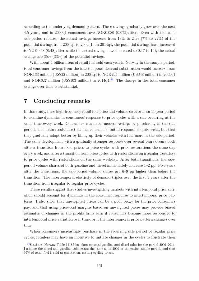
according to the underlying demand pattern. These savings gradually grow over the next4.5 years, and in 2009q1 consumers save NOK0.080 (0.075)/liter. Even with the samesale-period rebates, the actual savings increase from 13% to 24% (7% to 22%) of thepotential savings from 2004q4 to 2009q1. In 2014q4, the potential savings have increasedto NOK0.48 (0.48)/liter while the actual savings have increased to 0.17 (0.16); the actualsavings are 35% (33%) of the potential savings.

With about 4 billion liters of retail fuel sold each year in Norway in the sample period,total consumer savings from the intertemporal demand substitution would increase fromNOK133 million (US$22 million) in 2004q4 to NOK295 million (US$48 million) in 2009q1and NOK627 million (US$103 million) in 2014q4.34 The change in the total consumersavings over time is substantial.

7 Concluding remarks

In this study, I use high-frequency retail fuel price and volume data over an 11-year periodto examine dynamics in consumers’ response to price cycles with a sale occurring at thesame time every week. Consumers can make modest savings by purchasing in the saleperiod. The main results are that fuel consumers’ initial response is quite weak, but thatthey gradually adapt better by filling up their vehicles with fuel more in the sale period.The same development with a gradually stronger response over several years occurs bothafter a transition from fixed prices to price cycles with price restorations the same dayevery week, and after a transition from price cycles with restorations on irregular weekdaysto price cycles with restorations on the same weekday. After both transitions, the sale-period volume shares of both gasoline and diesel immediately increase 1–2 pp. Five yearsafter the transitions, the sale-period volume shares are 6–9 pp higher than before thetransition. The intertemporal elasticity of demand triples over the first 5 years after thetransition from irregular to regular price cycles.

These results suggest that studies investigating markets with intertemporal price vari-ation should account for dynamics in the consumer response to intertemporal price pat-terns. I also show that unweighted prices can be a poor proxy for the price consumerspay, and that using price–cost margins based on unweighted prices may provide biasedestimates of changes in the profits firms earn if consumers become more responsive tointertemporal price variation over time, or if the intertemporal price pattern changes overtime.

When consumers increasingly purchase in the recurring sale period of regular pricecycles, retailers may have an incentive to initiate changes in the cycles to frustrate their

34Statistics Norway Table 11185 has data on total gasoline and diesel sales for the period 2009–2014.I assume the diesel and gasoline volume are the same as in 2009 in the entire sample period, and that95% of retail fuel is sold at gas stations setting cycling prices.

161

attempts to purchase when prices are low. Norway, Perth in Australia, and Germany haveall had regular fuel price cycles over many years and have recently seen changes in thesecycles. In Norway, the largest retail chain initiated a transition to irregular restorationdays in 2017 (Foros & Ones, 2021); in Perth, the restoration day changed from Tuesdayto Wednesday in 2020 (ACCC, 2020); and in Germany, new price restorations aroundnoon and in the afternoon were introduced in 2015 and 2017 (Eibelshäuser & Wilhelm,2018). Future research could investigate if a stronger consumer response to price cycleswas contributing to these transitions.

Price cycles as well as other types of retail sales invoke intertemporal price variation.Other retail sales may be more salient for consumers because they are often advertisedand often entail a large discount on an otherwise stable price. Even so, consumers maybecome better informed about sales activity over time and may also be slow to changetheir habits. Thus, dynamics may also be present in the response of consumers to variousother types of sales. Future research should then investigate the possible dynamics andimplications for firms determining the type and frequency of sales.

162

References

ACCC. (2020). Report on the Australian Petroleum Market - June Quarter2020. Retrieved 2021-05-12, from https://www.accc.gov.au/system/files/20-27RPT_Petrol%2520Quarterly%2520Report%2520-%2520June%25202020_FA.pdf

Assad, S., Clark, R., Ershov, D., & Xu, L. (2020). Algorithmic Pricing and Competition:Empirical Evidence from the German Retail Gasoline Market. Working Paper .

Baker, A., Larcker, D., & Wang, C. (2021). How Much Should We Trust StaggeredDifference-In-Differences Estimates? Working Paper .

Byrne, D. P., & de Roos, N. (2019). Learning to Coordinate - A Study in Retail Gasoline.American Economic Review, 109 (2), 591-619.

Byrne, D. P., Leslie, G. W., & Ware, L. R. (2015). How do Consumers Respond toGasoline Price Cycles? Energy Journal, 36 (1), 115-147.

Cengiz, D., Dube, A., Lindner, A., & Zipperer, B. (2019). The Effect of Minimum Wageson Low-Wage Jobs. Quarterly Journal of Economics, 134 (3), 1405-1454.

de Roos, N., & Smirnov, V. (2020). Collusion with Intertemporal Price Dispersion. RANDJournal of Economics, 51 (1), 158-188.

Deryugina, T., MacKay, A., & Reif, J. (2020). The Long-Run Dynamics of ElectricityDemand: Evidence from Municipal Aggregation. American Economic Journal: AppliedEconomics, 12 (1), 86-114.

Drivkraft Norge. (2021). Salg av Bransjens Hovedprodukter tilbake til 1952(Sale of the Industries Main Products back to 1952. Retrieved 2021-08-25, from https://www.drivkraftnorge.no/siteassets/dokumenter--filer/statistikk/salg/salg-tilbake-til-1952-til-hjemmesiden.xlsx

Eckert, A. (2013). Empirical Studies of Gasoline Retailing: A Guide to the Literature.Journal of Economic Surveys, 27 (1), 140-166.

Eibelshäuser, S., & Wilhelm, S. (2018). High-Frequency Price Fluctuations in Brick-and-Mortar Retailing. Working paper .

European Commission. (2016). A European Strategy for Low-Emission Mobility.

Fabra, N., Rapson, D., Reguant, M., & Wang, J. (2021). Estimating the Elasticity toReal Time Pricing: Evidence from the Spanish Electricity Market. AEA – Papers andProceedings(111), 425-429.

163

Finanskriseutvalget. (2011). NOU 2011:1 Bedre Rustet mot Finanskriser (Better PreparedAgainst Financial Crises).

Foros, Ø., & Ones, M. N. (2021). Coordinate to Obfuscate? The Role of Prior Announce-ments of Recommended Prices. Economics Letters, 198 .

Foros, Ø., & Steen, F. (2013). Vertical Control and Price Cycles in Gasoline Retailing.Scandinavian Journal of Economics, 115 (3), 640-661.

Foros, Ø., Steen, F., & Nguyen-Ones, M. (2021). The Effects of a Day off from RetailPrice Competition: Evidence on Consumer Behavior and Firm Performance in GasolineRetailing. International Journal of the Economics of Business, 28 (1), 49-87.

Hastings, J. S., & Shapiro, J. M. (2013). Fungibility and Consumer Choice: Evidencefrom Commodity Price Shocks. Quarterly Journal of Economics, 128 (4), 1449-1498.

Hendel, I., & Nevo, A. (2006). Sales and Consumer Inventorties. RAND Journal ofEconomics, 37 (3), 543-561.

Hortaçsu, A., Madanizadeh, S. A., & Puller, S. L. (2017). Power to Choose? An Analysisof Consumer Inertia in the Residential Electricity Market. American Economic Journal:Economic Policy, 9 (4), 192-226.

Hvitved-Jacobsen, K. (2002). Tank på tirsdager. Retrieved 2021-02-15, from https://dinside.dagbladet.no/okonomi/tank-pa-tirsdager/62540851

Jessoe, K., & Rapson, D. (2014). Knowledge Is (Less) Power: Experimental Evidencefrom Residential Energy Use. American Economic Review, 104 (4), 1417-1438.

Konkurransetilsynet. (2014). Drivstoff Markedet i Norge - Marginøkning og Ny Pristopp(The Norwegian Fuel Market – Margin increase and a New Price Peak).

Levin, L., Lewis, M. S., & Wolak, F. A. (2017). High Frequency Evidence on the Demandfor Gasoline. American Economic Journal: Economic Policy, 9 (3), 314–347.

Maskin, E., & Tirole, J. (1988). A Theory of Dynamic Oligopoly, II: Price Competition,Kinked Demand Curves, and Edgeworth Cycles. Econometrica, 56 (3), 571-599.

Noel, M. D. (2012). Edgeworth Price Cycles and Intertemporal Price Discrimination.Energy Economics, 34 (4), 942–954.

Noel, M. D. (2015). Do Edgeworth Price Cycles Lead to Higher or Lower Prices? .International Journal of Industrial Organization, 42 (1), 81-93.

Noel, M. D. (2019). Calendar Synchronization of Gasoline Price Increases. Journal ofEconomics and Managment Science, 28 (2), 355-370.

164

Pilskog, G. M. (2018). Frå Global Klimavinnar til Lokal Forureinar (From Global ClimateWinner to Local Polluter).

Statistics Norway. (2021a). 07849: Registered vehicles, by type of transport and type offuel (M) 2008 - 2020. Retrieved 2021-09-8, from https://www.ssb.no/en/statbank/table/07849

Statistics Norway. (2021b). 12575: Kjørelengder, etter Kjøretøytype og Alder 2005 - 2019(Drive Distances, by Type of Vehicle and Age 2005 - 2019. Retrieved 2021-03-9, fromhttps://www.ssb.no/statbank/table/12575/

Tveito, A. (2021a). The Costs and Benefits of Price Leadership – Evidence from RetailGasoline. Working Paper .

Tveito, A. (2021b). Might as Well Jump! Coordinating More Frequent Price Hikes in aRetail Gasoline Market. Working Paper .

Wang, Z. (2009). (Mixed) Strategy in Oligopoly Pricing: Evidence from Gasoline PriceCycles Before and Under a Timing Regulation. Journal of Political Economy, 117 (61),987-1030.

165

Appendices

A Additional figures

Figure A.1: Gasoline share of total retail fuel volume

.3

.4

.5

.6

.7

Gas

olin

e sh

are

20052007

20092011

2013

Year

Note: The figure shows the average gasoline share of total retail fuel volume each year in the sampleperiod. Station-days when either gasoline or diesel volume are missing are dropped before the averagesare calculated.

166

Figure A.2: Number of cycling and non-cycling stations

100

500

1000

1500

Num

ber o

f sta

tions

20052007

20092011

2013

Year

(a) Gasoline

100

500

1000

1500

Num

ber o

f sta

tions

20052007

20092011

2013

Year

(b) Diesel

No Cycle Cycle

Figure A.3: Average prices through the week with irregular cycle

-0.9

-0.8

-0.7

-0.6

-0.5

-0.4

-0.3

-0.2

-0.1

0.0

0.1

NO

K

Mon TueWed Thu Fri Sat

Sun

(a) Gasoline

-0.9

-0.8

-0.7

-0.6

-0.5

-0.4

-0.3

-0.2

-0.1

0.0

0.1

Mon TueWed Thu Fri Sat

Sun

(b) Diesel

Note: The figure shows average gasoline and diesel prices in each hour of the week relative to the hourwith the highest average price in the period when price hikes occur on irregular weekdays.

167

Figure A.4: Average prices

9

10

11

12

13

14

Pric

e

2005q12007q1

2009q12011q1

2013q12014q4

Quarter

Gasoline Diesel

Note: The figure depicts the quarterly average price of gasoline and diesel across all cycling stations.The first and second vertical lines mark the two periods in 2004 with Monday restorations, 2004q2 and2004q4. The third vertical line marks 2009q1. Prices include taxes. Take note of the following:

1. Gasoline and diesel prices both generally increase over the sample period.2. After large price decreases, both the gasoline and diesel prices are at about the same level in the

start of 2009 as they where in 2005.

168

Figure A.5: Sale-period prices vs other prices, 2004

-0.50

-0.25

0.00

0.25

0.50

0.75N

OK

05jan2004

26apr2004

30aug2004

18oct2004

(a) Gasoline

-0.50

-0.25

0.00

0.25

0.50

0.75

NO

K

05jan2004

26apr2004

30aug2004

18oct2004

Week

(b) Diesel

Sun00-11 Sun11-16 Sun16-24 Mon00-11

Note: The figure shows the week to week development in average prices in different parts of the weekrelative to the weekly average for the year 2004. The averages are calculated across all cycling stations.Each line represents the relative price in 1 of the 21 intra-week periods as defined in Section 5.2. Thecolored lines represent prices in different parts of Sunday and Monday morning and the gray lines otherparts of the week. The first vertical line marks the change from irregular restoration days to Mondayrestorations. The second and third dashed lines mark the start and end of the 6-week reversion toirregular restoration days. Take note of the following:

1. Prices are never lowest on Sundays/Monday mornings in weeks with irregular restoration days.2. Prices are always lowest on Sundays/Monday mornings in weeks when restorations occur on

Monday.

169

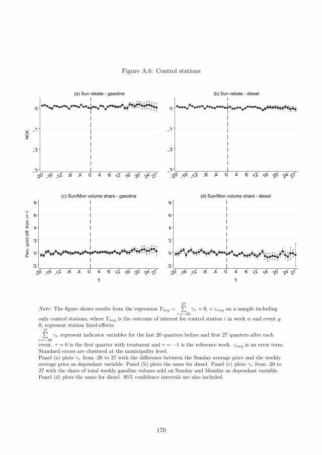
Figure A.6: Control stations

-.3

-.2

-.1

0

NO

K

-20 -16 -12 -8 -4 0 4 8 12 16 20 24 27

(a) Sun rebate - gasoline

-.3

-.2

-.1

0

-20 -16 -12 -8 -4 0 4 8 12 16 20 24 27

(b) Sun rebate - diesel

-2

0

2

4

6

8

Perc

. poi

nt d

iff. f

rom

τ=-

1

-20 -16 -12 -8 -4 0 4 8 12 16 20 24 27

τ

(c) Sun/Mon volume share - gasoline

-2

0

2

4

6

8

-20 -16 -12 -8 -4 0 4 8 12 16 20 24 27

τ

(d) Sun/Mon volume share - diesel

Note: The figure shows results from the regression Yiwg =27∑

τ=−20γτ + θi + εiwg on a sample including

only control stations, where Yiwg is the outcome of interest for control station i in week w and event g.θi represent station fixed-effects.

27∑τ=−20

γτ represent indicator variables for the last 20 quarters before and first 27 quarters after each

event. τ = 0 is the first quarter with treatment and τ = −1 is the reference week. εiwg is an error term.Standard errors are clustered at the municipality level.Panel (a) plots γτ from -20 to 27 with the difference between the Sunday average price and the weeklyaverage price as dependant variable. Panel (b) plots the same for diesel. Panel (c) plots γτ from -20 to27 with the share of total weekly gasoline volume sold on Sunday and Monday as dependant variable.Panel (d) plots the same for diesel. 95% confidence intervals are also included.

170

Figure A.7: Above/below median distance to nearest station

-.3

-.2

-.1

0

NO

K

-20 -16 -12 -8 -4 0 4 8 12 16 20 24 27

(a) Sun relative price - gasoline

-.3

-.2

-.1

0

-20 -16 -12 -8 -4 0 4 8 12 16 20 24 27

(b) Sun relative price - diesel

-2

0

2

4

6

8

Perc

. poi

nt d

iff. f

rom

τ=-

1

-20 -16 -12 -8 -4 0 4 8 12 16 20 24 27τ

(c) Sun/Mon volume share - gasoline

-2

0

2

4

6

8

-20 -16 -12 -8 -4 0 4 8 12 16 20 24 27τ

(d) Sun/Mon volume share - diesel

Closest Farthest

Note: The blue lines show results from Eq. 1 on a sample of stations with below the median distance tothe nearest station (average distance to nearest station=3km), and the red lines the same for stationsabove the median distance to the nearest station (average distance to nearest station=25km). Panel (a)plots γτ from -20 to 27 with the difference between the Sunday average price and the weekly averageprice as dependant variable. Panel (b) plots the same for diesel. Panel (c) plots γτ from -20 to 27 withthe share of total weekly gasoline volume that sold on Sunday and Monday as dependant variable.Panel (d) plots the same for diesel. 95% confidence intervals are also included.

171

Figure A.8: Average prices around events

-3

-2

-1

0

1

2

NO

K

-20 -16 -12 -8 -4 0 4 8 12 16 20 24 27τ

(a) Avg. price - gasoline

-3

-2

-1

0

1

2

NO

K

-20 -16 -12 -8 -4 0 4 8 12 16 20 24 27τ

(b) Avg. price - diesel

Note: The figure shows results from the regression Yiw =27∑

τ=−20γτ + θi + εiw on a sample including only

treated stations, where Yiw is the average weekly price of the fuel type of interest for station i in week

w. θi represent station fixed-effects.27∑

τ=−20γτ represent indicator variables for the last 20 quarters

before and first 27 quarters after each event. τ = 0 is the first quarter with treatment and τ = −1 is thereference week. εiw an error term. Standard errors are clustered at the municipality level. Panel (a)plots γτ from -20 to 27 for the gasoline sample and panel (b) the same for diesel. 95% confidenceintervals are also included.

172

Figure A.9: Sale-period volume share, 2004

0.18

0.20

0.22

0.24

0.26Sh

are

26apr2004

30aug2004

18oct2004

(a) Cycling

0.18

0.20

0.22

0.24

0.26

Shar

e

26apr2004

30aug2004

18oct2004

Weeks

(b) Non-cycling

Gasoline Diesel

Note: The figure shows cycling stations’ week-to-week development in the share of gasoline and dieselvolume sold in the sale-period. The first vertical line marks the first week with Mon restorations, andthe second and third vertical lines mark the last week before and first week after the 6-week reversionperiod. Take note of the following:

1. Non-cycling stations’ diesel and gasoline sale-period volume shares are stationary through 2004.2. Cycling stations’ gasoline (diesel) sale-period volume share increases slightly from an average of

22% (20%) in the period before the transition to Monday restorations to 23% (22%) in the first 4months after the transition.

3. In the 6-week reversion period, the sale shares fall to about the same level as before the transitionto Monday restorations. After the reversion period, the sale share increases again to 24% (22%).

4. There are some indications that the sale share is increasing over time in the periods with Mondayrestorations. The gasoline sale share is close to 22% (21%) in the first weeks with Mondayrestorations and 24-25% (22-23%) in the end of 2004.

*Point estimates are based on the coefficients from a model similar to Eq. 2, but with θ representingweeks. Each point is the sum of βn, θτ and γτn. 95% confidence intervals based on standard errorscalculated with the delta method are shown.

173

Figure A.10: Sale-period split, cycling stations

0.04

0.06

0.08

0.10

0.12

0.14

0.16

0.18

Shar

e

2005q12007q1

2009q12011q1

2013q12014q4

Gasoline Sun Gasoline Mon00-11 Gasoline Mon11-16Diesel Sun Diesel Mon00-11 Diesel Mon11-16

Note: Note: The figure shows cycling stations’ quarterly development in the share of gasoline and dieselvolume sold in different parts of the sale period. The first and second vertical lines mark the 2 periodsin 2004 with Monday restorations, 2004q2 and 2004q4. The third vertical line marks 2009q1. Take noteof the following:

1. The gasoline (diesel) Sunday volume shares increase from 15% (11%) in 2004q4 to 18% (14%) in2009q1 . They then fall to 16% (13%) from 2009q2-2010q4, and then increase to around 18%(14-15%) in 2011 and mostly stay at this level.

2. The gasoline (diesel) Monday morning volume shares increase from 6% (6%) in 2004q4 to 9%(10%) in 2009q1. They then fall to 8% (9%) from 2009q2-2010q4 and gradually increase to about13% in 2014.

3. The Monday midday volume shares increase from 3.5% (3.9%) in 2004q4 to 4.5% (4.8%) in2009q1. They continue to gradually increase to 6.6% (7.4) in 2014.

*Point estimates are based on the coefficients from a model similar to Eq. 2, but with the sale periodsplit in Sunday, Monday until 11:00, and Monday 11:00-16:00. Each point is the sum of βn, θτ and γτn.The 95% confidence intervals based on standard errors calculated with the delta method.

174

Figure A.11: Volume shares in non-sale periods

0.25

0.30

0.35

0.40

0.45

0.50

Shar

e

2005q12007q1

2009q12011q1

2013q12014q4

(a) Gasoline

0.25

0.30

0.35

0.40

0.45

0.50

2005q12007q1

2009q12011q1

2013q12014q4

(b) Diesel

Mon16_Thu16 Thu16_Sat24

Note: The figure shows cycling stations’ quarterly development in the share of gasoline and dieselvolume sold in respectively Monday 16:00–Thursday 16:00 and Thursday 16:00–Saturday 24:00. Thefirst and second vertical lines mark the two periods in 2004 with Monday restorations, 2004q2 and2004q4. The third vertical line marks 2009q1. Take note of the following:

1. The Monday 16:00–Thursday 16:00 volume shares decrease steadily after 2004q4.2. The Thursday 16:00–Saturday 24:00 shares mostly decrease until a sudden increase in 2009q2.

They start to decrease again in 2011 and continue to fall through the rest of the sample period.*Point estimates are based on the coefficient Eq. 2. Each point is the sum of βn, θτ and γτn. 95%confidence intervals based on standard errors calculated with the delta method are shown.

175

Figure A.12: Non-adjusted and adjusted intertemporal elasticity

-12

-10

-8

-6

-4

-2

0

Inte

rtem

pora

l ela

stic

ity

2005q12007q1

2009q12011q1

2013q12014q4

Quarter

Adjusted Non-adjusted

Note: The figure depicts the development in the adjusted and unadjusted intertemporal elasticities forcycling stations in the overall retail fuel market. The first and second vertical lines mark the twoperiods in 2004 with Monday restorations, 2004q2 and 2004q4. The third vertical line marks 2009q1.*The lines plots the βτ from Eq. 3 with respectively unadjusted and adjusted volumes as dependantvariable. 95 % confidence intervals are also shown.

176

Figure A.13: Intertemporal elasticity, gasoline, diesel and overall

-12

-10

-8

-6

-4

-2

0

Inte

rtem

pora

l ela

stic

ity

2005q12007q1

2009q12011q1

2013q12014q4

Quarter

Both fuel types Gasoline Diesel

Note: The figure depicts the development in the adjusted intertemporal elasticities for cycling stationsin the overall retail fuel market, for gasoline retailing and diesel retailing. The first and second verticallines mark the two periods in 2004 with Monday restorations, 2004q2 and 2004q4. The third verticalline marks 2009q1.*The line plots the βτ from Eq. 3 on a sample consisting of respectively both gasoline and diesel, onlygasoline, and only diesel. 95 % confidence intervals are also shown.

177

Figure A.14: Intertemporal elasticity, municipality and station level

-12

-10

-8

-6

-4

-2

0

Inte

rtem

pora

l ela

stic

ity

2005q12007q1

2009q12011q1

2013q12014q4

Quarter

Municipality level Station level

Note: The figure depicts the development in the adjusted intertemporal elasticities for cycling stationsestimated on respectively a dataset aggregated to the municipality level and a station-level dataset.The first and second vertical lines mark the two periods in 2004 with Monday restorations, 2004q2 and2004q4. The third vertical line marks 2009q1.*The line plots the estimated βτ from Eq. 3. When estimating is run on the station level dataset, themunicipality fixed-effects are replaced with station fixed-effects and standard errors are clustered at themunicipality level. 95 % confidence intervals are also shown.

178

Figure A.15: Sale-period rebates and volume, groups with different cycle amplitude

-0.60

-0.40

-0.20

0.00

Sale

-per

iod

reba

te

2005q12007q1

2009q12011q1

2013q12014q4

(a) Rebate - Gasoline

-0.60

-0.40

-0.20

0.00

2005q12007q1

2009q12011q1

2013q12014q4

(b) Rebate - Diesel

0.200.250.300.350.400.45

Sale

-per

iod

volu

me

shar

e

2005q12007q1

2009q12011q1

2013q12014q4

(c) Share - Gasoline

0.200.250.300.350.400.45

2005q12007q1

2009q12011q1

2013q12014q4

(d) Share - Diesel

1st quartile 2nd quartile 3rd quartile 4th quartile

Note: The stations are split in four quartiles, where the first quartile is the 25% stations with the lowestaverage difference between the top of the cycle (prices on Monday between 16:00 and 24:00) and thebottom of the cycle (prices on Monday between 00:00 and 11:00) across all operative weeks between2004q4 and 2014q4. The fourth quartile is the 25% of stations with highest average difference betweentop and bottom.Panel (a) and (b) show the development in the sale-period rebates (average prices across Sundays andMonday before 11:00 relative to the weekly average price) for the different quartiles. Panel (c) and (d)show the development in the share of volume that is sold in the sale-period for the different quartiles.The first and second vertical lines mark the two periods in 2004 with Monday restorations, 2004q2 and2004q4. The third vertical line marks 2009q1.*Point estimates in panel (c) and (d) are based on the coefficients from Eq. 2 run on the four differentquartile samples. Each point is the sum of βn, θτ and γτn. Standard errors for the combined coefficientsare calculated with the delta method.

179

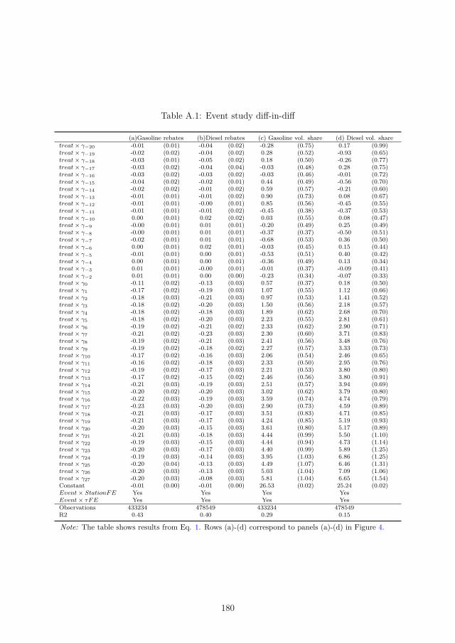
Table A.1: Event study diff-in-diff

(a)Gasoline rebates (b)Diesel rebates (c) Gasoline vol. share (d) Diesel vol. sharetreat× γ−20 -0.01 (0.01) -0.04 (0.02) -0.28 (0.75) 0.17 (0.99)treat× γ−19 -0.02 (0.02) -0.04 (0.02) 0.28 (0.52) -0.93 (0.65)treat× γ−18 -0.03 (0.01) -0.05 (0.02) 0.18 (0.50) -0.26 (0.77)treat× γ−17 -0.03 (0.02) -0.04 (0.04) -0.03 (0.48) 0.28 (0.75)treat× γ−16 -0.03 (0.02) -0.03 (0.02) -0.03 (0.46) -0.01 (0.72)treat× γ−15 -0.04 (0.02) -0.02 (0.01) 0.44 (0.49) -0.56 (0.70)treat× γ−14 -0.02 (0.02) -0.01 (0.02) 0.59 (0.57) -0.21 (0.60)treat× γ−13 -0.01 (0.01) -0.01 (0.02) 0.90 (0.73) 0.08 (0.67)treat× γ−12 -0.01 (0.01) -0.00 (0.01) 0.85 (0.56) -0.45 (0.55)treat× γ−11 -0.01 (0.01) -0.01 (0.02) -0.45 (0.38) -0.37 (0.53)treat× γ−10 0.00 (0.01) 0.02 (0.02) 0.03 (0.55) 0.08 (0.47)treat× γ−9 -0.00 (0.01) 0.01 (0.01) -0.20 (0.49) 0.25 (0.49)treat× γ−8 -0.00 (0.01) 0.01 (0.01) -0.37 (0.37) -0.50 (0.51)treat× γ−7 -0.02 (0.01) 0.01 (0.01) -0.68 (0.53) 0.36 (0.50)treat× γ−6 0.00 (0.01) 0.02 (0.01) -0.03 (0.45) 0.15 (0.44)treat× γ−5 -0.01 (0.01) 0.00 (0.01) -0.53 (0.51) 0.40 (0.42)treat× γ−4 0.00 (0.01) 0.00 (0.01) -0.36 (0.49) 0.13 (0.34)treat× γ−3 0.01 (0.01) -0.00 (0.01) -0.01 (0.37) -0.09 (0.41)treat× γ−2 0.01 (0.01) 0.00 (0.00) -0.23 (0.34) -0.07 (0.33)treat× γ0 -0.11 (0.02) -0.13 (0.03) 0.57 (0.37) 0.18 (0.50)treat× γ1 -0.17 (0.02) -0.19 (0.03) 1.07 (0.55) 1.12 (0.66)treat× γ2 -0.18 (0.03) -0.21 (0.03) 0.97 (0.53) 1.41 (0.52)treat× γ3 -0.18 (0.02) -0.20 (0.03) 1.50 (0.56) 2.18 (0.57)treat× γ4 -0.18 (0.02) -0.18 (0.03) 1.89 (0.62) 2.68 (0.70)treat× γ5 -0.18 (0.02) -0.20 (0.03) 2.23 (0.55) 2.81 (0.61)treat× γ6 -0.19 (0.02) -0.21 (0.02) 2.33 (0.62) 2.90 (0.71)treat× γ7 -0.21 (0.02) -0.23 (0.03) 2.30 (0.60) 3.71 (0.83)treat× γ8 -0.19 (0.02) -0.21 (0.03) 2.41 (0.56) 3.48 (0.76)treat× γ9 -0.19 (0.02) -0.18 (0.02) 2.27 (0.57) 3.33 (0.73)treat× γ10 -0.17 (0.02) -0.16 (0.03) 2.06 (0.54) 2.46 (0.65)treat× γ11 -0.16 (0.02) -0.18 (0.03) 2.33 (0.50) 2.95 (0.76)treat× γ12 -0.19 (0.02) -0.17 (0.03) 2.21 (0.53) 3.80 (0.80)treat× γ13 -0.17 (0.02) -0.15 (0.02) 2.46 (0.56) 3.80 (0.91)treat× γ14 -0.21 (0.03) -0.19 (0.03) 2.51 (0.57) 3.94 (0.69)treat× γ15 -0.20 (0.02) -0.20 (0.03) 3.02 (0.62) 3.79 (0.80)treat× γ16 -0.22 (0.03) -0.19 (0.03) 3.59 (0.74) 4.74 (0.79)treat× γ17 -0.23 (0.03) -0.20 (0.03) 2.90 (0.73) 4.59 (0.89)treat× γ18 -0.21 (0.03) -0.17 (0.03) 3.51 (0.83) 4.71 (0.85)treat× γ19 -0.21 (0.03) -0.17 (0.03) 4.24 (0.85) 5.19 (0.93)treat× γ20 -0.20 (0.03) -0.15 (0.03) 3.61 (0.80) 5.17 (0.89)treat× γ21 -0.21 (0.03) -0.18 (0.03) 4.44 (0.99) 5.50 (1.10)treat× γ22 -0.19 (0.03) -0.15 (0.03) 4.44 (0.94) 4.73 (1.14)treat× γ23 -0.20 (0.03) -0.17 (0.03) 4.40 (0.99) 5.89 (1.25)treat× γ24 -0.19 (0.03) -0.14 (0.03) 3.95 (1.03) 6.86 (1.25)treat× γ25 -0.20 (0.04) -0.13 (0.03) 4.49 (1.07) 6.46 (1.31)treat× γ26 -0.20 (0.03) -0.13 (0.03) 5.03 (1.04) 7.09 (1.06)treat× γ27 -0.20 (0.03) -0.08 (0.03) 5.81 (1.04) 6.65 (1.54)Constant -0.01 (0.00) -0.01 (0.00) 26.53 (0.02) 25.24 (0.02)Event× StationFE Yes Yes Yes YesEvent× τFE Yes Yes Yes YesObservations 433234 478549 433234 478549R2 0.43 0.40 0.29 0.15

Note: The table shows results from Eq. 1. Rows (a)-(d) correspond to panels (a)-(d) in Figure 4.

180

Table A.2: Gasoline and diesel, sale-period volume shares

Quarter Gasoline Diesel2004q1 0.221 (0.001) 0.201 (0.001)2004q2 0.229 (0.002) 0.215 (0.002)2004q3 0.222 (0.002) 0.204 (0.001)2004q4 0.241 (0.004) 0.216 (0.003)2005q1 0.249 (0.004) 0.223 (0.003)2005q2 0.253 (0.005) 0.230 (0.004)2005q3 0.250 (0.005) 0.229 (0.004)2005q4 0.247 (0.005) 0.228 (0.005)2006q1 0.251 (0.004) 0.234 (0.003)2006q2 0.249 (0.003) 0.235 (0.003)2006q3 0.259 (0.003) 0.254 (0.004)2006q4 0.271 (0.005) 0.268 (0.005)2007q1 0.272 (0.004) 0.261 (0.004)2007q2 0.267 (0.004) 0.264 (0.004)2007q3 0.272 (0.004) 0.270 (0.004)2007q4 0.281 (0.005) 0.268 (0.005)2008q1 0.292 (0.005) 0.267 (0.005)2008q2 0.290 (0.004) 0.274 (0.005)2008q3 0.294 (0.005) 0.278 (0.005)2008q4 0.315 (0.006) 0.280 (0.005)2009q1 0.313 (0.005) 0.290 (0.006)2009q2 0.281 (0.004) 0.272 (0.005)2009q3 0.283 (0.004) 0.278 (0.005)2009q4 0.288 (0.004) 0.275 (0.005)2010q1 0.280 (0.004) 0.262 (0.005)2010q2 0.279 (0.004) 0.265 (0.004)2010q3 0.282 (0.004) 0.270 (0.005)2010q4 0.286 (0.004) 0.268 (0.005)2011q1 0.306 (0.005) 0.283 (0.005)2011q2 0.311 (0.005) 0.283 (0.005)2011q3 0.303 (0.005) 0.290 (0.005)2011q4 0.314 (0.005) 0.292 (0.005)2012q1 0.322 (0.005) 0.301 (0.005)2012q2 0.317 (0.005) 0.298 (0.005)2012q3 0.313 (0.005) 0.296 (0.005)2012q4 0.324 (0.005) 0.302 (0.006)2013q1 0.321 (0.005) 0.301 (0.006)2013q2 0.330 (0.005) 0.313 (0.006)2013q3 0.332 (0.006) 0.315 (0.006)2013q4 0.347 (0.006) 0.325 (0.007)2014q1 0.363 (0.007) 0.344 (0.008)2014q2 0.350 (0.006) 0.327 (0.007)2014q3 0.356 (0.006) 0.349 (0.007)2014q4 0.377 (0.006) 0.356 (0.007)

Note: The table shows the development in the sale-period volume share based on Eq. 2 for cyclingstations. The results are also reported in panel (a) in Figure 5.

181

Table A.3: Quarterly intertemporal elasticity

Overall Gasoline Diesel2004q1 × ln(price) -2.38 (0.099) -3.24 (0.10) -1.68 (0.13)2004q2 × ln(price) -1.96 (0.15) -2.99 (0.15) -1.36 (0.17)2004q3 × ln(price) -3.01 (0.13) -4.33 (0.17) -2.03 (0.12)2004q4 × ln(price) -2.29 (0.16) -3.83 (0.17) -1.39 (0.19)2005q1 × ln(price) -2.87 (0.19) -4.29 (0.19) -1.85 (0.21)2005q2 × ln(price) -3.74 (0.21) -5.12 (0.23) -2.83 (0.23)2005q3 × ln(price) -3.35 (0.13) -4.02 (0.14) -2.82 (0.15)2005q4 × ln(price) -3.38 (0.16) -4.50 (0.15) -2.74 (0.18)2006q1 × ln(price) -3.62 (0.17) -5.17 (0.18) -2.89 (0.20)2006q2 × ln(price) -4.24 (0.19) -5.32 (0.19) -3.89 (0.22)2006q3 × ln(price) -4.55 (0.22) -5.85 (0.21) -4.24 (0.24)2006q4 × ln(price) -5.31 (0.23) -6.89 (0.27) -4.76 (0.23)2007q1 × ln(price) -4.69 (0.22) -6.54 (0.25) -3.92 (0.24)2007q2 × ln(price) -4.03 (0.19) -5.57 (0.23) -3.60 (0.21)2007q3 × ln(price) -4.74 (0.18) -6.22 (0.19) -4.29 (0.20)2007q4 × ln(price) -4.11 (0.20) -6.55 (0.24) -3.19 (0.20)2008q1 × ln(price) -5.02 (0.20) -7.18 (0.22) -3.60 (0.22)2008q2 × ln(price) -6.04 (0.23) -8.11 (0.25) -4.75 (0.24)2008q3 × ln(price) -6.42 (0.21) -7.82 (0.22) -5.52 (0.24)2008q4 × ln(price) -5.26 (0.16) -7.45 (0.19) -3.91 (0.17)2009q1 × ln(price) -5.72 (0.18) -6.72 (0.20) -4.94 (0.22)2009q2 × ln(price) -4.92 (0.19) -5.38 (0.22) -4.66 (0.21)2009q3 × ln(price) -5.71 (0.20) -6.26 (0.24) -5.47 (0.22)2009q4 × ln(price) -6.20 (0.24) -7.60 (0.29) -5.35 (0.27)2010q1 × ln(price) -5.85 (0.25) -7.48 (0.30) -4.91 (0.27)2010q2 × ln(price) -6.14 (0.24) -7.83 (0.30) -5.08 (0.25)2010q3 × ln(price) -5.84 (0.23) -7.12 (0.30) -5.27 (0.24)2010q4 × ln(price) -5.37 (0.23) -7.02 (0.27) -4.43 (0.23)2011q1 × ln(price) -6.74 (0.25) -8.50 (0.30) -5.64 (0.25)2011q2 × ln(price) -7.76 (0.26) -9.47 (0.30) -6.71 (0.29)2011q3 × ln(price) -7.52 (0.26) -8.92 (0.27) -6.60 (0.28)2011q4 × ln(price) -7.96 (0.26) -10.6 (0.32) -6.31 (0.26)2012q1 × ln(price) -8.14 (0.31) -9.03 (0.35) -7.54 (0.33)2012q2 × ln(price) -9.35 (0.36) -10.6 (0.38) -8.50 (0.39)2012q3 × ln(price) -8.16 (0.33) -9.03 (0.34) -7.51 (0.34)2012q4 × ln(price) -8.77 (0.38) -11.0 (0.40) -7.23 (0.38)2013q1 × ln(price) -8.48 (0.36) -9.54 (0.37) -7.63 (0.38)2013q2 × ln(price) -8.72 (0.34) -9.42 (0.36) -8.00 (0.39)2013q3 × ln(price) -8.21 (0.33) -8.87 (0.34) -7.63 (0.34)2013q4 × ln(price) -9.28 (0.27) -11.6 (0.29) -7.68 (0.28)2014q1 × ln(price) -10.0 (0.25) -11.5 (0.26) -8.95 (0.29)2014q2 × ln(price) -8.11 (0.25) -9.08 (0.28) -7.35 (0.27)2014q3 × ln(price) -9.00 (0.25) -9.81 (0.26) -8.35 (0.27)2014q4 × ln(price) -8.94 (0.21) -10.3 (0.22) -7.85 (0.24)Constant 22.6 (0.38) 26.3 (0.41) 20.4 (0.40)λiθwγf Yes Yes YesObservations 5369767 2677705 2692170R2 0.86 0.85 0.87

Note: The table shows the development in the intertemporal elasticity based on Eq. 3 for cycling stations.The results are also reported in Figures 6 and A.13.

182

Graphic design: Comm

unication Division, UiB / Print: Skipnes Komm

unikasjon AS

uib.no

ISBN: 9788230866979 (print)9788230841662 (PDF)