Statistical Methodology 7 (2010) 552–573

Contents lists available at ScienceDirect

Statistical Methodology

journal homepage: www.elsevier.com/locate/stamet

Predicting losses of residential structures in the state ofFlorida by the public hurricane loss evaluation modelShahid Hamid a, B.M. Golam Kibria b, Sneh Gulati b,∗, Mark Powell c,Bachir Annane d, Steve Cocke e, Jean-Paul Pinelli f, Kurt Gurley g,Shu-Ching Chen ha Department of Finance, Florida International University, Miami, FL 33199, USAb Department of Statistics, Florida International University, Miami, FL 33199, USAc NOAA Hurricane Research Division, Miami, FL, USAd CIMAS, Rosenstiel School/University of Miami, USAe Florida State University, Tallahassee, FL, USAf Department of Civil Engineering, Florida Institute of Technology, Melbourne, FL 32901, USAg Department of Civil and Coastal Engineering, University of Florida, Gainsville, FL 32611, USAh School of Computing and Information Sciences, Florida International University, Miami, FL 33199, USA

a r t i c l e i n f o

Article history:Received 4 December 2008Accepted 28 February 2010

Keywords:DamageGoodness of fitHurricaneInsurance lossPoissonRegressionSensitivityUncertaintyValidationWind model

a b s t r a c t

As an environmental phenomenon, hurricanes cause significantproperty damage and loss of life in coastal areas almost everyyear. Although a number of commercial loss projection modelshave been developed to predict the property losses, only a handfulof studies are available in the public domain to predict damagefor hurricane prone areas. The state of Florida has developed anopen, public model for the purpose of probabilistic assessment ofrisk to insured residential property associated with wind damagefrom hurricanes. The model comprises three components; viz.the atmospheric science component, the engineering componentand the actuarial science component. The atmospheric componentincludes modeling the track and intensity life cycle of eachsimulated hurricane within the Florida threat area. Based onhistorical hurricane statistics, thousands of storms are simulatedallowing determination of the wind risk for all residential ZipCode locations in Florida. The wind risk information is thenprovided to the engineering and actuarial components to modeldamage and average annual loss, respectively. The actuarial team

∗ Corresponding author. Tel.: +1 305 348 2065.E-mail address: gulati@fiu.edu (S. Gulati).

1572-3127/$ – see front matter© 2010 Elsevier B.V. All rights reserved.doi:10.1016/j.stamet.2010.02.004

S. Hamid et al. / Statistical Methodology 7 (2010) 552–573 553

finds the county-wise loss and the total loss for the entire stateof Florida. The computer team then compiles all informationfrom atmospheric science, engineering and actuarial components,processes all hurricane related data and completes the project. Themodel was submitted to the Florida Commission on Hurricane LossProjection Methodology for approval and went through a rigorousreview and was revised as per the suggestions of the commission.The final model was approved for use by the insurance companiesin Florida by the commission. At every stage of the process,statistical procedures were used to model various parameters andvalidate the model. This paper presents a brief summary of themain components of the model (meteorology, vulnerability andactuarial) and then focuses on the statistical validation of the same.

© 2010 Elsevier B.V. All rights reserved.

1. Introduction

Due to threat of natural disasters (like hurricane, cyclone, earthquake etc.) to life and property, itis very important to predict the possible damage and loss. A hurricane is a type of tropical cyclone,which is a generic term for a low-pressure system that generally forms over warm, tropical oceans.Usually a hurricane is several hundred miles in diameter and is accompanied by violent winds, bigwaves, heavy rains and floods. Normally a hurricane starts as a tropical depression, becomes a tropicalstorm when the maximum sustained wind speed exceeds 38 mph and finally turns into a hurricanewhen the winds have a speed higher than 74 mph. Hurricanes have an eye and an eye wall. The eyeis the calm area near the rotational axis of the hurricane. Surrounding the eye are the thick clouds,called the eye wall, which is the violent area of a hurricane [39]. Hurricanes are categorized accordingto their severity using the Saffir–Simpson hurricane scale, ranging from 1 to 5 [40]. A category 1storm has the lowest wind speeds while a category 5 hurricane has the strongest. These are relativeterms, because lower category storms can sometimes inflict greater damage than higher categorystorms, depending on where they strike and the particular hazards they bring. It is reported thatevery year approximately ten tropical storms develop over the Atlantic Ocean. Although many ofthese remain over the ocean, some become hurricanes and strike the United States coastline with atleast two of these being stronger than Category 3, thus posing enormous threats to life and property.Sophisticated three-dimensional numerical weather prediction models [21] are computationally tooexpensive to conduct hurricane loss projection simulation studies. In order to project losses associatedwith landfalling hurricanes, statistical Monte-Carlo simulations [35] are conducted, which attemptto model thousands of years of hurricane activity based on the statistical character of the historicalstorms in the vicinity of the location of interest. We refer the reader to [47,9]among others for Modelson extreme for wind speed or extreme wind gusts.The historical record for establishing the risk of hurricanes throughout the coastal United States

is limited to a period of about 100 years, with relatively reliable and complete records [25].Unfortunately, the number of landfalling hurricanes during this period is not sufficiently large enoughto establish risk without large errors so alternative methods have been used since the 1970s [35,2].Hurricane riskmodels are currently used to conduct simulations of thousands of years of storms basedon probability distributions of important historically observed parameters. The paper is based on theFlorida Public Hurricane Loss Model (FPHLM). The model is a very complex set of computer programswhich track a hurricane from its genesis to landfall and predict the total and insured loss for residentialstructures in Florida. The FPHLM consists of the following major three components: atmosphericscience (meteorology), vulnerability (engineering), and insured loss cost (actuarial). Each componentprovides one-way input to the next component in line until the end result (average annual loss per ZipCode) is achieved. Finally, the computer team compiles and processes all the information provided bythe three components.A number of models have been developed and widely used to predict losses due to hurricane or

other kind of natural disasters. However, they are for the most part, not publicly available. Although

554 S. Hamid et al. / Statistical Methodology 7 (2010) 552–573

several commercial models are available to predict the losses, this is the first public model specificallydesigned to predict the residential losses for the insurance industrywhich is accessible to the scientificcommunity and public. This paper discusses the development of Florida Public Hurricane Loss Model(FPHLM). The outline of the paper is as follows: Section 2 describes about the atmospheric sciencecomponent. Section 3 discusses about the engineering component. Section 4 deals with the actuarialscience component. The computer science component and statistical validation of the models aregiven in Sections 5 and 6 respectively. Finally some concluding remarks are added in Section 7.

2. Atmospheric science component

In this section we discuss the atmospheric science component of the model. It has the followingthree major components which are discussed below.

2.1. Threat area and annual occurrence

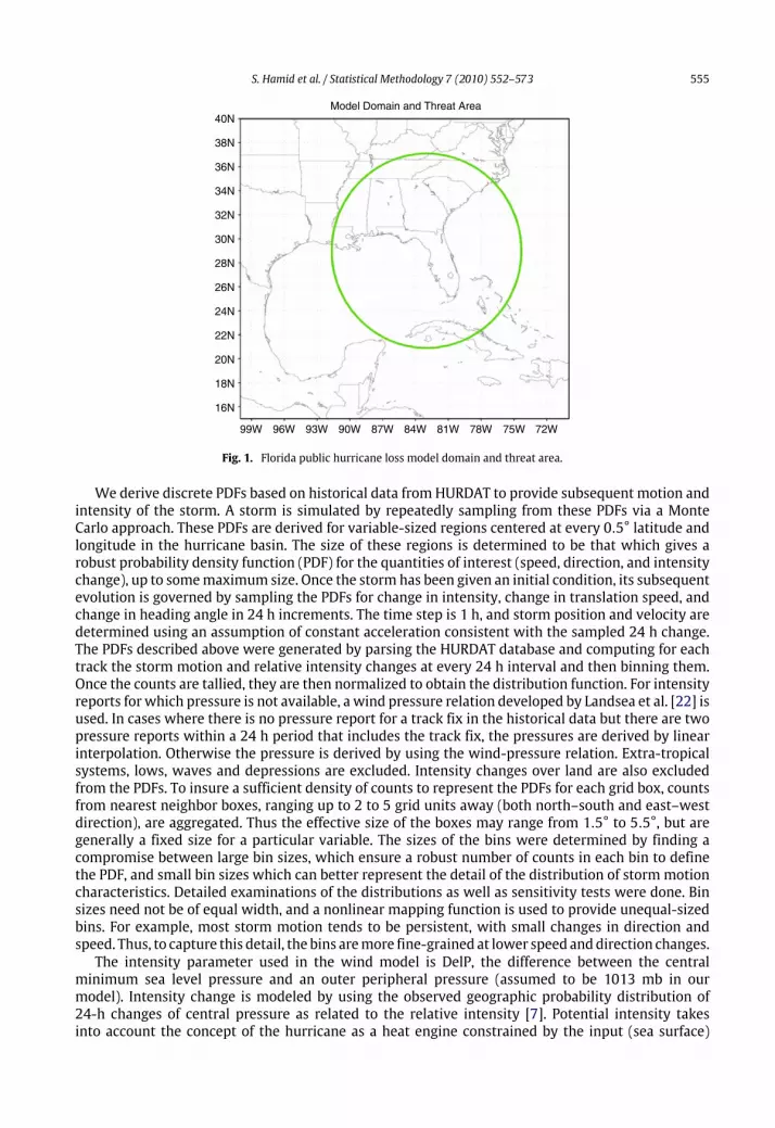
A threat area is defined to best capture the statistical characteristics of historical tropical cyclonesthat have affected the state. The area within 1000 km of a location (26.0 N, 82.0 W) off the southwestcoast of Florida (Fig. 1) was chosen since this captures storms that can affect the panhandle, west, andnortheast coasts of Florida, as well as storms that approach South Florida from the vicinity of Cuba andthe Bahamas. The historical record for the Atlantic tropical cyclone basin (known as ‘‘HURDAT’’) is a sixhourly record of tropical storm and hurricane positions and intensities [17], which are expressed asestimated maximum 1 min surface (10 m) winds and, when available, central sea level pressure. Theperiod 1851–2006 is the largest available, but the period 1900–2005 is used most often. This is dueto uncertainties about 19th century storms (especially for Florida) due to a lack of population centersand meteorological measurements of hurricanes before the start of the 20th century. There are alsouncertainties about the first half of the 20th century since aircraft reconnaissance only began in the1940s so another choice in the period of record are the years 1944–2004. Four additional choices areavailable which simulate the warm (El Nino, fewer hurricanes) and neutral or cold (La Nina, morehurricanes) inter annual climate cycles in tropical cyclone activity, as well as the cold or warm phasesof the Multi-decadal climate cycles. These choices are primarily for research purposes and constrainthe historical record to use only years with the specified climate cycle to fit annual tropical cycloneoccurrence.The first step in the atmospheric science component is to model annual hurricane occurrence.

Clearly, there are two choices here: the Poisson distribution (based on homogeneous hurricanefrequencies) and the negative binomial (based on nonhomogeneous annual occurrence rate.).However, the Chi-square goodness of fit test run on the two models indicated that the Poissondistribution with its higher p-value was a better fit. The chosen fit is then randomly sampled todetermine how many storms occur for each year of the simulation. Once the number of tropicalcyclones within the threat area for a given year is determined, the distribution of the genesis timewasobtained from by sampling from on the historical storm tracks and smoothing the resulting empiricaldistribution. More on this topic we refer [5].

2.2. Hurricane track and intensity

The storm track model generates storm tracks and intensities based on historical storm conditionsand motions. The initial seeds for the storms are derived from the historical record for the Atlantictropical bases database. For historical landfalling storms in Florida and neighboring states, the initialpositions, intensities andmotions are taken from the track fix 36 h prior to first landfall. For historicalstorms that do not make landfall, the initial conditions are taken from the first track fix of the stormafter it enters a threat area as a hurricane. Small, uniform random error terms are added to the initialposition, storm motion change, and to the storm intensity change. The initial conditions derivedfrom HURDAT are recycled as necessary to generate thousands of years of stochastic tracks. After thestorm is initiated, the subsequentmotion and intensity changes are sampled from empirically derivedprobability distribution functions over the model domain for the state of Florida (Fig. 1).

S. Hamid et al. / Statistical Methodology 7 (2010) 552–573 555

Model Domain and Threat Area40N

38N

36N

34N

32N

30N

28N

26N

24N

22N

20N

18N

16N

99W 96W 93W 90W 87W 84W 81W 78W 75W 72W

Fig. 1. Florida public hurricane loss model domain and threat area.

We derive discrete PDFs based on historical data from HURDAT to provide subsequent motion andintensity of the storm. A storm is simulated by repeatedly sampling from these PDFs via a MonteCarlo approach. These PDFs are derived for variable-sized regions centered at every 0.5° latitude andlongitude in the hurricane basin. The size of these regions is determined to be that which gives arobust probability density function (PDF) for the quantities of interest (speed, direction, and intensitychange), up to somemaximum size. Once the storm has been given an initial condition, its subsequentevolution is governed by sampling the PDFs for change in intensity, change in translation speed, andchange in heading angle in 24 h increments. The time step is 1 h, and storm position and velocity aredetermined using an assumption of constant acceleration consistent with the sampled 24 h change.The PDFs described above were generated by parsing the HURDAT database and computing for eachtrack the storm motion and relative intensity changes at every 24 h interval and then binning them.Once the counts are tallied, they are then normalized to obtain the distribution function. For intensityreports for which pressure is not available, a wind pressure relation developed by Landsea et al. [22] isused. In cases where there is no pressure report for a track fix in the historical data but there are twopressure reports within a 24 h period that includes the track fix, the pressures are derived by linearinterpolation. Otherwise the pressure is derived by using the wind-pressure relation. Extra-tropicalsystems, lows, waves and depressions are excluded. Intensity changes over land are also excludedfrom the PDFs. To insure a sufficient density of counts to represent the PDFs for each grid box, countsfrom nearest neighbor boxes, ranging up to 2 to 5 grid units away (both north–south and east–westdirection), are aggregated. Thus the effective size of the boxes may range from 1.5° to 5.5°, but aregenerally a fixed size for a particular variable. The sizes of the bins were determined by finding acompromise between large bin sizes, which ensure a robust number of counts in each bin to definethe PDF, and small bin sizes which can better represent the detail of the distribution of stormmotioncharacteristics. Detailed examinations of the distributions as well as sensitivity tests were done. Binsizes need not be of equal width, and a nonlinear mapping function is used to provide unequal-sizedbins. For example, most storm motion tends to be persistent, with small changes in direction andspeed. Thus, to capture this detail, the bins aremore fine-grained at lower speed anddirection changes.The intensity parameter used in the wind model is DelP, the difference between the central

minimum sea level pressure and an outer peripheral pressure (assumed to be 1013 mb in ourmodel). Intensity change is modeled by using the observed geographic probability distribution of24-h changes of central pressure as related to the relative intensity [7]. Potential intensity takesinto account the concept of the hurricane as a heat engine constrained by the input (sea surface)

556 S. Hamid et al. / Statistical Methodology 7 (2010) 552–573

SD

C –

FS

U

30N

31N

32N

33N

29N

28N

27N

26N

25N

24N

23N

22N

21N

20N

19N

18N75W76W77W78W79W80W81W82W83W84W85W86W87W88W89W90W

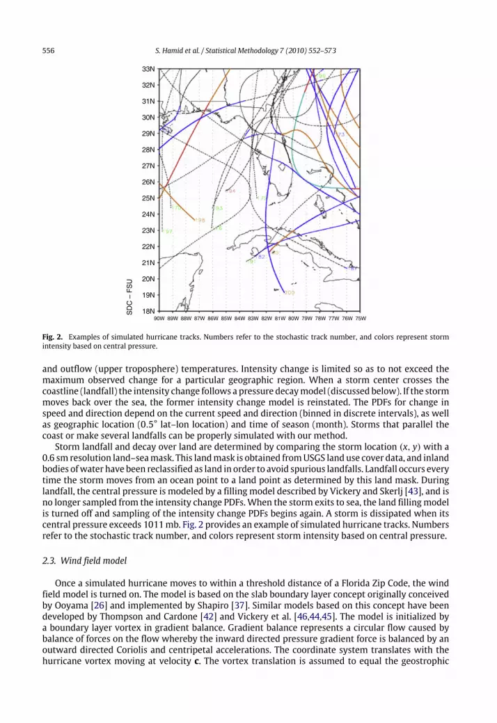
Fig. 2. Examples of simulated hurricane tracks. Numbers refer to the stochastic track number, and colors represent stormintensity based on central pressure.

and outflow (upper troposphere) temperatures. Intensity change is limited so as to not exceed themaximum observed change for a particular geographic region. When a storm center crosses thecoastline (landfall) the intensity change follows a pressure decaymodel (discussed below). If the stormmoves back over the sea, the former intensity change model is reinstated. The PDFs for change inspeed and direction depend on the current speed and direction (binned in discrete intervals), as wellas geographic location (0.5° lat–lon location) and time of season (month). Storms that parallel thecoast or make several landfalls can be properly simulated with our method.Storm landfall and decay over land are determined by comparing the storm location (x, y) with a

0.6 sm resolution land–seamask. This landmask is obtained fromUSGS land use cover data, and inlandbodies ofwater have been reclassified as land in order to avoid spurious landfalls. Landfall occurs everytime the storm moves from an ocean point to a land point as determined by this land mask. Duringlandfall, the central pressure is modeled by a filling model described by Vickery and Skerlj [43], and isno longer sampled from the intensity change PDFs.When the storm exits to sea, the land fillingmodelis turned off and sampling of the intensity change PDFs begins again. A storm is dissipated when itscentral pressure exceeds 1011mb. Fig. 2 provides an example of simulated hurricane tracks. Numbersrefer to the stochastic track number, and colors represent storm intensity based on central pressure.

2.3. Wind field model

Once a simulated hurricane moves to within a threshold distance of a Florida Zip Code, the windfield model is turned on. The model is based on the slab boundary layer concept originally conceivedby Ooyama [26] and implemented by Shapiro [37]. Similar models based on this concept have beendeveloped by Thompson and Cardone [42] and Vickery et al. [46,44,45]. The model is initialized bya boundary layer vortex in gradient balance. Gradient balance represents a circular flow caused bybalance of forces on the flow whereby the inward directed pressure gradient force is balanced by anoutward directed Coriolis and centripetal accelerations. The coordinate system translates with thehurricane vortex moving at velocity c. The vortex translation is assumed to equal the geostrophic

S. Hamid et al. / Statistical Methodology 7 (2010) 552–573 557

flow associated with the large scale pressure gradient. In cylindrical coordinates that translate withthemoving vortex, equations for a slab hurricane boundary layer under a prescribed pressure gradientare:

u∂u∂r−v2

r− f v +

v

r∂u∂φ+∂p∂r− K

(∇2u−

ur2−2r2∂u∂φ

)+ F(

→

c , u) = 0 =∂u∂t

(1)

u(∂v

∂r+v

r

)+ fu+

v

r∂v

∂φ− K

(∇2v −

v

r2+2r2∂u∂φ

)+ F(

→

c , v) = 0 =∂v

∂t(2)

where u and v are the respective radial and tangential wind components relative to themoving storm,p is the sea-level pressure which varies with radius (r), f is the Coriolis parameter which varieswith latitude, φ is the azimuthal coordinate, K is the eddy diffusion coefficient, and F(c, u), F(c, v)are frictional drag terms (discussed below). All terms are assumed to be representative of meansthrough the boundary layer. The motion of the vortex is determined by the modeled storm track.The symmetric pressure field p(r) is specified by the Holland [13] pressure profile with the centralpressure specified according to the intensity modeling in concert with the storm track. A model forthe Holland B pressure profile parameter was developed based on a subset of the data publishedby Willoughby and Rahn [48]. The radius of maximum wind at landfall is modeled as a function oflatitude and Pmin using a database constructed from a variety of landfall data including the NWS-38publication, extended best track by DeMaria, and NOAA HRD archives. Rmax data were fitted usingboth lognormal and gamma distributions. However based on the p-values, we found that Gammadistribution is a good fit for Rmax data (details are in Section 6). Thewind field is solved on a polar gridwith a 0.1 R/Rmax resolution. The input Rmax is adjusted to remove a bias caused by a tendency of thewind field solution to place Rmax one grid point radially outward from the input value. The slabmeanboundary layer wind speed is adjusted to the surface based on reduction factors published in [32]and is adjusted to maximum sustained and peak 3 s gust values according to gust factors as describedin [43]. Flow transition from marine to land or from one land roughness to another is dependent onaerodynamic roughness as modeled by Simiu and Scanlan [38]. The roughness database derived fromMulti-Resolution Land Cover (MRLC)National Land ClassificationDatabase (NLCD) of 2001 [14] is usedin associationwith the SourceAreaModel [36,1] to determine anupstream fetch dependent roughnessvalue at all Florida Zip Codes. We corrected some anomalies where the population centroids were notnear residential properties. To remedy this, we set a lower limit of roughness equivalent to that of alow intensity residential area to all land points within 0.311 miles of the centroid. For special caseswhere the centroid is over water, the roughness was set to that of a low intensity residential areafor all points within 0.311 miles of the centroid. For coastal regions, we corrected the roughness byaveraging the effective roughness for coastal fetches. Fig. 3 showed the comparison of observed (right)and modeled (left) landfall wind fields of Hurricanes Charley (2004) in south Florida. Line segmentindicates storm heading. Horizontal coordinates are in units of R/Rmax and winds units of miles perhour. Fig. 3 exhibited a nice fit of the wind model. More information on the atmospheric component,we refer to [13,23,11,7,19,42,40,3,30], Powell et al. (2003), [31] among others. The final wind speedwill be useful to design the vulnerability matrix which are described in the following section.

3. Engineering component

The engineering component consists of the following components and their details are presentedbelow.

3.1. The vulnerability component

The vulnerability model uses a Monte Carlo simulation based on a component approach todetermine the external vulnerability of buildings at various wind speeds. The simulation relatesestimated probabilistic strength capacities of building components to a series of deterministic 3 speak gust wind speeds through a detailed wind and structural engineering analysis that includeseffects of wind-borne missiles. The internal, utilities, and contents damages to the building are then

558 S. Hamid et al. / Statistical Methodology 7 (2010) 552–573

–4

–2

0

2

4

CHARLEY modeled wind Speed at landfall IN MPH

–4 –2 0 2 4

CHARLEY SURFACE WINDFIELD 8/13/04 20:30 UTC MPH

–4 –2 0 2 4

–4

–2

0

2

4

Fig. 3. Comparison of observed (right) and modeled (left) landfall wind fields of Hurricanes Charley (2004) in south Florida.

extrapolated from the external damage. The resulting estimates of total building damage result inthe formulation of vulnerability matrices for each building type that is statistically significant in theFlorida building stock, including manufactured homes.

3.1.1. Site built modelsA statistical exposure study of Florida identified the most common types of single-family

residential buildings in North, Central, and South Florida, in addition to the Keys. All model hometypes have 15 windows, a two-car garage, a front entrance door, and a sliding glass back door.Identical models are created for homes that are equipped with hurricane shutters, where windowcapacities are increased so that failure is much less likely. In addition to a classification of buildingby structural types, it was also necessary to classify the buildings by relative strength. Residentialconstruction methods have evolved in Florida as experience with severe winds drives the need toreduce vulnerability. To address this, the vulnerability team has developed a strong model, mediumstrength model, and a weak model for each site-built structural type to represent relative quality ofconstruction.The strong model was developed first and both the weak and medium models were derived from

the strongmodel, using various levels of capacity within the standardmodel framework. For example,the standardmodel for south, concrete block, gable roof construction is converted to a weakmodel bysimply lowering the roof-to-wall (r2w) connection capacity to toe–nail strength, lowering the garagecapacity, and lowering the sheathing capacity. Simulations have been generated for gable roof, 1 and2-storywood and 1-story concrete blockwall, north, central and south regions. This has been repeatedwith plywood shutters in place. Themediummodels are the same as theweak ones except for the cliproof to wall connections.

3.1.2. Manufacture homes modelsBased on the exposure study, it was also decided to model four manufactured home (MH) types.

These types include: Pre-1994—Fully Tied down; Pre-1994—Not Tied down; Post-1994—HUD Zone II;Post-1994—HUD Zone III.The partially tied down homes are assumed to have a vulnerability that is an average of the

vulnerabilities of fully tied-down and not tied-down homes. Because little information is availableregarding the distribution of manufactured home types by size or geometry, it is assumed that allmodel types are single-wide manufactured homes. The modeled single-wide manufactured homesare 56 ft× 13 ft, have gable roofs, 8 windows, a front entrance door, and a sliding glass back door.

S. Hamid et al. / Statistical Methodology 7 (2010) 552–573 559

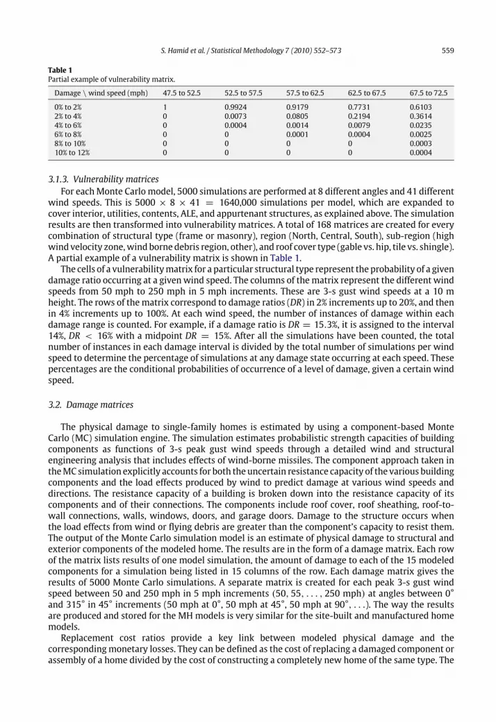
Table 1Partial example of vulnerability matrix.

Damage \wind speed (mph) 47.5 to 52.5 52.5 to 57.5 57.5 to 62.5 62.5 to 67.5 67.5 to 72.5

0% to 2% 1 0.9924 0.9179 0.7731 0.61032% to 4% 0 0.0073 0.0805 0.2194 0.36144% to 6% 0 0.0004 0.0014 0.0079 0.02356% to 8% 0 0 0.0001 0.0004 0.00258% to 10% 0 0 0 0 0.000310% to 12% 0 0 0 0 0.0004

3.1.3. Vulnerability matricesFor eachMonte Carlo model, 5000 simulations are performed at 8 different angles and 41 different

wind speeds. This is 5000 × 8 × 41 = 1640,000 simulations per model, which are expanded tocover interior, utilities, contents, ALE, and appurtenant structures, as explained above. The simulationresults are then transformed into vulnerability matrices. A total of 168 matrices are created for everycombination of structural type (frame or masonry), region (North, Central, South), sub-region (highwind velocity zone,wind borne debris region, other), and roof cover type (gable vs. hip, tile vs. shingle).A partial example of a vulnerability matrix is shown in Table 1.The cells of a vulnerabilitymatrix for a particular structural type represent the probability of a given

damage ratio occurring at a givenwind speed. The columns of thematrix represent the different windspeeds from 50 mph to 250 mph in 5 mph increments. These are 3-s gust wind speeds at a 10 mheight. The rows of thematrix correspond to damage ratios (DR) in 2% increments up to 20%, and thenin 4% increments up to 100%. At each wind speed, the number of instances of damage within eachdamage range is counted. For example, if a damage ratio is DR = 15.3%, it is assigned to the interval14%, DR < 16% with a midpoint DR = 15%. After all the simulations have been counted, the totalnumber of instances in each damage interval is divided by the total number of simulations per windspeed to determine the percentage of simulations at any damage state occurring at each speed. Thesepercentages are the conditional probabilities of occurrence of a level of damage, given a certain windspeed.

3.2. Damage matrices

The physical damage to single-family homes is estimated by using a component-based MonteCarlo (MC) simulation engine. The simulation estimates probabilistic strength capacities of buildingcomponents as functions of 3-s peak gust wind speeds through a detailed wind and structuralengineering analysis that includes effects of wind-borne missiles. The component approach taken intheMC simulation explicitly accounts for both the uncertain resistance capacity of the various buildingcomponents and the load effects produced by wind to predict damage at various wind speeds anddirections. The resistance capacity of a building is broken down into the resistance capacity of itscomponents and of their connections. The components include roof cover, roof sheathing, roof-to-wall connections, walls, windows, doors, and garage doors. Damage to the structure occurs whenthe load effects from wind or flying debris are greater than the component’s capacity to resist them.The output of the Monte Carlo simulation model is an estimate of physical damage to structural andexterior components of the modeled home. The results are in the form of a damage matrix. Each rowof the matrix lists results of one model simulation, the amount of damage to each of the 15 modeledcomponents for a simulation being listed in 15 columns of the row. Each damage matrix gives theresults of 5000 Monte Carlo simulations. A separate matrix is created for each peak 3-s gust windspeed between 50 and 250 mph in 5 mph increments (50, 55, . . . , 250 mph) at angles between 0°and 315° in 45° increments (50 mph at 0°, 50 mph at 45°, 50 mph at 90°, . . .). The way the resultsare produced and stored for the MH models is very similar for the site-built and manufactured homemodels.Replacement cost ratios provide a key link between modeled physical damage and the

correspondingmonetary losses. They can be defined as the cost of replacing a damaged component orassembly of a home divided by the cost of constructing a completely new home of the same type. The

560 S. Hamid et al. / Statistical Methodology 7 (2010) 552–573

sum of these ratios is greater than 100% because the replacement costs include the additional costs ofremoval, repair, and remodeling. Knowing the components of a home and the typical square footage,the cost of repairing all damaged components is estimated using cost estimation resources (e.g. RSMeans Residential Cost Data and CEIA) and expert advice. These resources provide cost data fromactual jobs based on successful estimates and represent an average of typical conditions. Unmodelednon-structural interior, plumbing, mechanical, and electrical utilities make up a significant portion ofrepair costs for a home.A very simple and explicit procedure is used to convert physical damage of the modeled

components to monetary damage. Since the replacement ratio of eachmodeled component is known,themonetary damage resulting from damage to a component expressed as a percentage of the home’svalue can be obtained by multiplying the damaged percentage of the component by the component’sreplacement ratio. For example, if 30% of the roof cover is damaged, and for this particular hometype the replacement ratio of roof cover is 14%, the value of the home lost as a result of the damagedroof cover would be 0.30 × 0.14 = 4.2%. If the value of this home were say $150,000, the cost toreplace 30% of the roof would be $150,000 × 0.042 = $6300. In addition, the costs will be adjustedas necessary due to certain requirements of the Florida building code that might result in an increaseof the repair costs. The damage model is complemented with estimates of appurtenant structuresdamage, contents, and Additional Living Expenses (ALE).

3.2.1. Interior and utilities damageFor the interior andutilities of a home, there is no explicitmeans bywhich to compute damages and

resulting damage. Unlike the modeled exterior components for which we know that, for each windspeed, loads in excess of the capacity will cause damage and the cost of replacing these componentsis fairly certain, damage to the interior and utilities occurs when the building envelope is breachedallowing wind and rain to enter, and the cost of repairing this damage could be highly variable. Of allthe modeled components for site-built homes, damage to roof sheathing, roof cover, walls, windows,doors, and gable ends present the greatest threat of causing interior damage. Formanufactured homes,additional interior damage could be caused by sliding or overturning off the foundation.For each wind speed, interior damage equations are derived as functions of each of the modeled

components mentioned earlier. These equations are developed primarily on the basis of experienceand engineering judgment. Observations of homes damaged during the 2004 hurricane season helpedto validate the predictions. The interior equations are derived by estimating typical percentagesof damage to each interior component given a percentage of damage to a modeled component.The interior damage as a function of each modeled component is the same for both site-built andmanufactured homes.To model the uncertainties inherent in the determination of interior damage, the output of the

equations is multiplied by a random factor with mean unity. Based on engineering judgment, thefactor is assumed to have a Weibull distribution with tail length parameter 2. For the factor to havemean unity, the scale parameter must be 0.7854, resulting in a variance of 0.2732. This choice ofWeibull parameters is assumed to be reasonable, and a sensitivity study was done to confirm thatassumption and to show that it has no effect on the mean vulnerability, as expected.To compute the total interior damage for each model simulation, first of all, all values in the

damage matrices are converted to percentages of component damage. The interior equations areapplied to each component and the total interior damage for each model simulation is taken to bethe maximum interior damage value produced by these equations. The maximum value is used toavoid the possibility of counting the same interior damage more than once.The simplest and most logical method to estimate utilities damage is based upon the prediction of

interior damage. To extrapolate the utilities damage, a coefficient is defined for each utility (electrical,plumbing, and mechanical), which is then multiplied by the interior equation defined for eachcomponent, and the total damage is taken to be themaximumvalue. The utilities coefficients are basedon engineering judgment. In both site-built and manufactured homes, it is assumed that electricaldamage occurs at about half the rate of interior damage, and each interior equation is multipliedby a coefficient ke = 0.5. Plumbing damage is predicted in the same way as electrical damage.

S. Hamid et al. / Statistical Methodology 7 (2010) 552–573 561

However, plumbing damage is assumed to occur at a slower rate than electrical damage. Therefore,the coefficient kp is set equal to 0.35 for site-built homes and for manufactured homes. It is assumedthat mechanical damage will occur at a lower rate than electrical damage but at a slightly higher ratethan plumbing damage. The value of km is set to 0.4 for site-built homes and formanufactured homes.

3.2.2. Contents damageContents include just about anything in the home that is not attached to the structure itself. Like the

interior and utilities, the contents of the home are not modeled by Monte Carlo simulations. Contentsdamage is assumed to be a function of the interior damage caused by eachmodeled component failurethat causes a breach of the building envelope. The functions are based on engineering judgment andvalidated using actual claims data.

3.2.3. Additional Living ExpensesAdditional Living Expense (ALE) is coverage for the increase in living expenses that arise when

an insured individual must live away from the insured damaged home. ALE coverage covers onlyexpenses actually paid by the insured. This coverage does not pay all living expenses, only the increasein living expense that results directly from the covered damage, and having to live away from theinsured location. The value of an ALE claim is obviously dependent on the time it takes to repair adamaged home as well as the surrounding utilities and infrastructure.The equations and methods used for manufactured and residential homes are identical. However,

it seems logical to reduce the manufactured home ALE predictions because typically a faster repair orreplacement time may be expected for these home types. Therefore, a factor Rf was introduced intothe manufactured home model. This Rf factor is now set at 0.75 based on engineering judgment, andit multiplies the ALE predictions to adjust the values.

3.2.4. Appurtenant structuresAppurtenant structures, typically, are structures not attached to the dwelling or main residence

of the home, but located on the insured property. These types of structures could include: detachedgarages, guesthouses, pool houses, sheds, gazebos, patio covers, patio decks, swimming pools, spas,etc. From insurance claims data there appears to be no obvious relationship between building damageand appurtenant structure claims. One of the primary reasons for this maybe the variability of thestructures that are covered by an appurtenant structure policy.To model appurtenant structure damage, three separate equations were developed. Each

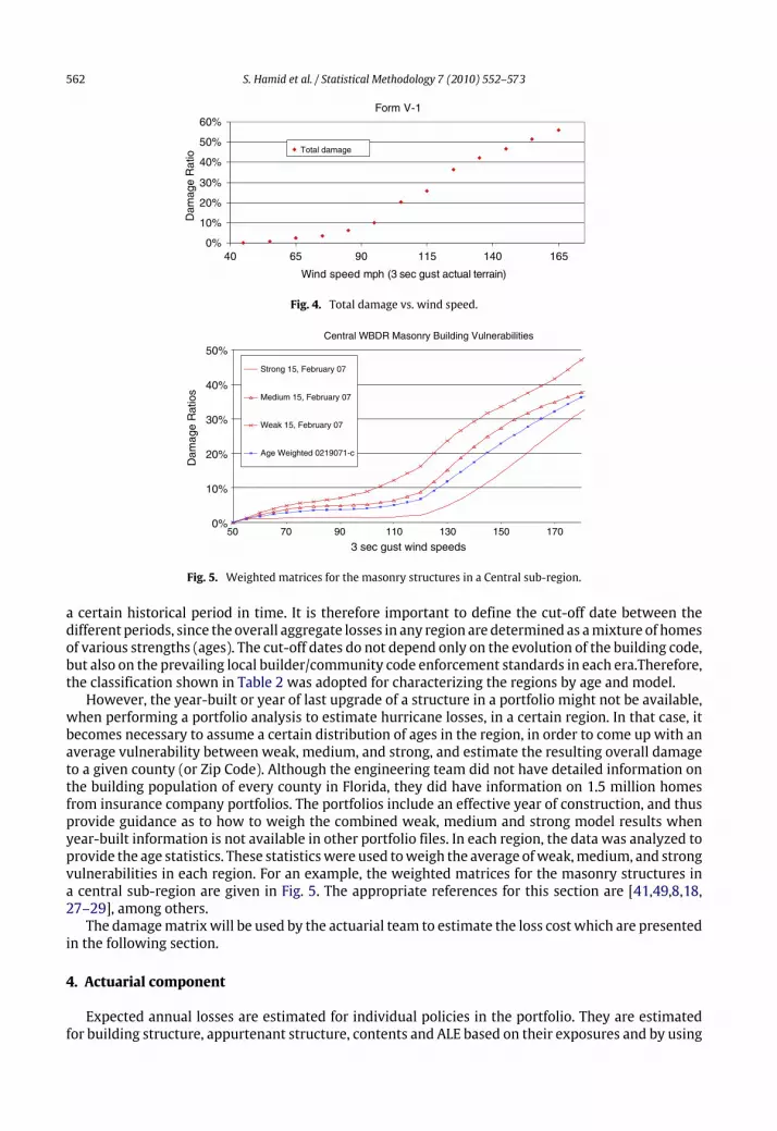
determines the appurtenant structure insured damage ratio as a function of wind speed (vulnerabilitycurve). One equation predicts damage for structures highly susceptible towind damage, the second formoderately susceptible, and the third for structures which are affected only slightly by wind. As withequations to predict interior damage, a Weibull distribution is applied to account for uncertainties. Inthis case, the β parameter of the Weibull distribution was reduced to 1, which yields an exponentialdistribution. The very limited insurance data available shows a high concentration of claims withzero appurtenant loss and a very large scatter of loss elsewhere. This is indicative of an exponentialdistribution, which supports the decision to reduce the β parameter. Because a typical insuranceportfolio file gives no indication of the type of appurtenant structure covered under a particular policy,a distribution of the three types (slightly vulnerable, moderately vulnerable, and highly vulnerable)must be assumed, and is validated against the claim data. Total damage vs wind speed is shown inFig. 4. It showed that as wind speed increases damage ratio is also increase.

3.3. Models distribution in time

Over time, engineers and builders learned more about the interaction between wind andstructures, more stringent building codes were enacted, and when properly enforced, resulted instronger structures. The weakmodel, medium strength model, and standard (strong) strength model,developedby the vulnerability team, represent this evolution in timeof relative quality of constructionin Florida. Each set of models is representative of the prevalent wind vulnerability of buildings for

562 S. Hamid et al. / Statistical Methodology 7 (2010) 552–573

Form V-1

0%

10%

20%

30%

40%

50%

60%

40 65 90 115 140 165

Wind speed mph (3 sec gust actual terrain)

Total damage

Dam

age

Rat

io

Fig. 4. Total damage vs. wind speed.

Central WBDR Masonry Building Vulnerabilities

50 70 90 110 130 150 170

3 sec gust wind speeds

Dam

age

Rat

ios

Strong 15, February 07

Medium 15, February 07

Weak 15, February 07

Age Weighted 0219071-c

0%

10%

20%

30%

40%

50%

Fig. 5. Weighted matrices for the masonry structures in a Central sub-region.

a certain historical period in time. It is therefore important to define the cut-off date between thedifferent periods, since the overall aggregate losses in any region are determined as amixture of homesof various strengths (ages). The cut-off dates do not depend only on the evolution of the building code,but also on the prevailing local builder/community code enforcement standards in each era.Therefore,the classification shown in Table 2 was adopted for characterizing the regions by age and model.However, the year-built or year of last upgrade of a structure in a portfolio might not be available,

when performing a portfolio analysis to estimate hurricane losses, in a certain region. In that case, itbecomes necessary to assume a certain distribution of ages in the region, in order to come up with anaverage vulnerability between weak, medium, and strong, and estimate the resulting overall damageto a given county (or Zip Code). Although the engineering team did not have detailed information onthe building population of every county in Florida, they did have information on 1.5 million homesfrom insurance company portfolios. The portfolios include an effective year of construction, and thusprovide guidance as to how to weigh the combined weak, medium and strong model results whenyear-built information is not available in other portfolio files. In each region, the data was analyzed toprovide the age statistics. These statisticswere used toweigh the average ofweak,medium, and strongvulnerabilities in each region. For an example, the weighted matrices for the masonry structures ina central sub-region are given in Fig. 5. The appropriate references for this section are [41,49,8,18,27–29], among others.The damagematrixwill be used by the actuarial team to estimate the loss cost which are presented

in the following section.

4. Actuarial component

Expected annual losses are estimated for individual policies in the portfolio. They are estimatedfor building structure, appurtenant structure, contents and ALE based on their exposures and by using

S. Hamid et al. / Statistical Methodology 7 (2010) 552–573 563

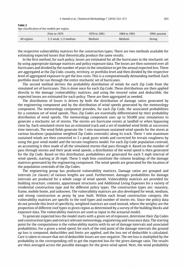
Table 2Age classification of the models per region.

Prior to 1970 1970 to 1983 1984 to 1993 1994–present

All regions 1/2 weak, 1/2 medium Medium Medium Strong

the respective vulnerability matrices for the construction types. There are two methods available forestimating expected losses that theoretically produce the same results.In the first method, for each policy, losses are estimated for all the hurricanes in the stochastic set

by using appropriate damage matrices and policy exposure data. The losses are then summed over allhurricanes and divided by the number of years in the simulation to get the annual expected loss. Theseare aggregated at the Zip Code, county, territory, or portfolio level and then divided by the respectivelevel of aggregated exposure to get the loss costs. This is a computationally demanding method. Eachportfolio must be run through the entire stochastic set of hurricanes.The second method derives the probability distribution of winds for each Zip Code from the

simulated set of hurricanes. This is done once for each Zip Code. These distributions are then applieddirectly to the damage (vulnerability) matrices, and using the insured value and deductible, theexpected losses are estimated for each policy. These are then aggregated as needed.The distribution of losses is driven by both the distribution of damage ratios generated by

the engineering component and by the distribution of wind speeds generated by the meteorologycomponent. The meteorology component provides, for each Zip Code, the associated probabilitiesfor a common set of wind speeds. Thus, Zip Codes are essentially differentiated by their probabilitydistribution of wind speeds. The meteorology component uses up to 50,000 year simulations togenerate a stochastic set of storms. The storms are hurricane events at landfall or when bypassingclose by. Each simulated storm has an estimated track and a set of modeled wind fields at successivetime intervals. The wind fields generate the 1 min maximum sustained wind speeds for the storm atvarious locations (population weighted Zip Codes centroids) along its track. These 1 min maximumsustained winds are then converted to 3 s peak gusts winds and corrected for terrain roughness byusing the gust wind model and the terrain roughness model. For each Zip Code population centroid,an accounting is then made of all the simulated storms that pass through it. Based on the number ofpass through storms and their peak wind speeds, a distribution of the wind speed is then generatedfor the Zip Code. Based on this distribution, probabilities are generated for each 5 mph interval ofwind speeds, starting at 20 mph. These 5 mph bins constitute the column headings of the damagematrices generated by the engineering component. The wind speeds are generated for the location ofthe population centroids of the Zip Codes.The engineering group has produced vulnerability matrices. Damage ratios are grouped and

intervals (or classes) of various lengths are used. Furthermore, damages probabilities for damageintervals are produced for a whole range of wind speeds. Vulnerability matrices are provided forbuilding structure, contents, appurtenant structures and Additional Living Expenses for a variety ofresidential construction type and for different policy types. The construction types are: masonry,frame, mobile home, and unknown. The vulnerability matrices are also developed for weak, medium,and strong construction as proxy by year built. Within each broad construction category, thevulnerability matrices are specific to the roof types and number of stories etc. Since the policy datado not provide this level of specificity, weighted matrices are used instead, where the weights are theproportion of different roof types in given region as determined by a survey of the building blocks andexposure data. The vulnerability matrices are used as input in the actuarial model.To generate expected loss the model starts with a given set of exposure, determine their Zip Codes

and construction types and extract relevantmeteorology, engineering and insurance data. The startingpoint for the computations is the vulnerability matrix with its set of damage intervals and associatedprobabilities. For a given a wind speed, for each of the mid point of the damage intervals the groundup loss is computed, deductibles and limits are applied, and the loss net of deductible is calculated.Care is taken to ensure that net of deductible losses are non-negative. The net loss is multiplied by theprobability in the corresponding cell to get the expected loss for the given damage ratio. The resultsare then averaged across the possible damages for the given wind speed. Next, the wind probability

564 S. Hamid et al. / Statistical Methodology 7 (2010) 552–573

weighted loss is calculated to produce the expected loss for the property. The expected losses arethen adjusted by the appropriate expected demand surge factor. The expected losses can be summedacross all structures of the type in the Zip Code and also across Zip Codes to get expected aggregateloss. For more on this component we refer [12,20] among others. All of the wind speed, damage, andlosses data were processed in the computer which is described in the following sections.

5. Computer system architecture

FPHLM is a large-scale system, which is designed to store, retrieve, and process huge amount ofhurricane historical data and the simulated data. In addition, intensive computations are supportedfor hurricane damage assessment and insured loss projection. In order to achieve system robustness,flexibility, and resistance to potential change, the three-tier architecture is adopted and deployedin our system. It aims to solve a number of recurring design and development problems, and hencemakes the application developmentwork easier andmore efficient. The computer systemarchitectureconsists of three layers, namely the user interface layer, application logic layer, and database layer.The interface layer offers the user a friendly and convenient user interface to communicate with

the system. It manages the input/output data and their display. To offer great convenience to theusers, the system is prototyped on theWeb so that the users can access the systemwith existing webbrowser software.The application logic layer handles the controlling functionalities and manipulates the underlying

logic connection of the information flows. This is themiddle tier in the computer system architecture.It aims to bridge the gap between the user interface and the underlying database and to hide thetechnical details from the users.The database layer is responsible for data modeling to store, index, manage, and model the

information for this application. Data needed by the application logic layer are retrieved from thedatabase, and the computation results produced by the application logic layer are stored back to thedatabase. Computer part consists of the following components:

5.1. Software, hardware, and program structure

The system is primarily a web-based application that is hosted in Oracle 9i web application server.The backend server environment is Linux and the server side scripts are written in Java Server Pages(JSP) and Java beans. Backend probabilistic calculations are coded in C++ using IMSL library and calledthrough Java Native Interface (JNI). The system uses an Oracle database runs on a Sun workstation.Server side software requirements are IMSL library CNL 5.0, OC4J v1.0.2.2.1, Oracle 9i AS 9.0.2.0.0A,JNI 1.3.1, and JDK 1.3.1.The end-user workstation requirements are minimal. Internet Explorer 5.5 or 6 running on

Windows 2000 or XP are the recommended web browsers. However, other web browsers such asMozilla Firefox should also deliver the optimal user experience. Typically, themanufacturer’sminimalfeature for a given web browser and operating system combination is sufficient for an optimaloperation of the application.

5.2. Translation from model structure to program structure

FPHLM uses a component-based approach in converting from model structure to programstructure. The model is divided into distinct components or modules, i.e., Storm Forecast Module,Wind Field Module, Damage Estimation Module, and Loss Estimation Module. Each of these modulesfulfills its individual functionality and communicates with other modules via well-defined interfaces.The architecture and program flowof eachmodule are defined in its corresponding use case documentfollowing software engineering specifications. Each model element is translated into subroutines,functions, or class methods on a one-to-one basis. Changes to the models are strictly reflected in thesoftware code. Flow diagram of the computer model is given in Fig. 7. Some references among othersare [5,4].

S. Hamid et al. / Statistical Methodology 7 (2010) 552–573 565

Fig. 6. Flow diagram of the computer model.

Number of Storms per Year

Fre

quen

cy

Florida Landfall Occurrence Rate

Fig. 7. Comparison of simulated vs. historical occurrences.

566 S. Hamid et al. / Statistical Methodology 7 (2010) 552–573

Occ

urre

nce

Distribution of the B parameter

B parameter

Fig. 8. Comparison between the modeled and observed Willoughby and Rahn [48] B data set.

6. Statistical validation

This section dealswith the validation of different components of themodel. The various parametersin the PHLM were modeled using either parametric or non parametric procedures. However, thevalidation results discussed here are only for the parametersmodeled through parametric procedures.

6.1. Modeled results and goodness of fit

6.1.1. Historical and modeled occurrencesThe model uses the National Hurricane Center HURDAT file from June 2006 for the period

1900–2005. Historical initial conditions are used to provide the seed for storm genesis in themodel. Small uniform random error terms are added to the historical starting positions, intensitiesand changes in storm motion. Subsequent storm motion and intensity is determined by randomlysampling empirical probability distribution functions derived from the HURDAT historical record.Fig. 7 shows the occurrence rate of both modeled (based on Poisson distribution which is discussed inSection 2.1) and historical landfalling storms in Florida. The figure shows a good agreement betweenhistorical andmodeled occurrences. A Chi square goodness of fit test gives a p-value of approximately0.24 which indicates a good fit.

6.1.2. Holland B parameterThe random error term for the Holland B is modeled using a Gaussian distribution with a standard

deviation of 0.286. Fig. 8 shows a comparison between the Willoughby and Rahn [48] B data set andthe modeled results (scaled to equal the 116 measured occurrences in the observed data set). Themodeled results with the error term have a mean of about 1.38 and are consistent with the observedresults. The figure indicates excellent agreement, and the Chi square goodness of fit gives a p-valueabout 0.89.

6.1.3. RmaxWe develop an Rmax model using the revised landfall Rmax database which includes 108

measurements for storms up to 2005. Since landfall Rmax is most relevant for loss cost estimation,and has a larger independent sample size, we have chosen to model the landfall data set. Since Rmaxdata are positively skewed, it makes more sense to model the distribution using either a lognormal orgamma distribution. The maximum likelihood estimates of the parameters for the lognormal fit werefound to be µ̂ = 3.15, and σ̂ 2 = 0.2327, while for the gamma distribution we obtained k̂ = 5.53547and θ̂ = 4.67749. Using these estimated values, the plots of the observed and expected distribution

S. Hamid et al. / Statistical Methodology 7 (2010) 552–573 567

5 10 15 20 25 30 35 40 45 50 550

2.5

5

7.5

10

12.5

15

17.5

20

22.5Lognormal vs Observed

Gamma vs Observed

Observed

Lognorm al

5 10 15 20 25 30 35 40 45 50 550

2.5

5

7.5

10

12.5

15

17.5

20

22.5

Observed

Gam m a

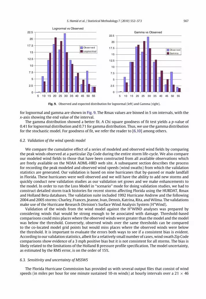
Fig. 9. Observed and expected distribution for lognormal (left) and Gamma (right).

for lognormal and gamma are shown in Fig. 9. The Rmax values are binned in 5 sm intervals, with thex-axis showing the end value of the interval.The gamma distribution showed a better fit. A Chi square goodness of fit test yields a p-value of

0.41 for lognormal distribution and 0.71 for gamma distribution. Thus, we use the gamma distributionfor the stochastic model. For goodness of fit, we refer the reader to [6,10] among others.

6.2. Validation of the wind speeds model

We compare the cumulative effect of a series of modeled and observed wind fields by comparingthe peak winds observed at a particular Zip Code during the entire storm life-cycle. We also compareour modeled wind fields to those that have been constructed from all available observations whichare freely available on the NOAA AOML-HRD web site. A subsequent section describes the processfor recording the peak modeled and observed wind speeds (wind swaths) from which the validationstatistics are generated. Our validation is based on nine hurricanes that by-passed or made landfallin Florida. These hurricanes were well observed and we will have the ability to add new storms andquickly conduct new validation studies as our validation set grows and we make enhancements tothe model. In order to run the Loss Model in ‘‘scenario’’ mode for doing validation studies, we had toconstruct detailed storm track histories for recent storms affecting Florida using the HURDAT, Rmaxand Holland Beta databases. The validation suite included 1992 Hurricane Andrew and the following2004 and2005 storms: Charley, Frances, Jeanne, Ivan, Dennis, Katrina, Rita, andWilma. The validationsmake use of the Hurricane Research Division’s Surface Wind Analysis System (H*Wind).Validation of the winds from the wind model against the H*WIND analyses was prepared by

considering winds that would be strong enough to be associated with damage. Threshold-basedcomparisons couldmiss places where the observedwindswere greater than themodel and themodelwas below the threshold. Conversely, observed winds over the same thresholds can be comparedto the co-located model grid points but would miss places where the observed winds were belowthe threshold. It is important to evaluate the errors both ways to see if a consistent bias is evident.According to our validation statistics, albeit for a relatively small number of cases,wind swath Zip Codecomparisons show evidence of a 3 mph positive bias but it is not consistent for all storms. The bias islikely related to the limitations of the Holland B pressure profile specification. Themodel uncertainty,as estimated by the RMS error, is on the order of 15%.

6.3. Sensitivity and uncertainty of MSSWS

The Florida Hurricane Commission has provided us with several output files that consist of windspeeds (in miles per hour for one minute sustained 10-m winds) at hourly intervals over a 21 × 46

568 S. Hamid et al. / Statistical Methodology 7 (2010) 552–573

Fig. 10. Stand regression coefficients vs. time at grid coordinates (30, 0) for category 3.

grid for the 500 combinations of initial conditions specified in the Excel file for the following modelinputs:

• CP= central pressure (in millibars)• Rmax= radius of maximum winds (in statute miles)• VT= translational velocity (forward speed in miles per hour)• Holland B pressure profile parameter.

The 21×46 grid of coordinates uses approximate 3 statute mile spacing and is depicted in Fig. 6 ofReport of Activities (ROA) [33] by Florida Hurricane Commission for all three hurricane categories. Forpurposes of hurricane decay, the modeler is instructed to use existing terrain consistent with thegrid in Fig. 6 of ROA [33] (page 146). The point (0, 0) is the location of the center of the hurricaneat time 0, and is 30 miles east of the landfall location (25.7739 N, 80.1300 W), identified by the redrectangle in Fig. 6 of ROA. The exact latitudes and longitudes for the 966 vertices in the grid (21× 46)are given in the seventhworksheet of the Excel input file. For details see ROA [33] available in thewebhttp://www.sbafla.com/methodology/.

6.3.1. Sensitivity analysis of MSSWSA linear regression model that regress maximum sustained surface wind speed (MSSWS) on

Rmax,VT, CP and Holland B(HB) could be fit for 966 grid points for each time point and for eachhurricane category. The model is defined as

Y = β0 + β1Rmax+ β2VT+ β3CP+ β4Holland B+ e,

where Rmax,VT,HBandCP are predictors or independent variables andβs are regression parameters.Given a fitted model, a researcher wants to compare the regression coefficients in terms of themagnitude of their effects. Themagnitude ofβs cannot be compared directly due to their different unitof measurements. Standardized regression coefficients (SRC) may be used to compare the importanceof different predictors/regressors. For sensitivity analyses, we refer [15] among others.For the sensitivity analysis, a graph of the standardized regression coefficients vs. time and for a

Category 3 hurricane is provided in Fig. 10. From this graph, we observed that themaximum sustainedsurface wind speed (MSSWS) is most sensitive to Rmax parameter followed by VT, Holland B and CP.At hour 0, MSSWS is the most sensitive to Rmax, where as at hour 12, MSSWS is the most sensitive toVT. We also noticed that the sensitivity of MSSWS depends on the time, grid points and the categoryof hurricanes.Modelwind speeds are very sensitive to Zip Code roughness,which in turn dependon landuse/land

cover determined from satellite remote sensing, and the assignment of roughness to mean landuse/land cover classifications as well as the upstream filtering or weighting factor applied to integratethe upstream roughness elements within a 45° sector to windward of the Zip Code. When Zip Codesare updated to reflect annual changes and population centroids are updated, the roughness tableis also updated. Zip Code location changes will generate different wind speeds. Experiments withdifferent land use land cover filtering factors suggest that extending the filtering further upstream

S. Hamid et al. / Statistical Methodology 7 (2010) 552–573 569

Fig. 11. Expected percentage reductions in the Var(MSSWS) for a category 3 hurricane vs. time at coordinate (30, 0).

has the effect of a small reduction in roughness at Florida Zip Codes (probably due to proximity to thecoast or smoother Everglades areas) with slightly higher wind speeds.

6.3.2. Uncertainty analysis of MSSWSThe goal of uncertainty analysis is to quantify the contributions of the input parameters to the

uncertainty in maximum sustained surface wind speed (MSSWS). The simple model isY = X1 + X2 + X3 + X4.

The variance of Y can be expressed as a conditional variance on X ’s. Here X ’s are Rmax, CP,VT and HBetc. Following [16], the expected percentage reduction (EPR) in V (Y ) is expressed as

EPR in Var(Y ) =Var(E(Y/X))Var(Y )

× 100.

The uncertainty analysis provides the information about the influence of the uncertainty of theregressors (Rmax, VT, Holland B and CP) in MSSWS over the time. For uncertainty analysis we refer[16] among others.Expected Percentage Reductions in the variance of Maximum Sustained Surface Wind Speed

(MSSWS) for Category 3 Hurricane versus Time at Coordinate (30, 0) are presented in Fig. 11. Themajor contribution to the uncertainty in the model is Rmax followed by VT, Holland B and CP. Athour 0, Rmax produces the most uncertainty and at hour 12VT contributed the highest uncertainty inthemodel. It is also noted that at hour 2 there is no uncertainty among the four parameters except VT.There is still considerable uncertainty in the assessment of hurricane intensity. Recent preliminary

research results based on SFMR measurements indicate that some Saffir–Simpson 1–3 Categoryhurricanes may be rated too high while the Category 4 and 5 storms are probably rated accurately.Uncertainty in Zip Code roughness has a significant impact on wind uncertainty. For a given Zip Code,changing the Zip Code roughness tables from 2004 to 2006 demonstrated some instances of largechanges in roughness for the same Zip Code for specific upstream flow directions. This is due to ashift in the Zip Code population-weighted centroid location, and a resulting incorporation of differentupstream land use/land cover elements.

6.3.3. Sensitivity for loss costFig. 12 shows the sample sensitivity analysis results for the loss cost for all input variables based

on a model that utilizes the Holland B parameter as the Quantile variable. It is observed from thisfigure is that the loss cost is sensitive to parameters Holland B, Rmax, VT and CP. The loss cost is leastsensitive to VT. Holland B has positive effect while CP has negative effect on the loss cost. Rmax hasboth positive and negative effects on loss cost depend on the category of hurricane.

6.3.4. Uncertainty analysis for loss costFig. 13 shows the sample uncertainty analysis results for the loss cost for all input variables based

on a model that utilizes the Holland B parameter as the quantile variable. From these graphs we

570 S. Hamid et al. / Statistical Methodology 7 (2010) 552–573

Fig. 12. Standardized regression coefficients for loss cost by hurricane category for each input variables for coordinate (30, 3).

Fig. 13. Expected percentage reduction for loss cost by hurricane category for each input variable at grid point (30, 3).

observed that the major contributions of uncertainty for loss cost are Rmax,VT and Holland B. Theuncertainty increases with the increase of the hurricane category. It appears that CP is the leastinfluential.

6.4. Model validation for loss cost

This section will discuss the validation of the loss cost model.

6.4.1. Number of simulation runsThe number of simulation runs was determined using the following process: The average loss

cost, X̄Y , and standard deviation sY , was determined for each county Y using an initial run of 10,600simulations. Then the maximum error of estimate will be 2.5% of the estimated mean loss cost, if thenumber of simulation runs for county Y is:

NY =(

s0.025× x̄

)2.

Based on the initial 10,700 years simulation runs the minimum number of years required is NY =35,080 for Lafayette County, which had the highest number of years required of all the counties.Therefore we have decided to use 53,500 (500 × 107) years of simulation for our final results. Fromthe 53,500 simulation runs we find that the standard errors are less than 2.5% for each county.

6.4.2. Validation based on the company dataFor model validation purposes, the actual and modeled losses for 39 different hurri-

canes/companies for residential coverage have been considered. The scatter plot of these data is pre-sented in Fig. 14. The correlation (measure of precision) between actual andmodeled losses is found tobe 0.988, which indicates a very strong positive correlation between actual andmodeled losses.When

S. Hamid et al. / Statistical Methodology 7 (2010) 552–573 571

Fig. 14. Scatter plot between total actual losses vs. total modeled losses.

we tested the difference in paired mean values equals zero, the paired t-test (t = 0.9882, df = 38,p-value= 0.3293) indicates that we fail to reject the null hypothesis based on this data, and concludethat there is insufficient evidence to suggest a difference between actual and modeled losses. Wealso observed that about 51% of the actual losses are more than the corresponding model losses and49% of the model losses are less than the corresponding actual losses. Following [24], the bias correc-tion factor (measure of accuracy) is obtained as 0.985 and the sample concordance correlation coeffi-cient is found to be 0.973 which showed a very good agreement between actual and model losses.

6.4.3. Statewide loss costs-historical versus modeledHere we consider the average annual zero deductible statewide historical versus modeled loss

costs. The loss costs are generated using a simulated body of hurricanes. The number of trials usedin the simulations is found to be 53,500. The standard errors are within less than 2.5% of the meansfor all counties. The average annual zero deductible statewide loss costs produced by the model onan average industry basis is $2.6 billion and the corresponding historical average loss is $2.8 billion.The 95% confidence interval on the difference between the mean of the historical and the mean ofthe modeled losses is between −1.240.97 and 0.911.20 billion dollars. Since the interval contains 0,we are 95% confident that there is no significant difference between the historical and the modeledlosses. Using Splus, we have also done statistical test of equalitymeans using a parametric test (t-test)(t = −0.3043, df = 53,605, p-value = 0.7609) (t = 0.2086, df = 50,105, p-value = 0.8348) andequality of CDFs using a nonparametric (KS) test (ks = 0.0629, p-value = 0.7887) (KS = 0.0638,p-value = 0.7734). In both parametric and non-parametric cases, we have high p-values. Therefore,we may conclude that the average historical and modeled losses are not statistically different.

7. Concluding remarks

A Monte Carlo simulation model has been developed to estimate the average annual loss fromhurricane wind damage to residential properties in the state of Florida. The model comprises of theatmospheric science, engineering, and financial/actuarial components. The atmospheric componentincludes modeling the track and intensity life cycle of each simulated hurricane within the Floridathreat area. Based on historical hurricane statistics, thousands of storms are simulated allowingdetermination of the wind risk for all residential Zip Code locations in Florida. The wind riskinformation is then provided to the engineering and actuarial components to assess damage andaverage annual loss, respectively. The actuarial team finds the loss cost for all counties and finally

572 S. Hamid et al. / Statistical Methodology 7 (2010) 552–573

for the state of Florida. The model incorporates the results of many recent research advances whilekeeping it basic enough to run in a reasonable amount of time. It is expected that the model wouldbe run once per year to take advantage of the latest historical data to assess annual wind exceedanceprobabilities at each Zip Code in Florida. Such information can then be provided to the engineering andactuarial components of the model to assess average annual loss for any given residential propertyexposure portfolio. The model will reside at the Florida International University’s InternationalHurricane Research Center in Miami, USA. The model has satisfied all the standards stated in ROA[34] and has been approved by the Florida Commission for Hurricane Loss Projection Methodology tobe used in rate filings or by insurance companies as they see fit. Themodel is open in the sense that allresults are accessible to the public and the methodology is completely documented and available forexamination. It is noted that the model has been used successfully by several companies in the stateof Florida. We expect that the model will be useful for other states as well all other countries in theworld. The full model is available at http://www.cis.fiu.edu/hurricaneloss/html/research001.html.

Acknowledgements

This research is supported by the State of Florida through a Department of Financial Services grantto the Florida International University International Hurricane Research Center. We are thankful to agroup of Graduate Students for their hard work throughout the development of the model. Withouttheir help it would have been impossible to complete this task. We would also like to express ourthanks to the International Hurricane Research Center for providing us the use of their facilities.Finally, the authors are grateful to the referees and the associate editor for their valuable comments

and suggestions which improved this paper greatly.

References

[1] L.M. Axe, Hurricane surface wind model for risk assessment, M.S. Thesis, Department of Meteorology, Florida StateUniversity, 2003.

[2] M.E. Batts, M.R. Cordes, L.R. Russell, E. Simiu, Hurricane wind speeds in the United States, National Bureau of Standards,Report no BSS-124, US Department of Commerce, 1980.

[3] E. Casson, S. Coles, Simulation and extremal analysis of hurricane events, Appl. Statist. 49 (Part 2) (2000) 227–245.[4] K. Chatterjee, K. Saleem, N. Zhao, M. Chen, S.-C. Chen, S. Hamid, Modeling methodology for component reuse andsystem integration for hurricane loss projection application, in: Proceedings of the 2006 IEEE International Conferenceon Information Reuse and Integration, IEEE IRI-2006, Hawaii, USA, September 16–18, 2006, pp. 57–62.

[5] S.-C. Chen, S. Gulati, S. Hamid, X. Huang, L. Luo, N. Morisseau-Leroy, M.D. Powell, C. Zhanl, C. Zhang, A web-baseddistributed system for hurricane occurrence projection, Softw. Pract. Exp. 34 (2004) 1–23.

[6] R.B. D’Agostino, M.A. Stephens, Goodness-of-Fit Techniques, Marcel Dekker, New York, 1986.[7] R.W.R. Darling, Estimating probabilities of hurricane wind speeds using a large scale empirical model, J. Clim. 4 (1991)1035–1046.

[8] R.A. Davidson, H. Zhao, V. Kumer, Quantitative model to forecast changes in hurricane vulnerability of regional buildinginventory, J. Infrastruct. Syst. (2003) 58–64.

[9] L. Fawcett, D. Walshaw, A hierarchical model for extreme wind speeds, Appl. Statist. 55 (Part 5) (2006) 631–646.[10] J.D. Hart, Nonparametric Smoothing and Lack-of-Fit Tests, Springer, New York, 1997.[11] F.P. Ho, J.C. Su, K.L. Hanevich, R.J. Smith, F.P. Richards, Hurricane climatology for the Atlantic and Gulf coasts of the United

States, NOAA Technical Memo NWS 38, NWS Silver Spring, MD, 1987.[12] R. Hogg, S. Klugman, Loss Distributions, Wiley, New York, 1984.[13] G.J. Holland, An analyticmodel of thewind and pressure profiles in hurricanes, Mon.Weather Rev. 108 (1980) 1212–1218.[14] C. Homer, C. Huang, L. Yang, B. Wylie, M. Coan, Development of a 2001 National landcover database for the United States,

Photogramm. Eng. Remote Sens. 70 (7) (2004) 829–840.[15] R.L. Iman, M.E. Johnson, T. Schroeder, Assessing hurricane effects. Part 1. Sensitivity analysis, Reliab. Eng. Syst. Saf. 78

(2002) 131–145.[16] R.L. Iman, M.E. Johnson, T. Schroeder, Assessing hurricane effects. Part 2. Uncertainty analysis, Reliab. Eng. Syst. Saf. 78

(2002) 147–155.[17] .B.R. Jarvinen, C.J. Neumann, M.A.S. Davis, A tropical cyclone data tape for the North Atlantic basin 1886–1963: contents

limitations and uses, NOAA Technical Memo NWS NHC 22, National Hurricane Center, 1984, 22 pp.[18] A.C. Kanduri, G.C. Morrow, Vulnerability of buildings to windstorms and insurance loss estimation, J. Wind Eng. Ind.

Aerodyn. 91 (2003) 455–467.[19] J. Kaplan, M. DeMaria, A simple empirical model for predicting the decay of tropical cyclone winds after landfall, J. Appl.

Meteorol. 34 (1995).[20] S.A. Klugman, H.H. Panjer, G.E. Willmot, Loss Models: From Data to Decisions, John Wiley and Sons, New York, 1998.[21] Y.M. Kurihara, M.A. Bender, R.E. Tuleya, R.J. Ross, Improvements in the GFDL hurricane prediction system, Mon. Weather

Rev. 123 (1995) 2791–2801.

S. Hamid et al. / Statistical Methodology 7 (2010) 552–573 573

[22] C.W. Landsea, R.A. Pielke Jr., A.M. Mestas-Nunez, J.A. Knaff, Atlantic basin hurricanes: indices of climatic changes, Clim.Change 42 (1999) 89–129.

[23] W.G. Large, S. Pond, Open oceanmomentum fluxmeasurements inmoderate to strongwinds, J. Phys. Oceanogr. 11 (1981)324–336.

[24] L.I. Lin, A concordance correlation coefficient to evaluate reproducibility, Biometrics 45 (1989) 255–268.[25] .C.J. Neumann, B.R. Jarvinen, C.J. McAdie, G.R. Hammer, Tropical cyclones of the North Atlantic Ocean, 1871–1998,

in: National Oceanic and Atmospheric Administration, 1999, 206 pp.[26] K.V. Ooyama, Numerical simulation of the life cycle of tropical cyclones, J. Atmos. Sci. 26 (1969) 3–40.[27] J.-P. Pinelli, E. Simiu, K. Gurley, C. Subramanian, L. Zhang, A. Cope, J. Filliben, S. Hamid, Hurricane damage predictionmodel

for residential structures, J. Struct. Eng. ASCE 130 (11) (2004) 1685–1691.[28] Jean-Paul Pinelli, Chelakara Subramanian, KurtGurley, ShahidHamid, SnehGulati, Florida hurricane loss predictionmodel:

implementation and validation, in: Proceedings, 10th Americas Conference onWind Engineering, Baton Rouge, Louisiana,May 31–June 4, 2005.

[29] Jean-Paul Pinelli, Chelakara Subramanian, JoshMurphree, Kurt Gurley, Anne Cope, Simiu Gulati, Sneh Emil, Shahid Hamid,Hurricane loss prediction: model development, results, and validation, in: Proceedings, ICOSSAR 2005, Rome, Italy, June19–23, 2005.

[30] M.D. Powell, S.H. Houston, T. Reinhold, Hurricane Andrew’s landfall in South Florida. Part I: standardizing measurementsfor documentation of surface wind fields, Weather Forecast. 11 (1996) 304–328.

[31] M.D. Powell, G. Soukup, S. Cocke, S. Gulati, N. Morisseau-Leroy, S. Hamid, N. Dorst, L. Axe, State of Florida hurricane lossprojection model: atmospheric science component, J. Wind Eng. Ind. Aerodyn. 93 (2005) 651–674.

[32] M.D. Powell, P.J. Vickery, T.A. Reinhold, Reduced drag coefficient for high wind speeds in tropical cyclones, Nature 422(2003) 279–283.

[33] Report of activities as of November 1, 2006, Florida Commission on Hurricane Loss Projection Methodology. Availablefrom: www.fsba.state.fl.us/methodology/meetings.asp.

[34] Report of activities as of November 1, 2007, Florida Commission on Hurricane Loss Projection Methodology. Availablefrom: www.fsba.state.fl.us/methodology/meetings.asp.

[35] L.R. Russell, Probability distributions for hurricane effects, J. Waterw. Harbor Coast. Eng. Div. ASCE 97 (1971) 139–154.[36] H.P. Schmidt, T.R. Oke, A model to estimate the source area contributing to turbulent exchange in the surface layer over

patchy terrain, Q. J. R. Meteorol. Soc. 116 (1990) 965–988.[37] L. Shapiro, The asymmetric boundary layer flow under a translating hurricane, J. Atmos. Sci. 40 (1983) 1984–1998.[38] E. Simiu, R.H. Scanlan, Wind Effects on Structures: Fundamentals and Applications to Design, Wiley, New York, 1996.[39] R.H. Simpson, R. Anthes, M. Garstang (Eds.), Hurricane! Coping with Disaster, American Geophysical Union, Washington

DC, 2003.[40] E. Smith, Atlantic and east coast hurricanes 1900–1998: a frequency and intensity study for the twenty-first century, Bull.

Am. Meteorol. Soc. 18 (12) (1999) 2717–2720.[41] P.R. Sparks, S.D. Schiff, T.A. Reinhold, Wind damage to envelopes of houses and consequent insurance losses, J. Wind Eng.

Ind. Aerodyn. 53 (1994) 145–155.[42] E.F. Thompson, V.J. Cardone, Practical modeling of hurricane surface wind fields, J. Waterw. Port Coastal Ocean Eng. Div.

ASCE 122 (1996) 195–205.[43] P.J. Vickery, P.F. Skerlj, Hurricane gust factors revisited, J. Struct. Eng. 131 (2005) 825–832.[44] P.J. Vickery, P.F. Skerjl, A.C. Steckley, L.A. Twisdale, A hurricane wind field model for use in simulations, J. Struct. Eng. 126

(2000) 1203–1222.[45] P.J. Vickery, P.F. Skerjl, L.A. Twisdale, Simulation of hurricane risk in the United States using an empirical storm track

modeling technique, J. Struct. Eng. 126 (2000) 1222–1237.[46] P.J. Vickery, L.A. Twisdale, Wind field and filling models for hurricane wind speed predictions, Struct. Eng. 121 (1995)

1700–1709.[47] D. Walshaw, C.W. Anderson, A model for extreme wind gusts, Appl. Statist. 49 (Part 4) (2000) 499–508.[48] H.E.Willoughby,M.E. Rahn, Parametric representation of the primary hurricane vortex part I: observations and evaluation

of the Holland (1980) model, Mon. Weather Rev. 132 (2004) 3033–3048.[49] H. Zhigand, D.V. Rosowsky, P.R. Sparks, Long-term hurricane risk assessment and expected damage to residential

structures, Reliab. Eng. Syst. Saf. 74 (2001) 239–249.