Quarterly Journal of the Royal Meteorological Society Q. J. R. Meteorol. Soc. 136: 400–413, January 2010 Part B

Predictability of extreme meteo-oceanographic eventsin the Adriatic Sea

L. Cavaleri,a* L. Bertotti,a R. Buizza,b A. Buzzi,c V. Masato,a G. Umgiessera and M. ZampiericaISMAR-CNR, Venice, Italy

bECMWF, Reading, Berkshire, UKcISAC-CNR, Bologna, Italy

*Correspondence to: L. Cavaleri, ISMAR-CNR, Castello 1364, 30122 Venice, Italy.E-mail: luigi.cavaleri@ismar.cnr.it

The performance of state-of-the-art meteorological and oceanographic numericalsystems in predicting the sea state in the Adriatic Sea during intense storms isassessed. Two major storms that affected Venice are discussed. The first stormoccurred on 4 November 1966, when Venice suffered its most dramatic floodevent. The damage and loss of life caused by the storm and the associated floodwere extremely high also because the event was poorly forecast. The 1966 eventis reanalysed using state-of-the-art meteorological and oceanographic numericalsystems to investigate whether the poor forecast quality was due to a lack of dataor of suitable numerical modelling. The second severe storm took place on 22December 1979, when Venice experienced the second-worst ‘acqua-alta’ conditionsin recorded history. Results show that with the present numerical systems bothstorms and associated wave and surge conditions could have been forecast severaldays in advance. Potential implications for the prediction of more frequent lessintense storms are discussed, and a suitably enhanced system based on a globalmeteorological model and a limited area one is outlined. Copyright c© 2010 RoyalMeteorological Society

Key Words: wind waves; surge; historical storms; meteorological modelling; downscaling

Received 22 October 2008; Revised 1 October 2009; Accepted 27 November 2009; Published online in WileyInterScience 1 February 2010

Citation: Cavaleri L, Bertotti L, Buizza R, Buzzi A, Masato V, Umgiesser G, Zampieri M. 2010. Predictabilityof extreme meteo-oceanographic events in the Adriatic Sea. Q. J. R. Meteorol. Soc. 136: 400–413.DOI:10.1002/qj.567

1. Introduction: The historical storms

On 4 November 1966 an exceptional storm hit thecentral and north-eastern part of Italy with very intenseprecipitation over large areas and strong winds over theAdriatic Sea, east of the Italian peninsula (see Figure 1 for ananalysis of that time of the weather situation at the surface).The storm caused the flood of two of the greatest historicaltowns of Italy, Florence and Venice, inflicted severe damageto the economic and artistic patrimony of these and othertowns and villages in central and north-eastern Italy, andclaimed the lives of more than 100 people. Because of this,and since at that time the quality of a weather forecastwas very limited, the storm has been extensively studied

afterwards. The interested reader is referred to, amongothers, Fea et al. (1968), Warner and Hsu (2000), Bertoet al. (2005), De Zolt et al. (2006) and Malguzzi et al. (2006).

Most of the past studies have focused on themeteorological and hydrological components of this storm,often dealing specifically with the estimate and distributionof the amount of rain and the consequent flood of Florenceby the Arno River and with the widespread floods andlandslides in the eastern Alps (see, for example, the recentpaper by Malguzzi et al. (2006)). In the present paper wefocus on the oceanographic aspect of the storm, hence onthe flood of Venice due to the exceptional surge of theAdriatic Sea. More specifically, our aim is to analyse thepredictability not only of the atmospheric, but also of the

Copyright c© 2010 Royal Meteorological Society

Predictability of Extreme Events in the Adriatic 401

Figure 1. Weather map re-elaborated from hand-drawn analysis published in Fea et al. (1968). The basic meteorological fields refer to 4 November 1966,0000 UTC. Continuous black lines: mean-sea-level pressure −1000 hPa (contour interval 2 hPa). Coloured thin lines: pressure tendency in 6 hours (blue:positive; red: negative; contour interval hPa/6h). Wind barbs in knots. Low pressure centres: B; high pressure: A. The green spots reproduce reflectivitymaxima of the meteorological radar in Rome Fiumicino at 0040 UTC, same day. The thick line indicates the position of the cold front at 1200 UTC of thesame day (after Malguzzi et al., 2006). The highlighted coastline borders the Adriatic Sea. The red circle shows the position of the oceanographic tower(see Figure 5), 15 km off the coast of Venice.

marine conditions on the Adriatic Sea associated with thisstorm. As mentioned above, at the time of the storm therewas practically no anticipation of what was about to come.At that time there was no operational numerical modellingguide available to the forecasters, so forecasts were basedessentially on the synoptic interpretation of the availablecharts, guided by personal training and experience. In thecase of the 1966 storm, unfortunately, this experience wasnot enough to help forecasters to issue a skilful forecast afew days before the storm, mainly because of the exceptionalnature, and rarity, of the event.

One of the questions that we will be addressing is whetherthe atmospheric data available prior to the storm (which didnot include all the satellite data that are presently available,which nowadays constitute more than 90% of the data usedto estimate the current state of the atmosphere) would havebeen sufficient to issue an alert if the analysis and modellingtools of today had been available. Could these two events bepredicted a few days in advance? More precisely, how longin advance could the sea conditions have been predicted?This is explored using two sources of meteorological data:a global model and a limited area one, both using the samebackground data. This will allow, if not firm conclusions,some discussion on the possible advantages of the twoapproaches.

The same methodology has been applied to a second, stillexceptional, storm that affected the western Mediterranean

13 years later, on 22 December 1979. Although this stormdid not reach the severity level of the 1966 one, it led tothe second-ranked record sea level in Venice. Although werecognize that it is difficult to generalize conclusions drawnfrom the analysis of two storms, we think that this studycan give some useful indications of general validity, and canguide the development of future alert systems.

We begin our paper with a description, in section 2, ofthe key morphological characteristics of the area affectedby the event, and, in section 3, of the atmospheric and seaconditions during the two storms. In section 4 we presentin detail the methodology we have followed and the datawe have used. The two following sections, 5 and 6, aredevoted to the presentation of the results of the numericalsimulations of the two storms. We discuss our findings anddraw our conclusions in the final section 7.

2. Morphological and physical characteristics of the areaof interest

The Adriatic Sea (Figure 1) is an elongated basin to theeast of Italy, enclosed between the Italian peninsula and theBalkans. It is about 750 km long, 200 km wide, aligned inthe north-west to south-east direction. At its southern endit is connected with the Mediterranean Sea via the narrowStrait of Otranto. The sea is shallow in its northern part, thebottom sloping down from the northern coast at a gradient

Copyright c© 2010 Royal Meteorological Society Q. J. R. Meteorol. Soc. 136: 400–413 (2010)

402 L. Cavaleri et al.

(a) (b)

Figure 2. ERA-40 maps of (left) geopotential heights at 500 hPa (contour interval 40 m) and (right) of mean-sea-level pressure (contour interval 4 hPa)at 1200 UTC 4 November 1966. This figure is available in colour online at www.interscience.wiley.com/journal/qj

of 1 in 1000. Beyond the 200-metre isobath the bottomdeepens suddenly, remaining so until Otranto except for thenarrow strip of shallow water along the Italian peninsula.

The bordering orography affects the local wind patternssubstantially. The whole eastern border is characterisedby the long ridge of the Dinaric Alps. Along the Italiancoast the sea is bordered by the Apennines mountain rangefor most of its length. This orographic configuration hasa strong influence on the low-level winds that affect theAdriatic Sea, in particular on the sirocco, a south-easterlywind often blowing along the whole length of the basin.Sirocco conditions often cause flooding of the coastal areasfacing the northern parts of the Adriatic Sea, e.g. theVenice lagoon. This was actually the case in November1966 (Figure 1), when the flow at the surface was channelledby the bordering orography along the longitudinal axis ofthe basin. The reader is referred to Pirazzoli and Tomasin(2003) for a more detailed description of the main types offlow conditions that affect the Adriatic area.

For the following discussion it is important to note that,at a given position and for a given wind stress, when theocean is in dynamical equilibrium, then the surface spatialgradient of the sea elevation associated with a surge tendsto increase inversely to the local depth (see Pugh (1987)for an analysis of the dynamics of a surge, and Tomasin(2005) for a description of its local characteristics). The seabecomes shallower while moving northwards towards theVenetian coast. Therefore, when the sirocco reaches thesemost northerly positions, we expect to find here the steepestgradients of the sea elevation and therefore an enhancedpeak of the surge towards the coast.

Once the storm is over and if, as expected, the basin isout of balance, a sequence of oscillations (seiche) of thewhole basin is initiated with two dominant periods, 11 and22 hours, the latter being the stronger one (Tomasin, 2005).Their amphidromic (pivotal) points are respectively in themiddle and at the lower end of the Adriatic Sea. The largestoscillations are found in its northern part, adding to theVenice tide.

3. The two flood events in Venice of 1966 and 1979

3.1. The flood of 4 November 1966

Between 1 and 2 November, a deep tropospheric troughpositioned over Spain started intensifying and rotatinganticlockwise. By 3 November, the trough deepened veryrapidly over Spain, and strong south-easterly and thensoutherly winds started affecting the mid-troposphere overthe Italian peninsula. At the surface on 3 Novembercyclogenesis started over Spain. The surface cyclone movedover the western Mediterranean and was reinforced bya secondary, small-scale depression coming from NorthAfrica. At the same time, an anticyclone over the Balkansintensified in place. The result was a strong southerly flowover the Adriatic (Figure 2, left panel) that at the surface(right panel), channelled by the bordering orography, led toa strong sirocco wind over the whole basin.

As noted in Malguzzi et al. (2006), although the low-pressure centre located over northern Italy was not verydeep (see right panel), the west-to-east pressure gradient,and hence the south-easterly wind over the Adriatic Sea,was very strong. On 4 November (Figure 1), the wind wasfurther intensified by the advancing cold front from thewest, assuming the character of a pre-frontal low-level jet.As will be discussed again later, the correct positioning andtiming of this cold front played a crucial role in the accuracyof the forecasts.

No report of the surface wind speed over the sea isavailable, but an unofficial anemometer located at the edgeof the Venetian lagoon, very close to the sea coastline,reported sustained winds close to or above 20 m/s from0800 until 1600 UTC 4 November. As might be expected, nowave measurements were available, but the storm destroyedthe final 100–200 metres of the jetties bordering the threeinlets connecting the Venice lagoon to the sea. Some of thesejetties housed open-sea tide gauges that were obviouslywiped out. Tide records exist from the Venice area, insidethe lagoon. However, based on previous experience, thesetide gauges had been designed for a maximum level of

Copyright c© 2010 Royal Meteorological Society Q. J. R. Meteorol. Soc. 136: 400–413 (2010)

Predictability of Extreme Events in the Adriatic 403

Figure 3. Time history of the flood of 4 November 1966 in Venice. Ordinate scale in m. Dashed line: meteorological tide; solid line: record; dotted line:astronomical tide. The vertical and horizontal lines, plus the arrow, point out the time of the peak and the corresponding astronomical tide level. Thisfigure is available in colour online at www.interscience.wiley.com/journal/qj

1.80 m above the nominal sea level†. The maximum sealevel reached during this storm was estimated at +1.94 mfrom the marks left on the walls by the oil exiting fromthe flooded tanks and floating on top of the water. Theofficially accepted time history of the flood is given by thesolid line in Figure 3, showing also (a full description willbe given in section 5) the astronomical tide and the isolated,by difference, meteorological contribution. It is worthwhileto remember that the part of the diagram above 1.80 mwas guessed and traced by hand later on. Note also that thewater in the lagoon was oscillating wildly, reaching differentlevels at different times and positions. Hence also the 1.94 mfigure must be considered accurate only to within a fewcentimetres.

Compared to the statistics derived from previous data,recorded since 1872, the 1966 event stands out dramatically,and it was variously judged (Cecconi et al., 1999) to havea return period of 150–300 years. It is interesting to notethat two comparable, but not properly quantified, eventsreported in historical documents happened in 1822 and1867, when no instrumental measurements were taken(Camuffo, 1993). It seems likely that the latter event triggeredthe start of official measurements.

Another remarkable detail that highlights even furtherthe exceptional character of the 1966 storm is that the floodwas entirely due to the storm surge, with actually a negativecontribution (-11 cm with respect to the present meansea level) coming from the astronomical tide. In order tointerpret Figure 3 correctly in this respect it is necessary toconsider (see footnote) that the actual mean sea level in 1966

†In Venice all the tidal data are referred to an official referencecorresponding to the mean sea level (msl) present in the town in 1896(according to the local tide measurements). Both because of absolutesea level rise and of Venice sinking (the latter a process now halted), theactual msl had risen in 1966 by about 23 cm. So the nominal 194 cm surgecorresponds, with respect to the present msl, to an actual elevation ofabout 171 cm. Of course for the daily life in Venice 194 cm is the measureof interest, which is the reason for still using this official reference.

Figure 4. Synoptic situation, according to the T511 ECMWF analysis,over Europe at 1200 UTC 22 December 1979. Mean-sea-level pressure(contour interval 4 hPa). This figure is available in colour online atwww.interscience.wiley.com/journal/qj

was 23 cm higher than the nominal value, established backin 1896 and still in use today.

3.2. The flood of 22 December 1979

The basic meteorological situation of the 1979 storm (seeFigure 4) was similar to the 1966 one, although withoutthe same dramatically strong pressure gradients over theAdriatic area. A deep low-pressure minimum was locatedwest of Italy, over the Tyrrhenian Sea, and contrasted withan anticyclone over eastern Europe. Sustained sirocco windsdeveloped all along the Adriatic Sea. Due to the reinforcedouter ends of the jetty and to the fact that the storm was lessextreme than in 1966, in this case no damage was inflicted tothe jetties. However, the storm was strong enough to cause

Copyright c© 2010 Royal Meteorological Society Q. J. R. Meteorol. Soc. 136: 400–413 (2010)

404 L. Cavaleri et al.

Figure 5. Left panel: the oceanographic tower of ISMAR located 15 km offshore the Venetian littoral (see Figure 1). Right panel: the tower after the stormof 22 November 1979. The second floor, corresponding to the right extending platform, is shown.

severe damage to the superstructures of the oceanographictower (see Figure 5) located in the northern Adriatic Sea,15 km offshore the Venetian coast in a 16-metre depth.The tower was, and is, manned by ISMAR, the Instituteof Marine Sciences established in Venice by the ItalianNational Research Council after the 1966 storm. Becauseof the consequent lack of power, no measured wave data isavailable. The only oceanographic instrument that survived,barely but sufficiently, the storm and provided useful datawas a mechanical tide gauge with its recording unit locatedon the second floor of the tower, the one shown in the rightpanel of Figure 5. Its location just behind one of the towerlegs shielded it from the highly directional sea. Togetherwith the contemporary sea-level data from the tide gaugesat the jetty ends, the tower data provided evidence of asustained wave set-up at the coast reaching more than 40 cm.(Wave set-up is the increase of sea level in the shore areadue to the horizontal flux of momentum associated withwind waves and their breaking when moving into shallowareas; see Longuet-Higgins and Stewart (1964) and Bowenet al. (1968) for a complete description of the process.)Bertotti and Cavaleri (1985) provide a full discussion ofthe case. Given that the outer end of the jetty, where thereference coastal tide gauge is located, protrudes more than2 km into the sea and the water depth at its end is more than6 metres, a much higher set-up was present at the coast.

Notwithstanding the lack of recorded data, a conservativeestimate of the maximum wave height at the tower can bederived from the fact that the tower suffered substantialdamage up to about 9 m above the mean sea level.Taking tide into consideration together with the nonlinearcharacter of these extreme waves leads to an estimatedmaximum height of the order of 12 m, practically in orclose to breaking conditions. Bertotti and Cavaleri (1985)provide a full description of the storm and related set-up.

4. Methodology

4.1. The meteorological simulation models

All meteorological simulations have been started from ERA-40 data (ERA is the European Centre for Medium-Range

Weather Forecasts Re-Analysis, see Uppala et al. (2005)),or have been produced using the tools developed by theECMWF ERA group. Aiming at a better resolution thanthe related T159 truncation level corresponding to about125 km resolution, we have repeated the analysis withT511, corresponding to about 40 km resolution. We haveused the 31R1 version of the ECMWF meteorologicalmodel, operational at the time when we carried out ourexperiments. For both the considered storms, a sequenceof analyses was done at 12-hour intervals, beginning tendays before the date of the storm peak. Starting fromeach analysis, we have generated a series of ten-dayforecasts, still with T511, saving the model output fieldsat 3-hour intervals. Including the initial analysis fields,these forecast fields constitute the initial and boundaryconditions for the limited-area forecasts made with theBologna Limited Area Model (BOLAM, see below) andprovide the meteorological forcing to drive the surge andwave oceanographic models.

There is a difference between the simulations with thesurge and the wave models. As seen in Figure 1, the narrowconnection to the Mediterranean Sea at the southern endof the Adriatic basin ensures that the wave conditions,particularly in its northern part, depend almost entirelyon the waves generated within the basin. Hence for ourpresent purposes the memory of the system is relativelyshort. This is not the case with the surge conditions. Thesea level at the Strait of Otranto affects the whole AdriaticSea, and thus it is necessary to model the circulation in thewhole Mediterranean Sea to have a proper storm surgesimulation. The related response time and memory ofthe system being much longer than in the wave case, westarted the surge simulation one month in advance. Thisrequired a month of meteorological data that, for the timeintervals preceding the already considered ten-day forecastsat T511 resolution, was derived directly from the ERA-40analysis.

The accuracy of the surface wind fields thus obtainedwas not good enough for the wave and surge modelling,both being very sensitive to small errors of the drivingwind fields. Indeed (Cavaleri and Bertotti, 1997, 2006) adirect application of the ECMWF winds in the Adriaticleads to significant wave heights too low by several tens

Copyright c© 2010 Royal Meteorological Society Q. J. R. Meteorol. Soc. 136: 400–413 (2010)

Predictability of Extreme Events in the Adriatic 405

of percent. This problem was addressed in two differentways. On the one hand, following Cavaleri and Bertotti(1997, 2006), we have enhanced the ECMWF 10 m windspeed over the Adriatic by a constant coefficient. The windspeed over the Mediterranean has been enhanced accordingto the calibrations derived within the project MEDATLAS(Cavaleri and Sclavo, 2006). On the other hand, we havemade use of a higher-resolution meteorological modelnested into the ECMWF one. It is essential to stress thatthe first approach has not been done ad hoc for these tests,but is a well established and quantified procedure derivedfrom long-term tests, regularly applied in the wave (Bertottiand Cavaleri, 2009) and surge (Canestrelli and Zampato,2005) operational forecast systems in the Adriatic Sea. Thecorrection coefficient in the Adriatic, suitable for siroccostorms, depends on the resolution of the meteorologicalmodel. It was derived by extensive comparisons of boththe wind and associated wave fields against scatterometer,altimeter and buoy data. While we can expect the correctioncoefficient to vary in space and with the kind of storm, forthe oceanographic conditions in the northern part of thebasin and sirocco storms, a single coefficient turned out tobe a realistic and satisfactory solution. The value 1.35, theone pre-evaluated for the T511 resolution, was used for thepresent tests.

As mentioned above, the other approach to cope withthe problems related to the relatively low resolution ofthe global meteorological model is to use a nested higher-resolution one (Jung et al., 2006; Rotach et al., 2009).This was done using a two-step high-resolution limited-areamodel based on the BOLAM model developed at the Instituteof Atmospheric Sciences and Climate (ISAC) (Buzzi et al.,1994; Malguzzi and Tartaglione, 1999; Zampieri et al., 2005),run with a 0.18 degree resolution grid (father), covering thearea from Portugal to Greece, and a nested grid at 0.06degree (son), centred over the Adriatic Sea. All the BOLAMruns, done in forecast mode (i.e. using the forecasts aslateral boundary conditions), extended till 1200 UTC of 5November 1966 and 23 December 1979, respectively, witha maximum range of 72 hours. The initial and boundaryconditions of the father were provided by the ECMWF T511analyses and forecasts discussed above. Such forecasts wereused also for the surge runs to fill the surface wind fieldsfrom Greece up to the eastern border of the basin. For theforecasts starting before 1200 UTC of 2 November 1966 and20 December 1979, the BOLAM runs were started in any caseat these times, using as initial conditions the correspondingECMWF T511 forecasts. It is important to stress, also for thesubsequent evaluations, that, at variance with the ECMWFfields, no correction was imposed or attempted on theBOLAM wind fields. In this respect our aim was to verify ifthe quality of the results obtained with the higher resolutionof the BOLAM inner grid would have been good enough toovercome the problems associated with the use of a globalmodel in an enclosed basin.

4.2. The oceanographic simulation models

The general circulation and sea-level distribution over thewhole Mediterranean Sea, and in particular the surgein the Adriatic Sea, were estimated using SHYFEM, athree-dimensional (3D) finite elements model developedat ISMAR and used here in its 2D version. SHYFEM isa shallow-water, hydrostatic, primitive equation model. It

runs on an unstructured grid that in the present case becomesprogressively denser entering the Adriatic and approachingthe main target area, i.e. moving towards its upper end.Note that the SHYFEM grid includes also the lagoon, a50 × 10 km area on the border of the sea, where Venice islocated (see Figure 1). A complete description of the modelis given by Umgiesser et al. (2004).

For the estimate of the wave conditions we used theWAM model (Wamdi Group, 1988; Komen et al., 1994), awell established third-generation model amply describedin the literature. It is a spectral model based on apurely physical description of the processes involved inthe generation/evolution/dissipation/advection of the oceanwave field. WAM has been integrated with a geographicalgrid at 1/8 degree resolution, about 14 × 10 km in latitudeand longitude respectively. The grid covered the wholeMediterranean Sea when used with the ECMWF winds. Itwas limited to the Adriatic Sea when used with the BOLAMwinds as input. As expected, some direct tests showedthat this limitation did not have any impact on the waveconditions in the northern part of the basin.

The WAM and SHYFEM runs have been done forboth the ECMWF and BOLAM wind sources. Themeteorological and the two oceanographic models have beenrun independently. Lionello et al. (1998, 2003) made severaltests on the implications of considering a fully coupledatmosphere–waves–circulation, including surge, system.Their results suggest that the atmosphere–ocean couplingis relevant, for whatever waves and surge are concerned,in areas with a strong air–sea temperature difference. Asalso verified from the meteorological data, this was not thecase with the warm southerly sirocco winds. As for thewave–surge coupling, we point out that, although relevantfor Venice (with the only exception of a zone very closeto the coast) the depth variation associated with the surgeis negligible with respect to the local depth. Therefore, asverified also by some direct tests, the implications of couplingcan be judged not relevant for our present results.

For the purposes of this paper the tide results are reportedat the Salute tide gauge at the border of the Venice area. Thewave results correspond to the position of the oceanographictower (see Figure 1), 15 km offshore, in 16 metres of depth.

5. Results for the November 1966 case

After a general picture of the storm, we discuss first themeteorological, and then the oceanographic results.

The ECMWF ERA-40 analyses of 10 m enhanced windfields over the Adriatic Sea at 1200 and 1800 UTC on 4November are shown in Figure 6. The intense sirocco windblowing over the whole basin is clearly represented, withpeak wind speeds at 1200 UTC, in front of Venice, higherthan 28 m/s. The wave conditions follow accordingly, andtheir peak is shown in Figure 7. Offshore the northern coast,in the area with the highest wind speed, the significant waveheight Hs was estimated to exceed 8 m. This value is fullyconsistent with the damage inflicted by the storm to thejetties (see section 3).

5.1. Meteorological models

Concerning the evolution of the storm, Figure 6(b) showsthe passage of the cold front, as represented by the ECMWFanalysis, over the northern part of the basin, indicated by a

Copyright c© 2010 Royal Meteorological Society Q. J. R. Meteorol. Soc. 136: 400–413 (2010)

406 L. Cavaleri et al.

16

16

16

16

(a) (b)

Figure 6. Wind speed distribution at 10 m height over the Adriatic Sea at (a) 1200, (b) 1800 UTC 4 November 1966 according to the T511 ECMWFanalysis. Isotachs at 4 m/s intervals.

Figure 7. Distribution of wave heights on the Adriatic Sea at 1200 UTC4 November 1966 according to the T511 ECMWF analysis. Isolines ofsignificant wave height at 1 metre intervals. Maximum values are above8 m, just offshore of Venice at the north-western end of the basin.

sudden shift of the wind direction, associated with a speeddrop in the cold sector where the direction is from west tosouthwest. This wind pattern associated with the cold frontis consistent with the pre-frontal low-level jet character ofthe sirocco wind in this event. In practice, the frontal passagecoincided with the end of the meteorological storm over theAdriatic. The timing of the frontal passage in the ECMWFanalysis of Figure 6 (10 m wind speed corrected with the samecoefficient as applied to the forecasts) is also consistent withthe position of the cold front subjectively analysed by Feaet al. (1968) at 1200 UTC (Figure 1) and with the data fromthe Venice unofficial anemometer mentioned in section 3,that pinpointed between 1600 and 1700 UTC as the time thecold front passed over the town. Therefore, the relevanceof a correct estimate of the frontal propagation is evident

Figure 8. Wind speed distribution at 10 m height over the Adriatic Sea at1200 UTC 4 November 1966 according to the BOLAM forecast initiated48 hours in advance. Isotachs at 4 m/s intervals.

for what concerns also the impact on the oceanographiccomponent, as discussed below.

Figure 8 shows the corresponding wind peak conditionsforecast by the 0.06 degree resolution BOLAM run initialized48 hours in advance. Overall, there is a good agreementbetween the ECMWF 10 m wind analysis (Figure 6(a)) andthe BOLAM (uncorrected) forecast fields. However, somelocal, relevant differences are present in the most northerlypart of the basin. Consistent with the analysis shown inFigure 6(a), the corresponding ECMWF 48-hour forecast(not shown) places the area of maximum wind speeds infront of Venice. On the contrary, due to the fact that theBOLAM forecast overestimates the propagation speed of thecold front to the east, in this high-resolution forecast the areaof most intense wind speeds is shifted towards the east coastof the basin, with substantially lower wind speeds in a large

Copyright c© 2010 Royal Meteorological Society Q. J. R. Meteorol. Soc. 136: 400–413 (2010)

Predictability of Extreme Events in the Adriatic 407

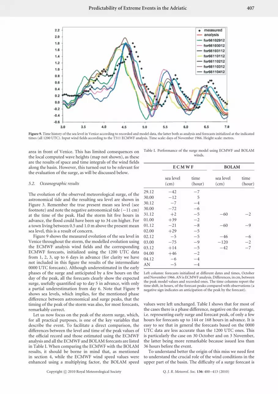
Figure 9. Time history of the sea level in Venice according to recorded and model data, the latter both as analysis and forecasts initialized at the indicatedtimes (all 1200 UTC). Input wind fields according to the T511 ECMWF analysis. Time scale: days of November 1966. Height scale: metres.

area in front of Venice. This has limited consequences onthe local computed wave heights (map not shown), as theseare the results of space and time integrals of the wind fieldsalong the basin. However, this turned out to be relevant forthe evaluation of the surge, as will be discussed below.

5.2. Oceanographic results

The evolution of the observed meteorological surge, of theastronomical tide and the resulting sea level are shown inFigure 3. Remember the true present mean sea level (seefootnote) and note the negative astronomical tide (−11 cm)at the time of the peak. Had the storm hit five hours inadvance, the flood could have been up to 34 cm higher. Fora town living between 0.5 and 1.0 m above the present meansea level, this is a result of concern.

Figure 9 shows the measured evolution of the sea level inVenice throughout the storm, the modelled evolution usingthe ECMWF analysis wind fields and the correspondingECMWF forecasts, initialized using the 1200 UTC datafrom 1, 2, 3, up to 6 days in advance (for clarity we havenot included in this figure the results of the intermediate0000 UTC forecasts). Although underestimated in the earlyphases of the surge and anticipated by a few hours on theday of the peak, all the forecasts clearly show the expectedsurge, usefully quantified up to day 5 in advance, with onlya partial underestimation from day 6. Note that Figure 9shows sea levels, which implies, for the mentioned phasedifference between astronomical and surge peaks, that thetiming of the peak of the storm was also, for most forecasts,remarkably correct.

Let us now focus on the peak of the storm surge, which,for all practical purposes, is one of the key variables thatdescribe the event. To facilitate a direct comparison, thedifferences between the level and time of the peak values ofthe official record and those estimated using the ECMWFanalysis and all the ECMWF and BOLAM forecasts are listedin Table I. When comparing the ECMWF with the BOLAMresults, it should be borne in mind that, as mentionedin section 4, while the ECMWF wind speed values wereenhanced using a multiplying factor, the BOLAM speed

Table I. Performance of the surge model using ECMWF and BOLAMwinds.

E C M W F BOLAM

sea level time sea level time(cm) (hour) (cm) (hour)

29.12 −42 −730.00 −12 530.12 −7 −430.00 −72 −631.12 +2 −5 −60 −201.00 +39 −201.12 −21 −8 −60 −902.00 +29 −502.12 −5 −5 −46 −603.00 −75 −9 −120 −203.12 +14 −5 −42 −704.00 +46 −204.12 −6 −4AN −5 −4

Left column: forecasts initialized at different dates and times, Octoberand November 1966. AN is ECMWF analysis. Differences, in cm, betweenthe peak model values and recorded ones. The time columns report thetime shift, in hours, of the forecast peaks compared with observations (anegative sign indicates an anticipation of the peak by the forecast).

values were left unchanged. Table I shows that for most ofthe cases there is a phase difference, negative on the average,i.e. representing early surge and forecast peak, of only a fewhours for forecasts up to 144 or 168 hours in advance. It iseasy to see that in general the forecasts based on the 0000UTC data are less accurate than the 1200 UTC ones. Thisis particularly the case on 30 October and on 3 November,the latter being more remarkable because issued less than36 hours before the event.

To understand better the origin of this miss we need firstto understand the crucial role of the wind conditions in theupper part of the basin. The difficulty of a surge forecast is

Copyright c© 2010 Royal Meteorological Society Q. J. R. Meteorol. Soc. 136: 400–413 (2010)

408 L. Cavaleri et al.

Figure 10. Longitudinal section, along its main axis, of the sea-leveldistribution in the Adriatic Sea (see Figure 1) at the peak of the flood at1200 UTC 4 November 1966.

well exemplified in Figure 10, where we see a section of thesea-level distribution along the main axis of the Adriatic atthe time of the peak of the surge. For a given surface stress, theincreased spatial gradient with decreasing depth leads to thesurge just in front of the Venice coast. It follows that even lim-ited differences of the wind field in this area, e.g. a shift of thelocation of maximum strength with a decrease of the windspeeds in the shallower area, can substantially alter the surge.This explains why the maximum sea-level values derivedfrom the BOLAM forecasts are lower than the ECMWF ones(and than the ‘official’ peak) by about 40 cm. As discussedabove and seen in Figure 8, the area of maximum windspeeds in BOLAM is adjacent to the Croatian coast, leavingsubstantially lower wind speeds in front of the northerncoast, where (Figure 10) most of the surge is concentrated.Given the comparison between the ECMWF and BOLAMsurge results in Table I, this seems to be a characteristic ofall the BOLAM forecasts analysed in this 1966 case-study.

Having clearly in mind the role of the wind in theupper part of the basin, we can now go back to the wrongforecast issued 36 hours before the 1966 event. For clarityreasons in Figure 9 we have shown only the surge forecastsissued at 1200 UTC, while all the results are reported inTable I. Indeed the forecast starting at 03.00 (0000 UTC3 November) is not only substantially underestimated, butfor all practical purposes according to this forecast there

would be no flood at all. Also the forecast wave heightsare much lower. The interpretation of the nature – not ofthe cause – of the meteorological forecast error is shownin Figure 11. Here we compare the analysis wind field of1200 UTC 4 November, the peak of the storm, with thecorresponding forecast started 36 hours in advance. Clearlythe forecast has anticipated the passage of the cold front.A comparison with its actual position 6 hours later inFigure 6(b) suggests a time shift of about 9 hours. Thematter becomes clear when we look at the distribution ofthe surge in Figure 10. Due to the mentioned increase ofthe sea-level spatial gradients with decreasing depth, andbecause of the wind distribution (see Figure 6(a)), mostof the surge was concentrated in the upper part of thebasin, in practice in front of Venice. The anticipation ofthe frontal passage completely changed the wind speed anddirection in this area at the crucial moment when the surgewas mounting. The result is the drastic underestimate seenin Table I. This highlights how critical the surge forecastscan be, depending on small shifts in time and positionof the forcing fields. To a lesser extent because of theirstronger dependence on the overall field, the wave heightsalso showed locally a substantial decrease. This was probablyassociated with the local breaking (steep waves movinginto shallower depths) and absence of direct forcing bywind.

The question is how this was possible. Note that theprevious and following forecasts, initialized at 1200 UTC 2and 3 November respectively, pinpoint the storm exactly.Something similar happened on 15–16 October 1987, whenan exceptional Atlantic storm hit Brittany, the south of theUnited Kingdom and the Channel area. A good descriptionof the event and discussion of the forecasts was given, amongothers, by Burt and Mansfield (1988) and Morris and Gadd(1988). The storm had been predicted in the previous days,but it was practically absent on the maps issued during thelast period before the event. The later analysis showed thiswas due to a wrong ship report, one of the few available in thearea at the crucial moment. Thus, one possible explanation ofthe poor prediction started at 0000 UTC of 3 November 1966could be the poor quality, and/or the lack of enough data to

(a) (b)

Figure 11. Left panel: distribution of the 10 m wind field (analysis) over the Adriatic Sea at 1200 UTC 4 November 1966 (see Figure 6(a)). Right panel:corresponding field according to the forecast initialized 36 hours in advance.

Copyright c© 2010 Royal Meteorological Society Q. J. R. Meteorol. Soc. 136: 400–413 (2010)

Predictability of Extreme Events in the Adriatic 409

Table II. Performance of the wave model using ECMWF and BOLAMwinds.

E C M W F BOLAM

Hs (m) time (hour) Hs (m) time (hour)

29.12 5.3 −630.00 1.6 −1830.12 4.7 031.00 3.8 −631.12 5.3 0 4.4 +301.00 7.3 +301.12 6.2 −6 5.2 −602.00 7.2 002.12 7.3 −3 6.8 −603.00 3.8 −12 2.7 −1203.12 7.0 −3 7.2 −604.00 7.3 +3AN 6.3 –

Left column: forecasts initialized at different dates and times, October andNovember 1966. AN is ECMWF analysis. Hs is the maximum significantwave height (m) estimated at the position of the oceanographic tower(see Figure 1 for its position and Figure 6 for the implications). The timecolumns report the time shift, in 3-hour steps, of the forecast wave peakscompared with the analysis (a negative sign indicates an anticipation bythe forecast).

produce an accurate analysis of that time. We attempted adeeper analysis in this direction (Cardinali et al., 2007; Kellyet al., 2007), but no definite conclusion was reached.

In general, the lower quality of the 0000 UTC forecasts canbe expected to be associated with that of the correspondinganalysis. We speculate that in turn this might be related tothe lack, or to a lower quality, of the data available at 0000UTC compared to that recorded at 1200 UTC.

The results of the wave simulations are summarised inTable II. Apart from the already mentioned forecasts startedat 0000 UTC of 3 November and of 30 October, the valuesconfirm that also for the waves the situation was predictableup to six days in advance. Note that the BOLAM andECMWF models give more consistent (between the twomodels) forecasts of the wave fields (Table II) than of the sealevel (Table I). The reason is that the wave conditions in thenorthern part of the basin depend on the whole wind fieldsalong the Adriatic. In the respect, the ECMWF and BOLAMaverage wind fields are much more similar to each other,and the shift towards the east of the BOLAM peak area doesnot have the same consequences as for the surge forecasts.

6. Results for the December 1979 case

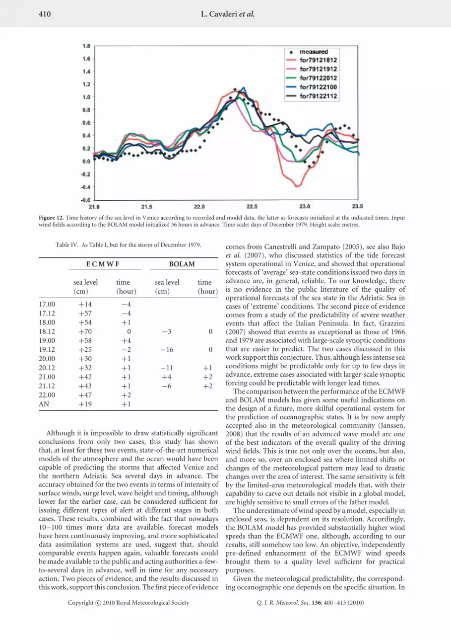
Figure 12 shows the time series of recorded and forecastsurge in Venice modelled using the BOLAM winds. Ratherthan also plotting the ECMWF results, peak values computedusing both model winds are contrasted in Table III. Table IIIindicates that both forecasts have very good timings, witha maximum shift of less than four hours, reduced to oneor two for initial conditions in the few days preceding theflood.

The comparison between the ECMWF and BOLAM waveheights and surges at the measuring tower offshore Veniceconfirms again the crucial role of the wind in the shallowarea in front of Venice. Let us consider first in Table III

Table III. As Table II, but for the storm of December 1979.

E C M W F BOLAM

Hs (m) time (hour) Hs (m) time (hour)

17.00 4.8 −317.12 6.5 −318.00 6.8 018.12 7.2 −3 4.9 019.00 6.6 019.12 6.3 −3 4.8 020.00 6.2 −320.12 5.9 0 4.4 021.00 6.4 0 4.9 021.12 6.4 0 4.9 022.00 6.5 0AN 5.6 –

the wave results. The waves obtained using the enhancedECMWF winds are higher and appear to be more consistentwith the damage seen in Figure 5. Because the wave heightsdepend on the overall situation on the basin, we derive that(see also the discussion in section 7) the enhanced ECMWFwind fields are more representative of the situation in theAdriatic Sea. However, Table IV shows that the BOLAMsurge peak values fit the measured one better. Following ourprevious argument in section 2 and section 5, this suggeststoo-high ECMWF wind speeds in the area in front of Venice.Indeed a direct inspection (not shown) of the ECMWF andBOLAM surface wind maps in the hours just before the peakshows the former wind speeds to be on average 20–30%higher than the latter ones. This conclusion is supported bya direct comparison of the values reported in Table V withthe data from the (mechanical) anemometer on-board thetower. Seen on the left, the ECMWF data are too high forpractically the whole duration of the storm. Focusing on thevalue at the peak of the storm (0600 UTC 22 December), wecompare on the right the ECMWF and BOLAM peak valuesfrom the forecasts issued at different dates and times. Withrespect to the 16.4 m/s measured value, the ECMWF windspeeds are too high, while, starting from the 19 December1200 UTC forecast, the BOLAM values have practically nobias.

These results indicate that, while in the Adriatic Sea thewind field is generally correct for ECMWF but it is too weakfor BOLAM, in front of Venice the local wind speed is toohigh for ECMWF but practically correct for BOLAM. Thequality of the surge forecasts followed accordingly.

7. Discussion and conclusions

The performance of state-of-the-art meteorological andoceanographic numerical systems in predicting the sea statein the Adriatic Sea during intense storms is assessed, also inthe case of past storms, when the amount of data availablewas much lower than today. The key issue that has beenaddressed by this study is whether severe events such asthose that affected Venice in 1966 and in 1979 could havebeen predicted if the forecasting models/data available nowhad been present at that time.

Copyright c© 2010 Royal Meteorological Society Q. J. R. Meteorol. Soc. 136: 400–413 (2010)

410 L. Cavaleri et al.

Figure 12. Time history of the sea level in Venice according to recorded and model data, the latter as forecasts initialized at the indicated times. Inputwind fields according to the BOLAM model initialized 36 hours in advance. Time scale: days of December 1979. Height scale: metres.

Table IV. As Table I, but for the storm of December 1979.

E C M W F BOLAM

sea level time sea level time(cm) (hour) (cm) (hour)

17.00 +14 −417.12 +57 −418.00 +54 +118.12 +70 0 −3 019.00 +58 +419.12 +25 −2 −16 020.00 +30 +120.12 +32 +1 −11 +121.00 +42 +1 +4 +221.12 +43 +1 −6 +222.00 +47 +2AN +19 +1

Although it is impossible to draw statistically significantconclusions from only two cases, this study has shownthat, at least for these two events, state-of-the-art numericalmodels of the atmosphere and the ocean would have beencapable of predicting the storms that affected Venice andthe northern Adriatic Sea several days in advance. Theaccuracy obtained for the two events in terms of intensity ofsurface winds, surge level, wave height and timing, althoughlower for the earlier case, can be considered sufficient forissuing different types of alert at different stages in bothcases. These results, combined with the fact that nowadays10–100 times more data are available, forecast modelshave been continuously improving, and more sophisticateddata assimilation systems are used, suggest that, shouldcomparable events happen again, valuable forecasts couldbe made available to the public and acting authorities a-few-to-several days in advance, well in time for any necessaryaction. Two pieces of evidence, and the results discussed inthis work, support this conclusion. The first piece of evidence

comes from Canestrelli and Zampato (2005), see also Bajoet al. (2007), who discussed statistics of the tide forecastsystem operational in Venice, and showed that operationalforecasts of ‘average’ sea-state conditions issued two days inadvance are, in general, reliable. To our knowledge, thereis no evidence in the public literature of the quality ofoperational forecasts of the sea state in the Adriatic Sea incases of ‘extreme’ conditions. The second piece of evidencecomes from a study of the predictability of severe weatherevents that affect the Italian Peninsula. In fact, Grazzini(2007) showed that events as exceptional as those of 1966and 1979 are associated with large-scale synoptic conditionsthat are easier to predict. The two cases discussed in thiswork support this conjecture. Thus, although less intense seaconditions might be predictable only for up to few days inadvance, extreme cases associated with larger-scale synopticforcing could be predictable with longer lead times.

The comparison between the performance of the ECMWFand BOLAM models has given some useful indications onthe design of a future, more skilful operational system forthe prediction of oceanographic states. It is by now amplyaccepted also in the meteorological community (Janssen,2008) that the results of an advanced wave model are oneof the best indicators of the overall quality of the drivingwind fields. This is true not only over the oceans, but also,and more so, over an enclosed sea where limited shifts orchanges of the meteorological pattern may lead to drasticchanges over the area of interest. The same sensitivity is feltby the limited-area meteorological models that, with theircapability to carve out details not visible in a global model,are highly sensitive to small errors of the father model.

The underestimate of wind speed by a model, especially inenclosed seas, is dependent on its resolution. Accordingly,the BOLAM model has provided substantially higher windspeeds than the ECMWF one, although, according to ourresults, still somehow too low. An objective, independentlypre-defined enhancement of the ECMWF wind speedsbrought them to a quality level sufficient for practicalpurposes.

Given the meteorological predictability, the correspond-ing oceanographic one depends on the specific situation. In

Copyright c© 2010 Royal Meteorological Society Q. J. R. Meteorol. Soc. 136: 400–413 (2010)

Predictability of Extreme Events in the Adriatic 411

Table V. Comparison between recorded and ECMWF analysis wind speeds at the position of the oceanographic tower (see Figure 5).

date time Record ECMWF analysis date time ECMWF forecast BOLAM forecast

21 18 12.8 12.421 13.3 15.2

22 00 11.3 17.1 18 12 22.3 17.003 10.8 17.2 19 12 20.0 16.506 16.4 18.1 forecast 20 12 19.7 16.209 – 18.3 21 00 18.6 16.612 13.8 18.5 21 12 18.2 16.315 13.3 16.918 8.7 10.4

Values in m/s. Dates and times shown in the first two columns. The period is December 1979. Right part: focusing on the value at 0600 UTC 22December, comparison with the corresponding forecast values using ECMWF and BOLAM winds. Forecasts initialized at the indicated dates andtimes.

the case of the Adriatic Sea, and also in the more generalcase, waves depend on the wind distribution over the overallbasin of interest. Therefore limited changes in the wind dis-tribution are not likely to have drastic consequences. This isnot the case with storm surges, the more so the shallowerthe water. Because most of the surge is concentrated in thelower depth areas, limited variations of the wind field in thiszone could lead to large differences in the results.

An example is given by the wrong forecast issued on thebasis of the data available on 3 November 1966. Comparingthis situation to a similar miss which happened on theFrench–English coasts in October 1987, we have tried totrace back the origin of the mistake. However, the kindand structure of the data available for 1966 did not allowany conclusion to be reached. The relevant question iswhether such a miss could also happen today, 20 yearsafter the failure of 1987. We tend to think that thepresent enormous amount of data and the keen analysisof their consistency done before and during assimilationshould exclude that one or a few isolated wrong datacould drastically affect the analysis, hence the forecast.Unfortunately, after 1987, models struggled, for example,to correctly predict the development of two severe stormsthat hit France and north-central Europe in December 1999(Buizza and Hollingsworth, 2002). Should a storm like thisoccur over the Mediterranean, it could cause single forecaststo miss the prediction of severe sea-state conditions a fewdays ahead, thus making it impossible to issue warnings afew days before the occurrence of the event.

Is there a way to further improve and reduce the forecastuncertainty? Buizza and Hollingsworth (2002) showed thatfor the two storms of December 1999 a probabilisticapproach to the prediction of severe events led to earlyindications of possible severe storm occurrence. Theyconcluded that a probabilistic, ensemble-based approachto weather prediction gives users valuable forecasts aboutone day before single forecasts, and illustrated that theECMWF Ensemble Prediction System (EPS) is an extremelyvaluable tool for assessing quantitatively the risk of severeweather and issuing early warnings of possible disruptions.Saetra et al. (2004) compared the performance of EPS-basedprobabilistic and single forecasts of sea waves and windsfor about 2.5 years, and concluded that EPS probabilisticforecasts are more valuable for decision makers. A goodexample of practical application of the ensemble techniqueto surge forecasts is given by Flowerdew et al. (2009). The

reader is referred also to Buizza et al. (2007) and Palmeret al. (2007) for further discussions of the performance ofthe ECMWF EPS in predicting weather conditions. Work toassess the performance of ECMWF probabilistic forecasts ofthe sea state in the Adriatic Sea is in progress, and will bereported in due course.

In conclusion, the implications of this work on the futureprediction of sea-state events such as the ones that affectedVenice in 1966 and 1979 are the following:

(1) Notwithstanding the substantial lack of data thatcharacterised those early years, the application of thepresent tools (computers and models) to the data of1966 and 1979 has shown that in principle usefulforecasts would have been possible up to several daysin advance. One of the reasons why the prediction ofthis (extreme) type of event could be easier that theprediction of ‘average’ states is that extreme sea-stateconditions are associated with large-scale synopticforcing, which makes them more predictable thansmall-scale, local phenomena.

(2) Particularly in enclosed seas, the oceanographic modelresults are very sensitive to errors in the inputwind fields. Especially in shallow-water areas, thisis more the case for surge than wave results, the latterdepending more on the general distribution of thewinds on the considered basin.

(3) The ECMWF wind speeds, as representative of theglobal models, turn out to be too low in enclosed seas.Much better results, although somehow still lowerthan the truth, are obtained with high-resolutionlimited-area meteorological models. For a given basinan alternative approach is to use suitable enhancementcoefficients for the global model wind speeds, derivedfrom long-term comparison between atmosphericand wave model results and measured data in the areaof interest. Depending on the geometry and orographyof the basin, these coefficients may depend on thetype of storm. They depend also on the resolutionof the meteorological model. Results have indicatedthat dynamical downscaling of the large-scale weatherfields with a limited-area model could improve thesea-state prediction, especially of the wave field.

(4) Results so far indicate that a warning system forthe Adriatic Sea that includes a high-quality globalweather model, a high-quality limited-area modeland sea-state and surge models, should provide users

Copyright c© 2010 Royal Meteorological Society Q. J. R. Meteorol. Soc. 136: 400–413 (2010)

412 L. Cavaleri et al.

with valuable forecasts up to several days in advance,particularly in the case of severe events.

(5) But it should be pointed out that small errors in theinitial analysis fields will always be present, e.g. dueto possible observation errors. These initial errorsmay lead to substantial errors in the forecast ofmeteorological situations, and thus to even largeroceanographic errors (see also point (2)). One way toaddress this issue is to use a probabilistic approach,and thus develop a probabilistic sea-state forecastingsystem that includes a global EPS, a limited-area EPSand a sea-state ensemble system.

Work along the lines of this latter point to assess thevalue of the probabilistic forecast of sea states in case of‘acqua-alta’ in Venice is under progress, and results will bereported in due course.

Acknowledgements

We want to thank Graeme Kelly and Sakari Uppala for theirhelp with generating higher-resolution re-analyses of thesituations. The original idea of this research, of applyingthe present methods for a posteriori forecasts of storms verymuch in the past, was suggested by Tony Hollingsworth.

The study has been partially supported by the ConsorzioVenezia Nuova in relation to the predictability of the bigfloods affecting Venice.

References

Bajo M, Zampato L, Umgiesser G, Cucco A, Canestrelli P. 2007. A finiteelement operational model for storm surge prediction in Venice.Estuar. Coast. Shelf Sci. 75: 236–249.

Berto A, Buzzi A, Nardi D. 2005. ‘A warm conveyor belt mechanismaccompanying extreme precipitation events over north-easternItaly.’ Proceedings 28th ICAM, The annual Scientific MAP Meeting,2005, Zadar, extended abstracts. Hrv. Meteorol. Casopis (CroatianMeteorological Journal) 40: 338–341.

Bertotti L, Cavaleri L. 1985. Coastal set-up and wave breaking. Oceanol.Acta 8: 237–242.

Bertotti L, Cavaleri L. 2009. Large and small scale wave forecast in theMediterranean Sea. Natural Hazards Earth Syst. Sci. 9: 779–788.

Bowen AJ, Inman DL, Simmons VP. 1968. Wave ‘set-down’ and set-up.J. Geophys. Res. 73: 2569–2577.

Buizza R, Hollingsworth A. 2002. Storm prediction over Europe usingthe ECMWF Ensemble Prediction System. Meteorol. Appl. 9: 289–305.

Buizza R, Cardinali C, Kelly G, Thepaut J-N. 2007. The value ofobservations. II: The value of observations located in singular-vector-based target areas. Q. J. R. Meteorol. Soc. 133: 1817–1832.

Burt SD, Mansfield DA. 1988. The great storm of 15–16 October 1987.Weather 43: 90–114.

Buzzi A, Fantini M, Malguzzi P, Nerozzi F. 1994. Validation of a limitedarea model in cases of Mediterranean cyclogenesis: Surface fields andprecipitation scores. Meteorol. Atmos. Phys. 53: 137–153.

Camuffo D. 1993. Analysis of the sea surges at Venice from AD 782 to1990. Theor. Appl. Climatol. 47: 1–14.

Canestrelli P, Zampato L. 2005. Sea-level forecasting at the CentroPrevisioni e Segnalazioni Maree (CPSM) of the Venice Municipality.Pp 85–97 in Flooding and environmental challenges for Venice and itslagoon: State of knowledge, Fletcher C, Spencer T (eds). CambridgeUniversity Press: Cambridge, UK.

Cardinali C, Buizza R, Kelly G, Shapiro M, Thepaut J-N. 2007. The valueof observations. III: Influence of weather regimes on targeting. Q. J.R. Meteorol. Soc. 133: 1833–1842.

Cavaleri L, Bertotti L. 1997. In search of the correct wind and wave fieldsin a minor basin. Mon. Weather Rev. 125: 1964–1975.

Cavaleri L, Bertotti L. 2006. The improvement of modelled wind andwave fields with increasing resolution. Ocean Engineering 33: 553–565.

Cavaleri L, Sclavo M. 2006. The calibration of wind and wave model datain the Mediterranean Sea. Coastal Engineering 53: 613–627.

Cecconi G, Canestrelli P, Corte C, Di Donato M. 1999. ‘Climaterecord of storm surges in Venice.’ Pp 149–156 in Impact of climate

change on flooding and sustainable river management, RIBAMODWorkshop, Wallingford, 26–27 February 1998. EUR 18287 EN.European Commission: Luxembourg.

De Zolt S, Lionello P, Nuhu A, Tomasin A. 2006. The disastrous stormof 4 November 1966 on Italy. Natural Hazards Earth Syst. Sci. 6:861–879.

Fea G, Gazzola A, Cicala A. 1968. ‘Prima documentazione generale dellasituazione meteorological relativa alla grande alluvione del novembre1966.’ CNR-CENFAM PV 32: 215 pp.

Flowerdew J, Horsburgh KJ, Mylne KR. 2009. Ensemble forecasting ofstorm surges. Mar. Geodesy 32: 91–99.

Grazzini F. 2007. Predictability of a large-scale flow conducive toextreme precipitation over the western Alps. Meteorol. Atmos. Phys.95: 123–138.

Janssen PAEM. 2008. Progress in ocean wave forecasting. J. Comput.Phys. 227: 3572–3594.

Jung T, Gulev SK, Rudeva I, Soloviov V. 2006. ‘Sensitivity ofextratropical cyclone characteristics to horizontal resolution in theECMWF model.’ ECMWF RD Tech. Memo. 485. Available fromECMWF, Shinfield Park, Reading RG2 9AX, UK (also fromwww.ecmwf.int/publications/library).

Kelly G, Thepaut J-N, Buizza R, Cardinali C. 2007. The value ofobservations. I: Data denial experiments for the Atlantic and thePacific. Q. J. R. Meteorol. Soc. 133: 1803–1815.

Komen GJ, Cavaleri L, Donelan M, Hasselmann K, Hasselmann S,Janssen PAEM. 1994. Dynamics and modelling of ocean waves.Cambridge University Press.

Lionello P, Malguzzi P, Buzzi A. 1998. Coupling between the atmosphericcirculation and the ocean wave field: An idealized case. J. Phys.Oceanogr. 28: 161–177.

Lionello P, Martucci G, Zampieri M. 2003. Implementation of a coupledatmosphere–wave–ocean model in the Mediterranean Sea: Sensitivityof the short time scale evolution to the air–sea coupling mechanisms.Global Atmos. Ocean System 9: 65–95.

Longuet-Higgins MS, Stewart RW. 1964. Radiation stresses in waterwaves: A physical discussion with applications. Deep-Sea Res. 11:529–562.

Malguzzi P, Tartaglione N. 1999. An economical second-order advectionscheme for numerical weather prediction. Q. J. R. Meteorol. Soc. 125:2291–2303.

Malguzzi P, Grossi G, Buzzi A, Ranzi R, Buizza R. 2006. The 1966‘century’ flood in Italy: A meteorological and hydrological revisitation.J. Geophys. Res. 111: D24106, DOI:10.1029/2006JD007111.

Morris RM, Gadd AJ. 1988. Forecasting the storm of 15–16 October1987. Weather 43: 70–90.

Palmer TN, Buizza R, Leutbecher M, Hagedorn R, Jung T, Rodwell M,Vitart F, Berner J, Hagel E, Lawrence A, Pappenberger F, Park Y-Y,von Bremen L, Gilmour I. 2007. ‘The Ensemble Prediction System:Recent and ongoing developments. A paper presented at the 36th Sessionof the ECMWF Scientific Advisory Committee.’ ECMWF ResearchDepartment Technical Memorandum 540, ECMWF, Shinfield Park,Reading, RG2 9AX, UK.

Pirazzoli PA, Tomasin A. 2003. Recent near-surface wind changes inthe central Mediterranean and Adriatic areas. Int. J. Climatol. 23:963–973.

Pugh DT. 1987. Tides, surges, and mean sea-level. John Wiley & Sons:Chichester, New York.

Rotach MW, Ambrosetti P, Ament F, Appenzeller C, Arpagaus M,Bauer H-S, Behrendt A, Bouttier F, Buzzi A, Corazza M, Davolio S,Denhard M, Dorninger M, Fontannaz L, Frick J, Fundel F, Germann U,Gorgas T, Hegg C, Hering A, Keil C, Liniger MA, Marsigli C,McTaggart-Cowan R, Montaini A, Mylne KR, Ranzi R, Richard E,Rossa A, Santos-Munoz D, Schar C, Seity Y, Staudinger M, Stoll M,Volkert H, Walser A, Wang Y, Werhahn J, Wulfmeyer V, Zappa M.2009. MAP D-PHASE: Real-time demonstration of weather forecastquality in the Alpine region. Bull. Am. Meteorol. Soc. 90: 1321–1336.

Saetra Ø, Hersbach H, Bidlot J-R, Richardson DS. 2004. Effects ofobservation errors on the statistics for ensemble spread and reliability.Mon. Weather Rev. 132: 1487–1501.

Tomasin A. 2005. Forecasting the water level in Venice: Physicalbackground and perspectives. Pp 71–78 in Flooding and environmentalchallenges for Venice and its lagoon: State of knowledge, Fletcher CA,Spencer T (eds). Cambridge University Press.

Umgiesser G, Melaku Canu D, Cucco A, Solidoro C. 2004. A finiteelement model for the Venice lagoon: Development, set up, calibrationand validation. J. Mar. Sys. 51: 123–145.

Uppala SM, Kallberg PW, Simmons AJ, Andrae U, da Costa Bechtold V,Fiorino M, Gibson JK, Haseler J, Hernandez A, Kelly GA, Li X,Onogi K, Saarinen S, Sokka N, Allan RP, Andersson E, Arpe K,Balmaseda MA, Beljaars ACM, van de Berg L, Bidlot J, Bormann N,

Copyright c© 2010 Royal Meteorological Society Q. J. R. Meteorol. Soc. 136: 400–413 (2010)

Predictability of Extreme Events in the Adriatic 413

Caires S, Chevallier F, Dethof A, Dragosavac M, Fisher M, Fuentes M,Hagemann S, Holm E, Hoskins BJ, Isaksen L, Janssen PAEM, Jenne R,McNally AP, Mahfouf J-F, Morcrette J-J, Rayner NA, Saunders RW,Simon P, Sterl A, Trenberth KE, Untch A, Vasiljevic D, Viterbo P,Woollen J. 2005. The ERA-40 reanalysis. Q. J. R. Meteorol. Soc. 131:2961–3012.

Wamdi Group. 1988. The WAM model – A third generation ocean waveprediction model. J. Phys. Oceanogr. 18: 1775–1810.

Warner TT, Hsu H-M. 2000. Nested-model simulation of moistconvection: The impact of coarse-grid parameterized convection onfine-grid resolved convection. Mon. Weather Rev. 128: 2211–2231.

Zampieri M, Malguzzi P, Buzzi A. 2005. Sensitivity of quantitativeprecipitation forecasts to boundary layer parameterization: A flashflood case study in the Western Mediterranean. Natural HazardsEarth Syst. Sci. 5: 603–612.

Copyright c© 2010 Royal Meteorological Society Q. J. R. Meteorol. Soc. 136: 400–413 (2010)