precalculus - an investigation of functions - opentextbookstore
TRANSCRIPT
Precalculus An Investigation of Functions
Edition 1.5
David Lippman
Melonie Rasmussen
This book is also available to read free online at
http://www.opentextbookstore.com/precalc/ If you want a printed copy, buying from the bookstore is cheaper than printing yourself.
ii
Copyright © 2015 David Lippman and Melonie Rasmussen
This text is licensed under a Creative Commons Attribution-Share Alike 3.0 United
States License.
To view a copy of this license, visit http://creativecommons.org/licenses/by-sa/3.0/us/ or send a letter to
Creative Commons, 171 Second Street, Suite 300, San Francisco, California, 94105, USA.
You are free:
to Share — to copy, distribute, display, and perform the work
to Remix — to make derivative works
Under the following conditions:
Attribution. You must attribute the work in the manner specified by the author or licensor (but not in
any way that suggests that they endorse you or your use of the work).
Share Alike. If you alter, transform, or build upon this work, you may distribute the resulting work
only under the same, similar or a compatible license.
With the understanding that:
Waiver. Any of the above conditions can be waived if you get permission from the copyright holder.
Other Rights. In no way are any of the following rights affected by the license:
Your fair dealing or fair use rights;
Apart from the remix rights granted under this license, the author's moral rights;
Rights other persons may have either in the work itself or in how the work is used, such as
publicity or privacy rights.
Notice — For any reuse or distribution, you must make clear to others the license terms of
this work. The best way to do this is with a link to this web page:
http://creativecommons.org/licenses/by-sa/3.0/us/
In addition to these rights, we give explicit permission to remix small portions of this
book (less than 10% cumulative) into works that are CC-BY, CC-BY-SA-NC, or GFDL
licensed.
Selected exercises were remixed from Precalculus by D.H. Collingwood and K.D.
Prince, originally licensed under the GNU Free Document License, with permission from
the authors.
Cover Photo by David Lippman, of artwork by
John Rogers Lituus, 2010 Dichromatic glass and aluminum Washington State Arts Commission in partnership with Pierce College
This is the fifth official version of Edition 1. It contains typo corrections and language
clarification, but is page number and problem set number equivalent to the original
Edition 1.

i
About the Authors
David Lippman received his master’s degree in mathematics from
Western Washington University and has been teaching at Pierce
College since Fall 2000.
Melonie Rasmussen also received her
master’s degree in mathematics from
Western Washington University and has
been teaching at Pierce College since Fall
2002. Prior to this Melonie taught for the
Puyallup School district for 6 years after
receiving her teaching credentials from Pacific Lutheran
University.
We have both been long time advocates of open learning, open materials, and basically
any idea that will reduce the cost of education for students. It started by supporting the
college’s calculator rental program, and running a book loan scholarship program.
Eventually the frustration with the escalating costs of commercial text books and the
online homework systems that charged for access led them to take action.
First, David developed IMathAS, open source online math homework software that runs
WAMAP.org and MyOpenMath.com. Through this platform, we became integral parts
of a vibrant sharing and learning community of teachers from around Washington State
that support and contribute to WAMAP. Our pioneering efforts, supported by dozens of
other dedicated faculty and financial support from the Transition Math Project, have led
to a system used by thousands of students every quarter, saving hundreds of thousands of
dollars over comparable commercial offerings.
David continued further and wrote his first open textbook, Math in Society, a math for
liberal arts majors book, after being frustrated by students having to pay $100+ for a
textbook for a terminal course. Together, frustrated by both cost and the style of
commercial texts, we began writing PreCalculus: An Investigation of Functions in 2010.

ii
Acknowledgements
We would like to thank the following for their generous support and feedback.
The community of WAMAP users and developers for creating a majority of the
homework content used in our online homework sets.
Pierce College students in our Fall 2010 - Summer 2011 Math 141 and Math 142
classes for helping correct typos, identifying videos related to the homework, and
being our willing test subjects.
The Open Course Library Project for providing the support needed to produce a
full course package for these courses.
Mike Kenyon, Chris Willett, Tophe Anderson, and Vauhn Foster-Grahler for
reviewing the course and giving feedback and suggestions.
Our Pierce College colleagues for providing their suggestions.
Tophe Anderson, James Gray, and Lawrence Morales for their feedback and
suggestions in content and examples.
Jeff Eldridge for extensive proofreading and suggestions for clarification.
James Sousa for developing videos associated with the online homework.
Kevin Dimond for his work on indexing the book and creating PowerPoint slides.
Faculty at Green River Community College and the Maricopa College District for
their feedback and suggestions.
iii
Preface
Over the years, when reviewing books we found that many had been mainstreamed by
the publishers in an effort to appeal to everyone, leaving them with very little character.
There were only a handful of books that had the conceptual and application driven focus
we liked, and most of those were lacking in other aspects we cared about, like providing
students sufficient examples and practice of basic skills. The largest frustration, however,
was the never ending escalation of cost and being forced into new editions every three
years. We began researching open textbooks, however the ability for those books to be
adapted, remixed, or printed were often limited by the types of licenses, or didn’t
approach the material the way we wanted.
This book is available online for free, in both Word and PDF format. You are free to
change the wording, add materials and sections or take them away. We welcome
feedback, comments and suggestions for future development at
[email protected]. Additionally, if you add a section, chapter or problems,
we would love to hear from you and possibly add your materials so everyone can benefit.
In writing this book, our focus was on the story of functions. We begin with function
notation, a basic toolkit of functions, and the basic operation with functions: composition
and transformation. Building from these basic functions, as each new family of functions
is introduced we explore the important features of the function: its graph, domain and
range, intercepts, and asymptotes. The exploration then moves to evaluating and solving
equations involving the function, finding inverses, and culminates with modeling using
the function.
The "rule of four" is integrated throughout - looking at the functions verbally,
graphically, numerically, as well as algebraically. We feel that using the “rule of four”
gives students the tools they need to approach new problems from various angles. Often
the “story problems of life” do not always come packaged in a neat equation. Being able
to think critically, see the parts and build a table or graph a trend, helps us change the
words into meaningful and measurable functions that model the world around us.
There is nothing we hate more than a chapter on exponential equations that begins
"Exponential functions are functions that have the form f(x)=ax." As each family of
functions is introduced, we motivate the topic by looking at how the function arises from
life scenarios or from modeling. Also, we feel it is important that precalculus be the
bridge in level of thinking between algebra and calculus. In algebra, it is common to see
numerous examples with very similar homework exercises, encouraging the student
to mimic the examples. Precalculus provides a link that takes students from the basic
plug & chug of formulaic calculations towards building an understanding that equations
and formulas have deeper meaning and purpose. While you will find examples and
similar exercises for the basic skills in this book, you will also find examples of multistep
problem solving along with exercises in multistep problem solving. Often times these
exercises will not exactly mimic the exercises, forcing the students to employ their
critical thinking skills and apply the skills they've learned to new situations. By

iv
developing students’ critical thinking and problem solving skills this course prepares
students for the rigors of Calculus.
While we followed a fairly standard ordering of material in the first half of the book, we
took some liberties in the trig portion of the book. It is our opinion that there is no need
to separate unit circle trig from triangle trig, and instead integrated them in the first
chapter. Identities are introduced in the first chapter, and revisited throughout. Likewise,
solving is introduced in the second chapter and revisited more extensively in the third
chapter. As with the first part of the book, an emphasis is placed on motivating the
concepts and on modeling and interpretation.
Supplements
During Spring 2010, the Washington Open Course Library (OCL) project was announced
with the goal of creating open courseware for the 81 highest enrolled community college
courses with a price cap on course materials of $30. We were chosen to work on
precalculus for this project, and that helped drive us to complete our book, and allowed
us to create supplemental materials.
A course package is available that contains the following features:
Suggested syllabus
Day by day course guide
Instructor guide with lecture outlines and examples
Additional online resources, with links to other textbooks, videos, and other
resources
Discussion forums
Diagnostic review
Online homework for each section (algorithmically generated, free response)
A list of videos related to the online homework
Printable class worksheets, activities, and handouts
Chapter review problems
Sample quizzes
Sample chapter exams
The course shell was built for the IMathAS online homework platform, and is available
for Washington State faculty at www.wamap.org and mirrored for others at
www.myopenmath.com.
The course shell was designed to follow Quality Matters (QM) guidelines, but has not yet
been formally reviewed.

v
How To Be Successful In This Course
This is not a high school math course, although for some of you the content may seem
familiar. There are key differences to what you will learn here, how quickly you will be
required to learn it and how much work will be required of you.
You will no longer be shown a technique and be asked to mimic it repetitively as the only
way to prove learning. Not only will you be required to master the technique, but you
will also be required to extend that knowledge to new situations and build bridges
between the material at hand and the next topic, making the course highly cumulative.
As a rule of thumb, for each hour you spend in class, you should expect this course will
require an average of 2 hours of out-of-class focused study. This means that some of you
with a stronger background in mathematics may take less, but if you have a weaker
background or any math anxiety it will take you more.
Notice how this is the equivalent of having a part time job, and if you are taking a
fulltime load of courses as many college students do, this equates to more than a full time
job. If you must work, raise a family and take a full load of courses all at the same time,
we recommend that you get a head start & get organized as soon as possible. We also
recommend that you spread out your learning into daily chunks and avoid trying to cram
or learn material quickly before an exam.
To be prepared, read through the material before it is covered in class and note or
highlight the material that is new or confusing. The instructor’s lecture and activities
should not be the first exposure to the material. As you read, test your understanding
with the Try it Now problems in the book. If you can’t figure one out, try again after
class, and ask for help if you still can’t get it.
As soon as possible after the class session recap the day’s lecture or activities into a
meaningful format to provide a third exposure to the material. You could summarize
your notes into a list of key points, or reread your notes and try to work examples done in
class without referring back to your notes. Next, begin any assigned homework. The
next day, if the instructor provides the opportunity to clarify topics or ask questions, do
not be afraid to ask. If you are afraid to ask, then you are not getting your money’s
worth! If the instructor does not provide this opportunity, be prepared to go to a tutoring
center or build a peer study group. Put in quality effort and time and you can get quality
results.
Lastly, if you feel like you do not understand a topic. Don’t wait, ASK FOR HELP!
ASK: Ask a teacher or tutor, Search for ancillaries, Keep a detailed list of questions
FOR: Find additional resources, Organize the material, Research other learning options
HELP: Have a support network, Examine your weaknesses, List specific examples & Practice
Best of luck learning! We hope you like the course & love the price.
David & Melonie
vi
Table of Contents
About the Authors ............................................................................................................ i
Acknowledgements ......................................................................................................... ii
Preface ........................................................................................................................... iii
Supplements ................................................................................................................... iv
How To Be Successful In This Course ........................................................................... v
Table of Contents ........................................................................................................... vi
Chapter 1: Functions ........................................................................................................ 1 Section 1.1 Functions and Function Notation ................................................................. 1
Section 1.2 Domain and Range ..................................................................................... 21
Section 1.3 Rates of Change and Behavior of Graphs .................................................. 34
Section 1.4 Composition of Functions .......................................................................... 49
Section 1.5 Transformation of Functions ..................................................................... 61
Section 1.6 Inverse Functions ....................................................................................... 90
Chapter 2: Linear Functions.......................................................................................... 99 Section 2.1 Linear Functions ........................................................................................ 99
Section 2.2 Graphs of Linear Functions ..................................................................... 111
Section 2.3 Modeling with Linear Functions .............................................................. 126
Section 2.4 Fitting Linear Models to Data .................................................................. 138
Section 2.5 Absolute Value Functions ........................................................................ 146
Chapter 3: Polynomial and Rational Functions ......................................................... 155 Section 3.1 Power Functions & Polynomial Functions .............................................. 155
Section 3.2 Quadratic Functions ................................................................................. 163
Section 3.3 Graphs of Polynomial Functions ............................................................. 176
Section 3.4 Rational Functions ................................................................................... 188
Section 3.5 Inverses and Radical Functions ............................................................... 206
Chapter 4: Exponential and Logarithmic Functions ................................................. 215 Section 4.1 Exponential Functions ............................................................................. 215
Section 4.2 Graphs of Exponential Functions ............................................................ 232
Section 4.3 Logarithmic Functions ............................................................................. 242
Section 4.4 Logarithmic Properties ............................................................................ 253
Section 4.5 Graphs of Logarithmic Functions ............................................................ 262
Section 4.6 Exponential and Logarithmic Models ...................................................... 270
Section 4.7 Fitting Exponentials to Data .................................................................... 289
vii
Chapter 5: Trigonometric Functions of Angles ......................................................... 297 Section 5.1 Circles ...................................................................................................... 297
Section 5.2 Angles ...................................................................................................... 307
Section 5.3 Points on Circles using Sine and Cosine ................................................. 321
Section 5.4 The Other Trigonometric Functions ........................................................ 333
Section 5.5 Right Triangle Trigonometry ................................................................... 343
Chapter 6: Periodic Functions ..................................................................................... 353 Section 6.1 Sinusoidal Graphs .................................................................................... 353
Section 6.2 Graphs of the Other Trig Functions ......................................................... 369
Section 6.3 Inverse Trig Functions ............................................................................. 379
Section 6.4 Solving Trig Equations ............................................................................ 387
Section 6.5 Modeling with Trigonometric Equations ................................................. 397
Chapter 7: Trigonometric Equations and Identities ................................................. 409 Section 7.1 Solving Trigonometric Equations with Identities .................................... 409
Section 7.2 Addition and Subtraction Identities ......................................................... 417
Section 7.3 Double Angle Identities ........................................................................... 431
Section 7.4 Modeling Changing Amplitude and Midline ........................................... 442
Chapter 8: Further Applications of Trigonometry.................................................... 451 Section 8.1 Non-right Triangles: Law of Sines and Cosines ...................................... 451
Section 8.2 Polar Coordinates ..................................................................................... 467
Section 8.3 Polar Form of Complex Numbers ............................................................ 480
Section 8.4 Vectors ..................................................................................................... 491
Section 8.5 Parametric Equations ............................................................................... 504
Solutions to Selected Exercises .................................................................................... 519 Chapter 1 ..................................................................................................................... 519
Chapter 2 ..................................................................................................................... 526
Chapter 3 ..................................................................................................................... 530
Chapter 4 ..................................................................................................................... 534
Chapter 5 ..................................................................................................................... 539
Chapter 6 ..................................................................................................................... 542
Chapter 7 ..................................................................................................................... 546
Chapter 8 ..................................................................................................................... 549
Index ............................................................................................................................... 555

viii
Section 1.1 Functions and Function Notation 1
This chapter is part of Precalculus: An Investigation of Functions © Lippman & Rasmussen 2011.
This material is licensed under a Creative Commons CC-BY-SA license.
Chapter 1: Functions Section 1.1 Functions and Function Notation ................................................................. 1
Section 1.2 Domain and Range ..................................................................................... 21
Section 1.3 Rates of Change and Behavior of Graphs .................................................. 34
Section 1.4 Composition of Functions .......................................................................... 49
Section 1.5 Transformation of Functions...................................................................... 61
Section 1.6 Inverse Functions ....................................................................................... 90
Section 1.1 Functions and Function Notation
What is a Function?
The natural world is full of relationships between quantities that change. When we see
these relationships, it is natural for us to ask “If I know one quantity, can I then determine
the other?” This establishes the idea of an input quantity, or independent variable, and a
corresponding output quantity, or dependent variable. From this we get the notion of a
functional relationship in which the output can be determined from the input.
For some quantities, like height and age, there are certainly relationships between these
quantities. Given a specific person and any age, it is easy enough to determine their
height, but if we tried to reverse that relationship and determine age from a given height,
that would be problematic, since most people maintain the same height for many years.
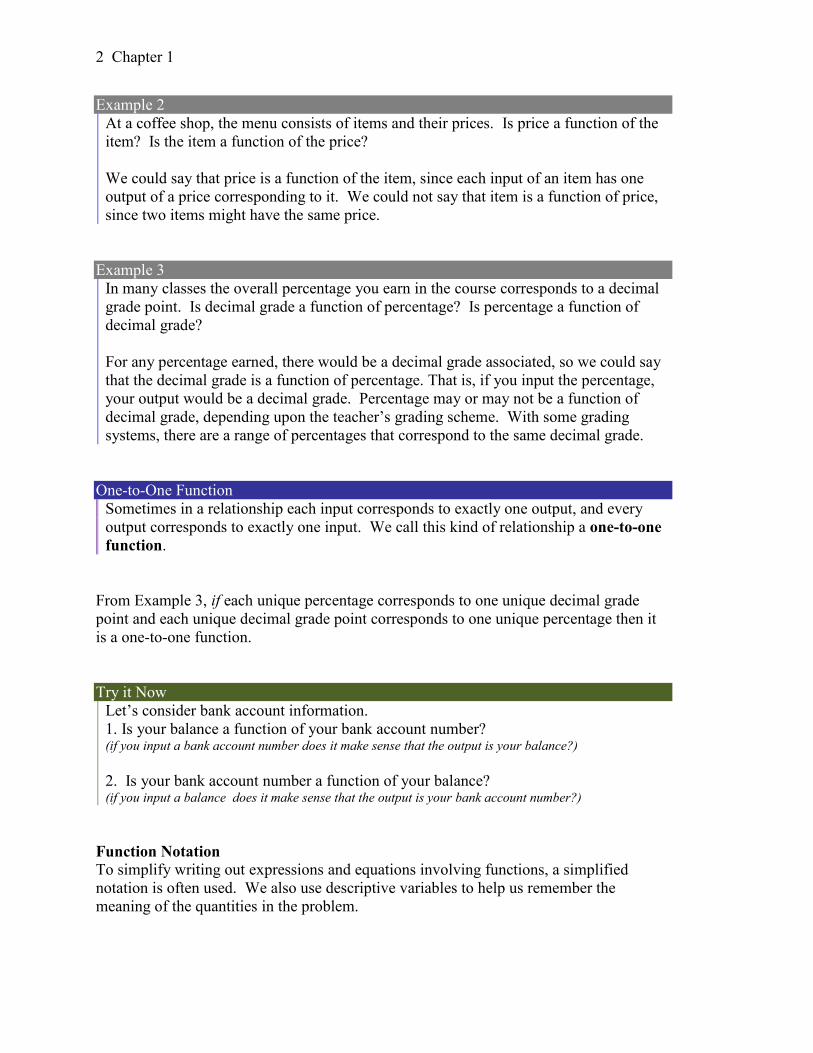
Function
Function: A rule for a relationship between an input, or independent, quantity and an
output, or dependent, quantity in which each input value uniquely determines one
output value. We say “the output is a function of the input.”
Example 1
In the height and age example above, is height a function of age? Is age a function of
height?
In the height and age example above, it would be correct to say that height is a function
of age, since each age uniquely determines a height. For example, on my 18th birthday,
I had exactly one height of 69 inches.
However, age is not a function of height, since one height input might correspond with
more than one output age. For example, for an input height of 70 inches, there is more
than one output of age since I was 70 inches at the age of 20 and 21.
2 Chapter 1
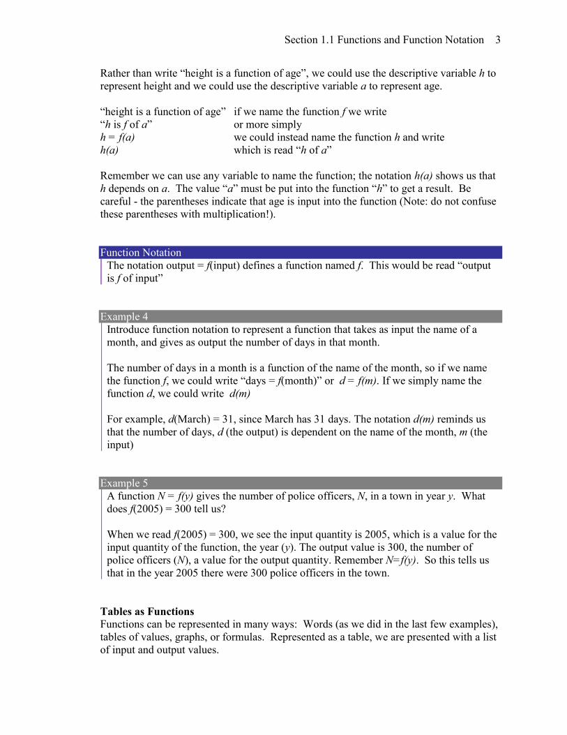
Example 2
At a coffee shop, the menu consists of items and their prices. Is price a function of the
item? Is the item a function of the price?
We could say that price is a function of the item, since each input of an item has one
output of a price corresponding to it. We could not say that item is a function of price,
since two items might have the same price.
Example 3
In many classes the overall percentage you earn in the course corresponds to a decimal
grade point. Is decimal grade a function of percentage? Is percentage a function of
decimal grade?
For any percentage earned, there would be a decimal grade associated, so we could say
that the decimal grade is a function of percentage. That is, if you input the percentage,
your output would be a decimal grade. Percentage may or may not be a function of
decimal grade, depending upon the teacher’s grading scheme. With some grading
systems, there are a range of percentages that correspond to the same decimal grade.
One-to-One Function
Sometimes in a relationship each input corresponds to exactly one output, and every
output corresponds to exactly one input. We call this kind of relationship a one-to-one
function.
From Example 3, if each unique percentage corresponds to one unique decimal grade
point and each unique decimal grade point corresponds to one unique percentage then it
is a one-to-one function.
Try it Now
Let’s consider bank account information.
1. Is your balance a function of your bank account number? (if you input a bank account number does it make sense that the output is your balance?)
2. Is your bank account number a function of your balance? (if you input a balance does it make sense that the output is your bank account number?)
Function Notation
To simplify writing out expressions and equations involving functions, a simplified
notation is often used. We also use descriptive variables to help us remember the
meaning of the quantities in the problem.
Section 1.1 Functions and Function Notation 3
Rather than write “height is a function of age”, we could use the descriptive variable h to
represent height and we could use the descriptive variable a to represent age.
“height is a function of age” if we name the function f we write
“h is f of a” or more simply
h = f(a) we could instead name the function h and write
h(a) which is read “h of a”
Remember we can use any variable to name the function; the notation h(a) shows us that
h depends on a. The value “a” must be put into the function “h” to get a result. Be
careful - the parentheses indicate that age is input into the function (Note: do not confuse
these parentheses with multiplication!).
Function Notation
The notation output = f(input) defines a function named f. This would be read “output
is f of input”
Example 4
Introduce function notation to represent a function that takes as input the name of a
month, and gives as output the number of days in that month.
The number of days in a month is a function of the name of the month, so if we name
the function f, we could write “days = f(month)” or d = f(m). If we simply name the
function d, we could write d(m)
For example, d(March) = 31, since March has 31 days. The notation d(m) reminds us
that the number of days, d (the output) is dependent on the name of the month, m (the
input)
Example 5
A function N = f(y) gives the number of police officers, N, in a town in year y. What
does f(2005) = 300 tell us?
When we read f(2005) = 300, we see the input quantity is 2005, which is a value for the
input quantity of the function, the year (y). The output value is 300, the number of
police officers (N), a value for the output quantity. Remember N=f(y). So this tells us
that in the year 2005 there were 300 police officers in the town.
Tables as Functions
Functions can be represented in many ways: Words (as we did in the last few examples),
tables of values, graphs, or formulas. Represented as a table, we are presented with a list
of input and output values.
4 Chapter 1
In some cases, these values represent everything we know about the relationship, while in
other cases the table is simply providing us a few select values from a more complete
relationship.
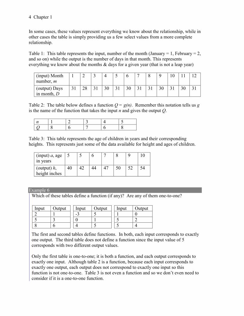
Table 1: This table represents the input, number of the month (January = 1, February = 2,
and so on) while the output is the number of days in that month. This represents
everything we know about the months & days for a given year (that is not a leap year)
(input) Month
number, m
1 2 3 4 5 6 7 8 9 10 11 12
(output) Days
in month, D
31 28 31 30 31 30 31 31 30 31 30 31
Table 2: The table below defines a function Q = g(n). Remember this notation tells us g
is the name of the function that takes the input n and gives the output Q.
n 1 2 3 4 5
Q 8 6 7 6 8
Table 3: This table represents the age of children in years and their corresponding
heights. This represents just some of the data available for height and ages of children.
(input) a, age
in years
5 5 6 7 8 9 10
(output) h,
height inches
40 42 44 47 50 52 54
Example 6
Which of these tables define a function (if any)? Are any of them one-to-one?
The first and second tables define functions. In both, each input corresponds to exactly
one output. The third table does not define a function since the input value of 5
corresponds with two different output values.
Only the first table is one-to-one; it is both a function, and each output corresponds to
exactly one input. Although table 2 is a function, because each input corresponds to
exactly one output, each output does not correspond to exactly one input so this
function is not one-to-one. Table 3 is not even a function and so we don’t even need to
consider if it is a one-to-one function.
Input Output
2 1
5 3
8 6
Input Output
-3 5
0 1
4 5
Input Output
1 0
5 2
5 4
Section 1.1 Functions and Function Notation 5
Try it Now
3. If each percentage earned translated to one letter grade, would this be a function? Is
it one-to-one?
Solving and Evaluating Functions:
When we work with functions, there are two typical things we do: evaluate and solve.
Evaluating a function is what we do when we know an input, and use the function to
determine the corresponding output. Evaluating will always produce one result, since
each input of a function corresponds to exactly one output.
Solving equations involving a function is what we do when we know an output, and use
the function to determine the inputs that would produce that output. Solving a function
could produce more than one solution, since different inputs can produce the same
output.
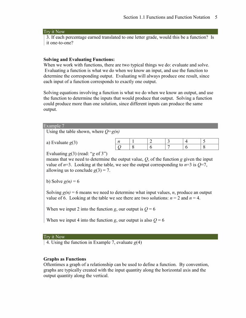
Example 7
Using the table shown, where Q=g(n)
a) Evaluate g(3)
Evaluating g(3) (read: “g of 3”)
means that we need to determine the output value, Q, of the function g given the input
value of n=3. Looking at the table, we see the output corresponding to n=3 is Q=7,
allowing us to conclude g(3) = 7.
b) Solve g(n) = 6
Solving g(n) = 6 means we need to determine what input values, n, produce an output
value of 6. Looking at the table we see there are two solutions: n = 2 and n = 4.
When we input 2 into the function g, our output is Q = 6
When we input 4 into the function g, our output is also Q = 6
Try it Now
4. Using the function in Example 7, evaluate g(4)
Graphs as Functions
Oftentimes a graph of a relationship can be used to define a function. By convention,
graphs are typically created with the input quantity along the horizontal axis and the
output quantity along the vertical.
n 1 2 3 4 5
Q 8 6 7 6 8
6 Chapter 1
The most common graph has y on the vertical axis and x on the horizontal axis, and we
say y is a function of x, or y = f(x) when the function is named f.
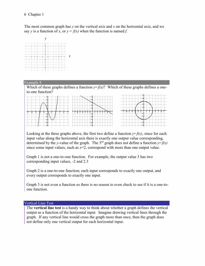
Example 8
Which of these graphs defines a function y=f(x)? Which of these graphs defines a one-
to-one function?
Looking at the three graphs above, the first two define a function y=f(x), since for each
input value along the horizontal axis there is exactly one output value corresponding,
determined by the y-value of the graph. The 3rd graph does not define a function y=f(x)
since some input values, such as x=2, correspond with more than one output value.
Graph 1 is not a one-to-one function. For example, the output value 3 has two
corresponding input values, -2 and 2.3
Graph 2 is a one-to-one function; each input corresponds to exactly one output, and
every output corresponds to exactly one input.
Graph 3 is not even a function so there is no reason to even check to see if it is a one-to-
one function.
Vertical Line Test
The vertical line test is a handy way to think about whether a graph defines the vertical
output as a function of the horizontal input. Imagine drawing vertical lines through the
graph. If any vertical line would cross the graph more than once, then the graph does
not define only one vertical output for each horizontal input.
x
y
Section 1.1 Functions and Function Notation 7
Horizontal Line Test
Once you have determined that a graph defines a function, an easy way to determine if
it is a one-to-one function is to use the horizontal line test. Draw horizontal lines
through the graph. If any horizontal line crosses the graph more than once, then the
graph does not define a one-to-one function.
Evaluating a function using a graph requires taking the given input and using the graph to
look up the corresponding output. Solving a function equation using a graph requires
taking the given output and looking on the graph to determine the corresponding input.
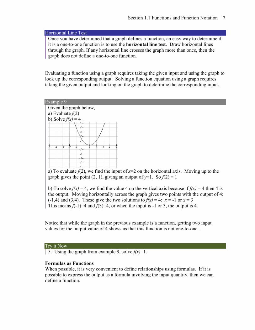
Example 9
Given the graph below,
a) Evaluate f(2)
b) Solve f(x) = 4
a) To evaluate f(2), we find the input of x=2 on the horizontal axis. Moving up to the
graph gives the point (2, 1), giving an output of y=1. So f(2) = 1
b) To solve f(x) = 4, we find the value 4 on the vertical axis because if f(x) = 4 then 4 is
the output. Moving horizontally across the graph gives two points with the output of 4:
(-1,4) and (3,4). These give the two solutions to f(x) = 4: x = -1 or x = 3
This means f(-1)=4 and f(3)=4, or when the input is -1 or 3, the output is 4.
Notice that while the graph in the previous example is a function, getting two input
values for the output value of 4 shows us that this function is not one-to-one.
Try it Now
5. Using the graph from example 9, solve f(x)=1.
Formulas as Functions
When possible, it is very convenient to define relationships using formulas. If it is
possible to express the output as a formula involving the input quantity, then we can
define a function.
8 Chapter 1
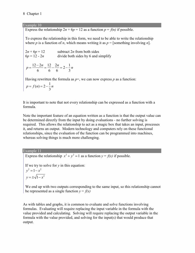
Example 10
Express the relationship 2n + 6p = 12 as a function p = f(n) if possible.
To express the relationship in this form, we need to be able to write the relationship
where p is a function of n, which means writing it as p = [something involving n].
2n + 6p = 12 subtract 2n from both sides
6p = 12 - 2n divide both sides by 6 and simplify
12 2 12 2 12
6 6 6 3
n np n
Having rewritten the formula as p=, we can now express p as a function:
1( ) 2
3p f n n
It is important to note that not every relationship can be expressed as a function with a
formula.
Note the important feature of an equation written as a function is that the output value can
be determined directly from the input by doing evaluations - no further solving is
required. This allows the relationship to act as a magic box that takes an input, processes
it, and returns an output. Modern technology and computers rely on these functional
relationships, since the evaluation of the function can be programmed into machines,
whereas solving things is much more challenging.
Example 11
Express the relationship 2 2 1x y as a function y = f(x) if possible.
If we try to solve for y in this equation: 2 21y x
21y x
We end up with two outputs corresponding to the same input, so this relationship cannot
be represented as a single function y = f(x)
As with tables and graphs, it is common to evaluate and solve functions involving
formulas. Evaluating will require replacing the input variable in the formula with the
value provided and calculating. Solving will require replacing the output variable in the
formula with the value provided, and solving for the input(s) that would produce that
output.
Section 1.1 Functions and Function Notation 9
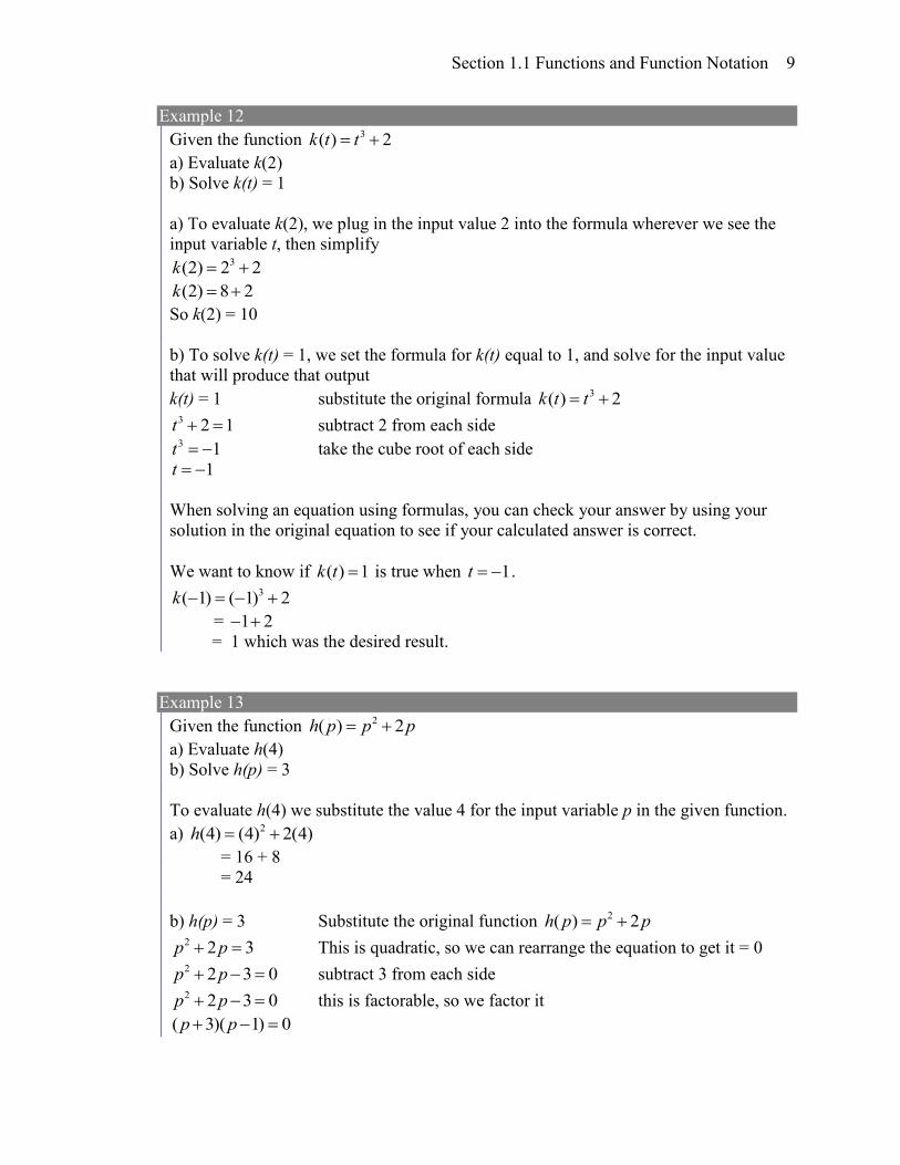
Example 12
Given the function 3( ) 2k t t
a) Evaluate k(2)
b) Solve k(t) = 1
a) To evaluate k(2), we plug in the input value 2 into the formula wherever we see the
input variable t, then simplify 3(2) 2 2k
(2) 8 2k
So k(2) = 10
b) To solve k(t) = 1, we set the formula for k(t) equal to 1, and solve for the input value
that will produce that output
k(t) = 1 substitute the original formula 3( ) 2k t t 3 2 1t subtract 2 from each side 3 1t take the cube root of each side
1t
When solving an equation using formulas, you can check your answer by using your
solution in the original equation to see if your calculated answer is correct.
We want to know if ( ) 1k t is true when 1t . 3( 1) ( 1) 2k
= 1 2
= 1 which was the desired result.
Example 13
Given the function 2( ) 2h p p p
a) Evaluate h(4)
b) Solve h(p) = 3
To evaluate h(4) we substitute the value 4 for the input variable p in the given function.
a) 2(4) (4) 2(4)h
= 16 + 8
= 24
b) h(p) = 3 Substitute the original function 2( ) 2h p p p 2 2 3p p This is quadratic, so we can rearrange the equation to get it = 0 2 2 3 0p p subtract 3 from each side 2 2 3 0p p this is factorable, so we factor it
( 3)( 1) 0p p
10 Chapter 1
By the zero factor theorem since ( 3)( 1) 0p p , either ( 3) 0p or ( 1) 0p (or
both of them equal 0) and so we solve both equations for p, finding p = -3 from the first
equation and p = 1 from the second equation.
This gives us the solution: h(p) = 3 when p = 1 or p = -3
We found two solutions in this case, which tells us this function is not one-to-one.
Try it Now
6. Given the function ( ) 4g m m
a. Evaluate g(5)
b. Solve g(m) = 2
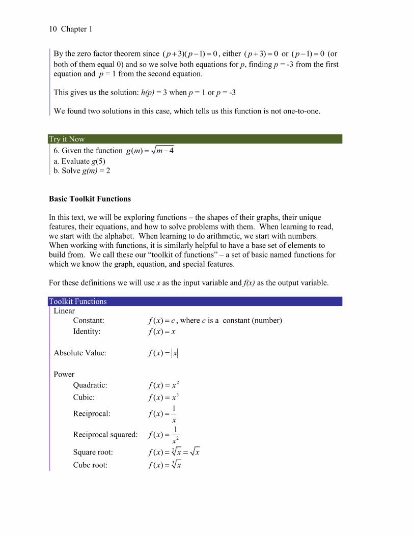
Basic Toolkit Functions
In this text, we will be exploring functions – the shapes of their graphs, their unique
features, their equations, and how to solve problems with them. When learning to read,
we start with the alphabet. When learning to do arithmetic, we start with numbers.
When working with functions, it is similarly helpful to have a base set of elements to
build from. We call these our “toolkit of functions” – a set of basic named functions for
which we know the graph, equation, and special features.
For these definitions we will use x as the input variable and f(x) as the output variable.
Toolkit Functions
Linear
Constant: ( )f x c , where c is a constant (number)
Identity: ( )f x x
Absolute Value: xxf )(
Power
Quadratic: 2)( xxf
Cubic: 3)( xxf
Reciprocal: 1
( )f xx
Reciprocal squared: 2
1( )f x
x
Square root: 2( )f x x x
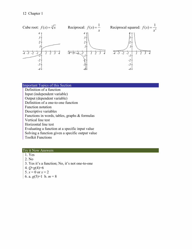
Cube root: 3( )f x x
Section 1.1 Functions and Function Notation 11
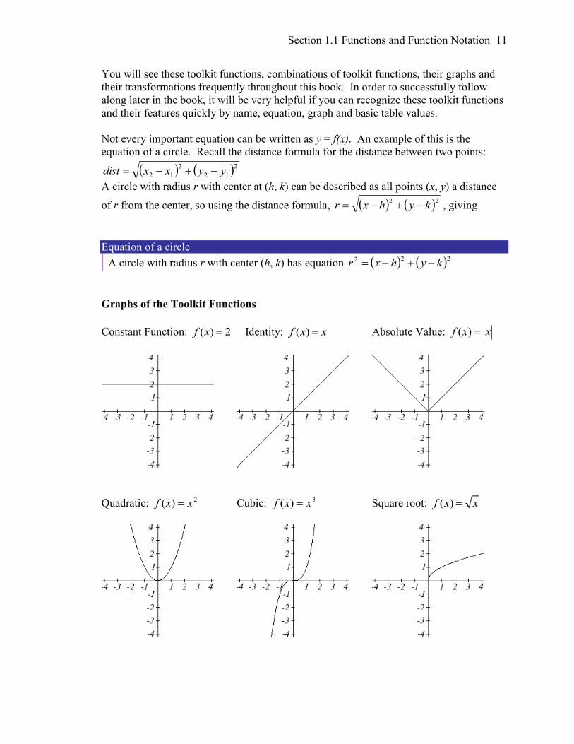
You will see these toolkit functions, combinations of toolkit functions, their graphs and
their transformations frequently throughout this book. In order to successfully follow
along later in the book, it will be very helpful if you can recognize these toolkit functions
and their features quickly by name, equation, graph and basic table values.
Not every important equation can be written as y = f(x). An example of this is the
equation of a circle. Recall the distance formula for the distance between two points:
2
12
2
12 yyxxdist
A circle with radius r with center at (h, k) can be described as all points (x, y) a distance
of r from the center, so using the distance formula, 22kyhxr , giving
Equation of a circle
A circle with radius r with center (h, k) has equation 222 kyhxr
Graphs of the Toolkit Functions
Constant Function: ( ) 2f x Identity: ( )f x x Absolute Value: xxf )(
Quadratic: 2)( xxf Cubic: 3)( xxf Square root: ( )f x x
12 Chapter 1
Cube root: 3( )f x x Reciprocal: 1
( )f xx
Reciprocal squared: 2
1( )f x
x
Important Topics of this Section
Definition of a function
Input (independent variable)
Output (dependent variable)
Definition of a one-to-one function
Function notation
Descriptive variables
Functions in words, tables, graphs & formulas
Vertical line test
Horizontal line test
Evaluating a function at a specific input value
Solving a function given a specific output value
Toolkit Functions
Try it Now Answers
1. Yes
2. No
3. Yes it’s a function; No, it’s not one-to-one
4. Q=g(4)=6
5. x = 0 or x = 2
6. a. g(5)=1 b. m = 8
Section 1.1 Functions and Function Notation 13
Section 1.1 Exercises
1. The amount of garbage, G, produced by a city with population p is given by
( )G f p . G is measured in tons per week, and p is measured in thousands of people.
a. The town of Tola has a population of 40,000 and produces 13 tons of garbage
each week. Express this information in terms of the function f.
b. Explain the meaning of the statement 5 2f .
2. The number of cubic yards of dirt, D, needed to cover a garden with area a square
feet is given by ( )D g a .
a. A garden with area 5000 ft2 requires 50 cubic yards of dirt. Express this
information in terms of the function g.
b. Explain the meaning of the statement 100 1g .
3. Let ( )f t be the number of ducks in a lake t years after 1990. Explain the meaning of
each statement:
a. 5 30f b. 10 40f
4. Let ( )h t be the height above ground, in feet, of a rocket t seconds after launching.
Explain the meaning of each statement:
a. 1 200h b. 2 350h
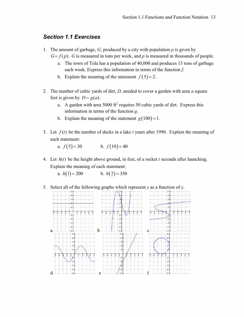
5. Select all of the following graphs which represent y as a function of x.
a b c
d e f
14 Chapter 1
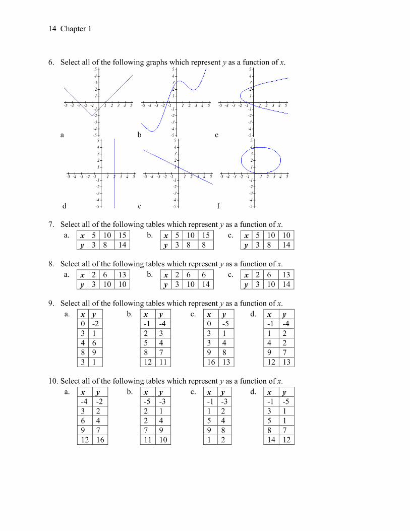
6. Select all of the following graphs which represent y as a function of x.
a b c
d e f
7. Select all of the following tables which represent y as a function of x.
a. x 5 10 15
y 3 8 14
b. x 5 10 15
y 3 8 8
c. x 5 10 10
y 3 8 14
8. Select all of the following tables which represent y as a function of x.
a. x 2 6 13
y 3 10 10
b. x 2 6 6
y 3 10 14
c. x 2 6 13
y 3 10 14
9. Select all of the following tables which represent y as a function of x.
a. x y
0 -2
3 1
4 6
8 9
3 1
b. x y
-1 -4
2 3
5 4
8 7
12 11
c. x y
0 -5
3 1
3 4
9 8
16 13
d. x y
-1 -4
1 2
4 2
9 7
12 13
10. Select all of the following tables which represent y as a function of x.
a. x y
-4 -2
3 2
6 4
9 7
12 16
b. x y
-5 -3
2 1
2 4
7 9
11 10
c. x y
-1 -3
1 2
5 4
9 8
1 2
d. x y
-1 -5
3 1
5 1
8 7
14 12
Section 1.1 Functions and Function Notation 15
11. Select all of the following tables which represent y as a function of x and are one-to-
one.
a. x 3 8 12
y 4 7 7
b. x 3 8 12
y 4 7 13
c. x 3 8 8
y 4 7 13
12. Select all of the following tables which represent y as a function of x and are one-to-
one.
a. x 2 8 8
y 5 6 13
b. x 2 8 14
y 5 6 6
c. x 2 8 14
y 5 6 13
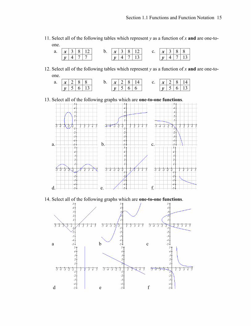
13. Select all of the following graphs which are one-to-one functions.
a. b. c.
d. e. f.
14. Select all of the following graphs which are one-to-one functions.
a b c
d e f
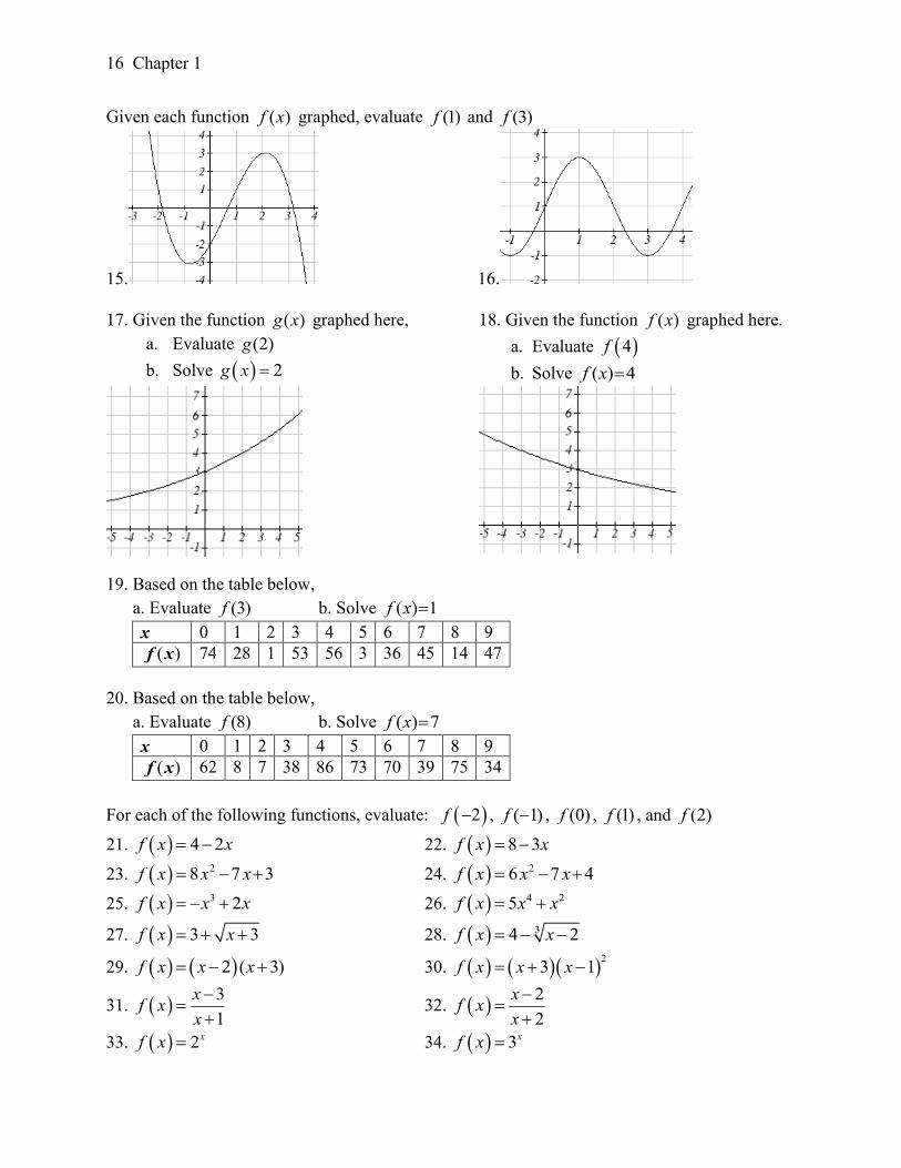
16 Chapter 1
Given each function ( )f x graphed, evaluate (1)f and (3)f
15. 16.
17. Given the function ( )g x graphed here,
a. Evaluate (2)g
b. Solve 2g x
18. Given the function ( )f x graphed here.
a. Evaluate 4f
b. Solve ( ) 4f x
19. Based on the table below,
a. Evaluate (3)f b. Solve ( ) 1 f x
x 0 1 2 3 4 5 6 7 8 9
( )f x 74 28 1 53 56 3 36 45 14 47
20. Based on the table below,
a. Evaluate (8)f b. Solve ( ) 7f x
x 0 1 2 3 4 5 6 7 8 9
( )f x 62 8 7 38 86 73 70 39 75 34
For each of the following functions, evaluate: 2f , ( 1)f , (0)f , (1)f , and (2)f
21. 4 2f x x 22. 8 3f x x
23. 28 7 3f x x x 24. 26 7 4f x x x
25. 3 2f x x x 26. 4 25f x x x
27. 3 3f x x 28. 34 2f x x
29. 2 ( 3)f x x x 30. 2
3 1f x x x
31. 3
1
xf x
x
32.
2
2
xf x
x
33. 2xf x 34. 3xf x
Section 1.1 Functions and Function Notation 17
35. Suppose 2 8 4f x x x . Compute the following:
a. ( 1) (1)f f b. ( 1) (1)f f
36. Suppose 2 3f x x x . Compute the following:
a. ( 2) (4)f f b. ( 2) (4)f f
37. Let 3 5f t t
a. Evaluate (0)f b. Solve 0f t
38. Let 6 2g p p
a. Evaluate (0)g b. Solve 0g p
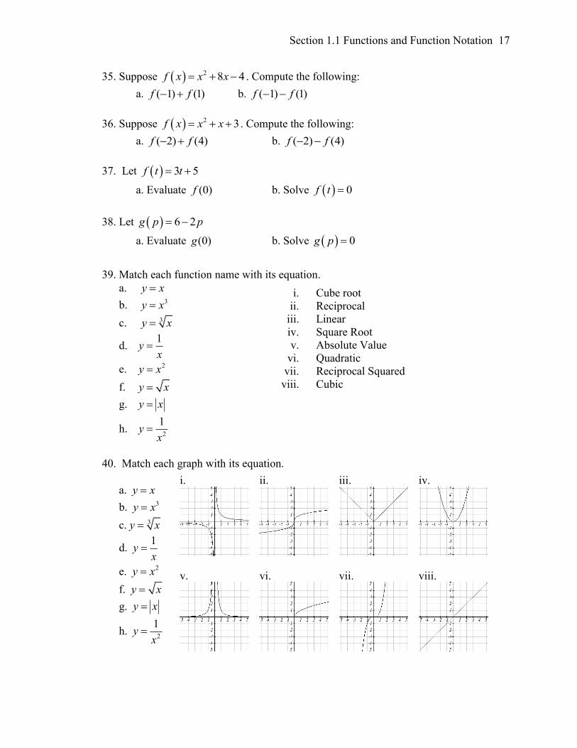
39. Match each function name with its equation.
a. y x
b. 3y x
c. 3y x
d. 1
yx
e. 2y x
f. y x
g. y x
h. 2
1y
x
40. Match each graph with its equation.
a. y x
b. 3y x
c. 3y x
d. 1
yx
e. 2y x
f. y x
g. y x
h. 2
1y
x
i. ii. iii. iv.
v.
vi.
vii.
viii.
i. Cube root
ii. Reciprocal
iii. Linear
iv. Square Root
v. Absolute Value
vi. Quadratic
vii. Reciprocal Squared
viii. Cubic
18 Chapter 1
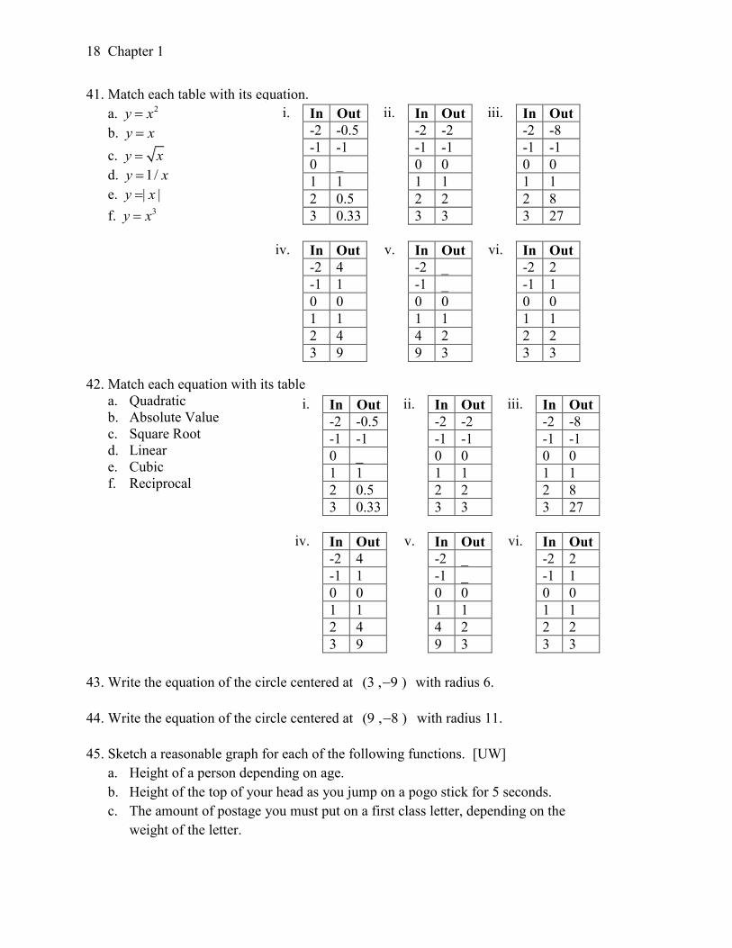
41. Match each table with its equation.
a. 2y x
b. y x
c. y x
d. 1/y x
e. | |y x
f. 3y x
42. Match each equation with its table
a. Quadratic
b. Absolute Value
c. Square Root
d. Linear
e. Cubic
f. Reciprocal
43. Write the equation of the circle centered at (3 , 9 ) with radius 6.
44. Write the equation of the circle centered at (9 , 8 ) with radius 11.
45. Sketch a reasonable graph for each of the following functions. [UW]
a. Height of a person depending on age.
b. Height of the top of your head as you jump on a pogo stick for 5 seconds.
c. The amount of postage you must put on a first class letter, depending on the
weight of the letter.
i. In Out
-2 -0.5
-1 -1
0 _
1 1
2 0.5
3 0.33
ii. In Out
-2 -2
-1 -1
0 0
1 1
2 2
3 3
iii. In Out
-2 -8
-1 -1
0 0
1 1
2 8
3 27
iv. In Out
-2 4
-1 1
0 0
1 1
2 4
3 9
v. In Out
-2 _
-1 _
0 0
1 1
4 2
9 3
vi. In Out
-2 2
-1 1
0 0
1 1
2 2
3 3
i. In Out
-2 -0.5
-1 -1
0 _
1 1
2 0.5
3 0.33
ii. In Out
-2 -2
-1 -1
0 0
1 1
2 2
3 3
iii. In Out
-2 -8
-1 -1
0 0
1 1
2 8
3 27
iv. In Out
-2 4
-1 1
0 0
1 1
2 4
3 9
v. In Out
-2 _
-1 _
0 0
1 1
4 2
9 3
vi. In Out
-2 2
-1 1
0 0
1 1
2 2
3 3
Section 1.1 Functions and Function Notation 19
46. Sketch a reasonable graph for each of the following functions. [UW]
a. Distance of your big toe from the ground as you ride your bike for 10 seconds.
b. Your height above the water level in a swimming pool after you dive off the high
board.
c. The percentage of dates and names you’ll remember for a history test, depending
on the time you study.
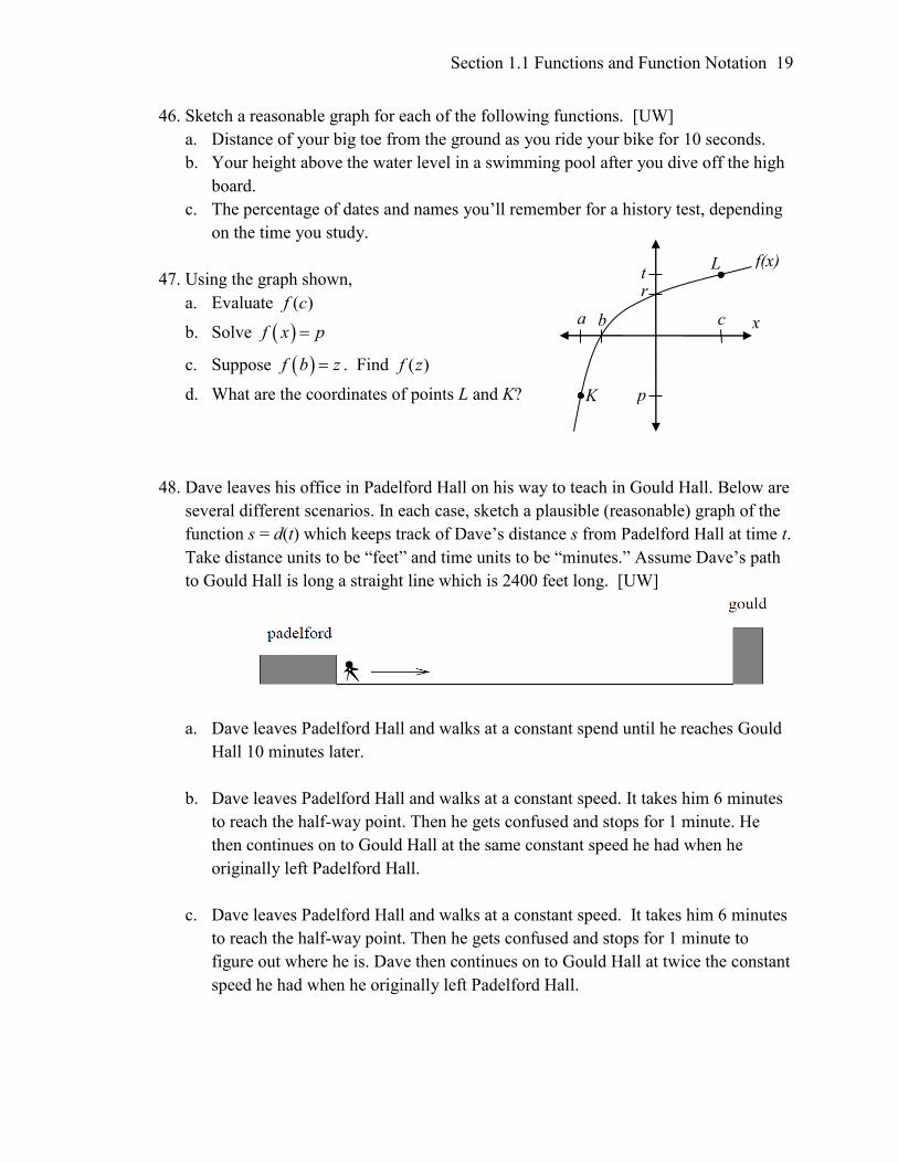
47. Using the graph shown,
a. Evaluate ( )f c
b. Solve f x p
c. Suppose f b z . Find ( )f z
d. What are the coordinates of points L and K?
48. Dave leaves his office in Padelford Hall on his way to teach in Gould Hall. Below are
several different scenarios. In each case, sketch a plausible (reasonable) graph of the
function s = d(t) which keeps track of Dave’s distance s from Padelford Hall at time t.
Take distance units to be “feet” and time units to be “minutes.” Assume Dave’s path
to Gould Hall is long a straight line which is 2400 feet long. [UW]
a. Dave leaves Padelford Hall and walks at a constant spend until he reaches Gould
Hall 10 minutes later.
b. Dave leaves Padelford Hall and walks at a constant speed. It takes him 6 minutes
to reach the half-way point. Then he gets confused and stops for 1 minute. He
then continues on to Gould Hall at the same constant speed he had when he
originally left Padelford Hall.
c. Dave leaves Padelford Hall and walks at a constant speed. It takes him 6 minutes
to reach the half-way point. Then he gets confused and stops for 1 minute to
figure out where he is. Dave then continues on to Gould Hall at twice the constant
speed he had when he originally left Padelford Hall.
x
f(x)
a b c
p
r t
K
L
20 Chapter 1
d. Dave leaves Padelford Hall and walks at a constant speed. It takes him 6 minutes
to reach the half-way point. Then he gets confused and stops for 1 minute to
figure out where he is. Dave is totally lost, so he simply heads back to his office,
walking the same constant speed he had when he originally left Padelford Hall.
e. Dave leaves Padelford heading for Gould Hall at the same instant Angela leaves
Gould Hall heading for Padelford Hall. Both walk at a constant speed, but Angela
walks twice as fast as Dave. Indicate a plot of “distance from Padelford” vs.
“time” for the both Angela and Dave.
f. Suppose you want to sketch the graph of a new function s = g(t) that keeps track
of Dave’s distance s from Gould Hall at time t. How would your graphs change in
(a)-(e)?
Section 1.2 Domain and Range 21
Section 1.2 Domain and Range
One of our main goals in mathematics is to model the real world with mathematical
functions. In doing so, it is important to keep in mind the limitations of those models we
create.
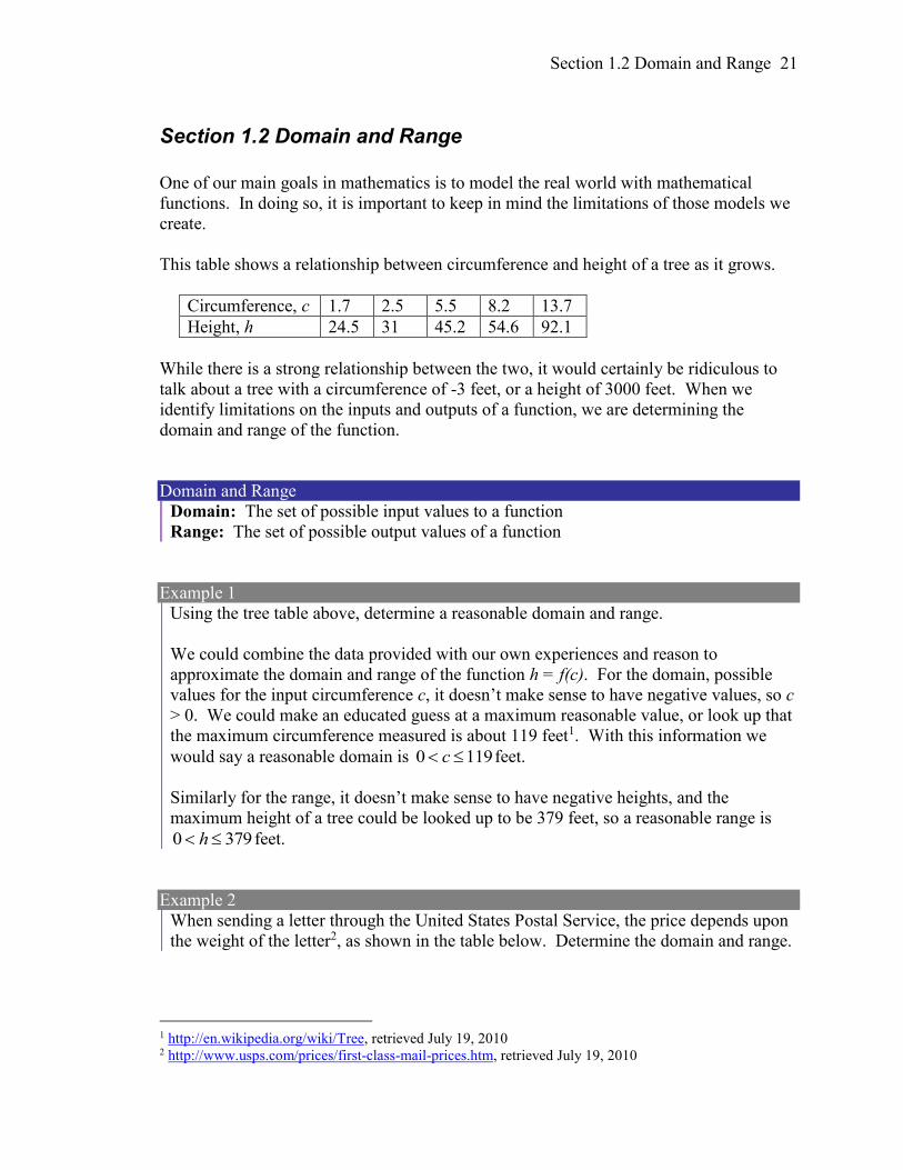
This table shows a relationship between circumference and height of a tree as it grows.
Circumference, c 1.7 2.5 5.5 8.2 13.7
Height, h 24.5 31 45.2 54.6 92.1
While there is a strong relationship between the two, it would certainly be ridiculous to
talk about a tree with a circumference of -3 feet, or a height of 3000 feet. When we
identify limitations on the inputs and outputs of a function, we are determining the
domain and range of the function.
Domain and Range
Domain: The set of possible input values to a function
Range: The set of possible output values of a function
Example 1
Using the tree table above, determine a reasonable domain and range.
We could combine the data provided with our own experiences and reason to
approximate the domain and range of the function h = f(c). For the domain, possible
values for the input circumference c, it doesn’t make sense to have negative values, so c
> 0. We could make an educated guess at a maximum reasonable value, or look up that
the maximum circumference measured is about 119 feet1. With this information we
would say a reasonable domain is 0 119c feet.
Similarly for the range, it doesn’t make sense to have negative heights, and the
maximum height of a tree could be looked up to be 379 feet, so a reasonable range is
0 379h feet.
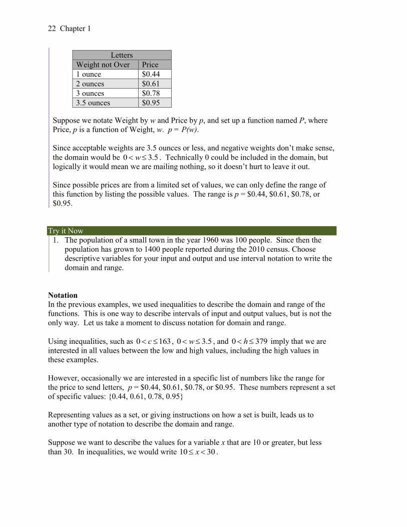
Example 2
When sending a letter through the United States Postal Service, the price depends upon
the weight of the letter2, as shown in the table below. Determine the domain and range.
1 http://en.wikipedia.org/wiki/Tree, retrieved July 19, 2010 2 http://www.usps.com/prices/first-class-mail-prices.htm, retrieved July 19, 2010
22 Chapter 1
Suppose we notate Weight by w and Price by p, and set up a function named P, where
Price, p is a function of Weight, w. p = P(w).
Since acceptable weights are 3.5 ounces or less, and negative weights don’t make sense,
the domain would be 0 3.5w . Technically 0 could be included in the domain, but
logically it would mean we are mailing nothing, so it doesn’t hurt to leave it out.
Since possible prices are from a limited set of values, we can only define the range of
this function by listing the possible values. The range is p = $0.44, $0.61, $0.78, or
$0.95.
Try it Now
1. The population of a small town in the year 1960 was 100 people. Since then the
population has grown to 1400 people reported during the 2010 census. Choose
descriptive variables for your input and output and use interval notation to write the
domain and range.
Notation
In the previous examples, we used inequalities to describe the domain and range of the
functions. This is one way to describe intervals of input and output values, but is not the
only way. Let us take a moment to discuss notation for domain and range.
Using inequalities, such as 0 163c , 0 3.5w , and 0 379h imply that we are
interested in all values between the low and high values, including the high values in
these examples.
However, occasionally we are interested in a specific list of numbers like the range for
the price to send letters, p = $0.44, $0.61, $0.78, or $0.95. These numbers represent a set
of specific values: {0.44, 0.61, 0.78, 0.95}
Representing values as a set, or giving instructions on how a set is built, leads us to
another type of notation to describe the domain and range.
Suppose we want to describe the values for a variable x that are 10 or greater, but less
than 30. In inequalities, we would write 10 30x .
Letters
Weight not Over Price
1 ounce $0.44
2 ounces $0.61
3 ounces $0.78
3.5 ounces $0.95
Section 1.2 Domain and Range 23
When describing domains and ranges, we sometimes extend this into set-builder
notation, which would look like this: |10 30x x . The curly brackets {} are read as
“the set of”, and the vertical bar | is read as “such that”, so altogether we would read
|10 30x x as “the set of x-values such that 10 is less than or equal to x and x is less
than 30.”
When describing ranges in set-builder notation, we could similarly write something like
( ) | 0 ( ) 100f x f x , or if the output had its own variable, we could use it. So for our
tree height example above, we could write for the range | 0 379h h . In set-builder
notation, if a domain or range is not limited, we could write | is a real numbert t , or
|t t , read as “the set of t-values such that t is an element of the set of real numbers.
A more compact alternative to set-builder notation is interval notation, in which
intervals of values are referred to by the starting and ending values. Curved parentheses
are used for “strictly less than,” and square brackets are used for “less than or equal to.”
Since infinity is not a number, we can’t include it in the interval, so we always use curved
parentheses with ∞ and -∞. The table below will help you see how inequalities
correspond to set-builder notation and interval notation:
Inequality Set Builder Notation Interval notation
5 10h | 5 10h h (5, 10]
5 10h | 5 10h h [5, 10)
5 10h | 5 10h h (5, 10)
10h | 10h h ( ,10)
10h | 10h h [10, )
all real numbers |h h ( , )
To combine two intervals together, using inequalities or set-builder notation we can use
the word “or”. In interval notation, we use the union symbol, , to combine two
unconnected intervals together.
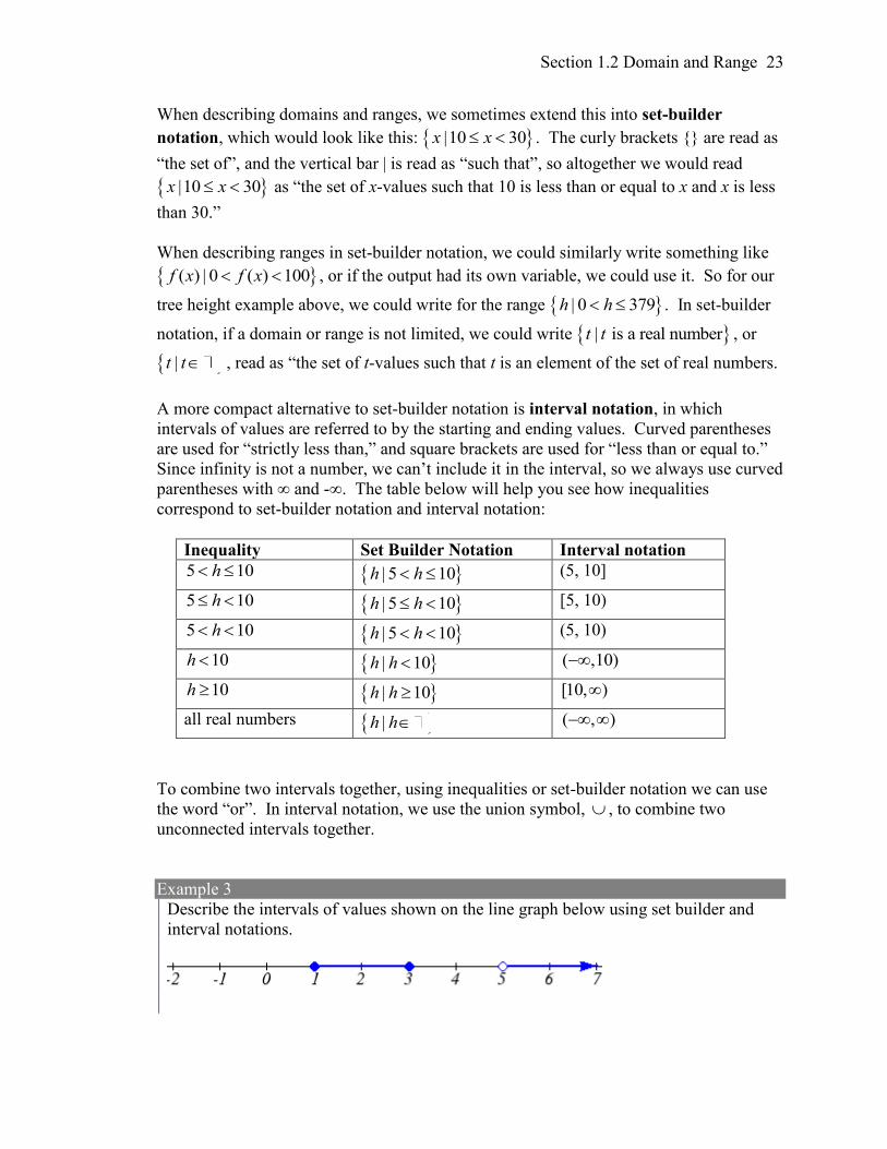
Example 3
Describe the intervals of values shown on the line graph below using set builder and
interval notations.
24 Chapter 1
To describe the values, x, that lie in the intervals shown above we would say, “x is a real
number greater than or equal to 1 and less than or equal to 3, or a real number greater
than 5.”
As an inequality it is: 1 3 or 5x x
In set builder notation: |1 3 or 5x x x
In interval notation: [1,3] (5, )
Remember when writing or reading interval notation:
Using a square bracket [ means the start value is included in the set
Using a parenthesis ( means the start value is not included in the set
Try it Now
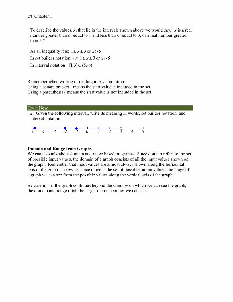
2. Given the following interval, write its meaning in words, set builder notation, and
interval notation.
Domain and Range from Graphs
We can also talk about domain and range based on graphs. Since domain refers to the set
of possible input values, the domain of a graph consists of all the input values shown on
the graph. Remember that input values are almost always shown along the horizontal
axis of the graph. Likewise, since range is the set of possible output values, the range of
a graph we can see from the possible values along the vertical axis of the graph.
Be careful – if the graph continues beyond the window on which we can see the graph,
the domain and range might be larger than the values we can see.
Section 1.2 Domain and Range 25
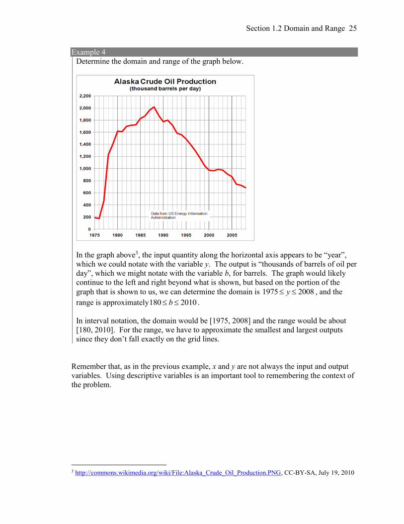
Example 4
Determine the domain and range of the graph below.
In the graph above3, the input quantity along the horizontal axis appears to be “year”,
which we could notate with the variable y. The output is “thousands of barrels of oil per
day”, which we might notate with the variable b, for barrels. The graph would likely
continue to the left and right beyond what is shown, but based on the portion of the
graph that is shown to us, we can determine the domain is 1975 2008y , and the
range is approximately180 2010b .
In interval notation, the domain would be [1975, 2008] and the range would be about
[180, 2010]. For the range, we have to approximate the smallest and largest outputs
since they don’t fall exactly on the grid lines.
Remember that, as in the previous example, x and y are not always the input and output
variables. Using descriptive variables is an important tool to remembering the context of
the problem.
3 http://commons.wikimedia.org/wiki/File:Alaska_Crude_Oil_Production.PNG, CC-BY-SA, July 19, 2010
26 Chapter 1
Try it Now
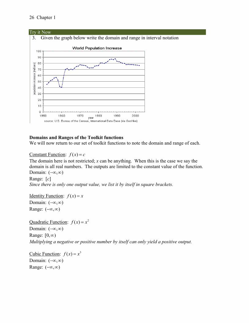
3. Given the graph below write the domain and range in interval notation
Domains and Ranges of the Toolkit functions
We will now return to our set of toolkit functions to note the domain and range of each.
Constant Function: ( )f x c
The domain here is not restricted; x can be anything. When this is the case we say the
domain is all real numbers. The outputs are limited to the constant value of the function.
Domain: ( , )
Range: [c]
Since there is only one output value, we list it by itself in square brackets.
Identity Function: ( )f x x
Domain: ( , )
Range: ( , )
Quadratic Function: 2( )f x x
Domain: ( , )
Range: [0, )
Multiplying a negative or positive number by itself can only yield a positive output.
Cubic Function: 3( )f x x
Domain: ( , )
Range: ( , )
Section 1.2 Domain and Range 27
Reciprocal: 1
( )f xx
Domain: ( ,0) (0, )
Range: ( ,0) (0, )
We cannot divide by 0 so we must exclude 0 from the domain.
One divide by any value can never be 0, so the range will not include 0.
Reciprocal squared: 2
1( )f x
x
Domain: ( ,0) (0, )
Range: (0, )
We cannot divide by 0 so we must exclude 0 from the domain.
Cube Root: 3( )f x x
Domain: ( , )
Range: ( , )
Square Root: 2( )f x x , commonly just written as, ( )f x x
Domain: [0, )
Range: [0, )
When dealing with the set of real numbers we cannot take the square root of a negative
number so the domain is limited to 0 or greater.
Absolute Value Function: ( )f x x
Domain: ( , )
Range: [0, )
Since absolute value is defined as a distance from 0, the output can only be greater than
or equal to 0.
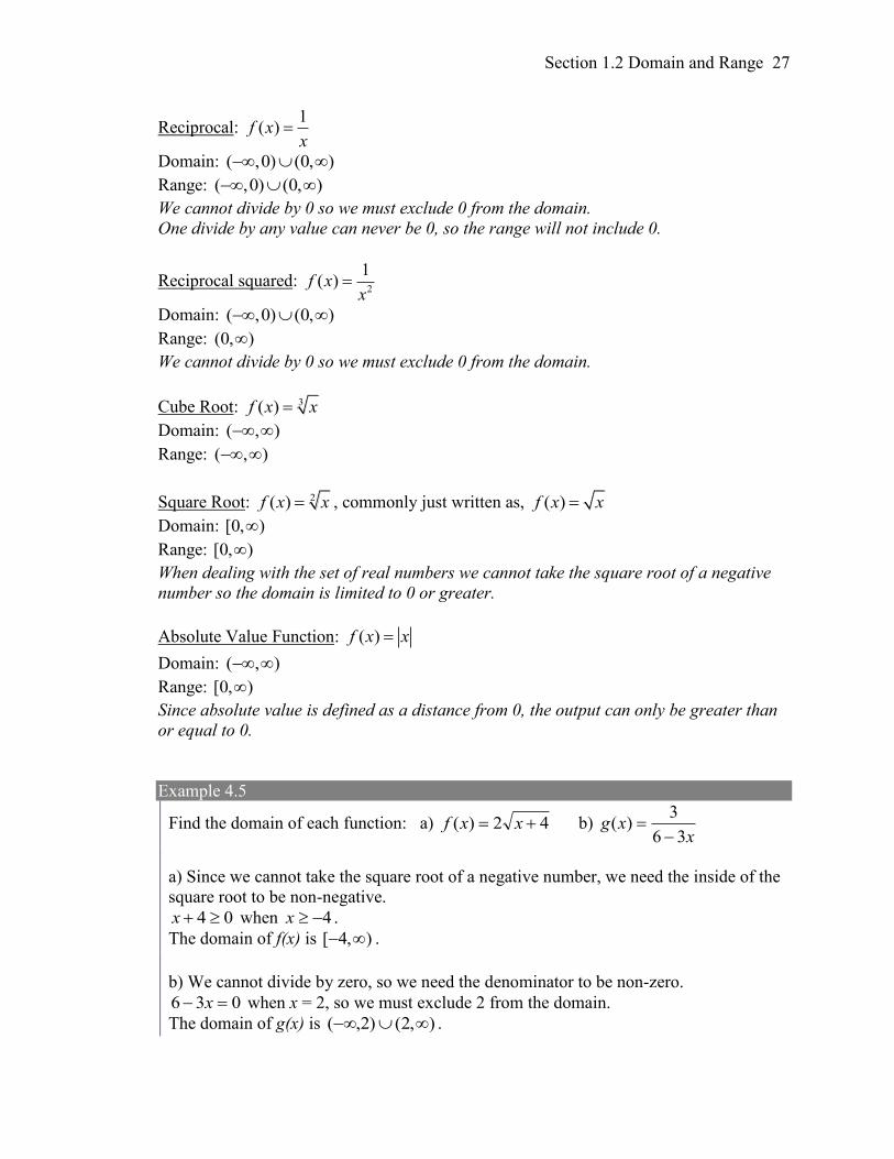
Example 4.5
Find the domain of each function: a) 42)( xxf b) x
xg36
3)(
a) Since we cannot take the square root of a negative number, we need the inside of the
square root to be non-negative.
04 x when 4x .
The domain of f(x) is ),4[ .
b) We cannot divide by zero, so we need the denominator to be non-zero.
036 x when x = 2, so we must exclude 2 from the domain.
The domain of g(x) is ),2()2,( .
28 Chapter 1
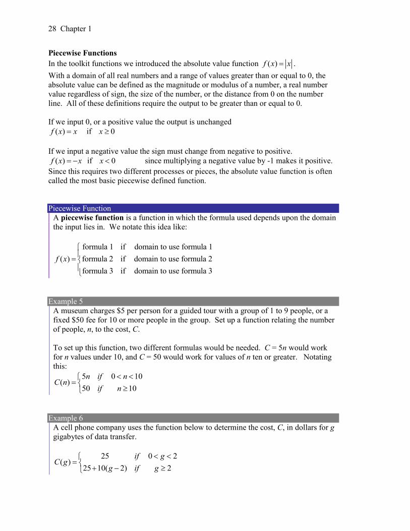
Piecewise Functions
In the toolkit functions we introduced the absolute value function ( )f x x .
With a domain of all real numbers and a range of values greater than or equal to 0, the
absolute value can be defined as the magnitude or modulus of a number, a real number
value regardless of sign, the size of the number, or the distance from 0 on the number
line. All of these definitions require the output to be greater than or equal to 0.
If we input 0, or a positive value the output is unchanged
( )f x x if 0x
If we input a negative value the sign must change from negative to positive.
( )f x x if 0x since multiplying a negative value by -1 makes it positive.
Since this requires two different processes or pieces, the absolute value function is often
called the most basic piecewise defined function.
Piecewise Function
A piecewise function is a function in which the formula used depends upon the domain
the input lies in. We notate this idea like:
formula 1 if domain to use formula 1
( ) formula 2 if domain to use formula 2
formula 3 if domain to use formula 3
f x
Example 5
A museum charges $5 per person for a guided tour with a group of 1 to 9 people, or a
fixed $50 fee for 10 or more people in the group. Set up a function relating the number
of people, n, to the cost, C.
To set up this function, two different formulas would be needed. C = 5n would work
for n values under 10, and C = 50 would work for values of n ten or greater. Notating
this:
5 0 10( )
50 10
n if nC n
if n
Example 6
A cell phone company uses the function below to determine the cost, C, in dollars for g
gigabytes of data transfer.
25 0 2( )
25 10( 2) 2
if gC g
g if g
Section 1.2 Domain and Range 29
Find the cost of using 1.5 gigabytes of data, and the cost of using 4 gigabytes of data.
To find the cost of using 1.5 gigabytes of data, C(1.5), we first look to see which piece
of domain our input falls in. Since 1.5 is less than 2, we use the first formula, giving
C(1.5) = $25.
The find the cost of using 4 gigabytes of data, C(4), we see that our input of 4 is greater
than 2, so we’ll use the second formula. C(4) = 25 + 10(4-2) = $45.
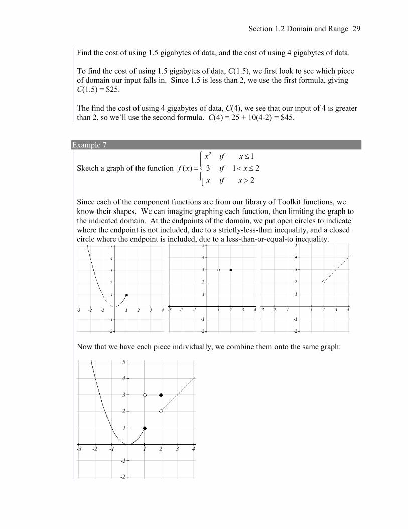
Example 7
Sketch a graph of the function
2 1
( ) 3 1 2
2
x if x
f x if x
x if x
Since each of the component functions are from our library of Toolkit functions, we
know their shapes. We can imagine graphing each function, then limiting the graph to
the indicated domain. At the endpoints of the domain, we put open circles to indicate
where the endpoint is not included, due to a strictly-less-than inequality, and a closed
circle where the endpoint is included, due to a less-than-or-equal-to inequality.
Now that we have each piece individually, we combine them onto the same graph:
30 Chapter 1
Try it Now
4. At Pierce College during the 2009-2010 school year tuition rates for in-state residents
were $89.50 per credit for the first 10 credits, $33 per credit for credits 11-18, and for
over 18 credits the rate is $73 per credit4. Write a piecewise defined function for the
total tuition, T, at Pierce College during 2009-2010 as a function of the number of
credits taken, c. Be sure to consider a reasonable domain and range.
Important Topics of this Section
Definition of domain
Definition of range
Inequalities
Interval notation
Set builder notation
Domain and Range from graphs
Domain and Range of toolkit functions
Piecewise defined functions
Try it Now Answers
1. Domain; y = years [1960,2010] ; Range, p = population, [100,1400]
2. a. Values that are less than or equal to -2, or values that are greater than or equal to -
1 and less than 3
b. | 2 1 3x x or x
c. ( , 2] [ 1,3)
3. Domain; y=years, [1952,2002] ; Range, p=population in millions, [40,88]
4.
18)18(731159
1810)10(33895
105.89
)(
cifc
cifc
cifc
cT Tuition, T, as a function of credits, c.
Reasonable domain should be whole numbers 0 to (answers may vary), e.g. [0,23]
Reasonable range should be $0 – (answers may vary), e.g. [0,1524]
4 https://www.pierce.ctc.edu/dist/tuition/ref/files/0910_tuition_rate.pdf, retrieved August 6, 2010
Section 1.2 Domain and Range 31
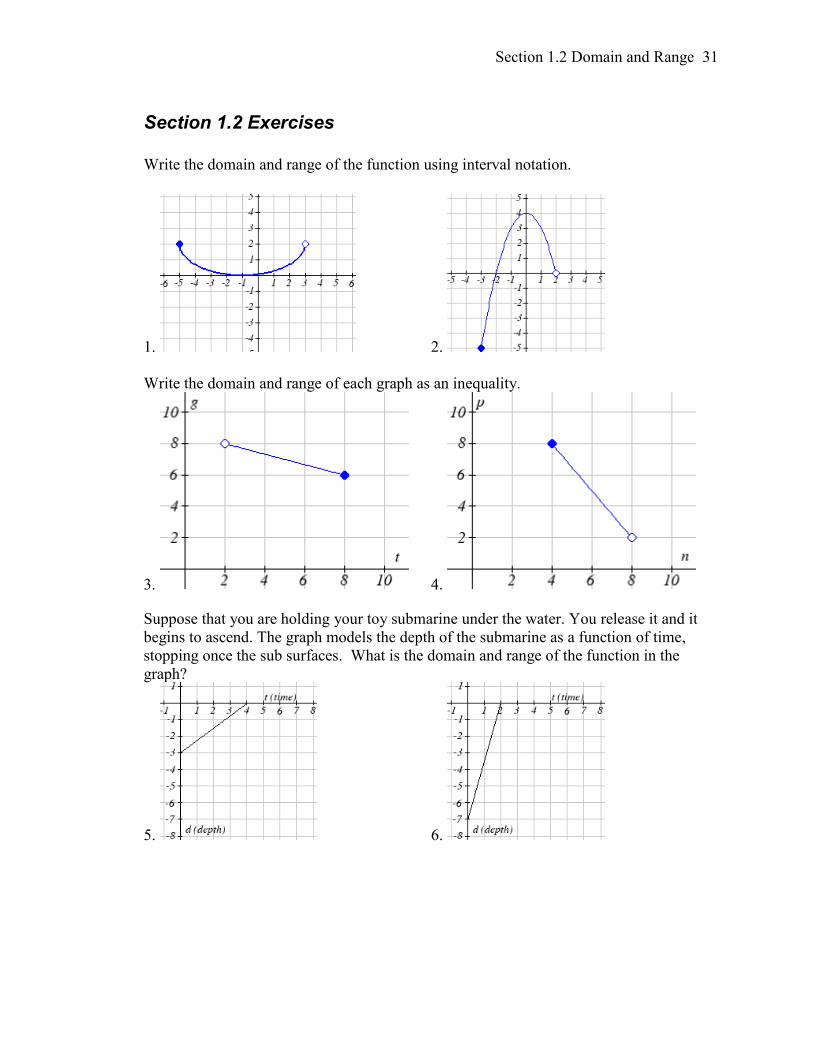
Section 1.2 Exercises
Write the domain and range of the function using interval notation.
1. 2.
Write the domain and range of each graph as an inequality.
3. 4.
Suppose that you are holding your toy submarine under the water. You release it and it
begins to ascend. The graph models the depth of the submarine as a function of time,
stopping once the sub surfaces. What is the domain and range of the function in the
graph?
5. 6.
32 Chapter 1
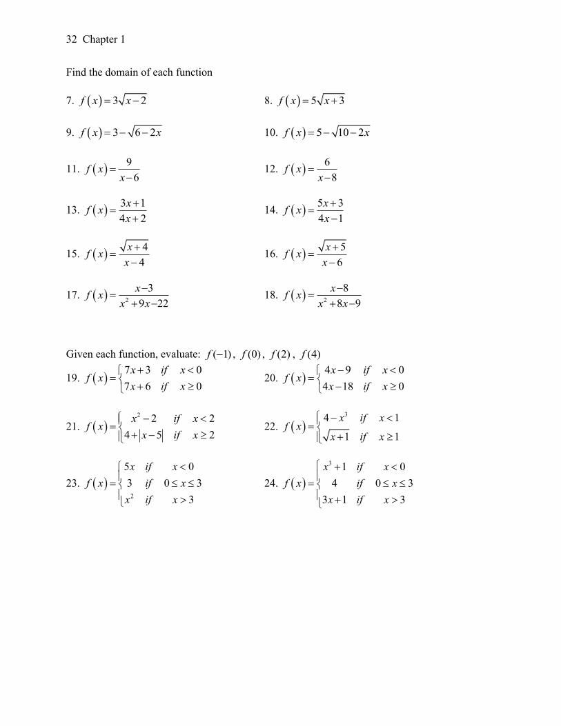
Find the domain of each function
7. 3 2f x x 8. 5 3f x x
9. 3 6 2f x x 10. 5 10 2f x x
11. 9
6f x
x
12.
6
8f x
x
13. 3 1
4 2
xf x
x
14.
5 3
4 1
xf x
x
15. 4
4
xf x
x
16.
5
6
xf x
x
17. 2
3
9 22
xf x
x x
18. 2
8
8 9
xf x
x x
Given each function, evaluate: ( 1)f , (0)f , (2)f , (4)f
19. 7 3 0
7 6 0
x if xf x
x if x
20.
4 9 0
4 18 0
x if xf x
x if x
21. 2 2 2
4 5 2
x if xf x
x if x
22.
34 1
1 1
x if xf x
x if x
23. 2
5 0
3 0 3
3
x if x
f x if x
x if x
24.
3 1 0
4 0 3
3 1 3
x if x
f x if x
x if x
Section 1.2 Domain and Range 33
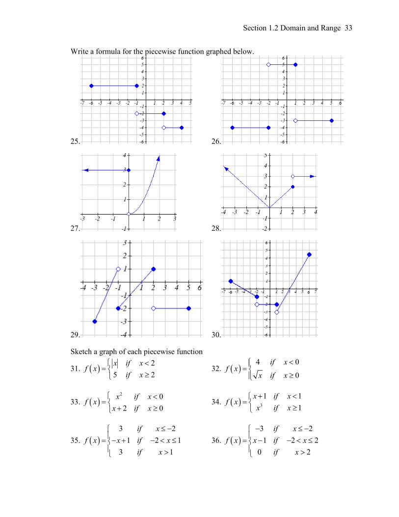
Write a formula for the piecewise function graphed below.
25. 26.
27. 28.
29. 30.
Sketch a graph of each piecewise function
31. 2
5 2
x if xf x
if x
32.
4 0
0
if xf x
x if x
33. 2 0
2 0
x if xf x
x if x
34. 3
1 1
1
x if xf x
x if x
35.
3 2
1 2 1
3 1
if x
f x x if x
if x
36.
3 2
1 2 2
0 2
if x
f x x if x
if x
34 Chapter 1
Section 1.3 Rates of Change and Behavior of Graphs
Since functions represent how an output quantity varies with an input quantity, it is
natural to ask about the rate at which the values of the function are changing.
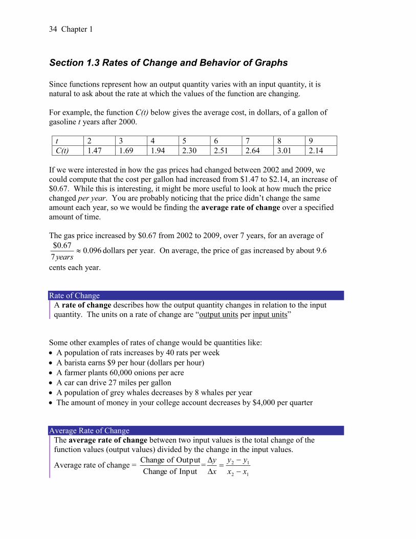
For example, the function C(t) below gives the average cost, in dollars, of a gallon of
gasoline t years after 2000.
t 2 3 4 5 6 7 8 9
C(t) 1.47 1.69 1.94 2.30 2.51 2.64 3.01 2.14
If we were interested in how the gas prices had changed between 2002 and 2009, we
could compute that the cost per gallon had increased from $1.47 to $2.14, an increase of
$0.67. While this is interesting, it might be more useful to look at how much the price
changed per year. You are probably noticing that the price didn’t change the same
amount each year, so we would be finding the average rate of change over a specified
amount of time.
The gas price increased by $0.67 from 2002 to 2009, over 7 years, for an average of
096.07
67.0$
yearsdollars per year. On average, the price of gas increased by about 9.6
cents each year.
Rate of Change
A rate of change describes how the output quantity changes in relation to the input
quantity. The units on a rate of change are “output units per input units”
Some other examples of rates of change would be quantities like:
A population of rats increases by 40 rats per week
A barista earns $9 per hour (dollars per hour)
A farmer plants 60,000 onions per acre
A car can drive 27 miles per gallon
A population of grey whales decreases by 8 whales per year
The amount of money in your college account decreases by $4,000 per quarter
Average Rate of Change
The average rate of change between two input values is the total change of the
function values (output values) divided by the change in the input values.
Average rate of change = Input of Change
Output of Change=
12
12
xx
yy
x
y
Section 1.3 Rates of Change and Behavior of Graphs 35
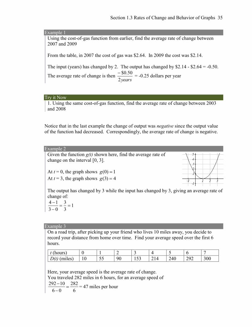
Example 1
Using the cost-of-gas function from earlier, find the average rate of change between
2007 and 2009
From the table, in 2007 the cost of gas was $2.64. In 2009 the cost was $2.14.
The input (years) has changed by 2. The output has changed by $2.14 - $2.64 = -0.50.
The average rate of change is then years2
50.0$ = -0.25 dollars per year
Try it Now
1. Using the same cost-of-gas function, find the average rate of change between 2003
and 2008
Notice that in the last example the change of output was negative since the output value
of the function had decreased. Correspondingly, the average rate of change is negative.
Example 2
Given the function g(t) shown here, find the average rate of
change on the interval [0, 3].
At t = 0, the graph shows 1)0( g
At t = 3, the graph shows 4)3( g
The output has changed by 3 while the input has changed by 3, giving an average rate of
change of:
13
3
03
14
Example 3
On a road trip, after picking up your friend who lives 10 miles away, you decide to
record your distance from home over time. Find your average speed over the first 6
hours.
Here, your average speed is the average rate of change.
You traveled 282 miles in 6 hours, for an average speed of
292 10 282
6 0 6
= 47 miles per hour
t (hours) 0 1 2 3 4 5 6 7
D(t) (miles) 10 55 90 153 214 240 292 300
36 Chapter 1
We can more formally state the average rate of change calculation using function
notation.
Average Rate of Change using Function Notation
Given a function f(x), the average rate of change on the interval [a, b] is
Average rate of change = ab
afbf
)()(
Input of Change
Output of Change
Example 4
Compute the average rate of change of x
xxf1
)( 2 on the interval [2, 4]
We can start by computing the function values at each endpoint of the interval
2
7
2
14
2
12)2( 2 f
4
63
4
116
4
14)4( 2 f
Now computing the average rate of change
Average rate of change = 8
49
2
4
49
24
2
7
4
63
24
)2()4(
ff
Try it Now
2. Find the average rate of change of xxxf 2)( on the interval [1, 9]
Example 5
The magnetic force F, measured in Newtons, between two magnets is related to the
distance between the magnets d, in centimeters, by the formula 2
2)(
ddF . Find the
average rate of change of force if the distance between the magnets is increased from 2
cm to 6 cm.
We are computing the average rate of change of 2
2)(
ddF on the interval [2, 6]
Average rate of change = 26
)2()6(
FF Evaluating the function
Section 1.3 Rates of Change and Behavior of Graphs 37
26
)2()6(
FF=
26
2
2
6
222
Simplifying
4
4
2
36
2
Combining the numerator terms
4
36
16
Simplifying further
9
1 Newtons per centimeter
This tells us the magnetic force decreases, on average, by 1/9 Newtons per centimeter
over this interval.
Example 6
Find the average rate of change of 13)( 2 tttg on the interval ],0[ a . Your answer
will be an expression involving a.
Using the average rate of change formula
0
)0()(
a
gag Evaluating the function
0
)1)0(30()13( 22
a
aa Simplifying
a
aa 1132 Simplifying further, and factoring
a
aa )3( Cancelling the common factor a
3a
This result tells us the average rate of change between t = 0 and any other point t = a.
For example, on the interval [0, 5], the average rate of change would be 5+3 = 8.
Try it Now
3. Find the average rate of change of 2)( 3 xxf on the interval ],[ haa .
38 Chapter 1
Graphical Behavior of Functions
As part of exploring how functions change, it is interesting to explore the graphical
behavior of functions.
Increasing/Decreasing
A function is increasing on an interval if the function values increase as the inputs
increase. More formally, a function is increasing if f(b) > f(a) for any two input values
a and b in the interval with b>a. The average rate of change of an increasing function
is positive.
A function is decreasing on an interval if the function values decrease as the inputs
increase. More formally, a function is decreasing if f(b) < f(a) for any two input values
a and b in the interval with b>a. The average rate of change of a decreasing function is
negative.
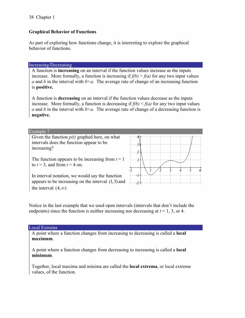
Example 7
Given the function p(t) graphed here, on what
intervals does the function appear to be
increasing?
The function appears to be increasing from t = 1
to t = 3, and from t = 4 on.
In interval notation, we would say the function
appears to be increasing on the interval (1,3) and
the interval ),4(
Notice in the last example that we used open intervals (intervals that don’t include the
endpoints) since the function is neither increasing nor decreasing at t = 1, 3, or 4.
Local Extrema
A point where a function changes from increasing to decreasing is called a local
maximum.
A point where a function changes from decreasing to increasing is called a local
minimum.
Together, local maxima and minima are called the local extrema, or local extreme
values, of the function.
Section 1.3 Rates of Change and Behavior of Graphs 39
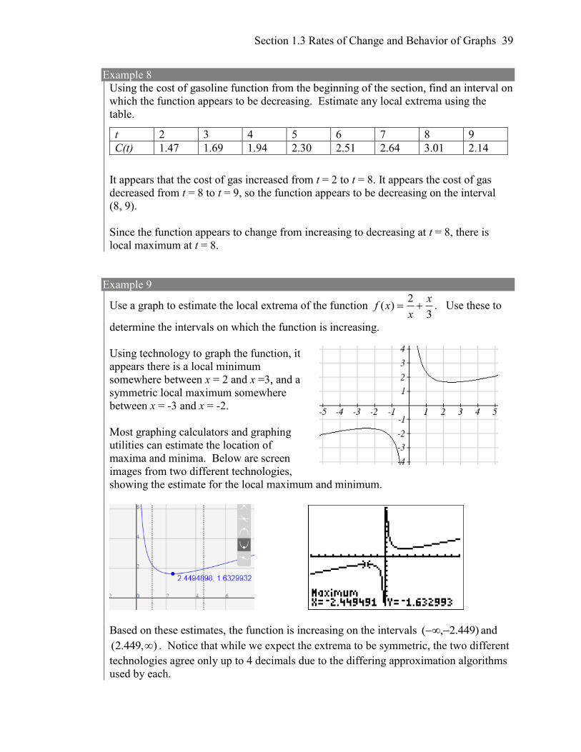
Example 8
Using the cost of gasoline function from the beginning of the section, find an interval on
which the function appears to be decreasing. Estimate any local extrema using the
table.
It appears that the cost of gas increased from t = 2 to t = 8. It appears the cost of gas
decreased from t = 8 to t = 9, so the function appears to be decreasing on the interval
(8, 9).
Since the function appears to change from increasing to decreasing at t = 8, there is
local maximum at t = 8.
Example 9
Use a graph to estimate the local extrema of the function 3
2)(
x
xxf . Use these to
determine the intervals on which the function is increasing.
Using technology to graph the function, it
appears there is a local minimum
somewhere between x = 2 and x =3, and a
symmetric local maximum somewhere
between x = -3 and x = -2.
Most graphing calculators and graphing
utilities can estimate the location of
maxima and minima. Below are screen
images from two different technologies,
showing the estimate for the local maximum and minimum.
Based on these estimates, the function is increasing on the intervals )449.2,( and
),449.2( . Notice that while we expect the extrema to be symmetric, the two different
technologies agree only up to 4 decimals due to the differing approximation algorithms
used by each.
t 2 3 4 5 6 7 8 9
C(t) 1.47 1.69 1.94 2.30 2.51 2.64 3.01 2.14
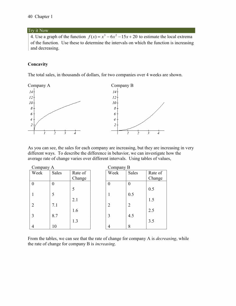
40 Chapter 1
Try it Now
4. Use a graph of the function 20156)( 23 xxxxf to estimate the local extrema
of the function. Use these to determine the intervals on which the function is increasing
and decreasing.
Concavity
The total sales, in thousands of dollars, for two companies over 4 weeks are shown.
Company A Company B
As you can see, the sales for each company are increasing, but they are increasing in very
different ways. To describe the difference in behavior, we can investigate how the
average rate of change varies over different intervals. Using tables of values,
From the tables, we can see that the rate of change for company A is decreasing, while
the rate of change for company B is increasing.
Company A
Week Sales Rate of
Change
0 0
5
1 5
2.1
2 7.1
1.6
3 8.7
1.3
4 10
Company B
Week Sales Rate of
Change
0 0
0.5
1 0.5
1.5
2 2
2.5
3 4.5
3.5
4 8
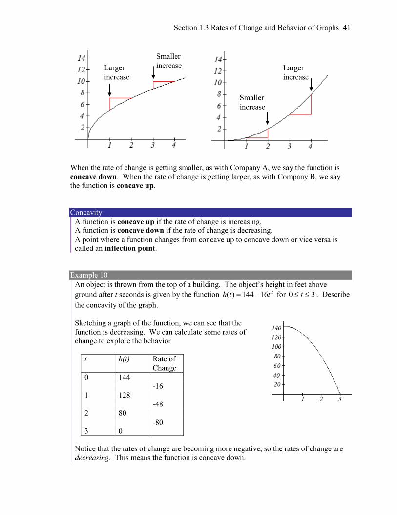
Section 1.3 Rates of Change and Behavior of Graphs 41
When the rate of change is getting smaller, as with Company A, we say the function is
concave down. When the rate of change is getting larger, as with Company B, we say
the function is concave up.
Concavity
A function is concave up if the rate of change is increasing.
A function is concave down if the rate of change is decreasing.
A point where a function changes from concave up to concave down or vice versa is
called an inflection point.
Example 10
An object is thrown from the top of a building. The object’s height in feet above
ground after t seconds is given by the function 216144)( tth for 30 t . Describe
the concavity of the graph.
Sketching a graph of the function, we can see that the
function is decreasing. We can calculate some rates of
change to explore the behavior
Notice that the rates of change are becoming more negative, so the rates of change are
decreasing. This means the function is concave down.
Larger
increase
Smaller
increase
Smaller
increase Larger
increase
t h(t) Rate of
Change
0 144
-16
1 128
-48
2 80
-80
3 0
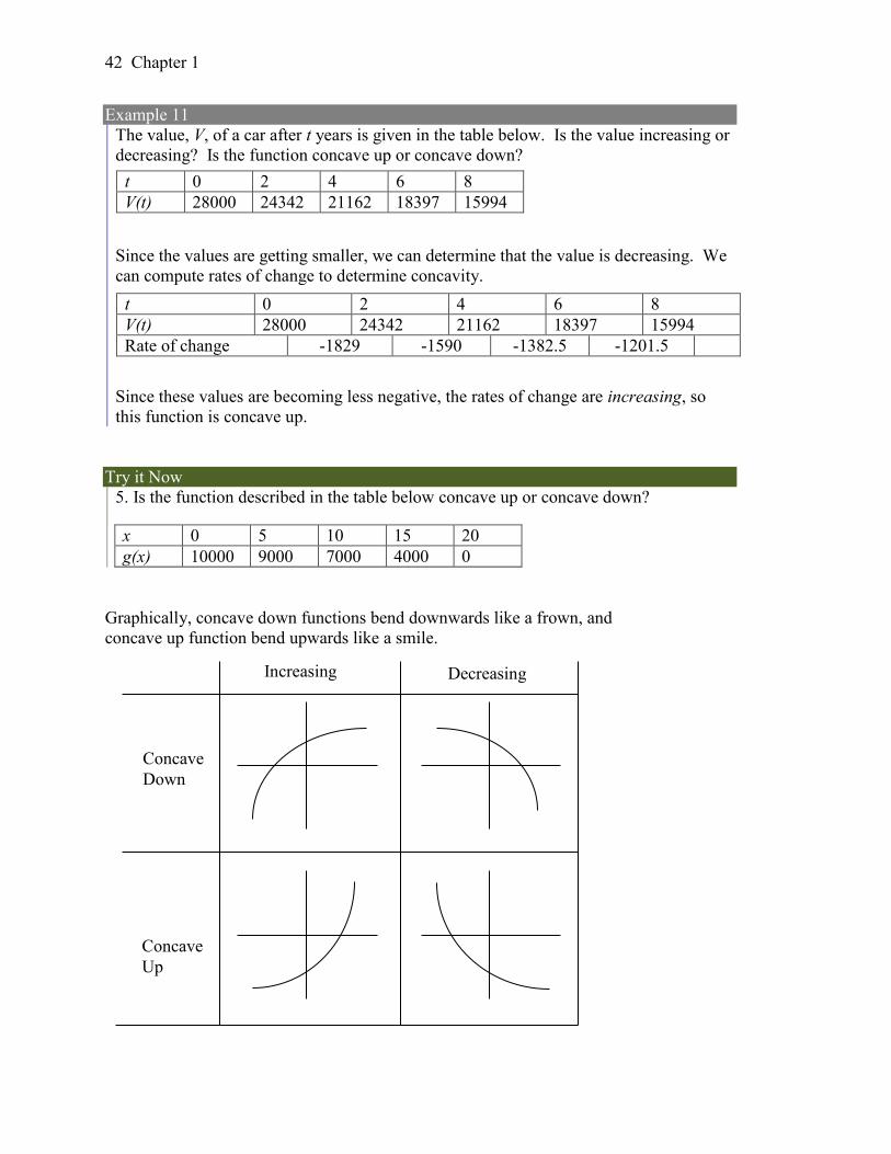
42 Chapter 1
Example 11
The value, V, of a car after t years is given in the table below. Is the value increasing or
decreasing? Is the function concave up or concave down?
Since the values are getting smaller, we can determine that the value is decreasing. We
can compute rates of change to determine concavity.
Since these values are becoming less negative, the rates of change are increasing, so
this function is concave up.
Try it Now
5. Is the function described in the table below concave up or concave down?
Graphically, concave down functions bend downwards like a frown, and
concave up function bend upwards like a smile.
Increasing Decreasing
Concave
Down
Concave
Up
t 0 2 4 6 8
V(t) 28000 24342 21162 18397 15994
t 0 2 4 6 8
V(t) 28000 24342 21162 18397 15994
Rate of change -1829 -1590 -1382.5 -1201.5
x 0 5 10 15 20
g(x) 10000 9000 7000 4000 0
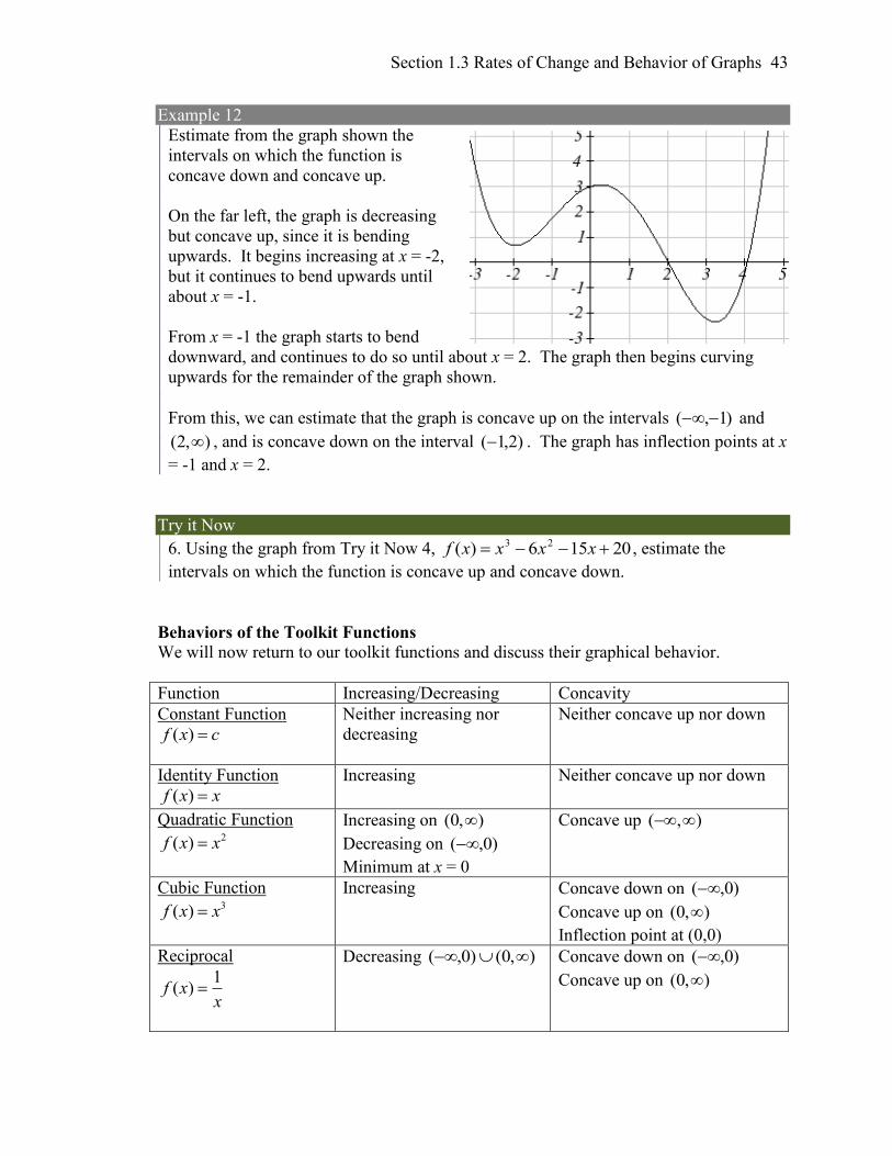
Section 1.3 Rates of Change and Behavior of Graphs 43
Example 12
Estimate from the graph shown the
intervals on which the function is
concave down and concave up.
On the far left, the graph is decreasing
but concave up, since it is bending
upwards. It begins increasing at x = -2,
but it continues to bend upwards until
about x = -1.
From x = -1 the graph starts to bend
downward, and continues to do so until about x = 2. The graph then begins curving
upwards for the remainder of the graph shown.
From this, we can estimate that the graph is concave up on the intervals )1,( and
),2( , and is concave down on the interval )2,1( . The graph has inflection points at x
= -1 and x = 2.
Try it Now
6. Using the graph from Try it Now 4, 20156)( 23 xxxxf , estimate the
intervals on which the function is concave up and concave down.
Behaviors of the Toolkit Functions We will now return to our toolkit functions and discuss their graphical behavior.
Function Increasing/Decreasing Concavity
Constant Function
( )f x c
Neither increasing nor
decreasing
Neither concave up nor down
Identity Function
( )f x x
Increasing Neither concave up nor down
Quadratic Function 2( )f x x
Increasing on ),0(
Decreasing on )0,(
Minimum at x = 0
Concave up ( , )
Cubic Function 3( )f x x
Increasing Concave down on )0,(
Concave up on ),0(
Inflection point at (0,0)
Reciprocal
1( )f x
x
Decreasing ),0()0,( Concave down on )0,(
Concave up on ),0(
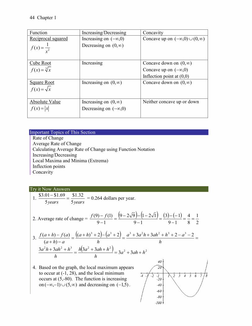
44 Chapter 1
Function Increasing/Decreasing Concavity
Reciprocal squared
2
1( )f x
x
Increasing on )0,(
Decreasing on ),0(
Concave up on ),0()0,(
Cube Root 3( )f x x
Increasing Concave down on ),0(
Concave up on )0,(
Inflection point at (0,0)
Square Root
( )f x x
Increasing on ),0( Concave down on ),0(
Absolute Value
( )f x x
Increasing on ),0(
Decreasing on )0,(
Neither concave up or down
Important Topics of This Section
Rate of Change
Average Rate of Change
Calculating Average Rate of Change using Function Notation
Increasing/Decreasing
Local Maxima and Minima (Extrema)
Inflection points
Concavity
Try it Now Answers
1. yearsyears 5
32.1$
5
69.1$01.3$
= 0.264 dollars per year.
2. Average rate of change =
2
1
8
4
19
13
19
121929
19
)1()9(
ff
3.
h
ahahhaa
h
aha
aha
afhaf 223322)(
)(
)()( 3322333
22
22322
333333
hahah
hahah
h
hahha
4. Based on the graph, the local maximum appears
to occur at (-1, 28), and the local minimum
occurs at (5,-80). The function is increasing
on ),5()1,( and decreasing on )5,1( .
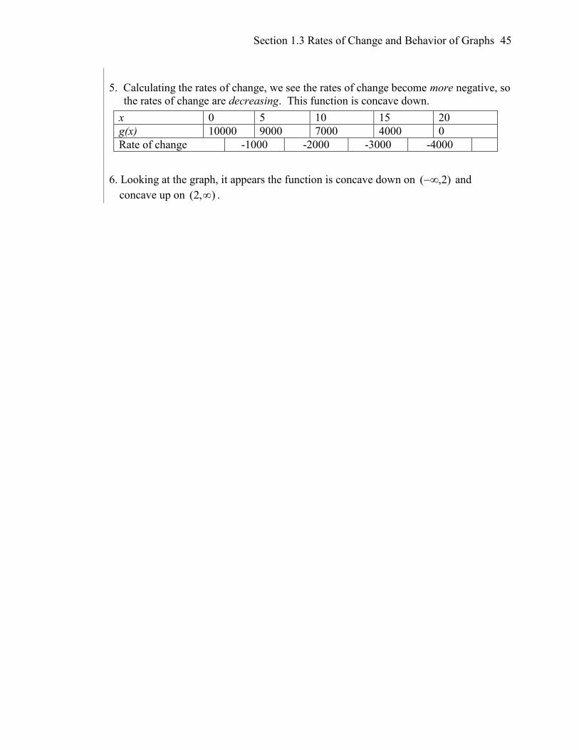
Section 1.3 Rates of Change and Behavior of Graphs 45
5. Calculating the rates of change, we see the rates of change become more negative, so
the rates of change are decreasing. This function is concave down.
6. Looking at the graph, it appears the function is concave down on )2,( and
concave up on ),2( .
x 0 5 10 15 20
g(x) 10000 9000 7000 4000 0
Rate of change -1000 -2000 -3000 -4000
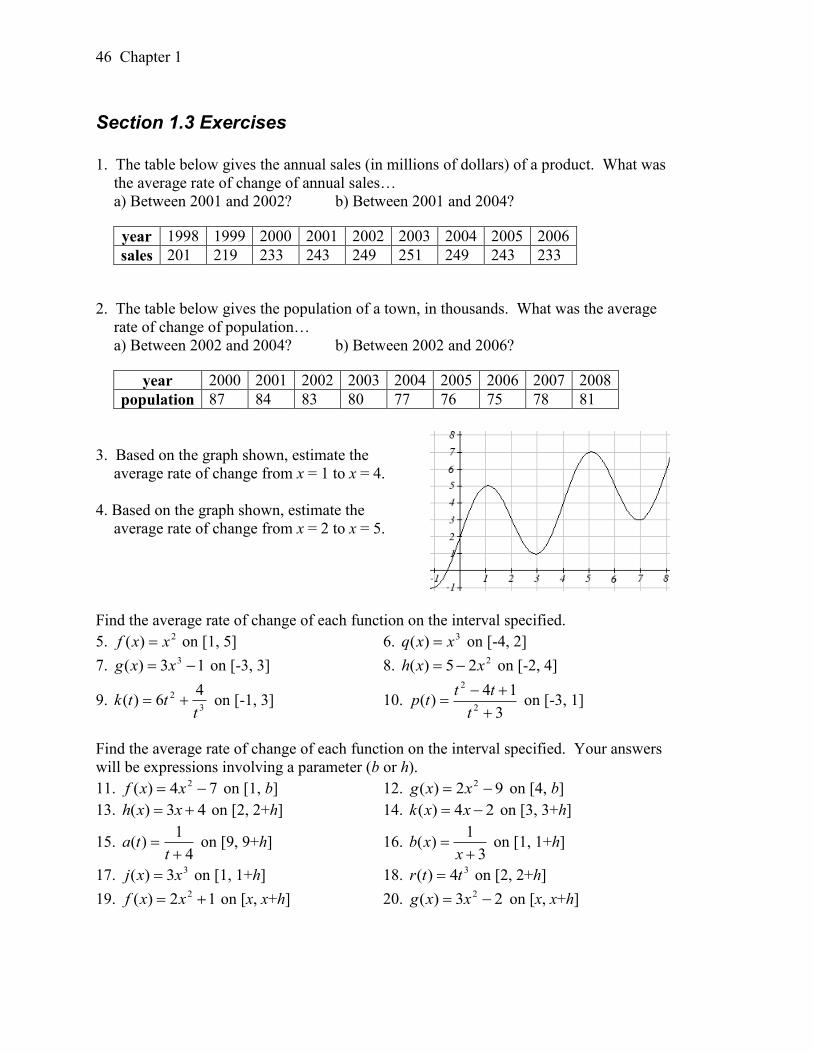
46 Chapter 1
Section 1.3 Exercises
1. The table below gives the annual sales (in millions of dollars) of a product. What was
the average rate of change of annual sales…
a) Between 2001 and 2002? b) Between 2001 and 2004?
year 1998 1999 2000 2001 2002 2003 2004 2005 2006
sales 201 219 233 243 249 251 249 243 233
2. The table below gives the population of a town, in thousands. What was the average
rate of change of population…
a) Between 2002 and 2004? b) Between 2002 and 2006?
year 2000 2001 2002 2003 2004 2005 2006 2007 2008
population 87 84 83 80 77 76 75 78 81
3. Based on the graph shown, estimate the
average rate of change from x = 1 to x = 4.
4. Based on the graph shown, estimate the
average rate of change from x = 2 to x = 5.
Find the average rate of change of each function on the interval specified.
5. 2)( xxf on [1, 5] 6. 3)( xxq on [-4, 2]
7. 13)( 3 xxg on [-3, 3] 8. 225)( xxh on [-2, 4]
9. 3
2 46)(
tttk on [-1, 3] 10.
3
14)(
2
2
t
tttp on [-3, 1]
Find the average rate of change of each function on the interval specified. Your answers
will be expressions involving a parameter (b or h).
11. 74)( 2 xxf on [1, b] 12. 92)( 2 xxg on [4, b]
13. 43)( xxh on [2, 2+h] 14. 24)( xxk on [3, 3+h]
15. 4
1)(
tta on [9, 9+h] 16.
3
1)(
xxb on [1, 1+h]
17. 33)( xxj on [1, 1+h] 18. 34)( ttr on [2, 2+h]
19. 12)( 2 xxf on [x, x+h] 20. 23)( 2 xxg on [x, x+h]
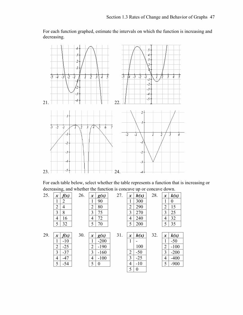
Section 1.3 Rates of Change and Behavior of Graphs 47
For each function graphed, estimate the intervals on which the function is increasing and
decreasing.
21. 22.
23. 24.
For each table below, select whether the table represents a function that is increasing or
decreasing, and whether the function is concave up or concave down.
25. x f(x)
1 2
2 4
3 8
4 16
5 32
26. x g(x)
1 90
2 80
3 75
4 72
5 70
27. x h(x)
1 300
2 290
3 270
4 240
5 200
28. x k(x)
1 0
2 15
3 25
4 32
5 35
29. x f(x)
1 -10
2 -25
3 -37
4 -47
5 -54
30. x g(x)
1 -200
2 -190
3 -160
4 -100
5 0
31. x h(x)
1 -
100
2 -50
3 -25
4 -10
5 0
32. x k(x)
1 -50
2 -100
3 -200
4 -400
5 -900
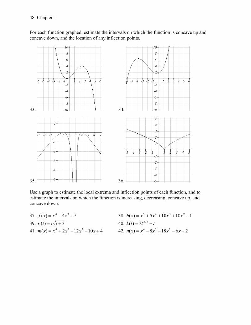
48 Chapter 1
For each function graphed, estimate the intervals on which the function is concave up and
concave down, and the location of any inflection points.
33. 34.
35. 36.
Use a graph to estimate the local extrema and inflection points of each function, and to
estimate the intervals on which the function is increasing, decreasing, concave up, and
concave down.
37. 54)( 34 xxxf 38. 110105)( 2345 xxxxxh
39. 3)( tttg 40. tttk 3/23)(
41. 410122)( 234 xxxxxm 42. 26188)( 234 xxxxxn
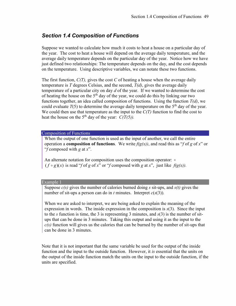
Section 1.4 Composition of Functions 49
Section 1.4 Composition of Functions
Suppose we wanted to calculate how much it costs to heat a house on a particular day of
the year. The cost to heat a house will depend on the average daily temperature, and the
average daily temperature depends on the particular day of the year. Notice how we have
just defined two relationships: The temperature depends on the day, and the cost depends
on the temperature. Using descriptive variables, we can notate these two functions.
The first function, C(T), gives the cost C of heating a house when the average daily
temperature is T degrees Celsius, and the second, T(d), gives the average daily
temperature of a particular city on day d of the year. If we wanted to determine the cost
of heating the house on the 5th day of the year, we could do this by linking our two
functions together, an idea called composition of functions. Using the function T(d), we
could evaluate T(5) to determine the average daily temperature on the 5th day of the year.
We could then use that temperature as the input to the C(T) function to find the cost to
heat the house on the 5th day of the year: C(T(5)).
Composition of Functions
When the output of one function is used as the input of another, we call the entire
operation a composition of functions. We write f(g(x)), and read this as “f of g of x” or
“f composed with g at x”.
An alternate notation for composition uses the composition operator:
))(( xgf is read “f of g of x” or “f composed with g at x”, just like f(g(x)).
Example 1
Suppose c(s) gives the number of calories burned doing s sit-ups, and s(t) gives the
number of sit-ups a person can do in t minutes. Interpret c(s(3)).
When we are asked to interpret, we are being asked to explain the meaning of the
expression in words. The inside expression in the composition is s(3). Since the input
to the s function is time, the 3 is representing 3 minutes, and s(3) is the number of sit-
ups that can be done in 3 minutes. Taking this output and using it as the input to the
c(s) function will gives us the calories that can be burned by the number of sit-ups that
can be done in 3 minutes.
Note that it is not important that the same variable be used for the output of the inside
function and the input to the outside function. However, it is essential that the units on
the output of the inside function match the units on the input to the outside function, if the
units are specified.
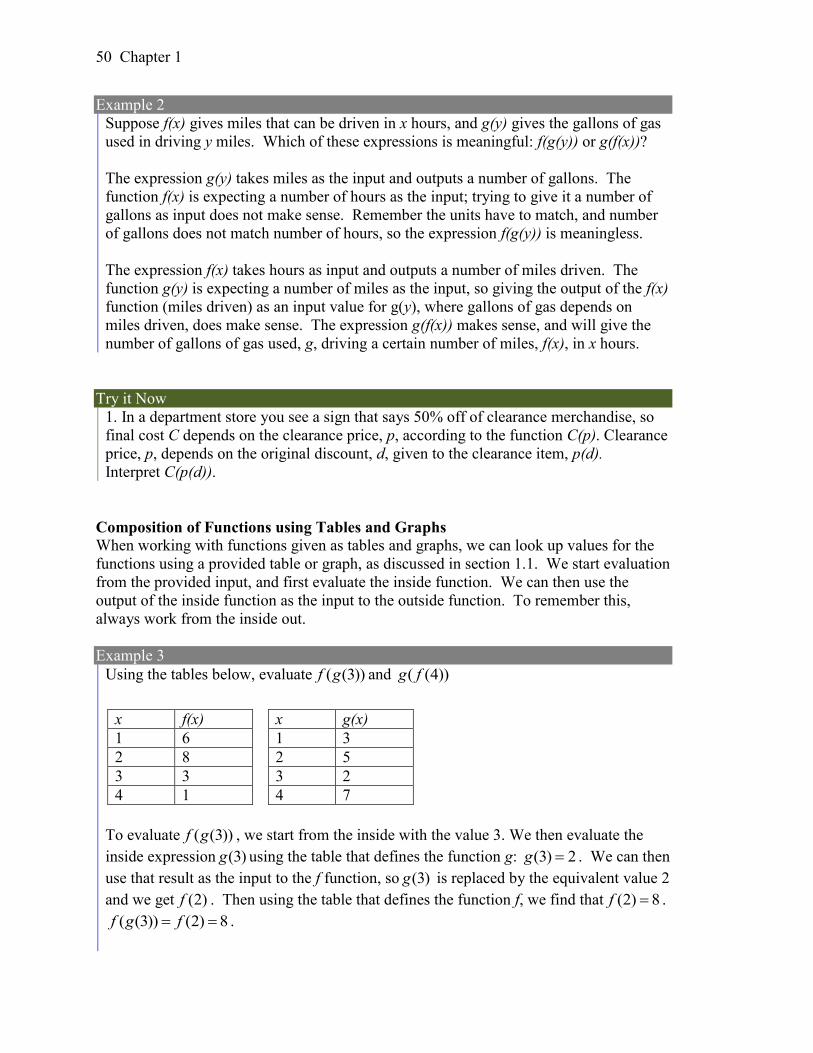
50 Chapter 1
Example 2
Suppose f(x) gives miles that can be driven in x hours, and g(y) gives the gallons of gas
used in driving y miles. Which of these expressions is meaningful: f(g(y)) or g(f(x))?
The expression g(y) takes miles as the input and outputs a number of gallons. The
function f(x) is expecting a number of hours as the input; trying to give it a number of
gallons as input does not make sense. Remember the units have to match, and number
of gallons does not match number of hours, so the expression f(g(y)) is meaningless.
The expression f(x) takes hours as input and outputs a number of miles driven. The
function g(y) is expecting a number of miles as the input, so giving the output of the f(x)
function (miles driven) as an input value for g(y), where gallons of gas depends on
miles driven, does make sense. The expression g(f(x)) makes sense, and will give the
number of gallons of gas used, g, driving a certain number of miles, f(x), in x hours.
Try it Now
1. In a department store you see a sign that says 50% off of clearance merchandise, so
final cost C depends on the clearance price, p, according to the function C(p). Clearance
price, p, depends on the original discount, d, given to the clearance item, p(d).
Interpret C(p(d)).
Composition of Functions using Tables and Graphs
When working with functions given as tables and graphs, we can look up values for the
functions using a provided table or graph, as discussed in section 1.1. We start evaluation
from the provided input, and first evaluate the inside function. We can then use the
output of the inside function as the input to the outside function. To remember this,
always work from the inside out.
Example 3
Using the tables below, evaluate ( (3))f g and ( (4))g f
To evaluate ( (3))f g , we start from the inside with the value 3. We then evaluate the
inside expression (3)g using the table that defines the function g: (3) 2g . We can then
use that result as the input to the f function, so (3)g is replaced by the equivalent value 2
and we get (2)f . Then using the table that defines the function f, we find that (2) 8f .
( (3)) (2) 8f g f .
x f(x)
1 6
2 8
3 3
4 1
x g(x)
1 3
2 5
3 2
4 7
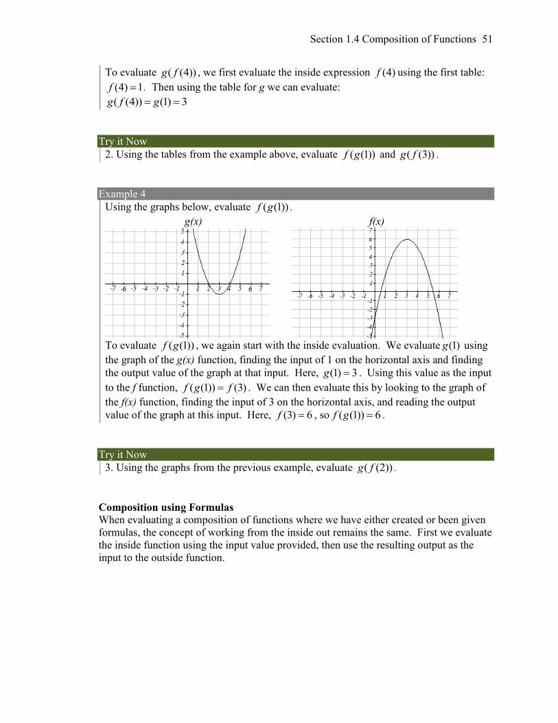
Section 1.4 Composition of Functions 51
To evaluate ( (4))g f , we first evaluate the inside expression (4)f using the first table:
(4) 1f . Then using the table for g we can evaluate:
( (4)) (1) 3g f g
Try it Now
2. Using the tables from the example above, evaluate ( (1))f g and ( (3))g f .
Example 4
Using the graphs below, evaluate ( (1))f g .
g(x) f(x)
To evaluate ( (1))f g , we again start with the inside evaluation. We evaluate (1)g using
the graph of the g(x) function, finding the input of 1 on the horizontal axis and finding
the output value of the graph at that input. Here, (1) 3g . Using this value as the input
to the f function, ( (1)) (3)f g f . We can then evaluate this by looking to the graph of
the f(x) function, finding the input of 3 on the horizontal axis, and reading the output
value of the graph at this input. Here, (3) 6f , so ( (1)) 6f g .
Try it Now
3. Using the graphs from the previous example, evaluate ( (2))g f .
Composition using Formulas
When evaluating a composition of functions where we have either created or been given
formulas, the concept of working from the inside out remains the same. First we evaluate
the inside function using the input value provided, then use the resulting output as the
input to the outside function.
52 Chapter 1
Example 5
Given tttf 2)( and 23)( xxh , evaluate ( (1))f h .
Since the inside evaluation is (1)h we start by evaluating the h(x) function at 1:
52)1(3)1( h
Then ( (1)) (5)f h f , so we evaluate the f(t) function at an input of 5:
2055)5())1(( 2 fhf
Try it Now
4. Using the functions from the example above, evaluate ( ( 2))h f .
While we can compose the functions as above for each individual input value, sometimes
it would be really helpful to find a single formula which will calculate the result of a
composition f(g(x)). To do this, we will extend our idea of function evaluation. Recall
that when we evaluate a function like tttf 2)( , we put whatever value is inside the
parentheses after the function name into the formula wherever we see the input variable.
Example 6
Given tttf 2)( , evaluate (3)f and ( 2)f .
33)3( 2 f
)2()2()2( 2 f
We could simplify the results above if we wanted to 2(3) 3 3 9 3 6f
2( 2) ( 2) ( 2) 4 2 6f
We are not limited, however, to using a numerical value as the input to the function. We
can put anything into the function: a value, a different variable, or even an algebraic
expression, provided we use the input expression everywhere we see the input variable.
Example 7
Using the function from the previous example, evaluate f(a)
This means that the input value for t is some unknown quantity a. As before, we
evaluate by replacing the input variable t with the input quantity, in this case a.
aaaf 2)(
Section 1.4 Composition of Functions 53
The same idea can then be applied to expressions more complicated than a single letter.
Example 8
Using the same f(t) function from above, evaluate )2( xf .
Everywhere in the formula for f where there was a t, we would replace it with the input
( 2)x . Since in the original formula the input t was squared in the first term, the entire
input 2x needs to be squared when we substitute, so we need to use grouping
parentheses. To avoid problems, it is advisable to always use parentheses around
inputs.
)2()2()2( 2 xxxf
We could simplify this expression further to 23)2( 2 xxxf if we wanted to:
( 2) ( 2)( 2) ( 2)f x x x x Use the “FOIL” technique (first, outside, inside, last) 2( 2) 2 2 4 ( 2)f x x x x x distribute the negative sign 2( 2) 2 2 4 2f x x x x x combine like terms 2( 2) 3 2f x x x
Example 9
Using the same function, evaluate )( 3tf .
Note that in this example, the same variable is used in the input expression and as the
input variable of the function. This doesn’t matter – we still replace the original input t
in the formula with the new input expression, 3t . 363233 )()()( tttttf
Try it Now
5. Given xxxg 3)( , evaluate )2( tg .
This now allows us to find an expression for a composition of functions. If we want to
find a formula for f(g(x)), we can start by writing out the formula for g(x). We can then
evaluate the function f(x) at that expression, as in the examples above.
54 Chapter 1
Example 10
Let 2)( xxf and xx
xg 21
)( , find f(g(x)) and g(f(x)).
To find f(g(x)), we start by evaluating the inside, writing out the formula for g(x)
xx
xg 21
)(
We then use the expression 1
2xx
as input for the function f.
x
xfxgf 2
1))((
We then evaluate the function f(x) using the formula for g(x) as the input.
Since 2)( xxf then
2
21
21
x
xx
xf
This gives us the formula for the composition:
2
21
))((
x
xxgf
Likewise, to find g(f(x)), we evaluate the inside, writing out the formula for f(x)
2))(( xgxfg
Now we evaluate the function g(x) using x2 as the input.
2
22
1))(( x
xxfg
Try it Now
6. Let xxxf 3)( 3 and xxg )( , find f(g(x)) and g(f(x)).
Example 11
A city manager determines that the tax revenue, R, in millions of dollars collected on a
population of p thousand people is given by the formula pppR 03.0)( , and that
the city’s population, in thousands, is predicted to follow the formula 23.0260)( tttp , where t is measured in years after 2010. Find a formula for the
tax revenue as a function of the year.
Since we want tax revenue as a function of the year, we want year to be our initial input,
and revenue to be our final output. To find revenue, we will first have to predict the
city population, and then use that result as the input to the tax function. So we need to
find R(p(t)). Evaluating this,
Section 1.4 Composition of Functions 55
222 3.02603.026003.03.0260))(( ttttttRtpR
This composition gives us a single formula which can be used to predict the tax revenue
during a given year, without needing to find the intermediary population value.
For example, to predict the tax revenue in 2017, when t = 7 (because t is measured in
years after 2010)
079.12)7(3.0)7(260)7(3.0)7(26003.0))7(( 22 pR million dollars
In some cases, it is desirable to decompose a function – to write it as a composition of
two simpler functions.
Example 12
Write 253)( xxf as the composition of two functions.
We are looking for two functions, g and h, so ))(()( xhgxf . To do this, we look for a
function inside a function in the formula for f(x). As one possibility, we might notice
that 25 x is the inside of the square root. We could then decompose the function as: 25)( xxh
xxg 3)(
We can check our answer by recomposing the functions:
22 535))(( xxgxhg
Note that this is not the only solution to the problem. Another non-trivial
decomposition would be 2)( xxh and xxg 53)(
Important Topics of this Section
Definition of Composition of Functions
Compositions using:
Words
Tables
Graphs
Equations
56 Chapter 1
Try it Now Answers
1. The final cost, C, depends on the clearance price, p, which is based on the original
discount, d. (Or the original discount d, determines the clearance price and the final
cost is half of the clearance price.)
2. ( (1)) (3) 3f g f and ( (3)) (3) 2g f g
3. ( (2)) (5) 3g f g
4. ( ( 2)) (6) 20h f h did you remember to insert your input values using parentheses?
5. ( 2) 3( 2) ( 2)g t t t
6. 3
( ( )) 3f g x f x x x
3 3( ( )) 3 3g f x g x x x x
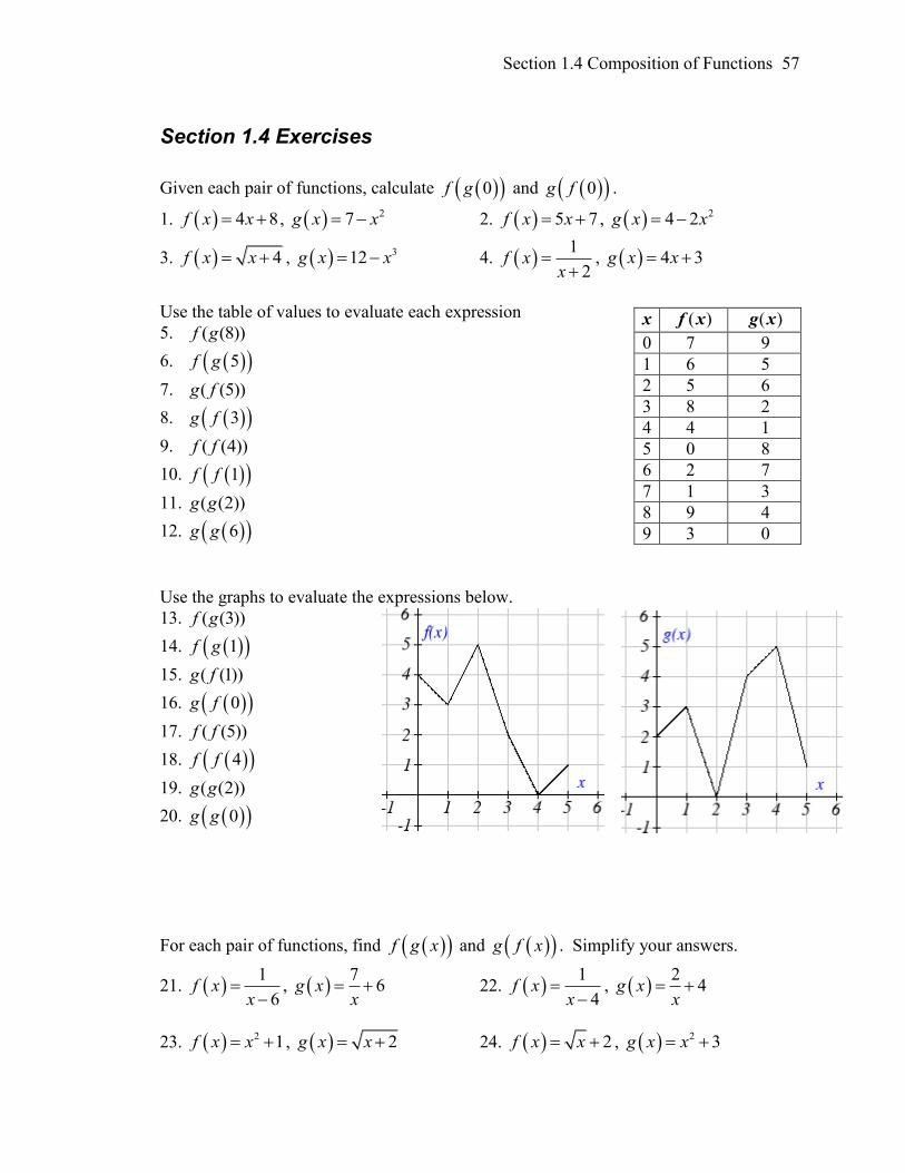
Section 1.4 Composition of Functions 57
Section 1.4 Exercises
Given each pair of functions, calculate 0f g and 0g f .
1. 4 8f x x , 27g x x 2. 5 7f x x , 24 2g x x
3. 4f x x , 312g x x 4. 1
2f x
x
, 4 3g x x
Use the table of values to evaluate each expression
5. ( (8))f g
6. 5f g
7. ( (5))g f
8. 3g f
9. ( (4))f f
10. 1f f
11. ( (2))g g
12. 6g g
Use the graphs to evaluate the expressions below.
13. ( (3))f g
14. 1f g
15. ( (1))g f
16. 0g f
17. ( (5))f f
18. 4f f
19. ( (2))g g
20. 0g g
For each pair of functions, find f g x and g f x . Simplify your answers.
21. 1
6f x
x
,
76 g x
x 22.
1
4f x
x
,
24g x
x
23. 2 1f x x , 2g x x 24. 2f x x , 2 3g x x
x ( )f x ( )g x
0 7 9
1 6 5
2 5 6
3 8 2
4 4 1
5 0 8
6 2 7
7 1 3
8 9 4
9 3 0
58 Chapter 1
25. f x x , 5 1g x x 26. 3f x x , 3
1xg x
x
27. If 4 6f x x , ( ) 6 g x x and ( ) h x x , find ( ( ( )))f g h x
28. If 2 1f x x , 1
g xx
and 3h x x , find ( ( ( )))f g h x
29. Given functions 1
p xx
and 2 4m x x , state the domains of the following
functions using interval notation.
a. Domain of
p x
m x
b. Domain of ( ( ))p m x
c. Domain of ( ( )) m p x
30. Given functions 1
q xx
and 2 9h x x , state the domains of the following
functions using interval notation.
a. Domain of
q x
h x
b. Domain of ( ( ))q h x
c. Domain of ( ( )) h q x
31. The function ( )D p gives the number of items that will be demanded when the price
is p. The production cost, ( )C x is the cost of producing x items. To determine the
cost of production when the price is $6, you would do which of the following:
a. Evaluate ( (6))D C b. Evaluate ( (6))C D
c. Solve ( ( )) 6D C x d. Solve ( ( )) 6C D p
32. The function ( )A d gives the pain level on a scale of 0-10 experienced by a patient
with d milligrams of a pain reduction drug in their system. The milligrams of drug in
the patient’s system after t minutes is modeled by ( )m t . To determine when the
patient will be at a pain level of 4, you would need to:
a. Evaluate 4A m b. Evaluate 4m A
c. Solve 4A m t d. Solve 4m A d
Section 1.4 Composition of Functions 59
33. The radius r, in inches, of a spherical balloon is related to the volume, V, by
33
( )4
Vr V
. Air is pumped into the balloon, so the volume after t seconds is given
by 10 20V t t .
a. Find the composite function r V t
b. Find the time when the radius reaches 10 inches.
34. The number of bacteria in a refrigerated food product is given by
223 56 1 N T T T , 3 33T , where T is the temperature of the food. When
the food is removed from the refrigerator, the temperature is given by ( ) 5 1.5T t t ,
where t is the time in hours.
a. Find the composite function N T t
b. Find the time when the bacteria count reaches 6752
Find functions ( )f x and ( )g x so the given function can be expressed as
h x f g x .
35. 2
2h x x 36. 3
5h x x
37. 3
5h x
x
38.
2
4
2h x
x
39. 3 2h x x 40. 34h x x
41. Let ( )f x be a linear function, with form f x ax b for constants a and b. [UW]
a. Show that f f x is a linear function
b. Find a function ( )g x such that 6 8g g x x
42. Let 1
32
f x x [UW]
a. Sketch the graphs of , , f x f f x f f f x on the interval −2 ≤ x ≤ 10.
b. Your graphs should all intersect at the point (6, 6). The value x = 6 is called a
fixed point of the function f(x)since (6) 6f ; that is, 6 is fixed - it doesn’t move
when f is applied to it. Give an explanation for why 6 is a fixed point for any
function ( ( (... ( )...)))f f f f x .
c. Linear functions (with the exception of ( )f x x ) can have at most one fixed
point. Quadratic functions can have at most two. Find the fixed points of the
function 2 2g x x .
d. Give a quadratic function whose fixed points are x = −2 and x = 3.

60 Chapter 1
43. A car leaves Seattle heading east. The speed of the car in mph after m minutes is
given by the function 2
2
70
10
mC m
m
. [UW]
a. Find a function ( )m f s that converts seconds s into minutes m. Write out the
formula for the new function ( ( ))C f s ; what does this function calculate?
b. Find a function (m g h ) that converts hours h into minutes m. Write out the
formula for the new function ( ( ))C g h ; what does this function calculate?
c. Find a function ( )z v s that converts mph s into ft/sec z. Write out the formula
for the new function ( ( )v C m ; what does this function calculate?
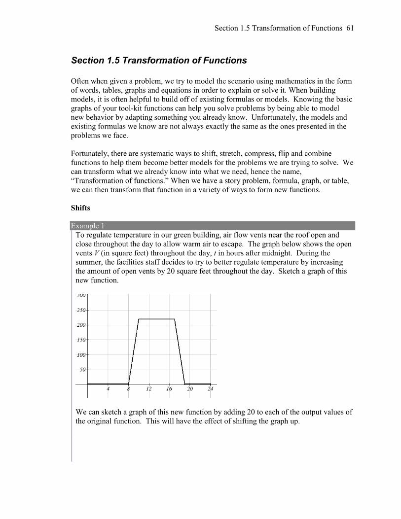
Section 1.5 Transformation of Functions 61
Section 1.5 Transformation of Functions
Often when given a problem, we try to model the scenario using mathematics in the form
of words, tables, graphs and equations in order to explain or solve it. When building
models, it is often helpful to build off of existing formulas or models. Knowing the basic
graphs of your tool-kit functions can help you solve problems by being able to model
new behavior by adapting something you already know. Unfortunately, the models and
existing formulas we know are not always exactly the same as the ones presented in the
problems we face.
Fortunately, there are systematic ways to shift, stretch, compress, flip and combine
functions to help them become better models for the problems we are trying to solve. We
can transform what we already know into what we need, hence the name,
“Transformation of functions.” When we have a story problem, formula, graph, or table,
we can then transform that function in a variety of ways to form new functions.
Shifts
Example 1
To regulate temperature in our green building, air flow vents near the roof open and
close throughout the day to allow warm air to escape. The graph below shows the open
vents V (in square feet) throughout the day, t in hours after midnight. During the
summer, the facilities staff decides to try to better regulate temperature by increasing
the amount of open vents by 20 square feet throughout the day. Sketch a graph of this
new function.
We can sketch a graph of this new function by adding 20 to each of the output values of
the original function. This will have the effect of shifting the graph up.
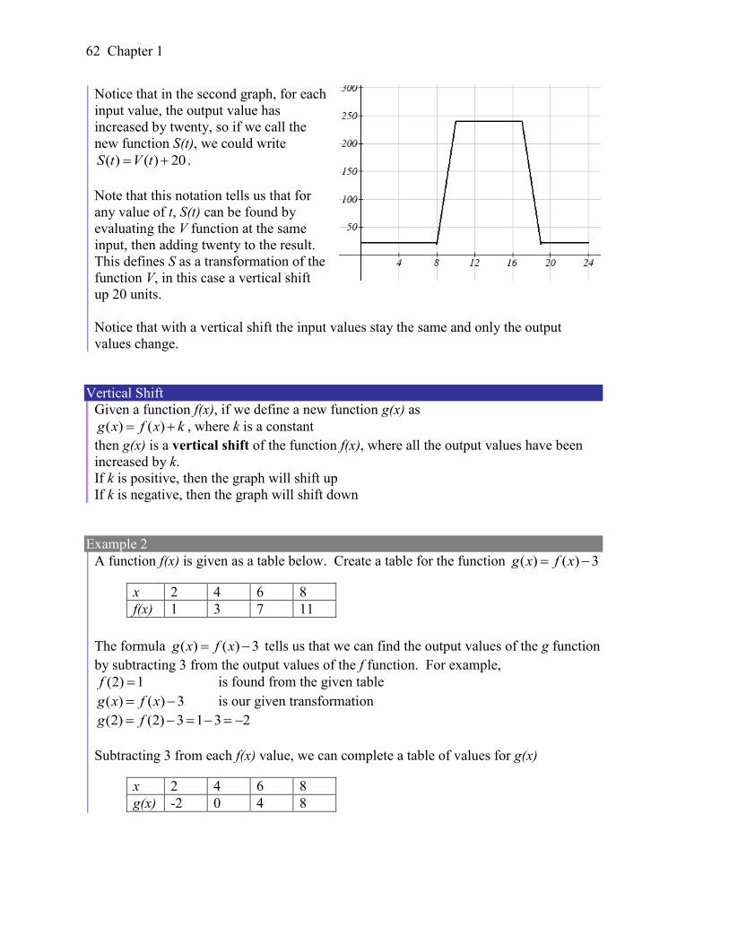
62 Chapter 1
Notice that in the second graph, for each
input value, the output value has
increased by twenty, so if we call the
new function S(t), we could write
( ) ( ) 20S t V t .
Note that this notation tells us that for
any value of t, S(t) can be found by
evaluating the V function at the same
input, then adding twenty to the result.
This defines S as a transformation of the
function V, in this case a vertical shift
up 20 units.
Notice that with a vertical shift the input values stay the same and only the output
values change.
Vertical Shift
Given a function f(x), if we define a new function g(x) as
( ) ( )g x f x k , where k is a constant
then g(x) is a vertical shift of the function f(x), where all the output values have been
increased by k.
If k is positive, then the graph will shift up
If k is negative, then the graph will shift down
Example 2
A function f(x) is given as a table below. Create a table for the function ( ) ( ) 3g x f x
The formula ( ) ( ) 3g x f x tells us that we can find the output values of the g function
by subtracting 3 from the output values of the f function. For example,
(2) 1f is found from the given table
( ) ( ) 3g x f x is our given transformation
(2) (2) 3 1 3 2g f
Subtracting 3 from each f(x) value, we can complete a table of values for g(x)
x 2 4 6 8
f(x) 1 3 7 11
x 2 4 6 8
g(x) -2 0 4 8
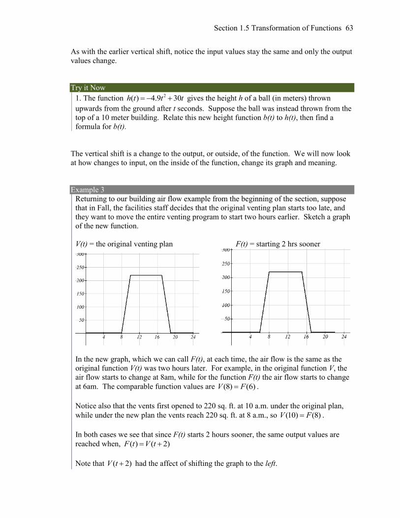
Section 1.5 Transformation of Functions 63
As with the earlier vertical shift, notice the input values stay the same and only the output
values change.
Try it Now
1. The function 2( ) 4.9 30h t t t gives the height h of a ball (in meters) thrown
upwards from the ground after t seconds. Suppose the ball was instead thrown from the
top of a 10 meter building. Relate this new height function b(t) to h(t), then find a
formula for b(t).
The vertical shift is a change to the output, or outside, of the function. We will now look
at how changes to input, on the inside of the function, change its graph and meaning.
Example 3
Returning to our building air flow example from the beginning of the section, suppose
that in Fall, the facilities staff decides that the original venting plan starts too late, and
they want to move the entire venting program to start two hours earlier. Sketch a graph
of the new function.
V(t) = the original venting plan F(t) = starting 2 hrs sooner
In the new graph, which we can call F(t), at each time, the air flow is the same as the
original function V(t) was two hours later. For example, in the original function V, the
air flow starts to change at 8am, while for the function F(t) the air flow starts to change
at 6am. The comparable function values are (8) (6)V F .
Notice also that the vents first opened to 220 sq. ft. at 10 a.m. under the original plan,
while under the new plan the vents reach 220 sq. ft. at 8 a.m., so (10) (8)V F .
In both cases we see that since F(t) starts 2 hours sooner, the same output values are
reached when, ( ) ( 2)F t V t
Note that ( 2)V t had the affect of shifting the graph to the left.
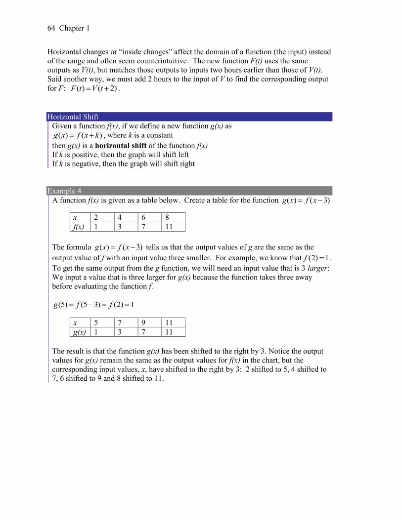
64 Chapter 1
Horizontal changes or “inside changes” affect the domain of a function (the input) instead
of the range and often seem counterintuitive. The new function F(t) uses the same
outputs as V(t), but matches those outputs to inputs two hours earlier than those of V(t).
Said another way, we must add 2 hours to the input of V to find the corresponding output
for F: ( ) ( 2)F t V t .
Horizontal Shift
Given a function f(x), if we define a new function g(x) as
( ) ( )g x f x k , where k is a constant
then g(x) is a horizontal shift of the function f(x)
If k is positive, then the graph will shift left
If k is negative, then the graph will shift right
Example 4
A function f(x) is given as a table below. Create a table for the function ( ) ( 3)g x f x
The formula ( ) ( 3)g x f x tells us that the output values of g are the same as the
output value of f with an input value three smaller. For example, we know that (2) 1f .
To get the same output from the g function, we will need an input value that is 3 larger:
We input a value that is three larger for g(x) because the function takes three away
before evaluating the function f.
(5) (5 3) (2) 1g f f
The result is that the function g(x) has been shifted to the right by 3. Notice the output
values for g(x) remain the same as the output values for f(x) in the chart, but the
corresponding input values, x, have shifted to the right by 3: 2 shifted to 5, 4 shifted to
7, 6 shifted to 9 and 8 shifted to 11.
x 2 4 6 8
f(x) 1 3 7 11
x 5 7 9 11
g(x) 1 3 7 11
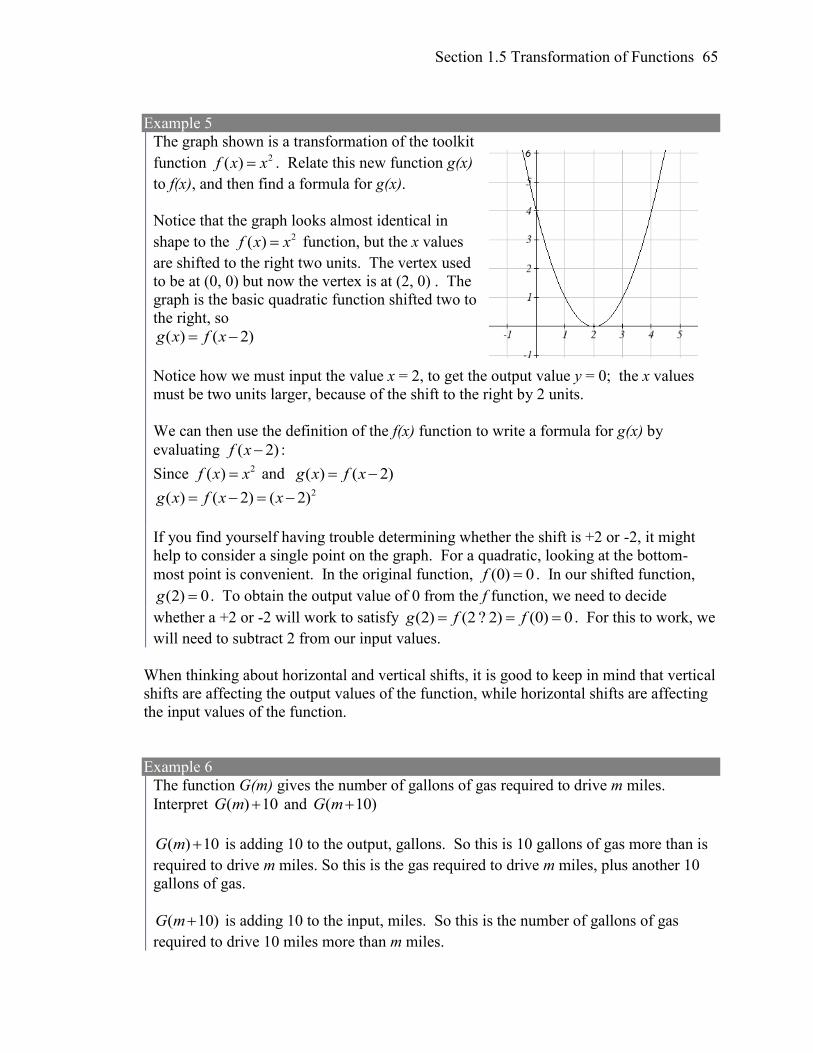
Section 1.5 Transformation of Functions 65
Example 5
The graph shown is a transformation of the toolkit
function 2( )f x x . Relate this new function g(x)
to f(x), and then find a formula for g(x).
Notice that the graph looks almost identical in
shape to the 2( )f x x function, but the x values
are shifted to the right two units. The vertex used
to be at (0, 0) but now the vertex is at (2, 0) . The
graph is the basic quadratic function shifted two to
the right, so
( ) ( 2)g x f x
Notice how we must input the value x = 2, to get the output value y = 0; the x values
must be two units larger, because of the shift to the right by 2 units.
We can then use the definition of the f(x) function to write a formula for g(x) by
evaluating ( 2)f x :
Since 2( )f x x and ( ) ( 2)g x f x 2( ) ( 2) ( 2)g x f x x
If you find yourself having trouble determining whether the shift is +2 or -2, it might
help to consider a single point on the graph. For a quadratic, looking at the bottom-
most point is convenient. In the original function, (0) 0f . In our shifted function,
(2) 0g . To obtain the output value of 0 from the f function, we need to decide
whether a +2 or -2 will work to satisfy (2) (2 ? 2) (0) 0g f f . For this to work, we
will need to subtract 2 from our input values.
When thinking about horizontal and vertical shifts, it is good to keep in mind that vertical
shifts are affecting the output values of the function, while horizontal shifts are affecting
the input values of the function.
Example 6
The function G(m) gives the number of gallons of gas required to drive m miles.
Interpret ( ) 10G m and ( 10)G m
( ) 10G m is adding 10 to the output, gallons. So this is 10 gallons of gas more than is
required to drive m miles. So this is the gas required to drive m miles, plus another 10
gallons of gas.
( 10)G m is adding 10 to the input, miles. So this is the number of gallons of gas
required to drive 10 miles more than m miles.
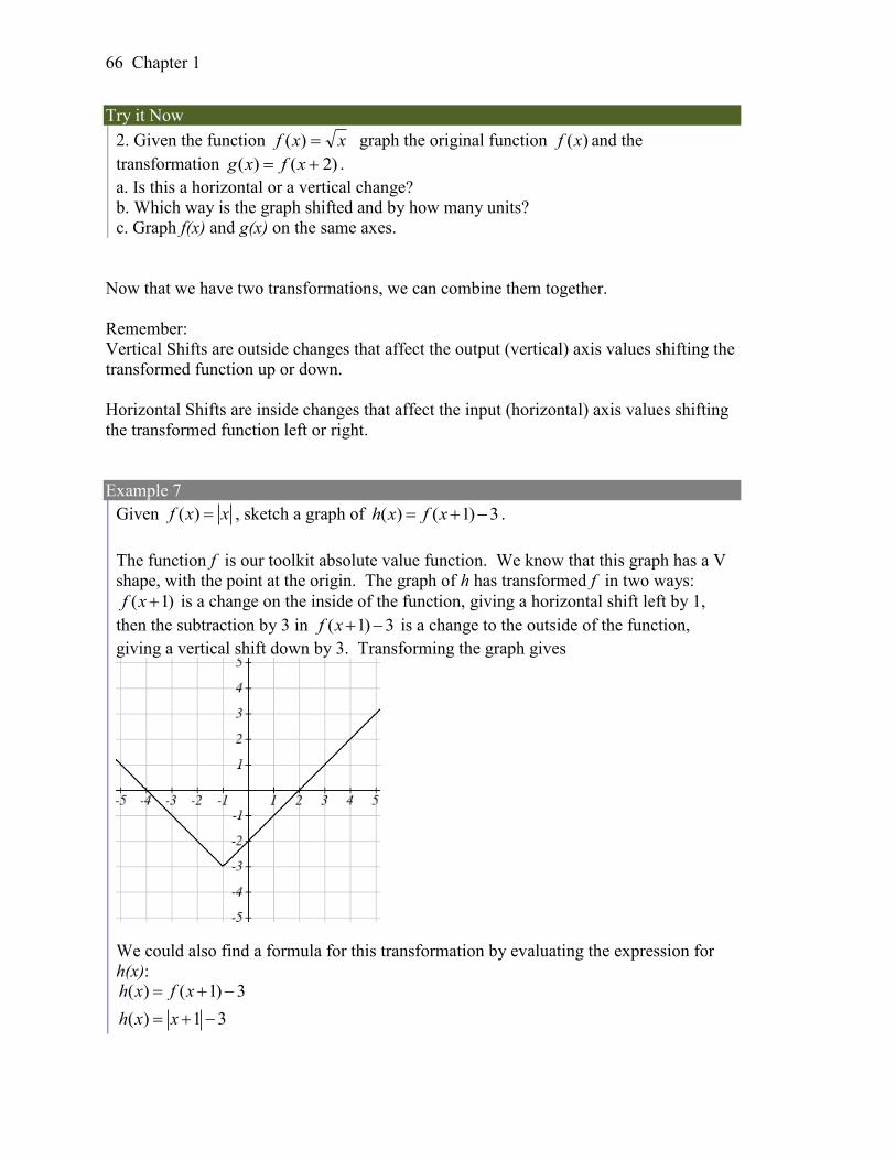
66 Chapter 1
Try it Now
2. Given the function xxf )( graph the original function )(xf and the
transformation )2()( xfxg .
a. Is this a horizontal or a vertical change?
b. Which way is the graph shifted and by how many units?
c. Graph f(x) and g(x) on the same axes.
Now that we have two transformations, we can combine them together.
Remember:
Vertical Shifts are outside changes that affect the output (vertical) axis values shifting the
transformed function up or down.
Horizontal Shifts are inside changes that affect the input (horizontal) axis values shifting
the transformed function left or right.
Example 7
Given ( )f x x , sketch a graph of ( ) ( 1) 3h x f x .
The function f is our toolkit absolute value function. We know that this graph has a V
shape, with the point at the origin. The graph of h has transformed f in two ways:
( 1)f x is a change on the inside of the function, giving a horizontal shift left by 1,
then the subtraction by 3 in ( 1) 3f x is a change to the outside of the function,
giving a vertical shift down by 3. Transforming the graph gives
We could also find a formula for this transformation by evaluating the expression for
h(x): ( ) ( 1) 3
( ) 1 3
h x f x
h x x
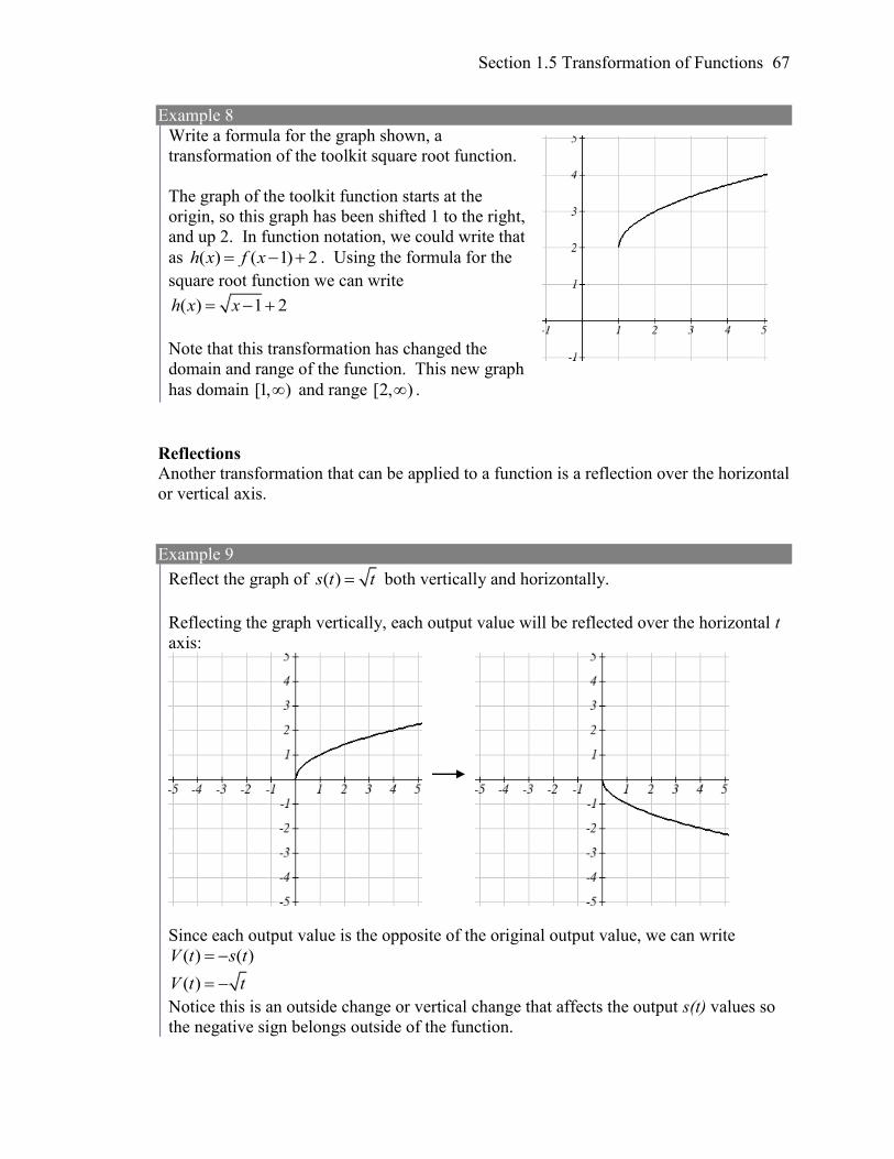
Section 1.5 Transformation of Functions 67
Example 8
Write a formula for the graph shown, a
transformation of the toolkit square root function.
The graph of the toolkit function starts at the
origin, so this graph has been shifted 1 to the right,
and up 2. In function notation, we could write that
as ( ) ( 1) 2h x f x . Using the formula for the
square root function we can write
( ) 1 2h x x
Note that this transformation has changed the
domain and range of the function. This new graph
has domain [1, ) and range [2, ) .
Reflections Another transformation that can be applied to a function is a reflection over the horizontal
or vertical axis.
Example 9
Reflect the graph of ( )s t t both vertically and horizontally.
Reflecting the graph vertically, each output value will be reflected over the horizontal t
axis:
Since each output value is the opposite of the original output value, we can write
( ) ( )V t s t
( )V t t
Notice this is an outside change or vertical change that affects the output s(t) values so
the negative sign belongs outside of the function.
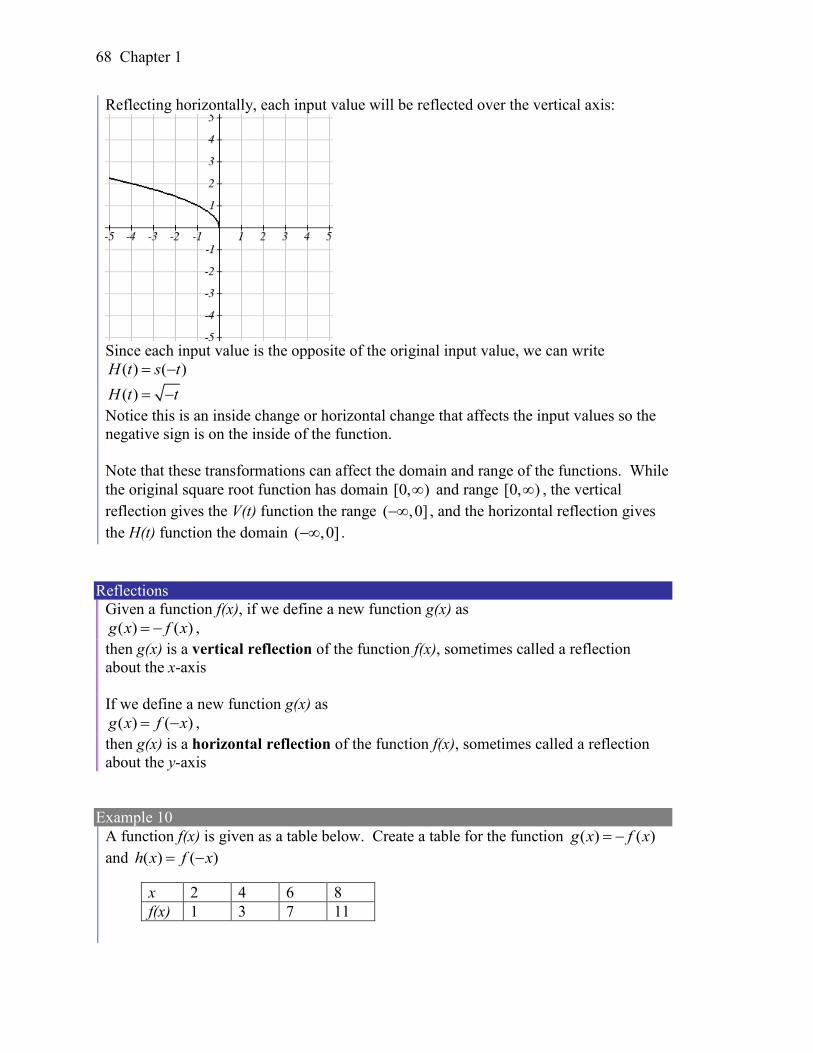
68 Chapter 1
Reflecting horizontally, each input value will be reflected over the vertical axis:
Since each input value is the opposite of the original input value, we can write
( ) ( )H t s t
( )H t t
Notice this is an inside change or horizontal change that affects the input values so the
negative sign is on the inside of the function.
Note that these transformations can affect the domain and range of the functions. While
the original square root function has domain [0, ) and range [0, ) , the vertical
reflection gives the V(t) function the range ( ,0] , and the horizontal reflection gives
the H(t) function the domain ( ,0] .
Reflections
Given a function f(x), if we define a new function g(x) as
( ) ( )g x f x ,
then g(x) is a vertical reflection of the function f(x), sometimes called a reflection
about the x-axis
If we define a new function g(x) as
( ) ( )g x f x ,
then g(x) is a horizontal reflection of the function f(x), sometimes called a reflection
about the y-axis
Example 10
A function f(x) is given as a table below. Create a table for the function ( ) ( )g x f x
and ( ) ( )h x f x
x 2 4 6 8
f(x) 1 3 7 11
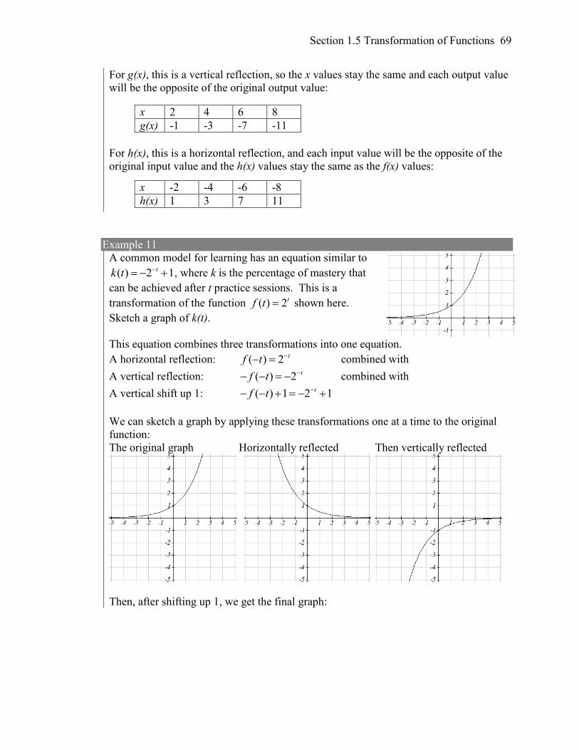
Section 1.5 Transformation of Functions 69
For g(x), this is a vertical reflection, so the x values stay the same and each output value
will be the opposite of the original output value:
For h(x), this is a horizontal reflection, and each input value will be the opposite of the
original input value and the h(x) values stay the same as the f(x) values:
Example 11
A common model for learning has an equation similar to
( ) 2 1tk t , where k is the percentage of mastery that
can be achieved after t practice sessions. This is a
transformation of the function ( ) 2tf t shown here.
Sketch a graph of k(t).
This equation combines three transformations into one equation.
A horizontal reflection: ( ) 2 tf t combined with
A vertical reflection: ( ) 2 tf t combined with
A vertical shift up 1: ( ) 1 2 1tf t
We can sketch a graph by applying these transformations one at a time to the original
function:
The original graph Horizontally reflected Then vertically reflected
Then, after shifting up 1, we get the final graph:
x 2 4 6 8
g(x) -1 -3 -7 -11
x -2 -4 -6 -8
h(x) 1 3 7 11
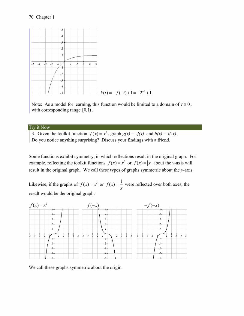
70 Chapter 1
( ) ( ) 1 2 1tk t f t .
Note: As a model for learning, this function would be limited to a domain of 0t ,
with corresponding range [0,1) .
Try it Now
3. Given the toolkit function 2( )f x x , graph g(x) = -f(x) and h(x) = f(-x).
Do you notice anything surprising? Discuss your findings with a friend.
Some functions exhibit symmetry, in which reflections result in the original graph. For
example, reflecting the toolkit functions 2( )f x x or ( )f x x about the y-axis will
result in the original graph. We call these types of graphs symmetric about the y-axis.
Likewise, if the graphs of 3( )f x x or 1
( )f xx
were reflected over both axes, the
result would be the original graph:
3( )f x x ( )f x ( )f x
We call these graphs symmetric about the origin.
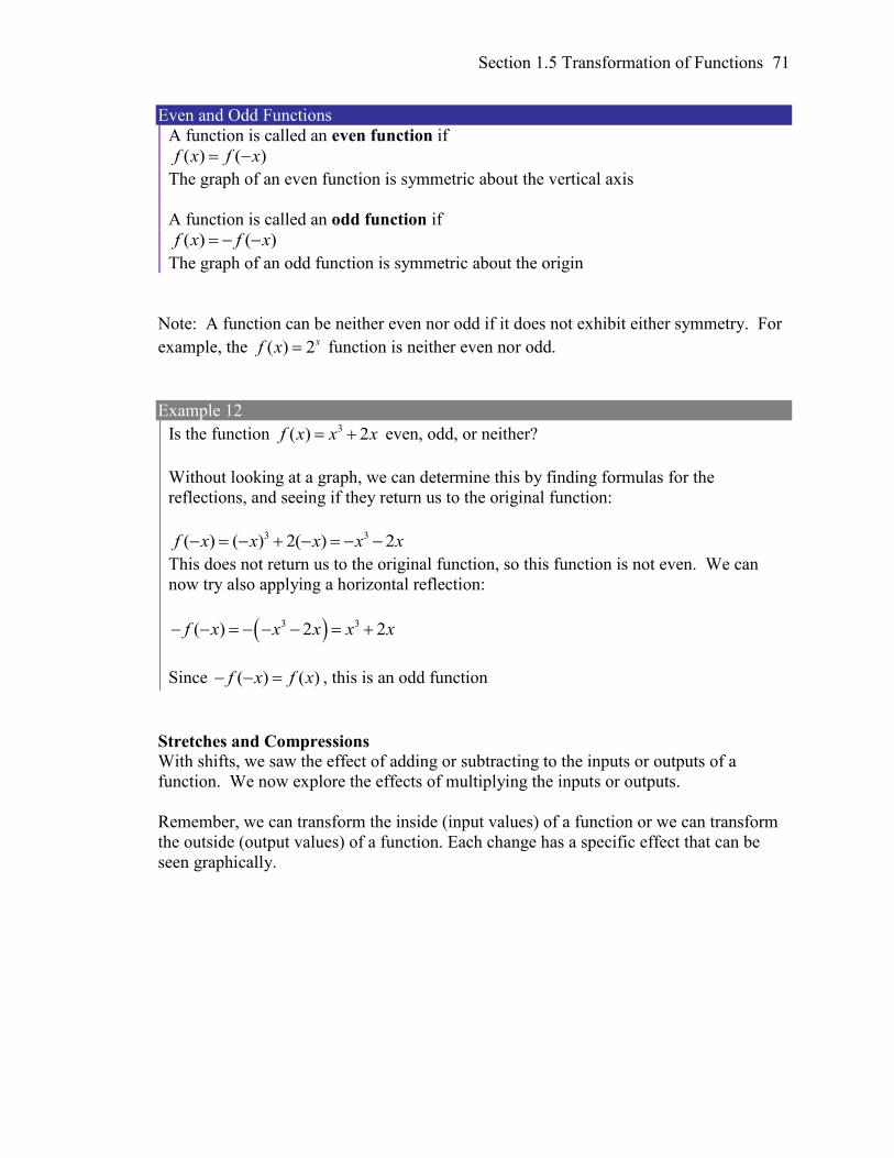
Section 1.5 Transformation of Functions 71
Even and Odd Functions
A function is called an even function if
( ) ( )f x f x
The graph of an even function is symmetric about the vertical axis
A function is called an odd function if
( ) ( )f x f x
The graph of an odd function is symmetric about the origin
Note: A function can be neither even nor odd if it does not exhibit either symmetry. For
example, the ( ) 2xf x function is neither even nor odd.
Example 12
Is the function 3( ) 2f x x x even, odd, or neither?
Without looking at a graph, we can determine this by finding formulas for the
reflections, and seeing if they return us to the original function:
3 3( ) ( ) 2( ) 2f x x x x x
This does not return us to the original function, so this function is not even. We can
now try also applying a horizontal reflection:
3 3( ) 2 2f x x x x x
Since ( ) ( )f x f x , this is an odd function
Stretches and Compressions With shifts, we saw the effect of adding or subtracting to the inputs or outputs of a
function. We now explore the effects of multiplying the inputs or outputs.
Remember, we can transform the inside (input values) of a function or we can transform
the outside (output values) of a function. Each change has a specific effect that can be
seen graphically.
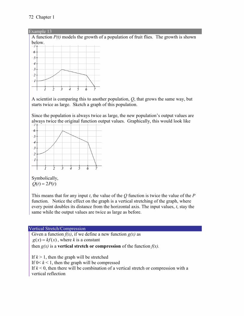
72 Chapter 1
Example 13
A function P(t) models the growth of a population of fruit flies. The growth is shown
below.
A scientist is comparing this to another population, Q, that grows the same way, but
starts twice as large. Sketch a graph of this population.
Since the population is always twice as large, the new population’s output values are
always twice the original function output values. Graphically, this would look like
Symbolically,
)(2)( tPtQ
This means that for any input t, the value of the Q function is twice the value of the P
function. Notice the effect on the graph is a vertical stretching of the graph, where
every point doubles its distance from the horizontal axis. The input values, t, stay the
same while the output values are twice as large as before.
Vertical Stretch/Compression
Given a function f(x), if we define a new function g(x) as
)()( xkfxg , where k is a constant
then g(x) is a vertical stretch or compression of the function f(x).
If k > 1, then the graph will be stretched
If 0< k < 1, then the graph will be compressed
If k < 0, then there will be combination of a vertical stretch or compression with a
vertical reflection
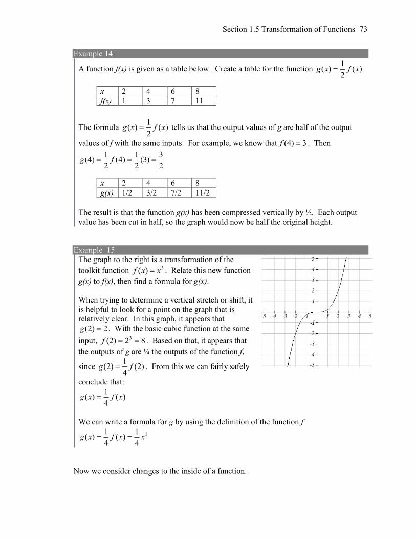
Section 1.5 Transformation of Functions 73
Example 14
A function f(x) is given as a table below. Create a table for the function )(2
1)( xfxg
The formula )(2
1)( xfxg tells us that the output values of g are half of the output
values of f with the same inputs. For example, we know that 3)4( f . Then
2
3)3(
2
1)4(
2
1)4( fg
The result is that the function g(x) has been compressed vertically by ½. Each output
value has been cut in half, so the graph would now be half the original height.
Example 15
The graph to the right is a transformation of the
toolkit function 3)( xxf . Relate this new function
g(x) to f(x), then find a formula for g(x).
When trying to determine a vertical stretch or shift, it
is helpful to look for a point on the graph that is
relatively clear. In this graph, it appears that
2)2( g . With the basic cubic function at the same
input, 82)2( 3 f . Based on that, it appears that
the outputs of g are ¼ the outputs of the function f,
since )2(4
1)2( fg . From this we can fairly safely
conclude that:
)(4
1)( xfxg
We can write a formula for g by using the definition of the function f
3
4
1)(
4
1)( xxfxg
Now we consider changes to the inside of a function.
x 2 4 6 8
f(x) 1 3 7 11
x 2 4 6 8
g(x) 1/2 3/2 7/2 11/2
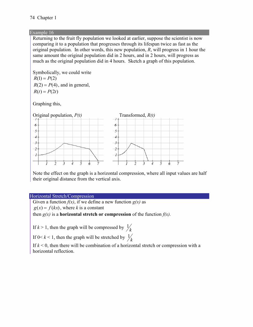
74 Chapter 1
Example 16
Returning to the fruit fly population we looked at earlier, suppose the scientist is now
comparing it to a population that progresses through its lifespan twice as fast as the
original population. In other words, this new population, R, will progress in 1 hour the
same amount the original population did in 2 hours, and in 2 hours, will progress as
much as the original population did in 4 hours. Sketch a graph of this population.
Symbolically, we could write
)2()1( PR
)4()2( PR , and in general,
)2()( tPtR
Graphing this,
Original population, P(t) Transformed, R(t)
Note the effect on the graph is a horizontal compression, where all input values are half
their original distance from the vertical axis.
Horizontal Stretch/Compression
Given a function f(x), if we define a new function g(x) as
)()( kxfxg , where k is a constant
then g(x) is a horizontal stretch or compression of the function f(x).
If k > 1, then the graph will be compressed by k
1
If 0< k < 1, then the graph will be stretched by k
1
If k < 0, then there will be combination of a horizontal stretch or compression with a
horizontal reflection.
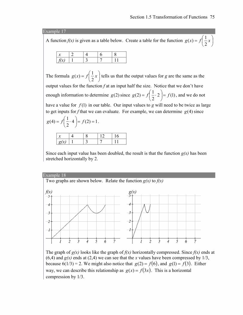
Section 1.5 Transformation of Functions 75
Example 17
A function f(x) is given as a table below. Create a table for the function
xfxg
2
1)(
The formula
xfxg
2
1)( tells us that the output values for g are the same as the
output values for the function f at an input half the size. Notice that we don’t have
enough information to determine )2(g since )1(22
1)2( ffg
, and we do not
have a value for )1(f in our table. Our input values to g will need to be twice as large
to get inputs for f that we can evaluate. For example, we can determine )4(g since
1)2(42
1)4(
ffg .
Since each input value has been doubled, the result is that the function g(x) has been
stretched horizontally by 2.
Example 18
Two graphs are shown below. Relate the function g(x) to f(x)
f(x) g(x)
The graph of g(x) looks like the graph of f(x) horizontally compressed. Since f(x) ends at
(6,4) and g(x) ends at (2,4) we can see that the x values have been compressed by 1/3,
because 6(1/3) = 2. We might also notice that 6)2( fg , and 3)1( fg . Either
way, we can describe this relationship as xfxg 3)( . This is a horizontal
compression by 1/3.
x 2 4 6 8
f(x) 1 3 7 11
x 4 8 12 16
g(x) 1 3 7 11
76 Chapter 1
Notice that the coefficient needed for a horizontal stretch or compression is the
reciprocal of the stretch or compression. So to stretch the graph horizontally by 4, we
need a coefficient of 1/4 in our function: 1
4f x
. This means the input values must be
four times larger to produce the same result, requiring the input to be larger, causing the
horizontal stretching.
Try it Now
4. Write a formula for the toolkit square root function horizontally stretched by three.
It is useful to note that for most toolkit functions, a horizontal stretch or vertical stretch
can be represented in other ways. For example, a horizontal compression of the function
2f x x by ½ would result in a new function 2
2g x x , but this can also be written
as 24g x x , a vertical stretch of f(x) by 4. When writing a formula for a transformed
toolkit, we only need to find one transformation that would produce the graph.
Combining Transformations
When combining transformations, it is very important to consider the order of the
transformations. For example, vertically shifting by 3 and then vertically stretching by 2
does not create the same graph as vertically stretching by 2 and then vertically shifting by
3.
When we see an expression like 3)(2 xf , which transformation should we start with?
The answer here follows nicely from order of operations, for outside transformations.
Given the output value of f(x), we first multiply by 2, causing the vertical stretch, then
add 3, causing the vertical shift. (Multiplication before Addition)
Combining Vertical Transformations
When combining vertical transformations written in the form kxaf )( ,
first vertically stretch by a, then vertically shift by k.
Horizontal transformations are a little trickier to think about. When we write
)32()( xfxg for example, we have to think about how the inputs to the g function
relate to the inputs to the f function. Suppose we know 12)7( f . What input to g
would produce that output? In other words, what value of x will allow
)12()32()( fxfxg ? We would need 1232 x . To solve for x, we would first
subtract 3, resulting in horizontal shift, then divide by 2, causing a horizontal
compression.
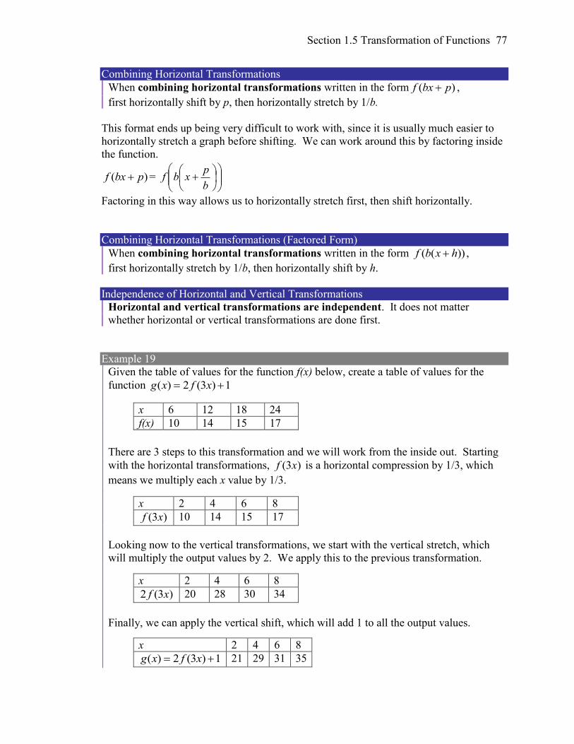
Section 1.5 Transformation of Functions 77
Combining Horizontal Transformations
When combining horizontal transformations written in the form )( pbxf ,
first horizontally shift by p, then horizontally stretch by 1/b.
This format ends up being very difficult to work with, since it is usually much easier to
horizontally stretch a graph before shifting. We can work around this by factoring inside
the function.
)( pbxf =
b
pxbf
Factoring in this way allows us to horizontally stretch first, then shift horizontally.
Combining Horizontal Transformations (Factored Form)
When combining horizontal transformations written in the form ))(( hxbf ,
first horizontally stretch by 1/b, then horizontally shift by h.
Independence of Horizontal and Vertical Transformations
Horizontal and vertical transformations are independent. It does not matter
whether horizontal or vertical transformations are done first.
Example 19
Given the table of values for the function f(x) below, create a table of values for the
function 1)3(2)( xfxg
There are 3 steps to this transformation and we will work from the inside out. Starting
with the horizontal transformations, )3( xf is a horizontal compression by 1/3, which
means we multiply each x value by 1/3.
Looking now to the vertical transformations, we start with the vertical stretch, which
will multiply the output values by 2. We apply this to the previous transformation.
Finally, we can apply the vertical shift, which will add 1 to all the output values.
x 6 12 18 24
f(x) 10 14 15 17
x 2 4 6 8
)3( xf 10 14 15 17
x 2 4 6 8
)3(2 xf 20 28 30 34
x 2 4 6 8
1)3(2)( xfxg 21 29 31 35
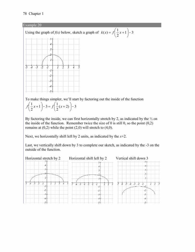
78 Chapter 1
Example 20
Using the graph of f(x) below, sketch a graph of 312
1)(
xfxk
To make things simpler, we’ll start by factoring out the inside of the function
3)2(2
131
2
1
xfxf
By factoring the inside, we can first horizontally stretch by 2, as indicated by the ½ on
the inside of the function. Remember twice the size of 0 is still 0, so the point (0,2)
remains at (0,2) while the point (2,0) will stretch to (4,0).
Next, we horizontally shift left by 2 units, as indicated by the x+2.
Last, we vertically shift down by 3 to complete our sketch, as indicated by the -3 on the
outside of the function.
Horizontal stretch by 2 Horizontal shift left by 2 Vertical shift down 3
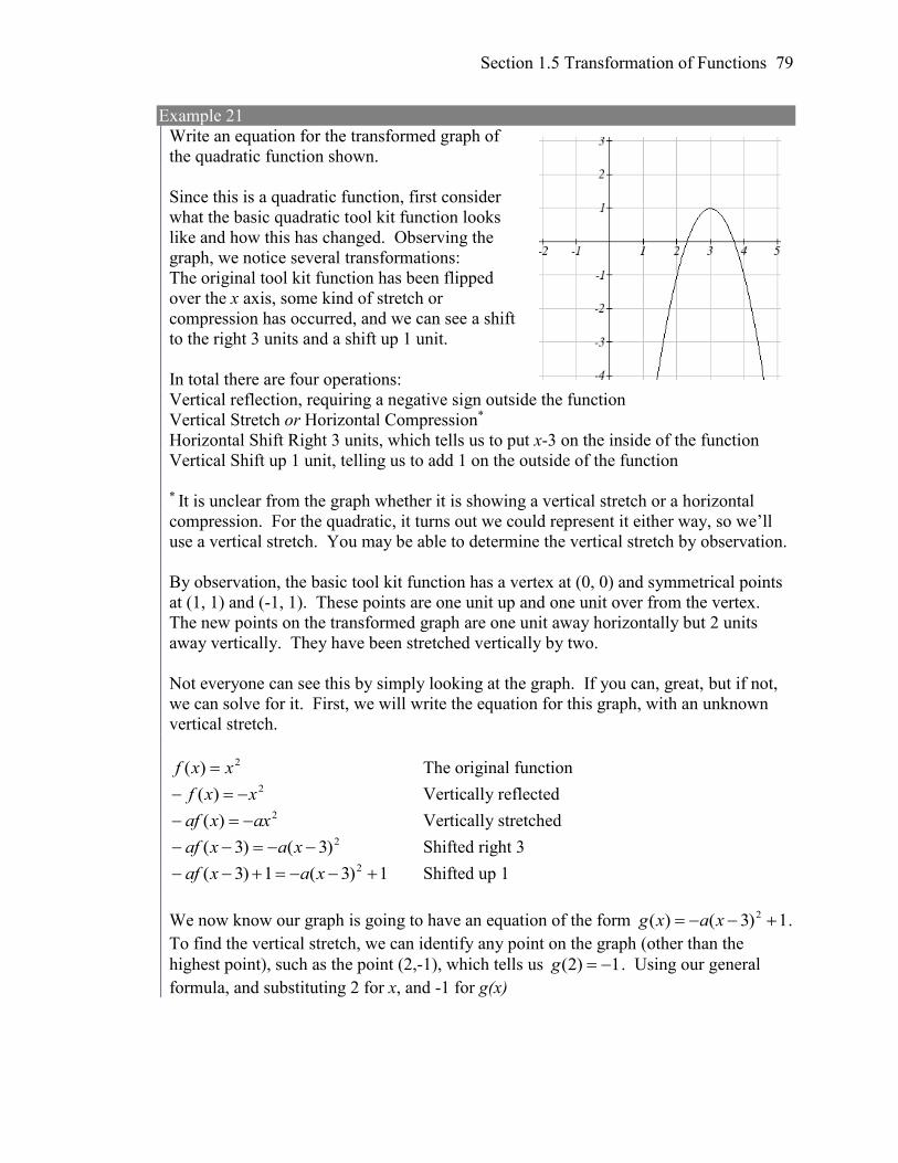
Section 1.5 Transformation of Functions 79
Example 21
Write an equation for the transformed graph of
the quadratic function shown.
Since this is a quadratic function, first consider
what the basic quadratic tool kit function looks
like and how this has changed. Observing the
graph, we notice several transformations:
The original tool kit function has been flipped
over the x axis, some kind of stretch or
compression has occurred, and we can see a shift
to the right 3 units and a shift up 1 unit.
In total there are four operations:
Vertical reflection, requiring a negative sign outside the function
Vertical Stretch or Horizontal Compression*
Horizontal Shift Right 3 units, which tells us to put x-3 on the inside of the function
Vertical Shift up 1 unit, telling us to add 1 on the outside of the function
* It is unclear from the graph whether it is showing a vertical stretch or a horizontal
compression. For the quadratic, it turns out we could represent it either way, so we’ll
use a vertical stretch. You may be able to determine the vertical stretch by observation.
By observation, the basic tool kit function has a vertex at (0, 0) and symmetrical points
at (1, 1) and (-1, 1). These points are one unit up and one unit over from the vertex.
The new points on the transformed graph are one unit away horizontally but 2 units
away vertically. They have been stretched vertically by two.
Not everyone can see this by simply looking at the graph. If you can, great, but if not,
we can solve for it. First, we will write the equation for this graph, with an unknown
vertical stretch.
2)( xxf The original function
2)( xxf Vertically reflected 2)( axxaf Vertically stretched
2)3()3( xaxaf Shifted right 3
1)3(1)3( 2 xaxaf Shifted up 1
We now know our graph is going to have an equation of the form 1)3()( 2 xaxg .
To find the vertical stretch, we can identify any point on the graph (other than the
highest point), such as the point (2,-1), which tells us 1)2( g . Using our general
formula, and substituting 2 for x, and -1 for g(x)
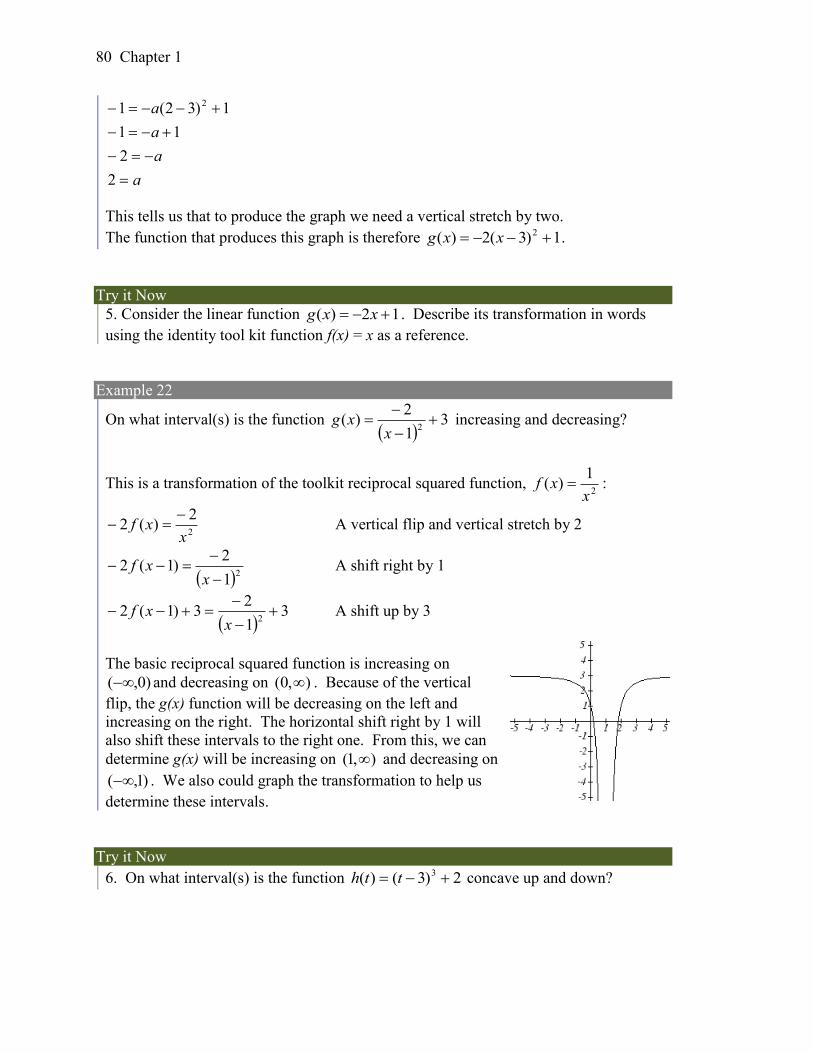
80 Chapter 1
a
a
a
a
2
2
11
1)32(1 2
This tells us that to produce the graph we need a vertical stretch by two.
The function that produces this graph is therefore 1)3(2)( 2 xxg .
Try it Now
5. Consider the linear function 12)( xxg . Describe its transformation in words
using the identity tool kit function f(x) = x as a reference.
Example 22
On what interval(s) is the function
31
2)(
2
xxg increasing and decreasing?
This is a transformation of the toolkit reciprocal squared function, 2
1)(
xxf :
2
2)(2
xxf
A vertical flip and vertical stretch by 2
21
2)1(2
xxf A shift right by 1
3
1
23)1(2
2
xxf A shift up by 3
The basic reciprocal squared function is increasing on
)0,( and decreasing on ),0( . Because of the vertical
flip, the g(x) function will be decreasing on the left and
increasing on the right. The horizontal shift right by 1 will
also shift these intervals to the right one. From this, we can
determine g(x) will be increasing on ),1( and decreasing on
)1,( . We also could graph the transformation to help us
determine these intervals.
Try it Now
6. On what interval(s) is the function 2)3()( 3 tth concave up and down?
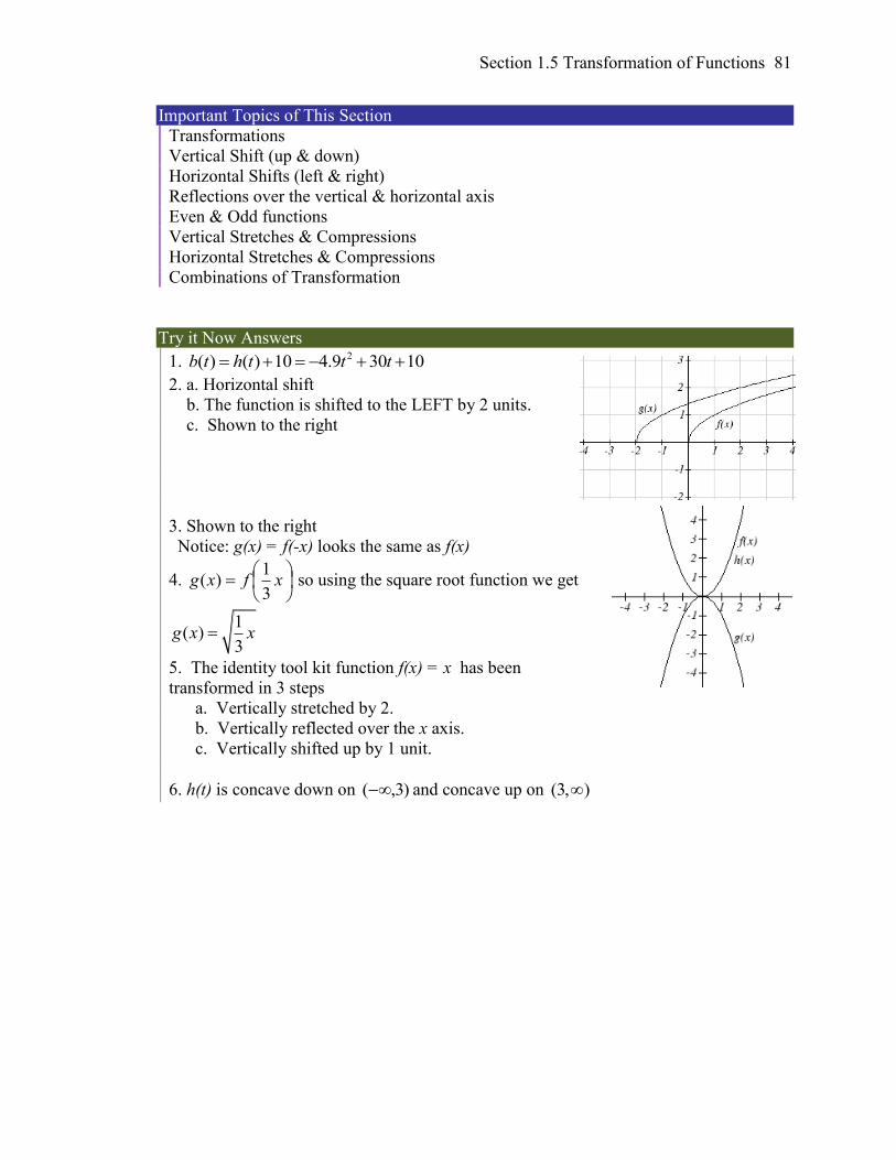
Section 1.5 Transformation of Functions 81
Important Topics of This Section
Transformations
Vertical Shift (up & down)
Horizontal Shifts (left & right)
Reflections over the vertical & horizontal axis
Even & Odd functions
Vertical Stretches & Compressions
Horizontal Stretches & Compressions
Combinations of Transformation
Try it Now Answers
1. 2( ) ( ) 10 4.9 30 10b t h t t t
2. a. Horizontal shift
b. The function is shifted to the LEFT by 2 units.
c. Shown to the right
3. Shown to the right
Notice: g(x) = f(-x) looks the same as f(x)
4.
xfxg
3
1)( so using the square root function we get
1( )
3g x x
5. The identity tool kit function f(x) = x has been
transformed in 3 steps
a. Vertically stretched by 2.
b. Vertically reflected over the x axis.
c. Vertically shifted up by 1 unit.
6. h(t) is concave down on )3,( and concave up on ),3(
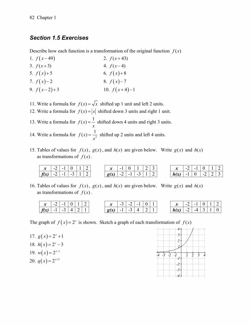
82 Chapter 1
Section 1.5 Exercises
Describe how each function is a transformation of the original function ( )f x
1. 49f x 2. ( 43)f x
3. ( 3)f x 4. ( 4)f x
5. 5f x 6. 8f x
7. 2f x 8. 7f x
9. 2 3f x 10. 4 1f x
11. Write a formula for ( )f x x shifted up 1 unit and left 2 units.
12. Write a formula for ( )f x x shifted down 3 units and right 1 unit.
13. Write a formula for 1
( )f xx
shifted down 4 units and right 3 units.
14. Write a formula for 2
1 ( )f x
x shifted up 2 units and left 4 units.
15. Tables of values for ( )f x , ( )g x , and ( )h x are given below. Write ( )g x and ( )h x
as transformations of ( )f x .
x -2 -1 0 1 2
f(x) -2 -1 -3 1 2
x -1 0 1 2 3
g(x) -2 -1 -3 1 2
x -2 -1 0 1 2
h(x) -1 0 -2 2 3
16. Tables of values for ( )f x , ( )g x , and ( )h x are given below. Write ( )g x and ( )h x
as transformations of ( )f x .
x -2 -1 0 1 2
f(x) -1 -3 4 2 1
x -3 -2 -1 0 1
g(x) -1 -3 4 2 1
x -2 -1 0 1 2
h(x) -2 -4 3 1 0
The graph of 2xf x is shown. Sketch a graph of each transformation of ( )f x
17. 2 1xg x
18. 2 3xh x
19. 12xw x
20. 32xq x
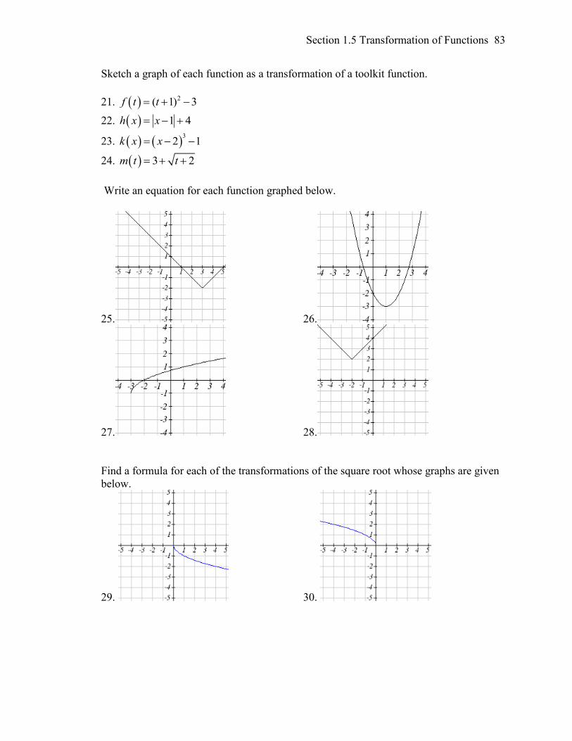
Section 1.5 Transformation of Functions 83
Sketch a graph of each function as a transformation of a toolkit function.
21. 2( 1) 3f t t
22. 1 4h x x
23. 3
2 1k x x
24. 3 2m t t
Write an equation for each function graphed below.
25. 26.
27. 28.
Find a formula for each of the transformations of the square root whose graphs are given
below.
29. 30.
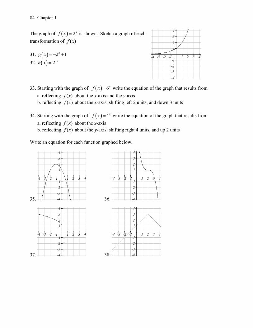
84 Chapter 1
The graph of 2xf x is shown. Sketch a graph of each
transformation of ( )f x
31. 2 1xg x
32. 2 xh x
33. Starting with the graph of 6xf x write the equation of the graph that results from
a. reflecting ( )f x about the x-axis and the y-axis
b. reflecting ( )f x about the x-axis, shifting left 2 units, and down 3 units
34. Starting with the graph of 4xf x write the equation of the graph that results from
a. reflecting ( )f x about the x-axis
b. reflecting ( )f x about the y-axis, shifting right 4 units, and up 2 units
Write an equation for each function graphed below.
35. 36.
37. 38.
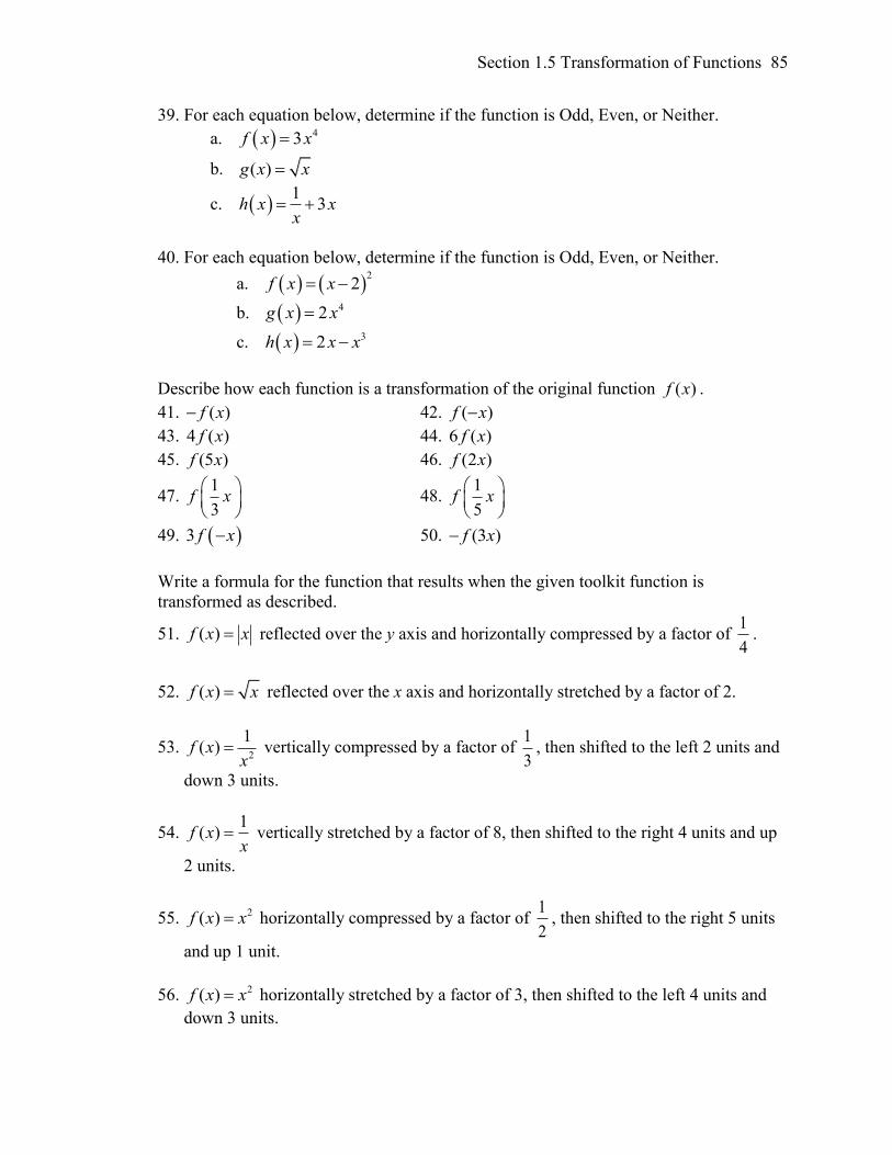
Section 1.5 Transformation of Functions 85
39. For each equation below, determine if the function is Odd, Even, or Neither.
a. 43 f x x
b. ( )g x x
c. 1
3 h x xx
40. For each equation below, determine if the function is Odd, Even, or Neither.
a. 2
2f x x
b. 42 g x x
c. 32 h x x x
Describe how each function is a transformation of the original function ( )f x .
41. ( )f x 42. ( )f x
43. 4 ( )f x 44. 6 ( )f x
45. (5 )f x 46. (2 )f x
47. 1
3f x
48. 1
5f x
49. 3 f x 50. (3 )f x
Write a formula for the function that results when the given toolkit function is
transformed as described.
51. ( )f x x reflected over the y axis and horizontally compressed by a factor of 1
4.
52. ( )f x x reflected over the x axis and horizontally stretched by a factor of 2.
53. 2
1( )f x
x vertically compressed by a factor of
1
3, then shifted to the left 2 units and
down 3 units.
54. 1
( )f xx
vertically stretched by a factor of 8, then shifted to the right 4 units and up
2 units.
55. 2( )f x x horizontally compressed by a factor of 1
2, then shifted to the right 5 units
and up 1 unit.
56. 2( )f x x horizontally stretched by a factor of 3, then shifted to the left 4 units and
down 3 units.
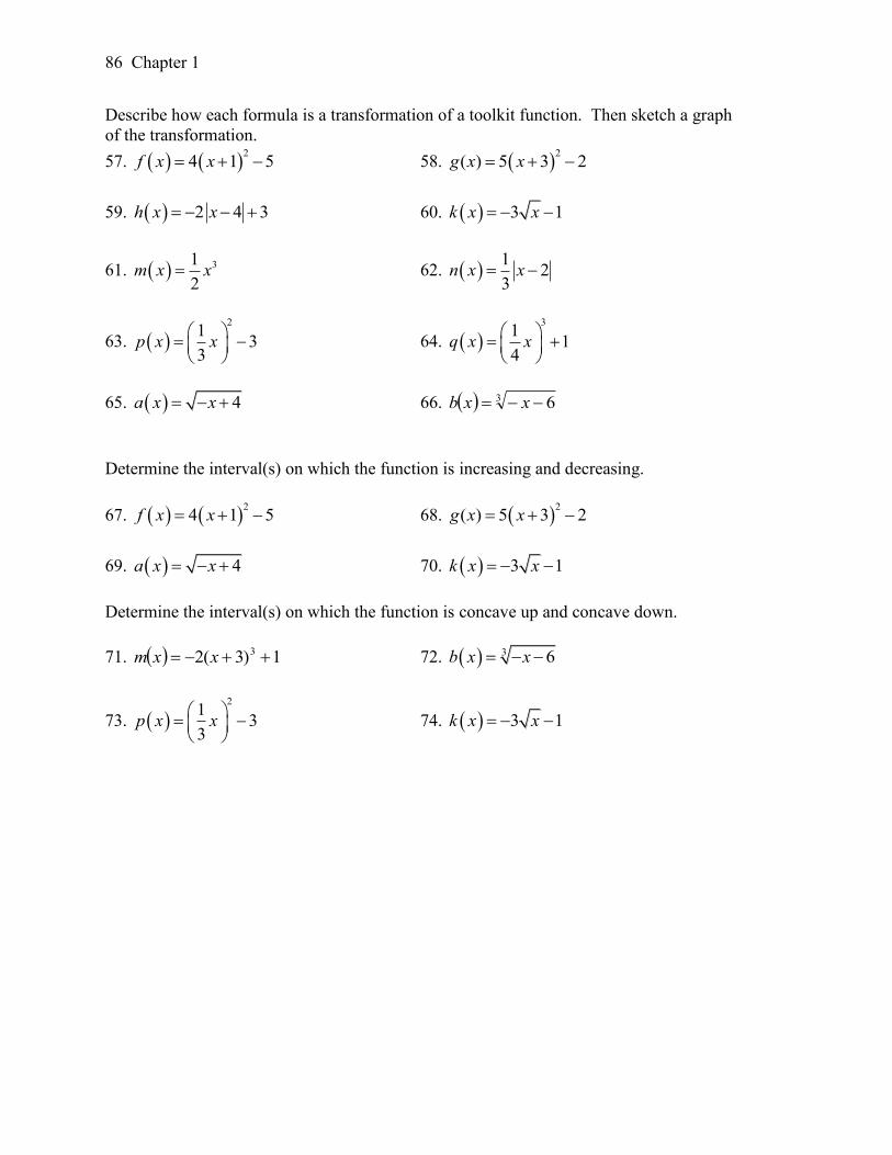
86 Chapter 1
Describe how each formula is a transformation of a toolkit function. Then sketch a graph
of the transformation.
57. 2
4 1 5f x x 58. 2
( ) 5 3 2g x x
59. 2 4 3h x x 60. 3 1k x x
61. 31
2m x x 62.
12
3n x x
63. 2
13
3p x x
64. 3
11
4q x x
65. 4a x x 66. 3 6 xxb
Determine the interval(s) on which the function is increasing and decreasing.
67. 2
4 1 5f x x 68. 2
( ) 5 3 2g x x
69. 4a x x 70. 3 1k x x
Determine the interval(s) on which the function is concave up and concave down.
71. 1)3(2 3 xxm 72. 3 6b x x
73. 2
13
3p x x
74. 3 1k x x
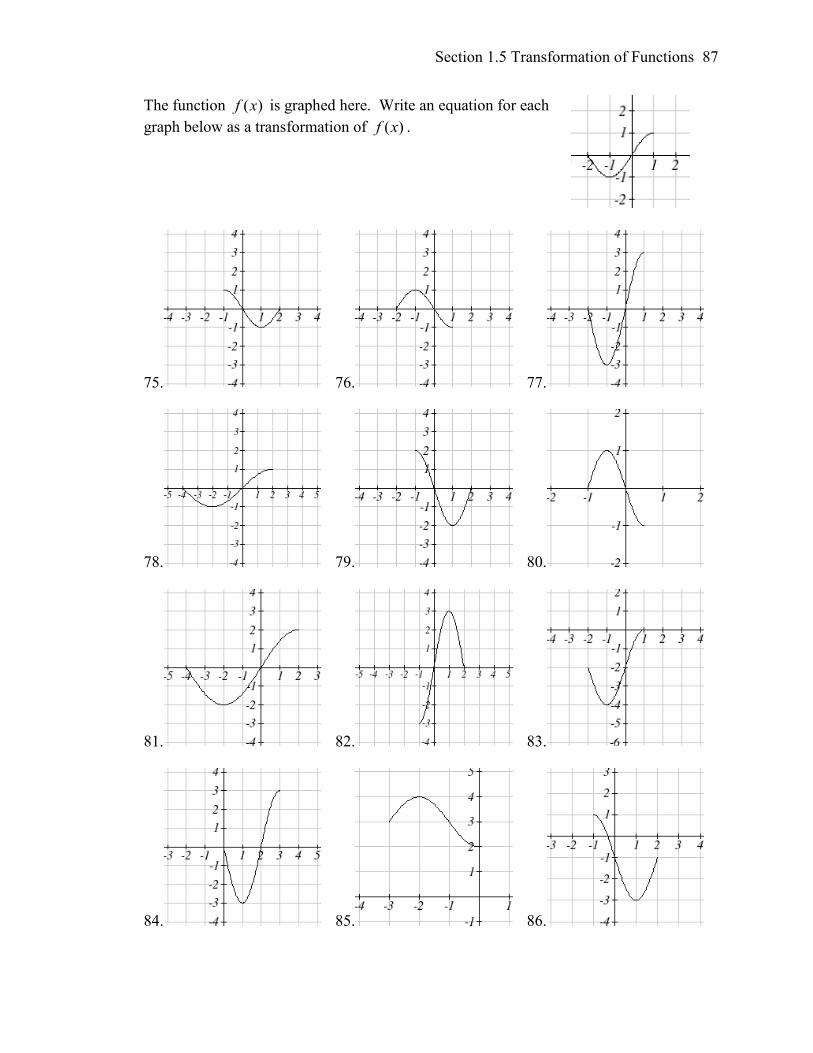
Section 1.5 Transformation of Functions 87
The function ( )f x is graphed here. Write an equation for each
graph below as a transformation of ( )f x .
75. 76. 77.
78. 79. 80.
81. 82. 83.
84. 85. 86.
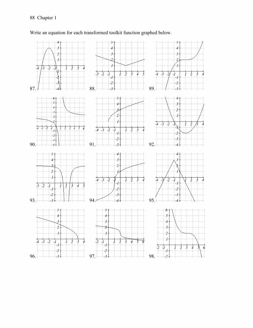
88 Chapter 1
Write an equation for each transformed toolkit function graphed below.
87. 88. 89.
90. 91. 92.
93. 94. 95.
96. 97. 98.
Section 1.5 Transformation of Functions 89
99. Suppose you have a function ( )y f x such that the domain of ( )f x is 1 ≤ x ≤ 6 and
the range of ( )f x is −3 ≤ y ≤ 5. [UW]
a. What is the domain of (2( 3)) f x ?
b. What is the range of ))3(2( xf ?
c. What is the domain of 2 ( ) 3f x ?
d. What is the range of 2 ( ) 3f x ?
e. Can you find constants B and C so that the domain of ( ( ))f B x C is 8 ≤ x ≤ 9?
f. Can you find constants A and D so that the range of ( ) Af x D is 0 ≤ y ≤ 1?
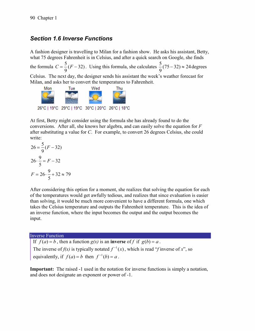
90 Chapter 1
Section 1.6 Inverse Functions
A fashion designer is travelling to Milan for a fashion show. He asks his assistant, Betty,
what 75 degrees Fahrenheit is in Celsius, and after a quick search on Google, she finds
the formula )32(9
5 FC . Using this formula, she calculates 24)3275(
9
5 degrees
Celsius. The next day, the designer sends his assistant the week’s weather forecast for
Milan, and asks her to convert the temperatures to Fahrenheit.
At first, Betty might consider using the formula she has already found to do the
conversions. After all, she knows her algebra, and can easily solve the equation for F
after substituting a value for C. For example, to convert 26 degrees Celsius, she could
write:
79325
926
325
926
)32(9
526
F
F
F
After considering this option for a moment, she realizes that solving the equation for each
of the temperatures would get awfully tedious, and realizes that since evaluation is easier
than solving, it would be much more convenient to have a different formula, one which
takes the Celsius temperature and outputs the Fahrenheit temperature. This is the idea of
an inverse function, where the input becomes the output and the output becomes the
input.
Inverse Function
If baf )( , then a function g(x) is an inverse of f if abg )( .
The inverse of f(x) is typically notated )(1 xf , which is read “f inverse of x”, so
equivalently, if baf )( then abf )(1 .
Important: The raised -1 used in the notation for inverse functions is simply a notation,
and does not designate an exponent or power of -1.
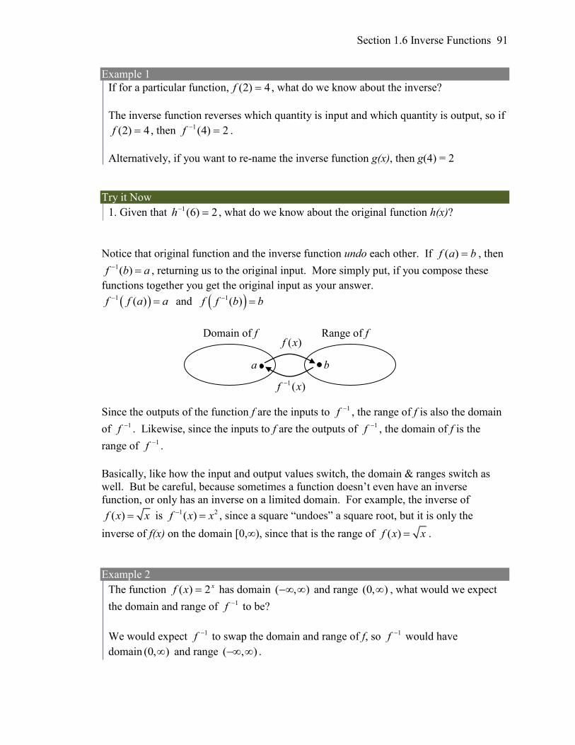
Section 1.6 Inverse Functions 91
Example 1
If for a particular function, 4)2( f , what do we know about the inverse?
The inverse function reverses which quantity is input and which quantity is output, so if
4)2( f , then 2)4(1 f .
Alternatively, if you want to re-name the inverse function g(x), then g(4) = 2
Try it Now
1. Given that 2)6(1 h , what do we know about the original function h(x)?
Notice that original function and the inverse function undo each other. If baf )( , then 1( )f b a , returning us to the original input. More simply put, if you compose these
functions together you get the original input as your answer.
1 ( )f f a a and 1( )f f b b
Since the outputs of the function f are the inputs to 1f , the range of f is also the domain
of 1f . Likewise, since the inputs to f are the outputs of 1f , the domain of f is the
range of 1f .
Basically, like how the input and output values switch, the domain & ranges switch as
well. But be careful, because sometimes a function doesn’t even have an inverse
function, or only has an inverse on a limited domain. For example, the inverse of
( )f x x is 1 2( )f x x , since a square “undoes” a square root, but it is only the
inverse of f(x) on the domain [0,∞), since that is the range of ( )f x x .
Example 2
The function xxf 2)( has domain ),( and range ),0( , what would we expect
the domain and range of 1f to be?
We would expect 1f to swap the domain and range of f, so 1f would have
domain ),0( and range ( , ) .
Domain of f Range of f
a b
)(1 xf
)(xf
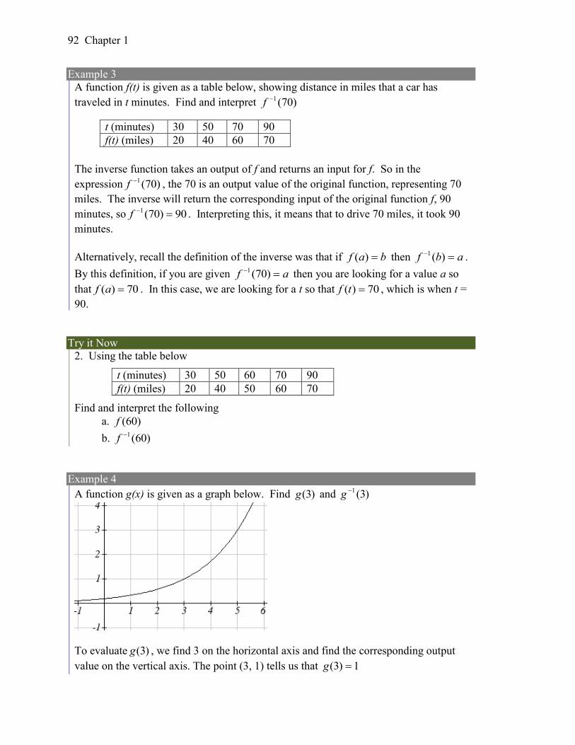
92 Chapter 1
Example 3
A function f(t) is given as a table below, showing distance in miles that a car has
traveled in t minutes. Find and interpret )70(1f
The inverse function takes an output of f and returns an input for f. So in the
expression )70(1f , the 70 is an output value of the original function, representing 70
miles. The inverse will return the corresponding input of the original function f, 90
minutes, so 90)70(1 f . Interpreting this, it means that to drive 70 miles, it took 90
minutes.
Alternatively, recall the definition of the inverse was that if baf )( then abf )(1 .
By this definition, if you are given af )70(1 then you are looking for a value a so
that 70)( af . In this case, we are looking for a t so that 70)( tf , which is when t =
90.
Try it Now
2. Using the table below
Find and interpret the following
a. )60(f
b. )60(1f
Example 4
A function g(x) is given as a graph below. Find )3(g and )3(1g
To evaluate )3(g , we find 3 on the horizontal axis and find the corresponding output
value on the vertical axis. The point (3, 1) tells us that 1)3( g
t (minutes) 30 50 70 90
f(t) (miles) 20 40 60 70
t (minutes) 30 50 60 70 90
f(t) (miles) 20 40 50 60 70
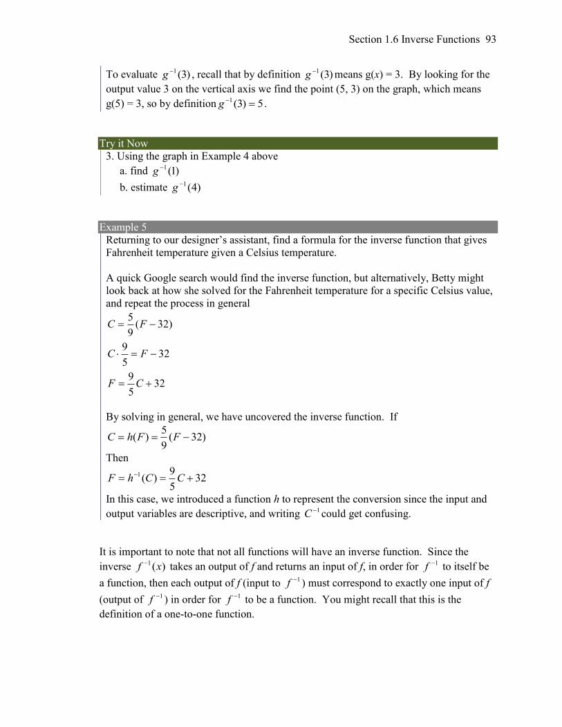
Section 1.6 Inverse Functions 93
To evaluate )3(1g , recall that by definition )3(1g means g(x) = 3. By looking for the
output value 3 on the vertical axis we find the point (5, 3) on the graph, which means
g(5) = 3, so by definition 5)3(1 g .
Try it Now
3. Using the graph in Example 4 above
a. find )1(1g
b. estimate )4(1g
Example 5
Returning to our designer’s assistant, find a formula for the inverse function that gives
Fahrenheit temperature given a Celsius temperature.
A quick Google search would find the inverse function, but alternatively, Betty might
look back at how she solved for the Fahrenheit temperature for a specific Celsius value,
and repeat the process in general
325
9
325
9
)32(9
5
CF
FC
FC
By solving in general, we have uncovered the inverse function. If
)32(9
5)( FFhC
Then
325
9)(1 CChF
In this case, we introduced a function h to represent the conversion since the input and
output variables are descriptive, and writing 1C could get confusing.
It is important to note that not all functions will have an inverse function. Since the
inverse )(1 xf takes an output of f and returns an input of f, in order for 1f to itself be
a function, then each output of f (input to 1f ) must correspond to exactly one input of f
(output of 1f ) in order for 1f to be a function. You might recall that this is the
definition of a one-to-one function.
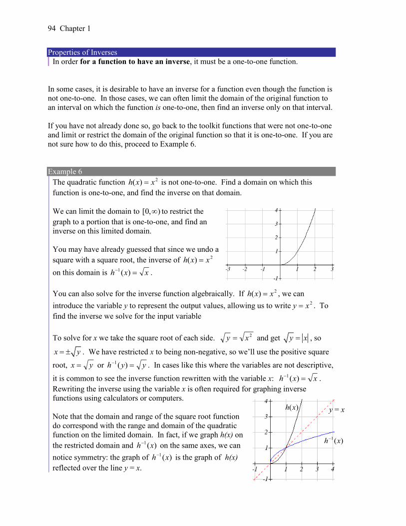
94 Chapter 1
Properties of Inverses
In order for a function to have an inverse, it must be a one-to-one function.
In some cases, it is desirable to have an inverse for a function even though the function is
not one-to-one. In those cases, we can often limit the domain of the original function to
an interval on which the function is one-to-one, then find an inverse only on that interval.
If you have not already done so, go back to the toolkit functions that were not one-to-one
and limit or restrict the domain of the original function so that it is one-to-one. If you are
not sure how to do this, proceed to Example 6.
Example 6
The quadratic function 2)( xxh is not one-to-one. Find a domain on which this
function is one-to-one, and find the inverse on that domain.
We can limit the domain to ),0[ to restrict the
graph to a portion that is one-to-one, and find an
inverse on this limited domain.
You may have already guessed that since we undo a
square with a square root, the inverse of 2)( xxh
on this domain is xxh )(1 .
You can also solve for the inverse function algebraically. If 2)( xxh , we can
introduce the variable y to represent the output values, allowing us to write 2xy . To
find the inverse we solve for the input variable
To solve for x we take the square root of each side. 2xy and get y x , so
x y . We have restricted x to being non-negative, so we’ll use the positive square
root, yx or yyh )(1 . In cases like this where the variables are not descriptive,
it is common to see the inverse function rewritten with the variable x: xxh )(1 .
Rewriting the inverse using the variable x is often required for graphing inverse
functions using calculators or computers.
Note that the domain and range of the square root function
do correspond with the range and domain of the quadratic
function on the limited domain. In fact, if we graph h(x) on
the restricted domain and )(1 xh on the same axes, we can
notice symmetry: the graph of )(1 xh is the graph of h(x)
reflected over the line y = x.
)(1 xh
)(xh y = x
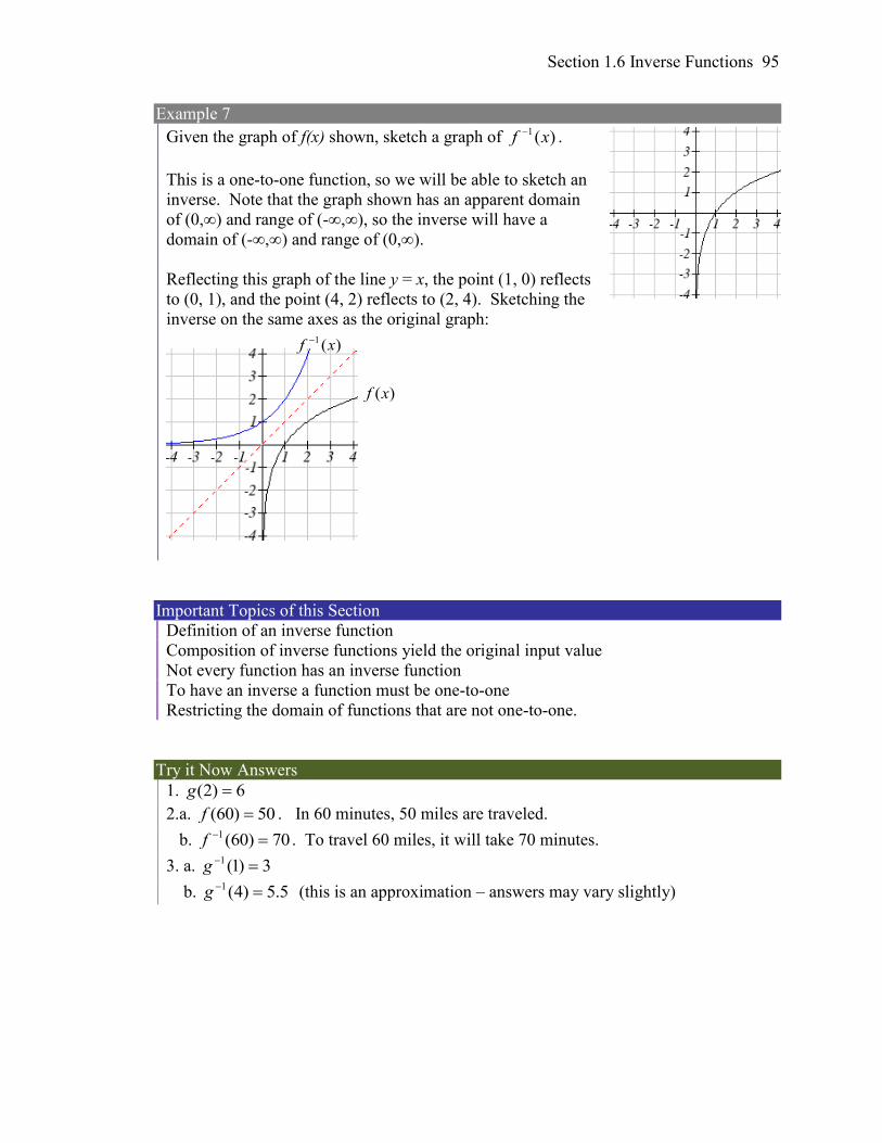
Section 1.6 Inverse Functions 95
Example 7
Given the graph of f(x) shown, sketch a graph of )(1 xf .
This is a one-to-one function, so we will be able to sketch an
inverse. Note that the graph shown has an apparent domain
of (0,∞) and range of (-∞,∞), so the inverse will have a
domain of (-∞,∞) and range of (0,∞).
Reflecting this graph of the line y = x, the point (1, 0) reflects
to (0, 1), and the point (4, 2) reflects to (2, 4). Sketching the
inverse on the same axes as the original graph:
Important Topics of this Section
Definition of an inverse function
Composition of inverse functions yield the original input value
Not every function has an inverse function
To have an inverse a function must be one-to-one
Restricting the domain of functions that are not one-to-one.
Try it Now Answers
1. 6)2( g
2.a. 50)60( f . In 60 minutes, 50 miles are traveled.
b. 70)60(1 f . To travel 60 miles, it will take 70 minutes.
3. a. 3)1(1 g
b. 5.5)4(1 g (this is an approximation – answers may vary slightly)
)(1 xf
)(xf
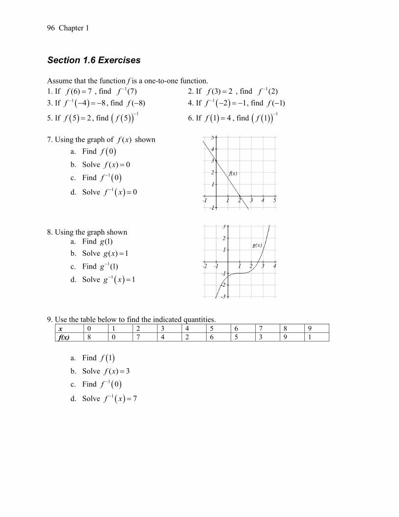
96 Chapter 1
Section 1.6 Exercises
Assume that the function f is a one-to-one function.
1. If (6) 7f , find 1(7)f 2. If (3) 2f , find 1(2)f
3. If 1 4 8f , find ( 8)f 4. If 1 2 1f , find ( 1)f
5. If 5 2f , find 1
5f
6. If 1 4f , find 1
1f
7. Using the graph of ( )f x shown
a. Find 0f
b. Solve ( ) 0f x
c. Find 1 0f
d. Solve 1 0f x
8. Using the graph shown
a. Find (1)g
b. Solve ( ) 1g x
c. Find 1(1)g
d. Solve 1 1g x
9. Use the table below to find the indicated quantities.
x 0 1 2 3 4 5 6 7 8 9
f(x) 8 0 7 4 2 6 5 3 9 1
a. Find 1f
b. Solve ( ) 3f x
c. Find 1 0f
d. Solve 1 7f x
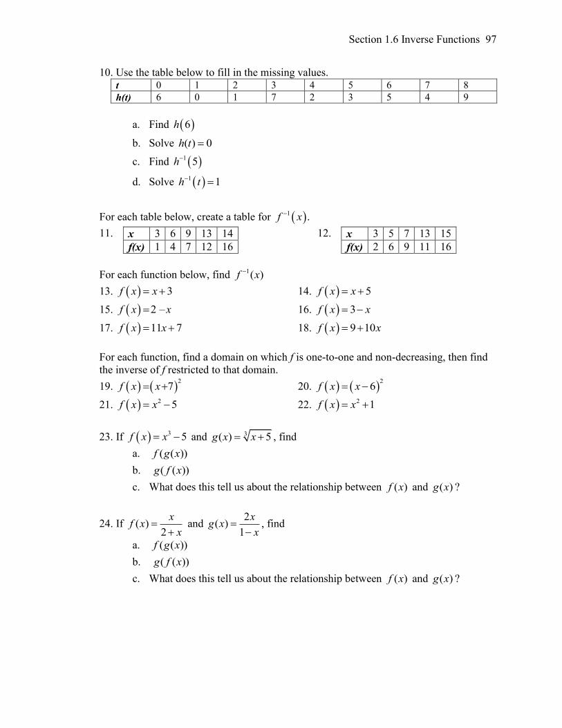
Section 1.6 Inverse Functions 97
10. Use the table below to fill in the missing values.
t 0 1 2 3 4 5 6 7 8
h(t) 6 0 1 7 2 3 5 4 9
a. Find 6h
b. Solve ( ) 0h t
c. Find 1 5h
d. Solve 1 1h t
For each table below, create a table for 1 .f x
11. x 3 6 9 13 14
f(x) 1 4 7 12 16
12. x 3 5 7 13 15
f(x) 2 6 9 11 16
For each function below, find 1( )f x
13. 3f x x 14. 5f x x
15. 2 – f x x 16. 3f x x
17. 11 7f x x 18. 9 10f x x
For each function, find a domain on which f is one-to-one and non-decreasing, then find
the inverse of f restricted to that domain.
19. 2
7f x x 20. 2
6f x x
21. 2 5f x x 22. 2 1f x x
23. If 3 5f x x and 3( ) 5g x x , find
a. ( ( ))f g x
b. ( ( ))g f x
c. What does this tell us about the relationship between ( )f x and ( )g x ?
24. If ( )2
xf x
x
and
2( )
1
xg x
x
, find
a. ( ( ))f g x
b. ( ( ))g f x
c. What does this tell us about the relationship between ( )f x and ( )g x ?

98 Chapter 1
This chapter is part of Precalculus: An Investigation of Functions © Lippman & Rasmussen 2011.
This material is licensed under a Creative Commons CC-BY-SA license.
Chapter 2: Linear Functions Chapter one was a window that gave us a peek into the entire course. Our goal was to
understand the basic structure of functions and function notation, the toolkit functions,
domain and range, how to recognize and understand composition and transformations of
functions and how to understand and utilize inverse functions. With these basic
components in hand we will further research the specific details and intricacies of each
type of function in our toolkit and use them to model the world around us.
Mathematical Modeling
As we approach day to day life we often need to quantify the things around us, giving
structure and numeric value to various situations. This ability to add structure enables us
to make choices based on patterns we see that are weighted and systematic. With this
structure in place we can model and even predict behavior to make decisions. Adding a
numerical structure to a real world situation is called Mathematical Modeling.
When modeling real world scenarios, there are some common growth patterns that are
regularly observed. We will devote this chapter and the rest of the book to the study of
the functions used to model these growth patterns.
Section 2.1 Linear Functions ........................................................................................ 99
Section 2.2 Graphs of Linear Functions ..................................................................... 111
Section 2.3 Modeling with Linear Functions .............................................................. 126
Section 2.4 Fitting Linear Models to Data .................................................................. 138
Section 2.5 Absolute Value Functions ........................................................................ 146
Section 2.1 Linear Functions
As you hop into a taxicab in Las Vegas, the meter will immediately read $3.30; this is the
“drop” charge made when the taximeter is activated. After that initial fee, the taximeter
will add $2.40 for each mile the taxi drives1. In this scenario, the total taxi fare depends
upon the number of miles ridden in the taxi, and we can ask whether it is possible to
model this type of scenario with a function. Using descriptive variables, we choose m for
miles and C for Cost in dollars as a function of miles: C(m).
We know for certain that 30.3)0( C , since the $3.30 drop charge is assessed regardless
of how many miles are driven. Since $2.40 is added for each mile driven, then
70.540.230.3)1( C
If we then drove a second mile, another $2.40 would be added to the cost:
10.8)2(40.230.340.240.230.3)2( C
1 http://taxi.state.nv.us/FaresFees.htm, retrieved July 28, 2010. There is also a waiting fee assessed when
the taxi is waiting at red lights, but we’ll ignore that in this discussion.
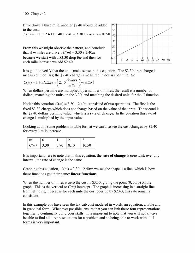
Chapter 2
100
If we drove a third mile, another $2.40 would be added
to the cost:
50.10)3(40.230.340.240.240.230.3)3( C
From this we might observe the pattern, and conclude
that if m miles are driven, mmC 40.230.3)(
because we start with a $3.30 drop fee and then for
each mile increase we add $2.40.
It is good to verify that the units make sense in this equation. The $3.30 drop charge is
measured in dollars; the $2.40 charge is measured in dollars per mile. So
milesmmile
dollarsdollarsmC
40.230.3)(
When dollars per mile are multiplied by a number of miles, the result is a number of
dollars, matching the units on the 3.30, and matching the desired units for the C function.
Notice this equation mmC 40.230.3)( consisted of two quantities. The first is the
fixed $3.30 charge which does not change based on the value of the input. The second is
the $2.40 dollars per mile value, which is a rate of change. In the equation this rate of
change is multiplied by the input value.
Looking at this same problem in table format we can also see the cost changes by $2.40
for every 1 mile increase.
m 0 1 2 3
C(m) 3.30 5.70 8.10 10.50
It is important here to note that in this equation, the rate of change is constant; over any
interval, the rate of change is the same.
Graphing this equation, mmC 40.230.3)( we see the shape is a line, which is how
these functions get their name: linear functions
When the number of miles is zero the cost is $3.30, giving the point (0, 3.30) on the
graph. This is the vertical or C(m) intercept. The graph is increasing in a straight line
from left to right because for each mile the cost goes up by $2.40; this rate remains
consistent.
In this example you have seen the taxicab cost modeled in words, an equation, a table and
in graphical form. Whenever possible, ensure that you can link these four representations
together to continually build your skills. It is important to note that you will not always
be able to find all 4 representations for a problem and so being able to work with all 4
forms is very important.
Section 2.1 Linear Functions
101
Linear Function
A linear function is a function whose graph produces a line. Linear functions can
always be written in the form
mxbxf )( or bmxxf )( ; they’re equivalent
where
b is the initial or starting value of the function (when input, x = 0), and
m is the constant rate of change of the function
Many people like to write linear functions in the form mxbxf )( because it
corresponds to the way we tend to speak: “The output starts at b and increases at a rate
of m.”
For this reason alone we will use the mxbxf )( form for many of the examples, but
remember they are equivalent and can be written correctly both ways.
Slope and Increasing/Decreasing
m is the constant rate of change of the function (also called slope). The slope
determines if the function is an increasing function or a decreasing function.
mxbxf )( is an increasing function if 0m
mxbxf )( is a decreasing function if 0m
If 0m , the rate of change zero, and the function ( ) 0f x b x b is just a horizontal
line passing through the point (0, b), neither increasing nor decreasing.
Example 1
Marcus currently owns 200 songs in his iTunes collection. Every month, he adds 15
new songs. Write a formula for the number of songs, N, in his iTunes collection as a
function of the number of months, m. How many songs will he own in a year?
The initial value for this function is 200, since he currently owns 200 songs, so
200)0( N . The number of songs increases by 15 songs per month, so the rate of
change is 15 songs per month. With this information, we can write the formula:
mmN 15200)( .
N(m) is an increasing linear function.
With this formula we can predict how many songs he will have in 1 year (12 months):
380180200)12(15200)12( N . Marcus will have 380 songs in 12 months.
Chapter 2
102
Try it Now
1. If you earn $30,000 per year and you spend $29,000 per year write an equation for
the amount of money you save after y years, if you start with nothing.
“The most important thing, spend less than you earn!2”
Calculating Rate of Change
Given two values for the input, 21 and xx , and two corresponding values for the output,
21 and yy , or a set of points, ) ,( 11 yx and ) ,( 22 yx , if we wish to find a linear function
that contains both points we can calculate the rate of change, m:
12
12
inputin change
outputin change
xx
yy
x
ym
Rate of change of a linear function is also called the slope of the line.
Note in function notation, )( 11 xfy and )( 22 xfy , so we could equivalently write
2 1
2 1
f x f xm
x x
Example 2
The population of a city increased from 23,400 to 27,800 between 2002 and 2006. Find
the rate of change of the population during this time span.
The rate of change will relate the change in population to the change in time. The
population increased by 44002340027800 people over the 4 year time interval. To
find the rate of change, the number of people per year the population changed by:
year
people
years
people1100
4
4400 = 1100 people per year
Notice that we knew the population was increasing, so we would expect our value for m
to be positive. This is a quick way to check to see if your value is reasonable.
Example 3
The pressure, P, in pounds per square inch (PSI) on a diver depends upon their depth
below the water surface, d, in feet, following the equation ddP 434.0696.14)( .
Interpret the components of this function.
2 http://www.thesimpledollar.com/2009/06/19/rule-1-spend-less-than-you-earn/
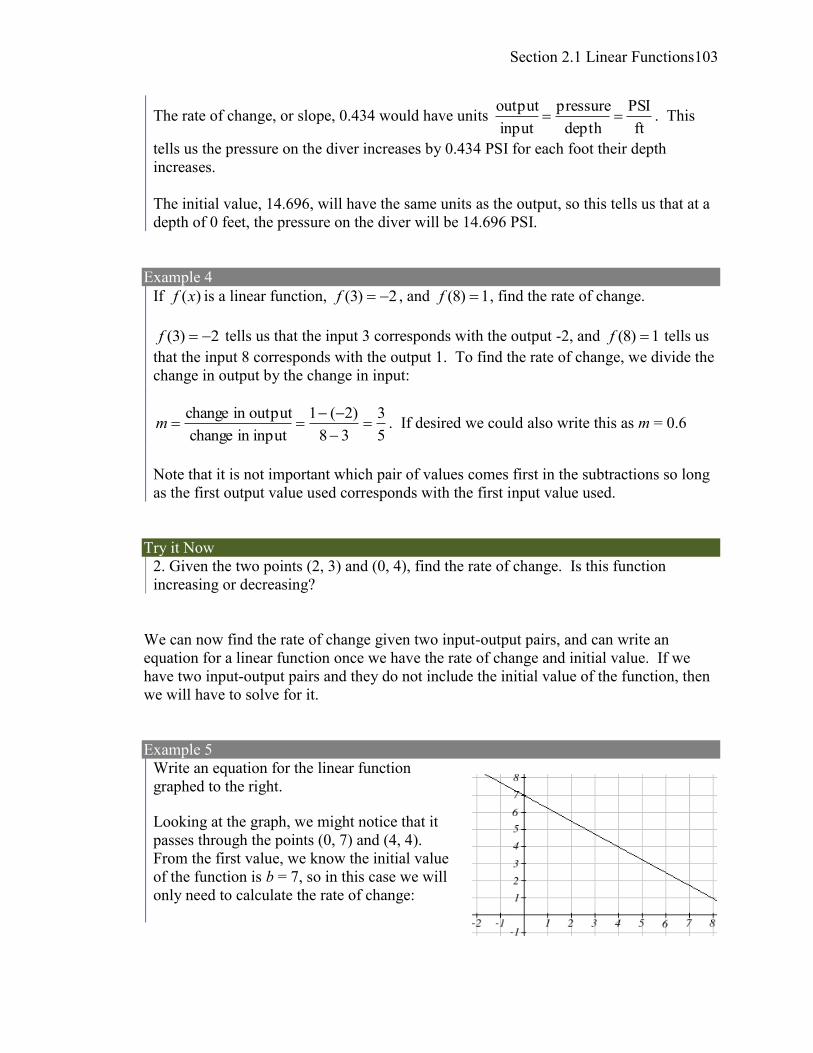
Section 2.1 Linear Functions
103
The rate of change, or slope, 0.434 would have units ft
PSI
depth
pressure
input
output . This
tells us the pressure on the diver increases by 0.434 PSI for each foot their depth
increases.
The initial value, 14.696, will have the same units as the output, so this tells us that at a
depth of 0 feet, the pressure on the diver will be 14.696 PSI.
Example 4
If )(xf is a linear function, 2)3( f , and 1)8( f , find the rate of change.
2)3( f tells us that the input 3 corresponds with the output -2, and 1)8( f tells us
that the input 8 corresponds with the output 1. To find the rate of change, we divide the
change in output by the change in input:
5
3
38
)2(1
inputin change
outputin change
m . If desired we could also write this as m = 0.6
Note that it is not important which pair of values comes first in the subtractions so long
as the first output value used corresponds with the first input value used.
Try it Now
2. Given the two points (2, 3) and (0, 4), find the rate of change. Is this function
increasing or decreasing?
We can now find the rate of change given two input-output pairs, and can write an
equation for a linear function once we have the rate of change and initial value. If we
have two input-output pairs and they do not include the initial value of the function, then
we will have to solve for it.
Example 5
Write an equation for the linear function
graphed to the right.
Looking at the graph, we might notice that it
passes through the points (0, 7) and (4, 4).
From the first value, we know the initial value
of the function is b = 7, so in this case we will
only need to calculate the rate of change:
Chapter 2
104
4
3
04
74
m
This allows us to write the equation:
xxf4
37)(
Example 6
If )(xf is a linear function, 2)3( f , and 1)8( f , find an equation for the function.
In example 3, we computed the rate of change to be 5
3m . In this case, we do not
know the initial value )0(f , so we will have to solve for it. Using the rate of change,
we know the equation will have the form xbxf5
3)( . Since we know the value of
the function when x = 3, we can evaluate the function at 3.
)3(5
3)3( bf Since we know that 2)3( f , we can substitute on the left side
)3(5
32 b This leaves us with an equation we can solve for the initial value
5
19
5
92
b
Combining this with the value for the rate of change, we can now write a formula for
this function:
xxf5
3
5
19)(
Example 7
Working as an insurance salesperson, Ilya earns a base salary and a commission on each
new policy, so Ilya’s weekly income, I, depends on the number of new policies, n, he
sells during the week. Last week he sold 3 new policies, and earned $760 for the week.
The week before, he sold 5 new policies, and earned $920. Find an equation for I(n),
and interpret the meaning of the components of the equation.
The given information gives us two input-output pairs: (3,760) and (5,920). We start
by finding the rate of change.
802
160
35
760920
m
Section 2.1 Linear Functions
105
Keeping track of units can help us interpret this quantity. Income increased by $160
when the number of policies increased by 2, so the rate of change is $80 per policy; Ilya
earns a commission of $80 for each policy sold during the week.
We can then solve for the initial value
nbnI 80)( then when n = 3, (3) 760I , giving
)3(80760 b this allows us to solve for b
520)3(80760 b
This value is the starting value for the function. This is Ilya’s income when n = 0,
which means no new policies are sold. We can interpret this as Ilya’s base salary for
the week, which does not depend upon the number of policies sold.
Writing the final equation:
nnI 80520)(
Our final interpretation is: Ilya’s base salary is $520 per week and he earns an
additional $80 commission for each policy sold each week.
Flashback
Looking at Example 7:
Determine the independent and dependent variables.
What is a reasonable domain and range?
Is this function one-to-one?
Try it Now
3. The balance in your college payment account, C, is a function of the number of
quarters, q, you attend. Interpret the function C(a) = 20000 – 4000q in words. How
many quarters of college can you pay for until this account is empty?
Example 8
Given the table below write a linear equation that represents the table values
We can see from the table that the initial value of rats is 1000 so in the linear format
( )P w b mw , b = 1000.
Rather than solving for m, we can notice from the table that the population goes up by
80 for every 2 weeks that pass. This rate is consistent from week 0, to week 2, 4, and 6.
w, number of
weeks
0 2 4 6
P(w), number
of rats
1000 1080 1160 1240
Chapter 2
106
The rate of change is 80 rats per 2 weeks. This can be simplified to 40 rats per week and
we can write
( )P w b mw as wwP 401000)(
If you didn’t notice this from the table you could still solve for the slope using any two
points from the table. For example, using (2, 1080) and (6, 1240),
1240 1080 16040
6 2 4m
rats per week
Important Topics of this Section
Definition of Modeling
Definition of a linear function
Structure of a linear function
Increasing & Decreasing functions
Finding the vertical intercept (0, b)
Finding the slope/rate of change, m
Interpreting linear functions
Try it Now Answers
1. yyyyS 1000000,29000,30)( $1000 is saved each year.
2. 2
1
2
1
20
34
m ; Decreasing because m < 0
3. Your College account starts with $20,000 in it and you withdraw $4,000 each quarter
(or your account contains $20,000 and decreases by $4000 each quarter.) You can pay
for 5 quarters before the money in this account is gone.
Flashback Answers
n (number of policies sold) is the independent variable
I(n) (weekly income as a function of policies sold) is the dependent variable.
A reasonable domain is (0, 15)*
A reasonable range is ($540, $1740)* *answers may vary given reasoning is stated; 15 is an arbitrary upper limit based on
selling 3 policies per day in a 5 day work week and $1740 corresponds with the domain.
Yes this function is one-to-one
Section 2.1 Linear Functions
107
Section 2.1 Exercises
1. A town's population has been growing linearly. In 2003, the population was 45,000,
and the population has been growing by 1700 people each year. Write an
equation, , P t for the population t years after 2003.
2. A town's population has been growing linearly. In 2005, the population was 69,000,
and the population has been growing by 2500 people each year. Write an
equation, , P t for the population t years after 2005.
3. Sonya is currently 10 miles from home, and is walking further away at 2 miles per
hour. Write an equation for her distance from home t hours from now.
4. A boat is 100 miles away from the marina, sailing directly towards it at 10 miles per
hour. Write an equation for the distance of the boat from the marina after t hours.
5. Timmy goes to the fair with $40. Each ride costs $2. How much money will he have
left after riding n rides?
6. At noon, a barista notices she has $20 in her tip jar. If she makes an average of $0.50
from each customer, how much will she have in her tip jar if she serves n more
customers during her shift?
Determine if each function is increasing or decreasing
7. 4 3f x x 8. 5 6g x x
9. 5 2a x x 10. 8 3b x x
11. 2 4h x x 12. 4 1k x x
13. 1
32
j x x 14. 1
54
p x x
15. 1
23
n x x 16. 3
38
m x x
Find the slope of the line that passes through the two given points
17. (2, 4) and (4, 10) 18. (1, 5) and (4, 11)
19. (-1,4) and (5, 2) 20. (-2, 8) and (4, 6)
21. (6,11) and (-4,3) 22. (9,10) and (-6,-12)
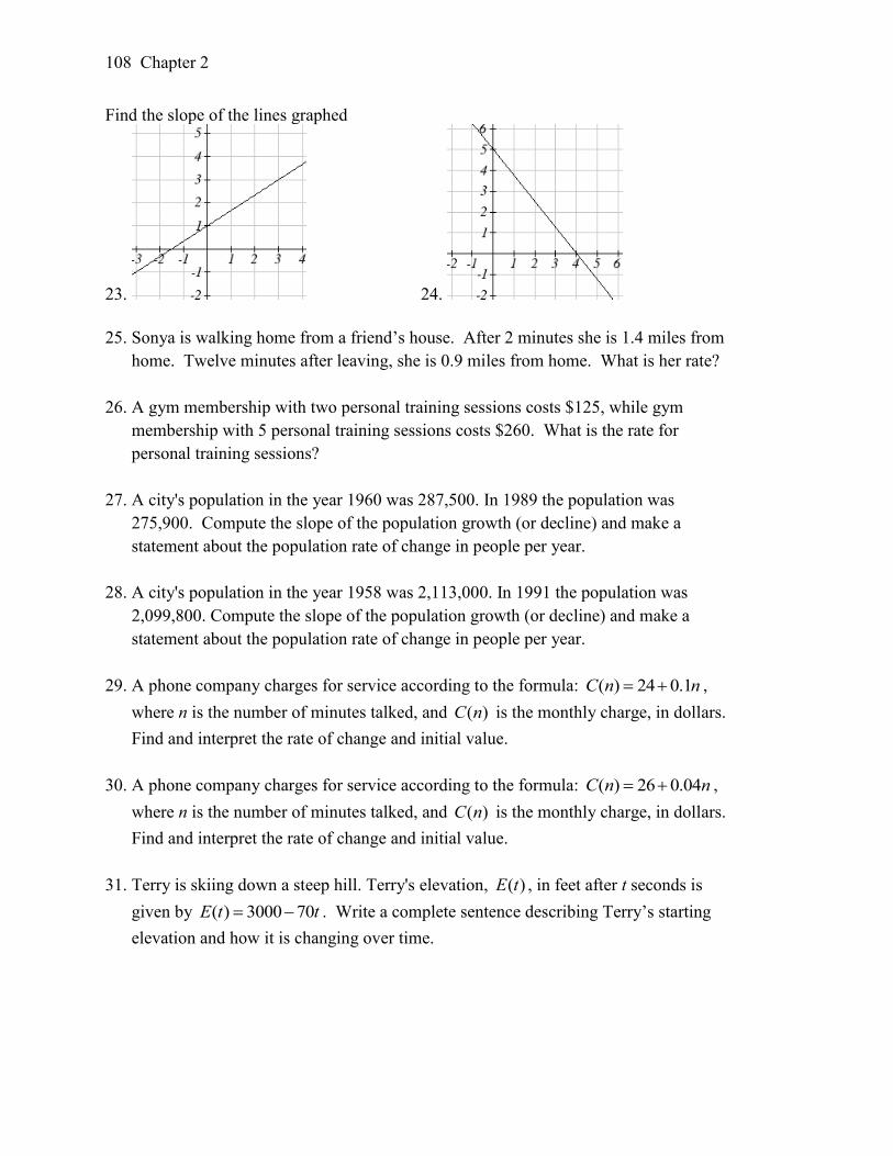
Chapter 2
108
Find the slope of the lines graphed
23. 24.
25. Sonya is walking home from a friend’s house. After 2 minutes she is 1.4 miles from
home. Twelve minutes after leaving, she is 0.9 miles from home. What is her rate?
26. A gym membership with two personal training sessions costs $125, while gym
membership with 5 personal training sessions costs $260. What is the rate for
personal training sessions?
27. A city's population in the year 1960 was 287,500. In 1989 the population was
275,900. Compute the slope of the population growth (or decline) and make a
statement about the population rate of change in people per year.
28. A city's population in the year 1958 was 2,113,000. In 1991 the population was
2,099,800. Compute the slope of the population growth (or decline) and make a
statement about the population rate of change in people per year.
29. A phone company charges for service according to the formula: ( ) 24 0.1C n n ,
where n is the number of minutes talked, and ( )C n is the monthly charge, in dollars.
Find and interpret the rate of change and initial value.
30. A phone company charges for service according to the formula: ( ) 26 0.04C n n ,
where n is the number of minutes talked, and ( )C n is the monthly charge, in dollars.
Find and interpret the rate of change and initial value.
31. Terry is skiing down a steep hill. Terry's elevation, ( )E t , in feet after t seconds is
given by ( ) 3000 70E t t . Write a complete sentence describing Terry’s starting
elevation and how it is changing over time.
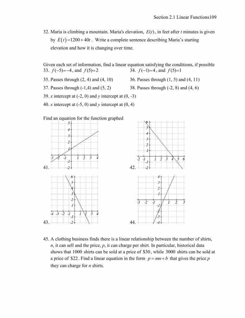
Section 2.1 Linear Functions
109
32. Maria is climbing a mountain. Maria's elevation, ( )E t , in feet after t minutes is given
by 1 200 40E t t . Write a complete sentence describing Maria’s starting
elevation and how it is changing over time.
Given each set of information, find a linear equation satisfying the conditions, if possible
33. ( 5) 4f , and (5) 2f 34. ( 1) 4f , and (5) 1 f
35. Passes through (2, 4) and (4, 10) 36. Passes through (1, 5) and (4, 11)
37. Passes through (-1,4) and (5, 2) 38. Passes through (-2, 8) and (4, 6)
39. x intercept at (-2, 0) and y intercept at (0, -3)
40. x intercept at (-5, 0) and y intercept at (0, 4)
Find an equation for the function graphed
41. 42.
43. 44.
45. A clothing business finds there is a linear relationship between the number of shirts,
n, it can sell and the price, p, it can charge per shirt. In particular, historical data
shows that 1000 shirts can be sold at a price of $30 , while 3000 shirts can be sold at
a price of $22 . Find a linear equation in the form p mn b that gives the price p
they can charge for n shirts.
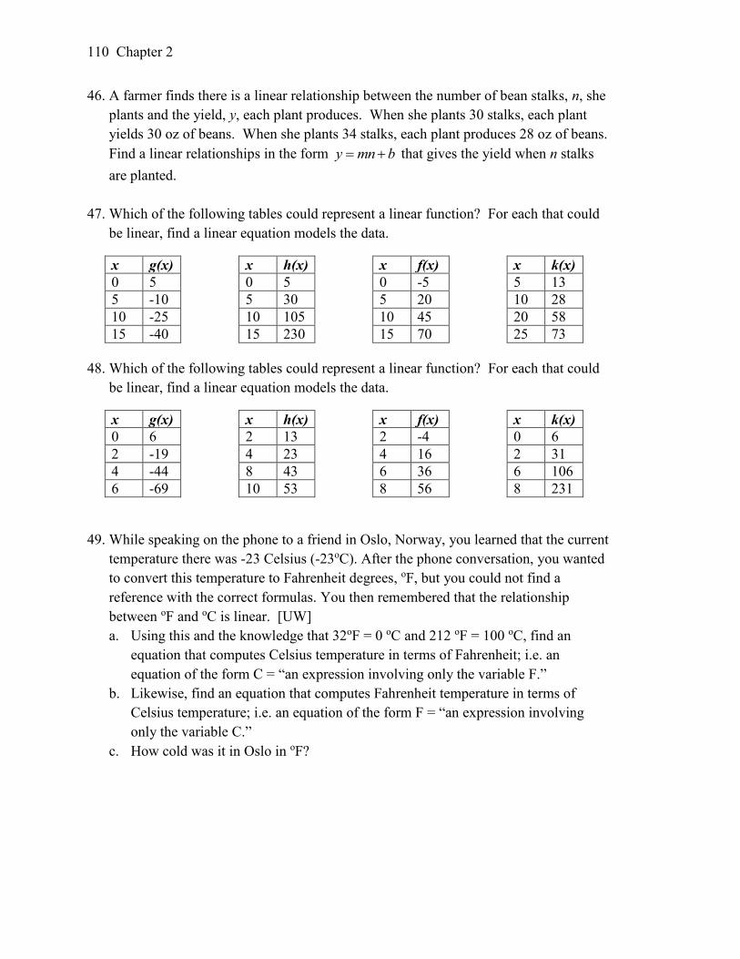
Chapter 2
110
46. A farmer finds there is a linear relationship between the number of bean stalks, n, she
plants and the yield, y, each plant produces. When she plants 30 stalks, each plant
yields 30 oz of beans. When she plants 34 stalks, each plant produces 28 oz of beans.
Find a linear relationships in the form y mn b that gives the yield when n stalks
are planted.
47. Which of the following tables could represent a linear function? For each that could
be linear, find a linear equation models the data.
x g(x)
0 5
5 -10
10 -25
15 -40
x h(x)
0 5
5 30
10 105
15 230
x f(x)
0 -5
5 20
10 45
15 70
x k(x)
5 13
10 28
20 58
25 73
48. Which of the following tables could represent a linear function? For each that could
be linear, find a linear equation models the data.
x g(x)
0 6
2 -19
4 -44
6 -69
x h(x)
2 13
4 23
8 43
10 53
x f(x)
2 -4
4 16
6 36
8 56
x k(x)
0 6
2 31
6 106
8 231
49. While speaking on the phone to a friend in Oslo, Norway, you learned that the current
temperature there was -23 Celsius (-23oC). After the phone conversation, you wanted
to convert this temperature to Fahrenheit degrees, oF, but you could not find a
reference with the correct formulas. You then remembered that the relationship
between oF and oC is linear. [UW]
a. Using this and the knowledge that 32oF = 0 oC and 212 oF = 100 oC, find an
equation that computes Celsius temperature in terms of Fahrenheit; i.e. an
equation of the form C = “an expression involving only the variable F.”
b. Likewise, find an equation that computes Fahrenheit temperature in terms of
Celsius temperature; i.e. an equation of the form F = “an expression involving
only the variable C.”
c. How cold was it in Oslo in oF?
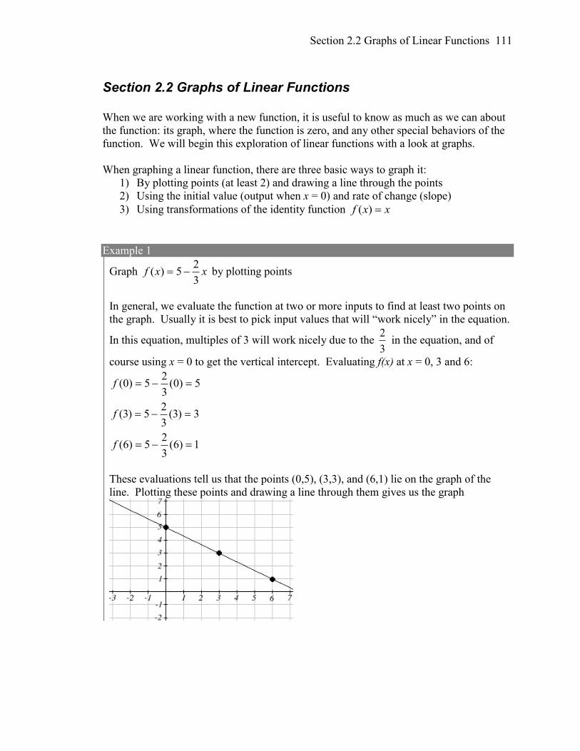
Section 2.2 Graphs of Linear Functions 111
Section 2.2 Graphs of Linear Functions
When we are working with a new function, it is useful to know as much as we can about
the function: its graph, where the function is zero, and any other special behaviors of the
function. We will begin this exploration of linear functions with a look at graphs.
When graphing a linear function, there are three basic ways to graph it:
1) By plotting points (at least 2) and drawing a line through the points
2) Using the initial value (output when x = 0) and rate of change (slope)
3) Using transformations of the identity function xxf )(
Example 1
Graph xxf3
25)( by plotting points
In general, we evaluate the function at two or more inputs to find at least two points on
the graph. Usually it is best to pick input values that will “work nicely” in the equation.
In this equation, multiples of 3 will work nicely due to the 3
2 in the equation, and of
course using x = 0 to get the vertical intercept. Evaluating f(x) at x = 0, 3 and 6:
1)6(3
25)6(
3)3(3
25)3(
5)0(3
25)0(
f
f
f
These evaluations tell us that the points (0,5), (3,3), and (6,1) lie on the graph of the
line. Plotting these points and drawing a line through them gives us the graph
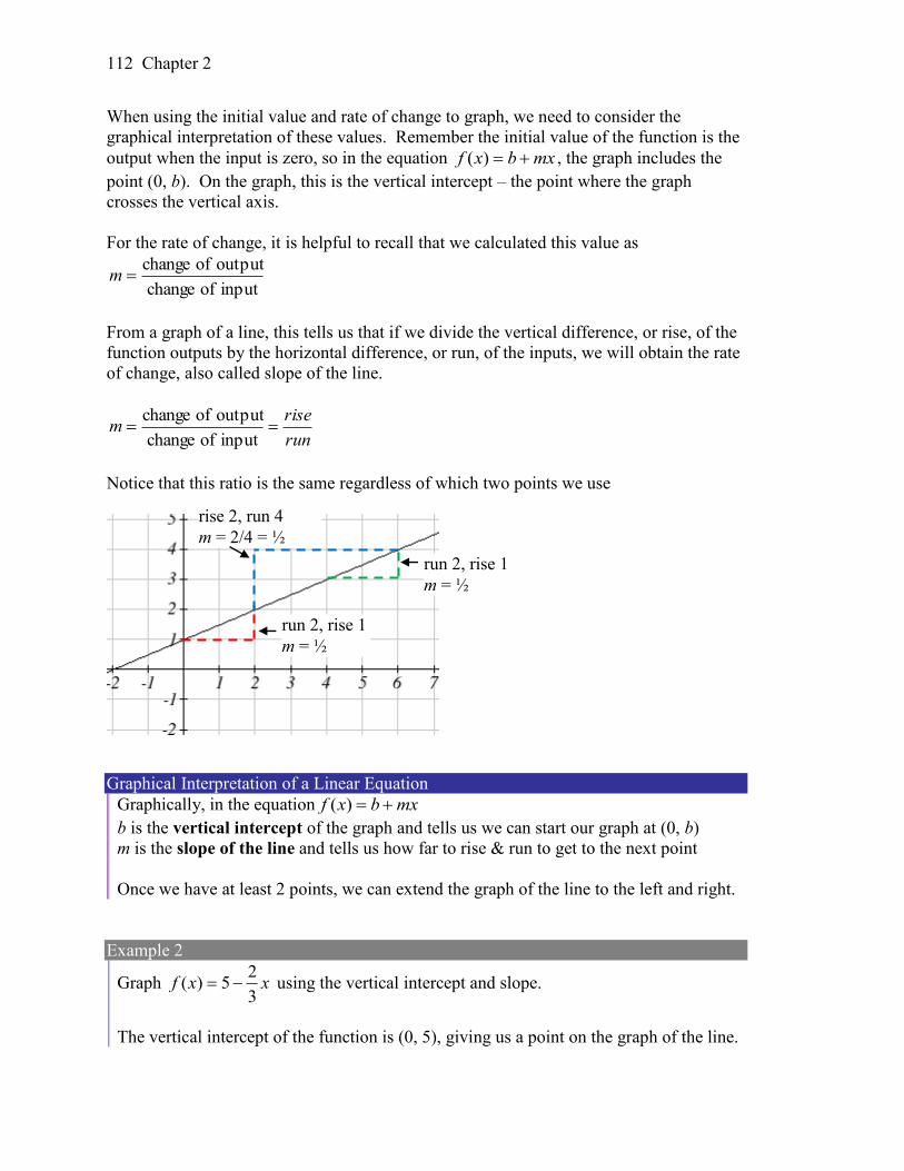
Chapter 2
112
When using the initial value and rate of change to graph, we need to consider the
graphical interpretation of these values. Remember the initial value of the function is the
output when the input is zero, so in the equation mxbxf )( , the graph includes the
point (0, b). On the graph, this is the vertical intercept – the point where the graph
crosses the vertical axis.
For the rate of change, it is helpful to recall that we calculated this value as
input of change
output of changem
From a graph of a line, this tells us that if we divide the vertical difference, or rise, of the
function outputs by the horizontal difference, or run, of the inputs, we will obtain the rate
of change, also called slope of the line.
run
risem
input of change
output of change
Notice that this ratio is the same regardless of which two points we use
Graphical Interpretation of a Linear Equation
Graphically, in the equation mxbxf )(
b is the vertical intercept of the graph and tells us we can start our graph at (0, b)
m is the slope of the line and tells us how far to rise & run to get to the next point
Once we have at least 2 points, we can extend the graph of the line to the left and right.
Example 2
Graph xxf3
25)( using the vertical intercept and slope.
The vertical intercept of the function is (0, 5), giving us a point on the graph of the line.
run 2, rise 1
m = ½
rise 2, run 4
m = 2/4 = ½
run 2, rise 1
m = ½
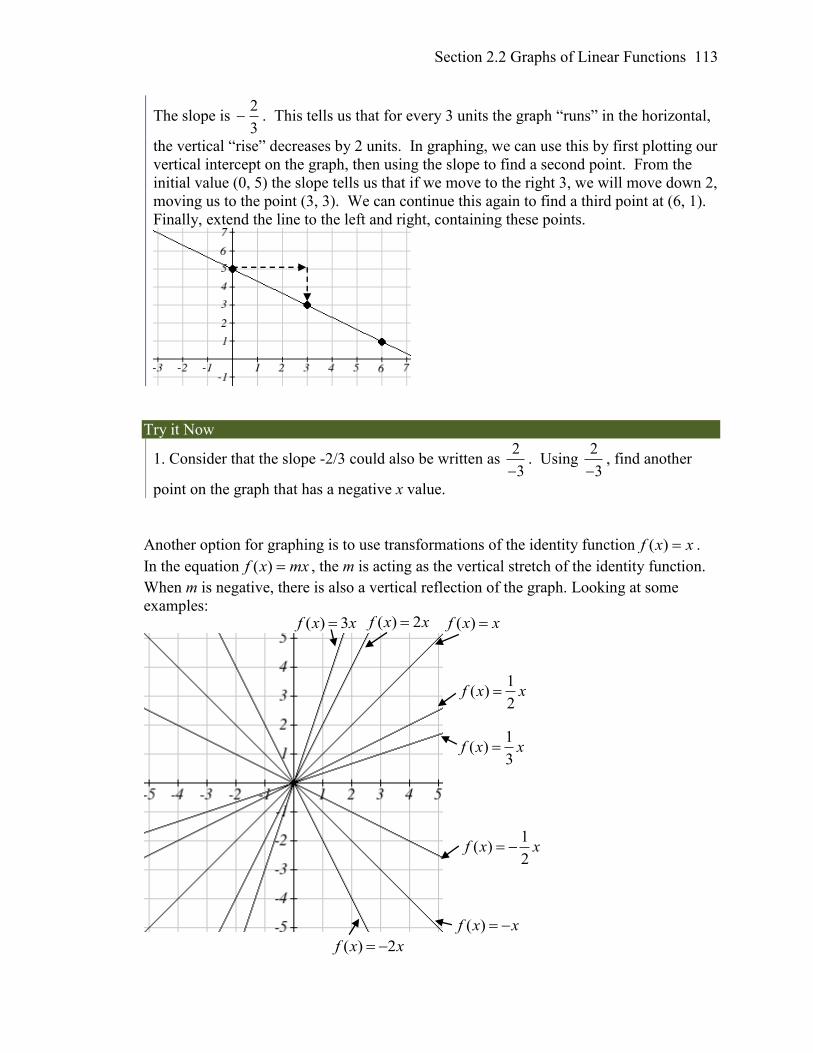
Section 2.2 Graphs of Linear Functions 113
The slope is 3
2 . This tells us that for every 3 units the graph “runs” in the horizontal,
the vertical “rise” decreases by 2 units. In graphing, we can use this by first plotting our
vertical intercept on the graph, then using the slope to find a second point. From the
initial value (0, 5) the slope tells us that if we move to the right 3, we will move down 2,
moving us to the point (3, 3). We can continue this again to find a third point at (6, 1).
Finally, extend the line to the left and right, containing these points.
Try it Now
1. Consider that the slope -2/3 could also be written as 2
3. Using
2
3, find another
point on the graph that has a negative x value.
Another option for graphing is to use transformations of the identity function xxf )( .
In the equation mxxf )( , the m is acting as the vertical stretch of the identity function.
When m is negative, there is also a vertical reflection of the graph. Looking at some
examples:
1( )
2f x x
1( )
3f x x
( )f x x ( ) 3f x x ( ) 2f x x
1( )
2f x x
( )f x x
( ) 2f x x
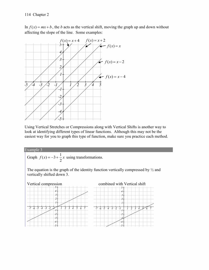
Chapter 2
114
In bmxxf )( , the b acts as the vertical shift, moving the graph up and down without
affecting the slope of the line. Some examples:
Using Vertical Stretches or Compressions along with Vertical Shifts is another way to
look at identifying different types of linear functions. Although this may not be the
easiest way for you to graph this type of function, make sure you practice each method.
Example 3
Graph xxf2
13)( using transformations.
The equation is the graph of the identity function vertically compressed by ½ and
vertically shifted down 3.
Vertical compression combined with Vertical shift
( ) 2f x x
( )f x x
( ) 2f x x
( ) 4f x x
( ) 4f x x
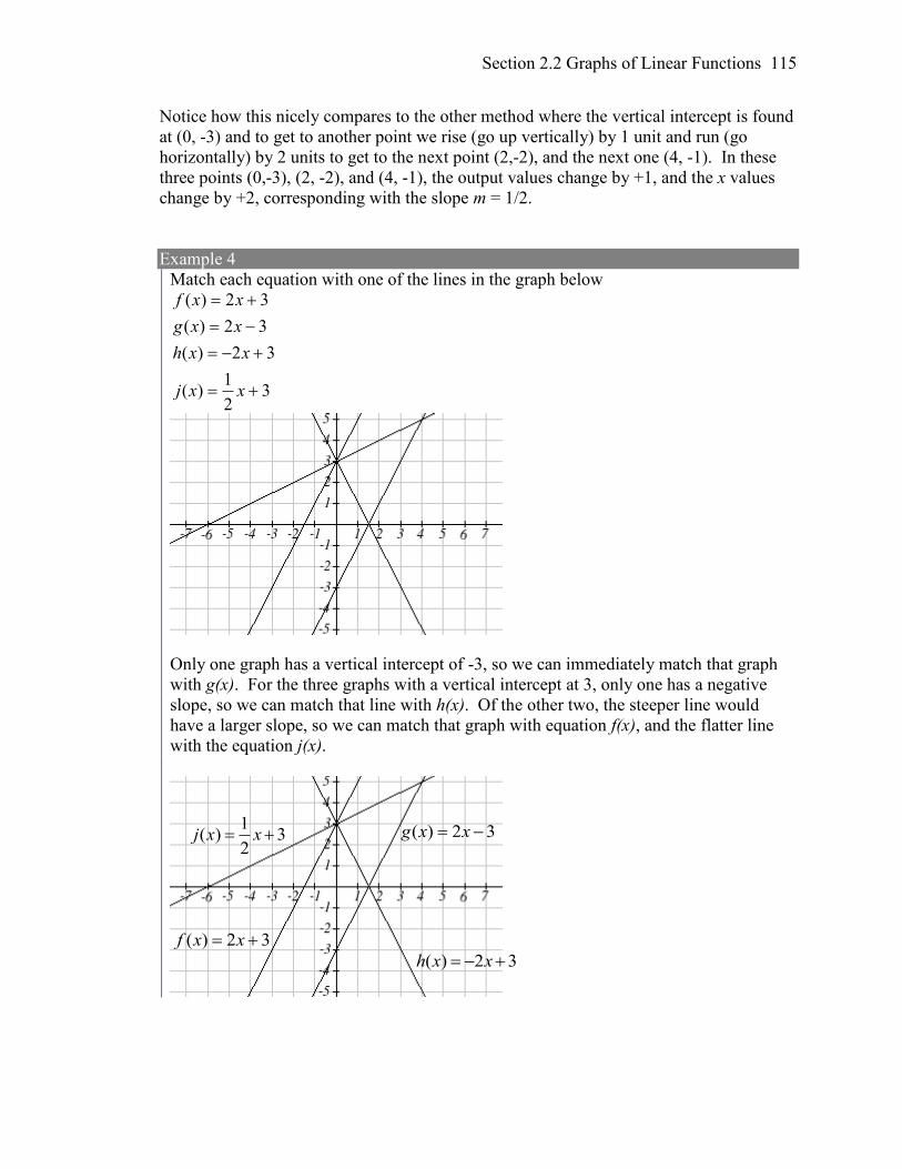
Section 2.2 Graphs of Linear Functions 115
Notice how this nicely compares to the other method where the vertical intercept is found
at (0, -3) and to get to another point we rise (go up vertically) by 1 unit and run (go
horizontally) by 2 units to get to the next point (2,-2), and the next one (4, -1). In these
three points (0,-3), (2, -2), and (4, -1), the output values change by +1, and the x values
change by +2, corresponding with the slope m = 1/2.
Example 4
Match each equation with one of the lines in the graph below
32
1)(
32)(
32)(
32)(
xxj
xxh
xxg
xxf
Only one graph has a vertical intercept of -3, so we can immediately match that graph
with g(x). For the three graphs with a vertical intercept at 3, only one has a negative
slope, so we can match that line with h(x). Of the other two, the steeper line would
have a larger slope, so we can match that graph with equation f(x), and the flatter line
with the equation j(x).
1( ) 3
2j x x
( ) 2 3h x x
( ) 2 3g x x
( ) 2 3f x x
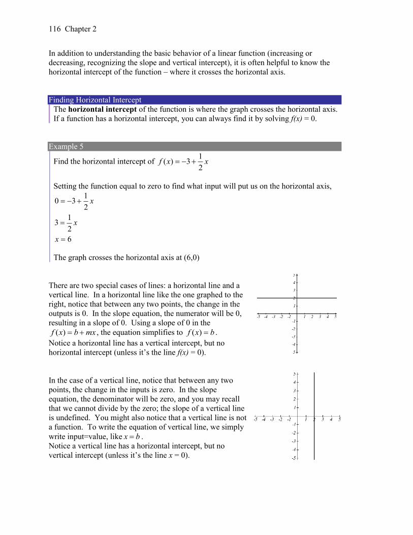
Chapter 2
116
In addition to understanding the basic behavior of a linear function (increasing or
decreasing, recognizing the slope and vertical intercept), it is often helpful to know the
horizontal intercept of the function – where it crosses the horizontal axis.
Finding Horizontal Intercept
The horizontal intercept of the function is where the graph crosses the horizontal axis.
If a function has a horizontal intercept, you can always find it by solving f(x) = 0.
Example 5
Find the horizontal intercept of xxf2
13)(
Setting the function equal to zero to find what input will put us on the horizontal axis,
6
2
13
2
130
x
x
x
The graph crosses the horizontal axis at (6,0)
There are two special cases of lines: a horizontal line and a
vertical line. In a horizontal line like the one graphed to the
right, notice that between any two points, the change in the
outputs is 0. In the slope equation, the numerator will be 0,
resulting in a slope of 0. Using a slope of 0 in the
mxbxf )( , the equation simplifies to bxf )( .
Notice a horizontal line has a vertical intercept, but no
horizontal intercept (unless it’s the line f(x) = 0).
In the case of a vertical line, notice that between any two
points, the change in the inputs is zero. In the slope
equation, the denominator will be zero, and you may recall
that we cannot divide by the zero; the slope of a vertical line
is undefined. You might also notice that a vertical line is not
a function. To write the equation of vertical line, we simply
write input=value, like x b .
Notice a vertical line has a horizontal intercept, but no
vertical intercept (unless it’s the line x = 0).
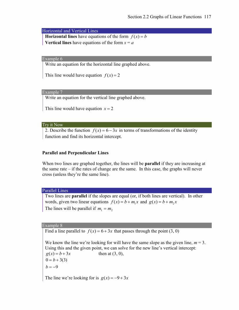
Section 2.2 Graphs of Linear Functions 117
Horizontal and Vertical Lines
Horizontal lines have equations of the form bxf )(
Vertical lines have equations of the form x = a
Example 6
Write an equation for the horizontal line graphed above.
This line would have equation ( ) 2f x
Example 7
Write an equation for the vertical line graphed above.
This line would have equation 2x
Try it Now
2. Describe the function xxf 36)( in terms of transformations of the identity
function and find its horizontal intercept.
Parallel and Perpendicular Lines
When two lines are graphed together, the lines will be parallel if they are increasing at
the same rate – if the rates of change are the same. In this case, the graphs will never
cross (unless they’re the same line).
Parallel Lines
Two lines are parallel if the slopes are equal (or, if both lines are vertical). In other
words, given two linear equations xmbxf 1)( and xmbxg 2)(
The lines will be parallel if 21 mm
Example 8
Find a line parallel to xxf 36)( that passes through the point (3, 0)
We know the line we’re looking for will have the same slope as the given line, m = 3.
Using this and the given point, we can solve for the new line’s vertical intercept:
xbxg 3)( then at (3, 0),
9
)3(30
b
b
The line we’re looking for is xxg 39)(
Chapter 2
118
If two lines are not parallel, one other interesting possibility is that the lines are
perpendicular, which means the lines form a right angle (90 degree angle – a square
corner) where they meet. In this case, the slopes when multiplied together will equal -1.
Solving for one slope leads us to the definition:
Perpendicular Lines
Given two linear equations xmbxf 1)( and xmbxg 2)(
The lines will be perpendicular if 121 mm , and so 1
2
1
mm
We often say the slope of a perpendicular line is the “negative reciprocal” of the other
line’s slope.
Example 9
Find the slope of a line perpendicular to a line with:
a) a slope of 2. b) a slope of -4. c) a slope of 3
2.
If the original line had slope 2, the perpendicular line’s slope would be 2
12
m
If the original line had slope -4, the perpendicular line’s slope would be 4
1
4
12
m
If the original line had slope 3
2, the perpendicular line’s slope would be
2
3
32
12
m
Example 10
Find the equation of a line perpendicular to xxf 36)( and passing through the point
(3, 0)
The original line has slope m = 3. The perpendicular line will have slope 3
1m .
Using this and the given point, we can find the equation for the line.
xbxg3
1)( then at (3, 0),
1
)3(3
10
b
b
The line we’re looking for is xxg3
11)(
Section 2.2 Graphs of Linear Functions 119
Try it Now
3. Given the line tth 24)( , find an equation for the line passing through (0, 0) that
is: a) parallel to h(t). b) perpendicular to h(t).
Example 12
A line passes through the points (-2, 6) and (4, 5). Find the equation of a perpendicular
line that passes through the point (4, 5).
From the two given points on the reference line, we can calculate the slope of that line:
6
1
)2(4
651
m
The perpendicular line will have slope
6
61
12
m
We can then solve for the vertical intercept that makes the line pass through the desired
point:
xbxg 6)( then at (4, 5),
19
)4(65
b
b
Giving the line xxg 619)(
Intersections of Lines
The graphs of two lines will intersect if they are not parallel. They will intersect at the
point that satisfies both equations. To find this point when the equations are given as
functions, we can solve for an input value so that )()( xgxf . In other words, we can
set the formulas for the lines equal, and solve for the input that satisfies the equation.
Example 13
Find the intersection of the lines 43)( tth and ttj 5)(
Setting )()( tjth ,
4
9
94
543
t
t
tt
This tells us the lines intersect when the input is 4
9.
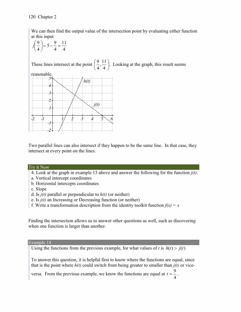
Chapter 2
120
We can then find the output value of the intersection point by evaluating either function
at this input
4
11
4
95
4
9
j
These lines intersect at the point
4
11,
4
9. Looking at the graph, this result seems
reasonable.
Two parallel lines can also intersect if they happen to be the same line. In that case, they
intersect at every point on the lines.
Try it Now
4. Look at the graph in example 13 above and answer the following for the function j(t):
a. Vertical intercept coordinates
b. Horizontal intercepts coordinates
c. Slope
d. Is j(t) parallel or perpendicular to h(t) (or neither)
e. Is j(t) an Increasing or Decreasing function (or neither)
f. Write a transformation description from the identity toolkit function f(x) = x
Finding the intersection allows us to answer other questions as well, such as discovering
when one function is larger than another.
Example 14
Using the functions from the previous example, for what values of t is )()( tjth
To answer this question, it is helpful first to know where the functions are equal, since
that is the point where h(t) could switch from being greater to smaller than j(t) or vice-
versa. From the previous example, we know the functions are equal at 4
9t .
h(t)
j(t)
Section 2.2 Graphs of Linear Functions 121
By examining the graph, we can see that h(t), the function with positive slope, is going
to be larger than the other function to the right of the intersection. So )()( tjth when
4
9t
Important Topics of this Section
Methods for graphing linear functions
Another name for slope = rise/run
Horizontal intercepts (a,0)
Horizontal lines
Vertical lines
Parallel lines
Perpendicular lines
Intersecting lines
Try it Now Answers
1. (-3,7) found by starting at the vertical intercept, going up 2 units and 3 in the
negative horizontal direction. You could have also answered, (-6, 9) or (-9, 11) etc…
2. Vertically stretched by a factor of 3, Vertically flipped (flipped over the x axis),
Vertically shifted up by 6 units. 6-3x=0 when x=2
3. Parallel ttf 2)( ; Perpendicular 1
( )2
g t t
4. Given j(t) = 5-t
a. (0,5)
b. (5,0)
c. Slope -1
d. Neither parallel nor perpendicular
e. Decreasing function
f. Given the identity function, perform a vertical flip (over the t axis) and shift up 5
units.
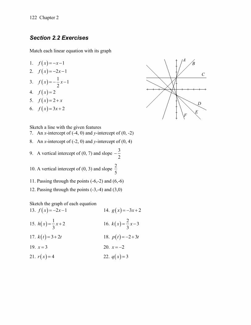
Chapter 2
122
Section 2.2 Exercises
Match each linear equation with its graph
1. 1f x x
2. 2 1f x x
3. 1
12
f x x
4. 2f x
5. 2f x x
6. 3 2f x x
Sketch a line with the given features
7. An x-intercept of (-4, 0) and y-intercept of (0, -2)
8. An x-intercept of (-2, 0) and y-intercept of (0, 4)
9. A vertical intercept of (0, 7) and slope 3
2
10. A vertical intercept of (0, 3) and slope 2
5
11. Passing through the points (-6,-2) and (6,-6)
12. Passing through the points (-3,-4) and (3,0)
Sketch the graph of each equation
13. 2 1f x x 14. 3 2g x x
15. 1
23
h x x 16. 2
33
k x x
17. 3 2k t t 18. 2 3p t t
19. 3x 20. 2x
21. 4r x 22. 3q x
A B
C
D
E F
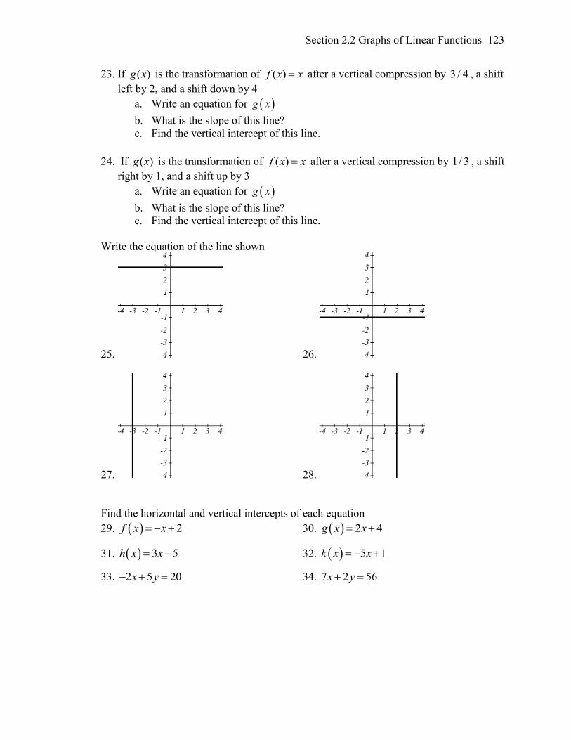
Section 2.2 Graphs of Linear Functions 123
23. If ( )g x is the transformation of ( )f x x after a vertical compression by 3 / 4 , a shift
left by 2, and a shift down by 4
a. Write an equation for g x
b. What is the slope of this line?
c. Find the vertical intercept of this line.
24. If ( )g x is the transformation of ( )f x x after a vertical compression by 1/ 3 , a shift
right by 1, and a shift up by 3
a. Write an equation for g x
b. What is the slope of this line?
c. Find the vertical intercept of this line.
Write the equation of the line shown
25. 26.
27. 28.
Find the horizontal and vertical intercepts of each equation
29. 2f x x 30. 2 4g x x
31. 3 5h x x 32. 5 1k x x
33. 2 5 20x y 34. 7 2 56x y
Chapter 2
124
Given below are descriptions of two lines. Find the slopes of Line 1 and Line 2. Is each
pair of lines parallel, perpendicular or neither?
35. Line 1: Passes through (0,6) and (3, 24)
Line 2: Passes through ( 1,19) and (8, 71)
36. Line 1: Passes through ( 8, 55) and (10, 89)
Line 2: Passes through (9, 44) and (4, 14)
37. Line 1: Passes through (2,3) and (4, 1)
Line 2: Passes through (6,3) and (8,5)
38. Line 1: Passes through (1, 7) and (5,5)
Line 2: Passes through ( 1, 3) and (1,1)
39. Line 1: Passes through (0, 5) and (3,3)
Line 2: Passes through (1, 5) and (3, 2)
40. Line 1: Passes through (2,5) and (5, 1)
Line 2: Passes through ( 3,7) and (3, 5)
41. Write an equation for a line parallel to 5 3f x x and passing through the point
(2,-12)
42. Write an equation for a line parallel to ( ) 3 1g x x and passing through the point
(4,9)
43. Write an equation for a line perpendicular to ( ) 2 4h t t and passing through the
point (-4,-1)
44. Write an equation for a line perpendicular to ( ) 3 4p t t and passing through the
point (3,1)
45. Find the point at which the line ( ) 2 1f x x intersects the line ( )g x x
46. Find the point at which the line ( ) 2 5f x x intersects the line ( ) 3 5g x x
Section 2.2 Graphs of Linear Functions 125
47. Use algebra to find the point at which the line 4 274
5 25
f x x intersects the line
9 73
4 10
h x x
48. Use algebra to find the point at which the line 7 457
4 60
f x x intersects the line
4 31
3 5
g x x
49. A car rental company offers two plans for renting a car.
Plan A: 30 dollars per day and 18 cents per mile
Plan B: 50 dollars per day with free unlimited mileage
How many miles would you need to drive for plan B to save you money?
50. A cell phone company offers two data options for its prepaid phones
Pay per use: $0.002 per Kilobyte (KB) used
Data Package: $5 for 5 Megabytes (5120 Kilobytes) + $0.002 per addition KB
Assuming you will use less than 5 Megabytes, under what circumstances will the data
package save you money?
51. Sketch an accurate picture of the line having equation 1
22
f x x . Let c be an
unknown constant. [UW]
a. Find the point of intersection between the line you have graphed and the
line 1g x cx ; your answer will be a point in the xy plane whose
coordinates involve the unknown c.
b. Find c so that the intersection point in (a) has x-coordinate 10.
c. Find c so that the intersection point in (a) lies on the x-axis.
Chapter 2
126
Section 2.3 Modeling with Linear Functions
When modeling scenarios with a linear function and solving problems involving
quantities changing linearly, we typically follow the same problem solving strategies that
we would use for any type of function:
Problem solving strategy
1) Identify changing quantities, and then carefully and clearly define descriptive
variables to represent those quantities. When appropriate, sketch a picture or define
a coordinate system.
2) Carefully read the problem to identify important information. Look for information
giving values for the variables, or values for parts of the functional model, like slope
and initial value.
3) Carefully read the problem to identify what we are trying to find, identify, solve, or
interpret.
4) Identify a solution pathway from the provided information to what we are trying to
find. Often this will involve checking and tracking units, building a table or even
finding a formula for the function being used to model the problem.
5) When needed, find a formula for the function.
6) Solve or evaluate using the formula you found for the desired quantities.
7) Reflect on whether your answer is reasonable for the given situation and whether it
makes sense mathematically.
8) Clearly convey your result using appropriate units, and answer in full sentences
when appropriate.
Example 1
Emily saved up $3500 for her summer visit to Seattle. She anticipates spending $400
each week on rent, food, and fun. Find and interpret the horizontal intercept and
determine a reasonable domain and range for this function.
In the problem, there are two changing quantities: time and money. The amount of
money she has remaining while on vacation depends on how long she stays. We can
define our variables, including units.
Output: M, money remaining, in dollars
Input: t, time, in weeks
Reading the problem, we identify two important values. The first, $3500, is the initial
value for M. The other value appears to be a rate of change – the units of dollars per
week match the units of our output variable divided by our input variable. She is
spending money each week, so you should recognize that the amount of money
remaining is decreasing each week and the slope is negative.
Section 2.3 Modeling with Linear Functions 127
To answer the first question, looking for the horizontal intercept, it would be helpful to
have an equation modeling this scenario. Using the intercept and slope provided in the
problem, we can write the equation: ttM 4003500)( .
To find the horizontal intercept, we set the output to zero, and solve for the input:
75.8400
3500
40035000
t
t
The horizontal intercept is 8.75 weeks. Since this represents the input value where the
output will be zero, interpreting this, we could say: Emily will have no money left after
8.75 weeks.
When modeling any real life scenario with functions, there is typically a limited domain
over which that model will be valid – almost no trend continues indefinitely. In this
case, it certainly doesn’t make sense to talk about input values less than zero. It is also
likely that this model is not valid after the horizontal intercept (unless Emily’s going to
start using a credit card and go into debt).
The domain represents the set of input values and so the reasonable domain for this
function is 75.80 t .
However, in a real world scenario, the rental might be weekly or nightly. She may not
be able to stay a partial week and so all options should be considered. Emily could stay
in Seattle for 0 to 8 full weeks (and a couple of days), but would have to go into debt to
stay 9 full weeks, so restricted to whole weeks, a reasonable domain without going in to
debt would be 80 t , or 90 t if she went into debt to finish out the last week.
The range represents the set of output values and she starts with $3500 and ends with $0
after 8.75 weeks so the corresponding range is 3500)(0 tM .
If we limit the rental to whole weeks however, if she left after 8 weeks because she
didn’t have enough to stay for a full 9 weeks, she would have M(8) = 3500 -400(8) =
$300 dollars left after 8 weeks, giving a range of 3500)(300 tM . If she wanted to
stay the full 9 weeks she would be $100 in debt giving a range of 3500)(100 tM .
Most importantly remember that domain and range are tied together, and what ever you
decide is most appropriate for the domain (the independent variable) will dictate the
requirements for the range (the dependent variable).
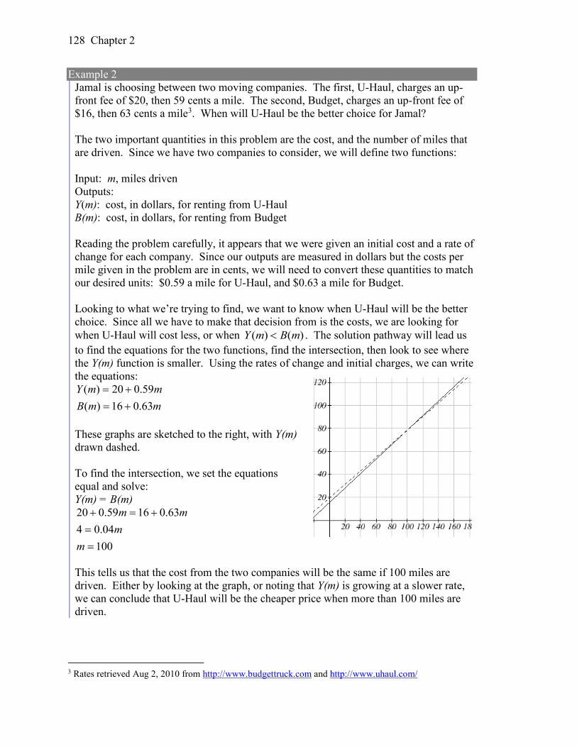
Chapter 2
128
Example 2
Jamal is choosing between two moving companies. The first, U-Haul, charges an up-
front fee of $20, then 59 cents a mile. The second, Budget, charges an up-front fee of
$16, then 63 cents a mile3. When will U-Haul be the better choice for Jamal?
The two important quantities in this problem are the cost, and the number of miles that
are driven. Since we have two companies to consider, we will define two functions:
Input: m, miles driven
Outputs:
Y(m): cost, in dollars, for renting from U-Haul
B(m): cost, in dollars, for renting from Budget
Reading the problem carefully, it appears that we were given an initial cost and a rate of
change for each company. Since our outputs are measured in dollars but the costs per
mile given in the problem are in cents, we will need to convert these quantities to match
our desired units: $0.59 a mile for U-Haul, and $0.63 a mile for Budget.
Looking to what we’re trying to find, we want to know when U-Haul will be the better
choice. Since all we have to make that decision from is the costs, we are looking for
when U-Haul will cost less, or when )()( mBmY . The solution pathway will lead us
to find the equations for the two functions, find the intersection, then look to see where
the Y(m) function is smaller. Using the rates of change and initial charges, we can write
the equations:
mmB
mmY
63.016)(
59.020)(
These graphs are sketched to the right, with Y(m)
drawn dashed.
To find the intersection, we set the equations
equal and solve:
Y(m) = B(m)
100
04.04
63.01659.020
m
m
mm
This tells us that the cost from the two companies will be the same if 100 miles are
driven. Either by looking at the graph, or noting that Y(m) is growing at a slower rate,
we can conclude that U-Haul will be the cheaper price when more than 100 miles are
driven.
3 Rates retrieved Aug 2, 2010 from http://www.budgettruck.com and http://www.uhaul.com/
Section 2.3 Modeling with Linear Functions 129
Example 3
A town’s population has been growing linearly. In 2004 the population was 6,200. By
2009 the population had grown to 8,100. If this trend continues,
a. Predict the population in 2013
b. When will the population reach 15000?
The two changing quantities are the population and time. While we could use the actual
year value as the input quantity, doing so tends to lead to very ugly equations, since the
vertical intercept would correspond to the year 0, more than 2000 years ago!
To make things a little nicer, and to make our lives easier too, we will define our input
as years since 2004:
Input: t, years since 2004
Output: P(t), the town’s population
The problem gives us two input-output pairs. Converting them to match our defined
variables, the year 2004 would correspond to t = 0, giving the point (0, 6200). Notice
that through our clever choice of variable definition, we have “given” ourselves the
vertical intercept of the function. The year 2009 would correspond to t = 5, giving the
point (5, 8100).
To predict the population in 2013 (t = 9), we would need an equation for the population.
Likewise, to find when the population would reach 15000, we would need to solve for
the input that would provide an output of 15000. Either way, we need an equation. To
find it, we start by calculating the rate of change:
3805
1900
05
62008100
m people per year
Since we already know the vertical intercept of the line, we can immediately write the
equation:
ttP 3806200)(
To predict the population in 2013, we evaluate our function at t = 9
9620)9(3806200)9( P
If the trend continues, our model predicts a population of 9,620 in 2013.
To find when the population will reach 15,000, we can set P(t) = 15000 and solve for t.
158.23
3808800
380620015000
t
t
t
Our model predicts the population will reach 15,000 in a little more than 23 years after
2004, or somewhere around the year 2027.
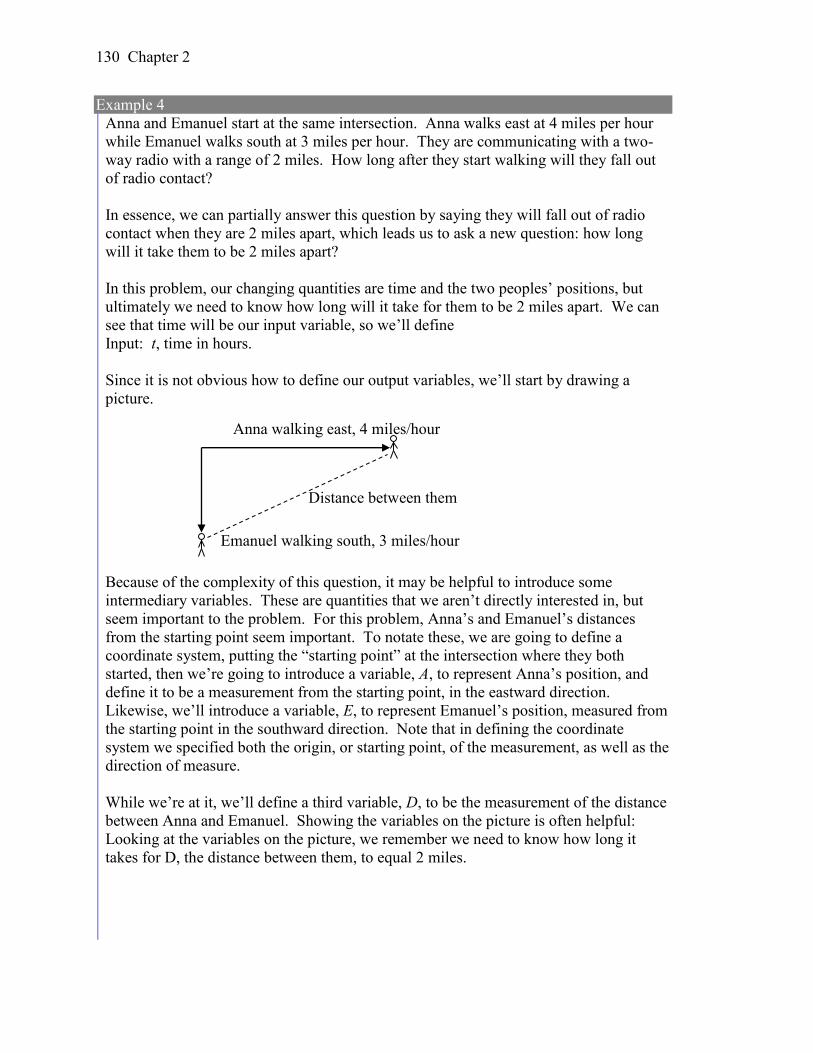
Chapter 2
130
Example 4
Anna and Emanuel start at the same intersection. Anna walks east at 4 miles per hour
while Emanuel walks south at 3 miles per hour. They are communicating with a two-
way radio with a range of 2 miles. How long after they start walking will they fall out
of radio contact?
In essence, we can partially answer this question by saying they will fall out of radio
contact when they are 2 miles apart, which leads us to ask a new question: how long
will it take them to be 2 miles apart?
In this problem, our changing quantities are time and the two peoples’ positions, but
ultimately we need to know how long will it take for them to be 2 miles apart. We can
see that time will be our input variable, so we’ll define
Input: t, time in hours.
Since it is not obvious how to define our output variables, we’ll start by drawing a
picture.
Because of the complexity of this question, it may be helpful to introduce some
intermediary variables. These are quantities that we aren’t directly interested in, but
seem important to the problem. For this problem, Anna’s and Emanuel’s distances
from the starting point seem important. To notate these, we are going to define a
coordinate system, putting the “starting point” at the intersection where they both
started, then we’re going to introduce a variable, A, to represent Anna’s position, and
define it to be a measurement from the starting point, in the eastward direction.
Likewise, we’ll introduce a variable, E, to represent Emanuel’s position, measured from
the starting point in the southward direction. Note that in defining the coordinate
system we specified both the origin, or starting point, of the measurement, as well as the
direction of measure.
While we’re at it, we’ll define a third variable, D, to be the measurement of the distance
between Anna and Emanuel. Showing the variables on the picture is often helpful:
Looking at the variables on the picture, we remember we need to know how long it
takes for D, the distance between them, to equal 2 miles.
Anna walking east, 4 miles/hour
Emanuel walking south, 3 miles/hour
Distance between them
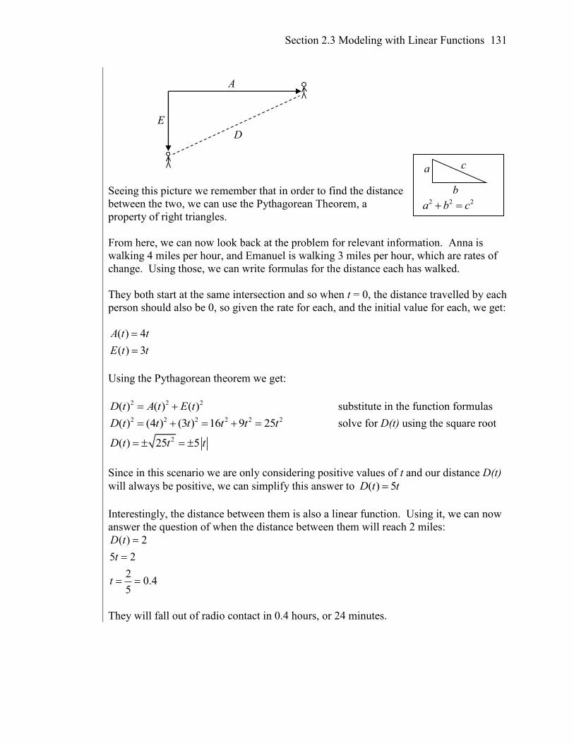
Section 2.3 Modeling with Linear Functions 131
Seeing this picture we remember that in order to find the distance
between the two, we can use the Pythagorean Theorem, a
property of right triangles.
From here, we can now look back at the problem for relevant information. Anna is
walking 4 miles per hour, and Emanuel is walking 3 miles per hour, which are rates of
change. Using those, we can write formulas for the distance each has walked.
They both start at the same intersection and so when t = 0, the distance travelled by each
person should also be 0, so given the rate for each, and the initial value for each, we get:
( ) 4
( ) 3
A t t
E t t
Using the Pythagorean theorem we get:
2 2 2( ) ( ) ( )D t A t E t substitute in the function formulas 2 2 2 2 2 2( ) (4 ) (3 ) 16 9 25D t t t t t t solve for D(t) using the square root
2( ) 25 5D t t t
Since in this scenario we are only considering positive values of t and our distance D(t)
will always be positive, we can simplify this answer to ( ) 5D t t
Interestingly, the distance between them is also a linear function. Using it, we can now
answer the question of when the distance between them will reach 2 miles:
( ) 2
5 2
20.4
5
D t
t
t
They will fall out of radio contact in 0.4 hours, or 24 minutes.
A
E
D
2 2 2a b c
a
b
c
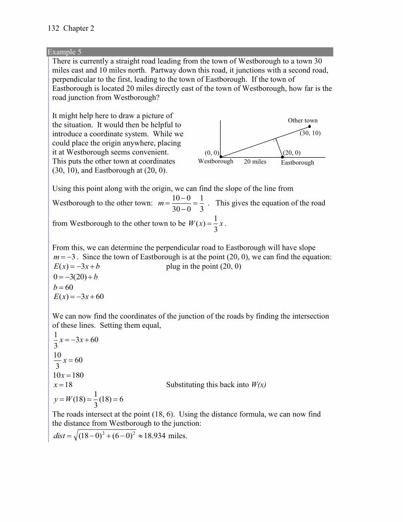
Chapter 2
132
Example 5
There is currently a straight road leading from the town of Westborough to a town 30
miles east and 10 miles north. Partway down this road, it junctions with a second road,
perpendicular to the first, leading to the town of Eastborough. If the town of
Eastborough is located 20 miles directly east of the town of Westborough, how far is the
road junction from Westborough?
It might help here to draw a picture of
the situation. It would then be helpful to
introduce a coordinate system. While we
could place the origin anywhere, placing
it at Westborough seems convenient.
This puts the other town at coordinates
(30, 10), and Eastborough at (20, 0).
Using this point along with the origin, we can find the slope of the line from
Westborough to the other town: 3
1
030
010
m . This gives the equation of the road
from Westborough to the other town to be xxW3
1)( .
From this, we can determine the perpendicular road to Eastborough will have slope
3m . Since the town of Eastborough is at the point (20, 0), we can find the equation:
bxxE 3)( plug in the point (20, 0)
b )20(30
60b
603)( xxE
We can now find the coordinates of the junction of the roads by finding the intersection
of these lines. Setting them equal,
6033
1 xx
603
10x
18010 x
18x Substituting this back into W(x)
6)18(3
1)18( Wy
The roads intersect at the point (18, 6). Using the distance formula, we can now find
the distance from Westborough to the junction:
934.18)06()018( 22 dist miles.
Westborough
Other town
(30, 10)
20 miles Eastborough
(20, 0) (0, 0)

Section 2.3 Modeling with Linear Functions 133
Important Topics of this Section
The problem solving process
1) Identify changing quantities, and then carefully and clearly define descriptive
variables to represent those quantities. When appropriate, sketch a picture or define
a coordinate system.
2) Carefully read the problem to identify important information. Look for information
giving values for the variables, or values for parts of the functional model, like slope
and initial value.
3) Carefully read the problem to identify what we are trying to find, identify, solve, or
interpret.
4) Identify a solution pathway from the provided information to what we are trying to
find. Often this will involve checking and tracking units, building a table or even
finding a formula for the function being used to model the problem.
5) When needed, find a formula for the function.
6) Solve or evaluate using the formula you found for the desired quantities.
7) Reflect on whether your answer is reasonable for the given situation and whether it
makes sense mathematically.
8) Clearly convey your result using appropriate units, and answer in full sentences
when appropriate.
Chapter 2
134
Section 2.3 Exercises
1. In 2004, a school population was 1001. By 2008 the population had grown to 1697.
Assume the population is changing linearly.
a. How much did the population grow between the year 2004 and 2008?
b. How long did it take the population to grow from 1001 students to 1697
students?
c. What is the average population growth per year?
d. What was the population in the year 2000?
e. Find an equation for the population, P, of the school t years after 2000.
f. Using your equation, predict the population of the school in 2011.
2. In 2003, a town’s population was 1431. By 2007 the population had grown to 2134.
Assume the population is changing linearly.
a. How much did the population grow between the year 2003 and 2007?
b. How long did it take the population to grow from 1431 people to 2134?
c. What is the average population growth per year?
d. What was the population in the year 2000?
e. Find an equation for the population, P, of the town t years after 2000.
f. Using your equation, predict the population of the town in 2014.
3. A phone company has a monthly cellular plan where a customer pays a flat monthly
fee and then a certain amount of money per minute used on the phone. If a customer
uses 410 minutes, the monthly cost will be $71.50. If the customer uses 720 minutes,
the monthly cost will be $118.
a. Find a linear equation for the monthly cost of the cell plan as a function of x,
the number of monthly minutes used.
b. Interpret the slope and vertical intercept of the equation.
c. Use your equation to find the total monthly cost if 687 minutes are used.
4. A phone company has a monthly cellular data plan where a customer pays a flat
monthly fee and then a certain amount of money per megabyte (MB) of data used on
the phone. If a customer uses 20 MB, the monthly cost will be $11.20. If the customer
uses 130 MB, the monthly cost will be $17.80.
a. Find a linear equation for the monthly cost of the data plan as a function of x,
the number of MB used.
b. Interpret the slope and vertical intercept of the equation.
c. Use your equation to find the total monthly cost if 250 MB are used.
Section 2.3 Modeling with Linear Functions 135
5. In 1991, the moose population in a park was measured to be 4360. By 1999, the
population was measured again to be 5880. If the population continues to change
linearly,
a. Find a formula for the moose population, P.
b. What does your model predict the moose population to be in 2003?
6. In 2003, the owl population in a park was measured to be 340. By 2007, the
population was measured again to be 285. If the population continues to change
linearly,
a. Find a formula for the owl population, P.
b. What does your model predict the owl population to be in 2012?
7. The Federal Helium Reserve held about 16 billion cubic feet of helium in 2010, and is
being depleted by about 2.1 billion cubic feet each year.
a. Give a linear equation for the remaining federal helium reserves, R, in terms
of t, the number of years since 2010.
b. In 2015, what will the helium reserves be?
c. If the rate of depletion doesn’t change, when will the Federal Helium Reserve
be depleted?
8. Suppose the world's current oil reserves are 1820 billion barrels. If, on average, the
total reserves is decreasing by 25 billion barrels of oil each year:
a. Give a linear equation for the remaining oil reserves, R, in terms of t, the
number of years since now.
b. Seven years from now, what will the oil reserves be?
c. If the rate of depletion isn’t change, when will the world’s oil reserves be
depleted?
9. You are choosing between two different prepaid cell phone plans. The first plan
charges a rate of 26 cents per minute. The second plan charges a monthly fee of
$19.95 plus 11 cents per minute. How many minutes would you have to use in a
month in order for the second plan to be preferable?
10. You are choosing between two different window washing companies. The first
charges $5 per window. The second charges a base fee of $40 plus $3 per window.
How many windows would you need to have for the second company to be
preferable?
11. When hired at a new job selling jewelry, you are given two pay options:
Option A: Base salary of $17,000 a year, with a commission of 12% of your sales
Option B: Base salary of $20,000 a year, with a commission of 5% of your sales
How much jewelry would you need to sell for option A to produce a larger income?
Chapter 2
136
12. When hired at a new job selling electronics, you are given two pay options:
Option A: Base salary of $14,000 a year, with a commission of 10% of your sales
Option B: Base salary of $19,000 a year, with a commission of 4% of your sales
How much electronics would you need to sell for option A to produce a larger
income?
13. Find the area of a triangle bounded by the y axis, the line 6
97
f x x , and the line
perpendicular to ( )f x that passes through the origin.
14. Find the area of a triangle bounded by the x axis, the line 1
123
f x x , and the
line perpendicular to ( )f x that passes through the origin.
15. Find the area of a parallelogram bounded by the y axis, the line 3x , the line
1 2f x x , and the line parallel to ( )f x passing through (2, 7)
16. Find the area of a parallelogram bounded by the x axis, the line ( ) 2g x , the line
3f x x , and the line parallel to ( )f x passing through (6, 1)
17. If 0b and 0m , then the line f x b mx cuts off a triangle from the first
quadrant. Express the area of that triangle in terms of m and b. [UW]
18. Find the value of m so the lines 5f x mx and g x x and the y-axis form a
triangle with an area of 10. [UW]
19. The median home values in Mississippi and Hawaii (adjusted for inflation) are shown
below. If we assume that the house values are changing linearly,
Year Mississippi Hawaii
1950 25200 74400
2000 71400 272700
a. In which state have home values increased at a higher rate?
b. If these trends were to continue, what would be the median home value in
Mississippi in 2010?
c. If we assume the linear trend existed before 1950 and continues after 2000,
the two states' median house values will be (or were) equal in what year? (The
answer might be absurd)
Section 2.3 Modeling with Linear Functions 137
20. The median home value ins Indiana and Alabama (adjusted for inflation) are shown
below. If we assume that the house values are changing linearly,
Year Indiana Alabama
1950 37700 27100
2000 94300 85100
a. In which state have home values increased at a higher rate?
b. If these trends were to continue, what would be the median home value in
Indiana in 2010?
c. If we assume the linear trend existed before 1950 and continues after 2000,
the two states' median house values will be (or were) equal in what year? (The
answer might be absurd)
21. Pam is taking a train from the town of Rome to the town of Florence. Rome is located
30 miles due West of the town of Paris. Florence is 25 miles East, and 45 miles North
of Rome. On her trip, how close does Pam get to Paris? [UW]
22. You’re flying from Joint Base Lewis-McChord (JBLM) to an undisclosed location
226 km south and 230 km east. Mt. Rainier is located approximately 56 km east and
40 km south of JBLM. If you are flying at a constant speed of 800 km/hr, how long
after you depart JBLM will you be the closest to Mt. Rainier?
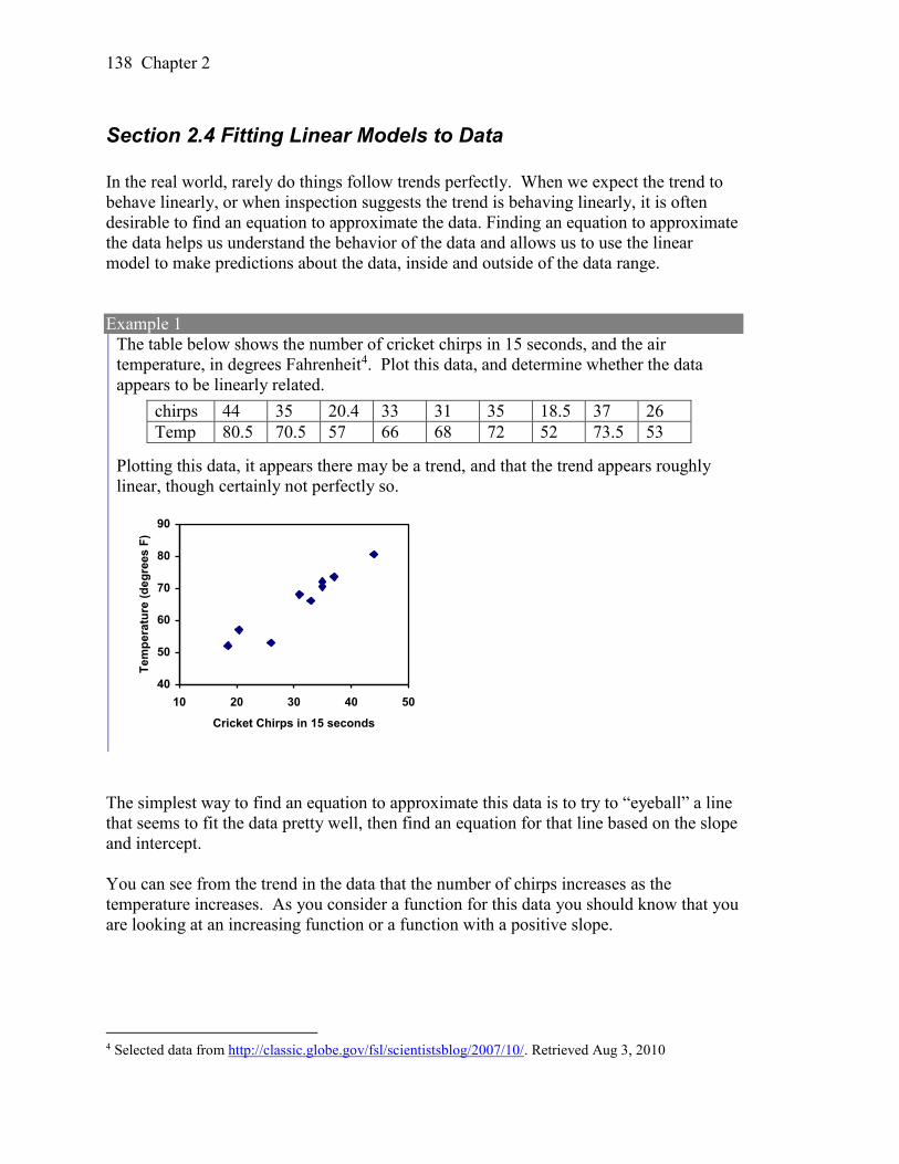
Chapter 2
138
Section 2.4 Fitting Linear Models to Data
In the real world, rarely do things follow trends perfectly. When we expect the trend to
behave linearly, or when inspection suggests the trend is behaving linearly, it is often
desirable to find an equation to approximate the data. Finding an equation to approximate
the data helps us understand the behavior of the data and allows us to use the linear
model to make predictions about the data, inside and outside of the data range.
Example 1
The table below shows the number of cricket chirps in 15 seconds, and the air
temperature, in degrees Fahrenheit4. Plot this data, and determine whether the data
appears to be linearly related.
Plotting this data, it appears there may be a trend, and that the trend appears roughly
linear, though certainly not perfectly so.
40
50
60
70
80
90
10 20 30 40 50
Cricket Chirps in 15 seconds
Te
mp
era
ture
(d
eg
rees F
)
The simplest way to find an equation to approximate this data is to try to “eyeball” a line
that seems to fit the data pretty well, then find an equation for that line based on the slope
and intercept.
You can see from the trend in the data that the number of chirps increases as the
temperature increases. As you consider a function for this data you should know that you
are looking at an increasing function or a function with a positive slope.
4 Selected data from http://classic.globe.gov/fsl/scientistsblog/2007/10/. Retrieved Aug 3, 2010
chirps 44 35 20.4 33 31 35 18.5 37 26
Temp 80.5 70.5 57 66 68 72 52 73.5 53
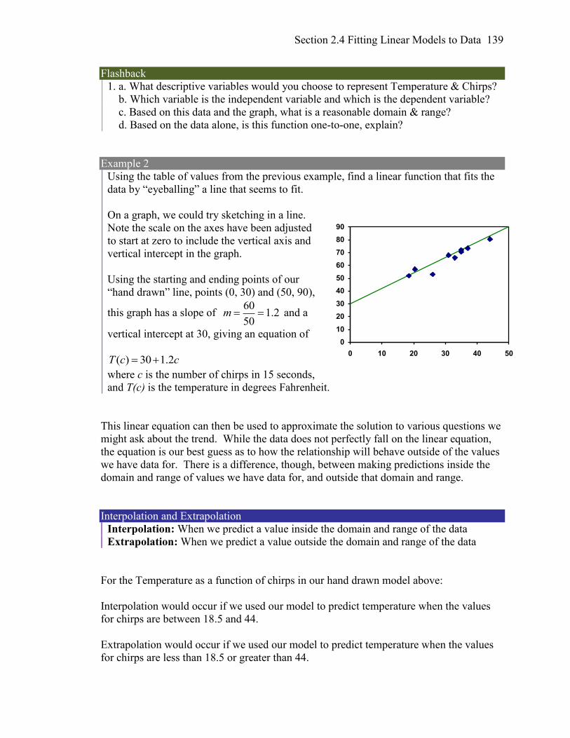
Section 2.4 Fitting Linear Models to Data 139
Flashback
1. a. What descriptive variables would you choose to represent Temperature & Chirps?
b. Which variable is the independent variable and which is the dependent variable?
c. Based on this data and the graph, what is a reasonable domain & range?
d. Based on the data alone, is this function one-to-one, explain?
Example 2
Using the table of values from the previous example, find a linear function that fits the
data by “eyeballing” a line that seems to fit.
On a graph, we could try sketching in a line.
Note the scale on the axes have been adjusted
to start at zero to include the vertical axis and
vertical intercept in the graph.
Using the starting and ending points of our
“hand drawn” line, points (0, 30) and (50, 90),
this graph has a slope of 60
1.250
m and a
vertical intercept at 30, giving an equation of
( ) 30 1.2T c c
where c is the number of chirps in 15 seconds,
and T(c) is the temperature in degrees Fahrenheit.
This linear equation can then be used to approximate the solution to various questions we
might ask about the trend. While the data does not perfectly fall on the linear equation,
the equation is our best guess as to how the relationship will behave outside of the values
we have data for. There is a difference, though, between making predictions inside the
domain and range of values we have data for, and outside that domain and range.
Interpolation and Extrapolation
Interpolation: When we predict a value inside the domain and range of the data
Extrapolation: When we predict a value outside the domain and range of the data
For the Temperature as a function of chirps in our hand drawn model above:
Interpolation would occur if we used our model to predict temperature when the values
for chirps are between 18.5 and 44.
Extrapolation would occur if we used our model to predict temperature when the values
for chirps are less than 18.5 or greater than 44.
0
10
20
30
40
50
60
70
80
90
0 10 20 30 40 50
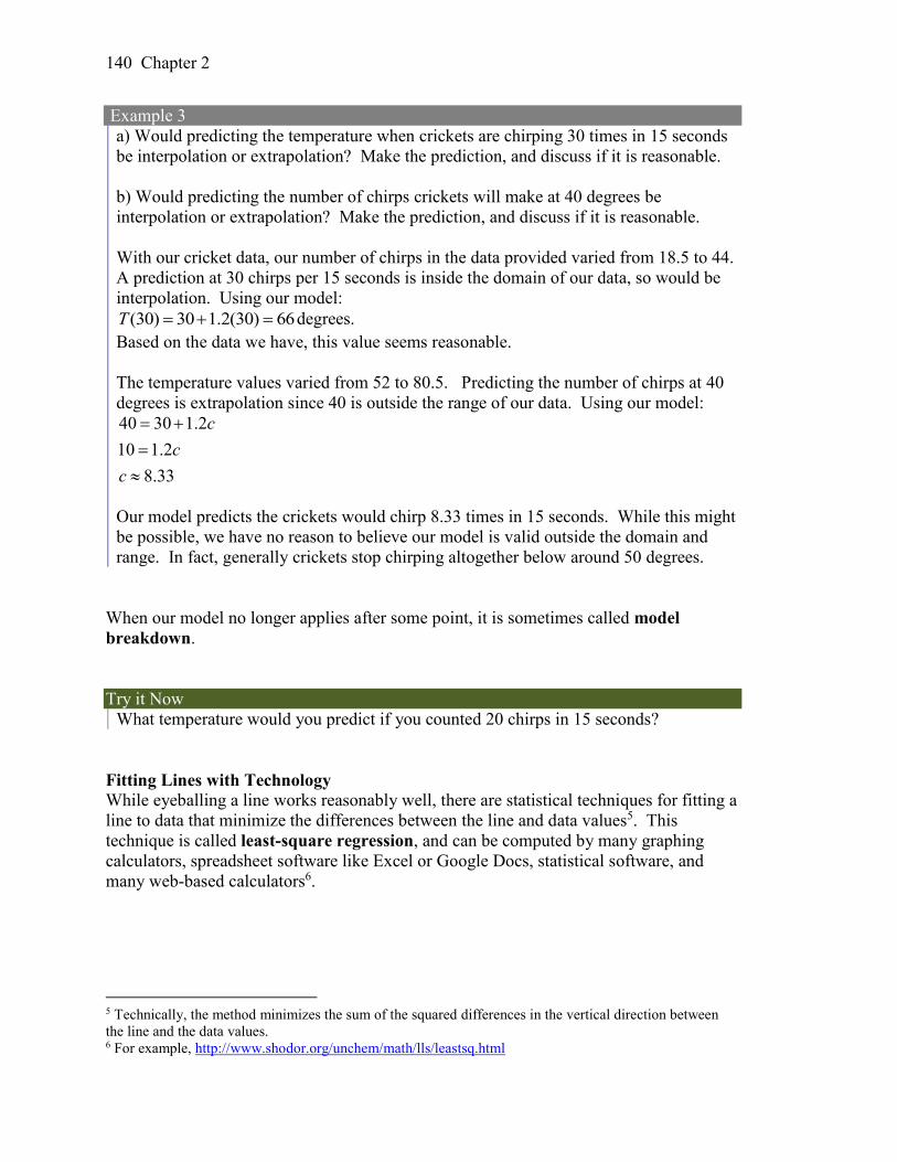
Chapter 2
140
Example 3
a) Would predicting the temperature when crickets are chirping 30 times in 15 seconds
be interpolation or extrapolation? Make the prediction, and discuss if it is reasonable.
b) Would predicting the number of chirps crickets will make at 40 degrees be
interpolation or extrapolation? Make the prediction, and discuss if it is reasonable.
With our cricket data, our number of chirps in the data provided varied from 18.5 to 44.
A prediction at 30 chirps per 15 seconds is inside the domain of our data, so would be
interpolation. Using our model:
(30) 30 1.2(30) 66T degrees.
Based on the data we have, this value seems reasonable.
The temperature values varied from 52 to 80.5. Predicting the number of chirps at 40
degrees is extrapolation since 40 is outside the range of our data. Using our model:
40 30 1.2
10 1.2
8.33
c
c
c
Our model predicts the crickets would chirp 8.33 times in 15 seconds. While this might
be possible, we have no reason to believe our model is valid outside the domain and
range. In fact, generally crickets stop chirping altogether below around 50 degrees.
When our model no longer applies after some point, it is sometimes called model
breakdown.
Try it Now
What temperature would you predict if you counted 20 chirps in 15 seconds?
Fitting Lines with Technology While eyeballing a line works reasonably well, there are statistical techniques for fitting a
line to data that minimize the differences between the line and data values5. This
technique is called least-square regression, and can be computed by many graphing
calculators, spreadsheet software like Excel or Google Docs, statistical software, and
many web-based calculators6.
5 Technically, the method minimizes the sum of the squared differences in the vertical direction between
the line and the data values. 6 For example, http://www.shodor.org/unchem/math/lls/leastsq.html
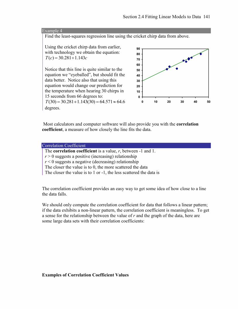
Section 2.4 Fitting Linear Models to Data 141
Example 4
Find the least-squares regression line using the cricket chirp data from above.
Using the cricket chirp data from earlier,
with technology we obtain the equation:
( ) 30.281 1.143T c c
Notice that this line is quite similar to the
equation we “eyeballed”, but should fit the
data better. Notice also that using this
equation would change our prediction for
the temperature when hearing 30 chirps in
15 seconds from 66 degrees to:
(30) 30.281 1.143(30) 64.571 64.6T
degrees.
Most calculators and computer software will also provide you with the correlation
coefficient, a measure of how closely the line fits the data.
Correlation Coefficient
The correlation coefficient is a value, r, between -1 and 1.
r > 0 suggests a positive (increasing) relationship
r < 0 suggests a negative (decreasing) relationship
The closer the value is to 0, the more scattered the data
The closer the value is to 1 or -1, the less scattered the data is
The correlation coefficient provides an easy way to get some idea of how close to a line
the data falls.
We should only compute the correlation coefficient for data that follows a linear pattern;
if the data exhibits a non-linear pattern, the correlation coefficient is meaningless. To get
a sense for the relationship between the value of r and the graph of the data, here are
some large data sets with their correlation coefficients:
Examples of Correlation Coefficient Values
0
10
20
30
40
50
60
70
80
90
0 10 20 30 40 50
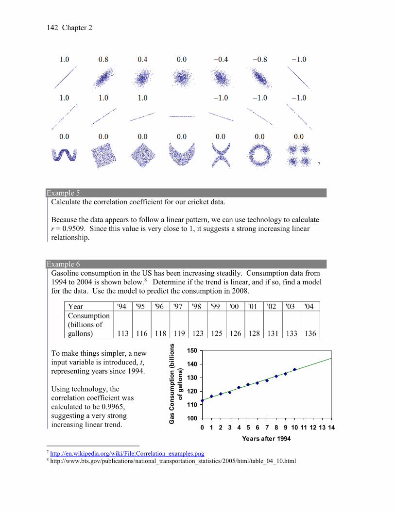
Chapter 2
142
Year '94 '95 '96 '97 '98 '99 '00 '01 '02 '03 '04
Consumption
(billions of
gallons) 113 116 118 119 123 125 126 128 131 133 136
7
Example 5
Calculate the correlation coefficient for our cricket data.
Because the data appears to follow a linear pattern, we can use technology to calculate
r = 0.9509. Since this value is very close to 1, it suggests a strong increasing linear
relationship.
Example 6
Gasoline consumption in the US has been increasing steadily. Consumption data from
1994 to 2004 is shown below.8 Determine if the trend is linear, and if so, find a model
for the data. Use the model to predict the consumption in 2008.
To make things simpler, a new
input variable is introduced, t,
representing years since 1994.
Using technology, the
correlation coefficient was
calculated to be 0.9965,
suggesting a very strong
increasing linear trend.
7 http://en.wikipedia.org/wiki/File:Correlation_examples.png 8 http://www.bts.gov/publications/national_transportation_statistics/2005/html/table_04_10.html
100
110
120
130
140
150
0 1 2 3 4 5 6 7 8 9 10 11 12 13 14
Years after 1994
Gas C
on
su
mp
tio
n (
bil
lio
ns
of
gall
on
s)

Section 2.4 Fitting Linear Models to Data 143
The least-squares regression equation is:
ttC 209.2318.113)( .
Using this to predict consumption in 2008 (t = 14),
(14) 113.318 2.209(14) 144.244C billions of gallons
The model predicts 144.244 billion gallons of gasoline will be consumed in 2008.
Try it Now
2. Use the model created by technology in example 6 to predict the gas consumption in
2011. Is this an interpolation or an extrapolation?
Important Topics of this Section
Fitting linear models to data by hand
Fitting linear models to data using technology
Interpolation
Extrapolation
Correlation coefficient
Flashback Answers
1. a. T = Temperature, C = Chirps (answers may vary)
b. Independent (Chirps) , Dependent (Temperature)
c. Reasonable Domain (18.5, 44) , Reasonable Range (52, 80.5) (answers may vary)
d. NO, it is not one-to-one, there are two different output values for 35 chirps.
Try it Now Answers
1. 54 degrees Fahrenheit
2. 150.871 billion gallons, extrapolation
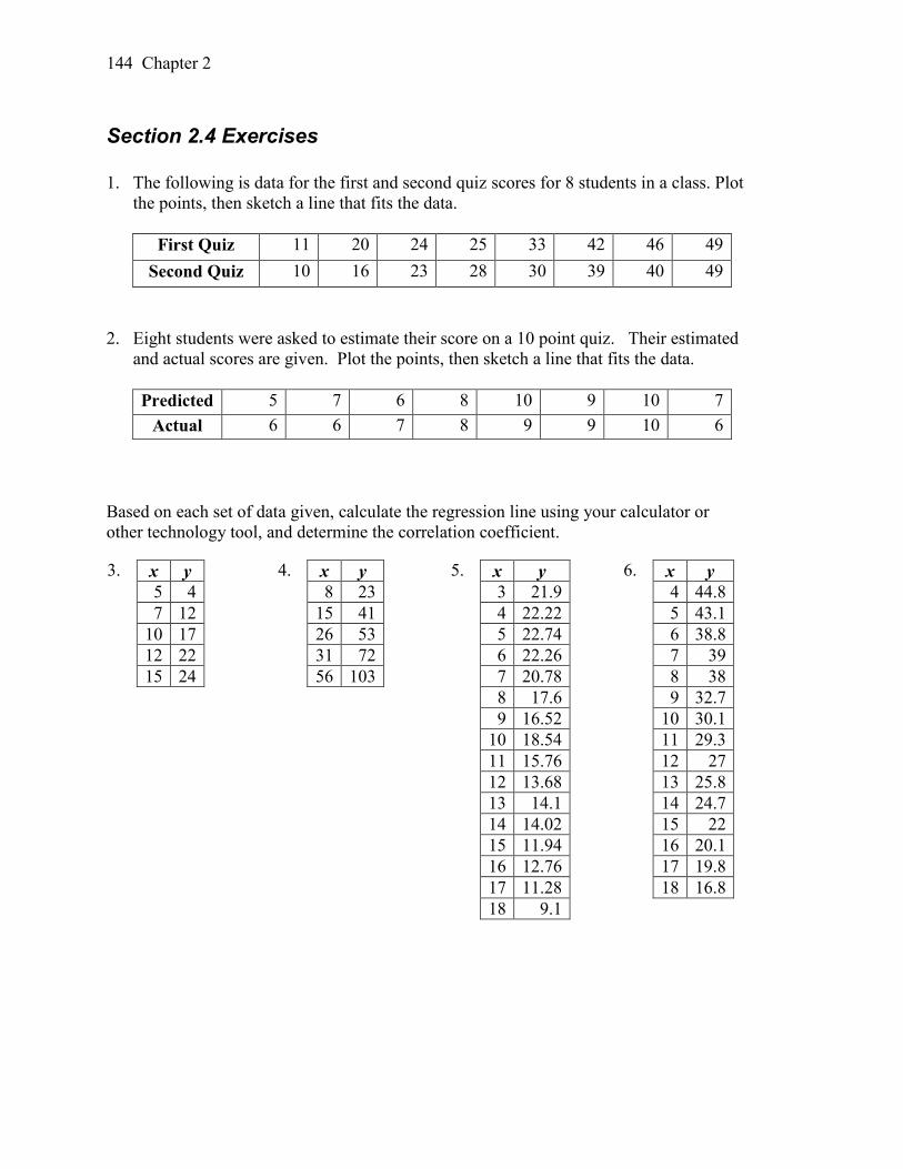
Chapter 2
144
Section 2.4 Exercises
1. The following is data for the first and second quiz scores for 8 students in a class. Plot
the points, then sketch a line that fits the data.
First Quiz 11 20 24 25 33 42 46 49
Second Quiz 10 16 23 28 30 39 40 49
2. Eight students were asked to estimate their score on a 10 point quiz. Their estimated
and actual scores are given. Plot the points, then sketch a line that fits the data.
Predicted 5 7 6 8 10 9 10 7
Actual 6 6 7 8 9 9 10 6
Based on each set of data given, calculate the regression line using your calculator or
other technology tool, and determine the correlation coefficient.
3. x y
5 4
7 12
10 17
12 22
15 24
4. x y
8 23
15 41
26 53
31 72
56 103
5. x y
3 21.9
4 22.22
5 22.74
6 22.26
7 20.78
8 17.6
9 16.52
10 18.54
11 15.76
12 13.68
13 14.1
14 14.02
15 11.94
16 12.76
17 11.28
18 9.1
6. x y
4 44.8
5 43.1
6 38.8
7 39
8 38
9 32.7
10 30.1
11 29.3
12 27
13 25.8
14 24.7
15 22
16 20.1
17 19.8
18 16.8
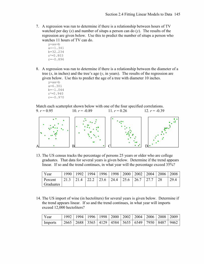
Section 2.4 Fitting Linear Models to Data 145
7. A regression was run to determine if there is a relationship between hours of TV
watched per day (x) and number of situps a person can do (y). The results of the
regression are given below. Use this to predict the number of situps a person who
watches 11 hours of TV can do. y=ax+b
a=-1.341
b=32.234
r2=0.803
r=-0.896
8. A regression was run to determine if there is a relationship between the diameter of a
tree (x, in inches) and the tree’s age (y, in years). The results of the regression are
given below. Use this to predict the age of a tree with diameter 10 inches. y=ax+b
a=6.301
b=-1.044
r2=0.940
r=-0.970
Match each scatterplot shown below with one of the four specified correlations.
9. r = 0.95 10. r = -0.89 11. r = 0.26 12. r = -0.39
A B C D
13. The US census tracks the percentage of persons 25 years or older who are college
graduates. That data for several years is given below. Determine if the trend appears
linear. If so and the trend continues, in what year will the percentage exceed 35%?
Year 1990 1992 1994 1996 1998 2000 2002 2004 2006 2008
Percent
Graduates
21.3 21.4 22.2 23.6 24.4 25.6 26.7 27.7 28 29.4
14. The US import of wine (in hectoliters) for several years is given below. Determine if
the trend appears linear. If so and the trend continues, in what year will imports
exceed 12,000 hectoliters?
Year 1992 1994 1996 1998 2000 2002 2004 2006 2008 2009
Imports 2665 2688 3565 4129 4584 5655 6549 7950 8487 9462
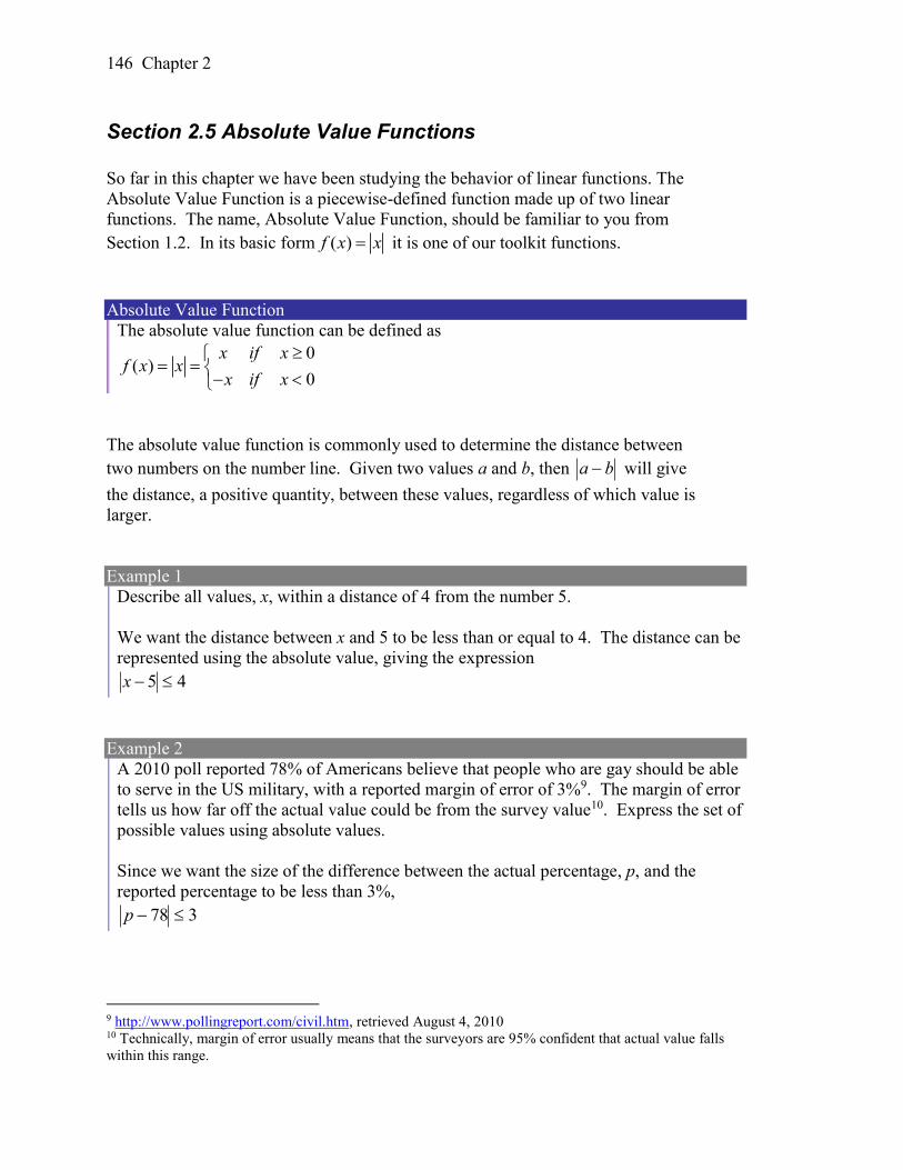
Chapter 2
146
Section 2.5 Absolute Value Functions
So far in this chapter we have been studying the behavior of linear functions. The
Absolute Value Function is a piecewise-defined function made up of two linear
functions. The name, Absolute Value Function, should be familiar to you from
Section 1.2. In its basic form ( )f x x it is one of our toolkit functions.
Absolute Value Function
The absolute value function can be defined as
0( )
0
x if xf x x
x if x
The absolute value function is commonly used to determine the distance between
two numbers on the number line. Given two values a and b, then ba will give
the distance, a positive quantity, between these values, regardless of which value is
larger.
Example 1
Describe all values, x, within a distance of 4 from the number 5.
We want the distance between x and 5 to be less than or equal to 4. The distance can be
represented using the absolute value, giving the expression
45 x
Example 2
A 2010 poll reported 78% of Americans believe that people who are gay should be able
to serve in the US military, with a reported margin of error of 3%9. The margin of error
tells us how far off the actual value could be from the survey value10. Express the set of
possible values using absolute values.
Since we want the size of the difference between the actual percentage, p, and the
reported percentage to be less than 3%,
378 p
9 http://www.pollingreport.com/civil.htm, retrieved August 4, 2010 10 Technically, margin of error usually means that the surveyors are 95% confident that actual value falls
within this range.
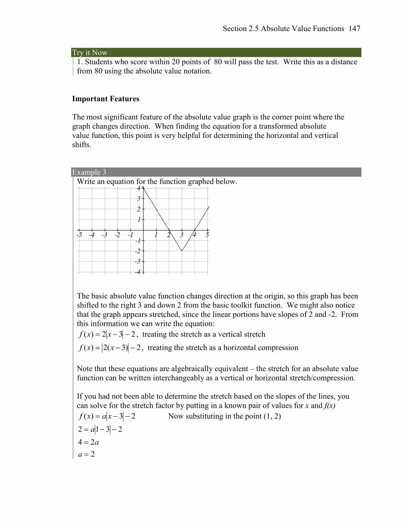
Section 2.5 Absolute Value Functions 147
Try it Now
1. Students who score within 20 points of 80 will pass the test. Write this as a distance
from 80 using the absolute value notation.
Important Features
The most significant feature of the absolute value graph is the corner point where the
graph changes direction. When finding the equation for a transformed absolute
value function, this point is very helpful for determining the horizontal and vertical
shifts.
Example 3
Write an equation for the function graphed below.
The basic absolute value function changes direction at the origin, so this graph has been
shifted to the right 3 and down 2 from the basic toolkit function. We might also notice
that the graph appears stretched, since the linear portions have slopes of 2 and -2. From
this information we can write the equation:
232)( xxf , treating the stretch as a vertical stretch
2)3(2)( xxf , treating the stretch as a horizontal compression
Note that these equations are algebraically equivalent – the stretch for an absolute value
function can be written interchangeably as a vertical or horizontal stretch/compression.
If you had not been able to determine the stretch based on the slopes of the lines, you
can solve for the stretch factor by putting in a known pair of values for x and f(x)
23)( xaxf Now substituting in the point (1, 2)
2
24
2312
a
a
a
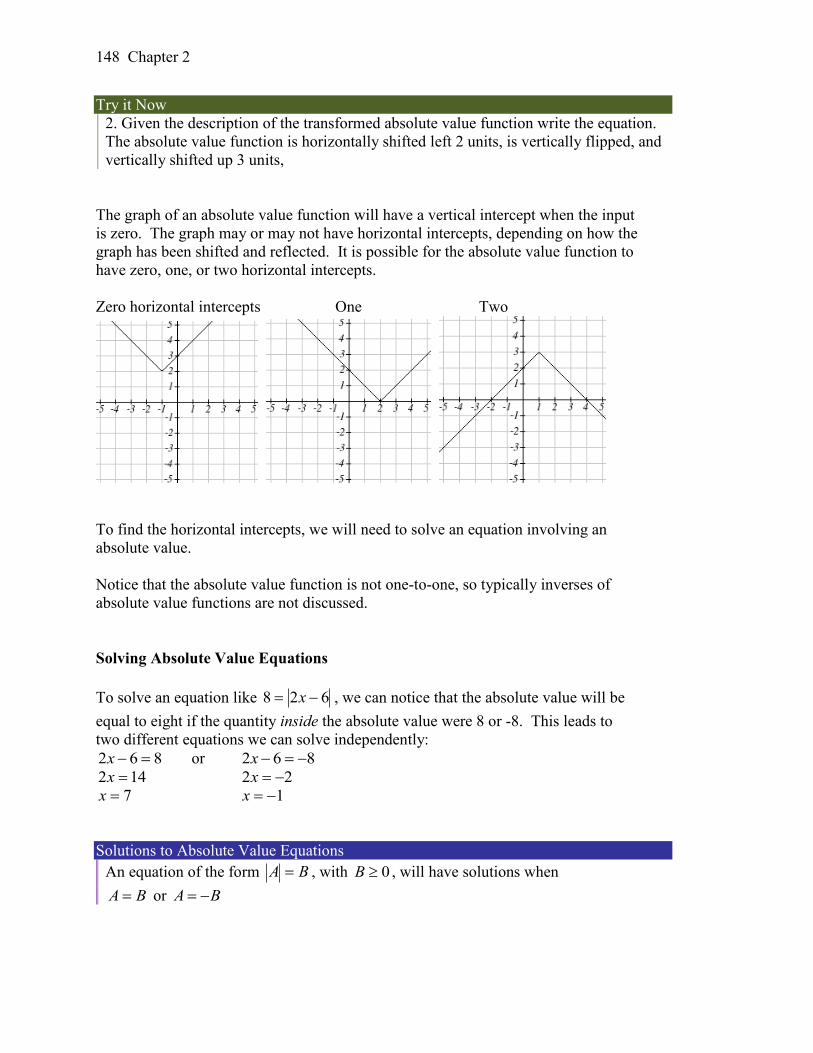
Chapter 2
148
Try it Now
2. Given the description of the transformed absolute value function write the equation.
The absolute value function is horizontally shifted left 2 units, is vertically flipped, and
vertically shifted up 3 units,
The graph of an absolute value function will have a vertical intercept when the input
is zero. The graph may or may not have horizontal intercepts, depending on how the
graph has been shifted and reflected. It is possible for the absolute value function to
have zero, one, or two horizontal intercepts.
Zero horizontal intercepts One Two
To find the horizontal intercepts, we will need to solve an equation involving an
absolute value.
Notice that the absolute value function is not one-to-one, so typically inverses of
absolute value functions are not discussed.
Solving Absolute Value Equations
To solve an equation like 628 x , we can notice that the absolute value will be
equal to eight if the quantity inside the absolute value were 8 or -8. This leads to
two different equations we can solve independently:
862 x or 862 x
142 x 22 x
7x 1x
Solutions to Absolute Value Equations
An equation of the form BA , with 0B , will have solutions when
BA or BA
Section 2.5 Absolute Value Functions 149
Example 4
Find the horizontal intercepts of the graph of 714)( xxf
The horizontal intercepts will occur when 0)( xf . Solving,
7140 x Isolate the absolute value on one side of the equation
147 x Now we can break this into two separate equations:
2
3
4
6
46
147
x
x
x
or
24
8
48
147
x
x
x
The graph has two horizontal intercepts, at 2
3x and x = -2
Example 5
Solve 2241 x
Isolating the absolute value on one side the equation,
2241 x
241 x
24
1 x
At this point, we notice that this equation has no solutions – the absolute value always
returns a positive value, so it is impossible for the absolute value to equal a negative
value.
Try it Now
3. Find the horizontal & vertical intercepts for the function 32)( xxf
Solving Absolute Value Inequalities
When absolute value inequalities are written to describe a set of values, like the
inequality 45 x we wrote earlier, it is sometimes desirable to express this set of
values without the absolute value, either using inequalities, or using interval
notation.
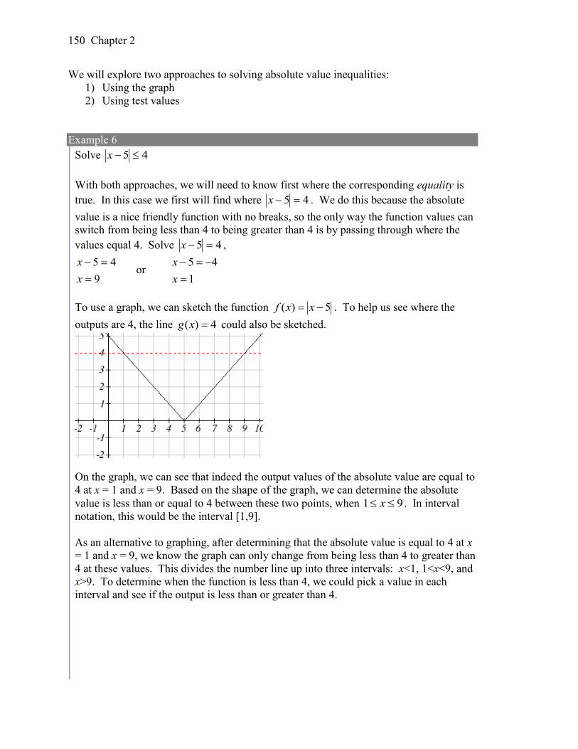
Chapter 2
150
We will explore two approaches to solving absolute value inequalities:
1) Using the graph
2) Using test values
Example 6
Solve 45 x
With both approaches, we will need to know first where the corresponding equality is
true. In this case we first will find where 45 x . We do this because the absolute
value is a nice friendly function with no breaks, so the only way the function values can
switch from being less than 4 to being greater than 4 is by passing through where the
values equal 4. Solve 45 x ,
9
45
x
x or
1
45
x
x
To use a graph, we can sketch the function 5)( xxf . To help us see where the
outputs are 4, the line 4)( xg could also be sketched.
On the graph, we can see that indeed the output values of the absolute value are equal to
4 at x = 1 and x = 9. Based on the shape of the graph, we can determine the absolute
value is less than or equal to 4 between these two points, when 91 x . In interval
notation, this would be the interval [1,9].
As an alternative to graphing, after determining that the absolute value is equal to 4 at x
= 1 and x = 9, we know the graph can only change from being less than 4 to greater than
4 at these values. This divides the number line up into three intervals: x<1, 1<x<9, and
x>9. To determine when the function is less than 4, we could pick a value in each
interval and see if the output is less than or greater than 4.
Section 2.5 Absolute Value Functions 151
Interval Test x f(x) <4 or >4?
x<1 0 550 greater
1<x<9 6 156 less
x>9 11 6511 greater
Since 91 x is the only interval in which the output at the test value is less than 4,
we can conclude the solution to 45 x is 91 x .
Example 7
Given the function 3542
1)( xxf , determine for what x values the function
values are negative.
We are trying to determine where f(x) < 0, which is when 03542
1 x . We begin
by isolating the absolute value:
3542
1 x when we multiply both sides by -2, it reverses the inequality
654 x
Next we solve for the equality 654 x
4
11
114
654
x
x
x
or
4
1
14
654
x
x
x
We can now either pick test values or sketch a graph of the function to determine on
which intervals the original function value are negative. Notice that it is not even really
important exactly what the graph looks like, as long as we know that it crosses the
horizontal axis at 4
1x and
4
11x , and that the graph has been reflected vertically.
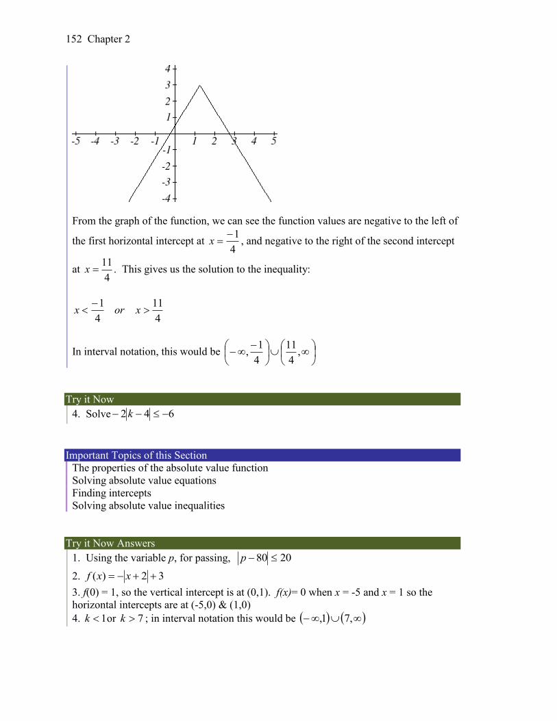
Chapter 2
152
From the graph of the function, we can see the function values are negative to the left of
the first horizontal intercept at 4
1x , and negative to the right of the second intercept
at 4
11x . This gives us the solution to the inequality:
4
11
4
1
xorx
In interval notation, this would be
,
4
11
4
1,
Try it Now
4. Solve 642 k
Important Topics of this Section
The properties of the absolute value function
Solving absolute value equations
Finding intercepts
Solving absolute value inequalities
Try it Now Answers
1. Using the variable p, for passing, 2080 p
2. 32)( xxf
3. f(0) = 1, so the vertical intercept is at (0,1). f(x)= 0 when x = -5 and x = 1 so the
horizontal intercepts are at (-5,0) & (1,0)
4. 1k or 7k ; in interval notation this would be ,71,
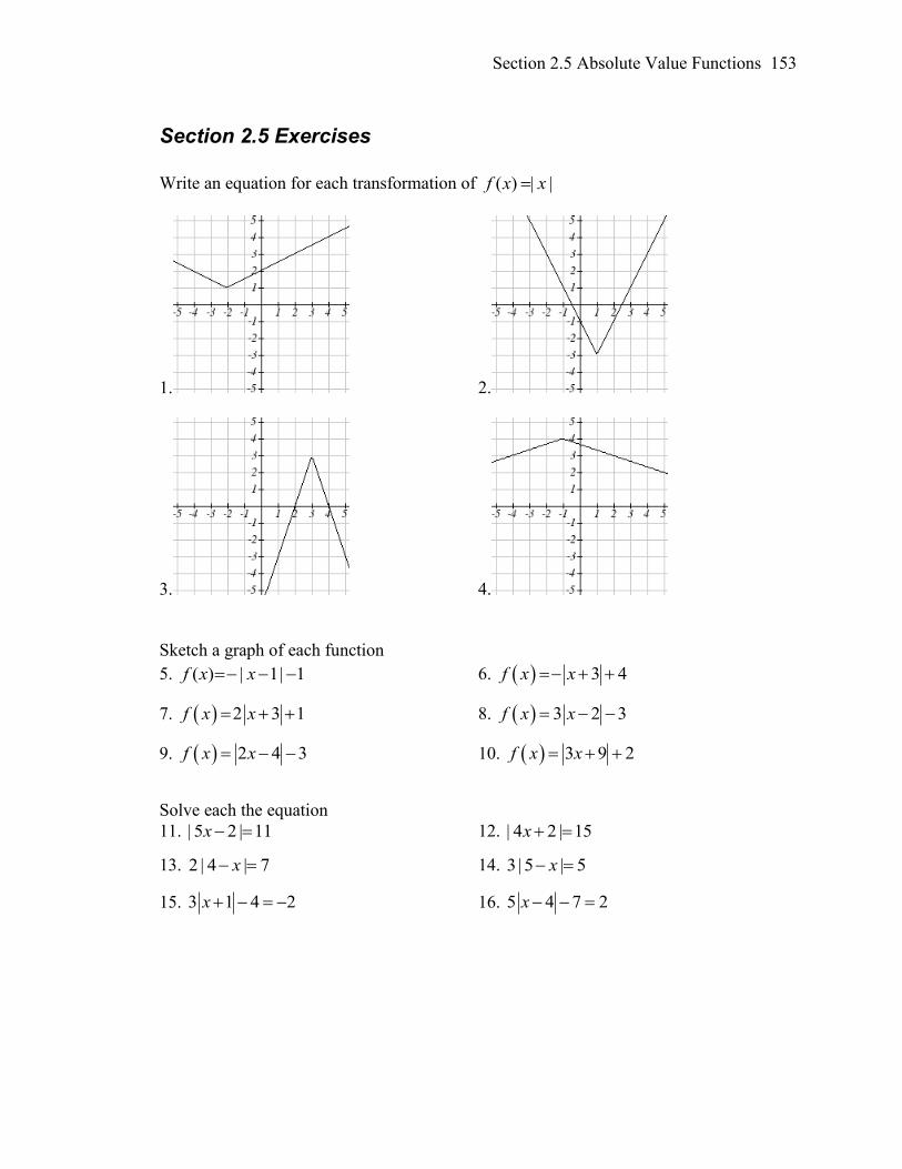
Section 2.5 Absolute Value Functions 153
Section 2.5 Exercises
Write an equation for each transformation of ( ) | |f x x
1. 2.
3. 4.
Sketch a graph of each function
5. ( ) | 1| 1f x x 6. 3 4f x x
7. 2 3 1f x x 8. 3 2 3f x x
9. 2 4 3f x x 10. 3 9 2f x x
Solve each the equation
11. | 5 2 | 11 x 12. | 4 2 | 15x
13. 2 | 4 | 7 x 14. 3| 5 | 5x
15. 3 1 4 2 x 16. 5 4 7 2x
Chapter 2
154
Find the horizontal and vertical intercepts of each function
17. ( ) 2 | 1| 10f x x 18. 4 3 4f x x
19. 3 2 1f x x 20. 2 1 6f x x
Solve each inequality
21. | 5 | 6x 22. | 3 | 7x
23. | 2 | 3x 24. | 4 | 2x
25. | 3 9 | 4x 26. | 2 9 | 8x
3.1 Power and Polynomial Functions 155
This chapter is part of Precalculus: An Investigation of Functions © Lippman & Rasmussen 2011.
This material is licensed under a Creative Commons CC-BY-SA license.
Chapter 3: Polynomial and Rational Functions Section 3.1 Power Functions & Polynomial Functions .............................................. 155
Section 3.2 Quadratic Functions ................................................................................. 163
Section 3.3 Graphs of Polynomial Functions ............................................................. 176
Section 3.4 Rational Functions ................................................................................... 188
Section 3.5 Inverses and Radical Functions ............................................................... 206
Section 3.1 Power Functions & Polynomial Functions
A square is cut out of cardboard, with each side having length L. If we wanted to write a
function for the area of the square, with L as the input and the area as output, you may
recall that the area of a rectangle can be found by multiplying the length times the width.
Since our shape is a square, the length & the width are the same, giving the formula: 2)( LLLLA
Likewise, if we wanted a function for the volume of a cube with each side having some
length L, you may recall volume of a rectangular box can be found by multiplying length
by width by height, which are all equal for a cube, giving the formula: 3)( LLLLLV
These two functions are examples of power functions, functions that are some power of
the variable.
Power Function
A power function is a function that can be represented in the form pxxf )(
Where the base is a variable and the exponent, p, is a number.
Example 1
Which of our toolkit functions are power functions?
The constant and identity functions are power functions, since they can be written as 0)( xxf and 1)( xxf respectively.
The quadratic and cubic functions are both power functions with whole number powers: 2)( xxf and 3)( xxf .
The reciprocal and reciprocal squared functions are both power functions with negative
whole number powers since they can be written as 1)( xxf and 2)( xxf .
The square and cube root functions are both power functions with fractional powers
since they can be written as 21)( xxf or 31)( xxf .
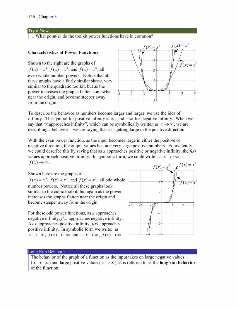
Chapter 3 156
Try it Now
1. What point(s) do the toolkit power functions have in common?
Characteristics of Power Functions
Shown to the right are the graphs of 642 )(and,)(,)( xxfxxfxxf , all
even whole number powers. Notice that all
these graphs have a fairly similar shape, very
similar to the quadratic toolkit, but as the
power increases the graphs flatten somewhat
near the origin, and become steeper away
from the origin.
To describe the behavior as numbers become larger and larger, we use the idea of
infinity. The symbol for positive infinity is , and for negative infinity. When we
say that “x approaches infinity”, which can be symbolically written as x , we are
describing a behavior – we are saying that x is getting large in the positive direction.
With the even power function, as the input becomes large in either the positive or
negative direction, the output values become very large positive numbers. Equivalently,
we could describe this by saying that as x approaches positive or negative infinity, the f(x)
values approach positive infinity. In symbolic form, we could write: as x ,
)(xf .
Shown here are the graphs of 753 )(and,)(,)( xxfxxfxxf , all odd whole
number powers. Notice all these graphs look
similar to the cubic toolkit, but again as the power
increases the graphs flatten near the origin and
become steeper away from the origin.
For these odd power functions, as x approaches
negative infinity, f(x) approaches negative infinity.
As x approaches positive infinity, f(x) approaches
positive infinity. In symbolic form we write: as
x , )(xf and as x , )(xf .
Long Run Behavior
The behavior of the graph of a function as the input takes on large negative values
( x ) and large positive values ( x ) as is referred to as the long run behavior
of the function.
2( )f x x
6( )f x x 4( )f x x
3( )f x x
7( )f x x 5( )f x x
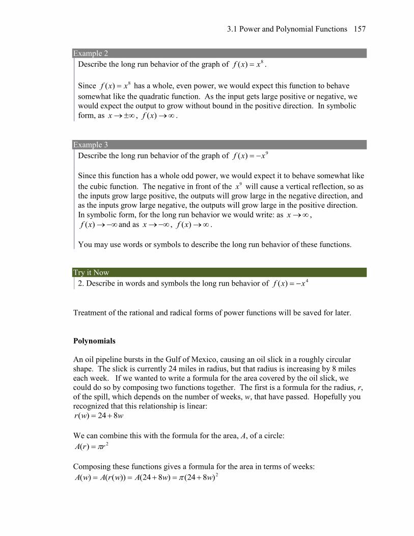
3.1 Power and Polynomial Functions 157
Example 2
Describe the long run behavior of the graph of 8)( xxf .
Since 8)( xxf has a whole, even power, we would expect this function to behave
somewhat like the quadratic function. As the input gets large positive or negative, we
would expect the output to grow without bound in the positive direction. In symbolic
form, as x , )(xf .
Example 3
Describe the long run behavior of the graph of 9)( xxf
Since this function has a whole odd power, we would expect it to behave somewhat like
the cubic function. The negative in front of the 9x will cause a vertical reflection, so as
the inputs grow large positive, the outputs will grow large in the negative direction, and
as the inputs grow large negative, the outputs will grow large in the positive direction.
In symbolic form, for the long run behavior we would write: as x ,
)(xf and as x , )(xf .
You may use words or symbols to describe the long run behavior of these functions.
Try it Now
2. Describe in words and symbols the long run behavior of 4)( xxf
Treatment of the rational and radical forms of power functions will be saved for later.
Polynomials
An oil pipeline bursts in the Gulf of Mexico, causing an oil slick in a roughly circular
shape. The slick is currently 24 miles in radius, but that radius is increasing by 8 miles
each week. If we wanted to write a formula for the area covered by the oil slick, we
could do so by composing two functions together. The first is a formula for the radius, r,
of the spill, which depends on the number of weeks, w, that have passed. Hopefully you
recognized that this relationship is linear:
wwr 824)(
We can combine this with the formula for the area, A, of a circle: 2)( rrA
Composing these functions gives a formula for the area in terms of weeks: 2)824()824())(()( wwAwrAwA
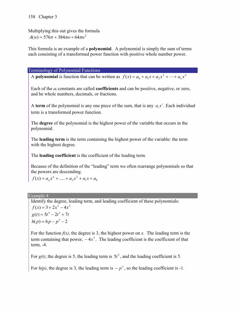
Chapter 3 158
Multiplying this out gives the formula 264384576)( wwwA
This formula is an example of a polynomial. A polynomial is simply the sum of terms
each consisting of a transformed power function with positive whole number power.
Terminology of Polynomial Functions
A polynomial is function that can be written as n
n xaxaxaaxf 2
210)(
Each of the ai constants are called coefficients and can be positive, negative, or zero,
and be whole numbers, decimals, or fractions.
A term of the polynomial is any one piece of the sum, that is any i
i xa . Each individual
term is a transformed power function.
The degree of the polynomial is the highest power of the variable that occurs in the
polynomial.
The leading term is the term containing the highest power of the variable: the term
with the highest degree.
The leading coefficient is the coefficient of the leading term.
Because of the definition of the “leading” term we often rearrange polynomials so that
the powers are descending.
01
2
2.....)( axaxaxaxf n
n
Example 4
Identify the degree, leading term, and leading coefficient of these polynomials: 32 423)( xxxf
ttttg 725)( 35
26)( 3 ppph
For the function f(x), the degree is 3, the highest power on x. The leading term is the
term containing that power, 34x . The leading coefficient is the coefficient of that
term, -4.
For g(t), the degree is 5, the leading term is 55t , and the leading coefficient is 5.
For h(p), the degree is 3, the leading term is 3p , so the leading coefficient is -1.
3.1 Power and Polynomial Functions 159
Long Run Behavior of Polynomials
For any polynomial, the long run behavior of the polynomial will match the long run
behavior of the leading term.
Example 5
What can we determine about the long run behavior and degree of the equation for the
polynomial graphed here?
Since the output grows large and positive as the inputs grow large and positive, we
describe the long run behavior symbolically by writing: as x , )(xf .
Similarly, as x , )(xf .
In words, we could say that as x values approach infinity, the function values approach
infinity, and as x values approach negative infinity the function values approach
negative infinity.
We can tell this graph has the shape of an odd degree power function which has not
been reflected, so the degree of the polynomial creating this graph must be odd, and the
leading coefficient would be positive.
Try it Now
3. Given the function )5)(1)(2(2.0)( xxxxf use your algebra skills to write the
function in standard polynomial form (as a sum of terms) and determine the leading
term, degree, and long run behavior of the function.
Short Run Behavior Characteristics of the graph such as vertical and horizontal intercepts and the places the
graph changes direction are part of the short run behavior of the polynomial.
Like with all functions, the vertical intercept is where the graph crosses the vertical axis,
and occurs when the input value is zero. Since a polynomial is a function, there can only
be one vertical intercept, which occurs at the point ),0( 0a . The horizontal intercepts
occur at the input values that correspond with an output value of zero. It is possible to
have more than one horizontal intercept.
Horizontal intercepts are also called zeros, or roots of the function.
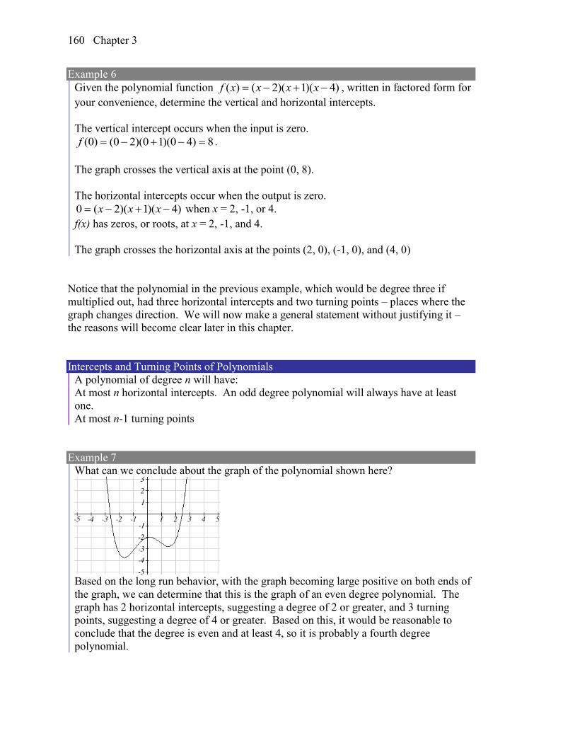
Chapter 3 160
Example 6
Given the polynomial function )4)(1)(2()( xxxxf , written in factored form for
your convenience, determine the vertical and horizontal intercepts.
The vertical intercept occurs when the input is zero.
8)40)(10)(20()0( f .
The graph crosses the vertical axis at the point (0, 8).
The horizontal intercepts occur when the output is zero.
)4)(1)(2(0 xxx when x = 2, -1, or 4.
f(x) has zeros, or roots, at x = 2, -1, and 4.
The graph crosses the horizontal axis at the points (2, 0), (-1, 0), and (4, 0)
Notice that the polynomial in the previous example, which would be degree three if
multiplied out, had three horizontal intercepts and two turning points – places where the
graph changes direction. We will now make a general statement without justifying it –
the reasons will become clear later in this chapter.
Intercepts and Turning Points of Polynomials
A polynomial of degree n will have:
At most n horizontal intercepts. An odd degree polynomial will always have at least
one.
At most n-1 turning points
Example 7
What can we conclude about the graph of the polynomial shown here?
Based on the long run behavior, with the graph becoming large positive on both ends of
the graph, we can determine that this is the graph of an even degree polynomial. The
graph has 2 horizontal intercepts, suggesting a degree of 2 or greater, and 3 turning
points, suggesting a degree of 4 or greater. Based on this, it would be reasonable to
conclude that the degree is even and at least 4, so it is probably a fourth degree
polynomial.
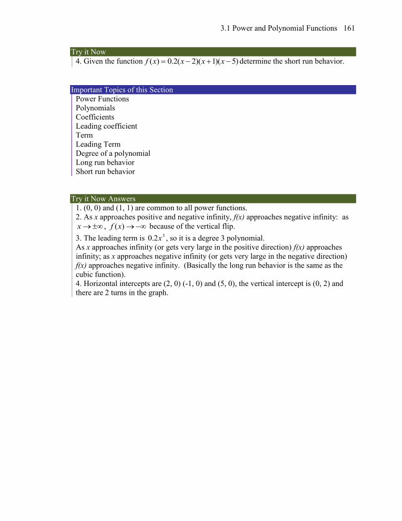
3.1 Power and Polynomial Functions 161
Try it Now
4. Given the function )5)(1)(2(2.0)( xxxxf determine the short run behavior.
Important Topics of this Section
Power Functions
Polynomials
Coefficients
Leading coefficient
Term
Leading Term
Degree of a polynomial
Long run behavior
Short run behavior
Try it Now Answers
1. (0, 0) and (1, 1) are common to all power functions.
2. As x approaches positive and negative infinity, f(x) approaches negative infinity: as
x , )(xf because of the vertical flip.
3. The leading term is 32.0 x , so it is a degree 3 polynomial.
As x approaches infinity (or gets very large in the positive direction) f(x) approaches
infinity; as x approaches negative infinity (or gets very large in the negative direction)
f(x) approaches negative infinity. (Basically the long run behavior is the same as the
cubic function).
4. Horizontal intercepts are (2, 0) (-1, 0) and (5, 0), the vertical intercept is (0, 2) and
there are 2 turns in the graph.
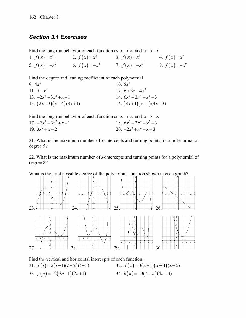
Chapter 3 162
Section 3.1 Exercises
Find the long run behavior of each function as x and x
1. 4f x x 2. 6f x x 3. 3f x x 4. 5f x x
5. 2f x x 6. 4f x x 7. 7f x x 8. 9f x x
Find the degree and leading coefficient of each polynomial
9. 74x 10. 65x
11. 25 x 12. 36 3 4x x
13. 4 22 3 1 x x x 14. 5 4 26 2 3x x x
15. 2 3 4 (3 1)x x x 16. 3 1 1 (4 3)x x x
Find the long run behavior of each function as x and x
17. 4 22 3 1 x x x 18. 5 4 26 2 3x x x
19. 23 2x x 20. 3 22 3x x x
21. What is the maximum number of x-intercepts and turning points for a polynomial of
degree 5?
22. What is the maximum number of x-intercepts and turning points for a polynomial of
degree 8?
What is the least possible degree of the polynomial function shown in each graph?
23. 24. 25. 26.
27. 28. 29. 30.
Find the vertical and horizontal intercepts of each function.
31. 2 1 2 ( 3)f t t t t 32. 3 1 4 ( 5)f x x x x
33. 2 3 1 (2 1)g n n n 34. 3 4 (4 3)k u n n
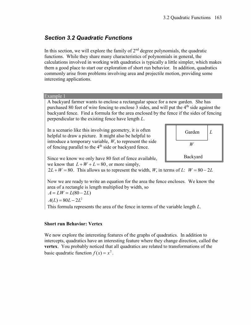
3.2 Quadratic Functions 163
Section 3.2 Quadratic Functions
In this section, we will explore the family of 2nd degree polynomials, the quadratic
functions. While they share many characteristics of polynomials in general, the
calculations involved in working with quadratics is typically a little simpler, which makes
them a good place to start our exploration of short run behavior. In addition, quadratics
commonly arise from problems involving area and projectile motion, providing some
interesting applications.
Example 1
A backyard farmer wants to enclose a rectangular space for a new garden. She has
purchased 80 feet of wire fencing to enclose 3 sides, and will put the 4th side against the
backyard fence. Find a formula for the area enclosed by the fence if the sides of fencing
perpendicular to the existing fence have length L.
In a scenario like this involving geometry, it is often
helpful to draw a picture. It might also be helpful to
introduce a temporary variable, W, to represent the side
of fencing parallel to the 4th side or backyard fence.
Since we know we only have 80 feet of fence available,
we know that 80 LWL , or more simply,
802 WL . This allows us to represent the width, W, in terms of L: LW 280
Now we are ready to write an equation for the area the fence encloses. We know the
area of a rectangle is length multiplied by width, so
)280( LLLWA 2280)( LLLA
This formula represents the area of the fence in terms of the variable length L.
Short run Behavior: Vertex
We now explore the interesting features of the graphs of quadratics. In addition to
intercepts, quadratics have an interesting feature where they change direction, called the
vertex. You probably noticed that all quadratics are related to transformations of the
basic quadratic function 2)( xxf .
Backyard
Garden
W
L
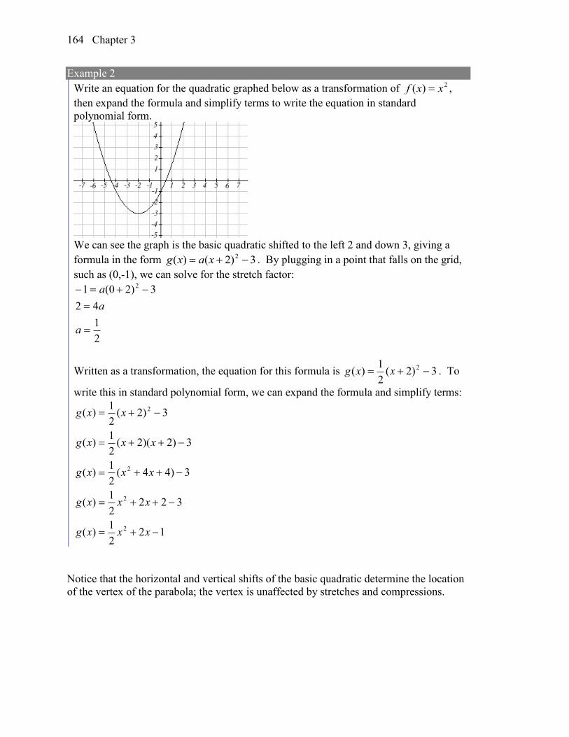
Chapter 3 164
Example 2
Write an equation for the quadratic graphed below as a transformation of 2)( xxf ,
then expand the formula and simplify terms to write the equation in standard
polynomial form.
We can see the graph is the basic quadratic shifted to the left 2 and down 3, giving a
formula in the form 3)2()( 2 xaxg . By plugging in a point that falls on the grid,
such as (0,-1), we can solve for the stretch factor:
2
1
42
3)20(1 2
a
a
a
Written as a transformation, the equation for this formula is 3)2(2
1)( 2 xxg . To
write this in standard polynomial form, we can expand the formula and simplify terms:
122
1)(
3222
1)(
3)44(2
1)(
3)2)(2(2
1)(
3)2(2
1)(
2
2
2
2
xxxg
xxxg
xxxg
xxxg
xxg
Notice that the horizontal and vertical shifts of the basic quadratic determine the location
of the vertex of the parabola; the vertex is unaffected by stretches and compressions.
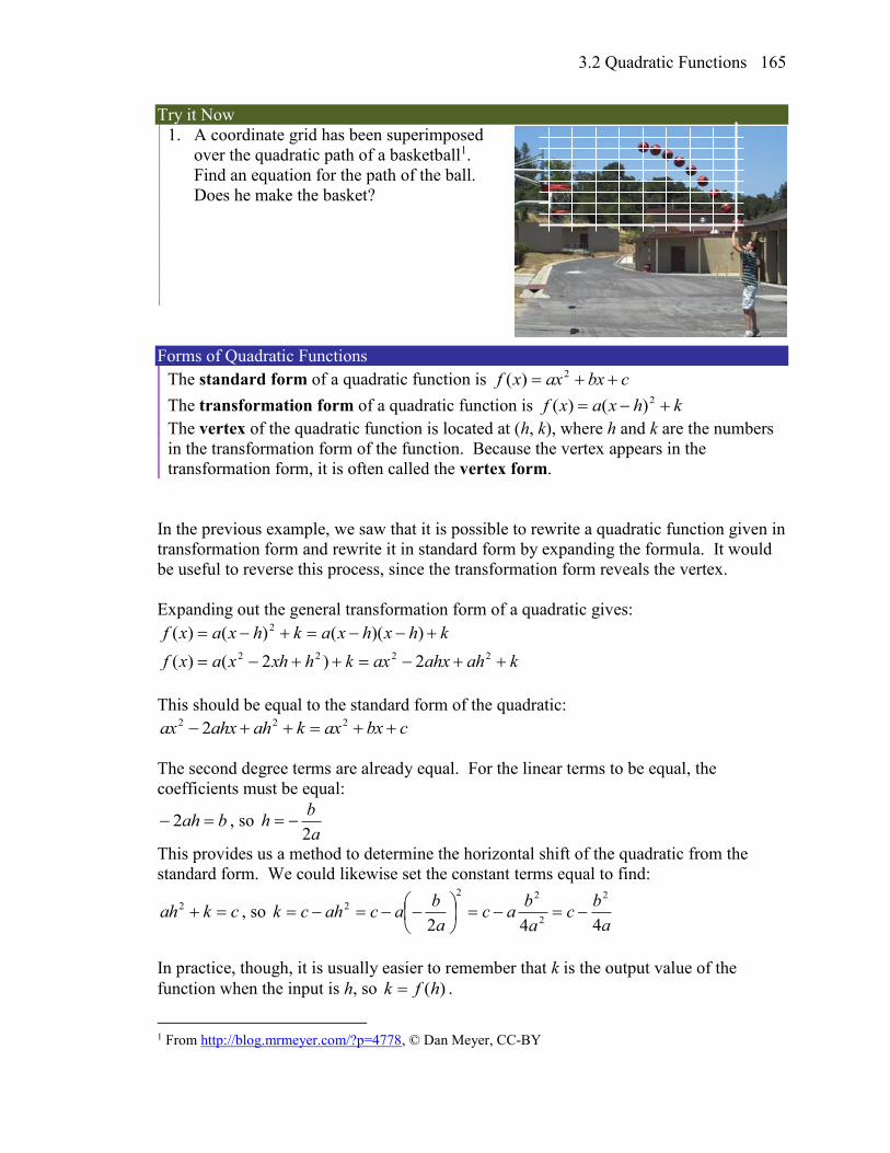
3.2 Quadratic Functions 165
Try it Now
1. A coordinate grid has been superimposed
over the quadratic path of a basketball1.
Find an equation for the path of the ball.
Does he make the basket?
Forms of Quadratic Functions
The standard form of a quadratic function is cbxaxxf 2)(
The transformation form of a quadratic function is khxaxf 2)()(
The vertex of the quadratic function is located at (h, k), where h and k are the numbers
in the transformation form of the function. Because the vertex appears in the
transformation form, it is often called the vertex form.
In the previous example, we saw that it is possible to rewrite a quadratic function given in
transformation form and rewrite it in standard form by expanding the formula. It would
be useful to reverse this process, since the transformation form reveals the vertex.
Expanding out the general transformation form of a quadratic gives:
kahahxaxkhxhxaxf
khxhxakhxaxf
2222
2
2)2()(
))(()()(
This should be equal to the standard form of the quadratic:
cbxaxkahahxax 222 2
The second degree terms are already equal. For the linear terms to be equal, the
coefficients must be equal:
bah 2 , so a
bh
2
This provides us a method to determine the horizontal shift of the quadratic from the
standard form. We could likewise set the constant terms equal to find:
ckah 2 , so a
bc
a
bac
a
bacahck
442
2
2
22
2
In practice, though, it is usually easier to remember that k is the output value of the
function when the input is h, so )(hfk .
1 From http://blog.mrmeyer.com/?p=4778, © Dan Meyer, CC-BY
Chapter 3 166
Finding the Vertex of a Quadratic
For a quadratic given in standard form, the vertex (h, k) is located at:
a
bh
2 , ( )
2
bk f h f
a
Example 3
Find the vertex of the quadratic 762)( 2 xxxf . Rewrite the quadratic into
transformation form (vertex form).
The horizontal coordinate of the vertex will be at 2
3
4
6
)2(2
6
2
a
bh
The vertical coordinate of the vertex will be at 2
57
2
36
2
32
2
32
f
Rewriting into transformation form, the stretch factor will be the same as the a in the
original quadratic. Using the vertex to determine the shifts,
2
5
2
32)(
2
xxf
Try it Now
2. Given the equation xxxg 613)( 2 write the equation in standard form and then
in transformation/vertex form.
In addition to enabling us to more easily graph a quadratic written in standard form,
finding the vertex serves another important purpose – it allows us to determine the
maximum or minimum value of the function, depending on which way the graph opens.
Example 4
Returning to our backyard farmer from the beginning of the section, what dimensions
should she make her garden to maximize the enclosed area?
Earlier we determined the area she could enclose with 80 feet of fencing on three sides
was given by the equation 2280)( LLLA . Notice that quadratic has been vertically
reflected, since the coefficient on the squared term is negative, so the graph will open
downwards, and the vertex will be a maximum value for the area.
In finding the vertex, we take care since the equation is not written in standard
polynomial form with decreasing powers. But we know that a is the coefficient on the
squared term, so a = -2, b = 80, and c = 0.
3.2 Quadratic Functions 167
Finding the vertex:
20)2(2
80
h , 800)20(2)20(80)20( 2 Ak
The maximum value of the function is an area of 800 square feet, which occurs when L
= 20 feet. When the shorter sides are 20 feet, that leaves 40 feet of fencing for the
longer side. To maximize the area, she should enclose the garden so the two shorter
sides have length 20 feet, and the longer side parallel to the existing fence has length 40
feet.
Example 5
A local newspaper currently has 84,000 subscribers, at a quarterly charge of $30.
Market research has suggested that if they raised the price to $32, they would lose 5,000
subscribers. Assuming that subscriptions are linearly related to the price, what price
should the newspaper charge for a quarterly subscription to maximize their revenue?
Revenue is the amount of money a company brings in. In this case, the revenue can be
found by multiplying the charge per subscription times the number of subscribers. We
can introduce variables, C for charge per subscription and S for the number subscribers,
giving us the equation
Revenue = CS
Since the number of subscribers changes with the price, we need to find a relationship
between the variables. We know that currently S = 84,000 and C = 30, and that if they
raise the price to $32 they would lose 5,000 subscribers, giving a second pair of values,
C = 32 and S = 79,000. From this we can find a linear equation relating the two
quantities. Treating C as the input and S as the output, the equation will have form
bmCS . The slope will be
500,22
000,5
3032
000,84000,79
m
This tells us the paper will lose 2,500 subscribers for each dollar they raise the price.
We can then solve for the vertical intercept
bCS 2500 Plug in the point S = 84,000 and C = 30
b )30(2500000,84 Solve for b
000,159b
This gives us the linear equation 000,159500,2 CS relating cost and subscribers.
We now return to our revenue equation.
CSRevenue Substituting the equation for S from above
)000,159500,2(Revenue CC Expanding
CC 000,159500,2Revenue 2
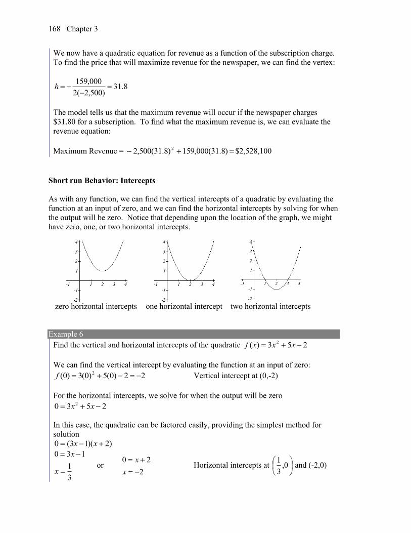
Chapter 3 168
We now have a quadratic equation for revenue as a function of the subscription charge.
To find the price that will maximize revenue for the newspaper, we can find the vertex:
8.31)500,2(2
000,159
h
The model tells us that the maximum revenue will occur if the newspaper charges
$31.80 for a subscription. To find what the maximum revenue is, we can evaluate the
revenue equation:
Maximum Revenue = )8.31(000,159)8.31(500,2 2 $2,528,100
Short run Behavior: Intercepts
As with any function, we can find the vertical intercepts of a quadratic by evaluating the
function at an input of zero, and we can find the horizontal intercepts by solving for when
the output will be zero. Notice that depending upon the location of the graph, we might
have zero, one, or two horizontal intercepts.
zero horizontal intercepts one horizontal intercept two horizontal intercepts
Example 6
Find the vertical and horizontal intercepts of the quadratic 253)( 2 xxxf
We can find the vertical intercept by evaluating the function at an input of zero:
22)0(5)0(3)0( 2 f Vertical intercept at (0,-2)
For the horizontal intercepts, we solve for when the output will be zero
2530 2 xx
In this case, the quadratic can be factored easily, providing the simplest method for
solution
)2)(13(0 xx
3
1
130
x
x
or 2
20
x
x Horizontal intercepts at
0,
3
1 and (-2,0)
3.2 Quadratic Functions 169
Notice that in the standard form of a quadratic, the constant term c reveals the vertical
intercept of the graph.
Example 7
Find the horizontal intercepts of the quadratic 442)( 2 xxxf
Again we will solve for when the output will be zero
4420 2 xx
Since the quadratic is not easily factorable in this case, we solve for the intercepts by
first rewriting the quadratic into transformation form.
1)2(2
4
2
a
bh 64)1(4)1(2)1( 2 fk
6)1(2)( 2 xxf
Now we can solve for when the output will be zero
31
31
)1(3
)1(26
6)1(20
2
2
2
x
x
x
x
x
The graph has horizontal intercepts at )0,31( and )0,31(
Try it Now
3. In Try it Now problem 2 we found the standard & transformation form for the
function xxxg 613)( 2 . Now find the Vertical & Horizontal intercepts (if any).
This process is done commonly enough that sometimes people find it easier to solve the
problem once in general and remember the formula for the result, rather than repeating
the process each time. Based on our previous work we showed that any quadratic in
standard form can be written into transformation form as:
a
bc
a
bxaxf
42)(
22
Chapter 3 170
Solving for the horizontal intercepts using this general equation gives:
a
bc
a
bxa
420
22
start to solve for x by moving the constants to the other side
22
24
a
bxac
a
b divide both sides by a
2
2
2
24
a
bx
a
c
a
b find a common denominator to combine fractions
2
22
2
24
4
4
a
bx
a
ac
a
b combine the fractions on the left side of the equation
2
2
2
24
4
a
bx
a
acb take the square root of both sides
a
bx
a
acb
24
42
2
subtract b/2a from both sides
xa
acb
a
b
2
4
2
2
combining the fractions
a
acbbx
2
42 Notice that this can yield two different answers for x
Quadratic Formula
For a quadratic function given in standard form 2( )f x ax bx c , the quadratic
formula gives the horizontal intercepts of the graph of this function.
a
acbbx
2
42
Example 8
A ball is thrown upwards from the top of a 40 foot high building at a speed of 80 feet
per second. The ball’s height above ground can be modeled by the equation 2( ) 16 80 40H t t t .
What is the maximum height of the ball?
When does the ball hit the ground?
To find the maximum height of the ball, we would need to know the vertex of the
quadratic.
2
5
32
80
)16(2
80
h ,
25 5 5
16 80 40 1402 2 2
k H
The ball reaches a maximum height of 140 feet after 2.5 seconds.
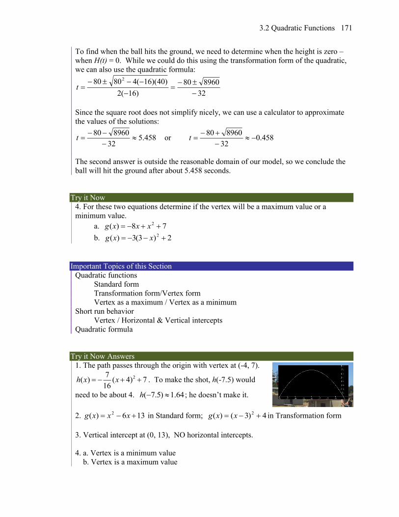
3.2 Quadratic Functions 171
To find when the ball hits the ground, we need to determine when the height is zero –
when H(t) = 0. While we could do this using the transformation form of the quadratic,
we can also use the quadratic formula:
32
896080
)16(2
)40)(16(48080 2
t
Since the square root does not simplify nicely, we can use a calculator to approximate
the values of the solutions:
458.532
896080
t or 458.0
32
896080
t
The second answer is outside the reasonable domain of our model, so we conclude the
ball will hit the ground after about 5.458 seconds.
Try it Now
4. For these two equations determine if the vertex will be a maximum value or a
minimum value.
a. 78)( 2 xxxg
b. 2)3(3)( 2 xxg
Important Topics of this Section
Quadratic functions
Standard form
Transformation form/Vertex form
Vertex as a maximum / Vertex as a minimum
Short run behavior
Vertex / Horizontal & Vertical intercepts
Quadratic formula
Try it Now Answers
1. The path passes through the origin with vertex at (-4, 7).
27( ) ( 4) 7
16h x x . To make the shot, h(-7.5) would
need to be about 4. ( 7.5) 1.64h ; he doesn’t make it.
2. 136)( 2 xxxg in Standard form; 4)3()( 2 xxg in Transformation form
3. Vertical intercept at (0, 13), NO horizontal intercepts.
4. a. Vertex is a minimum value
b. Vertex is a maximum value
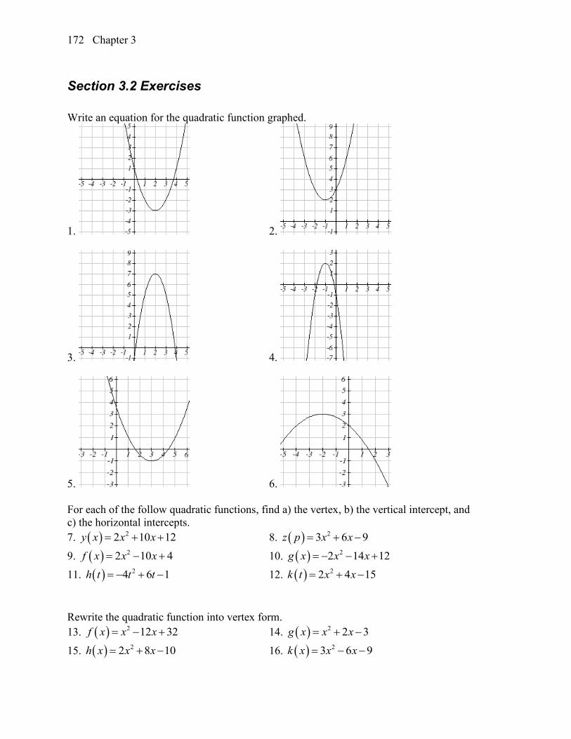
Chapter 3 172
Section 3.2 Exercises
Write an equation for the quadratic function graphed.
1. 2.
3. 4.
5. 6.
For each of the follow quadratic functions, find a) the vertex, b) the vertical intercept, and
c) the horizontal intercepts.
7. 22 10 12y x x x 8. 23 6 9z p x x
9. 22 10 4f x x x 10. 22 14 12g x x x
11. 24 6 1h t t t 12. 22 4 15 k t x x
Rewrite the quadratic function into vertex form.
13. 2 12 32f x x x 14. 2 2 3g x x x
15. 22 8 10h x x x 16. 23 6 9k x x x
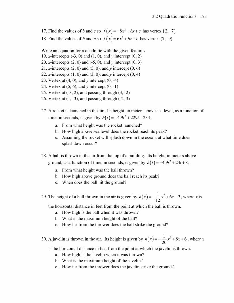
3.2 Quadratic Functions 173
17. Find the values of b and c so 28f x x bx c has vertex 2, 7
18. Find the values of b and c so 26f x x bx c has vertex (7, 9)
Write an equation for a quadratic with the given features
19. x-intercepts (-3, 0) and (1, 0), and y intercept (0, 2)
20. x-intercepts (2, 0) and (-5, 0), and y intercept (0, 3)
21. x-intercepts (2, 0) and (5, 0), and y intercept (0, 6)
22. x-intercepts (1, 0) and (3, 0), and y intercept (0, 4)
23. Vertex at (4, 0), and y intercept (0, -4)
24. Vertex at (5, 6), and y intercept (0, -1)
25. Vertex at (-3, 2), and passing through (3, -2)
26. Vertex at (1, -3), and passing through (-2, 3)
27. A rocket is launched in the air. Its height, in meters above sea level, as a function of
time, in seconds, is given by 24.9 229 234h t t t .
a. From what height was the rocket launched?
b. How high above sea level does the rocket reach its peak?
c. Assuming the rocket will splash down in the ocean, at what time does
splashdown occur?
28. A ball is thrown in the air from the top of a building. Its height, in meters above
ground, as a function of time, in seconds, is given by 24.9 24 8h t t t .
a. From what height was the ball thrown?
b. How high above ground does the ball reach its peak?
c. When does the ball hit the ground?
29. The height of a ball thrown in the air is given by 216 3
12h x x x , where x is
the horizontal distance in feet from the point at which the ball is thrown.
a. How high is the ball when it was thrown?
b. What is the maximum height of the ball?
c. How far from the thrower does the ball strike the ground?
30. A javelin is thrown in the air. Its height is given by 218 6
20h x x x , where x
is the horizontal distance in feet from the point at which the javelin is thrown.
a. How high is the javelin when it was thrown?
b. What is the maximum height of the javelin?
c. How far from the thrower does the javelin strike the ground?
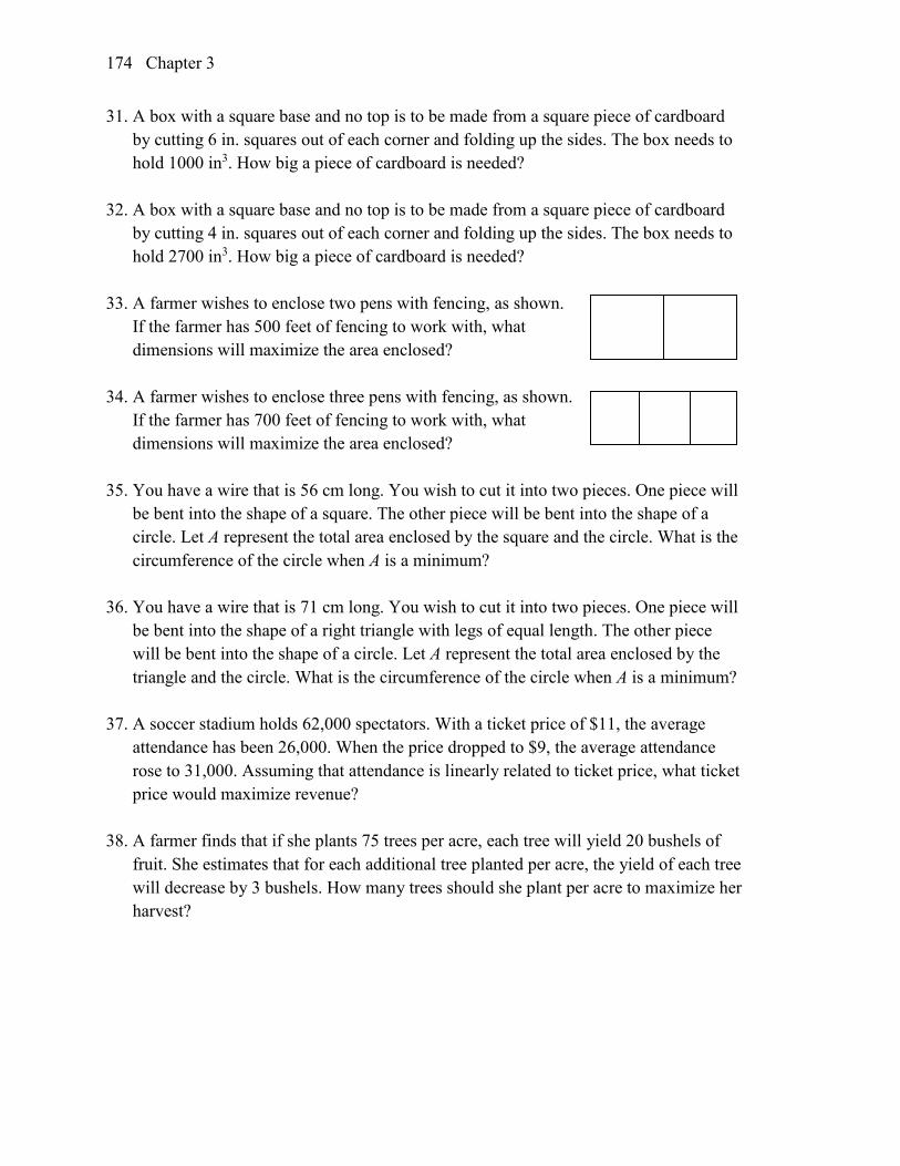
Chapter 3 174
31. A box with a square base and no top is to be made from a square piece of cardboard
by cutting 6 in. squares out of each corner and folding up the sides. The box needs to
hold 1000 in3. How big a piece of cardboard is needed?
32. A box with a square base and no top is to be made from a square piece of cardboard
by cutting 4 in. squares out of each corner and folding up the sides. The box needs to
hold 2700 in3. How big a piece of cardboard is needed?
33. A farmer wishes to enclose two pens with fencing, as shown.
If the farmer has 500 feet of fencing to work with, what
dimensions will maximize the area enclosed?
34. A farmer wishes to enclose three pens with fencing, as shown.
If the farmer has 700 feet of fencing to work with, what
dimensions will maximize the area enclosed?
35. You have a wire that is 56 cm long. You wish to cut it into two pieces. One piece will
be bent into the shape of a square. The other piece will be bent into the shape of a
circle. Let A represent the total area enclosed by the square and the circle. What is the
circumference of the circle when A is a minimum?
36. You have a wire that is 71 cm long. You wish to cut it into two pieces. One piece will
be bent into the shape of a right triangle with legs of equal length. The other piece
will be bent into the shape of a circle. Let A represent the total area enclosed by the
triangle and the circle. What is the circumference of the circle when A is a minimum?
37. A soccer stadium holds 62,000 spectators. With a ticket price of $11, the average
attendance has been 26,000. When the price dropped to $9, the average attendance
rose to 31,000. Assuming that attendance is linearly related to ticket price, what ticket
price would maximize revenue?
38. A farmer finds that if she plants 75 trees per acre, each tree will yield 20 bushels of
fruit. She estimates that for each additional tree planted per acre, the yield of each tree
will decrease by 3 bushels. How many trees should she plant per acre to maximize her
harvest?
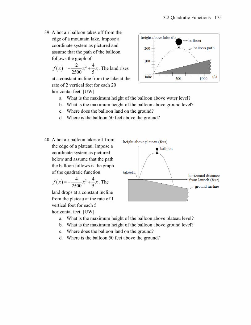
3.2 Quadratic Functions 175
39. A hot air balloon takes off from the
edge of a mountain lake. Impose a
coordinate system as pictured and
assume that the path of the balloon
follows the graph of
22 4
2500 5f x x x . The land rises
at a constant incline from the lake at the
rate of 2 vertical feet for each 20
horizontal feet. [UW]
a. What is the maximum height of the balloon above water level?
b. What is the maximum height of the balloon above ground level?
c. Where does the balloon land on the ground?
d. Where is the balloon 50 feet above the ground?
40. A hot air balloon takes off from
the edge of a plateau. Impose a
coordinate system as pictured
below and assume that the path
the balloon follows is the graph
of the quadratic function
24 4
2500 5f x x x . The
land drops at a constant incline
from the plateau at the rate of 1
vertical foot for each 5
horizontal feet. [UW]
a. What is the maximum height of the balloon above plateau level?
b. What is the maximum height of the balloon above ground level?
c. Where does the balloon land on the ground?
d. Where is the balloon 50 feet above the ground?
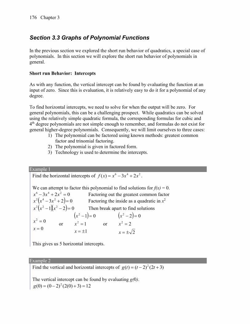
Chapter 3 176
Section 3.3 Graphs of Polynomial Functions
In the previous section we explored the short run behavior of quadratics, a special case of
polynomials. In this section we will explore the short run behavior of polynomials in
general.
Short run Behavior: Intercepts
As with any function, the vertical intercept can be found by evaluating the function at an
input of zero. Since this is evaluation, it is relatively easy to do it for a polynomial of any
degree.
To find horizontal intercepts, we need to solve for when the output will be zero. For
general polynomials, this can be a challenging prospect. While quadratics can be solved
using the relatively simple quadratic formula, the corresponding formulas for cubic and
4th degree polynomials are not simple enough to remember, and formulas do not exist for
general higher-degree polynomials. Consequently, we will limit ourselves to three cases:
1) The polynomial can be factored using known methods: greatest common
factor and trinomial factoring.
2) The polynomial is given in factored form.
3) Technology is used to determine the intercepts.
Example 1
Find the horizontal intercepts of 246 23)( xxxxf .
We can attempt to factor this polynomial to find solutions for f(x) = 0.
023 246 xxx Factoring out the greatest common factor
023 242 xxx Factoring the inside as a quadratic in x2
021 222 xxx Then break apart to find solutions
0
02
x
x or
1
1
01
2
2
x
x
x
or
2
2
02
2
2
x
x
x
This gives us 5 horizontal intercepts.
Example 2
Find the vertical and horizontal intercepts of )32()2()( 2 tttg
The vertical intercept can be found by evaluating g(0).
12)3)0(2()20()0( 2 g
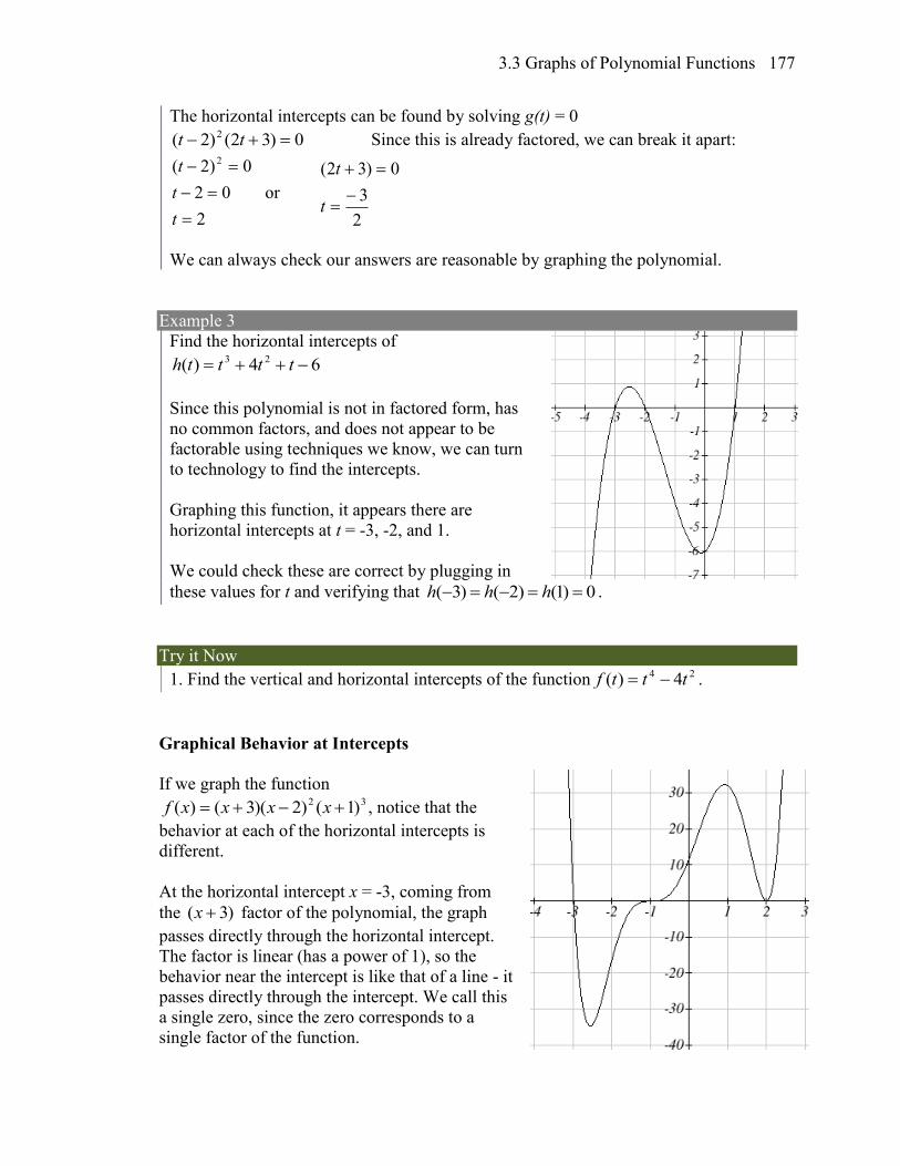
3.3 Graphs of Polynomial Functions 177
The horizontal intercepts can be found by solving g(t) = 0
0)32()2( 2 tt Since this is already factored, we can break it apart:
2
02
0)2( 2
t
t
t
or
2
3
0)32(
t
t
We can always check our answers are reasonable by graphing the polynomial.
Example 3
Find the horizontal intercepts of
64)( 23 tttth
Since this polynomial is not in factored form, has
no common factors, and does not appear to be
factorable using techniques we know, we can turn
to technology to find the intercepts.
Graphing this function, it appears there are
horizontal intercepts at t = -3, -2, and 1.
We could check these are correct by plugging in
these values for t and verifying that ( 3) ( 2) (1) 0h h h .
Try it Now
1. Find the vertical and horizontal intercepts of the function 24 4)( tttf .
Graphical Behavior at Intercepts
If we graph the function 32 )1()2)(3()( xxxxf , notice that the
behavior at each of the horizontal intercepts is
different.
At the horizontal intercept x = -3, coming from
the )3( x factor of the polynomial, the graph
passes directly through the horizontal intercept.
The factor is linear (has a power of 1), so the
behavior near the intercept is like that of a line - it
passes directly through the intercept. We call this
a single zero, since the zero corresponds to a
single factor of the function.
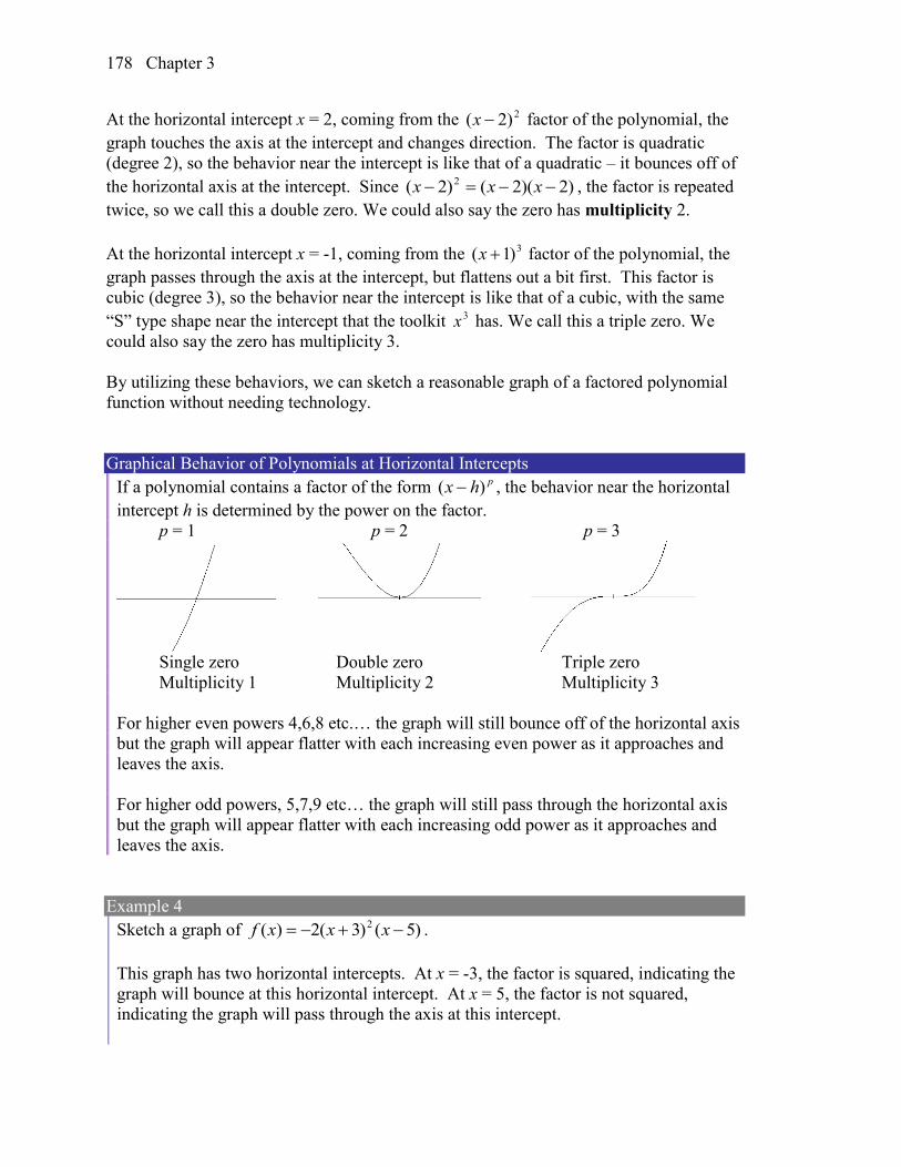
Chapter 3 178
At the horizontal intercept x = 2, coming from the 2)2( x factor of the polynomial, the
graph touches the axis at the intercept and changes direction. The factor is quadratic
(degree 2), so the behavior near the intercept is like that of a quadratic – it bounces off of
the horizontal axis at the intercept. Since )2)(2()2( 2 xxx , the factor is repeated
twice, so we call this a double zero. We could also say the zero has multiplicity 2.
At the horizontal intercept x = -1, coming from the 3)1( x factor of the polynomial, the
graph passes through the axis at the intercept, but flattens out a bit first. This factor is
cubic (degree 3), so the behavior near the intercept is like that of a cubic, with the same
“S” type shape near the intercept that the toolkit 3x has. We call this a triple zero. We
could also say the zero has multiplicity 3.
By utilizing these behaviors, we can sketch a reasonable graph of a factored polynomial
function without needing technology.
Graphical Behavior of Polynomials at Horizontal Intercepts
If a polynomial contains a factor of the form phx )( , the behavior near the horizontal
intercept h is determined by the power on the factor.
p = 1 p = 2 p = 3
Single zero Double zero Triple zero
Multiplicity 1 Multiplicity 2 Multiplicity 3
For higher even powers 4,6,8 etc.… the graph will still bounce off of the horizontal axis
but the graph will appear flatter with each increasing even power as it approaches and
leaves the axis.
For higher odd powers, 5,7,9 etc… the graph will still pass through the horizontal axis
but the graph will appear flatter with each increasing odd power as it approaches and
leaves the axis.
Example 4
Sketch a graph of )5()3(2)( 2 xxxf .
This graph has two horizontal intercepts. At x = -3, the factor is squared, indicating the
graph will bounce at this horizontal intercept. At x = 5, the factor is not squared,
indicating the graph will pass through the axis at this intercept.
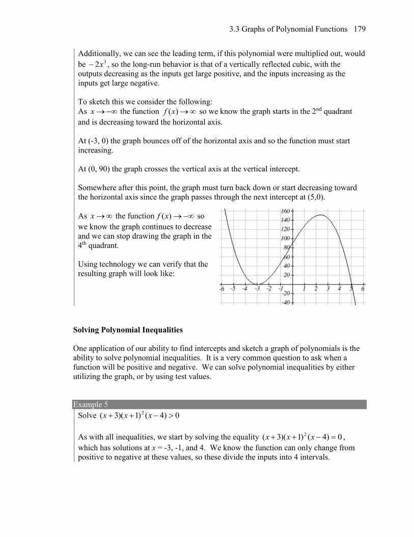
3.3 Graphs of Polynomial Functions 179
Additionally, we can see the leading term, if this polynomial were multiplied out, would
be 32x , so the long-run behavior is that of a vertically reflected cubic, with the
outputs decreasing as the inputs get large positive, and the inputs increasing as the
inputs get large negative.
To sketch this we consider the following:
As x the function )(xf so we know the graph starts in the 2nd quadrant
and is decreasing toward the horizontal axis.
At (-3, 0) the graph bounces off of the horizontal axis and so the function must start
increasing.
At (0, 90) the graph crosses the vertical axis at the vertical intercept.
Somewhere after this point, the graph must turn back down or start decreasing toward
the horizontal axis since the graph passes through the next intercept at (5,0).
As x the function )(xf so
we know the graph continues to decrease
and we can stop drawing the graph in the
4th quadrant.
Using technology we can verify that the
resulting graph will look like:
Solving Polynomial Inequalities
One application of our ability to find intercepts and sketch a graph of polynomials is the
ability to solve polynomial inequalities. It is a very common question to ask when a
function will be positive and negative. We can solve polynomial inequalities by either
utilizing the graph, or by using test values.
Example 5
Solve 0)4()1)(3( 2 xxx
As with all inequalities, we start by solving the equality 0)4()1)(3( 2 xxx ,
which has solutions at x = -3, -1, and 4. We know the function can only change from
positive to negative at these values, so these divide the inputs into 4 intervals.
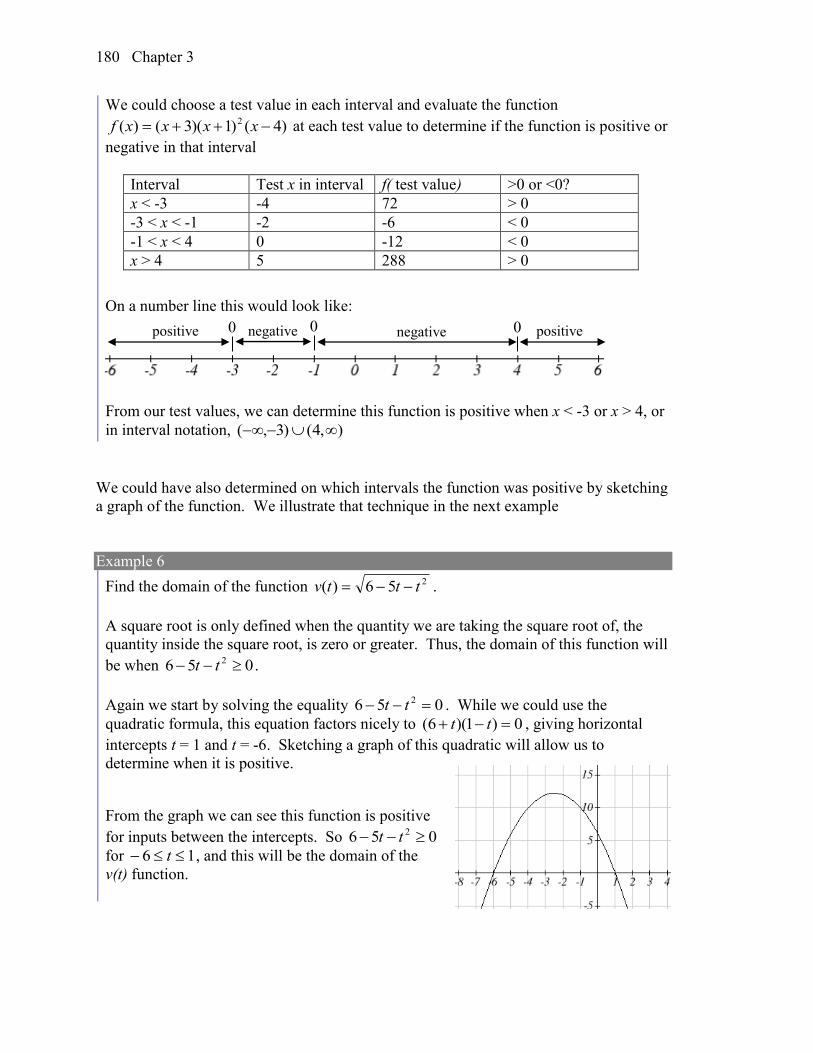
Chapter 3 180
We could choose a test value in each interval and evaluate the function
)4()1)(3()( 2 xxxxf at each test value to determine if the function is positive or
negative in that interval
On a number line this would look like:
From our test values, we can determine this function is positive when x < -3 or x > 4, or
in interval notation, ),4()3,(
We could have also determined on which intervals the function was positive by sketching
a graph of the function. We illustrate that technique in the next example
Example 6
Find the domain of the function 256)( tttv .
A square root is only defined when the quantity we are taking the square root of, the
quantity inside the square root, is zero or greater. Thus, the domain of this function will
be when 056 2 tt .
Again we start by solving the equality 056 2 tt . While we could use the
quadratic formula, this equation factors nicely to 0)1)(6( tt , giving horizontal
intercepts t = 1 and t = -6. Sketching a graph of this quadratic will allow us to
determine when it is positive.
From the graph we can see this function is positive
for inputs between the intercepts. So 056 2 tt
for 16 t , and this will be the domain of the
v(t) function.
Interval Test x in interval f( test value) >0 or <0?
x < -3 -4 72 > 0
-3 < x < -1 -2 -6 < 0
-1 < x < 4 0 -12 < 0
x > 4 5 288 > 0
0 0 0 positive negative negative positive
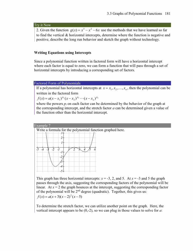
3.3 Graphs of Polynomial Functions 181
Try it Now
2. Given the function xxxxg 6)( 23 use the methods that we have learned so far
to find the vertical & horizontal intercepts, determine where the function is negative and
positive, describe the long run behavior and sketch the graph without technology.
Writing Equations using Intercepts
Since a polynomial function written in factored form will have a horizontal intercept
where each factor is equal to zero, we can form a function that will pass through a set of
horizontal intercepts by introducing a corresponding set of factors.
Factored Form of Polynomials
If a polynomial has horizontal intercepts at nxxxx ,,, 21 , then the polynomial can be
written in the factored form np
n
ppxxxxxxaxf )()()()( 21
21
where the powers pi on each factor can be determined by the behavior of the graph at
the corresponding intercept, and the stretch factor a can be determined given a value of
the function other than the horizontal intercept.
Example 7
Write a formula for the polynomial function graphed here.
This graph has three horizontal intercepts: x = -3, 2, and 5. At x = -3 and 5 the graph
passes through the axis, suggesting the corresponding factors of the polynomial will be
linear. At x = 2 the graph bounces at the intercept, suggesting the corresponding factor
of the polynomial will be 2nd degree (quadratic). Together, this gives us:
)5()2)(3()( 2 xxxaxf
To determine the stretch factor, we can utilize another point on the graph. Here, the
vertical intercept appears to be (0,-2), so we can plug in those values to solve for a:
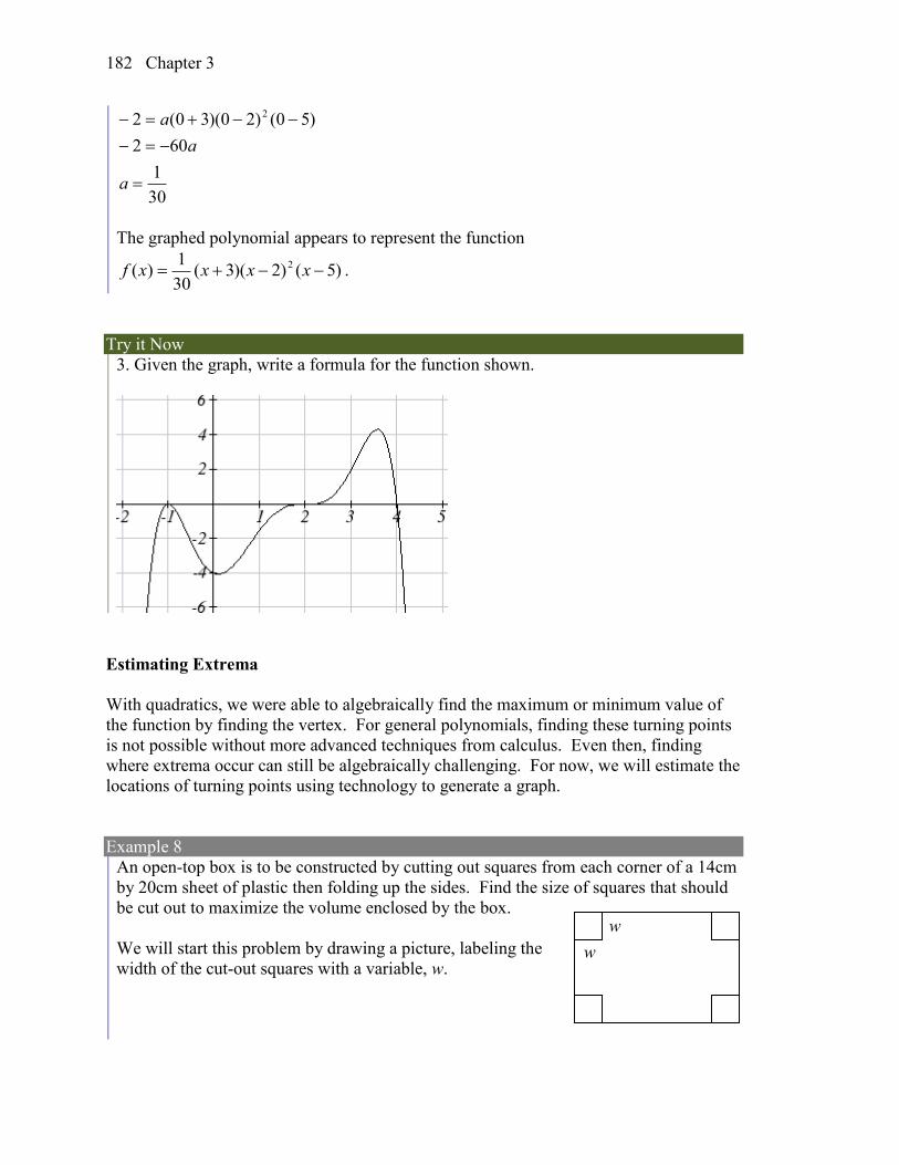
Chapter 3 182
30
1
602
)50()20)(30(2 2
a
a
a
The graphed polynomial appears to represent the function
)5()2)(3(30
1)( 2 xxxxf .
Try it Now
3. Given the graph, write a formula for the function shown.
Estimating Extrema
With quadratics, we were able to algebraically find the maximum or minimum value of
the function by finding the vertex. For general polynomials, finding these turning points
is not possible without more advanced techniques from calculus. Even then, finding
where extrema occur can still be algebraically challenging. For now, we will estimate the
locations of turning points using technology to generate a graph.
Example 8
An open-top box is to be constructed by cutting out squares from each corner of a 14cm
by 20cm sheet of plastic then folding up the sides. Find the size of squares that should
be cut out to maximize the volume enclosed by the box.
We will start this problem by drawing a picture, labeling the
width of the cut-out squares with a variable, w.
w
w
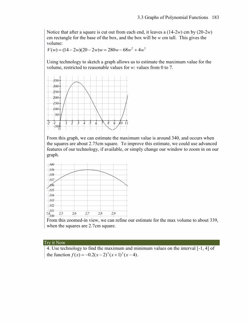
3.3 Graphs of Polynomial Functions 183
Notice that after a square is cut out from each end, it leaves a (14-2w) cm by (20-2w)
cm rectangle for the base of the box, and the box will be w cm tall. This gives the
volume: 32 468280)220)(214()( wwwwwwwV
Using technology to sketch a graph allows us to estimate the maximum value for the
volume, restricted to reasonable values for w: values from 0 to 7.
From this graph, we can estimate the maximum value is around 340, and occurs when
the squares are about 2.75cm square. To improve this estimate, we could use advanced
features of our technology, if available, or simply change our window to zoom in on our
graph.
From this zoomed-in view, we can refine our estimate for the max volume to about 339,
when the squares are 2.7cm square.
Try it Now
4. Use technology to find the maximum and minimum values on the interval [-1, 4] of
the function )4()1()2(2.0)( 23 xxxxf .

Chapter 3 184
Important Topics of this Section
Short Run Behavior
Intercepts (Horizontal & Vertical)
Methods to find Horizontal intercepts
Factoring Methods
Factored Forms
Technology
Graphical Behavior at intercepts
Single, Double and Triple zeros (or multiplicity 1, 2, and 3 behaviors)
Solving polynomial inequalities using test values & graphing techniques
Writing equations using intercepts
Estimating extrema
Try it Now Answers
1. Vertical intercept (0, 0), Horizontal intercepts (0, 0), (-2, 0), (2, 0)
2. Vertical intercept (0, 0), Horizontal intercepts (-2, 0), (0, 0), (3, 0)
The function is negative on ( , -2) and (0, 3)
The function is positive on (-2, 0) and (3, )
The leading term is 3x so as x , )(xg and as x , )(xg
3. 3 21( ) ( 2) ( 1) ( 4)
8f x x x x
4. The minimum occurs at approximately the point (0, -6.5), and the maximum occurs
at approximately the point (3.5, 7).
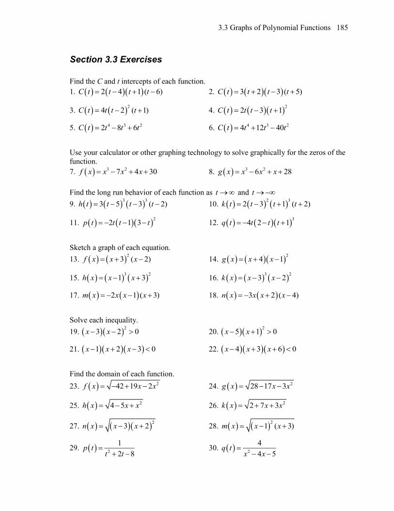
3.3 Graphs of Polynomial Functions 185
Section 3.3 Exercises
Find the C and t intercepts of each function.
1. 2 4 1 ( 6)C t t t t 2. 3 2 3 ( 5)C t t t t
3. 2
4 2 ( 1)C t t t t 4. 2
2 3 1C t t t t
5. 4 3 22 8 6C t t t t 6. 4 3 24 12 40C t t t t
Use your calculator or other graphing technology to solve graphically for the zeros of the
function.
7. 3 27 4 30f x x x x 8. 3 26 28g x x x x
Find the long run behavior of each function as t and t
9. 3 3
3 5 3 ( 2)h t t t t 10. 2 3
2 3 1 ( 2)k t t t t
11. 2
2 1 3p t t t t 12. 3
4 2 1q t t t t
Sketch a graph of each equation.
13. 2
3 ( 2)f x x x 14. 2
4 1g x x x
15. 3 2
1 3h x x x 16. 3 2
3 2k x x x
17. 2 1 ( 3)m x x x x 18. 3 2 ( 4)n x x x x
Solve each inequality.
19. 2
3 2 0x x 20. 2
5 1 0x x
21. 1 2 3 0x x x 22. 4 3 6 0x x x
Find the domain of each function.
23. 242 19 2f x x x 24. 228 17 3g x x x
25. 24 5h x x x 26. 22 7 3k x x x
27. 2
3 2n x x x 28. 2
1 ( 3)m x x x
29. 2
1
2 8p t
t t
30. 2
4
4 5q t
x x
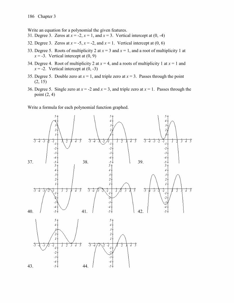
Chapter 3 186
Write an equation for a polynomial the given features.
31. Degree 3. Zeros at x = -2, x = 1, and x = 3. Vertical intercept at (0, -4)
32. Degree 3. Zeros at x = -5, x = -2, and x = 1. Vertical intercept at (0, 6)
33. Degree 5. Roots of multiplicity 2 at x = 3 and x = 1, and a root of multiplicity 1 at
x = -3. Vertical intercept at (0, 9)
34. Degree 4. Root of multiplicity 2 at x = 4, and a roots of multiplicity 1 at x = 1 and
x = -2. Vertical intercept at (0, -3)
35. Degree 5. Double zero at x = 1, and triple zero at x = 3. Passes through the point
(2, 15)
36. Degree 5. Single zero at x = -2 and x = 3, and triple zero at x = 1. Passes through the
point (2, 4)
Write a formula for each polynomial function graphed.
37. 38. 39.
40. 41. 42.
43. 44.
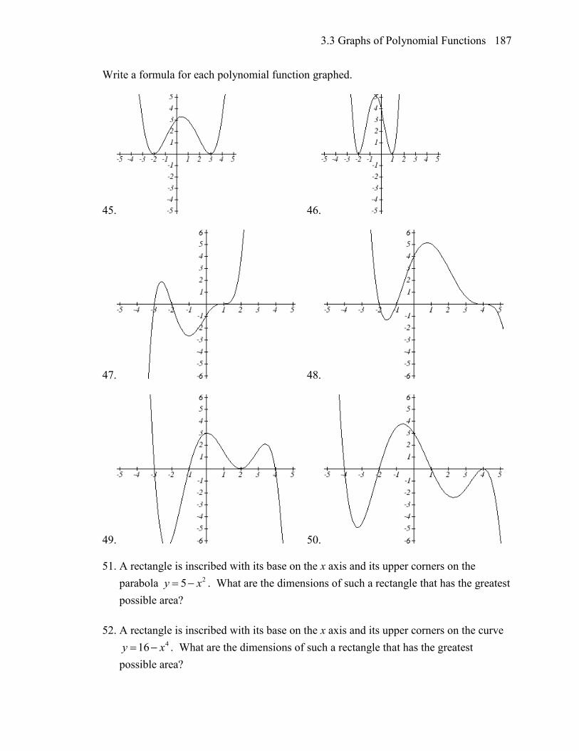
3.3 Graphs of Polynomial Functions 187
Write a formula for each polynomial function graphed.
45. 46.
47. 48.
49. 50.
51. A rectangle is inscribed with its base on the x axis and its upper corners on the
parabola 25y x . What are the dimensions of such a rectangle that has the greatest
possible area?
52. A rectangle is inscribed with its base on the x axis and its upper corners on the curve 416y x . What are the dimensions of such a rectangle that has the greatest
possible area?
Chapter 3 188
Section 3.4 Rational Functions
In the last few sections, we have built polynomials based on the positive whole number
power functions. In this section we explore functions based on power functions with
negative integer powers, called rational functions.
Example 1
You plan to drive 100 miles. Find a formula for the time the trip will take as a function
of the speed you drive.
You may recall that multiplying speed by time will give you distance. If we let t
represent the drive time in hours, and v represent the velocity (speed or rate) at which
we drive, then distancevt . Since our distance is fixed at 100 miles, 100vt .
Solving this relationship for the time gives us the function we desired:
1100100
)( vv
vt
While this type of relationship can be written using the negative exponent, it is more
common to see it written as a fraction.
This particular example is one of an inversely proportional relationship – where one
quantity is a constant divided by the other quantity, like 5
yx
.
Notice that this is a transformation of the reciprocal toolkit function, 1
( )f xx
Several natural phenomena, such as gravitational force and volume of sound, behave in a
manner inversely proportional to the square of another quantity. For example, the
volume, V, of a sound heard at a distance d from the source would be related by 2d
kV
for some constant value k.
These functions are transformations of the reciprocal squared toolkit function 2
1( )f x
x .
We have seen the graphs of the basic reciprocal function and the squared reciprocal
function from our study of toolkit functions. These graphs have several important
features.
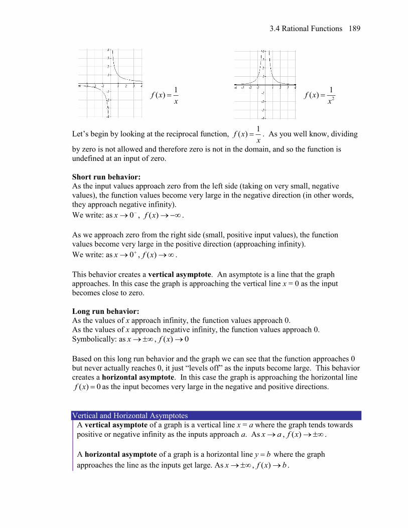
3.4 Rational Functions 189
1( )f x
x
2
1( )f x
x
Let’s begin by looking at the reciprocal function, 1
( )f xx
. As you well know, dividing
by zero is not allowed and therefore zero is not in the domain, and so the function is
undefined at an input of zero.
Short run behavior:
As the input values approach zero from the left side (taking on very small, negative
values), the function values become very large in the negative direction (in other words,
they approach negative infinity).
We write: as 0x , )(xf .
As we approach zero from the right side (small, positive input values), the function
values become very large in the positive direction (approaching infinity).
We write: as 0x , )(xf .
This behavior creates a vertical asymptote. An asymptote is a line that the graph
approaches. In this case the graph is approaching the vertical line x = 0 as the input
becomes close to zero.
Long run behavior:
As the values of x approach infinity, the function values approach 0.
As the values of x approach negative infinity, the function values approach 0.
Symbolically: as x , 0)( xf
Based on this long run behavior and the graph we can see that the function approaches 0
but never actually reaches 0, it just “levels off” as the inputs become large. This behavior
creates a horizontal asymptote. In this case the graph is approaching the horizontal line
( ) 0f x as the input becomes very large in the negative and positive directions.
Vertical and Horizontal Asymptotes
A vertical asymptote of a graph is a vertical line x = a where the graph tends towards
positive or negative infinity as the inputs approach a. As ax , )(xf .
A horizontal asymptote of a graph is a horizontal line y b where the graph
approaches the line as the inputs get large. As x , bxf )( .
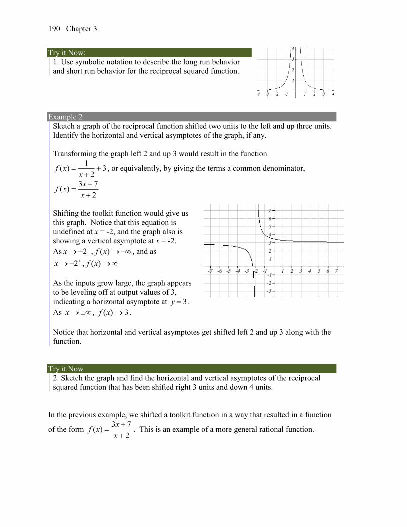
Chapter 3 190
Try it Now:
1. Use symbolic notation to describe the long run behavior
and short run behavior for the reciprocal squared function.
Example 2
Sketch a graph of the reciprocal function shifted two units to the left and up three units.
Identify the horizontal and vertical asymptotes of the graph, if any.
Transforming the graph left 2 and up 3 would result in the function
32
1)(
xxf , or equivalently, by giving the terms a common denominator,
2
73)(
x
xxf
Shifting the toolkit function would give us
this graph. Notice that this equation is
undefined at x = -2, and the graph also is
showing a vertical asymptote at x = -2.
As 2x , ( )f x , and as
2x , ( )f x
As the inputs grow large, the graph appears
to be leveling off at output values of 3,
indicating a horizontal asymptote at 3y .
As x , 3)( xf .
Notice that horizontal and vertical asymptotes get shifted left 2 and up 3 along with the
function.
Try it Now
2. Sketch the graph and find the horizontal and vertical asymptotes of the reciprocal
squared function that has been shifted right 3 units and down 4 units.
In the previous example, we shifted a toolkit function in a way that resulted in a function
of the form 2
73)(
x
xxf . This is an example of a more general rational function.
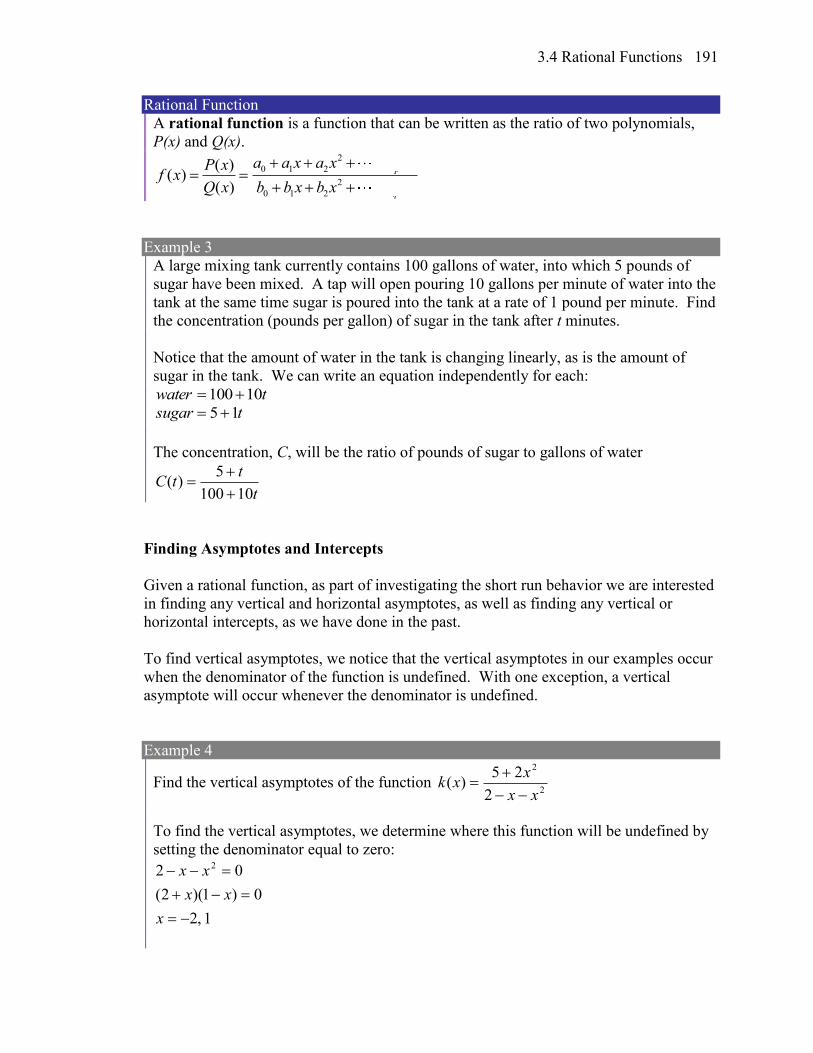
3.4 Rational Functions 191
Rational Function
A rational function is a function that can be written as the ratio of two polynomials,
P(x) and Q(x). 2
0 1 2
2
0 1 2
( )( )
( )
p
p
q
q
a a x a x a xP xf x
Q x b b x b x b x
Example 3
A large mixing tank currently contains 100 gallons of water, into which 5 pounds of
sugar have been mixed. A tap will open pouring 10 gallons per minute of water into the
tank at the same time sugar is poured into the tank at a rate of 1 pound per minute. Find
the concentration (pounds per gallon) of sugar in the tank after t minutes.
Notice that the amount of water in the tank is changing linearly, as is the amount of
sugar in the tank. We can write an equation independently for each:
twater 10100
tsugar 15
The concentration, C, will be the ratio of pounds of sugar to gallons of water
t
ttC
10100
5)(
Finding Asymptotes and Intercepts
Given a rational function, as part of investigating the short run behavior we are interested
in finding any vertical and horizontal asymptotes, as well as finding any vertical or
horizontal intercepts, as we have done in the past.
To find vertical asymptotes, we notice that the vertical asymptotes in our examples occur
when the denominator of the function is undefined. With one exception, a vertical
asymptote will occur whenever the denominator is undefined.
Example 4
Find the vertical asymptotes of the function 2
2
2
25)(
xx
xxk
To find the vertical asymptotes, we determine where this function will be undefined by
setting the denominator equal to zero:
1,2
0)1)(2(
02 2
x
xx
xx
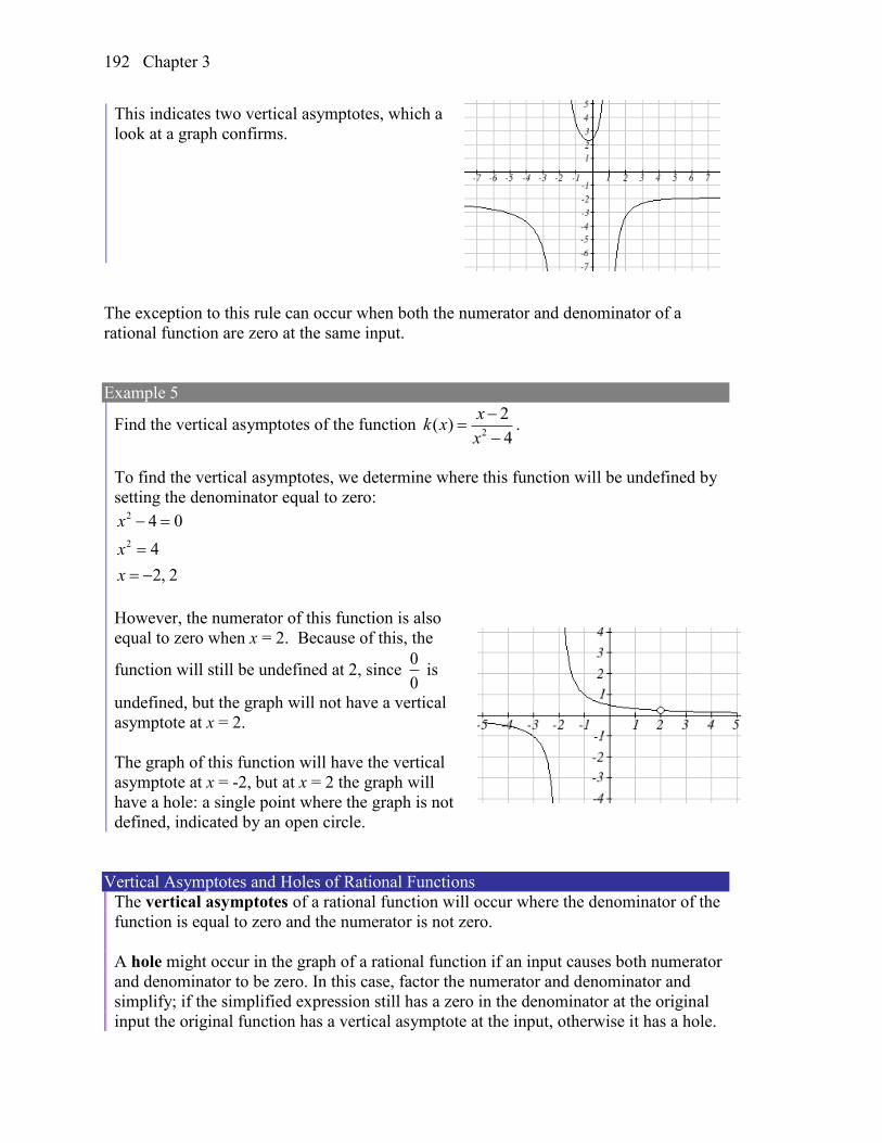
Chapter 3 192
This indicates two vertical asymptotes, which a
look at a graph confirms.
The exception to this rule can occur when both the numerator and denominator of a
rational function are zero at the same input.
Example 5
Find the vertical asymptotes of the function 2
2( )
4
xk x
x
.
To find the vertical asymptotes, we determine where this function will be undefined by
setting the denominator equal to zero: 2
2
4 0
4
2, 2
x
x
x
However, the numerator of this function is also
equal to zero when x = 2. Because of this, the
function will still be undefined at 2, since 0
0 is
undefined, but the graph will not have a vertical
asymptote at x = 2.
The graph of this function will have the vertical
asymptote at x = -2, but at x = 2 the graph will
have a hole: a single point where the graph is not
defined, indicated by an open circle.
Vertical Asymptotes and Holes of Rational Functions
The vertical asymptotes of a rational function will occur where the denominator of the
function is equal to zero and the numerator is not zero.
A hole might occur in the graph of a rational function if an input causes both numerator
and denominator to be zero. In this case, factor the numerator and denominator and
simplify; if the simplified expression still has a zero in the denominator at the original
input the original function has a vertical asymptote at the input, otherwise it has a hole.
3.4 Rational Functions 193
To find horizontal asymptotes, we are interested in the behavior of the function as the
input grows large, so we consider long run behavior of the numerator and denominator
separately. Recall that a polynomial’s long run behavior will mirror that of the leading
term. Likewise, a rational function’s long run behavior will mirror that of the ratio of the
leading terms of the numerator and denominator functions.
There are three distinct outcomes when this analysis is done:
Case 1: The degree of the denominator > degree of the numerator
Example: 54
23)(
2
xx
xxf
In this case, the long run behavior is 2
3 3( )
xf x
x x . This tells us that as the inputs grow
large, this function will behave similarly to the function 3
( )g xx
. As the inputs grow
large, the outputs will approach zero, resulting in a horizontal asymptote at 0y .
As x , 0)( xf
Case 2: The degree of the denominator < degree of the numerator
Example: 5
23)(
2
x
xxf
In this case, the long run behavior is23
( ) 3x
f x xx
. This tells us that as the inputs
grow large, this function will behave similarly to the function ( ) 3g x x . As the inputs
grow large, the outputs will grow and not level off, so this graph has no horizontal
asymptote.
As x , )(xf , respectively.
Ultimately, if the numerator is larger than the denominator, the long run behavior of the
graph will mimic the behavior of the reduced long run behavior fraction. As another
example if we had the function 5 23
( )3
x xf x
x
with long run behavior
543
( ) 3x
f x xx
, the long run behavior of the graph would look similar to that of an
even polynomial, and as x , )(xf .
Case 3: The degree of the denominator = degree of the numerator
Example: 54
23)(
2
2
xx
xxf
Chapter 3 194
In this case, the long run behavior is 2
2
3( ) 3
xf x
x . This tells us that as the inputs grow
large, this function will behave like the function ( ) 3g x , which is a horizontal line. As
x , 3)( xf , resulting in a horizontal asymptote at 3y .
Horizontal Asymptote of Rational Functions
The horizontal asymptote of a rational function can be determined by looking at the
degrees of the numerator and denominator.
Degree of denominator > degree of numerator: Horizontal asymptote at 0y
Degree of denominator < degree of numerator: No horizontal asymptote
Degree of denominator = degree of numerator: Horizontal asymptote at ratio of leading
coefficients.
Example 6
In the sugar concentration problem from earlier, we created the equation
t
ttC
10100
5)(
.
Find the horizontal asymptote and interpret it in context of the scenario.
Both the numerator and denominator are linear (degree 1), so since the degrees are
equal, there will be a horizontal asymptote at the ratio of the leading coefficients. In the
numerator, the leading term is t, with coefficient 1. In the denominator, the leading
term is 10t, with coefficient 10. The horizontal asymptote will be at the ratio of these
values: As t , 1
( )10
C t . This function will have a horizontal asymptote at
1
10y .
This tells us that as the input gets large, the output values will approach 1/10. In
context, this means that as more time goes by, the concentration of sugar in the tank will
approach one tenth of a pound of sugar per gallon of water or 1/10 pounds per gallon.
Example 7
Find the horizontal and vertical asymptotes of the function
)5)(2)(1(
)3)(2()(
xxx
xxxf
First, note this function has no inputs that make both the numerator and denominator
zero, so there are no potential holes. The function will have vertical asymptotes when
the denominator is zero, causing the function to be undefined. The denominator will be
zero at x = 1, -2, and 5, indicating vertical asymptotes at these values.
3.4 Rational Functions 195
The numerator has degree 2, while the denominator has degree 3. Since the degree of
the denominator is greater than the degree of the numerator, the denominator will grow
faster than the numerator, causing the outputs to tend towards zero as the inputs get
large, and so as x , 0)( xf . This function will have a horizontal asymptote at
0y .
Try it Now
3. Find the vertical and horizontal asymptotes of the function
)3)(2(
)12)(12()(
xx
xxxf
Intercepts
As with all functions, a rational function will have a vertical intercept when the input is
zero, if the function is defined at zero. It is possible for a rational function to not have a
vertical intercept if the function is undefined at zero.
Likewise, a rational function will have horizontal intercepts at the inputs that cause the
output to be zero (unless that input corresponds to a hole). It is possible there are no
horizontal intercepts. Since a fraction is only equal to zero when the numerator is zero,
horizontal intercepts will occur when the numerator of the rational function is equal to
zero.
Example 8
Find the intercepts of )5)(2)(1(
)3)(2()(
xxx
xxxf
We can find the vertical intercept by evaluating the function at zero
5
3
10
6
)50)(20)(10(
)30)(20()0(
f
The horizontal intercepts will occur when the function is equal to zero:
)5)(2)(1(
)3)(2(0
xxx
xx This is zero when the numerator is zero
3,2
)3)(2(0
x
xx
Try it Now
4. Given the reciprocal squared function that is shifted right 3 units and down 4 units,
write this as a rational function and find the horizontal and vertical intercepts and the
horizontal and vertical asymptotes.
Chapter 3 196
From the previous example, you probably noticed that the numerator of a rational
function reveals the horizontal intercepts of the graph, while the denominator reveals the
vertical asymptotes of the graph. As with polynomials, factors of the numerator may
have integer powers greater than one. Happily, the effect on the shape of the graph at
those intercepts is the same as we saw with polynomials.
When factors of the denominator have integer powers greater than one, the behavior at
the corresponding vertical asymptote will mirror one of the two toolkit reciprocal
functions.
We get this behavior when the degree of the factor in the
denominator is odd. The distinguishing characteristic is that
on one side of the vertical asymptote the graph heads towards
positive infinity, and on the other side the graph heads
towards negative infinity.
We get this behavior when the degree of the factor in the
denominator is even. The distinguishing characteristic is
that the graph either heads toward positive infinity on both
sides of the vertical asymptote, or heads toward negative
infinity on both sides.
For example, the graph of
)2()3(
)3()1()(
2
2
xx
xxxf is shown here.
At the horizontal intercept x = -1
corresponding to the 2)1( x factor of
the numerator, the graph bounces at the
intercept, consistent with the quadratic
nature of the factor.
At the horizontal intercept x = 3 corresponding to the )3( x factor of the numerator, the
graph passes through the axis as we’d expect from a linear factor.
At the vertical asymptote x = -3 corresponding to the 2)3( x factor of the denominator,
the graph heads towards positive infinity on both sides of the asymptote, consistent with
the behavior of the 2
1
x toolkit.
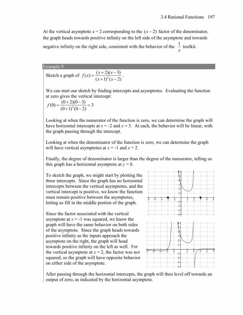
3.4 Rational Functions 197
At the vertical asymptote x = 2 corresponding to the )2( x factor of the denominator,
the graph heads towards positive infinity on the left side of the asymptote and towards
negative infinity on the right side, consistent with the behavior of the x
1 toolkit.
Example 9
Sketch a graph of 2
( 2)( 3)( )
( 1) ( 2)
x xf x
x x
.
We can start our sketch by finding intercepts and asymptotes. Evaluating the function
at zero gives the vertical intercept:
2
(0 2)(0 3)(0) 3
(0 1) (0 2)f
Looking at when the numerator of the function is zero, we can determine the graph will
have horizontal intercepts at x = -2 and x = 3. At each, the behavior will be linear, with
the graph passing through the intercept.
Looking at when the denominator of the function is zero, we can determine the graph
will have vertical asymptotes at x = -1 and x = 2.
Finally, the degree of denominator is larger than the degree of the numerator, telling us
this graph has a horizontal asymptote at y = 0.
To sketch the graph, we might start by plotting the
three intercepts. Since the graph has no horizontal
intercepts between the vertical asymptotes, and the
vertical intercept is positive, we know the function
must remain positive between the asymptotes,
letting us fill in the middle portion of the graph.
Since the factor associated with the vertical
asymptote at x = -1 was squared, we know the
graph will have the same behavior on both sides
of the asymptote. Since the graph heads towards
positive infinity as the inputs approach the
asymptote on the right, the graph will head
towards positive infinity on the left as well. For
the vertical asymptote at x = 2, the factor was not
squared, so the graph will have opposite behavior
on either side of the asymptote.
After passing through the horizontal intercepts, the graph will then level off towards an
output of zero, as indicated by the horizontal asymptote.
Chapter 3 198
Try it Now
5. Given the function )3()1(2
)2()2()(
2
2
xx
xxxf , use the characteristics of polynomials
and rational functions to describe its behavior and sketch the function .
Since a rational function written in factored form will have a horizontal intercept where
each factor of the numerator is equal to zero, we can form a numerator that will pass
through a set of horizontal intercepts by introducing a corresponding set of factors.
Likewise, since the function will have a vertical asymptote where each factor of the
denominator is equal to zero, we can form a denominator that will produce the vertical
asymptotes by introducing a corresponding set of factors.
Writing Rational Functions from Intercepts and Asymptotes
If a rational function has horizontal intercepts at nxxxx ,,, 21 , and vertical
asymptotes at mvvvx ,,, 21 then the function can be written in the form
n
n
q
m
p
n
pp
vxvxvx
xxxxxxaxf
)()()(
)()()()(
21
21
21
21
where the powers pi or qi on each factor can be determined by the behavior of the graph
at the corresponding intercept or asymptote, and the stretch factor a can be determined
given a value of the function other than the horizontal intercept, or by the horizontal
asymptote if it is nonzero.
Example 10
Write an equation for the rational function
graphed here.
The graph appears to have horizontal
intercepts at x = -2 and x = 3. At both, the
graph passes through the intercept, suggesting
linear factors.
The graph has two vertical asymptotes. The
one at x = -1 seems to exhibit the basic
behavior similar to x
1, with the graph heading toward positive infinity on one side and
heading toward negative infinity on the other. The asymptote at x = 2 is exhibiting a
behavior similar to 2
1
x, with the graph heading toward negative infinity on both sides
of the asymptote.
3.4 Rational Functions 199
Utilizing this information indicates an function of the form
2)2)(1(
)3)(2()(
xx
xxaxf
To find the stretch factor, we can use another clear point on the graph, such as the
vertical intercept (0,-2):
3
4
6
8
4
62
)20)(10(
)30)(20(2
2
a
a
a
This gives us a final function of 2)2)(1(3
)3)(2(4)(
xx
xxxf
Important Topics of this Section
Inversely proportional; Reciprocal toolkit function
Inversely proportional to the square; Reciprocal squared toolkit function
Horizontal Asymptotes
Vertical Asymptotes
Rational Functions
Finding intercepts, asymptotes, and holes.
Given equation sketch the graph
Identifying a function from its graph
Try it Now Answers
1. Long run behavior, as x , 0)( xf
Short run behavior, as 0x , )(xf (there are no horizontal or vertical
intercepts)
2.
The function and the asymptotes are shifted 3 units right and 4 units down.
As 3x , )(xf and as x , 4)( xf
Chapter 3 200
3. Vertical asymptotes at x = 2 and x = -3; horizontal asymptote at y = 4
4. For the transformed reciprocal squared function, we find the rational form.
96
35244
)3)(3(
)96(41
)3(
)3(414
)3(
1)(
2
22
2
2
2
xx
xx
xx
xx
x
x
xxf
Since the numerator is the same degree as the denominator we know that as
x , 4)( xf . 4y is the horizontal asymptote. Next, we set the
denominator equal to zero to find the vertical asymptote at x = 3, because as 3x ,
)(xf . We set the numerator equal to 0 and find the horizontal intercepts are at
(2.5,0) and (3.5,0), then we evaluate at 0 and the vertical intercept is at
9
35,0
5.
Horizontal asymptote at y = 1/2.
Vertical asymptotes are at x = 1, and x = 3.
Vertical intercept at (0, 4/3),
Horizontal intercepts (2, 0) and (-2, 0)
(-2, 0) is a double zero and the graph bounces off
the axis at this point.
(2, 0) is a single zero and crosses the axis at this
point.
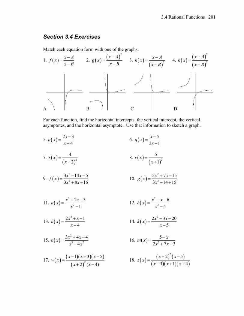
3.4 Rational Functions 201
Section 3.4 Exercises
Match each equation form with one of the graphs.
1. x A
f xx B
2.
2
x Ag x
x B
3.
2
x Ah x
x B
4.
2
2
x Ak x
x B
A B C D
For each function, find the horizontal intercepts, the vertical intercept, the vertical
asymptotes, and the horizontal asymptote. Use that information to sketch a graph.
5. 2 3
4
xp x
x
6.
5
3 1
xq x
x
7.
2
4
2s x
x
8.
2
5
1r x
x
9. 2
2
3 14 5
3 8 16
x xf x
x x
10.
2
2
2 7 15
3 14 15
x xg x
x
11. 2
2
2 3
1
x xa x
x
12.
2
2
6
4
x xb x
x
13. 22 1
4
x xh x
x
14.
22 3 20
5
x xk x
x
15. 2
3 2
3 4 4
4
x xn x
x x
16. 2
5
2 7 3
xm x
x x
17.
2
1 3 5
2 ( 4)
x x xw x
x x
18.
22 5
3 1 4
x xz x
x x x
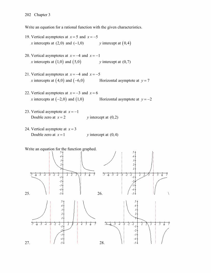
Chapter 3 202
Write an equation for a rational function with the given characteristics.
19. Vertical asymptotes at 5x and 5x
x intercepts at (2, 0) and ( 1, 0) y intercept at 0, 4
20. Vertical asymptotes at 4x and 1x
x intercepts at 1, 0 and 5, 0 y intercept at (0, 7)
21. Vertical asymptotes at 4x and 5x
x intercepts at 4, 0 and 6, 0 Horizontal asymptote at 7y
22. Vertical asymptotes at 3x and 6x
x intercepts at 2, 0 and 1, 0 Horizontal asymptote at 2y
23. Vertical asymptote at 1x
Double zero at 2x y intercept at (0, 2)
24. Vertical asymptote at 3x
Double zero at 1x y intercept at (0, 4)
Write an equation for the function graphed.
25. 26. \
27. 28.
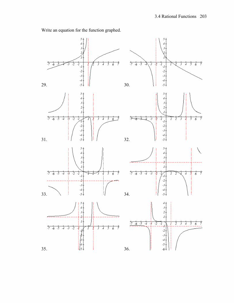
3.4 Rational Functions 203
Write an equation for the function graphed.
29. 30.
31. 32.
33. 34.
35. 36.
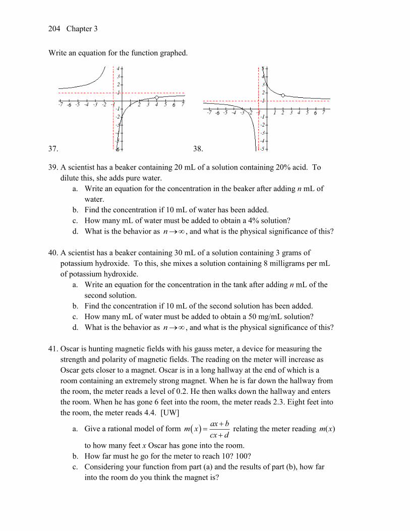
Chapter 3 204
Write an equation for the function graphed.
37. 38.
39. A scientist has a beaker containing 20 mL of a solution containing 20% acid. To
dilute this, she adds pure water.
a. Write an equation for the concentration in the beaker after adding n mL of
water.
b. Find the concentration if 10 mL of water has been added.
c. How many mL of water must be added to obtain a 4% solution?
d. What is the behavior as n , and what is the physical significance of this?
40. A scientist has a beaker containing 30 mL of a solution containing 3 grams of
potassium hydroxide. To this, she mixes a solution containing 8 milligrams per mL
of potassium hydroxide.
a. Write an equation for the concentration in the tank after adding n mL of the
second solution.
b. Find the concentration if 10 mL of the second solution has been added.
c. How many mL of water must be added to obtain a 50 mg/mL solution?
d. What is the behavior as n , and what is the physical significance of this?
41. Oscar is hunting magnetic fields with his gauss meter, a device for measuring the
strength and polarity of magnetic fields. The reading on the meter will increase as
Oscar gets closer to a magnet. Oscar is in a long hallway at the end of which is a
room containing an extremely strong magnet. When he is far down the hallway from
the room, the meter reads a level of 0.2. He then walks down the hallway and enters
the room. When he has gone 6 feet into the room, the meter reads 2.3. Eight feet into
the room, the meter reads 4.4. [UW]
a. Give a rational model of form ax b
m xcx d
relating the meter reading ( )m x
to how many feet x Oscar has gone into the room.
b. How far must he go for the meter to reach 10? 100?
c. Considering your function from part (a) and the results of part (b), how far
into the room do you think the magnet is?
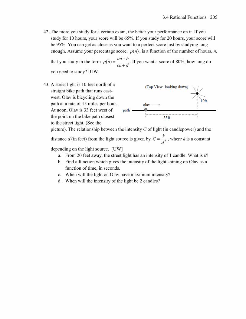
3.4 Rational Functions 205
42. The more you study for a certain exam, the better your performance on it. If you
study for 10 hours, your score will be 65%. If you study for 20 hours, your score will
be 95%. You can get as close as you want to a perfect score just by studying long
enough. Assume your percentage score, ( )p n , is a function of the number of hours, n,
that you study in the form ( )an b
p ncn d
. If you want a score of 80%, how long do
you need to study? [UW]
43. A street light is 10 feet north of a
straight bike path that runs east-
west. Olav is bicycling down the
path at a rate of 15 miles per hour.
At noon, Olav is 33 feet west of
the point on the bike path closest
to the street light. (See the
picture). The relationship between the intensity C of light (in candlepower) and the
distance d (in feet) from the light source is given by 2
kC
d , where k is a constant
depending on the light source. [UW]
a. From 20 feet away, the street light has an intensity of 1 candle. What is k?
b. Find a function which gives the intensity of the light shining on Olav as a
function of time, in seconds.
c. When will the light on Olav have maximum intensity?
d. When will the intensity of the light be 2 candles?
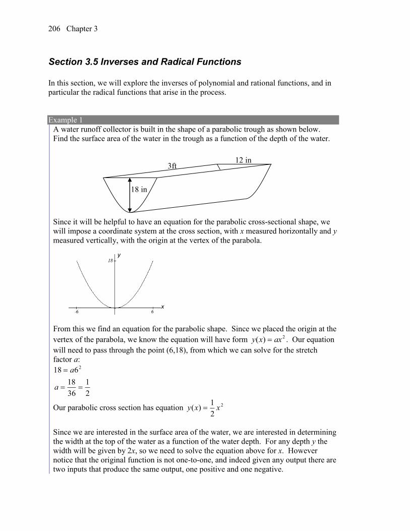
Chapter 3 206
Section 3.5 Inverses and Radical Functions
In this section, we will explore the inverses of polynomial and rational functions, and in
particular the radical functions that arise in the process.
Example 1
A water runoff collector is built in the shape of a parabolic trough as shown below.
Find the surface area of the water in the trough as a function of the depth of the water.
Since it will be helpful to have an equation for the parabolic cross-sectional shape, we
will impose a coordinate system at the cross section, with x measured horizontally and y
measured vertically, with the origin at the vertex of the parabola.
From this we find an equation for the parabolic shape. Since we placed the origin at the
vertex of the parabola, we know the equation will have form 2)( axxy . Our equation
will need to pass through the point (6,18), from which we can solve for the stretch
factor a:
2
1
36
18
618 2
a
a
Our parabolic cross section has equation 2
2
1)( xxy
Since we are interested in the surface area of the water, we are interested in determining
the width at the top of the water as a function of the water depth. For any depth y the
width will be given by 2x, so we need to solve the equation above for x. However
notice that the original function is not one-to-one, and indeed given any output there are
two inputs that produce the same output, one positive and one negative.
3ft 12 in
18 in
x
y
3.5 Inverses and Radical Functions 207
To find an inverse, we can restrict our original function to a limited domain on which it
is one-to-one. In this case, it makes sense to restrict ourselves to positive x values. On
this domain, we can find an inverse by solving for the input variable:
2
2
2
2
1
xy
xy
yx 2
This is not a function as written. Since we are limiting ourselves to positive x values,
we eliminate the negative solution, giving us the inverse function we’re looking for
yyx 2)(
Since x measures from the center out, the entire width of the water at the top will be 2x.
Since the trough is 3 feet (36 inches) long, the surface area will then be 36(2x), or in
terms of y:
yxArea 27272
The previous example illustrated two important things:
1) When finding the inverse of a quadratic, we have to limit ourselves to a domain
on which the function is one-to-one.
2) The inverse of a quadratic function is a square root function. Both are toolkit
functions and different types of power functions.
Functions involving roots are often called radical functions.
Example 2
Find the inverse of 143)2()( 22 xxxxf
From the transformation form of the function, we can see this is a transformed quadratic
with vertex at (2,-3) that opens upwards. Since the graph will be decreasing on one
side of the vertex, and increasing on the other side, we can restrict this function to a
domain on which it will be one-to-one by limiting the domain to 2x .
To find the inverse, we will use the vertex form of the quadratic. We start by replacing
the f(x) with a simple variable y, then solve for x.
3)2( 2 xy Add 3 to both sides 2)2(3 xy Take the square root
23 xy Add 2 to both sides
xy 32
Chapter 3 208
Of course, as written this is not a function. Since we restricted our original function to a
domain of 2x , the outputs of the inverse should be the same, telling us to utilize the
+ case:
32)(1 yyfx
If the quadratic had not been given in vertex form, rewriting it into vertex form is
probably the best approach. Alternatively, we could have taken the standard equation
and rewritten it equal to zero:
yxx 140 2
We would then be able to use the quadratic formula with 1a , 4b , and (1 )c y ,
resulting in the same solutions we found above: 2( 4) ( 4) 4(1)(1 ) 12 4
2 2 32 2
y yx y
Try it Now
1. Find the inverse of the function 2( ) 1f x x , on the domain 0x .
While it is not possible to find an inverse of most polynomial functions, some other basic
polynomials are invertible.
Example 3
Find the inverse of the function 15)( 3 xxf .
This is a transformation of the basic cubic toolkit function, and based on our knowledge
of that function, we know it is one-to-one. Solving for the inverse by solving for x
31
3
3
3
5
1)(
5
1
51
15
yyfx
xy
xy
xy
Notice that this inverse is also a transformation of a power function with a fractional
power, x1/3.
Try it Now
2. Which toolkit functions have inverse functions without restricting their domain?
3.5 Inverses and Radical Functions 209
Besides being important as an inverse function, radical functions are common in
important physical models.
Example 4
The velocity, v in feet per second, of a car that slammed on its brakes can be determined
based on the length of skid marks that the tires left on the ground. This relationship is
given by
gfddv 2)(
In this formula, g represents acceleration due to gravity (32 ft/sec2), d is the length of
the skid marks in feet, and f is a constant representing the friction of the surface. A car
lost control on wet asphalt, with a friction coefficient of 0.5, leaving 200 foot skid
marks. How fast was the car travelling when it lost control?
Using the given values of f = 0.5 and d = 200, we can evaluate the given formula:
(200) 2(32)(0.5)(200) 80 ft/secv , which is about 54.5 miles per hour.
When radical functions are composed with other functions, determining domain can
become more complicated.
Example 5
Find the domain of the function )1(
)3)(2()(
x
xxxf .
Since a square root is only defined when the quantity under the radical is non-negative,
we need to determine where 0)1(
)3)(2(
x
xx. A rational function can change signs
(change from positive to negative or vice versa) at horizontal intercepts and at vertical
asymptotes. For this equation, the graph could change signs at x = -2, 1, and 3.
To determine on which intervals the rational expression is positive, we could evaluate
the expression at test values, or sketch a graph. While both approaches work equally
well, for this example we will use a graph.
This function has two horizontal intercepts, both of which exhibit linear behavior,
where the graph will pass through the intercept. There is one vertical asymptote,
corresponding to a linear factor, leading to a behavior similar to the basic reciprocal
toolkit function. There is a vertical intercept at (0, 6). This graph does not have a
horizontal asymptote, since the degree of the numerator is larger than the degree of the
denominator.
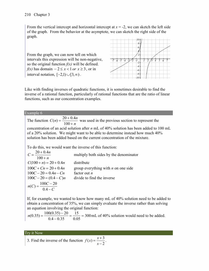
Chapter 3 210
From the vertical intercept and horizontal intercept at x = -2, we can sketch the left side
of the graph. From the behavior at the asymptote, we can sketch the right side of the
graph.
From the graph, we can now tell on which
intervals this expression will be non-negative,
so the original function f(x) will be defined.
f(x) has domain 312 xorx , or in
interval notation, ),3[)1,2[ .
Like with finding inverses of quadratic functions, it is sometimes desirable to find the
inverse of a rational function, particularly of rational functions that are the ratio of linear
functions, such as our concentration examples.
Example 6
The function n
nnC
100
4.020)( was used in the previous section to represent the
concentration of an acid solution after n mL of 40% solution has been added to 100 mL
of a 20% solution. We might want to be able to determine instead how much 40%
solution has been added based on the current concentration of the mixture.
To do this, we would want the inverse of this function:
n
nC
100
4.020 multiply both sides by the denominator
nnC 4.020)100( distribute
nCnC 4.020100 group everything with n on one side
CnnC 4.020100 factor out n
nCC )4.0(20100 divide to find the inverse
C
CCn
4.0
20100)(
If, for example, we wanted to know how many mL of 40% solution need to be added to
obtain a concentration of 35%, we can simply evaluate the inverse rather than solving
an equation involving the original function:
30005.0
15
35.04.0
20)35.0(100)35.0(
n mL of 40% solution would need to be added.
Try it Now
3. Find the inverse of the function 3
( )2
xf x
x
.
3.5 Inverses and Radical Functions 211
Important Topics of this Section
Imposing a coordinate system
Finding an inverse function
Restricting the domain
Invertible toolkit functions
Radical Functions
Inverses of rational functions
Try it Now Answers
1. 1)(1 yyfx
2. identity, cubic, square root, cube root
3. 1 2 3( )
1
yf y
y
Chapter 3 212
Section 3.5 Exercises
For each function, find a domain on which the function is one-to-one and non-decreasing,
then find an inverse of the function on this domain.
1. 2
4f x x 2. 2
2f x x
3. 212f x x 4. 29f x x
5. 33 1f x x 6. 34 2f x x
Find the inverse of each function.
7. 9 4 4f x x 8. 6 8 5f x x
9. 39 2f x x 10. 33f x x
11. 2
8f x
x
12.
3
4f x
x
13. 3
7
xf x
x
14.
2
7
xf x
x
15. 3 4
5 4
xf x
x
16.
5 1
2 5
xf x
x
Police use the formula 20v L to estimate the speed of a car, v, in miles per hour,
based on the length, L, in feet, of its skid marks when suddenly braking on a dry, asphalt
road.
17. At the scene of an accident, a police officer measures a car's skid marks to be 215 feet
long. Approximately how fast was the car traveling?
18. At the scene of an accident, a police officer measures a car's skid marks to be 135 feet
long. Approximately how fast was the car traveling?
The formula 2.7v r models the maximum safe speed, v, in miles per hour, at which a
car can travel on a curved road with radius of curvature r, in feet.
19. A highway crew measures the radius of curvature at an exit ramp on a highway as
430 feet. What is the maximum safe speed?
20. A highway crew measures the radius of curvature at a tight corner on a highway as
900 feet. What is the maximum safe speed?
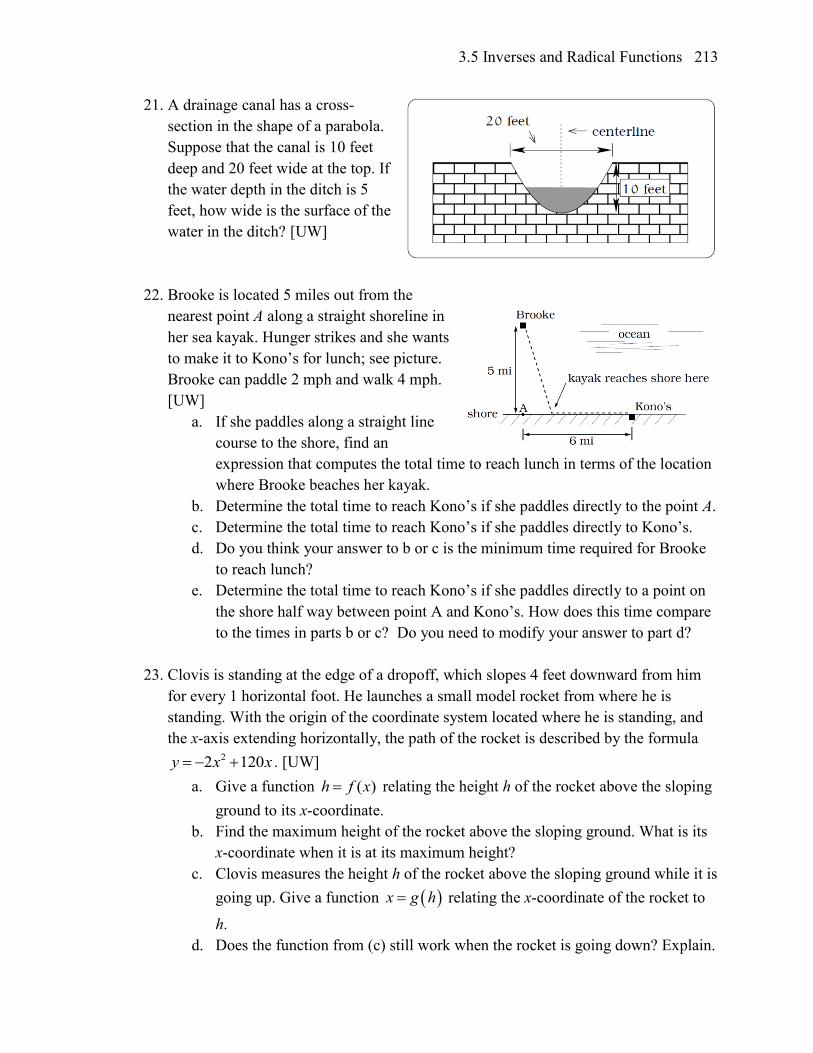
3.5 Inverses and Radical Functions 213
21. A drainage canal has a cross-
section in the shape of a parabola.
Suppose that the canal is 10 feet
deep and 20 feet wide at the top. If
the water depth in the ditch is 5
feet, how wide is the surface of the
water in the ditch? [UW]
22. Brooke is located 5 miles out from the
nearest point A along a straight shoreline in
her sea kayak. Hunger strikes and she wants
to make it to Kono’s for lunch; see picture.
Brooke can paddle 2 mph and walk 4 mph.
[UW]
a. If she paddles along a straight line
course to the shore, find an
expression that computes the total time to reach lunch in terms of the location
where Brooke beaches her kayak.
b. Determine the total time to reach Kono’s if she paddles directly to the point A.
c. Determine the total time to reach Kono’s if she paddles directly to Kono’s.
d. Do you think your answer to b or c is the minimum time required for Brooke
to reach lunch?
e. Determine the total time to reach Kono’s if she paddles directly to a point on
the shore half way between point A and Kono’s. How does this time compare
to the times in parts b or c? Do you need to modify your answer to part d?
23. Clovis is standing at the edge of a dropoff, which slopes 4 feet downward from him
for every 1 horizontal foot. He launches a small model rocket from where he is
standing. With the origin of the coordinate system located where he is standing, and
the x-axis extending horizontally, the path of the rocket is described by the formula 22 120y x x . [UW]
a. Give a function ( )h f x relating the height h of the rocket above the sloping
ground to its x-coordinate.
b. Find the maximum height of the rocket above the sloping ground. What is its
x-coordinate when it is at its maximum height?
c. Clovis measures the height h of the rocket above the sloping ground while it is
going up. Give a function x g h relating the x-coordinate of the rocket to
h.
d. Does the function from (c) still work when the rocket is going down? Explain.
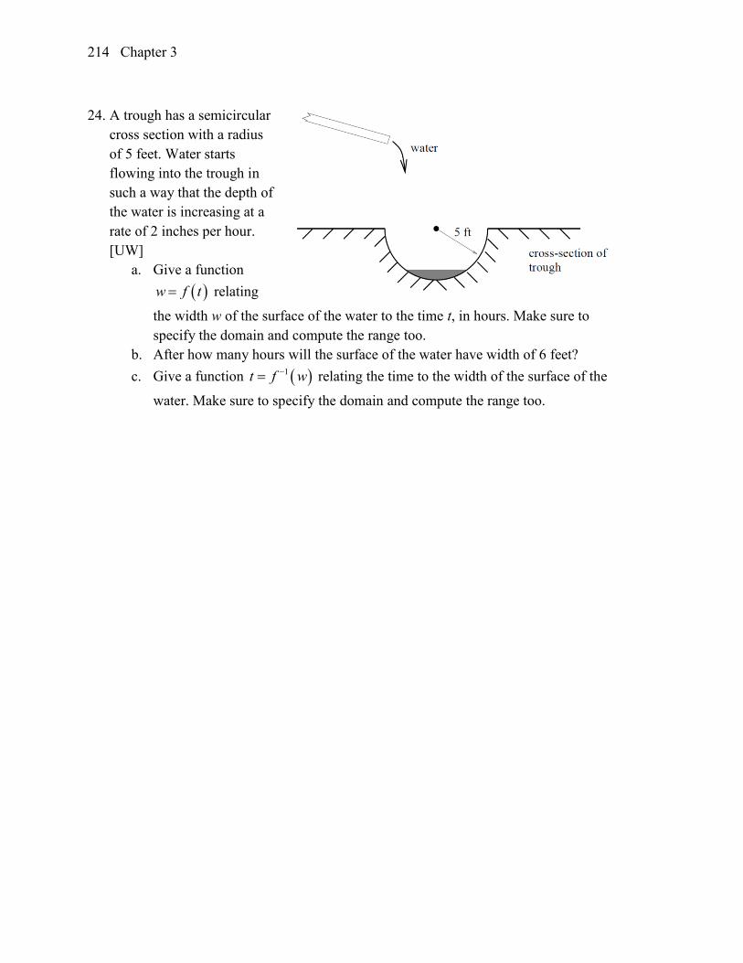
Chapter 3 214
24. A trough has a semicircular
cross section with a radius
of 5 feet. Water starts
flowing into the trough in
such a way that the depth of
the water is increasing at a
rate of 2 inches per hour.
[UW]
a. Give a function
w f t relating
the width w of the surface of the water to the time t, in hours. Make sure to
specify the domain and compute the range too.
b. After how many hours will the surface of the water have width of 6 feet?
c. Give a function 1t f w relating the time to the width of the surface of the
water. Make sure to specify the domain and compute the range too.
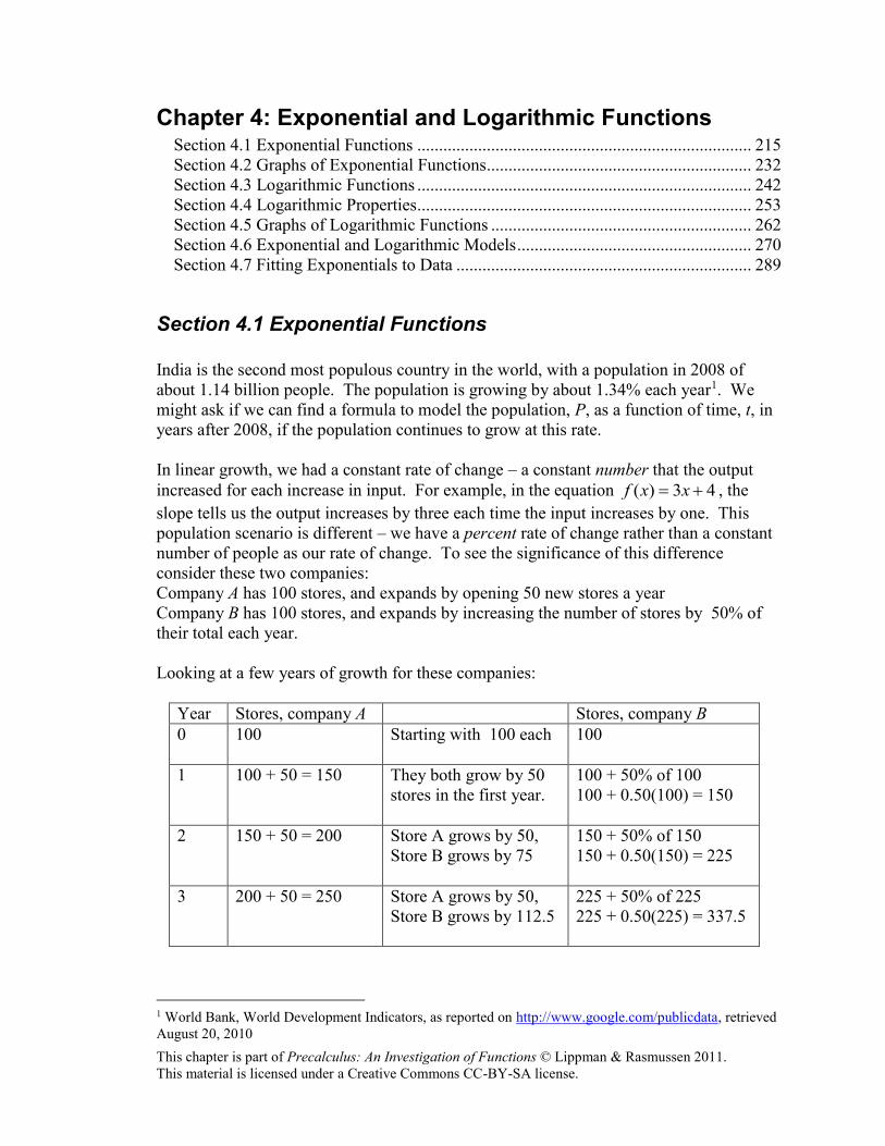
This chapter is part of Precalculus: An Investigation of Functions © Lippman & Rasmussen 2011.
This material is licensed under a Creative Commons CC-BY-SA license.
Chapter 4: Exponential and Logarithmic Functions Section 4.1 Exponential Functions ............................................................................. 215
Section 4.2 Graphs of Exponential Functions............................................................. 232
Section 4.3 Logarithmic Functions ............................................................................. 242
Section 4.4 Logarithmic Properties............................................................................. 253
Section 4.5 Graphs of Logarithmic Functions ............................................................ 262
Section 4.6 Exponential and Logarithmic Models ...................................................... 270
Section 4.7 Fitting Exponentials to Data .................................................................... 289
Section 4.1 Exponential Functions
India is the second most populous country in the world, with a population in 2008 of
about 1.14 billion people. The population is growing by about 1.34% each year1. We
might ask if we can find a formula to model the population, P, as a function of time, t, in
years after 2008, if the population continues to grow at this rate.
In linear growth, we had a constant rate of change – a constant number that the output
increased for each increase in input. For example, in the equation 43)( xxf , the
slope tells us the output increases by three each time the input increases by one. This
population scenario is different – we have a percent rate of change rather than a constant
number of people as our rate of change. To see the significance of this difference
consider these two companies:
Company A has 100 stores, and expands by opening 50 new stores a year
Company B has 100 stores, and expands by increasing the number of stores by 50% of
their total each year.
Looking at a few years of growth for these companies:
Year Stores, company A Stores, company B
0 100 Starting with 100 each
100
1 100 + 50 = 150 They both grow by 50
stores in the first year.
100 + 50% of 100
100 + 0.50(100) = 150
2 150 + 50 = 200 Store A grows by 50,
Store B grows by 75
150 + 50% of 150
150 + 0.50(150) = 225
3 200 + 50 = 250 Store A grows by 50,
Store B grows by 112.5
225 + 50% of 225
225 + 0.50(225) = 337.5
1 World Bank, World Development Indicators, as reported on http://www.google.com/publicdata, retrieved
August 20, 2010
Chapter 4 216
Notice that with the percent growth, each year the company is grows by 50% of the
current year’s total, so as the company grows larger, the number of stores added in a year
grows as well.
To try to simplify the calculations, notice that after 1 year the number of stores for
company B was:
)100(50.0100 or equivalently by factoring
150)50.01(100
We can think of this as “the new number of stores is the original 100% plus another
50%”.
After 2 years, the number of stores was:
)150(50.0150 or equivalently by factoring
)50.01(150 now recall the 150 came from 100(1+0.50). Substituting that,
225)50.01(100)50.01)(50.01(100 2
After 3 years, the number of stores was:
)225(50.0225 or equivalently by factoring
)50.01(225 now recall the 225 came from 2)50.01(100 . Substituting that,
5.337)50.01(100)50.01()50.01(100 32
From this, we can generalize, noticing that to show a 50% increase, each year we
multiply by a factor of (1+0.50), so after n years, our equation would be nnB )50.01(100)(
In this equation, the 100 represented the initial quantity, and the 0.50 was the percent
growth rate. Generalizing further, we arrive at the general form of exponential functions.
Exponential Function
An exponential growth or decay function is a function that grows or shrinks at a
constant percent growth rate. The equation can be written in the form xraxf )1()( or xabxf )( where b = 1+r
Where
a is the initial or starting value of the function
r is the percent growth or decay rate, written as a decimal
b is the growth factor or growth multiplier. Since powers of negative numbers behave
strangely, we limit b to positive values.
To see more clearly the difference between exponential and linear growth, compare the
two tables and graphs below, which illustrate the growth of company A and B described
above over a longer time frame if the growth patterns were to continue
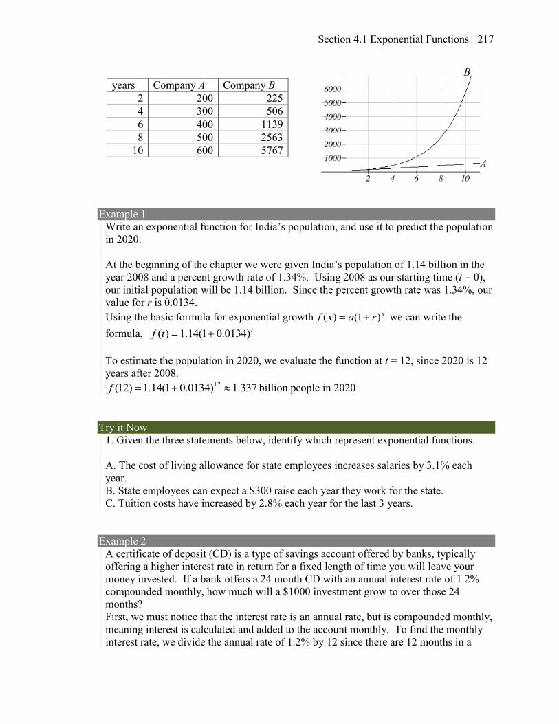
Section 4.1 Exponential Functions 217
B
years Company A Company B
2 200 225
4 300 506
6 400 1139
8 500 2563
10 600 5767
A
Example 1
Write an exponential function for India’s population, and use it to predict the population
in 2020.
At the beginning of the chapter we were given India’s population of 1.14 billion in the
year 2008 and a percent growth rate of 1.34%. Using 2008 as our starting time (t = 0),
our initial population will be 1.14 billion. Since the percent growth rate was 1.34%, our
value for r is 0.0134.
Using the basic formula for exponential growth xraxf )1()( we can write the
formula, ttf )0134.01(14.1)(
To estimate the population in 2020, we evaluate the function at t = 12, since 2020 is 12
years after 2008.
337.1)0134.01(14.1)12( 12 f billion people in 2020
Try it Now
1. Given the three statements below, identify which represent exponential functions.
A. The cost of living allowance for state employees increases salaries by 3.1% each
year.
B. State employees can expect a $300 raise each year they work for the state.
C. Tuition costs have increased by 2.8% each year for the last 3 years.
Example 2
A certificate of deposit (CD) is a type of savings account offered by banks, typically
offering a higher interest rate in return for a fixed length of time you will leave your
money invested. If a bank offers a 24 month CD with an annual interest rate of 1.2%
compounded monthly, how much will a $1000 investment grow to over those 24
months?
First, we must notice that the interest rate is an annual rate, but is compounded monthly,
meaning interest is calculated and added to the account monthly. To find the monthly
interest rate, we divide the annual rate of 1.2% by 12 since there are 12 months in a
Chapter 4 218
year: 1.2%/12 = 0.1%. Each month we will earn 0.1% interest. From this, we can set
up an exponential function, with our initial amount of $1000 and a growth rate of r =
0.001, and our input m measured in months. m
mf
12
012.11000)(
mmf )001.01(1000)(
After 24 months, the account will have grown to 24(24) 1000(1 0.001) $1024.28f
Try it Now
2. Looking at these two equations that represent the balance in two different savings
accounts, which account is growing faster, and which account will have a higher
balance after 3 years?
ttA 05.11000)( ttB 075.1900)(
In all the preceding examples, we saw exponential growth. Exponential functions can
also be used to model quantities that are decreasing at a constant percent rate. An
example of this is radioactive decay, a process in which radioactive isotopes of certain
atoms transform to an atom of a different type, causing a percentage decrease of the
original material over time.
Example 3
Bismuth-210 is an isotope that radioactively decays by about 13% each day, meaning
13% of the remaining Bismuth-210 transforms into another atom (polonium-210 in this
case) each day. If you begin with 100 mg of Bismuth-210, how much remains after one
week?
With radioactive decay, instead of the quantity increasing at a percent rate, the quantity
is decreasing at a percent rate. Our initial quantity is a = 100 mg, and our growth rate
will be negative 13%, since we are decreasing: r = -0.13. This gives the equation: dddQ )87.0(100)13.01(100)(
This can also be explained by recognizing that if 13% decays, then 87 % remains.
After one week, 7 days, the quantity remaining would be
73.37)87.0(100)7( 7 Q mg of Bismuth-210 remains.
Try it Now
3. A population of 1000 is decreasing 3% each year. Find the population in 30 years.
Section 4.1 Exponential Functions 219
Example 4
T(q) represents the total number of Android smart phone contracts, in thousands, held
by a certain Verizon store region measured quarterly since January 1, 2010,
Interpret all of the parts of the equation 3056.231)64.1(86)2( 2 T .
Interpreting this from the basic exponential form, we know that 86 is our initial value.
This means that on Jan. 1, 2010 this region had 86,000 Android smart phone contracts.
Since b = 1 + r = 1.64, we know that every quarter the number of smart phone contracts
grows by 64%. T(2) = 231.3056 means that in the 2nd quarter (or at the end of the
second quarter) there were approximately 231,305 Android smart phone contracts.
Finding Equations of Exponential Functions In the previous examples, we were able to write equations for exponential functions since
we knew the initial quantity and the growth rate. If we do not know the growth rate, but
instead know only some input and output pairs of values, we can still construct an
exponential function.
Example 5
In 2002, 80 deer were reintroduced into a wildlife refuge area from which the
population had previously been hunted to elimination. By 2008, the population had
grown to 180 deer. If this population grows exponentially, find a formula for the
function.
By defining our input variable to be t, years after 2002, the information listed can be
written as two input-output pairs: (0,80) and (6,180). Notice that by choosing our input
variable to be measured as years after the first year value provided, we have effectively
“given” ourselves the initial value for the function: a = 80. This gives us an equation
of the form tbtf 80)( .
Substituting in our second input-output pair allows us to solve for b: 6180 80b Divide by 80
6 180 9
80 4b Take the 6th root of both sides.
69
1.14474
b
This gives us our equation for the population: ttf )1447.1(80)(
Recall that since b = 1+r, we can interpret this to mean that the population growth rate
is r = 0.1447, and so the population is growing by about 14.47% each year.
In this example, you could also have used (9/4)^(1/6) to evaluate the 6th root if your
calculator doesn’t have an nth root button.
Chapter 4 220
In the previous example, we chose to use the xabxf )( form of the exponential
function rather than the xraxf )1()( form. This choice was entirely arbitrary – either
form would be fine to use.
When finding equations, the value for b or r will usually have to be rounded to be written
easily. To preserve accuracy, it is important to not over-round these values. Typically,
you want to be sure to preserve at least 3 significant digits in the growth rate. For
example, if your value for b was 1.00317643, you would want to round this no further
than to 1.00318.
In the previous example, we were able to “give” ourselves the initial value by clever
definition of our input variable. Next we consider a situation where we can’t do this.
Example 6
Find a formula for an exponential function passing through the points (-2,6) and (2,1).
Since we don’t have the initial value, we will take a general approach that will work for
any function form with unknown parameters: we will substitute in both given input-
output pairs in the function form xabxf )( and solve for the unknown values, a and b.
Substituting in (-2, 6) gives 26 ab
Substituting in (2, 1) gives 21 ab
We now solve these as a system of equations. To do so, we could try a substitution
approach, solving one equation for a variable, then substituting that expression into the
second equation.
Solving 26 ab for a:
2
2
66a b
b
In the second equation, 21 ab , we substitute the expression above for a:
6389.06
1
6
1
61
)6(1
4
4
4
22
b
b
b
bb
Going back to the equation 26ba lets us find a:
4492.2)6389.0(66 22 ba
Putting this together gives the equation xxf )6389.0(4492.2)(
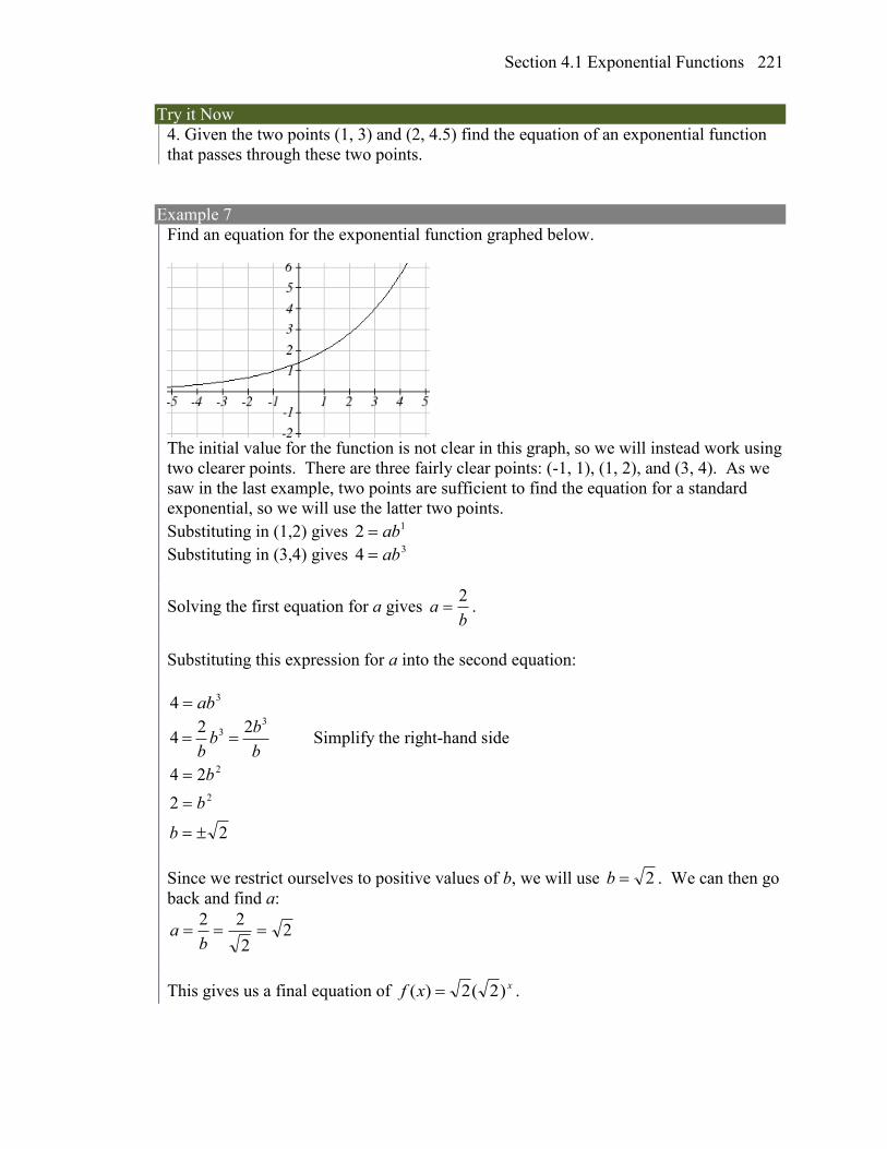
Section 4.1 Exponential Functions 221
Try it Now
4. Given the two points (1, 3) and (2, 4.5) find the equation of an exponential function
that passes through these two points.
Example 7
Find an equation for the exponential function graphed below.
The initial value for the function is not clear in this graph, so we will instead work using
two clearer points. There are three fairly clear points: (-1, 1), (1, 2), and (3, 4). As we
saw in the last example, two points are sufficient to find the equation for a standard
exponential, so we will use the latter two points.
Substituting in (1,2) gives 12 ab
Substituting in (3,4) gives 34 ab
Solving the first equation for a gives b
a2
.
Substituting this expression for a into the second equation:
34 ab
b
bb
b
33 22
4 Simplify the right-hand side
2
2
24
2
2
b
b
b
Since we restrict ourselves to positive values of b, we will use 2b . We can then go
back and find a:
22
22
ba
This gives us a final equation of xxf )2(2)( .
Chapter 4 222
Compound Interest In the bank certificate of deposit (CD) example earlier in the section, we encountered
compound interest. Typically bank accounts and other savings instruments in which
earnings are reinvested, such as mutual funds and retirement accounts, utilize compound
interest. The term compounding comes from the behavior that interest is earned not on
the original value, but on the accumulated value of the account.
In the example from earlier, the interest was compounded monthly, so we took the annual
interest rate, usually called the nominal rate or annual percentage rate (APR) and
divided by 12, the number of compounds in a year, to find the monthly interest. The
exponent was then measured in months.
Generalizing this, we can form a general formula for compound interest. If the APR is
written in decimal form as r, and there are k compounding periods per year, then the
interest per compounding period will be r/k. Likewise, if we are interested in the value
after t years, then there will be kt compounding periods in that time.
Compound Interest Formula
Compound Interest can be calculated using the formula kt
k
ratA
1)(
Where
A(t) is the account value
t is measured in years
a is the starting amount of the account, often called the principal
r is the annual percentage rate (APR), also called the nominal rate
k is the number of compounding periods in one year
Example 8
If you invest $3,000 in an investment account paying 3% interest compounded
quarterly, how much will the account be worth in 10 years?
Since we are starting with $3000, a = 3000
Our interest rate is 3%, so r = 0.03
Since we are compounding quarterly, we are compounding 4 times per year, so k = 4
We want to know the value of the account in 10 years, so we are looking for A(10), the
value when t = 10.
05.4045$4
03.013000)10(
)10(4
A
The account will be worth $4045.05 in 10 years.
Section 4.1 Exponential Functions 223
Example 9
A 529 plan is a college savings plan in which a relative can invest money to pay for a
child’s later college tuition, and the account grows tax free. If Lily wants to set up a
529 account for her new granddaughter, wants the account to grow to $40,000 over 18
years, and she believes the account will earn 6% compounded semi-annually (twice a
year), how much will Lily need to invest in the account now?
Since the account is earning 6%, r = 0.06
Since interest is compounded twice a year, k = 2
In this problem, we don’t know how much we are starting with, so we will be solving
for a, the initial amount needed. We do know we want the end amount to be $40,000,
so we will be looking for the value of a so that A(18) = 40,000.
801,13$8983.2
000,40
)8983.2(000,40
2
06.01)18(000,40
)18(2
a
a
aA
Lily will need to invest $13,801 to have $40,000 in 18 years.
Try it now
5. Recalculate example 2 from above with quarterly compounding.
Because of compounding throughout the year, with compound interest the actual increase
in a year is more than the annual percentage rate. If $1,000 were invested at 10%, the
table below shows the value after 1 year at different compounding frequencies:
Frequency Value after 1 year
Annually $1100
Semiannually $1102.50
Quarterly $1103.81
Monthly $1104.71
Daily $1105.16
If we were to compute the actual percentage increase for the daily compounding, there
was an increase of $105.16 from an original amount of $1,000, for a percentage increase
of 10516.01000
16.105 = 10.516% increase. This quantity is called the annual percentage
yield (APY).
Chapter 4 224
Notice that given any starting amount, the amount after 1 year would be k
k
raA
1)1( . To find the total change, we would subtract the original amount, then
to find the percentage change we would divide that by the original amount:
11
1
k
k
k
r
a
ak
ra
Annual Percentage Yield
The annual percentage yield is the actual percent a quantity increases in one year. It
can be calculated as
11
k
k
rAPY
Notice this is equivalent to finding the value of $1 after 1 year, and subtracting the
original dollar.
Example 10
Bank A offers an account paying 1.2% compounded quarterly. Bank B offers an
account paying 1.1% compounded monthly. Which is offering a better rate?
We can compare these rates using the annual percentage yield – the actual percent
increase in a year.
Bank A: 012054.014
012.01
4
APY = 1.2054%
Bank B: 011056.0112
011.01
12
APY = 1.1056%
Bank B’s monthly compounding is not enough to catch up with Bank A’s better APR.
Bank A offers a better rate.
A Limit to Compounding
As we saw earlier, the amount we earn increases as we increase the compounding
frequency. The table, though, shows that the increase from annual to semi-annual
compounding is larger than the increase from monthly to daily compounding. This might
lead us to believe that although increasing the frequency of compounding will increase
our result, there is an upper limit to this process.
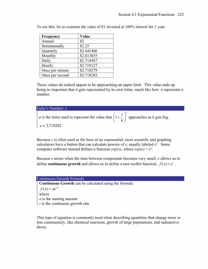
Section 4.1 Exponential Functions 225
To see this, let us examine the value of $1 invested at 100% interest for 1 year.
Frequency Value
Annual $2
Semiannually $2.25
Quarterly $2.441406
Monthly $2.613035
Daily $2.714567
Hourly $2.718127
Once per minute $2.718279
Once per second $2.718282
These values do indeed appear to be approaching an upper limit. This value ends up
being so important that it gets represented by its own letter, much like how represents a
number.
Euler’s Number: e
e is the letter used to represent the value that
k
k
11 approaches as k gets big.
718282.2e
Because e is often used as the base of an exponential, most scientific and graphing
calculators have a button that can calculate powers of e, usually labeled ex. Some
computer software instead defines a function exp(x), where exp(x) = ex.
Because e arises when the time between compounds becomes very small, e allows us to
define continuous growth and allows us to define a new toolkit function, ( ) xf x e .
Continuous Growth Formula
Continuous Growth can be calculated using the formula rxaexf )(
where
a is the starting amount
r is the continuous growth rate
This type of equation is commonly used when describing quantities that change more or
less continuously, like chemical reactions, growth of large populations, and radioactive
decay.
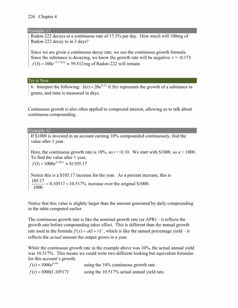
Chapter 4 226
Example 11
Radon-222 decays at a continuous rate of 17.3% per day. How much will 100mg of
Radon-222 decay to in 3 days?
Since we are given a continuous decay rate, we use the continuous growth formula.
Since the substance is decaying, we know the growth rate will be negative: r = -0.173
512.59100)3( )3(173.0 ef mg of Radon-222 will remain.
Try it Now
6. Interpret the following: 0.12( ) 20 tS t e if S(t) represents the growth of a substance in
grams, and time is measured in days.
Continuous growth is also often applied to compound interest, allowing us to talk about
continuous compounding.
Example 12
If $1000 is invested in an account earning 10% compounded continuously, find the
value after 1 year.
Here, the continuous growth rate is 10%, so r = 0.10. We start with $1000, so a = 1000.
To find the value after 1 year,
17.1105$1000)1( )1(10.0 ef
Notice this is a $105.17 increase for the year. As a percent increase, this is
%517.1010517.01000
17.105 increase over the original $1000.
Notice that this value is slightly larger than the amount generated by daily compounding
in the table computed earlier.
The continuous growth rate is like the nominal growth rate (or APR) – it reflects the
growth rate before compounding takes effect. This is different than the annual growth
rate used in the formula xraxf )1()( , which is like the annual percentage yield – it
reflects the actual amount the output grows in a year.
While the continuous growth rate in the example above was 10%, the actual annual yield
was 10.517%. This means we could write two different looking but equivalent formulas
for this account’s growth: 0.10( ) 1000 tf t e using the 10% continuous growth rate
( ) 1000(1.10517)tf t using the 10.517% actual annual yield rate.
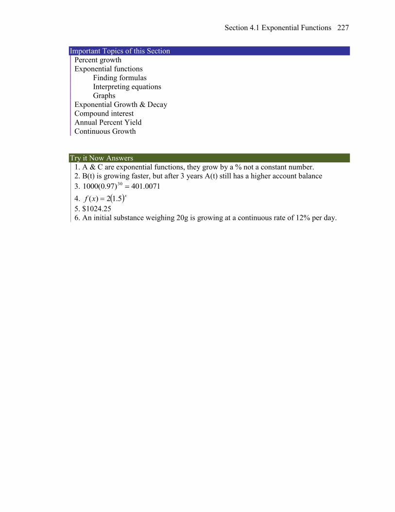
Section 4.1 Exponential Functions 227
Important Topics of this Section
Percent growth
Exponential functions
Finding formulas
Interpreting equations
Graphs
Exponential Growth & Decay
Compound interest
Annual Percent Yield
Continuous Growth
Try it Now Answers
1. A & C are exponential functions, they grow by a % not a constant number.
2. B(t) is growing faster, but after 3 years A(t) still has a higher account balance
3. 0071.401)97.0(1000 30
4. xxf 5.12)(
5. $1024.25
6. An initial substance weighing 20g is growing at a continuous rate of 12% per day.
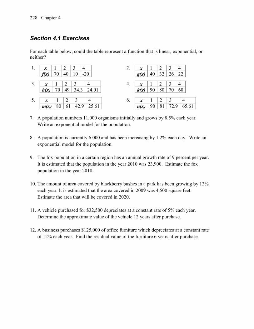
Chapter 4 228
Section 4.1 Exercises
For each table below, could the table represent a function that is linear, exponential, or
neither?
1. x 1 2 3 4
f(x) 70 40 10 -20
2. x 1 2 3 4
g(x) 40 32 26 22
3. x 1 2 3 4
h(x) 70 49 34.3 24.01
4. x 1 2 3 4
k(x) 90 80 70 60
5. x 1 2 3 4
m(x) 80 61 42.9 25.61
6. x 1 2 3 4
n(x) 90 81 72.9 65.61
7. A population numbers 11,000 organisms initially and grows by 8.5% each year.
Write an exponential model for the population.
8. A population is currently 6,000 and has been increasing by 1.2% each day. Write an
exponential model for the population.
9. The fox population in a certain region has an annual growth rate of 9 percent per year.
It is estimated that the population in the year 2010 was 23,900. Estimate the fox
population in the year 2018.
10. The amount of area covered by blackberry bushes in a park has been growing by 12%
each year. It is estimated that the area covered in 2009 was 4,500 square feet.
Estimate the area that will be covered in 2020.
11. A vehicle purchased for $32,500 depreciates at a constant rate of 5% each year.
Determine the approximate value of the vehicle 12 years after purchase.
12. A business purchases $125,000 of office furniture which depreciates at a constant rate
of 12% each year. Find the residual value of the furniture 6 years after purchase.
Section 4.1 Exponential Functions 229
Find a formula for an exponential function passing through the two points.
13. 0, 6 , (3, 750) 14. 0, 3 , (2, 75)
15. 0, 2000 , (2, 20) 16. 0, 9000 , (3, 72)
17. 3
1, , 3, 242
18. 2
1, , 1,105
19. 2,6 , 3,1 20. 3,4 , (3, 2)
21. 3,1 , (5, 4) 22. 2,5 , (6, 9)
23. A radioactive substance decays exponentially. A scientist begins with 100 milligrams
of a radioactive substance. After 35 hours, 50 mg of the substance remains. How
many milligrams will remain after 54 hours?
24. A radioactive substance decays exponentially. A scientist begins with 110 milligrams
of a radioactive substance. After 31 hours, 55 mg of the substance remains. How
many milligrams will remain after 42 hours?
25. A house was valued at $110,000 in the year 1985. The value appreciated to $145,000
by the year 2005. What was the annual growth rate between 1985 and 2005?
Assume that the house value continues to grow by the same percentage. What did the
value equal in the year 2010?
26. An investment was valued at $11,000 in the year 1995. The value appreciated to
$14,000 by the year 2008. What was the annual growth rate between 1995 and 2008?
Assume that the value continues to grow by the same percentage. What did the value
equal in the year 2012?
27. A car was valued at $38,000 in the year 2003. The value depreciated to $11,000 by
the year 2009. Assume that the car value continues to drop by the same percentage.
What will the value be in the year 2013?
28. A car was valued at $24,000 in the year 2006. The value depreciated to $20,000 by
the year 2009. Assume that the car value continues to drop by the same percentage.
What will the value be in the year 2014?
29. If $4,000 is invested in a bank account at an interest rate of 7 per cent per year, find
the amount in the bank after 9 years if interest is compounded annually, quarterly,
monthly, and continuously.
Chapter 4 230
30. If $6,000 is invested in a bank account at an interest rate of 9 per cent per year, find
the amount in the bank after 5 years if interest is compounded annually, quarterly,
monthly, and continuously.
31. Find the annual percentage yield (APY) for a savings account with annual percentage
rate of 3% compounded quarterly.
32. Find the annual percentage yield (APY) for a savings account with annual percentage
rate of 5% compounded monthly.
33. A population of bacteria is growing according to the equation 0.21 ( ) 1 600 tP t e , with t
measured in years. Estimate when the population will exceed 7569.
34. A population of bacteria is growing according to the equation 0.17 ( ) 1 200 tP t e , with t
measured in years. Estimate when the population will exceed 3443.
35. In 1968, the U.S. minimum wage was $1.60 per hour. In 1976, the minimum wage
was $2.30 per hour. Assume the minimum wage grows according to an exponential
model ( )w t , where t represents the time in years after 1960. [UW]
a. Find a formula for ( )w t .
b. What does the model predict for the minimum wage in 1960?
c. If the minimum wage was $5.15 in 1996, is this above, below or equal to what
the model predicts?
36. In 1989, research scientists published a model for predicting the cumulative number
of AIDS cases (in thousands) reported in the United States: 3
1980155
10
ta t
,
where t is the year. This paper was considered a “relief”, since there was a fear the
correct model would be of exponential type. Pick two data points predicted by the
research model ( )a t to construct a new exponential model ( )b t for the number of
cumulative AIDS cases. Discuss how the two models differ and explain the use of the
word “relief.” [UW]

Section 4.1 Exponential Functions 231
37. You have a chess board as pictured, with
squares numbered 1 through 64. You also have
a huge change jar with an unlimited number of
dimes. On the first square you place one dime.
On the second square you stack 2 dimes. Then
you continue, always doubling the number
from the previous square. [UW]
a. How many dimes will you have
stacked on the 10th square?
b. How many dimes will you have
stacked on the nth square?
c. How many dimes will you have
stacked on the 64th square?
d. Assuming a dime is 1 mm thick, how
high will this last pile be?
e. The distance from the earth to the sun is approximately 150 million km.
Relate the height of the last pile of dimes to this distance.
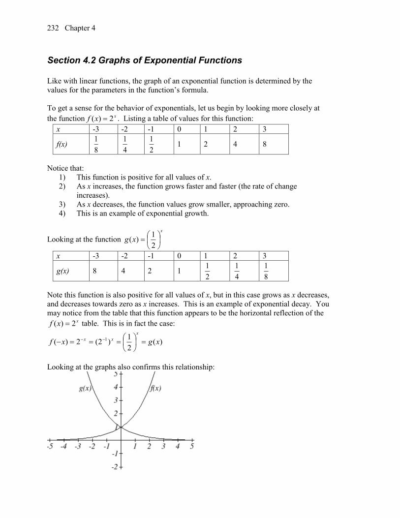
Chapter 4 232
Section 4.2 Graphs of Exponential Functions
Like with linear functions, the graph of an exponential function is determined by the
values for the parameters in the function’s formula.
To get a sense for the behavior of exponentials, let us begin by looking more closely at
the function xxf 2)( . Listing a table of values for this function:
x -3 -2 -1 0 1 2 3
f(x) 8
1
4
1
2
1 1 2 4 8
Notice that:
1) This function is positive for all values of x.
2) As x increases, the function grows faster and faster (the rate of change
increases).
3) As x decreases, the function values grow smaller, approaching zero.
4) This is an example of exponential growth.
Looking at the function
x
xg
2
1)(
x -3 -2 -1 0 1 2 3
g(x) 8 4 2 1 2
1
4
1
8
1
Note this function is also positive for all values of x, but in this case grows as x decreases,
and decreases towards zero as x increases. This is an example of exponential decay. You
may notice from the table that this function appears to be the horizontal reflection of the xxf 2)( table. This is in fact the case:
)(2
1)2(2)( 1 xgxf
x
xx
Looking at the graphs also confirms this relationship:
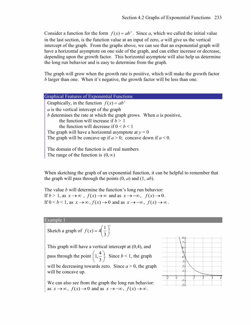
Section 4.2 Graphs of Exponential Functions 233
Consider a function for the form xabxf )( . Since a, which we called the initial value
in the last section, is the function value at an input of zero, a will give us the vertical
intercept of the graph. From the graphs above, we can see that an exponential graph will
have a horizontal asymptote on one side of the graph, and can either increase or decrease,
depending upon the growth factor. This horizontal asymptote will also help us determine
the long run behavior and is easy to determine from the graph.
The graph will grow when the growth rate is positive, which will make the growth factor
b larger than one. When it’s negative, the growth factor will be less than one.
Graphical Features of Exponential Functions
Graphically, in the function xabxf )(
a is the vertical intercept of the graph
b determines the rate at which the graph grows. When a is positive,
the function will increase if b > 1
the function will decrease if 0 < b < 1
The graph will have a horizontal asymptote at y = 0
The graph will be concave up if a > 0; concave down if a < 0.
The domain of the function is all real numbers
The range of the function is (0, )
When sketching the graph of an exponential function, it can be helpful to remember that
the graph will pass through the points (0, a) and (1, ab).
The value b will determine the function’s long run behavior:
If b > 1, as x , )(xf and as x , 0)( xf .
If 0 < b < 1, as x , 0)( xf and as x , )(xf .
Example 1
Sketch a graph of
x
xf
3
14)(
This graph will have a vertical intercept at (0,4), and
pass through the point
3
4,1 . Since b < 1, the graph
will be decreasing towards zero. Since a > 0, the graph
will be concave up.
We can also see from the graph the long run behavior:
as x , 0)( xf and as x , )(xf .
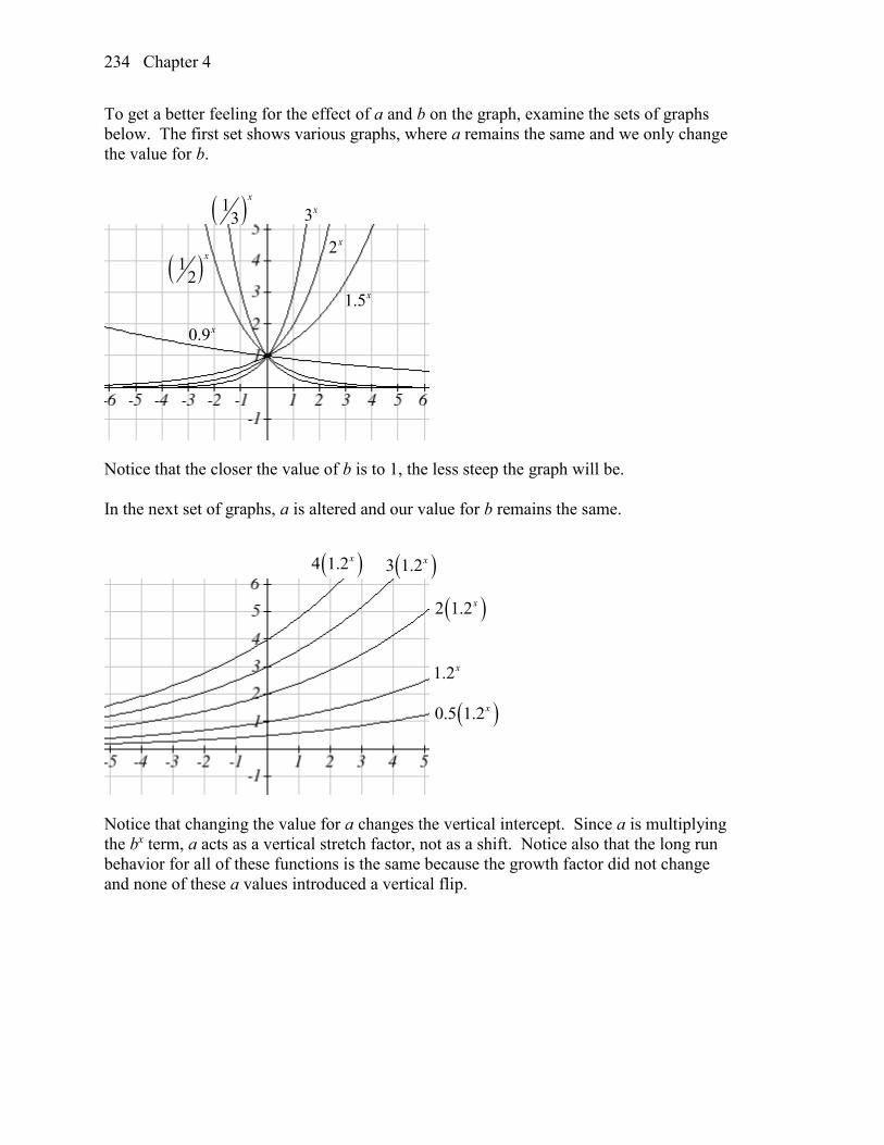
Chapter 4 234
To get a better feeling for the effect of a and b on the graph, examine the sets of graphs
below. The first set shows various graphs, where a remains the same and we only change
the value for b.
Notice that the closer the value of b is to 1, the less steep the graph will be.
In the next set of graphs, a is altered and our value for b remains the same.
Notice that changing the value for a changes the vertical intercept. Since a is multiplying
the bx term, a acts as a vertical stretch factor, not as a shift. Notice also that the long run
behavior for all of these functions is the same because the growth factor did not change
and none of these a values introduced a vertical flip.
2x
1.5x
3x
0.9x
12
x
13
x
0.5 1.2x
1.2x
2 1.2x
3 1.2x 4 1.2x
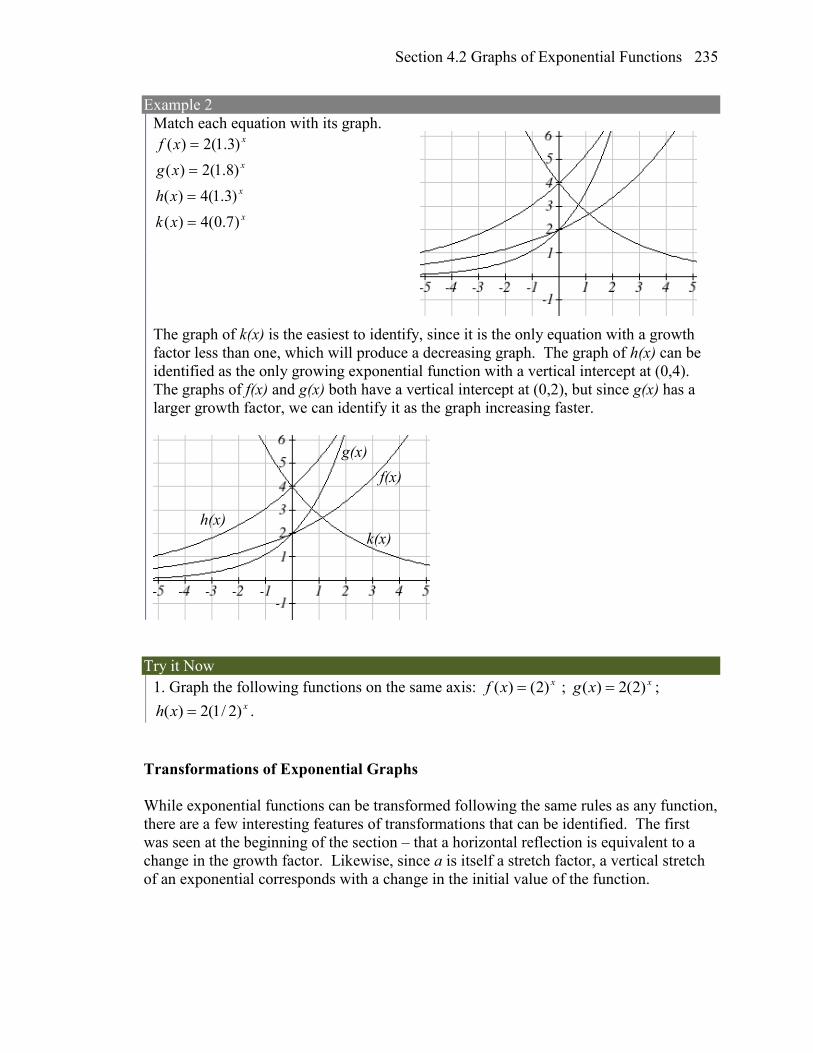
Section 4.2 Graphs of Exponential Functions 235
Example 2
Match each equation with its graph.
x
x
x
x
xk
xh
xg
xf
)7.0(4)(
)3.1(4)(
)8.1(2)(
)3.1(2)(
The graph of k(x) is the easiest to identify, since it is the only equation with a growth
factor less than one, which will produce a decreasing graph. The graph of h(x) can be
identified as the only growing exponential function with a vertical intercept at (0,4).
The graphs of f(x) and g(x) both have a vertical intercept at (0,2), but since g(x) has a
larger growth factor, we can identify it as the graph increasing faster.
Try it Now
1. Graph the following functions on the same axis: xxf )2()( ; xxg )2(2)( ; xxh )2/1(2)( .
Transformations of Exponential Graphs
While exponential functions can be transformed following the same rules as any function,
there are a few interesting features of transformations that can be identified. The first
was seen at the beginning of the section – that a horizontal reflection is equivalent to a
change in the growth factor. Likewise, since a is itself a stretch factor, a vertical stretch
of an exponential corresponds with a change in the initial value of the function.
f(x)
g(x)
h(x)
k(x)
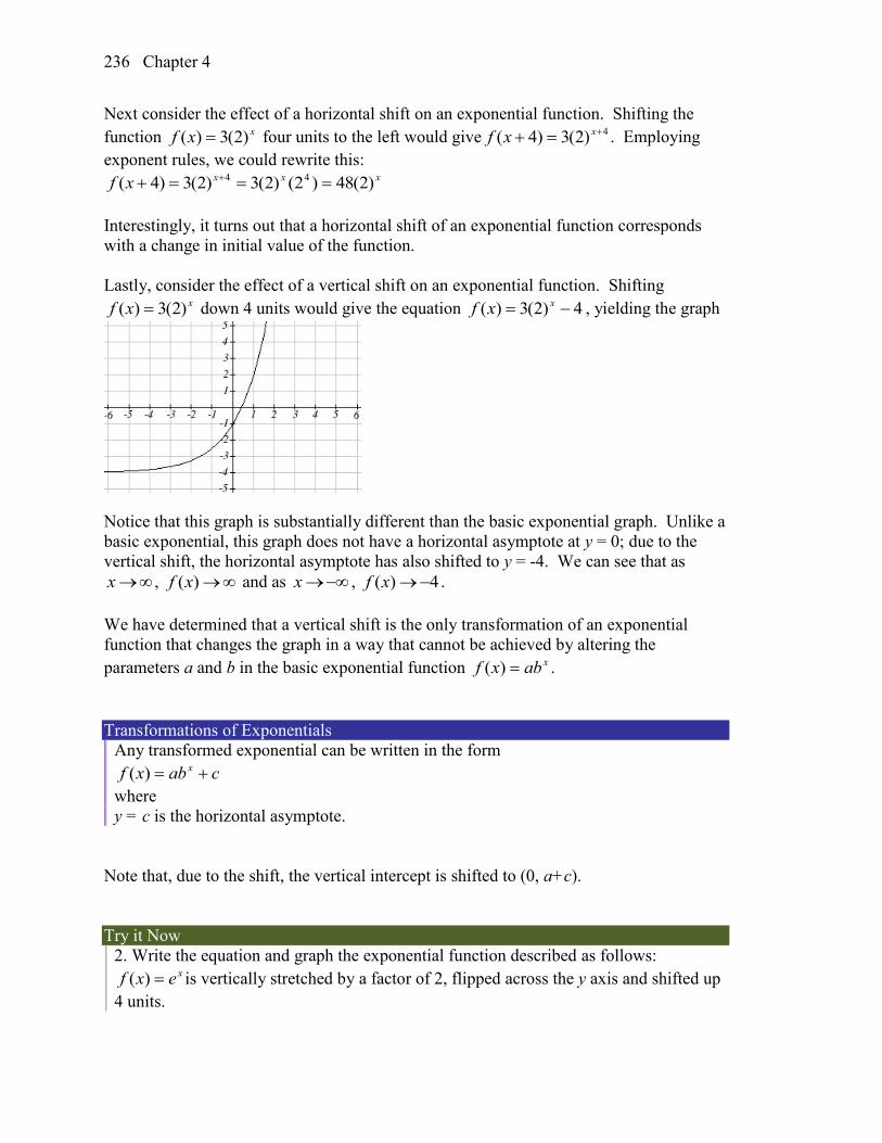
Chapter 4 236
Next consider the effect of a horizontal shift on an exponential function. Shifting the
function xxf )2(3)( four units to the left would give 4)2(3)4( xxf . Employing
exponent rules, we could rewrite this: xxxxf )2(48)2()2(3)2(3)4( 44
Interestingly, it turns out that a horizontal shift of an exponential function corresponds
with a change in initial value of the function.
Lastly, consider the effect of a vertical shift on an exponential function. Shifting xxf )2(3)( down 4 units would give the equation 4)2(3)( xxf , yielding the graph
Notice that this graph is substantially different than the basic exponential graph. Unlike a
basic exponential, this graph does not have a horizontal asymptote at y = 0; due to the
vertical shift, the horizontal asymptote has also shifted to y = -4. We can see that as
x , ( )f x and as x , ( ) 4f x .
We have determined that a vertical shift is the only transformation of an exponential
function that changes the graph in a way that cannot be achieved by altering the
parameters a and b in the basic exponential function xabxf )( .
Transformations of Exponentials
Any transformed exponential can be written in the form
cabxf x )(
where
y = c is the horizontal asymptote.
Note that, due to the shift, the vertical intercept is shifted to (0, a+c).
Try it Now
2. Write the equation and graph the exponential function described as follows: xexf )( is vertically stretched by a factor of 2, flipped across the y axis and shifted up
4 units.
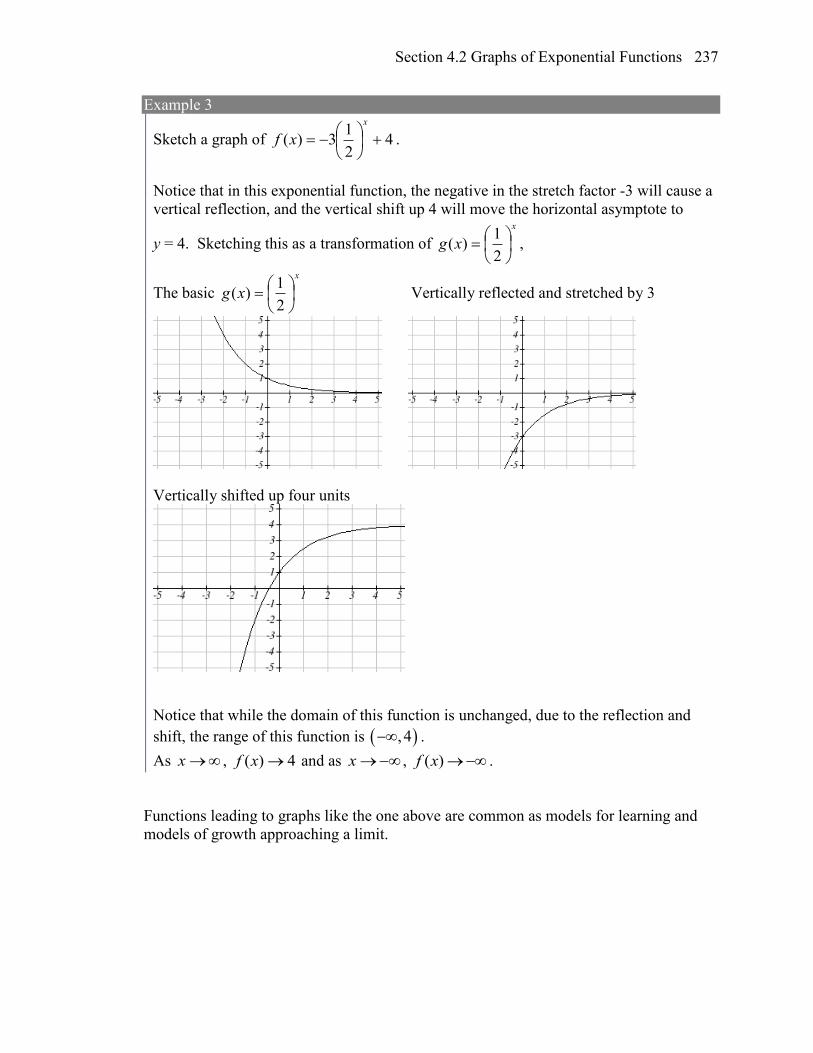
Section 4.2 Graphs of Exponential Functions 237
Example 3
Sketch a graph of 42
13)(
x
xf .
Notice that in this exponential function, the negative in the stretch factor -3 will cause a
vertical reflection, and the vertical shift up 4 will move the horizontal asymptote to
y = 4. Sketching this as a transformation of
x
xg
2
1)( ,
The basic
x
xg
2
1)( Vertically reflected and stretched by 3
Vertically shifted up four units
Notice that while the domain of this function is unchanged, due to the reflection and
shift, the range of this function is , 4 .
As x , 4)( xf and as x , ( )f x .
Functions leading to graphs like the one above are common as models for learning and
models of growth approaching a limit.
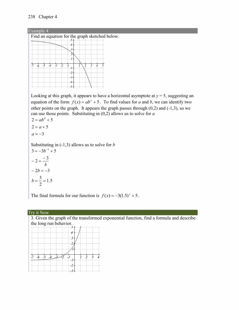
Chapter 4 238
Example 4
Find an equation for the graph sketched below.
Looking at this graph, it appears to have a horizontal asymptote at y = 5, suggesting an
equation of the form 5)( xabxf . To find values for a and b, we can identify two
other points on the graph. It appears the graph passes through (0,2) and (-1,3), so we
can use those points. Substituting in (0,2) allows us to solve for a
3
52
52 0
a
a
ab
Substituting in (-1,3) allows us to solve for b
5.12
3
32
32
533 1
b
b
b
b
The final formula for our function is 5)5.1(3)( xxf .
Try it Now
3. Given the graph of the transformed exponential function, find a formula and describe
the long run behavior.
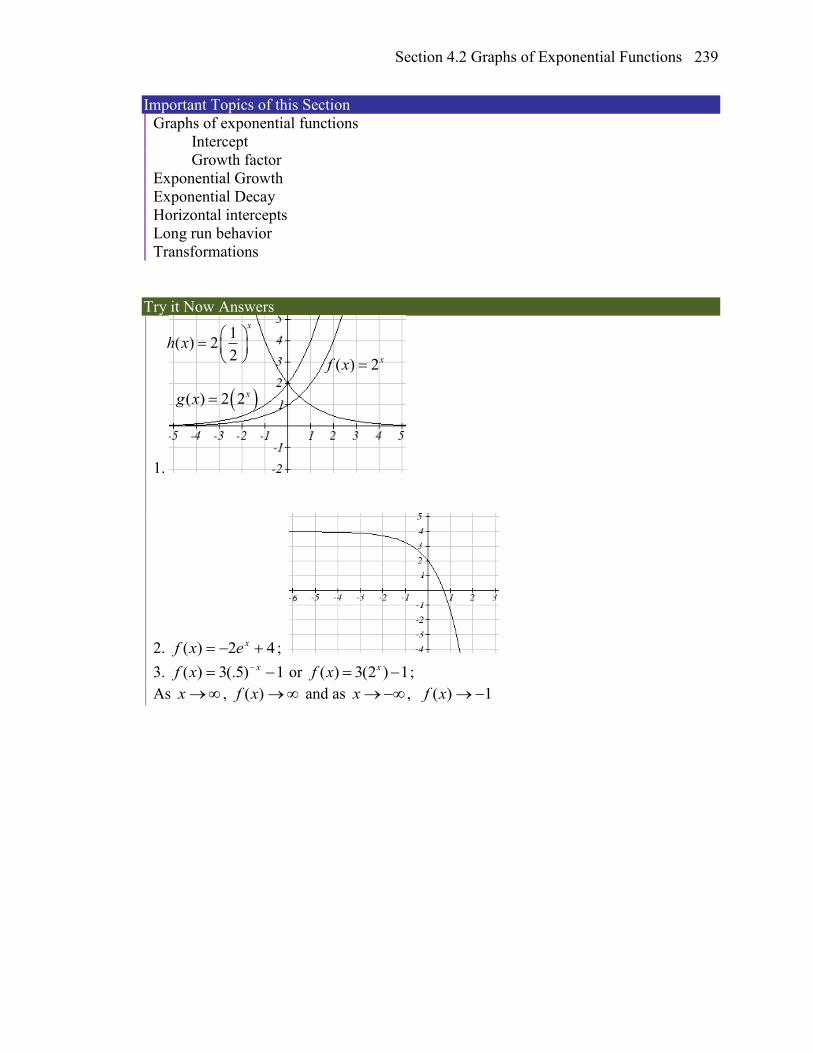
Section 4.2 Graphs of Exponential Functions 239
Important Topics of this Section
Graphs of exponential functions
Intercept
Growth factor
Exponential Growth
Exponential Decay
Horizontal intercepts
Long run behavior
Transformations
Try it Now Answers
1.
2. 42)( xexf ;
3. 1)5(.3)( xxf or ( ) 3(2 ) 1xf x ;
As x , )(xf and as x , 1)( xf
( ) 2xf x
( ) 2 2xg x
1( ) 2
2
x
h x
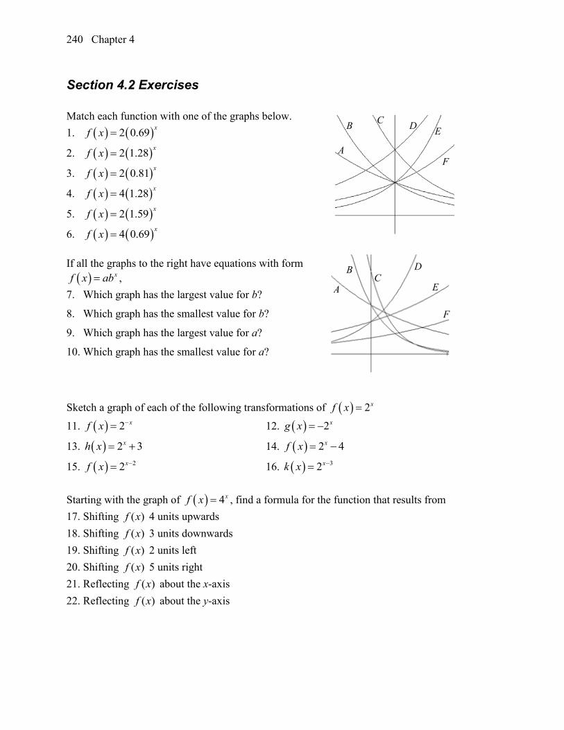
Chapter 4 240
Section 4.2 Exercises
Match each function with one of the graphs below.
1. 2 0.69x
f x
2. 2 1.28x
f x
3. 2 0.81x
f x
4. 4 1.28x
f x
5. 2 1.59x
f x
6. 4 0.69x
f x
If all the graphs to the right have equations with form
xf x ab ,
7. Which graph has the largest value for b?
8. Which graph has the smallest value for b?
9. Which graph has the largest value for a?
10. Which graph has the smallest value for a?
Sketch a graph of each of the following transformations of 2xf x
11. 2 xf x 12. 2xg x
13. 2 3xh x 14. 2 4xf x
15. 22xf x 16. 32xk x
Starting with the graph of 4xf x , find a formula for the function that results from
17. Shifting ( )f x 4 units upwards
18. Shifting ( )f x 3 units downwards
19. Shifting ( )f x 2 units left
20. Shifting ( )f x 5 units right
21. Reflecting ( )f x about the x-axis
22. Reflecting ( )f x about the y-axis
A
B C
D E
F
A
B C
D
E
F
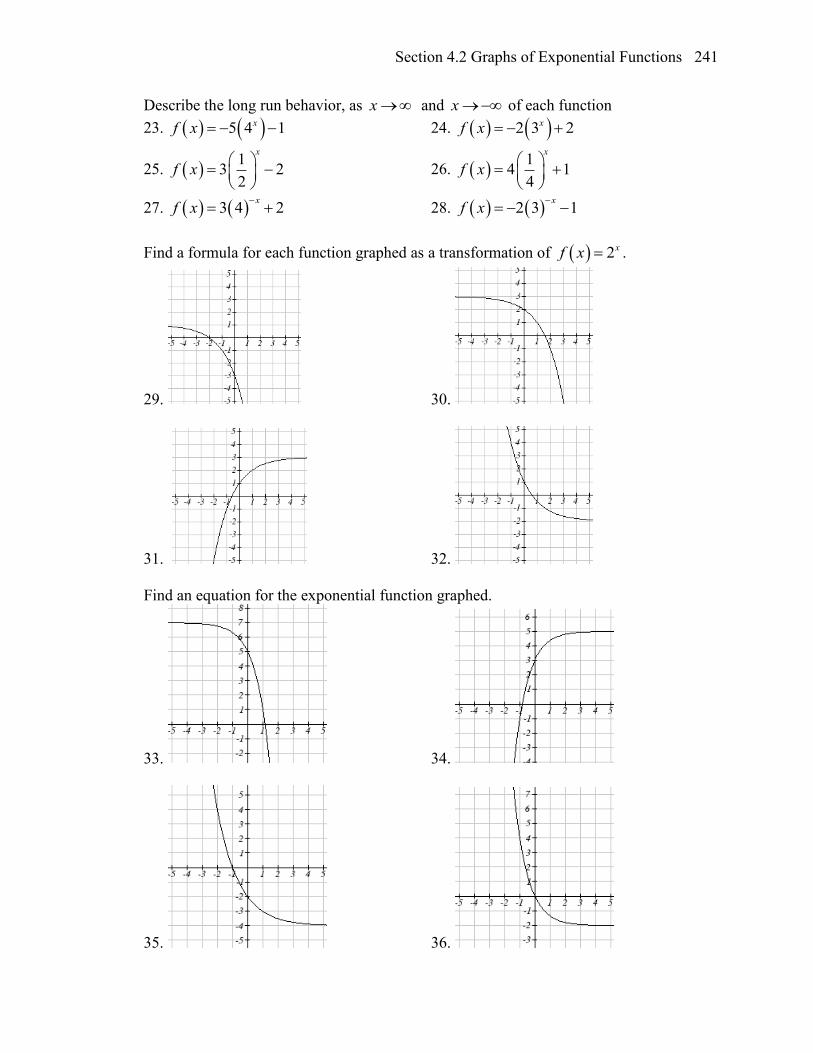
Section 4.2 Graphs of Exponential Functions 241
Describe the long run behavior, as x and x of each function
23. 5 4 1xf x 24. 2 3 2xf x
25. 1
3 22
x
f x
26. 1
4 14
x
f x
27. 3 4 2x
f x
28. 2 3 1x
f x
Find a formula for each function graphed as a transformation of 2xf x .
29. 30.
31. 32.
Find an equation for the exponential function graphed.
33. 34.
35. 36.
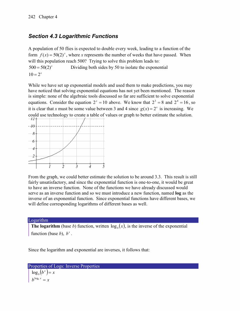
Chapter 4 242
Section 4.3 Logarithmic Functions
A population of 50 flies is expected to double every week, leading to a function of the
form xxf )2(50)( , where x represents the number of weeks that have passed. When
will this population reach 500? Trying to solve this problem leads to:
500 50(2)x Dividing both sides by 50 to isolate the exponential
10 2x
While we have set up exponential models and used them to make predictions, you may
have noticed that solving exponential equations has not yet been mentioned. The reason
is simple: none of the algebraic tools discussed so far are sufficient to solve exponential
equations. Consider the equation 102 x above. We know that 823 and 1624 , so
it is clear that x must be some value between 3 and 4 since ( ) 2xg x is increasing. We
could use technology to create a table of values or graph to better estimate the solution.
From the graph, we could better estimate the solution to be around 3.3. This result is still
fairly unsatisfactory, and since the exponential function is one-to-one, it would be great
to have an inverse function. None of the functions we have already discussed would
serve as an inverse function and so we must introduce a new function, named log as the
inverse of an exponential function. Since exponential functions have different bases, we
will define corresponding logarithms of different bases as well.
Logarithm
The logarithm (base b) function, written xblog , is the inverse of the exponential
function (base b), xb .
Since the logarithm and exponential are inverses, it follows that:
Properties of Logs: Inverse Properties
xb x
b log
xbxb
log
Section 4.3 Logarithmic Functions 243
Recall also from the definition of an inverse function that if caf )( , then acf )(1 .
Applying this to the exponential and logarithmic functions:
Logarithm Equivalent to an Exponential
The statement cba is equivalent to the statement acb )(log .
Alternatively, we could show this by starting with the exponential function ac b , then
taking the log base b of both sides, giving log ( ) log a
b bc b . Using the inverse property
of logs we see that log ( )b c a .
Since log is a function, it is most correctly written as )(log cb , using parentheses to
denote function evaluation, just as we would with f(c). However, when the input is a
single variable or number, it is common to see the parentheses dropped and the
expression written as cblog .
Example 1
Write these exponential equations as logarithmic equations:
823 2552 10000
110 4
823 is equivalent to 3)8(log 2
2552 is equivalent to 2)25(log5
4 110
10000
is equivalent to 10
1log 4
10000
Example 2
Write these logarithmic equations as exponential equations:
2
16log 6 29log3
2
16log 6 is equivalent to 66 2/1
29log3 is equivalent to 932
Try it Now
Write the exponential equation 1642 as a logarithmic equation.
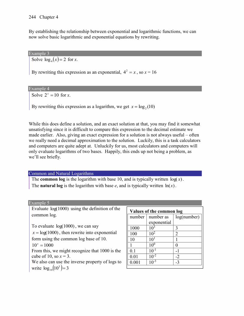
Chapter 4 244
By establishing the relationship between exponential and logarithmic functions, we can
now solve basic logarithmic and exponential equations by rewriting.
Example 3
Solve 2log 4 x for x.
By rewriting this expression as an exponential, x24 , so x = 16
Example 4
Solve 102 x for x.
By rewriting this expression as a logarithm, we get )10(log 2x
While this does define a solution, and an exact solution at that, you may find it somewhat
unsatisfying since it is difficult to compare this expression to the decimal estimate we
made earlier. Also, giving an exact expression for a solution is not always useful – often
we really need a decimal approximation to the solution. Luckily, this is a task calculators
and computers are quite adept at. Unluckily for us, most calculators and computers will
only evaluate logarithms of two bases. Happily, this ends up not being a problem, as
we’ll see briefly.
Common and Natural Logarithms
The common log is the logarithm with base 10, and is typically written )log( x .
The natural log is the logarithm with base e, and is typically written )ln(x .
Example 5
Evaluate )1000log( using the definition of the
common log.
To evaluate )1000log( , we can say
)1000log(x , then rewrite into exponential
form using the common log base of 10.
100010 x
From this, we might recognize that 1000 is the
cube of 10, so x = 3.
We also can use the inverse property of logs to
write 310log 3
10
Values of the common log
number number as
exponential
log(number)
1000 103 3
100 102 2
10 101 1
1 100 0
0.1 10-1 -1
0.01 10-2 -2
0.001 10-3 -3
Section 4.3 Logarithmic Functions 245
Try it Now
2. Evaluate )1000000log( .
Example 6
Evaluate eln .
We can rewrite eln as 2/1ln e . Since ln is a log base e, we can use the inverse
property for logs: 2
1logln 2/12/1 ee e .
Example 7
Evaluate log(500) using your calculator or computer.
Using a computer, we can evaluate 69897.2)500log(
To utilize the common or natural logarithm functions to evaluate expressions like
)10(log 2 , we need to establish some additional properties.
Properties of Logs: Exponent Property
ArA b
r
b loglog
To show why this is true, we offer a proof.
Since the logarithmic and exponential functions are inverses, AbAb
log.
So rAr bbAlog
Utilizing the exponential rule that states q
p pqx x ,
ArrAr bb bbAloglog
So then Ar
b
r
bbbA
logloglog
Again utilizing the inverse property on the right side yields the result
ArA b
r
b loglog
Example 8
Rewrite 25log3 using the exponent property for logs.
Since 25 = 52,
5log25log25log 3
2
33
Chapter 4 246
Example 9
Rewrite )ln(4 x using the exponent property for logs.
Using the property in reverse, 4ln)ln(4 xx
Try it Now
3. Rewrite using the exponent property for logs:
2
1ln
x.
The exponent property allows us to find a method for changing the base of a logarithmic
expression.
Properties of Logs: Change of Base
)(log
)(loglog
b
AA
c
cb
Proof:
Let xAb log . Rewriting as an exponential gives Ab x . Taking the log base c of
both sides of this equation gives
Ab c
x
c loglog
Now utilizing the exponent property for logs on the left side,
Abx cc loglog
Dividing, we obtain
b
Ax
c
c
log
log or replacing our expression for x,
b
AA
c
cb
log
loglog
With this change of base formula, we can finally find a good decimal approximation to
our question from the beginning of the section.
Example 10
Evaluate )10(log 2 using the change of base formula.
According to the change of base formula, we can rewrite the log base 2 as a logarithm
of any other base. Since our calculators can evaluate the natural log, we might choose
to use the natural logarithm, which is the log base e:
2ln
10ln
2log
10log10log 2
e
e
Using our calculators to evaluate this,
Section 4.3 Logarithmic Functions 247
3219.369315.0
30259.2
2ln
10ln
This finally allows us to answer our original question – the population of flies we
discussed at the beginning of the section will take 3.32 weeks to grow to 500.
Example 11
Evaluate )100(log5 using the change of base formula.
We can rewrite this expression using any other base. If our calculators are able to
evaluate the common logarithm, we could rewrite using the common log, base 10.
861.269897.0
2
5log
100log)100(log
10
105
While we were able to solve the basic exponential equation 102 x by rewriting in
logarithmic form and then using the change of base formula to evaluate the logarithm, the
proof of the change of base formula illuminates an alternative approach to solving
exponential equations.
Solving exponential equations:
1. Isolate the exponential expressions when possible
2. Take the logarithm of both sides
3. Utilize the exponent property for logarithms to pull the variable out of the exponent
4. Use algebra to solve for the variable.
Example 12
Solve 102 x for x.
Using this alternative approach, rather than rewrite this exponential into logarithmic
form, we will take the logarithm of both sides of the equation. Since we often wish to
evaluate the result to a decimal answer, we will usually utilize either the common log or
natural log. For this example, we’ll use the natural log:
)10ln(2ln x Utilizing the exponent property for logs,
)10ln(2ln x Now dividing by ln(2),
ln(10)
2.861ln 2
x
Notice that this result matches the result we found using the change of base formula.
Chapter 4 248
Example 13
In the first section, we predicted the population (in billions) of India t years after 2008
by using the function ttf )0134.01(14.1)( . If the population continues following
this trend, when will the population reach 2 billion?
We need to solve for the t so that f(t) = 2
t)0134.1(14.12 Divide by 1.14 to isolate the exponential expression
t0134.114.1
2 Take the logarithm of both sides of the equation
t0134.1ln14.1
2ln
Apply the exponent property on the right side
0134.1ln14.1
2ln t
Divide both sides by ln(1.0134)
23.42
0134.1ln
14.1
2ln
t years
If this growth rate continues, the model predicts the population of India will reach 2
billion about 42 years after 2008, or approximately in the year 2050.
Try it Now
4. Solve 10)93.0(5 x .
In addition to solving exponential equations, logarithmic expressions are common in
many physical situations.
Example 14
In chemistry, pH is a measure of the acidity or basicity of a liquid. The pH is related to
the concentration of hydrogen ions, [H+], measured in moles per liter, by the equation
logpH H .
If a liquid has concentration of 0.0001 moles per liber, determine the pH.
Determine the hydrogen ion concentration of a liquid with pH of 7.
To answer the first question, we evaluate the expression 0001.0log . While we could
use our calculators for this, we do not really need them here, since we can use the
inverse property of logs:
4)4(10log0001.0log 4
Section 4.3 Logarithmic Functions 249
To answer the second question, we need to solve the equation 7 log H . Begin
by isolating the logarithm on one side of the equation by multiplying both sides by -1:
7 log H
Rewriting into exponential form yields the answer 710 0.0000001H moles per liter.
Logarithms also provide us a mechanism for finding continuous growth models for
exponential growth given two data points.
Example 15
A population grows from 100 to 130 in 2 weeks. Find the continuous growth rate.
Measuring t in weeks, we are looking for an equation rtaetP )( so that P(0) = 100 and
P(2) = 130. Using the first pair of values, 0100 rae , so a = 100.
Using the second pair of values, 2130 100 re Divide by 100
2
100
130 re Take the natural log of both sides
2ln)3.1ln( re Use the inverse property of logs
1312.02
)3.1ln(
2)3.1ln(
r
r
This population is growing at a continuous rate of 13.12% per week.
In general, we can relate the standard form of an exponential with the continuous growth
form by noting (using k to represent the continuous growth rate to avoid the confusion of
using r in two different ways in the same formula): kxx aera )1(
kxx er )1( ker 1
Using this, we see that it is always possible to convert from the continuous growth form
of an exponential to the standard form and vice versa. Remember that the continuous
growth rate k represents the nominal growth rate before accounting for the effects of
continuous compounding, while r represents the actual percent increase in one time unit
(one week, one year, etc.).
Chapter 4 250
Example 16
A company’s sales can be modeled by the function tetS 12.05000)( , with t measured in
years. Find the annual growth rate.
Noting that ker 1 , then 1275.0112.0 er , so the annual growth rate is 12.75%.
The sales function could also be written in the form ttS )1275.01(5000)( .
Important Topics of this Section
The Logarithmic function as the inverse of the exponential function
Writing logarithmic & exponential expressions
Properties of logs
Inverse properties
Exponential properties
Change of base
Common log
Natural log
Solving exponential equations
Try it Now Answers
1. 4log24log216log 4
2
44
2. 6
3. )ln(2 x
4. 5513.9)93.0ln(
)2ln(
Section 4.3 Logarithmic Functions 251
Section 4.3 Exercises
Rewrite each equation in exponential form
1. 4log ( )q m 2. 3log ( )t k 3. log ( )a b c 4. log ( )p z u
5. log v t 6. log r s 7. ln w n 8. ln x y
Rewrite each equation in logarithmic form.
9. 4x y 10. 5y x 11. dc k 12. zn L
13. 10a b 14. 10p v 15. ke h 16. ye x
Solve for x.
17. 3log 2x 18. 4log ( ) 3x 19. 2log ( ) 3x 20. 5log ( ) 1x
21. log 3x 22. log 5x 23. ln 2x 24. ln 2x
Simplify each expression using logarithm properties.
25. 5log 25 26. 2log 8 27. 3
1log
27
28. 6
1log
36
29. 6log 6 30. 35log 5 31. log 10,000 32. log 100
33. log 0.001 34. log 0.00001 35. 2ln e 36. 3ln e
Evaluate using your calculator.
37. log 0.04 38. log 1045 39. ln 15 40. ln 0.02
Solve each equation for the variable.
41. 5 14x 42. 3 23x 43. 1
715
x 44. 1
34
x
45. 5 17xe 46. 3 12xe 47. 4 53 38x 48. 2 34 44x
49. 1000 1.03 5000t 50. 200 1.06 550
t
51. 3
3 1.04 8t 52.
42 1.08 7
t
53. 0.1250 10te 54. 0.0310 4te
55. 1
10 8 52
x
56.
1100 100 70
4
x
Chapter 4 252
Convert the equation into continuous growth form, ktf t ae .
57. 300 0.91t
f t 58. 120 0.07t
f t
59. 10 1.04t
f t 60. 1400 1.12t
f t
Convert the equation into annual growth form, tf t ab .
61. 0.061 50 tf t e 62. 0.12100 tf t e
63. 0.01250 tf t e 64. 0.8580 tf t e
65. The population of Kenya was 39.8 million in 2009 and has been growing by about
2.6% each year. If this trend continues, when will the population exceed 45 million?
66. The population of Algeria was 34.9 million in 2009 and has been growing by about
1.5% each year. If this trend continues, when will the population exceed 45 million?
67. The population of Seattle grew from 563,374 in 2000 to 608,660 in 2010. If the
population continues to grow exponentially at the same rate, when will the population
exceed 1 million people?
68. The median household income (adjusted for inflation) in Seattle grew from $42,948
in 1990 to $45,736 in 2000. If it continues to grow exponentially at the same rate,
when will median income exceed $50,000?
69. A scientist begins with 100 mg of a radioactive substance. After 4 hours, it has
decayed to 80 mg. How long after the process began will it take to decay to 15 mg?
70. A scientist begins with 100 mg of a radioactive substance. After 6 days, it has
decayed to 60 mg. How long after the process began will it take to decay to 10 mg?
71. If $1000 is invested in an account earning 3% compounded monthly, how long will it
take the account to grow in value to $1500?
72. If $1000 is invested in an account earning 2% compounded quarterly, how long will it
take the account to grow in value to $1300?
Section 4.4 Logarithmic Properties 253
Section 4.4 Logarithmic Properties
In the previous section, we derived two important properties of logarithms, which
allowed us to solve some basic exponential and logarithmic equations.
Properties of Logs
Inverse Properties:
xb x
b log
xbxb
log
Exponential Property:
ArA b
r
b loglog
Change of Base:
)(log
)(loglog
b
AA
c
cb
While these properties allow us to solve a large number of problems, they are not
sufficient to solve all problems involving exponential and logarithmic equations.
Properties of Logs
Sum of Logs Property:
)(logloglog ACCA bbb
Difference of Logs Property:
C
ACA bbb logloglog
It’s just as important to know what properties logarithms do not satisfy as to memorize
the valid properties listed above. In particular, the logarithm is not a linear function,
which means that it does not distribute: log(A + B) ≠ log(A) + log(B).
To help in this process we offer a proof to help solidify our new rules and show how they
follow from properties you’ve already seen.
Let Aa blog and Cc blog , so by definition of the logarithm, Aba and Cbc
Chapter 4 254
Using these expressions, cabbAC
Using exponent rules on the right, cabAC
Taking the log of both sides, and utilizing the inverse property of logs,
cabAC ca
bb loglog
Replacing a and c with their definition establishes the result
CAAC bbb logloglog
The proof for the difference property is very similar.
With these properties, we can rewrite expressions involving multiple logs as a single log,
or break an expression involving a single log into expressions involving multiple logs.
Example 1
Write 2log8log5log 333 as a single logarithm.
Using the sum of logs property on the first two terms,
40log85log8log5log 3333
This reduces our original expression to 2log40log 33
Then using the difference of logs property,
20log2
40log2log40log 3333
Example 2
Evaluate 4log5log2 without a calculator by first rewriting as a single logarithm.
On the first term, we can use the exponent property of logs to write
25log5log5log2 2
With the expression reduced to a sum of two logs, 4log25log , we can utilize the
sum of logs property
)100log()254log(4log25log
Since 100 = 102, we can evaluate this log without a calculator:
210log)100log( 2
Try it Now
1. Without a calculator evaluate by first rewriting as a single logarithm:
4log8log 22
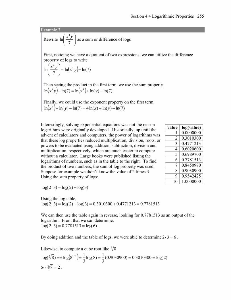
Section 4.4 Logarithmic Properties 255
Example 3
Rewrite
7ln
4 yx as a sum or difference of logs
First, noticing we have a quotient of two expressions, we can utilize the difference
property of logs to write
)7ln(ln7
ln 44
yx
yx
Then seeing the product in the first term, we use the sum property
)7ln()ln(ln)7ln(ln 44 yxyx
Finally, we could use the exponent property on the first term
)7ln()ln()ln(4)7ln()ln(ln 4 yxyx
Interestingly, solving exponential equations was not the reason
logarithms were originally developed. Historically, up until the
advent of calculators and computers, the power of logarithms was
that these log properties reduced multiplication, division, roots, or
powers to be evaluated using addition, subtraction, division and
multiplication, respectively, which are much easier to compute
without a calculator. Large books were published listing the
logarithms of numbers, such as in the table to the right. To find
the product of two numbers, the sum of log property was used.
Suppose for example we didn’t know the value of 2 times 3.
Using the sum property of logs:
)3log()2log()32log(
Using the log table,
7781513.04771213.03010300.0)3log()2log()32log(
We can then use the table again in reverse, looking for 0.7781513 as an output of the
logarithm. From that we can determine:
)6log(7781513.0)32log( .
By doing addition and the table of logs, we were able to determine 632 .
Likewise, to compute a cube root like 3 8
)2log(3010300.0)9030900.0(3
1)8log(
3
18log)8log( 3/13
So 283 .
value log(value)
1 0.0000000
2 0.3010300
3 0.4771213
4 0.6020600
5 0.6989700
6 0.7781513
7 0.8450980
8 0.9030900
9 0.9542425
10 1.0000000
Chapter 4 256
Although these calculations are simple and insignificant they illustrate the same idea that
was used for hundreds of years as an efficient way to calculate the product, quotient,
roots, and powers of large and complicated numbers, either using tables of logarithms or
mechanical tools called slide rules.
These properties still have other practical applications for interpreting changes in
exponential and logarithmic relationships.
Example 4
Recall that in chemistry, logpH H . If the concentration of hydrogen ions in a
liquid is doubled, what is the affect on pH?
Suppose C is the original concentration of hydrogen ions, and P is the original pH of the
liquid, so CP log . If the concentration is doubled, the new concentration is 2C.
Then the pH of the new liquid is
CpH 2log
Using the sum property of logs,
)log()2log()log()2log(2log CCCpH
Since CP log , the new pH is
301.0)2log( PPpH
When the concentration of hydrogen ions is doubled, the pH decreases by 0.301.
Log properties in solving equations
The logarithm properties often arise when solving problems involving logarithms.
Example 5
Solve 2)log()2550log( xx .
In order to rewrite in exponential form, we need a single logarithmic expression on the
left side of the equation. Using the difference property of logs, we can rewrite the left
side:
22550
log
x
x
Rewriting in exponential form reduces this to an algebraic equation:
100102550 2
x
x
Section 4.4 Logarithmic Properties 257
Solving,
2
1
50
25
5025
1002550
x
x
xx
Checking this answer in the original equation, we can verify there are no domain issues,
and this answer is correct.
Try it Now
2. Solve )2log(1)4log( 2 xx .
More complex exponential equations can often be solved in more than one way. In the
following example, we will solve the same problem in two ways – one using logarithm
properties, and the other using exponential properties.
Example 6a
In 2008, the population of Kenya was approximately 38.8 million, and was growing by
2.64% each year, while the population of Sudan was approximately 41.3 million and
growing by 2.24% each year2. If these trends continue, when will the population of
Kenya match that of Sudan?
We start by writing an equation for each population in terms of t, the number of years
after 2008.
( ) 38.8(1 0.0264)
( ) 41.3(1 0.0224)
t
t
Kenya t
Sudan t
To find when the populations will be equal, we can set the equations equal
38.8(1.0264) 41.3(1.0224)t t
For our first approach, we take the log of both sides of the equation
log 38.8(1.0264) log 41.3(1.0224)t t
Utilizing the sum property of logs, we can rewrite each side,
log(38.8) log 1.0264 log(41.3) log 1.0224t t
Then utilizing the exponent property, we can pull the variables out of the exponent
2 World Bank, World Development Indicators, as reported on http://www.google.com/publicdata, retrieved
August 24, 2010
Chapter 4 258
log(38.8) log 1.0264 log(41.3) log 1.0224t t
Moving all the terms involving t to one side of the equation and the rest of the terms to
the other side,
log 1.0264 log 1.0224 log(41.3) log(38.8)t t
Factoring out the t on the left,
log 1.0264 log 1.0224 log(41.3) log(38.8)t
Dividing to solve for t
log(41.3) log(38.8)
15.991log 1.0264 log 1.0224
t
years until the populations will be equal.
Example 6b
Solve the problem above by rewriting before taking the log.
Starting at the equation
38.8(1.0264) 41.3(1.0224)t t
Divide to move the exponential terms to one side of the equation and the constants to
the other side
1.0264 41.3
1.0224 38.8
t
t
Using exponent rules to group on the left,
1.0264 41.3
1.0224 38.8
t
Taking the log of both sides
1.0264 41.3log log
1.0224 38.8
t
Utilizing the exponent property on the left,
1.0264 41.3log log
1.0224 38.8t
Dividing gives
41.3log
38.815.991
1.0264log
1.0224
t
years
Section 4.4 Logarithmic Properties 259
While the answer does not immediately appear identical to that produced using the
previous method, note that by using the difference property of logs, the answer could be
rewritten:
41.3log
log(41.3) log(38.8)38.8
1.0264 log(1.0264) log(1.0224)log
1.0224
t
While both methods work equally well, it often requires fewer steps to utilize algebra
before taking logs, rather than relying solely on log properties.
Try it Now
3. Tank A contains 10 liters of water, and 35% of the water evaporates each week.
Tank B contains 30 liters of water, and 50% of the water evaporates each week. In how
many weeks will the tanks contain the same amount of water?
Important Topics of this Section
Inverse
Exponential
Change of base
Sum of logs property
Difference of logs property
Solving equations using log rules
Try it Now Answers
1. 5
2. 12
3. 4.1874 weeks
Chapter 4 260
Section 4.4 Exercises
Simplify to a single logarithm, using logarithm properties.
1. 3 3log 28 log 7 2. 3 3log 32 log 4
3. 3
1log
7
4. 4
1log
5
5. 3 3
1log log 50
10
6. 4 4log 3 log (7)
7. 7
1log 8
3 8. 5
1log 36
2
9. 4 5log 2 log 3x x 10. 2 3ln 4 ln 3x x
11. 9 2ln 6 ln 3x x 12. 4log 12 log 4x x
13. 2log 3log 1x x 14. 23log 2logx x
15. 1
log log 3log2
x y z 16. 1
2log log log3
x y z
Use logarithm properties to expand each expression.
17. 15 13
19log
x y
z
18. 2 3
5log
a b
c
19. 2
4 5ln
a
b c
20. 2 3
5ln
a b
c
21. 3 4log x y 22. 3 2log x y
23. ln1
yy
y
24. 2
ln1
x
x
25. 2 3 2 53log x y x y 26. 3 4 3 97log x y x y
Section 4.4 Logarithmic Properties 261
Solve each equation for the variable.
27. 4 7 9 64 3x x 28. 2 5 3 72 7x x
29. 17 1.14 19 1.16x x 30. 20 1.07 8 1.13
x x
31. 0.12 0.085 10t te e 32. 0.09 0.143 t te e
33. 2log 7 6 3x 34. 3log (2 4) 2x
35. 2ln 3x 3 1 36. 4ln 5 5 2x
37. 3log 2x 38. 5log 3x
39. log log 3 3x x 40. log 4 log 9x x
41. log 4 log 3 1x x 42. log 5 log 2 2x x
43. 2
6 6log log ( 1) 1x x 44. 2
3 3log ( ) log ( 2) 5x x
45. log 12 log log 12x x 46. log 15 log log 15x x
47. ln ln 3 ln 7x x x 48. ln ln 6 ln 6x x x
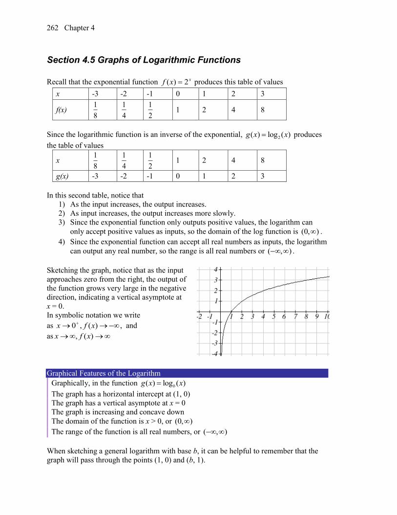
Chapter 4 262
Section 4.5 Graphs of Logarithmic Functions
Recall that the exponential function xxf 2)( produces this table of values
x -3 -2 -1 0 1 2 3
f(x) 8
1
4
1
2
1 1 2 4 8
Since the logarithmic function is an inverse of the exponential, 2( ) log ( )g x x produces
the table of values
x 8
1
4
1
2
1 1 2 4 8
g(x) -3 -2 -1 0 1 2 3
In this second table, notice that
1) As the input increases, the output increases.
2) As input increases, the output increases more slowly.
3) Since the exponential function only outputs positive values, the logarithm can
only accept positive values as inputs, so the domain of the log function is ),0( .
4) Since the exponential function can accept all real numbers as inputs, the logarithm
can output any real number, so the range is all real numbers or ),( .
Sketching the graph, notice that as the input
approaches zero from the right, the output of
the function grows very large in the negative
direction, indicating a vertical asymptote at
x = 0.
In symbolic notation we write
as )(,0 xfx , and
as )(, xfx
Graphical Features of the Logarithm
Graphically, in the function ( ) log ( )bg x x
The graph has a horizontal intercept at (1, 0)
The graph has a vertical asymptote at x = 0
The graph is increasing and concave down
The domain of the function is x > 0, or ),0(
The range of the function is all real numbers, or ),(
When sketching a general logarithm with base b, it can be helpful to remember that the
graph will pass through the points (1, 0) and (b, 1).
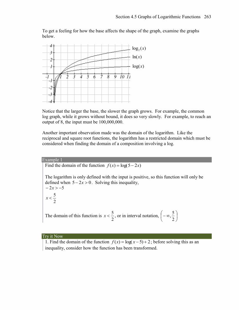
Section 4.5 Graphs of Logarithmic Functions 263
To get a feeling for how the base affects the shape of the graph, examine the graphs
below.
Notice that the larger the base, the slower the graph grows. For example, the common
log graph, while it grows without bound, it does so very slowly. For example, to reach an
output of 8, the input must be 100,000,000.
Another important observation made was the domain of the logarithm. Like the
reciprocal and square root functions, the logarithm has a restricted domain which must be
considered when finding the domain of a composition involving a log.
Example 1
Find the domain of the function )25log()( xxf
The logarithm is only defined with the input is positive, so this function will only be
defined when 025 x . Solving this inequality,
2
5
52
x
x
The domain of this function is 2
5x , or in interval notation,
2
5,
Try it Now
1. Find the domain of the function 2)5log()( xxf ; before solving this as an
inequality, consider how the function has been transformed.
2log ( )x
ln( )x
log( )x
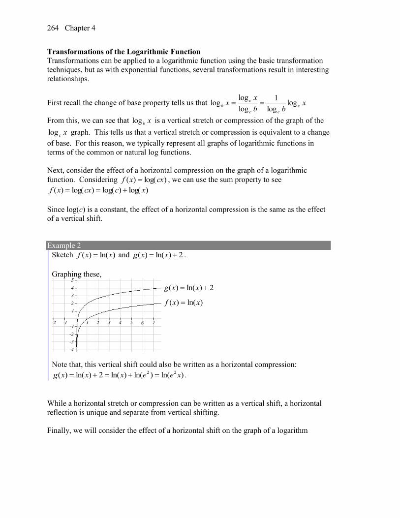
Chapter 4 264
Transformations of the Logarithmic Function Transformations can be applied to a logarithmic function using the basic transformation
techniques, but as with exponential functions, several transformations result in interesting
relationships.
First recall the change of base property tells us that xbb
xx c
cc
cb log
log
1
log
loglog
From this, we can see that xblog is a vertical stretch or compression of the graph of the
xclog graph. This tells us that a vertical stretch or compression is equivalent to a change
of base. For this reason, we typically represent all graphs of logarithmic functions in
terms of the common or natural log functions.
Next, consider the effect of a horizontal compression on the graph of a logarithmic
function. Considering )log()( cxxf , we can use the sum property to see
)log()log()log()( xccxxf
Since log(c) is a constant, the effect of a horizontal compression is the same as the effect
of a vertical shift.
Example 2
Sketch )ln()( xxf and 2)ln()( xxg .
Graphing these,
Note that, this vertical shift could also be written as a horizontal compression:
)ln()ln()ln(2)ln()( 22 xeexxxg .
While a horizontal stretch or compression can be written as a vertical shift, a horizontal
reflection is unique and separate from vertical shifting.
Finally, we will consider the effect of a horizontal shift on the graph of a logarithm
)ln()( xxf
2)ln()( xxg
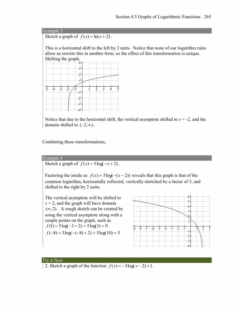
Section 4.5 Graphs of Logarithmic Functions 265
Example 3
Sketch a graph of )2ln()( xxf .
This is a horizontal shift to the left by 2 units. Notice that none of our logarithm rules
allow us rewrite this in another form, so the effect of this transformation is unique.
Shifting the graph,
Notice that due to the horizontal shift, the vertical asymptote shifted to x = -2, and the
domain shifted to ( 2, ) .
Combining these transformations,
Example 4
Sketch a graph of )2log(5)( xxf .
Factoring the inside as ))2(log(5)( xxf reveals that this graph is that of the
common logarithm, horizontally reflected, vertically stretched by a factor of 5, and
shifted to the right by 2 units.
The vertical asymptote will be shifted to
x = 2, and the graph will have domain
( ,2) . A rough sketch can be created by
using the vertical asymptote along with a
couple points on the graph, such as
5)10log(5)2)8(log(5)8(
0)1log(5)21log(5)1(
f
f
Try it Now
2. Sketch a graph of the function 1)2log(3)( xxf .
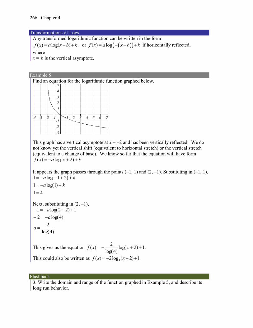
Chapter 4 266
Transformations of Logs
Any transformed logarithmic function can be written in the form
( ) log( )f x a x b k , or ( ) logf x a x b k if horizontally reflected,
where
x = b is the vertical asymptote.
Example 5
Find an equation for the logarithmic function graphed below.
This graph has a vertical asymptote at x = –2 and has been vertically reflected. We do
not know yet the vertical shift (equivalent to horizontal stretch) or the vertical stretch
(equivalent to a change of base). We know so far that the equation will have form
kxaxf )2log()(
It appears the graph passes through the points (–1, 1) and (2, –1). Substituting in (–1, 1),
k
ka
ka
1
)1log(1
)21log(1
Next, substituting in (2, –1),
)4log(
2
)4log(2
1)22log(1
a
a
a
This gives us the equation 1)2log()4log(
2)( xxf .
This could also be written as 4( ) 2log ( 2) 1f x x .
Flashback
3. Write the domain and range of the function graphed in Example 5, and describe its
long run behavior.
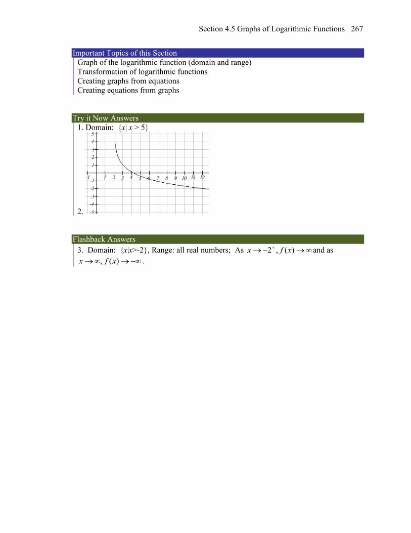
Section 4.5 Graphs of Logarithmic Functions 267
Important Topics of this Section
Graph of the logarithmic function (domain and range)
Transformation of logarithmic functions
Creating graphs from equations
Creating equations from graphs
Try it Now Answers
1. Domain: {x| x > 5}
2.
Flashback Answers
3. Domain: {x|x>-2}, Range: all real numbers; As )(,2 xfx and as
)(, xfx .
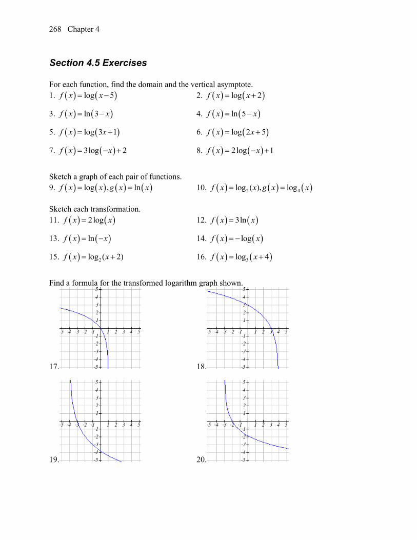
Chapter 4 268
Section 4.5 Exercises
For each function, find the domain and the vertical asymptote.
1. log 5f x x 2. log 2f x x
3. ln 3f x x 4. ln 5f x x
5. log 3 1f x x 6. log 2 5f x x
7. 3log 2f x x 8. 2log 1f x x
Sketch a graph of each pair of functions.
9. log , lnf x x g x x 10. 2 4log ( ), logf x x g x x
Sketch each transformation.
11. 2logf x x 12. 3lnf x x
13. lnf x x 14. logf x x
15. 2log ( 2)f x x 16. 3log 4f x x
Find a formula for the transformed logarithm graph shown.
17. 18.
19. 20.
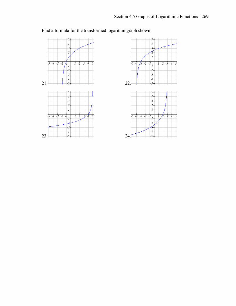
Section 4.5 Graphs of Logarithmic Functions 269
Find a formula for the transformed logarithm graph shown.
21. 22.
23. 24.
Chapter 4 270
Section 4.6 Exponential and Logarithmic Models
While we have explored some basic applications of exponential and logarithmic
functions, in this section we explore some important applications in more depth.
Radioactive Decay In an earlier section, we discussed radioactive decay – the idea that radioactive isotopes
change over time. One of the common terms associated with radioactive decay is half-
life.
Half Life
The half-life of a radioactive isotope is the time it takes for half the substance to decay.
Given the basic exponential growth/decay equation tabth )( , half-life can be found by
solving for when half the original amount remains; by solving tbaa )(2
1 , or more
simply tb2
1. Notice how the initial amount is irrelevant when solving for half-life.
Example 1
Bismuth-210 is an isotope that decays by about 13% each day. What is the half-life of
Bismuth-210?
We were not given a starting quantity, so we could either make up a value or use an
unknown constant to represent the starting amount. To show that starting quantity does
not affect the result, let us denote the initial quantity by the constant a. Then the decay
of Bismuth-210 can be described by the equation dadQ )87.0()( .
To find the half-life, we want to determine when the remaining quantity is half the
original: 1
2a . Solving,
daa )87.0(2
1 Dividing by a,
d87.02
1 Take the log of both sides
d87.0log2
1log
Use the exponent property of logs
87.0log2
1log d
Divide to solve for d
Section 4.6 Exponential and Logarithmic Models 271
1log
24.977
log 0.87d
days
This tells us that the half-life of Bismuth-210 is approximately 5 days.
Example 2
Cesium-137 has a half-life of about 30 years. If you begin with 200mg of cesium-137,
how much will remain after 30 years? 60 years? 90 years?
Since the half-life is 30 years, after 30 years, half the original amount, 100mg, will
remain.
After 60 years, another 30 years have passed, so during that second 30 years, another
half of the substance will decay, leaving 50mg.
After 90 years, another 30 years have passed, so another half of the substance will
decay, leaving 25mg.
Example 3
Cesium-137 has a half-life of about 30 years. Find the annual decay rate.
Since we are looking for an annual decay rate, we will use an equation of the form tratQ )1()( . We know that after 30 years, half the original amount will remain.
Using this information
30)1(2
1raa Dividing by a
30)1(2
1r Taking the 30th root of both sides
r12
130 Subtracting one from both sides,
02284.012
130 r
This tells us cesium-137 is decaying at an annual rate of 2.284% per year.
Try it Now
Chlorine-36 is eliminated from the body with a biological half-life of 10 days3. Find the
daily decay rate.
3 http://www.ead.anl.gov/pub/doc/chlorine.pdf
Chapter 4 272
Example 4
Carbon-14 is a radioactive isotope that is present in organic materials, and is commonly
used for dating historical artifacts. Carbon-14 has a half-life of 5730 years. If a bone
fragment is found that contains 20% of its original carbon-14, how old is the bone?
To find how old the bone is, we first will need to find an equation for the decay of the
carbon-14. We could either use a continuous or annual decay formula, but opt to use
the continuous decay formula since it is more common in scientific texts. The half life
tells us that after 5730 years, half the original substance remains. Solving for the rate,
5730
2
1 raea Dividing by a
5730
2
1 re Taking the natural log of both sides
5730ln2
1ln re
Use the inverse property of logs on the right side
r57302
1ln
Divide by 5730
000121.05730
2
1ln
r
Now we know the decay will follow the equation taetQ 000121.0)( . To find how old
the bone fragment is that contains 20% of the original amount, we solve for t so that
Q(t) = 0.20a.
taea 000121.020.0
te 000121.020.0
te 000121.0ln)20.0ln(
t000121.0)20.0ln(
13301000121.0
)20.0ln(
t years
The bone fragment is about 13,300 years old.
Try it Now
2. In Example 2, we learned that Cesium-137 has a half-life of about 30 years. If you
begin with 200mg of cesium-137, will it take more or less than 230 years until only 1
milligram remains?
Section 4.6 Exponential and Logarithmic Models 273
Doubling Time For decaying quantities, we asked how long it takes for half the substance to decay. For
growing quantities we might ask how long it takes for the quantity to double.
Doubling Time
The doubling time of a growing quantity is the time it takes for the quantity to double.
Given the basic exponential growth equation tabth )( , doubling time can be found by
solving for when the original quantity has doubled; by solving xbaa )(2 , or more
simply xb2 . Again notice how the initial amount is irrelevant when solving for
doubling time.
Example 5
Cancer cells sometimes increase exponentially. If a cancerous growth contained 300
cells last month and 360 cells this month, how long will it take for the number of cancer
cells to double?
Defining t to be time in months, with t = 0 corresponding to this month, we are given
two pieces of data: this month, (0, 360), and last month, (-1, 300).
From this data, we can find an equation for the growth. Using the form tabtC )( , we
know immediately a = 360, giving tbtC 360)( . Substituting in (-1, 300),
2.1300
360
360300
360300 1
b
b
b
This gives us the equation ttC )2.1(360)(
To find the doubling time, we look for the time until we have twice the original amount,
so when C(t) = 2a.
taa )2.1(2
t)2.1(2
t2.1log2log
2.1log2log t
802.32.1log
2logt months.
It will take about 3.8 months for the number of cancer cells to double.
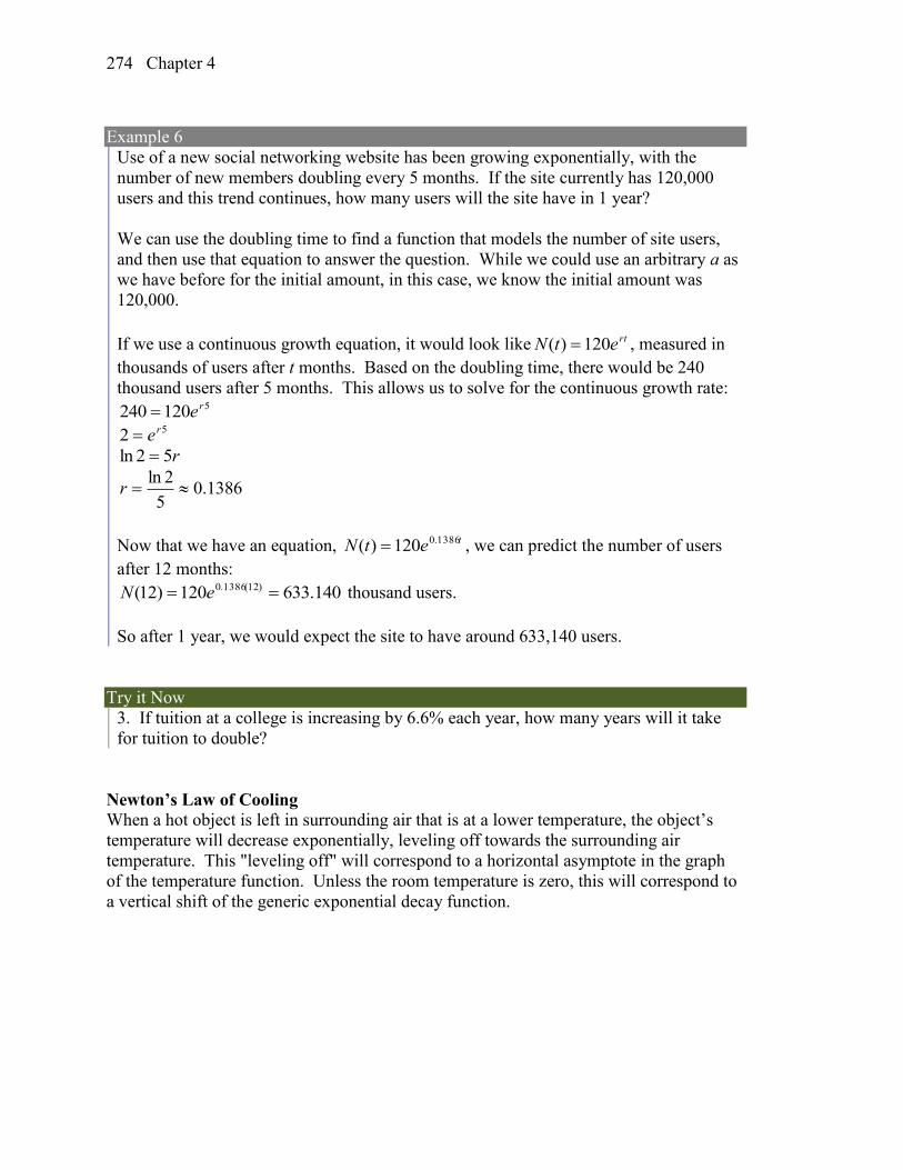
Chapter 4 274
Example 6
Use of a new social networking website has been growing exponentially, with the
number of new members doubling every 5 months. If the site currently has 120,000
users and this trend continues, how many users will the site have in 1 year?
We can use the doubling time to find a function that models the number of site users,
and then use that equation to answer the question. While we could use an arbitrary a as
we have before for the initial amount, in this case, we know the initial amount was
120,000.
If we use a continuous growth equation, it would look like rtetN 120)( , measured in
thousands of users after t months. Based on the doubling time, there would be 240
thousand users after 5 months. This allows us to solve for the continuous growth rate: 5120240 re
52 re
r52ln
1386.05
2lnr
Now that we have an equation, tetN 1386.0120)( , we can predict the number of users
after 12 months:
140.633120)12( )12(1386.0 eN thousand users.
So after 1 year, we would expect the site to have around 633,140 users.
Try it Now
3. If tuition at a college is increasing by 6.6% each year, how many years will it take
for tuition to double?
Newton’s Law of Cooling When a hot object is left in surrounding air that is at a lower temperature, the object’s
temperature will decrease exponentially, leveling off towards the surrounding air
temperature. This "leveling off" will correspond to a horizontal asymptote in the graph
of the temperature function. Unless the room temperature is zero, this will correspond to
a vertical shift of the generic exponential decay function.
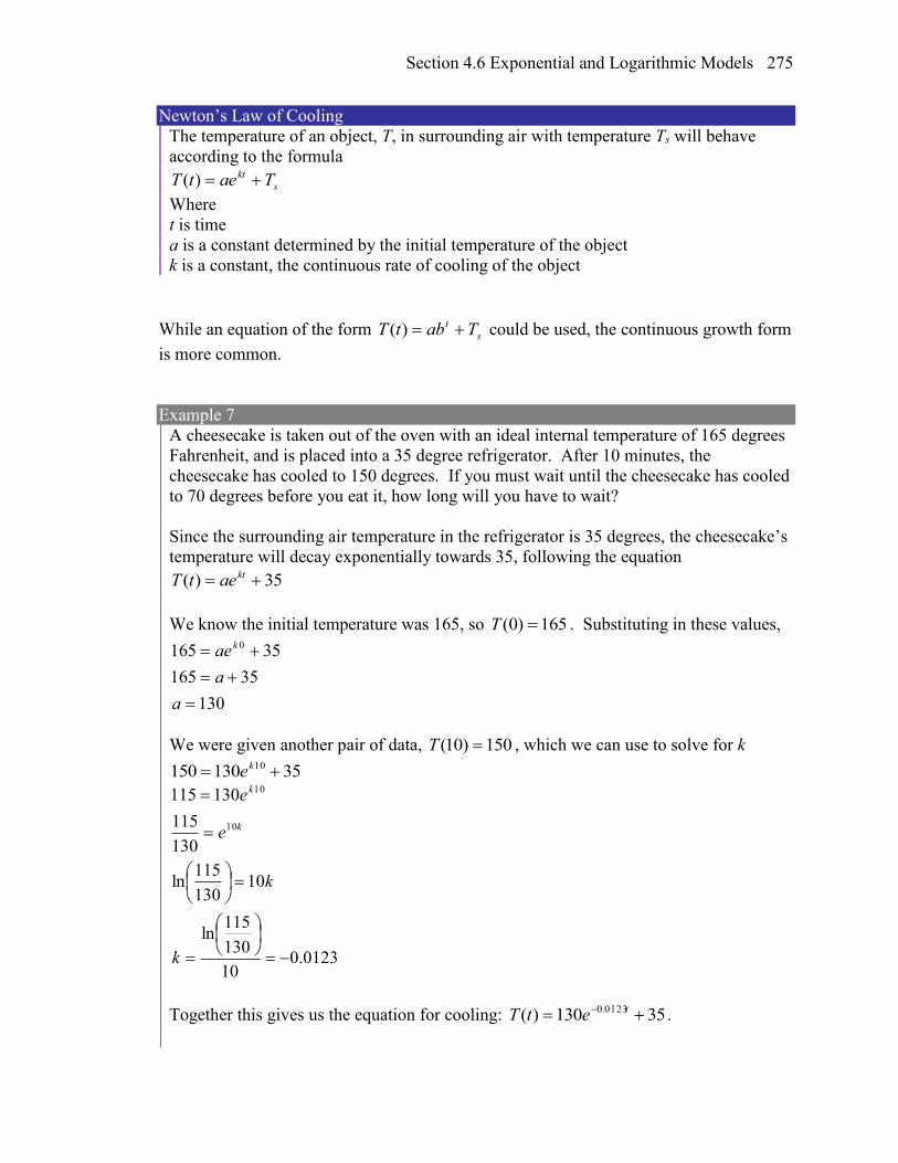
Section 4.6 Exponential and Logarithmic Models 275
Newton’s Law of Cooling
The temperature of an object, T, in surrounding air with temperature Ts will behave
according to the formula
s
kt TaetT )(
Where
t is time
a is a constant determined by the initial temperature of the object
k is a constant, the continuous rate of cooling of the object
While an equation of the form s
t TabtT )( could be used, the continuous growth form
is more common.
Example 7
A cheesecake is taken out of the oven with an ideal internal temperature of 165 degrees
Fahrenheit, and is placed into a 35 degree refrigerator. After 10 minutes, the
cheesecake has cooled to 150 degrees. If you must wait until the cheesecake has cooled
to 70 degrees before you eat it, how long will you have to wait?
Since the surrounding air temperature in the refrigerator is 35 degrees, the cheesecake’s
temperature will decay exponentially towards 35, following the equation
35)( ktaetT
We know the initial temperature was 165, so 165)0( T . Substituting in these values,
130
35165
35165 0
a
a
aek
We were given another pair of data, 150)10( T , which we can use to solve for k
35130150 10 ke
0123.010
130
115ln
10130
115ln
130
115
130115
10
10
k
k
e
e
k
k
Together this gives us the equation for cooling: 35130)( 0123.0 tetT .
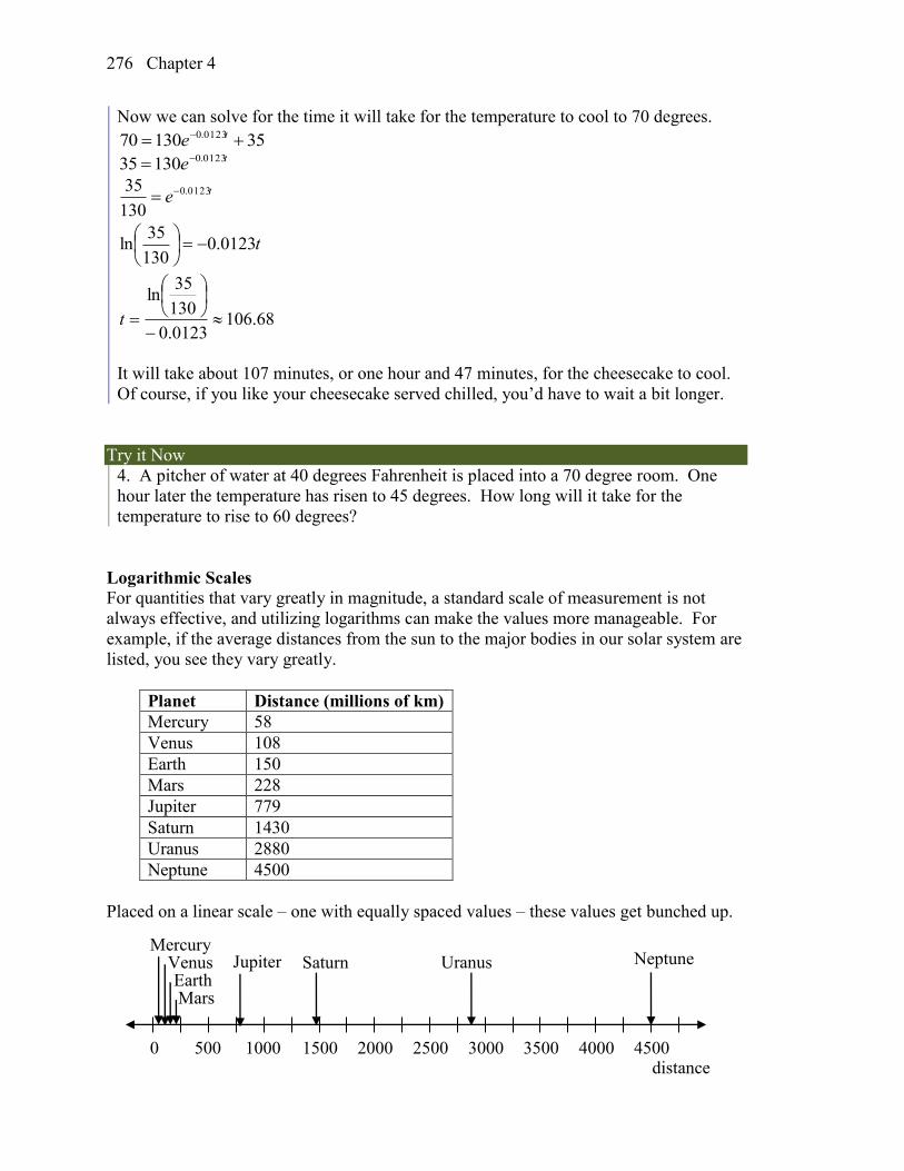
Chapter 4 276
Now we can solve for the time it will take for the temperature to cool to 70 degrees.
3513070 0123.0 te te 0123.013035
te 0123.0
130
35
t0123.0130
35ln
68.1060123.0
130
35ln
t
It will take about 107 minutes, or one hour and 47 minutes, for the cheesecake to cool.
Of course, if you like your cheesecake served chilled, you’d have to wait a bit longer.
Try it Now
4. A pitcher of water at 40 degrees Fahrenheit is placed into a 70 degree room. One
hour later the temperature has risen to 45 degrees. How long will it take for the
temperature to rise to 60 degrees?
Logarithmic Scales For quantities that vary greatly in magnitude, a standard scale of measurement is not
always effective, and utilizing logarithms can make the values more manageable. For
example, if the average distances from the sun to the major bodies in our solar system are
listed, you see they vary greatly.
Planet Distance (millions of km)
Mercury 58
Venus 108
Earth 150
Mars 228
Jupiter 779
Saturn 1430
Uranus 2880
Neptune 4500
Placed on a linear scale – one with equally spaced values – these values get bunched up.
0 500 1000 1500 2000 2500 3000 3500 4000 4500
Mercury Venus Earth Mars
Jupiter Saturn Uranus Neptune
distance
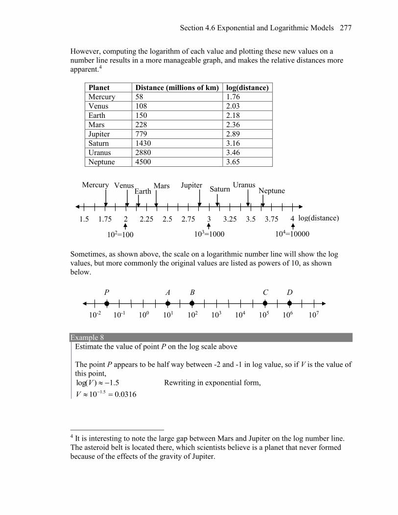
Section 4.6 Exponential and Logarithmic Models 277
However, computing the logarithm of each value and plotting these new values on a
number line results in a more manageable graph, and makes the relative distances more
apparent.4
Planet Distance (millions of km) log(distance)
Mercury 58 1.76
Venus 108 2.03
Earth 150 2.18
Mars 228 2.36
Jupiter 779 2.89
Saturn 1430 3.16
Uranus 2880 3.46
Neptune 4500 3.65
Sometimes, as shown above, the scale on a logarithmic number line will show the log
values, but more commonly the original values are listed as powers of 10, as shown
below.
Example 8
Estimate the value of point P on the log scale above
The point P appears to be half way between -2 and -1 in log value, so if V is the value of
this point,
5.1)log( V Rewriting in exponential form,
0316.010 5.1 V
4 It is interesting to note the large gap between Mars and Jupiter on the log number line.
The asteroid belt is located there, which scientists believe is a planet that never formed
because of the effects of the gravity of Jupiter.
102 103 104 105 106 101 100 10-1 10-2 107
A B P C D
Mercury Venus Neptune
1.5 1.75 2 2.25 2.5 2.75 3 3.25 3.5
Earth Mars
3.75
Jupiter Saturn
Uranus
4
104=10000 103=1000 102=100
log(distance)
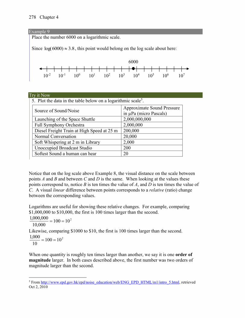
Chapter 4 278
Example 9
Place the number 6000 on a logarithmic scale.
Since 8.3)6000log( , this point would belong on the log scale about here:
Try it Now
5. Plot the data in the table below on a logarithmic scale5.
Notice that on the log scale above Example 8, the visual distance on the scale between
points A and B and between C and D is the same. When looking at the values these
points correspond to, notice B is ten times the value of A, and D is ten times the value of
C. A visual linear difference between points corresponds to a relative (ratio) change
between the corresponding values.
Logarithms are useful for showing these relative changes. For example, comparing
$1,000,000 to $10,000, the first is 100 times larger than the second.
210100000,10
000,000,1
Likewise, comparing $1000 to $10, the first is 100 times larger than the second.
21010010
000,1
When one quantity is roughly ten times larger than another, we say it is one order of
magnitude larger. In both cases described above, the first number was two orders of
magnitude larger than the second.
5 From http://www.epd.gov.hk/epd/noise_education/web/ENG_EPD_HTML/m1/intro_5.html, retrieved
Oct 2, 2010
102 103 104 105 106 101 100 10-1 10-2 107
6000
Source of Sound/Noise Approximate Sound Pressure
in µPa (micro Pascals)
Launching of the Space Shuttle 2,000,000,000
Full Symphony Orchestra 2,000,000
Diesel Freight Train at High Speed at 25 m 200,000
Normal Conversation 20,000
Soft Whispering at 2 m in Library 2,000
Unoccupied Broadcast Studio 200
Softest Sound a human can hear 20
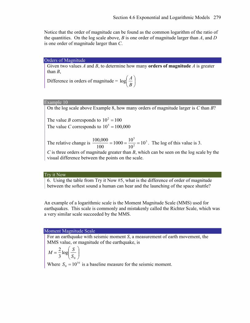
Section 4.6 Exponential and Logarithmic Models 279
Notice that the order of magnitude can be found as the common logarithm of the ratio of
the quantities. On the log scale above, B is one order of magnitude larger than A, and D
is one order of magnitude larger than C.
Orders of Magnitude
Given two values A and B, to determine how many orders of magnitude A is greater
than B,
Difference in orders of magnitude =
B
Alog
Example 10
On the log scale above Example 8, how many orders of magnitude larger is C than B?
The value B corresponds to 100102
The value C corresponds to 000,100105
The relative change is 3
2
5
1010
101000
100
000,100 . The log of this value is 3.
C is three orders of magnitude greater than B, which can be seen on the log scale by the
visual difference between the points on the scale.
Try it Now
6. Using the table from Try it Now #5, what is the difference of order of magnitude
between the softest sound a human can hear and the launching of the space shuttle?
An example of a logarithmic scale is the Moment Magnitude Scale (MMS) used for
earthquakes. This scale is commonly and mistakenly called the Richter Scale, which was
a very similar scale succeeded by the MMS.
Moment Magnitude Scale
For an earthquake with seismic moment S, a measurement of earth movement, the
MMS value, or magnitude of the earthquake, is
0
log3
2
S
SM
Where 16
0 10S is a baseline measure for the seismic moment.
Chapter 4 280
Example 11
If one earthquake has a MMS magnitude of 6.0, and another has a magnitude of 8.0,
how much more powerful (in terms of earth movement) is the second earthquake?
Since the first earthquake has magnitude 6.0, we can find the amount of earth
movement. The value of S0 is not particularly relevant, so we will not replace it with its
value.
0
log3
20.6
S
S
0
log2
30.6
S
S
0
log9S
S
9
0
10S
S
0
910 SS
Doing the same with the second earthquake with a magnitude of 8.0,
0
log3
20.8
S
S
0
1210 SS
From this, we can see that this second value’s earth movement is 1000 times as large as
the first earthquake.
Example 12
One earthquake has magnitude of 3.0. If a second earthquake has twice as much earth
movement as the first earthquake, find the magnitude of the second quake.
Since the first quake has magnitude 3.0,
Section 4.6 Exponential and Logarithmic Models 281
0
5.4
0
5.4
0
0
0
10
10
log5.4
log2
30.3
log3
20.3
SS
S
S
S
S
S
S
S
S
Since the second earthquake has twice as much earth movement, for the second quake,
0
5.4102 SS
Finding the magnitude,
0
0
5.4102log
3
2
S
SM
201.3102log3
2 5.4 M
The second earthquake with twice as much earth movement will have a magnitude of
about 3.2.
In fact, using log properties, we could show that whenever the earth movement doubles,
the magnitude will increase by about 0.201:
00
2log3
22log
3
2
S
S
S
SM
0
log)2log(3
2
S
SM
0
log3
2)2log(
3
2
S
SM
0
log3
2201.0
S
SM
This illustrates the most important feature of a log scale: that multiplying the quantity
being considered will add to the scale value, and vice versa.
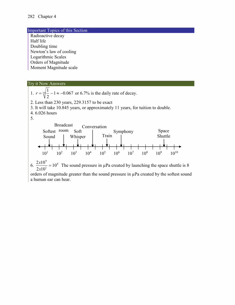
Chapter 4 282
Important Topics of this Section
Radioactive decay
Half life
Doubling time
Newton’s law of cooling
Logarithmic Scales
Orders of Magnitude
Moment Magnitude scale
Try it Now Answers
1. 067.012
110 r or 6.7% is the daily rate of decay.
2. Less than 230 years, 229.3157 to be exact
3. It will take 10.845 years, or approximately 11 years, for tuition to double.
4. 6.026 hours
5.
6. 8
1
9
10102
102
x
x The sound pressure in µPa created by launching the space shuttle is 8
orders of magnitude greater than the sound pressure in µPa created by the softest sound
a human ear can hear.
105 106 107 108 109 104 103 102 101 1010
Softest
Sound
Broadcast
room Soft
Whisper
Conversation
Train
Symphony Space
Shuttle
Section 4.6 Exponential and Logarithmic Models 283
Section 4.6 Exercises
1. You go to the doctor and he injects you with 13 milligrams of radioactive dye. After
12 minutes, 4.75 milligrams of dye remain in your system. To leave the doctor's
office, you must pass through a radiation detector without sounding the alarm. If the
detector will sound the alarm whenever more than 2 milligrams of the dye are in your
system, how long will your visit to the doctor take, assuming you were given the dye
as soon as you arrived and the amount of dye decays exponentially?
2. You take 200 milligrams of a headache medicine, and after 4 hours, 120 milligrams
remain in your system. If the effects of the medicine wear off when less than 80
milligrams remain, when will you need to take a second dose, assuming the amount
of medicine in your system decays exponentially?
3. The half-life of Radium-226 is 1590 years. If a sample initially contains 200 mg,
how many milligrams will remain after 1000 years?
4. The half-life of Fermium-253 is 3 days. If a sample initially contains 100 mg, how
many milligrams will remain after 1 week?
5. The half-life of Erbium-165 is 10.4 hours. After 24 hours a sample still contains 2
mg. What was the initial mass of the sample, and how much will remain after another
3 days?
6. The half-life of Nobelium-259 is 58 minutes. After 3 hours a sample still contains10
mg. What was the initial mass of the sample, and how much will remain after another
8 hours?
7. A scientist begins with 250 grams of a radioactive substance. After 225 minutes, the
sample has decayed to 32 grams. Find the half-life of this substance.
8. A scientist begins with 20 grams of a radioactive substance. After 7 days, the sample
has decayed to 17 grams. Find the half-life of this substance.
9. A wooden artifact from an archeological dig contains 60 percent of the carbon-14 that
is present in living trees. How long ago was the artifact made? (The half-life of
carbon-14 is 5730 years.)
Chapter 4 284
10. A wooden artifact from an archeological dig contains 15 percent of the carbon-14 that
is present in living trees. How long ago was the artifact made? (The half-life of
carbon-14 is 5730 years.)
11. A bacteria culture initially contains 1500 bacteria and doubles in size every half hour.
Find the size of the population after: a) 2 hours b) 100 minutes
12. A bacteria culture initially contains 2000 bacteria and doubles in size every half hour.
Find the size of the population after: a) 3 hours b) 80 minutes
13. The count of bacteria in a culture was 800 after 10 minutes and 1800 after 40
minutes.
a. What was the initial size of the culture?
b. Find the doubling time.
c. Find the population after 105 minutes.
d. When will the population reach 11000?
14. The count of bacteria in a culture was 600 after 20 minutes and 2000 after 35
minutes.
a. What was the initial size of the culture?
b. Find the doubling time.
c. Find the population after 170 minutes.
d. When will the population reach 12000?
15. Find the time required for an investment to double in value if invested in an account
paying 3% compounded quarterly.
16. Find the time required for an investment to double in value if invested in an account
paying 4% compounded monthly
17. The number of crystals that have formed after t hours is given by 0.01320 tn t e .
How long does it take the number of crystals to double?
18. The number of building permits in Pasco t years after 1992 roughly followed the
equation 0.143400 tn t e . What is the doubling time?
Section 4.6 Exponential and Logarithmic Models 285
19. A turkey is pulled from the oven when the internal temperature is 165° Fahrenheit,
and is allowed to cool in a 75° room. If the temperature of the turkey is 145° after
half an hour,
a. What will the temperature be after 50 minutes?
b. How long will it take the turkey to cool to 110°?
20. A cup of coffee is poured at 190° Fahrenheit, and is allowed to cool in a 70° room. If
the temperature of the coffee is 170° after half an hour,
a. What will the temperature be after 70 minutes?
b. How long will it take the coffee to cool to 120°?
21. The population of fish in a farm-stocked lake after t years could be modeled by the
equation 0.6
1000
1 9 tP t
e
.
a. Sketch a graph of this equation.
b. What is the initial population of fish?
c. What will the population be after 2 years?
d. How long will it take for the population to reach 900?
22. The number of people in a town who have heard a rumor after t days can be modeled
by the equation 0.7
500
1 49 tN t
e
.
a. Sketch a graph of this equation.
b. How many people started the rumor?
c. How many people have heard the rumor after 3 days?
d. How long will it take until 300 people have heard the rumor?
Find the value of the number shown on each logarithmic scale
23. 24.
25. 26.
Plot each set of approximate values on a logarithmic scale.
27. Intensity of sounds: Whisper: 10 210 /W m , Vacuum: 4 210 /W m , Jet: 2 210 /W m
28. Mass: Amoeba: 510 g , Human: 510 g , Statue of Liberty: 810 g
Chapter 4 286
29. The 1906 San Francisco earthquake had a magnitude of 7.9 on the MMS scale. Later
there was an earthquake with magnitude 4.7 that caused only minor damage. How
many times more intense was the San Francisco earthquake than the second one?
30. The 1906 San Francisco earthquake had a magnitude of 7.9 on the MMS scale. Later
there was an earthquake with magnitude 6.5 that caused less damage. How many
times more intense was the San Francisco earthquake than the second one?
31. One earthquake has magnitude 3.9 on the MMS scale. If a second earthquake has 750
times as much energy as the first, find the magnitude of the second quake.
32. One earthquake has magnitude 4.8 on the MMS scale. If a second earthquake has
1200 times as much energy as the first, find the magnitude of the second quake.
33. A colony of yeast cells is estimated to contain 106 cells at time t = 0. After collecting
experimental data in the lab, you decide that the total population of cells at time t
hours is given by the function 6 0.49510510 tf t e . [UW]
a. How many cells are present after one hour?
b. How long does it take of the population to double?.
c. Cherie, another member of your lab, looks at your notebook and says: “That
formula is wrong, my calculations predict the formula for the number of yeast
cells is given by the function. 0.693147610 2.042727
tf t .” Should you be
worried by Cherie’s remark?
d. Anja, a third member of your lab working with the same yeast cells, took
these two measurements: 67.246 10 cells after 4 hours; 616.504 10 cells
after 6 hours. Should you be worried by Anja’s results? If Anja’s
measurements are correct, does your model over estimate or under estimate
the number of yeast cells at time t?
34. As light from the surface penetrates water, its intensity is diminished. In the clear
waters of the Caribbean, the intensity is decreased by 15 percent for every 3 meters of
depth. Thus, the intensity will have the form of a general exponential function. [UW]
a. If the intensity of light at the water’s surface is 0I , find a formula for ( )I d , the
intensity of light at a depth of d meters. Your formula should depend on 0I and
d.
b. At what depth will the light intensity be decreased to 1% of its surface
intensity?
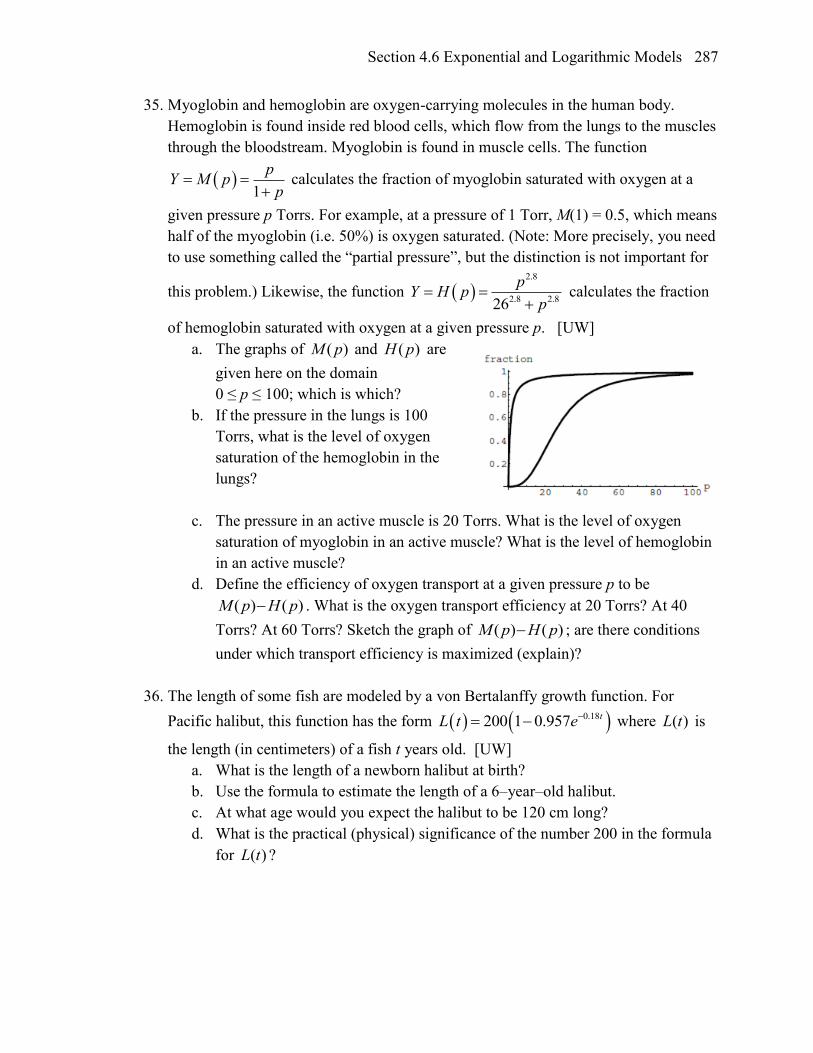
Section 4.6 Exponential and Logarithmic Models 287
35. Myoglobin and hemoglobin are oxygen-carrying molecules in the human body.
Hemoglobin is found inside red blood cells, which flow from the lungs to the muscles
through the bloodstream. Myoglobin is found in muscle cells. The function
1
pY M p
p
calculates the fraction of myoglobin saturated with oxygen at a
given pressure p Torrs. For example, at a pressure of 1 Torr, M(1) = 0.5, which means
half of the myoglobin (i.e. 50%) is oxygen saturated. (Note: More precisely, you need
to use something called the “partial pressure”, but the distinction is not important for
this problem.) Likewise, the function 2.8
2.8 2.826
pY H p
p
calculates the fraction
of hemoglobin saturated with oxygen at a given pressure p. [UW]
a. The graphs of ( )M p and ( )H p are
given here on the domain
0 ≤ p ≤ 100; which is which?
b. If the pressure in the lungs is 100
Torrs, what is the level of oxygen
saturation of the hemoglobin in the
lungs?
c. The pressure in an active muscle is 20 Torrs. What is the level of oxygen
saturation of myoglobin in an active muscle? What is the level of hemoglobin
in an active muscle?
d. Define the efficiency of oxygen transport at a given pressure p to be
( ) ( )M p H p . What is the oxygen transport efficiency at 20 Torrs? At 40
Torrs? At 60 Torrs? Sketch the graph of ( ) ( )M p H p ; are there conditions
under which transport efficiency is maximized (explain)?
36. The length of some fish are modeled by a von Bertalanffy growth function. For
Pacific halibut, this function has the form 0.18200 1 0.957 tL t e where ( )L t is
the length (in centimeters) of a fish t years old. [UW]
a. What is the length of a newborn halibut at birth?
b. Use the formula to estimate the length of a 6–year–old halibut.
c. At what age would you expect the halibut to be 120 cm long?
d. What is the practical (physical) significance of the number 200 in the formula
for ( )L t ?
Chapter 4 288
37. A cancer cell lacks normal biological growth regulation and can divide continuously.
Suppose a single mouse skin cell is cancerous and its mitotic cell cycle (the time for
the cell to divide once) is 20 hours. The number of cells at time t grows according to
an exponential model. [UW]
a. Find a formula ( )C t for the number of cancerous skin cells after t hours.
b. Assume a typical mouse skin cell is spherical of radius 50×10−4 cm. Find the
combined volume of all cancerous skin cells after t hours. When will the
volume of cancerous cells be 1 cm3?
38. A ship embarked on a long voyage. At the start of the voyage, there were 500 ants in
the cargo hold of the ship. One week into the voyage, there were 800 ants. Suppose
the population of ants is an exponential function of time. [UW]
a. How long did it take the population to double?
b. How long did it take the population to triple?
c. When were there be 10,000 ants on board?
d. There also was an exponentially growing population of anteaters on board. At
the start of the voyage there were 17 anteaters, and the population of anteaters
doubled every 2.8 weeks. How long into the voyage were there 200 ants per
anteater?
39. The populations of termites and spiders in a certain house are growing exponentially.
The house contains 100 termites the day you move in. After 4 days, the house
contains 200 termites. Three days after moving in, there are two times as many
termites as spiders. Eight days after moving in, there were four times as many
termites as spiders. How long (in days) does it take the population of spiders to
triple? [UW]
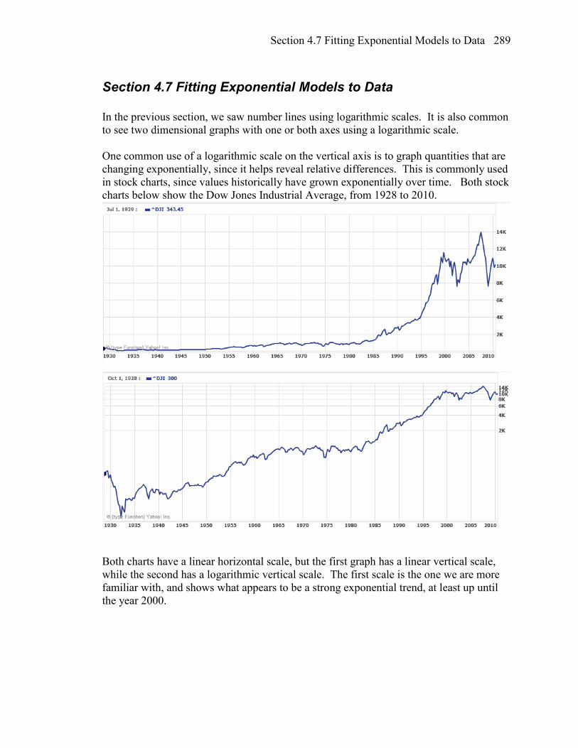
Section 4.7 Fitting Exponential Models to Data 289
Section 4.7 Fitting Exponential Models to Data
In the previous section, we saw number lines using logarithmic scales. It is also common
to see two dimensional graphs with one or both axes using a logarithmic scale.
One common use of a logarithmic scale on the vertical axis is to graph quantities that are
changing exponentially, since it helps reveal relative differences. This is commonly used
in stock charts, since values historically have grown exponentially over time. Both stock
charts below show the Dow Jones Industrial Average, from 1928 to 2010.
Both charts have a linear horizontal scale, but the first graph has a linear vertical scale,
while the second has a logarithmic vertical scale. The first scale is the one we are more
familiar with, and shows what appears to be a strong exponential trend, at least up until
the year 2000.
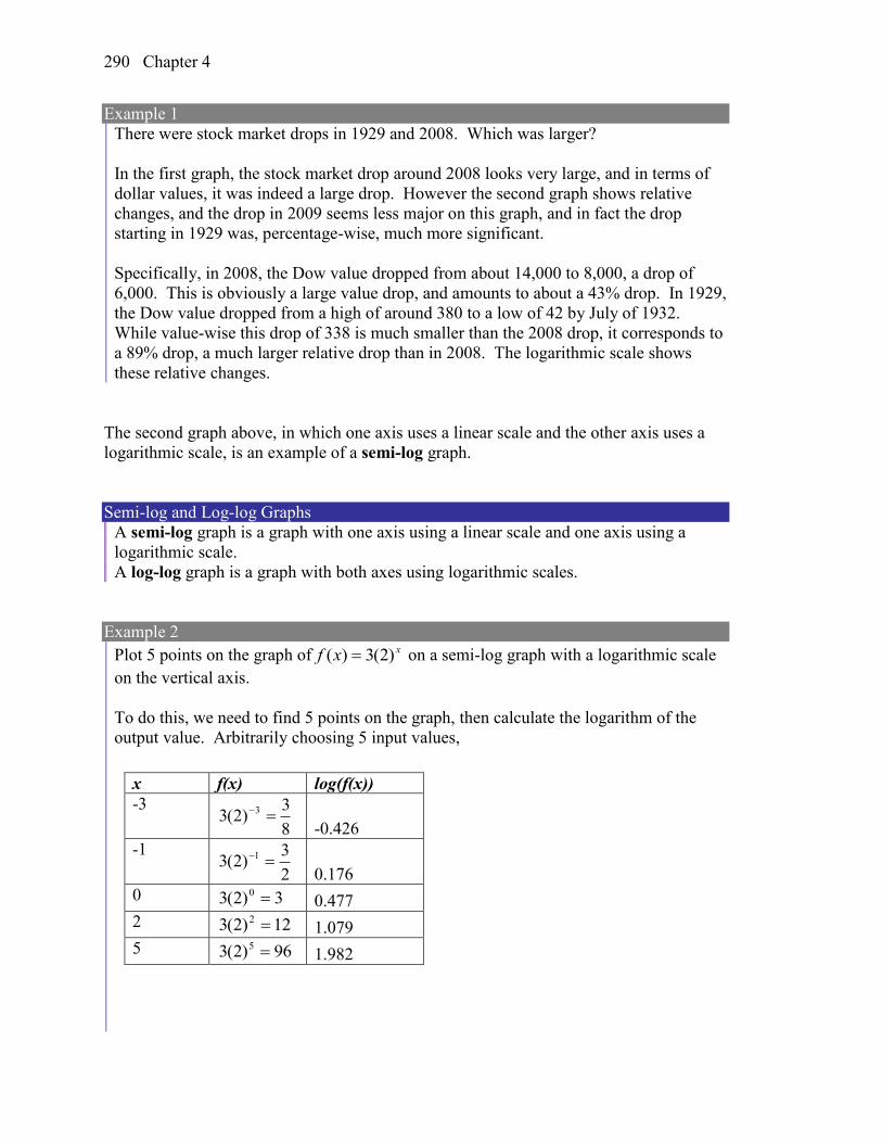
Chapter 4 290
Example 1
There were stock market drops in 1929 and 2008. Which was larger?
In the first graph, the stock market drop around 2008 looks very large, and in terms of
dollar values, it was indeed a large drop. However the second graph shows relative
changes, and the drop in 2009 seems less major on this graph, and in fact the drop
starting in 1929 was, percentage-wise, much more significant.
Specifically, in 2008, the Dow value dropped from about 14,000 to 8,000, a drop of
6,000. This is obviously a large value drop, and amounts to about a 43% drop. In 1929,
the Dow value dropped from a high of around 380 to a low of 42 by July of 1932.
While value-wise this drop of 338 is much smaller than the 2008 drop, it corresponds to
a 89% drop, a much larger relative drop than in 2008. The logarithmic scale shows
these relative changes.
The second graph above, in which one axis uses a linear scale and the other axis uses a
logarithmic scale, is an example of a semi-log graph.
Semi-log and Log-log Graphs
A semi-log graph is a graph with one axis using a linear scale and one axis using a
logarithmic scale.
A log-log graph is a graph with both axes using logarithmic scales.
Example 2
Plot 5 points on the graph of xxf )2(3)( on a semi-log graph with a logarithmic scale
on the vertical axis.
To do this, we need to find 5 points on the graph, then calculate the logarithm of the
output value. Arbitrarily choosing 5 input values,
x f(x) log(f(x))
-3
8
3)2(3 3
-0.426
-1
2
3)2(3 1
0.176
0 3)2(3 0 0.477
2 12)2(3 2 1.079
5 96)2(3 5 1.982
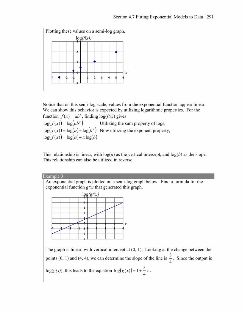
Section 4.7 Fitting Exponential Models to Data 291
Plotting these values on a semi-log graph,
-1
0
1
2
3
-4 -3 -2 -1 0 1 2 3 4 5 6
Notice that on this semi-log scale, values from the exponential function appear linear.
We can show this behavior is expected by utilizing logarithmic properties. For the
function xabxf )( , finding log(f(x)) gives
xabxf log)(log Utilizing the sum property of logs,
xbaxf loglog)(log Now utilizing the exponent property,
bxaxf loglog)(log
This relationship is linear, with log(a) as the vertical intercept, and log(b) as the slope.
This relationship can also be utilized in reverse.
Example 3
An exponential graph is plotted on a semi-log graph below. Find a formula for the
exponential function g(x) that generated this graph.
-3
-2
-1
0
1
2
3
4
5
-4 -3 -2 -1 0 1 2 3 4
The graph is linear, with vertical intercept at (0, 1). Looking at the change between the
points (0, 1) and (4, 4), we can determine the slope of the line is 4
3. Since the output is
log(g(x)), this leads to the equation xxg4
31)(log .
x
log(f(x))
x
log(g(x))
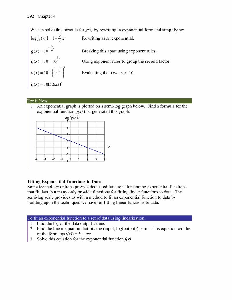
Chapter 4 292
We can solve this formula for g(x) by rewriting in exponential form and simplifying:
xxg4
31)(log Rewriting as an exponential,
x
xg 4
31
10)(
Breaking this apart using exponent rules,
x
xg 4
3
1 1010)( Using exponent rules to group the second factor, x
xg
4
3
1 1010)( Evaluating the powers of 10,
xxg 623.510)(
Try it Now
1. An exponential graph is plotted on a semi-log graph below. Find a formula for the
exponential function g(x) that generated this graph.
-1
0
1
2
3
4
5
-4 -3 -2 -1 0 1 2 3 4
Fitting Exponential Functions to Data Some technology options provide dedicated functions for finding exponential functions
that fit data, but many only provide functions for fitting linear functions to data. The
semi-log scale provides us with a method to fit an exponential function to data by
building upon the techniques we have for fitting linear functions to data.
To fit an exponential function to a set of data using linearization
1. Find the log of the data output values
2. Find the linear equation that fits the (input, log(output)) pairs. This equation will be
of the form log(f(x)) = b + mx
3. Solve this equation for the exponential function f(x)
x
log(g(x))
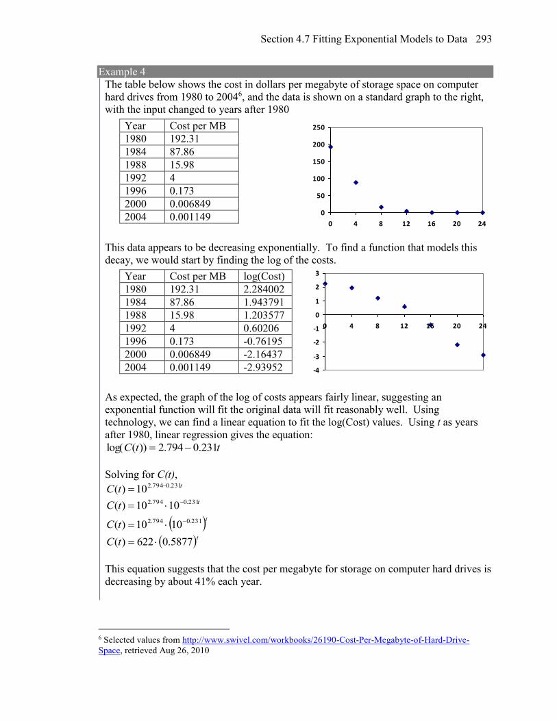
Section 4.7 Fitting Exponential Models to Data 293
Example 4
The table below shows the cost in dollars per megabyte of storage space on computer
hard drives from 1980 to 20046, and the data is shown on a standard graph to the right,
with the input changed to years after 1980
This data appears to be decreasing exponentially. To find a function that models this
decay, we would start by finding the log of the costs.
As expected, the graph of the log of costs appears fairly linear, suggesting an
exponential function will fit the original data will fit reasonably well. Using
technology, we can find a linear equation to fit the log(Cost) values. Using t as years
after 1980, linear regression gives the equation:
ttC 231.0794.2))(log(
Solving for C(t), ttC 231.0794.210)(
ttC 231.0794.2 1010)(
ttC 231.0794.2 1010)(
ttC 5877.0622)(
This equation suggests that the cost per megabyte for storage on computer hard drives is
decreasing by about 41% each year.
6 Selected values from http://www.swivel.com/workbooks/26190-Cost-Per-Megabyte-of-Hard-Drive-
Space, retrieved Aug 26, 2010
Year Cost per MB
1980 192.31
1984 87.86
1988 15.98
1992 4
1996 0.173
2000 0.006849
2004 0.001149
Year Cost per MB log(Cost)
1980 192.31 2.284002
1984 87.86 1.943791
1988 15.98 1.203577
1992 4 0.60206
1996 0.173 -0.76195
2000 0.006849 -2.16437
2004 0.001149 -2.93952
0
50
100
150
200
250
0 4 8 12 16 20 24
-4
-3
-2
-1
0
1
2
3
0 4 8 12 16 20 24
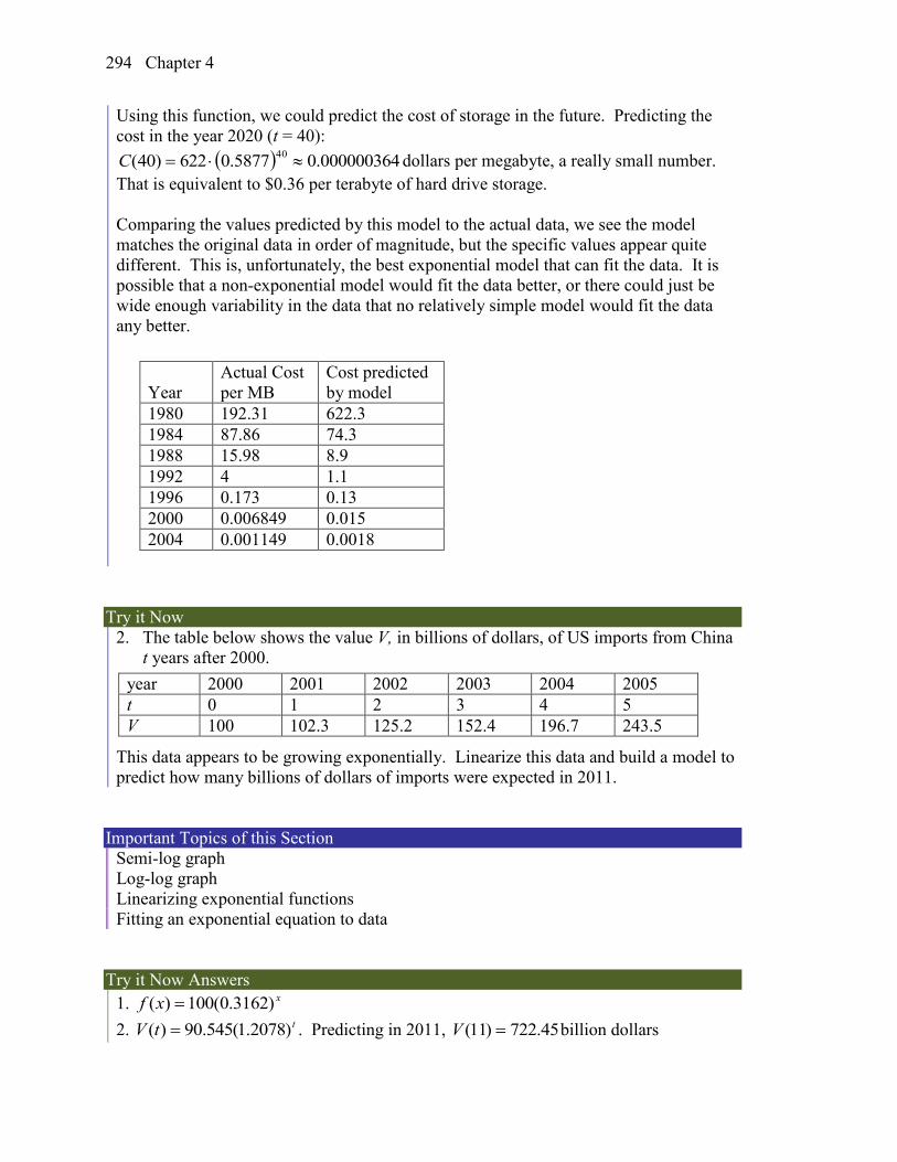
Chapter 4 294
Using this function, we could predict the cost of storage in the future. Predicting the
cost in the year 2020 (t = 40):
000000364.05877.0622)40(40C dollars per megabyte, a really small number.
That is equivalent to $0.36 per terabyte of hard drive storage.
Comparing the values predicted by this model to the actual data, we see the model
matches the original data in order of magnitude, but the specific values appear quite
different. This is, unfortunately, the best exponential model that can fit the data. It is
possible that a non-exponential model would fit the data better, or there could just be
wide enough variability in the data that no relatively simple model would fit the data
any better.
Try it Now
2. The table below shows the value V, in billions of dollars, of US imports from China
t years after 2000.
This data appears to be growing exponentially. Linearize this data and build a model to
predict how many billions of dollars of imports were expected in 2011.
Important Topics of this Section
Semi-log graph
Log-log graph
Linearizing exponential functions
Fitting an exponential equation to data
Try it Now Answers
1. xxf )3162.0(100)(
2. ttV )2078.1(545.90)( . Predicting in 2011, 45.722)11( V billion dollars
Year
Actual Cost
per MB
Cost predicted
by model
1980 192.31 622.3
1984 87.86 74.3
1988 15.98 8.9
1992 4 1.1
1996 0.173 0.13
2000 0.006849 0.015
2004 0.001149 0.0018
year 2000 2001 2002 2003 2004 2005
t 0 1 2 3 4 5
V 100 102.3 125.2 152.4 196.7 243.5
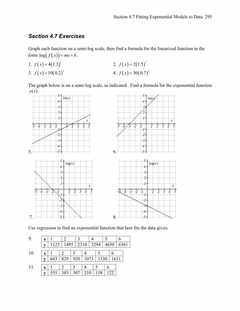
Section 4.7 Fitting Exponential Models to Data 295
Section 4.7 Exercises
Graph each function on a semi-log scale, then find a formula for the linearized function in the
form log f x mx b .
1. 4 1.3x
f x 2. 2 1.5x
f x
3. 10 0.2x
f x 4. 30 0.7x
f x
The graph below is on a semi-log scale, as indicated. Find a formula for the exponential function
( )y x .
5. 6.
7. 8.
Use regression to find an exponential function that best fits the data given.
9. x 1 2 3 4 5 6
y 1125 1495 2310 3294 4650 6361
10. x 1 2 3 4 5 6
y 643 829 920 1073 1330 1631
11. x 1 2 3 4 5 6
y 555 383 307 210 158 122
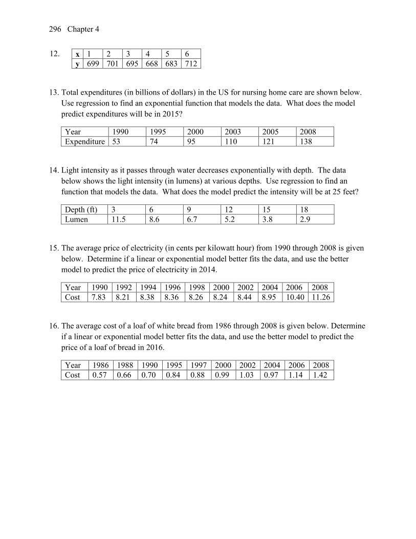
Chapter 4 296
12. x 1 2 3 4 5 6
y 699 701 695 668 683 712
13. Total expenditures (in billions of dollars) in the US for nursing home care are shown below.
Use regression to find an exponential function that models the data. What does the model
predict expenditures will be in 2015?
Year 1990 1995 2000 2003 2005 2008
Expenditure 53 74 95 110 121 138
14. Light intensity as it passes through water decreases exponentially with depth. The data
below shows the light intensity (in lumens) at various depths. Use regression to find an
function that models the data. What does the model predict the intensity will be at 25 feet?
Depth (ft) 3 6 9 12 15 18
Lumen 11.5 8.6 6.7 5.2 3.8 2.9
15. The average price of electricity (in cents per kilowatt hour) from 1990 through 2008 is given
below. Determine if a linear or exponential model better fits the data, and use the better
model to predict the price of electricity in 2014.
Year 1990 1992 1994 1996 1998 2000 2002 2004 2006 2008
Cost 7.83 8.21 8.38 8.36 8.26 8.24 8.44 8.95 10.40 11.26
16. The average cost of a loaf of white bread from 1986 through 2008 is given below. Determine
if a linear or exponential model better fits the data, and use the better model to predict the
price of a loaf of bread in 2016.
Year 1986 1988 1990 1995 1997 2000 2002 2004 2006 2008
Cost 0.57 0.66 0.70 0.84 0.88 0.99 1.03 0.97 1.14 1.42
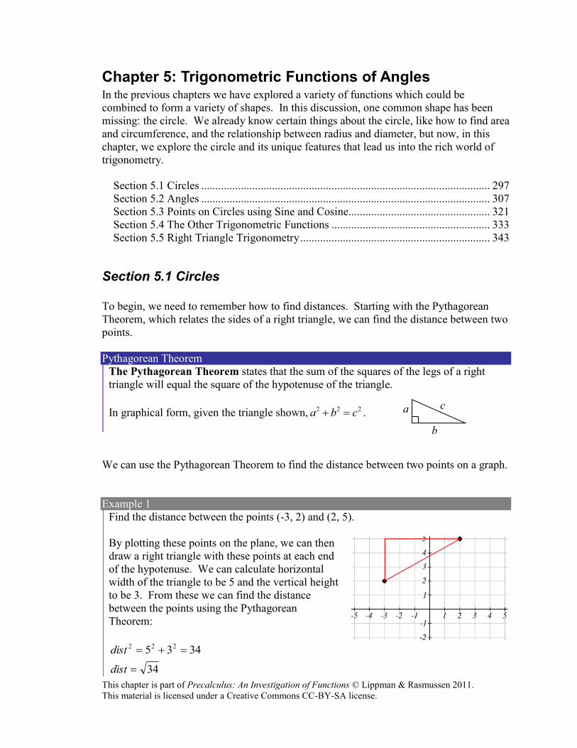
This chapter is part of Precalculus: An Investigation of Functions © Lippman & Rasmussen 2011.
This material is licensed under a Creative Commons CC-BY-SA license.
Chapter 5: Trigonometric Functions of Angles In the previous chapters we have explored a variety of functions which could be
combined to form a variety of shapes. In this discussion, one common shape has been
missing: the circle. We already know certain things about the circle, like how to find area
and circumference, and the relationship between radius and diameter, but now, in this
chapter, we explore the circle and its unique features that lead us into the rich world of
trigonometry.
Section 5.1 Circles ...................................................................................................... 297 Section 5.2 Angles ...................................................................................................... 307
Section 5.3 Points on Circles using Sine and Cosine.................................................. 321 Section 5.4 The Other Trigonometric Functions ........................................................ 333 Section 5.5 Right Triangle Trigonometry ................................................................... 343
Section 5.1 Circles
To begin, we need to remember how to find distances. Starting with the Pythagorean
Theorem, which relates the sides of a right triangle, we can find the distance between two
points.
Pythagorean Theorem
The Pythagorean Theorem states that the sum of the squares of the legs of a right
triangle will equal the square of the hypotenuse of the triangle.
In graphical form, given the triangle shown, 2 2 2a b c .
We can use the Pythagorean Theorem to find the distance between two points on a graph.
Example 1
Find the distance between the points (-3, 2) and (2, 5).
By plotting these points on the plane, we can then
draw a right triangle with these points at each end
of the hypotenuse. We can calculate horizontal
width of the triangle to be 5 and the vertical height
to be 3. From these we can find the distance
between the points using the Pythagorean
Theorem:
34
3435 222
dist
dist
a
b
c
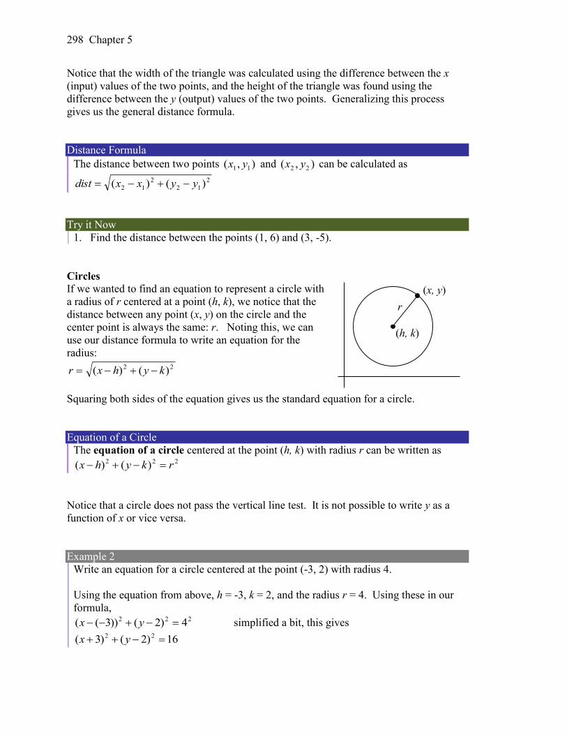
298 Chapter 5
Notice that the width of the triangle was calculated using the difference between the x
(input) values of the two points, and the height of the triangle was found using the
difference between the y (output) values of the two points. Generalizing this process
gives us the general distance formula.
Distance Formula
The distance between two points ),( 11 yx and ),( 22 yx can be calculated as
2
12
2
12 )()( yyxxdist
Try it Now
1. Find the distance between the points (1, 6) and (3, -5).
Circles If we wanted to find an equation to represent a circle with
a radius of r centered at a point (h, k), we notice that the
distance between any point (x, y) on the circle and the
center point is always the same: r. Noting this, we can
use our distance formula to write an equation for the
radius: 22 )()( kyhxr
Squaring both sides of the equation gives us the standard equation for a circle.
Equation of a Circle
The equation of a circle centered at the point (h, k) with radius r can be written as 222 )()( rkyhx
Notice that a circle does not pass the vertical line test. It is not possible to write y as a
function of x or vice versa.
Example 2
Write an equation for a circle centered at the point (-3, 2) with radius 4.
Using the equation from above, h = -3, k = 2, and the radius r = 4. Using these in our
formula, 222 4)2())3(( yx simplified a bit, this gives
16)2()3( 22 yx
r
(h, k)
(x, y)
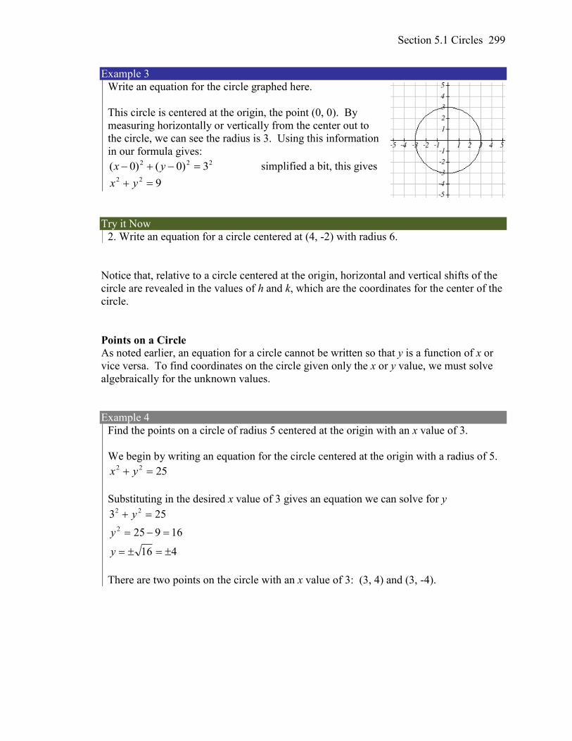
Section 5.1 Circles 299
Example 3
Write an equation for the circle graphed here.
This circle is centered at the origin, the point (0, 0). By
measuring horizontally or vertically from the center out to
the circle, we can see the radius is 3. Using this information
in our formula gives: 222 3)0()0( yx simplified a bit, this gives
922 yx
Try it Now
2. Write an equation for a circle centered at (4, -2) with radius 6.
Notice that, relative to a circle centered at the origin, horizontal and vertical shifts of the
circle are revealed in the values of h and k, which are the coordinates for the center of the
circle.
Points on a Circle As noted earlier, an equation for a circle cannot be written so that y is a function of x or
vice versa. To find coordinates on the circle given only the x or y value, we must solve
algebraically for the unknown values.
Example 4
Find the points on a circle of radius 5 centered at the origin with an x value of 3.
We begin by writing an equation for the circle centered at the origin with a radius of 5.
2522 yx
Substituting in the desired x value of 3 gives an equation we can solve for y
416
16925
253
2
22
y
y
y
There are two points on the circle with an x value of 3: (3, 4) and (3, -4).
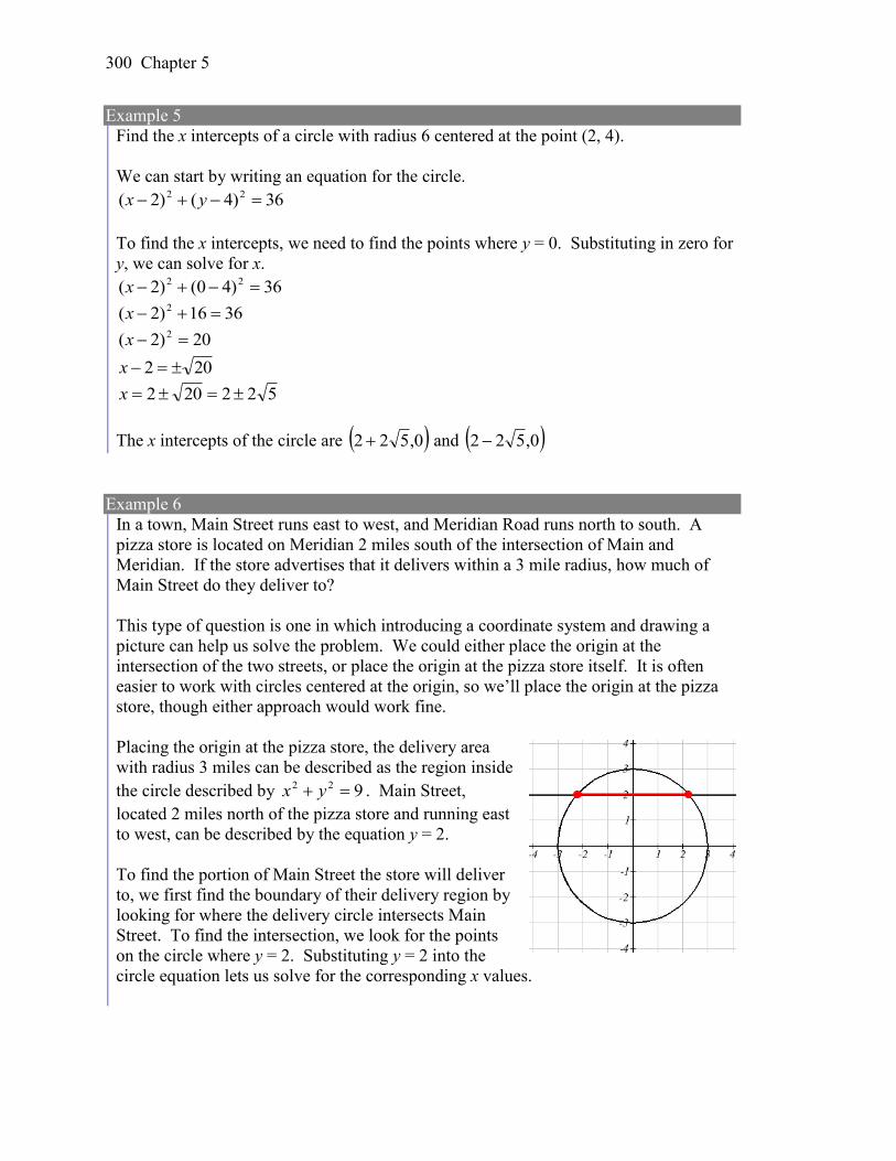
300 Chapter 5
Example 5
Find the x intercepts of a circle with radius 6 centered at the point (2, 4).
We can start by writing an equation for the circle.
36)4()2( 22 yx
To find the x intercepts, we need to find the points where y = 0. Substituting in zero for
y, we can solve for x.
36)40()2( 22 x
3616)2( 2 x
20)2( 2 x
202 x
522202 x
The x intercepts of the circle are 0,522 and 0,522
Example 6
In a town, Main Street runs east to west, and Meridian Road runs north to south. A
pizza store is located on Meridian 2 miles south of the intersection of Main and
Meridian. If the store advertises that it delivers within a 3 mile radius, how much of
Main Street do they deliver to?
This type of question is one in which introducing a coordinate system and drawing a
picture can help us solve the problem. We could either place the origin at the
intersection of the two streets, or place the origin at the pizza store itself. It is often
easier to work with circles centered at the origin, so we’ll place the origin at the pizza
store, though either approach would work fine.
Placing the origin at the pizza store, the delivery area
with radius 3 miles can be described as the region inside
the circle described by 922 yx . Main Street,
located 2 miles north of the pizza store and running east
to west, can be described by the equation y = 2.
To find the portion of Main Street the store will deliver
to, we first find the boundary of their delivery region by
looking for where the delivery circle intersects Main
Street. To find the intersection, we look for the points
on the circle where y = 2. Substituting y = 2 into the
circle equation lets us solve for the corresponding x values.
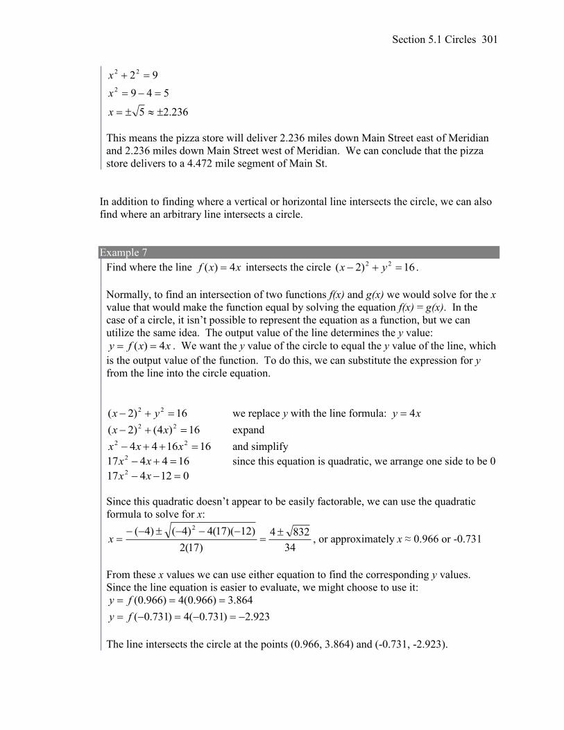
Section 5.1 Circles 301
236.25
549
92
2
22
x
x
x
This means the pizza store will deliver 2.236 miles down Main Street east of Meridian
and 2.236 miles down Main Street west of Meridian. We can conclude that the pizza
store delivers to a 4.472 mile segment of Main St.
In addition to finding where a vertical or horizontal line intersects the circle, we can also
find where an arbitrary line intersects a circle.
Example 7
Find where the line xxf 4)( intersects the circle 16)2( 22 yx .
Normally, to find an intersection of two functions f(x) and g(x) we would solve for the x
value that would make the function equal by solving the equation f(x) = g(x). In the
case of a circle, it isn’t possible to represent the equation as a function, but we can
utilize the same idea. The output value of the line determines the y value:
xxfy 4)( . We want the y value of the circle to equal the y value of the line, which
is the output value of the function. To do this, we can substitute the expression for y
from the line into the circle equation.
16)2( 22 yx we replace y with the line formula: xy 4
16)4()2( 22 xx expand
161644 22 xxx and simplify
164417 2 xx since this equation is quadratic, we arrange one side to be 0
012417 2 xx
Since this quadratic doesn’t appear to be easily factorable, we can use the quadratic
formula to solve for x:
34
8324
)17(2
)12)(17(4)4()4( 2
x , or approximately x ≈ 0.966 or -0.731
From these x values we can use either equation to find the corresponding y values.
Since the line equation is easier to evaluate, we might choose to use it:
923.2)731.0(4)731.0(
864.3)966.0(4)966.0(
fy
fy
The line intersects the circle at the points (0.966, 3.864) and (-0.731, -2.923).
302 Chapter 5
Try it Now
3. A small radio transmitter broadcasts in a 50 mile radius. If you drive along a straight
line from a city 60 miles north of the transmitter to a second city 70 miles east of the
transmitter, during how much of the drive will you pick up a signal from the
transmitter?
Important Topics of This Section
Distance formula
Equation of a Circle
Finding the x coordinate of a point on the circle given the y coordinate or vice versa
Finding the intersection of a circle and a line
Try it Now Answers
1. 55
2. 36)2()4( 22 yx
3.
2
2 26060 50
70x x
gives x = 14 or x = 45.29, corresponding to points (14,
48)and (45.29, 21.18), resulting in a distance of 41.21 miles.
Section 5.1 Circles 303
Section 5.1 Exercises
1. Find the distance between the points (5,3) and (-1,-5).
2. Find the distance between the points (3,3) and (-3,-2).
3. Write an equation of the circle centered at (8 , -10) with radius 8.
4. Write an equation of the circle centered at (-9, 9) with radius 16.
5. Write an equation of the circle centered at (7, -2) that passes through (-10, 0).
6. Write an equation of the circle centered at (3, -7) that passes through (15, 13).
7. Write an equation for a circle where the points (2, 6) and (8, 10) lie along a diameter.
8. Write an equation for a circle where the points (-3, 3) and (5, 7) lie along a diameter.
9. Sketch a graph of 2 2
2 3 9x y .
10. Sketch a graph of 2 2
1 2 1 6x y .
11. Find the y intercept(s) of the circle with center (2, 3) with radius 3.
12. Find the x intercept(s) of the circle with center (2, 3) with radius 4.
13. At what point in the first quadrant does the line with equation 2 5y x intersect a
circle with radius 3 and center (0, 5)?
14. At what point in the first quadrant does the line with equation 2y x intersect the
circle with radius 6 and center (0, 2)?
15. At what point in the second quadrant does the line with equation 2 5y x intersect a
circle with radius 3 and center (-2, 0)?
16. At what point in the first quadrant does the line with equation 2y x intersect the
circle with radius 6 and center (-1,0)?
17. A small radio transmitter broadcasts in a 53 mile radius. If you drive along a straight
line from a city 70 miles north of the transmitter to a second city 74 miles east of the
transmitter, during how much of the drive will you pick up a signal from the
transmitter?
18. A small radio transmitter broadcasts in a 44 mile radius. If you drive along a straight
line from a city 56 miles south of the transmitter to a second city 53 miles west of the
transmitter, during how much of the drive will you pick up a signal from the
transmitter?
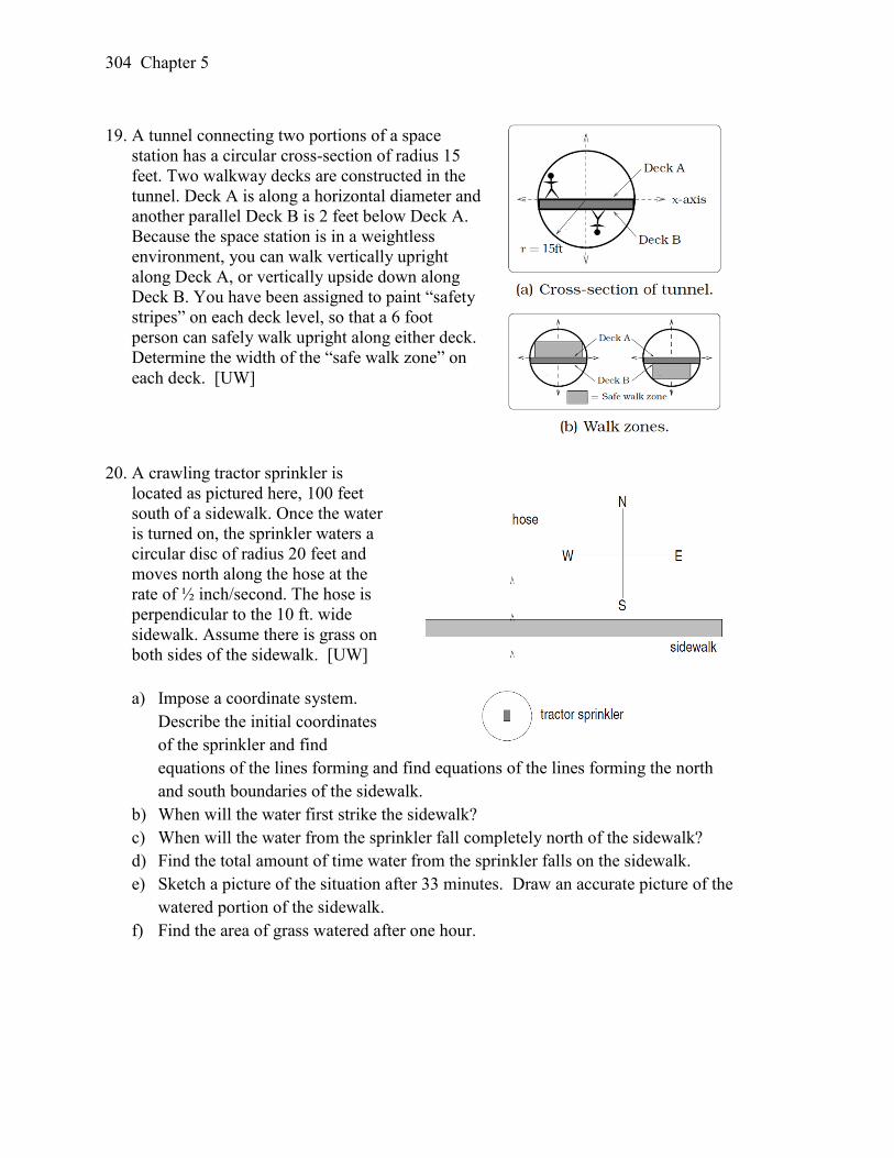
304 Chapter 5
19. A tunnel connecting two portions of a space
station has a circular cross-section of radius 15
feet. Two walkway decks are constructed in the
tunnel. Deck A is along a horizontal diameter and
another parallel Deck B is 2 feet below Deck A.
Because the space station is in a weightless
environment, you can walk vertically upright
along Deck A, or vertically upside down along
Deck B. You have been assigned to paint “safety
stripes” on each deck level, so that a 6 foot
person can safely walk upright along either deck.
Determine the width of the “safe walk zone” on
each deck. [UW]
20. A crawling tractor sprinkler is
located as pictured here, 100 feet
south of a sidewalk. Once the water
is turned on, the sprinkler waters a
circular disc of radius 20 feet and
moves north along the hose at the
rate of ½ inch/second. The hose is
perpendicular to the 10 ft. wide
sidewalk. Assume there is grass on
both sides of the sidewalk. [UW]
a) Impose a coordinate system.
Describe the initial coordinates
of the sprinkler and find
equations of the lines forming and find equations of the lines forming the north
and south boundaries of the sidewalk.
b) When will the water first strike the sidewalk?
c) When will the water from the sprinkler fall completely north of the sidewalk?
d) Find the total amount of time water from the sprinkler falls on the sidewalk.
e) Sketch a picture of the situation after 33 minutes. Draw an accurate picture of the
watered portion of the sidewalk.
f) Find the area of grass watered after one hour.
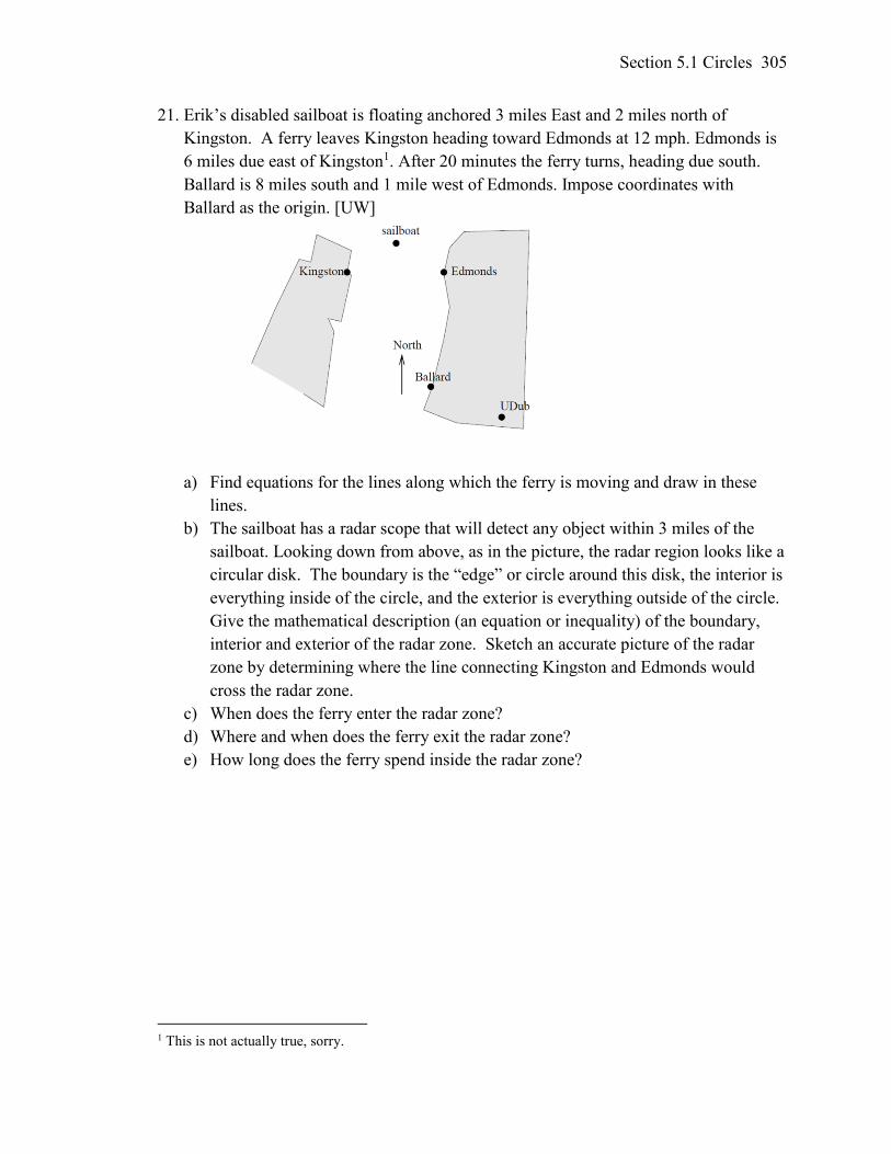
Section 5.1 Circles 305
21. Erik’s disabled sailboat is floating anchored 3 miles East and 2 miles north of
Kingston. A ferry leaves Kingston heading toward Edmonds at 12 mph. Edmonds is
6 miles due east of Kingston1. After 20 minutes the ferry turns, heading due south.
Ballard is 8 miles south and 1 mile west of Edmonds. Impose coordinates with
Ballard as the origin. [UW]
a) Find equations for the lines along which the ferry is moving and draw in these
lines.
b) The sailboat has a radar scope that will detect any object within 3 miles of the
sailboat. Looking down from above, as in the picture, the radar region looks like a
circular disk. The boundary is the “edge” or circle around this disk, the interior is
everything inside of the circle, and the exterior is everything outside of the circle.
Give the mathematical description (an equation or inequality) of the boundary,
interior and exterior of the radar zone. Sketch an accurate picture of the radar
zone by determining where the line connecting Kingston and Edmonds would
cross the radar zone.
c) When does the ferry enter the radar zone?
d) Where and when does the ferry exit the radar zone?
e) How long does the ferry spend inside the radar zone?
1 This is not actually true, sorry.
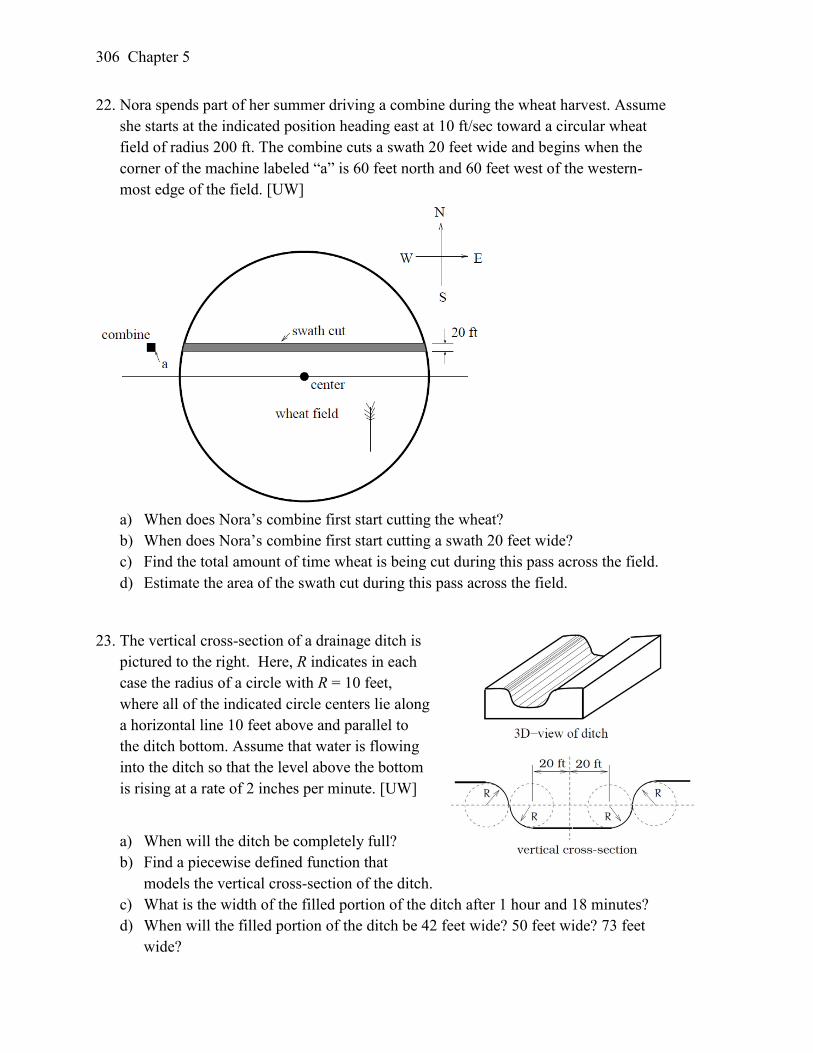
306 Chapter 5
22. Nora spends part of her summer driving a combine during the wheat harvest. Assume
she starts at the indicated position heading east at 10 ft/sec toward a circular wheat
field of radius 200 ft. The combine cuts a swath 20 feet wide and begins when the
corner of the machine labeled “a” is 60 feet north and 60 feet west of the western-
most edge of the field. [UW]
a) When does Nora’s combine first start cutting the wheat?
b) When does Nora’s combine first start cutting a swath 20 feet wide?
c) Find the total amount of time wheat is being cut during this pass across the field.
d) Estimate the area of the swath cut during this pass across the field.
23. The vertical cross-section of a drainage ditch is
pictured to the right. Here, R indicates in each
case the radius of a circle with R = 10 feet,
where all of the indicated circle centers lie along
a horizontal line 10 feet above and parallel to
the ditch bottom. Assume that water is flowing
into the ditch so that the level above the bottom
is rising at a rate of 2 inches per minute. [UW]
a) When will the ditch be completely full?
b) Find a piecewise defined function that
models the vertical cross-section of the ditch.
c) What is the width of the filled portion of the ditch after 1 hour and 18 minutes?
d) When will the filled portion of the ditch be 42 feet wide? 50 feet wide? 73 feet
wide?
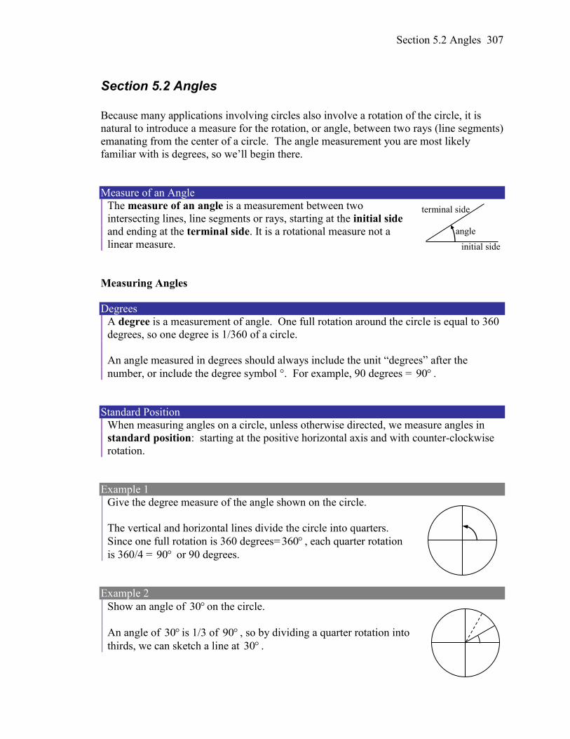
Section 5.2 Angles 307
Section 5.2 Angles
Because many applications involving circles also involve a rotation of the circle, it is
natural to introduce a measure for the rotation, or angle, between two rays (line segments)
emanating from the center of a circle. The angle measurement you are most likely
familiar with is degrees, so we’ll begin there.
Measure of an Angle
The measure of an angle is a measurement between two
intersecting lines, line segments or rays, starting at the initial side
and ending at the terminal side. It is a rotational measure not a
linear measure.
Measuring Angles
Degrees
A degree is a measurement of angle. One full rotation around the circle is equal to 360
degrees, so one degree is 1/360 of a circle.
An angle measured in degrees should always include the unit “degrees” after the
number, or include the degree symbol °. For example, 90 degrees = 90 .
Standard Position
When measuring angles on a circle, unless otherwise directed, we measure angles in
standard position: starting at the positive horizontal axis and with counter-clockwise
rotation.
Example 1
Give the degree measure of the angle shown on the circle.
The vertical and horizontal lines divide the circle into quarters.
Since one full rotation is 360 degrees= 360 , each quarter rotation
is 360/4 = 90 or 90 degrees.
Example 2
Show an angle of 30 on the circle.
An angle of 30 is 1/3 of 90 , so by dividing a quarter rotation into
thirds, we can sketch a line at 30 .
initial side
terminal side
angle
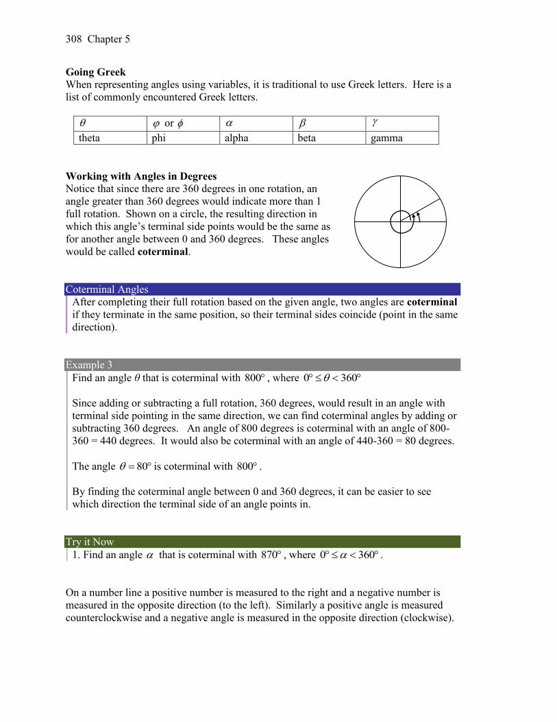
308 Chapter 5
Going Greek
When representing angles using variables, it is traditional to use Greek letters. Here is a
list of commonly encountered Greek letters.
or
theta phi alpha beta gamma
Working with Angles in Degrees Notice that since there are 360 degrees in one rotation, an
angle greater than 360 degrees would indicate more than 1
full rotation. Shown on a circle, the resulting direction in
which this angle’s terminal side points would be the same as
for another angle between 0 and 360 degrees. These angles
would be called coterminal.
Coterminal Angles
After completing their full rotation based on the given angle, two angles are coterminal
if they terminate in the same position, so their terminal sides coincide (point in the same
direction).
Example 3
Find an angle θ that is coterminal with 800 , where 0 360
Since adding or subtracting a full rotation, 360 degrees, would result in an angle with
terminal side pointing in the same direction, we can find coterminal angles by adding or
subtracting 360 degrees. An angle of 800 degrees is coterminal with an angle of 800-
360 = 440 degrees. It would also be coterminal with an angle of 440-360 = 80 degrees.
The angle 80 is coterminal with 800 .
By finding the coterminal angle between 0 and 360 degrees, it can be easier to see
which direction the terminal side of an angle points in.
Try it Now
1. Find an angle that is coterminal with 870 , where 3600 .
On a number line a positive number is measured to the right and a negative number is
measured in the opposite direction (to the left). Similarly a positive angle is measured
counterclockwise and a negative angle is measured in the opposite direction (clockwise).
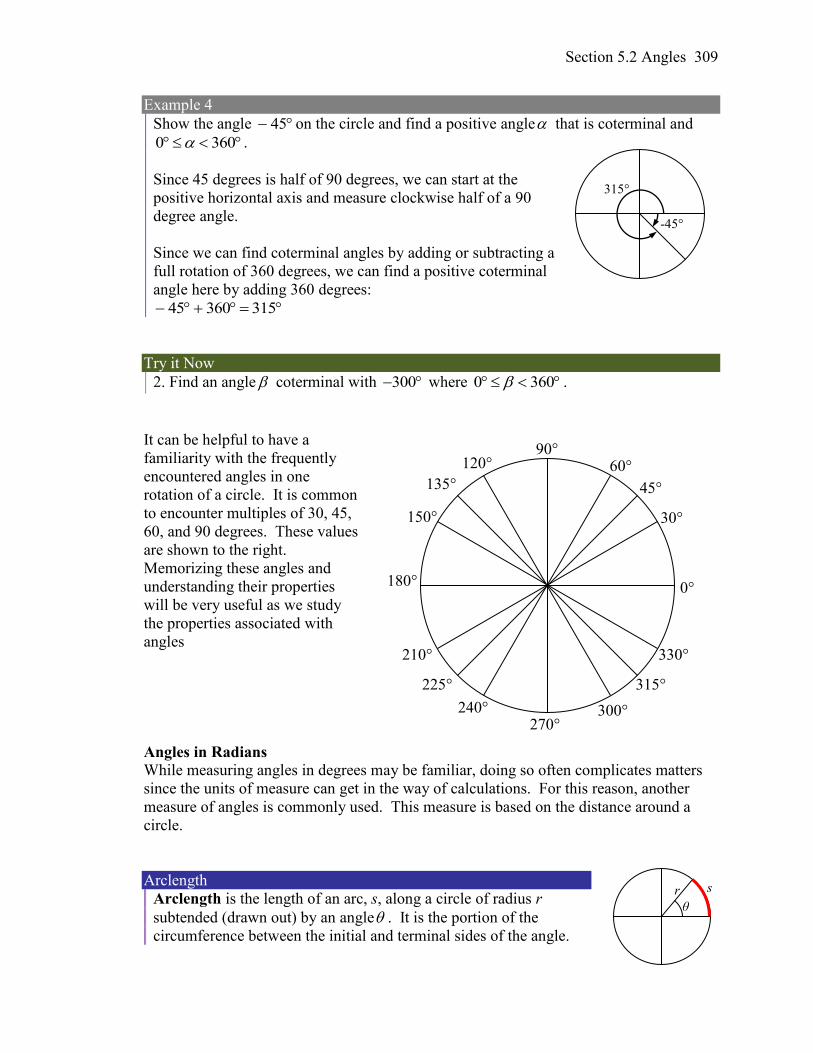
Section 5.2 Angles 309
Example 4
Show the angle 45 on the circle and find a positive angle that is coterminal and
3600 .
Since 45 degrees is half of 90 degrees, we can start at the
positive horizontal axis and measure clockwise half of a 90
degree angle.
Since we can find coterminal angles by adding or subtracting a
full rotation of 360 degrees, we can find a positive coterminal
angle here by adding 360 degrees:
31536045
Try it Now
2. Find an angle coterminal with 300 where 0 360 .
It can be helpful to have a
familiarity with the frequently
encountered angles in one
rotation of a circle. It is common
to encounter multiples of 30, 45,
60, and 90 degrees. These values
are shown to the right.
Memorizing these angles and
understanding their properties
will be very useful as we study
the properties associated with
angles
Angles in Radians
While measuring angles in degrees may be familiar, doing so often complicates matters
since the units of measure can get in the way of calculations. For this reason, another
measure of angles is commonly used. This measure is based on the distance around a
circle.
Arclength
Arclength is the length of an arc, s, along a circle of radius r
subtended (drawn out) by an angle . It is the portion of the
circumference between the initial and terminal sides of the angle.
-45°
315°
θ
r s
0°
30°
60° 90°
120°
150°
180°
210°
240° 270°
300°
330°
45° 135°
225° 315°
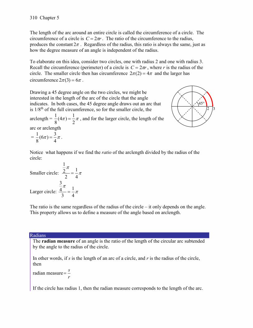
310 Chapter 5
The length of the arc around an entire circle is called the circumference of a circle. The
circumference of a circle is rC 2 . The ratio of the circumference to the radius,
produces the constant 2 . Regardless of the radius, this ratio is always the same, just as
how the degree measure of an angle is independent of the radius.
To elaborate on this idea, consider two circles, one with radius 2 and one with radius 3.
Recall the circumference (perimeter) of a circle is rC 2 , where r is the radius of the
circle. The smaller circle then has circumference 4)2(2 and the larger has
circumference 6)3(2 .
Drawing a 45 degree angle on the two circles, we might be
interested in the length of the arc of the circle that the angle
indicates. In both cases, the 45 degree angle draws out an arc that
is 1/8th of the full circumference, so for the smaller circle, the
arclength = 1 1
(4 )8 2
, and for the larger circle, the length of the
arc or arclength
= 1 3
(6 )8 4
.
Notice what happens if we find the ratio of the arclength divided by the radius of the
circle:
Smaller circle:
112
2 4
Larger circle:
314
3 4
The ratio is the same regardless of the radius of the circle – it only depends on the angle.
This property allows us to define a measure of the angle based on arclength.
Radians
The radian measure of an angle is the ratio of the length of the circular arc subtended
by the angle to the radius of the circle.
In other words, if s is the length of an arc of a circle, and r is the radius of the circle,
then
radian measures
r
If the circle has radius 1, then the radian measure corresponds to the length of the arc.
45°
2 3
Section 5.2 Angles 311
Because radian measure is the ratio of two lengths, it is a unitless measure. It is not
necessary to write the label “radians” after a radian measure, and if you see an angle that
is not labeled with “degrees” or the degree symbol, you should assume that it is a radian
measure.
Considering the most basic case, the unit circle (a circle with radius 1), we know that 1
rotation equals 360 degrees, 360 . We can also track one rotation around a circle by
finding the circumference, rC 2 , and for the unit circle 2C . These two different
ways to rotate around a circle give us a way to convert from degrees to radians.
1 rotation = 360 = 2 radians
½ rotation = 180 = radians
¼ rotation = 90 = 2/ radians
Example 5
Find the radian measure of one third of a full rotation.
For any circle, the arclength along such a rotation would be one third of the
circumference, 3
2)2(
3
1 rrC
. The radian measure would be the arclength divided
by the radius:
Radian measure = 2 2
3 3
r
r
.
Converting Between Radians and Degrees
1 degree = 180
radians
or: to convert from degrees to radians, multiply by radians
180
1 radian = 180
degrees
or: to convert from radians to degrees, multiply by 180
radians
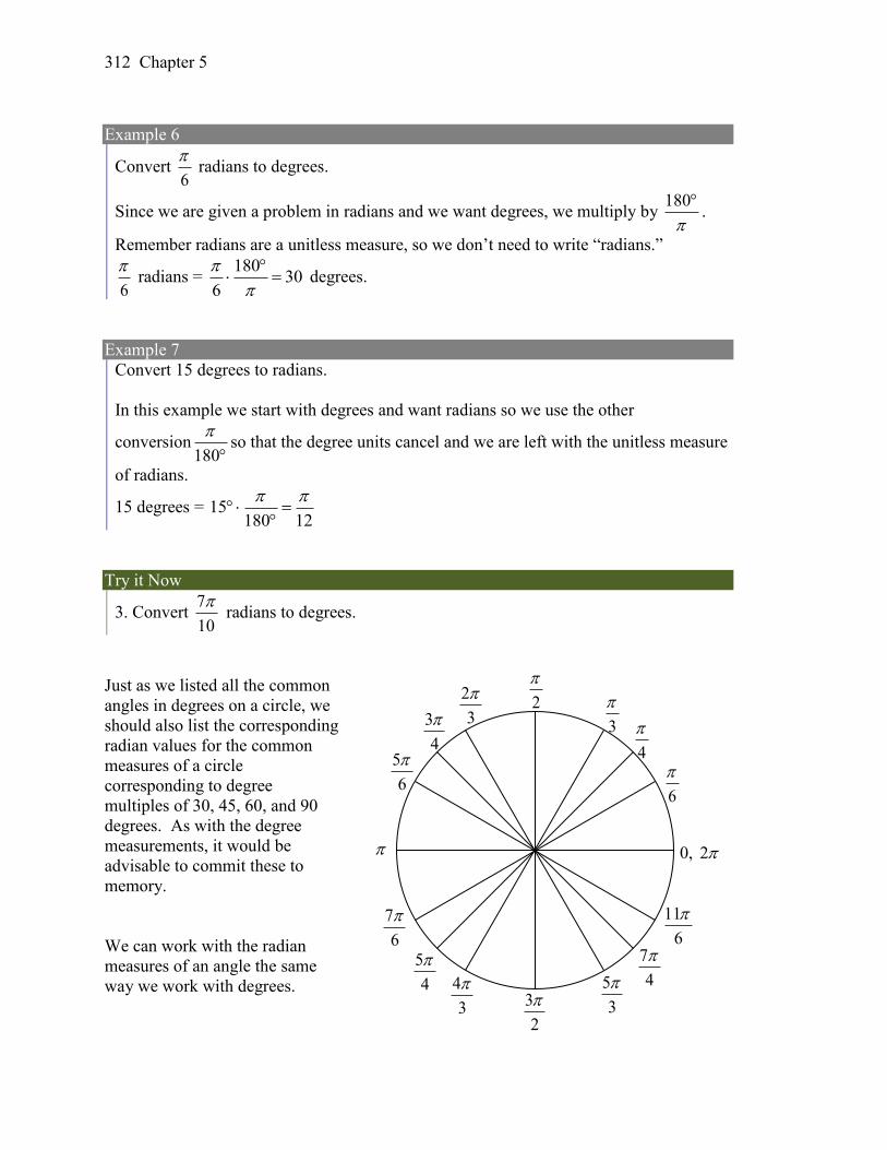
312 Chapter 5
Example 6
Convert 6
radians to degrees.
Since we are given a problem in radians and we want degrees, we multiply by
180.
Remember radians are a unitless measure, so we don’t need to write “radians.”
6
radians = 30
180
6
degrees.
Example 7
Convert 15 degrees to radians.
In this example we start with degrees and want radians so we use the other
conversion180
so that the degree units cancel and we are left with the unitless measure
of radians.
15 degrees = 12180
15
Try it Now
3. Convert 10
7 radians to degrees.
Just as we listed all the common
angles in degrees on a circle, we
should also list the corresponding
radian values for the common
measures of a circle
corresponding to degree
multiples of 30, 45, 60, and 90
degrees. As with the degree
measurements, it would be
advisable to commit these to
memory.
We can work with the radian
measures of an angle the same
way we work with degrees.
0, 2
6
4
3
2
2
3
3
4
5
6
7
6
5
4
4
3
3
2
5
3
7
4
11
6
Section 5.2 Angles 313
Example 8
Find an angle that is coterminal with 19
4
, where 20
When working in degrees, we found coterminal angles by adding or subtracting 360
degrees, a full rotation. Likewise, in radians, we can find coterminal angles by adding
or subtracting full rotations of 2 radians.
19 19 8 112
4 4 4 4
The angle11
4
is coterminal, but not less than 2 , so we subtract another rotation.
11 11 8 32
4 4 4 4
The angle 3
4
is coterminal with
19
4
.
Try it Now
4. Find an angle that is coterminal with 17
6
where 20 .
Arclength and Area of a Sector
Recall that the radian measure of an angle was defined as the ratio of the arclength of a
circular arc to the radius of the circle, s
r . From this relationship, we can find
arclength along a circle given an angle.
Arclength on a Circle
The length of an arc, s, along a circle of radius r subtended by angle in radians is
s r
Example 9
Mercury orbits the sun at a distance of approximately 36 million miles. In one Earth
day, it completes 0.0114 rotation around the sun. If the orbit was perfectly circular,
what distance through space would Mercury travel in one Earth day?
To begin, we will need to convert the decimal rotation value to a radian measure. Since
one rotation = 2 radians,
0.0114 rotation = 2 (0.0114) 0.0716 radians.
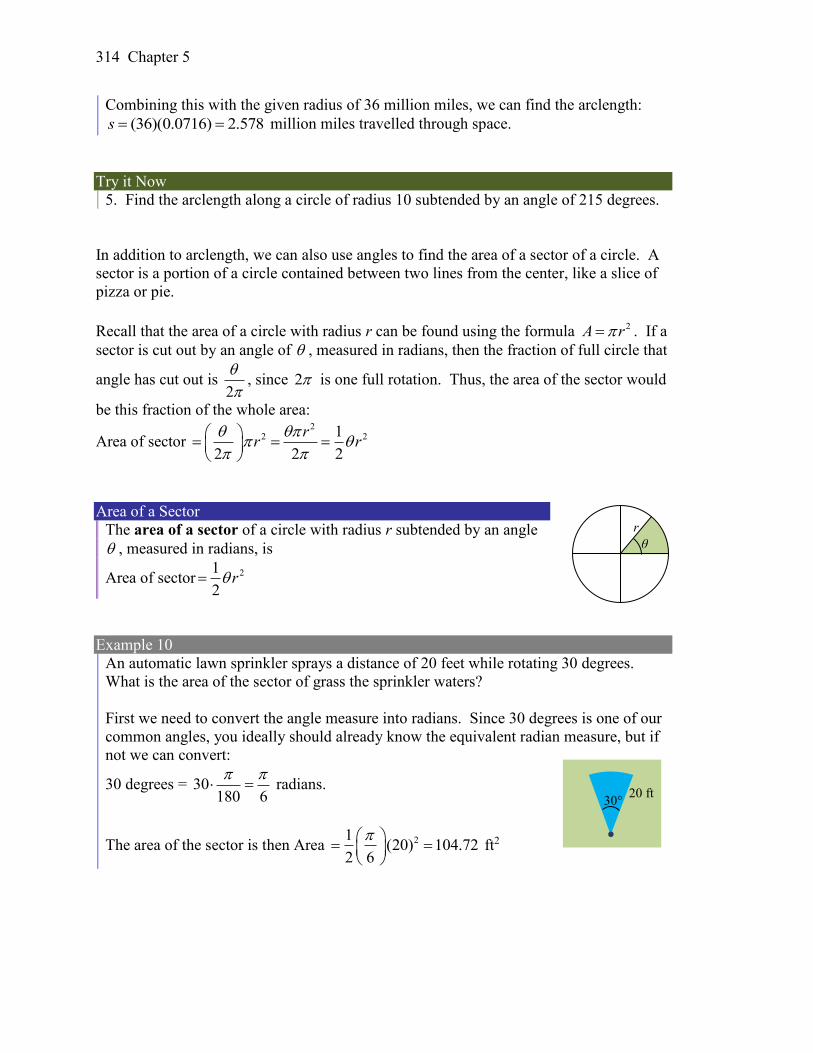
314 Chapter 5
Combining this with the given radius of 36 million miles, we can find the arclength:
(36)(0.0716) 2.578s million miles travelled through space.
Try it Now
5. Find the arclength along a circle of radius 10 subtended by an angle of 215 degrees.
In addition to arclength, we can also use angles to find the area of a sector of a circle. A
sector is a portion of a circle contained between two lines from the center, like a slice of
pizza or pie.
Recall that the area of a circle with radius r can be found using the formula 2A r . If a
sector is cut out by an angle of , measured in radians, then the fraction of full circle that
angle has cut out is 2
, since 2 is one full rotation. Thus, the area of the sector would
be this fraction of the whole area:
Area of sector 2
2 21
2 2 2
rr r
Area of a Sector
The area of a sector of a circle with radius r subtended by an angle
, measured in radians, is
Area of sector 21
2r
Example 10
An automatic lawn sprinkler sprays a distance of 20 feet while rotating 30 degrees.
What is the area of the sector of grass the sprinkler waters?
First we need to convert the angle measure into radians. Since 30 degrees is one of our
common angles, you ideally should already know the equivalent radian measure, but if
not we can convert:
30 degrees = 30180 6
radians.
The area of the sector is then Area 21(20) 104.72
2 6
ft2
r
θ
20 ft 30°
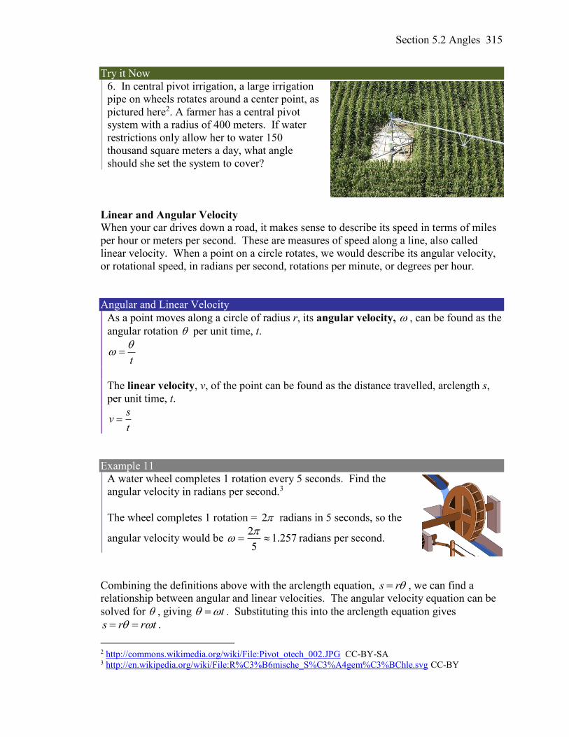
Section 5.2 Angles 315
Try it Now
6. In central pivot irrigation, a large irrigation
pipe on wheels rotates around a center point, as
pictured here2. A farmer has a central pivot
system with a radius of 400 meters. If water
restrictions only allow her to water 150
thousand square meters a day, what angle
should she set the system to cover?
Linear and Angular Velocity When your car drives down a road, it makes sense to describe its speed in terms of miles
per hour or meters per second. These are measures of speed along a line, also called
linear velocity. When a point on a circle rotates, we would describe its angular velocity,
or rotational speed, in radians per second, rotations per minute, or degrees per hour.
Angular and Linear Velocity
As a point moves along a circle of radius r, its angular velocity, , can be found as the
angular rotation per unit time, t.
t
The linear velocity, v, of the point can be found as the distance travelled, arclength s,
per unit time, t.
sv
t
Example 11
A water wheel completes 1 rotation every 5 seconds. Find the
angular velocity in radians per second.3
The wheel completes 1 rotation = 2 radians in 5 seconds, so the
angular velocity would be 2
1.2575
radians per second.
Combining the definitions above with the arclength equation, s r , we can find a
relationship between angular and linear velocities. The angular velocity equation can be
solved for , giving t . Substituting this into the arclength equation gives
s r r t .
2 http://commons.wikimedia.org/wiki/File:Pivot_otech_002.JPG CC-BY-SA 3 http://en.wikipedia.org/wiki/File:R%C3%B6mische_S%C3%A4gem%C3%BChle.svg CC-BY
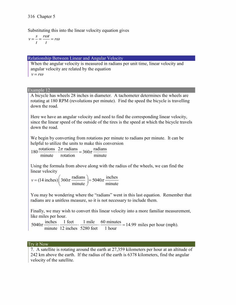
316 Chapter 5
Substituting this into the linear velocity equation gives
s r tv r
t t
Relationship Between Linear and Angular Velocity
When the angular velocity is measured in radians per unit time, linear velocity and
angular velocity are related by the equation
v r
Example 12
A bicycle has wheels 28 inches in diameter. A tachometer determines the wheels are
rotating at 180 RPM (revolutions per minute). Find the speed the bicycle is travelling
down the road.
Here we have an angular velocity and need to find the corresponding linear velocity,
since the linear speed of the outside of the tires is the speed at which the bicycle travels
down the road.
We begin by converting from rotations per minute to radians per minute. It can be
helpful to utilize the units to make this conversion
rotations 2 radians radians180 360
minute rotation minute
Using the formula from above along with the radius of the wheels, we can find the
linear velocity
radians inches(14 inches) 360 5040
minute minutev
You may be wondering where the “radians” went in this last equation. Remember that
radians are a unitless measure, so it is not necessary to include them.
Finally, we may wish to convert this linear velocity into a more familiar measurement,
like miles per hour.
inches 1 feet 1 mile 60 minutes5040 14.99
minute 12 inches 5280 feet 1 hour miles per hour (mph).
Try it Now
7. A satellite is rotating around the earth at 27,359 kilometers per hour at an altitude of
242 km above the earth. If the radius of the earth is 6378 kilometers, find the angular
velocity of the satellite.
Section 5.2 Angles 317
Important Topics of This Section
Degree measure of angle
Radian measure of angle
Conversion between degrees and radians
Common angles in degrees and radians
Coterminal angles
Arclength
Area of a sector
Linear and angular velocity
Try it Now Answers
1. 150
2. 60
3. 126
4. 6
7
5. 525.3718
215
6. 43.107
7. 4.1328 radians per hour
318 Chapter 5
Section 5.2 Exercises
1. Indicate each angle on a circle: 30°, 300°, -135°, 70°, 2
3
,
7
4
2. Indicate each angle on a circle: 30°, 315°, -135°, 80°, 7
6
,
3
4
3. Convert the angle 180° to radians.
4. Convert the angle 30° to radians.
5. Convert the angle 5
6
from radians to degrees.
6. Convert the angle 11
6
from radians to degrees.
7. Find the angle between 0° and 360° that is coterminal with a 685° angle.
8. Find the angle between 0° and 360° that is coterminal with a 451° angle.
9. Find the angle between 0° and 360° that is coterminal with a -1746° angle.
10. Find the angle between 0° and 360° that is coterminal with a -1400° angle.
11. Find the angle between 0 and 2π in radians that is coterminal with the angle 26
9
.
12. Find the angle between 0 and 2π in radians that is coterminal with the angle 17
3
.
13. Find the angle between 0 and 2π in radians that is coterminal with the angle 3
2
.
14. Find the angle between 0 and 2π in radians that is coterminal with the angle 7
6
.
15. On a circle of radius 7 miles, find the length of the arc that subtends a central angle of
5 radians.
16. On a circle of radius 6 feet, find the length of the arc that subtends a central angle of 1
radian.
Section 5.2 Angles 319
17. On a circle of radius 12 cm, find the length of the arc that subtends a central angle of
120 degrees.
18. On a circle of radius 9 miles, find the length of the arc that subtends a central angle of
800 degrees.
19. Find the distance along an arc on the surface of the Earth that subtends a central angle
of 5 minutes (1 minute = 1/60 degree). The radius of the Earth is 3960 miles.
20. Find the distance along an arc on the surface of the Earth that subtends a central angle
of 7 minutes (1 minute = 1/60 degree). The radius of the Earth is 3960 miles.
21. On a circle of radius 6 feet, what angle in degrees would subtend an arc of length 3
feet?
22. On a circle of radius 5 feet, what angle in degrees would subtend an arc of length 2
feet?
23. A sector of a circle has a central angle of 45°. Find the area of the sector if the radius
of the circle is 6 cm.
24. A sector of a circle has a central angle of 30°. Find the area of the sector if the radius
of the circle is 20 cm.
25. A truck with 32-in.-diameter wheels is traveling at 60 mi/h. Find the angular speed of
the wheels in rad/min. How many revolutions per minute do the wheels make?
26. A bicycle with 24-in.-diameter wheels is traveling at 15 mi/h. Find the angular speed
of the wheels in rad/min. How many revolutions per minute do the wheels make?
27. A wheel of radius 8 in. is rotating 15°/sec. What is the linear speed v, the angular
speed in RPM, and the angular speed in rad/sec?
28. A wheel of radius 14 in. is rotating 0.5 rad/sec. What is the linear speed v, the angular
speed in RPM, and the angular speed in deg/sec?
29. A CD has diameter of 120 millimeters. When playing audio, the angular speed varies
to keep the linear speed constant where the disc is being read. When reading along
the outer edge of the disc, the angular speed is about 200 RPM (revolutions per
minute). Find the linear speed.
30. When being burned in a writable CD-R drive, the angular speed of a CD is often
much faster than when playing audio, but the angular speed still varies to keep the
linear speed constant where the disc is being written. When writing along the outer
edge of the disc, the angular speed of one drive is about 4800 RPM (revolutions per
minute). Find the linear speed.
320 Chapter 5
31. You are standing on the equator of the Earth (radius 3960 miles). What is your linear
and angular speed?
32. The restaurant in the Space Needle in Seattle rotates at the rate of one revolution per
hour. [UW]
a) Through how many radians does it turn in 100 minutes?
b) How long does it take the restaurant to rotate through 4 radians?
c) How far does a person sitting by the window move in 100 minutes if the radius of
the restaurant is 21 meters?
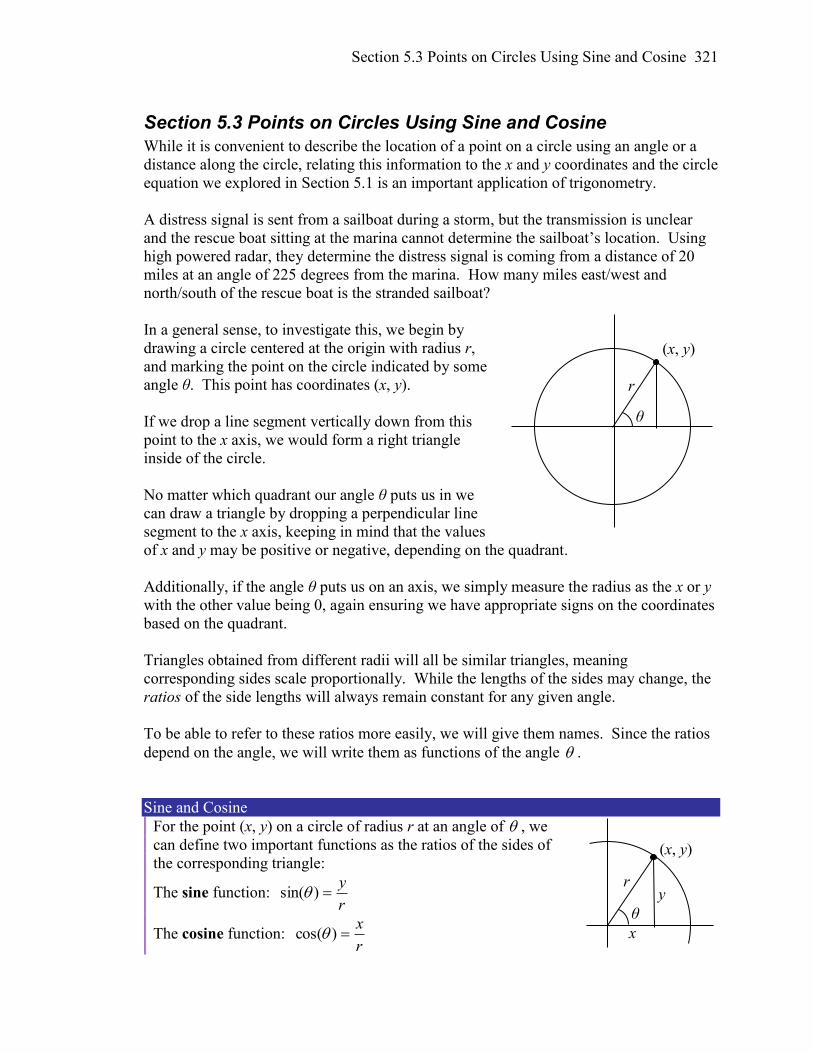
Section 5.3 Points on Circles Using Sine and Cosine 321
Section 5.3 Points on Circles Using Sine and Cosine
While it is convenient to describe the location of a point on a circle using an angle or a
distance along the circle, relating this information to the x and y coordinates and the circle
equation we explored in Section 5.1 is an important application of trigonometry.
A distress signal is sent from a sailboat during a storm, but the transmission is unclear
and the rescue boat sitting at the marina cannot determine the sailboat’s location. Using
high powered radar, they determine the distress signal is coming from a distance of 20
miles at an angle of 225 degrees from the marina. How many miles east/west and
north/south of the rescue boat is the stranded sailboat?
In a general sense, to investigate this, we begin by
drawing a circle centered at the origin with radius r,
and marking the point on the circle indicated by some
angle θ. This point has coordinates (x, y).
If we drop a line segment vertically down from this
point to the x axis, we would form a right triangle
inside of the circle.
No matter which quadrant our angle θ puts us in we
can draw a triangle by dropping a perpendicular line
segment to the x axis, keeping in mind that the values
of x and y may be positive or negative, depending on the quadrant.
Additionally, if the angle θ puts us on an axis, we simply measure the radius as the x or y
with the other value being 0, again ensuring we have appropriate signs on the coordinates
based on the quadrant.
Triangles obtained from different radii will all be similar triangles, meaning
corresponding sides scale proportionally. While the lengths of the sides may change, the
ratios of the side lengths will always remain constant for any given angle.
To be able to refer to these ratios more easily, we will give them names. Since the ratios
depend on the angle, we will write them as functions of the angle .
Sine and Cosine
For the point (x, y) on a circle of radius r at an angle of , we
can define two important functions as the ratios of the sides of
the corresponding triangle:
The sine function: r
y)sin(
The cosine function: r
x)cos(
(x, y)
r
θ
(x, y)
r
θ
y
x
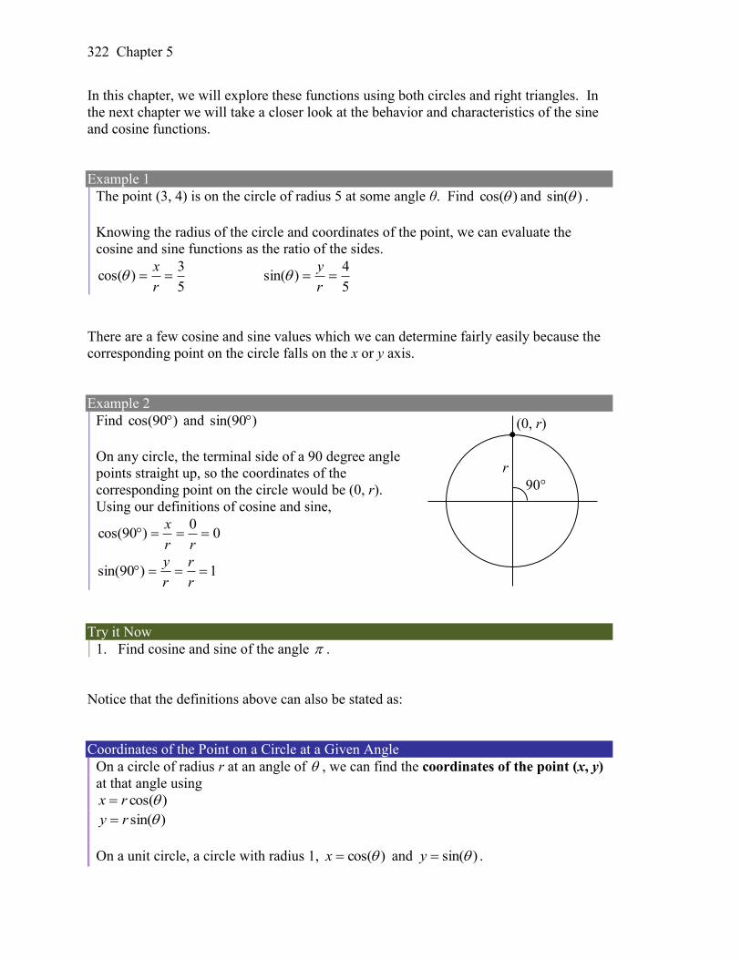
322 Chapter 5
In this chapter, we will explore these functions using both circles and right triangles. In
the next chapter we will take a closer look at the behavior and characteristics of the sine
and cosine functions.
Example 1
The point (3, 4) is on the circle of radius 5 at some angle θ. Find )cos( and )sin( .
Knowing the radius of the circle and coordinates of the point, we can evaluate the
cosine and sine functions as the ratio of the sides.
5
3)cos(
r
x
5
4)sin(
r
y
There are a few cosine and sine values which we can determine fairly easily because the
corresponding point on the circle falls on the x or y axis.
Example 2
Find )90cos( and )90sin(
On any circle, the terminal side of a 90 degree angle
points straight up, so the coordinates of the
corresponding point on the circle would be (0, r).
Using our definitions of cosine and sine,
00
)90cos( rr
x
1)90sin( r
r
r
y
Try it Now
1. Find cosine and sine of the angle .
Notice that the definitions above can also be stated as:
Coordinates of the Point on a Circle at a Given Angle
On a circle of radius r at an angle of , we can find the coordinates of the point (x, y)
at that angle using
)cos(rx
)sin(ry
On a unit circle, a circle with radius 1, )cos(x and )sin(y .
r
90°
(0, r)
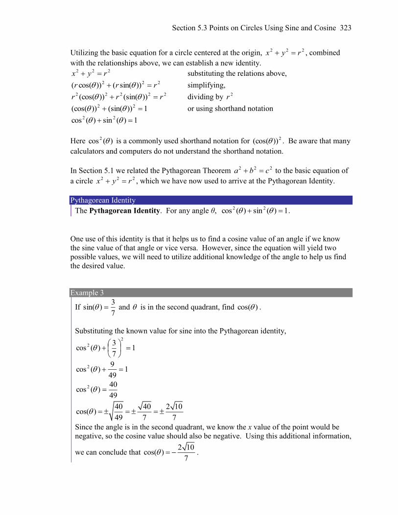
Section 5.3 Points on Circles Using Sine and Cosine 323
Utilizing the basic equation for a circle centered at the origin, 222 ryx , combined
with the relationships above, we can establish a new identity. 222 ryx substituting the relations above,
222 ))sin(())cos(( rrr simplifying, 22222 ))(sin())(cos( rrr dividing by 2r
1))(sin())(cos( 22 or using shorthand notation
1)(sin)(cos 22
Here )(cos 2 is a commonly used shorthand notation for 2))(cos( . Be aware that many
calculators and computers do not understand the shorthand notation.
In Section 5.1 we related the Pythagorean Theorem 222 cba to the basic equation of
a circle 222 ryx , which we have now used to arrive at the Pythagorean Identity.
Pythagorean Identity
The Pythagorean Identity. For any angle θ, 1)(sin)(cos 22 .
One use of this identity is that it helps us to find a cosine value of an angle if we know
the sine value of that angle or vice versa. However, since the equation will yield two
possible values, we will need to utilize additional knowledge of the angle to help us find
the desired value.
Example 3
If 7
3)sin( and is in the second quadrant, find )cos( .
Substituting the known value for sine into the Pythagorean identity,
17
3)(cos
2
2
149
9)(cos 2
49
40)(cos 2
40 40 2 10cos( )
49 7 7
Since the angle is in the second quadrant, we know the x value of the point would be
negative, so the cosine value should also be negative. Using this additional information,
we can conclude that 2 10
cos( )7
.
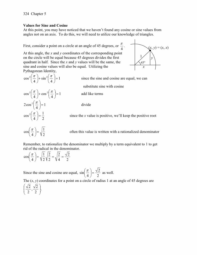
324 Chapter 5
Values for Sine and Cosine
At this point, you may have noticed that we haven’t found any cosine or sine values from
angles not on an axis. To do this, we will need to utilize our knowledge of triangles.
First, consider a point on a circle at an angle of 45 degrees, or 4
.
At this angle, the x and y coordinates of the corresponding point
on the circle will be equal because 45 degrees divides the first
quadrant in half. Since the x and y values will be the same, the
sine and cosine values will also be equal. Utilizing the
Pythagorean Identity,
14
sin4
cos 22
since the sine and cosine are equal, we can
substitute sine with cosine
14
cos4
cos 22
add like terms
14
cos2 2
divide
2
1
4cos 2
since the x value is positive, we’ll keep the positive root
2
1
4cos
often this value is written with a rationalized denominator
Remember, to rationalize the denominator we multiply by a term equivalent to 1 to get
rid of the radical in the denominator.
2
2
4
2
2
2
2
1
4cos
Since the sine and cosine are equal, 2
2
4sin
as well.
The (x, y) coordinates for a point on a circle of radius 1 at an angle of 45 degrees are
2
2,
2
2.
1
45°
y
x
(x, y) = (x, x)
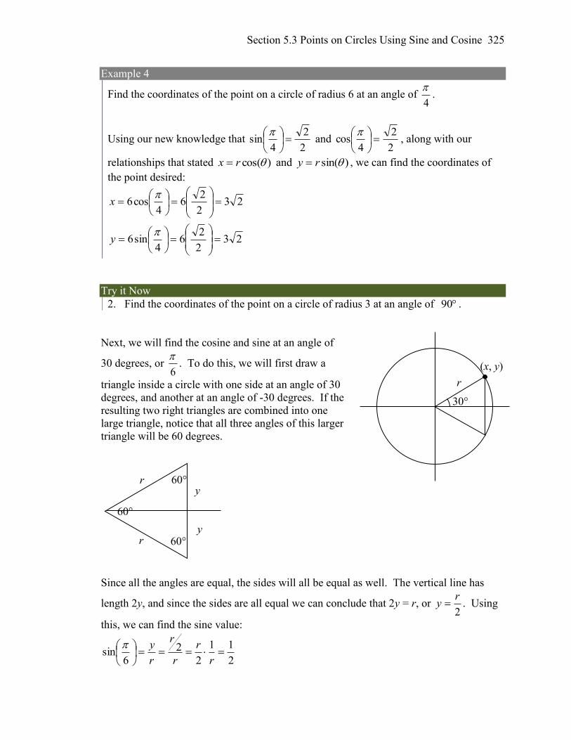
Section 5.3 Points on Circles Using Sine and Cosine 325
Example 4
Find the coordinates of the point on a circle of radius 6 at an angle of 4
.
Using our new knowledge that 2
2
4sin
and
2
2
4cos
, along with our
relationships that stated )cos(rx and )sin(ry , we can find the coordinates of
the point desired:
232
26
4cos6
x
232
26
4sin6
y
Try it Now
2. Find the coordinates of the point on a circle of radius 3 at an angle of 90 .
Next, we will find the cosine and sine at an angle of
30 degrees, or 6
. To do this, we will first draw a
triangle inside a circle with one side at an angle of 30
degrees, and another at an angle of -30 degrees. If the
resulting two right triangles are combined into one
large triangle, notice that all three angles of this larger
triangle will be 60 degrees.
Since all the angles are equal, the sides will all be equal as well. The vertical line has
length 2y, and since the sides are all equal we can conclude that 2y = r, or 2
ry . Using
this, we can find the sine value:
2
11
2
2
6sin
r
r
r
r
r
y
60°
60°
60°
r
r
y
y
r
30°
(x, y)
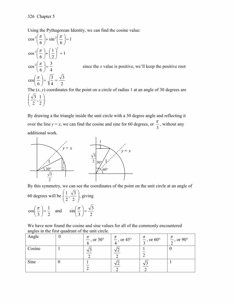
326 Chapter 5
Using the Pythagorean Identity, we can find the cosine value:
16
sin6
cos 22
12
1
6cos
2
2
4
3
6cos 2
since the x value is positive, we’ll keep the positive root
2
3
4
3
6cos
The (x, y) coordinates for the point on a circle of radius 1 at an angle of 30 degrees are
2
1,
2
3.
By drawing a the triangle inside the unit circle with a 30 degree angle and reflecting it
over the line y = x, we can find the cosine and sine for 60 degrees, or 3
, without any
additional work.
By this symmetry, we can see the coordinates of the point on the unit circle at an angle of
60 degrees will be
2
3,
2
1, giving
2
1
3cos
and
2
3
3sin
We have now found the cosine and sine values for all of the commonly encountered
angles in the first quadrant of the unit circle.
Angle 0
6
, or 30°
4
, or 45°
3
, or 60°
2
, or 90°
Cosine 1 3
2
2
2
1
2
0
Sine 0 1
2 2
2
3
2
1
30°
2
1
2
3
1
y = x
30°
2
1
1
60°
y = x
2
3
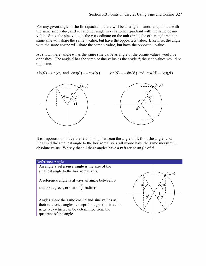
Section 5.3 Points on Circles Using Sine and Cosine 327
For any given angle in the first quadrant, there will be an angle in another quadrant with
the same sine value, and yet another angle in yet another quadrant with the same cosine
value. Since the sine value is the y coordinate on the unit circle, the other angle with the
same sine will share the same y value, but have the opposite x value. Likewise, the angle
with the same cosine will share the same x value, but have the opposite y value.
As shown here, angle α has the same sine value as angle θ; the cosine values would be
opposites. The angle β has the same cosine value as the angle θ; the sine values would be
opposites.
)sin()sin( and )cos()cos( )sin()sin( and )cos()cos(
It is important to notice the relationship between the angles. If, from the angle, you
measured the smallest angle to the horizontal axis, all would have the same measure in
absolute value. We say that all these angles have a reference angle of θ.
Reference Angle
An angle’s reference angle is the size of the
smallest angle to the horizontal axis.
A reference angle is always an angle between 0
and 90 degrees, or 0 and 2
radians.
Angles share the same cosine and sine values as
their reference angles, except for signs (positive or
negative) which can be determined from the
quadrant of the angle.
(x, y)
r θ
α
(x, y)
θ
θ
θ
θ
(x, y)
r θ
β
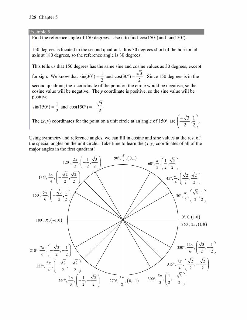
328 Chapter 5
Example 5
Find the reference angle of 150 degrees. Use it to find )150cos( and )150sin( .
150 degrees is located in the second quadrant. It is 30 degrees short of the horizontal
axis at 180 degrees, so the reference angle is 30 degrees.
This tells us that 150 degrees has the same sine and cosine values as 30 degrees, except
for sign. We know that 2
1)30sin( and
2
3)30cos( . Since 150 degrees is in the
second quadrant, the x coordinate of the point on the circle would be negative, so the
cosine value will be negative. The y coordinate is positive, so the sine value will be
positive.
2
1)150sin( and
2
3)150cos(
The (x, y) coordinates for the point on a unit circle at an angle of 150 are
2
1,
2
3.
Using symmetry and reference angles, we can fill in cosine and sine values at the rest of
the special angles on the unit circle. Take time to learn the (x, y) coordinates of all of the
major angles in the first quadrant!
3 130 , , ,
6 2 2
2 245 , , ,
4 2 2
1 360 , ,
3 2 2,
90 , , 0 1
2,
2 1 3
120 , ,3 2 2
,
3 2 2135 , ,
4 2 2,
5 3 1150 , ,
6 2 2,
180 , , 1 0,
5 2 2225 , ,
4 2 2,
4 1 3240 , ,
3 2 2,
3
270 , , 0 12
,
5 1 3
300 , ,3 2 2
,
7 2 2315 , ,
4 2 2,
11 3 1330 , ,
6 2 2,
0 , 0, 1, 0
360 , 2 , 1, 0
7 3 1210 , ,
6 2 2,
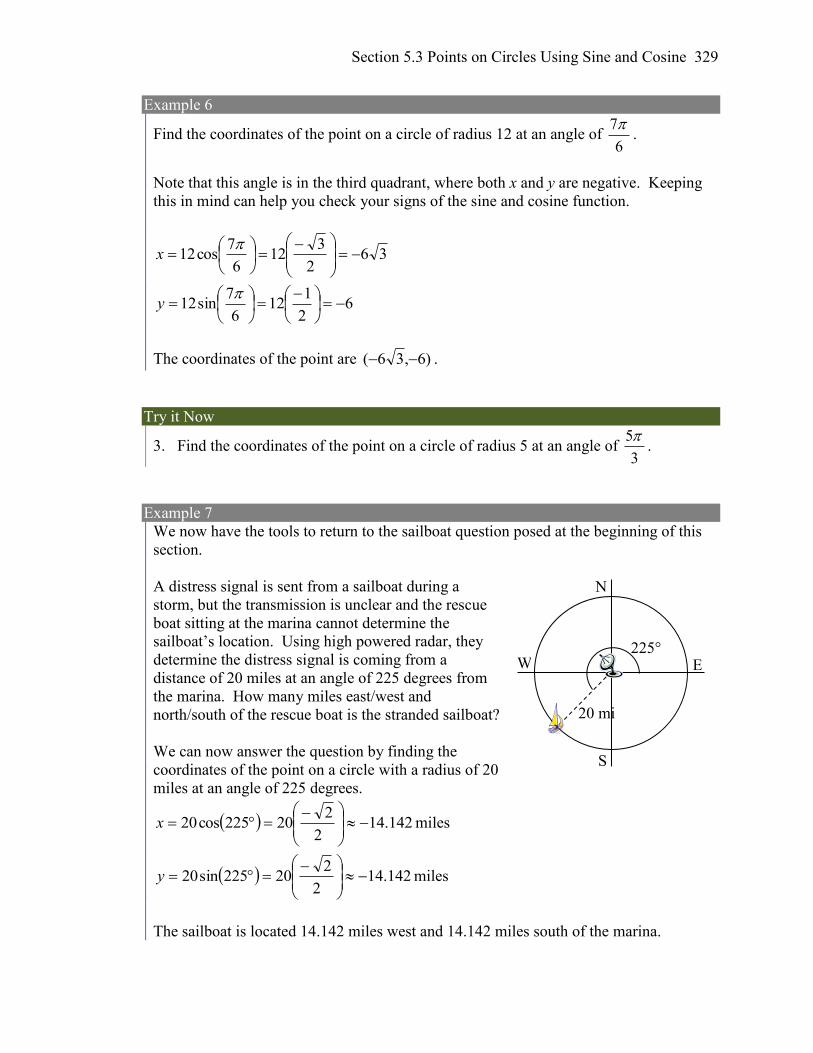
Section 5.3 Points on Circles Using Sine and Cosine 329
Example 6
Find the coordinates of the point on a circle of radius 12 at an angle of 6
7.
Note that this angle is in the third quadrant, where both x and y are negative. Keeping
this in mind can help you check your signs of the sine and cosine function.
362
312
6
7cos12
x
62
112
6
7sin12
y
The coordinates of the point are )6,36( .
Try it Now
3. Find the coordinates of the point on a circle of radius 5 at an angle of 5
3
.
Example 7
We now have the tools to return to the sailboat question posed at the beginning of this
section.
A distress signal is sent from a sailboat during a
storm, but the transmission is unclear and the rescue
boat sitting at the marina cannot determine the
sailboat’s location. Using high powered radar, they
determine the distress signal is coming from a
distance of 20 miles at an angle of 225 degrees from
the marina. How many miles east/west and
north/south of the rescue boat is the stranded sailboat?
We can now answer the question by finding the
coordinates of the point on a circle with a radius of 20
miles at an angle of 225 degrees.
142.142
220225cos20
x miles
142.142
220225sin20
y miles
The sailboat is located 14.142 miles west and 14.142 miles south of the marina.
20 mi
225°
E
W
N
S
330 Chapter 5
The special values of sine and cosine in the first quadrant are very useful to know, since
knowing them allows you to quickly evaluate the sine and cosine of very common angles
without needing to look at a reference or use your calculator. However, scenarios do
come up where we need to know the sine and cosine of other angles.
To find the cosine and sine of any other angle, we turn to a computer or calculator. Be
aware: most calculators can be set into “degree” or “radian” mode, which tells the
calculator the units for the input value. When you evaluate “cos(30)” on your calculator,
it will evaluate it as the cosine of 30 degrees if the calculator is in degree mode, or the
cosine of 30 radians if the calculator is in radian mode. Most computer software with
cosine and sine functions only operates in radian mode.
Example 8
Evaluate the cosine of 20 degrees using a calculator or computer.
On a calculator that can be put in degree mode, you can evaluate this directly to be
approximately 0.939693.
On a computer or calculator without degree mode, you would first need to convert the
angle to radians, or equivalently evaluate the expression
180
20cos
.
Important Topics of This Section
The sine function
The cosine function
Pythagorean Identity
Unit Circle values
Reference angles
Using technology to find points on a circle
Try it Now Answers
1. 1)cos( 0)sin(
2.
3132
sin3
0032
cos3
y
x
3.
2
35,
2
5
Section 5.3 Points on Circles Using Sine and Cosine 331
Section 5.3 Exercises
1. Find the quadrant in which the terminal point determined by t lies if
a. sin( ) 0t and cos( ) 0t b. sin( ) 0t and cos( ) 0t
2. Find the quadrant in which the terminal point determined by t lies if
a. sin( ) 0t and cos( ) 0t b. sin( ) 0t and cos( ) 0t
3. The point P is on the unit circle. If the y-coordinate of P is 3
5, and P is in quadrant II,
find the x coordinate.
4. The point P is on the unit circle. If the x-coordinate of P is 1
5, and P is in quadrant
IV, find the y coordinate.
5. If 1
cos7
and θ is in the 4th quadrant, find sin .
6. If 2
cos9
and θ is in the 1st quadrant, find sin .
7. If 3
sin8
and θ is in the 2nd quadrant, find cos .
8. If 1
sin4
and θ is in the 3rd quadrant, find cos .
9. For each of the following angles, find the reference angle and which quadrant the
angle lies in. Then compute sine and cosine of the angle.
a. 225° b. 300° c. 135° d. 210°
10. For each of the following angles, find the reference angle and which quadrant the
angle lies in. Then compute sine and cosine of the angle.
a. 120° b. 315° c. 250° d. 150°
11. For each of the following angles, find the reference angle and which quadrant the
angle lies in. Then compute sine and cosine of the angle.
a. 5
4
b.
7
6
c.
5
3
d.
3
4
12. For each of the following angles, find the reference angle and which quadrant the
angle lies in. Then compute sine and cosine of the angle.
a. 4
3
b.
2
3
c.
5
6
d.
7
4
332 Chapter 5
13. Give exact values for sin and cos for each of these angles.
a. 3
4
b.
23
6
c.
2
d. 5
14. Give exact values for sin and cos for each of these angles.
a. 2
3
b.
17
4
c.
6
d. 10
15. Find an angle θ with 0 360 or 0 2 that has the same sine value as:
a. 3
b. 80° c. 140° d.
4
3
e. 305°
16. Find an angle θ with 0 360 or 0 2 that has the same sine value as:
a. 4
b. 15° c. 160° d.
7
6
e. 340°
17. Find an angle θ with 0 360 or 0 2 that has the same cosine value as:
a. 3
b. 80° c. 140° d.
4
3
e. 305°
18. Find an angle θ with 0 360 or 0 2 that has the same cosine value as:
a. 4
b. 15° c. 160° d.
7
6
e. 340°
19. Find the coordinates of the point on a circle with radius 15 corresponding to an angle
of 220°.
20. Find the coordinates of the point on a circle with radius 20 corresponding to an angle
of 280°.
21. Marla is running clockwise around a circular track. She runs at a constant speed of 3
meters per second. She takes 46 seconds to complete one lap of the track. From her
starting point, it takes her 12 seconds to reach the northernmost point of the track. Impose
a coordinate system with the center of the track at the origin, and the northernmost point
on the positive y-axis. [UW]
a) Give Marla’s coordinates at her starting point.
b) Give Marla’s coordinates when she has been running for 10 seconds.
c) Give Marla’s coordinates when she has been running for 901.3 seconds.
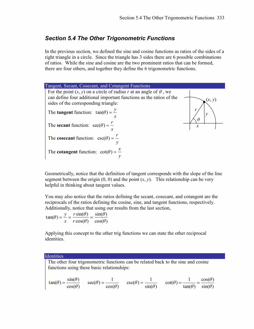
Section 5.4 The Other Trigonometric Functions 333
Section 5.4 The Other Trigonometric Functions
In the previous section, we defined the sine and cosine functions as ratios of the sides of a
right triangle in a circle. Since the triangle has 3 sides there are 6 possible combinations
of ratios. While the sine and cosine are the two prominent ratios that can be formed,
there are four others, and together they define the 6 trigonometric functions.
Tangent, Secant, Cosecant, and Cotangent Functions
For the point (x, y) on a circle of radius r at an angle of , we
can define four additional important functions as the ratios of the
sides of the corresponding triangle:
The tangent function: x
y)tan(
The secant function: x
r)sec(
The cosecant function: y
r)csc(
The cotangent function: y
x)cot(
Geometrically, notice that the definition of tangent corresponds with the slope of the line
segment between the origin (0, 0) and the point (x, y). This relationship can be very
helpful in thinking about tangent values.
You may also notice that the ratios defining the secant, cosecant, and cotangent are the
reciprocals of the ratios defining the cosine, sine, and tangent functions, respectively.
Additionally, notice that using our results from the last section,
)cos(
)sin(
)cos(
)sin()tan(
r
r
x
y
Applying this concept to the other trig functions we can state the other reciprocal
identities.
Identities
The other four trigonometric functions can be related back to the sine and cosine
functions using these basic relationships:
)cos(
)sin()tan(
)cos(
1)sec(
)sin(
1)csc(
1 cos( )cot( )
tan( ) sin( )
(x, y)
r
θ
y
x
334 Chapter 5
These relationships are called identities. Identities are statements that are true for all
values of the input on which they are defined. Identities are usually something that can
be derived from definitions and relationships we already know, similar to how the
identities above were derived from the circle relationships of the six trig functions. The
Pythagorean Identity we learned earlier was derived from the Pythagorean Theorem and
the definitions of sine and cosine. We will discuss the role of identities more after an
example.
Example 1
Evaluate )45tan( and
6
5sec
.
Since we know the sine and cosine values for these angles, it makes sense to relate the
tangent and secant values back to the sine and cosine values.
1
22
22
)45cos(
)45sin()45tan(
Notice this result is consistent with our interpretation of the tangent value as the slope
of the line passing through the origin at the given angle: a line at 45 degrees would
indeed have a slope of 1.
3
2
23
1
6
5cos
1
6
5sec
, which could also be written as
3
32.
Try it Now
1. Evaluate
6
7csc
.
Just as we often need to simplify algebraic expressions, it is often also necessary or
helpful to simplify trigonometric expressions. To do so, we utilize the definitions and
identities we have established.
Section 5.4 The Other Trigonometric Functions 335
Example 2
Simplify
tan
sec.
We can simplify this by rewriting both functions in terms of sine and cosine
cossin
cos1
tan
sec To divide the fractions we could invert and multiply
sin
cos
cos
1 cancelling the cosines,
csc
sin
1 simplifying and using the identity
By showing that
tan
sec can be simplified to csc , we have, in fact, established a new
identity: that
csc
tan
sec .
Occasionally a question may ask you to “prove the identity” or “establish the identity.”
This is the same idea as when an algebra book asks a question like “show that
12)1( 22 xxx .” In this type of question we must show the algebraic
manipulations that demonstrate that the left and right side of the equation are in fact
equal. You can think of a “prove the identity” problem as a simplification problem where
you know the answer: you know what the end goal of the simplification should be, and
just need to show the steps to get there.
To prove an identity, in most cases you will start with the expression on one side of the
identity and manipulate it using algebra and trigonometric identities until you have
simplified it to the expression on the other side of the equation. Do not treat the identity
like an equation to solve – it isn’t! The proof is establishing if the two expressions are
equal, so we must take care to work with one side at a time rather than applying
an operation simultaneously to both sides of the equation.
Example 3
Prove the identity 1 cot( )
sin( ) cos( )csc( )
.
Since the left side seems a bit more complicated, we will start there and simplify the
expression until we obtain the right side. We can use the right side as a guide for what
might be good steps to make. In this case, the left side involves a fraction while the
right side doesn’t, which suggests we should look to see if the fraction can be reduced.
336 Chapter 5
Additionally, since the right side involves sine and cosine and the left does not, it
suggests that rewriting the cotangent and cosecant using sine and cosine might be a
good idea.
1 cot( )
csc( )
Rewriting the cotangent and cosecant
cos( )1
sin( )
1
sin( )
To divide the fractions, we invert and multiply
cos( ) sin( )1
sin( ) 1
Distributing,
sin( ) cos( ) sin( )1
1 sin( ) 1
Simplifying the fractions,
sin( ) cos( ) Establishing the identity.
Notice that in the second step, we could have combined the 1 and cos( )
sin( )
before
inverting and multiplying. It is very common when proving or simplifying identities for
there to be more than one way to obtain the same result.
We can also utilize identities we have previously learned, like the Pythagorean Identity,
while simplifying or proving identities.
Example 4
Establish the identity
sin1
sin1
cos 2
.
Since the left side of the identity is more complicated, it makes sense to start there. To
simplify this, we will have to reduce the fraction, which would require the numerator to
have a factor in common with the denominator. Additionally, we notice that the right
side only involves sine. Both of these suggest that we need to convert the cosine into
something involving sine.
Recall the Pythagorean Identity told us 1)(sin)(cos 22 . By moving one of the
trig functions to the other side, we can establish:
)(cos1)(sin 22 and )(sin1)(cos 22
Utilizing this, we now can establish the identity. We start on one side and manipulate:
Section 5.4 The Other Trigonometric Functions 337
sin1
cos 2
Utilizing the Pythagorean Identity
=
sin1
sin1 2
Factoring the numerator
sin1
sin1sin1
Cancelling the like factors
sin1 Establishing the identity
We can also build new identities from previously established identities. For example, if
we divide both sides of the Pythagorean Identity by cosine squared (which is allowed
since we’ve already shown the identity is true),
)(cos
1
)(cos
)(sin)(cos22
22
Splitting the fraction on the left,
)(cos
1
)(cos
)(sin
)(cos
)(cos22
2
2
2
Simplifying and using the definitions of tan and sec
)(sec)(tan1 22 .
Try it Now
2. Use a similar approach to establish that )(csc1)(cot 22 .
Identities
Alternate forms of the Pythagorean Identity
)(sec)(tan1 22
)(csc1)(cot 22
Example 5
If 7
2)tan( and is in the 3rd quadrant, find )cos( .
There are two approaches to this problem, both of which work equally well.
Approach 1
Since x
y)tan( and the angle is in the third quadrant, we can imagine a triangle in a
circle of some radius so that the point on the circle is (-7, -2). Using the Pythagorean
Theorem, we can find the radius of the circle: 222 )2()7( r , so 53r .
338 Chapter 5
Now we can find the cosine value:
53
7)cos(
r
x
Approach 2
Using the )(sec)(tan1 22 form of the Pythagorean Identity with the known
tangent value,
)(sec)(tan1 22
)(sec7
21 2
2
)(sec49
53 2
7
53
49
53)sec(
Since the angle is in the third quadrant, the cosine value will be negative so the secant
value will also be negative. Keeping the negative result, and using definition of secant,
7
53)sec(
7
53
)cos(
1
Inverting both sides
53
537
53
7)cos(
Try it Now
3. If 3
7)sec( and
2
, find tan( ) and sin( ) .
Important Topics of This Section
6 Trigonometric Functions:
Sine
Cosine
Tangent
Cosecant
Secant
Cotangent
Trig identities
Section 5.4 The Other Trigonometric Functions 339
Try it Now Answers
1. -2
2.
)(csc1)(cot
)(sin
1
)(sin
)(sin
)(sin
)(cos
1sin
)(sin)(cos
22
22
2
2
2
2
22
3. 7
40)sin(
3
40)tan(
340 Chapter 5
Section 5.4 Exercises
1. If
4
, find exact values for sec ,csc , tan , cot .
2. If 7
4
, find exact values for sec ,csc , tan , cot .
3. If 5
6
, find exact values for sec ,csc , tan , cot .
4. If
6
, find exact values for sec ,csc , tan , cot .
5. If 2
3
, find exact values for sec ,csc , tan , cot .
6. If 4
3
, find exact values for sec ,csc , tan , cot .
7. Evaluate: a. sec 135 b. csc 210 c. tan 60 d. cot 225
8. Evaluate: a. sec 30 b. csc 315 c. tan 135 d. cot 150
9. If 3
sin4
, and is in quadrant II, find cos , sec ,csc , tan , cot .
10. If 2
sin7
, and is in quadrant II, find cos , sec ,csc , tan , cot .
11. If 1
cos3
, and is in quadrant III, find
sin , sec ,csc , tan , cot .
12. If 1
cos5
, and is in quadrant I, find sin , sec ,csc , tan , cot .
13. If 12
tan5
, and 02
, find sin , cos ,sec , csc , cot .
14. If tan 4 , and 02
, find sin , cos ,sec , csc , cot .
Section 5.4 The Other Trigonometric Functions 341
15. Use a calculator to find sine, cosine, and tangent of the following values:
a. 0.15 b. 4 c. 70° d. 283°
16. Use a calculator to find sine, cosine, and tangent of the following values:
a. 0.5 b. 5.2 c. 10° d. 195°
Simplify each of the following to an expression involving a single trig function with no
fractions.
17. csc( ) tant t
18. cos( )csct t
19.
sec
csc
t
t
20.
cot
csc
t
t
21.
sec cos
sin
t t
t
22.
tan
sec cos
t
t t
23.
1 cot
1 tan
t
t
24.
1 sin
1 csc
t
t
25.
2 2
2
sin cos
cos
t t
t
26.
2
2
1 sin
sin
t
t
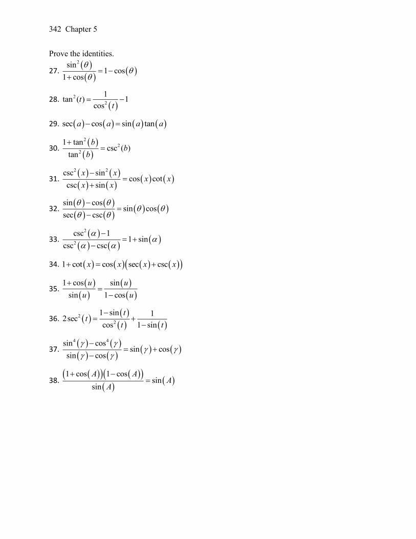
342 Chapter 5
Prove the identities.
27.
2sin1 cos
1 cos
28.
2
2
1tan ( ) 1
cost
t
29. sec cos sin tana a a a
30.
2
2
2
1 tancsc ( )
tan
bb
b
31.
2 2csc sincos cot
csc sin
x xx x
x x
32.
sin cossin cos
sec csc
33.
2
2
csc 11 sin
csc csc
34. 1 cot cos sec cscx x x x
35.
1 cos sin
sin 1 cos
u u
u u
36.
2
2
1 sin 12sec
cos 1 sin
tt
t t
37.
4 4sin cossin cos
sin cos
38.
1 cos 1 cossin
sin
A AA
A
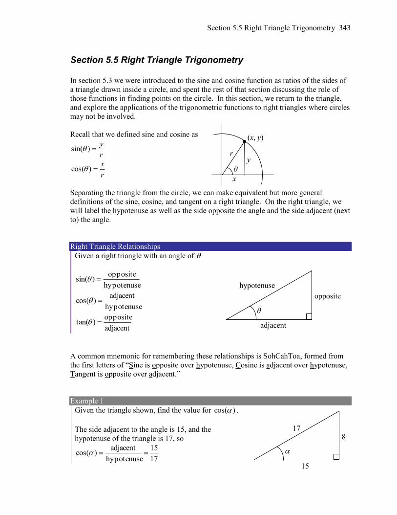
Section 5.5 Right Triangle Trigonometry 343
Section 5.5 Right Triangle Trigonometry
In section 5.3 we were introduced to the sine and cosine function as ratios of the sides of
a triangle drawn inside a circle, and spent the rest of that section discussing the role of
those functions in finding points on the circle. In this section, we return to the triangle,
and explore the applications of the trigonometric functions to right triangles where circles
may not be involved.
Recall that we defined sine and cosine as
r
y)sin(
r
x)cos(
Separating the triangle from the circle, we can make equivalent but more general
definitions of the sine, cosine, and tangent on a right triangle. On the right triangle, we
will label the hypotenuse as well as the side opposite the angle and the side adjacent (next
to) the angle.
Right Triangle Relationships
Given a right triangle with an angle of
hypotenuse
opposite)sin(
hypotenuse
adjacent)cos(
adjacent
opposite)tan(
A common mnemonic for remembering these relationships is SohCahToa, formed from
the first letters of “Sine is opposite over hypotenuse, Cosine is adjacent over hypotenuse,
Tangent is opposite over adjacent.”
Example 1
Given the triangle shown, find the value for )cos( .
The side adjacent to the angle is 15, and the
hypotenuse of the triangle is 17, so
17
15
hypotenuse
adjacent)cos(
(x, y)
r
θ
y
x
θ
adjacent
opposite
hypotenuse
15
8 17
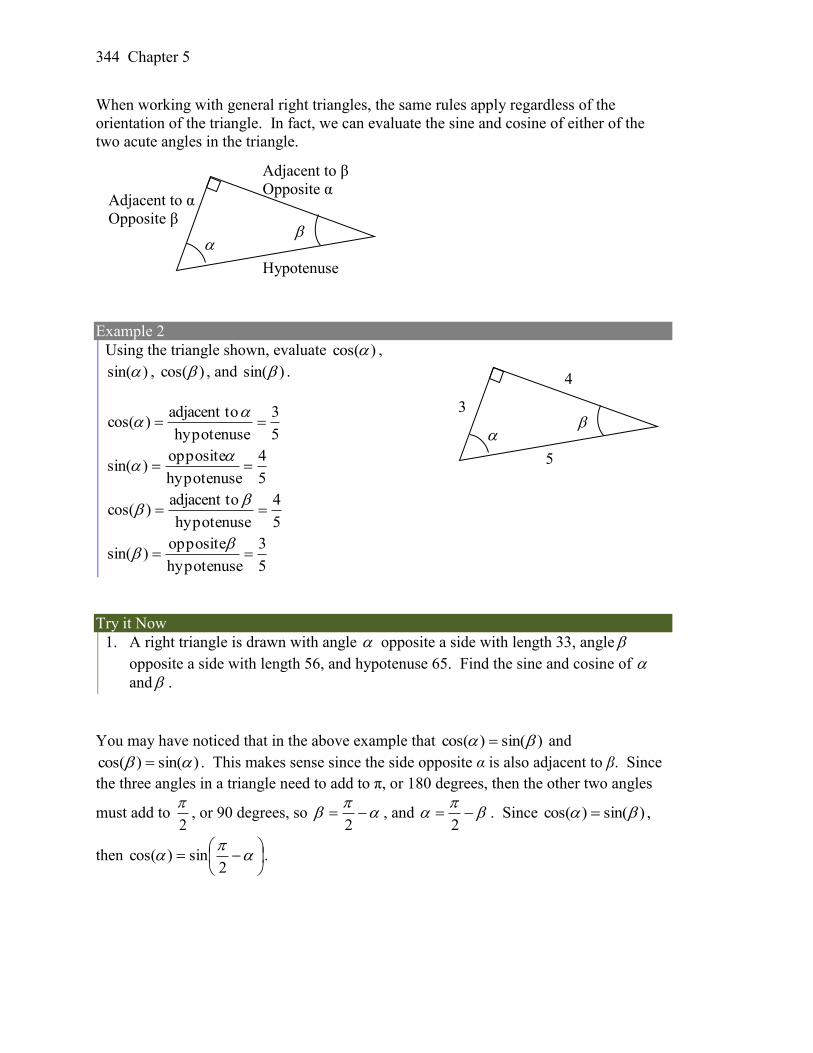
344 Chapter 5
When working with general right triangles, the same rules apply regardless of the
orientation of the triangle. In fact, we can evaluate the sine and cosine of either of the
two acute angles in the triangle.
Example 2
Using the triangle shown, evaluate )cos( ,
)sin( , )cos( , and )sin( .
5
3
hypotenuse
oadjacent t)cos(
5
4
hypotenuse
opposite)sin(
5
4
hypotenuse
oadjacent t)cos(
5
3
hypotenuse
opposite)sin(
Try it Now
1. A right triangle is drawn with angle opposite a side with length 33, angle
opposite a side with length 56, and hypotenuse 65. Find the sine and cosine of
and .
You may have noticed that in the above example that )sin()cos( and
)sin()cos( . This makes sense since the side opposite α is also adjacent to β. Since
the three angles in a triangle need to add to π, or 180 degrees, then the other two angles
must add to 2
, or 90 degrees, so
2, and
2. Since )sin()cos( ,
then
2sin)cos( .
Adjacent to α
Opposite β
Hypotenuse
Adjacent to β
Opposite α
3
5
4
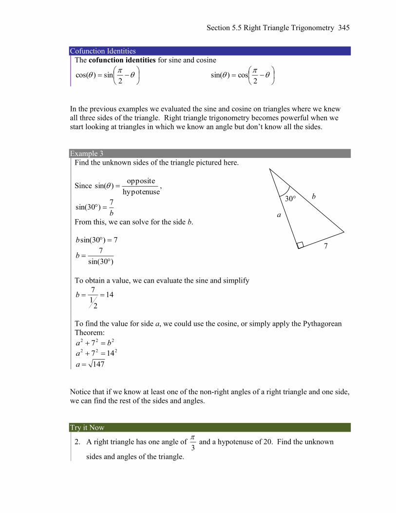
Section 5.5 Right Triangle Trigonometry 345
Cofunction Identities
The cofunction identities for sine and cosine
2sin)cos(
2cos)sin(
In the previous examples we evaluated the sine and cosine on triangles where we knew
all three sides of the triangle. Right triangle trigonometry becomes powerful when we
start looking at triangles in which we know an angle but don’t know all the sides.
Example 3
Find the unknown sides of the triangle pictured here.
Since hypotenuse
opposite)sin( ,
b
7)30sin(
From this, we can solve for the side b.
7)30sin( b
)30sin(
7
b
To obtain a value, we can evaluate the sine and simplify
14
21
7b
To find the value for side a, we could use the cosine, or simply apply the Pythagorean
Theorem: 222 7 ba
222 147 a
147a
Notice that if we know at least one of the non-right angles of a right triangle and one side,
we can find the rest of the sides and angles.
Try it Now
2. A right triangle has one angle of 3
and a hypotenuse of 20. Find the unknown
sides and angles of the triangle.
30°
a
7
b
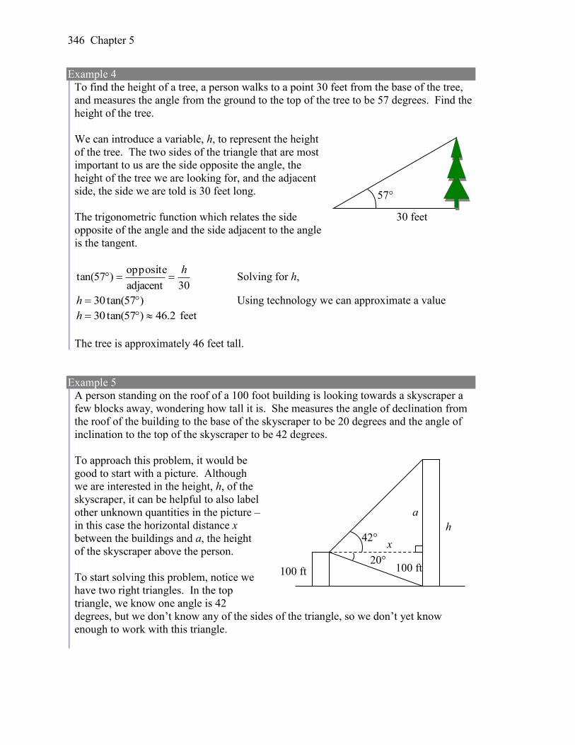
346 Chapter 5
Example 4
To find the height of a tree, a person walks to a point 30 feet from the base of the tree,
and measures the angle from the ground to the top of the tree to be 57 degrees. Find the
height of the tree.
We can introduce a variable, h, to represent the height
of the tree. The two sides of the triangle that are most
important to us are the side opposite the angle, the
height of the tree we are looking for, and the adjacent
side, the side we are told is 30 feet long.
The trigonometric function which relates the side
opposite of the angle and the side adjacent to the angle
is the tangent.
30adjacent
opposite)57tan(
h Solving for h,
)57tan(30 h Using technology we can approximate a value
2.46)57tan(30 h feet
The tree is approximately 46 feet tall.
Example 5
A person standing on the roof of a 100 foot building is looking towards a skyscraper a
few blocks away, wondering how tall it is. She measures the angle of declination from
the roof of the building to the base of the skyscraper to be 20 degrees and the angle of
inclination to the top of the skyscraper to be 42 degrees.
To approach this problem, it would be
good to start with a picture. Although
we are interested in the height, h, of the
skyscraper, it can be helpful to also label
other unknown quantities in the picture –
in this case the horizontal distance x
between the buildings and a, the height
of the skyscraper above the person.
To start solving this problem, notice we
have two right triangles. In the top
triangle, we know one angle is 42
degrees, but we don’t know any of the sides of the triangle, so we don’t yet know
enough to work with this triangle.
57°
30 feet
100 ft
h
a
x 42°
20° 100 ft
Section 5.5 Right Triangle Trigonometry 347
In the lower right triangle, we know one angle is 20 degrees, and we know the vertical
height measurement of 100 ft. Since we know these two pieces of information, we can
solve for the unknown distance x.
x
100
adjacent
opposite)20tan( Solving for x
100)20tan( x
)20tan(
100
x
Now that we have found the distance x, we know enough information to solve the top
right triangle.
)20tan(100adjacent
opposite)42tan(
a
x
a
100
)20tan()42tan(
a
)20tan()42tan(100 a
a
)20tan(
)42tan(100
Approximating a value,
4.247)20tan(
)42tan(100
a feet
Adding the height of the first building, we determine that the skyscraper is about 347
feet tall.
Important Topics of This Section
SOH CAH TOA
Cofunction identities
Applications with right triangles
Try it Now Answers
1. 33
sin( )65
56
cos( )65
56
sin( )65
65
33)cos(
2. 20
Adj
hypoteuse
adjacent
3cos
so, 10
2
120
3cos20adjacent
20
Opp
hypoteuse
Opposite
3sin
so, 310
2
320
3sin20opposite
Missing angle = 30 degrees or 6
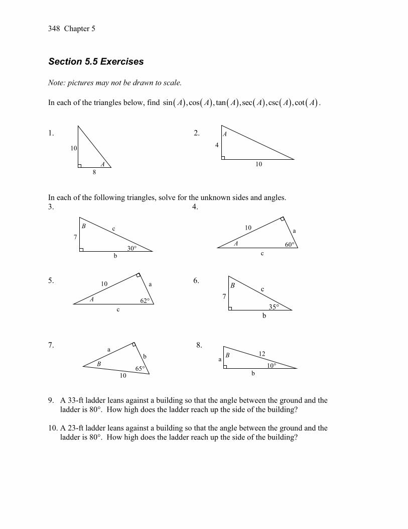
348 Chapter 5
Section 5.5 Exercises
Note: pictures may not be drawn to scale.
In each of the triangles below, find sin ,cos , tan ,sec ,csc ,cotA A A A A A .
1. 2.
In each of the following triangles, solve for the unknown sides and angles.
3. 4.
5. 6.
7. 8.
9. A 33-ft ladder leans against a building so that the angle between the ground and the
ladder is 80°. How high does the ladder reach up the side of the building?
10. A 23-ft ladder leans against a building so that the angle between the ground and the
ladder is 80°. How high does the ladder reach up the side of the building?
60°
a 10
c
A
10° b
a 12 B
65°
b a
10
B
A
8
10
A
10
4
30°
7
c B
b
35°
7 c
B
b
62°
a 10
c
A
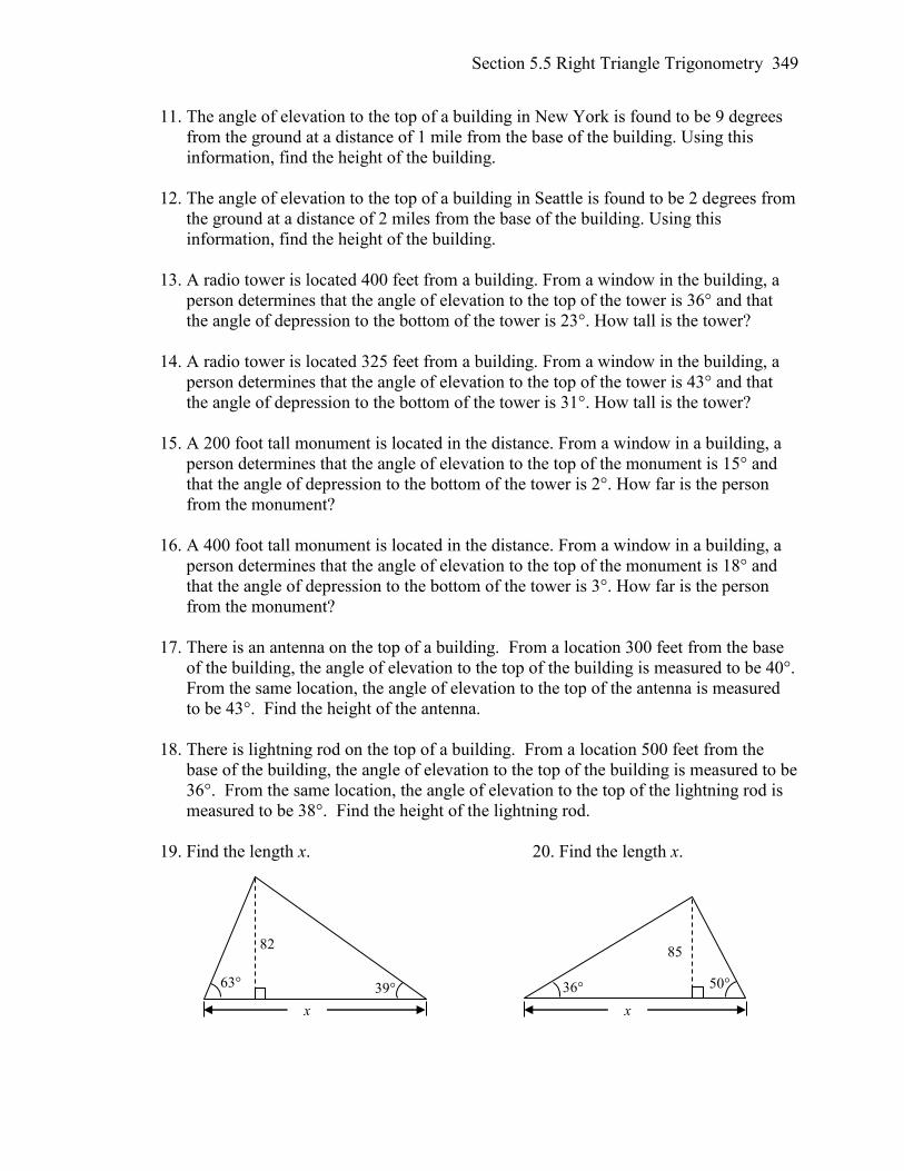
Section 5.5 Right Triangle Trigonometry 349
11. The angle of elevation to the top of a building in New York is found to be 9 degrees
from the ground at a distance of 1 mile from the base of the building. Using this
information, find the height of the building.
12. The angle of elevation to the top of a building in Seattle is found to be 2 degrees from
the ground at a distance of 2 miles from the base of the building. Using this
information, find the height of the building.
13. A radio tower is located 400 feet from a building. From a window in the building, a
person determines that the angle of elevation to the top of the tower is 36° and that
the angle of depression to the bottom of the tower is 23°. How tall is the tower?
14. A radio tower is located 325 feet from a building. From a window in the building, a
person determines that the angle of elevation to the top of the tower is 43° and that
the angle of depression to the bottom of the tower is 31°. How tall is the tower?
15. A 200 foot tall monument is located in the distance. From a window in a building, a
person determines that the angle of elevation to the top of the monument is 15° and
that the angle of depression to the bottom of the tower is 2°. How far is the person
from the monument?
16. A 400 foot tall monument is located in the distance. From a window in a building, a
person determines that the angle of elevation to the top of the monument is 18° and
that the angle of depression to the bottom of the tower is 3°. How far is the person
from the monument?
17. There is an antenna on the top of a building. From a location 300 feet from the base
of the building, the angle of elevation to the top of the building is measured to be 40°.
From the same location, the angle of elevation to the top of the antenna is measured
to be 43°. Find the height of the antenna.
18. There is lightning rod on the top of a building. From a location 500 feet from the
base of the building, the angle of elevation to the top of the building is measured to be
36°. From the same location, the angle of elevation to the top of the lightning rod is
measured to be 38°. Find the height of the lightning rod.
19. Find the length x. 20. Find the length x.
x
85
36° 50°
x
82
63° 39°
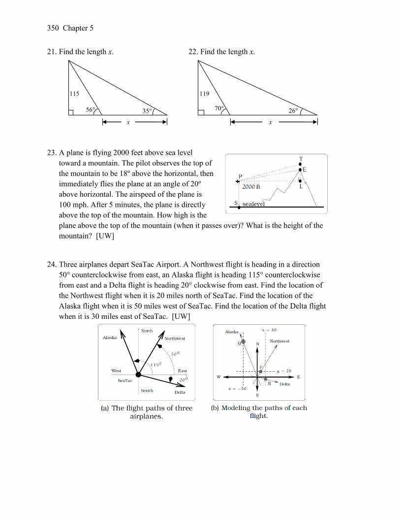
350 Chapter 5
21. Find the length x. 22. Find the length x.
23. A plane is flying 2000 feet above sea level
toward a mountain. The pilot observes the top of
the mountain to be 18o above the horizontal, then
immediately flies the plane at an angle of 20o
above horizontal. The airspeed of the plane is
100 mph. After 5 minutes, the plane is directly
above the top of the mountain. How high is the
plane above the top of the mountain (when it passes over)? What is the height of the
mountain? [UW]
24. Three airplanes depart SeaTac Airport. A Northwest flight is heading in a direction
50° counterclockwise from east, an Alaska flight is heading 115° counterclockwise
from east and a Delta flight is heading 20° clockwise from east. Find the location of
the Northwest flight when it is 20 miles north of SeaTac. Find the location of the
Alaska flight when it is 50 miles west of SeaTac. Find the location of the Delta flight
when it is 30 miles east of SeaTac. [UW]
x
119
70° 26°
x
115
56° 35°
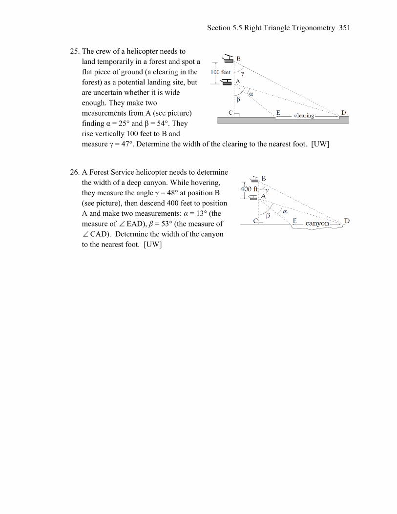
Section 5.5 Right Triangle Trigonometry 351
25. The crew of a helicopter needs to
land temporarily in a forest and spot a
flat piece of ground (a clearing in the
forest) as a potential landing site, but
are uncertain whether it is wide
enough. They make two
measurements from A (see picture)
finding α = 25° and β = 54°. They
rise vertically 100 feet to B and
measure γ = 47°. Determine the width of the clearing to the nearest foot. [UW]
26. A Forest Service helicopter needs to determine
the width of a deep canyon. While hovering,
they measure the angle γ = 48° at position B
(see picture), then descend 400 feet to position
A and make two measurements: α = 13° (the
measure of EAD), β = 53° (the measure of
CAD). Determine the width of the canyon
to the nearest foot. [UW]

352 Chapter 5
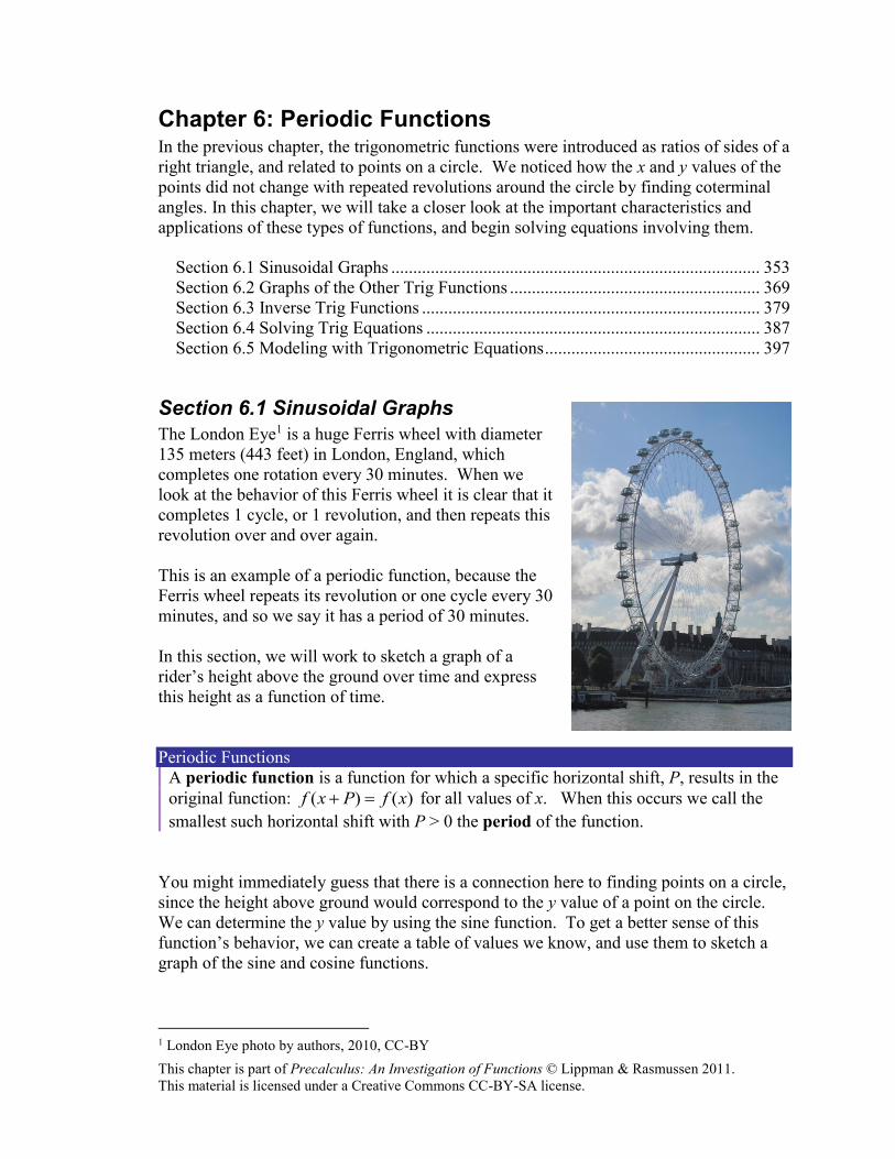
This chapter is part of Precalculus: An Investigation of Functions © Lippman & Rasmussen 2011.
This material is licensed under a Creative Commons CC-BY-SA license.
Chapter 6: Periodic Functions In the previous chapter, the trigonometric functions were introduced as ratios of sides of a
right triangle, and related to points on a circle. We noticed how the x and y values of the
points did not change with repeated revolutions around the circle by finding coterminal
angles. In this chapter, we will take a closer look at the important characteristics and
applications of these types of functions, and begin solving equations involving them.
Section 6.1 Sinusoidal Graphs .................................................................................... 353 Section 6.2 Graphs of the Other Trig Functions ......................................................... 369 Section 6.3 Inverse Trig Functions ............................................................................. 379
Section 6.4 Solving Trig Equations ............................................................................ 387 Section 6.5 Modeling with Trigonometric Equations ................................................. 397
Section 6.1 Sinusoidal Graphs
The London Eye1 is a huge Ferris wheel with diameter
135 meters (443 feet) in London, England, which
completes one rotation every 30 minutes. When we
look at the behavior of this Ferris wheel it is clear that it
completes 1 cycle, or 1 revolution, and then repeats this
revolution over and over again.
This is an example of a periodic function, because the
Ferris wheel repeats its revolution or one cycle every 30
minutes, and so we say it has a period of 30 minutes.
In this section, we will work to sketch a graph of a
rider’s height above the ground over time and express
this height as a function of time.
Periodic Functions
A periodic function is a function for which a specific horizontal shift, P, results in the
original function: )()( xfPxf for all values of x. When this occurs we call the
smallest such horizontal shift with P > 0 the period of the function.
You might immediately guess that there is a connection here to finding points on a circle,
since the height above ground would correspond to the y value of a point on the circle.
We can determine the y value by using the sine function. To get a better sense of this
function’s behavior, we can create a table of values we know, and use them to sketch a
graph of the sine and cosine functions.
1 London Eye photo by authors, 2010, CC-BY
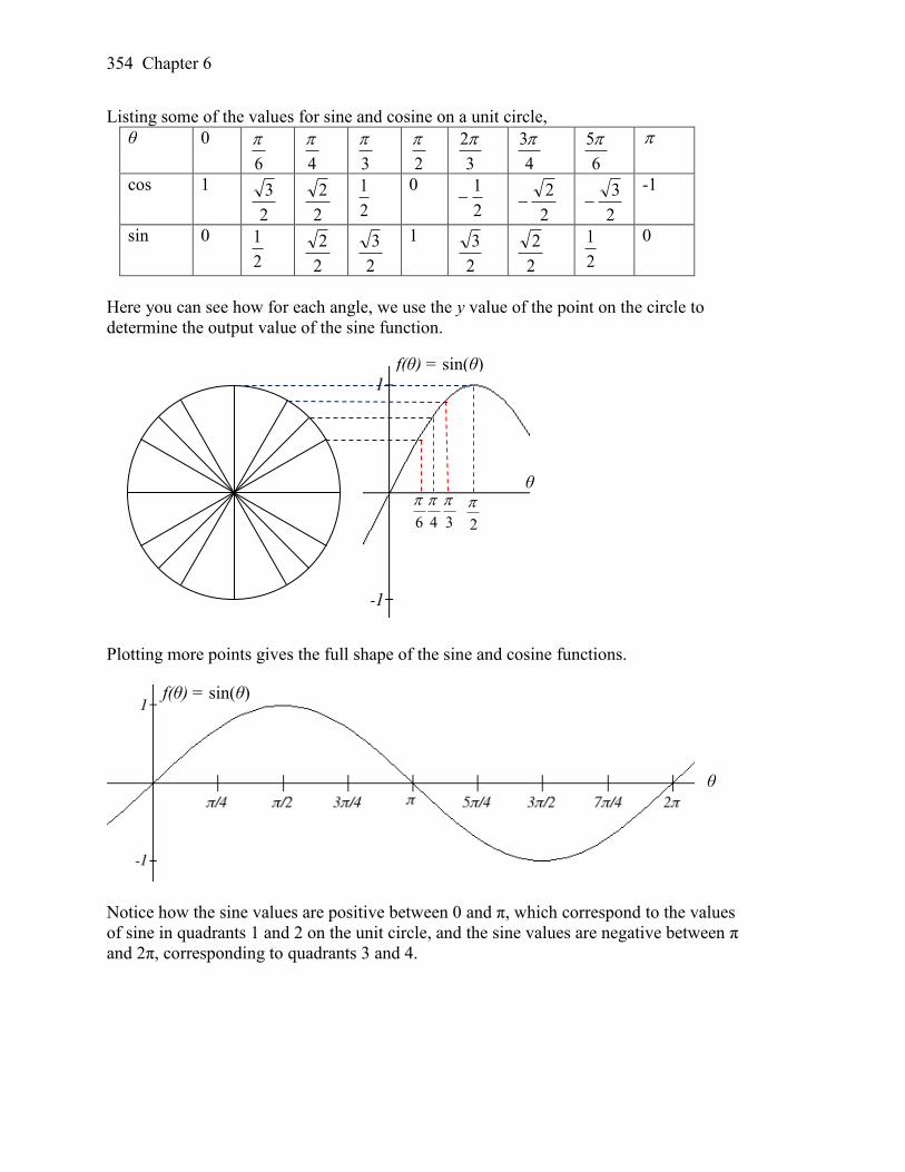
354 Chapter 6
Listing some of the values for sine and cosine on a unit circle,
θ 0
6
4
3
2
3
2
4
3
6
5
cos 1
2
3
2
2
2
1
0
2
1
2
2
2
3
-1
sin 0
2
1
2
2
2
3
1
2
3
2
2
2
1
0
Here you can see how for each angle, we use the y value of the point on the circle to
determine the output value of the sine function.
Plotting more points gives the full shape of the sine and cosine functions.
Notice how the sine values are positive between 0 and π, which correspond to the values
of sine in quadrants 1 and 2 on the unit circle, and the sine values are negative between π
and 2π, corresponding to quadrants 3 and 4.
6
4
3
2
θ
f(θ) = sin(θ)
f(θ) = sin(θ)
θ
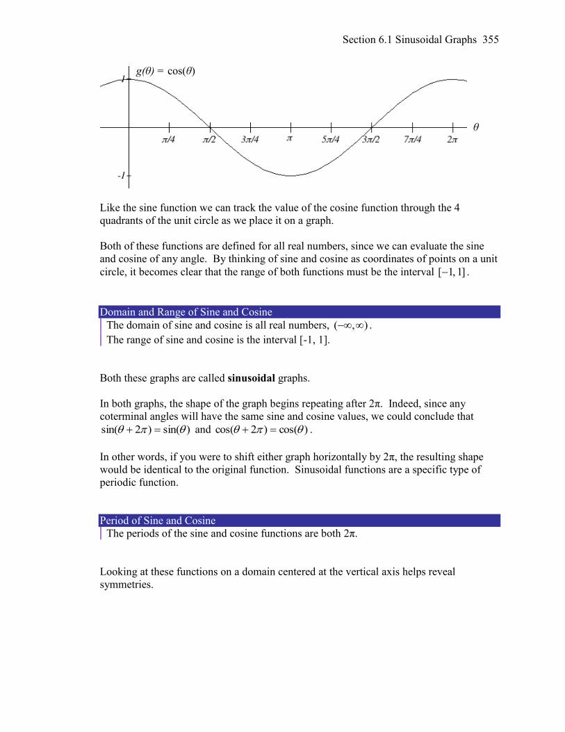
Section 6.1 Sinusoidal Graphs 355
Like the sine function we can track the value of the cosine function through the 4
quadrants of the unit circle as we place it on a graph.
Both of these functions are defined for all real numbers, since we can evaluate the sine
and cosine of any angle. By thinking of sine and cosine as coordinates of points on a unit
circle, it becomes clear that the range of both functions must be the interval ]1,1[ .
Domain and Range of Sine and Cosine
The domain of sine and cosine is all real numbers, ( , ) .
The range of sine and cosine is the interval [-1, 1].
Both these graphs are called sinusoidal graphs.
In both graphs, the shape of the graph begins repeating after 2π. Indeed, since any
coterminal angles will have the same sine and cosine values, we could conclude that
)sin()2sin( and )cos()2cos( .
In other words, if you were to shift either graph horizontally by 2π, the resulting shape
would be identical to the original function. Sinusoidal functions are a specific type of
periodic function.
Period of Sine and Cosine
The periods of the sine and cosine functions are both 2π.
Looking at these functions on a domain centered at the vertical axis helps reveal
symmetries.
θ
g(θ) = cos(θ)
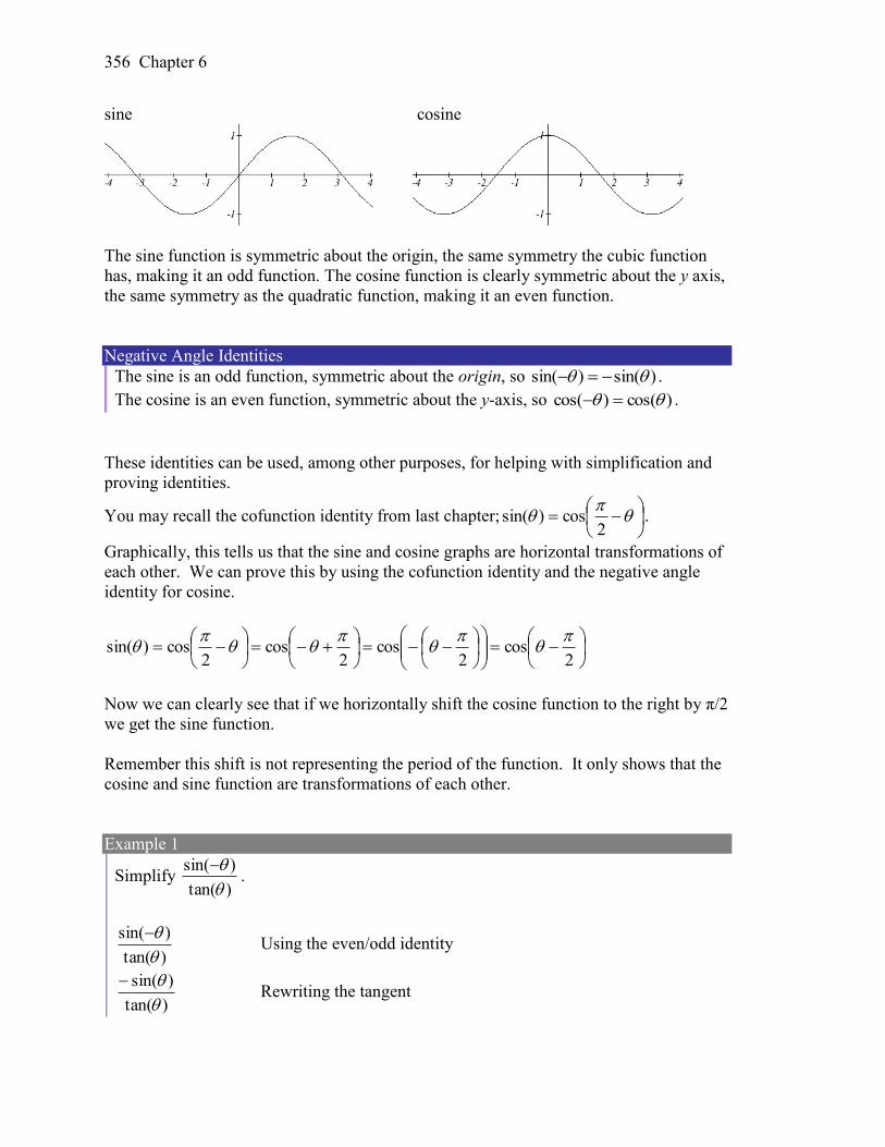
356 Chapter 6
sine cosine
The sine function is symmetric about the origin, the same symmetry the cubic function
has, making it an odd function. The cosine function is clearly symmetric about the y axis,
the same symmetry as the quadratic function, making it an even function.
Negative Angle Identities
The sine is an odd function, symmetric about the origin, so )sin()sin( .
The cosine is an even function, symmetric about the y-axis, so )cos()cos( .
These identities can be used, among other purposes, for helping with simplification and
proving identities.
You may recall the cofunction identity from last chapter;
2cos)sin( .
Graphically, this tells us that the sine and cosine graphs are horizontal transformations of
each other. We can prove this by using the cofunction identity and the negative angle
identity for cosine.
2cos
2cos
2cos
2cos)sin(
Now we can clearly see that if we horizontally shift the cosine function to the right by π/2
we get the sine function.
Remember this shift is not representing the period of the function. It only shows that the
cosine and sine function are transformations of each other.
Example 1
Simplify )tan(
)sin(
.
)tan(
)sin(
Using the even/odd identity
)tan(
)sin(
Rewriting the tangent
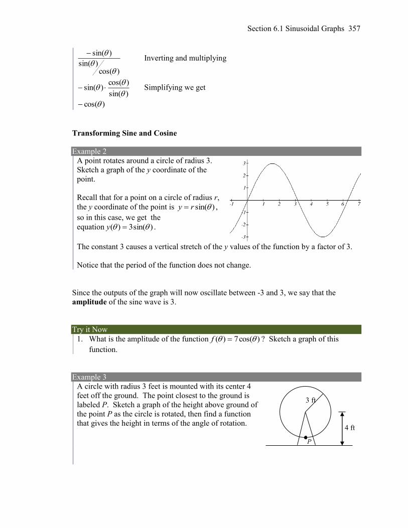
Section 6.1 Sinusoidal Graphs 357
)cos()sin(
)sin(
Inverting and multiplying
)sin(
)cos()sin(
Simplifying we get
)cos(
Transforming Sine and Cosine
Example 2
A point rotates around a circle of radius 3.
Sketch a graph of the y coordinate of the
point.
Recall that for a point on a circle of radius r,
the y coordinate of the point is )sin(ry ,
so in this case, we get the
equation )sin(3)( y .
The constant 3 causes a vertical stretch of the y values of the function by a factor of 3.
Notice that the period of the function does not change.
Since the outputs of the graph will now oscillate between -3 and 3, we say that the
amplitude of the sine wave is 3.
Try it Now
1. What is the amplitude of the function )cos(7)( f ? Sketch a graph of this
function.
Example 3
A circle with radius 3 feet is mounted with its center 4
feet off the ground. The point closest to the ground is
labeled P. Sketch a graph of the height above ground of
the point P as the circle is rotated, then find a function
that gives the height in terms of the angle of rotation.
3 ft
4 ft
P
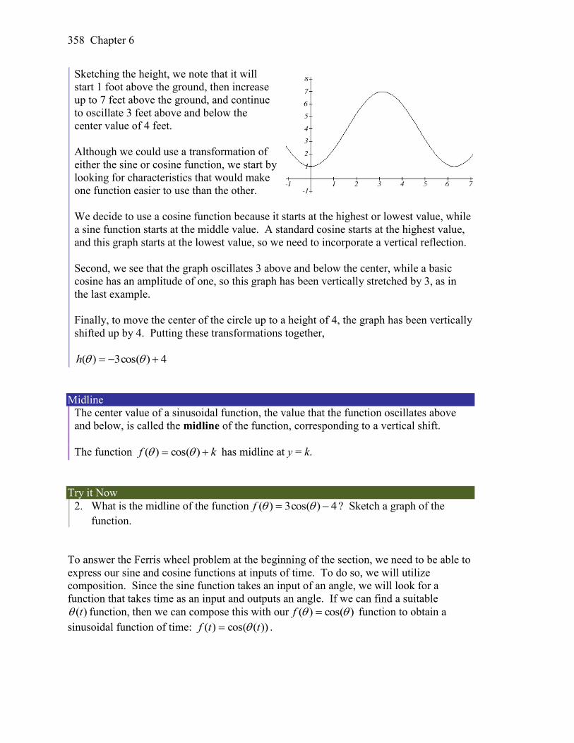
358 Chapter 6
Sketching the height, we note that it will
start 1 foot above the ground, then increase
up to 7 feet above the ground, and continue
to oscillate 3 feet above and below the
center value of 4 feet.
Although we could use a transformation of
either the sine or cosine function, we start by
looking for characteristics that would make
one function easier to use than the other.
We decide to use a cosine function because it starts at the highest or lowest value, while
a sine function starts at the middle value. A standard cosine starts at the highest value,
and this graph starts at the lowest value, so we need to incorporate a vertical reflection.
Second, we see that the graph oscillates 3 above and below the center, while a basic
cosine has an amplitude of one, so this graph has been vertically stretched by 3, as in
the last example.
Finally, to move the center of the circle up to a height of 4, the graph has been vertically
shifted up by 4. Putting these transformations together,
4)cos(3)( h
Midline
The center value of a sinusoidal function, the value that the function oscillates above
and below, is called the midline of the function, corresponding to a vertical shift.
The function kf )cos()( has midline at y = k.
Try it Now
2. What is the midline of the function 4)cos(3)( f ? Sketch a graph of the
function.
To answer the Ferris wheel problem at the beginning of the section, we need to be able to
express our sine and cosine functions at inputs of time. To do so, we will utilize
composition. Since the sine function takes an input of an angle, we will look for a
function that takes time as an input and outputs an angle. If we can find a suitable
)(t function, then we can compose this with our )cos()( f function to obtain a
sinusoidal function of time: ))(cos()( ttf .
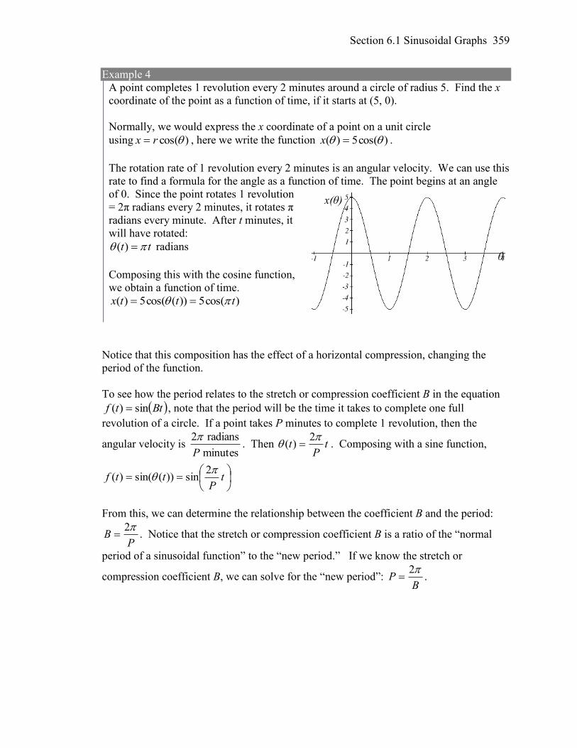
Section 6.1 Sinusoidal Graphs 359
Example 4
A point completes 1 revolution every 2 minutes around a circle of radius 5. Find the x
coordinate of the point as a function of time, if it starts at (5, 0).
Normally, we would express the x coordinate of a point on a unit circle
using )cos(rx , here we write the function )cos(5)( x .
The rotation rate of 1 revolution every 2 minutes is an angular velocity. We can use this
rate to find a formula for the angle as a function of time. The point begins at an angle
of 0. Since the point rotates 1 revolution
= 2π radians every 2 minutes, it rotates π
radians every minute. After t minutes, it
will have rotated:
tt )( radians
Composing this with the cosine function,
we obtain a function of time.
)cos(5))(cos(5)( tttx
Notice that this composition has the effect of a horizontal compression, changing the
period of the function.
To see how the period relates to the stretch or compression coefficient B in the equation
Bttf sin)( , note that the period will be the time it takes to complete one full
revolution of a circle. If a point takes P minutes to complete 1 revolution, then the
angular velocity is minutes
radians2
P
. Then t
Pt
2)( . Composing with a sine function,
t
Pttf
2sin))(sin()(
From this, we can determine the relationship between the coefficient B and the period:
PB
2 . Notice that the stretch or compression coefficient B is a ratio of the “normal
period of a sinusoidal function” to the “new period.” If we know the stretch or
compression coefficient B, we can solve for the “new period”: B
P2
.
θ
x(θ)
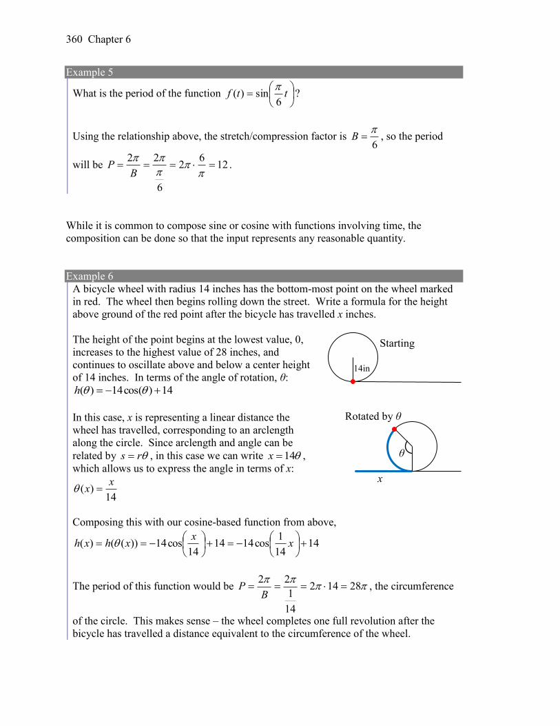
360 Chapter 6
Example 5
What is the period of the function
ttf
6sin)(
?
Using the relationship above, the stretch/compression factor is 6
B , so the period
will be 126
2
6
22
BP .
While it is common to compose sine or cosine with functions involving time, the
composition can be done so that the input represents any reasonable quantity.
Example 6
A bicycle wheel with radius 14 inches has the bottom-most point on the wheel marked
in red. The wheel then begins rolling down the street. Write a formula for the height
above ground of the red point after the bicycle has travelled x inches.
The height of the point begins at the lowest value, 0,
increases to the highest value of 28 inches, and
continues to oscillate above and below a center height
of 14 inches. In terms of the angle of rotation, θ:
14)cos(14)( h
In this case, x is representing a linear distance the
wheel has travelled, corresponding to an arclength
along the circle. Since arclength and angle can be
related by rs , in this case we can write 14x ,
which allows us to express the angle in terms of x:
14)(
xx
Composing this with our cosine-based function from above,
1414
1cos1414
14cos14))(()(
x
xxhxh
The period of this function would be
28142
14
1
22
BP , the circumference
of the circle. This makes sense – the wheel completes one full revolution after the
bicycle has travelled a distance equivalent to the circumference of the wheel.
θ
Starting
Rotated by θ
14in
x
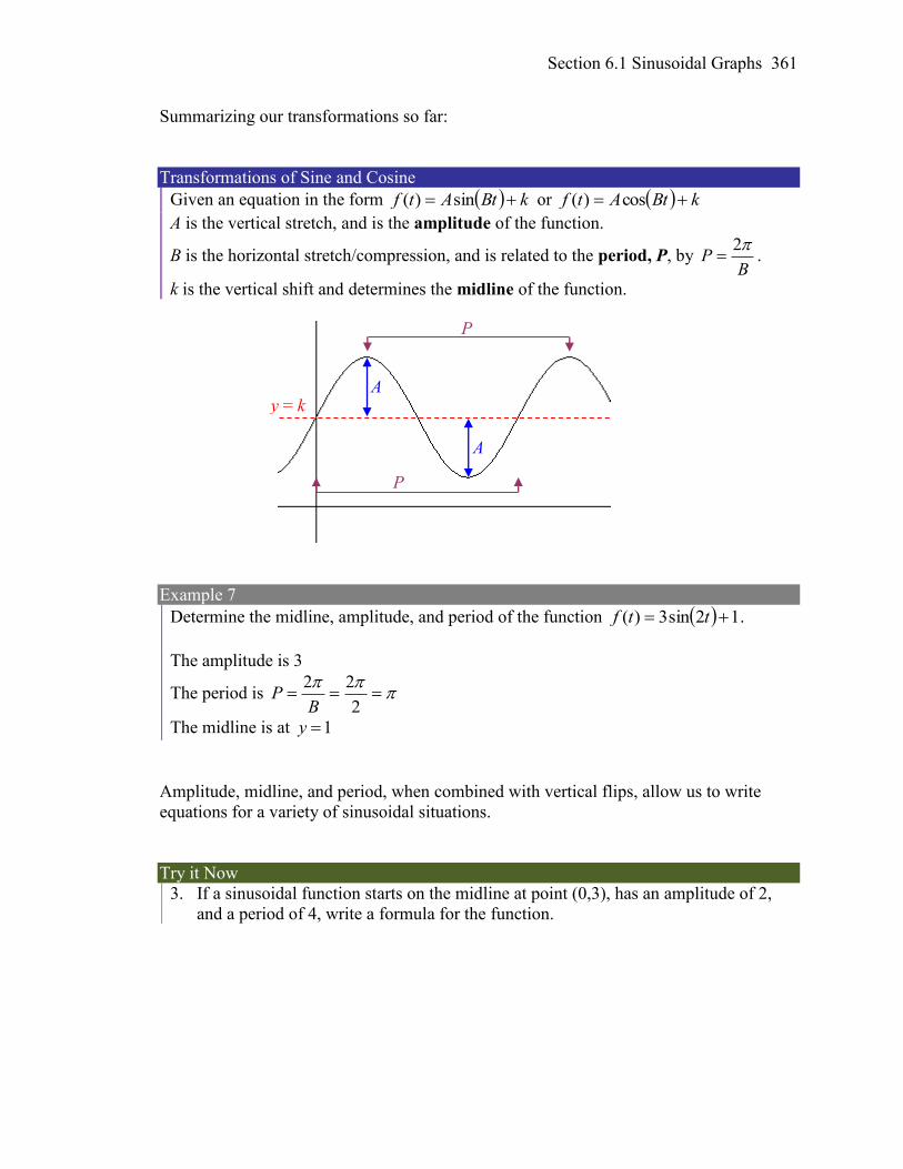
Section 6.1 Sinusoidal Graphs 361
Summarizing our transformations so far:
Transformations of Sine and Cosine
Given an equation in the form kBtAtf sin)( or kBtAtf cos)(
A is the vertical stretch, and is the amplitude of the function.
B is the horizontal stretch/compression, and is related to the period, P, by B
P2
.
k is the vertical shift and determines the midline of the function.
Example 7
Determine the midline, amplitude, and period of the function 12sin3)( ttf .
The amplitude is 3
The period is
2
22
BP
The midline is at 1y
Amplitude, midline, and period, when combined with vertical flips, allow us to write
equations for a variety of sinusoidal situations.
Try it Now
3. If a sinusoidal function starts on the midline at point (0,3), has an amplitude of 2,
and a period of 4, write a formula for the function.
y = k A
A
P
P
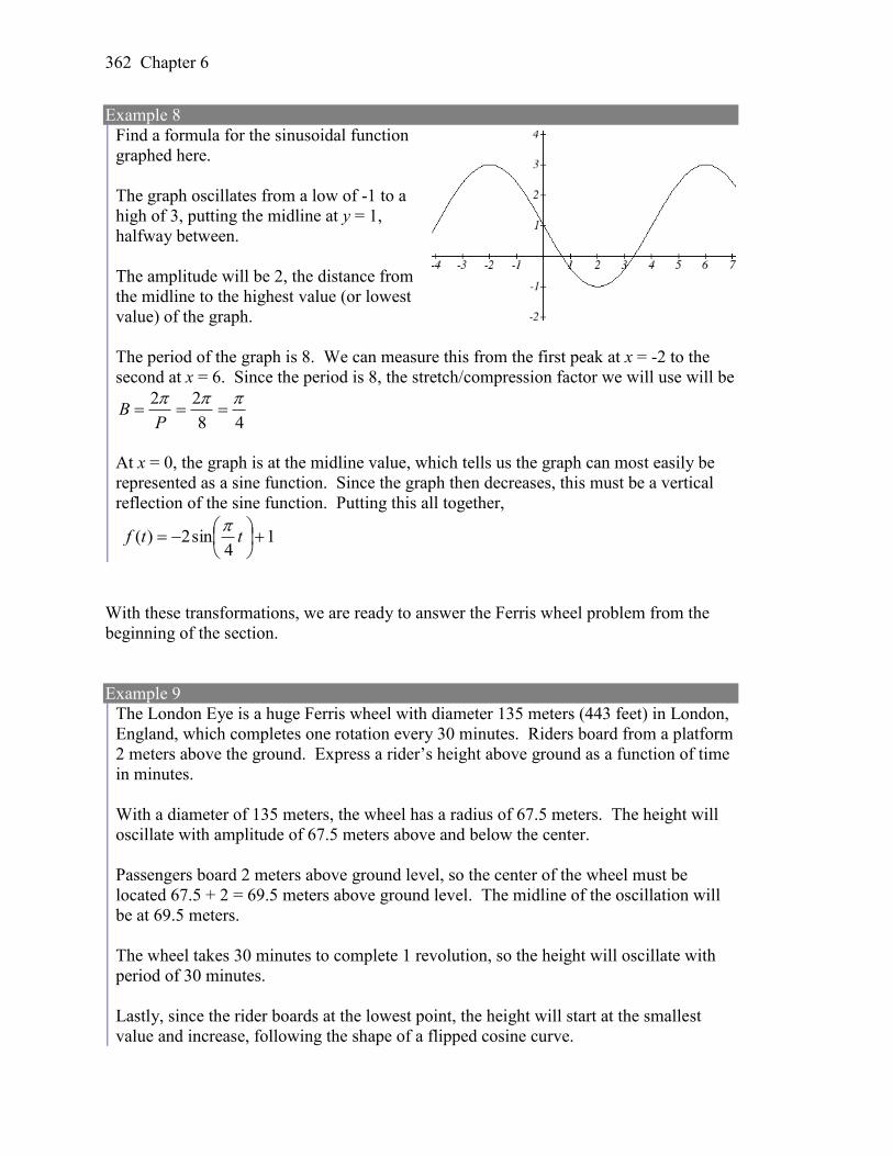
362 Chapter 6
Example 8
Find a formula for the sinusoidal function
graphed here.
The graph oscillates from a low of -1 to a
high of 3, putting the midline at y = 1,
halfway between.
The amplitude will be 2, the distance from
the midline to the highest value (or lowest
value) of the graph.
The period of the graph is 8. We can measure this from the first peak at x = -2 to the
second at x = 6. Since the period is 8, the stretch/compression factor we will use will be
48
22
PB
At x = 0, the graph is at the midline value, which tells us the graph can most easily be
represented as a sine function. Since the graph then decreases, this must be a vertical
reflection of the sine function. Putting this all together,
14
sin2)(
ttf
With these transformations, we are ready to answer the Ferris wheel problem from the
beginning of the section.
Example 9
The London Eye is a huge Ferris wheel with diameter 135 meters (443 feet) in London,
England, which completes one rotation every 30 minutes. Riders board from a platform
2 meters above the ground. Express a rider’s height above ground as a function of time
in minutes.
With a diameter of 135 meters, the wheel has a radius of 67.5 meters. The height will
oscillate with amplitude of 67.5 meters above and below the center.
Passengers board 2 meters above ground level, so the center of the wheel must be
located 67.5 + 2 = 69.5 meters above ground level. The midline of the oscillation will
be at 69.5 meters.
The wheel takes 30 minutes to complete 1 revolution, so the height will oscillate with
period of 30 minutes.
Lastly, since the rider boards at the lowest point, the height will start at the smallest
value and increase, following the shape of a flipped cosine curve.
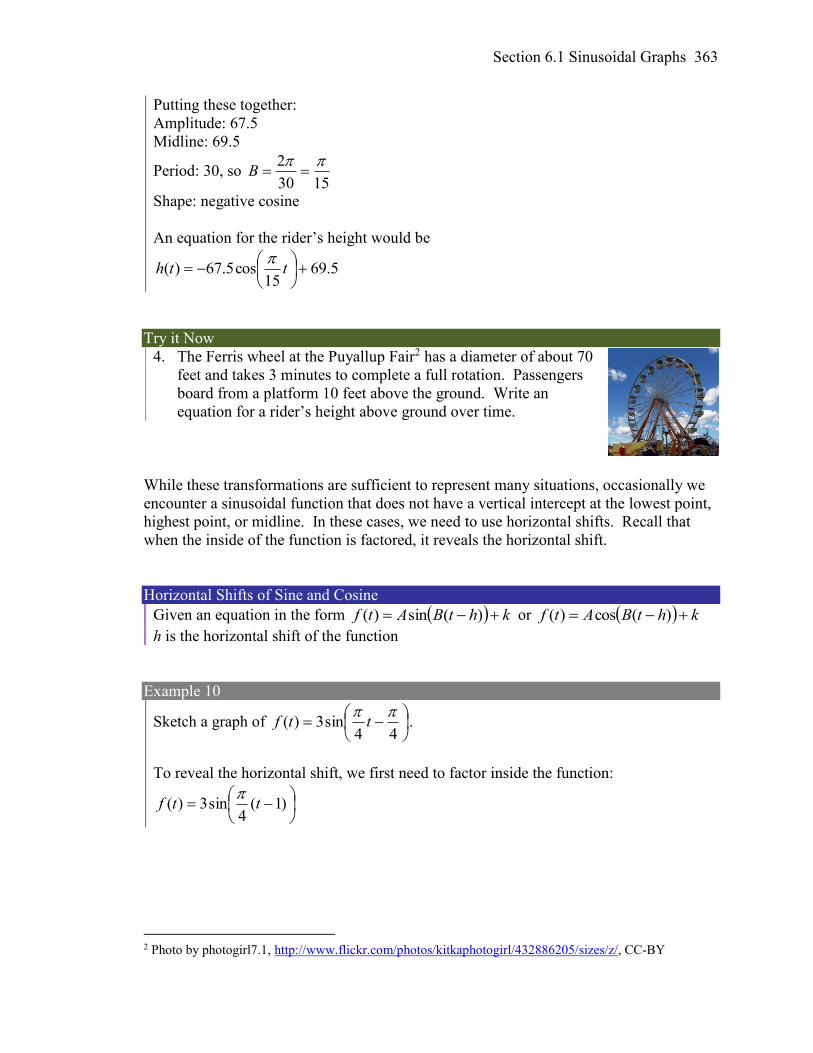
Section 6.1 Sinusoidal Graphs 363
Putting these together:
Amplitude: 67.5
Midline: 69.5
Period: 30, so 1530
2 B
Shape: negative cosine
An equation for the rider’s height would be
5.6915
cos5.67)(
tth
Try it Now
4. The Ferris wheel at the Puyallup Fair2 has a diameter of about 70
feet and takes 3 minutes to complete a full rotation. Passengers
board from a platform 10 feet above the ground. Write an
equation for a rider’s height above ground over time.
While these transformations are sufficient to represent many situations, occasionally we
encounter a sinusoidal function that does not have a vertical intercept at the lowest point,
highest point, or midline. In these cases, we need to use horizontal shifts. Recall that
when the inside of the function is factored, it reveals the horizontal shift.
Horizontal Shifts of Sine and Cosine
Given an equation in the form khtBAtf )(sin)( or khtBAtf )(cos)(
h is the horizontal shift of the function
Example 10
Sketch a graph of
44sin3)(
ttf .
To reveal the horizontal shift, we first need to factor inside the function:
)1(
4sin3)( ttf
2 Photo by photogirl7.1, http://www.flickr.com/photos/kitkaphotogirl/432886205/sizes/z/, CC-BY
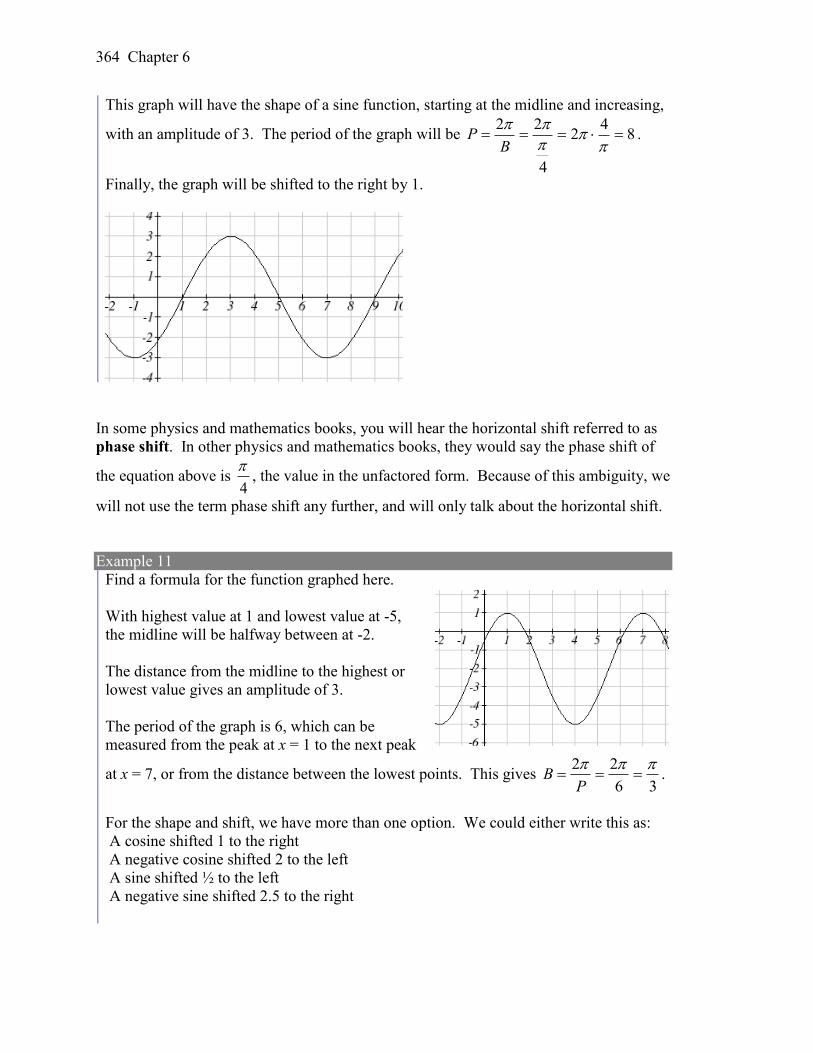
364 Chapter 6
This graph will have the shape of a sine function, starting at the midline and increasing,
with an amplitude of 3. The period of the graph will be 84
2
4
22
BP .
Finally, the graph will be shifted to the right by 1.
In some physics and mathematics books, you will hear the horizontal shift referred to as
phase shift. In other physics and mathematics books, they would say the phase shift of
the equation above is 4
, the value in the unfactored form. Because of this ambiguity, we
will not use the term phase shift any further, and will only talk about the horizontal shift.
Example 11
Find a formula for the function graphed here.
With highest value at 1 and lowest value at -5,
the midline will be halfway between at -2.
The distance from the midline to the highest or
lowest value gives an amplitude of 3.
The period of the graph is 6, which can be
measured from the peak at x = 1 to the next peak
at x = 7, or from the distance between the lowest points. This gives 36
22
PB .
For the shape and shift, we have more than one option. We could either write this as:
A cosine shifted 1 to the right
A negative cosine shifted 2 to the left
A sine shifted ½ to the left
A negative sine shifted 2.5 to the right
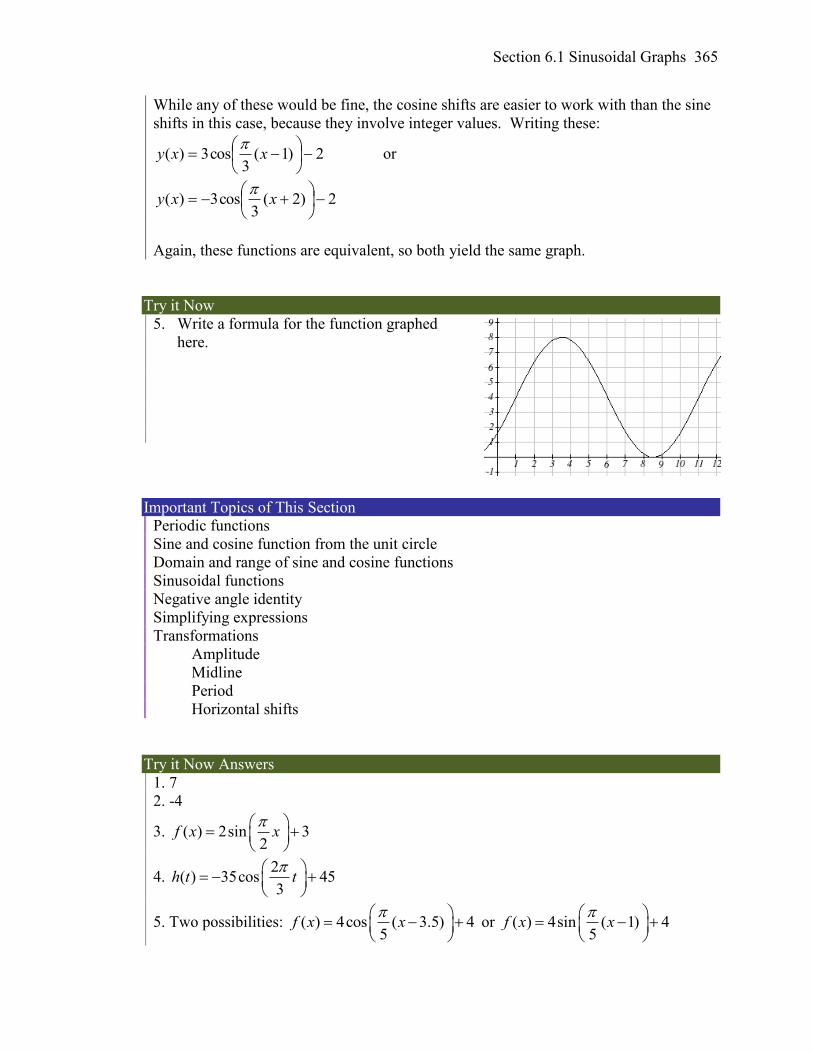
Section 6.1 Sinusoidal Graphs 365
While any of these would be fine, the cosine shifts are easier to work with than the sine
shifts in this case, because they involve integer values. Writing these:
2)1(3
cos3)(
xxy
or
2)2(3
cos3)(
xxy
Again, these functions are equivalent, so both yield the same graph.
Try it Now
5. Write a formula for the function graphed
here.
Important Topics of This Section
Periodic functions
Sine and cosine function from the unit circle
Domain and range of sine and cosine functions
Sinusoidal functions
Negative angle identity
Simplifying expressions
Transformations
Amplitude
Midline
Period
Horizontal shifts
Try it Now Answers
1. 7
2. -4
3. ( ) 2sin 32
f x x
4. 2
( ) 35cos 453
h t t
5. Two possibilities: ( ) 4cos ( 3.5) 45
f x x
or ( ) 4sin ( 1) 45
f x x
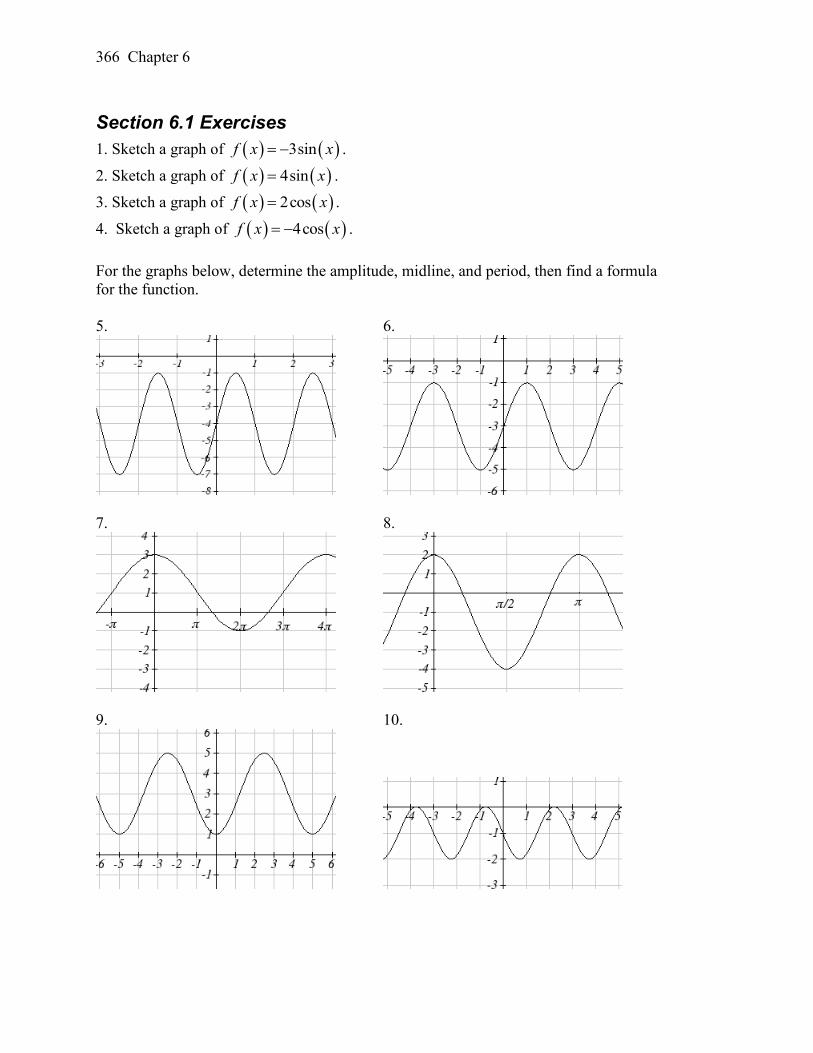
366 Chapter 6
Section 6.1 Exercises
1. Sketch a graph of 3sinf x x .
2. Sketch a graph of 4sinf x x .
3. Sketch a graph of 2cosf x x .
4. Sketch a graph of 4cosf x x .
For the graphs below, determine the amplitude, midline, and period, then find a formula
for the function.
5. 6.
7. 8.
9. 10.
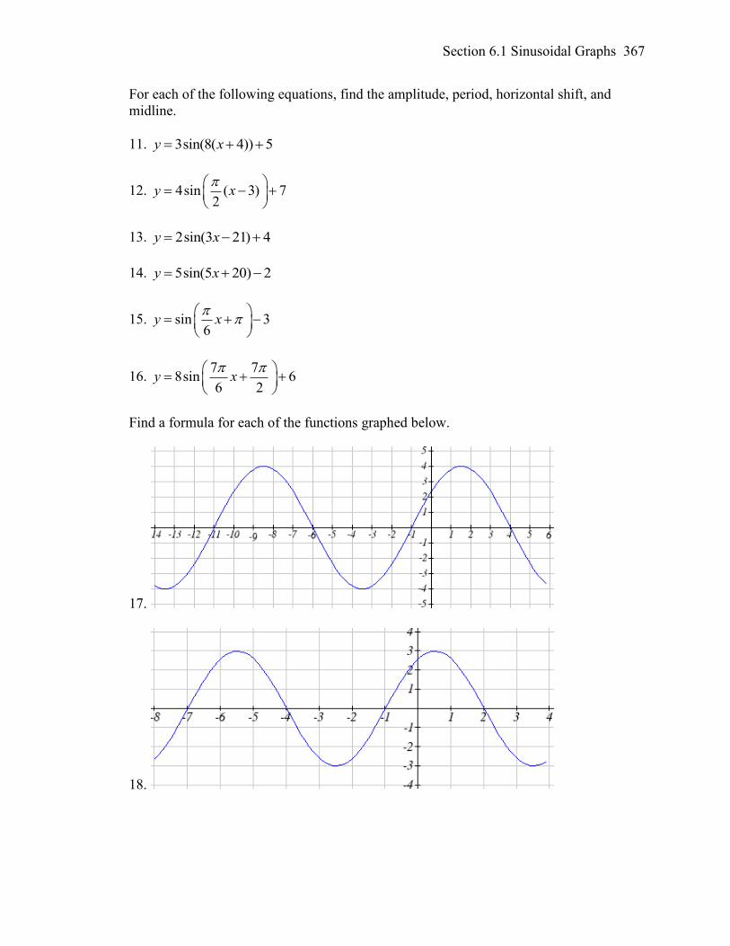
Section 6.1 Sinusoidal Graphs 367
For each of the following equations, find the amplitude, period, horizontal shift, and
midline.
11. 3sin(8( 4)) 5y x
12. 4sin ( 3) 72
y x
13. 2sin(3 21) 4y x
14. 5sin(5 20) 2y x
15. sin 36
y x
16. 7 7
8sin 66 2
y x
Find a formula for each of the functions graphed below.
17.
18.
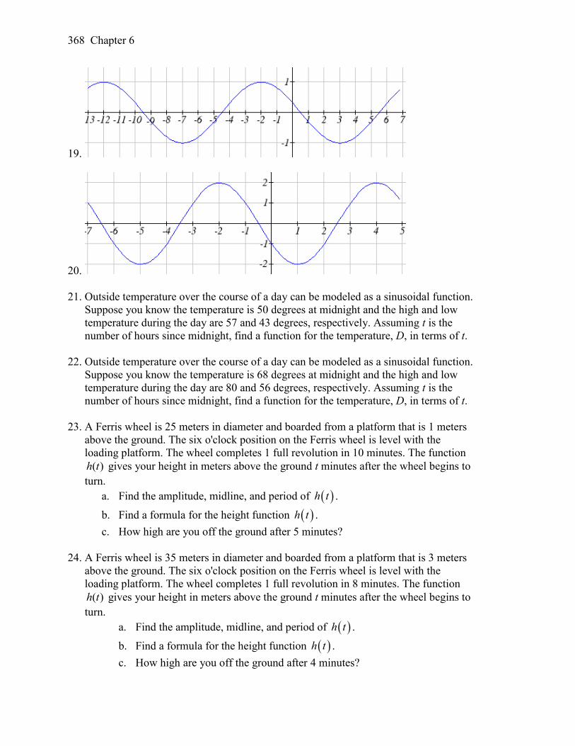
368 Chapter 6
19.
20.
21. Outside temperature over the course of a day can be modeled as a sinusoidal function.
Suppose you know the temperature is 50 degrees at midnight and the high and low
temperature during the day are 57 and 43 degrees, respectively. Assuming t is the
number of hours since midnight, find a function for the temperature, D, in terms of t.
22. Outside temperature over the course of a day can be modeled as a sinusoidal function.
Suppose you know the temperature is 68 degrees at midnight and the high and low
temperature during the day are 80 and 56 degrees, respectively. Assuming t is the
number of hours since midnight, find a function for the temperature, D, in terms of t.
23. A Ferris wheel is 25 meters in diameter and boarded from a platform that is 1 meters
above the ground. The six o'clock position on the Ferris wheel is level with the
loading platform. The wheel completes 1 full revolution in 10 minutes. The function
( )h t gives your height in meters above the ground t minutes after the wheel begins to
turn.
a. Find the amplitude, midline, and period of h t .
b. Find a formula for the height function h t .
c. How high are you off the ground after 5 minutes?
24. A Ferris wheel is 35 meters in diameter and boarded from a platform that is 3 meters
above the ground. The six o'clock position on the Ferris wheel is level with the
loading platform. The wheel completes 1 full revolution in 8 minutes. The function
( )h t gives your height in meters above the ground t minutes after the wheel begins to
turn.
a. Find the amplitude, midline, and period of h t .
b. Find a formula for the height function h t .
c. How high are you off the ground after 4 minutes?
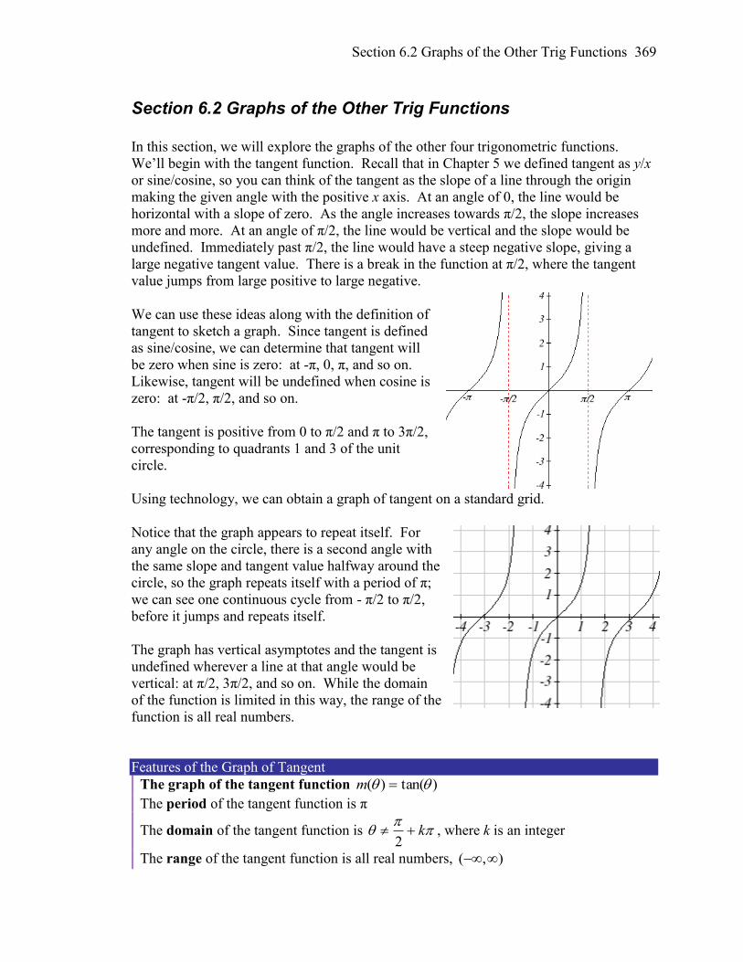
Section 6.2 Graphs of the Other Trig Functions 369
Section 6.2 Graphs of the Other Trig Functions
In this section, we will explore the graphs of the other four trigonometric functions.
We’ll begin with the tangent function. Recall that in Chapter 5 we defined tangent as y/x
or sine/cosine, so you can think of the tangent as the slope of a line through the origin
making the given angle with the positive x axis. At an angle of 0, the line would be
horizontal with a slope of zero. As the angle increases towards π/2, the slope increases
more and more. At an angle of π/2, the line would be vertical and the slope would be
undefined. Immediately past π/2, the line would have a steep negative slope, giving a
large negative tangent value. There is a break in the function at π/2, where the tangent
value jumps from large positive to large negative.
We can use these ideas along with the definition of
tangent to sketch a graph. Since tangent is defined
as sine/cosine, we can determine that tangent will
be zero when sine is zero: at -π, 0, π, and so on.
Likewise, tangent will be undefined when cosine is
zero: at -π/2, π/2, and so on.
The tangent is positive from 0 to π/2 and π to 3π/2,
corresponding to quadrants 1 and 3 of the unit
circle.
Using technology, we can obtain a graph of tangent on a standard grid.
Notice that the graph appears to repeat itself. For
any angle on the circle, there is a second angle with
the same slope and tangent value halfway around the
circle, so the graph repeats itself with a period of π;
we can see one continuous cycle from - π/2 to π/2,
before it jumps and repeats itself.
The graph has vertical asymptotes and the tangent is
undefined wherever a line at that angle would be
vertical: at π/2, 3π/2, and so on. While the domain
of the function is limited in this way, the range of the
function is all real numbers.
Features of the Graph of Tangent
The graph of the tangent function )tan()( m
The period of the tangent function is π
The domain of the tangent function is
k2
, where k is an integer
The range of the tangent function is all real numbers, ( , )
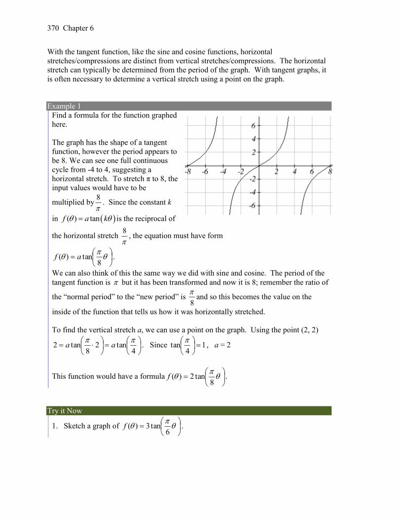
370 Chapter 6
With the tangent function, like the sine and cosine functions, horizontal
stretches/compressions are distinct from vertical stretches/compressions. The horizontal
stretch can typically be determined from the period of the graph. With tangent graphs, it
is often necessary to determine a vertical stretch using a point on the graph.
Example 1
Find a formula for the function graphed
here.
The graph has the shape of a tangent
function, however the period appears to
be 8. We can see one full continuous
cycle from -4 to 4, suggesting a
horizontal stretch. To stretch π to 8, the
input values would have to be
multiplied by
8. Since the constant k
in ( ) tanf a k is the reciprocal of
the horizontal stretch
8, the equation must have form
8tan)( af .
We can also think of this the same way we did with sine and cosine. The period of the
tangent function is but it has been transformed and now it is 8; remember the ratio of
the “normal period” to the “new period” is 8
and so this becomes the value on the
inside of the function that tells us how it was horizontally stretched.
To find the vertical stretch a, we can use a point on the graph. Using the point (2, 2)
4tan2
8tan2
aa . Since 1
4tan
, a = 2
This function would have a formula
8tan2)(f .
Try it Now
1. Sketch a graph of
6tan3)(f .
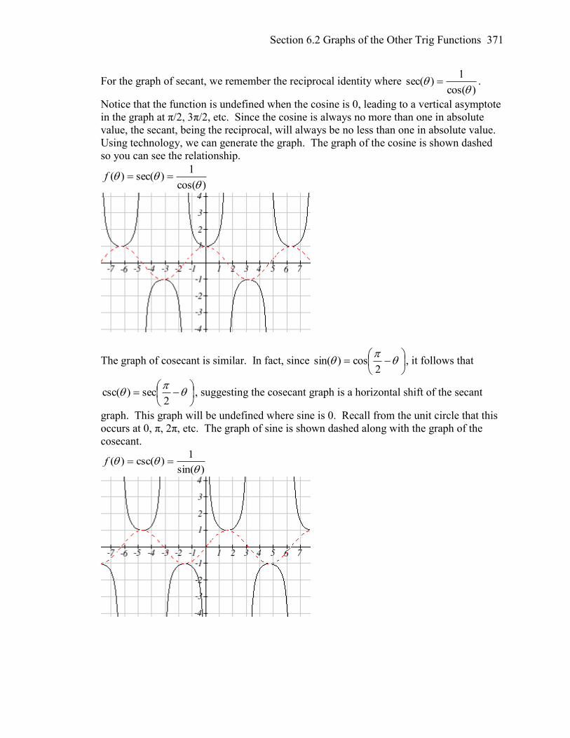
Section 6.2 Graphs of the Other Trig Functions 371
For the graph of secant, we remember the reciprocal identity where )cos(
1)sec(
.
Notice that the function is undefined when the cosine is 0, leading to a vertical asymptote
in the graph at π/2, 3π/2, etc. Since the cosine is always no more than one in absolute
value, the secant, being the reciprocal, will always be no less than one in absolute value.
Using technology, we can generate the graph. The graph of the cosine is shown dashed
so you can see the relationship.
)cos(
1)sec()(
f
The graph of cosecant is similar. In fact, since
2cos)sin( , it follows that
2sec)csc( , suggesting the cosecant graph is a horizontal shift of the secant
graph. This graph will be undefined where sine is 0. Recall from the unit circle that this
occurs at 0, π, 2π, etc. The graph of sine is shown dashed along with the graph of the
cosecant.
)sin(
1)csc()(
f
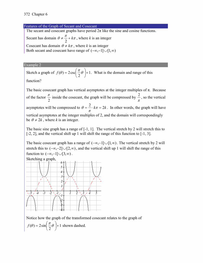
372 Chapter 6
Features of the Graph of Secant and Cosecant
The secant and cosecant graphs have period 2π like the sine and cosine functions.
Secant has domain
k2
, where k is an integer
Cosecant has domain k , where k is an integer
Both secant and cosecant have range of ),1[]1,(
Example 2
Sketch a graph of 12
csc2)(
f . What is the domain and range of this
function?
The basic cosecant graph has vertical asymptotes at the integer multiples of π. Because
of the factor 2
inside the cosecant, the graph will be compressed by
2, so the vertical
asymptotes will be compressed to kk 22
. In other words, the graph will have
vertical asymptotes at the integer multiples of 2, and the domain will correspondingly
be k2 , where k is an integer.
The basic sine graph has a range of [-1, 1]. The vertical stretch by 2 will stretch this to
[-2, 2], and the vertical shift up 1 will shift the range of this function to [-1, 3].
The basic cosecant graph has a range of ),1[]1,( . The vertical stretch by 2 will
stretch this to ),2[]2,( , and the vertical shift up 1 will shift the range of this
function to ),3[]1,( .
Sketching a graph,
Notice how the graph of the transformed cosecant relates to the graph of
12
sin2)(
f shown dashed.
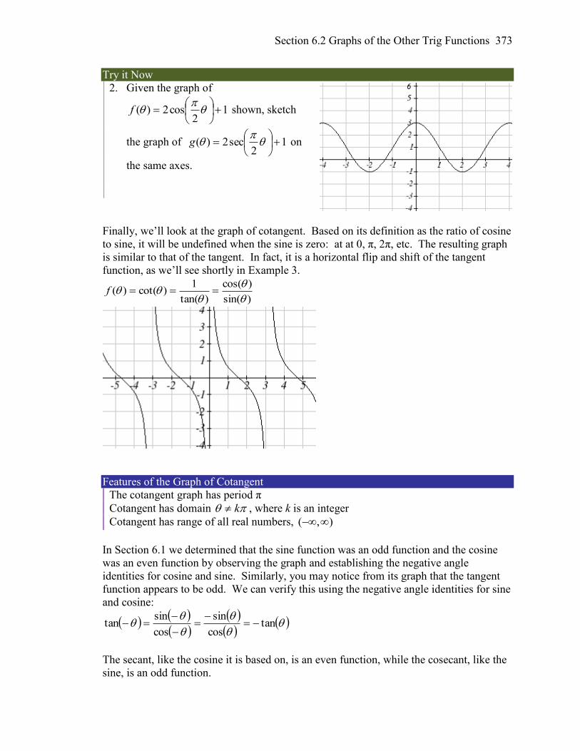
Section 6.2 Graphs of the Other Trig Functions 373
Try it Now
2. Given the graph of
12
cos2)(
f shown, sketch
the graph of 12
sec2)(
g on
the same axes.
Finally, we’ll look at the graph of cotangent. Based on its definition as the ratio of cosine
to sine, it will be undefined when the sine is zero: at at 0, π, 2π, etc. The resulting graph
is similar to that of the tangent. In fact, it is a horizontal flip and shift of the tangent
function, as we’ll see shortly in Example 3.
)sin(
)cos(
)tan(
1)cot()(
f
Features of the Graph of Cotangent
The cotangent graph has period π
Cotangent has domain k , where k is an integer
Cotangent has range of all real numbers, ( , )
In Section 6.1 we determined that the sine function was an odd function and the cosine
was an even function by observing the graph and establishing the negative angle
identities for cosine and sine. Similarly, you may notice from its graph that the tangent
function appears to be odd. We can verify this using the negative angle identities for sine
and cosine:
tan
cos
sin
cos
sintan
The secant, like the cosine it is based on, is an even function, while the cosecant, like the
sine, is an odd function.
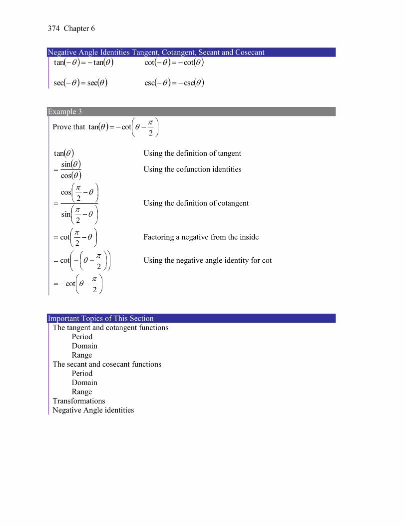
374 Chapter 6
Negative Angle Identities Tangent, Cotangent, Secant and Cosecant
tantan cotcot
secsec csccsc
Example 3
Prove that
2cottan
tan Using the definition of tangent
cos
sin Using the cofunction identities
2sin
2cos
Using the definition of cotangent
2cot Factoring a negative from the inside
2cot
Using the negative angle identity for cot
2cot
Important Topics of This Section
The tangent and cotangent functions
Period
Domain
Range
The secant and cosecant functions
Period
Domain
Range
Transformations
Negative Angle identities
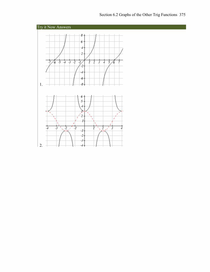
Section 6.2 Graphs of the Other Trig Functions 375
Try it Now Answers
1.
2.
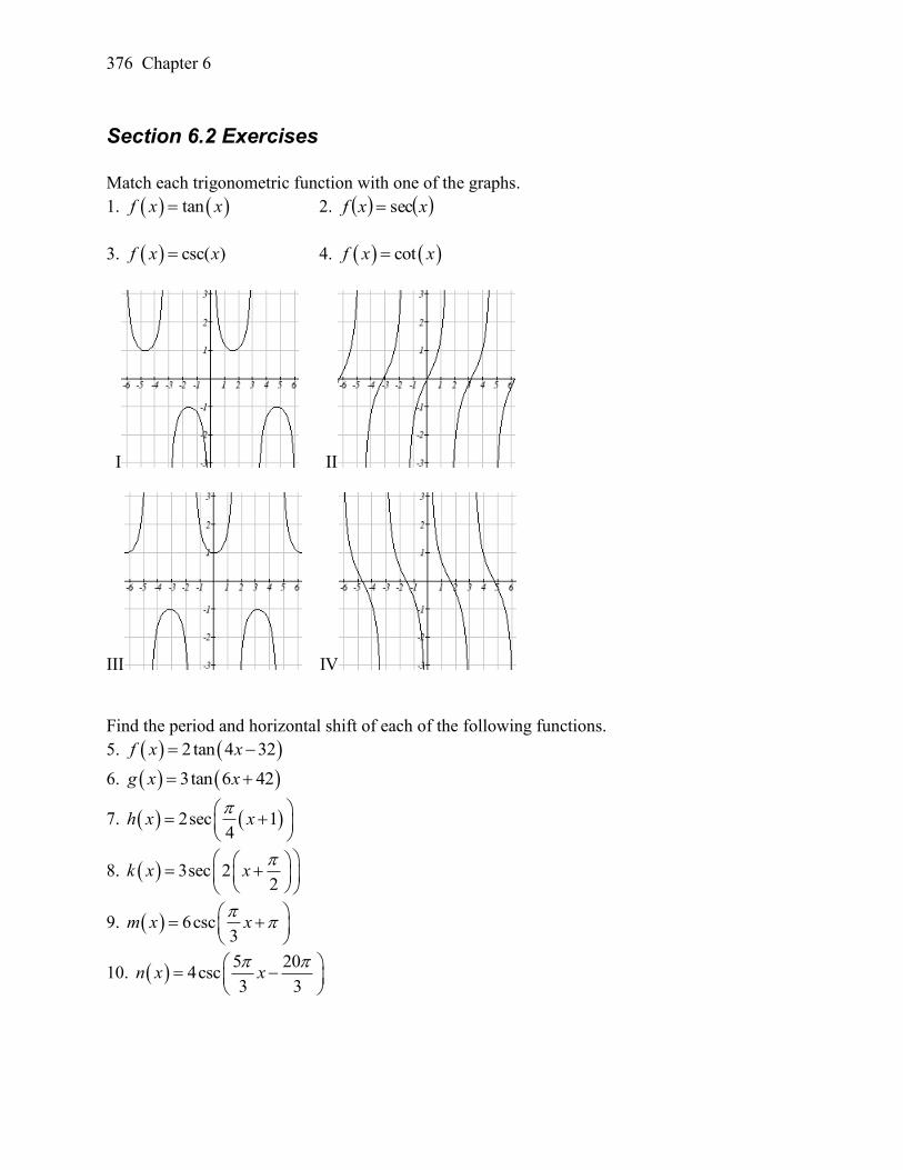
376 Chapter 6
Section 6.2 Exercises
Match each trigonometric function with one of the graphs.
1. tanf x x 2. sec xxf
3. csc( )f x x 4. cotf x x
I II
III IV
Find the period and horizontal shift of each of the following functions.
5. 2tan 4 32f x x
6. 3tan 6 42g x x
7. 2sec 14
h x x
8. 3sec 22
k x x
9. 6csc3
m x x
10. 5 20
4csc3 3
n x x
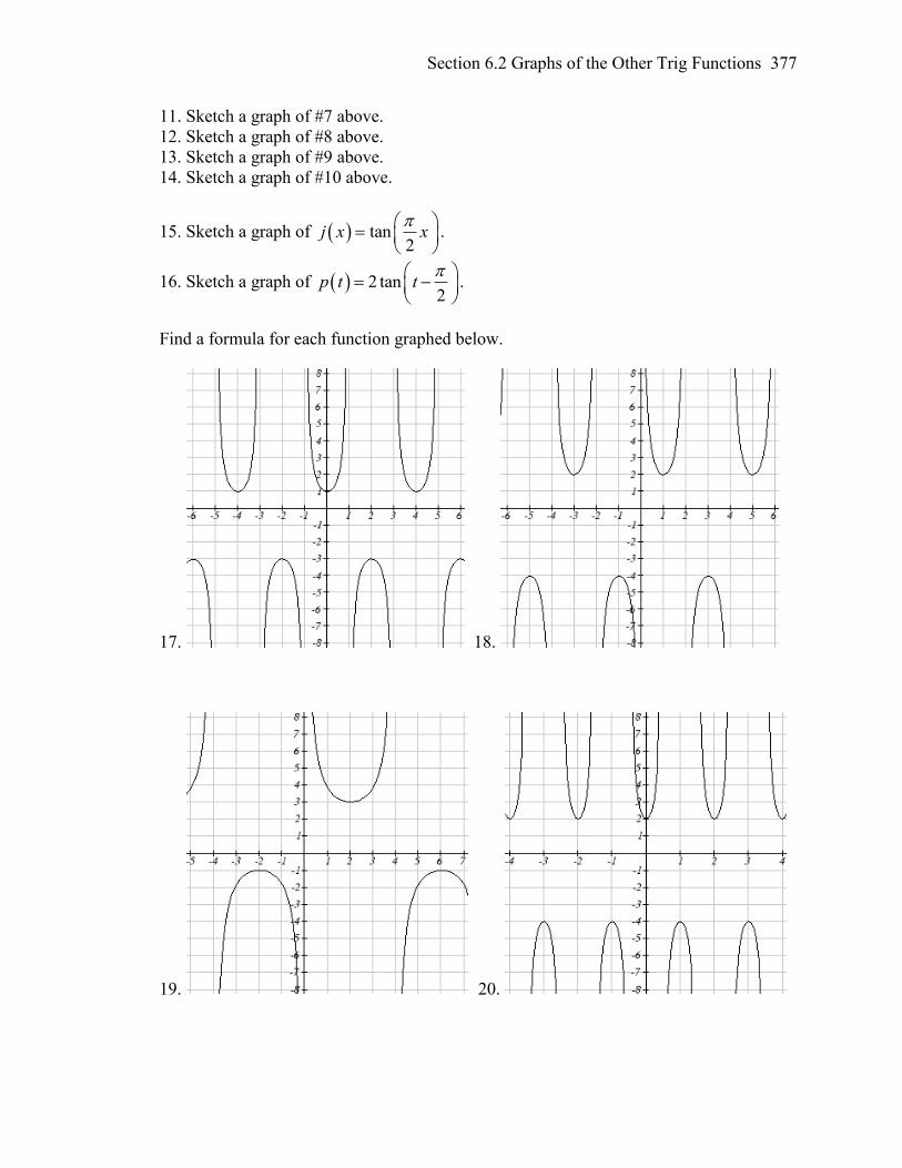
Section 6.2 Graphs of the Other Trig Functions 377
11. Sketch a graph of #7 above.
12. Sketch a graph of #8 above.
13. Sketch a graph of #9 above.
14. Sketch a graph of #10 above.
15. Sketch a graph of tan2
j x x
.
16. Sketch a graph of 2 tan2
p t t
.
Find a formula for each function graphed below.
17. 18.
19. 20.
378 Chapter 6
21. If tan 1.5x , find tan x .
22. If tan 3x , find tan x .
23. If sec 2x , find sec x .
24. If sec 4x , find sec x .
25. If csc 5x , find csc x .
26. If csc 2x , find csc x .
Simplify each of the following expressions completely.
27. cot cos sinx x x
28. cos tan sinx x x
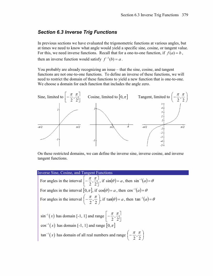
Section 6.3 Inverse Trig Functions 379
Section 6.3 Inverse Trig Functions
In previous sections we have evaluated the trigonometric functions at various angles, but
at times we need to know what angle would yield a specific sine, cosine, or tangent value.
For this, we need inverse functions. Recall that for a one-to-one function, if baf )( ,
then an inverse function would satisfy abf )(1 .
You probably are already recognizing an issue – that the sine, cosine, and tangent
functions are not one-to-one functions. To define an inverse of these functions, we will
need to restrict the domain of these functions to yield a new function that is one-to-one.
We choose a domain for each function that includes the angle zero.
Sine, limited to
2,
2
Cosine, limited to ,0 Tangent, limited to ,
2 2
On these restricted domains, we can define the inverse sine, inverse cosine, and inverse
tangent functions.
Inverse Sine, Cosine, and Tangent Functions
For angles in the interval
2,
2
, if asin , then a1sin
For angles in the interval ,0 , if acos , then a1cos
For angles in the interval
2,
2
, if atan , then a1tan
1sin x has domain [-1, 1] and range
2,
2
1cos x has domain [-1, 1] and range ,0
1tan x has domain of all real numbers and range
2,
2
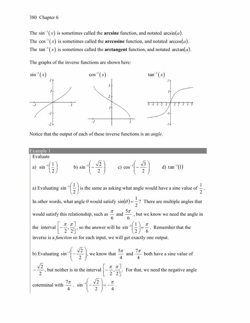
380 Chapter 6
The 1sin x is sometimes called the arcsine function, and notated aarcsin .
The 1cos x is sometimes called the arccosine function, and notated aarccos .
The 1tan x is sometimes called the arctangent function, and notated aarctan .
The graphs of the inverse functions are shown here:
1sin x 1cos x 1tan x
Notice that the output of each of these inverse functions is an angle.
Example 1
Evaluate
a)
2
1sin 1
b)
2
2sin 1 c)
2
3cos 1 d) 1tan 1
a) Evaluating
2
1sin 1
is the same as asking what angle would have a sine value of 2
1.
In other words, what angle θ would satisfy 2
1sin ? There are multiple angles that
would satisfy this relationship, such as 6
and
6
5 , but we know we need the angle in
the interval
2,
2
, so the answer will be
62
1sin 1
. Remember that the
inverse is a function so for each input, we will get exactly one output.
b) Evaluating
2
2sin 1
, we know that 4
5 and
4
7 both have a sine value of
2
2 , but neither is in the interval
2,
2
. For that, we need the negative angle
coterminal with 4
7.
42
2sin 1
.
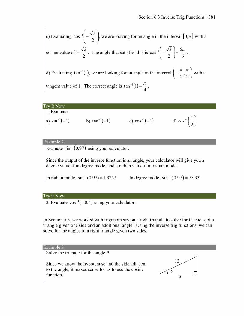
Section 6.3 Inverse Trig Functions 381
c) Evaluating
2
3cos 1 , we are looking for an angle in the interval ,0 with a
cosine value of 2
3 . The angle that satisfies this is
6
5
2
3cos 1
.
d) Evaluating 1tan 1, we are looking for an angle in the interval
2,
2
with a
tangent value of 1. The correct angle is 4
1tan 1 .
Try It Now
1. Evaluate
a) 1sin 1 b) 1tan 1
c) 1cos 1 d)
2
1cos 1
Example 2
Evaluate 97.0sin 1 using your calculator.
Since the output of the inverse function is an angle, your calculator will give you a
degree value if in degree mode, and a radian value if in radian mode.
In radian mode, 1sin (0.97) 1.3252 In degree mode, 1sin 0.97 75.93
Try it Now
2. Evaluate 4.0cos 1 using your calculator.
In Section 5.5, we worked with trigonometry on a right triangle to solve for the sides of a
triangle given one side and an additional angle. Using the inverse trig functions, we can
solve for the angles of a right triangle given two sides.
Example 3
Solve the triangle for the angle θ.
Since we know the hypotenuse and the side adjacent
to the angle, it makes sense for us to use the cosine
function.
12
9
θ
382 Chapter 6
12
9cos Using the definition of the inverse,
12
9cos 1 Evaluating
7227.0 , or about 41.4096°
There are times when we need to compose a trigonometric function with an inverse
trigonometric function. In these cases, we can find exact values for the resulting
expressions
Example 4
Evaluate
6
13cossin 1
.
a) Here, we can directly evaluate the inside of the composition.
2
3
6
13cos
Now, we can evaluate the inverse function as we did earlier.
32
3sin 1
Try it Now
3. Evaluate
4
11sincos 1
.
Example 5
Find an exact value for
5
4cossin 1 .
Beginning with the inside, we can say there is some angle so
5
4cos 1 , which
means 5
4cos , and we are looking for sin . We can use the Pythagorean identity
to do this.
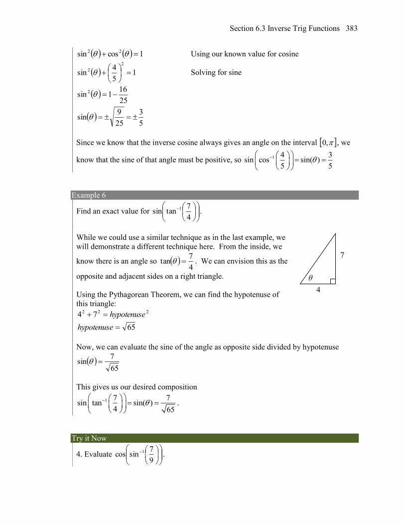
Section 6.3 Inverse Trig Functions 383
1cossin 22 Using our known value for cosine
15
4sin
2
2
Solving for sine
25
161sin 2
5
3
25
9sin
Since we know that the inverse cosine always gives an angle on the interval ,0 , we
know that the sine of that angle must be positive, so 1 4 3sin cos sin( )
5 5
Example 6
Find an exact value for
4
7tansin 1 .
While we could use a similar technique as in the last example, we
will demonstrate a different technique here. From the inside, we
know there is an angle so 4
7tan . We can envision this as the
opposite and adjacent sides on a right triangle.
Using the Pythagorean Theorem, we can find the hypotenuse of
this triangle: 222 74 hypotenuse
65hypotenuse
Now, we can evaluate the sine of the angle as opposite side divided by hypotenuse
65
7sin
This gives us our desired composition
1 7 7sin tan sin( )
4 65
.
Try it Now
4. Evaluate
9
7sincos 1 .
7
4
θ
384 Chapter 6
We can also find compositions involving algebraic expressions.
Example 7
Find a simplified expression for
3sincos 1 x
, for 33 x .
We know there is an angle θ so that 3
sinx
. Using the Pythagorean Theorem,
1cossin 22 Using our known expression for sine
1cos3
2
2
x Solving for cosine
9
1cos2
2 x
3
9
9
9cos
22 xx
Since we know that the inverse sine must give an angle on the interval
2,
2
, we
can deduce that the cosine of that angle must be positive. This gives us
3
9
3sincos
21 xx
Try it Now
5. Find a simplified expression for x4tansin 1, for
4
1
4
1 x .
Important Topics of This Section
Inverse trig functions: arcsine, arccosine and arctangent
Domain restrictions
Evaluating inverses using unit circle values and the calculator
Simplifying numerical expressions involving the inverse trig functions
Simplifying algebraic expressions involving the inverse trig functions
Section 6.3 Inverse Trig Functions 385
Try it Now Answers
1. a) 2
b)
4
c) d)
3
2. 1.9823 or 113.578°
3. 4
3
4. 9
24
5. 116
4
2 x
x
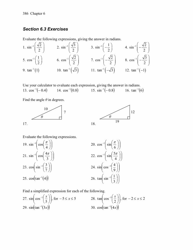
386 Chapter 6
Section 6.3 Exercises
Evaluate the following expressions, giving the answer in radians.
1. 1 2sin
2
2. 1 3sin
2
3. 1 1
sin2
4. 1 2sin
2
5. 1 1
cos2
6. 1 2cos
2
7. 1 2cos
2
8. 1 3cos
2
9. 1tan 1 10. 1tan 3
11. 1tan 3 12. 1tan 1
Use your calculator to evaluate each expression, giving the answer in radians.
13. 4.0cos 1 14. 8.0cos 1
15. 8.0sin 1 16. 6tan 1
Find the angle θ in degrees.
17. 18.
Evaluate the following expressions.
19.
4cossin 1
20.
6sincos 1
21.
3
4cossin 1
22.
4
5sincos 1
23.
7
3sincos 1 24.
9
4cossin 1
25. 4tancos 1 26.
3
1sintan 1
Find a simplified expression for each of the following.
27.
5cossin 1 x
, for 55 x 28.
2costan 1 x
, for 22 x
29. x3tansin 1 30. x4tancos 1
12
19
θ
10 7
θ
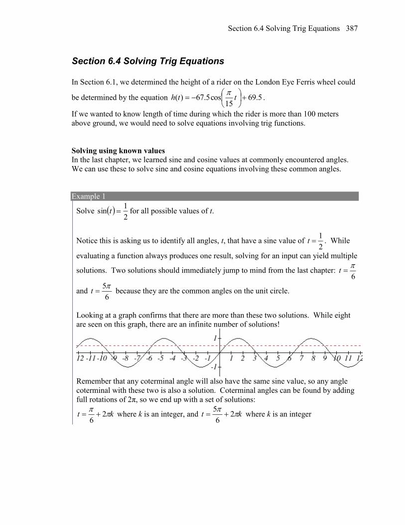
Section 6.4 Solving Trig Equations 387
Section 6.4 Solving Trig Equations
In Section 6.1, we determined the height of a rider on the London Eye Ferris wheel could
be determined by the equation 5.6915
cos5.67)(
tth
.
If we wanted to know length of time during which the rider is more than 100 meters
above ground, we would need to solve equations involving trig functions.
Solving using known values In the last chapter, we learned sine and cosine values at commonly encountered angles.
We can use these to solve sine and cosine equations involving these common angles.
Example 1
Solve 2
1sin t for all possible values of t.
Notice this is asking us to identify all angles, t, that have a sine value of 1
2t . While
evaluating a function always produces one result, solving for an input can yield multiple
solutions. Two solutions should immediately jump to mind from the last chapter: 6
t
and 6
5t because they are the common angles on the unit circle.
Looking at a graph confirms that there are more than these two solutions. While eight
are seen on this graph, there are an infinite number of solutions!
Remember that any coterminal angle will also have the same sine value, so any angle
coterminal with these two is also a solution. Coterminal angles can be found by adding
full rotations of 2π, so we end up with a set of solutions:
kt
26 where k is an integer, and kt
2
6
5 where k is an integer
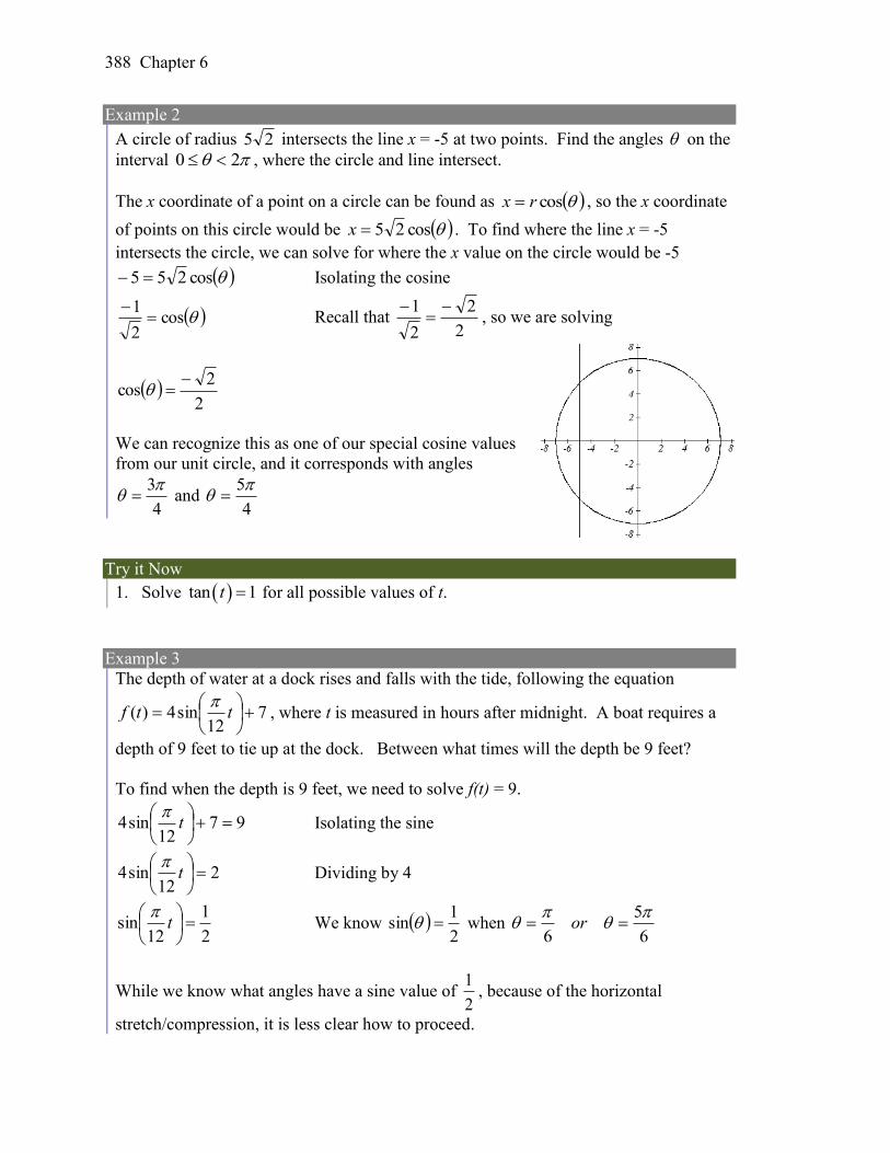
388 Chapter 6
Example 2
A circle of radius 25 intersects the line x = -5 at two points. Find the angles on the
interval 20 , where the circle and line intersect.
The x coordinate of a point on a circle can be found as cosrx , so the x coordinate
of points on this circle would be cos25x . To find where the line x = -5
intersects the circle, we can solve for where the x value on the circle would be -5
cos255 Isolating the cosine
cos2
1
Recall that
2
2
2
1
, so we are solving
2
2cos
We can recognize this as one of our special cosine values
from our unit circle, and it corresponds with angles
4
3 and
4
5
Try it Now
1. Solve tan 1t for all possible values of t.
Example 3
The depth of water at a dock rises and falls with the tide, following the equation
712
sin4)(
ttf
, where t is measured in hours after midnight. A boat requires a
depth of 9 feet to tie up at the dock. Between what times will the depth be 9 feet?
To find when the depth is 9 feet, we need to solve f(t) = 9.
9712
sin4
t
Isolating the sine
212
sin4
t
Dividing by 4
2
1
12sin
t
We know
2
1sin when
6
5
6
or
While we know what angles have a sine value of 1
2, because of the horizontal
stretch/compression, it is less clear how to proceed.
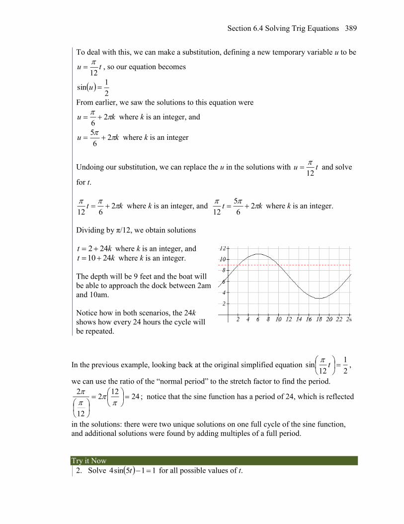
Section 6.4 Solving Trig Equations 389
To deal with this, we can make a substitution, defining a new temporary variable u to be
tu12
, so our equation becomes
2
1sin u
From earlier, we saw the solutions to this equation were
ku
26 where k is an integer, and
ku
26
5 where k is an integer
Undoing our substitution, we can replace the u in the solutions with tu12
and solve
for t.
kt
2612 where k is an integer, and kt
2
6
5
12 where k is an integer.
Dividing by π/12, we obtain solutions
kt 242 where k is an integer, and
kt 2410 where k is an integer.
The depth will be 9 feet and the boat will
be able to approach the dock between 2am
and 10am.
Notice how in both scenarios, the 24k
shows how every 24 hours the cycle will
be repeated.
In the previous example, looking back at the original simplified equation 2
1
12sin
t
,
we can use the ratio of the “normal period” to the stretch factor to find the period.
2412
2
12
2
; notice that the sine function has a period of 24, which is reflected
in the solutions: there were two unique solutions on one full cycle of the sine function,
and additional solutions were found by adding multiples of a full period.
Try it Now
2. Solve 115sin4 t for all possible values of t.
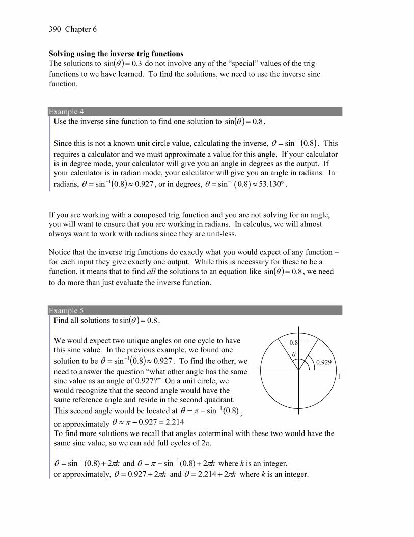
390 Chapter 6
Solving using the inverse trig functions
The solutions to 3.0sin do not involve any of the “special” values of the trig
functions to we have learned. To find the solutions, we need to use the inverse sine
function.
Example 4
Use the inverse sine function to find one solution to 8.0sin .
Since this is not a known unit circle value, calculating the inverse, 8.0sin 1 . This
requires a calculator and we must approximate a value for this angle. If your calculator
is in degree mode, your calculator will give you an angle in degrees as the output. If
your calculator is in radian mode, your calculator will give you an angle in radians. In
radians, 927.08.0sin 1 , or in degrees, 1sin 0.8 53.130 .
If you are working with a composed trig function and you are not solving for an angle,
you will want to ensure that you are working in radians. In calculus, we will almost
always want to work with radians since they are unit-less.
Notice that the inverse trig functions do exactly what you would expect of any function –
for each input they give exactly one output. While this is necessary for these to be a
function, it means that to find all the solutions to an equation like 8.0sin , we need
to do more than just evaluate the inverse function.
Example 5
Find all solutions to 8.0sin .
We would expect two unique angles on one cycle to have
this sine value. In the previous example, we found one
solution to be 927.08.0sin 1 . To find the other, we
need to answer the question “what other angle has the same
sine value as an angle of 0.927?” On a unit circle, we
would recognize that the second angle would have the
same reference angle and reside in the second quadrant.
This second angle would be located at )8.0(sin 1 ,
or approximately 214.2927.0
To find more solutions we recall that angles coterminal with these two would have the
same sine value, so we can add full cycles of 2π.
k 2)8.0(sin 1 and k 2)8.0(sin 1
where k is an integer,
or approximately, k 2927.0 and k 2214.2 where k is an integer.
0.8
1
0.929 θ
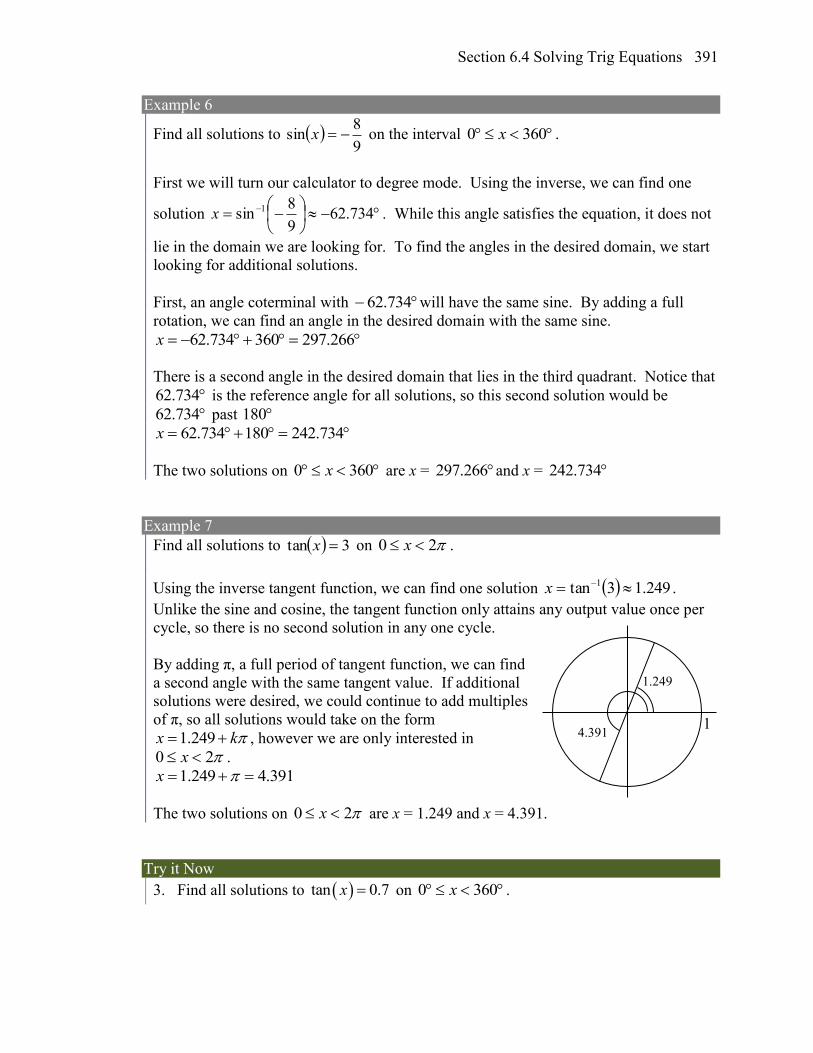
Section 6.4 Solving Trig Equations 391
Example 6
Find all solutions to 9
8sin x on the interval 3600 x .
First we will turn our calculator to degree mode. Using the inverse, we can find one
solution
734.62
9
8sin 1x . While this angle satisfies the equation, it does not
lie in the domain we are looking for. To find the angles in the desired domain, we start
looking for additional solutions.
First, an angle coterminal with 734.62 will have the same sine. By adding a full
rotation, we can find an angle in the desired domain with the same sine.
266.297360734.62x
There is a second angle in the desired domain that lies in the third quadrant. Notice that
734.62 is the reference angle for all solutions, so this second solution would be
734.62 past 180
734.242180734.62x
The two solutions on 3600 x are x = 266.297 and x = 734.242
Example 7
Find all solutions to 3tan x on 20 x .
Using the inverse tangent function, we can find one solution 249.13tan 1 x .
Unlike the sine and cosine, the tangent function only attains any output value once per
cycle, so there is no second solution in any one cycle.
By adding π, a full period of tangent function, we can find
a second angle with the same tangent value. If additional
solutions were desired, we could continue to add multiples
of π, so all solutions would take on the form
kx 249.1 , however we are only interested in
20 x .
391.4249.1 x
The two solutions on 20 x are x = 1.249 and x = 4.391.
Try it Now
3. Find all solutions to tan 0.7x on 3600 x .
1
1.249
4.391
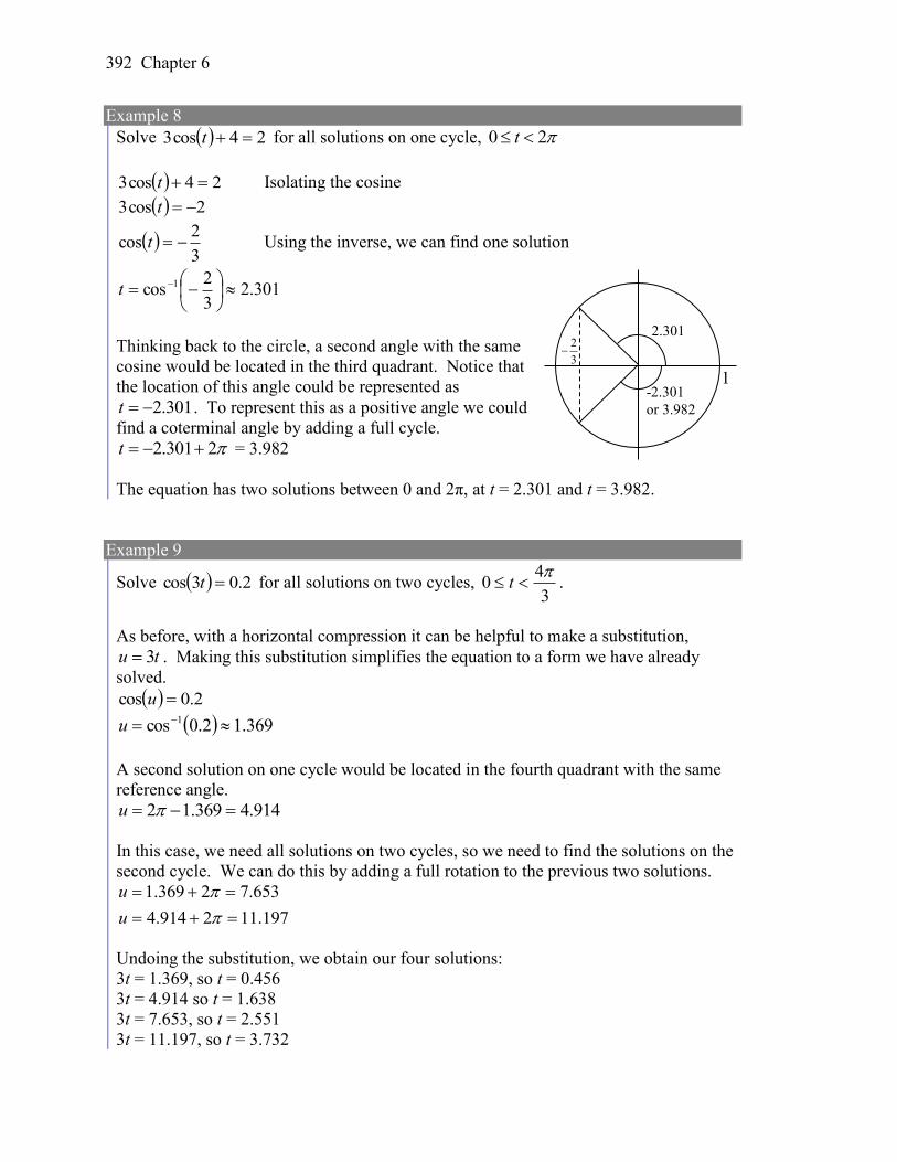
392 Chapter 6
Example 8
Solve 24cos3 t for all solutions on one cycle, 0 2t
24cos3 t Isolating the cosine
2cos3 t
3
2cos t Using the inverse, we can find one solution
301.23
2cos 1
t
Thinking back to the circle, a second angle with the same
cosine would be located in the third quadrant. Notice that
the location of this angle could be represented as
301.2t . To represent this as a positive angle we could
find a coterminal angle by adding a full cycle.
2301.2 t = 3.982
The equation has two solutions between 0 and 2π, at t = 2.301 and t = 3.982.
Example 9
Solve 2.03cos t for all solutions on two cycles, 3
40
t .
As before, with a horizontal compression it can be helpful to make a substitution,
tu 3 . Making this substitution simplifies the equation to a form we have already
solved.
2.0cos u
369.12.0cos 1 u
A second solution on one cycle would be located in the fourth quadrant with the same
reference angle.
914.4369.12 u
In this case, we need all solutions on two cycles, so we need to find the solutions on the
second cycle. We can do this by adding a full rotation to the previous two solutions.
197.112914.4
653.72369.1
u
u
Undoing the substitution, we obtain our four solutions:
3t = 1.369, so t = 0.456
3t = 4.914 so t = 1.638
3t = 7.653, so t = 2.551
3t = 11.197, so t = 3.732
2
3
1
2.301
-2.301
or 3.982
Section 6.4 Solving Trig Equations 393
Example 10
Solve 2sin3 t for all solutions.
2sin3 t Isolating the sine
3
2sin t We make the substitution tu
3
2sin u Using the inverse, we find one solution
730.03
2sin 1
u
This angle is in the fourth quadrant. A second angle with the same sine would be in the
third quadrant with 0.730 as a reference angle:
871.3730.0 u
We can write all solutions to the equation 3
2sin u as
ku 2730.0 where k is an integer, or
ku 2871.3
Undoing our substitution, we can replace u in our solutions with tu and solve for t
kt 2730.0 or kt 2871.3 Divide by π
kt 2232.0 or kt 2232.1
Try it Now
4. Solve 032
sin5
t
for all solutions on one cycle, 20 t .
Solving Trig Equations 1) Isolate the trig function on one side of the equation
2) Make a substitution for the inside of the sine, cosine, or tangent (or other trig
function)
3) Use inverse trig functions to find one solution
4) Use symmetries to find a second solution on one cycle (when a second exists)
5) Find additional solutions if needed by adding full periods
6) Undo the substitution
We now can return to the question we began the section with.
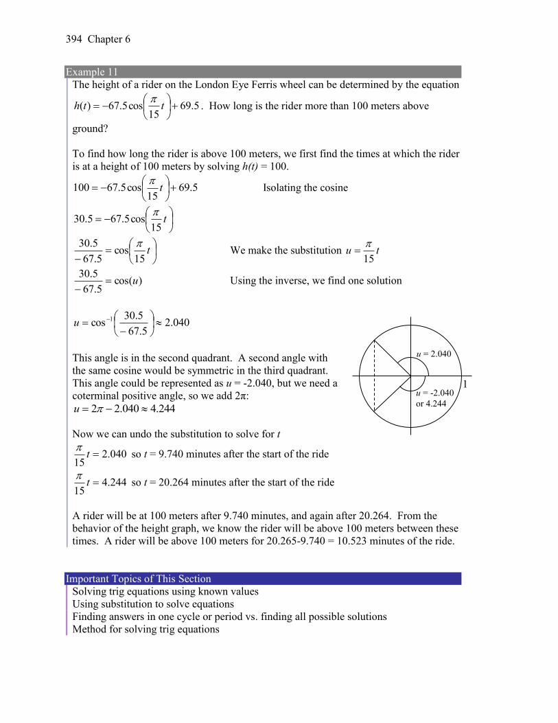
394 Chapter 6
Example 11
The height of a rider on the London Eye Ferris wheel can be determined by the equation
5.6915
cos5.67)(
tth
. How long is the rider more than 100 meters above
ground?
To find how long the rider is above 100 meters, we first find the times at which the rider
is at a height of 100 meters by solving h(t) = 100.
5.6915
cos5.67100
t
Isolating the cosine
t
15cos5.675.30
t
15cos
5.67
5.30 We make the substitution tu
15
)cos(5.67
5.30u
Using the inverse, we find one solution
040.25.67
5.30cos 1
u
This angle is in the second quadrant. A second angle with
the same cosine would be symmetric in the third quadrant.
This angle could be represented as u = -2.040, but we need a
coterminal positive angle, so we add 2π:
244.4040.22 u
Now we can undo the substitution to solve for t
040.215
t
so t = 9.740 minutes after the start of the ride
244.415
t
so t = 20.264 minutes after the start of the ride
A rider will be at 100 meters after 9.740 minutes, and again after 20.264. From the
behavior of the height graph, we know the rider will be above 100 meters between these
times. A rider will be above 100 meters for 20.265-9.740 = 10.523 minutes of the ride.
Important Topics of This Section
Solving trig equations using known values
Using substitution to solve equations
Finding answers in one cycle or period vs. finding all possible solutions
Method for solving trig equations
1
u = 2.040
u = -2.040
or 4.244
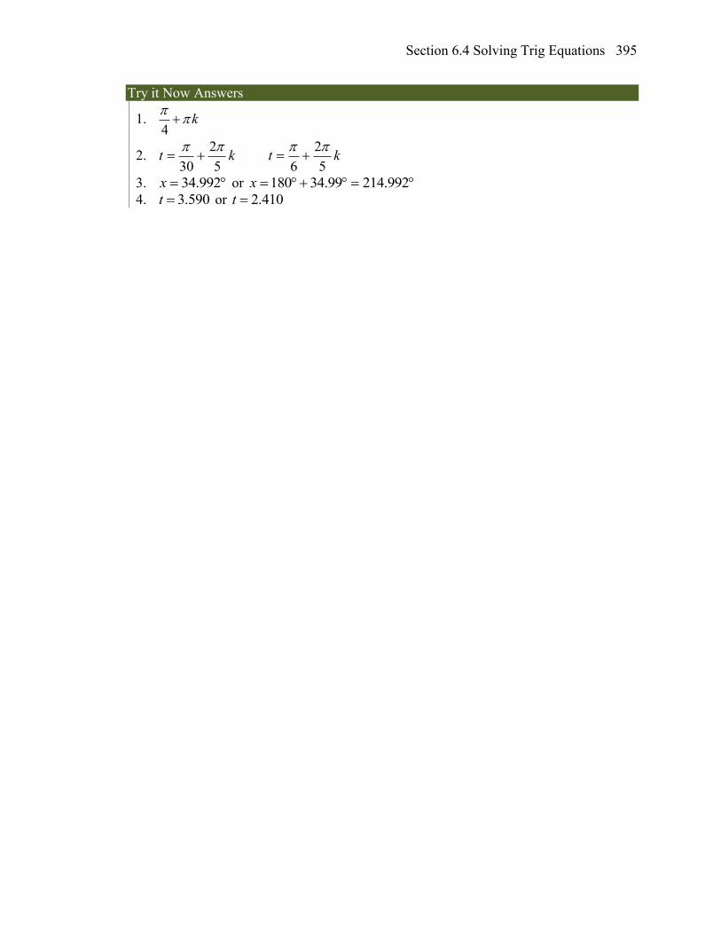
Section 6.4 Solving Trig Equations 395
Try it Now Answers
1. 4
k
2. kt5
2
30
kt
5
2
6
3. 992.34x or 992.21499.34180x
4. 3.590t or 2.410t
396 Chapter 6
Section 6.4 Exercises
Give all answers in radians unless otherwise indicated.
Find all solutions on the interval 0 2 .
1. 2sin 2 2. 2sin 3 3. 2cos 1 4. 2cos 2
5. sin 1 6. sin 0 7. cos 0 8. cos 1
Find all solutions.
9. 2cos 2 10. 2cos 1 11. 2sin 1 12. 2sin 3
Find all solutions.
13. 2sin 3 1 14. 2sin 2 3 15. 2sin 3 2
16. 2sin 3 1 17. 2cos 2 1 18. 2cos 2 3
19. 2cos 3 2 20. 2cos 2 1 21. cos 14
22. sin 13
23. 2sin 1 . 24. 2cos 3
5
Find all solutions on the interval 0 2x .
25. sin 0.27x 26. sin 0.48x 27. sin 0.58x 28. sin 0.34x
29. cos 0.55x 30. sin 0.28x 31. cos 0.71x 32. cos 0.07x
Find the first two positive solutions.
33. 7sin 6 2x 34. 7sin 5 6x 35. 5cos 3 3x 36. 3cos 4 2x
37. 3sin 24
x
38. 7sin 65
x
39. 5cos 13
x
40. 3cos 22
x
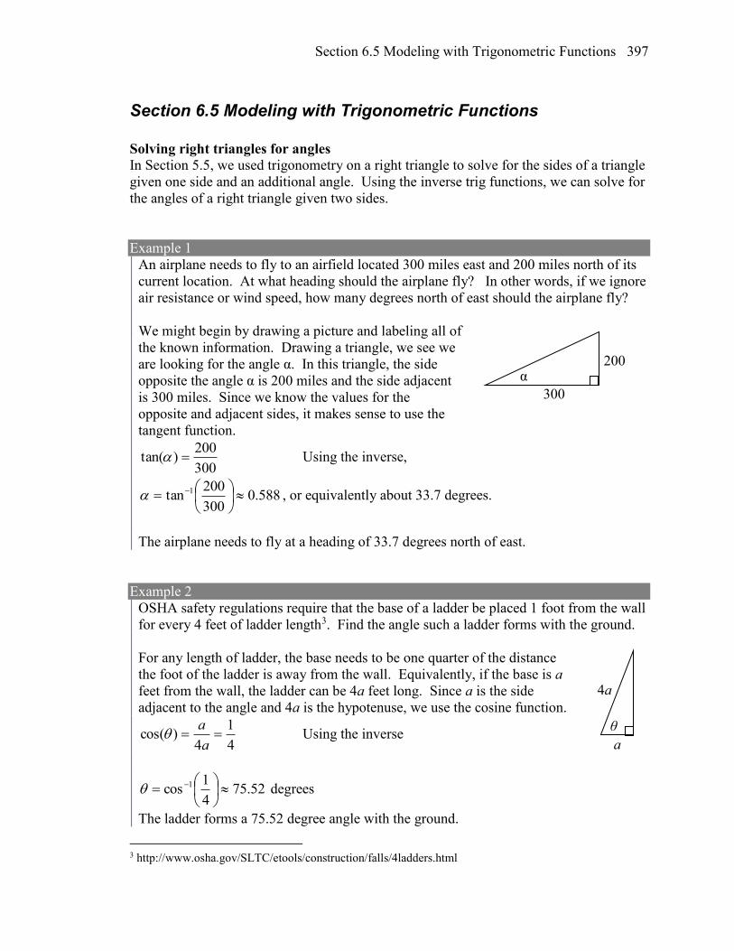
Section 6.5 Modeling with Trigonometric Functions 397
Section 6.5 Modeling with Trigonometric Functions
Solving right triangles for angles
In Section 5.5, we used trigonometry on a right triangle to solve for the sides of a triangle
given one side and an additional angle. Using the inverse trig functions, we can solve for
the angles of a right triangle given two sides.
Example 1
An airplane needs to fly to an airfield located 300 miles east and 200 miles north of its
current location. At what heading should the airplane fly? In other words, if we ignore
air resistance or wind speed, how many degrees north of east should the airplane fly?
We might begin by drawing a picture and labeling all of
the known information. Drawing a triangle, we see we
are looking for the angle α. In this triangle, the side
opposite the angle α is 200 miles and the side adjacent
is 300 miles. Since we know the values for the
opposite and adjacent sides, it makes sense to use the
tangent function.
300
200)tan( Using the inverse,
588.0300
200tan 1
, or equivalently about 33.7 degrees.
The airplane needs to fly at a heading of 33.7 degrees north of east.
Example 2
OSHA safety regulations require that the base of a ladder be placed 1 foot from the wall
for every 4 feet of ladder length3. Find the angle such a ladder forms with the ground.
For any length of ladder, the base needs to be one quarter of the distance
the foot of the ladder is away from the wall. Equivalently, if the base is a
feet from the wall, the ladder can be 4a feet long. Since a is the side
adjacent to the angle and 4a is the hypotenuse, we use the cosine function.
4
1
4)cos(
a
a Using the inverse
52.754
1cos 1
degrees
The ladder forms a 75.52 degree angle with the ground.
3 http://www.osha.gov/SLTC/etools/construction/falls/4ladders.html
200
300
α
a
4a
θ
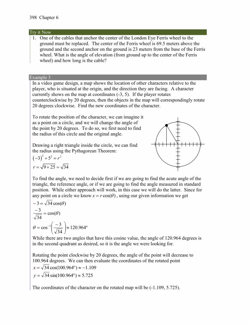
398 Chapter 6
Try it Now
1. One of the cables that anchor the center of the London Eye Ferris wheel to the
ground must be replaced. The center of the Ferris wheel is 69.5 meters above the
ground and the second anchor on the ground is 23 meters from the base of the Ferris
wheel. What is the angle of elevation (from ground up to the center of the Ferris
wheel) and how long is the cable?
Example 3
In a video game design, a map shows the location of other characters relative to the
player, who is situated at the origin, and the direction they are facing. A character
currently shows on the map at coordinates (-3, 5). If the player rotates
counterclockwise by 20 degrees, then the objects in the map will correspondingly rotate
20 degrees clockwise. Find the new coordinates of the character.
To rotate the position of the character, we can imagine it
as a point on a circle, and we will change the angle of
the point by 20 degrees. To do so, we first need to find
the radius of this circle and the original angle.
Drawing a right triangle inside the circle, we can find
the radius using the Pythagorean Theorem:
2 2 23 5
9 25 34
r
r
To find the angle, we need to decide first if we are going to find the acute angle of the
triangle, the reference angle, or if we are going to find the angle measured in standard
position. While either approach will work, in this case we will do the latter. Since for
any point on a circle we know )cos(rx , using our given information we get
)cos(343
)cos(34
3
964.120
34
3cos 1
While there are two angles that have this cosine value, the angle of 120.964 degrees is
in the second quadrant as desired, so it is the angle we were looking for.
Rotating the point clockwise by 20 degrees, the angle of the point will decrease to
100.964 degrees. We can then evaluate the coordinates of the rotated point
109.1)964.100cos(34 x
725.5)964.100sin(34 y
The coordinates of the character on the rotated map will be (-1.109, 5.725).
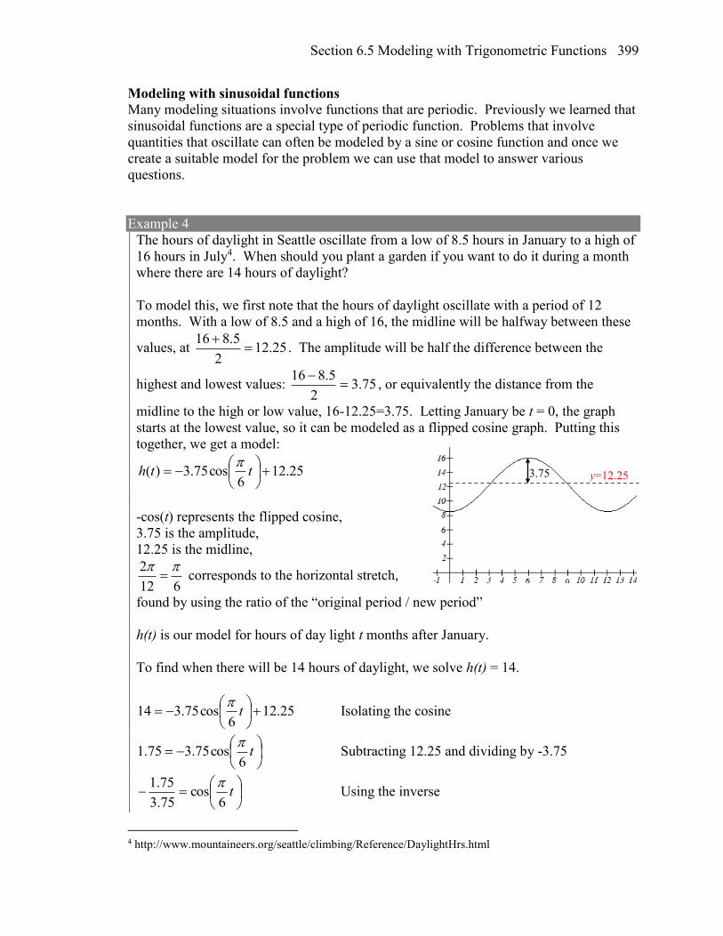
Section 6.5 Modeling with Trigonometric Functions 399
Modeling with sinusoidal functions
Many modeling situations involve functions that are periodic. Previously we learned that
sinusoidal functions are a special type of periodic function. Problems that involve
quantities that oscillate can often be modeled by a sine or cosine function and once we
create a suitable model for the problem we can use that model to answer various
questions.
Example 4
The hours of daylight in Seattle oscillate from a low of 8.5 hours in January to a high of
16 hours in July4. When should you plant a garden if you want to do it during a month
where there are 14 hours of daylight?
To model this, we first note that the hours of daylight oscillate with a period of 12
months. With a low of 8.5 and a high of 16, the midline will be halfway between these
values, at 25.122
5.816
. The amplitude will be half the difference between the
highest and lowest values: 75.32
5.816
, or equivalently the distance from the
midline to the high or low value, 16-12.25=3.75. Letting January be t = 0, the graph
starts at the lowest value, so it can be modeled as a flipped cosine graph. Putting this
together, we get a model:
25.126
cos75.3)(
tth
-cos(t) represents the flipped cosine,
3.75 is the amplitude,
12.25 is the midline,
2
12 6
corresponds to the horizontal stretch,
found by using the ratio of the “original period / new period”
h(t) is our model for hours of day light t months after January.
To find when there will be 14 hours of daylight, we solve h(t) = 14.
25.126
cos75.314
t
Isolating the cosine
t
6cos75.375.1
Subtracting 12.25 and dividing by -3.75
t
6cos
75.3
75.1 Using the inverse
4 http://www.mountaineers.org/seattle/climbing/Reference/DaylightHrs.html
3.75 y=12.25
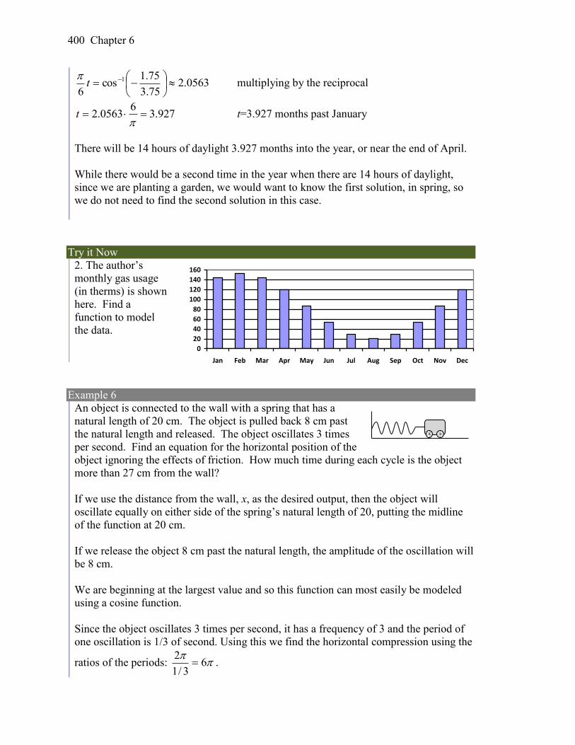
400 Chapter 6
0563.275.3
75.1cos
6
1
t
multiplying by the reciprocal
927.36
0563.2
t t=3.927 months past January
There will be 14 hours of daylight 3.927 months into the year, or near the end of April.
While there would be a second time in the year when there are 14 hours of daylight,
since we are planting a garden, we would want to know the first solution, in spring, so
we do not need to find the second solution in this case.
Try it Now
2. The author’s
monthly gas usage
(in therms) is shown
here. Find a
function to model
the data.
Example 6
An object is connected to the wall with a spring that has a
natural length of 20 cm. The object is pulled back 8 cm past
the natural length and released. The object oscillates 3 times
per second. Find an equation for the horizontal position of the
object ignoring the effects of friction. How much time during each cycle is the object
more than 27 cm from the wall?
If we use the distance from the wall, x, as the desired output, then the object will
oscillate equally on either side of the spring’s natural length of 20, putting the midline
of the function at 20 cm.
If we release the object 8 cm past the natural length, the amplitude of the oscillation will
be 8 cm.
We are beginning at the largest value and so this function can most easily be modeled
using a cosine function.
Since the object oscillates 3 times per second, it has a frequency of 3 and the period of
one oscillation is 1/3 of second. Using this we find the horizontal compression using the
ratios of the periods:
63/1
2 .
0
20
40
60
80
100
120
140
160
Jan Feb Mar Apr May Jun Jul Aug Sep Oct Nov Dec
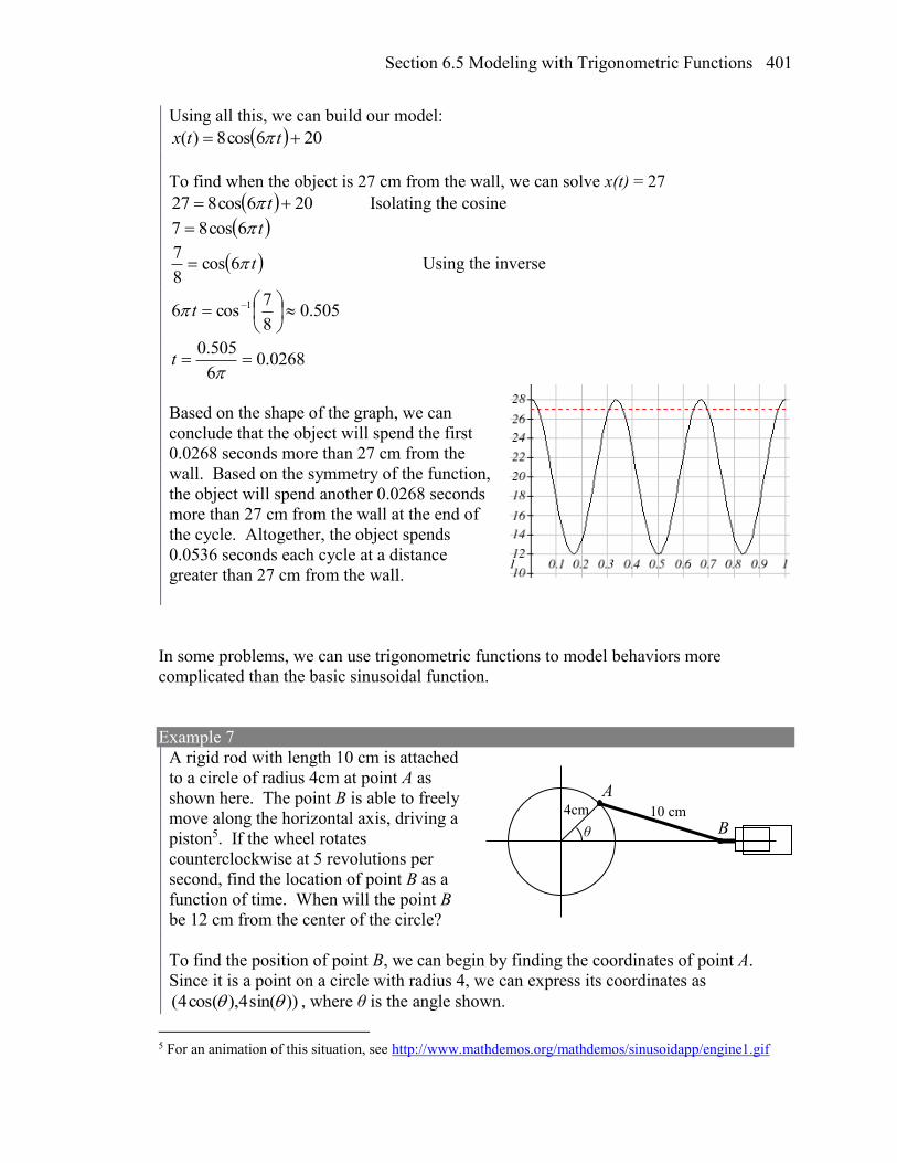
Section 6.5 Modeling with Trigonometric Functions 401
Using all this, we can build our model:
206cos8)( ttx
To find when the object is 27 cm from the wall, we can solve x(t) = 27
206cos827 t Isolating the cosine
t6cos87
t6cos8
7 Using the inverse
505.08
7cos6 1
t
0268.06
505.0
t
Based on the shape of the graph, we can
conclude that the object will spend the first
0.0268 seconds more than 27 cm from the
wall. Based on the symmetry of the function,
the object will spend another 0.0268 seconds
more than 27 cm from the wall at the end of
the cycle. Altogether, the object spends
0.0536 seconds each cycle at a distance
greater than 27 cm from the wall.
In some problems, we can use trigonometric functions to model behaviors more
complicated than the basic sinusoidal function.
Example 7
A rigid rod with length 10 cm is attached
to a circle of radius 4cm at point A as
shown here. The point B is able to freely
move along the horizontal axis, driving a
piston5. If the wheel rotates
counterclockwise at 5 revolutions per
second, find the location of point B as a
function of time. When will the point B
be 12 cm from the center of the circle?
To find the position of point B, we can begin by finding the coordinates of point A.
Since it is a point on a circle with radius 4, we can express its coordinates as
))sin(4),cos(4( , where θ is the angle shown.
5 For an animation of this situation, see http://www.mathdemos.org/mathdemos/sinusoidapp/engine1.gif
A
B 10 cm 4cm
θ
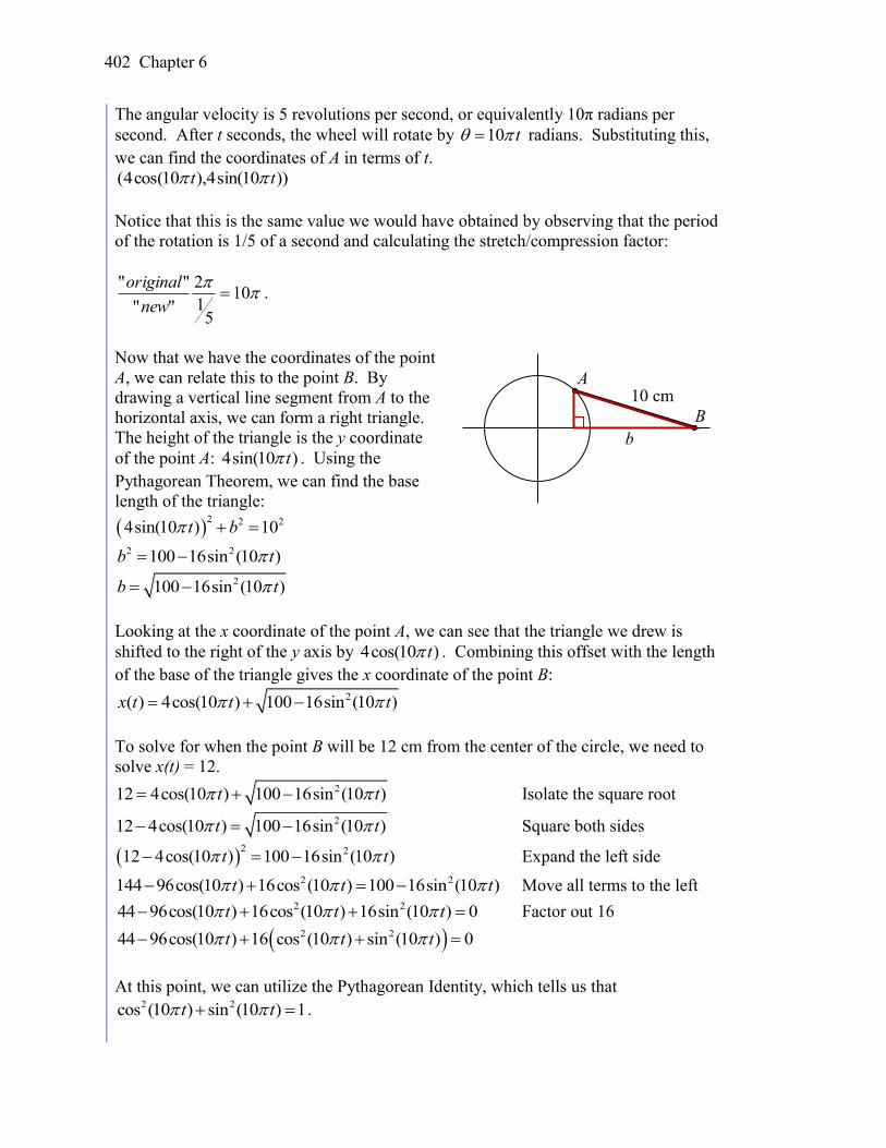
402 Chapter 6
The angular velocity is 5 revolutions per second, or equivalently 10π radians per
second. After t seconds, the wheel will rotate by 10 t radians. Substituting this,
we can find the coordinates of A in terms of t.
))10sin(4),10cos(4( tt
Notice that this is the same value we would have obtained by observing that the period
of the rotation is 1/5 of a second and calculating the stretch/compression factor:
10
51
2
""
""
new
original.
Now that we have the coordinates of the point
A, we can relate this to the point B. By
drawing a vertical line segment from A to the
horizontal axis, we can form a right triangle.
The height of the triangle is the y coordinate
of the point A: 4sin(10 )t . Using the
Pythagorean Theorem, we can find the base
length of the triangle:
2 2 24sin(10 ) 10t b
2 2100 16sin (10 )b t
2100 16sin (10 )b t
Looking at the x coordinate of the point A, we can see that the triangle we drew is
shifted to the right of the y axis by 4cos(10 )t . Combining this offset with the length
of the base of the triangle gives the x coordinate of the point B: 2( ) 4cos(10 ) 100 16sin (10 )x t t t
To solve for when the point B will be 12 cm from the center of the circle, we need to
solve x(t) = 12. 212 4cos(10 ) 100 16sin (10 )t t Isolate the square root
212 4cos(10 ) 100 16sin (10 )t t Square both sides
2 212 4cos(10 ) 100 16sin (10 )t t Expand the left side
2 2144 96cos(10 ) 16cos (10 ) 100 16sin (10 )t t t Move all terms to the left 2 244 96cos(10 ) 16cos (10 ) 16sin (10 ) 0t t t Factor out 16
2 244 96cos(10 ) 16 cos (10 ) sin (10 ) 0t t t
At this point, we can utilize the Pythagorean Identity, which tells us that 2 2cos (10 ) sin (10 ) 1t t .
A
B
10 cm
b
Section 6.5 Modeling with Trigonometric Functions 403
Using this identity, our equation simplifies to
44 96cos(10 ) 16 0t Combine the constants and move to the right side
96cos(10 ) 60t Divide
60cos(10 )
96t Make a substitution
96
60)cos( u
896.096
60cos 1
u By symmetry we can find a second solution
388.5896.02 u Undoing the substitution
10 0.896t , so t = 0.0285
10 5.388t , so t = 0.1715
The point B will be 12 cm from the center of the circle 0.0285 seconds after the process
begins, 0.1715 seconds after the process begins, and every 1/5 of a second after each of
those values.
Important Topics of This Section
Modeling with trig equations
Modeling with sinusoidal functions
Solving right triangles for angles in degrees and radians
Try it Now Answers
1. Angle of elevation for the cable is 71.69 degrees and the cable is 73.21 m long
2. Approximately ( ) 66cos ( 1) 876
G t t
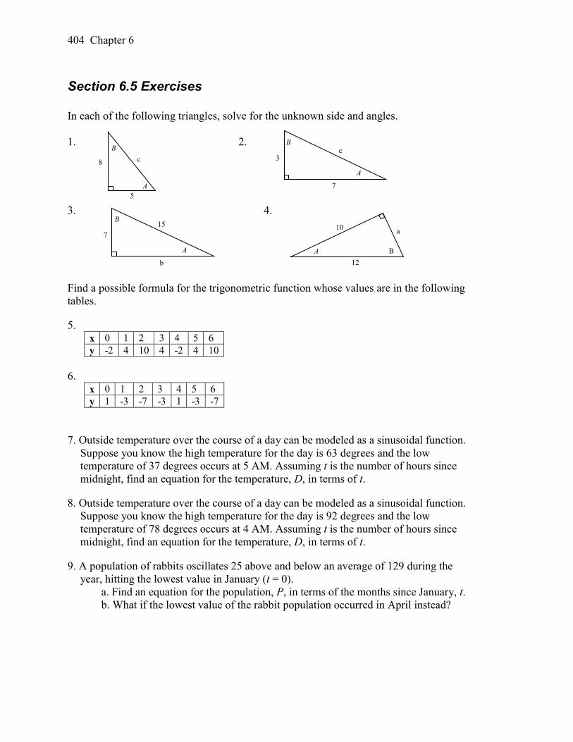
404 Chapter 6
Section 6.5 Exercises
In each of the following triangles, solve for the unknown side and angles.
1. 2.
3. 4.
Find a possible formula for the trigonometric function whose values are in the following
tables.
5.
x 0 1 2 3 4 5 6
y -2 4 10 4 -2 4 10
6.
x 0 1 2 3 4 5 6
y 1 -3 -7 -3 1 -3 -7
7. Outside temperature over the course of a day can be modeled as a sinusoidal function.
Suppose you know the high temperature for the day is 63 degrees and the low
temperature of 37 degrees occurs at 5 AM. Assuming t is the number of hours since
midnight, find an equation for the temperature, D, in terms of t.
8. Outside temperature over the course of a day can be modeled as a sinusoidal function.
Suppose you know the high temperature for the day is 92 degrees and the low
temperature of 78 degrees occurs at 4 AM. Assuming t is the number of hours since
midnight, find an equation for the temperature, D, in terms of t.
9. A population of rabbits oscillates 25 above and below an average of 129 during the
year, hitting the lowest value in January (t = 0).
a. Find an equation for the population, P, in terms of the months since January, t.
b. What if the lowest value of the rabbit population occurred in April instead?
A
5
8
B
c
B
7
3
A
c
A
b
7
15 B
B
a 10
12
A
Section 6.5 Modeling with Trigonometric Functions 405
10. A population of elk oscillates 150 above and below an average of 720 during the year,
hitting the lowest value in January (t = 0).
a. Find an equation for the population, P, in terms of the months since January, t.
b. What if the lowest value of the rabbit population occurred in March instead?
11. Outside temperature over the course of a day can be modeled as a sinusoidal function.
Suppose you know the high temperature of 105 degrees occurs at 5 PM and the
average temperature for the day is 85 degrees. Find the temperature, to the nearest
degree, at 9 AM.
12. Outside temperature over the course of a day can be modeled as a sinusoidal function.
Suppose you know the high temperature of 84 degrees occurs at 6 PM and the
average temperature for the day is 70 degrees. Find the temperature, to the nearest
degree, at 7 AM.
13. Outside temperature over the course of a day can be modeled as a sinusoidal function.
Suppose you know the temperature varies between 47 and 63 degrees during the day
and the average daily temperature first occurs at 10 AM. How many hours after
midnight does the temperature first reach 51 degrees?
14. Outside temperature over the course of a day can be modeled as a sinusoidal function.
Suppose you know the temperature varies between 64 and 86 degrees during the day
and the average daily temperature first occurs at 12 AM. How many hours after
midnight does the temperature first reach 70 degrees?
15. A Ferris wheel is 20 meters in diameter and boarded from a platform that is 2 meters
above the ground. The six o'clock position on the Ferris wheel is level with the
loading platform. The wheel completes 1 full revolution in 6 minutes. How many
minutes of the ride are spent higher than 13 meters above the ground?
16. A Ferris wheel is 45 meters in diameter and boarded from a platform that is 1 meter
above the ground. The six o'clock position on the Ferris wheel is level with the
loading platform. The wheel completes 1 full revolution in 10 minutes. How many
minutes of the ride are spent higher than 27 meters above the ground?
17. The sea ice area around the North Pole fluctuates between about 6 million square
kilometers in September to 14 million square kilometers in March. Assuming
sinusoidal fluctuation, during how many months are there less than 9 million square
kilometers of sea ice?
18. The sea ice area around the South Pole fluctuates between about 18 million square
kilometers in September to 3 million square kilometers in March. Assuming
sinusoidal fluctuation, during how many months are there more than 15 million
square kilometers of sea ice?
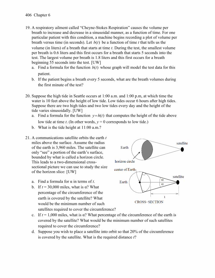
406 Chapter 6
19. A respiratory ailment called “Cheyne-Stokes Respiration” causes the volume per
breath to increase and decrease in a sinusoidal manner, as a function of time. For one
particular patient with this condition, a machine begins recording a plot of volume per
breath versus time (in seconds). Let ( )b t be a function of time t that tells us the
volume (in liters) of a breath that starts at time t. During the test, the smallest volume
per breath is 0.6 liters and this first occurs for a breath that starts 5 seconds into the
test. The largest volume per breath is 1.8 liters and this first occurs for a breath
beginning 55 seconds into the test. [UW]
a. Find a formula for the function ( )b t whose graph will model the test data for this
patient.
b. If the patient begins a breath every 5 seconds, what are the breath volumes during
the first minute of the test?
20. Suppose the high tide in Seattle occurs at 1:00 a.m. and 1:00 p.m, at which time the
water is 10 feet above the height of low tide. Low tides occur 6 hours after high tides.
Suppose there are two high tides and two low tides every day and the height of the
tide varies sinusoidally. [UW]
a. Find a formula for the function ( )y h t that computes the height of the tide above
low tide at time t. (In other words, y = 0 corresponds to low tide.)
b. What is the tide height at 11:00 a.m.?
21. A communications satellite orbits the earth t
miles above the surface. Assume the radius
of the earth is 3,960 miles. The satellite can
only “see” a portion of the earth’s surface,
bounded by what is called a horizon circle.
This leads to a two-dimensional cross-
sectional picture we can use to study the size
of the horizon slice: [UW]
a. Find a formula for α in terms of t.
b. If t = 30,000 miles, what is α? What
percentage of the circumference of the
earth is covered by the satellite? What
would be the minimum number of such
satellites required to cover the circumference?
c. If t = 1,000 miles, what is α? What percentage of the circumference of the earth is
covered by the satellite? What would be the minimum number of such satellites
required to cover the circumference?
d. Suppose you wish to place a satellite into orbit so that 20% of the circumference
is covered by the satellite. What is the required distance t?
Section 6.5 Modeling with Trigonometric Functions 407
22. Tiffany is a model rocket enthusiast. She has been working on a pressurized rocket
filled with nitrous oxide. According to her design, if the atmospheric pressure exerted
on the rocket is less than 10 pounds/sq.in., the nitrous oxide chamber inside the rocket
will explode. Tiff worked from a formula /1014.7 hp e pounds/sq.in. for the
atmospheric pressure h miles above sea level. Assume that the rocket is launched at
an angle of α above level ground at sea level with an initial speed of 1400 feet/sec.
Also, assume the height (in feet) of the rocket at time t seconds is given by the
equation 216 1400siny t t t . [UW]
a. At what altitude will the rocket explode?
b. If the angle of launch is α = 12°, determine the minimum atmospheric pressure
exerted on the rocket during its flight. Will the rocket explode in midair?
c. If the angle of launch is α = 82°, determine the minimum atmospheric pressure
exerted on the rocket during its flight. Will the rocket explode in midair?
d. Find the largest launch angle α so that the rocket will not explode.

408 Chapter 6
Section 7.1 Solving Trigonometric Equations and Identities 409
This chapter is part of Precalculus: An Investigation of Functions © Lippman & Rasmussen 2011.
This material is licensed under a Creative Commons CC-BY-SA license.
Chapter 7: Trigonometric Equations and Identities
In the last two chapters we have used basic definitions and relationships to simplify
trigonometric expressions and solve trigonometric equations. In this chapter we will look
at more complex relationships. By conducting a deeper study of trigonometric identities
we can learn to simplify complicated expressions, allowing us to solve more interesting
applications.
Section 7.1 Solving Trigonometric Equations with Identities .................................... 409
Section 7.2 Addition and Subtraction Identities ......................................................... 417
Section 7.3 Double Angle Identities ........................................................................... 431
Section 7.4 Modeling Changing Amplitude and Midline ........................................... 442
Section 7.1 Solving Trigonometric Equations with Identities
In the last chapter, we solved basic trigonometric equations. In this section, we explore
the techniques needed to solve more complicated trig equations.
Building from what we already know makes this a much easier task.
Consider the function 2( ) 2f x x x . If you were asked to solve 0)( xf , it require
simple algebra:
02 2 xx Factor
0)12( xx Giving solutions
x = 0 or x = 2
1
Similarly, for ( ) sin( )g t t , if we asked you to solve 0)( tg , you can solve this using
unit circle values:
0)sin( t for 2,,0t and so on.
Using these same concepts, we consider the composition of these two functions:
)sin()(sin2))(sin())(sin(2))(( 22 tttttgf
This creates an equation that is a polynomial trig function. With these types of functions,
we use algebraic techniques like factoring and the quadratic formula, along with
trigonometric identities and techniques, to solve equations.
As a reminder, here are some of the essential trigonometric identities that we have
learned so far:
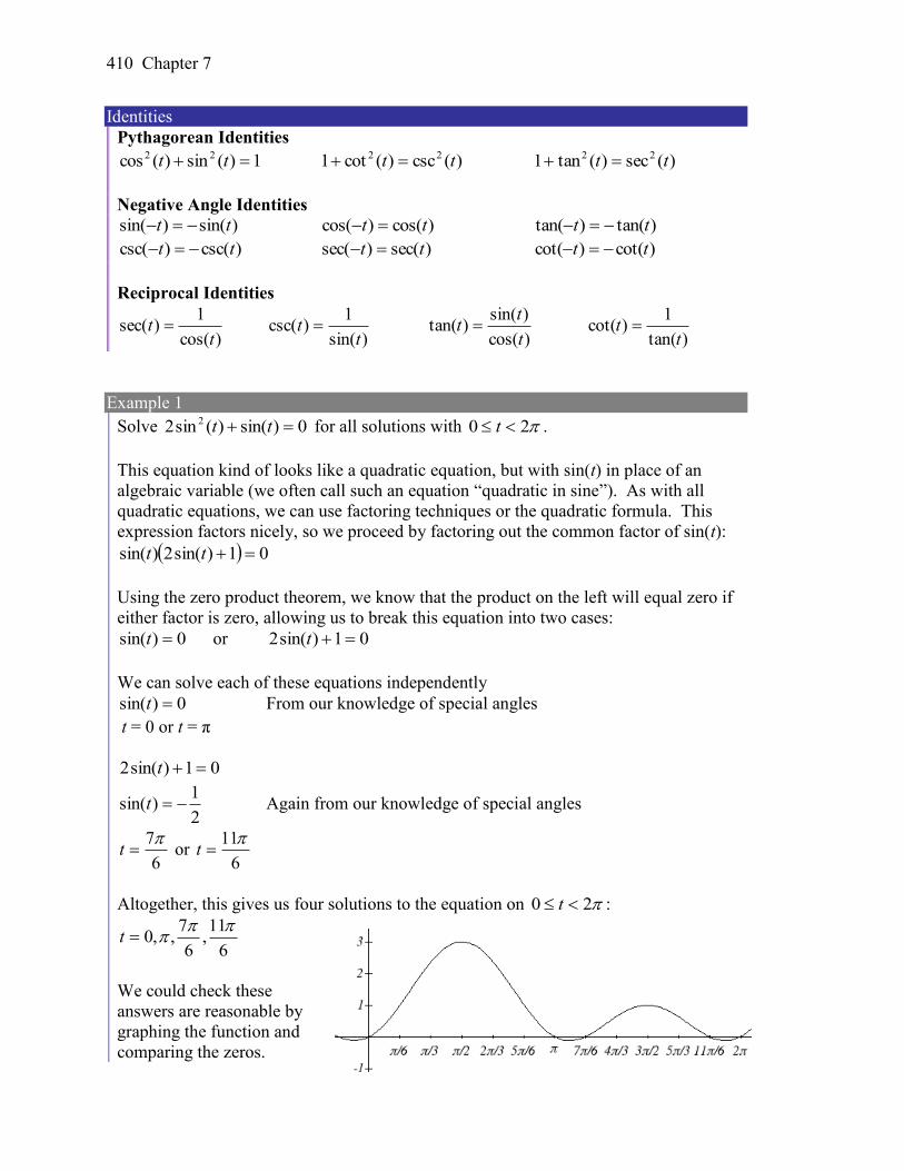
410 Chapter 7
Identities
Pythagorean Identities
1)(sin)(cos 22 tt )(csc)(cot1 22 tt )(sec)(tan1 22 tt
Negative Angle Identities
)sin()sin( tt )cos()cos( tt )tan()tan( tt
)csc()csc( tt )sec()sec( tt )cot()cot( tt
Reciprocal Identities
)cos(
1)sec(
tt
)sin(
1)csc(
tt
)cos(
)sin()tan(
t
tt
)tan(
1)cot(
tt
Example 1
Solve 0)sin()(sin2 2 tt for all solutions with 20 t .
This equation kind of looks like a quadratic equation, but with sin(t) in place of an
algebraic variable (we often call such an equation “quadratic in sine”). As with all
quadratic equations, we can use factoring techniques or the quadratic formula. This
expression factors nicely, so we proceed by factoring out the common factor of sin(t):
01)sin(2)sin( tt
Using the zero product theorem, we know that the product on the left will equal zero if
either factor is zero, allowing us to break this equation into two cases:
0)sin( t or 01)sin(2 t
We can solve each of these equations independently
0)sin( t From our knowledge of special angles
t = 0 or t = π
01)sin(2 t
2
1)sin( t Again from our knowledge of special angles
6
7t or
6
11t
Altogether, this gives us four solutions to the equation on 20 t :
6
11,
6
7,,0
t
We could check these
answers are reasonable by
graphing the function and
comparing the zeros.
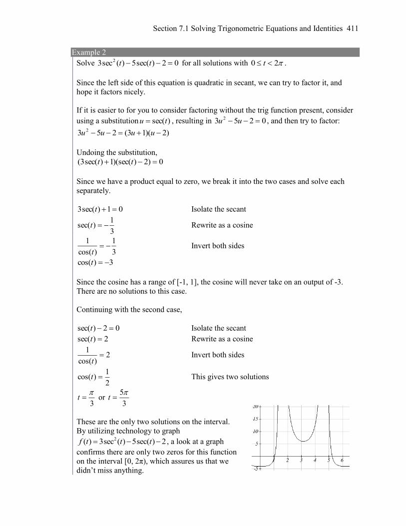
Section 7.1 Solving Trigonometric Equations and Identities 411
Example 2
Solve 02)sec(5)(sec3 2 tt for all solutions with 20 t .
Since the left side of this equation is quadratic in secant, we can try to factor it, and
hope it factors nicely.
If it is easier to for you to consider factoring without the trig function present, consider
using a substitution )sec(tu , resulting in 0253 2 uu , and then try to factor:
)2)(13(253 2 uuuu
Undoing the substitution,
0)2))(sec(1)sec(3( tt
Since we have a product equal to zero, we break it into the two cases and solve each
separately.
01)sec(3 t Isolate the secant
3
1)sec( t Rewrite as a cosine
3
1
)cos(
1
t Invert both sides
3)cos( t
Since the cosine has a range of [-1, 1], the cosine will never take on an output of -3.
There are no solutions to this case.
Continuing with the second case,
02)sec( t Isolate the secant
2)sec( t Rewrite as a cosine
2)cos(
1
t Invert both sides
2
1)cos( t This gives two solutions
3
t or
3
5t
These are the only two solutions on the interval.
By utilizing technology to graph 2( ) 3sec ( ) 5sec( ) 2f t t t , a look at a graph
confirms there are only two zeros for this function
on the interval [0, 2π), which assures us that we
didn’t miss anything.
412 Chapter 7
Try it Now
1. Solve 01)sin(3)(sin2 2 tt for all solutions with 20 t .
When solving some trigonometric equations, it becomes necessary to first rewrite the
equation using trigonometric identities. One of the most common is the Pythagorean
Identity, 1)(cos)(sin 22 which allows you to rewrite )(sin 2 in terms of )(cos 2
or vice versa, 2 2
2 2
sin ( ) 1 cos ( )
cos ( ) 1 sin ( )
This identity becomes very useful whenever an equation involves a combination of sine
and cosine functions.
Example 3
Solve 1)cos()(sin2 2 tt for all solutions with 20 t .
Since this equation has a mix of sine and cosine functions, it becomes more complicated
to solve. It is usually easier to work with an equation involving only one trig function.
This is where we can use the Pythagorean Identity.
1)cos()(sin2 2 tt Using )(cos1)(sin 22
1)cos()(cos12 2 tt Distributing the 2
1)cos()(cos22 2 tt
Since this is now quadratic in cosine, we rearrange the equation so one side is zero and
factor.
01)cos()(cos2 2 tt Multiply by -1 to simplify the factoring
01)cos()(cos2 2 tt Factor
01)cos(1)cos(2 tt
This product will be zero if either factor is zero, so we can break this into two separate
cases and solve each independently.
01)cos(2 t or 01)cos( t
2
1)cos( t or 1)cos( t
3
t or
3
5t or t
Section 7.1 Solving Trigonometric Equations and Identities 413
Try it Now
2. Solve )cos(3)(sin2 2 tt for all solutions with 20 t .
In addition to the Pythagorean Identity, it is often necessary to rewrite the tangent, secant,
cosecant, and cotangent as part of solving an equation.
Example 4
Solve )sin(3)tan( xx for all solutions with 20 x .
With a combination of tangent and sine, we might try rewriting tangent
)sin(3)tan( xx
)sin(3)cos(
)sin(x
x
x Multiplying both sides by cosine
)cos()sin(3)sin( xxx
At this point, you may be tempted to divide both sides of the equation by sin(x). Resist
the urge. When we divide both sides of an equation by a quantity, we are assuming the
quantity is never zero. In this case, when sin(x) = 0 the equation is satisfied, so we’d
lose those solutions if we divided by the sine.
To avoid this problem, we can rearrange the equation so that one side is zero1.
0)cos()sin(3)sin( xxx Factoring out sin(x) from both parts
0)cos(31)sin( xx
From here, we can see we get solutions when 0)sin( x or 0)cos(31 x .
Using our knowledge of the special angles of the unit circle
0)sin( x when x = 0 or x = π.
For the second equation, we will need the inverse cosine.
0)cos(31 x
3
1)cos( x Using our calculator or technology
231.13
1cos 1
x Using symmetry to find a second solution
052.5231.12 x
We have four solutions on 20 x :
x = 0, 1.231, π, 5.052
1 You technically can divide by sin(x) as long as you separately consider the case where sin(x) = 0. Since it
is easy to forget this step, the factoring approach used in the example is recommended.
414 Chapter 7
Try it Now
3. Solve )cos(2)sec( to find the first four positive solutions.
Example 5
Solve 2
43cos 2cot tan
sec ( )
for all solutions with 0 2 .
2
43cos 2cot tan
sec ( )
Using the reciprocal identities
)tan()tan(
12)cos(3)(cos4 2
Simplifying
24cos 3cos 2 Subtracting 2 from each side
24cos 3cos 2 0
This does not appear to factor nicely so we use the quadratic formula, remembering that
we are solving for cos(θ).
8
413
)4(2
)2)(4(433)cos(
2
Using the negative square root first,
175.18
413)cos(
This has no solutions, since the cosine can’t be less than -1.
Using the positive square root,
425.08
413)cos(
131.1425.0cos 1 By symmetry, a second solution can be found
152.5131.12
Important Topics of This Section
Review of Trig Identities
Solving Trig Equations
By Factoring
Using the Quadratic Formula
Utilizing Trig Identities to simplify
Section 7.1 Solving Trigonometric Equations and Identities 415
Try it Now Answers
1. 7 3 11
, ,6 2 6
t
2. 5
,3 3
t
3. 3 5 7
, , ,4 4 4 4
416 Chapter 7
Section 7.1 Exercises
Find all solutions on the interval 0 2 .
1. 2sin 1 2. 2sin 3 3. 2cos 1 4. 2cos 2
Find all solutions.
5. 2sin 1 4
x
6. 2sin 23
x
7. 2cos 2 3t 8. 2cos 3 1t
9. 3cos 25
x
10. 8cos 62
x
11. 7sin 3 2t 12. 4sin 4 1t
Find all solutions on the interval [0, 2 ) .
13. 10sin cos 6cosx x x 14. 3sin 15cos sint t t
15. csc 2 9 0x 16. sec 2 3
17. sec sin 2sin 0x x x 18. tan sin sin 0x x x
19. 2 1sin
4x 20. 2 1
cos2
21. 2sec 7x 22. 2csc 3t
23. 22sin 3sin 1 0w w 24. 28sin 6sin 1 0x x
25. 22cos cos 1t t 26. 28cos 3 2cos
27. 24cos ( ) 4 15cosx x 28. 29sin 2 4sin ( )w w
29. 212sin cos 6 0t t 30. 26cos 7sin 8 0x x
31. 2cos 6sin 32. 2sin cost t
33. 3tan 3tanx x 34. 3cos cost t
35. 5tan tanx x 36. 5tan 9 tan 0x x
37. 4sin cos 2sin 2cos 1 0x x x x
38. 2sin cos sin 2cos 1 0x x x x
39. tan 3sin 0x x 40. 3cos cotx x
41. 22 tan 3sect t 42. 21 2tan tanw w
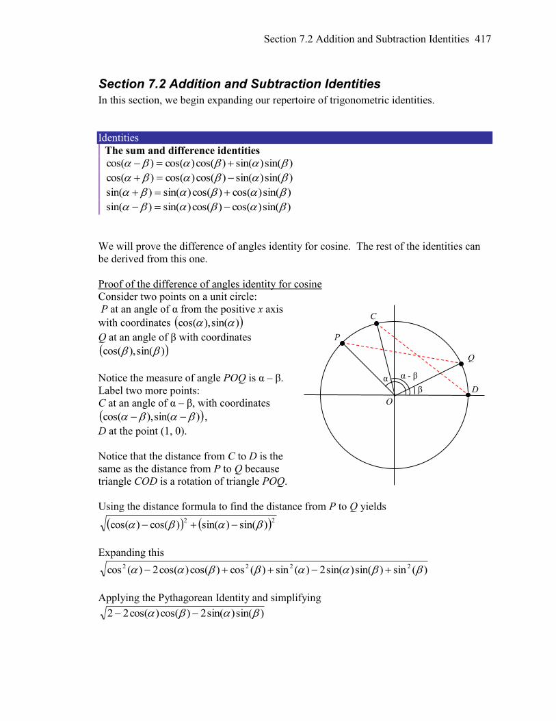
Section 7.2 Addition and Subtraction Identities 417
Section 7.2 Addition and Subtraction Identities
In this section, we begin expanding our repertoire of trigonometric identities.
Identities
The sum and difference identities
)sin()sin()cos()cos()cos(
)sin()sin()cos()cos()cos(
)sin()cos()cos()sin()sin(
)sin()cos()cos()sin()sin(
We will prove the difference of angles identity for cosine. The rest of the identities can
be derived from this one.
Proof of the difference of angles identity for cosine
Consider two points on a unit circle:
P at an angle of α from the positive x axis
with coordinates )sin(),cos(
Q at an angle of β with coordinates
)sin(),cos(
Notice the measure of angle POQ is α – β.
Label two more points:
C at an angle of α – β, with coordinates
)sin(),cos( ,
D at the point (1, 0).
Notice that the distance from C to D is the
same as the distance from P to Q because
triangle COD is a rotation of triangle POQ.
Using the distance formula to find the distance from P to Q yields
22)sin()sin()cos()cos(
Expanding this
)(sin)sin()sin(2)(sin)(cos)cos()cos(2)(cos 2222
Applying the Pythagorean Identity and simplifying
)sin()sin(2)cos()cos(22
β
α - β α
P
Q
C
D
O
418 Chapter 7
Similarly, using the distance formula to find the distance from C to D
220)sin(1)cos(
Expanding this
)(sin1)cos(2)(cos 22
Applying the Pythagorean Identity and simplifying
2)cos(2
Since the two distances are the same we set these two formulas equal to each other and
simplify
2)cos(2)sin()sin(2)cos()cos(22
2)cos(2)sin()sin(2)cos()cos(22
)cos()sin()sin()cos()cos(
Establishing the identity.
Try it Now
1. By writing )cos( as cos , show the sum of angles identity for cosine
follows from the difference of angles identity proven above.
The sum and difference of angles identities are often used to rewrite expressions in other
forms, or to rewrite an angle in terms of simpler angles.
Example 1
Find the exact value of )75cos( .
Since 453075 , we can evaluate )75cos( as
)4530cos()75cos( Apply the cosine sum of angles identity
)45sin()30sin()45cos()30cos( Evaluate
2
2
2
1
2
2
2
3 Simply
4
26
Try it Now
2. Find the exact value of
12sin
.

Section 7.2 Addition and Subtraction Identities 419
Example 2
Rewrite
4sin
x in terms of sin(x) and cos(x).
4sin
x Use the difference of angles identity for sine
=
4sincos
4cossin
xx Evaluate the cosine and sine and rearrange
xx cos2
2sin
2
2
Additionally, these identities can be used to simplify expressions or prove new identities
Example 3
Prove )tan()tan(
)tan()tan(
)sin(
)sin(
ba
ba
ba
ba
.
As with any identity, we need to first decide which side to begin with. Since the left
side involves sum and difference of angles, we might start there
)sin(
)sin(
ba
ba
Apply the sum and difference of angle identities
)sin()cos()cos()sin(
)sin()cos()cos()sin(
baba
baba
Since it is not immediately obvious how to proceed, we might start on the other side,
and see if the path is more apparent.
)tan()tan(
)tan()tan(
ba
ba
Rewriting the tangents using the tangent identity
)cos(
)sin(
)cos(
)sin(
)cos(
)sin(
)cos(
)sin(
b
b
a
a
b
b
a
a
Multiplying the top and bottom by cos(a)cos(b)
)cos()cos()cos(
)sin(
)cos(
)sin(
)cos()cos()cos(
)sin(
)cos(
)sin(
bab
b
a
a
bab
b
a
a
Distributing and simplifying
420 Chapter 7
)cos()sin()cos()sin(
)cos()sin()cos()sin(
abba
abba
From above, we recognize this
)sin(
)sin(
ba
ba
Establishing the identity
These identities can also be used to solve equations.
Example 4
Solve 2
3)2cos()cos()2sin()sin( xxxx .
By recognizing the left side of the equation as the result of the difference of angles
identity for cosine, we can simplify the equation
2
3)2cos()cos()2sin()sin( xxxx Apply the difference of angles identity
2
3)2cos( xx
2
3)cos( x Use the negative angle identity
2
3)cos( x
Since this is a special cosine value we recognize from the unit circle, we can quickly
write the answers:
kx
kx
26
11
26
, where k is an integer
Combining Waves of Equal Period
A sinusoidal function of the form )sin()( CBxAxf can be rewritten using the sum of
angles identity.
Example 5
Rewrite
33sin4)(
xxf as a sum of sine and cosine.
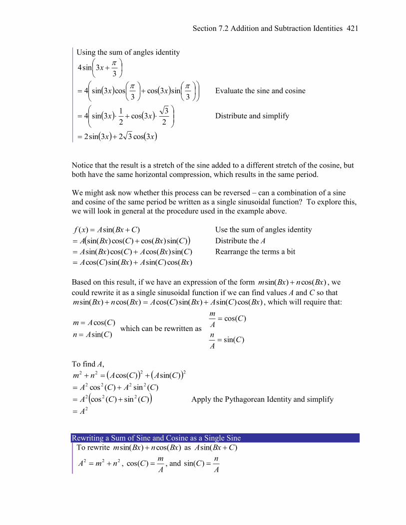
Section 7.2 Addition and Subtraction Identities 421
Using the sum of angles identity
33sin4
x
3sin3cos
3cos3sin4
xx Evaluate the sine and cosine
2
33cos
2
13sin4 xx Distribute and simplify
xx 3cos323sin2
Notice that the result is a stretch of the sine added to a different stretch of the cosine, but
both have the same horizontal compression, which results in the same period.
We might ask now whether this process can be reversed – can a combination of a sine
and cosine of the same period be written as a single sinusoidal function? To explore this,
we will look in general at the procedure used in the example above.
)sin()( CBxAxf Use the sum of angles identity
)sin()cos()cos()sin( CBxCBxA Distribute the A
)sin()cos()cos()sin( CBxACBxA Rearrange the terms a bit
)cos()sin()sin()cos( BxCABxCA
Based on this result, if we have an expression of the form )cos()sin( BxnBxm , we
could rewrite it as a single sinusoidal function if we can find values A and C so that
)cos()sin( BxnBxm )cos()sin()sin()cos( BxCABxCA , which will require that:
)sin(
)cos(
CAn
CAm
which can be rewritten as
)sin(
)cos(
CA
n
CA
m
To find A,
2222 )sin()cos( CACAnm
)(sin)(cos 2222 CACA
)(sin)(cos 222 CCA Apply the Pythagorean Identity and simplify 2A
Rewriting a Sum of Sine and Cosine as a Single Sine
To rewrite )cos()sin( BxnBxm as )sin( CBxA
222 nmA , A
mC )cos( , and
A
nC )sin(
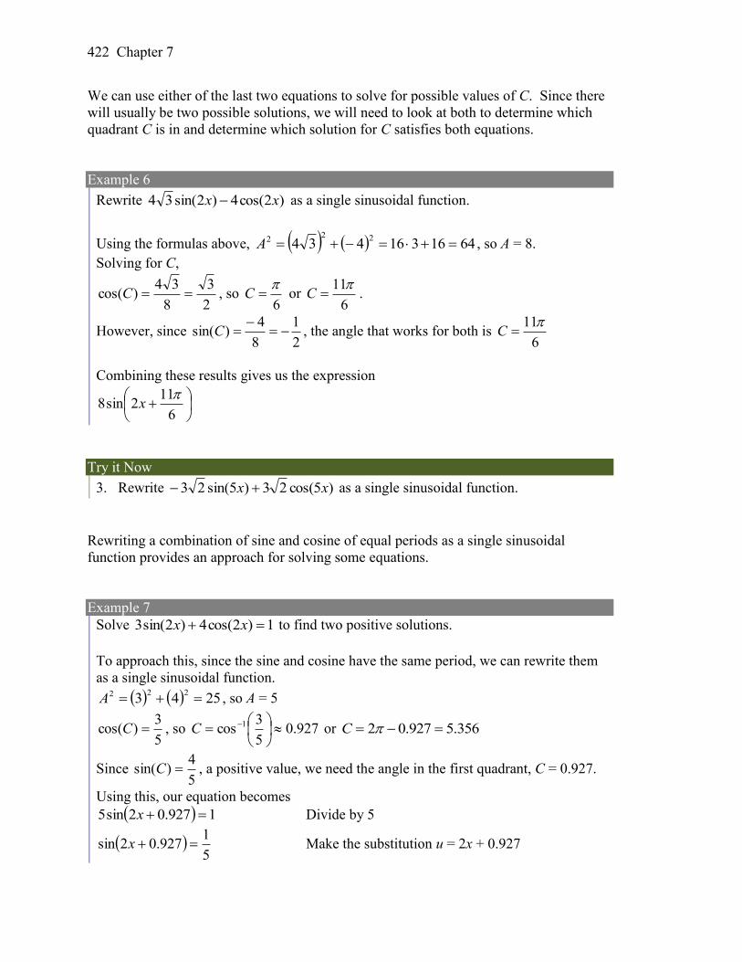
422 Chapter 7
We can use either of the last two equations to solve for possible values of C. Since there
will usually be two possible solutions, we will need to look at both to determine which
quadrant C is in and determine which solution for C satisfies both equations.
Example 6
Rewrite )2cos(4)2sin(34 xx as a single sinusoidal function.
Using the formulas above, 641631643422
2 A , so A = 8.
Solving for C,
2
3
8
34)cos( C , so
6
C or
6
11C .
However, since 2
1
8
4)sin(
C , the angle that works for both is
6
11C
Combining these results gives us the expression
6
112sin8
x
Try it Now
3. Rewrite )5cos(23)5sin(23 xx as a single sinusoidal function.
Rewriting a combination of sine and cosine of equal periods as a single sinusoidal
function provides an approach for solving some equations.
Example 7
Solve 1)2cos(4)2sin(3 xx to find two positive solutions.
To approach this, since the sine and cosine have the same period, we can rewrite them
as a single sinusoidal function.
2543222 A , so A = 5
5
3)cos( C , so 927.0
5
3cos 1
C or 356.5927.02 C
Since 5
4)sin( C , a positive value, we need the angle in the first quadrant, C = 0.927.
Using this, our equation becomes
1927.02sin5 x Divide by 5
5
1927.02sin x Make the substitution u = 2x + 0.927
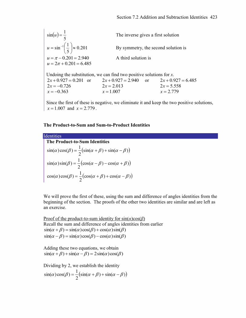
Section 7.2 Addition and Subtraction Identities 423
5
1sin u The inverse gives a first solution
201.05
1sin 1
u By symmetry, the second solution is
940.2201.0 u A third solution is
485.6201.02 u
Undoing the substitution, we can find two positive solutions for x.
201.0927.02 x or 940.2927.02 x or 485.6927.02 x
726.02 x 013.22 x 558.52 x
363.0x 007.1x 779.2x
Since the first of these is negative, we eliminate it and keep the two positive solutions,
007.1x and 779.2x .
The Product-to-Sum and Sum-to-Product Identities
Identities
The Product-to-Sum Identities
)cos()cos(2
1)cos()cos(
)cos()cos(2
1)sin()sin(
)sin()sin(2
1)cos()sin(
We will prove the first of these, using the sum and difference of angles identities from the
beginning of the section. The proofs of the other two identities are similar and are left as
an exercise.
Proof of the product-to-sum identity for sin(α)cos(β)
Recall the sum and difference of angles identities from earlier
)sin()cos()cos()sin()sin(
)sin()cos()cos()sin()sin(
Adding these two equations, we obtain
)cos()sin(2)sin()sin(
Dividing by 2, we establish the identity
)sin()sin(2
1)cos()sin(
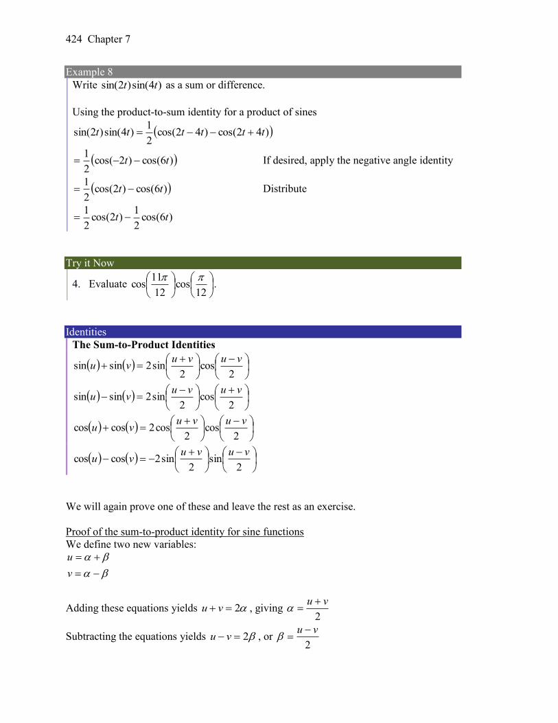
424 Chapter 7
Example 8
Write )4sin()2sin( tt as a sum or difference.
Using the product-to-sum identity for a product of sines
)42cos()42cos(2
1)4sin()2sin( tttttt
)6cos()2cos(2
1tt If desired, apply the negative angle identity
)6cos()2cos(2
1tt Distribute
)6cos(2
1)2cos(
2
1tt
Try it Now
4. Evaluate
12cos
12
11cos
.
Identities
The Sum-to-Product Identities
2cos
2sin2sinsin
vuvuvu
2cos
2sin2sinsin
vuvuvu
2cos
2cos2coscos
vuvuvu
2sin
2sin2coscos
vuvuvu
We will again prove one of these and leave the rest as an exercise.
Proof of the sum-to-product identity for sine functions
We define two new variables:
v
u
Adding these equations yields 2 vu , giving 2
vu
Subtracting the equations yields 2 vu , or 2
vu
Section 7.2 Addition and Subtraction Identities 425
Substituting these expressions into the product-to-sum identity
)sin()sin(2
1)cos()sin( gives
vuvuvu
sinsin2
1
2cos
2sin
Multiply by 2 on both sides
vuvuvu
sinsin2
cos2
sin2
Establishing the identity
Example 9
Evaluate )75cos()15cos( .
Using the sum-to-product identity for the difference of cosines,
)75cos()15cos(
2
7515sin
2
7515sin2 Simplify
30sin45sin2 Evaluate
2
2
2
1
2
22
Example 10
Prove the identity )tan()2sin()4sin(
)2cos()4cos(t
tt
tt
.
Since the left side seems more complicated, we can start there and simplify.
)2sin()4sin(
)2cos()4cos(
tt
tt
Using the sum-to-product identities
2
24cos
2
24sin2
2
24sin
2
24sin2
tttt
tttt
Simplify
tt
tt
cos3sin2
sin3sin2 Simplify further
t
t
cos
sin Rewrite as a tangent
)tan(t Establishing the identity
Try it Now
426 Chapter 7
5. Notice that, using the negative angle identity, )sin()sin(sinsin vuvu . Use
this along with the sum of sines identity to prove the sum-to-product identity for
vu sinsin .
Example 11
Solve sin sin 3 cos( )t t t for all solutions with 20 t .
In an equation like this, it is not immediately obvious how to proceed. One option
would be to combine the two sine functions on the left side of the equation. Another
would be to move the cosine to the left side of the equation, and combine it with one of
the sines. For no particularly good reason, we’ll begin by combining the sines on the
left side of the equation and see how things work out.
sin sin 3 cos( )t t t Apply the sum to product identity on the left
3 32sin cos cos( )
2 2
t t t tt
Simplify
2sin 2 cos cos( )t t t Apply the negative angle identity
2sin 2 cos cos( )t t t Rearrange the equation to be 0 on one side
2sin 2 cos cos( ) 0t t t Factor out the cosine
cos 2sin 2 1 0t t
Using the Zero Product Theorem we know that at least one of the two factors must be
zero. The first factor, cos t , has period 22
P , so the solution interval of
20 t represents one full cycle of this function.
cos 0t Substitute u t
0cos u On one cycle, this has solutions
2
u or
2
3u Undo the substitution
2t
, so
2
1t
3
2t
, so
2
3t
The second factor, 2sin 2 1t , has period of 12
2
P , so the solution interval
20 t contains two complete cycles of this function.
2sin 2 1 0t Isolate the sine
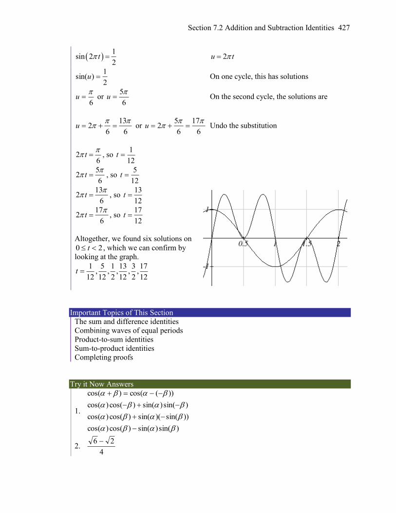
Section 7.2 Addition and Subtraction Identities 427
1
sin 22
t 2u t
2
1)sin( u On one cycle, this has solutions
6
u or
6
5u On the second cycle, the solutions are
6
13
62
u or
6
17
6
52
u Undo the substitution
26
t
, so 12
1t
52
6t
, so
12
5t
132
6t
, so
12
13t
172
6t
, so
12
17t
Altogether, we found six solutions on
20 t , which we can confirm by
looking at the graph.
12
17,
2
3,
12
13,
2
1,
12
5,
12
1t
Important Topics of This Section
The sum and difference identities
Combining waves of equal periods
Product-to-sum identities
Sum-to-product identities
Completing proofs
Try it Now Answers
1.
)sin()sin()cos()cos(
))sin()(sin()cos()cos(
)sin()sin()cos()cos(
))(cos()cos(
2. 4
26
428 Chapter 7
3.
4
35sin6
x
4. 4
32
5. )sin()sin( vu Use negative angle identity for sine
)sin()sin( vu Use sum-to-product identity for sine
2cos
2sin2
vuvu
Eliminate the parenthesis
2cos
2sin2
vuvu
Establishing the identity
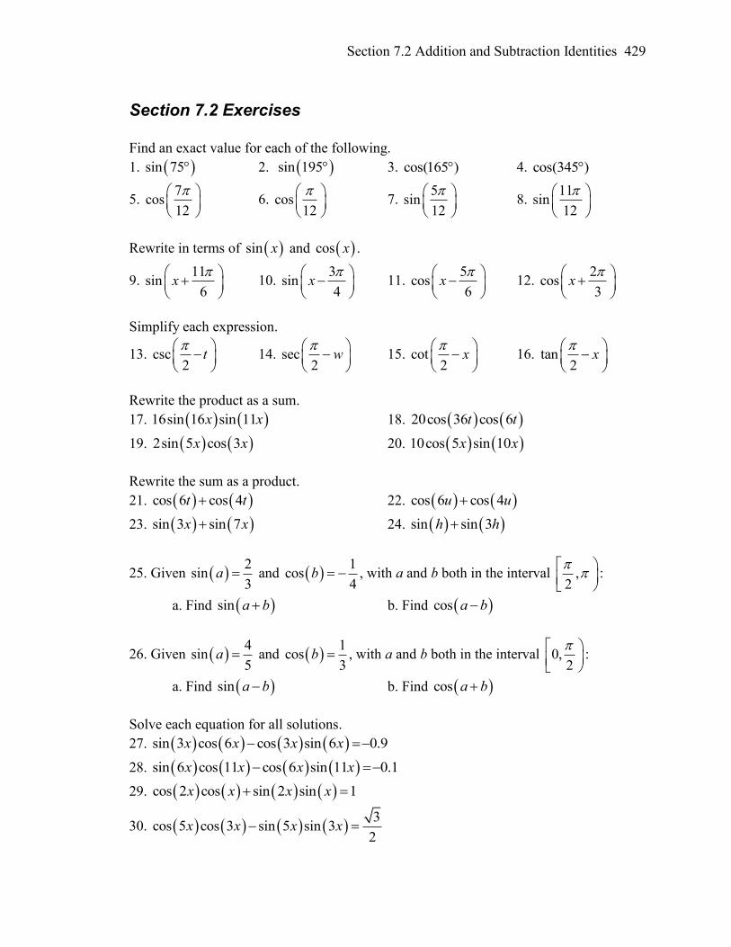
Section 7.2 Addition and Subtraction Identities 429
Section 7.2 Exercises
Find an exact value for each of the following.
1. sin 75 2. sin 195 3. cos(165 ) 4. cos(345 )
5. 7
cos12
6. cos12
7. 5
sin12
8. 11
sin12
Rewrite in terms of sin x and cos x .
9. 11
sin6
x
10. 3
sin4
x
11. 5
cos6
x
12. 2
cos3
x
Simplify each expression.
13. csc 2
t
14. sec
2w
15. cot
2x
16. tan
2x
Rewrite the product as a sum.
17. 16sin 16 sin 11x x 18. 20cos 36 cos 6t t
19. 2sin 5 cos 3x x 20. 10cos 5 sin 10x x
Rewrite the sum as a product.
21. cos 6 cos 4t t 22. cos 6 cos 4u u
23. sin 3 sin 7x x 24. sin sin 3h h
25. Given 2
sin3
a and 1
cos4
b , with a and b both in the interval ,2
:
a. Find sin a b b. Find cos a b
26. Given 4
sin5
a and 1
cos3
b , with a and b both in the interval 0,2
:
a. Find sin a b b. Find cos a b
Solve each equation for all solutions.
27. sin 3 cos 6 cos 3 sin 6 0.9x x x x
28. sin 6 cos 11 cos 6 sin 11 0.1x x x x
29. cos 2 cos sin 2 sin 1x x x x
30. 3
cos 5 cos 3 sin 5 sin 32
x x x x
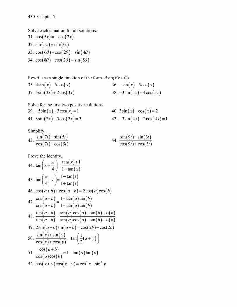
430 Chapter 7
Solve each equation for all solutions.
31. cos 5 cos 2x x
32. sin 5 sin 3x x
33. cos 6 cos 2 sin 4
34. cos 8 cos 2 sin 5
Rewrite as a single function of the form sin( ) A Bx C .
35. 4sin 6cosx x 36. sin 5cosx x
37. 5sin 3 2cos 3x x 38. 3sin 5 4cos 5x x
Solve for the first two positive solutions.
39. 5sin 3cos 1x x 40. 3sin cos 2x x
41. 3sin 2 5cos 2 3x x 42. 3sin 4 2cos 4 1x x
Simplify.
43.
sin 7 sin 5
cos 7 cos 5
t t
t t
44.
sin 9 sin 3
cos 9 cos 3
t t
t t
Prove the identity.
44.
tan 1tan
4 1 tan
xx
x
45.
1 tantan
4 1 tan
tt
t
46. cos cos 2cos cosa b a b a b
47.
cos 1 tan tan
cos 1 tan tan
a b a b
a b a b
48.
tan sin cos sin cos
tan sin cos sin cos
a b a a b b
a b a a b b
49. 2sin sin cos 2 cos(2 )a b a b b a
50.
sin sin 1tan
cos cos 2
x yx y
x y
51.
cos1 tan tan
cos cos
a ba b
a b
52. 2 2cos cos cos sinx y x y x y
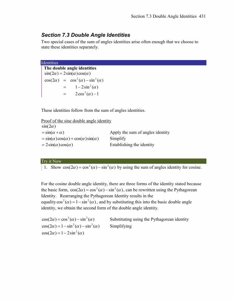
Section 7.3 Double Angle Identities 431
Section 7.3 Double Angle Identities
Two special cases of the sum of angles identities arise often enough that we choose to
state these identities separately.
Identities
The double angle identities
)cos()sin(2)2sin(
1)(cos2
)(sin21
)(sin)(cos)2cos(
2
2
22
These identities follow from the sum of angles identities.
Proof of the sine double angle identity
)2sin(
)sin( Apply the sum of angles identity
)sin()cos()cos()sin( Simplify
)cos()sin(2 Establishing the identity
Try it Now
1. Show )(sin)(cos)2cos( 22 by using the sum of angles identity for cosine.
For the cosine double angle identity, there are three forms of the identity stated because
the basic form, )(sin)(cos)2cos( 22 , can be rewritten using the Pythagorean
Identity. Rearranging the Pythagorean Identity results in the
equality )(sin1)(cos 22 , and by substituting this into the basic double angle
identity, we obtain the second form of the double angle identity.
)(sin)(cos)2cos( 22 Substituting using the Pythagorean identity
)(sin)(sin1)2cos( 22 Simplifying
)(sin21)2cos( 2
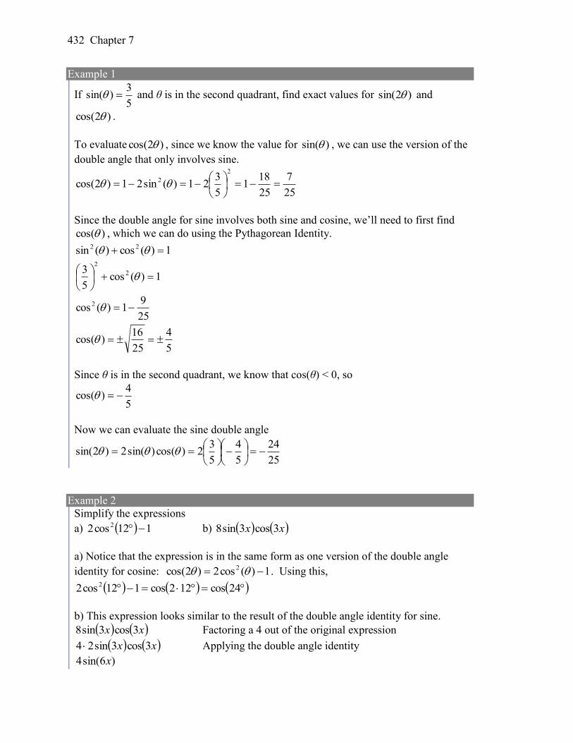
432 Chapter 7
Example 1
If 5
3)sin( and θ is in the second quadrant, find exact values for )2sin( and
)2cos( .
To evaluate )2cos( , since we know the value for sin( ) , we can use the version of the
double angle that only involves sine.
25
7
25
181
5
321)(sin21)2cos(
2
2
Since the double angle for sine involves both sine and cosine, we’ll need to first find
)cos( , which we can do using the Pythagorean Identity.
1)(cos)(sin 22
1)(cos5
3 2
2
25
91)(cos 2
5
4
25
16)cos(
Since θ is in the second quadrant, we know that cos(θ) < 0, so
5
4)cos(
Now we can evaluate the sine double angle
25
24
5
4
5
32)cos()sin(2)2sin(
Example 2
Simplify the expressions
a) 112cos2 2 b) xx 3cos3sin8
a) Notice that the expression is in the same form as one version of the double angle
identity for cosine: 1)(cos2)2cos( 2 . Using this,
24cos122cos112cos2 2
b) This expression looks similar to the result of the double angle identity for sine.
xx 3cos3sin8 Factoring a 4 out of the original expression
xx 3cos3sin24 Applying the double angle identity
)6sin(4 x
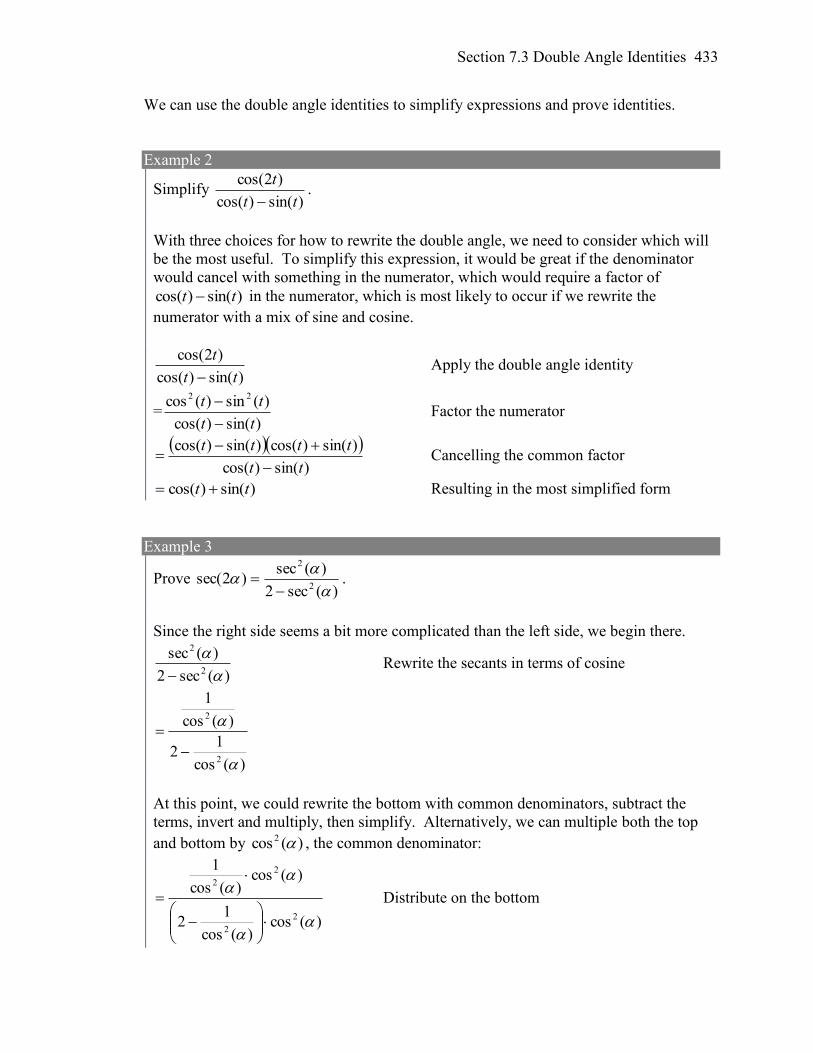
Section 7.3 Double Angle Identities 433
We can use the double angle identities to simplify expressions and prove identities.
Example 2
Simplify )sin()cos(
)2cos(
tt
t
.
With three choices for how to rewrite the double angle, we need to consider which will
be the most useful. To simplify this expression, it would be great if the denominator
would cancel with something in the numerator, which would require a factor of
)sin()cos( tt in the numerator, which is most likely to occur if we rewrite the
numerator with a mix of sine and cosine.
)sin()cos(
)2cos(
tt
t
Apply the double angle identity
=)sin()cos(
)(sin)(cos 22
tt
tt
Factor the numerator
)sin()cos(
)sin()cos()sin()cos(
tt
tttt
Cancelling the common factor
)sin()cos( tt Resulting in the most simplified form
Example 3
Prove )(sec2
)(sec)2sec(
2
2
.
Since the right side seems a bit more complicated than the left side, we begin there.
)(sec2
)(sec2
2
Rewrite the secants in terms of cosine
)(cos
12
)(cos
1
2
2
At this point, we could rewrite the bottom with common denominators, subtract the
terms, invert and multiply, then simplify. Alternatively, we can multiple both the top
and bottom by )(cos 2 , the common denominator:
)(cos)(cos
12
)(cos)(cos
1
2
2
2
2
Distribute on the bottom
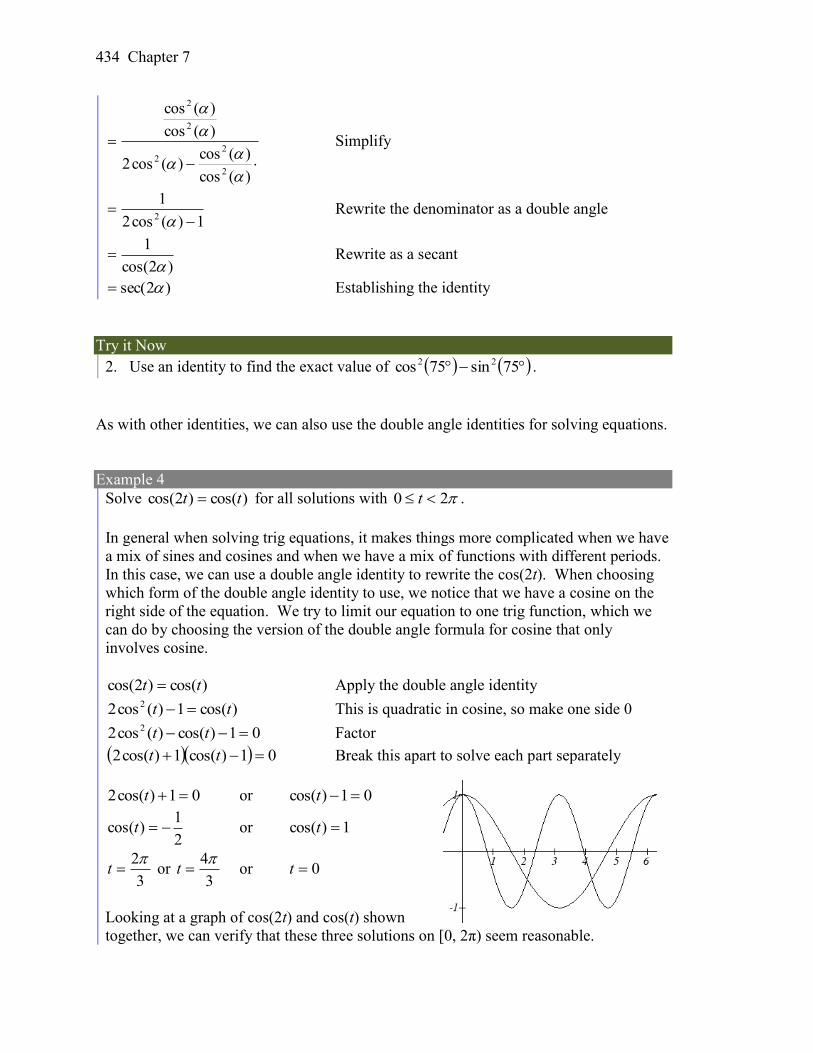
434 Chapter 7
)(cos
)(cos)(cos2
)(cos
)(cos
2
22
2
2
Simplify
1)(cos2
12
Rewrite the denominator as a double angle
)2cos(
1
Rewrite as a secant
)2sec( Establishing the identity
Try it Now
2. Use an identity to find the exact value of 75sin75cos 22 .
As with other identities, we can also use the double angle identities for solving equations.
Example 4
Solve )cos()2cos( tt for all solutions with 20 t .
In general when solving trig equations, it makes things more complicated when we have
a mix of sines and cosines and when we have a mix of functions with different periods.
In this case, we can use a double angle identity to rewrite the cos(2t). When choosing
which form of the double angle identity to use, we notice that we have a cosine on the
right side of the equation. We try to limit our equation to one trig function, which we
can do by choosing the version of the double angle formula for cosine that only
involves cosine.
)cos()2cos( tt Apply the double angle identity
)cos(1)(cos2 2 tt This is quadratic in cosine, so make one side 0
01)cos()(cos2 2 tt Factor
01)cos(1)cos(2 tt Break this apart to solve each part separately
01)cos(2 t or 01)cos( t
2
1)cos( t or 1)cos( t
3
2t or
3
4t or 0t
Looking at a graph of cos(2t) and cos(t) shown
together, we can verify that these three solutions on [0, 2π) seem reasonable.
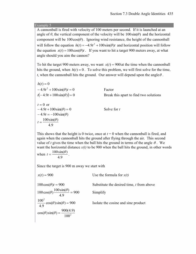
Section 7.3 Double Angle Identities 435
Example 5
A cannonball is fired with velocity of 100 meters per second. If it is launched at an
angle of θ, the vertical component of the velocity will be )sin(100 and the horizontal
component will be )cos(100 . Ignoring wind resistance, the height of the cannonball
will follow the equation ttth )sin(1009.4)( 2 and horizontal position will follow
the equation ttx )cos(100)( . If you want to hit a target 900 meters away, at what
angle should you aim the cannon?
To hit the target 900 meters away, we want 900)( tx at the time when the cannonball
hits the ground, when 0)( th . To solve this problem, we will first solve for the time,
t, when the cannonball hits the ground. Our answer will depend upon the angle .
0)( th
0)sin(1009.4 2 tt Factor
0)sin(1009.4 tt Break this apart to find two solutions
0t or
0)sin(1009.4 t Solve for t
)sin(1009.4 t
9.4
)sin(100 t
This shows that the height is 0 twice, once at t = 0 when the cannonball is fired, and
again when the cannonball hits the ground after flying through the air. This second
value of t gives the time when the ball hits the ground in terms of the angle . We
want the horizontal distance x(t) to be 900 when the ball hits the ground, in other words
when 9.4
)sin(100 t .
Since the target is 900 m away we start with
900)( tx Use the formula for x(t)
900)cos(100 t Substitute the desired time, t from above
9009.4
)sin(100)cos(100
Simplify
900)sin()cos(9.4
1002
Isolate the cosine and sine product
2100
)9.4(900)sin()cos(
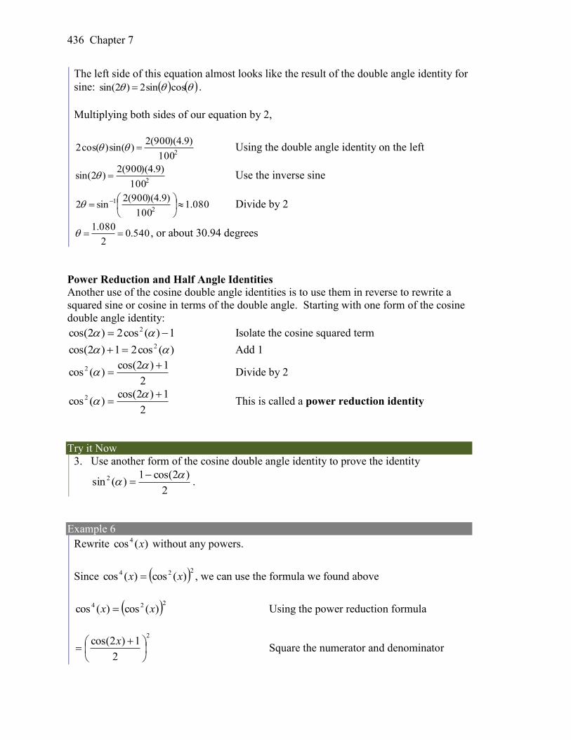
436 Chapter 7
The left side of this equation almost looks like the result of the double angle identity for
sine: cossin2)2sin( .
Multiplying both sides of our equation by 2,
2100
)9.4)(900(2)sin()cos(2 Using the double angle identity on the left
2100
)9.4)(900(2)2sin( Use the inverse sine
080.1100
)9.4)(900(2sin2
2
1
Divide by 2
540.02
080.1 , or about 30.94 degrees
Power Reduction and Half Angle Identities Another use of the cosine double angle identities is to use them in reverse to rewrite a
squared sine or cosine in terms of the double angle. Starting with one form of the cosine
double angle identity:
1)(cos2)2cos( 2 Isolate the cosine squared term
)(cos21)2cos( 2 Add 1
2
1)2cos()(cos 2
Divide by 2
2
1)2cos()(cos 2
This is called a power reduction identity
Try it Now
3. Use another form of the cosine double angle identity to prove the identity
2
)2cos(1)(sin 2
.
Example 6
Rewrite )(cos 4 x without any powers.
Since 224 )(cos)(cos xx , we can use the formula we found above
224 )(cos)(cos xx Using the power reduction formula
2
2
1)2cos(
x Square the numerator and denominator
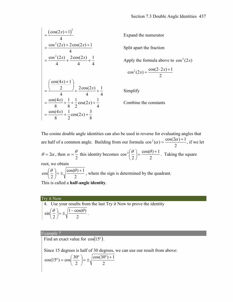
Section 7.3 Double Angle Identities 437
2
cos(2 ) 1
4
x Expand the numerator
4
1)2cos(2)2(cos 2
xx Split apart the fraction
4
1
4
)2cos(2
4
)2(cos 2
xx
Apply the formula above to )2(cos 2 x
2 cos(2 2 ) 1cos (2 )
2
xx
4
1
4
)2cos(2
4
2
1)4cos(
x
x
Simplify
4
1)2cos(
2
1
8
1
8
)4cos( x
x Combine the constants
8
3)2cos(
2
1
8
)4cos( x
x
The cosine double angle identities can also be used in reverse for evaluating angles that
are half of a common angle. Building from our formula 2
1)2cos()(cos 2
, if we let
2 , then 2
this identity becomes
2
1)cos(
2cos 2
. Taking the square
root, we obtain
2
1)cos(
2cos
, where the sign is determined by the quadrant.
This is called a half-angle identity.
Try it Now
4. Use your results from the last Try it Now to prove the identity
2
)cos(1
2sin
.
Example 7
Find an exact value for 15cos .
Since 15 degrees is half of 30 degrees, we can use our result from above:
2
1)30cos(
2
30cos)15cos(
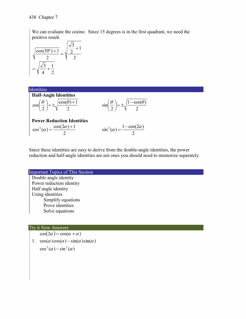
438 Chapter 7
We can evaluate the cosine. Since 15 degrees is in the first quadrant, we need the
positive result.
2
12
3
2
1)30cos(
2
1
4
3
Identities
Half-Angle Identities
2
1)cos(
2cos
2
)cos(1
2sin
Power Reduction Identities
2
1)2cos()(cos 2
2
)2cos(1)(sin 2
Since these identities are easy to derive from the double-angle identities, the power
reduction and half-angle identities are not ones you should need to memorize separately.
Important Topics of This Section
Double angle identity
Power reduction identity
Half angle identity
Using identities
Simplify equations
Prove identities
Solve equations
Try it Now Answers
1.
)(sin)(cos
)sin()sin()cos()cos(
)cos(2cos
22
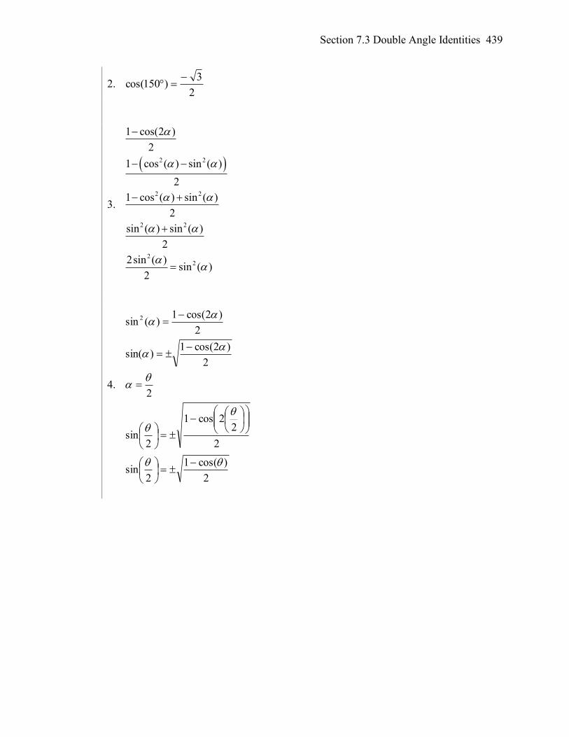
Section 7.3 Double Angle Identities 439
2. 2
3)150cos(
3.
2 2
2 2
2 2
22
1 cos(2 )
2
1 cos ( ) sin ( )
2
1 cos ( ) sin ( )
2
sin ( ) sin ( )
2
2sin ( )sin ( )
2
4.
2
)cos(1
2sin
2
22cos1
2sin
2
2
)2cos(1)sin(
2
)2cos(1)(sin 2
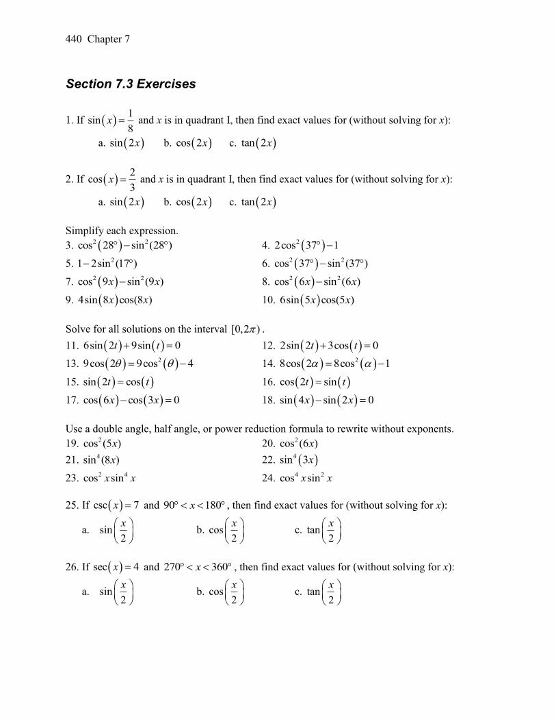
440 Chapter 7
Section 7.3 Exercises
1. If 1
sin8
x and x is in quadrant I, then find exact values for (without solving for x):
a. sin 2x b. cos 2x c. tan 2x
2. If 2
cos3
x and x is in quadrant I, then find exact values for (without solving for x):
a. sin 2x b. cos 2x c. tan 2x
Simplify each expression.
3. 2 2cos 28 sin (28 ) 4. 22cos 37 1
5. 21 2sin (17 ) 6. 2 2cos 37 sin (37 )
7. 2 2cos 9 sin (9 )x x 8. 2 2cos 6 sin (6 )x x
9. 4sin 8 cos(8 )x x 10. 6sin 5 cos(5 )x x
Solve for all solutions on the interval [0, 2 ) .
11. 6sin 2 9sin 0t t 12. 2sin 2 3cos 0t t
13. 29cos 2 9cos 4 14. 28cos 2 8cos 1
15. sin 2 cost t 16. cos 2 sint t
17. cos 6 cos 3 0x x 18. sin 4 sin 2 0x x
Use a double angle, half angle, or power reduction formula to rewrite without exponents.
19. 2cos (5 )x 20. 2cos (6 )x
21. 4sin (8 )x 22. 4sin 3x
23. 2 4cos sinx x 24. 4 2cos sinx x
25. If csc 7x and 90 180x , then find exact values for (without solving for x):
a. sin2
x
b. cos2
x
c. tan2
x
26. If sec 4x and 270 360x , then find exact values for (without solving for x):
a. sin2
x
b. cos2
x
c. tan2
x
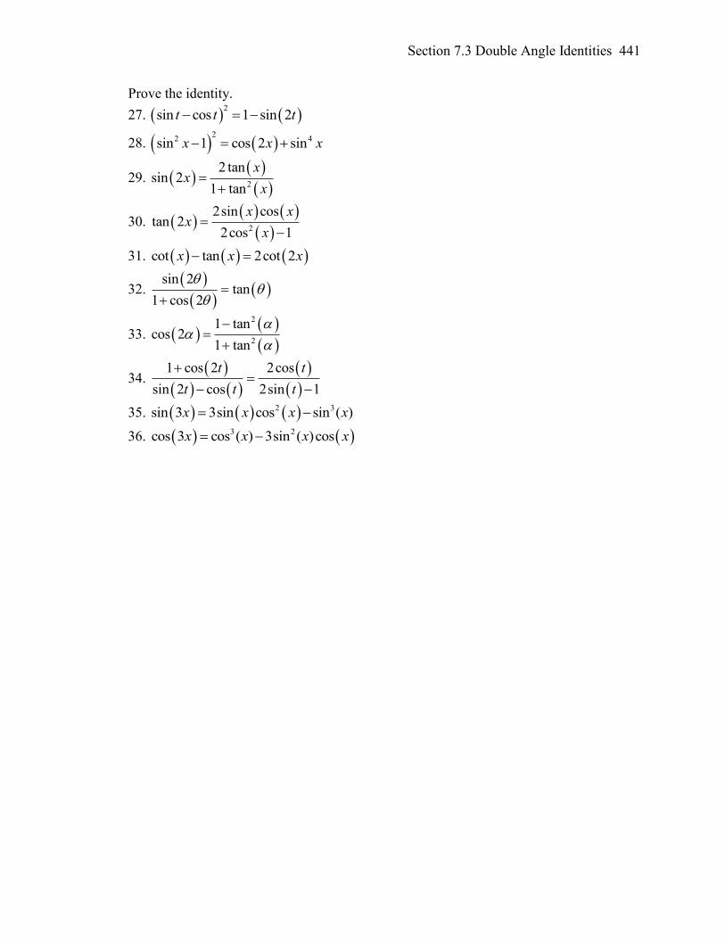
Section 7.3 Double Angle Identities 441
Prove the identity.
27. 2
sin cos 1 sin 2t t t
28. 2
2 4sin 1 cos 2 sinx x x
29.
2
2 tansin 2
1 tan
xx
x
30.
2
2sin costan 2
2cos 1
x xx
x
31. cot tan 2cot 2x x x
32.
sin 2tan
1 cos 2
33.
2
2
1 tancos 2
1 tan
34.
1 cos 2 2cos
sin 2 cos 2sin 1
t t
t t t
35. 2 3sin 3 3sin cos sin ( )x x x x
36. 3 2cos 3 cos ( ) 3sin ( )cosx x x x
442 Chapter 7
Section 7.4 Modeling Changing Amplitude and Midline
While sinusoidal functions can model a variety of behaviors, it is often necessary to
combine sinusoidal functions with linear and exponential curves to model real
applications and behaviors. We begin this section by looking at changes to the midline of
a sinusoidal function. Recall that the midline describes the middle, or average value, of
the sinusoidal function.
Changing Midlines
Example 1
A population of elk currently averages 2000 elk, and that average has been growing by
4% each year. Due to seasonal fluctuation, the population oscillates from 50 below
average in the winter up to 50 above average in the summer. Find a function that
models the number of elk after t years.
There are two components to the behavior of the elk population: the changing average,
and the oscillation. The average is an exponential growth, starting at 2000 and growing
by 4% each year. Writing a formula for this:
(1 ) 2000(1 0.04)t taverage initial r
For the oscillation, since the population oscillates 50 above and below average, the
amplitude will be 50. Since it takes one year for the population to cycle, the period is 1.
We find the value of the horizontal stretch coefficientoriginal period 2
2new period 1
B
.
Additionally, since we weren’t told when t was first measured we will have to decide if
t = 0 corresponds to winter, or summer. If we choose winter then the shape of the
function would be a negative cosine, since it starts at the lowest value.
Putting it all together, the equation would be:
( ) 50cos(2 )P t t midline
Since the midline represents the average population, we substitute in the exponential
function into the population equation to find our final equation:
( ) 50cos(2 ) 2000(1 0.04)tP t t
This is an example of changing midline – in this case an exponentially changing midline.
Changing Midline
A function of the form )()sin()( tgBtAtf will oscillate above and below the
average given by the function g(t).
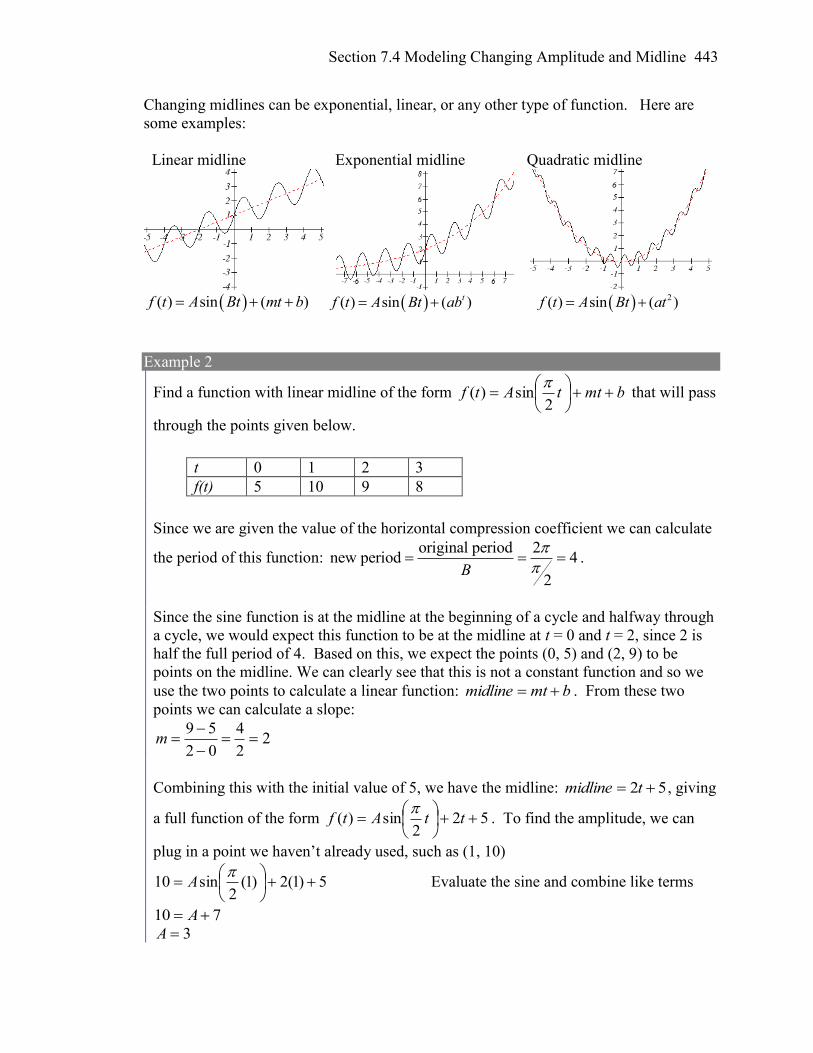
Section 7.4 Modeling Changing Amplitude and Midline 443
Changing midlines can be exponential, linear, or any other type of function. Here are
some examples:
Linear midline Exponential midline Quadratic midline
( ) sin ( )f t A Bt mt b ( ) sin ( )tf t A Bt ab 2( ) sin ( )f t A Bt at
Example 2
Find a function with linear midline of the form bmttAtf
2sin)(
that will pass
through the points given below.
Since we are given the value of the horizontal compression coefficient we can calculate
the period of this function: original period 2
new period 4
2B
.
Since the sine function is at the midline at the beginning of a cycle and halfway through
a cycle, we would expect this function to be at the midline at t = 0 and t = 2, since 2 is
half the full period of 4. Based on this, we expect the points (0, 5) and (2, 9) to be
points on the midline. We can clearly see that this is not a constant function and so we
use the two points to calculate a linear function: bmtmidline . From these two
points we can calculate a slope:
22
4
02
59
m
Combining this with the initial value of 5, we have the midline: 52 tmidline , giving
a full function of the form 522
sin)(
ttAtf
. To find the amplitude, we can
plug in a point we haven’t already used, such as (1, 10)
5)1(2)1(2
sin10
A Evaluate the sine and combine like terms
710 A
3A
t 0 1 2 3
f(t) 5 10 9 8
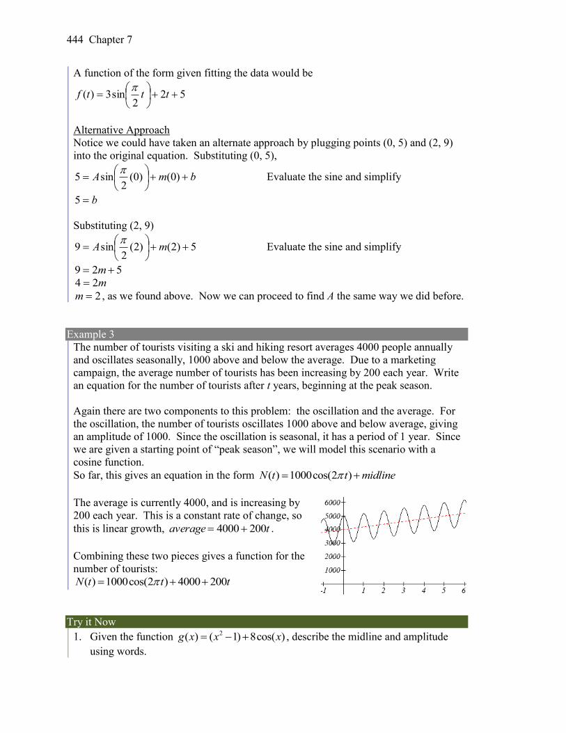
444 Chapter 7
A function of the form given fitting the data would be
522
sin3)(
tttf
Alternative Approach
Notice we could have taken an alternate approach by plugging points (0, 5) and (2, 9)
into the original equation. Substituting (0, 5),
bmA
)0()0(
2sin5
Evaluate the sine and simplify
b5
Substituting (2, 9)
5)2()2(2
sin9
mA
Evaluate the sine and simplify
529 m
m24
2m , as we found above. Now we can proceed to find A the same way we did before.
Example 3
The number of tourists visiting a ski and hiking resort averages 4000 people annually
and oscillates seasonally, 1000 above and below the average. Due to a marketing
campaign, the average number of tourists has been increasing by 200 each year. Write
an equation for the number of tourists after t years, beginning at the peak season.
Again there are two components to this problem: the oscillation and the average. For
the oscillation, the number of tourists oscillates 1000 above and below average, giving
an amplitude of 1000. Since the oscillation is seasonal, it has a period of 1 year. Since
we are given a starting point of “peak season”, we will model this scenario with a
cosine function.
So far, this gives an equation in the form ( ) 1000cos(2 )N t t midline
The average is currently 4000, and is increasing by
200 each year. This is a constant rate of change, so
this is linear growth, taverage 2004000 .
Combining these two pieces gives a function for the
number of tourists:
( ) 1000cos(2 ) 4000 200N t t t
Try it Now
1. Given the function 2( ) ( 1) 8cos( )g x x x , describe the midline and amplitude
using words.
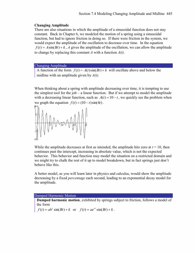
Section 7.4 Modeling Changing Amplitude and Midline 445
Changing Amplitude
There are also situations in which the amplitude of a sinusoidal function does not stay
constant. Back in Chapter 6, we modeled the motion of a spring using a sinusoidal
function, but had to ignore friction in doing so. If there were friction in the system, we
would expect the amplitude of the oscillation to decrease over time. In the equation
kBtAtf )sin()( , A gives the amplitude of the oscillation, we can allow the amplitude
to change by replacing this constant A with a function A(t).
Changing Amplitude
A function of the form kBttAtf )sin()()( will oscillate above and below the
midline with an amplitude given by A(t).
When thinking about a spring with amplitude decreasing over time, it is tempting to use
the simplest tool for the job – a linear function. But if we attempt to model the amplitude
with a decreasing linear function, such as ttA 10)( , we quickly see the problem when
we graph the equation )4sin()10()( tttf .
While the amplitude decreases at first as intended, the amplitude hits zero at t = 10, then
continues past the intercept, increasing in absolute value, which is not the expected
behavior. This behavior and function may model the situation on a restricted domain and
we might try to chalk the rest of it up to model breakdown, but in fact springs just don’t
behave like this.
A better model, as you will learn later in physics and calculus, would show the amplitude
decreasing by a fixed percentage each second, leading to an exponential decay model for
the amplitude.
Damped Harmonic Motion
Damped harmonic motion, exhibited by springs subject to friction, follows a model of
the form
kBtabtf t )sin()( or kBtaetf rt )sin()( .
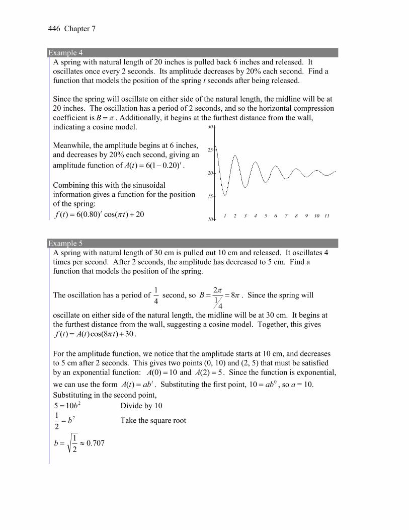
446 Chapter 7
Example 4
A spring with natural length of 20 inches is pulled back 6 inches and released. It
oscillates once every 2 seconds. Its amplitude decreases by 20% each second. Find a
function that models the position of the spring t seconds after being released.
Since the spring will oscillate on either side of the natural length, the midline will be at
20 inches. The oscillation has a period of 2 seconds, and so the horizontal compression
coefficient is B . Additionally, it begins at the furthest distance from the wall,
indicating a cosine model.
Meanwhile, the amplitude begins at 6 inches,
and decreases by 20% each second, giving an
amplitude function of ttA )20.01(6)( .
Combining this with the sinusoidal
information gives a function for the position
of the spring:
20)cos()80.0(6)( ttf t
Example 5
A spring with natural length of 30 cm is pulled out 10 cm and released. It oscillates 4
times per second. After 2 seconds, the amplitude has decreased to 5 cm. Find a
function that models the position of the spring.
The oscillation has a period of 1
4 second, so
28
14
B
. Since the spring will
oscillate on either side of the natural length, the midline will be at 30 cm. It begins at
the furthest distance from the wall, suggesting a cosine model. Together, this gives
( ) ( )cos(8 ) 30f t A t t .
For the amplitude function, we notice that the amplitude starts at 10 cm, and decreases
to 5 cm after 2 seconds. This gives two points (0, 10) and (2, 5) that must be satisfied
by an exponential function: 10)0( A and 5)2( A . Since the function is exponential,
we can use the form tabtA )( . Substituting the first point, 010 ab , so a = 10.
Substituting in the second point, 2105 b Divide by 10
2
2
1b Take the square root
707.02
1b
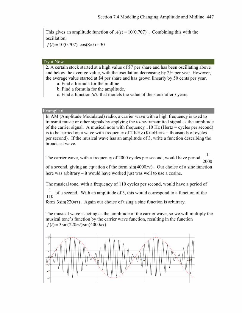
Section 7.4 Modeling Changing Amplitude and Midline 447
This gives an amplitude function of ttA )707.0(10)( . Combining this with the
oscillation,
( ) 10(0.707) cos(8 ) 30tf t t
Try it Now
2. A certain stock started at a high value of $7 per share and has been oscillating above
and below the average value, with the oscillation decreasing by 2% per year. However,
the average value started at $4 per share and has grown linearly by 50 cents per year.
a. Find a formula for the midline
b. Find a formula for the amplitude.
c. Find a function S(t) that models the value of the stock after t years.
Example 6
In AM (Amplitude Modulated) radio, a carrier wave with a high frequency is used to
transmit music or other signals by applying the to-be-transmitted signal as the amplitude
of the carrier signal. A musical note with frequency 110 Hz (Hertz = cycles per second)
is to be carried on a wave with frequency of 2 KHz (KiloHertz = thousands of cycles
per second). If the musical wave has an amplitude of 3, write a function describing the
broadcast wave.
The carrier wave, with a frequency of 2000 cycles per second, would have period 2000
1
of a second, giving an equation of the form sin(4000 )t . Our choice of a sine function
here was arbitrary – it would have worked just was well to use a cosine.
The musical tone, with a frequency of 110 cycles per second, would have a period of
110
1 of a second. With an amplitude of 3, this would correspond to a function of the
form 3sin(220 )t . Again our choice of using a sine function is arbitrary.
The musical wave is acting as the amplitude of the carrier wave, so we will multiply the
musical tone’s function by the carrier wave function, resulting in the function
( ) 3sin(220 )sin(4000 )f t t t
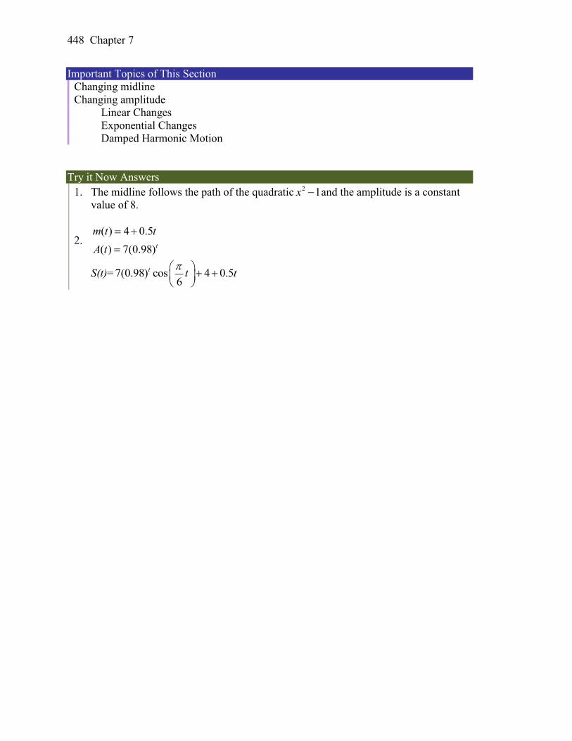
448 Chapter 7
Important Topics of This Section
Changing midline
Changing amplitude
Linear Changes
Exponential Changes
Damped Harmonic Motion
Try it Now Answers
1. The midline follows the path of the quadratic 2 1x and the amplitude is a constant
value of 8.
2. ( ) 4 0.5
( ) 7(0.98)t
m t t
A t
S(t)= 7(0.98) cos 4 0.56
t t t
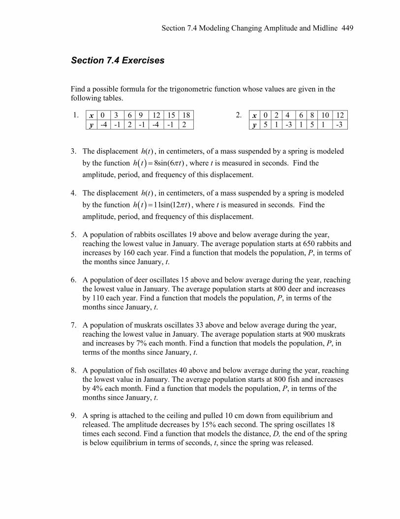
Section 7.4 Modeling Changing Amplitude and Midline 449
Section 7.4 Exercises
Find a possible formula for the trigonometric function whose values are given in the
following tables.
1. x 0 3 6 9 12 15 18
y -4 -1 2 -1 -4 -1 2
2. x 0 2 4 6 8 10 12
y 5 1 -3 1 5 1 -3
3. The displacement ( )h t , in centimeters, of a mass suspended by a spring is modeled
by the function 8sin(6 )h t t , where t is measured in seconds. Find the
amplitude, period, and frequency of this displacement.
4. The displacement ( )h t , in centimeters, of a mass suspended by a spring is modeled
by the function 11sin(12 )h t t , where t is measured in seconds. Find the
amplitude, period, and frequency of this displacement.
5. A population of rabbits oscillates 19 above and below average during the year,
reaching the lowest value in January. The average population starts at 650 rabbits and
increases by 160 each year. Find a function that models the population, P, in terms of
the months since January, t.
6. A population of deer oscillates 15 above and below average during the year, reaching
the lowest value in January. The average population starts at 800 deer and increases
by 110 each year. Find a function that models the population, P, in terms of the
months since January, t.
7. A population of muskrats oscillates 33 above and below average during the year,
reaching the lowest value in January. The average population starts at 900 muskrats
and increases by 7% each month. Find a function that models the population, P, in
terms of the months since January, t.
8. A population of fish oscillates 40 above and below average during the year, reaching
the lowest value in January. The average population starts at 800 fish and increases
by 4% each month. Find a function that models the population, P, in terms of the
months since January, t.
9. A spring is attached to the ceiling and pulled 10 cm down from equilibrium and
released. The amplitude decreases by 15% each second. The spring oscillates 18
times each second. Find a function that models the distance, D, the end of the spring
is below equilibrium in terms of seconds, t, since the spring was released.
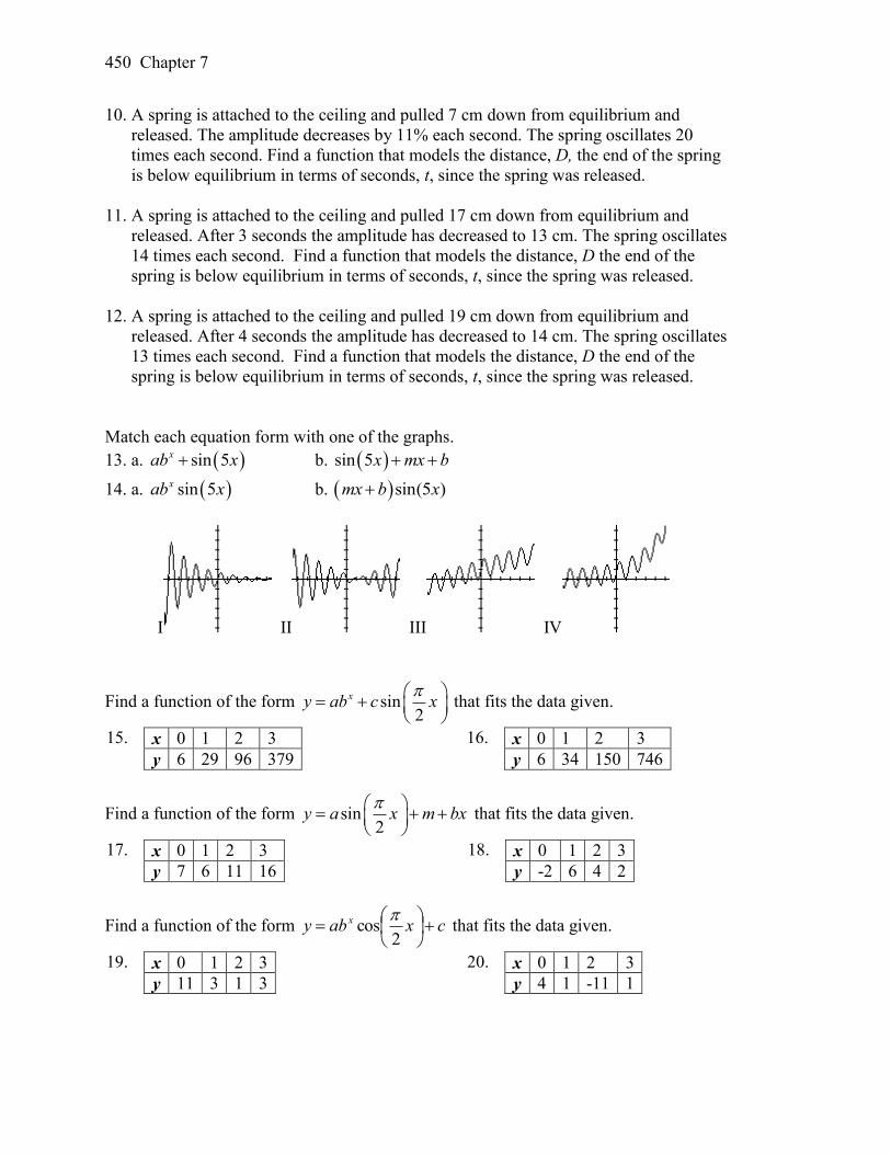
450 Chapter 7
10. A spring is attached to the ceiling and pulled 7 cm down from equilibrium and
released. The amplitude decreases by 11% each second. The spring oscillates 20
times each second. Find a function that models the distance, D, the end of the spring
is below equilibrium in terms of seconds, t, since the spring was released.
11. A spring is attached to the ceiling and pulled 17 cm down from equilibrium and
released. After 3 seconds the amplitude has decreased to 13 cm. The spring oscillates
14 times each second. Find a function that models the distance, D the end of the
spring is below equilibrium in terms of seconds, t, since the spring was released.
12. A spring is attached to the ceiling and pulled 19 cm down from equilibrium and
released. After 4 seconds the amplitude has decreased to 14 cm. The spring oscillates
13 times each second. Find a function that models the distance, D the end of the
spring is below equilibrium in terms of seconds, t, since the spring was released.
Match each equation form with one of the graphs.
13. a. sin 5xab x b. sin 5x mx b
14. a. sin 5xab x b. sin(5 )mx b x
I II III IV
Find a function of the form sin2
xy ab c x
that fits the data given.
15. x 0 1 2 3
y 6 29 96 379
16. x 0 1 2 3
y 6 34 150 746
Find a function of the form sin2
y a x m bx
that fits the data given.
17. x 0 1 2 3
y 7 6 11 16
18. x 0 1 2 3
y -2 6 4 2
Find a function of the form cxaby x
2cos
that fits the data given.
19. x 0 1 2 3
y 11 3 1 3
20. x 0 1 2 3
y 4 1 -11 1
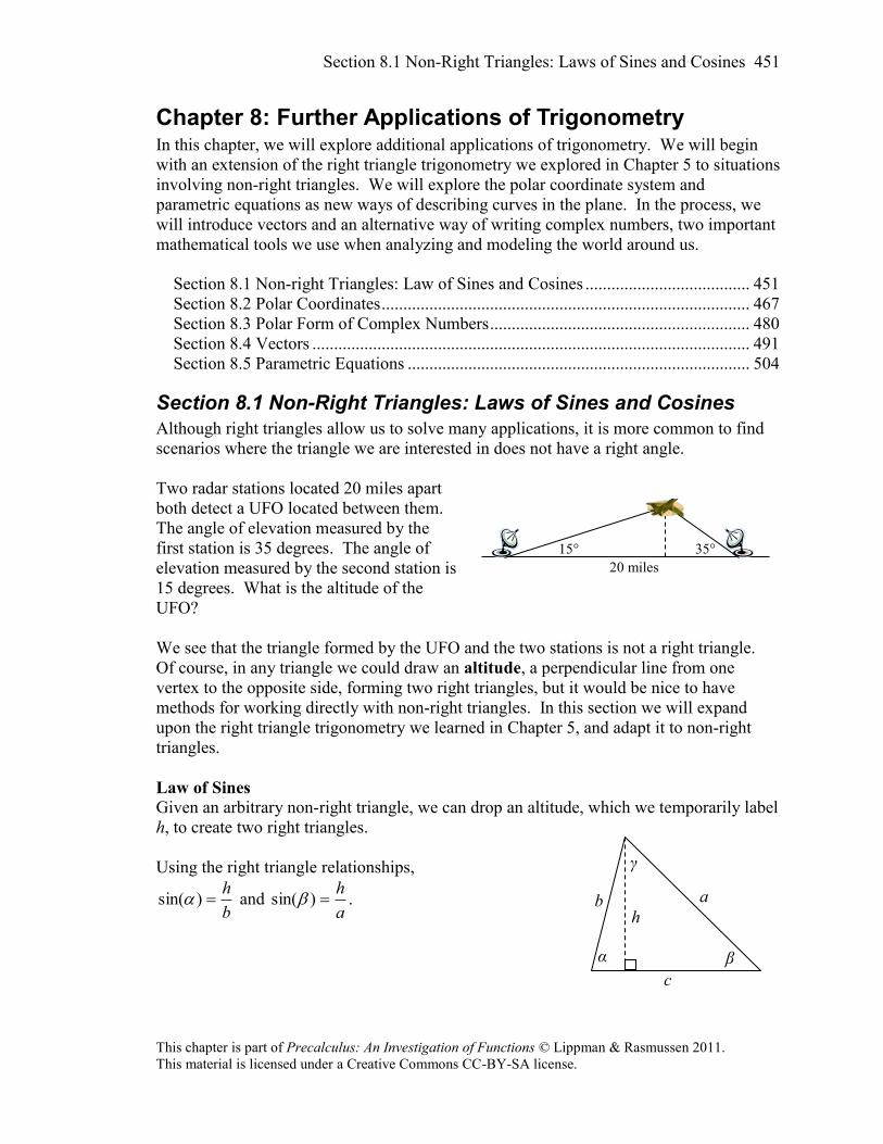
Section 8.1 Non-Right Triangles: Laws of Sines and Cosines 451
This chapter is part of Precalculus: An Investigation of Functions © Lippman & Rasmussen 2011.
This material is licensed under a Creative Commons CC-BY-SA license.
Chapter 8: Further Applications of Trigonometry In this chapter, we will explore additional applications of trigonometry. We will begin
with an extension of the right triangle trigonometry we explored in Chapter 5 to situations
involving non-right triangles. We will explore the polar coordinate system and
parametric equations as new ways of describing curves in the plane. In the process, we
will introduce vectors and an alternative way of writing complex numbers, two important
mathematical tools we use when analyzing and modeling the world around us.
Section 8.1 Non-right Triangles: Law of Sines and Cosines ...................................... 451 Section 8.2 Polar Coordinates ..................................................................................... 467
Section 8.3 Polar Form of Complex Numbers ............................................................ 480 Section 8.4 Vectors ..................................................................................................... 491 Section 8.5 Parametric Equations ............................................................................... 504
Section 8.1 Non-Right Triangles: Laws of Sines and Cosines
Although right triangles allow us to solve many applications, it is more common to find
scenarios where the triangle we are interested in does not have a right angle.
Two radar stations located 20 miles apart
both detect a UFO located between them.
The angle of elevation measured by the
first station is 35 degrees. The angle of
elevation measured by the second station is
15 degrees. What is the altitude of the
UFO?
We see that the triangle formed by the UFO and the two stations is not a right triangle.
Of course, in any triangle we could draw an altitude, a perpendicular line from one
vertex to the opposite side, forming two right triangles, but it would be nice to have
methods for working directly with non-right triangles. In this section we will expand
upon the right triangle trigonometry we learned in Chapter 5, and adapt it to non-right
triangles.
Law of Sines Given an arbitrary non-right triangle, we can drop an altitude, which we temporarily label
h, to create two right triangles.
Using the right triangle relationships,
b
h)sin( and
a
h)sin( .
15° 35°
20 miles
α β
a b h
γ
c
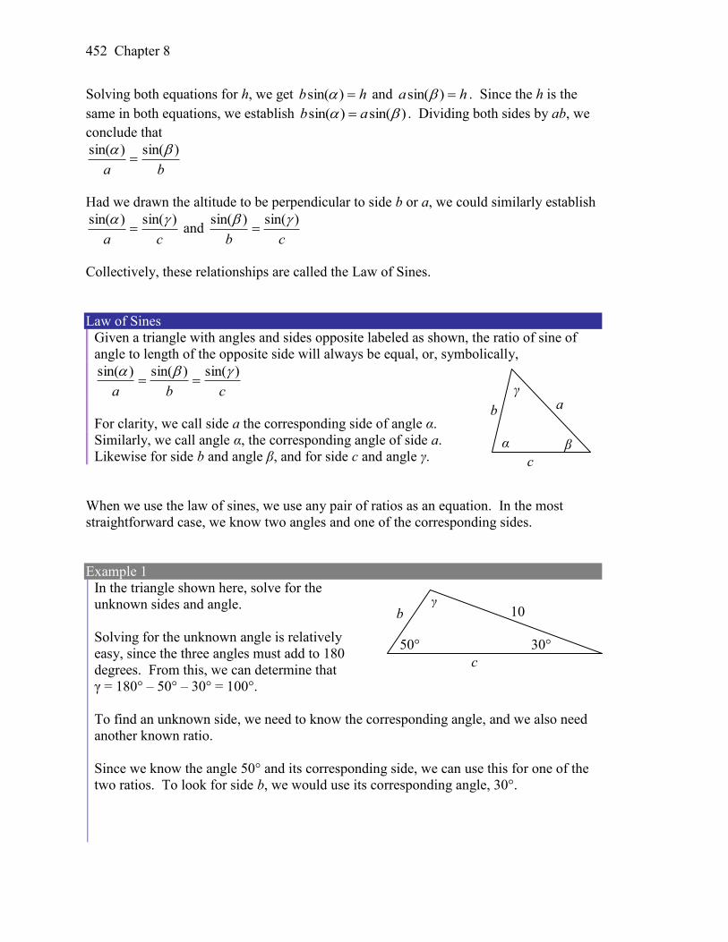
452 Chapter 8
Solving both equations for h, we get hb )sin( and ha )sin( . Since the h is the
same in both equations, we establish )sin()sin( ab . Dividing both sides by ab, we
conclude that
ba
)sin()sin(
Had we drawn the altitude to be perpendicular to side b or a, we could similarly establish
ca
)sin()sin( and
cb
)sin()sin(
Collectively, these relationships are called the Law of Sines.
Law of Sines
Given a triangle with angles and sides opposite labeled as shown, the ratio of sine of
angle to length of the opposite side will always be equal, or, symbolically,
cba
)sin()sin()sin(
For clarity, we call side a the corresponding side of angle α.
Similarly, we call angle α, the corresponding angle of side a.
Likewise for side b and angle β, and for side c and angle γ.
When we use the law of sines, we use any pair of ratios as an equation. In the most
straightforward case, we know two angles and one of the corresponding sides.
Example 1
In the triangle shown here, solve for the
unknown sides and angle.
Solving for the unknown angle is relatively
easy, since the three angles must add to 180
degrees. From this, we can determine that
γ = 180° – 50° – 30° = 100°.
To find an unknown side, we need to know the corresponding angle, and we also need
another known ratio.
Since we know the angle 50° and its corresponding side, we can use this for one of the
two ratios. To look for side b, we would use its corresponding angle, 30°.
50°
10 b
30°
c
γ
α β
a b
c
γ
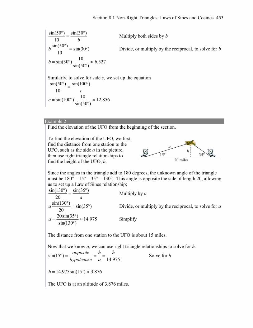
Section 8.1 Non-Right Triangles: Laws of Sines and Cosines 453
b
)30sin(
10
)50sin(
Multiply both sides by b
)30sin(10
)50sin(
b Divide, or multiply by the reciprocal, to solve for b
527.6)50sin(
10)30sin(
b
Similarly, to solve for side c, we set up the equation
c
)100sin(
10
)50sin(
856.12)50sin(
10)100sin(
c
Example 2
Find the elevation of the UFO from the beginning of the section.
To find the elevation of the UFO, we first
find the distance from one station to the
UFO, such as the side a in the picture,
then use right triangle relationships to
find the height of the UFO, h.
Since the angles in the triangle add to 180 degrees, the unknown angle of the triangle
must be 180° – 15° – 35° = 130°. This angle is opposite the side of length 20, allowing
us to set up a Law of Sines relationship:
a
)35sin(
20
)130sin(
Multiply by a
)35sin(20
)130sin(
a Divide, or multiply by the reciprocal, to solve for a
975.14)130sin(
)35sin(20
a Simplify
The distance from one station to the UFO is about 15 miles.
Now that we know a, we can use right triangle relationships to solve for h.
975.14)15sin(
h
a
h
hypotenuse
opposite Solve for h
876.3)15sin(975.14 h
The UFO is at an altitude of 3.876 miles.
15° 35°
20 miles
h a
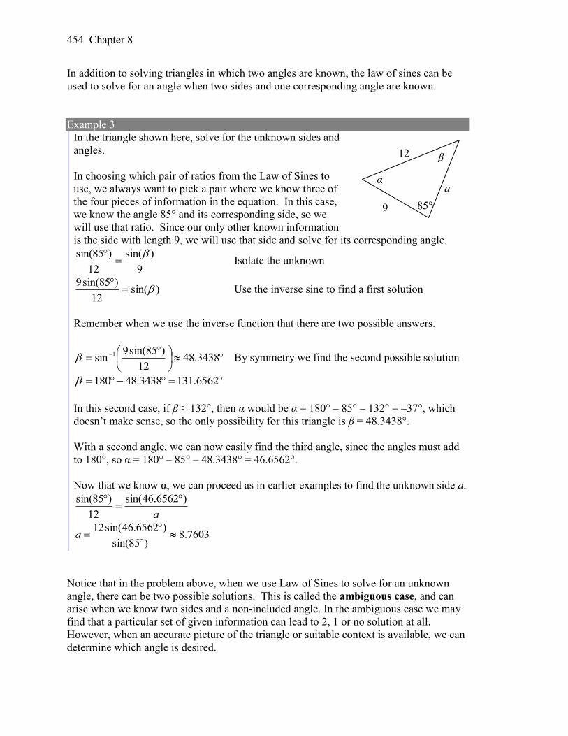
454 Chapter 8
In addition to solving triangles in which two angles are known, the law of sines can be
used to solve for an angle when two sides and one corresponding angle are known.
Example 3
In the triangle shown here, solve for the unknown sides and
angles.
In choosing which pair of ratios from the Law of Sines to
use, we always want to pick a pair where we know three of
the four pieces of information in the equation. In this case,
we know the angle 85° and its corresponding side, so we
will use that ratio. Since our only other known information
is the side with length 9, we will use that side and solve for its corresponding angle.
9
)sin(
12
)85sin(
Isolate the unknown
)sin(12
)85sin(9
Use the inverse sine to find a first solution
Remember when we use the inverse function that there are two possible answers.
3438.48
12
)85sin(9sin 1 By symmetry we find the second possible solution
6562.1313438.48180
In this second case, if β ≈ 132°, then α would be α = 180° – 85° – 132° = –37°, which
doesn’t make sense, so the only possibility for this triangle is β = 48.3438°.
With a second angle, we can now easily find the third angle, since the angles must add
to 180°, so α = 180° – 85° – 48.3438° = 46.6562°.
Now that we know α, we can proceed as in earlier examples to find the unknown side a.
a
)6562.46sin(
12
)85sin(
7603.8)85sin(
)6562.46sin(12
a
Notice that in the problem above, when we use Law of Sines to solve for an unknown
angle, there can be two possible solutions. This is called the ambiguous case, and can
arise when we know two sides and a non-included angle. In the ambiguous case we may
find that a particular set of given information can lead to 2, 1 or no solution at all.
However, when an accurate picture of the triangle or suitable context is available, we can
determine which angle is desired.
9
12
a
85°
β
α
Section 8.1 Non-Right Triangles: Laws of Sines and Cosines 455
Try it Now
1. Given 121 and ,120,80 ba , find the corresponding and missing side and
angles. If there is more than one possible solution, show both.
Example 4
Find all possible triangles if one side has length 4 opposite an angle of 50° and a second
side has length 10.
Using the given information, we can look for the angle opposite the side of length 10.
10
)sin(
4
)50sin(
915.14
)50sin(10)sin(
Since the range of the sine function is [-1, 1], it is impossible for the sine value to be
1.915. There are no triangles that can be drawn with the provided dimensions.
Example 5
Find all possible triangles if one side has length 6 opposite an angle of 50° and a second
side has length 4.
Using the given information, we can look for the angle opposite the side of length 4.
4
)sin(
6
)50sin(
511.06
)50sin(4)sin(
Use the inverse to find one solution
710.30511.0sin 1 By symmetry there is a second possible solution
290.149710.30180
If we use the angle 710.30 , the third angle would be 290.99710.3050180 .
We can then use Law of Sines again to find the third side.
c
)290.99sin(
6
)50sin(
Solve for c
c = 7.730
If we used the angle α = 149.290°, the third angle would be 180° – 50° – 149.290° =
–19.29°, which is impossible, so the previous triangle is the only possible one.
Try it Now
2. Given 10 and ,100,80 ba find the missing side and angles. If there is more
than one possible solution, show both.
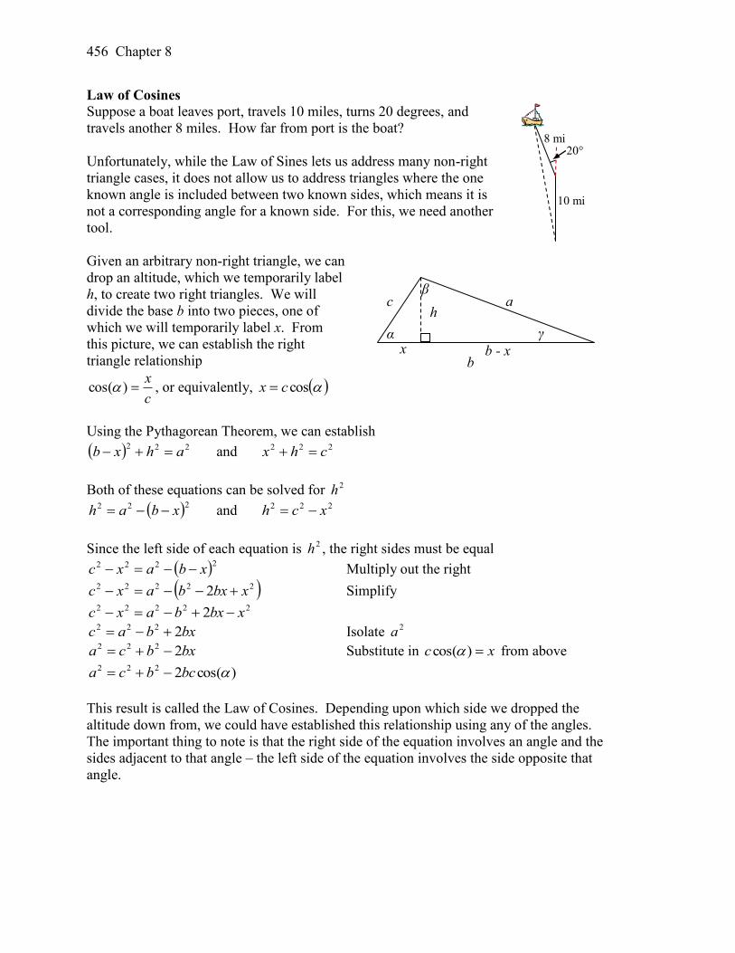
456 Chapter 8
Law of Cosines
Suppose a boat leaves port, travels 10 miles, turns 20 degrees, and
travels another 8 miles. How far from port is the boat?
Unfortunately, while the Law of Sines lets us address many non-right
triangle cases, it does not allow us to address triangles where the one
known angle is included between two known sides, which means it is
not a corresponding angle for a known side. For this, we need another
tool.
Given an arbitrary non-right triangle, we can
drop an altitude, which we temporarily label
h, to create two right triangles. We will
divide the base b into two pieces, one of
which we will temporarily label x. From
this picture, we can establish the right
triangle relationship
c
x)cos( , or equivalently, coscx
Using the Pythagorean Theorem, we can establish
222ahxb and 222 chx
Both of these equations can be solved for 2h
222 xbah and 222 xch
Since the left side of each equation is 2h , the right sides must be equal
2222 xbaxc Multiply out the right
22222 2 xbxbaxc Simplify 22222 2 xbxbaxc
bxbac 2222 Isolate 2a
bxbca 2222 Substitute in xc )cos( from above
)cos(2222 bcbca
This result is called the Law of Cosines. Depending upon which side we dropped the
altitude down from, we could have established this relationship using any of the angles.
The important thing to note is that the right side of the equation involves an angle and the
sides adjacent to that angle – the left side of the equation involves the side opposite that
angle.
α γ
a c h
β
x b - x b
20°
10 mi
8 mi
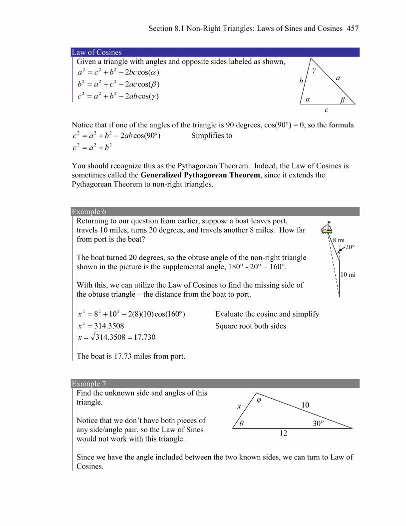
Section 8.1 Non-Right Triangles: Laws of Sines and Cosines 457
Law of Cosines
Given a triangle with angles and opposite sides labeled as shown,
)cos(2222 bcbca
)cos(2222 accab
)cos(2222 abbac
Notice that if one of the angles of the triangle is 90 degrees, cos(90°) = 0, so the formula
)90cos(2222 abbac Simplifies to 222 bac
You should recognize this as the Pythagorean Theorem. Indeed, the Law of Cosines is
sometimes called the Generalized Pythagorean Theorem, since it extends the
Pythagorean Theorem to non-right triangles.
Example 6
Returning to our question from earlier, suppose a boat leaves port,
travels 10 miles, turns 20 degrees, and travels another 8 miles. How far
from port is the boat?
The boat turned 20 degrees, so the obtuse angle of the non-right triangle
shown in the picture is the supplemental angle, 180° - 20° = 160°.
With this, we can utilize the Law of Cosines to find the missing side of
the obtuse triangle – the distance from the boat to port.
)160cos()10)(8(2108 222 x Evaluate the cosine and simplify
3508.3142 x Square root both sides
730.173508.314 x
The boat is 17.73 miles from port.
Example 7
Find the unknown side and angles of this
triangle.
Notice that we don’t have both pieces of
any side/angle pair, so the Law of Sines
would not work with this triangle.
Since we have the angle included between the two known sides, we can turn to Law of
Cosines.
θ
10 x
30°
12
φ
φ
α β
a b
c
γ
20°
10 mi
8 mi
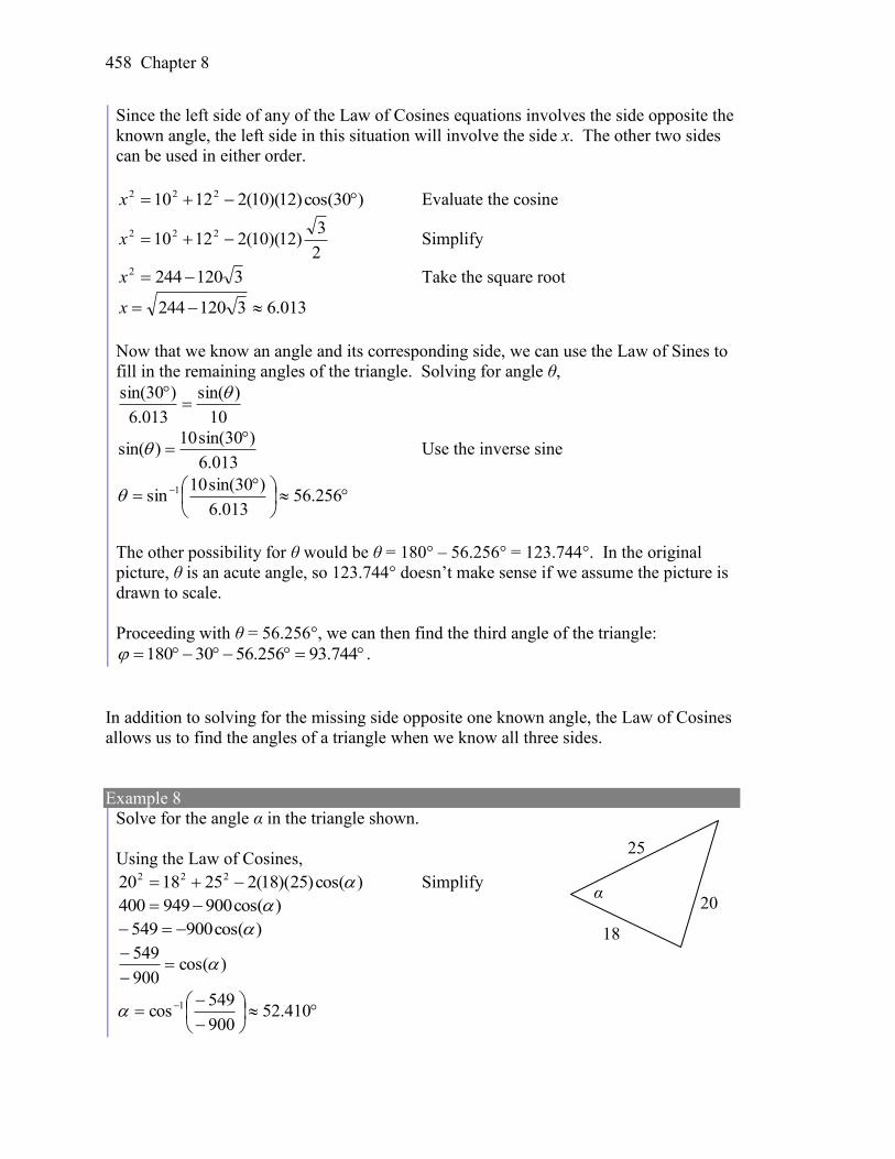
458 Chapter 8
Since the left side of any of the Law of Cosines equations involves the side opposite the
known angle, the left side in this situation will involve the side x. The other two sides
can be used in either order.
)30cos()12)(10(21210 222 x Evaluate the cosine
2
3)12)(10(21210 222 x Simplify
31202442 x Take the square root
013.63120244 x
Now that we know an angle and its corresponding side, we can use the Law of Sines to
fill in the remaining angles of the triangle. Solving for angle θ,
10
)sin(
013.6
)30sin(
013.6
)30sin(10)sin(
Use the inverse sine
256.56
013.6
)30sin(10sin 1
The other possibility for θ would be θ = 180° – 56.256° = 123.744°. In the original
picture, θ is an acute angle, so 123.744° doesn’t make sense if we assume the picture is
drawn to scale.
Proceeding with θ = 56.256°, we can then find the third angle of the triangle:
744.93256.5630180 .
In addition to solving for the missing side opposite one known angle, the Law of Cosines
allows us to find the angles of a triangle when we know all three sides.
Example 8
Solve for the angle α in the triangle shown.
Using the Law of Cosines,
)cos()25)(18(2251820 222 Simplify
)cos(900949400
)cos(900549
)cos(900
549
410.52
900
549cos 1
18
25
20 α
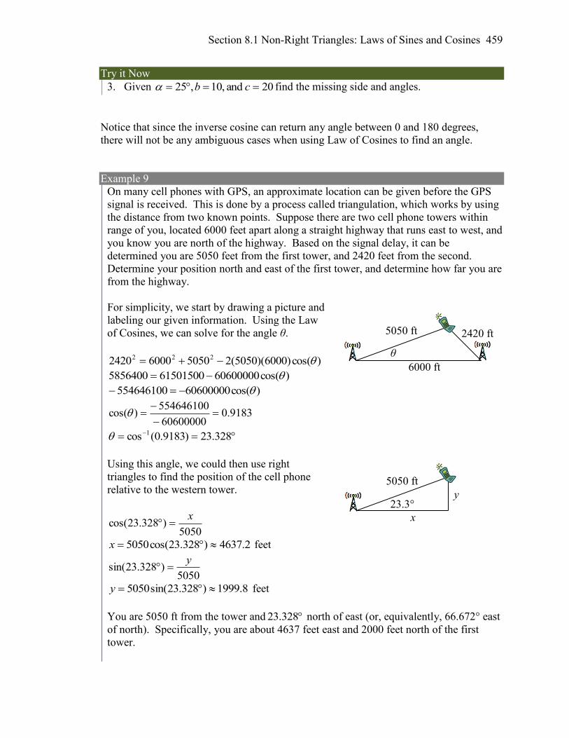
Section 8.1 Non-Right Triangles: Laws of Sines and Cosines 459
Try it Now
3. Given 20 and ,10,25 cb find the missing side and angles.
Notice that since the inverse cosine can return any angle between 0 and 180 degrees,
there will not be any ambiguous cases when using Law of Cosines to find an angle.
Example 9
On many cell phones with GPS, an approximate location can be given before the GPS
signal is received. This is done by a process called triangulation, which works by using
the distance from two known points. Suppose there are two cell phone towers within
range of you, located 6000 feet apart along a straight highway that runs east to west, and
you know you are north of the highway. Based on the signal delay, it can be
determined you are 5050 feet from the first tower, and 2420 feet from the second.
Determine your position north and east of the first tower, and determine how far you are
from the highway.
For simplicity, we start by drawing a picture and
labeling our given information. Using the Law
of Cosines, we can solve for the angle θ.
)cos()6000)(5050(2505060002420 222
)cos(60600000615015005856400
)cos(60600000554646100
9183.060600000
554646100)cos(
328.23)9183.0(cos 1
Using this angle, we could then use right
triangles to find the position of the cell phone
relative to the western tower.
5050)328.23cos(
x
2.4637)328.23cos(5050 x feet
5050)328.23sin(
y
8.1999)328.23sin(5050 y feet
You are 5050 ft from the tower and 328.23 north of east (or, equivalently, 66.672° east
of north). Specifically, you are about 4637 feet east and 2000 feet north of the first
tower.
2420 ft 5050 ft
6000 ft
θ
5050 ft
23.3° y
x
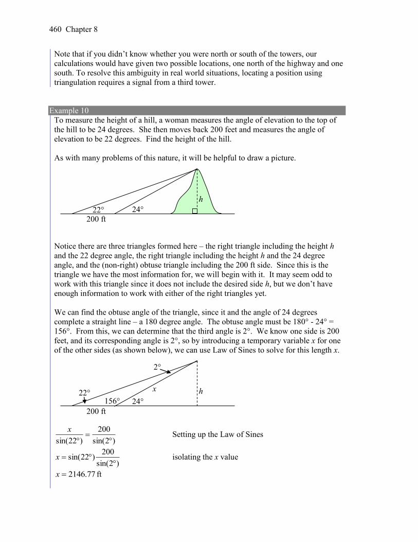
460 Chapter 8
Note that if you didn’t know whether you were north or south of the towers, our
calculations would have given two possible locations, one north of the highway and one
south. To resolve this ambiguity in real world situations, locating a position using
triangulation requires a signal from a third tower.
Example 10
To measure the height of a hill, a woman measures the angle of elevation to the top of
the hill to be 24 degrees. She then moves back 200 feet and measures the angle of
elevation to be 22 degrees. Find the height of the hill.
As with many problems of this nature, it will be helpful to draw a picture.
Notice there are three triangles formed here – the right triangle including the height h
and the 22 degree angle, the right triangle including the height h and the 24 degree
angle, and the (non-right) obtuse triangle including the 200 ft side. Since this is the
triangle we have the most information for, we will begin with it. It may seem odd to
work with this triangle since it does not include the desired side h, but we don’t have
enough information to work with either of the right triangles yet.
We can find the obtuse angle of the triangle, since it and the angle of 24 degrees
complete a straight line – a 180 degree angle. The obtuse angle must be 180° - 24° =
156°. From this, we can determine that the third angle is 2°. We know one side is 200
feet, and its corresponding angle is 2°, so by introducing a temporary variable x for one
of the other sides (as shown below), we can use Law of Sines to solve for this length x.
)2sin(
200
)22sin(
x Setting up the Law of Sines
)2sin(
200)22sin(
x isolating the x value
77.2146x ft
24° 22°
200 ft
h
156°
2°
x
24° 22° 200 ft
h
Section 8.1 Non-Right Triangles: Laws of Sines and Cosines 461
Now that we know x, we can use right triangle properties to solve for h.
77.2146hypotenuse
opposite)24sin(
h
x
h
17.873)24sin(77.2146 h ft
The hill is 873 feet high.
Important Topics of This Section
Law of Sines
Solving for sides
Solving for angles
Ambiguous case, 0, 1 or 2 solutions
Law of Cosines
Solving for sides
Solving for angles
Generalized Pythagorean Theorem
Try it Now Answers
1. 1st possible solution
2.35
8.16
2.83
c
2nd solution
9.6
2.3
8.96
c
If we were given a picture of the triangle it may be possible to eliminate one of these
2. 25.101,35.94,65.5 c
3. 725.11,9.133,1.21 a
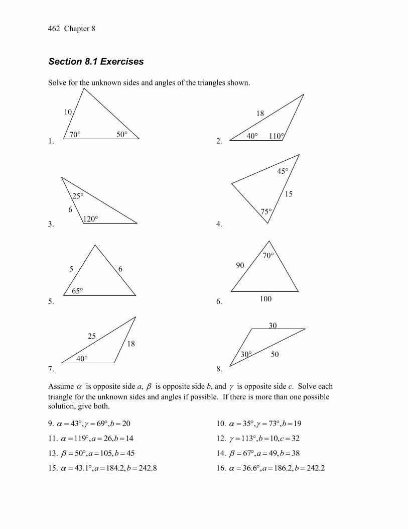
462 Chapter 8
Section 8.1 Exercises
Solve for the unknown sides and angles of the triangles shown.
1. 2.
3. 4.
5. 6.
7. 8.
Assume is opposite side a, is opposite side b, and is opposite side c. Solve each
triangle for the unknown sides and angles if possible. If there is more than one possible
solution, give both.
9. 20, 69, 43 b 10. 19, 73, 35 b
11. 14, 26, 119 ba 12. 32, 10, 113 cb
13. 45,105, 50 ba 14. 38,49, 67 ba
15. 8.242,2.184, 1.43 ba 16. 2.242,2.186, 6.36 ba
30
50 30°
18
40°
25
70°
90
100 65°
5 6
75°
45°
15
120°
6
25°
40° 110°
18
70° 50°
10
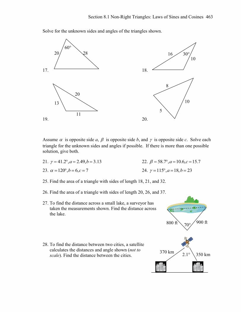
Section 8.1 Non-Right Triangles: Laws of Sines and Cosines 463
Solve for the unknown sides and angles of the triangles shown.
17. 18.
19. 20.
Assume is opposite side a, is opposite side b, and is opposite side c. Solve each
triangle for the unknown sides and angles if possible. If there is more than one possible
solution, give both.
21. 13.3, 49.2, 2.41 ba 22. 7.15, 6.10, 7.58 ca
23. 7, 6, 120 cb 24. 23,18, 115 ba
25. Find the area of a triangle with sides of length 18, 21, and 32.
26. Find the area of a triangle with sides of length 20, 26, and 37.
27. To find the distance across a small lake, a surveyor has
taken the measurements shown. Find the distance across
the lake.
28. To find the distance between two cities, a satellite
calculates the distances and angle shown (not to
scale). Find the distance between the cities.
5
8
10 13
11
20
30° 16 10
60°
20 28
800 ft 900 ft 70°
350 km 370 km
2.1°
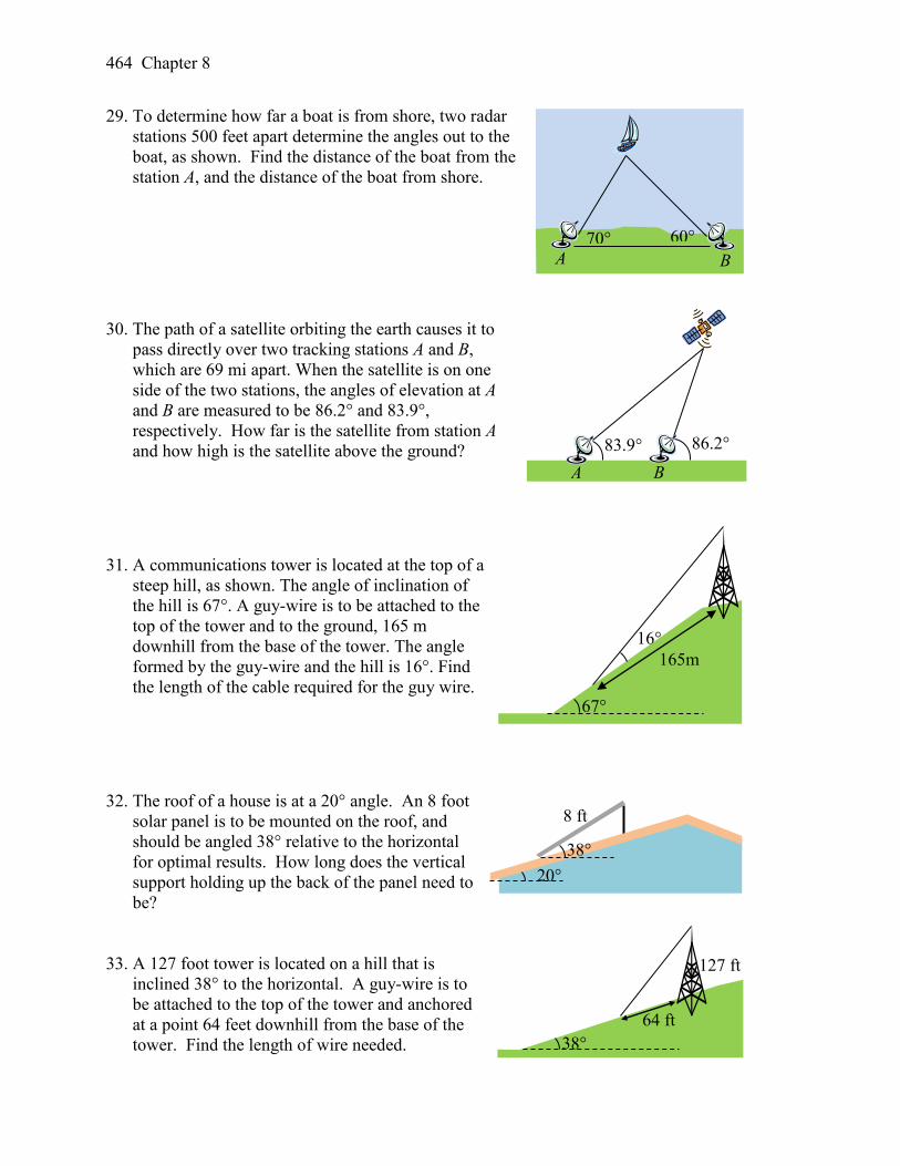
464 Chapter 8
29. To determine how far a boat is from shore, two radar
stations 500 feet apart determine the angles out to the
boat, as shown. Find the distance of the boat from the
station A, and the distance of the boat from shore.
30. The path of a satellite orbiting the earth causes it to
pass directly over two tracking stations A and B,
which are 69 mi apart. When the satellite is on one
side of the two stations, the angles of elevation at A
and B are measured to be 86.2° and 83.9°,
respectively. How far is the satellite from station A
and how high is the satellite above the ground?
31. A communications tower is located at the top of a
steep hill, as shown. The angle of inclination of
the hill is 67°. A guy-wire is to be attached to the
top of the tower and to the ground, 165 m
downhill from the base of the tower. The angle
formed by the guy-wire and the hill is 16°. Find
the length of the cable required for the guy wire.
32. The roof of a house is at a 20° angle. An 8 foot
solar panel is to be mounted on the roof, and
should be angled 38° relative to the horizontal
for optimal results. How long does the vertical
support holding up the back of the panel need to
be?
33. A 127 foot tower is located on a hill that is
inclined 38° to the horizontal. A guy-wire is to
be attached to the top of the tower and anchored
at a point 64 feet downhill from the base of the
tower. Find the length of wire needed.
70° A
60°
B
86.2° 83.9°
A B
67°
16°
165m
38°
64 ft
127 ft
20°
38°
8 ft
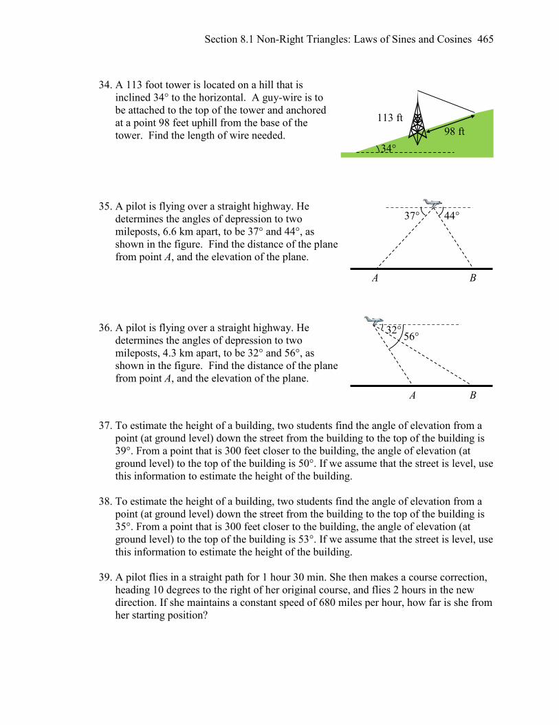
Section 8.1 Non-Right Triangles: Laws of Sines and Cosines 465
34. A 113 foot tower is located on a hill that is
inclined 34° to the horizontal. A guy-wire is to
be attached to the top of the tower and anchored
at a point 98 feet uphill from the base of the
tower. Find the length of wire needed.
35. A pilot is flying over a straight highway. He
determines the angles of depression to two
mileposts, 6.6 km apart, to be 37° and 44°, as
shown in the figure. Find the distance of the plane
from point A, and the elevation of the plane.
36. A pilot is flying over a straight highway. He
determines the angles of depression to two
mileposts, 4.3 km apart, to be 32° and 56°, as
shown in the figure. Find the distance of the plane
from point A, and the elevation of the plane.
37. To estimate the height of a building, two students find the angle of elevation from a
point (at ground level) down the street from the building to the top of the building is
39°. From a point that is 300 feet closer to the building, the angle of elevation (at
ground level) to the top of the building is 50°. If we assume that the street is level, use
this information to estimate the height of the building.
38. To estimate the height of a building, two students find the angle of elevation from a
point (at ground level) down the street from the building to the top of the building is
35°. From a point that is 300 feet closer to the building, the angle of elevation (at
ground level) to the top of the building is 53°. If we assume that the street is level, use
this information to estimate the height of the building.
39. A pilot flies in a straight path for 1 hour 30 min. She then makes a course correction,
heading 10 degrees to the right of her original course, and flies 2 hours in the new
direction. If she maintains a constant speed of 680 miles per hour, how far is she from
her starting position?
34°
98 ft
113 ft
A B
37° 44°
A B
32° 56°
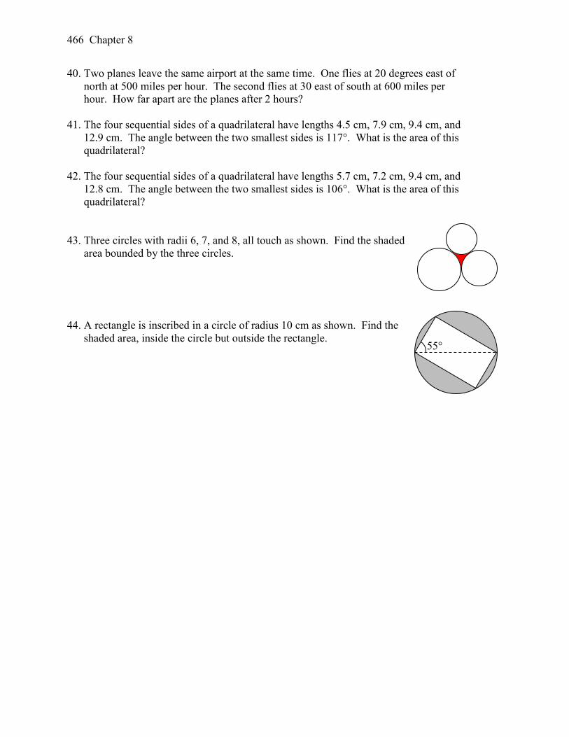
466 Chapter 8
40. Two planes leave the same airport at the same time. One flies at 20 degrees east of
north at 500 miles per hour. The second flies at 30 east of south at 600 miles per
hour. How far apart are the planes after 2 hours?
41. The four sequential sides of a quadrilateral have lengths 4.5 cm, 7.9 cm, 9.4 cm, and
12.9 cm. The angle between the two smallest sides is 117°. What is the area of this
quadrilateral?
42. The four sequential sides of a quadrilateral have lengths 5.7 cm, 7.2 cm, 9.4 cm, and
12.8 cm. The angle between the two smallest sides is 106°. What is the area of this
quadrilateral?
43. Three circles with radii 6, 7, and 8, all touch as shown. Find the shaded
area bounded by the three circles.
44. A rectangle is inscribed in a circle of radius 10 cm as shown. Find the
shaded area, inside the circle but outside the rectangle.
55°
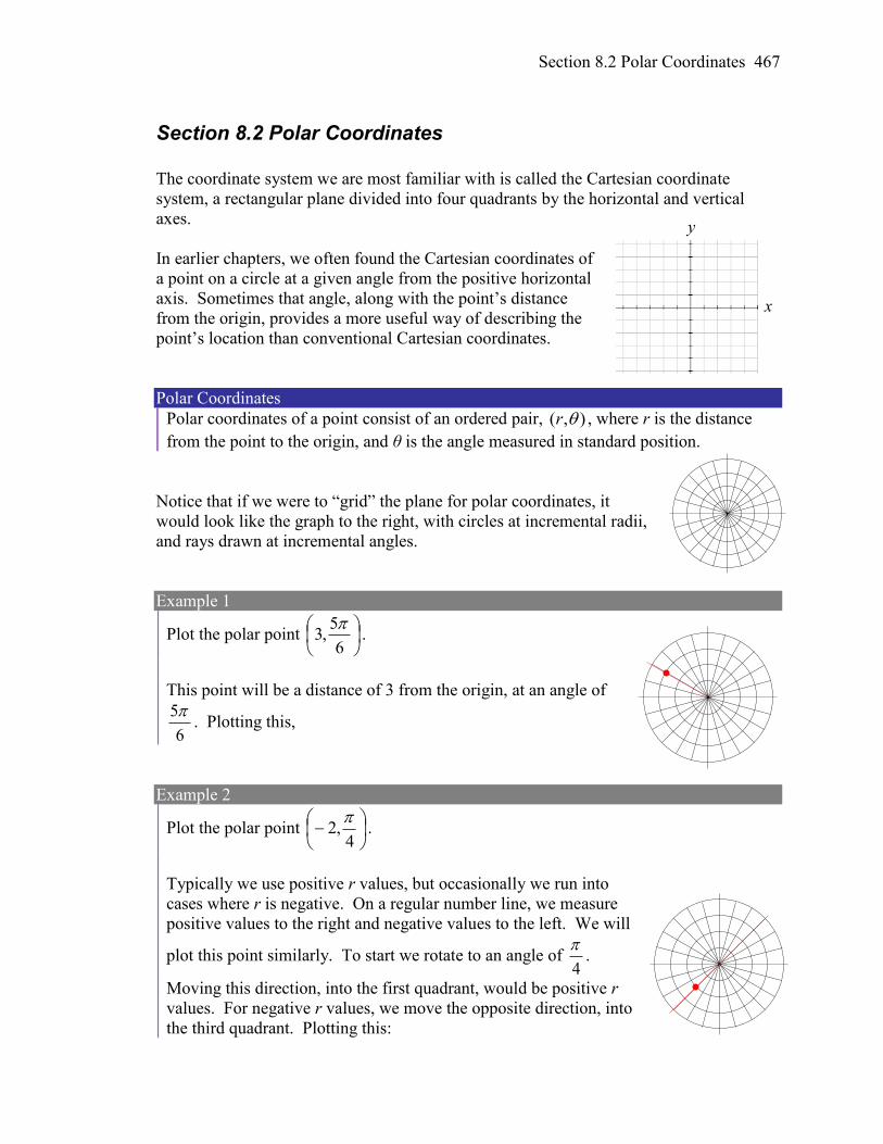
Section 8.2 Polar Coordinates 467
Section 8.2 Polar Coordinates
The coordinate system we are most familiar with is called the Cartesian coordinate
system, a rectangular plane divided into four quadrants by the horizontal and vertical
axes.
In earlier chapters, we often found the Cartesian coordinates of
a point on a circle at a given angle from the positive horizontal
axis. Sometimes that angle, along with the point’s distance
from the origin, provides a more useful way of describing the
point’s location than conventional Cartesian coordinates.
Polar Coordinates
Polar coordinates of a point consist of an ordered pair, ),( r , where r is the distance
from the point to the origin, and θ is the angle measured in standard position.
Notice that if we were to “grid” the plane for polar coordinates, it
would look like the graph to the right, with circles at incremental radii,
and rays drawn at incremental angles.
Example 1
Plot the polar point
6
5,3
.
This point will be a distance of 3 from the origin, at an angle of
6
5. Plotting this,
Example 2
Plot the polar point
4,2
.
Typically we use positive r values, but occasionally we run into
cases where r is negative. On a regular number line, we measure
positive values to the right and negative values to the left. We will
plot this point similarly. To start we rotate to an angle of 4
.
Moving this direction, into the first quadrant, would be positive r
values. For negative r values, we move the opposite direction, into
the third quadrant. Plotting this:
y
x
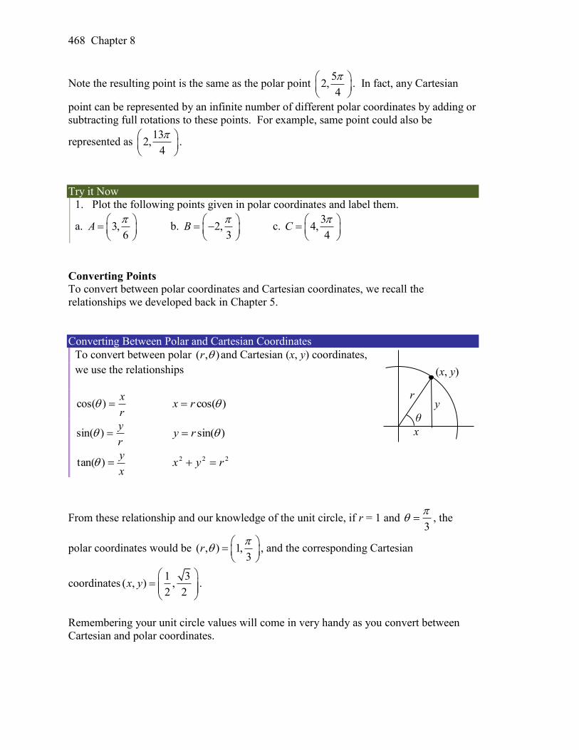
468 Chapter 8
Note the resulting point is the same as the polar point 5
2,4
. In fact, any Cartesian
point can be represented by an infinite number of different polar coordinates by adding or
subtracting full rotations to these points. For example, same point could also be
represented as 13
2,4
.
Try it Now
1. Plot the following points given in polar coordinates and label them.
a. 3,6
A
b. 2,3
B
c. 3
4,4
C
Converting Points To convert between polar coordinates and Cartesian coordinates, we recall the
relationships we developed back in Chapter 5.
Converting Between Polar and Cartesian Coordinates
To convert between polar ),( r and Cartesian (x, y) coordinates,
we use the relationships
r
x)cos( )cos(rx
r
y)sin( )sin(ry
x
y)tan( 222 ryx
From these relationship and our knowledge of the unit circle, if r = 1 and 3
, the
polar coordinates would be ( , ) 1,3
r
, and the corresponding Cartesian
coordinates1 3
( , ) ,2 2
x y
.
Remembering your unit circle values will come in very handy as you convert between
Cartesian and polar coordinates.
(x, y)
r
θ
y
x
Section 8.2 Polar Coordinates 469
Example 3
Find the Cartesian coordinates of a point with polar coordinates
3
2,5),(
r .
To find the x and y coordinates of the point,
2
5
2
15
3
2cos5)cos(
rx
2
35
2
35
3
2sin5)sin(
ry
The Cartesian coordinates are
2
35,
2
5.
Example 4
Find the polar coordinates of the point with Cartesian coordinates )4,3( .
We begin by finding the distance r using the Pythagorean relationship 222 ryx 222 )4()3( r
29 16 r
252 r
5r
Now that we know the radius, we can find the angle using any of the three trig
relationships. Keep in mind that any of the relationships will produce two solutions on
the circle, and we need to consider the quadrant to determine which solution to accept.
Using the cosine, for example:
5
3)cos(
r
x
214.25
3cos 1
By symmetry, there is a second possibility at
069.4214.22
Since the point (-3, -4) is located in the 3rd quadrant, we can determine that the second
angle is the one we need. The polar coordinates of this point are )069.4,5(),( r .
Try it Now
2. Convert the following.
a. Convert polar coordinates ( , ) 2,r to ( , )x y .
b. Convert Cartesian coordinates ( , ) (0, 4)x y to ( , )r .
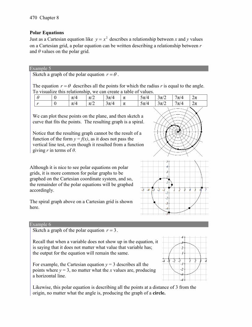
470 Chapter 8
Polar Equations
Just as a Cartesian equation like 2xy describes a relationship between x and y values
on a Cartesian grid, a polar equation can be written describing a relationship between r
and θ values on the polar grid.
Example 5
Sketch a graph of the polar equation r .
The equation r describes all the points for which the radius r is equal to the angle.
To visualize this relationship, we can create a table of values.
We can plot these points on the plane, and then sketch a
curve that fits the points. The resulting graph is a spiral.
Notice that the resulting graph cannot be the result of a
function of the form y = f(x), as it does not pass the
vertical line test, even though it resulted from a function
giving r in terms of θ.
Although it is nice to see polar equations on polar
grids, it is more common for polar graphs to be
graphed on the Cartesian coordinate system, and so,
the remainder of the polar equations will be graphed
accordingly.
The spiral graph above on a Cartesian grid is shown
here.
Example 6
Sketch a graph of the polar equation 3r .
Recall that when a variable does not show up in the equation, it
is saying that it does not matter what value that variable has;
the output for the equation will remain the same.
For example, the Cartesian equation y = 3 describes all the
points where y = 3, no matter what the x values are, producing
a horizontal line.
Likewise, this polar equation is describing all the points at a distance of 3 from the
origin, no matter what the angle is, producing the graph of a circle.
θ 0 π/4 π/2 3π/4 π 5π/4 3π/2 7π/4 2π
r 0 π/4 π/2 3π/4 π 5π/4 3π/2 7π/4 2π
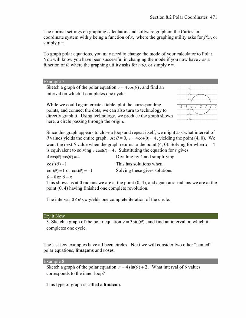
Section 8.2 Polar Coordinates 471
The normal settings on graphing calculators and software graph on the Cartesian
coordinate system with y being a function of x, where the graphing utility asks for f(x), or
simply y =.
To graph polar equations, you may need to change the mode of your calculator to Polar.
You will know you have been successful in changing the mode if you now have r as a
function of θ, where the graphing utility asks for r(θ), or simply r =.
Example 7
Sketch a graph of the polar equation )cos(4 r , and find an
interval on which it completes one cycle.
While we could again create a table, plot the corresponding
points, and connect the dots, we can also turn to technology to
directly graph it. Using technology, we produce the graph shown
here, a circle passing through the origin.
Since this graph appears to close a loop and repeat itself, we might ask what interval of
θ values yields the entire graph. At θ = 0, 4)0cos(4 r , yielding the point (4, 0). We
want the next θ value when the graph returns to the point (4, 0). Solving for when x = 4
is equivalent to solving 4)cos( r . Substituting the equation for r gives
4)cos()cos(4 Dividing by 4 and simplifying
1)(cos2 This has solutions when
1)cos( or 1)cos( Solving these gives solutions
0 or
This shows us at 0 radians we are at the point (0, 4), and again at radians we are at the
point (0, 4) having finished one complete revolution.
The interval 0 yields one complete iteration of the circle.
Try it Now
3. Sketch a graph of the polar equation 3sin( )r , and find an interval on which it
completes one cycle.
The last few examples have all been circles. Next we will consider two other “named”
polar equations, limaçons and roses.
Example 8
Sketch a graph of the polar equation 2)sin(4 r . What interval of θ values
corresponds to the inner loop?
This type of graph is called a limaçon.
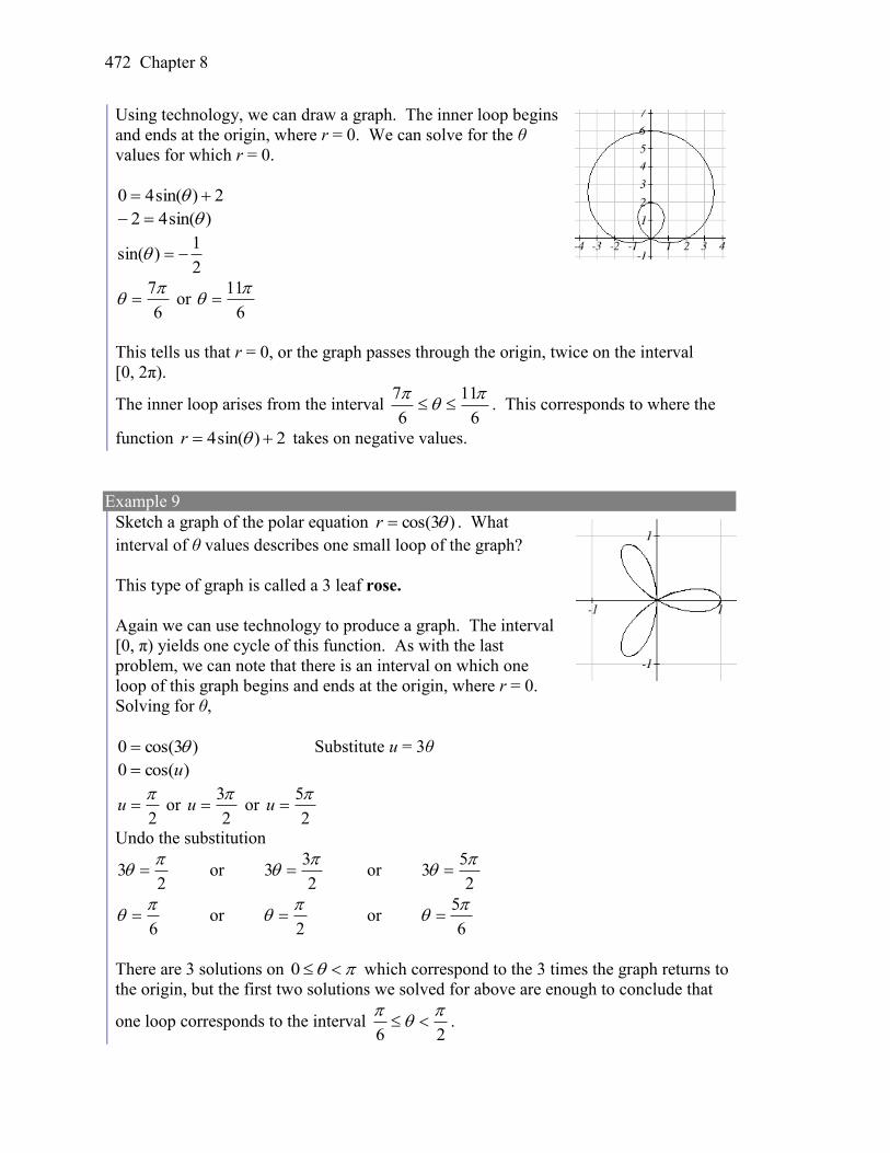
472 Chapter 8
Using technology, we can draw a graph. The inner loop begins
and ends at the origin, where r = 0. We can solve for the θ
values for which r = 0.
2)sin(40
)sin(42
2
1)sin(
6
7 or
6
11
This tells us that r = 0, or the graph passes through the origin, twice on the interval
[0, 2π).
The inner loop arises from the interval 6
11
6
7
. This corresponds to where the
function 2)sin(4 r takes on negative values.
Example 9
Sketch a graph of the polar equation )3cos( r . What
interval of θ values describes one small loop of the graph?
This type of graph is called a 3 leaf rose.
Again we can use technology to produce a graph. The interval
[0, π) yields one cycle of this function. As with the last
problem, we can note that there is an interval on which one
loop of this graph begins and ends at the origin, where r = 0.
Solving for θ,
)3cos(0 Substitute u = 3θ
)cos(0 u
2
u or
2
3u or
2
5u
Undo the substitution
23
or
2
33
or
2
53
6
or
2
or
6
5
There are 3 solutions on 0 which correspond to the 3 times the graph returns to
the origin, but the first two solutions we solved for above are enough to conclude that
one loop corresponds to the interval 26
.
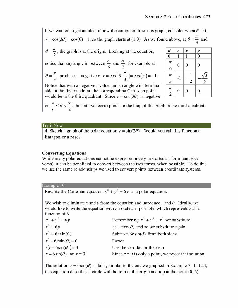
Section 8.2 Polar Coordinates 473
If we wanted to get an idea of how the computer drew this graph, consider when θ = 0.
cos(3 ) cos(0) 1r , so the graph starts at (1,0). As we found above, at 6
and
2
, the graph is at the origin. Looking at the equation,
notice that any angle in between 6
and
2
, for example at
3
, produces a negative r: cos 3 cos 1
3r
.
Notice that with a negative r value and an angle with terminal
side in the first quadrant, the corresponding Cartesian point
would be in the third quadrant. Since )3cos( r is negative
on 26
, this interval corresponds to the loop of the graph in the third quadrant.
Try it Now
4. Sketch a graph of the polar equation sin(2 )r . Would you call this function a
limaçon or a rose?
Converting Equations While many polar equations cannot be expressed nicely in Cartesian form (and vice
versa), it can be beneficial to convert between the two forms, when possible. To do this
we use the same relationships we used to convert points between coordinate systems.
Example 10
Rewrite the Cartesian equation yyx 622 as a polar equation.
We wish to eliminate x and y from the equation and introduce r and θ. Ideally, we
would like to write the equation with r isolated, if possible, which represents r as a
function of θ.
yyx 622 Remembering 222 ryx we substitute
yr 62 )sin(ry and so we substitute again
)sin(62 rr Subtract )sin(6 r from both sides
0)sin(62 rr Factor
0)sin(6 rr Use the zero factor theorem
)sin(6 r or r = 0 Since r = 0 is only a point, we reject that solution.
The solution )sin(6 r is fairly similar to the one we graphed in Example 7. In fact,
this equation describes a circle with bottom at the origin and top at the point (0, 6).
θ r x y
0 1 1 0
6
0 0 0
3
-1
1
2
3
2
2
0 0 0
474 Chapter 8
Example 11
Rewrite the Cartesian equation 23 xy as a polar equation.
23 xy Use )sin(ry and )cos(rx
2)cos(3)sin( rr Move all terms with r to one side
2)cos(3)sin( rr Factor out r
2)cos(3)sin( r Divide
)cos(3)sin(
2
r
In this case, the polar equation is more unwieldy than the Cartesian equation, but there
are still times when this equation might be useful.
Example 12
Rewrite the polar equation )cos(21
3
r as a Cartesian equation.
We want to eliminate θ and r and introduce x and y. It is usually easiest to start by
clearing the fraction and looking to substitute values that will eliminate θ.
)cos(21
3
r Clear the fraction
3)cos(21 r Use r
x)cos( to eliminate θ
321
r
xr Distribute and simplify
32 xr Isolate the r
xr 23 Square both sides
22 23 xr Use 222 ryx
222 23 xyx
When our entire equation has been changed from r and θ to x and y we can stop unless
asked to solve for y or simplify.
In this example, if desired, the right side of the equation could be expanded and the
equation simplified further. However, the equation cannot be written as a function in
Cartesian form.
Try it Now
5. a. Rewrite the Cartesian equation in polar form: 23y x
b. Rewrite the polar equation in Cartesian form: 2sin( )r
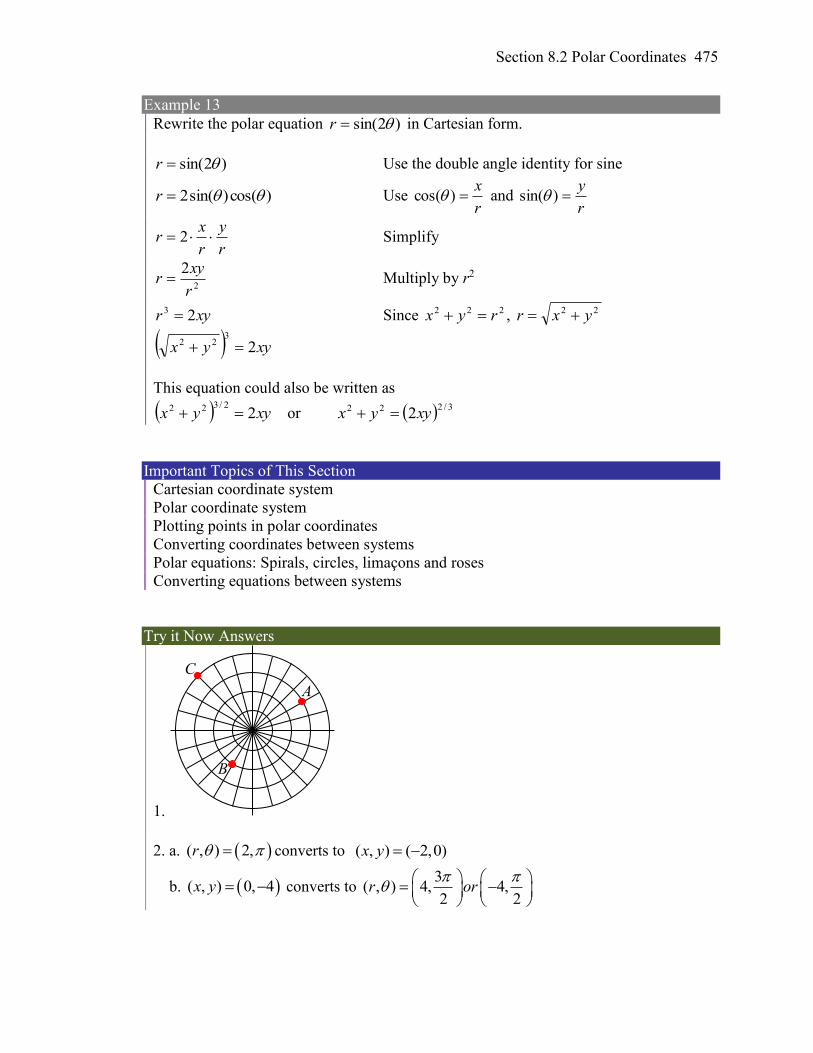
Section 8.2 Polar Coordinates 475
Example 13
Rewrite the polar equation )2sin( r in Cartesian form.
)2sin( r Use the double angle identity for sine
)cos()sin(2 r Use r
x)cos( and
r
y)sin(
r
y
r
xr 2 Simplify
2
2
r
xyr Multiply by r2
xyr 23 Since 222 ryx , 22 yxr
xyyx 23
22
This equation could also be written as
xyyx 22/322 or 3/222 2xyyx
Important Topics of This Section
Cartesian coordinate system
Polar coordinate system
Plotting points in polar coordinates
Converting coordinates between systems
Polar equations: Spirals, circles, limaçons and roses
Converting equations between systems
Try it Now Answers
1.
2. a. ( , ) 2,r converts to ( , ) ( 2,0)x y
b. ( , ) 0, 4x y converts to 3
( , ) 4, 4,2 2
r or
A
B
C
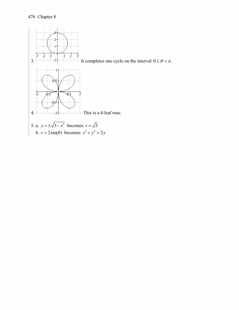
476 Chapter 8
3. It completes one cycle on the interval 0 .
4. This is a 4-leaf rose.
5. a. 23y x becomes 3r
b. 2sin( )r becomes 2 2 2x y y
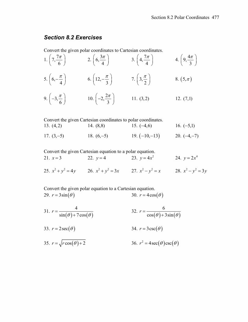
Section 8.2 Polar Coordinates 477
Section 8.2 Exercises
Convert the given polar coordinates to Cartesian coordinates.
1. 7
7,6
2. 3
6,4
3. 7
4,4
4. 4
9,3
5.
4, 6
6. 12,3
7. 3,
2
8. 5,
9. 3,6
10. 2
2,3
11. (3,2) 12. (7,1)
Convert the given Cartesian coordinates to polar coordinates.
13. (4,2) 14. (8, 8) 15. ( 4, 6) 16. ( 5,1 )
17. (3, 5) 18. (6, 5) 19. 10, 13 20. ( 4, 7)
Convert the given Cartesian equation to a polar equation.
21. 3x 22. 4y 23. 24y x 24. 42y x
25. 2 2 4x y y 26. 2 2 3x y x 27. 2 2x y x 28. 2 2 3x y y
Convert the given polar equation to a Cartesian equation.
29. 3sinr 30. 4cosr
31.
4
sin 7cosr
32.
6
cos 3sinr
33. 2secr 34. 3cscr
35. cos 2r r 36. 2 4sec cscr
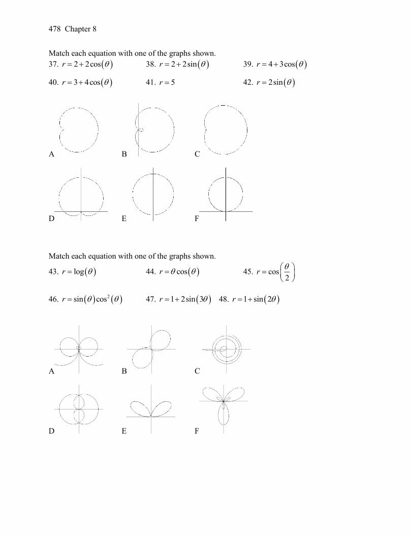
478 Chapter 8
Match each equation with one of the graphs shown.
37. 2 2cosr 38. 2 2sinr 39. 4 3cosr
40. 3 4cosr 41. 5r 42. 2sinr
A B C
D E F
Match each equation with one of the graphs shown.
43. logr 44. cosr 45. cos2
r
46. 2sin cosr 47. 1 2sin 3r 48. 1 sin 2r
A B C
D E F
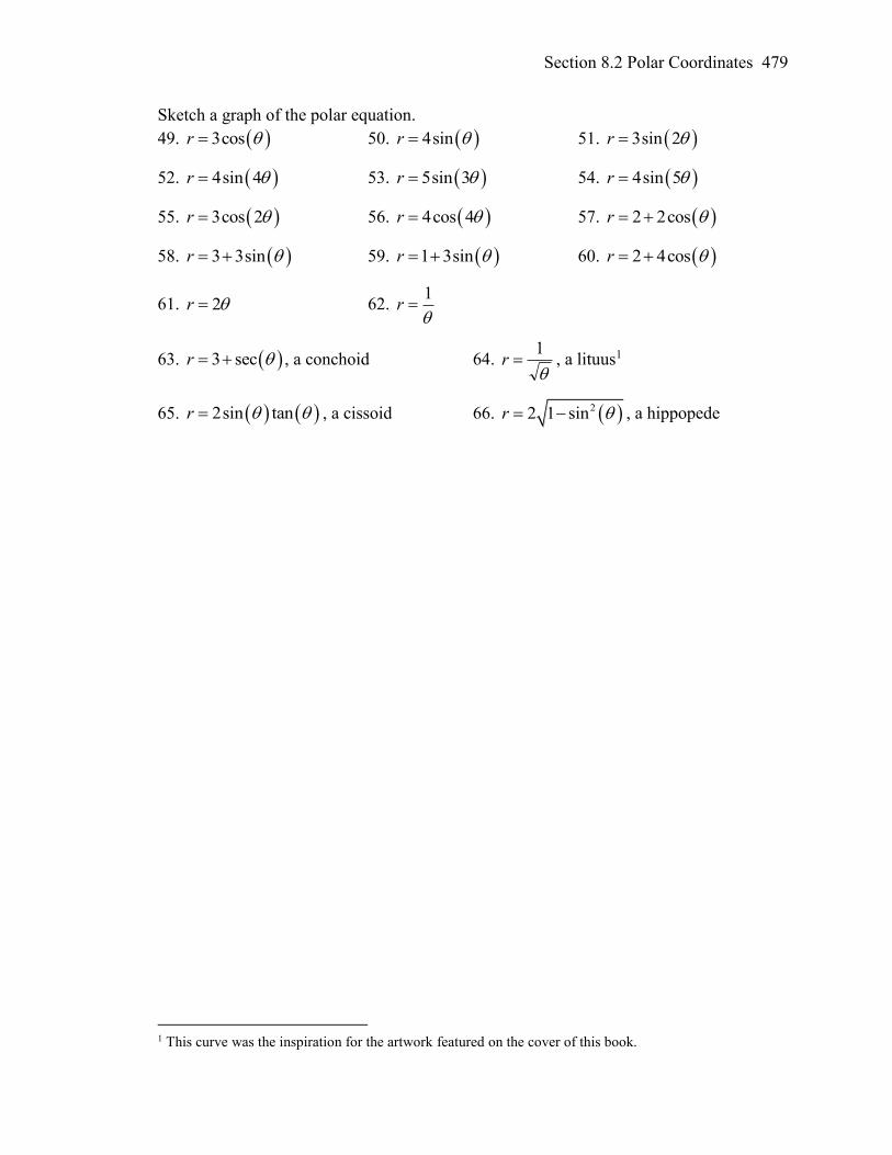
Section 8.2 Polar Coordinates 479
Sketch a graph of the polar equation.
49. 3cosr 50. 4sinr 51. 3sin 2r
52. 4sin 4r 53. 5sin 3r 54. 4sin 5r
55. 3cos 2r 56. 4cos 4r 57. 2 2cosr
58. 3 3sinr 59. 1 3sinr 60. 2 4cosr
61. 2r 62. 1
r
63. 3 secr , a conchoid 64.
1r , a lituus1
65. 2sin tanr , a cissoid 66. 22 1 sinr , a hippopede
1 This curve was the inspiration for the artwork featured on the cover of this book.
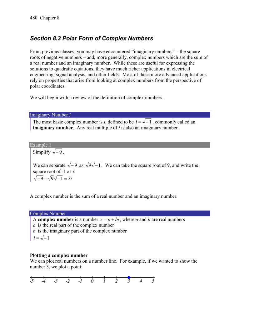
480 Chapter 8
Section 8.3 Polar Form of Complex Numbers
From previous classes, you may have encountered “imaginary numbers” – the square
roots of negative numbers – and, more generally, complex numbers which are the sum of
a real number and an imaginary number. While these are useful for expressing the
solutions to quadratic equations, they have much richer applications in electrical
engineering, signal analysis, and other fields. Most of these more advanced applications
rely on properties that arise from looking at complex numbers from the perspective of
polar coordinates.
We will begin with a review of the definition of complex numbers.
Imaginary Number i
The most basic complex number is i, defined to be 1i , commonly called an
imaginary number. Any real multiple of i is also an imaginary number.
Example 1
Simplify 9 .
We can separate 9 as 19 . We can take the square root of 9, and write the
square root of -1 as i.
9 = i319
A complex number is the sum of a real number and an imaginary number.
Complex Number
A complex number is a number biaz , where a and b are real numbers
a is the real part of the complex number
b is the imaginary part of the complex number
1i
Plotting a complex number We can plot real numbers on a number line. For example, if we wanted to show the
number 3, we plot a point:
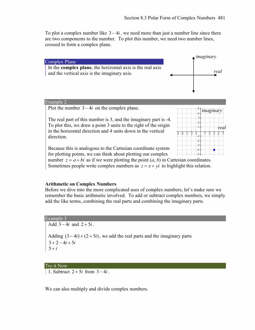
Section 8.3 Polar Form of Complex Numbers 481
To plot a complex number like i43 , we need more than just a number line since there
are two components to the number. To plot this number, we need two number lines,
crossed to form a complex plane.
Complex Plane
In the complex plane, the horizontal axis is the real axis
and the vertical axis is the imaginary axis.
Example 2
Plot the number i43 on the complex plane.
The real part of this number is 3, and the imaginary part is -4.
To plot this, we draw a point 3 units to the right of the origin
in the horizontal direction and 4 units down in the vertical
direction.
Because this is analogous to the Cartesian coordinate system
for plotting points, we can think about plotting our complex
number biaz as if we were plotting the point (a, b) in Cartesian coordinates.
Sometimes people write complex numbers as z x yi to highlight this relation.
Arithmetic on Complex Numbers
Before we dive into the more complicated uses of complex numbers, let’s make sure we
remember the basic arithmetic involved. To add or subtract complex numbers, we simply
add the like terms, combining the real parts and combining the imaginary parts.
Example 3
Add i43 and i52 .
Adding )52()43( ii , we add the real parts and the imaginary parts
ii 5423
i5
Try it Now
1. Subtract i52 from i43 .
We can also multiply and divide complex numbers.
real
imaginary
real
imaginary
482 Chapter 8
Example 4
Multiply: )52(4 i .
To multiply the complex number by a real number, we simply distribute as we would
when multiplying polynomials.
)52(4 i
= i5424
i208
Example 5
Divide (2 5 )
(4 )
i
i
.
To divide two complex numbers, we have to devise a way to write this as a complex
number with a real part and an imaginary part.
We start this process by eliminating the complex number in the denominator. To do
this, we multiply the numerator and denominator by a special complex number so that
the result in the denominator is a real number. The number we need to multiply by is
called the complex conjugate, in which the sign of the imaginary part is changed.
Here, 4+i is the complex conjugate of 4–i. Of course, obeying our algebraic rules, we
must multiply by 4+i on both the top and bottom.
(2 5 ) (4 )
(4 ) (4 )
i i
i i
To multiply two complex numbers, we expand the product as we would with
polynomials (the process commonly called FOIL – “first outer inner last”). In the
numerator:
(2 5 )(4 )i i Expand 28 20 2 5i i i Since 1i , 12 i
8 20 2 5( 1)i i Simplify
3 22i
Following the same process to multiply the denominator
(4 )(4 )i i Expand 2(16 4 4 )i i i Since 1i , 12 i
(16 ( 1))
=17
Combining this we get 3 22 3 22
17 17 17
i i
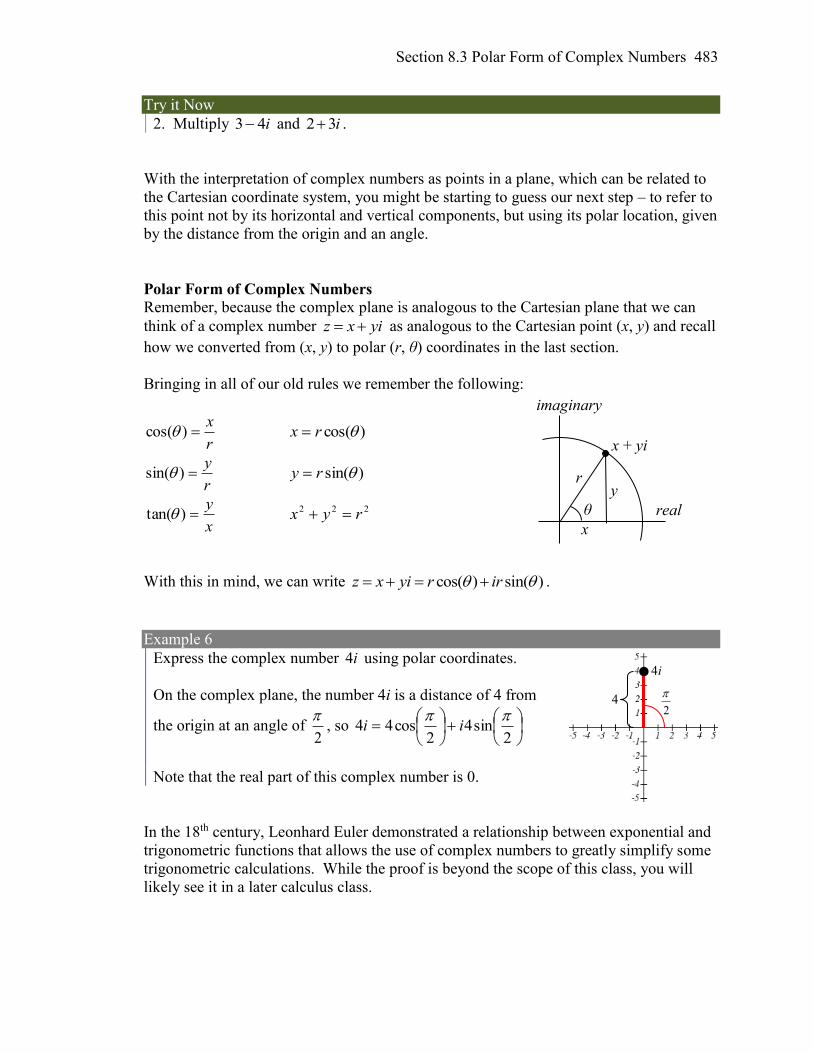
Section 8.3 Polar Form of Complex Numbers 483
Try it Now
2. Multiply i43 and 2 3i .
With the interpretation of complex numbers as points in a plane, which can be related to
the Cartesian coordinate system, you might be starting to guess our next step – to refer to
this point not by its horizontal and vertical components, but using its polar location, given
by the distance from the origin and an angle.
Polar Form of Complex Numbers Remember, because the complex plane is analogous to the Cartesian plane that we can
think of a complex number z x yi as analogous to the Cartesian point (x, y) and recall
how we converted from (x, y) to polar (r, θ) coordinates in the last section.
Bringing in all of our old rules we remember the following:
r
x)cos( )cos(rx
r
y)sin( )sin(ry
x
y)tan( 222 ryx
With this in mind, we can write cos( ) sin( )z x yi r ir .
Example 6
Express the complex number i4 using polar coordinates.
On the complex plane, the number 4i is a distance of 4 from
the origin at an angle of 2
, so
2sin4
2cos44
ii
Note that the real part of this complex number is 0.
In the 18th century, Leonhard Euler demonstrated a relationship between exponential and
trigonometric functions that allows the use of complex numbers to greatly simplify some
trigonometric calculations. While the proof is beyond the scope of this class, you will
likely see it in a later calculus class.
x + yi
r
θ
y
x
real
imaginary
2
4i
4
484 Chapter 8
Polar Form of a Complex Number and Euler’s Formula
The polar form of a complex number is irez , where Euler’s Formula holds:
)sin()cos( irrrei
Similar to plotting a point in the polar coordinate system we need r and to find the
polar form of a complex number.
Example 7
Find the polar form of the complex number -7.
Treating this is a complex number, we can consider the unsimplified version -7+0i.
Plotted in the complex plane, the number -7 is on the negative horizontal axis, a
distance of 7 from the origin at an angle of π from the positive horizontal axis.
The polar form of the number -7 is ie7 .
Plugging r = 7 and θ = π back into Euler’s formula, we have:
707)sin(7)cos(77 iiei as desired.
Example 8
Find the polar form of i44 .
On the complex plane, this complex number would correspond to the point (-4, 4) on a
Cartesian plane. We can find the distance r and angle θ as we did in the last section.
222 yxr
222 4)4( r
2432 r
To find θ, we can use r
x)cos(
2
2
24
4)cos(
This is one of known cosine values, and since the point is in
the second quadrant, we can conclude that 4
3 .
The polar form of this complex number is i
e 4
3
24
.
4
3
-4+4i
24
Section 8.3 Polar Form of Complex Numbers 485
Note we could have used x
y)tan( instead to find the angle, so long as we remember to
check the quadrant.
Try it Now
3. Write 3 i in polar form.
Example 9
Write i
e 63
in complex a bi form.
6sin3
6cos33 6
iei
Evaluate the trig functions
2
13
2
33 i Simplify
2
3
2
33i
The polar form of a complex number provides a powerful way to compute powers and
roots of complex numbers by using exponent rules you learned in algebra. To compute a
power of a complex number, we:
1) Convert to polar form
2) Raise to the power, using exponent rules to simplify
3) Convert back to a + bi form, if needed
Example 10
Evaluate 644 i .
While we could multiply this number by itself five times, that would be very tedious.
To compute this more efficiently, we can utilize the polar form of the complex number.
In an earlier example, we found that i
ei 4
3
2444
. Using this,
644 i Write the complex number in polar form 6
4
3
24
i
e
Utilize the exponent rule mmm baab )(
6
4
36
24
i
e
On the second factor, use the rule mnnm aa )(
486 Chapter 8
64
36
24
i
e
Simplify
i
e 2
9
32768
At this point, we have found the power as a complex number in polar form. If we want
the answer in standard a + bi form, we can utilize Euler’s formula.
2
9sin32768
2
9cos3276832768 2
9
iei
Since 2
9 is coterminal with
2
, we can use our special angle knowledge to evaluate
the sine and cosine.
2
9sin32768
2
9cos32768
i ii 32768)1(32768)0(32768
We have found that ii 32768446 .
The result of the process can be summarized by DeMoivre’s Theorem.
DeMoivre’s Theorem
If cos sinz r i , then for any integer n, cos sinn nz r n i n
We omit the proof, but note we can easily verify it holds in one case using Example 10:
iiii 327682
9sin
2
9cos32768
4
36sin
4
36cos24)44(
66
Example 11
Evaluate i9 .
To evaluate the square root of a complex number, we can first note that the square root
is the same as having an exponent of 2
1: 2/1)9(9 ii .
To evaluate the power, we first write the complex number in polar form. Since 9i has
no real part, we know that this value would be plotted along the vertical axis, a distance
of 9 from the origin at an angle of 2
. This gives the polar form:
i
ei 299
.
Section 8.3 Polar Form of Complex Numbers 487
2/1)9(9 ii Use the polar form
=
2/1
29
i
e
Use exponent rules to simplify
2/1
22/19
i
e
2
1
22/19
i
e
Simplify
i
e 43
Rewrite using Euler’s formula if desired
4sin3
4cos3
i Evaluate the sine and cosine
2
23
2
23 i
Using the polar form, we were able to find a square root of a complex number.
ii2
23
2
239
Alternatively, using DeMoivre’s Theorem we can write 2/1
29
i
e
3 cos sin4 4
i
and simplify
Try it Now
4. Write 6
3 i in polar form.
You may remember that equations like 42 x have two solutions, 2 and -2 in this case,
though the square root 4 only gives one of those solutions. Likewise, the square root
we found in Example 11 is only one of two complex numbers whose square is 9i.
Similarly, the equation 3 8z would have three solutions where only one is given by the
cube root. In this case, however, only one of those solutions, z = 2, is a real value. To
find the others, we can use the fact that complex numbers have multiple representations
in polar form.
Example 12
Find all complex solutions to 3 8z .
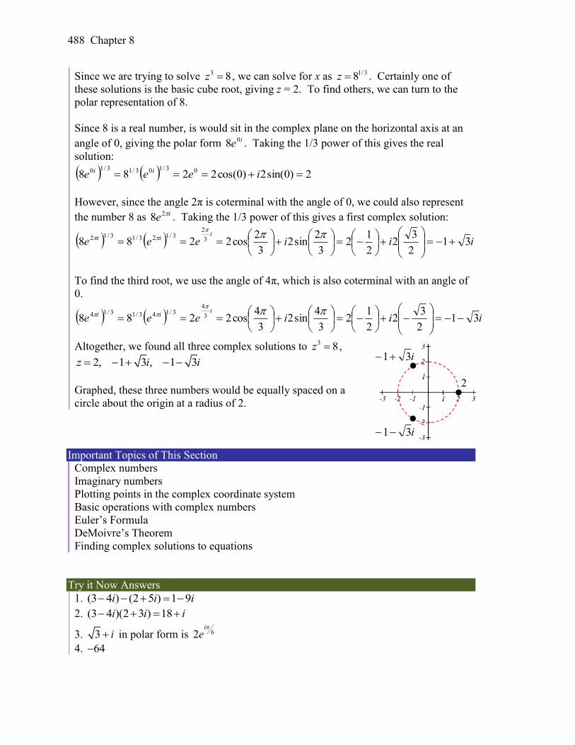
488 Chapter 8
Since we are trying to solve 3 8z , we can solve for x as 1/38z . Certainly one of
these solutions is the basic cube root, giving z = 2. To find others, we can turn to the
polar representation of 8.
Since 8 is a real number, is would sit in the complex plane on the horizontal axis at an
angle of 0, giving the polar form ie08 . Taking the 1/3 power of this gives the real
solution:
2)0sin(2)0cos(2288 03/103/13/10 ieee ii
However, since the angle 2π is coterminal with the angle of 0, we could also represent
the number 8 as ie 28 . Taking the 1/3 power of this gives a first complex solution:
iiieeei
ii 312
32
2
12
3
2sin2
3
2cos2288 3
23/123/13/12
To find the third root, we use the angle of 4π, which is also coterminal with an angle of
0.
iiieeei
ii 312
32
2
12
3
4sin2
3
4cos2288 3
43/143/13/14
Altogether, we found all three complex solutions to 3 8z ,
2, 1 3 , 1 3z i i
Graphed, these three numbers would be equally spaced on a
circle about the origin at a radius of 2.
Important Topics of This Section
Complex numbers
Imaginary numbers
Plotting points in the complex coordinate system
Basic operations with complex numbers
Euler’s Formula
DeMoivre’s Theorem
Finding complex solutions to equations
Try it Now Answers
1. (3 4 ) (2 5 ) 1 9i i i
2. (3 4 )(2 3 ) 18i i i
3. 3 i in polar form is 62i
e
4. 64
2
i31
i31
Section 8.3 Polar Form of Complex Numbers 489
Section 8.3 Exercises
Simplify each expression to a single complex number.
1. 9 2. 16 3. 6 24
4. 3 75 5. 2 12
2
6.
4 20
2
Simplify each expression to a single complex number.
7. 3 2 (5 3 )i i 8. 2 4 1 6i i
9. 5 3 (6 )i i 10. 2 3 (3 2 )i i
11. 2 3 (4 )i i 12. 5 2 (3 )i i
13. 6 2 (5)i 14. 2 4 8i
15. 2 3 (4 )i i 16. 1 2 ( 2 3 )i i
17. 4 2 (4 2 )i i 18. 3 4 3 4i i
19. 3 4
2
i 20.
6 2
3
i
21. 5 3
2
i
i
22.
6 4i
i
23. 2 3
4 3
i
i
24.
3 4
2
i
i
25. 6i 26. 11i 27. 17i 28. 24i
Rewrite each complex number from polar form into a bi form.
29. 23 ie 30. 44 ie 31. 66i
e
32. 38i
e
33. 5
43i
e
34. 7
45i
e
Rewrite each complex number into polar ire form.
35. 6 36. 8 37. 4i 38. 6i
39. 2 2i 40. 4 4i 41. 3 3i 42. 4 4i
43. 5 3i 44. 4 7i 45. 3 i 46. 2 3i
47. 1 4i 48. 3 6i 49. 5 i 50. 1 3i
490 Chapter 8
Compute each of the following, leaving the result in polar ire form.
51. 6 43 2 i i
e e
52. 2 5
3 32 4i i
e e
53.
3
4
6
6
3
i
i
e
e
54.
4
3
2
24
6
i
i
e
e
55.
10
42i
e
56.
4
63i
e
57. 2
316 i
e
58.3
29i
e
Compute each of the following, simplifying the result into a bi form.
59. 8
2 2i 60. 6
4 4i 61. 3 3i
62. 4 4i 63. 3 5 3i 64. 4 4 7i
Solve each of the following equations for all complex solutions.
65. 5 2z 66. 7 3z 67. 6 1z 68. 8 1z
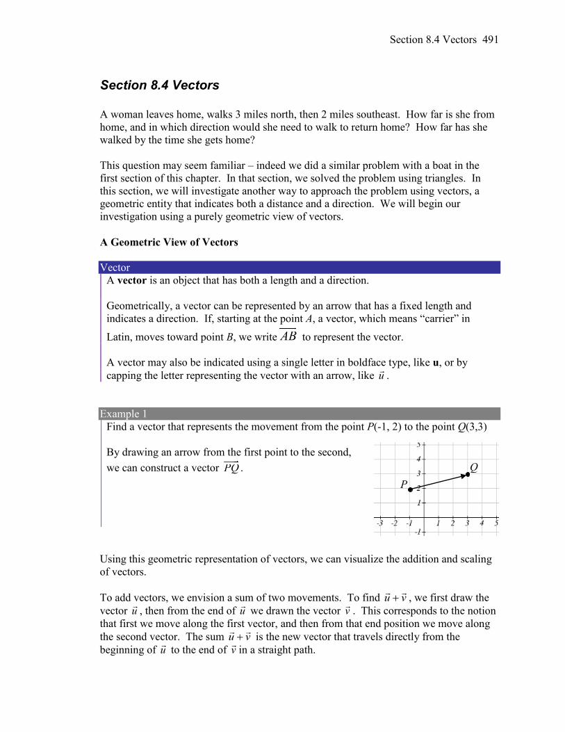
Section 8.4 Vectors 491
Section 8.4 Vectors
A woman leaves home, walks 3 miles north, then 2 miles southeast. How far is she from
home, and in which direction would she need to walk to return home? How far has she
walked by the time she gets home?
This question may seem familiar – indeed we did a similar problem with a boat in the
first section of this chapter. In that section, we solved the problem using triangles. In
this section, we will investigate another way to approach the problem using vectors, a
geometric entity that indicates both a distance and a direction. We will begin our
investigation using a purely geometric view of vectors.
A Geometric View of Vectors
Vector
A vector is an object that has both a length and a direction.
Geometrically, a vector can be represented by an arrow that has a fixed length and
indicates a direction. If, starting at the point A, a vector, which means “carrier” in
Latin, moves toward point B, we write AB to represent the vector.
A vector may also be indicated using a single letter in boldface type, like u, or by
capping the letter representing the vector with an arrow, like u
.
Example 1
Find a vector that represents the movement from the point P(-1, 2) to the point Q(3,3)
By drawing an arrow from the first point to the second,
we can construct a vector PQ .
Using this geometric representation of vectors, we can visualize the addition and scaling
of vectors.
To add vectors, we envision a sum of two movements. To find vu
, we first draw the
vector u
, then from the end of u
we drawn the vector v
. This corresponds to the notion
that first we move along the first vector, and then from that end position we move along
the second vector. The sum vu
is the new vector that travels directly from the
beginning of u
to the end of v
in a straight path.
P
Q
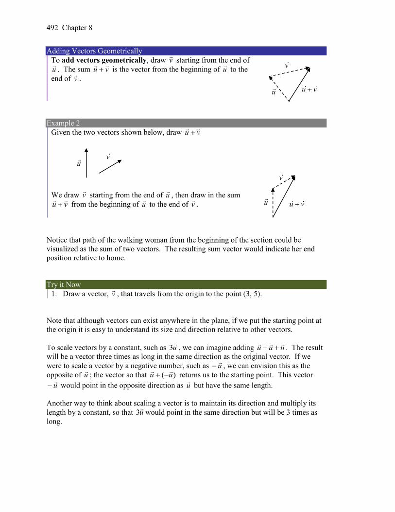
492 Chapter 8
Adding Vectors Geometrically
To add vectors geometrically, draw v
starting from the end of
u
. The sum vu
is the vector from the beginning of u
to the
end of v
.
Example 2
Given the two vectors shown below, draw vu
We draw v
starting from the end of u
, then draw in the sum
vu
from the beginning of u
to the end of v
.
Notice that path of the walking woman from the beginning of the section could be
visualized as the sum of two vectors. The resulting sum vector would indicate her end
position relative to home.
Try it Now
1. Draw a vector, v
, that travels from the origin to the point (3, 5).
Note that although vectors can exist anywhere in the plane, if we put the starting point at
the origin it is easy to understand its size and direction relative to other vectors.
To scale vectors by a constant, such as u
3 , we can imagine adding uuu
. The result
will be a vector three times as long in the same direction as the original vector. If we
were to scale a vector by a negative number, such as u
, we can envision this as the
opposite of u
; the vector so that )( uu
returns us to the starting point. This vector
u
would point in the opposite direction as u
but have the same length.
Another way to think about scaling a vector is to maintain its direction and multiply its
length by a constant, so that u
3 would point in the same direction but will be 3 times as
long.
u
v
u v
u
v
u
v
u v
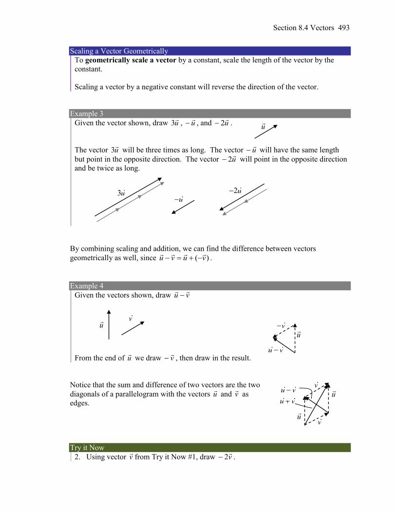
Section 8.4 Vectors 493
Scaling a Vector Geometrically
To geometrically scale a vector by a constant, scale the length of the vector by the
constant.
Scaling a vector by a negative constant will reverse the direction of the vector.
Example 3
Given the vector shown, draw u
3 , u
, and u
2 .
The vector u
3 will be three times as long. The vector u
will have the same length
but point in the opposite direction. The vector u
2 will point in the opposite direction
and be twice as long.
By combining scaling and addition, we can find the difference between vectors
geometrically as well, since )( vuvu
.
Example 4
Given the vectors shown, draw vu
From the end of u
we draw v
, then draw in the result.
Notice that the sum and difference of two vectors are the two
diagonals of a parallelogram with the vectors u
and v
as
edges.
Try it Now
2. Using vector v
from Try it Now #1, draw v
2 .
u
3u u
2u
u
v
u v
u
v
u
v u v
u
v
u v
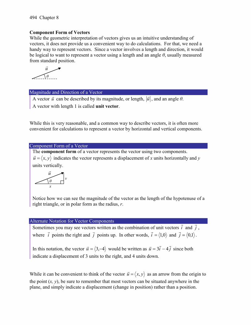
494 Chapter 8
Component Form of Vectors While the geometric interpretation of vectors gives us an intuitive understanding of
vectors, it does not provide us a convenient way to do calculations. For that, we need a
handy way to represent vectors. Since a vector involves a length and direction, it would
be logical to want to represent a vector using a length and an angle θ, usually measured
from standard position.
Magnitude and Direction of a Vector
A vector u
can be described by its magnitude, or length, u
, and an angle θ.
A vector with length 1 is called unit vector.
While this is very reasonable, and a common way to describe vectors, it is often more
convenient for calculations to represent a vector by horizontal and vertical components.
Component Form of a Vector
The component form of a vector represents the vector using two components.
yxu ,
indicates the vector represents a displacement of x units horizontally and y
units vertically.
Notice how we can see the magnitude of the vector as the length of the hypotenuse of a
right triangle, or in polar form as the radius, r.
Alternate Notation for Vector Components
Sometimes you may see vectors written as the combination of unit vectors i
and j
,
where i
points the right and j
points up. In other words, 0,1i
and 1,0j
.
In this notation, the vector 4,3 u
would be written as jiu
43 since both
indicate a displacement of 3 units to the right, and 4 units down.
While it can be convenient to think of the vector yxu ,
as an arrow from the origin to
the point (x, y), be sure to remember that most vectors can be situated anywhere in the
plane, and simply indicate a displacement (change in position) rather than a position.
u
θ
u
θ
x
x
y
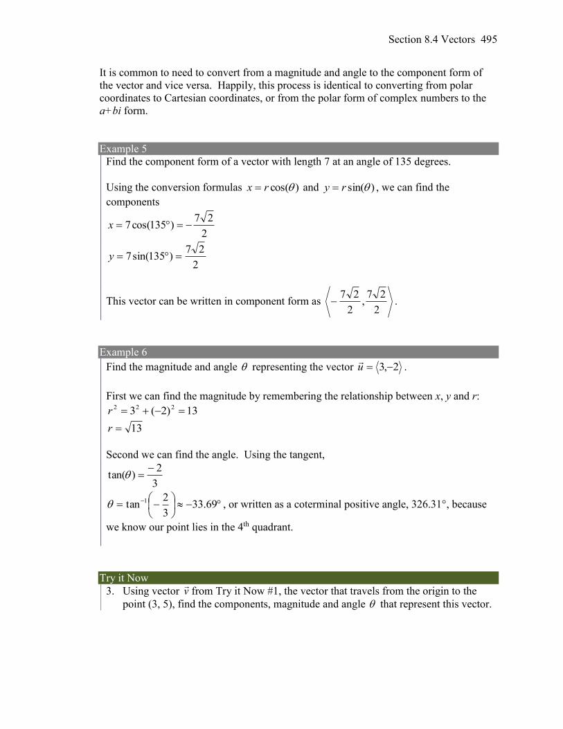
Section 8.4 Vectors 495
It is common to need to convert from a magnitude and angle to the component form of
the vector and vice versa. Happily, this process is identical to converting from polar
coordinates to Cartesian coordinates, or from the polar form of complex numbers to the
a+bi form.
Example 5
Find the component form of a vector with length 7 at an angle of 135 degrees.
Using the conversion formulas )cos(rx and )sin(ry , we can find the
components
2
27)135cos(7 x
2
27)135sin(7 y
This vector can be written in component form as 2
27,
2
27 .
Example 6
Find the magnitude and angle representing the vector 2,3 u
.
First we can find the magnitude by remembering the relationship between x, y and r:
13)2(3 222 r
13r
Second we can find the angle. Using the tangent,
3
2)tan(
69.33
3
2tan 1 , or written as a coterminal positive angle, 326.31°, because
we know our point lies in the 4th quadrant.
Try it Now
3. Using vector v
from Try it Now #1, the vector that travels from the origin to the
point (3, 5), find the components, magnitude and angle that represent this vector.
496 Chapter 8
In addition to representing distance movements, vectors are commonly used in physics
and engineering to represent any quantity that has both direction and magnitude,
including velocities and forces.
Example 7
An object is launched with initial velocity 200 meters per second at an angle of 30
degrees. Find the initial horizontal and vertical velocities.
By viewing the initial velocity as a vector, we can resolve the vector into horizontal and
vertical components.
205.1732
3200)30cos(200 x m/sec
1002
1200)30sin(200 y m/sec
This tells us that, absent wind resistance, the object will travel horizontally at about 173
meters each second. Gravity will cause the vertical velocity to change over time – we’ll
leave a discussion of that to physics or calculus classes.
Adding and Scaling Vectors in Component Form
To add vectors in component form, we can simply add the corresponding components.
To scale a vector by a constant, we scale each component by that constant.
Combining Vectors in Component Form
To add, subtract, or scale vectors in component form
If 21,uuu
, 21,vvv
, and c is any constant, then
2211 , vuvuvu
2211 , vuvuvu
21,cucuuc
Example 8
Given 2,3 u
and 4,1v
, find a new vector vuw
23
Using the vectors given,
vuw
23
4,122,33 Scale each vector
8,26,9 Subtract corresponding components
14,11
200 m/s
30°
173 m/s
100 m/s
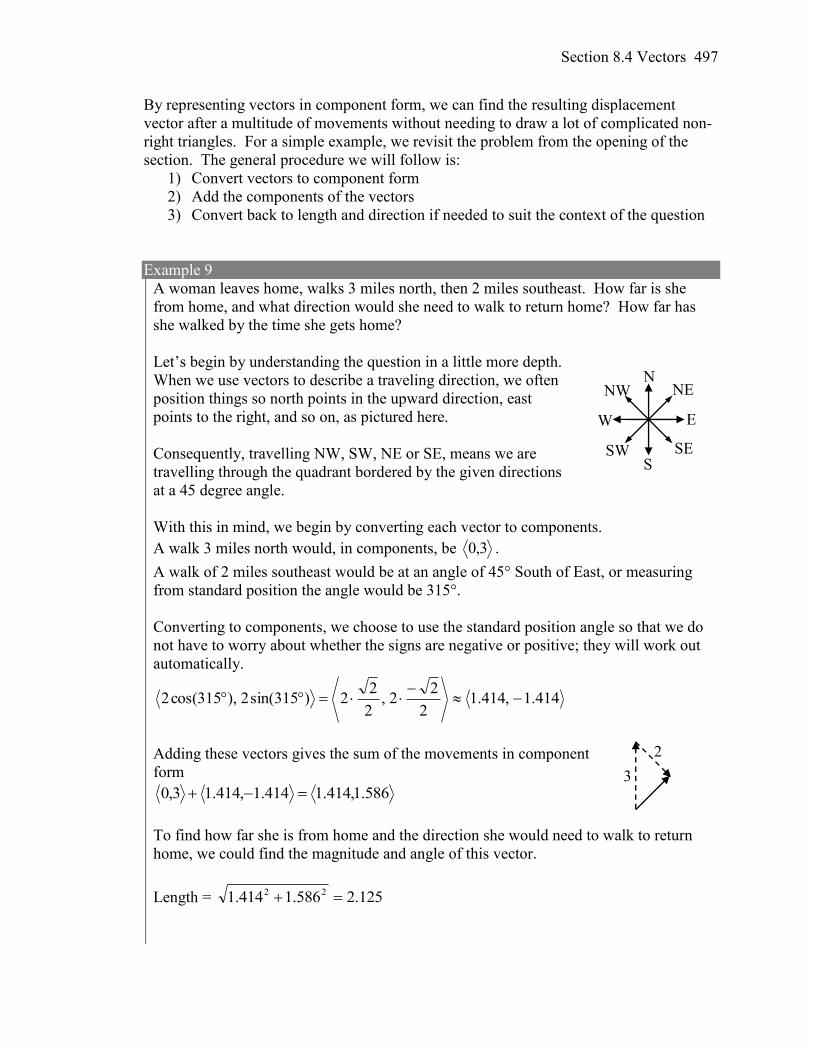
Section 8.4 Vectors 497
By representing vectors in component form, we can find the resulting displacement
vector after a multitude of movements without needing to draw a lot of complicated non-
right triangles. For a simple example, we revisit the problem from the opening of the
section. The general procedure we will follow is:
1) Convert vectors to component form
2) Add the components of the vectors
3) Convert back to length and direction if needed to suit the context of the question
Example 9
A woman leaves home, walks 3 miles north, then 2 miles southeast. How far is she
from home, and what direction would she need to walk to return home? How far has
she walked by the time she gets home?
Let’s begin by understanding the question in a little more depth.
When we use vectors to describe a traveling direction, we often
position things so north points in the upward direction, east
points to the right, and so on, as pictured here.
Consequently, travelling NW, SW, NE or SE, means we are
travelling through the quadrant bordered by the given directions
at a 45 degree angle.
With this in mind, we begin by converting each vector to components.
A walk 3 miles north would, in components, be 3,0 .
A walk of 2 miles southeast would be at an angle of 45° South of East, or measuring
from standard position the angle would be 315°.
Converting to components, we choose to use the standard position angle so that we do
not have to worry about whether the signs are negative or positive; they will work out
automatically.
414.1,414.12
22,
2
22)315sin(2),315cos(2
Adding these vectors gives the sum of the movements in component
form
586.1,414.1414.1,414.13,0
To find how far she is from home and the direction she would need to walk to return
home, we could find the magnitude and angle of this vector.
Length = 125.2586.1414.1 22
3
2
N NE
E
SE S
SW
W
NW
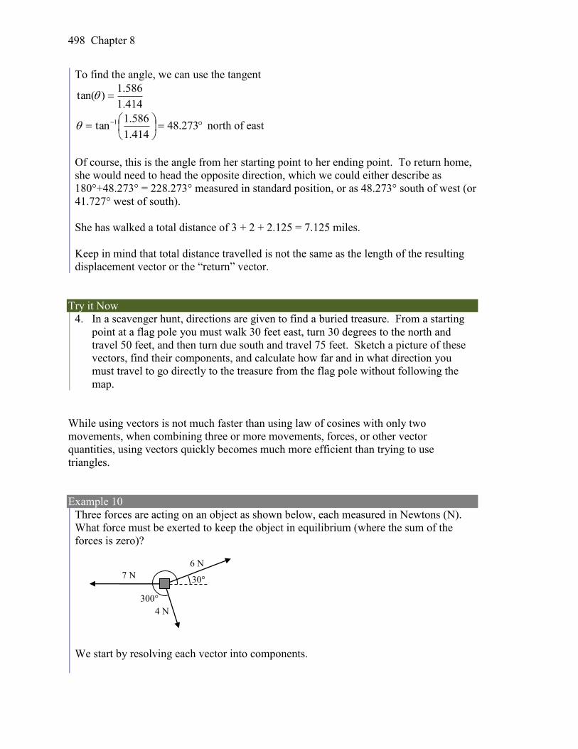
498 Chapter 8
To find the angle, we can use the tangent
414.1
586.1)tan(
273.48
414.1
586.1tan 1 north of east
Of course, this is the angle from her starting point to her ending point. To return home,
she would need to head the opposite direction, which we could either describe as
180°+48.273° = 228.273° measured in standard position, or as 48.273° south of west (or
41.727° west of south).
She has walked a total distance of 3 + 2 + 2.125 = 7.125 miles.
Keep in mind that total distance travelled is not the same as the length of the resulting
displacement vector or the “return” vector.
Try it Now
4. In a scavenger hunt, directions are given to find a buried treasure. From a starting
point at a flag pole you must walk 30 feet east, turn 30 degrees to the north and
travel 50 feet, and then turn due south and travel 75 feet. Sketch a picture of these
vectors, find their components, and calculate how far and in what direction you
must travel to go directly to the treasure from the flag pole without following the
map.
While using vectors is not much faster than using law of cosines with only two
movements, when combining three or more movements, forces, or other vector
quantities, using vectors quickly becomes much more efficient than trying to use
triangles.
Example 10
Three forces are acting on an object as shown below, each measured in Newtons (N).
What force must be exerted to keep the object in equilibrium (where the sum of the
forces is zero)?
We start by resolving each vector into components.
30°
6 N
7 N
4 N
300°
Section 8.4 Vectors 499
The first vector with magnitude 6 Newtons at an angle of 30 degrees will have
components
3,332
16,
2
36)30sin(6),30cos(6
The second vector is only in the horizontal direction, so can be written as 0,7 .
The third vector with magnitude 4 Newtons at an angle of 300 degrees will have
components
32,22
34,
2
14)300sin(4),300cos(4
To keep the object in equilibrium, we need to find a force vector yx, so the sum of
the four vectors is the zero vector, 0,0 .
3 3, 3 7, 0 2, 2 3 , 0, 0x y Add component-wise
3 3 7 2, 3 0 2 3 , 0, 0x y Simplify
3 3 5, 3 2 3 , 0, 0x y Solve
, 0, 0 3 3 5, 3 2 3x y
, 3 3 5, 3 2 3 0.196, 0.464x y
This vector gives in components the force that would need to be applied to keep the
object in equilibrium. If desired, we could find the magnitude of this force and
direction it would need to be applied in.
Magnitude = 504.0464.0)196.0( 22 N
Angle:
196.0
464.0)tan(
089.67
196.0
464.0tan 1 .
This is in the wrong quadrant, so we adjust by finding the next angle with the same
tangent value by adding a full period of tangent:
911.112180089.67
To keep the object in equilibrium, a force of 0.504 Newtons would need to be applied at
an angle of 112.911°.
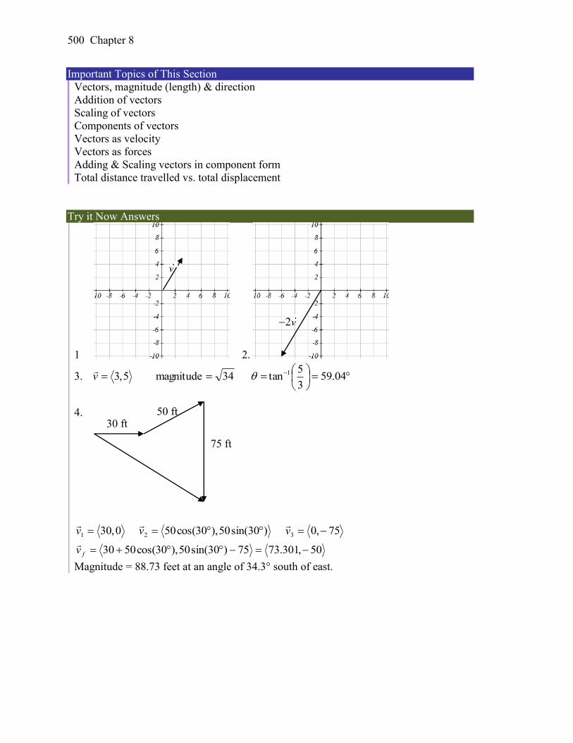
500 Chapter 8
Important Topics of This Section
Vectors, magnitude (length) & direction
Addition of vectors
Scaling of vectors
Components of vectors
Vectors as velocity
Vectors as forces
Adding & Scaling vectors in component form
Total distance travelled vs. total displacement
Try it Now Answers
1 2.
3.
04.59
3
5tan34magnitude5,3 1v
4.
50,301.7375)30sin(50),30cos(5030
75,0)30sin(50),30cos(500,30 321
fv
vvv
Magnitude = 88.73 feet at an angle of 34.3° south of east.
75 ft
50 ft 30 ft
v
2v
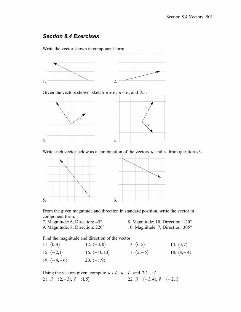
Section 8.4 Vectors 501
Section 8.4 Exercises
Write the vector shown in component form.
1. 2.
Given the vectors shown, sketch u v , u v , and 2u .
3. 4.
Write each vector below as a combination of the vectors u and v from question #3.
5. 6.
From the given magnitude and direction in standard position, write the vector in
component form.
7. Magnitude: 6, Direction: 45° 8. Magnitude: 10, Direction: 120°
9. Magnitude: 8, Direction: 220° 10. Magnitude: 7, Direction: 305°
Find the magnitude and direction of the vector.
11. 4,0 12. 0,3 13. 5,6 14. 7,3
15. 1,2 16. 13,10 17. 5,2 18. 4,8
19. 6,4 20. 9,1
Using the vectors given, compute u v , u v , and 2 3u v .
21. 5,1, 3,2 vu
22. 1,2, 4,3 vu
502 Chapter 8
23. A woman leaves home and walks 3 miles west, then 2 miles southwest. How far
from home is she, and in what direction must she walk to head directly home?
24. A boat leaves the marina and sails 6 miles north, then 2 miles northeast. How far
from the marina is the boat, and in what direction must it sail to head directly back to
the marina?
25. A person starts walking from home and walks 4 miles east, 2 miles southeast, 5 miles
south, 4 miles southwest, and 2 miles east. How far have they walked? If they
walked straight home, how far would they have to walk?
26. A person starts walking from home and walks 4 miles east, 7 miles southeast, 6 miles
south, 5 miles southwest, and 3 miles east. How far have they walked? If they
walked straight home, how far would they have to walk?
27. Three forces act on an object: 7,4,1,0, 5,8 321 FFF
. Find the net
force acting on the object.
28. Three forces act on an object: 7,0,3,8, 5,2 321 FFF
. Find the net force
acting on the object.
29. A person starts walking from home and walks 3 miles at 20° north of west, then 5
miles at 10° west of south, then 4 miles at 15° north of east. If they walked straight
home, how far would they have to walk, and in what direction?
30. A person starts walking from home and walks 6 miles at 40° north of east, then 2
miles at 15° east of south, then 5 miles at 30° south of west. If they walked straight
home, how far would they have to walk, and in what direction?
31. An airplane is heading north at an airspeed of 600 km/hr, but there is a wind blowing
from the southwest at 80 km/hr. How many degrees off course will the plane end up
flying, and what is the plane’s speed relative to the ground?
32. An airplane is heading north at an airspeed of 500 km/hr, but there is a wind blowing
from the northwest at 50 km/hr. How many degrees off course will the plane end up
flying, and what is the plane’s speed relative to the ground?
33. An airplane needs to head due north, but there is a wind blowing from the southwest
at 60 km/hr. The plane flies with an airspeed of 550 km/hr. To end up flying due
north, the pilot will need to fly the plane how many degrees west of north?
Section 8.4 Vectors 503
34. An airplane needs to head due north, but there is a wind blowing from the northwest
at 80 km/hr. The plane flies with an airspeed of 500 km/hr. To end up flying due
north, the pilot will need to fly the plane how many degrees west of north?
35. As part of a video game, the point (5, 7) is rotated counterclockwise about the origin
through an angle of 35 degrees. Find the new coordinates of this point.
36. As part of a video game, the point (7, 3) is rotated counterclockwise about the origin
through an angle of 40 degrees. Find the new coordinates of this point.
37. Two children are throwing a ball back and forth straight across the back seat of a car.
The ball is being thrown 10 mph relative to the car, and the car is travelling 25 mph
down the road. If one child doesn't catch the ball and it flies out the window, in what
direction does the ball fly (ignoring wind resistance)?
38. Two children are throwing a ball back and forth straight across the back seat of a car.
The ball is being thrown 8 mph relative to the car, and the car is travelling 45 mph
down the road. If one child doesn't catch the ball and it flies out the window, in what
direction does the ball fly (ignoring wind resistance)?
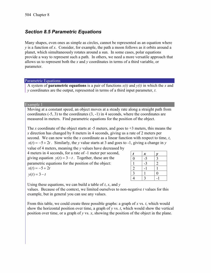
504 Chapter 8
Section 8.5 Parametric Equations
Many shapes, even ones as simple as circles, cannot be represented as an equation where
y is a function of x. Consider, for example, the path a moon follows as it orbits around a
planet, which simultaneously rotates around a sun. In some cases, polar equations
provide a way to represent such a path. In others, we need a more versatile approach that
allows us to represent both the x and y coordinates in terms of a third variable, or
parameter.
Parametric Equations
A system of parametric equations is a pair of functions x(t) and y(t) in which the x and
y coordinates are the output, represented in terms of a third input parameter, t.
Example 1
Moving at a constant speed, an object moves at a steady rate along a straight path from
coordinates (-5, 3) to the coordinates (3, -1) in 4 seconds, where the coordinates are
measured in meters. Find parametric equations for the position of the object.
The x coordinate of the object starts at -5 meters, and goes to +3 meters, this means the
x direction has changed by 8 meters in 4 seconds, giving us a rate of 2 meters per
second. We can now write the x coordinate as a linear function with respect to time, t,
ttx 25)( . Similarly, the y value starts at 3 and goes to -1, giving a change in y
value of 4 meters, meaning the y values have decreased by
4 meters in 4 seconds, for a rate of -1 meter per second,
giving equation tty 3)( . Together, these are the
parametric equations for the position of the object:
tty
ttx
3)(
25)(
Using these equations, we can build a table of t, x, and y
values. Because of the context, we limited ourselves to non-negative t values for this
example, but in general you can use any values.
From this table, we could create three possible graphs: a graph of x vs. t, which would
show the horizontal position over time, a graph of y vs. t, which would show the vertical
position over time, or a graph of y vs. x, showing the position of the object in the plane.
t x y
0 -5 3
1 -3 2
2 -1 1
3 1 0
4 3 -1
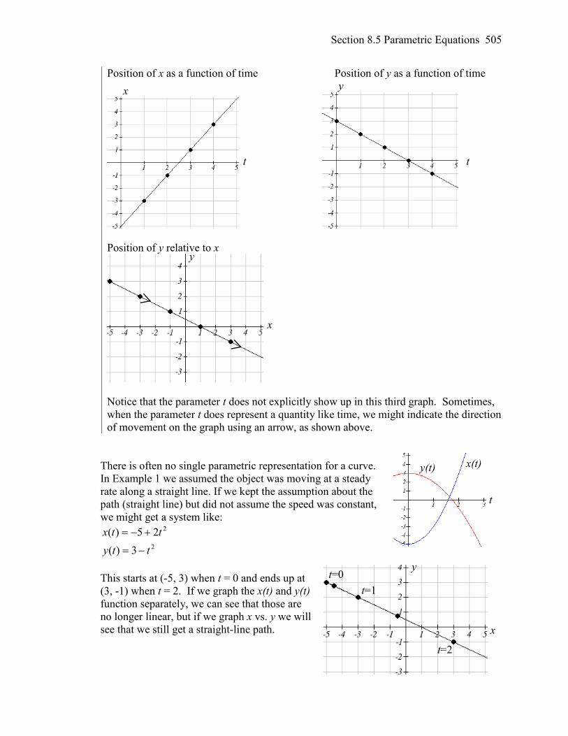
Section 8.5 Parametric Equations 505
Position of x as a function of time Position of y as a function of time
Position of y relative to x
Notice that the parameter t does not explicitly show up in this third graph. Sometimes,
when the parameter t does represent a quantity like time, we might indicate the direction
of movement on the graph using an arrow, as shown above.
There is often no single parametric representation for a curve.
In Example 1 we assumed the object was moving at a steady
rate along a straight line. If we kept the assumption about the
path (straight line) but did not assume the speed was constant,
we might get a system like:
2
2
3)(
25)(
tty
ttx
This starts at (-5, 3) when t = 0 and ends up at
(3, -1) when t = 2. If we graph the x(t) and y(t)
function separately, we can see that those are
no longer linear, but if we graph x vs. y we will
see that we still get a straight-line path.
t
x y
t
x
y
x
y
t
y(t) x(t)
t=0
t=1
t=2
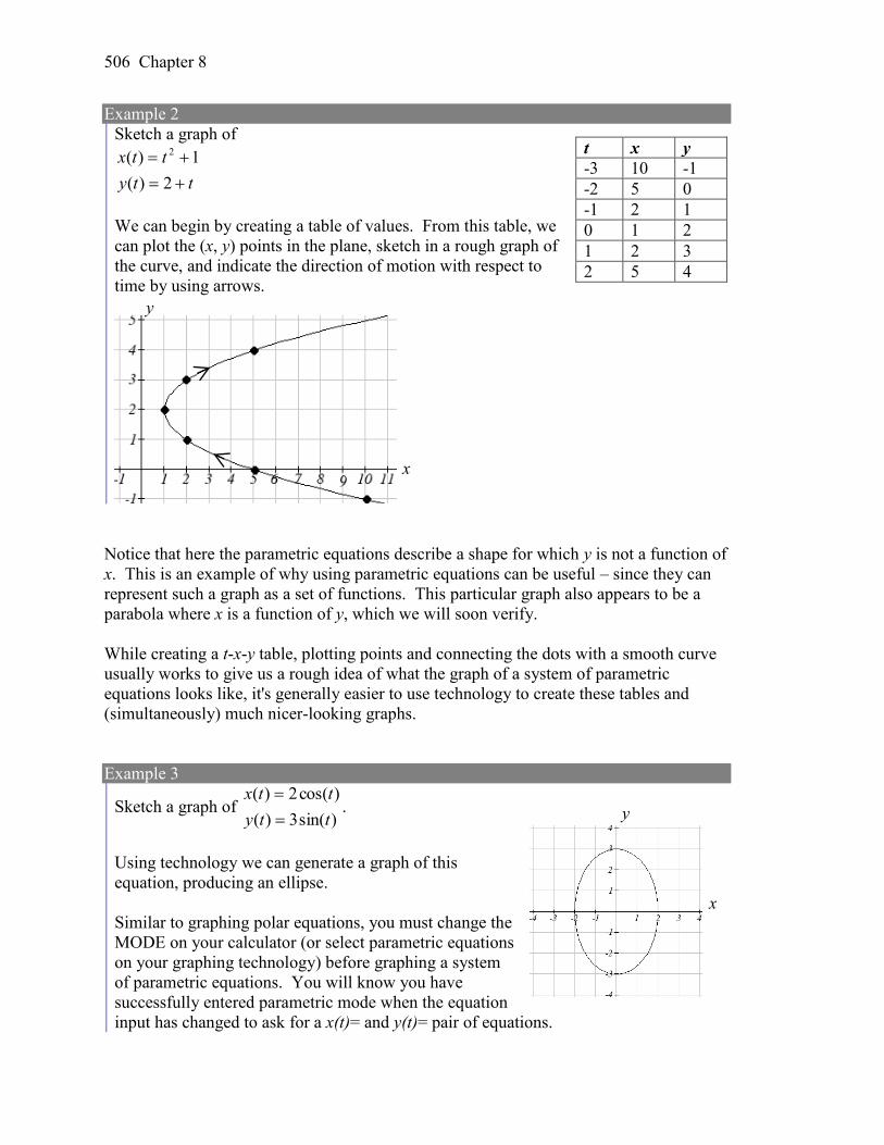
506 Chapter 8
Example 2
Sketch a graph of
tty
ttx
2)(
1)( 2
We can begin by creating a table of values. From this table, we
can plot the (x, y) points in the plane, sketch in a rough graph of
the curve, and indicate the direction of motion with respect to
time by using arrows.
Notice that here the parametric equations describe a shape for which y is not a function of
x. This is an example of why using parametric equations can be useful – since they can
represent such a graph as a set of functions. This particular graph also appears to be a
parabola where x is a function of y, which we will soon verify.
While creating a t-x-y table, plotting points and connecting the dots with a smooth curve
usually works to give us a rough idea of what the graph of a system of parametric
equations looks like, it's generally easier to use technology to create these tables and
(simultaneously) much nicer-looking graphs.
Example 3
Sketch a graph of )sin(3)(
)cos(2)(
tty
ttx
.
Using technology we can generate a graph of this
equation, producing an ellipse.
Similar to graphing polar equations, you must change the
MODE on your calculator (or select parametric equations
on your graphing technology) before graphing a system
of parametric equations. You will know you have
successfully entered parametric mode when the equation
input has changed to ask for a x(t)= and y(t)= pair of equations.
t x y
-3 10 -1
-2 5 0
-1 2 1
0 1 2
1 2 3
2 5 4
x
y
x
y
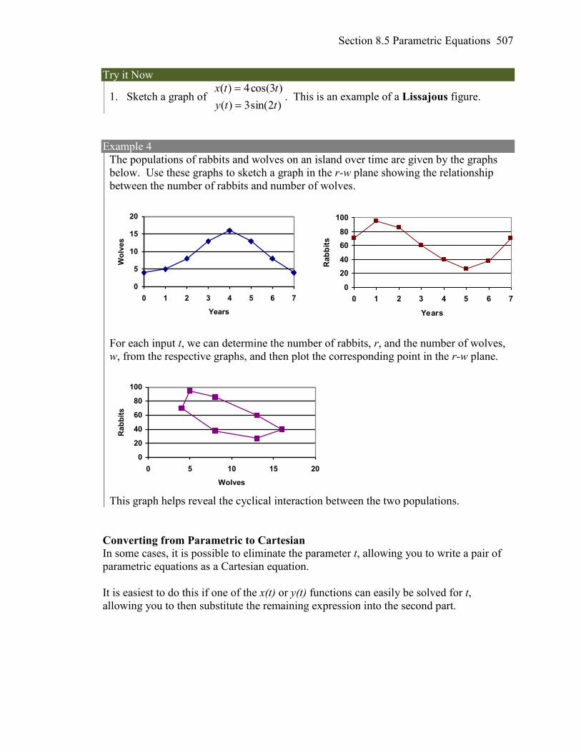
Section 8.5 Parametric Equations 507
Try it Now
1. Sketch a graph of )2sin(3)(
)3cos(4)(
tty
ttx
. This is an example of a Lissajous figure.
Example 4
The populations of rabbits and wolves on an island over time are given by the graphs
below. Use these graphs to sketch a graph in the r-w plane showing the relationship
between the number of rabbits and number of wolves.
0
5
10
15
20
0 1 2 3 4 5 6 7
Years
Wo
lves
For each input t, we can determine the number of rabbits, r, and the number of wolves,
w, from the respective graphs, and then plot the corresponding point in the r-w plane.
0
20
40
60
80
100
0 5 10 15 20
Wolves
Rab
bit
s
This graph helps reveal the cyclical interaction between the two populations.
Converting from Parametric to Cartesian
In some cases, it is possible to eliminate the parameter t, allowing you to write a pair of
parametric equations as a Cartesian equation.
It is easiest to do this if one of the x(t) or y(t) functions can easily be solved for t,
allowing you to then substitute the remaining expression into the second part.
0
20
40
60
80
100
0 1 2 3 4 5 6 7
Years
Rab
bit
s
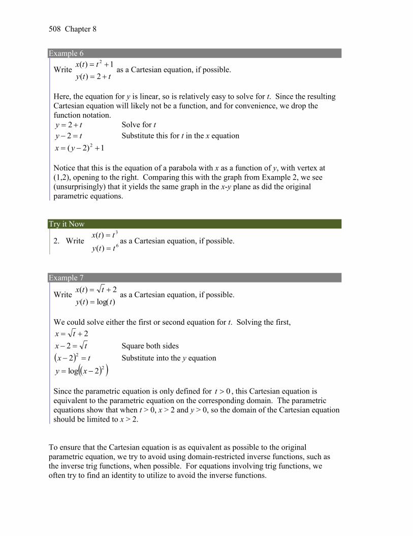
508 Chapter 8
Example 6
Write tty
ttx
2)(
1)( 2
as a Cartesian equation, if possible.
Here, the equation for y is linear, so is relatively easy to solve for t. Since the resulting
Cartesian equation will likely not be a function, and for convenience, we drop the
function notation.
ty 2 Solve for t
ty 2 Substitute this for t in the x equation
1)2( 2 yx
Notice that this is the equation of a parabola with x as a function of y, with vertex at
(1,2), opening to the right. Comparing this with the graph from Example 2, we see
(unsurprisingly) that it yields the same graph in the x-y plane as did the original
parametric equations.
Try it Now
2. Write 6
3
)(
)(
tty
ttx
as a Cartesian equation, if possible.
Example 7
Write )log()(
2)(
tty
ttx
as a Cartesian equation, if possible.
We could solve either the first or second equation for t. Solving the first,
2 tx
tx 2 Square both sides
tx 2
2 Substitute into the y equation
22log xy
Since the parametric equation is only defined for 0t , this Cartesian equation is
equivalent to the parametric equation on the corresponding domain. The parametric
equations show that when t > 0, x > 2 and y > 0, so the domain of the Cartesian equation
should be limited to x > 2.
To ensure that the Cartesian equation is as equivalent as possible to the original
parametric equation, we try to avoid using domain-restricted inverse functions, such as
the inverse trig functions, when possible. For equations involving trig functions, we
often try to find an identity to utilize to avoid the inverse functions.
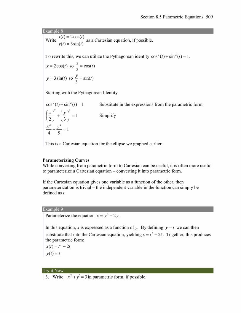
Section 8.5 Parametric Equations 509
Example 8
Write )sin(3)(
)cos(2)(
tty
ttx
as a Cartesian equation, if possible.
To rewrite this, we can utilize the Pythagorean identity 1)(sin)(cos 22 tt .
)cos(2 tx so )cos(2
tx
)sin(3 ty so )sin(3
ty
Starting with the Pythagorean Identity
1)(sin)(cos 22 tt Substitute in the expressions from the parametric form
132
22
yx Simplify
194
22
yx
This is a Cartesian equation for the ellipse we graphed earlier.
Parameterizing Curves While converting from parametric form to Cartesian can be useful, it is often more useful
to parameterize a Cartesian equation – converting it into parametric form.
If the Cartesian equation gives one variable as a function of the other, then
parameterization is trivial – the independent variable in the function can simply be
defined as t.
Example 9
Parameterize the equation yyx 23 .
In this equation, x is expressed as a function of y. By defining ty we can then
substitute that into the Cartesian equation, yielding ttx 23 . Together, this produces
the parametric form:
tty
tttx
)(
2)( 3
Try it Now
3. Write 322 yx in parametric form, if possible.
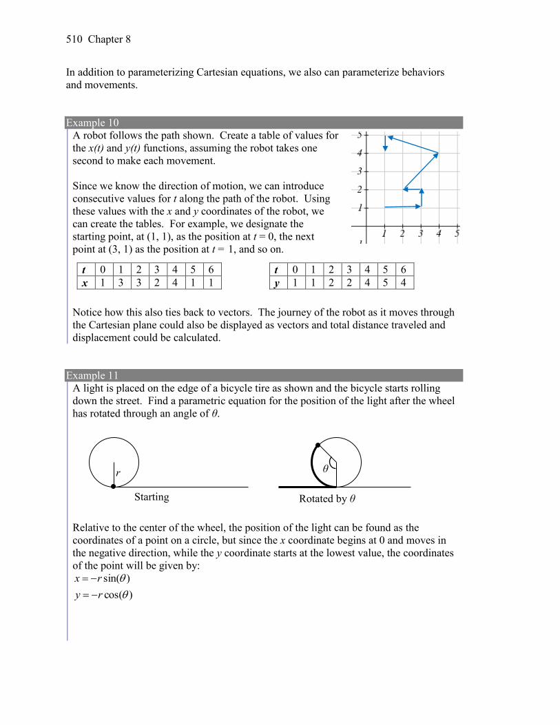
510 Chapter 8
In addition to parameterizing Cartesian equations, we also can parameterize behaviors
and movements.
Example 10
A robot follows the path shown. Create a table of values for
the x(t) and y(t) functions, assuming the robot takes one
second to make each movement.
Since we know the direction of motion, we can introduce
consecutive values for t along the path of the robot. Using
these values with the x and y coordinates of the robot, we
can create the tables. For example, we designate the
starting point, at (1, 1), as the position at t = 0, the next
point at (3, 1) as the position at t = 1, and so on.
Notice how this also ties back to vectors. The journey of the robot as it moves through
the Cartesian plane could also be displayed as vectors and total distance traveled and
displacement could be calculated.
Example 11
A light is placed on the edge of a bicycle tire as shown and the bicycle starts rolling
down the street. Find a parametric equation for the position of the light after the wheel
has rotated through an angle of θ.
Relative to the center of the wheel, the position of the light can be found as the
coordinates of a point on a circle, but since the x coordinate begins at 0 and moves in
the negative direction, while the y coordinate starts at the lowest value, the coordinates
of the point will be given by:
)cos(
)sin(
ry
rx
θ
Starting Rotated by θ
r
t 0 1 2 3 4 5 6
x 1 3 3 2 4 1 1
t 0 1 2 3 4 5 6
y 1 1 2 2 4 5 4
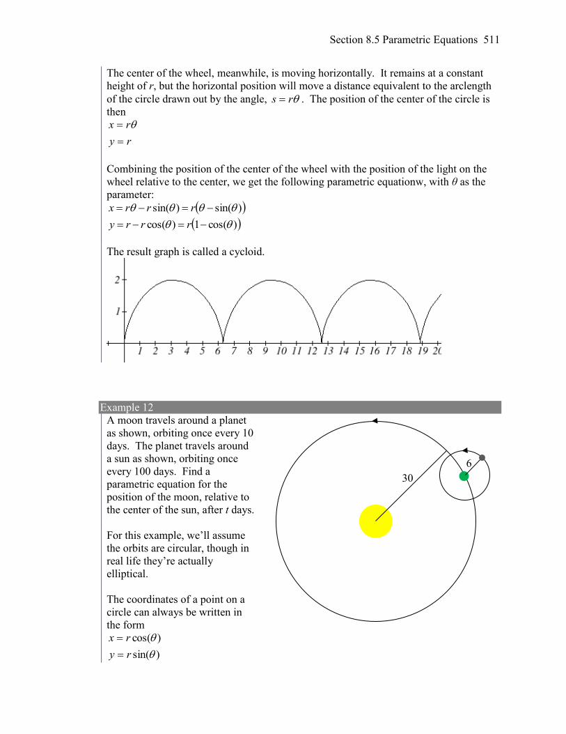
Section 8.5 Parametric Equations 511
The center of the wheel, meanwhile, is moving horizontally. It remains at a constant
height of r, but the horizontal position will move a distance equivalent to the arclength
of the circle drawn out by the angle, rs . The position of the center of the circle is
then
ry
rx
Combining the position of the center of the wheel with the position of the light on the
wheel relative to the center, we get the following parametric equationw, with θ as the
parameter:
)cos(1)cos(
)sin()sin(
rrry
rrrx
The result graph is called a cycloid.
Example 12
A moon travels around a planet
as shown, orbiting once every 10
days. The planet travels around
a sun as shown, orbiting once
every 100 days. Find a
parametric equation for the
position of the moon, relative to
the center of the sun, after t days.
For this example, we’ll assume
the orbits are circular, though in
real life they’re actually
elliptical.
The coordinates of a point on a
circle can always be written in
the form
)sin(
)cos(
ry
rx
6
30
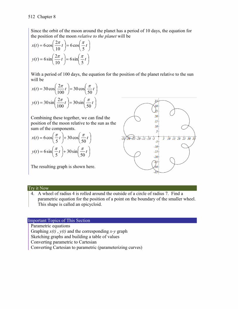
512 Chapter 8
Since the orbit of the moon around the planet has a period of 10 days, the equation for
the position of the moon relative to the planet will be
ttty
tttx
5sin6
10
2sin6)(
5cos6
10
2cos6)(
With a period of 100 days, the equation for the position of the planet relative to the sun
will be
ttty
tttx
50sin30
100
2sin30)(
50cos30
100
2cos30)(
Combining these together, we can find the
position of the moon relative to the sun as the
sum of the components.
ttty
tttx
50sin30
5sin6)(
50cos30
5cos6)(
The resulting graph is shown here.
Try it Now
4. A wheel of radius 4 is rolled around the outside of a circle of radius 7. Find a
parametric equation for the position of a point on the boundary of the smaller wheel.
This shape is called an epicycloid.
Important Topics of This Section
Parametric equations
Graphing x(t) , y(t) and the corresponding x-y graph
Sketching graphs and building a table of values
Converting parametric to Cartesian
Converting Cartesian to parametric (parameterizing curves)
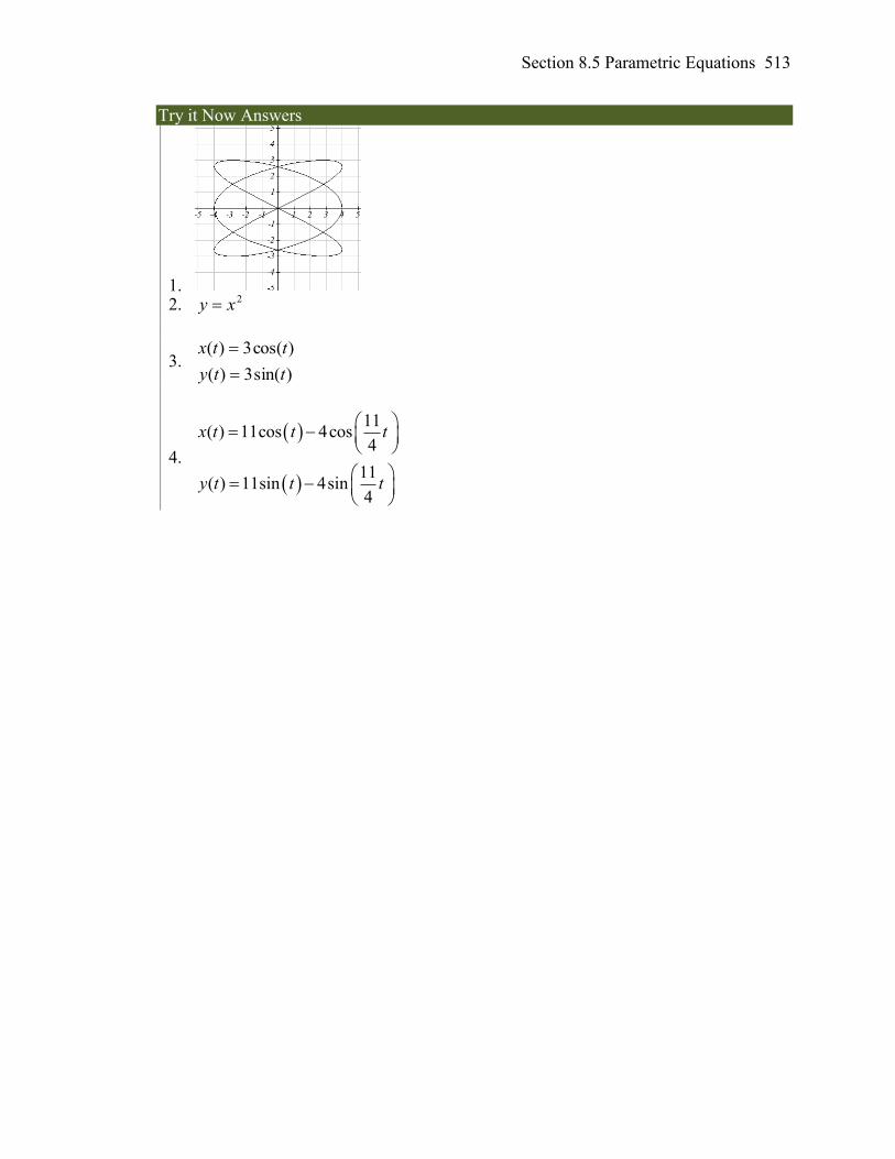
Section 8.5 Parametric Equations 513
Try it Now Answers
1. 2. 2xy
3. )sin(3)(
)cos(3)(
tty
ttx
4.
11( ) 11cos 4cos
4
11( ) 11sin 4sin
4
x t t t
y t t t
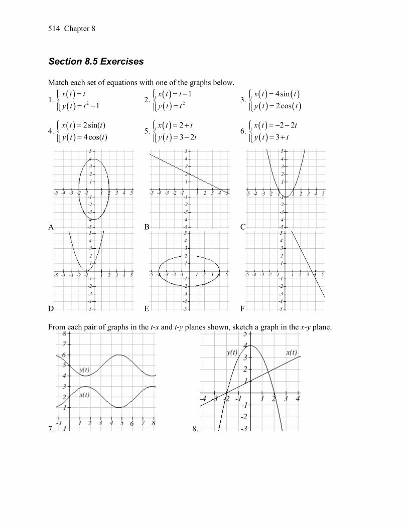
514 Chapter 8
Section 8.5 Exercises
Match each set of equations with one of the graphs below.
1. 2 1
x t t
y t t
2.
2
1x t t
y t t
3.
4sin
2cos
x t t
y t t
4.
2sin( )
4cos( )
x t t
y t t
5.
2
3 2
x t t
y t t
6.
2 2
3
x t t
y t t
A B C
D E F
From each pair of graphs in the t-x and t-y planes shown, sketch a graph in the x-y plane.
7. 8.
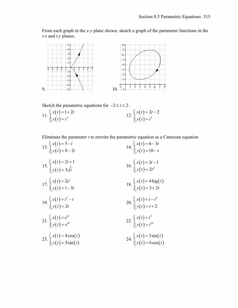
Section 8.5 Parametric Equations 515
From each graph in the x-y plane shown, sketch a graph of the parameter functions in the
t-x and t-y planes.
9. 10.
Sketch the parametric equations for 2 2t .
11. 2
1 2x t t
y t t
12.
3
2 2x t t
y t t
Eliminate the parameter t to rewrite the parametric equation as a Cartesian equation
13.
5
8 2
x t t
y t t
14.
6 3
10
x t t
y t t
15.
2 1
3
x t t
y t t
16. 2
3 1
2
x t t
y t t
17.
2
1 5
tx t e
y t t
18.
4log
3 2
x t t
y t t
19.
3
2
x t t t
y t t
20.
4
2
x t t t
y t t
21.
2
6
t
t
x t e
y t e
22.
5
10
x t t
y t t
23.
4cos
5sin
x t t
y t t
24.
3sin
6cos
x t t
y t t
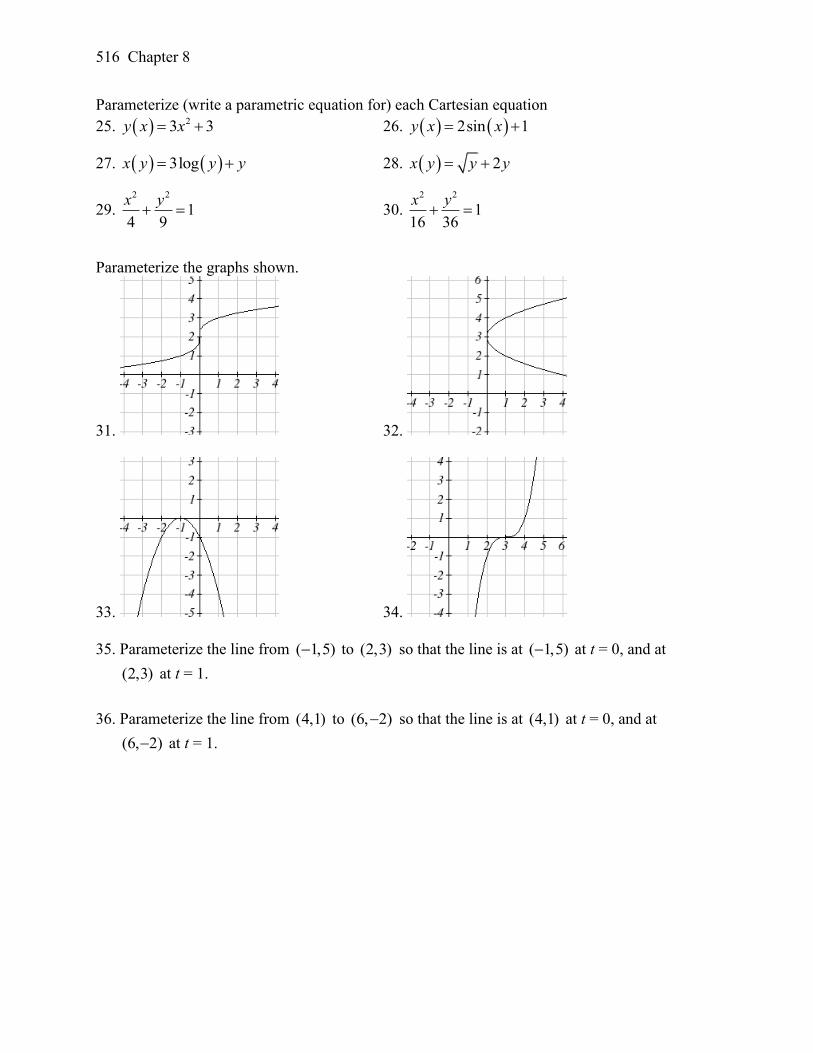
516 Chapter 8
Parameterize (write a parametric equation for) each Cartesian equation
25. 23 3y x x 26. 2sin 1y x x
27. 3logx y y y 28. 2x y y y
29. 2 2
14 9
x y 30.
2 2
116 36
x y
Parameterize the graphs shown.
31. 32.
33. 34.
35. Parameterize the line from ( 1,5) to (2,3) so that the line is at ( 1,5) at t = 0, and at
(2, 3) at t = 1.
36. Parameterize the line from (4,1) to (6, 2) so that the line is at (4,1) at t = 0, and at
(6, 2) at t = 1.
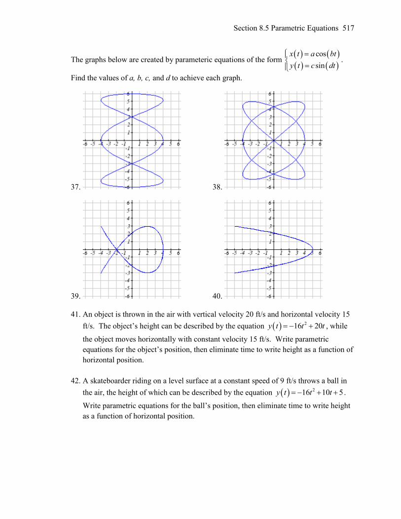
Section 8.5 Parametric Equations 517
The graphs below are created by parameteric equations of the form
cos
sin
x t a bt
y t c dt
.
Find the values of a, b, c, and d to achieve each graph.
37. 38.
39. 40.
41. An object is thrown in the air with vertical velocity 20 ft/s and horizontal velocity 15
ft/s. The object’s height can be described by the equation 216 20y t t t , while
the object moves horizontally with constant velocity 15 ft/s. Write parametric
equations for the object’s position, then eliminate time to write height as a function of
horizontal position.
42. A skateboarder riding on a level surface at a constant speed of 9 ft/s throws a ball in
the air, the height of which can be described by the equation 216 10 5y t t t .
Write parametric equations for the ball’s position, then eliminate time to write height
as a function of horizontal position.
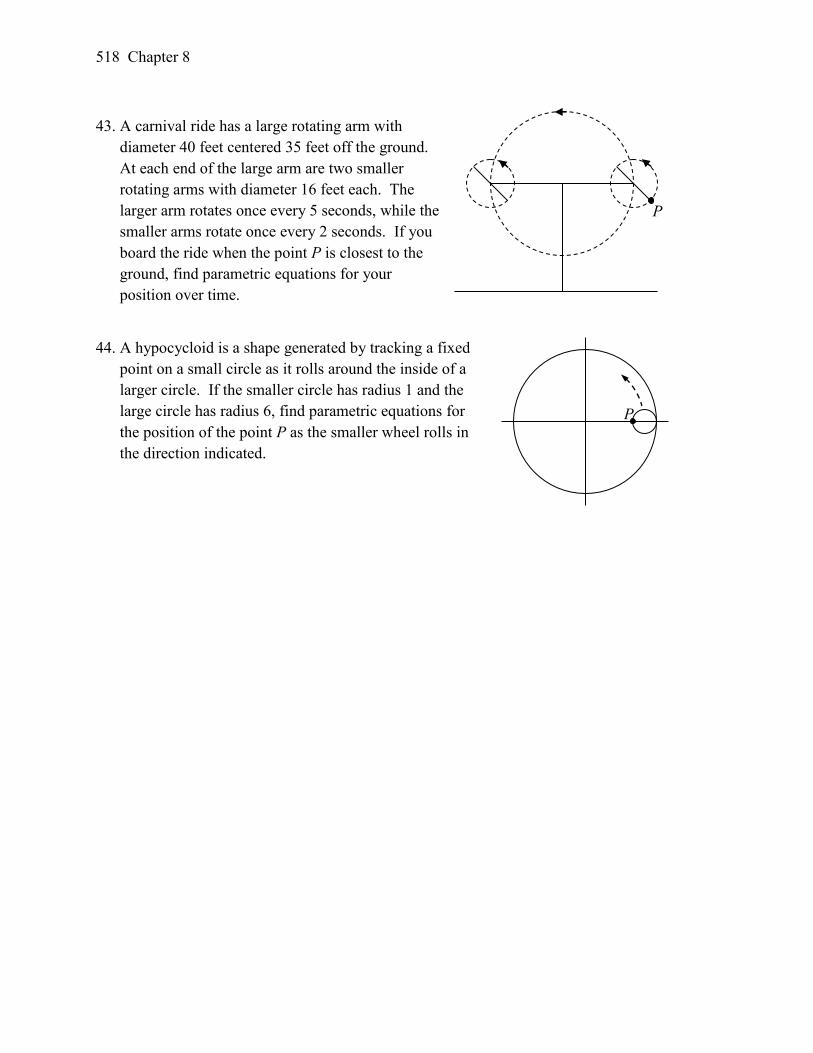
518 Chapter 8
43. A carnival ride has a large rotating arm with
diameter 40 feet centered 35 feet off the ground.
At each end of the large arm are two smaller
rotating arms with diameter 16 feet each. The
larger arm rotates once every 5 seconds, while the
smaller arms rotate once every 2 seconds. If you
board the ride when the point P is closest to the
ground, find parametric equations for your
position over time.
44. A hypocycloid is a shape generated by tracking a fixed
point on a small circle as it rolls around the inside of a
larger circle. If the smaller circle has radius 1 and the
large circle has radius 6, find parametric equations for
the position of the point P as the smaller wheel rolls in
the direction indicated.
P
P

519
Solutions to Selected Exercises
Chapter 1
Section 1.1
1. a. 40 13f
b. 2 Tons of garbage per week is produced by a city with a population of 5,000.
3. a. In 1995 there are 30 ducks in the lake
b. In 2000 there are 40 ducks in the late
5. a ,b, d, e 7. a, b 9. a, b, d
11. b 13. b, c, e, f 15. 1 1, 3 1f f
17. 2 4, 3 2g g 19. 3 53, 2 1f f
2f 1f 0f 1f 2f
21. 8 6 4 2 0
23. 49 18 3 4 21
25. 4 -1 0 1 -4
27. 4 4.414 4.732 5 5.236
29. -4 -6 -6 -4 0
31. 5 DNE -3 -1 -1/3
33. 1/4 1/2 1 2 4
35. a. -6 b.-16 37. a. 5 b. 5
3
39. a. iii b. viii c. I d. ii e. vi f. iv g. v h. vii
41. a. iv b. ii c. v d. I e. vi f. iii
43. 36)9()3( 22 yx
45. (a) (b) (c)
47a. t b. a c. r d. L: (c, t) and K: (a, p)
hei
gh
t
age
hei
gh
t o
f h
ead
time
po
sta
ge
weight
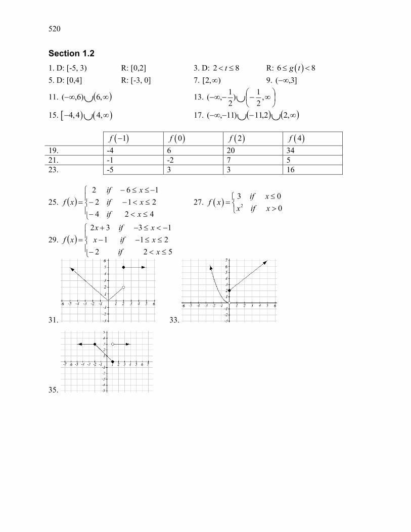
520
Section 1.2
1. D: [-5, 3) R: [0,2] 3. D: 2 8t R: 6 8g t
5. D: [0,4] R: [-3, 0] 7. ),2[ 9. ]3,(
11. ,6 ) 6,( 13.
,
2
1 )
2
1,(
15. 4,4 4, 17. ,2 2,11 ) 11,(
1f 0f 2f 4f
19. -4 6 20 34
21. -1 -2 7 5
23. -5 3 3 16
25.
42 4
212
1 62
xif
xif
xif
xf 27. 2
3 0
0
if xf x
x if x
29.
52 2
21 1
13 32
xif
xifx
xifx
xf
31. 33.
35.
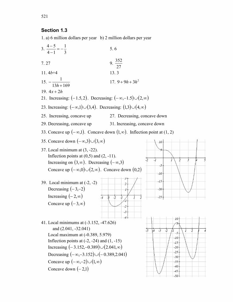
521
Section 1.3
1. a) 6 million dollars per year b) 2 million dollars per year
3. 3
1
14
54
5. 6
7. 27 9. 27
352
11. 4b+4 13. 3
15. 16913
1
h 17. 2399 hh
19. hx 24
21. Increasing: 2,5.1 . Decreasing: ,25.1,
23. Increasing: 4,31, . Decreasing: ,43,1
25. Increasing, concave up 27. Decreasing, concave down
29. Decreasing, concave up 31. Increasing, concave down
33. Concave up 1, . Concave down ,1 . Inflection point at (1, 2)
35. Concave down ,33,
37. Local minimum at (3, -22).
Inflection points at (0,5) and (2, -11).
Increasing on ,3 . Decreasing 3,
Concave up ,20, . Concave down 2,0
39. Local minimum at (-2, -2)
Decreasing 2,3
Increasing ,2
Concave up ,3
41. Local minimums at (-3.152, -47.626)
and (2.041, -32.041)
Local maximum at (-0.389, 5.979)
Inflection points at (-2, -24) and (1, -15)
Increasing ,041.2389.0,152.3
Decreasing 041.2,389.0152.3,
Concave up ,12,
Concave down 1,2
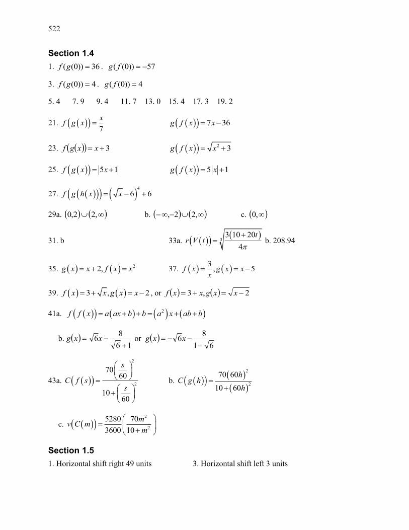
522
Section 1.4
1. 36))0(( gf . 57))0(( fg
3. 4))0(( gf . 4))0(( fg
5. 4 7. 9 9. 4 11. 7 13. 0 15. 4 17. 3 19. 2
21. 7
xf g x 7 36g f x x
23. 3 xxgf 2 3g f x x
25. 5 1f g x x 5 1g f x x
27. 4
6 6f g h x x
29a. ,22,0 b. ,22, c. ,0
31. b 33a.
33 10 20
4
tr V t
b. 208.94
35. 22, g x x f x x 37. 3
, 5f x g x xx
39. 3 , 2f x x g x x , or 2, 3 xxgxxf
41a. 2f f x a ax b b a x ab b
b. 16
86
xxg or
61
86
xxg
43a.
2
2
7060
1060
s
C f ss
b.
2
2
70 60
10 60
hC g h
h
c. 2
2
5280 70
3600 10
mv C m
m
Section 1.5
1. Horizontal shift right 49 units 3. Horizontal shift left 3 units
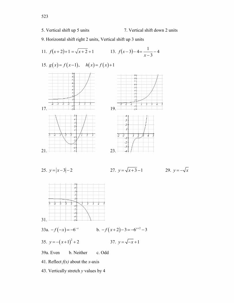
523
5. Vertical shift up 5 units 7. Vertical shift down 2 units
9. Horizontal shift right 2 units, Vertical shift up 3 units
11. 12 12 xxf 13. 43
1 43
xxf
15. 1 , 1g x f x h x f x
17. 19.
21. 23.
25. 3 2y x 27. 3 1y x 29. y x
31.
33a. 6 xf x b. 22 3 6 3xf x
35. 2
1 2y x 37. 1y x
39a. Even b. Neither c. Odd
41. Reflect f(x) about the x-axis
43. Vertically stretch y values by 4
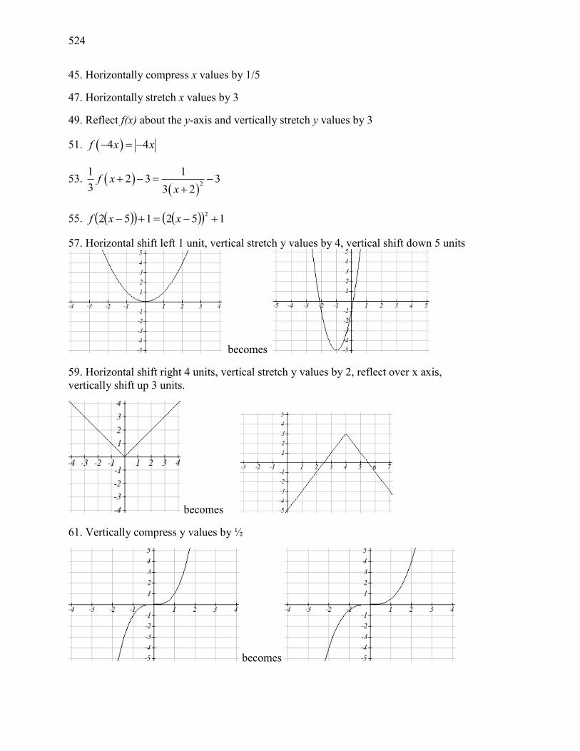
524
45. Horizontally compress x values by 1/5
47. Horizontally stretch x values by 3
49. Reflect f(x) about the y-axis and vertically stretch y values by 3
51. 4 4f x x
53.
2
1 12 3 3
3 3 2f x
x
55. 1521522 xxf
57. Horizontal shift left 1 unit, vertical stretch y values by 4, vertical shift down 5 units
becomes
59. Horizontal shift right 4 units, vertical stretch y values by 2, reflect over x axis,
vertically shift up 3 units.
becomes
61. Vertically compress y values by ½
becomes
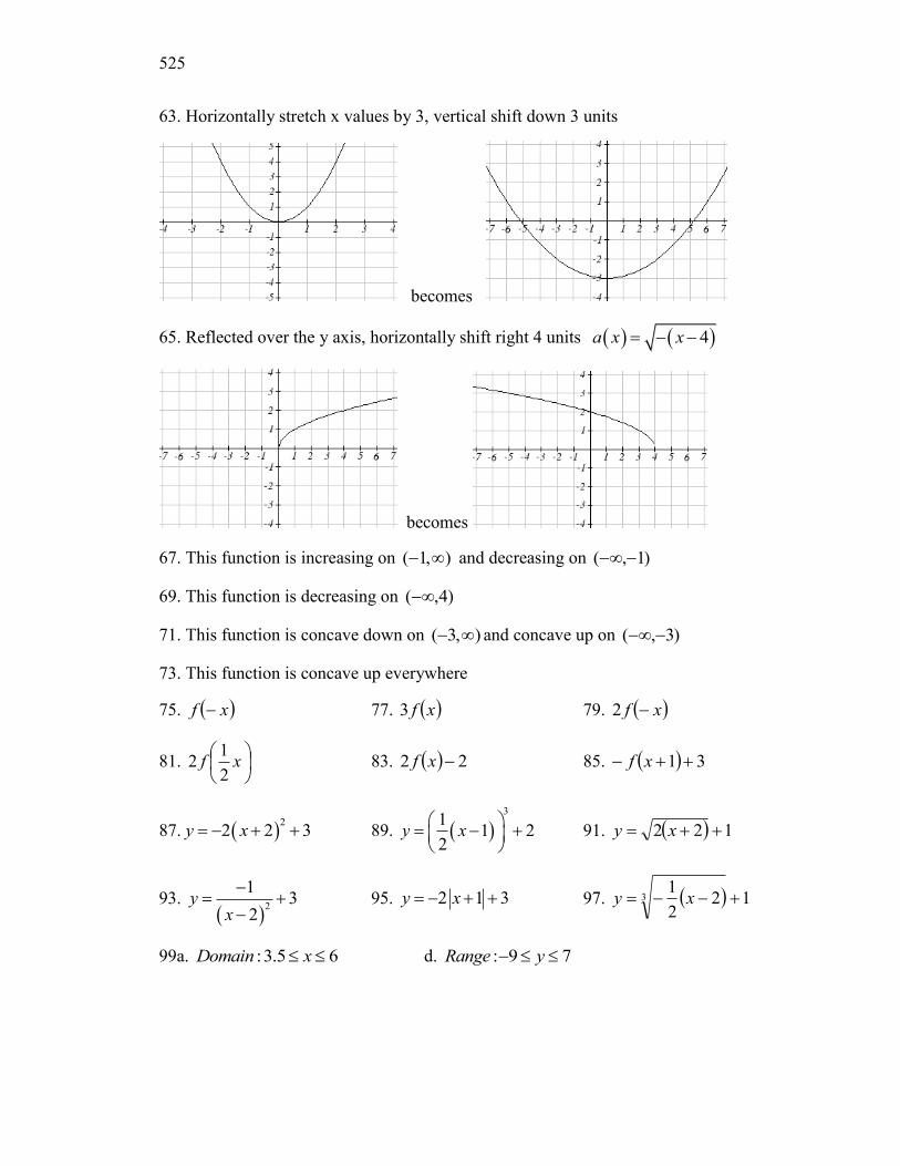
525
63. Horizontally stretch x values by 3, vertical shift down 3 units
becomes
65. Reflected over the y axis, horizontally shift right 4 units 4a x x
becomes
67. This function is increasing on ),1( and decreasing on )1,(
69. This function is decreasing on )4,(
71. This function is concave down on ),3( and concave up on )3,(
73. This function is concave up everywhere
75. xf 77. xf3 79. xf 2
81.
xf
2
12 83. 22 xf 85. 31 xf
87. 2
2 2 3y x 89. 3
11 2
2y x
91. 122 xy
93.
2
13
2y
x
95. 2 1 3y x 97. 12
2
13 xy
99a. :3.5 6Domain x d. : 9 7Range y
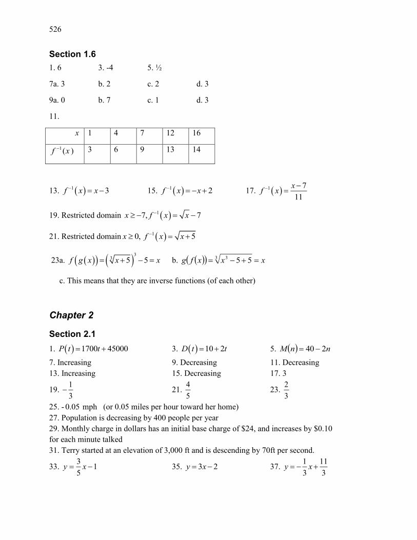
526
Section 1.6
1. 6 3. -4 5. ½
7a. 3 b. 2 c. 2 d. 3
9a. 0 b. 7 c. 1 d. 3
11.
x 1 4 7 12 16
xf (1 ) 3 6 9 13 14
13. 1 3f x x 15. 1 2f x x 17. 1 7
11
xf x
19. Restricted domain 17, 7x f x x
21. Restricted domain 10, 5x f x x
23a. 3
3 5 5f g x x x b. xxxfg 3 3 55
c. This means that they are inverse functions (of each other)
Chapter 2
Section 2.1
1. 1700 45000P t t 3. 10 2D t t 5. nnM 240
7. Increasing 9. Decreasing 11. Decreasing
13. Increasing 15. Decreasing 17. 3
19. 1
3 21.
4
5 23.
2
3
25. - 0.05 mph (or 0.05 miles per hour toward her home)
27. Population is decreasing by 400 people per year
29. Monthly charge in dollars has an initial base charge of $24, and increases by $0.10
for each minute talked
31. Terry started at an elevation of 3,000 ft and is descending by 70ft per second.
33. 15
3 xy 35. 3 2y x 37.
1 11
3 3y x
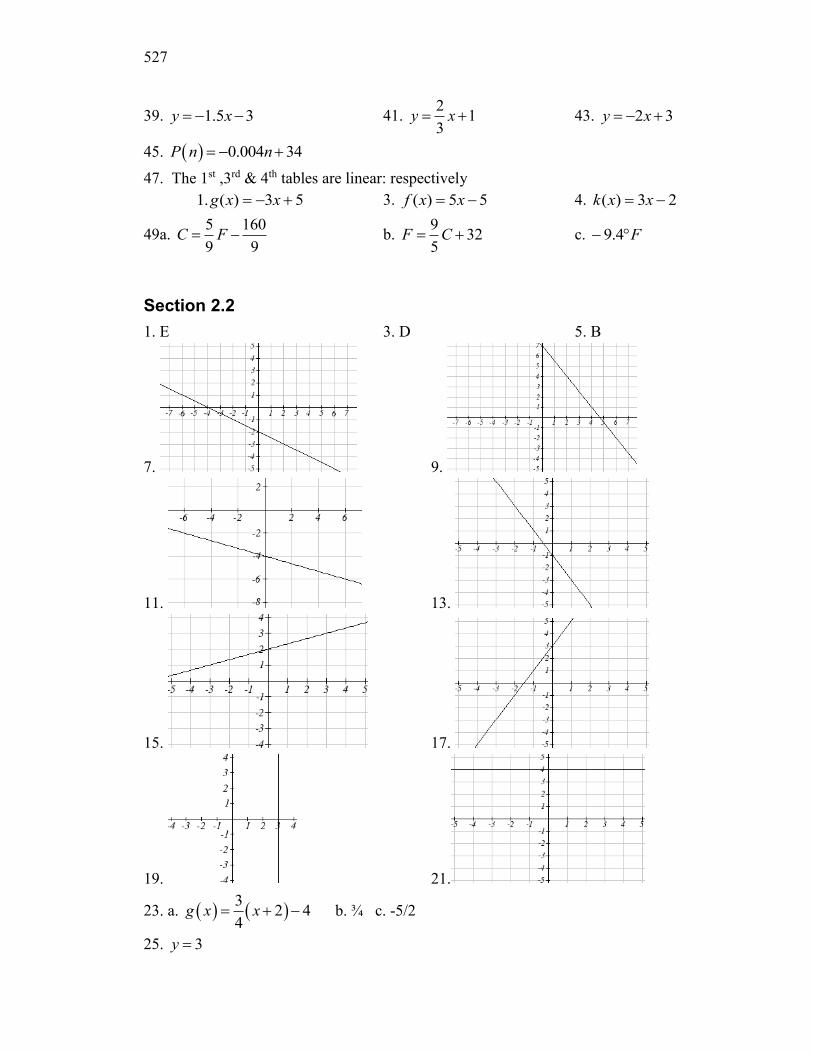
527
39. 1.5 3 y x 41. 2
13
y x 43. 2 3y x
45. 0.004 34P n n
47. The 1st ,3rd & 4th tables are linear: respectively
53)(. 1 xxg 3. 55)( xxf 4. 23)( xxk
49a. 5 160
9 9C F b.
932
5F C c. F 4.9
Section 2.2
1. E 3. D 5. B
7. 9.
11. 13.
15. 17.
19. 21.
23. a. 3
2 44
g x x b. ¾ c. -5/2
25. 3y
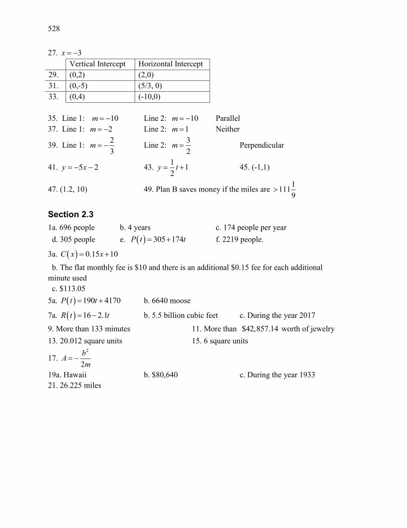
528
27. 3x
Vertical Intercept Horizontal Intercept
29. (0,2) (2,0)
31. (0,-5) (5/3, 0)
33. (0,4) (-10,0)
35. Line 1: 10m Line 2: 10m Parallel
37. Line 1: 2 m Line 2: 1m Neither
39. Line 1: 2
3
m Line 2: 3
2m Perpendicular
41. 25 xy 43. 1
12
y t 45. (-1,1)
47. (1.2, 10) 49. Plan B saves money if the miles are 1
1119
Section 2.3
1a. 696 people b. 4 years c. 174 people per year
d. 305 people e. 305 174P t t f. 2219 people.
3a. 0.15 10C x x
b. The flat monthly fee is $10 and there is an additional $0.15 fee for each additional
minute used
c. $113.05
5a. 190 4170P t t b. 6640 moose
7a. 16 2.1R t t b. 5.5 billion cubic feet c. During the year 2017
9. More than 133 minutes 11. More than $42,857.14 worth of jewelry
13. 20.012 square units 15. 6 square units
17. 2
2
bA
m
19a. Hawaii b. $80,640 c. During the year 1933
21. 26.225 miles
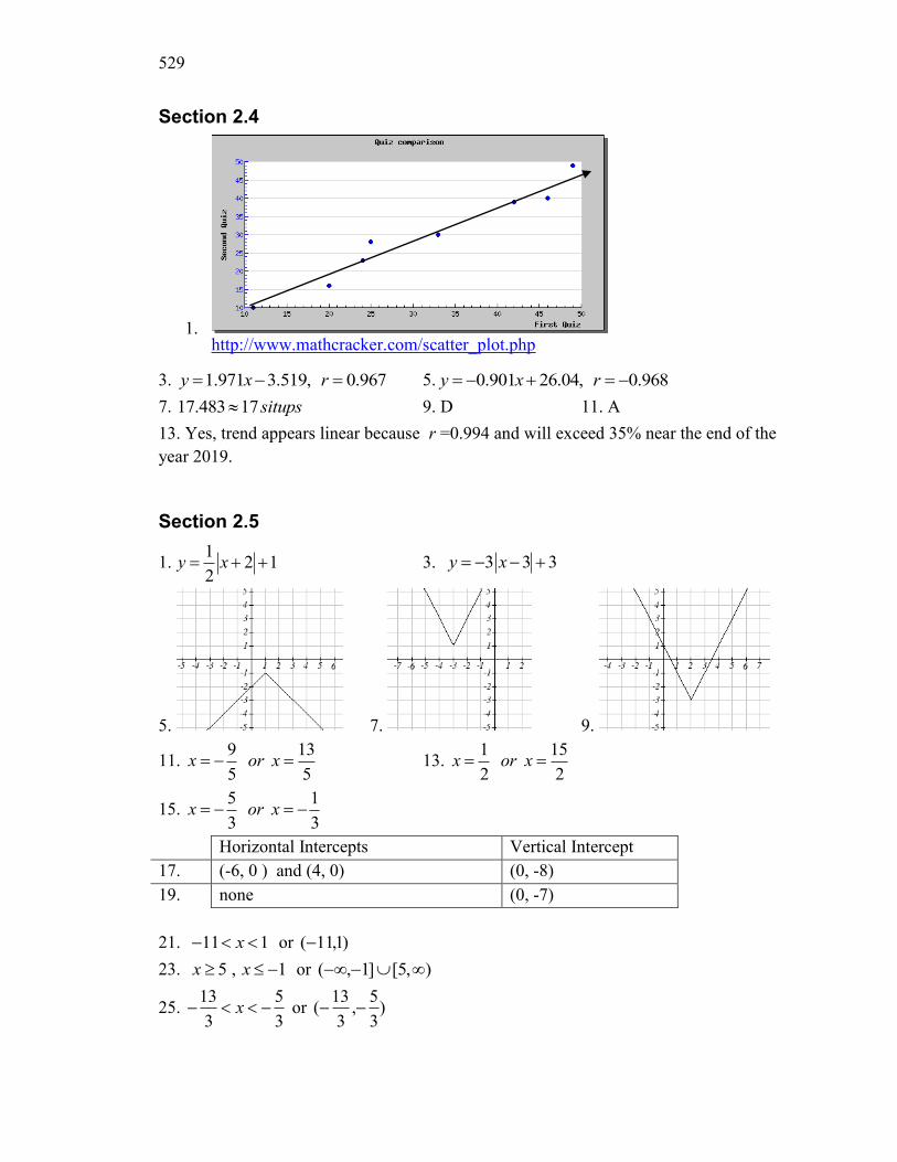
529
Section 2.4
1. http://www.mathcracker.com/scatter_plot.php
3. 1.971 3.519, 0.967y x r 5. 0.901 26.04, 0.968y x r
7. 17.483 17 situps 9. D 11. A
13. Yes, trend appears linear because r =0.994 and will exceed 35% near the end of the
year 2019.
Section 2.5
1. 122
1 xy 3. 3 3 3y x
5. 7. 9.
11. 9 13
5 5
x or x 13. 1 15
2 2
x or x
15. 5 1
3 3
x or x
Horizontal Intercepts Vertical Intercept
17. (-6, 0 ) and (4, 0) (0, -8)
19. none (0, -7)
21. 11 1x or )1,11(
23. 5 , 1x x or ),5[]1,(
25. 13 5
3 3x or )
3
5,
3
13(
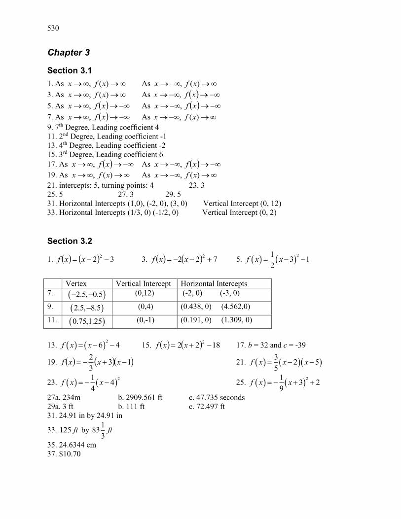
530
Chapter 3
Section 3.1
1. As )(, xfx As )(, xfx
3. As )(, xfx As xfx ,
5. As xfx , As xfx ,
7. As xfx , As )(, xfx
9. 7th Degree, Leading coefficient 4
11. 2nd Degree, Leading coefficient -1
13. 4th Degree, Leading coefficient -2
15. 3rd Degree, Leading coefficient 6
17. As xfx , As xfx ,
19. As )(, xfx As )(, xfx
21. intercepts: 5, turning points: 4 23. 3
25. 5 27. 3 29. 5
31. Horizontal Intercepts (1,0), (-2, 0), (3, 0) Vertical Intercept (0, 12)
33. Horizontal Intercepts (1/3, 0) (-1/2, 0) Vertical Intercept (0, 2)
Section 3.2
1. 322 xxf 3. 722
2 xxf 5.
213 1
2f x x
Vertex Vertical Intercept Horizontal Intercepts
7. 2.5, 0.5 (0,12) (-2, 0) (-3, 0)
9. 2.5, 8.5 (0,4) (0.438, 0) (4.562,0)
11. 0.75,1.25 (0,-1) (0.191, 0) (1.309, 0)
13. 2
6 4f x x 15. 18222 xxf 17. b = 32 and c = -39
19. 133
2 xxxf 21.
32 5
5f x x x
23. 21
44
f x x 25. 21
3 29
f x x
27a. 234m b. 2909.561 ft c. 47.735 seconds
29a. 3 ft b. 111 ft c. 72.497 ft
31. 24.91 in by 24.91 in
33. 125 ft by 1
83 3
ft
35. 24.6344 cm
37. $10.70
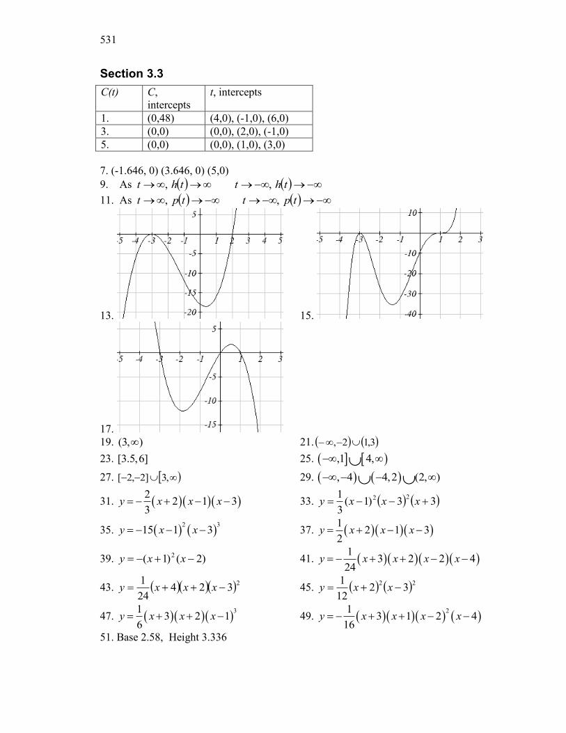
531
Section 3.3
C(t) C,
intercepts
t, intercepts
1. (0,48) (4,0), (-1,0), (6,0)
3. (0,0) (0,0), (2,0), (-1,0)
5. (0,0) (0,0), (1,0), (3,0)
7. (-1.646, 0) (3.646, 0) (5,0)
9. As thttht , ,
11. As tpttpt , ,
13. 15.
17.
19. (3, ) 21. 3,12,
23. [3.5,6] 25. ,1 4,
27. ,3]2,2[ 29. , 4 4,2 (2, )
31. 2
2 1 33
y x x x 33. 33)1(3
1 22 xxxy
35. 2 3
15 1 3y x x 37. 1
2 1 32
y x x x
39. )2()1( 2 xxy 41. 1
3 2 2 424
y x x x x
43. 2324
24
1 xxxy 45. 22
3212
1 xxy
47. 31
3 2 16
y x x x 49. 21
3 1 2 416
y x x x x
51. Base 2.58, Height 3.336
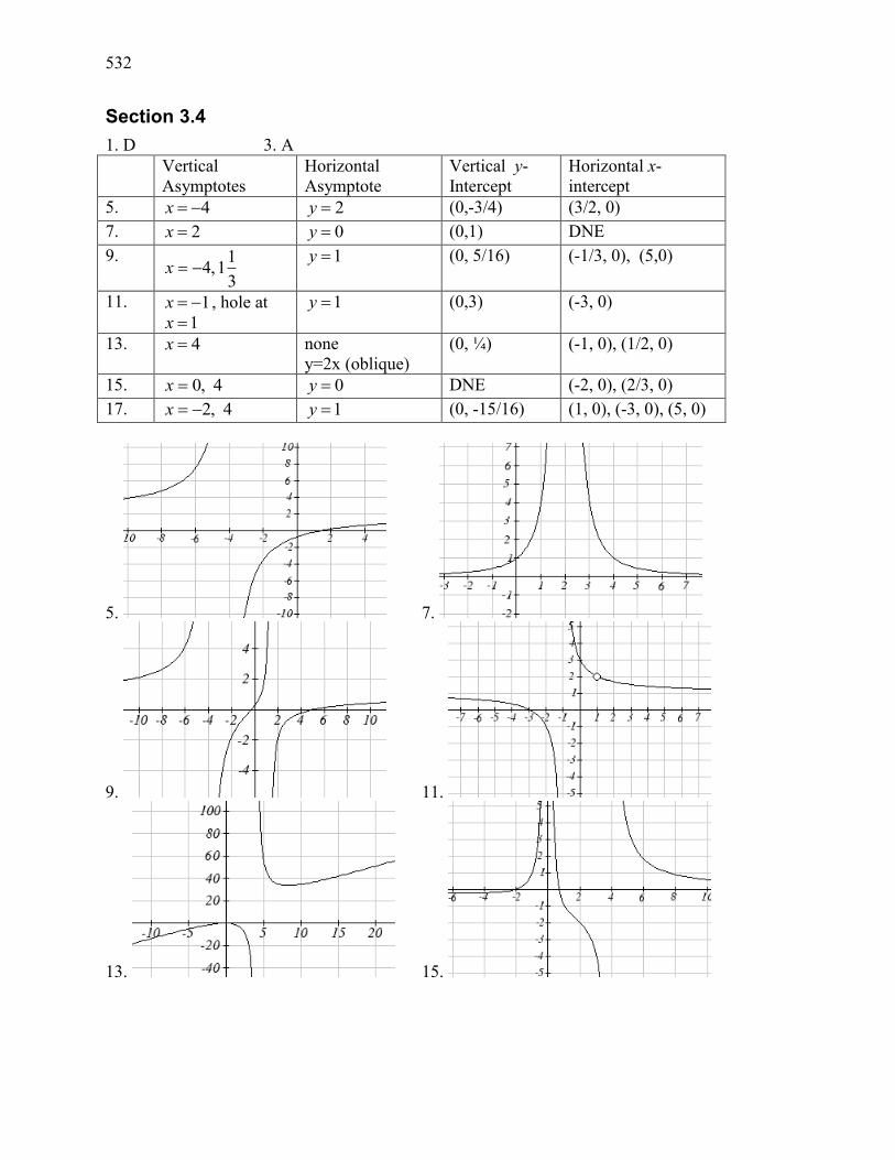
532
Section 3.4
1. D 3. A
Vertical
Asymptotes
Horizontal
Asymptote
Vertical y-
Intercept
Horizontal x-
intercept
5. 4x 2y (0,-3/4) (3/2, 0)
7. 2x 0y (0,1) DNE
9.
3
11 ,4x
1y (0, 5/16) (-1/3, 0), (5,0)
11. 1x , hole at
1x
1y (0,3) (-3, 0)
13. 4x none
y=2x (oblique)
(0, ¼) (-1, 0), (1/2, 0)
15. 4 ,0x 0y DNE (-2, 0), (2/3, 0)
17. 4 ,2x 1y (0, -15/16) (1, 0), (-3, 0), (5, 0)
5. 7.
9. 11.
13. 15.
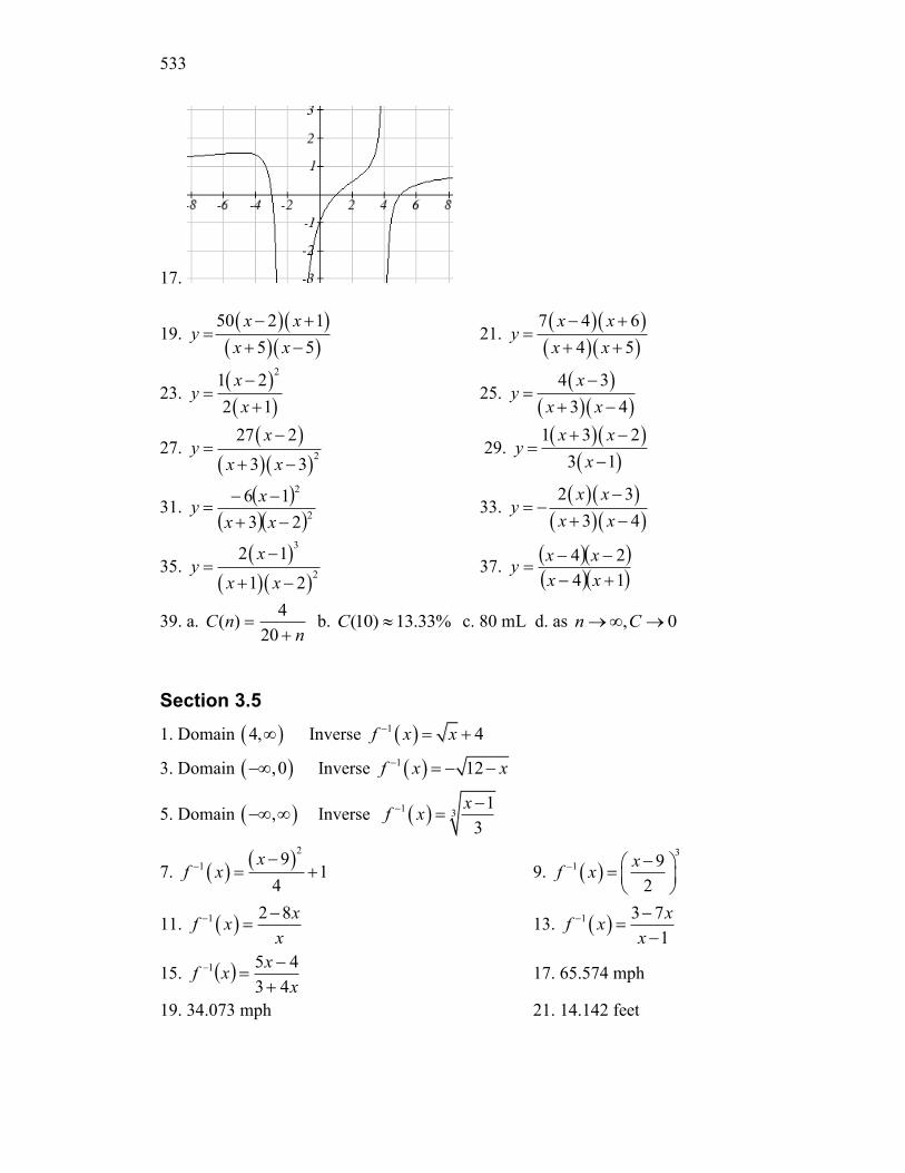
533
17.
19.
50 2 1
5 5
x xy
x x
21.
7 4 6
4 5
x xy
x x
23.
21 2
2 1
xy
x
25.
4 3
3 4
xy
x x
27.
2
27 2
3 3
xy
x x
29.
1 3 2
3 1
x xy
x
31.
22
23
16
xx
xy 33.
2 3
3 4
x xy
x x
35.
3
2
2 1
1 2
xy
x x
37.
14
24
xx
xxy
39. a. n
nC
20
4)( b. %33.13)10( C c. 80 mL d. as 0, Cn
Section 3.5
1. Domain 4, Inverse 1 4f x x
3. Domain ,0 Inverse 1 12f x x
5. Domain , Inverse 13
1
3
xf x
7.
2
19
14
xf x
9.
3
1 9
2
xf x
11. 1 2 8xf x
x
13. 1 3 7
1
xf x
x
15. x
xxf
43
451
17. 65.574 mph
19. 34.073 mph 21. 14.142 feet
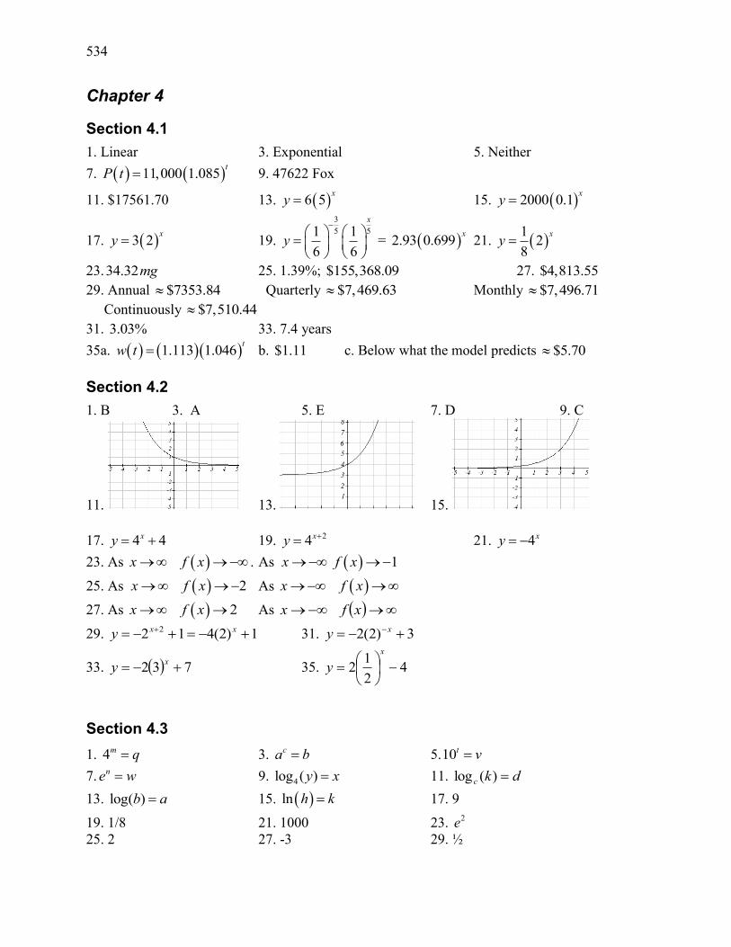
534
Chapter 4
Section 4.1
1. Linear 3. Exponential 5. Neither
7. 11,000 1.085t
P t 9. 47622 Fox
11. $17561.70 13. 6 5x
y 15. 2000 0.1x
y
17. 3 2x
y 19.
3
5 51 1
6 6
x
y
= 2.93 0.699x 21.
12
8
xy
23.34.32 mg 25. 1.39%; $155,368.09 27. $4,813.55
29. Annual $7353.84 Quarterly $7,469.63 Monthly $7,496.71
Continuously $7,510.44
31. 3.03% 33. 7.4 years
35a. 1.113 1.046t
w t b. $1.11 c. Below what the model predicts $5.70
Section 4.2
1. B 3. A 5. E 7. D 9. C
11. 13. 15.
17. 4 4xy 19. 24xy 21. 4xy
23. As x f x . As 1 x f x
25. As 2x f x As x f x
27. As 2x f x As xfx
29. 1)2(412 2 xxy 31. 3)2(2 xy
33. 732 x
y 35. 42
12
x
y
Section 4.3
1. 4m q 3. ca b 5.10t v
7. ne w 9. 4log ( )y x 11. dkc )(log
13. log( )b a 15. ln h k 17. 9
19. 1/8 21. 1000 23. 2e
25. 2 27. -3 29. ½
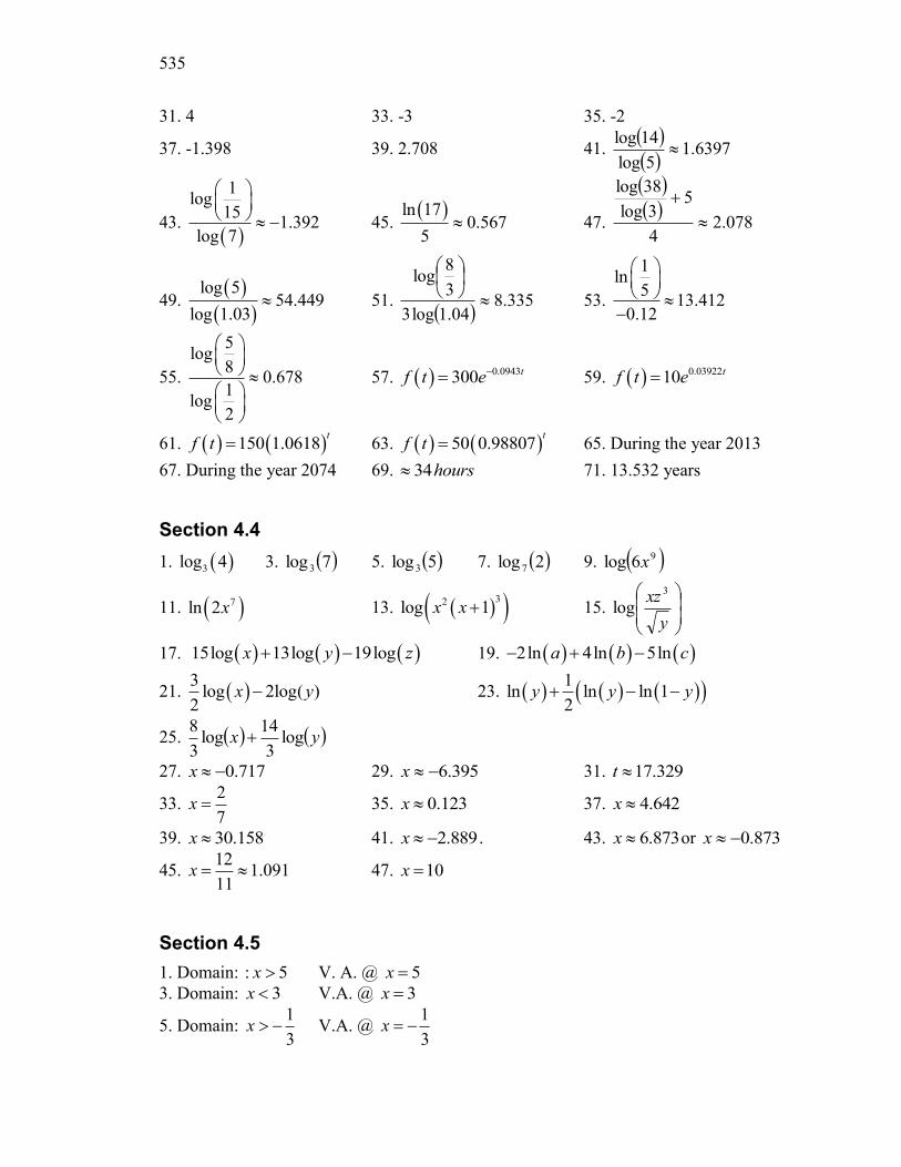
535
31. 4 33. -3 35. -2
37. -1.398 39. 2.708 41.
6397.15log
14log
43.
1log
151.392
log 7
45.
ln 170.567
5 47.
078.24
53log
38log
49.
log 554.449
log 1.03 51.
335.8
04.1log3
3
8log
53.
1ln
513.412
0.12
55.
5log
80.678
1log
2
57. 0.0943300 tf t e 59. 0.0392210 tf t e
61. 150 1.0618t
f t 63. 50 0.98807t
f t 65. During the year 2013
67. During the year 2074 69. 34 hours 71. 13.532 years
Section 4.4
1. 3log 4 3. 7log3 5. 5log3 7. 2log 7 9. 96log x
11. 7ln 2x 13. 32log 1x x 15.
y
xz 3
log
17. 15log 13log 19logx y z 19. 2ln 4ln 5lna b c
21. 3
log 2log( )2
x y 23. 1
ln ln ln 12
y y y
25. yx log3
14log
3
8
27. 0.717x 29. 395.6x 31. 17.329t
33. 2
7x 35. 0.123x 37. 4.642x
39. 30.158x 41. 2.889x . 43. 6.873x or 873.0x
45. 12
1.09111
x 47. 10x
Section 4.5
1. Domain: : 5x V. A. @ 5x
3. Domain: 3x V.A. @ 3x
5. Domain: 1
3x V.A. @
1
3x
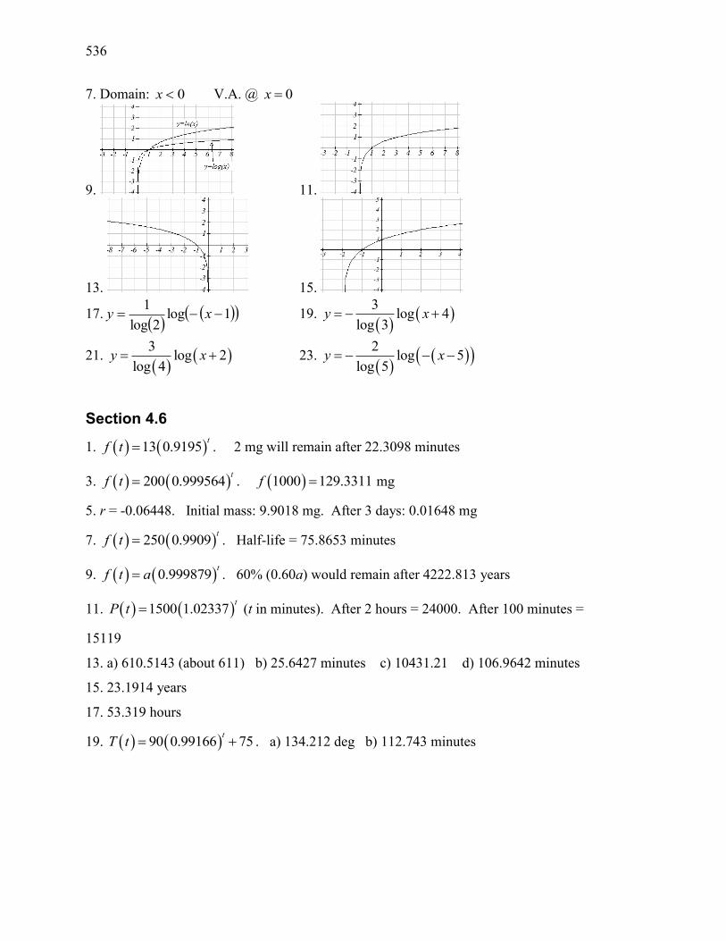
536
7. Domain: 0x V.A. @ 0x
9. 11.
13. 15.
17.
1log2log
1 xy 19.
3log 4
log 3y x
21.
3
log 2log 4
y x 23.
2
log 5log 5
y x
Section 4.6
1. 13 0.9195t
f t . 2 mg will remain after 22.3098 minutes
3. 200 0.999564t
f t . 1000 129.3311f mg
5. r = -0.06448. Initial mass: 9.9018 mg. After 3 days: 0.01648 mg
7. 250 0.9909t
f t . Half-life = 75.8653 minutes
9. 0.999879t
f t a . 60% (0.60a) would remain after 4222.813 years
11. 1500 1.02337t
P t (t in minutes). After 2 hours = 24000. After 100 minutes =
15119
13. a) 610.5143 (about 611) b) 25.6427 minutes c) 10431.21 d) 106.9642 minutes
15. 23.1914 years
17. 53.319 hours
19. 90 0.99166 75t
T t . a) 134.212 deg b) 112.743 minutes
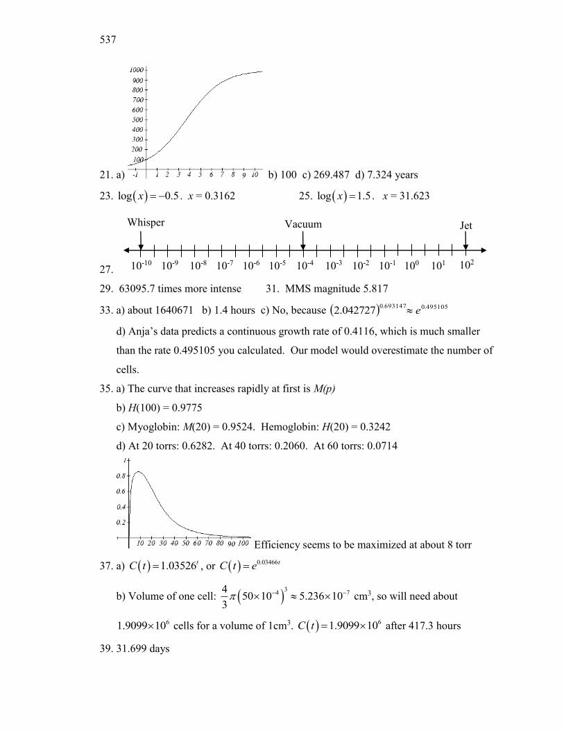
537
21. a) b) 100 c) 269.487 d) 7.324 years
23. log 0.5x . x = 0.3162 25. log 1.5x . x = 31.623
27.
29. 63095.7 times more intense 31. MMS magnitude 5.817
33. a) about 1640671 b) 1.4 hours c) No, because 495105.0693147.0 042727.2 e
d) Anja’s data predicts a continuous growth rate of 0.4116, which is much smaller
than the rate 0.495105 you calculated. Our model would overestimate the number of
cells.
35. a) The curve that increases rapidly at first is M(p)
b) H(100) = 0.9775
c) Myoglobin: M(20) = 0.9524. Hemoglobin: H(20) = 0.3242
d) At 20 torrs: 0.6282. At 40 torrs: 0.2060. At 60 torrs: 0.0714
Efficiency seems to be maximized at about 8 torr
37. a) 1.03526tC t , or 0.03466tC t e
b) Volume of one cell: 3
4 7450 10 5.236 10
3 cm3, so will need about
61.9099 10 cells for a volume of 1cm3. 61.9099 10C t after 417.3 hours
39. 31.699 days
10-6 10-5 10-4 10-3 10-2 10-7 10-8 10-9 10-10 10-1
Whisper Vacuum
Jet
100 101 102
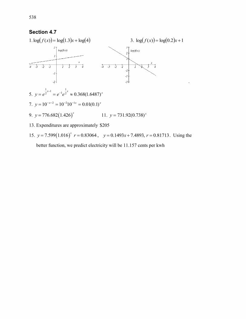
538
Section 4.7
1. 4log3.1log)(log xxf 3. 12.0log)(log xxf
.
5. xxx
eeey )6487.1(368.02
1
11
2
1
7. xxxy )1.0(01.0101010 122
9. 776.682 1.426x
y 11. xy )738.0(92.731
13. Expenditures are approximately $205
15. 7.599 1.016 0.83064x
y r , 0.1493 7.4893, 0.81713y x r . Using the
better function, we predict electricity will be 11.157 cents per kwh
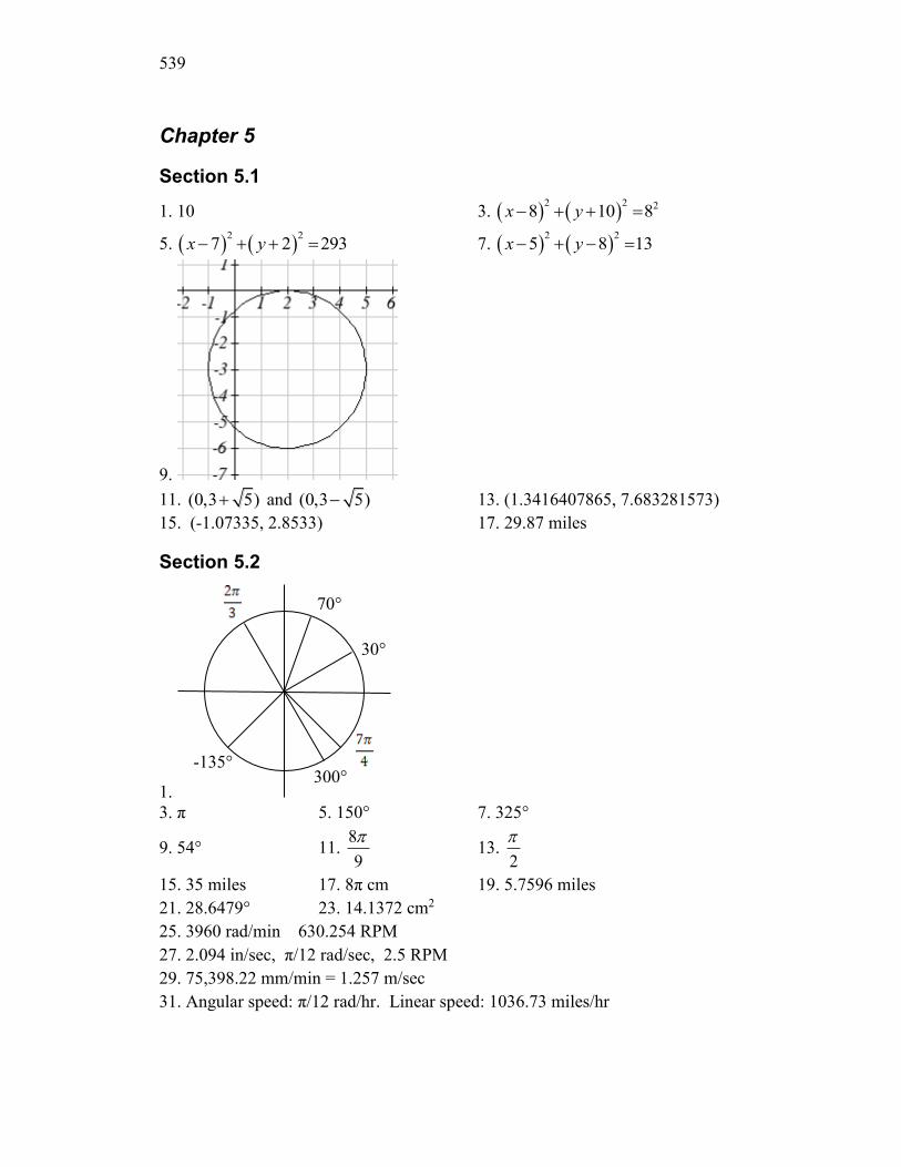
539
Chapter 5
Section 5.1
1. 10 3. 2 2 28 10 8x y
5. 2 2
7 2 293x y 7. 2 2
5 8 1 3x y
9.
11. (0, 3 5) and (0, 3 5) 13. (1.3416407865, 7.683281573)
15. (-1.07335, 2.8533) 17. 29.87 miles
Section 5.2
1.
3. π 5. 150° 7. 325°
9. 54° 11. 8
9
13.
2
15. 35 miles 17. 8π cm 19. 5.7596 miles
21. 28.6479° 23. 14.1372 cm2
25. 3960 rad/min 630.254 RPM
27. 2.094 in/sec, π/12 rad/sec, 2.5 RPM
29. 75,398.22 mm/min = 1.257 m/sec
31. Angular speed: π/12 rad/hr. Linear speed: 1036.73 miles/hr
30°
70°
-135° 300°
540
Section 5.3
1. a. III b. II 3. 4
5
5. 4 3
7 7.
55
8
9. a. reference: 45°. Quadrant III. 2
sin 2252
. 2
cos 2252
b. reference: 60°. Quadrant IV. 3
sin 3002
. 1
cos 3002
c. reference: 45°. Quadrant II. 2
sin 1352
. 2
cos 1352
d. reference: 30°. Quadrant III. 1
sin 2102
. 3
cos 2102
11. a. reference: 4
. Quadrant III.
5 2sin
4 2
.
5 2cos
4 2
b. reference: 6
. Quadrant III.
7 1sin
6 2
.
7 3cos
6 2
c. reference: 3
. Quadrant IV.
5 3sin
3 2
.
5 1cos
3 2
d. reference: 4
. Quadrant II.
3 2sin
4 2
.
3 2cos
4 2
13. a. 3 2
sin4 2
3 2
cos4 2
b. 23 1
sin6 2
23 3cos
6 2
c. sin 12
cos 02
d. sin 5 0 cos 5 1
15. a. 2
3
b. 100° c. 40° d.
5
3
e. 235°
17. a. 5
3
b. 280° c. 220° d.
2
3
e. 55°
19. (-11.491, -9.642)
541
Section 5.4
1. sec 2 , csc 2 , tan 1 , cot 1
3. 2 3
sec3
, csc 2 , 3
tan3
, cot 3
5. sec 2 , 2 3
csc3
, tan 3 , 3
cot3
7. a. sec 135 2 b. csc 210 2 c. tan 60 3 . d. cot 225 1
9. 7
cos4
, 4 7
sec7
, 4
csc3
, 3 7
tan7
, 7
cot3
11. 2 2
sin3
, 4
23csc , 3sec , tan 2 2 ,
2cot
4
13. 12
sin13
, 5
cos13
, 13
sec5
, 13
csc12
, 5
cot12
15. a. sin(0.15) = 0.1494 cos(0.15) = 0.9888 tan(0.15) = 0.1511
b. sin(4) = -0.7568 cos(4) = -0.6536 tan(4) = 1.1578
c. sin(70°) = 0.9397 cos(70°) = 0.3420 tan(70°) = 2.7475
d. sin(283°) = -0.9744 cos(283°) = 0.2250 tan(283°) = -4.3315
17. sec( )t 19. tan( )t 21. tan( )t 23. cot( )t 25. 2
sec( )t
Section 5.5
1.
4
5tan,
41
414cos,
41
415sin AAA
5
4cot,
4
41csc,
5
41sec AAA
3. 14, 7 3, 60c b B 5. 5.3171, 11.3257, 28a c A
7. 9.0631, 4.2262, 25a b B 9. 32.4987 ft
11. 836.2698 ft 13. 460.4069 ft
15. 660.35 feet 17. 28.025 ft
19. 143.0427 21. 86.6685
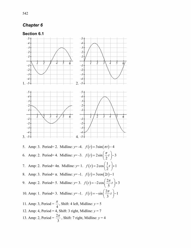
542
Chapter 6
Section 6.1
1. 2.
3. 4.
5. Amp: 3. Period= 2. Midline: y= -4. 3sin 4f t t
6. Amp: 2. Period= 4. Midline: y= -3. 2sin 32
f t t
7. Amp: 2. Period= 4π. Midline: y= 1. 1
2cos 12
f t t
8. Amp: 3. Period= π. Midline: y= -1. 3cos 2 1f t t
9. Amp: 2. Period= 5. Midline: y= 3. 2
2cos 35
f t t
10. Amp: 1. Period= 3. Midline: y= -1. 2
sin 13
f t t
11. Amp: 3, Period = 4
, Shift: 4 left, Midline: y = 5
12. Amp: 4, Period = 4, Shift: 3 right, Midline: y = 7
13. Amp: 2, Period = 2
3
, Shift: 7 right, Midline: y = 4
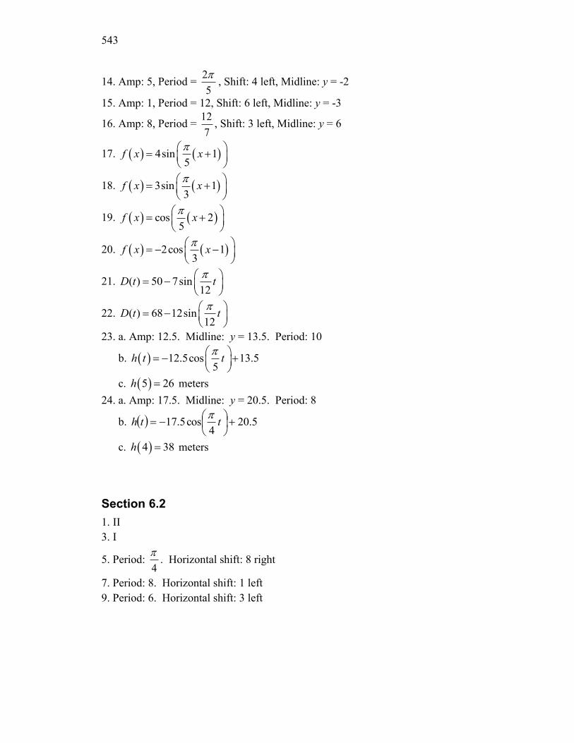
543
14. Amp: 5, Period = 2
5
, Shift: 4 left, Midline: y = -2
15. Amp: 1, Period = 12, Shift: 6 left, Midline: y = -3
16. Amp: 8, Period = 12
7, Shift: 3 left, Midline: y = 6
17. 4sin 15
f x x
18. 3sin 13
f x x
19. cos 25
f x x
20. 2cos 13
f x x
21. ( ) 50 7sin12
D t t
22. ( ) 68 12sin12
D t t
23. a. Amp: 12.5. Midline: y = 13.5. Period: 10
b. 12.5cos 13.55
h t t
c. 5 26h meters
24. a. Amp: 17.5. Midline: y = 20.5. Period: 8
b. 5.204
cos5.17
tth
c. 4 38h meters
Section 6.2
1. II
3. I
5. Period: 4
. Horizontal shift: 8 right
7. Period: 8. Horizontal shift: 1 left
9. Period: 6. Horizontal shift: 3 left
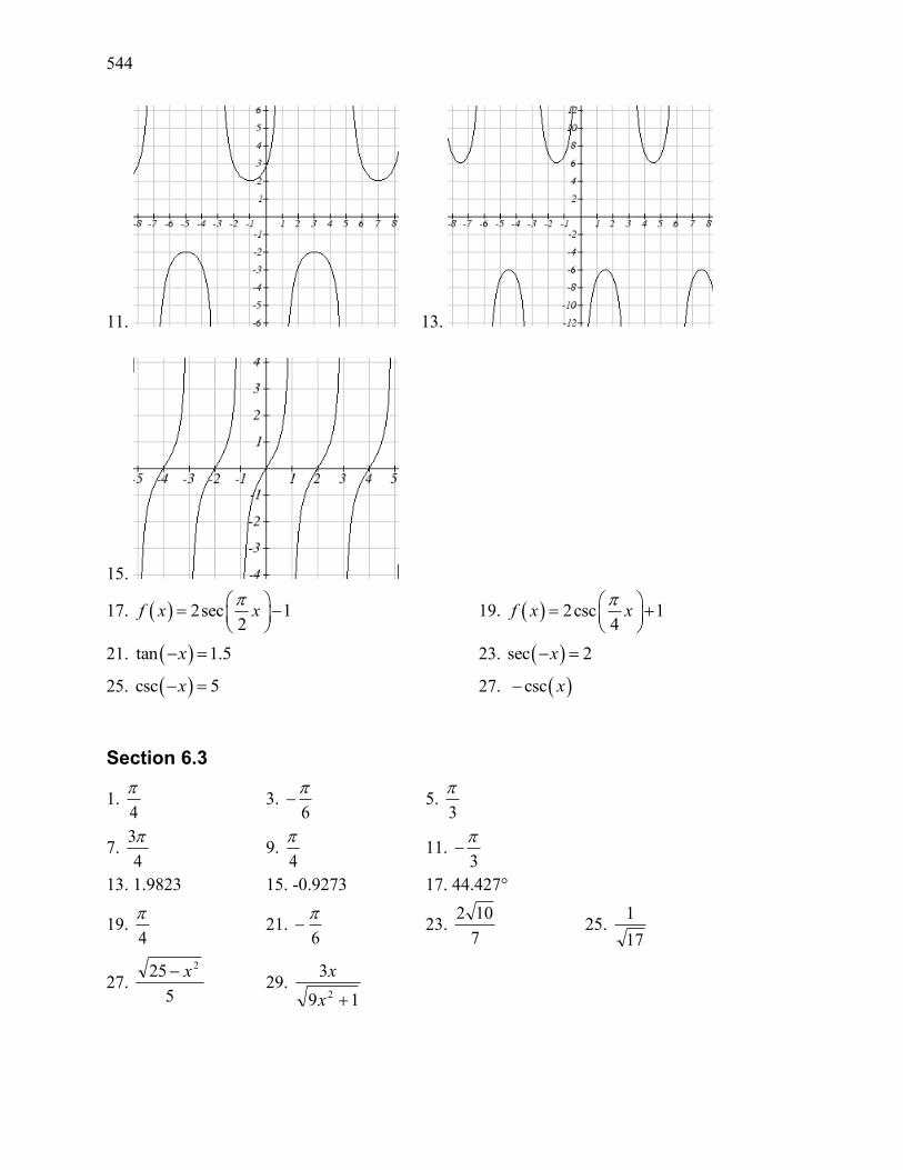
544
11. 13.
15.
17. 2sec 1 2
f x x
19. 2csc 14
f x x
21. tan 1.5x 23. sec 2x
25. csc 5x 27. csc x
Section 6.3
1. 4
3.
6
5.
3
7. 3
4
9.
4
11.
3
13. 1.9823 15. -0.9273 17. 44.427°
19. 4
21.
6
23.
7
102 25.
17
1
27. 5
25 2x 29.
19
3
2 x
x
545
Section 6.4
1. 5 7
,4 4
3.
5,
3 3
5.
2
7.
3,
2 2
9. 7
2 , 24 4
k k
, where k is an integer
11. 7 11
2 , 26 6
k k
, where k is an integer
13. 2 5 2
,18 3 18 3
k k , where k is an integer
15. 5 2 7 2
,12 3 12 3
k k , where k is an integer
17. 5
,6 6
k k
, where k is an integer
19. 2 5 2
,4 3 12 3
k k , where k is an integer
21. 4 8k , where k is an integer
23. 1 5
2 , 26 6
k k , where k is an integer
25. 0.2734, 2.8682 27. 3.7603, 5.6645 29. 2.1532, 4.1300
31. 0.7813, 5.5019 33. 0.04829, 0.47531 35. 0.7381, 1.3563
37. 0.9291, 3.0709 39. 1.3077, 4.6923
Section 6.5
1. 89c , A = 57.9946°, B = 32.0054°
3. 1 76b , A = 27.8181°, B = 62.1819°
5. 6sin 1 42
y x x
7. π
50 13cos t 512
D t
9. a. 129 25cos6
P t t
b. 129 25cos ( 3)6
P t t
11. 75 degrees
13. 8
15. 2.80869431742
17. 5.035 months
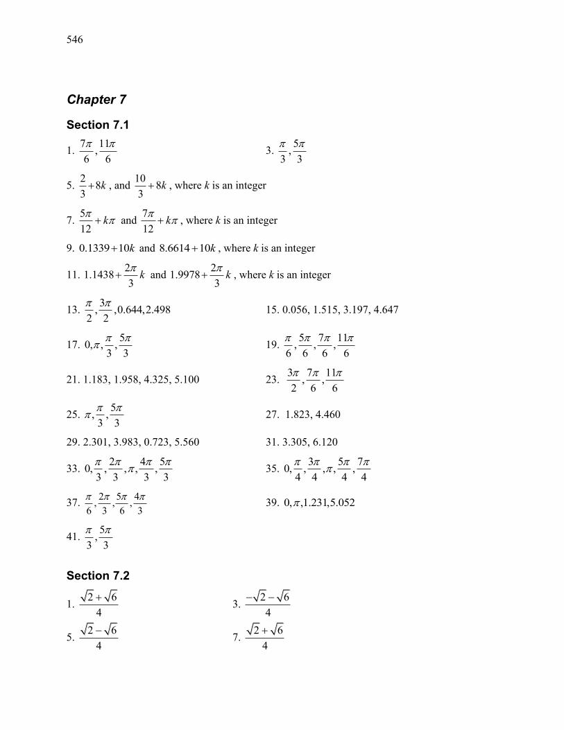
546
Chapter 7
Section 7.1
1. 7 11
,6 6
3.
5,
3 3
5. 2
83
k , and 10
83
k , where k is an integer
7. 5
12k
and
7
12k
, where k is an integer
9. 0.1339 10k and k106614.8 , where k is an integer
11. 2
1.14383
k
and 2
1.99783
k
, where k is an integer
13. 3
, , 0.644, 2.4982 2
15. 0.056, 1.515, 3.197, 4.647
17. 5
0, , , 3 3
19.
5 7 11, , ,
6 6 6 6
21. 1.183, 1.958, 4.325, 5.100 23. 3 7 11
, ,2 6 6
25. 5
, ,3 3
27. 1.823, 4.460
29. 2.301, 3.983, 0.723, 5.560 31. 3.305, 6.120
33. 2 4 5
0, , , , ,3 3 3 3
35.
3 5 70, , , , ,
4 4 4 4
37. 3
4,
6
5,
3
2,
6
39. 0, ,1 .231, 5.052
41. 5
,3 3
Section 7.2
1. 2 6
4
3.
2 6
4
5. 2 6
4
7.
2 6
4
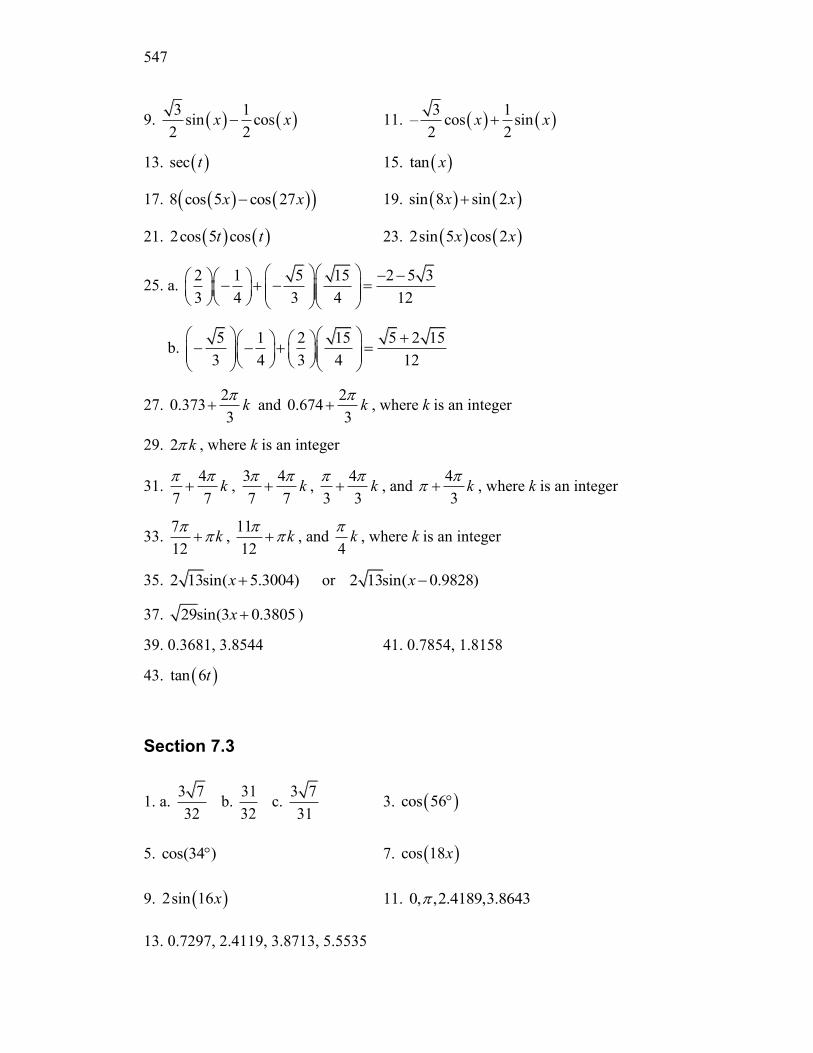
547
9. 3 1
sin cos2 2
x x 11. 3 1
– cos sin2 2
x x
13. sec t 15. tan x
17. 8 cos 5 cos 27x x 19. sin 8 sin 2x x
21. 2cos 5 cost t 23. 2sin 5 cos 2x x
25. a. 2 1 5 15 2 5 3
3 4 3 4 12
b. 5 1 2 15 5 2 15
3 4 3 4 12
27. 2
0.3733
k
and 2
0.6743
k
, where k is an integer
29. k2 , where k is an integer
31. 4
7 7k
,
3 4
7 7k
,
4
3 3k
, and
4
3k
, where k is an integer
33. 7
12k
,
11
12k
, and
4k
, where k is an integer
35. 2 13sin( 5.3004)x or 2 13sin( 0.9828)x
37. 29sin(3 0.3805x )
39. 0.3681, 3.8544 41. 0.7854, 1.8158
43. tan 6t
Section 7.3
1. a. 3 7
32 b.
31
32 c.
3 7
31 3. cos 56
5. cos(34 ) 7. cos 18x
9. 2sin 16x 11. 0, , 2.4189, 3.8643
13. 0.7297, 2.4119, 3.8713, 5.5535
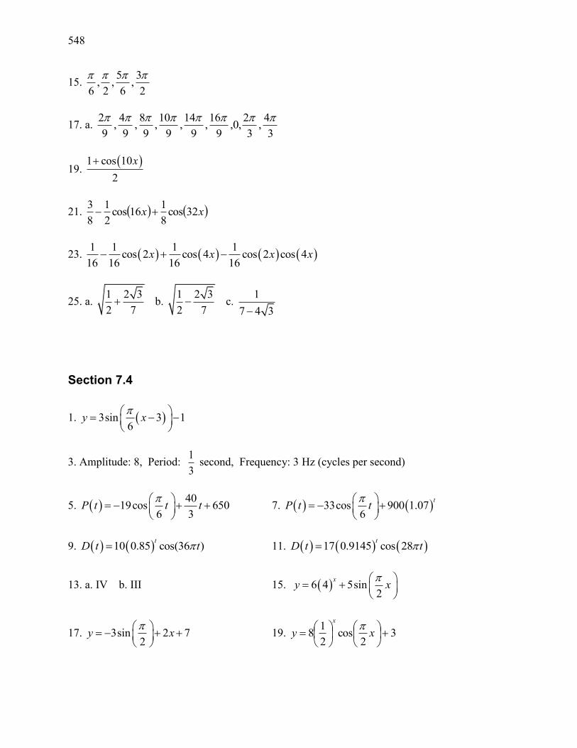
548
15. 5 3
, , ,6 2 6 2
17. a. 3
4,
3
2, 0,
9
16,
9
14,
9
10,
9
8,
9
4,
9
2
19. 1 cos 10
2
x
21. xx 32cos8
116cos
2
1
8
3
23. 1 1 1 1
cos 2 cos 4 cos 2 cos 416 16 16 16
x x x x
25. a. 1 2 3
2 7 b.
1 2 3
2 7 c.
1
7 4 3
Section 7.4
1. 3sin 3 16
y x
3. Amplitude: 8, Period: 1
3 second, Frequency: 3 Hz (cycles per second)
5. 40
19cos 6506 3
P t t t
7. 33cos 900 1.076
tP t t
9. 10 0.85 cos(36 )t
D t t 11. 17 0.9145 cos 28t
D t t
13. a. IV b. III 15. 6 4 5sin2
xy x
17. 3sin 2 72
y x
19. 32
cos2
18
xy
x
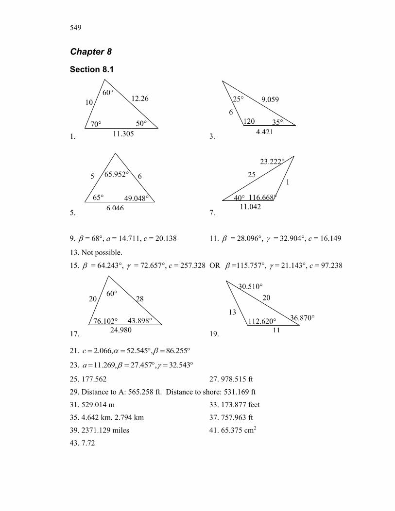
549
Chapter 8
Section 8.1
1. 3.
5. 7.
9. = 68°, a = 14.711, c = 20.138 11. = 28.096°, = 32.904°, c = 16.149
13. Not possible.
15. = 64.243°, = 72.657°, c = 257.328 OR =115.757°, = 21.143°, c = 97.238
17. 19.
21. 255.86, 545.52,066.2 c
23. 543.32, 457.27,269.11 a
25. 177.562 27. 978.515 ft
29. Distance to A: 565.258 ft. Distance to shore: 531.169 ft
31. 529.014 m 33. 173.877 feet
35. 4.642 km, 2.794 km 37. 757.963 ft
39. 2371.129 miles 41. 65.375 cm2
43. 7.72
13
11
20
112.620°
30.510°
36.870°
60° 20 28
24.980
43.898° 76.102°
1
8 40°
25
116.668°
23.222°
11.042
65°
5 6
49.048°
65.952°
6.046
120
°
6
25°
35°
4.421
9.059
70° 50°
10
60° 12.26
7
11.305
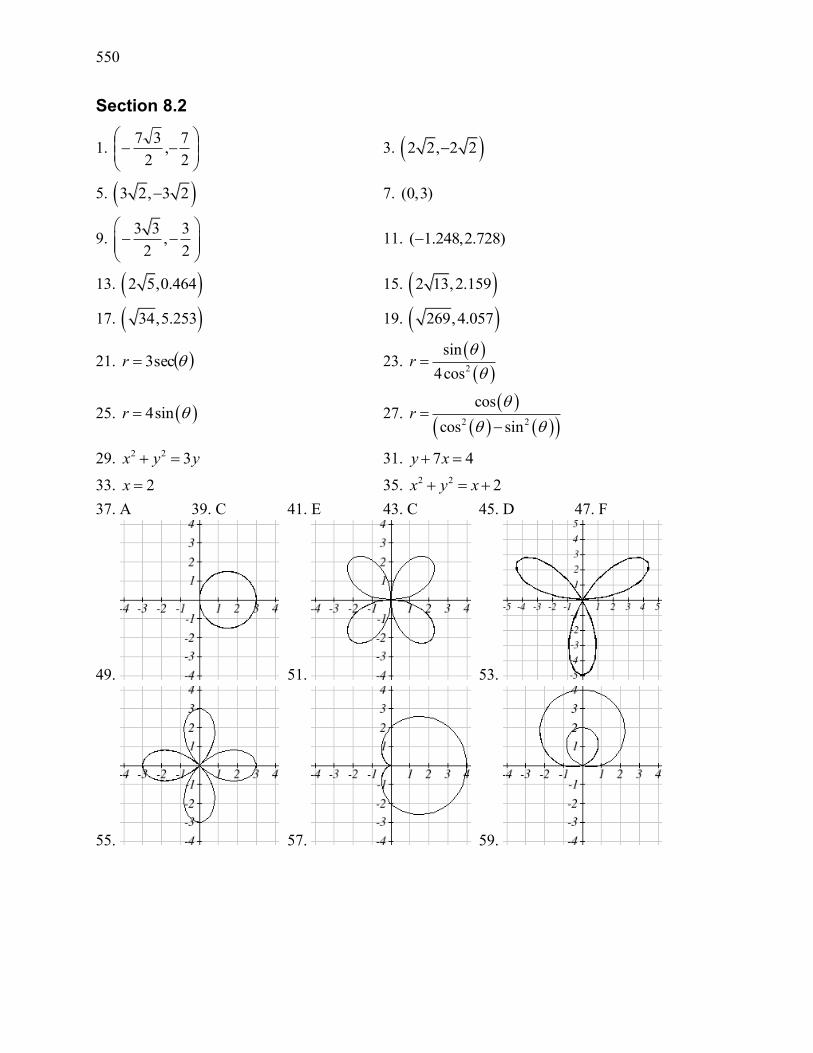
550
Section 8.2
1.
2
7,
2
37 3. 2 2, 2 2
5. 3 2, 3 2 7. (0,3)
9. 3 3 3
,2 2
11. ( 1.248, 2.728)
13. 2 5, 0.464 15. 2 13,2.159
17. 34,5.253 19. 269,4.057
21. sec3r 23.
2
sin
4cosr
25. 4sinr 27.
2 2
cos
cos sinr
29. 2 2 3x y y 31. 7 4y x
33. 2x 35. 2 2 2x y x
37. A 39. C 41. E 43. C 45. D 47. F
49. 51. 53.
55. 57. 59.
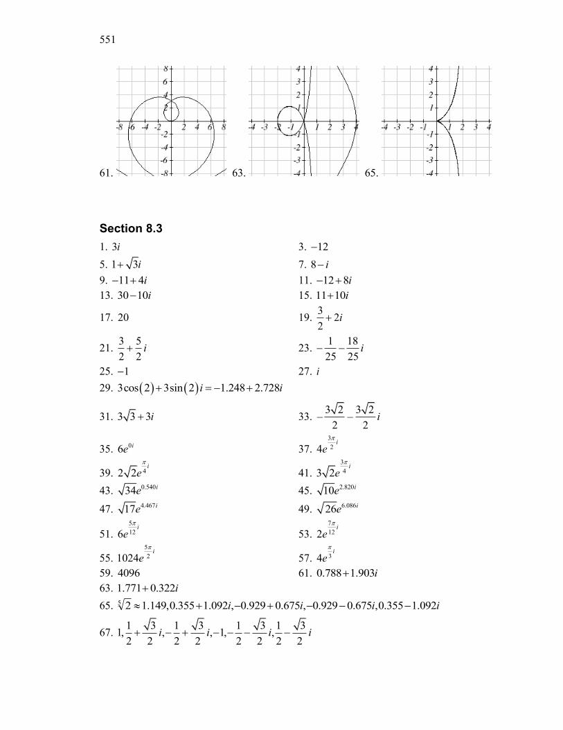
551
61. 63. 65.
Section 8.3
1. 3i 3. 12
5. 1 3i 7. 8 i
9. 11 4i 11. 12 8i
13. 30 10i 15. 11 10i
17. 20 19. 3
22
i
21. 3 5
2 2i 23.
1 18
25 25i
25. 1 27. i
29. 3cos 2 3sin 2 1.248 2.728i i
31. 3 3 3i 33. 3 2 3 2
– –2 2
i
35. 06 ie 37. 3
24i
e
39. 42 2i
e
41. 3
43 2i
e
43. 0.54034 ie 45. 2.82010 ie
47. 4.46717 ie 49. 6.086 26 ie
51. 5
126i
e
53. 7
122i
e
55. 5
21024i
e
57. 34i
e
59. 4096 61. 0.788 1.903i
63. 1.771 0.322i
65. iiii 092.1355.0, 675.0929.0, 675.0929.0, 092.1355.0, 149.125
67. 1 3 1 3 1 3 1 3
1, , , 1, , 2 2 2 2 2 2 2 2
i i i i
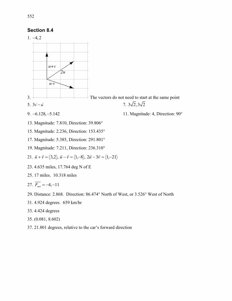
552
Section 8.4
1. 4,2
3. The vectors do not need to start at the same point
5. 3v u 7. 3 2,3 2
9. 6.128, 5.142 11. Magnitude: 4, Direction: 90°
13. Magnitude: 7.810, Direction: 39.806°
15. Magnitude: 2.236, Direction: 153.435°
17. Magnitude: 5.385, Direction: 291.801°
19. Magnitude: 7.211, Direction: 236.310°
21. 21,132, 8,1, 2,3 vuvuvu
23. 4.635 miles, 17.764 deg N of E
25. 17 miles. 10.318 miles
27. 4, 11netF
29. Distance: 2.868. Direction: 86.474° North of West, or 3.526° West of North
31. 4.924 degrees. 659 km/hr
33. 4.424 degrees
35. (0.081, 8.602)
37. 21.801 degrees, relative to the car’s forward direction
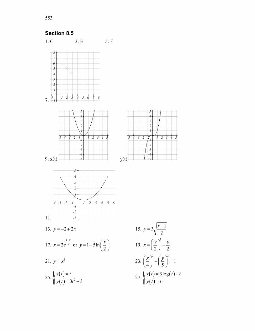
553
Section 8.5
1. C 3. E 5. F
7.
9. x(t) y(t)
11.
13. 2 2y x 15. 1
32
xy
17. 1
52y
x e
or 1 5ln2
xy
19.
3
2 2
y yx
21. 3y x 23.
2 2
14 5
x y
25. 23 3
x t t
y t t
27.
3logx t t t
y t t
.
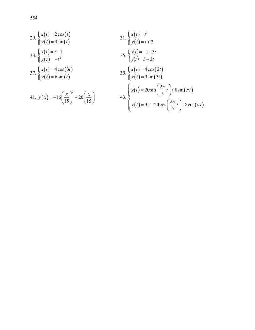
554
29.
2cos
3sin
x t t
y t t
31.
3
2
x t t
y t t
33. 2
1x t t
y t t
35.
tty
ttx
25
31
37.
4cos 3
6sin
x t t
y t t
39.
4cos 2
3sin 3
x t t
y t t
41. 2
16 2015 15
x xy x
43.
220sin 8sin
5
235 20cos 8cos
5
x t t t
y t t t
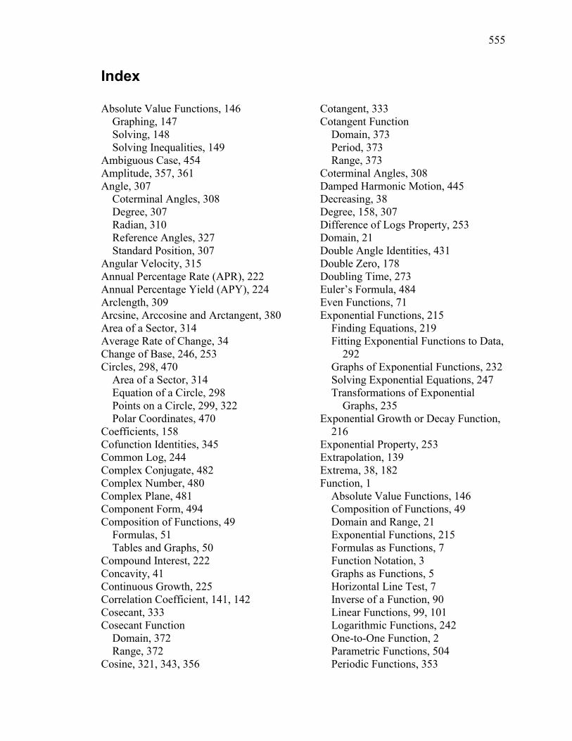
555
Index
Absolute Value Functions, 146
Graphing, 147
Solving, 148
Solving Inequalities, 149
Ambiguous Case, 454
Amplitude, 357, 361
Angle, 307
Coterminal Angles, 308
Degree, 307
Radian, 310
Reference Angles, 327
Standard Position, 307
Angular Velocity, 315
Annual Percentage Rate (APR), 222
Annual Percentage Yield (APY), 224
Arclength, 309
Arcsine, Arccosine and Arctangent, 380
Area of a Sector, 314
Average Rate of Change, 34
Change of Base, 246, 253
Circles, 298, 470
Area of a Sector, 314
Equation of a Circle, 298
Points on a Circle, 299, 322
Polar Coordinates, 470
Coefficients, 158
Cofunction Identities, 345
Common Log, 244
Complex Conjugate, 482
Complex Number, 480
Complex Plane, 481
Component Form, 494
Composition of Functions, 49
Formulas, 51
Tables and Graphs, 50
Compound Interest, 222
Concavity, 41
Continuous Growth, 225
Correlation Coefficient, 141, 142
Cosecant, 333
Cosecant Function
Domain, 372
Range, 372
Cosine, 321, 343, 356
Cotangent, 333
Cotangent Function
Domain, 373
Period, 373
Range, 373
Coterminal Angles, 308
Damped Harmonic Motion, 445
Decreasing, 38
Degree, 158, 307
Difference of Logs Property, 253
Domain, 21
Double Angle Identities, 431
Double Zero, 178
Doubling Time, 273
Euler’s Formula, 484
Even Functions, 71
Exponential Functions, 215
Finding Equations, 219
Fitting Exponential Functions to Data,
292
Graphs of Exponential Functions, 232
Solving Exponential Equations, 247
Transformations of Exponential
Graphs, 235
Exponential Growth or Decay Function,
216
Exponential Property, 253
Extrapolation, 139
Extrema, 38, 182
Function, 1
Absolute Value Functions, 146
Composition of Functions, 49
Domain and Range, 21
Exponential Functions, 215
Formulas as Functions, 7
Function Notation, 3
Graphs as Functions, 5
Horizontal Line Test, 7
Inverse of a Function, 90
Linear Functions, 99, 101
Logarithmic Functions, 242
One-to-One Function, 2
Parametric Functions, 504
Periodic Functions, 353
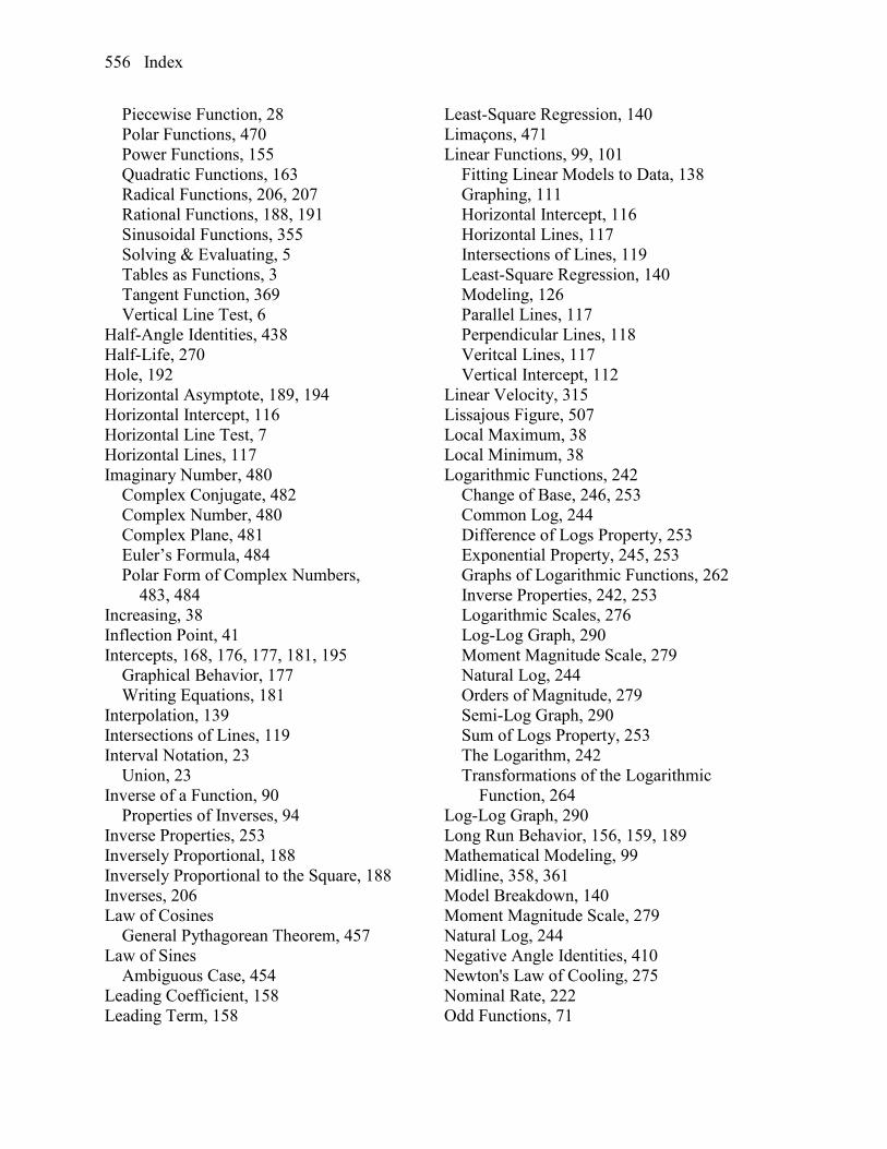
556 Index
Piecewise Function, 28
Polar Functions, 470
Power Functions, 155
Quadratic Functions, 163
Radical Functions, 206, 207
Rational Functions, 188, 191
Sinusoidal Functions, 355
Solving & Evaluating, 5
Tables as Functions, 3
Tangent Function, 369
Vertical Line Test, 6
Half-Angle Identities, 438
Half-Life, 270
Hole, 192
Horizontal Asymptote, 189, 194
Horizontal Intercept, 116
Horizontal Line Test, 7
Horizontal Lines, 117
Imaginary Number, 480
Complex Conjugate, 482
Complex Number, 480
Complex Plane, 481
Euler’s Formula, 484
Polar Form of Complex Numbers,
483, 484
Increasing, 38
Inflection Point, 41
Intercepts, 168, 176, 177, 181, 195
Graphical Behavior, 177
Writing Equations, 181
Interpolation, 139
Intersections of Lines, 119
Interval Notation, 23
Union, 23
Inverse of a Function, 90
Properties of Inverses, 94
Inverse Properties, 253
Inversely Proportional, 188
Inversely Proportional to the Square, 188
Inverses, 206
Law of Cosines
General Pythagorean Theorem, 457
Law of Sines
Ambiguous Case, 454
Leading Coefficient, 158
Leading Term, 158
Least-Square Regression, 140
Limaçons, 471
Linear Functions, 99, 101
Fitting Linear Models to Data, 138
Graphing, 111
Horizontal Intercept, 116
Horizontal Lines, 117
Intersections of Lines, 119
Least-Square Regression, 140
Modeling, 126
Parallel Lines, 117
Perpendicular Lines, 118
Veritcal Lines, 117
Vertical Intercept, 112
Linear Velocity, 315
Lissajous Figure, 507
Local Maximum, 38
Local Minimum, 38
Logarithmic Functions, 242
Change of Base, 246, 253
Common Log, 244
Difference of Logs Property, 253
Exponential Property, 245, 253
Graphs of Logarithmic Functions, 262
Inverse Properties, 242, 253
Logarithmic Scales, 276
Log-Log Graph, 290
Moment Magnitude Scale, 279
Natural Log, 244
Orders of Magnitude, 279
Semi-Log Graph, 290
Sum of Logs Property, 253
The Logarithm, 242
Transformations of the Logarithmic
Function, 264
Log-Log Graph, 290
Long Run Behavior, 156, 159, 189
Mathematical Modeling, 99
Midline, 358, 361
Model Breakdown, 140
Moment Magnitude Scale, 279
Natural Log, 244
Negative Angle Identities, 410
Newton's Law of Cooling, 275
Nominal Rate, 222
Odd Functions, 71
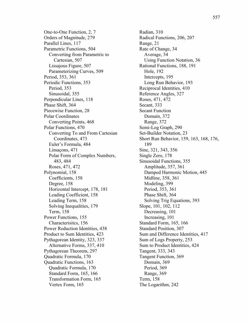
557
One-to-One Function, 2, 7
Orders of Magnitude, 279
Parallel Lines, 117
Parametric Functions, 504
Converting from Parametric to
Cartesian, 507
Lissajous Figure, 507
Parameterizing Curves, 509
Period, 353, 361
Periodic Functions, 353
Period, 353
Sinusoidal, 355
Perpendicular Lines, 118
Phase Shift, 364
Piecewise Function, 28
Polar Coordinates
Converting Points, 468
Polar Functions, 470
Converting To and From Cartesian
Coordinates, 473
Euler’s Formula, 484
Limaçons, 471
Polar Form of Complex Numbers,
483, 484
Roses, 471, 472
Polynomial, 158
Coefficients, 158
Degree, 158
Horizontal Intercept, 178, 181
Leading Coefficient, 158
Leading Term, 158
Solving Inequalities, 179
Term, 158
Power Functions, 155
Characterisitcs, 156
Power Reduction Identities, 438
Product to Sum Identities, 423
Pythagorean Identity, 323, 337
Alternative Forms, 337, 410
Pythagorean Theorem, 297
Quadratic Formula, 170
Quadratic Functions, 163
Quadratic Formula, 170
Standard Form, 165, 166
Transformation Form, 165
Vertex Form, 165
Radian, 310
Radical Functions, 206, 207
Range, 21
Rate of Change, 34
Average, 34
Using Function Notation, 36
Rational Functions, 188, 191
Hole, 192
Intercepts, 195
Long Run Behavior, 193
Reciprocal Identities, 410
Reference Angles, 327
Roses, 471, 472
Secant, 333
Secant Function
Domain, 372
Range, 372
Semi-Log Graph, 290
Set-Builder Notation, 23
Short Run Behavior, 159, 163, 168, 176,
189
Sine, 321, 343, 356
Single Zero, 178
Sinusoidal Functions, 355
Amplitude, 357, 361
Damped Harmonic Motion, 445
Midline, 358, 361
Modeling, 399
Period, 353, 361
Phase Shift, 364
Solving Trig Equations, 393
Slope, 101, 102, 112
Decreasing, 101
Increasing, 101
Standard Form, 165, 166
Standard Position, 307
Sum and Difference Identities, 417
Sum of Logs Property, 253
Sum to Product Identities, 424
Tangent, 333, 343
Tangent Function, 369
Domain, 369
Period, 369
Range, 369
Term, 158
The Logarithm, 242
558 Index
Toolkit Functions, 11
Domains and Ranges of Toolkit
Functions, 26
Transformation Form, 165
Transformations of Functions, 61
Combining Horizontal
Transformations, 77
Combining Vertical Transformations,
76
Horizontal Reflections, 68
Horizontal Shifts, 64
Horizontal Stretch or Compression, 74
Vertical Reflections, 68
Vertical Shifts, 62
Vertical Stretch or Compression, 72
Trigonometric Identities, 334
Alternative Forms of the Pythagorean
Identity, 337, 410
Cofunction Identities, 345
Double Angle Identities, 431
Half-Angle Identities, 438
Negative Angle Identities, 410
Power Reduction Identities, 438
Product to Sum Identities, 423
Pythagorean Identity, 323
Reciprocal Identities, 410
Sum and Difference Identities, 417
Sum to Product Identities, 424
Trigonometry
Cosecant, 333
Cosine, 321, 343, 356
Cotangent, 333
Right Triangles, 343
Secant, 333
Sine, 321, 343, 356
SohCahToa, 343
Solving Trig Equations, 393
Tangent, 333, 343
The Pythagorean Theorem, 297
Unit Circle, 328
Triple Zero, 178
Unit Circle, 328
Vector, 491, 494
Adding Vectors Geometrically, 492
Adding, Subtracting, or Scaling
Vectors in Component Form, 496
Geometrically Scaling a Vector, 493
Vertex, 163, 165
Vertex Form, 165
Vertical Asymptote, 189, 192
Vertical Intercept, 112
Vertical Line Test, 6
Vertical Lines, 117